
Reconstruction of interfaces from the elastic farfield measurements using CGO solutions
42
SIAM J. MATH. ANAL. c 2014 Society for Industrial and Applied Mathematics Vol. 46, No. 4, pp. 2650–2691 RECONSTRUCTION OF INTERFACES FROM THE ELASTIC FARFIELD MEASUREMENTS USING CGO SOLUTIONS ∗ MANAS KAR † AND MOURAD SINI † Abstract. In this work, we are concerned with the inverse scattering by interfaces for the linearized and isotropic elastic model at a fixed frequency. First, we derive complex geometrical optic solutions with linear or spherical phases having a computable dominant part and an H α - decaying remainder term with α< 3, where H α is the classical Sobolev space. Second, based on these properties, we estimate the convex hull as well as nonconvex parts of the interface using the far fields of only one of the two reflected body waves (pressure waves or shear waves) as measurements. The results are given for both the impenetrable obstacles, with traction boundary conditions, and the penetrable obstacles. In the analysis, we require the surfaces of the obstacles to be Lipschitz regular and, for the penetrable obstacles, the Lam´ e coefficients to be measurable and bounded with the usual jump conditions across the interface. Key words. scattering, elasticity, far fields, complex geometrical optic solutions, integral equa- tions AMS subject classifications. 35P25, 35R30, 78A45 DOI. 10.1137/120903130 1. Introduction and statement of the result. Let D be a bounded and open set of R 3 such that R 3 \ D is connected. The boundary ∂D of D is Lipschitz. We denote by λ and μ the Lam´ e coefficients and by κ the frequency. We assume that those coefficients are measurable and bounded and satisfy the conditions μ> 0, 2μ +3λ> 0 and μ = μ 0 ,λ = λ 0 for x ∈ R 3 \ D with μ 0 and λ 0 being constants. In addition, we set λ D := λ − λ 0 and μ D := μ − μ 0 and assume that 2μ D +3λ D ≥ 0 and μ D > 0. 1 The direct scattering problem can be formulated as follows. Let u i be an incident field, i.e., a vector field satisfying μ 0 Δu i +(λ 0 + μ 0 )∇∇ · u i + κ 2 u i = 0 in R 3 , and u s (u i ) be the scattered field associated to the incident field u i . In the impenetrable case, the scattering problem reads as (1.1) ⎧ ⎪ ⎪ ⎪ ⎪ ⎨ ⎪ ⎪ ⎪ ⎪ ⎩ μ 0 Δu s +(λ 0 + μ 0 )∇∇ · u s + κ 2 u s =0 in R 3 \ D, σ(u s ) · ν = −σ(u i ) · ν on ∂D, lim |x|→∞ |x| ∂u s p ∂ |x| − iκ p u s p = 0 and lim |x|→∞ |x| ∂u s s ∂ |x| − iκ s u s s =0, ∗ Received by the editors December 19, 2012; accepted for publication (in revised form) March 26, 2014; published electronically July 22, 2014. http://www.siam.org/journals/sima/46-4/90313.html † RICAM, Austrian Academy of Sciences, A-4040, Linz, Austria ([email protected], [email protected]). The first author was supported by Austrian Science Fund (FWF) P22341- N18. The second author was partially supported by Austrian Science Fund (FWF) P22341-N18. 1 The assumptions on the jumps can be relaxed. It is needed only at the vicinity of the points on the interface ∂D. In addition, we can also consider the case 2μ D +3λ D ≤ 0 and μ D < 0; see Remark 5.5. These extra assumptions are needed only for the inverse problems and not for the forward problems. 2650
-
Upload
independent -
Category
Documents
-
view
3 -
download
0
Transcript of Reconstruction of interfaces from the elastic farfield measurements using CGO solutions
SIAM J. MATH. ANAL. c© 2014 Society for Industrial and Applied MathematicsVol. 46, No. 4, pp. 2650–2691
RECONSTRUCTION OF INTERFACES FROM THE ELASTICFARFIELD MEASUREMENTS USING CGO SOLUTIONS∗
MANAS KAR† AND MOURAD SINI†
Abstract. In this work, we are concerned with the inverse scattering by interfaces for thelinearized and isotropic elastic model at a fixed frequency. First, we derive complex geometricaloptic solutions with linear or spherical phases having a computable dominant part and an Hα-decaying remainder term with α < 3, where Hα is the classical Sobolev space. Second, based onthese properties, we estimate the convex hull as well as nonconvex parts of the interface using the farfields of only one of the two reflected body waves (pressure waves or shear waves) as measurements.The results are given for both the impenetrable obstacles, with traction boundary conditions, andthe penetrable obstacles. In the analysis, we require the surfaces of the obstacles to be Lipschitzregular and, for the penetrable obstacles, the Lame coefficients to be measurable and bounded withthe usual jump conditions across the interface.
Key words. scattering, elasticity, far fields, complex geometrical optic solutions, integral equa-tions
AMS subject classifications. 35P25, 35R30, 78A45
DOI. 10.1137/120903130
1. Introduction and statement of the result. Let D be a bounded andopen set of R3 such that R3\D is connected. The boundary ∂D of D is Lipschitz.We denote by λ and μ the Lame coefficients and by κ the frequency. We assumethat those coefficients are measurable and bounded and satisfy the conditions μ > 0,2μ + 3λ > 0 and μ = μ0, λ = λ0 for x ∈ R
3\D with μ0 and λ0 being constants. Inaddition, we set λD := λ−λ0 and μD := μ−μ0 and assume that 2μD +3λD ≥ 0 andμD > 0.1
The direct scattering problem can be formulated as follows. Let ui be an incidentfield, i.e., a vector field satisfying
μ0Δui + (λ0 + μ0)∇∇ · ui + κ2ui = 0 in R
3,
and us(ui) be the scattered field associated to the incident field ui. In the impenetrablecase, the scattering problem reads as
(1.1)
⎧⎪⎪⎪⎪⎨⎪⎪⎪⎪⎩
μ0Δus + (λ0 + μ0)∇∇ · us + κ2us = 0 in R3\D,
σ(us) · ν = −σ(ui) · ν on ∂D,
lim|x|→∞ |x|(∂usp∂|x| − iκpu
sp
)= 0 and lim|x|→∞ |x|
(∂uss∂|x| − iκsu
ss
)= 0,
∗Received by the editors December 19, 2012; accepted for publication (in revised form) March 26,2014; published electronically July 22, 2014.
http://www.siam.org/journals/sima/46-4/90313.html†RICAM, Austrian Academy of Sciences, A-4040, Linz, Austria ([email protected],
[email protected]). The first author was supported by Austrian Science Fund (FWF) P22341-N18. The second author was partially supported by Austrian Science Fund (FWF) P22341-N18.
1The assumptions on the jumps can be relaxed. It is needed only at the vicinity of the pointson the interface ∂D. In addition, we can also consider the case 2μD + 3λD ≤ 0 and μD < 0; seeRemark 5.5. These extra assumptions are needed only for the inverse problems and not for theforward problems.
2650
DETECTION OF INTERFACES FROM THE ELASTIC FARFIELDS 2651
where the last two limits are uniform in all the directions x := x|x| ∈ S2 with
σ(us) · ν := (2μ∂ν + λν∇ ·+μν × curl)us
and the unit normal vector ν is directed into the exterior of D. In the penetrableobstacle case, the total field ut := us + ui satisfies
(1.2)
⎧⎪⎨⎪⎩∇ · (σ(ut)) + κ2ut = 0 in R3,
lim|x|→∞ |x|(∂usp∂|x| − iκpu
sp
)= 0 and lim|x|→∞ |x|
(∂uss∂|x| − iκsu
ss
)= 0.
The two limits in (1.1) and (1.2) are called the Kupradze radiation conditions. Thestress tensor σ is defined as follows, for any displacement field v taken as a columnvector:
σ(v) := λ(∇ · v)I3 + 2με(v),
where I3 is the 3× 3 identity matrix and
ε(v) =1
2(∇v + (∇v)�),
with ε being the infinitesimal strain tensor. Note that for v = (v1, v2, v3)�, ∇v denotes
the 3× 3 matrix whose jth row is ∇vj for j = 1, 2, 3. Also for a 3× 3 matrix functionA, ∇ ·A denotes the column vector whose jth component is the divergence of the jthrow of A for j = 1, 2, 3.
In both (1.1) and (1.2), we denoted
usp := −κ−2p ∇∇ · us
to be the longitudinal (or the pressure) part of the field us and
uss := κ−2s curl curl us
to be the transversal (or the shear) part of the field us. The constants κp :=κ√
2μ0+λ0
and κs :=κ√μ0
are known as the longitudinal and transversal wave numbers, respec-
tively. From the first equality of (1.1) (and equally the one of (1.2) for x ∈ R3\D),we obtain the well-known decomposition of the scattered field us as the sum of itslongitudinal and transversal parts, i.e., us = usp + uss. It is well known that the scat-tering problems (1.1) and (1.2) are well posed; see, for instance, [8], [10], [14], [25],[26], [27].
The scattered field us has the asymptotic expansion at infinity
(1.3) us(x) :=eiκp|x|
|x| u∞p (x) +eiκs|x|
|x| u∞s (x) +O
(1
|x|2), |x| → ∞,
uniformly in all the directions x ∈ S2; see [2], for instance. The fields u∞p (x) andu∞s (x) defined on S2 are called correspondingly the longitudinal and transversal partsof the far field pattern. The longitudinal part u∞p (x) is normal to S2, while thetransversal part u∞s (x) is tangential to S
2. It is well known that scattering problemsin linear elasticity occur when we excite one of the two types of incident plane waves,pressure (or longitudinal) waves and shear (or transversal) waves. They have theanalytic forms upi (x, d) := deiκpd·x and usi (x, d) := d⊥eiκsd·x, respectively, where d⊥
is any vector in S2 orthogonal to d. Note that upi (·, d) is normal to S2 and usi (·, d) is
2652 MANAS KAR AND MOURAD SINI
tangential to S2. As in earlier studies of problems in elasticity we use superpositionsof incident pressure and shear waves given by
(1.4) ui(x, d) := αdeiκpd·x + βd⊥eiκsd·x,
where α, β ∈ C, d ∈ S2.
We denote by u∞(·, d, α, β) the far field pattern associated with the incident wavesof the form (1.4). We also denote by u∞p (·, d, α, β) and u∞s (·, d, α, β) the correspondinglongitudinal and transversal parts of the far field u∞(·, d, α, β), i.e.,
u∞(·, d, α, β) = (u∞p (·, d, α, β), u∞s (·, d, α, β)).Hence, we obtain the far field measurements
(1.5) (upi , usi ) �→ F (upi , u
si ) :=
[u∞,pp (·, d) u∞,s
p (·, d)u∞,ps (·, d) u∞,s
s (·, d)
],
where1. (u∞,p
p (·, d), u∞,ps (·, d)) is the far field pattern associated with the pressure
incident field upi (·, d);2. (u∞,s
p (·, d), u∞,ss (·, d)) is the far field pattern associated with the shear incident
field usi (·, d).Our concern now is to investigate the following geometrical inverse problem: From
the knowledge of u∞(·, d, α, β) for all directions x and d in S2 and a couple (α, β) �=(0, 0) in C, determine D.
We can also restate this problem as follows: From the knowledge of the matrix(1.5) for all directions x and d in S2 determine D.
The first uniqueness result was proved by Hahner and Hsiao for the model (1.1);see [14]. It says that every column of the matrix (1.5) for all directions x and d in S2
determines D. Later Alves and Kress [2], Arens [3], Charalambopoulos, Gintides, andKiriaki [5], [6], and Gintides and Kiriaki [11] proposed sampling type methods to solvethe inverse problem using the full matrix (1.5) for all directions x and d in S2. We alsomention the works by Guzina and his collaborators using the full near fields [4], [13],[32]. We remark that not only does one need the information over all directions ofincidence and measurements, but also both pressure and shear far fields are necessary.In recent works we proved that it is possible to reduce the amount of data for detectingD as follows: The knowledge of u∞p (x, d, α, β) (or, respectively, u∞s (x, d, α, β)) for alldirections x and d in S2 and the couple (α, β) = (1, 0) or (α, β) = (0, 1) uniquelydetermines the obstacle D.
In other words, this result says that every component of the matrix (1.5) for alldirections x and d in S2 determines D. In [12], we assumed a C4-regularity of ∂Dto prove this result for the impenetrable obstacle with free boundary conditions, themodel (1.1). This C4-regularity is used to derive explicitly the first order term inthe asymptotic of the indicator functions of the probe or singular sources method interms of the source points. This regularity is reduced to Lipschitz in [20] for bothmodels (1.1) and (1.2); see also [16] for the rigid obstacles.
It is known that these probe/singular sources methods are based on the use ofapproximating domains isolating the source point of the used point sources; see [33].Since this source point has to move around and near the interface, it creates extrainstabilities of the method. To overcome this difficulty, Ikehata [17] proposed theenclosure method which has the same principle as the probe/singular sources methods,

DETECTION OF INTERFACES FROM THE ELASTIC FARFIELDS 2653
but instead of using point sources, he uses complex geometrical optics (CGO) typesolutions with linear phases. The price to pay is that, in contrast to the point sourceswith which we obtain the whole interface ∂D, we can only obtain the intersection ofthe level-curves of the CGO solutions with ∂D. In the case of linear phases, we canestimate the convex hull; see [19] for an overview of this method. Later, in the work[23] by Kenig, Sjostrand, and Uhlmann, other CGO solutions were proposed to solvethe EIT problem using the localized Dirichlet–Neumann map. These CGO solutionshave a phase of quadratic form, i.e., behaving as spherical waves. Inspired by theseCGO solutions, Nakamura and Yoshida proposed in [31] an enclosure method basedon CGO solutions with spherical waves with which they could estimate, in addition tothe convex hull ofD, some nonconvex parts of ∂D. Another family of CGO solutions isproposed by Uhlmann and Wang [36], where the phases are the harmonic polynomialsin the two-dimensional (2D) case. With these CGO, one can recover all the visiblepart, by straight rays, of the interface ∂D. We refer the reader to [9] for a classificationof these CGO solutions. Regarding the Lame model, the CGO solutions with linearor spherical phases are constructed in [35] for the stationary case, i.e., κ = 0, while in[24] the ones with harmonic polynomial phases in the 2D case are investigated. Thegeneral form of these CGOs is
(1.6) u := e−τ(φ+iψ)(a+ r),
where φ is the known and explicit phase we were talking about, ψ is also explicitlyknown, a is either known explicitly or computable, and the remainder r is small inthe classical Sobolev Hα-norm, α < 1, in terms of the parameter τ , i.e., precisely onehas the estimate ‖r‖Hα = O(τα−1), α ≤ 1.
In our work, we use p-parts or s-parts of the far field measurements. The CGOsolutions of the form (1.6) are not enough, in particular when we use mixed mea-surements, i.e., p-incident (respectively, s-incident) waves and s-parts (respectively,p-parts) of the corresponding far field patterns. Instead, we construct CGO solutionsof the form
(1.7) u := e−τ(φ+iψ)(a0 + a1τ−1 + a2τ
−2 + r)
with linear or logarithmic phases, where now a0, a1, and a2 either are known explicitlyor computable and the remainder r is small with the Hα-norm, α < 3, in termsof the parameter τ , i.e., ‖r‖Hα = O(τα−3), α ≤ 3. Having these CGO solutionsat hand, we state the indicator function of the enclosure method directly from thefar field measurements and use only one of the two body waves (pressure or shearwaves). Then we justify the enclosure method with no geometrical assumptions onthe interface ∂D. The analysis is based on the use of integral equation methods onSobolev spaces Hs(∂D), s ∈ R, for the impenetrable case and Lp estimates of thegradients of the solutions of the Lame system with discontinuous Lame coefficientsfor the penetrable case. This is a generalization to the Lame system of the previousworks [22] and [34] concerning the Maxwell and acoustic cases, respectively.
The paper is organized as follows. In section 2, we define the indicator func-tions via the far field pattern. Then using the denseness property of the Herglotzwave functions and the well posedness of the forward problem, we link the far fieldmeasurements with the CGO solutions. In section 3, the construction of the CGOsolutions is discussed, while in section 4, we state the main theorem, and we describethe reconstruction scheme. In section 5, we prove the main theorem, and we postponeto section 6 and the appendix the justification of the needed estimates for the CGOsolutions.
2654 MANAS KAR AND MOURAD SINI
2. The indicator functions linking the used far field parts to the CGOsolutions. In this section, we follow the procedure of [21], where we showed the linkbetween far field and CGO solutions in the scalar Helmholtz case. So, we start withthe following identity (see, for instance, Lemma 3.1 in [2]):
(2.1)
∫∂D
(U · σ(wh) · ν − wh · σ(U) · ν)ds(x) = 4π
∫S2
(U∞p hp + U∞
s hs)ds(x)
for all radiating fields U and wh, where wh is the scattered field associated with theHerglotz field vh for h = (hp, hs) ∈ L2
p(S2)× L2
s(S2), i.e.,
vh(x) :=
∫S2
[eiκpx·dhp(d) + eiκsx·dhs(d)]ds(d)
with L2p(S
2) := {U ∈ (L2(S2))3;U(d)×d = 0}, while L2s(S
2) := {U ∈ (L2(S2))3;U(d) ·d = 0}.
Let v be a CGO solution for the Lame system and state Ω := Ωcgo to be its domainof definition with D ⊂⊂ Ω. Examples of these CGO solutions will be described insection 3. We take its p-part vp and its s-part vs. We can find sequences of densities(hnp )n and (hns )n such that the Herglotz waves vhn
pand vhn
sconverge to vp and vs,
respectively, on any domain Ω containing D and contained in Ω. These sequences canbe obtained as follows.
We define H : (L2(S2))3 → (L2(∂Ω))3 as (Hg)(x) := vg(x). We know that His injective and has a dense range if κ2 is not an eigenvalue of the Dirichlet–Lameoperator on Ω. Due to the monotonicity of these eigenvalues in terms of the domains,we change, if needed, Ω slightly so that κ2 is not an eigenvalue anymore. Hence, wecan find a sequence gn ∈ (L2(S2))3 such that Hgn → v in (L2(∂Ω))3. Recall thatboth Hgn and v satisfy the interior Lame problem. By the well posedness of theinterior problem and the interior estimates, we deduce that Hgn → v in C∞(Ω), sinceD ⊂⊂ Ω ⊂⊂ Ω. Hence, −κ−2
p ∇∇ ·Hgn → vp and κ−2s curl curlHgn → vs in C∞(Ω).
But −κ−2p ∇∇ ·Hgn = Hhnp and κ−2
s curl curlHgn = Hhns , where hnp := d(d · gn) and
hns := −d ∧ (d ∧ gn).We set us(vs) to be the scattered field corresponding to the s incident wave vs.
The p and s parts of the scattered field us(vs) are usp(vs) and uss(vs), respectively.Similarly, we set us(vp) to be the scattered field corresponding to the p incident wavevp. The p and s parts of the scattered field us(vp) are u
sp(vp) and u
ss(vp), respectively.
2.1. Using longitudinal waves. Let (u∞,pp , u∞,p
s ) be the far field associated to
the incident field deiκpd·x. By the principle of superposition, the far field associatedto the incident field
vg(x) :=
∫S2
deiκpd·x(d · g(d))ds(d)
is given by
u∞g (x) := (u∞,pg (x), u∞,s
g (x))
=
(∫S2
u∞,pp (x, d)(d · g(d))ds(d),
∫S2
u∞,ps (x, d)(d · g(d))ds(d)
),
where each component is a vector. Replacing in (2.1), using the fact that Hhnp con-
verges to vp in C∞(Ω), with D ⊂⊂ Ω, the trace theorem and the well posedness ofthe scattering problem, we obtain

DETECTION OF INTERFACES FROM THE ELASTIC FARFIELDS 2655
4π limm,n→∞
∫S2
∫S2
[u∞,pp (x, d)d · gn(d)] · [x(x · gm(x))]ds(x)ds(d)(2.2)
=
∫∂D
[us(vp) · (σ(vp) · ν)− vp · (σ(us(vp)) · ν)]ds(x)
and 4π limm,n→∞
∫S2
∫S2
[u∞,ps (x, d)d · gn(d)] · [x ∧ (x ∧ gm(x))]ds(x)ds(d)(2.3)
=
∫∂D
[us(vp) · (σ(vs) · ν)− vs · (σ(us(vp)) · ν)]ds(x).
2.2. Using shear incident waves. Let i1 and i2 be two vectors linearly inde-pendent and tangent to S2. Then d ∧ (d ∧ i1) and d ∧ (d ∧ i2) are obviously alsotangent to S2 and in addition they are linearly independent. Indeed, α1d ∧ (d ∧ i1)+α2d ∧ (d ∧ i2) = 0 ⇔ d ∧ (d ∧ (α1i1 + α2i2)) = 0 ⇔ α1 = α2 = 0. Letnow (u∞,s
p (x, d), u∞,ss (x, d)) be the far field associated with the incident plane wave
d ∧ (d ∧ ij)eiκsx·d, j = 1, 2. Hence the far field associated with the Herglotz wave
vg(x) :=
∫S2
d ∧ (d ∧ g)eiκsx·dds(d)
is
v∞g (x) :=
2∑j=1
(∫S2
u∞,sp (x, d)(ij · g)ds(d),
∫S2
u∞,ss (x, d)(ij · g)ds(d)
),
since d ∧ (d ∧ g) = d ∧ (d ∧ i1)(i1 · g) + d ∧ (d ∧ i2)(i2 · g). Hence,
4π limm,n→∞
2∑j=1
∫S2
∫S2
[u∞,ss (x, d)(ij · gn)(d)] · [x ∧ x ∧ gm(x)]ds(x)ds(d)(2.4)
=
∫∂D
[us(vs) · (σ(vs) · ν)− vs · (σ(us(vs)) · ν)]ds(x)and
4π limm,n→∞
2∑j=1
∫S2
∫S2
[u∞,sp (x, d)(ij · gn)(d)] · [x(x · gm(x))]ds(x)ds(d)(2.5)
=
∫∂D
[us(vs) · (σ(vp) · ν)− vp · (σ(us(vs)) · ν)]ds(x).
2.3. The indicator functions. We set
Ipp := 4π limm,n→∞
∫S2
∫S2
[u∞,pp (x, d)d · gn(d)] · [x(x · gm(x))]ds(x)ds(d),(2.6)
Ips := 4π limm,n→∞
∫S2
∫S2
[u∞,ps (x, d)d · gn(d)] · [x ∧ (x ∧ gm(x))]ds(x)ds(d),(2.7)
Iss := 4π limm,n→∞
2∑j=1
∫S2
∫S2
[u∞,ss (x, d)(ij · gn)(d)] · [x ∧ x ∧ gm(x)]ds(x)ds(d),(2.8)
and
Isp := 4π limm,n→∞
2∑j=1
∫S2
∫S2
[u∞,sp (x, d)(ij · gn)(d)] · [x(x · gm(x))]ds(x)ds(d).(2.9)

2656 MANAS KAR AND MOURAD SINI
Therefore, the indicator function Ipp is defined based on p-parts of the far fieldassociated to p-incident wave. Correspondingly Ips depends on s-part of the far fieldassociated to p-incident wave, Iss depends on s-part of the far field associated to thes-incident wave, and finally Isp depends on p-part of the far field associated to thes-incident wave.
3. Construction of CGO solutions.
3.1. CGO solutions for Ipp and Iss. Let us assume u to be a solution for thefollowing Lame system:
(3.1) μ0Δu+ (λ0 + μ0)∇∇ · u+ κ2u = 0.
Applying the identity curl curl = ∇∇ · −Δ in (3.1), we have
u = −λ0 + 2μ0
κ2∇∇ · u+
μ0
κ2curl curlu =: up + us,
where up and us are the p-part and s-part of the solution u, respectively.
3.1.1. p-type CGO solution for Ipp. Taking ∇· in both sides in (3.1), weobtain
μ0Δ(∇ · u) + (λ0 + μ0)Δ(∇ · u) = −κ2(∇ · u).
Define U := ∇·u. Therefore U satisfies the Helmholtz equation ΔU+κ2pU = 0. Hence
the p-part of u is −λ0+2μ0
κ2 ∇U . This suggest taking the CGO solution for the Lamesystem of the form
(3.2) ∇U,
where U is the CGO solution for scalar Helmholtz equation, i.e., U satisfies
(3.3) ΔU + κ2pU = 0.
The resulting vector field ∇U , in (3.2), is also a solution of (3.1) and it is of p-typesince its s-part is zero.
3.1.2. s-type CGO solution for Iss. Define V =: curlu, where u satisfies(3.1). It satisfies the vector Helmholtz equation
(3.4) ΔV + κ2sV = 0.
The s-part of the solution u is μ0
κ2 curlV. This suggests taking the CGO solution forthe Lame system of the form
(3.5) curlV.
The resulting vector field curlV , in (3.5), is also a solution of (3.1) and it is of s-typesince its p-part is zero.

DETECTION OF INTERFACES FROM THE ELASTIC FARFIELDS 2657
3.1.3. The forms of the corresponding CGO solutions. In the followingproposition, we provide the forms of the CGO solutions for the Helmholtz type equa-tions in (3.3) and (3.4). The CGO solutions we use for Ipp and Iss are then deducedusing (3.2) and (3.5), respectively.
Proposition 3.1.
1. (Linear phase.) Let ρ, ρ⊥ ∈ S2, with ρ · ρ⊥ = 0 and t, τ > 0. The function
U(x; τ, t) := eτ(x·ρ−t)+i√τ2+κ2
l x·ρ⊥ satisfies (Δ + κ2l )U = 0 in R3, for l = s
or l = p.2. (Logarithmic phase.) Let Ω be a C2-smooth domain and set ch(Ω) to be its
convex hull. Choose x0 ∈ R3\ch(Ω) and let ω0 ∈ S2 be a vector such that{x ∈ R3;x − x0 = λω0, λ ∈ R} ∩ ∂Ω = ∅. Then there exists a solution of(Δ + κ2l )U = 0 of the form
(3.6) U(x; τ, t) := eτ(t−log |x−x0|)−iτψ(x)(a0 + τ−1a1 + r),
where a0 and a1 are smooth and computable functions which depend on κl, l =s or l = p, and r has the behavior
(3.7) ‖r‖H2scl(Ω) ≤ Cτ−2, C > 0 is a universal constant,
where H2scl(Ω) is the semiclassical Sobolev space defined by H2
scl(Ω) := {V ∈L2(Ω)/(τ−1∂)αV ∈ L2(Ω), |α| ≤ 2}, equipped with the norm ‖V ‖2
H2scl(Ω)
:=∑|α|≤2 ‖(τ−1∂)αV ‖2L2(Ω). From (3.7), we have in particular
(3.8) ‖r‖Hs(Ω) ≤ Cτ−(2−s), 0 ≤ s ≤ 2.
Proof. The CGO solutions with linear phases are given in [17]. The CGO solutionswith log-phases are given in [23] for κ = 0 of the form eτ(t−log |x−x0|)−iτψ(x)(a0 +r) and ‖r‖H1
scl(Ω) ≤ cτ−1. The CGO solutions stated in this proposition, with the
corresponding estimate (3.7) of the remainder term, are given in [34].
3.2. CGO solutions for Isp and Ips. The natural CGO solutions introducedin section 3.1.1 are useful for Ipp. However, with such functions as incident wavesthe other indicator functions Ips, Iss, and Isp vanish (see (2.3), (2.4), and (2.5), re-spectively) since the s-part, vs, of the CGO solution is null and hence not useful.Similarly, the CGO solutions constructed in section 3.1.2 are useful for Iss but notfor Ipp, Isp, and Ips. To construct CGO solutions useful for Isp and Ips, we need toconsider the full Lame system, i.e., solutions with nonvanishing p and s parts. Toconstruct such CGO solutions, we follow the approach by Uhlmann and Wang [35].The nondivergence form of the isotropic elasticity system can be written as
(3.9) μ0Δu + (λ0 + μ0)∇(∇ · u) + κ2u = 0 on Ω.
Let W =(wg
)satisfy
(3.10) PW := Δ
(w
g
)+A
(∇g∇ · w
)+Q
(w
g
)= 0,
where A =(0 0
0λ0+μ0λ0+2μ0
μ120
)and Q = κ2
( 1μ0
0
0 1λ0+2μ0
). Then u := μ
− 12
0 w + μ0−1∇g
satisfies (3.9). Consider now the matrix operator Pτ−1 = −τ−2P. Then the operatorP in (3.10) turns out to be the following operator:
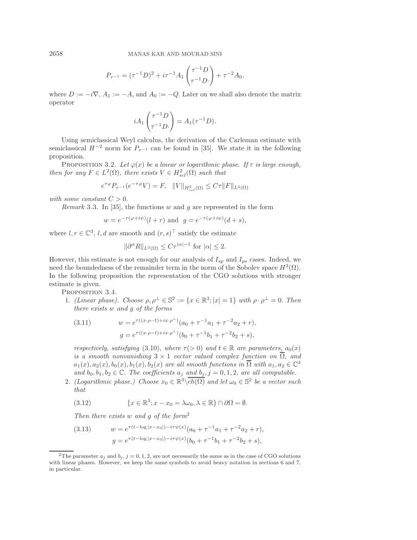
2658 MANAS KAR AND MOURAD SINI
Pτ−1 = (τ−1D)2 + iτ−1A1
(τ−1D
τ−1D·
)+ τ−2A0,
where D := −i∇, A1 := −A, and A0 := −Q. Later on we shall also denote the matrixoperator
iA1
(τ−1D
τ−1D·
)= A1(τ
−1D).
Using semiclassical Weyl calculus, the derivation of the Carleman estimate withsemiclassical H−2 norm for Pτ−1 can be found in [35]. We state it in the followingproposition.
Proposition 3.2. Let ϕ(x) be a linear or logarithmic phase. If τ is large enough,then for any F ∈ L2(Ω), there exists V ∈ H2
scl(Ω) such that
eτϕPτ−1(e−τϕV ) = F, ‖V ‖H2scl(Ω) ≤ Cτ‖F‖L2(Ω)
with some constant C > 0.Remark 3.3. In [35], the functions w and g are represented in the form
w = e−τ(ϕ+iψ)(l + r) and g = e−τ(ϕ+iψ)(d+ s),
where l, r ∈ C3, l, d are smooth and (r, s)� satisfy the estimate
‖∂αR‖L2(Ω) ≤ Cτ |α|−1 for |α| ≤ 2.
However, this estimate is not enough for our analysis of Isp and Ips cases. Indeed, weneed the boundedness of the remainder term in the norm of the Sobolev space H3(Ω).In the following proposition the representation of the CGO solutions with strongerestimate is given.
Proposition 3.4.
1. (Linear phase). Choose ρ, ρ⊥ ∈ S2 := {x ∈ R3; |x| = 1} with ρ · ρ⊥ = 0. Thenthere exists w and g of the forms
w = eτ((x·ρ−t)+ix·ρ⊥)(a0 + τ−1a1 + τ−2a2 + r),(3.11)
g = eτ((x·ρ−t)+ix·ρ⊥)(b0 + τ−1b1 + τ−2b2 + s),
respectively, satisfying (3.10), where τ(> 0) and t ∈ R are parameters, a0(x)is a smooth nonvanishing 3 × 1 vector valued complex function on Ω, anda1(x), a2(x), b0(x), b1(x), b2(x) are all smooth functions in Ω with a1, a2 ∈ C3
and b0, b1, b2 ∈ C. The coefficients aj and bj, j = 0, 1, 2, are all computable.
2. (Logarithmic phase.) Choose x0 ∈ R3\ch(Ω) and let ω0 ∈ S2 be a vector suchthat
(3.12) {x ∈ R3;x− x0 = λω0, λ ∈ R} ∩ ∂Ω = ∅.
Then there exists w and g of the form2
w = eτ(t−log |x−x0|)−iτψ(x)(a0 + τ−1a1 + τ−2a2 + r),(3.13)
g = eτ(t−log |x−x0|)−iτψ(x)(b0 + τ−1b1 + τ−2b2 + s),
2The parameter aj and bj , j = 0, 1, 2, are not necessarily the same as in the case of CGO solutionswith linear phases. However, we keep the same symbols to avoid heavy notation in sections 6 and 7,in particular.

DETECTION OF INTERFACES FROM THE ELASTIC FARFIELDS 2659
satisfying (3.10), where τ(> 0), t ∈ R are parameters, a0(x) is a smoothnonvanishing 3×1 vector valued complex function on Ω, and a1(x), a2(x), b0(x),b1(x), b2(x) are all smooth functions on Ω with a1, a2 ∈ C3 and b0, b1, b2 ∈ C.ψ(x) is defined by
ψ(x) := dS2
(x− x0|x− x0| , ω0
)
with the distance function dS2(·, ·) on S2. The coefficients aj, bj, j = 0, 1, 2,are all computable.
In addition, for both linear and logarithmic phases, the remainder term R := (r, s)�
enjoys the estimates
(3.14) ‖∂αR‖L2(Ω) ≤ Cτ |α|−3 for |α| ≤ 2
and
(3.15) ‖∇R‖H2(Ω0) ≤ C for any Ω0 ⊂⊂ Ω as τ → ∞.
Finally, for both linear and logarithmic phases u := μ0− 1
2w + μ0−1∇g is a CGO
solution for (3.9). The p-part and s-part of these CGO solutions, denoted by up andus, respectively, are represented by
up = −κ−2p [μ
− 12
0 ∇(∇ · w) + μ−10 ∇(Δg)] and(3.16)
us = −κ−2s μ
− 12
0 [∇(∇ · w) −Δw].(3.17)
Proof. First, note that we can get rid of the constant terms e−τt and eτt in (3.11)and (3.13). We construct the solution of (3.10) of the form
U = e−τ(ϕ+iψ)(L0 + τ−1L1 + τ−2L2 +R),
where (ϕ + iψ) is a phase function, L0, L1, L2 are smooth functions in Ω, and R ∈H2(Ω) is the remainder. Applying the WKB method for the conjugate operatoreτϕτ−2Pe−τψ, we obtain
(3.18)
eτϕτ−2Pe−τ(ϕ+iψ)(L0 + τ−1L1 + τ−2L2)
= e−iτψ[(−(∇(ϕ+ iψ))2 + τ−1Q+ τ−2P )(L0 + τ−1L1 + τ−2L2)
]= e−iτψ[−(∇(ϕ+ iψ))2L0 + τ−1{−(∇(ϕ+ iψ))2L1 + QL0}+ τ−2{−(∇(ϕ+ iψ))2L2 + QL1 + PL0}+ τ−3{QL2 + PL1}+ τ−4{PL2}],
where Q := −∇ψ · D − D · ∇ψ + i∇ϕ · D + iD · ∇ϕ + A1(i∇ϕ − ∇ψ). We chooseϕ, ψ, L0, L1, and L2 such that
(∇(ϕ+ iψ))2 = 0,(3.19)
−(∇(ϕ+ iψ))2L1 + QL0 = 0,(3.20)
−(∇(ϕ+ iψ))2L2 + QL1 + PL0 = 0,(3.21)
QL2 + PL1 = 0.(3.22)
2660 MANAS KAR AND MOURAD SINI
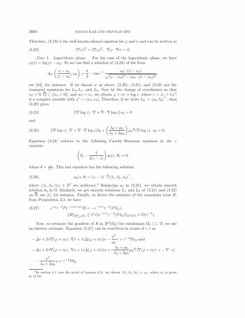
Therefore, (3.19) is the well-known eikonal equation for ϕ and ψ and can be written as
(3.23) (∇ψ)2 = (∇ϕ)2, ∇ϕ · ∇ψ = 0.
Case 1. Logarithmic phase. For the case of the logarithmic phase, we haveϕ(x) = log |x− x0|. So we can find a solution of (3.23) of the form
dS2
(x− x0|x− x0| , ω0
)=π
2− tan−1 ω0 · (x− x0)√
(x− x0)2 − (ω0 · (x− x0))2;
see [34], for instance. If we choose ψ as above, (3.20), (3.21), and (3.22) are thetransport equations for L0, L1, and L2. Now by the change of coordinates so thatx0 = 0, Ω ⊂ {x3 > 0}, and w0 = e1, we obtain ϕ + iψ = log z, where z = x1 + i|x′|is a complex variable with x′ := (x2, x3). Therefore, if we write L0 := (a0, b0)
�, then(3.20) gives
[(∇ log z) · ∇+∇ · ∇ log z]a0 = 0(3.24)
and
[(∇ log z) · ∇+∇ · ∇ log z] b0 +
(λ0 + μ0
λ0 + 2μ0
)μ0
12 (∇ log z) · a0 = 0.(3.25)
Equation (3.24) reduces to the following Cauchy–Riemann equation in the zvariable: (
∂z − 1
2(z − z)
)a0(z, θ) = 0,
where θ = x′|x′| . This last equation has the following solution:
(3.26) a0(z, θ) = (z − z)−12 (β1, β2, β3)
�,
where (β1, β2, β3) ∈ S2 are arbitrary.3 Replacing a0 in (3.25), we obtain smoothsolution b0 in Ω. Similarly, we get smooth solutions L1 and L2 of (3.21) and (3.22)on Ω; see [1], for instance. Finally, to derive the estimate of the remainder term R,from Proposition 3.2, we have
eτϕτ−2Pe−τ(ϕ+iψ)R = −e−iτψτ−4(PL2),(3.27)
‖R‖H2scl(Ω) ≤ Cτ‖e−iτψτ−4(PL2)‖L2(Ω) = O(τ−3).
Now, to estimate the gradient of R in H2(Ω0) for subdomain Ω0 ⊂⊂ Ω, we usean interior estimate. Equation (3.27) can be rewritten in terms of r, s as
−Δr + 2τ∇(ϕ+ iψ) · ∇r + τ(Δ(ϕ + iψ))r − κ2
μ0r = τ−2Pa2 and
−Δs+ 2τ∇(ϕ+ iψ) · ∇s+ τ(Δ(ϕ + iψ))s+ τλ0 + μ0
λ0 + 2μ0μ0
12 [∇(ϕ+ iψ) · r −∇ · r]
− κ2
λ0 + 2μ0s = τ−2Pb2.
3In section 6.1 (see the proof of Lemma 6.3), we choose (β1, β2, β3) = ω0, where ω0 is givenin (3.12).
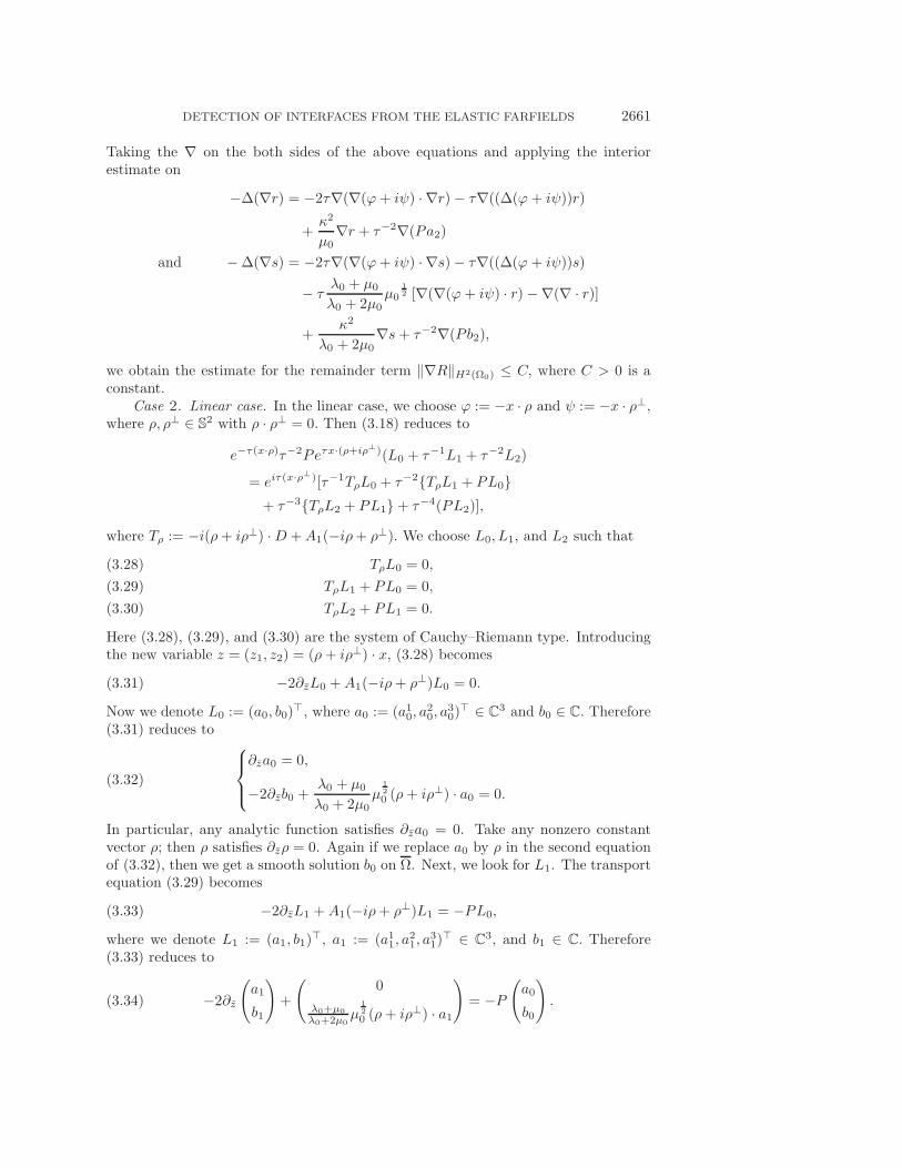
DETECTION OF INTERFACES FROM THE ELASTIC FARFIELDS 2661
Taking the ∇ on the both sides of the above equations and applying the interiorestimate on
−Δ(∇r) = −2τ∇(∇(ϕ+ iψ) · ∇r) − τ∇((Δ(ϕ + iψ))r)
+κ2
μ0∇r + τ−2∇(Pa2)
and −Δ(∇s) = −2τ∇(∇(ϕ+ iψ) · ∇s)− τ∇((Δ(ϕ + iψ))s)
− τλ0 + μ0
λ0 + 2μ0μ0
12 [∇(∇(ϕ + iψ) · r) −∇(∇ · r)]
+κ2
λ0 + 2μ0∇s+ τ−2∇(Pb2),
we obtain the estimate for the remainder term ‖∇R‖H2(Ω0) ≤ C, where C > 0 is aconstant.
Case 2. Linear case. In the linear case, we choose ϕ := −x · ρ and ψ := −x · ρ⊥,where ρ, ρ⊥ ∈ S2 with ρ · ρ⊥ = 0. Then (3.18) reduces to
e−τ(x·ρ)τ−2Peτx·(ρ+iρ⊥)(L0 + τ−1L1 + τ−2L2)
= eiτ(x·ρ⊥)[τ−1TρL0 + τ−2{TρL1 + PL0}
+ τ−3{TρL2 + PL1}+ τ−4(PL2)],
where Tρ := −i(ρ+ iρ⊥) ·D +A1(−iρ+ ρ⊥). We choose L0, L1, and L2 such that
TρL0 = 0,(3.28)
TρL1 + PL0 = 0,(3.29)
TρL2 + PL1 = 0.(3.30)
Here (3.28), (3.29), and (3.30) are the system of Cauchy–Riemann type. Introducingthe new variable z = (z1, z2) = (ρ+ iρ⊥) · x, (3.28) becomes
(3.31) −2∂zL0 +A1(−iρ+ ρ⊥)L0 = 0.
Now we denote L0 := (a0, b0)�, where a0 := (a10, a
20, a
30)
� ∈ C3 and b0 ∈ C. Therefore(3.31) reduces to
(3.32)
⎧⎪⎨⎪⎩∂za0 = 0,
−2∂zb0 +λ0 + μ0
λ0 + 2μ0μ
120 (ρ+ iρ⊥) · a0 = 0.
In particular, any analytic function satisfies ∂za0 = 0. Take any nonzero constantvector ρ; then ρ satisfies ∂zρ = 0. Again if we replace a0 by ρ in the second equationof (3.32), then we get a smooth solution b0 on Ω. Next, we look for L1. The transportequation (3.29) becomes
(3.33) −2∂zL1 +A1(−iρ+ ρ⊥)L1 = −PL0,
where we denote L1 := (a1, b1)�, a1 := (a11, a
21, a
31)
� ∈ C3, and b1 ∈ C. Therefore(3.33) reduces to
(3.34) −2∂z
(a1
b1
)+
(0
λ0+μ0
λ0+2μ0μ
120 (ρ+ iρ⊥) · a1
)= −P
(a0
b0
).
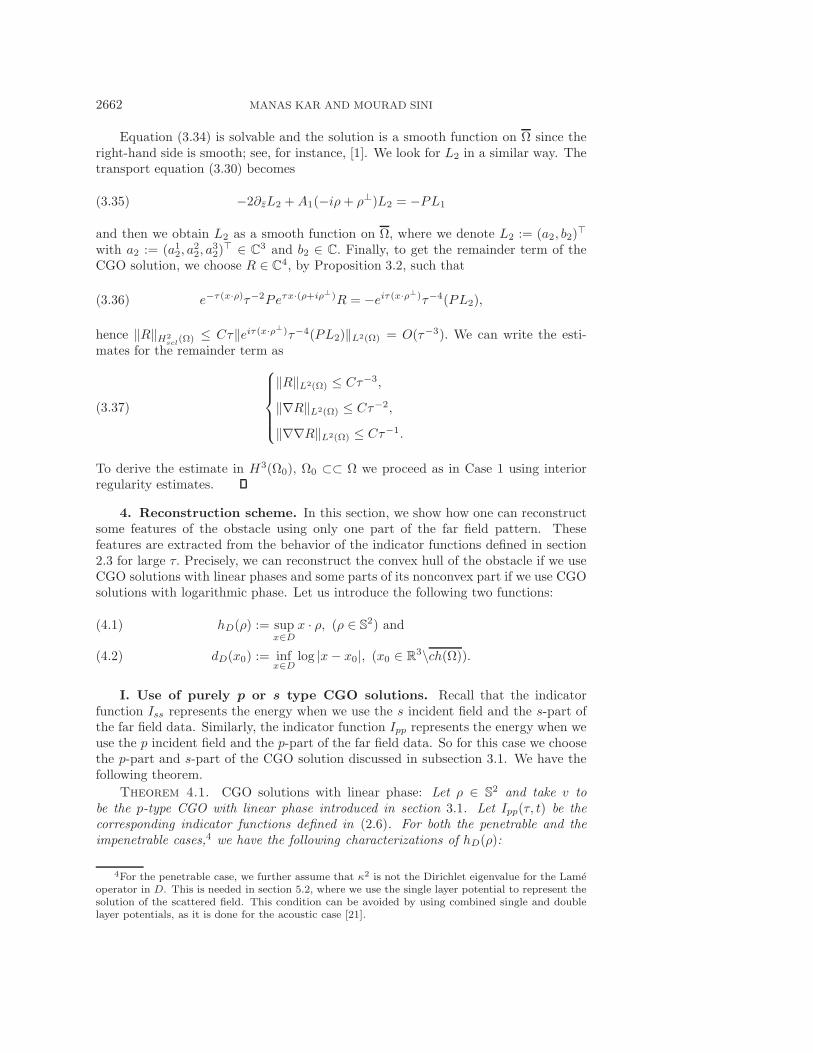
2662 MANAS KAR AND MOURAD SINI
Equation (3.34) is solvable and the solution is a smooth function on Ω since theright-hand side is smooth; see, for instance, [1]. We look for L2 in a similar way. Thetransport equation (3.30) becomes
(3.35) −2∂zL2 +A1(−iρ+ ρ⊥)L2 = −PL1
and then we obtain L2 as a smooth function on Ω, where we denote L2 := (a2, b2)�
with a2 := (a12, a22, a
32)
� ∈ C3 and b2 ∈ C. Finally, to get the remainder term of the
CGO solution, we choose R ∈ C4, by Proposition 3.2, such that
(3.36) e−τ(x·ρ)τ−2Peτx·(ρ+iρ⊥)R = −eiτ(x·ρ⊥)τ−4(PL2),
hence ‖R‖H2scl(Ω) ≤ Cτ‖eiτ(x·ρ⊥)τ−4(PL2)‖L2(Ω) = O(τ−3). We can write the esti-
mates for the remainder term as
(3.37)
⎧⎪⎪⎪⎨⎪⎪⎪⎩‖R‖L2(Ω) ≤ Cτ−3,
‖∇R‖L2(Ω) ≤ Cτ−2,
‖∇∇R‖L2(Ω) ≤ Cτ−1.
To derive the estimate in H3(Ω0), Ω0 ⊂⊂ Ω we proceed as in Case 1 using interiorregularity estimates.
4. Reconstruction scheme. In this section, we show how one can reconstructsome features of the obstacle using only one part of the far field pattern. Thesefeatures are extracted from the behavior of the indicator functions defined in section2.3 for large τ. Precisely, we can reconstruct the convex hull of the obstacle if we useCGO solutions with linear phases and some parts of its nonconvex part if we use CGOsolutions with logarithmic phase. Let us introduce the following two functions:
hD(ρ) := supx∈D
x · ρ, (ρ ∈ S2) and(4.1)
dD(x0) := infx∈D
log |x− x0|, (x0 ∈ R3\ch(Ω)).(4.2)
I. Use of purely p or s type CGO solutions. Recall that the indicatorfunction Iss represents the energy when we use the s incident field and the s-part ofthe far field data. Similarly, the indicator function Ipp represents the energy when weuse the p incident field and the p-part of the far field data. So for this case we choosethe p-part and s-part of the CGO solution discussed in subsection 3.1. We have thefollowing theorem.
Theorem 4.1. CGO solutions with linear phase: Let ρ ∈ S2 and take v tobe the p-type CGO with linear phase introduced in section 3.1. Let Ipp(τ, t) be thecorresponding indicator functions defined in (2.6). For both the penetrable and theimpenetrable cases,4 we have the following characterizations of hD(ρ):
4For the penetrable case, we further assume that κ2 is not the Dirichlet eigenvalue for the Lameoperator in D. This is needed in section 5.2, where we use the single layer potential to represent thesolution of the scattered field. This condition can be avoided by using combined single and doublelayer potentials, as it is done for the acoustic case [21].
DETECTION OF INTERFACES FROM THE ELASTIC FARFIELDS 2663
|τ−1Ipp(τ, t)| ≤ Ce−cτ , τ � 1, c, C > 0, and, in particular,(4.3)
limτ→∞ |Ipp(τ, t)| = 0 (t > hD(ρ)),
lim infτ→∞ |τ−1Ipp(τ, hD(ρ))| > 0 and precisely(4.4)
c ≤ τ−1|Ipp(τ, hD(ρ))| ≤ Cτ2, τ � 1, c, C > 0,
|τ−1Ipp(τ, t)| ≥ Cecτ , τ � 1, c, C > 0, and, in particular,(4.5)
limτ→∞ |Ipp(τ, t)| = ∞ (t < hD(ρ)).
CGO solutions with logarithmic phase: Let x0 ∈ R3\ch(Ω) and set v to bethe p-type CGO with logarithmic phase introduced in section 3.1.2. Let Ipp(τ, t) bethe corresponding indicator functions defined in (2.6). For both the penetrable and theimpenetrable case, we have the following characterizations of dD(x0):
|τ−1Ipp(τ, t)| ≤ Ce−cτ , τ � 1, c, C > 0, and, in particular,(4.6)
limτ→∞ |Ipp(τ, t)| = 0 (t < dD(x0)),
lim infτ→∞ |τ−1Ipp(τ, dD(x0))| > 0 and precisely(4.7)
c ≤ τ−1|Ipp(τ, dD(x0))| ≤ Cτ2, τ � 1, c, C > 0,
|τ−1Ipp(τ, t)| ≥ Cecτ , τ � 1, c, C > 0, and, in particular,(4.8)
limτ→∞ |Ipp(τ, t)| = ∞ (t > dD(x0)).
The above estimates are also valid if we replace Ipp by Iss and the p-type CGO solutionsby the s-type CGO solutions introduced in sections 3.1 and 3.2.
II. Use of CGO solutions with both nonvanishing p and s parts. Regard-ing the indicator function Isp, which depends on an s-incident wave and a p-part ofthe far field, and similarly for Ips, which depends on a p-incident wave and an s-partof the far field, we cannot use the expression of the CGO solution as in (3.2) and(3.5), since the s-part of (3.2) and the p-part of (3.5) are zero. Instead, we use theCGO solutions discussed in subsection 3.2. Using these CGO solutions, we have thefollowing theorem.
Theorem 4.2. CGO solutions with linear phases: Let ρ ∈ S2. For both the pen-etrable and the impenetrable case,5 we have the following characterizations of hD(ρ):
|τ−3Isp(τ, t)| ≤ Ce−cτ , τ � 1, c, C > 0, and, in particular,(4.9)
limτ→∞ |Isp(τ, t)| = 0 (t > hD(ρ)),
lim infτ→∞ |τ−3Isp(τ, hD(ρ))| > 0 and precisely(4.10)
c ≤ τ−3|Isp(τ, hD(ρ))| ≤ Cτ2, τ � 1, c, C > 0,
|τ−3Isp(τ, t)| ≥ Cecτ , τ � 1, c, C > 0, and, in particular,(4.11)
limτ→∞ |Isp(τ, t)| = ∞ (t < hD(ρ)).
CGO solutions with logarithmic phases: Let x0 ∈ R3\ch(Ω). For both the pene-
trable and the impenetrable case, we have the following characterizations of dD(x0):
5Same comments as for Theorem 4.1.

2664 MANAS KAR AND MOURAD SINI
|τ−3Isp(τ, t)| ≤ Ce−cτ , τ � 1, c, C > 0, and, in particular,(4.12)
limτ→∞ |Isp(τ, t)| = 0 (t < dD(x0)),
lim infτ→∞ |τ−3Isp(τ, dD(x0))| > 0 and precisely(4.13)
c ≤ τ−3|Isp(τ, dD(x0))| ≤ Cτ2, τ � 1, c, C > 0,
|τ−3Isp(τ, t)| ≥ Cecτ , τ � 1, c, C > 0, and, in particular,(4.14)
limτ→∞ |Isp(τ, t)| = ∞ (t > dD(x0)).
The above estimates are valid if we replace Isp by Ips.From the above two theorems, we see that in the case of the linear phase for a fixed
direction ρ (accordingly, in the case of logarithmic phase for a fixed direction x0), thebehavior of the indicator function Iij , where ij = pp, ss, sp, or ps, changes drasticallyin terms of τ : exponentially decaying if t > hD(ρ) (accordingly t < dD(x0) for thelogarithmic phase), polynomially behaving if t = hD(ρ) (accordingly t = dD(x0) forthe logarithmic phase), and exponentially growing if t < hD(ρ) (accordingly t >dD(x0) for the logarithmic phase). Using this property of the indicator functionswe can reconstruct the support function hD(ρ), ρ ∈ S2 (accordingly the distancedD(x0), x0 ∈ R3\ch(Ω), for the logarithmic phase) from the far field measurement.Finally, from this support function for linear phase, we can reconstruct the convex hullof D and from the distance function for the logarithmic phase, we can, in additionto the convex hull, reconstruct parts of the nonconvex part of the obstacle D. Letus finish this section by rephrasing the formulas in Theorems 4.1 and 4.2 as follows:
hD(ρ)− t = limτ→∞log |Iij(τ,t)|
2τ for ij = pp, ss, sp, ps when we use CGO solutions with
the linear phase and t − dD(x0) = limτ→∞log |Iij(τ,t)|
2τ for ij = pp, ss, sp, ps when weuse CGO solutions with the logarithmic phase. The formulas are easily deduced from(4.4), (4.7), (4.10), and (4.13) and the following identities:
Iij(τ, t) = e2τ(hD(ρ)−t)Iij(τ, hD(ρ)),(4.15)
Iij(τ, t) = e2τ(t−dD(x0))Iij(τ, dD(x0)).(4.16)
5. Justification of the reconstruction schemes. In this section, we provethe above two theorems using all the CGO solutions for both the penetrable andimpenetrable obstacle cases. For that we only focus on the four points (4.4), (4.7),(4.10), and (4.13) since we have (4.15) and (4.16). In addition, the lower estimatesin (4.4), (4.7), (4.10), and (4.13) are the most difficult part since the upper boundsare easily obtained using the Cauchy–Schwarz inequality, the well posedness of theforward problems, and the upper estimate of the H1-norms of the CGO solutionsgiven in section 6. So, we mainly focus in our proofs on the lower estimates.
5.1. The penetrable obstacle case. We consider w as an incident field andus(w) the scattered field; therefore the total field wt = w+us(w) satisfies the problem
(5.1)
⎧⎨⎩∇ · (σ(wt)) + κ2wt = 0 in R3,
us(w) satisfies the Kupradze radiation condition,
recalling that σ(wt) = λ(∇·wt)I3+μ(∇wt+(∇wt)�). The incident CGO field satisfies
(5.2) ∇ · (σ0(w)) + κ2w = 0 in Ω,
DETECTION OF INTERFACES FROM THE ELASTIC FARFIELDS 2665
where σ0(v) = λ0(∇·v)I3 +2μ0ε(v) for any displacement field v. Accordingly, we willuse σD(v) to denote σ(v)− σ0(v), i.e., σD(v) = λD(∇ · v)I3 + 2μDε(v). Note that for
a matrix A = (aij), we use |A| to denote (∑
i,j |aij |2)12 . For any matrices A = (aij)
and B = (bij) we define the product as follows:
(5.3) A : B� = tr(AB),
where tr(A) is the trace of the matrix A. Also frequently we will use the basic identity
(5.4) σ(u) : (∇v)� = σ(v) : (∇u)�
and Betti’s identity
(5.5)
∫Ω
(∇ · σ(u)) · vdx = −∫Ω
σ(u) : (∇v)�dx+
∫∂Ω
(σ(u) · ν) · vds(x).
Lemma 5.1. We have the following identity:
tr(σ(u)∇u) = 3λ+ 2μ
3|∇ · u|2 + 2μ
∣∣∣∣ε(u)− ∇ · u3
I3
∣∣∣∣2
.
Proof. Define Sym∇u := 12 (∇u + (∇u)�) = ε(u). For any α, β, and a matrix A,
we have the following identity [17]:
(5.6) α|tr(A)|2 + 2β|SymA|2 =3α+ 2β
3|tr(A)|2 + 2β
∣∣∣∣SymA− tr(A)
3I3
∣∣∣∣2
.
Substituting A = ∇u, α = λ, β = μ in (5.6), we obtain
tr(σ(u)∇u) = λ|∇ · u|2 + 2μ|ε(u)|2
=3λ+ 2μ
3|∇ · u|2 + 2μ
∣∣∣∣ε(u)− ∇ · u3
I3
∣∣∣∣2
.
Let v and w be two incident waves. We set
I(v, w) :=
∫D
[us(v) · (σ(w) · ν)− v · (σ(us(w)) · ν)]ds(x).
Hence from (2.2), (2.3), (2.4), and (2.5), we have
(5.7)
Iss(τ, t) = I(vs, vs), Ipp(τ, t)= I(vp, vp), Ips(τ, t)= I(vp, vs), and Isp(τ, t)= I(vs, vp).
5.1.1. Some key inequalities.
Lemma 5.2. Let v and w be two incident waves. We have the following estimatesfor the indicator function:
I(v, w) = −∫Ω
σD(w) : (∇v)�dx−∫Ω
σD(us(w)) : (∇v)�dx
2666 MANAS KAR AND MOURAD SINI
and
−I(v, v) ≥∫D
4μ0μD3μ
|ε(v)|2dx−∫D
4μ0μD9μ
|(∇ · v)I3|2dx− κ2∫Ω
|us(v)|2dx(5.8)
−∫∂Ω
(σ(us(v)) · ν) · us(v)ds(x).
Proof. We have wt = w + us(w) and vt = v + us(v). So, from Betti’s identity weobtain ∫
∂Ω
(σ(wt) · ν) · vds(x) =∫Ω
(∇ · σ(wt)) · vdx+
∫Ω
σ(wt) : (∇v)�dx(5.9)
= −κ2∫Ω
wt · vdx+
∫Ω
σ(wt) : (∇v)�dx.
On the other hand, again applying Betti’s identity we have∫∂Ω
(σ(v) · ν) · wtds(x) =∫∂Ω
(σ0(v) · ν) · wtds(x) =∫Ω
(∇ · σ0(v)) · wtdx(5.10)
+
∫Ω
σ0(v) : (∇wt)�dx
= −κ2∫Ω
v · wtdx+
∫Ω
σ0(v) : (∇wt)�dx.
Subtracting (5.9) and (5.10) gives
∫∂Ω
(σ(wt) · ν) · vds(x) −∫∂Ω
(σ(v) · ν) · wtds(x) =∫Ω
(σ(wt)− σ0(wt)) : (∇v)�dx
(5.11)
=
∫Ω
σD(wt) : (∇v)�dx
=
∫Ω
σD(v) : (∇wt)�dx.
Therefore replacing wt by w + us(w) in (5.11), we obtain
I(v, w) :=
∫∂Ω
us(w) · (σ(v) · ν)ds(x) −∫∂Ω
v · (σ(us(w)) · ν)ds(x)(5.12)
=
∫∂Ω
(σ(w) · ν) · vds(x)−∫∂Ω
(σ(v) · ν) · wds(x) −∫Ω
σD(w) : (∇v)�dx
−∫Ω
σD(us(w)) : (∇v)�dx.
Since v and w satisfy the equations
∇ · σ0(v) + κ2v = 0,(5.13)
∇ · σ0(w) + κ2w = 0,(5.14)
multiplying (5.13) by w and (5.14) by v and doing integration by parts, we end upwith the following Graffi’s reciprocity identity:
(5.15)
∫∂Ω
(σ0(w) · ν) · vds(x) −∫∂Ω
(σ0(v) · ν) · wds(x) = 0.

DETECTION OF INTERFACES FROM THE ELASTIC FARFIELDS 2667
Therefore substituting (5.15) in (5.12) we have the formula for I(v, w):
(5.16) I(v, w) = −∫Ω
σD(w) : (∇v)�dx−∫Ω
σD(us(w)) : (∇v)�dx.
Now we look for the estimate of I(v, v). Replacing w by v, we have
I(v, v) = −∫Ω
σD(v) : (∇v)�dx−∫Ω
σD(us(v)) : (∇v)�dx = −
∫Ω
σD(vt) : (∇v)�dx
(5.17)
= −∫Ω
σD(v) : (∇vt)�dx = −∫Ω
σD(vt) : (∇vt)�dx
+
∫Ω
σD(us(v)) : (∇vt)�dx
= −∫Ω
σD(vt) : (∇vt)�dx+
∫Ω
σD(vt) : (∇us(v))�dx.
On the other hand we have
κ2∫Ω
|us(v)|2dx=∫Ω
(σ(vt)−σ0(v)) : (∇us(v))�dx−∫∂Ω
((σ(vt)−σ0(v))·ν)·us(v)ds(x).
Substituting v = vt− us(v) in the first term and vt = v+ us(v) in the second term inthe right side of the above identity, we obtain
κ2∫Ω
|us(v)|2dx =
∫Ω
(σ(vt)− σ0(vt) + σ0(u
s(v))) : (∇us(v))�dx(5.18)
−∫∂Ω
(σ(us(v)) · ν) · us(v)ds(x)
=
∫Ω
σD(vt) : (∇us(v))�dx +
∫Ω
σ0(us(v)) : (∇us(v))�dx
−∫∂Ω
(σ(us(v) · ν)) · us(v)ds(x).
Combining (5.17) and (5.18), we obtain
−I(v, v) =∫Ω
σD(vt) : (∇vt)�dx+
∫Ω
σ0(us(v)) : (∇us(v))�dx − κ2
∫Ω
|us(v)|2dx(5.19)
−∫∂Ω
(σ(us(v)) · ν) · us(v)ds(x).
Therefore from Lemma 5.1, we have
−I(v, v) =∫Ω
3λD + 2μD3
|∇ · vt|2dx+
∫Ω
2μD|ε(vt)− ∇ · vt3
I3|2dx(5.20)
+
∫Ω
3λ0 + 2μ0
3|∇ · us(v)|2dx
+
∫Ω
2μ0
∣∣∣∣ε(us(v))− ∇ · us(v)3
I3
∣∣∣∣2
dx− κ2∫Ω
|us(v)|2dx
−∫∂Ω
(σ(us(v)) · ν) · us(v)ds(x).
2668 MANAS KAR AND MOURAD SINI
To estimate the first four integrals in the right-hand side of (5.20), we follow a few
steps from [18, Proposition 5.1]. Set B1 = ε(v)− ∇·v3 I3 and B2 = ε(vt)− ∇·vt
3 I3. So,
3λD + 2μD3
|∇ · vt|2 + 2μD
∣∣∣∣ε(vt)− ∇ · vt3
I3
∣∣∣∣2
+3λ0 + 2μ0
3|∇ · us(v)|2
+ 2μ0
∣∣∣∣ε(us(v)) − ∇ · us(v)3
I3
∣∣∣∣2
=3λD + 2μD
3|∇ · vt|2 + 2μD|B2|2 + 3λ0 + 2μ0
3|∇ · us(v)|2 + 2μ0|B1 −B2|2
=3λ+ 2μ
3|∇ · vt|2 − 2(3λ0 + 2μ0)
3(∇ · v)(∇ · vt) + 2μ|B2|2 − 2μ0B1 ·B2
+3λ0 + 2μ0
3|∇ · v|2 + 2μ0|B1|2
=
∣∣∣∣∣√
3λ+ 2μ
3∇ · vt −
√3
3λ+ 2μ
3λ0 + 2μ0
3∇ · v
∣∣∣∣∣2
+
∣∣∣∣√2μB2 − 2μ0√2μB1
∣∣∣∣2
+
{3λ0 + 2μ0
3− 3
3λ+ 2μ
(3λ0 + 2μ0
3
)2}|∇ · v|2 +
{2μ0 − (2μ0)2
2μ
}|B1|2
≥ 3λ0 + 2μ0
3(3λ+ 2μ){3λD + 2μD} |∇ · v|2 + 2μ0μD
μ
∣∣∣∣ε(v)− ∇ · v3
I3
∣∣∣∣2
.
Hence
−I(v, v) ≥∫D
{3λ0 + 2μ0
3(3λ+ 2μ)(3λD + 2μD)|∇ · v|2 + 2μ0μD
μ
∣∣∣∣ε(v)− ∇ · v3
I3
∣∣∣∣2}dx
− κ2∫Ω
|us(v)|2dx−∫∂Ω
(σ(us(v)) · ν) · us(v)ds(x).
(5.21)
Therefore,
− I(v, v)
≥∫D
2μ0μDμ
∣∣∣∣ε(v)− ∇ · v3
I3
∣∣∣∣2
dx− κ2∫Ω
|us(v)|2dx−∫∂Ω
(σ(us(v)) · ν) · us(v)ds(x)
≥∫D
4μ0μD3μ
|ε(v)|2dx−∫D
4μ0μD9μ
|(∇ · v)I3|2dx− κ2∫Ω
|us(v)|2dx
−∫∂Ω
(σ(us(v)) · ν) · us(v)ds(x).
Lemma 5.3. Let v be an incident field and us(v) the corresponding scattered field.Then we have
(5.22)
∣∣∣∣∫∂Ω
(σ(us(v)) · ν) · us(v)ds(x)∣∣∣∣ ≤ CF‖∇v‖2L2(D),
where F is defined by
F :=
∫B\Ω
‖(∇Φ(x, ·))�‖2L2(D)dx+
∫B\Ω
‖∇(∇Φ(x, ·))�‖2L2(D)dx,

DETECTION OF INTERFACES FROM THE ELASTIC FARFIELDS 2669
with B as any smooth domain containing Ω and Φ is the fundamental solution for theelasticity.
Proof. Let us take a ball B such that D ⊂⊂ B ⊂⊂ Ω. The scattering field us(v)satisfies
(5.23)
⎧⎨⎩∇ · σ(us(v)) + κ2us(v) = −∇ · σD(v) in R3,
us(v) satisfies the radiation condition,
and Φ(·, ·) is the fundamental solution for elasticity and satisfies
(5.24) ∇ · σ(Φ(x, y)) + κ2Φ(x, y) = δx(y) in R3,
where δx is the Dirac measure at x.
Step 1. First we show that for x ∈ R3\B, we have
(5.25) us(v)(x) =
∫D
σD(v(y)) : (∇Φ(x, y))�dy.
Indeed, take x ∈ R3\B. Then multiplying by Φ(x, y) in (5.23) and doing integration
by parts we obtain∫B
σD(v) : (∇Φ(x, y))�dy(5.26)
= −∫B
σ(us(v)) : (∇Φ(x, y))�dy +∫∂B
(σ(us(v)) · ν) · Φ(x, y)ds(y)
+ κ2∫B
us(v) · Φ(x, y)dy
= −∫B
σ(∇Φ(x, y)) : (us(v))�dy +∫∂B
(σ(us(v)) · ν) · Φ(x, y)ds(y)
+ κ2∫B
us(v) · Φ(x, y)dy.
Applying integration by parts and from (5.24), we have∫B
σD(v) : (∇Φ(x, y))�dy =
∫∂B
(σ(us(v)) · ν) · Φ(x, y)ds(y)(5.27)
−∫∂B
(σ(Φ(x, y)) · ν) · us(v)ds(y).
On the other hand, consider a ball BR such that B ⊂ BR and take x ∈ BR\B.Now multiplying both sides in (5.23) by Φ(x, y) and applying integration by parts,we obtain
−∫BR\(B∪Bε)
σ(Φ(x, y)) : (∇us(v))�dy +∫∂B∪∂Bε
(σ(us(v)) · ν) · Φ(x, y)ds(y)(5.28)
+κ2∫BR\(B∪Bε)
us(v) · Φ(x, y)dy = 0.
2670 MANAS KAR AND MOURAD SINI
Again doing integration by parts on the first term of (5.28) and from (5.24), we have
(5.29)∫∂B∪∂Bε
(σ(us(v)) · ν) · Φ(x, y)ds(y) −∫∂B∪∂Bε
(σ(Φ(x, y)) · ν) · us(v)ds(y) = 0.
Combining (5.27) and (5.29) together with the following relation (see, for instance,[7])
limε→0
[∫∂Bε
(σ(Φ(x, y)) · ν) · us(v)ds(y)−∫∂Bε
(σ(us(v)) · ν) · Φ(x, y)ds(y)]= us(v)(x).
Hence, we obtain (5.25).Step 2. We justify the estimate (5.22). Consider a smooth domain B such that
Ω ⊂⊂ B. Using the Cauchy–Schwarz inequality and the trace theorem we have∣∣∣∣∫∂Ω
(σ(us(v)) · ν) · us(v)ds(x)∣∣∣∣ ≤ ‖us(v)‖
H12 (∂Ω)
‖σ(us(v)) · ν‖H− 1
2 (∂Ω)(5.30)
≤ C‖us(v)‖2H1(B\Ω)
.
On the other hand, from (5.25) using the Cauchy–Schwarz inequality, we obtain forx ∈ B\Ω
|us(v)(x)| ≤ ‖σD(v)‖L2(D)‖(∇Φ(x, ·))�‖L2(D),
|∇us(v)(x)| ≤ ‖σD(v)‖L2(D)‖(∇(∇Φ(x, ·))�)‖L2(D).
Therefore from (5.30) together with the estimate
‖us(v)‖2H1(B\Ω)
≤ ‖σD(v)‖2L2(D)
×{∫
B\Ω‖(∇Φ(x, ·))�‖2L2(D)dx+
∫B\Ω
‖∇(∇Φ(x, ·))�‖2L2(D)dx
},
we obtain our required estimate (5.22).Lemma 5.4 (L2−Lq-estimate). There exists 1 ≤ q0 < 2 such that for q0 < q ≤ 2,
‖us(v)‖L2(Ω) ≤ C‖∇v‖Lq(D)
with a positive constant C.Proof. We recall that us(v) satisfies
(5.31)
{∇ · σ(us(v)) + κ2us(v) = −∇ · σD(v) in Ω,
us(v) = us(v)|∂Ω on ∂Ω.
We write it as us(v) = us1(v) + us2(v), where us1(v) satisfies
(5.32)
{∇ · σ(us1(v)) + κ2us1(v) = 0 in Ω,
us1(v) = us(v)|∂Ω on ∂Ω
and us2(v) satisfies
(5.33)
{∇ · σ(us2(v)) + κ2us2(v) = −∇ · σD(v) in Ω,
us2(v) = 0 on ∂Ω.
DETECTION OF INTERFACES FROM THE ELASTIC FARFIELDS 2671
Step 1. There exists a positive constant C such that for every q > 1, we have
(5.34) ‖us1(v)‖L2(Ω) ≤ C‖∇v‖Lq(D).
Indeed, from (5.25), we deduce that ‖us(v)‖H
12 (∂Ω)
≤ C‖∇v‖Lq(D), since D ⊂⊂ Ω.
The estimate (5.34) comes now from the well posedness of (5.32).Step 2. There exists 1 ≤ q0 < 2 such that for q0 < q ≤ 2, we have
‖us2(v)‖L2(Ω) ≤ C‖∇v‖Lq(D).
Indeed, let u ∈ H10 (Ω) be the distribution solution satisfying the elastic model
∇ · (σ(u)) + κ2u = us2(v) in Ω.
Multiplying both sides of the last equation by us2(v) and integrating by parts, weobtain
‖us2(v)‖2L2(Ω) = −∫Ω
tr(σ(u)∇us2(v))dx + κ2∫Ω
u · us2(v)dx(5.35)
= −∫Ω
tr(σ(us2(v))∇u)dx + κ2∫Ω
u · us2(v)dx.
Similarly, multiplying both sides of the equation ∇ ·σ(us2(v))+ κ2us2(v) = −∇ ·σD(v)by u and integrating by parts, we have
(5.36) −∫Ω
tr(σ(us2(v))∇u)dx+ κ2∫Ω
us2(v) · udx =
∫Ω
tr(σD(v)∇u)dx.
From (5.35) and (5.36) we get
‖us2(v)‖2L2(Ω) =
∫Ω
tr(σD(v)∇u)dx.
Then applying Holder’s inequality, for any 1 ≤ q′ <∞, we obtain
(5.37) ‖us2(v)‖2L2(Ω) ≤ ‖σD(v)‖Lq(D)‖∇u‖Lq′ (Ω),
where 1q +
1q′ = 1. By definition of u we have
(5.38)
{∇ · (σ(u)) = us(v)− κ2u in Ω,
u = 0 on ∂Ω.
In [15], problem (5.38) is studied in the Lp(Ω) spaces and it is proved that ∃ q′1 > 2and C > 0 such that ∀ 2 ≤ q′ < q′1, we have
‖u‖W 1,q′ (Ω) ≤ C‖us2(v)− κ2u‖W−1,q′ (Ω).
Since L2(Ω) ↪→W−1,q′(Ω) for 2 ≤ q′ ≤ 6, then we deduce that
(5.39) ‖∇u‖Lq′(Ω) ≤ C{‖u‖L2(Ω) + ‖us2(v)‖L2(Ω)}
2672 MANAS KAR AND MOURAD SINI
for some C > 0. From the well posedness in H1(Ω), we have the L2-estimate
(5.40) ‖u‖L2(Ω) ≤ C‖us2(v)‖L2(Ω).
Therefore from (5.39) and (5.40) we have
(5.41) ‖∇u‖Lq′(Ω) ≤ C‖us2(v)‖L2(Ω)
for some C > 0. Combining (5.37) and (5.41), we obtain ‖us2(v)‖L2(Ω) ≤ C‖∇v‖Lq(D)
for some C =C(κ, λ, μ), for q0<q≤ 2, where 1q0
+ 1q′0
=1 with q′0 =
min{q′1, 6}.Applying the Korn’s inequality, the first term of the right-hand side of inequality
(5.8) can be lower bounded by the norms of the CGO solutions only. In the (p, p)case, the second term behaves like the CGO solution of the Helmholtz equation andfor the (s, s) case it will be zero. Therefore, using Lemmas 5.3 and 5.4, from theinequality (5.8) we deduce that
(5.42) −I(v, v) ≥ (C1 −F)‖∇v‖2L2(D) + c1‖v‖2L2(D) − c2‖V ‖2L2(D) − c3‖∇v‖2Lq(D),
where q0 < q < 2 and v is considered to be up, v = up = ∇V with V as the CGOsolutions satisfying (Δ + κ2p)V = 0 and
(5.43) −I(v, v) ≥ (C1 −F)‖∇v‖2L2(D) + c1‖v‖2L2(D) − c3‖∇v‖2Lq(D),
where v is considered to be us, v = us := curlW, W as the CGO solutions satisfying(Δ + κ2s)W = 0.
For the mixed case the indicator function can be written in the form
I(us, up) = −I(us, us) + I(us, u),
I(up, us) = −I(us, us) + I(u, us),
where CGO u = up+ us. Using the well posedness of the forward scattering problem,the trace theorem, and the Cauchy’s ε-inequality, we have
|I(us, u)| ≤ C
([1
ε‖∇u‖2L2(D) + ε‖∇us‖2L2(D)
]+
[1
ε‖u‖2L2(D) + ε‖us‖2L2(D)
]);
then from Lemmas 5.2 and 5.3, we obtain for q0 < q < 2,
I(us, up), I(up, us)(5.44)
≥ (C −F − Cε)‖∇us‖2L2(D) + (C − Cε)‖us‖2L2(D) − c1‖∇us‖2Lq(D)
− C
ε‖∇u‖2L2(D) −
C
ε‖u‖L2(D).

DETECTION OF INTERFACES FROM THE ELASTIC FARFIELDS 2673
5.1.2. Proof of Theorem 4.1. Assume v to be the p-part of the CGO solutionswith linear and logarithmic phases. From (5.42) together with Lemma 6.4 we obtain
−τ−1I(v, v)
‖v‖2L2(D)
≥ τ−1
[(C1 −F)
‖∇v‖2L2(D)
‖v‖2L2(D)
+ c1 − c2‖V ‖2L2(D)
‖v‖2L2(D)
− κ2‖∇v‖2Lq(Ω)
‖v‖2L2(D)
].
≥ τ−1[(C1 −F)cτ2 + c1 − c2τ
−2 − c3τ3− 2
q].
Therefore−τ−1I(v, v) ≥ (C1−F)c, τ � 1, c > 0. Note that B is taken to be arbitrary(but containing Ω). Hence, we choose it such that ∂B is very close to Ω. Due to thesmoothness of Φ(x, z) for x away from z, we can choose B such that C1−F > c0 > 0.Hence |τ−1I(v, v)| ≥ C > 0, τ � 1. Similarly, considering v to be the s-part of theCGO solutions with linear and logarithmic phases, Theorem 4.1 follows from (5.43)and Lemma 6.4.
5.1.3. Proof of Theorem 4.2. Recall that up and us are the p-part and thes-part of the CGO solutions for both the linear and logarithmic phases constructedin Proposition 3.4. Also, the total field u is u = up + us. From Lemma 6.7 and theestimate (5.44), we have
I(us, up)
‖∇us‖2L2(D)
≥ (C −F − Cε) + (C − C2)ε‖us‖2L2(D)
‖∇us‖2L2(D)
− C1
‖∇us‖2Lq(D)
‖∇us‖2L2(D)
− C
ε
‖∇u‖2L2(D)
‖∇us‖2L2(D)
− C
ε
‖u‖2L2(D)
‖∇us‖2L2(D)
≥ (C −F − Cε)− c1τ−2 − c2τ
(1− 2q ) − c3
ετ−2 − C
ετ−4.
We can choose ε > 0 and F such that (C − F − Cε) > c0 > 0, where c0 is another
constant. ThereforeI(us,up)
‖∇us‖2L2(D)
≥ c0 for τ � 1, and together with ‖∇us‖2L2(D) ≥O(τ3), we obtain our required estimate |τ−3I(us, up)| > c0 > 0, τ � 1.
Remark 5.5. In the case of a penetrable obstacle D, the interface ∂D is charac-terized by the condition 2μD+3λD ≥ 0 and μD > 0 (or 2μD+3λD ≤ 0 and μD < 0).As we said in the introduction, these conditions are needed only in the vicinity of ∂D,since the CGO solutions and their derivatives are exponentially decaying locally inthe interior of D, or its image by the local transformations (6.1) or (6.2); see sections6 and 7. If μD = 0 in D or near ∂D, then we cannot conclude by using s-parts ofthe far field patterns corresponding to s incident waves to reconstruct D. The reasonis that the corresponding indicator function is lower bounded by c
∫D|∇ · v|2 + lot
(see (5.21)), where “lot” stands for lower order terms. Since v is s incident type,∇ · v = 0. Similarly, we cannot conclude by using p-parts of the far field patternscorresponding to p incident waves for the reconstruction as ∇ · v = −κ2pV and henceits L2(D) norm is absorbed by the term “lot.” The same conclusion applies for themixed cases. Hence the particular case μD = 0 and λD �= 0 near ∂D is not coveredby our results. However, this case can be covered if we use the full far field patterninstead of its p or s parts.
5.2. The impenetrable obstacle case.
5.2.1. Key inequalities. It is shown in section 2 that the indicator functionshave the general form
(5.45) I(v, w) :=
∫∂D
[us(w) · (σ(v) · ν)− v · (σ(us(w)) · ν)]ds(x),

2674 MANAS KAR AND MOURAD SINI
where us(w) is the scattered field associated to the incident field w. Using integrationby parts and the boundary conditions, we can write∫
∂D
us(w) · (σ(v) · ν)ds(x)
= −∫∂D
us(w) · (σ(us(v)) · ν)ds(x)
= −∫∂Ω
us(w) · (σ(us(v)) · ν)ds(x) +∫Ω\D
σ(us(v)) : ∇us(w)dx
− κ2∫Ω\D
us(w) · us(v)dx
and∫∂D
v·(σ(us(w))·ν)ds(x) = −∫∂D
v·(σ(w)·ν)ds(x) = −∫D
σ(v) : ∇wdx+κ2∫D
w·vdx.
Hence (5.45) becomes
I(v, w) =−∫∂Ω
us(w) · (σ(us(v)) · ν)ds(x) +∫Ω\D
σ(us(v)) : ∇us(w)dx(5.46)
− κ2∫Ω\D
us(w) · us(v)dx
+
∫D
σ(v) : ∇wdx − κ2∫D
w · vdx.
The inequalities for Iss and Ipp. In this case, we take v = w. Hence, we have
I(v, v) ≥ −∫∂Ω
us(v) · (σ(us(v)) · ν)ds(x) +∫D
σ(v) : ∇vdx
−κ2∫Ω\D
|us(v)|2dx− κ2∫D
|v|2dx.
By the ellipticity condition of the elasticity tensor and the Korn inequality, we have∫D
σ(v) : ∇vdx=∫D
�(ε(v))ε(v)dx≥ c1
∫D
ε(v) : ε(v)dx≥ c1CK
‖∇v‖2L2(D)−c1‖v‖2L2(D),
where CK is the Korn constant and � is the elasticity tensor. Hence
I(v, v) ≥ −∫∂Ω
us(v) · (σ(us(v)) · ν)ds(x) + c2‖∇v‖2L2(D)(5.47)
−κ2∫Ω\D
|us(v)|2dx− (κ2 + c3)
∫D
|v|2dx.
The inequalities for Isp and Ips. In this case, we take v �= w. We then usethe form I(v, w) = −I(v, v) + I(v, U), where U := v + w. As in the penetrable case,using the well posedness of the forward scattering problem and the trace theorem, weshow that
|I(v, U)| ≤ C
(1
ε‖∇U‖2L2(D) + ε‖∇v‖2L2(D)
)+ C
(1
ε‖U‖2L2(D) + ε‖v‖2L2(D)
)
DETECTION OF INTERFACES FROM THE ELASTIC FARFIELDS 2675
for 0 < ε� 1. Combining this estimate with (5.47), we obtain
−I(v, w)≥ I(v, v)−C
(1
ε‖∇U‖2L2(D) + ε‖∇v‖2L2(D)
)−C
(1
ε‖U‖2L2(D) + ε‖v‖2L2(D)
).
(5.48)
In the next subsection, we derive the lower bound for the indicator function I(v, v) interms of the CGO solutions only.
5.2.2. Estimating the dominant terms.Step 1. In this step, we prove that
∫∂Ω u
s(v) · (σ(us(v)) · ν)ds(x) is dominated by‖v‖2H1(D). To do this, we represent us as a single layer potential
(5.49) us :=
∫∂D
Φ(x, z)f(z)ds(z) := (Sf)(x),
where f satisfies
(5.50)
(−1
2I +K∗
)f = σn(u
s) = −σn(v)
and K∗ is the adjoint of the double layer potential K for the Lame system.The following lemma shows that the integral equation (5.50) is solvable in the
spaces H−s(∂D) for s ∈ [−1, 1] if we assume that κ2 is not an eigenvalue of theDirichlet–Lame operator stated in D.
Lemma 5.6. Assume that κ2 is not a Dirichlet eigenvalue of the Lame operatorin D. Then the operator
−1
2I +K∗ : H−t(∂D) −→ H−t(∂D), 0 ≤ t ≤ 1,
is invertible.Now, we use the estimate∣∣∣∣
∫∂Ω
us(v) · (σ(us(v)) · ν)ds(x)∣∣∣∣ ≤ ‖us‖
H12 (∂Ω)
‖σn(us) · ν‖H− 1
2 (∂Ω)
≤ C‖us‖2H1(B\Ω)
, C > 0,
where B is a measurable set containing Ω. Using the representation (5.49), we obtain
‖us‖H1(B\Ω) ≤ ‖f‖H−t(∂D)‖F‖H1(B\Ω)
for 0 ≤ t ≤ 1, where F (x) := ‖Φ(x, ·)‖Ht(∂D). Note that ‖F‖H1(B\Ω) makes sense
since ∂D is away from B\Ω. From (5.50) and Proposition 5.7, stated at the end ofthis section, we deduce that
(5.51) ‖f‖H−t(∂D) ≤ ‖σn(v)‖H−t(∂D) ≤ C‖v‖H−t+3
2 (D)for
1
2≤ t < 1.
Therefore, we have
(5.52)
∣∣∣∣∫∂Ω
us(v) · (σ(us(v)) · ν)ds(x)∣∣∣∣ ≤ C‖v‖2
H−t+32 (D)
for 12 ≤ t < 1.
2676 MANAS KAR AND MOURAD SINI
Step 2. We prove that ‖us(v)‖L2(Ω\D) is dominated by ‖v‖H1(D). The single layer
operator S : H−t(∂D) → H−t+ 3
2
loc (R3), 0 ≤ t ≤ 1, defined in (5.49), is bounded; see[28]. Hence we obtain
(5.53) ‖us(v)‖L2(Ω\D) ≤ C‖f‖H−t(∂D), 0 ≤ t ≤ 1.
From (5.51), for 12 ≤ t < 1, we have
(5.54) ‖us‖2L2(Ω\D)
≤ ‖v‖2H−t+3
2 (D).
We choose 12 < t < 1; then by interpolation and using the Cauchy’s ε-inequality, we
obtain
(5.55) ‖v‖2H−t+3
2 (D)≤ ε‖∇v‖2L2(D) +
C
ε‖v‖2L2(D)
with some C > 0 fixed and every ε > 0. Finally, combining (5.47), (5.52), (5.54), and(5.55), we deduce that
(5.56) I(v, v) ≥ c‖∇v‖2L2(D) − C‖v‖2L2(D), τ � 1,
with positive constants c and C independent on v, w, and τ .6 Also for two differenttypes of CGO solutions v, w, combining the estimates (5.48) and (5.56), we obtain
−I(v, w) ≥ (c− ε)‖∇v‖2L2(D) − C(1 + ε)‖v‖2L2(D) −c1ε‖∇U‖2L2(D) −
C
ε‖U‖2L2(D),
recalling that U = v + w is the total field, where c, C, c1 are positive constants andε > 0 is chosen very small so that c−ε will be greater than some positive real number.Therefore, the inequalities for the indicator functions are as follows:
I(up, up) ≥ c‖∇vp‖2L2(D) − C‖vp‖2L2(D),
(5.57)
−I(up, us) ≥ (c− ε)‖∇vp‖2L2(D) − C(1 + ε)‖vp‖2L2(D) −c1ε‖∇v‖2L2(D) −
C
ε‖v‖2L2(D),
(5.58)
I(us, us) ≥ c‖∇vs‖2L2(D) − C‖vs‖2L2(D),
(5.59)
−I(us, up) ≥ (c− ε)‖∇vs‖2L2(D) − C(1 + ε)‖vs‖2L2(D) −c1ε‖∇v‖2L2(D) −
C
ε‖v‖2L2(D),
(5.60)
where v is the CGO solution (with linear or logarithmic phases) for elasticity andvp, vs are its p- and s-parts, respectively. As in the penetrable obstacle case, usingthe behavior of the CGO solutions in terms of τ, we justify Theorems 4.1 and 4.2 forthe impenetrable obstacle case.
Proof of Lemma 5.6. The free space fundamental solution of the Lame system
in R3 is given by Φκ(x, y) :=κ2s
4πκ2eiκs|x−y||x−y| I + 1
4πκ2∇x∇�x
[eiκs|x−y||x−y| − eiκp|x−y|
|x−y|]for
6We can also replace in the right-hand side of (5.56) v by w.

DETECTION OF INTERFACES FROM THE ELASTIC FARFIELDS 2677
a positive frequency κ and Φ0(x, y) := − A4π
1|x−y|I − B
4π∇x∇�x
[1
|x−y|], where A :=
12 (
1μ + 1
λ+2μ ), B := 12 (
1μ − 1
λ+2μ ) and I is the identity matrix. These functions satisfy
the equation [μΔ+ (λ + μ)∇∇ · +κ2](Φκ − Φ0) = −κ2Φ0, in R3. Let Q be a largeenough domain containing D. Multiplying this last equation by Φκ and integrating byparts in Q, we obtain (Φκ − Φ0)(x, y) = −κ2 ∫ΩΦκ(x, z)Φ0(y, z)dz +BT (∂Ω), wherethe boundary term is BT (∂Ω) :=
∫∂Ω
(σn(Φκ−Φ0)(x, z)Φκ(y, z)− σn(Φκ)(x, z)(Φκ−Φ0)(y, z))ds(z). From this representation we deduce that
|∇(Φκ − Φ0)(x, y)| ≤ C
∫Ω
|x− z|−2|y − z|−1dz + C for x, z in or near D
where C is a positive constant depending on the distance of D to ∂Q. This meansthat |∇(Φκ − Φ0)(x, y)| ≤ C ln(|x − z|) for x, z in or near D. With this estimate athand, we deduce that K∗−K∗
0 is a smoothing operator; hence it is a compact operatorfrom H−t(∂D) to itself. Here we denoted by K∗
0 the adjoint of the double layerpotential for the zero frequency κ = 0.
In [8], it is shown that the operator − 12I +K0 : L2(∂D) → L2(∂D) is invertible.
In Theorem 13 of [29] (see also [27]), it is shown that this operator is also invertiblefrom H1(∂D) to H1(∂D). Now, arguing as in [30], by interpolation and duality, weconclude that − 1
2I +K∗0 : H−t(∂D) → H−t(∂D) is invertible for t ∈ [0, 1].
We write − 12I +K∗ = (− 1
2I +K∗0 ) + (K∗ −K∗
0 ). From the above analysis, thisoperator is Fredholm of index zero. Let us now show that it is injective. Let f ∈H−t(∂D) such that (− 1
2I+K∗)f = 0. This implies that (− 1
2I+K∗0 )f = −(K∗−K∗
0 )f .Since K∗ − K∗
0 goes from H−t to H−t+1 and H−t+1 ⊂ L2(∂D) for t ∈ [0, 1], then(K∗ −K∗
0 )f ∈ L2(∂D). In addition, − 12I +K∗
0 is invertible from L2(∂D) to L2(∂D);then we deduce that f ∈ L2(∂D). Now, by the standard argument, using jumps ofthe adjoint of the double layer potential with L2(∂D) densities, and the assumptionon κ2, we deduce that f = 0.
We need the following trace property of the CGO solutions v in the Sobolev spacesof negative orders.
Proposition 5.7. Let D be a Lipschitz domain and v be a solution of theHelmholtz equation in a set containing D. Then there exists a positive constant Cindependent of v such that
‖σn(v)‖H−t(∂D) ≤ C‖v‖H−t+ 3
2 (D),1
2≤ t < 1.
Proof. The proof goes exactly the same way as in the Helmholtz case; see [34].We do not repeat those arguments.
6. Estimating the CGO solutions. For our analysis of the inverse problem weneeded to estimate the remainder terms of the CGO solutions. In the case of the linearphase, ϕ is defined as ϕ := −x ·ρ and ψ := −x ·ρ⊥, where ρ, ρ⊥ ∈ S2 := {x ∈ R3; |x| =1} and ρ ·ρ⊥ = 0. Following the usual notation (see [17, 31, 34]), we define K := ∂D∩{x ∈ R3;x·ρ = hD(ρ)}. For any α ∈ K, define B(α, δ) := {x ∈ R3; |x−α| < δ} (δ > 0).Then, K ⊂ ⋃
α∈K B(α, δ). Since K is compact, there exist α1, . . . , αN ∈ K such that
K ⊂ B(α1, δ) ∪ · · ·B(αN , δ). Then we define Dj,δ := D ∩ B(αj , δ), Dδ :=⋃Nj=1Dj,δ.
Note that∫D\Dδ
e−pτ(hD(ρ)−x·ρ)dx = O(e−pcτ ) (τ → ∞). Let αj ∈ K. By a rotation
and a translation, we may assume that αj = 0 and the vector αj−x0 = −x0 is parallelto e3 = (0, 0, 1). Then, we consider a change of coordinates near αj :
(6.1) y′ = x′, y3 = hD(ρ)− x · ρ,

2678 MANAS KAR AND MOURAD SINI
where x′ = (x1, x2), y′ = (y1, y2), x = (x′, x3), y = (y′, y3). We denote the parametriza-
tion of ∂D, after transforming D by (6.1), near αj by lj(y′). Note that we keep the
same notation D after the transformation.Lemma 6.1 (analysis of the remainder term for the linear phase). For 1 ≤ q ≤ 2,
we have the following estimates for τ � 1:1.
∫De−qτ(hD(ρ)−x·ρ)|r|qdx
≤ C
{τ−2q− 2−q
2 o(1)− τ−2q− 2−q2 e−qτδ for r in (3.6),
τ−3q− 2−q2 o(1)− τ−3q− 2−q
2 e−qτδ for r in (3.11) or (3.13).
2.∫D e
−qτ(hD(ρ)−x·ρ)|∇r|qdx
≤ C
{τ−q−
2−q2 o(1)− τ−q−
2−q2 e−qτδ for r in (3.6),
τ−2q− 2−q2 o(1)− τ−2q− 2−q
2 e−qτδ for r in (3.11) or (3.13).
3.∫D e
−qτ(hD(ρ)−x·ρ)|∇∇r|qdx
≤ C
{τ−
2−q2 o(1)− τ−
2−q2 e−qτδ for r in (3.6),
τ−q−2−q2 o(1)− τ−q−
2−q2 e−qτδ for r in (3.11) or (3.13).
4.∫De−qτ(hD(ρ)−x·ρ)|∇(Δr)|qdx≤ Cτ−
2−q2 o(1)− τ−
2−q2 e−qτδ for r in (3.11) or (3.13).
The above estimates are also valid if we replace r by s, recalling that R :=(rs
)in
(3.11) or (3.13).Proof.1. For 1 ≤ q < 2, we have
∫De−qτ(hD(ρ)−x·ρ)|r|qdx =
( ∫Dδ
+∫D\Dδ
)e−qτ(hD(ρ)−x·ρ)|r|qdx.
Applying the Holder inequality, we obtain∫Dδ
e−qτ(hD(ρ)−x·ρ)|r|qdx
≤(∫
Dδ
e−pqτ(hD(ρ)−x·ρ)) 1
p(∫
Dδ
|r|p′q) 1
p′,
where1
p+
1
p′= 1 and consider p′q = 2, then
≤ C
⎧⎪⎪⎪⎪⎪⎪⎪⎪⎨⎪⎪⎪⎪⎪⎪⎪⎪⎩
τ−2q[∑N
j=1
∫∫|y′|<δ dy
′ ∫ δlj(y′)
e−qτy3dy3] 1
p
since ‖r‖L2(Ω) ≤ Cτ−2(see (3.7)),
τ−3q[∑N
j=1
∫∫|y′|<δ dy
′ ∫ δlj(y′)
e−qτy3dy3] 1
p
,
since ‖r‖L2(Ω) ≤ Cτ−3(see (3.14)),
= C
⎧⎪⎪⎨⎪⎪⎩τ−2q
[τ−1
∑Nj=1
∫∫|y′|<δ e
−pqτlj(y′) − τ−1e−pqτδ] 1
p
,
τ−3q[τ−1
∑Nj=1
∫∫|y′|<δ e
−pqτlj(y′) − τ−1e−pqτδ] 1
p
,
≤ C
⎧⎨⎩τ−2q− 2−q
2 o(1)− τ−2q− 2−q2 e−qτδ,
τ−3q− 2−q2 o(1)− τ−3q− 2−q
2 e−qτδ
DETECTION OF INTERFACES FROM THE ELASTIC FARFIELDS 2679
since∑N
j=1
∫∫|y′|<δ e
−pqτlj(y′) = o(1) (τ → ∞) by the Lebesgue dominated
convergence theorem.For q = 2, we have∫
Dδ
e−2τ(hD(ρ)−x·ρ)|r|2dx ≤ C‖e−2τ(hD(ρ)−x·ρ)‖L∞(Dδ)‖r‖2L2(Dδ)
≤ C
{τ−4 since ‖r‖L2(Ω) ≤ Cτ−2(see (3.7)),
τ−6 since ‖r‖L2(Ω) ≤ Cτ−3(see (3.14)).
2. Similarly, from the estimates (3.8) and (3.14) with r = 1, we obtain therequired estimate.
3. Here also, we need the estimates (3.8) and (3.14) with r = 2.4. For this case, we use the property ‖∇(Δr)‖L2(Dδ) ≤ C (see (3.15)) to obtain
the estimate.In the case of the logarithmic phase, i.e., ϕ(x) = log |x−x0|, we introduce the changeof coordinates corresponding to (6.1):
(6.2) y′ = x′, y3 = log |x− x0| − dD(x0),
where x′ = (x1, x2), y′ = (y1, y2), x = (x′, x3), y = (y′, y3), and the parametrization of
∂D, after transforming D by (6.2), near αj ∈ K is denoted by Lj(y′). Then, we have
a similar analysis for the remainder term as in the case of the linear phase.Lemma 6.2 (analysis of the remainder term for the logarithmic phase). For
1 ≤ q ≤ 2, we have the following estimates for τ � 1:1.
∫De−qτ(log |x−x0|−dD(x0))|r|qdx
≤ C
{τ−2q− 2−q
2 o(1)− τ−2q− 2−q2 e−qτδ for r in (3.6),
τ−3q− 2−q2 o(1)− τ−3q− 2−q
2 e−qτδ for r in (3.11) or (3.13).
2.∫De−qτ(log |x−x0|−dD(x0))|∇r|qdx
≤ C
{τ−q−
2−q2 o(1)− τ−q−
2−q2 e−qτδ for r in (3.6),
τ−2q− 2−q2 o(1)− τ−2q− 2−q
2 e−qτδ for r in (3.11) or (3.13).
3.∫De−qτ(log |x−x0|−dD(x0))|∇∇r|qdx
≤ C
{τ−
2−q2 o(1)− τ−
2−q2 e−qτδ for r in (3.6),
τ−q−2−q2 o(1)− τ−q−
2−q2 e−qτδ for r in (3.11) or (3.13).
4.∫D e
−qτ(log |x−x0|−dD(x0))|∇(Δr)|qdx≤ C[τ−
2−q2 o(1)− τ−
2−q2 e−qτδ] for r in (3.11) or (3.13).
The above estimates are also valid if we replace r by s for r in (3.11) or (3.13).The proof is similar to the one of Lemma 6.1 since the estimates are due to the
ones provided in Propositions 3.1 and 3.4; see (3.7), (3.14), and (3.15).
6.1. Estimating the CGO solutions for Ipp and Iss.Lemma 6.3. Let v be the p-part or s-part of the CGO solutions of the linear
phase introduced in Proposition 3.1. For 1 ≤ q ≤ 2, we have the following estimatesfor τ � 1:
1.∫D |v|2dx ≥ Cτ
∑Nj=1
∫∫|y′|<δ e
−2τlj(y′)dy′ − τ−2o(1),
2.∫D |v|qdx ≤ Cτq−1
∑Nj=1
∫∫|y′|<δ e
−qτlj(y′)dy′ + τ−q−2−q2 o(1),
3.∫D|∇v|2dx ≥ Cτ3
∑Nj=1
∫∫|y′|<δ e
−2τlj(y′)dy′ − o(1),

2680 MANAS KAR AND MOURAD SINI
4.∫D |∇v|qdx ≤ Cτ2q−1
∑Nj=1
∫∫|y′|<δ e
−qτlj(y′)dy′ + τ−2−q2 o(1), where C is a
positive constant.The above estimates are all valid also for logarithmic phase. For this case lj shouldbe replaced by Lj .
Proof. We show the proof for points 1 and 2. Similar arguments can be used tojustify 3 and 4.
Case 1 (estimating the CGO solutions for Ipp case). Recall that the CGOsolutions of Proposition 3.1 are of the form V (x, τ, t) = e−τ(ϕ+iψ)(a0 + τ−1a1 + r),where a0, a1 are smooth on Ω, a0 > 0, and the remainder term r ∈ H2
scl(Ω) hasthe estimate ‖r‖H2
scl(Ω) ≤ Cτ−2, and then by interpolation ‖r‖Hs(Ω) ≤ Cτ−(2−s),
0 ≤ s ≤ 2. The p-part of the CGO solutions for elasticity is of the form up = ∇V =e−τ(ϕ+iψ)[−τ(∇ϕ+i∇ψ)(a0+τ−1a1+r)+∇(a0+τ
−1a1+r)], and then for j = 1, 2, 3,we have
∂up∂xj
= −τ(∂ϕ
∂xj+ i
∂ψ
∂xj
)up + e−τ(ϕ+iψ)
[− τ
(∂
∂xj(∇ϕ+ i∇ψ)
)(a0 + τ−1a1 + r)
− τ(∇ϕ + i∇ψ)(
∂
∂xj(a0 + τ−1a1 + r)
)+
∂
∂xj(∇(a0 + τ−1a1 + r))
].
1. Applying Cauchy’s ε-inequality with ε = 12 , we have
∫D
|up|2 ≥ 1
2
∫D
e−2τϕ{τ2|∇ϕ+ i∇ψ|2|a0|2
− |[(−τ)(∇ϕ + i∇ψ)(τ−1a1 + r) +∇(a0 + τ−1a1 + r)]|2}≥
∫D
|a0|2τ2e−2τϕ −∫D
e−2τϕ[τ2(τ−2|a1|2 + |r|2) + |∇a0|2
+ τ−2|∇a1|2 + |∇r|2]
≥ τ2[c1
∫D
e−2τϕ − c2
∫D
e−2τϕ{τ−2 + |r|2 + τ−4 + τ−2|∇r|2}].
(6.3)
(i) Ipp case using the logarithmic phase: Replacing ϕ(x) by log |x−x0|− dD(x0)in (6.3) and using Lemma 6.2 we have for τ � 1,∫
D
|up|2 ≥ τ2[{c1 − c2τ
−2 − c3τ−4}
∫D
e−2τ(log |x−x0|−dD(x0))dx
]− c[τ−2o(1)− τ−2e−2τδ].
(6.4)
Therefore for τ � 1, combining the estimate
∫D
e−2τ(log |x−x0|−dD(x0))dx
(6.5)
≥∫Dδ
e−2τ(log |x−x0|−dD(x0))dx ≥ C
N∑j=1
∫∫|y′|<δ
dy′∫ δ
Lj(y′)e−2τy3dy3
≥ Cτ−1N∑j=1
∫∫|y′|<δ
e−2τLj(y′)dy′ − C
2τ−1e−2δτ

DETECTION OF INTERFACES FROM THE ELASTIC FARFIELDS 2681
with (6.4), we obtain
∫D
|up|2 ≥ Cτ
N∑j=1
∫∫|y′|<δ
e−2τLj(y′)dy′ − τ−2o(1)(6.6)
+ exponentially decaying term.
Observe that in (6.6) the first term is the dominating term as∑Nj=1
∫∫|y′|<δ e
−2τLj(y′)dy′ ≥ Cτ−2; see (6.11).
(ii) Ipp case using the linear phase: In the linear case, the p-part of the CGOsolution is explicitly given
up =(τρ+ i
√τ2 + κ2pρ
⊥)eτ(x·ρ−t)+i
√τ2+κ2
px·ρ⊥ .
The estimate for the lower bound follows as in (i). In this case a0, a1 andthe remainder terms are not appearing, so the computations are easier. Thenreplacing Lj by lj we obtain the required form.
2. We have for 1 ≤ q ≤ 2,
(6.7)
∫D
|up|q ≤ c1
∫D
e−qτϕ[τq(1 + τ−q + |r|q) + 1 + τ−q + |∇r|q] .
(i) Ipp case using the logarithmic phase: For τ � 1, replacing ϕ(x) bylog |x− x0| − dD(x0) in (6.7) and using Lemma 6.2 we have∫
D
|up|q ≤ c1τq
[∫D
e−qτ(log |x−x0|−dD(x0))(1 + τ−q + τ−2q)
]
+ c[τ−q−2−q2 o(1)− τ−q−
2−q2 e−qτδ].
(6.8)
Combining the estimate
∫D
e−qτ(log |x−x0|−dD(x0))dx =
(∫Dδ
+
∫D\Dδ
)e−qτ(log |x−x0|−dD(x0))dx
(6.9)
≤ CN∑j=1
∫∫|y′|<δ
dy′∫ δ
Lj(y′)e−qτy3dy3 + O(e−qcτ )
≤ Cτ−1N∑j=1
∫∫|y′|<δ
e−qτLj(y′)dy′
− C
qτ−1e−qδτ + Ce−qcτ
with (6.8), for τ � 1, we obtain
∫D
|up|q ≤ Cτq−1N∑j=1
∫∫|y′|<δ
e−qτLj(y′)dy′ + τ−q−
2−q2 o(1)
+ exponentially decaying term.

2682 MANAS KAR AND MOURAD SINI
(ii) Ipp case using the linear phase: The procedure is similar to the logarithmiccase.
Case 2 (estimating the CGO solutions for the Iss case). Now let v be the s-partof the CGO solutions for elasticity. Recall that it is given by curlU , where U isthe CGO solution of the vector Helmholtz equation Δ + κ2s of the form U(x, τ, t) =e−τ(ϕ+iψ)(a0 + τ−1a1 + r)(β1, β2, β3)
�, where a0, a1, r depend on κs and a0, a1 aresmooth on Ω and r satisfies (3.8). Therefore us = curlU = (X2,3, X3,1, X1,2), where
Xl,m := e−τ(ϕ+iψ){(
βm∂a0∂xl
− βl∂a0∂xm
)+ τ−1
(βm
∂a1∂xl
− βl∂a1∂xm
)
+
(βm
∂r
∂xl− βl
∂r
∂xm
)− τ(a0 + τ−1a1 + r)
((βm
∂ϕ
∂xl− βl
∂ϕ
∂xm
)
+ i
(βm
∂ψ
∂xl− βl
∂ψ
∂xm
))}
with (l,m) = (2, 3), (3, 1), and (1, 2). Also the gradient term can be written as ∇us =(∇X2,3,∇X3,1,∇X1,2), where
∂Xl,m
∂xj= −τ
(∂ϕ
∂xj+ i
∂ψ
∂xj
)Xl,m + e−τ(ϕ+iψ)
{(βm
∂2a0∂xj∂xl
− βl∂2a0
∂xj∂xm
)
+ τ−1
(βm
∂2a1∂xj∂xl
− βl∂2a1
∂xj∂xm
)+
(βm
∂2r
∂xj∂xl− βl
∂2r
∂xj∂xm
)
− τ
(∂a0∂xj
+ τ−1 ∂a1∂xj
+∂r
∂xj
)((βm
∂ϕ
∂xl− βl
∂ϕ
∂xm
)+ i
(βm
∂ψ
∂xl− βl
∂ψ
∂xm
))
− τ(a0 + τ−1a1 + r)
((βm
∂2ϕ
∂xj∂xl− βl
∂2ϕ
∂xj∂xm
)
+ i
(βm
∂2ψ
∂xj∂xl− βl
∂2ψ
∂xj∂xm
))}.
1. Arguing as in Case 1, for τ � 1, using Cauchy’s ε-inequality and Lemma 6.1,the dominant term for the lower bound of ‖vs‖2L2(D) has the following form:
∫D
|us|2 ≥ Cτ2∫D
e−2τϕ∑l,m
[(βm
∂ϕ
∂xl− βl
∂ϕ
∂xm
)2
+
(βm
∂ψ
∂xl− βl
∂ψ
∂xm
)2]
− τ−2o(1).
(i) Iss case using the logarithmic phase: Using the explicit forms of ϕ and ψ, weneed the term
(6.10)∑l,m
[(βm
∂ϕ
∂xl− βl
∂ϕ
∂xm
)2
+
(βm
∂ψ
∂xl− βl
∂ψ
∂xm
)2]
to be greater than some positive constant in D. If the term (6.10) is equal tozero, then both the square terms will be zero. However, (βm
∂ϕ∂xl
−βl ∂ϕ∂xm)2(x) =
0 implies x lies on the line {x ∈ R3;x − x0 = x1−x01
β1(β1, β2, β3)}, which we
write as {x ∈ R3, x − x0 = λ(β1, β2, β3), λ ∈ R}. So, it is enough to choose

DETECTION OF INTERFACES FROM THE ELASTIC FARFIELDS 2683
(β1, β2, β3) such that {x ∈ R3, x − x0 = λ(β1, β2, β3), λ ∈ R} ∩ D = ∅. Anatural choice is (β1, β2, β3) := ω0, where ω0 is given in (3.12) in Proposition3.4 since D ⊂ Ω and {x ∈ R3, x−x0 = λω0, λ ∈ R}∩∂Ω = ∅. The remainingpart of the proof is the same as in Case 1.
(ii) Iss case using the linear phase: In this case, the CGO has a simple form (seeProposition 3.1) and (6.10) is equal to
∑l,m
[(ρl − ρm)2 + (ρ⊥l − ρ⊥m)2
], so it
is positive in D.2. As in Case 1, the leading order term is τ2q for 1 ≤ q ≤ 2, so using the previous
argument we have the result for both the linear and logarithmic phases.
Lemma 6.4. Let v be the p-part or s-part of the CGO solutions of both thelinear and logarithmic phases introduced in section 3.1. Let also V be the solution of(Δ + κ2p)V = 0 introduced in section 3.1. Then we have the following estimates:
1.‖∇v‖2
L2(D)
‖v‖2L2(D)
≥ Cτ2, τ � 1.
2.‖V ‖2
L2(D)
‖v‖2L2(D)
≤ Cτ−2 and ‖v‖2L2(D) ≥ Cτ−1, τ � 1.
3. For q0 < q < 2,‖∇v‖2
Lq(Ω)
‖v‖2L2(D)
≤ Cτ3−2q , τ � 1.
Proof. Note that
N∑j=1
∫∫|y′|<δ
e−2τlj(y′)dy′ ≥ C
N∑j=1
∫∫|y′|<δ
e−2τ |y′|dy′(6.11)
≥ Cτ−2N∑j=1
∫∫|y′|<τδ
e−2|y′|dy′ = Cτ−2 (τ � 1),
since we have lj(y′) ≤ C|y′| if ∂D is Lipschitz.
1. Using Lemma 6.3 and (6.11), we obtain
∫D |∇v|2dx∫D|v|2dx ≥ C
τ3∑N
j=1
∫∫|y′|<δ e
−2τlj(y′)dy′ − o(1)
τ∑N
j=1
∫∫|y′|<δ e
−2τlj(y′)dy′ + τ−2o(1)
= Cτ21− τ−3o(1)
∑Nj=1
∫∫|y′ |<δ
e−2τlj(y′)dy′
1 + τ−3o(1)∑N
j=1
∫∫|y′ |<δ
e−2τlj(y′)dy′
= Cτ2 (τ � 1).
2. The proof of this part is similar to that of 1.3. Using the Holder inequality with exponent q = 2
q > 1, we have
N∑j=1
∫∫|y′|<δ
e−qτlj(y′)dy′ ≤ C
⎡⎣ N∑j=1
∫∫|y′|<δ
e−2τlj(y′)dy′
⎤⎦
q2
.

2684 MANAS KAR AND MOURAD SINI
Therefore
‖∇v‖2Lq(Ω)
‖v‖2L2(D)
≤[Cτ2q−1
∑Nj=1
∫∫|y′|<δ e
−qτlj(y′)dy′ + τ−2−q2 o(1)]
2q
[Cτ∑N
j=1
∫∫|y′|<δ e
−2τlj(y′)dy′ − τ−2o(1)]
≤Cτ (2q−1) 2
q∑Nj=1
∫∫|y′|<δ e
−2τlj(y′)dy′ + τ−
2−qq o(1)
Cτ∑N
j=1
∫∫|y′|<δ e
−2τlj(y′)dy′ − τ−2o(1)
≤ Cτ3−2q , (τ � 1).
Note that the proof of the logarithmic case is similar; the only change is to replace ljby Lj .
6.2. Estimating the CGO solutions for Ips and Isp.Lemma 6.5. Consider us to be the s-part of the CGO solutions with linear
and logarithmic phases, introduced in Proposition 3.4. Then we have the followingestimates for the linear phase: For 1 ≤ q ≤ 2, we have
1.
∫D
|us|qdx ≤ Cτ2q−1N∑j=1
∫∫|y′|<δ
e−qτlj(y′)dy′ + τ−q−
2−q2 o(1),
2.
∫D
|us|2dx ≥ Cτ3N∑j=1
∫∫|y′|<δ
e−2τlj(y′)dy′ − τ−2o(1),
3.
∫D
|∇us|qdx ≤ Cτ3q−1N∑j=1
∫∫|y′|<δ
e−qτlj(y′)dy′ + τ−
2−q2 o(1),
4.
∫D
|∇us|2dx ≥ Cτ5N∑j=1
∫∫|y′|<δ
e−2τlj(y′)dy′ − o(1).
In the logarithmic case, all the above estimates hold replacing lj in each estimateby Lj.
Proof. We give the proofs for points 1 and 2. The proof of 3 and 4 is similar.1. Assume that ϕ is the linear phase, i.e., ϕ(x) = t − x · ρ, t > 0. Now, fort = hD(ρ), for the τ � 1, the estimate (7.8) in the appendix together withthe behavior of the remainder term in Lemma 6.1 gives∫
D
|us|qdx ≤ Cτ2q∫D
e−qτ(hD(ρ)−x·ρ)dx+ τ−q−2−qq o(1)
≤ Cτ2q−1N∑j=1
∫∫|y′|<δ
e−qτlj(y′)dy′ + τ−q−
2−qq o(1)
+ exponentially decaying terms.
Note that the last inequality follows as in (6.9). Similarly, applying Lemma6.2 and the estimate (7.8) in the appendix, we prove the required estimatefor the case of the logarithmic phase.
2.(i) Linear case: Consider ϕ to be the linear phase. From estimate (7.7) (see
appendix and Lemma 6.1), we have, for τ � 1,
(6.12)
∫D
|us|2dx ≥ Cτ4∫D
e−2τ(hD(ρ)−x·ρ)|a0|2 − τ−2o(1).
DETECTION OF INTERFACES FROM THE ELASTIC FARFIELDS 2685
Recall that a0 = ρ; then |a0| = |ρ| = 1. Therefore for large τ , from (6.12) and(6.5) we obtain
∫D
|us|2dx ≥ Cτ4∫D
e−2τ(hD(ρ)−x·ρ)dx− τ−2o(1)
≥ Cτ4∫Dδ
e−2τ(hD(ρ)−x·ρ)dx− τ−2o(1)
≥ Cτ4N∑j=1
∫∫|y′|<δ
dy′∫ δ
lj(y′)e−2τy3dy3 − τ−2o(1)
+ exponentially decaying terms
= Cτ3N∑j=1
∫∫|y′|<δ
e−2τlj(y′)dy′ − τ−2o(1)
+ exponentially decaying terms.
(ii) Logarithmic case: Consider ϕ(x) = log |x − x0|. Recall that the supportfunction has the form dD(x0) := infx∈D log |x − x0|. (x0 ∈ R
3\ch(Ω)). From(7.7) in the appendix and Lemma 6.2, we have, for τ � 1,
(6.13)
∫D
|us|2dx ≥ Cτ4∫D
e−2τ(dD(x0)−log |x−x0|)|a0|2 − τ−2o(1).
Since |a0| > c0 > 0 in D (see (3.26)), (6.13) reduces to
∫D
|us|2dx ≥ Cτ4∫D
e−2τ(dD(x0)−log |x−x0|)dx− τ−2o(1)
≥ Cτ3N∑j=1
∫∫|y′|<δ
e−2τLj(y′)dy′ − τ−2o(1)
+ exponentially decaying terms.
Note that the last inequality follows from (6.5).
Lemma 6.6. Let u be the CGO solution constructed in Proposition 3.4. If u hasa linear phase, then we have
‖∇u‖2L2(D) ≤ Cτ3N∑j=1
∫∫|y′|<δ
e−2τlj(y′)dy′ + exponentially decaying term.
The estimate is true for the CGO solutions with logarithmic phase as well, replacinglj by Lj.

2686 MANAS KAR AND MOURAD SINI
Proof. Let us recall that the CGO solution for the elasticity model is of the form
u = μ− 1
20 w + μ−1
0 ∇g, where w and g are defined as in Proposition 3.4. Consideringthe behavior of the remainder term from Lemma 6.1 and doing the same analysis asgiven in the proof of Lemma 6.5, we deduce that
‖∇u‖2L2(D) ≤ C[‖∇w‖2L2(D) + ‖∇∇g‖2L2(D)
]≤ Cτ4
∫D
e−2τ(hD(ρ)−x·ρ)dx
≤ Cτ3N∑j=1
∫∫|y′|<δ
e−2τlj(y′)dy′ + exponentially decaying term.
Lemma 6.7. Let u be the CGO solution constructed in Proposition 3.4 and us beits s-part. Then we have the following estimates:
1.‖∇u‖2
L2(D)
‖∇us‖2L2(D)
≤ Cτ−2 and‖us‖2
L2(D)
‖∇us‖2L2(D)
≤ Cτ−2.
2. For q0 < q < 2,‖∇us‖2
Lq(D)
‖∇us‖2L2(D)
≤ Cτ (1−2q ), (τ → ∞).
Proof. The proof follows from Lemmas 6.5 and 6.6.
7. Appendix. In this section, we are only concerned with the CGO solutionsconstructed in Proposition 3.4. Let ϕ + iψ be the phase function, where ϕ is eitherlinear or logarithmic. Recall that the s-part of the CGO solution is
(7.1) us = κ−2s μ
− 12
0 [∇(∇ · w)−Δw] ,
where w = e−τ(ϕ+iψ(a0 + τ−1a1 + τ−2a2 + r). Writing (7.1) explicitly we obtain
us = (u1s, u2s, u
3s)
�, where ujs := κ−2s μ
− 12
0 e−τ(ϕ+iψ) [I − II] with
(7.2)
I :=[τ2(∇(ϕ + iψ)) · (a0 + τ−1a1 + τ−2a2 + r)− τ∇ · (a0 + τ−1a1 + τ−2a2 + r)
]× ∂
∂xj(ϕ+ iψ)
+∂
∂xj
[−τ(∇(ϕ + iψ)) · (a0 + τ−1a1 + τ−2a2 + r)
+ ∇ · (a0 + τ−1a1 + τ−2a2 + r)]and
(7.3)
II := −τ(Δ(ϕ+ iψ))(aj0 + τ−1aj1 + τ−2aj2 + rj)− 2τ(∇(ϕ + iψ))
· ∇(aj0 + τ−1aj1 + τ−2aj2 + rj)
+ (Δaj0 + τ−1Δaj1 + τ−2Δaj2 +Δrj).
Here aj0, aj1, a
j2, and rj are the jth component of a0, a1, a2, and r, respectively,
j = 1, 2, 3.
7.1. Estimating the lower bound for ‖us‖L2(D). Applying Cauchy’s ε in-
equality with ε = 12 , we have |ujs|2 ≥ κ−4
s μ−10 e−2τϕ(12 |I|2 − |II|2). To get the lower
estimate for |I|2, again using Cauchy’s ε inequality with ε = 12 , we have
DETECTION OF INTERFACES FROM THE ELASTIC FARFIELDS 2687
(7.4)
3∑j=1
∫D
e−2τϕ|I|2
≥ 1
2
3∑j=1
∫D
e−2τϕ
∣∣∣∣τ2(∇(ϕ + iψ) · a0) ∂
∂xj(ϕ+ iψ)
∣∣∣∣2
−3∑j=1
∫D
e−2τϕ
{c1
∣∣∣∣τ2(∇(ϕ + iψ) · τ−1a1)∂
∂xj(ϕ+ iψ)
∣∣∣∣2
+ c2
∣∣∣∣τ2(∇(ϕ + iψ) · τ−2a2)∂
∂xj(ϕ+ iψ)
∣∣∣∣2
+ c3
∣∣∣∣τ2(∇(ϕ + iψ) · r) ∂
∂xj(ϕ+ iψ)
∣∣∣∣2}
− C
3∑j=1
∫D
e−2τϕ
{∣∣∣∣τ(∇ · a0) ∂
∂xj(ϕ+ iψ)
∣∣∣∣2
+
∣∣∣∣τ(∇ · τ−1a1)∂
∂xj(ϕ+ iψ)
∣∣∣∣2
+
∣∣∣∣τ(∇ · τ−2a2)∂
∂xj(ϕ+ iψ)
∣∣∣∣2}
(7.5)
+
∣∣∣∣τ(∇ · r) ∂
∂xj(ϕ+ iψ)
∣∣∣∣2 }
− C
{ ∣∣∣∣ ∂
∂xj(−τ∇(ϕ + iψ) · a0)
∣∣∣∣2
+
∣∣∣∣ ∂
∂xj(−τ∇(ϕ + iψ) · τ−1a1)
∣∣∣∣2
+
∣∣∣∣ ∂
∂xj(−τ∇(ϕ + iψ) · τ−2a2)
∣∣∣∣2
+
∣∣∣∣ ∂
∂xj(−τ∇(ϕ + iψ) · r)
∣∣∣∣2
+
∣∣∣∣ ∂
∂xj(∇ · a0)
∣∣∣∣2
+
∣∣∣∣ ∂
∂xj(∇ · τ−1a1)
∣∣∣∣2
+
∣∣∣∣ ∂
∂xj(∇ · τ−2a2)
∣∣∣∣2
+
∣∣∣∣ ∂
∂xj(∇ · r)
∣∣∣∣2 }
≥∫D
e−2τϕ
[1
2τ4|a0|2 − c1(1 + τ2 + τ−2 + τ−4)− c2(τ
4|r|2 + τ2|∇r|2 + |∇∇r|2)].
Computations for the term II are as follows:
(7.6)
3∑j=1
∫D
e−2τϕ|II|2 ≤ C
3∑j=1
∫D
e−2τϕ{τ2|(Δ(ϕ+ iψ))aj0|2 + |(Δ(ϕ + iψ))aj1|2
+ τ−2|(Δ(ϕ + iψ))aj2|2 + τ2|(Δ(ϕ+ iψ))rj |2+ τ2|∇(ϕ+ iψ) · ∇aj0|2+ |∇(ϕ + iψ) · ∇aj1|2 + τ−2|∇(ϕ + iψ) · ∇aj2|2+ τ2|∇(ϕ+ iψ) · ∇rj |2 + |Δaj0|2 + τ−2|Δaj1|2+ τ−4|Δaj2|2 + |Δrj |2}
≤ C
∫D
e−2τϕ[1 + τ2 + τ−2 + τ−4
]dx
+ C
[∫D
τ2e−2τϕ|r|2 +∫D
τ2e−2τϕ|∇r|2 +∫D
e−2τϕ|Δr|2].
2688 MANAS KAR AND MOURAD SINI
Therefore from (7.4) and (7.6) we obtain the lower bound of ‖us‖L2(D) as follows:∫D
|us|2dx ≥ cτ4∫D
e−2τϕ[|a0|2 − c1{τ−2 + τ−4 + τ−6 + τ−8}(7.7)
− c2{τ−2|r|2 + τ−2|∇r|2 + τ−4|∇∇r|2 + |r|2 + τ−2|∇ · r|2}].7.2. Estimating the upper bound for ‖us‖Lq(D). For 1 ≤ q ≤ 2, we have
the following upper estimate:
(7.8)∫D
|us|q ≤ C
∫D
e−qτϕ[1 + τq + τ2q + τ−q + τ−2q ]
+
∫D
e−qτϕ[τq|r|q + τ2q |r|q + τq|∇r|q + τq |∇ · r|q + |∇∇r|q + |Δr|q] .
7.3. Estimating the lower bound for ‖∇us‖L2(D). We have (∇u1s,∇u2s,∇u3s)�, where, for j = 1, 2, 3, ∇ujs = κ−2
s μ− 1
20
[∇e−τ(ϕ+iψ)(I − II) + e−τ(ϕ+iψ)(∇I−∇II)] = κ−2
s μ− 1
20 e−τ(ϕ+iψ)[A+B] with A := −τ(∇ϕ+ i∇ψ)(I−II), B := ∇I−∇II,
and I, II are defined as in (7.2) and (7.3), respectively. Therefore,
(7.9)
∫D
|∇us|2dx ≥ κ−4s μ−1
0
∫D
e−2τϕ3∑j=1
[1
2|A|2 − |B|2
].
To get the estimate for the term A, we use (7.4), (7.6), and the following estimate:
(7.10)
∫D
e−2τϕ3∑j=1
|A|2 ≥ τ2∫D
e−2τϕ3∑j=1
[1
2|I|2 − |II|2
].
Again we have∫D
e−2τϕ3∑j=1
|B|2dx ≤ C
∫D
e−2τϕ3∑j=1
[|∇I|2 + |∇II|2](7.11)
≤ C
{∫D
e−2τϕ[1 + τ2 + τ4 + τ−2 + τ−4
]
+
∫D
e−2τϕ
⎡⎣τ4|∇(∇(ϕ+ iψ) · r)|2
+ τ2 |∇(∇ · r)|2 + τ23∑j=1
∣∣∣∣∇(
∂
∂xj(∇(ϕ + iψ) · r)
)∣∣∣∣2⎤⎦
+
∫D
e−2τϕ3∑j=1
[ ∣∣∣∣∇(
∂
∂xj(∇ · r)
)∣∣∣∣2
+τ2|∇(rjΔ(ϕ+ iψ))|2 + τ2|∇(∇(ϕ + iψ) · ∇rj)|2]
+
∫D
e−2τϕ3∑j=1
|∇(Δrj)|2}.

DETECTION OF INTERFACES FROM THE ELASTIC FARFIELDS 2689
Combining (7.9), (7.10), and (7.11), we get the lower bound for the gradient term asfollows:∫
D
|∇us|2dx ≥ cτ6∫D
e−2τϕ
[|a0|2 − c1{τ−2 + τ−4 + τ−6 + τ−8 + τ−10}
− c2
{τ−2|r|2 + τ−2|∇r|2 + τ−4|Δr|2 + |r|2 + τ−2|∇ · r|2
+ τ−43∑j=1
∣∣∣∣ ∂
∂xj(∇ · r)
∣∣∣∣2 }
− c3
{τ−2|∇(∇(ϕ + iψ) · r)|2 + τ−4|∇(∇ · r)|2
+ τ−43∑j=1
∣∣∣∣∇(
∂
∂xj(∇(ϕ + iψ) · r)
)∣∣∣∣2
+ τ−63∑j=1
∣∣∣∣∇(
∂
∂xj(∇ · r)
)∣∣∣∣2
+ τ−43∑j=1
∣∣∇(rj(Δ(ϕ+ iψ)))∣∣2
+ τ−43∑j=1
∣∣∇(∇(ϕ + iψ) · ∇rj)∣∣2 + τ−63∑j=1
∣∣∇(Δrj)∣∣2 }]
.
7.4. Estimating the upper bound for ‖∇us‖Lq(D). For 1 ≤ q ≤ 2,
(7.12)∫D
|∇us|qdx ≤ C
∫D
e−τqϕ3∑j=1
[|A|q + |B|q]
≤ C
∫D
e−τqϕ[1 + τq + τ−q + τ2q + τ−2q + τ3q ]
+ τq∫D
e−τqϕ[τ2q|∇(ϕ+ iψ) · r|q + τq |∇ · r|q
+
3∑j=1
τq∣∣∣∣ ∂
∂xj(∇(ϕ+ iψ) · r)
∣∣∣∣q ]
+ τq∫D
3∑j=1
e−τqϕ[∣∣∣∣ ∂
∂xj(∇ · r)
∣∣∣∣q
+ τq |rjΔ(ϕ+ iψ)|q
+τq|∇rj |q + |Δrj |q]
+ C
∫D
e−τqϕ[τ2q |∇(∇(ϕ + iψ) · r)|q + τq|∇(∇ · r)|q
+ τq3∑j=1
∣∣∣∣∇(
∂
∂xj(∇(ϕ+ iψ) · r)
)∣∣∣∣q ]
+ C
∫D
e−τqϕ3∑j=1
[∇
(∂
∂xj(∇ · r)
)+ τq |∇(rjΔ(ϕ+ iψ))|q
+ τ |∇(∇(ϕ + iψ) · ∇rj)|q + |∇(Δrj)|q].
2690 MANAS KAR AND MOURAD SINI
By simplifying, we get
∫D
|∇us|qdx ≤ cτ3q∫D
e−qτϕ[1 + τ−q + τ−2q + τ−3q + τ−4q + τ−5q(7.13)
+ c1{(1 + τ−q)|r|q + τ−q|∇r|q + (τ−2q + τ−3q)|∇∇r|q+ τ−3q |∇(Δr)|q}].
REFERENCES
[1] M. J. Ablowitz and A. S. Fokas, Complex Variables: Introduction and Applications, 2nded., Cambridge Texts Appl. Math., Cambridge University Press, Cambridge, UK, 2003.
[2] C. J. S. Alves and R. Kress, On the far-field operator in elastic obstacle scattering, IMA J.Appl. Math., 67 (2002), pp. 1–21.
[3] T. Arens, Linear sampling methods for 2D inverse elastic wave scattering, Inverse Problems,17 (2001), pp. 1445–1464.
[4] K. Baganas, B. B. Guzina, A. Charalambopoulos, and G. D. Manolis, A linear sam-pling method for the inverse transmission problem in near-field elastodynamics, InverseProblems, 22 (2006), pp. 1835–1853.
[5] A. Charalambopoulos, D. Gintides, and K. Kiriaki, The linear sampling method for thetransmission problem in three-dimensional linear elasticity, Inverse Problems, 18 (2002),pp. 547–558.
[6] A. Charalambopoulos, D. Gintides, and K. Kiriaki, The linear sampling method for non-absorbing penetrable elastic bodies, Inverse Problems, 19 (2003), pp. 549–561.
[7] D. Colton and R. Kress, Inverse Acoustic and Electromagnetic Scattering Theory, 2nd ed.,Appl. Math. Sci., 93, Springer-Verlag, Berlin, 1998.
[8] B. E. J. Dahlberg and C. E. Kenig, Lp estimates for the three-dimensional systems ofelastostatics on Lipschitz domains, in Analysis and Partial Differential Equations, Lect.Notes Pure Appl. Math., CRC Press, Boca Raton, FL, 1990, pp. 621–634.
[9] D. Dos Santos Ferreira, C. E. Kenig, M. Salo, and G. Uhlmann, Limiting Carlemanweights and anisotropic inverse problems, Invent. Math., 178 (2009), pp. 119–171.
[10] L. Escauriaza and J. K. Seo, Regularity properties of solutions to transmission problems,Trans. Amer. Math. Soc., 338 (1993), pp. 405–430.
[11] D. Gintides and K. Kiriaki, The far-field equations in linear elasticity—an inversion scheme,ZAMM Z. Angew. Math. Mech., 81 (2001), pp. 305–316.
[12] D. Gintides and M. Sini, Identification of obstacles using only the scattered P-waves or thescattered S-waves, Inverse Probl. Imaging, 6 (2012), pp. 39–55.
[13] B. B. Guzina and A. I. Madyarov, A linear sampling approach to inverse elastic scatteringin piecewise-homogeneous domains, Inverse Problems, 23 (2007), pp. 1467–1493.
[14] P. Hahner and G. C. Hsiao, Uniqueness theorems in inverse obstacle scattering of elasticwaves, Inverse Problems, 9 (1993), pp. 525–534.
[15] R. Herzog, C. Meyer, and G. Wachsmuth, Integrability of displacement and stresses inlinear and nonlinear elasticity with mixed boundary conditions, J. Math. Anal. Appl., 382(2011), pp. 802–813.
[16] G. Hu, A. Kirsch, and M. Sini, Some inverse problems arising from elastic scattering by rigidobstacles, Inverse Problems, 29 (2013), 015009.
[17] M. Ikehata, How to draw a picture of an unknown inclusion from boundary measurements:Two mathematical inversion algorithms, J. Inverse Ill-Posed Probl., 7 (1999), pp. 255–271.
[18] M. Ikehata, Reconstruction of inclusion from boundary measurements, J. Inverse Ill-PosedProbl., 10 (2002), pp. 37–65.
[19] M. Ikehata, The Probe and Enclosure Methods for Inverse Obstacle Scattering Problems. ThePast and Present, J. Elasticity (2014), pp. 1–24.
[20] M. Kar and M. Sini, On the Inverse Elastic Scattering by Interfaces Using One Type ofScattered Waves, Appl. Anal., 93 (2014), pp. 1327–1336.
[21] M. Kar and M. Sini, Reconstructing obstacles by the enclosure method using in one step thefar field measurements, Appl. Anal., (2013), pp. 1–10.
[22] M. Kar and M. Sini, Reconstruction of Interfaces Using CGO Solutions for the MaxwellEquations, J. Inverse III-Posed Probl. 22 (2014), pp. 169–208.
[23] C. E. Kenig, J. Sjostrand, and G. Uhlmann, The Calderon problem with partial data, Ann.of Math. (2), 165 (2007), pp. 567–591.
DETECTION OF INTERFACES FROM THE ELASTIC FARFIELDS 2691
[24] R. Kuan, Reconstruction of penetrable inclusions in elastic waves by boundary measurements,J. Differential Equations, 252 (2012), pp. 1494–1520.
[25] V. D. Kupradze, Potential Methods in the Theory of Elasticity, Israel Program for ScientificTranslations, Jerusalem, 1965.
[26] V. D. Kupradze, T. G. Gegelia, M. O. Basheleıshvili, and T. V. Burchuladze, Three-Dimensional Problems of the Mathematical Theory of Elasticity and Thermoelasticity, Ser.Appl. Math. Mech., 25, North-Holland, Amsterdam, 1979.
[27] S. Mayboroda and M. Mitrea, The Poisson problem for the Lame system on low-dimensionalLipschitz domains, in Integral Methods in Science and Engineering, Birkhauser–Boston,Boston, 2006, pp. 137–160.
[28] W. McLean, Strongly Elliptic Systems and Boundary Integral Equations, Cambridge Univer-sity Press, Cambridge, UK, 2000.
[29] O. Mendez and M. Mitrea, The Banach envelopes of Besov and Triebel-Lizorkin spaces andapplications to partial differential equations, J. Fourier Anal. Appl., 6 (2000), pp. 503–531.
[30] D. Mitrea, The method of layer potentials for non-smooth domains with arbitrary topology,Integral Equations Operator Theory, 29 (1997), pp. 320–338.
[31] G. Nakamura and K. Yoshida, Identification of a non-convex obstacle for acoustical scatter-ing, J. Inverse Ill-Posed Probl., 15 (2007), pp. 611–624.
[32] S. N. Fata and B. B. Guzina, Elastic scatterer reconstruction via the adjoint sampling method,SIAM J. Appl. Math., 67 (2007), pp. 1330–1352.
[33] R. Potthast, A survey on sampling and probe methods for inverse problems, Inverse Problems,22 (2006), pp. R1–R47.
[34] M. Sini and K. Yoshida, On the reconstruction of interfaces using complex geometrical opticssolutions for the acoustic case, Inverse Problems, 28 (2012), 055013.
[35] G. Uhlmann and J.-N. Wang, Complex spherical waves for the elasticity system and probingof inclusions, SIAM J. Math. Anal., 38 (2007), pp. 1967–1980.
[36] G. Uhlmann and J.-N. Wang, Reconstructing discontinuities using complex geometrical opticssolutions, SIAM J. Appl. Math., 68 (2008), pp. 1026–1044.


![Dinamica Urbano-regional: Rede urbana e suas interfaces [Urban-Regional Dynamics:Urban Network and its Interfaces]](https://static.fdokumen.com/doc/165x107/631e4d8c05964b686800bf4c/dinamica-urbano-regional-rede-urbana-e-suas-interfaces-urban-regional-dynamicsurban.jpg)