Higher order model for soft and hard elastic interfaces

Raaella Rizzoni∗, Serge Dumont∗∗, Frédéric Lebon†, Elio Sacco‡1

∗ ENDIF, Università di Ferrara, Italy∗∗ LAMFA, CNRS UMR 7352, UFR des Sciences, Amiens, France

† LMA, CNRS UPR 7051, Centrale Marseille, Université Aix-Marseille,

Marseille, France‡ DICeM, Università di Cassino e del Lazio Meridionale, Italy

Abstract

The present paper deals with the derivation of a higher order theory of interface models. In

particular, it is studied the problem of two bodies joined by an adhesive interphase for which

soft and hard linear elastic constitutive laws are considered. For the adhesive, interface

models are determined by using two dierent methods. The rst method is based on the

matched asymptotic expansion technique, which adopts the strong formulation of classical

continuum mechanics equations (compatibility, constitutive and equilibrium equations). The

second method adopts a suitable variational (weak) formulation, based on the minimization

of the potential energy. First and higher order interface models are derived for soft and hard

adhesives. In particular, it is shown that the two approaches, strong and weak formulations,

lead to the same asymptotic equations governing the limit behavior of the adhesive as its

thickness vanishes. The governing equations derived at zero order are then put in comparison

with the ones accounting for the rst order of the asymptotic expansion, thus remarking

the inuence of the higher order terms and of the higher order derivatives on the interface

response. Moreover, it is shown how the elastic properties of the adhesive enter the higher

1Accepted in International Journal of Solids and StructuresDOI: 10.1016/j.ijsolstr.2014.08.005The original publication is available at www.sciencedirect.com

order terms. The eects taken into account by the latter ones could play an important

role in the nonlinear response of the interface, herein not investigated. Finally, two simple

applications are developed in order to illustrate the dierences among the interface theories

at the dierent orders.

Keywords Soft Interface; Hard Interface; Asymptotic Analysis; Higher Order Theory.

1. Introduction

Interface models are widely used for structural analyses in several elds of engineering ap-

plications. They are adopted to simulate dierent structural situations as, for instance, to

reproduce the crack evolution in a body according to the cohesive fracture mechanics [3, 31],

to study the delamination process for composite laminates [11, 34, 35], to simulate the pres-

ence of strain localization problems [4, 30, 32] or to model the bond between two or more

bodies [15, 44]. Interfaces are mostly characterized by zero thickness even when the physical

bond has a nite thickness, as in the case of glued bodies. This physical thickness of the

adhesive can also be signicant, as in the case of the mortar joining articial bricks or natural

blocks in the masonry material.

Interface models have the very attractive feature that the stress dened on the corresponding

points of the two bonded surfaces, σn with n unit vector normal to the interface, assumes the

same value, [σn] = 0, and it is a function of the relative displacement, [u]:

σn ↔ [u], (1)

where the brackets [ ] denote the jump in the enclosed quantity across the interface.

As a consequence, the interface constitutive law is assumed to relate the stress to the dis-

placement jump. This constitutive relationship can be linear or it can take into account

nonlinear eects, such as damage, plasticity, viscous phenomena, unilateral contact and fric-

tion [2, 12, 33, 36, 37, 40, 43]. As a consequence, dierent interface models have been proposed

in the scientic literature. Moreover, interface models are implemented in many commercial

and research codes as special nite elements.

2

Interface models can be categorized into two main groups. In the rst group, the interface

is characterized by a nite stiness, so that relative displacements occur even for very low

values of interface stresses; in such a case, the interface is often named in literature as soft:

[u] = f(σn), [σn] = 0. (2)

On the contrary, in the second group of models, interfaces are characterized by a rigid response,

preceding the eventual damage or other inelastic phenomena; the interface is called hard

and for the linear case it is governed by the equations:

[u] = 0, [σn] = 0. (3)

The interface models in the rst group are widely treated in literature, as they are governed by

smooth functions and, consequently, they can be more easily implemented in nite element

codes; moreover, inelastic eects can be included as in a classical continuum material. In

this instance, the numerical procedures and algorithms are derived and implemented as an

extension of the ones typical of continuum mechanics.

The models in the second group are less studied in literature; they are governed by non-

smooth functions when nonlinearities are considered and they require the use of quite powerful

mathematical techniques; moreover, nite element implementations are more complicated [14].

A rigorous and mathematically elegant way to recover the governing equations of both soft

and hard interfaces is represented by the use of the concepts of the asymptotic expansion

method. This method was developed by Sanchez-Palencia [41] to derive the homogenized

response of composites; it is based on the choice of a geometrically small parameter (e.g. the

size of the microstructure) and on the expansion of the relevant elds (displacement, stress

and strain) in a power series with respect to the chosen small parameter. This technique was

successfully used to recover the plate and shell theories [9, 10] or the governing equations of

interface models [16, 21, 22, 27, 29].

When the thickness of the bonding material, ε, is not so small, higher order terms in the

asymptotic expansions with respect to ε should be considered in the derivation of the in-

3

terface governing equations. Previous studies have established that, if the stiness of the

adhesive material is comparable with the stiness of the adherents, then various mathemat-

ical approaches (asymptotic expansions [1, 5, 6, 17, 18, 21, 25], Γ−convergence techniques

[7, 23, 26, 28, 42], energy methods [24, 38]) can be used to obtain the model of perfect in-

terface at the rst (zero) order in the asymptotic expansion. At the next (one) order, it is

obtained a model of imperfect interface, which is non-local due to the presence of tangential

derivatives entering the interface equations [1, 18, 23, 24, 38, 39].

The aim of this paper is the derivation of the governing equations for soft and hard anisotropic

interfaces accounting for higher order terms in the asymptotic expansion, being the zero order

terms classical and well-known in the literature. While the terms computed at the order

one for hard interfaces (eqns. (64)) have been derived previously [23, 24, 39], the terms

computed at the order one for soft interfaces (eqns. (56)) represent a new contribution. A

novel asymptotic analysis is presented based on two dierent asymptotic methods: matching

asymptotic expansions and an asymptotic method based on energy minimization. In the

rst method, the derivation of the governing equations is performed by adopting the strong

formulation of the equilibrium problem, i.e. by writing the classical compatibility, constitutive

and equilibrium equations. The second method relies on a weak formulation of the equilibrium

problem and it is an original improvement of asymptotic methods proposed in [23], because

the terms at the various orders in the energy expansion are minimized together and not

successively starting from the term at the lowest order. The asymptotic analysis via the energy

method is useful to ascertain the consistency and the equivalence with the method based on

matched asymptotic expansions. Indeed, a main result of the paper consists in showing that

the two approaches, one based on the strong and the other on the weak formulation, lead

to the same governing equations. In addition, the derivation of the boundary conditions for

an interface of nite length is straightforward via the energy method, while these conditions

have to be specically investigated using matched asymptotic expansions [1]. Finally, the

weak formulation is the basis of development of numerical procedures, such as nite element

approaches, which can be used to perform numerical analyses in order to evaluate the inuence

4

and the importance of higher order eects in the response of the interface.

Another original result of the paper is a comparison of the equations governing the behavior

of soft and hard interfaces obtained at order zero with the ones obtained at the rst order in

the asymptotic expansions. The inuence of the higher order terms and of the higher order

derivatives on the interface response is also highlighted and their dependence on the elastic

properties of the adhesive is determined. Notably, the eects taken into account by the higher

order terms in the asymptotic analysis could play an important role in the nonlinear response

of the interface, herein not investigated.

The analysis of the regularity of the limit problems and of the singularities of the stress and

displacement elds near the external boundary of the adhesive are not considered in this

paper. For the model of soft interface computed at order zero, these questions are considered

in [17]. Finally, it should be emphasized that the present analysis considers planar interphases

of constant thickness. Thin layers of varying thickness have been considered in [19] and higher

order eects in curved interphases of constant thickness have been studied in [39] only for the

case of a hard material.

The paper is organized as follows. In Section 2, the problem of two bodies in adhesion is

posed, the rescaling technique is introduced and the governing equations of the adherents and

of the adhesive are written, together with the matching conditions. In Section 3, the interface

equations are derived for both the two cases of an adhesive constituted of a soft and a hard

materials, and higher order terms in the asymptotic expansion are considered. In Section

4, the variational approach to the derivation of the governing equations of the interface is

presented. Section 5 is devoted to the comparison between the lower and the higher order for

both soft and hard interface models. Finally, two analytical examples are presented, the shear

and the stretching of a two-dimensional composite block, and the main results are discussed.

5

Figure 1: Geometry of the assembled composite system.

2. Generalities of asymptotic expansions

A thin layer Bε with cross-section S and uniform small thickness ε ≪ 1 is considered, S

being an open bounded set in R2 with a smooth boundary. In the following Bε and S will be

called interphase and interface, respectively. The interphase lies between two bodies, named

as adherents, occupying the reference congurations Ωε± ⊂ R3. In such a way, the interphase

represents the adhesive joining the two bodies Ωε+ and Ωε

−. Let Sε± be taken to denote the

plane interfaces between the interphase and the adherents and let Ωε = Ωε±∪Sε

±∪Bε denote

the composite system comprising the interphase and the adherents.

It is assumed that the adhesive and the adherents are perfectly bonded in order to ensure the

continuity of the displacement and stress vector elds across Sε±.

2.1. Notations

An orthonormal Cartesian basis (O, i1, i2, i3) is introduced and let (x1, x2, x3) be taken to

denote the three coordinates of a particle. The origin lies at the center of the interphase

midplane and the x3−axis runs perpendicular to the open bounded set S, as illustrated in

gure 1.

6

The materials of the composite system are assumed to be homogeneous and linearly elastic

and let a±,bε be the elasticity tensors of the adherents and of the interphase, respectively.

The tensors a±,bε are assumed to be symmetric, with the minor and major symmetries, and

positive denite. The adherents are subjected to a body force density f : Ωε± 7→ R3 and to

a surface force density g : Γεg 7→ R3 on Γε

g ⊂ (∂Ωε+ \ Sε

+) ∪ (∂Ωε− \ Sε

−). Body forces are

neglected in the adhesive.

On Γεu = (∂Ωε

+ \ Sε+) ∪ (∂Ωε

− \ Sε−) \ Γε

g, homogeneous boundary conditions are prescribed:

uε = 0 on Γεu, (4)

where uε : Ωε 7→ R3 is the displacement eld dened on Ωε. Γεg,Γ

εu are assumed to be

located far from the interphase, in particular the external boundary of the interphase Bε , i.e.

∂S × (−ε/2, ε/2), is assumed to be stress-free. The elds of the external forces are endowed

with sucient regularity to ensure the existence of equilibrium conguration.

2.2. Rescaling

In the interphase, the change of variables p : (x1, x2, x3) → (z1, z2, z3) proposed by Ciarlet [9]

is operated, which is such that:

z1 = x1, z2 = x2, z3 =x3ε, (5)

resulting∂

∂z1=

∂

∂x1,

∂

∂z2=

∂

∂x2,

∂

∂z3= ε

∂

∂x3. (6)

Moreover, in the adherents the following change of variables p : (x1, x2, x3) → (z1, z2, z3) is

also introduced:

z1 = x1, z2 = x2, z3 = x3 ±1

2(1− ε), (7)

where the plus (minus) sign applies whenever x ∈ Ωε+ (x ∈ Ωε

−), with

∂

∂z1=

∂

∂x1,

∂

∂z2=

∂

∂x2,

∂

∂z3=

∂

∂x3. (8)

7

After the change of variables (5), the interphase occupies the domain

B = (z1, z2, z3) ∈ R3 : (z1, z2) ∈ S, |z3| <1

2 (9)

and the adherents occupy the domains Ω± = Ωε±± 1

2(1−ε)i3, as shown in gure 1.b. The sets

S± = (z1, z2, z3) ∈ R3 : (z1, z2) ∈ S, z3 = ±12 are taken to denote the interfaces between

B and Ω± and Ω = Ω+ ∪ Ω− ∪ B ∪ S+ ∪ S− is the rescaled conguration of the composite

body. Lastly, Γu and Γg indicates the images of Γεu and Γε

g under the change of variables, and

f := f p−1 and g := g p−1 the rescaled external forces.

2.3. Kinematics

After taking uε = uε p−1 and uε = uε p−1 to denote the displacement elds from the

rescaled adhesive and adherents, respectively, the asymptotic expansions of the displacement

elds with respect to the small parameter ε take the form:

uε(x1, x2, x3) = u0 + εu1 + ε2u2 + o(ε2), (10)

uε(z1, z2, z3) = u0 + εu1 + ε2u2 + o(ε2), (11)

uε(z1, z2, z3) = u0 + εu1 + ε2u2 + o(ε2). (12)

2.3.1. Interphase

The displacement gradient tensor of the eld uε in the rescaled interphase is computed as:

H = ε−1

0 u0α,3

0 u03,3

+

u0α,β u1α,3

u03,β u13,3

+ ε

u1α,β u2α,3

u13,β u23,3

+O(ε2), (13)

where α = 1, 2, so that the strain tensor can be obtained as:

e(uε) = ε−1e−1 + e0 + εe1 +O(ε2), (14)

with:

e−1 =

01

2u0α,3

1

2u0α,3 u03,3

= Sym(u0,3 ⊗ i3), (15)

8

ek =

Sym(ukα,β))1

2(uk3,α + uk+1

α,3 )

1

2(uk3,α + uk+1

α,3 ) uk+13,3

= Sym(uk,1 ⊗ i1 + uk

,2 ⊗ i2 + uk+1,3 ⊗ i3), (16)

where Sym(·) gives the symmetric part of the enclosed tensor and k = 0, 1.

2.3.2. Adherents

The displacement gradient tensor of the eld uε in the adherents is computed as:

H =

u0α,β u0α,3

u03,β u03,3

+ ε

u1α,β u1α,3

u13,β u13,3

+O(ε2), (17)

so that the strain tensor can be obtained as:

e(uε) = ε−1e−1 + e0 + εe1 +O(ε2), (18)

with:

e−1 = 0, (19)

ek =

Sym(ukα,β))1

2(uk3,α + ukα,3)

1

2(uk3,α + ukα,3) uk3,3

= Sym(uk,1 ⊗ i1 + uk

,2 ⊗ i2 + uk,3 ⊗ i3), (20)

k = 0, 1.

2.4. Stress elds

The stress elds in the rescaled adhesive and adherents, σε = σ p−1 and σε = σ p−1

respectively, are also represented as asymptotic expansions:

σε = σ0 + εσ1 +O(ε2), (21)

σε = σ0 + εσ1 +O(ε2), (22)

σε = σ0 + εσ1 +O(ε2). (23)

9

2.4.1. Equilibrium equations in the interphase

As body forces are neglected in the adhesive, the equilibrium equation is:

divσε = 0. (24)

Substituting the representation form (22) into the equilibrium equation (24) and using (6), it

becomes:

0 = σεiα,α + ε−1σε

i3,3

= ε−1σ0i3,3 + σ0

iα,α + σ1i3,3 + εσ1

iα,α +O(ε), (25)

where α = 1, 2. Equation (25) has to be satised for any value of ε, leading to:

σ0i3,3 = 0, (26)

σ0i1,1 + σ0

i2,2 + σ1i3,3 = 0, (27)

where i = 1, 2, 3.

Equation (26) shows that σ0i3 is independent of z3 in the adhesive, and thus it can be written:[

σ0i3

]= 0, (28)

where [.] denotes the jump between z3 =12 and z3 = −1

2 .

In view of (28), equation (27) when i = 3 can be rewritten in the integrated form

[σ133] = −σ0

13,1 − σ023,2. (29)

2.4.2. Equilibrium equations in the adherents

The equilibrium equation in the adherents is:

divσε + f = 0. (30)

Substituting the representation form (23) into the equilibrium equation (30) and taking into

account that it has to be satised for any value of ε, it leads to:

divσ0 + f = 0, (31)

divσ1 = 0. (32)

10

2.5. Matching external and internal expansions

As a perfect contact law between the adhesive and the adherents is assumed, the continuity

of the displacement and stress vector elds is enforced. In particular, the continuity of the

displacements gives:

uε(x,±ε

2) = uε(z,±1

2) = uε(z,±1

2), (33)

where x := (x1, x2), z := (z1, z2) ∈ S. Expanding the displacement in the adherent, uε, in

Taylor series along the x3−direction and taking into account the asymptotic expansion (10),

it results:

uε(x,±ε

2) = uε(x, 0±)± ε

2uε,3(x, 0

±) + · · ·

= u0(x, 0±) + εu1(x, 0±)± ε

2u0,3(x, 0

±) + · · · (34)

Substituting the expressions (11) and (12) together with formula (34) into the continuity

condition (33), it holds true:

u0(x, 0±) + εu1(x, 0±)± ε

2u0,3(x, 0

±) + · · · = u0(z,±1

2) + εu1(z,±1

2) + · · ·

= u0(z,±1

2) + εu1(z,±1

2) + · · · (35)

After identifying the terms in the same powers of ε, equation (35) gives:

u0(x, 0±) = u0(z,±1

2) = u0(z,±1

2), (36)

u1(x, 0±)± 1

2u0,3(x, 0

±) = u1(z,±1

2) = u1(z,±1

2). (37)

Following a similar analysis for the stress vector, analogous results are obtained:

σ0i3(x, 0

±) = σ0i3(z,±

1

2) = σ0

i3(z,±1

2), (38)

σ1i3(x, 0

±)± 1

2σ0i3,3(x, 0

±) = σ1i3(z,±

1

2) = σ1

i3(z,±1

2), (39)

for i = 1, 2, 3.

11

Using the above results, it is possible to rewrite equations (28) and (29) in the following form:

[[σ0i3]] = 0, i = 1, 2, 3,

[[σ133]] = −σ0

13,1 − σ023,2− << σ0

33,3 >>, (40)

where [[f ]] := f(x, 0+)−f(x, 0−) is taken to denote the jump across the surface S of a generic

function f dened on the limit conguration obtained as ε → 0, as schematically illustrated

in gure 1.c, while it is set << f >>:=1

2(f(x, 0+) + f(x, 0−)).

All equations written so far are general in the sense that they are independent of the consti-

tutive behavior of the material.

2.6. Constitutive equations

The specic constitutive behavior of the materials is now introduced. In particular, the

linearly elastic constitutive laws for the adherents and the interphase, relating the stress with

the strain, are given by the equations:

σε = a±(e(uε)), (41)

σε = bε(e(uε)), (42)

where a±ijkl, bεijkl are the classical elastic constants of elasticity of the adherents and of the

interphase, respectively.

The matrices Kjlε (with j, l = 1, 2, 3) are introduced, whose components are dened by the

relation:

(Kjlε )ki := bεijkl. (43)

In view of the symmetry properties of the elasticity tensor bε, it results that Kjlε = (Klj

ε )T ,

with j, l = 1, 2, 3.

3. Internal/interphase analysis

In the following, two specic cases of linearly elastic material are studied for the interphase.

One, called soft material, is characterized by elastic moduli which are linearly rescaled with

12

respect to the thickness ε; the second case, called hard material, is characterized by elastic

moduli independent of the thickness ε. The two cases are relevant for the development of

interface laws classically used in technical problems. Indeed, models of perfect and imperfect

interfaces, which are currently used in nite element simulations, are known to arise from the

hard and the soft cases, respectively, at the rst (zero) order of the asymptotic expansion

[5, 7, 20, 23].

3.1. Soft interphase analysis

Assuming that the interphase is soft, one denes:

bε = εb, (44)

where the tensor b does not depend on ε. Accordingly to position (43), it is set:

Kjlki := bijkl. (45)

Taking into account relations (14) and (22), the stress-strain law takes the following form:

σ0 + εσ1 = b(e−1 + εe0) + o(ε). (46)

As equation (46) is true for any value of ε, the following expressions are derived:

σ0 = b(e−1),

σ1 = b(e0).(47)

Substituting the expression (45) into (47)1, it results:

σ0ij = bijkle

−1kl = Kjl

kie−1kl , (48)

and using formula (15), it follows that:

σ0ij = K3ju0,3, (49)

for j = 1, 2, 3. Integrating equation (49) written for j = 3 with respect to z3, it results:

σ0i3 = K33[u0

], (50)

13

which represents the classical law for a soft interface.

Analogously, substituting the expression (45) into (47)2, and using formula (16) written for

k = 0, one has:

σ1ij = K1ju0,1 +K2ju0

,2 +K3ju1,3, (51)

for j = 1, 2, 3.

On the other hand, taking into account formula (49), written for j = 1, 2, the equilibrium

equation (27) explicitly becomes:

(K31u0,3),1 + (K32u0

,3),2 + (σ1i3),3 = 0, (52)

and thus, integrating with respect to z3 between −12 and 1

2 , it gives:[σ1i3

]= −K31

[u0

],1−K32

[u0

],2. (53)

It can be remarked that, because of equation (26), the stress components σ0i3, with i = 1, 2, 3,

are independent of z3. Consequently, taking into account equation (49) written for j = 3,

the derivatives u0i,3 are also independent of z3; thus, the displacement components u0i are

linear functions of z3. Therefore, equation (53) reveals that the stress components σ1i3, with

i = 1, 2, 3, are linear functions of z3, allowing to write the following representation form for

the stress components:

σ1i3 =[σ1i3

]z3+ < σ1i3 >, (54)

where < f > (z) :=1

2

(f(z,

1

2) + f(z,−1

2)). Substituting equation (51) written for j = 3 into

expression (54) and integrating with respect to z3 it yields:

< σ1i3 >= Kα3 < u0 >,α +K33[u1

], (55)

where the sum over α = 1, 2 is performed. Combining equations (53), (54) and (55), it results:

σ1(z,±1

2)i3 = K33[u1](z) +

1

2(Kα3 ∓K3α)u0

,α(z,1

2) +

1

2(Kα3 ±K3α)u0

,α(z,−1

2). (56)

14

3.2. Hard interphase analysis

For a hard interphase, it is set:

bε = b, (57)

where the tensor b does not depend on ε, and Kjl is still taken to denote the matrices such

that Kjlki := bijkl.

Taking into account relations (14) and (22), the stress-strain equation takes the following

form:

σ0 + εσ1 = b(ε−1e−1 + e0 + εe1) + o(ε). (58)

As equation (58) is true for any value of ε, the following conditions are derived:

0 = b(e−1),

σ0 = b(e0).(59)

Taking into account equation (15) and the positive deniteness of the tensor b, relation (59)1

gives:

u0,3 = 0 ⇒ [u0] = 0, (60)

which corresponds to the kinematics of the perfect interface.

Substituting the expression (16) written for k = 0 into (59)2, one has:

σ0ij = K1ju0,1 +K2ju0

,2 +K3ju1,3, (61)

for j = 1, 2, 3. Integrating equation (61) written for j = 3 with respect to z3, it results:

[u1] = (K33)−1(σ0i3 −Kα3u0

,α

). (62)

Recalling the equations (61) written for j = 1, 2, the equilibrium equation (27) explicitly

becomes:

(K11u0,1 +K21u0

,2 +K31u1,3),1 + (K12u0

,1 +K22u0,2 +K32u1

,3),2 + (σ1i3),3 = 0, (63)

15

and thus, integrating with respect to z3 between −1/2 and 1/2 and using (62), it gives:[σ1i3

]=

(−Kαβu0

,β −K3α[u1]),α

=(−Kαβu0

,β −K3α(K33)−1(σ0i3 −Kβ3u0

,β

)),α. (64)

It can be noted that, in equation (64) higher order eects occur related to the appearance of

in-plane derivatives, which are usually neglected in the classical rst (zero) order theories of

interfaces. These terms, which are related to second-order derivatives and thus, indirectly, to

the curvature of the deformed interface, model a membrane eect in the adhesive.

4. Asymptotic analysis via an energy approach

In this section, an energy based approach is proposed to asymptotically analyze the limit

behavior of the interphase as ε → 0. This analysis is of great interest for at least three

reasons. First, the aim is to prove the consistency and the equivalence of the two asymptotic

approaches, one based on matched asymptotic expansions, considered in the previous section,

and the other based on a variational formulation and illustrated in this section. Next, the

energy approach allows to derive in a very straight way the boundary conditions when a nite

length of the interface is considered. These conditions are not obvious and they have to be

specically studied using matched asymptotic expansions [1]. Finally, variational formulations

are the basis of development of numerical procedures, such as nite element approaches,

which can be used to perform numerical analyses in order to evaluate the inuence and the

importance of higher order eects in the response of the interphase.

The energy approach is based on the fact that equilibrium congurations of the composite

assemblage minimize the total energy:

Eε(u) =

ˆΩε±

(1

2a±(e(u)) · e(u)− f · u) dVx −

ˆΓεg

g · u dAx

+

ˆBε

1

2bε(e(u)) · e(u) dVx , (65)

in the space of kinematically admissible displacements:

V ε = u ∈ H(Ωε;R3) : u = 0 on Γεu, (66)

16

whereH(Ωε;R3) is the space of the vector-valued functions on the set Ωε, which are continuous

and dierentiable as many times as necessary. Under suitable regularity assumptions, the

existence of a unique minimizer uε in V ε is ensured [8, Theorem 6.3-2].

Using the changes of variables (5)(8), the rescaled energy takes the form:

Eε(uε, uε) :=

ˆΩ±

(1

2a±(e(u

ε)) · e(uε)− f · uε) dVz −ˆΓg

g · uε dAz

+

ˆB

1

2(ε−1K33

ε (uε,3) · uε

,3 + 2Kα3ε (uε

,α) · uε,3 + εKαβ

ε (uε,α) · uε

,β) dVz. (67)

4.1. Soft interphase

Substituting position (44), (45) and the expansions (11), (12) into the rescaled energy (67),

it is obtained:

Eε(uε, uε) =

ˆΩ±

(1

2a±(e(u

ε)) · e(uε)− f · uε) dVz −ˆΓg

g · uε dAz

+

ˆB

1

2(K33(uε

,3) · uε,3 + 2εKα3(uε

,α) · uε,3 + ε2Kαβ(uε

,α) · uε,β) dVz

= E0(u0, u0) + ε E1(u0, u1, u0, u1) + o(ε), (68)

where:

E0(u0, u0) :=

ˆΩ±

(1

2a±(e(u

0)) · e(u0)− f · u0) dVz −ˆΓg

g · u0 dAz

+

ˆB

1

2K33(u0

,3) · u0,3 dVz, (69)

E1(u0, u1, u0, u1) :=

ˆΩ±

(a±(e(u0)) · e(u1)− f · u1) dVz −

ˆΓg

g · u1 dAz

+

ˆB(K33(u0

,3) · u1,3 +K3α(u0

,3) · u0,α) dVz. (70)

The two energies E0 and E1, dened in equations (143) and (148), respectively, are minimized

with respect to couples (ui, ui), i = 0, 1, 2 in the set:

V = (u, u) ∈ H(Ω±;R3)×H(B;R3) : u = 0 on Γu, u(z,±(

1

2)∓) = u(z,±(

1

2)±), z ∈ S.

(71)

17

The minimization of the energy functionals is performed using the classical rules of calculus

of variations; specically, the Euler-Lagrange dierential equations for the two energies are

determined:

Euler-Lagrange equation for the energy E0:

ˆΩ±

(a±(e(u0)) · e(η)− f · η) dVz −

ˆΓg

g · η dAz

+

ˆBK33(u0

,3) · η,3 dVz = 0, (72)

where η, η ∈ V are perturbations of u0, u0, respectively;

Euler-Lagrange equations for the energy E1:

ˆΩ±

(a±(e(u0)) · e(η)− f · η) dVz −

ˆΓg

g · η dAz

+

ˆBK33(u0

,3) · η,3 dVz = 0, (73)

ˆΩ±

a±(e(u1) · e(η)) dVz +

ˆB

(K33(u1

,3) +Kα3(u0,α)

)· η,3 dVz

+

ˆBK3α(u0

,3) · η,α dVz = 0, (74)

where (η, η) ∈ V are perturbations of (u1, u1) in (73) and of (u0, u0) in (74), respectively.

In view of the arbitrariness of the perturbations, equations (72) and (73) are identical, there-

fore it is sucient to consider only the minimization of the highest order energy to derive all

the Euler-Lagrange equations governing the problem.

Notably, the fact that the same equations are obtained (cfr. (72) and (73)) is at the base

of the equivalence between the asymptotic method based on energy minimization and the

asymptotic method based on the strong formulation and matching asymptotic expansions.

A similar situation will occur in the case of a hard material, where the six Euler-Lagrange

equations reduce to three equations (see equations (93)-(95) below).

18

From (73), using standard arguments, the following equilibrium equations are obtained:

div(a±(e(u0))) + f = 0 in Ω±, (75)

a±(e(u0))n = g on Γg, (76)

a±(e(u0))n = 0 on ∂Ω± \ (Γg ∪ Γu ∪ S±), (77)

(K33u0,3),3 = 0 in B, (78)

a±(e(u0))i3 = K33u0

,3 on S±, (79)

where n is taken to denote the outward normal. Equations (75)(77) are the equilibrium

equations of the adherents, with the suitable boundary conditions. Equation (78) shows

that K33u0,3 does not depend on z3 in B. This result together with condition (79) imply

the continuity of the traction vector, and thus equation (28) is reobtained. Integration of

equation (78) with respect to z3 and use of (79) give again relationship (49) and then (50),

up to substituting u0 with u0 which are equal at the surfaces S±.

Conversely, it can be remarked that equation (78) can be also obtained by the combination of

equations (49), written for j = 3, and (28). Note also that equations (36) and (38) together

with (41) and (49), written for j = 3, imply (79).

On use of the divergence and Gauss Green theorems, equation (74) yields the equilibrium

equations:

div(a±(e(u1))) = 0 in Ω±, (80)

a±(e(u1))n = 0 on Γg, (81)

a±(e(u1))n = 0 on ∂Ω± \ (Γg ∪ Γu ∪ S±), (82)

K33u1,33 + (Kα3 +K3α)u0

,3α = 0 in B, (83)

a±(e(u1))i3 = K33u1

,3 +Kα3u0,α on S±, (84)

up to a term on the lateral boundary of B, which will be discussed in Section 5.4. Equations

(80)(82) are the equilibrium equations of the adherents at the higher (one) order, with the

suitable boundary conditions.

19

Equations (83), (84) are equivalent to equations (51) and (56), up to the continuity conditions

(37), (39) and the constitutive equation of the adherent (41), thus providing the interface laws

(56). To show it, note that in view of (78), u0 can be written in the useful form:

u0(z, z3) = [u0](z)z3+ < u0 > (z), (85)

where the condition u0 = u0 on S± has been also taken into account. Integrating equation

(83) with respect to z3 gives:

K33u1,3 + (Kα3 +K3α)u0

,α = ϕ(z), in B, (86)

with ϕ independent of z3 and to be determined. Substituting (85) into (86) and integrating

with respect to z3 between −1/2 and 1/2 allow to determine ϕ(z):

K33[u1] + (Kα3 +K3α) < u0 >,α= ϕ(z), z in S. (87)

Eliminating ϕ from (86) and (87) and rearranging the terms give:

K33u1,3 = K33[u1]− (Kα3 +K3α)[u0],αz3, (z, z3) in B. (88)

Substituting the latter result into equation (84), using the denition of < u0 >, simplifying

and introducing the notation σ1± := a±(e(u

1)), relation (84) leads to equation (56).

The converse equivalence, which ensures that the equations determined via strong formulation

can lead to the one recovered via variational approach, can also be proved.

On the basis of the above results, the two approaches, the matching expansions method and

the energy based formulation, are equivalent, leading to the same governing equations.

4.2. Hard interphase

For hard interphase, one can proceed as done for the case of a soft interphase, substituting

position (57) and the expansions (11), (12) into the rescaled energy (67); then, it is obtained:

Eε(uε, uε) =

ˆΩ±

(1

2a±(e(u

ε)) · e(uε)− f · uε) dVz −ˆΓg

g · uε dAz

+

ˆB

1

2(ε−1K33(uε

,3) · uε,3 + 2Kα3(uε

,α) · uε,3 + εKαβ(uε

,α) · uε,β) dVz

= E−1(u0) + E0(u0, u0, u1) + ε E1(u0, u0, u1, u1, u2) + o(ε), (89)

20

where:

E−1(u0) :=

ˆB

1

2K33(u0

,3) · u0,3 dVz, (90)

E0(u0, u0, u1) :=

ˆΩ±

(1

2a±(e(u

0)) · e(u0)− f · u0) dVz −ˆΓg

g · u0 dAz

+

ˆB(K33(u0

,3) · u1,3 +K3α(u0

,3) · u0,α) dVz, (91)

E1(u0, u0, u1, u1, u2) :=

ˆΩ±

(a±(e(u0)) · e(u1)− f · u1) dVz −

ˆΓg

g · u1 dAu

+

ˆB(K33(u0

,3) · u2,3 +

1

2K33(u1

,3) · u1,3) dVz

+

ˆB(Kα3(u0

,α) · u1,3 +K3α(u0

,3) · u1,α +

1

2uαβ(u0

,α) · u0,β) dVu.

(92)

Minimizing these three energies in the set V dened as in (71) gives six Euler-Lagrange

equations, which can be reduced to the following three independent equations:

ˆBK33(u0

,3) · η,3 dVz = 0, (93)

ˆΩ±

(a±(e(u0)) · e(η)− f · η) dVz −

ˆΓg

g · η dAz

+

ˆB(K33(u1

,3) · u,3 +Kα3(u0,α) · η,3 +K3α(u0

,3) · η,α) dVz = 0, (94)

ˆΩ±

a±(e(u1) · e(η)) dVz +

ˆB(K33(u2

,3) +Kα3(u1,α)) · η,3 dVz

+

ˆB(K3β(u1

,3) +Kαβ(u0,α)) · η,β dVz = 0, (95)

with (η, η) perturbations in V. From equation (93) and the arbitrariness of η, it results:

K33(u0,33) = 0 in B, (96)

K33(u0,3) = 0 on S±, (97)

implying u0,3 = 0 in B, which is exactly (60).

Using the divergence theorem and the arbitrariness of η, η ∈ V in (94), equations (75)(77)

21

are reobtained. Moreover, the following additional conditions are recovered:

K33u1,33 + (Kα3 +K3α)u0

,3α = 0 in B, (98)

a±(e(u0))i3 = K33u1

,3 +Kα3u0,α on S±, (99)

and a term on the lateral boundary of B, which vanishes because u0,3 = 0 in B. For the same

reason, equation (98) implies that u1,33 = 0 in B, i.e. u1 admits a representation of the form:

u1(z, z3) = [u1](z)z3+ < u1 > (z), (100)

where the continuity condition u1 = u1 on S± has been taken into account. Recalling that

the terms on the right-hand side of equation (99) do not depend on z3, the jump of stress

vector across B vanishes, i.e.

a+(e(u0(z,+

1

2)))i3 = a−(e(u

0(z,−1

2)))i3, (101)

which is just the continuity of the stress vector at the order zero (cf. equation (28)). Deriving

expression (100) with respect to z3 and substituting into (99), the following condition is

obtained:

[u1] = (K33)−1(a±(e(u0))i3 −Kα3u0

,α), (102)

which allows to determine the displacement jump at the order 1, i.e. the equation (62) is

recovered.

Using the divergence theorem and the arbitrariness of η, η ∈ V in the stationary condition

(95), equations (80)(82) are reobtained. In addition, the following equations are recovered:

K33u2,33 + (Kα3 +K3α)u1

,3α +Kαβu0,αβ = 0 in B, (103)

a±(e(u1))i3 = K33u2

,3 +Kα3u1,α on S±, (104)

and a term on the lateral boundary of B, which which will be discussed in Section 5.4. Using

a procedure similar to the one adopted in equations (86)(88), equation (103) gives:

K33u2,3 = K33[u2]−

((Kα3 +K3α)[u1],α +Kαβu0

,αβ

)z3, (z, z3) in B. (105)

22

Substituting the latter result into equation (104), evaluated at z3 = ±12 , gives the two rela-

tions:

a±(e(u1))i3 = K33[u2]∓ 1

2

(K3α[u1],α +Kαβu0

,αβ

)+Kα3 < u1 >,α on S±. (106)

which, subtracted each other, give in turn:

[σ1i3] = −(K3α[u1],α +Kαβu0

,αβ

)on S±. (107)

with σ1± := a±(e(u

1)). In view of expression (102), the latter formula leads exactly to equation

(64).

The converse equivalence, which ensures that the equations determined via strong formulation

can lead to the one recovered via variational approach, can also be proved for the zero and

one order.

Table 1: Synthesis of the asymptotic analysis.

Kind of interface Soft Hard

Constitutive equation level −1 eqn. (59)1Constitutive equation level 0 eqn. (47)1 eqn. (59)2Constitutive equation level 1 eqn. (47)2

Interphase laws Order 0 eqn. (50) [eqs. (78) & (79)] eqn. (60) [eqs. (96) & (97)]

Interphase laws Order 1 eqn. (56) [eqs. (83) & (84)] eqn. (64) [eqs. (103) & (104)]

5. Overall response of the interface and concluding remarks

5.1. Comparison of interphase laws

In table 1 the comparison of the equations governing the soft and the hard interphase models

at the dierent levels is reported. In the upper part of the table, the references to the equations

arising from the two dierent approaches (i.e., the matching and the energy approaches) at

the various orders are summarized. Then, the equations governing the interphase laws at the

orders zero and one are indicated.

The aim of the table is to illustrate the similarities and the dierences between the soft and

the hard interphase laws.

23

As for the similarities, the equilibrium equations for the adherents do not change in the two

cases, being (75)(77) at order zero and (80)(82) at order one. Another common fact is the

presence of jumps in the displacement and stress vector elds at the higher (one) order.

On the other hand, the interphase laws for soft and hard cases are quite dierent. In the soft

case for the higher (one) order, the jumps in the stress and displacement vector elds (see eqn.

(56)) depend on the rst derivatives of the in-plane displacement at the lowest (zero) order,

while in the hard case the same jumps are functions of the rst and second derivatives of the

in-plane displacement. Furthermore, in the case of the soft interphase, the relation between

the stress vector and the displacement jump (see eqn. (64)) involves terms of the same order,

both at the rst (zero) and higher (one) order. On the contrary, this does not occur for the

hard interphase, where the stress vector at higher (one) order depends only on terms at the

lowest (zero) order.

It can be remarked that at the level minus one, no constitutive equations are written for the

soft interphase; analogously, at level one, no constitutive equations are written for the hard

interphase. Indeed in this second case, constitutive equations could be written if further terms

were considered in the asymptotic development.

5.2. Soft interface

Using the matching relations (38) and (39), the interface laws calculated at order zero and

order one can be rewritten in the nal conguration represented in gure 2.c as follows:

σ0(·, 0)i3 = K33[[u0]], (108)

σ1(·, 0±)i3 = K33([[u1]]+ << u0,3 >>) +

1

2(Kα3 ∓K3α)u0

,α(·, 0+)

+1

2(Kα3 ±K3α)u0

,α(·, 0−)∓1

2σ0,3(·, 0±)i3. (109)

Equation (108) is the classical imperfect (spring-type) interface law characterized by a nite

stiness of the interphase. Equation (109) allows to evaluate the stress vector at the higher

(one) order which depends not only on displacement jump at the higher (one) order but also

on the displacement and stress elds evaluated at the rst (zero) order and their derivatives.

24

The stress eld in the interface can be obtained from equation (22), by taking into account

the response at the orders zero and one given by (108) and (109), respectively. Finally, it

results:

σε(·, 0±)i3 ≈ K33[[u0]] + ε(K33([[u1]]+ << u0

,3 >>)

+1

2(Kα3 ∓K3α)u0

,α(·, 0+)

+1

2(Kα3 ±K3α)u0

,α(·, 0−)∓1

2σ0,3(·, 0±)i3

). (110)

It can be remarked that the latter relation improves the classic interface law at order zero

by linearly linking the stress vector and the relative displacement via a higher order term,

involving the in-plane rst derivatives of the displacement. Moreover, the stress vector is no

longer continuous, as it occurs at the lowest (zero) order; indeed, inspection of (110) clearly

shows that the stress vector takes dierent values on the top and the bottom of the interface.

5.3. Hard interface

Using the matching relations (36), (37) and (38), (39) the interface laws calculated at order

one can be rewritten in the nal conguration represented in gure 1.c as follows:

[[u0]] = 0, (111)

[[u1]] = −(K33)−1(σ0i3 −Kα3u0

,α

)− << u0

,3 >>, (112)

[[σ0 i3]] = 0, (113)

[[σ1 i3]] =(−Kαβu0

,β +K3α(K33)−1(σ0i3 −Kβ3u0

,β

)),α− << σ0

,3 i3 >> . (114)

Equations (111), (113) represent the classical perfect interface law characterized by the con-

tinuity of the displacement and stress vector elds. Equations (112), (114) are imperfect

interface conditions, allowing jumps in the displacement and in the stress vector elds at the

higher (one) order across S. In fact, these jumps depend on the displacement and the stress

elds at the rst (zero) order and on their rst and second derivatives.

The constitutive law for the hard interface written in terms of jumps in the displacement and

in the stress from the nal conguration (Figure 2.c) can be obtained from equation (10) with

25

(111) and (112), and from equations (21), (113) and (114), respectively, leading to:

[[uε]] = −ε((K33)−1

(σ0i3 +Kα3u0

,α

)− << u0

,3 >>), (115)

[[σε i3]] = ε((

−Kαβu0,β +K3α(K33)−1

(σ0i3 −Kβ3u0

,β

)),α− << σ0

,3 i3 >>). (116)

5.4. Emerging forces at the adhesive-adherent interface boundary

Integrating by part the last term of the weak form of the equilibrium equation (74), stresses

arise on the boundary ∂S × −12 ,

12. The resultant of these stresses can be considered as a

force applied at boundary of interface S, and it can be evaluated as:

Fsoft = εK3α(u0,3)nα = εK3α(K33)−1(σ0i3)nα, (117)

where equation (49) is used.

Analogously, after integrating by part the last term of equation (95), the following emerging

force arises:

Fhard = ε(K3β(u1

,3) +Kαβ(u0,α)

),βnβ

= ε(K3α(K33)−1(σ0i3) + (Kαβ −K3α(K33)−1Kβ3)u0

,β))nα.

(118)

The presence of these forces is not directly taken into account by the interface laws. Therefore,

in order to satisfy the equilibrium equations (74) for a soft interface and (95) for a hard

interface, additional terms have to be introduced in the expansions of the stress or of the

displacement elds. In particular, in [13], the authors have inserted in the expansion of the

displacement at order one in the adherent a term denoted as w1. The introduction of this

term yields the further condition

σ1n = F on ∂S × −1/2, 1/2, (119)

with n = nαiα, and F =

ˆ 12

− 12

F dz3 given by (117) and (118) in the soft and the hard case,

respectively.

26

5.5. Formal equivalence between soft and hard theories

It is well known that, at order zero, it is possible to recover from the soft interface model

the hard interface model by innitely increasing the stiness of the interphase material. The

question is if it is possible to obtain the same result at order one.

To this end, let us denote u := u0 + εu1 and σ := σ0 + εσ1. These elds are approximations

of uε, σε at the rst order.

Using the interface laws (50) and (55), for the soft interphase, it results:

[u] = (K33)−1(σ0i3 + ε <σ1i3> +εKα3 < u0,α>)

= (K33)−1(<σi3> +εKα3 < u,α>) + o(ε2), (120)

It is now shown that this interface law is general enough to describe the interface laws pre-

scribing the displacement jump in the case of a hard interface, after a suitable rescaling of

the matrices Kij and up to neglecting higher order terms in ε. Indeed, to simulate the case

of a hard interface, the matrices Kij with ε−1Kij and the relations:

ε <σi3> = ε(σ0 + ε <σ1>)i3 = ε σ0i3 + o(ε2) = ε σi3 + o(ε2), (121)

ε < u,α> = ε(u0,α + ε < u1

,α>) = ε u0,α + o(ε2) = ε u,α + o(ε2), (122)

are substituted into (120) to obtain:

[u] = (K33)−1(εσi3 + ε Kα3u,α) + o(ε2), (123)

which, formally, is the interface law governing the displacement jump for the hard case.

Note that replacing Kij with εKij in (123) and taking into account the discontinuity of the

traction vector yield back (120).

Analogously, in view of (67) and (72) the following general relation holds true for the hard

case:

[σi3] = −εK3α(K33)−1(σi3 −Kβ3u,α),α −Kαβu,αβ. (124)

27

To simulate the soft case, we substitute Kij with εKij in (124) to get:

[σi3] = −εK3α(K33)−1(σi3 − εKβ3u,α),α − εKαβu,αβ

= εK3α(K33)−1(σi3),α + o(ε2), (125)

which is formally equivalent to the relation governing the traction jump in the soft case.

5.6. Other form of the soft interface law

The hard interface law is often written in terms of jumps in the displacement and in the

stress, whereas the soft interface law is written as a relation between stress vector and jump

in the displacement. In this section, the soft interface law is rewritten in terms of jumps, as

done for the law of a hard interface. For this purpose, the conditions (56) written on S+ and

on S− are added together to obtain:

[u1] = (K33)−1(< σ1i3 > +Kα3 < u0,α >). (126)

On the other hand, subtracting the two conditions (56) gives:

[σ1i3] = −K3α < u0 >,α . (127)

The two conditions (126) and (127) taken together are equivalent to conditions (56) and they

show that the soft interface laws at order one prescribe the jumps in the displacement and in

the stress vector elds.

5.7. Condensed form of the hard interface law

In this section, a condensed form of the hard interface law is proposed, i.e. a form which

summarizes the interface laws at orders zero and one in only one couple of equations. To this

end, after taking into account equations (11), (60) and (62), the jump of displacement in the

rescaled adhesive results:

[uε] ≈ −ε(K33ε )−1

(σεi3 −Kα3

ε uε,α

). (128)

28

Analogously, after taking into account equations (22), (61) and (64), the jump of the interface

stress in the rescaled adhesive results:

[σεi3] ≈ ε(−Kαβuε

,β −K3α[uε]),α

≈ ε(−Kαβ

ε uε,β +K3α

ε (K33ε )−1

(σεi3 −Kβ3

ε uε,β

)),α. (129)

This implicit formulation could be more useful for a numerical implementation.

5.8. Examples

To conclude this Section and to remark the dierences among the the zero and one order

interface models and among the soft and hard constitutive laws, two examples are reported.

The rst one is the shear of a composite block. Due to its simplicity, the closed form solution

for a block with an interphase is available and directly comparable to the approximated

solution obtained with the interface laws calculated in this paper. An even simplied version

of this example was given in [23] only for the case of a hard interface, and it is reproposed

here because it allows a direct and interesting comparison of the two cases of soft and hard

interfaces.

The second example is the stretching of a two dimensional solid composed of two identical

adherents separated by a soft or a hard interface. By using the interface laws proposed in

this paper, the (average) elastic modulus of the solid is calculated by taking into account the

presence of the adhesive up to the rst order.

5.8.1. Shear of a composite block

The shear test of a composite body is considered in the plane (x2, x3). Two elastic isotropic

rectangular blocks Ωε− and Ωε

+, with the same length and heights h− and h+ respectively, are

joined by a thin elastic isotropic glue and subjected to a pure shear stress τ on the boundary,

so that the resulting stress tensor is σε = τ(i2 ⊗ i3 + i3 ⊗ i2). The displacement is assumed to

be equal to zero on the lower edge of Ωε−. The Lamé constants of the three dierent materials

are λ−, µ− and λ+, µ+ for the two adherents, and λ, µ for the glue.

29

The solution for a block with an interphase of nite thickness ε in terms of displacements is

given by

uε = uε2 i2, uε2 =

τµ−

(x3 + h− + ε

2

)in Ωε

−,

τµ

(x3 +

ε2

)+ τ

µ−h− in Bε,

τµ+

(x3 − ε

2

)+ τ

µε+τµ−

h− in Ωε+.

(130)

For the soft case, i.e. considering λ = ελ, µ = εµ, the problem at the order zero is given by

equations (75)(77) and equation (108) which it is written as

[[u02

]]=

τ

µ. (131)

A straightforward calculation gives the following solution at the order zero in terms of dis-

placements

u0 = u02 i2, u02 =

τµ−

(x3 + h−) in Ω0−,

τµ+

x3 +τµε+

τµ−

h− in Ω0+,

(132)

and the solution σ0 = τ(i2 ⊗ i3 + i3 ⊗ i2) in terms of stress. This solution corresponds to

the shearing of the two adherents given by the amounts τ/µ±h±, and a sliding of the upper

adherent (+) of the amount τ/µ in the direction of the applied load (cf. Figure 2). The

sliding is clearly due to the spring-type response of the adhesive interface, mimicking the

shear deformability of the interphase.

The problem at order one is given by equations (80)(82) and equation (109) which, in view

of (136), it is written as

σ1(·, 0±)i2 = K33([[u1]] +1

2

(τ

µ++

τ

µ−

)i2), (133)

with

K33 =

µ 0 0

0 µ 0

0 0 2µ+ λ

. (134)

30

A solution in terms of displacements to the problem at order one is

u1 = u12 i2, u12 =

0 in Ω0−,

−12

(τµ+

+ τµ−

)in Ω0

+,(135)

and the corresponding solution in terms of stress is σ1 = 0. This solution corresponds to the

rigid body motion obtained by sliding the upper adherent in the direction opposite to the

shear load of the amount τ/2(1/µ+ + 1/µ−). The superposition of the two solutions at the

orders zero and one, i.e. u0 + εu1, gives back the exact solution (130) in the adherents up to

the substitution µ = µε−1.

For the hard case, i.e. considering λ = λ, µ = µ, the problem at the order zero is given

by equations (75)(77) and equations (111),(113) which prescribe a vanishing jump of the

displacement and stress vectors at the interface. The corresponding solution in terms of

displacements is

u0 = u02 i2, u02 =

τµ−

(x3 + h−) in Ω0−,

τµ+

x3 +τµ−

h− in Ω0+,

(136)

and the solution in terms of stress is σ0 = τ(i2⊗ i3+ i3⊗ i2). This solution corresponds to the

shearing of the two adherents and to a perfect interface behavior of the adhesive (cf. Figure

2).

The problem at order one for the hard interface is given by equations (80)(82) and equations

(112),(114) which take the form

[[u1]] =( τµ− 1

2

(τ

µ++

τ

µ−

))i2, (137)

[[σ1 i3]] = 0. (138)

A solution in terms of displacements is

u1 = u12 i2, u12 =

0 in Ω0−,

τµ − 1

2

(τµ+

+ τµ−

)in Ω0

+,(139)

31

and the corresponding solution in terms of stress is σ1 = 0. This solution corresponds to

the rigid body motion obtained by sliding the upper adherent in the direction of the load of

the amount τ/µ − τ/2(1/µ+ + 1/µ−). The superposition of the two solutions at the orders

zero and one, i.e. u0 + εu1, gives back the exact solution (130) in the adherents up to the

substitution µ = µ.

The deformed congurations of the composite blocks at the dierent orders and for the two

cases of a soft and a hard adhesive are compared in Figure 2. It can be noted that the two

cases dier for the sliding of the upper adherent of the amount τ/µ. This rigid body motion

reproduces the shear deformation of the interphase, which is captured at the order zero in the

case of a soft adhesive and at the order one in the case of a hard adhesive.

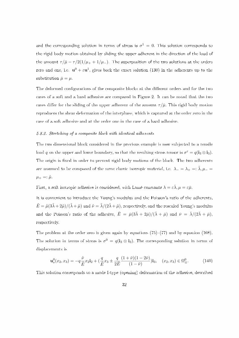
5.8.2. Stretching of a composite block with identical adherents

The two-dimensional block considered in the previous example is now subjected to a tensile

load q on the upper and lower boundary, so that the resulting stress tensor is σε = q(i3 ⊗ i3).

The origin is xed in order to prevent rigid body motions of the block. The two adherents

are assumed to be composed of the same elastic isotropic material, i.e. λ− = λ+ =: λ, µ− =

µ+ =: µ.

First, a soft isotropic adhesive is considered, with Lamé constants λ = ελ, µ = εµ.

It is convenient to introduce the Young's modulus and the Poisson's ratio of the adherents,

E = µ(3λ+2µ)/(λ+ µ) and ν = λ/(2λ+ µ), respectively, and the rescaled Young's modulus

and the Poisson's ratio of the adhesive, E = µ(3λ + 2µ)/(λ + µ) and ν = λ/(2λ + µ),

respectively.

The problem at the order zero is given again by equations (75)(77) and by equation (108).

The solution in terms of stress is σ0 = q(i3 ⊗ i3). The corresponding solution in terms of

displacements is

u0s(x2, x3) = −q

ν

Ex2i2 + (

q

Ex3 ±

q

2E

(1 + ν)(1− 2ν)

(1− ν))i3, (x2, x3) ∈ Ω0

±. (140)

This solution corresponds to a mode I-type (opening) deformation of the adhesive, described

32

Figure 2: Deformed congurations of composite blocks with soft and hard adhesive undergoing shear.

33

by the jump [[u0s

]]· i3 =

q

E

(1 + ν)(1− 2ν)

(1− ν)(141)

superimposed to a uniform stretching of the adherents.

The macroscopic response of the block composed of the two identical adherents and the soft

interface at the order zero is

q = E0s

(u0s(x2, h

+)− u0s(x2,−h−)) · i3

(h+ + h−)(142)

with

E0s =

E(1 + E

E(1+ν)(1−2ν)

(1−ν)(h++h−)

) (143)

the homogeneized elastic modulus of the block at the order zero.

The problem at order one is given by equations (80)(82) and equation (109) which, in view

of (134), (140), and of the relations

K13 =

0 0 µ

0 0 0

λ 0 0

, K23 =

0 0 0

0 0 µ

0 λ 0

. (144)

it is written as

σ1(x2, 0±)i2 =

E

2(1 + ν)([[u1

s]] · i2)i2 +( E(1− ν)

(1 + ν)(1− 2ν)([[u1

s]] · i3)− qE

E

2νν

(1 + ν)(1− 2ν)

)i3.

(145)

The solution in terms of stress is σ1 = 0, and the corresponding solution in terms of displace-

ments is

u1s(x2, x3) = (∓ q

2E± qν

E

ν

(1− ν))i3, (x2, x3) ∈ Ω0

±. (146)

i.e., a mode I-type (opening) deformation of the adhesive described by the jump[[u1s

]]· i3 = − q

E+

q

E

2νν

(1− ν). (147)

The eld uεs := u0

s + εu1s is an approximated solution in the adherents to the original equilib-

rium problem of the block composed by the adherents and the elastic interphase, and it gives

34

the approximated macroscopic response formally analogous to (142) but with E0s substituted

by the approximated homogeneized elastic modulus

Eεs = E

1(1 + ε

(h++h−)1

(1−ν)

(EεE

(1 + ν)(1− 2ν) + 2νν − 1 + ν)) . (148)

A hard isotropic adhesive is considered next, with Lamé constants λ = λ, µ = µ and Young's

modulus and Poisson's coecient, E, ν, dened as for the soft case. The problem at the

order zero for the hard case is given by equations (75)(77) and equations (111),(113) which

prescribe perfect interface conditions. The corresponding solution in terms of stress is again

σ0 = q(i3 ⊗ i3), and the solution in terms of displacements is just a uniform stretching of the

adherents

u0h(x2, x3) = −q

ν

Ex2i2 +

q

Ex3i3, (x2, x3) ∈ Ω0

±. (149)

The response of the block at the order zero is just described by the Young's modulus of the

adherents, E0h := E.

The problem at order one for the hard interface is given by equations (80)(82) and equations

(112),(114) which now take the form

[[u1h]] =

( q

E

(1 + ν)(1− 2ν)

(1− ν)− q

E+

q

E

2νν

(1− ν)

)i3. (150)

A solution in terms of stress is σ1 = 0, and the corresponding solution in terms of displace-

ments is just a relative displacement along the 3−axis of the two adherents of the amount

given by the jump (150)

u1h(x2, x3) = ±1

2

( q

E

(1 + ν)(1− 2ν)

(1− ν)− q

E+

q

E

2νν

(1− ν)

)i3, (x2, x3) ∈ Ω0

±. (151)

By considering the approximated solution uεh := u0

h + εu1h, the macroscopic response is de-

scribed by the following homogeneized elastic modulus

Eεh = E

1(1 + ε

(h++h−)1

(1−ν)

(EE(1 + ν)(1− 2ν) + 2νν − 1 + ν

)) . (152)

The two moduli (148) and (152) formally coincide up to the substitution of εE with E.

35

6. Conclusion

Higher order theories of interface models have been obtained for two bodies joined by an

adhesive interphase for which soft and hard linear elastic constitutive laws have been

considered. In order to obtain the interface model, two dierent methods were applied, one

based on the matched asymptotic expansion technique and the strong formulation of the

equilibrium problem, and the other based on the minimization of the potential energy, i.e.

on the weak formulation of the equilibrium problem. First and higher order interface models

have been derived for soft and hard adhesives and it is shown that the two approaches, strong

and weak formulations, lead to the same asymptotic equations governing the behavior of the

interface, geometrical limit of the adhesive as its thickness vanishes.

The governing equations derived at zero order have been compared with the ones accounting

for the rst order of the asymptotic expansion. Approximated constitutive law for soft and

hard interfaces have been proposed, obtained by superimposing to the law calculated at the

order zero the law calculated at the order one, rescaled with ε. The result is the constitutive

law for a soft interface given by equation (110), and the constitutive law for a hard interface

given by equation (115),(116).

The asymptotic method based on energy minimization allows to calculate the expressions of

emerging forces at the adhesive-adherent interface boundary, whose presence is not directly

taken into account by the interface laws.

Finally, two simple applications have been developed in order to illustrate the dierences

among the interface theories at the dierent orders. Both applications, based on a homogenous

deformation on the adherents, show that the two cases of soft and hard adhesive dier for

the fact that the deformation of the adhesive, described by a relative sliding in the example

with shear and by a relative opening in the example with stretching, is captured at the order

zero and order one in the case of a soft adhesive and at the order one in the case of a hard

adhesive.

36

References

[1] R. Abdelmoula, M. Coutris, and J. Marigo. Comportment asymptotique d'une interphase

élastique mince. Compte Rendu Académie des Sciences Série IIb, 326:237242, 1998.

[2] G. Alfano, S. Mara, and E. Sacco. A cohesive damage-friction interface model accounting

for water pressure on crack propagation. Computer Methods in Applied Mechanics and

Engineering, 196(13):192209, 2006.

[3] G.I. Barenblatt. The mathematical theory of equilibrium cracks in brittle fracture. vol-

ume 7 of Advances in Applied Mechanics, pages 55 129. Elsevier, 1962.

[4] T. Belytschko and T. Black. Elastic crack growth in nite elements with minimal remesh-

ing. International Journal for Numerical Methods in Engineering, 45, 1999.

[5] Y. Benveniste. A general interface model for a three-dimensional curved thin anisotropic

interphase between two anisotropic media. Journal of the Mechanics and Physics of

Solids, 54(4):708 734, 2006.

[6] Y. Benveniste and T. Miloh. Imperfect soft and sti interfaces in two-dimensional elas-

ticity. Mechanics of Materials, 33(6):309323, 2001.

[7] D. Caillerie. The eect of a thin inclusion of high rigidity in an elastic body. Mathematical

Methods in Applied Sciences, 2:251270, 1980.

[8] P.G. Ciarlet. Mathematical Elasticity. Volume I: Three-Dimensional Elasticity. North-

Holland, 1988.

[9] P.G. Ciarlet. Mathematical Elasticity. Volume II: Theory of Plates. Series Studies in

Mathematics and its Applications, North-Holland, 1997.

[10] P.G. Ciarlet and P. Destuynder. A justication of the two-dimensional plate model.

Journal de Mécanique, 6(18):315 344, 1987.

37

[11] A. Corigliano. Formulation, identication and use of interface models in the numeri-

cal analysis of composite delamination. International Journal of Solids and Structures,

30(20):2779 2811, 1993.

[12] G. Del Piero and M. Raous. A unied model for adhesive interfaces with damage, vis-

cosity, and friction. European Journal of Mechanics - A/Solids, 29(4):496 507, 2010.

[13] H. Le Dret and A. Raoult. The nonlinear membrane model as variational limit of nonlin-

ear three-dimensional elasticity. Journal de Mathématiques Pures et Appliquées, 74(6):549

578, 1995.

[14] S. Dumont, F. Lebon, and R. Rizzoni. An asymptotic approach to the adhesion of thin

sti lms. Mechanics Research Communications, submitted.

[15] M. Frémond. Adhérence des solides. Journal de mécanique théorique et appliquée-

A/Solids, 6(3):383 407, 1987.

[16] G. Geymonat and F. Krasucki. Analyse asymptotique du comportement en exion

de deux plaques collées. Comptes Rendus de l'Académie des Sciences - Series IIB -

Mechanics-Physics-Chemistry-Astronomy, 325(6):307 314, 1997.

[17] G. Geymonat, F. Krasucki, and S. Lenci. Mathematical analysis of a bonded joint with

a soft thin adhesive. Mathematics and Mechanics of Solids, 16:201225, 1999.

[18] Z. Hashin. Thin interphase/imperfect interface in elasticity with application to coated

ber composites. Journal of the Mechanics and Physics of Solids, 50(12):25092537,

2002.

[19] A. Ould Khaoua. Etude théorique et numérique de pro- blèmes de couches minces en

elasticité. PhD thesis, Montpellier II, 1995.

[20] A. Klarbring. Derivation of the adhesively bonded joints by the asymptotic expansion

method. International Journal of Engineering Science, 29:493512, 1991.

38

[21] A. Klarbring and A.B. Movchan. Asymptotic modelling of adhesive joints. Mechanics of

Materials, 28(1-4):137 145, 1998.

[22] F. Lebon, A. Ould-Khaoua, and C. Licht. Numerical study of soft adhesively bonded

joints in nite elasticity. Computational Mechanics, 21:134140, 1997.

[23] F. Lebon and R. Rizzoni. Asymptotic analysis of a thin interface: The case involving

similar rigidity. International Journal of Engineering Science, 48(5):473 486, 2010.

[24] F. Lebon and R. Rizzoni. Asymptotic behavior of a hard thin linear elastic interphase:

An energy approach. International Journal of Solids and Structures, 48(3-4):441 449,

2011.

[25] F. Lebon, R. Rizzoni, and S. Ronel-Idrissi. Asymptotic analysis of some non-linear

soft thin layers. Computers & Structures, 82(2326):1929 1938, 2004. Computational

Structures Technology.

[26] C. Licht. Comportement asymptotique d'une bande dissipative mince de faible rigidité.

Compte Rendu Académie des Sciences Série I, 317:429433, 1993.

[27] C. Licht and G. Michaille. Une modélisation du comportement d'un joint collé élastique.

Compte Rendu Académie des Sciences Série I, 322:295300, 1996.

[28] C. Licht and G. Michaille. A modeling of elastic adhesive bonded joints. Advances in

Mathematical Sciences and Applications, 7:711740, 1997.

[29] J.-J. Marigo, H. Ghidouche, and Z. Sedkaoui. Des poutres exibles aux ls extensibles:

une hiérarchie de modéles asymptotiques. Comptes Rendus de l'Académie des Sciences -

Series IIB - Mechanics-Physics-Chemistry-Astronomy, 326(2):79 84, 1998.

[30] N. Moës and T. Belytschko. Extended nite element method for cohesive crack growth.

Engineering Fracture Mechanics, 69(7):813 833, 2002.

[31] A. Needleman. An analysis of tensile decohesion along an interface. Journal of the

Mechanics and Physics of Solids, 38(3):289 324, 1990.

39

[32] M. Ortiz, Y. Leroy, and A. Needleman. A nite element method for localized failure

analysis. Computer Methods in Applied Mechanics and Engineering, 61(2):189 214,

1987.

[33] F. Parrinello, B. Failla, and G. Borino. Cohesive-frictional interface constitutive model.

International Journal of Solids and Structures, 46(13):2680 2692, 2009.

[34] N. Point and E. Sacco. A delamination model for laminated composites. International

Journal of Solids and Structures, 33(4):483 509, 1996.

[35] N. Point and E. Sacco. Mathematical properties of a delamination model. Mathematical

and Computer Modelling, 28(4-8):359371, 1998. Recent Advances in Contact Mechanics.

[36] M. Raous. Interface models coupling adhesion and friction. Comptes Rendus Mécanique,

339(7-8):491 501, 2011. Surface mechanics : facts and numerical models.

[37] M. Raous, L. Cangémi, and M. Cocu. A consistent model coupling adhesion, friction,

and unilateral contact. Computer Methods in Applied Mechanics and Engineering, 177(3-

4):383 399, 1999.

[38] R. Rizzoni and F. Lebon. Asymptotic analysis of an adhesive joint with mismatch strain.

European Journal of Mechanics - A/Solids, 36(0):1 8, 2012.

[39] R. Rizzoni and F. Lebon. Imperfect interfaces as asymptotic models of thin curved elastic

adhesive interphases. Mechanics Research Communications, 51(0):39 50, 2013.

[40] E. Sacco and F. Lebon. A damage-friction interface model derived from micromechanical

approach. International Journal of Solids and Structures, 49(26):3666 3680, 2012.

[41] E. Sanchez-Palencia. Non-homogeneous media and vibration theory. Lecture Notes in

Physics 127, Spriger-Verlag, 1980.

[42] M. Serpilli and S. Lenci. Limit models in the analysis of three dierent layered elastic

strips. European Journal of Mechanics, A/Solids, 27(2):247268, 2008.

40

[43] J. Toti, S. Mara, and E. Sacco. Coupled body-interface nonlocal damage model for FRP

detachment. Computer Methods in Applied Mechanics and Engineering, 260(0):1 23,

2013.

[44] W. Xu and Y. Wei. Strength and interface failure mechanism of adhesive joints. Inter-

national Journal of Adhesion and Adhesives, 34(0):80 92, 2012.

41