Reconciling fiscal consolidation with growth and equity - OECD
85
From: OECD Journal: Economic Studies Access the journal at: http://dx.doi.org/10.1787/19952856 Reconciling fiscal consolidation with growth and equity Boris Cournède, Antoine Goujard, Álvaro Pina Please cite this article as: Cournède, Boris , Antoine Goujard and Álvaro Pina (2014), “Reconciling fiscal consolidation with growth and equity”, OECD Journal: Economic Studies, Vol. 2013/1. http://dx.doi.org/10.1787/eco_studies-2013-5jzb44vzbkhd
-
Upload
khangminh22 -
Category
Documents
-
view
1 -
download
0
Transcript of Reconciling fiscal consolidation with growth and equity - OECD

From:OECD Journal: Economic Studies
Access the journal at:http://dx.doi.org/10.1787/19952856
Reconciling fiscal consolidation with growthand equity
Boris Cournède, Antoine Goujard, Álvaro Pina
Please cite this article as:
Cournède, Boris , Antoine Goujard and Álvaro Pina (2014), “Reconcilingfiscal consolidation with growth and equity”, OECD Journal: EconomicStudies, Vol. 2013/1.http://dx.doi.org/10.1787/eco_studies-2013-5jzb44vzbkhd

This work is published on the responsibility of the Secretary-General of the OECD. Theopinions expressed and arguments employed herein do not necessarily reflect the official viewsof the Organisation or of the governments of its member countries.
This document and any map included herein are without prejudice to the status of orsovereignty over any territory, to the delimitation of international frontiers and boundaries and tothe name of any territory, city or area.

OECD Journal: Economic Studies
Volume 2013
© OECD 2014
7
Reconciling fiscal consolidationwith growth and equity
by
Boris Cournède, Antoine Goujard and Álvaro Pina*
Despite sustained efforts made in recent years to rein in budget deficits, a majority of OECDcountries still face substantial public finance consolidation needs. While essential to avoid thedisruption and large costs ultimately associated with unsustainable public finances, fiscalconsolidation complicates the task of achieving other policy goals. In most cases, it weighs ondemand in the short term. And, if too little attention is paid to the mix of instruments used toachieve consolidation, it can undermine long-term growth, exacerbate income inequality andslow the process of global rebalancing. It is therefore important for governments to adoptconsolidation strategies that minimise these adverse side-effects. The analysis proposesconsolidation strategies that take into account other policy goals as well as country-specificcircumstances and preferences. To do so, increases in particular taxes and cuts in specificspending areas are assessed for their effects on short- and long-term growth, incomedistribution and external accounts. The results of detailed illustrative simulations indicate thata significant number of OECD countries may have to raise harmful taxes or cut valuablespending areas to deliver sufficient consolidation, underscoring the need for structural reformsto counteract these side-effects. The results are robust to an extensive range of sensitivitychecks.
JEL classification: H62, H63, H68
Keywords: Fiscal consolidation, growth, equity, global imbalances, income distribution,structural reforms
* The authors are members of the OECD Economics Department. Álvaro Pina is also affiliated with ISEG(Lisboa School of Economics and Management, Universidade de Lisboa) and UECE (Research Unit onComplexity and Economics, Lisboa). This paper originated as a document prepared for a meeting of theWorking Party No. 1 of the Economic Policy Committee (March 2013).Versions of the paper have also beenpresented at a Department of Economics seminar at ISEG, at the 9th BMRC-QASS Conference on Macroand Financial Economics (both in May 2013) and at a special Lisbon Council event in July 2013. Theauthors would like to thank Alain de Serres, who co-ordinated the project, the meeting participants aswell as Pier-Carlo Padoan, Jørgen Elmeskov, Jean-Luc Schneider, Alain de Serres, Sebastian Barnes,Ray Barrell, Henrik Braconier, Orsetta Causa, Roger Farmer, Alberto Gonzalez Pandiella, Peter Hoeller,Isabell Koske, Stephen Matthews, Oliver Roehn and Eckhard Wurzel for helpful comments on earlierdrafts, Caroline Abettan and Lyn Urmston for excellent editorial support, Agnès Cavaciuti for expertstatistical assistance and they are indebted to Benjamin Carton and Andreas Wörgötter for valuablecomments and suggestions. The views expressed in this paper are the authors’ and are not necessarilyshared by the OECD or its member countries. Corresponding author: [email protected] statistical data for Israel are supplied by and under the responsibility of the relevant Israeliauthorities. The use of such data by the OECD is without prejudice to the status of the Golan Heights,East Jerusalem and Israeli settlements in the West Bank under the terms of international law.

RECONCILING FISCAL CONSOLIDATION WITH GROWTH AND EQUITY
OECD JOURNAL: ECONOMIC STUDIES – VOLUME 2013 © OECD 20148
1. Introduction and main messagesDespite considerable progress in recent years, many OECD countries were still facing
sizeable fiscal consolidation at the end of 2012 to bring back or keep public debt within
manageable levels and avoid the cumulative costs and risks associated with the build-up
of unsustainable public-finance positions. The origin of fiscal consolidation needs is
complex and manifold, including inter alia initial conditions, the fiscal damage from
financial crises, spending pressures from demographic developments and liquidation
losses from public assets. Building on previous OECD and other work, the article presents
a structured approach to choosing the instruments of fiscal consolidation strategies in
ways that minimise adverse side-effects on growth and equity in the short and the long
term as well as on external imbalances. As such, the focus of the paper is on the
composition of consolidation. For in-depth recent studies about the size of consolidation
needs and the optimal timing of consolidation, see for instance Sutherland et al. (2012) and
Rawdanowicz (2012), respectively. The paper provides illustrative quantitative applications
of the approach.
The main messages can be summarised as follows:
● In most OECD countries, compared with what had been achieved by end 2012, additional
consolidation is needed in the short to medium term to put government debt on a
trajectory toward more prudent levels (defined for simplicity as gross debt at 60% of GDP)
and even more to keep debt stable in the very long run, i.e. in 2060.
● Consolidation instruments (increases in particular taxes and cuts in specific spending
areas) can be ranked according to their effects on short- and long-term growth, income
distribution and current accounts, with the rankings taking into account country
circumstances.
● Based on these rankings, illustrative consolidation packages to optimise the side-effects
of consolidation on other policy objectives can be drawn up for each country.
● The packages are based on using instruments sequentially, and within reasonable limits,
starting from the most desirable and moving down the ranking until consolidation needs
are satisfied.
● Based on this approach, half of OECD countries appear to be in a position to fulfil their
short- to medium-term consolidation needs entirely through instruments that are well
ranked (that is to say ranked in the top half). This suggests that, in these countries, well-
designed consolidation packages can avoid severe adverse side effects on growth, equity
and current-account imbalances.
● In the simulations, eight countries use some poorly-ranked instruments but achieve
more than half their short- to medium-term consolidation through well-ranked
instruments.
● Finally, in the illustrative simulations, three countries (Japan, United Kingdom and the
United States) implement more than 50% of their short-to-medium-term consolidation

RECONCILING FISCAL CONSOLIDATION WITH GROWTH AND EQUITY
OECD JOURNAL: ECONOMIC STUDIES – VOLUME 2013 © OECD 2014 9
packages through instruments that have low rankings meaning that they are likely to
involve substantial adverse side-effects.
● Despite the generally stronger consolidation requirements in the long term, 20 countries
would manage to keep debt durably stable at 60% of GDP by relying only on well-ranked
instruments.
● In the simulated very long-term packages, six countries use some poorly-ranked
instruments but can nonetheless achieve more than 50% of their adjustment with well-
ranked instruments.
● Finally, a few countries would have to implement most of their simulated very long-term
consolidation packages relying on poorly-ranked instruments (that have more adverse
effects on long-term growth and equity objectives).
● On average across countries, spending reductions would account for 41% of short- to
medium-term and 65% of long-term consolidation packages, the rest being achieved
through tax hikes. The difference mostly reflects the greater concern for demand effects
in the short term.
● The proposed illustrative consolidation packages lead to some, but not much,
convergence in spending and revenue structure across countries over time. This result
can be interpreted as meaning that the proposed approach is largely respectful of the
diversity of national preferences over spending and revenue structure.
● Extensive sensitivity analysis indicates that all the above results are largely robust to
uncertainty about the assessments of the effects of instruments except the spending-tax
split in simulated short-term consolidation plans. The simulation results are also very
robust to changes to the method used to adapt instrument rankings to country
circumstances. The assumptions made to define the maximum amount by which each
consolidation instrument can be used have a direct influence on the degree to which
countries with large adjustment needs have to rely on the most harmful categories of tax
hikes or spending cuts.
● Trade-offs between consolidation and other policy objectives can be eased by exploiting
the scope for efficiency gains through structural reforms.
In a preliminary step providing inputs for the subsequent analysis of ways to minimise
the side-effects of consolidation, the study first estimates fiscal consolidation needs in the
short to medium term and the long term (Section 2). It then moves to its core subject and
discusses the definition of growth, equity and current-account objectives before
presenting the list of potential consolidation instruments, evaluating their effects along
these three dimensions and proposing a generic illustrative hierarchy of instruments
(Section 3). On that basis, Section 4 proposes a method for developing country-specific
hierarchies of instruments taking into account country specificities. A file available online
allows readers to build their own rankings of consolidation instruments by keying in their
preferred weights on growth, equity and current-account objectives.1 The study proceeds
with an illustrative evaluation of how far down each country has to go on its list from more
to less welcome instruments to meet its consolidation objectives without departing too
much from its revealed preferences about government spending and revenue items and
checks the robustness of the findings (Section 5). The results underscore the need for
structural changes to be part of fiscal adjustment (Section 6). Section 7 then makes a few
concluding remarks and offers suggestions for future research.

RECONCILING FISCAL CONSOLIDATION WITH GROWTH AND EQUITY
OECD JOURNAL: ECONOMIC STUDIES – VOLUME 2013 © OECD 201410
Appendix A reports country details of the main simulations as well as summary
statistics from alternative simulations based on random draws. Appendix B provides
supporting material on: the methodology used to estimate consolidation needs
(summarised in Boxes 1 and 2), the dataset, the assessment of instrument impact, the
analysis of debt behaviour during consolidation episodes, a variant without clustering
analysis and another variant with increased room for manœuvre. Further supporting
empirical evidence is provided by Barbiero and Cournède (2013) and Goujard (2013).
2. Estimated consolidation needsThe legacy of the financial crisis and earlier fiscal imbalances has burdened many
OECD governments with high debt levels often accompanied by still significant structural
deficits (Figure 1) which call for large consolidation efforts to reduce debt to more prudent
levels. As a preliminary intermediate step to permit a quantitative analysis of the
composition of consolidation strategies, this section presents estimates of consolidation
needs for both the short to medium term and the long term. The present calculations are
based on a gradual consolidation effort, embodied in smooth time paths for the structural
primary balance (see Appendix A, Section 1 for more details). This approach ensures that
the debt ratio is on a stable trajectory at the end of the consolidation horizon (2060).
Second, in order to ensure that by 2060 the debt ratio not only stabilises but does so at the
desired target level (60% as in Johansson et al., 2013), the present work differentiates short-
from long-term consolidation needs, as explained in greater detail below. As developed in
Box 1, this approach differs in purpose and methodology from the consolidation
requirements reported in the OECD Economic Outlook, May 2013 (OECD, 2013a).
The short- to medium-term consolidation need is defined as the difference between a
baseline and the peak of a trajectory for the underlying primary balance that brings gross
general government debt to 60% of GDP by 2060. A uniform target of 60% of gross debt to
GDP has been chosen for the sake of simplicity and because it represents an important
reference in EU countries. However, in practice, national circumstances warrant different
objectives. In particular, the presence or not of large amounts of financial assets on the
government balance sheet is an important point to consider when setting targets for gross
Figure 1. Debt and underlying primary balances in 2012
6
4
2
0
-2
-4
-6
-8
-100 20 40 60 80 100 120 140 160 180 200 220 240
AUS
AUTBEL
CAN
CHE CZE DEUDNK
ESP
EST
FINFRA
GBR
GRC
HUN
IRL
ISL
ISR
ITA
JPN
KOR
LUXNLD
NOR NZLPOL
PRT
SVK
SVNSWE
USA
Underlying primary fiscal balance, % of potential GDP
Government debt, % of potential GDP

RECONCILING FISCAL CONSOLIDATION WITH GROWTH AND EQUITY
OECD JOURNAL: ECONOMIC STUDIES – VOLUME 2013 © OECD 2014 11
debt. A variant including drawing down financial assets to smooth the adjustment is
included and discussed below. Another factor bearing on the level of debt that the
government can carry without exacerbating risks of instability is private-sector
indebtedness and associated risks of deleveraging. Recent OECD work suggests that the
prospect of deleveraging is real in a number of OECD countries (Bouis et al., 2013).
Box 1. Short- vs. long-term consolidation needs and average requirements
The estimated consolidation needs presented here differ from the average consolidationrequirements reported in OECD (2013a) as they serve different purposes and therefore usedifferent assumptions. The present set of consolidation needs forms a basis for thesubsequent quantitative analysis of detailed consolidation packages that minimise sideeffects. The focus is firstly on how far these packages need to go in the short to mediumterm to bring debt under control and secondly on what has to be done to keep debt stablein the very long term, that is to say in 2060 and beyond. This differs from the objective ofthe requirements reported in OECD (2013a) which was to show how much effort beyondthat already built into the near-term projection is needed on average from 2015 to 2030.From these different purposes and perspectives result different methodological choiceswith the main differences summarised as follows:
● The reference point for comparisons is 2012 in the current study, so that neededchanges in individual areas of tax and spending can be compared with the latesthistorical point (or estimate). The reference point in OECD (2013a) is fiscal projectionsto 2014 to provide an idea of how much remains to be done in aggregate after theexpected consolidation to 2014.
● The present estimates refer to the peak effort needed in the short- to medium-term andin 2060 whereas the requirements reported in OECD (2013a) relate to the average effortover 2015-30. The former is needed for the present exercise as the point to assess howfar, at the peak, instruments have to be used, and whether these instruments have to bemaintained or can be partly reversed afterwards. To assess the size of aggregateconsolidation efforts in an extended medium-term perspective as is the case in OECD(2013a), however, the average offers a more robust measure given that many differentpaths with many different peaks can be imagined for moving to debt stabilisation.
● In order to allow more realistic estimates of consolidation needs in the very long run(2060), the present estimated needs are calculated over a baseline where governmentexpenditure on health and long-term care increases gradually over time as inde la Maisonneuve and Oliveira Martins (2013). The baseline for comparisons in OECD(2013a) does not incorporate such cost pressures which have a lesser impact whenlooking at average effort over 2015-30.
● For the sake of comparability of consolidation packages and in line with the long-termfocus of the study, the present set of estimates assumes that all countries reach 60%gross debt-GDP ratios by 2060. In OECD (2013a), in line with the extended medium-termfocus, the time horizon is 2030 but, to avoid too abrupt changes, some countries areallowed to reach their 60% target after 2030.
Despite the differences of purposes and method, the cross-country correlation betweenthe present set of short- to medium-term consolidation needs and the requirementspresented in OECD (2013a) is very strong with a coefficient of 96%.
Source: OECD (2013a), OECD Economic Outlook, May 2013.

RECONCILING FISCAL CONSOLIDATION WITH GROWTH AND EQUITY
OECD JOURNAL: ECONOMIC STUDIES – VOLUME 2013 © OECD 201412
Evidently, different consolidation paths can be taken to attain the 60% target, each
leading to a different profile for the underlying primary balance (see Box 4.5 in OECD,
2013a). For the purpose of this exercise, and although some countries plan to adjust faster
(see OECD, 2013a), the underlying primary balance is assumed to improve from its
2012 level at a rate of 1% of potential GDP each year for as long as necessary to put debt on
a trajectory toward the target. This is a simplifying assumption to derive estimates on a
uniform basis across countries because this study does not focus on the optimal timing of
consolidation but on its composition. For a study about the optimal timing of consolidation
from a welfare perspective, see for instance Rawdanowicz (2012).
After that initial period of consolidation, which varies considerably in length across
countries, the underlying primary balance is assumed to converge very gradually to the
2060 level which stabilises debt at 60% of GDP (see Figure 1 and Section 1 in Appendix B).
Initial improvement in the underlying primary balance at the fast annual pace of 1%
(1½ per cent in Japan) helps to ensure that debt is put on a downward path in a not too
distant future.2 Interest rates and GDP growth, important drivers of debt dynamics, are
assumed to follow the long-term baseline projections published OECD (2013a) of which the
main assumptions are summarised in Box 2. The calculations are based on the effective
interest rate paid by governments on the stock of debt, as projected in the OECD (2013a)
long-term projections, so that the maturity structure of the debt stock is taken into
account. Last historic point (2012) data for general government debt and underlying
primary balances are also taken from the OECD (2013a). Figure 3 shows two concrete
examples of baseline and debt-reducing trajectories.
The long-term consolidation need compares the “debt-control” underlying primary
balance with the baseline at the end of the projection period. The baseline corresponds to
a policy scenario where sufficient reforms are introduced for public pension spending to
remain constant relative to potential GDP and for government expenditure on health and
long-term care to grow at a contained pace. Other tax and expenditure components are
assumed to be unchanged from their 2012 levels relative to GDP except for cyclical effects
associated with the projected closure of output gaps.
Figure 2. Defining short- to medium-term and long-term consolidation needs
2060
Underlyingprimarybalance
2012 outturn
Debt-control pathfor the underlying
balande
Steady-stateunderlyingprimary surplus
Peak underlyingprimary surplus
Baseline
Time
Short- tomedium-termconsodidationneed
Long-termconsolidation
need
RECONCILING FISCAL CONSOLIDATION WITH GROWTH AND EQUITY
OECD JOURNAL: ECONOMIC STUDIES – VOLUME 2013 © OECD 2014 13
The baseline scenario therefore incorporates significant reform in the areas of
pensions and health.
● Many countries expect large increases in government pension expenditure relative to
GDP on current policy settings (Figure 4). The baseline scenario assumes that, in these
countries, substantial reforms are implemented, including adjustments of the effective
retirement age, so as to keep stable the ratio of public pension spending to GDP.
● Similarly, the continuation of past trends in public spending on health and long-term
care would appear to result in large further increases, as apparent in the projected “cost-
pressure” scenario presented in de la Maisonneuve and Oliveira Martins (2013) and
plotted in Figure 5. Hence, the baseline incorporates (unspecified) measures to contain
cost pressures in health and long-term care, which could include a more frequent
re-evaluation of drug prices, centralised bargaining for drug purchases, more user choice
of health providers and incentives to enhance prevention inter alia (Joumard et al., 2010).
Nonetheless, even under the cost-containment assumption, health spending is
projected to rise as a share of GDP, which explains the trend decline in the primary
balance in the baseline paths shown in Figures 2 and 3.
Estimates based on the approach described above suggest that in Greece, Japan,
Portugal, Spain, the United Kingdom and the United States, a short- to medium-term
consolidation in excess of 5% of potential GDP is required to reduce debt to 60% of GDP
by 2060 (Figure 6). This is the result of currently high debt (Greece, Ireland, and Portugal), a
large initial underlying primary deficit (Spain), or their combination (Japan,
United Kingdom and United States). In a first subgroup of these countries (Greece,
Portugal, Spain), the estimated large consolidation needs are associated with substantial
risk premia in long-term interest rates. In a second subset (Japan, the United Kingdom and
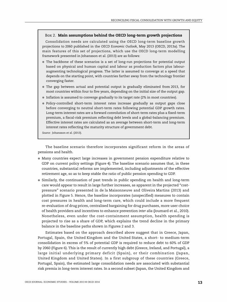
Box 2. Main assumptions behind the OECD long-term growth projections
Consolidation needs are calculated using the OECD long-term baseline growthprojections to 2060 published in the OECD Economic Outlook, May 2013 (OECD, 2013a). Themain features of this set of projections, which use the OECD long-term modellingframework presented in Johansson et al. (2013) are as follows:
● The backbone of these scenarios is a set of long-run projections for potential outputbased on physical and human capital and labour as production factors plus labour-augmenting technological progress. The latter is assumed to converge at a speed thatdepends on the starting point, with countries farther away from the technology frontierconverging faster.
● The gap between actual and potential output is gradually eliminated from 2013, formost countries within four to five years, depending on the initial size of the output gap.
● Inflation is assumed to converge gradually to its target rate (2% in most countries).
● Policy-controlled short-term interest rates increase gradually as output gaps closebefore converging to neutral short-term rates following potential GDP growth rates.Long-term interest rates are a forward convolution of short-term rates plus a fixed-termpremium, a fiscal-risk premium reflecting debt levels and a global-balancing premium.Effective interest rates are calculated as an average between short-term and long-terminterest rates reflecting the maturity structure of government debt.
Source: Johansson et al. (2013).

RECONCILING FISCAL CONSOLIDATION WITH GROWTH AND EQUITY
OECD JOURNAL: ECONOMIC STUDIES – VOLUME 2013 © OECD 201414
the United States), long-term interest rates are much lower, which can be related to the large-
scale purchases of government bonds by central banks under their quantitative-easing
policies. To bring debt to the same level, another group needs short- to medium-term
consolidation by more than 3% of GDP – though less than 5% – because of high debt levels
(France, Iceland) or a significant underlying primary deficit (Finland, Poland, Slovak Republic).
Other countries, including in particular Italy and Germany, face little or no short- to medium-
term structural consolidation needs, though high debt in the former makes this conclusion
vulnerable to interest-rate changes. When needed, consolidation is in most cases relatively
brief in the simulations: three out of four countries that require short- to medium-term
consolidation complete it in four years or less. Many countries have made consolidation plans
that go a long way toward meeting these consolidation needs (OECD, 2013a).
Figure 3. Illustration of the budget consolidation profilecompared with baseline in two countries
Simulated underlying primary balance, per cent of potential GDP
Source: OECD Economic Outlook, May 2013 database and OECD calculations.
10
8
6
4
2
0
-2
-4
-6
-8
-10
-122012 2022 2032 2042 2052
10
8
6
4
2
0
-2
-4
-6
-8
-10
-122012 2022 2032 2042 2052
Japan Belgium
Debt-control path Baseline
Figure 4. Projected change in government pension expenditure on unchanged policies
Source: EC (2012) for EU countries and Norway, OECD (2011a) for other countries except Japan where the estimate is taken from Merolaand Sutherland (2012) and Israel where it has been estimated for 2030 based on projections to 2025 communicated by the Bank of Israel.
10
9
8
7
4
3
6
5
2
1
0
-1
-2
-3
LUX
SVN
BEL
KOR
TUR S
VK N
OR IRL
NZL ESP
NLD IS
L FIN H
UN C
ZEDEU CHE
AUTAUS
GBR M
EXCAN
GRC S
WEFR
AJP
NPRT
USADNK ITA ES
TPOL
ISR
2010-30 2010-60

RECONCILING FISCAL CONSOLIDATION WITH GROWTH AND EQUITY
OECD JOURNAL: ECONOMIC STUDIES – VOLUME 2013 © OECD 2014 15
Consolidation needs are estimated to be greater in the long than the short term for the
majority of countries. The difference is particularly large in countries where short-term
needs are limited thanks to low initial debt levels. The high estimated level of long-term
consolidation needs reflects large expected spending increases on health and long-term
care. That said, since the cross-country variation in projected increases in government
health spending is limited, it does not account for much of the differences in estimated
long-term consolidation needs. The latter are primarily due to the starting point for the
underlying primary surplus in 2012. Another significant source of differences is that the
OECD long-term growth scenarios project interest rates rising well above nominal GDP
growth rates by 2060, which leaves governments holding large amounts of financial assets
Figure 5. Projected percentage point increase in total public healthand long-term care spending, 2010-2060
Range of estimates across sensitivity analyses
Notes: Countries are ranked by the increase of expenditures between 2010 and 2060 in the cost-containmentscenario. The vertical bars correspond to the range of the alternative scenarios, including sensitivity analysis.Source: de la Maisonneuve and Oliveira Martins (2013).
Figure 6. Estimated consolidation needsDifference between debt-control and baseline underlying primary surplus, per cent of potential GDP
Source: OECD Economic Outlook, May 2013 long-term database and OECD calculations.
12
7
8
9
10
11
6
5
4
3
2
1
0
KOR T
UR C
HLMEX
ESP
LUX
SVK
SVN
POL
GRC
PRT
ITA C
HE N
LD JP
N A
US IR
L IS
L C
AN N
ZL A
UT C
ZE D
EU E
ST H
UN N
OR F
RA B
EL U
SA D
NK FI
N G
BR IS
L S
WE
Range of estimates across sensitivity analysis Cost pressure Cost containment
20
18
16
14
12
10
8
6
4
2
0
JPN
GBR
GRC
USA
PRT
IRL
ESP
FRA
SVK
POL
FIN
ISL
NLD
CAN
SVN
AUS
HUN
ISR
NZL
CZE
BEL
SWE
ITA
LUX
AUT
CHE
DEU
DNK
EST
KOR
In the year when initial consolidation ends (short to medium term) In 2060 (long term)

RECONCILING FISCAL CONSOLIDATION WITH GROWTH AND EQUITY
OECD JOURNAL: ECONOMIC STUDIES – VOLUME 2013 © OECD 201416
with substantial capital income to service their debt. This effect reduces the estimated
long-term consolidation needs of Canada, Finland, Japan, Korea and Norway by
2½ per cent of GDP or more compared with a situation where these countries’ governments
had no financial assets. This set of long-term estimates is subject to particularly strong
uncertainty.3 If no pension reform was assumed in the baseline, that is to say if public
pension expenditure was allowed to increase in line with unchanged policy projections,
estimated long-term consolidation needs would be considerably larger in many countries
(Figure 7). These very large differences underscore the critical need for pension reform in
countries that have not yet adjusted their systems to ensure that government pension
spending remains contained in the face of ageing. In addition to being key to fiscal
sustainability, successful pension reform also brings important benefits in terms of greater
labour supply (Duval, 2003) and intergenerational equity (Gonand, 2010).
The choice of a gross debt target can exaggerate consolidation needs for governments
that have large sellable financial assets or substantial implicit assets for instance in the
form of deferred tax on pension savings. A limited group of OECD governments (Estonia,
Finland, Korea, Luxembourg, Norway, Sweden) report net positive financial asset positions.
A significant number of OECD governments hold financial assets that are valued at more
than half of their country’s GDP (Canada, Denmark, Finland, Greece, Iceland, Japan, Korea,
Luxembourg, Norway, Slovenia, Sweden).4 Selling assets to meet consolidation needs, for
instance by drawing them down to 50% of GDP in countries that currently hold more,
eliminates estimated short- to medium-term consolidation needs almost entirely in Denmark
and fully in Sweden (Figure 8, upper panel). This draw-down hypothesis also reduces
consolidation needs significantly in Japan, where they diminish by nearly 2 percentage points
but remain nonetheless elevated at 16½ per cent of GDP. In the long term, however, this draw-
down hypothesis results in larger consolidation needs (Figure 8, lower panel) because asset
depletion reduces the amount of capital income on government assets compared with the
assumption of keeping them constant as a share of GDP. In practice, the ease with which
Figure 7. Long-term consolidation needs:Estimates with and without pension reform
Difference between debt-control and baseline underlying primary surplus in 2060, per cent of potential GDP
Source: OECD Economic Outlook, May 2013 and OECD calculations.
15.0
2.5
5.0
7.5
10.0
12.5
0
JPN
GBR
USA
SVK A
US P
OL E
SP N
ZL ISR
FRA
NLD IR
L C
AN S
VN C
ZE P
RT L
UX B
EL H
UN D
NK A
UT C
HE FI
N S
WE D
EU E
ST IS
L K
OR G
RC
The baseline includes reforms to keep pension spending constant as a share of GDPThe baseline includes no change from current policies

RECONCILING FISCAL CONSOLIDATION WITH GROWTH AND EQUITY
OECD JOURNAL: ECONOMIC STUDIES – VOLUME 2013 © OECD 2014 17
financial assets can be liquidated varies across countries depending on their nature, on the
extent to which they are earmarked to prefund budgetary commitments and on whether
they are owned by the central or other levels of government (Rawdanowicz et al., 2011).
The chosen level of the debt target also has implications for consolidation needs. While
there is no obvious optimal maximum ratio of public debt to GDP, the 60% value has been
retained as the main reference point for the simulations because of its widespread use as a
policy target within the OECD membership. Aiming at a higher 100% target would reduce
estimated short- to medium-term consolidation needs by about 2% of GDP in most OECD
countries (Figure 8A). Allowing greater indebtedness however comes at the cost of larger
interest payments to keep the debt ratio stable, pushing up estimated long-term consolidation
needs by about 1% of GDP in most OECD countries (Figure 8B).These considerations mean that
the consolidation needs used in the rest of the paper, which correspond to the 60% of GDP
gross debt target without asset draw-down, should be seen as illustrative as the choice of a
debt target and the level of the target ought to be country specific.
Figure 8. Estimated consolidation needs
Source: OECD Economic Outlook, May 2013 long-term database and OECD calculations.
20.0
5.0
7.5
2.5
10.0
12.5
15.0
17.5
0
JPN
GBR
GRCUSA
PRT
IRL
ESP
FRA
SVKPOL FIN IS
L N
LD C
AN S
VN A
US H
UN IS
R N
ZL C
ZE B
EL S
WE IT
A A
UT C
HE D
EU D
NK E
STKOR
LUX
20.0
5.0
7.5
2.5
10.0
12.5
15.0
17.5
0
JPN
GBR
USASVK
AUS
POL E
SPNZL ISR
FRA
NLD IRL
CAN S
VN C
ZE P
RT L
UX B
EL H
UN D
NK A
UT C
HE FI
N S
WE D
EU E
ST IS
L K
ORGRC
ITA
60% debt target 60% debt target with asset draw-down to 50% 100% debt target
A. Short-to-medium term needs: Debt-control minus baseline underlying primary surplusin the year when initial consolidation ends, % of potential GDP
B. Long-term needs: Debt-control minus baseline underlying primary surplusin 2060, % of potential GDP

RECONCILING FISCAL CONSOLIDATION WITH GROWTH AND EQUITY
OECD JOURNAL: ECONOMIC STUDIES – VOLUME 2013 © OECD 201418
Feedback from consolidation to activity could also influence consolidation needs in
ways that are not fully reflected in the present set of estimates. In many countries, deeper
consolidation would, through multiplier effects, reduce growth and at least temporarily
create more adverse debt dynamics than assumed in the present simulations in the short
to medium term. These effects could be magnified by the fact that most countries
consolidate, implying that each country faces additional headwinds from external demand
in its consolidation effort.5 Afterwards, however, the return of output to potential would
create more favourable growth and therefore debt dynamics than the one underpinning
the present calculations. Simulations incorporating such effects by Rawdanowicz (2012)
suggest that, even if multipliers are large, their effects on debt dynamics during and after
the consolidation largely cancel out so that they have little effect on the estimated size of
consolidation needs. One channel through which deep fiscal tightening can influence
consolidation needs sizeably is if it generates hysteresis effects that depress potential
output permanently, something which is assumed not to happen in the projections
presented here. This consideration underscores the need to design consolidation strategies
in ways that minimise the risk of generating hysteresis (see Section 4 below).
Feedback from consolidation to real interest rates could reduce consolidation needs.
Consolidation strategies that are credibly seen as bringing back debt firmly within
manageable levels are likely to lower risk premia and real interest rates (Turner and
Spinelli, 2012). This favourable effect materialises in full only after the disinflationary
consequences of any consolidation-induced contraction wear off. The historical
experience is that, on average across large fiscal consolidation episodes, it takes three
years after they start before the ratio of debt to potential GDP begins to fall and seven years
before it becomes smaller than at the start (see Figure 9 and Blöchliger et al., 2012). Lower
real interest rates improve debt dynamics directly, by fuelling demand, and also by
Figure 9. Large fiscal consolidationand the government debt-to-potential-GDP ratioDeviation from cross-country and time-period averages, per cent
Note: The solid line shows the association between fiscal consolidation and the public debt to GDP ratio.Consolidations are defined as a 1.5% of GDP action-based consolidation effort: countries and period episodes aretaken from Devries et al. (2011). Consecutive years of consolidation are dropped as in Alesina and Ardagna (2010).Driscoll-Kraay (1998) standard errors robust to heteroskedasticity, arbitrary spatial correlation and autocorrelation upto five years. Government debt and GDP data are taken from the OECD Economic Outlook No. 92 Database. SeeAppendix B, Section 4 for more details on the methodology.
15
10
5
0
-5
-10
-15
-20-10 -9 -8 -7 -6 -5 -4 -3 -2 -1 0 1 2 3 4 5 6 7 8 9 10
90% CI upper bound Point estimate 90% CI lower bound
Public debt/Potential GDP
Years since the start of the consolidation

RECONCILING FISCAL CONSOLIDATION WITH GROWTH AND EQUITY
OECD JOURNAL: ECONOMIC STUDIES – VOLUME 2013 © OECD 2014 19
boosting potential output, but it takes time for these effects to materialise. They could
however be particularly strong, and materialise faster, in crisis countries where credible
consolidation can carry them from a situation of high and rising indebtedness, elevated
risk premia and low growth to a “good equilibrium” characterised by falling debt, lower risk
premia and higher growth (Padoan et al., 2012).
3. The effects of consolidation instruments on other policy objectives
3.1. Other policy objectives
While the point of fiscal consolidation is to reduce debt, it cannot ignore other policy
objectives. The present study looks at the extent to which fiscal consolidation can proceed
while minimising adverse effects on short-term growth, preserving long-term prosperity,
avoiding exacerbating income inequality in the short and long term and contributing to
global rebalancing. In addition to being an objective in its own right, equity may influence
the sustainability of fiscal adjustment programmes. Consolidation strategies perceived as
inequitable are more likely to be reversed and to fail to reduce debt.
The distinction made here between short- and long-term effects does not relate to
specific time spans but to adjustment processes. Short-term effects correspond to the
direct impact of measures as they are implemented. Long-term effects describe their
consequences when cyclical adjustment has run its course and behaviour has responded
fully to the measures (meaning in particular that any general-equilibrium impacts have
materialised).
3.2. Instruments
The instruments considered are policies that permanently affect government
underlying primary spending and revenues. Government underlying primary spending is
broken into ten categories, including four consumption items, three transfer items,
subsidies, public investment (Table 1) and a residual item which is not considered as an
instrument of consolidation. The expenditure breakdown broadly follows national
accounts classifications with the difference that user charges are not netted out from
government consumption. Instead, user charges are included among the eight
consolidation instruments considered on the revenue side. Cutting tax expenditures, a
potentially large and attractive source of revenue, is nevertheless not included as an
instrument because of the lack of sufficiently reliable and internationally comparable data
across countries. Section 6, however, discusses how reductions in tax expenditures can
Table 1. Instruments of consolidation
Expenditure cuts Revenue increases
Public consumption: education Personal income taxes
Public consumption: health Social security contributions
Public consumption: other (except family) Corporate income taxes
Cash transfers: pensions Environmental taxes
Cash transfers: unemployment benefits Consumption taxes (non-environmental)
Cash transfers: sickness and disability Recurrent taxes on immovable property
Public consumption and cash transfers: family Other property taxes
Subsidies Sales of goods and services
Public investment
Source: See Appendix B.
RECONCILING FISCAL CONSOLIDATION WITH GROWTH AND EQUITY
OECD JOURNAL: ECONOMIC STUDIES – VOLUME 2013 © OECD 201420
contribute to policy strategies that combine fiscal consolidation with structural reform.
Appendix B, Section 2 provides details on the definition of the categories, on the sources
used and on the methods employed to gather data from different sources in a way that
adds up to government primary spending as recorded in national accounts.
3.3. The effects of instruments on objectives
An attempt is made at evaluating the effect of revenue increases and expenditure cuts
on growth, equity and global rebalancing objectives. The effects of instruments on the
current account are also evaluated because consolidation strategies should take into
account co-ordinated efforts in multilateral settings such as the G20 to achieve balanced
growth at the global level. For the purpose of this exercise, the instruments are assessed on
their own without considering how their side-effects on long-term growth and equity
could be minimised through structural reforms in the tax or spending area under
consideration, other structural reforms or redistributive policies. The distinction between
purely fiscal changes and structural reform is obviously not so clear cut in practice.6 Still, it
is useful insofar as it allows for an assessment of the side-effects that some consolidation
instruments can imply for other policy objectives (this section) before discussing the
benefits of joint policy strategies that combine consolidation with structural reform
(Section 6).
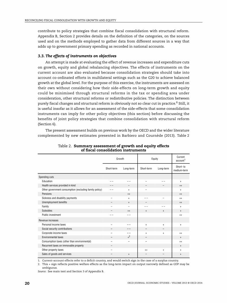
The present assessment builds on previous work by the OECD and the wider literature
complemented by new estimates presented in Barbiero and Cournède (2013). Table 2
Table 2. Summary assessment of growth and equity effectsof fiscal consolidation instruments
Growth EquityCurrent
account1
Short-term Long-term Short-term Long-termShort- to
medium-term
Spending cuts
Education – – – – – – – +
Health services provided in kind – – – – – ++
Other government consumption (excluding family policy) – – + – +
Pensions ++ ++
Sickness and disability payments – + – – – ++
Unemployment benefits – + – ++
Family – – – – – – +
Subsidies – ++ + + +
Public investment – – – – ++
Revenue increases
Personal income taxes – – – + + +
Social security contributions – – – – –
Corporate income taxes – – – + + ++
Environmental taxes – +2 – +
Consumption taxes (other than environmental) – – – ++
Recurrent taxes on immovable property – +
Other property taxes – ++ + +
Sales of goods and services – + – – +
1. Current-account effects refer to a deficit country, and would switch sign in the case of a surplus country.2. This + sign reflects positive welfare effects as the long-term impact on output narrowly defined as GDP may be
ambiguous.Source: See main text and Section 3 of Appendix B.

RECONCILING FISCAL CONSOLIDATION WITH GROWTH AND EQUITY
OECD JOURNAL: ECONOMIC STUDIES – VOLUME 2013 © OECD 2014 21
summarises this assessment which is based on the main points discussed immediately
below while Appendix B, Section 3, provides additional supporting material on the growth
and equity effects of consolidation instruments. Besides showing the estimated direction
of the effect, some crude indications of the relative strength are also provided, based on
empirical evidence.
3.3.1. Long-term growth effects
A number of fiscal consolidation instruments can enhance the long-term level of
output by improving efficiency in the economy or the supply of resources. Evidence
suggests that, in advanced economies, reducing the size of government increases long-
term output although there is clearly no consensus on what constitutes the optimal size of
the public sector even from a strict efficiency point of view (OECD, 2003; Cournède and
Gonand, 2006; Barbiero and Cournède, 2013; Afonso and Tovar Jalles, 2013). This output-
enhancing effect of reducing government spending is likely to be stronger in areas such as
subsidies7 where public expenditure frequently distorts the allocation of resources in the
economy. Similarly, cuts in public spending that can prompt a positive response of labour
utilisation, such as in pensions, are likely to have a particularly favourable effect on the
long-term level of output per capita. Reductions in public spending on unemployment
benefits can also boost employment and output per capita insofar as they do not bring
unemployment benefits down to a level prompting inefficient employee-job matches that
could curb productivity. Cuts in disability payments can boost labour utilisation
(Hagemann, 2012) although this effect will arise only insofar as workers with significant
residual capacity are receiving rehabilitation assistance.
Some revenue measures can also contribute positively to long-term output when they
promote more efficient use or allocation of services or resources that were previously
inadequately priced. To the extent that their current levels correspond to under-pricing,
higher user charges reduce the waste of economic resources, thereby boosting productivity
and output. Better pricing the use of environmental services through taxation can lead to
welfare gains through improved environmental amenities that are not measured in GDP.
While, as other forms of taxation, environmental taxes reduce labour supply and the
accumulation of human-made capital, they also have long-term effects that go in the
direction of boosting output compared with a baseline of wasteful use of environmental
capital (de Serres et al., 2010). For instance, if no action is taken, climate change can involve
large losses of physical and human capital as well as reduced productivity through more
frequent and intense storms, rising sea levels, additional deaths from specific diseases
(e.g. malaria) and deteriorating air quality (de Serres et al., 2010). Whether the net long-
term output effect is positive is ambiguous conceptually and difficult to estimate
empirically especially because of the very long lags involved.
In contrast, other consolidation instruments can reduce the productive potential of
economies. At a general level, raising the tax burden tends to reduce factor supply and
long-term output (OECD, 2003; Bouis et al., 2011). Evidence on the impact of the tax
structure (Johansson et al., 2008; Bouis et al., 2011) indicates that taxes on mobile or
adjustable production factors affect aggregate supply with particular severity. In the
present classification of instruments, personal income taxes, social security contributions
and corporate income taxes fall into this category. Other taxes such as value-added or
consumption taxes have proven to exert still meaningful but less strong distortionary
effects (Johansson et al., 2008).

RECONCILING FISCAL CONSOLIDATION WITH GROWTH AND EQUITY
OECD JOURNAL: ECONOMIC STUDIES – VOLUME 2013 © OECD 201422
Spending reductions can entail potentially large long-term losses in output when they
cut into areas where governments provide particularly valuable public goods or growth-
enhancing services that are insufficiently produced by market forces. Empirical evidence
(OECD, 2003; Sutherland and Price, 2007) suggests that cuts in public investment or
government spending on education broadly fall into this category. As developed in
Section 6, cuts in government investment or education that respectively focus on low-
externality projects or are accompanied by education reform can have more limited, or
even favourable, growth effects. However, as mentioned earlier, the simple assessment
summarised in Table 2 is concerned only with plain fiscal changes without structural
reform, implying a lower provision of public goods and services. Cuts in health care can
also reduce output per capita by reducing labour supply and productivity. When controlling
for taxes, public health spending appears to have a positive, albeit moderate, effect on
output per capita (Barbiero and Cournède, 2013).8 Through its contribution to well-being,
health spending is most likely to have additional positive welfare effects that are not
measured in GDP.
Cuts in childcare can reduce output per capita primarily by depressing labour force
participation (OECD, 2007). Reductions in family benefits have a more ambiguous effect on
output per capita through three channels that work in opposite directions. Firstly, they can
prompt greater labour-market participation, boosting output per capita. Secondly, such
cuts can increase child poverty (Whiteford and Adema, 2007), hampering the formation of
human capital and resulting in lower long-term output per capita. Thirdly, cuts in family
benefits are likely to have a negative, albeit small, effect on fertility rates (OECD, 2011b).9
Overall, the net effect of cuts in the aggregate of childcare and family benefits on long-term
output per capita is most likely to be negative. Some consolidation instruments are likely
to have neutral or very weak long-run effects on output. Such is the case of taxes with
relatively low distortive effects, such as property taxes (Johansson et al., 2008).
3.3.2. Short-term growth effects
Most fiscal consolidation instruments are harmful for growth in the short run, but
there are differences among them and a few exceptions.10 Although the vast literature on
fiscal multipliers has not achieved consensus, international experience largely suggests
that they are highest for public investment and government consumption and substantial
but smaller for transfers and taxes (Figure 10; OECD, 2009a; Barrell et al., 2012). The main
reason behind this difference is that changes in government investment and consumption
affect activity directly while the effects of changes in taxes and transfers transit through
the accounts of households and firms, offering greater possibilities for offset from saving
behaviour. Consistent with this ranking, empirical evidence indicates that private-sector
offsets from changes in government balances depend on their composition and are
strongest for revenues, intermediate for spending and weakest for investment (Röhn,
2010).
The short-term output effects of instruments will depend on their design. In most
cases, this design dependence does not preclude a broad assessment of their effect, but as
far as cuts in pension spending are concerned, even the direction of the impact can change
depending on how they are implemented. If cuts fall on current pensioners, they
correspond to a reduction in transfers and are likely to affect output with a similar
multiplier. In contrast, if pension spending is cut by raising the retirement age including for
workers close to this age when the change is implemented, some positive demand effects

RECONCILING FISCAL CONSOLIDATION WITH GROWTH AND EQUITY
OECD JOURNAL: ECONOMIC STUDIES – VOLUME 2013 © OECD 2014 23
are possible (Kerdrain et al., 2010) at the same time as supply expands, with an ambiguous
net effect on the degree of economic slack.
In countries that are experiencing confidence crises because of their fiscal positions,
the estimated multipliers reported above, which are calculated as historical averages, may
not apply to their current circumstances. In fiscal-crisis countries, the absence of
consolidation could translate into a massive loss of confidence triggering economic
collapse. If it helps avoiding such extreme counterfactual scenarios, consolidation may be
highly expansionary. There is also a possibility that, in such circumstances, different
instruments may have different expansionary effects, notably by signalling the degree of
determination of public authorities and thereby the likelihood that consolidation may be
maintained. In particular, cuts in spending areas that raise serious political-economy
challenges, such as subsidies, have been found to increase the probability of large
consolidations to be successful (Molnar, 2012). There is however no consensus on the
existence of these potential expansionary effects of consolidation, on their strength, on
measuring when they may apply and how they may differ across instruments at a
disaggregated level. For these reasons, these potential expansionary effects are not
integrated in the assessment but should be seen as caveats regarding the extent to which
the summary assessment presented in Table 2 applies to actual or potential crisis
countries.
3.3.3. Effects on equity11
Many consolidation instruments work in the direction of aggravating income
inequality (Table 2). Transfers in particular have strong redistributive power so that cuts in
benefits are generally regressive, perhaps with the exception of public pensions where the
equity effect is likely to be muted in countries where they are based on earned income and
close to actuarial neutrality. Reducing the provision of public services likewise contributes
Figure 10. Estimates of short-term fiscal multipliers for different consolidationinstruments
GDP contraction from a permanent 1 percentage-point increase in the underlying primary balance, per cent
Notes: The effects plotted in the chart are unweighted averages of country estimates reported in the quoteddocuments. The effect is averaged over the first and second years of consolidation for OECD (2009a) estimates andrefers to the first year for Barrell et al. (2012) estimates. The simulations underlying Barrell et al. (2012) multipliersassume unchanged monetary policy in the year of the fiscal shock, but they incorporate the positive output effect ofa fall in long-term interest rates resulting from the anticipation of a more accommodative monetary-policy path inthe years following the shock. No multiplier estimate is available for public investment in Barrell et al. (2012).
0 0.1 0.2 0.3 0.4 0.5 0.6 0.7 0.8 0.9 1.0 1.1 1.2 1.3 1.4
OECD (2009a) Barrell et al. (2012)
Public investment
Government consumption
Transfers
Direct taxes
Indirect taxes

RECONCILING FISCAL CONSOLIDATION WITH GROWTH AND EQUITY
OECD JOURNAL: ECONOMIC STUDIES – VOLUME 2013 © OECD 201424
to increasing inequality in effective consumption (OECD, 2011d).12 Also, a number of taxes
fall more heavily on lower-income households, with the implication that increasing them
would raise disposable income inequality.
Some fiscal consolidation instruments, on the other hand, can reduce income or
wealth inequality. Such is particularly the case of hikes in inheritance and capital gains
taxes, which the classification used in the present study includes among “other property
taxes”.13 Increasing taxes that are typically designed to be progressive, such as personal
income taxes, or concentrated on capital income, such as corporate income taxes, also
goes in the direction of reducing disposable income inequality. The same holds for hikes in
revenue instruments that are concentrated on capital income such as corporate income
taxes (although some of their burden also falls on labour).
The equity implications of fiscal consolidation instruments can also evolve as
behaviour responds to fiscal changes. Cuts in unemployment insurance payments,
disability benefits or other social assistance programmes that are partly used as a way of
withdrawing from the labour market can over time foster greater labour force
participation. Since labour income tends to be greater than benefit payments, the supply
response will work over time to reduce the regressive impact of cuts. On the tax side,
environmental taxes, although they tend to be regressive in the short term, provide
benefits that accrue in priority to low-income groups as those are more exposed to
environmental degradation (Serret and Johnstone, 2006). Some of these effects, such as
better health allowing greater labour supply, are reflected in higher measured income.
Other often lagged effects such as improved wellbeing from better environmental
conditions are not reflected in income distribution data. Consumption taxes, which are
regressive in the short term because low-income households save a smaller share of their
income than better-off ones, are neutral in a lifetime perspective taking into account the
period when former savers spend what they previously accumulated. Finally, the
redistributive benefits of some consolidation measures can wane over time as individuals
put in place effective avoidance strategies as appears to be the case for inheritance taxes
(Kopczuk, 2007).
3.3.4. Short- to medium-term effects on the current account
At a broad level fiscal consolidation works to push the current account towards a
surplus over the short to medium term, but different instruments can have different
effects depending on how they shape private saving and investment decisions. The
impacts of individual consolidation instruments over and above the general
macroeconomic effect are assessed based on the results reported in Kerdrain et al. (2010).
Reductions in health care spending and in unemployment or disability benefits are likely
to strengthen the current account through increased precautionary saving, whereas
cutting pension benefits should lead to higher saving by the working-age population to
smooth consumption over the life cycle. An increase in corporate taxation could improve
the current account through lower investment (Schwellnus and Arnold, 2008; Vartia, 2008).
Higher consumption taxes tend to penalise imports relative to exports, and thus may
temporarily strengthen the current account, while the opposite holds for social security
contributions.

RECONCILING FISCAL CONSOLIDATION WITH GROWTH AND EQUITY
OECD JOURNAL: ECONOMIC STUDIES – VOLUME 2013 © OECD 2014 25
3.4. A generic hierarchy of instruments
Based on the estimated impacts reported above, a generic hierarchy of consolidation
instruments can be established (Figure 11). This is done simply by putting the same weight
on each objective, assigning numerical values to the pluses and minuses and using the
resulting scores to rank the instruments. The generic hierarchy puts no weight on the
current account because the pursuit of global rebalancing operates in opposite ways
depending on the sign of the imbalance and not at all in countries that have broadly
balanced positions. Instead, current-account effects enter at a more country-specific level
(see further below).
A long-term variant of the generic hierarchy can also be established for the purposes
of looking solely at very long-term consolidation strategies by considering only long-term
growth and equity effects, with equal weights. In this long-term variant, the instruments
follow this ranking: 1. Subsidies; 2. Pensions; 3. Other government consumption,
Unemployment benefits, Environmental taxes and Other property taxes; 7. Sickness and
disability payments, Recurrent taxes on immovable property and Sales of goods and
services; 10. Consumption, Personal income and Corporate income taxes; 13. Public
Investment, Health services; 15. Family policy and Social security contributions;
17. Education.
Figure 11 also illustrates the sensitivity of instrument ranking to different weighting
schemes and to uncertainty about the assessment of effects. When changing the weights
attributed to objectives, a certain degree of sensitivity is indeed observed as instruments
score differently across objectives, but the ranking of most instruments remains broadly
stable in particular at both ends of the spectrum (Figure 11A). Similar robustness is
observed when modifying the assessment of effects, even though the changes applied are
strong, being equivalent to adding or withdrawing one plus or one minus sign in a full
column of Table 2 (Figure 11B). Even combining these two sources of uncertainty leaves the
ranking broadly stable, especially at both ends of the hierarchy (Figure 11C). Reductions in
subsidies and in pension spending as well as increases in other property taxes come out
robustly as preferred consolidation instruments. At the lower end, spending cuts in the
areas of education, health care and family policy, as well as hikes in social-security
contributions, appear as particularly unfavourable in terms of generating adverse side
effects for growth and equity. In contrast, the middle part of the ranking is more fluid.
In addition to the arbitrary nature of the scoring and weighting scheme, considerable
caveats surround the rankings above. They are based on an assessment of equity and
growth effects of consolidation instruments which is drawn primarily from studies that
estimate average effects in historical experience across countries. In practice, however, the
growth and equity effects of instruments vary across countries: for instance, cutting
investment in new roads in a country where highway density is already high should be less
harmful to long-term growth than in a country with severe infrastructure gaps. Taking this
cross-country variation into account is beyond the scope of this study, but it nonetheless
goes beyond a pure one-size-fits-all approach. More specifically, the economic and social
situation of countries in need of consolidation is taken into account by changing the
weight of the different objectives, as is developed below. Also, the way in which the room
for manœuvre is evaluated for each instrument takes into account whether or not the level
of taxation or spending in this area is particularly high in the country under consideration.

RECONCILING FISCAL CONSOLIDATION WITH GROWTH AND EQUITY
OECD JOURNAL: ECONOMIC STUDIES – VOLUME 2013 © OECD 201426
Figure 11. A possible generic hierarchy of consolidation instrumentsand its sensitivity to assumptions
Note: The rankings are based on the assessment in Table 2. Scores of +1 and -1 are given to each + and - sign, respectively, each objective(except the current account) is given a weight, and the resulting indicator is used to rank instruments. The sensitivity range displays the10th and 90th percentiles of the instrument rankings in random draws.1. Randomly generated weights ranging each from 0.15 to 0.55 and summing to unity have been given to each objective in 10 000 draws.
Weights have been restricted to be no smaller than 0.15 because each objective is considered important.2. For deriving ranges, each individual instrument score along each objective shown in Table 2 is kept with a probability of 3/4 or
increased by +1 with a probability of 1/8 or reduced by -1 with a probability of 1/8. A total of 10 000 random draws have been made.3. Each individual instrument score based on the assessment in Table 2 is kept with a probability of 3/4 or increased by +1 with a
probability of 1/8 or reduced by -1 with a probability of 1/8. Weights ranging each from 0.15 to 0.55 and summing to unity have beengiven to each objective. A total of 40 000 random draws have been made.
0 1 2 3 4 5 6 7 8 9 10 11 12 13 14 15 16 17 18
0 1 2 3 4 5 6 7 8 9 10 11 12 13 14 15 16 17 18
0 1 2 3 4 5 6 7 8 9 10 11 12 13 14 15 16 17 18
Instrument rank
Instrument rank
Instrument rank
B. Sensitivity to uncertainty about the assessment of instruments (pluses and minuses) in Table 22
C. Sensitivity to joint uncertainty about weights and assessments3
A. Sensitivity to uncertainty about the weights given to objectives1
Equal weights Sensitivity range
EducationChildcare and family
Social security contributionsHealth services in kind
Public investmentConsumption taxesSickness payments
Sales of goods and servicesOther gov. consumption
Rec. taxes on imm. propertyEnvironmental taxes
Corporate income taxesPersonal income taxes
Unemployment insuranceOther property taxes
PensionsSubsidies

RECONCILING FISCAL CONSOLIDATION WITH GROWTH AND EQUITY
OECD JOURNAL: ECONOMIC STUDIES – VOLUME 2013 © OECD 2014 27
4. Adjusting instrument rankings for country circumstances over the shortto medium term
The generic hierarchy is adapted to country-specific circumstances by adjusting the
weights put on growth, equity and global rebalancing objectives. Summary indicators are
defined for each of the growth, equity and current-account dimensions, and then used to
compare country situations and form country groups. This makes it possible to derive a set
of weights for each group and therefore a hierarchy of instruments for each group. While
technically feasible, a country-specific ranking of instruments would give a false
impression of accuracy with respect to country-specific instrument impacts and risk
obscuring the substantial uncertainties and error margins of the exercise.
The group-specific rankings derived here will guide the choice of instruments for
short- to medium-term consolidation efforts in the illustrative simulations. In the long run,
however, a single hierarchy of instruments (presented in Section 3) is assumed to apply. As
further addressed below, this is because some of the dimensions taken on board to form
country groups lose relevance as the time horizon expands (e.g. short-run growth and
current-account imbalances), while a solid basis is absent for giving differentiated weights
to long-run growth impacts.
4.1. Characterising country circumstances
4.1.1. Short-run growth
This study attaches different weights to the short-run growth impacts of fiscal
retrenchment depending on the degree of cyclical weakness faced by countries and their
vulnerability to hysteresis.14 A deeper negative output gap makes any short-run output
losses from consolidation more painful, especially if fiscal multipliers of the Keynesian
kind have become larger under such circumstances. Indeed, some recent studies find
multipliers to be larger in recessions than expansions (Auerbach and Gorodnichenko, 2012;
Baum et al., 2012), particularly in a context of financial crisis with monetary policy
constrained by the zero nominal interest rate bound (IMF, 2010; Christiano et al., 2011;
Corsetti et al., 2012). In turn, hysteresis effects could translate short-run slack into
permanently lower levels of potential output through channels such as higher structural
unemployment and a smaller capital stock (Bouis et al., 2012).
The degree of openness also has an influence on the magnitude of multipliers. The
well-known inverse relationship between trade openness and multiplier size (OECD, 2009)
could be invoked to give a lower weight to short-run growth impacts in more open
economies. However, this would ignore the stronger negative spillover effects on partners’
output that fiscal consolidation in those economies will tend to exert (Goujard, 2013).
Consistent with ruling out a beggar-thy-neighbour approach to fiscal consolidation, the
impact of openness on fiscal multipliers is therefore not taken into account.
The average of two variables, the output gap in 2012 and the 2007-12 percentage point
change in the long-term unemployment rate, is used as a synthetic indicator of how
different countries fare on the counts above. Long-term unemployment is used as a proxy
of vulnerability to hysteresis, since it is a key variable in the transmission of short-run
labour market slack to structural unemployment (Guichard and Rusticelli, 2010). It is taken
in changes (and not levels) so as to capture impacts from the current crisis rather than pre-
existing structural characteristics, which are better addressed through structural reforms
in labour markets, as well as in product markets and tax and welfare systems.

RECONCILING FISCAL CONSOLIDATION WITH GROWTH AND EQUITY
OECD JOURNAL: ECONOMIC STUDIES – VOLUME 2013 © OECD 201428
4.1.2. Long-term growth
Assessing for which countries fiscal policy needs to be more supportive of long-run
growth, with a concomitantly larger weight given to this objective, would be a hazardous
task. Using weaker growth prospects as an argument for a larger weight runs into the
difficulty that long-term growth projections are inevitably fraught with uncertainty and
depend, to a significant degree, on policy assumptions in a wide range of areas, such as
education, retirement age or product-market and trade regulations (Johansson et al., 2013).
The long-term growth impacts of fiscal consolidation instruments are therefore deemed
equally important for all countries.
4.1.3. Income distribution
The impacts of fiscal instruments on income distribution arguably gain increased
prominence in more unequal countries. The links between inequality, growth and welfare
are admittedly complex, and, to some extent, inequality differences across countries are
rooted in social preferences, so that strong opposition to regressive changes might arise at
comparatively low levels of inequality in strongly egalitarian societies. Still, beyond certain
levels, inequality, and particularly poverty, may be bad for growth. Channels of
transmission of inequality’s detrimental effects include hampered investment in human
capital, an area where inequalities can be self-perpetuating (Causa and Johansson, 2009;
Hoeller et al., 2012). The Gini coefficient and the poverty rate (defined as income below 60%
of the median) are combined into one indicator to summarise where countries stand as
regards inequality. While the Gini coefficient encapsulates the whole income distribution,
the poverty rate focuses on the lower tail. These two variables are computed after taxes
and cash transfers, thus reflecting both the direct (on disposable incomes) and indirect (on
market incomes) impacts of those fiscal tools on income distribution, though not the direct
impact (on effective consumption) of in-kind transfers.
4.1.4. Current account balance
Addressing significant external imbalances is also a widely shared objective of
economic policy (G20, 2009), which calls for taking account of the current-account impacts
of different budget items when designing consolidation strategies. Imbalances carry risks
for the individual countries concerned (the prospect of a hard landing for debtors, or
growing credit risk for surplus countries), all the more so when they are particularly large,
but also for the global economy (OECD, 2012). National positions are characterised on the
basis of estimates of cyclically-adjusted current-account balances, which correct headline
balances for the difference in output gaps between countries (Ollivaud and Schwellnus,
2013): a country facing a deeper downturn than its trading partners will temporarily tend
to post a headline current account stronger than the adjusted one, as imports become
more depressed than exports. The summary indicator used is the average of two variables:
adjusted current-account balances in 2012 as percentages of both national and OECD GDP.
The ratio of the cyclically-adjusted current-account balance to OECD GDP, which captures
the absolute size of imbalances, serves as a proxy for their global implications which
countries are assumed to internalise as part of the global rebalancing agenda.
4.2. Hierarchies of instruments for groups of countries
A cluster analysis has been performed to identify groups of countries that share
similar characteristics regarding short-term growth, equity and external imbalances (Box 3).

RECONCILING FISCAL CONSOLIDATION WITH GROWTH AND EQUITY
OECD JOURNAL: ECONOMIC STUDIES – VOLUME 2013 © OECD 2014 29
Box 3. Forming country groups and deriving group-specific weightsfor objectives
Country groups capturing similarities along three dimensions (short-term growth,equity and the current account) are derived from a hierarchical cluster analysis based onthe three summary indicators discussed in the text, with squared Euclidean distance tomeasure differences between groups, and a k-means algorithm used in a second stage tominimise the distance of each country to its cluster centre. The several variables used tocharacterise country circumstances as well as the ensuing summary indicators (repeatedbelow for ease of reference) have all been normalised (i.e. set to zero mean and unitstandard deviation) so that scale differences do not affect results:
● Short-term growth concerns have been summarised by the average of the output gapin 2012 and the 2007-12 percentage point change in the long-term unemployment rate.
● Equity concerns by the average of the Gini coefficient and the 60% threshold poverty rate(both applied to measures of household income after taxes and transfers) at the end ofthe 2000s.
● And current-account disequilibria by the average of cyclically-adjusted current-accountbalances in 2012 as a percentage of, respectively, national GDP and of OECD GDP.
The three co-ordinates of each cluster centre (one for each of the three summaryindicators) have then been used to derive cluster-specific weights for short-term growth,equity (where the derived weight is applied to both the short and the long term) and thecurrent account (as explained in the main text, the weight of the long-term growthobjective is pre-set at a uniform 0.25 for all country groups).
These weights are derived in two steps. First, since weights cannot be negative, thecluster centre co-ordinates are transformed into values in the [0,1] interval whilepreserving their ordering (from smallest to largest). This is done for each summaryindicator by fitting a logistic cumulative distribution function (F) to the co-ordinates (x) ofthe several cluster centres. The current-account summary indicator has been handleddifferently, both to treat in a symmetric way deficits and surpluses, and to focus on largerather than small imbalances: F has been fitted to the log of the indicator’s absolute value,and the smaller ensuing F(x) values have been reset to zero (in clusters comprising up tohalf of the total number of countries under analysis).
Second, the three F(x) values obtained for each cluster have been renormalised, so thatweights for each cluster add up to one. More precisely, for cluster c, the weights of the fourdimensions, d = 1,… , 4 (counting short-term and long-term equity separately) are derivedfrom the F(xcd) values (again, using twice the F(x) value for equity) so as to sum to 0.75 (oneminus the weight of long-term growth):
The ensuing weights (w) are displayed in Table 3. It should be borne in mind that weightscompare the relative importance of the several dimensions considered within a cluster, butnot across clusters. It is therefore possible that a cluster with pressing concerns on severalfronts (like clusters No. 2 and 3) will display smaller weights for some objectives than acluster where those same objectives, though less problematic in a cross-cluster comparison,are the sole concern which stands out (such as short-term growth in cluster No. 4).
=3
4×
( )
( )

RECONCILING FISCAL CONSOLIDATION WITH GROWTH AND EQUITY
OECD JOURNAL: ECONOMIC STUDIES – VOLUME 2013 © OECD 201430
Based on the summary indicators discussed above, five clusters have been identified:
1. The first cluster is formed by 11 geographically-dispersed countries (Australia, Canada,
Estonia, Israel, Italy, Japan, Korea, New Zealand, Poland, Portugal and the
United Kingdom), which mainly have in common above-average levels of inequality.
Short-term growth risks are generally moderate (Italy and Portugal being exceptions)
and current-account positions, though with considerable heterogeneity, do not include
cases of extreme imbalances and are on average fairly close to balance.
2. The United States finds itself alone in the second cluster, as the sheer absolute size of its
current account deficit places it at a considerable distance even from other deficit
countries. Inequality is high and cyclical developments carry potentially substantial
hysteresis risks although the materialisation of these risks would run counter to
historical experience.
3. The third cluster comprises three euro area members from the geographical periphery
(Greece, Ireland and Spain) sharing very high cyclical slack and hysteresis risks. Greece
and Spain (but not Ireland) also display above-average inequality and large underlying
external deficits.
4. A fourth cluster is formed by 11 European countries: Austria, Belgium, the
Czech Republic, Denmark, Finland, France, Hungary, Iceland, Norway, Slovakia and
Slovenia. It is the most egalitarian cluster. As in the first group of countries, current-
account imbalances are on average small, though with significant intra-group
heterogeneity,15 and short-term growth risks are generally moderate.
5. The fifth and final cluster comprises five countries, Germany, Luxembourg, the
Netherlands, Sweden and Switzerland, all with large current-account surpluses.
Inequality levels are below-average and short-term growth vulnerability risks are among
the lowest in the OECD.
For each of these clusters, specific weights are calculated for the short-term growth,
equity and current-account objectives (Table 3). The weights depend on the degree to
which each objective is relevant for the cluster as a whole in comparison with the other
objectives (but do not compare the importance of each objective across different clusters of
countries). For instance, short-run growth will attract a strong weight in groups of
countries where cyclical weakness and hysteresis risks – whether very high in themselves
(cluster 3) or only moderate (cluster 4) – are clearly a more important concern than equity
or current-account issues. Similarly, the high weight attached to the current-account
objective in cluster 5 stems from the contrast between large surpluses and mostly benign
short-term growth and equity outlooks. As mentioned above, the same weight (25%) is
given to long-term growth in all clusters. These cluster-specific weights are used to
aggregate the pluses and minuses reported in Table 2 after converting them into numerical
values, give scores to instruments and rank them.
Table 4 displays the ensuing cluster-specific instrument rankings. Rank variation
across country groups is widest for instruments with the sharpest trade-offs between
growth, equity and the current account. For instance, personal and corporate income taxes
come out as good candidate instruments for cluster 1, where equity objectives carry a high
weight, but much less so for countries such as those forming clusters 4 and 5 where
relatively equal income distribution is assumed to lead to less emphasis on outcomes in
this area. In the cluster 5, the ranking of corporate income tax hikes is brought down
further by their likely detrimental effects on investment which complicate external surplus

RECONCILING FISCAL CONSOLIDATION WITH GROWTH AND EQUITY
OECD JOURNAL: ECONOMIC STUDIES – VOLUME 2013 © OECD 2014 31
reduction. In contrast, increases in social contributions move up a few ranks due to their
effect that goes in the direction of reducing current-account surpluses via labour costs.
Short-term growth impacts do not vary considerably across instruments (as there are
no positive effects) and are therefore a less powerful determinant of rank variation. Their
influence is nonetheless visible, for instance in the lower position of other government
consumption in clusters 3 and 4 where short-term contractionary effects carry more
weight. Rank variation across country groups is smallest for the instruments that have
similar impacts on virtually all objectives, such as education, subsidies or property taxes.
Table 3. Weights put on the growth, equity and current account dimensionsacross groups of countries
ClusterGrowth Equity
Currentaccount
Short-term Long-term Short-term Long-term Short-term
1Australia, Canada, Estonia, Israel, Italy, Japan, Korea,New Zealand, Poland, Portugal, United Kingdom
0.13 0.25 0.30 0.30 0.01
2 United States 0.13 0.25 0.21 0.21 0.20
3 Greece, Ireland, Spain 0.29 0.25 0.18 0.18 0.10
4Austria, Belgium, Czech Republic, Denmark, Finland, France,Hungary, Iceland, Norway, Slovak Republic, Slovenia
0.47 0.25 0.14 0.14 0.00
5 Germany, Luxembourg, Netherlands, Sweden, Switzerland 0.12 0.25 0.15 0.15 0.33
Table 4. Possible hierarchies of consolidation instruments for groups of countries
InstrumentsGenericranking
Cluster-specific ranking Long-termranking1 2 3 4 5
Subsidies 1 1 1 2 2 1 1
Pensions 2-3 3 2 1 1 3 2
Other property taxes 2-3 2 3 3 3 2 3-6
Unemployment benefits 4-8 7 4 4 4 9 3-6
Personal income taxes 4-8 5 8 9 9-10 8 10-12
Corporate income taxes 4-8 4 5 7 9-10 12 10-12
Environmental taxes 4-8 8 6 5 4 4 3-6
Recurrent taxes on immovable property 4-8 6 7 6 6 5 7-9
Other government in kind consumption 9-10 9 9 11 11 6 3-6
Sales of goods and services 9-10 10 10 8 7 7 7-9
Sickness and disability payments 11-12 13 11 10 8 11 7-9
Consumption taxes (other than environmental) 11-12 11 12 12 12 13 10-12
Public investment 13 12 13 13 15 15 13-14
Health services provided in kind 14-15 14 14 14 16 16 13-14
Social security contributions 14-15 15 16 15 13 10 15-16
Family 16 16 15 16 14 14 15-16
Education 17 17 17 17 17 17 17
Note: The rankings are based on the assessments in Table 2 with scores of +1 and –1 given to each + and – sign,respectively, and weights taken from Table 3. The current-account scores of Table 2 switch sign for surplus clusters.The long-term ranking in the final column is based on equal weights given to impacts on long-term growth andequity. Cluster 1 regroups Australia, Canada, Estonia, Israel, Italy, Japan, Korea, New Zealand, Poland, Portugal andthe United Kingdom. Cluster 2 includes only the United States. Cluster 3 comprises Greece, Ireland and Spain.Cluster 4 is formed by Austria, Belgium, the Czech Republic, Denmark, Finland, France, Hungary, Iceland, Norway,Slovakia and Slovenia. Cluster 5 is made up by Germany, Luxembourg, the Netherlands, Sweden and Switzerland.

RECONCILING FISCAL CONSOLIDATION WITH GROWTH AND EQUITY
OECD JOURNAL: ECONOMIC STUDIES – VOLUME 2013 © OECD 201432
4.3. Robustness of country-specific rankings to the choice of a clustering technique
While there is something intrinsically mechanical to the derivation of weights from a
mathematical clustering technique, the ensuing instrument hierarchies are reasonably
robust to shocks to weights as suggested by the relative stability of the ranking plotted in
Panel B of Figure 11. This robustness has been checked further in a variant exposed in
Section 5 of Appendix B: countries have been divided in three groups solely on the basis of
their current-account positions and equal weights have been given to each objective within
each group. The instrument hierarchies that result from this alternative weighting scheme
are very highly correlated with the clustering-based ones plotted in Table 4: the rank
correlations between alternative and clustering-based hierarchies are greater than 93% in
all clusters except cluster 4 where it is 89%.
5. How far down instrument rankings do countries need to go? Someillustrative simulations
In this section simulations are performed to investigate how far down instrument
rankings countries may need to go in order to meet their consolidation needs. Countries
are assumed to implement budget tightening according to the relevant instrument
ranking, i.e. to start by adjusting the most beneficial (or least detrimental) instrument and
only proceed down the list after exhausting the estimated room for manœuvre available in
the preceding instrument. In practice, implementing this approach would raise political-
economy challenges: the top ranking instruments tend to be either streams of spending
accruing to politically powerful constituencies, such as subsidies or pensions, or forms of
taxation where planned increases often meet with strong resistance, such as property
taxes. Nevertheless, it may still provide a useful benchmark for considering a consolidation
strategy.
The analysis is conducted separately for the short to medium term and for the long
term, and requires three building blocks, themselves differentiated according to the
respective time dimension: i) estimated consolidation needs for both horizons, as
presented in Section 2; ii) a hierarchy of instruments, which is common to all countries in
the long run simulation (as presented in Section 3) but varies across clusters in the short to
medium term (Table 4 and Section 4); iii) estimates of the available margin for adjustment
in each instrument, which is discussed next.
5.1. Room for manœuvre in instruments
Although it is an important building block when drawing up an illustrative
consolidation plan, estimating the room for manœuvre for each policy instrument – or, put
differently, the margin of feasible adjustment – is necessarily judgemental. As such, it can
only be done in an indicative and approximate way that is to some degree arbitrary. In a
cross-country setting, it is impossible to fully account for the economic circumstances,
social preferences and institutions which, in each country, shape the relative size of budget
items. At one extreme, it could be assumed that the current structure of budgets already
equalises the marginal costs and benefits of adjusting the different instruments (whose
growth and equity impacts vary across countries, as acknowledged above), and is therefore
optimal. If so, consolidation should be pursued, at least at the beginning, through a
proportional adjustment of budget items. At another extreme, the budget structure status
quo, hard to change as it may be, could be viewed as the sub-optimal outcome of political
and institutional distortions, the correction of which would require sweeping changes. For

RECONCILING FISCAL CONSOLIDATION WITH GROWTH AND EQUITY
OECD JOURNAL: ECONOMIC STUDIES – VOLUME 2013 © OECD 2014 33
instance, it could be the case that property taxes should be increased further even in
countries where they are already high by international comparison.
This exercise attempts to strike a balance between the above considerations by
assuming that there is some margin, albeit limited, to scale back expenditure items that
are large relative to a significant number of other OECD countries and similarly to increase
revenue streams that are relatively low. One reason for not pushing adjustment along each
individual item too far is that the positive and negative assessments underpinning the
rankings can be expected to be most reliable in standard situations. The effects may
change if adjustment along one item takes a country to a more extreme situation. For
instance, up to a point, reducing spending on unemployment benefits improves incentives
to take up a new job and boosts long-term output through higher employment, but if cuts
are pushed too far they can impair the quality of labour-market matches and harm output
through lower productivity while also resulting in insufficient macroeconomic
stabilisation. On the tax side, marginal rate increases from a high starting point are more
distortive than from a low-rate baseline. At the same time, social preference and political
feasibility considerations call for putting an upper bound on the amount of change to any
spending cuts (tax hikes) in a given item, no matter how high (low) the departure point is.
In operational terms, simulations assume that room for manœuvre exists in a revenue
instrument if a country is below the 66th percentile in the cross-country distribution of
cyclically-adjusted receipts from this instrument as a share of potential GDP. In other
terms, there is room to increase a given tax if one-third of OECD countries raise more
income, relative to potential GDP, with this tax. Similarly, room for manœuvre on the
spending side exists if a country is above the 33rd percentile in the cross-country
distribution of cyclically-adjusted spending on this instrument as a share of potential GDP.
The room for manœuvre is given in the general case by: i) the gap between the value in the
country under consideration and the 66th or 33rd percentile; or by ii) the standard
deviation of the cross-country distribution of the instrument at hand, whichever is
smallest (Box 4). It turns out that this simulation design imposes only a moderate degree of
convergence in budget structures across countries (Section 5.3).
A few additional adjustments have been made to improve comparability and
minimise the mechanical nature of the simulations (described below and presented in
technical form in Box 4):
● Spending on pensions, education and unemployment benefits as a share of potential
GDP has been corrected for the number of potential beneficiaries, defined in terms of age
cohorts or labour market status. For instance, this acknowledges that, all else being
equal, a higher rate of structural unemployment implies a smaller room for manœuvre
in reducing the unemployment benefits bill.
● Further to the above correction, a special adjustment is made to reduce the available
room for cuts in pension spending to acknowledge that the baseline already incorporates
significant effort. More specifically, the room for manœuvre is set at the standard
deviation of the cross-country distribution minus the projected increase until 2060 in
government pension expenditure on unchanged policies (Figure 4). This increase is
taken as an estimate of the implicit effort in keeping baseline pension spending constant
as a share of potential GDP. In the short- to medium-term, the room for manœuvre is set
at a quarter of its long-run value, as the budget savings yielded by most measures

RECONCILING FISCAL CONSOLIDATION WITH GROWTH AND EQUITY
OECD JOURNAL: ECONOMIC STUDIES – VOLUME 2013 © OECD 201434
Box 4. Simulation design: technical details on instrument adjustment
This box sets out in more detail the rules governing the use of fiscal instruments insimulations. It is assumed that country i has some room for manœuvre (RM) in revenueitem T when its value Ti (adjusted for the cycle and one-offs and taken as a percentage ofpotential GDP) stands below the cross-country 66th percentile for that item (TP66). Roomfor manœuvre is then given by the minimum of the cross-country standard deviation (T)and the gap to the 66th percentile (TP66 – Ti), except if the latter falls below a certainthreshold, in which case a minimum scope for adjustment (set at a quarter of the standarddeviation) is admitted. This tries to avoid cases of either implausibly large or pointlesslysmall instrument adjustment. Formally:
On the spending side, room for manœuvre exists when the country value (Gi) exceeds the33rd percentile (GP33) and is defined along similar lines:
Cross-country distributions refer to 2012 for the short- to medium-term simulations (seeAppendix A for a presentation of the dataset) and to 2060 for the long-term simulations.Because in the baseline most fiscal variables are assumed to remain constant as apercentage of (potential) GDP, their cross-country distributions will be identical in bothyears, and so will countries’ room for manœuvre. The only exception is health care, wherelong-term pressures are taken into account as described in Section 2, giving rise to largerspending relative to GDP in 2060 than in 2012.
Room for manœuvre in a total of five fiscal instruments, three on the spending side andtwo among revenues, is the object of additional adjustments, thus departing somewhatfrom the above formulas. To take account of country differences in demographic andlabour-market circumstances, expenditure on pensions, education and unemploymentbenefits is adjusted for the number of potential beneficiaries, defined respectively asindividuals aged 65 and over, aged 25 and below, and those unemployed when theeconomy is operating at potential. In each of the three cases, a scaled variable Gi/RGi isconstructed, where RGi is the ratio of potential beneficiaries to total population; this scaledvariable corresponds to spending per potential beneficiary relative to GDP per capita, andtherefore, as regards pensions and unemployment benefits, bears some resemblance to areplacement rate. The cross-country distribution of G/RG yields estimates of room formanœuvre – (G/RG) – by application of the formula above in the case of education andunemployment benefits, whereas for pensions, in addition, a smaller upper bound onlong-run spending reductions is set ( minus the 2012-60 change – when positive – ingovernment pension spending on unchanged policies, also scaled by RGi). Room formanœuvre scaled back to percentage points of potential GDP is then given by:
RMi (G) = RGi. (G/RG)
As regards education and unemployment benefits, these adjustments are performedseparately for 2012 and 2060 and therefore introduce some differentiation in cross-countrydistributions (and ensuing room for manœuvre) between the two simulation horizons. Inthe area of pensions, the room for manœuvre in the short to medium run is assumed to befour times smaller than in the long run, the latter being computed as described above.
( ) =min[ ,max( , 4)], <
0,
( ) =min[ ,max( , 4)], >
0,
RMi
RMi

RECONCILING FISCAL CONSOLIDATION WITH GROWTH AND EQUITY
OECD JOURNAL: ECONOMIC STUDIES – VOLUME 2013 © OECD 2014 35
(e.g. raising the retirement age, or lowering the replacement rate for new retirees) will
only accrue gradually over time.
● Leeway for raising personal income tax and social security contributions is assessed on
the basis of the cross-country distribution of their sum, taking account of the wide
heterogeneity across countries in the balance between those two revenue items which
are often largely substitutes. For instance, a country that raises very low amounts of
social contributions may nevertheless have little room for manœuvre along this
instrument if it has very high personal income taxation, as is the case in Denmark.
5.2. Meeting consolidation needs
5.2.1. Short- to medium-term consolidation needs
Under the simulation design outlined above, almost all countries have the scope to
meet their short- to medium-term consolidation needs within the constraints put on
instrument use. The only exception is Japan where the constraints imposed by the chosen
simulation design limit consolidation to 15% of GDP against an estimated need of
18½ per cent of GDP. This discrepancy implies that, in practice, the constraints imposed on
instrument use would have to be eased.
However, even when fully meeting consolidation needs, several countries are forced to
resort to a significant degree to instruments which lie towards the bottom of their
respective instrument hierarchies (Table 4), and thus generally have an overall detrimental
Box 4. Simulation design: technical details on instrument adjustment (cont.)
Long-run population projections are taken from Eurostat and United Nations sources as inJohansson et al. (2013) while projected NAIRU and trend labour force come from the OECDEconomic Outlook, May 2013 long-term database.
The room for manœuvre in personal income tax (PIT) and social security contributions(SSC) is assessed on the basis of the cross-country distribution of their sum according to thegeneral formula above. The individual distributions of PIT and SSC are nonetheless takeninto account and impose additional constraints on increases in these items, which cannotexceed one standard deviation of the respective individual instrument nor take place if thatinstrument already exceeds the 66th percentile of its cross-country distribution.
When instruments are tied in rankings (which is rare in the short- to medium-termsimulations, but relatively common in the long run), spending items are used before revenueitems, as spending-based fiscal adjustments are often found to be more durable (Alesina andArdagna, 2012; Molnar, 2012). In case of ties between two spending instruments (or tworevenue ones) both are used in proportion to the respective room for manœuvre.
Besides the 17 instruments considered, property income and residual items (both onrevenue and expenditure sides) also stem from the budget decomposition performed(Section 3.2 and Appendix B). Residual items are not regarded as instruments, since theirheterogeneous character makes it hard to assess their growth and equity impacts.However, they are assumed to take part in the overall consolidation effort by keeping a(broadly) constant share in total receipts and disbursements. More precisely, if after agiven revenue (spending) instrument has been used the consolidation needs of the countryat hand have not yet been fully met, before moving to the next instrument the residualrevenue (spending) item is increased (decreased) so as to restore it to its baseline share intotal underlying primary revenue (expenditure).

RECONCILING FISCAL CONSOLIDATION WITH GROWTH AND EQUITY
OECD JOURNAL: ECONOMIC STUDIES – VOLUME 2013 © OECD 201436
impact on objectives. On the basis of the marginal (i.e. worst) instrument used (Figure 12)
as well as the full consolidation packages pursued (Tables A1 to A5, Appendix A), three
groups of countries can be identified:
● Sixteen countries (Australia, Austria, Belgium, Canada, Czech Republic, Hungary, Israel,
Italy, Luxembourg, Netherlands, Poland, Portugal, Slovak Republic, Slovenia, Spain and
Sweden) only need to use instruments featuring in the top half (first nine places) of their
respective cluster-specific rankings. All these countries have short- to medium-term
consolidation needs which do not exceed 3 percentage points of potential GDP. Though
the simulated adjustment is not without economic costs, these will be mainly of a
Keynesian nature, while negative impacts on equity or on long-term growth will be
absent or, at worst, limited.
● Six countries (Finland, France, Greece, Iceland, Ireland and New Zealand) use marginal
instruments placed in the lower half of the respective cluster-specific hierarchies
(ranked 10th or worse), but manage to implement consolidation packages where more
than 50% of the adjustment comes from instruments in the upper half. While the use of
detrimental instruments remains moderate, fiscal tightening will entail costs which go
beyond short-run aggregate demand, raising concerns about impacts on equity and
long-term growth.
● Three countries (Japan, United Kingdom and the United States) have to resort to
marginal instruments ranked 14th or worst, with more than 50% of pursued
consolidation packages consisting in the use of instruments placed in the lower half of
rankings. Short- to medium-term consolidation therefore presents considerable
challenges for these countries as it appears difficult to avoid potentially strong
detrimental effects on both growth and equity.
Among the countries covered in this study, six do not need any short- to medium-term
fiscal tightening (Denmark, Estonia, Germany, Korea, Norway and Switzerland) so no
packages have been simulated for them.
Figure 12. Marginal instrument rank and achieved short-to medium-term consolidation
20
18
16
14
12
10
8
6
4
2
00 1 2 3 4 5 6 7 8 9 10 11 12 13 14 15 16
AUTLUX
SWEITA CZE
BELISR POL
HUNSVN
NLDSVK
AUS CAN ESP PRTFIN
ISL FRA GRCNZL IRL
USA GBR
JPN
Marginal instrument rank
Achieved consolidation (per cent of potential GDP)

RECONCILING FISCAL CONSOLIDATION WITH GROWTH AND EQUITY
OECD JOURNAL: ECONOMIC STUDIES – VOLUME 2013 © OECD 2014 37
5.2.2. Long-term needs
Despite generally larger consolidation needs in the long run, all countries can meet
them fully while complying with the constraints imposed by the simulation design.
However, as with short- to medium-term consolidation packages, there is a risk of
significant negative impacts on equity and long-term growth for some countries. As above,
one can identify three groups of countries according to their marginal instrument
(Figure 13) and full consolidation packages (Appendix Table A6):
● Twenty countries (Austria, Belgium, Canada, Czech Republic, Denmark, Estonia, Finland,
France, Germany, Greece, Hungary, Iceland, Korea, Luxembourg, Netherlands, Poland,
Portugal, Slovenia, Sweden and Switzerland) with low or moderate consolidation needs
enjoy the favourable position of only having to use instruments in the upper half (top
nine places) of the uniform long-run hierarchy, of which the overall impact on long-run
growth and equity can be deemed mostly beneficial or fairly neutral.16
● Six countries (Ireland, Israel, Japan, Slovak Republic, Spain and the United Kingdom)
resort to marginal instruments in the lower half of the ranking (10th to 17th places),
which may entail more detrimental consequences for growth and equity objectives.
However, these countries have consolidation packages where more than half (and in
some cases virtually all) of the adjustment comes from better instruments (those in the
upper half of the hierarchy).
● Three countries (Australia, New Zealand and the United States) with large long-term
consolidation needs face the unpleasant prospect of both employing low-quality marginal
instruments and letting poor instruments (those in the lower half of the ranking) account
for more than half of the total fiscal adjustment. Therefore this group faces a substantial
risk of overall negative impacts of consolidation on growth and equity.
With the assumptions outlined above, Italy and Norway have no estimated long-term
consolidation needs and therefore no simulated packages at that horizon.
Despite estimated consolidation needs being generally larger in the long than the
short run, more countries rely fully on well-ranked instruments in their simulated long-
term packages than in the short- to medium term ones. One reason is that other
Figure 13. Marginal instrument rank and achieved long-term consolidation
16
14
12
10
8
6
4
2
00 1 2 3 4 5 6 7 8 9 10 11
GRC SWE AUT PRT
ISLEST DEU
CHE
DNK HUNBEL
CZECAN
FRA
POL
KORLUX
SVN NLD
IRL
ISR ESP SVK JPN
AUS USAGBR
NZL
FIN
Marginal instrument rank
Achieved consolidation (per cent of potential GDP)

RECONCILING FISCAL CONSOLIDATION WITH GROWTH AND EQUITY
OECD JOURNAL: ECONOMIC STUDIES – VOLUME 2013 © OECD 201438
government consumption, an area with substantial consolidation potential in many
countries, is much better ranked in the long term when demand effects are no longer taken
into account. Another reason is that the simulations are designed to offer more room for
adjustment in public pension spending in the long than the short term, reflecting that
expenditure savings in general accrue gradually in this area. Finally, more countries are
estimated to face positive consolidation needs in the long than the short term.
At either simulation horizon, countries facing the unpleasant prospect of having to
resort on a large scale to low-ranking instruments have two non-mutually exclusive
options. The first, further discussed in Section 6, is to supplement the use of such
instruments by structural changes that make them more growth- or equity-friendly. The
second option is to use the best instruments more intensively than implied by the
somewhat arbitrary constraints. The simulation design implies that countries such as
Australia, New Zealand and the United States which start out with an above-average use of
the least detrimental forms of taxation or below-average spending in the least effective
areas tend to lack room for manœuvre in the best budget instruments. If the constraint
that adjustment cannot take a country into the group of the ten OECD countries that tax
most or spend least in the area of under consideration is relaxed by moving from ten- to
five-country reference groups, then New Zealand and the United States achieve close to
half of their simulated long-term consolidation with well-ranked instruments. With this
relaxation of the constraint, Australia carries out three-quarters of its simulated long-term
adjustment with well-ranked instruments.
In either simulation horizon, countries facing the unpleasant prospect of having to
rely heavily on detrimental instruments have two non-mutually exclusive options. The
first, further discussed in Section 6, is to supplement the quantitative use of such
instruments by structural changes that make them more growth- or equity-friendly. The
second option is to increase the room for manœuvre in the best instruments, by
implementing larger spending cuts or tax hikes in those budget items already being used,
or accepting to increase revenue items (cut expenditure items) which do not rank low
(high) in international comparison. The simulation design implies that countries such as
Australia, New Zealand and the United States which start out with an above-average use of
the least detrimental forms of taxation or below-average spending in the least effective
areas tend to lack room for manœuvre in the best budget instruments. Relaxing the
constraints on instrument use makes it possible for these countries to achieve more of
their consolidation with better instruments, as apparent in the alternative simulation
summarised in Section 5.4 and reported in Section 6 of Appendix B.
5.3. Consolidation packages and shifts in budget structure
The sequential nature of instrument use in the simulations, based on hierarchies
which have strong resemblances across groups of countries (in the short to medium term)
or are even common to all countries (in the long run), results in some instruments
featuring much more often than others in consolidation packages. As a consequence,
revenue and expenditure structures evolve and undergo some convergence across
countries. While this sub-section discusses general trends across countries, Appendix A,
Tables A1 to A6 provide detailed information by country about the illustrative
consolidation packages.
In the short to medium term, subsidies and other property taxes are the most widely
used instruments, and together account, on average, across countries for about a third of

RECONCILING FISCAL CONSOLIDATION WITH GROWTH AND EQUITY
OECD JOURNAL: ECONOMIC STUDIES – VOLUME 2013 © OECD 2014 39
consolidation packages (Table 5). This large figure, however, should be kept in perspective,
as it is heavily influenced by the fact that some countries with small short-term
consolidation needs, such as Austria, Italy and Sweden, use subsidy reductions as the
prime or even the sole adjustment tool. Spending reductions on unemployment benefits
and pensions as well as increases in environmental taxes, corporate and personal income
taxes, and recurring property taxes come next in frequency of use. Cuts in the areas of
health, education and family policy are very rare in simulated packages, as are increases in
Table 5. Summary indicators about consolidation packages
Description
Memorandum itemsNumber of countries
resorting to instrumentBaseline average (% ofpotential GDP)
Baseline standard deviation(pp potential GDP)
Short-term Long-term Short-term Long-term Short-term Long-term
Subsidies 1.2 1.2 0.8 0.8 14 15
(13-15) (14-15)
Pensions 8.1 8.1 3.3 3.3 11 12
(9-12) (12-12)
Other property taxes 0.7 0.7 0.6 0.6 16 11
(12-16) (8-14)
Unemployment benefits 1.1 1.1 0.9 0.9 11 13
(6-12) (7-15)
Personal income taxes 8.6 8.6 3.3 3.3 9 7
(5-12) (0-8)
Corporate income taxes 2.9 2.9 0.9 0.9 11 5
(4-14) (1-6)
Environmental taxes 2.3 2.3 0.7 0.7 13 11
(7-15) (10-14)
Recurrent taxes on immovable property 1.3 1.3 1 1 9 4
(3-12) (3-8)
Other government in kind consumption 8.4 8.4 2.4 2.4 8 14
(excluding family policy) (4-12) (11-17)
Sales of goods and services 2.8 2.8 1 1 7 7
(3-11) (6-9)
Sickness and disability payments 2 2 0.6 0.6 4 7
(1-9) (5-12)
Consumption taxes 9 9 2.4 2.4 4 8
(other than environmental) (3-10) (3-9)
Public investment 2.6 2.6 1 1 4 4
(1-6) (2-6)
Health services provided in kind 6.5 9.6 1.4 1.3 3 4
(2-4) (3-7)
Social security contributions 11.2 11.2 5.4 5.4 1 0
(1-3) (0-3)
Family 2.4 2.4 1.1 1.1 0 1
(0-2) (0-3)
Education 5.3 5.3 1.1 1.1 1 0
(1-2) (0-1)
Note: Instruments are ranked as in Figure 11. ST and LT denote, respectively, short to medium term and long term. Allfigures in the table refer to the 24 countries common to both simulation horizons. Average shares of instruments arecomputed across national consolidation packages (Tables A1 to A6 in Appendix A). Policy reversals (cases of strongerinstrument use in ST than in LT) exclude cases solely due to a smaller room for manœuvre (i.e. in both ST andLT instrument use exhausts the available room for manœuvre, which is smaller in LT than in ST). Simulated interdecileintervals shown between brackets are computed using 200 random draws. Each individual assessment (i.e. each cell) inTable 2 is increased by one, decreased by one or retained with probabilities 1/8, 1/8 and 3/4, respectively.

RECONCILING FISCAL CONSOLIDATION WITH GROWTH AND EQUITY
OECD JOURNAL: ECONOMIC STUDIES – VOLUME 2013 © OECD 201440
social-security contributions, reflecting their negative side-effects across the growth and
equity dimensions. This finding is very robust to uncertainty about the effects of
instruments and their ranking (Table 5).
The simulated long-term consolidation packages exhibit some differences from their
short- to medium-term counterparts for two main reasons:
● Firstly, instruments resulting in cuts to public expenditure move up the ranking in the
long term as their larger Keynesian demand effects are no longer taken into account.
Cuts in other government consumption as a result play a much more important role in
long- than in short-term simulated packages.
● Secondly, more room for manœuvre is assumed to be available in the area of pensions
(over and above the effort implicit in the baseline) in a 2060 perspective than over the
Table 5. Summary indicators about consolidation packages (cont.)
Description
Average use among countriesresorting to instrument (% of
potential GDP)
Average share of instrument intotal consolidation (%)
Policy reversals
Number ofcases
Averagereversal (pp ofpotential GDP)
Short-term Long-term Short-term Long-term Short-term Long-term
Subsidies 0.6 0.6 19.8 15.3 0 0
(0.6-0.6) (0.6-0.6) (15.6-23.9) (13.4-15.3) (0-2) (0.0-0.3)
Pensions 0.5 1.7 8.2 22.1 0 0
(0.4-0.5) (1.5-1.8) (3.4-9.5) (16.0-23.5) (0-1) (0.0-0.2)
Other property taxes 0.4 0.4 10.1 3.6 8 0.3
(0.4-0.5) (0.4-0.5) (6.4-12.4) (2.0-6.7) (3-9) (0.2-0.4)
Unemployment benefits 0.6 0.5 7.7 6.3 3 0.4
(0.5-0.7) (0.4-0.6) (2.8-9.3) (3.3-10.5) (0-3) (0.0-0.7)
Personal income taxes 1.9 1 11 3.5 6 2
(1.8-2.3) (0.0-1.5) (5.5-19.2) (0.0-7.0) (5-9) (1.6-2.3)
Corporate income taxes 0.5 0.2 4.2 0.8 10 0.4
(0.3-0.5) (0.0-0.5) (1.0-7.6) (0.0-1.9) (3-11) (0.3-0.5)
Environmental taxes 0.6 0.5 8.1 4 6 0.3
(0.4-0.6) (0.5-0.6) (2.6-10.4) (3.0-6.9) (2-7) (0.1-0.5)
Recurrent taxes on immovable property 0.8 0.7 7.6 2.5 6 0.8
(0.6-0.8) (0.4-0.8) (1.2-11.1) (0.8-4.7) (2-9) (0.5-0.8)
Other government in kind consumption 1 1.4 7.2 20.5 4 0.6
(excluding family policy) (1.0-1.5) (1.3-1.5) (3.6-18.8) (13.2-27.3) (1-5) (0.7-1.3)
Sales of goods and services 0.6 0.7 3 3.5 2 0.3
(0.5-0.7) (0.4-0.8) (0.7-6.5) (1.2-4.6) (1-6) (0.1-0.4)
Sickness and disability payments 0.4 0.5 1.4 2.8 2 0.4
(0.1-0.5) (0.4-0.6) (0.1-4.7) (1.5-4.5) (0-4) (0.0-0.4)
Consumption taxes 1.9 1.3 3.7 5.9 2 0.7
(other than environmental) (1.4-2.1) (1.0-1.8) (3.0-11.6) (2.2-10.2) (2-6) (0.5-1.6)
Public investment 0.5 0.5 1 1.4 3 0.5
(0.5-1.1) (0.4-0.7) (0.3-3.5) (0.5-2.4) (1-3) (0.1-1.1)
Health services provided in kind 1.4 0.6 1.8 1.5 0 0
(1.2-1.5) (0.4-1.0) (1.1-2.3) (0.7-3.9) (0-0) (0.0-0.0)
Social security contributions 0.9 0 0.2 0 1 0.9
(0.8-1.6) (0.0-0.7) (0.2-2.6) (0.0-1.8) (1-3) (0.8-1.7)
Family 0 0.5 0 0.4 0 0
(0.0-1.0) (0.0-0.7) (0.0-1.2) (0.0-1.6) (0-2) (0.0-0.8)
Education 0.3 0 0.1 0 0 0
(0.3-0.3) (0.0-0.3) (0.1-0.2) (0.0-0.2) (0-0) (0.0-0.0)

RECONCILING FISCAL CONSOLIDATION WITH GROWTH AND EQUITY
OECD JOURNAL: ECONOMIC STUDIES – VOLUME 2013 © OECD 2014 41
medium term. Consequently, pensions are used more intensively to meet consolidation
needs in the long than the short term.
These two factors result in a number of policy reversals, that is to say cases where a
given country makes a larger use of a given instrument in the short to medium term than
in the long term. Such policy reversals mainly concern taxes, and in particular property
and corporate income taxes (Table 5), which generally fall from the upper to the lower half
of instrument hierarchies as the time horizon expands.
As a result from this shift in the use of consolidation tools, the average share of
spending reductions across national consolidation packages rises from 41% in the short to
medium term to 65% in the long term. At both simulation horizons, the share of spending
is particularly high among countries with modest consolidation needs, which to a large
extent can be fulfilled with instruments like subsidies or pensions, which occupy top
places in most rankings. In contrast, countries with substantial consolidation gaps often
need to use large tax items as well, leading to a more balanced revenue-expenditure split
or even to revenue-side adjustment becoming predominant.
Revenue and expenditure structures undergo some change from 2012 (the starting
year) to 2020 (the medium term) and 2060 (the long term), reflecting both baseline
developments (in the form of health spending pressures) and consolidation patterns. On
the expenditure side, the share of health care in total spending rises at the expense of
virtually all other instruments (Table 6). In the long run, this increase prevents overall
primary spending from falling relative to GDP. In line with the different intensities of
instrument use, pensions and other government consumption fall the most relative to GDP
(mainly after 2020), while family and education spending remains broadly unchanged.
Revenue items broadly follow a hump-shaped profile where they rise relative to GDP to
meet short- to medium-term needs before falling back to on average 1 percentage point
above their 2012 ratios to GDP in the very long term.
Budget structures also display some convergence across countries, as a consequence
of broadly similar instrument orderings, but not much primarily because of the constraints
imposed on instrument use (Table 7). On both revenue and expenditure sides, the cross-
country dispersion of the size of budget items displays a general downward trend, which,
unsurprisingly, tends to be more marked in the case of widely used instruments, such as
subsidies, other government consumption, environmental levies and consumption taxes.
Even in these cases, however, dispersion is only reduced by a third in the long term, and by
much less in most other instruments.
5.4. Robustness of the simulated consolidation packages
5.4.1. Sensitivity to uncertainty about the assessment of instrument impacts
Numerous checks have been performed to test the robustness of the findings to
uncertainty about the assessments of the side-effects of consolidation instruments.
A large number (200) of alternative scenarios have been simulated: in each of these, one in
every four assessments in Table 2, which is the equivalent of a full column, is chosen
randomly and modified by adding a plus or minus sign. For each random draw, cluster-
specific and long-term rankings corresponding to the new assessment of impacts are
calculated. Then, for each random draw, full consolidation packages are simulated for the
short to medium term as well as the long term. The values between brackets in Tables 5

RECONCILING FISCAL CONSOLIDATION WITH GROWTH AND EQUITY
OECD JOURNAL: ECONOMIC STUDIES – VOLUME 2013 © OECD 201442
to 6 and Tables A1 to A6 show the 10th and 90th percentiles of the values spanned by the
results in the simulations associated with the random draws.
Table 6. Evolution of expenditure and revenue structuresAverages across countries
2012 2020 2060
% of potentialGDP
Share of spendingor revenue (%)
% of potentialGDP
Share of spendingor revenue (%)
% of potentialGDP
Share of spendingor revenue (%)
ExpenditurePublic investment 2.6 6.2 2.5 6.3 2.5 6
(2.5-2.6) (6.1-6.4) (2.4-2.6) (5.8-6.1)Education 5.3 12.5 5.2 12.9 5.3 12.4
(5.2-5.2) (12.9-13.0) (5.2-5.3) (12.4-12.5)Health services provided in kind 6.5 15.5 6.4 15.7 9.5 22.4
(6.4-6.4) (15.6-15.9) (9.3-9.5) (22.0-22.5)Other in kind consumption 8.4 19.9 8.1 19.9 7.6 18(excluding family policy) (7.7-8.2) (19.2-20.2) (7.5-7.8) (17.7-18.4)Pensions 8.1 19.1 7.9 19.4 7.2 17.1
(7.8-7.9) (19.3-19.5) (7.2-7.3) (17.0-17.4)Sickness and disability payments 2 4.7 1.9 4.7 1.8 4.3
(1.8-2.0) (4.5-4.8) (1.8-1.9) (4.2-4.4)Unemployment benefits 1.1 2.6 0.8 2 0.9 2
(0.8-1.0) (2.0-2.4) (0.8-1.0) (1.8-2.2)Family 2.4 5.6 2.4 5.8 2.3 5.5
(2.3-2.4) (5.7-5.8) (2.3-2.4) (5.3-5.6)Subsidies 1.2 2.8 0.8 2 0.8 1.8
(0.8-0.9) (2.0-2.1) (0.8-0.8) (1.8-1.9)Residual spending items 4.7 11.1 4.5 11.2 4.5 10.5
Total of spending instruments 42.2 100 40.5 100 42.3 100(40.3-40.7) (42.1-42.5)
RevenuePersonal income taxes 8.6 21.3 9.3 21.7 8.8 21.2
(9.1-9.5) (21.4-22.4) (8.6-9.1) (20.6-21.7)Social security contributions 11.2 27.8 11.2 26.3 11.2 26.7
(11.2-11.4) (26.2-26.7) (11.2-11.3) (26.7-27.0)Corporate income taxes 2.9 7.1 3.1 7.2 2.9 7
(2.9-3.2) (6.9-7.4) (2.9-3.0) (6.9-7.1)Environmental taxes 2.3 5.8 2.6 6.2 2.6 6.2
(2.5-2.7) (5.8-6.3) (2.5-2.7) (6.1-6.4)Consumption taxes 9 22.4 9.3 21.9 9.4 22.5(other than environmental) (9.2-9.6) (21.8-22.5) (9.1-9.7) (21.9-23.1)Recurring taxes on immovable property 1.3 3.1 1.5 3.6 1.4 3.3
(1.3-1.6) (3.2-3.8) (1.3-1.5) (3.1-3.5)Other property taxes 0.7 1.7 1 2.3 0.9 2.1
(0.9-1.0) (2.1-2.4) (0.8-1.0) (2.0-2.3)Sales of goods and services 2.8 7 3 7 3 7.2
(2.9-3.0) (6.8-7.2) (2.9-3.1) (6.9-7.3)Residual revenue items 1.5 3.8 1.6 3.8 1.6 3.8
Total of revenue instruments 40.2 100 42.6 100 41.7 100(42.3-42.8) (41.5-41.9)
Note: The table reports the size of the 17 fiscal instruments in p.p. of potential GDP, averaged across the 24 countries common to bothsimulation horizons, in 2012, 2020 and 2060. Figures for 2020 and 2060 reflect baseline developments in health spending as well as theconsolidation packages implemented by each country in the short to medium term and in the long term, respectively. For simplicity, theyear 2020 is taken as the medium-term consolidation horizon, though the latter varies somewhat across countries. Simulated interdecileintervals shown between brackets are computed using 200 random draws. Each individual assessment (i.e. each cell) in Table 2 is increased byone, decreased by one or retained with probabilities 1/8, 1/8 and 3/4, respectively. Residual spending and revenue items are not reported, astheir share in the respective total remains broadly constant by simulation design (Box 4).

RECONCILING FISCAL CONSOLIDATION WITH GROWTH AND EQUITY
OECD JOURNAL: ECONOMIC STUDIES – VOLUME 2013 © OECD 2014 43
The conclusions from these 200 randomly-generated simulations can be summarised
as follows:
● The degree to which countries have to use poorly-ranked instruments, or can avoid
doing so, is robust to uncertainty about impact assessments, especially in countries with
large consolidation needs (Tables A1 to A6). In particular, in the alternative scenarios,
there are very few shifts from being able to achieve most of the consolidation with well-
ranked instruments to being forced to rely heavily on badly-ranked instruments, neither
is there much movement in the opposite direction.
● The average use of each instrument is quite stable across alternative scenarios for both
very well and very poorly ranked instruments (Table 5). There is more variation for
middle-ranked instruments.
● The finding that short- as well as long-term simulated consolidation packages very
seldom involve cuts in the areas of health, education and family policy holds very
strongly in the robustness checks (Table 5).
● While the split between spending and tax adjustment shows sensitivity to uncertainty,
especially at the country level (Tables A1 to A5), the findings that long-term packages
rely more on spending reductions than tax increases and that short-term adjustment
give a larger role to tax increases are very robust (Table A6).
● Policy reversals show some sensitivity to uncertainty (Table 5). The reason is that policy
reversals occur mostly for instruments that feature in the middle of the generic ranking,
which is the most unstable part of the ranking.
Table 7. Cross-country convergence in expenditure and revenue structures
Standard deviation (percentage point of potential GDP)
2012 2020 2060
Expenditure
Public investment 1 0.9 0.9
Education 1.1 1.1 1.1
Health services provided in kind 1.4 1.3 1.2
Other government in kind consumption 2.4 2.3 1.9
Pensions 3.3 3.1 2.8
Sickness and disability payments 0.6 0.6 0.5
Unemployment benefits 0.9 0.6 0.6
Family policy 1.1 1.1 1
Subsidies 0.8 0.6 0.5
Revenue
Personal income taxes 3.3 3 3.1
Social security contributions 5.4 5.4 5.4
Corporate income taxes 0.9 0.9 0.9
Environmental taxes 0.7 0.5 0.5
Consumption taxes 2.4 2 1.9
Recurrent taxes on immovable property 1 0.9 1
Other property taxes 0.6 0.5 0.5
Sales of goods and services 1 0.9 0.9
Note: The table reports variability indicators computed across the 24 countries common to both simulation horizons,in 2012, 2020 and 2060. Figures for 2020 and 2060 reflect baseline developments in health spending as well as theconsolidation packages implemented by each country in the short to medium term and in the long term, respectively.The year 2020 is taken as a proxy for the medium-term consolidation horizon although the latter varies acrosscountries (Appendix B, Section 1).

RECONCILING FISCAL CONSOLIDATION WITH GROWTH AND EQUITY
OECD JOURNAL: ECONOMIC STUDIES – VOLUME 2013 © OECD 201444
● The finding that the simulated packages largely respect the diversity of revealed
preferences about tax and spending structures by prompting only very limited cross-
country convergence is very robust in the random simulations (Table 6).
5.4.2. Sensitivity to the chosen clustering technique
A variant of the framework for simulating short- to medium-term consolidation
packages has been prepared to check the sensitivity of the results to the weights put on
objectives as a result of the clustering techniques. In this alternative framework, the
clustering technique is replaced by splitting covered OECD countries into three equal-sized
groups depending on the sign and size of the current account: strongly positive, strongly
negative and close to balance. Instead of deriving the weighting scheme from clustering
analysis, in the variant framework all objectives receive the same weight. Section 5 of
Appendix B describes the methodology used to prepare this variant in greater detail and
reports the results in Tables B4 to B8.
In summary, the results are relatively close to the main set of short- to medium-term
simulations and corroborate its main findings although they take country circumstances
less well into account. In addition, 200 random simulations have been conducted around
this variant to assess its sensitivity to uncertainty about the assessment of the effects of
instruments. The results are the same for the variant as for the main framework: most
results are quite robust to uncertainty about instrument assessment (Tables B4 to B8). The
only notable exception is the tax-spending split especially in countries with small
consolidation needs.
5.4.3. Sensitivity to the assumptions made on the available room for manœuvre for each instrument
Variants of the short- to medium-term and long-term simulations have been
conducted to explore the influence of the constraints on instrument use. The constraint
that a given tax can be raised until the country reaches the 66th percentile of the covered
OECD countries (and a spending item cut until the 33rd percentile) has been relaxed by
allowing instrument use until the 80th and 20th percentiles for tax and spending items,
respectively. The constraint that each instrument cannot be used for an amount greater
than one standard deviation of the cross-country distribution has been retained.
In the short- to medium-term as well as the long-term simulations, relaxing the
constraint on instrument use in this manner makes it possible for countries to make much
more of their adjustment with well-ranked instruments (see Tables B9 to B14 for detailed
results). The difference is particularly apparent for countries that make most of their
adjustment through poorly-ranked instruments in the main simulations. In the long-term
packages, as mentioned above, Australia, New Zealand and the United States find
themselves in this situation. When the constraint on instrument use is relaxed as
presented here, almost three-quarters of the adjustment is achieved with well-ranked
instruments in Australia, and about half in New Zealand and the United States.
At the other extreme, another possibility would be to constrain the room for
manœuvre at the median of OECD countries. In other words, for a tax instrument, the
adjustment would be allowed only as long as a country does not raise more revenue with
it, as a share of GDP, than half the OECD countries covered in the study. For a spending
instrument, the limit on the room for manœuvre would be to spend no less in this area
than half the covered OECD countries. The asterisks appearing in Appendix Tables B1 to B6

RECONCILING FISCAL CONSOLIDATION WITH GROWTH AND EQUITY
OECD JOURNAL: ECONOMIC STUDIES – VOLUME 2013 © OECD 2014 45
indicate all cases where the adjustment along one instrument crosses the median. The
large number of asterisks in these tables illustrate that crossing the median is common in
the simulations. Consequently, constraining the adjustment to stop at the median would
result in greater use of poorly-ranked instruments.
6. The case for combining structural reforms and fiscal adjustmentFor the purpose of the simulations reported above, no consideration was given to the
scope for achieving efficiency gains when raising taxes or reducing spending. Structural
reforms, while desirable in their own right, can also ease the trade-offs between
consolidation, equity and long-term growth objectives. In the most favourable cases,
structural reform can even eliminate trade-offs with growth and equity goals as well as
bring fiscal improvements (OECD, 2013b).17 As a result, structural reforms have the
potential to make fiscal consolidation more likely to succeed (Alesina and Ardagna, 2012;
Mauro, 2011).
At a general level, structural reforms that improve efficiency in the delivery of public
services can reduce the adverse growth impact of spending cuts in productive areas of
government spending (Jourmard et al., 2010; St Aubyn et al., 2009; Sutherland et al., 2007).
Similarly, the negative equity impact of spending cuts can be headed off by structural
reforms that ensure a better targeting of public services and transfers and stimulate labour
supply. On the tax side, the adverse growth impact of hikes can be reduced through the
closing of loopholes and base broadening (including by curbing fraud and evasion) rather
than via rate increases (OECD, 2010a and 2010b). Hence, an important way of improving the
trade-off between raising more revenue and preserving growth-friendly incentives is to cut
back tax expenditures, though this recommendation should not be made across the board
as some tax expenditures work to preserve productive potential, alleviate poverty or both.
Such is the case of tax credits for low-income earners, which tackle poverty traps created
by other parts of the tax and transfer system and help boost the employment of low-skill
workers. Well-designed corporate income tax credits for research and development
activities represent another example as they can provide remuneration for the growth-
enhancing externalities from R&D (Jaumotte and Pain, 2005; Johansson et al., 2008,
Westmore, 2013).
Even though substantial consolidation often requires deep changes in taxation and
spending parameters, these changes do not in themselves amount to effective structural
reform. International experience suggests that in fast-paced consolidation episodes the
need for quick spending reductions or tax increases means that the changes in tax and
spending parameters introduced for consolidation purposes often tend to be at odds with
efficiency objectives. In particular, when the main objective is to achieve fiscal results
quickly, it appears very difficult to introduce effective structural reforms in areas such as
pension and health care where long lead times are required. Furthermore, changes in tax
and spending items that are presented to the public as needed essentially for fiscal
adjustment can meet strong, sometimes successful, pressure to reverse them once
consolidation is achieved. These lessons from experience indicate that effective structural
reform does not necessarily ensue from fiscal consolidation efforts. Policy strategies that
explicitly combine fiscal and structural efforts in a common framework are thus desirable
to take full advantage of their complementarities.

RECONCILING FISCAL CONSOLIDATION WITH GROWTH AND EQUITY
OECD JOURNAL: ECONOMIC STUDIES – VOLUME 2013 © OECD 201446
7. Concluding remarksThe present study proposed one structured way of thinking about the detailed
instruments with which fiscal-consolidation plans can be implemented to reduce adverse
side effects on other policy objectives. With a number of assumptions, it draws up
illustrative quantitative simulations aimed at giving indications about the feasibility of
such strategies, in particular to assess to what extent focussing on more favourable
instruments requires deviations from existing tax and spending structures. These
simulations are found to be broadly robust to uncertainty about the assessment of the
effects of consolidation instruments on other policy objectives. Despite their limitations,
the simulations indicate that prioritisation offers most countries distinct possibilities to
adjust fiscal balances without much harm to other economic objectives. However, they also
highlight that a few OECD countries find themselves in a more challenging situation where
it may be appropriate to use better instruments more aggressively than assumed in the
main simulations so as to avoid having to resort to more harmful fiscal variables.
While the simulated packages can provide suggestions about ways to pursue growth-
and equity-friendly consolidation, they are not meant to substitute for country-by-country
analysis of the best design of consolidation. The actual design of fiscal consolidation has to
take into account the ways in which consolidation instruments interact with each other
and with a country’s particular characteristics. The study of interactions between
instruments of consolidation appears to offer an interesting avenue for further research.
Another potentially valuable extension of the present work would be to take into account
feedbacks from the composition of consolidation on long-term growth potential and
therefore public-debt dynamics.
Notes
1. This can be downloaded from: www.oecd.org/eco/public-finance/Simulation-ranking-web.xlsx.
2. This initial improvement at a fast pace, which generates a peak in the trajectory for the underlyingprimary balance, is needed in most but not all countries. Countries with a better starting fiscalposition do not need such a peak. Nevertheless, the time path for the underlying primary balancealways exhibits a kink (often, but not always, a peak), which provides the point where short- tomedium-term consolidation needs are calculated.
3. Small deviations from baseline assumptions can accumulate to large differences in 2060 because:1) demography, 2) the impact of pension reforms, 3) the impact of health care reforms and 4) long-term care cost projections can all change.
4. These assessments use end-2012 data or estimates for general government financial assets andliabilities on a national accounts basis as reported in the May 2013 OECD Economic Outlook Database.
5. Empirical evidence suggests that, when trading partners consolidate, growth is reduced, even aftercontrolling for growth in trading-partner countries (Goujard, 2013). This finding that consolidationhas cross-border effects over and above direct growth spillovers is consistent with the view thatconsolidation tends to rebalance production toward servicing external demand (IMF, 2010).
6. On the spending side, for instance, cuts in education spending achieved through reduced serviceprovision can be described as pure budgetary measures whereas efficiency gains that canmaintain a similar level of service for lower costs represents structural reform. On the revenueside, one example where the distinction is clear is indirect taxation where an increase in thestandard VAT rate can be seen as a pure fiscal change while measures such as reducing thereliance on reduced rates and exemptions are part of structural tax reform. One example wherethe distinction is difficult to make is unemployment insurance where almost any form ofreduction in benefits will amount to a change in structural policy settings.
7. Some categories of subsidies, however, can work in the direction of growth potential. In particular,government subsidies can encourage business research and development activities where the
RECONCILING FISCAL CONSOLIDATION WITH GROWTH AND EQUITY
OECD JOURNAL: ECONOMIC STUDIES – VOLUME 2013 © OECD 2014 47
social rate of return exceeds the private rate of return because of cross-company spillovers(Jaumotte and Pain, 2005).
8. Although part of the empirical literature finds a negative effect of public health spending on GDPper capita, this appears to be related to the output cost of the associated taxes which the presentstudy considers separately (see for instance Box 6.1 in OECD, 2011c).
9. While for about two decades a reduction in the fertility rate works in the direction of lowering thedependency ratio and boosting output per capita, in the following five to six decades it contributesto an increase in the dependency ratio with negative implications for output per capita.
10. In theory, fiscal policy changes could, under specific conditions, be expected to have no majorimpact on aggregate demand if households anticipate the future tax benefits from debt reductionand adjust their saving in a way that just offset the rise in public savings. In practice, given thatsuch a Ricardian equivalence effect depends on many conditions, including the access to completefinancial markets, which typically fail to hold, a significant short-term impact from consolidationon aggregate spending is generally observed (Sutherland et al., 2010)
11. The assessment of the effect of instruments on income inequality draws largely on OECD (2012)and Rawdanowicz et al. (2013).
12. The study however incorporates no assessment of the impact of public investment on inequality.At a conceptual level, the effect is ambiguous. By providing the basis for public capital services thatare consumed without relation to income, public investment should promote equality in effectiveconsumption. On the other hand, inasmuch as public capital is complementary to private capitaland boosts returns on capital, it could work in the direction of exacerbating income inequalitybecause of the concentration of control over private capital. While there is evidence in favour ofnet equality-enhancing effects of public investment in developing countries, there are nocomparable findings for OECD countries.
13. No positive or negative assessment is included for real estate taxes because of a lack of clearevidence. In most OECD countries, lower-income households pay a higher share of their income inrecurring property taxes than higher income taxes, so that on this count recurring property taxesmight be described as regressive. However, this situation largely reflects larger home ownershipamong retirees, implying that recurring property taxation is not necessarily regressive in adynamic perspective, and may even be progressive if adjusting income fully for the market valueof owner-occupied housing services.
14. Besides affecting the choice of fiscal instruments, short-run growth impacts also have importantimplications for the optimal pace and timing of consolidation, an issue from which this paperlargely abstracts and for which the reader is referred for instance to Rawdanowicz (2012).
15. As is well known, Norway has a huge current account surplus (17.4% of 2012 GDP in cyclically-adjusted terms). However, unlike other surplus countries, this is largely due to the exploitation offinite natural resources (fossil fuels). As the Norwegian external position reflects exceptionalcircumstances, it has not been taken into account when forming clusters, and Norway has beentreated as if it had a balanced current account.
16. The top nine instruments have either i) beneficial impacts on both long-term growth and long-term equity (Table 2), as is the case of subsidy reduction, ii) impacts which are beneficial on oneobjective and fairly neutral on the other, as it happens with reductions in other governmentconsumption, or iii) opposite impacts on long-term growth and long-term equity which cansomehow be regarded as compensating each other, reductions in sickness and disability paymentsbeing an example. Implicit in this “compensation” argument is the use of +1 and –1 scores foreach + and – sign in Table 2, which is admittedly a simplifying assumption, rather than an attemptto calibrate a social-welfare function.
17. The baseline scenario against which consolidation needs are estimated already incorporatessignificant structural reform (see Johansson et al., 2013). Correspondingly, far-reaching structuralreforms going beyond the assumptions in Johansson et al. (2013) would be required to reduceconsolidation needs compared with the estimates presented previously.

RECONCILING FISCAL CONSOLIDATION WITH GROWTH AND EQUITY
OECD JOURNAL: ECONOMIC STUDIES – VOLUME 2013 © OECD 201448
References
Afonso, A. and J.T. Jalles (2013), “Economic Performance, Government Size and Institutional Quality”,in Fiscal Policy and Growth, Banca d’Italia, Rome.
Alesina, A. and S. Ardagna (2010), “Large Changes in Fiscal Policy: Taxes vs. Spending”, in Tax Policy andthe Economy, Vol. 24, The University of Chicago Press.
Alesina, R. and S. Ardagna (2012), “The Design of Fiscal Adjustments”, NBER Working Paper Series,No. 18423.
Auerbach, A.J. and Y. Gorodnichenko (2012), “Measuring the Output Responses to Fiscal Policy”,American Economic Journal: Economic Policy 2012, 4(2), pp. 1-27.
Barbiero, O. and B. Cournède (2013), “New Econometric Estimates of Long-Term Growth Effects ofDifferent Areas of Public Spending”, OECD Economics Department Working Papers, No. 1100.
Barrell, R., D. Holland and I. Hurst (2012), “Fiscal Consolidation Part 2: Fiscal Multipliers and FiscalConsolidation”, OECD Economics Department Working Papers, No. 933.
Baum, A., M. Poplawski-Ribeiro and A. Weber (2012), “Fiscal Multipliers and the State of the Economy”,IMF Working Paper, No. 12/286, IMF, Washington, DC.
Blöchliger, H. (2012), “Fiscal Consolidation across Government Levels”, paper presented to the jointIMF-OECD Fiscal Workshop on Instruments of Fiscal Consolidation, Paris, 11-12 November,available at www.oecd.org/eco/public-finance/jointimf-oecdfiscalworkshop.htm.
Blöchliger, H., D.H. Song and D. Sutherland (2012), “Fiscal Consolidation Part 4: Case Studies of LargeFiscal Consolidation Episodes,” OECD Economics Department Working Papers, No. 935.
Blöchliger, H. (2013), “Decentralisation and Growth Part 1: Decentralisation, Economic Activity andEducational Performance”, OECD Economics Department Working Papers, forthcoming.
Blöchliger, H. and B. Égert (2013), “Decentralisation and Growth Part 2: Decentralisation and its Impacton Economic Activity, Productivity and Investment”, OECD Economics Department Working Papers,forthcoming.
Bouis, R., B. Cournède and A.K. Christensen (2012), “Implications of Output Gap Uncertainty in Timesof Crisis”, OECD Economics Department Working Papers, No. 977.
Bouis, R., A.K. Christensen and B. Cournède (2013), “Deleveraging: Challenges, Progress and Policies”,OECD Economics Department Working Papers, No. 1077.
Bouis, R., R. Duval and F. Murtin (2011), “The Policy and Institutional Drivers of Economic GrowthAcross OECD and Non-OECD Economies”, OECD Economic Department Working Papers, No. 843.
Bouis, R., O. Causa, L. Demmou, R. Duval and A. Zdzienicka (2012), “The Short-Term Effects ofStructural Reforms: An Empirical Analysis”, OECD Economics Department Working Papers, No. 949.
Causa, O. and C. Chapuis (2009), “Equity in Student Achievement Across OECD Countries: AnInvestigation of the Role of Policies”, OECD Economics Department Working Papers, No. 708.
Causa, O. and Å. Johansson (2009), “Intergenerational Social Mobility”, OECD Economics DepartmentWorking Papers, No. 707.
Christiano, L., M. Eichenbaum, and S. Rebelo (2011), “When is the Government Spending MultiplierLarge?”, Journal of Political Economy, Vol. 119, No. 1 (February), pp. 78-121.
Corsetti, G., A. Meier and G.J. Müller (2012), “What Determines Government Spending Multipliers?”,Economic Policy (October), pp. 521-565.
Cournède, B., A. Goujard and Á. Pina (2013), “How to Achieve Growth- and Equity-Friendly FiscalConsolidation? A Proposed Methodology for Instrument Choice with an Illustrative Application toOECD Countries”, OECD Economics Department Working Papers, No. 1088.
Cournède, B. and F. Gonand (2006), “Restoring Fiscal Sustainability in the Euro Area: Raise Taxes orCurb Spending?”, OECD Economics Department Working Papers, No. 520.
Crain, W.M. and J.B. O’Roark (2004), “The Impact of Performance-Based Budgeting on State FiscalPerformance”, Economics of Governance, Vol. 5.
Curristine, T., Z. Lonti and I. Joumard (2007), “Improving Public Sector Efficiency: Challenges andOpportunities,” OECD Journal on Budgeting, Vol. 7, No. 1, OECD Publishing.
de la Maisonneuve, C. and J. Oliveira Martins (2013), “Public Spending on Health and Long-Term Care:A New Set of Projections”, OECD Economics Department Working Papers, forthcoming.

RECONCILING FISCAL CONSOLIDATION WITH GROWTH AND EQUITY
OECD JOURNAL: ECONOMIC STUDIES – VOLUME 2013 © OECD 2014 49
DeLong, J.B. and L.H. Summers (2012), “Fiscal Policy in a Depressed Economy”, Brookings Papers onEconomic Activity, Spring 2012.
de Serres, A., F. Murtin and G. Nicoletti (2010), “A Framework for Assessing Green Growth Policies”,OECD Economics Department Working Papers, No. 774.
Devries, P., J. Guajardo, D. Leigh and A. Pescatori (2011), “A New Action-Based Dataset on FiscalConsolidation”, IMF Working Papers, No. 11/128, Washington, DC.
European Commission (2012), “Fiscal Sustainability Report 2012”, European Economy, Vol. 8/2012.
Goujard, A. (2013), “Cross-Country Spillovers from Fiscal Consolidation”, OECD Economics DepartmentWorking Papers, No. 1099.
Guichard, S. and E. Rusticelli (2010), “Assessing the Impact of the Financial Crisis on StructuralUnemployment in OECD Countries”, OECD Economics Department Working Papers, No. 767.
Hagemann, R. (2012), “Fiscal Consolidation: Part 6. What Are the Best Policy Instruments for FiscalConsolidation?”, OECD Economics Department Working Papers, No. 937.
Hoeller, P. et al. (2012), “Less Income Inequality and More Growth – Are They Compatible? Part 1.Mapping Income Inequality across the OECD”, OECD Economics Department Working Papers, No. 924.
IMF (2010), “Will it Hurt? Macroeconomic Effects of Fiscal Consolidation”, IMF World Economic Outlook,Chapter 3, October, Washington, DC.
Jaumotte, F. and N. Pain (2005), “Innovation in the Business Sector”, OECD Economics DepartmentWorking Papers, No. 459.
Johansson, Å., C. Heady, J. Arnold, B. Brys and L. Vartia (2008), “Taxation and Economic Growth”, OECDEconomics Department Working Papers, No. 620.
Johansson, Å., D. Turner, Y. Guillemette, F. Murtin, C. de la Maisonneuve, P. Bagnoli, G. Bousquet andF. Spinelli (2013), “Long-Term Growth Scenarios”, OECD Economics Department Working Papers,No. 1000.
Joumard, I., P. Hoeller, C. André and C. Nicq (2010), Health Care Systems: Efficiency and Policy Settings,OECD Publishing.
Kerdrain, C., I. Koske and I. Wanner (2010), “The Impact of Structural Policies on Saving, Investmentand Current Accounts”, OECD Economics Department Working Papers, No. 815.
Kopczuk, W. (2007), “Bequest and Tax Planning: Evidence from Estate Tax Returns”, Quarterly Journal ofEconomics, MIT Press, Vol. 122.
Larch, M. and A. Turini (2008), “Received Wisdom and Beyond: Lessons from Fiscal Consolidations inthe EU”, European Economy, Economic Papers, No. 320.
Mauro, P. (ed.) (2011), Chipping Away at Public Debt, Wiley.
Molnar, M. (2012), “Fiscal Consolidation Part 5: What Factors Determine the Success of ConsolidationEfforts?”, OECD Economics Department Working Papers, No. 936.
OECD (2009), “The Effectiveness and Scope of Fiscal Stimulus”, OECD Economic Outlook: Interim Report,March, OECD Publishing.
OECD (2003), The Sources of Growth in OECD Countries, OECD Publishing.
OECD (2007a), Babies and Bosses: Reconciling Work and Family Life, OECD Publishing.
OECD (2007b), Performance Budgeting in OECD Countries, OECD Publishing.
OECD (2009a), Interim OECD Economic Outlook, OECD Publishing.
OECD (2009b), The Political Economy of Reform: Lessons from Pensions, Product Markets and Labour Markets inTen OECD Countries, OECD Publishing.
OECD (2009c), Government at a Glance 2009, OECD Publishing.
OECD (2010a), Choosing a Broad Base-Low Rate Approach to Taxation, OECD Publishing.
OECD (2010b), OECD Economic Outlook, No. 88, November, OECD Publishing.
OECD (2010c), Tax Expenditures in OECD Countries, OECD Publishing.
OECD (2011a), Pensions At a Glance: Retirement Income Systems in OECD and G20 Countries, OECDPublishing.

RECONCILING FISCAL CONSOLIDATION WITH GROWTH AND EQUITY
OECD JOURNAL: ECONOMIC STUDIES – VOLUME 2013 © OECD 201450
OECD (2011b), Doing Better for Families, OECD Publishing.
OECD (2011c), Going for Growth: Economic Policy Reforms, OECD Publishing.
OECD (2011d), Divided We Stand: Why Inequality Keeps Rising, OECD Publishing.
OECD (2013a), OECD Economic Outlook, No. 93, May, OECD Publishing.
OECD (2013b), Economic Policy Reforms 2013: Going for Growth, OECD, Publishing.
Ollivaud, P. and C. Schwellnus (2013), “International Imbalances: Recent Developments and Medium-Term Outlook”, OECD Economics Department Working Papers, forthcoming.
Padoan, P.C., U. Sila and P. van den Noord (2012), “Avoiding Debt Traps: Fiscal Consolidation, FinancialBackstops and Structural Reforms”, OECD Journal: Economic Studies, OECD Publishing.
Rawdanowicz, L., E. Wurzel and P. Ollivaud (2011), “Current Issues in Managing Government Debt andAssets”, OECD Economics Department Working Papers, No. 923.
Rawdanowicz, L. (2012), “Choosing the Pace of Fiscal Consolidation”, OECD Economics DepartmentWorking Papers, No. 992.
Rawdanowicz, L., E. Wurzel and A.K. Christensen (2013), “The Equity Implications of FiscalConsolidation”, OECD Economics Department Working Papers, No. 1013.
Röhn, O. (2010), “New Evidence on the Private Saving Offset and Ricardian Equivalence”, OECDEconomics Department Working Papers, No. 762.
Schwellnus, C. and J.M. Arnold (2008), “Do Corporate Taxes Reduce Productivity and Investment at theFirm Level? Cross-Country Evidence From the Amadeus Dataset”, OECD Economics DepartmentWorking Papers, No. 641.
Serret, Y. and N. Johnstone (2006) (ed.), The Distributional Effects of Environmental Policy, OECD Publishing.
St. Aubyn, M., Á. Pina, F. Garcia and J. Pais (2009), “Study on the Efficiency and Effectiveness of PublicSpending on Tertiary Education”, Economic Papers, No. 390, European Commission, Directorate-General for Economic and Financial Affairs.
Sutherland, D. and R. Price (2007), “Linkages Between Performance and Institutions in the Primary andSecondary Education Sector”, OECD Economics Department Working Papers, No. 558.
Sutherland, D., P. Hoeller, B. Égert and O. Roehn (2010), “Counter-Cyclical Economic Policy”, OECDEconomics Department Working Papers, No. 760.
Sutherland, D., P. Hoeller and R. Merola (2012), “Fiscal Consolidation: Part 1. How Much is Needed toReduce Debt to a Prudent Level?”, OECD Economics Department Working Papers, No. 932.
Turner, D. and F. Spinelli (2012) “Explaining the Interest-Rate-Growth Differential UnderlyingGovernment Debt Dynamics”, OECD Economics Department Working Papers, No. 919.
Vartia, L. (2008), “How do Taxes Affect Investment and Productivity? An Industry-Level Analysis ofOECD Countries”, OECD Economics Department Working Papers No. 656.
Westmore, B. (2013), “R&D, Patenting and Productivity: The Role of Public Policy”, OECD EconomicsDepartment Working Paper (forthcoming).
Whiteford, P. and W. Adema (2007), “What Works Best in Reducing Child Poverty: A Benefit or WorkStrategy?”, OECD Social, Employment and Migration Working Papers, No. 51.

RECONCILING FISCAL CONSOLIDATION WITH GROWTH AND EQUITY
OECD JOURNAL: ECONOMIC STUDIES – VOLUME 2013 © OECD 2014 51
APPENDIX A
Detailed composition of consolidation packages
The present section provides detailed quantitative information about the illustrative
consolidation packages presented in Section 5 of the main text. Tables A1 to A5 provide
results about the illustrative short- to medium-term consolidation packages of countries
with one table per cluster. Table A6 details the illustrative long-term consolidation
packages for all countries covered. The instruments used are as described in Section 2 of
Appendix B. The categories “used spending residual” and “used revenue residual” refer to
the part of the adjustment that is achieved through residual items of primary expenditure
and receipts which are not considered as instruments of consolidation as they have no
direct economic interpretation. However, there is no reason to assume that they remain
constant as a share of potential GDP when other budgetary items adjust, so the
assumption is made that they remain fixed as shares of total primary spending or revenues
(whichever is relevant).

RECONCILING FISCAL CONSOLIDATION WITH GROWTH AND EQUITY
OECD JOURNAL: ECONOMIC STUDIES – VOLUME 2013 © OECD 201452
Table A1. Instrument use and achieved short- to medium-term consolidation vs. needsin cluster No. 1
Percentages of potential GDP except if otherwise mentioned
Description AUS CAN GBR ISR ITA JPN NZL POL PRT
Subsidies 0.6* 0.3 0 0 0.3 0 0 0 0
(0.6-0.6) (0.3-0.3) (0.0-0.0) (0.0-0.0) (0.0-0.3) (0.0-0.0) (0.0-0.0) (0.0-0.0) (0.0-0.0)
Other property taxes 0 0.5* 0.2 0.2 0 0.4* 0.7* 0.7* 0.4*
(0.0-0.0) (0.5-0.5) (0.2-0.2) (0.2-0.2) (0.0-0.0) (0.4-0.4) (0.7-0.7) (0.7-0.7) (0.3-0.3)
Pensions 0 0 0.3 0.2 0.3 0.8 0 0.9 0.9
(0.0-0.0) (0.0-0.0) (0.3-0.3) (0.0-0.2) (0.0-0.7) (0.8-0.8) (0.0-0.0) (0.0-0.9) (0.9-0.9)
Corporate income taxes 0 0.2 0.4* 0 0 0 0 0.9* 0.2
(0.0-0.0) (0.0-0.2) (0.4-0.4) (0.0-0.0) (0.0-0.3) (0.0-0.0) (0.0-0.0) (0.0-0.9) (0.0-0.2)
Personal income taxes 0 0 0.5 1.3 0 4.6* 0 1.3 4.1*
(0.0-0.0) (0.0-0.0) (0.5-0.5) (0.0-1.5) (0.0-0.0) (4.6-4.6) (0.0-0.0) (0.0-2.7) (3.9-4.1)
Recurrent taxes on immovable property0 0 0 0 0 0 0 0 0.8*
(0.0-0.0) (0.0-0.0) (0.0-0.0) (0.0-0.0) (0.0-0.0) (0.0-0.0) (0.0-0.0) (0.0-0.3) (0.0-0.8)
Unemployment benefits 0 0.2* 0 0 0 0.3 0 0 0.3
(0.0-0.0) (0.0-0.2) (0.0-0.0) (0.0-0.0) (0.0-0.0) (0.3-0.3) (0.0-0.0) (0.0-0.0) (0.0-0.3)
Environmental taxes 0.7* 0.7 0.2* 0 0 0.7 0.7 0 0.2
(0.0-0.7) (0.0-0.7) (0.2-0.2) (0.0-0.0) (0.0-0.0) (0.7-0.7) (0.0-0.7) (0.0-0.7) (0.0-0.2)
Other government in kind consumption0.6 0.6 2.2* 0 0 0 0 0 0.2
(0.0-1.0) (0.0-1.8) (2.2-2.2) (0.0-1.3) (0.0-0.0) (0.0-0.0) (0.0-0.0) (0.0-1.1) (0.0-0.6)
Sales of goods and services0 0 0.7* 0 0 1.0* 0 0 0
(0.0-0.0) (0.0-0.0) (0.7-0.7) (0.0-0.0) (0.0-0.0) (1.0-1.0) (0.0-0.0) (0.0-0.0) (0.0-0.3)
Consumption taxes (other thanenvironmental)
0 0 1.4* 0 0 2.5 0 0 0
(0.0-0.6) (0.0-0.8) (0.0-1.4) (0.0-0.0) (0.0-0.0) (2.5-2.5) (0.0-0.0) (0.0-0.0) (0.0-0.6)
Public investment 0 0 0.3 0 0 1.1 0.2 0 0
(0.0-0.6) (0.0-0.6) (0.0-0.3) (0.0-0.0) (0.0-0.0) (1.1-1.1) (0.0-0.9) (0.0-0.0) (0.0-0.0)
Sickness and disability payments0 0 0.7* 0 0 0 0 0 0
(0.0-0.0) (0.0-0.0) (0.0-0.7) (0.0-0.0) (0.0-0.0) (0.0-0.0) (0.0-0.4) (0.0-0.0) (0.0-0.2)
Health services provided in kind0 0 1.5* 0 0 1.5* 0 0 0
(0.0-0.0) (0.0-0.0) (0.0-1.5) (0.0-0.0) (0.0-0.0) (1.5-1.5) (0.0-0.2) (0.0-0.0) (0.0-0.0)
Social security contributions0 0 0 0 0 0.9* 0 0 0
(0.0-0.0) (0.0-0.0) (0.0-3.0) (0.0-0.0) (0.0-0.0) (0.9-0.9) (0.0-0.0) (0.0-0.0) (0.0-0.0)
Family 0 0 0 0 0 0 0 0 0
(0.0-0.0) (0.0-0.0) (0.0-0.4) (0.0-0.0) (0.0-0.0) (0.0-0.0) (0.0-0.0) (0.0-0.0) (0.0-0.0)
Education 0 0 0 0 0 0.3 0 0 0
(0.0-0.0) (0.0-0.0) (0.0-0.2) (0.0-0.0) (0.0-0.0) (0.3-0.3) (0.0-0.0) (0.0-0.0) (0.0-0.0)
Used spending residual 0.1 0.1 0.9 0 0 0.6 0 0.1 0.1
Used revenue residual 0 0 0.2 0 0 0.5 0.1 0.1 0.4
Share spending efforts 65 45 62 14 100 30 9 25 20
(35-97) (23-81) (35-64) (0-89) (53-100) (30-31) (9-56) (0-53) (17-25)
Achieved consolidation 1.9 2.7 9.2 1.7 0.7 15.3 1.7 4 7.5
Consolidation needs 1.9 2.7 9.2 1.7 0.7 18.3 1.7 4 7.5
Share top 9 instruments 100 100 45 100 100 48 90 100 100
(70-100) (78-100) (27-61) (100-100) (100-100) (47-66) (88-100) (100-100) (96-100)
Instruments crossing the median2 2 7 0 0 5 1 2 3
(1-2) (1-3) (5-7) (0-1) (0-1) (5-5) (1-2) (1-2) (3-4)
Note: Simulated interdecile intervals in parentheses are computed using 200 random draws. Each individual assessment (i.e. each cell) inTable 2 is increased by one, decreased by one or retained with probabilities 1/8, 1/8 and 3/4, respectively.* Denotes that the proposed adjustment takes the country from above to below the median for spending reductions or from below to
above the median for tax increases. Simulated interdecile intervals are not reported for these items.

RECONCILING FISCAL CONSOLIDATION WITH GROWTH AND EQUITY
OECD JOURNAL: ECONOMIC STUDIES – VOLUME 2013 © OECD 2014 53
Table A2. Instrument use and achieved short- to medium-term consolidationvs. needs in cluster No. 2
Percentages of potential GDP except if otherwise mentioned
Description United States
Subsidies 0
(0.0-0.0)
Pensions 0.5
(0.5-0.5)
Other property taxes 0.7*
(0.7-0.7)
Unemployment benefits 0.2
(0.2-0.2)
Corporate income taxes 0.2
(0.2-0.2)
Environmental taxes 0.7
(0.7-0.7)
Recurrent taxes on immovable property 0
(0.0-0.0)
Personal income taxes 1
(1.0-1.0)
Other government in kind consumption (excludingfamily policy)
0
(0.0-0.0)
Sales of goods and services 0
(0.0-0.0)
Sickness and disability payments 0
(0.0-0.0)
Consumption taxes (other than environmental) 2.5
(2.5-2.5)
Public investment 0.3
(0.0-0.3)
Health services provided in kind 1.3*
(1.3-1.5)
Family 0
(0.0-0.0)
Social security contributions 0
(0.0-0.6)
Education 0
(0.0-0.0)
Used spending residual 0.2
Used revenue residual 0.2
Share spending efforts 31
(31-37)
Achieved consolidation 7.7
Consolidation needs 7.7
Share top 9 instruments 45
(31-74)
Instruments crossing the median 2
(2-2)
Note: See notes to Table A1.

RECONCILING FISCAL CONSOLIDATION WITH GROWTH AND EQUITY
OECD JOURNAL: ECONOMIC STUDIES – VOLUME 2013 © OECD 201454
Table A3. Instrument use and achieved short- to medium-term consolidationvs. needs in cluster No. 3
Percentages of potential GDP except if otherwise mentioned
Description ESP GRC IRL
Pensions 0 0.6 0
(0.0-0.0) (0.6-0.6) (0.0-0.0)
Subsidies 0.2 0 0
(0.2-0.2) (0.0-0.0) (0.0-0.0)
Other property taxes 0 0 0
(0.0-0.0) (0.0-0.0) (0.0-0.0)
Unemployment benefits 1.6 0 1.1
(0.2-1.6) (0.0-0.0) (1.1-1.1)
Environmental taxes 0.7 0.2 0.3*
(0.0-0.7) (0.0-0.2) (0.3-0.3)
Recurrent taxes on immovable property 0.4 1.0* 1.0*
(0.0-0.4) (0.7-1.0) (0.5-1.0)
Corporate income taxes 0.9* 0.2 0.8*
(0.0-0.9) (0.0-0.2) (0.0-0.8)
Sales of goods and services 1 0.3 0.3*
(0.0-1.0) (0.0-0.3) (0.0-0.3)
Personal income taxes 0.3 3.4* 0.3
(0.0-2.5) (2.3-3.4) (0.0-0.3)
Sickness and disability payments 0 0 0.3*
(0.0-0.7) (0.0-0.0) (0.0-0.3)
Other government in kind consumption (excludingfamily policy)
0 1.9* 0
(0.0-0.6) (1.1-2.3) (0.0-0.0)
Consumption taxes (other than environmental) 0 0 1.4
(0.0-2.5) (0.0-0.7) (1.4-2.5)
Public investment 0 0 0
(0.0-0.0) (0.0-0.0) (0.0-0.0)
Health services provided in kind 0 0 0
(0.0-0.0) (0.0-0.0) (0.0-0.0)
Social security contributions 0 0 0
(0.0-0.0) (0.0-0.0) (0.0-0.0)
Family 0 0 0
(0.0-0.0) (0.0-0.0) (0.0-0.0)
Education 0 0 0
(0.0-0.0) (0.0-0.0) (0.0-0.0)
Used spending residual 0.1 0.1 0.2
Used revenue residual 0.1 0.4 0.2
Share spending efforts 36 33 27
(18-58) (23-41) (22-27)
Achieved consolidation 5.3 8.2 5.8
Consolidation needs 5.3 8.2 5.8
Share top 9 instruments 100 75 69
(100-100) (36-100) (52-100)
Instruments crossing the median 1 3 5
(1-2) (2-3) (4-5)
Note: See notes to Table A1.

RECONCILING FISCAL CONSOLIDATION WITH GROWTH AND EQUITY
OECD JOURNAL: ECONOMIC STUDIES – VOLUME 2013 © OECD 2014 55
Table A4. Instrument use and achieved short- to medium-term consolidation vs. needsin cluster No. 4
Percentages of potential GDP except if otherwise mentioned
Description AUT BEL CZE FIN FRA HUN ISL SVK SVN
Pensions 0.2 0 0.1 0 0.6 0.2 0 0 0
(0.0-0.2) (0.0-0.0) (0.1-0.1) (0.0-0.0) (0.6-0.6) (0.2-0.2) (0.0-0.0) (0.0-0.0) (0.0-0.0)
Subsidies 0 0.8 0.8 0.7* 0.7* 0.7* 0.8* 0.5* 0.5*
(0.0-0.2) (0.8-0.8) (0.7-0.8) (0.7-0.7) (0.7-0.7) (0.7-0.7) (0.8-0.8) (0.5-0.5) (0.5-0.5)
Other property taxes 0 0 0.6* 0.4* 0 0.2 0.3 0.7* 0.7*
(0.0-0.0) (0.0-0.0) (0.0-0.6) (0.4-0.4) (0.0-0.0) (0.0-0.2) (0.3-0.3) (0.6-0.7) (0.2-0.7)
Unemployment benefits 0 0.7 0 0.9 0.8* 0.2 0.6 0 0
(0.0-0.0) (0.0-0.7) (0.0-0.5) (0.0-0.9) (0.6-0.8) (0.0-0.2) (0.0-0.6) (0.0-0.0) (0.0-0.0)
Environmental taxes 0 0 0 0 0.7* 0 0.5* 0.7 0
(0.0-0.0) (0.0-0.6) (0.0-0.0) (0.0-0.0) (0.4-0.7) (0.0-0.0) (0.0-0.5) (0.0-0.7) (0.0-0.0)
Recurrent taxes on immovable property 0 0 0 0.8* 0 0.4* 0 1.0* 0.9*
(0.0-0.0) (0.0-0.3) (0.0-0.6) (0.0-0.8) (0.0-0.0) (0.0-0.9) (0.0-0.0) (0.0-1.0) (0.0-0.9)
Sales of goods and services 0 0 0 0 0 0 0.3 1 0
(0.0-0.0) (0.0-0.7) (0.0-0.2) (0.0-0.0) (0.0-0.0) (0.0-0.3) (0.0-0.3) (0.0-1.0) (0.0-0.0)
Sickness and disability payments 0 0 0 0.7 0 0 0.2 0 0
(0.0-0.0) (0.0-0.3) (0.0-0.0) (0.0-0.7) (0.0-0.0) (0.0-0.4) (0.0-0.2) (0.0-0.0) (0.0-0.2)
Personal income taxes 0 0 0 0 0 0 0 0 0
(0.0-0.0) (0.0-0.0) (0.0-0.0) (0.0-0.0) (0.0-0.0) (0.0-0.4) (0.0-0.0) (0.0-2.0) (0.0-0.9)
Corporate income taxes 0 0 0 0.1 0.5* 0 0.5* 0 0
(0.0-0.0) (0.0-0.0) (0.0-0.0) (0.0-0.9) (0.0-0.5) (0.0-0.4) (0.0-0.5) (0.0-0.4) (0.0-0.9)
Other government in kind consumption (excluding family policy) 0 0 0 0 1.2* 0 0.2 0 0
(0.0-0.0) (0.0-0.0) (0.0-0.0) (0.0-1.7) (0.0-1.8) (0.0-0.0) (0.0-1.6) (0.0-0.0) (0.0-0.3)
Consumption taxes (other than environmental) 0 0 0 0 0 0 0 0 0
(0.0-0.0) (0.0-0.0) (0.0-0.0) (0.0-0.0) (0.0-0.0) (0.0-0.0) (0.0-0.0) (0.0-2.0) (0.0-0.0)
Social security contributions 0 0 0 0 0 0 0 0 0
(0.0-0.0) (0.0-0.0) (0.0-0.0) (0.0-0.0) (0.0-0.0) (0.0-0.0) (0.0-0.3) (0.0-0.0) (0.0-0.0)
Family 0 0 0 0 0 0 0 0 0
(0.0-0.0) (0.0-0.0) (0.0-0.0) (0.0-0.0) (0.0-1.1) (0.0-0.0) (0.0-0.2) (0.0-0.0) (0.0-0.0)
Public investment 0 0 0 0 0 0 0 0 0
(0.0-0.0) (0.0-0.0) (0.0-0.0) (0.0-0.0) (0.0-0.0) (0.0-0.0) (0.0-0.0) (0.0-0.0) (0.0-0.0)
Health services provided in kind 0 0 0 0 0 0 0 0 0
(0.0-0.0) (0.0-0.0) (0.0-0.0) (0.0-0.0) (0.0-0.0) (0.0-0.0) (0.0-0.0) (0.0-0.0) (0.0-0.0)
Education 0 0 0 0 0 0 0 0 0
(0.0-0.0) (0.0-0.0) (0.0-0.0) (0.0-0.0) (0.0-0.0) (0.0-0.0) (0.0-0.0) (0.0-0.0) (0.0-0.0)
Used spending residual 0 0.1 0.1 0.2 0.2 0.1 0.2 0.1 0.1
Used revenue residual 0 0 0 0 0 0 0 0.1 0.1
Share spending efforts 100 100 64 65 73 67 56 13 23
(100-100) (56-100) (60-100) (45-88) (73-89) (51-90) (50-83) (13-13) (23-55)
Achieved consolidation 0.2 1.6 1.6 3.8 4.7 1.8 3.6 4 2.2
Consolidation needs 0.2 1.6 1.6 3.8 4.7 1.8 3.6 4 2.2
Share top 9 instruments 100 100 100 97 63 100 79 100 100
(100-100) (100-100) (100-100) (79-100) (63-100) (100-100) (78-100) (100-100) (100-100)
Instruments crossing the median 0 0 1 3 5 2 3 3 3
(0-0) (0-1) (1-2) (2-4) (3-5) (1-2) (2-3) (2-4) (2-3)
Note: See notes to Table A1.

RECONCILING FISCAL CONSOLIDATION WITH GROWTH AND EQUITY
OECD JOURNAL: ECONOMIC STUDIES – VOLUME 2013 © OECD 201456
Table A5. Instrument use and achieved short- to medium-term consolidationvs. needs in cluster No. 5
Percentages of potential GDP except if otherwise mentioned
Description LUX NLD SWE
Subsidies 0.2 0.6* 0.7*
(0.2-0.2) (0.6-0.6) (0.3-0.8)
Other property taxes 0 0.2 0.2
(0.0-0.0) (0.0-0.2) (0.0-0.7)
Pensions 0 0 0
(0.0-0.0) (0.0-0.0) (0.0-0.3)
Environmental taxes 0 0 0
(0.0-0.0) (0.0-0.0) (0.0-0.0)
Recurrent taxes on immovable property 0 0.8* 0
(0.0-0.0) (0.0-0.8) (0.0-0.0)
Other government in kind consumption (excludingfamily policy)
0 1.1 0
(0.0-0.0) (0.0-1.9) (0.0-0.0)
Sales of goods and services 0 0 0
(0.0-0.0) (0.0-0.0) (0.0-0.0)
Personal income taxes 0 0 0
(0.0-0.0) (0.0-0.0) (0.0-0.0)
Unemployment benefits 0 0 0
(0.0-0.0) (0.0-0.4) (0.0-0.0)
Social security contributions 0 0 0
(0.0-0.0) (0.0-0.0) (0.0-0.0)
Corporate income taxes 0 0 0
(0.0-0.0) (0.0-0.0) (0.0-0.0)
Sickness and disability payments 0 0 0
(0.0-0.0) (0.0-0.0) (0.0-0.0)
Consumption taxes (other than environmental)0 0 0
(0.0-0.0) (0.0-0.0) (0.0-0.0)
Family 0 0 0
(0.0-0.0) (0.0-0.0) (0.0-0.0)
Public investment 0 0 0
(0.0-0.0) (0.0-0.0) (0.0-0.0)
Health services provided in kind 0 0 0
(0.0-0.0) (0.0-0.0) (0.0-0.0)
Education 0 0 0
(0.0-0.0) (0.0-0.0) (0.0-0.0)
Used spending residual 0 0.1 0.1
Used revenue residual 0 0 0
Share spending efforts 100 65 85
(100-100) (65-92) (30-100)
Achieved consolidation 0.2 2.8 1
Consolidation needs 0.2 2.8 1
Share top 9 instruments 100 100 100
(100-100) (100-100) (100-100)
Instruments crossing the median 0 2 1
(0-0) (1-2) (1-2)
Note: See note to Table A1.

RECONCILING FISCAL CONSOLIDATION WITH GROWTH AND EQUITY
OECD JOURNAL: ECONOMIC STUDIES – VOLUME 2013 © OECD 2014 57
Table A6. Instrument use and achieved long-term consolidation vs. needsPercentages of potential GDP except if otherwise mentioned
Description JPN GBR USA SVK AUS POL ESP NZL
Subsidies 0 0 0 0.5* 0.6* 0 0.2 0
(0.0-0.0) (0.0-0.0) (0.0-0.0) (0.5-0.5) (0.6-0.6) (0.0-0.0) (0.2-0.2) (0.0-0.0)
Pensions 3.2 1 1.9 0 0 3.7 0 3.2
(3.2-3.2) (1.0-1.0) (1.9-1.9) (0.0-0.0) (0.0-0.0) (3.7-3.7) (0.0-0.0) (3.2-3.2)
Other in kind consumption (excluding family policy) 0 2.2* 0 0 1 1.1 0.6 0
(0.0-0.0) (2.2-2.2) (0.0-0.0) (0.0-0.0) (1.0-1.0) (0.6-1.1) (0.6-0.6) (0.0-0.0)
Unemployment benefits 0.3 0 0.2 0 0 0 1.4 0.3
(0.3-0.3) (0.0-0.0) (0.2-0.2) (0.0-0.0) (0.0-0.0) (0.0-0.0) (1.4-1.4) (0.3-0.3)
Environmental taxes 0.7 0.2* 0.7 0.7 0.7* 0.6 0.7 0.7
(0.7-0.7) (0.2-0.2) (0.7-0.7) (0.7-0.7) (0.7-0.7) (0.0-0.7) (0.7-0.7) (0.7-0.7)
Other property taxes 0.4* 0.2 0.7* 0.7* 0 0.6* 0 0.4*
(0.4-0.4) (0.2-0.2) (0.7-0.7) (0.7-0.7) (0.0-0.0) (0.0-0.7) (0.0-0.0) (0.4-0.4)
Sickness and disability payments 0 0.7* 0 0 0 0 0.7* 0
(0.0-0.0) (0.7-0.7) (0.0-0.0) (0.0-0.0) (0.0-0.0) (0.0-0.4) (0.4-0.7) (0.0-0.0)
Recurrent taxes on immovable property 0 0 0 1.0* 0 0 0.4 0
(0.0-0.0) (0.0-0.0) (0.0-0.0) (0.4-1.0) (0.0-0.0) (0.0-0.1) (0.0-0.4) (0.0-0.0)
Sales of goods and services 1.0* 0.7* 0 1 0 0 1 1.0*
(0.6-1.0) (0.7-0.7) (0.0-0.0) (0.5-1.0) (0.0-0.0) (0.0-0.5) (0.2-1.0) (0.6-1.0)
Personal income taxes 2.8 0.5 1 1.8 0 0 0.4 2.8
(0.0-4.4) (0.0-0.5) (0.0-1.0) (0.0-3.3) (0.0-0.0) (0.0-0.0) (0.0-1.5) (0.0-4.4)
Corporate income taxes 0 0.4* 0.2 0.2* 0 0 0.1 0
(0.0-0.0) (0.0-0.4) (0.0-0.2) (0.0-0.4) (0.0-0.0) (0.0-0.0) (0.0-0.9) (0.0-0.0)
Consumption taxes (other than environmental) 1.5 1.4* 2.5 0.9 2.5 0 0.4 1.5
(0.0-2.5) (0.0-1.4) (1.1-2.5) (0.0-2.3) (2.0-2.5) (0.0-0.0) (0.0-1.6) (0.0-2.5)
Public investment 0 0.1 0.1 0 0.8 0 0 0
(0.0-1.1) (0.0-0.3) (0.0-0.3) (0.0-0.3) (0.0-1.1) (0.0-0.0) (0.0-0.0) (0.0-1.1)
Health services provided in kind 0 0.2 0.3 0 0.4 0 0 0
(0.0-1.3) (0.0-1.2) (0.0-1.3) (0.0-0.3) (0.0-0.5) (0.0-0.0) (0.0-0.9) (0.0-1.3)
Family 0 0 0 0 0 0 0 0
(0.0-0.0) (0.0-0.3) (0.0-0.0) (0.0-0.0) (0.0-0.8) (0.0-0.0) (0.0-0.0) (0.0-0.0)
Social security contributions 0 0 0 0 0 0 0 0
(0.0-0.0) (0.0-0.0) (0.0-0.1) (0.0-0.0) (0.0-0.1) (0.0-0.0) (0.0-0.0) (0.0-0.0)
Education 0 0 0 0 0 0 0 0
(0.0-0.0) (0.0-0.0) (0.0-0.0) (0.0-0.0) (0.0-0.0) (0.0-0.0) (0.0-0.0) (0.0-0.0)
Used spending residual (0.4-0.7) (0.8-1.1) (0.5-0.8) (0.1-0.2) (0.2-0.3) (0.2-0.3) (0.1-0.1) (0.4-0.7)
Used revenue residual (0.1-0.3) (0.1-0.2) (0.1-0.3) (0.2-0.4) (0.0-0.0) (0.0-0.1) (0.0-0.1) (0.1-0.3)
Share spending efforts 37 59 36 8 49 80 49 37
(37-54) (59-76) (35-54) (7-13) (49-56) (76-88) (40-64) (37-54)
Achieved consolidation 10.5 8.5 8.3 7 6.3 6.3 6.1 10.5
Consolidation needs 10.5 8.5 8.3 7 6.3 6.3 6.1 10.5
Share top 9 instruments 57 66 46 58 39 100 85 57
(48-94) (63-82) (46-79) (49-94) (39-80) (100-100) (82-100) (48-94)
Instruments crossing the median 2 6 1 4 2 1 1 2
(1-3) (6-7) (1-2) (3-5) (2-3) (0-2) (1-2) (1-3)
Note: See note to Table A1.

RECONCILING FISCAL CONSOLIDATION WITH GROWTH AND EQUITY
OECD JOURNAL: ECONOMIC STUDIES – VOLUME 2013 © OECD 201458
Table A6. Instrument use and achieved long-term consolidation vs. needs (cont.)Percentage of potential GDP except if otherwise mentioned
Description ISR FRA NLD IRL CAN SVN CZE PRT
Subsidies 0 0.7* 0.6* 0 0.3 0.5* 0.8 0
(0.0-0.0) (0.7-0.7) (0.6-0.6) (0.0-0.0) (0.3-0.3) (0.5-0.5) (0.8-0.8) (0.0-0.0)
Pensions 0.8 2.2 0 0 0 0 0.4 3.4
(0.8-0.8) (1.8-2.3) (0.0-0.0) (0.0-0.0) (0.0-0.0) (0.0-0.0) (0.4-0.4) (2.8-3.4)
Other in kind consumption (excluding family policy) 2.3 1.1* 2.3 0 2.3* 2.0* 1.4* 0
(2.3-2.3) (0.0-1.7) (2.3-2.3) (0.0-0.0) (1.8-2.3) (2.0-2.0) (0.9-1.4) (0.0-0.5)
Unemployment benefits 0 0.4 0.5 0.9 0.2* 0 0.4* 0
(0.0-0.0) (0.0-0.7) (0.5-0.5) (0.9-0.9) (0.0-0.2) (0.0-0.0) (0.1-0.4) (0.0-0.3)
Environmental taxes 0 0 0 0.3* 0.3 0 0 0
(0.0-0.0) (0.0-0.7) (0.0-0.0) (0.3-0.3) (0.0-0.7) (0.0-0.0) (0.0-0.0) (0.0-0.0)
Other property taxes 0.2 0 0.2 0 0.2* 0.7* 0.3* 0
(0.2-0.2) (0.0-0.0) (0.0-0.2) (0.0-0.0) (0.0-0.5) (0.2-0.7) (0.0-0.6) (0.0-0.0)
Sickness and disability payments0.5* 0 0.6 0.3* 0 0.2* 0 0
(0.1-0.5) (0.0-0.0) (0.0-0.7) (0.3-0.3) (0.0-0.0) (0.0-0.2) (0.0-0.3) (0.0-0.0)
Recurrent taxes on immovable property 0 0 0 1.0* 0 0 0 0
(0.0-0.0) (0.0-0.0) (0.0-0.6) (0.5-1.0) (0.0-0.0) (0.0-0.5) (0.0-0.2) (0.0-0.0)
Sales of goods and services 0.5* 0 0 0.3* 0 0 0 0
(0.1-0.5) (0.0-0.0) (0.0-0.0) (0.1-0.3) (0.0-0.0) (0.0-0.0) (0.0-0.1) (0.0-0.0)
Personal income taxes 0.2 0 0 0.1 0 0 0 0
(0.0-0.8) (0.0-0.0) (0.0-0.0) (0.0-0.3) (0.0-0.0) (0.0-0.0) (0.0-0.0) (0.0-0.0)
Corporate income taxes 0 0 0 0.3 0 0 0 0
(0.0-0.0) (0.0-0.0) (0.0-0.0) (0.0-0.8) (0.0-0.0) (0.0-0.0) (0.0-0.0) (0.0-0.0)
Consumption taxes (other than environmental) 0.1 0 0 1 0 0 0 0
(0.0-0.7) (0.0-0.0) (0.0-0.1) (0.3-2.0) (0.0-0.0) (0.0-0.0) (0.0-0.0) (0.0-0.0)
Public investment 0 0 0 0 0 0 0 0
(0.0-0.0) (0.0-0.0) (0.0-0.0) (0.0-0.0) (0.0-0.0) (0.0-0.0) (0.0-0.0) (0.0-0.0)
Health services provided in kind 0 0 0 0 0 0 0 0
(0.0-0.0) (0.0-0.0) (0.0-0.0) (0.0-0.0) (0.0-0.0) (0.0-0.0) (0.0-0.0) (0.0-0.0)
Family 0 0 0 0 0 0 0 0
(0.0-0.0) (0.0-0.0) (0.0-0.0) (0.0-0.0) (0.0-0.0) (0.0-0.0) (0.0-0.0) (0.0-0.0)
Social security contributions 0 0 0 0 0 0 0 0
(0.0-0.0) (0.0-0.0) (0.0-0.0) (0.0-0.0) (0.0-0.0) (0.0-0.0) (0.0-0.0) (0.0-0.0)
Education 0 0 0 0 0 0 0 0
(0.0-0.0) (0.0-0.0) (0.0-0.0) (0.0-0.0) (0.0-0.0) (0.0-0.0) (0.0-0.0) (0.0-0.0)
Used spending residual (0.3-0.4) (0.2-0.4) (0.3-0.3) (0.1-0.1) (0.1-0.3) (0.3-0.3) (0.2-0.3) (0.0-0.2)
Used revenue residual (0.0-0.1) (0.0-0.0) (0.0-0.0) (0.1-0.2) (0.0-0.0) (0.0-0.1) (0.0-0.0) (0.0-0.0)
Share spending efforts 80 100 95 29 87 80 92 100
(69-80) (84-100) (81-97) (29-29) (66-87) (74-83) (82-100) (100-100)
Achieved consolidation 5 4.7 4.5 4.4 3.7 3.6 3.6 3.6
Consolidation needs 5 4.7 4.5 4.4 3.7 3.6 3.6 3.6
Share top 9 instruments 93 100 100 65 100 100 100 100
(83-100) (100-100) (100-100) (50-98) (100-100) (100-100) (100-100) (100-100)
Instruments crossing the median 2 2 1 4 3 4 3 0
(1-2) (2-3) (1-2) (3-5) (2-3) (3-4) (2-4) (0-0)
Note: See note to Table A1.
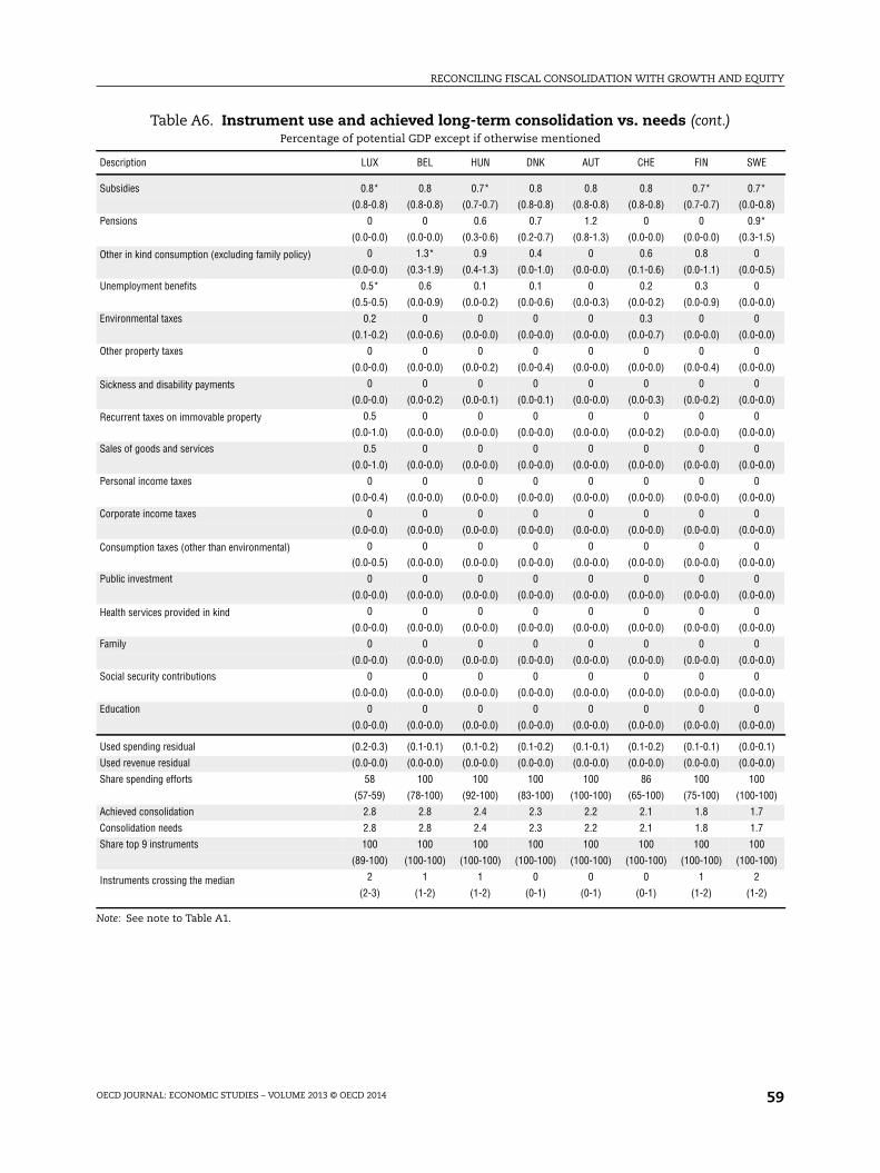
RECONCILING FISCAL CONSOLIDATION WITH GROWTH AND EQUITY
OECD JOURNAL: ECONOMIC STUDIES – VOLUME 2013 © OECD 2014 59
Table A6. Instrument use and achieved long-term consolidation vs. needs (cont.)Percentage of potential GDP except if otherwise mentioned
Description LUX BEL HUN DNK AUT CHE FIN SWE
Subsidies 0.8* 0.8 0.7* 0.8 0.8 0.8 0.7* 0.7*
(0.8-0.8) (0.8-0.8) (0.7-0.7) (0.8-0.8) (0.8-0.8) (0.8-0.8) (0.7-0.7) (0.0-0.8)
Pensions 0 0 0.6 0.7 1.2 0 0 0.9*
(0.0-0.0) (0.0-0.0) (0.3-0.6) (0.2-0.7) (0.8-1.3) (0.0-0.0) (0.0-0.0) (0.3-1.5)
Other in kind consumption (excluding family policy) 0 1.3* 0.9 0.4 0 0.6 0.8 0
(0.0-0.0) (0.3-1.9) (0.4-1.3) (0.0-1.0) (0.0-0.0) (0.1-0.6) (0.0-1.1) (0.0-0.5)
Unemployment benefits 0.5* 0.6 0.1 0.1 0 0.2 0.3 0
(0.5-0.5) (0.0-0.9) (0.0-0.2) (0.0-0.6) (0.0-0.3) (0.0-0.2) (0.0-0.9) (0.0-0.0)
Environmental taxes 0.2 0 0 0 0 0.3 0 0
(0.1-0.2) (0.0-0.6) (0.0-0.0) (0.0-0.0) (0.0-0.0) (0.0-0.7) (0.0-0.0) (0.0-0.0)
Other property taxes 0 0 0 0 0 0 0 0
(0.0-0.0) (0.0-0.0) (0.0-0.2) (0.0-0.4) (0.0-0.0) (0.0-0.0) (0.0-0.4) (0.0-0.0)
Sickness and disability payments 0 0 0 0 0 0 0 0
(0.0-0.0) (0.0-0.2) (0.0-0.1) (0.0-0.1) (0.0-0.0) (0.0-0.3) (0.0-0.2) (0.0-0.0)
Recurrent taxes on immovable property 0.5 0 0 0 0 0 0 0
(0.0-1.0) (0.0-0.0) (0.0-0.0) (0.0-0.0) (0.0-0.0) (0.0-0.2) (0.0-0.0) (0.0-0.0)
Sales of goods and services 0.5 0 0 0 0 0 0 0
(0.0-1.0) (0.0-0.0) (0.0-0.0) (0.0-0.0) (0.0-0.0) (0.0-0.0) (0.0-0.0) (0.0-0.0)
Personal income taxes 0 0 0 0 0 0 0 0
(0.0-0.4) (0.0-0.0) (0.0-0.0) (0.0-0.0) (0.0-0.0) (0.0-0.0) (0.0-0.0) (0.0-0.0)
Corporate income taxes 0 0 0 0 0 0 0 0
(0.0-0.0) (0.0-0.0) (0.0-0.0) (0.0-0.0) (0.0-0.0) (0.0-0.0) (0.0-0.0) (0.0-0.0)
Consumption taxes (other than environmental) 0 0 0 0 0 0 0 0
(0.0-0.5) (0.0-0.0) (0.0-0.0) (0.0-0.0) (0.0-0.0) (0.0-0.0) (0.0-0.0) (0.0-0.0)
Public investment 0 0 0 0 0 0 0 0
(0.0-0.0) (0.0-0.0) (0.0-0.0) (0.0-0.0) (0.0-0.0) (0.0-0.0) (0.0-0.0) (0.0-0.0)
Health services provided in kind 0 0 0 0 0 0 0 0
(0.0-0.0) (0.0-0.0) (0.0-0.0) (0.0-0.0) (0.0-0.0) (0.0-0.0) (0.0-0.0) (0.0-0.0)
Family 0 0 0 0 0 0 0 0
(0.0-0.0) (0.0-0.0) (0.0-0.0) (0.0-0.0) (0.0-0.0) (0.0-0.0) (0.0-0.0) (0.0-0.0)
Social security contributions 0 0 0 0 0 0 0 0
(0.0-0.0) (0.0-0.0) (0.0-0.0) (0.0-0.0) (0.0-0.0) (0.0-0.0) (0.0-0.0) (0.0-0.0)
Education 0 0 0 0 0 0 0 0
(0.0-0.0) (0.0-0.0) (0.0-0.0) (0.0-0.0) (0.0-0.0) (0.0-0.0) (0.0-0.0) (0.0-0.0)
Used spending residual (0.2-0.3) (0.1-0.1) (0.1-0.2) (0.1-0.2) (0.1-0.1) (0.1-0.2) (0.1-0.1) (0.0-0.1)
Used revenue residual (0.0-0.0) (0.0-0.0) (0.0-0.0) (0.0-0.0) (0.0-0.0) (0.0-0.0) (0.0-0.0) (0.0-0.0)
Share spending efforts 58 100 100 100 100 86 100 100
(57-59) (78-100) (92-100) (83-100) (100-100) (65-100) (75-100) (100-100)
Achieved consolidation 2.8 2.8 2.4 2.3 2.2 2.1 1.8 1.7
Consolidation needs 2.8 2.8 2.4 2.3 2.2 2.1 1.8 1.7
Share top 9 instruments 100 100 100 100 100 100 100 100
(89-100) (100-100) (100-100) (100-100) (100-100) (100-100) (100-100) (100-100)
Instruments crossing the median 2 1 1 0 0 0 1 2
(2-3) (1-2) (1-2) (0-1) (0-1) (0-1) (1-2) (1-2)
Note: See note to Table A1.

RECONCILING FISCAL CONSOLIDATION WITH GROWTH AND EQUITY
OECD JOURNAL: ECONOMIC STUDIES – VOLUME 2013 © OECD 201460
Table A6. Instrument use and achieved long-term consolidation vs. needs (cont.)Percentage of potential GDP except if otherwise mentioned
Description DEU EST ISL KOR GRC
Subsidies 0.3 0.3 0.8* 0 0
(0.3-0.3) (0.3-0.3) (0.7-0.8) (0.0-0.0) (0.0-0.0)
Pensions 0.8 0 0 0 0.9
(0.6-0.8) (0.0-0.0) (0.0-0.0) (0.0-0.0) (0.5-0.9)
Other in kind consumption (excluding family policy) 0 1.3* 0.2 0 0
(0.0-0.0) (0.4-1.3) (0.0-0.3) (0.0-0.0) (0.0-0.4)
Unemployment benefits 0.4 0 0.1 0.1 0
(0.0-0.6) (0.0-0.0) (0.0-0.3) (0.1-0.1) (0.0-0.0)
Environmental taxes 0 0 0 0 0
(0.0-0.4) (0.0-0.0) (0.0-0.2) (0.0-0.0) (0.0-0.0)
Other property taxes 0 0 0 0 0
(0.0-0.4) (0.0-0.7) (0.0-0.3) (0.0-0.0) (0.0-0.0)
Sickness and disability payments 0 0 0 0 0
(0.0-0.0) (0.0-0.1) (0.0-0.0) (0.0-0.0) (0.0-0.0)
Recurrent taxes on immovable property 0 0 0 0.3 0
(0.0-0.0) (0.0-0.0) (0.0-0.0) (0.0-0.6) (0.0-0.0)
Sales of goods and services 0 0 0 0.5 0
(0.0-0.0) (0.0-0.0) (0.0-0.0) (0.0-0.9) (0.0-0.0)
Personal income taxes 0 0 0 0 0
(0.0-0.0) (0.0-0.0) (0.0-0.0) (0.0-0.6) (0.0-0.0)
Corporate income taxes 0 0 0 0 0
(0.0-0.0) (0.0-0.0) (0.0-0.0) (0.0-0.0) (0.0-0.0)
Consumption taxes (other than environmental) 0 0 0 0 0
(0.0-0.0) (0.0-0.0) (0.0-0.0) (0.0-0.5) (0.0-0.0)
Public investment 0 0 0 0 0
(0.0-0.0) (0.0-0.0) (0.0-0.0) (0.0-0.0) (0.0-0.0)
Health services provided in kind 0 0 0 0 0
(0.0-0.0) (0.0-0.0) (0.0-0.0) (0.0-0.0) (0.0-0.0)
Family 0 0 0 0 0
(0.0-0.0) (0.0-0.0) (0.0-0.0) (0.0-0.0) (0.0-0.0)
Social security contributions 0 0 0 0 0
(0.0-0.0) (0.0-0.0) (0.0-0.0) (0.0-0.0) (0.0-0.0)
Education 0 0 0 0 0
(0.0-0.0) (0.0-0.0) (0.0-0.0) (0.0-0.0) (0.0-0.0)
Used spending residual (0.1-0.1) (0.0-0.0) (0.0-0.1) (0.0-0.0) (0.0-0.0)
Used revenue residual (0.0-0.0) (0.0-0.0) (0.0-0.0) (0.0-0.0) (0.0-0.0)
Share spending efforts 100 100 100 12 100
(76-100) (53-100) (76-100) (12-12) (100-100)
Achieved consolidation 1.6 1.6 1.2 1 0.9
Consolidation needs 1.6 1.6 1.2 1 0.9
Share top 9 instruments 100 100 100 100 100
(100-100) (100-100) (100-100) (74-100) (100-100)
Instruments crossing the Median 0 1 1 0 0
(0-1) (1-1) (1-1) (0-0) (0-0)
Note: See note to Table A1.

RECONCILING FISCAL CONSOLIDATION WITH GROWTH AND EQUITY
OECD JOURNAL: ECONOMIC STUDIES – VOLUME 2013 © OECD 2014 61
APPENDIX B
Supporting material
B1. Estimating fiscal consolidation needs: Additional technical informationThe present section provides additional background information on the calculation of
fiscal consolidation needs that are presented in Section 2 of the main text. The present set
of consolidation needs estimates is aimed at indicating a way in which the fiscal balance
can evolve so as to reduce (or contain) public debt to a manageable level (set at 60% of GDP)
and keep it there at the end of the projection period (2060). A target of 60% for gross general
government debt relative to GDP has been chosen for reasons of consistency with the OECD
long-term growth scenarios (OECD, 2012a; Johansson et al., 2013; OECD, 2013). In addition
to reaching this 60% target, a second objective of the consolidation path is to keep debt
stable at this 60% of GDP by 2060. The debt target is specified in gross terms, while
government financial assets are assumed to remain constant as a ratio to GDP.
The debt to GDP ratio in country i at the end of year t results primarily from the past
debt ratio , the real interest rate paid on government debt, the real growth rate ,
and the primary balance (as a share of GDP) . Another driver of the debt ratio is the
income generated by government financial assets (at the real rate ) net of the
reinvestment needed to keep the asset-GDP ratio ai constant. Consequently, the debt ratio
evolves according to the following accumulation equation:
(E1)
The primary balance ratio to GDP can itself be written as a function of the underlying
primary balance as a ratio to potential GDP , the output gap as a ratio to potential GDP
, a semi-elasticity i and the amount of one-off factors :
(E2)
In the present study, the fiscal consolidation path is defined as a trajectory for that
starts from the 2012 estimate in the OECD Economic Outlook, May 2013 and then takes
projected values from 2013 to 2060. Using equation (E2), the fiscal consolidation path is
combined with the projections for in the OECD Economic Outlook Long-Term
Database, May 2013 to obtain projections of the primary deficit ratio from 2013 to 2060.
This path for the primary deficit ratio is then fed into equation (E1) to calculate the debt
trajectory starting from the 2012 estimate of and the long-term projections for – in
the OECD Economic Outlook, May 2013. The rates and are the effective interest rates
paid and received by the government on its liabilities and assets, respectively, as projected
in the OECD Economic Outlook Long-Term Database, May 2013, deflated by the rate of change
= 1(1 + ) + ( )
pit = pi
t + ioit + fi
t
+
.

RECONCILING FISCAL CONSOLIDATION WITH GROWTH AND EQUITY
OECD JOURNAL: ECONOMIC STUDIES – VOLUME 2013 © OECD 201462
of the GDP deflator taken from the same source.1 The effective interest rate takes into
account the maturity structure of the stock of government debt.
The consolidation path must satisfy the desired objectives of debt reaching
60% of GDP by 2060 (O1) and being stable (O2):
(O1)
(O2)
Using equation (E1) and then (O2) and observing that cyclical effects and one-offs have
vanished by 2060, it follows that the stability objective (O2) is satisfied if and only if:
(E3)
The stability condition (O2) therefore pins down the end point for the consolidation path.
Nevertheless, there are an infinite number of consolidation paths that satisfy
the first objective (O1) of a 60% debt-to-GDP ratio by 2060.
The present study chooses a particular functional form for the consolidation path. It
assumes that the underlying primary balance moves by 1% of GDP each year until it
reaches a certain value and from then on evolves in equal yearly steps until its end
value. In symbols instead of words, this functional form is defined as follows:
where (D1)
if (D2)
With this choice of functional form,2 the problem reduces to finding the value for such
that, with , the debt-accumulation equation (E1) yields .
The study covers all the OECD membership except Chile, Mexico and Turkey where the
necessary national accounts data and projections for the general government sector are
not available. As mentioned above, all the data and projections for the variables mentioned
in this section are taken from the OECD long-term baseline published in the OECD Economic
Outlook, May 2013.
The consolidation paths for all countries covered are plotted in Appendix 3 of
Cournède, Goujard and Pina (2013). Most countries follow the hump shape depicted in
Figures 2 and 3 of the main text : they first have to increase their
primary balance to get rid of legacy debt before they can allow it to diminish to reach the
lower level that is consistent with debt being stable as a ratio to GDP at 60%. A number of
countries (Australia, Czech Republic, Finland, New Zealand, Poland, Slovak Republic,
Slovenia), however, do not exhibit this pattern as they start from low debt so that the short-
to medium-term level of the surplus required to make sure that debt remains below 60%
until 2060 is lower than the surplus required in 2060 to keep the debt ratio stable
. Finally, in a group of countries (Denmark, Estonia, Korea, Luxembourg,
Norway, Sweden, Switzerland) the uniform objective of a 60% debt-to-GDP ratio results
mechanically in a profile of fiscal relaxation to reach the target from the bottom. Such a
profile does not appear advisable in practice as the 60% target is set relatively high, leaving
little room for shock absorption, and because fiscal relaxation often proves very difficult to
reverse in practice. These countries are considered as having no short- to medium-term
consolidation need, and the corresponding discussion does not apply to them.
d = 60%
d = 0
p = p = d r g + a r g
, ,
= p + (t 2012)sign p p if t t t = 2012 + abs p p
= p + p p t > t
= , , d = 60%
> >
2012 < < 2060( )

RECONCILING FISCAL CONSOLIDATION WITH GROWTH AND EQUITY
OECD JOURNAL: ECONOMIC STUDIES – VOLUME 2013 © OECD 2014 63
Consolidation needs are estimated by comparing these “debt-control” trajectories for
the underlying primary surplus that stabilise debt at 60% by 2060 with a baseline . As
described in the main text, the baseline for the underlying primary surplus starts from the
2012 estimated value in the OECD Economic Outlook, May 2013 . The baseline
incorporates the assumption that pension reforms, including adjustments to the
retirement age in line with longevity, keep public pension spending stable as a share of
potential GDP. The baseline also incorporates some reform of health and long-term care so
that public spending in this area increases in line with the projections in the “cost-
containment” scenario presented in de la Maisonneuve and Oliveira Martins (2013). In
other areas, fiscal policy parameters are assumed to be unchanged in the sense that
corresponding spending and revenue items stay constant as a proportion of potential GDP.
As a result, the baseline underlying primary balance evolves as:
.
The short- to medium-term consolidation need is defined as the difference
between the underlying primary surplus in the year when the value is reached and
the baseline in the same year: . Given the choice of increasing the
underlying primary balance by 1% of potential GDP per year, there is a very direct link
between the duration and size of consolidation. The short- to medium-term part of the
simulated consolidation is completed by 2017 in the vast majority of covered countries, the
exceptions being Greece, Ireland, Japan, Portugal, the United Kingdom and the
United States.
The long-term consolidation need is defined as the difference between the
underlying primary surplus that stabilises a 60% debt-GDP ratio and its baseline level
in 2060: . With a common target debt-ratio, differences in the long-term
objective for the primary surplus only reflect differences in assumptions about real growth
and interest rates by 2060 in the OECD long-term scenarios, which are small. The variation
in estimated long-term consolidation needs (Figure 3 of the main text), therefore, primarily
reflect differences in the baseline. The cross-country variation in projected increases in
public health and long-term care spending is relatively limited in the cost-containment
scenario. As a result, the main source of variation in estimated long-term consolidation
needs comes from the starting point for the underlying primary surplus.
B2. The dataset of fiscal consolidation instruments
B.2.1. Defining the instruments
The revenue and expenditure sides of budgets are decomposed into sets of variables
which may potentially be the object of consolidation measures, and are hence referred to
as the instruments of consolidation. Their definition balances concerns of economic
interpretability, parsimony and data availability, while ensuring a consistent accounting
framework where no budget items are missed or overlap, and hence the various categories
of spending and revenue sum to total spending and revenue. A total of 17 consolidation
instruments are identified, plus residual and property income items (Tables B1 and B2).
Revenue instruments span the main categories of taxes plus a non-tax item, sales of goods
and services (mainly user charges). Spending instruments articulate the economic and
functional classifications of expenditure, where the former focuses on the economic
nature of transactions (such as wages, cash transfers or public investment) and the latter
on their purpose (like education, health or defence). Residual spending and revenue
2012 = 2012
=
l=
= 2060 2060

RECONCILING FISCAL CONSOLIDATION WITH GROWTH AND EQUITY
OECD JOURNAL: ECONOMIC STUDIES – VOLUME 2013 © OECD 201464
categories are heterogeneous and hence hard to characterise: though they are not taken as
instruments, they are assumed to take part in the overall consolidation effort by keeping a
constant share to underlying primary disbursements and receipts. Property income (paid
or received) follows from the trajectories of interest rates and asset stocks.
Consolidation instruments are hence defined in a quantitative, internationally-
comparable way, and their use to achieve budget targets does not map into specific policy
measures. For instance, resorting to an increase in personal income taxes could be done
either through higher marginal rates or by curbing tax expenditures. Likewise, spending on
health care could be brought down either by reducing the levels of service provision or by
achieving efficiency gains. Structural reforms of taxation and public spending, of which
tackling tax expenditures and spending inefficiencies are prime examples, are strongly
advocated, especially when large consolidation requirements force governments to use
instruments with growth- or equity-damaging impacts. However, severe data limitations,
as well as the need to preserve a consistent accounting framework, preclude the
identification of tax expenditures and efficiency gains in specific areas as autonomous
instruments. Though the scope for base broadening can be quantified for some taxes, such
as VAT (through the VAT revenue ratio), efforts at international comparisons of tax
expenditures across various tax bases have been subject to important limitations and
covered only a subset of OECD members (OECD, 2010a). Potential savings from efficiency
gains have been estimated in only a limited number of areas (e.g. Sutherland et al., 2007,
for primary and secondary education; OECD, 2010b, for health care) and are also subject to
important qualifications. For these reasons, the study considers the quantitative changes
in the instruments of fiscal consolidation (spending cuts and revenue increases) separately
from the structural measures that can accompany or contribute to them.
A dataset containing estimates in 2012 of all consolidation instruments in 31 OECD
countries has been constructed, as described in more detail below (severe data limitations
have prevented the inclusion of Chile, Mexico and Turkey). Using values in 2012 ensures
consistency with the estimates of consolidation requirements and incorporates the effects
of the various consolidation measures already implemented by member countries.3
Further, instruments are defined in underlying terms (i.e. net of cyclical effects and of one-
offs), as a percentage of potential GDP. This avoids distortions in the cross-country
comparison of fiscal variables. For instance, the use of nominal values as a percentage of
actual GDP could have resulted in overestimating the structural importance of spending
items in countries with big negative output gaps.
B.2.2. Constructing the fiscal dataset
Underlying instrument values in 2012 have been estimated in three main steps. First,
actual values in the most recent year available have been collected. Second, values have
been updated to 2012 on the basis of the dataset in the OECD Economic Outlook, May 2013
(OECD, 2013). Third, instruments have been adjusted for the cycle and for one-offs, also in
a way consistent with OECD (2013).
In the first step, data is collected or estimated for the most recent year available in
both the main statistical sources, national accounts and the OECD Revenue Statistics. This
year (call it year Y) varies across countries, though it is often 2010 or 2011 (Table B3).
However, on the spending side, though these sources give the totals for wages,
intermediate consumption and transfers in kind and for social transfers other than in kind,
they do not provide the functional breakdown defining the first seven instruments, as

RECONCILING FISCAL CONSOLIDATION WITH GROWTH AND EQUITY
OECD JOURNAL: ECONOMIC STUDIES – VOLUME 2013 © OECD 2014 65
COFOG data is insufficiently disaggregated or simply not available. Alternative sources are
then used (Tables B1, B2 and B3) and, when they refer to a year before year Y, values are
extrapolated by assuming a constant share of the instrument in question in the respective
national accounts total. For instance, Education at a Glance data for 2009 is extrapolated
to 2010 (assuming this is year Y) by preserving the 2009 share of education spending
relative to total wages, intermediate consumption and transfers in kind.
In the second step, the change from year Y to 2012 in the fiscal variables contained in
OECD (2013) is allocated to the several instruments of consolidation (plus residual and
property income items), ensuring that total revenue and total expenditure in the dataset of
instruments equal those totals in OECD (2013). Tables B1 and B2 set the correspondence
used. Since the dataset of instruments is more disaggregated than the OECD (2013) fiscal
block, it is often assumed that instruments keep a constant share relative to certain
variables. For instance, while the change in the OECD (2013) variable TKTRG is fully
allocated to the expenditure residual item, the change in TOCR is split between sales of
goods and services and the residual item by assuming that the year Y ratio between sales
and the residual (net of TKTRG) is maintained. On the spending side, it is worth
underlining that unemployment benefits are assumed to remain a constant proportion of
cash transfers in cyclically-adjusted rather than nominal terms.
In the third step, instruments are adjusted for the cycle and for one-offs, drawing
again on OECD (2013) fiscal variables (Tables B1 and B2) and, as above, often making an
assumption of constant proportions. Adjusted instruments are in all cases taken as a
percentage of potential, rather than actual, GDP.
B.2.3. Country-specific issues
For each country, Table B3 documents the date of the latest available information from
several sources. Further, Swiss institutional features have given rise to a number of
adjustments. In Switzerland, most health expenditure recorded as public in the health
accounts is not classified as general government expenditure in national accounts, since
the system is largely managed by private non-profit organisations (OECD, 2011a). This
would imply an artificially low value for other government consumption (item 3 in
Table B2), since the latter is obtained by difference. To correct this problem, the difference
in public spending on health between health accounts and national accounts is added to
other government consumption. On the revenue side, a similar adjustment is made for
social contributions to ensure budget-balance neutrality and improve international
comparability.
B.3. Additional considerations on the growth and equity effectsof consolidation instruments
This section gives detail, additional to that in the main text, on the underpinning of
the assessment summarised by the plus and minus signs in Table 2 of the main text. The
assessment proposed in Table 2 focuses on the effects of consolidation instruments
themselves and does not incorporate the possible response of joint reform of structural or
redistributive policies. In principle, all the long-term-growth-damaging instruments listed
below can be accompanied by structural reforms that could mitigate, offset, or even more
than offset, their harmful growth implications. Similarly, all regressive instruments can be
supplemented by redistributive provisions tailored to preserve, or equalise, the income
distribution. For many instruments the same behavioural responses to their

RECONCILING FISCAL CONSOLIDATION WITH GROWTH AND EQUITY
OECD JOURNAL: ECONOMIC STUDIES – VOLUME 2013 © OECD 201466
implementation shape long-term effects along both the growth and equity dimensions
which are therefore discussed together in the present section.
B.3.1. Government consumption
B.3.1.1. Health care
Government spending on health care reduces inequality in effective consumption
(Hoeller et al., 2012). The favourable welfare effects of providing health services to people
who cannot afford them otherwise are likely to be particularly large.
With good health contributing to human capital preservation, health spending can be
expected to contribute positively to the productive potential of an economy (Joumard et al.,
2010). Investment in health has indeed been found to boost economic output in OECD
countries (Gyimah-Brempong and Wilson, 2004). On the plausible assumption that private
funding cannot fully substitute for public expenditure, government spending on health
care can be expected to boost potential output, a positive link that seems present in the
data for OECD countries (see Barbiero and Cournède, 2013).
B.3.1.2. Education
Empirical estimates suggest that the distributional effect of government spending is
progressive for primary and secondary education and regressive for tertiary education
(OECD, 2011). Given that governments spend more on the primary and secondary levels of
education, an across-the-board cut in education spending can be considered as regressive.
Government spending on education generally tends to increase intergenerational social
mobility as well (Causa and Johansson, 2010), meaning that the inequitable consequences
of cuts in this area are likely to grow over time.
B.3.1.3. Other government consumption
Cuts in other government consumption that include reductions in government
employment are likely to increase income inequality (Fournier and Koske, 2012). More
broadly, reducing the government wage bill can be expected to increase income inequality
in most countries (Bova et al., 2012). Cuts in government-provided services will also have
the effect of increasing inequality in effective consumption.
B.3.2. Government investment
OECD work on the sources of economic growth found a positive long-term relationship
between private and public capital accumulation, suggesting complementarity between
the two and a positive effect of government investment on long-term output (see Table 2.7
in OECD, 2003a; and Sutherland et al., 2009). On US data, Leduc and Wilson (forthcoming)
identify strong, positive long-term GDP effects of road infrastructure grants. Evidence from
583 studies surveyed by Bom and Ligthart (2013) indicates that public capital has positive
short- and long-run effects on output. With a depreciation rate of 5% and a real interest
rate of 3%, the marginal cost of public capital (8%) is lower than the estimated marginal rate
of return (10 to 24%). This situation suggests underinvestment in public capital,
particularly for core public capital where the marginal rate of return may be close to 24%.
Evidence on the effect of public investment on inequality in OECD countries is too
limited for inclusion in the assessment summarised in Table 2 of the main text. Estimates
by Calderon and Serven (2004) show that infrastructure development, a key area of

RECONCILING FISCAL CONSOLIDATION WITH GROWTH AND EQUITY
OECD JOURNAL: ECONOMIC STUDIES – VOLUME 2013 © OECD 2014 67
government investment, promotes income equality. This study has however been
conducted with a database consisting primarily of developing countries, which raises a
question as to whether its finding applies to advanced economies. Furthermore, a model-
based study by Chatterjee and Turnovsky (2012) suggests a conceptual channel whereby
government investment could increase wealth inequality: because of complementarities
between public and private capital, a greater public capital stock raises the value of private
capital, the holding of which is concentrated at the top end of the wealth distribution.
Finally, the short-term impact of government investment on the income distribution is
likely to be positive given the large role of low-skilled labour in construction work, but
there is little empirical evidence to document this effect.
B.3.3. Transfers
Transfers equalise income more strongly than taxes (Rawdanowicz et al., 2012;
Joumard et al., 2012; Bastagli et al., 2012). On the other hand, aggregate higher social
protection expenditure, especially “passive” income support, much of which is achieved
through transfers, has been found to be associated with lower economic growth (Arjona
et al., 2002). Some categories, such as active labour market programmes (ALMP), are linked
with higher growth (Arjona et al., 2002), but most of ALMP spending is recorded as
government consumption or subsidies rather than transfers.
B.3.3.1. Pensions
The distributional impact of reducing public pension spending can change direction
depending on the way in which it is implemented. Reducing spending by increasing the
average retirement age will have the effect that people who would otherwise have retired
and drawn a sometimes low pension will keep drawing a higher salary. The effect is likely
to be a more equal distribution of income. On the other hand, as public pension systems
are progressive, although to varying degrees across OECD countries, reducing replacement
rates would tend to be regressive on impact. The effect will diminish over time if labour
supply increases in response.
B.3.3.2. Unemployment benefits
Reducing unemployment benefits increases inequality, even in insurance-based
systems because less paid workers are more likely to be laid off. In the long term, however,
reducing the level of unemployment benefits translates into higher employment rates,
implying little if any change in steady-state income distribution (Rawdanowicz et al., 2012).
B.3.3.3. Sickness and disability benefits
Reducing sickness and disability benefits would mechanically increase inequality as
replacement rate tend to be higher for low-income earners (OECD, 2010). However, in the
long term, poorly-targeted disability benefits can lock up individuals with residual working
capacity in poverty traps with negative growth effects and potentially negative effects on
equity. In that regard, well-targeted reductions in government spending on disability
benefits are likely to have regressive effects that diminish over time (Rawdanowicz et al.,
2012). Unfocused budgetary cuts will have lasting regressive effects since part of them fall
on people who cannot supply labour to compensate.

RECONCILING FISCAL CONSOLIDATION WITH GROWTH AND EQUITY
OECD JOURNAL: ECONOMIC STUDIES – VOLUME 2013 © OECD 201468
B.3.4. Subsidies
In the present taxonomy of instruments, following the national accounts framework,
subsidies are defined as current payments to businesses based on their production levels.
Unless they correct market failures, such production subsidies have the potential to distort
resource allocation and restrict competition (OECD, 2001) and have been long identified as
reducing productive potential (Ford and Suyker, 1990). Agricultural and fossil-fuel subsidies
in particular can, in addition, encourage inefficient use of natural resources (OECD, 2003b),
eroding the resource base for long-term growth and harming those most exposed to
environmental degradation, which are typically concentrated at the bottom of the income
distribution (Serret and Johnstone, 2006).
B.3.5. Taxes
An increase in distortionary taxes (labour and capital income taxes, social security
contributions, property taxes) of 1% of GDP is estimated to reduce the level of GDP by 3.2%
after ten years according to a recent empirical study (Gemmell, Kneller and Sanz, 2011).
B.3.5.1. Tax expenditures
The present study does not include tax expenditures in its quantitative analysis of
possible consolidation strategies for lack of comparable data across the OECD membership.
Tax expenditures have the potential of distorting resource allocation and hurting growth.
To give just one example, the combination of mortgage interest relief with no taxation of
owner-occupied rental services favours investment in housing over other, typically more
productive, forms of capital. With the notable exception of tax relief or credit for low-wage
workers, many tax deductions have higher value for high-income earners and are therefore
regressive (Rawdanowicz et al., 2012).
B.3.5.2. Consumption taxes
Consumption taxes are typically regressive because lower-income households spend a
higher share of their income (Rawdanowicz et al., 2012). Fiscal authorities often try to limit
the regressive effects of indirect taxes by applying reduced rates on bare necessities, but
these reductions have large fiscal costs as they are enjoyed not only by low-income
households but by all consumers.
B.3.5.3. Personal income tax and social security contributions
Progressive income taxation reduces growth and equalises after-tax income
immediately (Joumard et al., 2012) and permanently (Echevarria, 2012). In many countries,
however, a wide array of tax breaks, which have higher value for higher-income
households, reduces the redistributive power of personal income taxation. Social security
contributions, in contrast, tend to be regressive as they are often concentrated on labour
income, which makes a smaller share of the income of higher-income households.
The direction of the growth effects of progressive income taxation, compared with
flatter tax schedules, is ambiguous in theory. Progressive income taxation reduces the
return on work more for more productive workers. Depending on whether they work more
to maintain their income (the income effect) or less because of the higher after-tax relative
value of leisure (the substitution effect), progressive taxation will boost or reduce output.
Another channel is that, in the presence of financial constraints, progressive tax schedules
leave lower-income workers with more after-tax income from which they can build savings
RECONCILING FISCAL CONSOLIDATION WITH GROWTH AND EQUITY
OECD JOURNAL: ECONOMIC STUDIES – VOLUME 2013 © OECD 2014 69
to start their own business. In the first instance, this channel means that progressive
taxation should be growth-enhancing. However, general-equilibrium effects push up the
wages of low-productivity workers under flat tax schedules, which can partly compensate,
or more than offset, the previous direct effect depending on the characteristics of the
progressive and flat tax schemes being compared (Bohacek and Zubricki, 2012). Overall, the
question is empirical, and the evidence is largely conclusive that progressive taxation
reduces long-term growth (Johansson et al., 2008). Social security contribution schemes are
typically far less progressive than income tax (OECD, 2012b).
B.3.5.4. Corporate income tax
Corporate income taxes are one way of taxing capital income, directly and also by
limiting the incentive for owners to shelter capital earnings from personal income taxation
by keeping them in corporations (Johansson et al., 2008). As capital control is concentrated
among higher-income households, corporate income taxation works in the direction of
equalising income.
A large body of empirical evidence indicates that corporate income taxes are highly
distortive to long-term output (see for instance Johansson et al., 2008). Because it is
calculated on earnings after interest payments, corporate income taxation creates a strong
bias in favour of debt over equity financing, contributing to excess leverage and instability
(Sutherland et al., 2012; De Mooij, 2012). Higher corporate income taxes have been found to
deter FDI (Becker et al., 2012).
B.3.5.5. Recurring taxes on immovable property
In a number of OECD countries lower-income households pay a larger share of their
earnings in recurring real estate taxes than higher-income households, so that recurring
property taxes can be seen as regressive in the static income distribution. However, this
situation is to some extent (but not fully) related to larger property holdings among
pensioners, implying that property taxation is not necessarily regressive in the perspective
of lifetime income or wealth distribution (Rawdanowicz et al., 2012). Furthermore, some
OECD countries have introduced exemptions or rebates for low-income households to
alleviate, or reverse, the regressive effects of recurring real estate taxes (Joumard et al.,
2012). Against this background, increases in recurring taxes on immovable property cannot
be described as being generally progressive or regressive.
B.3.5.6. Other property taxes
Inheritance, gift and wealth taxes, which make up much of this category, are highly
redistributive because tax schedules are generally strongly progressive and wealth is more
concentrated than income (Joumard et al., 2012). The progressive effects of increases,
however, are likely to diminish over time due to the mobility of many forms of capital and
the greater incentive to put in place tax avoidance strategies for more wealthy households.
B.3.5.7. Environmental taxes
Environmental taxes can improve welfare by increasing the marginal cost of activities
that harm the environment. This welfare benefit is not measured in GDP which for the
most part does not record environmental services. One of the effects of environmental
taxes, however, is to support long-term output to the extent that they discourage the
excessive use of environmental resources that are needed for future production. However,

RECONCILING FISCAL CONSOLIDATION WITH GROWTH AND EQUITY
OECD JOURNAL: ECONOMIC STUDIES – VOLUME 2013 © OECD 201470
another of their effects, shared with other taxes, is to reduce labour supply and physical
capital accumulation. Where applying to internationally-mobile activities, environmental
taxation will entail smaller gross effects on GDP and bring larger environmental benefits if
it is co-ordinated across countries.
Lower-income households, who spend more of their income than better-off
households on basic resources, therefore tend to pay a greater share of their income in
environmental taxes. Prima facie, environmental taxes may therefore be considered as
regressive. However, lower-income households are more exposed to environmental
degradation than the rest of the population. As a result, when the benefits of higher
environmental taxation materialise, the net welfare effect of environmental taxation may
not necessarily be regressive.
B.3.6. User charges
Charging more for the use of public services can boost growth by avoiding their
inefficient use. The distributional effects of increases in user charges are likely to be
regressive except in cases (such as tertiary education) where public services are used more
heavily by higher-income groups.
B.4. Methodological information on estimating debt behaviour duringconsolidation episodes
This section provides detailed information about the methodology used to document
the behaviour of debt-GDP ratios during consolidation episodes shown in Figure 6 of the
main text. Episodes of fiscal consolidation are defined using the IMF Action-Based Dataset
(Devries et al., 2011). This definition of fiscal adjustments and discretionary policy choices
of fiscal authorities is, in principle, less affected by countries’ macroeconomic conditions
than measures of the fiscal stance based on cyclical adjustment (Guajardo et al., 2011).
A period of fiscal adjustment is defined as a year in which the action-based budget balance
improves by at least 1½ per cent of GDP. As a robustness check, two thresholds of 1.75 and
2% of GDP were also used, but the results were very similar to the ones reported in Figure 6.
This definition rules out fiscal adjustments which are small annually but prolonged over
several years. Furthermore, it selects both one-year consolidation episodes and multi-
period adjustments as in Alesina and Ardagna (2010).
Figure 6 in the main text presents difference-in-differences estimates of the
association between the public debt ratio d and consolidation episodes, from 10 years
before to 10 years after the onset of a consolidation. These specifications control for
country and year fixed effects according to the following specification:
where c stands for the starting year of a consolidation episode, I the country and t the year
under consideration. The period from 15 to 11 years before the onset of a consolidation
episode is omitted, meaning that all estimates are relative to these earlier years of data.
Each country-year observation has the same weight in the estimation. On the solid lines,
each point corresponds to the estimate of k, the difference between the level of public debt
in pre- or post-consolidation year k relative to the rest of the sample. Dashed lines
represent the 90% confidence interval adjusted for heteroskedasticity, spatial
autocorrelation and within-country autocorrelation as in Driscoll and Kraay (1998) and
Auerbach and Gorodnichenko (2012).
= 1 + + +
RECONCILING FISCAL CONSOLIDATION WITH GROWTH AND EQUITY
OECD JOURNAL: ECONOMIC STUDIES – VOLUME 2013 © OECD 2014 71
B.5. Alternative simulations based on simple country groups insteadof clustering
A variant has been prepared to test the sensitivity of clustering-based instrument
rankings and consolidation packages. In this variant, instead of deriving weights from
clustering analysis, countries are divided in three groups of identical sizes based on their
current-account positions, and each objective receives the same weight within each group.
Current account-positions are evaluated on the basis of cyclically adjusted current account
balances as shares of both national and OECD GDP. The country groups and weights are as
follows:
1. A first group gathers 10 countries with the largest current-account deficits: Australia,
France, Greece, Iceland, New Zealand, Poland, Portugal, Spain, the United Kingdom and
the United States. Weights of 20% each are given to each objective (short- and long-term
growth and equity, current account).
2. A second group gathers 11 countries with the largest current-account surpluses: Austria,
Denmark, Germany, Ireland, Japan, Korea, Luxembourg, Netherlands, the
Slovak Republic, Sweden and Switzerland. Weights of 20% each are given to each
objective (short- and long-term growth and equity, current account). The signs of the
assessments of current-account effects shown in Table 3 of the main text are reversed to
take into account the surplus position of these countries.
3. The third group gathers the remaining 10 countries: Belgium, Canada, the
Czech Republic, Estonia, Finland, Hungary, Israel, Italy, Norway and Slovenia. Weights of
25% each are given to each objective (short- and long-term growth and equity).
The rankings that result from this alternative weighting scheme are very highly
correlated with the ones obtained with the clustering technique reported in the main text.
Rank correlations between clustering-based and alternative rankings are 96% for Cluster 1,
98% for Cluster 2, 93% for Cluster 3, 89% for Cluster 4 and 95% for Cluster 5.
As a result, the consolidation packages are also very similar as is apparent from
comparing Tables B4 to B8 which refer to the alternative simulations to Tables A1 to A5
which refer to the main ones. To facilitate comparison with the main Tables A1 to A5, the
Tables B4 to B8 for the variant are shown with the same grouping of countries by cluster
although uniform weights for the three above-listed groups have been used. Overall, the
simulated consolidation packages in the variant are very close to the clustering-based
ones. Noticeable differences appear only in Clusters 3 and 4 where clustering-based
weights differ substantially from 25%. For instance, the instrument mix of the
Slovak Republic and Spain changes with greater use of personal income taxes. The variant
is similarly robust to shocks to the assessment of effects as the main clustering-based
results. The interdecile variations shown between brackets in Tables B4 to B8 remain
generally narrow.
B.6. Alternative simulations allowing additional room for manoeuvreAn important assumption in the simulation design relates to the amount up to which
each instrument can be used. As presented in greater detail in Box 4, which also spells out
the adjustments made to deal with special cases, two constraints are imposed in the main
simulations:
1. A tax can be increased up until proceeds from this tax reach the 66th percentile of the
cross-country distribution of receipts from this kind of tax, as a share of potential GDP.

RECONCILING FISCAL CONSOLIDATION WITH GROWTH AND EQUITY
OECD JOURNAL: ECONOMIC STUDIES – VOLUME 2013 © OECD 201472
Similarly, spending in one area can be reduced until the country reaches the
33rd percentile of the cross-country distribution of spending in this area, as a share of
potential GDP.
2. Adjustment along one instrument is capped at one standard deviation of the cross-
country distribution of tax or spending in the area under consideration as a share of
potential GDP.
In the present set of alternative simulations, the first constraint is relaxed by allowing
movement until reaching the 80th percentile for taxes and the 20th percentile for
spending. The second constraint is retained.
Tables B9 to B13 present country details of the short- to medium-term packages
simulated under the relaxed first constraint on instrument use. Compared with the main
results reported in Tables A1 to A5, these alternative simulations show that allowing more
room for manoeuvre makes it possible for countries to achieve much more of their
adjustment with well-ranked instruments. The same finding holds for the simulated long-
term packages reported in Table B14 for the variant with additional room for manoeuvre
and Table A6 for the main scenario. These findings are obtained even though the relaxation
of the constraint is relatively moderate in the sense that the one-standard-deviation
constraint is maintained.
Table B1. Revenue categories: Definitions and sources
ItemNo.
DescriptionDefinitions and sources1
(codes in brackets)Updating to 2012:
EO93 variablesAdjusting for the cycle and for one-offs:
EO93 variables
1 Personal income taxes RS (1100 + 1300) TYH (part) TYHA-TYH (part)
2 Social security contributions RS (2000 + 3000) + NA (D612r) SSRG (100%) SSRGA-SSRG (100%)
3 Corporate income taxes RS (1200) TYB (part) TYBA-TYB (part)
4 Environmental taxesOECD/EEA Database on instrumentsused for environmental policy
TIND (part) TINDA-TIND (part)
5 Other consumption taxes RS (5000 + 6000) – item 4 TIND (part) TINDA-TIND (part)
6Recurrent taxes on immovableproperty
RS (4100 + 4600) TYH (part), TYB (part), TIND(part)2
TINDA-TIND (part), TYHA-TYH (part),TYBA-TYB (part)2
7 Other property taxes RS (4200 to 4500) TYH (part), TYB (part), TIND(part)2
TINDA-TIND (part), TYHA-TYH (part),TYBA-TYB (part)2
8 Sales of goods and services NA (P11 + P12 + P131) TOCR (part)
9 Other (non-property) receipts NA (TR) – sum of items 1-8 and 10 TKTRG (100%), TOCR (part) TKTRGU-TKTRG-TRGOE (100%)
10 Property income received NA (D4r) YPERG (100%)
1. RS = OECD Revenue Statistics; NA = National Accounts.2. Items 6 and 7 are each assumed to consist in equal parts of direct (TY) and indirect (TIND) taxes, and, within TY, TYH and TYB are
assumed to observe the proportions of items 1 and 3.Note: EO93 stands for the OECD Economic Outlook, No. 93 (OECD, 2013).

RECONCILING FISCAL CONSOLIDATION WITH GROWTH AND EQUITY
OECD JOURNAL: ECONOMIC STUDIES – VOLUME 2013 © OECD 2014 73
Table B2. Expenditure categories: definitions and sources
ItemNo.
DescriptionDefinition: National
Accounts codesData sources
and proxies used1Updating to 2012:
EO93 variablesAdjusting for the cycle
and one-offs: EO93 variables
1Education (wages,intermediate consumption andsocial transfers in kind)
D1p + P2 + D6311p + 63121p+ 63131p within COFOG 09
OECD Education at a Glance2 (CGAA-CFKG + revenueitem 8) (part)
2Health (wages, intermediateconsumption and socialtransfers in kind)
D1p + P2 + D6311p + 63121p+ 63131p within COFOG 07
Health Accounts (SHA)3 (CGAA-CFKG + revenueitem 8) (part)
3
Wages, intermediateconsumption and transfers inkind – other purposes (exceptfamily and children)
D1p + P2 + D6311p + 63121p+ 63131p within remainingCOFOG divisions (except 10.4,family and children)
NA(D1p + P2 + D6311p + 63121p +63131p) – item 7 (benefits inkind) – items 1 and 2
(CGAA-CFKG + revenueitem 8) (part)
4Old-age and survivor pensions(social transfers other than inkind)
D62p withinCOFOG 10.2 + 10.3
SOCX Database, old age andsurvivors (cash benefits)
SSPG (part)
5Sickness and disability (socialtransfers other than in kind)
D62p within COFOG 10.1SOCX Database, incapacityrelated (cash benefits)
SSPG (part)
6Unemployment benefits(social transfers other than inkind)
D62p within COFOG 10.5SOCX Database, unemployment(cash benefits)
SSPG (part) YPGA – YPG (100%)
7
Family and children (wages,intermediate consumption andsocial transfers in cash and inkind)
D1p + P2 + D62p + D6311p+ 63121p + 63131pwithin COFOG 10.4
SOCX Database, family (cashbenefits + benefits in kind)
(CGAA-CFKG + revenueitem 8) (part), SSPG (part)
8 Subsidies D3p NA (D3p) (YPOTG net of revenueitem 8) (part)
9 Public investment P51 NA (P51) IGAA (100%)
10 Other primary expenditure
D62p(remainder) + D29p + D5p+ D7p + P52 + P53 + K2+ D9p
NA (TE, total expenditure)– items 1-9 and 11
TKPG (100%), (YPOTGnet of revenue item 8) (part), SSPG (part)
TKPGU – TKPG – TPGOE(100%)
11 Property income paid D4p NA (D4p) YPEPG (100%)
1. NA = National Accounts.2. General government expenditures (all levels, all educational programmes, and all types of transactions).3. General government total expenditure (HC.1-HC.9; HC.R.1) for the UK, and general government total current expenditure (HC.1-HC.9,
individual and collective health care) for all other countries.

RECONCILING FISCAL CONSOLIDATION WITH GROWTH AND EQUITY
OECD JOURNAL: ECONOMIC STUDIES – VOLUME 2013 © OECD 201474
Table B3. Country data sources
Nationalaccounts
Revenuestatistics
Healthaccounts
Social ExpenditureDatabase
Educationat a Glance
Environmentaltaxes
Australia 2009 2009 2009 2009 2009 2009
Austria 2011 2011 2010 2009 2009 2011
Belgium 2011 2011 2010 2009 2009 2011
Canada 2010 2010 2010 2009 2009 2010
Czech Republic 2011 2011 2010 2009 2009 2011
Denmark 2011 2011 2010 2009 2009 2011
Estonia 2011 2011 2010 2009 2009 2011
Finland 2011 2011 2010 2009 2009 2011
France 2011 2011 2010 2009 2009 2011
Germany 2011 2011 2010 2009 2009 2011
Greece 2010 2010 2007 2009 2005 2010
Hungary 2011 2011 2010 2009 2009 2011
Iceland 2011 2011 2010 2009 2009 2011
Ireland 2011 2011 2010 2009 2009 2011
Israel 2011 2011 2009 2009 2009 2010
Italy 2011 2011 2011 2009 2009 2011
Japan 2010 2010 2009 2009 2009 2010
Korea 2010 2010 2010 2009 2009 2010
Luxembourg 2011 2011 2009 2009 2002 2011
Netherlands 2010 2010 2010 2009 2009 2010
New Zealand 2010 2010 2010 2009 2009 2010
Norway 2011 2011 2011 2009 2009 2011
Poland 2010 2010 2010 2009 2009 2010
Portugal 2010 2010 2010 2009 2009 2010
Slovak Republic 2011 2011 2010 2009 2009 2011
Slovenia 2011 2011 2010 2009 2009 2010
Spain 2011 2011 2010 2009 2009 2011
Sweden 2011 2011 2010 2009 2009 2011
Switzerland 2011 2011 2010 2008 2009 2011
United Kingdom 2011 2011 2010 2009 2009 2011
United States 2011 2011 2010 2009 2009 2010
Median 2011 2011 2010 2009 2009 2011
Min. 2009 2009 2007 2008 2002 2009
Max. 2011 2011 2011 2009 2009 2011
Source: OECD National Accounts and Revenue Statistics, OECD Health Accounts, OECD Social Expenditure Database, OECDEducation at a Glance, and the OECD/European Environment Agency Database on instruments used for environmentalpolicy and natural resources management.

RECONCILING FISCAL CONSOLIDATION WITH GROWTH AND EQUITY
OECD JOURNAL: ECONOMIC STUDIES – VOLUME 2013 © OECD 2014 75
Table B4. Instrument use and short- to medium-term consolidation with fixed weightsin cluster No. 1
Percentage of potential GDP except if otherwise mentioned
Description AUS CAN GBR ISR ITA JPN NZL POL PRT
Subsidies 0.6* 0.3 0 0 0.3 0 0 0 0
(0.6-0.6) (0.3-0.3) (0.0-0.0) (0.0-0.0) (0.0-0.3) (0.0-0.0) (0.0-0.0) (0.0-0.0) (0.0-0.0)
Other property taxes 0 0.5* 0.2 0.2 0 0.4* 0.7* 0.7* 0.3*
(0.0-0.0) (0.5-0.5) (0.2-0.2) (0.2-0.2) (0.0-0.0) (0.3-0.3) (0.7-0.7) (0.7-0.7) (0.3-0.3)
Pensions 0 0 0.3 0.2 0.3 0.8 0 0.9 0.9
(0.0-0.0) (0.0-0.0) (0.3-0.3) (0.2-0.2) (0.3-0.7) (0.8-0.8) (0.0-0.0) (0.9-0.9) (0.9-0.9)
Corporate income taxes0 0.2 0.5* 0 0 0 0 0.9* 0.3
(0.0-0.0) (0.0-0.2) (0.5-0.5) (0.0-0.0) (0.0-0.0) (0.0-0.0) (0.0-0.0) (0.0-0.9) (0.0-0.3)
Personal income taxes 0 0 0.5 1.3 0 4.6* 0 1.1 4.1*
(0.0-0.0) (0.0-0.0) (0.5-0.5) (0.0-1.3) (0.0-0.0) (4.6-4.6) (0.0-0.0) (0.0-2.0) (3.2-4.1)
Recurrent taxes on immovable property 0 0 0 0 0 0 0 0.1 0.8*
(0.0-0.0) (0.0-0.0) (0.0-0.0) (0.0-0.0) (0.0-0.0) (0.0-0.0) (0.0-0.0) (0.0-0.3) (0.3-0.8)
Unemployment benefits 0 0.2* 0 0 0 0.2 0 0 0.3
(0.0-0.0) (0.0-0.2) (0.0-0.0) (0.0-0.0) (0.0-0.0) (0.2-0.2) (0.0-0.0) (0.0-0.0) (0.0-0.3)
Environmental taxes 0.7* 0.7 0.2* 0 0 0.7 0.7 0.2 0.2
(0.0-0.7) (0.0-0.7) (0.2-0.2) (0.0-0.0) (0.0-0.0) (0.7-0.7) (0.0-0.7) (0.0-0.7) (0.0-0.2)
Other government in kind consumption 0.6 0.6 2.2* 0 0 0 0 0 0.2
(0.0-1.0) (0.0-1.8) (2.2-2.2) (0.0-1.3) (0.0-0.0) (0.0-0.0) (0.0-0.0) (0.0-1.1) (0.0-0.6)
Sales of goods and services 0 0 0.7* 0 0 1.0* 0 0 0
(0.0-0.0) (0.0-0.0) (0.6-0.7) (0.0-0.1) (0.0-0.0) (1.0-1.0) (0.0-0.0) (0.0-0.4) (0.0-0.3)
Consumption taxes (other thanenvironmental)
0 0 1.3* 0 0 2.5 0 0 0
(0.0-1.3) (0.0-1.0) (1.3-1.3) (0.0-0.0) (0.0-0.0) (2.5-2.5) (0.0-0.0) (0.0-0.5) (0.0-0.6)
Public investment 0 0 0.3 0 0 1.1 0 0 0
(0.0-0.6) (0.0-0.1) (0.2-0.3) (0.0-0.0) (0.0-0.0) (1.1-1.1) (0.0-0.6) (0.0-0.1) (0.0-0.0)
Sickness and disability payments 0 0 0.7* 0 0 0 0.2 0 0
(0.0-0.0) (0.0-0.0) (0.7-0.7) (0.0-0.1) (0.0-0.0) (0.0-0.0) (0.0-0.7) (0.0-0.4) (0.0-0.2)
Health services provided in kind 0 0 1.5* 0 0 1.5* 0 0 0
(0.0-0.0) (0.0-0.0) (0.3-1.5) (0.0-0.0) (0.0-0.0) (1.5-1.5) (0.0-0.1) (0.0-0.0) (0.0-0.0)
Social security contributions 0 0 0 0 0 0.9* 0 0 0
(0.0-0.0) (0.0-0.0) (0.0-0.7) (0.0-0.0) (0.0-0.0) (0.9-0.9) (0.0-0.0) (0.0-0.0) (0.0-0.0)
Family 0 0 0 0 0 0 0 0 0
(0.0-0.0) (0.0-0.0) (0.0-0.8) (0.0-0.0) (0.0-0.0) (0.0-0.0) (0.0-0.0) (0.0-0.0) (0.0-0.0)
Education 0 0 0 0 0 0.3 0 0 0
(0.0-0.0) (0.0-0.0) (0.0-0.0) (0.0-0.0) (0.0-0.0) (0.3-0.3) (0.0-0.0) (0.0-0.0) (0.0-0.0)
Used spending residual 0.1 0.1 0.8 0 0 0.6 0 0.1 0.1
Used revenue residual 0 0 0.2 0 0 0.6 0.1 0.1 0.4
Share spending efforts 64 45 62 13 100 30 9 25 19
(35-97) (23-82) (62-65) (13-89) (100-100) (29-30) (9-57) (25-54) (17-28)
Achieved consolidation 1.9 2.7 9.2 1.7 0.7 15 1.7 4 7.5
Consolidation needs 1.9 2.7 9.2 1.7 0.7 18.3 1.7 4 7.5
Share top 9 instruments 100 100 46 100 100 48 90 100 100
(70-100) (77-100) (28-62) (100-100) (100-100) (43-64) (89-100) (100-100) (51-100)
Instruments crossing the median2 2 7 0 0 5 1 2 3
(1-2) (2-3) (6-7) (0-1) (0-0) (5-5) (1-1) (1-3) (3-4)
Note: Simulated interdecile intervals in parentheses computed using 200 random draws. Each dimension of the assessments in Table 2is increased by 1 or decreased by 1 with equal probability (1/8, 1/8). The use of residual items is marginal. Simulated interdecile intervalsare not reported for residual items.* Denotes an instrument crossing the OECD median.

RECONCILING FISCAL CONSOLIDATION WITH GROWTH AND EQUITY
OECD JOURNAL: ECONOMIC STUDIES – VOLUME 2013 © OECD 201476
Table B5. Instrument use and short- to medium-term consolidationwith fixed weights in cluster No. 2
Percentage of potential GDP except if otherwise mentioned
Description USA
Subsidies 0
(0.0-0.0)
Pensions 0.5
(0.6-0.6)
Other property taxes 0.7*
(0.7-0.7)
Unemployment benefits 0.2
(0.2-0.2)
Corporate income taxes 0.2
(0.2-0.2)
Environmental taxes 0.7
(0.7-0.7)
Recurrent taxes on immovable property 0
(0.0-0.0)
Personal income taxes 1
(1.0-1.0)
Other government in kind consumption (excluding family policy) 0
(0.0-0.0)
Sales of goods and services 0
(0.0-0.0)
Sickness and disability payments 0
(0.0-0.0)
Consumption taxes (other than environmental) 2.5
(2.1-2.5)
Public investment 0.3
(0.0-0.3)
Health services provided in kind 1.1*
(1.1-1.5)
Family 0
(0.0-0.0)
Social security contributions 0
(0.0-0.6)
Education 0
(0.0-0.0)
Used spending residual 0.3
Used revenue residual 0.2
Share spending efforts 31
(31-39)
Achieved consolidation 7.7
Consolidation needs 7.7
Share top 9 instruments 46
(36-80)
Instruments crossing the median 2
(2-2)
Note: See note to Table B4.

RECONCILING FISCAL CONSOLIDATION WITH GROWTH AND EQUITY
OECD JOURNAL: ECONOMIC STUDIES – VOLUME 2013 © OECD 2014 77
Table B6. Instrument use and short- to medium-term consolidation with fixedweights in cluster No. 3
Percentage of potential GDP except if otherwise mentioned
Description ESP GRC IRL
Pensions 0 0.6 0
(0.0-0.0) (0.6-0.6) (0.0-0.0)
Subsidies 0.2 0 0
(0.2-0.2) (0.0-0.0) (0.0-0.0)
Other property taxes 0 0 0
(0.0-0.0) (0.0-0.0) (0.0-0.0)
Unemployment benefits 1.6 0 1.1
(0.6-1.6) (0.0-0.0) (1.1-1.1)
Environmental taxes 0.5 0.2 0.3*
(0.0-0.7) (0.0-0.2) (0.3-0.3)
Recurrent taxes on immovable property 0.3 1.0* 1.0*
(0.0-0.4) (0.3-1.0) (0.9-1.0)
Corporate income taxes 0.9* 0 0.3*
(0.0-0.9) (0.0-0.0) (0.3-0.3)
Sales of goods and services 0 0 0.3*
(0.0-1.0) (0.0-0.3) (0.0-0.3)
Personal income taxes 1.7* 3.7* 0.1
(0.0-2.5) (2.8-3.7) (0.1-0.1)
Sickness and disability payments 0 0 0.2
(0.0-0.7) (0.0-0.0) (0.0-0.2)
Other government in kind consumption (excludingfamily policy)
0 2.1* 0
(0.0-0.6) (1.1-2.3) (0.0-0.0)
Consumption taxes (other than environmental) 0 0 2.2*
(0.0-1.9) (0.0-0.7) (0.6-2.5)
Public investment 0 0 0
(0.0-0.0) (0.0-0.0) (0.0-0.3)
Health services provided in kind 0 0 0
(0.0-0.0) (0.0-0.0) (0.0-0.0)
Social security contributions 0 0 0
(0.0-0.0) (0.0-0.0) (0.0-1.5)
Family 0 0 0
(0.0-0.0) (0.0-0.0) (0.0-0.0)
Education 0 0 0
(0.0-0.0) (0.0-0.0) (0.0-0.0)
Used spending residual 0.1 0.1 0.1
Used revenue residual 0.1 0.4 0.1
Share spending efforts 36 35 26
(28-60) (22-41) (21-32)
Achieved consolidation 5.3 8.2 5.8
Consolidation needs 5.3 8.2 5.8
Share top 9 instruments 100 100 51
(93-100) (51-100) (38-87)
Instruments crossing the median 2 3 5
(1-2) (2-3) (4-5)
Note: See note to Table B4.

RECONCILING FISCAL CONSOLIDATION WITH GROWTH AND EQUITY
OECD JOURNAL: ECONOMIC STUDIES – VOLUME 2013 © OECD 201478
Table B7. Instrument use and short- to medium-term consolidation with fixedweights in cluster No. 4
Percentage of potential GDP except if otherwise mentioned
Description AUT BEL CZE FIN FRA
Pensions 0 0 0.1 0 0.6
(0.0-0.1) (0.0-0.0) (0.0-0.1) (0.0-0.0) (0.6-0.6)
Subsidies 0.2 0.8 0.8 0.7* 0.7*
(0.0-0.2) (0.8-0.8) (0.8-0.8) (0.7-0.7) (0.6-0.6)
Other property taxes 0 0 0.5* 0.4* 0
(0.0-0.2) (0.0-0.0) (0.0-0.6) (0.4-0.4) (0.0-0.0)
Unemployment benefits 0 0.7 0 0.9 0.9*
(0.0-0.0) (0.0-0.7) (0.0-0.0) (0.0-0.9) (0.8-0.9)
Environmental taxes 0 0 0 0 0.7*
(0.0-0.0) (0.0-0.6) (0.0-0.0) (0.0-0.0) (0.0-0.7)
Recurrent taxes on immovable property 0 0 0 0.8* 0
(0.0-0.0) (0.0-0.3) (0.0-0.0) (0.0-0.8) (0.0-0.0)
Sales of goods and services 0 0 0 0 0
(0.0-0.0) (0.0-0.0) (0.0-0.0) (0.0-0.0) (0.0-0.0)
Sickness and disability payments 0 0 0 0 0
(0.0-0.0) (0.0-0.0) (0.0-0.0) (0.0-0.7) (0.0-0.0)
Personal income taxes 0 0 0 0 0
(0.0-0.0) (0.0-0.0) (0.0-0.0) (0.0-0.0) (0.0-0.0)
Corporate income taxes 0 0 0 0.5* 0.6*
(0.0-0.0) (0.0-0.2) (0.0-0.0) (0.0-0.5) (0.2-0.6)
Other government in kind consumption (excludingfamily policy)
0 0 0 0.3 1.0*
(0.0-0.0) (0.0-0.5) (0.0-0.0) (0.0-2.1) (0.0-1.8)
Consumption taxes (other than environmental) 0 0 0 0 0
(0.0-0.0) (0.0-0.0) (0.0-0.0) (0.0-0.0) (0.0-0.0)
Social security contributions 0 0 0 0 0
(0.0-0.0) (0.0-0.0) (0.0-0.0) (0.0-0.0) (0.0-0.0)
Family 0 0 0 0 0
(0.0-0.0) (0.0-0.0) (0.0-0.0) (0.0-0.0) (0.0-0.0)
Public investment 0 0 0 0 0
(0.0-0.0) (0.0-0.0) (0.0-0.0) (0.0-0.1) (0.0-1.0)
Health services provided in kind 0 0 0 0 0
(0.0-0.0) (0.0-0.0) (0.0-0.0) (0.0-0.0) (0.0-0.5)
Education 0 0 0 0 0
(0.0-0.0) (0.0-0.0) (0.0-0.0) (0.0-0.0) (0.0-0.0)
Used spending residual 0 0.1 0.1 0.2 0.2
Used revenue residual 0 0 0 0 0
Share spending efforts 100 100 66 55 71
(0-100) (56-100) (61-66) (55-89) (71-86)
Achieved consolidation 0.2 1.6 1.6 3.8 4.7
Consolidation needs 0.2 1.6 1.6 3.8 4.7
Share top 9 instruments 100 100 100 100 100
(100-100) (100-100) (100-100) (91-100) (78-100)
Instruments crossing the median 0 0 1 4 5
(0-0) (0-1) (1-1) (2-4) (4-5)
Note: See note to Table B4.

RECONCILING FISCAL CONSOLIDATION WITH GROWTH AND EQUITY
OECD JOURNAL: ECONOMIC STUDIES – VOLUME 2013 © OECD 2014 79
Table B7. Instrument use and short- to medium-term consolidation with fixedweights in cluster No. 4 (cont.)
Percentage of potential GDP except if otherwise mentioned
Description HUN ISL SVK SVN
Pensions 0.2 0 0 0
(0.2-0.2) (0.0-0.0) (0.0-0.0) (0.0-0.0)
Subsidies 0.7* 0.8* 0.5* 0.5*
(0.7-0.7) (0.8-0.8) (0.5-0.5) (0.5-0.5)
Other property taxes 0.2 0.3 0.7* 0.7*
(0.0-0.2) (0.3-0.3) (0.7-0.7) (0.4-0.7)
Unemployment benefits 0.2* 0.6 0 0
(0.0-0.2) (0.3-0.6) (0.0-0.0) (0.0-0.0)
Environmental taxes 0 0.5* 0.3 0
(0.0-0.0) (0.0-0.4) (0.0-0.7) (0.0-0.0)
Recurrent taxes on immovable property 0.1 0 0.4* 0.2
(0.0-0.7) (0.0-0.0) (0.0-1.0) (0.0-0.9)
Sales of goods and services 0 0 0 0
(0.0-0.0) (0.0-0.3) (0.0-1.0) (0.0-0.0)
Sickness and disability payments 0 0.1 0 0
(0.0-0.0) (0.0-0.2) (0.0-0.0) (0.0-0.0)
Personal income taxes 0.3 0 2 0.5
(0.0-0.7) (0.0-0.0) (0.0-2.8) (0.0-0.9)
Corporate income taxes 0.1 0.6* 0 0.2
(0.0-0.7) (0.0-0.6) (0.0-0.6) (0.0-0.9)
Other government in kind consumption (excludingfamily policy)
0 0.5 0 0
(0.0-0.6) (0.1-1.6) (0.0-0.0) (0.0-0.9)
Consumption taxes (other than environmental) 0 0 0 0
(0.0-0.0) (0.0-0.0) (0.0-0.0) (0.0-0.0)
Social security contributions 0 0 0 0
(0.0-0.0) (0.0-0.0) (0.0-0.0) (0.0-0.0)
Family 0 0 0 0
(0.0-0.0) (0.0-0.0) (0.0-0.0) (0.0-0.0)
Public investment 0 0 0 0
(0.0-0.0) (0.0-0.0) (0.0-0.0) (0.0-0.0)
Health services provided in kind 0 0 0 0
(0.0-0.0) (0.0-0.1) (0.0-0.0) (0.0-0.0)
Education 0 0 0 0
(0.0-0.0) (0.0-0.0) (0.0-0.0) (0.0-0.0)
Used spending residual 0.1 0.1 0.1 0.1
Used revenue residual 0 0 0 0.1
Share spending efforts 68 61 13 23
(51-90) (54-85) (13-13) (23-66)
Achieved consolidation 1.8 3.6 4 2.2
Consolidation needs 1.8 3.6 4 2.2
Share top 9 instruments 100 99 100 100
(100-100) (83-100) (96-100) (100-100)
Instruments crossing the median 2 3 3 2
(1-2) (2-3) (2-4) (2-3)
Note: See note to Table B4.

RECONCILING FISCAL CONSOLIDATION WITH GROWTH AND EQUITY
OECD JOURNAL: ECONOMIC STUDIES – VOLUME 2013 © OECD 201480
Table B8. Instrument use and short- to medium-term consolidation with fixedweights in cluster No. 5
Percentage of potential GDP except if otherwise mentioned
Description LUX NLD SWE
Subsidies 0.2 0.6* 0.7*
(0.2-0.2) (0.6-0.6) (0.2-0.8)
Other property taxes 0 0.2 0.2
(0.0-0.0) (0.2-0.2) (0.0-0.7)
Pensions 0 0 0
(0.0-0.0) (0.0-0.0) (0.0-0.4)
Environmental taxes 0 0 0
(0.0-0.0) (0.0-0.0) (0.0-0.0)
Recurrent taxes on immovable property 0 0.8* 0
(0.0-0.0) (0.0-0.8) (0.0-0.0)
Other government in kind consumption (excludingfamily policy)
0 1 0
(0.0-0.0) (0.0-1.9) (0.0-0.0)
Sales of goods and services 0 0 0
(0.0-0.0) (0.0-0.0) (0.0-0.0)
Personal income taxes 0 0 0
(0.0-0.0) (0.0-0.0) (0.0-0.0)
Unemployment benefits 0 0.2 0
(0.0-0.0) (0.0-0.4) (0.0-0.0)
Social security contributions 0 0 0
(0.0-0.0) (0.0-0.0) (0.0-0.0)
Sickness and disability payments 0 0 0
(0.0-0.0) (0.0-0.0) (0.0-0.0)
Corporate income taxes 0 0 0
(0.0-0.0) (0.0-0.9) (0.0-0.0)
Consumption taxes (other than environmental) 0 0 0
(0.0-0.0) (0.0-0.0) (0.0-0.0)
Family 0 0 0
(0.0-0.0) (0.0-0.0) (0.0-0.0)
Public investment 0 0 0
(0.0-0.0) (0.0-0.0) (0.0-0.0)
Health services provided in kind 0 0 0
(0.0-0.0) (0.0-0.0) (0.0-0.0)
Education 0 0 0
(0.0-0.0) (0.0-0.0) (0.0-0.0)
Used spending residual 0 0.1 0.1
Used revenue residual 0 0 0
Share spending efforts 100 65 85
(100-100) (32-92) (31-100)
Achieved consolidation 0.2 2.8 1
Consolidation needs 0.2 2.8 1
Share top 9 instruments 100 100 100
(100-100) (100-100) (100-100)
Instruments crossing the median 0 2 1
(0-0) (1-3) (1-2)
Note: See note to Table B4.

RECONCILING FISCAL CONSOLIDATION WITH GROWTH AND EQUITY
OECD JOURNAL: ECONOMIC STUDIES – VOLUME 2013 © OECD 2014 81
Table B9. Instrument use and short- to medium-term consolidation with additional roomfor manoeuvre in cluster No. 1
Percentage of potential GDP except if otherwise mentioned
Description AUS CAN GBR ISR ITA JPN NZL POL PRT
Subsidies 0.8* 0.6 0.2 0.3 0.6 0.2 0 0 0.2
Other property taxes 0.2 0.7* 0.4 0.4 0 0.6* 0.7* 0.7* 0.6*
Pensions 0 0 0.3 0.2 0 0.8 0 0.9 0.9
Corporate income taxes 0 0.6 0.8* 0 0 0 0 0.9* 0.6
Personal income taxes 0.9 0.7 2.5 0.8 0 4.6* 0 1.3 4.6*
Recurrent taxes on immovable property 0 0 0 0 0 0 0.2 0 0.1
Unemployment benefits 0 0 0 0 0 0.4 0 0 0
Environmental taxes 0 0 0.5* 0 0 0.7 0.7 0 0
Other government in kind consumption (excluding familypolicy)
0 0 2.3* 0 0 0.6 0 0 0
Sales of goods and services 0 0 1.0* 0 0 1.0* 0 0 0
Consumption taxes (other than environmental) 0 0 0.4* 0 0 2.5 0 0 0
Public investment 0 0 0 0 0 1.1 0 0 0
Sickness and disability payments 0 0 0 0 0 0 0 0 0
Health services provided in kind 0 0 0 0 0 1.5* 0 0 0
Social security contributions 0 0 0 0 0 0.9* 0 0 0
Family 0 0 0 0 0 0 0 0 0
Education 0 0 0 0 0 0.4 0 0 0
Used spending residual 0.1 0.1 0.5 0.1 0.1 0.8 0 0.1 0.1
Used revenue residual 0 0 0.3 0 0 0.6 0.1 0.1 0.3
Share spending efforts 46 25 35 31 100 35 0 25 16
Achieved consolidation 1.9 2.7 9.2 1.7 0.7 16.7 1.7 4 7.5
Consolidation needs 1.9 2.7 9.2 1.7 0.7 18.3 1.7 4 7.5
Share top 9 instruments 100 100 83 100 100 52 100 100 100
Instruments crossing the median 1 1 5 0 0 5 1 2 2
Note: The room for manoeuvre is defined by the 20th percentile of OECD countries for spending items and the 80th percentile of OECDcountries for revenue items.* Denotes an instrument crossing the OECD median.

RECONCILING FISCAL CONSOLIDATION WITH GROWTH AND EQUITY
OECD JOURNAL: ECONOMIC STUDIES – VOLUME 2013 © OECD 201482
Table B10. Instrument use and short- to medium-term consolidation withadditional room for manoeuvre in cluster No. 2
Percentage of potential GDP except if otherwise mentioned
Description USA
Subsidies 0
Pensions 0.5
Other property taxes 0.7*
Unemployment benefits 0.2
Corporate income taxes 0.5
Environmental taxes 0.7
Recurrent taxes on immovable property 0
Personal income taxes 3
Other government in kind consumption (excluding family policy) 0
Sales of goods and services 0
Sickness and disability payments 0
Consumption taxes (other than environmental) 1.7
Public investment 0
Health services provided in kind 0
Family 0
Social security contributions 0
Education 0
Used spending residual 0.1
Used revenue residual 0.2
Share spending efforts 11
Achieved consolidation 7.7
Consolidation needs 7.7
Share top 9 instruments 77
Instruments crossing the median 1
Note: The room for manoeuvre is defined by the 20th percentile of OECD countries for spending items and the80th percentile of OECD countries for revenue items.* Denotes an instrument crossing the OECD median.

RECONCILING FISCAL CONSOLIDATION WITH GROWTH AND EQUITY
OECD JOURNAL: ECONOMIC STUDIES – VOLUME 2013 © OECD 2014 83
Table B11. Instrument use and short- to medium-term consolidation withadditional room for manoeuvre in cluster No. 3
Percentage of potential GDP except if otherwise mentioned
Description ESP GRC IRL
Pensions 0 0.6 0
Subsidies 0.4 0 0
Other property taxes 0.2 0.3 0.2
Unemployment benefits 1.9 0 1.1
Environmental taxes 0.7 0.3 0.6*
Recurrent taxes on immovable property 1 1.0* 1.0*
Corporate income taxes 0.9* 0.4 0.9*
Sales of goods and services 0 0.5 0.7*
Personal income taxes 0 4.6* 1
Sickness and disability payments 0 0 0
Other government in kind consumption (excluding family policy) 0 0 0
Consumption taxes (other than environmental) 0 0 0
Public investment 0 0 0
Health services provided in kind 0 0 0
Social security contributions 0 0 0
Family 0 0 0
Education 0 0 0
Used spending residual 0.1 0.1 0.1
Used revenue residual 0.1 0.3 0.2
Share spending efforts 45 9 22
Achieved consolidation 5.3 8.2 5.8
Consolidation needs 5.3 8.2 5.8
Share top 9 instruments 100 100 100
Instruments crossing the median 1 2 4
Note: The room for manoeuvre is defined by the 20th percentile of OECD countries for spending items and the80th percentile of OECD countries for revenue items.* Denotes an instrument crossing the OECD median.

RECONCILING FISCAL CONSOLIDATION WITH GROWTH AND EQUITY
OECD JOURNAL: ECONOMIC STUDIES – VOLUME 2013 © OECD 201484
Table B12. Instrument use and short- to medium-term consolidationwith additional room for manoeuvre in cluster No. 4
Percentage of potential GDP except if otherwise mentioned
Description AUT BEL CZE FIN FRA HUN ISL SVK SVN
Pensions 0.2 0 0.1 0 0.6 0.2 0 0 0
Subsidies 0 0.8 0.8 0.8* 0.8* 0.8* 0.8* 0.7* 0.7*
Other property taxes 0 0 0.6* 0.7* 0 0.4 0.6 0.7* 0.7*
Unemployment benefits 0 0.7 0 0.9 0.9* 0.2 0.6 0 0.2
Environmental taxes 0 0 0 0 0.7* 0 0.7* 0.7 0
Recurrent taxes on immovable property 0 0 0 1.0* 0 0 0.4 1.0* 0.4*
Sales of goods and services 0 0 0 0 0 0 0.2 0.6 0
Sickness and disability payments 0 0 0 0.2 0.2 0 0 0 0
Personal income taxes 0 0 0 0 0 0 0 0 0
Corporate income taxes 0 0 0 0 0.9* 0 0 0 0
Other government in kind consumption (excludingfamily policy)
0 0 0 0 0.2 0 0 0 0
Consumption taxes (other than environmental) 0 0 0 0 0 0 0 0 0
Social security contributions 0 0 0 0 0 0 0 0 0
Family 0 0 0 0 0 0 0 0 0
Public investment 0 0 0 0 0 0 0 0 0
Health services provided in kind 0 0 0 0 0 0 0 0 0
Education 0 0 0 0 0 0 0 0 0
Used spending residual 0 0.1 0.1 0.2 0.3 0.2 0.1 0.1 0.1
Used revenue residual 0 0 0 0 0 0 0 0.1 0.1
Share spending efforts 100 100 64 56 65 78 45 21 47
Achieved consolidation 0.2 1.6 1.6 3.8 4.7 1.8 3.6 4 2.2
Consolidation needs 0.2 1.6 1.6 3.8 4.7 1.8 3.6 4 2.2
Share top 9 instruments 100 100 100 100 74 100 100 100 100
Instruments crossing the median 0 0 1 3 4 1 2 3 3
Note: The room for manoeuvre is defined by the 20th percentile of OECD countries for spending items and the80th percentile of OECD countries for revenue items.* Denotes an instrument crossing the OECD median.

RECONCILING FISCAL CONSOLIDATION WITH GROWTH AND EQUITY
OECD JOURNAL: ECONOMIC STUDIES – VOLUME 2013 © OECD 2014 85
Table B13. Instrument use and short- to medium-term consolidation withadditional room for manoeuvre in cluster No. 5
Percentage of potential GDP except if otherwise mentioned
Description LUX NLD SWE
Subsidies 0.2 0.8* 0.8*
Other property taxes 0 0.5 0.1
Pensions 0 0 0
Environmental taxes 0 0 0
Recurrent taxes on immovable property 0 1.0* 0
Other government in kind consumption (excluding family policy) 0 0.4 0
Sales of goods and services 0 0 0
Personal income taxes 0 0 0
Unemployment benefits 0 0 0
Social security contributions 0 0 0
Sickness and disability payments 0 0 0
Corporate income taxes 0 0 0
Consumption taxes (other than environmental) 0 0 0
Family 0 0 0
Public investment 0 0 0
Health services provided in kind 0 0 0
Education 0 0 0
Used spending residual 0 0.1 0.1
Used revenue residual 0 0 0
Share spending efforts 100 47 95
Achieved consolidation 0.2 2.8 1
Consolidation needs 0.2 2.8 1
Share top 9 instruments 100 100 100
Instruments crossing the median 0 2 1
Note: The room for manoeuvre is defined by the 20th percentile of OECD countries for spending items and the80th percentile of OECD countries for revenue items.* Denotes an instrument crossing the OECD median.

RECONCILING FISCAL CONSOLIDATION WITH GROWTH AND EQUITY
OECD JOURNAL: ECONOMIC STUDIES – VOLUME 2013 © OECD 201486
Table B14. Instrument use and long-term consolidation with additional room for manoeuvrePercentage of potential GDP except if otherwise mentioned
Description JPN GBR USA SVK AUS POL ESP NZL ISR FRA NLD IRL CAN SVN CZE
Subsidies 0.2 0.2 0 0.7* 0.8* 0 0.4 0 0.3 0.8* 0.8* 0 0.6 0.7* 0.8
Pensions 3.2 1 2.2 0 0 3.7 0 0 0.8 2.2 0 0 0 0 0.4
Other government in kind consumption(excluding family policy)
0.6 2.3* 0 0.6 1.5 1.5 0.6 0 2.3 1.3* 2.3 0.6 2.3* 2.3* 1.8*
Unemployment benefits 0.4 0 0.2 0 0.2 0 1.4 0 0 0 0.5 0.9 0.3* 0.2 0.3*
Environmental taxes 0.7 0.5* 0.7 0.7 0.7* 0.7 0.7 0.7 0 0 0 0.6* 0.2 0 0
Other property taxes 0.6* 0.4 0.7* 0.7* 0.2 0 0.2 0.7* 0.4 0 0.5 0.2 0 0.1 0
Sickness and disability payments 0 0.7* 0 0.2 0.2 0 0.7* 0.7 0.7* 0 0.1 0.5* 0 0 0
Recurrent taxes on immovable property 0 0 0 1.0* 0.6 0 1 0.2 0 0 0 1.0* 0 0 0
Sales of goods and services 1.0* 1.0* 0 1 0.3 0 0.9 0.3 0.1 0 0 0.3* 0 0 0
Personal income taxes 3.1 1.3 3 1.6 1.6 0 0 0 0 0 0 0 0 0 0
Corporate income taxes 0 0 0.5 0 0 0 0 0 0 0 0 0 0 0 0
Consumption taxes (other than environmental) 0 0 0.3 0 0 0 0 0 0 0 0 0 0 0 0
Public investment 0 0 0 0 0 0 0 1.1* 0 0 0 0 0 0 0
Health services provided in kind 0 0 0 0 0 0 0 1.3 0 0 0 0 0 0 0
Family 0 0 0 0 0 0 0 0 0 0 0 0 0 0 0
Social security contributions 0 0 0 0 0 0 0 0 0 0 0 0 0 0 0
Education 0 0 0 0 0 0 0 0 0 0 0 0 0 0 0
Used spending residual 0.5 0.8 0.5 0.3 0.2 0.3 0.1 0.4 0.4 0.3 0.3 0.2 0.4 0.4 0.3
Used revenue residual 0.1 0.1 0.2 0.2 0 0 0 0.1 0 0 0 0.1 0 0 0
Share spending efforts 47 60 34 25 45 88 53 63 89 100 89 50 96 98 100
Achieved consolidation 10.5 8.5 8.3 7 6.3 6.3 6.1 5.6 5 4.7 4.5 4.4 3.7 3.6 3.6
Consolidation needs 10.5 8.5 8.3 7 6.3 6.3 6.1 5.6 5 4.7 4.5 4.4 3.7 3.6 3.6
Share top 9 instruments 69 82 50 75 73 100 100 52 100 100 100 100 100 100 100
Instruments crossing the median 2 4 1 3 2 0 1 2 1 2 1 4 2 2 2
Note: The room for manoeuvre is defined by the 20th percentile of OECD countries for spending items and the 80th percentile of OECDcountries for revenue items.* Denotes an instrument crossing the OECD median.
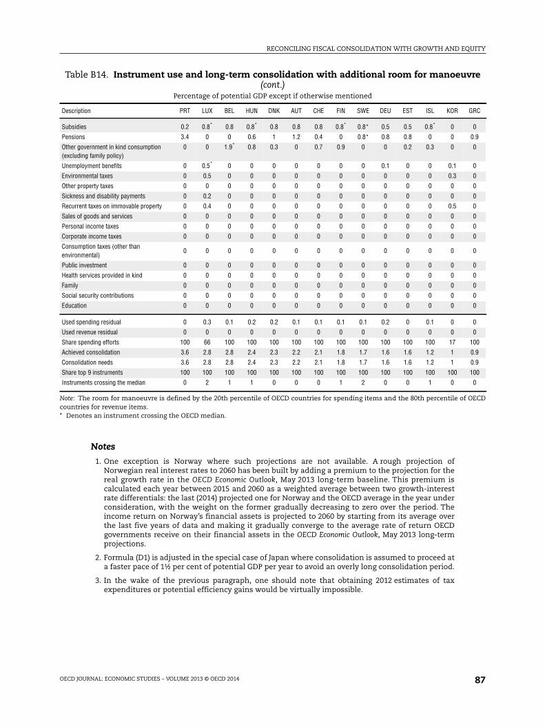
RECONCILING FISCAL CONSOLIDATION WITH GROWTH AND EQUITY
OECD JOURNAL: ECONOMIC STUDIES – VOLUME 2013 © OECD 2014 87
Notes
1. One exception is Norway where such projections are not available. A rough projection ofNorwegian real interest rates to 2060 has been built by adding a premium to the projection for thereal growth rate in the OECD Economic Outlook, May 2013 long-term baseline. This premium iscalculated each year between 2015 and 2060 as a weighted average between two growth-interestrate differentials: the last (2014) projected one for Norway and the OECD average in the year underconsideration, with the weight on the former gradually decreasing to zero over the period. Theincome return on Norway’s financial assets is projected to 2060 by starting from its average overthe last five years of data and making it gradually converge to the average rate of return OECDgovernments receive on their financial assets in the OECD Economic Outlook, May 2013 long-termprojections.
2. Formula (D1) is adjusted in the special case of Japan where consolidation is assumed to proceed ata faster pace of 1½ per cent of potential GDP per year to avoid an overly long consolidation period.
3. In the wake of the previous paragraph, one should note that obtaining 2012 estimates of taxexpenditures or potential efficiency gains would be virtually impossible.
Table B14. Instrument use and long-term consolidation with additional room for manoeuvre(cont.)
Percentage of potential GDP except if otherwise mentioned
Description PRT LUX BEL HUN DNK AUT CHE FIN SWE DEU EST ISL KOR GRC
Subsidies 0.2 0.8* 0.8 0.8* 0.8 0.8 0.8 0.8* 0.8* 0.5 0.5 0.8* 0 0
Pensions 3.4 0 0 0.6 1 1.2 0.4 0 0.8* 0.8 0.8 0 0 0.9
Other government in kind consumption(excluding family policy)
0 0 1.9* 0.8 0.3 0 0.7 0.9 0 0 0.2 0.3 0 0
Unemployment benefits 0 0.5* 0 0 0 0 0 0 0 0.1 0 0 0.1 0
Environmental taxes 0 0.5 0 0 0 0 0 0 0 0 0 0 0.3 0
Other property taxes 0 0 0 0 0 0 0 0 0 0 0 0 0 0
Sickness and disability payments 0 0.2 0 0 0 0 0 0 0 0 0 0 0 0
Recurrent taxes on immovable property 0 0.4 0 0 0 0 0 0 0 0 0 0 0.5 0
Sales of goods and services 0 0 0 0 0 0 0 0 0 0 0 0 0 0
Personal income taxes 0 0 0 0 0 0 0 0 0 0 0 0 0 0
Corporate income taxes 0 0 0 0 0 0 0 0 0 0 0 0 0 0
Consumption taxes (other thanenvironmental)
0 0 0 0 0 0 0 0 0 0 0 0 0 0
Public investment 0 0 0 0 0 0 0 0 0 0 0 0 0 0
Health services provided in kind 0 0 0 0 0 0 0 0 0 0 0 0 0 0
Family 0 0 0 0 0 0 0 0 0 0 0 0 0 0
Social security contributions 0 0 0 0 0 0 0 0 0 0 0 0 0 0
Education 0 0 0 0 0 0 0 0 0 0 0 0 0 0
Used spending residual 0 0.3 0.1 0.2 0.2 0.1 0.1 0.1 0.1 0.2 0 0.1 0 0
Used revenue residual 0 0 0 0 0 0 0 0 0 0 0 0 0 0
Share spending efforts 100 66 100 100 100 100 100 100 100 100 100 100 17 100
Achieved consolidation 3.6 2.8 2.8 2.4 2.3 2.2 2.1 1.8 1.7 1.6 1.6 1.2 1 0.9
Consolidation needs 3.6 2.8 2.8 2.4 2.3 2.2 2.1 1.8 1.7 1.6 1.6 1.2 1 0.9
Share top 9 instruments 100 100 100 100 100 100 100 100 100 100 100 100 100 100
Instruments crossing the median 0 2 1 1 0 0 0 1 2 0 0 1 0 0
Note: The room for manoeuvre is defined by the 20th percentile of OECD countries for spending items and the 80th percentile of OECDcountries for revenue items.* Denotes an instrument crossing the OECD median.

RECONCILING FISCAL CONSOLIDATION WITH GROWTH AND EQUITY
OECD JOURNAL: ECONOMIC STUDIES – VOLUME 2013 © OECD 201488
Appendix references
Alesina, R. and S. Ardagna (2010), “Large Changes in Fiscal Policy: Taxes versus Spending”, in Tax Policyand the Economy, Vol. 24, pp. 35-68, National Bureau of Economic Research.
Arjona, R., M. Ladaique and M. Pearson (2002), “Social Protection and Growth”, OECD Economic Studies,No. 35, OECD Publishing, Paris.
Auerbach, A. and Y. Gorodnichenko (2012), “Fiscal Multipliers in Recession and Expansion”, in FiscalPolicy after the Financial Crisis, National Bureau of Economic Research.
Barbiero, O. and B. Cournède (2013), “New Econometric Estimates of Long-Term Growth Effects ofDifferent Areas of Public Spending”, OECD Economics Department Working Papers, No. 1100.
Bastagli, F., D. Coady and S. Gupta (2012), “Income Inequality and Fiscal Policy”, IMF Staff DiscussionNote, SDN/12/08 (Revised), 27 September, IMF, Washington, DC.
Becker, J., C. Fuest and N. Riedel (2012), “Corporate Tax Effects on the Quality and Quantity of FDI”,European Economic Review, No. 56.
Bom, P. and J. Ligthart (2013) “What Have We Learned from Three Decades Of Research on theProductivity of Public Capital?”, Journal of Economic Surveys.
Bova, E., T. Kinda, J. Woo and S. Zhang (2012), “Distributional Consequences of Fiscal Consolidationand the Role of Fiscal Policy: What Do the Data Say?”, forthcoming, IMF, Washington, DC.
Calderon, S. (2004), “The Effects of Infrastructure Development on Growth and Income Distribution”,World Bank Policy Research Working Paper Series, No. 3400.
Chatterjee, S. and S. Turnovsky (2012), “Infrastructure and Inequality”, European Economic Review,Vol. 56.
Causa, O. and Å. Johansson (2010), “Intergenerational Social Mobility in OECD Countries”, OECDJournal: Economic Studies, OECD Publishing, Paris.
de la Maisonneuve, C. and J. Oliveira Martins (2013), “Public Spending on Health and Long-Term Care:A New Set of Projections”, OECD Economics Department Working Paper, forthcoming.
De Mooij, R. (2012), “Tax Biases to Debt Finance: Assessing the Problem, Finding Solutions”, FiscalStudies, Vol. 33, No. 4.
Devries, P., J. Guajardo, D. Leigh and A. Pescatori (2011), “A New Action-Based Dataset on FiscalConsolidation”, IMF Working Paper, No. 11/128, Washington, DC.
Driscoll, J.C. and A.C. Kraay (1998), “Consistent Covariance Matrix Estimation with SpatiallyDependent Panel Data”, The Review of Economics and Statistics, Vol. 80(4), pp. 549-560, MIT Press,November.
Duval, R. (2003), “Retirement Behaviour in OECD Countries: Impact of Old-Age Pension Schemes andOther Social Transfer Programmes”, OECD Economic Studies, No. 37, OECD Publishing, Paris.
Echevarria, C. (2012), “Income Tax Progressivity, Physical Capital, Aggregate Uncertainty and Long-RunGrowth in an Old Economy”, Journal of Macroeconomics, Vol. 34(4), pp. 955-974.
Ford, R. and W. Suyker (1990), “Industrial Subsidies in the OECD Economies”, OECD Economic Studies,No. 15, OECD Publishing, Paris.
Fournier, J.-M. and I. Koske (2012), “Less Income Inequality and More Growth – Are they Compatible?Part 7. The Drivers of Labour Earnings Inequality – An Analysis Based on Conditional andUnconditional Quantile Regressions”, OECD Economics Department Working Papers, No. 930.
Gemmell, N., R. Kneller and Ismael Sanz (2011), “The Timing and Persistence of Fiscal Policy Impactson Growth: Evidence from OECD Countries”, Economic Journal, Vol. 121(550), pp. 33-58.
Gonand, F. (2010), “Choosing A Pension Reform: A Framework for the Social Planner”, Pension Reform,Fiscal Policy and Economic Performance, paper presented at the Banca d’Italia workshop held inPerugia, 26-28 March 2009, Printing Office of the Banca d’Italia, Rome.
Guajardo, J., D. Leigh and A. Pescatori (2011), “Expansionary Austerity: New International Evidence”,IMF Working Papers, WP/11/158.
Gyimah-Brempong, K. and M. Wilson (2004), “Health Human Capital And Economic Growth In Sub-Saharan African and OECD Countries”, The Quarterly Review of Economics and Finance, Vol. 44. No. 2.

RECONCILING FISCAL CONSOLIDATION WITH GROWTH AND EQUITY
OECD JOURNAL: ECONOMIC STUDIES – VOLUME 2013 © OECD 2014 89
Hoeller, P., I. Joumard, M. Pisu and D. Bloch (2012), “Less Income Inequality and More Growth: Are TheyCompatible? Part 1. Mapping Income Inequality Across the OECD”, OECD Economics DepartmentWorking Papers, No. 924.
Johansson, Å, C. Heady, J. Arnold, B. Brys and L. Vartia (2008), “Taxation and Economic Growth”, OECDEconomics Department Working Papers, No. 620.
Johansson, Å., D. Turner, Y. Guillemette, F. Murtin, C. de la Maisonneuve, P. Bagnoli, G. Bousquet andF. Spinelli (2013), “Long-Term Growth Scenarios”, OECD Economics Department Working Papers,No. 1000.
Joumard, I., P. Hoeller, C. André and C. Nicq (2010), Health Care Systems: Efficiency and Policy Settings,OECD Publishing, Paris.
Joumard, I., M. Pisu and D. Bloch (2012), “Less Income Inequality and More Growth – Are TheyCompatible? Part 3. Income Redistribution via Taxes and Transfers in OECD Countries”, OECDEconomics Department Working Papers, No. 926.
Leduc, S. and D. Wilson (forthcoming), “Roads to Prosperity or Bridges to Nowhere? Theory andEvidence on the Impact of Public Infrastructure Investment”, NBER Macroeconomics Annual 2012.
OECD (2001), Competition Policy in Subsidies and State Aid, OECD Publishing, Paris.
OECD (2003a), Sources of Economic Growth in OECD Countries, OECD Publishing, Paris.
OECD (2003b), Environmentally Harmful Subsidies: Policy Issues and Challenges, OECD Publishing, Paris.
OECD (2010), Sickness, Disability and Work: Breaking the Barriers, OECD Publishing, Paris.
OECD (2010a), Tax Expenditures in OECD Countries, OECD Publishing, Paris.
OECD (2010b), “Health Care Systems: Getting More Value for Money”, OECD Economics Department PolicyNotes, No. 2, OECD Publishing, Paris.
OECD (2011), Divided We Stand, OECD Publishing, Paris.
OECD (2011a), OECD Economic Surveys: Switzerland 2011, OECD Publishing, Paris.
OECD (2012a), “Looking to 2060: Long-Term Global Growth Prospects – A Going for Growth Report”,OECD Economic Policy Papers, No. 3, OECD Publishing, Paris.
OECD (2012b), “Special Feature: Trends in Personal Income Tax and Employee Social SecurityContribution Schedules”, Taxing Wages 2011, OECD Publishing, Paris.
OECD (2013), OECD Economic Outlook, Vol. 2013/1, No. 93, May, OECD Publishing, Paris.
Rawdanowicz, L., E. Wurzel and A.K. Christensen (2012), “The Equity Implications of FiscalConsolidation”, OECD Economics Department Working Papers, No. 1013.
Serret, Y. and N Johnstone (2006) (ed.), The Distributional Effects of Environmental Policy, OECD Publishing,Paris.
Sutherland, D., R. Price, I. Joumard and C. Nicq (2007), “Performance and Indicators for Public SpendingEfficiency in Primary and Secondary Education”, OECD Economics Department Working Papers,No. 546.
Sutherland, D., S. Araujo, B. Egert and T. Kozluk (2009), “Infrastructure Investment: Links to Growthand The Role of Public Policies”, OECD Economics Department Working Papers, No. 686.
Sutherland, D., P. Hoeller, R. Merola and V. Ziemann (2012), “Debt and Macroeconomic Stability”, OECDEconomics Department Working Papers, No. 1003.