
Recommending social network applications via ... - CiteSeerX
Upload
khangminh22Category
view
0download
0
RECOMMENDING RECOMMENDER SYSTEMS TACKLING THE COLLABORATIVE FILTERING ALGORITHM SELECTION PROBLEM
TIAGO DANIEL SÁ CUNHA TESE DE DOUTORAMENTO APRESENTADA À FACULDADE DE ENGENHARIA DA UNIVERSIDADE DO PORTO EM ENGENHARIA INFORMÁTICA
D 2019


Recommending Recommender Systems: tackling theCollaborative Filtering algorithm selection problem
Tiago Daniel Sá Cunha
Programa Doutoral em Engenharia Informática
Supervisor: Carlos Manuel Milheiro de Oliveira Pinto Soares, PhD
Co-Supervisor: André Carlos Ponce de Leon Ferreira de Carvalho, PhD
Approved by:
President: João Manuel Paiva Cardoso, PhD
Referee: Myra Spiliopoulou, PhD
Referee: Alexandros Kalousis, PhD
Referee: Alípio Mário Jorge, PhD
Referee: Eugénio da Costa Oliveira, PhD
Referee: José Luís Cabral da Moura Borges, PhD
Supervisor: Carlos Manuel Milheiro de Oliveira Pinto Soares, PhD
December 13, 2019


Agradecimentos
Chegado ao culminar desta etapa, reconheço que tenho muito que agradecer. Acima de tudo, tenhomuito a quem agradecer. Até porque apesar de o doutoramento ser um trabalho individual, nuncasenti que estivesse sozinho. A esses agradeço agora.
Em primeiro lugar, quero agradecer ao Carlos. Foi ele quem me motivou a fazer no Doutora-mento, quem me orientou neste caminho por vezes sinuoso e quem me deu oportunidades decrescer como investigador. De facto, sem ele provavelmente não teria sequer começado esta aven-tura, muito menos estaria aqui neste momento. Acima de tudo, o que mais agradeço é o facto desempre ter confiado nas minhas capacidades e me mostrar que eu devia fazer o mesmo.
Em segundo lugar, quero agradecer ao André. Especialmente, por estar sempre presente.Ainda hoje acho impressionante a forma como o consegue apesar da distância, do fuso horário ede todos os compromissos. Agradeço também a oportunidade de ter estado em São Carlos comele, que efetivamente foi um período marcante na minha carreira como investigador. Mas acimade tudo, agradeço ter-me mostrado que a humildade e o sucesso andam de mãos dadas.
Na minha carreira como investigador, existe um Tiago antes de entrar para o INESC e outroapós. Foi nesta casa que aprendi o que realmente significa ser investigador, qual o meu papel nasociedade e que é isto que quero fazer no resto da minha carreira. No entanto, as lições que maisme marcaram surgiram a partir das experiências partilhadas com os meus amigos da CESE. Porisso, gostaria de agradecer ao Fábio, Catarina, Pedro, Bruno, Dario, Samuel, Eric, Maria João,Miguel, João, Filipa, Diogo e a todos os outros, que felizmente são demasiados para listar aqui.Por fim, gostaria de agradecer ao Rui e ao Hugo por toda a orientação profissional.
Quero também agradecer aos meus amigos, que são na verdade família: Freitas, Sousa, Macedoe Zé. Obrigado por me aturarem sempre que precisei, por me apoiarem sempre que pedi e porestarem lá para me distrair dos problemas. Ah, e por gerirem bem o meu capital :)
À minha família, não sei se tenho sequer palavras para agradecer. São vocês os culpadosprincipais desta façanha, por tudo o que fizeram antes, durante e, tenho a certeza, depois. Aos meuspais e ao meu irmão, obrigado por puxarem por mim, por ouvirem os meus desabafos (mesmo nãosabendo o que raio eu estava a dizer!) e por me ensinarem os valores certos. Quero tambémagradecer ao resto da família, em especial ao meu avô por ter sido (e continuar a ser) uma dasmaiores inspirações da minha vida. Por último, a ti Dani. Estarás para sempre connosco.
Esta mensagem não estaria completa sem agradecer também à minha família "adotiva" Costa.Apesar de só vos conhecer há dois anos, sei que estarão comigo sempre que precisar. Obrigadopor me fazerem sentir tão bem-vindo e importante nas vossas vidas.
Acima de tudo, quero agradecer à minha querida Joana. Obrigado pela paciência, compreen-são, motivação, apoio, carinho e amor. Não fazes sequer ideia do quão importante foste para euterminar o Doutoramento e o que significas para mim. Obrigado por nunca me teres faltado e porestares disposta a enfrentar ao meu lado os novos desafios que a vida nos reserva. O que vale éque teremos sempre o Dexter para nos ajudar :)
A todos vocês, obrigado pela aventura. Foi longa e difícil. Mas valeu tanto a pena.
i

ii

Acknowledgements
This research was supported by:
• ProDEI scholarship: issued by the Doctoral Program in Computer Engineering at the Fac-uldade de Engenharia da Universidade do Porto [June 2014 - May 2015];
• MANTIS project: supported by the ECSEL Joint Undertaking, framework program for re-search and innovation horizon 2020 (2014-2020) under grant agreement 662189-MANTIS-2014-1 [June 2015 - March 2016];
• FASCOM project: financed by the European Regional Development Fund through theOperational Program for Competitiveness and Internationalization - COMPETE 2020 underthe Portugal 2020 Partnership Agreement, and through the Portuguese National InnovationAgency (ANI) as a part of project FASCOM | POCI-01-0247-FEDER-003506 [March 2016- May 2017];
• FCT PhD scholarship: issued by Fundação para a Ciência e a Tecnologia through the grantnumber SFRH/BD/117531/2016 [June 2017 - May 2019].
iii

iv

Publications
Journals
Tiago Cunha, Carlos Soares, André C.P.L.F. de Carvalho (2018). Metalearning and RecommenderSystems: A literature review and empirical study on the algorithm selection problem for Collabo-rative Filtering. Information Sciences, 423.
Conferences
Tiago Cunha, Carlos Soares and André C. P. L. F. de Carvalho (2016). Selecting CollaborativeFiltering Algorithms Using Metalearning. In European Conference on Machine Learning andKnowledge Discovery in Databases, Part II (pp. 393–409).
Tiago Cunha, Carlos Soares, André C.P.L.F. de Carvalho (2017). Metalearning for Context-awareFiltering: Selection of Tensor Factorization Algorithms. In ACM Conference on RecommenderSystems (pp. 14–22).
Tiago Cunha, Carlos Soares, André C.P.L.F. de Carvalho (2017). Recommending CollaborativeFiltering algorithms using subsampling landmarkers. In Discovery Science (pp. 189–203).
Tiago Cunha, Carlos Soares, André C.P.L.F. de Carvalho (2018). A Label Ranking approachfor selecting rankings of Collaborative Filtering algorithms. In ACM Symposium on AppliedComputing (pp. 1393–1395).
Tiago Cunha, Carlos Soares, André C.P.L.F. de Carvalho (2018). CF4CF-META: Hybrid Collab-orative Filtering Algorithm Selection Framework. In Discovery Science (pp. 114–128).
Tiago Cunha, Carlos Soares, André C.P.L.F. de Carvalho (2018). CF4CF: Recommending Collab-orative Filtering Algorithms Using Collaborative Filtering. In ACM Conference on RecommenderSystems (pp. 357–361).
Pre-prints
Tiago Cunha, Carlos Soares, André C.P.L.F. de Carvalho (2018). Algorithm Selection for Col-laborative Filtering: the influence of graph metafeatures and multicriteria metatargets. ArXivE-Prints.
Tiago Cunha, Carlos Soares, André C.P.L.F. de Carvalho (2018). cf2vec: Collaborative Filteringalgorithm selection using graph distributed representations. ArXiv E-Prints.
v

vi

“The world is woven from billions of lives, every strand crossing every other.What we call premonition is just movement of the web.
If you could attenuate to every strand of quivering data, the future would be entirely calculable.As inevitable as mathematics.”
Sherlock Holmes
vii

viii

Resumo
A internet tem se tornado uma ferramenta indispensável, quer para uso pessoal ou profissional. Noentanto, a vasta quantidade de informação online impede um utilizador da Internet de manter-seao corrente dos seus interesses. Os Sistemas de Recomendação surgiram com o intuito de resolvereste problema, sugerindo itens potencialmente interessantes aos utilizadores. Já existem váriasestratégias estudadas e implementadas para este tipo de sistemas, que seguem diversos paradigmaspara computar as recomendações. Apesar de existir uma forte presença em vários websites hojeem dia, ainda existem vários desafios que necessitam de ser ultrapassados no que toca a Sistemasde Recomendação. Entre esses desafios, o facto de ainda não existir uma conceptualização bemdefinida sobre quais são as melhores estratégias de recomendação para cada tipo de problemalimita a progressão segura e válida desta área de investigação.
Atualmente este problema é abordado através da avaliação experimental de vários algoritmosde recomendação em alguns conjuntos de dados. No entanto, estes estudos requerem uma quan-tidade considerável de recursos computacionais, especialmente em termos de tempo. Para evitarestes problemas, alguns investigadores procuraram aplicar técnicas de meta-aprendizagem para oproblema de seleção do melhor algoritmo de recomendação. Apesar de efectivamente se teremprovado eficazes e terem demonstrado o potencial destas soluções, estes estudos não possuem aescala e maturidade essenciais para ser possível generalizar o meta-conhecimento obtido.
Desta forma, esta tese foca-se em várias limitações identificadas nos trabalhos relacionadosde forma e melhorar as soluções existentes em diversas vertentes do problema. Nomeadamente,pretende-se encontrar mais metafeatures informativas, metatargets mais ricos e metalearners es-pecialmente dedicados para a seleção de algoritmos de Collaborative Filtering. Todas as con-tribuições são validadas através de estudos empíricos, que são continuamente aprimorados nodecorrer do documento. A tese foca-se em algoritmos de Matrix Factorization e usam o processoexperimental maior e mais complexo conhecido até à data.
As conclusões apontam para o facto de que todas as contribuições propostas têm um impactopositivo no problema de seleção de algoritmos de Collaborative Filtering. Nomeadamente, foramidentificados cinco novos conjuntos de metafeatures (criados através da extensão e generalizaçãode metafeatures de trabalhos relacionados e de técnicas de Representational Learning), duas no-vas classes de metalearners (em que um deles aborda o problema de seleção de algoritmos semmetafeatures e o outro combina o uso de performance ratings com múltiplas outras metafeatures)e um novo metatarget (que é capaz de criar rankings de algoritmos para cada conjunto de dados,tendo em consideração várias métricas de avaliação). Para além disto, os estudos efetuados per-mitem perceber qual o impacto das metafeatures e dos metalearners considerados em diversosproblemas de recomendação e para diversos algoritmos de recomendação.
ix

x

Abstract
The internet has become an essential everyday tool, both for professional and personal use. How-ever, the large amount of online information does not allow internet users to keep up with theirinterests. Recommender Systems address this problem by suggesting potentially interesting itemsto users. Several recommendation strategies have been developed and studied to compute theserecommendations. Despite their strong presence in many websites today, there are still severalchallenges to cope with. One of them is the fact that there is still no knowledge regarding whichis the best recommendation method available for a given problem.
The current trend to solve this problem is the experimental evaluation of several recommen-dation methods in a handful of datasets. However, these studies require an extensive amount ofcomputational resources, especially in terms of time. To avoid such drawbacks, some researchersused Metalearning to tackle the selection of the best recommendation algorithms for new prob-lems. Despite proving effective and showing the potential of such solutions, these studies lack theproper scale and maturity required to generalize the metaknowledge obtained.
Therefore, this Thesis addresses several limitations identified in the related work by improvingupon the existing solutions in multiple dimensions of the problem. Namely, it focuses on findingmore informative metafeatures, richer metatargets and tailor-made metalearners for CollaborativeFiltering algorithm selection. All contributions are validated through an empirical study, whichis continuously improved throughout the document. The Thesis focuses on Matrix Factorizationalgorithms in the largest and most complex experimental setup available to date.
We conclude that all proposed contributions positively impact the CF algorithm selection prob-lem. Namely, we identify five new sets of metafeatures (created by extending and generalizingthe state of the art metafeatures from other domains and automatic Representational Learningtechniques), two classes of metalearners (one which performs algorithm selection without anymetafeatures and another which leverages performance ratings in combination with other metafea-tures) and one novel metatarget (which is able to create a single ranking of algorithms per datasetwhile considering the input of multiple evaluation measures). Furthermore, we identify the impactof metafeatures and metalearners on multiple recommendation datasets and algorithms.
xi

xii

Contents
Abbreviations xxi
1 Introduction 11.1 Problem overview . . . . . . . . . . . . . . . . . . . . . . . . . . . . . . . . . . 21.2 Thesis Statement . . . . . . . . . . . . . . . . . . . . . . . . . . . . . . . . . . 31.3 Contributions . . . . . . . . . . . . . . . . . . . . . . . . . . . . . . . . . . . . 41.4 Implications of Research . . . . . . . . . . . . . . . . . . . . . . . . . . . . . . 51.5 Document Structure . . . . . . . . . . . . . . . . . . . . . . . . . . . . . . . . . 6
2 Background 72.1 Recommender Systems . . . . . . . . . . . . . . . . . . . . . . . . . . . . . . . 7
2.1.1 Collaborative Filtering . . . . . . . . . . . . . . . . . . . . . . . . . . . 82.1.2 Other recommendation strategies . . . . . . . . . . . . . . . . . . . . . 112.1.3 Evaluation . . . . . . . . . . . . . . . . . . . . . . . . . . . . . . . . . 14
2.2 Metalearning and Algorithm Selection . . . . . . . . . . . . . . . . . . . . . . . 162.2.1 Metatarget and Metalearner . . . . . . . . . . . . . . . . . . . . . . . . 182.2.2 Metadata . . . . . . . . . . . . . . . . . . . . . . . . . . . . . . . . . . 192.2.3 Systematic Metafeatures Framework . . . . . . . . . . . . . . . . . . . . 192.2.4 Metalevel evaluation . . . . . . . . . . . . . . . . . . . . . . . . . . . . 20
2.3 Algorithm Selection and Collaborative Filtering . . . . . . . . . . . . . . . . . . 222.4 Representational Learning . . . . . . . . . . . . . . . . . . . . . . . . . . . . . 23
3 Systematic Literature Review and Empirical Study 253.1 Systematic Literature Review . . . . . . . . . . . . . . . . . . . . . . . . . . . . 25
3.1.1 Methodology . . . . . . . . . . . . . . . . . . . . . . . . . . . . . . . . 263.1.2 Research Questions . . . . . . . . . . . . . . . . . . . . . . . . . . . . . 263.1.3 Related work . . . . . . . . . . . . . . . . . . . . . . . . . . . . . . . . 263.1.4 Discussion . . . . . . . . . . . . . . . . . . . . . . . . . . . . . . . . . 283.1.5 Summary . . . . . . . . . . . . . . . . . . . . . . . . . . . . . . . . . . 32
3.2 Empirical study . . . . . . . . . . . . . . . . . . . . . . . . . . . . . . . . . . . 333.2.1 Related work . . . . . . . . . . . . . . . . . . . . . . . . . . . . . . . . 333.2.2 Experimental setup . . . . . . . . . . . . . . . . . . . . . . . . . . . . . 343.2.3 Results . . . . . . . . . . . . . . . . . . . . . . . . . . . . . . . . . . . 37
3.3 Conclusions . . . . . . . . . . . . . . . . . . . . . . . . . . . . . . . . . . . . . 45
4 Metafeatures for Collaborative Filtering 474.1 Rating Matrix systematic metafeatures . . . . . . . . . . . . . . . . . . . . . . . 484.2 Subsampling Landmarkers . . . . . . . . . . . . . . . . . . . . . . . . . . . . . 49
xiii

xiv CONTENTS
4.3 Graph-based systematic metafeatures . . . . . . . . . . . . . . . . . . . . . . . . 514.3.1 Graph-level . . . . . . . . . . . . . . . . . . . . . . . . . . . . . . . . . 514.3.2 Node-level . . . . . . . . . . . . . . . . . . . . . . . . . . . . . . . . . 524.3.3 Pairwise-level . . . . . . . . . . . . . . . . . . . . . . . . . . . . . . . . 524.3.4 Sub-graph-level . . . . . . . . . . . . . . . . . . . . . . . . . . . . . . . 53
4.4 Results . . . . . . . . . . . . . . . . . . . . . . . . . . . . . . . . . . . . . . . . 544.4.1 Experimental setup . . . . . . . . . . . . . . . . . . . . . . . . . . . . . 544.4.2 Metalevel accuracy . . . . . . . . . . . . . . . . . . . . . . . . . . . . . 554.4.3 Impact on the baselevel performance . . . . . . . . . . . . . . . . . . . . 564.4.4 Computational Cost . . . . . . . . . . . . . . . . . . . . . . . . . . . . 574.4.5 Metaknowledge . . . . . . . . . . . . . . . . . . . . . . . . . . . . . . . 58
4.5 Conclusions . . . . . . . . . . . . . . . . . . . . . . . . . . . . . . . . . . . . . 62
5 Multicriteria Label Ranking metamodels for Collaborative Filtering 635.1 Label Ranking for CF algorithm selection . . . . . . . . . . . . . . . . . . . . . 64
5.1.1 Problem formulation . . . . . . . . . . . . . . . . . . . . . . . . . . . . 645.1.2 Label Ranking Metalearning Process . . . . . . . . . . . . . . . . . . . 64
5.2 Multicriteria Metatargets . . . . . . . . . . . . . . . . . . . . . . . . . . . . . . 655.3 Results . . . . . . . . . . . . . . . . . . . . . . . . . . . . . . . . . . . . . . . . 67
5.3.1 Experimental setup . . . . . . . . . . . . . . . . . . . . . . . . . . . . . 675.3.2 Metalevel ranking accuracy . . . . . . . . . . . . . . . . . . . . . . . . 675.3.3 Impact on the baselevel performance . . . . . . . . . . . . . . . . . . . . 705.3.4 Metaknowledge analysis . . . . . . . . . . . . . . . . . . . . . . . . . . 74
5.4 Conclusions . . . . . . . . . . . . . . . . . . . . . . . . . . . . . . . . . . . . . 81
6 Recommending Recommenders 836.1 CF4CF . . . . . . . . . . . . . . . . . . . . . . . . . . . . . . . . . . . . . . . . 846.2 CF4CF-META . . . . . . . . . . . . . . . . . . . . . . . . . . . . . . . . . . . 856.3 Results . . . . . . . . . . . . . . . . . . . . . . . . . . . . . . . . . . . . . . . . 86
6.3.1 Experimental setup . . . . . . . . . . . . . . . . . . . . . . . . . . . . . 866.3.2 Meta-accuracy . . . . . . . . . . . . . . . . . . . . . . . . . . . . . . . 876.3.3 Top-N Metalevel Accuracy . . . . . . . . . . . . . . . . . . . . . . . . . 906.3.4 Impact on the baselevel performance . . . . . . . . . . . . . . . . . . . . 916.3.5 Metaknowledge analysis . . . . . . . . . . . . . . . . . . . . . . . . . . 91
6.4 Conclusions . . . . . . . . . . . . . . . . . . . . . . . . . . . . . . . . . . . . . 94
7 cf2vec: dataset embeddings 957.1 cf2vec: Distributed Representations as CF metafeatures . . . . . . . . . . . . . . 96
7.1.1 Convert CF matrix into graph . . . . . . . . . . . . . . . . . . . . . . . 967.1.2 Sampling graphs . . . . . . . . . . . . . . . . . . . . . . . . . . . . . . 967.1.3 Learn distributed representation . . . . . . . . . . . . . . . . . . . . . . 977.1.4 Learn metamodel . . . . . . . . . . . . . . . . . . . . . . . . . . . . . . 98
7.2 Results . . . . . . . . . . . . . . . . . . . . . . . . . . . . . . . . . . . . . . . . 997.2.1 Experimental setup . . . . . . . . . . . . . . . . . . . . . . . . . . . . . 997.2.2 Hyperparameter sensitivity analysis . . . . . . . . . . . . . . . . . . . . 1007.2.3 Metalevel accuracy . . . . . . . . . . . . . . . . . . . . . . . . . . . . . 1027.2.4 Impact on the baselevel performance . . . . . . . . . . . . . . . . . . . . 1037.2.5 Metaknowledge analysis . . . . . . . . . . . . . . . . . . . . . . . . . . 104
7.3 Conclusions . . . . . . . . . . . . . . . . . . . . . . . . . . . . . . . . . . . . . 108

CONTENTS xv
8 Conclusions and Future Work 1118.1 Conclusions . . . . . . . . . . . . . . . . . . . . . . . . . . . . . . . . . . . . . 1118.2 Limitations . . . . . . . . . . . . . . . . . . . . . . . . . . . . . . . . . . . . . 1138.3 Future Work . . . . . . . . . . . . . . . . . . . . . . . . . . . . . . . . . . . . . 114
A Offline evaluation metrics 117A.1 Rating accuracy . . . . . . . . . . . . . . . . . . . . . . . . . . . . . . . . . . . 117A.2 Rating correlation . . . . . . . . . . . . . . . . . . . . . . . . . . . . . . . . . . 118A.3 Classification accuracy . . . . . . . . . . . . . . . . . . . . . . . . . . . . . . . 118A.4 Ranking accuracy . . . . . . . . . . . . . . . . . . . . . . . . . . . . . . . . . . 119A.5 Satisfaction . . . . . . . . . . . . . . . . . . . . . . . . . . . . . . . . . . . . . 120A.6 Coverage and diversity . . . . . . . . . . . . . . . . . . . . . . . . . . . . . . . 121A.7 Novelty . . . . . . . . . . . . . . . . . . . . . . . . . . . . . . . . . . . . . . . 121
B Metatarget Analysis 123B.1 Best algorithm Metatarget . . . . . . . . . . . . . . . . . . . . . . . . . . . . . 123B.2 Single criterion Ranking Metatarget . . . . . . . . . . . . . . . . . . . . . . . . 125B.3 Multicriteria Ranking Metatarget . . . . . . . . . . . . . . . . . . . . . . . . . . 130
C Metafeature Selection 133C.1 Rating Matrix systematic metafeatures . . . . . . . . . . . . . . . . . . . . . . . 133C.2 Subsampling Landmarkers . . . . . . . . . . . . . . . . . . . . . . . . . . . . . 134C.3 Graph-based systematic metafeatures . . . . . . . . . . . . . . . . . . . . . . . . 139C.4 Comprehensive Metafeatures . . . . . . . . . . . . . . . . . . . . . . . . . . . . 141
D Detailed Evaluation Results 143D.1 CF4CF . . . . . . . . . . . . . . . . . . . . . . . . . . . . . . . . . . . . . . . . 143D.2 CF4CF-META . . . . . . . . . . . . . . . . . . . . . . . . . . . . . . . . . . . 144D.3 Label Ranking . . . . . . . . . . . . . . . . . . . . . . . . . . . . . . . . . . . . 146D.4 ALORS . . . . . . . . . . . . . . . . . . . . . . . . . . . . . . . . . . . . . . . 150D.5 ASLIB . . . . . . . . . . . . . . . . . . . . . . . . . . . . . . . . . . . . . . . . 151
References 157

xvi CONTENTS

List of Figures
2.1 Rating matrix. . . . . . . . . . . . . . . . . . . . . . . . . . . . . . . . . . . . . 82.2 Matrix Factorization procedure. . . . . . . . . . . . . . . . . . . . . . . . . . . 102.3 Rice’s algorithm selection framework . . . . . . . . . . . . . . . . . . . . . . . 172.4 Metadatabase. . . . . . . . . . . . . . . . . . . . . . . . . . . . . . . . . . . . . 172.5 Metalearning process . . . . . . . . . . . . . . . . . . . . . . . . . . . . . . . . 182.6 Metalearning evaluation process. . . . . . . . . . . . . . . . . . . . . . . . . . . 20
3.1 Experimental procedure . . . . . . . . . . . . . . . . . . . . . . . . . . . . . . . 343.2 Metalevel accuracy. . . . . . . . . . . . . . . . . . . . . . . . . . . . . . . . . . 383.3 Critical Difference diagram . . . . . . . . . . . . . . . . . . . . . . . . . . . . . 383.4 Impact on the baselevel performance. . . . . . . . . . . . . . . . . . . . . . . . 393.5 Metafeature importance . . . . . . . . . . . . . . . . . . . . . . . . . . . . . . . 413.6 Baselevel dataset impact . . . . . . . . . . . . . . . . . . . . . . . . . . . . . . 423.7 Algorithm footprints. . . . . . . . . . . . . . . . . . . . . . . . . . . . . . . . . 44
4.1 Rating matrix formulation. . . . . . . . . . . . . . . . . . . . . . . . . . . . . . 484.2 SL metafeature extraction procedure. . . . . . . . . . . . . . . . . . . . . . . . . 504.3 Rating matrix and graph version of the CF problem. . . . . . . . . . . . . . . . . 514.4 Metalevel accuracy . . . . . . . . . . . . . . . . . . . . . . . . . . . . . . . . . 554.5 Critical Difference diagram . . . . . . . . . . . . . . . . . . . . . . . . . . . . . 554.6 Impact on the baselevel performance . . . . . . . . . . . . . . . . . . . . . . . . 564.7 Metafeature importance . . . . . . . . . . . . . . . . . . . . . . . . . . . . . . . 584.8 Baselevel dataset impact . . . . . . . . . . . . . . . . . . . . . . . . . . . . . . 604.9 Algorithm footprints . . . . . . . . . . . . . . . . . . . . . . . . . . . . . . . . 61
5.1 LR metadatabase formulation. . . . . . . . . . . . . . . . . . . . . . . . . . . . 645.2 Dataset-Interest space. . . . . . . . . . . . . . . . . . . . . . . . . . . . . . . . 665.3 Metalevel accuracy for single criterion metatargets. . . . . . . . . . . . . . . . . 685.4 Metalevel accuracy for multicriteria metatargets. . . . . . . . . . . . . . . . . . . 705.5 Critical Difference diagram . . . . . . . . . . . . . . . . . . . . . . . . . . . . . 715.6 Impact on the baselevel performance in single criterion metatargets. . . . . . . . 725.7 Impact on the baselevel performance in multicriteria metatargets. . . . . . . . . . 735.8 Metafeature importance . . . . . . . . . . . . . . . . . . . . . . . . . . . . . . . 755.9 Baselevel dataset impact for proposed metafeatures . . . . . . . . . . . . . . . . 775.10 Baselevel dataset impact for related work metafeatures . . . . . . . . . . . . . . 785.11 Algorithm footprints using rankings for proposed metafeatures. . . . . . . . . . . 795.12 Algorithm footprints using rankings for related work metafeatures. . . . . . . . . 80
6.1 CF4CF metadatabase. . . . . . . . . . . . . . . . . . . . . . . . . . . . . . . . . 84
xvii

xviii LIST OF FIGURES
6.2 CF4CF-META metadatabase. . . . . . . . . . . . . . . . . . . . . . . . . . . . 856.3 CF4CF threshold sensitivity analysis. . . . . . . . . . . . . . . . . . . . . . . . 886.4 CF4CF-META threshold sensitivity analysis. . . . . . . . . . . . . . . . . . . . 886.5 Metalevel accuracy . . . . . . . . . . . . . . . . . . . . . . . . . . . . . . . . . 896.6 Critical Difference diagram. . . . . . . . . . . . . . . . . . . . . . . . . . . . . 896.7 NDCG metalevel evaluation in the Item Recommendation problem. . . . . . . . 906.8 NDCG metalevel evaluation in the Rating Prediction problem. . . . . . . . . . . 906.9 Impact on the baselevel performance. . . . . . . . . . . . . . . . . . . . . . . . 916.10 Metafeature Importance . . . . . . . . . . . . . . . . . . . . . . . . . . . . . . . 926.11 Baselevel dataset impact . . . . . . . . . . . . . . . . . . . . . . . . . . . . . . 93
7.1 Rating matrix and graph version of CF problem . . . . . . . . . . . . . . . . . . 967.2 Skipgram architecture . . . . . . . . . . . . . . . . . . . . . . . . . . . . . . . . 977.3 Label Ranking Metadatabase. . . . . . . . . . . . . . . . . . . . . . . . . . . . . 987.4 Metalevel performance in terms of the amount of nodes sampled per graph . . . . 1007.5 Metalevel performance in terms of the distributed representation size . . . . . . . 1017.6 Metalevel performance in terms of the amount of context sub-graphs . . . . . . . 1017.7 Performance scatter plot. . . . . . . . . . . . . . . . . . . . . . . . . . . . . . . 1027.8 Metalevel accuracy. . . . . . . . . . . . . . . . . . . . . . . . . . . . . . . . . . 1027.9 Critical difference diagram. . . . . . . . . . . . . . . . . . . . . . . . . . . . . . 1037.10 Impact on the baselevel performance. . . . . . . . . . . . . . . . . . . . . . . . 1037.11 Baselevel dataset impact . . . . . . . . . . . . . . . . . . . . . . . . . . . . . . 1057.12 Metadata visualization for the Item Recommendation problem. . . . . . . . . . . 1067.13 Metadata visualization for the Rating Prediction problem. . . . . . . . . . . . . . 107
B.1 Distributions of correlations between single criterion and multicriteria rankings. . 132
C.1 Metalevel accuracy for relative SL in best algorithm selection. . . . . . . . . . . 136C.2 Critical Difference diagram for relative SL in best algorithm selection. . . . . . . 137C.3 Impact on the baselevel performance using relative SL in best algorithm selection. 137C.4 Metalevel accuracy for relative SL in best algorithm ranking selection. . . . . . . 138C.5 Critical Difference diagram for relative SL in best algorithm ranking selection. . 138C.6 Impact on the baselevel performance for relative SL in best algorithm ranking
selection. . . . . . . . . . . . . . . . . . . . . . . . . . . . . . . . . . . . . . . 139

List of Tables
2.1 Related work on CF meta-approaches to recommend ML algorithms. . . . . . . . 22
3.1 Related work on ML meta-approaches to recommend CF algorithms. . . . . . . . 283.2 Summary description about the datasets used in the experimental study. . . . . . 353.3 Computational time required to extract related work metafeatures. . . . . . . . . 40
4.1 Example of relative landmarkers. . . . . . . . . . . . . . . . . . . . . . . . . . . 504.2 Computational time required for the extraction of RM, SL and GR metafeatures. . 57
6.1 Mapping between Rice’s framework and CF4CF and CF4CF-META. . . . . . . . 84
A.1 Confusion Matrix . . . . . . . . . . . . . . . . . . . . . . . . . . . . . . . . . . 118
B.1 Best models obtained on multiple evaluation metrics for each dataset. . . . . . . 124B.2 NDCG single criterion metatarget. . . . . . . . . . . . . . . . . . . . . . . . . . 125B.3 AUC single criterion metatarget. . . . . . . . . . . . . . . . . . . . . . . . . . . 126B.4 NMAE single criterion metatarget. . . . . . . . . . . . . . . . . . . . . . . . . . 127B.5 RMSE single criterion metatarget. . . . . . . . . . . . . . . . . . . . . . . . . . 128B.6 IR multicriteria metatarget. . . . . . . . . . . . . . . . . . . . . . . . . . . . . . 130B.7 RP multicriteria metatarget. . . . . . . . . . . . . . . . . . . . . . . . . . . . . . 131
C.1 RM metafeatures used in the experiments after CFS. . . . . . . . . . . . . . . . 134C.2 SL metafeatures used in the experiments after CFS. . . . . . . . . . . . . . . . . 135C.3 Graph metafeatures used in the experiments after CFS. . . . . . . . . . . . . . . 140C.4 Comprehensive metafeatures. . . . . . . . . . . . . . . . . . . . . . . . . . . . . 141
D.1 Kendall’s Tau Ranking accuracy performance for CF4CF approach. . . . . . . . 143D.2 NDCG Top-N accuracy performance for CF4CF approach. . . . . . . . . . . . . 143D.3 Impact on baselevel performance for CF4CF approach in the Item Recommenda-
tion problem. . . . . . . . . . . . . . . . . . . . . . . . . . . . . . . . . . . . . 144D.4 Impact on baselevel performance for CF4CF approach in the Item Recommenda-
tion problem. . . . . . . . . . . . . . . . . . . . . . . . . . . . . . . . . . . . . 144D.5 Kendall’s Tau Ranking accuracy performance for CF4CF-META approach. . . . 144D.6 NDCG Top-N accuracy performance for CF4CF-META approach. . . . . . . . . 145D.7 Impact on baselevel performance for CF4CF-META approach in the Item Recom-
mendation problem. . . . . . . . . . . . . . . . . . . . . . . . . . . . . . . . . 145D.8 Impact on baselevel performance for CF4CF-META approach in the Rating Pre-
diction problem. . . . . . . . . . . . . . . . . . . . . . . . . . . . . . . . . . . 146D.9 Kendall’s Tau Ranking accuracy performance for Label Ranking approach. . . . 147D.10 NDCG Top-N accuracy performance for Label Ranking approach. . . . . . . . . 148
xix

xx LIST OF TABLES
D.11 Impact on baselevel performance for Label Ranking approach in the Item Recom-mendation problem. . . . . . . . . . . . . . . . . . . . . . . . . . . . . . . . . 149
D.12 Impact on baselevel performance for Label Ranking approach in the Rating Pre-diction problem. . . . . . . . . . . . . . . . . . . . . . . . . . . . . . . . . . . 149
D.13 Kendall’s Tau Ranking accuracy performance for ALORS approach. . . . . . . . 150D.14 NDCG Top-N accuracy performance for ALORS approach. . . . . . . . . . . . 150D.15 Impact on baselevel performance for ALORS approach in the Item Recommenda-
tion problem. . . . . . . . . . . . . . . . . . . . . . . . . . . . . . . . . . . . . 150D.16 Impact on baselevel performance for ALORS approach in the Rating Prediction
problem. . . . . . . . . . . . . . . . . . . . . . . . . . . . . . . . . . . . . . . 150D.17 Kendall’s Tau Ranking accuracy performance for ASLIB approach. . . . . . . . 151D.18 NDCG Top-N accuracy performance for ASLIB approach in the Item Recommen-
dation task. . . . . . . . . . . . . . . . . . . . . . . . . . . . . . . . . . . . . . 152D.19 NDCG Top-N accuracy performance for ASLIB approach in the Rating Prediction
task. . . . . . . . . . . . . . . . . . . . . . . . . . . . . . . . . . . . . . . . . . 153D.20 Impact on baselevel performance for ASLIB approach in the Item Recommenda-
tion problem. . . . . . . . . . . . . . . . . . . . . . . . . . . . . . . . . . . . . 154D.21 Impact on baselevel performance for ASLIB approach in the Rating Prediction
problem. . . . . . . . . . . . . . . . . . . . . . . . . . . . . . . . . . . . . . . 155
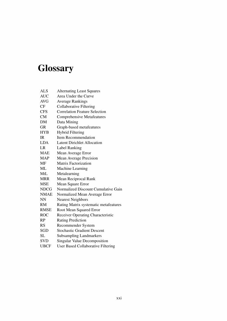
Glossary
ALS Alternating Least SquaresAUC Area Under the CurveAVG Average RankingsCF Collaborative FilteringCFS Correlation Feature SelectionCM Comprehensive MetafeaturesDM Data MiningGR Graph-based metafeaturesHYB Hybrid FilteringIR Item RecommendationLDA Latent Dirichlet AllocationLR Label RankingMAE Mean Average ErrorMAP Mean Average PrecisionMF Matrix FactorizationML Machine LearningMtL MetalearningMRR Mean Reciprocal RankMSE Mean Square ErrorNDCG Normalized Discount Cumulative GainNMAE Normalized Mean Average ErrorNN Nearest NeighborsRM Rating Matrix systematic metafeaturesRMSE Root Mean Squared ErrorROC Receiver Operating CharacteristicRP Rating PredictionRS Recommender SystemSGD Stochastic Gradient DescentSL Subsampling LandmarkersSVD Singular Value DecompositionUBCF User Based Collaborative Filtering
xxi


Chapter 1
Introduction
The shift towards an online economy increased the number of customers, markets and revenue
streams. Although it has facilitated the presentation of large product catalogs to potential cus-
tomers, it has inadvertedly created a problem: every platform has more information than its cus-
tomers can consume. This issue, present in most online digital economy website, is known as the
information overload problem (Bobadilla et al., 2013).
In early days, Information Retrieval systems were the answer to this problem. They are able
to fulfill user needs by processing an user query and match it with the contents in the business
database. The result was a ranked list of results, expected to fulfill his user needs as closely as
possible. Although useful, such approach requires the user to explicitly state the needs, usually by
a set of keywords. More importantly, this process is repeated every time the user has a new need.
Considering how this negatively affects the user experience, better alternatives were sought after.
A solution was provided by Recommender Systems (RSs) (Adomavicius et al., 2005). These
systems avoid explicitly inquiring the user regarding his needs, by creating and leveraging user
profiles instead. Each user profile is enriched by data collected regarding the user behavior and
interactions with the platform, meaning the user needs are now implicitly formulated and per-
manently available. Machine Learning (ML) algorithms can then be used to make inferences
regarding user preferences and thus make recommendations of relevant items at any time.
However, each online platform is different. This difference impacts directly in the data col-
lected and, in turn, in the richness of user profiles and the ML solutions applicable. Thus, the RS
research community has striven to create domain agnostic strategies, in order to be able to formal-
ize solutions that can be used in multiple domains. This is why the same recommendation strategy
can be used in multiple websites, whether the recommended items range from material objects
(books, DVDs, CDs, movies) to non-material entities (Jobs, Dates, Friends) (Lü et al., 2012).
Among the most important recommendation strategies, a few must be highlighted due to its
significance (Bobadilla et al., 2011): Content-based Filtering, Social-based Filtering, Context-
aware Recommendations and Hybrid Recommendations. All of them rely on a different hypothesis
to model the user profile and, by extension, the recommendation problem. However, the earliest
and most iconic recommendation strategy is known as Collaborative Filtering (CF) (Sarwar et al.,
1

2 Introduction
2000). It recommends items found relevant by other users with similar preferences. CF popularity
arises from the fact that it requires only transactional data, common in online platforms. Thus, this
recommendation strategy employs user feedback (e.g., user purchased a book or an user viewed a
movie) to define user profiles.
1.1 Problem overview
One of the open research issues in RSs is the lack of guidance regarding which algorithm would
be more adequate for a new recommendation task, and, more importantly, why. This problem
becomes even more evident when several recommendation strategies are considered, each with
several suitable algorithms. To deal with this issue, the practitioner is forced to evaluate every
available algorithm for a new task before selecting the best suited (Park et al., 2012). This pro-
cess has a high cost, not only regarding time, but also human and computational resources. An
alternative to reduce such costs is to automate the algorithm selection process.
A prime candidate for this automation is Metalearning (MtL) (Brazdil et al., 2009). It em-
ploys ML algorithms to find the relationship between a set of characteristics extracted from tasks
(i.e. metafeatures) and the performance of algorithms when applied to those tasks (i.e. metatar-
get). Thus, in any MtL solution, learning occurs in two levels: baselevel and metalevel. In the
first, baselearners accumulate experience on previous learning tasks. In the latter, metalearners
accumulate experience on the behavior of multiple baselearners on multiple learning tasks. This
allows to generate metaknowledge, which refers to the knowledge about the learning process (Van-
schoren, 2010). Although useful in multiple tasks, MtL is primarily used to address the algorithm
selection problem (Rice, 1976). It refers to the act of using a metamodel (i.e. a ML model which
identifies the mapping between metafeatures and metatargets) to predict the best algorithm(s) for
a new task.
There are few works investigating the use of MtL in RSs (Adomavicius and Zhang, 2012; Grif-
fith et al., 2012; Matuszyk and Spiliopoulou, 2014; Zapata et al., 2015). Although this helps in
justifying the need for further research in the topic, it also opens too many possibilities. Therefore,
this Thesis limits the scope of research in this topic by addressing only the problem of algorithm
selection for a single recommendation strategy is considered: CF. This strategy was chosen be-
cause it is the only with a large amount of public datasets and algorithms, essential to create a
meaningful metadataset. Another advantage is the existence of a large number of related work
approaches to serve as baselines.
Having defined the scope of this thesis, it is important to clarify the problems to be addressed.
Although there is some related work in this topic, which obtained relevant results and showed the
potential of these solutions, they are limited in several aspects. In particular, there are problems
regarding (1) the proper formulation and evaluation of the algorithm selection tasks, (2) there is
no empirical comparison of the proposed solutions, making it difficult to understand their relative
merits, (3) there is no systematic proposal and validation of CF metafeatures that leverage upon
the merits found in other ML domains, (4) the metatargets considered are usually very simple and

1.2 Thesis Statement 3
differ among solutions and (5) there are no tailored solutions in terms of metalearners and metatar-
gets to allow further improvement in terms of predictive performance. All of these issues impede
to make proper generalizations about the CF algorithm selection task, which consequently pre-
vents to obtain significant metaknowledge. This Thesis aims to reduce the effect of these previous
considerations by tackling various issues in the metafeatures, metatargets and metalearners.
1.2 Thesis Statement
In this thesis, the algorithm selection problem in CF is addressed by introducing multiple contri-
butions in order to improve upon the existing solutions. In essence, two hypothesis are considered:
Hypothesis 1. It is possible to leverage the relationships between the CF data characteristics (i.e.
metafeatures) and the performance of CF algorithms (i.e. metatargets) in order to predict the best
CF algorithm(s) for new CF datasets.
Hypothesis 2. The CF algorithm selection problem can be posed using multiple metafeatures,
metatargets and metalearners, thus creating different use cases concerning a different perspective
of the problem.
Hypothesis 3. The CF algorithm selection solutions can be evaluated in a way which allows to
extract meaningful metaknowledge regarding the CF task.
To investigate this hypothesis, 3 essential research questions must be addressed:
(RQ1) How mature are the CF algorithm selection approaches available in the literature?The answer to this question aims to determine the merits of existing approaches both
in terms of theoretical coverage and empirical efficacy. To answer this question, a
systematic literature review and empirical study are performed. Their goal is to aid in
clarifying the issue and thus motivate and justify further lines of research.
(RQ2) How can the current CF algorithm selection solutions be improved? After con-
sidering the horizon established by the previous studies, each individual dimension of
the problem is addressed via the introduction of proposals aimed for their improve-
ment. The improvement is made by proposing new metafeatures, metalearners and
metatargets. Notice that many of such contributions, although designed for CF, are
also applicable to multiple other domains.
(RQ3) What metaknowledge is obtained and how does it affect RS research? Lastly,
after improving the existing solutions on the topic, it is important to reason about the
patterns observed. To do so, it is important to assess the impact that metafeatures and
metalearners on the baselevel datasets and algorithms. Such analysis will be performed
throughout the various stages of the research conducted, thus assessing the merits of
MtL on multiple perspectives of the CF algorithm selection problem.

4 Introduction
1.3 Contributions
The main contributions in this Thesis are:
• Systematic literature review and empirical study: This study focused on previous work
on algorithm selection for RSs. It addresses several critical dimensions of the MtL method-
ology, used to review and formalize the related work on this novel research area. Further-
more, it performed an experimental study to assess the merits of the current approaches,
thus establishing a starting point for further research.
• Empirical Research: The empirical nature adopted in this Thesis allows to continuously
build upon the algorithm selection process by iteratively proposing new solutions and as-
sessing their merits. Thus, throughout the Thesis, multiple solutions for CF algorithm selec-
tion will be presented, which include solutions both from the related work and the proposed
contributions. By doing so, one is able to validate the existing contributions to the prob-
lem in a unified scenario and understand which dimensions require further work and which
are already suitable. Furthermore, the experimental setup used is considerably expanded,
increasing the confidence of the conclusions.
• Metafeatures: Alternative metafeatures were proposed, especially designed for CF. To do
so the first proposals took advantage of metafeatures used in other ML domains and make
adaptations to be able to create CF metafeatures. As result, 4 sets of metafeatures were de-
signed: Systematic Rating matrix metafeatures, Subsampling Landmarkers for CF, Graph-
based metafeatures and Comprehensive metafeatures. Afterwards, a technique that allows to
automatically create metafeatures recurring only to a Representational Learning ML model
is also proposed: cf2vec.
• Metatargets: The problem is first addressed using standard metatargets, namely by con-
sidering only the best algorithm per dataset. However, due to limitations of this approach,
the research shifts towards a setup where rankings of algorithms are used instead. Here,
two approaches are considered: single criterion and multicriteria metatargets. While the
first creates rankings by using the straightforward ordering performance scores obtained by
a single evaluation measure, the latter takes advantage of multiple evaluation measures to
create a single ranking of algorithms. To do so, it takes advantage of Pareto frontiers, which
allows to create fairer rankings of algorithms.
• Metalearners: The metalearners used in this Thesis are concordant with the metatargets
used. Thus, while at the start, standard classification algorithms are used to address algo-
rithm selection problem when the metatarget contains only the best algorithm, this paradigm
changes by using ranking based approaches when the metatargets follow suit. Here, a Label
Ranking approach for algorithm selection is formalized, which allows to make predictions
of the relative position for all available recommendation algorithms. This solution is also

1.4 Implications of Research 5
improved by considering data and algorithmic nuances from such formulation. First, a met-
alearner based on CF algorithms is proposed in order to predict the best ranking of CF
algorithms, while disregarding the influence of metafeatures: CF4CF. Furthermore, one im-
proves on the data and algorithmic advantages of both approaches by proposing an hybrid
solution: CF4CF-META. The results show the solution achieved the best performance on
the experimental setup, thus materializing as the best solution to the problem yet.
• Metaknowledge: Another important issue in the algorithm selection problem is to under-
stand how do the metafeatures and metalearners influence the relative performance of rec-
ommendation algorithms on particular baselevel datasets. Thus, extensive metaknowledge
analysis are provided throughout the Thesis in multiple perspectives of the problem in order
to clarify which are the most meaningful meta-approaches for each specific case (i.e. base-
level dataset and algorithm). To do so, metafeature importance analysis, baselevel dataset
impact analysis and algorithm footprints are employed (and adapted) throughout the Thesis.
1.4 Implications of Research
First and foremost, the studies developed here allow to formalize the research area of algorithm
selection for CF. This is a very important contribution, since the few existing approaches do not
address the algorithm selection problem in the most correct and complete way. Therefore, critical
dimensions of the problem are identified, which guide the contributions introduced in the Thesis
and, more importantly, to properly organize the problem for future contributions.
Furthermore, this Thesis presents the most extensive and deep study to the problem known to
date. In fact, it addresses many problems found in the literature review on the subject, namely
experimental setup design flaws and incomplete validation procedures. To deal with this issue, the
same experimental setup is used throughout the Thesis. Furthermore, an exhaustive experimental
validation procedure is proposed, which is replicated in every single Chapter. This yields a wide
range of performance assessments, which compare multiple aspects of the problem throughout the
Thesis.
Another important implication of this research is the wide range of the proposals. Namely, 5
new sets of CF metafeatures, 3 new classes of metalearners and 1 novel metatarget are introduced.
More importantly, all have proven useful to the CF algorithm selection problem, even if in different
aspects of the problem. Thus, all proposed contributions allow to push the state of the art in this
research area, proven by the multiple metalevel evaluation scopes considered. In fact, one must
notice that many of the contributions introduced may also be useful for other domains.
Lastly, this Thesis has an important implication for research in RS: it provides meaningful
help in order to guide the RS community towards MtL solutions to address the algorithm selection
problem. Namely, by investigating the important metafeatures and metalevel patterns found in the
mapping between metafeatures and metatargets, one is able to establish the groundwork for future
design and development of RS algorithms.

6 Introduction
1.5 Document Structure
This document is organized as follows:
• Chapter 2 presents an overview of the research areas associated with this Thesis: RS, MtL,
the algorithm selection problem in CF and Representational Learning.
• Chapter 3 provides a literature review on the existing CF algorithm selection solutions and
an empirical study comparing them.
• Chapter 4 introduces four CF metafeatures proposals designed through systematic proce-
dures: Rating Matrix, Subsampling Landmarkers, Graph and Comprehensive metafeatures.
• Chapter 5 describes the proposed formalization that uses Label Ranking to address the al-
gorithmic selection problem. Furthermore, it also includes the proposal for multicriteria
metatargets.
• Chapter 6 builds upon the previous Label Ranking formulation by proposing two different
classes of metalearners: CF4CF and CF4CF-META.
• Chapter 7 presents a Representational Learning approach to CF metafeatures: cf2vec.
• Chapter 8 discusses the main conclusions found and the directions for future work.

Chapter 2
Background
This chapter presents the State of the Art regarding several research issues important to this Thesis:
Recommender Systems (Section 2.1), Metalearning (2.2), Algorithm Selection and Collaborative
Filtering (2.3) and Representational Learning (Section 2.4). Every concept is detailed in order to
introduce and position the contributions of the remaining Chapters to this Thesis.
2.1 Recommender Systems
The information overload problem refers to the impossibility of an online user to process all in-
formation required, since the volume of relevant information available largely surpass the user
capability to understand it. Hence, automatic alternatives able to filter the information, keeping
only relevant contents and in a manageable quantity are desired (Yang et al., 2014; Bobadilla et al.,
2011). Such Machine Learning models are known as Recommender Systems (RSs).
Despite usually having the same purpose, RSs can take advantage of different recommendation
strategies. Such strategies depend on the data available and can be sourced from different aspects
of the domain of interest. RSs aim to capture patterns that explain how items are related and, as a
consequence, in which circumstances they should be recommended.
The first and foremost recommendation RS strategy is Collaborative Filtering (CF) (Goldberg
et al., 1992; Sarwar et al., 2000; Deshpande and Karypis, 2004). Despite research in the area
have started almost 30 years ago, it is still actively researched and widely used in real world
scenarios (Chen et al., 2018). Although this thesis focuses on CF, this chapter also briefly reviews
other RS strategies: Content based Filtering (CBF) (Diaby et al., 2013; Tan et al., 2014), Social
based Filtering (SBF) (Kazienko et al., 2011; Bugaychenko and Dzuba, 2013), Social Tagging
Filtering (STF) (Song et al., 2011; Jin and Chen, 2012), Hybrid Recommendation (HYB) (Cai
et al., 2014; Saveski and Mantrach, 2014) and Context-aware Recommendation (Adomavicius
et al., 2005; Burke, 2007). The reader is directed towards more appropriate literature (Resnick
and Varian, 1997; Burke, 2002; Adomavicius and Tuzhilin, 2005; Wei et al., 2007; Tintarev and
Masthoff, 2007; Verbert et al., 2012; Shi et al., 2014; Yang et al., 2014).
7
8 Background
2.1.1 Collaborative Filtering
CF recommendations are based on the premise that a user should like the items favored by a similar
user. Usually, it does not assume that the current user is aware of preferences from similar users.
Instead, the RS is charged with finding similar users based on the preferences of the current user
and then decide which are the most interesting items to be recommended.
The data used in CF, named user feedback, states the degree of preference (feedback) an user
has provided towards a given item (Bobadilla et al., 2013). User feedback can be categorized in:
• Explicit feedback: such data assumes the user knowingly assigns preference to items.
These can be numerical (a rating value from a predefined Likert scale issued to a specific
item), ordinal (a ranked list of preferred items, with no rating value assigned) or binary
(whether the item is favored or not).
• Implicit feedback: this data is collected from the user’s behavior within the domain, for
instance from click-through data from the search engine and the duration of time spent, on
a web page. It is also known as positive-only feedback, meaning it only allows to express
interest, never the lack thereof.
Collecting user feedback through explicit and implicit methodologies have positive and nega-
tive aspects: implicit methodologies are considered unobtrusive and allow to substantially increase
the amount and diversity of feedback available, but explicitly acquired data is more accurate in ex-
pressing preferences (Belén et al., 2009).
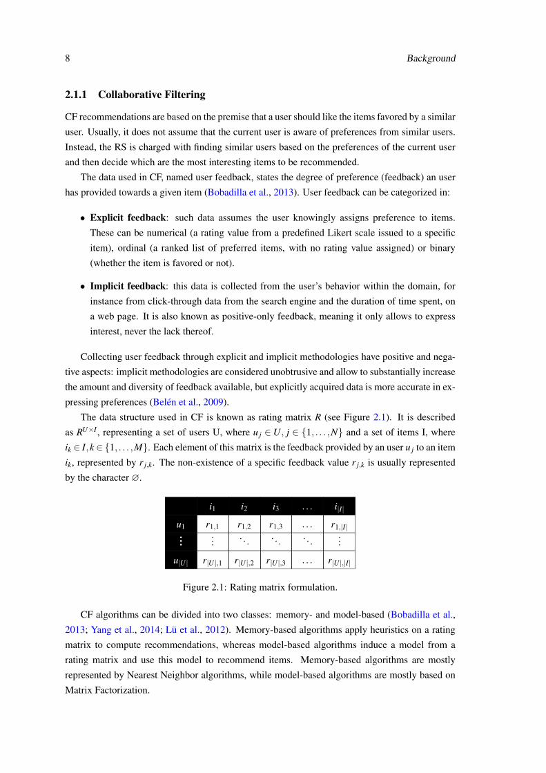
The data structure used in CF is known as rating matrix R (see Figure 2.1). It is described
as RU×I , representing a set of users U, where u j ∈U, j ∈ 1, . . . ,N and a set of items I, where
ik ∈ I,k∈ 1, . . . ,M. Each element of this matrix is the feedback provided by an user u j to an item
ik, represented by r j,k. The non-existence of a specific feedback value r j,k is usually represented
by the character ∅.
i1 i2 i3 . . . i|I|
u1 r1,1 r1,2 r1,3 . . . r1,|I|...
.... . . . . . . . .
...
u|U | r|U |,1 r|U |,2 r|U |,3 . . . r|U |,|I|
Figure 2.1: Rating matrix formulation.
CF algorithms can be divided into two classes: memory- and model-based (Bobadilla et al.,
2013; Yang et al., 2014; Lü et al., 2012). Memory-based algorithms apply heuristics on a rating
matrix to compute recommendations, whereas model-based algorithms induce a model from a
rating matrix and use this model to recommend items. Memory-based algorithms are mostly
represented by Nearest Neighbor algorithms, while model-based algorithms are mostly based on
Matrix Factorization.

2.1 Recommender Systems 9
Nearest Neighbors CF using Nearest Neighbor (NN) algorithms (Sarwar et al., 2000; Desh-
pande and Karypis, 2004) can be divided into two sub-categories: user-based and item-based. In
common, they have the following steps: to compute the degree of similarity between entities (ei-
ther users or items); to create a neighborhood of K entities (users or items) having the highest
degree of similarity; to predict the rating for a specific item based on previously calculated simi-
larities (Said and Bellogín, 2014). However, there are substantial differences in both approaches.
User-based NN finds users with similar item rating patterns. This is achieved by employing
suitable similarity functions, such as Cosine similarity (Equation 2.1) and Pearson’s Correlation
(Equation 2.2). Thus, the similarity between two vectors v and w, extracted from the rating matrix
is given by:
sim(v,w) =v.w||v||w||
(2.1)
sim(v,w) =∑
Kk=1(vk− v)(wk−w)√
∑Kk=1(vk− v)2 ∑
Kk=1(wk−w)2
(2.2)
with v and w representing the average value in each vector.
Having established the neighborhoods, then the following function can be used to predict the
missing rating of an user u j to an item ik:
pred(u j, ik) = ru j +∑n⊂neighbors(u j) sim(u j,n).(rn,ik − rn)
∑n⊂neighbors(uk) sim(u j,n)(2.3)
where ru j,ik is the rating of the user u j to an item ik and ru is the average value of recommen-
dations for the user u j.
However, in item-based NN, similarity is used differently: instead of calculating user similarity
directly by the respective user feedback vectors, now an item-item similarity is sought after. This
means the item feedback vectors are now used to build a similarity matrix. The same similarity
functions can be used in this context: Cosine similarity (Equation 2.1) and Pearson’s Correlation
(Equation 2.2).
Then, item-Based NN uses the ratings assigned by each user to items identified as similar and
predicts the rating for any item using the following expression (Sarwar et al., 2001):
pred(u j, ik) = rik +∑l∈ratedItems(u j) sim(ik, l).(ru j,l− rik
∑l∈ratedItems(u j) sim(ik, l)(2.4)
Notice that the formulations presented are used in explicit numerical feedback. Thus, the usage
of any other data type requires changes to the similarity function.
Matrix Factorization Matrix Factorization (MF) is currently one of the most efficient and robust
approaches for CF (Koren et al., 2009). It assumes that the original rating matrix values can
be approximated by the multiplication of at least two matrices with latent features that capture
the underlying data patterns (Takács et al., 2009). The computation is iterative and optimizes

10 Background
a performance measure, usually RMSE. In its most simple formulation, the rating matrix R is
approximated by the product of two matrices: R ≈ PQ, where P is an N×K matrix and Q is a
K×M matrix. P is named the user feature matrix, Q the item feature matrix and K is the number
of latent features in the given factorization. This process is illustrated in Figure 2.2.
Figure 2.2: Matrix Factorization procedure.
Consider two vectors: the rows pu ∈ P and the columns qi ∈ Q extracted from the factorized
matrices. The elements in pu measure the extent of the user preference over the latent factors and
the elements in qi represent the presence of these factors in the item. Thus, the users and items are
described using a set of latent features that are available in both matrices. After the factorization
process, the resulting matrix contains the approximation found to the original matrix. These values
are then used to provide the recommendation.
The predictions provided by MF use Equation 2.5 (Koren et al., 2009). MF estimates the pre-
dicted preference pred(u j, ik) by the user u j towards the item ik by multiplying the factor vectors:
pred(u j, ik) = qTik pu j (2.5)
To learn the factor vectors used in the previous equation, a regularization formula is used
to minimize the regularized squared error, in an attempt to minimize the difference between the
predicted ratings and the original values for known instances Bokde et al. (2015):
argmin ∑(u j,ik)
(ru j,ik −qTik pu j)
2 +λi||qik ||2 +λu||pu j ||2 (2.6)
where λu and λi refer to the user and item bias regularization terms, respectively. These terms
aim to compensate specific user/item differences against the average values of the preferences
stated by either users or items. The purpose is to consider the fact that users have different rating
habits, which should be correctly normalized in the factorization process, under the penalty of
incurring in overfitting.
In essence, MF algorithms solve an optimization problem in which the provided formula is
subjected to multiple iterations until the values converge to a satisfactory solution. Afterwards,
the MF model is able to predict the ratings for the missing instances, since the preference formula
can be used for any pairs of user/item, according to Equation 2.5. Several optimization methods
have been successfully used in CF to perform MF. The most frequent are Stochastic Gradient
Descent (SGD) and Alternating Least Squares (ALS).
2.1 Recommender Systems 11
SGD In SGD, the original rating ru j,ik is first compared with the predicted value (Koren et al.,
2009) in order to obtain an error measure: eu j,ik = ru j,ik − qTik pu j . This error measure is used to
update the factor vectors pu j and qik using the following equations:
qik ← qik + γ(eu j,ik pu j − γqik)
pu j ← pu j + γ(eu j,ik qik − γ pu j)(2.7)
where γ is a scaling value. Therefore, this algorithm uses the error of each prediction to
update the respective factor vectors in the opposite direction of the gradient. By performing several
iterations, the error is reduced and the model converges to a satisfactory solution. This solution
was adopted in (Baltrunas et al., 2010; Pálovics et al., 2014) and a variant, Stochastic Gradient
Ascent, was used in (Shi et al., 2012).
ALS The ALS algorithm alternates between two steps: the P− step, which fixes Q and recom-
putes P, and the Q−step, where P is fixed and Q is recomputed. The re-computation on the P-step
employs a regression model for each user, whose input is the vector qi and the output is the original
user rating vector. The process continues for several iterations until the solution converges. ALS
has been used in CF by (Pilászy et al., 2010; Takács and Tikk, 2012; Saveski and Mantrach, 2014).
2.1.2 Other recommendation strategies
This Section presents CF recommendation alternatives. The purpose is simply to present a sum-
mary introduction, thus leaving more advanced discussion to other works (Yang et al., 2014).
2.1.2.1 Content-based Filtering (CBF)
CBF recommendations propose the use of item properties to drive recommendations. This ratio-
nale implies that if an user bought an item from a specific category in the past, the user will be
probably interested in a new item from the same category in the future.
Most CBF methods take advantage of items the user found interesting in the past to serve
as initial feedback. Next, similarity calculations are performed to find and recommend the most
similar items (Bobadilla et al., 2013). Each item is described by several properties, which depend
on the domain used. For instance, movies can be described by their actors and studio, while in
music, artists and album properties can be used.
CBF typically uses a vector space model (Salton et al., 1975) to represent items and their prop-
erties. In this representation, each row represents a different item and each column is a property of
this item. With this formulation, similarity between items is simply given by the similarity of their
vectors (i.e. rows in the vector space model). Common similarity measures are Cosine similarity
and Euclidean Distance. However, the literature also offers examples of other algorithms: AR
(Aciar and Zhang, 2007; Xie, 2010), kNN (Dumitru et al., 2011), MF (Pilászy and Tikk, 2009)
and Latent Dirichlet Allocation (LDA) (McAuley and Leskovec, 2013; Tan et al., 2014).

12 Background
2.1.2.2 Social-based Filtering (SBF)
SBF provides recommendations taking into account user’s social relationships and embedded so-
cial information (Yang et al., 2014). It assumes that recommendations made while taking into
account the taste of friends are better than those from users with similar tastes (Lü et al., 2012).
The user relationships required establish connections between entities and are usually stored
in a graph, where nodes represent entities and edges the relationship between them. These connec-
tions can adopt a user-user or user-item connection (Huang et al., 2005; Lee et al., 2011). These
relationships can be classified as explicit, if there is a direct connection between two entities in
the data (e.g. social network connecting users), or implicit, if there is an intermediate entity to
connect other entities (e.g. users that declare similar tags, consume similar documents, etc.) (Guy
et al., 2009). Such relationships can even be enriched with extra information, which enables them
to take advantage of more advanced methods. One example is the Trust-aware recommendations
paradigm, in which social relationships are accompanied by a degree of trust. Such data can be
represented with explicit trust values (Golbeck and Hendler, 2006) or simply via unary assign-
ments of trust (Yang et al., 2012).
SBF methods typically use NN algorithms to compute the recommendations. They usually
extend the CF prediction process by weighting the predictions accordingly to the feedback from
friends towards each specific candidate item. Furthermore, they employ graph traversing tech-
niques to find neighbors to be used as candidates. The literature provides several examples of
SBF approaches that employed Depth-first search (Golbeck and Hendler, 2006; Guy et al., 2009;
Silva et al., 2010; Kazienko et al., 2011), random walk (Yin et al., 2010; Jamali and Ester, 2009;
Bugaychenko and Dzuba, 2013), heat-spreading algorithm (Zhou et al., 2010), PageRank (Lee
et al., 2011) and Epidemic protocols (Anglade et al., 2007).
2.1.2.3 Social Tagging Filtering (STF)
STF recommendations are based on the relationships stated by users towards specific items, whose
preferences are expressed by similar tags. In essence, it is an extension of CF where the feedback
is given by tags, rather than using numeric feedback. However, ordinary CF approaches are not
suitable to such data, since the tags do not have a numeric nature. Hence, STF approaches draw
inspiration also from CBF and SBF paradigms to perform recommendations.
The data used in SBF, also known as social bookmarks, is defined as a set of triplets specifying
the user, item and tag (Niwa et al., 2006; Shepitsen et al., 2008). The literature shows examples
adopting either a vector space model representation (Niwa et al., 2006; Shepitsen et al., 2008;
Zanardi and Capra, 2008; Krestel et al., 2009), a bipartite graph (Song et al., 2011) or instead
tensors (i.e. matrix representation with order greater than 2) (Symeonidis et al., 2008, 2010).
STF methods include adaptations of well-identified methods used in CF, CBF and SBF: IR
techniques (Niwa et al., 2006; Shepitsen et al., 2008), kNN (Zanardi and Capra, 2008), LDA (Kres-
tel et al., 2009). Higher Order SVD (HOSVD), an extension of Matrix Factorization, has also been
used in tensors (Symeonidis et al., 2008, 2010).

2.1 Recommender Systems 13
2.1.2.4 Hybrid Filtering (HYB)
HYB RS combines multiple recommendation strategies in an attempt to overcome the problems
that each strategy poses by using positive functionalities from others. Early HYB approaches
investigated the combination of CF and CBF strategies (Bobadilla et al., 2013). As result, 4 dif-
ferent hybridization solutions were proposed: (A) implement CF and CBF algorithms separately
and combine their predictions (Christakou et al., 2007; Belén et al., 2009), (B) incorporate some
CBF characteristics into a CF algorithms (Melville et al., 2002) , (C) build a general unifying
model that incorporates both CF and CBF characteristics (Gunawardana and Meek, 2009; Wu
et al., 2014; Saveski and Mantrach, 2014) and (D) include some CF characteristics into a CBF
algorithm (Jeong, 2010; McAuley and Leskovec, 2013). Notice that although these RS use only
CF and CBF, the hybridization strategies can be applied to any pair of recommendation strategies.
Nowadays, many other hybridization strategies exist (Burke, 2002; Çano and Morisio, 2019).
Namely, Weighted (i.e. combines scores from multiple recommendation strategies to create a
single recommendation), Switching (i.e. a recommendation agent decides which strategy works
best depending on the situation), Mixed (i.e. provide recommendations from multiple individual
recommenders without any attempt to merge the strategies in algorithmic terms), Feature Combi-
nation (i.e. merge data from different strategies into a single recommendation algorithm), Cascade
(i.e. one recommender refines the recommendations given by another), Feature Augmentation (i.e.
the recommendations created by one strategy are used as input feature in another) and Metalevel
(i.e. the model learned by one strategy is used as input to another).
2.1.2.5 Context-aware Filtering (CAF)
CAF uses contextual information to enrich the recommendation model, hoping to increase the ac-
curacy of the recommendations (Bobadilla et al., 2013). The rationale implies that recommenda-
tions for the same user should be different depending on the current time or location, for instance.
Thus, in this strategy, the context has as much importance as the other dimensions used (i.e. users
and items). Therefore, CAF can be classified as a special type of HYB, since (1) it uses context
data - which is a special type of side information - and (2) it requires a non-contextual base strat-
egy to compute the recommendations - and not necessarily multiple recommendation strategies.
There are three different ways of incorporating context information into RSs (Adomavicius and
Tuzhilin, 2011): (1) pre-filtering, (2) post-filtering and (3) modeling.
In contextual pre-filtering, the context is applied to the data selection and data construction
phases of the learning process (Adomavicius et al., 2005; Kuang et al., 2012; Levi et al., 2012;
Gupta et al., 2013). Contextual post-filtering only considers the context in the final stage of rec-
ommendation, after the execution of a typical non-contextual RS. Finally, in contextual modeling,
the context information is incorporated into the modeling phase, as a part of the rating estima-
tion (Yu et al., 2006; Ricci and Nguyen, 2007; Boutemedjet and Ziou, 2008; Karatzoglou et al.,
2010; Xie, 2010; Domingues et al., 2009; Natarajan et al., 2013; Cheng et al., 2014). For further
details, the reader is directed to (Villegas et al., 2018).

14 Background
2.1.3 Evaluation
Much like any other ML problem, RSs also require extensive evaluation in order to assess their
merits. Here, two different kinds of evaluations are discussed: offline and online.
2.1.3.1 Offline Evaluation
Offline evaluation uses only a data snapshot to assess model performance. To do so, the recom-
mendation dataset is divided into training and testing sets. While the first is used to induce the
recommendation model, the latter is used to assess the performance on new, previously unseen,
data. Common data splitting strategies are used to assign different ratings to each set, usually hold-
out or k-fold cross-validation (Herlocker et al., 2004). However, more advanced techniques exist
and depend on the domain selected. For instance, there are examples of prequential evaluation
useful for streaming scenarios (Vinagre et al., 2015).
The test phase in RSs has an important difference when comparing to supervised ML eval-
uation: since there is not a clearly defined target variable to be predicted, the user feedback is
used both as feedback for prediction and as the target. Thus, the feedback f for every user u is
randomly split into two vectors: initial feedback and target. Formally, fu = iu ∪ tu. When the
predictions pu = recommendation(iu) are calculated, comparisons between pu and tu can be per-
formed to assess the impact of recommendation for each user in the test set. When the procedure
is repeated for all users in the test set, a global evaluation score can be obtained representing the
entire RS predictive performance. It is important to notice that, at each fold of the cross-validation,
the feedback fu should be split differently into iu and tu, to provide a fair evaluation.
There are multiple ways to compare pu and tu, each depending on the scope of the recom-
mendation to be evaluated (Bobadilla et al., 2013; Lü et al., 2012; Yang et al., 2014). The scopes
identified, originally proposed for other ML tasks, are:
• Rating accuracy: assess the point-wise difference between a predicted rating value and its
actual rating. Examples include the NMAE (Normalized Mean Absolute Error) and RMSE
(Root Mean Squared Error);
• Rating correlation: calculate pairwise correlations between sets of predicted and real ratings.
Examples include Pearson correlation and Kendall’s Tau;
• Classification accuracy: evaluate correct and incorrect decisions about item relevance in
each recommendation. In RS, the evaluation is usually performed in a Top-K scenario.
Thus, only K items in the top of the predicted items are used in the evaluation. Metrics such
as Precision@K, Recall@K and Area Under the Curve (AUC@K) are often used;
• Ranking accuracy: assess how well does the predicted ranking of algorithms match the
true ranking, ignoring the ratings. Examples include NDCG (Normalized Cumulative Dis-
counted Gain) and MRR (Mean Reciprocal Rank);
2.1 Recommender Systems 15
RS evaluation also includes metrics designed for specific recommendation requirements. Ex-
amples include catalog coverage, user satisfaction, recommendation diversity and novelty. All
offline evaluation measures discussed here are detailed in Appendix A. Further discussion on this
topic is available in (Jalili et al., 2018).
Offline evaluation provides an easy way to assess recommendation performance. However,
important unanswered issues must be considered: there is no consensus on which metrics should
be used for each RS, or even which are the best metrics (Lü et al., 2012). Recently, there has
been some advances on this issue regarding real world scenarios. For instance, while earlier works
focused on rating accuracy performance even though the goal was to predict rankings of items,
nowadays this practice has been abolished and its inadequacy well documented (Lee et al., 2011;
Diaz-Aviles et al., 2012).
2.1.3.2 Online Evaluation
Despite efforts to find a bridge between offline evaluation metrics and the feedback provided by
real world scenarios, the literature shows no offline analysis can truly determine whether users will
prefer a particular system. The main reason lies in the fact that human factors are not included
in the process (Herlocker et al., 2004; Beel et al., 2013). Hence, suitable evaluations must use
directly the user feedback collected from real users.
These online evaluation methodologies can be characterized by whether they explicitly re-
quire the user feedback or if the user behavior is inferred. The first employs surveys, interviews
and questionnaires (Bostandjiev et al., 2012), while the second is usually an analysis of user be-
havior (Herlocker et al., 2004). A common approach to perform the latter analysis is through A/B
testing Kohavi et al. (2009). The idea is to compare two recommendation solutions used in two dif-
ferent groups: control and treatment. Each recommendation solution is evaluated using the same
performance metric and, afterwards, the results of both groups are compared. The comparison
typically involves assessing if the change in the solution performance is statistically significant or
not, in order to either accept or reject the new recommendation solution.
With A/B testing, for each RS being evaluated, it is also possible to compare the predictions
and real feedback per user. However, in this case, feedback fu is not split into initial feedback
and target. Instead, fu is considered as the initial feedback provided to the RS, hence allowing to
obtain pu = recommendation( fu). After obtaining pu, future user actions are analyzed in order to
create the actual tu. Thus, pu and tu can once again be compared and evaluation for the entire RS
be performed.
Within this problem frame, all offline evaluation measures can be used to ascertain the merits
of each RS. However, since an A/B test requires a real world RS, usually there are domain-specific
goals (such as KPI, for instance) which can be used instead. The most popular online metric
used is the user acceptance ratio (also known as conversion rate) (Herlocker et al., 2004). The
value of this ratio is given by the number of items which the user finds acceptable (either by
watching, purchasing, etc.) divided by the total amount of recommended items. The literature
also provides examples of other metrics: Interest Ratio (ratio between the number of positive

16 Background
and negative recommendations (Guy et al., 2009))and novelty (Blanco-Fernández et al., 2010;
Bugaychenko and Dzuba, 2013).
Ideally, all RSs should be evaluated using online evaluation measures. In practice, most do-
mains (in particular, academic) rarely have access to a suitable infrastructure. Furthermore, the
amount of resources required to perform this evaluation is much higher than the amount required
using an offline evaluation procedure, which poses further impediments to the adoption of this
evaluation procedure (Bugaychenko and Dzuba, 2013). Hence, despite its faults, offline evalua-
tion cannot be entirely discarded. In fact, it is argued that offline evaluation can have some inherent
value, especially if the online performance is poor and the offline evaluation results are good (Beel
et al., 2013). The justification lies on the fact that users who contributed to the offline dataset know
better than users receiving recommendations.
2.2 Metalearning and Algorithm Selection
There have always been efforts towards developing a super-algorithm able to obtain the best pos-
sible performance for every instance of a given task. This goal has been theoretically refuted by
the No Free Lunch Theorem (Wolpert and Macready, 1997). It states that, if all possible data
distributions are equally likely, any pair of learning algorithms will, on average, have the same
performance. Thus, for any algorithm, superior performance over one group of task instances is
compensated with inferior performance over another group. Therefore, it is impossible to build a
single best, universal learning algorithm (Vanschoren, 2010).
Therefore, the goal must be to understand each algorithm’s behavior in order to ascertain
where they will be most successful. This behavior, henceforth denominated as algorithm bias,
refers to any preference for choosing one data-independent hypothesis to explain the data over
another (equally acceptable) hypothesis (Brazdil et al., 2009). In fact, the reason why learning
algorithms perform differently on the same data is that they are all biased towards finding certain
types of regularities (Vanschoren, 2010). Therefore, if one can find the bias of existing algorithms,
one should be able predict the best algorithm for a new dataset.
MtL, a research area that studies the behavior of algorithms, focuses on using ML to under-
stand ML algorithms (and their configurations) in order to improve their results in future appli-
cations (Rossi et al., 2012; Nguyen et al., 2012). To do so, there are two basic approaches (Van-
schoren, 2018): to learn metamodels purely from model evaluations (van Rijn et al., 2015; Abdul-
rahman et al., 2018) or to learn metamodels which find the relationships between data character-
istics and learning performance (Soares et al., 2004; Rossi et al., 2014). This Thesis will present
examples of both approaches, with emphasis on the latter.
Although many other tasks can be tackled by either approach (Rossi et al., 2012), MtL is
mostly used to support the task of selecting a suitable predictive algorithm (Brazdil et al., 2009):
this is also known as the algorithm selection problem and was first conceptualized by (Rice, 1976).
It states that given:
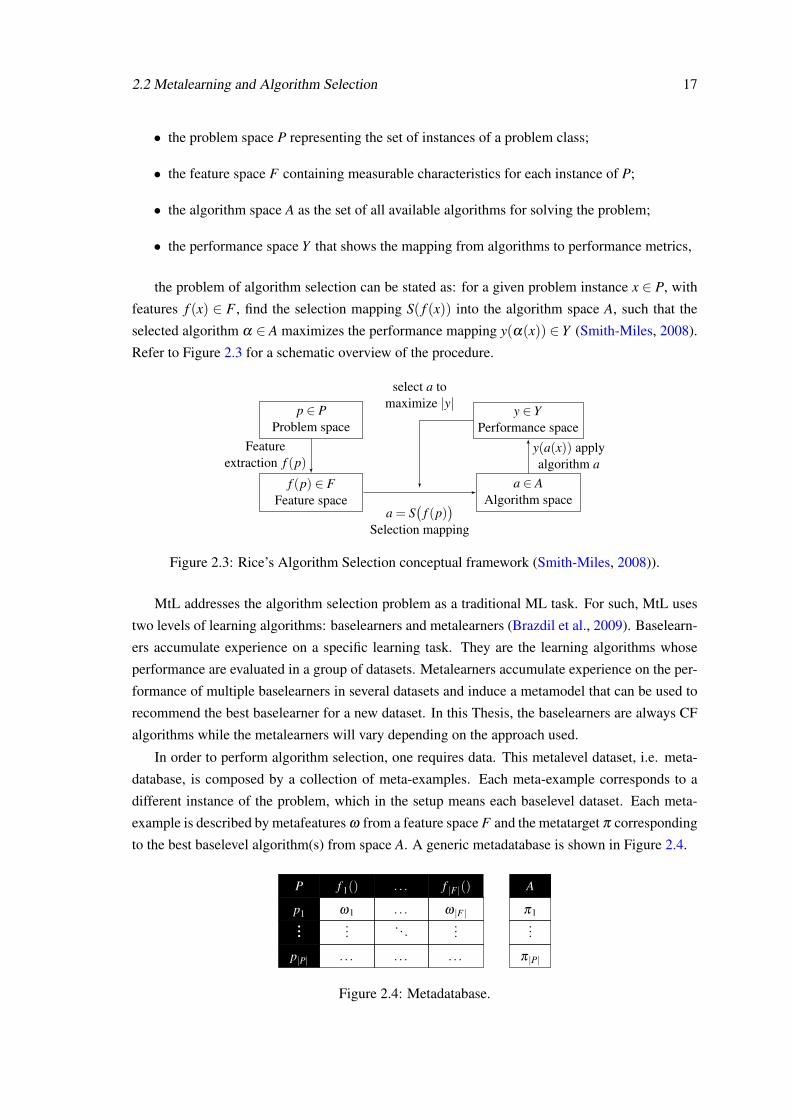
2.2 Metalearning and Algorithm Selection 17
• the problem space P representing the set of instances of a problem class;
• the feature space F containing measurable characteristics for each instance of P;
• the algorithm space A as the set of all available algorithms for solving the problem;
• the performance space Y that shows the mapping from algorithms to performance metrics,
the problem of algorithm selection can be stated as: for a given problem instance x ∈ P, with
features f (x) ∈ F , find the selection mapping S( f (x)) into the algorithm space A, such that the
selected algorithm α ∈ A maximizes the performance mapping y(α(x)) ∈ Y (Smith-Miles, 2008).
Refer to Figure 2.3 for a schematic overview of the procedure.
p ∈ PProblem space
f (p) ∈ FFeature space
a ∈ AAlgorithm space
y ∈ YPerformance space
Featureextraction f (p)
a = S(
f (p))
Selection mapping
y(a(x)) applyalgorithm a
select a tomaximize |y|
Figure 2.3: Rice’s Algorithm Selection conceptual framework (Smith-Miles, 2008)).
MtL addresses the algorithm selection problem as a traditional ML task. For such, MtL uses
two levels of learning algorithms: baselearners and metalearners (Brazdil et al., 2009). Baselearn-
ers accumulate experience on a specific learning task. They are the learning algorithms whose
performance are evaluated in a group of datasets. Metalearners accumulate experience on the per-
formance of multiple baselearners in several datasets and induce a metamodel that can be used to
recommend the best baselearner for a new dataset. In this Thesis, the baselearners are always CF
algorithms while the metalearners will vary depending on the approach used.
In order to perform algorithm selection, one requires data. This metalevel dataset, i.e. meta-
database, is composed by a collection of meta-examples. Each meta-example corresponds to a
different instance of the problem, which in the setup means each baselevel dataset. Each meta-
example is described by metafeatures ω from a feature space F and the metatarget π corresponding
to the best baselevel algorithm(s) from space A. A generic metadatabase is shown in Figure 2.4.
P f 1() . . . f |F |()
p1 ω1 . . . ω |F |...
.... . .
...
p|P| . . . . . . . . .
A
π1...
π |P|
Figure 2.4: Metadatabase.

18 Background
To build the metadatabase, two essential steps are required: 1) to extract metafeatures from
all baselevel datasets, which will be used as the independent variables of the MtL problem (see
Section 2.2.2) and 2) to create the metatarget by selecting the best algorithm(s) for each baselevel
dataset (see Section 2.2.1). Afterwards, one can train a metalearner on the metadatabase, hence
creating a metamodel which is able to predict the best algorithm(s) for new datasets (Serban et al.,
2013). This process is illustrated in Figure 2.5.
Figure 2.5: Metalearning process (Brazdil et al., 2009)
2.2.1 Metatarget and Metalearner
The metatarget (i.e. the target variable of the algorithm selection problem) is the element that
dictates which ML task must be used. The literature shows the following examples:
• To predict the best algorithm: this setup assumes that each meta-example is associated with
a single best algorithm. Thus, MtL can be seen as a classification task;
• To predict an un-ordered set of algorithms: here, the desired output is a set of algorithms
that will perform well for the new dataset. This task can be modelled as a Multi-Label
classification task.
• To predict algorithm performance estimate: here the goal is to predict the real-valued per-
formance of an algorithm, hence it is best described as a regression task.
• To predict the best ranking of algorithms: requires a model from Learning to Rank or Label
Ranking tasks, which is able to order the algorithms according to their fit to the problem.
Thus, it can be seen as a ranking classification task.
Notice that the metatarget also defines which class of metalearners can be used, since it de-
pends on the ML task chosen. In this Thesis we will focus on the first and last metatarget types.

2.2 Metalearning and Algorithm Selection 19
2.2.2 Metadata
Metafeatures are descriptors able to describe relevant aspects of a dataset. They should correlate
well with the performance of the models learned by different algorithms (Brazdil et al., 2009;
Kalousis and Hilario, 2003). This is considered the greatest challenge in MtL (Smith-Miles, 2008),
since it is uncertain which will be the problem characteristics which are in fact informative. To
address the problem, several classes of metafeatures exist:
• Statistical and/or information-theoretical measures: describe the dataset characteristics us-
ing a set of measures from statistics and information theory. These metafeatures assume
that there are patterns in the dataset which can be related to the most suitable algorithms for
these datasets. Examples include simple measures, such as the number of examples and fea-
tures in the dataset, to more advanced measures, such as entropy, skewness and kurtosis of
features and even mutual information and correlation between features Brazdil et al. (2009).
• Model-based characteristics: properties extracted from fast and/or simple models induced
from the dataset. In a classification or regression MtL scenario, they refer, for instance, to
the number of leaf nodes in a decision tree Brazdil et al. (2009).
• Landmarkers: fast estimates of the algorithm performance on the dataset. There are two
different types of landmarkers: those obtained from the application of fast and simple algo-
rithms on complete datasets (e.g. a decision stump can be regarded as a simplified version
of a decision tree) and those which are achieved by using complete models for samples of
datasets, also known as subsampling landmarkers Fürnkranz et al. (2002) (e.g. applying the
full decision tree on a sample).
2.2.3 Systematic Metafeatures Framework
Regardless of the class of metafeatures used, it is useful to find a formalism that allows the use
of a common language to describe them. To that end, a systematic framework has been proposed
by (Pinto et al., 2016). This framework provides a theoretical approach to systematically explore
a given problem in order to derive metafeatures from any dataset. We shall use this framework
throughout the Thesis in order to properly describe metafeatures, both proposed or in the related
work.
The framework is based on three essential elements: the set of objects O, the set of functions
F and the set of post-functions PF . The framework applies each function to each object and all
post-functions to the output from the previous element. At the end of this process, we will have
the final metafeature. Thus, any metafeature can be represented using the following notation:
O.F.PF (2.8)

20 Background
As an example, consider user.ratings.mean. This formulation means that the metafeature
represents the average rating value for all users in a specific dataset. Notice that if one wishes to
disregard the PF , it can be replaced by the character ∅.
This framework can be formulated in a recursive fashion with two levels (i.e. inner and outer
levels, respectively IL and OL). The OL considers the actual domain objects and it submits them
to the IL to be decomposed and more finely described. When IL finishes processing the provided
objects through more exhaustive processes, it returns the outcome to the OL for final processing.
In essence: the outcome of the IL application of the framework can be used as the result of the
OL. This property is useful in complex scenarios in which the entities to be used are enclosed in a
hierarchy or the concepts are not directly obtained. Formally:
OL-O.OL-F.OL-PF= OL-O.[IL-O.IL-F.IL-PF
].OL-PF (2.9)
Considering the previous example, let us suppose we wish to replace the function ratings for a
more complex descriptor. To do so, one needs simply to refer to the OL as OL= user.IL.mean, thus
needing only to describe which is the computation to be performed in the IL. For instance, if one
wished to perform a normalization of ratings, the IL can be defined as : IL = user.normalize.∅.
2.2.4 Metalevel evaluation
The evaluation of a MtL solution is similar to the evaluation of a conventional learning solu-
tion. The dataset is partitioned using a data sampling strategy (hold-out, leave-one-out or k-fold
cross-validation) to create the training and test datasets. The metamodel trained using the training
metadataset is used to predict the metatarget of the instances in the test metadataset. Figure 2.6
presents this procedure.
Figure 2.6: Metalearning evaluation process (Brazdil et al., 2009)

2.2 Metalearning and Algorithm Selection 21
The metamodel predictions must be evaluated in two ways (Brazdil et al., 2009): in terms
of metalevel accuracy (i.e. to compare predicted and true best algorithm(s)) and to assess the
impact on the baselevel performance (compare baselevel performances of the predicted and true
best algorithm(s)). Both are essential since they ascertain different dimensions, which may not be
aligned. This is particularly important since one wishes to ascertain the best metamodel and it can
only achieve this title if it performs well in both tasks.
Metalevel accuracy aims to understand how frequently the metamodel predicts the correct
metalabel. The measures depend on the metatarget used, but are mostly characterized by accuracy
measures. For instance, when the goal is to predict the best algorithm, classification accuracy
measures are suitable. In another example, if the metatarget is rankings of algorithms, ranking
accuracy measures must be employed. Thus, this evaluation provides an overall performance
score which measures the metamodel’s ability to properly match predicted and true metalabels.
On the other hand, the impact on the baselevel performance allows to understand what is the
actual cost of failing in the prediction of the best algorithm. This means that even though the
best and predicted algorithm may not be the same, what matters is to compare their performance,
i.e. the differences in their baselevel performance are most significant to understand the cost of
such classification mistake. Therefore, such evaluation uses the baselevel performances obtained
by the predicted algorithms for each dataset in the test metadataset as the score. The predictive
performance can be assessed using the averaged scores, which illustrate how much baselevel per-
formance is reached, on average, using the metamodel.
Formally, consider for a dataset di, the best algorithm adi with a performance P(adi). Now,
consider also the predicted algorithm adi for di and its performance P(adi). Notice that the goal is
to have P(adi) ≈ P(adi), even if a 6= a. Thus, in order to obtain an aggregated score to represent
the metamodel’s performance for all di ∈ D, the impact on the baselevel performance score θ is:
θ =∑|D|i=1 P(adi)
|D|(2.10)
In order to facilitate comparison between metamodels, it is useful to calculate a relative score,
which considers their deviation from the baseline. Thus, the percentage lift θL, which indicates the
percentile improvement against the baseline, is employed. Formally, considering the performances
of the best algorithm (i.e. oracle), the predicted algorithm by a metamodel and the predicted
algorithm by the baseline as P(adi), P(adi) and P(adi , respectively. This results in the following
revised score:
θL =∑|D|i=1
P(adi )−P(adi )
P(adi )−P(bdi )∗100
|D|(2.11)
Using this revised score, then the interpretation is simple: a positive score means one per-
forms better than the baseline; plus, the performance value refers to the percentage of possible
improvement, where 100% refers to the oracle’s score.

22 Background
2.3 Algorithm Selection and Collaborative Filtering
Before dwelling on the related work on algorithm selection approaches for CF, it is important to
investigate the related work that merges the research areas of CF and MtL.1 This is essential in
order to position the work to be developed in this Thesis. Recall that using the MtL paradigm,
there are two levels with ML algorithms. As a consequence, the potential research areas are those
which use CF algorithms in the metalevel, the baselevel or both. Thus, three alternative algorithm
selection categories can be formulated: 1) ML meta-approaches to recommend CF algorithms; 2)
CF meta-approaches to recommend ML algorithms and 3) CF meta-approaches to recommend CF
algorithms.
Our extensive analysis of the literature has shown that several works exist on the first two cat-
egories. While the ML meta-approaches to recommend CF algorithms are reviewed in Chapter 3
in the respective Systematic Literature review, here the focus lies on the second category. This
separation is used since our major goal is to address the first solution, regardless of whether CF
algorithms are used or not as the metalearner. However, we review other works in order to provide
complete review of the related work. On this note, as far as the authors are aware, there is only
one solution to address the third category and it is proposed in Chapter 6 of this Thesis.
In terms of CF meta-approaches to recommend ML algorithms, the literature provides a few
examples (Stern et al., 2010; Smith et al., 2014; Wang and Hebert, 2015; Mısır and Sebag, 2017).
An overview of such works is presented in Table 2.1. This table presents several dimensions on
this issue: application domain, data, algorithms, metatarget, evaluation metrics and whether the
work addresses the Cold Start Problem or not.
Table 2.1: Related work on CF meta-approaches to recommend ML algorithms.
Reference Domain Data Algorithm Metatarget Evaluation metricsColdStart
(Stern et al., 2010)
ConstraintSolving and
CombinatorialAuctions
AlgorithmPerformanceand Metadata
custom MF BestAlgorithm
Time and Numberof solved instances No
(Smith et al., 2014) ClassificationAlgorithm
Performance
k-Means,MF,PCA
BestAlgorithmRanking
Accuracy No
(Wang and Hebert, 2015)Computer
VisionAlgorithm
Performance SVD, MF BestAlgorithm
Mean AveragePrecision No
(Mısır and Sebag, 2017)
PropositionalSatisfiability
and ConstraintSatisfaction
AlgorithmPerformance custom MF
BestAlgorithmRanking
Ranking Accuracy,Time, Ratio of solvedinstances and Regret
Yes
The results show that the domains investigated vary widely, including for instance Constraint
Solving and Computer Vision. Regarding the data used in these approaches, they all use algorithm
performance as the feedback to CF algorithms as expected. However, the work developed by
(Stern et al., 2010) also uses metadata, thus making it more similar to a Hybrid strategy.
1As this Thesis focuses on algorithm selection approaches alone, previous works on AutoML using CF (Fusi andElibol, 2017; Yang et al., 2018) were left out.

2.4 Representational Learning 23
Regarding algorithms, most approaches use MF algorithms (either standard or customized
versions), which is expected as MF is a widely used and effective approach for CF. There are also
examples of the use of k-means and PCA, despite not being standard CF algorithms.
The metatargets are evenly balanced: two approaches recommend the best algorithm (Stern
et al., 2010; Wang and Hebert, 2015) and two others the best algorithm rankings (Smith et al.,
2014; Mısır and Sebag, 2017).
Regarding the evaluation metrics, some of them are not commonly used in the evaluation
of CF algorithms, namely: number or ratio of solved instances (Stern et al., 2010; Mısır and
Sebag, 2017) and Regret (Mısır and Sebag, 2017). This happens because they are related to the
baselevel task rather than the metalevel task. Furthermore, it can be observed that only the earliest
work (Stern et al., 2010) fails in evaluating the accuracy of the recommendations. But this practice
has changed, especially when considering the latest work (Mısır and Sebag, 2017), which presents
both metalevel accuracy and impact on the baselevel performance analysis.
One particularly important issue in RSs is the Cold Start Problem, which is the need to provide
recommendations when there is none or little data. This issue is harder in this case because there is
no information about the performance of any of the algorithms and, thus, the performance matrix
which is used as rating matrix, is empty in the corresponding row. In MtL, this is a trivial task:
one simply extracts the respective metafeatures and uses the predictive abilities of the metamodel.
However, since in CF there are no metafeatures, it is necessary to develop strategies able to deal
with this problem.
We found only one work (Mısır and Sebag, 2017) that tackles this problem, thus making it
the only suitable candidate for comparison. The authors take advantage of two models: a MF
algorithm and a multi-output regression algorithm. The first is used to learn latent representations
for both datasets and algorithms, much like in similar related works (Mısır, 2017; Alcobaça et al.,
2018). The second learns the mapping between metafeatures and the respective dataset latent
matrix representations. Thus, for a new problem, it is necessary only to provide the respective
metafeatures to the regression model in order to obtain a prediction of the latent representation.
Afterwards, the performance prediction is calculated by standard matrix multiplication operation.
2.4 Representational Learning
Lastly, we briefly review a research area which focuses on finding alternative representations for
learning problems: Representational Learning (RL) (Bengio et al., 2013). Although such ap-
proaches can serve multiple purposes, this Thesis dwells on this subject as a way to provide related
work for Chapter 7. Particularly, we use this technique to create alternative CF metafeatures to
those presented in Chapters 3 and 4.
RL uses ML algorithms and domain knowledge to learn alternative and potentially richer rep-
resentations for a given problem to enhance predictive performance in other ML tasks. Examples
of successful applications of RL are text classification (Bengio et al., 2013) and image recogni-
tion (He et al., 2016).

24 Background
Although there are alternatives, like probabilistic models and manifold learning (Bengio, 2011;
Bengio et al., 2013), the purest RL technique is the Autoencoder (Bourlard and Kamp, 1988; Le-
cun, 1987). Autoencoders are obtained by training a neural network to reproduce the input vector
in the output vector using a hidden layer with different amount of neurons than the output layer.
The most interesting aspect of such technique is the fact that it operates in a fully unsupervised
fashion. For such, the network learns two functions: an encoding function f and a decoding func-
tion g. Since the hidden layer is able to preserve useful properties of the data, it can represent
the input (Goodfellow et al., 2016; Lecun et al., 2015; Schmidhuber, 2015). There are multiple
versions of Autoencoders specifically designed for the CF scope (Sedhain et al., 2015; Wu et al.,
2016).
A better alternative is the distributed representations (Lecun et al., 2015). As the name sug-
gests, each entity is represented by a pattern of activity distributed over many elements, and each
element participates in the representation of many different entities (Rumelhart et al., 1986). In
essence, they also represent the input as a real-valued vector, but using a different network archi-
tecture. The most significant techniques for this problem are discussed next:
• word2vec (Mikolov et al., 2013) assumes that two words are similar (and have similar
representations) if they have similar contexts. In this case, the context refers to a predefined
amount of neighboring words. One architecture proposed to learn these representations
is the skipgram, which predicts surrounding words given the current word. For such, each
target word wt , represented as one-hot encoding for a vocabulary V , is connected to a hidden
layer h. This hidden layer, where the distributed representations are, has a predefined size d.
Each distributed representation is connected to the previous and next c context words (i.e.
wt−c,w...,wt−1,wt+1,w...,wt+c).
• doc2vec (Le and Mikolov, 2014) learns distributed representations for sequence of words
with different lengths (i.e. paragraphs, documents, etc.). One of the introduced algorithms
(i.e. Paragraph Vector Distributed Bag of Words (PV-DBOW)) allows a straightforward
adaptation of word2vec’s skipgram: instead of predicting context words based on a cur-
rent word, now the neural network predicts sequences of words belonging to a particular
document.
• A variation of doc2vec is graph2vec (Narayanan et al., 2017): by considering each graph
as a document, graph2vec can represent each graph by its underlying nodes. The process
has two stages: 1) create rooted sub-graphs in order to generate vocabulary and 2) train the
PV-DBOW skipgram model. WE will present this technique in more detail in Chapter 7.
Lastly, one should notice that many more Representational Learning techniques exist. Notice
that we did not cover them in this brief review, since they fall outside the scope of this Thesis.
Nevertheless, various works can be consulted for further information (Bengio et al., 2013; Goyal
and Ferrara, 2018).

Chapter 3
Systematic Literature Review andEmpirical Study
This Chapter discusses seminal works regarding the problem of algorithm selection for RSs, with
focus on CF approaches. The discussion aims to understand the current state of research in order
to help motivate and guide the work to be conducted in this Thesis. To achieve this goal, this
Chapter provides two contributions:
• Systematic literature review (Section 3.1). The related work is reviewed on the key dimen-
sions required to solve the algorithm selection problem. In each dimension, the extent of the
research conducted so far is discussed, thus exposing advantages and disadvantages in exist-
ing contributions. With this, one can highlight lines of research for future work. Notice that
contributions addressed in this Thesis are clearly marked in the appropriate key dimensions.
• Empirical study (Section 3.2). The most suitable CF metafeatures proposed in the related
work are experimentally evaluated in order to ascertain their performance on the same exper-
imental conditions. To that end, a large experimental study of baselevel datasets, algorithms
and evaluation metrics is conducted. Afterwards, each meta-approach is implemented and
evaluated on the same metalevel setup, i.e. same metatarget, meta-algorithms and evaluation
measures. Finally, conclusions are drawn from the behavior of the current state of the art
meta-approaches with regards to several aspects of the algorithm selection problem. This
also allows to establish a baseline, which we take into account in future Chapters.
3.1 Systematic Literature Review
This Section is organized as follows: Section 3.1.1 presents the methodology chosen to collect
relevant related work. Afterwards, Section 3.1.2 poses the identified key dimensions as research
questions. Section 3.1.3 presents each meta-approach and Section 3.1.4 answers the research
questions identified previously. Lastly, Section 3.1.5 presents a summary of the main findings and
discusses possible improvements.
25

26 Systematic Literature Review and Empirical Study
3.1.1 Methodology
In order to perform the literature review on the subject of algorithm selection for RSs, several
online databases were consulted: Elsevier’s Scopus, Thomson Reuters’s Web of Science, IEEE
Xplore Digital Library, Google Scholar and ACM Digital Library. The search queries combined
the keywords: "recommender system", "metalearning", "algorithm selection" and "performance
prediction". This yielded a total of 6 suitable documents, at the time of this search1.
3.1.2 Research Questions
Considering the MtL work flow described in Section 2.2, the most important dimensions of the
algorithm selection problem for RS were identified: learning problem, data, algorithms and eval-
uation measures. The dimensions, which have been split into of base and metalevels, are now
translated into Research Questions (RQ):
(RQ1) Which recommendation strategies have been included in MtL studies?
(RQ2) Are the public datasets used representative and sufficient for metalearning?
(RQ3) Is the pool of recommendation algorithms suitable and complete?
(RQ4) How well are the RSs performance measures covered?
(RQ5) Are the metafeatures used diversified in nature and enough?
(RQ6) In the studies, what is the typical metatarget?
(RQ7) Which algorithms are employed in the metalevel?
(RQ8) Are the evaluation measures used in the metalevel suitable?
3.1.3 Related work
The previous search literature has yielded a few approaches for RS algorithm selection problem.
These are presented next in chronological order, identified by a specific letter. Furthermore, notice
the metafeature nomenclature presented in Section 2.2.3 is used in order to formalize the proposed
metafeatures in each meta-approach.
A This meta-approach studies the CF algorithm selection problem by mapping the data onto
a graph instead of a rating matrix (Huang and Zeng, 2011). Graph-dependent metafeatures are
derived and then used to select the most appropriate NN algorithms. These are based on clustering
coefficients and clustering participation measures. The selection process uses a domain-dependent
rules-based model instead of using a ML algorithm.
1Search conducted on November-December 2016, yet still up to date.

3.1 Systematic Literature Review 27
B The next study to appear (Adomavicius and Zhang, 2012), extracts metafeatures directly
from the ratings matrix: dataset.density.∅, dataset.shape.∅, dataset.density.∅, item.count.gini,
item.count.skew, user.count.gini, user.count.skew and dataset.ratings.variance. The problem was
addressed as a regression task, optimizing for RMSE. The outcome is a linear regression model
which states the meaningful dimensions for the experimental setup used.
C This meta-approach, proposed by (Ekstrand and Riedl, 2012), resembles meta-approach B in
the sense that it too used a regression algorithm, optimized towards RMSE. However, the metafea-
tures proposed are extracted per each user instead per each dataset. The metafeatures, which use
always the user perspective, can be formalized as: user.count.∅, user.mean.∅ and user.variance.∅.
D The following work studies the expected error of the recommendations of a NN algorithm
using a decision tree regression model (Griffith et al., 2012). Once again, this approach fo-
cuses on describing user-level metafeatures: user.mean.∅, user.count.∅, item.count.∅, user.std.∅,
item.mean.∅, user.neighbors.∅, user.similarity.∅, user.clustering.∅, coratings.jaccard.∅,
user.TFIDF.∅ and item.entropy.∅.
E This meta-approach creates an auxiliary data structure, i.e. co-ratings matrix, from which the
metafeatures are extracted (Matuszyk and Spiliopoulou, 2014). First, equivalence classes (EC) are
created, which include users with similar amount of ratings. Then, the EC matrix is created by
pairwise comparison of EC in terms of the average number of co-rated items in common. The
metafeatures are: dataset.sparsity.∅, EC.co-ratings.gini and EC.co-ratings.entropy. The process
uses a regression model to predict the RMSE performance of NN and MF algorithms.
F The algorithm selection problem was extended beyond CF, when a Group Recommendation
(GR) meta-approach was proposed (Zapata et al., 2015). It derived domain-dependent metafea-
tures and used several classification algorithms to rank the best vote aggregation algorithms.
All these works are presented in Table 3.1. Each work is described in terms of the RQ identified
earlier, with some sub-divided for readability purposes:
• The baselevel algorithms (RQ3) are organized by type - Heuristics (H), Nearest Neighbors
(NN), Matrix Factorization (MF) and others (O).
• The baselevel evaluation measures (RQ4) are organized into error based (E), classification
accuracy (CA) and ranking accuracy (RA).
• The metafeatures (RQ5) are divided according to the subject evaluated: user (U), item (I),
ratings (RT), data structure (S) and others (O).
• The metatargets (RQ6) are: 1) best algorithm (BA), 2) ranking of algorithms (RA) and 3)
performance estimation (PE).
• The metalevel (RQ7) uses classification (C), regression (RG) or other (O) algorithms.

28 Systematic Literature Review and Empirical Study
Table 3.1: Related work on ML meta-approaches to recommend CF algorithms.
Ref. A B C D E FB
asel
evel
RQ1 CF CF CF CF CF GRRQ2 3 4 1 3 4 4
RQ3
H 2 - 1 - - 11NN 2 2 2 1 1 -MF - 1 1 - 1 -O - - 1 - - -
RQ4E - 1 1 1 1 1
CA 3 - - - - -RA 1 - - - - -
Met
alev
el
RQ5
U - 1 3 11 - 5I - 1 - - - -
RT - 1 - - - -S 2 3 - - 3 -O 2 - - - - -
RQ6 BA PE BA PE PE RA
RQ7C - - 1 - - 4
RG - 1 - 1 1 -O 1 - - - - -
RQ8 AUC Correlation AUC MAE Correlation MRR
3.1.4 Discussion
3.1.4.1 Recommendation strategies
Since this research area is still in the early stages (all works were published in the last 6 years2), it
is expected that only a few RS strategies would have been studied. In fact, like in the RS research
area, the majority of the researches has been performed on CF. This is justified by the lack of
public frameworks and datasets beyond this recommendation strategy. The exception is a recent
study on the algorithm selection problem for Group Recommendation (GR) (Zapata et al., 2015).
Therefore, it is essential to 1) expand the scope of RS strategies studied and 2) perform a deeper
analysis of the algorithm selection problem for CF.
3.1.4.2 Datasets
The related works use at most 4 datasets to investigate algorithm selection. While on some cases
this may be acceptable if the problem is appropriately modeled (for instance, select the best algo-
rithm for each user instead of per each dataset (Ekstrand and Riedl, 2012; Griffith et al., 2012)),
this is usually a drawback. In fact, algorithm selection meta-approaches must use a large amount
of diverse datasets to ensure a proper exploration of the problem space P. This dimension must
2Recall that this study has been completed in 2017.

3.1 Systematic Literature Review 29
be improved, although there are few public datasets. In this Thesis, we shall extend to 38 recom-
mendation datasets. The metafeature extraction process involves applying all strategies discussed
in Section 3.2.1 to all CF datasets listed in Table 3.2.
The public datasets used in the related work are: BookCrossing (Ziegler et al., 2005), Epin-
ions (Richardson et al., 2003), Flixter (Zafarani and Liu, 2009), Jester (Goldberg et al., 2001),
LastFM (Bertin-Mahieux et al., 2011), MovieLens (GroupLens, 2016) and Netflix (Netflix, 2009).
Only two works use private data (Huang and Zeng, 2011; Zapata et al., 2015), which are excluded
from further analysis since we cannot access its characteristics.
The results show a large variation in how frequent each dataset is used in these works. The
most common dataset belongs to the MovieLens category (used 4 times out of 6). This follows
the trend in the RS research area, where these datasets are considered benchmarks. The second
choices fell on the Netflix datasets, which became popular after a world-wide competition that
finished in 2009 (Koren et al., 2009). The remaining datasets appear only once.
These observations point to the idea that the choice of datasets is suitable since they are all
CF datasets. However, for algorithm selection purposes, the amount and diversity are extremely
scarce. The main drawback lies in the fact that empirical conclusions drawn from such a small
sample will most probably lead to incorrect conclusions. Hence, it is of the utmost importance to
include more diverse datasets in future CF algorithm selection studies.
3.1.4.3 Baselevel algorithms
The baselevel algorithms frequently used are distributed in the following categories: Heuristics
(14), NN (8), MF (3) and Others (1). The fact that NN approaches are abundant is expected, since
they are the earliest and easier to implement in CF. The large amount of heuristics refers mostly
to the GR approach, which studies 11 algorithms of this nature. In CF, heuristics are typically
associated with naive approaches, such as random and most popular algorithms, which can also
be considered baselines. One important note lies in the fact that MF algorithms are widely under-
represented, even though they are the current standard in CF.
The most frequently used algorithms are user-based NN and SVD++, closely followed by
item-based NN. This represents the most basic approaches for CF and are therefore available in
a larger amount of recommendation platforms. Newer approaches, such as MF, are usually more
difficult to find in recommendation platforms. This is an important limitation, but it also justifies
their exclusion from the related work. Averages and most popular algorithms are more common
than random. This is expected, since they are better baselines (Koren et al., 2009).
Although the algorithms used are suitable for CF, the studies fail to reach a state where there
are enough algorithms which allow to extract meaningful conclusions. Therefore, in order to
properly explore the algorithm space A for CF, it is important to include new algorithms.

30 Systematic Literature Review and Empirical Study
3.1.4.4 Baselevel evaluation
The study shows that most evaluation measures are error based (used in 5 out of 6 works). On the
other hand, classification accuracy measures are only used in 1 work. The most frequently used
error measures are RMSE and MAE and classification accuracy evaluated through precision and
recall. Although suitable for Rating Prediction problems, such measures do not follow the current
needs in RSs, where the goal is now to predict rankings of items. Hence, none of the related works
is currently relevant given that the way CF is approached is outdated. This Thesis addresses both
kinds of problems for completeness purposes.
It is important to notice that the evaluation procedures usually assess only one aspect of the
recommendation process, contradicting the guidelines from the RS literature (Herlocker et al.,
2004). In fact, only 1 work expanded the evaluation scope to classification measures (Huang and
Zeng, 2011). Furthermore, newer evaluation measures such as novelty, satisfaction and diversity
are never employed. This demonstrates the incompleteness of the evaluation in the related work.
On the other hand, such measures are still not entirely validated, thus explaining their exclusion.
Further investigations are required to improve the exploration of the performance space Y ,
including increase the scope of offline evaluation measures and to perform the same studies using
online rather than offline evaluation procedures.
3.1.4.5 Metafeatures
The metafeatures used in the related works are all statistical and information-theoretical measures.
They can be organized into several categories: user (19), data structure (8), item (1), ratings distri-
bution (1) and others (2). The fact that most metafeatures are focused on the user is not surprising,
given its central position in the CF problem. In fact, some research considers this perspective so
important that only metafeatures of this dimension are used (Ekstrand and Riedl, 2012; Griffith
et al., 2012; Zapata et al., 2015). Characteristics related to the data structure are also common and
are available in 3 out of 6 works. Notice that only one metafeature per item and rating distribution
appear, showing how understudied these are.
The number of metafeatures used usually ranges from 3 to 11. Although one aims to avoid
the curse of dimensionality by using few but informative metafeatures, the current state of af-
fairs does not allow to understand whether the metafeatures proposed are the best suited to tackle
the problem. Hence, in order to properly explore the feature space F , more and more complex
metafeatures must be proposed and their merits validated. Afterwards, feature importance tech-
niques must show which are the most informative and, therefore, the best metafeatures.
The analysis of metafeatures in a deeper level allows us to understand which type of statistical
and information-theoretical measures used: mostly ratios, averages and sums. This is expected,
since they are the simplest metafeatures found in the MtL literature. Entropy and Gini index appear
in the second position (in 3 works). All other functions appear only once.
Despite the fact that diverse metafeatures are proposed, few studies look towards different
aspects of the problem. In fact, 4 studies focus their metafeatures on a single subject, which

3.1 Systematic Literature Review 31
typically is the user. Plus, there are few examples of metafeatures that look towards relation-
ships between the different subjects of the problem. This makes difficult to find complex pat-
terns in the data, restricting the metaknowledge extracted. To address these issues, one must: 1)
propose and adapt new metafeatures for other RS strategies; 2) propose problem-specific (and
eventually domain-specific) metafeatures and 3) study new metafeatures besides statistical and/or
information-theoretical, such as for instance, landmarkers.
3.1.4.6 Metatarget
Related work on CF algorithm selection has adopted several metatargets. The most common is
the performance estimation (PE), available in 3 out of 6 works. There are also two examples of
best algorithm (BA) and one ranking (RA) selections. Although all metatargets are suitable and
important, it is the authors belief that the most beneficial way to address the problem is using
RA. The main reason why is based on the fact that when the metatarget is a ranking, although the
learning problem becomes more complex, it also provides more information. Hence, the authors
suggest that future works address the problem towards RA.
3.1.4.7 Metalevel algorithms
Usually, only one algorithm is used in the metalevel. This algorithm must match the required
metatarget. When PE is used as metatarget, regression algorithms are used (mainly linear regres-
sion algorithms). For BA and RA, popular classification algorithms, like rule-based classifiers,
Naive Bayes, SVM and kNN, are used. An exception happens when a custom procedure based on
rules is used (Huang and Zeng, 2011).
Although the number of algorithms used in the metalevel does not have the same impact as
the number used in the baselevel, the use of a larger and more diverse set of algorithms in the
metalevel increases the chances of uncover hidden relationships in the metadataset. Only one
study uses more than one algorithm in the metalevel (Zapata et al., 2015). A relevant future work
is the application of RS on the metalevel. Although this topic has not received any attention so
far for the selection of recommendation algorithms, it has been successful in other domains (Stern
et al., 2010; Smith et al., 2014; Wang and Hebert, 2015; Mısır and Sebag, 2017). Such works are
important to understand whether MtL approaches are indeed the best way to tackle the algorithm
selection problem.
3.1.4.8 Metalevel evaluation
The last RQ focuses on the evaluation measures used in the metalevel. Once again, these must be
in conformity with the metatarget and meta-algorithm. This is noted by the usage of error based
measures or correlation assessments for PE (Griffith et al., 2012; Adomavicius and Zhang, 2012;
Ekstrand and Riedl, 2012; Matuszyk and Spiliopoulou, 2014), classification accuracy measures
for BA (Huang and Zeng, 2011) and ranking accuracy measures (Zapata et al., 2015). Thus, one
concludes all related work perform suitable validation for the algorithm selection task.

32 Systematic Literature Review and Empirical Study
However, it is paramount to understand that no related work does ever analyze the impact on
the baselevel performance, which is arguably the most important measure of efficacy in algorithm
selection problems. For more details, please see Section 2.2.4.
3.1.5 Summary
After reviewing in extent each key topic of the algorithm selection problem for CF, the following
key conclusions were found:
• With the exception of one study on Group Recommendation, only CF has been studied on
the algorithm selection problem. Furthermore, the study of algorithm selection in CF is
limited. This Thesis addresses exclusively the second challenge in all remaining chapters of
this document, for which an extensive list of contributions is made.
• Since related work uses at most 4 datasets in each study, it is safe to state that the amount
of datasets is not enough to properly analyze the algorithm selection problem. This Thesis
addresses this issue by extending the set of datasets to a grand total of 38. Notice that all
experiments conducted from this point onward use this collection of datasets.
• The pool of recommendation algorithms studied in algorithm selection studies is always
suitable, but never complete. Particularly, there is noticeable absence of MF algorithms,
one of the most meaningful class of recommendation algorithms. In this Thesis, this issue
is solved by using 10 MF algorithms in all experiments in all remaining Chapters.
• Most approaches evaluate CF with a single error-based measure. This is outdated, since
the standard is now to evaluate using rank-based measures and more than one measure is
required to evaluate RS. This Thesis directly tackles this issue by investigating both the
Rating Prediction problem (using error based measures) and the Item Recommendation one
(using classification and ranking-based measures).
• Although a diverse set of metafeatures is available, the related works typically use few
metafeatures and usually focused on a single aspect of the CF problem. This Thesis con-
tributes extensively to this subject by proposing 3 different sets of metafeatures in Chap-
ter 4. While the first type focuses on tackling the problems of the metafeatures proposed in
the related work by proposing a systematic procedure to analyze the rating matrix, newer
metafeatures such as subsampling landmarkers and graph metafeatures are also proposed.
Furthermore, Representational Learning techniques are used in Chapter 7 to attempt to de-
rive metafeatures without human interaction.
• Although the typical metatarget is performance estimation, this is not the best choice. If
rankings of algorithms are predicted, then there is more knowledge to be obtained. This
Thesis addresses this issue from Chapter 5 onwards (Chapters 3 and 4 predict only the best
algorithm per dataset). Furthermore, in Chapter 5, a new proposal is introduced which

3.2 Empirical study 33
provides a way to score each baselevel algorithm using multiple evaluation measures in
order to create the multicriteria metatargets.
• Despite most studies working with regression algorithms to build metamodels, the change
in metatarget has fueled the shift in meta-algorithms. This Thesis shows the usage of clas-
sification algorithms (see Chapters 3 and 4), Label Ranking algorithms (see Chapters 5 and
7) and even CF algorithms to select CF algorithms (see Chapter 6).
• Suitable metalevel evaluation measures were used in all related works. Since these depend
on the metatarget used, this Thesis uses measures from different scopes: classification accu-
racy, ranking correlation and ranking accuracy. Furthermore, it evaluates the impact on the
baselevel performance, whose nonexistence in the related work is a major deficiency.
3.2 Empirical study
This empirical study aims to compare the performance of all related work metafeatures on the
same experimental setup. This Section is organized as follows: Section 3.2.1 discusses which
meta-approaches are considered in this analysis, while Section 3.2.2 presents the experimental
setup. Lastly, Section 3.2.3 presents the results and discusses the findings.
3.2.1 Related work
In order to choose the meta-approaches to use in the experimental study, certain requirements must
be established to ensure a fair evaluation. This means some will be adapted and others discarded:
• The recommendation strategy must be the same: this study will devote its attention to CF,
since it is the most popular. This filters meta-approach F (Zapata et al., 2015), since the
metafeatures designed for GR cannot be reproduced for the CF domain.
• The metafeatures must be specific to the dataset and not to users: the goal here is to compare
meta-approaches that select the best algorithm for a whole dataset. Therefore, studies which
devotes attention to the selection of algorithms per CF user should be ruled out (Griffith
et al., 2012; Ekstrand and Riedl, 2012). However, in an attempt to enrich the analysis,
such metafeatures have been adapted to the dataset-level. The procedure samples users and
extracts the metafeatures for such set. Then, it aggregates the results using averages of such
metafeatures. Due to experimental restrictions, the amount of users sampled is given by
max(|U |,1000). This way, meta-approaches C and D are kept.
• The metafeatures must reflect the characteristics of either implicit or explicit feedback
datasets: since the majority of approaches are designed for explicit feedback, meta-approach
A (Huang and Zeng, 2011) must be filtered. This is required because the comparison of
metafeatures for different rating scales would yield unfair and unreliable results.
Hence, this experimental setup will focus on meta-approaches B, C, D and E presented in 3.1.3.

34 Systematic Literature Review and Empirical Study
3.2.2 Experimental setup
The experimental procedure used to compare the merits of the several meta-approaches presented
earlier is now presented. Figure 3.1 presents the base and metalevels in terms of data, algorithm
and evaluation measures in a similar representation to the one presented in Figure 2.5. Notice the
baselevel configuration is constant for all approaches, and so are the meta-algorithms, metatarget
and metalevel evaluation measures. The only difference is the set of metafeatures employed by
each meta-approach. More formally, the search spaces P, A and Y are fixed, while space F varies.
Figure 3.1: Experimental procedure used in the best algorithm selection problem.
All metalevel experiments are performed in a workstation with Intel Core i7-5500U CPU with
16GB RAM using Ubuntu 16.04. Baselevel experiments are performed in a Grid Computing3.
3.2.2.1 Baselevel
The baselevel experiments refer to the CF problem, where a collection of datasets is evaluated on a
pool of suitable algorithms. The 38 datasets used are split up into several domains, namely Ama-
zon Reviews (McAuley and Leskovec, 2013), BookCrossing (Ziegler et al., 2005), Flixter (Za-
farani and Liu, 2009), Jester (Goldberg et al., 2001), MovieLens (GroupLens, 2016), MovieTweet-
ings (Dooms et al., 2013), Tripadvisor (Wang et al., 2011), Yahoo! Music and Movies (Yahoo!,
2016) and Yelp (Yelp, 2016). Table 3.2 presents the datasets and some characteristics.
Experiments were carried out with MyMediaLite (Gantner et al., 2011). Two types of CF
problems were addressed: Rating Prediction (RP) and Item Recommendation (IR).
Rating Prediction In RP, the goal is to predict the missing rating an user would assign to a new
instance. The following algorithms were used in this work:
• Matrix Factorization (MF), which uses a standard factorization strategy without user/item
bias and employs SGD to perform the learning process;
• BiasedMatrixFactorization (BMF) is an extension of the previous MF algorithm which in-
cludes user/item bias (Salakhutdinov and Mnih, 2008);
3More details available in: https://grid.fe.up.pt/dokuwiki/doku.php?id=clusters

3.2 Empirical study 35
Table 3.2: Summary description about the datasets used in the experimental study.
Dataset Acronym #users #items #ratings ReferenceAmazon Apps AMZ-apps 132391 24366 264233
(McAuley and Leskovec, 2013)
Amazon Automotive AMZ-automotive 85142 73135 138039Amazon Baby AMZ-baby 53188 23092 91468Amazon Beauty AMZ-beauty 121027 76253 202719Amazon CD AMZ-cd 157862 151198 371275Amazon Clothes AMZ-clothes 311726 267503 574029Amazon Digital Music AMZ-music 47824 47313 83863Amazon Food AMZ-food 76844 51139 130235Amazon Games AMZ-games 82676 24600 133726Amazon Garden AMZ-garden 71480 34004 99111Amazon Health AMZ-health 185112 84108 298802Amazon Home AMZ-home 251162 123878 425764Amazon Instant Video AMZ-video 42692 8882 58437Amazon Instruments AMZ-instruments 33922 22964 50394Amazon Kindle AMZ-kindle 137107 131122 308158Amazon Movies AMZ-movies 7278 1847 11215Amazon Office AMZ-office 90932 39229 124095Amazon Pet Supplies AMZ-pet 74099 33852 123236Amazon Phones AMZ-phones 226105 91289 345285Amazon Sports AMZ-sports 199052 127620 326941Amazon Tools AMZ-tools 121248 73742 192015Amazon Toys AMZ-toys 134291 94594 225670Bookcrossing BC 7780 29533 39944 (Ziegler et al., 2005)Flixter FL 14761 22040 812930 (Zafarani and Liu, 2009)Jester1 JT1 2498 100 181560
(Goldberg et al., 2001)Jester2 JT2 2350 100 169783Jester3 JT3 2493 96 61770Movielens 100k ML100k 94 1202 100000
(GroupLens, 2016)Movielens 10m ML10m 6987 9814 10171590Movielens 1m ML1m 604 3421 1069260Movielens 20m ML20m 13849 16680 20365520Movielens Latest ML-latest 22906 17133 21111760MovieTweetings latest MT-latest 3702 7358 39097 (Dooms et al., 2013)MovieTweetings RecSys2014 MT-RS14 2491 4754 20913Tripadvisor TA 77851 10590 151030 (Wang et al., 2011)Yahoo! Movies YH-movies 764 4078 22135 (Yahoo!, 2016)Yahoo! Music YH-music 613 4620 30852Yelp YE 55233 46045 211627 (Yelp, 2016)
• LatentFeatureLogLinearModel (LFLLM) (Menon and Elkan, 2010) is an algorithm in-
spired on logistic regression, instead of the standard MF. Although is uses SGD for opti-
mization, it has no user/item bias;
• SVDPlusPlus (SVD++) is a MF strategy that extends the basic SVD strategy to include the
items rated by the users and user/item bias in the optimization formula (Koren, 2008).
• Three algorithms, which adapt the standard MF algorithm by modelling the user (or item)
factors by which items were rated by the users (or by which users rated the items), were also
included. The algorithms focus on asymmetric changes on item (SIAFM), user (SUAFM)
and both user and item (SCAFM) (Paterek, 2007). These algorithms assume that by mod-
eling the problem in an asymmetric fashion, the prediction formula in SVD can be linearly
combined with these factors to obtain more accurate results. All these algorithms have
user/item bias and optimization performed by SGD.
• A MF-based algorithm was adopted as baseline: UserItemBaseline (UIB) (Koren, 2010). It

36 Systematic Literature Review and Empirical Study
uses the average rating value plus a regularized user/item bias in the optimization formula.
Learning is achieved using ALS;
• Three algorithms are also included as baselines: GlobalAverage (GA), ItemAverage (IA)
and UserAverage (UA). These algorithms make the predictions based on the average rating
for all ratings, items and users, respectively.
The RP algorithms were evaluated using the Normalized Mean Average Error (NMAE) and
the Root Mean Squared Error (RMSE) (Herlocker et al., 2004).
Item Recommendation In IR, the goal is to recommend a list of ranked items matching the
user’s preferences. Here, the algorithms used are:
• BPRMF which optimizes a criterion based on Bayesian logic (Rendle et al., 2009). It
reduces the ranking problem to a pairwise classification task, optimizing the Area under the
Curve (AUC) metric. It uses SGD as the learning strategy and no user/item bias;
• WeightedBPRMF (WBPRMF) is a variation of BPRMF that includes a sampling mecha-
nism that promotes low scored items and includes user/item bias;
• SoftMarginRankingMF (SMRMF) is a variation of BPRMF, but it replaces the optimization
formula in SGD by a soft margin ranking loss from SVM classifiers (Weimer et al., 2008);
• WRMF (Hu et al., 2008) uses ALS as the optimization algorithm and introduces user/item
bias to regularize the process;
• The only baseline algorithm available in this scope is MostPopular (MP). Here, items are
ranked by how often they have been seen in the past.
The IR evaluation is performed using Normalized Discount Cumulative Gain (NDCG) and
AUC (Herlocker et al., 2004).
All performances were assessed using 10-fold cross-validation and the algorithms were trained
using the default hyperparameters suggested in the literature or the implementation used. Although
this does not lead to the optimal performance, such limitation proved necessary due to the size and
complexity of experimental setup used. Conceptually speaking, the authors are aware that this
decision does not allow to predict the absolute best algorithms per dataset. Instead, the problem
focuses on predicting the best algorithm given its default bias. This means it is up to the prac-
titioner to perform appropriate hyperparameter optimization on the recommended CF algorithm
using the predicted CF algorithm.
Notice that despite providing the largest amount of MF algorithms to date, this empirical setup
does not include any NN algorithms. This happens due to scalability issues which render these
algorithms incompatible with the size of all datasets used. Due to the importance of MF algorithms
to CF, it is the authors belief that this limitation can be accepted, since the experimental setup has
improved in terms of amount and diversity of datasets, which is a more important aspect in the
algorithm selection problem.

3.2 Empirical study 37
3.2.2.2 Metalevel
As illustrated in Figure 3.1, the metalevel refers to the metafeatures, the metatargets and the mea-
sures used to evaluate the metamodels.
The metafeature extraction process involves applying all strategies discussed in Section 3.2.1
to all CF datasets listed in Table 3.2. The outcome is 4 different sets of metafeatures, which refer
to the independent variables of the MtL problem. Recall they are identified by their appropriate
letters, as identified in Section 3.1.3.
The metatarget is built by identifying the best algorithm for each specific dataset (see Table B.1
to understand which are the best algorithms per dataset). Since different baselevel evaluation
measures are used, then it is expected that different algorithms are selected as the best choice
for a specific dataset for different measures. Thus, NDCG and AUC are used to select the best
algorithms in IR tasks, while in RP tasks, RMSE and NMAE are used. This creates 4 different
metatargets, which when combined with the 5 different sets of metafeatures, leads to the total
amount of 20 metadatasets to be used in the algorithm selection problem.
These problems are addressed as classification tasks where the goal is to predict the absolute
best algorithm for each dataset. A total of 11 algorithms were tested on each of those metadatasets,
with different biases: C4.5, kNN, SVM (linear, polynomial and radial kernels), random forest,
xgboost and a baseline algorithm: majority vote. The majority vote does not take into account any
metafeatures and always predicts the class which appears more often. Since the metadatasets have
a reduced number of examples, the accuracy of the metalevel algorithms was estimated using a
leave one out strategy (LOOCV).
Lastly, please notice the results presented can be reproduced by accessing the repository
https://github.com/tiagodscunha/cf_metafeatures.
3.2.3 Results
This Section focuses on presenting and discussing the metalevel performance results. To simplify
the focus of such analysis, the baselevel results are discussed in Appendix B.
3.2.3.1 Metalevel accuracy
The metalevel performance aims to assess classification accuracy, i.e. whether the true and pre-
dicted algorithms are the same. Figure 3.2 presents the mean accuracy for each metamodel for all
baselevel datasets considered. The results are presented for each pair meta-approach/metatarget.
The results show all meta-approaches are able to outperform the baseline. This is a very
important result in the sense that it proves that all meta-approaches considered provide informa-
tive metafeatures. However, they also show the effectiveness of meta-approaches depends on the
metatarget chosen: while on NDCG and RMSE the vast majority of metamodels outperform the
baseline, in AUC and NMAE there are 3 and 9 cases respectively where the performance is worse.
Although the results do not show any meta-approach consistently better than the competitors,
it is possible to observe that xgboost provides the best results across all meta-approaches and

38 Systematic Literature Review and Empirical Study
B C D E
AU
CN
DC
GN
MA
ER
MS
E
0.7
0.8
0.9
0.7
0.8
0.9
0.7
0.8
0.9
0.7
0.8
0.9
Acc
urac
y
Meta−algorithmsc4.5knnmajority voter_forestsvm_linearsvm_polysvm_radialxgboost
Figure 3.2: Metalevel accuracy.
metatargets. In fact, it is the absolute best metamodel in 11 out of 16 cases and a close second in
the remaining.
The previous observations points to the idea that there is no superior meta-approach. To assess
this, Critical Difference (CD) diagrams (Demšar, 2006) were employed. They refer to a statistical
significance technique which compares multiple algorithms on multiple datasets. To do so, it em-
ploys post hoc pairwise Friedman tests. It ranks algorithms based on their accuracy and calculates
the CD interval, which state whether the difference in performance is statistically significant or
not (i.e. two elements not connected by a line can be considered different).
In order to compare the various meta-approaches using this technique, the best scoring meta-
model is selected as its representative. Then, each metamodel is characterized by all accuracy
scores, calculated for each baselevel datasets on all metatargets. Figure 3.3 presents the CD dia-
gram for this setup, proving there is no statistically significant difference among meta-approaches.
2 3
CD
DB
CE
Figure 3.3: Critical Difference diagram comparing several meta-approaches.

3.2 Empirical study 39
3.2.3.2 Impact on the baselevel performance
Figure 3.4 presents the results of the impact on the baselevel performance analysis in terms of
percentage lift. Recall the procedure is described in Section 2.2.4.
B C D E
AU
CN
DC
GN
MA
ER
MS
E
020406080
0
20
40
60
80
−20
0
20
40
60
0.0
2.5
5.0
7.5
Lift
(%)
Meta−algorithmsc45knnr_forestsvm_linearsvm_polysvm_radialxgboost
Figure 3.4: Impact on the baselevel performance.
This analysis shows the vast majority of metamodels outperform the baseline. In fact, all
metamodels in NDCG and RMSE are better than the baseline, while only on 3 occasions in the
remaining metatargets does the performance yields negative scores. Furthermore, one observes
that it is harder to beat the baseline in RP than in IR. Notice that the best improvement in RMSE
is approximately 8.5% and most metamodels in NMAE show at most a 20% improvement, while
it is common in AUC and NDCG to find improvements of 80%.
Overall, all meta-approaches provide comparable performances across all metatargets and xg-
boost is still the best metamodel. Although now there are more metamodels with comparable per-
formance, this algorithm stands out due to its consistency in all pairs meta-approach/metatargets.
These results confirm its superiority in this experimental setup, since the results match with the
superiority in terms of metalevel accuracy.
Lastly, one must notice that this analysis proved essential to validate metalevel performance.
Despite the proven superiority of xgboost in both evaluation scopes, the results show plenty ex-
amples where this is not seen. One example can be found in SVM with linear kernel using meta-
approach C in the AUC metatarget, where despite having the same metalevel accuracy as the
baseline, it has worse impact on the baselevel performance.

40 Systematic Literature Review and Empirical Study
3.2.3.3 Computational Cost
One important aspect to be evaluated in the comparison of related work meta-approaches is the
amount of time required for metafeature extraction. Table 3.3 presents the recorded values for the
total and average amount of time required. While the first refers to the time required to extract all
metafeatures for all datasets, the second indicates the average time for one dataset. This last value
serves as an indicator of the time required for the application on a new problem.
Table 3.3: Computational time required to extract related work metafeatures.
Meta-approach Total time (seconds) Average time (seconds)B 16.647 0.438C 16.142 0.425D 27.379 0.721E 206.629 5.438
According to the results, meta-approaches C, and B are the fastest. These results are expected
due to fact that their metafeatures are the simplest to calculate and require only the rating matrix
to be produced. On the other hand, meta-approach E is the most time consuming. The reason
behind it lies with the usage of an alternative data structure and the extraction of more detailed
metafeatures. However, the requirements imposed are not prohibitive. Furthermore, the authors
acknowledge the performance can be improved by means of parallel computing meta-approaches.
3.2.3.4 Metaknowledge
To understand the metaknowledge is a complex task and usually there is no perfect way to do it.
It depends directly on the domain studied and on the MtL approach used. In order to be able to
compare MtL approaches with different metafeatures, metalearners and metatargets, this Thesis
addresses three metaknowledge analysis tasks, which can be adapted to any learning problem:
metafeature importance, baselevel datasets analysis and baselevel algorithms analysis.
Metafeature Importance Metafeature importance analysis aims to understand which are the
most important metafeatures per meta-approach in terms of their predictive power. Hence, the
procedure compares AUC scores for xgboost metamodels trained on each metafeature of each
meta-approach individually. This way, the area obtained by a metamodel with a specific metafea-
ture is the importance score of said metafeature in the overall metamodel. Notice the procedure
averages the scores over all metatargets in order to obtain an overall measure of metafeature im-
portance. The results are presented in Figure 3.5. The Figure shows the average AUC scores per
metafeature, which are organized by their specific meta-approach.
The results show in meta-approach B, the most informative metafeature is dataset.density.∅.
It is closely followed by item.count.gini, which also scores above 0.2. In meta-approach C, the
best metafeature is user.count.mean, followed by user.mean.mean. Plus, coratings.jaccard.mean
is by far the most informative metafeature from meta-approach D, with a score approximately 3
times higher than the next competitor. Lastly, in meta-approach E, two metafeatures score above
0.3 and are ranked first, respectively: EC.co-ratings.entropy and EC.co-ratings.gini.

3.2 Empirical study 41
dataset.density.none
dataset.ratings.variance
item.count.gini
item.count.skewness
user.count.gini
user.count.skewness
0.0
0.1
0.2
0.3
B
user.count.mean
user.mean.mean
user.variance.mean
0.0
0.1
0.2
0.3
0.4
C
coratings.jaccard.mean
item.count.mean
item.entropy.mean
item.mean.mean
user.clustering.mean
user.count.mean
user.mean.mean
user.neighbours.mean
user.similarity.mean
user.std.mean
user.TFIDF.mean
0.0
0.1
0.2
0.3
D
dataset.sparsity.none
EC.co−ratings.entropy
EC.co−ratings.gini
0.0
0.1
0.2
0.3
0.4
E
Met
afea
ture
impo
rtan
ce (
AU
C)
Figure 3.5: Metafeature importance for related work metafeatures.
This analysis shows different metafeatures from different meta-approaches have high predic-
tive power. However, this also means that there is not a definitive set of metafeatures which are
acknowledged as best for CF algorithm selection. Further analysis will be performed in order to
draw more conclusions regarding the merits of such metafeatures.
Dataset Analysis Now, it is important to understand how do the metamodels affect the baselevel
datasets. To do so, the distribution of accuracy scores for all datasets in each meta-approach are
presented in violin plots in Figure 3.6. Such representations allow to understand what is the
percentage of existing metalearners which are able to predict the best algorithm for each specific
dataset. In essence, one is able to understand how difficult it is to predict best algorithm for a
particular dataset. Such analysis enables to understand (dis)similarity patterns for multiple meta-
approaches with regards to the specific baselevel datasets.
Overall, the results show all meta-approaches work perfectly for the majority of AMZ datasets
(this is shown by the existence of a single mark on the right hand side of the plot, meaning that all
scores are placed at that position). However, notice there are exceptions within the AMZ domain,
since not all meta-approaches are able to always predict the best algorithm correctly. For instance,
AMZ-movies fails at least once in all meta-approaches. There are also many datasets which are

42 Systematic Literature Review and Empirical Study
D E
B C
0.00 0.25 0.50 0.75 1.00 0.00 0.25 0.50 0.75 1.00
0.00 0.25 0.50 0.75 1.00 0.00 0.25 0.50 0.75 1.00
AMZ−apps
AMZ−automotive
AMZ−baby
AMZ−beauty
AMZ−cd
AMZ−clothes
AMZ−food
AMZ−games
AMZ−garden
AMZ−health
AMZ−home
AMZ−instruments
AMZ−kindle
AMZ−movies
AMZ−music
AMZ−office
AMZ−pet−supplies
AMZ−phones
AMZ−sports
AMZ−tools
AMZ−toys
AMZ−video
BC
FL
JT1
JT2
JT3
ML100k
ML10m
ML1m
ML20m
ML−latest
MT−latest
MT−RS14
TA
YE
YH−movies
YH−music
Accuracy
data
set
Metafeatures
B
C
D
E
Figure 3.6: Accuracy scores per baselevel dataset for related work metafeatures.

3.2 Empirical study 43
usually wrongly classified (e.g. MT-RS14, ML1m and YH-music) and some which are mostly
well classified (e.g. ML20m, JT2, JT3 and BC) in all meta-approaches. Finally, notice TA is
always incorrectly classified, regardless of the meta-approach selected.
Comparing now the meta-approaches, there is no clear pattern which explains any favoritism.
This happens since the good performance in some datasets is compensated by a worse performance
in others. This is expected, as we have seen in the Kendall’s tau performance in previous anal-
ysis and also because it is the foundation of the algorithm selection problem. Therefore, instead
of a global comparison, one must analyze which datasets are favored by which meta-approach,
particularly in the cases which it is not favored in the others. Prime examples are YH-movies
(well classified by meta-approach B), YE (well classified by B and E meta-approaches), ML-latest
(well classified by meta-approach D) and BC (perfectly classified by meta-approach B). Thus, the
conclusion of this analysis lies in the fact that different datasets are favored by different meta-
approaches. Therefore, the best current approach is to leave to the practitioner to select which
is the recommendation domain which is favored by each meta-approach. However, we wish to
address this issue in further Chapters in order to attempt to find better representations.
Baselearner Analysis Regarding the baselearners, one wishes to understand how well do the
representations explain their performance. Therefore, we draw inspiration from algorithm foot-
prints (Smith-Miles and Tan, 2012). This technique first reduces the dimensionality of any dataset
to a 2-dimensional space. Then, it maps instances according to their position in the latent space and
assigns a color representing whether the performance is better or worse than a specific threshold.
Notice however that such procedure usually explores pairwise algorithm comparisons, effectively
showing in which areas one algorithm outperforms the other. However, here we aim to explore
each algorithm independently with regards to the impact on baselevel datasets and their respective
representations.
The definition of good performance threshold depends on the task’s goal. Here, this threshold
is defined by whether the baselevel performance scores for all are above or equal those of the
75th percentile. For simplicity, we report only the results for the most frequent baselearners in the
metatargets: MP, BPRMF, WRMF, BMF, SUAFM and SVD++ (see Section B.1 for more details).
Figure 3.7 presents the results of this analysis.
The interpretation of the results is performed as follows: if the areas of good and bad perfor-
mance are well identified, then it means the representation is meaningful. If not, then it shows the
metafeatures are not the best solution to create representations to such problem. Taking this into
account, one observes meta-approaches D and E are particularly good at creating different regions
for good and bad performances for all algorithms considered. However, meta-approach B is also
quite meaningful in BPRMF, WRMF and MP (i.e. all IR baselearners). Also, meta-approach B
creates most overlapping of performance results, thus indicating it is not the ideal solution.
An important observation lies in the fact that the best performances are usually concentrated
in the same region, meaning all algorithms have better performance for the same datasets. This
shows the difficulty of the algorithm selection task.

44 Systematic Literature Review and Empirical Study
B C D EB
PR
MF
WR
MF
MP
BM
FS
VD
++
SU
AF
M
−2 0 2 4 −2 0 2 4 −2 0 2 4 −2 0 2 4
−4
−2
0
2
−4
−2
0
2
−4
−2
0
2
−4
−2
0
2
−4
−2
0
2
−4
−2
0
2
bad good
Figure 3.7: Algorithm footprints for the related work metafeatures. The threshold for goodperformance is the third quartile of the distribution of all its performances.

3.3 Conclusions 45
3.3 Conclusions
This work analyzes in depth the problem of algorithm selection for RSs, with focus on CF. It
starts with a systematic literature review regarding related work meta-approaches. In this review,
the problem is framed within the classical algorithm selection framework and each of the avail-
able works is presented and discussed on the several dimensions of the problem. Afterwards, an
empirical study is performed to assess the quality of a subset of the approaches discussed on the
selection of algorithms. Experimental results regarding the metalevel accuracy, baselevel impact,
computational resources and metaknowledge analysis are presented and discussed.
The literature review shows that most work is performed on CF, with a reduced number of
datasets, algorithms and evaluation measures in the baselevel. In terms of metalevel, there are
several approaches which look at the algorithm selection problem in different and valid perspec-
tives. Most works used regression approaches with a small amount of metafeatures and usually
focusing on user characteristics. Here, several issues were highlighted, most of which will be ad-
dressed in this Thesis, by taking into account contributions in terms of metafeatures, metatargets
and metalearners.
The literature review also showed there was no comparison among metafeatures proposed,
which prevents the understanding of their merits. To solve this problem, an empirical study was
conducted. It employed the largest and more diverse baselevel empirical setup known to date.
Furthermore, the metalevel has been evaluated in multiple scopes, thus addressing an important
limitation in the related work: no impact on the baselevel performance exists.
The results have shown that all meta-approaches are able to create effective models to solve
the algorithm selection problem, with no statistically significant difference among them. The
results are especially good when the meta-algorithm chosen is xgboost. Also, there seems to exist
little difference among strategies for the majority of the metatargets and meta-algorithms. Further
analysis shows that it is easier to tackle the algorithm selection problem in IR than in RP, due to
the different amount of algorithms available in each metatarget. The metaknowledge analysis has
shown that the meta-approaches perform differently depending on the baselevel dataset and that
some strategies are better at mapping the algorithm performance than others.
In summary, the main conclusion of this study lies in the fact that there is no single best meta-
approach that always outperforms the others, but rather aspects on which the performance is better.
The authors highlighted the advantages and weaknesses of each work, but the choice of the best
metafeatures are still unknown. To tackle this issue, the research moves towards Chapter 4, in
which a set of alternative metafeatures is proposed, whose aim is to outperform and complement
those reviewed in this Chapter.

46 Systematic Literature Review and Empirical Study

Chapter 4
Metafeatures for Collaborative Filtering
One of the most important factors in the success of a MtL approach is the definition of a set
of metafeatures that contain information about the (relative) performance of the baselevel algo-
rithms (Brazdil et al., 2009). Despite the effectiveness of the meta-approaches presented in Chap-
ter 3, there are still several approaches which remain to be tested. Hence, it is the purpose of this
Chapter to further explore this issue in order to derive powerful metafeatures.
First, it is essential to clarify an issue which directly impacts metafeature design in CF: there
is no clear distinction between dependent and independent variables. This means that traditionally
powerful metafeatures, such as correlation between features and target variables, are not directly
applicable here. This deeply impacts the design of new metafeatures and justifies the need to create
CF-specific metafeatures. To do so, the MtL practitioner must rationalize about the CF domain
in order to explore alternative metafeatures, possibly adapting metafeatures from other domains.
This is the approach used in this Chapter, where 3 different meta-approaches are proposed:
• Rating matrix systematic metafeatures (Section 4.1): these metafeatures describe a CF
dataset by systematically analyzing three different perspectives on their ratings distribu-
tion: in terms of user, item and ratings. These distributions are aggregated using simple,
standard summary statistical functions (Pinto et al., 2016).
• Subsampling landmarkers (Section 4.2): this set of metafeatures describes each CF dataset
by the performances obtained by multiple algorithms on several evaluation measures, when
using only a sample of said dataset. The study also assesses the effect of using relative
landmarkers (Fürnkranz et al., 2002).
• Graph-based systematic metafeatures (Section 4.3): the CF problem is modeled as a CF bi-
partite graph and metafeatures based on Graph Theory measures are extracted (West, 2001;
Godsil and Royle, 2013). The process leverages on a systematic procedure, supported by an
hierarchical decomposition procedure (Cunha et al., 2017).
All meta-approaches are experimentally compared in order to understand their merits in se-
lecting the best CF algorithm per dataset. To that end, Section 4.4 presents the wide range of
evaluation scopes assessed and Section 4.5 presents the final conclusions in this Chapter.
47

48 Metafeatures for Collaborative Filtering
4.1 Rating Matrix systematic metafeatures (RM)
MtL literature has shown that statistical and/or information-theoretical metafeatures are quite easy
and fast to extract, while also obtaining considerable discriminatory power (Brazdil et al., 2009).
Furthermore, as shown in Chapter 3, such observation also holds in the CF scope. However,
since there is no systematic exploration of the problem in the related work, there may be room
for improvement. Hence, this set of metafeatures is based on two pillars: 1) the application of
a systematic procedure to develop metafeatures (Pinto et al., 2016) (see Section 2.2.3 for further
details) and 2) to extend and generalize the state of the art metafeatures for CF (Adomavicius and
Zhang, 2012; Griffith et al., 2012; Matuszyk and Spiliopoulou, 2014).
Consider the rating matrix R|U |×|I| presented in Figure 4.1, with users u j ∈U , items ik ∈ I and
ratings r j,k representing the ratings user u j assigned to item ik. In order to derive metafeatures
using the systematic metafeature framework, one needs to identify suitable objects, functions and
post-functions.
i1 i2 i3 . . . i|I|
u1 r1,1 r1,2 r1,3 . . . r1,|I|...
.... . . . . . . . .
...
u|U | r|U |,1 r|U |,2 r|U |,3 . . . r|U |,|I|
Figure 4.1: Rating matrix formulation.
Unlike the related work, which directly explores some perspectives of the problem based on
the practitioner’s interpretation of the problem, this work aims to perform metafeature extraction in
a less restrictive way. Therefore, multiple suitable objects which can be directly derived from the
rating matrix R are proposed, while at the same time using a set of functions and post-functions to
characterize them. Notice that inspiration is drawn from the related work, since some metafeatures
proposed are also available there. The difference, however, lies in the systematic approach used
and which promotes a more extensive analysis of the problem.
Hence, the entities from the systematic framework are devised as follows:
• o: the matrix R and the sets of users and items, respectively U and I. These represent three
different yet essential perspectives of the problem, which are not well covered in the related
work. By assuming all objects are equally important, contrary to the belief practitioners
may have, allows to properly explore the CF problem;
• f : depending on the object o, the functions f return several perspectives from the rating
data distributions on said objects: original ratings (ratings), ratings count (count), ratings
mean (mean) and ratings sum (sum). By looking beyond the original ratings, which the
vast majority of related work approaches focus on, one allows the exploration of unseen
perspectives of the problem;

4.2 Subsampling Landmarkers 49
• p f : the outcome of applying any function to an object can be regarded as a distribution of
values. Hence, in order to create a single metafeature, these are aggregated using univariate
statistics and Information Theory measures: maximum, minimum, mean, standard devia-
tion, median, mode, entropy, Gini index, skewness and kurtosis. Such post-functions are
selected in order to provide a wide range of summary descriptors, which in turn allow to
further explore the different perspectives of the CF problem.
For each rating matrix R, the set of meta-features, M, is extracted in two steps: (1) application
of a function f to the ratings rui in each row ( f (U)), column ( f (I)) and the entire dataset ( f (R))
to obtain three different ratings distributions and (2) post-process the outcome of each function f
(in the shape of distribution) with the so-called post-functions p f by extracting statistics that can
be used as meta-features. Therefore, the set of meta-features is described as:
M = p f [ f (U)]∪ p f [ f (I)]∪ p f [ f (R)] (4.1)
Additionally, it includes 4 simple statistics: the number of users, items, ratings and the matrix
sparsity. Although not properly formulated in the framework, their inclusion lies in the fact that
similar concepts have been widely used in the related work in other domains (Brazdil et al., 2009).
As a final note, please note the current selection of objects, functions and post-functions is
justified by the analysis performed in the Systematic literature review (see Section 3.1). However,
this list is not exhaustive, meaning it is theoretically possible to improve the performance.
4.2 Subsampling Landmarkers (SL)
No approach in the related work investigates the merits of landmarkers as metafeatures in the
particular scope of CF, even though they are quite well known in other domains (Pfahringer et al.,
2000; Bensusan and Kalousis, 2001; Fürnkranz et al., 2002; Ler et al., 2005; Kück et al., 2016;
Kanda et al., 2016). Since these metafeatures use simple estimates of performance to predict the
actual performance of algorithms, its efficacy in solving the algorithm selection problem is not
only expected but has been demonstrated in various other tasks. Therefore, it is important to
understand if their effect is similarly positive in CF.
Landmarkers assume the existence of fast and simple algorithms, since the goal is to extract
metafeatures as fast as possible. However, since there are no CF algorithms which meet such
demands, the alternative approach of subsampling landmarkers was selected instead. Here, any CF
algorithm ai can be used, since one works only with samples of the data. Hence, the formulation
for subsampling landmarkers is based on the estimation of the performance of algorithms ai on
random samples s j from the original datasets d j. Then, CF algorithms ai are trained on and their
performance assessed using different metrics mk. The outcome is a subsampling landmarker for
each pair algorithm/evaluation measure, represented as ai.mk. Figure 4.2 presents the procedure
used to extract SL metafeatures. Notice the procedure shown is independent of the algorithms

50 Metafeatures for Collaborative Filtering
and evaluation measures selected. In this thesis, all available baselevel algorithms ans evaluation
measures in the experimental setup in Section 3.2.2 are considered.
Dataset Sample a₁
a₁.m₁
a₁.m₂
a₁.m₃
m₁
m₂
m₃
Figure 4.2: SL metafeature extraction procedure. The diagram represents each dataset beingprocessed by one algorithm on multiple evaluation measures.
Furthermore, since a proper exploration of the concept must be ensured, this work employs the
concept of relative landmarkers (Fürnkranz et al., 2002). These modify the original performance
estimations by comparing them with other landmarkers. The following categories exist:
• Absolute (AB): this approach refers to the original performance values.
• Ranking (RK): landmarkers are ranked according to their score, creating L = l1, l2, ..., ln.The metafeatures are now the respective ranking, with 1 being the best and n the worst.
• Pairwise (PW): this approach performs pairwise comparison for all pairs of landmarkers.
Consider two landmarkers li and l j. If the performance of li is greater, equal or worse than
l j, then the final metafeature values are 1, 0 or -1, respectively.
• Ratio (RT): calculates the ratio between landmarkers, i.e. given two landmarkers li and l j,
the metafeature value becomes li/l j.
As an example, let us consider two CF algorithms, A and B, and the NMAE performance mea-
sure. Given a data sample, they are applied to it and the corresponding NMAE score is computed.
Table 4.1 illustrates such values and all the corresponding subsampling landmarkers. Notice Ab-
solute is equal to the original NMAE, Ranking assigns the ranking of the algorithms, Pairwise
assigns 1 to the best algorithm and -1 to the worst and Ratio presents the ratios of NMAE. It
should be noted that the process is repeated for each evaluation measure.
Table 4.1: Example of relative landmarkers.
Algorithm NMAE Absolute Ranking Pairwise RatioA 0.73 0.73 1 1 0.839B 0.87 0.87 2 -1 1.192

4.3 Graph-based systematic metafeatures 51
4.3 Graph-based systematic metafeatures (GR)
Given that rating matrix R can be regarded as a (weighed) adjacency matrix, it means that a CF
problem can be represented as a (bipartite) graph. The hypothesis, in terms of CF algorithm se-
lection, is that such alternative representation allows to extract meaningful patterns, unattainable
otherwise. In fact, it has been shown that RS performance is correlated with multiple graph charac-
teristics (Wang et al., 2018). Supported by this evidence and inspired by the related work approach
to derive metafeatures from implicit feedback in CF graphs (Huang and Zeng, 2011), the issue is
now addressed in a systematic and exhaustive way.
Hence, this study models the CF problem as a bipartite graph G, whose nodes U and I represent
users and items, respectively. The set of edges E connects elements of both groups and represent
the feedback of users regarding items. The edges are weighted, representing the preference values
(i.e. ratings). Figure 4.3 illustrates an example with the conversion used from standard CF problem
to a graph representation, which allows the extraction of the metafeatures proposed here.
i1 i2 i3
u1 5 3 4
u2 4 . . . 2
u3 . . . 3 5
(a) Rating Matrix.
u1
u2
u3
i1i2i3
U I53
44
23
5
(b) Bipartite Graph.
Figure 4.3: Example for two different and valid CF representations.
The proposed meta-approach is based on Graph Theory (West, 2001; Godsil and Royle, 2013).
Although the literature provides several functions for graph characterization, they have a major
limitation: the characteristics describe the graph at a high-level, which limits the representation
power. To deal with this, the work uses the systematic metafeature extraction (Pinto et al., 2016)
(see Section 2.2.3) and hierarchical decomposition of complex data structures (Cunha et al., 2017)
approaches for metafeature design. An exploratory approach is adopted in order to obtain and
characterize different graph levels. These are now discussed in detail.
4.3.1 Graph-level
When trying to propose metafeatures for a complex structure, it is common to consider high level
characteristics first. Although in the context of algorithm selection this is not typically effec-
tive (Cunha et al., 2017), it is nevertheless important to verify it. Hence, at this level, only one
object is considered for metafeature extraction: the whole bipartite graph G, which can be directly
characterized through several Graph Theory measures (West, 2001; Godsil and Royle, 2013). This
work selects a subset of potentially useful characteristics to be used as metafeatures. These are:
G.edge density,girth,order,size,radius.∅ (4.2)

52 Metafeatures for Collaborative Filtering
The functions refer, respectively, to the ratio of the number of existing edges over the number
of possible edges, length of the shortest circle, number of nodes, number of edges and the smallest
maximum distance between the farthest nodes of the graph. Since these functions return a single
value, no post-processing is required hence the usage of symbol ∅.
4.3.2 Node-level
This level focuses on the main entities in the graph: nodes. In this bipartite graph, there are
two clearly well defined sets of nodes: users and items. Considering their influence in CF, it is
important to find and evaluate the importance of suitable metafeatures for each one. Hence, Node-
level metafeatures use three different objects: the graph G, the set of users U and the set of items
I. These consider all nodes in the entire graph and each subset of nodes independently.
The functions used at this level describe the nodes through their edge relationships. A wide
variety of functions suitable to describe bipartite graphs is selected: Bonacich’s alpha central-
ity (Bonacich and Lloyd, 2001), Kleinberg’s authority score (Kleinberg, 1999), Closeness central-
ity, Burt’s constraint score (Burt, 2004), Coreness score, Degree, Diversity, Eccentricity, Eigenvec-
tor Centrality score:, Kleinberg’s hub centrality score (Kleinberg, 1999), nearest neighbor degree
(KNN), Neighbors, Local Scan score, Google’s PageRank score and Strength.
Since the application of these functions return a distribution of values, these values must be
aggregated into a single metafeature value. To do so, several post-processing functions p f are
used: mean, variance, skewness and entropy. These functions, based on statistical univariate
analysis (central tendency, dispersion and shape) and Information Theory, have performed well in
other recommendation metafeatures (Cunha et al., 2017). These metafeatures are described as:
G,U, I.al pha,authority,closeness,constraint,coreness,degree,diversity,
eccentricity,eigenvector,hub,knn,neighbors,scan,PageRank,strength.p f(4.3)
4.3.3 Pairwise-level
Pairwise comparisons of simpler elements in a complex data structure have proven themselves
successful in other algorithm selection domains (Cunha et al., 2017). Hence, such metafeatures
are adapted to this domain by focusing on node comparisons. Due to the complexity of the data
structure, the pairwise-level defines 2 layers - inner (IL) and outer (OL) - which are presented next.
Inner Layer (IL) The IL, responsible for node comparison, applies pairwise comparison func-
tions to all pairs of nodes ni,n j. The output is stored in the specific row i and column j of a IL
matrix, used to keep intermediate records. The functions used to perform pairwise comparisons are
based on node similarity (i.e. amount of common neighbors) and the geodesic distance between
nodes. The post-processing functions used in this layer are the matrix post-processing functions
(mp f ). The sum, mean, count and variance functions are applied to each matrix row. The output
is a set of summarized comparison values for each function, which are submitted to the OL.

4.3 Graph-based systematic metafeatures 53
Outer Layer (OL) The OL takes advantage of the recursiveness in the systematic metafeature
framework. It does so by using the same objects as used in the Node-level: G,U ,I. Each of
these sets of nodes are separately submitted to the IL to obtain the actual node comparison scores.
Finally, the values returned by each set of nodes are aggregated to create the final metafeatures,
using the same post-processing functions as before: mean, variance, skewness and entropy. The
formalization of the metafeatures in this level is:
G,U, I.[gi/g j,uk/ul, im/in.similarity,distance.mp f
].p f=
G,U, I.similarity,distance.mp f.p f(4.4)
4.3.4 Sub-graph-level
So far, measures that characterize the whole graph or very small parts of it (nodes and pairs of
nodes) were used. However, a graph may contain parts that have very specific structures, which are
different from the rest (e.g. the most popular items will define a very dense sub-graph). Therefore,
it is important to include metafeatures that provide information about those sub-graphs. Hence,
the metafeatures at this level split the graph into relevant sub-graphs, describes each one with
specific functions and aggregates the final outcome to produce the metafeature. Once again, due
to complexity, one IL and one OL are defined.
Inner Layer (IL) The IL assumes the existence of a sub-graph. The proposal is to use Node-
level metafeatures to describe it. Further functions could be included, such as for instance the
Pairwise-level metafeatures. However, they were discarded due to the high computational re-
sources required. Since the outcome is a metafeature value for each node in the sub-graph, the
values necessary to describe the overall sub-graph must be aggregated. In order to deal with this
issue, the mean, variance, skewness and entropy p f functions are used.
Outer Layer (OL) The OL is responsible to create the sub-graphs to be provided to the IL. The
sub-graphs characterized here are communities obtained using the Louvain’s community detection
algorithm (Blondel et al., 2008) and components, which refer to sub-graphs of maximal strongly
connected nodes of a graph. After providing each sub-graph to the IL, one must once again
aggregate the results. This is necessary to obtain a fixed-size description of the communities and
components that characterizes a varying number of its sub-graphs. These metafeatures are:
communities,components.[sub−graph.Node− level.p f
].p f=
communities,components.al pha,authority,closeness,constraint,coreness,degree,diversity,
eccentricity,eigenvector,hub,knn,neighbors,scan,PageRank,strength.p f.p f(4.5)

54 Metafeatures for Collaborative Filtering
4.4 Results
The experiments conducted here follow the same evaluation procedures as the ones discussed
in Section 3.2.3: metalevel accuracy, impact on the baselevel performance, computational cost
comparison and metaknowledge analysis. The goal is to create a systematic evaluation analysis,
thus ensuring complete results are reported.
4.4.1 Experimental setup
In order to allow fair comparison of metafeatures, this Chapter uses exactly the same experimental
setup as the one presented in Section 3.2. The only difference lies in which are the metafeatures
employed. Here, the performance of the proposed metafeatures is studied: RM, SL, GR. Further-
more, the Comprehensive Metafeatures (CM), a collection which contains all metafeatures from
all meta-approaches is also included. Once again, to simplify the results presentations, we direct
all details regarding the implementation of metafeatures in this experimental setup to Appendix C.
However, a summary of the metafeatures selected for this experimental setup is provided:
• RM contains 14 out of 74 possible metafeatures, from which the item, user and dataset
objects are described by 7,4 and 2 metafeatures. Most metafeatures use the mean function
and several post-functions. The number of users is also included.
• All relative landmarkers in SL have been evaluated with a 10% sample size and considering
all baselevel algorithms and evaluation measures listed in Section 3.2.2. The results show
the AB approach is the best, yielding 11 metafeatures representing IR and RP through 4 and
7 metafeatures, respectively. The most common algorithms are WBPRMF and LFLLM, but
there is no evident preference towards any evaluation measure.
• GR metafeatures are adjusted to this experimental setup by reducing the total amount of
metafeatures from the theoretical 713 to only 65. The metafeatures do not contain any
graph-level characteristic and are divided by node, pairwise and sub-graph levels with 12,
10 and 43 metafeatures, respectively. This means that communities and components are the
objects which are most commonly used in this framework, although all objects (user, item
and graph) are considered in the remaining levels.
• CM metafeatures contain 49 metafeatures and include metafeatures from all proposed meta-
approaches (13, 10 and 26 for RM, SL and GR respectively). These are computed by con-
sidering Correlation Feature selection procedure.
Lastly, please notice the results presented can be reproduced by accessing the repository
https://github.com/tiagodscunha/cf_metafeatures.

4.4 Results 55
4.4.2 Metalevel accuracy
The results for metalevel accuracy are presented in Figure 4.4.
RM SL GR CMA
UC
ND
CG
NM
AE
RM
SE
0.50.60.70.80.9
0.50.60.70.80.9
0.50.60.70.80.9
0.50.60.70.80.9
Acc
urac
y
Meta−algorithmsc4.5knnmajority voter_forestsvm_linearsvm_polysvm_radialxgboost
Figure 4.4: Metalevel accuracy performance for proposed metafeatures.
The results show all metafeatures are able to outperform the baseline. This means that all
metafeatures proposed so far are suitable for the algorithm selection problem. Furthermore, the
effectiveness of meta-approaches depends on the metatarget chosen. In fact, there are no metatar-
gets where all metamodels outperform the baseline. Also, there is no clearly identifiable best
meta-approach, although there seems to be a slight advantage of SL and CM meta-approaches.
Lastly, although xgboost is usually the best metamodel, this is not always the case. Namely, in the
NMAE metatarget, its performance is tied in first place with other meta-algorithms.
In order to properly compare meta-approaches from both Chapters, all 8 meta-approaches are
included in the CD diagrams of Figure 4.5.
4 5
CD
SL
D
CM
B
C
E
GR
RM
Figure 4.5: Critical Difference diagram comparing proposed meta-approaches.

56 Metafeatures for Collaborative Filtering
The results show that there is no difference in terms of metalevel accuracy for all metafea-
tures when using the best xgboost metamodel. Although this does not favor the ambitions of
proposing metafeatures which outperform the related work meta-approaches, it does confirm that
all metafeatures proposed are suitable and competitive.
4.4.3 Impact on the baselevel performance
Figure 4.6 shows the results of the impact on the baselevel analysis for the proposed metafeatures.
The procedure used is described in Section 2.2.4.
RM SL GR CM
AU
CN
DC
GN
MA
ER
MS
E
−100
−50
0
50
0
25
50
75
100
−25
0
25
50
−250
255075
100
Lift
(%)
Meta−algorithmsc45knnr_forestsvm_linearsvm_polysvm_radialxgboost
Figure 4.6: Impact of meta-algorithms on the baselevel performance measures for proposedmetafeatures.
The results show the majority of metamodels outperform the baseline. However, there are also
more metamodels which do not outperform the baseline. Once again, the performance seems to
be inconsistent across meta-algorithms. Despite this, there is a substantial improvement in RMSE.
While competitors achieved 7.5% lift at best, here there are 4 cases where such a performance is
raised to over 90%. This surprising result comes from the fact that even though the amount of mis-
classifications is similar, the mistakes made are much less costly. The performance is comparable
in all remaining metatargets.
Overall, no meta-approach is better than the competitors. Although there are some exceptions,
such as SL in the NMAE metatarget, there is not a significant difference among meta-approaches.
When comparing to the related work, one observes that the best metamodels reach similar per-
formance levels, although the metamodels trained using the new metafeatures are less consistent
in achieving good results. Finally, xgboost is no longer the best metamodel. For instance, in the

4.4 Results 57
RMSE metatarget it is never the best, being defeated by SVM with polynomial kernel. Further-
more, using GR in the AUC and NMAE metatargets it even scores below the baseline. However,
it does perform well in most of the examples found in the IR problem.
4.4.4 Computational Cost
Similarly to the analysis reported in Section 3.2.3, we aim to assess the computational cost re-
quired to calculate the proposed metafeatures. However, due to impractically high computational
resources, it is not useful nor easy to provide such measurements for any another meta-approach
beyond RM metafeatures. The overall results show these metafeatures require 112.531 and 2.961
seconds to extract such metafeatures to all datasets and on average per dataset, respectively. This
is indeed slower than the results reported for the related work metafeatures, but by a lower margin.
However, one must note that time has not played a central part in the design of these metafea-
tures. Instead, the goal has always been to perform an extensive and deep analysis of the metafea-
ture generation problem for CF, which required quite complex computations. Such endeavour
would always lead to worse computational performance, especially when considering the process
would inevitably also include metafeatures which may not be important for the specific exper-
imental setup. However, it is also true that once the best metafeatures are found, it is always
possible to filter out the least important and, as a consequence, be more efficient. Furthermore, the
computational requirements can differ extensively depending on the implementation and hardware
used. For instance, parallel computing procedures could potentially solve the issue.
Having said that, a measure of computational resources is still provided for all proposed meta-
approaches. Since it is prohibitively expensive to recalculate all metafeatures for all datasets 1,
then a decision has been made to perform a comparative analysis in a small group of datasets.
This allows to assess the differences in magnitude among measurements and can be used as a
guideline for other datasets. Table 4.2 presents the computational cost measured in seconds for
meta-approaches RM, SL and GR for 4 datasets: AMZ-movies, ML100k, YH-movies and YH-
music. Notice that CM results are disregarded since they are a sum of the three meta-approaches.
Table 4.2: Computational time required for the extraction of RM, SL and GR metafeatures.
Dataset RM SL GRAMZ-movies 0.242 361.239 1214.400
ML100k 0.124 339.254 23.506YH-movies 0.194 658.955 262.734YH-music 0.266 5814.624 115.759
The results show RM is much faster than the competitors. In fact, it takes less than a second
to be calculated for all datasets considered. This was expected since the procedure requires only
the rating matrix. However, in the best case scenario, SL is over 1000 times slower than RM. This
is mainly due to the high cost in training and evaluating all algorithms for each sample. There
is much room for improvement here, if the absolute best metafeatures are found and the experi-
mental requirements reduced. Furthermore, GR works fast for ML100k, but it takes longer for the1It took a grid computing framework running multiple parallel jobs over the course of several days.

58 Metafeatures for Collaborative Filtering
remaining datasets. It requires 23 seconds to extract all GR metafeatures from these datasets, but
upwards of 100 seconds for the remainder. Such disparity in costs is given by the fact that now,
computational costs are caused by the amount of nodes rather than by the amount of ratings, as
happens both in RM and SL. However, considering the expected space and time complexity of
such process, these results are encouraging.
4.4.5 Metaknowledge
The metaknowledge analysis procedure used here replicates the one introduced in Section 3.2.3.4.
Namely, three analysis are performed: metafeature importance, baselevel datasets analysis and
baselevel algorithms analysis.
Metafeature importance The metafeature importance results are presented in Figure 4.7. No-
tice that due to high amount of metafeatures, only those with highest ranking are presented.
I.count.min
I.mean.entropy
I.mean.kurtosis
I.mean.mode
0.00
0.05
0.10
0.15
0.20
RM
BMF.NMAE
BMF.RMSE
BPRMF.NDCG
LFLLM.NMAE
MP.AUC
0.0
0.1
0.2
0.3
0.4
SL
com.alpha.mean.ent
com.alpha.mean.skewn
com.alpha.skew.ent
G.sim.var.var
0.00
0.05
0.10
0.15
GR
I.mean.entropy
I.mean.kurtosis
I.mean.mode
0.00
00.
025
0.05
00.
075
0.10
0
CM
Met
afea
ture
impo
rtan
ce (
AU
C)
Figure 4.7: Metafeature importance for proposed metafeatures.
The results show that all best RM metafeatures are based on the item ratings distribution.
This is an interesting result when considering that related work mostly focuses on user ratings
distributions, instead. Furthermore, SL highlights 2 metafeatures belonging to IR and 3 to RP. It
is also visible that BMF shows up twice, indicating its performance is paramount in the algorithm
selection problem. Regarding GR, 3 metafeatures related to the communities object in sub-graph-
level and one in the Pairwise level are selected. This shows two things: 1) the best metafeatures
are those which describe more detailed levels of the CF graph and 2) there are many metafeatures

4.4 Results 59
in this domain which are not particularly informative. Lastly, the results in CM show that all best
metafeatures belong to the RM meta-approach. This either means RM is more important than the
remaining meta-approaches or the procedure used to create CM metafeatures is not ideal.
Dataset Analysis Now, the impact of the proposed meta-approaches on the baselevel datasets is
investigated. Particularly, Figure 4.8 presents the violin plots regarding the accuracy scores for all
proposed meta-approaches. Notice that the scores consider all metalearners and metatargets.
The results show that, unlike the related meta-approaches, there seems to exist fewer cases
where the vast majority of datasets are incorrectly classified. This happens particularly in the
RM and SL meta-approaches, where results seem more balanced. This seems to point to the fact
that the proposed metafeatures have higher sensitivity to the data properties, even if that does not
reflect in superior predictive performance. A prime example is the TA dataset. Recall that this was
always incorrectly predicted by related meta-approaches (and still is by RM and SL), but now here
are a few cases where GR and CM actually can correctly predict the best algorithm.
However, the results are not optimal. There are now more occasions when AMZ datasets are
not perfectly predicted (even though the vast majority of times it is). Furthermore, the fact that
some datasets present a balanced amount of correct and incorrect prediction implies that perfor-
mance depends mostly on the metamodel’s tuning rather than on the representation chosen. In
summary, one observes that despite similar performances, the metamodels tend to make different
mistakes. This analysis then shows which metafeatures should be preferred, depending on the
recommendation domain.
Baselearner analysis Now, the focus shifts towards assessing the impact of metafeatures on the
baselevel performance. To do so, a procedure inspired in algorithm footprints is applied to all
proposed metafeatures. Figure 4.9 presents the results.
The results show an improvement in terms of dataset discrimination for RM, SL and CM meta-
approaches, when compared to the related work meta-approaches. This is justified by the clearer
separation between good and bad performances for all baselearners considered. However, GR
representations yield more compact representations which impedes a proper analysis of results.
This happens since PCA is used to reduce dimensionality to 2 dimensions, which is insufficient to
represent the level of detail in these metafeatures.
Once more, the algorithms tend to perform better for the same datasets. This is indicated by
the fact that regions of good and bad performance are usually the same, regardless of the meta-
approach chosen. However, the representations (with the exception of GR) used make it clearer to
understand the performance variations.
Lastly, one observes that IR algorithms usually have clearer regions of good and bad perfor-
mances. One reaches this conclusion since the results show there are fewer outliers in these cases.
In this aspect, RM and SL are the best solutions.

60 Metafeatures for Collaborative Filtering
RM SL
CM GR
0.00 0.25 0.50 0.75 1.00 0.00 0.25 0.50 0.75 1.00
0.00 0.25 0.50 0.75 1.00 0.00 0.25 0.50 0.75 1.00
AMZ−apps
AMZ−automotive
AMZ−baby
AMZ−beauty
AMZ−cd
AMZ−clothes
AMZ−food
AMZ−games
AMZ−garden
AMZ−health
AMZ−home
AMZ−instruments
AMZ−kindle
AMZ−movies
AMZ−music
AMZ−office
AMZ−pet−supplies
AMZ−phones
AMZ−sports
AMZ−tools
AMZ−toys
AMZ−video
BC
FL
JT1
JT2
JT3
ML100k
ML10m
ML1m
ML20m
ML−latest
MT−latest
MT−RS14
TA
YE
YH−movies
YH−music
Accuracy
data
set
Metafeatures
CM
GR
RM
SL
Figure 4.8: Accuracy scores per baselevel dataset for proposed metafeatures.

4.4 Results 61
CM GR RM SL
BP
RM
FW
RM
FM
PB
MF
SV
D+
+S
UA
FM
−2 −1 0 1 2 3 −2 −1 0 1 2 3 −2 −1 0 1 2 3 −2 −1 0 1 2 3
−2
0
2
4
−2
0
2
4
−2
0
2
4
−2
0
2
4
−2
0
2
4
−2
0
2
4
bad good
Figure 4.9: Algorithm footprints for the related work metafeatures. The threshold for goodperformance is the third quartile of the distribution of all its performances.

62 Metafeatures for Collaborative Filtering
4.5 Conclusions
This Chapter has proposed several meta-approaches to generate metafeatures for CF problems,
which have been designed to extend state of the art metafeatures discussed in Chapter 3. To that
end, the first contribution has been a set of metafeatures which systematically describe a CF dataset
and whose functions are inspired in those found in the related work. Furthermore, the merits of
subsampling landmarkers in CF were investigated and the research extended by evaluating mul-
tiple relative landmarkers meta-approaches, designed to explore the absolute performance values
in multiple perspectives. Afterwards, an extensive set of metafeatures based on a graph perspec-
tive of the CF problem was proposed. The technique developed has based itself on a systematic
and hierarchical decomposition approach, which allowed to obtain metafeatures of extensive de-
tail. Lastly, all metafeatures proposed are combined in a single meta-approach, which are named
Comprehensive Metafeatures.
All metafeatures have been validated on the same experimental setup used in Chapter 3. The
results show that all proposed meta-approaches perform approximately the same, even though
different perspectives of the CF problem have been studied. Metaknowledge analysis has provided
several insights into the CF problem: the most informative RM metafeatures are statistics from
the item ratings distribution; the fact that BPRMF and BMF are the most important algorithms
in SL; how the best GR metafeatures belong to the pairwise and sub-graphs levels, namely on
community detection and node similarity statistics; and, that the procedure used to create CM
metafeatures is not effective, since all best metafeatures belong to RM. Further analysis on the
metaknowledge generated indicates the proposed representations are more sensitive in terms of
accuracy per dataset and also in terms of discrimination regarding baselearners. Furthermore, it
would be interesting to assess dataset similarity through performance similarity, i.e. two datasets
are similar if the best algorithm ranking is similar Nguyen et al. (2012).
The results also point out that there is no statistically significant difference in performances
between the proposed metafeatures and the ones in the related work. This is an important re-
sult because it proves that the proposals have all been meaningful, even if not the ideal candidates.
However, it also makes it obvious that the depth of description employed in designing the metafea-
tures did not yield the superior discriminatory power anticipated. Associating this limitation with
the extensive computational costs required, leads to the conclusion that the metafeatures proposed
are not as meaningful as hoped.
The limitations in predictive power can be explained by multiple reasons. However, the main
problem lies in limitations in the baselevel experimental setup: 1) too few datasets, meaning there
are not enough data points in order to take full advantage of the systematic procedures used; 2) high
class imbalance given by the fact that the algorithm selection problem is addressed as classification
and 3) the fact that some algorithms fail to appear in the algorithm selection problem. Since there
is a limit in terms of how many datasets one is able to include in the setup, these issues will
instead be tackled by investigating the discriminatory power of such metafeatures using rankings
of algorithms in Chapter 5.

Chapter 5
Multicriteria Label Rankingmetamodels for Collaborative Filtering
The related work in CF algorithm selection has never investigated the selection of rankings of
algorithms, having focused instead on predicting the best algorithm or assessing performance
estimation. This limits the metaknowledge extracted, by not knowing how other methods are
expected to perform. However, if one tackles the algorithm selection problem using rankings,
then there is a sorted predicted utility for all algorithms (Brazdil et al., 2003). This way, the
metamodels are more complex, but also more powerful. By modelling CF algorithm selection
using this paradigm, two contributions are introduced:
• Label Ranking metamodels Considering CF algorithms as labels in the classification prob-
lem, then one can use ranking-based techniques to tackle the problem of selecting the best
ranking of algorithms. However, it is important to consider all candidate algorithms in the
predictions, since the system is unaware of which recommended algorithms the practitioner
will actually choose (Brazdil et al., 2003). This motivates the usage of Label Ranking (LR)
metamodels, since it fulfills both requirements. Section 5.1 presents this contribution.
• Multicriteria metatargets Currently, ranking metatargets are created using a single evalu-
ation measure. This leads to limited and measure-dependent metaknowledge. However, RS
literature clearly states that a single evaluation measure is not enough to properly character-
ize algorithm performance (Herlocker et al., 2004; Gunawardana and Shani, 2009). Thus,
one hypothesizes that MtL can benefit from using more complex metatargets, which include
multiple evaluation scopes. To that end, multicriteria metatargets are introduced. This tech-
nique creates unique metatargets by taking into creating Pareto-Efficient rankings (Ribeiro
et al., 2013). This is presented in Section 5.2.
The remaining of this Chapter presents the experimental results in Section 5.3, where multiple
CF metafeatures are evaluated on LR metamodels. The results mimic the analysis in previous
Chapters, focusing on metalevel accuracy, impact on the baselevel performance and metaknowl-
edge analysis. Lastly, Section 5.4 presents the conclusions on the contributions proposed.
63

64 Multicriteria Label Ranking metamodels for Collaborative Filtering
5.1 Label Ranking for CF algorithm selection
5.1.1 Problem formulation
LR aims to predict a preference relationship among a finite set of labels or alternatives (Hüller-
meier et al., 2008; Vembu and Gärtner, 2010). Let us consider a finite set of labels L= l1, l2, ..., lnfor which predictions will be made, where n is the total number of labels available. Consider also
that a binary preference relation x ⊆ L×L allows to dictate the preference associated to an in-
stance x⊂ X regarding sets of two labels. When all possible preference relations are specified for
an instance, then a total strict order of L is obtained, i.e. a ranking of labels. This ranking, πx ⊂Ω,
can be seen as a permutation of 1, ...,n, where n is the number of labels. In LR, each instance
x is associated with a ranking πx. The goal of a LR learning algorithm is to find the mapping
g : X → Ω, such that a loss function in Ω is minimized. Typically, ranking accuracy measures,
such as Kendall’s tau and Spearman’s rank, are used for this purpose (de Sá et al., 2016).
Rice’s formulation of the algorithm selection problem (Rice, 1976), discussed in Section 2.2,
can be straightforwardly used to accommodate a LR approach. Thus, the set of labels L ∈ Ω, for
which predictions will be made, is given by the names of all algorithms a ∈ A. Recall that in order
to create the rankings π , the predictive performance of all CF algorithms is assessed regarding a
specific evaluation measure. The preference relations, which are the basis to the rankings π , are
established based on those performance estimates. Therefore, the algorithm selection problem for
CF using LR can be defined as follows: for every dataset p ∈ P, with features f (p) ∈ F associated
with the respective rankings πp, find the selection mapping g( f (p)) into the permutation space Ω,
such that the selected ranking of algorithms πp maximizes the performance mapping y(πp) ∈ Y .
5.1.2 Label Ranking Metalearning Process
LR introduces minimal changes regarding the classification task used to address the CF algorithm
selection problem so far. The main change required relates to the metatarget, although it does also
affect the meta-algorithms and metalevel evaluation measures. To clarify the change in paradigm,
Figure 5.1 presents the metadatabase format required for the current formulation. Notice it is an
adaptation of the earlier formulation discussed in Section 2.2.
d m f 1 . . . m f |F ′|
d1 ω1 . . . ω |F |...
.... . .
...
d|P| . . . . . . . . .
a1 . . . a|A|
π1 . . . π |A|...
. . ....
. . . . . . . . .
dα ω1 . . . ω |F | π1 . . . π |A|
Figure 5.1: LR metadatabase formulation.

5.2 Multicriteria Metatargets 65
The metadatabase is composed by a set of blocks, which are organized into training and pre-
diction data (top, bottom) and independent and dependent variables (left, right), respectively. More
formally, all datasets di ∈ P are represented through metafeatures ω =m f (di), i.e. the independent
variables of the predictive task. This formulation does not make any assumptions regarding such
representations, meaning any type of metafeatures can be used.
To create the dependent variables, each dataset di is associated with the respective ranking of
algorithms π(di). Such ranking can be directly obtained based on the performance values for a
specific evaluation measure mk. It considers a static ordering of the algorithms a j to define the
multiple dependent variables. The ranking values assigned, corresponding to the ranking position,
refer to permutations of values 1, ..., |A|.
Modelling the problem this way enables to use any LR algorithm to induce a metamodel. The
metamodel can be applied to metafeatures ω = m f (dα) extracted from a new dataset dα to predict
the best ranking of algorithms ˆπ(di) for this dataset.
5.2 Multicriteria Metatargets
In order to define a multicriteria metatarget, one needs first to formalize how a standard ranking of
algorithms πM(di) is created for each dataset di. Consider the baselevel performance pmk(a j|di),
representing how well does algorithm a j is on dataset di through evaluation measure mk. Thus, the
individual ranking can be formalized as follows:
π(di) = SORT(
pmk(a j|di))|A|
j=1 (5.1)
where SORT refers to any function able to rank the performance values. Notice that such
function should be concordant with optimization goal of evaluation measure mk, meaning it should
create a decreasing ordering when the goal is to maximize and vice-versa.
To define how to address the problem using more than one evaluation measure mk, Pareto-
Efficient Rankings (Ribeiro et al., 2013) are used as inspiration. The original work focused on
defining a single ranked list of items for every user, while using rankings of items predicted by
different algorithms. Such task is believed to be quite similar to the one considered here. Specifi-
cally, if one were to change the words "user", "algorithms" and "items" respectively by "dataset",
"evaluation measures" and "algorithms", the parallelism becomes clear. Since the original frame-
work makes no further assumptions, it is believed this technique is suitable to this problem.
To solve this multi-objective optimization problem, one must first create a search space for
each dataset di: Dataset-Interest space Sdi . This space characterizes each algorithm a j on a mul-
tidimensional representation, with each dimension representing an individual evaluation measure
mk. It is important to consider that all evaluation measures used must have the same optimiza-
tion bias, i.e. all have a maximization or minimization goal. Alternatively, performance results
can theoretically be scaled to fit the same bias. Thus, the Dataset-Interest space is defined as

66 Multicriteria Label Ranking metamodels for Collaborative Filtering
Sdi = [pmk(a j|di)]|A|i=1. Figure 5.2 shows a Dataset-Interest space with two evaluation measures and
fifteen algorithms. These are represented as the axis and data points, respectively.
frontier 1frontier 2
frontier 3
pa2(ui|t) (Algorithm 2)
p a1(
u i|t)
(A
lgor
ithm
1)
frontier 1frontier 2
frontier 3
pm2(ai|d) (Measure 2)
p m1(
a i|d
) (M
easu
re 1
)
Figure 5.2: Dataset-Interest space. Each axis refers to a different evaluation measure, with pointsrepresenting each baselearner performance on this multi-dimensional problem. The frontiers,
identified by lines, represent baselearners with identical ranking.
An informal interpretation of this illustration allows to understand its convenience in solving
the problem: assuming the evaluation measures have a maximization goal, it is possible to intu-
itively understand that the best algorithms are placed on the top right corner. However, when using
multiple evaluation measures, the problem becomes intractable and cannot be solved manually.
The goal is to do this procedure while taking into account performances on a wide range of
evaluation measures. Hence, the concept of Pareto frontiers is used, which refers to delimitations
in the Dataset-Interest space which identifies the areas of algorithm dominance. These are repre-
sented in Figure 5.2 as lines connecting data points, i.e. algorithms. Thus, the frontiers highlight
two different relationships: algorithms within the same frontier can be considered similar, while
those in different frontiers are effectively different.
If one assigns to any algorithm a frontier, then one is able to obtain a solution to the problem.
Similarly to the original work, the frontiers are calculated using the skyline operator algorithm (Lin
et al., 2007). Formally, consider that the skyline operator creates a set F of frontiers, where each
frontier is represented as fk ∈ K. Now, each algorithm ak is associated to a specific frontier fk,
formally fk(a j|di). Thus, this work proposes to use the frontier of each algorithm fk(a j|di) instead
of the original performance values (pmk(a j|di) in order to formally define the multicriteria ranking:
πM(di) = SORT(
fk(a j|di))|A|
j=1 (5.2)
where the SORT function takes into account the frontiers, rather than the performance scores.
The advantages of multicriteria metatargets are two-fold: (1) since the practitioner is not forced
to blindly assign a different ranking to all algorithms, this results in a more representative and fair
assignment of algorithm ranking positions and (2) since the process is defined using a multidimen-
sional Dataset-Interest space, any number of evaluation measures can be used simultaneously.

5.3 Results 67
5.3 Results
This Section dwells on the validation of both contributions proposed. The procedure mimics
the one used in both previous Chapters, but adapts it to the current ranking setup. The tasks
addressed are: metalevel ranking accuracy, statistical validation, impact on the baselevel perfor-
mance and metaknowledge analysis. Furthermore, the results are reported for all combinations of
meta-approach and metatarget employed. However, we present the experimental setup first.
5.3.1 Experimental setup
This section presents the experimental setup used in this new CF algorithm selection paradigm.
The baselevel remain the same as the presented in Section 3.2.2. On the metalevel, all metafea-
tures presented in Chapters 3 and 4 are included: related work metafeatures(i.e. B, C, D, E) and
proposed metafeatures (RM, SL, GR and CM). The main difference lies in the metatargets studied:
• Single criterion: this metatarget uses the rankings of algorithms based solely on the sorting
of algorithm performances for all datasets. Since 4 baselevel evaluation measures are used
- NDCG, AUC, RMSE and NMAE -, then 4 different metatargets are created.
• Multicriteria: this metatarget takes advantage of the proposed multicriteria metatarget
methodology and creates a unique ranking of algorithms for both the Item Recommenda-
tion (IR) and the Rating Prediction (RP) problems. The procedure takes into consideration
RMSE and NMAE to create the RP metatarget, while NDCG and AUC are used to create
the IR metatarget.
Notice that all ranking metatargets are available in Appendix B. Using these metatargets also
affects the meta-algorithms and evaluation measures used. In this setup, several LR algorithms
are used: KNN (Soares, 2015), Ranking Tree (RT), Ranking Random Forest (RF) (de Sá et al.,
2016) and the baseline Average Ranking (AVG). The metamodels are evaluated using Kendall’s
Tau ranking accuracy. The validation procedure uses leave one out cross-validation and the meta-
models are tuned using grid search hyperparameter optimization.
Lastly, please notice the results presented can be reproduced by accessing the repository
https://github.com/tiagodscunha/lr_alg_sel.
5.3.2 Metalevel ranking accuracy
The metalevel predictive performance is measured in terms of ranking accuracy using Kendall’s
tau coefficient. The results consider both sets of metafeatures (related and proposed) and both
metatargets (single criterion and multicriteria). This is done in order to properly validate the
multicriteria metatargets proposed and allow comparison among meta-approaches.

68 Multicriteria Label Ranking metamodels for Collaborative Filtering
5.3.2.1 Single criterion Metatarget
Figures 5.3a and 5.3b present Kendall’s tau ranking accuracy for all metamodels for the proposed
and related work metafeatures. The results are organized by meta-approach and metatarget.
RM SL GR CM
AU
CN
DC
GN
MA
ER
MS
E
0.50.60.70.80.91.0
0.50.60.70.80.91.0
0.50.60.70.80.91.0
0.50.60.70.80.91.0
Ken
dall'
s ta
u Meta−algorithmsAVGKNNRTRFR
(a) Proposed metafeatures.
B C D E
AU
CN
DC
GN
MA
ER
MS
E
0.50.60.70.80.91.0
0.50.60.70.80.91.0
0.50.60.70.80.91.0
0.50.60.70.80.91.0
Ken
dall'
s ta
u Meta−algorithmsAVGKNNRTRFR
(b) Related work metafeatures.
Figure 5.3: Metalevel accuracy for single criterion metatargets.
Overall, the vast majority of metalearners performs better than the baseline. However, this

5.3 Results 69
behavior is slightly different in proposed and related work metafeatures: while no related work
metafeatures fail at this task, SL metafeatures in RT and RFR metamodels fail to beat AVG.
One also observes performance is mostly stable across metatargets. This is supported by the
fact that metamodels tend to be ranked similarly and with approximate performance in every col-
umn, regardless of the meta-approach considered. This is mostly characterized when considering
KNN’s performance , which appears to be the best meta-algorithm throughout.
However, when considering the variation in terms of meta-approaches, then there are some
significant differences. This difference is particularly evident when considering proposed and
related work metafeatures: while all metamodels in the latter are very good, SL underperforms in
all metatargets, particularly when using RT and RFR. Thus, this observation indicates SL may not
be the most suited approach for ranking metatargets.
In summary, all meta-approaches proposed are suitable for the CF algorithm selection prob-
lem. Now, one must validate whether these assumptions holds for the multicriteria metatargets.
5.3.2.2 Multicriteria Metatarget
Figures 5.4a and 5.4b present the Kendall’s tau ranking accuracy for all metamodels trained using
the multicriteria metatargets, using the proposed or related work metafeatures respectively.
Regarding the proposed metafeatures, the results show RM and CM are the best solutions, with
comparable performance, while SL is the worst meta-approach. The related work metafeatures
perform very similarly, with quite constant performances regardless of the algorithm used.
However, more important than the differences are the common observations in both setups: all
meta-approaches perform above the baseline, with KNN outperforming its competitors in every
case. Furthermore, with the exception of SL metafeatures, all meta-approaches perform approxi-
mately equally well. This shows not only that LR is a suitable approach to CF algorithm selection
but also that the representation power yielded in terms of best algorithm selection also happens
when rankings of algorithms are considered.
Lastly, notice the similarity between single criterion and multicriteria metatargets. This shows
multicriteria metatargets are a suitable alternative, since the most important patterns are kept.
5.3.2.3 Statistical Validation
To validate the observations performed, statistical significance tests using CD diagrams are em-
ployed. Each meta-approach is represented by its best metamodel, meaning all Kendall’s Tau
performances for all datasets are used to characterize said meta-approach. Figures 5.5a and 5.5b
present the results for single criterion and multicriteria metatargets, respectively.
The results show all meta-approaches, regardless of the metatarget, are always better than the
baseline. However, there are some differences in the merits of meta-approaches depending on
the metatarget type. While in single criterion metatarget, all related work metafeatures and RM
metafeatures hold the best performance by a clear margin, in the multicriteria metatarget this does
not happen. Instead, all metafeatures beyond SL are ranked first.
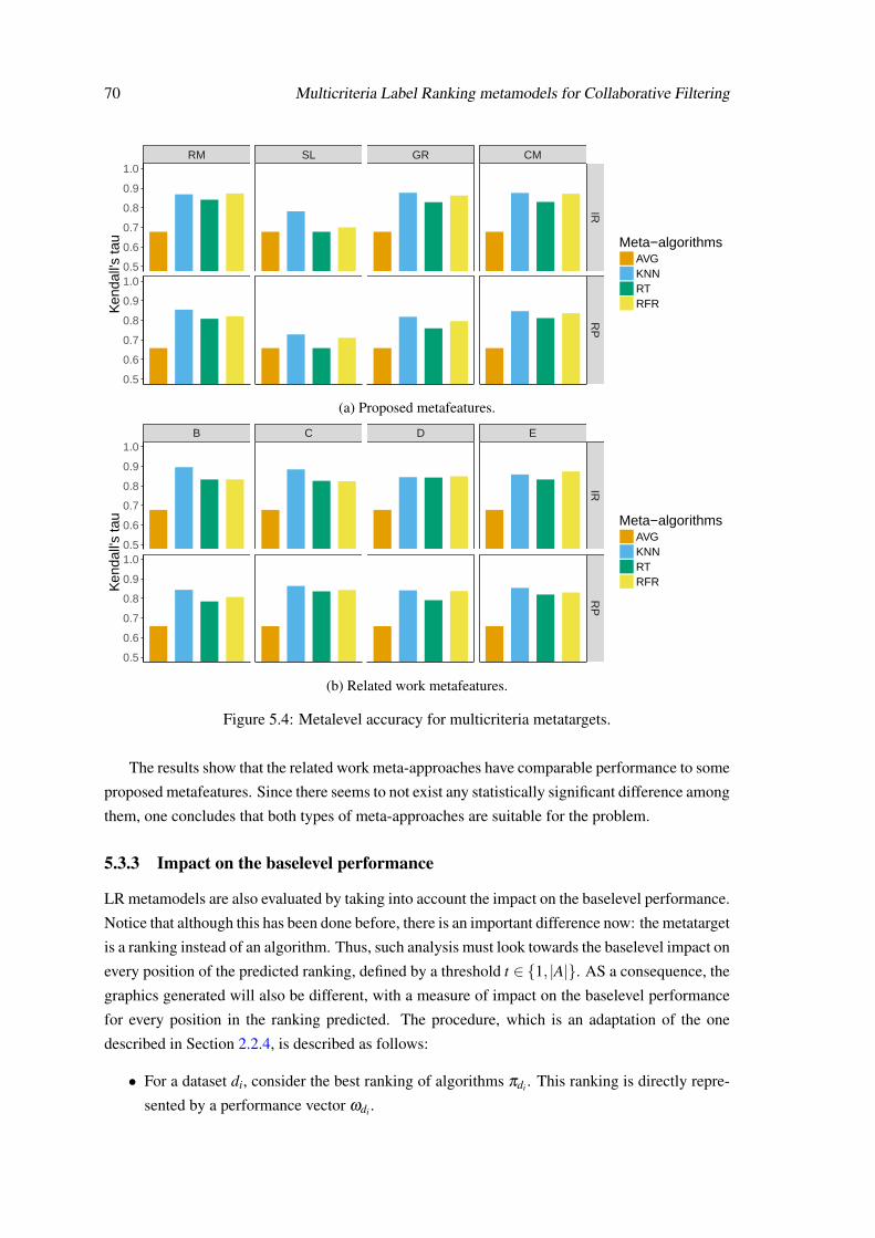
70 Multicriteria Label Ranking metamodels for Collaborative Filtering
RM SL GR CM
IRR
P0.5
0.6
0.7
0.8
0.9
1.0
0.5
0.6
0.7
0.8
0.9
1.0
Ken
dall'
s ta
u Meta−algorithmsAVGKNNRTRFR
(a) Proposed metafeatures.
B C D E
IRR
P
0.5
0.6
0.7
0.8
0.9
1.0
0.5
0.6
0.7
0.8
0.9
1.0
Ken
dall'
s ta
u Meta−algorithmsAVGKNNRTRFR
(b) Related work metafeatures.
Figure 5.4: Metalevel accuracy for multicriteria metatargets.
The results show that the related work meta-approaches have comparable performance to some
proposed metafeatures. Since there seems to not exist any statistically significant difference among
them, one concludes that both types of meta-approaches are suitable for the problem.
5.3.3 Impact on the baselevel performance
LR metamodels are also evaluated by taking into account the impact on the baselevel performance.
Notice that although this has been done before, there is an important difference now: the metatarget
is a ranking instead of an algorithm. Thus, such analysis must look towards the baselevel impact on
every position of the predicted ranking, defined by a threshold t ∈ 1, |A|. AS a consequence, the
graphics generated will also be different, with a measure of impact on the baselevel performance
for every position in the ranking predicted. The procedure, which is an adaptation of the one
described in Section 2.2.4, is described as follows:
• For a dataset di, consider the best ranking of algorithms πdi . This ranking is directly repre-
sented by a performance vector ωdi .

5.3 Results 71
4 5 6 7 8
CD
EC
RMD
CMBGRSLAVG
(a) Single criterion metatarget.
4 5 6 7 8
CD
EBCD
RMCMGRSLAVG
(b) Multicriteria metatarget.
Figure 5.5: Critical Difference diagrams for different metafeatures using LR metamodels.
• Consider now a predicted ranking πdi for di. The respective performance vector ωdi is
created by obtaining the baselevel performances of every algorithm ai from the original
performances ωdi . To do so, the algorithms from πdi and πdi are matched by name.
• The performance vector ωdi is regularized to ensure that at each threshold t (i.e. each pos-
sible ranking position), the values are set to be either better or the same as the previous
threshold value. This is essential due to the nature of the analysis, e.g. if at ranking t = 2
the performance is worse than at t = 1, then the best performance so far should be preserved
in order to fairly evaluate the metamodel.
• The process is repeated for all datasets, obtaining a set of performance vectors. Afterwards,
the performance values are averaged for each threshold value t, creating an average perfor-
mance vector that represents the metamodel performance in terms of baselevel impact.
• Since one aims to calculate the percentage lift, then the performance vector is adjusted
considering the baseline’s performance vector ωdi and the best absolute performance vector
ωdi . This procedure uses the same calculations presented in Equation 2.2.4, but applied to
every threshold t independently.
Now, this analysis is performed for both sets of metafeatures (proposed and related work) and
metatargets (single criterion and multicriteria).
5.3.3.1 Single criterion Metatarget
Figures 5.6a and 5.6b present the percentage lift used to measure the impact on the baselevel
performance for metamodels trained using the single criterion metatargets. Notice the results are

72 Multicriteria Label Ranking metamodels for Collaborative Filtering
presented for every threshold t for all metamodels and that these are different in IR and RP. This
happens due to the different amount of baselearners included in the rankings, respectively 5 and 9.
RM SL GR CMA
UC
ND
CG
NM
AE
RM
SE
1 2 3 4 5 6 7 8 9 1 2 3 4 5 6 7 8 9 1 2 3 4 5 6 7 8 9 1 2 3 4 5 6 7 8 9
0.0
0.5
1.0
1.5
2.0
0.0
0.2
0.4
0.6
−0.050.000.050.100.150.20
−5
0
5
Lift
(%)
KNNRFRT
(a) Proposed metafeatures.
B C D E
AU
CN
DC
GN
MA
ER
MS
E
1 2 3 4 5 6 7 8 9 1 2 3 4 5 6 7 8 9 1 2 3 4 5 6 7 8 9 1 2 3 4 5 6 7 8 9
0.0
0.5
1.0
1.5
2.0
0.0
0.2
0.4
0.0
0.2
0.4
0.6
−5
0
5
10
Lift
(%) KNN
RFRT
(b) Related work metafeatures.
Figure 5.6: Impact on the baselevel performance in single criterion metatargets.
The results show RMSE is the most problematic metatarget, in which only CM, C, D and E
are able to obtain meaningful positive impact. On all other metatargets, all metamodels across

5.3 Results 73
all meta-approaches are able to obtain positive impact. However, the scores obtained depend on
the metatarget: AUC, NDCG, NMAE and RMSE usually have positive impact for t = 1, t < 5,
t < 7 and t < 3. Furthermore, the scores are also different depending on the metatarget: the
maximum improvement for AUC, NDCG, NMAE and RMSE is approximately 2%, 0.6%, 0.6%
and 10%. These results indicate meta-approaches are particularly effective at finding patterns
in all metatargets, with the exception of RMSE. Also, there is no obvious difference between
metafeatures. In fact, the differences are given primarily due to the metamodels used and not
the representative power of the meta-approach. Overall, KNN performs the best in all metatargets
(the only exception is in the RMSE metatarget, where it even achieves negative lift). However, this
pattern is more obvious in the proposed metafeatures than in the related work meta-approaches.
5.3.3.2 Multicriteria Metatarget
Figures 5.7a and 5.7b present the percentage lift used to measure the impact on the baselevel
performance for metamodels trained using multicriteria metatargets.
RM SL GR CM
IRR
P
1 2 3 4 5 6 7 8 9 1 2 3 4 5 6 7 8 9 1 2 3 4 5 6 7 8 9 1 2 3 4 5 6 7 8 9
0.0
0.3
0.6
0.9
0
2
4
Lift
(%)
KNNRFRT
(a) Proposed metafeatures.
B C D E
IRR
P
1 2 3 4 5 6 7 8 9 1 2 3 4 5 6 7 8 9 1 2 3 4 5 6 7 8 9 1 2 3 4 5 6 7 8 9
0.0
0.3
0.6
0.9
0
2
4
6
Lift
(%)
KNNRFRT
(b) Related work metafeatures.
Figure 5.7: Impact on the baselevel performance in multicriteria metatargets.

74 Multicriteria Label Ranking metamodels for Collaborative Filtering
The results show that the performance obtained for all meta-approaches beyond SL are quite
similar: the metamodels have positive influence for t ∈ 1,2 and t = 1 in IR and RP, respectively.
Afterwards, the impact is the same as the baseline. The maximum score achieved is approximately
1% and 6% for IR and RP, respectively. In the case of SL, although the behavior is the same,
the performance obtained is lower. This is particularly evident in the IR metatarget. There is a
difference, however, in terms of metalearners: while in the proposed metafeatures KNN works
best in IR while RT performs best in RP, the related work metafeatures always favor KNN.
5.3.4 Metaknowledge analysis
The analysis shifts now towards metaknowledge analysis, with similar studies as the ones per-
formed in Section 4.4.5: metafeature importance and dataset and baselearner impact analysis.
5.3.4.1 Metafeature importance
Since there is no standard feature importance procedure for Label Ranking, a heuristic strategy
is used instead: to traverse all trees in the RFR metamodels, assign all metafeatures with the
respective tree level (i.e. its ranking) and average the results per metafeature. This score indicates
the metafeature’s global ranking, where lower scores are better. Figure 5.8a shows these results.
The results show most RM metafeatures are statistics from the distribution of the number of
ratings per item. This behavior is different from what it is found in the best algorithm metatarget,
in which only one metafeature of this type was present.
In terms of the SL meta-approach, the best metafeatures belong to RP algorithms. Among
these, there is a particular interest in LFLLM’s performance since it has 2 out of the 3 most
informative metafeatures. However, the most meaningful metafeature overall is BMF.NMAE.
Furthermore, the most important GR metafeatures refer to communities while described by
two functions: alpha and diversity. While alpha has been quite important in the best algorithm
metatarget contributing with 4 metafeatures, the diversity function was not present. Furthermore,
the results show that pairwise and sub-graph levels were the most informative GR metafeatures.
Regarding CM metafeatures, all important metafeatures belong to the RM meta-approach.
This behavior has been observed before in the best algorithm metatarget, meaning there is little
to be gained by using such metafeatures. Furthermore, the most important CM metafeatures are
not the same identified as best in RM, with the exception of R.ratings.skewness: now, the mean
ratings per item yield 2 metafeatures, while the number of ratings per items appears only once.
Moving now to the related work, meta-approach B now favours dataset.density.none. This
differs from the results observed on the previous metatarget, with dataset.ratings.variance being
the best choice. However, user.count.skewness ranks second in both problems.
In meta-approach C, the best and worst metafeatures change places whether the metatarget is
best algorithm selection or to predict the best ranking of algorithms: now, user.variance.mean is
more important than user.count.mean. The second place is still assigned to user.mean.mean.

5.3 Results 75
I.count.entropy
I.count.kurtosis
I.count.mean
I.mean.skewness
R.ratings.skewness
0 20 40 60
RM
BMF.NMAE
LFLLM.NMAE
LFLLM.RMSE
0 1 2 3 4
SL
com.alpha.var.var
com.diver.var.skew
G.sim.var.skew
0 10 20 30
GR
I.count.gini
I.mean.entropy
I.mean.mode
R.ratings.skewness
0 10 20 30 40
CM
Met
afea
ture
impo
rtan
ce (
aver
age
rank
)
(a) Proposed metafeatures.
dataset.density.none
dataset.ratings.variance
item.count.gini
item.count.skewness
user.count.gini
user.count.skewness
0 2 4
B
user.count.mean
user.mean.mean
user.variance.mean
0 1 2
C
item.count.mean
item.entropy.mean
item.mean.mean
user.average_similarity.mean
user.clustering_coefficient.mean
user_coratings.jaccard.mean
user.count.mean
user.mean.mean
user.number_neighbours.mean
user.standard_deviation.mean
user.TFIDF.mean
0 3 6 9
D
dataset.sparsity.none
EC.co−ratings.entropy
EC.co−ratings.gini
0 1 2 3
E
Met
afea
ture
impo
rtan
ce (
aver
age
rank
)
(b) Related work metafeatures.
Figure 5.8: Metafeature importance for LR metamodels using multicriteria metatargets.
Meta-approach D is the one which introduces most changes to the best metafeatures in this
setup: item.count.mean, followed by item.entropy.mean and user.count.mean. None of these is
among the best metafeatures in the previous metatarget.
Lastly, dataset.sparsity.none is still the most informative metafeature in meta-approach E.
Then, EC.co− ratings.entropy is better than EC.co− ratings.gini in this metatarget, unlike what
happens in the best algorithm metatarget.
One final observation lies in the fact that no metafeature holds the same importance in all
meta-approaches. Namely, user.mean.mean ranks 2 and 8 in meta-approaches E and D, respec-
tively. This is expected because more metafeatures mean different patterns can be extracted. This

76 Multicriteria Label Ranking metamodels for Collaborative Filtering
fact indeed makes the metafeature importance analysis volatile, thus inhibiting the definition of
metafeatures which are universally good.
5.3.4.2 Dataset Analysis
Now, the metamodel’s impact on each baselevel dataset is investigated. The procedure is the same
as the one used in Section 4.4.5, but with a difference in the evaluation measure used: now, the
results represent Kendall’s tau instead of accuracy. Figures 5.9 and 5.10 present the results of
such analysis. Notice also that in this setup there are fewer metamodels per meta-approach, thus
justifying the less detail in the violin plots created.
The main pattern observed in the best algorithm metatarget still holds in this setup: the pre-
dictions for AMZ datasets are usually always correct. However, the performance is not always
perfect. This happens due to Kendall’s tau nature, which outputs a continuous score in Leave One
Out cross validation, unlike accuracy which yields a binary score.
Another difference imposed by the evaluation measure lies in the scale of possible values.
Since Kendall’s tau lies in the interval [−1,1], then it is possible to have datasets for which the
predictions have mostly negative correlation. In this regard all meta-approaches produce negative
scores for YH-music, MT-RS14 and ML100k. This shows these datasets are the ones for which is
more difficult to find patterns between metafeatures and the current metatargets. However, while
TA predictions can be negative using proposed metafeatures, the same does not happen in related
work metafeatures.
The results also show the related work metafeatures can attain perfect score in some datasets
which the proposed metafeatures cannot: YH-movies, ML10m and BC. The inverse behavior does
not occur. However, the difference in the maximum performance obtained is rather small, with
multiple proposed metafeatures scoring above 0.9.
Despite these small performance fluctuations, the main pattern observed is the fact that there
is little difference between related work and proposed metafeatures. Once again, the differences
can be observed mostly on a handful of datasets and usually with small variations in performance.
Thus, this analysis concludes that proposed and related work metafeatures are comparable.
5.3.4.3 Baselearner Analysis
The last metaknowledge analysis pertains to the impact of the metafeature representations on the
baselearners. To that end, the algorithm footprints procedure (Muñoz et al., 2018; Smith-Miles
and Tan, 2012) is adapted to inspect the behavior on the top ranking algorithms. Notice this differs
from the previous analysis, where the goal was to establish areas of good and bad performance
per baselearner. Now, we shall observe areas where baselearners are ranked in the interval [1,3].
Figures 5.11 and 5.12 show the results of this adapted algorithm footprints procedure for the
propose and related work metafeatures, respectively. Notice also that datasets which do not assign
a ranking in the predefined interval to a specific baselearner are removed in order to facilitate
analysis.

5.3 Results 77
GR CM
RM SL
0.0 0.5 1.0 0.0 0.5 1.0
0.0 0.5 1.0 0.0 0.5 1.0
AMZ−apps
AMZ−automotive
AMZ−baby
AMZ−beauty
AMZ−cd
AMZ−clothes
AMZ−food
AMZ−games
AMZ−garden
AMZ−health
AMZ−home
AMZ−instruments
AMZ−kindle
AMZ−movies
AMZ−music
AMZ−office
AMZ−pet−supplies
AMZ−phones
AMZ−sports
AMZ−tools
AMZ−toys
AMZ−video
BC
FL
JT1
JT2
JT3
ML100k
ML10m
ML1m
ML20m
ML−latest
MT−latest
MT−RS14
TA
YE
YH−movies
YH−music
value
data
set
Metafeatures
RM
SL
GR
CM
Figure 5.9: Kendall’s tau scores per baselevel dataset for proposed metafeatures.

78 Multicriteria Label Ranking metamodels for Collaborative Filtering
D E
B C
0.0 0.5 1.0 0.0 0.5 1.0
0.0 0.5 1.0 0.0 0.5 1.0
AMZ−apps
AMZ−automotive
AMZ−baby
AMZ−beauty
AMZ−cd
AMZ−clothes
AMZ−food
AMZ−games
AMZ−garden
AMZ−health
AMZ−home
AMZ−instruments
AMZ−kindle
AMZ−movies
AMZ−music
AMZ−office
AMZ−pet−supplies
AMZ−phones
AMZ−sports
AMZ−tools
AMZ−toys
AMZ−video
BC
FL
JT1
JT2
JT3
ML100k
ML10m
ML1m
ML20m
ML−latest
MT−latest
MT−RS14
TA
YE
YH−movies
YH−music
value
data
set
Metafeatures
B
C
D
E
Figure 5.10: Kendall’s tau scores per baselevel dataset for related work metafeatures.

5.3 Results 79
CM GR RM SL
BP
RM
FW
RM
FM
PB
MF
SV
D+
+S
UA
FM
−3 −2 −1 0 1 2 −3 −2 −1 0 1 2 −3 −2 −1 0 1 2 −3 −2 −1 0 1 2
−4
−2
0
2
−4
−2
0
2
−4
−2
0
2
−4
−2
0
2
−4
−2
0
2
−4
−2
0
2
rank 1 2 3
Figure 5.11: Algorithm footprints using rankings for proposed metafeatures.

80 Multicriteria Label Ranking metamodels for Collaborative Filtering
B C D EB
PR
MF
WR
MF
MP
BM
FS
VD
++
SU
AF
M
−2 0 2 4 −2 0 2 4 −2 0 2 4 −2 0 2 4
−4
−2
0
2
−4
−2
0
2
−4
−2
0
2
−4
−2
0
2
−4
−2
0
2
−4
−2
0
2
rank 1 2 3
Figure 5.12: Algorithm footprints using rankings for related work metafeatures.

5.4 Conclusions 81
Even before dwelling in details, there is a clear difference to the previous algorithm footprint
analysis: this representation does not assign the same the preference regions to all baselearners.
Instead, one is able to clearer understand in which areas does one baselearner performs better than
other. Thus, the procedure seems better suited to analyze ranking metatargets.
The results for the proposed metafeatures show an interesting result: some algorithms, from
different CF tasks, have similar representations. This representation has in common the ranking
assigned to the same datasets: while MP and BMF have a similar representation regarding rank
1, BPRMF and SVD++ follow suit but for rank 2. This means that there is a strong relationship
between each pair of algorithms for the same datasets at the top positions in each metatarget.
Another pattern is that the figures complement one another. Notice how the datasets which yield
a rank 1 to MP, also assign a rank 2 to BPRMF.
Furthermore, the results show that all proposed meta-approaches are effective at discerning
between the top three positions in the rankings. This differs from the previous analysis where GR
yielded confusing results. In this regard, the related metafeatures create less obvious representa-
tions, even if in most occurrences there are clear patterns. However, this is mainly due to the fact
that points are more concentrated than in the proposed metafeatures, thus preventing to extract
more meaningful observations.
As a final note, please consider this analysis is made with regards to each baselearner. Since
the metamodels consider more complex and complete metatargets, it is expected the patterns will
not be as clearer. The purpose of this analysis is therefore to understand partial patterns which
may help understand for which baselearners it may easier to discern metafeature impact on their
ranking prediction.
5.4 Conclusions
This Chapter presented a novel way to address CF algorithm selection, where rankings of algo-
rithms are used as metatargets in Label Ranking metamodels. Furthermore, the rankings of al-
gorithms are manipulated through a multicriteria procedure, which creates rankings of algorithms
that consider multiple evaluation measures. All perspectives of the problem have been extensively
validated, using 8 different sets of metafeatures in conjunction with the standard analysis used so
far: metalevel accuracy, impact on the baselevel performance and metaknowledge analysis.
The results show Label Ranking metamodels are suitable to tackle the CF algorithm selection
problem. The results have been particularly stable for the KNN algorithm in all meta-approaches
and metatargets. Furthermore, these metamodels have been effective at solving two issues from
previous experiments, namely class imbalance and limited metaknowledge from not considering
all baselearners in the metatargets. For this reason, LR metamodels are now the baseline to beat
and shall be compared against in the following Chapters. Also, even though the issue is not ap-
proached in this thesis, Learn to rank algorithms directly defined to optimize for ranking accuracy
measures could be investigated, given their merits on ranking problems Burges (2010); Nguyen
et al. (2016).

82 Multicriteria Label Ranking metamodels for Collaborative Filtering
Regarding multicriteria metatargets, the results have shown all metamodels assessed using
these metatargets yield comparable performances to single criterion metatargets. The small fluc-
tuation in results is justified by the fact that the metatargets are actually highly correlated. On one
hand, this impedes further analysis regarding the merits of the proposed approach. On the other,
it reduces the effort required to analyze the MtL process. Further investigations are required,
particularly using other evaluation scopes.
Furthermore, the results have shown that all metafeatures beyond SL are all comparable in both
single criterion and multicriteria metatargets, with no statistically significant differences. Also,
other metaknowledge analysis have clarified that there is no obvious difference in their merits.
Although, this disproves the belief that the proposed metafeatures would be more informative, the
fact is that proposed metafeatures are meaningful, even when considering ranking metatargets.
Thus, we shall use this set of metafeatures exclusively in future experiments.
Moving forward, even though the solutions presented are already suitable for CF algorithm
selection, there are multiple issues which can still be improved. However, considering the efforts
employed so far in terms of metafeatures and metatargets, one argues that the improvement must
be achieved in another scope of the algorithm selection problem: the metalearners. This way, the
next Chapter introduces two types of metamodels: CF4CF and CF4CF-META. While the first does
not use any metafeatures at model fitting, the latter attempts to combine the merits of metafeatures
and the previous metamodel.

Chapter 6
Recommending Recommenders
Although several successful approaches to CF algorithm selection have been presented, the results
have yielded comparable performances for all metafeatures considered. This behavior, accompa-
nied by the fact that it is difficult to understand what the metafeatures actually mean, may lead
to suspicions regarding their predictive power. Therefore, it is essential to understand whether
they bear information or if their predictive power comes from noise or chance. To address this
issue, two different algorithm selection approaches are proposed, which attempt to verify whether
metafeatures are actually important. The goal is to draw conclusions regarding the merits of
metafeatures by analyzing metamodel performance. The proposed metalearners are:
• CF4CF: this approach focusses on the premise that an algorithm selection solution is es-
sentially a recommendation model. Thus, any recommendation algorithm can theoretically
be used to tackle the issue. Therefore, this work proposes CF4CF, a technique which uses
CF algorithms to select the best ranking of CF algorithms for a new problem. It does so by
taking into account only the algorithm performance (either of the entire dataset or a sample
of it - i.e. using subsampling landmarkers). Therefore, this is the only approach known to
date which disregards entirely standard metafeatures. Section 6.1 presents the method.
• CF4CF-META: This approach builds on the good results obtained by the LR approach
presented in Chapter 5 by including algorithmic and metadata changes proposed in CF4CF.
The goal is to capitalize on the integration of both approaches in a unified algorithm selec-
tion framework in order to attempt to improve the predictive performance. Particularly, the
process uses metafeatures from LR and ratings from CF4CF and modifies the LR procedure
to deal with partial rankings at prediction time. This way, not only is it possible to answer
whether metafeatures from LR are informative but also what is the impact of the ratings
used in CF4CF. Section 6.2 presents the proposed method.
This Chapter provides extensive evaluation analysis in order to objectively compare all pro-
posed approaches. The evaluation procedure discussed in Section 6.3 performs the standard evalu-
ation methodologies, namely: metalevel accuracy, impact on the baselevel performance and meta-
knowledge analysis. Lastly, Section 6.4 presents the conclusions found.
83

84 Recommending Recommenders
6.1 CF4CF
The proposal to address CF algorithm selection without explicitly using metafeatures in model
fitting is introduced now: CF4CF. To do so, the nomenclature from Section 5.1 is re-used in
Table 6.1. Notice that F = F ′ ∪F ′′, meaning that metafeatures from both dataset and algorithm
approaches can be used. They are differentiated here since it helps in clarifying the methods
proposed.
Table 6.1: Mapping between Rice’s framework and CF4CF and CF4CF-META.
Sets Description This setup NotationP instances CF datasets di, i ∈ 1, . . . , |P|A algorithms CF algorithms a j, j ∈ 1, . . . , |A|Y performance CF evaluation measures mk,k ∈ 1, . . . , |Y |F ′ CF metafeatures Systematic metafeatures m f l, l ∈ 1, . . . , |F ′|F ′′ algorithm characteristics Subsampling landmarkers slm,m ∈ 1, . . . , |A|× |Y |
CF4CF is a method which allows to use any CF algorithm as the metamodel. To do so, it draws
a parallelism from standard CF recommendation and MtL: users and items can be represented by
datasets and algorithms, respectively. This way, the problem can be formulated as a rating matrix
R, where each dataset di ∈ P and the set of algorithms A where each algorithm a j ∈ A refer to
the rows and columns, respectively. Afterwards, algorithm performance is used to serve as ratings
and therefore complete the matrix. This representation is illustrated in Figure 6.1 and is organized
into training and prediction steps (top, bottom). The prediction stage shows the subsampling
landmarkers εsl and predicted ratings ε .
d a1 a2 a3 . . . a|A|−1 a|A|
d1 ε1 ε2 ε3 . . . ε |A|−1 ε |A|...
.... . . . . . . . . . . .
...
d|P| . . . . . . . . . . . . . . . . . .
dα εsl1 . . . εslN ε1 . . . ε |A|
Figure 6.1: CF4CF metadatabase.
Notice that unlike in standard MtL approaches, no metafeatures are used here. Instead, CF4CF
uses the rankings of algorithms π for every dataset di. Essentially, this algorithm uses only the
metatargets form previous LR metamodels as the sole data source to address algorithm selection.
However, in order to fit a standard CF algorithm and because ratings have the ability to provide
different degrees of preference to each element, the procedure converts such rankings π into ratings

6.2 CF4CF-META 85
ε by a custom linear transformation rat. Formally, to convert the ranking π into a specific ratings
scale S ∈ [smin,smax], the transformation rat is applied to each ranking position l ∈ 1, . . . , |A|:
rat(π, l) =(Smax−Smin)(|A|− l)
|A|−1+Smin (6.1)
This transformation is a combination of an inverse function (to state that high ratings must be
assigned to the algorithm of lower ranking value) and a linear re-scaling function (to adapt the
ordered values to a specific ratings scale). Thus, every dataset di is now described as a ratings
vector ε =(rat(πl)
)|A|l=1. The aggregation of all ratings for all datasets produces the CF4CF’s
rating matrix. Next, a CF algorithm is used to train the metamodel.
The prediction requires initial ratings to be provided to the CF model. However, it is reason-
able to assume that no performance estimations exist for any algorithm at prediction time. Hence,
CF4CF leverages subsampling landmarkers, a performance-based metafeature to obtain initial
data. This way, CF4CF provides NSL subsampling landmarkers to create the initial dataset rep-
resentation and therefore allow the CF model to predict the remaining |A|−NSL ratings. Hence,
a subset of landmarkers (slm)NSLm=1 for dataset dα are converted into the partial ranking π ′. Such
ranking is posteriorly converted into ratings also using the linear transformation rat. Thus, the
initial ratings are now given by εsl =(rat(π ′n)
)NSL
n=1. Providing these εsl ratings, the CF metamodel
is able to predict the missing ε ratings for the remaining algorithms. Considering now the entire
set of ratings r(dα) = εsl∪ ε , the final predicted ranking π is created by decreasingly sorting r(dα)
and assigning the ranking positions to the respective algorithms a j.
6.2 CF4CF-META
CF4CF-META is a hybrid framework which aims to combine both data and algorithmic ap-
proaches from CF4CF and LR metamodels. It is described in Figure 6.2, with datasets di rep-
resented by a union of both types of metafeatures (regular m fl and subsampling landmarkers as
ratings slm) and associated with rankings of algorithms a j. The process is modeled as a Label
Ranking task, similarly to the procedure discussed in Chapter 5. However, the prediction stage is
modified to fit CF4CF’s ability to deal with incomplete data. Thus, the process is organized into
training and prediction stages (top, bottom) and independent and dependent variables (left, right).
d m f 1 . . . m f |F | sl1 . . . . . . sl|A|
d1 ω1 . . . ω |F | ε1 . . . . . . ε |A|...
.... . .
......
. . . . . ....
d|P| . . . . . . . . . . . . . . . . . . . . .
a1 . . . a|A|
π1 . . . π |A|...
. . ....
. . . . . . . . .
dα ω1 . . . ω |F | εsl1 . . . εslN ∅ π1 . . . π |A|
Figure 6.2: CF4CF-META metadatabase.

86 Recommending Recommenders
To build the new metadatabase, every dataset di is submitted to a metafeature extraction pro-
cess, yielding a vector of metafeatures ω = m f (di). Next, the subsampling landmarkers slm are
converted into ratings and leveraged as the remaining metafeatures. Notice, however, that although
this characterization is similar to CF4CF’s, there is a major difference: while in CF4CF the rat-
ings from the original performance were used as training data, here one is bound to use ratings
from subsampling landmarkers. Otherwise, one would be using ratings created from the original
algorithm performance to predict the rankings also obtained from the original algorithm perfor-
mance, which would be an invalid procedure. Thus, the ratings definition considers the ranking
of algorithms π ′ created from all available slm to obtain the ratings ε =(rat(π ′n)
)|A|n=1. The inde-
pendent variables of the algorithm selection problem are now represented as F = ω ∪ ε . To create
the dependent variables, each dataset di is associated with the respective ranking of algorithms π ,
similarly to MtL. A standard Label Ranking algorithm is then used to train the metamodel.
In the prediction stage, the new dataset dα is first submitted to the metafeature extraction pro-
cess, yielding metafeatures ω = m f (dα). Next, like in CF4CF, NSL subsampling landmarkers are
used to create the initial data. Although CF4CF-META allows to use all subsampling landmarkers,
it is important to provide a procedure that allows to calculate fewer landmarkers. This is mostly
due to the significant cost in calculating this type of metafeatures, which CF4CF-META’s aims to
reduce without compromising predictive performance.
Formally, consider a set of landmarkers (slm)Nm=1 for dataset dα and its respective partial rank-
ing π ′. With it, it is possible to obtain the initial ratings εsl =(rat(π ′n)
)Nn=1. Unlike in CF4CF, no
ratings are predicted for the missing values. However, this is not a problem, since CF4CF-META
is able to work with missing values (these are represented in Figure 6.2 by ∅). Aggregating now
the metafeatures m f (dα) = ω ∪ ε ∪∅, one is able to predict π .
6.3 Results
Now, the proposed approaches are validated and compared to some related work competitors.
The evaluation procedure involves metalevel accuracy, impact on the baselevel performance and
metaknowledge analysis, similarly to what has been done in previous Chapters. However, in this
scope a new evaluation perspective is introduced: Top-N evaluation, which uses NDCG to evaluate
the top of the rankings of algorithms predicted.
6.3.1 Experimental setup
The experimental setup used here is divided in two levels, much like in previous Chapters: base-
level (it remains the same as the one presented in Section 3.2.2) and metalevel. The metalevel
used is an extension of the one presented in Section 5.3.1 in the sense that it maintains the usage
of multicriteria metatargets and the metalevel evaluation procedure. However, now there are sev-
eral meta-approaches used, which differ in the algorithms and metadata used. Please notice that
the related work metafeatures identified in Chapter 3 are not considered in this setup. The reasons
are two-fold: 1) they have performed equally well as the metafeatures proposed in Chapter 4 and

6.3 Results 87
2) one aims to reduce the complexity of results to be analyzed and feel that such analysis has been
covered in previous experiments. Having said this, the total set of meta-approaches considered
include the proposed approaches and 3 baseline meta-approaches (LR, ALORS and ASLIB):
• CF4CF It is analyzed in two variations, given by the CF algorithm used: ALS or UBCF.
• CF4CF-META This proposal is analyzed in terms of multiple perspectives: algorithms (i.e.
KNN, RT and RFR) and metadata (i.e. RM, GR and CM).
• LR This baseline is the one proposed in Chapter 5. All metafeatures (RM, SL, GR and CM)
and all meta-algorithms (KNN, RT and RFR) are considered.
• ALORS The method introduced by (Mısır and Sebag, 2017) is an algorithm selection ap-
proach which uses CF algorithms as metamodels (see Section 2.3). Since the original source
code was not available, this work has implemented the solution as similar as possible. Thus,
the regression and MF algorithms selected are the Multivariate Random Forest and ALS,
respectively. The metafeatures used are RM, SL, GR and CM.
• ASLIB The final baseline refers to a general purpose algorithm selection framework (Bischl
et al., 2015). This framework is able to address multiple algorithm selection tasks, namely
to predict the performance of all algorithms or the best algorithm only, respectively. Thus,
it employs standard regression and classification algorithms to do so. However, it does
not offer any direct solution to predict rankings of algorithms. The standard procedure is
modified by using the regression approach to learn the mappings between metafeatures and
targets and posteriorly rank the algorithms according to the scores predicted. This approach
is evaluated for multiple metafeatures (RM, SL, GR and CM) and uses the following algo-
rithms from the MLR package (Bischl et al., 2016): Generalized Linear Regression Model
(LM), XGBOOST, SVM, Regularized Random Forests (RRF), RPART and RKNN.
The extensive list of results for all variations proposed are listed in Appendix D. The results
are presented independently per approach in all evaluation perspectives considered. However, to
simplify the readability, only the best solution for each approach is considered as its represen-
tative: CF4CF (using ALS), CF4CF-META (KNN with RM metafeatures), LR (RFR with CM
metafeatures), ALORS (with CM metafeatures) and ASLIB (RKNN with CM metafeatures).
Lastly, please notice the results presented can be reproduced by accessing the repository
https://github.com/tiagodscunha/cf4cf.
6.3.2 Meta-accuracy
Meta-accuracy in terms of Kendall’s Tau coefficient are analyzed here in two perspectives: first,
one aims to understand the effect that the amount of subsampling landmarkers (NSL) holds in both
CF4CF and CF4CF-META. Thus, a threshold sensitivity analysis is conducted. Afterwards, all
meta-approaches are compared in a similar fashion to what has been done in previous Chapters.
Notice that in the latter case, the meta-approaches considered use their best settings.

88 Recommending Recommenders
6.3.2.1 Threshold Sensitivity
The threshold sensitivity analysis results for CF4CF and CF4CF-META are presented in Fig-
ures 6.3 and 6.4, respectively. The results present the Kendall’s Tau performance for all NSL
considered in each metatarget. Recall that 1 ≤ NSL ≤ |A| − 1. Furthermore, the baseline is also
included to facilitate the analysis.
IR RP
1 2 3 4 1 2 3 4 5 6 7 8
0.2
0.4
0.6
0.8
Sampled
Ken
dall'
s Ta
u
AlgorithmAVGCF4CF−ALSCF4CF−UBCF
Figure 6.3: CF4CF threshold sensitivity analysis.
IR RP
1 2 3 4 1 2 3 4 5 6 7 80.65
0.70
0.75
0.80
0.85
Sampled
Ken
dall'
s Ta
u AlgorithmAVGCF4CF−META−KNNCF4CF−META−RFRCF4CF−META−RT
Figure 6.4: CF4CF-META threshold sensitivity analysis.
The results show CF4CF works on IR but not in RP, since it is only able to beat the baseline for
NSL = 4. However, since it performs poorly otherwise, it shows an inconsistent behavior. On the
other hand, CF4CF-META works very well on both metatargets will all metamodels outperform-
ing the baseline in all threshold NSL. More importantly, CF4CF-META works better than CF4CF
even for NSL = 1. This means that the combination of metafeatures and ratings has positive impact,
thus indicating the existence of information in both representations.
In terms of CF4CF metalearners, UBCF and ALS performance is quite similar. This happens
in most threshold NSL, although in the best case scenario ALS has a slight advantage. In CF4CF-
META’s case, the advantage leans towards RT and RFR in IR and RP, respectively. However,
KNN is the only metalearner for which the amount of SL has a positive impact. This means only
metalearners which use distance-based heuristics are able to capture meaningful relationships from
the subsampling landmarkers provided.

6.3 Results 89
Overall, the best performance results throughout are achieved with the maximum amount of
subsampling landmarkers. The results show that this has a greater importance in CF4CF than in
CF4CF-META. This is another indication that metafeatures are informative.
6.3.2.2 Comparison to related work
Now, the focus lies on the Kendall’s tau performance for all meta-approaches considered. The
results are presented in Figure 6.5 for all meta-approaches selected.
IR RP
0.00
0.25
0.50
0.75
Ken
dall'
s ta
u
Meta−algorithmsALORSASLIBAVGCF4CFCF4CF_METALR
Figure 6.5: Kendall’s tau for all meta-approaches.
The results show only three meta-approaches beat the baseline in both metatargets: ALORS,
CF4CF-META AND LR. On the other hand, CF4CF only performs well in IR, while ASLIB is
worse than the baseline in both metatargets. The first results can be explained by the fact that
ratings are not always enough by themselves. As for the ASLIB results, it clearly shows that the
adaptation of a regression approach to predict rankings of algorithms is not a suitable approach.
The results clearly show that the best meta-approaches are CF4CF-META and LR, although
there seems to be very small differences between them. In order to validate these observations,
the statistical validation test used in Section 5.3.2.3 is re-used. The corresponding CD diagram is
presented in Figure 6.6.
2 3 4 5 6
CD
CF4CF_METALR
ALORS
CF4CFAVGASLIB
Figure 6.6: Critical Difference diagram.
The analysis confirms the observations, since there is no statistically significant difference
between CF4CF-META and LR. Furthermore, ALORS is proven to be better than the baseline,
while ASLIB performs much worse. Lastly, there is no significant difference between CF4CF and
the baseline.

90 Recommending Recommenders
6.3.3 Top-N Metalevel Accuracy
Notice also that the metalevel evaluation considers now an extra evaluation step: Top-N evaluation.
This aims to evaluate how good are the top N positions in the ranking instead of considering the
complete ranking of algorithms. The rationale is simple: since the algorithms in the top positions
are the most interesting, it is important to assess how well do the metamodels perform in this
task. Thus, NDCG is employed to evaluate the predictions of metamodels. Notice that N has
different values depending on the metatarget chosen, i.e. N = 1,2,3 and N = 1,3,5 for the
IR and RP metatargets, respectively. This decision is justified by the fact that IR and RP have a
different amount of algorithms in the rankings, namely 5 and 9 respectively. Thus, such thresholds
were selected since they represent algorithms in the interval between the best (N = 1) and mean
performances (N = 3 or N = 5).
Now, the focus lies on analyzing how good are the metamodels considering only the top po-
sitions in the predicted rankings of algorithms. To do so, Figures 6.7 and 6.8 presents the NDCG
results for all the meta-approaches considered in the IR and RP metatargets, respectively.
NDCG@1 NDCG@2 NDCG@3
IR
0.00
0.25
0.50
0.75
1.00
ND
CG
Meta−algorithmsALORSASLIBAVGCF4CFCF4CF_METALR
Figure 6.7: NDCG metalevel evaluation in the Item Recommendation problem.
NDCG@1 NDCG@3 NDCG@5
RP
0.00
0.25
0.50
0.75
1.00
ND
CG
Meta−algorithmsALORSASLIBAVGCF4CFCF4CF_METALR
Figure 6.8: NDCG metalevel evaluation in the Rating Prediction problem.
The results show that ASLIB is never able to beat the baseline and that overall CF4CF and
ALORS perform poorly, although there are some cases where they marginally beat the baseline.
These are important results which mean that their ability to predict the top positions in the ranking
is poor or quite similar to the baseline’s.

6.3 Results 91
Furthermore, the results also show CF4CF-META works well in terms of NDCG. Unfortu-
nately, it does so only for N = 1, while performing worse than the baseline for the remaining
thresholds selected. This means that the proposed approach is best suited to select the absolute
best algorithm and not necessarily the remaining algorithms in the top positions. Lastly, the re-
sults show that LR is the only meta-approach to systematically beat the baseline, even if it doesn’t
always achieve the best performance. Thus, in this evaluation scope, it is clearly the best approach.
6.3.4 Impact on the baselevel performance
The next analysis is about the impact on the baselevel performance. To do so, the procedure
explained in Section 5.3.3 is replicated. The results for this experimental setup are displayed in
Figure 6.9.
IR RP
1 2 3 4 5 1 2 3 4 5 6 7 8 9
0.0
2.5
5.0
Lift
(%) ALORS
ASLIBCF4CFCF4CF_METALR
Figure 6.9: Impact on the baselevel performance.
According to the results, most meta-approaches prove useful for t ∈ 1,2 and t ≤ 6 for IR
and RP, respectively. Among these, LR and CF4CF-META perform quite well and reach a maxi-
mum improvement of approximately 1% and 7% in IR and RP, respectively. However, the results
also show that ASLIB and CF4CF perform quite poorly since they achieve negative lift for most
thresholds for IR and RP, respectively. ALORS performs well in both metatargets, but without
ever standing out.
6.3.5 Metaknowledge analysis
The current metaknowledge analysis procedures focuses on two issues: metafeature importance
and dataset impact analysis. Here, the baselearner impact analysis using algorithm footprints is
not investigated since such results are only dependent on the metafeatures and metatargets. Since
this Chapter focus entirely on the metalearners, there are no new results to be obtained.
6.3.5.1 Metafeature importance
To perform the analysis regarding metafeature importance, the process used in Section 5.3.4 is re-
used. Notice that CF4CF-META is used with a RFR metamodel, which takes advantage of both

92 Recommending Recommenders
CM metafeatures and the performance ratings. This has been chosen taking into account the best
settings found in previous experiments. Figure 6.10 presents the results of such analysis.
I.mean.entropy
I.sum.entropy
I.sum.skew
MP
0 5 10 15
IR
I.count.min
I.mean.entropy
I.mean.kurtosis
I.mean.mode
I.sum.skew
nusers
0 5 10 15
RP
Met
afea
ture
impo
rtan
ce (
aver
age
rank
)
Figure 6.10: Metafeature importance for CF4CF-META metamodels.
The results show that there is no rating-based metafeature in the top metafeatures selected
for Rating Prediction, while in Item Recommendation MP ratings are the third best metafeature.
This means that rating data is more important to Item Recommendation, while CM metafeatures
perform better in Rating Prediction. However, even in this case, no similarities could be found in
terms of metafeatures when comparing to CF4CF-META’s results without using ratings metafea-
tures. This points to the observation that ratings actually have influence in the process, changing
the patterns that are found within the metamodel.
6.3.5.2 Dataset analysis
This analysis mimics the ones used so far to understand the influence of metafeatures on baselevel
datasets through metamodel performance. However, since the focus of this Chapter lies with the
MtL frameworks, then the results are aggregated differently. In essence, the results contain the per-
formances for all metalearners trained on all metafeatures and metatargets considered, aggregated
by MtL framework. The results are presented in Figure 6.11.
The results show CF4CF-META and LR have similar patterns, with a higher skew towards
perfect scores. This is explained by the usage of LR metamodels in both approaches. ALORS ap-
pears next with an approximate behavior to the previous frameworks, although with fewer perfect
performances. On the other hand, in some datasets the performances have less variation, showing
consistency.
CF4CF provides lower average performances than LR, CF4CF-META and ALORS. Its results
are more unstable, as shown by the skew of the violin plots. However, it still performs better than
ASLIB. This behavior is clear when one considers three observations: there is higher variations of
results, the mean Kendall’s tau lies near zero and it is the MtL framework with more scores near
-1 (i.e. imperfect score).

6.3 Results 93
LR
CF4CF CF4CF_META
ALORS ASLIB
−0.5 0.0 0.5 1.0
−0.5 0.0 0.5 1.0 −0.5 0.0 0.5 1.0
−0.5 0.0 0.5 1.0 −1.0 −0.5 0.0 0.5 1.0
AMZ−appsAMZ−automotive
AMZ−babyAMZ−beauty
AMZ−cdAMZ−clothes
AMZ−foodAMZ−gamesAMZ−gardenAMZ−healthAMZ−home
AMZ−instrumentsAMZ−kindle
AMZ−moviesAMZ−musicAMZ−office
AMZ−pet−suppliesAMZ−phonesAMZ−sports
AMZ−toolsAMZ−toys
AMZ−videoBCFL
JT1JT2JT3
ML100kML10m
ML1mML20m
ML−latestMT−latestMT−RS14
TAYE
YH−moviesYH−music
AMZ−appsAMZ−automotive
AMZ−babyAMZ−beauty
AMZ−cdAMZ−clothes
AMZ−foodAMZ−gamesAMZ−gardenAMZ−healthAMZ−home
AMZ−instrumentsAMZ−kindle
AMZ−moviesAMZ−musicAMZ−office
AMZ−pet−suppliesAMZ−phonesAMZ−sports
AMZ−toolsAMZ−toys
AMZ−videoBCFL
JT1JT2JT3
ML100kML10mML1m
ML20mML−latestMT−latestMT−RS14
TAYE
YH−moviesYH−music
Metalearners
ALORS
ASLIB
CF4CF
CF4CF_META
LR
Figure 6.11: Kendall’s tau scores per baselevel dataset for all metalearners proposed.

94 Recommending Recommenders
6.4 Conclusions
This Chapter introduced two novel CF algorithm selection frameworks: CF4CF and CF4CF-
META. Their main difference lies in the metafeatures used for model fitting and which is the
algorithm selected to induce the metamodel: CF4CF uses only algorithm performance as ratings
and subsampling landmarkers in a customized CF algorithm, while CF4CF-META leverages stan-
dard metafeatures and the algorithm performance as ratings from CF4CF in a LR metamodel.
An extensive experimental analysis has been performed and in which three baselines have
been included: the previously proposed LR metamodels, ALORS and the generic algorithm selec-
tion framework ASLIB. The results have shown that CF4CF has informative power, especially in
the Item Recommendation problem. Thus, it was shown that it is possible to perform algorithm
selection without metafeatures. However, it also shows inconsistent results, since it does perform
poorly in multiple evaluation scopes. Thus, this behavior puts into question whether using only
the ratings from algorithm performance is enough.
CF4CF-META, however, has proved itself consistent throughout the several evaluation anal-
ysis, especially in terms of the top position of the ranking. Furthermore, CF4CF-META solves
a critical problem in CF4CF, by performing better when using a reduced amount of subsampling
landmarkers used at prediction time. Thus, although the primary motivation for the proposal of
these approaches has been regarding the investigation of the merits of metafeatures in CF algorithm
selection, it is now known that CF4CF-META is the best solution to the CF algorithm selection
problem.
Regarding the baselines, the results also show that LR still maintains itself as an excellent
solution, even beating CF4CF-META in multiple occasions. In fact, statistical validation has
shown that there is no significant difference between them in terms of Kendall’s tau. Further-
more, although ALORS works well in all evaluation scopes, it rarely does so as well as LR and
CF4CF-META. However, ASLIB performs poorly in all evaluation scopes selected. Although the
framework has proven successful in other domains, these results are an indication that it is not
properly designed to handle ranking metatargets nor is it a good fit to CF algorithm selection.
The investigations regarding the merits of metafeatures have shown that the data used in
CF4CF-META has different impact depending on the CF task addressed: rating data is more im-
portant to Item Recommendation, while systematic metafeatures perform better in Rating Predic-
tion. However, by considering the performance of CF4CF and CF4CF-META meta-approaches,
one is also able to draw further conclusions regarding the merits of metafeatures: 1) metafeatures
are indeed informative, since CF4CF-META is better than CF4CF and 2) there is information in
ratings obtained from algorithm performance, since CF4CF-META performs slightly better than
LR. Having established that metafeatures are actually meaningful, the focus shifts now towards
another approach to metafeature design on Chapter 7, which aims to remove the human from the
metafeature generation process.

Chapter 7
cf2vec: dataset embeddings
As seen in Chapters 4 and 5, CF metafeatures tend to perform roughly the same, even when
multiple perspectives of the problem are chosen to create the metafeatures. Despite proving that
they indeed hold informative power in Chapter 6, the experiments show that it is not possible to
obtain a unique dataset characterization technique that outperforms all others. This points to the
fact that a new perspective of the problem should be considered in order to achieve the goal.
In this Chapter, the starting point for all current metafeature generation processes is put into
question. Namely, notice that all metafeatures are hand tailored, meaning it is the MtL practi-
tioner’s experience and perspective of the problem which dictates which characterization measures
are suitable for the task at hand. Therefore, the authors argue that an algorithmic-centric approach
may be better to approach the problem.
To do so, the work shifts focus to an alternative: Representational Learning (RL) (Bengio
et al., 2013). Such techniques use ML algorithms and domain knowledge to learn alternative and
potentially richer representations for a given problem. Examples of successful applications can be
found in text classification (Bengio et al., 2013) and image recognition (He et al., 2016). However,
to the best of the author’s knowledge, this approach has never been used for algorithm selection.
In this Chapter, a RL approach is used to automatically design metafeatures for the prob-
lem of CF algorithm selection. Namely, a distributed representations technique is employed:
graph2vec (Narayanan et al., 2017). To do so, inspiration is drawn from the CF graph for-
mulation used to derive graph-based metafeatures presented in Chapter 4. However, instead of at-
tempting to describe the problem using complex hand designed metafeatures, the current proposal
aims to use graph2vec in order to create a dataset embedding representation. Such representa-
tion consists of a set of latent metafeatures, which aim to replace traditional metafeatures.
The Chapter is organized as follows: the dataset embedding technique cf2vec is presented
in Section 7.1, while Section 7.2 presents the extensive evaluation procedure conducted to verify
the merits of such metafeatures. Lastly, Section 7.3 highlights the main conclusions of the impact
of the proposed methodology in CF algorithm selection.
95

96 cf2vec: dataset embeddings
7.1 cf2vec: Distributed Representations as CF metafeatures
This section introduces the main contribution of this work: cf2vec. Next, its essential steps are
presented: 1) to create the CF graph, 2) to reduce the problem complexity via graph sampling, 3)
to learn the distributed representations and 4) to train a metamodel with alternative metafeatures.
7.1.1 Convert CF matrix into graph
CF is usually described by a rating matrix R|U |×|I|, representing a set of users U and items I. Each
element of this matrix is the feedback provided by each user for each item. Figure 7.1a shows a
toy example of a rating matrix. Recall that in order to use graph2vec, the input elements must
be graphs. Thus, the CF graph formulation, discussed in Section 4.3, is re-used here. The process
has shown that a CF rating matrix can be seen as an adjacency matrix. This allows to directly
construct a bipartite graph G, whose nodes U and I represent users and items, respectively. The
edges E connects elements of the two groups and represent the feedback provided by users to
items. The edges can be weighted in order to represent preference values (ratings). Figure 7.1b
shows the conversion of the toy example from Figure 7.1a.
i1 i2 i3
u1 5 3 4
u2 4 . . . 2
u3 . . . 3 5
(a) Rating Matrix example.
u1
u2
u3
i1i2i3
U I53
44
23
5
(b) Bipartite Graph.
Figure 7.1: Toy example for two different CF representations.
7.1.2 Sampling graphs
An important part of metafeature design is the effort required (Vanschoren, 2010): if the task is
slower than training and evaluating all algorithms on the new problem, then it is useless. Consid-
ering how CF graphs can reach quite large sizes, this is a pressing issue and it motivates reducing
the problem dimensionality. Since one is not interested in the actual time required, but rather on
reducing the amount of data to be processed in order to reduce the time needed, the focus lies on
investigating which is the minimum amount of data which allows to maintain a high predictive
performance.
Thus, an intermediate (but not mandatory) step is added: graph sampling. In order to find a
distributed representation as closely related as possible to the entire graph, a sampling technique
able to preserve the graph structural properties must be chosen. According to (Leskovec and
Faloutsos, 2006), a good choice is random walk. It performs multiple explorations of graph paths
until θ nodes are reached and uses all of them to obtain the respective sub-graph.

7.1 cf2vec: Distributed Representations as CF metafeatures 97
7.1.3 Learn distributed representation
Taking advantage of graph2vec’s agnostic nature, one argues that the problem can be defined
as follows: given a set of CF graphs G = g1,g2, ... and a positive integer σ referring to the
distributed representation size, one aims to learn a σ -dimensional distributed representation for
every graph. Hence, this process creates a matrix of distributed representations E |G|×σ , which can
be regarded as the metafeatures for all considered graphs (and by extension, to all CF problems).
This procedure requires two steps: 1) to extract of rooted sub-graphs and 2) to learn matrix E.
7.1.3.1 Extract rooted sub-graphs
A rooted sub-graph sgδn is composed by the set of nodes (and corresponding edges) around node
n ∈ gi that are reachable in δ hops. Learning the distributed representation requires the extraction
of rooted sub-graphs for all nodes. Thus, N nodes are used, with N = |U |+ |I|.Rooted sub-graphs in graph2vec are generated using the Weisfeiler-Lehman relabeling pro-
cedure (Shervashidze et al., 2011). Beyond being able to inspect neighboring nodes, it is also able
to incorporate information about the neighbors in a single node’s name. As a result, it creates
a rich textual description for every graph. To do so, it traverses each node in the rub-graph and
uses all neighbors as the current node label at each iteration. Next, it replaces the original node
labels by new compressed names, which represent a neighborhood structure. The process repeats
until d hops are reached. Every rooted sub-graph can be represented by a numeric vector with the
frequency that each node (original or compressed) appears in the representation, similar to one-hot
encoding.
7.1.3.2 Learn matrix E
Consider now the parallelism between adjacent edges connecting nodes and the sequence of words
in a given vocabulary, then the skipgram model can be used straightforwardly. As it can be seen
in Figure 7.2, each graph gi is represented by its identifier and connected to δ context rooted sub-
graphs sg. Training such a neural network allows to learn similar distributed representations for
graphs with similar rooted sub-graphs.
. . .gi
sg1
sgδ
. . .E |G|×σ
Cσ×N
Cσ×N
Figure 7.2: Skipgram architecture used in graph2vec (Narayanan et al., 2017).
In order to learn the weights, then one must train the network. The learning process, based on
Stochastic Gradient Descent, iterates on these steps until conversion is achieved: 1) feedforward

98 cf2vec: dataset embeddings
weights from input to the output layer, 2) application of a softmax classifier to compare the output
layer’s weights with the sub-graph representations and 3) backpropagation of the errors through
the network. Doing so, it learns matrices E and C, which represent the distributed representations
and context matrices, respectively. Notice the skipgram is trained using Negative Sampling, which
refrains from using all sub-graphs of a specific graph. Instead, it takes advantage of few random
sub-graphs that do not belong to the graph. This way, training is more efficient.
7.1.4 Learn metamodel
Notice that matrix E can be considered as independent variables to any predictive problem and,
as a consequence, can be easily used as metafeatures. Thus, every problem pi is described by in-
dependent variables (the i-th row of matrix E) and the dependent variables (the respective ranking
of algorithms). Obtaining these pairs for all gi, allows to create a metadatabase like the one in
Figure 7.3.
P f 1() . . . f |F |()
p1 ω1 . . . ω |F |...
.... . .
...
p|P| . . . . . . . . .
a1 . . . a|A|
π1 . . . π |A|...
. . ....
. . . . . . . . .
pα ω1 . . . ω |F | π1 . . . π |A|
Figure 7.3: Label Ranking Metadatabase.
Formally, the submission of all problems pi (i.e. gi) to cf2vec produces the metafeatures ω =
f (pi). To create the dependent variables, each problem pi is associated with the respective ranking
of algorithms π , based on the performance values for a specific evaluation measure yk ∈ Y . This
ranking considers a static ordering of the algorithms a j (using for instance an alphabetical order)
and is composed by a permutation of values 1, ..., |A|. These values indicate, for each position
l, the respective ranking. Notice also that the work does not make any imposition regarding which
is the technique chosen to create the ranking of algorithms. The authors have decided to take
advantage of multicriteria metatargets discussed in Section 5.2. A learning algorithm is then used
to induce a metamodel which learns the mapping between dataset embeddings and the metatarget.
In order to make predictions, the metamodel can be applied to metafeatures ω extracted from a
new problem pα to predict its best ranking of algorithms π . Notice that ω are now obtained by
taking advantage of the pre-trained neural network. This means the neural network is able to make
the predictions of which is the dataset embedding, simply by considering the CF graph. Therefore,
the prediction step is efficient.
Considering how the CF algorithm selection problem has been addressed so far in this Thesis,
the ideal solution is Label Ranking, which has been explained in Section 5.1. Although this formu-
lation is favored, since it allows to validate the merits of these metafeatures by considering them

7.2 Results 99
alone, the MtL process is not limited to such metamodels. This means that other meta-algorithms,
such as the ones reviewed in Chapter 6, can take advantage of such dataset embeddings.
7.2 Results
Now the focus lies on properly evaluating the aforementioned proposal. To do so, the same eval-
uation scopes from previous Chapters are re-used, namely: metalevel accuracy, impact on the
baselevel performance and metaknowledge analysis.
7.2.1 Experimental setup
The experimental setup used here is divided in two levels, much like in previous Chapters: base-
level (it remains the same as the one presented in Section 3.2.2) and metalevel. This metalevel uses
2 meta-approaches (LR and CF4CF-META), both represented by KNN meta-algorithm which was
chosen due to its superior predictive performance. Furthermore, two types of metafeatures (CM
and cf2vec) are used in conjunction with multicriteria metatargets. Thus, the metalevel differs
only from the one in Section 6.3.1 since it adds a new set of metafeatures: cf2vec. The complete
list of meta-approaches considered here is:
• LR+CM: KNN LR meta-algorithm using CM metafeatures.
• LR+cf2vec: KNN LR meta-algorithm using cf2vec metafeatures.
• CF4CF-META+CM: KNN CF4CF-META meta-algorithm using CM metafeatures.
• CF4CF-META+cf2vec: KNN CF4CF-META meta-algorithm using cf2vec metafeatures.
• AVG: Average Rankings.
Notice that the best metamodels which use CM metafeatures have been selected based on
the experimental results detailed in Appendix D. Furthermore, notice that the results are directly
comparable to those presented using multicriteria metatargets in Chapters 5 and 6, since the ex-
perimental details are precisely the same, apart from the meta-approaches used.
One important issue to address in cf2vec is the hyperparameter optimization since depending
on their settings, different representations are produced. This work pays special attention to δ and
σ , since they were shown to be the most important in (Mikolov et al., 2013). An analysis of the
sensitivity of such hyperparameters is presented in Section 7.2.2, where all hyperparameters were
tuned using grid search (Bergstra and Bengio, 2012).
Lastly, please notice the results presented can be reproduced by accessing the repository
https://github.com/tiagodscunha/cf2vec.
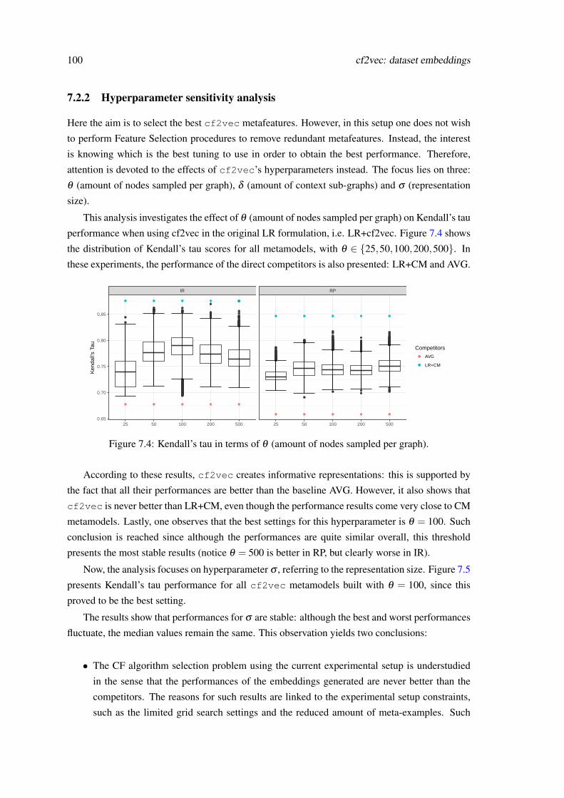
100 cf2vec: dataset embeddings
7.2.2 Hyperparameter sensitivity analysis
Here the aim is to select the best cf2vec metafeatures. However, in this setup one does not wish
to perform Feature Selection procedures to remove redundant metafeatures. Instead, the interest
is knowing which is the best tuning to use in order to obtain the best performance. Therefore,
attention is devoted to the effects of cf2vec’s hyperparameters instead. The focus lies on three:
θ (amount of nodes sampled per graph), δ (amount of context sub-graphs) and σ (representation
size).
This analysis investigates the effect of θ (amount of nodes sampled per graph) on Kendall’s tau
performance when using cf2vec in the original LR formulation, i.e. LR+cf2vec. Figure 7.4 shows
the distribution of Kendall’s tau scores for all metamodels, with θ ∈ 25,50,100,200,500. In
these experiments, the performance of the direct competitors is also presented: LR+CM and AVG.
IR RP
25 50 100 200 500 25 50 100 200 5000.65
0.70
0.75
0.80
0.85
Ken
dall'
s Ta
u
Competitors
AVG
LR+CM
Figure 7.4: Kendall’s tau in terms of θ (amount of nodes sampled per graph).
According to these results, cf2vec creates informative representations: this is supported by
the fact that all their performances are better than the baseline AVG. However, it also shows that
cf2vec is never better than LR+CM, even though the performance results come very close to CM
metamodels. Lastly, one observes that the best settings for this hyperparameter is θ = 100. Such
conclusion is reached since although the performances are quite similar overall, this threshold
presents the most stable results (notice θ = 500 is better in RP, but clearly worse in IR).
Now, the analysis focuses on hyperparameter σ , referring to the representation size. Figure 7.5
presents Kendall’s tau performance for all cf2vec metamodels built with θ = 100, since this
proved to be the best setting.
The results show that performances for σ are stable: although the best and worst performances
fluctuate, the median values remain the same. This observation yields two conclusions:
• The CF algorithm selection problem using the current experimental setup is understudied
in the sense that the performances of the embeddings generated are never better than the
competitors. The reasons for such results are linked to the experimental setup constraints,
such as the limited grid search settings and the reduced amount of meta-examples. Such

7.2 Results 101
IR RP
10 20 30 50 100 200 10 20 30 50 100 2000.65
0.70
0.75
0.80
0.85K
enda
ll's
Tau
Competitors
AVG
LR+CM
Figure 7.5: Kendall’s tau in terms of σ (distributed representation size).
constraints have proven to be too strong for a unsupervised RL technique, which is heavily
dependent on the availability of data.
• Furthermore, the results also show that the experimental setup is flawed in the sense that it
may be possible to achieve the same results with a even lower σ value. The consequence
in this case is that we may be looking at perhaps 2 or 3 metafeatures which may be able to
explain the entire mapping between metafeatures and metatargets. In this Thesis, this issue
is not approached, but it remains an interesting topic for future research.
This analysis considers the effects of the amount of context sub-graphs (i.e. δ ) on Figure 7.6.
IR RP
3 4 5 6 7 8 3 4 5 6 7 80.65
0.70
0.75
0.80
0.85
Ken
dall'
s Ta
u
Competitors
AVG
LR+CM
Figure 7.6: Kendall’s tau in terms of δ (context sub-graphs).
According to these results, hyperparameter δ has a significant impact on the predictive perfor-
mance: both metatargets increase their performance until δ = 6. Soon after, their performances
decrease. However, lower amounts of context sub-graphs lead to better performance (observe how
δ ∈ 3,4,5 perform better than δ = 8).

102 cf2vec: dataset embeddings
7.2.3 Metalevel accuracy
Although the independent impact of hyperparameters has been analyzed, one must select the best
cf2vec hyperparameter settings for both CF problems. To illustrate how the performance is
distributed, Figure 7.7 presents the Kendall’s tau performances. Notice the results are zoomed,
thus showing only the best performing metamodels. The metamodels are identified by σ and δ .
0.80
0.82
0.84
0.86
0.77 0.78 0.79 0.80 0.81 0.82
RP
IR
σ10
20
30
50
100
200
δ3
4
5
6
7
8
Figure 7.7: Performance scatter plot. Each axis represents the performance that each metamodelhas achieved in each CF problem. The metamodels are also characterized in terms of the σ and δ
hyperparameters.
The results show that metamodels with δ = 6 occupy the vast majority of performances that
simultaneously maximize the performance on both tasks. Among these, the best hyperparameter
settings correspond to the performance point placed at (0.805,0.858), in which σ = 30. The meta-
model trained with this hyperparameter settings is henceforth used as cf2vec’s representative.
Taking these settings into consideration, an extensive evaluation in terms of Kendall’s tau has
been performed for all meta-approaches listed previously. Figure 7.8 presents the results of all
meta-approaches.
IR RP
0.00
0.25
0.50
0.75
Ken
dall'
s ta
u Meta−algorithmsAVGCF4CF−META+cf2vecCF4CF−META+CMLR+cf2vecLR+CM
Figure 7.8: Metalevel accuracy.
The results show that all meta-approaches are better than the baseline, thus proving their use-
fulness. The results also show that LR+CM and CF4CF-META+CM yield the best results, closely
followed by LR+cf2vec. In the last position one finds CF4CF-META+cf2vec. These results seem
to point out that cf2vec metafeatures are not as informative as CM, regardless of whether LR

7.2 Results 103
or CF4CF-META are used. To verify the observations, CD diagrams (Demšar, 2006) have been
employed once again. Figure 7.9 shows the results for all meta-approaches considered.
2 3 4 5
CD
CF4CF−META+CMLR+CM
LR+cf2vecCF4CF−META+cf2vecAVG
Figure 7.9: Critical difference diagram.
The results confirm the previous observations. Furthermore, they show that there is no statis-
tically significant difference between CF4CF-META+CM, LR+CM and LR+cf2vec, even though
the latter is ranked lower. However, it is now possible to see that both CF4CF-META+CM and
LR+CM are indeed better than CF4CF-META+cf2vec, while LR+cf2vec only outperforms the
baseline with statistically significant differences. In essence, these results show that despite not
being able to outperform CM metafeatures, cf2vec is able to produce as good metafeatures as
the ones proposed in Chapter 4.
7.2.4 Impact on the baselevel performance
The next analysis is about the impact on the baselevel performance. To do so, the procedure
explained in Section 5.3.3 is re-used. Furthermore, the results for this experimental setup are
displayed in Figure 7.10.
IR RP
1 2 3 4 5 1 2 3 4 5 6 7 8 9
0
2
4
6
8
Lift
(%) LR+cf2vec
LR+CMCF4CF−META+cf2vecCF4CF−META+CM
Figure 7.10: Impact on the baselevel performance.
The results show that in IR all meta-approaches perform well for t ∈ 1,2. Among these, the
best results are achieved by metamodels with CM metafeatures and achieve over 1% improvement
for t = 1. However, in RP the results are very different: the best performing metamodels belong
to LR technique and they perform above the baseline for t ≤ 7. Notice that in this case, cf2vec
metafeatures are the ones which perform best. Furthermore, CF4CF-META metamodels under-
perform, although those with CM metafeatures are able to perform well for t ≤ 7, while those

104 cf2vec: dataset embeddings
using cf2vec metafeatures have inconsistent results, usually close to the baseline’s performance.
In summary, these results show that cf2vec obtains a comparable (and even higher) baselevel
performance to the remaining metafeatures, depending on the CF problem addressed.
7.2.5 Metaknowledge analysis
Recall that previous metaknowledge analysis involved ascertaining the most important metafea-
tures, by means of feature importance procedures. The goal was to understand which of the pro-
posed metafeatures were most meaningful in hope to state which are the CF characteristics which
influence algorithm performance. However, cf2vec creates latent metafeatures, which have no
clear meaning. Therefore, such analysis, although possible, is useless. Thus, this metaknowledge
analysis focus instead on assessing the impact of metamodels on the baselevel datasets and also to
compare which metafeatures create clearer patterns with regards to the metatargets used.
7.2.5.1 Dataset analysis
This analysis extends upon the procedure used in Section 6.3.5 by considering not only the MtL
frameworks but also including the metafeatures used. This way, one is able to assess how these
two dimensions impact the baselevel datasets. Figure 7.11 shows the results of such analysis.
The results show metamodels using CM metafeatures perform very similarly regardless of the
MtL framework chosen. On the other hand, cf2vec seems to favor LR metamodels, given these
attain slightly better performances. However, CF4CF-META has less variations in performance,
which also indicates merits regarding consistency. Once again, results show there is no universally
best meta-approach overall. This provides further evidence metafeatures have equal performance,
ultimately validating the proposed cf2vec meta-approach.
7.2.5.2 Metafeature analysis
Like in Section 5.3.4, one proposes to analyze the metaknowledge by considering the metafeatures
and their relationship to the metatargets. This has been done using adaptations of the algorithm
footprint procedure (Muñoz et al., 2018; Smith-Miles and Tan, 2012). However, as seen before,
none of the solutions is ideal to consider the complete ranking of algorithms used in Label Ranking
metatargets. Thus, a new technique is used to assess such impact, which considers full rankings.
The procedure still performs PCA to reduce the metafeatures to a 2-dimensional space. Notice
other techniques have also been studied at this time, namely t-sne (Van Der Maaten and Hinton,
2008). However, the experimental results have shown it did not yield better results than PCA,
therefore it was discarded. Also, each metadataset is plotted and associated with data from the
metatarget. However, instead of considering the good vs bad performance from algorithm foot-
prints or even the ranking position of algorithms in the posteriorly adapted procedure, one assigns
each dataset with the complete ranking of algorithms. To differentiate among metatargets, a color
is assigned to each individual metatarget. Notice colors are assigned based on metatarget similarity
given by string comparison. This highlights clear patterns between metafeatures and metatargets:

7.2 Results 105
CF4CF_META LR
cf2vecC
M
0.0 0.5 1.0 0.0 0.5 1.0
AMZ−apps
AMZ−automotive
AMZ−baby
AMZ−beauty
AMZ−cd
AMZ−clothes
AMZ−food
AMZ−games
AMZ−garden
AMZ−health
AMZ−home
AMZ−instruments
AMZ−kindle
AMZ−movies
AMZ−music
AMZ−office
AMZ−pet−supplies
AMZ−phones
AMZ−sports
AMZ−tools
AMZ−toys
AMZ−video
BC
FL
JT1
JT2
JT3
ML100k
ML10m
ML1m
ML20m
ML−latest
MT−latest
MT−RS14
TA
YE
YH−movies
YH−music
AMZ−apps
AMZ−automotive
AMZ−baby
AMZ−beauty
AMZ−cd
AMZ−clothes
AMZ−food
AMZ−games
AMZ−garden
AMZ−health
AMZ−home
AMZ−instruments
AMZ−kindle
AMZ−movies
AMZ−music
AMZ−office
AMZ−pet−supplies
AMZ−phones
AMZ−sports
AMZ−tools
AMZ−toys
AMZ−video
BC
FL
JT1
JT2
JT3
ML100k
ML10m
ML1m
ML20m
ML−latest
MT−latest
MT−RS14
TA
YE
YH−movies
YH−music
Figure 7.11: Kendall’s tau scores per baselevel dataset for all metalearners (i.e. CF4CF-METAand LR) and metafeatures (cf2vec and CM).

106 cf2vec: dataset embeddings
if similar (or the same) metatargets are assigned to two similar datasets (placed near one another),
then the representation allows to properly identify the metatarget, thus creating a valid pattern.
Figures 7.12 and 7.13 illustrate the results for Item Recommendation and Rating Prediction, re-
spectively.
AMZ−appsAMZ−automotiveAMZ−baby
AMZ−beauty
AMZ−cd AMZ−clothesAMZ−music
AMZ−foodAMZ−games
AMZ−garden
AMZ−health
AMZ−home
AMZ−video
AMZ−instrumentsAMZ−kindle
AMZ−movies
AMZ−office
AMZ−pet−suppliesAMZ−phones
AMZ−sports
AMZ−tools
AMZ−toys
BCFLJT1JT2
JT3ML100k
ML10m
ML1m
ML20m
ML−latestMT−latest
MT−RS14TA
YH−moviesYH−music
YE
AMZ−appsAMZ−automotive
AMZ−babyAMZ−beauty
AMZ−cd
AMZ−clothes
AMZ−music
AMZ−food
AMZ−gamesAMZ−garden
AMZ−healthAMZ−home
AMZ−video
AMZ−instruments
AMZ−kindle
AMZ−movies
AMZ−office AMZ−pet−supplies
AMZ−phones
AMZ−sports
AMZ−tools
AMZ−toys
BCFL
JT1JT2
JT3ML100k
ML10m
ML1m
ML20m
ML−latestMT−latestMT−RS14
TA
YH−movies
YH−music
YE
cf4vecC
M
−2 0 2
−2
0
2
4
−2
0
2
4
Metatarget
BPRMF,MP,WRMF,SMRMF,WBPRMF
BPRMF,WBPRMF,MP,SMRMF
BPRMF,WRMF,SMRMF,WBPRMF,MP
MP,BPRMF,SMRMF,WBPRMF
MP,BPRMF,SMRMF,WRMF,WBPRMF
MP,BPRMF,WRMF,SMRMF,WBPRMF
MP,WBPRMF,WRMF,BPRMF,SMRMF
MP,WRMF,BPRMF,SMRMF
MP,WRMF,BPRMF,SMRMF,WBPRMF
MP,WRMF,BPRMF,WBPRMF,SMRMF
WRMF,BPRMF,MP,SMRMF,WBPRMF
WRMF,BPRMF,MP,WBPRMF,SMRMF
WRMF,BPRMF,WBPRMF,SMRMF,MP
WRMF,WBPRMF,BPRMF,MP,SMRMF
Figure 7.12: Metadata visualization for the Item Recommendation problem.
The results show that both metafeatures work well in two cases, in which the same metatargets
are assigned to datasets placed near one another:
• Same domain and similar metatargets: most datasets from the same domain have clearly
visible patterns in the mappings between metafeatures and metatargets. This occurs for the
AMZ and JT domains, where most data points are placed near each other and have similar
colors assigned.
• Different domains but similar metatargets: some datasets from different domains, and shar-
ing similar metatargets, are close to each other. This happens for the BC and FL datasets in
Item Recommendation and for the YE and FL datasets in Rating Prediction.
The previous observations refer to the easily predictable meta-instances. The fact that both
types of metafeatures are able to properly map the instances together is a good reason to explain
why they perform well for the majority of datasets. However, some problems were found:
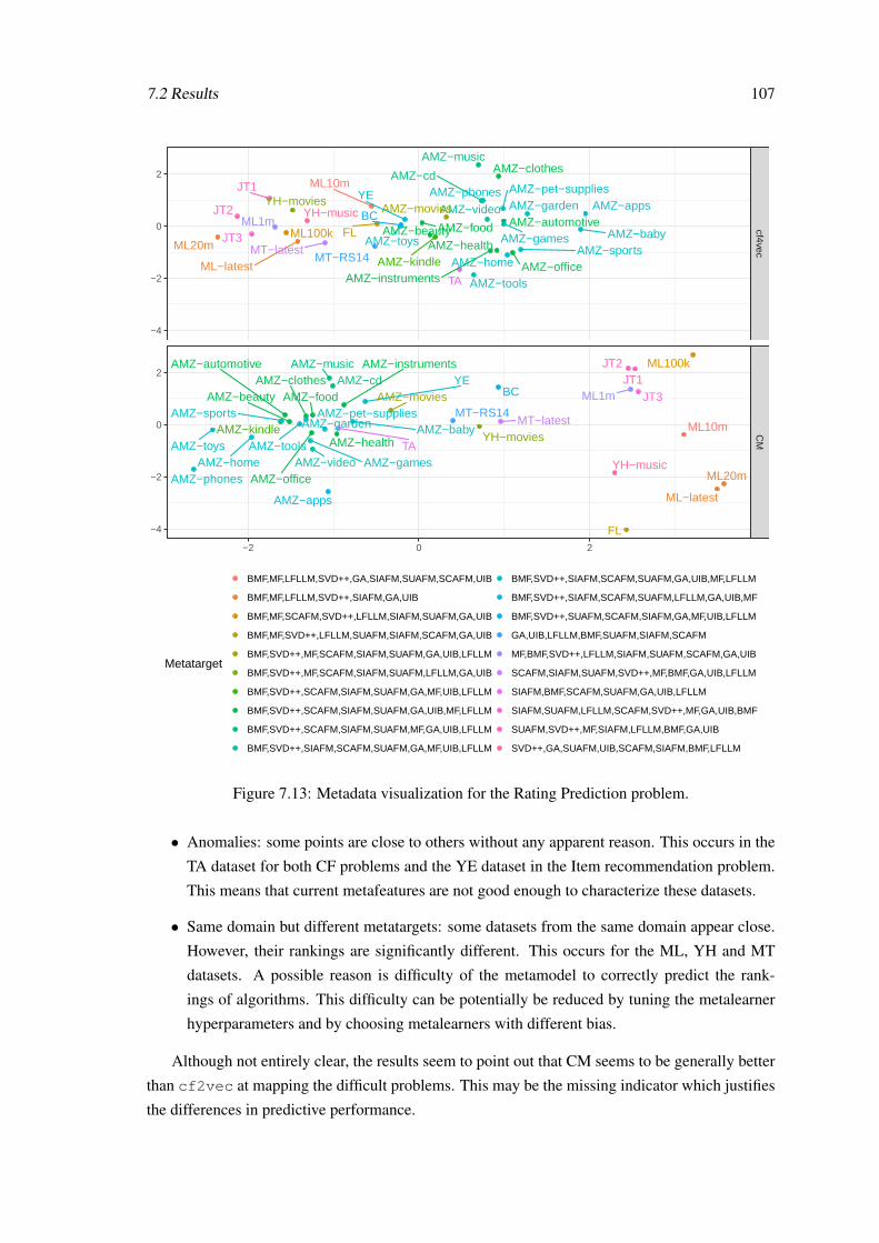
7.2 Results 107
AMZ−appsAMZ−automotive
AMZ−babyAMZ−beauty
AMZ−cdAMZ−clothes
AMZ−music
AMZ−foodAMZ−games
AMZ−garden
AMZ−healthAMZ−home
AMZ−video
AMZ−instrumentsAMZ−kindle
AMZ−movies
AMZ−office
AMZ−pet−suppliesAMZ−phones
AMZ−sports
AMZ−tools
AMZ−toys
BCFL
JT1
JT2
JT3 ML100k
ML10m
ML1m
ML20m
ML−latestMT−latest
MT−RS14
TA
YH−moviesYH−music
YE
AMZ−apps
AMZ−automotive
AMZ−baby
AMZ−beautyAMZ−cdAMZ−clothes
AMZ−music
AMZ−food
AMZ−games
AMZ−garden
AMZ−health
AMZ−home AMZ−video
AMZ−instruments
AMZ−kindle
AMZ−movies
AMZ−office
AMZ−pet−supplies
AMZ−phones
AMZ−sports
AMZ−toolsAMZ−toys
BC
FL
JT1JT2
JT3
ML100k
ML10m
ML1m
ML20m
ML−latest
MT−latestMT−RS14
TAYH−movies
YH−music
YE
cf4vecC
M
−2 0 2
−4
−2
0
2
−4
−2
0
2
Metatarget
BMF,MF,LFLLM,SVD++,GA,SIAFM,SUAFM,SCAFM,UIB
BMF,MF,LFLLM,SVD++,SIAFM,GA,UIB
BMF,MF,SCAFM,SVD++,LFLLM,SIAFM,SUAFM,GA,UIB
BMF,MF,SVD++,LFLLM,SUAFM,SIAFM,SCAFM,GA,UIB
BMF,SVD++,MF,SCAFM,SIAFM,SUAFM,GA,UIB,LFLLM
BMF,SVD++,MF,SCAFM,SIAFM,SUAFM,LFLLM,GA,UIB
BMF,SVD++,SCAFM,SIAFM,SUAFM,GA,MF,UIB,LFLLM
BMF,SVD++,SCAFM,SIAFM,SUAFM,GA,UIB,MF,LFLLM
BMF,SVD++,SCAFM,SIAFM,SUAFM,MF,GA,UIB,LFLLM
BMF,SVD++,SIAFM,SCAFM,SUAFM,GA,MF,UIB,LFLLM
BMF,SVD++,SIAFM,SCAFM,SUAFM,GA,UIB,MF,LFLLM
BMF,SVD++,SIAFM,SCAFM,SUAFM,LFLLM,GA,UIB,MF
BMF,SVD++,SUAFM,SCAFM,SIAFM,GA,MF,UIB,LFLLM
GA,UIB,LFLLM,BMF,SUAFM,SIAFM,SCAFM
MF,BMF,SVD++,LFLLM,SIAFM,SUAFM,SCAFM,GA,UIB
SCAFM,SIAFM,SUAFM,SVD++,MF,BMF,GA,UIB,LFLLM
SIAFM,BMF,SCAFM,SUAFM,GA,UIB,LFLLM
SIAFM,SUAFM,LFLLM,SCAFM,SVD++,MF,GA,UIB,BMF
SUAFM,SVD++,MF,SIAFM,LFLLM,BMF,GA,UIB
SVD++,GA,SUAFM,UIB,SCAFM,SIAFM,BMF,LFLLM
Figure 7.13: Metadata visualization for the Rating Prediction problem.
• Anomalies: some points are close to others without any apparent reason. This occurs in the
TA dataset for both CF problems and the YE dataset in the Item recommendation problem.
This means that current metafeatures are not good enough to characterize these datasets.
• Same domain but different metatargets: some datasets from the same domain appear close.
However, their rankings are significantly different. This occurs for the ML, YH and MT
datasets. A possible reason is difficulty of the metamodel to correctly predict the rank-
ings of algorithms. This difficulty can be potentially be reduced by tuning the metalearner
hyperparameters and by choosing metalearners with different bias.
Although not entirely clear, the results seem to point out that CM seems to be generally better
than cf2vec at mapping the difficult problems. This may be the missing indicator which justifies
the differences in predictive performance.

108 cf2vec: dataset embeddings
Having said this, it is important to understand that the analysis presented is limited in several
aspects: (1) the metafeatures processed via PCA are not directly used in the metamodel and (2) the
analysis with regards to the assignment of datasets to metatargets is informal. Thus, the authors
acknowledge that the validity of the conclusions observed is limited and must therefore be consid-
ered only in terms of exploratory data analysis and not as a proxy for the metamodel’s ability to
find the mappings between metafeatures and metatargets.
Lastly, the representations provided by PCA, allow a visual inspection of the mapping between
metafeatures and metatargets. Although it has been quite helpful in the extraction of metaknowl-
edge, it poses a question regarding whether the metafeatures proposed would benefit from such
transformation previous to the metalearner fitting. This issue has not been addressed in this The-
sis, yet it remains an interesting research point for future works and applications of the proposed
contributions.
7.3 Conclusions
This Chapter introduced a novel technique for CF metafeature extraction: cf2vec. It adapts a
known distributed representation technique graph2vec to the context of CF algorithm selection.
To do so, the procedure converts CF datasets into graphs, reduces the problem complexity via
graph sampling, learns the distributed representation and uses them as alternative metafeatures.
An extensive experimental study has been conducted, which allowed to understand which are
cf2vec’s best hyperparameter settings, namely θ = 100, δ = 6 and σ = 30. However, more
importantly, the results show that all hyperparameter settings tried are able to outperform the
baseline, thus showing beyond any doubt that cf2vec creates informative CF representations.
Furthermore, it has been shown that the proposed approach performs approximately the same as
other CF metafeatures in terms of metalevel accuracy and impact of the baselevel performance,
even though it is unable to surpass them at any point. Despite this, the results have shown that there
is no statistically significant difference between them. Furthermore, the results show that a simple
LR approach is better suited for cf2vec metafeatures, with CF4CF-META performing worse.
This observation leads to the conclusion that such representations do not benefit from the added
information provided by the performance ratings, unlike what happened in previous Chapters.
Thus, the proposed technique holds an important advantage in the sense that the metafeatures
are automatically generated without any human intervention, while reaching the same performance
as the state-of-the-art metafeatures. However, cf2vec’s predictive performance is never able to
outperform other metafeatures. This has been justified by the metaknowledge analysis procedure,
which showed that CM metafeatures are slightly better at discriminating datasets. These results
arise from the fact that RL techniques require much more data than other metafeature generation
processes. Therefore, the authors believe that using 38 CF datasets is the only impediment which
prevents this technique to reach its full potential.
Furthermore, the results have shown that the current solution still has room for improvement,
given by the possibility of having the same predictive performance using representations of even

7.3 Conclusions 109
lower cardinality and that dimensionality reduction techniques may be helpful not only in cf2vec,
but also in all proposed metafeatures. Such conclusions, even though highlighting the limitations
of the current state of affairs, allow to further cement and guide the future research in the field. In
this topic, one main idea comes to mind: to change the learning procedure by including simulta-
neously the embedding learning stage and the MtL predictive procedure. Such approach, which
would be the first MtL RL task-specific solution, would enable to find embeddings while taking
into account network structure and algorithm performance.

110 cf2vec: dataset embeddings
Chapter 8
Conclusions and Future Work
This Chapter provides the main conclusions, limitations and future work research regarding all
proposed contributions to the CF algorithm selection problems studied in this Thesis.
8.1 Conclusions
This Thesis has presented a systematic literature review on the CF algorithm selection problem.
It was shown that there are few and not properly explored approaches to the problem, mainly
characterized by the analysis of Nearest Neighbours performance using at most 4 datasets. This
analysis allowed to identify the problems which needed to be addressed and how to position the
work developed throughout the Thesis. This Thesis has successfully built on such works in terms
of multiple aspects of the problem, namely: metafeatures, metalearners and metatargets.
The research has continued via an empirical study, which compared the related work ap-
proaches. This has yielded important results, which served as the starting point for further propos-
als. The experiments proved that the related work metafeatures contain useful information since
their performance has been well positioned above the baseline. In fact, its performance has been
proven to be so good that it justified their usage throughout the Thesis. They have maintained a
positive performance, making themselves hard to beat in multiple variations of the CF algorithm
selection problem studied.
Even so, various efforts were undertaken to improve the solutions available to the problem.
These new proposals, varying in terms of metafeatures, metatargets and metalearners, have en-
abled to deepen the understanding of the task at hand. The experimental results have shown that
the vast majority of solutions is able to provide meaningful metamodels, thus showing their im-
portance. In fact, only in two cases this observation does not hold: while using SL metafeatures in
LR metamodels and CF4CF metamodels in the Rating Prediction problem. Such results are quite
encouraging since it effectively means that the proposals introduced are useful.
In terms of the proposed metafeatures, it is clear that this thesis has gone above and beyond
in finding new ways to describe the CF datasets, in an effort to attempt to improve upon the re-
lated work metafeatures performance. The wide range of metafeatures proposed included 4 sets
111

112 Conclusions and Future Work
of metafeatures based on the adaptation of standard metafeature extraction procedures to the CF
domain (RM, SL, GR and CM) and cf2vec, an automatic approach to build CF dataset represen-
tations using distributed representations technique. All have proved useful, since they consistently
outperform the baseline. However, the results show that there is no statistically significant differ-
ence to the metafeatures proposed in the related work. The extensive experimental results have
shown that RM and CM seem to be the most consistent and meaningful, even though most RM
metafeatures belong to CM. Regarding cf2vec, it was observed that the process always provides
informative representations, regardless of the hyperparameter settings used.
The metatargets have also been an important topic of study in this Thesis. The initial solu-
tions for algorithm selection problem used only the best algorithm, as it is usual in other MtL
solutions. However, it was soon moved towards a ranking approach, since it was observed that
there was important information discarded from the process. Thus, the problem has been modeled
using LR metamodels in order to predict complete rankings of algorithms. This solution allows to
predict the complete ranking of algorithms, having proved to be effective even in Top-N analysis.
Furthermore, the ranking metatargets used in this solution were modified by incorporating the in-
puts of multiple evaluation measures in a single ranking of algorithms, thus creating multicriteria
metatargets. The validation of this solution has been straightforward since the rankings of algo-
rithms are fairly similar for most datasets. As a consequence, this technique allowed for easier
comprehension of results and fairer assignment of algorithms to the respective rank.
Furthermore, multiple classes of metalearners have been introduced. Their arisal has become
necessary due to the different nature of metatargets considered. The first experiments, which
were modeled as classification tasks, were addressed using standard classification algorithms. The
experimental results have shown that xgboost provides the best results by beating its competitors
in multiple evaluation scopes. Afterwards, in order to use rankings of algorithms in the metatarget,
three novel techniques to CF algorithm selection were introduced: LR, CF4CF and CF4CF-META.
The supremacy of LR and CF4CF-META was proved regarding the direct competitors ASLIB and
ALORS in multiple evaluation scopes. Although not consistently, CF4CF has shown that it is
possible to perform algorithm selection without any metafeatures. In terms of metalearners, KNN
has outperformed RT and RFR in several tasks.
Lastly, despite the fact that the Thesis started by empirically comparing only the related work
approaches, the entire empirical studies in this Thesis were designed to be both incremental and
comparable. To do so, much of the settings from the experimental setups in previous Chapters
are re-used. This paradigm has also allowed to incrementally modify the CF algorithm selection
pipeline depending on the conclusions found for particular contributions in hope to improve the
predictive performance. Furthermore, it was shown that such organization has helped in organiz-
ing the Thesis structure and therefore help in the interpretation of results across Chapters. Such
procedure has also been extended to metaknowledge analysis, which allowed to increasingly create
more advanced and enriched representations to assess the impact of the MtL solutions developed
both on the baselearners and baselevel datasets.

8.2 Limitations 113
8.2 Limitations
However, despite presenting an extensive study on the CF algorithm selection problem, some lim-
itations exist: first and foremost, although this Thesis has effectively improved the experimental
setups used in so far related works, there are still elements which are still not ideal in the exper-
imental setup. Three main issues are identified: datasets, algorithms and evaluation measures.
First, the amount of datasets used in reduced when compared to other MtL studies in other do-
mains. The main implication is that this prevents us from obtaining a suitable amount of data
points in the metadatabase, which impedes to extract more stable conclusions from the MtL anal-
ysis performed. However, when considering the CF scope, this is clearly better than the related
meta-approaches and even empirical studies (Huang et al., 2007; Panniello et al., 2009; Adomavi-
cius and Zhang, 2010; Vargas and Castells, 2011; O’Doherty et al., 2012; Kluver and Konstan,
2014; Ekstrand et al., 2014; Guo et al., 2014). This issue arises because there are few public
datasets available. Regarding the algorithms used, although the selected set is suitable and more
extensive than in the related work, it focuses only on MF algorithms. Research in CF has now
moved towards more advanced algorithms, including Deep Learning (Wu et al., 2016; He et al.,
2017), which it is not covered in this Thesis. Lastly, 4 evaluation measures are used throughout
the Thesis in order to evaluate the recommendations, which also proved to be an improvement.
However, this selection means that concepts such as novelty, satisfaction and diversity are not
considered in these studies.
Another important limitation in this work lies in the fact that only the default hyperparameters
are considered for the CF algorithms in the baselevel. Although this directly impacts the results
since the optimal results are not considered, such approach was deemed necessary due to computa-
tional time constraints. In such cases, the MtL studies tend to reduce the number of configurations
tested and thus save valuable time (Vanschoren, 2018). The limitation in this case is that the
predictions obtained from the metamodels must be used to use in a warm-start setting alone, i.e.
simply to guide the selection process, leaving the hyperparameter optimization in charge of the
practitioner.
Lastly, although multiple and diverse metalevel frameworks have been used, the list of avail-
able algorithms in each task has not been exhausted. This has been seen in Label Ranking and
Collaborative Filtering meta-approaches, where algorithms such as Approximate Ranking Tree
Forests (Sun and Pfahringer, 2013) and other MF approaches beyond ALS have been excluded.
This decision has been made since the selected set of metalearners is representative and because
one does not wish to further complicate the metalevel configurations used. Despite this, it is be-
lieved that not using Learn to Rank algorithms may be the main limitation in this issue. The
preference towards Label Ranking algorithms lies in the motivation to predict the full ranking of
algorithms, considering all their relative positions equally. However, as discussed previously, it is
usually the algorithms on the top ranking positions which are most interesting. To minimize the
impact of such limitation, a Top-N metalevel analysis using NDCG has been used to assess LR
merits on such task.
114 Conclusions and Future Work
8.3 Future Work
The following directions for future work are proposed:
• Baselevel experimental setup There are several ways to address the limitations identified
earlier. However, the authors would like to highlight a selected few, which are considered
to be of the utmost importance: to use implicit feedback datasets (since they are now more
frequently available), to include other CF algorithms (particularly by extending the exper-
iments to other more updated recommendation frameworks), inclusion of multiple offline
evaluation measures from different evaluation scopes and lastly, to replace offline evalua-
tions from the results of online evaluations in order to create the metatargets of algorithms.
• Expand contributions to other domains Notice that several contributions presented, al-
though designed for CF algorithm selection, are suitable to many other domains. Namely, it
would be interesting to assess the impact of graph-based and cf2vec metafeatures, multi-
criteria metatargets and all 3 meta-frameworks proposed: LR, CF4CF and CF4CF-META.
• Other Recommendation strategies Recall that there is only one related work approach
which studies algorithm selection in RS beyond CF. Particularly, the paper studied the pre-
diction of the best ranking of heuristics for Group Recommendations. However, there are
multiple other recommendation approaches, such as Content Based or Hybrid RS, which
have not yet been addressed. The authors would like to highlight a contribution made in this
subject, where a set of tensor metafeatures were proposed to predict rankings of Tensor Fac-
torization algorithms for Context-aware Recommendations (Cunha et al., 2017). Further-
more, the Label Ranking formulation presented in Chapter 5 was also employed. Although
the work was removed from this Thesis due to organizational purposes, it is important to
acknowledge the existence of this novel technique, especially since it derives from the con-
tributions presented in this Thesis.
• Representational Learning Perhaps one of the most interesting contributions of this work
is the cf2vec, which enabled to automatically create CF metafeatures without any human
interaction in the decision process. As far as the authors know, this has been the first attempt
to do so in the context of CF. Therefore, this is an interesting direction for future work. As a
starting point, we suggest a recent survey on graph embedding techniques, which provides
multiple suitable candidates Goyal and Ferrara (2018).
• Deep Metalearning One current research trend is the usage of Deep Learning MtL solu-
tions (Santoro et al., 2016; Edwards and Storkey, 2017; Mishra et al., 2017; Li et al., 2017;
Vartak et al., 2017). However, as far as the know, there is no existing solution to this issue
which applies directly to CF algorithm selection. However, given the maturity of meta-
knowledge generated from this Thesis, it may be interesting to explore the application of
such techniques to the scope of CF algorithm selection.

8.3 Future Work 115
• User Algorithm Selection Recall that the current work has focused on the selection of the
best algorithm(s) per dataset. However, particularly in the context of RS, one could perform
algorithm selection on a user level. Despite the fact that this problem has already been
addressed in the related work (Griffith et al., 2012; Ekstrand and Riedl, 2012; Collins et al.,
2018), there are multiple ways to expand upon it. One example could focus on the adaptation
of the methods proposed in this Thesis. Furthermore, techniques such as Contextual Bandits
could be an interesting solution to perform an user algorithm selection approach.
• AutoML Notice that all contributions presented in this Thesis have focused on the algorithm
selection problem. However, the current trend in MtL lies with AutoML solutions, which
focus on the entire ML pipeline, including the algorithm selection step. Therefore, it may
be important to assess the merits of such solutions on the CF problem, using for instance
the wide range of metafeatures proposed. In fact, the research could even approach novel
AutoML approaches, which leverage CF as metalearners (Fusi and Elibol, 2017; Yang et al.,
2018) and apply it to the CF problem.

116 Conclusions and Future Work

Appendix A
Offline evaluation metrics
Here the offline evaluation metrics are presented and organized by type: rating accuracy, rat-
ing correlation, classification accuracy, ranking accuracy, satisfaction, coverage and diversity and
lastly novelty.
A.1 Rating accuracy
These metrics are characterized by measuring the difference between the predicted rating and the
actual rating. Therefore, it is considered the predicted rating for user u to item i as pui and the real
rating as rui. N and N are the total amount of predicted ratings and the total amount of ratings,
respectively Herlocker et al. (2004); Jiang et al. (2011).
MAE =∑
Nk=1 |pui− rui|
N(A.1)
MSE =∑
Nk=1(pui− rui)
2
N(A.2)
RMSE =
√∑
Nk=1(pui− rui)2
N(A.3)
NMAE =MAE
∑Ml=0 rui
M
(A.4)
117

118 Offline evaluation metrics
A.2 Rating correlation
The metrics calculate the correlation between the predicted and the true ratings Lü et al. (2012).
Therefore, it is considered the predicted rating for user u to item i as pui and the real rating as rui.
p and r are the average of the predicted ratings and the average of real ratings, respectively.
Pearson =∑α(pui− p)(rui− r)√
∑α(pui− p)√
∑α(rui− r)(A.5)
The Spearman’s correlation is very similar to Pearson’s although the ratings pui and rui are
replaced by the rankings rpui and rrui:
Spearman =∑α(rpui− p)(rrui− r)√
∑α(rpui− p)√
∑α(rrui− r)(A.6)
In the case of Kendall’s Tau, the computation is rather different. The variables used are C and
D respectively for the number of concordant and discordant pairs. A pair is concordant if the RS
predicts its ranking correctly or discordant otherwise. St is the number of object pairs for which
the true ratings are the same, and Sp is the number of object pairs for which the predicted ratings
are the same.
τ =C−D√
(C+D+St)(C+D+Sp(A.7)
A.3 Classification accuracy
These metrics are IR based and their formulations are widely known. In the adaptation to RS, one
must consider that the precision is the proportion of recommendations that are good recommenda-
tions, and recall is the proportion of good recommendations that appear in top recommendations
Gunawardana and Shani (2009). It is possible to measure if a recommendation is good by assign-
ing it to a class that is deemed satisfactory. For instance, in explicit feedback it is possible to state
a threshold to define when a recommendation is good while on implicit feedback one can consider
that it is either good or bad.
Table A.1: Confusion Matrix
Recommended Not recommendedPreferred True Positives (TP) False Negatives (FN)Not preferred False Positives (FP) True Negatives (TN)
The values used for Precision and Recall can be visually displayed through a confusion matrix
(see Table A.1). The Precision and Recall equations are:
Precision =T P
T P+FP(A.8)

A.4 Ranking accuracy 119
Recall =T P
T P+FN(A.9)
From these metrics one can extract the F-measure Shin and Woo (2009):
F−measure =2∗Precision∗Recall
Precision+Recall(A.10)
The accuracy in RS has the same equation as the precision. It is defined as the ratio of the
number of items recommended and purchased to the number of items recommended by the system
Lee et al. (2008); Jeong (2010); Talabeigi et al. (2010). Therefore, the items recommended and
purchased are the TP and the items recommended are both the TP and the FP.
The ROC curve attempts to measure the extent to which a learning system can successfully
distinguish between signal (relevance) and noise (non-relevance) Huang et al. (2007). The ROC
curve is obtained by plotting the TP rate (fraction of true positives) as a function of FP rate (fraction
of false positives) Diaby et al. (2013). Different values are computed by changing the parameters
of the method which will lead to different TP and FP rates. Afterwards, AUC-ROC (Area Under
ROC Curve) is calculated via integral calculations. A perfect score is obtained when AUC=1 and
it is only representative if AUC>0.5.
A.4 Ranking accuracy
In ranking accuracy metrics, the goal is to assess how good is the order of recommendations. DCG
(Discounted Cumulative Gain) at a rank k is defined for an user u with a true rating ruin for item inranked at order N by:
DCGuk = rui1 +
k
∑N=2
ruiN
log2(N)(A.11)
NDCG (Normalized Discounted Cumulative Gain) is the ratio between the DCG and the
IDCG, which is the maximum possible gain value for user u Baltrunas et al. (2010):
NDCGuk =
DCGuk
IDCGuk
(A.12)
MAP (Mean Average Precision) takes in account the metric Precision@N, where n is the
ranking degree evaluated Cheng et al. (2014). P(i) means the precision at cut-off n in the item list.
Precision@N =n
∑i=1
P(i)N
(A.13)
Therefore, the equation for MAP, considering U users, is:
MAP =U
∑i=1
Precision@Ni
U(A.14)

120 Offline evaluation metrics
MRR (Mean Reciprocal Rank) equation is the multiplicative inverse of the rank of the first
correct answer, where ranki is the first correctly recommended item for user u Nanopoulos et al.
(2010):
MRR =1U
U
∑u=1
1ranku
(A.15)
Hit ratio calculates the average of true positives in the top raking position Deshpande and
Karypis (2004). In this metric, the number of hits H is the number of items in the test set that are
also present in the top-N recommended items returned for each user, while U is to total amount of
users in the system:
Hit− ratio =HU
(A.16)
ARHR (Average Reciprocal Hit Rate) is a variation of Hit-Ratio that calculates the impact of
the number of hits for each position pi in the ranked list:
ARHR =1U
H
∑i=1
1pi
(A.17)
Another metric that evaluates ranking accuracy is the ARP (Average Relative Position) Pilászy
et al. (2010). However, this metric is specific for implicit feedback datasets. The relative position
of an item i to an user u for a number x of zero ratings is defined as:
rposui =posui
x(A.18)
From this metric, ARP is defined for the entire number of ratings R as:
ARP =∑(u,i)∈R rposui
R(A.19)
A.5 Satisfaction
Satisfaction measures aim to assess how much does the recommendations will have a positive
impact on the user. There is one metric to assess the user satisfaction: the half-life utility. The
metric attempts to evaluate the utility of a ranked list to the user, by calculating the difference
between the user’s rating rui for an item and its "default rating" d. The default rating is generally
a neutral or slightly negative rating. Considering that the parameter α is the half-life, this metric
can be calculated as follows:
Hal f − li f e utility =I
∑i=0
max(rui,d)2(i−1)(α−1) (A.20)

A.6 Coverage and diversity 121
A.6 Coverage and diversity
Coverage measures the percentage of items for which a recommender system is capable of making
predictions. There are two types of coverage: prediction coverage and catalog coverage. While
the first calculates the percentage of the items for which the system is able to generate a recom-
mendation, the second one computes the percentage of the available items which effectively are
ever recommended to a user Ge et al. (2010). Considering I as the set of available items and Ip as
the set of items for which a prediction can be made, prediction coverage can be calculated by:
Coverage =|Ip||I|
(A.21)
Catalog coverage is usually measured on a set of recommendation sessions, examining for a
determined period of time the recommendations returned to users Ge et al. (2010). Considering I jL
as the set of items in list L returned by the jth recommendations observed during the measurement
time and N as the total number of recommendations observed, the equation for catalog coverage
is:
Catalog Coverage =|∪ j=1...N I j
L|I
(A.22)
Diversity refers to how different the recommended items are with respect to each other. There
are two types of diversity: inter-diversity (also known as Hamming distance) that assesses the
ability of a method to return different results to different users and the intra-diversity that measures
the extent to which an method can provide diverse objects to each individual user Lü et al. (2012).
Given users i and j and the Qi j(n) as the number of common objects in the top-n places of the
lists, the Hamming distance can be calculated as:
Hamming distance = 1−Qi j(N)
N(A.23)
To calculate the intra-similarity measure, one is required to use a similarity function sim(k, l)
to assess how equal are two items k and l. The intra-similarity measure is given by:
intra− similarity =1
N(1−N) ∑k 6=l
sim(k, l) (A.24)
A.7 Novelty
Novelty refers to how different the recommended items are with respect to what the users have
already seen before. The simplest way to quantify the ability of a method to generate novel and
unexpected results is to measure the average popularity of the recommended items Lü et al. (2012).
For a recommendation list Li of user i and kα being the popularity of object α , the equation is:
Popularity =1
MN
M
∑i=1
∑α∈Li
kα (A.25)

122 Offline evaluation metrics
Surprisal is another metric to measure the unexpectedness. Given an object α , the chance that
a randomly-selected user has collected it is kα/M and thus its self-information is:
Surprisal = log2(M/kα) (A.26)
The EPC (Expected Popularity Complement) metric measures the long-tail novelty Vargas and
Castells (2014). This metric is calculated per each item i in a recommendation list L by:
EPC =1|L|∑i∈L
nov(i) (A.27)
where nov(i) measures the novelty of an item as the probability of not being known by an user.

Appendix B
Metatarget Analysis
This Chapter presents all metatargets used in this Thesis. Namely, it presents the best algorithm
metatargets used for classification tasks - which were used in Chapters 3 and 4 - and the single
criterion and multicriteria ranking metatargets, used in the remaining Chapters.
B.1 Best algorithm Metatarget
The best algorithms for each dataset and metric at the baselevel are presented in Table B.1. These
refer also to the metatargets used to select the best CF algorithm.
Several observations can be made:
• The most common algorithms are BMF and MP in RP and IR, respectively. The results
show a clear bias towards these algorithms, especially in the Amazon datasets. The behavior
can be explained by the fact that these datasets have not been properly processed for RS
purposes, hence impeding the best performance possible. However, there is high variance
in terms of the best algorithms in the remaining datasets.
• Some algorithms are never chosen as the best: LFLLM, UIB, IA, UA and SMRMF.This observation has serious implications in the MtL problem: since these algorithms are
never chosen as the best, then they are never used in the metatarget. As a consequence, no
information regarding their effects in the algorithm selection problem can be drawn. This
shows the limitation in using classification as the task to approach algorithm selection.
• Two algorithms are the best only in a single dataset (i.e. SCAFM and GA). This too
poses important limitations in the algorithm selection problem: on one hand, algorithms
present in very few data points will not provide enough evidence, hence limiting the met-
alearner’s ability to learn. On the other hand, it points to high class imbalance, which allows
to foresee a high accuracy performance from the baseline algorithm (i.e. majority voting);
• The same algorithm is usually the best on both metrics of each problem. Although not
expected, it is not a particularly important issue. In the RP problem specifically, this is even
justified by the fact that both evaluation measures are error-based in nature;
123

124 Metatarget Analysis
Table B.1: Best models obtained on multiple evaluation metrics for each dataset.
dataset Rating Prediction Item RecommendationNMAE RMSE NDCG AUC
AMZ-apps BMF BMF MP MPAMZ-auto BMF BMF MP MPAMZ-baby BMF BMF MP MPAMZ-beauty BMF BMF MP MPAMZ-cd BMF BMF MP MPAMZ-clothes BMF BMF MP MPAMZ-digital-music BMF BMF MP MPAMZ-food BMF BMF MP MPAMZ-games BMF BMF MP MPAMZ-garden BMF BMF MP MPAMZ-health BMF BMF MP MPAMZ-home BMF BMF MP MPAMZ-instruments BMF BMF MP MPAMZ-kindle BMF BMF MP MPAMZ-movies BMF BMF WBPRMF MPAMZ-office BMF BMF MP MPAMZ-pet BMF BMF MP MPAMZ-phones BMF BMF MP MPAMZ-sports BMF BMF MP MPAMZ-tools BMF BMF MP MPAMZ-toys BMF BMF MP MPAMZ-video SVD++ BMF MP MPBC BMF BMF MP MPFL BMF BMF WRMF BPRMFJT1 SVD++ SUAFM MP MPJT2 SVD++ SUAFM MP MPJT3 SIAFM SUAFM MP MPML100k BMF BMF WRMF WRMFML10m MF BMF WRMF WRMFML1m MF MF WRMF BPRMFML20m BMF BMF WRMF WRMFML-latest BMF BMF WRMF BPRMFMT-latest SCAFM SCAFM WRMF MPMT-recsys2014 GA GA MP MPTA SIAFM SIAFM WBPRMF BPRMFYH-movies BMF BMF WRMF WRMFYH-music SVD++ SVD++ WRMF WRMFYE BMF BMF WRMF MP
• RP baselines are easier to outperform than in IR. This happens because CF is known to
be biased towards the most popular items, hence making MP very hard to beat. In fact, this
is shown in several works both in the academia and in the industry. On the other hand, the
baselines in RP are not known for their supremacy, hence making beating them much easier.
B.2 Single criterion Ranking Metatarget 125
B.2 Single criterion Ranking Metatarget
The single criterion ranking metatargets refer to the ranking built using only one evaluation mea-
sure. Tables B.2, B.3, B.4 and B.2 refer to the rankings produced using NDCG, AUC, NMAE and
RMSE, respectively. Notice that some rankings are incomplete, meaning said algorithms failed to
be evaluated in those particular datasets.
Table B.2: NDCG single criterion metatarget.
Dataset a1 a2 a3 a4 a5AMZ-apps MP BPRMF WRMF SMRMF WBPRMFAMZ-auto MP BPRMF WRMF SMRMF WBPRMFAMZ-baby MP BPRMF WRMF SMRMF WBPRMFAMZ-beauty MP BPRMF SMRMF WBPRMFAMZ-cd MP BPRMF WRMF WBPRMF SMRMFAMZ-clothes MP BPRMF WRMF SMRMF WBPRMFAMZ-music MP BPRMF WRMF SMRMF WBPRMFAMZ-food MP BPRMF WRMF SMRMF WBPRMFAMZ-games MP BPRMF SMRMF WRMF WBPRMFAMZ-garden MP BPRMF SMRMF WRMF WBPRMFAMZ-health MP BPRMF SMRMF WRMF WBPRMFAMZ-home MP BPRMF SMRMF WRMF WBPRMFAMZ-video MP BPRMF SMRMF WRMF WBPRMFAMZ-instruments MP BPRMF SMRMF WRMF WBPRMFAMZ-kindle MP BPRMF SMRMF WBPRMFAMZ-movies WBPRMF WRMF MP BPRMF SMRMFAMZ-office MP BPRMF SMRMF WRMF WBPRMFAMZ-pet MP BPRMF SMRMF WBPRMFAMZ-phones MP BPRMF WRMF SMRMF WBPRMFAMZ-sports MP BPRMF SMRMF WBPRMFAMZ-tools MP BPRMF SMRMF WRMF WBPRMFAMZ-toys MP BPRMF SMRMF WRMF WBPRMFBK MP BPRMF WRMF WBPRMF SMRMFFL WRMF MP BPRMF WBPRMF SMRMFJT1 MP WRMF BPRMF SMRMFJT2 MP WRMF BPRMF SMRMFJT3 MP BPRMF WRMF SMRMF WBPRMFML-latest WRMF WBPRMF MP BPRMF SMRMFML100k WRMF BPRMF WBPRMF SMRMF MPML10m WRMF BPRMF WBPRMF MP SMRMFML1m WRMF BPRMF WBPRMF SMRMF MPML20m WRMF MP BPRMF WBPRMF SMRMFMT-latest WRMF MP BPRMF WBPRMF SMRMFMT-recsys2014 MP BPRMF SMRMF WBPRMFTA WBPRMF BPRMF MP SMRMFYH-movies WRMF MP BPRMF WBPRMF SMRMFYH-music WRMF WBPRMF MP BPRMF SMRMFYE WRMF MP BPRMF WBPRMF SMRMF

126 Metatarget Analysis
Table B.3: AUC single criterion metatarget.
Dataset a1 a2 a3 a4 a5AMZ-apps MP BPRMF SMRMF WRMF WBPRMFAMZ-auto MP BPRMF SMRMF WRMF WBPRMFAMZ-baby MP BPRMF SMRMF WRMF WBPRMFAMZ-beauty MP BPRMF SMRMF WBPRMFAMZ-cd MP BPRMF SMRMF WRMF WBPRMFAMZ-clothes MP BPRMF SMRMF WRMF WBPRMFAMZ-music MP BPRMF SMRMF WRMF WBPRMFAMZ-food MP BPRMF SMRMF WRMF WBPRMFAMZ-games MP BPRMF SMRMF WRMF WBPRMFAMZ-garden MP BPRMF SMRMF WRMF WBPRMFAMZ-health MP BPRMF SMRMF WRMF WBPRMFAMZ-home MP BPRMF SMRMF WRMF WBPRMFAMZ-video MP BPRMF SMRMF WRMF WBPRMFAMZ-instruments MP BPRMF SMRMF WRMF WBPRMFAMZ-kindle MP BPRMF SMRMF WBPRMFAMZ-movies MP BPRMF SMRMF WRMF WBPRMFAMZ-office MP BPRMF SMRMF WRMF WBPRMFAMZ-pet MP BPRMF SMRMF WBPRMFAMZ-phones MP BPRMF SMRMF WRMF WBPRMFAMZ-sports MP BPRMF SMRMF WBPRMFAMZ-tools MP BPRMF SMRMF WRMF WBPRMFAMZ-toys MP BPRMF SMRMF WRMF WBPRMFBK MP BPRMF WRMF SMRMF WBPRMFFL BPRMF MP SMRMF WBPRMF WRMFJT1 MP WRMF BPRMF SMRMFJT2 MP WRMF BPRMF SMRMFJT3 MP BPRMF WRMF SMRMF WBPRMFML-latest BPRMF MP WRMF SMRMF WBPRMFML100k WRMF BPRMF WBPRMF SMRMF MPML10m WRMF BPRMF MP WBPRMF SMRMFML1m BPRMF WRMF SMRMF WBPRMF MPML20m WRMF BPRMF MP SMRMF WBPRMFMT-latest MP BPRMF SMRMF WRMF WBPRMFMT-recsys2014 MP BPRMF SMRMF WBPRMFTA BPRMF SMRMF MP WBPRMFYH-movies WRMF BPRMF MP WBPRMF SMRMFYH-music WRMF WBPRMF BPRMF MP SMRMFYE MP WRMF BPRMF WBPRMF SMRMF
B.2 Single criterion Ranking Metatarget 127
Table B.4: NMAE single criterion metatarget.
Dataset a1 a2 a3 a4 a5 a6 a7 a8 a9AMZ-apps BMF SVD++ SIAFM SCAFM SUAFM LFLLM GA UIB MFAMZ-auto BMF SVD++ SCAFM SIAFM SUAFM GA UIB MF LFLLMAMZ-baby BMF SVD++ SIAFM SCAFM SUAFM GA UIB MF LFLLMAMZ-beauty BMF SVD++ SCAFM SIAFM SUAFM GA UIB MF LFLLMAMZ-cd BMF SVD++ SCAFM SIAFM SUAFM MF GA UIB LFLLMAMZ-clothes BMF SVD++ SCAFM SIAFM SUAFM GA UIB MF LFLLMAMZ-music BMF SVD++ SCAFM SIAFM SUAFM MF GA UIB LFLLMAMZ-food BMF SVD++ SCAFM SIAFM SUAFM GA UIB MF LFLLMAMZ-games BMF SVD++ SIAFM SCAFM SUAFM GA UIB MF LFLLMAMZ-garden BMF SVD++ SIAFM SCAFM SUAFM GA UIB MF LFLLMAMZ-health BMF SVD++ SCAFM SIAFM SUAFM GA UIB MF LFLLMAMZ-home BMF SVD++ SIAFM SCAFM SUAFM GA UIB MF LFLLMAMZ-video SVD++ BMF SIAFM SCAFM SUAFM MF GA UIB LFLLMAMZ-instruments BMF SVD++ SCAFM SIAFM SUAFM GA UIB MF LFLLMAMZ-kindle BMF SVD++ SCAFM SIAFM SUAFM MF GA UIB LFLLMAMZ-movies BMF SVD++ MF SCAFM SIAFM SUAFM GA UIB LFLLMAMZ-office BMF SVD++ SCAFM SIAFM SUAFM GA UIB MF LFLLMAMZ-pet BMF SVD++ SIAFM SCAFM SUAFM GA UIB MF LFLLMAMZ-phones BMF SVD++ SIAFM SCAFM SUAFM GA UIB MF LFLLMAMZ-sports BMF SVD++ SIAFM SCAFM SUAFM GA UIB MF LFLLMAMZ-tools BMF SVD++ SIAFM SCAFM SUAFM GA UIB MF LFLLMAMZ-toys BMF SVD++ SIAFM SCAFM SUAFM GA UIB MF LFLLMBK BMF SVD++ SUAFM SCAFM SIAFM MF GA UIB LFLLMFL BMF MF SVD++ LFLLM SUAFM SIAFM SCAFM GA UIBJT1 SVD++ MF SIAFM LFLLM BMF GA UIB SUAFMJT2 SVD++ MF SIAFM LFLLM BMF GA UIB SUAFMJT3 SIAFM SVD++ LFLLM MF GA UIB SUAFM SCAFM BMFML-latest BMF MF LFLLM SVD++ SIAFM GA UIBML100k BMF MF SVD++ SCAFM LFLLM SIAFM SUAFM GA UIBML10m MF BMF LFLLM SVD++ GA SIAFM SUAFM SCAFM UIBML1m MF BMF SVD++ LFLLM SIAFM SUAFM SCAFM GA UIBML20m BMF MF LFLLM SVD++ SIAFM GA UIBMT-latest SCAFM SUAFM SIAFM SVD++ MF BMF GA UIB LFLLMMT-recsys2014 GA UIB LFLLM BMF SUAFM SIAFM SCAFMTA SIAFM BMF SCAFM SUAFM GA UIB LFLLMYH-movies BMF SVD++ MF SCAFM SIAFM SUAFM LFLLM GA UIBYH-music SVD++ SUAFM SCAFM GA UIB SIAFM BMF LFLLMYE BMF SVD++ SIAFM SCAFM SUAFM GA UIB MF LFLLM

128 Metatarget Analysis
Table B.5: RMSE single criterion metatarget.
Dataset a1 a2 a3 a4 a5 a6 a7 a8 a9AMZ-apps BMF SVD++ SIAFM SCAFM SUAFM LFLLM GA UIB MFAMZ-auto BMF SVD++ SCAFM SIAFM SUAFM GA UIB MF LFLLMAMZ-baby BMF SVD++ SIAFM SCAFM SUAFM GA UIB MF LFLLMAMZ-beauty BMF SVD++ SCAFM SIAFM SUAFM GA UIB MF LFLLMAMZ-cd BMF SVD++ SCAFM SIAFM SUAFM MF GA UIB LFLLMAMZ-clothes BMF SVD++ SCAFM SIAFM SUAFM GA UIB MF LFLLMAMZ-music BMF SVD++ SCAFM SIAFM SUAFM MF GA UIB LFLLMAMZ-food BMF SVD++ SCAFM SIAFM SUAFM GA UIB MF LFLLMAMZ-games BMF SVD++ SIAFM SCAFM SUAFM GA UIB MF LFLLMAMZ-garden BMF SVD++ SIAFM SCAFM SUAFM GA UIB MF LFLLMAMZ-health BMF SVD++ SIAFM SCAFM SUAFM GA UIB MF LFLLMAMZ-home BMF SVD++ SIAFM SCAFM SUAFM GA UIB MF LFLLMAMZ-video BMF SVD++ SIAFM SCAFM SUAFM GA UIB MF LFLLMAMZ-instruments BMF SVD++ SIAFM SCAFM SUAFM GA UIB MF LFLLMAMZ-kindle BMF SVD++ SCAFM SIAFM SUAFM GA UIB MF LFLLMAMZ-movies BMF SVD++ SCAFM SIAFM SUAFM MF GA UIB LFLLMAMZ-office BMF SVD++ SIAFM SCAFM SUAFM GA UIB MF LFLLMAMZ-pet BMF SVD++ SIAFM SCAFM SUAFM GA UIB MF LFLLMAMZ-phones BMF SVD++ SIAFM SCAFM SUAFM GA UIB MF LFLLMAMZ-sports BMF SVD++ SIAFM SCAFM SUAFM GA UIB MF LFLLMAMZ-tools BMF SVD++ SIAFM SCAFM SUAFM GA UIB MF LFLLMAMZ-toys BMF SVD++ SIAFM SCAFM SUAFM GA UIB MF LFLLMBK BMF SVD++ SUAFM SCAFM SIAFM GA UIB MF LFLLMFL BMF MF SVD++ SUAFM SIAFM SCAFM LFLLM GA UIBJT1 SUAFM SVD++ MF SIAFM LFLLM GA UIB BMFJT2 SUAFM SVD++ MF SIAFM LFLLM GA UIB BMFJT3 SUAFM SCAFM SIAFM LFLLM SVD++ MF GA UIB BMFML-latest BMF MF SVD++ SIAFM LFLLM GA UIBML100k BMF SCAFM SVD++ SIAFM LFLLM SUAFM MF GA UIBML10m BMF MF SVD++ SIAFM SUAFM SCAFM LFLLM GA UIBML1m MF BMF SVD++ LFLLM SIAFM SUAFM SCAFM GA UIBML20m BMF MF SVD++ SIAFM LFLLM GA UIBMT-latest SCAFM SIAFM SUAFM SVD++ MF BMF GA UIB LFLLMMT-recsys2014 GA UIB LFLLM BMF SUAFM SIAFM SCAFMTA SIAFM BMF SCAFM SUAFM GA UIB LFLLMYH-movies BMF SVD++ SCAFM SIAFM SUAFM MF LFLLM GA UIBYH-music SVD++ GA UIB SUAFM SCAFM SIAFM BMF LFLLMYE BMF SVD++ SIAFM SCAFM SUAFM GA UIB MF LFLLM

B.2 Single criterion Ranking Metatarget 129
The results show:
• Ranking metatargets are more informative than classification metatargets. Besides
providing more information to the algorithm selection problem, this formulation solves two
important problems identified in classification metatargets: class imbalance and missing
algorithms in the metatarget.
• The results are still biased, particularly in Amazon datasets. Throughout all metatargets,
there are ranking that appear more often. For instance, in AUC metatarget the ranking "MP,
BPRMF, SMRMF, WRMF, WBPRMF" appears in 18 out of 38 instances. This means that
high accuracy performance from the baseline Average Rankings are to be expected, thus
meaning the problem not easy to solve.
• The metatargets present high similarity in terms of average rankings. The results show
that both IR metatargets yield the average ranking of algorithms "MP, BPRMF, WRMF,
SMRMF, WBPRMF", although with slightly different scores. In RP, the average ranking
is also very similar: in NMAE it is "BMF, SVD++, SIAFM, SCAFM, SUAFM, MF, GA,
UIB, LFLLM", while in RMSE only MF and GA switch places. The fact that both metatar-
gets within each CF task are similar is an indication that the application of multicriteria
metatargets will be straightforward.

130 Metatarget Analysis
B.3 Multicriteria Ranking Metatarget
Tables B.6 and B.7 present the multicriteria metatargets produced using the procedure explained
in Section 5.2 on the experimental setup used in this Thesis.
Table B.6: IR multicriteria metatarget.
Dataset a−1 a−2 a−3 a−4 a−5AMZ-apps MP BPRMF SMRMF WRMF WBPRMFAMZ-automotive MP BPRMF SMRMF WRMF WBPRMFAMZ-baby MP BPRMF SMRMF WRMF WBPRMFAMZ-beauty MP BPRMF SMRMF WBPRMFAMZ-cd MP BPRMF SMRMF WRMF WBPRMFAMZ-clothes MP BPRMF SMRMF WRMF WBPRMFAMZ-digital-music MP BPRMF SMRMF WRMF WBPRMFAMZ-food MP BPRMF SMRMF WRMF WBPRMFAMZ-games MP BPRMF SMRMF WRMF WBPRMFAMZ-garden MP BPRMF SMRMF WRMF WBPRMFAMZ-health MP BPRMF SMRMF WRMF WBPRMFAMZ-home MP BPRMF SMRMF WRMF WBPRMFAMZ-instant-video MP BPRMF SMRMF WRMF WBPRMFAMZ-instruments MP BPRMF SMRMF WRMF WBPRMFAMZ-kindle MP BPRMF SMRMF WBPRMFAMZ-movies MP WBPRMF WRMF BPRMF SMRMFAMZ-office MP BPRMF SMRMF WRMF WBPRMFAMZ-pet-supplies MP BPRMF SMRMF WBPRMFAMZ-phones MP BPRMF SMRMF WRMF WBPRMFAMZ-sports MP BPRMF SMRMF WBPRMFAMZ-tools MP BPRMF SMRMF WRMF WBPRMFAMZ-toys MP BPRMF SMRMF WRMF WBPRMFBK MP BPRMF WRMF SMRMF WBPRMFFL BPRMF MP WRMF SMRMF WBPRMFJT1 MP WRMF BPRMF SMRMFJT2 MP WRMF BPRMF SMRMFJT3 MP BPRMF WRMF SMRMF WBPRMFML-latest BPRMF MP WRMF SMRMF WBPRMFML100k WRMF BPRMF WBPRMF SMRMF MPML10m WRMF BPRMF MP WBPRMF SMRMFML1m BPRMF WRMF SMRMF WBPRMF MPML20m WRMF BPRMF MP SMRMF WBPRMFMT-latest MP WRMF BPRMF SMRMF WBPRMFMT-recsys2014 MP BPRMF SMRMF WBPRMFTA BPRMF WBPRMF MP SMRMFYH-movies WRMF BPRMF MP WBPRMF SMRMFYH-music WRMF WBPRMF BPRMF MP SMRMFYE MP WRMF BPRMF WBPRMF SMRMF

B.3 Multicriteria Ranking Metatarget 131
Table B.7: RP multicriteria metatarget.
Dataset a−1 a−2 a−3 a−4 a−5 a−6 a−7 a−8 a−9AMZ-apps BMF SVD++ SIAFM SCAFM SUAFM LFLLM GA UIB MFAMZ-automotive BMF SVD++ SCAFM SIAFM SUAFM GA UIB MF LFLLMAMZ-baby BMF SVD++ SIAFM SCAFM SUAFM GA UIB MF LFLLMAMZ-beauty BMF SVD++ SCAFM SIAFM SUAFM GA UIB MF LFLLMAMZ-cd BMF SVD++ SCAFM SIAFM SUAFM MF GA UIB LFLLMAMZ-clothes BMF SVD++ SCAFM SIAFM SUAFM GA UIB MF LFLLMAMZ-music BMF SVD++ SCAFM SIAFM SUAFM MF GA UIB LFLLMAMZ-food BMF SVD++ SCAFM SIAFM SUAFM GA UIB MF LFLLMAMZ-games BMF SVD++ SIAFM SCAFM SUAFM GA UIB MF LFLLMAMZ-garden BMF SVD++ SIAFM SCAFM SUAFM GA UIB MF LFLLMAMZ-health BMF SVD++ SCAFM SIAFM SUAFM GA UIB MF LFLLMAMZ-home BMF SVD++ SIAFM SCAFM SUAFM GA UIB MF LFLLMAMZ-video BMF SVD++ SIAFM SCAFM SUAFM GA MF UIB LFLLMAMZ-instruments BMF SVD++ SCAFM SIAFM SUAFM GA UIB MF LFLLMAMZ-kindle BMF SVD++ SCAFM SIAFM SUAFM GA MF UIB LFLLMAMZ-movies BMF SVD++ MF SCAFM SIAFM SUAFM GA UIB LFLLMAMZ-office BMF SVD++ SCAFM SIAFM SUAFM GA UIB MF LFLLMAMZ-pet BMF SVD++ SIAFM SCAFM SUAFM GA UIB MF LFLLMAMZ-phones BMF SVD++ SIAFM SCAFM SUAFM GA UIB MF LFLLMAMZ-sports BMF SVD++ SIAFM SCAFM SUAFM GA UIB MF LFLLMAMZ-tools BMF SVD++ SIAFM SCAFM SUAFM GA UIB MF LFLLMAMZ-toys BMF SVD++ SIAFM SCAFM SUAFM GA UIB MF LFLLMBK BMF SVD++ SUAFM SCAFM SIAFM GA MF UIB LFLLMFL BMF MF SVD++ LFLLM SUAFM SIAFM SCAFM GA UIBJT1 SUAFM SVD++ MF SIAFM LFLLM BMF GA UIBJT2 SUAFM SVD++ MF SIAFM LFLLM BMF GA UIBJT3 SIAFM SUAFM LFLLM SCAFM SVD++ MF GA UIB BMFML-latest BMF MF LFLLM SVD++ SIAFM GA UIBML100k BMF MF SCAFM SVD++ LFLLM SIAFM SUAFM GA UIBML10m BMF MF LFLLM SVD++ GA SIAFM SUAFM SCAFM UIBML1m MF BMF SVD++ LFLLM SIAFM SUAFM SCAFM GA UIBML20m BMF MF LFLLM SVD++ SIAFM GA UIBMT-latest SCAFM SIAFM SUAFM SVD++ MF BMF GA UIB LFLLMMT-recsys2014 GA UIB LFLLM BMF SUAFM SIAFM SCAFMTA SIAFM BMF SCAFM SUAFM GA UIB LFLLMYH-movies BMF SVD++ MF SCAFM SIAFM SUAFM LFLLM GA UIBYH-music SVD++ GA SUAFM UIB SCAFM SIAFM BMF LFLLMYE BMF SVD++ SIAFM SCAFM SUAFM GA UIB MF LFLLM

132 Metatarget Analysis
The results show the multicriteria metatargets produced have high resemblances with the single
criterion metatargets seen before. To verify this observation, the correlation between the rankings
of algorithms produced by each single criterion metatarget and those in the multicriteria metatarget
per each baselevel dataset are calculated. Figure B.1 illustrates the distributions of correlations.
The results are zoomed in the [0.8,1] range, which contains over 93% of the correlations.
0.80 0.85 0.90 0.95 1.00
correlationsNDCGAUCRMSENMAE
Figure B.1: Distributions of correlations between single criterion and multicriteria rankings.
According to these results, most correlations fall in the [0.9,1] interval, indicating that the
single criterion and multicriteria metatargets are very similar. Therefore, one can conclude that
there are very few differences in the metatargets. On one hand, this shows that the procedure keeps
the algorithm orderings present in the single criterion metatargets. On the other hand, it also shows
that this experimental setup offers little variation in rankings, hence making the problem of finding
a consensus metatarget an easy task. This prevents us from proving the efficacy of the procedure,
although the results produced are certainly acceptable.

Appendix C
Metafeature Selection
The exploratory nature employed in all proposed meta-approaches has yielded an extensive range
of metafeatures. However, in order to properly assess their predictive merits, one needs first to
fit them to this particular experimental setup. This Chapter provides details regarding the feature
selection procedures employed to achieve that goal.
Feature selection in this Chapter is achieved by means of Correlation Feature Selection (CFS).
Although simple, this technique has an advantage of not requiring the target in order to oper-
ate. Since the goal is to address algorithm selection using metatargets of different kinds (see
Appendix B for further details), then it is of the utmost importance to use a technique which is
suitable for all domains to be considered.
CFS assess which features are highly correlated and removes the least meaningful ones. To
do so, a correlation threshold θ is defined, which allows to create a cutoff point. Thus, pairs of
metafeatures whose correlation lies above the threshold are considered to removal. Based on the
frequency each feature appears in such whose correlation is above θ , the procedure decides which
must be removed and which must remain. The problem then becomes how to choose the correct
θ . Although there is no universal answer, informally one needs to select a value which allows to
keep a suitable amount of features, while promoting an overall low correlation score.
C.1 Rating Matrix systematic metafeatures
Now, the RM metafeatures kept after CFS are presented. Threshold θ = 0.7 was found to be
the one to provide the best results. Table C.1 presents the metafeatures, organized by object and
respective amount.
The Table shows:
• Most metafeatures are related to the item and user perspectives. This shows the merits
of systematically evaluating each perspective of the rating matrix instead of looking only at
the original ratings.
133

134 Metafeature Selection
Table C.1: RM metafeatures used in the experiments after CFS.
Object Metafeatures selected #
Item
I.count.minimum
7
I.mean.entropyI.mean.kurtosisI.mean.modeI.sum.entropyI.sum.skewnessI.sum.maximum
User
U.count.maximum
4U.mean.giniU.mean.kurtosisU.mean.minimum
DatasetR.ratings.kurtosis
2R.ratings.standard_deviation
Other nusers 1
• Only one simple metafeature is kept. From the extra metafeatures considered, only nusers
remains. This is a surprising result since sparsity was expected to appear also, due to its
recognized importance in CF domain.
• Most functions and post-functions proposed are kept. In fact, only one function is miss-
ing - there is no example of the user sum of ratings distribution - and only two post-functions
are left out: mean and median. This shows that the wide variety of functions proposed are
suitable and important to this setup.
C.2 Subsampling Landmarkers
In order to extract SL, random samples of 10% for each of the original 38 CF datasets are defined.
These samples are then used to train CF algorithms, from which performance estimations are
assessed via suitable evaluation metrics. This allows the extraction of what are referred as the
Absolute relative landmarkers (AB). Afterwards, the remaining relative landmarkers (Ranking,
Pairwise and Ratio) are computed based on the values of the Absolute landmarkers.
The entire process creates 4 different sets of metafeatures: AB, RK, PW and RT. These
metafeatures are submitted to a similar CFS procedure, maintaining θ = 0.7. This has yielded
the metafeatures presented in Table C.2, which are organized by relative landmarker and CF task.
The analysis allows to understand:
• Different relative landmarkers are characterized by different amounts of metafea-tures. AB, RK, PW and RT are respectively represented by 11, 7, 22 and 13 metafeatures.
• All evaluation measures are available in all relative landmarkers. This result shows that
SL is dependent on the evaluation measure used.

C.2 Subsampling Landmarkers 135
Table C.2: SL metafeatures used in the experiments after CFS.
Relative Landmarker CF task Metafeatures selected #
ABIR
BPRMF.NDCG, MP.AUC,WBPRMF.AUC, WBPRMF.NDCG 11
RP
BMF.NMAE, BMF.RMSE,LFLLM.NMAE, LFLLM.RMSE,SCAFM.NMAE, SIAFM.NMAE,
UIB.RMSE
RKIR BPRMF.AUC, MP.NDCG, SMRMF.NDCG
7RP
MF.RMSE, SVD++.RMSE,SUAFM.RMSE, UIB.NMAE
PW
IR
BPRMF.AUC/MP.AUC,BPRMF.AUC/WBPRMF.AUC,
BPRMF.NDCG/WBPRMF.NDCG,MP.NDCG/SMRMF.NDCG,
SMRMF.NDCG/WRMF.NDCG,WRMF.AUC/WBPRMF.AUC,
WRMF.NDCG/WBPRMF.NDCG22
RP
BMF.MAE/MF.MAE,BMF.NMAE/MF.NMAE,
BMF.NMAE/SVD++.NMAE,BMF.RMSE/LFLLM.RMSE,
BMF.RMSE/MF.RMSE,LFLLM.NMAE/MF.NMAE,
LFLLM.RMSE/SVD++.RMSE,MF.MAE/UIB.MAE,
MF.NMAE/SCAFM.NMAE,SVD++.RMSE/SUAFM.RMSE,
SCAFM.MAE/SIAFM.MAE,SCAFM.NMAE/SIAFM.NMAE,SCAFM.RMSE/SUAFM.RMSE,SIAFM.RMSE/SUAFM.RMSE,
SUAFM.NMAE/UIB.NMAE
RT
IR
BPRMF.AUC/SMRMF.AUC,BPRMF.NDCG/MP.NDCG,
BPRMF.NDCG/SMRMF.NDCG,SMRMF.NDCG/WRMF.NDCG,
SMRMF.NDCG/WBPRMF.NDCG,WRMF.NDCG/WBPRMF.NDCG
13
RP
BMF.NMAE/MF.NMAE,LFLLM.NMAE/SUAFM.NMAE,
MF.RMSE/SCAFM.RMSE,SVD++.RMSE/SUAFM.RMSE,SCAFM.RMSE/SIAFM.RMSE,SCAFM.RMSE/SUAFM.RMSE,
SIAFM.NMAE/UIB.NMAE

136 Metafeature Selection
• Not all algorithms are present in SL. For instance, there is no metafeature for algorithms
SMRMF and WRMF in AB.
• Some metafeatures in derived relative landmarkers are not available in the originalAB. This is an expected behavior since the purpose of relative landmarkers is to find new
ways to model the original performance values in the hope of finding more informative
representations.
• The results show that RT keeps fewer metafeatures than PW. For instance, while in
PW there are 5 metafeatures regarding BMF, in RT only one remains. Such results allow
to understand that different perspectives of the SL are indeed created, which in turn are
translated into different metadata properties.
Despite the observations found, it is still unclear which relative landmarkers has the highest
impact in the MtL problem. In order to simplify the results presentation, the predictive merits of
the proposed relative landmarkers are investigated. The goal is to find the best relative landmarker,
which in turn will be used as the SL representative in further analysis. Since several tasks to
address to CF algorithm selection problem are used, each will be discussed individually.
Best algorithm selection In this scope, a full metalevel evaluation procedure for a classification
task is conducted. Figure C.1 presents the metalevel accuracy for all the relative landmarkers.
AB PW RK RT
AU
CN
DC
GN
MA
ER
MS
E
0.50.60.70.80.9
0.50.60.70.80.9
0.50.60.70.80.9
0.50.60.70.80.9
Acc
urac
y
Meta−algorithmsc4.5knnmajority voter_forestsvm_linearsvm_polysvm_radialxgboost
Figure C.1: Metalevel accuracy for relative SL in best algorithm selection.
The results show that all relative landmarkers are able to outperform the baseline, hence prov-
ing they are informative. However, there is no clear winner since the results show there is not a

C.2 Subsampling Landmarkers 137
meaningful difference between relative landmarkers in terms of metalevel accuracy. Furthermore,
xgboost is the best metamodel since it almost always outperforms the competitors across relative
landmarkers and metatargets.
To verify the previous observations, the CD diagram referring to xgboost’s performance on all
relative landmarkers is presented in Figure C.2. The results confirm the observations, since they
state that no statistically significant differences among relative landmarkers.
2 3
CD
ABPW
RTRK
Figure C.2: Critical Difference diagram for relative SL in best algorithm selection.
The impact on the baselevel performance results are presented in Figure C.3
AB PW RK RT
AU
CN
DC
GN
MA
ER
MS
E
0
25
50
75
0
25
50
75
100
0
20
40
60
0.0
2.5
5.0
7.5
Lift
(%)
Meta−algorithmsc45knnr_forestsvm_linearsvm_polysvm_radialxgboost
Figure C.3: Impact on the baselevel performance using relative SL in best algorithm selection.
The results show that performance is mostly similar, although there seems to exist a slight
advantage of AB. This is particularly evident in the NMAE and RMSE metatargets, where they
achieve the best performance. Considering the fact that they represent the simplest and less costly
approach in relative landmarkers, AB is selected as SL’s representative in the Chapters where a
classification task is used to address the algorithm selection problem.

138 Metafeature Selection
Best algorithm ranking selection Now, the focus shifts towards the metalevel evaluation of
relative landmarkers when the task is addressed using Label Ranking algorithm with multicriteria
metatargets. For such, Figure C.4 presents the Kendall’s tau evaluation for all relative landmarkers
proposed.
AB PW RK RTIR
RP
0.5
0.6
0.7
0.8
0.9
1.0
0.5
0.6
0.7
0.8
0.9
1.0
Ken
dall'
s ta
u Meta−algorithmsAVGKNNRTRFR
Figure C.4: Metalevel accuracy for relative SL in best algorithm ranking selection.
The results show that KNN presents the best performance throughout, with RT and RF barely
beating the baseline in most cases. Furthermore, the results show that its performances are com-
parable in all pairs meta-approach/metatarget. To validate this assessment, statistical significance
tests using CD diagrams were employed. Figure C.5 presents the results comparing the perfor-
mances of KNN in all relative landmarkers.
2 3
CD
PWRK
ABRT
Figure C.5: Critical Difference diagram for relative SL in best algorithm ranking selection.
The results clearly show that despite PW and RK relative landmarkers scoring slightly better
than the remaining, the difference in performance is not statistically significant. Now, one eval-
uates the impact on the baselevel performance, recurring to the same evaluation procedure used
before. Figure C.6 presents the results of this analysis.
The results show that most metamodels outperform the baseline, except RK in IR and PW and
RT in RP. This shows that in this evaluation scope, the performance is not stable for all the relative
landmarkers. However, notice that AB is able to outperform the baseline in this scope in both
metatargets for t = 1 with KNN. Thus, AB is selected as the SL representative meta-approach,
similarly to what happened in the best algorithm metatarget.

C.3 Graph-based systematic metafeatures 139
AB PW RK RT
IRR
P
1 2 3 4 5 6 7 8 9 1 2 3 4 5 6 7 8 9 1 2 3 4 5 6 7 8 9 1 2 3 4 5 6 7 8 9
0.0
0.1
0.2
0.3
0.4
0
1
2
3Lift
(%)
KNNRFRT
Figure C.6: Impact on the baselevel performance for relative SL in best algorithm rankingselection.
C.3 Graph-based systematic metafeatures
The same CFS technique used before is replicated here. Table C.3 presents the metafeatures
selected for θ = 0.7, organized by level and object. Notice that in the cases where a metafeature
shares multiple post-functions, these are joined in the nomenclature using the set symbol "" in
order to facilitate the analysis.
This analysis shows that:
• No Graph-level metafeatures are kept. This points out to the fact that they represent
concepts which are too simple to be useful in out MtL setup.
• The remaining levels (Node, Pairwise and Subgraph) keep 7%, 10.4% and 9% of theirmetafeatures respectively. Although the percentage of metafeatures kept is small, it still
account for 65 metafeatures, a collection larger than its competitors.
• The vast majority of selected metafeatures belong to the Subgraph level. This means
that the level which takes most advantage of the hierarchical decomposition process is the
one with most meaningful metafeatures.
• The metafeatures include all objects defined. Although there is a bias towards communi-
ties and components, it is always possible to find at least one example of all objects in the
remaining metafeatures.
• Most proposed functions are used. However, some functions appear more often than
others: for instance, al pha and diversity in Subgraph-level and similarity in the Pairwise
level are responsible for the majority of metafeatures in the respective levels.
• The post-functions used are well distributed. This means there is no particular preference
for any of these functions. However, cases such as components.coreness.skewness.p f are

140 Metafeature Selection
Table C.3: Graph metafeatures used in the experiments after CFS.
Level Object Metafeatures selected #
NodeGraph
G.authority.variance2
G.closeness.variance
Item
I.degree.skewness
4I.diversity.skewnessI.eccentricity.skewnessI.PageRank,variance
UserU.al pha.mean,entropy.skewness
6U.closeness.varianceU.diversity.entropy,skewness
Pairwise
Graph G.similarity.variance.skewness 1
Item
I.similarity.count.skewness,variance
6I.similarity.mean.varianceI.similarity.sum.varianceI.similarity.variance.skewnessI.distances.sum.skewness
User U.similarity.variance.entropy,skewness,variance 3
Subgraph
Commu-nities
communities.al pha.mean.entropy,skewness
16
communities.al pha.skewness.entropycommunities.al pha.variance.variancecommunities.authority.skewness.skewnesscommunities.closeness.skewness.variancecommunities.coreness.entropy.skewnesscommunities.coreness.skewness.mean,skewnesscommunities.diversity.mean.skewnesscommunities.diversity.skewness.entropycommunities.diversity.variance.mean,skewnesscommunities.hub.entropy.meancommunities.knn.skewness.skewnesscommunities.strength.skewness.entropy
Compo-nents
components.al pha.skewness.entropy,skewness
27
components.al pha.variance.skewnesscomponents.closeness.skewness.skewnesscomponents.closeness.variance.skewness,variancecomponents.closeness.skewness.skewnesscomponents.constraint.skewness.entropy,skewnesscomponents.coreness.skewness.entropy,mean,skew,variancecomponents.diversity.entropy.mean,skew,variancecomponents.diversity.mean.skewness,variancecomponents.diversity.skewness.entropy,skewnesscomponents.diversity.variance.mean,skewness,variancecomponents.eccentricity.skewness.entropy,meancomponents.eigenvector.entropy.skewnesscomponents.eigenvector.skewness.variancecomponents.knn.skewness.entropy

C.4 Comprehensive Metafeatures 141
interesting, since they include all post-functions. This points out the potential informative
power of this type of graph characteristics.
C.4 Comprehensive Metafeatures
This work also introduces a new set of Comprehensive metafeatures (CM), which is composed of
metafeatures from all proposed meta-approaches, namely RM, SL and GR. This allows to verify
whether using characteristics from multiple domains in a single collection does yield better results
in terms of algorithm selection. These metafeatures are obtained aggregating all proposed metafea-
tures and performing Correlation Feature Selection (θ = 0.7). Table C.4 presents the metafeatures
selected, organized by meta-approach. Notice that the metafeatures presented shorten the nomen-
clature using the set symbol "" in order to facilitate the analysis.
Table C.4: Comprehensive metafeatures.
Meta-approach Metafeatures
RM
I.count.minimumI.mean.entropy,kurtosis,mode
I.sum.entropy,skewness,maximumU.count.maximum
U.mean.gini,minimumR.ratings.kurtosis,standard_deviation
nusers
SL
BPRMF.NDCG,MP.AUC,WBPRMF.AUC,WBPRMF.NDCG,BMF.NMAE,BMF.RMSE,LFLLM.NMAE,LFLLM.RMSE,UIB.RMSE,
UIB.NMAE,SUAFM.RMSE
GR
I.diversity,eccentricity.p fU.al pha.skewness
G.similarity.variance.skewnessI.similarity.mp f.p f
U.similarity.variance.skewnessI.distances.sum.skewness
communities.al pha,authority,closeness,coreness,diversity,hub,knn,strength.p f.p f
components.al pha,closeness,constraint,coreness,diversity,eccentricity,eigenvector.p f.p f

142 Metafeature Selection
The analysis shows that:
• CM contains metafeatures from all proposed meta-approaches. GR has the highest con-
tribution with 26 metafeatures, while RM and SL provide 13 and 10 metafeatures, respec-
tively. This observation shows that all proposed meta-approaches complement one another.
Since this means the correlations among metafeatures from different meta-approaches are
not high, it provides evidence towards the fact that the meta-approaches indeed describe
different aspects of the CF problem. Therefore, their inclusion has potential to allow to
discriminate algorithms more easily.
• Not all metafeatures are kept. RM no longer keeps U.mean.kurtosis, while in SL, two
metafeatures change: SCAFM.NMAE and SIAFM.NMAE are replaced by UIB.NMAE
and SUAFM.RMSE. In GR, there are fewer metafeatures represented (for instance, the
user alpha distribution is characterized only by the skewness). Also, some metafeatures are
entirely removed, namely: G.authority,closeness.variance, I.degree,PageRank.p f,U.closeness,diversity.p f, components.knn.p f.p f and
communities.strength.p f.p f

Appendix D
Detailed Evaluation Results
This Chapter presents all evaluation results regarding the experimental setup presented in Chap-
ter 6. It encompasses 5 different algorithmic approaches (CF4CF, CF4CF-META, Label Ranking,
ALORS and ASLIB) and all their variations both in terms of metafeatures and meta-algorithms.
The analysis shows the Kendall’s tau metalevel accuracy, Top-N metalevel accuracy and impact
on the baselevel performance analysis. Notice that the models which outperform the baseline at
each ranking are highlighted.
D.1 CF4CF
The results in terms of Kendall’s tau metalevel accuracy, Top-N metalevel accuracy and impact
on the baselevel performance analysis for the CF4CF metamodels are presented in Tables D.1,
D.2, D.3 and D.3. Notice that NSL has been selected accordingly to the results presented in Sec-
tion 6.3.2.1.
Table D.1: Kendall’s Tau Ranking accuracy performance for CF4CF approach.
CF task UBCF ALS AVGIR 0.787 ± 0.171 0.806 ± 0.161 0.663 ± 0.336RP 0.489 ± 0.28 0.51 ± 0.279 0.656 ± 0.324
Table D.2: NDCG Top-N accuracy performance for CF4CF approach.
Metric UBCF ALS AVGITEM RECOMMENDATION
NDCG@1 0.668 ± 0.264 0.676 ± 0.243 0.763 ± 0.431NDCG@2 0.953 ± 0.08 0.979 ± 0.074 0.974 ± 0.162NDCG@3 0.972 ± 0.033 0.981 ± 0.041 0.981 ± 0.057
RATING PREDICTIONNDCG@1 0.239 ± 0.381 0.195 ± 0.336 0.789 ± 0.413NDCG@3 0.822 ± 0.166 0.848 ± 0.165 0.949 ± 0.181NDCG@5 0.949 ± 0.08 0.954 ± 0.086 0.956 ± 0.087
143

144 Detailed Evaluation Results
Table D.3: Impact on baselevel performance for CF4CF approach in the Item Recommendationproblem.
Algorithm 1 2 3 4 5AVG 0.533 0.539 0.547 0.547 0.547ALS 0.543 0.546 0.547 0.547 0.547
UBCF 0.543 0.545 0.546 0.547 0.547
Table D.4: Impact on baselevel performance for CF4CF approach in the Item Recommendationproblem.
Algorithm 1 2 3 4 5 6 7 8 9AVG 0.297 0.260 0.255 0.240 0.205 0.205 0.185 0.185 0.185ALS 0.296 0.278 0.267 0.247 0.197 0.188 0.187 0.185 0.185
UBCF 0.292 0.280 0.262 0.235 0.201 0.187 0.187 0.185 0.185
The results allow to perceive:
• CF4CF performs well in terms of Kendall’s tau, but only in the IR problem. Both UBCF
and ALS are suitable in this case, with a slight advantage for ALS.
• The results in terms of NDCG are poor, since in only one case does the performance beat
the baseline: for ALS metamodels in NDCG@2 in the IR metatarget.
• Both ALS and UBCF are able to beat the baseline in terms of impact on the baselevel
performance for t ≤ 2 and t = 1 in the IR and RP metatargets, respectively.
• Although the results are not impressive, ALS is the best solution in CF4CF.
D.2 CF4CF-META
The results in terms of Kendall’s tau, Top-N metalevel accuracy and impact on the baselevel per-
formance analysis for the CF4CF metamodels are presented in Tables D.5, D.6, D.7 and D.8.
Notice that NSL has been selected accordingly to the results presented in Section 6.3.2.1.
Table D.5: Kendall’s Tau Ranking accuracy performance for CF4CF-META approach.
Metadata KNN RT RFR AVGITEM RECOMMENDATION
RM 0.869 ± 0.208 0.663 ± 0.336 0.864 ± 0.2260.663 ± 0.336GR 0.861 ± 0.204 0.663 ± 0.336 0.789 ± 0.33
CM 0.863 ± 0.236 0.863 ± 0.266 0.845 ± 0.244RATING PREDICTION
RM 0.861 ± 0.26 0.827 ± 0.265 0.815 ± 0.2960.656 ± 0.324GR 0.847 ± 0.279 0.759 ± 0.274 0.736 ± 0.32
CM 0.858 ± 0.282 0.766 ± 0.28 0.802 ± 0.272

D.2 CF4CF-META 145
Table D.6: NDCG Top-N accuracy performance for CF4CF-META approach.
Metadata KNN RT RFR AVGITEM RECOMMENDATION
NDCG@1RM 0.871 ± 0.203 0.663 ± 0.336 0.787 ± 0.33
0.763 ± 0.431GR 0.87 ± 0.216 0.663 ± 0.336 0.787 ± 0.33CM 0.864 ± 0.23 0.663 ± 0.336 0.787 ± 0.33
NDCG@2RM 0.865 ± 0.202 0.663 ± 0.336 0.789 ± 0.33
0.974 ± 0.162GR 0.859 ± 0.202 0.663 ± 0.336 0.789 ± 0.33CM 0.865 ± 0.2 0.663 ± 0.336 0.789 ± 0.33
NDCG@3RM 0.865 ± 0.232 0.863 ± 0.266 0.845 ± 0.244
0.981 ± 0.057GR 0.864 ± 0.231 0.863 ± 0.266 0.845 ± 0.244CM 0.868 ± 0.234 0.863 ± 0.266 0.845 ± 0.244
RATING PREDICTIONNDCG@1
RM 0.858 ± 0.26 0.827 ± 0.265 0.815 ± 0.2960.789 ± 0.413GR 0.854 ± 0.262 0.827 ± 0.265 0.815 ± 0.296
CM 0.857 ± 0.26 0.827 ± 0.265 0.815 ± 0.296NDCG@3
RM 0.847 ± 0.28 0.757 ± 0.277 0.736 ± 0.320.949 ± 0.181GR 0.848 ± 0.278 0.758 ± 0.28 0.736 ± 0.32
CM 0.848 ± 0.279 0.757 ± 0.276 0.736 ± 0.32NDCG@5
RM 0.857 ± 0.282 0.766 ± 0.28 0.802 ± 0.2720.956 ± 0.087GR 0.856 ± 0.28 0.766 ± 0.28 0.802 ± 0.272
CM 0.856 ± 0.282 0.766 ± 0.28 0.802 ± 0.272
Table D.7: Impact on baselevel performance for CF4CF-META approach in the ItemRecommendation problem.
Metadata Algorithm 1 2 3 4 5AVG 0.533 0.539 0.547 0.547 0.547
RMKNN 0.541 0.544 0.547 0.547 0.547RT 0.533 0.539 0.547 0.547 0.547
RFR 0.536 0.539 0.544 0.547 0.547
GRKNN 0.540 0.544 0.547 0.547 0.547RT 0.533 0.539 0.547 0.547 0.547
RFR 0.538 0.539 0.547 0.547 0.547
CMKNN 0.541 0.545 0.547 0.547 0.547RT 0.541 0.544 0.547 0.547 0.547
RFR 0.538 0.543 0.547 0.547 0.547

146 Detailed Evaluation Results
Table D.8: Impact on baselevel performance for CF4CF-META approach in the RatingPrediction problem.
Metadata Algorithm 1 2 3 4 5 6 7 8 9AVG 0.297 0.260 0.255 0.240 0.205 0.205 0.185 0.185 0.185
RMKNN 0.253 0.225 0.199 0.188 0.188 0.188 0.188 0.185 0.185RT 0.234 0.209 0.205 0.205 0.205 0.185 0.185 0.185 0.185
RFR 0.252 0.225 0.222 0.205 0.205 0.205 0.185 0.185 0.185
GRKNN 0.244 0.225 0.204 0.191 0.188 0.188 0.188 0.185 0.185RT 0.219 0.209 0.205 0.205 0.187 0.185 0.185 0.185 0.185
RFR 0.279 0.245 0.223 0.222 0.205 0.185 0.185 0.185 0.185
CMKNN 0.244 0.225 0.204 0.194 0.188 0.188 0.188 0.185 0.185RT 0.218 0.209 0.205 0.205 0.205 0.185 0.185 0.185 0.185
RFR 0.246 0.209 0.205 0.205 0.205 0.205 0.185 0.185 0.185
The results show:
• All metamodels are able to beat the baseline in terms of Kendall’s tau, with the exception of
the RT metamodel using RM and GR metafeatures. The results also show that there seems
to exist an advantage of RM metafeatures, especially when using KNN.
• These metamodels are particularly good for NDCG@1 for both metatargets (although RT
does not perform well in IR). However, they are never better than the baseline for the re-
maining thresholds.
• The impact on the baselevel performance analysis shows that the vast majority of metamod-
els are better than the baseline for t ≤ 2 and t ≤ 6 for IR and RP metatargets, respectively.
Although RT achieves the best performance in RP, its performance in IR is poor. However,
KNN is able to always outperform the baseline regardless of the metafeatures employed.
• Considering all evaluation scopes, KNN with RM metafeatures seems the best solution.
D.3 Label Ranking
The results in terms of Kendall’s tau metalevel accuracy, Top-N metalevel accuracy and impact on
the baselevel performance analysis for the Label Ranking metamodels are presented in Tables D.9,
D.10, D.11 and D.12.

D.3 Label Ranking 147
Table D.9: Kendall’s Tau Ranking accuracy performance for Label Ranking approach.
Metadata KNN RT RFR AVGITEM RECOMMENDATION
RM 0.730 ± 0.335 0.839 ± 0.264 0.856 ± 0.233
0.663 ± 0.336SL 0.527 ± 0.345 0.663 ± 0.336 0.681 ± 0.306GR 0.597 ± 0.386 0.844 ± 0.233 0.838 ± 0.268CM 0.714 ± 0.300 0.863 ± 0.266 0.857 ± 0.227
RATING PREDICTIONRM 0.764 ± 0.289 0.827 ± 0.265 0.832 ± 0.301
0.656 ± 0.324SL 0.545 ± 0.285 0.656 ± 0.324 0.674 ± 0.329GR 0.611 ± 0.433 0.732 ± 0.307 0.756 ± 0.316CM 0.746 ± 0.362 0.766 ± 0.280 0.818 ± 0.279
Considering all results presented, several observations can be made:
• In terms of Kendall’s tau, the results show LR metamodels perform better than the baseline
for RM and CM metafeatures in both metatargets. Furthermore, RFR is the best metamodel
since it is always able to extract the best performances (and beat the baseline) regardless of
the metafeatures used.
• Considering now the Top-N evaluation, one observes that RFR still obtains the best per-
formance throughout, although RT is now a strong competitor. The thresholds where such
models perform better are N = 1 and N = 3 for IR and N = 1 and N = 5 for RP. This means
that such metamodels are useful are predicting the absolute best algorithm and the top half
of the ranking of algorithms.
• The impact on the baselevel performance analysis shows that most metamodels with RM,
GR and CM metafeatures are better than the baseline for t ≤ 2 and t ≤ 4 for IR and RP
metatargets, respectively. RT and RFR are the best solutions, although they are unable to
perform well using SL metafeatures.
• Considering all evaluation scopes, RFR with CM metafeatures seems to be the best solution.

148 Detailed Evaluation Results
Table D.10: NDCG Top-N accuracy performance for Label Ranking approach.
Metadata KNN RT RFR AVGITEM RECOMMENDATION
NDCG@1RM 0.737 ± 0.446 0.816 ± 0.393 0.789 ± 0.413
0.763 ± 0.431SL 0.658 ± 0.481 0.763 ± 0.431 0.789 ± 0.413GR 0.711 ± 0.460 0.895 ± 0.311 0.868 ± 0.343CM 0.711 ± 0.460 0.842 ± 0.370 0.816 ± 0.393
NDCG@2RM 0.974 ± 0.162 1 ± 0 1 ± 0
0.974 ± 0.162SL 0.868 ± 0.343 0.974 ± 0.162 0.974 ± 0.162GR 0.947 ± 0.226 1 ± 0 1 ± 0CM 0.974 ± 0.162 0.974 ± 0.162 1 ± 0
NDCG@3RM 0.990 ± 0.042 0.995 ± 0.030 0.995 ± 0.030
0.981 ± 0.057SL 0.961 ± 0.087 0.981 ± 0.057 0.981 ± 0.057GR 0.976 ± 0.063 0.990 ± 0.042 0.990 ± 0.042CM 0.985 ± 0.050 0.990 ± 0.042 0.995 ± 0.030
RATING PREDICTIONNDCG@1
RM 0.763 ± 0.431 0.842 ± 0.370 0.842 ± 0.370
0.789 ± 0.413SL 0.605 ± 0.495 0.789 ± 0.413 0.789 ± 0.413GR 0.658 ± 0.481 0.737 ± 0.446 0.789 ± 0.413CM 0.842 ± 0.370 0.816 ± 0.393 0.868 ± 0.343
NDCG@3RM 0.94 ± 0.183 0.949 ± 0.181 0.945 ± 0.182
0.949 ± 0.181SL 0.866 ± 0.311 0.949 ± 0.181 0.945 ± 0.182GR 0.88 ± 0.313 0.949 ± 0.176 0.913 ± 0.234CM 0.892 ± 0.28 0.949 ± 0.176 0.954 ± 0.174
NDCG@5RM 0.962 ± 0.081 0.966 ± 0.092 0.969 ± 0.077
0.956 ± 0.087SL 0.94 ± 0.093 0.956 ± 0.087 0.958 ± 0.087GR 0.937 ± 0.105 0.971 ± 0.073 0.964 ± 0.082CM 0.961 ± 0.095 0.97 ± 0.073 0.974 ± 0.075

D.3 Label Ranking 149
Table D.11: Impact on baselevel performance for Label Ranking approach in the ItemRecommendation problem.
Metadata Algorithm 1 2 3 4 5AVG 0.533 0.539 0.547 0.547 0.547
RMKNN 0.538 0.542 0.546 0.547 0.547RT 0.538 0.543 0.547 0.547 0.547
RFR 0.538 0.544 0.547 0.547 0.547
SLKNN 0.529 0.538 0.546 0.547 0.547RT 0.533 0.539 0.547 0.547 0.547
RFR 0.533 0.539 0.547 0.547 0.547
GRKNN 0.533 0.539 0.547 0.547 0.547RT 0.544 0.544 0.547 0.547 0.547
RFR 0.541 0.543 0.547 0.547 0.547
CMKNN 0.537 0.543 0.547 0.547 0.547RT 0.541 0.544 0.547 0.547 0.547
RFR 0.538 0.541 0.547 0.547 0.547
Table D.12: Impact on baselevel performance for Label Ranking approach in the RatingPrediction problem.
Metadata Algorithm 1 2 3 4 5 6 7 8 9AVG 0.297 0.260 0.255 0.240 0.205 0.205 0.185 0.185 0.185
RMKNN 0.264 0.225 0.223 0.205 0.205 0.205 0.185 0.185 0.185RT 0.234 0.209 0.205 0.205 0.205 0.185 0.185 0.185 0.185
RFR 0.234 0.225 0.205 0.205 0.205 0.205 0.185 0.185 0.185
SLKNN 0.302 0.265 0.246 0.241 0.206 0.185 0.185 0.185 0.185RT 0.297 0.260 0.255 0.240 0.205 0.205 0.185 0.185 0.185
RFR 0.297 0.260 0.255 0.240 0.205 0.185 0.185 0.185 0.185
GRKNN 0.309 0.263 0.260 0.224 0.208 0.192 0.188 0.185 0.185RT 0.221 0.209 0.205 0.205 0.205 0.205 0.185 0.185 0.185
RFR 0.253 0.243 0.222 0.220 0.205 0.205 0.185 0.185 0.185
CMKNN 0.235 0.231 0.206 0.206 0.205 0.205 0.188 0.185 0.185RT 0.218 0.209 0.205 0.205 0.205 0.185 0.185 0.185 0.185
RFR 0.228 0.209 0.205 0.205 0.205 0.205 0.185 0.185 0.185

150 Detailed Evaluation Results
D.4 ALORS
The results in terms of Kendall’s tau metalevel accuracy, Top-N metalevel accuracy and impact
on the baselevel performance analysis for the ALORS metamodels are presented in Tables D.13,
D.14, D.15 and D.16.
Table D.13: Kendall’s Tau Ranking accuracy performance for ALORS approach.
CF task RM SL GR CM AVGIR 0.732 ± 0.313 0.668 ± 0.358 0.721 ± 0.356 0.742 ± 0.275 0.663 ± 0.336RP 0.783 ± 0.31 0.614 ± 0.31 0.681 ± 0.375 0.761 ± 0.331 0.656 ± 0.324
Table D.14: NDCG Top-N accuracy performance for ALORS approach.
Metric RM SL GR CM AVGITEM RECOMMENDATION
NDCG@1 0.184 ± 0.393 0.132 ± 0.343 0.184 ± 0.393 0.184 ± 0.393 0.763 ± 0.431NDCG@2 0.974 ± 0.162 0.947 ± 0.226 0.895 ± 0.311 0.921 ± 0.273 0.974 ± 0.162NDCG@3 0.971 ± 0.068 0.913 ± 0.093 0.951 ± 0.082 0.966 ± 0.072 0.981 ± 0.057
RATING PREDICTIONNDCG@1 0.026 ± 0.162 0.184 ± 0.393 0.132 ± 0.343 0.105 ± 0.311 0.789 ± 0.413NDCG@3 0.906 ± 0.175 0.807 ± 0.303 0.896 ± 0.185 0.896 ± 0.185 0.949 ± 0.181NDCG@5 0.956 ± 0.125 0.935 ± 0.116 0.933 ± 0.109 0.965 ± 0.076 0.956 ± 0.087
Table D.15: Impact on baselevel performance for ALORS approach in the Item Recommendationproblem.
Metadata 1 2 3 4 5AVG 0.533 0.539 0.547 0.547 0.547RM 0.542 0.544 0.547 0.547 0.547SL 0.532 0.539 0.546 0.547 0.547GR 0.539 0.546 0.546 0.547 0.547CM 0.540 0.547 0.547 0.547 0.547
Table D.16: Impact on baselevel performance for ALORS approach in the Rating Predictionproblem.
Metadata 1 2 3 4 5 6 7 8 9AVG 0.297 0.260 0.255 0.240 0.205 0.205 0.185 0.185 0.185RM 0.234 0.209 0.206 0.205 0.205 0.205 0.185 0.185 0.185SL 0.300 0.261 0.256 0.240 0.205 0.185 0.185 0.185 0.185GR 0.270 0.245 0.209 0.208 0.205 0.205 0.188 0.185 0.185CM 0.269 0.209 0.206 0.205 0.205 0.205 0.185 0.185 0.185

D.5 ASLIB 151
The results allow to observe:
• The vast majority of metamodels are able to outperform the baseline, with the exception of
SL metafeatures in the RP metatarget. Here, RM and CM provide the best performance in
the RP and IR metatargets, respectively.
• The performance in terms of Top-N evaluation is poor since only in one occasion does the
performance beat the baseline.
• The impact on the baselevel performance analysis shows that the vast majority of metamod-
els are better than the baseline for t ≤ 2 and t ≤ 4 for IR and RP metatargets, respectively.
It is also noticeable that SL performs poorly and there seems to be an advantage to CM.
• The best solution considering all evaluation scopes is CM.
D.5 ASLIB
The results in terms of Kendall’s tau metalevel accuracy, Top-N metalevel accuracy and impact
on the baselevel performance analysis for the CF4CF-ALORS metamodels are presented in Ta-
bles D.17, D.18, D.19, D.20 and D.21.
Table D.17: Kendall’s Tau Ranking accuracy performance for ASLIB approach.
Algorithm RM SL GR CMITEM RECOMMENDATION
AVG 0.663 ± 0.336LM 0.395 ± 0.314 0.363 ± 0.328 0.268 ± 0.260 0.374 ± 0.375
XGBOOST 0.089 ± 0.311 0.189 ± 0.386 0.374 ± 0.268 0.321 ± 0.379SVM 0.289 ± 0.236 0.474 ± 0.396 0.337 ± 0.309 0.353 ± 0.333RRF 0.279 ± 0.321 0.542 ± 0.41 0.332 ± 0.264 0.337 ± 0.251
RPART 0.3 ± 0.443 0.289 ± 0.455 0.4 ± 0.335 0.4 ± 0.481RKNN 0.305 ± 0.308 0.295 ± 0.365 0.316 ± 0.249 0.316 ± 0.24
RATING PREDICTIONAVG 0.656 ± 0.324LM -0.026 ± 0.16 0.068 ± 0.282 0.198 ± 0.199 0.037 ± 0.186
XGBOOST 0.154 ± 0.224 -0.137 ± 0.249 0.152 ± 0.213 -0.155 ± 0.279SVM -0.004 ± 0.226 -0.095 ± 0.172 -0.198 ± 0.166 0.06 ± 0.248RRF -0.158 ± 0.278 -0.199 ± 0.241 -0.171 ± 0.236 -0.19 ± 0.235
RPART -0.17 ± 0.295 -0.133 ± 0.238 -0.205 ± 0.262 -0.32 ± 0.296RKNN -0.079 ± 0.132 0.12 ± 0.269 0.081 ± 0.201 0.214 ± 0.247

152 Detailed Evaluation Results
Table D.18: NDCG Top-N accuracy performance for ASLIB approach in the ItemRecommendation task.
Algorithm RM SL GR CMNDCG@1
AVG 0.763 ± 0.431LM 0.474 ± 0.506 0.421 ± 0.5 0.447 ± 0.504 0.211 ± 0.413
XGBOOST 0.184 ± 0.393 0.447 ± 0.504 0.184 ± 0.393 0.263 ± 0.446SVM 0.289 ± 0.46 0.526 ± 0.506 0.632 ± 0.489 0.158 ± 0.37RRF 0.447 ± 0.504 0.526 ± 0.506 0.526 ± 0.506 0.342 ± 0.481
RPART 0.395 ± 0.495 0.237 ± 0.431 0.5 ± 0.507 0.395 ± 0.495RKNN 0.5 ± 0.507 0.526 ± 0.506 0.368 ± 0.489 0.5 ± 0.507
NDCG@2AVG 0.974 ± 0.162LM 0.921 ± 0.273 0.947 ± 0.226 0.974 ± 0.162 0.974 ± 0.162
XGBOOST 0.974 ± 0.162 0.868 ± 0.343 0.947 ± 0.226 0.895 ± 0.311SVM 0.974 ± 0.162 0.921 ± 0.273 0.974 ± 0.162 0.974 ± 0.162RRF 0.947 ± 0.226 0.974 ± 0.162 0.947 ± 0.226 0.974 ± 0.162
RPART 0.921 ± 0.273 0.947 ± 0.226 0.895 ± 0.311 0.921 ± 0.273RKNN 0.974 ± 0.162 0.947 ± 0.226 0.974 ± 0.162 0.947 ± 0.226
NDCG@3AVG 0.981 ± 0.057LM 0.942 ± 0.097 0.971 ± 0.068 0.995 ± 0.03 0.971 ± 0.068
XGBOOST 0.976 ± 0.063 0.937 ± 0.107 0.976 ± 0.063 0.932 ± 0.09SVM 0.985 ± 0.05 0.976 ± 0.076 0.981 ± 0.057 0.995 ± 0.03RRF 0.99 ± 0.042 0.966 ± 0.072 0.981 ± 0.057 0.99 ± 0.042
RPART 0.917 ± 0.111 0.932 ± 0.09 0.956 ± 0.1 0.947 ± 0.095RKNN 0.985 ± 0.05 0.985 ± 0.05 0.995 ± 0.03 0.981 ± 0.057
The results show:
• No metamodel is able to outperform the baseline in terms of Kendall’s Tau.
• A few metamodels are able to beat the baseline for NDCG@3 in IR metatarget. However,
they fail to do the same in the other perspectives of Top-N evaluation.
• The results in terms of impact on the baselevel performance show that there are meaningful
metamodels for N = 1 and 2≤ N ≤ 6 in IR and RP, respectively. RKNN performs particu-
larly well in this task, since it is the only metamodel able to do so with all metafeatures.
• Despite poor results in terms of metalevel accuracy, RKNN with CM metafeatures seems to
be the most appropriate solution.

D.5 ASLIB 153
Table D.19: NDCG Top-N accuracy performance for ASLIB approach in the Rating Predictiontask.
Algorithm RM SL GR CMNDCG@1
AVG 0.789 ± 0.413LM 0.053 ± 0.226 0.737 ± 0.446 0.026 ± 0.162 0.711 ± 0.46
XGBOOST 0.053 ± 0.226 0.789 ± 0.413 0.763 ± 0.431 0.763 ± 0.431SVM 0.789 ± 0.413 0.053 ± 0.226 0.763 ± 0.431 0.789 ± 0.413RRF 0.079 ± 0.273 0.026 ± 0.162 0.053 ± 0.226 0.053 ± 0.226
RPART 0.079 ± 0.273 0.132 ± 0.343 0.053 ± 0.226 0.105 ± 0.311RKNN 0.079 ± 0.273 0.789 ± 0.413 0.789 ± 0.413 0.763 ± 0.431
NDCG@3AVG 0.949 ± 0.181LM 0.499 ± 0.47 0.83 ± 0.336 0.434 ± 0.438 0.856 ± 0.313
XGBOOST 0.676 ± 0.406 0.911 ± 0.191 0.872 ± 0.281 0.879 ± 0.24SVM 0.935 ± 0.179 0.631 ± 0.34 0.843 ± 0.279 0.918 ± 0.241RRF 0.661 ± 0.402 0.53 ± 0.472 0.372 ± 0.457 0.603 ± 0.376
RPART 0.625 ± 0.409 0.683 ± 0.428 0.545 ± 0.478 0.542 ± 0.458RKNN 0.63 ± 0.41 0.894 ± 0.241 0.877 ± 0.279 0.824 ± 0.271
NDCG@5AVG 0.956 ± 0.087LM 0.716 ± 0.11 0.852 ± 0.127 0.687 ± 0.181 0.809 ± 0.161
XGBOOST 0.779 ± 0.088 0.852 ± 0.099 0.791 ± 0.148 0.808 ± 0.142SVM 0.782 ± 0.106 0.698 ± 0.115 0.87 ± 0.141 0.779 ± 0.103RRF 0.78 ± 0.086 0.701 ± 0.172 0.698 ± 0.18 0.714 ± 0.134
RPART 0.723 ± 0.119 0.728 ± 0.159 0.77 ± 0.166 0.745 ± 0.112RKNN 0.699 ± 0.131 0.849 ± 0.139 0.825 ± 0.108 0.872 ± 0.134

154 Detailed Evaluation Results
Table D.20: Impact on baselevel performance for ASLIB approach in the Item Recommendationproblem.
Metadata Algorithm 1 2 3 4 5AVG 0.533 0.539 0.547 0.547 0.547
RM
LM 0.530 0.538 0.539 0.539 0.547XGBOOST 0.522 0.538 0.539 0.540 0.547
SVM 0.529 0.537 0.539 0.539 0.547RRF 0.528 0.538 0.539 0.540 0.547
RPART 0.490 0.535 0.544 0.547 0.547RKNN 0.536 0.539 0.539 0.540 0.547
SL
LM 0.504 0.538 0.543 0.545 0.547XGBOOST 0.474 0.535 0.541 0.545 0.547
SVM 0.525 0.538 0.539 0.539 0.547RRF 0.526 0.538 0.538 0.543 0.547
RPART 0.515 0.537 0.539 0.544 0.547RKNN 0.532 0.539 0.540 0.543 0.547
GRLM 0.535 0.538 0.546 0.547 0.547
XGBOOST 0.514 0.538 0.546 0.547 0.547SVM 0.531 0.538 0.539 0.539 0.547RRF 0.532 0.538 0.546 0.547 0.547
RPART 0.521 0.534 0.540 0.545 0.547RKNN 0.535 0.538 0.539 0.542 0.547
CMLM 0.528 0.538 0.539 0.539 0.547
XGBOOST 0.495 0.536 0.543 0.547 0.547SVM 0.534 0.538 0.539 0.539 0.547RRF 0.532 0.539 0.539 0.541 0.547
RPART 0.513 0.532 0.539 0.546 0.547RKNN 0.537 0.538 0.539 0.540 0.547

D.5 ASLIB 155
Table D.21: Impact on baselevel performance for ASLIB approach in the Rating Predictionproblem.
Metadata Algorithm 1 2 3 4 5 6 7 8 9AVG 0.297 0.260 0.255 0.240 0.205 0.205 0.185 0.185 0.185
RM
LM 0.381 0.271 0.266 0.249 0.221 0.195 0.193 0.188 0.185XGBOOST 0.298 0.244 0.231 0.228 0.228 0.226 0.222 0.220 0.185
SVM 0.297 0.271 0.248 0.231 0.223 0.223 0.203 0.202 0.185RRF 0.780 0.280 0.248 0.244 0.221 0.215 0.210 0.205 0.185
RPART 0.797 0.306 0.258 0.244 0.216 0.197 0.195 0.189 0.185RKNN 0.297 0.276 0.228 0.209 0.209 0.206 0.185 0.185 0.185
SL
LM 0.305 0.260 0.231 0.230 0.208 0.205 0.205 0.188 0.185XGBOOST 0.451 0.284 0.270 0.229 0.220 0.220 0.212 0.192 0.185
SVM 0.303 0.284 0.273 0.227 0.225 0.224 0.222 0.185 0.185RRF 0.430 0.300 0.264 0.251 0.229 0.209 0.208 0.185 0.185
RPART 0.710 0.286 0.257 0.225 0.215 0.192 0.190 0.190 0.185RKNN 0.297 0.248 0.222 0.203 0.187 0.187 0.185 0.185 0.185
GR
LM 0.362 0.290 0.277 0.257 0.246 0.228 0.227 0.189 0.185XGBOOST 0.361 0.283 0.247 0.220 0.215 0.212 0.193 0.193 0.185
SVM 0.298 0.250 0.247 0.227 0.227 0.227 0.227 0.185 0.185RRF 0.388 0.292 0.275 0.245 0.213 0.193 0.191 0.188 0.185
RPART 0.705 0.273 0.261 0.225 0.217 0.209 0.191 0.191 0.185RKNN 0.297 0.268 0.248 0.241 0.239 0.239 0.206 0.187 0.185
CM
LM 0.300 0.268 0.264 0.244 0.191 0.191 0.188 0.185 0.185XGBOOST 0.297 0.266 0.250 0.243 0.191 0.191 0.188 0.185 0.185
SVM 0.297 0.256 0.249 0.247 0.227 0.224 0.187 0.185 0.185RRF 0.302 0.239 0.229 0.228 0.228 0.224 0.222 0.202 0.185
RPART 0.779 0.311 0.280 0.250 0.227 0.207 0.205 0.195 0.185RKNN 0.299 0.215 0.212 0.210 0.190 0.188 0.188 0.185 0.185

156 Detailed Evaluation Results

References
Salisu Mamman Abdulrahman, Pavel Brazdil, Jan N Van Rijn, and Joaquin Vanschoren. Speedingup algorithm selection using average ranking and active testing by introducing runtime. MachineLearning, 107:79–108, 2018.
Silvana Aciar and Debbie Zhang. Informed Recommender: Basing recommendations on consumerproduct reviews. IEEE Intelligent Systems, 22(3):39–47, 2007.
Gediminas Adomavicius and Alexander Tuzhilin. Toward the Next Generation of RecommenderSystems: A Survey of the State-of-the-Art and Possible Extensions. IEEE Transactions onKnowledge and Data Engineering, 17(6):734–749, 2005.
Gediminas Adomavicius and Alexander Tuzhilin. Context-Aware Recommender Systems. InPaul B. Ricci, Francesco and Rokach, Lior and Shapira, Bracha and Kantor, editor, Recom-mender Systems Handbook, chapter 7, pages 217–253. Springer US, 2011.
Gediminas Adomavicius and Jingjing Zhang. On the Stability of Recommendation Algorithms.In ACM Conference on Recommender Systems, pages 47–54, 2010.
Gediminas Adomavicius and Jingjing Zhang. Impact of data characteristics on recommender sys-tems performance. ACM Transactions on Management Information Systems, 3(1):1–17, 2012.
Gediminas Adomavicius, Ramesh Sankaranarayanan, Shahana Sen, and Alexander Tuzhilin. In-corporating Contextual Information in Recommender Systems Using a Multidimensional Ap-proach. ACM Transactions on Information Systems, 23(1):103–145, 2005.
E. Alcobaça, R. G. Mantovani, A. L. D. Rossi, and A. C. P. L. F. de Carvalho. Dimensionalityreduction for the algorithm recommendation problem. In Brazilian Conference on IntelligentSystems, pages 318–323, Oct 2018.
Amelie Anglade, Marco Tiemann, and Fabio Vignoli. Complex-Network Theoretic Clustering forIdentifying Groups of Similar Listeners in P2P Systems. In ACM Conference on RecommenderSystems, pages 41–48, 2007.
Linas Baltrunas, Tadas Makcinskas, and Francesco Ricci. Group Recommendations with RankAggregation and Collaborative Filtering. In ACM Conference on Recommender Systems, pages119–126, 2010.
Joeran Beel, Marcel Genzmehr, Stefan Langer, Andreas Nürnberger, and Bela Gipp. A compar-ative analysis of offline and online evaluations and discussion of research paper recommendersystem evaluation. International Workshop on Reproducibility and Replication in RecommenderSystems Evaluation - RepSys ’13, pages 7–14, 2013.
157

158 REFERENCES
Ana Belén, Barragáns Martínez, José J Pazos Arias, Ana Fernández Vilas, Jorge García Duque,and Martín López Nores. What’s on TV Tonight? An Efficient and Effective PersonalizedRecommender System of TV Programs. IEEE Transactions on Consumer Electronics, 55(1):286–294, 2009.
Yoshua Bengio. Deep Learning of Representations for Unsupervised and Transfer Learning. Jour-nal of Machine Learning Research, 7:1–20, 2011.
Yoshua Bengio, Aaron Courville, and Pascal Vincent. Representation Learning: Review and NewPerspectives. IEEE Transactions on Pattern Analysis and Machine Intelligence, 35(8):1798–1828, 2013.
Hilan Bensusan and Alexandros Kalousis. Estimating the Predictive Accuracy of a Classifier.European Conference on Machine Learning, pages 25–36, 2001.
James Bergstra and Yoshua Bengio. Random Search for Hyper-Parameter Optimization. Journalof Machine Learning Research, 13:281–305, 2012.
Thierry Bertin-Mahieux, Daniel P W Ellis, Brian Whitman, and Paul Lamere. The Million SongDataset. In International Conference on Music Information Retrieval, 2011.
Bernd Bischl, Pascal Kerschke, Lars Kotthoff, and Marius Lindauer. ASlib: A Benchmark Libraryfor Algorithm Selection. ArXiv e-prints, 2015.
Bernd Bischl, Michel Lang, Lars Kotthoff, Julia Schiffner, Jakob Richter, Erich Studerus,Giuseppe Casalicchio, and Zachary M Jones. mlr: Machine Learning in R. Journal of Ma-chine Learning Research, 17(170):1–5, 2016.
Yolanda Blanco-Fernández, Martín López-Nores, José J. Pazos-Arias, Alberto Gil-Solla, andManuel Ramos-Cabrer. Exploiting Digital TV Users ’ Preferences in a Tourism RecommenderSystem based on Semantic Reasoning. IEEE Transactions on Consumer Electronics, 56(2):904–912, 2010.
Vincent D Blondel, Jean-Loup Guillaume, Renaud Lambiotte, and Etienne Lefebvre. Fast unfold-ing of community hierarchies in large networks. CoRR, abs/0803.0476, 2008.
J. Bobadilla, F. Ortega, A. Hernando, and A. Gutiérrez. Recommender systems survey.Knowledge-Based Systems, 46:109–132, 2013.
Jesus Bobadilla, Antonio Hernando, Fernando Ortega, and Jesus Bernal. A framework for collabo-rative filtering recommender systems. Expert Systems with Applications, 38(12):14609–14623,November 2011.
Dheeraj Bokde, Sheetal Girase, and Debajyoti Mukhopadhyay. Matrix Factorization model inCollaborative Filtering algorithms: A survey. Procedia Computer Science, 49(1):136–146,2015.
Phillip Bonacich and Paulette Lloyd. Eigenvector-like measures of centrality for asymmetric rela-tions. Social Networks, 23(3):191–201, 2001.
Svetlin Bostandjiev, John O’Donovan, and Tobias Höllerer. TasteWeights: A Visual InteractiveHybrid Recommender System. In ACM Conference on Recommender Systems, pages 35–42,2012.

REFERENCES 159
H Bourlard and Y Kamp. Auto-association by multilayer perceptrons and singular value decom-position. Biological Cybernetics, 59(4):291–294, 1988.
Sabri Boutemedjet and Djemel Ziou. A Graphical Model for Context-Aware Visual Content Rec-ommendation. IEEE Transactions on Multimedia, 10(1):52–62, 2008.
Pavel Brazdil, Carlos Soares, and Joaquim da Costa. Ranking Learning Algorithms : Using IBLand Meta-Learning on Accuracy and Time Results. Machine Learning, 50(3):251–277, 2003.
Pavel Brazdil, Christophe Giraud-Carrier, Carlos Soares, and Ricardo Vilalta. Metalearning: Ap-plications to Data Mining. Springer Publishing Company, Incorporated, 1 edition, 2009.
Dmitry Bugaychenko and Alexandr Dzuba. Musical recommendations and personalization in asocial network. In ACM Conference on Recommender Systems, October 2013.
Chris J.C. Burges. From ranknet to lambdarank to lambdamart: An overview. Technical ReportMSR-TR-2010-82, Microsoft Research, June 2010.
Robin Burke. Hybrid Recommender Systems: Survey and Experiments. User Modelling andUser-Adapted Interaction, 12(4):331–370, 2002.
Robin Burke. Hybrid web recommender systems. The adaptive web, pages 377–408, 2007.
Ronald S Burt. Structural Holes and Good Ideas. American Journal of Sociology, 110(2):349–399,2004.
Yi Cai, Ho-fung Leung, Qing Li, Huaqing Min, Jie Tang, and Juanzi Li. Typicality-Based Collab-orative Filtering Recommendation. IEEE Transactions on Knowledge and Data Engineering,26(3):766–779, 2014.
Erion Çano and Maurizio Morisio. Hybrid recommender systems: A systematic literature review.CoRR, abs/1901.03888, 2019.
Rui Chen, Qingyi Hua, Yan-Shuo Chang, Bo Wang, Lei Zhang, and Xiangjie Kong. A Surveyof Collaborative Filtering-Based Recommender Systems: From Traditional Methods to HybridMethods Based on Social Networks. IEEE Access, 6:64301–64320, 2018.
Chen Cheng, Fen Xia, Tong Zhang, Irwin King, and Michael R. Lyu. Gradient Boosting Factor-ization Machines. In ACM Conference on Recommender Systems, pages 265–272, 2014.
Christina Christakou, Spyros Vrettos, and Andreas Stafylopatis. A Hybrid Movie RecommenderSystem based on Neural Networks. International Journal on Artificial Intelligence Tools, 16(5):771–792, 2007.
Andrew Collins, Joeran Beel, and Dominika Tkaczyk. One-at-a-time: A Meta-LearningRecommender-System for Recommendation. ArXiv e-prints, 2018.
Tiago Cunha, Carlos Soares, and André C.P.L.F. Carvalho. Metalearning for Context-aware Fil-tering: Selection of Tensor Factorization Algorithms. In ACM Conference on RecommenderSystems, pages 14–22, 2017.
Cláudio Rebelo de Sá, Carlos Soares, Arno Knobbe, and Paulo Cortez. Label Ranking Forests.Expert Systems, 2016.

160 REFERENCES
Janez Demšar. Statistical Comparisons of Classifiers over Multiple Data Sets. Journal of MachineLearning Research, 7:1–30, 2006.
Mukund Deshpande and George Karypis. Item-based top-N recommendation algorithms. ACMTransactions on Information Systems, 22(1):143–177, January 2004.
Mamadou Diaby, Emmanuel Viennet, and Tristan Launay. Toward the Next Generation of Re-cruitment Tools: An Online Social Network-based Job Recommender System. In InternationalConference on Advances in Social Networks Analysis and Mining, pages 821–828, 2013.
Ernesto Diaz-Aviles, Lucas Drumond, Lars Schmidt-Thieme, and Wolfgang Nejdl. Real-TimeTop-N Recommendation in Social Streams. In ACM Conference on Recommender Systems,pages 59–66, 2012.
MA Domingues, AM Jorge, and Carlos Soares. Using contextual information as virtual itemson top-n recommender systems. ACM Conference on Recommender Systems - Workshop onContext-Aware Recommender Systems, 2009.
Simon Dooms, Toon De Pessemier, and Luc Martens. MovieTweetings: a Movie Rating DatasetCollected From Twitter. In Workshop on Crowdsourcing and Human Computation for Recom-mender Systems, CrowdRec at ACM Conference on Recommender Systems 2013, 2013.
Horatiu Dumitru, Marek Gibiec, Negar Hariri, Jane Cleland-Huang, Bamshad Mobasher, CarlosCastro-Herrera, and Mehdi Mirakhorli. On-demand feature recommendations derived frommining public product descriptions. In International conference on Software engineering -ICSE, pages 181–190, New York, New York, USA, 2011. ACM Press.
Harrison Edwards and Amos Storkey. Towards a Neural Statistician. ArXiv e-prints, 2017.
Michael Ekstrand and John Riedl. When Recommenders Fail: Predicting Recommender Failurefor Algorithm Selection and Combination. ACM Conference on Recommender Systems, pages233–236, 2012.
Michael D. Ekstrand, F. Maxwell Harper, Martijn C. Willemsen, and Joseph A. Konstan. Userperception of differences in recommender algorithms. In ACM Conference on RecommenderSystems, pages 161–168, New York, New York, USA, 2014. ACM Press.
Johannes Fürnkranz, Johann Petrak, Pavel Bradzil, and Carlos Soares. On the use of fast subsam-pling estimates for algorithm recommendation. Technical report, Austrian Research Institutefor Artificial Intelligence, 2002.
Nicolo Fusi and Huseyn Melih Elibol. Probabilistic Matrix Factorization for Automated MachineLearning. arXiv e-Print, 2017.
Zeno Gantner, Steffen Rendle, Christoph Freudenthaler, and Lars Schmidt-Thieme. MyMediaLite:A Free Recommender System Library. In ACM Conference on Recommender Systems, pages305–308, 2011.
Mouzhi Ge, Carla Delgado-Battenfeld, and Dietmar Jannach. Beyond Accuracy: Evaluating Rec-ommender Systems by Coverage and Serendipity. In ACM Conference on Recommender Sys-tems, pages 257–260, 2010.
Chris Godsil and Gordon F Royle. Algebraic graph theory, volume 207. Springer Science &Business Media, 2013.

REFERENCES 161
Jennifer Golbeck and James Hendler. FilmTrust: Movie Recommendations using Trust in Web-based Social Networks. In Consumer Communications and Networking Conference, pages 282–286, 2006.
David Goldberg, David Nichols, Brian M. Oki, and Douglas Terry. Using Collaborative Filteringto weave an Information Tapestry. Communications of the ACM, 35(12):61–70, 1992.
Ken Goldberg, Theresa Roeder, Dhruv Gupta, and Chris Perkins. Eigentaste: A Constant TimeCollaborative Filtering Algorithm. Information Retrieval, 4(2):133–151, 2001.
Ian Goodfellow, Yoshua Bengio, and Aaron Courville. Deep Learning. MIT Press, 2016.
Palash Goyal and Emilio Ferrara. Graph embedding techniques, applications, and performance:A survey. Knowledge-Based Systems, 151:78–94, 2018.
Josephine Griffith, Colm O’Riordan, and Humphrey Sorensen. Investigations into user ratinginformation and predictive accuracy in a collaborative filtering domain. In ACM Symposium onApplied Computing, pages 937–942, 2012.
GroupLens. MovieLens datasets, 2016. URL http://grouplens.org/datasets/movielens/.
Asela Gunawardana and Christopher Meek. A unified approach to building hybrid recommendersystems. In ACM Conference on Recommender Systems, pages 117–124, New York, New York,USA, 2009. ACM Press.
Asela Gunawardana and Guy Shani. A Survey of Accuracy Evaluation Metrics of Recommenda-tion Tasks. The Journal of Machine Learning Research, 10:2935–2962, 2009.
Guibing Guo, Jie Zhang, Daniel Thalmann, Anirban Basu, and Neil Yorke-smith. From Ratingsto Trust: An Empirical Study of Implicit Trust in Recommender Systems. In Symposium OnApplied Computing, pages 248–253, 2014.
Rahul Gupta, Arpit Jain, Satakshi Rana, and Sanjay Singh. Contextual Information based Recom-mender System using Singular Value Decomposition. In International Conference on Advancesin Computing, Communications and Informatics, pages 2084–2089, 2013.
Ido Guy, Naama Zwerdling, David Carmel, Inbal Ronen, Erel Uziel, Sivan Yogev, and Shila Ofek-koifman. Personalized Recommendation of Social Software Items Based on Social Relations.In ACM Conference on Recommender Systems, pages 53–60, 2009.
K He, X Zhang, S Ren, and J Sun. Deep residual learning for image recognition. In IEEEConference on Computer Vision and Pattern Recognition, pages 770–778, 2016.
Xiangnan He, Lizi Liao, Hanwang Zhang, Liqiang Nie, Xia Hu, and Tat-Seng Chua. NeuralCollaborative Filtering. In Int. Conf. on World Wide Web, pages 173–182, 2017.
Jonathan L. Herlocker, Joseph a. Konstan, Loren G. Terveen, and John T. Riedl. Evaluatingcollaborative filtering recommender systems. ACM Transactions on Information Systems, 22(1):5–53, January 2004.
Yifan Hu, Yehuda Koren, and Chris Volinsky. Collaborative Filtering for Implicit FeedbackDatasets. In IEEE International Conference on Data Mining, pages 263 – 272, 2008.

162 REFERENCES
Zan Huang and Daniel Dajun Zeng. Why does collaborative filtering work? transaction-based rec-ommendation model validation and selection by analyzing bipartite random graphs. INFORMS,23(1):138–152, 2011.
Zan Huang, Xin Li, and Hsinchun Chen. Link prediction approach to collaborative filtering. InACM/IEEE-CS joint conference on Digital libraries, page 141, New York, New York, USA,2005. ACM Press.
Zan Huang, Daniel Zeng, and Hsinchun Chen. A comparison of collaborative-filtering recommen-dation algorithms for e-commerce. IEEE Intelligent Systems, 22(5):68–78, 2007.
Eyke Hüllermeier, Johannes Fürnkranz, Weiwei Cheng, and Klaus Brinker. Label ranking bylearning pairwise preferences. Artificial Intelligence, 172(16-17):1897–1916, 2008.
Mahdi Jalili, Sajad Ahmadian, Maliheh Izadi, Parham Moradi, and Mostafa Salehi. EvaluatingCollaborative Filtering Recommender Algorithms: A Survey. IEEE Access, 6:74003–74024,2018.
Mohsen Jamali and Martin Ester. TrustWalker: A Random Walk Model for Combining Trust-based and Item-based Recommendation. In ACM SIGKDD International Conference on Knowl-edge Discovery and Data Mining, pages 397–406, 2009.
Myong K Jeong. A Hybrid Recommendation Method with Reduced Data for Large-Scale Ap-plication. IEEE Transactions on Systems, Man, and Cybernetics, 40(5):557–566, September2010.
Yechun Jiang, Jianxun Liu, Mingdong Tang, and Xiaoqing Liu. An Effective Web Service Rec-ommendation Method Based on Personalized Collaborative Filtering. In IEEE InternationalConference on Web Services, pages 211–218, July 2011.
Jian Jin and Qun Chen. A trust-based Top-K recommender system using social tagging network.In International Conference on Fuzzy Systems and Knowledge Discovery, pages 1270–1274,May 2012.
Alexandros Kalousis and Melanie Hilario. Representational issues in meta-learning. In Pro-ceedings of the Twentieth International Conference on International Conference on MachineLearning, ICML’03, pages 313–320. AAAI Press, 2003. ISBN 1-57735-189-4.
Jorge Kanda, Andre de Carvalho, Eduardo Hruschka, Carlos Soares, and Pavel Brazdil. Meta-learning to select the best meta-heuristic for the Traveling Salesman Problem: A comparison ofmeta-features. Neurocomputing, 205:393–406, 2016.
Alexandros Karatzoglou, Xavier Amatriain, Linas Baltrunas, and Nuria Oliver. Multiverse Rec-ommendation: N-dimensional Tensor Factorization for Context-aware Collaborative Filtering.In ACM Conference on Recommender Systems, pages 79–86, 2010.
Przemysław Kazienko, Katarzyna Musiał, and Tomasz Kajdanowicz. Multidimensional SocialNetwork in the Social Recommender System. IEEE Transactions on Systems, Man, and Cyber-netics, 41(4):746–759, 2011.
Jon M Kleinberg. Authoritative Sources in a Hyperlinked Environment. J. ACM, 46(5):604–632,1999.

REFERENCES 163
Daniel Kluver and Joseph a. Konstan. Evaluating recommender behavior for new users. In ACMConference on Recommender Systems, pages 121–128, New York, New York, USA, 2014. ACMPress.
Ron Kohavi, Roger Longbotham, Dan Sommerfield, and Randal M. Henne. Controlled experi-ments on the web: Survey and practical guide. Data Mining and Knowledge Discovery, 18(1):140–181, 2009.
Yehuda Koren. Factorization meets the neighborhood: a multifaceted collaborative filtering model.In Proceeding of the 14th ACM SIGKDD international conference on Knowledge discovery anddata mining, pages 426–434, 2008.
Yehuda Koren. Factor in the neighbors: Factor in the Neighbors: Scalable and Accurate Collabo-rative Filtering. ACM Transactions on Knowledge Discovery from Data, 4(1):1–24, 2010.
Yehuda Koren, Robert Bell, and Chris Volinsky. Matrix Factorization Techniques for Recom-mender Systems. Computer, 42(8):30–37, 2009.
Ralf Krestel, Peter Fankhauser, and Wolfgang Nejdl. Latent dirichlet allocation for tag recommen-dation. In ACM Conference on Recommender Systems, page 61, New York, New York, USA,2009. ACM Press.
Li Kuang, Yingjie Xia, and Yuxin Mao. Personalized Services Recommendation Based onContext-Aware QoS Prediction. In IEEE International Conference on Web Services, pages400–406, June 2012.
Mirko Kück, Sven F Crone, and Michael Freitag. Meta-Learning with Neural Networks and Land-marking for Forecasting Model Selection - An Empirical Evaluation of Different Feature SetsApplied to Industry Data Meta-Learning with Neural Networks and Landmarking for Forecast-ing Model Selection. In International Joint Conference on Neural Networks, pages 1499–1506,2016.
Quoc Le and Tomas Mikolov. Distributed Representations of Sentences and Documents. In Int.Conf. on Machine Learning, pages II–1188—-II–1196, 2014.
Yann Lecun. PhD thesis: Modeles connexionnistes de l’apprentissage (connectionist learningmodels). Universite P. et M. Curie (Paris 6), 1987.
Yann Lecun, Yoshua Bengio, and Geoffrey Hinton. Deep learning. Nature, 521(7553):436–444,2015.
Sangkeun Lee, Sang-il Song, Minsuk Kahng, Dongjoo Lee, and Sang-goo Lee. Random walkbased entity ranking on graph for multidimensional recommendation. In ACM Conference onRecommender systems, pages 93–100, New York, New York, USA, 2011. ACM Press.
Tong Queue Lee, Young Park, and Yong-Tae Park. A time-based approach to effective recom-mender systems using implicit feedback. Expert Systems with Applications, 34(4):3055–3062,May 2008.
D. Ler, I. Koprinska, and S. Chawla. Utilizing regression-based landmarkers within a meta-learning framework for algorithm selection. Technical report, School of Information Tech-nologies University of Sydney, 2005.

164 REFERENCES
Jure Leskovec and Christos Faloutsos. Sampling from large graphs. In ACM SIGKDD Interna-tional Conference on Knowledge Discovery and Data Mining, pages 631–636, 2006.
Asher Levi, Osnat Ossi Mokryn, Christophe Diot, and Nina Taft. Finding a Needle in a Haystackof Reviews: Cold Start Context-Based Hotel Recommender System. In ACM Conference onRecommender Systems, pages 115–122, 2012.
Zhenguo Li, Fengwei Zhou, Fei Chen, and Hang Li. Meta-SGD : Learning to Learn Quickly forFew-Shot Learning. arXiv e-Print, 2017.
Xuemin Lin, Yidong Yuan, Qing Zhang, and Ying Zhang. Selecting Stars: The k Most Represen-tative Skyline Operator. In IEEE International Conference on Data Engineering, pages 86–95,2007.
Linyuan Lü, Matúš Medo, Chi Ho Yeung, Yi-Cheng Zhang, Zi-Ke Zhang, and Tao Zhou. Recom-mender systems. Physics Reports, 519(1):1–49, October 2012.
Pawel Matuszyk and Myra Spiliopoulou. Predicting the Performance of Collaborative FilteringAlgorithms. In International Conference on Web Intelligence, Mining and Semantics, pages38:1—-38:6, 2014.
Julian McAuley and Jure Leskovec. Hidden Factors and Hidden Topics: Understanding RatingDimensions with Review Text. In ACM Conference on Recommender Systems, pages 165–172,2013.
Prem Melville, Raymod J. Mooney, and Ramadass Nagarajan. Content-boosted collaborativefiltering for improved recommendations. In Eighteenth National Conference on Artificial Intel-ligence, pages 187–192, 2002.
Aditya Krishna Menon and Charles Elkan. A log-linear model with latent features for dyadicprediction. In Proceedings - IEEE International Conference on Data Mining, ICDM, pages364–373, 2010.
Tomas Mikolov, Kai Chen, Greg Corrado, and Jeffrey Dean. Efficient Estimation of Word Repre-sentations in Vector Space. ArXiv e-prints, pages 1–12, 2013.
Nikhil Mishra, Mostafa Rohaninejad, Xi Chen, and Pieter Abbeel. Meta-Learning with TemporalConvolutions. ArXiv e-prints, 2017.
Mario A. Muñoz, Laura Villanova, Davaatseren Baatar, and Kate Smith-Miles. Instance spacesfor machine learning classification. Machine Learning, 107:109–147, 2018.
M. Mısır. Data sampling through collaborative filtering for algorithm selection. In IEEE Congresson Evolutionary Computation, pages 2494–2501, June 2017.
Mustafa Mısır and Michèle Sebag. Alors: An algorithm recommender system. Artificial Intelli-gence, 244(244):291–314, 2017.
Alexandros Nanopoulos, Dimitrios Rafailidis, Panagiotis Symeonidis, and Yannis Manolopoulos.MusicBox: Personalized Music Recommendation Based on Cubic Analysis of Social Tags.IEEE Transactions on Audio, Speech, and Language Processing, 18(2):407–412, 2010.
Annamalai Narayanan, Rajasekar Chandramohan, Mahinthan Venkatesan, Lihui Chen, Yang Liu,and Shantanu Jaiswal. graph2vec: Learning Distributed Representations of Graphs. ArXive-prints, pages 1–8, 2017.

REFERENCES 165
Nagarajan Natarajan, Donghyuk Shin, and Inderjit S. Dhillon. Which App Will You Use Next?Collaborative Filtering with Interactional Context. In ACM Conference on Recommender Sys-tems, pages 201–208, 2013.
Netflix. Netflix Prize Data Set, 2009. URL http://archive.ics.uci.edu/ml/datasets/Netflix+Prize.
Phong Nguyen, Jun Wang, Melanie Hilario, and Alexandros Kalousis. Learning HeterogeneousSimilarity Measures for Hybrid-Recommendations in Meta-Mining. IEEE International Con-ference on Data Mining, pages 1026–1031, 2012.
Phong Nguyen, Jun Wang, and Alexandros Kalousis. Factorizing lambdamart for cold startrecommendations. Machine Learning, 104(2):223–242, Sep 2016. ISSN 1573-0565. doi:10.1007/s10994-016-5579-3.
Satoshi Niwa, Takuo Doi, and Shinichi Honiden. Web Page Recommender System based onFolksonomy Mining for ITNG’06 Submissions. International Conference on Information Tech-nology: New Generations (ITNG’06), pages 388–393, 2006.
Daire O’Doherty, Salim Jouili, and Peter Van Roy. Trust-based recommendation: an empiricalanalysis. In ACM SIGKDD Workshop on Social Network Mining and Analysis, 2012.
Róbert Pálovics, András a. Benczúr, Levente Kocsis, Tamás Kiss, and Erzsébet Frigó. Exploitingtemporal influence in online recommendation. In ACM Conference on Recommender Systems,pages 273–280, New York, New York, USA, 2014. ACM Press.
Umberto Panniello, Alexander Tuzhilin, Michele Gorgoglione, Cosimo Palmisano, and Anto Pe-done. Experimental Comparison of Pre- vs . Post-Filtering Approaches in Context-Aware Rec-ommender Systems. In ACM Conference on Recommender Systems, pages 3–6, 2009.
Deuk Hee Park, Hyea Kyeong Kim, Il Young Choi, and Jae Kyeong Kim. A literature reviewand classification of recommender systems research. Expert Systems with Applications, 39(11):10059–10072, September 2012.
Arkadiusz Paterek. Improving regularized singular value decomposition for collaborative filtering.In Proceedings of KDD cup and workshop, pages 2–5, 2007.
Bernhard Pfahringer, Hilan Bensusan, and Christophe Giraud-Carrier. Meta-Learning by Land-marking Various Learning Algorithms. International Conference on Machine Learning, pages743–750, 2000.
István Pilászy and Tikk. Recommending New Movies: Even a Few Ratings Are More ValuableThan Metadata. In ACM Conference on Recommender Systems, pages 93–100, 2009.
István Pilászy, Dávid Zibriczky, and Domonkos Tikk. Fast ALS-based Matrix Factorization forExplicit and Implicit Feedback Datasets. In ACM Conference on Recommender Systems, pages71–78, 2010.
Fábio Pinto, Carlos Soares, and João Mendes-Moreira. Towards automatic generation of metafea-tures. In Advances in Knowledge Discovery and Data Mining, pages 215–226. Springer, 2016.
Steffen Rendle, Christoph Freudenthaler, Zeno Gantner, and Lars Schmidt-thieme. BPR: BayesianPersonalized Ranking from Implicit Feedback. In Proceedings of the Twenty-Fifth Conferenceon Uncertainty in Artificial Intelligence, pages 452–461, 2009.

166 REFERENCES
Paul Resnick and Hal R. Varian. Recommender Systems. Communications of the ACM, 40(3):56–58, 1997.
Marco Tulio Ribeiro, Anisio Lacerda, Edleno Silva Moura, Itamar Hata, Adriano Veloso, andNivio Ziviani. Multi-Objective Pareto-Efficient Approaches for Recommender Systems. ACMTransactions on Intelligent Systems and Technology, 9(1), 2013.
Francesco Ricci and Quang Nhat Nguyen. Acquiring and Revising Preferences in a RecommenderSystem. IEEE Intelligent Systems, 22(3):22–29, 2007.
John Rice. The Algorithm Selection Problem. Advances in Computers, 15:65–118, 1976.
Matthew Richardson, Rakesh Agrawal, and Pedro Domingos. Trust management for the semanticweb. In International Semantic Web Conferenc, pages 351–368, Berlin, Heidelberg, 2003.Springer Berlin Heidelberg.
André Luis Debiaso Rossi, André Carvalho, and Carlos Soares. Meta-Learning for Periodic Al-gorithm Selection in Time-Changing Data. Brazilian Symposium on Neural Networks, pages7–12, October 2012.
André Luis Debiaso Rossi, André Carlos Ponce De Leon Ferreira de Carvalho, Carlos Soares,and Bruno Feres de Souza. MetaStream: A meta-learning based method for periodic algorithmselection in time-changing data. Neurocomputing, 127:52–64, March 2014.
David E. Rumelhart, James L. McClelland, and CORPORATE PDP Research Group, editors.Parallel Distributed Processing: Explorations in the Microstructure of Cognition, Vol. 1: Foun-dations. MIT Press, Cambridge, MA, USA, 1986.
Alan Said and Alejandro Bellogín. Comparative Recommender System Evaluation: Benchmark-ing Recommendation Frameworks. In ACM Conference on Recommender Systems, pages 129–136, 2014.
R Salakhutdinov and A Mnih. Probabilistic Matrix Factorization. In Advances in Neural Informa-tion Processing Systems (NIPS ’08), pages 1257–1264, 2008.
G. Salton, A. Wong, and C. S. Yang. A Vector Space Model for Automatic Indexing. Communi-cations of the ACM, 18(11):613–620, 1975.
Adam Santoro, Sergey Bartunov, Matthew Botvinick, Daan Wierstra, and Timothy Lillicrap. One-shot Learning with Memory-Augmented Neural Networks. ArXiv e-prints, 2016.
Badrul Sarwar, George Karypis, Joseph Konstan, and John Riedl. Analysis of RecommendationAlgorithms for E-Commerce. In ACM Conference on Electronic commerce, pages 158–167,2000.
Badrul Sarwar, George Karypis, Joseph Konstan, and John Riedl. Item-Based Collaborative Fil-tering Recommendation Algorithms. In International Conference on World Wide Web, pages285–295, 2001.
Martin Saveski and Amin Mantrach. Item Cold-Start Recommendations: Learning Local Collec-tive Embeddings. In ACM Conference on Recommender Systems, pages 89–96, 2014.
Jürgen Schmidhuber. Deep learning in neural networks: An overview. Neural Networks, 61:85–117, jan 2015.

REFERENCES 167
Suvash Sedhain, Aditya Krishna Menon, Scott Sanner, and Lexing Xie. AutoRec : AutoencodersMeet Collaborative Filtering. In WWW, pages 111–112, 2015.
Floarea Serban, Joaquin Vanschoren, and Abraham Bernstein. A survey of intelligent assistantsfor data analysis. ACM Computing Surveys, V(212):1–35, 2013.
Andriy Shepitsen, Jonathan Gemmell, Bamshad Mobasher, and Robin Burke. Personalized rec-ommendation in social tagging systems using hierarchical clustering. In ACM Conference onRecommender Systems, pages 259–266, New York, New York, USA, 2008. ACM Press.
Nino Shervashidze, Pascal Schweitzer, Erik Jan van Leeuwen, Kurt Mehlhorn, and Karsten MBorgwardt. Weisfeiler-Lehman Graph Kernels. Journal of Machine Learning Research, 12:2539–2561, 2011.
Yue Shi, Alexandros Karatzoglou, Linas Baltrunas, Martha Larson, Nuria Oliver, and Alan Han-jalic. CLiMF: Learning to Maximize Reciprocal Rank with Collaborative Less-is-More Filter-ing. In ACM Conference on Recommender Systems, pages 139–146, 2012.
Yue Shi, Martha Larson, and Alan Hanjalic. Collaborative Filtering beyond the User-Item Matrix:A Survey of the State of the Art and Future Challenges. ACM Computing Surveys, 47(1):1–45,2014.
Choonsung Shin and Woontack Woo. Socially aware tv program recommender for multiple view-ers. IEEE Transactions on Consumer Electronics, 55(2):927–932, May 2009.
Nitai B. Silva, Ing-Ren Tsang, George D. C. Cavalcanti, and Ing-Jyh Tsang. A graph-basedfriend recommendation system using Genetic Algorithm. In IEEE Congress on EvolutionaryComputation, pages 1–7, July 2010.
Michael R. Smith, Logan Mitchell, Christophe Giraud-Carrier, and Tony Martinez. Recommend-ing learning algorithms and their associated hyperparameters. CEUR Workshop Proceedings,1201:39–40, 2014.
Kate Smith-Miles. Cross-disciplinary perspectives on meta-learning for algorithm selection. ACMComputing Surveys, 41(1):1–25, December 2008.
Kate Smith-Miles and Thomas T. Tan. Measuring Algorithm Footprints in Instance Space. InIEEE World Congress on Computational Intelligence, pages 10–15, 2012.
Carlos Soares. labelrank: Predicting Rankings of Labels, 2015. https://cran.r-project.org/package=labelrank.
Carlos Soares, Pavel B Brazdil, and Petr Kuba. A Meta-Learning Method to Select the KernelWidth in Support Vector Regression. Machine Learning, 54(3):195–209, 2004.
Yang Song, Lu Zhang, and C. Lee Giles. Automatic Tag Recommendation Algorithms for SocialRecommender Systems. ACM Transactions on the Web, 5(1):1–31, February 2011.
David Stern, Horst Samulowitz, Luca Pulina, and Universita Genova. Collaborative Expert Port-folio Management. In AAAI Conference on Artificial Intelligence, pages 179–184, 2010.
Quan Sun and Bernhard Pfahringer. Pairwise meta-rules for better meta-learning-based algorithmranking. Machine Learning, 93:141–161, 2013.

168 REFERENCES
Panagiotis Symeonidis, Alexandros Nanopoulos, and Yannis Manolopoulos. Tag recommenda-tions based on tensor dimensionality reduction. In ACM Conference on Recommender Systems,pages 43–50, New York, New York, USA, 2008. ACM Press.
Panagiotis Symeonidis, Alexandros Nanopoulos, and Yannis Manolopoulos. A Unified Frame-work for Providing Recommendations in Social Tagging Systems Based on Ternary SemanticAnalysis. IEEE Transactions on Knowledge and Data Engineering, 22(2):179–192, February2010.
Gábor Takács and Domonkos Tikk. Alternating least squares for personalized ranking. In ACMConference on Recommender Systems, pages 83–90, 2012.
Gábor Takács, István Pilászy, Bottyán Németh, and Domonkos Tikk. Scalable Collaborative Fil-tering Approaches for Large Recommender Systems. Journal of Machine Learning Research,10:623–656, 2009.
Mojdeh Talabeigi, Rana Forsati, and Mohammad Reza Meybodi. A Hybrid Web RecommenderSystem Based on Cellular Learning Automata. In IEEE International Conference on GranularComputing, pages 453–458, August 2010.
Shulong Tan, Jiajun Bu, Xuzhen Qin, Chun Chen, and Deng Cai. Cross domain recommendationbased on multi-type media fusion. Neurocomputing, 127:124–134, March 2014.
Nava Tintarev and Judith Masthoff. A Survey of Explanations in Recommender Systems. In IEEEInternational Conference on Data Engineering Workshop, pages 801–810, April 2007.
L J P Van Der Maaten and G E Hinton. Visualizing high-dimensional data using t-sne. Journal ofMachine Learning Research, 9:2579–2605, 2008.
Jan N. van Rijn, Salisu Mamman Abdulrahman, Pavel Brazdil, and Joaquin Vanschoren. FastAlgorithm Selection Using Learning Curves. In Intelligent Data Analysis, pages 298–309,2015.
Joaquin Vanschoren. Understanding machine learning performance with experiment databases.PhD thesis, Katholieke Universiteit Leuven, 2010.
Joaquin Vanschoren. Meta-learning: A survey. CoRR, abs/1810.03548, 2018.
Saúl Vargas and Pablo Castells. Rank and relevance in novelty and diversity metrics for recom-mender systems. In ACM Conference on Recommender Systems, pages 109–116. ACM Press,2011.
Saúl Vargas and Pablo Castells. Improving sales diversity by recommending users to items. InACM Conference on Recommender Systems, pages 145–152, New York, New York, USA, 2014.ACM Press.
Manasi Vartak, Arvind Thiagarajan, Conrado Miranda, Jeshua Bratman, and Hugo Larochelle. AMeta-Learning Perspective on Cold-Start Recommendations for Items. In Advances in NeuralInformation Processing Systems 30, pages 6904–6914. Curran Associates, Inc., 2017.
Shankar Vembu and Thomas Gärtner. Label ranking algorithms: A survey. In Preference Learn-ing, pages 45–64. Springer Berlin Heidelberg, 2010.

REFERENCES 169
Katrien Verbert, Nikos Manouselis, Xavier Ochoa, Martin Wolpers, Hendrik Drachsler, IvanaBosnic, Student Member, and Erik Duval. Context-Aware Recommender Systems for Learning:A Survey and Future Challenges. IEEE Transactions on Learning Technologies, 5(4):318–335,2012.
Norha M. Villegas, Cristian Sánchez, Javier Díaz-Cely, and Gabriel Tamura. Characterizingcontext-aware recommender systems: A systematic literature review. Knowledge-Based Sys-tems, 140:173–200, 2018.
João Vinagre, Alípio Mário Jorge, and João Gama. Evaluation of recommender systems in stream-ing environments. CoRR, abs/1504.08175, 2015.
Hongning Wang, Yue Lu, and ChengXiang Zhai. Latent Aspect Rating Analysis Without AspectKeyword Supervision. In Proceedings of the 17th ACM SIGKDD International Conference onKnowledge Discovery and Data Mining, pages 618–626. ACM, 2011.
Qing-Xian Wang, Jian Li, Xin Luo, Jian-Jun Xu, and Ming-Sheng Shang. Effects of the bipartitestructure of a network on performance of recommenders. Physica A, 492:1257–1266, 2018.
Yu Xiong Wang and Martial Hebert. Model recommendation: Generating object detectors fromfew samples. IEEE Computer Vision and Pattern Recognition, pages 1619–1628, 2015.
K. Wei, J. Huang, and S. Fu. A survey of e-commerce recommender systems. In 2007 Interna-tional Conference on Service Systems and Service Management, pages 1–5, June 2007.
Markus Weimer, Alexandros Karatzoglou, and Alex Smola. Improving Maximum Margin MatrixFactorization. Machine Learning, 72(3):263–276, 2008.
Douglas Brent West. Introduction to graph theory, volume 2. Prentice Hall, 2001.
David Wolpert and William Macready. No free lunch theorems for optimization. IEEE Transac-tions on Evolutionary Computation, 1(1):67–82, April 1997.
Caihua Wu, Junwei Wang, Juntao Liu, and Wenyu Liu. Recurrent neural network based recom-mendation for time heterogeneous feedback. Knowledge-Based Systems, 109:90–103, 2016.
Meng-Lun Wu, Chia-Hui Chang, and Rui-Zhe Liu. Integrating content-based filtering with collab-orative filtering using co-clustering with augmented matrices. Expert Systems with Applications,41(6):2754–2761, May 2014.
Xing Xie. Potential Friend Recommendation in Online Social Network. In IEEE/ACM Conferenceon Green Computing and Communications & Intelligence Conference on Cyber, Physical andSocial Computing, pages 831–835, December 2010.
Yahoo! Webscope datasets, 2016. URL https://webscope.sandbox.yahoo.com/.
Chengrun Yang, Yuji Akimoto, Dae Won Kim, and Madeleine Udell. OBOE: Collaborative Fil-tering for AutoML Initialization. ArXiv e-prints, 2018.
Xiwang Yang, Harald Steck, Yang Guo, and Yong Liu. On Top-k Recommendation using SocialNetworks. In ACM Conference on Recommender Systems, pages 67–74, 2012.
Xiwang Yang, Yang Guo, Yong Liu, and Harald Steck. A survey of collaborative filtering basedsocial recommender systems. Computer Communications, 41:1–10, March 2014.

170 REFERENCES
Yelp. Yelp Dataset Challenge, 2016. URL https://www.yelp.com/dataset_challenge.
Zhijun Yin, Manish Gupta, Tim Weninger, and Jiawei Han. A Unified Framework for Link Recom-mendation Using Random Walks. In International Conference on Advances in Social NetworksAnalysis and Mining, pages 152–159, August 2010.
Zhiwen Yu, Xingshe Zhou, Daqing Zhang, Chung-yau Chin, Xiaohang Wang, and Ji Men. Sup-porting Context-Aware Media Recommendations for Smart Phones. IEEE Pervasive Comput-ing, 5(3):68–75, 2006.
R Zafarani and H Liu. Social Computing Data Repository at ASU, 2009. URL http://socialcomputing.asu.edu.
Valentina Zanardi and Licia Capra. Social Ranking: Uncovering Relevant Content Using Tag-based Recommender Systems. In ACM Conference on Recommender Systems, pages 51–58,2008.
Alfredo Zapata, Víctor H. Menéndez, Manuel E. Prieto, and Cristóbal Romero. Evaluation andselection of group recommendation strategies for collaborative searching of learning objects.International Journal of Human-Computer Studies, 76:22–39, 2015.
Tao Zhou, Zoltán Kuscsik, Jian-Guo Liu, Matús Medo, Joseph Rushton Wakeling, and Yi-ChengZhang. Solving the apparent diversity-accuracy dilemma of recommender systems. Proceed-ings of the National Academy of Sciences of the United States of America, 107(10):4511–4515,March 2010.
Cai-Nicolas C.N. Ziegler, Sean M. S.M. McNee, Joseph a. J.a. Konstan, and Georg Lausen. Im-proving recommendation lists through topic diversification. In International Conference onWorld Wide Web, page 22, 2005.
Copyright © 2022 FDOKUMEN