Context-aware recommender systems for real-world applications
231
HAL Id: tel-02275811 https://pastel.archives-ouvertes.fr/tel-02275811 Submitted on 2 Sep 2019 HAL is a multi-disciplinary open access archive for the deposit and dissemination of sci- entific research documents, whether they are pub- lished or not. The documents may come from teaching and research institutions in France or abroad, or from public or private research centers. L’archive ouverte pluridisciplinaire HAL, est destinée au dépôt et à la diffusion de documents scientifiques de niveau recherche, publiés ou non, émanant des établissements d’enseignement et de recherche français ou étrangers, des laboratoires publics ou privés. Context-aware recommender systems for real-world applications Marie Al-Ghossein To cite this version: Marie Al-Ghossein. Context-aware recommender systems for real-world applications. Artificial Intel- ligence [cs.AI]. Université Paris-Saclay, 2019. English. NNT: 2019SACLT008. tel-02275811
-
Upload
khangminh22 -
Category
Documents
-
view
2 -
download
0
Transcript of Context-aware recommender systems for real-world applications

HAL Id: tel-02275811https://pastel.archives-ouvertes.fr/tel-02275811
Submitted on 2 Sep 2019
HAL is a multi-disciplinary open accessarchive for the deposit and dissemination of sci-entific research documents, whether they are pub-lished or not. The documents may come fromteaching and research institutions in France orabroad, or from public or private research centers.
L’archive ouverte pluridisciplinaire HAL, estdestinée au dépôt et à la diffusion de documentsscientifiques de niveau recherche, publiés ou non,émanant des établissements d’enseignement et derecherche français ou étrangers, des laboratoirespublics ou privés.
Context-aware recommender systems for real-worldapplications
Marie Al-Ghossein
To cite this version:Marie Al-Ghossein. Context-aware recommender systems for real-world applications. Artificial Intel-ligence [cs.AI]. Université Paris-Saclay, 2019. English. NNT : 2019SACLT008. tel-02275811

Thes
ede
doct
orat
NN
T:2
019S
AC
LT00
8
Context-Aware Recommender Systemsfor Real-World Applications
These de doctorat de l’Universite Paris-Saclaypreparee a Telecom ParisTech
Ecole doctorale n580 Sciences et Technologies de l’Information et de laCommunication (STIC)
Specialite de doctorat : Informatique
These presentee et soutenue a Paris, le 11 fevrier 2019, par
MARIE AL-GHOSSEIN
Composition du Jury :
Talel AbdessalemProfesseur, Telecom ParisTech Directeur de these
Anthony BarreDirecteur Data, JCDecaux SA Examinateur
Dario ColazzoProfesseur, Universite Paris-Dauphine Rapporteur
Antoine CornuejolsProfesseur, AgroParisTech President
Noam KoenigsteinChercheur, Microsoft Examinateur
Nuria OliverDirectrice de recherche, Vodafone Examinateur
Fabrice RossiProfesseur, Universite Paris 1 Pantheon-Sorbonne Rapporteur


Abstract
Recommender systems have proven to be valuable tools to help users overcome the in-
formation overload, and significant advances have been made in the field over the last two
decades. In particular, contextual information has been leveraged to model the dynamics
occurring within users and items. Context is a complex notion and its traditional definition,
which is adopted in most recommender systems, fails to cope with several issues occurring in
real-world applications. In this thesis, we address the problems of partially observable and
unobservable contexts in two particular applications, hotel recommendation and online rec-
ommendation, challenging several aspects of the traditional definition of context, including
accessibility, relevance, acquisition, and modeling.
The first part of the thesis investigates the problem of hotel recommendation which
suffers from the continuous cold-start issue, limiting the performance of classical approaches
for recommendation. Traveling is not a frequent activity and users tend to have multifaceted
behaviors depending on their specific situation. Following an analysis of the user behavior in
this domain, we propose novel recommendation approaches integrating partially observable
context affecting users and we show how it contributes in improving the recommendation
quality.
The second part of the thesis addresses the problem of online adaptive recommendation in
streaming environments where data is continuously generated. Users and items may depend
on some unobservable context and can evolve in different ways and at different rates. We
propose to perform online recommendation by actively detecting drifts and updating models
accordingly in real-time. We design novel methods adapting to changes occurring in user
preferences, item perceptions, and item descriptions, and show the importance of online
adaptive recommendation to ensure a good performance over time.
iii


Acknowledgements
This thesis was accomplished with the help of many amazing people that I would like to
thank from the bottom of my heart.
Thank you to my supervisor Talel, for your wise guidance, for your valuable advices, for
your support during these years, and for always lifting me up when I needed it. This whole
adventure started on a day of spring when I entered your office with a few questions. If it
were not for our discussion then, I would have been on a completely different path.
Thank you to my (other) supervisor Anthony, for making me feel welcome at Accor and
for ensuring that I have an excellent work environment. Most of all, I am grateful for your
continuous presence until the very end and for not leaving me hanging when circumstances
suggested so. Thank you for always being available, positive, thoughtful, and encouraging.
Thank you to my reviewers, Dario Colazzo and Fabrice Rossi, for taking the time to
review my thesis and for providing me with constructive feedback. Thank you to the mem-
bers of my jury, Antoine Cornuejols, Noam Koenigstein, and Nuria Oliver, for doing me the
honor of being part of it.
Thank you to the entire DIG (ex-DBWeb) team, always gathering amazing people, for
setting an incredible and welcoming atmosphere. I have had the pleasure to spend my days
at Telecom with you and have learned so much from our discussions and from our diversity.
Thank you to Albert, Antoine, Atef, Fabian, Jacob, Jean-Benoit, Jean-Louis, Jonathan,
Julien, Luis, Marc, Mauro, Maximilien, Mikael, Ned, Oana, Pierre, Thomas, and Thomas.
Special thanks to Maroua, our sweetest footballer; to Pierre-Alexandre: even though I keep
on repeating that you are an old tourist, you are still my youngest co-author with whom
I had the craziest deadlines; to Quentin for taking charge of being our sociologist; and to
Ziad, my compatriot, for your help and for our numerous discussions.
Thank you to the colleagues at AccorHotels and to the Data Science team that took too
many different forms since my first day there, the only constant thing being the fun and
pleasant atmosphere that was reigning. Thank you for the efforts you all did to keep me
involved and up-to-date, while filling me in on the exciting news that were happening during
my absence. Special thanks to Agnes, Allan, Amaury, Assitan, Julien, Matthieu, Nicolas,
Romain, Vincent, and Zyed.
Far away from the world of research, I am very lucky to have incredible friends that have
been filling my life since forever or only more recently. I do not say it much, which cost me
my reputation, but I am extremely grateful for your devotion, for all of your efforts, and for
always being here for me without me even asking. Special thanks to my date every Friday
night, to my best shortfriend, to the one who was bad influence during our youth, to our
tourist guide in our own hometown, and to my neighbor during my first few years in Paris.
Special thanks also to those who took a day off, missed welcoming their first intern, or even
had to cross the sea to attend my defense.
v

vi Contents
Thank you to my amazing mentors who have guided me in accomplishing things outside
the world of science. You taught me so much, contributed in making me who I am today,
and were a great source of inspiration.
Thank you to all of my relatives, mainly spread across the US, France, Lebanon, and
Dubai, for showering me with love and for sharing so many unforgettable moments. We
have followed different paths but we have always stayed close in our hearts. Those who left
us have had the biggest contributions and will never be forgotten.
Most importantly, thank you to my parents, Eliane and Imad. You have been my rock
since day one and the greatest role models. Watching you excel in your respective domains
has always inspired me to be a better person. Thank you for teaching me strong values,
for encouraging me to set high ambitions, and for always being there for me even when
it involves getting on the plane as many times as needed. Thank you for the privilege of
a fulfilled life and for sacrificing yours in the process. You have gifted me with the three
treasures I cherish most, Najib, Nabil, and Rima. They have always been looking over my
shoulder, even when I did not deserve it, and provided tremendous emotional support. You
are all source of an immeasurable joy in my life.

Contents
List of Figures xi
List of Tables xiii
List of Abbreviations xv
I Introduction and Background 1
1 Introduction 3
1.1 Context in Real-World Recommender Systems . . . . . . . . . . . . . . . . . 4
1.2 Contributions . . . . . . . . . . . . . . . . . . . . . . . . . . . . . . . . . . . . 7
1.3 Organization of the Thesis . . . . . . . . . . . . . . . . . . . . . . . . . . . . . 9
1.3.1 Publications . . . . . . . . . . . . . . . . . . . . . . . . . . . . . . . . . 10
2 Recommender Systems 13
2.1 The Recommendation Problem . . . . . . . . . . . . . . . . . . . . . . . . . . 14
2.1.1 Problem Formulation . . . . . . . . . . . . . . . . . . . . . . . . . . . 14
2.1.2 Types of Feedback . . . . . . . . . . . . . . . . . . . . . . . . . . . . . 15
2.1.3 Challenges and Limitations . . . . . . . . . . . . . . . . . . . . . . . . 15
2.1.4 Data Representation and Notations . . . . . . . . . . . . . . . . . . . 17
2.2 Evaluation of Recommender Systems . . . . . . . . . . . . . . . . . . . . . . . 19
2.2.1 Evaluation Methods . . . . . . . . . . . . . . . . . . . . . . . . . . . . 19
2.2.1.1 Offline Evaluation . . . . . . . . . . . . . . . . . . . . . . . . 19
2.2.1.2 User Studies . . . . . . . . . . . . . . . . . . . . . . . . . . . 20
2.2.1.3 Online Evaluation . . . . . . . . . . . . . . . . . . . . . . . . 20
2.2.2 Evaluation Criteria . . . . . . . . . . . . . . . . . . . . . . . . . . . . . 21
2.2.3 Evaluation Metrics . . . . . . . . . . . . . . . . . . . . . . . . . . . . . 22
2.3 Recommendation Approaches . . . . . . . . . . . . . . . . . . . . . . . . . . . 24
2.4 Content-Based Filtering Approaches . . . . . . . . . . . . . . . . . . . . . . . 24
2.4.1 Example of a Content-Based Filtering Approach . . . . . . . . . . . . 25
2.4.2 Advantages and Disadvantages . . . . . . . . . . . . . . . . . . . . . . 26
2.4.3 Related Recommendation Approaches . . . . . . . . . . . . . . . . . . 26
2.5 Collaborative Filtering Approaches . . . . . . . . . . . . . . . . . . . . . . . . 27
2.5.1 Memory-Based Approaches . . . . . . . . . . . . . . . . . . . . . . . . 28
vii

viii Contents
2.5.1.1 User-Based Collaborative Filtering . . . . . . . . . . . . . . . 28
2.5.1.2 Item-Based Collaborative Filtering . . . . . . . . . . . . . . . 29
2.5.1.3 Extensions, Complexity, Advantages and Disadvantages . . . 29
2.5.2 Matrix Factorization Approaches . . . . . . . . . . . . . . . . . . . . . 30
2.5.2.1 Matrix Factorization Framework . . . . . . . . . . . . . . . . 30
2.5.2.2 Singular Value Decomposition . . . . . . . . . . . . . . . . . 31
2.5.2.3 Minimizing Squared Loss and Other Loss Functions . . . . . 32
2.5.2.4 Dealing with Implicit Feedback . . . . . . . . . . . . . . . . . 36
2.5.2.5 Probabilistic Models . . . . . . . . . . . . . . . . . . . . . . . 38
2.6 Hybrid Approaches . . . . . . . . . . . . . . . . . . . . . . . . . . . . . . . . . 39
2.7 Context-Aware Approaches . . . . . . . . . . . . . . . . . . . . . . . . . . . . 39
2.7.1 Paradigms for Incorporating Context . . . . . . . . . . . . . . . . . . . 41
2.7.2 From Context-Aware to Context-Driven Recommender Systems . . . . 42
2.8 Conclusion . . . . . . . . . . . . . . . . . . . . . . . . . . . . . . . . . . . . . 42
II Partially Observable Context in Hotel Recommendation 43
3 The Hotel Recommendation Problem 45
3.1 Introduction . . . . . . . . . . . . . . . . . . . . . . . . . . . . . . . . . . . . . 45
3.2 Scope of Our Work . . . . . . . . . . . . . . . . . . . . . . . . . . . . . . . . . 46
3.3 Comparison with Recommendation in Other Domains . . . . . . . . . . . . . 50
3.4 Challenges and Limitations . . . . . . . . . . . . . . . . . . . . . . . . . . . . 52
3.5 Related Work . . . . . . . . . . . . . . . . . . . . . . . . . . . . . . . . . . . . 53
3.6 Context in the Hotel Domain . . . . . . . . . . . . . . . . . . . . . . . . . . . 56
3.7 Conclusion . . . . . . . . . . . . . . . . . . . . . . . . . . . . . . . . . . . . . 58
4 Leveraging Explicit Context 59
4.1 Introduction . . . . . . . . . . . . . . . . . . . . . . . . . . . . . . . . . . . . . 59
4.2 Influence of the Physical Context . . . . . . . . . . . . . . . . . . . . . . . . . 60
4.3 Influence of the Social Context . . . . . . . . . . . . . . . . . . . . . . . . . . 62
4.3.1 Collaborative Topic Modeling . . . . . . . . . . . . . . . . . . . . . . . 63
4.3.2 Handling Positive and Negative Reviews . . . . . . . . . . . . . . . . . 65
4.4 Influence of the Modal Context . . . . . . . . . . . . . . . . . . . . . . . . . . 66
4.5 Overview of the System . . . . . . . . . . . . . . . . . . . . . . . . . . . . . . 68
4.6 Experimental Results . . . . . . . . . . . . . . . . . . . . . . . . . . . . . . . . 68
4.6.1 Contribution of the Physical Context . . . . . . . . . . . . . . . . . . . 69
4.6.2 Contribution of the Social and Modal Contexts . . . . . . . . . . . . . 70
4.6.3 User Segmentation and Performance . . . . . . . . . . . . . . . . . . . 72
4.7 Conclusion . . . . . . . . . . . . . . . . . . . . . . . . . . . . . . . . . . . . . 75
5 Leveraging Implicit Context 77
5.1 Introduction . . . . . . . . . . . . . . . . . . . . . . . . . . . . . . . . . . . . . 77
5.2 Event Recommendation . . . . . . . . . . . . . . . . . . . . . . . . . . . . . . 79
5.3 Problem Formulation . . . . . . . . . . . . . . . . . . . . . . . . . . . . . . . . 80

Contents ix
5.4 Data Collection and Analysis . . . . . . . . . . . . . . . . . . . . . . . . . . . 81
5.4.1 Event Dataset . . . . . . . . . . . . . . . . . . . . . . . . . . . . . . . 81
5.4.2 Booking Dataset . . . . . . . . . . . . . . . . . . . . . . . . . . . . . . 84
5.5 Proposed Framework . . . . . . . . . . . . . . . . . . . . . . . . . . . . . . . . 84
5.5.1 Overview . . . . . . . . . . . . . . . . . . . . . . . . . . . . . . . . . . 84
5.5.2 Notations and Definitions . . . . . . . . . . . . . . . . . . . . . . . . . 85
5.5.3 Modules . . . . . . . . . . . . . . . . . . . . . . . . . . . . . . . . . . . 85
5.5.3.1 Building All-Inclusive Profiles Based on Location and Time . 86
5.5.3.2 Measuring Events’ Similarities . . . . . . . . . . . . . . . . . 87
5.5.3.3 Building Limited Profiles Based on Cohesiveness . . . . . . . 88
5.5.3.4 Learning Preferences for Hotels and Events . . . . . . . . . . 89
5.5.3.5 Recommending Hotels and Events . . . . . . . . . . . . . . . 89
5.6 Experimental Results . . . . . . . . . . . . . . . . . . . . . . . . . . . . . . . . 90
5.6.1 Qualitative Evaluation Through Concrete Examples . . . . . . . . . . 90
5.6.2 Quantitative Evaluation Through Offline Experiments . . . . . . . . . 92
5.7 Discussion . . . . . . . . . . . . . . . . . . . . . . . . . . . . . . . . . . . . . . 95
5.8 Conclusion . . . . . . . . . . . . . . . . . . . . . . . . . . . . . . . . . . . . . 96
6 Transferring Context Knowledge Across Domains 97
6.1 Introduction . . . . . . . . . . . . . . . . . . . . . . . . . . . . . . . . . . . . . 97
6.2 Cross-Domain Recommendation . . . . . . . . . . . . . . . . . . . . . . . . . . 98
6.3 Proposed Approach . . . . . . . . . . . . . . . . . . . . . . . . . . . . . . . . . 101
6.3.1 Mapping Items from Both Domains . . . . . . . . . . . . . . . . . . . 102
6.3.2 Mapping Users from Both Domains . . . . . . . . . . . . . . . . . . . 104
6.3.3 Merging Preferences from Both Domains . . . . . . . . . . . . . . . . . 104
6.4 Experimental Results . . . . . . . . . . . . . . . . . . . . . . . . . . . . . . . . 106
6.5 Conclusion . . . . . . . . . . . . . . . . . . . . . . . . . . . . . . . . . . . . . 109
III From Unobservable Context to Online Adaptive Recommendation111
7 The Online Adaptive Recommendation Problem 113
7.1 Introduction . . . . . . . . . . . . . . . . . . . . . . . . . . . . . . . . . . . . . 113
7.2 Time Dimension in Recommender Systems . . . . . . . . . . . . . . . . . . . 115
7.3 Adaptive Data Stream Mining . . . . . . . . . . . . . . . . . . . . . . . . . . 117
7.4 Online Adaptive Recommendation . . . . . . . . . . . . . . . . . . . . . . . . 121
7.4.1 Memory Module . . . . . . . . . . . . . . . . . . . . . . . . . . . . . . 121
7.4.2 Learning Module . . . . . . . . . . . . . . . . . . . . . . . . . . . . . . 122
7.4.2.1 Incremental Memory-Based Approaches . . . . . . . . . . . . 122
7.4.2.2 Incremental Matrix Factorization and Other Model-BasedApproaches . . . . . . . . . . . . . . . . . . . . . . . . . . . . 123
7.4.3 Retrieval Module . . . . . . . . . . . . . . . . . . . . . . . . . . . . . . 126
7.4.4 Evaluation Module . . . . . . . . . . . . . . . . . . . . . . . . . . . . . 127
7.5 Conclusion . . . . . . . . . . . . . . . . . . . . . . . . . . . . . . . . . . . . . 129
x Contents
8 Dynamic Local Models 131
8.1 Introduction . . . . . . . . . . . . . . . . . . . . . . . . . . . . . . . . . . . . . 131
8.2 Local Models for Recommendation . . . . . . . . . . . . . . . . . . . . . . . . 132
8.3 Proposed Approach . . . . . . . . . . . . . . . . . . . . . . . . . . . . . . . . . 134
8.4 Experimental Results . . . . . . . . . . . . . . . . . . . . . . . . . . . . . . . . 136
8.5 Conclusion . . . . . . . . . . . . . . . . . . . . . . . . . . . . . . . . . . . . . 139
9 Adaptive Incremental Matrix Factorization 141
9.1 Introduction . . . . . . . . . . . . . . . . . . . . . . . . . . . . . . . . . . . . . 141
9.2 Learning Rate Schedules for Matrix Factorization . . . . . . . . . . . . . . . . 142
9.3 Proposed Approach . . . . . . . . . . . . . . . . . . . . . . . . . . . . . . . . . 146
9.4 Experimental Results . . . . . . . . . . . . . . . . . . . . . . . . . . . . . . . . 148
9.4.1 Performance of AdaIMF on Synthetic Datasets . . . . . . . . . . . . . 149
9.4.2 Performance of AdaIMF on Real-World Datasets . . . . . . . . . . . . 151
9.5 Conclusion . . . . . . . . . . . . . . . . . . . . . . . . . . . . . . . . . . . . . 157
10 Adaptive Collaborative Topic Modeling 159
10.1 Introduction . . . . . . . . . . . . . . . . . . . . . . . . . . . . . . . . . . . . . 159
10.2 Related Work . . . . . . . . . . . . . . . . . . . . . . . . . . . . . . . . . . . . 160
10.3 Proposed Approach for Online Topic Modeling . . . . . . . . . . . . . . . . . 162
10.4 Proposed Approach for Online Recommendation . . . . . . . . . . . . . . . . 166
10.5 Experimental Results . . . . . . . . . . . . . . . . . . . . . . . . . . . . . . . . 166
10.5.1 Performance of AWILDA for Online Topic Modeling . . . . . . . . . . 169
10.5.1.1 Results for Topic Drift Detection . . . . . . . . . . . . . . . . 170
10.5.1.2 Results for Document Modeling . . . . . . . . . . . . . . . . 172
10.5.2 Performance of CoAWILDA for Online Recommendation . . . . . . . 172
10.6 Conclusion . . . . . . . . . . . . . . . . . . . . . . . . . . . . . . . . . . . . . 177
IV Concluding Remarks 179
11 Conclusions and Future Work 181
11.1 Summary and Conclusions . . . . . . . . . . . . . . . . . . . . . . . . . . . . . 181
11.2 Future Work . . . . . . . . . . . . . . . . . . . . . . . . . . . . . . . . . . . . 183
A Resume en francais 185
A.1 La notion de contexte dans les systemes de recommandation du monde reel . 187
A.2 Contributions . . . . . . . . . . . . . . . . . . . . . . . . . . . . . . . . . . . . 189
A.3 Organisation de la these . . . . . . . . . . . . . . . . . . . . . . . . . . . . . . 192
A.3.1 Publications . . . . . . . . . . . . . . . . . . . . . . . . . . . . . . . . . 194
Bibliography 195

List of Figures
2.1 Representation of the feedback matrix . . . . . . . . . . . . . . . . . . . . . . 18
2.2 Representation of Matrix Factorization (MF) . . . . . . . . . . . . . . . . . . 31
2.3 Graphical model for Probabilistic Matrix Factorization (PMF) . . . . . . . . 38
3.1 Brands owned by AccorHotels [AHP, 2018] . . . . . . . . . . . . . . . . . . . 47
3.2 Example of an email received by Le Club customers containing promotionaloffers and hotel recommendations . . . . . . . . . . . . . . . . . . . . . . . . . 49
3.3 Percentage of users enrolled in the loyalty program per number of bookingsmade, represented by filled bars, and per number of distinct visited hotels,represented by empty bars, on a period of four years . . . . . . . . . . . . . . 52
3.4 Internal and external factors influencing the traveler’s decision. Figure adaptedfrom [Horner and Swarbrooke, 2016]. . . . . . . . . . . . . . . . . . . . . . . . 57
4.1 Generative model for Latent Dirichlet Allocation (LDA) . . . . . . . . . . . . 63
4.2 Answering Q4. Recall@10 and NDCG@10 of traditional recommendationapproaches for the dataset Ah-Maxi . . . . . . . . . . . . . . . . . . . . . . . 73
4.3 Answering Q5. Recall@10 and NDCG@10 of context-aware approaches percategory of user for the dataset Ah-Trip . . . . . . . . . . . . . . . . . . . . 74
5.1 Examples of hotel-centric and event-centric recommendations . . . . . . . . . 81
5.2 Architecture of the proposed framework for recommending hotels and events 86
6.1 Hierarchical structure used to map items from the source and target domains 103
6.2 Proposed approach for cross-domain recommendation considering the LBSNand the hotel domains . . . . . . . . . . . . . . . . . . . . . . . . . . . . . . . 105
6.3 Recall@5, NDCG@5, recall@10, and NDCG@10 for the dataset Ah, repre-sented with respect to the number of bookings present in the training set . . 108
7.1 Concept drift forms represented over time. Figure adapted from [Gama et al.,2014]. . . . . . . . . . . . . . . . . . . . . . . . . . . . . . . . . . . . . . . . . 119
7.2 A generic framework for online adaptive learning. Figure adapted from [Gamaet al., 2014]. . . . . . . . . . . . . . . . . . . . . . . . . . . . . . . . . . . . . . 119
9.1 Experimental results for the dataset Syn1 showing the behavior of AdaIMF . . 150
9.2 MRR@m of AdaIMF and FS-IMF for the dataset Syn2 . . . . . . . . . . . . . . 150
9.3 Recall@N and DCG@N of AdaIMF and other variants and incremental meth-ods for the dataset Lastfm, using different values of N , for K = 50 . . . . . 156
xi

xii List of Figures
9.4 Recall@N and DCG@N of AdaIMF and other variants and incremental meth-ods for the dataset Gowalla, using different values of N , for K = 50 . . . . 156
9.5 Recall@N and DCG@N of AdaIMF and other variants and incremental meth-ods for the dataset Foursquare, using different values of N , for K = 50 . . 156
10.1 Topic drift detection for the dataset Sd4 using AWILDA and its variants . . . . 170
10.2 Topic drift detection using AWILDA for synthetic and semi-synthetic datasets . 171
10.3 Performance evaluation of AWILDA and OnlineLDA for the task of documentmodeling using the measure of perplexity . . . . . . . . . . . . . . . . . . . . 173
10.4 DCG@m of CoAWILDA and other variants and incremental methods, where mis the number of available items. The evolution of DCG@m with the numberof evaluated observations is reported. . . . . . . . . . . . . . . . . . . . . . . . 175
10.5 Recall@5, recall@10, recall@50, and recall@100 of CoAWILDA and its variantsfor the dataset Ml-100k . . . . . . . . . . . . . . . . . . . . . . . . . . . . . . 176
10.6 Recall@5, recall@10, recall@50, and recall@100 of CoAWILDA and its variantsfor the dataset Plista . . . . . . . . . . . . . . . . . . . . . . . . . . . . . . . 177

List of Tables
2.1 Common notations used in this thesis . . . . . . . . . . . . . . . . . . . . . . 18
2.2 Examples of MF models based on different objective functions . . . . . . . . . 35
3.1 Proportion of available data by user feature for a set of customers enrolled inthe loyalty program . . . . . . . . . . . . . . . . . . . . . . . . . . . . . . . . 48
3.2 Statistics of the booking dataset, Ah, used for the hotel recommendationproblem . . . . . . . . . . . . . . . . . . . . . . . . . . . . . . . . . . . . . . . 50
4.1 Proportion of bookings made by Australian residents in selected destinationsduring periods of one month . . . . . . . . . . . . . . . . . . . . . . . . . . . . 61
4.2 Proportion of bookings made by French residents in selected destinationsduring periods of one month . . . . . . . . . . . . . . . . . . . . . . . . . . . . 61
4.3 Examples of clusters of countries which residents have similar behaviors re-garding visited destinations and periods of visit (non-exhaustive list per cluster) 62
4.4 Statistics of the booking datasets used in this chapter . . . . . . . . . . . . . 69
4.5 Answering Q1. Recall@N and NDCG@N of the Knni and BPR methods underthe globalRS and localRSk settings for the dataset Ah . . . . . . . . . . . . 70
4.6 Answering Q2. Recall@N and NDCG@N of CTRk+ and other variants forthe dataset Ah-Trip . . . . . . . . . . . . . . . . . . . . . . . . . . . . . . . . 71
4.7 Answering Q3. Recall@N and NDCG@N of BPRx3 and other variants for thedataset Ah-Mini . . . . . . . . . . . . . . . . . . . . . . . . . . . . . . . . . . 72
4.8 Answering Q5. Recall@10 of the proposed recommendation methods for thedataset Ah-Trip represented per category of users . . . . . . . . . . . . . . . 73
4.9 Answering Q5. NDCG@10 of the proposed recommendation methods for thedataset Ah-Trip represented per category of users . . . . . . . . . . . . . . . 74
5.1 Examples of crawled events from Eventful, considered as major events sus-ceptible of attracting travelers . . . . . . . . . . . . . . . . . . . . . . . . . . . 82
5.2 Examples of crawled events from Eventful, considered as local events that donot have a major impact on travelers . . . . . . . . . . . . . . . . . . . . . . . 83
5.3 Statistics of the crawled dataset, Event-Full, and the filtered dataset, Event 83
5.4 Statistics of the booking dataset Ah-Event used for recommending packagesof hotels and events . . . . . . . . . . . . . . . . . . . . . . . . . . . . . . . . 84
5.5 Nearest neighbors of examples of venues . . . . . . . . . . . . . . . . . . . . . 91
5.6 Nearest neighbors of examples of performers . . . . . . . . . . . . . . . . . . . 91
5.7 Nearest neighbors of examples of events . . . . . . . . . . . . . . . . . . . . . 92
xiii

xiv List of Tables
5.8 Two examples of users’ history of bookings, the association with events, andgenerated recommendations . . . . . . . . . . . . . . . . . . . . . . . . . . . . 94
5.9 Recall@N and NDCG@N for MFev and other recommendation approaches . . 94
8.1 Statistics of the real-world datasets used to evaluate DOLORES . . . . . . . 136
8.2 Recall@N and DCG@N for DOLORES, its variants, and other methods for thedataset Ah Eur . . . . . . . . . . . . . . . . . . . . . . . . . . . . . . . . . . 137
8.3 Recall@N and DCG@N for DOLORES, its variants, and other methods for thedataset Ml-1M+ . . . . . . . . . . . . . . . . . . . . . . . . . . . . . . . . . . 137
8.4 Recall@N and DCG@N for DOLORES, its variants, and other methods for thedataset Ml-10M+ . . . . . . . . . . . . . . . . . . . . . . . . . . . . . . . . . 138
9.1 Statistics of the real-world datasets used to evaluate AdaIMF . . . . . . . . . 152
9.2 Performance of AdaIMF and its variants for the dataset Ah-Eur for K = 20 . 153
9.3 Performance of AdaIMF and its variants for the dataset Ml-1M for K = 20 . 154
9.4 Performance of AdaIMF and its variants for the dataset Lastfm for K = 20 . 154
9.5 Performance of AdaIMF and its variants for the dataset Gowalla for K = 20 154
9.6 Performance of AdaIMF and its variants for the dataset Foursquare for K = 20155
10.1 Statistics of the real-world datasets used to evaluate CoAWILDA . . . . . . . 168

List of Abbreviations
AdaIMF Adaptive Incremental Matrix Factorization
ADWIN ADaptive WINdowing
ALS Alternating Least Squares
AWILDA Adaptive Window based Incremental Latent Dirichlet Allocation
BPR Bayesian Personalized Ranking
CARS Context-Aware Recommender System
CBF Content-Based Filtering
CDRS Context-Driven Recommender System
CF Collaborative Filtering
CoAWILDA Collaborative Adaptive Window based Incremental Latent DirichletAllocation
CTR Collaborative Topic Regression
DCG Discounted Cumulative Gain
DOLORES Dynamic Local Online REcommender System
EBSN Event-Based Social Networks
FM Factorization Machines
IDF Inverse Document Frequency
IMF Incremental Matrix Factorization
IT Information Technology
LBSN Location-Based Social Networks
LDA Latent Dirichlet Allocation
MAE Mean Absolute Error
MF Matrix Factorization
MRR Mean Reciprocal Rank
MSE Mean Squared Error
NDCG Normalized Discounted Cumulative Gain
xv

xvi List of Abbreviations
PMF Probabilistic Matrix Factorization
POI Point Of Interest
RMSE Root Mean Squared Error
RS Recommender System
SGD Stochastic Gradient Descent
SVD Singular Value Decomposition
TARS Time-Aware Recommender System
TF Term Frequency
TnF Tensor Factorization
WRMF Weighted Regularized Matrix Factorization

Part I
Introduction and Background
1


Chapter 1
Introduction
In the early 1960s, a number of works related to selective dissemination of informationemerged, where intelligent systems were designed to filter streams of electronic documentsaccording to individual preferences [Hensley, 1963]. These systems leveraged explicit doc-ument information such as keywords, to perform filtering. In the next decades, with theincreasing use of emails and in an attempt to control the flood of information and filterout spam emails, the Tapestry email filtering system [Goldberg et al., 1992] was developed.The novelty of Tapestry relied in leveraging opinions given by all users to benefit each oneof them, which proved to be a powerful approach. These early efforts paved the way to acategory of systems that were later referred to as Recommender Systems (RS) [Resnick andVarian, 1997].
In their most general form, RS are used to recommend various types of items to usersby filtering the most relevant ones. Such items can include products, books, movies, newsarticles, and friends, among others. Marketing studies, highlighting the multiple benefitsof product recommendations, accompanied the first technical advances related to RS [Westet al., 1999]. Their main advantage relies on helping users overcome the information over-load in domains where the catalog of items is enormous, thus improving the user experienceand satisfaction. The potential of increasing user loyalty and sales volume attracted onlineservices that raced to implement RS in an attempt to boost their performance. One ofthe early adopters was Amazon.com which reported the huge impact RS had on its busi-ness [Linden et al., 2003]. This success story motivated many other players to apply theconcepts in their respective domains [Bennett and Lanning, 2007; Celma, 2010; Mooney andRoy, 2000] and fueled research in the field.
The research community has been developing ideas and techniques for RS ever since,combining multi-disciplinary efforts from various neighboring areas such as artificial intel-ligence, data mining, and human computer interaction. The core element of a RS is therecommender algorithm that offers recommendations by estimating items’ relevance for eachuser and can be seen as performing a prediction task [Adomavicius and Tuzhilin, 2005]. Pastuser behavior, collected under multiple forms and assumed to exhibit user preferences, isanalyzed and then exploited to predict items’ relevance.
3

4 Chapter 1. Introduction
Non-stationarity in RS. Looking at the general problem of learning from data and build-ing predictive models [Mitchell, 1997], the main assumption made is that observations thatwill be generated in the future follow similar patterns to observations previously collectedwithin the same environment: Data observed overall is expected to be generated by thesame distribution. In the scope of RS, this implies that previously recorded observationscan help in predicting future behavior, provided that user interests and item perceptionsare consistent over time. In a dynamic world where users and items are constantly evolvingand being influenced by many varying factors [Koren, 2009], this assumption does not hold.
Motivating example. Imagine Alice to be a tourist visiting the city of Paris. This isnot her first visit to the city as she traveled there for business before. While she usuallybooks a hotel near her company’s offices, she would prefer a hotel located in downtownthis time in order to be closer to the multiple touristic sites. Alice usually likes to wanderaround the streets and admire the beautiful buildings. However, since the weather channelsare forecasting heavy rains then, she will most probably end up visiting various museums.On Friday night, she is meeting Carl, an old friend of hers. Their ritual over the past fewyears consisted in eating street food and hanging around in a park. Yet, since both of themhave high-paying jobs now, they can afford dinner at a fancy restaurant. Imagine now theassistant that is supposed to help Alice organize the trip. Based on her past behavior, theassistant would recommend a hotel next to La Defense, a walking tour of the Champs-Elyseesunder the rain, and a hot-dog stand by the Jardin des Tuileries. However, an ideal assistantis expected to take into account contextual factors that would impact Alice’s preferences,e.g., trip’s intent, weather, and social status, in order to deliver relevant suggestions.
Context-Aware RS (CARS). The notion of situated actions [Suchman, 1987], takinginto account that preferences may differ based on the context, has led to the developmentof Context-Aware RS (CARS) [Adomavicius and Tuzhilin, 2015]. These RS incorporatecontextual information and tailor recommendations to specific circumstances. Research onCARS began in the early 2000s with a series of work showing the interest of using contextin RS and applying them in several domains [Hayes and Cunningham, 2004; Van Settenet al., 2004]. Nowadays, CARS cover a wide range of paradigms and techniques, and aresubject to multiple classifications. They also intersect with other families of RS [Camposet al., 2014; Cantador et al., 2015], but most importantly they consider, under all theirforms, the dynamics existing in user-generated data due to multiple factors. The mainchallenges around CARS concern, first, understanding and modeling the notion of context,and second, developing algorithms that incorporate this notion. While the second challengestrongly depends on the first one, several limitations related to context understanding andmodeling persist in today’s existing solutions.
1.1 Context in Real-World Recommender Systems
Context is a complex notion that has been studied across different research disciplines [Ado-mavicius and Tuzhilin, 2015]. The definition introduced by [Dey, 2001] has been widelyadopted for CARS and states the following: “Context is any information that can be usedto characterize the situation of an entity. An entity is a person, place, or object that isconsidered relevant to the interaction between a user and an application.”. Without loss

Chapter 1. Introduction 5
of generality, the broad notion of context can be seen as a set of various relevant factors.Several efforts have been made to model and represent these factors in CARS, and mostCARS proposed in the literature adopt relatively similar concepts that are presented in thefollowing.
Context definition. The representational view of context, introduced by [Dourish, 2004],is the standard approach to defining context in CARS. It assumes that contextual factorsare represented by a predefined set of observable attributes with a structure that does notchange over time and values that are known a priori. In contrast, the interactional viewdefines context as a relational property held between activities and determined dynamically:It is not possible to enumerate relevant contextual factors before the user activity arises.
Context integration. While contextual factors can be of various types, it is often assumedthat attribute values are nominal and atomic, e.g., “family” or “colleagues” for the factorcompany and “summer” or “winter” for the factor season. There are actually two datamodels that have been extensively used to represent context alongside users and items inCARS: the hierarchical model and the multidimensional dataspace model. Following thehierarchical model [Palmisano et al., 2008], context is modeled as a set of contextual factorsand each factor as a set of attributes having a hierarchical structure. Each level of the hier-archy defines a different level of granularity with regards to the contextual knowledge. Onthe other hand, the multidimensional dataspace model [Adomavicius et al., 2005] considersthe Cartesian product of contextual factors where each factor is again the Cartesian productof one or more attributes. Each situation is described by the combination of attribute valuesfor all attributes of all factors.
Limitations in real-world RS. While it is extensively adopted in CARS, the represen-tational view of context fails to address several issues occurring in real-world applicationswhich remain unexplored. In addition, there exists a gap between the traditional contextmodeling in CARS and the context as emerging in real-world RS, making previously pro-posed CARS insufficient. This gap is related to multiple aspects of context, arises at differentlevels for any considered factor, and is described in the following:
• Context accessibility. The representational view assumes that contextual factorsaffecting the user behavior are explicitly observed by the system. This is naturally notalways the case, especially when dealing with factors that cannot be easily accessiblelike the user’s mood or intent. Moreover, in some cases, context is only revealed oncethe action is achieved, not before nor independently of its occurrence. A classificationof approaches to represent context that goes beyond the representational and inter-actional views was presented in [Adomavicius et al., 2011] and is based on the aspectof observability, i.e., what the RS knows about the contextual factors, their structure,and their values. This knowledge falls into one of the three following categories: fullyobservable, partially observable, and unobservable. The representational view of con-text considers the fully observable setting while the two others were not thoroughlystudied.
• Context relevance. Context is modeled as a multidimensional variable where alldimensions, referring to the multiple factors, are treated equally. Since generic rec-ommendation methods do not integrate domain knowledge, all contextual factors are

6 Chapter 1. Introduction
assumed to affect the user behavior in the same way. In reality, this is not always validgiven that users tend to prioritize some factors over others, which leads to factors notcontributing equally to the decision-making process.
• Context acquisition. Traditionally, context can be obtained explicitly, implicitlyor by inference [Adomavicius and Tuzhilin, 2015]. Explicit context, e.g., mood, isprovided by the user and implicit context, e.g., time and location, is collected by thesystem and does not require an action from the user. Context can also be inferredusing statistical or data mining methods. In reality, context frequently appears indomains other than the target domain, i.e., the domain where the recommendation isperformed. Identifying the action’s context is then not trivial. It requires establishingconnections between domains and transferring knowledge from one to the other.
• Context modeling. The vast majority of CARS considers nominal and atomic valuesfor attributes of contextual factors. However, this is not always feasible as the contextmay occur under complicated forms involving unstructured data, and may result inthe loss of valuable information. Moreover, attribute values may not be known inadvance and unexpected new events may be accompanied by new contextual values.
The definition of context under the representational and interactional views does notcover the limitations we mentioned and occurring in real-world applications. Therefore, werely on the definitions of partially observable and unobservable contexts, originally proposedin [Adomavicius et al., 2011], that we extend to consider real-world constraints.
Partially observable context. Context is considered partially observable in cases whereonly some information about contextual factors is explicitly known while other informationis missing. This notion of partial observability may concern one or several of the previouslydefined aspects, as explained in the following:
• Context accessibility. Context is considered partially observable when some of therelevant contextual factors are unobservable or inaccessible. This is also the case when,given an observable factor, the availability of context values is delayed: Context is notavailable at the moment of recommendation but after the interaction is completed.
• Context relevance. Context is considered partially observable when the relevance ofcontextual factors is not clearly defined. This involves cases where contextual factorsare not equally pertinent for all users and where this information is missing.
• Context acquisition. Context is considered partially observable when the contextknowledge is available in a domain other than the target domain and has to be trans-ferred to benefit the target domain where the recommendation is performed. In thisscope, the direct relation between the contextual factor and the RS’ entities, i.e., usersand items, may not be observed and has to be established.
• Context modeling. Context is considered partially observable when the structureof some contextual factors is unknown. This also occurs when all possible values forcontext attributes are not known a priori.

Chapter 1. Introduction 7
Unobservable context. On the other hand, context is considered unobservable whenrelated information is totally unknown or inaccessible, e.g., user’s mood or intent. Therefore,it cannot be explicitly exploited for recommendation. Nevertheless, the main concern inthese cases is that unobservable context causes the emergence of temporal dynamics in user-generated data and should be taken into account in order to offer accurate recommendations.As an example, and following our definition, time-aware RS [Campos et al., 2014] that modelthe evolution of users and items over time are considered to handle a sort of unobservablecontext that is expected to influence users and items and affect their behavior over time.While the RS only has access to users’ behaviors, it models the dynamics occurring due tosome underlying hidden context.
1.2 Contributions
This thesis addresses the problems of partially observable and unobservable contexts intwo different applications respectively: hotel recommendation and online recommendation.Overall, each problem is thoroughly analyzed, novel context-aware approaches are proposedconsidering the dynamics existing within users and items, and the impact on the recommen-dation performance is studied.
Hotel recommendation. Hotel recommendation [Zoeter, 2015] is an interesting and chal-lenging problem that has received little attention. The goal is to recommend hotels that theuser may like to visit based on his past behavior. While the development of RS is challeng-ing in general, the development of such systems in the hotel domain, in particular, needs tosatisfy specific constraints making the direct application of classical approaches insufficient.There is an inherent complexity to the problem, starting from the decision-making processfor selecting accommodations, which is sharply different from the one for acquiring tangiblegoods, to the multifaceted behavior of travelers who often select accommodations based oncontextual factors. In addition, travelers recurrently fall into the cold-start status due to thevolatility of interests and the change in attitudes depending on the context. While CARSare a promising way to address this problem, the notion of context is complex and not easilyintegrated into existing CARS.
Partially observable context in hotel recommendation. Using context to boost hotelrecommendation implies integrating data from different sources, each of them providingdifferent information about the user’s context while introducing new modeling challenges.After identifying the main characteristic of the hotel recommendation problem, we explorethe incorporation of several contextual factors, considered as partially observable, into thehotel RS to improve its performance. Our main contributions can be summarized as follows:
• Leveraging explicit context. We propose a CARS for hotel recommendation thattakes into account the physical, social, and modal contexts of users. We design context-aware models that integrate geographical and temporal dimensions, textual reviewsextracted from social media, and the trips’ intents, in order to alleviate the shortcom-ings of only using information related to past user behavior. Explicit context is usedin reference to contextual information directly related either to users or hotels andprovided by the users. We demonstrate the effectiveness of using context to improve

8 Chapter 1. Introduction
the recommendation quality and we further study the sensibility of users with regardsto the different factors.
• Leveraging implicit context. Given that planned events constitute a major motivefor traveling, we propose a novel framework that leverages the schedule of forthcomingevents to perform hotel recommendation. Events are available within a rather shorttime span and may occur under novel forms. While they are considered to be partof the context influencing users’ decisions, hotels and events belong to two differentdomains and there is no explicit link established between users and hotels on one side,and events on the other side. Implicit context is used in reference to the contextualinformation collected by the system. We propose a solution to this problem and showthe advantages of exploiting event data for hotel recommendation.
• Transferring context knowledge across domains. We propose a cross-domain RSthat leverages check-ins information from Location-Based Social Networks (LBSN) tolearn mobility patterns and use them for hotel recommendation, given that the choiceof destination is an important factor for hotel selection. Cross-domain recommendationis a way to face the sparsity problem by exploiting knowledge from a related domainwhere feedback can be easily collected. Context knowledge related to the mobility ofusers is learned in the LBSN domain and then transferred to the hotel domain. Wepropose an approach for cross-domain recommendation in this setting and show inwhich cases such information can be beneficial for hotel recommendation.
Following the definitions previously introduced, contextual factors relevant to hotel rec-ommendation are considered partially observable for several reasons that are detailed inrelevant parts of the thesis, and thus require the design of adapted approaches. On theother hand, the problem of unobservable context is studied in the scope of online recom-mendation.
Online recommendation. With the explosion of the volume of user-generated data,designing online RS that learn from data streams has become essential [Vinagre et al., 2014b].Most RS proposed in the literature build first a model from a large static dataset, and thenrebuild it periodically as new chunks of data arrive and are added to the original dataset.Training a model on a continuously growing dataset is computationally expensive and thefrequency of model updates usually depends on the model’s complexity and scalability.Therefore, user feedback that is generated after a model update cannot be taken into accountby the RS before the next update, which means that the model cannot adapt to quick changesand hence will come up with lower quality recommendations. One way to address this issueis to approach the recommendation problem as a data stream problem and develop onlineRS that learn from continuous data streams and adapt to changes in real-time.
Unobservable context in online recommendation. The difficulty with learning fromreal-world data is that the concept of interest may depend on some hidden context that is notgiven explicitly [Tsymbal, 2004]. Changes in this hidden context can induce changes in thetarget concept, which is known as concept drift and constitute a challenge in learning fromdata streams [Gama et al., 2014]. Several efforts have been made to develop drift detectiontechniques and adapt the models accordingly. The problem is even more complicated inonline RS since several concepts, i.e., users and items, are evolving in different ways and at

Chapter 1. Introduction 9
different rates. We study the problem of online adaptive recommendation, which remainsan underexplored problem albeit its high relevance in real-world applications, and show thelimitations of the relatively few existing approaches within a framework we introduce. Ourcontributions can be summarized as follows:
• Dynamic local models. We propose dynamic local models that learn from streamsof user interactions and adapt to user drifts or changes in user interests that mayoccur due to some hidden context. Local models are known for their ability to capturediverse preferences among user subsets. Our approach automatically detects the driftof preferences that leads a user to adopt a behavior closer to users of another subsetand adjusts the models accordingly. We show the interest of relying on local modelsto account for user drifts.
• Adaptive incremental matrix factorization. We propose an adaptive learningrate method for Incremental Matrix Factorization (IMF), accounting for item driftsor changes in item perceptions occurring in real-time and independently for each item.The learning rate is dynamically adapted over time based on the performance of eachitem model and manages to maintain the models up to date. We demonstrate theeffectiveness of adaptive learning in non-stationary environments instead of learningat a constant pace.
• Adaptive collaborative topic modeling. We design a hybrid online RS that lever-ages textual content to model new items received in real-time in addition to preferenceslearned from user interactions. Our approach accounts for item drifts or changes occur-ring in item descriptions, by combining a topic model with a drift detection technique.In addition to addressing the item cold-start problem in real-time, we ensure thatmodels are representing the current states of users and items. We highlight that inthe absence of a drift detection component, textual information introduces noise anddeteriorates the recommendation quality.
We show, for all of the proposed approaches, how the RS performance evolves over timeas more adaptive learning is done and we prove the interest of considering the drifts anddynamics occurring due to some hidden context, for a better recommendation quality.
1.3 Organization of the Thesis
Based on the structure presented in the previous section, the thesis is organized as follows:
Chapter 2. We introduce preliminaries related to RS. We cover the definition of therecommendation problem, its challenges and limitations, methodologies used to evaluatethe recommendation quality, and the diverse set of existing recommendation approacheswith additional details about those relevant to this thesis.
Chapter 3. We present the hotel recommendation problem as occurring in real-worldapplications and we discuss the particular challenges it faces and its relation to other rec-ommendation problems. We also give insights about travelers’ behaviors and describe thenotion of context arising in the domain.

10 Chapter 1. Introduction
Chapter 4. We propose our CARS for hotel recommendation, integrating the physical,social, and modal contexts of users, including geography, temporality, textual reviews ex-tracted from social media, and the trips’ intents. We present the architecture of the systemdeveloped in industry and we show the impact of considering contextual factors and usersegmentation on improving the quality of recommendation.
Chapter 5. We propose our framework integrating information related to planned eventsinto hotel RS and addressing the hotel-centric and event-centric problems, which are alsointroduced in that chapter. We demonstrate the functioning of our framework through aqualitative and a quantitative evaluation, and show the advantages of leveraging event datafor hotel recommendation.
Chapter 6. We propose our cross-domain RS leveraging knowledge about user mobilityextracted from LBSN to benefit hotel recommendation. We present how we map users anditems from both domains and show how knowledge from LBSN contributes in boosting hotelrecommendation.
Chapter 7. We introduce the problem of online adaptive recommendation and discuss itsrelation with existing work in the RS and data stream mining fields. We present a frameworkfor online adaptive recommendation that we use to review previous work and highlight itslimitations for the problem considered.
Chapter 8. We present DOLORES, our approach to adapt to user drifts occurring inonline RS. DOLORES is based on local models that are able to capture diverse and opposingpreferences among user groups. We show the effectiveness of using local models to adapt tochanges in user preferences.
Chapter 9. We present AdaIMF, our approach to adapt to drifts in item perceptions occur-ring in online RS. AdaIMF leverages a novel adaptive learning rate schedule for IncrementalMatrix Factorization (IMF). We show how AdaIMF behaves in the presence of item driftsand the importance of accounting for drifts in item perceptions.
Chapter 10. We present CoAWILDA, our approach to adapt to drifts in item descriptionsoccurring in online RS, and to address the item cold-start problem. CoAWILDA combinestechniques from Collaborative Filtering (CF), topic modeling, and drift detection. We showhow textual information deteriorates the recommendation quality in the absence of a driftdetection component.
Chapter 11. We summarize our contributions and indicate directions for future work.
1.3.1 Publications
Some of the results presented in this thesis are based on the following publications.
Chapter 4 contains results from [Al-Ghossein et al., 2018d]:
[Al-Ghossein et al., 2018d] Marie Al-Ghossein, Talel Abdessalem, and Anthony Barre. Ex-ploiting Contextual and External Data for Hotel Recommendation. In Adjunct Publication

Chapter 1. Introduction 11
of the 26th Conference on User Modeling, Adaptation and Personalization (UMAP), pages323–328, 2018d
Chapter 5 contains results from [Al-Ghossein et al., 2018a]:
[Al-Ghossein et al., 2018a] Marie Al-Ghossein, Talel Abdessalem, and Anthony Barre. Opendata in the hotel industry: leveraging forthcoming events for hotel recommendation. Journalof Information Technology & Tourism, pages 1–26, 2018a
Chapter 6 contains results from [Al-Ghossein and Abdessalem, 2016; Al-Ghossein et al.,2018c]:
[Al-Ghossein and Abdessalem, 2016] Marie Al-Ghossein and Talel Abdessalem. SoMap: Dy-namic Clustering and Ranking of Geotagged Posts. In Proc. 25th International ConferenceCompanion on World Wide Web (WWW), pages 151–154, 2016
[Al-Ghossein et al., 2018c] Marie Al-Ghossein, Talel Abdessalem, and Anthony Barre. Cross-Domain Recommendation in the Hotel Sector. In Proc. Workshop on Recommenders inTourism at the 12th ACM Conference on Recommender Systems (RecTour@RecSys), pages1–6, 2018c
Chapter 8 contains results from [Al-Ghossein et al., 2018b]:
[Al-Ghossein et al., 2018b] Marie Al-Ghossein, Talel Abdessalem, and Anthony Barre. Dy-namic Local Models for Online Recommendation. In Companion Proc. of the The WebConference (WWW), pages 1419–1423, 2018b
Chapter 10 contains results from [Al-Ghossein et al., 2018e,f; Murena et al., 2018]:
[Murena et al., 2018] Pierre-Alexandre Murena, Marie Al-Ghossein, Talel Abdessalem, andAntoine Cornuejols. Adaptive Window Strategy for Topic Modeling in Document Streams.In Proc. International Joint Conference on Neural Networks (IJCNN), pages 1–7, 2018
[Al-Ghossein et al., 2018f] Marie Al-Ghossein, Pierre-Alexandre Murena, Antoine Cornuejols,and Talel Abdessalem. Online Learning with Reoccurring Drifts: The Perspective of Case-Based Reasoning. In Proc. Workshop on Synergies between CBR and Machine Learningat the 26th International Conference on Case-Based Reasoning (CBRML@ICCBR), pages133–142, 2018f
[Al-Ghossein et al., 2018e] Marie Al-Ghossein, Pierre-Alexandre Murena, Talel Abdessalem,Anthony Barre, and Antoine Cornuejols. Adaptive Collaborative Topic Modeling for OnlineRecommendation. In Proc. 12th ACM Conference on Recommender Systems (RecSys),pages 338–346, 2018e


Chapter 2
Recommender Systems
Recommender Systems (RS) [Ricci et al., 2015] are software tools and techniques that pro-vide personalized suggestions of items for users, the items being drawn from a large catalog.RS rely on a set of multidisciplinary theories and techniques from varied fields such as in-formation retrieval, machine learning, decision support systems, human computer interface,marketing, and others. There has been extensive research trying to tackle the differentaspects and challenges of RS especially due to their usefulness in scenarios where users areoverwhelmed by information overload. They have wide applicability since they can increasecore business metrics such as user satisfaction, user loyalty, and revenue. In fact, RS havebeen used to recommend movies at Netflix [Gomez-Uribe and Hunt, 2016], products atAmazon [Linden et al., 2003], videos at Youtube [Covington et al., 2016], music at Spo-tify [Jacobson et al., 2016], and friends in social networks like Facebook or Twitter [Hannonet al., 2010], among others.
In all their forms, RS analyze the past behavior of individual users that reveals theirpreferences towards certain items and that is recorded under various forms of actions likeclicks, ratings, and purchases. These actions and the detected patterns are then used topredict items’ relevance and compute recommendations matching the user profiles.
This chapter provides a general overview of the area of RS, focusing on the definitions,concepts, and techniques that are relevant to this thesis. We start by defining the recommen-dation problem and we outline the main challenges and limitations encountered in the field.We then provide the data representation and summarize the main notations used throughoutthe thesis, for the reader’s convenience. After discussing the methodologies used to evaluateRS, we present a broad classification of recommendation techniques and particularly focuson two of them: Collaborative Filtering (CF) and context-aware approaches.
13

14 Chapter 2. Recommender Systems
2.1 The Recommendation Problem
2.1.1 Problem Formulation
In October 2006, Netflix announced the Netflix Prize 1 [Bennett and Lanning, 2007], acompetition to predict movie ratings on a 5-star scale. The company released a large movierating dataset and challenged the community to develop a RS that would beat the accuracyof their own for a $1 million prize. This event highlighted the value of generating personalizedrecommendations, and the academic interest towards the RS field has increased dramaticallysince then.
Launching the competition required formulating a recommendation problem that couldbe easily evaluated and quantified. The formulated problem, known as the rating predictionproblem, became the standard one adopted when developing and evaluating recommendationapproaches and has been widely studied for several applications.
Definition 2.1. Rating prediction. The rating prediction problem states that the taskof a RS is to estimate a utility function that predicts the rating that a user will give to anitem he did not rate, i.e., predicting the preference that a user has for an item.
The objective in rating prediction is to define a utility function that minimizes the errorbetween predicted ratings and actual ratings for all observed ratings. The predicted ratingsare then used to order the list of items for each user and perform recommendation. Furtheradvances in the field realized that in real-world RS, users tend to look at the top providedrecommendations without being interested in the items situated at the middle or the bottomof the list. It is therefore a lot more valuable to provide relevant top recommendations ratherthan accurately predicting ratings for all observed items, including those at the bottom ofthe list that are not reached by the user. The recommendation problem took then a moreadapted formulation which is known as the top-N recommendation problem [Deshpande andKarypis, 2004].
Definition 2.2. Top-N recommendation. The top-N recommendation problem statesthat the task of a RS is to estimate a utility function that predicts whether the user willchoose an item or not, i.e., predicting the relevance of an item for a user.
In both formulations, the core of the RS that is expected to generate recommendations isconsidered to follow the same process [Adomavicius and Tuzhilin, 2005]. The recommenderalgorithm predicts the utility of each item, i.e., the rating in the rating prediction problemand a relevance score in the top-N recommendation problem, for a target user. This utilitymeasure reveals the usefulness of an item for a user. Items chosen then for recommendationare the ones maximizing the predicted utility. Initially, the utility function is not observed onthe whole space but only on a subset of it: Users only interact with a small subset of items.The central problem of RS lies in correctly defining this utility function and extrapolatingit on the whole space.
1http://www.netflixprize.com

Chapter 2. Recommender Systems 15
2.1.2 Types of Feedback
The dataset released by Netflix within the context of the Netflix Prize gathered 100 millionratings with their dates from over 480 thousand anonymous users on nearly 18 thousandmovies. Feedback was thus recorded in the form of ratings explicitly provided by users andconsists what is called explicit feedback.
Definition 2.3. Explicit feedback. Explicit feedback is a form of feedback directly re-ported by the user to the system and is often provided in the form of ratings on a numericalscale, e.g., 5-star scale. Other forms of explicit feedback also exist [Schafer et al., 2007] suchas binary feedback, e.g., like or dislike, and feedback on ordinal scales, e.g., disagree; neutral;agree. Explicit feedback can also be collected in the form of textual tags or comments.
The emergence of new application domains for RS highlighted the fact that rating datais not always available: Users may be unwilling to provide ratings or the system may beunable to collect this sort of data. RS rely then on implicit feedback data to uncover userpreferences.
Definition 2.4. Implicit feedback. Implicit feedback [Oard and Kim, 1998] is collectedby the system without the intervention of the user. It is inferred from the user behavior andincludes user interactions like clicks on items, bookmarks of pages, and item purchases.
Implicit feedback is more abundant than explicit feedback as it is easier to be acquiredand requires no user involvement. However, it is inherently noisy due to its nature and hasto be treated carefully when inferring user preferences.
2.1.3 Challenges and Limitations
The winning algorithm of the Netflix Prize succeeded in reducing the prediction error by 10%compared to the existing system at Netflix and was based on the combination of hundreds ofmodels [Bell and Koren, 2007a]. However, this algorithm, as originally designed, was neverused in industry: The additional increase in performance did not justify the engineeringeffort required to deploy the solution in a production environment [Amatriain and Basilico,2012]. Furthermore, the original solution was built to handle 100 million ratings whileNetflix had over 5 billion [Amatriain and Basilico, 2016]. It was also designed to work on astatic dataset and had no capacity of adapting as new ratings were provided by users.
This interesting fact spotlights the gap between research contributions and industrialapplications where RS are actually deployed. Even though the research and development inthe field of RS contributed to improve the accuracy of recommendations and enhance usersatisfaction, it also highlighted several open challenges and issues that limit the usefulness ofrecommendations in real-world applications and that should be specifically addressed. Weoutline the most important ones in the following, knowing that we do not tackle all of themin this thesis.
Rating data sparsity. Users usually only interact with a small number of items selectedfrom a very large catalog of available items. Some recommendation approaches are not able

16 Chapter 2. Recommender Systems
to infer a proper utility function from insufficient data, resulting in a bad recommendationquality.
Cold-start. In a system that is constantly evolving, new users regularly arrive to use theservice for the first time and new items are regularly added to the catalog. Since historicaldata is missing, it is difficult to generate recommendations for new users and to recom-mend new items for existing users. This is an important challenge in RS, commonly knownas the cold-start problem [Kluver and Konstan, 2014]. An efficient RS should be able toproduce recommendations under cold-start conditions. When evaluating recommendationapproaches, a common practice among researchers is to discard users that have made lessthan a certain number of interactions which prevents a proper analysis of the recommenda-tion performance in such conditions. Nevertheless, several efforts have been made to developapproaches that specifically cope with cold-start scenarios [Gantner et al., 2010a; Park andChu, 2009; Schein et al., 2002] by mainly leveraging features and content information de-scribing users and items.
Overspecialization. Recommendation algorithms tend to recommend items that are toosimilar to what the user already experienced, resulting in overspecialized recommenda-tions [Adamopoulos and Tuzhilin, 2014]. Although similarity to previous user selections isa good predictor of user relevance, it does not serve the core purpose of a RS which includesallowing the discovery of new and unexpected content. Providing diverse recommendationsis thus essential to address the variety of user interests and avoid what is commonly calledthe filter bubble effect [Nguyen et al., 2014].
Popularity bias. Most item catalogs exhibit the long tail effect where a small numberof items are popular and concerned by the majority of user interactions, and the largestportion of items are unpopular and have none or few interactions. The long tail effect raisestwo issues in particular. On one hand, some recommendation approaches, suffering froma popularity bias, run the risk of recommending popular items to everyone [Zhao et al.,2013]. On the other hand, it becomes harder for the RS to promote long tail items withlittle available feedback.
Implicit feedback. Implicit feedback is much more available than explicit feedback and ismore relevant in several applications where common user actions include clicking, buying,watching, listening, or reading. Dealing with this type of feedback introduces importantchallenges [Hu et al., 2008]. Observations recorded for each user consist of positive items,i.e., items the user interacted with, and negative items, i.e., items the user did not interactwith. In reality, every positive item is not necessarily an item liked by the user. For example,the user may be buying a product for someone else or he may be unsatisfied with it. It isalso not possible to determine which positive item is preferred over any other positive one.On the other hand, negative items are a mixture of unliked items and unknown items.An absence of interaction may indicate that the user does not like the item or that he isnot aware of its existence. Handling implicit feedback requires the development of specificrecommendation approaches that account for these challenges [Rendle et al., 2009].
New feedback integration. Most recommendation approaches are meant to run on astatic dataset and are not equipped to integrate new feedback, new users, and new items,which are constantly observed and generated in real-world scenarios. Recommendations arethus not adapted to the current user preferences and item descriptions, which deteriorates

Chapter 2. Recommender Systems 17
the RS performance. Online RS are designed to address this problem by continuouslyintegrating new observations [Rendle and Schmidt-Thieme, 2008].
Temporal dynamics. User preferences and item perceptions are changing over time dueto the emergence of new items and to seasonality factors, for example. While modelingtemporal dynamics in recommendation approaches is essential to offer accurate recommen-dations, it introduces specific challenges related, in particular, to the fact that users anditems are shifting simultaneously in different ways [Koren, 2009].
Scalability. The main focus of researches in the RS field has been on improving the qualityof recommendations. From an industry perspective, providing accurate recommendations isnot the only thing that matters. In particular, a recommendation algorithm should have theability to scale with the growing number of users and items, and recommendations shouldbe computed in a reasonable time [Aiolli, 2013].
2.1.4 Data Representation and Notations
General notations. We present in this section the notations used throughout this thesis.All matrices are represented by bold upper case letters, e.g., A,B,C. All vectors arerepresented by bold lower case letters and are column vectors, e.g., a,b, c. The i-th rowof a matrix A is denoted by a>i and the j-th column by aj . The element of a matrix Acorresponding to the i-th row and the j-th column is denoted by aij . All sets are representedby calligraphic letters, e.g., A,B, C. Aside from the mathematical notations, datasets arerepresented by small capitals, e.g., Dataset, and evaluated recommendation methods by atypewriter font, e.g., Method.
RS notations. Without loss of generality, the recommendation problem can be formulatedas suggesting a limited number of elements selected from a catalog of items to a target user.We denote by U the set of users handled by the system and by n the number of users |U|.We denote by I the set of items contained in the catalog and by m the number of items |I|.
Making personalized recommendations requires some knowledge about the feedbackgiven by users to items through interactions of various types, e.g., ratings, clicks, and pur-chases. We denote by D the set of observed interactions, having that one interaction isrepresented by the triple (u, i, t) where u denotes the individual user, i the item, and t thetimestamp at which the interaction happened. The feedback data is encoded in a matrixR of size n ×m, called the feedback matrix or rating matrix and illustrated in Figure 2.1.The entry rui represents the feedback given by user u to item i, if any feedback is given.The vector r>u , i.e., the row u of the matrix R, represents the feedback provided by user uto all items, and the vector ri, i.e., the column i of the matrix R, represents the feedbackprovided by all users to item i.
In settings where users provide explicit feedback in the form of numerical ratings, ruitakes the value of the rating given by user u to item i. When considering implicit feedback,rui takes the value 1 if user u interacted with item i. Computing recommendations requirespredicting the values of the missing elements from R and a predicted value is denoted byrui.

18 Chapter 2. Recommender Systems
1 1
1 1 1
1 1
1 1
1 1
n
m
Figure 2.1: Representation of the feedback matrix
Table 2.1: Common notations used in this thesis
Symbol Definition
U set of usersn number of usersI set of itemsm number of itemsu individual useri individual item
(u, i, t) interaction at time tD set of interactionsR feedback matrixr>u feedback vector of user uri feedback vector for item irui feedback of user u for item irui predicted feedback of user u for item iUi set of users that have rated item iIu set of items rated by user uN number of recommended items
We refer to the items the user has interacted with as observed or rated items, even ifthe interaction is under a form different than a numerical rating. The set of users that haverated item i is denoted by Ui and the set of items rated by user u is denoted by Iu. Table 2.1is a reference table containing all common notations used in this thesis and is provided forthe reader’s convenience.
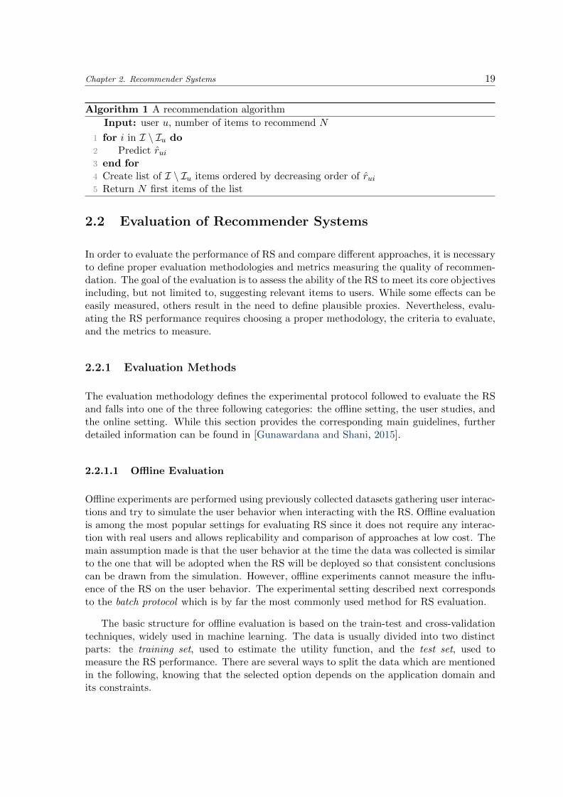
Algorithm 1 presents a standard recommendation algorithm as described in Section 2.1.1and following the notations introduced in this section. We note that this version of therecommendation algorithm does not consider already rated items as candidates for recom-mendation. Domains where repeated interactions are expected consider the whole set ofitems I for recommendation.
Chapter 2. Recommender Systems 19
Algorithm 1 A recommendation algorithm
Input: user u, number of items to recommend N
1 for i in I \ Iu do2 Predict rui3 end for4 Create list of I \ Iu items ordered by decreasing order of rui5 Return N first items of the list
2.2 Evaluation of Recommender Systems
In order to evaluate the performance of RS and compare different approaches, it is necessaryto define proper evaluation methodologies and metrics measuring the quality of recommen-dation. The goal of the evaluation is to assess the ability of the RS to meet its core objectivesincluding, but not limited to, suggesting relevant items to users. While some effects can beeasily measured, others result in the need to define plausible proxies. Nevertheless, evalu-ating the RS performance requires choosing a proper methodology, the criteria to evaluate,and the metrics to measure.
2.2.1 Evaluation Methods
The evaluation methodology defines the experimental protocol followed to evaluate the RSand falls into one of the three following categories: the offline setting, the user studies, andthe online setting. While this section provides the corresponding main guidelines, furtherdetailed information can be found in [Gunawardana and Shani, 2015].
2.2.1.1 Offline Evaluation
Offline experiments are performed using previously collected datasets gathering user interac-tions and try to simulate the user behavior when interacting with the RS. Offline evaluationis among the most popular settings for evaluating RS since it does not require any interac-tion with real users and allows replicability and comparison of approaches at low cost. Themain assumption made is that the user behavior at the time the data was collected is similarto the one that will be adopted when the RS will be deployed so that consistent conclusionscan be drawn from the simulation. However, offline experiments cannot measure the influ-ence of the RS on the user behavior. The experimental setting described next correspondsto the batch protocol which is by far the most commonly used method for RS evaluation.
The basic structure for offline evaluation is based on the train-test and cross-validationtechniques, widely used in machine learning. The data is usually divided into two distinctparts: the training set, used to estimate the utility function, and the test set, used tomeasure the RS performance. There are several ways to split the data which are mentionedin the following, knowing that the selected option depends on the application domain andits constraints.

20 Chapter 2. Recommender Systems
Random split. The separation of sets is done by shuffling user interactions and randomlyselecting a certain percentage for each set, e.g., 80% of the interactions in the training setand 20% in the test set. The random selection is done without replacement, i.e., usinga hold-out method, to prevent one interaction from being used both for training and fortesting. The k-fold cross-validation method is carried out by repeating this procedure ktimes and measuring the performance each time.
Given-n split. The training set is constituted by randomly selecting a fixed number n ofinteractions for each user. The rest of the interactions form the test set. By setting a smallvalue for n, experiments allow to test the RS robustness to user cold-start scenarios wherelittle information about users is available.
Chronological split. When the temporal information of interactions is available, it ispossible to divide the dataset by considering interactions that have occurred before a certaintime threshold in the training set and those after the threshold in the test set. This settingsimulates the case where the utility function is estimated at the time threshold and thenused to perform recommendations without accounting for interactions received afterward.
Further realism can be obtained by simulating what the RS predictions could have beenif it had been running at the time the dataset was collected, which is the idea adopted inthe sequential protocol. In this setting, interactions are considered one by one in temporalorder, provided that temporal information is available [Burke, 2010; Lathia et al., 2009].For each considered interaction, we attempt to perform recommendation and then add theinteraction to the set of interactions used to estimate the utility function.
As mentioned before, offline evaluation faces some limitations. In particular, there isno certainty that the results obtained from this evaluation will align with the actual resultsobtained in a real-world RS. It is also not possible to measure the real impact of recommen-dations on the user behavior. Therefore, more costly evaluation protocols requiring userinvolvement should be considered.
2.2.1.2 User Studies
In order to properly evaluate RS, real user responses to suggestions should be collected.One way to achieve this is by conducting user studies involving a small number of userswho are recruited and asked to interact with the RS. The user behavior is recorded whilerunning controlled experiments and each user may also provide explicit feedback about theexperience. The user studies methodology delivers more insights than offline evaluationbut is also subject to limitations. The small number of users involved in addition to theirawareness of participating in a study where their behavior is being recorded may introducebiases in the collected data.
2.2.1.3 Online Evaluation
Online evaluation is performed when evaluating real-world RS and is only possible whenthe RS is deployed online. This type of evaluation is the one that provides the strongest

Chapter 2. Recommender Systems 21
evidence as the RS is being used by real users in a real setting. The idea is to measure thechange in user behavior when interacting with different RS and draw conclusions related tothe performance.
A/B testing is an online evaluation method widely used to evaluate new algorithmsor design features [Amatriain, 2013]. It can be seen as a two-sample hypothesis testingmethodology where two versions of the RS are compared, i.e., the current one and thenew one. The user traffic is randomly divided between both of them, and some metricsare measured for a certain period of time. Comparing the results drives the conclusion ofwhether or not the new alternative should be adopted.
The risk taken when performing online evaluation is to negatively affect the experienceof real users when testing under-performing approaches. Some companies follow an offline-online testing process to get the best of the offline and online evaluations [Amatriain, 2013].Offline evaluation is first used as an indicator to make informed decisions and A/B tests arethen performed to prove hypothesis previously validated by offline evaluation.
2.2.2 Evaluation Criteria
RS are expected to meet a variety of criteria, each of them answering a different requirementwhich importance is determined by the application domain where the RS is deployed. Theoverall performance is obtained by trading off the multiple criteria. Some of them are citedin the following while a complete list and further information can be found in [Gunawardanaand Shani, 2015].
Accuracy. At the core of the RS lies a prediction engine that predicts the utility of an itemfor a user. A RS providing more accurate predictions is expected to be preferred by users,and several metrics have been introduced to measure the accuracy of predictions [Gunawar-dana and Shani, 2015].
Coverage. A typical item catalog suffers from the long tail effect where the largest part ofitems is rarely selected for consumption. It is often desirable to optimize a RS for a widercatalog coverage by including and promoting long-tail items [Ge et al., 2010]. User coverageis also relevant: The RS is evaluated with regards to the proportion of users for which itcan deliver recommendations.
Novelty. RS are expected to recommend items which the user is not aware of. In particular,recommending items that have been previously rated or seen by the user is not valuable inapplications that require novel recommendations [Celma and Herrera, 2008; Vargas andCastells, 2011].
Diversity. RS should be capable of recommending items that span the whole set of userpreferences and not only very similar items related to a single user interest. Recommenda-tions should thus be diverse and include items that are different from each others [Zhangand Hurley, 2008; Ziegler et al., 2005].
Serendipity. Serendipity measures how surprising the relevant recommendations are [Geet al., 2010; Murakami et al., 2007]. RS are not expected to recommend obvious options

22 Chapter 2. Recommender Systems
but rather unexpected ones that users would not have been able to find while searching ontheir own.
Explainability. Recommendations may not be considered reliable from a user point ofview unless they can be reasonably explained and justified [Tintarev and Masthoff, 2015].This criteria affects the user experience and raises ethical concerns around the opacity ofalgorithms and the manipulation of users.
2.2.3 Evaluation Metrics
Accuracy is by far the most used property to evaluate RS in the literature [Gunawardanaand Shani, 2015]. We focus in this part on the different metrics used to evaluate accuracy.These metrics can be divided into two categories: prediction accuracy metrics and top-Nmetrics.
Prediction accuracy metrics. Prediction accuracy metrics are used to evaluate ratingprediction approaches for recommendation by measuring the accuracy with which the ratingsare predicted for each rating included in the test set T . This category of metrics includesthe Mean Absolute Error (MAE) and the Root Mean Squared Error (RMSE) which wasadopted as the standard metric for the Netflix Prize [Bennett and Lanning, 2007]. The lowerthe error value, the better the predictive power of the system is.
• The Mean Absolute Error (MAE) measures the average absolute deviation betweeneach rating rui contained in the test set T and its prediction rui. It is defined asfollows:
MAE =1
|T |∑
(u,i)∈T
|rui − rui| (2.1)
• The Root Mean Squared Error (RMSE) relies on the Mean Squared Error (MSE) whichpenalizes large errors compared to the MAE, and is defined as follows:
RMSE =√MSE =
√√√√ 1
|T |∑
(u,i)∈T
(rui − rui)2 (2.2)
These metrics are applicable in domains where explicit ratings are available and wherethe RS is optimized for rating prediction.
Top-N metrics. Top-N metrics evaluate the quality of top-N recommendation lists gener-ated by RS. Often borrowed from information retrieval, these metrics measure the relevanceof recommendations, knowing that the item relevancy can be determined in different ways,e.g., the user bought the item, rated it, or clicked on it.
In particular, precision and recall [Baeza-Yates and Ribeiro-Neto, 2011] are two metricsmeasuring the usage prediction of the RS. Given that the algorithm recommends N items,we denote by Lu(N) the set of items recommended to user u, by Su the set of relevant itemsamong all items for user u, and by Tu the set of users having interactions in the test set T .

Chapter 2. Recommender Systems 23
• The precision measures the fraction of relevant recommended items and is defined asfollows:
Precision@N =1
|Tu|∑u∈Tu
Precisionu@N =1
|Tu|∑u∈Tu
|Lu(N) ∩ Su||Lu(N)| (2.3)
• The recall measures which fraction of the relevant items are present in the recommen-dation list and is defined as follows:
Recall@N =1
|Tu|∑u∈Tu
Recallu@N =1
|Tu|∑u∈Tu
|Lu(N) ∩ Su||Su|
(2.4)
Increasing the size of the recommendation list, N , may increase the recall since a longerrecommendation list has more chances of including relevant items, but it also decreases theprecision. The F1 measure evaluates the balance between these two measures and is definedas follows:
F1@N =1
|Tu|∑u∈Tu
2 .P recisionu@N . Recallu@N
Precisionu@N + Recallu@N(2.5)
Ranked lists introduce a position bias according to which the probability of selectionof an item decays when its rank increases in the list [Craswell et al., 2008]. It is thusimportant to evaluate not only the relevance of the items in the recommendation list butalso the ranking quality. Two of the most popular ranking measures are the NormalizedDiscounted Cumulative Gain (NDCG) and the Mean Reciprocal Rank (MRR) introducedin the following.
• The Discounted Cumulative Gain (DCG) is first defined for user u as follows:
DCGu@N =N∑i=1
reluilog2(i+ 1)
(2.6)
where relui = 1 if the item displayed at rank i is relevant for user u and relui = 0otherwise.
The Normalized Discounted Cumulative Gain (NDCG) [Jarvelin and Kekalainen, 2002]is then defined as follows:
NDCG@N =1
|Tu|∑u∈Tu
DCGu@N
DCG∗u@N, (2.7)
where DCG∗u@N is the best possible DCGu obtained if all recommended items wererelevant.
• The Mean Reciprocal Rank (MRR) computes the reciprocal of the rank of the firstrelevant item in the full ordered list of items, denoted by ranku for user u, and isdefined as follows:
MRR =1
|Tu|∑u∈Tu
MRRu =1
|Tu|∑u∈Tu
1
ranku(2.8)

24 Chapter 2. Recommender Systems
Other measures used for evaluating the accuracy of RS include the mean average preci-sion [Baeza-Yates and Ribeiro-Neto, 2011], the area under the ROC curve [Bradley, 1997],the expected reciprocal rank [Chapelle et al., 2009], the hit-rate [Deshpande and Karypis,2004], and the average-reciprocal hit rank [Deshpande and Karypis, 2004].
2.3 Recommendation Approaches
A recommendation approach, also referred to as recommendation method or recommen-dation algorithm, is expected to predict the utilities of items for a set of target users andgenerate appropriate recommendations. A large range of approaches have been proposed tooffer accurate recommendations and can be classified according to multiple criteria includingthe recommendation problem they address, i.e., rating prediction or top-N recommendation,or the type of feedback they employ, i.e., explicit or implicit feedback (Section 2.1.1).
The most common classification found in the literature refers to how the informationrelated to users and items is exploited for the recommendation task and establishes thefollowing categories:
• Content-Based Filtering (CBF) approaches. These approaches make explicit use ofdomain knowledge related to users or items.
• Collaborative Filtering (CF) approaches. Recommendations are only based on theuser behavior and on previous interactions, without further explicit information aboutusers or items.
• Hybrid approaches. These approaches combine the two previous strategies using bothuser and item information, and user interactions.
• Context-aware approaches. These approaches leverage contextual information aboutusers and items in order to propose appropriate recommendations.
2.4 Content-Based Filtering Approaches
Content-Based Filtering (CBF) approaches [Pazzani and Billsus, 2007] use content infor-mation about users and items in order to generate recommendations. This information cantake various forms such as features, textual descriptions, and tags. In order to recommendrelevant items, the main idea is to match user profiles and item profiles based on user pref-erences for item attributes. Therefore, users receive suggestions about items that are similarto the ones they previously interacted with. Deploying a CBF approach requires extractingrelevant information about the content of items, building item profiles and user profiles, andfiltering items according to the similarity between profiles.

Chapter 2. Recommender Systems 25
2.4.1 Example of a Content-Based Filtering Approach
CBF techniques build models using either machine learning techniques, e.g., naıve Bayes ordecision trees, based on underlying data [De Gemmis et al., 2008; Lops et al., 2011; Pazzaniand Billsus, 1997] or heuristic functions inspired from information retrieval methods [Bal-abanovic and Shoham, 1997; Diederich and Iofciu, 2006]. In order to give an example ofthe process followed by CBF approaches, we illustrate in the following the functioning ofa CBF technique relying on a function from the information retrieval field to representitems [Cantador et al., 2010].
Building item profiles. Most CBF systems exploit textual features describing items andextracted from various sources like Web pages and product descriptions. The representationis traditionally based on the vector space model [Lops et al., 2011] which is a spatial repre-sentation of text documents. Each document is represented by a vector in a n-dimensionalspace, denoted by vi for the document related to item i, where each dimension correspondsto a term from the vocabulary V. Weighting terms is done with TF-IDF which is the prod-uct of Term Frequency (TF) and Inverse Document Frequency (IDF) defined as follows, foreach word w in document di:
TFw,di =fw,di
maxw′∈di
fw′,di, IDFw,di = log
|I|1 + |i ∈ I : w ∈ di|
(2.9)
where fw,di is the number of occurrences of the word w in the document di.
The normalized TF-IDF is used for representation and is given by:
vi,w =TFw,di . IDFw,di√ ∑
w′∈diTF 2
w′,di.√ ∑w′∈di
IDF 2w′,di
(2.10)
In cases where items are described by a set of attributes having specific values, the itemprofile is built naturally by allocating one dimension to each feature.
Building user profiles. In order to match users and items, CBF approaches require thecreation of vectors describing user preferences in the same space where items are represented.User profiles indicate the user interest in the various item dimensions. An estimate of a userprofile, which is denoted by vu for user u, can be obtained by aggregating the profiles of theitems he rated.
Measuring similarities. Predicting the user’s interest in a particular item can be done bycomputing the similarity between user and item profiles. There are several existing measurescomputing the proximity of two vectors. Cosine similarity is one of the most widely usedand is defined as follows:

26 Chapter 2. Recommender Systems
simCS(u, i) =
∑w∈V
vu,w . vi,w√∑w∈V
v2u,w .
√∑w∈V
v2i,w
(2.11)
2.4.2 Advantages and Disadvantages
CBF approaches offer a number of advantages, some of which are mentioned in the following:
• Item cold-start. CBF approaches exploit user interactions made by the target user andcontent information about items in order to generate recommendations. Interactionsmade by other users are not needed and items are recommended based on their de-scriptions even if they have not been rated by any user. CBF approaches are thereforeable to deliver recommendations in item cold-start scenarios (Section 2.1.3).
• Explainability. It is possible to explain the results of recommendations by providingthe set of content features that caused an item to appear in the recommendation list.Those features indicate whether or not recommendations can be trusted by the userand increase the system’s transparency (Section 2.2.2).
However, CBF approaches suffer from several shortcomings:
• Content availability. One obvious limitation is due to the fact that the performanceof these techniques is tied to the number and type of features associated with items.Domain knowledge is often required and enough information about items, which is notalways available, should be gathered in order to appropriately discriminate items.
• Overspecialization. CBF approaches propose items that are similar to the ones theuser has previously interacted with and cannot provide unexpected suggestions. Theysuffer from overspecialization and are not able to offer novel or serendipitous recom-mendations (Section 2.1.3).
• User cold-start. Building a consistent user profile requires gathering enough user in-teractions, making CBF approaches unsuitable for cases where only a few interactionsare available or, more specifically, in user cold-start scenarios (Section 2.1.3).
2.4.3 Related Recommendation Approaches
Classifications of recommendation approaches identify additional categories than the onementioned in Section 2.3. Some of them are related to the CBF category and are mentionedin the following, for the sake of completeness:
• Demographic filtering approaches. These techniques are based on the user demographicinformation [Krulwich, 1997; Pazzani, 1999] and are related to CBF approaches since
Chapter 2. Recommender Systems 27
they leverage content about users. Different recommendations are generated for differ-ent demographic profiles that include for example the user’s country, age, and gender.Given that user preferences cannot be inferred based on their demographic features,these approaches do not perform very well. However, demographic information can beexploited to boost the performance of other well-performing approaches.
• Knowledge-based approaches. Given the specific needs and preferences of users, theseapproaches use domain knowledge around item features to determine if an item isadapted or not. Compared to CBF approaches, knowledge-based approaches do notrely on previous user interactions but rather analyze the user’s current query or need inaddition to item descriptions. Knowledge-based RS are essentially case-based [Bridgeet al., 2005; Chen and Pu, 2012]. When enough information about user interactionsis available, these RS are surpassed by approaches leveraging user interactions.
2.5 Collaborative Filtering Approaches
The term Collaborative Filtering (CF) first appeared in Tapestry [Goldberg et al., 1992], anexperimental mail system which was developed to control the flood of information received byusers by filtering out spam emails. It designated the fact that users collaborate to help eachothers filter the emails by annotating the usefulness of a particular email and propagatingthe information to the others. This was the first idea of filtering information based on thefeedback of other users, knowing that details about how similar users were found or howpersonalization was performed were not provided.
Several systems in other domain applications were then developed based on CF [Hillet al., 1995; Resnick et al., 1994; Shardanand and Maes, 1995], and a large number of CFapproaches were proposed for performing personalized recommendation. These approachesare based on the following principle: Users who are similar with regards to the history ofinteractions are considered to be like-minded and are susceptible to share similar preferencesin the future. Recommendations are thus based on the user history and on the past behaviorof similar users. In contrast to CBF approaches, no additional information about items isrequired to perform recommendation.
Relation to classification. CF can be formulated as the problem of jointly solving manyclassification problems, having one classification problem for each available item [Verstrepenet al., 2017]. In every single problem, the corresponding item i serves as the class, the otheritems as the features, and the users that have interacted with i as the labeled examples.Since all the problems share several features, jointly solving them allows the exchange ofinformation and the collaboration between them, which is more efficient than independentlysolving many classification problems.
CF approaches can be divided into the two general categories of memory-based andmodel-based methods [Koren and Bell, 2015; Ning et al., 2015]. While memory-based ap-proaches directly use the recorded user interactions to compute recommendations, model-based approaches exploit these interactions to learn a predictive model which is then usedfor recommendation. We provide in the following an overview of these two categories ofapproaches.
28 Chapter 2. Recommender Systems
2.5.1 Memory-Based Approaches
Memory-based approaches for CF, i.e., neighborhood-based or heuristic-based approaches,are based on the idea that similar users are interested in the same items or that similaritems interest the same users, assuming that user preferences remain stable over time. Theseapproaches can be user-based or item-based [Desrosiers and Karypis, 2011]. In a user-basedapproach, and to select items to suggest to user u, we refer to users who are the most similarto u. In an item-based approach [Deshpande and Karypis, 2004], we rely on items that aresimilar to the items that u has rated in the past. In both cases, a neighborhood methodfirst determines the neighbors of an entity using a similarity measure and then relies on theneighbors and on previous user interactions to generate recommendations. Details aboutthe functioning of each approach are provided in the following.
2.5.1.1 User-Based Collaborative Filtering
In a user-based approach, the first step is to find the neighbors of the target user u. Givena similarity measure able to assess the resemblance between two users, we compute thesimilarities between u and every other user in U . The k most similar users to u constitutethe set of neighbors, denoted by B(u). To predict the rating rui, we rely on the ratings givenby the k neighbors to item i. We may compute the simple average of the available ratingsgiven by the neighbors or the weighted average taking into account the degree of similaritybetween users and defined as follows:
rui =
∑v∈B(u)
sim(u, v) . rvi∑v∈B(u)
sim(u, v)(2.12)
where sim(u, v) is the similarity measure applied to users u and v.
Similarity measures play an essential role as they intervene in the neighborhood selectionand in the rating prediction. Several measures have been proposed for this task, and wemention in the following some of the most widely used.
Pearson Correlation.
simPC(u, v) =
∑x∈Iuv
(rux − ru)(rvx − rv)√ ∑x∈Iuv
(rux − ru)2√ ∑x∈Iuv
(rvx − rv)2(2.13)
where ru and rv are the average ratings given by user u and v respectively, and Iuv isequal to Iu ∩ Iv.
Cosine similarity.
simCS(u, v) =r>u . r>v‖r>u ‖ ‖r>v ‖
(2.14)

Chapter 2. Recommender Systems 29
where x . y is the scalar product between vectors x and y, and ‖x‖ is the norm of x.
Jaccard similarity.
simJS(u, v) =|Iu ∩ Iv||Iu ∪ Iv|
(2.15)
2.5.1.2 Item-Based Collaborative Filtering
Item-based CF [Deshpande and Karypis, 2004] focuses on finding and exploiting the neigh-bors of items. To predict the rating rui, an item-based approach examines the neighbors ofitem i and the ratings given by user u to these neighbors. We first compute the similaritiesbetween item i and every other item in I, and select the k most similar items as neighbors ofi forming the set denoted by B(i). Similarly to user-based CF (Section 2.5.1.1), we computethe predicted rating rui as follows:
rui =
∑j∈B(i)
sim(i, j) . ruj∑j∈B(i)
sim(i, j)(2.16)
where sim(i, j) is the similarity measure applied to items i and j. The similarity mea-sures defined in Equations (2.13)–(2.15) can be applied, using the vectors ri and rj insteadof the vectors r>u and r>v , and the sets Ui and Uj instead of the sets Iu and Iv.
2.5.1.3 Extensions, Complexity, Advantages and Disadvantages
Extensions. Important extensions applicable to memory-based CF have been proposed[Breese et al., 1998]. Default voting was first introduced and consists in assuming a defaultvalue for unseen ratings. These values are then used to measure similarities instead ofonly using observed ratings, i.e., ratings in Iu ∩ Iv. This is in particular effective in sparsesettings where |Iu ∩ Iv| is relatively small. The default value is defined with regards to theapplication domain where the absence of observations may sometimes indicate a negativefeedback. Inverse user frequency was then proposed and consists in giving more weight toless popular items in the process of computing similarities. It is based on the idea thatpopular items, i.e., items liked by a majority, are not as relevant as less popular itemswhen it comes to capturing similarity. Another extension, case amplification, transformssimilarities in the prediction phase by boosting high weights and punishing low ones. Thisis in particular effective to reduce noise.
Complexity. Memory-based approaches first compute nearest neighbors, i.e., the k mostsimilar users or items, and then use these neighbors for prediction. The time complexityfor computing neighbors is O(n2p) in user-based CF where p = max
u∈U|Iu|, and O(m2q) in
item-based CF where q = maxi∈I|Ui|. The time complexity for retrieving recommendations is
O(mk) for both approaches.

30 Chapter 2. Recommender Systems
Advantages and disadvantages. Memory-based CF is a simple and intuitive approachfor recommendation that does not require more than one parameter, i.e., the number ofneighbors k, as input. Recommendations are easy to explain since they are the result ofexploiting similar users or items which are clearly identified. They supply statements like“Customers who bought this item also bought...” [Linden et al., 2003].
Item-based approaches perform more accurately than user-based approaches in mostreported cases [Sarwar et al., 2001] mainly since item relationships tend to be more stablethan user relationships. Item-based approaches are also more computationally efficient interms of complexity in settings where the number of users exceeds the number of availableitems. On the other hand, user-based approaches provide more original recommendationsand lead to a more satisfying experience [Desrosiers and Karypis, 2011].
Memory-based methods suffer from scalability issues and a lack of sensitivity to sparsedata [Lemire and Maclachlan, 2005]. Since CF methods rely on user behavior, a goodaccuracy is only obtained when enough interactions are collected and made available. Whilethis is valid for both memory-based and model-based approaches, model-based approacheshave been proven to outperform memory-based approaches in terms of accuracy. They aretherefore preferred in RS applications.
2.5.2 Matrix Factorization Approaches
Model-based approaches [Koren and Bell, 2015] exploit user interactions to learn a predictivemodel representing user preferences and item descriptions. Characteristics of users and itemsare captured by a set of model parameters. These parameters are learned from the dataand used then for prediction. Several model-based approaches have been explored includingclustering [Ungar and Foster, 1998], Bayesian methods [Miyahara and Pazzani, 2000], andneural networks [Salakhutdinov et al., 2007]. We provide in this section a presentationof Matrix Factorization (MF) methods [Koren et al., 2009] which are the most populartechniques among model-based approaches.
2.5.2.1 Matrix Factorization Framework
Matrix Factorization (MF) methods [Koren et al., 2009] model users and items by repre-senting them in a common latent space of dimensionality K where the affinity between auser and an item is determined by the inner product of their embedded vectors. While manyvariations and extensions of MF methods have been proposed, almost all of them rely onthe same framework, represented in Figure 2.2, but differ in the objective function they tryto optimize and the method they use to learn parameters.
In MF methods, each user u is associated with a vector pu ∈ RK and each item i witha vector qi ∈ RK . Latent factors represent characteristics inferred from the rating patternsand each value in the vectors pu and qi expresses to which extent the user is attracted byor the item has a certain feature, respectively. The hypothesis of MF methods is that thevalue of a rating rui can be captured by the inner product between pu and q>i :
rui = puq>i (2.17)

Chapter 2. Recommender Systems 31
R
P
QT
n
K
m
K
Figure 2.2: Representation of Matrix Factorization (MF)
The goal is to determine the vectors pu for each user u and qi for each item i. MFmethods approximate then the rating matrix R with the product of two low-rank densematrices P ∈ Rn×K for user latent factors and Q ∈ Rm×K for item latent factors:
R ≈ PQ> (2.18)
where K min(n,m).
The learning task consists in determining the values of P and Q based on the observedelements of R. The learned latent factors are then used to predict the unobserved elementsof R. The exact way the learning of parameters is performed differs across several proposedapproaches for MF. Some of the most representative methods are introduced in the following.
2.5.2.2 Singular Value Decomposition
Singular Value Decomposition (SVD) is a well-known technique used for matrix decompo-sition. SVD decomposes the matrix R into:
R = PΣQ> =d∑s=1
σspsq>s (2.19)
where P ∈ Rn×d is the set of left singular vectors, Q ∈ Rm×d is the set of right singularvectors, and Σ ∈ Rd×d is a diagonal matrix containing the d singular values on its diagonal.Given a SVD decomposition, the matrix R can be approximated by sorting the singularvectors in decreasing order of σs and selecting those corresponding to the K largest singular

32 Chapter 2. Recommender Systems
values. The best rank-K approximation of R is then given by:
R =K∑s=1
σspsq>s (2.20)
SVD is closely related to the MF problem introduced in Section 2.5.2.1 and can be appliedto uncover the user and item vectors used to approximate the rating matrix [Sarwar et al.,2000]. However, applying SVD for CF raises the issue of sparsity: While SVD requires a fullmatrix to be decomposed, the rating matrix is typically sparse and contains many unknownelements, i.e., user-item couples for which the preference is not specified. Some solutionshave been proposed including filling the rating matrix with default values, e.g., zeros oran average rating per user or per item [Kurucz et al., 2007]. This solution is inaccuratesince filling the matrix might falsify the represented concepts. It is also very expensiveas it increases the amount of data. Further advances showed that it is more efficient tofactorize the matrix R using only observed values [Paterek, 2007; Takacs et al., 2007] andare discussed in the following.
2.5.2.3 Minimizing Squared Loss and Other Loss Functions
The goal in MF is to learn the user and item feature matrices P and Q that minimize theobjective function, denoted by L(P,Q), which is the squared error between observed andpredicted ratings over known ratings that are included in the set D and defined as follows:
L(P,Q) =∑
(u,i)∈D
(rui − puq>i )2 (2.21)
The minimization problem is solved over the observed entries of R, but since only a fewof them are available, the model can easily overfit or be affected by extreme values. It istherefore important to consider regularization for a better generalization capacity [Srebroet al., 2005] by adding the regularization terms Ω(P) and Ω(Q) which prevent the valuesof P and Q from being too large. While several forms of regularization can be applied, weuse L2-regularization, i.e., ridge regression, to make L(P,Q) differentiable. The objectivefunction is then defined as follows:
L(P,Q) =∑
(u,i)∈D
(rui − puq>i )2 + λΩ(P) + λΩ(Q)
=∑
(u,i)∈D
(rui −
K∑l=1
pulqil
)2
+ λ
m∑u=1
K∑l=1
p2ul + λ
n∑i=1
K∑l=1
q2il
(2.22)
where λ is the parameter controlling the relative importance of least square fitting andregularization.

Chapter 2. Recommender Systems 33
The optimization of Equation 2.22 is non-convex due to the puq>i term where both pu
and qi are unknown. The two most popular families of algorithms for minimizing non-convexobjective functions in CF are Stochastic Gradient Descent (SGD) [Bottou and Bousquet,2008] and Alternating Least Squares (ALS) [Bell and Koren, 2007b]. While SGD is in generaleasier and faster to converge, ALS can benefit from parallel execution. We present both ofthem in the following.
Learning the parameters: SGD. SGD [Bottou and Bousquet, 2008] is a version ofGradient Descent (GD), a numerical optimization algorithm, that converges faster thanGD by approximating the true gradient using the gradient at a single observation. SGDfirst initializes the parameters, i.e., user and item latent features P and Q, randomly. Itthen loops, until convergence, over all observations (u, i) ∈ D and iteratively update theparameters in the direction that reduces L(P,Q) as follows:
pu ← pu − η∂Lu,i(P,Q)
∂pu, qi ← qi − η
∂Lu,i(P,Q)
∂qi(2.23)
where η is a hyperparameter called the learning rate and Lu,i(P,Q) is derived from L(P,Q)
for one observation (u, i) ∈ D as follows: Lu,i(P,Q) = (rui−K∑l=1
pulqil)2 +λ
K∑l=1
p2ul +λ
K∑l=1
q2il.
Updates are performed for each element of the matrices P and Q, and partial derivativesof Lu,i(P,Q) with respect to single elements are given as follows:
∂Lu,i(P,Q)
∂pul= 2qil(puq
>i − rui) + 2λpul (2.24)
∂Lu,i(P,Q)
∂qil= 2pul (puq
>i − rui) + 2λqil (2.25)
The algorithm of SGD is described in Algorithm 2. SGD is sensible to the learning ratechosen, η, and to the initialization of P and Q due to the non-convexity of the problem.The complexity of SGD per iteration is O(|D|K). Several approaches [Recht et al., 2011]have been proposed to parallelize SGD for a faster convergence, but this problem remainschallenging and harder than parallelizing ALS.
Learning the parameters: ALS. While the optimization of Equation 2.22 is non-convex,it is quadratic if we fix one of the unknown parameters and thus convex in any singleparameter. This setting requires alternating optimization algorithms such as ALS wherewe repeatedly iterate over the parameters, fix them, and solve the optimization problem.The cost function is improved with each parameter update, and since it is bounded by beingnon-negative, convergence is guaranteed. ALS [Bell and Koren, 2007b] consists in repeatedlyexecuting, until convergence, the two following steps:
1. Fix the item latent matrix Q. Solve the regularized linear least-square problem forthe user latent matrix P. The optimal value for P is given as follows, where I is theidentity matrix:
P = (QQ> + λI)−1QR> (2.26)

34 Chapter 2. Recommender Systems
Algorithm 2 Stochastic Gradient Descent (SGD)
Input: Rating matrix R, set of observed ratings D, stopping criterion ε, rank K,learning rate η, and regularization parameter λ
Output: Optimal user feature matrix P, optimal item feature matrix Q
1 Initialize P and Q, e.g., randomly2 while not converged, e.g.,
∥∥R−PQ>∥∥ > ε, do
3 for each (u, i) ∈ D do4 eui = puq
>i − rui
5 pu ← pu − 2η(euiqi + λpu)6 qi ← qi − 2η(euipu + λqi)7 end for8 end while
2. Fix the user latent matrix P. Solve the regularized linear least-square problem for theitem latent matrix Q. The optimal value for Q is given as follows:
Q = (PP> + λI)−1PR (2.27)
Algorithm 3 Alternating Least Squares (ALS)
Input: Rating matrix R and regularization parameter λOutput: Optimal user feature matrix P, optimal item feature matrix Q
1 Initialize P and Q, e.g., randomly2 while not converged do3 for u ∈ 1, . . . ,m do . update users4 pu ← (
∑i∈Iu
qiq>i + λI)−1
∑i∈Iu
ruiqi
5 end for6 for i ∈ 1, . . . , n do . update items7 qi ← (
∑u∈Ui
pup>u + λI)−1
∑u∈Ui
ruipu
8 end for9 end while
The algorithm of ALS is described in Algorithm 3. Each user vector update costsO(|Iu|K2 +K3) and each item vector update costs O(|Ui|K2 +K3), assuming a time com-plexity of O(K3) for inverting the matrices (
∑qiq>i +λI) and (
∑pup
>u +λI). The complex-
ity of ALS per iteration is then O(|D|K2 + (n+m)K3). Even though the time complexityis high, ALS is well-designed for parallelization [Zhou et al., 2008].
Beyond optimizing the squared loss function. The recommendation problem was his-torically first formulated as a rating prediction problem (Section 2.1.1), where the main goalis to accurately predict unobserved ratings by performing what is commonly called the ma-trix completion task. Within this scope, the RS performance is measured using the RMSE(Section 2.2.3) for example, and the main objective function to optimize is the squared lossfunction (Equation 2.21). Since then, the recommendation problem evolved beyond the

Chapter 2. Recommender Systems 35
Table 2.2: Examples of MF models based on different objective functions
Model Objective function
MF [Koren et al., 2009] `pointSL
WRMF [Hu et al., 2008] `pointSL with weights
MMMF [Rennie and Srebro, 2005] `pointHL
BPR-MF [Rendle et al., 2009] `pairLL
CCF [Yang et al., 2011] `pairHL
COFIRANK [Weimer et al., 2008] NDCG loss
CLiMF [Shi et al., 2012] MRR loss
matrix completion task and several objective functions for training recommendation modelswere further explored. These functions can roughly be divided into three categories: point-wise, pair-wise, and list-wise objective functions. Point-wise functions, such as the squaredloss function, focus on the accuracy of predictions of individual preferences. Pair-wise func-tions approximate the loss by considering the relative ranking of predictions for pairs ofitems. Finally, list-wise functions reflect the distance between the complete recommendedlist and the reference one. While some CF models rely on list-wise functions [Shi et al.,2010], they are not as widely adopted as the other two types of functions and we omitdetails about them in the following.
We denote by `(.) any loss function. A point-wise function evaluated for one data pointrui is denoted by `point(rui, rui). Following previous definitions, we have:
Lu,i(P,Q) = `point(rui,puq>i ) = `point(rui, rui) (2.28)
A pair-wise function is evaluated for triples in the form of (u, i, j) where user u is assumedto prefer item i over item j, i.e., rui > ruj , and is denoted by `pair(ruij , ruij) where ruij =rui − ruj and ruij = rui − ruj . Several options are possible for the definition of the lossfunction `(.) in point-wise and pair-wise settings. A few commonly used possibilities arelisted in the following:
• Squared Loss: `SL(y, y) = (y − y)2
• Logistic Loss: `LL(y, y) = log(1 + exp(−y . y))
• Hinge Loss: `HL(y, y) = max(0, 1− y . y)
Table 2.2 provides examples of recommendation models using the different loss functionspresented, in addition to losses related to the ranking of items in the recommendation list.In general, pair-wise functions are considered to be more suitable for solving the top-Nrecommendation problem, especially when handling implicit feedback which requires specialtreatment.

36 Chapter 2. Recommender Systems
2.5.2.4 Dealing with Implicit Feedback
Most research in the RS field was historically powered by applications where user prefer-ences were collected in the form of explicit ratings. This led to the development of severalalgorithms that are meant to accurately predict ratings. However, in many real-world ap-plications, only implicit feedback that is obtained without user intervention, e.g., purchases,clicks, and bookmarks, is available (Section 2.1.2). This type of feedback introduces newchallenges (Section 2.1.3), preventing the direct application of recommendation models de-veloped for the explicit feedback setting. Since implicit feedback is often “positive-only”,i.e., only information about liked items is available, this problem is often designated as“One-Class Collaborative Filtering” [Pan et al., 2008].
Dealing with implicit feedback and, more specifically, learning a MF model based onimplicit feedback should address two problems: transforming the original set of implicitobservations by integrating additional negative feedback and defining the objective function.
Augmenting implicit feedback datasets. Given that implicit feedback is positive-only,only considering the observed feedback assumes that interactions are missing at random,which is not true and results in a bad performance [Marlin et al., 2007]. Several solutionshave been proposed to transform implicit feedback datasets. The most widely used can beroughly decomposed in two families. The first one consists in converting implicit feedbackto ratings. Each observed user-item interaction takes the value of 1 in the rating matrix,i.e., rui = 1. Unobserved interactions can be treated as negative feedback, i.e., rui = 0,resulting in the strategy known as All Missing as Negative. Fitting a model to this datawithout proper regularization will strongly be biased towards negative feedback and willtend to always predict 0 [Rendle et al., 2009]. Another strategy, All Missing as Unknown,consists in treating unobserved interactions as unknown by ignoring them. In this case, themodel will strongly be biased towards positive feedback and this would result in a trivialsolution [Srebro and Jaakkola, 2003]. To avoid the drawbacks of these two extreme cases,the second family of approaches takes an in-between solution by attempting to discriminatenegative items from the unobserved ones. This is done by randomly sampling negativeitems [Rendle et al., 2009] or by using weighting techniques [Hu et al., 2008; Pan et al.,2008].
Defining the objective function. Dealing with implicit feedback usually implies solvinga top-N recommendation problem where the focus is on the ranking quality of items ratherthan on the value of predicted ratings. We present in the following two seminal MF ap-proaches proposed to deal with implicit feedback. The first relies on a weighted point-wisefunction [Hu et al., 2008] while the second on a pair-wise function [Rendle et al., 2009].
Weighted Regularized MF. In Weighted Regularized MF (WRMF) [Hu et al., 2008;Pan et al., 2008], the objective function is a weighted point-wise function where the weightindicates the confidence we have in the corresponding observation. If user u interacted withitem i, then we are confident that u likes i. If u never interacted with i, we can makeseveral assumptions with varying confidence levels. The objective function can be writtenas follows:

Chapter 2. Recommender Systems 37
L(P,Q) =∑
(u,i)∈D
cui(rui − puq>i )2 + λΩ(P) + λΩ(Q) (2.29)
where cui is the confidence we have in the observation rui. [Pan et al., 2008] suggest toset cui to 1 for positive observations, i.e., rui = 1, and to lower values, e.g., cui = 0.01,for unobserved interactions, i.e., rui = 0. [Hu et al., 2008] consider additional parameterswhen estimating cui, e.g., higher confidence for users who have rated more items or higherconfidence for items who have been rated by more users. ALS is used for optimization andin cases where cui is constant for unobserved items, the cost of learning the parameters isO(|D|K2 + (|U|+ |I|)K3) per iteration.
Bayesian Personalized Ranking. Bayesian Personalized Ranking (BPR) [Rendle et al.,2009] addresses the recommendation problem as a ranking task and relies on a pair-wiseinterpretation of the user feedback. The dataset is artificially augmented by includingpotential negative feedback. The goal of BPR is to find a personalized total ranking >u⊂ I2
for all users u ∈ U and pairs of items (i, j) ∈ I2 satisfying the properties of a total order.Therefore, BPR uses item pairs as training data and optimizes for correctly ranking them.The training data, denoted by Dbpr, is derived from the dataset of positive-only observationsand is based on the following assumption: User u who interacted with item i prefers i overevery item j for which u did not provide any feedback, i.e., j ∈ I \ Iu. If u interacted withi and j, it is not possible to deduce the preference for one item over the other. Dbpr is thendefined as follows:
Dbpr = (u, i, j)|i ∈ Iu ∧ j ∈ I \ Iu (2.30)
A personalized ranking of items is obtained by optimizing a general criterion calledBPR-Opt which can be applied to neighborhood models and MF. BPR-Opt is derivedthrough a Bayesian analysis of the problem where the aim is to maximize the posteriorprobability. Denoting by Θ the parameter vector of the underlying model, the posteriorprobability is given by p(Θ |>u) ∝ p(>u| Θ)p(Θ). BPR-Opt is formulated as follows:
BPR-Opt := ln p(Θ |>u)
= ln p(>u| Θ)p(Θ)
=∑
(u,i,j)∈Dbpr
lnσ(ruij)− λΘ ‖Θ‖2(2.31)
where σ(.) is the logistic sigmoid, σ(x) = 11+e−x , ruij = rui − ruj , and λΘ designates model
specific parameters for regularization. The optimization problem is solved using a SGD onthe parameters Θ. Since it is computationally expensive to consider all triples (u, i, j) ∈ Dbprdue to their large number, triples are uniformly sampled from Dbpr during the learningprocess.
In its most general form, MF can also be approached by probabilistic models which areintroduced in the following section.

38 Chapter 2. Recommender Systems
2.5.2.5 Probabilistic Models
MF techniques for RS were extended to probabilistic models by two seminal papers [Salakhut-dinov and Mnih, 2008a,b]. One of them, Probabilistic Matrix Factorization (PMF) [Salakhut-dinov and Mnih, 2008a], is represented as a graphical model in Figure 2.3.
σ
rij
pu qi
σP σQ
m
n
Figure 2.3: Graphical model for Probabilistic Matrix Factorization (PMF)
In PMF, we assume Gaussian priors on user and item feature matrices, given the hyper-parameters σ2
P and σ2Q:
P ∼ N (0, σ2P I) (2.32)
Q ∼ N (0, σ2QI) (2.33)
Ratings are generated according to a Gaussian with the hyperparameter σ2 as follows:
rij | P,Q ∼ N (puq>i , σ
2) (2.34)
Having defined Iui equal to 1 if (u, i) ∈ D and 0 otherwise, the log of the posteriordistribution is given by:
ln p(P,Q | R, σ2, σ2P , σ
2Q) =− 1
2σ2
n∑u=1
m∑i=1
Iui(rui − puq>i )2 − 1
2σ2P
n∑u=1
p>u pu −1
2σ2Q
m∑i=1
q>i qi
− 1
2
((n∑u=1
m∑i=1
Iui
)lnσ2 + nK lnσ2
P +mK lnσ2Q
)+ c
(2.35)where c is a constant independent of the parameters. Maximizing the log-posterior over userand item latent features is equivalent to minimizing the following objective function:
L =1
2
n∑u=1
m∑i=1
Iui(rui − puq>i )2 +
λP2
n∑u=1
‖pu‖2Fro +λQ2
m∑i=1
‖qi‖2Fro (2.36)

Chapter 2. Recommender Systems 39
where λP = σ2/σ2P , λQ = σ2/σ2
Q, and ‖ . ‖Fro denotes the Frobenius norm. By fixing thehyperparameters σP , σQ, we recover an objective function similar to the one in Equation(2.22). Nevertheless, PMF is an extension of MF with probabilistic interpretation allowingfurther developments of the model, such as a Bayesian version of PMF, BPMF [Salakhut-dinov and Mnih, 2008b], or the use of side information [Ma et al., 2008].
2.6 Hybrid Approaches
Since CBF and CF rely on different sources of input to make recommendations, each one ofthem has its own advantages and weaknesses, i.e., overspecialization for CBF and cold-startfor CF. Hybrid methods [Burke, 2002] were then proposed to get the best of both worlds.They assume that various sources of input are available at the same time which allows theuse of different recommendation approaches in one framework and avoids the limitations ofeach approach when used separately. On the other hand, competitions such as the NetflixPrize [Bennett and Lanning, 2007] and KDD cups [Tang et al., 2014] highlighted the fact thatthe best results are often achieved when different recommendation algorithms are combinedin a single model. Hybrid methods can take various forms, and an existing classificationcovering the main trends of hybrid recommendation [Adomavicius and Tuzhilin, 2005] ispresented in the following:
• Combining separate recommendations. The utilities predicted separately by severalrecommendation algorithms are combined to provide a single recommendation, usingmethods such as linear combination [Claypool et al., 1999] or voting schemes [Pazzani,1999].
• Incorporating content-based characteristics to CF approaches. User-based neighbor-hood approaches can be for example adapted to compute similarities based on content-based user profiles [Pazzani, 1999].
• Incorporating collaborative characteristics to CBF approaches. CF models can be ap-plied to a group of content-based profiles for text recommendation, for example [Sobo-roff and Nicholas, 1999].
• Developing a unifying model incorporating content-based and collaborative charac-teristics. Many approaches have been proposed within this scope such as a uni-fied probabilistic method for combining collaborative and content-based recommen-dations [Popescul et al., 2001; Schein et al., 2002].
2.7 Context-Aware Approaches
Further advances in the RS field recognized the importance of contextual information inpredicting item utility [Adomavicius and Tuzhilin, 2015]. User choices are not solely guidedby a fixed set of preferences related to item features and uncovered by CBF and CF ap-proaches, but strongly depends on their context, their current needs, and the situation theyare in. There are several types of contextual information that could help provide betterrecommendations when taken into account, the main examples being:

40 Chapter 2. Recommender Systems
• Location information. Location information can be useful in a variety of recommen-dation scenarios [Levandoski et al., 2012; Ye et al., 2011]. User geographical locationcan have a significant influence on preferences in terms of taste, culture, and habits.It can also indicate the type of the current user activity, e.g., work at the office orleisure in an entertaining place, which in turn affects the set of relevant preferences. Insome specific applications, e.g., restaurant recommendation, user location is essentialto filter out physically inaccessible options.
• Temporal information. Depending on the time of the day, on the day of the week, oron the season, users do not exhibit the same preferences across several domains, e.g.,clothing and tourism. Temporal information has thus been exploited to improve thequality of recommendation [Campos et al., 2014; Koren, 2009].
• Social information. The user behavior varies according to social factors. For example,a user may make different choices depending on whether he is in the company offriends or family [Adomavicius and Tuzhilin, 2015]. In addition, and especially withinthe scope of online social networks, behaviors of close users are expected to affect thetarget user and should be considered when offering recommendations [Ma et al., 2008].
As mentioned in Chapter 1, the vast majority of Context-Aware RS (CARS) adopt therepresentational view of context [Dourish, 2004]. This view makes the following assump-tions: (i) context is a form of information: It is something that can be known; (ii) contextis delineable: It is possible to define what counts as the context of activities for some setof applications; (iii) context is stable: The elements of context do not vary between in-stances of an activity within the same application; (iv) context and activities are separable:An activity happens within a context. In comparison, the interactional view argues that:(i) context is a relational property between objects or activities: One dimension may becontextually relevant or not to a particular activity; (ii) the scope of contextual featuresis defined dynamically ; (iii) context is an occasioned property relevant to particular events;(iv) context arises from the activity. While the first view considers that context is a sta-ble feature of the environment that is independent of individuals’ actions, the second viewassumes a bidirectional relationship between context and activities.
Integrating context into RS requires the consideration of an additional dimension besidesthe user and item dimensions which are originally encoded in the feedback matrix. The con-text being itself a multifaceted variable, the representation space of feedback becomes thenmultidimensional [Adomavicius and Tuzhilin, 2015]. While traditional RS aim to estimatea utility function defined on the space U × I and which observed values are in R, CARScover the space U × I × C where C represents the set of relevant contextual factors. It isoften assumed that context values are atomic and nominal, and that the context entity is theCartesian product of several contextual dimensions, e.g., Time×Company. Each dimensionis a subset of a Cartesian product of some attributes, e.g., Time ⊆ Y ear ×Month×Day,where each attribute defines a set of values. Three popular paradigms were identified for ad-dressing this multidimensional recommendation problem [Adomavicius and Tuzhilin, 2015]:contextual pre-filtering where context is used for input data selection, contextual post-filteringwhere context is used to filter recommendations, and contextual modeling where context isdirectly incorporated into the model.

Chapter 2. Recommender Systems 41
2.7.1 Paradigms for Incorporating Context
Contextual pre-filtering. In contextual pre-filtering, context drives the selection of datagiven as input to the recommendation algorithm. User interactions are filtered using con-textual factors and the data is then fed to a traditional RS. An example of contextualpre-filtering consists of using user micro-profiles where users are split into several sub-profiles, each of them representing the user behavior in a particular context [Baltrunas andAmatriain, 2009]. Prediction within a particular context is done using the correspondingmicro-profile instead of the full profile. Similarly to this user splitting approach, the itemsplitting technique creates several fictitious items according to the contexts in which theywere selected [Baltrunas and Ricci, 2014]. It is based on the assumption that the natureof items may change when available in different contextual conditions. In addition, someapproaches proposed to apply user and item splittings sequentially [Zheng et al., 2013].
Contextual post-filtering. In contextual post-filtering, the whole set of interactions isfed to a traditional RS while ignoring the contextual dimensions. The recommendationlist delivered in output is then refined using the contextual dimensions [Hariri et al., 2012].This is done either by removing recommendations that are irrelevant to the context or byadjusting the ranking of items in the recommendation list. [Panniello et al., 2009] providean experimental comparison of the pre-filtering paradigm and the post-filtering paradigmin several application domains. The empirical results show that the choice of a strategybetween pre-filtering and post-filtering depends on the recommendation problem. Never-theless, one major advantage of both paradigms is their ability to leverage the varioustraditional recommendation algorithms proposed in the literature.
Contextual modeling. In contextual modeling, the whole set of interactions is exploitedto train a multidimensional recommender. Tensor Factorization (TnF) is one of the mostsuccessful methods for integrating contextual information into the recommendation model.It can be seen as a generalization of MF in which a multidimensional cube is factorizedinstead of a 2-dimensional matrix, i.e., the feedback matrix. The additional dimensions cor-respond to the various contextual dimensions. Instead of learning two latent matrices, i.e.,user and item feature matrices, TnF creates a latent matrix for each dimension, i.e., one forthe users, one for the items, and one for each contextual dimension. A particularly notableexample of TnF for contextual modeling is the multiverse recommendation method [Karat-zoglou et al., 2010] that adapts the generic TnF approach to the recommendation setting.Another notable technique for contextual modeling is Factorization Machines (FM) [Rendle,2012] which can be viewed as a generalization of all the previously discussed factorizationmodels. The basic idea is to model ratings as the linear combination of interactions betweeninput variables. Each rating rui is modeled by a feature vector x which can be seen as thehorizontal stack of the corresponding one-hot-encoding of user, item, and contextual fea-tures. The multidimensional space is therefore flattened into a set of (m+n+d)-dimensionalrows, where d is the number of values of the contextual dimensions. The target variable foreach feature vector x is the corresponding rating value. Rating prediction using second-orderFM is then performed as follows:
rui = w0 +
p∑j=1
wjxj +
p∑j=1
p∑j′=j+1
wjj′xjxj′ (2.37)

42 Chapter 2. Recommender Systems
where w0 is a global bias, p is the number of features, i.e., p = m+ n+ d, wj are first orderinteraction parameters and wjj′ are second order factorized interaction parameters and aredefined as wjj′ = vj . vj′ where vj is a factorized vector for feature j. Model parameters,i.e., w0, the different values of wj , and each one of the vectors vj, are learned by optimizinga point-wise objective function defined over the data D. We note that the two modelsmentioned for contextual modeling were originally designed to handle explicit feedback.
2.7.2 From Context-Aware to Context-Driven Recommender Systems
Recent work [Pagano et al., 2016] highlighted the emergence of the contextual turn, creatingthe need for Context-Driven RS (CDRS) for which context is critical rather than additional.CDRS aim to contextualize recommendations, i.e., tailor recommendations to the user intentand situation, rather than personalize, i.e., tailor recommendations to the individual. Themain assumption is that users have more in common with other users in the same situationthan with the past version of themselves. Recommendations are based on what is goingaround the user, i.e., the user’s situation, and on what the user is trying to accomplish,i.e., the user’s intent. CDRS are therefore able to generate recommendations without pastinformation about users, i.e., in the cold-start setting. Several families of RS can be seen asa special case of CDRS. We mention for example session-based RS [Quadrana et al., 2018]that defines the context as a series of interactions carried out within a session.
2.8 Conclusion
Summary. In this chapter, we propose an overview of RS and present the problem formu-lation, challenges, and limitations. We discuss evaluation methodologies and present somerecommendation techniques in addition to recent emerging trends. We mention the trade-offs involved with each recommendation approach and the advantages and disadvantages ofadopting each one of them for recommendation. Research around RS was always inspiredby real-world applications that constantly re-framed the problem and the focus of actualdevelopments. This chapter is also an attempt to highlight this aspect, tracing the evolutionof the problem and the considerations from an industry perspective. Nevertheless, devel-oping RS requires the understanding of the user behavior in the corresponding domain andthe role the system is expected to fulfill in order to define which criteria to optimize.
Relation to our work. In the scope of this thesis, we focus on the problem of top-N recommendation based on implicit feedback and contextual information. We propose tohandle the data dynamics by considering two particular forms of context: partially observableand unobservable contexts, that cannot be taken into account using traditional methods andthat are further detailed in relevant parts of the thesis following the definitions of Chapter 1.Partially observable context is studied for the application of hotel recommendation in Part IIand unobservable context for the application of online recommendation in Part III.

Part II
Partially Observable Context inHotel Recommendation
43


Chapter 3
The Hotel RecommendationProblem
This chapter presents the hotel recommendation problem as occurring in real-world appli-cations in the hotel industry and as addressed in this thesis. We discuss its relation withother studied recommendation problems, its characteristics and specific challenges, and theimplications on building accurate RS for recommending hotels. We also provide a descrip-tion of the notion of context as emerging in the studied domain since it is proven to havean important influence on the traveler behavior.
3.1 Introduction
Information Technology (IT) and tourism. While tourism has a significant economicimpact, the industry has been witnessing dramatic changes over the past few years [Hornerand Swarbrooke, 2016]. The tourist behavior has been shifting with the evolution of thetravel experience itself and with the change of expectations and motivations. It exhibitsnowadays diverse personas that are complex to decode. In addition, the rapid developmentof IT has contributed to this radical transformation [Werthner et al., 2015], especially consid-ering the way we access information and purchase products. On the other hand, the IT fieldis also opening new business opportunities resulting in several value-generating strategiesand promising to enhance the tourism experience [Werthner and Ricci, 2004]. The chal-lenges faced by these applications require the combination of research and development atthe intersection of several disciplines including computer science, cognitive technologies, andtourism research. Relevant research topics can be divided into five layers [Werthner et al.,2015], covering the tourism ecosystem, which are stated in the following: (i) individual,(ii) group, (iii) corporate, (iv) industry, and (v) government.
The individual layer focuses on the interaction between any user from the demand orsupply side and any IT service. Given the heterogeneity of users, there is a need for per-sonalized applications and adaptive models in order to enhance the overall experience andreduce the cognitive load of users. Groups are formed by two or more users and can be
45

46 Chapter 3. The Hotel Recommendation Problem
identified as sharing similar preferences or as being present together in the same situation.Specific services can be developed to support group formations, group experiences, or groupdecision-making. The corporate layer concerns any organization in the tourism domain andcovers issues like knowledge management, the understanding of customers, and online rep-utation. The industry layer captures the overall structure of the sector and the interactionsbetween organizations. It highlights most importantly the rise of online travel agencies.Finally, the government layer deals with rules and regulations of IT in the tourism domain.
RS in tourism. RS interfere at the individual and group layers and are becoming essentialin the tourism domain. Travelers are actively searching for information to compose their va-cation packages and are rapidly facing the curse of information overload [Xiang et al., 2015].RS are able to support travelers in several ways and to accompany them during the wholeexperience [Borras et al., 2014; Felfernig et al., 2007; Gretzel, 2011]. They can recommenddestinations that suit the user preferences during the pre-trip destination selection [Ricci,2002], and then accommodations, attractions, restaurants, events, and points of interest,in addition to personalized routes guiding travelers throughout several attractions [Kurata,2011; Sebastia et al., 2009]. From a business point of view, RS participate in increasing theloyalty of users by improving their experiences. Therefore, personalization is becoming apriority for organizations, especially in the presence of a fierce competition in the market.
RS in the hotel domain. When making travel plans, accommodation is an essential partof the process and choosing the most appropriate option is an effortful and time-consumingtask for most people. As in any industry sector where RS are deployed, deploying RSin the hotel industry facilitates trip planning and helps increase the profitability of hotelcompanies and the loyalty of users. The particular problem of hotel recommendation is achallenging one that has had relatively little research devoted to it. It raises specific issuesthat cannot be addressed using traditional approaches for recommendation. Given the userpast behavior, the objective is to learn preferences for hotels and use them to performhotel recommendations. The rest of this chapter focuses on the hotel recommendationproblem and its main characteristics. We first start by defining the scope of our workin Section 3.2. Then, Section 3.3 provides a comparison of the problem addressed withother well-known studied recommendation problems and Section 3.4 describes its specificchallenges and limitations. We discuss related work in Section 3.5. We define the notion ofcontext as emerging in the hotel domain in Section 3.6 and conclude in Section 3.7.
3.2 Scope of Our Work
The work related to the problem of hotel recommendation reported in this thesis was con-ducted within the scope of AccorHotels1 which is a leading hotel operator. AccorHotels offersa vast choice of accommodations in more than 90 countries spread across all continents. Itoperates over 4,500 hotels and gathers over 35 hotel brands represented in Figure 3.1. Thesebrands range from economy to luxury and try to meet the needs of travelers moving aroundthe world for different reasons. In an attempt to retain travelers, the group introduced theLe Club AccorHotels2 loyalty program. Enrolled users benefit from preferential rates, early
1http://www.accorhotels.com2http://www.accorhotels.com/leclub

Chapter 3. The Hotel Recommendation Problem 47
Figure 3.1: Brands owned by AccorHotels [AHP, 2018]
access to private sales, advantages from partners, and additional rewards from the networkof owned brands.
In order to provide the best experience for its customers, AccorHotels announced in late2014 the launching of its digital transformation with a five-year investment plan [AHT, Oct2014]. One of the main pillars of this plan concerns the personalization and tailoring ofservices to increase customer fidelity. In a world where traveling has become a habit formillions of people, expectations are changing and tourism actors must strive to guaranteecustomer satisfaction. Existing and new online actors, e.g., Expedia3 and Airbnb4, are alsoaltering the market structure and making it more challenging to attract customers. Whilepersonalization has become a must, it is also expected to accompany travelers in everystep of their journey. Before the trip, they need assistance to select an appropriate optionfor accommodation, prepare their stay, and handle transportation concerns for example.
3http://www.expedia.com4http://www.airbnb.com

48 Chapter 3. The Hotel Recommendation Problem
Table 3.1: Proportion of available data by user feature for a set of customers enrolled inthe loyalty program
Country Gender City Birth date Nationality Profession Preferences
100% 93.6% 75.6% 16.7% 3.2% 2.3% 0.7%
During the stay, several services can be offered like room service, access to hotel facilities,tour organization, and taxi booking. Feedback is then collected once the stay is over.
Hotel recommendation deals with three major entities: users, hotels, and interactionsbetween users and hotels derived from user behavior and demonstrating the preferencesthat users hold for hotels. We expand the usage of the term users to cover the whole setof customers, knowing that AccorHotels is not restricted to an online platform. Registeredbookings could have been made on the spot or over the phone for example.
Users. Users who are not enrolled in the loyalty program cannot be uniquely identified dueto privacy concerns. In addition, their actions cannot be properly tracked given the multiplebooking channels they interact with. They are also not able to receive recommendations.Therefore, our focus is on users enrolled in the loyalty program to which we aim to deliverrelevant recommendations given their past behavior. When users register, they are askedto fill in personal information such as the gender, the country of residence, the nationality,and the address, among others, and they can grant consent of use of this information. Theuser profile can also be filled with preference information including the favorite brand androom options. Except for the country of residence, the fields are not mandatory and theinformation is often missing or wrong. Table 3.1 presents user features and the proportionof available data for each one of them for a set of 25 million registered users.
Hotels. Each hotel is described by a set of features that we enumerate in the following: thebrand, the city and the country where it is located, the number of stars, the segment cate-gory, the location category, and available services. These services include Wi-Fi connection,swimming pool, parking, meeting facilities, and children playground. Segment categoriescover the luxury, midscale, and economy categories. Location categories include, amongothers, the following categories: airport, beach, business district, shopping district, andentertainment district.
Interactions. User feedback can be collected through various forms. First, hotel bookingsconstitute a form of implicit feedback. Hotels selected by users are assumed to match theirneeds and tastes. Hotel bookings can therefore be leveraged to infer user preferences. Abooking is mainly defined by the hotel visited, the arrival and departure dates, the numberof adults and children accompanying the user, and the amount paid for the stay. Once thestay is over, users are invited to provide explicit feedback concerning their stay in the formof numerical ratings given on different aspects of the hotel, e.g., cleanliness, location, andservice. However, only a small proportion of users perform this task. Other than being rarelyavailable, there are actually two issues with this type of feedback. First, it is subject to biasesthat can occur on the user and hotel levels [Koren et al., 2009]: Some users tend to givehigher ratings than others for a comparable experience and some hotels are widely perceivedas better or worse than others. Second, ratings depend on the definition of the differenthotel aspects that each user adopts and the lack of a unified view leads to inconsistencies in

Chapter 3. The Hotel Recommendation Problem 49
04/11/18 21:31TR: ! Vivez le Paris qui vous ressemble Marie - AL GHOSSEIN Marie
Page 1 of 2https://outlook.office365.com/owa/?viewmodel=ReadMessageItem…%2BgABSfKnzAAAAA%3D%3D&IsPrintView=1&wid=55&ispopout=1&path=
Paris sera toujours Paris
ibis Roissy-CDG Paris Nord 57 €*
ibis Tour Eiffel Cambronne 95 €*
Novotel Paris Gare de Lyon 142 €*
Mercure Paris Tour Eiffel 143 €*
Pullman Paris - Bercy 171 €*
Pullman Paris Tour Eiffel 271 €*
TR: ! Vivez le Paris qui vous ressemble Marie
Bonjour Marie,
Embarquez pour un séjour inoubliable pour (re)découvrir la ville Lumière :" Balade le long de la Seine# Vue panoramique depuis Montmartre$ Shopping dans les Grands Magasins% Pause culture dans l'un de ses 206 musées¹... Et bien plus à explorer !
Nos établissements vous accueillent pour cette aventure parisienne, découvrez-les...
VOIR LES HÔTELS >
Nos coups de du momentPrix à partir de*
AL GHOSSEIN Marie
dim. 04/11/2018 21:30
À :AL GHOSSEIN Marie <[email protected]>;
Figure 3.2: Example of an email received by Le Club customers containing promotionaloffers and hotel recommendations
ratings. On the other hand, the development of AccorHotels’ online platform to book hotelsallowed the collection of additional feedback such as clicks on hotel items, viewing of hoteldescriptions, and destination selections, among others. Clickstream analysis being properlyadopted only recently, the feedback collected is limited to a relatively short period of timeand is not sufficient for the studied problem. Due to the previously mentioned reasons, weonly rely in our work on hotel bookings as indicators of user preferences. We clearly stateour problem in the following, based on the notations introduced in Section 2.1.4.
Definition 3.1. The hotel recommendation problem. Given a set of users U , a setof hotels I, and the set of bookings encapsulated in the feedback matrix R, the goal is toprovide a ranked list of N hotels for each user. These N elements represent hotel recom-mendations that the user is expected to be potentially interested in.
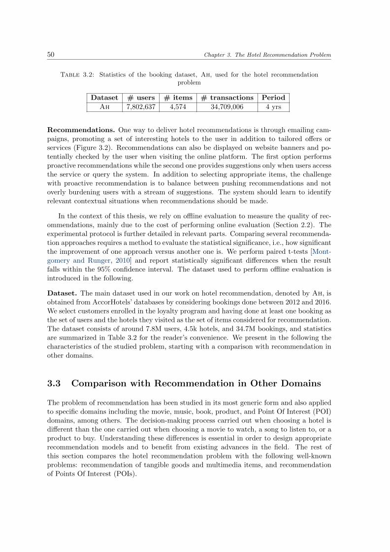
50 Chapter 3. The Hotel Recommendation Problem
Table 3.2: Statistics of the booking dataset, Ah, used for the hotel recommendationproblem
Dataset # users # items # transactions Period
Ah 7,802,637 4,574 34,709,006 4 yrs
Recommendations. One way to deliver hotel recommendations is through emailing cam-paigns, promoting a set of interesting hotels to the user in addition to tailored offers orservices (Figure 3.2). Recommendations can also be displayed on website banners and po-tentially checked by the user when visiting the online platform. The first option performsproactive recommendations while the second one provides suggestions only when users accessthe service or query the system. In addition to selecting appropriate items, the challengewith proactive recommendation is to balance between pushing recommendations and notoverly burdening users with a stream of suggestions. The system should learn to identifyrelevant contextual situations when recommendations should be made.
In the context of this thesis, we rely on offline evaluation to measure the quality of rec-ommendations, mainly due to the cost of performing online evaluation (Section 2.2). Theexperimental protocol is further detailed in relevant parts. Comparing several recommenda-tion approaches requires a method to evaluate the statistical significance, i.e., how significantthe improvement of one approach versus another one is. We perform paired t-tests [Mont-gomery and Runger, 2010] and report statistically significant differences when the resultfalls within the 95% confidence interval. The dataset used to perform offline evaluation isintroduced in the following.
Dataset. The main dataset used in our work on hotel recommendation, denoted by Ah, isobtained from AccorHotels’ databases by considering bookings done between 2012 and 2016.We select customers enrolled in the loyalty program and having done at least one booking asthe set of users and the hotels they visited as the set of items considered for recommendation.The dataset consists of around 7.8M users, 4.5k hotels, and 34.7M bookings, and statisticsare summarized in Table 3.2 for the reader’s convenience. We present in the following thecharacteristics of the studied problem, starting with a comparison with recommendation inother domains.
3.3 Comparison with Recommendation in Other Domains
The problem of recommendation has been studied in its most generic form and also appliedto specific domains including the movie, music, book, product, and Point Of Interest (POI)domains, among others. The decision-making process carried out when choosing a hotel isdifferent than the one carried out when choosing a movie to watch, a song to listen to, or aproduct to buy. Understanding these differences is essential in order to design appropriaterecommendation models and to benefit from existing advances in the field. The rest ofthis section compares the hotel recommendation problem with the following well-knownproblems: recommendation of tangible goods and multimedia items, and recommendationof Points Of Interest (POIs).

Chapter 3. The Hotel Recommendation Problem 51
Recommending tangible goods and multimedia items. In the case of a movie ora product selection process for example, users are aware that they have the possibility toswitch between movies or to return a product at a minimal charge if they are not satisfiedwith it. This is not the case when selecting accommodations given that users do not recovereasily after a bad choice of accommodations. Managing to change hotel bookings once on avacation or a business trip is not straightforward. It usually incurs significant costs and canspoil the travelers’ trips. The availability of hotels is also not guaranteed given the limitednumber of rooms. The high-stakes nature of the problem leads to a more challenging andcomplex decision-making process since customers can often have high levels of insecurityduring purchase [Zoeter, 2015]. Furthermore, traveling is not a frequent activity, especiallycompared to other activities such as watching movies or listening to music, and many peoplebook a hotel only once or twice a year [Bernardi et al., 2015]. As a result, the availablefeedback is sparse which makes it harder to extract relevant user preferences. Anotherdifference relies on the fact that decisions are made in a very specific context based on adynamic inventory [Cremonesi et al., 2014]. The issue of the limited availability of resourcesdoes not arise in the movie or the music domain where the resource is usually available toan unlimited number of users. The price of the options also varies over time, which requirestaking into account the context of decisions.
Recommending Points Of Interest (POIs). With the emergence of Location-BasedSocial Networks (LBSN), users easily post content associated with their location and sharethe positions of the places they are visiting. The availability of the vast amount of users’visiting history has led to an extensive study of the problem of POI recommendation [Liuet al., 2017]. Given the visiting history of users, the goal is to recommend for each usernew POIs that he will be likely visiting in the future. Compared to the classical problemof recommendation, POI recommendation is greatly affected by geography, time, and socialrelations. First, geographical distances separating POIs have a significant influence on theuser behavior [Ye et al., 2011]. Intuitively, users tend to visit POIs that are either close totheir place of residence or far from it but close to POIs they are in favor of. Therefore, POIsvisited by one user are rather grouped geographically. Power law distribution is usuallyused to model the visiting probability to the distance between a couple of POIs. Second,users may adopt different behaviors with respect to time and POIs may be accessible ornot at different time periods. Finally, and given that users share their activity on platformswhere they are interconnected via social links, social friends can be explored to performrecommendations. In particular, relevant information can be extracted from friends whohave close social ties or who exhibit similar behavior with the target user [Ye et al., 2011].
While hotel recommendation can also be influenced by almost the same factors, theuser behavior in the hotel domain follows different dynamics leading to a different set ofchallenges. POIs are usually visited successively and the distance between two consecutivevisited locations is taken into account when evaluating possible recommendations. In com-parison, hotel visits done by one user are, in most cases, independent and separated by areturn to the traveler’s residence. As a result, the assumptions made in POI recommen-dation concerning in particular the geographical influence do not hold in the case of hotelrecommendation. In addition, information about social relations between users is missingand cannot be leveraged to improve recommendations. Users adopt different attitudes ineach domain and consequently, specific challenges arise in each one of them. We present inthe following the challenges and limitations occurring in the hotel domain.

52 Chapter 3. The Hotel Recommendation Problem
0
10
20
30
40
50
60
70
0 1 2 3 4 56-
1011
-20
>20
Per
cen
tage
of
use
rs
Number of transactions
Figure 3.3: Percentage of users enrolled in the loyalty program per number of bookingsmade, represented by filled bars, and per number of distinct visited hotels, represented by
empty bars, on a period of four years
3.4 Challenges and Limitations
The decision-making process for selecting the appropriate accommodation is more complexthan the one for acquiring tangible goods, for example. As a result, the hotel recom-mendation problem faces particular challenges making the direct application of classicalrecommendation approaches insufficient.
Sparsity. It is well-known that a common problem from which suffer most RS is datasparsity (Section 2.1.3). People only interact with a small number of items and the collectedfeedback is usually sparse. However, this problem is aggravated in the hotel domain. Trav-eling is not a frequent activity and many people book a hotel only once or twice a year. Theavailable feedback is not always enough to extract relevant user preferences which tends toreduce the quality of recommendations. Figure 3.3 shows, in filled bars, the percentage ofusers enrolled in the loyalty program per number of bookings made between 2012 and 2016,highlighting the fact that more than 90% of users have made less than five bookings duringthe considered time period. In addition, some users are used to return to the same hotelsthey have visited in the past, generating repeated and less diverse feedback. This can beobserved by examining the proportion of users per number of visited hotels, represented byempty bars in Figure 3.3. There are more users who have visited one hotel than users whohave made one booking, and there are fewer users who have visited more than 10 differenthotels than users who have made 10 bookings.
An extreme case of the data sparsity occurs when new users or new hotels are introducedto the system. This is known as the cold-start problem (Section 2.1.3). Several solutions havebeen proposed in the literature to temporarily deal with cold users until enough informationis gathered (for example [Saveski and Mantrach, 2014; Schein et al., 2002]), under theassumption that users cannot return to the cold status. This assumption is not valid in thehotel domain: The cold-start problem experienced is relatively different from the classicalone and is framed as the continuous cold-start problem [Bernardi et al., 2015].

Chapter 3. The Hotel Recommendation Problem 53
Continuous cold-start. In the hotel domain, users remain cold for a long time, and evenafter collecting enough feedback, they may return to the cold status in specific situations,leading to the continuous cold-start setting. This formulation was first introduced by amajor online travel site [Bernardi et al., 2015]. The problem is known to arise in the hoteldomain in the three following cases:
• The user is newly introduced to the system. This case is equivalent to the classicalcold-start problem and is due to the fact that many users stay cold for a long timesince they only travel and book hotels a few times each year.
• The user changes his interest. This case is related to the volatility of preferences.The user interest changes over time bringing him back regularly to the cold status.For example, a phenomenon is observed when people’s standards evolve, moving frombooking hotels in one segment, e.g., economy segment, to booking hotels in a higherone, e.g., luxury segment.
• The user behavior changes depending on the context he is in. Several contextualfactors, such as the location, the weather, and the intent of the trip, highly influencetravelers’ decisions. The same user can behave differently when choosing a hotel tospend the summer vacation with his family or to attend business meetings.
Classical Content-Based Filtering (CBF) and Collaborative Filtering (CF) approachescannot address the continuous cold-start problem since they do not take into account thevolatility of user preferences and relevant contextual factors. While the continuous cold-startproblem has not been specifically addressed in the literature, several approaches are able tocope with each of the described aspects. Hybrid approaches [Burke, 2002], combining CBFand CF, deal with the classical cold-start problem. Time-aware RS [Campos et al., 2014] areable to model the evolution of user preferences by considering the chronologically orderedhistory of user transactions. In particular, Context-Aware RS (CARS) [Adomavicius andTuzhilin, 2015] offer a promising way to address the continuous cold-start problem [Bernardiet al., 2015]. Sparsity is addressed by introducing information about the user’s environmentand recommendations are driven by the actual context of the user. Preferences are alsomodeled according to the context and each behavior is associated with a specific situation.An appropriate solution requires the identification of the contextual factors influencing users,the collection of related data, and the design of models integrating these factors.
3.5 Related Work
Several solutions have been proposed to assist tourists and travelers in their planning pro-cess [Felfernig et al., 2007; Gretzel, 2011; Kabassi, 2010]. These solutions aim to recommendone item or a package of items including destinations, attractions, accommodations, and ac-tivities, among others. However, the particular problem of hotel recommendation has hadrelatively little research devoted to it. In this section, we review existing work related tothis problem. We first present existing approaches according to the exploited data source,and then discuss the problem of bounded resources and the related problem of destinationrecommendation.

54 Chapter 3. The Hotel Recommendation Problem
Explicit feedback for hotel recommendation. Explicit feedback in the form of textualreviews and ratings has been leveraged for hotel recommendation. In [Levi et al., 2012], acold-start RS relying on textual reviews is developed. The assumption made is that usersfavor reviews written by users with the same trip intent, e.g., business trip or leisure trip,of similar backgrounds, i.e., nationality, and with similar preferences for hotel aspects, e.g.,location, room, and service. These elements are used to measure similarities between usersand define context groups. Hotels are modeled as feature vectors by exploiting the wordsused in the corresponding reviews. Features are additionally extracted for each travel intent,nationality, and hotel aspect. Recommendation is then performed by combining preferencesof users who are similar to the target user with the importance assigned to each feature byusers. The dataset used was extracted from two travel search engines, Tripadvisor.com andVenere.com. A crowdsourcing experiment based on Amazon Mechanical Turk showed thatcommon traits for visitors of any hotel can be identified by mining reviews.
Another framework for hotel recommendation was proposed in [Zhang et al., 2015] andleverages textual reviews and ratings. The authors propose a hybrid approach where usersand hotels are first modeled in latent topic spaces based on the reviews given by users forhotels. Similarities between users and hotels are then derived from these models. Ratingprediction is performed by using Matrix Factorization (MF) and by adding a constraintthat enforces the learned models for each pair of users and hotels to be close if their com-puted similarity is high. The predicted ratings are then modified according to the user’stravel intent that is explicitly provided through the proposed framework. Finally, diversitytechniques are used to optimize the ranking of the recommended list by removing redun-dancies while maintaining relevance. To validate the proposed approach, experiments wereconducted on a dataset from the travel search engine Ctrip.com, and errors in rating pre-diction were reported. On another note, explicit feedback in the form of ratings assignedto various hotel aspects, e.g., location, cleanliness, services, and rooms, were also exploitedfor hotel recommendation. In [Nilashi et al., 2015], a 3-dimensional tensor is created by as-sociating the first dimension with users, the second one with items, and the third one withhotel aspects. The tensor is used to cluster users and a dimensionality reduction techniqueis applied within each cluster. Neural networks integrating fuzzy logic principles are thentrained to predict overall ratings in each cluster. Experiments were conducted on datasetsfrom Tripadvisor.com and proved the effectiveness of the proposed method and its severalcomponents for improving the accuracy of multi-criteria prediction.
Implicit feedback for hotel recommendation. Analyzing the user behavior can in-directly reflect his opinion, and implicit feedback, which is normally more abundant thanexplicit feedback, can be leveraged to infer user preferences [Hu et al., 2008]. Booking trans-actions, i.e., hotel visits, are an example of implicit feedback collected in the hotel domain.In [Saga et al., 2008], a preference transition network is built based on user bookings. Itis represented by a graph with hotels as nodes. Edges are established between pairs ofhotels depending on the likelihood of users who booked one hotel to book the other one.The recommendation phase consists of two steps. First, the user selects an initial hotel,generating a list of candidate hotels. Second, candidate hotels are scored by considering theindegree and outdegree in the graph, in addition to a factor accounting for the number oftimes the item was recommended and attempting to promote novelty in recommendations.The system was validated using bookings from a real hotel reservation service.

Chapter 3. The Hotel Recommendation Problem 55
Contextual factors for hotel recommendation. Like in any other domain, hotel recom-mendation can benefit from incorporating relevant contextual factors affecting users [Ado-mavicius and Tuzhilin, 2015]. Performing contextual recommendations requires the defi-nition of the notion of context and assessing the importance and relevance of each factor.When addressing the related problem of lodging recommendation in [Sanchez-Vazquez et al.,2017], the authors designed a context-aware approach inspired by socio-economic analyses ofuser behavior in sharing economy marketplaces. The proposed approach integrates featurescapturing five aspects of user’s consumption behavior: the perceived value or the trade-off between benefits and costs, the perceived risk in choosing an option rather than theothers, the price sensitivity or the extent to which the price affects the behavior, the per-ceived authenticity of the experience it could provide, and the electronic word-of-mouth. Theevaluation was done using a publicly available dataset from Airbnb, showed improvementscompared to other recommendation techniques, and enabled the study of the discriminativepower of the different features.
Bounded resources in hotel recommendation. As mentioned before, recommendationin the tourism domain in general and in the hotel domain in particular exhibits specificcharacteristics that differentiate it from other domains. In particular, each item, i.e., hotel,has a maximum capacity that cannot be exceeded and hotels cannot be consumed by anunlimited number of users. Recommending with bounded resources has first been studiedin [Cremonesi et al., 2013, 2014]. Offline and online experiments were performed to evaluatepersonalized and non-personalized algorithms in the low season setting, i.e., season where allthe items are available, and in the high season setting, i.e., season where most popular itemsare unavailable. Results showed that popularity-based methods outperform personalizedmethods in the low season setting: Popular hotels, i.e., those that are rated the highestby most people, are the best choices for most users. This can be due to the fact that theopinion of the crowd has a strong influence effect which is sometimes stronger than individualpreferences. Personalized approaches perform better in the high season setting: When themost popular hotels become unavailable, user preferences drive the decision. Consideringhotel availability is therefore essential to determine the recommendation approach to use.
Destination recommendation. The selection of an option for accommodation dependsgenerally on the choice of the destination to visit, and thus, the problem of hotel recommen-dation is related to the one of destination recommendation. [Kiseleva et al., 2015] investigatebasic recommendation strategies for suggesting destinations to users in the context of Book-ing.com, the travel search engine. In the setting they define, the user provides a list ofactivities that he wants to do during the trip and the system is expected to propose destina-tions matching these activities. The set of possible activities is defined and fixed, and userswho have visited hotels of a specific destination are asked to endorse it with representativeactivities. Strategies for ranking destinations include the one performing it randomly, theone based on the popularity of destinations, and the one based on Naive Bayes. Thesestrategies are compared with the baseline used at Booking.com and an online A/B testshowed that Naive Bayes significantly increases user engagement. Further advances in thisdirection extended the recommendation approach by considering contextual factors, in orderto address the continuous cold-start problem [Bernardi et al., 2015]. The work in [Kiselevaet al., 2016] investigated how to leverage context information for recommendation in caseswhere user history is not available, e.g., users not logged in or new to the system. The mainassumption made is that users give similar endorsements in similar situations, a situation

56 Chapter 3. The Hotel Recommendation Problem
being defined by a set of contextual factors, e.g., time, location, device type, and browser.Reviews are contextualized with respect to the defined factors. Typical user situations aredetected and constitute what is called contextual user profiles. Recommendation models arethen derived for each contextual user profile. When a user gets access to the system, thecontextual information is used to map him to a contextual user profile and the correspondingmodel is used for recommendation. Experiments were conducted within a production A/Btesting environment at Booking.com, comparing the contextual approach proposed with anon-contextual one. Results showed that the contextual approach substantially increasesuser engagement.
Relation to our work. The work presented in this thesis and related to hotel recommen-dation differs from previously proposed approaches in multiple ways. While previous workhas privileged the use of explicit feedback, e.g., ratings and reviews, we rely on implicitfeedback, i.e., bookings, since it is much more available and does not require additionalefforts from the user side [Amatriain and Basilico, 2016]. We address the problem as it isdelimited by real-world settings which has been rarely reported in previous work. However,we do not specifically address the problem of bounded resources. Simple solutions can beimplemented to cope with this problem, alternating between different recommendation ap-proaches depending on the availability of hotels [Cremonesi et al., 2014]. In an attemptto address the continuous cold-start problem [Bernardi et al., 2015], we design novel ap-proaches integrating multiple contextual factors that affect the decision-making process ofusers. Context-aware techniques have been previously exploited for recommendation in thetourism sector [Van Setten et al., 2004] but not in the hotel sector. In addition, the focushas been mostly on context in mobile applications which definition does not cover all thefactors we exploit in our work. Defining context is an important question itself since thequality of recommendation depends on the relevance of the contextual factors considered.We present in the next section the notion of context as it appears in the hotel domain andwe discuss how it affects the user behavior.
3.6 Context in the Hotel Domain
Following the definition introduced by [Dey, 2001], context is “any information that can beused to characterize the situation of an entity. An entity is a person, place, or object thatis considered relevant to the interaction between a user and an application.”. A concreteframing of the notion of context in a specific recommendation domain requires understandingthe decision-making process carried out during the task of selecting an option.
Decision-making process. The nature of tourism products purchased by customers forcesa complex decision-making process in which customers are highly involved and commit-ted [Horner and Swarbrooke, 2016]. Customers can have high level of insecurities duringpurchase since they cannot try the products before the definite selection. In addition, travel-ing is often an important event in people’s lives and decisions have a considerable emotionalsignificance for the people involved. In general, the decision is driven by a number of factorsrelated to customers and to external parameters heavily influencing them and which are be-yond their control. Figure 3.4 illustrates some of these internal and external factors [Hornerand Swarbrooke, 2016].

Chapter 3. The Hotel Recommendation Problem 57
Internal to the traveler External to the traveler
Personal motivators
Personality
Disposable income
Health
Commitments
Past experience
Hobbies and interests
Lifestyle
Attitudes, opinions, and perspectives
Availability of products
Advice of travel agents
Word-of-mouth recommendations
Political restrictions: visa, terrorism
Health problems
Special promotions and offers
Climate
Decision
Figure 3.4: Internal and external factors influencing the traveler’s decision.Figure adapted from [Horner and Swarbrooke, 2016].
Categories of context. A more refined classification of contextual factors is presentedin [Adomavicius and Tuzhilin, 2015; Fling, 2009] and introduces four broad categories ofcontext: physical context, social context, interaction media context, and modal context.While this classification was initially meant to frame context in mobile applications [Fling,2009], these categories can also be adapted to other types of applications. We present themin the following and discuss how they are observed in the hotel domain.
• Physical context. The physical or environmental context includes the user locationwhich greatly influences decisions and actions. It also covers the time, activity,weather, and temperature, in applications where these factors are relevant. Choosinga hotel to book depends on the destination the traveler is planning to visit whichselection is itself affected by the traveler’s country of residence, the season, and theweather, for example.
• Social context. The social context represents the presence and role of other peoplearound the user. Users can be strongly affected by other people during the decision-making process. This occurs in cases where a user is booking a vacation for a group ofpeople including himself. It also occurs when the decision is guided by other people’spast experiences and by the word-of-mouth or word-of-mouse including reviews postedon social media.
• Interaction media context. This category of context describes the device used to accessthe system and the type of channel used to deliver personalized recommendations.Users may have different behaviors when browsing on their mobile or on their personalcomputer. Different strategies of recommendations may then be adopted to addressthe different user attitudes. This problem is not addressed in our work, mainly becausethis type of information is missing or not exhaustive across the data we handle.
58 Chapter 3. The Hotel Recommendation Problem
• Modal context. The modal context covers the state of mind of the user, his goals, andhis mood. It plays an important role in the selection process. As an example, a singleuser behaves differently when organizing a business or a leisure trip.
Context at purchase vs. context at consumption. In applications where the actualconsumption of the item is close in time to its purchase, e.g., movie and music streamingapplications, the context is expected to remain stable between the two events. Therefore,contextual factors are evaluated at the moment of purchase and used to generate recom-mendations adapted to the context of consumption. This is obviously not the case whenpurchasing tourism products in general and hotels in particular. The context of the userwhen searching and booking a hotel is significantly different from his context during thetrip and during his visit to the hotel. However, elements from both contexts are relevantto the final decision. The location of the user during the purchase, e.g., his country of resi-dence, affects the chosen destination and the subset of candidate hotels that is considered.In addition, the location of the user during consumption, i.e., the destination, affects thechoice of the hotel since hotels do not have the same characteristics in all regions. There-fore, the environments of the user when choosing the hotel and when visiting it guide thedecision-making process.
3.7 Conclusion
We present in this chapter the problem of hotel recommendation with its characteristics asemerging in real-world applications and in the industrial context we consider in this the-sis. We discuss how this particular problem differs from other recommendation problemsaddressed in the literature, making the use of classical recommendation approaches insuffi-cient. The decision-making process carried out when choosing a hotel is complex: Users canhave high level of insecurities and organizing trips involves a considerable emotional signif-icance. Hotel recommendation also suffers from the continuous cold-start problem. In fact,users recurrently fall into the cold-start problem due to the rarity of the traveling activity,the volatility of preferences, and the multifaceted behavior. We discuss these limitationsand their implications, and we review existing work related to hotel recommendation. Giventhat contextual information can be exploited to address the problem, we provide a framingof the broad notion of context as it appears in the hotel domain.
Conventional context-aware approaches adopt the representational view of context [Dour-ish, 2004] which assumes that context is represented by a predefined set of observable staticattributes where all possible values are fixed, known, and atomic. In our work, we arguethat the context variable emerging in the hotel domain is partially observable. This notion ofpartial observability is related to context accessibility, relevance, acquisition, and modeling,as defined in Chapter 1. It requires the development of appropriate methods accounting forthe different categories of context, which we provide in Chapters 4, 5, and 6, alongside acharacterization of the contextual factors considered.
Chapter 4
Leveraging Explicit Context
This chapter presents the industrial solution we designed for hotel recommendation [Al-Ghossein et al., 2018d], combining several context-aware recommendation models in orderto alleviate the shortcomings of using traditional approaches as discussed in Chapter 3. Thephysical, social, and modal contexts of travelers are leveraged to improve the performanceof the RS, and information related to the geographical and temporal dimensions, textualreviews, and the trips’ intents is integrated into the system. Contextual information con-sidered in this chapter is explicitly provided by users and is directly related to at least oneof the RS entities, i.e., users, hotels, or user interactions with hotels. On the other hand, itis partially observable since the trips’ intents are not observed at the moment of recommen-dation but are only recorded for past interactions. The relevance of each contextual factorwith regards to target users is also unknown while affecting the overall performance of theRS. The proposed RS addresses these challenges and is validated on real-world datasets.
4.1 Introduction
Choosing the most appropriate option for accommodation when making travel plans is aneffortful and time-consuming task for most people. RS rely on personalization and deployingthem in the hotel domain facilitates trip planning. As discussed in Chapter 3, the hotelrecommendation problem is different from other recommendation problems studied in theliterature and faces, in particular, the continuous cold-start issue [Bernardi et al., 2015].
A promising way to address this issue is to leverage Context-Aware RS (CARS) [Ado-mavicius et al., 2011]. These systems take into account the contextual factors that affecttravelers’ choices. Recommendations are driven by the context and by the behavior of otherusers when they were in similar contexts. Building a robust CARS requires identifying therelevant contextual factors and designing models that integrate them. A survey conductedamong domain experts reveals that the traveler’s decision-making is mainly sensitive to dif-ferent types of context: the physical, social, and modal contexts, introduced in Section 3.6.
In this chapter, we propose context-aware models for hotel recommendation that takeinto account the multiple types of context in order to cope with the limitations of only
59

60 Chapter 4. Leveraging Explicit Context
relying on booking data. These models outperform state of the art methods and integrategeographical and temporal dimensions, textual reviews extracted from social media, andthe trips’ intents. We present an industrial solution combining the proposed models andhandling each user segment differently. Experiments prove the interest of integrating con-textual factors to improve the quality of recommendation and show how the performancediffers based on the targeted user segment. We also evaluate traditional recommendationmethods on a real-world dataset and show how they compare when applied to the particularproblem of hotel recommendation.
Notations. The notations adopted throughout the chapter are those introduced in Sec-tion 2.1.4. To generate recommendations for a target user u ∈ U , we compute the relevancescores, denoted by rui, for each hotel i ∈ I. Hotels are then ranked by decreasing order ofrui, and the top-N hotels of the list, i.e., the N hotels that score the highest, are selected forrecommendation. The key difference between the methods presented in this chapter residesin the way rui is computed.
The remainder of the chapter is organized as follows. In Sections 4.2, 4.3, and 4.4, wepresent the recommendation models designed, taking into account the physical, social, andmodal contexts of users, respectively. Section 4.5 gives an overview of the RS developed.Experiments and results are presented and discussed in Section 4.6. Finally, Section 4.7concludes the chapter.
4.2 Influence of the Physical Context
Motivation. The first factor we consider in the physical context is the geographical locationof hotels and the users’ country of residence. Users we handle come from all over the worldand hotels are spread in more than 90 countries. Choosing a hotel is highly correlatedwith the choice of the destination to visit. In addition, the user’s country of residence isimportant in the sense that residents of one country share the same culture and tend tohave similar tastes when it comes to traveling. Furthermore, as noticed in our datasets, thelarge majority of users’ bookings are in hotels located near their country of residence.
The second factor we consider is temporality: The timing of a trip has also an impact onthe users’ final destinations. Leisure trips, usually organized during holidays, are meant todiscover new trendy places while business trips occur almost all year long. The seasonalityfactor is also relevant. Some users are used to organize trips to the beach in the summerand to ski resorts in the winter. Another example of seasonality influence is observed whenresidents of cold countries tend to choose warm destinations in an attempt to escape thefreezing weather.
To illustrate these insights, Table 4.1 and Table 4.2 show the percentage of bookingsin selected destinations and during specific periods of one month made by Australian andFrench residents respectively. In our datasets, we notice that the majority of Australianresidents’ trips involve close destinations. However, the percentage of visits to Europe issignificantly higher in June than in December, thus highlighting the temporal influence.We note that the number of overall bookings in all periods is comparable. With respectto French residents, we notice that the number of visits to the Paris region in February is

Chapter 4. Leveraging Explicit Context 61
Table 4.1: Proportion of bookings made by Australian residents in selected destinationsduring periods of one month
Destinations March June September December
Oceania 76% 69% 71% 78%
Europe 4% 12% 12% 5%
Asia 9% 9% 8% 9%
Table 4.2: Proportion of bookings made by French residents in selected destinationsduring periods of one month
Destinations February May August November
Paris Region 34% 30% 22% 37%
South of France 22% 24% 33% 23%
Spain 0.5% 1% 2% 0.7%
greater than in the month of August. In addition, they tend to visit the south of Franceand Spain more frequently during summer. Given these observations, we conclude thatgeography and temporality have an influence on the global behavior of residents of the samecountry with respect to the visited destinations.
Approach. To integrate these ideas, we introduce localRS where we propose to clustercountries of residence, and consequently users, based on the destinations visited by itsresidents each period of the year. The main idea is to build a local recommendation modelfor each cluster instead of building a single global model for all users. Local models betterreflect the users’ interests since they cluster together those having similar tastes regardingvisited destinations. They are also able to capture new travel trends that start in a givenregion. The concept of building multiple local models instead of one global model hasbeen proposed in previous work [Christakopoulou and Karypis, 2016; Lee et al., 2014]. Weomit details about related work on local models in this chapter, only to mention that theapproaches previously proposed cluster users and items based on the observed behavior, i.e.,user interactions, and are therefore subject to limitations in sparse conditions.
In the process of clustering, a country of residence is represented by a set of features in-cluding a feature for each destination country each month of the year. Destination countriesconsidered are countries where hotels are available. The value of a feature is equal to theproportion of bookings made by residents in the destination country in the defined period.We apply the k-means clustering technique [Hartigan and Wong, 1979] and create k clustersof countries where residents have similar behaviors with respect to visited destinations andperiods of visits.
The k-means clustering is a popular technique for cluster analysis in data mining. It aimsto partition observations into k clusters where each observation is assigned to the cluster withthe nearest mean. It assumes a Euclidean space and that the number of clusters, k, is knownin advance. While the problem is computationally difficult, heuristic algorithms are usuallyemployed and converge to a local optimum. In the basic version of the k-means algorithm,we initially choose k points that are likely to be in different clusters and designate each oneof them as the centroid of a cluster — there are several ways to do this initial selection that

62 Chapter 4. Leveraging Explicit Context
Table 4.3: Examples of clusters of countries which residents have similar behaviors re-garding visited destinations and periods of visit (non-exhaustive list per cluster)
Cluster 1 Cluster 2 Cluster 3 Cluster 4
France Italy United States UAEBelgium Germany Canada BahrainAndorra Switzerland Peru KuwaitGuinea Netherlands Portugal QatarGuyana Greece India MoroccoAlgeria Romania China SpainTunisia Russia South Korea TanzaniaSenegal Turkey Vietnam Cuba
will not be discussed here. Then, for each remaining point, we find the the closest centroidand add the point to the corresponding cluster. After iterating over all points, the clusters’centroids are adjusted. This process is repeated until convergence.
Choosing the value of k is important. If k is too small, the recommendation algorithm issensitive to noise and if k is too large, we may be missing out on users who could be relevantfor the generation of recommendations. In our setting, the value of k is finally set followingextensive experiments.
Table 4.3 shows examples of computed clusters and a list of some of the countries includedin each cluster. The clustering technique as described here is dependent on two factors.First, it relies on the number of users present in each country and whether they constitutea representative sample of the whole population when it comes to the traveling behavior.Second, the technique depends on the worldwide availability of hotels, considering that thedensity of hotels is not comparable in all countries.
4.3 Influence of the Social Context
With the evolution of social platforms, most people rely on other people’s experiences andreviews to choose a hotel. Studies in the tourism sector have indicated that travelers perceiveonline reviews as more trustworthy than information provided by official websites [Filieriet al., 2015; Litvin et al., 2008]. Consequently, we integrate into the RS textual reviewsposted online as an additional source of information to describe hotels. The reviews areanonymous as we are not able to match the users leaving reviews on websites and ourtarget users. Introducing content description is a way to avoid overfitting given the sparsedata. It also enables recommending hotels that are newly introduced to the system 1 whenreviews are available. The proposed approach, which we refer to as CTRk+, is based onCollaborative Topic Regression (CTR) [Wang and Blei, 2011], also known as CollaborativeTopic Modeling, which is a hybrid recommendation method. While several other works haveexploited content for recommendation [Agarwal and Chen, 2009, 2010; Wang et al., 2015],CTR offers one of the most prominent framework that is presented in the following.
1http://pressroom.accorhotels-group.com/accorhotels-officially-welcomes-fairmont-raffles-and-swissotel

Chapter 4. Leveraging Explicit Context 63
4.3.1 Collaborative Topic Modeling
CTR [Wang and Blei, 2011], initially introduced to recommend scientific articles, is ahybrid approach that combines Collaborative Filtering (CF) based on latent factor mod-els [Salakhutdinov and Mnih, 2008a] and content analysis based on probabilistic topic mod-eling [Blei et al., 2003; Chang et al., 2009]. Latent factor models leverage user interactionsand topic models rely on articles’ content or textual descriptions of items. Introducing acontent analysis component with CF improves the recommendation performance and allowsto generalize to previously unseen items.
Topic models. The goal in topic modeling approaches [Blei and Lafferty, 2009] is toassociate a document seen as an unordered list of words with a vector of topics, i.e., ofword distributions. Documents are thus represented in a low-dimensional space and modelshave the characteristic of being interpretable [Chang et al., 2009]. CTR integrates LatentDirichlet Allocation (LDA) [Blei et al., 2003] which is one of the most influential topicmodeling approaches.
Latent Dirichlet Allocation. LDA [Blei et al., 2003] is a generative model describing textdocuments and corpora where the key notion involved in the description of a document is thenotion of topic. A topic corresponds to a word distribution (for instance in a music-orientedcorpus, the word “concert” would have a higher probability to be drawn than in a sport-oriented corpus) and a document is described as a mixture of topics. Topics are learned inan unsupervised fashion and, thus, do not necessarily correspond to human-understandableconcepts [Chang et al., 2009]. The popularity of LDA is due to its simplicity, modularity,and interpretability. Assuming there are K topics, the generative process for each documentin the corpus is presented in Figure 4.1 and is described as follows:
1. Choose topic proportions θ ∼ Dirichlet(α)
2. For each word wn in document:
(a) Choose a topic zn ∼Multinomial(θ)
(b) Choose a word wn from the multinomial p(wn|zn,β)
α θ z
β
w
N
M
Figure 4.1: Generative model for Latent Dirichlet Allocation (LDA)
In terms of document analysis, the parameters of LDA can be understood in the followingway:

64 Chapter 4. Leveraging Explicit Context
• The vector α represents the global topic trend. For instance, a parameter α =(1, . . . , 1) corresponds to a uniform choice over all topics, on average. The higherthe component αx is, the more frequent topic x will be in the whole corpus.
• The matrix β stores the probability of words inside topics. If a word w is set to belongto topic z, then it will be chosen with probability βz,w.
• The vector θ corresponds to the topic distribution inside one document.
Compared to clustering approaches where each observation is assigned to only one clus-ter, LDA enables documents to exhibit several topics. A training of LDA model is possiblebased on maximum likelihood principle [Blei et al., 2003]. In practice, it is suggested to useeither Gibbs sampling or variational inference for this task.
Collaborative Topic Modeling. CTR assumes that documents describing the items aregenerated by a topic model and represents users with topic interests. It adds a latent variablethat offsets the topic proportions when modeling user latent factors. This offset is derivedfrom the rating data and represents the fact that two similar items, i.e., having similar topicproportions, can be interesting to different types of users. As more users interact with theitem, the offset value becomes clearer. The latent factor model used in CTR is ProbabilisticMatrix Factorization (PMF) [Salakhutdinov and Mnih, 2008a] (Section 2.5.2.5) and thetopic model is LDA [Blei et al., 2003].
We assume that each hotel i is described by a document di containing ndi words andhaving a multinomial distribution θi over K topics. Users and items are modeled in the low-dimensional space of dimension K. Each user u is represented by the latent vector pu ∈ RK
and each hotel i by the latent vector qi ∈ RK . We define P = (pu)n1 and Q = (qi)m1 , and
we denote by λ∗ the regularization parameters. The generative process of CTR is given asfollows:
1. For each user u, choose user latent vector pu ∼ N (0, λ−1P IK)
2. For each hotel i,
(a) Choose topic proportions θi ∼ Dirichlet(α)
(b) Choose hotel latent offset εi ∼ N (0, λ−1Q IK) and set the hotel latent vector as
qi = εi + θi
(c) For each word win in di,
i. Choose topic assignment zin ∼Multinomial(θi)
ii. Choose word win ∼Multinomial(βzin)
3. For each user-hotel pair (u, i), choose the rating rui ∼ N (puq>i , c−1ui )
We note that IK is a K-dimensional identity matrix and cui is the precision parame-ter for rating rui defined in Section 2.5.2.4 and indicating the confidence we have in theobservation rui.

Chapter 4. Leveraging Explicit Context 65
Learning the parameters. Computing the full posterior of the parameters is intractable andthe authors in [Wang and Blei, 2011] develop an algorithm in the style of the expectation-maximization algorithm to learn the maximum a posteriori estimates. The maximizationof the posterior is equivalent to maximizing the log-likelihood of P, Q, (θi)
m1 , and R, given
λP , λQ, and β,
L = −λP2
∑u
‖pu‖22 −λQ2
∑i
‖qi − θi‖22 +∑i
∑n
log
(∑m
θimβm,win
)−∑u,i
cui2
(rui − puq>i )2
(4.1)
The function is optimized by coordinate ascent, iteratively optimizing the CF variablespu,qi and the topic proportions θi. The authors in [Wang and Blei, 2011] state thatfixing θi as the estimate from vanilla LDA gives a comparable performance and reducesthe complexity of computations. The final relevance scores, rui, are computed as follows:rui = puq
>i .
4.3.2 Handling Positive and Negative Reviews
Our approach integrating textual reviews as hotel descriptions into the recommendationmodel, CTRk+, is based on CTR. The PMF is replaced by a ranking model and topics areextracted separately from positive and negative reviews and finally combined in the model.
Pairwise approach. Motivated by Bayesian Personalized Ranking (BPR) [Rendle et al.,2009] (Section 2.5.2.4) and its superiority in implicit feedback settings, we introduce a pair-wise method for the CF part of CTR. Model parameters are learned by considering thepairwise ranking between hotels. The user u is assumed to prefer hotel i over hotel j ifrui = 1 and ruj = 0 and the pairwise preference probability is given by:
p(i >u j | Θ) = σ(puq>i − puq
>j ) (4.2)
where σ is the logistic sigmoid and Θ represents the model parameters. The set of trainingdata, Dbpr, is defined as follows: Dbpr := (u, i, j) | rui = 1 ∧ ruj = 0. This leadsto replacing, in Equation 4.1, −∑u,i
cui2 (rui − puq
>i )2 by
∑(u,i,j)∈Dbpr
lnσ(puq>i − puq
>j ),
since the elements of Dbpr are drawn from the probability σ(puq>i − puq
>j ) (item 3 in the
generative process of CTR). Learning is performed following the same algorithm as CTR andthe update equations are modified accordingly. Experiments on our datasets showed thatfixing θi as the estimate from LDA leads to a comparable performance, as in the originalwork of CTR, which was adopted in our setting.
Handling review polarity. We rely on reviews extracted from TripAdvisor 2 in orderto provide a textual description for hotels. TripAdvisor reviews are graded from 1 to 5,representing the level of user satisfaction. They can be divided into a set of positive reviews
2http://www.tripadvisor.com

66 Chapter 4. Leveraging Explicit Context
mentioning available and appreciated characteristics of the hotel and a set of negative reviewspointing out the missing or unsatisfying features. A large majority of users check the reviewsonline before booking a hotel and are influenced by what is shared. While the objectivedescription of hotels is available, we consider that the reviews are a richer source becausethey derive from the real user experience.
In the latent space in which users and hotels are represented, the elements of pu and qimeasure respectively how much the user is attracted to a latent factor and to what extentthe hotel possesses it, positively or negatively. A first approach to applying CTR to ourproblem is to concatenate all available reviews for a hotel i in one document di and use itto extract the topic proportions θi. The values of qi that we get indicate the probability ofa topic emerging in di. However, we do not distinguish between the cases where this topicdenotes a positive feature of i or a negative one.
We propose to extract topics separately from positive and negative reviews and combinethem to model items. Therefore, we model the hotel latent vector as follows:
qi = εi + θi+ − θi− (4.3)
where θi+ denotes the topic distribution extracted from positive reviews and θi− the oneextracted from negative reviews.
4.4 Influence of the Modal Context
The modal context covers the users’ state of mind and mood. We consider here two aspectsof the influence of modal context on users. First, the user’s interest may change over timeand the preference shift should be considered during the learning process by giving moreweight to recent interactions. Then, choosing accommodations is strongly related to thetrip’s intent which is not provided explicitly but can be inferred from features related to thestay. These features include information related to the lead time, the staying days of theweek, and the company of other people. The lead time is the time separating the reservationdate and the check-in date and is usually higher for leisure trips than for business trips,leisure trips being usually planned in advance. Analyzing the staying days of the week isinsightful since a stay only involving weekdays and organized in a non-holiday period is mostlikely a business one. Other information concerning the company of other people, i.e., thenumber of adults and the number of children, is also meaningful.
Since the trip’s intent is not provided at the moment of recommendation, we build aclassical recommendation model without explicitly modeling the context variable like in mostCARS (Section 2.7). Information about the trip’s intent is leveraged during the learningprocess where we propose to modify the probability of sampling observations depending onthe associated context. The approach we propose, which we refer to as BPRx3, is based onBPR [Rendle et al., 2009] (Section 2.5.2.4) where we rely on a biased sampling to learn themodel.

Chapter 4. Leveraging Explicit Context 67
BPR. As mentioned before, BPR assumes that user u prefers hotel i over hotel j if the pair(u, i) is observed and the pair (u, j) is not. The learning data is represented by the set
Dbpr := (u, i, j) | rui = 1 ∧ ruj = 0,the training triples being uniformly sampled from the data due to the very large number ofpairs (u, i, j).
BPRrec and the new interest aspect. We assume that hotels chosen recently are pre-ferred over the ones corresponding to older choices. BPR++ [Lerche and Jannach, 2014] isan extension of BPR and addresses, among other points, the recency and temporal aspectof events. The authors proposed a biased sampling that would sample alternatively fromDbpr or from another set that we denote by Drec
bpr and defined as follows:Drecbpr := (u, i, j) | rui = 1 ∧ ruj = 1 ∧ rec(u, i, j) = 1,
where the function rec(u, i, j) returns 1 if the booking done by u in i is more recent thanthe booking done in j, and 0 otherwise.
BPRint and the new situation aspect. We assume that a hotel observed in a certaincontext revealing the intent of the user’s trip is preferred over the ones usually chosen inthis same context. We denote by Fui the set of features related to the intent of the trip andassociated to rui, when the pair (u, i) is observed. Fui includes the lead time, the number ofadults and children accompanying the user, the week in which the check-in occurs, and thefact that the stay spans over a weekend or not. The learning data Dint
bpr is defined similarlyto Dbpr but the probability of sampling j is as follows:
p(j | Fui) ∝ |raj = 1 | Faj = Fui,∀a ∈ U|.
Some hotels are more targeted when traveling in a specific context and have thereforemore chances of being sampled as a negative item for that particular context, if they arenot observed.
Combining the three assumptions in BPRx3. We propose to use all three sets Dbpr,Drecbpr, and Dint
bpr to learn the model, and we introduce two parameters γrec and γint indicatingthe probability of sampling from each set. The learning procedure is detailed in Algorithm 4.
Algorithm 4 BPRx3: BPR based on a biased sampling
Input: Dbpr, Drecbpr, D
intbpr
1 initialize Θ . parameters of the model2 repeat3 p = random(0, 1)4 if p ≤ γrec then draw (u, i, j) from Drec
bpr
5 else6 if p ≤ γint then draw (u, i, j) from Dint
bpr
7 else draw (u, i, j) from Dbpr
8 end if9 end if
10 update Θ . similar to [Rendle et al., 2009]11 until convergence

68 Chapter 4. Leveraging Explicit Context
4.5 Overview of the System
This section describes the architecture of the RS designed in industry. It is based on thepreviously proposed methods and operates in two phases.
Phase 1. We cluster users in several buckets with respect to their country of residenceand to the visited destinations in different periods, taking into account the geographicaland temporal influences (Section 4.2). Grouping users affected similarly by both of thesedimensions before building the recommendation model helps to uncover users’ preferences.The models are then built locally for each cluster of users.
Phase 2. In this phase, we build local recommendation models taking into account theseveral types of context. The performance of the recommendation methods depends on thesparsity level of data for each user. While some approaches are adapted for new users, othersare more suited for frequent users. The user category also defines which type of context ismore relevant when selecting accommodations.
After testing multiple recommendation approaches (refer to Section 4.6), we select themost accurate one for each segment of users. As the user makes more and more bookings, wecollect additional information about his preferences and feed it to a more appropriate modelthus improving the overall quality of recommendation. To this end, with the help of domainexperts, we define a segmentation of users based on the number of bookings made. The usersegments are defined as follows: inactive users, rare users, occasional users, and frequentusers. We use the number of bookings as a threshold to separate users into segments. Thethresholds are derived from the data and we rely on extensive experiments to determinethem. We note that the definition of these segments is proper to our recommendationproblem and serves the purpose of building an accurate system. Section 4.6.3 details howwe form the segments and which method we apply for each one of them.
4.6 Experimental Results
Extensive experiments were conducted on several datasets to demonstrate the models pro-posed in the previous sections and to justify the architecture of the developed system. Thissection attempts to answer the following questions:
• Q1. How does the performance of local models built with respect to geography andtemporality compare to the performance obtained with one global model? (Section 4.2)
• Q2. Does introducing positive and negative reviews as a description of hotels improvethe quality of recommendation? (Section 4.3)
• Q3. Does introducing the recency of bookings and features related to the trip’s intentimprove the quality of recommendation? (Section 4.4)
• Q4. How do classical recommendation approaches compare when applied on a real-world dataset extracted from the hotel industry?

Chapter 4. Leveraging Explicit Context 69
Table 4.4: Statistics of the booking datasets used in this chapter
Dataset #users #hotels #bookings #reviews
Ah 7,802,637 4,574 34,709,006 -
Ah-Maxi 338,259 4,111 1,120,508 -
Ah-Mini 58,959 3,317 228,155 -
Ah-Trip 56,909 2,718 210,974 201,922
• Q5. How does the performance of the proposed approaches vary according to the usersegment? (Section 4.5)
Metrics. Recommendation models are evaluated on a set of held-out bookings. We considerthat we recommend N hotels to each user, and note which of these hotels were actuallyvisited. We use recall@N and NDCG@N for measuring the performance (Section 2.2.3).Since large values of N are not interesting for top-N recommendation, we set N to 5 and10 for the two metrics.
Parameters. We perform a grid search over the parameter space of each evaluated methodin order to find the parameters that give the best performance that is reported.
4.6.1 Contribution of the Physical Context
In order to prove the effectiveness of the localRS component, we compare the performanceof the recommendation models under two different settings. In the first one, globalRS, webuild one model for all users. In the second one, localRSk, we build one model per clusterof users, for a total of k clusters (Section 4.2).
Datasets. Ah is the original dataset described in Section 3.2. We associate to each clusteri ∈ [1, k] a dataset Ah-i derived from Ah.
Experimental setup. We split the dataset Ah into a training and a test set. We sortthe bookings of each user in a chronological order and select the first 80% to constitute thetraining set and the rest to constitute the test set. For users that appear only once in thebooking data, we randomly select 20% of them and add their booking to the test set inorder to evaluate the performance of the system on inactive users. We use the data fromthe training set of Ah in order to generate k clusters of users.
For the globalRS setting, we use the training and test sets of Ah in order to learn therecommendation model and test it. For the localRSk setting, we build one model for eachdataset Ah-i using its training set and we generate recommendations for users appearingin the corresponding test set. The training and test sets of each dataset Ah-i are derivedrespectively from the training and test sets of Ah by filtering the bookings made by theusers contained in the cluster i.
Compared methods. In order to compare globalRS and localRSk and highlight thecontribution of the clustering component, we show the results for two recommendationmethods:

70 Chapter 4. Leveraging Explicit Context
Table 4.5: Answering Q1. Recall@N and NDCG@N of the Knni and BPR methods underthe globalRS and localRSk settings for the dataset Ah
Method Metric globalRS localRS5 localRS10 localRS15
Knni
Recall@5 0.0846 0.0861 0.08590 0.0863Recall@10 0.1284 0.1306 0.1301 0.1306NDCG@5 0.0667 0.069 0.0689 0.069NDCG@10 0.0823 0.0848 0.0847 0.085
BPR
Recall@5 0.3212 0.3253 0.3261 0.3258Recall@10 0.3704 0.3740 0.3741 0.3741NDCG@5 0.2873 0.302 0.303 0.3028NDCG@10 0.3048 0.3194 0.3201 0.3201
• Knni is the item-based neighborhood method 2.5.1.2. We use the Jaccard similarityto measure items’ similarity and set the number of neighbors to 2000.
• BPR relies on pairwise preferences when learning the latent model [Rendle et al., 2009](Section 2.5.2.4). We set the number of latent factors to 100, and the regularizationparameters λP = λQ = 0.0025.
Answering Q1. Table 4.5 shows the recall@N and NDCG@N for N = 5, 10 of theKnni and BPR methods under the globalRS and localRSk settings. The quality of recom-mendation is improved under the localRSk setting — for all the represented values of k— underlining the importance of clustering users before generating recommendations. Theoptimal value of k varies with each tested model. After leading extensive experiments, weset k = 10, maximizing the overall gain we get on a representative set of methods when com-pared to the globalRS setting. Further experiments prove that the performance improveswhen in the localRSk setting regardless of the recommendation method.
4.6.2 Contribution of the Social and Modal Contexts
We evaluate here CTRk+ and BPRx3 proposed in Sections 4.3 and 4.4 respectively, highlight-ing the benefits of integrating textual reviews and features related to the trips’ intent intothe recommendation model.
Datasets. In the developed system, recommendation models are built for each cluster sep-arately (localRSk setting). We show the results for two clusters of different sizes whichdatasets are denoted by Ah-Mini and Ah-Maxi. Ah-Trip is derived from Ah-Mini and isused to validate the model introducing textual reviews. We extract 201k reviews from Tri-pAdvisor, written in the French language, and we keep in Ah-Trip the hotels with availablereviews and their related bookings. Reviews have been preprocessed by mainly removingstop words, removing words occurring once, and stemming remaining words. The detailsconcerning the composition of the datasets are in Table 4.4.

Chapter 4. Leveraging Explicit Context 71
Table 4.6: Answering Q2. Recall@N and NDCG@N of CTRk+ and other variants for thedataset Ah-Trip
Metric WRMF CTR CTRk CTRk+
Recall@5 0.3642 0.3721 0.3687 0.3732
Recall@10 0.4166 0.4371 0.4467 0.4542
NDCG@5 0.3358 0.343 0.3411 0.3447
NDCG@10 0.3584 0.3658 0.3701 0.3769
Methods compared. The models included in our comparison, as well as the correspondingparameters giving the best performance on held-out recommendations, are listed in thefollowing:
• WRMF is a Matrix Factorization (MF) technique handling implicit feedback datasets [Huet al., 2008] (Section 2.5.2.4). We set the number of latent factors to 100, λP = λQ =0.001, and cui = 1.0 for positive observations and cui = 0.01 for negative observations.
• CTR [Wang and Blei, 2011] is a model using topic modeling and CF simultaneously(Section 4.3). Each hotel is described by one document combining all of its reviews.We set the number of latent factors to 100, λP = 0.001, λQ = 10, and cui = 1.0 forpositive observations and cui = 0.01 for negative observations.
• CTRk is based on CTR and uses a pairwise method for performing the CF part (Sec-tion 4.3). We set the number of latent factors to 100, λP = 0.0025, λQ = 0.025, andcui = 1.0 for positive observations and cui = 0.01 for negative observations.
• CTRk+ is derived from CTRk where we distinguish between topics extracted from pos-itive and negative reviews (Section 4.3). We set the number of latent factors to 100,λP = 0.0025, λQ = 0.025, and cui = 1.0 for positive observations and cui = 0.01 fornegative observations.
• BPR [Rendle et al., 2009] is introduced in Section 2.5.2.4. We set the number of latentfactors to 100, and λP = λQ = 0.0025.
• BPRrec [Lerche and Jannach, 2014] expands BPR using the recency of bookings to learnpreferences (Section 4.4). We set the number of latent factors to 100, γrec = 0.1, andλP = λQ = 0.0025.
• BPRint uses features related to the trip’s intent when sampling triplets to learn themodel (Section 4.4). We set the number of latent factors to 100, γint = 0.5, andλP = λQ = 0.0025.
• BPRx3 relies on a biased sampling guided by the recency of bookings and by featuresrelated to the intent of the user’s trip (Section 4.4). We set the number of latentfactors to 100, γrec = 0.1, γint = 0.6, and λP = λQ = 0.0025.
Answering Q2. We measure recall@N and NDCG@N for N = 5, 10 for the followingmethods: WRMF, CTR, CTRk, and CTRk+ for the dataset Ah-Trip and we report the results

72 Chapter 4. Leveraging Explicit Context
Table 4.7: Answering Q3. Recall@N and NDCG@N of BPRx3 and other variants for thedataset Ah-Mini
Metric BPR BPRrec BPRint BPRx3
Recall@5 0.3396 0.3703 0.3497 0.3734
Recall@10 0.4328 0.4457 0.4376 0.4477
NDCG@5 0.3146 0.3548 0.3245 0.3577
NDCG@10 0.351 0.3847 0.3588 0.3871
in Table 4.6. We make the following observations: 1. CTR performs better than WRMF, whichhighlights the contribution of the textual reviews to the CF model; 2. As we increase thenumber of recommended hotels N , the ranking model CTRk becomes more adapted thanCTR; 3. CTRk+ outperforms the other models and proves the importance of handling positiveand negative reviews separately when extracting the topics.
Answering Q3. Table 4.7 shows the recall@N and NDCG@N for N = 5, 10 for thevariants of BPR that we propose and test for the Ah-Mini dataset. BPRrec and BPRint use abiased sampling taking into account respectively the recency of bookings and features relatedto the intent of the trip, and perform better than the classical BPR. The hypotheses we makeabout the preferences’ learning improve the quality of recommendation. BPRx3 relies on thethree different assumptions and outperforms the other models. The best performance isobtained for γrec = 0.1 and γint = 0.6, proving the interest of using all of the three learningsets: Dbpr, D
recbpr, and Dint
bpr.
4.6.3 User Segmentation and Performance
In favor of addressing the questions Q.4 and Q.5, we report the results separately for eachcategory of users, a category being defined by the number of bookings previously made bythe user. These categories will later constitute the segments of users we rely on in our work.
Methods. The methods evaluated in this subsection include WRMF, BPR, CTRk+, and BPRx3,in addition to the following methods:
• MostPop recommends the most popular hotels with respect to the user’s profile. Theuser profile includes a set of features related to the gender, the age category, and thecountry of residence. Note that this information is often missing in our setting, exceptfor the country of residence. MostPop recommends to a target user the most popularhotels chosen by those having the same or similar profiles.
• CB is a content-based method where hotels and users are represented in the spaceof hotels’ features using vector space models and TF-IDF weighting [Pazzani andBillsus, 2007] (Section 2.4.1). Hotel features cover the location, the brand, the segmentcategory, and offered services such as Wi-Fi connection, parking, meeting facilities, andchildren playground.

Chapter 4. Leveraging Explicit Context 73
Figure 4.2: Answering Q4. Recall@10 and NDCG@10 of traditional recommendationapproaches for the dataset Ah-Maxi
Table 4.8: Answering Q5. Recall@10 of the proposed recommendation methods for thedataset Ah-Trip represented per category of users
#bookingsRecall@10
MostPop Knnu CTRk+ BPRx3
0 0.3881 0.0000 0.0174 0.0159
1 0.3276 0.6383 0.6222 0.6193
2 0.3079 0.6236 0.6179 0.6138
3 0.3054 0.6221 0.6142 0.6171
4-10 0.2745 0.5671 0.5839 0.5796
10-30 0.1801 0.3501 0.3855 0.3791
30-50 0.1209 0.2165 0.2483 0.2515
>50 0.0831 0.1527 0.1802 0.1831
• Knnu is the user-based neighborhood method, described in Section 2.5.1.1. We relyon the Jaccard similarity metric to measure similarities between users. We set thenumber of neighbors to 2000.
Answering Q4. Figure 4.2 shows the performance of common approaches to recommen-dation for the dataset Ah-Maxi. By definition, and for a fixed value of N , the metrics weuse decrease when the number of bookings made by users increases. The performance of themethods depends on the category of users. MostPop is the only method able to recommendhotels to inactive users, i.e., users who have not done any booking. Knnu performs bestfor users who have done few bookings while BPR outperforms the other methods when thenumber of bookings increases significantly. Since we have at our disposal a large number offeatures describing the hotels, we may think that CB is a robust method for recommendation.Experiments show that users attribute great importance only for a small set of features, in-cluding the location of the hotel. Their decision is rather driven by dynamic features. Theresults show the differences in performances with respect to the user category and highlightseveral types of behaviors where each one is better addressed by a specific model.

74 Chapter 4. Leveraging Explicit Context
Figure 4.3: Answering Q5. Recall@10 and NDCG@10 of context-aware approaches percategory of user for the dataset Ah-Trip
Table 4.9: Answering Q5. NDCG@10 of the proposed recommendation methods for thedataset Ah-Trip represented per category of users
#bookingsNDCG@10
MostPop Knnu CTRk+ BPRx3
0 0.2378 0.0000 0.0088 0.0095
1 0.2012 0.555 0.5388 0.5386
2 0.1875 0.5466 0.5344 0.5356
3 0.1795 0.5281 0.5186 0.5249
4-10 0.1675 0.4509 0.4877 0.4786
10-30 0.1256 0.2772 0.3343 0.3234
30-50 0.1289 0.2349 0.2926 0.3144
>50 0.1232 0.2108 0.2793 0.2957
Answering Q5. We compare here the methods that perform best on different segmentsof users. Figure 4.3, Table 4.8, and Table 4.9 show the metrics for the dataset Ah-Trip.Based on these results, we define below the user segmentation we rely on to improve theoverall quality of recommendation:
• Segment 1. Inactive users. These users have not done any booking, and we canonly use MostPop to generate recommendations.
• Segment 2. Rare users. When users start to make bookings, Knnu outperformsthe other methods. At this stage, we start gathering information about users butnot enough to apply latent factor models. This segment includes users having donebetween 1 and 3 bookings.
• Segment 3. Occasional users. We rely on CTRk+ to recommend hotels for usersthat have previously done between 4 and 30 bookings. The contribution of the textualreviews is perceived on this segment where the introduction of auxiliary informationavoids overfitting the relatively small number of available bookings.

Chapter 4. Leveraging Explicit Context 75
• Segment 4. Frequent users. The benefits of using the recency of bookings andfeatures related to the trips’ intent (BPRx3) appear for users having done more than30 bookings, where the behavior becomes complex to decode. It is then essential todistinguish between the context of each booking for preference learning. The resultsshow that BPRx3 outperforms the other methods for this segment of users.
4.7 Conclusion
The increased amount of information related to tourism has made trip planning a challengingtask and personalized recommendations have thus become essential to guide users to the bestchoices. One of the main challenges in the hotel industry is related to the cold-start problem.In particular, users tend to return regularly to the cold status for multiple reasons, makingit harder for the RS to provide the best recommendations. To address this challenge, wedeveloped a RS that incorporates the contextual factors that influence the users’ decisions.The system operates in two phases. First, users are clustered based on their physical context,grouping those having similar patterns with respect to the visited destinations and the timeof the visits. Second, local models are built in each cluster and a different method is usedto target each segment of users. We proposed context-aware models that consider the socialcontext, i.e., textual reviews posted on a social platform, and the modal context, i.e., thetrips’ intents.
Further extensions of this work should consider the influence of contextual factors onproperties other than the accuracy of the RS. In particular, serendipity, evaluating howsurprising the relevant recommendations are, is a desirable characteristic (Section 2.2.2).The items suggested should be interesting and useful but not yet discovered by the user.Serendipitous recommendations lead to a more pleasant and engaging experience. Additionalefforts should be made to balance between the accuracy and the serendipity of the RS.
Partially observable contextual factors considered in this chapter are all directly relatedto users, hotels, or user interactions with hotels. This may not always be the case, especiallyin situations where the user’s context is observed in a domain other than the hotel domain.Mappings between auxiliary domains and the target domain have thus to be established.This idea is developed in Chapters 5 and 6 that exploit respectively event and mobilityinformation to boost hotel recommendation.


Chapter 5
Leveraging Implicit Context
This chapter presents our proposed approach to integrating information related to plannedevents into hotel RS [Al-Ghossein et al., 2018a], given the importance of context for hotelrecommendation as discussed in Chapter 3. Events are well-known to influence the travel-ers’ behaviors by motivating them to organize trips. In our setting, as in most real-worldapplications, events and hotels belong to two different domains and feedback about eventsis not provided by users visiting hotels. Events are then considered to be part of the con-text variable affecting users while related information is implicitly collected by the system.There are no direct links between events on one side and users and hotels on the other. Inaddition, due to the fact that events are unique and short-lived, users face a new context foreach organized event. The absence of direct links and the ephemeral nature of events qualifythe event dimension of context as partially observable. We propose a framework addressingthese challenges and evaluate it on real-world datasets.
5.1 Introduction
Planned events constitute a major motivator of tourism and have been playing an essentialrole in drawing attention to specific regions [Getz, 2008]. They are spatiotemporal andephemeral phenomenon characterized by the people involved, the setting, and the program,among others, making each one of them a unique occasion. This character of unicity oftenmotivates people to attend events as they will not reoccur in the exact same way in thefuture. Events can be classified into several categories [Getz, 2008]. Some are organized forfun and entertainment such as festivals and concerts while others are planned for businessand educational purposes such as meetings, conventions, and conferences. Events can alsopromote competition like sports games. They are usually held in venues that are known tohost specific types of events.
Guided by their preferences, people are usually interested in attending an event basedon its intrinsic features like its type, the performers involved, and the venue where it isorganized, but also based on external social factors, e.g., company of other people. In allcases, the experience of attending an event in one’s hometown is significantly different from
77

78 Chapter 5. Leveraging Implicit Context
the one of attending an event far from it. Travel becomes then a necessary condition forattendance and incurs additional costs and the need to organize a whole different experience.The process of organizing a trip requires, among other things, selecting the best option foraccommodation: When planning to attend an event abroad, people usually search for a hotelclose to the event’s venue. Therefore, event planning affects the hotel selection process.
As discussed in Chapter 3, hotel RS need to consider the contextual factors influencingthe travelers. Taking into account the schedule of events takes one step forward into mod-eling the real decision-making process of travelers. However, it is not a trivial task. Whiletravelers’ bookings may be associated with events organized in the neighborhood of the vis-ited hotels, this association is not available in an explicit form. Observations about users’bookings on one side and about the schedule of events on the other are totally decoupled:Travelers do not provide the reason of their visit or whether they took the trip to attenda specific event. Moreover, only important and impactful events that are able to attracttravelers from abroad are relevant to this task. Criteria and methods to filter these eventsneed to be clearly defined. On some social networks, e.g., Facebook 1 and Eventful 2, usershave the possibility to express their interest in attending an event. However, it is not easyto collect this information and it is thus not possible to learn user preferences for importantevents, even for an independent set of users, i.e., users of the social network. The ephemeraland unique character of events makes it also more challenging to generalize user preferencesbased on past events.
In this chapter, we explore the benefits of introducing open data related to events intohotel RS. We show how we can infer user preferences to events based on their history ofhotel bookings and on information related to events, and how we can use these preferencesand the schedule of future events to improve the quality of hotel recommendations. Byexploiting information about hotels’ environments and by recommending packages of hotelsand events, we aim to facilitate tourism planning and enhance the user experience. Weformulate our problem as two subproblems: the hotel-centric and event-centric problems,occurring in two different use cases, and we develop a novel framework addressing them.In our setting, direct feedback about events is not available since hotel organizations, whohave access to users’ bookings, do not have any information about the events these usersattended. Our experiments on a real-world dataset underline the potential of using opendata related to events in order to boost the performance of hotel RS.
The remainder of the chapter is organized as follows. In Section 5.2, we give a shortoverview of the related work on event recommendation and in Section 5.3, we formallyintroduce the problem we address. Section 5.4 details the process of collecting and cleaningdata related to events. Section 5.5 presents our framework that is developed to learn events’preferences and generate hotel recommendations. In Section 5.6, we perform an evaluationof the framework and in Section 5.7, we discuss the results. Finally, Section 5.8 concludesthe chapter.
1http://www.facebook.com2http://www.eventful.com

Chapter 5. Leveraging Implicit Context 79
5.2 Event Recommendation
Event-Based Social Networks (EBSN) such as Eventful and Meetup 3 allow users to create,share, and promote upcoming events. The vast amount of events available on EBSN hasraised the problem of event recommendation. Recommending events in EBSN is subject tothe new item cold-start problem (Section 2.1.3) that appears naturally in this setting: Allthe events to be recommended are new, ephemeral, and expected to occur in the future, andinformation about the historical attendance is not available. To overcome this limitation,event recommenders rely on additional relevant information related to users and events.
Hybrid recommendation. Hybrid approaches for event recommendation consider con-tent information describing events. Preferences for upcoming events are then inferred basedon preferences for past events with similar contents. [Minkov et al., 2010] leverage topicsinferred from announcements and other textual resources related to events. Event descrip-tions are mapped to a low-dimensional space and the user parameters are then associatedwith these coordinates rather than the original descriptions of events. In addition, contentdimensions shared collaboratively among users are distinguished from those that are uniqueto individual users. The proposed hybrid approach is proven to be more effective than apure content-based approach. Another hybrid approach for recommending events from themusic domain is presented in [Khrouf and Troncy, 2013]. Category information about theartists is extracted from DBpedia [Lehmann et al., 2015] and used to enrich the descriptionof events. The cohesiveness of the user’s content-based profile is also modeled to highlighthis core preferences. The content-based model is combined with a model based on socialinteractions between users in order to integrate the collaborative dimension. Experimentson a dataset collected from three event web directories, Eventful, Last.FM 4, and Upcoming,demonstrate the usefulness of each component.
Social dimension. Social interactions on EBSN have also been used in other works to en-hance the preference learning process. Users belonging to the same group or community areexpected to be attracted by related events. [Liu et al., 2012] exploit online and offline socialinteractions for event recommendation. Online social interactions are directly observed onthe EBSN while offline social interactions cover the interactions that are expected to hap-pen between users when they actually get together physically to attend events. Informationflow models are then developed to infer the user interest in an event based on the interestsof other users. Offline and online social interactions were also used in [Qiao et al., 2014]where the authors propose a Bayesian Matrix Factorization (MF) approach based on socialregularization factors.
Contextual recommendation. Contextual signals influence users’ decisions and are thusleveraged for event recommendation. In addition to content and social features, [Macedoet al., 2015] rely on location signals, i.e., users’ home distance to the events, and time signals,i.e., users’ time preferences. Mobility patterns of users are modeled to distinguish betweenusers who prefer to attend events in their neighborhood and those who are likely to attendevents far away. User preferences for temporal factors, e.g., day of the week and time-slots,may also affect the decision and are also considered. A single recommendation model is
3http://www.meetup.com4http://www.last.fm

80 Chapter 5. Leveraging Implicit Context
tailored to each signal and the different models are used as features for learning to rankevents. Experiments on data from Meetup demonstrate that this approach outperforms aContext-Aware RS (CARS) based on MF with social regularization.
Relation to our work. While event recommendation is the closest topic related to our workin this chapter, the problem we address remains significantly different than the formulationadopted in event recommendation. In EBSN, recommendations are made to users whoare actually interacting on the social network and expressing their interest towards eventsshared on the platform. In the problem we are addressing, users’ feedback about events isnot available. In addition, event recommendation is used to enhance tourism planning andhotel recommendation, and not for the only purpose of recommending events.
5.3 Problem Formulation
Given that events have an important attractive power in the tourism sector, our idea isto investigate the benefits of introducing open data related to events to generate hotelrecommendations. We consider the cases where the travelers’ visits to hotels are motivatedby events organized nearby that they plan on attending. Direct feedback about events is notexplicitly provided but is rather inferred from another source of information: the history ofbookings.
Motivation. Exploiting event data in the context of hotel recommendation can be beneficialto suggest packages of hotels and events. Interesting hotels can be proposed to users whenan event they are likely to attend is organized nearby. On one hand, this facilitates triporganization for users. On the other hand, it offers a solution for hotel organizations torefine their marketing campaigns by specifically targeting interested users when a specificevent is scheduled in the hotels’ neighborhood. Pushing hotel recommendations coupledwith events is also a way of explaining the suggestions and justifying the proposed selectionof hotels (Section 2.2.2).
Formal definition. We formulate our problem as two subproblems, occurring in twodifferent use cases. Given a hotel booking dataset gathering the set of hotels a travelervisited and given an event dataset underlining the characteristics and scheduling of events,the two subproblems are defined as follows:
• The hotel-centric problem. The main goal is to suggest hotels matching the travel-ers’ preferences. Hotel recommendations are accompanied by suggestions of activitiesto do in the surroundings of the hotels such as attending a specific event. An exampleof recommendation in the hotel-centric setting is provided in Figure 5.1a.
• The event-centric problem. When tracking a major event, the set of potentiallyinterested travelers are targeted in order to draw their attention to the event. Tofacilitate tourism planning, close hotels where they could stay are then proposed. Anexample of recommendation in the event-centric setting is provided in Figure 5.1b.
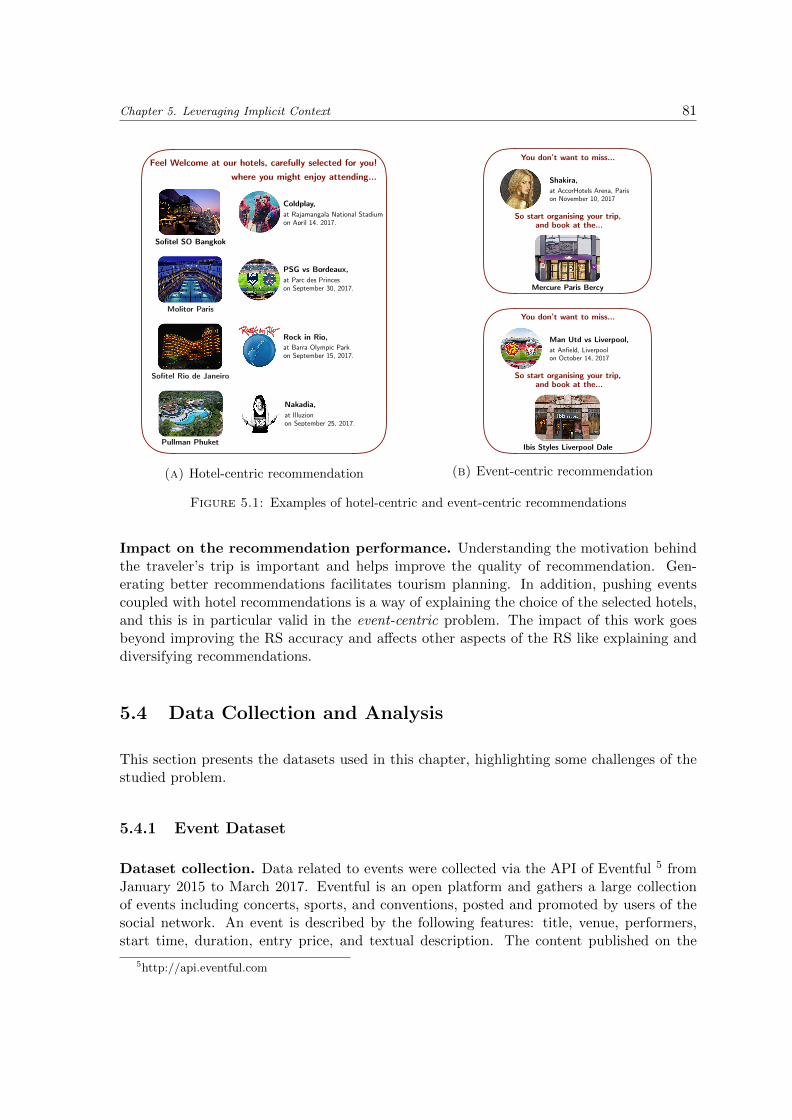
Chapter 5. Leveraging Implicit Context 81
Feel Welcome at our hotels, carefully selected for you!
Sofitel SO Bangkok
Molitor Paris
Sofitel Rio de Janeiro
Pullman Phuket
where you might enjoy attending…
Coldplay, at Rajamangala National Stadium on April 14, 2017.
PSG vs Bordeaux, at Parc des Princes on September 30, 2017.
Rock in Rio, at Barra Olympic Park on September 15, 2017.
Nakadia, at Illuzion on September 25, 2017.
(a) Hotel-centric recommendation
So start organising your trip, and book at the…
Mercure Paris Bercy
You don’t want to miss…
Shakira, at AccorHotels Arena, Paris on November 10, 2017
So start organising your trip, and book at the…
Ibis Styles Liverpool Dale
You don’t want to miss…
Man Utd vs Liverpool, at Anfield, Liverpool on October 14, 2017
(b) Event-centric recommendation
Figure 5.1: Examples of hotel-centric and event-centric recommendations
Impact on the recommendation performance. Understanding the motivation behindthe traveler’s trip is important and helps improve the quality of recommendation. Gen-erating better recommendations facilitates tourism planning. In addition, pushing eventscoupled with hotel recommendations is a way of explaining the choice of the selected hotels,and this is in particular valid in the event-centric problem. The impact of this work goesbeyond improving the RS accuracy and affects other aspects of the RS like explaining anddiversifying recommendations.
5.4 Data Collection and Analysis
This section presents the datasets used in this chapter, highlighting some challenges of thestudied problem.
5.4.1 Event Dataset
Dataset collection. Data related to events were collected via the API of Eventful 5 fromJanuary 2015 to March 2017. Eventful is an open platform and gathers a large collectionof events including concerts, sports, and conventions, posted and promoted by users of thesocial network. An event is described by the following features: title, venue, performers,start time, duration, entry price, and textual description. The content published on the
5http://api.eventful.com

82 Chapter 5. Leveraging Implicit Context
Table 5.1: Examples of crawled events from Eventful, considered as major events suscep-tible of attracting travelers
Title - Venue
Rihanna -Wembley Stadium, Wembley, Brent, UK
New York Knicks vs. Chicago Bulls -Madison Square Garden, New York, NY, US
Final Euro: Portugal vs France -Stade de France, Saint-Denis, FR
Salon Livre Paris 2016 -
Paris Expo Porte de Versailles, Paris, Ile-de-France, FR
Ed Sheeran -Sydney Entertainment Centre, Sydney, NSW, AU
Volleyball Men’s Gold Medal Olympic Games -Maracanazinho, Rio de Janeiro, Rio de Janeiro, BR
platform being generated by users, it is essential to filter, clean, and enrich the crawled databefore injecting it into the RS.
Filtering major events. From our perspective, some events posted on Eventful are consideredirrelevant as they do not play any role in attracting travelers from abroad. They representa gathering of people sharing the same interest on a local scale. It is important to discardthese events by filtering the crawled data, thus reducing the noise added to the RS. Thetask of identifying attractive events is not trivial and requires a good understanding ofevent tourism. We base our reasoning on the idea that major events are usually organizedin a limited set of famous and well-known venues. Therefore, we filter events based on theplaces where they are organized. We rely on knowledge bases in order to get backgroundinformation about venues. In particular, we use DBpedia [Lehmann et al., 2015] whichextracts structured information from Wikipedia. We retrieve the entities belonging to theclasses of venues and sports facilities, gathering locations where events are most likely totake place.
In order to be considered as famous, we suppose that a venue must verify one of thetwo criteria defined in the following. First, the Wikipedia page describing the venue mustbe translated in a minimal number of languages, attesting that the venue is world-famousor at least famous in a part of the world and that it is attracting travelers from outside theregion. Second, the venue’s capacity, e.g., seating capacity, should be large enough provingthat it can welcome a great number of travelers. Table 5.1 and Table 5.2 show examples offiltered and non-filtered events respectively, where events from Table 5.1 are considered assusceptible of attracting travelers.
Annotating events with featured performers. Events are available within a rather short timespan. The attention they draw and the interest they create are generally due to two factors:the venue where they are organized and the performers they feature. Linking future eventsof a performer to its past occurrences is essential to be able to measure similarities betweenevents and to model travelers’ preferences for events.

Chapter 5. Leveraging Implicit Context 83
Table 5.2: Examples of crawled events from Eventful, considered as local events that donot have a major impact on travelers
Title - Venue
Dine & Dance -Cafe Taste, Toronto, Ontario, CA
Yoga for a Stressful World -Manor Woods Elementary School, Ellicott City, MD, US
Learn to Swim -Curie Park, Chicago, IL, US
Drinks at the Refinery -The Refinery, Hackney, Hackney, UK
Les Femmes Savantes -L’Aqueduc, Dardilly, Rhone-Alpes, FR
Atelier Creativite et Bien-Etre -Doremifasoleil, Muret, Picardie, FR
Table 5.3: Statistics of the crawled dataset, Event-Full, and the filtered dataset, Event
Dataset Event-Full
# events 2,447,088
# venues 410,217
# performers 34,787
# categories 30
# represented countries 122
# languages used 14
average # of events per day 3,042
Dataset Event
# events 38,377
# venues 802
# performers 17,951
A small number of the crawled events from Eventful is annotated with performers (lessthan 7%) as the majority of them mentions in their title almost everything the attendeesneed to know. We use several methods in order to identify the events’ performers basedon their title. Targeting performers of music events, we extract from DBpedia the namesof artists and groups and we try to find matchings in the events’ titles. Concerning sportsevents, we identify tokens, e.g., versus and vs, allowing to parse the titles and select themultiple entities participating in the event.
Dataset size. Initially, around 2.5 million events were collected and constitute the datasetdenoted by Event-Full. These events are organized in 410,217 venues and belong to 30different categories including concerts, sports, food, education, and science. After filteringthe crawled venues and the corresponding events, we are left with approximatively 1.56%of the events and 0.2% of the venues. The filtered dataset is denoted by Event and isused in the rest of this chapter. Further information about the event datasets is providedin Table 5.3.

84 Chapter 5. Leveraging Implicit Context
Table 5.4: Statistics of the booking dataset Ah-Event used for recommending packagesof hotels and events
Dataset # users # items # transactions
Ah-Event 2,096,622 4,574 10,213,627
5.4.2 Booking Dataset
The booking dataset used in this chapter is created the same way the dataset Ah, describedin Section 3.2, was created, with two distinctions. First, we only select bookings madeduring the period covered by the event dataset. This is mainly because events organizedbefore the date at which we started collecting event data could not be retrieved. Second,we only consider users that can be associated with at least three events in order to haveenough observations to model preferences. The procedure of associating users with eventsis detailed in the next section. Further information about the resulting dataset, denoted byAh-Event, is provided in Table 5.4.
5.5 Proposed Framework
In this section, we describe the main modules of our framework which is designed to tacklethe hotel-centric and event-centric problems defined in Section 5.3. The final goal is topropose to each user a personalized list of pairs of hotels and events where the event isorganized in the surroundings of the corresponding hotel and can be attended by the hotel’svisitors. In the hotel-centric problem, we want to suggest hotels that match the user’spreferences. Events are then proposed to entertain users and enhance the tourism experience.In the event-centric problem, we draw the user’s attention to a future event and propose ahotel as part of the trip planning.
5.5.1 Overview
The proposed framework is constituted of five modules and its architecture is presentedin Figure 5.2. It is flexible in the sense that the methods used in each module can bemodified, improved, or even discarded, as long as the output of the module is providedin one way or another. We base our work on the assumption that each booking made bya traveler in any of the hotels was motivated by an event organized nearby in the sameperiod. This assumption is essential in order to simplify our work, knowing that the realmotivation behind each booking is unknown and that direct feedback about events is notprovided. The bookings that do not respect this assumption in practice are not expectedto drastically affect the performance of the RS since we are also capturing and leveragingpreferences for hotels derived from real interactions with hotels.
In order to associate each booking with its motivating event, we proceed in two phases.In the first phase, we select all the events that a user could have physically attended duringhis stay, based on location and time parameters (module 1, Section 5.5.3.1). In the second

Chapter 5. Leveraging Implicit Context 85
phase, we filter one of these events by taking into account the whole user profile and byensuring a degree of cohesiveness across the profile (module 3, Section 5.5.3.3). This steprequires the computation of similarities between events, measuring to which extent twoevents may interest the same person (module 2, Section 5.5.3.2). The set of interactionsuser-hotel and user-event are used to learn user preferences for events and hotels (module4, Section 5.5.3.4). Recommendations in the hotel-centric and event-centric approachesare generated based on these preferences and on the schedule of future events (module 5,Section 5.5.3.5).
5.5.2 Notations and Definitions
Following the notations defined in Section 2.1.4 (refer to Table 2.1), we denote by U the setof users, I the set of hotels, and we introduce the notation E for the set of events. We extendthe original notation of the set of items rated by a user u, Iu, to include triplets (i, din, dout)where i designates the hotel visited by u, din the check-in date, and dout the check-out date.An event e ∈ E is organized in the venue ve and features a set of performers denoted byFe = f1, f2, ..., fme, where me is the number of performers of e. One part of the workconsists in associating each booking with the corresponding event, principal motivator ofthe trip. To this end, we introduce for each user u two types of profiles described in thefollowing:
• The user’s all-inclusive profile. In the all-inclusive profile, denoted by Pallu foruser u, each booking b ∈ Iu is associated with the events that could be the potentialmotives of the trip based on location and time parameters. For each b = (i, din, dout),Pallu includes a tuple defined as < i, din, dout, e1, e2, ..., el > , where e1, e2, ..., el are theevents that occurred in the neighborhood of the hotel i in a period close to the onebounded by (din, dout). Each user u is assigned one profile Pallu gathering informationabout the bookings previously made.
• The user’s limited profile. The limited profile, denoted by P limu for user u, is derivedfrom the all-inclusive profile Pallu . Following the assumption made in Section 5.5.1,we select exactly one event for each booking b ∈ Iu and rely on a similarity measurebetween events to do the selection. Tuples in P limu are in the form of < i, din, dout, e >.P limu is then used to learn preferences of u for hotels and events.
5.5.3 Modules
The whole process is carried out through five modules detailed in the next subsections andrepresented in Figure 5.2. We explain the functionalities of each module pointing out therequired inputs, the generated output, and the motivation and intuitions that lead to theproposed methods.

86 Chapter 5. Leveraging Implicit Context
+
+
+
Module 1Building all-inclusive profiles
Module 3Building limited profiles
Module 4Learning preferences
Module 2Measuring events’ similarities
Module 5Recommending hotels & events
(U , I, E)i1
i2
e1
e2
e3
e4
e5
e6
i1
i2
e1
e2
e3
e4
e5
e6
i1 i2
e3 e5
e1
e2
e3
e4
e5
e6sim
(e 1, e 3
)
sim(e, e)
Pall P lim
&
(ph ,qh
)
(pe,q
e)
Pall
Figure 5.2: Architecture of the proposed framework for recommending hotels and events
5.5.3.1 Building All-Inclusive Profiles Based on Location and Time
Input. Booking data, event data, and hotels’ locations.
Output. Users’ all-inclusive profiles.
Functionality. This module builds users’ all-inclusive profiles by linking bookings andevents based on the venue’s location, the hotel’s location, the event’s date, and the periodof the stay. More formally, we associate each booking b ∈ Iu, where b = (i, din, dout), withthe set of events e1, e2, ..., el.
Motivation. When travelers organize their trips and plan on attending an event, theysearch in general for hotels located in the neighborhood of the event’s venue. From a hotelorganization perspective, experts track the set of venues that impact the hotel demand andperformance in order to better handle unusual activities.
We determine for each venue the set of hotels affected by the major events organized inthe venue. These hotels are specifically the ones targeted by travelers when attending thevenue’s events. In the simplest case, the distance separating venues and hotels can be usedto model the fact that the hotel is impacted or not by the venues’ activities. We define athreshold distance, denoted by dist(ve) for the venue ve, such that each hotel located withinthis distance from ve is affected by it. Several factors influence dist(ve). In particular,dist(ve) depends on the density of hotels located in the surroundings of the venue. Forvenues located in big cities where hundreds of hotels are concentrated in a relatively smallzone, the impacted region is smaller than the one for venues located in less crowded citiesor isolated regions. Travelers are more likely to stay in a hotel far from the event’s venue ina region where hotels are less implanted.
Method. Following these intuitions, we introduce some notations before defining dist(ve):

Chapter 5. Leveraging Implicit Context 87
• distmax is the maximal distance separating ve from a potentially impacted hotel. It isassigned a default value, i.e., 30 kilometers, with the help of domain experts, that isindependent of ve;
• nI(ve) is the number of hotels located within a distance equal to distmax from ve;
• distmin(ve) is the minimal distance separating ve from any hotel, i.e., the closest hotelto ve.
The threshold distance dist(ve), defined in the following, ranges between distmin(ve) anddistmax and decreases when the density of hotels increases:
dist(ve) = distmin(ve) + (distmax − distmin(ve)).e(−λ.nI(ve)) (5.1)
where λ is a positive constant set to 0.01 in our work.
Going back to the initial problem, let Vi refer to the set of venues impacting the hotel iwhere the booking b has been made. The events associated with b are those organized in anyv ∈ Vi during the period (din − (1 day), dout + (1 day)). It is worth mentioning that furtherdevelopments in this direction could consider the automatic identification of the impact ofevents on hotels by tracking the change of the occupancy rate and the room prices basedon the occurrence of events.
5.5.3.2 Measuring Events’ Similarities
Input. Users’ all-inclusive profiles.
Output. Similarities between pairs of events.
Functionality. The main functionality of this module is to compute similarities betweenevents, i.e., compute sim(ea, eb) for each couple of events (ea, eb) ∈ E × E . This measure islater used to derive limited profiles P lim∗ from all-inclusive profiles Pall∗ .
Motivation. Intuitively, two events are similar if they share the same or similar features.A sporting event is more similar to another event from the sports category than to a concertor a convention belonging to other categories. Two events happening in the same venue orfeaturing the same performers are also supposed to be related. Given the limited availabilityof features, another way to assess similarities is to rely on people’s feedback. Two eventsare similar if they are attended by the same people. Evaluating the similarity between twoentities requires representing them in a common space where it is possible to compare them.This common space can be composed of events’ features or latent features learned from thedata. The similarity between events is modeled as a weighted aggregation of the similaritybetween venues and the similarity between performers.
Method. Assuming we have the venues’ and performers’ representations, we use the cosinesimilarity (Section 2.5.1.1) to measure the similarity between venues of two events ea and eb,i.e., simv(ea, eb), and between the corresponding performers, i.e., simf (ea, eb). sim(ea, eb)

88 Chapter 5. Leveraging Implicit Context
is then given as follows:
sim(ea, eb) = α.simv(ea, eb) + (1− α).simf (ea, eb) (5.2)
where the parameter α ∈ [0, 1] determines the contribution of each type of similarity in thefinal measure. We rely on the all-inclusive profiles of users Pall∗ to learn the representationsof venues and performers, leveraging the wisdom of the crowd rather than the explicit set ofrelatively limited features. The problem is similar to the one we face in RS and, in particular,in MF approaches (Section 2.5.2), where we map users and items to a joint latent factorspace. We apply a MF technique on the set of user-venue interactions and user-performerinteractions respectively to model venues and performers in latent factor spaces.
5.5.3.3 Building Limited Profiles Based on Cohesiveness
Input. Users’ all-inclusive profiles and events’ similarities.
Output. Users’ limited profiles.
Functionality. This module generates the limited profiles P lim∗ . We identify for eachbooking exactly one event that could have been the main motivation of the trip. We takeinto account the whole set of bookings Iu for a user u ∈ U and the similarities betweenthem.
Motivation. The idea is to select one event for each booking — the event that motivatedthe trip — such that the events selected for all the bookings of one user are the most similar.We suppose that a user is more likely to be interested in similar events (the similarity beingdefined in Section 5.5.3.2). Starting from the user’s all-inclusive profile Pallu , the aim is topick one event for each tuple from Pallu such that the probability of this event belonging toP limu is maximal given the other elements of P limu . This probability depends on the eventspicked from the other tuples of Pallu . The selected events should maximize the cohesivenessof elements occurring in P limu .
Method. The ideas formulated above are resumed in the following assumption we make.The events selected from Pallu and included in P limu maximize the sum of similarities betweenall pairs of events. Due to the complexity of the optimization problem, we turn to graphtheory to solve it.
We build a graph for each user u ∈ U and develop an algorithm that selects one eventper stay with respect to our motivation. Let Gu be a weighted complete graph associatedwith user u where Gu = (Nu, Eu), Nu is the set of nodes, and Eu is the set of edges. Whenbuilding the graph, we iterate through the tuples of Pallu and add to Gu one node for eachevent appearing in each tuple. Each node is attributed a label and nodes derived from thesame tuple are assigned the same label. After iterating through all the tuples of Pallu andadding the nodes to Gu, we weight each edge connecting two nodes corresponding to theevents ea and eb with the value sim(ea, eb).
The problem we are trying to solve in this module is nearly equivalent to the Heaviest-k-Subgraph (HkS) problem with a few distinctions. Originally, the HkS problem can be seen

Chapter 5. Leveraging Implicit Context 89
as the weighted version of the well-known densest subgraph problem [Lee et al., 2010] withrestrictions on the size of the subgraph. In the HkS problem, k being an integer and k > 1,the task is to find a subgraph containing k nodes such that the sum of the weights of itsedges is maximal. Our setting imposes one additional constraint: each node of the subgraphhas to carry a unique label. k is also equal to the number of tuples of Pallu , knowing thatwe want to select one event per tuple, i.e., one node for each label. The nodes of the HkSselected by the algorithm correspond to the events that will be included in P limu . Inspiredby the work in [Letsios et al., 2016], we develop a branch and bound algorithm in order tosolve the problem.
The branch and bound algorithm is used to solve combinatorial optimization problems.The search space is divided into several branches of computation. The set of candidatesolutions is considered to be forming a tree with the full set at the root and smaller setsof solutions as children. The algorithm explores branches of the tree and check each one ofthem against upper and lower estimated bounds of the optimal solution. If the upper boundof a node is lower than the global lower bound, i.e., the maximum lower bound over the setof candidate solutions considered, the branch is pruned and its children are not explored.
In our method, the branching phase consists of deciding whether to add a node to theoptimal solution or not. While iterating over the existing labels, we decide which of thecorresponding nodes could be considered in the optimal solution and add the correspondingbranch to the tree. The lower bound is given by the sum of the weights of the edges of thesubgraph included in the candidate solution. The upper bound is the sum of the weights ofthe edges connected to the examined node when considering the heaviest edges connectingthe node to another one having a different label.
5.5.3.4 Learning Preferences for Hotels and Events
Input. Users’ limited profiles.
Output. Latent representations of users, hotels, and events.
Functionality. We use user-hotel and user-event interactions derived from P lim∗ to learnuser preferences for hotels and events.
Motivation. This module handles a classical recommendation problem and we count onuser interactions to learn preferences for items and make recommendations.
Method. We rely on MF (Section 2.5.2) to learn the latent representations of users, hotels,and events, and to evaluate the score of a hotel and an event for a user. We build twomodels based on the sets of user-hotel interactions and user-event interactions respectively,modeling the preferences for hotels and events.
5.5.3.5 Recommending Hotels and Events
Input. Latent representations of users, hotels, and events, and schedule of events.

90 Chapter 5. Leveraging Implicit Context
Output. Pairs of hotels and events recommendations.
Functionality. This module generates personalized recommendations of pairs of hotelsand events for each user. It handles both the hotel-centric and event-centric problems,addressing each one of them differently.
Motivation. In the hotel-centric problem, we focus on recommending hotels that match theuser preferences. We anticipate the need for looking for events to attend for entertainmentpurposes and we also propose an event organized nearby. In the event-centric approach, wecreate the need for a user to take part in an event and subsequently search for a hotel bydrawing his attention to a specific event.
Method. The computed scores are used to rank the list of items for one user and the top-Nitems of the list, i.e., items that score the highest, are selected for recommendation. In thehotel-centric problem, we first generate hotel recommendations for one user. We use theserecommendations to filter the ranked list of events where we discard events that are notlinked to any of the chosen hotels and that cannot be proposed together (Section 5.5.3.1).Filtering the ranked list of events allows the selection of one event per hotel, forming thepairs to recommend. In the event-centric problem, we proceed inversely: We first generateevents’ recommendations that are then used to filter the ranked list of hotels.
5.6 Experimental Results
In order to demonstrate the proposed framework, we proceed in two steps. We first illustratethe functioning of the framework using concrete examples. We introduce simulated usersand check the output produced by a number of modules. A quantitative evaluation is thenperformed: Offline experiments are conducted where we assess the accuracy of the RS asa whole and point out the interest of our work. It is worth mentioning that the resultsdepend on the set of events covered and on the worldwide availability of hotels included inthe datasets. Some interesting events may not be posted on Eventful and some bookingsmotivated by events may not be made in the hotels considered.
5.6.1 Qualitative Evaluation Through Concrete Examples
To gain a better insight into the presented framework, we simulate users with their historyof bookings and evaluate the results. These results concern the computation of similaritiesbetween different entities, i.e., venues, performers, and events. We also generate recommen-dations for the users and highlight the content of the intermediate structures and profilesthat lead to the final solution.
Similarities between venues. Table 5.5 contains nearest neighbors of two examples ofvenues sampled from the set of 800 venues. The first venue designates a stadium located inFrance and its nearest neighbors are stadiums mainly located in Europe. The second venueis a concert hall located in Luxembourg and its nearest neighbors cover European concerthalls, theaters, and music venues.

Chapter 5. Leveraging Implicit Context 91
Table 5.5: Nearest neighbors of examples of venues
Stade de France - Saint-Denis, FR
Stadio Dino Manuzzi - Cesena, IT
Cornaredo Stadium - Lugano, CH
Estadio Jose Rico Perez - Alicante, ES
Ostseestadion - Rostock, DE
KeyArena - Seattle, WA, US
Philharmonie de Luxembourg - Luxembourg, LU
Courtyard Theatre - London, GB
Theater des Westens - Berlin, DE
Laeiszhalle - Hamburg, DE
Royal Opera House - London, GB
La Monnaie - Brussels, BE
Table 5.6: Nearest neighbors of examples of performers
Paris Saint-Germain Manchester United FC
Girondins de Bordeaux Crystal Palace FC
FC Lorient Southampton FC
Lille LOSC West Ham United FC
OGC Nice Manchester City FC
Angers SCO Tottenham Hotspur FC
Taylor Swift Skillet
Chris Brown Rammstein
Sam Smith Last Train
Neil Diamond Baby Metal
Elton John Mass Hysteria
Robbie Williams Jane’s Addiction
Similarities between performers. Table 5.6 shows the nearest neighbors of some per-formers sampled from the set of 18k performers. Computing similarities between perform-ers allows gathering French football clubs (first example), English football clubs (secondexample), pop singers (third example), and rock/metal bands (fourth example). A travelerinterested in a specific performer is most likely to enjoy events featuring one of its neighbors.
Similarities between events. We combine venues’ and performers’ similarities to measuresimilarities between 38k events and we illustrate examples in Table 5.7. In a setting wherewe use events’ features, e.g., category and performers, to compare events, we are not ableto evaluate the resemblance between events that do not share the same features. However,the proposed method allows estimating if a traveler that has previously attended a footballmatch is likely to attend a concert featuring a specific performer or any other event.
Recommendations of hotels and events. Table 5.8 shows examples of recommendationsfor two simulated users based on their history of bookings. The all-inclusive profile of a usergathers all the events listed for all of his bookings. Only one event per booking, markedin bold, is included in the limited profile. User 1 is expected to have mainly attended

92 Chapter 5. Leveraging Implicit Context
Table 5.7: Nearest neighbors of examples of events
OM - Paris Saint-Germain - Stade Velodrome, FR
Olympique Marseille - Rennes - Stade Velodrome, FR
Auxerre - Paris Saint-Germain - Stade de France, FR
Nimes Olympique / Paris FC - Stade des Costieres, FR
Monaco vs Paris Saint-Germain - Stade Louis-II, MC
Montpellier - OM - Stade de la Mosson, FR
Ed Sheeran - Sydney Entertainment Centre, AU
Sam Smith - Hodern Pavilion, AU
Kylie Minogue - Sydney Entertainment Centre, AU
5 seconds of summer - Hodern Pavilion, AU
Coldplay - Allianz Stadium, AU
The Pink Floyd Experience - Enmore Theatre, AU
Swan Lake - Edinburgh Playhouse, GB
The Nutcracker - Edinburgh Playhouse, GB
Giselle - Edinburgh Playhouse, GB
Nicola plays Beethoven - Usher Hall, GB
To kill a mockingbird - Kings Theatre, GB
Rameau & Charpentier, Orchestra - Usher Hall, GB
4th eScience Symposium - Amsterdam Arena, NL
MaaS Meetup #2 - Amsterdam Arena, NL
Amazing datamonday - Amsterdam Arena, NL
Inspiration 360 - Ziggo Dome, NL
Big Data Small World - Amsterdam Arena, NL
SolarEdge Advanced Training - DSB Stadion, NL
football events in European venues. He is recommended to go to the FA Cup event heldin Manchester, England, among other events. User 2 is expected to be rather interestedin concerts featuring a specific genre of artists and is therefore recommended to attend theconcert of Chris Brown, for example.
5.6.2 Quantitative Evaluation Through Offline Experiments
The proposed framework is evaluated by measuring the accuracy of the recommendationsgenerated by the RS. The aim is to assess the influence of using event data on the qualityof hotel recommendation. The evaluation focuses on the event-centric problem described inSection 5.5.3.5.
Evaluation scheme. The booking dataset, Ah-Event, and the event dataset, Event,are used for evaluation (Section 5.4). Ah-Event is split into a training set used as inputto the framework and a test set to which we compare recommendations. We perform achronological split (Section 2.2.1.1): The test set consists of the bookings recorded duringthe last 6 months since the most recent booking and the training set gathers the olderbookings. Events considered for recommendation are those planned in the same time period.

Chapter 5. Leveraging Implicit Context 93
User 1: History of Bookings
Bookings Event - Venue
Jan. 12-17, 2015,Mercure Sydney
Roger Federer, Lleyton Hewitt, Sydney Exhibition Match -Sydney Entertainment CentreThe 1975 Sydney - Hordern PavilionSydney Festival 2015: Atomic Bomb! The Music of WilliamOnyeabor - Enmore Theatre
Aug. 21-24, 2015,Ibis Paris Saint-Denis France vs. England - Stade de France
Jan. 21-24, 2016,Ibis Styles
London Kensington
‘Responding to the new landscape’ Delivering Better Out-comes for All - Barbican CentreLooking Past Degrees: How to find the Best Young Talent- Barbican CentreNahko and Medicine for the People - Shepherd’s Bush Em-pireBig Sing Fridays - Royal Opera HouseWho’s Next - The 100 ClubA Postcard to Bill Evans - Southbank CentreTales from Hollywood - Donmar WarehouseKevin Hart: What Now? Tour - SSE Arena WembleyThe Complete Stone Roses - The 100 ClubCrystal Palace vs. Tottenham - Selhurst ParkRSC Shakespeare on Screen: King Lear (1971) - BarbicanCentre
Mar. 17-20, 2016,Ibis Manchester
Portland
UEFA Europa League: Manchester United FC vs.Liverpool FC - Old TraffordCosi Fan Tutte Manchester - The LowryMichael Morpurgo: Where My Wellies Take Me - The LowryManchester City vs. Manchester United - Etihad StadiumThe Edgeley Park Stadium Antiques & Collectors Fair -Edgeley Park
User 1: Recommendations
Event Date Event - Venue - Hotel
Dec. 2, 2016 Rod Stewart - Barclaycard Arena - Ibis Rotherham
Dec. 13, 2016 Coldplay Sydney - Allianz Stadium - Ibis Sydney DarlingHarbour
Mar. 1, 2017 FA Cup 2016/17 - Manchester City v Huddersfield - EtihadStadium - Ibis Manchester Princess Street
Mar. 11, 2017 Melbourne Victory vs Central Coast Mariners - Aami Park- Ibis Little Bourke Street

94 Chapter 5. Leveraging Implicit Context
User 2: History of Bookings
Bookings Event - Venue
May 28-31, 2015,Novotel Amsterdam City
Ariana Grande - Ziggo DomeToto - Ziggo DomeArmin Van Buuren & Nicky Romero, Amsterdam festivals -Olympic Stadium
Oct. 17-18, 2015,Ibis Styles Stuttgart
Imagine Dragons - Porsche-ArenaVfB Stuttgart vs. FC Ingolstadt 04 - Mercedes-Benz Arena
Feb. 12-15, 2016,Mercure Bad Duerkheim
WWE Live - SAP ArenaMario Barth: Manner sind bekloppt, aber sexy!MANNHEIM - SAP Arena
Mar. 08-09, 2016,Mercure Amsterdam Slo.
Debat “Talent naar de regio NHN”+BNR Gangmakers liveuitzending - DSB StadionMuse - Ziggo Dome
User 2: Recommendations
Event Date Event - Venue - Hotel
Oct. 10, 2016 The Legend of Zelda - Porsche-Arena - Mercure StuttgartCity Cent
Nov. 6, 2016 Chris Brown - Ziggo Dome - Novotel Amsterdam Schiphol
Nov. 9, 2016 WWE Live - Mercedes-Benz Arena - Mercure Stuttgart AptMesse
Nov. 10, 2016 The Cure Cologne - Lanxess Arena - Mercure DuesseldorfHafen
Table 5.8: Two examples of users’ history of bookings, the association with events, andgenerated recommendations
Table 5.9: Recall@N and NDCG@N for MFev and other recommendation approaches
Metric MostPop Knnu WRMF BPR MFev
Recall@5 0.0121 0.0542 0.0634 0.0722 0.0865
Recall@10 0.0218 0.0685 0.0895 0.1042 0.1197
NDCG@5 0.0188 0.0318 0.0473 0.0582 0.0708
NDCG@10 0.0243 0.0407 0.0512 0.0696 0.0892
Metrics. We use recall@N and NDCG@N , defined in Section 2.2.3, to measure the rec-ommendation accuracy, where N is the number of recommended items. Higher values forboth metrics indicate a better recommendation quality. Since large values of N are notinteresting for recommendation, we set N to 5 and 10.
Parameters. A grid search over the parameter space of each evaluated method is performedin order to find the parameters that give the best performance which we report.
Methods compared. The following methods are included in the comparison:
• MostPop. The N most popular hotels are recommended to users.

Chapter 5. Leveraging Implicit Context 95
• Knnu. Knnu is the user-based neighborhood method, described in Section 2.5.1.1. Weuse the Jaccard similarity metric to measure similarities between users. We set thenumber of neighbors to 1000.
• WRMF. Weighted Regularized Matrix Factorization [Hu et al., 2008] is a MF techniquespecifically designed to handle implicit feedback and presented in Section 2.5.2.4. Weset the number of latent factors to 100 and the regularization parameters to 0.001.
• BPR. Bayesian Personalized Ranking [Rendle et al., 2009] is a MF technique presentedin Section 2.5.2.4. We set the number of latent factors to 100 and the regularizationparameters to 0.0025.
• MFev. This is the approach we propose to solve the event-centric problem, lever-aging event data for hotel recommendation. MFev (in particular, modules 4 and 5,Section 5.5) is based on BPR since it outperforms the other methods for hotel recom-mendation on our dataset. The difference in performance we get by comparing BPR
and MFev shows the benefits of incorporating event data using our framework.
Results. Table 5.9 shows the recall@5, recall@10, NDCG@5, and NDCG@10 for the ap-proaches we compare. BPR performs better than the other recommendation methods thatare only based on hotel bookings. MFev outperforms BPR which highlights the contributionof event data in contextualizing hotel bookings and generating better recommendations.Furthermore, MFev offers the advantage of explaining hotel recommendations by associatingan event with each proposition. Providing explanations allow travelers to check the validityof the suggestions and helps them in their trip planning. While the usage of event data canbe beneficial for hotel recommendation, a discussion related to the obtained results and thelimitations they are subject to is proposed in the next section.
5.7 Discussion
People can be motivated by events to organize trips and are then required to choose anaccommodation which is usually selected as the mean to achieve the goal. Our experimentshave shown the interest of using event data when performing hotel recommendations. Inthis section, we summarize the contributions and we discuss how this solution can be usedin real-world environments, its limitations, and possible future improvements.
Contributions. Even though it is well-known that events affect the hotel industry, thework presented in this chapter is the first attempt to model the impact of events on userbehavior with respect to the choice of hotels and to benefit from this relation to improverecommendations. The problem addressed spans over two different domains. In the hoteldomain, we have information about hotels and users’ bookings while in the event domain,we only have information about events. The event domain is exploited in an attempt toimprove recommendations in the hotel domain. We first formulate the problem addressedand provide instructions on how to collect, preprocess, and enrich event data to this purpose.We then propose a framework that is able to infer user preferences for events based on theirhistory of bookings and leverage these preferences for recommending packages of hotels andevents. Overall, the aim is to improve the tourism planning and the user experience.

96 Chapter 5. Leveraging Implicit Context
Real-world applications. The designed approach is not meant to be the single one usedto generate recommendations in a real setting. It can be interesting to rely on a comparableapproach in one of the two use cases we defined and that occur in the hotel industry. First,when detecting an important future event, potentially interested users can be targeted. Theproposed solution allows suggesting a hotel where they could stay, helping them in the tripplanning. Second, for each hotel suggested, it is possible to propose an event that couldbe interesting for the user, improving the attractiveness of hotels being recommended andenhancing the user experience.
Limitations. We consider situations where people travel for the main purpose of attendingan event, e.g., a concert or a conference, which explains why each booking is linked to exactlyone event. Since only impactful events are filtered and considered, it is likely that travelerswho stayed in the hotel near the event’s venue during the corresponding period made the tripfor the event. It is also worth mentioning that these travelers were willing to pay the highprices for the rooms compared to the regular periods. From a hotel industry perspective,we do not have explicit information concerning the event that motivated the trip, leading usto make assumptions about the potential link between bookings and events. Assuming thatthis information becomes available, e.g., when arriving at the hotel, the traveler declareswhether he is attending an event or not, and which one it is, the performance of the systemcould be improved since the booking-event associations will be less noisy.
Improvements. Improvements in this direction should consider analyzing the behavior ofsubsets of users and detecting those who are particularly sensible to events. While events’type and hotels’ category may have an impact on recommendation, it is hard to evaluate itin an offline setting as more feedback is required from the user. Therefore, online evaluationis a must to be able to draw more conclusions and generalize the results.
5.8 Conclusion
This chapter proposes the integration of open data related to events into hotel RS. Weaddress two problems occurring in two different scenarios where the common task is torecommend packages of hotels and events in order to facilitate tourism planning. On onehand, we anticipate the need for looking for activities to do during the trip by proposingevents organized near the hotels. On the other hand, we create the need for a traveler toattend an event and organize a trip by recommending interesting events in addition to hotelslocated near the events’ venue. Experiments have shown the interest of using event datafor hotel recommendation. Further advances should consider adopting online evaluation tomeasure the influence of the RS on the user behavior.
This work is also an attempt to combine insights from two different domains, i.e., thehotel domain and the event domain, to benefit one of them. Leveraging knowledge fromseveral domains can empower RS, especially given that users are not only driven by theitem characteristics and features which are included in the target domain. The next chapterexplores the transfer of knowledge acquired in the domain of Location-Based Social Networks(LBSN) to the hotel domain, in order to enhance the recommendation quality.

Chapter 6
Transferring Context KnowledgeAcross Domains
This chapter presents our approach for exploiting knowledge about mobility extracted fromLocation-Based Social Networks (LBSN) to benefit the hotel RS that is in particular sensibleto the geography dimension [Al-Ghossein et al., 2018c]. Two distinct domains are involved:the source domain, i.e., the LBSN where a set of users are sharing their check-in activity,and the target domain, i.e., the hotel domain where another set of users are booking andvisiting hotels. Knowledge about the physical context is acquired in the source domainwhere the feedback is expected to be dense and is transferred to the target domain where itis thus considered to be partially observable. Experiments on real-world datasets highlightthe implications of transferring knowledge between these domains on the recommendationquality.
6.1 Introduction
Traveling is still considered to be a rare activity that is carried out by individuals only a fewtimes each year. As a result, the feedback collected in the hotel domain is sometimes notsufficient to learn user preferences. Sparsity constitutes a major limitation for Collabora-tive Filtering (CF) methods that are well-known for outperforming other recommendationapproaches. One way to address the sparsity problem is to leverage knowledge from otherrelated domains where it is easier to get information regarding the user behavior. Cross-domain RS [Cantador et al., 2015] take advantage of the abundance of heterogeneous dataproviding multiple views of user preferences. They aim to improve recommendations in atarget domain by exploiting preferences uncovered in source domains. When applied in thetourism domain, cross-domain RS can suggest, for example, hotels based on flight bookingsor events to attend based on hotel bookings.
When organizing a trip, travelers usually select the destination to visit before choosingthe hotel where they will stay and the choice of accommodation highly depends on itslocation. Choosing a destination to visit is in turn related to several factors. First, the
97

98 Chapter 6. Transferring Context Knowledge Across Domains
majority of trips are meant to explore destinations that are close to the place of residenceof travelers. Then, users tend to follow the actual trends running locally which are alsolikely to change with time. In addition, the timing of the trip has an impact on the chosendestination. Some destinations are more popular during summer than during winter, andleisure trips are more frequent during holidays.
Since hotel bookings are collected by organizations managing a subset of hotels andaccommodations, hotel booking datasets do not cover all the trips done and the destinationsvisited by users, which participates in aggravating the sparsity issue. On the other hand,recent years have witnessed the emergence of Location-Based Social Networks (LBSN), e.g.,Flickr and Foursquare, where users can connect with friends, upload photos, and share theirlocations via check-ins for Points Of Interest (POIs). LBSN constitute a rich data sourceto analyze travel experiences [Liu et al., 2017]. In particular, it is possible to capture themobility of users through their check-in history.
In this chapter, we address the problem of hotel recommendation that is suffering fromsparsity by leveraging check-in data from LBSN. We learn mobility patterns from the check-ins which are easily shared by users on LBSN and combine them with hotel preferences toboost hotel recommendations. We first map check-ins and hotels to a common space of geo-graphical regions based on the density of hotels spread worldwide. We learn preferences forthese regions, map users from both domains, and combine preferences for regions and for ho-tels to generate recommendations. Experiments using a dataset from the hotel industry anda dataset from a LBSN show the interest of using check-in data for hotel recommendation.
The rest of the chapter is organized as follows. In Section 6.2, we discuss related workon cross-domain recommendation. In Section 6.3, we present our approach for hotel recom-mendation leveraging mobility data from LBSN. Experiments, results, and a discussion arepresented in Section 6.4. Finally, Section 6.5 concludes the chapter.
6.2 Cross-Domain Recommendation
The traditional recommendation problem focuses on recommending items within a singledomain to users who have expressed their interest for a subset of these items. Given thatusers generally provide feedback for items in various domains, it may be beneficial to exploitall user data to enhance the recommendation quality. Cross-domain recommendation isbased on this idea and represents a potential solution for the cold-start and sparsity issues [Liet al., 2009]. It also constitutes a practical application of transfer learning [Pan et al., 2010].We provide in this section a short overview of existing work on cross-domain RS based onthe categorization proposed in [Cantador et al., 2015] where further details can be found.
Domain definition. Different notions of domains were adopted in the literature. Overall,a single domain can be defined at the following four levels:
• Attribute level. Items are of the same type and have the same attributes. Items fromdifferent domains have different values for certain attributes, e.g., action movies andcomedy movies.

Chapter 6. Transferring Context Knowledge Across Domains 99
• Type level. Items are of similar types and share some attributes. Items from differentdomains have different attribute subsets, e.g., movies and TV shows.
• Item level. Items are not of the same type, e.g, movies and books.
• System level. Items belong to separate systems considered as different domains, e.g.,movies rated on the MovieLens RS 1 and movies watched on the Netflix streamingservice 2.
Cross-domain recommendation tasks. Without loss of generality, cross-domain rec-ommendation exploits knowledge from a source domain, denoted as DS, to benefit a targetdomain, denoted as DT. We denote by US and UT the respective sets of users and by IS andIT the respective sets of items. Utilizing user data across different domains may particularlyserve three recommendation tasks that are cited in the following:
• Multi-domain recommendation. The task consists in recommending items in both thesource and target domains, i.e., recommending packages of items in IS ∪ IT to usersin US or users in US ∪UT. This problem is strongly related to bundle recommendationwhere the joint suggestion of items from different domains can be beneficial for users.
• Cross-selling. The task consists in recommending items in the target domain byexploiting knowledge from the source domain, i.e., recommending items in IT to usersin US by exploiting knowledge about US and IS. Item cross-selling is interesting in thecase of recommending items that require accessories, for example.
• Linked domains exploitation. The task consists in recommending items in the targetdomain by leveraging knowledge from the source and target domains, i.e., recommend-ing items in IT to users in US by exploiting knowledge about US ∪ UT and IS ∪ IT.Linking domains is beneficial to improve recommendation and to address the datasparsity problem.
Although specific approaches were proposed to tackle each task, the formulation of thecross-domain recommendation problem is considered to cover all of them.
Data overlap. Performing cross-domain recommendation requires some relations or over-laps between the different domains. Considering the two domains DS and DT, there are fourpossible scenarios of data overlap [Cremonesi et al., 2011]:
• No overlap. There is no overlap between users and items from both domains, i.e.,US ∩ UT = ∅ and IS ∩ IT = ∅.
• User overlap. There exist some users that have interacted with items from bothdomains, i.e., US ∩ UT 6= ∅, but every item belongs to a single domain.
• Item overlap. There exist some items that have been rated by users from both domains,i.e., IS ∩ IT 6= ∅.
1http://movielens.org2http://netflix.com

100 Chapter 6. Transferring Context Knowledge Across Domains
• Full overlap. There is an overlap between users and items from both domains, i.e.,US ∩ UT 6= ∅ and IS ∩ IT 6= ∅.
Cross-domain recommendation approaches. Various techniques were proposed toaddress the cross-domain recommendation problem. The most recent categorization of ap-proaches was presented in [Cantador et al., 2015] and is centered around the way knowledgeis exploited, resulting in a two-level categorization: aggregating knowledge and linking andtransferring knowledge.
Aggregating knowledge. Recommendations in the target domain may be enhanced by aggre-gating knowledge from source domains. This knowledge aggregation can be performed atdifferent levels.
First, merging user preferences, e.g., ratings and transactions, helps in generating richuser profiles and is considered the most widely used strategy for cross-domain recommenda-tion. Several recommendation approaches can then be applied to these aggregated prefer-ences. [Berkovsky et al., 2007] rely on a user-based neighborhood method where similaritiesbetween users are computed based on the merged preferences and nearest neighbors areused for recommendation. [Cremonesi et al., 2011] present a graph-based approach wherethey build a graph having the nodes associated with items and the edges revealing itemsimilarities. Edges between items from different domains are enhanced through strategiesrelying on the transitive closure. CF techniques leveraging the built graph are then evalu-ated. [Loni et al., 2014] apply an algorithm based on Factorization Machines (FM) whereuser preferences are mapped to latent features. While approaches based on merging userpreferences are the simplest ones, they require user overlap between the source and targetdomains.
Second, knowledge aggregation can be applied at an intermediate level by mediatingmodeling data. In CF systems where users are shared across domains, one can assume thatsimilar users in one domain are also similar in another one. [Shapira et al., 2013] computenearest neighbors of users in the source domain and use them to generate recommendationsin the target domain. This idea was also leveraged in model-based approaches for recom-mendation. [Low et al., 2011] develop a hierarchical probabilistic model where global anddomain-specific user latent vectors are built to perform cross-domain recommendation. Itis worth mentioning that these approaches require either user or item overlap.
Finally, item relevance estimations can be combined at the recommendation level. Forexample, aggregating user rating predictions is applied to the movie domain in [Berkovskyet al., 2007] where domains are defined according to movie genres. Recommendations arecomputed in source domains and aggregated in the target domain. There is user and itemoverlap since movies can be associated with various genres and users watch movies frommultiple genres.
Linking and transferring knowledge. While aggregating knowledge requires at least a useroverlap, knowledge linkage or transfer between domains may work without any overlap andis made possible through three variants of methods.
A first variant consists in linking domains based on some common knowledge betweenthe source and target domains. To cope with the heterogeneity of domains, it is essential to

Chapter 6. Transferring Context Knowledge Across Domains 101
establish correspondences between entities belonging to the multiple domains. Once domainsare linked, traditional recommendation approaches can be applied. Linking domains is madepossible by exploiting the overlap of user or item attributes [Chung et al., 2007], the overlapof social tags [Fernandez-Tobıas et al., 2013], the overlap of textual contents [Berkovskyet al., 2006], or knowledge-based rules [Cantador et al., 2013]. These methods are designedfor a particular cross-domain scenario and are difficult to generalize.
A second variant consists in sharing latent features between domains. One example isillustrated in [Pan et al., 2011] where the authors propose to learn latent features simulta-neously in all domains. A tri-factorization method is presented: An additional set of factorsis introduced to capture domain-dependent information and shared user and item factorsare expected to generate observations in all domains. While the approaches based on shar-ing latent features succeed in increasing accuracy, they are computationally expensive andrequire the overlap of users or items, depending on the method.
Finally, the third variant consists in transferring rating patterns between domains. Rat-ing patterns designate the fact that, even when there is no user and item overlap betweendomains, latent correlations may occur between preferences of sets of users for sets of items.[Li et al., 2009] co-cluster users and items in the source domain to extract rating patterns.The rating pattern representation, referred to as codebook, is used to transfer knowledgeand compute ratings in the target domain. Further approaches extended the codebookidea [Gao et al., 2013; Moreno et al., 2012] while [Cremonesi and Quadrana, 2014] refutedit empirically, showing that it does not transfer knowledge when domains do not overlap.
Relation to our work. In this chapter, we apply cross-domain recommendation to alleviatethe sparsity problem in hotel RS by leveraging check-in data from LBSN. The source andtarget domains we consider belong to two separate systems: The source domain is definedwithin the LBSN and the target domain is the hotel domain. The goal is to recommendhotels by linking both domains. In our setting, there is no overlap between users and itemssince users of the LBSN are different from users booking hotels and we are not able to identifycommon users, assuming they exist. In addition, while the first set of users is visiting POIs,the second one is booking and visiting hotels. Linking domains is made possible with respectto the geography dimension. To the best of our knowledge, this is the first work exploitingthis dimension to establish the link between entities from both domains.
6.3 Proposed Approach
In order to cope with the sparsity problem faced in hotel RS, we propose to learn mobilitypatterns from check-ins shared on LBSN and combine them with hotel preferences to gen-erate recommendations. In the source domain DS, we have active users on LBSN, US, whoshare their check-in activity. The items IS are the geolocated POIs. The target domain DT
is the hotel domain where users UT are the one booking hotels and the items to recom-mend, IT, are the hotels. In the problem we are considering, there is no overlap betweenusers from both domains as we are not able to link users posting on LBSN and users book-ing hotels. However, a mapping can be done between check-ins from IS and hotels from IT

102 Chapter 6. Transferring Context Knowledge Across Domains
based on the corresponding locations. Similarities between users from both domains, US
and UT, can also be computed based on the visited locations.
Our work is motivated by a number of ideas. First, our approach is inspired by the realdecision-making process of users when choosing a hotel: They first select a destination tovisit and then a hotel where they want to stay. The source domain contains the users’ pathsthrough their check-in activity. We try to use the knowledge from the source domain tolearn accessible destinations for users. Accessibility is encapsulated in data from LBSN andit usually relies on the distance, cost, value, and other hidden variables. We are thereforeinterested in the mobility patterns at a high scale. In our problem, preferences for regionsare more significant than preferences for specific POIs. Based on data from LBSN, wecan get the set of regions visited by a user, for example, and use this information forhotel recommendation. Once the destination is selected, the hotel choice is more likely todepend on its features. On the other hand, hotels are not spread equally worldwide. Whenconsidering regions where there is a high density of hotels, it would be relevant to learnpreferences for different subregions. Since all neighborhoods in a specific region do not havethe same characteristics, travelers may prefer one over the other.
We consider therefore a decomposition of the world map in several regions where theregion size depends on the corresponding hotel density. Items from both domains, IS and IT,are associated with these defined regions. Using the behavior of users on LBSN, we learnthe preferences of users to the regions. To benefit from these insights, and since there is nooverlap between users from both domains, we associate users from the target domain, UT,with users from the source domain, US, that are the most similar with respect to visitedregions. Preferences for geographical regions and hotels are finally combined to generatehotel recommendations.
In the following, we detail each part of our proposed approach that is illustrated inFigure 6.2. A recommendation method designates any latent factor model [Koren et al.,2009] that can be used for uncovering latent factors representing users and items. Generatingrecommendations for a target user u ∈ UT requires the computation of relevance scores rui,for each hotel i ∈ IT. Hotels are ranked by decreasing order of rui and the N hotels thatscore the highest are selected for recommendation.
6.3.1 Mapping Items from Both Domains
Linking items from the source domain, i.e., LBSN, and the target domain, i.e., the hoteldomain, is achieved by considering an intermediate layer of geographical regions to whichitems from both domains are mapped based on the corresponding locations. As mentionedbefore, the definition of regions relies on the distribution of hotels in the whole space. Inareas where there is a high density of hotels, we want to define small regions to distinguishbetween preferences for each subset of hotel locations whereas in areas where there is a lowdensity of hotels, bigger regions can be considered. We introduce therefore a decompositionof the world map in several regions where the region size depends on the corresponding hoteldensity. Items from both domains, IS and IT, are then associated with these regions thatform the set denoted by IR.

Chapter 6. Transferring Context Knowledge Across Domains 103
Level 1
Level i
Level i + 1
.
..
Figure 6.1: Hierarchical structure used to map items from the source and target domains
The region decomposition is inspired by STING [Wang et al., 1997], a statistical infor-mation grid-based method introduced for spatial data mining. STING is able to efficientlyprocess region oriented queries, i.e., queries where it is required to select regions satisfyingcertain conditions, on a set of points. The idea is to divide the space into rectangular cellsat different levels such that cells form a hierarchical structure. Statistical information abouteach cell is computed, stored, and then used to answer queries. STING has the advantageof being a query-independent approach and efficiently delivering answers.
Region decomposition. Inspired by STING [Wang et al., 1997], we assume the space isof two dimensions and we rely on a hierarchical division into rectangular cells representedin Figure 6.1 [Al-Ghossein and Abdessalem, 2016]. At the first level of the hierarchy, wehave one cell, i.e., the root node, covering the whole region considered which is the wholemap. Each cell at a higher level l is partitioned into 4 child cells at the next level l + 1and each child corresponds to one quadrant of the parent cell. The number of levels L isfixed and affects the size of the smallest region considered. Regions included in IR are cellsselected from this hierarchy based on a density criterion and are expected to cover the wholespace. The process of selecting relevant cells that will constitute the set IR is detailed inthe following.
The process is comparable to clustering hotels where each cluster is represented by acell of different size to ensure the coverage of the whole space and not only the space wherehotels are located. Each cell is characterized by a density variable representing the densityof hotels located in the region delimited by the cell. The density is defined as the numberof hotels divided by the area of the cell. We follow a top-down approach based on thehierarchical structure of cells. Starting from the root cell, we first compute its hotel density.Moving to the next higher level, we compute again the hotel density for each child cell andcompare it to the hotel density of the parent cell. If the hotel density of the child cell is

104 Chapter 6. Transferring Context Knowledge Across Domains
higher than the one of the parent cell, we add the child cell to IR. Otherwise, we move tothe next level and repeat the same process. The only difference is that we do not go throughthe cells that are already included in IR. The procedure is maintained until we reach themaximum level L. The last step of the algorithm consists in going through the cells includedin IR and merging those that are adjacent and that belong to the same hierarchy level.
Mapping items. The set of regions IR is used as an intermediate layer to map items from IS
and IT: Each item is associated with the region where it is located. User interactions fromboth domains can then be converted to interactions with regions. Using mapped data fromthe source domain DS, i.e., mapped check-in data, we can learn preferences for users of US
to the various regions.
6.3.2 Mapping Users from Both Domains
Mapping items from both domains is the first step towards the mapping of users. In fact,check-ins and bookings can be converted to interactions with regions due to the associationestablished between items from IS and IT with regions from IR. The goal is to exploitpreferences of users in US to regions in IR to enrich the modeling of preferences of usersin UT.
For each user in UT, we compute its nearest neighbors, i.e., most similar users, from theset US with respect to the visited regions. A similarity measure is thus used and handlesuser profiles from both domains. Each profile is defined as a binary vector which dimensionis equal to the cardinality of IR. If the user visited a POI or a hotel located in the region,the value in the vector is set to 1, otherwise, it is set to 0. Region scores for users in thetarget domain, UT, are then estimated by aggregating the region scores computed for eachnearest neighbor.
6.3.3 Merging Preferences from Both Domains
Performing hotel recommendation for a target user u ∈ UT requires computing hotels’ scores,denoted by rui, for each hotel i ∈ IT. We assume that the final preference for a hotel can bedecomposed into a preference for the region where it is located and a preference for the hotelitself. Therefore, the score rui is the combination of two scores: one from the source domain,denoted by rS
ur, which reveals the user preference for the region r ∈ IR, and the other fromthe target domain, denoted by rT
ui, which reveals the user preference for the hotel i ∈ IT.
In the source domain, we build a recommendation model modeling the preferences ofusers in US to regions in IR and enabling the computation of scores of regions r ∈ IR for eachuser z ∈ US, i.e., rS
zr. In the target domain, we build a recommendation model modelingthe preferences of users in UT to hotels in IT and enabling the computation of scores ofhotels i ∈ IT for each user u ∈ UT, i.e., rT
ui.
Final recommendations are performed for users from UT. The score revealing the regionpreference for a user u ∈ UT is the aggregation of scores for its nearest neighbors from US.The score revealing the hotel preference for a user in UT, rT
ui, is directly computed using the
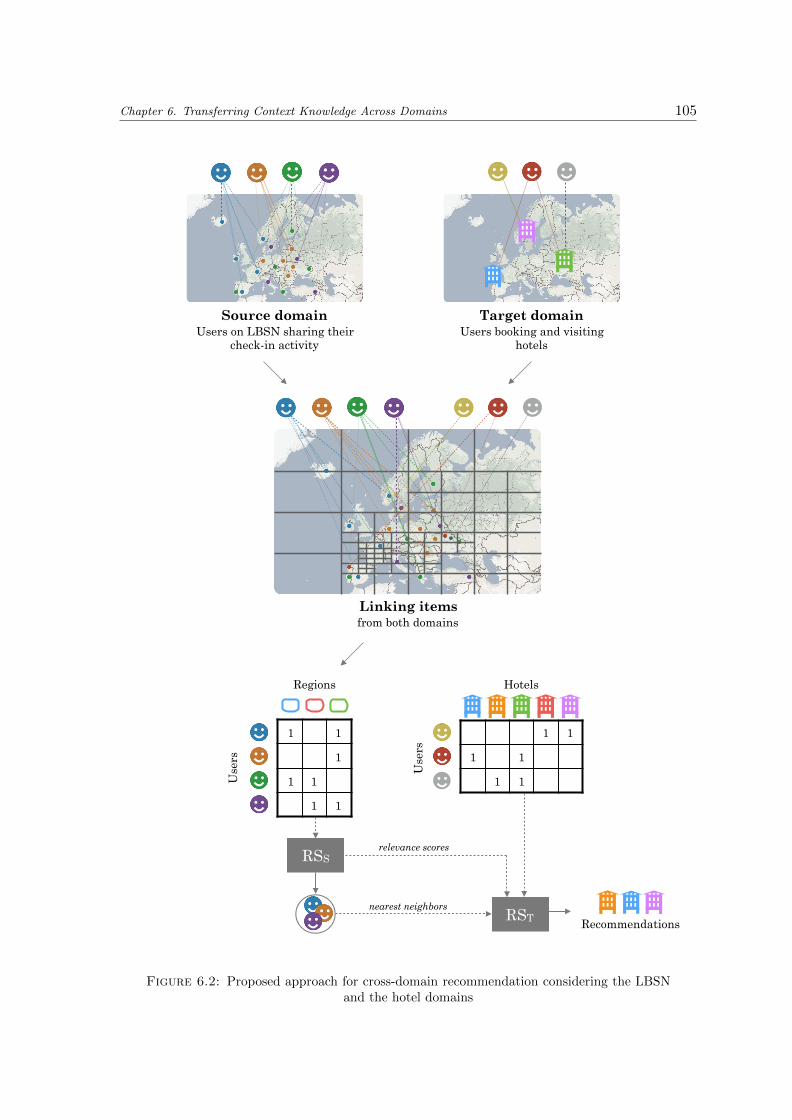
Chapter 6. Transferring Context Knowledge Across Domains 105
Source domain Users on LBSN sharing their
check-in activity
Target domain Users booking and visiting
hotels
Linking items from both domains
Use
rs
1 1
1 1
1 1
Hotels
1 1
1
1 1
1 1
Use
rs
Regions
RST
RSS
Recommendations
nearest neighbors
relevance scores
Figure 6.2: Proposed approach for cross-domain recommendation considering the LBSNand the hotel domains

106 Chapter 6. Transferring Context Knowledge Across Domains
model built. Both scores are combined and the final score for hotel i located in region r isgiven as follows, having a predefined weight parameter α and the number of neighbors Zu:
rui = α.rTui + (1− α).
∑z∈Zu
rSzr
|Zu|(6.1)
In our work, we use a Matrix Factorization (MF) method, Bayesian Personalized Ranking(BPR) [Rendle et al., 2009] (Section 2.5.2.4) to learn preferences and compute scores, since itperforms well on our dataset of bookings. We note that any other recommendation methodcould have been used within the same cross-domain approach.
6.4 Experimental Results
In this section, we present the experiments we conducted to evaluate the benefits of usingdata from LBSN for hotel recommendation and to prove the interest of our approach.
Datasets. We used one dataset from each domain to test our approach. The hotel bookingdataset, Ah, is extracted from the hotel industry and is presented in Section 3.2. It consistsof 7.8M users, 4.5k hotels, and 34M bookings (Table 3.2). Considering the geographydimension, users come from all countries and hotels are spread in more than 90 of them.Concerning the check-in data, we rely on the Yahoo Flickr Creative Commons (YFCC)dataset [Thomee et al., 2016] which is a real-world dataset that was published recently. Theoriginal dataset gathers 100M media objects including photos and videos that have beenuploaded to Flickr 3 between 2004 and 2014. Only a subset of these posts are annotatedwith geographic coordinates and can be handled as check-ins. Based on these posts, weconsider users that have visited more than 5 regions from the one we define in Section 6.3.1in order to have enough information to enrich the hotel domain. The filtered dataset weuse, denoted by Yfcc, contains around 24M check-ins done by 32k users.
Experimental setup. We split the dataset Ah into a training and a test set. We sortthe bookings of each user in a chronological order and select the first 80% to constitute thetraining set and the rest to constitute the test set. We also select 20% of the users who haveonly done one booking and add them to the test set in order to evaluate the performanceon new users. We use the data from the training set of Ah in addition to the dataset Yfccto train our recommendation method and evaluate its performance on the test set of Ah.
Evaluation metrics. We consider that we recommend N hotels to each user and notewhich of these hotels were actually visited based on the set of held-out bookings. We userecall@N and NDCG@N for measuring the performance (Section 2.2.3). Since large valuesof N are not interesting for top-N recommendation, we set N to 5 and 10 for both metrics.
Methods compared. We include in our comparison traditional recommendation methodsthat are listed in the following:
3http://www.flickr.com
Chapter 6. Transferring Context Knowledge Across Domains 107
• MostPop recommends the most popular hotels with respect to the user’s profile. Theuser profile includes a set of features related to the gender, the age category, and thecountry of residence. MostPop recommends to a target user the most popular hotelschosen by those having the same or similar profiles.
• CB is a content-based method where hotels and users are represented in the spaceof hotels’ features using vector space models and TF-IDF weighting [Pazzani andBillsus, 2007] (Section 2.4.1). Hotel features cover the location, the brand, the segmentcategory, and offered services such as Wi-Fi connection, parking, meeting facilities, andchildren playground.
• Knnu is a user-based neighborhood method (Section 2.5.1.1) where we use the Jaccardsimilarity metric to measure similarities between users and set the number of neighborsto 2000.
• WRMF is a MF technique handling implicit feedback [Hu et al., 2008] (Section 2.5.2.4).We set the number of latent factors to 100, the regularization parameters to 0.001,and cui = 1.0 for positive observations and cui = 0.01 for negative observations.
• BPR is a MF technique that relies on pairwise preferences to learn the latent model [Ren-dle et al., 2009] (Section 2.5.2.4). We set the number of factors to 100 and the regu-larization parameters to 0.0025.
• CD is the method we propose in this chapter, leveraging data from LBSN for hotelrecommendation. The maximum number of levels in the hierarchy (Section 6.3.1), L,is set to 14. We use the Jaccard similarity metric to measure similarities between users(Section 2.5.1.1) and set the number of neighbors to 500 and α to 0.7 — following agrid search process.
Results. Figure 6.3 shows the performance of the methods we consider. The results arerepresented for each category of users, a category being defined by the number of bookingsincluded in the training set. By definition, the metrics we measure decrease when thenumber of bookings increases. MostPop is the only method able to recommend hotels toinactive users, i.e., users with zero bookings in the training set. The inferiority of CB showsthat users do not attribute a great importance to all the hotels’ features considered. Furtherinvestigations showed that the location of the hotel is one of the few factors that greatlyaffect the decision. Knnu performs well for users with few bookings while BPR outperformsthe other methods when the number of bookings increases significantly.
The results obtained for CD show the interest of using data from LBSN to alleviate thesparsity problem. CD outperforms all the other methods when the number of bookings isless than or equal to 10 bookings. The interest of using cross-domain information decreaseswhen the number of bookings increases: BPR outperforms CD when the number of bookings isgreater than 30. One explanation may be due to the fact that the behavior of users activelysharing content on LBSN is not fully representative of the behavior of all travelers. Inparticular, people having done more than 30 bookings are more likely to be businesspeoplewhich behavior is not necessarily similar to users from LBSN. In addition, once enoughfeedback about hotels is collected, it may be sufficient to rely on hotel preferences to generateappropriate recommendations. The interest of using CD is highlighted in the cold-start

108 Chapter 6. Transferring Context Knowledge Across DomainsR
ecal
l@5
0,05
0,183
0,315
0,448
0,58
Number of bookings
0 1 2 3 4-10 10-30 30-50
MostPop CB Knnu WRMF BPR CD
ND
CG
@5
0,05
0,18
0,31
0,44
0,57
Number of bookings
0 1 2 3 4-10 10-30 30-50
Rec
all@
10
0,15
0,265
0,38
0,495
0,61
Number of bookings
0 1 2 3 4-10 10-30 30-50
ND
CG
@10
0,1
0,218
0,335
0,453
0,57
Number of bookings
0 1 2 3 4-10 10-30 30-50
Figure 6.3: Recall@5, NDCG@5, recall@10, and NDCG@10 for the dataset Ah, repre-sented with respect to the number of bookings present in the training set

Chapter 6. Transferring Context Knowledge Across Domains 109
setting where hotel bookings alone are not enough to infer preferences. We note that themajority of users in the booking dataset have done less than 10 bookings and, therefore, CDimproves the overall performance.
Discussion. This is the first work proposing to apply cross-domain recommendation inthe hotel sector using in particular abundantly available data from LBSN. While it can bea promising approach especially in a sparse data environment, it opens several interestingchallenges.
First, not all the users have their mobility behavior represented by active users postingon LBSN. These users will not directly benefit from the proposed approach. A finer analysisof users posting on LBSN, i.e., users in the source domain, and users booking hotels, i.e.,users in the target domain, may help to identify relevant user segments which behaviorcan be similar in both domains in terms of mobility and probably underrepresented in oneor in both domains. As a first basic approach, we tried addressing this issue by definingsegments based on the number of bookings made, considering that this number reveals acertain aspect of the user category. Other alternatives including more advanced techniquesmay be applied. One possibility to benefit from cross-domain recommendation may be tolearn local models per user category.
Second, further advances in this direction should consider evaluating the recommenda-tion diversity in terms of proposed locations. It is important to generate diverse recommen-dations and avoid suggesting hotels located in the same area. This may occur when oneregion gathering several hotels is specifically promoted for a particular user.
Transferring knowledge from LBSN to the hotel sector may go beyond the mobilityaspect by also considering temporality, i.e., periods during which one region is visited bya segment of users, and context of visits by analyzing meta-data associated to the posts.In addition, while we used a clustering component to map both domains, other approachesto integrating knowledge may be exploited. We may be considering to rely on a multi-taskapproach and to train models simultaneously in both domains.
6.5 Conclusion
In this chapter, we propose to use data from LBSN to boost hotel recommendation andto address the problem of sparsity due to the scarce feedback generated by the travelingactivity. Hotel selection largely depends on the visited destination and some destinationsare more accessible to users than others. Using the check-in activity from LBSN, we learnpreferences for regions and use these preferences for hotel recommendation. Mapping ofitems from both domains is done through a space of regions which definition is based on thedensity of hotels. Mapping of users from both domains is done by computing similaritiesbetween users based on the visited locations. Hotel recommendation accounts for regionpreferences and hotel preferences. Experiments show the interest of using cross-domaininformation for users with few observations, i.e., in the cold-start setting.
Temporality plays an important role in the decision-making process: One destination isnot considered by the same user in all periods of the year. Future work will involve adding

110 Chapter 6. Transferring Context Knowledge Across Domains
the time dimension and taking into account in which period of the year the check-in wasmade in order to distinguish between users visiting the same destinations at different periodsor seasons.
While Part II of the thesis was meant to address the challenges of partially observablecontext in hotel recommendation, we focus in Part III on the implications of the presenceof unobservable context in online recommendation.

Part III
From Unobservable Context toOnline Adaptive Recommendation
111


Chapter 7
The Online AdaptiveRecommendation Problem
This chapter presents the problem of online adaptive recommendation which is studied inPart III of this thesis. While real-world settings require the development of online RS, suchsystems face several challenges. They are expected, first, to continuously learn from datastreams and, then, to adapt to changes in real-time. In particular, users and items relyon some unobservable context that is hidden from the system, and any drift in the hiddencontext affects the represented concepts. Recommendation models have to actively accountfor these drifts in order to guarantee a good performance, introducing the problem of onlineadaptive recommendation. We provide a clear formulation of the problem and discuss relatedwork in both fields of RS and data stream mining, highlighting the shortcomings of existingapproaches.
7.1 Introduction
While RS apply techniques from various domains such as information retrieval and humancomputer interaction, the system’s core can be viewed as an instance of a data miningprocess [Amatriain and Pujol, 2015]: Data related to users and items is analyzed, a modelis inferred, and recommendations are produced for each user. The model is trained withall available data and the system is then queried for recommendations. While RS aredeployed online where data is continuously generated, recommendation models ensuringa good recommendation quality tend to suffer from very high latency. Training on largedatasets of user interactions is computationally expensive in terms of space and time andcannot be performed each time a new observation is received. In practice, most RS buildfirst a model from a large static dataset and then rebuild it periodically as new chunks ofdata arrive and are added to the original dataset.
This functioning in batch faces in particular two limitations. First, the RS cannottake into account the user feedback generated after a model update before the next oneand cannot thus consider the continuous activity of users. While user preferences and item
113
114 Chapter 7. The Online Adaptive Recommendation Problem
perceptions are dynamic concepts that are constantly changing over time, the same model isused to deliver recommendations and is indifferent to these temporal dynamics. The inabilityto adapt to quick changes by considering recent feedback leads to poor recommendationquality and user experience [Dias et al., 2008]. Second, training a model on a continuouslygrowing dataset is computationally expensive. This raises scalability issues in additionto the need for additional resources to store and process data. Solution options includescaling up systems which can be expensive, reducing the number of updates which canworsen recommendations, and decreasing the volume of data considered which may resultin discarding valuable information for recommendation.
Advances in the RS field have focused on a part of these limitations and attempted toaddress each one of them using different approaches. Time-Aware RS (TARS) [Camposet al., 2014] were introduced to handle the dynamic aspect of entities modeled by RS. Theyrespect the chronological order of observations and try to capture the evolution of users anditems over time. While these systems consider the temporal dimension, they are meant towork in batch and cannot technically integrate new user feedback as soon as it is generated.Some of the computational issues were addressed by considering efficient and distributedmodels [Gemulla et al., 2011; Teflioudi et al., 2012] but continuously growing datasets stillneeded to be stored and processed.
Recent work [Siddiqui et al., 2014; Vinagre et al., 2014b] has proposed to address therecommendation problem as a data stream problem by designing online RS, resulting ina more realistic setting. Elements of a data stream are expected to arrive indefinitely inreal-time at high uncontrolled rates. A parallel can thus be drawn with user-generated datahandled by RS that share actually the same characteristics. Online RS are expected to learnfrom continuous data streams and to maintain recommendation models up to date, and relyon incremental learning. By adapting to changes in real-time and operating independentlyof the number of observations, they address the previously mentioned limitations faced bybatch RS.
One of the core problems in data stream mining consists in dealing with concept driftswhich occur when the definition of modeled concepts change over time [Gama et al., 2014].Online RS have to be able to track multiple concepts changing in different ways at differentmoments and rates, including the preferences of each user and the perception of each item.Incremental learning is a natural way to account for a specific type of drift, i.e., incrementaldrift, where the concept slowly passes by intermediate states until reaching a new one.However, specific strategies and techniques need to be adopted to detect and adapt to othertypes of drifts such as more abrupt ones. While previous work has already proposed to designonline RS, limited effort has been made to develop online adaptive RS that automaticallyaccount for drifts in real-time.
In this chapter, we present the problem of online adaptive recommendation and discussrelated work in the recommendation and the data stream mining fields. Taking into accountthe evolution of concepts in RS can be traced back to TARS [Campos et al., 2014] with thelimitation of functioning in batch and not being able to maintain models up to date. OnlineRS were then proposed to cope with this issue. However, drift detection techniques stillneeded to be integrated to ensure a strong adaptive ability facing changes, which is themain idea explored in Part III of this thesis. Overall, online adaptive recommendation is

Chapter 7. The Online Adaptive Recommendation Problem 115
related to TARS due to the dynamic aspect of users and items and to data stream miningdue to the analysis of data streams in real-time.
The chapter is structured as follows. In Section 7.2, we discuss related work on TARS.Section 7.3 presents the problem of concept adaptation in data stream mining. In Section 7.4,we present the problem of online adaptive recommendation in addition to related worktackling different aspects of it. Finally, a summary is given in Section 7.5.
7.2 Time Dimension in Recommender Systems
Motivation. When learning user and item models based on a dataset of user interactions,traditional recommendation approaches assume that the user behavior follows a single spe-cific pattern that is expected to reappear in the future, making prediction a feasible task.This assumption does not hold in a dynamic world where users and items are constantlyevolving. Efficient RS are expected to maintain models that reflect the actual state of en-tities [Koren, 2009]. On the other hand, modeling temporal changes related to users anditems is a challenging task. First, changes may occur on a global scale: The introduction ofnew items may affect the behavior of users, and seasonal patterns, holidays, and unexpectedevents may also influence the attractiveness of items. Many of the changes are also drivenby local factors and hidden contexts related to users. A change in the user social status canresult in a change of behavior and user interests tend to shift with time. While tracking allof these changes is essential to guarantee the generation of appropriate recommendations,changes happen in different ways at different moments and rates for each user and item.Therefore, simple solutions that assume having a priori knowledge about the way conceptsare changing, e.g., solutions that discard old observations, are not sufficient. Instead, moreadvanced techniques that leverage signals extracted from past and recent observations needto be considered.
Historical perspective. The practical value of modeling temporal changes in RS was firsthighlighted within the context of the Netflix Prize (Section 2.1.1). [Koren, 2009] showedthat user ratings exhibit temporal patterns that could be exploited for the recommenda-tion task. The proposed solution allowed the distinction between long-term patterns andtemporary ones and was evaluated on the dataset of the competition. Including tempo-ral changes proved to be very useful to improve the recommendation quality and severalapproaches were further proposed, forming the category of RS known as Time-Aware RS(TARS) [Campos et al., 2014]. Then, the rise of Context-Aware RS (CARS) lead to in-vestigating the possibility of integrating time as a contextual dimension. One of the firstefforts following this direction [Baltrunas and Amatriain, 2009] proposed to build contextualmicro-profiles representing the user behavior in different temporal contexts, e.g., morningand evening or weekend and workday. This technique was then identified as being partof the pre-filtering paradigm for CARS (Section 2.7.1). On the other hand, recent yearshave witnessed the emergence of a related problem which is the problem of sequence-awarerecommendation [Quadrana et al., 2018]. The increased interest was mainly fueled by in-dustry through the release of a new dataset of session activity from a major e-commerceplatform within the context of the 2015 ACM RecSys Challenge [Ben-Shimon et al., 2015],and by the development of new deep learning techniques for sequence learning [Hidasi et al.,

116 Chapter 7. The Online Adaptive Recommendation Problem
2016]. Sequence-aware algorithms learn sequential patterns from user behavior and attemptto predict the user’s next action within a session or to detect short-term trends. TARS andsequence-aware RS share a number of common characteristics. However, while they bothrely on the order of interactions, sequence-aware RS do not focus on the exact point intime of past observations and try to detect patterns within the sequence itself. Approachingdata as a chronologically ordered sequence also gave rise to online RS that handle data asa stream [Siddiqui et al., 2014; Vinagre et al., 2014b]. These RS are based on incrementallearning which is a natural way to account for relatively small changes and to keep modelsadapted to the actual reality.
Time-Aware Recommender Systems (TARS). Several methods were proposed to in-tegrate the temporal dimension into RS. We can mainly distinguish between three categoriesof approaches merging time with Collaborative Filtering (CF) methods: recency-based time-aware models, contextual time-aware models, and continuous time-aware models. Othercategorizations can be found in [Campos et al., 2014; Vinagre et al., 2015b].
Recency-based time-aware models. Recency-based models are based on the assumption thatrecent observations are more relevant than older ones since they are more representativeof the actual reality: They should therefore be given more importance in the learning andrecommendation processes. These methods have the advantage of being simple and easy tointegrate into existing recommendation models. However, the main assumption establisheddoes not always hold in real-world scenarios. In particular, it is not uniformly valid forall users and items, resulting in a limited performance. The recency aspect can be tackledwith decay-based [Ding and Li, 2005; Liu et al., 2010c] or window-based [Lathia et al., 2009;Nasraoui et al., 2007] methods. Decay-based methods gradually decrease the importance andcontribution of past data while window-based methods only consider observations containedin a window of a certain length. We note that window-based methods can be viewed as aparticular case of decay-based methods with a binary decay function.
Contextual time-aware models. Contextual approaches integrate the time dimension byconsidering temporal information as context. Several contextual features can be extractedfrom the temporal information such as the time of day, the day of the week, the month,and the season. Once the contextual features are defined and specified, any context-awareapproach can be used to address the problem (Section 2.7.1).
The various paradigms existing for CARS were used for TARS. [Baltrunas and Am-atriain, 2009] proposed a pre-filtering method where they built contextual micro-profilesrepresenting the user behavior within different time frames and used them for recommenda-tion. Post-filtering was leveraged in [Panniello et al., 2009] for TARS: Contextual relevanceweights based on temporal features were computed and used to filter recommendations.In addition, factorization methods relying on Tensor Factorization (TnF) were applied toaddress this problem [Gantner et al., 2010b; Liu et al., 2010b].
Continuous time-aware models. Continuous models represent ratings and user interactionsas a function of time, and the model parameters are learned from the data. Some of thesemodels rely on time series models and others on factorization models.
In the first set of models, user ratings and interactions are encoded as time series andtime-series techniques are used to predict the current user interest. These techniques have

Chapter 7. The Online Adaptive Recommendation Problem 117
been applied when dealing with explicit feedback such as ratings in [Cao et al., 2009] andimplicit feedback such as web logs in [Zimdars et al., 2001]. [Jahrer et al., 2010] proposed tobuild several CF models for different time periods and used blending techniques to combinethe models’ recommendations.
On the other hand, [Koren, 2009] was one of the first works proposing to exploit factoriza-tion models for time-aware recommendations. The proposed solution relies on SVD++ [Ko-ren, 2008] that considers user and item biases, i.e., deviations from a global average, inaddition to a factor model capturing user preferences and item perceptions. Temporal userbiases are modeled using a decay function, different item biases are considered for each timewindow, and an additional decay function is used to weigh previous ratings for prediction.The model gained popularity due to the accuracy improvements obtained on the NetflixPrize dataset. A similar model was then presented for the task of music recommenda-tion [Koenigstein et al., 2011]. Another way to integrate time into the Matrix Factorization(MF) framework was proposed in [Karatzoglou, 2011] where differentiated item factors arelearned based on the ratings’ timestamps. We mention that several approaches also con-sidered modeling users’ short-term and long-term preferences separately [Liu and Aberer,2014; Xiang et al., 2010].
More recently, modeling the evolution of user preferences and item perceptions wasconsidered on a more refined individual level. Instead of relying on the information providedby other users, specific approaches were developed to build personalized models and profilethe evolution of individual users. [Liu, 2015] handled implicit feedback and proposed toextract topics from each user interaction observed at a certain time point. The evolutionof each topic for each user is then treated as a time series to predict the user’s futurepreference. In [Lu et al., 2016], user interests and their evolutions are learned simultaneouslyand collaboratively at each time point by combining MF and vector autoregression. [Gaoet al., 2017] built on this idea but considered in addition the evolution of items’ contents.
Relation to our work. We review in this section the main approaches proposed for TARSwhile omitting further details, given that all of them share one main limitation. Whileconsidering the evolution of modeled concepts over time, they are not adapted to the onlinesetting and cannot maintain models up to date in real-time. TARS assume that the wholedataset is available at the time of training and that multiple passes can be performed onthe data. We also do not review previous work on sequence-aware RS even though it isrelated in some way, given that we do not consider applications where relevant patternswithin sequences are expected to exist. Moving to a more realistic setting, we investigatethe problem of learning from a stream of user interactions with the challenge of adapting tochanges in real-time. We present in the next section the more general problem of adaptivestream mining before discussing the problem of online recommendation.
7.3 Adaptive Data Stream Mining
Data stream mining. In traditional data mining, models are built using historical datain an offline mode: The whole dataset is available for training and the model is used forprediction once the training is completed. With the massive and growing generation of

118 Chapter 7. The Online Adaptive Recommendation Problem
information and signals, data is commonly available as continuous streams that can onlybe appropriately processed in an online mode. This is due to the fact that elements of adata stream are expected to arrive in real-time at high rates and to be processed one afterthe other in only a few passes using limited time and memory per element. In an onlinelearning setting, data is processed sequentially and models are continuously trained whenreceiving new observations. Aside from the online nature of learning, handling data streamspresents the challenge of detecting and adapting to concept drifts. Concept drift occurs innon-stationary environments when the data distribution changes over time and imposes thedesign of adaptive models.
Concept drift. The main assumption made by most predictive models is that the trainingdata, i.e., observations used for learning, and the testing data, i.e., observations for which themodel will be generating predictions, are sampled from the same probability distribution.This assumption does not hold in real-world domains where predictive models are meantto be developed and applied, due to the evolution of target concepts over time. Learningis often performed in non-stationary environments and, thus, requires adaptive models thatare able to account for changes occurring unexpectedly over time. The difficulty in handlingsuch changes is initially derived from the fact that the target concept that is being repre-sented depends on some hidden context or on an underlying process that is unknown to thelearner [Tsymbal, 2004]. Any change in the hidden context can affect the target conceptand thus the performance of the learner.
The process of learning in non-stationary environments is formalized for the problem ofsupervised learning, resulting in a probabilistic definition of concept drift detailed in thefollowing. In a supervised learning setting, the goal is to predict a target variable y ∈ R orthe class y given a set of input features X ∈ Rn. Observations that are used for learning arethen denoted by (X, y) and predictions are performed for new observations where X is knownand y is unknown. Observations generated at time t are assumed to be sampled from thejoint probability distribution pt(X, y), and we denote by pt(y|X) the posterior distributionof class y and by pt(X) the evidence distribution. Concepts are expected to evolve over timeand consequently distributions dynamically change. A concept drift occurring between timepoints t0 and t1 is defined as [Ditzler et al., 2015; Gama et al., 2014]:
∃X : pt0(X, y) 6= pt1(X, y) (7.1)
Given that different natures of changes may be encountered, a terminology is adoptedto designate where the change originates from in addition to its form. Concerning thedistribution from which the change is originating, we distinguish two types of drifts. Realconcept drifts occur in cases where the posterior probability pt(y|X) changes over time whichmay happen independently from changes in the evidence pt(X). Virtual concept drifts occurin cases where the evidence probability pt(X) changes without affecting pt(y|X). In otherwords, virtual drifts happen when the distribution of received observations changes. Inboth cases, the model needs to be revisited given that the error generated may no longer betolerated.
On the other hand, concept drifts take different concrete forms. These multiple formsare illustrated in Figure 7.1, adapted from [Gama et al., 2014], where changes in the datamean are tracked. The concept drift can happen either abruptly resulting in a sudden

Chapter 7. The Online Adaptive Recommendation Problem 119
time
mea
n
Abrupt Incremental Gradual Recurrent Outlier (not concept drift)
Figure 7.1: Concept drift forms represented over time. Figure adapted from [Gama et al.,2014].
Data
Feedback
Prediction
AlarmLoss estimation
Change detection
LearningMemory
Figure 7.2: A generic framework for online adaptive learning. Figure adapted from [Gamaet al., 2014].
change, incrementally consisting in the existence of intermediate states between the oldconcept and the new one, or gradually where the change is not abrupt but we keep goingback to the previous concept for some period of time. Drifts can further be classifiedinto permanent drifts where the effect of the change is not bounded in time and transientdrifts which effect disappears after a certain period of time. While new concepts may beintroduced at each change, previously observed concepts may reoccur resulting in recurrentdrifts. Such settings benefit from the ability to retrieve previous knowledge related to similarobserved concepts. It is worth mentioning that concept drifts should not be mixed withoutliers referring to anomalies that may appear in the data and demanding no adaptivity ofthe models. Operating under the presence of concept drifts requires specific methods andtechniques able to detect and adapt to changes.
Online adaptive learning. The online adaptive procedure consists of the following threesteps, applied for each received observation: (i) Predict. A prediction yt is made for thereceived observation Xt using the current model, (ii) Evaluate. After receiving the truelabel yt, we estimate the loss f(yt, yt), (iii) Update. The observation (Xt, yt) may be usedto update the model.
[Gama et al., 2014] proposed a generic framework for online adaptive learning representedin Figure 7.2. It consists of four modules: memory, learning, change detection, and lossestimation, that we briefly review in the following.

120 Chapter 7. The Online Adaptive Recommendation Problem
Memory module. The memory module defines the strategies followed to select data for learn-ing on one hand and to discard old data on the other hand. Adaptive learning approachesassume that recent data is the most relevant to the current prediction task. Learning isthus done based on the most recent data and can be performed using a single or multipleobservations. Learning from a single observation requires storing only the correspondingobservation. This is the natural setting in online learning where models are continuouslyupdated using the received observations with no access to older ones. Adaptation to newconcepts is expected to happen naturally as more learning is performed and as conceptslearned from older data are gradually disappearing. Learning from multiple observationsrequires storing the most recent observations. Sliding windows of fixed or variable sizes areusually used to store observations which are then used to build new predictive models [Wid-mer and Kubat, 1996]. Discarding outdated data is a way of handling evolving streamsand is achieved through forgetting mechanisms which choice depends on a priori knowledgerelated to the nature of the change. Abrupt forgetting may be adopted by totally discardingobservations based on their relevance. This can be done using sliding windows or samplingtechniques [Vitter, 1985]. A less extreme form of forgetting, i.e., gradual forgetting, can beperformed by using all observations stored in the memory for training but weighting eachone based on its age [Klinkenberg, 2004].
Learning module. The learning module defines how to build predictive models and maintainthem up to date given the received observations. Predictive models can be retrained fromscratch using observations stored in the memory after discarding old models. They can alsobe incrementally updated using received data. In incremental learning, observations areprocessed one after the other. Existing models are updated after each received observationand may access older observations. In the more restrictive setting of online learning, datais processed once in a sequential fashion [Littlestone, 1988]. The streaming setting addslimitations on the memory and time resources required for processing data given its highrate. As learning is carried on, concepts learned from recent data tend to erase thosepreviously learned. Continuously updating models over time is a way to passively adaptto changes. Passive approaches face the limitation of being slow in reaction to changes:Learning is done at a constant speed independently from the changes occurring in theenvironment. Therefore, active approaches have been proposed where drifts are explicitlydetected triggering a learning mechanism to adapt the models [Elwell and Polikar, 2011].Drift detection is handled by the Change detection module, and once a drift is reported, itis possible to rebuild a model from scratch or adapt the part concerned with the change.Along this line, ensemble learning has been leveraged for adaptive stream mining [Gomeset al., 2017].
Change detection module. The change detection module handles techniques for the activedetection of drifts. According to [Gama et al., 2014], these techniques can be classified intoseveral categories and we mention some of them in the following. First, detectors based onsequential analysis include for example the cumulative sum. It analyzes the performanceof a predictor and reports a change when the mean of the analyzed data significantly devi-ates from zero [Alippi and Roveri, 2006]. Then, other methods consist in monitoring twodistributions. They rely on a fixed reference window representing the past observationsand a sliding one containing recent observations. Distributions over the two windows arecompared using statistical tests. Given that the null hypothesis states that distributions areequal, a change is detected when it is rejected. An example of these methods is ADaptive

Chapter 7. The Online Adaptive Recommendation Problem 121
WINdowing (ADWIN) [Bifet and Gavalda, 2007]. Additional solutions leverage statisticalprocess control or well-defined heuristics.
Loss estimation module. The loss estimation module analyzes the performance of the learn-ing algorithm and transfers information to the change detection module. The loss variablecan be defined with respect to the model, i.e., using properties tightly related to the predic-tive model, or independently from the model, e.g., by comparing two sliding windows.
Relation to our work. The vast majority of work related to RS considers learning predic-tive models in an offline mode. As mentioned at the beginning of the chapter, this settingis not adapted to real-world environments where user-generated data arrives in the form ofstreams and where concepts are expected to change over time. While previous work has al-ready proposed to learn recommendation models in an incremental or online mode, the arearemains underexplored or even unexplored when it comes to actively detecting drifts anddesigning online adaptive algorithms for recommendation. We introduce the formulation ofonline adaptive recommendation relying on the framework developed for stream mining andpresented in this section. We review previous work based on this formulation.
7.4 Online Adaptive Recommendation
As mentioned in previous sections, real-world settings require to formulate the recommen-dation problem as a data stream problem: User-generated data is continuously received andanalyzed and recommendations are delivered in real-time. Online recommenders can thusrely on the generic framework presented in Section 7.3, Figure 7.2 [Gama et al., 2014]. Inaddition to the modules included in the framework, we consider the following two modulesfor the problem of online adaptive recommendation: the retrieval module that is responsiblefor the efficient computation and retrieval of recommendations and the evaluation modulethat constantly evaluates and reports the RS performance. Previous work related to onlinerecommendation attempted to come up with solutions regarding one or several modules atonce. In the following, we propose to review related work according to the module concernedby the solution. We note that two modules are not mentioned: the change detection modulesince it was not specifically addressed for online RS and the loss estimation module sinceexisting solutions are included in other modules.
7.4.1 Memory Module
Assuming that recent data is more relevant than older one, predictive models have to learnfrom recent observations and forget old ones. This has been applied in the context of onlinerecommendation in several ways.
Forgetting in memory-based approaches. [Nasraoui et al., 2007] use a user-basedneighborhood approach that relies on a sliding window containing a fixed number of recentobservations. Along this line, [Siddiqui et al., 2014] propose a recommendation algorithmthat operates in two steps. Users are first clustered based on their previous interactions

122 Chapter 7. The Online Adaptive Recommendation Problem
and a user-based neighborhood approach is then applied in each cluster to perform recom-mendation. A sliding window is used over the stream: Only observations done during acertain time interval are considered when computing similarities and scores, and the othersare definitely discarded. Aside from sliding windows, fading factors have also been usedto gradually forget old information. [Vinagre and Jorge, 2012] propose to multiply usersimilarities by a positive scalar α < 1 before updating them with information received fromnew observations. The value of α controls the rate at which forgetting is performed.
Forgetting in Matrix Factorization (MF) approaches. [Matuszyk et al., 2015] intro-duce two sets of forgetting strategies within the scope of MF: rating-based forgetting andlatent factor-based forgetting. Rating-based strategies discard past ratings for each usereither using sliding windows, e.g., fixed size or covering a fixed time period, or using sensi-tivity analysis, e.g., forget ratings that imply abnormal changes in the user profile. On theother hand, latent factor-based strategies readjust the latent factors of MF to reduce theeffect of old observations. These strategies include forgetting unpopular or popular itemsand fading user factors.
Most online RS that only contribute on the level of the memory module face one mainlimitation. They require fixing a set of parameters, e.g., the size of a sliding window or afading factor, and anticipate that the RS should forget old observations. Therefore, theyassume we have a priori knowledge regarding the way the user behavior is changing andthat preferences of all users drift at the same rate, which is obviously not the case.
7.4.2 Learning Module
The learning module defines how recommendation models are learned and maintained up todate which is usually based on incremental learning. In fact, traditional CF methods, i.e.,memory-based and model-based approaches, have been adapted to the incremental settingand some of them are presented in the following.
7.4.2.1 Incremental Memory-Based Approaches
Applying memory-based algorithms in a streaming setting faces two major issues. First,similarity computation is performed in a costly offline phase where similarities between alluser pairs or item pairs are evaluated given the observed interactions. Second, the whole his-tory of user interactions cannot be stored in memory and used entirely for recommendation.Several solutions were proposed addressing one or both of these limitations.
Incremental neighborhood-based methods were first proposed in [Papagelis et al., 2005].The authors presented an incremental user-based approach handling explicit feedback in theform of ratings. User similarities are stored and incrementally updated for each receivedrating. Nearest neighbors and predicted ratings are then computed at the time of recom-mendation. Similarities are evaluated using Pearson Correlation (Section 2.5.1.1) which is
Chapter 7. The Online Adaptive Recommendation Problem 123
split in the following way:
A = simPC(u, v), B =∑x∈Iuv
(rux−ru)(rvx−rv), C =∑x∈Iuv
(rux−ru)2, D =∑x∈Iuv
(rvx−rv)2
(7.2)
where
A =B√C√D
(7.3)
Elements A, B, C, and D are stored and incrementally updated, and new similaritiescan be computed in a fast manner. Incremental user-based and item-based neighborhoodapproaches handling implicit feedback and using the cosine similarity were then presentedin [Miranda and Jorge, 2009]. The formulation of cosine similarity in an implicit feedbacksetting is based on user and item occurrence and co-occurrence counts. Two users co-occurfor every item they both interact with and two items co-occur for each user that interactswith both of them. Given that counts are stored, maintaining similarities up to date for eachreceived observation boils down to incrementing counts of occurrences and co-occurrences.Similarly to [Papagelis et al., 2005], nearest neighbors and scores are computed at themoment of recommendation. In an attempt to adapt to user and item changes in the scopeof a neighborhood-based method, [Liu et al., 2010c] introduced the online evolutionary CFframework. It relies on an incremental version of the item-based neighborhood methodand proposes instance weighting techniques to reduce the weight of old observations whencomputing similarities and scores.
A probabilistic neighborhood-based algorithm based on a min-hash technique was devel-oped in [Subbian et al., 2016]. Similarities between users are approximately computed bytracking the relevant users for each item in a min-hash index which is implemented usinghash functions. These hash functions are stored in memory instead of storing the full historyof user interactions. Other approaches for incremental CF built on co-clustering methodsfor recommendation [George and Merugu, 2005; Khoshneshin and Street, 2010]. In its mostsimple form, [George and Merugu, 2005] proposed incremental and parallel versions of theco-clustering algorithm that simultaneously clusters users and items. Predicted ratings areestimated based on the average rating of co-clusters, users’ bias, and items’ bias.
On the other hand, efficient frameworks and architectures for online recommendationwere presented based on neighborhood-based approaches. StreamRec [Chandramouli et al.,2011] implements a scalable item-based CF approach based on a stream processing systemand handles explicit ratings. While also relying on an item-based CF approach, Tencen-tRec [Huang et al., 2015] deals with implicit feedback and is designed to serve recommenda-tions for a wide range of applications having different requirements. It is built on Storm witha data access component and a data storage component, and proposes real-time pruning toreduce the computation cost.
7.4.2.2 Incremental Matrix Factorization and Other Model-Based Approaches
Due to the great success of Matrix Factorization (MF) and model-based approaches in thecontext of recommendation [Koren et al., 2009], several efforts have been made to adapt them

124 Chapter 7. The Online Adaptive Recommendation Problem
to the incremental and online settings. These efforts historically followed the evolution andadvances of MF approaches. While some of them focused on integrating newly observedusers and items into an existing model, the others managed to update parts of learnedmodels based on current observations.
Singular Value Decomposition (SVD). Early effort on Incremental Matrix Factoriza-tion (IMF) for RS was introduced in [Sarwar et al., 2002]. Incremental updates of SVD aremade through the fold-in projection technique: Latent vectors corresponding to new usersor new items are computed based on the current decomposition and are then appendedto the existing matrices. [Brand, 2003] defined incremental operations allowing the addi-tion, update, and removal of data already incorporated into the SVD model. This is madepossible through the basic algebraic properties of SVD. Although these techniques lead toa high efficiency, SVD suffers from several shortcomings such as the need to have an ini-tial matrix with no missing elements, resulting in a limited performance on sparse datasets(Section 2.5.2.2).
Point-wise approaches. With the rise of the MF framework for the problem of ratingprediction, [Rendle and Schmidt-Thieme, 2008] introduced regularized kernel MF as a gen-eralization of regularized MF. It provides a flexible method to derive new MF methods bytransforming the product of factor matrices using kernel functions. Within this context, anonline algorithm was proposed to allow the incremental addition of new users and items tothe existing MF model. Concretely, the algorithm retrains the whole feature vector corre-sponding to the new user or item and keeps the other feature vectors fixed. Along this line,[Takacs et al., 2009] proposed BRISMF, standing for Biased Regularized Incremental Si-multaneous MF, supporting incremental updates of latent factors given an initially trainedmodel and integrating user and item biases expected to model user and item tendencieswith respect to ratings. For each received rating, user features of the corresponding user areretrained considering all the ratings he previously made, and item features are kept fixedto avoid a larger retraining process. While [Rendle and Schmidt-Thieme, 2008] and [Takacset al., 2009] rely on Stochastic Gradient Descent (SGD) to learn latent factors, other IMFapproaches exploited variants of the Alternating Least Squares (ALS) method to benefitfrom its advantages (Section 2.5.2.3). [Yu et al., 2016] proposed one-sided least squares forupdating one side, i.e, user-side or item-side, of an existing MF model. It is applied whena new user or a new item is encountered and is also proposed to update both sides of themodel when it is required. We note that the complexity of the solution offered by ALS ishigher than the one offered by SGD (Section 2.5.2.3).
Aside from the rating prediction problem, [Vinagre et al., 2014b] proposed an IMFframework for the top-N recommendation problem and handling positive-only feedback.When either a user or an item is observed for the first time, it is added to the model withrandom initialization. User and item latent factors are then incrementally updated followingSGD, i.e., using the gradient of the objective function for the corresponding observation.[Vinagre et al., 2014b] allow slight updates of latent factors instead of total retraining likein previously mentioned approaches. The proposed method is detailed in Algorithm 5.
One limitation of the approach proposed in [Vinagre et al., 2014b] is related to the prob-lem of dealing with implicit feedback and concerns the lack of negative observations or theway missing observations should be interpreted (Section 2.5.2.4). In fact, only considering

Chapter 7. The Online Adaptive Recommendation Problem 125
Algorithm 5 Overview of IMF proposed in [Vinagre et al., 2014b]
Data: stream of observations DInput: number of factors k, learning rate η, regularization parameters λP and λQOutput: P, Q
1 for (u, i, t) in D do2 if u 6∈ Rows(P) then . new user observed3 pu ← Vector(size : K)4 pu ∼ N (0, 0.1)5 end if6 if i 6∈ Rows(Q) then . new item observed7 qi ← Vector(size : K)8 qi ∼ N (0, 0.1)9 end if
10 eui ← pu.q>i − 1
11 pu ← pu − 2η(euiqi + λPpu)12 qi ← qi − 2η(euipu + λQqi)13 end for
positive feedback for learning the model may result in an accuracy degradation. To dealwith this problem, [Vinagre et al., 2015a] extended the work in [Vinagre et al., 2014b] byartificially introducing negative feedback into the stream of observations. For each positiveobservation causing a model update, negative items are considered for the current user andresult in additional updates. Negative items are selected based on the recency of item occur-rences: The oldest items appearing in the stream of positive observations are considered asnegative feedback. Other methods were also introduced to deal with missing observations inan incremental setting. [Devooght et al., 2015] extended several loss functions, e.g., squaredand absolute losses, to take into account an explicit prior on unknown values and derivedonline learning algorithms to update the model. While this approach assumes that missingentries are equally likely to be negative feedback, [He et al., 2016] introduced a weightingstrategy for missing observations based on item popularity. The authors also proposed a newlearning algorithm based on ALS and handling variably-weighted missing data, in additionto an incremental strategy supporting online learning.
Pair-wise approaches. Ranking approaches based on pair-wise loss functions were de-signed for the task of top-N recommendation in the presence of implicit feedback (Sec-tion 2.5.2.4). In the scope of online recommendation, [Diaz-Aviles et al., 2012b] presentedStream Ranking MF or RMFX which relies on a pairwise approach to MF and uses a selec-tive sampling strategy based on active learning ideas to perform incremental model updates.The approach maintains a reservoir containing a fixed number of observations sampled fromthe stream of observations, and the model is updated by iterating through the reservoirinstead of going through the entire stream. [Diaz-Aviles et al., 2012a] is based on the sameapproach and further investigated additional sampling strategies.
Further advances in Incremental Matrix Factorization (IMF). The approach in-troduced in [Huang et al.] handles ratings batch by batch and proposes to design a linear

126 Chapter 7. The Online Adaptive Recommendation Problem
transformation of user and item latent factors over time, at each model update. On theother hand, and instead of only updating vectors related to the current received observa-tion, [Wang et al., 2013] explored multi-task learning and proposed to update additionalvectors according to a user interaction matrix. Compared to most previously mentioned ap-proaches that rely on vector retraining, a space retraining model is proposed in [Song et al.,2015]. The feature space is retrained via auxiliary feature learning and matrix sketchingstrategies.
Applications. [Das et al., 2007] was one of the first applications to tackle the problemof online recommendation in order to deliver news recommendations in real-time. Theauthors proposed a scalable approach combining different recommendation methods andusing parallel computation. They also relied on a time-decaying function for user interactionsand on a time-based window to evaluate co-visits of news. On the other hand, IMF hasbeen implemented to address the recommendation problem in specific domains. [Palovicset al., 2014] proposed a method for online music recommendation in a social media service.The approach is based on MF and exploits temporal and social influences between usersto improve recommendations. Users that are socially connected are expected to exhibitsimilar preferences in close periods of time. [Huang et al., 2016] developed a scalable MFalgorithm with an adjustable updating strategy for video recommendation. Different typesof implicit feedback, e.g., click, watch and comment, are considered and each one of them isattributed a different confidence level regarding the degree of user interest that it exhibits.These confidence levels affect the value of the learning rate used to update the IMF model.
Beyond Matrix Factorization (MF). Relatively few efforts have been made to adaptmethods other than MF to the online setting of recommendation. We mention in particularthe application of Tensor Factorization (TnF) [Zhang et al., 2014], Factorization Machines(FM) [Kitazawa, 2016], online regression [Agarwal et al., 2010], and bagging [Vinagre et al.,2018], omitting further details about these methods.
User and item dynamics. Beyond efficiently updating models and integrating new usersand items, online recommendation should account for the evolution of users and items overtime. Recently, [Chang et al., 2017] presented a framework that handles streams via acontinuous-time random process. Markov processes are meant to model each time-varyinguser and item factors in an attempt to capture the dynamics occurring in such settings.Another framework introduced in [Wang et al., 2018] is based on Bayesian PersonalizedRanking (BPR) and claims to handle users’ interest drifts, new users and items, and thesystem overload occurring in a streaming setting. It also relies on samples stored in areservoir in order to capture users’ long-term interests instead of only learning from recentobservations.
7.4.3 Retrieval Module
Without loss of generality, the recommendation problem can be divided into two tasks:learning a utility function and estimating the ratings or relevance scores of items for atarget user. In an online context, the utility function is constantly updated and scoreshave to be computed on the fly. In an attempt to be compliant with a streaming setting,

Chapter 7. The Online Adaptive Recommendation Problem 127
specific methods have to be developed and adopted to ensure an efficient retrieval of recom-mendations. Retrieving recommendations requires computing the scores for each item andselecting the N items scoring the highest. We review some of the methods in the following,even though not all of them are meant to work in a fully online setting.
[Koenigstein et al., 2012] propose to use metric trees, i.e., binary space-partitioning trees,to index item vectors, and use a branch and bound algorithm to obtain an exact solution.The technique is applied for neighborhood-based methods [Koenigstein and Koren, 2013]and MF methods [Koenigstein et al., 2012]. An approximate faster solution relying on aclustering of users is also proposed [Koenigstein et al., 2012]. Recommendations are com-puted for the cluster centers and presented as an approximate result to all users belongingto the corresponding cluster.
[Yin et al., 2015a] propose to compute one list of items per latent factor where items aresorted according to their generative probabilities with respect to the latent factor. Top-Nitems are computed for each list and returned in a priority list. An extended version of thethreshold algorithm [Fagin et al., 2003] is used to update the priority of lists in additionto the threshold score. A similar idea is also implemented in [Yin et al., 2015b] for POIrecommendation. [Teflioudi et al., 2015] propose to group the latent vectors into buckets ofsimilar lengths and then solve a smaller cosine similarity search problem between vectors ofeach bucket. We note that since these methods require an offline step, they are not adapted,as originally defined, to the online setting where models are constantly being updated.
7.4.4 Evaluation Module
Batch offline evaluation. With a new formulation for the recommendation problemcomes the need to design new appropriate evaluation methodologies. While the traditionalbatch mode of offline evaluation involving holdout methods is widely used to evaluate RS,it faces several limitations in the streaming setting (Section 2.2.1.1) [Vinagre et al., 2014a].By randomly sampling data for training and testing, holdout methods ignore the temporaldimension and do not take into account the natural ordering of observations. Recommen-dation algorithms designed to handle ordered data cannot thus be evaluated with thesemethods. In addition, shuffling observations may result in illogical operations such as usingfuture interactions to predict past interactions. Learning from shuffled observations wouldalso prevent capturing dynamics occurring within users and items. While batch offline evalu-ation expects models to be static during the recommendation phase, online RS continuouslyupdate models as recommendations are delivered. Ideas for evaluating RS in streamingsettings appeared in [Matuszyk and Spiliopoulou, 2014; Palovics et al., 2014; Siddiqui et al.,2014; Vinagre et al., 2014a,b]. In an attempt to address the limitations faced by batchoffline evaluation, most of them rely on the prequential methodology [Gama et al., 2013],presented in the following.
Prequential evaluation. Prequential evaluation consists of a test-then-learn procedurerepeated for each received observation [Vinagre et al., 2014a]. Given an implicit feedbacksetting where received observations are in the form of (u, i), i.e., user u interacted withitem i, the prequential evaluation methodology iterates over the following steps for eachobservation:

128 Chapter 7. The Online Adaptive Recommendation Problem
1. Use the current recommendation model to recommend N items for user u;
2. Evaluate the recommendation list given the observed item i;
3. Update the recommendation model using the observation (u, i) (optional step).
The prequential methodology offers several benefits. Aside from respecting the chrono-logical order of events, it allows the continuous monitoring of the RS performance in additionto its evolution over time. Recommendation algorithms can also exploit real-time statisticsreturned by prequential evaluation for drift detection and model adaptation. However, andin addition to the shortcomings inherited from the fact of being an offline evaluation method(Section 2.2.1.1), this methodology suffers from one particular limitation. The recommen-dation list generated by the RS is evaluated against a single item, i.e., item i, failing toacknowledge other potentially interesting recommendations occurring in the list. Therefore,it is not possible to distinguish between cases where the list holds relevant items that willbe chosen at a later time and cases where it holds totally irrelevant items. [Vinagre et al.,2014a] reported that after performing experiments where the recommendation list is eval-uated against all future observations of the target user instead of the current observationonly, the overall computed metrics do not improve significantly. Nevertheless, a possiblesolution consists in adopting hybrid evaluation methods such as in [Siddiqui et al., 2014].
Metrics. While Section 2.2.3 introduces several metrics commonly used to evaluate RS, wediscuss the consequences of adopting prequential evaluation on the metrics’ definitions. Themain characteristic in the streaming setting is that we are evaluating against a single item,and we are thus aware of the number of relevant items arising from the recommendationprocess. Metrics are evaluated and reported for each received observation (u, i). We presentsome of them in the following as defined in the scope of prequential evaluation [Frigo et al.,2017], and we denote by ranku(i) the rank of item i in the recommendation list of size Nfor user u.
Precision@N(u, i) =
0 if ranku(i) > N1N otherwise
(7.4)
Recall@N(u, i) =
0 if ranku(i) > N1 otherwise
(7.5)
DCG@N(u, i) =
0 if ranku(i) > N
1log2(ranku(i) + 1) otherwise
(7.6)
MRR@N(u, i) =
0 if ranku(i) > N
1ranku(i) otherwise
(7.7)
Given that there is only a single relevant item when applying the prequential evalua-tion methodology, no normalization is needed for the Discounted Cumulative Gain (DCG)metric. The Normalized Discounted Cumulative Gain (NDCG) is therefore not adopted, inopposition to the batch evaluation setting.

Chapter 7. The Online Adaptive Recommendation Problem 129
Evaluation protocol adopted. Since online RS usually require an initial phase of training,the operating environment is not exclusively a streaming environment. The evaluationshould thus consider the switch between learning an initial model in batch and moving intothe streaming setting. To this end, we rely on Part III of this thesis on the evaluationprotocol proposed in [Matuszyk and Spiliopoulou, 2014] and presented in the following.The dataset is sorted chronologically and then split into three subsets, with the proportions30%-20%-50%:
1. Batch Train subset, used as a training set for initializing the models in batch.
2. Batch Test - Stream Train subset, used as a test set for the model initially learned,and also used for incremental online learning to ensure the transition between (1) and(3).
3. Stream Test and Train subset, used for prequential evaluation [Vinagre et al.,2014a].
Statistical significance of the results is assessed using the signed McNemar test over asliding window [Vinagre et al., 2014a].
7.5 Conclusion
Summary. With the explosion of the volume of user-generated data, designing online RSthat learn from data streams has become essential. Taking into account the dynamics anddrifts occurring within users and items is also important to continuously adapt models andguarantee a good performance. Based on these two ideas, Part III of the thesis addresses theproblem of online adaptive recommendation. In this chapter, we formulate the consideredproblem, present the framework of online adaptive learning designed for stream mining, andreview existing work related to online RS based on it, even though the problem of online RSremains an underexplored subject in the recommendation field. Previous work considers,on one side, having a priori knowledge about the relevance of old observations and aboutthe way and the rate at which drifts are occurring (Section 7.4.1). On the other side, itfocuses on passive approaches that continuously update models over time without explicitlydetecting changes, resulting in an inability to adapt to sudden drifts (Section 7.4.2).
Relation to our work. To the best of our knowledge, previous work on online RS hasnot leveraged active approaches for drift detection and adaptation, which we investigate inPart III of the thesis. From the point of view of the RS, different types of drifts are expectedto occur. While the change of user preferences has an impact on a local scale and onlyconcerns a single user, a change of item perception or description affects recommendationacross all users and has a more global impact. Both of them should be taken into accountto ensure a good recommendation quality. The following chapters explore online adaptiverecommendation considering both types of changes: Chapter 8 handles drifts at the userpreference level, Chapter 9 handles drifts at the item perception level, and Chapter 10handles drifts at the item description level.


Chapter 8
Dynamic Local Models
This chapter presents DOLORES, our approach to adapt to drifts in user preferences inonline RS [Al-Ghossein et al., 2018b]. We leverage local models that are known for theirability to capture diverse and opposing preferences among user subsets. We automaticallydetect drifts of preferences that lead a user to adopt a behavior corresponding to anotheruser subset, and adjust the recommendation models accordingly. Experiments on real-worlddatasets show promising results regarding the use of local models to adapt to user drifts.
8.1 Introduction
RS are based on the idea that the observed user behavior exhibits core preferences that willbe the main driver of the user’s future actions. An accurate modeling of user preferencescan thus ensure a good prediction capacity. In reality, user preferences rely on variablesthat are hidden from the system and any change in these variables affect user preferences.The unavailability of all relevant factors complicates the modeling task. Being aware of theexistence of these hidden variables and their dynamicity, and in order to guarantee a goodrecommendation quality, RS have to account for user drifts, i.e., changes in user preferences,that can only be detected when tracking the user behavior.
Changes in user preferences are mainly resulting from changes in local parameters affect-ing the individual user independently from the others. One example in the hotel recommen-dation domain can be observed when users’ standards evolve due to a change in the socialstatus. Users typically move from booking hotels in one segment, e.g., economy segment, tobooking hotels in a higher one, e.g., luxury segment. In contrast, other changes may occuron a more global scale. They usually concern an entire subpopulation of users and derivefrom a change in item popularity or seasonality. As an example, preferences for destinationsvary with trends, seasons, and the occurrence of impactful events. These dynamics can thenbe modeled at the item level. As mentioned in Chapter 7, previous work related to modelinguser drifts in online RS faces several limitations. The proposed methods require fixing a setof parameters and anticipate that the RS should forget old observations. They also assumewe have a priori knowledge about the way the user behavior changes and that preferencesof all users drift at the same rate.
131

132 Chapter 8. Dynamic Local Models
In this chapter, we present a novel incremental approach relying on item-based localmodels to learn user preferences and track their evolution in online RS. Our approach main-tains one global model for all users and several local models built separately for each subsetof users. Local models have been exploited for batch RS and are able to capture diverseand opposing preferences [Christakopoulou and Karypis, 2016]. We propose to continuouslyevaluate over time user assignments to subsets. Users are moved from one subset to amore adapted one when a change in preferences is detected, and user profiles are updatedaccordingly. Experiments on three real datasets show promising results.
The remainder of the chapter is organized as follows. In Section 8.2, we discuss relatedwork on local models for recommendation. In Section 8.3, we present our approach per-forming online recommendation and adapting to changes in user behaviors. Experimentsand results are presented and discussed in Section 8.4. Finally, Section 8.5 concludes thechapter.
8.2 Local Models for Recommendation
The idea of learning multiple local models instead of one global model for recommenda-tion emerged due to its ability to capture diversity in users’ behavior. While this idea isimplemented differently in existing approaches, it is mainly based on the same intuition:A single global model may not be able to capture all preferences of a set of users in caseswhere diverse and opposing preferences exist while local models, if designed appropriately,can perform this task. In fact, a group of users may have similar tastes for one set of itemsbut different tastes for another set. It is therefore more interesting to consider user or itemsubsets when performing recommendations instead of the whole set of users and items, re-quiring the need to design local models. We review in the following previous work on localmodels for recommendation.
One of the first recommendation approaches proposing to rely on local models is pre-sented in [O’Connor and Herlocker, 1999]. In the context of rating prediction, items areclustered based on the observed feedback matrix. Predictions are then computed separatelyin each cluster given the local model built for each cluster. The authors reported mixedresults concerning accuracy improvements but proved that the approach increases scalabil-ity considerably. Close to the idea of exploiting local models, [Koren, 2008] proposed tocombine latent factor and neighborhood models for rating prediction. This approach canbe assimilated with the idea of combining global tendencies through the latent factor modeland local ones through neighborhood models.
[Xu et al., 2012] introduced an approach that co-clusters users and items and developsCollaborative Filtering (CF) methods separately for each cluster. Given that users anditems may belong to several clusters, rating predictions are computed in each one of themand combined using weights associated with each pair of user and cluster. By using binaryweights, the estimation of ratings relies on the cluster with the largest weight for the user.
[Lee et al., 2013] proposed LLORMA, standing for Local Low-Rank Matrix Approxi-mation, that is based on the idea that the feedback matrix is locally low-rank and can berepresented by the weighted sum of low-rank matrices. In other words, the assumption is

Chapter 8. Dynamic Local Models 133
that the entire feedback matrix is not low-rank whereas submatrices restricted to certaintypes of similar users and items are. Given a set of anchor points, submatrices are definedin the neighborhoods of these points based on a distance metric between pairs of users anditems. A local low-rank matrix is then estimated for each neighborhood. Estimating thesematrices is done iteratively by first estimating latent factors corresponding to the anchorpoints and then re-estimating latent factors based on the similarities between observationsand anchor points. This process is maintained until convergence. Ratings are computedas a weighted combination of the output of local models where the weight designates thesimilarity between anchor points and the computed element. While a first approach [Leeet al., 2013] used a squared error objective function, further advances investigated the useof a pairwise ranking objective function [Lee et al., 2014].
Instead of relying only on local models to perform recommendation, recent work proposedto combine global and local models for the task of top-N recommendation [Christakopoulouand Karypis, 2016]. Building on the success of item-based models, the authors proposed tocompute relevance scores by using a user-specific combination of the predictions given by aglobal and a local item-based models. The item-based model adopted is the Sparse LInearMethod (SLIM) [Ning and Karypis, 2011] which estimates item-item relations following aregularized optimization problem. A personalized weight is defined for each user indicat-ing the interplay between the global and local component given the user behavior. Themethod operates by jointly optimizing the item-based models’ estimation, the user-specificcombination, and the assignment of users to local models. Compared to LLORMA, theproposed approach is based on user subsets instead of anchor points of the feedback matrix,considers updating user subsets for which the local models were estimated, and uses a globalmodel. [Christakopoulou and Karypis, 2018] is based on the same ideas but uses latentfactor models instead of item-based models.
[Beutel et al., 2017] introduced the problem of focused learning, claiming that whenlearning one recommendation model and optimizing for an average metric, many items areleft badly modeled. Focused learning consists in estimating models that are meant to im-prove the modeling of a subset of items and enhance the prediction related to this subset.The defined problem is related to local modeling but existing local models are not sufficientto address focused learning. The authors formulate the problem as a hyperparameter opti-mization task where the idea is to find the hyperparameters optimizing an objective functionthat only covers a subset of items.
Relation to our work. Independently from the specific approach implemented, previouswork has shown the interest in using local models to improve the recommendation quality.However, all existing approaches are not adapted to the online setting. Local models are notupdated incrementally and data partitions are not determined in real-time. In this chapter,we exploit local models to take into account drifts in user preferences. Our approach isinspired by the method developed in [Christakopoulou and Karypis, 2016] for the advantagesit offers and for its flexibility.

134 Chapter 8. Dynamic Local Models
8.3 Proposed Approach
Motivation. The goal is to develop an online RS that detects the change in user preferencesand adapts to it. Our approach extends item-based methods since it has been shown thatthey outperform user-based methods in most cases [Deshpande and Karypis, 2004]. Asingle item-based model may not be enough to capture the preferences of a set of users. Inparticular, a single model can not detect the diversity of preferences existing in user subsets.Local models built separately for each subset of users try, for their part, to represent fine-grained patterns.
We focus on detecting the change of preferences that would push a user to adopt abehavior that is different from the one of those belonging to the same subset and closer tothe one of those assigned to another subset. In the hotel recommendation problem, thiscould be for example the consequence of a change in the user social status. The drift istherefore handled by assigning the user to a more adapted subset and updating the modelsaccordingly. Our approach is designed to extend any incremental item-based method andwe rely here on the item-based neighborhood method.
Incremental item-based neighborhood method. Item-based neighborhood methodsexplore similarities between items to provide recommendations. Relying on the cosine sim-ilarity to measure similarities in an implicit feedback setting and based on the notationsintroduced in Section 2.1.4, the similarity between item i and item j is given by:
simCS(i, j) =ri . rj‖ri‖ ‖rj‖
=|Ui ∩ Uj |√|Ui| ×
√|Uj |
(8.1)
An incremental version of the item-based neighborhood method based on cosine simi-larity is proposed in [Miranda and Jorge, 2009] (Section 7.4.2.1). The idea is to maintainone counter ci for each item i tracking its occurrence, i.e., the number of users that haveinteracted with it, and an additional counter cij for each pair of items (i, j) tracking theirco-occurrence, i.e., number of users that have interacted with both items. For each receivedobservation (u, i), the counters ci and cik for each item k that u has interacted with in thepast are incremented. Similarities between items can then be updated. At the recommen-dation step, nearest neighbors of items that the user has interacted with are computed andare used to assess items’ scores.
Dynamic local models. The approach we present is called DOLORES, standing for Dy-namic Local Online RS, and is shown in Algorithm 6. We maintain p local item-basedmodels and one global item-based model. Each model is represented by an item-item simi-larity matrix S∗. We learn p local similarity matrices denoted by Sl where l is the index ofthe user subset with which the local model is associated, and one global similarity matrixSg. At timestamp t, every user u belongs to one subset lu where lu ∈ 1, . . . , p and therating rui is given by:
rui = αg.(rui)g + (1− αg).(rui)lu (8.2)
(rui)g is computed using the global model, (rui)lu is computed using the local model lu,and αg is the weight controlling the contribution of the global and local models.

Chapter 8. Dynamic Local Models 135
Updating the models. Online RS assume that observations, i.e., user-item pairs (u, i), arecontinuously generated and handled. Each observation received is used to update the mod-els, i.e., the similarity matrices, and to update the assignments of users to subsets. The ideais to detect that u is adopting a behavior that is no longer similar to users of the subsetlu. We assume that this is the case when we find that there is a local model that performsbetter than lu for u. The change of user preferences also requires forgetting old informationthat is no longer relevant to the current behavior of u. We compare the performance of luusing the full profile of u, i.e., r>u , against the performances of the other local models usingonly recent observations of r>u .
Comparing the performances of local models. Given the online setting, estimating the errorof a model lu is only possible using a single observation (u, i). We define the metric measuringthe error of the model lu when tested for the pair (u, i) as follows:
err(lu, r>u ) = 1− 1
ranku(i)(8.3)
where ranku(i) returns the ranking of item i in the item list sorted by decreasing orderof (ru∗)lu . A better recommendation model should rank the relevant item higher in the list.
Forgetting irrelevant observations. When a change in the user behavior is detected, theassignment of u to user subsets is modified and his profile, i.e., the vector r>u of the matrixR, is updated. The old observations corresponding to the previously adopted behavior haveto be forgotten. To this end, we rely on a forgetting strategy [Matuszyk and Spiliopoulou,2014] where we keep in r>u the last f items observed for u and remove the older observations.We denote by r
′>u the result of applying the forgetting strategy to r>u .
Initializing item-based models. Real-world RS usually have access to part of the data beforerunning in an online fashion. We use part of the available data to perform an initial batchtraining (Section 7.4.4). Users are first separated into clusters either randomly or using aclustering algorithm. The local models and the global model are learned in batch. We thenfix the learned models, iterate over users, and verify that the subset they belong to generatesthe smallest error on the observed user-item pairs. If this is the case, the user remains inthe initial cluster. Otherwise, he is moved to the cluster with the smallest error.
Running time. We note that all the models can be trained in parallel and used for rec-ommendation independently. Our approach introduces a very low overhead to the originalitem-based method we extend. As mentioned in Section 7.4.2.1, specific approaches can beadopted to speed up neighborhood methods and adapt them to the streaming setting givenits constraints on resources. Therefore, running performance is not the main concern in thescope of our work but rather the impact of using local models on considering the evolutionof user preferences.

136 Chapter 8. Dynamic Local Models
Algorithm 6 Overview of our approach DOLORES
Data: stream of observations O
1 for o = (u, i) in O do2 Compute err(lu, r
>u )
3 for l ∈ 1, . . . , p such that l 6= lu do4 Compute err(l, r>u )5 end for6 set lopt = l such that err(lopt, r
>u ) = min
lerr(l, r>u )
7 if err(lopt, r>u ) < err(lu, r
>u ) then
8 Update the similarity matrix of global model Sg with (u, i)9 Assign user u to the local model lopt
10 r>u ← r′>u
11 else12 Update the similarity matrix of global model Sg with (u, i)13 Update the similarity matrix of local model lu Slu with (u, i)14 end if15 end for
Table 8.1: Statistics of the real-world datasets used to evaluate DOLORES
Dataset # users # items # transactions
Ah Eur 98,130 3,332 704,722
Ml-1M+ 6,014 3,232 226,310
Ml-10M+ 67,312 8,721 1,544,812
8.4 Experimental Results
In order to evaluate our approach, we rely on the evaluation protocol introduced in Sec-tion 7.4.4. We use two measures for evaluating the quality of recommendation, recall@Nand DCG@N, as defined in Section 7.4.4 [Frigo et al., 2017]. The metrics are computedindividually and averaged for all observations.
Datasets. The performance of DOLORES is evaluated on three datasets which charac-teristics are shown in Table 8.1. The Ah Eur is extracted from the hotel industry. Itis derived from the dataset Ah (Section 3.2) by selecting a cluster of European users asdefined in Section 4.2. Ah Eur gathers bookings of these users done during a period ofthree consecutive years. The Ml-1M+ and Ml-10M+ datasets are respectively derivedfrom the MovieLens 1M and MovieLens 10M datasets which gather movie ratings given byusers interacting with the MovieLens RS [Harper and Konstan, 2016]. In this chapter, andin order to use the data as implicit feedback, we follow the strategy employed in [Vinagreet al., 2014b] and we keep in the MovieLens datasets the pairs for which the rating is in the20% of the rating scale of the dataset, i.e., rating equal to 5.
Parameters. We performed a grid search over the parameter space of the methods in orderto find the parameters that give the best performance which we report. The number of local

Chapter 8. Dynamic Local Models 137
Ah Eur
Method Recall@5 DCG@5 Recall@10 DCG@10
KNNi 0.1621 0.1033 0.2819 0.1415
KNNiw 0.1683 0.1042 0.2831 0.1421
DOLORES 0.1852 0.1179 0.3045 0.1561
DOLORES-G 0.1816 0.1165 0.3012 0.1548
LORES 0.1694 0.1075 0.2902 0.1461
Table 8.2: Recall@N and DCG@N for DOLORES, its variants, and other methods for thedataset Ah Eur
Ml-1M+
Method Recall@5 DCG@5 Recall@10 DCG@10
KNNi 0.0407 0.0253 0.0716 0.0352
KNNiw 0.0409 0.0258 0.0717 0.0354
DOLORES 0.0521 0.0298 0.0798 0.0386
DOLORES-G 0.0505 0.0289 0.0788 0.0381
LORES 0.0412 0.0271 0.0729 0.0364
Table 8.3: Recall@N and DCG@N for DOLORES, its variants, and other methods for thedataset Ml-1M+
models p examined took on the values: 2, 5, 10, 15, 20. We fixed the number of neighborsto 100.
Methods compared. In order to demonstrate our proposed method, we evaluate theperformance of several recommendation models including variants of the proposed method:
• KNNi denotes the incremental item-based neighborhood method.
• KNNiw denotes the incremental item-based neighborhood method that uses a slidingwindow per user and retains only the last f items rated by each user. We set f=20for all Ah Eur, Ml-1M+, and Ml-10M+.
• DOLORES stands for Dynamic Local Online RS and denotes the method we propose inthis chapter. We set p = 15, f = 20, αg=0.5 for Ah Eur, and p = 15, f = 20, αg=0.7for Ml-1M+ and Ml-10M+.
• DOLORES-G stands for Dynamic Local Online RS without a Global model. This isequivalent to setting the parameter αg to 0 in Equation 8.2 and only using local modelsto perform recommendation. We set p = 15 and f = 20 for Ah Eur, Ml-1M+, andMl-10M+.
• LORES stands for Local Online RS. In LORES, the user assignment to subsets is fixedafter the initial optimal assignment of each user. We set p = 15, f = 20, αg = 0.5 forAh Eur, and p = 15, f = 20, αg = 0.7 for Ml-1M+ and Ml-10M+.
Performance of the methods. Experimental results are shown in Tables 8.2, 8.3 and 8.4.

138 Chapter 8. Dynamic Local Models
Ml-10M+
Method Recall@5 DCG@5 Recall@10 DCG@10
KNNi 0.0591 0.0389 0.0943 0.0502
KNNiw 0.0594 0.0390 0.0944 0.0502
DOLORES 0.0602 0.0394 0.0953 0.0511
DOLORES-G 0.0598 0.0392 0.0949 0.0508
LORES 0.0596 0.0390 0.0945 0.0505
Table 8.4: Recall@N and DCG@N for DOLORES, its variants, and other methods for thedataset Ml-10M+
• By comparing KNNi with DOLORES and its variants, we show the importance of buildinglocal models and considering the change in user preferences instead of relying on oneglobal model for all users. Given that all these approaches rely on the same basemodel, the gain in performance is due to the ability to capture fine-grained preferencesthrough local models.
• By comparing KNNiw with DOLORES, we highlight the advantage of using our approachinstead of sliding windows. KNNiw is systematically forgetting information over timewhile DOLORES considers that preferences evolve at different rates. Comparing KNNi
and KNNiw shows that forgetting information results in a minor improvement in per-formance especially for the Ml-1M+ and Ml-10M+ datasets where the benefit ofusing a sliding window is not really clear.
• By comparing DOLORES-G with DOLORES, we show the benefit of using a global modelto capture global patterns instead of only using local models. However, as mentionedbefore, DOLORES-G still performs better than KNNi and KNNiw.
• By comparing LORES with DOLORES, we demonstrate the benefit of reevaluating userassignments to subsets as new observations arrive. This also shows that the initiallocal model assigned to the user does not stay the most adapted one as time goes by,which can be explained by the shifting of user preferences over time. Results provethat taking into account this change of preferences has a high impact on the quality ofrecommendation. We note for example that for the Ah Eur dataset, user assignmentsto subsets are modified for 20% of the received observations.
DOLORES outperforms the other methods for the studied datasets and we can see the relativebenefit of each of its components.
Discussion: Extending DOLORES to other models. In principle, the idea of usinglocal models in an online setting while allowing user assignments to change over time can beapplied to any recommendation model. We relied in this chapter on item-based neighbor-hood models. These models, like any other item-based model, offer one particular advantagein the scope of deploying the idea mentioned above. In fact, the user model is independentof the space of local models: It is thus possible to evaluate the performance of each localmodel with regards to the target user without the need to have a specific user model for eachlocal model. In particular, in several item-based models, the user is represented by the set ofitems he previously interacted with and each local model defines a relation between pairs of

Chapter 8. Dynamic Local Models 139
items. In contrast, the same idea cannot be directly applied to latent factor models where auser model, i.e., a vector of latent factors, is strongly related to the local model it is assignedto. This statement implies that local models are learned separately and independently. Asa result, users and items assigned to different local models are not represented in the samespace of latent factors. As mentioned in Section 8.2, [Christakopoulou and Karypis, 2018]proposed two approaches based on latent factor models and combining global and user sub-set specific sets of latent factors. The base model for both approaches is Singular ValueDecomposition (SVD). Moving a user from a subset to another requires projecting him tothe new subset and learning his projected latent factors. This solution may not be feasiblein an online environment where computations should be done fast, and other solutions needto be considered.
8.5 Conclusion
Tracking the changes in user preferences in online RS raises unique challenges. On onehand, RS have to be able to process data streams and adapt to drifts in real-time. On theother hand, these drifts happen differently for each individual and knowledge about the waythey occur is not available. In this chapter, we propose DOLORES, a novel approach basedon local models, to address the problem. Relevance scores are computed using a globalmodel and a local model representing a subset to which the user is assigned. Our approachautomatically detects changes of preferences by continuously reevaluating the assignment ofusers to subsets and updating the models.
While our approach is based on the incremental item-based neighborhood method, fur-ther advances should consider relying on other recommendation models to benefit from theiradvantages. In particular, latent factor models constitute a promising direction given theirsuperiority for the problem of recommendation. Some challenges related to extending latentfactor models in the scope of DOLORES are mentioned in the discussion in Section 8.4.Another interesting direction would consider distinguishing between different types of driftsin user preferences, e.g., abrupt and gradual drifts, and handle them differently. While DO-LORES considers drifts in user preferences, the next chapter provides a solution to accountfor drifts in item perceptions.


Chapter 9
Adaptive Incremental MatrixFactorization
This chapter presents AdaIMF, our approach to adapt to drifts in item perceptions in onlineRS. We exploit the successful framework of Matrix Factorization (MF) and design a noveladaptive learning rate schedule for item latent factors. Learning rates are dynamicallyadapted based on the performance of item models, ensuring that the MF model reflectsthe current state of users and items. Experiments on synthetic and real-world datasetsdemonstrate the effectiveness of AdaIMF and showcase its behavior in the presence of itemdrifts.
9.1 Introduction
Modeling users and items within the scope of a RS requires understanding the underlyingdynamics and interactions occurring between both types of entities. While individuals maybe independently affected by some hidden personal context, they may also be subject tocommon influences, uniformly affecting their perception of items. In the context of hotelrecommendation, seasonality, holiday periods, and important events can impact hotel per-ceptions for all users considering to book a hotel. In fact, one hotel can be affected by theorganization of a big sporting or business event in the surrounding region [Getz, 2008], andalso by the political and economic situations of the country. In contrast to the examplewhere an individual gets a new job with a higher income and revises his behavior accord-ingly, changes in item perceptions concern a whole group of users and should be modeledon the item level.
From all the different recommendation approaches that have been proposed, MatrixFactorization (MF) techniques have been widely used for Collaborative Filtering (CF) andare known to deliver good accuracy and scalability (Section 2.5.2) [Hu et al., 2008; Ko-ren et al., 2009; Lee et al., 2013]. In its most basic form, MF represents both users anditems by vectors of latent factors that are inferred from observations and used to generaterecommendations. The model is usually learned using Stochastic Gradient Descent (SGD)
141
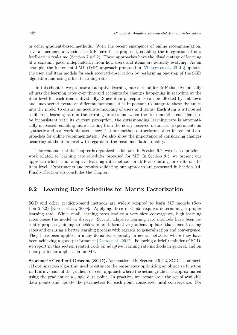
142 Chapter 9. Adaptive Incremental Matrix Factorization
or other gradient-based methods. With the recent emergence of online recommendation,several incremental versions of MF have been proposed, enabling the integration of newfeedback in real-time (Section 7.4.2.2). These approaches have the disadvantage of learningat a constant pace, independently from how users and items are actually evolving. As anexample, the Incremental MF (IMF) approach proposed in [Vinagre et al., 2014b] updatesthe user and item models for each received observation by performing one step of the SGDalgorithm and using a fixed learning rate.
In this chapter, we propose an adaptive learning rate method for IMF that dynamicallyadjusts the learning rates over time and accounts for changes happening in real-time at theitem level for each item individually. Since item perceptions can be affected by unknownand unexpected events at different moments, it is important to integrate these dynamicsinto the model to ensure an accurate modeling of users and items. Each item is attributeda different learning rate in the learning process and when the item model is considered tobe inconsistent with its current perception, the corresponding learning rate is automati-cally increased, enabling more learning from the newly received instances. Experiments onsynthetic and real-world datasets show that our method outperforms other incremental ap-proaches for online recommendation. We also show the importance of considering changesoccurring at the item level with regards to the recommendation quality.
The remainder of the chapter is organized as follows. In Section 9.2, we discuss previouswork related to learning rate schedules proposed for MF. In Section 9.3, we present ourapproach which is an adaptive learning rate method for IMF accounting for drifts on theitem level. Experiments and results validating our approach are presented in Section 9.4.Finally, Section 9.5 concludes the chapter.
9.2 Learning Rate Schedules for Matrix Factorization
SGD and other gradient-based methods are widely adopted to learn MF models (Sec-tion 2.5.2) [Koren et al., 2009]. Applying these methods requires determining a properlearning rate: While small learning rates lead to a very slow convergence, high learningrates cause the model to diverge. Several adaptive learning rate methods have been re-cently proposed, aiming to achieve more informative gradient updates than fixed learningrates and ensuring a better learning process with regards to generalization and convergence.They have been applied in many domains, especially in neural networks where they havebeen achieving a good performance [Dean et al., 2012]. Following a brief reminder of SGD,we report in this section related work on adaptive learning rate methods in general, and ontheir particular application for MF.
Stochastic Gradient Descent (SGD). As mentioned in Section 2.5.2.3, SGD is a numeri-cal optimization algorithm used to estimate the parameters optimizing an objective functionL. It is a version of the gradient descent approach where the actual gradient is approximatedusing the gradient at a single data point. In practice, we iterate over the set of availabledata points and update the parameters for each point considered until convergence. For

Chapter 9. Adaptive Incremental Matrix Factorization 143
each observation o, the model parameters x ∈ Rd are updated as follows:
x = x− η∂L(x; o)
∂x(9.1)
where η is the learning rate, determining the speed at which the optimal parameters arereached. Setting the value of η affects the learning process. In particular, high learning rateslead to a faster convergence but may cause numerical instability, and small learning ratesimply slow convergence. In addition to the difficulty of choosing an appropriate learningrate, traditional settings apply the same learning rate to all parameter updates which maynot always be convenient.
Adaptive learning rates. To address the learning rate issue, several adaptive learningrate methods were proposed and have proven to achieve a good performance in variousapplications. These methods are mainly designed to deal with sparse data and are basedon the idea of increasing gradient updates for infrequent parameters and decreasing themfor frequent parameters. In particular, AdaGrad [Duchi et al., 2011], standing for AdaptiveGradient, relies on this idea and was mainly exploited to improve the robustness of SGD inthe scope of training neural networks. AdaGrad assigns a different learning rate for eachparameter in x at a time step t, and updates are performed as follows:
xt+1 = xt −η√
Gt + ε gt (9.2)
where each element of gt, gt,k, denotes the gradient of L(x) with respect to parameter xkat time step t, Gt is a diagonal matrix where each diagonal element Gt,kk is the sum ofthe squares of the gradients g∗,k up to step t, and ε is a constant avoiding division byzero. Elements of Gt keep on accumulating positive terms corresponding to the squaredgradients. Therefore, the denominator keeps on growing causing the learning rate to dropiteration after iteration, reaching a point where it is infinitely small and learning can nolonger be performed. While this is achieving the initial goal of having higher learning ratesfor infrequent parameters and inversely, the monotonically decreasing learning rate preventsthe algorithm to keep on acquiring knowledge when convergence is not reached yet.
AdaDelta [Zeiler, 2012] was proposed as an extension of AdaGrad to cope with theproblem of continuously decreasing learning rates. Instead of keeping on accumulatingsquared gradients over all previous observations, only those included in a restricted slidingwindow of fixed size are considered. To avoid storing previous values and discarding themas they no longer fit in the window, a running average of the squared gradients is adopted.Given a decay constant ρ, the running average, denoted as E[g2]t at time step t, is computedas follows:
E[g2]t = ρE[g2]t−1 + (1− ρ)g2t (9.3)
√Gt + ε in Equation 9.2 is then replaced by
√E[g2]t + ε, which is equivalent to the
Root Mean Squared error of the gradient, RMS[g]t. Given that the units of updates donot match, the authors defined an additional running average for the squared parameterupdates as follows:
E[∆x2]t = ρE[∆x2]t−1 + (1− ρ)∆x2t (9.4)

144 Chapter 9. Adaptive Incremental Matrix Factorization
where ∆xt = xt+1 − xt.
Finally, the model parameters are updated as follows:
xt+1 = xt −RMS[∆x]t−1
RMS[g]tgt (9.5)
Further advances along this direction introduced the Adam method [Kingma and Ba,2015] where learning rates are adjusted by considering an exponentially decaying average ofthe first moment and the second moment of gradients.
Adaptive learning rates for Matrix Factorization (MF). Inspired by the success ofadaptive learning rates for SGD in the context of neural networks and other techniques,several learning rate schedules were designed to learn the parameters of a MF model. Theseschedules are based on different intuitions related to the learning of user and item models,in addition to the nature of observations analyzed to perform learning, e.g., ratings. Asmentioned before, the potential interest of adopting adaptive learning rate schedules residesin a faster convergence and a better generalization.
Vanilla SGD used to learn a MF model adopts a fixed schedule for the learning rate whichis set to the same constant value for all parameters during the whole learning process [Korenet al., 2009]. A monotonically decreasing schedule was proposed in [Yun et al., 2014] wherethe learning rate is updated at each iteration over the whole set of observations and decreasesover time. Given constant parameters α and β, the learning rate at iteration z is defined asfollows:
ηz =α
1 + β . z1.5(9.6)
On the other hand, early studies on backpropagation in neural networks introduced thebold driver heuristic [Battiti, 1989] which consists in adjusting the learning rate accordingto changes in the objective function values after each iteration. This approach was thenleveraged for MF [Gemulla et al., 2011] where, starting from an initial learning rate η0, thelearning rate at the next iteration is increased if the loss decreases, and inversely. This isperformed as follows:
ηz+1 =
αηz if ∆z < 0βηz otherwise
(9.7)
where α > 1, β ∈ [0, 1], and ∆z is the difference between the value of the objectivefunction at the beginning and the end of the z-th iteration.
Ideas developed in AdaGrad and AdaDelta were then introduced for MF. When con-sidering the direct application of AdaGrad for MF, each parameter, i.e., each user latentfactor and each item latent factor, is assigned a different learning rate that is being updatedat each iteration. [Chin et al., 2015] argue that the cost of implementing AdaGrad for MFcannot be disregarded. The space complexity is O((n+m)K) and each analyzed observationrequires O(K) additional operations to update the learning rate of each latent factor. [Chinet al., 2015] proposed then to adopt the same learning rate for all factors of one user modeland one item model, reducing the space complexity to O(n + m). An additional strategywas introduced, combining slow learners and fast learners, to prevent the learning rate from

Chapter 9. Adaptive Incremental Matrix Factorization 145
dropping rapidly at the first few iterations, especially due to the random initialization ofuser and item latent factors. A similar approach based on AdaDelta was also exploitedin [Wei et al., 2016].
The learning rate schedules presented so far are based on one of the following ideas: Thelearning rate should gradually decrease as we are expected to reach convergence with furtheriterations, the learning rate should increase when the loss function decreases and inversely,and different learning rates should be assigned for each user and item and should decreasefor frequent parameters. Taking another direction, recent work [Li et al., 2018] proposedto adjust the learning rate based on the noisiness of the evaluated ratings: Noisy ratingsare assigned small learning rates resulting in small gradient updates that prevent the MFmodel to be oversensitive to noise. These noisy ratings are expected to be associated withlarge training errors, and a different learning rate is associated with each rating rui, definedas follows:
ηzui =η0√
err(z−1)ui + ε
+ β (9.8)
where errui accumulates squared training errors in estimating rui evaluated at each iterationand up to iteration z, η0 is the predefined learning rate, ε is a constant avoiding division byzero, and β is a constant preventing the learning rate to become infinitely small. The authorsalso derived a theoretical analysis related to the convergence rate and the generalization errorbound.
Adaptive learning rate for Incremental Matrix Factorization (IMF). While learn-ing rate schedules are optimized for a faster convergence of MF models, the problem ofonline recommendation faces other constraints. Online RS are continuously handling userinteractions and update recommendation models by analyzing each interaction only once.In contrast to the batch setting, it is not possible to iterate over the whole dataset as muchas needed until convergence. In addition, convergence is not even desirable in such settings.We are looking to continuously integrate new observations and to represent the current stateof users and items. Given the non-stationarity nature of environments, we expect modelsto constantly evolve over time. Nevertheless, latent factors of several IMF approaches arelearned and updated using SGD (Section 7.4.2.2). In particular, the approach presentedin [Vinagre et al., 2014b] relies on a fixed learning rate schedule and update models for eachreceived observation.
Few IMF approaches leverage adaptive learning rates to learn the model parameters. Inthe context of video recommendation, [Huang et al., 2016] proposed an adjustable incre-mental SGD algorithm that updates the MF model in real-time. It has the particularity ofhandling different types of user interactions. The main assumption made is that each typeof interaction, e.g., impression, click, and play, exhibits a different degree of interest. Aninteraction related to user u and item i is assigned a weight wui based on its type, wherea higher weight indicates a stronger expected interest. These weights influence the learningprocedure by adjusting the learning rate for the observation (u, i) as follows:
ηui = η0 + αwui (9.9)
where η0 is the basic learning rate of the training process and α is the constant controllingthe influence of weights on learning.

146 Chapter 9. Adaptive Incremental Matrix Factorization
Relation to our work. Most learning rate schedules proposed to enhance the learning ofMF are adapted to the batch setting: Learning is performed by iterating several times overthe set of interactions and the learning rate is expected to decrease over time as convergenceis reached. Converging to a static model is not desirable in an online RS and in a non-stationary environment. The model is expected to evolve over time and to follow changesoccurring on the user and item levels. Convergence can only happen locally with respect totime, i.e., during bounded time periods where no changes are happening, and locally withrespect to the model, i.e., some users and items can be static while others are not. In thiscontext, learning rate schedules can be explored to control the learning process by enablingthe model to learn more from relevant observations. We propose a learning rate schedulethat accounts for drifts in item perceptions and we present our approach in the next section.
9.3 Proposed Approach
Motivation. In this chapter, we focus on the problem of online recommendation in non-stationary environments. We consider that item models may shift over time due to diverseunexpected and unknown events. Our goal is to take these shifts into account during thecontinuous learning process in order to learn models that are accurately representing thecurrent state of users and items. Since each item can drift at a different moment and at adifferent rate, we reason at the single item level and independently for each one of them.The problem we address consists in detecting if a change happened, and then in adaptingthe model.
Given the implicit feedback setting (Section 2.5.2.4), we are only observing positiveinteractions, e.g., clicks and transactions, in real-time, and we aim to perform top-N rec-ommendation for each observed user. Observations received for each item concern usersfor which the item should be ranked high in the recommendation list, i.e., the item shouldhave a high relevance score, since these users are interested in the item. Given an appro-priate recommendation model, our approach is based on the following idea: A drift in theitem model results in the deterioration of the recommendation quality for users choosingthis item. Therefore, when the item model is no longer delivering a good recommendationperformance, we consider that it is no longer adapted to the perception of users selectingit. One way to measure the recommendation performance is to rely on the ranking of theitem in the user recommendation list. In the absence of a drift, the performance of theitem model, or the series of rankings delivered for each observed user selecting the item, isexpected to be stable and learning is done at a constant rate. Otherwise, the ranking qualityis expected to deteriorate as more observations are generated and as no specific strategyis adopted to handle the change. In this case and in order to adapt the item model, wepropose to learn more from recent observations.
Our idea is to adopt a dynamic learning rate able to adapt the item model dependingon its ranking quality for received observations. We expect to have a different learning ratefor each item, defining at which rate the item model should learn from new observations.This rate should be fixed if there is no change detected when inspecting the stream ofinteractions concerning it. In contrast, it is expected to automatically increase when therecommendation performance decreases. However, the learning rate should not decrease

Chapter 9. Adaptive Incremental Matrix Factorization 147
under a certain threshold to maintain continuous update and adapting to incremental drifts.As mentioned before, we are not looking to converge to a single static model since we considernon-stationary environments where users and items are constantly shifting. On the contrary,we assume that each batch of observations is generated by a single model and that this modelis changing from one batch to the other.
Adaptive Incremental Matrix Factorization (AdaIMF). Our approach, AdaIMF, as-signs a different learning rate for each item and is based on the IMF framework proposedin [Vinagre et al., 2014b] (Section 7.4.2.2). Learning rates automatically adapt according tothe ranking quality for received observations: They increase when the ranking quality dete-riorates and inversely. Inspired by previously proposed learning rate schedules (Section 9.2),we define the learning rate of AdaIMF for item i at time step ti, i.e., t-th observation (u, i)for item i, as follows:
ηtii = η0 + αf tii (9.10)
where η0 is the fixed predefined learning rate ensuring minimal learning at each step, α isa constant controlling the influence of the dynamic part on the learning rate, and f tii is adynamic variable revealing the ranking quality delivered for item i up to time step ti.
The value of fi depends on the ranking of item i in recommendation lists of users thathave interacted with i up to time step ti. It should be averaged on a number of observationsto avoid being sensible to noisy data points and to consider how the performance changesover time. However, it should not account for all previous observations as variations canno longer be detected when the number of observations grows indefinitely. To enable thealgorithm to be sensitive to recent trends, fi monitors the ranking of i for recent observationsincluded in a fixed size sliding window. We avoid storing all elements included in the windowwhich is required by this solution, and we adopt the running average of rankings defined asfollows:
f tii = ρf ti−1i + (1− ρ)
ranktiu (i)
m(9.11)
where ρ is the decay constant controlling how much the algorithm is sensitive to recentobservations, ranktiu (i) is the ranking of item i in the recommendation list of u, and m isthe total number of items. When item i is being constantly ranked at the top of the listfor users that are actually interacting with it, fi will shrink. However, when i is ranked atthe end of the list, fi will increase causing the learning rate to increase too and the modelto learn more from new observations. A stable ranking quality will also result in a stablelearning rate leading to learning at a constant pace. ηi is expected to vary between η0 + α
mand η0+α. While one can argue that the gradient itself captures the prediction loss for item ion one observation, the adaptive learning rate tracks the loss on the series of consecutiveobservations.
Details related to the algorithm. The overall approach of AdaIMF is presented in Algo-rithm 7. As mentioned in Section 7.4.4, recommendation models used in online RS are firstinitialized in batch before the operating environment switches to a streaming environment.The values of fi are expected to be initialized during the batch phase and represent the av-erage ranking delivered for each item i before running the adaptive learning rate schedules.In order to compute ranktiu (i), the relevance score of each item is estimated for u using thescalar product between vectors pu and q>i . These scores are then ordered by decreasingorder and the rank of i is retrieved. On the other hand, given that AdaIMF only accounts

148 Chapter 9. Adaptive Incremental Matrix Factorization
for drifts at the item level, user parameters are updated with the constant learning rate η0,assuming that users are evolving at the same rate. Extending AdaIMF to handle user driftswill need careful considerations: User interactions are usually sparse and it is not clear ifthe feedback obtained from the actions of one user is enough to appropriately adapt the cor-responding learning rate. Nevertheless, in the setting of AdaIMF, we assume that learninguser latent factors at a constant rate is sufficient as a first solution.
Algorithm 7 Overview of our approach AdaIMF
Data: stream of observations DInput: number of latent factors K, initial learning rate η0, constant α,
decay constant ρ, regularization parameters λP and λQOutput: P, Q
1 Initialize f0i and ti = 1 for all i ∈ 1, . . . ,m
2 for (u, i) in D do3 if u 6∈ Rows(P) then . new user observed4 pu ∼ N (0, λ−1
P IK)5 end if6 if i 6∈ Rows(Q) then . new item observed7 qi ∼ N (0, λ−1
Q IK)8 end if9 Compute ranktiu (i) . details in Section 9.3
10 f tii ← ρf ti−1i + (1− ρ) rank
tiu (i)m
11 ηtii ← η0 + αf tii12 eui ← pu.q
>i − 1
13 pu ← pu − 2η0(euiqi + λPpu)14 qi ← qi − 2ηtii (euipu + λQqi)15 ti ← ti + 116 end for
Complexity. Compared to vanilla SGD, AdaIMF requires tuning two parameters: α and ρ,knowing that ρ could be set around 0.9. In terms of space complexity, we introduce onevariable per item resulting in O(m). Additional operations involve updating one learningrate for each received observation, requiring the computations of fi and ηi. We note that thecomplexity is lower than the one introduced by AdaError [Li et al., 2018] and by parameter-wise adaptive learning rate schedules such as AdaGrad [Duchi et al., 2011] which requiresthe update of K learning rates for each received observation.
9.4 Experimental Results
In this section, we present the experiments conducted to demonstrate the effectiveness ofour approach, AdaIMF. We first use synthetic datasets to show how AdaIMF performs inthe presence of simulated item drifts. We then report results for real-world datasets andshow the interest of considering temporal dynamics in real-world scenarios. The evaluation

Chapter 9. Adaptive Incremental Matrix Factorization 149
protocol is common in both series of experiments and is described in Section 7.4.4. Reportedresults correspond to observations included in the Stream Test and Train set. We use themetrics MRR@N , recall@N , and DCG@N to evaluate the quality of recommendations(Section 7.4.4).
9.4.1 Performance of AdaIMF on Synthetic Datasets
In the first series of experiments, we rely on synthetic datasets where we artificially introduceitem drifts in models generating the data and we examine how AdaIMF performs comparedto other incremental approaches.
Datasets. Given a MF model, i.e., a matrix of user latent factors P and a matrix of itemlatent factors Q, we describe in the following the procedure used to generate synthetic databased on the model. The synthetic dataset consists of an ordered sequence of observations.For each observation to generate, we first sample uniformly a user u from the set of n users.
Then, we sample an item i with a probability ofpuq>i
m∑j=0
puq>j
from the set of m items. This is
explained by the fact that, given an accurate MF model, items with a higher score are morelikely to be selected by the user, and the score of item i for user u is given by puq
>i . We
report results for two synthetic datasets, denoted by Syn1 and Syn2, and introduced in thefollowing.
The first synthetic dataset, Syn1, is the concatenation of two batches of observationsgenerated by two different MF models, where only one specific item model varies betweenboth models. The idea is to evaluate the effect of the shift of this single item on thewhole learning process and on the recommendation performance. In practice, we randomlyinitialize elements of the matrices P and Q from a normal distribution N (0, 0.1), andgenerate the first batch of observations. We then resample the latent factors of a singleitem i represented by vector q>i and generate the second batch of observations. Syn1 isobtained by processing one batch after the other. We set n and m to 50, the numberof latent factors K to 10, and each batch consists of a random number of observationscomprised between 50k and 100k.
In the second synthetic dataset, Syn2, we simulate the case where several items aredrifting independently at different moments. Syn2 is the concatenation of several batchesof observations where one item model is resampled between two consecutive batches. Theitem that is drifting is randomly chosen. We set n and m to 200, K to 10, and each batchconsists of a random number of observations comprised between 10k and 20k.
Experimental results for Syn1. Experiments run on Syn1 consisted in comparing theperformance of our approach AdaIMF with an IMF based on a Fixed Schedule for learningrates, i.e., using the same constant learning rate for all items, denoted by FS-IMF. Toavoid learning a model before launching the streaming setting, we assume that, before anyobservation is received, the MF model in both methods is the one initially used to generatethe first batch of Syn1. Then, the model is updated as observations are received. Asmentioned before, Syn1 consists of interactions generated by the same MF model exceptfor one item model that shifts at a certain point in time. Figure 9.1a shows the evolution of
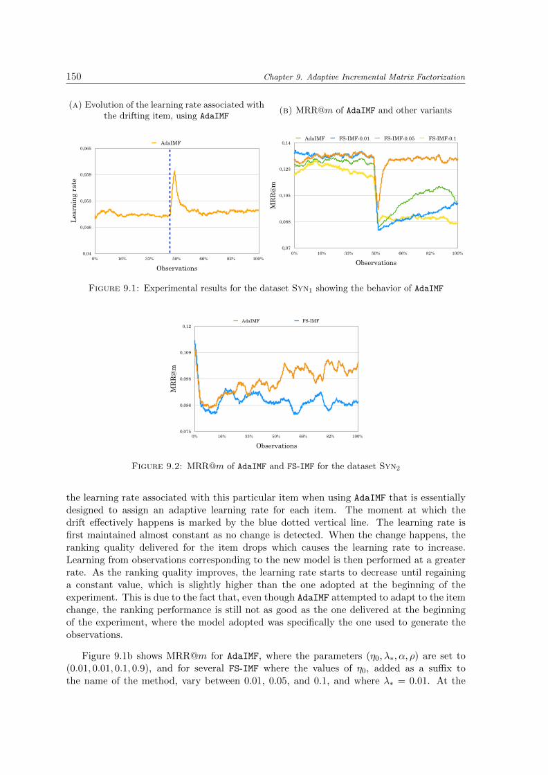
150 Chapter 9. Adaptive Incremental Matrix Factorization
(a) Evolution of the learning rate associated withthe drifting item, using AdaIMF
Lea
rnin
g ra
te
0,04
0,046
0,053
0,059
0,065
Observations
0% 16% 33% 50% 66% 82% 100%
AdaIMF
(b) MRR@m of AdaIMF and other variants
MRR@m
0,07
0,088
0,105
0,123
0,14
Observations
0% 16% 33% 50% 66% 82% 100%
AdaIMF FS-IMF-0.01 FS-IMF-0.05 FS-IMF-0.1
Figure 9.1: Experimental results for the dataset Syn1 showing the behavior of AdaIMF
MRR@m
0,075
0,086
0,098
0,109
0,12
Observations
0% 16% 33% 50% 66% 82% 100%
AdaIMF FS-IMF
Figure 9.2: MRR@m of AdaIMF and FS-IMF for the dataset Syn2
the learning rate associated with this particular item when using AdaIMF that is essentiallydesigned to assign an adaptive learning rate for each item. The moment at which thedrift effectively happens is marked by the blue dotted vertical line. The learning rate isfirst maintained almost constant as no change is detected. When the change happens, theranking quality delivered for the item drops which causes the learning rate to increase.Learning from observations corresponding to the new model is then performed at a greaterrate. As the ranking quality improves, the learning rate starts to decrease until regaininga constant value, which is slightly higher than the one adopted at the beginning of theexperiment. This is due to the fact that, even though AdaIMF attempted to adapt to the itemchange, the ranking performance is still not as good as the one delivered at the beginningof the experiment, where the model adopted was specifically the one used to generate theobservations.
Figure 9.1b shows MRR@m for AdaIMF, where the parameters (η0, λ∗, α, ρ) are set to(0.01, 0.01, 0.1, 0.9), and for several FS-IMF where the values of η0, added as a suffix tothe name of the method, vary between 0.01, 0.05, and 0.1, and where λ∗ = 0.01. At the

Chapter 9. Adaptive Incremental Matrix Factorization 151
beginning of the experiment, the performances of AdaIMF and FS-IMF-0.01 are roughlyequivalent. Significant differences in MRR@m for the different approaches appear when theitem drift actually happens. We observe that AdaIMF passes through a transition phasewhere the performance instantly drops and regains slowly a reasonable level after adaptivelearning is achieved. However, FS-IMF does not recover well after the item drift. Dependingon the value of η0 which needs to be tuned, the performance may slightly improve afterlearning is performed for some time, i.e., FS-IMF-0.05, or not at all, i.e., FS-IMF-0.1. Wenote that, even though only one item is drifting, its model is impacting the model of userswho are interacting with it, which are in turn impacting models of other items they areinteracting with, and so on. This experiment shows the importance of adopting an adaptivelearning rate schedule for IMF, i.e., AdaIMF, even in a setting where only one item is drifting.
Experimental results for Syn2. Experiments run on Syn2 compared the performancesof AdaIMF and FS-IMF in a setting where several items are drifting at different moments. Theparameters (η0, λ∗, α, ρ) are set to (0.01, 0.01, 0.1, 0.9) for AdaIMF and the parameters (η0, λ∗)to (0.1, 0.01) for FS-IMF. Figure 9.2 shows MRR@m for both methods. Similarly to theprotocol used for Syn1, models are first initialized with the MF model used to generatethe very first batch of observations. This explains the relatively good performance at thebeginning of the experiment, which then drops as multiple drifts are occurring. Results showthat AdaIMF outperforms FS-IMF and is able to maintain a good performance even thoughdrifts are happening. FS-IMF witnesses a decrease in the average performance due to thefact that it is learning at a constant rate which is not sufficient to account for item drifts.Assuming that items are drifting over time, we show in these experiments that AdaIMF
is well-designed to maintain a good recommendatin quality. Going further, experimentson real-world datasets, reported in the next section, prove that this assumption holds inreal-world settings.
9.4.2 Performance of AdaIMF on Real-World Datasets
Datasets. We use several real-world datasets in order to demonstrate AdaIMF. We exploitdatasets that can be used for the evaluation of online RS, that is datasets where interactionsare labeled with corresponding timestamps. We also attempt to focus on datasets whereitem perceptions are expected to change over time. The five real-world datasets used aredescribed below, and statistics related to these datasets are summarized in Table 9.1.
Booking dataset. The booking dataset used in this section is denoted by Ah Eur and isextracted from the hotel industry. It is derived from the dataset Ah (Section 3.2) and isintroduced in Section 8.4. Ah Eur gathers 704,722 bookings done by 98,130 Europeanusers in 3,332 hotels during a period of three consecutive years.
MovieLens dataset. The MovieLens 1M dataset, denoted here by Ml-1M, gathers 1M movieratings provided by 6,040 users on 3,706 movies. These ratings were originally collectedthrough the MovieLens RS [Harper and Konstan, 2016].
Lastfm-1K dataset. The Lastfm-1K dataset [Oscar Celma, 2010], denoted here by Lastfm,gathers users’ listening records between February 2005 and May 2009. We filter out users

152 Chapter 9. Adaptive Incremental Matrix Factorization
Table 9.1: Statistics of the real-world datasets used to evaluate AdaIMF
Dataset # users # items # transactions
Ah Eur 98,130 3,332 704,722
Ml-1M 6,040 3,706 1,000,000
Lastfm 990 26,216 17,319,094
Gowalla 18,737 32,510 1,278,274
Foursquare 24,941 28,593 1,196,248
that have listened to less than 5 artists, and artists selected by less than 5 different users.The final dataset used contains 990 users, 26,216 artists, and 17,319,094 listening records.
Gowalla dataset. The Gowalla check-in dataset 1, denoted here by Gowalla, was collectedfrom February 2009 to October 2010 and gathers check-ins shared on Gowalla. Similarto [Liu et al., 2017], we filter out users with less than 15 check-ins and Points Of Interest(POIs) with less than 10 visitors. The final dataset used contains 18,737 users, 32,510 POIs,and 1,278,274 check-ins.
Foursquare dataset. The Foursquare dataset 2, denoted here by Foursquare, was collectedfrom April 2012 to September 2013 and gathers check-ins shared on Foursquare [Yang et al.,2016]. Similar to [Liu et al., 2017], we use check-ins done within the United States, filterout users with less than 10 check-ins and POIs with less than 10 visitors. The final datasetcontains 24,941 users, 28,593 items, and 1,196,248 check-ins. We note that even though weexploit datasets related to POI recommendation, we do not consider any specific approachfor this type of problem since we are interested in the more generic problem of onlinerecommendation.
Parameters. We performed a grid search over the parameter space of the methods in orderto find the parameters that give the best performance. We mainly report the performancecorresponding to the parameters leading to the best results, unless stated otherwise.
Methods compared. AdaIMF is mainly compared against other incremental recommen-dation methods adapted to the online setting. We only consider one approach for IMF,which is the one proposed in [Vinagre et al., 2014b], given that the learning rate schedulewe introduce can be applied to any other IMF approach relying on SGD. While we exam-ine other existing learning rate schedules for IMF, we do not consider those that consistin indefinitely decreasing the learning rate over time, e.g., AdaGrad, since we want to en-sure continuous learning from new observations. The methods we evaluate are listed in thefollowing:
• AdaIMF is the approach we present in this chapter (Section 9.3) where we intro-duce an adaptive learning rate schedule attempting to dynamically adapt to itemdrifts. We set the parameters (η0, λ∗, α, ρ) to (0.01, 0.0001, 0.001, 0.9) for Ah Eur,(0.001, 0.0001, 0.1, 0.9) for Ml-1M, (0.0001, 0.1, 0.1, 0.9) for Lastfm, (0.001, 0.1, 1, 0.9)for Gowalla, and (0.01, 0.1, 0.1, 0.9) for Foursquare.
1http://snap.stanford.edu/data/loc-gowalla.html2http://sites.google.com/site/yangdingqi/home/foursquare-dataset

Chapter 9. Adaptive Incremental Matrix Factorization 153
Metric MF FS-IMF AdaDelta-IMF AdaIMF
MRR@m 0.1026 0.1318 0.1401 0.1543
Recall@1 0.0624 0.0641 0.0645 0.0751
Recall@5 0.1502 0.1781 0.1941 0.2147
Recall@10 0.1811 0.2416 0.2842 0.3171
Recall@50 0.2342 0.2933 0.6143 0.6439
Recall@100 0.2621 0.3177 0.7046 0.7306
DCG@5 0.1083 0.1111 0.1259 0.1459
DCG@10 0.1184 0.1552 0.1601 0.1788
DCG@50 0.1303 0.1669 0.2273 0.2512
DCG@100 0.1348 0.1708 0.2421 0.2654
Table 9.2: Performance of AdaIMF and its variants for the dataset Ah-Eur for K = 20
• AdaDelta-IMF is an IMF approach that adopts the AdaDelta learning rate methodin an online context [Zeiler, 2012](Section 9.2). Each item is assigned a learning ratewhich value depends on the accumulated squared gradients over recent observations.We set the parameters (η0, λ∗, ρ) to (0.01, 0.0001, 0.9) for Ah Eur, (0.001, 0.0001, 0.9)for Ml-1M, (0.01, 0.001, 0.9) for Lastfm, (0.01, 0.001, 0.9) for Gowalla, and (0.01,0.1, 0.9) for Foursquare.
• FS-IMF is the IMF approach proposed in [Vinagre et al., 2014b] and adopting a FixedSchedule (FS) for learning rates, i.e., the learning rate is the same for all items andremains constant during the training process. We set the parameters (η0, λ∗) to(0.01, 0.0001) for Ah Eur, (0.01, 0.01) for Ml-1M, (0.0001, 0.1) for Lastfm, (0.01, 0.1)for Gowalla, and (0.01, 0.1) for Foursquare.
• MF designates a MF approach that is only trained in batch on the first subset ofobservations. It is evaluated on the Stream Test and Train set (Section 7.4.4) withoutbeing updated when receiving new observations. Learning in batch is performed byiterating over the first subset of observations until convergence. We set the parameters(η0, λ∗) to (0.01, 0.0001) for Ah Eur, (0.001, 0.0001) for Ml-1M, (0.0001, 0.1) forLastfm, (0.01, 0.001) for Gowalla, and (0.01, 0.1) for Foursquare.
• Knni is the incremental item-based approach proposed in [Miranda and Jorge, 2009](Section 7.4.2.1) and using the cosine similarity. We set the number of neighbors to300 for all datasets.
• Rand randomly selects items for recommendation.
Results. Metrics measured for AdaIMF and the other methods are presented in Tables 9.2to 9.6 for all datasets, having K = 20. Results show that AdaIMF outperforms the othermethods for the studied datasets. The proposed adaptive learning rate strategy allows themodel to deliver better recommendation quality in terms of MRR, recall, and DCG, byadapting to the dynamics occurring on the item level. MF performs worse than the othermethods since the model is not being updated at all as new observations are being received,showing the interest of considering online RS where observations are integrated in real-time.
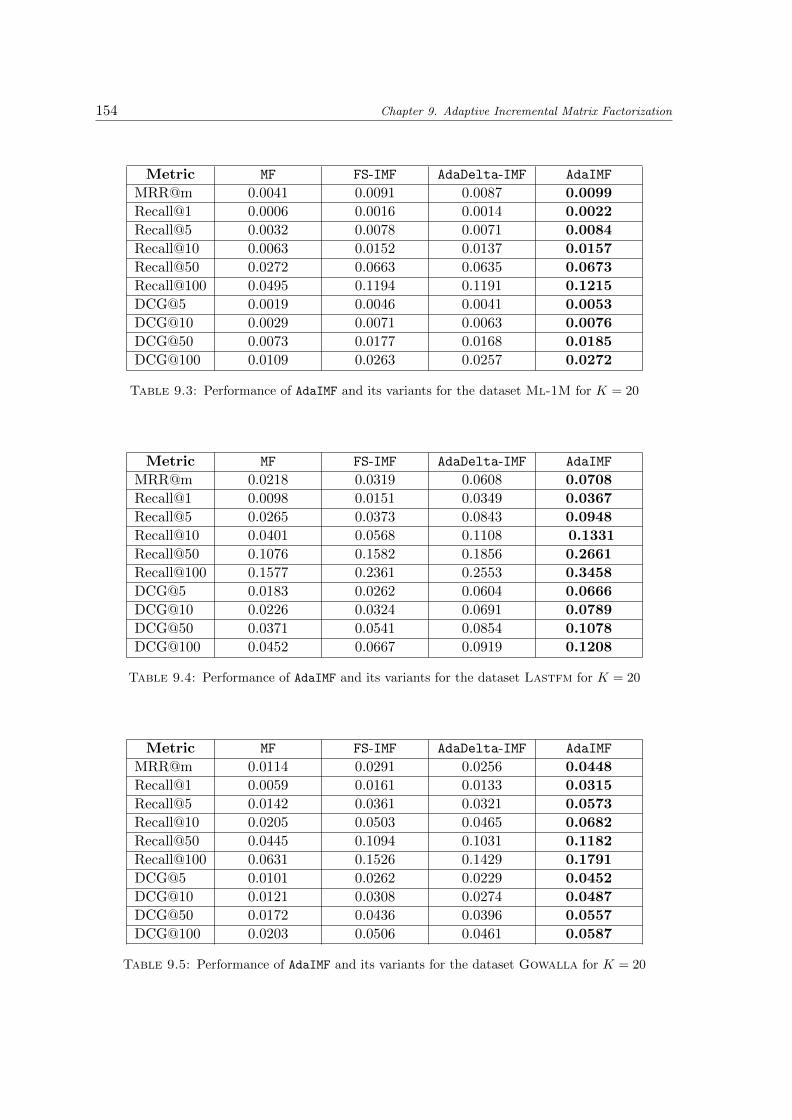
154 Chapter 9. Adaptive Incremental Matrix Factorization
Metric MF FS-IMF AdaDelta-IMF AdaIMF
MRR@m 0.0041 0.0091 0.0087 0.0099
Recall@1 0.0006 0.0016 0.0014 0.0022
Recall@5 0.0032 0.0078 0.0071 0.0084
Recall@10 0.0063 0.0152 0.0137 0.0157
Recall@50 0.0272 0.0663 0.0635 0.0673
Recall@100 0.0495 0.1194 0.1191 0.1215
DCG@5 0.0019 0.0046 0.0041 0.0053
DCG@10 0.0029 0.0071 0.0063 0.0076
DCG@50 0.0073 0.0177 0.0168 0.0185
DCG@100 0.0109 0.0263 0.0257 0.0272
Table 9.3: Performance of AdaIMF and its variants for the dataset Ml-1M for K = 20
Metric MF FS-IMF AdaDelta-IMF AdaIMF
MRR@m 0.0218 0.0319 0.0608 0.0708
Recall@1 0.0098 0.0151 0.0349 0.0367
Recall@5 0.0265 0.0373 0.0843 0.0948
Recall@10 0.0401 0.0568 0.1108 0.1331
Recall@50 0.1076 0.1582 0.1856 0.2661
Recall@100 0.1577 0.2361 0.2553 0.3458
DCG@5 0.0183 0.0262 0.0604 0.0666
DCG@10 0.0226 0.0324 0.0691 0.0789
DCG@50 0.0371 0.0541 0.0854 0.1078
DCG@100 0.0452 0.0667 0.0919 0.1208
Table 9.4: Performance of AdaIMF and its variants for the dataset Lastfm for K = 20
Metric MF FS-IMF AdaDelta-IMF AdaIMF
MRR@m 0.0114 0.0291 0.0256 0.0448
Recall@1 0.0059 0.0161 0.0133 0.0315
Recall@5 0.0142 0.0361 0.0321 0.0573
Recall@10 0.0205 0.0503 0.0465 0.0682
Recall@50 0.0445 0.1094 0.1031 0.1182
Recall@100 0.0631 0.1526 0.1429 0.1791
DCG@5 0.0101 0.0262 0.0229 0.0452
DCG@10 0.0121 0.0308 0.0274 0.0487
DCG@50 0.0172 0.0436 0.0396 0.0557
DCG@100 0.0203 0.0506 0.0461 0.0587
Table 9.5: Performance of AdaIMF and its variants for the dataset Gowalla for K = 20

Chapter 9. Adaptive Incremental Matrix Factorization 155
Metric MF FS-IMF AdaDelta-IMF AdaIMF
MRR@m 0.0623 0.0708 0.0771 0.0813
Recall@1 0.0462 0.0503 0.0546 0.0569
Recall@5 0.0776 0.0894 0.0974 0.1027
Recall@10 0.0917 0.1092 0.1191 0.1258
Recall@50 0.1277 0.1634 0.1798 0.1937
Recall@100 0.1485 0.1921 0.2123 0.2308
DCG@5 0.0629 0.0708 0.077 0.0811
DCG@10 0.0674 0.0772 0.0841 0.0884
DCG@50 0.0754 0.0891 0.0974 0.1034
DCG@100 0.0787 0.0938 0.1027 0.1094
Table 9.6: Performance of AdaIMF and its variants for the dataset Foursquare forK = 20
When comparing the results for FS-IMF and AdaDelta-IMF, it is not possible to form ageneral opinion about which one performs better in all cases. While AdaDelta-IMF outper-forms FS-IMF for the datasets Ah-Eur, Lastfm, and Foursquare, it is not the case for thedatasets Ml-1M and Gowalla. Understanding the behavior of AdaDelta-IMF in an onlinesetting is not trivial. In general, a higher absolute value of the gradient is derived from amore important loss evaluated for a specific data point. According to AdaDelta’s schedule,the learning rate decreases when the squared gradients recorded from previous observationsare significant. This can be related to the idea of drifts in item models. When the itemmodel is no longer adapted to the current observations, the learning rate in AdaDelta-IMFmay decrease and learning from new observations is not performed at high rates, in contrastwith AdaIMF. One can imagine that this may be beneficial in settings where the change isoccurring on a limited period of time. Instead of learning at a constant rate like in FS-IMF, itcan be interesting to decrease the learning rate and reduce thus the sensibility of the modelto the received observations. On the other hand, AdaDelta-IMF limits updates for frequentparameters, which may not be necessarily beneficial in an online dynamic environment. Inall cases, AdaIMF performs better than both of these methods. The improvements broughtby AdaIMF are amplified when the number of latent factors, K, increases, which can beobserved when comparing these results with the ones we describe next.
Figures 9.3, 9.4, and 9.5 show the recall@N and DCG@N for the datasets Lastfm,Gowalla, and Foursquare, for different values of N and for K = 50. When increasingthe number of factors, the superiority of the different approaches changes. In particular,FS-IMF outperforms AdaDelta-IMF for all represented datasets. In addition, for Lastfmand for small values of N , the performance of AdaDelta-IMF is comparable to, or evenworse than, the one of MF. AdaDelta-IMF may then not be adapted to the setting of onlinerecommendation. This observation may not necessarily come into sight when using thetraditional batch evaluation protocol. This shows, once again, that the adoption of onlineRS and sequential learning and evaluation can invalidate several recommendation techniquesthat perform well in batch mode. We note that Knni performs better than MF, proving theneed to develop incremental approaches that integrate interactions as soon as they aregenerated. Finally, and as shown in the previous series of experiments, AdaIMF outperformsall the other methods for the studied datasets. This observation strengthens the idea that

156 Chapter 9. Adaptive Incremental Matrix Factorization
Figure 9.3: Recall@N and DCG@N of AdaIMF and other variants and incremental meth-ods for the dataset Lastfm, using different values of N , for K = 50
Figure 9.4: Recall@N and DCG@N of AdaIMF and other variants and incremental meth-ods for the dataset Gowalla, using different values of N , for K = 50
Figure 9.5: Recall@N and DCG@N of AdaIMF and other variants and incremental meth-ods for the dataset Foursquare, using different values of N , for K = 50

Chapter 9. Adaptive Incremental Matrix Factorization 157
item drifts are occurring in the environment of RS and have to be taken into account toimprove the recommendation quality.
9.5 Conclusion
Within the ecosystem of RS intersect multiple users and items that are shifting simultane-ously while constantly influencing each others. Adapting to these changes in online RS raisesseveral challenges, especially due to the large number of concepts that are being tracked andto the lack of knowledge regarding the dynamics that are occurring. While some types ofshifts affect each user individually, others impact the item perceptions for a whole group ofusers and have to be modeled on the item level. In this chapter, we propose AdaIMF, anadaptive learning rate schedule for IMF that takes into account drifts in item perceptions.Each item is assigned a learning rate that automatically increases when the performance ofthe item model deteriorates, enabling more learning from recent observations correspondingto the new item perception. Experiments on synthetic datasets show that AdaIMF is ableto maintain a good recommendation quality in the presence of item drifts. Experiments onreal-world datasets prove the superiority of AdaIMF when compared to other incrementalapproaches and highlight the dynamics occurring in real-world settings.
While AdaIMF assumes that the whole item model should be updated at the same rate,real-world scenarios may suggest that the multiple aspects of a single item are evolvingindependently. These aspects may be represented by the latent factors, and future workshould investigate the adoption of an adaptive learning rate for each latent factor, based onthe ideas of AdaIMF. While this solution can induce a higher complexity, we may considersubgroups of items for which aspects are evolving in the same way.
While the approach proposed in this chapter inspects the dynamics in user interactions toadapt to item drifts, the next chapter presents our approach leveraging textual descriptionsof items to integrate drifts.


Chapter 10
Adaptive Collaborative TopicModeling
This chapter presents CoAWILDA, our approach to adapt to drifts in item descriptions inonline RS [Al-Ghossein et al., 2018e,f; Murena et al., 2018]. We propose an online hybridapproach that handles the item cold-start scenario by supporting the integration of newitems into the recommendation model in real-time. CoAWILDA combines a CollaborativeFiltering (CF) component, a topic model, and a drift detection technique, and is well-designed to automatically adapt to drifts occurring in real-time. Experiments on syntheticand real-world datasets show the effectiveness of CoAWILDA and demonstrate how it reactsin the presence of drifts.
10.1 Introduction
Collaborative Filtering (CF) mainly suffers from rating sparsity and from the cold-startproblem. Auxiliary information like texts and images has been leveraged to alleviate theseproblems, resulting in hybrid RS. Collaborative Topic Regression (CTR) [Wang and Blei,2011] is an example of a popular hybrid approach combining probabilistic topic modelingfor content analysis [Blei et al., 2003] and latent factor models for CF [Pan et al., 2008].While hybrid approaches were proven to be a good solution to get the best of Content BasedFiltering (CBF) and CF approaches, existing hybrid RS are meant to work in batch: Theycannot continuously maintain models up to date and are not able to adapt to changes inuser preferences and item descriptions which occur due to temporal dynamics.
In this chapter, we address the problem of online hybrid recommendation in a dynamicenvironment where users interact with items in real-time and where new items are expectedto arrive accompanied by a textual description. This setting is common in — but notrestricted to — the news and tweet recommendation domains, for example, where newarticles and tweets are continuously generated and read by users.
We propose an adaptive collaborative topic modeling approach for online recommen-dation. Our approach combines AWILDA, an adaptive version of online Latent Dirichlet
159

160 Chapter 10. Adaptive Collaborative Topic Modeling
Allocation (LDA) [Hoffman et al., 2010] that is able to analyze and model documents ar-riving in a stream on one side, and Incremental Matrix Factorization (IMF) [Vinagre et al.,2014b] to leverage user interactions for the learning of preferences on the other side. Ourapproach is adaptive as we actively detect changes in topics that may occur in the documentstream and adjust accordingly. We alternate online refinement of the topic model when nodrift is found with batch training when it is needed. The decision of retraining and thechunk of data on which we retrain the model are automatically determined by an adaptivesliding window technique [Bifet and Gavalda, 2007].
The purpose of introducing our approach is threefold. First, it is fully incremental andcan thus be used in an online setting to generate recommendations. Second, since it is ahybrid approach relying on users’ past interactions and on textual information, it addressesin particular the item cold-start problem which, to the best of our knowledge, has not beenstudied yet in the context of online recommendation. Third, its capacity of automaticallydetecting and adapting to drifts makes it suitable for real-world scenarios where changes intopics of document streams are frequently happening due to unexpected events and need tobe considered for a better quality of recommendation.
The chapter is structured as follows. In Section 10.2, we review previous work on severaltopics related to our work. Section 10.3 presents our approach for adaptive topic modelingand Section 10.4 our approach for online hybrid recommendation. Experiments and resultsare reported and discussed in Section 10.5. Finally, Section 10.6 concludes the chapter.
10.2 Related Work
In this section, we review related work on hybrid RS, relevant variants of LDA, and newsrecommendation which shares some commonalities with the problem addressed.
Hybrid RS. While several trends for hybrid recommendation exist (Section 2.6), we con-sider in this chapter the one that incorporates content-based characteristics into CF ap-proaches. Hybrid RS are able to recommend new items in the item cold-start scenario byleveraging auxiliary information. They also help alleviate the sparseness of feedback data,thus improving the quality of recommendation.
Previous work has utilized text data such as abstracts [Wang and Blei, 2011], syn-opses [Wang et al., 2015], and reviews [Bao et al., 2014]. Several techniques have been usedto model documents like LDA [Wang and Blei, 2011], stacked denoising autoencoders [Wanget al., 2015], and convolutional neural networks [Kim et al., 2016]. Images have also beenleveraged in this context and visual appearances of items can be added to the preferencemodel [He and McAuley, 2016].
While most hybrid RS are designed to work in batch, we propose an online hybrid RSthat is able to address the item cold-start problem in a dynamic environment where itemsare added in real-time. The model generating item descriptions is expected to change overtime due to some hidden factors and affects the recommendation process globally acrossall users. Among the few works that considered concept drifts in the context of onlinerecommendation, the focus has been on considering local changes occurring on the user

Chapter 10. Adaptive Collaborative Topic Modeling 161
level. In this chapter, we consider topic modeling for handling document streams and wemanage to detect drifts on the item level.
Topic modeling and concept drifts. Topic modeling is a machine learning task whichconsists in associating a document seen as an unordered list of words with a vector oftopics, i.e., of word distributions. One of the most influential topic modeling method is thegenerative model of Latent Dirichlet Allocation (LDA) [Blei et al., 2003] (Section 4.3.1).LDA models a document as a multivariate distribution, the parameter of which is drawnfrom a Dirichlet distribution. The popularity of LDA is due to its simplicity and modularity,as well as its interpretability. We refer the reader to [Jelodar et al., 2017] for a detailed surveyon LDA.
Vanilla LDA is not designed for evolving environments but only to infer topics based ona batch of accessible documents. Variants have been proposed to add a temporal aspect toLDA, including situations where the distribution evolves over time. A first variant, calledDynamic Topic Models (DTM) [Blei and Lafferty, 2006], considers that the word-topicdistribution varies over time. At each time step, parameters are re-evaluated, conditionedby their values at the previous step. The same idea, but implemented at the level of aparagraph in a book, is proposed by SeqLDA [Du et al., 2010]. A major drawback ofthese methods and other temporal adaptations of LDA (such as [AlSumait et al., 2008;Griffiths and Steyvers, 2004]) is the use of time slices, the size of which is arbitrary and doesnot depend on the observed data. In particular, changes in topic distribution can happenwithin a time period significantly smaller than the length of the chosen window. Continuoustime models offer solutions to this problem [Iwata et al., 2010]. A pioneer continuous timemethod [Wang and McCallum, 2006] modifies LDA by assuming that the word distributionover topics depends on word co-occurrences, and also on the date of the document. Despitethe benefit of this method, it cannot be used in practice for stream analysis since the learningis made offline: It requires the whole dataset to be accessible in one batch to be able to inferthe model.
For this reason, existing topic modeling methods are not suitable for data stream mining.Learning from data streams presents two major difficulties: the online nature of learningand the presence of concept drifts (Section 7.3). Regarding the former point, an onlinelearning algorithm for LDA has been proposed in [Hoffman et al., 2010]. It is based ononline stochastic optimization and can handle documents arriving in a stream by usingeach one of them to update the topic model parameters. On the other hand, conceptdrift designating the possible change in distribution that can happen in temporal and non-stationary environments, we propose to use change detection methods to estimate changes oftopics in document streams. While the approach presented in [Hoffman et al., 2010] passivelyupdate the model for each received document, we actively detect drifts and update the modelaccordingly. Among active methods, ADaptive WINdowing (ADWIN) [Bifet and Gavalda,2007] gained a lot of interest recently for the simplicity of its approach (comparing averagevalues of a time series on subwindows) and for the theoretical guarantees it proposes. Wepropose to combine LDA model and ADWIN algorithm for drift detection in streams ofdocuments.

162 Chapter 10. Adaptive Collaborative Topic Modeling
News recommendation. The problem we address in this chapter is common in the settingof tweets [Diaz-Aviles et al., 2012b], articles [Wang and Blei, 2011], and news recommenda-tion [Epure et al., 2017]. Our approach can be used to perform online recommendation ofnew items in any domain, whenever a textual description is available. We review in partic-ular the related problem of news recommendation since it has been specifically studied inthe literature.
News articles are continuously generated and while some of them could be relevant sev-eral weeks after the publication date, others have a shorter life cycle. In addition, readers’behavior is unstable compared to other domains given that users are often affected by exter-nal events such as breaking news and important occasions. Therefore, news recommendationoften considers recency and popularity [Ahmed et al., 2012; Doychev et al., 2014]. This isdone for example by filtering candidate articles for recommendation based on recency [Billsusand Pazzani, 2007], by periodically re-building models using fresh data [Das et al., 2007], orby using knowledge from Twitter to determine popular events [De Francisci Morales et al.,2012], among other solutions. Readers’ interests are captured using the categories of thearticles (if available) or keywords related to the articles’ topics [Doychev et al., 2014; Liuet al., 2010a], and are used for CBF recommendation. Hybrid approaches combining CBFand CF usually perform best for the problem of news recommendation [Das et al., 2007; Linet al., 2014; Liu et al., 2010a]. Combining long-term and short-term preferences has alsoproven to be beneficial in this context [Epure et al., 2017; Liu et al., 2010a]: While long-term preferences designate users’ genuine interests, short-term preferences can be triggeredby temporary events and fade away with time. In addition, session-aware RS have been usedto address this problem given that users are not always identified when browsing on newsplatforms. Session-aware RS focus on transitions between items, formulating the problem asa Markov decision process [Epure et al., 2017] or using recurrent neural networks [Quadranaet al., 2018].
Our work addresses the wider and more generic problem of online recommendation thatcould occur in any domain and with no existence of sessions. We only require a textualdescription of items which can be easily collected from abstracts or reviews. We leverageCF and online topic models, and we consider the evolution of content through drift detectionfor modeling items.
10.3 Proposed Approach for Online Topic Modeling
In this section, we present our algorithm designed for topic drift detection in LDA usingADWIN, which is called Adaptive Window based Incremental LDA (AWILDA). LDA is aprobabilistic graphical model designed to provide a definition of documents based on latentfeatures called topics. We refer the reader to Section 4.3.1 for a presentation of LDA andfor additional details about notations used in this section. While training of LDA canbe performed either offline [Blei et al., 2003] or online [Hoffman et al., 2010], our approachconsiders the online training given our real-time setting. We first start by presenting ADWINfollowed by a detailed presentation of AWILDA, our proposed approach.

Chapter 10. Adaptive Collaborative Topic Modeling 163
ADaptive WINdowing (ADWIN). ADWIN [Bifet and Gavalda, 2007] is an algorithmdeveloped for active mining of data streams. The idea of ADWIN is to keep a sliding windowW with the most recent observations of a stream of real-valued elements xt. At every timestep, the algorithm adds the new element to the window W and decides whether the newwindow W contains a drift or not. In a supervised context, these observations usuallycorrespond to risk measures.
The principle of ADWIN can be summed up as follows. The algorithm compares meansof elements of all possible sub-windows W0 and W1 of W . If the difference of means µW0
and µW1 of the two sub-windows is large enough and the size of the windows is large enough,then a drift is detected. The non-rigorous notions of “large enough” are defined through thechoice of a statistical test for the detection.
Besides its real simplicity, ADWIN admits a couple of interesting theoretical properties.Among them, bounds are given for the probability of incorrectly splitting the current win-dow, i.e., false positive rate bound, and correctly splitting the window, i.e., false negativerate bound.
Motivation. The proposed method for topic change detection is based on the use ofADWIN combined with a training of LDA. We consider a framework in which documentsarrive one by one in the form of a document stream. A document received at time step tis denoted by wt. Given parameters (α,β) where α is the parameter of the Dirichletdistribution and β the word-topic distribution, and given known latent variables (z,θ)where z is the set of topics and θ the topic distribution in a document, the likelihood of themodel is given by:
L(wt) =Γ (∑
i αi)∏i Γ(αi)
∫ ( K∏i=1
θαi−1i
) M∏m=1
K∑i=1
V∏j=1
(θiβij)wj
m
dθ (10.1)
where Γ is the gamma function, wjn measures the quantity of word j in the document,K is the number of topics, V is the vocabulary size, and M is the number of words in thedocument.
A change in the stream of likelihood corresponds to a change in the data distributionand can be detected by ADWIN algorithm. The retained documents, i.e., documents keptin the window after a drift is detected, correspond to the documents received after the drift.The principle of our method relies on the following intuitions:
• The likelihood measures the generative quality of the model with regards to observeddata. When a model is not adapted, the likelihood decreases.
• ADWIN is sensitive to changes in the mean value of a time series. Thus, it will detecta change in the likelihood caused by a change of the model.
• ADWIN will select large windows to train a new LDA model. The drift will bepredicted with a better accuracy for large window sizes, which is also optimal to traina LDA model.

164 Chapter 10. Adaptive Collaborative Topic Modeling
Following this idea, our method can be described as follows. At time step t, the systemhas access to a LDA model Mt which describes the data. When the system gets a newdocument, we compute the likelihood of observing the document, adds it to the currentwindow, and inspects it with ADWIN to check if a drift occurred. When a drift is detected,the current LDA model is trained on the documents selected by the retained sub-window.
Algorithm. The algorithm we present, AWILDA, is a direct implementation of these ideas.AWILDA relies on two LDA models. The first model, denoted by LDAm, is used for documentmodeling. The second model, denoted by LDAd, is only used for the detection of drifts. Thealgorithm works as described in Algorithm 8.
Algorithm 8 Overview of AWILDA
1 for wt in the stream of documents W do2 Compute likelihood L = p(wt|LDAd) for model LDAd3 Process L with ADWIN4 if ADWIN detects a drift for the window decomposition W = W0W1 then5 Retrain LDAm based on the documents in W1
6 Retrain LDAd based on the documents in W1
7 end if8 Update LDAm using the document wt based on the online LDA algorithm9 end for
We split the task of prediction and the task of drift detection by separating the models.The model used for prediction, LDAm, is kept up to date while no drift is detected. In contrast,the model LDAd is not modified; otherwise, the detected changes might not originate onlyfrom a change in the data distribution, but also from the change of the model. Both modelsare retrained on the batch of documents retained by ADWIN once a drift is detected. Thisresults in a hybrid adaptation to drifts for LDAm, combining active and passive approaches,i.e., incrementally updating the model for each received document and a more significantupdate when a drift is detected.
The AWILDA algorithm benefits from all the advantages of ADWIN. In particular, itoffers a strict control of false positive rate and false negative rate. If the underlying datageneration process does not change, the distribution of the likelihood is stationary, whichmakes the theorems relative to ADWIN still valid. We discuss in the following how thetheoretical properties of ADWIN can be transposed for AWILDA.
Theoretical guarantees. AWILDA presents interesting theoretical properties which guar-antee the quality of its results regarding drift detection. Using notations similar to the onesintroduced in [Bifet and Gavalda, 2007], we consider a window W of length nw which is di-vided into two sub-windows W0 and W1 of respective sizes n0 and n1. Let h be the harmonicmean of n0 and n1 (hence 1
h = 1n0
+ 1n1
). We suppose that, in ADWIN, the drift is detectedfor |µW1 − µW0 | ≥ εcut (where µW0 designates the mean value over sub-window W0). Let δbe such that:
εcut =
√1
2hln
4nwδ
(10.2)

Chapter 10. Adaptive Collaborative Topic Modeling 165
With these parameters, Theorem 3.1 in [Bifet and Gavalda, 2007] ensures both falsepositive rate bound and false negative rate bound. These results can be adapted to oursetting.
Theorem 10.1. At every time step, if documents are generated by a single LDA model inthe time period covered by W , the probability that AWILDA detects a drift at this step is atmost δ.
Proof. On the covered window, ADWIN gets a time series Xt = L(Dt) where Dt are equallydistributed (for a single LDA model) and L represents the likelihood of LDAd which is con-stant on W for AWILDA. Thus the mean of the variables remains constant on W . Theconclusion follows from the properties of ADWIN.
Following the same direction, the following theorem can be proven for false negative ratebound:
Theorem 10.2. Suppose that, at a time step t, window W can be split in two parts W0 andW1 and documents are independent and identically distributed by a LDA distribution LDA0(resp. LDA1) on sub-window W0 (resp. W1). If |ED∼LDAd [pLDA1(D)− pLDA0(D)]| ≥ 2εcut, thenwith probability 1− δ AWILDA detects a drift inside sub-window W1.
Proof. The idea of the proof is the same. The mean value of Xt = L(Dt) on sub-window W0
is:µt = ED∼LDA0 [pLDAd(D)] = ED∼LDAd [pLDA0(Dt)]
An equivalent result can be found for W1, and the theorem comes directly.
Unlike for Theorem 10.1, a simple interpretation of Theorem 10.2 is not direct. Forinstance, two LDA models can be distinct and not share the targeted property. Findingconditions on the parameters of the three distributions is an interesting task that we willnot address. However, it has to be noticed here that the guarantee on the false negativerate depends on the choice of LDAd.
In practice, concept drift can happen in different ways (Section 7.3). The case of abruptdrift has been explicitly studied with the setting of Theorem 10.2. It corresponds to thecase where the document distribution changes from one given state to another between sub-windows W0 and W1. Results given in [Bifet and Gavalda, 2007] show that the detectiondelay can be estimated by O(µ ln(1/δ)/ε2) where µ is the mean of the distribution beforedrift. In our case, this delay is of critical importance since it defines the size of the chunkfor retraining the model. AWILDA faces a trade-off between predicting a drift as early aspossible (in order to maximize the likelihood) and collecting as much data as possible to geta good estimator of the underlying LDA model.
The case of gradual drift is less adapted to the developed framework. Properties ofADWIN have been demonstrated in case of linear gradual drift, but these results are difficultto translate directly into our setting where the time series tracked by ADWIN has a complexmathematical definition. Understanding the behavior of AWILDA in the case of gradualdrift is a task that would come together with a proper study of Theorem 10.2.

166 Chapter 10. Adaptive Collaborative Topic Modeling
Practical considerations. As defined in Equation 10.1, the likelihood of a LDA modelis not computable. Thus, we rely on an upper-bound L′ proposed in variational inference(see Equation 1 in [Hoffman et al., 2010]). In practice, the results observed with thisupper-bound are not satisfying due to the lack of precision: The probabilities of observingdocuments are very low and the method fails to discriminate them with enough accuracy.In order to overcome this difficulty, we consider the logarithm of L′ (hence an upper-boundof the log-likelihood). This quantity is theoretically unbounded, which is a problem forADWIN, but in practice, it is observed that the values vary only in a small interval (thewidth of which depends on the dataset). In our experiments, we prevented this quantityto decrease too much by fixing a minimal bound so that the quantity of interest becomesbounded. A reasonably low value for this threshold was never reached in the scope of thepresented experiments (Section 10.5.1). However, we do not have any method to evaluatean optimal value for this bound in a general case.
10.4 Proposed Approach for Online Recommendation
In this section, we present our proposed algorithm for adaptive collaborative topic modeling,CoAWILDA, merging two components: AWILDA for topic modeling with drift detectionand Incremental Matrix Factorization (IMF) for CF (Section 7.4.2.2, Algorithm 5) [Vinagreet al., 2014b]. CoAWILDA is based on the framework of Collaborative Topic Regression(CTR) (Section 4.3.1). It benefits from the advantages of CTR, i.e., coping with sparsity anditem cold-start, is adapted to the online setting, and takes into account the non-stationaritynature of data in an evolving environment.
In our setting, observations are supposed to arrive in real-time and are mainly of twotypes. First, interactions, denoted by (u, i), designate positive actions, e.g., clicks, ratings,performed by users and related to a certain item. Second, additions of items, denoted by(i,wi), usually occur when a new item becomes available at a certain time step and weconsider that it is accompanied by a textual description.
CoAWILDA is presented in Algorithm 9. When a new item is received, we use AWILDAto model the descriptive document and extract topic proportions θi. The item latent vectorqi representing an item i results of the addition of the topic proportions θi and an item latentoffset εi. When a new interaction (u, i) is observed, we update the user latent factor pu andthe item latent offset εi following the procedure of IMF (Section 7.4.2.2). Recommendationis performed as defined in the MF framework, and rui = pu.q
>i = pu.(θi + εi)
>.
10.5 Experimental Results
In this section, we present the experiments we conducted to prove the effectiveness of ourapproach. We first show how AWILDA performs when modeling a stream of documents andthen discuss how CoAWILDA performs when addressing the problem of online recommen-dation, using synthetic and real-world datasets.

Chapter 10. Adaptive Collaborative Topic Modeling 167
Algorithm 9 Overview of CoAWILDA
Data: stream of observations OInput: number of factors K, learning rate η, regularization parameters λP and λQOutput: P, Q
1 for o in O do2 if o = (i,wi) then . new item added3 θi ← AWILDA(wi)4 εi ∼ N (0, λ−1
Q IK)5 qi ← θi + εi6 end if7 if o = (u, i) then . interaction observed8 if u 6∈ Rows(P) then . new user observed9 pu ∼ N (0, λ−1
P IK)10 end if11 eui ← pu.q
>i − 1
12 pu ← pu − 2η(euiqi + λPpu)13 εi ← εi − 2η(euipu + λQεi)14 qi ← θi + εi15 end if16 end for
Synthetic datasets for evaluating AWILDA. To demonstrate the ability to detectdrifts, we generate synthetic datasets where we artificially insert drifts at random momentsthroughout the sequence of documents. Synthetic datasets are denoted by Sdr, where ris the number of simulated drifts. Documents observed between two consecutive drifts aregenerated by a single LDA model following its generative process. At each occurring drift,we draw uniformly the hyperparameters α and β. The number of topics is fixed for all themodels used to generate one dataset.
We present experiments performed on the following two synthetic datasets: Sd4 andSd9, containing 4 and 9 drifts respectively. Handling document streams is a very commontask in environments where short texts are generated and shared, e.g., newswires, Twitter.Therefore, we choose to generate documents containing 100 words, and we fix the vocabularysize to 10,000 words and the number of topics, K, to 15. Following the setting in [Blei et al.,2003], the elements of α and β are first set to 50/K and 0.1 respectively, and are thenchanged at each drift. In Sd4, we generate exactly 2,000 documents from each distribution,separating two consecutive drifts by the same number of documents. In Sd9, we vary thenumber of documents generated by each model between 500 and 1,000 documents.
Semi-synthetic datasets for evaluating AWILDA. We also conduct experiments onsemi-synthetic data. We use the dataset Reuters-21758 1 consisting of newswire articlesclassified by categories and ordered by their date of issue. The ApteMod version of thisdatabase contains 12,902 documents and each document is classified in multiple categories
1http://archive.ics.uci.edu/ml/

168 Chapter 10. Adaptive Collaborative Topic Modeling
Table 10.1: Statistics of the real-world datasets used to evaluate CoAWILDA
Dataset # users # items # transactions Period
Ml-100k 1,000 1,700 100,000 18 mos.
Plista 1,362,097 8,318 32,706,307 1 mo.
for a total of 90 categories. In the procedure of data preprocessing, we down-cased andstemmed all words in the articles.
To demonstrate the functionality of AWILDA, we reorder the newswire articles basedon their categories. We artificially ensure a sudden emergence of topics at specific pointsof the document stream, trying to provoke a drift in the topic distributions. We derivefrom the initial ordered dataset two sets of articles that we use in our experiments. Inthe first set, denoted by Reuters1, we select the articles belonging to the category “acq”followed by the articles belonging to the category “earn”. We expect the algorithm to detectthe sudden change in topics mentioned in the documents. In the second set, denoted byReuters4, we select all articles from a specific category and add them consecutively to thedataset, considering the five following categories: “interest”, “trade”, “crude”, “grain”, and“money-fx”.
Real-world datasets for evaluating AWILDA and CoAWILDA. Data used to eval-uate our approach for online recommendation should be chronologically ordered and shouldinclude user interactions and the addition of items over time with a corresponding textualdescription. These two characteristics are not available in all datasets commonly used toevaluate RS. In our work, we use two real-world datasets: the ML-100k and the Plistadatasets.
The Ml-100k dataset corresponds to the MovieLens 100k dataset 2 [Harper and Kon-stan, 2016] and gathers 100,000 ratings from 1,000 users on 1,700 movies, spanning over 18months. Since we are addressing the problem of recommendation with implicit feedback,our goal is to recommend the movies the user is going to rate. Movies become availableaccording to their reported release date, and we use DBpedia 3 to collect abstracts writtenin English and describing each one of them.
The Plista dataset is described in [Kille et al., 2013] and contains a collection of newsarticles published in German on several news portals. The available dataset captures inter-actions collected during the month of February 2016. We remove from the dataset inter-actions corresponding to unknown users, users with less than three interactions, and itemswith no available textual description. Finally, the dataset gathers 32,706,307 interactionsfrom 1,362,097 users on 8,318 news articles.
Documents from both datasets have been preprocessed by mainly removing stop words,removing words occurring once, and stemming remaining words. Statistics about the real-world datasets used are summarized in Table 10.1.
2http://www.movielens.org3http://www.dbpedia.org

Chapter 10. Adaptive Collaborative Topic Modeling 169
10.5.1 Performance of AWILDA for Online Topic Modeling
Evaluation protocol. AWILDA is proposed to model a stream of documents using driftdetection. In our experimental setting, we consider that we are receiving the documentsone after the other, ordered by their availability date, e.g., release or publication datefor real-world datasets. For each received document, we first evaluate the topic modeland then process the document to update the underlying model. We use the first 20%documents of the stream to initially train the model which is evaluated and updated usingthe remaining documents. Our evaluation concerns the tasks of topic drift detection anddocument modeling.
Task of topic drift detection. We evaluate the ability to detect drifts by checking thelatency between the moment when the real drift occurs and the moment it is detected. Thisis only performed for synthetic and semi-synthetic datasets since they are annotated withthe occurrence of drifts whereas real-world datasets are not.
Task of document modeling. Given a LDA model trained on a set of documents, thegoal in document modeling is to maximize the likelihood on unseen documents (Dtest).Perplexity is the tool used by default in language modeling and measures the ability of amodel to generalize to new data [Blei et al., 2003]. It is defined as follows:
perplexity(Dtest) = exp
−∑|Dtest|
d=1 log2 p(wd)∑|Dtest|d=1 Md
(10.3)
where Md designates the number of words in document d. In the actual use of perplexity, theprobability p(wd) is approximated by its upper-bound (given by the variational inference)as explained in Section 10.3. A lower value of perplexity indicates a better generalizationcapacity. Since we are handling document streams, the perplexity is reported for eachreceived document using the current model. We note that in AWILDA, the perplexity ismeasured using LDAm since it is the actual module used to model documents.
Methods compared. Considering the task of topic drift detection, we compare AWILDAto three other variants. In these variants, the model LDAm is updated in a similar way as forAWILDA, but the methods differ in the way the detection model LDAd is updated:
• AWILDA2. LDAd is initially trained on a small chunk of documents that is used toinitialize the models. It is not updated as more documents are being received.
• AWILDA3. LDAd is updated for each received document. It is therefore equivalent to aclassical online LDA model [Hoffman et al., 2010].
• AWILDA4. LDAd is updated for each received document using the online LDA algorithm.In addition, when a drift is detected, the model is retrained on the sub-window selectedby ADWIN.
Regarding the theoretical study, it can be easily verified that Theorem 10.1 and Theo-rem 10.2 remain valid for AWILDA2, but not for AWILDA3 and AWILDA4. In particular, it isnoticeable that we do not have guarantees for the performances of AWILDA3 and AWILDA4

170 Chapter 10. Adaptive Collaborative Topic Modeling
(a) Results for AWILDA (b) Results for AWILDA2
(c) Results for AWILDA3 (d) Results for AWILDA4
Figure 10.1: Topic drift detection for the dataset Sd4 using AWILDA and its variants
since the model LDAd is updated at each step. A priori, there is no chance that the meansremain constant when the likelihood function L varies. We show the results for experimentswhere we set the number of topics to 10, knowing that similar patterns appear for differentvalues of this parameter.
Considering the task of topic modeling, we compare the performance of AWILDA tothe online version of LDA [Hoffman et al., 2010], denoted by OnlineLDA, given its capacityto handle document collections arriving in a stream. OnlineLDA is considered to processdocuments one by one as they are received and updates the underlying model at each step.
10.5.1.1 Results for Topic Drift Detection
Comparison of AWILDA and its variants. In the first set of experiments, we compare theperformance of AWILDA and its variants when performing the task of topic drift detectionon the synthetic dataset Sd4. The results are presented in Figure 10.1. The perplexityrepresented is related to the measure we track for drift detection. The LDA model used tocompute perplexity is learned and updated differently depending on the method considered.We represent the perplexity as a moving average with a sliding window of 100 observations.The exact occurrence of drifts is marked by a green dashed vertical line and the detectionof drifts is marked by a blue dotted vertical line.

Chapter 10. Adaptive Collaborative Topic Modeling 171
(a) Results for Sd4 (b) Results for Sd9
(c) Results for Reuters1 (d) Results for Reuters4
Figure 10.2: Topic drift detection using AWILDA for synthetic and semi-synthetic datasets
AWILDA and AWILDA2 only detect true positive drifts, while AWILDA3 and AWILDA4 detectfalse and true positive drifts. AWILDA is also more reactive than AWILDA2 and spots driftsfaster. Updating the LDAd model with each received document in AWILDA3 and AWILDA4
modifies the underlying distribution of topics, leading ADWIN to detect false positive drifts.AWILDA performs best for all the studied datasets, and we present in the following resultsfor the other datasets.
Performance of AWILDA on all the datasets. As shown in Figure 10.2, AWILDA is ableto detect all the drifts occurring in the datasets Sd4, Sd9, and Reuters1 after receivingonly a few observations from the new distribution. Concerning the Reuters4 dataset, ourapproach spots two drifts and misses the two others. We note that in this particular dataset,we switch from one topic to another relatively fast, i.e., around 500 documents per category.Topics in articles can also be interconnected which makes the task even more complicated.
Discussion. We notice that the observed properties of AWILDA and its variants are closeto the predictions which were given by Theorems 10.1 and 10.2. In particular, it has beenshown that AWILDA and AWILDA2 perform better than AWILDA3 and AWILDA4 with regardsto false positives.
The superiority of AWILDA over the other variants raises interesting questions. It isnoticeable that the best algorithm in terms of drift detection is also the only one whichdetection model is actively updated at each drift and not passively at each step or for eachobservation. This non-updating property is of particular interest: It illustrates the idea

172 Chapter 10. Adaptive Collaborative Topic Modeling
that good drift detection does not require to have good modeling properties, which may becounter-intuitive in a way. The extreme case, AWILDA2, also shows rather good performancewhile the model is not updated at all, which means that it does not encode any informationrelative to the underlying distribution. A random LDA model could also work for this task.The false-negative error rate might be affected though, which can be observed even here:If the detection model is too different from the actual model, there is a chance that thelikelihood change (when the underlying model varies) may not be important enough to bedetected.
10.5.1.2 Results for Document Modeling
Comparing AWILDA with OnlineLDA. Figure 10.3 shows the perplexity measured on thedocument streams of Reuters1, Ml-100k, and Plista for AWILDA and OnlineLDA. Theperplexity is represented as a moving average with a sliding window of 100 observationsfor Reuters1 and 200 observations for Ml-100k and Plista. AWILDA detects the existingdrift for Reuters1, two drifts for Ml-100k, and five drifts for Plista. This difference inbehavior is expected knowing the volume and nature of the datasets, e.g., movies vs. news.
Before detecting any drift, OnlineLDA and AWILDA are trained in the same way andon the same data, which explains the close values of perplexity. After detecting the firstdrift, AWILDA outperforms OnlineLDA for the task of document modeling. As documentscontinue to arrive, AWILDA is more adapted to the new data. Its drift detection componentallows it to adjust to changes after each drift, resulting in a better performance. Furtheranalysis of the datasets with experts from respective domains will help to establish the linkbetween detected drifts and real-life events occurring in the same time period, for betterunderstanding and explainability.
10.5.2 Performance of CoAWILDA for Online Recommendation
Evaluation protocol and measures. In order to evaluate CoAWILDA for the task ofonline recommendation on Ml-100k and Plista, we rely on the protocol introduced inSection 7.4.4. We use recall@N and DCG@N to measure the quality of recommendation.We report the results for the Stream Test and Train subset.
Parameters. We performed a grid search over the parameter space of the methods inorder to find the parameters that give the best performance. We report the performancecorresponding to the parameters leading to the best results. The parameters are providedalong with the methods below.
Methods compared. Since previous work has demonstrated the advantages of usingonline recommendation compared to batch recommendation [Frigo et al., 2017; Vinagreet al., 2014b], we focus on incremental methods for comparison. We also only consider oneapproach for IMF knowing that our method, CoAWILDA, can integrate any other algorithmfor IMF or any model-based method. We compare the performances of several incrementalmethods adapted to the online setting, including variants of the one we propose, mentionedin the following:
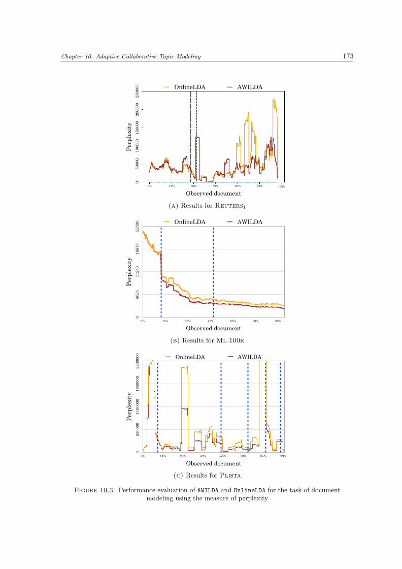
Chapter 10. Adaptive Collaborative Topic Modeling 173
Per
plex
ity
5625
1125
016
875
2250
0
Observed document0%
OnlineLDA AWILDA
0% 50% 100%17% 33% 67% 83%
5000
00
1000
0015
0000
2000
0025
0000
(a) Results for Reuters1
Per
plex
ity
056
2511
250
1687
522
500
Observed document0% 15% 30% 47% 63% 80% 95%
OnlineLDA AWILDA
(b) Results for Ml-100k
Per
plex
ity
055
0000
1100
000
1650
000
2200
000
Observed document0% 14% 28% 42% 56% 70% 85% 99%
OnlineLDA AWILDA
(c) Results for Plista
Figure 10.3: Performance evaluation of AWILDA and OnlineLDA for the task of documentmodeling using the measure of perplexity
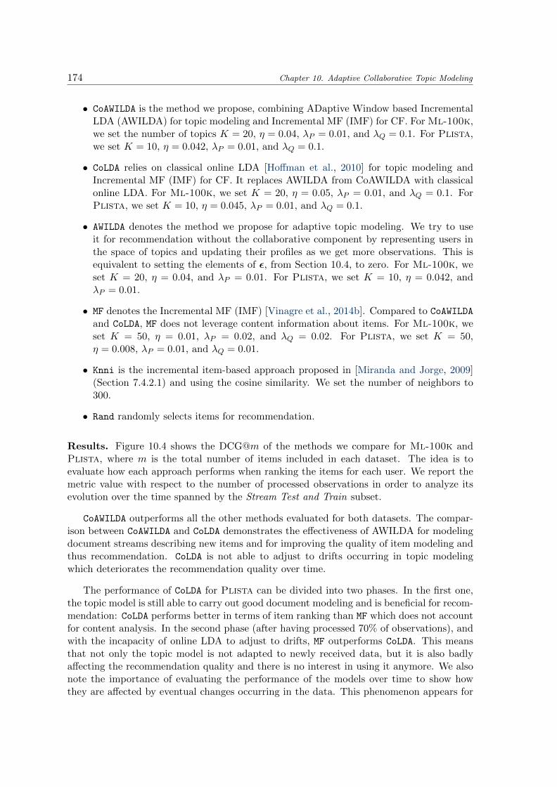
174 Chapter 10. Adaptive Collaborative Topic Modeling
• CoAWILDA is the method we propose, combining ADaptive Window based IncrementalLDA (AWILDA) for topic modeling and Incremental MF (IMF) for CF. For Ml-100k,we set the number of topics K = 20, η = 0.04, λP = 0.01, and λQ = 0.1. For Plista,we set K = 10, η = 0.042, λP = 0.01, and λQ = 0.1.
• CoLDA relies on classical online LDA [Hoffman et al., 2010] for topic modeling andIncremental MF (IMF) for CF. It replaces AWILDA from CoAWILDA with classicalonline LDA. For Ml-100k, we set K = 20, η = 0.05, λP = 0.01, and λQ = 0.1. ForPlista, we set K = 10, η = 0.045, λP = 0.01, and λQ = 0.1.
• AWILDA denotes the method we propose for adaptive topic modeling. We try to useit for recommendation without the collaborative component by representing users inthe space of topics and updating their profiles as we get more observations. This isequivalent to setting the elements of ε, from Section 10.4, to zero. For Ml-100k, weset K = 20, η = 0.04, and λP = 0.01. For Plista, we set K = 10, η = 0.042, andλP = 0.01.
• MF denotes the Incremental MF (IMF) [Vinagre et al., 2014b]. Compared to CoAWILDA
and CoLDA, MF does not leverage content information about items. For Ml-100k, weset K = 50, η = 0.01, λP = 0.02, and λQ = 0.02. For Plista, we set K = 50,η = 0.008, λP = 0.01, and λQ = 0.01.
• Knni is the incremental item-based approach proposed in [Miranda and Jorge, 2009](Section 7.4.2.1) and using the cosine similarity. We set the number of neighbors to300.
• Rand randomly selects items for recommendation.
Results. Figure 10.4 shows the DCG@m of the methods we compare for Ml-100k andPlista, where m is the total number of items included in each dataset. The idea is toevaluate how each approach performs when ranking the items for each user. We report themetric value with respect to the number of processed observations in order to analyze itsevolution over the time spanned by the Stream Test and Train subset.
CoAWILDA outperforms all the other methods evaluated for both datasets. The compar-ison between CoAWILDA and CoLDA demonstrates the effectiveness of AWILDA for modelingdocument streams describing new items and for improving the quality of item modeling andthus recommendation. CoLDA is not able to adjust to drifts occurring in topic modelingwhich deteriorates the recommendation quality over time.
The performance of CoLDA for Plista can be divided into two phases. In the first one,the topic model is still able to carry out good document modeling and is beneficial for recom-mendation: CoLDA performs better in terms of item ranking than MF which does not accountfor content analysis. In the second phase (after having processed 70% of observations), andwith the incapacity of online LDA to adjust to drifts, MF outperforms CoLDA. This meansthat not only the topic model is not adapted to newly received data, but it is also badlyaffecting the recommendation quality and there is no interest in using it anymore. We alsonote the importance of evaluating the performance of the models over time to show howthey are affected by eventual changes occurring in the data. This phenomenon appears for
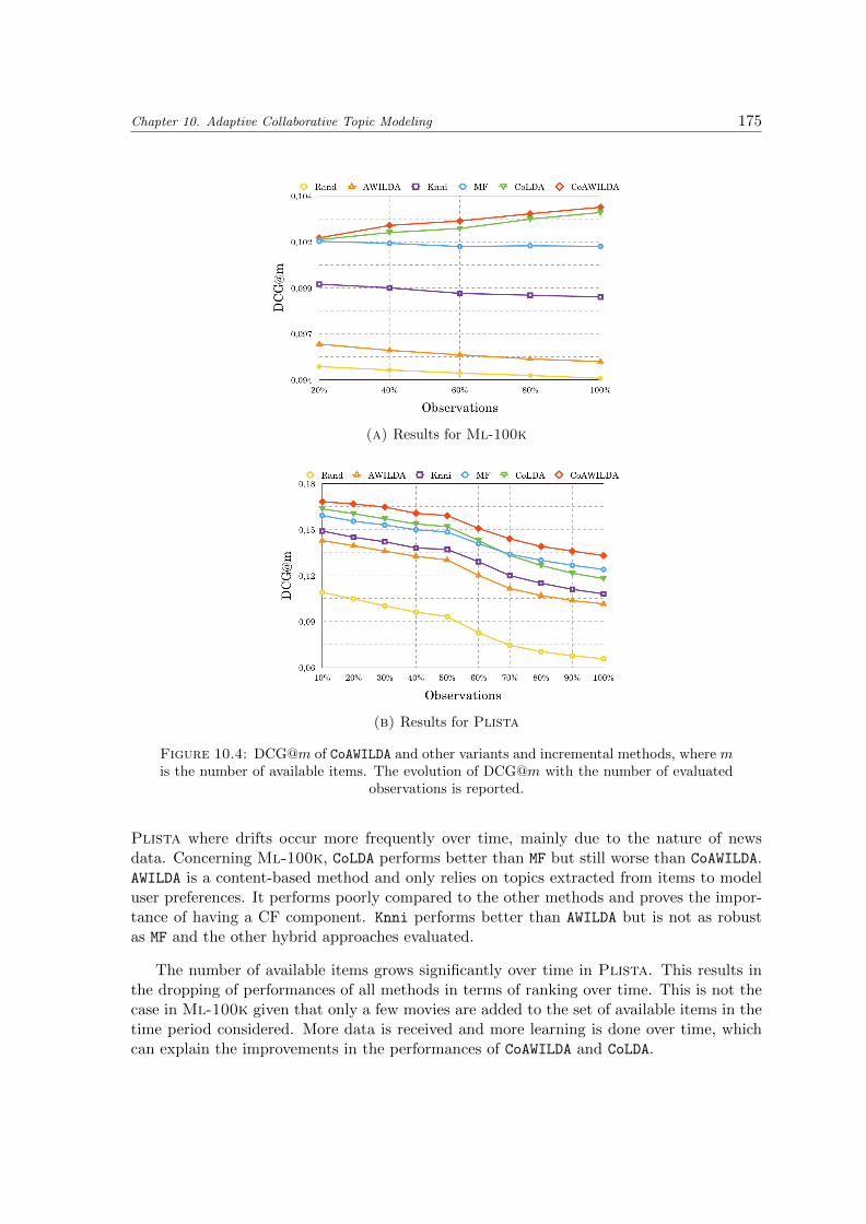
Chapter 10. Adaptive Collaborative Topic Modeling 175
(a) Results for Ml-100k
(b) Results for Plista
Figure 10.4: DCG@m of CoAWILDA and other variants and incremental methods, where mis the number of available items. The evolution of DCG@m with the number of evaluated
observations is reported.
Plista where drifts occur more frequently over time, mainly due to the nature of newsdata. Concerning Ml-100k, CoLDA performs better than MF but still worse than CoAWILDA.AWILDA is a content-based method and only relies on topics extracted from items to modeluser preferences. It performs poorly compared to the other methods and proves the impor-tance of having a CF component. Knni performs better than AWILDA but is not as robustas MF and the other hybrid approaches evaluated.
The number of available items grows significantly over time in Plista. This results inthe dropping of performances of all methods in terms of ranking over time. This is not thecase in Ml-100k given that only a few movies are added to the set of available items in thetime period considered. More data is received and more learning is done over time, whichcan explain the improvements in the performances of CoAWILDA and CoLDA.

176 Chapter 10. Adaptive Collaborative Topic Modeling
Figure 10.5: Recall@5, recall@10, recall@50, and recall@100 of CoAWILDA and its variantsfor the dataset Ml-100k
Figure 10.5 shows the recall@5, recall@10, recall@50, and recall@100 of CoAWILDA and itsvariants on Ml-100k. The experiments confirm the ideas we mentioned before. CoAWILDA
outperforms the other variants and performs better than CoLDA which relies on online LDAand does not adapt to changes in the data. CoLDA performs better than MF demonstratingthe benefits of using content information. AWILDA relies only on content information whichis a weak approach to model user preferences.
Figure 10.6 shows the recall@5, recall@10, recall@50, and recall@100 of CoAWILDA andits variants on Plista. The experiments highlight an interesting behavior. For recall@5 andrecall@10, MF performs better than CoLDA for all the observations considered. For recall@50and recall@100, we observe two different behaviors where, first, CoLDA performs better thanMF, and then MF outperforms CoLDA. We recall that the reported results are measured on thesecond half of the dataset (Stream Test and Train subset). Drifts may have occurred duringthe training phase, which is typically the case for Plista. When measuring the recall@N ,CoLDA is already weakened by the drifts that have happened and that were not taken intoaccount. This leads to a point where the information learned by the topic model hurtsthe recommendation quality, and MF starts performing better than CoLDA. This changeof behavior occurs at different points in time depending on the recall we are measuring.For higher values of N , i.e., recall@50 and recall@100, the performance of CoLDA remainssuperior to the performance of MF for a longer time than for lower values of N , i.e., recall@5and recall@10. Top list recommendation is thus more affected by the deterioration of thetopic model.

Chapter 10. Adaptive Collaborative Topic Modeling 177
Figure 10.6: Recall@5, recall@10, recall@50, and recall@100 of CoAWILDA and its variantsfor the dataset Plista
All experiments demonstrate the effectiveness of using CoAWILDA, the strength of whichrelies on adapting to changes occurring in the data. Methods that do not detect and adaptto these changes (CoLDA in particular) perform worse than CoAWILDA.
10.6 Conclusion
In this chapter, we address the problem of online hybrid recommendation in dynamic en-vironments and we tackle several subjects at once: hybrid approach for recommendation(merging CF and CBF), recommendation with concept drifts, and collaborative topic mod-eling. The solution we propose, which we call CoAWILDA, is designed for online recommen-dation where textual descriptions of items are provided as new items are becoming available.It combines the advantages of the drift detection method ADWIN, the flexibility of onlineLDA, and the online nature of Incremental Matrix Factorization (IMF). In the proposedsetting, user interactions arrive in a stream and the method adapts to new items becomingavailable and to user interactions. Leveraging the advantages of both document analysis andusers’ interactions, CoAWILDA is particularly suitable to alleviate the problem of cold startand offers an elegant and generic solution to deal with drifting item distributions. Since veryfew training steps are required, the algorithm is truly online and can run in real-time.

178 Chapter 10. Adaptive Collaborative Topic Modeling
An experimental validation has shown the actual efficiency of the proposed methodol-ogy. CoAWILDA outperforms its variants and other incremental methods we evaluated.In particular, it has been shown that a topic model which is not adjusting to drifts canhurt the quality of recommendation to an extent where its removal results in a much betterperformance. For that matter, recommendation at the top of the list is firstly affected.
The CoAWILDA framework is well-designed to handle abrupt drifts and can also workwhen gradual drifts occur. In some cases where the data distribution changes over time,previous states can reoccur and recurrent drifts can happen. Handling such re-occurrencesrequires to manage a memory of past states in order to benefit from previous observationscorresponding to the same distribution [Al-Ghossein et al., 2018f]. Future work will focuson extending CoAWILDA to handle such types of drifts.

Part IV
Concluding Remarks
179


Chapter 11
Conclusions and Future Work
This chapter briefly summarizes the work presented in this thesis and indicates directionsfor future work.
11.1 Summary and Conclusions
Overall, this thesis focuses on the problem of non-stationarity in Recommender Systems(RS). Initially, in quest of offering relevant suggestions, RS try to uncover user preferencesfor items based on past user behavior, given that it exhibits user interests. Along thisline, a countless number of works have proposed recommendation approaches that learnpreferences based on user interactions and model users and items in a common space. Theseapproaches assume that user interests and item perceptions remain static over time and inall circumstances.
While it is true that analyzing user behavior gives insights about preferences for items,the environment delimited by a RS is complex and dynamic, and involves several entitiesthat evolve each on its own and in a unique way. Dynamics occurring within users anditems can be explained by the presence of varying contextual factors impacting the environ-ment. Previous work valued the relevance of context in RS and proposed Context-Aware RS(CARS). These systems integrate contextual factors for a better recommendation quality.In this thesis, we discuss the limitations of conventional CARS in the scope of two real-worldapplications: hotel recommendation and online recommendation. While the traditional viewof CARS considers fully observable context, we argue that context is partially observable inthe hotel domain and we study unobservable context in the online setting, requiring thedevelopment of novel appropriate approaches.
At the broadest level, the contributions of this thesis fall into one of three followingcategories:
Analysis. We thoroughly analyze and present the two problems addressed in this thesis,which are the hotel recommendation (Chapter 3) and the online recommendation (Chap-ter 7) problems. We formulate the hotel recommendation problem, discuss its relation with
181

182 Chapter 11. Conclusions and Future Work
other well-known recommendation problems, and present its characteristics and specificchallenges that make the use of traditional recommendation approaches insufficient. Wealso provide a description of the notion of context as emerging in the hotel domain anddiscuss why it qualifies as partially observable, following our definition in Chapter 1.
On the other hand, after highlighting the importance of considering the online setting,we formulate the problem of online adaptive recommendation based on a framework inspiredby adaptive learning in data stream mining. We discuss the limitations of the relatively fewexisting approaches that attempt to account for drifts occurring due to unobservable contextin online RS. We explain how we adopt a substantially different direction to address theproblem.
Algorithms. We design novel context-aware approaches and algorithms that take intoaccount the dynamics existing in user interactions. Considering hotel recommendation, wepropose recommendation approaches that integrate contextual factors affecting the user’sdecision-making process. These factors include the geography and temporal dimensions,textual reviews extracted from social media, the trips’ intents, planned events, and users’mobility. Some of these factors are explicitly provided by the user while others are onlycollected by the system, and some of them are observed in auxiliary domains different thanthe hotel domain. The proposed approaches allow the incorporation of data related to theuser’s environment into hotel RS in order to improve the recommendation quality.
Considering online recommendation, we propose novel online algorithms that accountfor drifts in user preferences, item perceptions, and item descriptions. The novelty of ourapproaches rely on actively detecting drifts and on dynamically updating models accordingto the observed drifts, rather than only passively updating models in a constant incrementalfashion. Our approaches allow the continuous integration of user-generated feedback andmaintaining recommendation models up to date in real-time.
Lessons learned. We evaluate the proposed approaches on real-world datasets, comparethem to existing approaches, and derive conclusions with regards to the performance ofmethods and the benefits of taking into account the dynamic aspect of user-generated data.Experiments performed in the scope of hotel recommendation show the interest of usingcontextual information to improve the recommendation quality. They further highlight thesensitivity of different user subsets to the considered contextual factors.
Experiments performed in the scope of online recommendation show the importance ofactively accounting for different types of drifts occurring at the user and item levels. Modelsare maintained adapted to the current states of users and items, and the recommendationquality improves compared to other incremental approaches. Results also demonstrate howconventional recommendation approaches that learn at a constant pace fail to adapt to driftsand contribute in deteriorating the RS performance.
We now conclude the thesis by presenting open challenges and directions for futureresearch, related to each one of the studied problems.

Chapter 11. Conclusions and Future Work 183
11.2 Future Work
There are numerous possible directions for future work, some of which we mention in thefollowing.
Hotel recommendation. The problem of hotel recommendation can first benefit from theintegration of additional contextual factors that affect users and that were not considered inthis thesis. We mention in particular the impact of the weather forecast on travelers [Trat-tner et al., 2018]. The attractivity of destinations is known to change under different weatherconditions, and users often check the weather forecast when organizing a trip. While con-sidering temporality and seasonality is a first step towards addressing this problem, it is nota sufficient solution. This is especially true given that the weather is not constant duringone season and that it is not the same during several occurrences of the same season. Inte-grating the weather forecast into hotel RS could benefit hotel recommendation but requiresan appropriate framing of the weather dimension in addition to the design of appropriatemethods.
Another variable that could benefit hotel recommendation and that was not studied inthis thesis concerns the impact of prices on hotel selection [Sanchez-Vazquez et al., 2017].We considered a number of factors that are expected to implicitly affect prices, e.g., brandsand seasonality, but not the price variable itself. Compared to other domains, prices in thehotel domain are particularly characterized by their dynamic aspect where the same room ispriced differently each day of the year. An interesting direction would consider the impactof prices on user behavior and would incorporate this dimension into hotel RS. Consideringall the relevant factors in one RS also requires further developments that would combine thebenefits acquired by each one of them.
While the main goal of hotel RS is to offer relevant recommendations for users, otherinteresting use cases can be considered from a business point of view. First, users areusually confronted with hotels and accommodations owned by several companies during theselection process. The presence of competitors in the considered geographical region affectsthe decision-making process. Hotel companies can adjust their recommendation strategyaccording to information about competitors in each region to attract more travelers. Onthe other hand, when implemented in hotel organizations, RS can be used as an indicatorof preferences that could be integrated into the process of dynamically setting room prices.
Online recommendation. As mentioned in this thesis, online adaptive recommendationremains an underexplored problem albeit its relevance in real-world applications. It isbecoming essential to adopt the online setting for recommendation, especially given thatit would invalidate several recommendation techniques that perform well in batch. Whilewe prove in this thesis the importance of actively detecting and adapting to drifts in RS inreal-time, there are many directions for improving online RS that we present below.
The change detection module. While the work presented in this thesis considers incrementaland abrupt drifts, recurrent drifts are often appearing in online RS. Users can be affected byrecurring factors derived from seasonality variables for example. Handling such drifts allowsthe RS to benefit from previous observations corresponding to the same concepts. It requires

184 Chapter 11. Conclusions and Future Work
managing a memory of past states in order to leverage previously acquired knowledge [Al-Ghossein et al., 2018f]. Future work should consider developing online recommendationapproaches that account for these types of drifts. Specific methods should also be designed tohandle all types of drifts occurring on the user and item levels at once and in one framework.
The retrieval module. The problem of efficiently retrieving recommendations has emergedin recent work, especially given that real-world systems handle large numbers of users anditems. In these settings, and considering the Matrix Factorization (MF) framework, con-structing the entire feedback matrix given a learned model requires heavy computations andresources. Therefore, a number of works have proposed solutions to this problem [Koenig-stein and Koren, 2013; Koenigstein et al., 2012], but the focus has been on efficiently retriev-ing recommendations once the model is trained. These approaches cannot be applied foronline RS where models are constantly being updated. Nevertheless, adopting similar strate-gies is essential in the online setting that is subject to limitations in terms of resources andcomputation time. Future work should consider the development of efficient methodologiesto retrieve recommendations in an online setting where models are constantly updated.
The evaluation module. The prequential evaluation faces several limitations in the contextof online recommendation [Vinagre et al., 2014a]. In particular, recommendations are onlyevaluated against the single received observation. Relevant recommended items that wereselected in the near past or that will be selected in the near future can be penalized. Inaddition, previous work related to recommendation in online environments only considersthe evaluation of the accuracy and ranking of recommendations, e.g., using recall and DCG.Metrics related to other criteria such as diversity and novelty have to be adapted to theonline setting and evaluated for existing online recommendation approaches. In addition,the evolution of metrics over time in a sequential setting has to be assessed. The feed-back received from these evaluations could also be exploited to adapt recommendations inreal-time. Future work should consider solutions to the limitations faced by prequentialevaluation and additional metrics for the evaluation of online RS.
Connections with other areas in RS. It could be interesting to investigate connections be-tween online adaptive recommendation and other areas in RS. In particular, one promisingdirection would consider the design of cross-domain online adaptive RS. Cross-domain RSare known for their ability to enrich a target domain by transferring knowledge from auxil-iary domains [Cremonesi et al., 2011]. Knowledge acquired in real-time could then benefitthe target domain and could help in anticipating events or drifts. Further advances couldconsider the design of such methods and the evaluation of their performances.
Overall, the work presented in this thesis highlights the importance of dynamics existingin the ecosystem of RS and the benefits of taking them into account. It also underlinesthat deploying RS in real-world settings is subject to specific constraints that should beclearly identified and considered when developing new approaches. Despite all the advancesthat have been made in the field, the recommendation problem is still rich of challengingreal-world problems, bringing on exciting new directions for research.

Annexe A
Resume en francais
Au debut des annees 1960, un certain nombre de travaux lies a la diffusion selective del’information ont vu le jour. Des systemes intelligents furent concus pour filtrer les fluxde documents electroniques en fonction des preferences individuelles [Hensley, 1963]. Cessystemes utilisent des informations explicites relatives aux documents, telles que les mots-cles, pour effectuer le filtrage. Au cours des decennies suivantes, avec l’utilisation croissantedes courriels et dans le but de controler le flot d’informations et de filtrer les spams, lesysteme de filtrage de courriel Tapestry [Goldberg et al., 1992] fut developpe. La nouveautede Tapestry reposait sur l’exploitation des opinions exprimees par l’ensemble des utilisa-teurs afin de beneficier chacun d’eux individuellement, ce qui s’est avere etre une approcheprometteuse. Ces premiers efforts ont ouvert la voie a une categorie de systemes qui ontete ulterieurement denommes par systemes de recommandation (RS) [Resnick and Varian,1997].
Dans leur forme la plus generale, les RS sont utilises pour recommander des articles dedifferents types aux utilisateurs, en filtrant et selectionnant ceux qui sont les plus perti-nents. Ces articles peuvent etre des produits, des livres, des films, des articles de presse oudes amis, entre autres. Des etudes de marketing mettant en evidence les multiples avantagesde la recommandation de produits accompagnerent les premieres avancees techniques lieesaux RS [West et al., 1999]. Le principal avantage consiste a aider les utilisateurs a surmon-ter la surcharge informationnelle dans les domaines ou le catalogue d’articles est enorme,ameliorant ainsi l’experience et la satisfaction des utilisateurs. La promesse de renforcementde la fidelite des utilisateurs et de l’augmentation du volume des ventes attira les servicesen ligne qui se sont empresses de mettre en place des RS pour ameliorer leurs performances.Amazon.com fut l’un des premiers a adopter les RS et reporta l’impact considerable qu’ontces systemes sur son activite [Linden et al., 2003]. Cette reussite motiva de nombreux ac-teurs a appliquer ces concepts dans leurs domaines respectifs [Bennett and Lanning, 2007;Celma, 2010; Mooney and Roy, 2000], ce qui alimenta la recherche dans le domaine.
Depuis, la communaute scientifique developpe des idees et des techniques pour les RSet combine des travaux multidisciplinaires extraits de divers domaines voisins, tels que l’in-telligence artificielle, l’exploration de donnees et l’interaction homme-machine. Toutefois,l’element fondamental d’un RS est l’algorithme de recommandation qui estime la perti-nence des articles pour chaque utilisateur et peut etre considere comme effectuant une tache
185

186 Appendix A. Resume en francais
de prediction [Adomavicius and Tuzhilin, 2005]. Cette prediction de pertinence d’articlespasse par l’analyse et l’exploitation du comportement passe des utilisateurs, collecte sousplusieurs formes et suppose manifester leurs preferences.
Non-stationnarite dans les RS. En examinant le probleme general d’apprentissage apartir de donnees et de mise en place de modeles predictifs [Mitchell, 1997], la principalehypothese faite est que les observations qui seront generees a l’avenir suivent des motifs simi-laires a celles precedemment collectees dans un meme environnement. En d’autres termes,toutes les observations sont supposees etre generees par une meme distribution. Dans lecontexte d’un RS, cela signifie que le comportement passe des utilisateurs permet de prevoirleur comportement futur du moment que les preferences des utilisateurs et les perceptionsdes articles restent constantes avec le temps. Dans un monde dynamique ou les utilisateurset les articles evoluent constamment et sont influences par de nombreux facteurs [Koren,2009], cette hypothese ne tient pas.
Exemple illustratif. Imaginez Alice organisant son voyage touristique a Paris. Ceci nesera pas sa premiere visite a Paris ; elle s’y etait deja rendue lors de plusieurs voyagesd’affaires. Alors qu’elle reserve d’habitude un hotel pres des bureaux de son entreprise, elleprefererait cette fois-ci un hotel situe au centre-ville afin de se rapprocher des nombreuxsites touristiques. Alice aime generalement se promener dans les rues et admirer les beauxbatiments. Cependant, comme la meteo prevoit de fortes pluies pour la periode de son sejour,elle finira probablement par faire le tour des musees. Vendredi soir, elle rencontre Carl, unancien ami a elle. Leur rituel au cours des dernieres annees consistait a manger des sandwichset a traıner dans un parc. Maintenant qu’ils ont tous les deux des emplois bien remuneres,ils pourront se permettre de dıner dans un restaurant gastronomique. Imaginez maintenantl’assistant qui a pour role d’aider Alice dans l’organisation de son voyage. En se basantsur son comportement passe, l’assistant lui recommanderait probablement un hotel vers LaDefense, une promenade a pied sur les Champs-Elysees sous la pluie et un camion-restaurantoffrant des hot-dogs pres du jardin des Tuileries. Un assistant ideal est suppose prendre encompte les facteurs contextuels influencant les preferences d’Alice tels que la raison de sonvoyage, son statut social et la meteo, afin de pouvoir offrir des recommandations pertinentes.
RS contextuels (CARS). L’importance du contexte de l’activite humaine et de son in-fluence sur les preferences des individus [Suchman, 1987] a conduit au developpement desRS contextuels (CARS) [Adomavicius and Tuzhilin, 2015]. Ces RS incorporent des infor-mations relatives au contexte et offrent des recommandations adaptees aux circonstancesspecifiques des utilisateurs. Le developpement des CARS a commence au debut des annees2000 avec une serie de travaux montrant l’interet d’utiliser les informations contextuelleset les exploitant dans plusieurs domaines [Hayes and Cunningham, 2004; Van Setten et al.,2004]. De nos jours, les CARS couvrent un large eventail de paradigmes et de techniques.Malgre les multiples classifications existantes, les CARS prennent en compte, sous toutesleurs formes, le caractere dynamique des donnees generees par les utilisateurs. Les princi-paux defis relatifs a la mise en place de CARS concernent, d’une part, la comprehension etla modelisation de la notion de contexte et, d’autre part, le developpement d’algorithmesintegrant cette notion. Sachant que le deuxieme defi depend fortement du premier, plusieurslimitations liees a la comprehension et a la modelisation du contexte persistent dans lessolutions utilisees actuellement.

Appendix A. Resume en francais 187
A.1 La notion de contexte dans les systemes de recomman-dation du monde reel
Le contexte est une notion complexe qui fut etudiee dans differentes disciplines de recherche[Adomavicius and Tuzhilin, 2015]. La definition introduite par [Dey, 2001] a ete largementadoptee pour les CARS et enonce ce qui suit : Le contexte est toute information pouvantetre utilisee pour caracteriser la situation d’une entite. Une entite est une personne, un lieuou un objet considere comme pertinent dans le cadre d’une interaction entre un utilisateuret une application. . Sans perte de generalite, la notion de contexte peut etre representeepar un ensemble de facteurs contextuels pertinents etant donne une application specifique.Plusieurs efforts ont ete realises afin de modeliser et de representer ces facteurs dans lecadre des CARS. Cependant, la plupart des CARS proposes dans la litterature adoptentdes concepts relativement semblables et presentes dans ce qui suit.
La definition du contexte. La vue representationnelle du contexte, introduite par [Dou-rish, 2004], est l’approche standard utilisee pour definir la notion de contexte dans les CARS.Elle suppose que les facteurs contextuels sont representes par un ensemble predefini d’attri-buts observables qui ont une structure statique et des valeurs connues a priori. Par oppo-sition, la vue interactionnelle definit le contexte comme une propriete relationnelle etablieentre les activites et determinee dynamiquement. Il n’est donc pas possible d’enumerer lesfacteurs contextuels pertinents avant que l’activite de l’utilisateur ne se produise.
L’integration du contexte. Meme si les facteurs contextuels peuvent avoir des typesdifferents, il est souvent suppose que les attributs sont des variables categorielles et ato-miques, par exemple, famille ou collegues pour le facteur compagnie et ete ou hiver pour le facteur saison. Deux modeles de donnees ont ete largement utilises afinde representer le contexte avec les utilisateurs et les articles dans les CARS : le modelehierarchique et le modele d’espace de donnees multidimensionnel. Suivant le modele hierarchi-que [Palmisano et al., 2008], le contexte est modelise comme un ensemble de facteurs contex-tuels et chaque facteur comme un ensemble d’attributs ayant une structure hierarchique.Chaque niveau de la hierarchie definit un niveau de granularite different relatif a la connais-sance du contexte. D’autre part, le modele d’espace de donnees multidimensionnel [Adoma-vicius et al., 2005] represente le contexte par le produit cartesien des facteurs contextuels,chaque facteur etant a nouveau le produit cartesien d’un ou de plusieurs attributs. Chaquesituation est decrite par la combinaison des valeurs d’attributs pour tous les attributs detous les facteurs.
Limitations dans les RS du monde reel. Bien qu’elle soit largement adoptee dans lesCARS, la vue representationnelle du contexte ne permet pas de resoudre plusieurs problemesrencontres dans les applications du monde reel et qui restent inexplores. De plus, il existeun ecart entre la notion de contexte traditionnellement modelisee dans les CARS et celleemergeante dans les RS du monde reel, ce qui rend les approches precedemment proposeespour les CARS insuffisantes. Cet ecart survient a plusieurs niveaux et est decrit dans ce quisuit :
188 Appendix A. Resume en francais
• Accessibilite. La vue representationnelle du contexte suppose que le systeme ob-serve explicitement les facteurs contextuels affectant le comportement de l’utilisa-teur. Ceci n’est naturellement pas toujours le cas, en particulier lorsqu’il s’agit defacteurs difficilement accessibles, tels que l’humeur ou l’intention de l’utilisateur. Deplus, dans certains cas, le contexte n’est revele qu’une fois l’action realisee, et doncni avant ni independamment de son occurrence. Une classification d’approches pourla representation du contexte allant au-dela des vues representationnelle et interac-tionnelle a ete presentee dans [Adomavicius et al., 2011] et est basee sur l’aspectd’observabilite, a savoir ce que le RS sait sur les facteurs contextuels, leur struc-ture et leurs valeurs. Ces connaissances appartiennent a l’une des trois categories sui-vantes : integralement observable, partiellement observable et non observable. La vuerepresentationnelle du contexte considere le cas ou le contexte est entierement obser-vable, alors que les deux autres cas n’ont pas ete vraiment etudies dans la litterature.
• Pertinence. Le contexte est modelise comme une variable multidimensionnelle outoutes les dimensions, designant les multiples facteurs, sont traitees de maniere egale.Comme les methodes de recommandation generiques n’integrent pas une connaissanceliee du domaine, tous les facteurs contextuels sont supposes affecter le comportementde l’utilisateur de la meme maniere. En realite, cela n’est pas toujours vrai et les utili-sateurs ont tendance a privilegier certains facteurs par rapport a d’autres, conduisanta des cas ou les facteurs ne contribuent pas de maniere egale au processus de prise dedecision.
• Acquisition. Traditionnellement, le contexte peut etre acquis explicitement, implici-tement ou par inference [Adomavicius and Tuzhilin, 2015]. Un contexte explicite (parexemple, l’humeur de l’utilisateur) est fourni par l’utilisateur et un contexte implicite(par exemple, la date et la localisation) est collecte par le systeme et ne necessite au-cune action de la part de l’utilisateur. Le contexte peut egalement etre infere a l’aidede methodes statistiques ou d’exploration de donnees. En realite, le contexte apparaıtfrequemment dans des domaines autres que le domaine cible, c’est-a-dire le domainedans lequel la recommandation est effectuee. Identifier le contexte de l’action n’estalors pas trivial. Cela necessite d’etablir des liens entre les domaines et de transfererles connaissances de l’un a l’autre.
• Modelisation. La grande majorite des CARS considerent les attributs des facteurscontextuels comme des variables categorielles et atomiques. Toutefois, cela n’est pastoujours raisonnable. Le contexte peut se presenter sous des formes complexes et peutinclure des donnees non structurees, et un transtypage direct peut donc mener a laperte d’informations de valeur. De plus, l’ensemble des valeurs d’attributs peut etre in-connu a l’avance, etant donne que de nouveaux evenements peuvent etre accompagnesde nouvelles valeurs contextuelles.
La definition du contexte dans le cadre des vues representationnelle et interactionnellene couvre pas les limitations qui sont mentionnees ci-dessus et qui apparaissent dans lesapplications du monde reel. Par consequent, nous nous basons sur les definitions du contextepartiellement observable et non observable, initialement proposees dans [Adomavicius et al.,2011], que nous etendons pour prendre en compte les contraintes du monde reel.

Appendix A. Resume en francais 189
Contexte partiellement observable. Le contexte est considere partiellement observabledans les cas ou seules certaines informations relatives aux facteurs contextuels sont expli-citement connues tandis que de les autres sont manquantes. Cette notion d’observabilitepartielle peut toucher un ou plusieurs des niveaux definis precedemment, comme expliqueci-dessous :
• Accessibilite. Le contexte est considere partiellement observable dans les cas ou cer-tains facteurs contextuels sont non observables ou inaccessibles. Ceci inclut egalementles cas ou, etant donne un facteur contextuel, la disponibilite des valeurs des attri-buts de ce facteur est retardee : le contexte n’est pas disponible au moment de larecommandation, mais une fois l’interaction terminee.
• Pertinence. Le contexte est considere partiellement observable dans les cas ou l’in-formation concernant les pertinences relatives des facteurs contextuels n’est pas dis-ponible. Ceci inclut egalement les cas ou tous les facteurs contextuels ne sont pasegalement importants pour tous les utilisateurs et ou cette information est manquante.
• Acquisition. Le contexte est considere partiellement observable dans les cas ou ilest observe dans un domaine autre que le domaine cible. Les connaissances liees aucontexte doivent alors etre transferees afin d’etre exploitees dans le domaine cible oula recommandation est effectuee. Ainsi, le lien direct entre le contexte et les entitesd’un RS, c’est-a-dire les utilisateurs et les articles, est absent et doit alors etre etabli.
• Modelisation. Le contexte est considere partiellement observable dans les cas ou lastructure de certains facteurs contextuels est inconnue. Ceci inclut egalement les casou l’ensemble des valeurs possibles pour les attributs des facteurs contextuels n’est pasconnu a priori.
Contexte non observable. D’autre part, le contexte est considere non observable lorsqueles informations correspondantes sont totalement inconnues ou inaccessibles. Ce problemese pose lors du traitement de certains facteurs comme l’humeur ou l’intention de l’utilisa-teur. Par consequent, le contexte ne peut pas etre modelise explicitement et exploite par lasuite pour la recommandation. Neanmoins, ce contexte non observable cause l’emergence dedynamiques temporelles dans les donnees generees par les utilisateurs et devrait etre prisen compte afin de proposer des recommandations pertinentes. Par exemple, et suivant notredefinition, les RS sensibles a la dimension temporelle [Campos et al., 2014] peuvent etreconsideres comme gerant une sorte de contexte non observable qui influence les utilisateurset les articles. En modelisant l’evolution des utilisateurs et des articles au cours du temps enayant acces qu’aux comportements des utilisateurs, ils tiennent compte du contexte cachequi pousse les differentes entites a evoluer.
A.2 Contributions
Cette these aborde les problemes de contextes partiellement observable et non observabledans deux applications differentes : la recommandation d’hotels et la recommandation enligne. D’un point de vue global, chaque probleme est analyse de maniere approfondie, denouvelles approches contextuelles tenant compte de la dynamique existante au niveau desutilisateurs et des articles sont proposees, et l’impact sur la qualite de recommandation estetudie.

190 Appendix A. Resume en francais
Recommandation d’hotels. La recommandation d’hotels [Zoeter, 2015] est un problemeinteressant mais complexe et qui a ete peu etudie. L’objectif est de recommander deshotels que l’utilisateur appecierait, en se basant sur son comportement passe. Bien quele developpement de RS soit difficile en general, le developpement de ces systemes dans ledomaine hotelier en particulier doit repondre a des contraintes specifiques, rendant l’appli-cation directe des approches classiques insuffisante. Le processus de prise de decision lorsde la selection d’hotels differe radicalement de celui de l’acquisition de biens materiels et lesvoyageurs adoptent des comportements tres differents en fonction de leur situation. De plus,les RS font regulierement face au probleme de demarrage a froid, a cause de la volatilitedes preferences et du changement des comportements en fonction du contexte. Bien que lesCARS representent un moyen prometteur pour resoudre ce probleme, la notion de contextereste complexe et difficile a integrer dans les CARS existants.
Contexte partiellement observable dans le cadre de la recommandation d’hotels.Exploiter le contexte afin d’ameliorer la recommandation d’hotels implique l’integration dedonnees provenant de differentes sources. Chacune de ces sources est supposee fournir desinformations differentes relatives au contexte de l’utilisateur, tout en introduisant un nombrede defis au niveau de la modelisation. Apres avoir identifie les caracteristiques distinctivesdu probleme, nous explorons l’incorporation de plusieurs facteurs contextuels considerescomme partiellement observables dans les RS d’hotels, afin d’ameliorer leurs performances.Nos principales contributions peuvent etre resumees comme suit :
• Exploitation du contexte explicite. Nous proposons un CARS pour la recom-mandation d’hotels prenant en compte les contextes physique, social et modal desutilisateurs. Nous concevons des modeles contextuels qui integrent les dimensionsgeographique et temporelle, les commentaires textuels extraits des reseaux sociauxet la raison du voyage, afin de pallier les limitations liees a l’utilisation d’informa-tions uniquement liees aux comportements passes des utilisateurs. La denominationcontexte explicite est utilisee pour designer des informations contextuelles directementliees aux utilisateurs ou aux hotels et explicitement fournies par les utilisateurs. Nousdemontrons l’efficacite de l’utilisation du contexte pour ameliorer la qualite des recom-mandations et etudions la sensibilite des utilisateurs aux differents facteurs contex-tuels.
• Exploitation du contexte implicite. Etant donne que les evenements organisesconstituent une motivation majeure pour les voyages, nous proposons un nouveauRS qui exploite le calendrier d’evenements a venir pour effectuer la recommanda-tion d’hotels. Les evenements en question ont une occurrence unique et sont de na-ture ephemere. Alors que ces evenements influencent les decisions des utilisateurs, leshotels et les evenements appartiennent a deux domaines differents et il n’existe aucunlien explicite etabli entre les utilisateurs et les hotels d’un cote, et les evenements del’autre. La denomination contexte implicite est utilisee pour designer des informationscontextuelles collectees implicitement par le systeme. Nous proposons une solution a ceprobleme et montrons les avantages de l’exploitation des donnees d’evenements pourla recommandation d’hotels.

Appendix A. Resume en francais 191
• Transfert d’informations contextuelles entre domaines. Nous proposons unRS interdomaine qui exploite les check-ins partages sur les reseaux sociaux pour ap-prendre des preferences geographiques et les utiliser pour la recommandation d’hotels,etant donne que le choix de destination est important pour la selection d’hotels. Larecommandation interdomaine est un moyen de faire face au probleme de sparsite, enexploitant les connaissances d’un domaine connexe ou les donnees peuvent etre facile-ment collectees. Les connaissances relatives a la mobilite des utilisateurs sont acquisesdans le domaine des reseaux sociaux et ensuite transferees au domaine de l’hotellerie.Nous proposons alors une approche de recommandation interdomaine et montronsdans quels cas ces connaissances peuvent etre benefiques pour la recommandationd’hotels.
Suivant les definitions precedemment introduites, les facteurs contextuels pertinents pourla recommandation d’hotels sont consideres partiellement observables pour plusieurs raisonsdetaillees dans les parties correspondantes de la these, et necessitent donc la conceptionde nouvelles approches. Par ailleurs, nous etudions le probleme du contexte non observabledans le cadre de la recommandation en ligne.
Recommandation en ligne. Avec l’explosion du volume de donnees generees par lesutilisateurs, la conception de RS en ligne exploitant des flux de donnees est devenue essen-tielle [Vinagre et al., 2014b]. La plupart des RS proposes dans la litterature construisentd’abord un modele a partir d’un vaste ensemble de donnees statique, puis le reconstruisentperiodiquement, au fur et a mesure de la reception de nouvelles donnees. Apprendre unmodele a partir d’un jeu de donnees constamment en croissance est couteux et la frequencede mise a jour du modele depend generalement de sa complexite et de sa modularite. Parconsequent, les donnees generees par un utilisateur apres la mise a jour du modele ne peuventpas etre prises en compte par le RS avant la mise a jour suivante, ce qui signifie que le modelene peut pas s’adapter aux changements rapides et genere donc des recommandations demauvaise qualite. Une facon de resoudre ce probleme consiste a aborder le probleme derecommandation comme un probleme d’apprentissage sur flux de donnees et a developperdes RS en ligne qui exploitent des flux de donnees continus et s’adaptent aux changementsen temps reel.
Contexte non observable dans le cadre de la recommandation en ligne. La diffi-culte introduite par l’apprentissage a partir de donnees reelles est que le concept d’interetpeut dependre d’un contexte cache qui n’est pas explicitement fourni [Tsymbal, 2004]. Deschangements au niveau de ce contexte cache entraınent des modifications au niveau duconcept cible. Cette notion est connue sous le nom de derive de concept et constitue un defipour l’apprentissage a partir de flux de donnees [Gama et al., 2014]. Plusieurs efforts ont etedeployes pour developper des techniques de detection de derive de concepts et adapter lesmodeles en consequence. Le probleme est encore plus complique dans le cas des RS en lignecar plusieurs concepts, a savoir les utilisateurs et les articles, evoluent de manieres differenteset a des rythmes differents. Nous etudions le probleme de la recommandation adaptative enligne, qui reste un probleme sous-explore malgre sa grande pertinence dans les applicationsdu monde reel, montrons les limites du nombre reduit d’approches existantes et introduisonsdes approches plus performantes. Nos contributions peuvent etre resumees comme suit :

192 Appendix A. Resume en francais
• Modeles locaux dynamiques. Nous proposons un RS en ligne reposant sur desmodeles locaux dynamiques avec une capacite d’adaptation aux derives des utilisa-teurs ou aux changements au niveau des preferences des utilisateurs. Les modeleslocaux sont connus pour leur capacite de capturer des preferences de granularites finesa travers les sous-ensembles d’utilisateurs. Notre approche detecte automatiquementles changements de preferences qui conduisent un utilisateur a adopter un comporte-ment plus proche des utilisateurs d’un autre sous-ensemble et ajuste les modeles enconsequence. Nous montrons l’interet d’utiliser des modeles locaux afin de modeliserles derives des utilisateurs.
• Factorisation de matrices incrementale adaptative. Nous proposons une strate-gie d’adaptation dynamique du taux d’apprentissage pour la factorisation de matricesincrementale (IMF) qui tient en compte des derives d’articles ou des changementsau niveau des perceptions des articles, qui se produisent de facon independante pourchaque article. Le taux d’apprentissage est adapte dynamiquement en fonction desperformances de chaque modele d’article, ce qui permet de maintenir les modeles ajour. Nous demontrons l’avantage de l’apprentissage adaptatif dans les environnementsnon stationnaires compare a un apprentissage a rythme constant.
• Topic model collaboratif adaptatif. Nous concevons un RS hybride en ligne quiexploite la description textuelle pour la modelisation de nouveaux articles recus entemps reel en plus des preferences inferees a partir des interactions des utilisateurs.Notre approche prend en compte les derives d’articles ou les modifications survenuesau niveau des descriptions d’articles, en combinant un topic model avec une techniquede detection de derive de concepts. En plus de la gestion du probleme de demarragea froid en temps reel, nous veillons a ce que les modeles representent l’etat actuel desutilisateurs et des articles. Nous soulignons qu’en l’absence du module de detectionde derive, les informations textuelles tendent a introduire du bruit avec le temps etconduisent a de mauvaises recommandations.
Nous montrons, pour toutes les approches proposees, l’evolution de la performance duRS au fur et a mesure que l’apprentissage adaptatif est effectue, et nous prouvons l’interetde prendre en compte les derives de concepts et les dynamiques temporelles afin d’aboutira une meilleure qualite de recommandation.
A.3 Organisation de la these
La these est organisee comme suit :
Chapitre 2. Nous introduisons des notions preliminaires liees aux RS. Nous couvrons ladefinition du probleme de recommandation, ses defis et ses limites, les methodologies utiliseespour evaluer la qualite de recommandation, ainsi que le large ensemble d’approches derecommandation existantes, en fournissant plus de details concernant celles directementreliees a la these.

Appendix A. Resume en francais 193
Chapitre 3. Nous presentons le probleme de recommandation d’hotels, ses caracteristiquesdistinctives et sa relation avec d’autres problemes de recommandation. Nous donnons egale-ment une analyse du comportement des voyageurs et decrivons la notion de contexte tellequ’elle apparaıt dans le domaine.
Chapitre 4. Nous proposons un CARS pour la recommandation d’hotels, integrant lescontextes physique, social et modal des utilisateurs, notamment les dimensions geographiqueet temporelle, les commentaires textuels extraits des reseaux sociaux et la raison du voyage.Nous presentons l’architecture du systeme developpe en industrie et montrons l’impact dela prise en compte du contexte et de la segmentation des utilisateurs sur la qualite derecommandation.
Chapitre 5. Nous proposons un CARS integrant les informations relatives aux evenementsorganises pour la recommandation d’hotels et introduisons les problemes de recommandationcentree hotel et centree evenement. Nous demontrons le fonctionnement du CARS que nousproposons a travers des evaluations qualitative et quantitative et montrons les avantages del’utilisation des donnees reliees aux evenements pour la recommandation d’hotels.
Chapitre 6. Nous proposons un RS interdomaine qui extrait des connaissances reliees a lamobilite geographique a partir des reseaux sociaux et les transfere au domaine de l’hotelleriepour effectuer la recommandation. Nous decrivons comment nous associons les utilisateurs etles articles des deux domaines et montrons dans quels cas les donnees considerees contribuenta ameliorer la qualite de recommandation.
Chapitre 7. Nous introduisons le probleme de recommandation adaptative en ligne etexposons sa relation avec les travaux existants dans les domaines de l’exploration de fluxde donnees et des RS. Nous presentons une structure pour la recommandation adaptativeen ligne que nous utilisons pour passer en revue les travaux anterieurs et souligner leurslimitations.
Chapitre 8. Nous presentons DOLORES, le RS en ligne que nous proposons et qui s’adapteaux derives des utilisateurs. DOLORES est base sur des modeles locaux, capables de cap-turer des preferences diverses et opposees a travers les sous-ensembles d’utilisateurs. Nousmontrons l’efficacite de l’utilisation de modeles locaux dynamiques pour s’adapter aux chan-gements des preferences des utilisateurs.
Chapitre 9. Nous presentons AdaIMF, le RS en ligne que nous proposons et qui s’adapteaux derives des perceptions d’articles. AdaIMF se base sur une nouvelle strategie dyna-mique pour l’adaptation du taux d’apprentissage de la factorisation de matrices incrementale(IMF). Nous montrons comment AdaIMF se comporte en presence de derives et l’importancede la prise en compte de ces changements afin de delivrer de bonnes recommandations.
Chapitre 10. Nous presentons CoAWILDA, le RS en ligne que nous proposons et quis’adapte aux derives des descriptions d’articles. CoAWILDA combine des techniques de fil-trage collaboratif (CF), de topic modeling et de detection de derive. Nous montrons que lesdescriptions textuelles deteriorent la qualite de recommandation en l’absence d’un compo-sant de detection de derive.
Chapitre 11. Nous resumons nos contributions et indiquons les directions pour les travauxfuturs.
194 Appendix A. Resume en francais
A.3.1 Publications
Certains des resultats presentes dans cette these sont bases sur les publications suivantes :
Chapitre 4 contient des resultats extraits de [Al-Ghossein et al., 2018d] :
[Al-Ghossein et al., 2018d] Marie Al-Ghossein, Talel Abdessalem, and Anthony Barre. Ex-ploiting Contextual and External Data for Hotel Recommendation. In Adjunct Publicationof the 26th Conference on User Modeling, Adaptation and Personalization (UMAP), pages323–328, 2018d
Chapitre 5 contient des resultats extraits de [Al-Ghossein et al., 2018a] :
[Al-Ghossein et al., 2018a] Marie Al-Ghossein, Talel Abdessalem, and Anthony Barre. Opendata in the hotel industry : leveraging forthcoming events for hotel recommendation. Journalof Information Technology & Tourism, pages 1–26, 2018a
Chapitre 6 contient des resultats extraits de [Al-Ghossein and Abdessalem, 2016; Al-Ghossein et al., 2018c] :
[Al-Ghossein and Abdessalem, 2016] Marie Al-Ghossein and Talel Abdessalem. SoMap : Dy-namic Clustering and Ranking of Geotagged Posts. In Proc. 25th International ConferenceCompanion on World Wide Web (WWW), pages 151–154, 2016
[Al-Ghossein et al., 2018c] Marie Al-Ghossein, Talel Abdessalem, and Anthony Barre. Cross-Domain Recommendation in the Hotel Sector. In Proc. Workshop on Recommenders inTourism at the 12th ACM Conference on Recommender Systems (RecTour@RecSys), pages1–6, 2018c
Chapitre 8 contient des resultats extraits de [Al-Ghossein et al., 2018b] :
[Al-Ghossein et al., 2018b] Marie Al-Ghossein, Talel Abdessalem, and Anthony Barre. Dy-namic Local Models for Online Recommendation. In Companion Proc. of the The WebConference (WWW), pages 1419–1423, 2018b
Chapitre 10 contient des resultats extraits de [Al-Ghossein et al., 2018e,f; Murena et al.,2018] :
[Murena et al., 2018] Pierre-Alexandre Murena, Marie Al-Ghossein, Talel Abdessalem, andAntoine Cornuejols. Adaptive Window Strategy for Topic Modeling in Document Streams.In Proc. International Joint Conference on Neural Networks (IJCNN), pages 1–7, 2018
[Al-Ghossein et al., 2018f] Marie Al-Ghossein, Pierre-Alexandre Murena, Antoine Cornuejols,and Talel Abdessalem. Online Learning with Reoccurring Drifts : The Perspective of Case-Based Reasoning. In Proc. Workshop on Synergies between CBR and Machine Learningat the 26th International Conference on Case-Based Reasoning (CBRML@ICCBR), pages133–142, 2018f
[Al-Ghossein et al., 2018e] Marie Al-Ghossein, Pierre-Alexandre Murena, Talel Abdessalem,Anthony Barre, and Antoine Cornuejols. Adaptive Collaborative Topic Modeling for OnlineRecommendation. In Proc. 12th ACM Conference on Recommender Systems (RecSys), pages338–346, 2018e

Bibliography 195
Bibliography
AccorHotels Panorama Juin 2018, 2018. https://www.accorhotels.
group/-/media/Corporate/Home/Documents/Publications/PDF-for-pages/
AccorHotels-Panorama-FR-Sept18.pdf.
Accor launches its digital transformation - “Leading Digital Hospitality”, Oct 2014. https://www.hospitalitynet.org/news/4067567.html.
Panagiotis Adamopoulos and Alexander Tuzhilin. On Over-Specialization and Concentra-tion Bias of Recommendations: Probabilistic Neighborhood Selection in CollaborativeFiltering Systems. In Proc. RecSys, 2014.
Gediminas Adomavicius and Alexander Tuzhilin. Toward the Next Generation of Recom-mender Systems: A Survey of the State-of-the-Art and Possible Extensions. IEEE TKDE,(6), 2005.
Gediminas Adomavicius and Alexander Tuzhilin. Context-Aware Recommender System. InRecommender Systems Handbook. 2015.
Gediminas Adomavicius, Ramesh Sankaranarayanan, Shahana Sen, and Alexander Tuzhilin.Incorporating Contextual Information in Recommender Systems Using a Multidimen-sional Approach. ACM TOIS, 23(1), 2005.
Gediminas Adomavicius, Bamshad Mobasher, Francesco Ricci, and Alexander Tuzhilin.Context-Aware Recommender Systems. AI Magazine, 32(3), 2011.
Deepak Agarwal and Bee-Chung Chen. Regression-based Latent Factor Models. In Proc.KDD, 2009.
Deepak Agarwal and Bee-Chung Chen. fLDA: Matrix Factorization through Latent DirichletAllocation. In Proc. WSDM, 2010.
Deepak Agarwal, Bee-Chung Chen, and Pradheep Elango. Fast Online Learning throughOffline Initialization for Time-sensitive Recommendation. In Proc. KDD, 2010.
Amr Ahmed, Choon Hui Teo, S.V.N. Vishwanathan, and Alex Smola. Fair and Balanced:Learning to Present News Stories. In Proc. WSDM, 2012.
Fabio Aiolli. Efficient Top-N Recommendation for Very Large Scale Binary Rated Datasets.In Proc. RecSys, 2013.
Marie Al-Ghossein and Talel Abdessalem. SoMap: Dynamic Clustering and Ranking ofGeotagged Posts. In Proc. WWW, pages 151–154, 2016.
Marie Al-Ghossein, Talel Abdessalem, and Anthony Barre. Open data in the hotel industry:leveraging forthcoming events for hotel recommendation. JITT, pages 1–26, 2018a.
Marie Al-Ghossein, Talel Abdessalem, and Anthony Barre. Dynamic Local Models forOnline Recommendation. In Proc. WWW, pages 1419–1423, 2018b.

196 Bibliography
Marie Al-Ghossein, Talel Abdessalem, and Anthony Barre. Cross-Domain Recommendationin the Hotel Sector. In Proc. Workshop on Recommenders in Tourism@RecSys, pages 1–6,2018c.
Marie Al-Ghossein, Talel Abdessalem, and Anthony Barre. Exploiting Contextual andExternal Data for Hotel Recommendation. In Proc. UMAP, pages 323–328, 2018d.
Marie Al-Ghossein, Pierre-Alexandre Murena, Talel Abdessalem, Anthony Barre, and An-toine Cornuejols. Adaptive Collaborative Topic Modeling for Online Recommendation.In Proc. RecSys, pages 338–346, 2018e.
Marie Al-Ghossein, Pierre-Alexandre Murena, Antoine Cornuejols, and Talel Abdessalem.Online Learning with Reoccurring Drifts: The Perspective of Case-Based Reasoning. InProc. Workshop on Synergies between CBR and Machine Learning@ICCBR, pages 133–142, 2018f.
Cesare Alippi and Manuel Roveri. An Adaptive CUSUM-based Test for Signal ChangeDetection. In Proc. ISCAS. IEEE, 2006.
Loulwah AlSumait, Daniel Barbara, and Carlotta Domeniconi. On-Line LDA: AdaptiveTopic Models for Mining Text Streams with Applications to Topic Detection and Track-ing. In Proc. IEEE ICDM, 2008.
Xavier Amatriain. Mining Large Streams of User Data for Personalized Recommendations.SIGKDD Explorations, 14(2), 2013.
Xavier Amatriain and Justin Basilico. Netflix Recommendations: Beyondthe 5 stars (Part 1), 2012. https://medium.com/netflix-techblog/
netflix-recommendations-beyond-the-5-stars-part-1-55838468f429.
Xavier Amatriain and Justin Basilico. Past, Present, and Future of Recommender Systems:An Industry Perspective. In Proc. RecSys, 2016.
Xavier Amatriain and Josep M. Pujol. Data Mining Methods for Recommender Systems.In Recommender Systems Handbook. Springer, 2015.
Ricardo A. Baeza-Yates and Berthier A. Ribeiro-Neto. Modern Information Retrieval: theconcepts and technology behind search, Second edition. Pearson Education Ltd., Harlow,England, 2011.
Marko Balabanovic and Yoav Shoham. Fab: Content-Based, Collaborative Recommenda-tion. Commun. ACM, 40(3), 1997.
Linas Baltrunas and Xavier Amatriain. Towards Time-Dependant Recommendationbased on Implicit Feedback. In Proc. Workshop on Context-Aware Recommender Sys-tems@RecSys, 2009.
Linas Baltrunas and Francesco Ricci. Experimental evaluation of context-dependent collab-orative filtering using item splitting. UMUAI, 24(1-2), 2014.
Yang Bao, Hui Fang, and Jie Zhang. TopicMF: Simultaneously Exploiting Ratings andReviews for Recommendation. In Proc. AAAI. AAAI Press, 2014.

Bibliography 197
Roberto Battiti. Accelerated Backpropagation Learning: Two Optimization Methods. Com-plex Systems, 3(4), 1989.
Robert M Bell and Yehuda Koren. Lessons from the Netflix Prize Challenge. SIGKDDExplorations, 9(2), 2007a.
Robert M Bell and Yehuda Koren. Scalable Collaborative Filtering with Jointly DerivedNeighborhood Interpolation Weights. In Proc. IEEE ICDM, 2007b.
David Ben-Shimon, Alexander Tsikinovsky, Michael Friedmann, Bracha Shapira, LiorRokach, and Johannes Hoerle. RecSys Challenge 2015 and the YOOCHOOSE Dataset.In Proc. RecSys, 2015.
James Bennett and Stan Lanning. The Netflix Prize. In Proc. KDD Cup and Workshop,2007.
Shlomo Berkovsky, Dan Goldwasser, Tsvi Kuflik, and Francesco Ricci. Identifying Inter-Domain Similarities through Content-Based Analysis of Hierarchical Web-Directories. InProc. ECAI, 2006.
Shlomo Berkovsky, Tsvi Kuflik, and Francesco Ricci. Cross-Domain Mediation in Collabo-rative Filtering. In Proc. UMAP, 2007.
Lucas Bernardi, Jaap Kamps, Julia Kiseleva, and Melanie J. I. Muller. The ContinuousCold Start Problem in e-Commerce Recommender Systems. In Proc. Workshop on NewTrends on Content-Based Recommender Systems@RecSys, 2015.
Alex Beutel, Ed H Chi, Zhiyuan Cheng, Hubert Pham, and John Anderson. Beyond GloballyOptimal: Focused Learning for Improved Recommendations. In Proc. WWW, 2017.
Albert Bifet and Ricard Gavalda. Learning from Time-Changing Data with Adaptive Win-dowing. In Proc. SDM, 2007.
Daniel Billsus and Michael J Pazzani. Adaptive News Access. In The Adaptive Web.Springer, 2007.
David M Blei and John D Lafferty. Dynamic Topic Models. In Proc. ICML, 2006.
David M Blei and John D Lafferty. Topic Models. In Text Mining: Theory and Applications.Taylor and Francis, 2009.
David M Blei, Andrew Y Ng, and Michael I Jordan. Latent Dirichlet Allocation. JMLR, 3(Jan), 2003.
Joan Borras, Antonio Moreno, and Aida Valls. Intelligent tourism recommender systems:A survey. Expert Systems with Applications, 41(16), 2014.
Leon Bottou and Olivier Bousquet. The Tradeoffs of Large Scale Learning. In Proc. NIPS,2008.
Andrew P Bradley. The use of the area under the ROC curve in the evaluation of machinelearning algorithms. Pattern Recognition, 30(7), 1997.

198 Bibliography
Matthew Brand. Fast online SVD revisions for lightweight recommender systems. In Proc.SDM. SIAM, 2003.
John S Breese, David Heckerman, and Carl Kadie. Empirical Analysis of Predictive Al-gorithms for Collaborative Filtering. In Proc. UAI. Morgan Kaufmann Publishers Inc.,1998.
Derek Bridge, Mehmet H Goker, Lorraine McGinty, and Barry Smyth. Case-Based Recom-mender Systems. Knowledge Eng. Review, 20(3), 2005.
Robin Burke. Hybrid Recommender Systems: Survey and Experiments. UMUAI, 12(4),2002.
Robin Burke. Evaluating the Dynamic Properties of Recommendation Algorithms. In Proc.RecSys, 2010.
Pedro G Campos, Fernando Dıez, and Ivan Cantador. Time-aware recommender systems:a comprehensive survey and analysis of existing evaluation protocols. UMUAI, 24(1-2),2014.
Ivan Cantador, Alejandro Bellogın, and David Vallet. Content-based Recommendation inSocial Tagging Systems. In Proc. RecSys, 2010.
Ivan Cantador, Ignacio Fernandez-Tobıas, and Alejandro Bellogın. Relating PersonalityTypes with User Preferences in Multiple Entertainment Domains. In Proc. InternationalWorkshop on Emotions and Personality in Personalized Services@UMAP, 2013.
Ivan Cantador, Ignacio Fernandez-Tobıas, Shlomo Berkovsky, and Paolo Cremonesi. Cross-Domain Recommender Systems. In Recommender Systems Handbook. 2015.
Huanhuan Cao, Enhong Chen, Jie Yang, and Hui Xiong. Enhancing Recommender SystemsUnder Volatile User Interest Drifts. In Proc. CIKM, 2009.
Oscar Celma. Music Recommendation. In Music recommendation and discovery. Springer,2010.
Oscar Celma and Perfecto Herrera. A New Approach to Evaluating Novel Recommendations.In Proc. RecSys, 2008.
Badrish Chandramouli, Justin J Levandoski, Ahmed Eldawy, and Mohamed F Mokbel.StreamRec: A Real-Time Recommender System. In Proc. SIGMOD, 2011.
Jonathan Chang, Sean Gerrish, Chong Wang, Jordan L Boyd-Graber, and David M Blei.Reading Tea Leaves: How Humans Interpret Topic Models. In Proc. NIPS, 2009.
Shiyu Chang, Yang Zhang, Jiliang Tang, Dawei Yin, Yi Chang, Mark A. Hasegawa-Johnson,and Thomas S. Huang. Streaming Recommender Systems. In Proc. WWW, 2017.
Olivier Chapelle, Donald Metlzer, Ya Zhang, and Pierre Grinspan. Expected ReciprocalRank for Graded Relevance. In Proc. CIKM, 2009.
Li Chen and Pearl Pu. Critiquing-based recommenders: Survey and emerging trends.UMUAI, 22(1-2), 2012.

Bibliography 199
Wei-Sheng Chin, Yong Zhuang, Yu-Chin Juan, and Chih-Jen Lin. A Learning-rate Schedulefor Stochastic Gradient Methods to Matrix Factorization. In Proc. PAKDD. Springer,2015.
Evangelia Christakopoulou and George Karypis. Local Item-Item Models for Top-N Rec-ommendation. In Proc. RecSys, 2016.
Evangelia Christakopoulou and George Karypis. Local Latent Space Models for Top-NRecommendation. In Proc. KDD, 2018.
Ronald Chung, David Sundaram, and Ananth Srinivasan. Integrated Personal RecommenderSystems. In Proc. ICEC, 2007.
Mark Claypool, Anuja Gokhale, Tim Miranda, Paul Murnikov, Dmitry Netes, and MatthewSartin. Combing Content-Based and Collaborative Filters in an Online Newspaper. 1999.
Paul Covington, Jay Adams, and Emre Sargin. Deep Neural Networks for Youtube Recom-mendations. In Proc. RecSys, 2016.
Nick Craswell, Onno Zoeter, Michael Taylor, and Bill Ramsey. An Experimental Comparisonof Click Position-Bias Models. In Proc. WSDM, 2008.
Paolo Cremonesi and Massimo Quadrana. Cross-domain Recommendations without Over-lapping Data: Myth or Reality? In Proc. RecSys, 2014.
Paolo Cremonesi, Antonio Tripodi, and Roberto Turrin. Cross-Domain Recommender Sys-tems. In Proc. ICDMW, 2011.
Paolo Cremonesi, Franca Garzotto, and Massimo Quadrana. Evaluating Top-N Recommen-dations “When the Best are Gone”. In Proc. RecSys, 2013.
Paolo Cremonesi, Franca Garzotto, Roberto Pagano, and Massimo Quadrana. Recommend-ing without Short Head. In Proc. WWW, 2014.
Abhinandan S Das, Mayur Datar, Ashutosh Garg, and Shyam Rajaram. Google NewsPersonalization: Scalable Online Collaborative Filtering. In Proc. WWW, 2007.
Gianmarco De Francisci Morales, Aristides Gionis, and Claudio Lucchese. From Chatter toHeadlines: Harnessing the Real-Time Web for Personalized News Recommendation. InProc. WSDM, 2012.
Marco De Gemmis, Pasquale Lops, Giovanni Semeraro, and Pierpaolo Basile. IntegratingTags in a Semantic Content-based Recommender. In Proc. RecSys, 2008.
Jeffrey Dean, Greg Corrado, Rajat Monga, Kai Chen, Matthieu Devin, Quoc V Le, MarkMao, Andrew Senior, Paul Tucker, Ke Yang, and Andrew Y Ng. Large Scale DistributedDeep Networks. In Proc. NIPS, 2012.
Mukund Deshpande and George Karypis. Item-Based Top-N Recommendation Algorithms.ACM TOIS, 22(1), 2004.
Christian Desrosiers and George Karypis. A Comprehensive Survey of Neighborhood-basedRecommendation Methods. In Recommender Systems Handbook. Springer, 2011.
200 Bibliography
Robin Devooght, Nicolas Kourtellis, and Amin Mantrach. Dynamic Matrix Factorizationwith Priors on Unknown Values. In Proc. KDD, 2015.
Anind K Dey. Understanding and Using Context. Personal and Ubiquitous Computing, 5(1), 2001.
M Benjamin Dias, Dominique Locher, Ming Li, Wael El-Deredy, and Paulo JG Lisboa.The Value of Personalised Recommender Systems toe-Business: A Case Study. In Proc.RecSys, 2008.
Ernesto Diaz-Aviles, Lucas Drumond, Zeno Gantner, Lars Schmidt-Thieme, and WolfgangNejdl. What is Happening Right Now ... That Interests Me? Online Topic Discovery andRecommendation in Twitter. In Proc. CIKM, 2012a.
Ernesto Diaz-Aviles, Lucas Drumond, Lars Schmidt-Thieme, and Wolfgang Nejdl. Real-Time Top-N Recommendation in Social Streams. In Proc. RecSys, 2012b.
Jorg Diederich and Tereza Iofciu. Finding Communities of Practice from User Profiles Basedon Folksonomies. In Proc. EC-TEL06 Workshops, 2006.
Yi Ding and Xue Li. Time Weight Collaborative Filtering. In Proc. CIKM, 2005.
Gregory Ditzler, Manuel Roveri, Cesare Alippi, and Robi Polikar. Learning in NonstationaryEnvironments: A Survey. IEEE CIM, 10(4), 2015.
Paul Dourish. What We Talk About When We Talk About Context. Personal and Ubiq-uitous Computing, 8(1), 2004.
Doychin Doychev, Aonghus Lawlor, Rachael Rafter, and Barry Smyth. An Analysis ofRecommender Algorithms for Online News. In Proc. CLEF, 2014.
Lan Du, Wray Lindsay Buntine, and Huidong Jin. Sequential Latent Dirichlet Allocation:Discover Underlying Topic Structures within a Document. In Proc. IEEE ICDM, 2010.
John Duchi, Elad Hazan, and Yoram Singer. Adaptive Subgradient Methods for OnlineLearning and Stochastic Optimization. JMLR, 12(Jul), 2011.
Ryan Elwell and Robi Polikar. Incremental Learning of Concept Drift in NonstationaryEnvironments. IEEE Transactions on Neural Networks, 22(10), 2011.
Elena Viorica Epure, Benjamin Kille, Jon Espen Ingvaldsen, Rebecca Deneckere, CamilleSalinesi, and Sahin Albayrak. Recommending Personalized News in Short User Sessions.In Proc. RecSys, 2017.
Ronald Fagin, Amnon Lotem, and Moni Naor. Optimal aggregation algorithms for middle-ware. J. Comput. Sys. Sci., 66(4), 2003.
Alexander Felfernig, Sergiu Gordea, Dietmar Jannach, Erich Teppan, and Markus Zanker.A Short Survey of Recommendation Technologies in Travel and Tourism. OGAI-Journal,25(7), 2007.

Bibliography 201
Ignacio Fernandez-Tobıas, Ivan Cantador, and Laura Plaza. An Emotion Dimensional ModelBased on Social Tags: Crossing Folksonomies and Enhancing Recommendations. In Proc.EC-Web, 2013.
Raffaele Filieri, Salma Alguezaui, and Fraser McLeay. Why do travelers trust TripAdvisor?Antecedents of trust towards consumer-generated media and its influence on recommen-dationadoption and word of mouth. Tourism Management, 51, 2015.
Brian Fling. Mobile Design and Development: Practical concepts and techniques for creatingmobile sites and Web apps. O’Reilly Media, Inc., 2009.
Erzsebet Frigo, Robert Palovics, Domokos Kelen, Levente Kocsis, and Andras A. Benczur.Online ranking prediction in non-stationary environments. In Proc. Workshop on Tem-poral Reasoning in Recommender Systems@RecSys, 2017.
Joao Gama, Raquel Sebastiao, and Pedro Pereira Rodrigues. On evaluating stream learningalgorithms. Machine learning, 90(3), 2013.
Joao Gama, Indre Zliobaite, Albert Bifet, Mykola Pechenizkiy, and Abdelhamid Bouchachia.A Survey on Concept Drift Adaptation. ACM CSUR, 46(4), 2014.
Zeno Gantner, Lucas Drumond, Christoph Freudenthaler, Steffen Rendle, and Lars Schmidt-Thieme. Learning Attribute-to-Feature Mappings for Cold-start Recommendations. InProc. IEEE ICDM, 2010a.
Zeno Gantner, Steffen Rendle, and Lars Schmidt-Thieme. Factorization Models for Context-/Time-Aware Movie Recommendations. In Proc. Workshop on Context-Aware MovieRecommendation@RecSys, 2010b.
L Gao, J Wu, C Zhou, and Y Hu. Collaborative Dynamic Sparse Topic Regression withUser Profile Evolution for Item Recommendation. In Proc. AAAI, 2017.
Sheng Gao, Hao Luo, Da Chen, Shantao Li, Patrick Gallinari, and Jun Guo. Cross-DomainRecommendation via Cluster-Level Latent Factor Model. In ECML/PKDD. Springer,2013.
Mouzhi Ge, Carla Delgado-Battenfeld, and Dietmar Jannach. Beyond Accuracy: EvaluatingRecommender Systems by Coverage and Serendipity. In Proc. RecSys, 2010.
Rainer Gemulla, Erik Nijkamp, Peter J Haas, and Yannis Sismanis. Large-Scale MatrixFactorization with Distributed Stochastic Gradient Descent. In Proc. KDD, 2011.
Thomas George and Srujana Merugu. A Scalable Collaborative Filtering Framework basedon Co-clustering. In Proc. IEEE ICDM, 2005.
Donald Getz. Event tourism: Definition, evolution, and research. Tourism management, 29(3), 2008.
David Goldberg, David Nichols, Brian M Oki, and Douglas Terry. Using CollaborativeFiltering to Weave an Information Tapestry. Commun. ACM, 35(12), 1992.
Heitor Murilo Gomes, Jean Paul Barddal, Fabrıcio Enembreck, and Albert Bifet. A Surveyon Ensemble Learning for Data Stream Classification. ACM CSUR, 50(2), 2017.

202 Bibliography
Carlos A Gomez-Uribe and Neil Hunt. The Netflix Recommender System: Algorithms,Business Value, and Innovation. ACM TMIS, 6(4), 2016.
Ulrike Gretzel. Intelligent Systems in Tourism: A Social Science Perspective. Annals ofTourism Research, 38(3), 2011.
Thomas L Griffiths and Mark Steyvers. Finding scientific topics. Proc. NAS, 101(suppl 1),2004.
Asela Gunawardana and Guy Shani. Evaluating Recommender Systems. In RecommenderSystems Handbook. 2015.
John Hannon, Mike Bennett, and Barry Smyth. Recommending twitter users to follow usingcontent and collaborative filtering approaches. In Proc. RecSys, 2010.
Negar Hariri, Bamshad Mobasher, and Robin Burke. Context-Aware Music Recommenda-tion Based on Latent Topic Sequential Patterns. In Proc. RecSys, 2012.
F Maxwell Harper and Joseph A Konstan. The Movielens Datasets: History and Context.ACM TiiS, 5(4), 2016.
John A Hartigan and Manchek A Wong. Algorithm AS 136: A K-Means Clustering Al-gorithm. Journal of the Royal Statistical Society. Series C (Applied Statistics), 28(1),1979.
Conor Hayes and Padraig Cunningham. Context Boosting Collaborative Recommendations.J. Knowledge-Based Systems, 2(17), 2004.
Ruining He and Julian McAuley. VBPR: Visual Bayesian Personalized Ranking from Im-plicit Feedback. In Proc. AAAI. AAAI Press, 2016.
Xiangnan He, Hanwang Zhang, Min-Yen Kan, and Tat-Seng Chua. Fast Matrix Factoriza-tion for Online Recommendation with Implicit Feedback. In Proc. SIGIR, 2016.
C.B. Hensley. Selective Dissemination of Information (SDI): State of The Art in May, 1963.In Proc. AFIPS, 1963.
Balazs Hidasi, Massimo Quadrana, Alexandros Karatzoglou, and Domonkos Tikk. ParallelRecurrent Neural Network Architectures for Feature-rich Session-based Recommenda-tions. In Proc. RecSys, 2016.
Will Hill, Larry Stead, Mark Rosenstein, and George Furnas. Recommending and EvaluatingChoices in a Virtual Community of Use. In Proc. CHI. ACM Press/Addison-WesleyPublishing Co., 1995.
Matthew Hoffman, Francis R Bach, and David M Blei. Online Learning for Latent DirichletAllocation. In Proc. NIPS, 2010.
Susan Horner and John Swarbrooke. Consumer Behaviour in Tourism. Routledge, 2016.
Yifan Hu, Yehuda Koren, and Chris Volinsky. Collaborative Filtering for Implicit FeedbackDatasets. In Proc. IEEE ICDM, 2008.

Bibliography 203
Xunpeng Huang, Le Wu, Enhong Chen, Hengshu Zhu, Qi Liu, and Yijun Wang. IncrementalMatrix Factorization: A Linear Feature Transformation Perspective.
Yanxiang Huang, Bin Cui, Wenyu Zhang, Jie Jiang, and Ying Xu. TencentRec: Real-timeStream Recommendation in Practice. In Proc. SIGMOD, 2015.
Yanxiang Huang, Bin Cui, Jie Jiang, Kunqian Hong, Wenyu Zhang, and Yiran Xie. Real-time Video Recommendation Exploration. In Proc. SIGMOD, 2016.
Tomoharu Iwata, Takeshi Yamada, Yasushi Sakurai, and Naonori Ueda. Online MultiscaleDynamic Topic Models. In Proc. KDD, 2010.
Kurt Jacobson, Vidhya Murali, Edward Newett, Brian Whitman, and Romain Yon. MusicPersonalization at Spotify. In Proc. RecSys, 2016.
Michael Jahrer, Andreas Toscher, and Robert Legenstein. Combining Predictions for Ac-curate Recommender Systems. In Proc. KDD, 2010.
Kalervo Jarvelin and Jaana Kekalainen. Cumulated Gain-based Evaluation of IR Tech-niques. ACM TOIS, 20(4), 2002.
Hamed Jelodar, Yongli Wang, Chi Yuan, and Xia Feng. Latent Dirichlet Allocation (LDA)and Topic modeling: models, applications, a survey. arXiv preprint arXiv:1711.04305,2017.
Katerina Kabassi. Personalizing Recommendations for Tourists. Telematics and Informat-ics, 27(1), 2010.
Alexandros Karatzoglou. Collaborative Temporal Order Modeling. In Proc. RecSys, 2011.
Alexandros Karatzoglou, Xavier Amatriain, Linas Baltrunas, and Nuria Oliver. MultiverseRecommendation: N-dimensional Tensor Factorization for Context-aware CollaborativeFiltering. In Proc. RecSys, 2010.
Mohammad Khoshneshin and W Nick Street. Incremental Collaborative Filtering via Evo-lutionary Co-clustering. In Proc. RecSys, 2010.
Houda Khrouf and Raphael Troncy. Hybrid Event Recommendation using Linked Data andUser Diversity. In Proc. RecSys, 2013.
Benjamin Kille, Frank Hopfgartner, Torben Brodt, and Tobias Heintz. The plista dataset. InProc. International News Recommender Systems Workshop and Challenge@RecSys, 2013.
Donghyun Kim, Chanyoung Park, Jinoh Oh, Sungyoung Lee, and Hwanjo Yu. ConvolutionalMatrix Factorization for Document Context-Aware Recommendation. In Proc. RecSys,2016.
Diederik Kingma and Jimmy Ba. Adam: A Method for Stochastic Optimization. In ICLR,volume 5, 2015.
Julia Kiseleva, Melanie JI Mueller, Lucas Bernardi, Chad Davis, Ivan Kovacek, MatsStafseng Einarsen, Jaap Kamps, Alexander Tuzhilin, and Djoerd Hiemstra. Where toGo on Your Next Trip? Optimizing Travel Destinations Based on User Preferences. InProc. SIGIR, 2015.

204 Bibliography
Julia Kiseleva, Alexander Tuzhilin, Jaap Kamps, Melanie JI Mueller, Lucas Bernardi, ChadDavis, Ivan Kovacek, Mats Stafseng Einarsen, and Djoerd Hiemstra. Beyond Movie Rec-ommendations: Solving the Continuous Cold Start Problem in E-commerce Recommen-dations. arXiv preprint arXiv:1607.07904, 2016.
Takuya Kitazawa. Incremental Factorization Machines for Persistently Cold-starting OnlineItem Recommendation. arXiv preprint arXiv:1607.02858, 2016.
Ralf Klinkenberg. Learning drifting concepts: Example selection vs. example weighting.Intell. Data Anal., 8(3), 2004.
Daniel Kluver and Joseph A Konstan. Evaluating Recommender Behavior For New Users.In Proc. RecSys, 2014.
Noam Koenigstein and Yehuda Koren. Towards Scalable and Accurate Item-Oriented Rec-ommendations. In Proc. ReSys, 2013.
Noam Koenigstein, Gideon Dror, and Yehuda Koren. Yahoo! Music Recommendations:Modeling Music Ratings with Temporal Dynamics and Item Taxonomy. In Proc. RecSys,2011.
Noam Koenigstein, Parikshit Ram, and Yuval Shavitt. Efficient Retrieval of Recommenda-tions in a Matrix Factorization Framework. In Proc. CIKM, 2012.
Yehuda Koren. Factorization Meets the Neighborhood: a Multifaceted Collaborative Filter-ing Model. In Proc. KDD, 2008.
Yehuda Koren. Collaborative Filtering with Temporal Dynamics. In Proc. KDD, 2009.
Yehuda Koren and Robert Bell. Advances in Collaborative Filtering. In RecommenderSystems Handbook. Springer, 2015.
Yehuda Koren, Robert Bell, and Chris Volinsky. Matrix Factorization Techniques ForRecommender Systems. IEEE Computer, (8), 2009.
Bruce Krulwich. LIFESTYLE FINDER: Intelligent User Profiling Using Large-Scale De-mographic Data. AI magazine, 18(2), 1997.
Yohei Kurata. CT-Planner2: More Flexible and Interactive Assistance for Day Tour Plan-ning. In Proc. ENTER, 2011.
Miklos Kurucz, Andras A Benczur, and Karoly Csalogany. Methods for large scale SVDwith missing values. In Proc. KDD Cup and Workshop, volume 12, 2007.
Neal Lathia, Stephen Hailes, and Licia Capra. Temporal Collaborative Filtering WithAdaptive Neighbourhoods. In Proc. SIGIR, 2009.
Joonseok Lee, Seungyeon Kim, Guy Lebanon, and Yoram Singer. Local Low-rank MatrixApproximation. In Proc. ICML, 2013.
Joonseok Lee, Samy Bengio, Seungyeon Kim, Guy Lebanon, and Yoram Singer. LocalCollaborative Ranking. In Proc. WWW, 2014.

Bibliography 205
Victor E Lee, Ning Ruan, Ruoming Jin, and Charu Aggarwal. A Survey Of Algorithms ForDense Subgraph Discovery. In Managing and Mining Graph Data. Springer, 2010.
Jens Lehmann, Robert Isele, Max Jakob, Anja Jentzsch, Dimitris Kontokostas, Pablo NMendes, Sebastian Hellmann, Mohamed Morsey, Patrick Van Kleef, Soren Auer, andChristian Bizer. DBpedia – A Large-scale, Multilingual Knowledge Base Extracted fromWikipedia. Semantic Web, 6(2), 2015.
Daniel Lemire and Anna Maclachlan. Slope One Predictors for Online Rating-Based Col-laborative Filtering. In Proc. SDM. SIAM, 2005.
Lukas Lerche and Dietmar Jannach. Using Graded Implicit Feedback for Bayesian Person-alized Ranking. In Proc. RecSys, 2014.
Matthaios Letsios, Oana Denisa Balalau, Maximilien Danisch, Emmanuel Orsini, and MauroSozio. Finding Heaviest k-Subgraphs and Events in Social Media. In Proc. ICDMW, 2016.
Justin J Levandoski, Mohamed Sarwat, Ahmed Eldawy, and Mohamed F Mokbel. LARS:A Location-Aware Recommender System. In Proc. IEEE ICDE. IEEE, 2012.
Asher Levi, Osnat Mokryn, Christophe Diot, and Nina Taft. Finding a Needle in a Haystackof Reviews: Cold Start Context-Based Hotel Recommender System. In Proc. RecSys,2012.
Bin Li, Qiang Yang, and Xiangyang Xue. Can Movies and Books Collaborate? Cross-Domain Collaborative Filtering for Sparsity Reduction. In Proc. IJCAI, volume 9, 2009.
Dongsheng Li, Chao Chen, Qin Lv, Hansu Gu, Tun Lu, Li Shang, Ning Gu, and Stephen M.Chu. AdaError: An Adaptive Learning Rate Method for Matrix Approximation-basedCollaborative Filtering. In Proc. WWW, 2018.
Chen Lin, Runquan Xie, Xinjun Guan, Lei Li, and Tao Li. Personalized news recommen-dation via implicit social experts. Inf. Sci., 254, 2014.
Greg Linden, Brent Smith, and Jeremy York. Amazon.com Recommendations Item-to-ItemCollaborative Filtering. IEEE Internet Computing, (1), 2003.
Nick Littlestone. Learning Quickly When Irrelevant Attributes Abound: A New Linear-threshold Algorithm. Machine learning, 2(4), 1988.
Stephen W Litvin, Ronald E Goldsmith, and Bing Pan. Electronic Word-of-Mouth inHospitality and Tourism Management. Tourism management, 29(3), 2008.
Jiahui Liu, Peter Dolan, and Elin Rønby Pedersen. Personalized News RecommendationBased on Click Behavior. In Proc. IUI, 2010a.
Nathan N Liu, Bin Cao, Min Zhao, and Qiang Yang. Adapting neighborhood and matrixfactorization models for context aware recommendation. In Proc. Workshop on Context-Aware Movie Recommendation@RecSys, 2010b.
Nathan N Liu, Min Zhao, Evan Xiang, and Qiang Yang. Online Evolutionary CollaborativeFiltering. In Proc. RecSys, 2010c.

206 Bibliography
Xin Liu. Modeling Users’ Dynamic Preference for Personalized Recommendation. In Proc.IJCAI, 2015.
Xin Liu and Karl Aberer. Towards a dynamic top-N recommendation framework. In Proc.RecSys, 2014.
Xingjie Liu, Qi He, Yuanyuan Tian, Wang-Chien Lee, John McPherson, and Jiawei Han.Event-based Social Networks: Linking the Online and Offline Social Worlds. In Proc.KDD, 2012.
Yiding Liu, Tuan-Anh Nguyen Pham, Gao Cong, and Quan Yuan. An Experimental Evalu-ation of Point-of-Interest Recommendation in Location-Based Social Networks. PVLDB,10(10), 2017.
Babak Loni, Yue Shi, Martha Larson, and Alan Hanjalic. Cross-Domain CollaborativeFiltering with Factorization Machines. In Proc. ECIR, 2014.
Pasquale Lops, Marco De Gemmis, and Giovanni Semeraro. Content-based RecommenderSystems: State of the Art and Trends. In Recommender Systems Handbook. Springer,2011.
Yucheng Low, Deepak Agarwal, and Alexander J Smola. Multiple Domain User Personal-ization. In Proc. KDD, 2011.
Zhongqi Lu, Sinno Jialin Pan, Yong Li, Jie Jiang, and Qiang Yang. Collaborative Evolutionfor User Profiling in Recommender Systems. In Proc. IJCAI. AAAI Press, 2016.
Hao Ma, Haixuan Yang, Michael R Lyu, and Irwin King. SoRec: Social RecommendationUsing Probabilistic Matrix Factorization. In Proc. CIKM, 2008.
Augusto Q Macedo, Leandro B Marinho, and Rodrygo LT Santos. Context-Aware EventRecommendation in Event-based Social Networks. In Proc. RecSys, 2015.
Benjamin M. Marlin, Richard S. Zemel, Sam Roweis, and Malcolm Slaney. CollaborativeFiltering and the Missing at Random Assumption. In Proc. UAI, 2007.
Pawel Matuszyk and Myra Spiliopoulou. Selective Forgetting for Incremental Matrix Fac-torization in Recommender Systems. In Proc. DS, 2014.
Pawel Matuszyk, Joao Vinagre, Myra Spiliopoulou, Alıpio Mario Jorge, and Joao Gama.Forgetting Methods for Incremental Matrix Factorization in Recommender Systems. InProc. SAC, 2015.
Einat Minkov, Ben Charrow, Jonathan Ledlie, Seth Teller, and Tommi Jaakkola. Collabo-rative Future Event Recommendation. In Proc. CIKM, 2010.
Catarina Miranda and Alıpio Mario Jorge. Item-Based and User-Based Incremental Collab-orative Filtering for Web Recommendations. In Proc. EPIA. Springer, 2009.
Tom M Mitchell. Machine Learning. Burr Ridge, IL: McGraw Hill, 45(37), 1997.
Koji Miyahara and Michael J Pazzani. Collaborative Filtering with the Simple BayesianClassifier. In Proc. PRICAI. Springer, 2000.

Bibliography 207
Douglas C Montgomery and George C Runger. Applied statistics and probability for engi-neers. John Wiley & Sons, 2010.
Raymond J Mooney and Loriene Roy. Content Based Book Recommending Using Learningfor Text Categorization. In Proc. ACM DL, 2000.
Orly Moreno, Bracha Shapira, Lior Rokach, and Guy Shani. TALMUD – Transfer Learningfor Multiple Domains. In Proc. CIKM, 2012.
Tomoko Murakami, Koichiro Mori, and Ryohei Orihara. Metrics for Evaluating the Serendip-ity of Recommendation Lists. In Proc. JSAI. Springer, 2007.
Pierre-Alexandre Murena, Marie Al-Ghossein, Talel Abdessalem, and Antoine Cornuejols.Adaptive Window Strategy for Topic Modeling in Document Streams. In Proc. IJCNN,pages 1–7, 2018.
Olfa Nasraoui, Jeff Cerwinske, Carlos Rojas, and Fabio Gonzalez. Performance of Recom-mendation Systems in Dynamic Streaming Environments. In Proc. SDM. SIAM, 2007.
Tien T. Nguyen, Pik-Mai Hui, F. Maxwell Harper, Loren Terveen, and Joseph A. Konstan.Exploring the Filter Bubble: The Effect of Using Recommender Systems on ContentDiversity. In Proc. WWW, 2014.
Mehrbakhsh Nilashi, Othman bin Ibrahim, Norafida Ithnin, and Nor Haniza Sarmin. Amulti-criteria collaborative filtering recommender system for the tourism domain usingExpectation Maximization (EM) and PCA–ANFIS. Electronic Commerce Research andApplications, 14(6), 2015.
Xia Ning and George Karypis. Slim: Sparse Linear Methods for Top-N RecommenderSystems. In Proc. IEEE ICDM, 2011.
Xia Ning, Christian Desrosiers, and George Karypis. A comprehensive survey ofneighborhood-based recommendation methods. In Recommender Systems Handbook. 2015.
Douglas W. Oard and Jinmook Kim. Implicit Feedback for Recommender Systems. In Proc.Workshop on Recommender Systems@AAAI, 1998.
Mark O’Connor and Jon Herlocker. Clustering Items for Collaborative Filtering. In Proc.Workshop on Recommender Systems@SIGIR, volume 128, 1999.
Oscar Celma. Music Recommendation and Discovery: The Long Tail, Long Fail, and LongPlay in the Digital Music Space. Springer, 2010.
Roberto Pagano, Paolo Cremonesi, Martha Larson, Balazs Hidasi, Domonkos Tikk, Alexan-dros Karatzoglou, and Massimo Quadrana. The Contextual Turn: from Context-Awareto Context-Driven Recommender Systems. In Proc. RecSys, 2016.
Cosimo Palmisano, Alexander Tuzhilin, and Michele Gorgoglione. Using Context to ImprovePredictive Modeling of Customers in Personalization Applications. IEEE TKDE, 20(11),2008.
Robert Palovics, Andras A Benczur, Levente Kocsis, Tamas Kiss, and Erzsebet Frigo. Ex-ploiting Temporal Influence in Online Recommendation. In Proc. RecSys, 2014.

208 Bibliography
Rong Pan, Yunhong Zhou, Bin Cao, Nathan N Liu, Rajan Lukose, Martin Scholz, and QiangYang. One-Class Collaborative Filtering. In Proc. IEEE ICDM, 2008.
Weike Pan, Evan Wei Xiang, Nathan Nan Liu, and Qiang Yang. Transfer Learning inCollaborative Filtering for Sparsity Reduction. In Proc. AAAI, volume 10, 2010.
Weike Pan, Nathan N. Liu, Evan W. Xiang, and Qiang Yang. Transfer Learning to PredictMissing Ratings via Heterogeneous User Feedbacks. In Proc. IJCAI, 2011.
Umberto Panniello, Alexander Tuzhilin, Michele Gorgoglione, Cosimo Palmisano, and AntoPedone. Experimental Comparison of Pre- vs. Post-Filtering Approaches in Context-Aware Recommender systems. In Proc. RecSys, 2009.
Manos Papagelis, Ioannis Rousidis, Dimitris Plexousakis, and Elias Theoharopoulos. Incre-mental Collaborative Filtering for Highly-Scalable Recommendation Algorithms. In Proc.ISMIS. Springer, 2005.
Seung-Taek Park and Wei Chu. Pairwise Preference Regression for Cold-start Recommen-dation. In Proc. RecSys, 2009.
Arkadiusz Paterek. Improving regularized singular value decomposition for collaborativefiltering. In Proc. KDD Cup and Workshop, volume 2007, 2007.
Michael Pazzani and Daniel Billsus. Learning and Revising User Profiles: The Identificationof Interesting Web Sites. Machine learning, 27(3), 1997.
Michael J Pazzani. A Framework for Collaborative, Content-Based and Demographic Fil-tering. Artif. Intell. Rev., 13(5-6), 1999.
Michael J Pazzani and Daniel Billsus. Content-Based Recommendation Systems. In TheAdaptive Web. Springer, 2007.
Alexandrin Popescul, David M Pennock, and Steve Lawrence. Probabilistic Models forUnified Collaborative and Content-Based Recommendation in Sparse-Data Environments.In Proc. UAI, 2001.
Zhi Qiao, Peng Zhang, Chuan Zhou, Yanan Cao, Li Guo, and Yanchun Zhang. EventRecommendation in Event-Based Social Networks. In Proc. AAAI, 2014.
Massimo Quadrana, Paolo Cremonesi, and Dietmar Jannach. Sequence-Aware Recom-mender Systems. ACM CSUR, 51(4), 2018.
Benjamin Recht, Christopher Re, Stephen Wright, and Feng Niu. HOGWILD!: A Lock-FreeApproach to Parallelizing Stochastic Gradient Descent. In Proc. NIPS, 2011.
Steffen Rendle. Factorization Machines with libFM. ACM TIST, 3(3), 2012.
Steffen Rendle and Lars Schmidt-Thieme. Online-Updating Regularized Kernel MatrixFactorization Models for Large-Scale Recommender Systems. In Proc. RecSys, 2008.
Steffen Rendle, Christoph Freudenthaler, Zeno Gantner, and Lars Schmidt-Thieme. BPR:Bayesian Personalized Ranking from Implicit Feedback. In Proc. UAI, 2009.

Bibliography 209
Jasson DM Rennie and Nathan Srebro. Fast Maximum Margin Matrix Factorization forCollaborative Prediction. In Proc. ICML, 2005.
Paul Resnick and Hal R Varian. Recommender Systems. Commun. ACM, 40(3), 1997.
Paul Resnick, Neophytos Iacovou, Mitesh Suchak, Peter Bergstrom, and John Riedl. Grou-pLens: An Open Architecture for Collaborative Filtering of Netnews. In Proc. CSCW,1994.
Francesco Ricci. Travel Recommender Systems. IEEE Intelligent Systems, 17(6), 2002.
Francesco Ricci, Lior Rokach, and Bracha Shapira. Recommender Systems: Introductionand Challenges. In Recommender Systems Handbook. Springer, 2015.
Ryosuke Saga, Yoshihiro Hayashi, and Hiroshi Tsuji. Hotel Recommender System Based onUser’s Preference Transition. In Proc. SMC. IEEE, 2008.
Ruslan Salakhutdinov and Andriy Mnih. Probabilistic Matrix Factorization. In Proc. NIPS,2008a.
Ruslan Salakhutdinov and Andriy Mnih. Bayesian Probabilistic Matrix Factorization usingMarkov Chain Monte Carlo. In Proc. ICML, 2008b.
Ruslan Salakhutdinov, Andriy Mnih, and Geoffrey Hinton. Restricted Boltzmann Machinesfor Collaborative Filtering. In Proc. ICML, 2007.
Raul Sanchez-Vazquez, Jordan Silva, and Rodrygo LT Santos. Exploiting Socio-EconomicModels for Lodging Recommendation in the Sharing Economy. In Proc. RecSys, 2017.
Badrul Sarwar, George Karypis, Joseph Konstan, and John Riedl. Application of Dimen-sionality Reduction in Recommender System – A Case Study. 2000.
Badrul Sarwar, George Karypis, Joseph Konstan, and John Riedl. Item-Based CollaborativeFiltering Recommendation Algorithms. In Proc. WWW, 2001.
Badrul Sarwar, George Karypis, Joseph Konstan, and John Riedl. Incremental SingularValue Decomposition Algorithms for Highly Scalable Recommender Systems. In Proc.CIT, 2002.
Martin Saveski and Amin Mantrach. Item Cold-Start Recommendations: Learning LocalCollective Embeddings. In Proc. RecSys, 2014.
J. Ben Schafer, Dan Frankowski, Jon Herlocker, and Shilad Sen. Collaborative FilteringRecommender Systems. In The Adaptive Web. Springer, 2007.
Andrew I Schein, Alexandrin Popescul, Lyle H Ungar, and David M Pennock. Methods andMetrics for Cold-Start Recommendations. In Proc. SIGIR, 2002.
Laura Sebastia, Inma Garcia, Eva Onaindia, and Cesar Guzman. e-Tourism : A TouristRecommendation And Planning Application. IJAIT, 18(05), 2009.
Bracha Shapira, Lior Rokach, and Shirley Freilikhman. Facebook single and cross domaindata for recommendation systems. UMUAI, 23(2-3), 2013.

210 Bibliography
Upendra Shardanand and Pattie Maes. Social Information Filtering: Algorithms for Au-tomating “Word of Mouth”. In Proc. CHI. ACM Press/Addison-Wesley Publishing Co.,1995.
Yue Shi, Martha Larson, and Alan Hanjalic. List-Wise Learning to Rank with MatrixFactorization for Collaborative Filtering. In Proc. RecSys, 2010.
Yue Shi, Alexandros Karatzoglou, Linas Baltrunas, Martha Larson, Nuria Oliver, and AlanHanjalic. CLiMF: Learning to Maximize Reciprocal Rank with Collaborative Less-is-MoreFiltering. In Proc. RecSys, 2012.
Zaigham Faraz Siddiqui, Eleftherios Tiakas, Panagiotis Symeonidis, Myra Spiliopoulou, andYannis Manolopoulos. xStreams: Recommending Items to Users with Time-evolvingPreferences. In Proc. WIMS, 2014.
Ian Soboroff and Charles Nicholas. Combining Content and Collaboration in Text Filtering.In Proc. Workshop on Machine Learning for Information Filtering@IJCAI, 1999.
Qiang Song, Jian Cheng, and Hanqing Lu. Incremental Matrix Factorization via FeatureSpace Re-learning for Recommender System. In Proc. RecSys, 2015.
Nathan Srebro and Tommi Jaakkola. Weighted Low-Rank Approximations. In Proc. ICML,2003.
Nathan Srebro, Jason Rennie, and Tommi S Jaakkola. Maximum-Margin Matrix Factoriza-tion. In Proc. NIPS, 2005.
Karthik Subbian, Charu Aggarwal, and Kshiteesh Hegde. Recommendations For StreamingData. In Proc. CIKM, 2016.
Lucy A. Suchman. Plans and Situated Actions. 1987.
Gabor Takacs, Istvan Pilaszy, Bottyan Nemeth, and Domonkos Tikk. Major componentsof the Gravity Recommendation System. SIGKDD Explorations, 9(2), 2007.
Gabor Takacs, Istvan Pilaszy, Bottyan Nemeth, and Domonkos Tikk. Scalable CollaborativeFiltering Approaches for Large Recommender Systems. JMLR, 10(Mar), 2009.
Liang Tang, Yexi Jiang, Lei Li, and Tao Li. Ensemble Contextual Bandits for PersonalizedRecommendation. In Proc. RecSys, 2014.
Christina Teflioudi, Faraz Makari, and Rainer Gemulla. Distributed Matrix Completion. InProc. IEEE ICDM, 2012.
Christina Teflioudi, Rainer Gemulla, and Olga Mykytiuk. LEMP: Fast Retrieval of LargeEntries in a Matrix Product. In Proc. SIGMOD, 2015.
Bart Thomee, David A Shamma, Gerald Friedland, Benjamin Elizalde, Karl Ni, DouglasPoland, Damian Borth, and Li-Jia Li. YFCC100M: The New Data in Multimedia Re-search. Commun. ACM, 59(2), 2016.
Nava Tintarev and Judith Masthoff. Explaining Recommendations: Design and Evaluation.In Recommender Systems Handbook. Springer, 2015.

Bibliography 211
Christoph Trattner, Alexander Oberegger, Leandro Marinho, and Denis Parra. Investigatingthe Utility of the Weather Context for Point of Interest Recommendations. JITT, 19(1-4),2018.
Alexey Tsymbal. The Problem of Concept Drift: Definitions and Related Work. TechnicalReport, Department of Computer Science, TCD, 106(2), 2004.
Lyle H Ungar and Dean P Foster. Clustering Methods for Collaborative Filtering. InWorkshop on Recommendation Systems@AAAI, 1998.
Mark Van Setten, Stanislav Pokraev, and Johan Koolwaaij. Context-Aware Recommenda-tions in the Mobile Tourist Application COMPASS. In Proc. AH. Springer, 2004.
Saul Vargas and Pablo Castells. Rank and Relevance in Novelty and Diversity Metrics forRecommender Systems. In Proc. RecSys, 2011.
Koen Verstrepen, Kanishka Bhaduriy, Boris Cule, and Bart Goethals. Collaborative Filter-ing for Binary, Positive-only Data. SIGKDD Explorations, 19(1), 2017.
Joao Vinagre and Alıpio Mario Jorge. Forgetting mechanisms for scalable collaborativefiltering. J. Braz. Comp. Soc., 18(4), 2012.
Joao Vinagre, Alıpio Mario Jorge, and Joao Gama. Evaluation of Recommender Systemsin Streaming Environments. In Proc. Workshop on Recommender Systems Evaluation:Dimensions and Design@RecSys, 2014a.
Joao Vinagre, Alıpio Mario Jorge, and Joao Gama. Fast Incremental Matrix Factorizationfor Recommendation with Positive-Only Feedback. In Proc. UMAP, 2014b.
Joao Vinagre, Alıpio Mario Jorge, and Joao Gama. Collaborative filtering with recency-based negative feedback. In Proc. SAC, 2015a.
Joao Vinagre, Alıpio Mario Jorge, and Joao Gama. An overview on the exploitation of timein collaborative filtering. WIREs Data Min. Knowl. Discov., 5(5), 2015b.
Joao Vinagre, Alıpio Mario Jorge, and Joao Gama. Online Bagging for RecommenderSystems. Expert Systems, 35(4), 2018.
Jeffrey S Vitter. Random Sampling with a Reservoir. ACM TOMS, 11(1), 1985.
Chong Wang and David M Blei. Collaborative Topic Modeling for Recommending ScientificArticles. In Proc. KDD, 2011.
Hao Wang, Naiyan Wang, and Dit-Yan Yeung. Collaborative Deep Learning for Recom-mender Systems. In Proc. KDD, 2015.
Jialei Wang, Steven CH Hoi, Peilin Zhao, and Zhi-Yong Liu. Online Multi-Task Collabora-tive Filtering for On-the-Fly Recommender Systems. In Proc. RecSys, 2013.
Wei Wang, Jiong Yang, and Richard Muntz. STING : A Statistical Information Grid Ap-proach to Spatial Data Mining. In Proc. VLDB, 1997.
Weiqing Wang, Hongzhi Yin, Zi Huang, Qinyong Wang, Xingzhong Du, and Quoc Viet HungNguyen. Streaming Ranking Based Recommender Systems. In Proc. SIGIR, 2018.

212 Bibliography
Xuerui Wang and Andrew McCallum. Topics over Time: A Non-Markov Continuous-TimeModel of Topical Trends. In Proc. KDD, 2006.
Feng Wei, Hao Guo, Shaoyin Cheng, and Fan Jiang. AALRSMF: An Adaptive LearningRate Schedule for Matrix Factorization. In Proc. APWeb. Springer, 2016.
Markus Weimer, Alexandros Karatzoglou, Quoc V Le, and Alex J Smola. COFIRANKMaximum Margin Matrix Factorization for Collaborative Ranking. In Proc. NIPS, 2008.
Hannes Werthner and Francesco Ricci. E-commerce and tourism. Commun. ACM, 47(12),2004.
Hannes Werthner, Aurkene Alzua-Sorzabal, Lorenzo Cantoni, Astrid Dickinger, Ulrike Gret-zel, Dietmar Jannach, Julia Neidhardt, Birgit Proll, Francesco Ricci, Miriam Scaglione,Brigitte Stangl, Oliviero Stock, and Markus Zanker. Future Research Issues in IT andTourism. JITT, 15(1), 2015.
Patricia M West, Dan Ariely, Steve Bellman, Eric Bradlow, Joel Huber, Eric Johnson,Barbara Kahn, John Little, and David Schkade. Agents to the Rescue? Marketingletters, 10(3), 1999.
Gerhard Widmer and Miroslav Kubat. Learning in the Presence of Concept Drift andHidden Contexts. Machine learning, 23(1), 1996.
Liang Xiang, Quan Yuan, Shiwan Zhao, Li Chen, Xiatian Zhang, Qing Yang, and JimengSun. Temporal Recommendation on Graphs via Long- and Short-term Preference Fusion.In Proc. KDD, 2010.
Zheng Xiang, Vincent P Magnini, and Daniel R Fesenmaier. Information Technology andConsumer Behavior in Travel and Tourism: Insights from Travel Planning Using theInternet. J. Retailing and Consumer Services, 22, 2015.
Bin Xu, Jiajun Bu, Chun Chen, and Deng Cai. An Exploration of Improving CollaborativeRecommender Systems via User-Item Subgroups. In Proc. WWW, 2012.
Dingqi Yang, Daqing Zhang, and Bingqing Qu. Participatory Cultural Mapping Based onCollective Behavior Data in Location-Based Social Networks. ACM TIST, 7(3), 2016.
Shuang-Hong Yang, Bo Long, Alexander J Smola, Hongyuan Zha, and Zhaohui Zheng. Col-laborative Competitive Filtering: Learning Recommender Using Context of User Choice.In Proc. SIGIR, 2011.
Mao Ye, Peifeng Yin, Wang-Chien Lee, and Dik-Lun Lee. Exploiting Geographical Influencefor Collaborative Point-of-Interest Recommendation. In Proc. SIGIR, 2011.
Hongzhi Yin, Bin Cui, Ling Chen, Zhiting Hu, and Xiaofang Zhou. Dynamic User Modelingin Social Media Systems. ACM TOIS, 33(3), 2015a.
Hongzhi Yin, Bin Cui, Xiaofang Zhou, Yingxia Shao, Hao Wang, and Shazia Sadiq. JointModeling of User Check-in Behaviors for Real-time Point-of-Interest Recommendation.In Proc. CIKM, 2015b.

Bibliography 213
Tong Yu, Ole J Mengshoel, Alvin Jude, Eugen Feller, Julien Forgeat, and Nimish Radia.Incremental Learning for Matrix Factorization in Recommender Systems. In Proc. IEEEBigData, 2016.
Hyokun Yun, Hsiang-Fu Yu, Cho-Jui Hsieh, SVN Vishwanathan, and Inderjit Dhillon. NO-MAD: Non-locking, stOchastic Multi-machine algorithm for Asynchronous and Decen-tralized matrix completion. PVLDB, 7(11), 2014.
Matthew D Zeiler. ADADELTA: An Aadaptive Learning Rate Method. arXiv preprintarXiv:1212.5701, 2012.
Kai Zhang, Keqiang Wang, Xiaoling Wang, Cheqing Jin, and Aoying Zhou. Hotel recom-mendation based on user preference analysis. In Proc. ICDEW. IEEE, 2015.
Mi Zhang and Neil Hurley. Avoiding monotony: Improving the diversity of recommendationlists. In Proc. RecSys, 2008.
Wancai Zhang, Hailong Sun, Xudong Liu, et al. An Incremental Tensor FactorizationApproach for Web Service Recommendation. In Proc. ICDMW. IEEE, 2014.
Xiangyu Zhao, Zhendong Niu, and Wei Chen. Opinion-Based Collaborative Filtering toSolve Popularity Bias in Recommender Systems. In Proc. DEXA. Springer, 2013.
Yong Zheng, Robin Burke, and Bamshad Mobasher. The Role of Emotions in Context-awareRecommendation. 2013.
Yunhong Zhou, Dennis Wilkinson, Robert Schreiber, and Rong Pan. Large-scale ParallelCollaborative Filtering for the Netflix Prize. In Proc. AAIM. Springer, 2008.
Cai-Nicolas Ziegler, Sean M McNee, Joseph A Konstan, and Georg Lausen. ImprovingRecommendation Lists Through Topic Diversification. In Proc. WWW, 2005.
Andrew Zimdars, David Maxwell Chickering, and Christopher Meek. Using Temporal Datafor Making Recommendations. In Proc. UAI, 2001.
Onno Zoeter. Recommendations in Travel. In Proc. RecSys, 2015.

Titre : Systemes de recommandation contextuels pour les applications du monde reel
Mots cles : Systemes de recommandation, recommandation d’hotels, recommandation en ligne
Resume : L’exploitation de l’information contextuelledans les systemes de recommandation permet unemeilleure modelisation de l’aspect dynamique des uti-lisateurs et des articles. La definition traditionnelle ducontexte, adoptee dans la plupart des systemes derecommandation contextuels, ne repond pas a plu-sieurs contraintes rencontrees dans les applicationsdu monde reel. Dans cette these, nous abordonsles problemes de recommandation en presence d’in-formations contextuelles partiellement observableset non observables dans deux applications respec-tives, la recommandation d’hotels et la recomman-dation en ligne, remettant en question plusieurs as-pects de la definition traditionnelle du contexte, no-tamment l’accessibilite, la pertinence, l’acquisition etla modelisation.
La premiere partie de la these etudie leprobleme de recommandation d’hotels qui souffre dudemarrage a froid continu, limitant la performance desapproches classiques de recommandation. Le voyagen’est pas une activite frequente et les utilisateurs onttendance a adopter des comportements diversifies enfonction de leurs situations specifiques. Apres une
analyse du comportement des utilisateurs dans ce do-maine, nous proposons de nouvelles approches derecommandation integrant des informations contex-tuelles partiellement observables affectant les utili-sateurs. Nous montrons comment cela contribue aameliorer la qualite des recommandations.
La deuxieme partie de la these aborde leprobleme de recommandation adaptative en ligne enpresence de flux de donnees ou les observationsapparaissent continument a haute frequence. Nousconsiderons que les utilisateurs et les articles re-posent sur des informations contextuelles non ob-servables par le systeme et evoluent de faconsdifferentes a des rythmes differents. Nous proposonsalors d’effectuer de la detection active de change-ments et d’assurer la mise a jour des modeles entemps reel. Nous concevons de nouvelles methodesqui s’adaptent aux changements qui apparaissent auniveau des preferences des utilisateurs et des percep-tions et descriptions des articles, et montrons l’impor-tance de la recommandation adaptative en ligne pourgarantir de bonnes performances au cours du temps.
Title : Context-Aware Recommender Systems for Real-World Applications
Keywords : Recommender systems, hotel recommendation, online recommendation
Abstract : Recommender systems have proven tobe valuable tools to help users overcome the infor-mation overload, and significant advances have beenmade in the field over the last two decades. In par-ticular, contextual information has been leveraged tomodel the dynamics occurring within users and items.Context is a complex notion and its traditional defi-nition, which is adopted in most recommender sys-tems, fails to cope with several issues occurring inreal-world applications. In this thesis, we address theproblems of partially observable and unobservablecontexts in two particular applications, hotel recom-mendation and online recommendation, challengingseveral aspects of the traditional definition of context,including accessibility, relevance, acquisition, and mo-deling.
The first part of the thesis investigates the pro-blem of hotel recommendation which suffers from thecontinuous cold-start issue, limiting the performanceof classical approaches for recommendation. Trave-
ling is not a frequent activity and users tend to havemultifaceted behaviors depending on their specific si-tuation. Following an analysis of the user behavior inthis domain, we propose novel recommendation ap-proaches integrating partially observable context af-fecting users and we show how it contributes in im-proving the recommendation quality.
The second part of the thesis addresses the pro-blem of online adaptive recommendation in streamingenvironments where data is continuously generated.Users and items may depend on some unobservablecontext and can evolve in different ways and at dif-ferent rates. We propose to perform online recom-mendation by actively detecting drifts and updatingmodels accordingly in real-time. We design novel me-thods adapting to changes occurring in user prefe-rences, item perceptions, and item descriptions, andshow the importance of online adaptive recommenda-tion to ensure a good performance over time.
Universite Paris-SaclayEspace Technologique / Immeuble DiscoveryRoute de l’Orme aux Merisiers RD 128 / 91190 Saint-Aubin, France