Context-aware Image Compression Optimization for VisualAnalytics Offloading

ABSTRACTConvolutional Neural Networks (CNN) have given rise to numerousvisual analytics applications in Internet of Things (IoT) environ-ments. Visual data is typically captured by IoT cameras and then livestreamed to edge servers for analytics due to the prohibitive costof running CNN on computation-constrained IoT end devices. Toguarantee low-bandwidth and low-latency visual analytics offload-ing and accurate visual analytics, the key lies in image compressionthat minimizes the amount of visual data to offload. Despite thewide adoption, JPEG standard and traditional image compressiondo not address the accuracy of analytics tasks, leading to ineffec-tive compression for visual analytics offloading. Although recentmachine-centric image compression techniques leverage sophisti-cated neural network models or hardware architecture to supportthe accuracy-bandwidth trade-off, they introduce excessive latencyin the visual analytics offloading pipeline. This paper presents CICO,a Context-aware Image Compression Optimization framework toachieve low-bandwidth and low-latency visual analytics offload-ing. CICO contextualizes image compression for offloading by em-ploying easily-computable low-level image features to understandthe importance of different image regions for a visual analyticstask. Accordingly, CICO is able to optimize the trade-off betweencompression size and analytics accuracy. Extensive results fromreal-world experiments demonstrate that CICO reduces the band-width consumption of existing compression methods by up to 40%under a comparable analytics accuracy. In terms of the low-latencysupport, CICO achieves up to a 2x speedup over state-of-the-artcompression techniques.

1 INTRODUCTIONWith the advancement in Convolutional Neural Networks (CNN)[13, 17, 34], visual analytics tasks (herein referred to as vision apps)such as human face recognition [31], pedestrian detection [6], ortraffic monitoring [23] have been deployed in Internet of Things(IoT) environments. Typically, visual data is captured by the cam-eras of IoT end devices, e.g., underwater sensor nodes [21], andthen live streamed to edge servers for analysis due to the computa-tion constraints of the IoT end devices and the prohibitive cost ofrunning CNN models on these end devices.

To guarantee the performance of vision apps in IoT systems, thenetwork bandwidth required for visual analytics offloading mustbe minimized because of the challenging network conditions inIoT environments. For example, capturing and offloading imagesin drone object detection requires us to minimize the offloadingbandwidth since the network connection between the drone andedge server can be highly dynamic or even intermittent. Moreover,the latency of the whole visual analytics offloading pipeline, fromencoding to decoding, must be minimal to support time-sensitivevision apps. For example, during victim search in a fire incident,images of the firefighting site should be sent to the command center

for analysis as soon as possible so that commanders can guide therescue operation effectively.

The key to achieving the low-bandwidth and low-latency visualanalytics offloading is to minimize the amount of visual data to of-fload through image compression. Well-known image compressionstandards such as JPEG [41] and JPEG2000 [38] focus on improv-ing the visual quality of the reconstructed images under limitednetwork bandwidth. However, they are not able to consider theanalytics accuracy when they are applied to image offloading invision apps.

Machine-centric image compression [9] has been proposed to ad-dress this limitation by both enhancing the accuracy of vision appsand minimizing the size of the data to be offloaded. CNN-drivencompression [2, 3, 33, 43] is one category of such techniques. Thesemethods employ CNN models to encode an image into a vector atthe IoT end device for offloading and use generative models at theserver to reconstruct the image. They can compress images intosmaller sizes than traditional image compression standards whilepreserving the quality of reconstructed images. However, these ap-proaches usually require heavy computation power (e.g., GPU) toperform encoding (on the IoT end device) and/or decoding (on theedge server) through sophisticated CNN models [2, 3, 33], whichcould incur excessive end-to-end latency in the offloading pipelinefor vision apps. The other category of machine-centric compression– server-driven compression [9, 25] compresses images for offload-ing adaptively based on the information sent from the edge serverthat indicates the importance of image regions. Nevertheless, theserver feedback introduces an additional delay before the data canbe compressed for offloading. If the delay is significant, the regionsof interest (ROI) sent by the edge server can deviate from the ROIcurrently captured and the compression performance will degrade.

In this paper, we remedy the aforementioned issues of existingimage compression techniques by proposing CICO, Context-awareImage Compression Optimization. CICO is a lightweight frame-work that contextualizes and optimizes image compression for low-bandwidth and low-latency visual analytics offloading in visionapps. As low-level image features such as STAR [1] and FAST [35]reflect high-level image semantics that is of interest to the visionapps, CICO learns such a relationship and utilizes it to identify theimportance of different image regions for a vision app. Accordingly,CICO optimizes the trade-off between compression size and analyt-ics accuracy. By putting the compression of each image region undera vision app into a context, CICO is able to minimize the requirednetwork bandwidth for visual analytics offloading while preserv-ing the analytics accuracy. By employing image features that canbe computed efficiently in the runtime, CICO allows images to becompressed, offloaded, and reconstructed in a minimal end-to-endlatency. To the best of our knowledge, CICO is the first compressionframework that achieves low-bandwidth and low-latency visualanalytics offloading while ensuring analytics accuracy.

Realizing CICO requires us to overcome two challenges.

1. How to make the relationship between image featuresand image compression learnable? The basic principle of CICOis that the image region with a higher density of important im-age features should have a higher compression quality, i.e., lessinformation loss. To achieve this goal, design choices like 1) thesignificance of different features in a particular vision app and 2)the mapping from the feature density to the compression qualityhave to be made. We innovatively propose the context-aware com-pression module (CCM) within the CICO framework that models theabove design choices into learnable parameters (referred to as theconfiguration). The CCM is a generic module that can be built ontop of any other compression methods such that the compressionmethods will fit a vision app in a better way.

2. How to conduct the learning in order to compress im-ages? An essential step in CICO is to make the CCM aware ofand optimized for the target vision app. To this end, we model theselection of the configuration of the CCM into a multi-objectiveoptimization (MOO) problem. The variable is the configuration andthe objectives are 1) maximizing the analytics accuracy regardingthe vision app, e.g., the top-1 accuracy for image classification andthe mean average precision (mAP) for object detection [? ], and2) minimizing the size of data to be offloaded. Solving the MOOproblem means deriving its Pareto front, which is non-trivial be-cause of the infinite design space of the configuration and the costlyevaluation of a configuration. We address these issues with the com-pression optimizer (CO) within the CICO framework that optimizesthe choice of configurations and efficiently evaluates each configu-ration. The CO finds offline the optimal set of configurations forthe CCM in a reasonable amount of time.

We evaluate CICO by focusing on two vision apps (image classifi-cation and object detection) and two IoT end devices (Raspberry Pi4 Model B and Nvidia Jetson Nano) in two network environments(WiFi and LTE networks). By comparing CICOwith traditional JPEGstandard and a CNN-based compression method [43], our extensiveresults demonstrate that CICO improves the accuracy-bandwidthtrade-offs of JPEG and CNN-based encoders and achieves a lowerend-to-end latency and higher processing speed for visual analyticsoffloading. Specifically, CICO reduces the size of offloaded imagescompressed by existing compression techniques by up to 40% whilereaching a comparable analytics accuracy. In terms of the supportfor low-latency vision apps, CICO achieves up to a 2× speedup overstate-of-the-art compression techniques.

The contribution of this paper is summarized as follows.

• We propose CICO, a novel and lightweight framework thatcontextualizes and optimizes the image compression for low-bandwidth and low-latency offloading in vision apps.• Wemodel and solve the image compression as an MOO prob-lem offline, which allows online compression to be context-aware with minimal impact on the latency.• We optimize JPEG and a CNN-based encoder with CICO andconduct extensive evaluations to validate the low-bandwidthand low-latency benefits of CICO.

For the remainder of this paper, we first discuss the motivationand the related work in Section 2. Then, we present an overviewof the system architecture in Section 3. Two key components inCICO, the context-aware compression module, and the compression

optimizer are detailed in Section 4 and Section 5, respectively. CICOis evaluated in Section 6, which is followed by the discussion inSection 7 and the conclusion in Section 8.

Figure 1: Low-level image features indicate different ROI.

2 MOTIVATION AND RELATEDWORK2.1 MotivationLow-level image features (referred to as features) abstract imageinformation and are highly related to the vision app. They couldprovide the context to enhance image compression in a lightweightmanner if used appropriately. In essence, features are calculatedby making a binary decision at every pixel on whether it meets acertain criterion, e.g., STAR [1], FAST [35], and ORB [36]. Our ob-servation is that different features indicate different ROIs. As shownin Figure 1, we apply three feature extraction methods, FAST (redpoints), STAR (green points), and ORB (blue points), to two images.The first column shows the original image and the second columnshows the detected feature points. For the image in the first row,the image area with a high density of ORB feature points containsthe person who is surfing. For the image in the second row, theimage area with a high density of FAST feature points contains thetree. These results confirm that low-level image features correlateto high-level vision apps. More importantly, unlike computation-intensive CNN features [2, 33], these features can be detected in alightweight manner. Given a target vision app, we expect that thecompression algorithm can learn to locate ROI (i.e., the context) byusing these features and perform low-bandwidth and low-latencyimage compression accordingly.

2.2 Image Compression2.2.1 Traditional Image Compression. Traditional image compres-sion techniques like JPEG [41], JPEG2000 [38] and WebP [15] aimat preserving the visual quality of images. JPEG divides the imageinto 8 × 8 macroblocks and operates on the YUV components ofthem. It mainly consists of three steps, 1) discrete cosine transform(DCT) that extracts DCT coefficients from the YUV components, 2)quantization that divides DCT coefficients in all macroblocks by aquantization table and rounds results to integers, and 3) entropyencoding that applies Huffman coding to the quantized DCT coeffi-cients. Quantization is the step that determines the compressionquality of JPEG images. WebP is similar to JPEG in the sense that

it also operates on macroblocks and involves DCT, quantization,and entropy encoding. WebP improves on JPEG via predictive cod-ing that uses information in neighboring macroblocks to predict amacroblock. Unlike these techniques that focus on visual quality,CICO focuses on maximizing the accuracy regarding vision appsand minimizing the data to be offloaded.

2.2.2 Machine-Centric Image Compression. Machine-centric im-age compression techniques can be categorized into CNN-drivencompression and server-driven compression.

CNN-driven compression. The autoencoders [2, 3, 33] employa CNNmodel to encode an image into a vector and use another CNNmodel to reconstruct the image from the vector. The autoencoderis able to compress images into a much smaller size than tradi-tional compression techniques, e.g., JPEG. However, their encodingpart demands sophisticated CNN models to extract latent featuresfrom the image, which places a drastic computation burden on enddevices with limited computation capabilities. To deal with thisproblem, DeepCOD [43] proposes an “imbalanced” autoencoderthat consists of a lightweight encoder and a relatively more complexdecoder. The limitation of DeepCOD is that heavy computationcapability, e.g., GPUs such as Nvidia Titan V and Nvidia GeForceGTX Titan X, are required at the edge server to reconstruct imagesin real time.

Server-driven compression. Serve-driven compression hasbeen proposed to exploit the server-side ROI feedback to drive spa-tial quality adaptation at the end devices [9, 25]. The limitation isthat the additional delay introduced by device-server communica-tion can lead to excessive end-to-end latency and hamper the spatialquality adaptation. There are also approaches [42] that utilize fea-tures of interest provided by scientists to heuristically partition andcompress data. However, it is difficult to find the best configurationfor this heuristic approach or generalize it to compress a differenttype of data.

Unlike these CNN-driven and server-driven compression tech-niques that bring unacceptable end-to-end latency for visual analyt-ics offloading, CICO seeks for a lightweight compression algorithmthat would result in a minimal latency in the offloading pipeline.Furthermore, CICO adopts a more generalizable approach that mod-els image compression into an MOO problem and searches for theoptimal configuration on the Pareto front without any other priordomain knowledge.

2.3 Multi-Objective OptimizationThe multi-objective optimization (MOO) problem targets at theconfiguration denoted by 𝜽 = (\1, ...\𝑘 ) ∈ Ψ ⊆ IR𝑘 , where 𝑘 isthe dimension of the configuration and Ψ is the set of all feasibleconfigurations (also known as the design space) in the MOO prob-lem. The goal of the MOO problem is to find configurations thatmaximize𝑚 objective functions, i.e.,

max𝜽 ∈Ψ

𝒇 (𝜽 ) = (𝑓1 (𝜽 ), ..., 𝑓𝑚 (𝜽 )) ⊆ IR𝑚, (1)

where𝑚 = 1, 2, ....In the case of 𝑚 = 1, the configurations 𝜽 ∈ Ψ can be easily

ordered according to the objective function𝒇 (𝜽 ). When𝑚 >= 2, thedominance relation is introduced to partially order configurations

in the design space. We say 𝜽 is dominated by 𝜽′when

𝜽 ≺ 𝜽′=

{\𝑖 ≤ \

′𝑖∀𝑖 = 1, ...,𝑚

\𝑖 < \′𝑖∃𝑖 = 1, ...,𝑚

(2)

If a configuration is not dominated by any other feasible config-uration, this configuration is Pareto optimal. There exists a set ofPareto optimal configurations Ω such that

Ω = {𝜽 |¬∃𝜽′𝑠 .𝑡 .𝜽 ≺ 𝜽

′, 𝜽′∈ Ψ}. (3)

Ω is also called the exact Pareto front of Ψ, which is the solutionfor the MOO problem. Additionally, any subset Ω̂ ⊆ Ψ is an ap-proximate Pareto front. Due to the difficulty in finding the exactPareto front for certain problems. The goal becomes finding theapproximate Pareto front Ω̂, which is as close as possible to theexact Pareto front Ω.

Practical problems like the design of embedded systems [4, 30]and neural network architectures [26, 39] have been modeled andsolved as the MOO problem. The main challenge is the large designspace, which makes exhaustive search expensive. To address thisissue, design space exploration (DSE) approaches have been proposedto explore the design space efficiently, which are categorized intoheuristics-based and model-based approaches.

Heuristics-based DSE approaches exploit domain knowledgeto remove sub-optimal configurations [14, 19], identify the impor-tance of parameters in the configuration [11], or guide the directionof the exploration of configurations [8, 30].

Model-based DSE approaches assume little prior knowledgeabout the MOO problem but build models to assist DSE, e.g., Non-dominated Sorting Genetic Algorithm II (NGSA II) [7] and Multi-objective Bayesian Optimization (MOBO) [12, 40].

In this paper, we take the first attempt to model image compres-sion in CICO into an MOO problem that simultaneously optimizesthe accuracy of the vision app and the offloading bandwidth.

3 SYSTEM OVERVIEW

Figure 2: System Architecture

As shown in Figure 2, the architecture of CICO can be split intothe offline profiling stage and the online compression stage.

3.1 Offline Profiling StageIn the offline profiling stage, the compression optimizer (CO) in-teracts with the context-aware compression module (CCM) and thevision app to establish the profile for online compression in thefollowing five steps.

1. Initialization. The CO first samples a set of raw images (a)from the training data and selects a configuration (b) to be evaluated.

2. Image Compression. The selected images (a) are compressedby the CCM based on the selected configuration (b). Then, thecompressed images (c) will be offloaded to the edge server over thenetwork.

3. Image Processing.After receiving the compressed images (c),the edge server decodes them, performs analysis via CNN models,and sends back the result (d).

4. Metrics Collection. The performance analyzer calculates theaccuracy based on the received result (d) and measures the amountof image data reduced for offloading (referred to as the bandwidthreduction for clarity) (e). The metrics (f), including the accuracyand the bandwidth reduction, are sent to the CO.

5. Optimization. The CO receives metrics (f) of the configura-tion (b) and learns to select the next configuration based on thehistorical performance of all selected configurations.

The profile (g) consists of explored configurations that are Paretooptimal in terms of accuracy and bandwidth reduction. In otherwords, the profile is the approximate Pareto front on the trainingdata.

3.2 Online Compression StageIn the online compression stage, the CCM selects the optimal config-uration (h) from the profile (g) based on the bandwidth condition ofthe end device and the accuracy requirement. The configured CCMcompresses images from the testing data and generates compressedimages (i). Then, the compressed images are offloaded, decoded,and processed by CNN models in the edge server.

In the following, we present details of the context-aware com-pression module and the compression optimizer in Section 4 andSection 5, respectively.

4 CONTEXT-AWARE COMPRESSIONThe context-aware compression module (Figure 3) consists of fea-ture extraction, context derivation and base compression. Featureextraction and context derivation exploit low-level image featuresin the input image to derive the context that drives adaptive com-pression of the base compression.

Feature extraction. Low-level feature extraction distills infor-mation from input images efficiently.We start with a set of low-levelimage features represented by Γ = {𝐹 (1) , ..., 𝐹 (𝑀) }, where 𝐹 ( 𝑗) isthe j-th image feature and𝑀 is the number of classes of features.Common image feature extraction such as STAR [1], FAST [35],and ORB [36] can be applied to the input image 𝐼 for extractingfeature points.

Context Derivation. Context derivation translates low-levelimage features to the context, which is performed in the followingthree steps.1) Tiling. By spatially dividing a raw image 𝐼 into 𝑁 equal-sized

tiles, where each tile is indexed by 𝑖 ∈ {1, ..., 𝑁 }, we can get the

Figure 3: Context-aware Compression Module

vector of feature density 𝒅 ( 𝑗) = (𝑑 ( 𝑗)1 , ..., 𝑑( 𝑗)𝑁) for the j-th feature,

𝑗 = 1, ..., 𝑀 . 𝑑 ( 𝑗)𝑖

represents the feature density of the j-th featurein the i-th tile. Note that

∑𝑁𝑖=1 𝑑

( 𝑗)𝑖

= 1, 𝑗 = 1, ..., 𝑀 .2) Weight. We define the vector of weighted density 𝝆 to represent

the weighted density contributed by all features in each tile, i.e.,𝝆 = (𝜌1, ..., 𝜌𝑁 ). The vector of weights𝜶 = (𝛼1, ..., 𝛼𝑀 ) describesthe importance of different features. The weighted density iscalculated as the dot product of the vector of feature density andthe vector of weights, i.e., 𝜌𝑖 =

∑𝑀𝑗=1 𝛼 𝑗𝑑

( 𝑗)𝑖

, 𝑖 ∈ {1, ..., 𝑁 }. Notethat 𝜌𝑖 ∈ [0, 1] and

∑𝑁𝑖=1 𝜌𝑖 = 1.

3) Nonlinear. We use the nonlinear function 𝑔(·; 𝜷) defined on [0, 1]to map the vector of weighted density 𝝆 to the vector of com-pression quality 𝜼 = ([1, ..., [𝑁 ), where [𝑖 = 𝑔(𝜌𝑖 ; 𝜷) ∈ [0, 1]indicates the compression quality of the i-th tile. 𝜷 is a hyper-parameter. A higher compression quality implies less informationloss after compression.Base compression. Base compression utilizes the context to per-

form adaptive compression with an existing compression method,e.g., JPEG. Specifically, we apply the existing compression methodto different tiles in the image 𝐼 based on the compression qualityin that tile. For example, different quantization tables in JPEG canbe selected for a tile based on its compression quality. The basecompression is denoted by 𝐼

′= C(𝐼 ;𝜼), where C represents the

compression operation.The compression configuration is 𝜽 = (𝜶 , 𝜷). For clarity, the

derivation of the context can be treated as a mapping b from theinput image 𝐼 to the compression quality 𝜼, i.e., [ = b (𝐼 ;𝜽 ). Finally,the CCM can be expressed as

𝐼′= C(𝐼 ; b (𝐼 ;𝜽 )) . (4)

5 COMPRESSION OPTIMIZERThe compression optimizer consists of the exploration optimizerand the data sampler, as shown in Figure 4. The exploration opti-mizer generates configurations to be evaluated based on the accu-racy and bandwidth reduction of previously evaluated configura-tions. The data sampler randomly samples a subset of the data foreach evaluation. We will first formulate image compression via the

Figure 4: Compression Optimizer

CCM into an MOO problem and discuss challenges. Then, we detailhow the challenges are addressed by the exploration optimizer andthe data sampler.

5.1 Problem FormulationWith Equation 4, the CCM can transform an image dataset D intoa compressed image dataset D′ = {𝐼 ′ |𝐼 ′ = C(𝐼 ; b (𝐼 ;𝜽 )), 𝐼 ∈ D},which will be sent to the edge server, decoded and processed byCNN models. The configuration affects metrics like the accuracy a

regarding the vision app and the bandwidth reduction 𝑟 .The accuracy is calculated based on the result returned by the

vision app ((d) in Figure 2) and the ground truth. For simplicity, itis represented by a = V(𝜽 ;D) = V(𝜽 ), whereV is an abstractionfor accuracy metrics like the top-1 accuracy and the mAP.

The bandwidth reduction is calculated by 𝑟 = 1 −∑

𝐼′ ∈D′ |𝐼

′ |∑𝐼∈D |𝐼 |

=

R(𝜽 ;D) = R(𝜽 ), where | · | represents the size of an image. Ahigher value of 𝑟 means a smaller size after compression and moreloss of information.

We aim at finding configurations that maximize both the accu-racy and the bandwidth reduction, which can be formulated into amulti-objective optimization (MOO) problem as in Equation 5.

max𝜽 ∈Ψ

𝒇 (𝜽 ) = (V(𝜽 ),R(𝜽 )) ⊆ IR2, (5)

where Ψ = {𝜽 ∈ IR𝑀 |\𝑖 ∈ [0, 1], 𝑖 = 1, ..., 𝑀} is the design space.The goal of the compression optimizer is to find the approximatePareto front Ω̂ ⊆ Ψ of the MOO problem defined in Equation 5.

Challenges. A naive implementation of the compression opti-mizer can follow these steps to find the approximate Pareto front:1) draw a random set of configurations from the design space, where

each configuration is sampled with the same probability, i.e.,randomized exploration (RE),

2) evaluate each configuration over the whole dataset to obtainobjectives, i.e., the accuracy and the bandwidth reduction, and

3) find the Pareto front of explored configurations.However, there are two problems with this naive implementation:1) exploration inefficiency: the infinite design space makes it chal-lenging for RE to obtain a good approximate Pareto front, and 2)evaluation inefficiency: it is time-consuming to evaluate objectivesover the whole dataset.

5.2 Exploration OptimizerExploration inefficiency. To understand the exploration ineffi-ciency problem, we conduct a preliminary experiment to investigate

the offline profiling regarding the vision app based on image clas-sification. It is implemented with Meta Pseudo Labels (MPL) [32],the state-of-the-art image classification method, to classify imagesin the CIFAR10 dataset [22]. The base compression encodes anddecodes the image with the linear interpolation method, which isimplemented with the resize() function in OpenCV [5]. A lowercompression quality means a smaller size after encoding and moreinformation loss. The whole training set of CIFAR10 is used to eval-uate objectives, and RE is first adopted to select 100 configurationsfrom the design space. The configurations explored by RE are pre-sented in Figure 5(a), where each point represents the performanceof a configuration (top-1 accuracy, bandwidth reduction). We cannotice that the configurations on the Pareto front are unevenlysampled. Almost all explored configurations result in a bandwidthreduction over 40% while only one configuration results in a lowerbandwidth reduction (roughly 20%). Configurations resulting inlower rates and higher accuracy are rarely explored.

Challenges.We are trying to solve the design space exploration(DSE) problem, which aims at pruning unwanted configurations.Though it has been studied in the design of embedded systems[4, 30] and neural network architectures [26, 39], the design spacein these problems is mostly finite, and heuristics can be exploitedto solve it. Our problem, however, has an infinite number of config-urations, and there is a lack of knowledge of the impact of differentknobs in the configuration. AWStream [44] has proposed to scaleRE with up to 30 GPUs, but this is not affordable for everyone.

(a) Randomized Exploration

(b) MOBO

Figure 5: Explored configurations by RE and MOBO.

Solution.Weaddress this problemwithmulti-objective Bayesianoptimization (MOBO) [12]. We first set the maximum number ofiterations of the algorithm. MOBO models the objectives, i.e., theaccuracy and the bandwidth reduction, as drawn from the Gaussianprocess distribution to capture their relationship with the config-uration and to accommodate the noise at the same time. MOBOoptimizes the choice of configurations based on the historical per-formance of all selected configurations such that it 1) correctlylocates the Pareto optimal configurations (i.e., red points insteadof blue points in Figure 4) and 2) evenly samples Pareto optimal

configurations (the gray point in Figure 4). Algorithm 1 illustrateshow MOBO is utilized in the design space exploration. We firstset the maximum number of iterations 𝑁 . Then, we initialize theset of Pareto optimal configurations Ω to empty (line 1). Next, westart a loop to iterate over different configurations with MOBO. Inthis loop, MOBO chooses a configuration 𝜽 based on the historyof explored configurations and their performance (line 4). Withthe chosen configuration 𝜽 , we can obtain its performance a and 𝑟by running compression and the vision app (line 5). If the chosenconfiguration is not dominated by any other configurations in theset Ω, we add this configuration to Ω (line 6). Finally, we add theconfiguration and its performance to the history 𝐻 . Figure 5(b)demonstrates the optimized exploration achieved by MOBO, wherethe configurations are more evenly distributed and closer to theexact Pareto front.

Algorithm 1 Design Space Exploration with MOBORequire: The maximum number of iterations 𝑁1: Ω ← {}2: 𝐻 ← {}3: for 𝑘 = 1, 𝑘++, 𝑘 < 𝑁 do4: 𝜽 ←MOBO(𝐻 )5: a ←V(𝜽 ), 𝑟 ← R(𝜽 )6: if ¬∃𝜽 ′ ∈ Ω, s.t., \ ≺ 𝜽

′then

7: Ω ← Ω⋃{𝜽 }

8: 𝐻 ← 𝐻⋃{(𝜽 , a, 𝑟 )}

5.3 Data SamplerEvaluation inefficiency.To understand the evaluation inefficiencyproblem, we simulate a vision app that runs YOLOv5 [18], thestate-of-the-art object detection technique, on COCO2017 [24], alarge-scale dataset for object detection. COCO2017 contains 118, 287images on its training set, where the objects would take over 5 hoursto be detected with an Nvidia RTX 2080 GPU. This indicates thatwe need over 5 hours to evaluate a single configuration, which isnot acceptable considering that finding a good approximate Paretofront usually requires hundreds or even thousands of evaluations.The question is, do we really need to use the whole dataset to evaluatea single configuration?

Observations. We conduct an experiment to investigate howthe objectives would respond to the change in the size of thedataset. We randomly select a subset of configurations A ⊆ Ψand a subset of data D̂ ⊆ D. The accuracy and the bandwidthreduction averaged over configurations in A can be calculated bya = 1

|A |∑𝜽 ∈AV(𝜽 ; D̂) and 𝑟 = 1

|A |∑𝜽 ∈A R(𝜽 ; D̂), respectively.

By varying the size of D̂ (referred to as the sampling size), we collectthe average values of objectives using different sampling sizes. Theresults for two vision apps based on image classification (with MPLon CIFAR10) and object detection (with YOLOv5 on COCO2017)are shown in Figure 6(a) and Figure 6(b), respectively. We observethat although there are more than 50k images in CIFAR10 and morethan 100k images in COCO2017, the objectives quickly convergeand stabilize when the sampling size reaches several thousand.

Solution. Based on this observation, we configure the data sam-pler to randomly sample 100 × 32 images in the evaluation of each

103

104

105

Number of Images

0

50

100

Obje

ctives (

%)

Top-1 Accuracy BW Reduction

(a) Image Classification

103

104

105

Number of Images

0

50

100

Obje

ctives (

%)

mAP@0.5 BW Reduction

(b) Object Detection

Figure 6: Objectives vs. The Sampling Size.

configuration for both image classification and object detection,which significantly accelerates the compression optimizer.

6 EVALUATION6.1 MethodologyApplications. We evaluate CICO on two vision apps – imageclassification (CLS) and object detection (DET), respectively.

For CLS, we apply Meta Pseudo Labels (MPL) [32] to classify theCIFAR10 dataset [22]. The CIFAR10 dataset contains 60,000 colorimages. Each image in the dataset is labeled with one of 10 classes.The goodness metric we adopt is the top-1 accuracy. The CIFAR10dataset is divided into a training set of 50,000 images and a test setof 10,000 images.

For DET,we apply YOLOv5 [18] to detect objects in the COCO2017dataset [24]. COCO2017 contains over 120k color images. Eachimage contains one or multiple objects from 91 categories. Thegoodness metric we adopt is the mean average precision (mAP).Specifically, we use mAP@0.5 as the metric, which means a bound-ing box is correct if the intersection over union (IoU) of it and theground truth is over 0.5. The COCO2017 dataset is divided into atraining set of 118,287 images and a test set of 5,024 images.

Hardware.We include two models of IoT end devices – Rasp-berry Pi 4 Model B and Nvidia Jetson Nano. Raspberry Pi 4 Model B(denoted by RPi) is equipped with a Quad-core Cortex-A72 CPU @1.5GHz. Nvidia Jetson Nano (denoted by Nano) is equipped with aQuad-core Cortex-A57 CPU @ 1.5GHz. We also include two typesof edge servers. One configuration is a Linux desktop equipped withan Intel Core i9-8950HK CPU @ 2.90GHz ×8 (denoted by i9). Theother configuration is a Linux desktop equipped with an Intel Corei7-9700K CPU @ 3.60GHz×12 (denoted by i7). The edge serversare connected to the campus network via a 1Gbps cable. The enddevices are connected to the Internet via WiFi or LTE, as detailedbelow.

Networking.We consider two real-world network conditionsin the evaluation – WiFi and LTE. For WiFi, we adopt the 802.11acstandard with a frequency of 5 GHz and a bandwidth of 450Mbps.For LTE, we choose 4G LTE with an upload bandwidth of 50Mbps.

6.2 CICO settingsBase compression algorithm.We optimize two base compressionalgorithms with CICO, i.e., a traditional compression technique anda CNN-based compression technique. For the traditional compres-sion technique, we adopt JPEG [16], the de facto standard for imagecompression. For the CNN-based compression technique, we adoptthe encoder in DeepCOD [43] (denoted by CNN). The image is com-pressed by a single-layer CNN, a quantization layer, and an entropyencoding layer. In DeepCOD, the image is reconstructed using asophisticated CNN model consisting of residual networks and self-attention networks. To allow DeepCOD to run on our edge serverswith CPU, we adapt the decompression by applying operationsof compression in the reverse order, i.e., the decoder of entropyencoding, dequantization, and up-sampling (linear interpolation).The proposed compression techniques are denoted by CICO-J andCICO-C. For CICO-J, we apply JPEG compression to tiles with thequantization table of each tile selected based on the CICO-derivedcompression quality. A higher value of the compression qualitymeans smaller values in the quantization table and less informationloss. For CICO-C, we apply single-layer convolution to tiles withthe stride of the convolution kernel, which is equal to the size ofthe kernel, chosen based on the compression quality of the tile. Ahigher value of the compression quality means a smaller stride ofthe kernel and less information loss.

Low-level image feature. Considering the running time andthe performance of different features in image classification andobject detection, we use FAST [35], SIFT [28], and good featuresto track [37] in image classification, and STAR [1], FAST and ORB[36] in object detection.

Nonlinear function. The nonlinear function in the context-aware compression module (Figure 3) is defined as shown in Equa-tion 6.

𝑔(𝑥 ; 𝜷) ={

𝛽1 + (𝛽2 − 𝛽1) ∗ 𝑥2𝛽0−1 𝛽0 ∈ [0.5, 1]𝛽1 + (𝛽2 − 𝛽1) ∗ 𝑥

11−2𝛽0 𝛽0 ∈ [0, 0.5),

(6)

where 𝑥 ∈ [0, 1] and 𝜷 = (𝛽0, 𝛽1, 𝛽2), 𝛽𝑘 ∈ [0, 1], 𝑘 = 0, 1, 2.Figure 7 shows the shape of the nonlinear function under differentconfigurations of 𝜷 .

0.0 0.2 0.4 0.6 0.8 1.0x

0.0

0.2

0.4

0.6

0.8

1.0

g(x)

β0=0.25β0=0.5β0=0.75β0=1

(a) 𝛽1 = 0.1, 𝛽2 = 0.9

0.0 0.2 0.4 0.6 0.8 1.0x

0.0

0.2

0.4

0.6

0.8

1.0

g(x)

β0=0.25β0=0.5β0=0.75β0=1

(b) 𝛽1 = 0.9, 𝛽2 = 0.1

Figure 7: Illustration of the nonlinear function.

6.3 Accuracy-Bandwidth Trade-off

0 50 100

Bandwidth Reduction (%)

0

50

100

To

p-1

Accu

racy (

%)

CNN CICO-C JPEG CICO-J

Figure 8: Accuracy-bandwidth trade-offs (CLS).

0 20 40 60 80 100

Bandwidth Reduction (%)

0

20

40

60

mA

P@

0.5

(%

)

CNN CICO-C JPEG CICO-J

Figure 9: Accuracy-bandwidth trade-offs (DET).

In this subsection, we evaluate the accuracy-bandwidth trade-offs of different approaches. Figure 8 and Figure 9 show the accuracy-bandwidth trade-offs evaluatedwithMPL and YOLOv5, respectively,where each point represents the bandwidth reduction and the top-1accuracy/mAP@0.5 of a configuration. We observe that CICO-J andCICO-C outperform JPEG and the CNN-based encoder, respectively(curves higher in the figure). For example, in Figure 8, compared tothe bandwidth reduction of 76.9% and the top-1 accuracy of 79.8%achieved by the CNN-based encoder, CICO-C can achieve a band-width reduction of 86.1% and a top-1 accuracy of 79.9%. In otherwords, CICO reduces the size of compressed images by around40% over the CNN encoder at the same level of top-1 accuracy.This is because CICO optimizes the accuracy-bandwidth trade-offwhile considering the spatial differentiation among different imageregions. However, this is not addressed in the existing methods.On one hand, JPEG does not consider the analytics accuracy inthe design space. On the other hand, the CNN encoder is essen-tially a fixed-length encoder that does not address ROI because theconvolution is equally applied to different image regions.

In addition, we observe that, by comparing the curves of CICO-Jand CICO-C versus JPEG and CNN respectively, CICO demon-strates more improvement near the center of the curve while lessimprovement at both ends of the curve. The reason is that when the

bandwidth reduction is close to the lower bound or upper boundof the base compression, CICO tends to choose configurations thatassign the highest or the lowest compression quality to all tiles,respectively. Near the center of the curve, CICO can reassign andadapt the compression quality of tiles in a more effective way toimprove the accuracy-bandwidth trade-off.

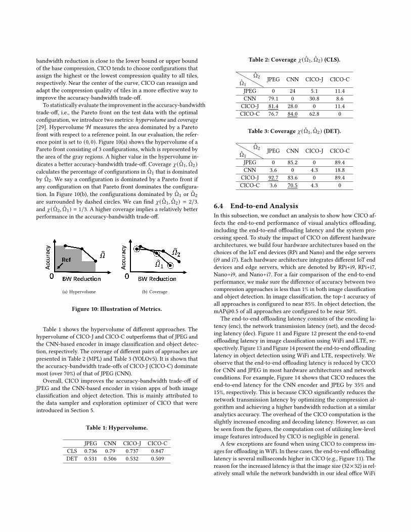
To statistically evaluate the improvement in the accuracy-bandwidthtrade-off, i.e., the Pareto front on the test data with the optimalconfiguration, we introduce two metrics: hypervolume and coverage[29]. Hypervolume H measures the area dominated by a Paretofront with respect to a reference point. In our evaluation, the refer-ence point is set to (0, 0). Figure 10(a) shows the hypervolume of aPareto front consisting of 3 configurations, which is represented bythe area of the gray regions. A higher value in the hypervolume in-dicates a better accuracy-bandwidth trade-off. Coverage 𝜒 (Ω̂1, Ω̂2)calculates the percentage of configurations in Ω̂1 that is dominatedby Ω̂2. We say a configuration is dominated by a Pareto front ifany configuration on that Pareto front dominates the configura-tion. In Figure 10(b), the configurations dominated by Ω̂1 or Ω̂2are surrounded by dashed circles. We can find 𝜒 (Ω̂1, Ω̂2) = 2/3.and 𝜒 (Ω̂2, Ω̂1) = 1/3. A higher coverage implies a relatively betterperformance in the accuracy-bandwidth trade-off.

(a) Hypervolume (b) Coverage

Figure 10: Illustration of Metrics.

Table 1 shows the hypervolume of different approaches. Thehypervolume of CICO-J and CICO-C outperforms that of JPEG andthe CNN-based encoder in image classification and object detec-tion, respectively. The coverage of different pairs of approaches arepresented in Table 2 (MPL) and Table 3 (YOLOv5). It is shown thatthe accuracy-bandwidth trade-offs of CICO-J (CICO-C) dominatemost (over 70%) of that of JPEG (CNN).

Overall, CICO improves the accuracy-bandwidth trade-off ofJPEG and the CNN-based encoder in vision apps of both imageclassification and object detection. This is mainly attributed tothe data sampler and exploration optimizer of CICO that wereintroduced in Section 5.

Table 1: Hypervolume.

JPEG CNN CICO-J CICO-CCLS 0.736 0.79 0.737 0.847DET 0.531 0.506 0.532 0.509

Table 2: Coverage 𝜒 (Ω̂1, Ω̂2) (CLS).

Ω̂1

Ω̂2 JPEG CNN CICO-J CICO-C

JPEG 0 24 5.1 11.4CNN 79.1 0 30.8 8.6CICO-J 81.4 28.0 0 11.4CICO-C 76.7 84.0 62.8 0

Table 3: Coverage 𝜒 (Ω̂1, Ω̂2) (DET).

Ω̂1

Ω̂2 JPEG CNN CICO-J CICO-C

JPEG 0 85.2 0 89.4CNN 3.6 0 4.3 18.8CICO-J 92.7 83.6 0 89.4CICO-C 3.6 70.5 4.3 0

6.4 End-to-end AnalysisIn this subsection, we conduct an analysis to show how CICO af-fects the end-to-end performance of visual analytics offloading,including the end-to-end offloading latency and the system pro-cessing speed. To study the impact of CICO on different hardwarearchitectures, we build four hardware architectures based on thechoices of the IoT end devices (RPi and Nano) and the edge servers(i9 and i7). Each hardware architecture integrates different IoT enddevices and edge servers, which are denoted by RPi+i9, RPi+i7,Nano+i9, and Nano+i7. For a fair comparison of the end-to-endperformance, we make sure the difference of accuracy between twocompression approaches is less than 1% in both image classificationand object detection. In image classification, the top-1 accuracy ofall approaches is configured to near 85%. In object detection, themAP@0.5 of all approaches are configured to be near 50%.

The end-to-end offloading latency consists of the encoding la-tency (enc), the network transmission latency (net), and the decod-ing latency (dec). Figure 11 and Figure 12 present the end-to-endoffloading latency in image classification using WiFi and LTE, re-spectively. Figure 13 and Figure 14 present the end-to-end offloadinglatency in object detection using WiFi and LTE, respectively. Weobserve that the end-to-end offloading latency is reduced by CICOfor CNN and JPEG in most hardware architectures and networkconditions. For example, Figure 14 shows that CICO reduces theend-to-end latency for the CNN encoder and JPEG by 35% and15%, respectively. This is because CICO significantly reduces thenetwork transmission latency by optimizing the compression al-gorithm and achieving a higher bandwidth reduction at a similaranalytics accuracy. The overhead of the CICO computation is theslightly increased encoding and decoding latency. However, as canbe seen from the figures, the computation cost of utilizing low-levelimage features introduced by CICO is negligible in general.

A few exceptions are found when using CICO to compress im-ages for offloading inWiFi. In these cases, the end-to-end offloadinglatency is several milliseconds higher in CICO (e.g., Figure 11). Thereason for the increased latency is that the image size (32×32) is rel-atively small while the network bandwidth in our ideal office WiFi

(several hundredMbps) is significantly high. As a result, the reducednetwork transmission latency is not sufficient to compensate forthe encoding/decoding latency added by CICO. However, we pointout that this phenomenon is unlikely to happen in more realisticsituations in practice where the IoT environment has significantlylower and unstable bandwidth (similar to or worse than LTE) andthe image data to be offloaded are generally larger. We will alsoshow in the following that such minor latency discrepancy doesnot affect the expedited performance of the whole CICO offloadingpipeline.

RPi+i9 RPi+i7 Nano+i9 Nano+i70

5

10

15

20

25

30

Tim

e (

ms)

CN

NC

ICO

-CJP

EG

CIC

O-J

Enc Net Dec

Figure 11: End-to-end offloading latency using WiFi (CLS).

RPi+i9 RPi+i7 Nano+i9 Nano+i70

50

100

150

Tim

e (

ms)

CN

NC

ICO

-CJP

EG

CIC

O-J

Enc Net Dec

Figure 12: End-to-end offloading latency using LTE (CLS).

Since component-wise and end-to-end latency evaluate the per-formance of a system rather than the quality of service that can bedelivered by a system, we evaluate the end-to-end processing speedto examine the quality of service of the visual analytics offload-ing. The processing speed is determined by the highest componentlatency among encoding, network transmission, and decoding. Un-like the absolute numbers of latency, the processing speed providesusers and system designers an intuitive way to understand howCICO can achieve ultra-fast visual analytics offloading comparedto state-of-the-art compression techniques. Figure 15 and Figure 16demonstrate the processing speed in image classification usingWiFiand LTE, respectively. Figure 17 and Figure 18 demonstrate the pro-cessing speed in object detection using WiFi and LTE, respectively.

RPi+i9 RPi+i7 Nano+i9 Nano+i70

50

100

150

Tim

e (

ms)

CN

NC

ICO

-CJP

EG

CIC

O-J

Enc Net Dec

Figure 13: End-to-end offloading latency using WiFi (DET).

RPi+i9 RPi+i7 Nano+i9 Nano+i70

200

400

600

800

1000

Tim

e (

ms)

CN

NC

ICO

-CJP

EG

CIC

O-J

Enc Net Dec

Figure 14: End-to-end offloading latency using LTE (DET).

Comparing the processing speed with and without CICO, we canfind that the processing speed has been significantly improved byCICO in different hardware architectures and network conditions.We observed up to a 2× speed up of the visual analytics offload-ing pipeline among all these scenarios. The results of end-to-endprocessing speed confirm that CICO is faster and more appropri-ate than existing compression techniques for time-sensitive visionapps that require a higher frame processing rate in visual analyticsoffloading.

In sum, CICO reduces the end-to-end offloading latency andimproves the processing speed for JPEG and the CNN-based encoderin most hardware architectures and network conditions.

RPi+i9 RPi+i7 Nano+i9 Nano+i70

20

40

60

80

100

120

Pro

ce

ssin

g S

pe

ed

(fp

s)

CNN CICO-C JPEG CICO-J

Figure 15: Processing speed using WiFi (CLS).

RPi+i9 RPi+i7 Nano+i9 Nano+i70

5

10

15

Pro

ce

ssin

g S

pe

ed

(fp

s)

CNN CICO-C JPEG CICO-J

Figure 16: Processing speed using LTE (CLS).

RPi+i9 RPi+i7 Nano+i9 Nano+i70

10

20

30

40

50

Pro

ce

ssin

g S

pe

ed

(fp

s)

CNN CICO-C JPEG CICO-J

Figure 17: Processing speed using WiFi (DET).

RPi+i9 RPi+i7 Nano+i9 Nano+i70

1

2

3

4

Pro

ce

ssin

g S

pe

ed

(fp

s)

CNN CICO-C JPEG CICO-J

Figure 18: Processing speed using LTE (DET).

6.5 Profiling CostThe profiling involves running the offline profiling stage (Figure 2)for two base compression modules on two applications, CLS andDET, which results in four offline profiling stages. We set the num-ber of configurations to explore to be 500. As discussed in Section 5.3,100× 32 samples will be used for each configuration. In each offlineprofiling stage, a total of 500 × 100 × 32 = 1, 600, 000 images will beencoded, transmitted, decoded, and processed by the application.The profiling is performed on a Linux server equipped with twoNvidia GeForce RTX 2080 GPUs. For image classification, the offlineprofiling for each compression approach takes about 20 hours. Forobject detection, the profiling for each compression approach takesabout 40 hours. Our proposed offline profiling method allows CICOto learn from the images and the vision apps in a reasonable periodof time.

6.6 Profiling ErrorTo demonstrate the difference of the profile obtained using the train-ing data and the performance of it on the test data, we introduce theprofiling error. It is defined as the absolute difference in the accuracy(or the bandwidth reduction) of the configuration measured withthe training data and the test data. The profiling error is averagedover all configurations on the profile (of CICO-J and CICO-C fortwo vision apps) and shown in Table 4. We can notice that theprofiling errors of the bandwidth reduction and the accuracy aresmall in general. This indicates that system designers can choosethe configuration on the profile to optimize the utilization of thebandwidth resource on the IoT end device.

Table 4: Profiling Error.

Accuracy BW ReductionCLS 2.7(±1.8)% 0.026(±0.049%)DET 4.3(±1.5)% 0.34(±0.23)%

7 DISCUSSIONChoice of the low-level image features. One advantage of ourapproach is that the system designer does not have to understandhow each type of low-level image feature affects the overall com-pression performance. Instead, our approach automatically learnshow to exploit different low-level image features in image compres-sion. The system designer only needs to include a few well-knownfeatures [1, 28, 35–37] and make sure the running time of the op-timized compression approach, which includes the time spent infeature extraction and compression, is acceptable. For example, therunning time should be kept under 33 ms for real-time applicationsat an offloading speed of 30 fps.

Choice of the nonlinear function. The nonlinear functionmodels the relationship between the feature density and the com-pression quality. We selected the one in Equation 6 to strike atrade-off between training complexity and compression perfor-mance. The nonlinear function can be defined in other forms aslong as it maps a density value in [0, 1] to a compression qualityvalue in [0, 1]. More parameters could be included in the nonlinearfunction to allow our approach to better model the relationshipbetween the feature density and the compression quality. However,the downside is that the design space of our system would be larger,which would take longer for the compression optimizer to learnthe optimal set of parameters.

Choice of the base compression module. The choice of thecompression method is generally flexible. It can be any traditional,e.g., JPEG, or machine learning-based, e.g., DeepCOD, compressionmethod. The base compression method would need to be config-ured in a way that it could compress different image tiles withdifferent qualities. The other consideration is that an excessivelycomplicated compression method should not be used because thebenefits introduced by CICO in bandwidth reduction and networklatency reduction might be offset by the additional delay incurredin the encoding and decoding modules.

The vision-based application. In addition to image classifi-cation and object detection, our approach is generic and can be

applied to other vision-based applications like car counting [27] andaction detection [20]. As long as a vision app explicitly gives out ametric that can evaluate the performance of an image dataset, CICOcan be used to learn the dataset and enhance the visual analyticsoffloading performance.

8 CONCLUSIONWe present CICO, a novel compression framework that contextual-izes and optimizes image compression for visual analytics offloadingin IoT. CICO is the first low-bandwidth and low-latency compres-sion framework that optimizes the accuracy and the bandwidth invisual analytics offloading. The compression problem is formulatedas an MOO problem and the Pareto front of the MOO problemis approximated by an MOBO-based exploration optimizer andan efficient data sampler. We evaluate the performance of CICOin extensive experimental settings. Our results show that, com-pared to state-of-the-art compression approaches, CICO elevatesthe accuracy-bandwidth trade-off and the end-to-end quality ofservice of visual analytics offloading in IoT.

REFERENCES[1] Motilal Agrawal, Kurt Konolige, and Morten Rufus Blas. 2008. Censure: Center

surround extremas for realtime feature detection and matching. In EuropeanConference on Computer Vision. Springer, 102–115.

[2] Eirikur Agustsson, Michael Tschannen, Fabian Mentzer, Radu Timofte, andLuc Van Gool. 2019. Generative adversarial networks for extreme learned imagecompression. In Proceedings of the IEEE/CVF International Conference on ComputerVision. 221–231.

[3] Johannes Ballé, Valero Laparra, and Eero P Simoncelli. 2016. End-to-end optimizedimage compression. arXiv preprint arXiv:1611.01704 (2016).

[4] Giovanni Beltrame, Luca Fossati, and Donatella Sciuto. 2010. Decision-theoreticdesign space exploration of multiprocessor platforms. IEEE Transactions onComputer-Aided Design of Integrated Circuits and Systems 29, 7 (2010), 1083–1095.

[5] G. Bradski. 2000. The OpenCV Library. Dr. Dobb’s Journal of Software Tools(2000).

[6] Zhaowei Cai, Mohammad Saberian, and Nuno Vasconcelos. 2015. Learningcomplexity-aware cascades for deep pedestrian detection. In Proceedings of theIEEE International Conference on Computer Vision. 3361–3369.

[7] Kalyanmoy Deb, Amrit Pratap, Sameer Agarwal, and TAMT Meyarivan. 2002. Afast and elitist multiobjective genetic algorithm: NSGA-II. IEEE transactions onevolutionary computation 6, 2 (2002), 182–197.

[8] Robert P Dick and Niraj K Jha. 1997. MOGAC: A multiobjective genetic algorithmfor the co-synthesis of hardware-software embedded systems. In iccad, Vol. 97.522–529.

[9] Kuntai Du, Ahsan Pervaiz, Xin Yuan, Aakanksha Chowdhery, Qizheng Zhang,Henry Hoffmann, and Junchen Jiang. 2020. Server-Driven Video Streaming forDeep Learning Inference. In Proceedings of the Annual conference of the ACMSpecial Interest Group on Data Communication on the applications, technologies,architectures, and protocols for computer communication. 557–570.

[10] ]pascal-voc-2012 M. Everingham, L. Van Gool, C. K. I. Williams,J. Winn, and A. Zisserman. [n. d.]. The PASCAL Visual ObjectClasses Challenge 2012 (VOC2012) Results. http://www.pascal-network.org/challenges/VOC/voc2012/workshop/index.html.

[11] William Fornaciari, Donatella Sciuto, Cristina Silvano, and Vittorio Zaccaria.2002. A sensitivity-based design space exploration methodology for embeddedsystems. Design Automation for Embedded Systems 7, 1 (2002), 7–33.

[12] Paulo Paneque Galuzio, Emerson Hochsteiner [de Vasconcelos Segundo], Leandrodos Santos Coelho, and Viviana Cocco Mariani. 2020. MOBOpt — multi-objectiveBayesian optimization. SoftwareX 12 (2020), 100520. https://doi.org/10.1016/j.softx.2020.100520

[13] Ross Girshick. 2015. Fast r-cnn. In Proceedings of the IEEE international conferenceon computer vision. 1440–1448.

[14] Tony Givargis, Frank Vahid, and Jörg Henkel. 2001. System-level exploration forpareto-optimal configurations in parameterized systems-on-a-chip. In IEEE/ACMInternational Conference on Computer Aided Design. ICCAD 2001. IEEE/ACMDigestof Technical Papers (Cat. No. 01CH37281). IEEE, 25–30.

[15] Google. 2020. A new image format for the Web. https://developers.google.com/speed/webp

[16] The Independent JPEG Group. 2014. libjpeg. https://github.com/LuaDist/libjpeg

[17] Kaiming He, Xiangyu Zhang, Shaoqing Ren, and Jian Sun. 2016. Deep residuallearning for image recognition. In Proceedings of the IEEE conference on computervision and pattern recognition. 770–778.

[18] Glenn Jocher, Alex Stoken, Jirka Borovec, NanoCode012, ChristopherSTAN,Liu Changyu, Laughing, tkianai, Adam Hogan, lorenzomammana, yxNONG,AlexWang1900, Laurentiu Diaconu, Marc, wanghaoyang0106, ml5ah, Doug, Fran-cisco Ingham, Frederik, Guilhen, Hatovix, Jake Poznanski, Jiacong Fang, LijunYu, changyu98, Mingyu Wang, Naman Gupta, Osama Akhtar, PetrDvoracek,and Prashant Rai. 2020. ultralytics/yolov5: v3.1 - Bug Fixes and PerformanceImprovements. https://doi.org/10.5281/zenodo.4154370

[19] Eunsuk Kang, Ethan Jackson, and Wolfram Schulte. 2010. An approach foreffective design space exploration. In Monterey Workshop. Springer, 33–54.

[20] Okan Köpüklü, Xiangyu Wei, and Gerhard Rigoll. 2019. You only watch once: Aunified cnn architecture for real-time spatiotemporal action localization. arXivpreprint arXiv:1911.06644 (2019).

[21] N Krishnaraj, Mohamed Elhoseny, M Thenmozhi, Mahmoud M Selim, and KShankar. 2020. Deep learning model for real-time image compression in Internetof Underwater Things (IoUT). Journal of Real-Time Image Processing 17, 6 (2020),2097–2111.

[22] Alex Krizhevsky, Geoffrey Hinton, et al. 2009. Learning multiple layers of featuresfrom tiny images. (2009).

[23] Yuanqi Li, Arthi Padmanabhan, Pengzhan Zhao, Yufei Wang, Guoqing Harry Xu,and Ravi Netravali. 2020. Reducto: On-Camera Filtering for Resource-EfficientReal-Time Video Analytics. In Proceedings of the Annual conference of the ACMSpecial Interest Group on Data Communication on the applications, technologies,architectures, and protocols for computer communication. 359–376.

[24] Tsung-Yi Lin, Michael Maire, Serge Belongie, James Hays, Pietro Perona, DevaRamanan, Piotr Dollár, and C Lawrence Zitnick. 2014. Microsoft coco: Commonobjects in context. In European conference on computer vision. Springer, 740–755.

[25] Luyang Liu, Hongyu Li, and Marco Gruteser. 2019. Edge assisted real-timeobject detection for mobile augmented reality. In The 25th Annual InternationalConference on Mobile Computing and Networking. 1–16.

[26] Zhichao Lu, Ian Whalen, Vishnu Boddeti, Yashesh Dhebar, Kalyanmoy Deb,Erik Goodman, and Wolfgang Banzhaf. 2019. Nsga-net: neural architecturesearch using multi-objective genetic algorithm. In Proceedings of the Genetic andEvolutionary Computation Conference. 419–427.

[27] Thomas Moranduzzo and Farid Melgani. 2013. Automatic car counting methodfor unmanned aerial vehicle images. IEEE Transactions on Geoscience and RemoteSensing 52, 3 (2013), 1635–1647.

[28] Pauline C Ng and Steven Henikoff. 2003. SIFT: Predicting amino acid changesthat affect protein function. Nucleic acids research 31, 13 (2003), 3812–3814.

[29] Gianluca Palermo, Cristina Silvano, and Vittorio Zaccaria. 2009. Respir: A re-sponse surface-based pareto iterative refinement for application-specific designspace exploration. IEEE Transactions on Computer-Aided Design of IntegratedCircuits and Systems 28, 12 (2009), 1816–1829.

[30] Maurizio Palesi and Tony Givargis. 2002. Multi-objective design space explorationusing genetic algorithms. In Proceedings of the tenth international symposium onHardware/software codesign. 67–72.

[31] Omkar M Parkhi, Andrea Vedaldi, and Andrew Zisserman. 2015. Deep facerecognition. (2015).

[32] Hieu Pham, Qizhe Xie, Zihang Dai, and Quoc V Le. 2020. Meta pseudo labels.arXiv preprint arXiv:2003.10580 (2020).

[33] Aaditya Prakash, Nick Moran, Solomon Garber, Antonella DiLillo, and JamesStorer. 2017. Semantic perceptual image compression using deep convolutionnetworks. In 2017 Data Compression Conference (DCC). IEEE, 250–259.

[34] Joseph Redmon, Santosh Divvala, Ross Girshick, and Ali Farhadi. 2016. Youonly look once: Unified, real-time object detection. In Proceedings of the IEEEconference on computer vision and pattern recognition. 779–788.

[35] Edward Rosten and Tom Drummond. 2006. Machine learning for high-speedcorner detection. In European conference on computer vision. Springer, 430–443.

[36] E. Rublee, V. Rabaud, K. Konolige, and G. Bradski. 2011. ORB: An efficientalternative to SIFT or SURF. In 2011 International Conference on Computer Vision.2564–2571. https://doi.org/10.1109/ICCV.2011.6126544

[37] Jianbo Shi et al. 1994. Good features to track. In 1994 Proceedings of IEEE conferenceon computer vision and pattern recognition. IEEE, 593–600.

[38] Athanassios Skodras, Charilaos Christopoulos, and Touradj Ebrahimi. 2001. Thejpeg 2000 still image compression standard. IEEE Signal processing magazine 18,5 (2001), 36–58.

[39] Sean C Smithson, Guang Yang, Warren J Gross, and Brett H Meyer. 2016. Neuralnetworks designing neural networks: multi-objective hyper-parameter optimiza-tion. In Proceedings of the 35th International Conference on Computer-Aided Design.1–8.

[40] Shinya Suzuki, Shion Takeno, Tomoyuki Tamura, Kazuki Shitara, and MasayukiKarasuyama. 2020. Multi-objective bayesian optimization using pareto-frontierentropy. In International Conference on Machine Learning. PMLR, 9279–9288.

[41] Gregory K Wallace. 1992. The JPEG still picture compression standard. IEEEtransactions on consumer electronics 38, 1 (1992), xviii–xxxiv.

[42] Chaoli Wang, Hongfeng Yu, and Kwan-Liu Ma. 2009. Application-driven com-pression for visualizing large-scale time-varying data. IEEE Computer Graphicsand Applications 30, 1 (2009), 59–69.

[43] Shuochao Yao, Jinyang Li, Dongxin Liu, Tianshi Wang, Shengzhong Liu, HuajieShao, and Tarek Abdelzaher. 2020. Deep compressive offloading: speeding upneural network inference by trading edge computation for network latency.

In Proceedings of the 18th Conference on Embedded Networked Sensor Systems.476–488.

[44] Ben Zhang, Xin Jin, Sylvia Ratnasamy, JohnWawrzynek, and Edward A Lee. 2018.Awstream: Adaptive wide-area streaming analytics. In Proceedings of the 2018Conference of the ACM Special Interest Group on Data Communication. 236–252.