A CONTEXT-AWARE LEARNING, PREDICTION AND MEDIATION

FRAMEWORK FOR RESOURCE MANAGEMENT IN SMART

PERVASIVE ENVIRONMENTS

by

NIRMALYA ROY

Presented to the Faculty of the Graduate School of

The University of Texas at Arlington in Partial Fulfillment

of the Requirements

for the Degree of

DOCTOR OF PHILOSOPHY

THE UNIVERSITY OF TEXAS AT ARLINGTON

August 2008

Copyright c© by NIRMALYA ROY 2008

All Rights Reserved

To my parents, for always supporting me in life and being always there for me. You

have made all of this possible. Thank You.

ACKNOWLEDGEMENTS

I would like to thank my advisor Prof. Sajal K. Das who has been amazingly

patient, helpful, and supportive during my research. He introduced me to the field

of pervasive computing, guided me throughout my graduate study and constantly

encouraged for high quality research. I would also like to thank Prof. Hao Che, Prof.

Yonghe Liu, Prof. Mohan Kumar and Prof. Bob Weems for their comments and

suggestions regarding my work in ubiquitous computing. My sincere regards to Prof.

Kalyan Basu for his technical guidance and help to me.

I take this opportunity to thank all my friends and colleagues at CReWMaN

laboratory for their valuable discussions and support.

I like to acknowledge the Computer Science and Engineering Department of UT

Arlington for providing me Teaching Assistantship and STEM Doctoral Fellowship

and Dean’s Fellowship. I would also like to acknowledge my previous institution

Jadavpur University (Calcutta), India, for offering me the first light of Computer

Science.

I would like to thank my parents and my brother for their constant encourage-

ment and support without which this work would have not been possible. Finally,

I would like to thank my wife, who had to endure long working hours while I was

working on this thesis and always supported me emotionally.

JULY 18, 2008

iv

ABSTRACT

A CONTEXT-AWARE LEARNING, PREDICTION AND MEDIATION

FRAMEWORK FOR RESOURCE MANAGEMENT IN SMART

PERVASIVE ENVIRONMENTS

NIRMALYA ROY, Ph.D.

The University of Texas at Arlington, 2008

Supervising Professor: Sajal K. Das

Advances in smart devices, mobile wireless communications, sensor networks,

pervasive computing, machine learning, middleware and agent technologies, and hu-

man computer interfaces have made the dream of smart environments a reality. An

important characteristic of such an intelligent, ubiquitous computing and communica-

tion paradigm lies in the autonomous and pro-active interaction of smart devices used

for determining inhabitants’ important contexts such as current and near-future loca-

tions, activities or vital signs. ‘Context Awareness’ is perhaps the most salient feature

of such an intelligent computing environment. An inhabitant’s mobility and activi-

ties play a significant role in defining his contexts in and around the home. Although

there exists optimal algorithm for location and activity tracking of a single inhabi-

tant, the correlation and dependence between multiple inhabitants’ contexts within

the same environment make the location and activity tracking more challenging. In

this thesis, first we propose a cooperative reinforcement learning policy for location-

aware resource management in multi-inhabitant smart homes. This approach adapts

v

to the uncertainty of multiple inhabitants’ locations and most likely routes, by vary-

ing the learning rate parameters. Using the proposed cooperative game-theory based

framework, all the inhabitants currently present in the house attempt to minimize

this overall uncertainty in the form of utility functions associated with them. Joint

optimization of the utility function corresponds to the convergence to Nash equilib-

rium and helps in accurate prediction of inhabitants’ future locations and activities.

Hypothesizing that every inhabitant wants to satisfy his own preferences about ac-

tivities, next we look into the problem from the perspective of non-cooperative game

theory where the inhabitants are the players and their activities are the strategies of

the game. We prove that the optimal location prediction across multiple inhabitants

in smart homes is an NP-hard problem and to capture the correlation and interac-

tions between different inhabitants’ movements (and hence activities), we develop a

novel framework based on a non-cooperative game theoretic, Nash H-learning ap-

proach that attempts to minimize the joint location uncertainty of inhabitants. Our

framework achieves a Nash equilibrium such that no inhabitant is given preference

over others. This results in more accurate prediction of contexts and more adap-

tive control of automated devices, thus leading to a mobility-aware resource (say,

energy) management scheme in multi-inhabitant smart homes. Experimental results

demonstrate that the proposed framework is capable of adaptively controlling a smart

environment, significantly reduces energy consumption and enhances the comfort of

the inhabitants.

To promote independent living and wellness management services in this smart

home environment we envision sensor rich computing and networking environments

that can capture various types of contexts of patients (or inhabitants of the envi-

ronment), such as their location, activities and vital signs. However, in reality, both

sensed and interpreted contexts may often be ambiguous, leading to fatal decisions if

vi

not properly handled. Thus, a significant challenge facing the development of real-

istic and deployable context-aware services for healthcare applications is the ability

to deal with ambiguous contexts to prevent hazardous situations. In this thesis, we

propose a quality assured context mediation framework, based on efficient context-

aware data fusion and information theoretic system parameter selection for optimal

state estimation in resource constrained sensor network. The proposed framework

provides a systematic approach based on dynamic Bayesian network to derive con-

text fragments and deal with context ambiguity or error in a probabilistic manner.

It has the ability to incorporate context representation according to the applications’

quality requirement. Experimental results demonstrate that the proposed framework

is capable of choosing a set of sensors corresponding to the most economically effi-

cient disambiguation action and successfully sensing, mediating and predicting the

patients’ context state and situation.

Energy-efficient determination of an individual’s context (both physiological

and activity) is an important technical challenge for this assisted living environments.

Given the expected availability of multiple sensors, context determination is viewed as

an estimation problem over multiple sensor data streams. We develop a formal, and

practically applicable, model to capture the tradeoff between the accuracy of context

estimation and the communication overheads of sensing. In particular, we propose

the use of tolerance ranges to reduce an individual sensor’s reporting frequency, while

ensuring acceptable accuracy of the derived context. We introduce an optimization

technique allowing the context service to compute both the best set of sensors, and

their associated tolerance values, that satisfy the QoINF target at minimum commu-

nication cost. Experimental results with SunSPOT sensors are presented to attest to

the promise of this approach.

vii

TABLE OF CONTENTS

ACKNOWLEDGEMENTS . . . . . . . . . . . . . . . . . . . . . . . . . . . . iv

ABSTRACT . . . . . . . . . . . . . . . . . . . . . . . . . . . . . . . . . . . . v

LIST OF FIGURES . . . . . . . . . . . . . . . . . . . . . . . . . . . . . . . . xii

LIST OF TABLES . . . . . . . . . . . . . . . . . . . . . . . . . . . . . . . . . xv

Chapter

1. INTRODUCTION . . . . . . . . . . . . . . . . . . . . . . . . . . . . . . . 1

1.1 Introduction . . . . . . . . . . . . . . . . . . . . . . . . . . . . . . . . 1

1.2 Challenges . . . . . . . . . . . . . . . . . . . . . . . . . . . . . . . . . 2

1.3 Problem Statement . . . . . . . . . . . . . . . . . . . . . . . . . . . . 4

1.4 Scope and Methodology . . . . . . . . . . . . . . . . . . . . . . . . . 5

1.5 Results . . . . . . . . . . . . . . . . . . . . . . . . . . . . . . . . . . . 6

1.6 Organization . . . . . . . . . . . . . . . . . . . . . . . . . . . . . . . 7

2. COOPERATIVE MOBILITY AWARE RESOURCE MANAGEMENT . . 8

2.1 Introduction . . . . . . . . . . . . . . . . . . . . . . . . . . . . . . . . 8

2.1.1 Our Contributions . . . . . . . . . . . . . . . . . . . . . . . . 9

2.2 Preliminaries . . . . . . . . . . . . . . . . . . . . . . . . . . . . . . . 11

2.2.1 Overview of Smart Homes . . . . . . . . . . . . . . . . . . . . 11

2.2.2 Cooperative Framework for Inhabitants Mobility . . . . . . . . 11

2.2.3 Information Theoretic Estimate for Location Uncertainty . . . 12

2.2.4 Learning in Cooperative Environments . . . . . . . . . . . . . 12

2.3 Inhabitant’s Utility Function based on Cooperative Learning . . . . . 13

2.3.1 Entropy Learning based on Individual Policy . . . . . . . . . . 13

viii

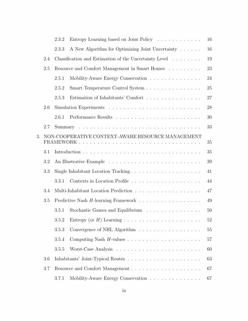
2.3.2 Entropy Learning based on Joint Policy . . . . . . . . . . . . 16

2.3.3 A New Algorithm for Optimizing Joint Uncertainty . . . . . . 16

2.4 Classification and Estimation of the Uncertainty Level . . . . . . . . 19

2.5 Resource and Comfort Management in Smart Homes . . . . . . . . . 23

2.5.1 Mobility-Aware Energy Conservation . . . . . . . . . . . . . . 24

2.5.2 Smart Temperature Control System . . . . . . . . . . . . . . . 25

2.5.3 Estimation of Inhabitants’ Comfort . . . . . . . . . . . . . . . 27

2.6 Simulation Experiments . . . . . . . . . . . . . . . . . . . . . . . . . 28

2.6.1 Performance Results . . . . . . . . . . . . . . . . . . . . . . . 30

2.7 Summary . . . . . . . . . . . . . . . . . . . . . . . . . . . . . . . . . 33

3. NON-COOPERATIVE CONTEXT-AWARE RESOURCE MANAGEMENTFRAMEWORK . . . . . . . . . . . . . . . . . . . . . . . . . . . . . . . . . 35

3.1 Introduction . . . . . . . . . . . . . . . . . . . . . . . . . . . . . . . . 35

3.2 An Illustrative Example . . . . . . . . . . . . . . . . . . . . . . . . . 39

3.3 Single Inhabitant Location Tracking . . . . . . . . . . . . . . . . . . . 41

3.3.1 Contexts in Location Profile . . . . . . . . . . . . . . . . . . . 44

3.4 Multi-Inhabitant Location Prediction . . . . . . . . . . . . . . . . . . 47

3.5 Predictive Nash H-learning Framework . . . . . . . . . . . . . . . . . 49

3.5.1 Stochastic Games and Equilibrium . . . . . . . . . . . . . . . 50

3.5.2 Entropy (or H) Learning . . . . . . . . . . . . . . . . . . . . . 52

3.5.3 Convergence of NHL Algorithm . . . . . . . . . . . . . . . . . 55

3.5.4 Computing Nash H-values . . . . . . . . . . . . . . . . . . . . 57

3.5.5 Worst-Case Analysis . . . . . . . . . . . . . . . . . . . . . . . 60

3.6 Inhabitants’ Joint-Typical Routes . . . . . . . . . . . . . . . . . . . . 63

3.7 Resource and Comfort Management . . . . . . . . . . . . . . . . . . . 67

3.7.1 Mobility-Aware Energy Conservation . . . . . . . . . . . . . . 67

ix

3.7.2 Estimation of Inhabitants’ Comfort . . . . . . . . . . . . . . . 68

3.8 Experimental Study . . . . . . . . . . . . . . . . . . . . . . . . . . . . 68

3.8.1 Simulation Environment . . . . . . . . . . . . . . . . . . . . . 69

3.8.2 Performance Results . . . . . . . . . . . . . . . . . . . . . . . 70

3.9 Summary . . . . . . . . . . . . . . . . . . . . . . . . . . . . . . . . . 78

4. AMBIGUOUS CONTEXT MEDIATION FRAMEWORK . . . . . . . . . 80

4.1 Introduction . . . . . . . . . . . . . . . . . . . . . . . . . . . . . . . . 80

4.1.1 Related Work . . . . . . . . . . . . . . . . . . . . . . . . . . . 81

4.1.2 Example Scenario . . . . . . . . . . . . . . . . . . . . . . . . . 84

4.1.3 Our Contributions . . . . . . . . . . . . . . . . . . . . . . . . 85

4.2 Context Model . . . . . . . . . . . . . . . . . . . . . . . . . . . . . . 87

4.2.1 Space-based Context Model . . . . . . . . . . . . . . . . . . . 87

4.2.2 Quality of Context . . . . . . . . . . . . . . . . . . . . . . . . 88

4.3 Context-Aware Data Fusion . . . . . . . . . . . . . . . . . . . . . . . 91

4.3.1 Dynamic Bayesian Network Based Model (DBN) . . . . . . . 92

4.4 Information Theoretic Reasoning . . . . . . . . . . . . . . . . . . . . 96

4.4.1 Problem Explanation . . . . . . . . . . . . . . . . . . . . . . . 99

4.4.2 Results . . . . . . . . . . . . . . . . . . . . . . . . . . . . . . . 100

4.5 Rule Based Model . . . . . . . . . . . . . . . . . . . . . . . . . . . . . 104

4.5.1 Example Rule Sets . . . . . . . . . . . . . . . . . . . . . . . . 105

4.5.2 Architecture . . . . . . . . . . . . . . . . . . . . . . . . . . . . 107

4.5.3 Rule based Engine Implementation . . . . . . . . . . . . . . . 109

4.6 Simulation Study . . . . . . . . . . . . . . . . . . . . . . . . . . . . . 114

4.6.1 Performance Results . . . . . . . . . . . . . . . . . . . . . . . 116

4.7 Summary . . . . . . . . . . . . . . . . . . . . . . . . . . . . . . . . . 125

5. QUALITY-OF-INFERENCE (QoINF)-AWARE CONTEXT DETERMINA-

x

TION FRAMEWORK . . . . . . . . . . . . . . . . . . . . . . . . . . . . . 127

5.1 Introduction . . . . . . . . . . . . . . . . . . . . . . . . . . . . . . . . 127

5.1.1 Related Work . . . . . . . . . . . . . . . . . . . . . . . . . . . 129

5.1.2 Contributions . . . . . . . . . . . . . . . . . . . . . . . . . . . 130

5.2 Context Inference and the QoINF Model . . . . . . . . . . . . . . . . 131

5.2.1 Role of Tolerance Ranges in Context Estimation Errors . . . . 132

5.2.2 Context Sensing Architecture . . . . . . . . . . . . . . . . . . 134

5.2.3 Minimum-Cost QoINF-Aware Problem . . . . . . . . . . . . . 135

5.3 QoINF Cost Optimization . . . . . . . . . . . . . . . . . . . . . . . . 136

5.3.1 Average Reporting Cost Optimization . . . . . . . . . . . . . 136

5.3.2 Suggested Optimization Heuristic . . . . . . . . . . . . . . . . 137

5.4 Techniques for Deriving QoINFC(.) . . . . . . . . . . . . . . . . . . . 139

5.5 Experimental Components and Evaluation . . . . . . . . . . . . . . . 141

5.5.1 Empirical Determination of Context Estimates . . . . . . . . . 141

5.5.2 Measurement of QoINF Accuracy & Sensor Overheads . . . . 142

5.5.3 The Benefit of Joint Sensing . . . . . . . . . . . . . . . . . . . 143

5.5.4 Next Steps and Ongoing Work . . . . . . . . . . . . . . . . . . 144

5.6 Summary . . . . . . . . . . . . . . . . . . . . . . . . . . . . . . . . . 146

6. RELATED WORK . . . . . . . . . . . . . . . . . . . . . . . . . . . . . . . 148

6.1 Introduction . . . . . . . . . . . . . . . . . . . . . . . . . . . . . . . . 148

6.2 Projects and Groups . . . . . . . . . . . . . . . . . . . . . . . . . . . 148

6.3 Pioneering Projects . . . . . . . . . . . . . . . . . . . . . . . . . . . . 152

6.4 Summary . . . . . . . . . . . . . . . . . . . . . . . . . . . . . . . . . 155

7. CONCLUSION AND FUTURE WORK . . . . . . . . . . . . . . . . . . . 160

REFERENCES . . . . . . . . . . . . . . . . . . . . . . . . . . . . . . . . . . . 162

BIOGRAPHICAL STATEMENT . . . . . . . . . . . . . . . . . . . . . . . . . 176

xi

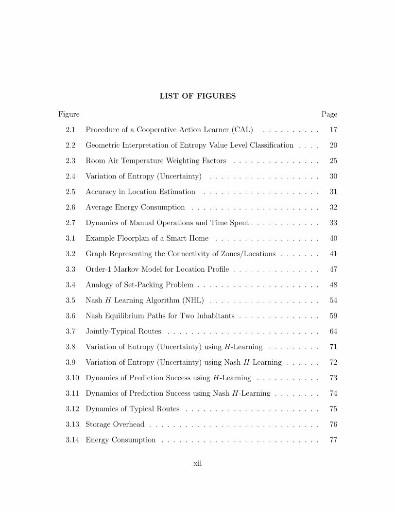
LIST OF FIGURES

Figure Page

2.1 Procedure of a Cooperative Action Learner (CAL) . . . . . . . . . . 17

2.2 Geometric Interpretation of Entropy Value Level Classification . . . . 20

2.3 Room Air Temperature Weighting Factors . . . . . . . . . . . . . . . 25

2.4 Variation of Entropy (Uncertainty) . . . . . . . . . . . . . . . . . . . 30

2.5 Accuracy in Location Estimation . . . . . . . . . . . . . . . . . . . . 31

2.6 Average Energy Consumption . . . . . . . . . . . . . . . . . . . . . . 32

2.7 Dynamics of Manual Operations and Time Spent . . . . . . . . . . . . 33

3.1 Example Floorplan of a Smart Home . . . . . . . . . . . . . . . . . . 40

3.2 Graph Representing the Connectivity of Zones/Locations . . . . . . . 41

3.3 Order-1 Markov Model for Location Profile . . . . . . . . . . . . . . . 47

3.4 Analogy of Set-Packing Problem . . . . . . . . . . . . . . . . . . . . . 48

3.5 Nash H Learning Algorithm (NHL) . . . . . . . . . . . . . . . . . . . 54

3.6 Nash Equilibrium Paths for Two Inhabitants . . . . . . . . . . . . . . 59

3.7 Jointly-Typical Routes . . . . . . . . . . . . . . . . . . . . . . . . . . 64

3.8 Variation of Entropy (Uncertainty) using H-Learning . . . . . . . . . 71

3.9 Variation of Entropy (Uncertainty) using Nash H-Learning . . . . . . 72

3.10 Dynamics of Prediction Success using H-Learning . . . . . . . . . . . 73

3.11 Dynamics of Prediction Success using Nash H-Learning . . . . . . . . 74

3.12 Dynamics of Typical Routes . . . . . . . . . . . . . . . . . . . . . . . 75

3.13 Storage Overhead . . . . . . . . . . . . . . . . . . . . . . . . . . . . . 76

3.14 Energy Consumption . . . . . . . . . . . . . . . . . . . . . . . . . . . 77

xii

3.15 Manual Operations and Time Spent . . . . . . . . . . . . . . . . . . . 78

4.1 A Middleware Framework for Ambiguous Context Mediation . . . . . 82

4.2 Subset of Sensors with Required QoC . . . . . . . . . . . . . . . . . . 90

4.3 Context-Aware Data Fusion Framework based on DynamicBayesian Networks . . . . . . . . . . . . . . . . . . . . . . . . . . . . 93

4.4 Ambiguous Context Mediation Algorithm (ACMA) . . . . . . . . . . 93

4.5 State-based Context Attribute Requirement Graph with the RequiredQoC . . . . . . . . . . . . . . . . . . . . . . . . . . . . . . . . . . . . 98

4.6 Ambiguous Context Mediation Subsystem . . . . . . . . . . . . . . . 107

4.7 An Event Graph Representing the ECA Rules . . . . . . . . . . . . . 108

4.8 Different Instances of ContextAttribute Class . . . . . . . . . . . . . . 110

4.9 Different Instances of GrandParents Class . . . . . . . . . . . . . . . . 110

4.10 RDF Model View of GrandParents Class . . . . . . . . . . . . . . . . 114

4.11 Bayesian Network . . . . . . . . . . . . . . . . . . . . . . . . . . . . . 115

4.12 Reduction in Ambiguity for Different States of the Application . . . . 118

4.13 Best Sensor Set for Different Values of Balance Coefficient α . . . . . 119

4.14 Situation Prediction Probability using Passive and Active Fusion . . . 120

4.15 Situation Prediction Probability using Multi Sensor Fusion . . . . . . 121

4.16 Variation of Situation Prediction Probability using QoC Constraint . 124

4.17 Variation of Situation Prediction Probability using Sensor Values . . . 125

5.1 Impact of Choice of Different Sensor Subsets on QoINF (NoConsideration of Tolerance Range) . . . . . . . . . . . . . . . . . . . . 133

5.2 Overall Architecture of QoINF-Aware Context Determination . . . . . 135

5.3 Proposed Sensor Set Selection Heuristic . . . . . . . . . . . . . . . . . 140

5.4 Communication Overhead & Inferencing Accuracy vs. Tolerance Rangeusing Motion Sensor . . . . . . . . . . . . . . . . . . . . . . . . . . . . 143

5.5 Communication Overhead & Inferencing Accuracy vs. Tolerance Rangeusing Light Sensor . . . . . . . . . . . . . . . . . . . . . . . . . . . . . 144

xiii

5.6 Inferencing Accuracy vs. Tolerance Range using both Motion andLight Sensor Together . . . . . . . . . . . . . . . . . . . . . . . . . . . 145

5.7 Comparison of Inferencing Accuracy Improvement using MultipleSensor . . . . . . . . . . . . . . . . . . . . . . . . . . . . . . . . . . . 146

xiv

LIST OF TABLES

Table Page

3.1 Inhabitant’s Location Profile between 7:00 am and 7:00 pm . . . . . . 44

3.2 Zone Sequence Extracted from the Location Profile of theInhabitant . . . . . . . . . . . . . . . . . . . . . . . . . . . . . . . . . 45

3.3 Contexts of Orders 0, 1 and 2 with Occurrence Frequencies . . . . . . 46

3.4 Zone Sequences Extracted from Location Profile . . . . . . . . . . . . 58

3.5 Stationary Strategy for Inhabitant 1 . . . . . . . . . . . . . . . . . . . 58

3.6 Nash H-Values . . . . . . . . . . . . . . . . . . . . . . . . . . . . . . 61

3.7 Context of Orders 0 with Occurrence Frequencies . . . . . . . . . . . 66

3.8 A Snapshot of the Collected RAW Data . . . . . . . . . . . . . . . . . 70

4.1 A Snapshot of the Collected RAW Data . . . . . . . . . . . . . . . . . 117

4.2 Utility Value without Considering Information Acquisition Cost . . . 117

4.3 Best sensor Set with Different Set Size for Different States of theApplication (α = 1) . . . . . . . . . . . . . . . . . . . . . . . . . . . . 122

4.4 Utility Value Considering Information Acquisition Cost . . . . . . . . 122

4.5 Multi Sensor Utility Value Considering Information AcquisitionCost . . . . . . . . . . . . . . . . . . . . . . . . . . . . . . . . . . . . 123

5.1 Calibrated Accelerometer Sample Values for Different ContextState . . . . . . . . . . . . . . . . . . . . . . . . . . . . . . . . . . . . 140

5.2 Light Sensor Values (lumen) for Different Context State . . . . . . . . 142

xv

CHAPTER 1

INTRODUCTION

1.1 Introduction

Advances in smart devices, mobile wireless communications, sensor networks,

pervasive computing, machine learning, middleware and agent technologies, and hu-

man computer interfaces have made the dream of smart pervasive environments a

reality. According to Cook and Das [22], a “smart environment” is one that is able to

autonomously acquire and apply knowledge about its users and their surroundings,

and adapt to the users’ behavior or preferences with the ultimate goal to improve

their experience in that environment. The type of experience that individuals ex-

pect from an environment varies with the individual and the type of environment

considered. This may include the safety of users, reduction of cost of maintain-

ing the environment, optimization of resources (e.g., energy bills or communication

bandwidth), task automation or the promotion of an intelligent independent living

environment for healthcare services and wellness management. An important charac-

teristic of such an intelligent, pervasive computing and communication paradigm lies

in the autonomous and pro-active interaction of smart devices used for determining

users’ important contexts such as current and near-future locations, activities, or vital

signs.

In this sense, ‘context awareness’ is a key issue for enhancing users living ex-

perience during their daily interaction with computer systems, as only a dynamic

adaptation to the task at hand will make computing environments just user friendly

and supportive. The combination of awareness with information appliances, or rather

1

2

the implementation of awareness in information appliances became known as context

awareness [104], since a device should act within its current context of use, by being

aware of the various aspects of its current environment. Context awareness is con-

cerned with the situation a device or user is in, and with adapting applications to

the current situation. But knowing the current context an application or system is

used in and dynamically adapting to it only allows to construct reactive systems, i.e.,

systems which run after changes in their environment. To maximize their usefulness

and user support, systems should rather adapt in advance to a new situation and be

prepared before they are actually used. This demands the development of proactive

systems, i.e., systems which predict changes in their environment and act in advance.

To this end, we strive to develop methods to learn and predict future context, to

mediate ambiguous context, enabling systems to become proactive with regard to

their context of use. Our concept is to provide applications not only with informa-

tion about the current user context, but also with predictions of future user context.

When equipped with various sensors, a system should classify current situations and,

based on those classes, learn the user’s behaviors and habits by deriving knowledge

from historical data. The focus of this thesis is to forecast future user contexts lu-

cidly by extrapolating the past and derive techniques that enable context prediction

in pervasive systems and leaves decisions about starting actions to applications built

on top of it.

1.2 Challenges

An instance of such an intelligent indoor environment is a smart home [27] that

perceives the surroundings through sensors and acts on it with the help of actuators.

In this environment, user’s mobility and activity create an uncertainty of their loca-

tions and hence subsequent activities. In order to be cognizant of his contexts, the

3

smart environment needs to minimize this uncertainty. An analysis of his daily rou-

tine and life style reveals that there exist some well defined patterns of these contexts.

Although these patterns may change over time, they do not change too frequently

and thus can be learned. An optimal algorithm for location (activity) tracking in

an indoor smart environment, based on dictionary management and online learning

of the inhabitant’s mobility profile, followed by a predictive location-aware resource

management (energy consumption) scheme for a single inhabitant smart home is

discussed in [94]. However, the presence of multiple inhabitants with dynamically

varying profiles as well as preferences make such tracking much more challenging.

This is due mainly to the fact that the relevant contexts of multiple inhabitants in

the same environment are often inherently correlated and inter-dependent on each

other. Therefore, the learning and prediction (decision making) paradigm needs to

consider the joint (simultaneous) location/activity tracking of multiple inhabitants

which we address in this thesis. Furthermore, hypothesizing that each inhabitant

in a smart home behaves in such a way as to fulfill his own objectives and maxi-

mizes his utility, the residence of multiple inhabitants with varying preferences might

lead to conflicting goals. Thus, a smart home must be intelligent enough to strike

a balance between multiple preferences, eventually attaining an equilibrium state.

This motivates us to investigate the multi-inhabitant location tracking problem from

the perspective of stochastic game theory, where the inhabitants are the players of

the game. The goal here is to achieve an equilibrium so that the system (i.e., smart

home) is able to probabilistically predict the inhabitants’ locations and activities with

sufficient accuracy in spite of possible correlations.

In this thesis we also look into how the various types of contexts of patients (or

inhabitants of the environment), such as their location, activities and vital signs can

provide health related and wellness management services in an intelligent, energy-

4

efficient way so as to promote independent living. However, in reality, both sensed

and interpreted contexts may often be ambiguous, leading to fatal decisions if not

properly handled. Thus, a significant challenge facing the development of realistic

and deployable context-aware services for healthcare applications is the ability to

deal with ambiguous contexts to prevent hazardous situations.

1.3 Problem Statement

Our main focus of research is on user centered learning and prediction of con-

text and presenting a context-aware middleware framework for autonomous resource

management and ambiguous context mediation subsystem. Context, in the field of

pervasive computing, has been defined in different ways. One of the first definitions

of context in [106] states that it comprises computing, user and physical properties.

The definition adopted within this thesis is the one by Dey et.al. [32], according to

which context is any information which can be used to characterize the situation of

an entity, where an entity is a person, place or object that is considered relevant to

the interaction between a user and an application, including the user and the appli-

cation themselves. We define context awareness as incorporating learned, predicted,

future context into the device behavior and being prepared to future situations. We

can define the problem statement as follows: What are the necessary concepts, ar-

chitectures and methods for context learning and prediction, context modeling and

mediation in smart pervasive systems? Thus, the research goal is to evaluate and, if

necessary, develop methods for learning, predicting, modeling and mediating context

with the limited resources of pervasive systems.

5

1.4 Scope and Methodology

A smart home aims at building intelligent automation with a goal to provide

its inhabitants with maximum possible comfort, minimum resource consumption and

thus reduced cost of home maintenance. ‘Context Awareness’ is perhaps the most

salient feature of such an intelligent environment. An inhabitant’s mobility and activ-

ities play a significant role in defining his contexts in and around the home. Although

there exists optimal algorithm for location and activity tracking of a single inhabi-

tant, the correlation and dependence between multiple inhabitants’ contexts within

the same environment make the location and activity tracking more challenging. In

this thesis, first we propose a cooperative entropy learning policy for location-aware

resource management in multi-inhabitant smart homes. This approach adapts to the

uncertainty of multiple inhabitants’ locations and most likely routes, by varying the

learning rate parameters and minimizing the Mahalanobish distance. However, the

complexity of multi-inhabitant location tracking problem was not characterized in this

work. But the optimal location prediction across multiple inhabitants in smart homes

is an NP-hard problem. Next, to capture the correlation and interactions between

different inhabitants’ movements (and hence activities), we develop a novel framework

based on a game theoretic, Nash H-learning approach that attempts to minimize the

joint location uncertainty of inhabitants. Our framework achieves a Nash equilibrium

such that no inhabitant is given preference over others. This results in more accurate

prediction of contexts and more adaptive control of automated devices, thus leading

to a mobility-aware resource (say, energy) management scheme in multi-inhabitant

smart homes. Experimental results demonstrate that the proposed framework is

capable of adaptively controlling a smart environment, significantly reduces energy

consumption and enhances the comfort of the inhabitants.

6

To promote independent living and wellness management services in a smart

home environment we envision sensor rich computing and networking environments

that can capture various types of contexts of patients (or inhabitants of the environ-

ment), such as their location, activities and vital signs. Given the expected availability

of multiple sensors, context determination may be viewed as an estimation problem

over multiple sensor data streams. We develop a formal, and practically applicable,

model to capture the tradeoff between the accuracy of context estimation and the

communication overheads of sensing. In particular, we propose the use of tolerance

ranges to reduce an individual sensor’s reporting frequency, while ensuring acceptable

accuracy of the derived context. We introduce an optimization technique allowing the

Context Service to compute both the best set of sensors, and their associated toler-

ance values, that satisfy the QoINF target at minimum communication cost. We also

propose a novel framework for context mediation, based on efficient context-aware

data fusion and information theoretic reasoning. The proposed framework provides a

systematic approach based on dynamic Bayesian network to derive context fragments

and deal with context ambiguity in a probabilistic manner. It has the ability to in-

corporate context representation within the applications and also easily composable

rules to mediate ambiguous contexts. We have implemented a demonstration of the

use of our model. Experimental results demonstrate that the proposed framework is

capable of choosing a set of sensors corresponding to the most economically efficient

disambiguation action and successfully predicting the patients’ situation.

1.5 Results

The present thesis analyzes prerequisite for user centered learning and predic-

tion of context and present a framework for autonomous resource management in

smart home environment and ambiguous context mediation subsystem with appli-

7

cation to smart healthacre. The developed system is being implemented in terms

of a flexible software framework and evaluated with real-world data from everyday

situations.

1.6 Organization

The remainder of this thesis is split into six Chapters. Chapter 2, which de-

fines the specific goals and presents the general concept for context-aware resource

management through learning and prediction in a cooperative multi-inhabitant smart

home. In Chapter 3 we look into the same problem from non-cooperative perspective

to strike a balance between multiple preferences of the inhabitants. Chapter 4 then

shows how context information is useful in providing health related and wellness man-

agement services in an intelligent way so as to promote independent living. Chapter

5 then presents the determination of this health related context in an efficient way

using the resource constrained sensor network. In Chapter 6, related work is summa-

rized and this thesis is positioned among and against other publications with regard

to novelties in our approach and differences to previous work. Finally, in Chapter

7 the thesis is summarized by pointing out the main arguments and the scientific

contribution and giving an outlook on possible future research.

CHAPTER 2

COOPERATIVE MOBILITY AWARE RESOURCE MANAGEMENT

2.1 Introduction

The vision of ubiquitous computing was first conceived by M. Weiser at Xerox

PARC as the future model for computing [121]. The most significant characteris-

tic of this computing paradigm lies in smart, pro-active interaction of the hand-held

computing devices with their peers and surrounding networks, often without explicit

operator control. Hence, the computing devices need to be imbued with an inher-

ent sentience [54] about their important contexts. This context-awareness is perhaps

the key characteristic of the next generation of intelligent networks and associated

applications. The advent of smart homes is germinated from the concept of ubiq-

uitous computing in an indoor environment with a goal to provide the inhabitants

with sufficient comfort at minimum possible operational. Obviously, the technology

needs to be weaved into the inhabitants’ everyday life such that it becomes “tech-

nology that disappears” [121]. A careful insight into the features of a smart home

reveals that the ability to capture the current and near-future locations and activities

(hence ‘contexts’) of different inhabitants often becomes the key to the environment’s

associated “smartness”. Intelligent prediction of inhabitants’ locations and routes

aids in efficient triggering of active databases or guaranteeing a precise time frame of

service, thereby supporting location-aware interactive, multimedia applications. This

also helps in pro-active management of resources such as energy consumption.

Given the wide variety of smart, indoor location-tracking paradigms, let us sum-

marize below some of the important ones. The Active Badge [45] and Active Bat [46]

8

9

use infra-red and ultrasonic time-of-flight techniques for indoor location tracking. On

the other hand, the Cricket Location Support System [92] delegates the responsibil-

ity of location reporting to the mobile object itself. RADAR [4], another RF-based

indoor location support system, uses signal strength and signal-to-noise ratio to com-

pute 2-D positioning. The Easy-living and the Home projects [72] use real-time 3D

cameras to provide stereo-vision positioning capability in an indoor environment. In

the Aware Home [87], the embedded pressure sensors capture inhabitant’s footfalls,

and the system uses this data for position tracking and pedestrian recognition. The

Neural Network House [82], Intelligent Home [77] and Intelligent House n [57] projects

focus on the development of adaptive control of home environments to anticipate the

needs of the inhabitants.

In an earlier work [94], we proposed location-aware resource management con-

sidering a single-inhabitant smart home. However, the presence of multiple inhabi-

tants with varying preferences and requirements makes the problem more challenging.

A suitable balance of preferences arising from multiple inhabitants [108] needs to be

considered. Thus, the environment (or system) needs to be more smart to extract

the best performance while satisfying the requirements of the inhabitants as much as

possible.

2.1.1 Our Contributions

In this chapter we have developed a framework for mobility-aware resource man-

agement in multi-inhabitant smart homes, based on a dynamic, cooperative learning

technique. Here the resource management means the reduction of the consumption

of energy. The movement pattern and various activities of the inhabitants always

create an uncertainty of their locations and subsequent activities. In order to be

cognizant of the inhabitants’ contexts, the system needs to minimize this uncertainty

10

which can be measured by Shannon’s entropy [26]. An analysis of inhabitants’ daily

routines reveals that every inhabitant has some patterns in daily-life that can be

learnt. Although the life style (pattern) changes over time, such changes are not fre-

quent and random. This observation helps us assume that the inhabitant’s mobility

and associated activities follow a piece-wise stationary, ergodic, stochastic process [7],

with some value of entropy (uncertainty) associated with it. The novelty of our work

lies in the development of a new framework based on cooperative game theory and

reinforcement learning to minimize the overall uncertainty associated with multiple

inhabitants currently present in the smart home. This is performed by developing a

joint utility function of entropy. Optimization of this utility function asymptotically

converges to Nash Equilibrium [8]. Minimizing the utility function of uncertainty

helps in accurate learning and estimation of inhabitants’ contexts (locations and as-

sociated activities). Thus, the system can control the operation of automated devices

in an adaptive manner, thereby developing an amicable environment inside the home

and providing sufficient comfort to the inhabitants. This also aids in minimizing the

energy usage, leading to a reduction of overall maintenance cost of the house.

The rest of the chapter is organized as follows. The problem definition, basic

concepts of cooperative framework and information theoretic estimation of location

uncertainty are discussed in Section 2.2. The new game-theoretic learning framework

that minimizes uncertainty associated with all inhabitants, is presented in Section 2.3.

In Section 2.4 we present the analytical model for estimation and classification process

of different values of uncertainty level. Section 2.5 demonstrates the use of the pro-

posed framework in resource optimization in multi-inhabitant smart homes. Simu-

lation results in Section 2.6 delineates the efficiency of our framework. Section 2.7

concludes the chapter with pointers to future researches.

11

2.2 Preliminaries

The smart home environment, basic concepts of cooperative framework, infor-

mation theoretic estimation of location uncertainty and the learning in cooperative

environments are discussed here.

2.2.1 Overview of Smart Homes

The MAVHome (Managing An intelligent Versatile Home) [27] is a multi-

disciplinary research project at the University of Texas at Arlington. It is focused on

the creation of an intelligent home environment capable of perceiving its surround-

ings through the use of sensors, and thereby adopting suitable actions by using the

actuators. In such a smart computing platform there exists movements of inhabitants

interacting with their surrounding environments through the hand-held devices. The

overall goal is to provide the inhabitant’s comfort at an optimal cost. Efficient and

intelligent estimate and prediction of inhabitants’ contexts (location and activity) is

the most necessary component of such a smart home.

2.2.2 Cooperative Framework for Inhabitants Mobility

Our proposed framework is based on symbolic interpretation of the inhabitant’s

movement (mobility) within the home, which is captured by sampling the in-building

sensors (RF-ID readers or pressure switches). Thus, the movement history of an

inhabitant is assumed as a string “v1v2v3 . . .” of symbols (sensor-ids) where vi ∈ ϑ

(the alphabet set). We argue that the inhabitant’s mobility and current location is

merely a reflection of his/her movement history (profile), which can be learned over

time in an on-line fashion. Characterizing such mobility as a probabilistic sequence

suggests that it can be defined as a stochastic process V = Vi, while the repetitive

nature of identifiable patterns adds stationarity as an essential property, leading to

12

Pr[Vi = vi] = Pr[Vi+l = vi] for all vi ∈ ϑ and for every shift l. The movement of

the set of inhabitants inside the smart home always create an uncertainty in their

locations and activities. The concept of entropy [26] in information theory is the

most fair measure to estimate this uncertainty.

2.2.3 Information Theoretic Estimate for Location Uncertainty

The entropy Hb(X) of a discrete random variable X with probability mass

function p(x), x ∈ X , is defined by: Hb(X) = −∑x∈X p(x) logb p(x). The limiting

value “limp→0 p logb p = 0” is used in the expression when p(x) = 0. The relative

entropy between two probability mass functions p(x) and q(x), x ∈ X , is given by

D(p||q) =∑

x∈X p(x) logp(x)q(x)

. This relative entropy is a fair measure of the inef-

ficiency of assuming that the distribution is q, when the actual distribution is p.

Also, the conditional entropy is defined as H(Y |X) =∑

x∈X p(x)H(Y |X = x). For

any set V1, V2, . . . , Vk of k discrete random variables with distribution given by

p(v1, v2, . . . , vk) = Pr [V1 = v1, V2 = v2, . . . , Vk = vk], where vi ∈ ϑ, the joint en-

tropy is given by H(V1, V2, . . . , Vk) =∑k

i=1H(Vi | V1, V2, . . . , Vi−1). The additive

terms on the right-hand side carry necessary information which makes the higher-

order context models more information-rich as compared to the lower-order ones.

2.2.4 Learning in Cooperative Environments

Our investigation in this chapter is focussed on n-player cooperative repeated

games. Let n denote the number of inhabitants, s the set of states, ai the set of

actions available to inhabitant i with A = (a1×a2× ...×an) as the joint action space,

π : s×A× s→ [0, 1] the probability of selecting a policy/route of moving from state

s to s′

on performing action A, and Hi the utility function of the i-th inhabitant

defined by s × A → H. We assume the inhabitants are fully rational in the sense

13

that they can fully use their available histories or beliefs to construct future route

strategy. Each inhabitant i keeps a count Cjaj

which represents the number of times

user j has followed an action for a specific route in the past for each j and aj ∈ Aj,

where 1 ≤ j ≤ n and i 6= j. When the game is encountered, inhabitant i believes the

relative frequencies of each of j,s move as indicative of j,s current route. So for each

inhabitant j, inhabitant i assumes j plays action aj ∈ Aj with probability [20]:

π(aj)i =Cj

aj∑[j∈Aj

Cj[j

(2.1)

We consider these counts as reflecting the observations an inhabitant has regarding the

route strategy of the other inhabitants. As a result, the decision making component

should not directly repeat the actions of the inhabitants but rather learn to perform

actions that optimize a given reward or utility function.

2.3 Inhabitant’s Utility Function based on Cooperative Learning

In a smart home environment, an inhabitant’s goal is to optimize the total utility

it receives. To address these requirements of optimization, the decision making com-

ponent of smart home uses reinforcement learning to acquire a policy that optimizes

overall uncertainty of the inhabitants which in turn helps in accurate prediction of

inhabitants’ locations and activities. In this section we present an algorithm from an

information-theoretic perspective for learning a value function that maps state-action

pairs to future discounted reward using Shannon’s entropy measure.

2.3.1 Entropy Learning based on Individual Policy

Most reinforcement-learning (RL) algorithms use evaluation or value functions

to cache the results of experience for solving discrete optimal control problems. This

is useful in our case because close approximations to optimal entropy value function

14

lead the inhabitant directly towards its goal by possessing some good control policies.

Here we closely follow the Q-learning (associate values with state-action pairs, called

Q values as in Watkins’ Q-learning) [120] for our Entropy learning (H-learning) al-

gorithm that combines new experience with old value functions to produce new and

statistically improved value functions in different ways. First, we discuss how the al-

gorithm uses its own system beliefs to change its estimate to optimal value functions

called update rule. Then we discuss a learning policy that maps histories of states

visited, probability of action chosen (π(aj)i), current hamming distance (dh) and the

utility received (Ht(st, at)); into a current choice of action. Finally, we claim that this

learning policy results in convergence when combined with the H-learning update

rule.

To achieve the desired performance of smart homes, a reward function, r, is

defined that takes into account the success rate of achieving the goal using system

beliefs. Here r is the instantaneous reward received which we have considered as

success rate of the predicted state. One measure of this prediction accuracy can be

estimated from per-symbol Hamming distance (dh) which provides the normalized

symbol-wise mismatch between the predicted and the actual routes followed by the

inhabitants. Intuitively, this measure should have correspondence with the relative

entropy between the two sequences. A direct consequence of information theory helps

in estimating this relationship [94].

Using the state space and reward function, the H-learning is used similar to

Q-learning algorithm to approximate an optimal action strategy by incrementally

estimating the entropy value, Ht(st, at), for state/action pairs. This value is the pre-

15

dicted future utility that will be achieved if the inhabitant executes action at in state

st. After each action, the utility is updated as

Ht+1(st, at) = (1− α)Ht(st, at) + α[rt + γmina∈A

Ht(st+1, at+1)] (2.2)

where Ht is the estimated entropy value at the beginning of the t-th time step, and

st, at, rt are the state, action and reward at time step t. Update ofHt+1(st, at) depends

on mina∈AHt(st+1, at+1) which relies on comparing various predicted actions [109].

The parameters α and γ are both in the range 0 to 1. When the learning rate

parameter α is close to 1, the H-table changes rapidly in response to new experience.

When the discount rate γ is close to 1, future interactions play a substantial role in

defining the total utility values. After learning the optimal entropy value, at can be

determined as

at = mina∈A

Ht(st, at) (2.3)

Here we propose a learning policy that selects an action based on the function

of the history of the states, actions and utility. This learning policy makes decision

based on a summary of history consisting of the current state s, current estimate of

the entropy value function as a utility, number of times inhabitant j has used its action

aj in the past and Hamming distance (dh). Such a learning policy can be expressed

as the probability Pr(a|s,Ht(st, at), π(aj)i, dh), that the action a is selected given the

history. An example of such a learning policy is a form of Boltzmann exploration [109]:

Pr(a|s,Ht(st, at), π(aj)i, dh) =eπ(aj)iHt(st, at)/dh∑eπ(aj)iHt(st, at)/dh

(2.4)

The differential distance parameter, dh, will be decreased over time as the inhabitant

reaches its goal. Consequently, the exploration probability is increased ensuring the

convergence.

16

2.3.2 Entropy Learning based on Joint Policy

For cooperative action learners (CAL), the selection of the actions should be

done carefully. To determine the relative values of their individual actions, each in-

habitant in a CAL algorithm maintains beliefs about the strategy of other inhabitants.

From this perspective, inhabitant i predicts the Expected Entropy Value (EEV ) of

its individual action ai at t-th time step as follows

EEVt(ai) =∑

a−i∈A

Ht(st, a−i(t)) ∪ (st, ai(t))∏

j 6=i

π(a−i)j (2.5)

2.3.3 A New Algorithm for Optimizing Joint Uncertainty

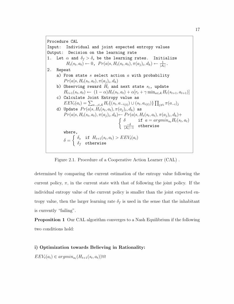
In this section we describe an algorithm (see Figure 2.1) for a rational and con-

vergent cooperative action learner. The basic idea is to vary the learning rate used

by the algorithm so as to accelerate the convergence, without sacrificing rationality.

In this algorithm we have a simple intuition like “learn quickly while predicting the

next state incorrectly”, and “learn slowly while predicting the next state correctly”.

The method used here for determining the prediction accuracy is by comparing the

current policy’s entropy with that of the expected entropy value earned by the coop-

erative action over time. This principle aids in convergence by giving more time for

the other inhabitants to adapt to changes in the inhabitant’s strategy that at first

appear beneficial, while allowing the inhabitant to adapt more quickly to the other

inhabitants’ strategy changes when they are harmful [8]. We use two learning rate

parameters, namely “succeeding” (δs) and “failing” (δf ), where δs < δf . The term

|Ai| denotes the number of available joint actions of i-th inhabitant. The policy is

improved by increasing the probability so that it selects the highest valued action

according to the learning rate. The learning rate used to update the probability de-

pends on whether the inhabitant is currently succeeding (δs) or failing (δf ). This is

17

Procedure CAL

Input: Individual and joint expected entropy values

Output: Decision on the learning rate

1. Let α and δf > δs be the learning rates. Initialize

Ht(st, at)← 0, Pr(a|s,Ht(st, at), π(aj)i, dh)← 1|Ai|

.

2. Repeat

a) From state s select action a with probability

Pr(a|s,Ht(st, at), π(aj)i, dh)b) Observing reward Ht and next state st, update

Ht+1(st, at)← (1− α)Ht(st, at) + α[rt + γmina∈AHt(st+1, at+1)]c) Calculate Joint Entropy value as

EEVt(ai) =∑

a−i∈AHt(st, a−i(t)) ∪ (st, ai(t))

∏j 6=i π(a−i)j

d) Update Pr(a|s,Ht(st, at), π(aj)i, dh) as

Pr(a|s,Ht(st, at), π(aj)i, dh)← Pr(a|s,Ht(st, at), π(aj)i, dh)+δ if a = argminat

Ht(st, at)−δ

|Ai|−1otherwise

where,

δ =

δs if Ht+1(st, at) > EEVt(ai)δf otherwise

Figure 2.1. Procedure of a Cooperative Action Learner (CAL) .

determined by comparing the current estimation of the entropy value following the

current policy, π, in the current state with that of following the joint policy. If the

individual entropy value of the current policy is smaller than the joint expected en-

tropy value, then the larger learning rate δf is used in the sense that the inhabitant

is currently “failing”.

Proposition 1 Our CAL algorithm converges to a Nash Equilibrium if the following

two conditions hold:

i) Optimization towards Believing in Rationality:

EEVt(ai) ∈ argminat(Ht+1(st, at))∀t

18

The joint expected entropy value tends to be one of the candidates of the set of all

optimal entropy values followed by our H-learning process defined previously.

ii) Convergence towards Playing in Believing:

limt→∞ |Ht+1(st, at)− EEVt(ai)| = 0

The difference between the current entropy value following the current policy π in

the current state with that of the joint entropy value tends to 0.

These two properties guarantee that the inhabitant will converge to a stationary

strategy that is optimal given the actions of the other inhabitants. As is standard

in the game theory literature, it is thus reasonable to assume that the opponent is

fully rational and chooses actions that are in its best interest. When all inhabitants

are rational, if they converge, then they must have converged to a Nash equilibrium.

Since all inhabitants converge to a stationary policy, each rational inhabitant must

converge to the best response to the opponent choice of actions. After all, if all

inhabitants are rational and convergent with respect to other inhabitant strategies,

then convergence to a Nash equilibrium is guaranteed [8].

Proposition 2 The learning rate α (0 ≤ α ≤ 1) decrease over time such that it

satisfies∑∞

t=0 α =∞ and∑∞

t=0 α2 ≤ ∞

Proposition 3 Each inhabitant samples each of its actions infinitely often. Thus

probability of inhabitant i choosing action at is nonzero. Hence Pri(at) 6= 0

Proposition 4 The probability of choosing some nonoptimal action in the long run

tends to zero since each inhabitant’s exploration strategy is exploitive.

Hence, limt→∞ Pr(a|s,Ht(st, at), π(aj)i, dh) = 0

Proposition 2 and 3 are required conditions for our Entropy learning algorithm.

They ensure that inhabitants could not adopt deterministic exploration strategies and

19

become strictly correlated. The last proposition states that the inhabitants always

explore their knowledge. This is necessary to ensure that an equilibrium will be

reached.

2.4 Classification and Estimation of the Uncertainty Level

Mahalanobis distance [102] is a very useful way of determining the “similarity”

of a set of values from an unknown sample to a set of values measured from a col-

lection of “known” samples. In our scenario, the entropy values calculated by the

inhabitants once in an individual mode and on the other hand in a cooperative mode

in the smart home environment are correlated to each other. From this perspective

we have used Mahalanobis distance as the basis for our analysis which takes distrib-

ution of the entropy correlations into account compared to the traditional Euclidean

distance. The advantage of using this approach lies in extending the inhabitants to

choose the most efficient route with the minimum entropy value.

To provide the most efficient route to the inhabitants of smart home, we consider

anN -dimensional space of individual Entropy Value Level (EVL) ℘ = [℘1, ℘2, ℘3, ..., ℘N ]

evolved by N different actions at different time instant. In our model, due to coopera-

tive learning among the inhabitants, another set of EVL such as e = [e1, e2, e3, ..., eN ]

could be evolved due to the joint actions of the inhabitants. Thus we have two differ-

ent estimation of the entropy values. One estimation has been done due to individual

action and the other estimation is due to joint actions in a cooperative environment.

Therefore we have two points, ℘ and e, in the N -dimensional space representing two

different EVL “states”.

Let us have two groups, G1 and G2, consisting of different inhabitants distin-

guished by their EVL measures. For example, group G1 may contain inhabitants who

provide route in accordance with EVL, ℘, and group G2 in accordance with e. If we

20

h1

h2

x

(u ,x)1 (u ,x)2

u1

u2

y=x h + x h1 1 22

G1

G2

u u1 - 2

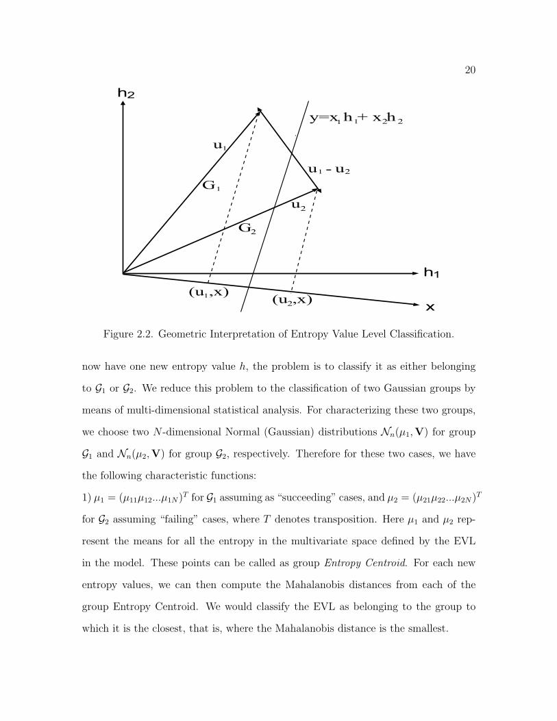
Figure 2.2. Geometric Interpretation of Entropy Value Level Classification.

now have one new entropy value h, the problem is to classify it as either belonging

to G1 or G2. We reduce this problem to the classification of two Gaussian groups by

means of multi-dimensional statistical analysis. For characterizing these two groups,

we choose two N -dimensional Normal (Gaussian) distributions Nn(µ1,V) for group

G1 and Nn(µ2,V) for group G2, respectively. Therefore for these two cases, we have

the following characteristic functions:

1) µ1 = (µ11µ12...µ1N)T for G1 assuming as “succeeding” cases, and µ2 = (µ21µ22...µ2N)T

for G2 assuming “failing” cases, where T denotes transposition. Here µ1 and µ2 rep-

resent the means for all the entropy in the multivariate space defined by the EVL

in the model. These points can be called as group Entropy Centroid. For each new

entropy values, we can then compute the Mahalanobis distances from each of the

group Entropy Centroid. We would classify the EVL as belonging to the group to

which it is the closest, that is, where the Mahalanobis distance is the smallest.

21

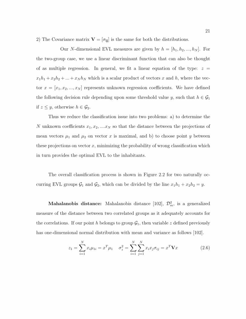
2) The Covariance matrix V = [σij] is the same for both the distributions.

Our N -dimensional EVL measures are given by h = [h1, h2, ..., hN ]. For

the two-group case, we use a linear discriminant function that can also be thought

of as multiple regression. In general, we fit a linear equation of the type: z =

x1h1 + x2h2 + ...+ xNhN which is a scalar product of vectors x and h, where the vec-

tor x = [x1, x2, ..., xN ] represents unknown regression coefficients. We have defined

the following decision rule depending upon some threshold value y, such that h ∈ G1

if z ≤ y, otherwise h ∈ G2.

Thus we reduce the classification issue into two problems: a) to determine the

N unknown coefficients x1, x2, ....xN so that the distance between the projections of

mean vectors µ1 and µ2 on vector x is maximal, and b) to choose point y between

these projections on vector x, minimizing the probability of wrong classification which

in turn provides the optimal EVL to the inhabitants.

The overall classification process is shown in Figure 2.2 for two naturally oc-

curring EVL groups G1 and G2, which can be divided by the line x1h1 + x2h2 = y.

Mahalanobis distance: Mahalanobis distance [102], D2m, is a generalized

measure of the distance between two correlated groups as it adequately accounts for

the correlations. If our point h belongs to group G1, then variable z defined previously

has one-dimensional normal distribution with mean and variance as follows [102].

z1 =N∑

i=1

xiµ1i = xTµ1 σ2z =

N∑

i=1

N∑

j=1

xixjσij = xTVx (2.6)

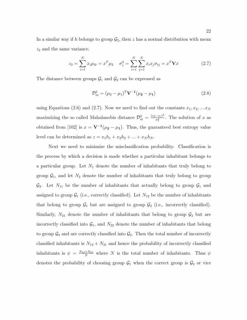
22

In a similar way if h belongs to group G2, then z has a normal distribution with mean

z2 and the same variance.

z2 =N∑

i=1

xiµ2i = xTµ2 σ2z =

N∑

i=1

N∑

j=1

xixjσij = xTVx (2.7)

The distance between groups G1 and G2 can be expressed as

D2m = (µ2 − µ1)

TV−1(µ2 − µ1) (2.8)

using Equations (2.6) and (2.7). Now we need to find out the constants x1, x2, ....xN

maximizing the so called Mahalanobis distance D2m = (z2−z1)2

σ2z

. The solution of x as

obtained from [102] is x = V−1(µ2 − µ1). Thus, the guaranteed best entropy value

level can be determined as z = x1h1 + x2h2 + ...+ xNhN .

Next we need to minimize the misclassification probability. Classification is

the process by which a decision is made whether a particular inhabitant belongs to

a particular group. Let N1 denote the number of inhabitants that truly belong to

group G1, and let N2 denote the number of inhabitants that truly belong to group

G2. Let N11 be the number of inhabitants that actually belong to group G1 and

assigned to group G1 (i.e., correctly classified). Let N12 be the number of inhabitants

that belong to group G1 but are assigned to group G2 (i.e., incorrectly classified).

Similarly, N21 denote the number of inhabitants that belong to group G2 but are

incorrectly classified into G1, and N22 denote the number of inhabitants that belong

to group G2 and are correctly classified into G2. Then the total number of incorrectly

classified inhabitants is N12 + N21 and hence the probability of incorrectly classified

inhabitants is ψ = N12+N21

Nwhere N is the total number of inhabitants. Thus ψ

denotes the probability of choosing group G1 when the correct group is G2 or vice

23

versa. The probability (ψ1) of choosing group G2 when the true one is G1 can be

expressed as [95]

ψ1 = Pr[G2|G1] = Pr[z > y|G1] = 1− Φ(y − z1

σz

) =N12

N(2.9)

where Φ denotes the normal distribution function. Similarly, the probability (ψ2) of

choosing group G1 when the true one is G2 can be expressed as

ψ2 = Pr[G1|G2] = Pr[z ≤ y|G2] = 1− Φ(z2 − yσz

) =N21

N(2.10)

Assuming the threshold value of the entropy value level y as z1+z2

2, the total probability

of misclassification can be expressed as

ψ = ψ1 + ψ2 = Pr[G2|G1] + Pr[G1|G2]

= 1− Φ(y − z1

σz

)+ 1− Φ(z2 − yσz

)

= 21− Φ(z2 − z1

2σz

) = 21− Φ(Dm

2)

= 2Φ(−Dm

2) =

N12 +N21

N(2.11)

2.5 Resource and Comfort Management in Smart Homes

One of the objectives behind the development of smart homes is to provide

the inhabitants with maximum possible comfort at minimum possible energy con-

sumption. However, the inhabitants’ location uncertainty inside the house leads to

uncertainty in their activities and operation of smart indoor appliances. Once this

uncertainty is minimized for the entire set of inhabitants, the house becomes intelli-

gent enough to make more accurate estimations of the inhabitants’ activities and aids

them with smart control of automated devices. The novelty of our approach lies in

the development of mobility-aware resource management framework, which considers

24

multiple inhabitants inside the house. Efficient estimation of most likely locations

and routes used by these set of inhabitants helps in pro-active, automated operations

of smart devices, thus developing an amicable environment inside the house, while

conserving the energy dissipation as much as possible.

2.5.1 Mobility-Aware Energy Conservation

The energy consumption over the entire smart home needs to be optimized for

reducing the maintenance cost. At the same time we need to consider the inhabi-

tant’s comfort by reducing the explicit manual operation and control of smart devices

and appliances. Today’s houses mostly use static energy management scheme, where

a fixed number of devices (electric lights, fans, etc) are kept on for a certain fixed

amount of time. Intuitively, this results in sufficient loss of valuable energy inside

the house. One obvious solution is to manually control these devices while leaving or

entering particular locations inside the house. However, such manual operations are

in the opposite pole of inhabitants’ comfort and automation. Hence, a smart energy

management system needs to be designed that will operate in a proactive fashion

while considering unnecessary wastage of in-house resources. We argue that location

awareness is the key behind such energy management framework. The automated

devices (e.g., lights and fans) operate in a pro-active mode to conserve energy during

the absence of any inhabitant in particular locations inside the house. These de-

vices also attempt to bring the indoor environment in an amicable condition before

the user actually enters into those specific locations. Also, whenever a particular

location/region of the house becomes unoccupied by the inhabitants, the automated

devices are switched off to conserve the energy.

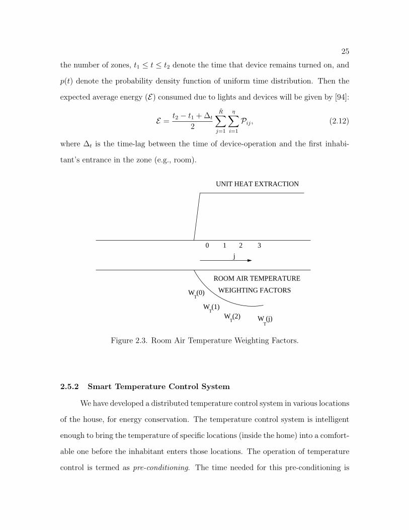
Let Pij denote the power of the i-th device in the j-th zone, η denote the max-

imum number of devices which remained turned on in the particular zone, R denote

25

the number of zones, t1 ≤ t ≤ t2 denote the time that device remains turned on, and

p(t) denote the probability density function of uniform time distribution. Then the

expected average energy (E) consumed due to lights and devices will be given by [94]:

E =t2 − t1 + ∆t

2

R∑

j=1

η∑

i=1

Pij, (2.12)

where ∆t is the time-lag between the time of device-operation and the first inhabi-

tant’s entrance in the zone (e.g., room).

0 1 2 3

W (0)T

T

T

W (1)W (2)

j

TW (j)

UNIT HEAT EXTRACTION

ROOM AIR TEMPERATURE

WEIGHTING FACTORS

Figure 2.3. Room Air Temperature Weighting Factors.

2.5.2 Smart Temperature Control System

We have developed a distributed temperature control system in various locations

of the house, for energy conservation. The temperature control system is intelligent

enough to bring the temperature of specific locations (inside the home) into a comfort-

able one before the inhabitant enters those locations. The operation of temperature

control is termed as pre-conditioning. The time needed for this pre-conditioning is

26

pre-conditioning period and the rate of energy required during this period is known

as pre-conditioning load. When the inhabitant is about to leave a particular loca-

tion, say l1, the predictive location management system estimates its most probable

set of routes and near future location (say l2). The pre-conditioning period (WT ) is

obtained by estimating the time taken by the inhabitant to move from l1 to l2, i.e.,

WT = tl1 − tl2 . During this period, the constant rate of energy at full capacity is sup-

plied to bring down the temperature to the comfort level. The shorter the duration

of pre-conditioning period WT , the larger is the pre-conditioning load. In order to

estimate this load, it is required to know the characteristics of air temperature vari-

ation caused by constant unit rate of heat extraction from the specific locations. As

depicted in Figure 2.3, WT is often termed as room air temperature weighting factors

for unit heat extraction [64]. Modern air-conditioning systems usually express this in

time series, which might be defined as temperature weighting factors for unit heat

extractions. If H(t) and ϕ(t) respectively denote heat extraction and air temperature

deviation at time t, then the relation is:

H(t) =∞∑

j=0

Wz(j)ϕ(t− j), (2.13)

where Wz(j) is known as the weighting factor for heat extraction in the indoor envi-

ronment. In our smart home, we have considered three major components of Wz(j)

responsible for heat exchange, namely walls, glass-windows and furniture. Thus, we

have,

Wz(j) = Wzw(j) +Wzg(j) +Wzf (j)

= −kw∑

i=1

Zw(i, j)Λw(i)

−kg∑

i=1

Zg(i, j)Λg(i)− Cf U , (2.14)

27

where Zw(i, j), Zg(i, j) are respectively Z-response factors [64] for i-th wall and glass

window, Λw(i), Λg(i) are the respective areas of i-th wall and glass window, Cf is the

heat capacity of the furniture and U is the volume of room space. Using the values

of H(t) and ϕ(t), ∀t = 0 to ∞, we can derive a series of equations from Equation

(2.13):

Wz(0)ϕ(0) = 1

Wz(0)ϕ(1) +Wz(1)ϕ(0) = 1

Wz(0)ϕ(2) +Wz(1)ϕ(1) +Wz(2)ϕ(0) = 1

. . . . . . . . . . . . . . . (2.15)

The solutions for ϕ(j) for all j can now be obtained successively from the above set of

equations. The temperature deviation without heat extraction until the occupancy of

the inhabitants in that particular location is calculated first. Let the total tempera-

ture deviation during start of occupancy be represented by ∆(ϕ). Let Hhe(t) denotes

the rate of heat extraction during t hours of pre-conditioning. Then

Hhe(t) =∆(ϕ)

ϕ(t)(2.16)

In the cooling mode, once the air conditioning is stopped (inhabitant’s departure

from specific location of the house), the temperature of that region increases rapidly.

The same mechanism is repeated whenever the inhabitant is about to move into the

specific locations inside the house. The pre-conditioning period is followed by the

conditioned period, when the room temperature is kept constant at a reference level.

2.5.3 Estimation of Inhabitants’ Comfort

While the goal behind the deployment of smart homes lies in providing the

inhabitants with sufficient comfort, this comfort is actually a subjective measure ex-

28

perienced by the inhabitants themselves. Thus, it is quite difficult to objectively

estimate their comfort in smart homes. In-building climate, specifically temperature,

plays an important role in defining this comfort. Moreover, the amount of manual

operations and the time spent by the inhabitants in performing the house-hold ac-

tivities also have significant influence on the inhabitants’ comfort. We define the

comfort as a joint function of temperature, manual operations and time spent by the

inhabitants. Obviously, increase in the temperature-deviation, the number of manual

operations and the amount of time spent reduces the overall comfort experienced by

the inhabitant. If ∆(ϕ), M and τ represent the temperature deviation, number of

manual operations and time an inhabitant spent in house-hold activities, then the

associated comfort for that inhabitant is represented by the following equation:

Comfort = f

(1

∆(ϕ),

1

M ,1

τ

)(2.17)

It should be noted that the reduction of joint entropy by using the co-operative learn-

ing algorithm, described in Figure 2.1, endows the house with sufficient knowledge

of the inhabitants’ contexts. This helps in accurate estimate of current and future

contexts (location, routes and activities) of the multiple inhabitants present in the

house. Successful estimate of these contexts results in adaptive control of environ-

mental conditions and automated operation of devices. This is necessary to reduce

the empirical values of ∆(ϕ),M and τ , thereby increasing the overall comfort.

2.6 Simulation Experiments

In this section, we study the performance of our mobility-aware resource opti-

mization framework for multi-inhabitant smart home. After describing our simulation

environment and assumptions, we present the performance results.

We have developed an object-oriented discrete-event simulation for support-

29

ing inhabitants’ movements, estimation of their locations, and comfort management

scheme. The data used for simulation is obtained from the X10 controller Active-

Home kit [117] deployed in the appliances in the MAVHome [27]. The time spent by

the inhabitant in different locations is obtained from the motion-sensors placed along

the walls. The different events are inhabitants’ actions (behaviors), which result in

the probabilistic movement of one or more inhabitants from one station to another

depending on their lifestyle. An event queue is used for holding and scheduling these

dynamic events. During the inhabitants’ probabilistic movements across the house

from one location to the another, the set of sensor-ids are collected. The inhabitants

are also assumed to follow a different lifestyle in the weekends and holidays, with

more household activities than during the weekdays.

Before presenting the details of the experimental results, let us enumerate a set

of common assumptions used in our simulation: (i) The co-operative, game-theoretic

framework for uncertainty minimization is performed in the smart home with an av-

erage number of 5 regular inhabitants and 3 visitors. (ii) The time spent at each

destination is assumed to be uniformly distributed between the maximum and mini-

mum stay at that particular destination. This maximum stay is different for regular

inhabitants and visitors. (iii) The delay between sensory data-acquisition, processing

and triggering the actuators is assumed to be negligible. (iv) The decision-making

associated with the resource and comfort management is performed as the inhabitants

leave every location for their next station. (v) The entire set of results is presented

by sampling every sensor at a time and observing the simulation environment for a

period of 10 weeks.

30

0 10 20 30 40 50 60 70 800

1

2

3

4

5

6

7

8

9

10

Days

En

tro

py (

Un

cert

ain

ty)

Entropy of Inhabitnat−1Entropy of Inhabitnat−2Entropy of Inhabitnat−3Total Individual EntropyJoint Entropy

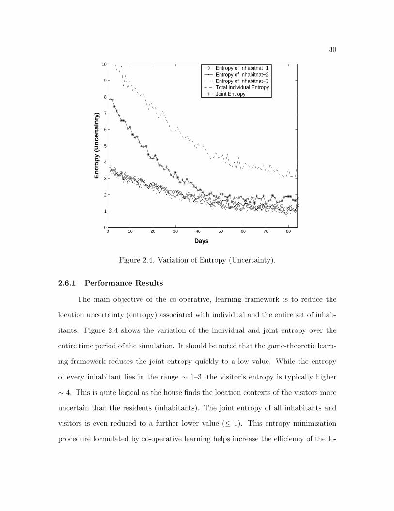
Figure 2.4. Variation of Entropy (Uncertainty).

2.6.1 Performance Results

The main objective of the co-operative, learning framework is to reduce the

location uncertainty (entropy) associated with individual and the entire set of inhab-

itants. Figure 2.4 shows the variation of the individual and joint entropy over the

entire time period of the simulation. It should be noted that the game-theoretic learn-

ing framework reduces the joint entropy quickly to a low value. While the entropy

of every inhabitant lies in the range ∼ 1–3, the visitor’s entropy is typically higher

∼ 4. This is quite logical as the house finds the location contexts of the visitors more

uncertain than the residents (inhabitants). The joint entropy of all inhabitants and

visitors is even reduced to a further lower value (≤ 1). This entropy minimization

procedure formulated by co-operative learning helps increase the efficiency of the lo-

31

0 10 20 30 40 50 60 70 800

10

20

30

40

50

60

70

80

90

100

Days

Pre

dic

tion

Su

cce

ss

Individual Prediction−success of Inhabitnat−1Individual Prediction−success of Inhabitnat−2Individual Prediction−success of Inhabitnat−3Joint Prediction−success

Figure 2.5. Accuracy in Location Estimation.

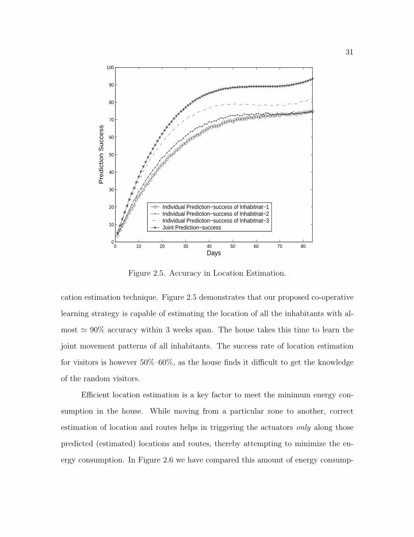
cation estimation technique. Figure 2.5 demonstrates that our proposed co-operative

learning strategy is capable of estimating the location of all the inhabitants with al-

most ' 90% accuracy within 3 weeks span. The house takes this time to learn the

joint movement patterns of all inhabitants. The success rate of location estimation

for visitors is however 50%–60%, as the house finds it difficult to get the knowledge

of the random visitors.

Efficient location estimation is a key factor to meet the minimum energy con-

sumption in the house. While moving from a particular zone to another, correct

estimation of location and routes helps in triggering the actuators only along those

predicted (estimated) locations and routes, thereby attempting to minimize the en-

ergy consumption. In Figure 2.6 we have compared this amount of energy consump-

32

0 10 20 30 40 50 60 70 802

4

6

8

10

12

14

16

18

20

22

Days

Avera

ge E

nerg

y C

on

su

mp

tio

n

Mobility−Aware Energy Plan in Smart HomesStatic Energy Plans in Current HomesOptimal Possible Energy Plan

Figure 2.6. Average Energy Consumption.

tion scheme resulting from our mobility-aware resource management framework with

the static energy plans and observed that our scheme is capable of saving almost 50%

of the energy consumption in comparison with today’s houses, using static energy

model. We believe that this scheme has the power to reduce the maintenance cost

by conserving sufficient amount of energy. As discussed earlier, the comfort of an

individual inhabitant is a subjective quality and is rather difficult to quantify. While

there exists no appropriate model for analyzing this comfort, we rely on measuring

the individual parameters responsible for this comfort. Figure 2.7 points out that suc-

cessful estimation of inhabitants’ routes and locations reduces the manual operations

performed by the inhabitants and the time required for performing those operations.

The scheme results in almost ∼ 12%–17% manual operations and time spent by

33

010

2030

4050

6070

0

50

100

150

200

0

20

40

60

80

100

120

140

160

DaysAverage Manual Operations

Ave

rag

e T

ime

Sp

en

t

Static Energy Plans in Current HomesMobility−Aware Energy Plan in Smart Homes

Figure 2.7. Dynamics of Manual Operations and Time Spent.

the inhabitants in comparison to the current houses using static energy management

scheme.

2.7 Summary

In this chapter, we have developed a novel mobility-aware resource manage-

ment framework for a multi-inhabitant smart home [96]. Characterizing the mobility

of inhabitants as a stationary, ergodic, stochastic process, our framework uses the

information theoretic measure to estimate the uncertainty associated with all the

inhabitants present in the house. A co-operative learning paradigm based on dy-

namic game theory is formulated, which learns and estimates the inhabitants’ loca-

tion (route) profiles by minimizing the overall entropy (uncertainty) associated with

34

it. Automated activation of devices and conservation of energy along these estimated

locations and routes provide the inhabitants with necessary comfort at a near optimal

cost. We believe that this is an integral step toward realization of smart pervasive

computing paradigm. In the next chapter we will focus on multi-inhabitant joint lo-

cation uncertainty problem from non-cooperative point of view using stochastic game

theory.

CHAPTER 3

NON-COOPERATIVE CONTEXT-AWARE RESOURCEMANAGEMENT FRAMEWORK

3.1 Introduction

Advances in smart devices, mobile wireless communications, sensor networks,

pervasive computing, machine learning, middleware and agent technologies, and hu-

man computer interfaces have made the dream of smart environments a reality. Ac-

cording to Cook and Das [22], a “smart environment” is one that is able to au-

tonomously acquire and apply knowledge about its inhabitants and their surround-

ings, and adapt to the inhabitants’ behavior or preferences with the ultimate goal to

improve their experience in that environment. The type of experience that individuals

expect from an environment varies with the individual and the type of environment

considered. This may include the safety of inhabitants, reduction of cost of maintain-

ing the environment, optimization of resources (e.g., energy bills or communication

bandwidth), or task automation. An instance of such an indoor environment is a

smart home (e.g., MavHome1) that perceives the surroundings through sensors and

acts on it with the help of actuators.

An important characteristic of such an intelligent, ubiquitous computing and

communication paradigm lies in the autonomous and pro-active interaction of smart

devices used for tracking inhabitants’ important contexts such as current and near-

future locations as well as activities. “Context awareness” is indeed a key to build a

smart environment and associated applications. For example, the embedded pressure

sensors in the Aware Home [87] capture inhabitants’ footfalls, and the system (i.e.,

1Managing an Adaptive Versatile Home [27]

35

36

smart home) uses these data for position tracking and pedestrian recognition. The

Neural Network House [82], the Intelligent Home [77], the Intelligent House n [57]

and the MavHome [27, 118] projects focus on the development of adaptive control

of home environments by also anticipating the location, routes and activities of the

inhabitants. The Active Badge [45] and Active Bat [46] takes the help of infra-red

and ultrasonic time-of-flight techniques to provide indoor location tracking frame-

work. On the other hand, MIT’s Cricket Location Support System [92] delegates the

responsibility of location reporting to the mobile object itself. RADAR [4], another

RF-based indoor location support system uses signal strength and signal-to-noise ratio

to compute 2-D positioning. Microsoft’s Easy-living and Microsoft Home [72] projects

use real-time 3D cameras to provide stereo-vision positioning capability in an indoor

environment. Intelligent prediction of these contexts helps in efficient triggering of

mobility-aware services.

Now, it is not difficult to understand that an inhabitant’s mobility and activity

create an uncertainty of their locations and hence subsequent activities. In order to

be cognizant of his contexts, the smart home needs to minimize this uncertainty as

captured by Shannon’s entropy measure [26]. An analysis of his daily routine and life

style reveals that there exist some well defined patterns of these contexts. Although

these patterns may change over time, they do not change too frequently and thus can

be learned. This simple observation leads us to assume that the inhabitant’s mobility

or activity is a piece-wise stationary, ergodic, stochastic process with an associated

uncertainty (entropy), as originally hypothesized by Bhattacharya and Das [7] for

personal mobility tracking in wide area wireless cellular networks.

In an earlier work [94], we designed an optimal algorithm for location (activity)

tracking in an indoor smart environment, based on dictionary management and online

learning of the inhabitant’s mobility profile, followed by a predictive location-aware

37

resource management (energy consumption) scheme for a single inhabitant smart

home. However, the presence of multiple inhabitants with dynamically varying pro-

files as well as preferences make such tracking much more challenging. This is due

mainly to the fact that the relevant contexts of multiple inhabitants in the same envi-

ronment are often inherently correlated and inter-dependent on each other. Therefore,

the learning and prediction (decision making) paradigm needs to consider the joint

(simultaneous) location/activity tracking of multiple inhabitants. In another prelim-

inary work [97], we proposed a cooperative entropy learning policy for location-aware

resource management in multi-inhabitant smart homes. This approach adapts to the

uncertainty of multiple inhabitants’ locations and most likely routes, by varying the

learning rate parameters and minimizing the Mahalanobish distance [95]. However,

the complexity of multi-inhabitant location tracking problem was not characterized

which we address in this Chapter [98].

Furthermore, hypothesizing that each inhabitant in a smart home behaves in

such a way as to fulfill his own objectives and maximizes his utility, the residence of

multiple inhabitants with varying preferences might lead to conflicting goals. Thus,

a smart home must be intelligent enough to strike a balance between multiple pref-

erences, eventually attaining an equilibrium state. If each inhabitant is aware of

the situation facing all others, a Nash equilibrium is a combination of determinis-

tic or randomized strategies, one for each inhabitant, from which no inhabitant has

an incentive to unilaterally move away. This motivates us to investigate the multi-

inhabitant location tracking problem from the perspective of stochastic game theory,

where the inhabitants are the players of the game. The goal here is to achieve a Nash

Equilibrium so that the system (i.e., smart home) is able to probabilistically predict

the inhabitants’ locations and activities with sufficient accuracy in spite of possible

correlations.

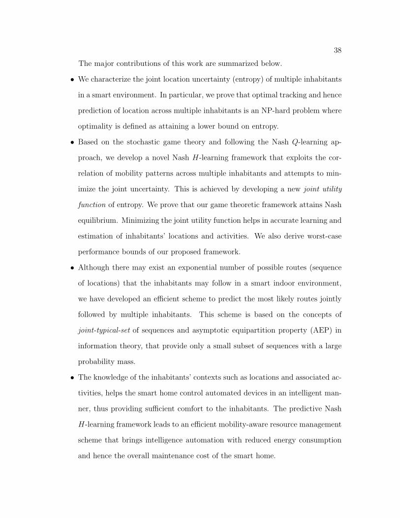
38

The major contributions of this work are summarized below.

• We characterize the joint location uncertainty (entropy) of multiple inhabitants

in a smart environment. In particular, we prove that optimal tracking and hence

prediction of location across multiple inhabitants is an NP-hard problem where

optimality is defined as attaining a lower bound on entropy.

• Based on the stochastic game theory and following the Nash Q-learning ap-

proach, we develop a novel Nash H-learning framework that exploits the cor-

relation of mobility patterns across multiple inhabitants and attempts to min-

imize the joint uncertainty. This is achieved by developing a new joint utility

function of entropy. We prove that our game theoretic framework attains Nash

equilibrium. Minimizing the joint utility function helps in accurate learning and

estimation of inhabitants’ locations and activities. We also derive worst-case

performance bounds of our proposed framework.

• Although there may exist an exponential number of possible routes (sequence

of locations) that the inhabitants may follow in a smart indoor environment,

we have developed an efficient scheme to predict the most likely routes jointly

followed by multiple inhabitants. This scheme is based on the concepts of

joint-typical-set of sequences and asymptotic equipartition property (AEP) in

information theory, that provide only a small subset of sequences with a large

probability mass.

• The knowledge of the inhabitants’ contexts such as locations and associated ac-

tivities, helps the smart home control automated devices in an intelligent man-

ner, thus providing sufficient comfort to the inhabitants. The predictive Nash

H-learning framework leads to an efficient mobility-aware resource management

scheme that brings intelligence automation with reduced energy consumption

and hence the overall maintenance cost of the smart home.

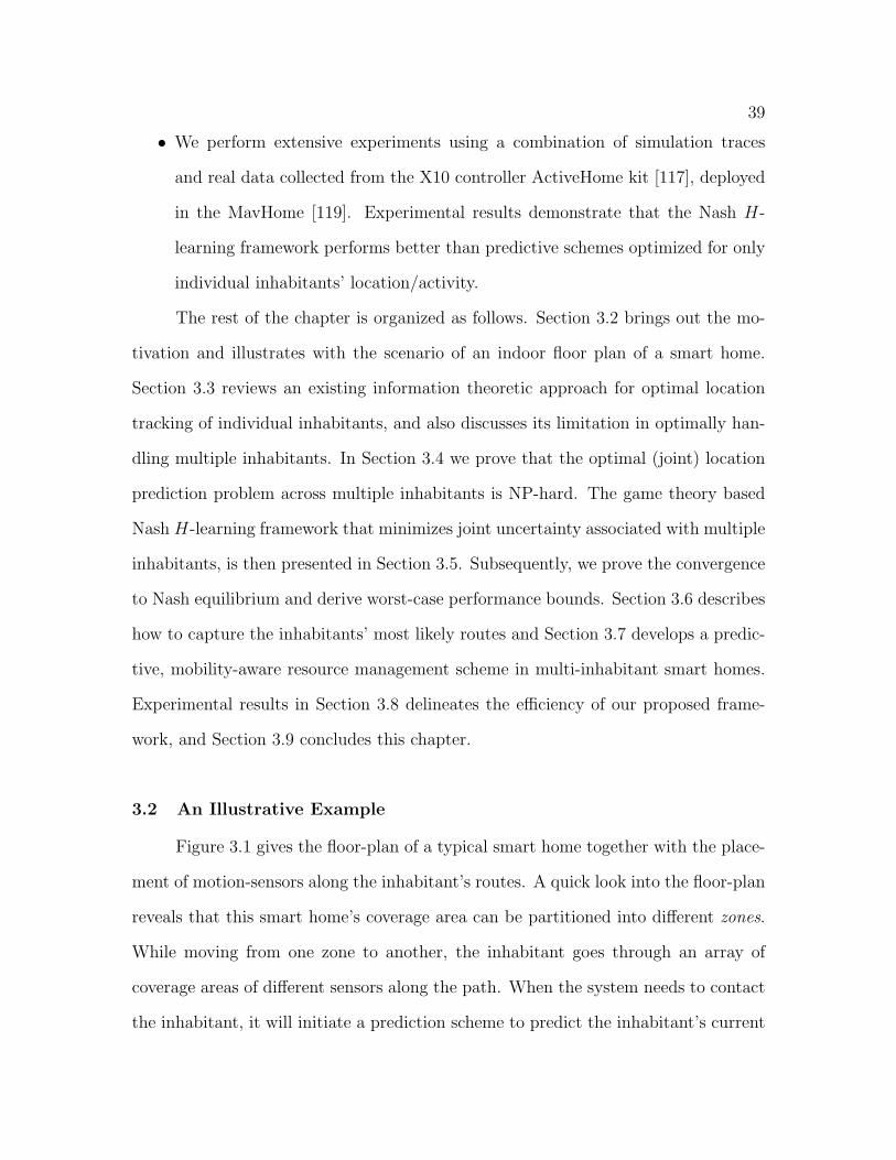
39

• We perform extensive experiments using a combination of simulation traces

and real data collected from the X10 controller ActiveHome kit [117], deployed

in the MavHome [119]. Experimental results demonstrate that the Nash H-

learning framework performs better than predictive schemes optimized for only

individual inhabitants’ location/activity.

The rest of the chapter is organized as follows. Section 3.2 brings out the mo-

tivation and illustrates with the scenario of an indoor floor plan of a smart home.

Section 3.3 reviews an existing information theoretic approach for optimal location

tracking of individual inhabitants, and also discusses its limitation in optimally han-

dling multiple inhabitants. In Section 3.4 we prove that the optimal (joint) location

prediction problem across multiple inhabitants is NP-hard. The game theory based

Nash H-learning framework that minimizes joint uncertainty associated with multiple

inhabitants, is then presented in Section 3.5. Subsequently, we prove the convergence

to Nash equilibrium and derive worst-case performance bounds. Section 3.6 describes

how to capture the inhabitants’ most likely routes and Section 3.7 develops a predic-

tive, mobility-aware resource management scheme in multi-inhabitant smart homes.

Experimental results in Section 3.8 delineates the efficiency of our proposed frame-

work, and Section 3.9 concludes this chapter.

3.2 An Illustrative Example

Figure 3.1 gives the floor-plan of a typical smart home together with the place-

ment of motion-sensors along the inhabitant’s routes. A quick look into the floor-plan

reveals that this smart home’s coverage area can be partitioned into different zones.

While moving from one zone to another, the inhabitant goes through an array of

coverage areas of different sensors along the path. When the system needs to contact

the inhabitant, it will initiate a prediction scheme to predict the inhabitant’s current

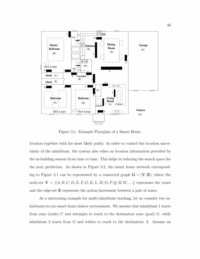
40

! !! !

" " "" " "# # ## # #

$ $$ $$ $$ $$ $$ $$ $

% %% %% %% %% %% %% %

& && && && && && && && &

' '' '' '' '' '' '' '' '

Master

Bedroom

Bedroom Bedroom

Garage

LivingRoom

dw

w d

closet

closet

Outdoor

(C)

(P) (Q)

(R)

(W)

(G)

(O)

(M)

(L)

Kitchen(K)

Dining

Room

(D)

(A)

(B)

o

u

Corridor

(E)

(F)

(Bed−Lamp)

(Bed−Lamp)

r

f

s

m

l

n

k

jih

eg

b a

(Bed−Lamp)

c

d

(Shelf)(Table)

S o f a

T. V.q

t

Figure 3.1. Example Floorplan of a Smart Home.

location together with his most likely paths. In order to control the location uncer-

tainty of the inhabitant, the system also relies on location information provided by

the in-building sensors from time to time. This helps in reducing the search space for

the next prediction. As shown in Figure 3.2, the smart home network correspond-

ing to Figure 3.1 can be represented by a connected graph G = (V,E), where the

node-set V = A,B,C,D,E, F,G,K,L,M,O, P,Q,R,W, . . . represents the zones

and the edge-set E represents the action/movement between a pair of zones.

As a motivating example for multi-inhabitant tracking, let us consider two in-

habitants in our smart home indoor environment. We assume that inhabitant 1 starts

from zone (node) C and attempts to reach to the destination zone (goal) G, while

inhabitant 2 starts from G and wishes to reach to the destination A. Assume an

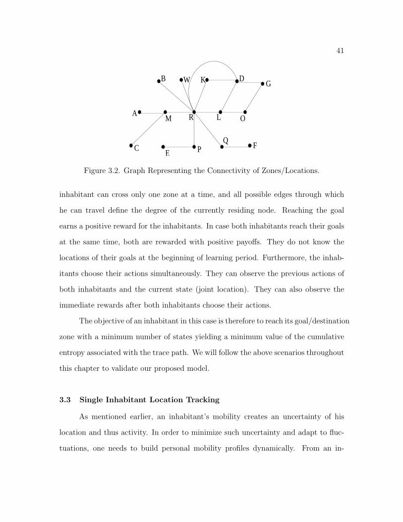
41

R L O

K DGWB

AM

CE P

QF

Figure 3.2. Graph Representing the Connectivity of Zones/Locations.

inhabitant can cross only one zone at a time, and all possible edges through which

he can travel define the degree of the currently residing node. Reaching the goal

earns a positive reward for the inhabitants. In case both inhabitants reach their goals

at the same time, both are rewarded with positive payoffs. They do not know the

locations of their goals at the beginning of learning period. Furthermore, the inhab-

itants choose their actions simultaneously. They can observe the previous actions of

both inhabitants and the current state (joint location). They can also observe the

immediate rewards after both inhabitants choose their actions.

The objective of an inhabitant in this case is therefore to reach its goal/destination

zone with a minimum number of states yielding a minimum value of the cumulative

entropy associated with the trace path. We will follow the above scenarios throughout

this chapter to validate our proposed model.

3.3 Single Inhabitant Location Tracking

As mentioned earlier, an inhabitant’s mobility creates an uncertainty of his

location and thus activity. In order to minimize such uncertainty and adapt to fluc-

tuations, one needs to build personal mobility profiles dynamically. From an in-

42

formation theoretic perspective, entropy [26] is an appropriate measure to quantify

this uncertainty. In the context of personal mobility tracking in cellular wireless net-

works, Bhattacharya and Das [7] proved that it is impossible for any location tracking

scheme to track down an inhabitant by exchanging any less information, on the av-

erage, than the uncertainty generated due to its mobility. A model-independent,

predictive framework based on on-line compression and learning, was also proposed

in [7] that minimizes location uncertainty and meets this information theoretic lower

bound on entropy.

In smart indoor environment, the above framework was adopted in [94] to de-

rive a location prediction scheme that is optimal only for single inhabitants. This

framework is based on symbolic interpretation of the inhabitant’s movement (mobil-

ity) history or profile, as captured by sampling the in-building smart devices such as

sensors, RFID readers, or pressure switches. More precisely, the inhabitant’s move-

ment history is assumed to be a string ν1ν2ν3 . . . of symbols (e.g., sensor-ids) where

νi is an element of the alphabet set, ϑ. Given that our daily life has repetitive ac-

tivity patterns, we argue that the inhabitant’s current location is merely a reflection

of his mobility/activity profile that can be learned over time in an on-line fashion.

Characterizing the mobility as a probabilistic sequence of symbols suggests that it

can be defined as a stochastic process V = Vi. The repetitive nature of identifi-

able patterns (routes) adds piece-wise stationarity as an essential property, leading to

Pr[Vi = νi] = Pr[Vi+` = νi], for all νi ∈ ϑ and for every shift `. The family of optimal

Lempel-Ziv text compression algorithms such as LZ-78 [123] is suitable for efficient

encoding of these variable length routes or contexts (substrings of symbols from the

mobility profile) such that the conditional entropy corresponding to the uncertainty

due to the inhabitant’s mobility is minimized. For details, refer to [7, 94].

43

Before proceeding further, let us formally define entropy and conditional entropy

of random variables of a stochastic process from information theoretic stand point

[26].

Definition 1 For a discrete random variable X of a stochastic process, with probabil-

ity mass function p(x), its entropy is defined as H(X) = −∑x∈X p(x) lg p(x). When

p(x) = 0, the limiting value “ limp→0 p lg p = 0” is used.

Definition 2 For a set V1, V2, . . . , Vk of k discrete random variables with joint

probability distribution p(ν1, . . . , νk) = Pr [V1 = ν1, . . . , Vk = νk], ∀ νi ∈ ϑ, the

joint entropy is given by H(V1, V2, . . . , Vk) =∑k

i=1H(Vi | V1, V2, . . . , Vi−1), where

H(Vi | V1, V2, . . . , Vi−1) is the conditional entropy of random variable Vi given the

history of previous (i− 1) random variables V1, V2, . . . , Vi−1.

The additive terms on the right-hand side of the equation in the above definition

carry necessary information which makes the higher order context models (explained

in the next subsection) more information-rich as compared to the lower order ones.

The above location tracking strategy is optimal for individual inhabitants only.

This is because it treats every inhabitant independently and fails to consider the

correlation between the activity and hence mobility patterns of multiple inhabitants

within the same home environment. Intuitively, independent application of the above

scheme for each individual actually increases the joint location uncertainty. Mathe-

matically, this can be observed from the fact that conditioning reduces entropy [26].

Result 1 For a stochastic ergodic process V containing the set of random variables

V1, V2, . . ., Vk, with distribution Pr(V1 = ν1, V2 = ν2, . . . , Vk = νk),

H(V) = H(V1, V2, . . . , Vk) =k∑

i=1

H(Vi|V1, . . . , Vi−1) ≤k∑

i=1

H(Vi)

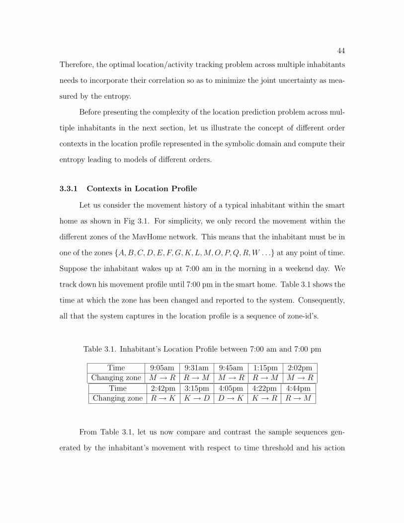
44

Therefore, the optimal location/activity tracking problem across multiple inhabitants

needs to incorporate their correlation so as to minimize the joint uncertainty as mea-

sured by the entropy.

Before presenting the complexity of the location prediction problem across mul-

tiple inhabitants in the next section, let us illustrate the concept of different order

contexts in the location profile represented in the symbolic domain and compute their

entropy leading to models of different orders.

3.3.1 Contexts in Location Profile

Let us consider the movement history of a typical inhabitant within the smart

home as shown in Fig 3.1. For simplicity, we only record the movement within the

different zones of the MavHome network. This means that the inhabitant must be in

one of the zones A,B,C,D,E, F,G,K,L,M,O, P,Q,R,W . . . at any point of time.

Suppose the inhabitant wakes up at 7:00 am in the morning in a weekend day. We

track down his movement profile until 7:00 pm in the smart home. Table 3.1 shows the

time at which the zone has been changed and reported to the system. Consequently,

all that the system captures in the location profile is a sequence of zone-id’s.

Table 3.1. Inhabitant’s Location Profile between 7:00 am and 7:00 pm

Time 9:05am 9:31am 9:45am 1:15pm 2:02pmChanging zone M → R R→M M → R R→M M → R

Time 2:42pm 3:15pm 4:05pm 4:22pm 4:44pmChanging zone R→ K K → D D → K K → R R→M

From Table 3.1, let us now compare and contrast the sample sequences gen-

erated by the inhabitant’s movement with respect to time threshold and his action

45

which is basically the transition from one zone to another. For the time based scheme,

we have considered two values of T , i.e., 1 hr and 1/2 hr. Observe that a smaller

value of T captures finer route granularities of the inhabitant as depicted in Table 3.2.

Regarding the action based scheme, A = 1 captures movement in the finest details

due to its one state transition feature at a time compared to A = 2 where we have

considered the state after a two step transition. A combined approach of time and

action based schemes makes the movement history more informative as it traces in

detail the routes taken by the inhabitant. The last row of Table 3.2 shows the se-

quence which generates with an hourly basis starting from 7:00am in the morning, as

well as when the zone has been changed.

Table 3.2. Zone Sequence Extracted from the Location Profile of the Inhabitant

Time dependent (T = 1hr) MMMRRRRMKDMMM . . .

Time dependent (T = 1/2 hr) MMMMMRRRRRRRRMMRKDDKMMMMM . . .

Action dependent (A = 1) MRMRMRKDKRM . . .

Action dependent ( A = 2) MMMKKM . . .

Time and Action dependent MMMRMRRRRRMMRKKDDKRMMMM . . .

(T = 1hr, A = 1)

The iid (independent and identically distributed) model [7] takes the first step

towards learning from movement history. Unfortunately, the iid model does not carry

any information about the symbols order of appearance and falls short in such situa-

tions which we call order-0 Markov model in our context. The single step transition

or order-1 Markov model carries a little more information about the ordering, at least

to the extent of one symbol context.

In the iid model, where Vi’s are independently and identically distributed, the

relative frequencies of the symbols are listed in Table 3.3. Thus the inhabitant’s

46

Table 3.3. Contexts of Orders 0, 1 and 2 with Occurrence Frequencies

Order-0 Order-1 Order-2M(10) M |M(6) R|K(1) M |MM(3) M |RM(2) M |KR(1)R(8) R|M(3) K|K(1) R|MM(2) R|RM(1) D|KK(1)K(3) M |R(3) D|K(1) M |MR(1) M |RR(1) D|KD(1)D(2) R|R(4) K|D(1) R|MR(1) R|RR(3) R|DK(1)

K|R(1) D|D(1) K|MR(1) K|RK(1) K|DD(1)

residence probabilities are estimated as πM = 10/23, πR = 8/23, πK = 3/23, πD =

2/23, and πA = πB = πC = πE = πP = πW = πL = πO = πG = πQ = πF = 0.

The corresponding entropy value is given by,

H(V) = −∑

ν∈V

p(ν) lg p(ν) = −∑

ν∈V

πν lg πν

=10

23lg

23

10+

8

23lg

23

8+

3

23lg

23

3+

2

23lg

23

2= 1.742bits (3.1)

Similarly, let us compute the entropy value for order-1 Markov model. From

the Markov chain in Figure 3.3, the probability transition matrix is given by

P =

2/3 1/3 0 0

3/8 1/2 1/8 0

0 1/3 1/3 1/3

0 0 1/2 1/2

Let Π = [πM , πR, πK , πD]T be the steady state probability vector. Solving for Π =

Π×P with πM +πR+πK +πD = 1, we obtain πM = 9/22, πR = 4/11, πK = 3/22, πD =

1/11, and πA = πB = πC = πE = πP = πW = πL = πO = πG = πQ = πF = 0.

Therefore, the entropy is given by

H ′(V) = −∑

i

πi

∑

j

Pi,j lg Pi,j

=9

22

(2

3lg

3

2+

1

3lg3

)+

4

11

(3

8lg

8

3+

1

2lg2 +

1

8lg8

)+

3

22

(3× 1

3lg3

)+

1

11

(2× 1

2lg2

)

= 1.194bits (3.2)

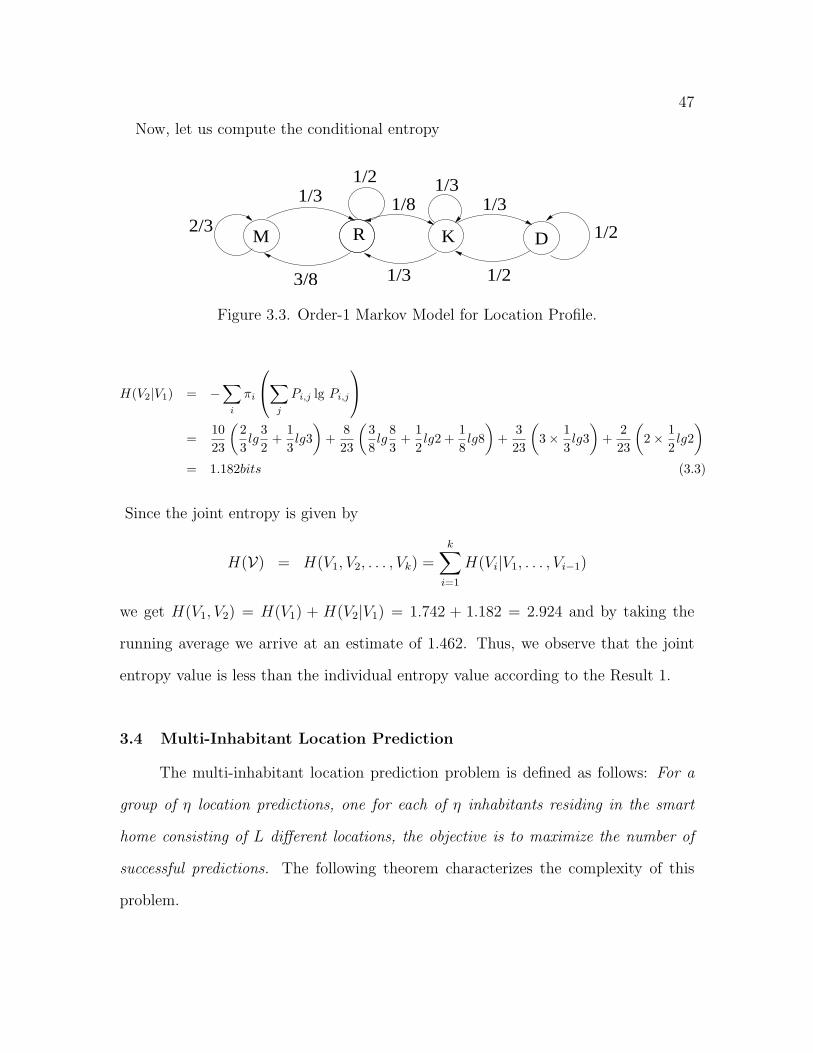
47

Now, let us compute the conditional entropy

2/3

1/3

3/8

1/2

1/8

1/3

1/31/3

1/2

1/2R K DM

Figure 3.3. Order-1 Markov Model for Location Profile.

H(V2|V1) = −∑

i

πi

∑

j

Pi,j lg Pi,j

=10

23

(2

3lg

3

2+

1

3lg3

)+

8

23

(3

8lg

8

3+

1

2lg2 +

1

8lg8

)+

3

23

(3× 1

3lg3

)+

2

23

(2× 1

2lg2

)

= 1.182bits (3.3)

Since the joint entropy is given by

H(V) = H(V1, V2, . . . , Vk) =k∑

i=1

H(Vi|V1, . . . , Vi−1)

we get H(V1, V2) = H(V1) + H(V2|V1) = 1.742 + 1.182 = 2.924 and by taking the

running average we arrive at an estimate of 1.462. Thus, we observe that the joint

entropy value is less than the individual entropy value according to the Result 1.

3.4 Multi-Inhabitant Location Prediction

The multi-inhabitant location prediction problem is defined as follows: For a

group of η location predictions, one for each of η inhabitants residing in the smart

home consisting of L different locations, the objective is to maximize the number of

successful predictions. The following theorem characterizes the complexity of this

problem.

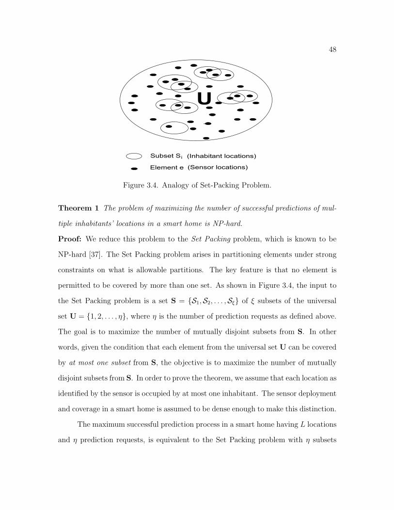
48

Subset S i

Element e

U

(Inhabitant locations)

(Sensor locations)

Figure 3.4. Analogy of Set-Packing Problem.

Theorem 1 The problem of maximizing the number of successful predictions of mul-

tiple inhabitants’ locations in a smart home is NP-hard.

Proof: We reduce this problem to the Set Packing problem, which is known to be

NP-hard [37]. The Set Packing problem arises in partitioning elements under strong

constraints on what is allowable partitions. The key feature is that no element is

permitted to be covered by more than one set. As shown in Figure 3.4, the input to

the Set Packing problem is a set S = S1,S2, . . . ,Sξ of ξ subsets of the universal

set U = 1, 2, . . . , η, where η is the number of prediction requests as defined above.

The goal is to maximize the number of mutually disjoint subsets from S. In other

words, given the condition that each element from the universal set U can be covered

by at most one subset from S, the objective is to maximize the number of mutually

disjoint subsets from S. In order to prove the theorem, we assume that each location as

identified by the sensor is occupied by at most one inhabitant. The sensor deployment

and coverage in a smart home is assumed to be dense enough to make this distinction.

The maximum successful prediction process in a smart home having L locations

and η prediction requests, is equivalent to the Set Packing problem with η subsets

49

and a universal set U of L elements. At any instance of time, an inhabitant i can

actually reside under the coverage of one or more sensors (locations), say li. Then the

prediction process, predicti, for inhabitant i is a collection of its possible locations,

i.e., predicti = li. Every such prediction is mapped to a particular subset Si. Each

single location (sensor coverage-area) of the smart home is mapped to an element of

the subset Si. The strategy that maximizes the number of successful predictions is

basically the one that maximizes the number of disjoint subsets from S. Thus, we

conclude that the multi-inhabitant optimal location prediction is NP-hard. •

Therefore, it is computationally infeasible to find an optimal strategy for max-

imizing the number of successful location predictions across multiple inhabitants. In

the following, we devise a suboptimal solution based on game theory. It attempts to

reach an equilibrium and maximizes the number of successful predictions across all

inhabitants.

3.5 Predictive Nash H-learning Framework

Hypothesizing that every inhabitant wants to satisfy his own preferences about

activities, we assume he behaves like a selfish agent to fulfill his own goals. Under this

circumstance, the objective of the system is to achieve a suitable balance among the

preferences of all inhabitants residing in the smart home. This motivates us to look

into the problem from the perspective of non-cooperative game theory where the in-

habitants are the players and their activities are the strategies of the game. Moreover,

there can be conflicts among the activity preferences. Our proposed game theoretic

framework aims at resolving these conflicts among inhabitants, while predicting their

activities (and hence locations) with as much accuracy as possible. Before going into

50

the details of our framework, let us briefly review the relevant concepts of game theory

required for our purpose.

3.5.1 Stochastic Games and Equilibrium

Stochastic games model multi-agent systems where the agents are the house

and the inhabitants, pursuing their individual (often conflicting) goals. We assume

there exists no enforceable agreement on the joint actions of the inhabitants.

Definition 3 [58] An n-player stochastic game, Γ, is defined as a tuple < S,A1, . . . ,An,

r1, . . . , rn, p >, where S is the state space and Ai is the action space of player i;

rit : S×A1×A2 . . .×An → R is the payoff or reward function for player i at instant

t; p : S ×A1 ×A2 . . .×An → ∆(S) is the transition probability map, where ∆(S) is

the set of probability distributions over the state space S.

Given a state s, the inhabitant agents independently perform their actions

a1, . . . , an, for ai ∈ Ai, and receive rewards rit(s, a

1, . . . , an), for i = 1, . . . , n. The

state s changes to the next state s′ based on transition probabilities, satisfying the

constraint

∑

s,s′∈S

p(s′|a1, . . . , an) = 1

In a stochastic game, the objective of each player is to maximize the sum of

rewards, with factor β ∈ [0, 1). If πi denotes the strategy of player i for choosing the

optimal state action pair , then for a given initial state s, the objective of player i is

to maximize the sum of rewards:

<i(s, π1, π2, . . . , πn) =∞∑

t=0

βtE(r1t |π1, . . . , πn, s0 = s) (3.4)

where E(.) is the expected value.

51

Definition 4 [58] A Nash equilibrium is a joint strategy where each agent is a best

response to the others. For a stochastic game, each agent strategy is defined over the

entire time horizon of the game. Hence, in a stochastic game Γ, a Nash equilibrium

point is a tuple of n strategies (π1∗, π

2∗, . . . , π

n∗ ) such that for all s ∈ S, i = 1, . . . , n

and ∀πi ∈ Πi,

<i(s, π1∗, . . . , π

i∗, . . . π

n∗ ) ≥ <i(s, π1

∗, . . . , πi−1∗ , πi, πi+1

∗ , . . . πn∗ ) (3.5)

where Πi is the set of all strategies available to agent i.

A fundamental result related to equilibria in stochastic games states that every n-

player stochastic game possesses at least one Nash equilibrium point in stationary

strategies [88]. Let us now develop a suitable multi-agent learning framework that

maximizes the number of successful location predictions in smart homes.

3.5.1.1 Representation of Stochastic Games

Considering the previous example, the individual action space of inhabitant i

is given by ai = all possible edges from the current residing node for i = 1, 2.

The individual state space is si = A,B,C,D,E, F,G,K,L,M,O, P,Q,R,W for

i = 1, 2. The joint state space is given by S = (A,B), (A,C), . . . , (W,R) where a

state s′ = (s1 × s2) represents the inhabitants’ joint location.

Instead of calculating the entropy at each and every step, we have considered

three different values of entropy to generate Nash H values from our proposed al-

gorithm. If inhabitant 1 and inhabitant 2 respectively reach their goal/destination

zones, then they achieve the minimum entropy value (assume 0.01 instead of 0 for our

calculation purpose). Here we define the reward (rit) function as inversely proportional

to this entropy value. Thus in this case , rit = 100.

52

If they would come into the same state, we consider the entropy as 1.0 and

added a penalty factor with the reward function for accelerating the convergence

towards the goal. Therefore, rit = −1.

If they appear in any other distinct zones than the destination, then we assume

entropy achieves a higher value and reward (rit) becomes 0.

So, if an inhabitant reaches the goal state, it receives a reward of 100. If it

reaches another state without colliding with the other inhabitant, its reward is zero.

If it collides with the other inhabitant, it receives−1 and both inhabitants are bounced

back to their previous states. Let s′ = `(s, a) be the potential new state resulting

from choosing action a in state s. The reward function is, for i = 1, 2, is defined as

rit =

100, if `(sit, a

it) = Goali

−1, if `(s1t , a

1t ) = `(s2

t , a2t ) and `(s2

t , a2t ) 6= Goalj, j = 1, 2

0, otherwise

(3.6)

3.5.2 Entropy (or H) Learning

The concept for general-sum games builds from the Nash equilibrium [83], in

which each player effectively holds a correct expectation (generally expressed in terms

of payoff, reward or utility value) about the other players behaviors, and acts ratio-

nally with respect to this expectation. Acting rationally means the agent follows the

strategy which corresponds to a best response to the others’ strategies. Any devi-

ation would make that agent worse off from achieving that equilibrium point. In

extending the Q-learning [58] to our multi-inhabitant smart home context aware re-

source management problem we adopt the basic framework of general sum stochastic

games. In single-agent systems, the concept of optimal Q-value can be defined in

terms of an agent maximizing its own expected payoffs with respect to a stochastic

environment. In multiagent systems, Q-values are contingent on other agents strate-

53

gies. In the framework of general-sum stochastic games, the optimal Q-values are

the subset of the Q-values received in a Nash equilibrium, and referred as Nash Q-

values. The goal of learning is to find Nash Q-values through repeated game. Based

on learned Q-values, the agent can then derive the Nash equilibrium and choose its

actions accordingly. In Nash Q-learning [58] algorithm, the agent attempts to learn

its equilibrium Q-values, starting from an arbitrary guess. Thus here the Nash Q-

learning agent maintains a model of other agents Q-values and uses that information

to update its own Q-values based on the payoff value and takes their equilibrium

actions in each state.

Our proposed Nash H-learning algorithm in this section enhanced the Nash

Q-learning algorithm in that it captures the location uncertainty in terms of entropy

at each and every step of the inhabitants’ path. Thus, in our case, Nash H-value

is determined which satisfies both Nash condition as well as our imposed entropy

minimization constraint.

We assume that the inhabitants are fully rational in the sense that they can

fully use their location histories to construct future routes. Each inhabitant i keeps

a count Cja representing the number of times an inhabitant j has followed an action

a ∈ A. When the game is encountered, inhabitant i believes the relative frequencies

of each of j,s movements as indicative of j,s current route. So for each inhabitant j,

the inhabitant i believes j plays action a ∈ A with probability:

P(a)i =Cj

a∑b∈A Cj

b

(3.7)

This set of route strategies forms a reduced profile of strategies for which in-

habitant i adopts a best response. After the game, inhabitant i updates its possible

belief of its neighbor appropriately, given the actions used by other inhabitants. We

consider these counts as reflecting the observations an inhabitant has regarding the

54

route strategy of the other inhabitants. As a result, the decision making component

should not directly repeat the actions of the inhabitants but rather learn to perform

actions that optimize a given reward (or utility) function.

Indeed, the decision making component of a smart home applies learning to

acquire a policy that optimizes joint uncertainty of the inhabitants’ activities which

in turn helps in accurate prediction of their activities and thus locations. For this op-

timization, our proposed entropy learning algorithm, called Nash H-learning (NHL),

learns a value function that maps the state-action pairs to future reward using the

entropy measure, H. It combines new experience with old value functions to pro-

duce new and statistically improved value functions. The proposed multi-agent Nash

H-learning algorithm updates with future Nash equilibrium payoffs.

Procedure NHL

Input: Individual entropy values

Output: Joint entropy values

1. Let the learning agent be indexed by i;

2. t := 0, Hjt (s, a

1, . . . , an) := 0, ∀s ∈ S and aj ∈ Aj, j = 1, . . . , n;3. Repeat

4. Choose action ait;

5. Compute r1t , . . . , r

nt , a1

t , . . . , ant and st+1 = s′;

6. for (j = 1, . . . , n),

7. Hjt+1(s, a

1, . . . , an) = (1− αt)Hjt (s, a

1, . . . , an) + αt

[rjt + βNashHj

t (s′)],

where αt ∈ (0, 1) is the learning rate

and NashHjt (s

′) =∏n

k=1 πk(s′)Hj

t (s′)

8. t := t+ 1;9. until (true)

Figure 3.5. Nash H Learning Algorithm (NHL).

Figure 4.4 describes the pseudo-code of the Nash H-learning algorithm which

has been explained next with a reference to each line number of the algorithm. (1.&2.)

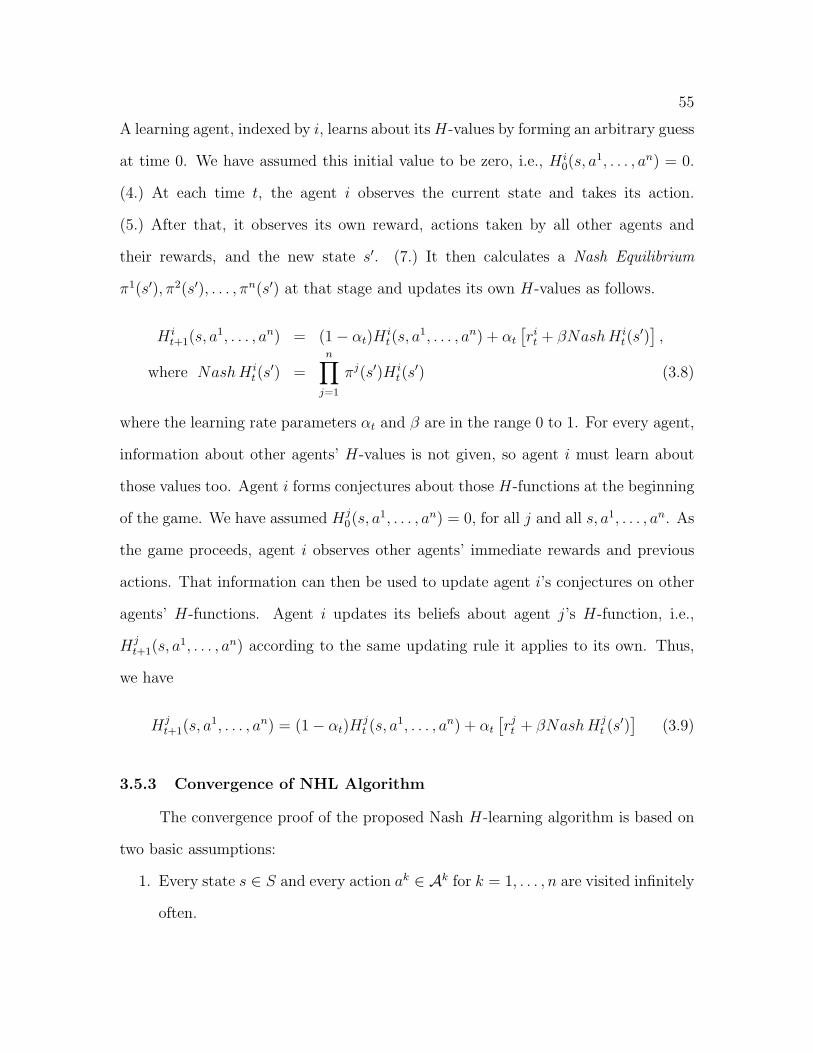
55

A learning agent, indexed by i, learns about itsH-values by forming an arbitrary guess

at time 0. We have assumed this initial value to be zero, i.e., H i0(s, a

1, . . . , an) = 0.

(4.) At each time t, the agent i observes the current state and takes its action.

(5.) After that, it observes its own reward, actions taken by all other agents and

their rewards, and the new state s′. (7.) It then calculates a Nash Equilibrium

π1(s′), π2(s′), . . . , πn(s′) at that stage and updates its own H-values as follows.

H it+1(s, a

1, . . . , an) = (1− αt)Hit(s, a

1, . . . , an) + αt

[rit + βNashH i

t(s′)],

where NashH it(s

′) =n∏

j=1

πj(s′)H it(s

′) (3.8)

where the learning rate parameters αt and β are in the range 0 to 1. For every agent,

information about other agents’ H-values is not given, so agent i must learn about

those values too. Agent i forms conjectures about those H-functions at the beginning

of the game. We have assumed Hj0(s, a

1, . . . , an) = 0, for all j and all s, a1, . . . , an. As

the game proceeds, agent i observes other agents’ immediate rewards and previous

actions. That information can then be used to update agent i’s conjectures on other

agents’ H-functions. Agent i updates its beliefs about agent j’s H-function, i.e.,

Hjt+1(s, a

1, . . . , an) according to the same updating rule it applies to its own. Thus,

we have

Hjt+1(s, a

1, . . . , an) = (1− αt)Hjt (s, a

1, . . . , an) + αt

[rjt + βNashHj

t (s′)]

(3.9)

3.5.3 Convergence of NHL Algorithm

The convergence proof of the proposed Nash H-learning algorithm is based on

two basic assumptions:

1. Every state s ∈ S and every action ak ∈ Ak for k = 1, . . . , n are visited infinitely

often.

56

2. The learning rate αt satisfies the following condition: 0 ≤ αt(s, a1, . . . , an) < 1,

and αt(s, a1, . . . , an) = 0 if (s, a1, . . . , an) 6= (st, a

1t , . . . , a

nt ). In other words, the

updates occur only on H-function elements which correspond to current state

st and actions a1t , . . . , a

nt .

Our proof relies on the following result, which establishes the convergence of a general

functional-learning process updated by a pseudo-contraction operator. Let U be the

space of all utility functions.

Result 2 [58]: Let there exists a number γ such that 0 < γ < 1 and a sequence

λt ≥ 0 converging to zero with probability 1 such that |PtU − PtU∗| ≤ γ|U − U∗|+ λt

for all U ∈ U and U∗E[PtU∗]. Then the following condition holds:

Pr [(Ut+1 = (1− αt)Ut + αt[PtUt])→ U∗] = 1 (3.10)

where Pt is a pseudo-contraction operator. In other words, we can say that the itera-

tive utility function Ut converges to the Nash Equilibrium U∗ with probability 1.

Replacing the general utility function U by the entropy or H function corresponding

to H-learning, we get

Pr [(Ht+1 = (1− αt)Ht + αt[PtHt])→ H∗] = 1.

For our n-player stochastic game we define the operator Pt as:

PtHk(s, a1, . . . , an) = rk

t (s, a1, . . . , an) + βπ1(s′) . . . πn(s′)Hk(s′), for k = 1, . . . , n

(3.11)

where s′ is the state at time t+1 and πk(s′) is an equilibrium strategy at that stage of

the game corresponding to the utility function Hk(s′). We now state the main result

along with its proof:

Result 3 For n-player stochastic game in smart homes, E[PtH∗] = H∗ = (H1∗ , . . . , H

n∗ )

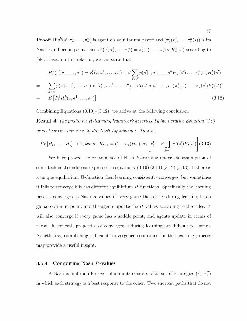
57

Proof: If vk(s′, π1∗, . . . , π

n∗ ) is agent k’s equilibrium payoff and (π1

∗(s), . . . , πn∗ (s)) is its

Nash Equilibrium point, then vk(s′, π1∗, . . . , π

n∗ ) = π1

∗(s), . . . , πn∗ (s)Hk

∗ (s′) according to

[58]. Based on this relation, we can state that

Hk∗ (s′, a1, . . . , an) = rk

t (s, a1, . . . , an) + β

∑

s′∈S

p(s′|s, a1, . . . , an)π1∗(s

′) . . . , πn∗ (s′)Hk

∗ (s′)

=∑

s′∈S

p(s′|s, a1, . . . , an)×[rkt (s, a

1, . . . , an) + βp(s′|s, a1, . . . , an)π1∗(s

′) . . . , πn∗ (s′)Hk

∗ (s′)]

= E[P k

t Hk∗ (s, a1, . . . , an)

](3.12)

Combining Equations (3.10)–(3.12), we arrive at the following conclusion:

Result 4 The predictive H-learning framework described by the iterative Equation (3.9)

almost surely converges to the Nash Equilibrium. That is,

Pr [Ht+1 → H∗]→ 1,where Ht+1 = (1− αt)Ht + αt

[rkt + β

n∏

j=1

πj(s′)Ht(s′)

](3.13)

We have proved the convergence of Nash H-learning under the assumption of

some technical conditions expressed in equations (3.10) (3.11) (3.12) (3.13). If there is

a unique equilibrium H-function then learning consistently converges, but sometimes

it fails to converge if it has different equilibrium H-functions. Specifically the learning

process converges to Nash H-values if every game that arises during learning has a

global optimum point, and the agents update the H-values according to the rules. It

will also converge if every game has a saddle point, and agents update in terms of

these. In general, properties of convergence during learning are difficult to ensure.

Nonetheless, establishing sufficient convergence conditions for this learning process

may provide a useful insight.

3.5.4 Computing Nash H-values

A Nash equilibrium for two inhabitants consists of a pair of strategies (π1∗, π

2∗)

in which each strategy is a best response to the other. Two shortest paths that do not

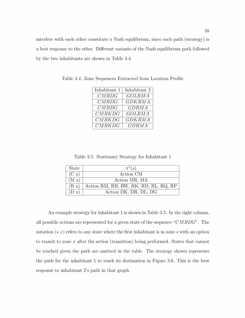
58

interfere with each other constitute a Nash equilibrium, since each path (strategy) is

a best response to the other. Different variants of the Nash equilibrium path followed

by the two inhabitants are shown in Table 3.4.

Table 3.4. Zone Sequences Extracted from Location Profile

Inhabitant 1 Inhabitant 2CMRDG GOLRMACMRDG GDKRMACMRDG GDRMACMRKDG GOLRMACMRKDG GDKRMACMRKDG GDRMA

Table 3.5. Stationary Strategy for Inhabitant 1

State π1(s)(C x) Action CM(M x) Action MR, MA(R x) Action RM, RB, RW, RK, RD, RL, RQ, RP(D x) Action DK, DR, DL, DG

An example strategy for inhabitant 1 is shown in Table 3.5. In the right column,

all possible actions are represented for a given state of the sequence “CMRDG”. The

notation (s x) refers to any state where the first inhabitant is in zone s with an option

to transit to zone x after the action (transition) being performed. States that cannot

be reached given the path are omitted in the table. The strategy shown represents

the path for the inhabitant 1 to reach its destination in Figure 3.6. This is the best

response to inhabitant 2’s path in that graph.

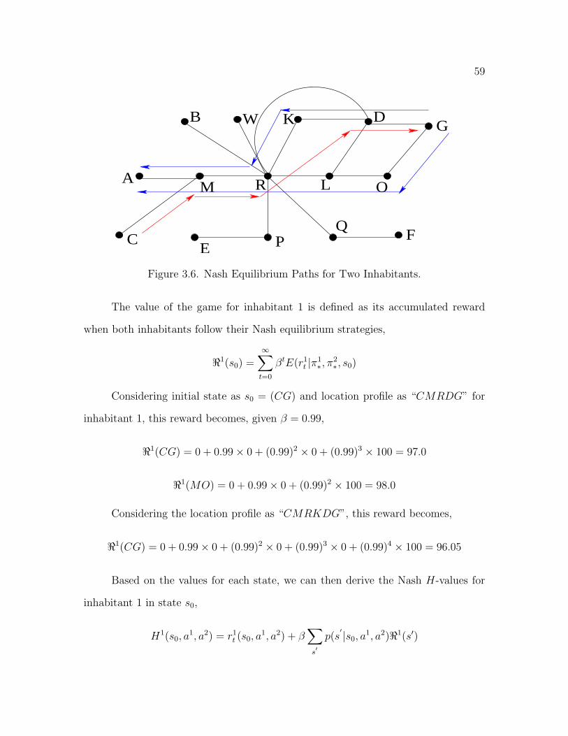
59

R L O

K DGWB

AM

CE P

QF

Figure 3.6. Nash Equilibrium Paths for Two Inhabitants.

The value of the game for inhabitant 1 is defined as its accumulated reward

when both inhabitants follow their Nash equilibrium strategies,

<1(s0) =∞∑

t=0

βtE(r1t |π1

∗, π2∗, s0)

Considering initial state as s0 = (CG) and location profile as “CMRDG” for

inhabitant 1, this reward becomes, given β = 0.99,

<1(CG) = 0 + 0.99× 0 + (0.99)2 × 0 + (0.99)3 × 100 = 97.0

<1(MO) = 0 + 0.99× 0 + (0.99)2 × 100 = 98.0

Considering the location profile as “CMRKDG”, this reward becomes,

<1(CG) = 0 + 0.99× 0 + (0.99)2 × 0 + (0.99)3 × 0 + (0.99)4 × 100 = 96.05

Based on the values for each state, we can then derive the Nash H-values for

inhabitant 1 in state s0,

H1(s0, a1, a2) = r1

t (s0, a1, a2) + β

∑

s′

p(s′|s0, a

1, a2)<1(s′)

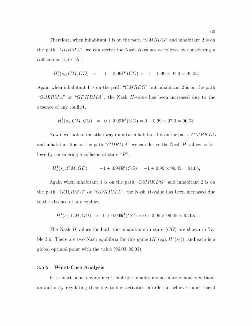
60

Therefore, when inhabitant 1 is on the path “CMRDG” and inhabitant 2 is on

the path “GDRMA”, we can derive the Nash H-values as follows by considering a

collision at state “R”,

H1∗ (s0, CM,GD) = −1 + 0.99<1(CG) = −1 + 0.99× 97.0 = 95.03,

Again when inhabitant 1 is on the path “CMRDG” but inhabitant 2 is on the path

“GOLRMA” or “GDKRMA”, the Nash H-value has been increased due to the

absence of any conflict,

H1∗ (s0, CM,GO) = 0 + 0.99<1(CG) = 0 + 0.99× 97.0 = 96.03.

Now if we look to the other way round as inhabitant 1 is on the path “CMRKDG”

and inhabitant 2 is on the path “GDRMA” we can derive the Nash H-values as fol-

lows by considering a collision at state “R”,

H1∗ (s0, CM,GD) = −1 + 0.99<1(CG) = −1 + 0.99× 96.05 = 94.08,

Again when inhabitant 1 is on the path “CMRKDG” and inhabitant 2 is on

the path “GOLRMA” or “GDKRMA”, the Nash H-value has been increased due

to the absence of any conflict,

H1∗ (s0, CM,GO) = 0 + 0.99<1(CG) = 0 + 0.99× 96.05 = 95.08.

The Nash H-values for both the inhabitants in state (CG) are shown in Ta-

ble 3.6. There are two Nash equilibria for this game (H1(s0), H2(s0)), and each is a

global optimal point with the value (96.03, 96.03).

3.5.5 Worst-Case Analysis

In a smart home environment, multiple inhabitants act autonomously without

an authority regulating their day-to-day activities in order to achieve some “social

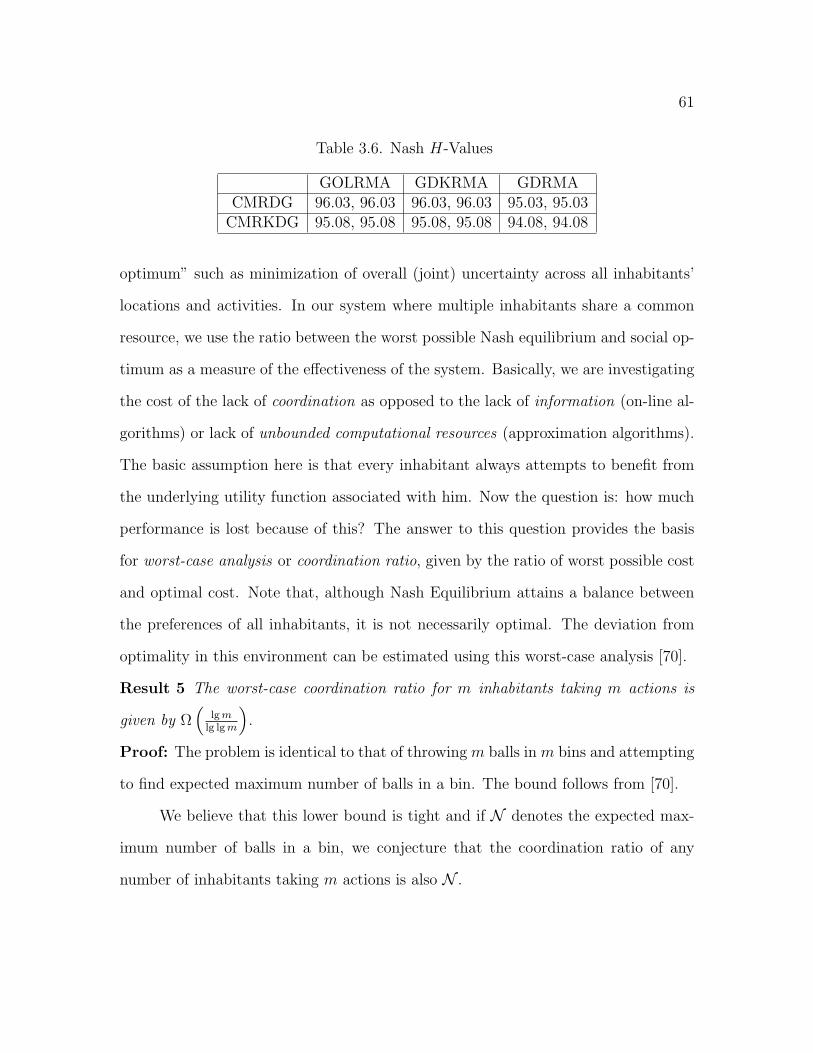
61

Table 3.6. Nash H-Values

GOLRMA GDKRMA GDRMACMRDG 96.03, 96.03 96.03, 96.03 95.03, 95.03

CMRKDG 95.08, 95.08 95.08, 95.08 94.08, 94.08

optimum” such as minimization of overall (joint) uncertainty across all inhabitants’

locations and activities. In our system where multiple inhabitants share a common

resource, we use the ratio between the worst possible Nash equilibrium and social op-

timum as a measure of the effectiveness of the system. Basically, we are investigating

the cost of the lack of coordination as opposed to the lack of information (on-line al-

gorithms) or lack of unbounded computational resources (approximation algorithms).

The basic assumption here is that every inhabitant always attempts to benefit from

the underlying utility function associated with him. Now the question is: how much

performance is lost because of this? The answer to this question provides the basis

for worst-case analysis or coordination ratio, given by the ratio of worst possible cost

and optimal cost. Note that, although Nash Equilibrium attains a balance between

the preferences of all inhabitants, it is not necessarily optimal. The deviation from

optimality in this environment can be estimated using this worst-case analysis [70].

Result 5 The worst-case coordination ratio for m inhabitants taking m actions is

given by Ω(

lg mlg lg m

).

Proof: The problem is identical to that of throwing m balls in m bins and attempting

to find expected maximum number of balls in a bin. The bound follows from [70].

We believe that this lower bound is tight and if N denotes the expected max-

imum number of balls in a bin, we conjecture that the coordination ratio of any

number of inhabitants taking m actions is also N .

62

Theorem 2 The coordination ratio of any number of inhabitants with m actions is

at most N = 3 +√

4m lgm.

Proof: A quantity associated with an equilibrium in our context is the expected

entropy over all actions for a specific route. From this perspective, inhabitant i

maintains beliefs about the strategy of other inhabitants and predicts the Expected

Entropy Value (EEV ) of its individual action ai at (t+ 1)-th time step as follows:

EEV it+1(a

i) =∑

a−i∈A

H it+1(s, a1, . . . , an) ∪ (s, a−1, . . . , a−n)

∏

j 6=i

P(a−i)j (3.14)

We call it the Nash equilibria cost which we wish to compare with the social optimum

entropy, Ψ. More precisely, we want to estimate the coordination ratio as the worst

case ratio, C = maxNash equilibria cost / Ψ where the maximum is taken over

all equilibria. Computing the social optimum (Ψ) is an NP-hard problem (equivalent

to the partition problem, see Theorem 1). However, for the purpose of upper bounding

C, it suffices to use simple approximations: Ψ ≥ maxH it+1(s, a

1, . . . , an), EEV it+1(a

i)/n

Using a martingale concentration bound known as the Azuma-Hoeffding in-

equality 2 [41], we will show that the utility (entropy) of a given action aj exceeds

(N − 1)Ψ with probability at most 1m2 . Then, the probability that the maximum

utility on all actions does not exceed (N − 1)Ψ is at least 1m

. It follows that the

expected maximum utility is bounded by (1 − 1m

)(N − 1)Ψ + 1m

(mΨ) ≤ NΨ. It

remains to show the probability that the utility of a given action aj exceeds (N −1)Ψ

is indeed small, at most 1m2 .

Let Xi be a random variable denoting the contribution of inhabitant i towards

the utility of action aj. In particular, Pr[Xi = H1] = P and Pr[Xi = 0] = 1 − P.

2Azuma-Hoeffding inequality: Suppose that for each i ≥ 0 there exist real numbers ai and

bi such that P (Yi ∈ [ai, bi]) = 1. Then for any ε ≥ 0 we have P [Sn − E(Sn) ≥ nε] ≤

exp(−2n2ε2 /

∑n−1

i=0(bi − ai)

2

)

63

Clearly, the random variables X1, . . . , Xn are independent. We are interested in es-

timating the probability Pr[∑Xi ≥ (N − 1)Ψ]. Since the entropy Ht+1 and prob-

abilities P may vary a lot, we do not expect the sum∑Xi to exhibit the good

concentration bounds of sum of binomial variables. However, we can get a weaker

bound using Azuma-Hoeffding inequality which gives very good results for probabil-

ities around 0.5. In our case, the probabilities are either 0 or 1.

Let µi = E[Xi] and consider the martingale St = X1 + . . .+Xt +µt+1 + . . .+µn.

Now notice that | St+1 − St |= |Xt+1 − µt+1 |≤ Ht+1. We can then apply the Azuma-

Hoeffding’s inequality:

P [Sn − E(Sn) ≥ x] ≤ exp(−x2

2/∑

i

H it+1

2)

Let x = (N −3)Ψ. Since E(Sn) =∑µi = EEV i

t+1(ai) ≤ 2Ψ, we get that the entropy

of action aj exceeds (N − 1)Ψ with probability at most exp(−x2

2/∑

iHit+1

2). It is

easy to establish that

∑

i

H it+1

2 ≤ maxmH21 ,m(

∑

i

H it+1/m)2 ≤ mΨ2

Thus, the probability that the entropy of action aj exceeds (N − 1)Ψ is at most

exp(−12(N − 3)2/m). For N = 3+

√4m lgm, this probability becomes 1/m2 and the

proof is complete [70].

3.6 Inhabitants’ Joint-Typical Routes

The collection of indoor locations inside the smart homes actually forms the

routes (paths) of the inhabitants. Although there may be an exponential number of

possible routes in general, in the long run the inhabitants typically follow only a small

subset of them according to the mobility profiles. The concepts of jointly-typical set

and asymptotic equipartition property (AEP) [26] in information theory help us derive

this small subset of highly probable routes maintained by a particular inhabitant.

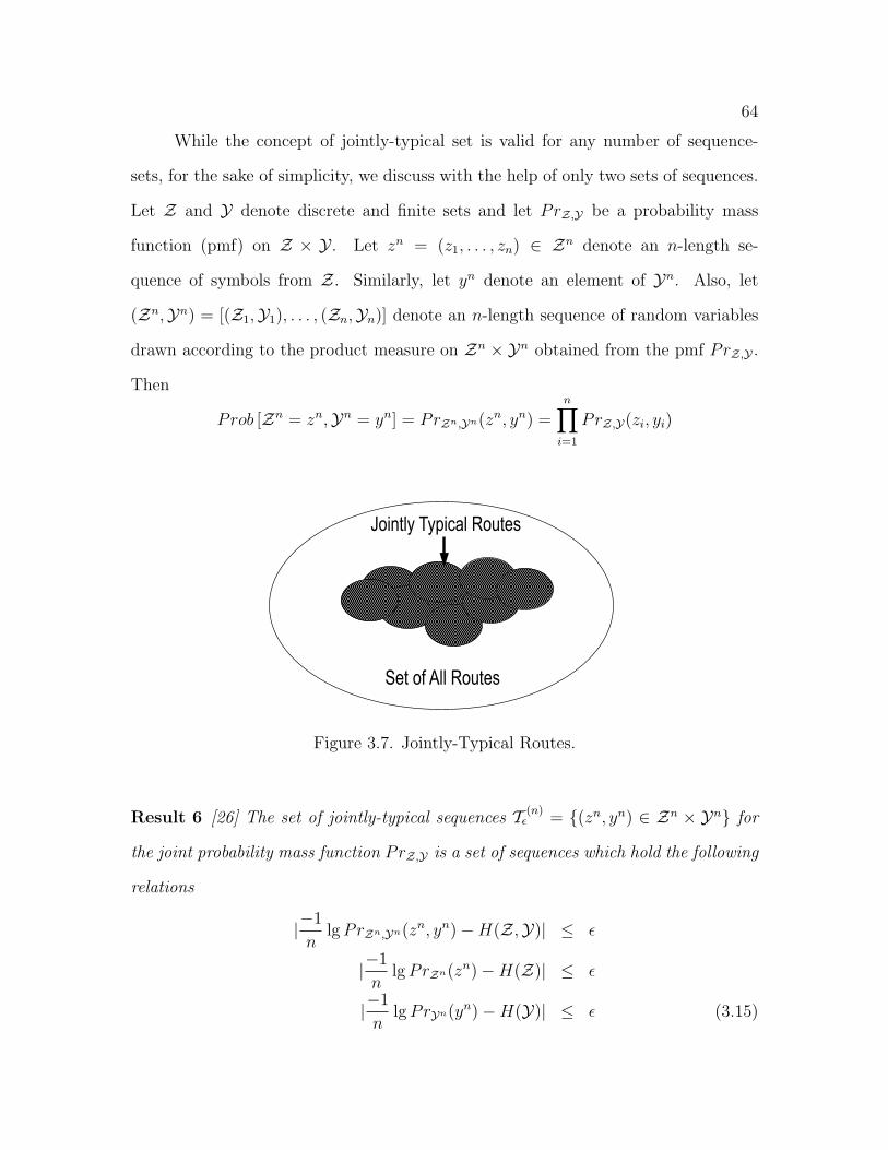
64

While the concept of jointly-typical set is valid for any number of sequence-

sets, for the sake of simplicity, we discuss with the help of only two sets of sequences.

Let Z and Y denote discrete and finite sets and let PrZ,Y be a probability mass

function (pmf) on Z × Y . Let zn = (z1, . . . , zn) ∈ Zn denote an n-length se-

quence of symbols from Z. Similarly, let yn denote an element of Yn. Also, let

(Zn,Yn) = [(Z1,Y1), . . . , (Zn,Yn)] denote an n-length sequence of random variables

drawn according to the product measure on Zn × Yn obtained from the pmf PrZ,Y .

Then

Prob [Zn = zn,Yn = yn] = PrZn,Yn(zn, yn) =n∏

i=1

PrZ,Y(zi, yi)

Jointly Typical Routes

Set of All Routes

Figure 3.7. Jointly-Typical Routes.

Result 6 [26] The set of jointly-typical sequences T (n)ε = (zn, yn) ∈ Zn × Yn for

the joint probability mass function PrZ,Y is a set of sequences which hold the following

relations

|−1

nlgPrZn,Yn(zn, yn)−H(Z,Y)| ≤ ε

|−1

nlgPrZn(zn)−H(Z)| ≤ ε

|−1

nlgPrYn(yn)−H(Y)| ≤ ε (3.15)

65

As shown in Figure 3.7, the most important feature of the jointly-typical set is that it

is sufficiently small and contains most of the probability mass of the set of sequences,

i.e., Pr[(Zn,Yn) ∈ T (n)ε ] → 1. This is basically the AEP for stationary ergodic

process [26]. This encompasses the inhabitant’s most likely routes and determines

the average nature of the large route-sequences.

Result 7 [26] AEP assures that that asymptotically almost all the probability mass is

concentrated in the jointly-typical set. This encompasses the inhabitants’ most likely

activities and paths and determines the average nature of the large route-sequences.

Formally, for fixed ε > 0, as n→∞,

Pr[(Zn,Yn) ∈ T (n)

ε

]→ 1 (3.16)

If Pr[φ1, φ2] denotes the joint probability of the two inhabitants’ contexts (routes)

Y and Z, each of length L(φ), their probabilistic difference is computed as: δ =

|Pr[φ1, φ2]− 2−L(φ)H(Z,Y)|. Clearly, δ provides the gap between the ideal probability

of typical routes and the probability of a particular route stored in the dictionary.

Choosing a higher value of δ leads to the inclusion of a large number of typical

mobility profiles and the framework starts deviating from the typical-set of routes. In

our experiments, we have used δ ≤ 0.01. Thus, the system captures a typical set of

inhabitant’s movement profiles from the H-learning scheme and uses them to predict

the inhabitants’ most likely routes.

To clarify the concept of jointly-typical set, we consider the following two se-

quences from Figure 3.6: CMRDG for Inhabitant 1 and GOLRMA or GDKRMA

Inhabitant 2, which correspond to a Nash equilibrium path. Now the joint se-

quence generated by both the inhabitants is given by C,G,M,O,R, L,D,R,G,M,A

or C,G,M,D,R,K,D,R,G,M,A. All other joint sequences are as follows: “C,G,M,

66

D,R,R,D,M,G,A”; “C,G,M,O,R, L,R,R,D,M,G,A”; “C,G,M,D,R,K,K,R,

D,M,G,A” and “C,G,M,D,R,R,K,M,D,A,G”.

Table 3.7. Context of Orders 0 with Occurrence Frequencies

C(1) G(2) M(2) O(1) R(2) L(1) D(1) A(1) -C(1) G(2) M(2) D(2) R(2) K(1) A(1) - -C(1) G(2) M(2) D(2) R(2) A(1) - - -C(1) G(2) M(2) O(1) R(2) L(1) K(1) D(1) A(1)C(1) G(2) M(2) D(2) R(2) K(2) A(1) - -C(1) G(2) M(2) D(2) R(2) K(1) A(1) - -

Then we calculate PrZ,Y , considering the first row of Table 3.7,

Prob [Zn = zn,Yn = yn] = PrZn,Yn(zn, yn) =n∏

i=1

PrZ,Y(zi, yi)

= (1

11× 2

11)× (

2

11× 1

11)× (

2

11× 1

11)× (

1

11× 1

11) ≈ 4× 10−8 (3.17)

and verify that

|−1

nlgPrZn,Yn(zn, yn)−H(Z,Y)| ≤ ε⇒ |0.68− 1

96.03| ≤ ε⇒ |0.67| ≤ ε (3.18)

Now here the set of the sequences which contains most of the probability mass is

“GMR”. So, in this case, the joint typical routes of both the inhabitants is “GMR”.

Similarly, for all other paths of both the inhabitants from Figure 3.6, we can obtain

the typical route segment as “GMDR”, “GMDR”, “GMR”, “GMDRK”, “GMDR”.

Considering all of the instances visited by both the inhabitants the joint typical route

is given by

“GMRGMDRGMDRGMRGMDRKGMDR”.

67

3.7 Resource and Comfort Management

The objectives of a smart home include how to efficiently automate device con-

trol, provide the inhabitants with maximum possible comfort, minimize operational

cost and consumption of resources, say energy. By managing the uncertainty related

to the inhabitant’s location, the house can facilitate accurate predictions of inhabi-

tants’ activities that help smart control of automated devices and appliances, leading

to better resource utilization. Minimizing energy consumption reduces the mainte-

nance cost, furthermore, reduction in explicit manual operations and control, in turn,

increases the inhabitants’ comfort. In the following, we develop a mobility-aware

resource management scheme for multiple inhabitant smart homes.

3.7.1 Mobility-Aware Energy Conservation

Let us first consider two simple but extremely useful energy management schemes.

In the worst-case scenario, a house may use a static scheme where a certain number

of devices (electric lights, fans, etc.) are switched on for a fixed amount of time

during a day. Intuitively, this results in unnecessary energy consumption. On the

other hand, in the best-case scenario, devices are manually controlled every time

while leaving or entering particular locations inside the house. However, such manual

operations are against the smart home’s goals of intelligent building automation and

support of calm computing. We believe a smart energy management scheme ought

to use the predicted routes and activities from the NHL algorithm for smart control

of devices, thus minimizing unnecessary consumption of valuable resources. This will

allow devices like lights, fans or air-conditioner operate in a pro-active manner to

conserve energy during the inhabitant’s absence in specific locations (zones) in the

home. These devices also attempts to bring the indoor environment, such as temper-

68

ature and light control, to amicable conditions before the inhabitant actually enters

into those locations.

3.7.2 Estimation of Inhabitants’ Comfort

The comfort is a subjective measure experienced by the inhabitants, and hence

quite difficult to derive analytically. In-building climate, specifically temperature,

plays the most important role in defining this comfort. Moreover, the amount of

manual operations and the time spent by the inhabitants in performing the house

hold activities also have significant influence on the inhabitants’ comfort. We define

the comfort as a joint function of temperature deviation, ∆(θ), number of manual

device operations (M) and time spent (τ) for those activities by the inhabitants

in the last Chapter. Our mobility-aware resource management framework attempts

to reduce empirical values of these controlling parameters, thereby increasing the

inhabitants’ comfort. Note that the reduction of joint entropy by using our proposed

NHL algorithm described in Figure 4.4, endows the house with sufficient knowledge

for accurate estimate of current and future contexts (locations, routes and activities)

of multiple inhabitants in the house. Successful estimate of these contexts results in

adaptive control of environmental conditions and automated operation of devices.

3.8 Experimental Study

In this section, the proposed Nash H-learning framework is implemented and

we conduct a series of experiments in MavHome [118] smart home environment to

study its performance on a group of three inhabitants in a smart home equipped with

smart devices and wireless sensors. The inhabitants wear radio frequency identifi-

cation (RFID) tags and are tracked by RFID-readers. The house is equipped with

explicit monitoring of inhabitants’ activities and locations for performing a trace-

69

driven simulation of the inhabitant’s mobility followed by the resource management

scheme.

3.8.1 Simulation Environment

We have developed an object-oriented discrete-event simulation platform for

generating and learning inhabitants’ mobility profiles, and predict the likely routes

that aid in the resource and comfort management scheme. In order to collect the test

data associated with the inhabitants’ life-style, the appliances in the MavHome are

equipped with X10 ActiveHome kit and HomeSeer [117], thus allowing the inhabi-

tants to automatically control the appliances. The identity of the inhabitants, their

locations and activities are captured by wireless sensors placed inside the home. The

inhabitants wear the RF-tags, which are sensed by the RF-readers to gather their

identities. The raw data [118][119] as shown in Table 4.1 is first parsed using pars-

ing tools like Perl and Tcl to remove unnecessary information. The different column

headings in Table 4.1 have the following meanings: Mark as the data and time stamp,

Zone and Number as unique sensor zone identifier and sensor number within it, State

as binary ‘on’ or ‘off’ of the sensor, Level as specific value if on, Source as the net-

work mode. Subsequently, we use these data to validate the mobility-aware resource

management scheme. The energy and comfort management framework is compared

with two reference platforms: (i) energy management without any predictive scheme,

and (ii) energy management associated with per-inhabitant location prediction. The

results are presented by sampling every sensor at a time and performing simulation

experiments for a period of 12 weeks over 3 inhabitants and 2 visitors.

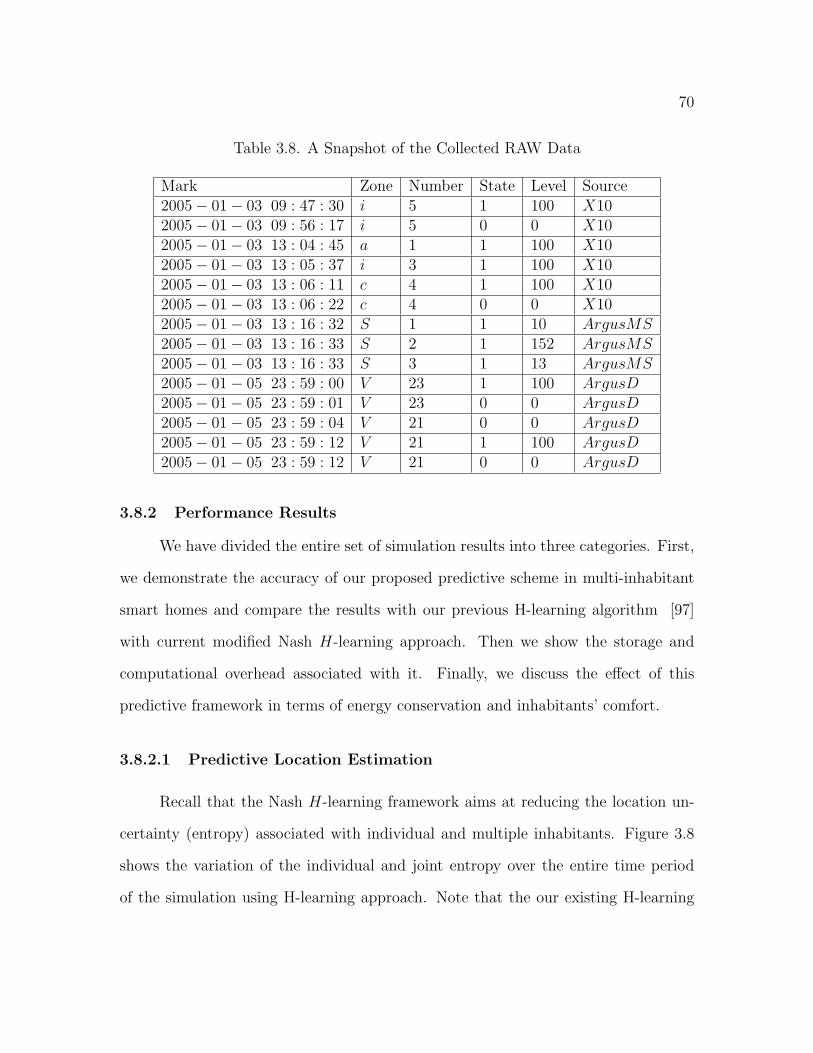
70

Table 3.8. A Snapshot of the Collected RAW Data

Mark Zone Number State Level Source2005− 01− 03 09 : 47 : 30 i 5 1 100 X102005− 01− 03 09 : 56 : 17 i 5 0 0 X102005− 01− 03 13 : 04 : 45 a 1 1 100 X102005− 01− 03 13 : 05 : 37 i 3 1 100 X102005− 01− 03 13 : 06 : 11 c 4 1 100 X102005− 01− 03 13 : 06 : 22 c 4 0 0 X102005− 01− 03 13 : 16 : 32 S 1 1 10 ArgusMS2005− 01− 03 13 : 16 : 33 S 2 1 152 ArgusMS2005− 01− 03 13 : 16 : 33 S 3 1 13 ArgusMS2005− 01− 05 23 : 59 : 00 V 23 1 100 ArgusD2005− 01− 05 23 : 59 : 01 V 23 0 0 ArgusD2005− 01− 05 23 : 59 : 04 V 21 0 0 ArgusD2005− 01− 05 23 : 59 : 12 V 21 1 100 ArgusD2005− 01− 05 23 : 59 : 12 V 21 0 0 ArgusD

3.8.2 Performance Results

We have divided the entire set of simulation results into three categories. First,

we demonstrate the accuracy of our proposed predictive scheme in multi-inhabitant

smart homes and compare the results with our previous H-learning algorithm [97]

with current modified Nash H-learning approach. Then we show the storage and

computational overhead associated with it. Finally, we discuss the effect of this

predictive framework in terms of energy conservation and inhabitants’ comfort.

3.8.2.1 Predictive Location Estimation

Recall that the Nash H-learning framework aims at reducing the location un-

certainty (entropy) associated with individual and multiple inhabitants. Figure 3.8

shows the variation of the individual and joint entropy over the entire time period

of the simulation using H-learning approach. Note that the our existing H-learning

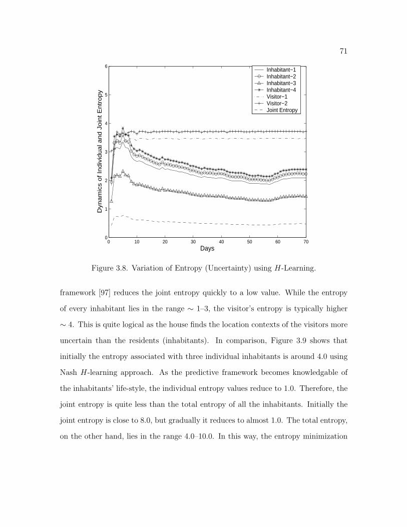
71

0 10 20 30 40 50 60 700

1

2

3

4

5

6

Days

Dyn

am

ics

of

Ind

ivid

ua

l an

d J

oin

t E

ntr

op

y

Inhabitant−1Inhabitant−2Inhabitant−3Inhabitant−4Visitor−1Visitor−2Joint Entropy

Figure 3.8. Variation of Entropy (Uncertainty) using H-Learning.

framework [97] reduces the joint entropy quickly to a low value. While the entropy

of every inhabitant lies in the range ∼ 1–3, the visitor’s entropy is typically higher

∼ 4. This is quite logical as the house finds the location contexts of the visitors more

uncertain than the residents (inhabitants). In comparison, Figure 3.9 shows that

initially the entropy associated with three individual inhabitants is around 4.0 using

Nash H-learning approach. As the predictive framework becomes knowledgable of

the inhabitants’ life-style, the individual entropy values reduce to 1.0. Therefore, the

joint entropy is quite less than the total entropy of all the inhabitants. Initially the

joint entropy is close to 8.0, but gradually it reduces to almost 1.0. The total entropy,

on the other hand, lies in the range 4.0–10.0. In this way, the entropy minimization

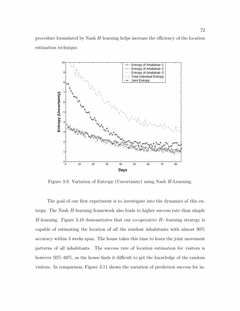
72

procedure formulated by Nash H-learning helps increase the efficiency of the location

estimation technique.

0 10 20 30 40 50 60 70 800

1

2

3

4

5

6

7

8

9

10

Days

En

tro

py (

Un

cert

ain

ty)

Entropy of Inhabitnat−1Entropy of Inhabitnat−2Entropy of Inhabitnat−3Total Individual EntropyJoint Entropy

Figure 3.9. Variation of Entropy (Uncertainty) using Nash H-Learning.

The goal of our first experiment is to investigate into the dynamics of this en-

tropy. The Nash H-learning framework also leads to higher success rate than simple

H-learning. Figure 3.10 demonstrates that our co-operative H- learning strategy is

capable of estimating the location of all the resident inhabitants with almost 90%

accuracy within 3 weeks span. The house takes this time to learn the joint movement

patterns of all inhabitants. The success rate of location estimation for visitors is

however 50%–60%, as the house finds it difficult to get the knowledge of the random

visitors. In comparison, Figure 3.11 shows the variation of prediction success for in-

73

dividual inhabitants and joint prediction success using Nash H-learning framework.

Initially, the success-rate is pretty low as the system proceeds through the learning

stage. Once the system becomes cognizant of inhabitants’ profiles, the success rate

increases and saturates at a particular value. The individual prediction process does

not consider the correlation among different inhabitants. Thus, it fails to capture

some important contexts and results in comparatively lower prediction success upto

80%. The joint prediction, however, takes the correlation among different inhabi-

tants into account and results in higher success rate (close to 95%) than the simple

H-learning framework.

The collection of the inhabitants’ joint typical-set is the key behind the devel-

0 10 20 30 40 50 60 7020

30

40

50

60

70

80

90

100

Days

Ave

rag

e S

ucc

ess

−R

ate

of L

oca

tion

Est

ima

tion

Inhabitant−1Inhabitant−2Inhabitant−3Inhabitant−4Visitor−1Visitor−2

Figure 3.10. Dynamics of Prediction Success using H-Learning.

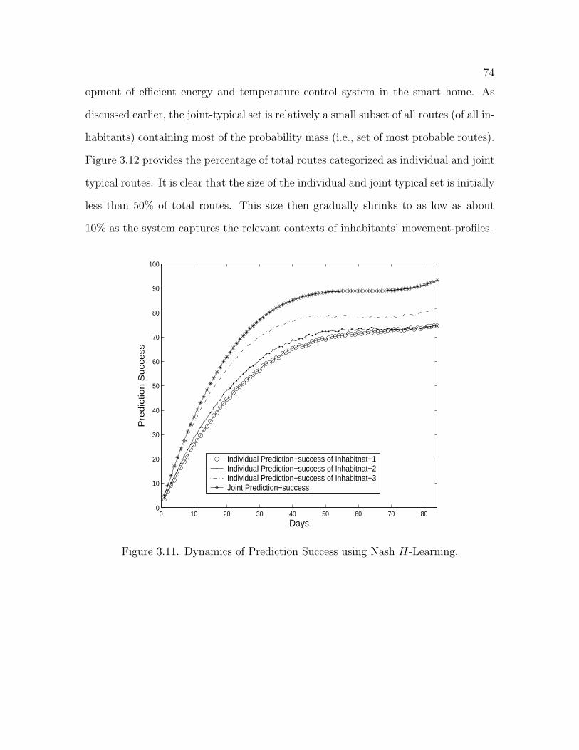
74

opment of efficient energy and temperature control system in the smart home. As

discussed earlier, the joint-typical set is relatively a small subset of all routes (of all in-

habitants) containing most of the probability mass (i.e., set of most probable routes).

Figure 3.12 provides the percentage of total routes categorized as individual and joint

typical routes. It is clear that the size of the individual and joint typical set is initially

less than 50% of total routes. This size then gradually shrinks to as low as about

10% as the system captures the relevant contexts of inhabitants’ movement-profiles.

0 10 20 30 40 50 60 70 800

10

20

30

40

50

60

70

80

90

100

Days

Pre

dic

tion

Su

cce

ss

Individual Prediction−success of Inhabitnat−1Individual Prediction−success of Inhabitnat−2Individual Prediction−success of Inhabitnat−3Joint Prediction−success

Figure 3.11. Dynamics of Prediction Success using Nash H-Learning.

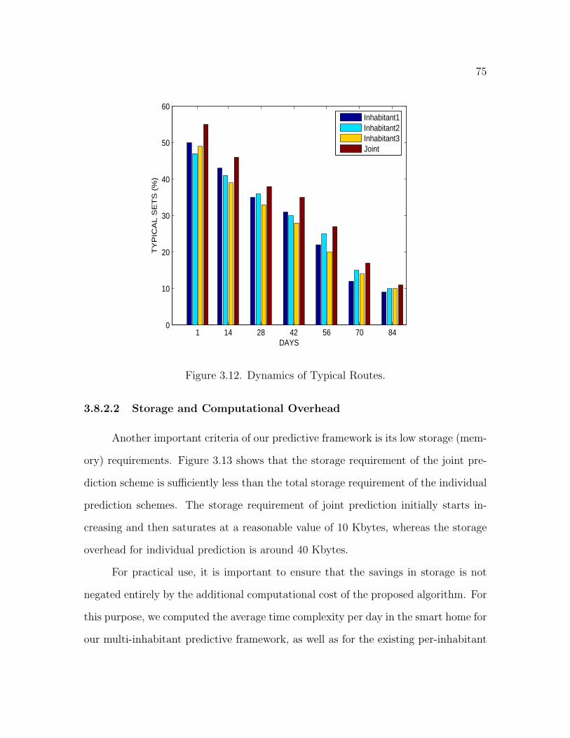
75

1 14 28 42 56 70 840

10

20

30

40

50

60

DAYS

TY

PIC

AL

SE

TS

(%

)

Inhabitant1Inhabitant2Inhabitant3Joint

Figure 3.12. Dynamics of Typical Routes.

3.8.2.2 Storage and Computational Overhead

Another important criteria of our predictive framework is its low storage (mem-

ory) requirements. Figure 3.13 shows that the storage requirement of the joint pre-

diction scheme is sufficiently less than the total storage requirement of the individual

prediction schemes. The storage requirement of joint prediction initially starts in-

creasing and then saturates at a reasonable value of 10 Kbytes, whereas the storage

overhead for individual prediction is around 40 Kbytes.

For practical use, it is important to ensure that the savings in storage is not

negated entirely by the additional computational cost of the proposed algorithm. For

this purpose, we computed the average time complexity per day in the smart home for

our multi-inhabitant predictive framework, as well as for the existing per-inhabitant

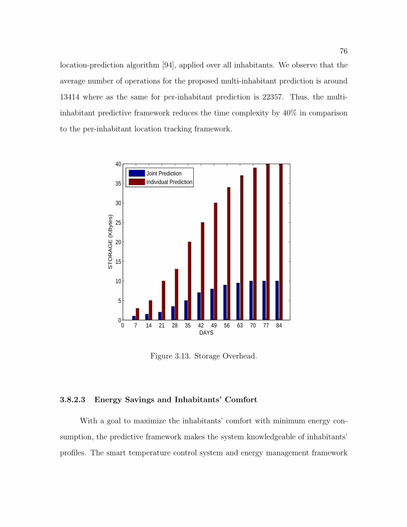
76

location-prediction algorithm [94], applied over all inhabitants. We observe that the

average number of operations for the proposed multi-inhabitant prediction is around

13414 where as the same for per-inhabitant prediction is 22357. Thus, the multi-

inhabitant predictive framework reduces the time complexity by 40% in comparison

to the per-inhabitant location tracking framework.

0 7 14 21 28 35 42 49 56 63 70 77 840

5

10

15

20

25

30

35

40

DAYS

ST

OR

AG

E (

KB

yte

s)

Joint PredictionIndividual Prediction

Figure 3.13. Storage Overhead.

3.8.2.3 Energy Savings and Inhabitants’ Comfort

With a goal to maximize the inhabitants’ comfort with minimum energy con-

sumption, the predictive framework makes the system knowledgeable of inhabitants’

profiles. The smart temperature control system and energy management framework

77

0 10 20 30 40 50 60 70 802

4

6

8

10

12

14

16

18

20

22

Days

Avera

ge E

nerg

y C

on

su

mp

tio

n

Mobility−Aware Energy Plan in Smart HomesStatic Energy Plans in Current HomesOptimal Possible Energy Plan

Figure 3.14. Energy Consumption.

makes intelligent use of these profiles to conserve energy. Figure 3.14 shows that using

the predictive framework, the daily average energy consumption can be kept about 5

KiloWatt-hour (KW-Hr), in comparison to 9 KW-Hr for energy management scheme

without the predictive framework. Figure 3.15 shows the reduction of manual opera-

tions and time spent for all the inhabitants. The predictive Nash H-learning scheme

aids the system with sufficient automation, by reducing the overall manual operations

performed by the inhabitants and the time spent behind all such operations which in

turn increases the overall comfort.

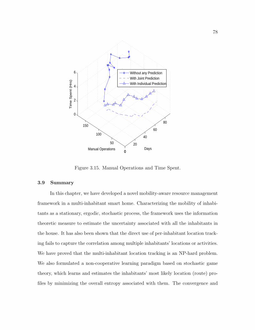
78

0

20

40

60

80

0

50

100

150

0

2

4

6

DaysManual Operations

Tim

e S

pe

nt

(Hrs

)Without any PredictionWith Joint PredictionWith Individual Prediction

Figure 3.15. Manual Operations and Time Spent.

3.9 Summary

In this chapter, we have developed a novel mobility-aware resource management

framework in a multi-inhabitant smart home. Characterizing the mobility of inhabi-

tants as a stationary, ergodic, stochastic process, the framework uses the information

theoretic measure to estimate the uncertainty associated with all the inhabitants in

the house. It has also been shown that the direct use of per-inhabitant location track-

ing fails to capture the correlation among multiple inhabitants’ locations or activities.

We have proved that the multi-inhabitant location tracking is an NP-hard problem.

We also formulated a non-cooperative learning paradigm based on stochastic game

theory, which learns and estimates the inhabitants’ most likely location (route) pro-

files by minimizing the overall entropy associated with them. The convergence and

79

worst-case performance bounds of this framework are also derived. Automated ac-

tivation of devices along the predicted locations/routes provide the inhabitants with

necessary comfort while minimizing energy consumption and cost. In the next chapter

we will focus how such context information is useful in providing health related and

wellness management services in an intelligent way to promote independent living in

a smart home environment.

CHAPTER 4

AMBIGUOUS CONTEXT MEDIATION FRAMEWORK

4.1 Introduction

Current research and development in smart environments [23, 28, 98] technol-

ogy offer a promising solution to the increasing needs of the elderly in home based

healthcare applications. Essential to such applications is what is called human-centric

computing and communication, where computers and devices are designed to adapt

to the user needs and preferences. The objective here is to create a total solution for

the perennial connection of the human with the environment, rather than focussing

merely on the devices for the sole purpose of obtaining input from the human. This

form of computing platforms are becoming ubiquitous in healthcare and nursing in-

dustry, thus transforming the patients from passive to active consumers of healthcare

benefits [29]. To this end, current research efforts have largely focused on the devel-

opment of communication technologies and intelligent user interfaces [34].

In this chapter we focus on the computational aspect of user-centric data to

provide context-aware services [28, 98] that promotes intelligent independent living.

Context-aware applications typically derive their desired context information (implicit

input) from physical sensors and other information sources. Though sensing is be-

coming more and more cost-effective and ubiquitous, the interpretation of sensed data

as contexts is still imperfect or ambiguous. Therefore, a critical challenge facing the

development of realistic and deployable context-aware services, particularly in health

related applications, is the ability to handle ambiguous contexts. The conversion of

raw data into high-level context information requires middleware to pre-process such

80

81

as filter, transform, and even aggregate the data collected from homogeneous or het-

erogeneous distributed sensors, with a goal to minimize the ambiguity of the derived

contexts. Only with reasonably accurate context(s), can applications be confident to

make adaptative and better decisions. The context processing could involve simple

filtering based on a value match, or sophisticated data correlation or data fusion tech-

niques [16, 80]. Contexts may also include various aspects of relevant information;

they may be instantaneous or durative, ambiguous or unambiguous. Furthermore,

heterogeneous information source sensors usually have different measurement objects,

different resolutions and accuracies, and different data rates and formats. Thus, the

mapping from sensory output to the context information is a non-trivial task. We

believe context-aware data fusion plays a critical role in improving the accuracy of

the derived contexts by reducing their ambiguity, although the exact fusion technique

to use is application and domain specific. This motivates our work.

4.1.1 Related Work

The ubiquitous computing paradigm [121] implies smart (i.e., pro-active) inter-

action of computing and communication devices with their peers and surrounding

networks, often without explicit operator control. Hence, such devices need to be

imbued with an inherent sentience [54] about their important contexts that can auto-

matically or implicitly sense information about their state and the presence of users

(inhabitants) in order to take action on those contexts. This concept has led to various

projects smart homes or environments in general [22, 23]. Existing work such as the

Reactive Room [24], Neural Network House [82], Intelligent Room [21] and House n

[60] do not provide explicit reusable support for users to manage or correct uncertainty

in the sensed data and their interpretations, and thereby assume that the sensed con-

texts are unambiguous. The work reported in [34] provided a toolkit to enable the

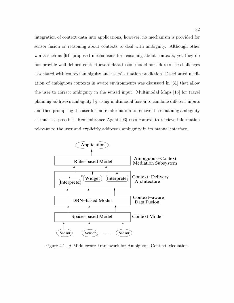
82

integration of context data into applications, however, no mechanism is provided for

sensor fusion or reasoning about contexts to deal with ambiguity. Although other

works such as [61] proposed mechanisms for reasoning about contexts, yet they do

not provide well defined context-aware data fusion model nor address the challenges

associated with context ambiguity and users’ situation prediction. Distributed medi-

ation of ambiguous contexts in aware environments was discussed in [31] that allow

the user to correct ambiguity in the sensed input. Multimodal Maps [15] for travel

planning addresses ambiguity by using multimodal fusion to combine different inputs

and then prompting the user for more information to remove the remaining ambiguity

as much as possible. Remembrance Agent [93] uses context to retrieve information

relevant to the user and explicitly addresses ambiguity in its manual interface.

Sensor Sensor Sensor

Space−based Model

DBN−based Model

Context Model

Context−aware

WidgetInterpreter

Interpreter Context−Delivery Architecture

Application

Mediation SubsystemAmbiguous−Context

Data Fusion

Rule−based Model

Figure 4.1. A Middleware Framework for Ambiguous Context Mediation.

83

Alongside, significant efforts have been made to develop middleware systems

that can effectively support context-aware applications in the presence of resource

constraints (e.g., sensor networks), also considering requirements for sensory data or

information fusion from middleware perspective [1]. For example, DFuse [73] is a data

fusion framework that facilitates dynamic transfer of different application level infor-

mation fusion into the network in order to save power. In adaptive middleware [55] for

context-aware applications in smart home setups, the application’s quality of context

(QoC) requirements is matched with the QoC attributes of the sensors with the help

of a utility function. Similarly, in MiLAN [49], application’s quality of service (QoS)

requirements are matched with the QoS provided by the sensor networks. However,

in this scheme, the QoS requirements of the applications are assumed to be prede-

termined, which the applications should know in advance in addition to the quality

associated with the type of sensors it can make use of. Given that in ubiquitous

computing environments, the nature (number, types and cost off usage, and benefits)

of such sensors available to the applications usually vary, it is impractical to include

a priori knowledge about them. The selection of right sensor with right informa-

tion at the right moment was originally introduced in [114], while the structure of an

optimal sensor configuration constrained by the wireless channel capacity was investi-

gated in [13]. By eliminating the simplifying assumption that all contexts are certain,

in an earlier work [99], we designed a context-aware data fusion algorithm based on

dynamic Bayesian network to mediate ambiguous context. But an intelligent sensor

management that provides energy-efficiency as well as a way to manage quality of

context requirements, which may change over time with changes in patient’s state,

has not been considered before. In this chapter an information theoretic approach is

taken to decide an optimal sensor configuration to determine the best current state

of the patient while satisfying the application QoC requirements. For end user an

84

ontological rule based approach using semantic web technology is proposed for fur-

ther reduction of context ambiguity with applications to context-aware healthcare

services. By eliminating the simplifying assumption that all contexts are certain, in

this chapter we propose a middleware architecture as shown in Fig. 4.1 (explained in

Section 4.5.2) that supports a variety of services, ranging from context-aware data

fusion to ambiguous context mediation subsystem with applications to context-aware

healthcare services [99]. The major contributions of this work are summarized later.

4.1.2 Example Scenario

As an example, let us take the scenario of a home care patient after hospi-

talization for cardiac infarction. Although such a patient should be guaranteed a

good quality of life and wellness management services in an independent way, he/she

still needs to be in constant contact with an expert physician so that his/her cardiac

activity (e.g., the heart rate and peripheral blood pressure), body temperature and

breathing frequency can be continuously monitored. However, the health condition

of a patient can only be partially evaluated through his vital signals and must be

mediated and integrated by other signals and information coming both from personal

characteristics (risk factors, degree of disease, age, sex, family history, psychological

features, etc.) and from the environmental context (e.g., whether in bed or mobile,

by him/herself or in company, at work or at home, the season and the temperature,

etc.). The monitoring system should be able to deduce the context from the available

data to provide a feedback to the patient as well as notifying his status to somebody

else, such as a relative, the family doctor, or the hospital, depending on the degree

of alert detected, and possibly adapting the level of service (i.e., the intensity of the

monitoring activity).

85

The above scenario requires the integration of patients’ vital signs monitored by

different sensory medical devices, of environmental data acquired by sensors located

near the patient, of patient data available from the electronic medical records stored

by the hospital. Although the current technologies offer the necessary means to

support this kind of health care, in our opinion without a contextual realization that

tailors the available data into usable information, the healthcare applications will

become practically unusable. Contextual information deals with information about

the user environment (e.g., location, activity) that enables this tailoring and reduces

efforts required to develop healthcare applications.

Application scenarios of the type presented above give rise to several issues. The

sensory devices constantly attached to the patient produce huge streams of physiolog-

ical data which must be collected and related to environmental conditions. To achieve

this we need a technique that can fuse acquired data with different modalities to infer

the current context state (activity) and situation space (behavior or sickness) asso-

ciated with the monitored person. Again these sensors should be light and portable

to reduce their impact on the patient’s well-being and thus must be constrained in

terms of energy capacity. Consequently, the amount of information transmitted to

the sensor fusion mediator (the data aggregator) should be minimized in order to

prolong its lifetime by selecting the structure of an optimal set of sensors based on

the QoC guarantees and cost of information acquisition.

4.1.3 Our Contributions

In this chapter, we propose a framework that fuses data from disparate sensors,

represents context state (activity) and reasons efficiently about this state, to support

context-aware services that deal with ambiguity and allow users to mediate ambiguity,

if any. For environments with ambiguous contexts, our goal is to build a framework

86

that resolves information overlap conflicts, and also ensures the conformance to the

application’s quality of context (QoC) bound based on an optimal sensor configu-

ration. For this purpose, we propose layered and modularized system design using

Dynamic Bayesian Networks (DBNs) [63] in which the sensed data is used to inter-

pret context state and the sensor fusion process is analogous to the human perception

and reasoning processes. The use of DBNs as our baseline sensor fusion mechanism

reflects this analogy whereas an information theoretic reasoning selects an optimal

context attribute (sensor data) value to satisfy the application QoC bound. However,

our proposed technique can not remove all the ambiguity in the sensed data, leaving

it up to the programmer and inhabitants to deal with. To alleviate this problem, we

propose to leverage off a rule based model [101] and involve end users in removing

any remaining ambiguity through a process, called ambiguous-context mediation sub-

system. We use Semantic Web [110] technology to implement this rule based model

to visualize wellness management services to the elderly person. Experimental results

demonstrate that the proposed framework is capable of adaptively enhancing the

effectiveness of the probabilistic sensor fusion scheme and patient’s situation predic-

tion by selectively choosing the sensor corresponds to the most economically efficient

disambiguation action.

The rest of the chapter is organized as follows. Section 4.2 describes the basic

concepts of context model and quality of context in resource limited sensor network.

Section 4.3 describes the context-aware (active) data fusion model based on the DBNs

for resolving ambiguity. In Section 4.4 we study the structure of an optimal sensor

configuration from an information theoretic point of view. A rule based model with

its prototype for the realization of unambiguous context has been discussed in Sec-

tion 4.5. The performance of our proposed system is evaluated for health monitoring

87

application in a smart home, and the results are presented in Section 4.6. Finally,

Section 4.7 concludes this Chapter.

4.2 Context Model

Context-aware data fusion in the face of ambiguities is a challenging research

problem as the data sent to the sensor fusion mediator collected from network of

multiple sensors are often characterized with a high degree of complexity due to the

following challenges: (i) data are often acquired from sensors of different modalities

and with different degrees of uncertainty and ambiguity, (ii) decision must be made

quickly, and (iii) the situation as well as sensory observations always evolve over time.

We make use of the space-based context model [89] and extend it with quality of

context (QoC) attributes. This model captures the underlying description of context

related knowledge and attempts to incorporate various intuitions that should impact

context inference, to produce a better fusion results. This approach is specifically

intended for use in context-aware applications, and exhibits many characteristics

desirable in reasoning about context.

4.2.1 Space-based Context Model

This model defines the following concepts:

Definition 5 Context Attribute: A context attribute, denoted by ai, is defined as

any type of data that is used in the process of inferring situations. A context attribute

is often associated with sensors, virtual or physical, where the values of the sensor

readings denote the context attribute value at a given time t, denoted by ati. The body

temperature “1000 F” of a patient measured by i-th sensor at a given time t is an

example of a context attribute.

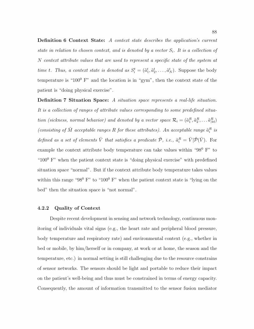
88

Definition 6 Context State: A context state describes the application’s current

state in relation to chosen context, and is denoted by a vector Si. It is a collection of

N context attribute values that are used to represent a specific state of the system at

time t. Thus, a context state is denoted as Sti = (at

1, at2, . . . , a

tN). Suppose the body

temperature is “1000 F” and the location is in “gym”, then the context state of the

patient is “doing physical exercise”.

Definition 7 Situation Space: A situation space represents a real-life situation.

It is a collection of ranges of attribute values corresponding to some predefined situa-

tion (sickness, normal behavior) and denoted by a vector space Ri = (aR1 , a

R2 , . . . a

RM)

(consisting of M acceptable ranges R for these attributes). An acceptable range aRi is

defined as a set of elements V that satisfies a predicate P, i.e., aRi = V |P(V ). For

example the context attribute body temperature can take values within “980 F” to

“1000 F” when the patient context state is “doing physical exercise” with predefined

situation space “normal”. But if the context attribute body temperature takes values

within this range “980 F” to “1000 F” when the patient context state is “lying on the

bed” then the situation space is “not normal”.

4.2.2 Quality of Context

Despite recent development in sensing and network technology, continuous mon-

itoring of individuals vital signs (e.g., the heart rate and peripheral blood pressure,

body temperature and respiratory rate) and environmental context (e.g., whether in

bed or mobile, by him/herself or in company, at work or at home, the season and the

temperature, etc.) in normal setting is still challenging due to the resource constrains

of sensor networks. The sensors should be light and portable to reduce their impact

on the patient’s well-being and thus must be constrained in terms of energy capacity.

Consequently, the amount of information transmitted to the sensor fusion mediator

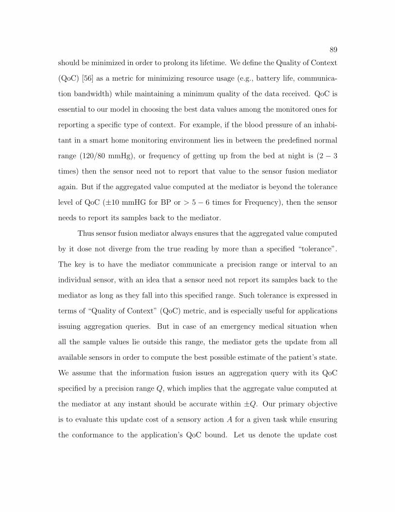
89

should be minimized in order to prolong its lifetime. We define the Quality of Context

(QoC) [56] as a metric for minimizing resource usage (e.g., battery life, communica-

tion bandwidth) while maintaining a minimum quality of the data received. QoC is

essential to our model in choosing the best data values among the monitored ones for

reporting a specific type of context. For example, if the blood pressure of an inhabi-

tant in a smart home monitoring environment lies in between the predefined normal

range (120/80 mmHg), or frequency of getting up from the bed at night is (2 − 3

times) then the sensor need not to report that value to the sensor fusion mediator

again. But if the aggregated value computed at the mediator is beyond the tolerance

level of QoC (±10 mmHG for BP or > 5 − 6 times for Frequency), then the sensor

needs to report its samples back to the mediator.

Thus sensor fusion mediator always ensures that the aggregated value computed

by it dose not diverge from the true reading by more than a specified “tolerance”.

The key is to have the mediator communicate a precision range or interval to an

individual sensor, with an idea that a sensor need not report its samples back to the

mediator as long as they fall into this specified range. Such tolerance is expressed in

terms of “Quality of Context” (QoC) metric, and is especially useful for applications

issuing aggregation queries. But in case of an emergency medical situation when

all the sample values lie outside this range, the mediator gets the update from all

available sensors in order to compute the best possible estimate of the patient’s state.

We assume that the information fusion issues an aggregation query with its QoC

specified by a precision range Q, which implies that the aggregate value computed at

the mediator at any instant should be accurate within ±Q. Our primary objective

is to evaluate this update cost of a sensory action A for a given task while ensuring

the conformance to the application’s QoC bound. Let us denote the update cost

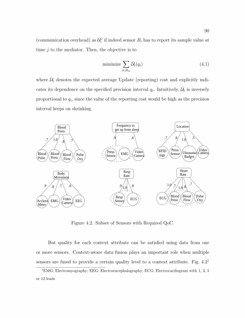
90

(communication overhead) as U ji if indeed sensor Bi has to report its sample value at

time j to the mediator. Then, the objective is to

minimize∑

i∈Bm

Ui(qi) (4.1)

where Ui denotes the expected average Update (reporting) cost and explicitly indi-

cates its dependence on the specified precision interval qi. Intuitively, Ui is inversely

proportional to qi, since the value of the reporting cost would be high as the precision

interval keeps on shrinking.

BloodPulse

Blood Press

Blood Press

Blood Flow

Pulse Oxy

.7 1.0 .8 .7

get up from sleepFrequency to

Press VideoSensor CameraEMG

.9 .6

RFID tags

PressSensor

VideoCameraUltrasonic

Badges

Location

.7 .6 1.0 .5

MovementBody

MeterAcclero EMG Camera EEGVideo

.9 .8 .7 .6

RespRate

SensorResp ECG

RateHeart

ECG Blood Press

Blood Flow

Pulse Oxy

1.0 .7 .7.9 .81.0 1.0 .8

Figure 4.2. Subset of Sensors with Required QoC.

But quality for each context attribute can be satisfied using data from one

or more sensors. Context-aware data fusion plays an important role when multiple

sensors are fused to provide a certain quality level to a context attribute. Fig. 4.21

1EMG: Electromyography; EEG: Electroencephalography; ECG: Electrocardiogram with 1, 3, 5

or 12 leads

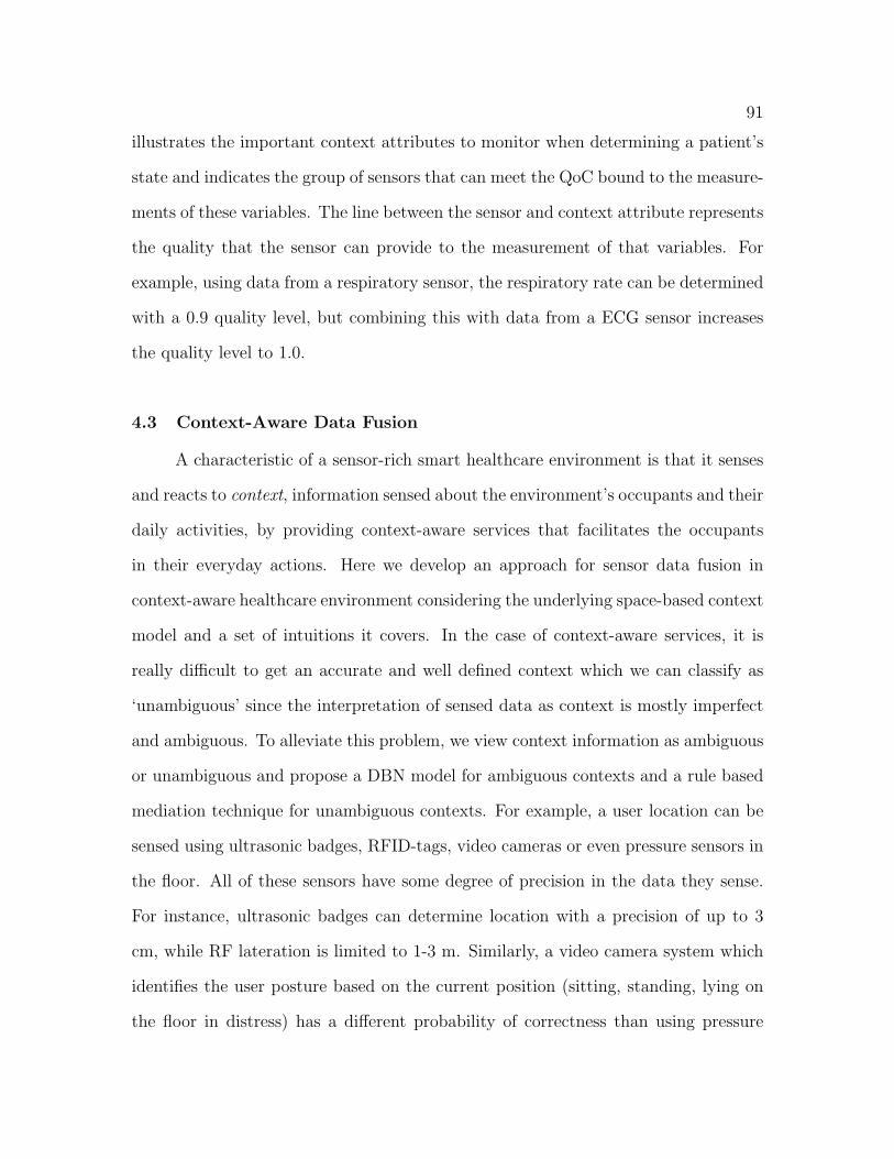
91

illustrates the important context attributes to monitor when determining a patient’s

state and indicates the group of sensors that can meet the QoC bound to the measure-

ments of these variables. The line between the sensor and context attribute represents

the quality that the sensor can provide to the measurement of that variables. For

example, using data from a respiratory sensor, the respiratory rate can be determined

with a 0.9 quality level, but combining this with data from a ECG sensor increases

the quality level to 1.0.

4.3 Context-Aware Data Fusion

A characteristic of a sensor-rich smart healthcare environment is that it senses

and reacts to context, information sensed about the environment’s occupants and their

daily activities, by providing context-aware services that facilitates the occupants

in their everyday actions. Here we develop an approach for sensor data fusion in

context-aware healthcare environment considering the underlying space-based context

model and a set of intuitions it covers. In the case of context-aware services, it is

really difficult to get an accurate and well defined context which we can classify as

‘unambiguous’ since the interpretation of sensed data as context is mostly imperfect

and ambiguous. To alleviate this problem, we view context information as ambiguous

or unambiguous and propose a DBN model for ambiguous contexts and a rule based

mediation technique for unambiguous contexts. For example, a user location can be

sensed using ultrasonic badges, RFID-tags, video cameras or even pressure sensors in

the floor. All of these sensors have some degree of precision in the data they sense.

For instance, ultrasonic badges can determine location with a precision of up to 3

cm, while RF lateration is limited to 1-3 m. Similarly, a video camera system which

identifies the user posture based on the current position (sitting, standing, lying on

the floor in distress) has a different probability of correctness than using pressure

92

sensors in furniture. The ambiguity problem becomes worse when the application

derives implicit higher-level context state (activity of the person) based upon those

inputs. For example, an application may infer that a person is lying in distress.

However, there may be other explanation of this phenomenon such as the person

might be lying to perform normal exercises. Thus, we design a context-aware (active)

data fusion framework based on DBNs to reduce this ambiguity as much as possible

during the situation inference (patient’s behavior or sickness) process.

4.3.1 Dynamic Bayesian Network Based Model (DBN)

Our motivation is to use the data fusion algorithm to develop a context-aware

model to gather knowledge from sensor data. We look for a technique which is

appropriate for performing context-aware data fusion with the flexibility of both top-

down and bottom-up inference mechanisms. The top-down inference can be used to

predict the utility of a particular sensory action with respect to a goal at the top.

For example, in the case of a given context state (going to restroom), it will fuse

the most relevant context attributes (time, frequency of getting up from the bed,

blood sugar level etc.). The bottom-up inference allows the integration of the context

attributes from a sensory action and update each node about the context state in

the network. Dynamic Bayesian Networks can be used for similar problems since it

provides a coherent and unified hierarchical probabilistic framework for sensory data

representation, integration and inference. Figure 4.3 (adopted from [122]) illustrates a

DBN based framework for context-aware data fusion system consisting of a situation

space, context states, context attributes, a sensor fusion mediator and network of

information sensors.

The selection of an information source (sensor) or the activation of a process

to compute new information is simply regarded as a set of actions available to the

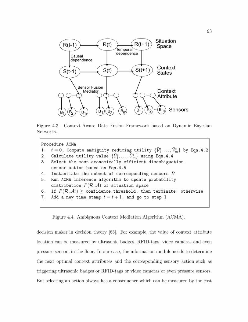
93

R(t-1) R(t) R(t+1)

S(t-1) S(t) S(t+1)

Sensor Fusion Mediator

Sensors

Situation Space

ContextStates

Temporaldependence

Causaldependence

B1 B B B B B B B B2 m m m

1 12 2

ContextAttribute

Figure 4.3. Context-Aware Data Fusion Framework based on Dynamic BayesianNetworks.

Procedure ACMA

1. t = 0, Compute ambiguity-reducing utility V t1, . . . , V t

m by Eqn.4.2

2. Calculate utility value U t1, . . . , U

tm using Eqn.4.4

3. Select the most economically efficient disambiguation

sensor action based on Eqn.4.5

4. Instantiate the subset of corresponding sensors B5. Run ACMA inference algorithm to update probability

distribution P (R,A) of situation space

6. If P (R,A∗) ≥ confidence threshold, then terminate; otherwise

7. Add a new time stamp t = t+ 1, and go to step 1

Figure 4.4. Ambiguous Context Mediation Algorithm (ACMA).

decision maker in decision theory [63]. For example, the value of context attribute

location can be measured by ultrasonic badges, RFID-tags, video cameras and even

pressure sensors in the floor. In our case, the information module needs to determine

the next optimal context attributes and the corresponding sensory action such as

triggering ultrasonic badges or RFID-tags or video cameras or even pressure sensors.

But selecting an action always has a consequence which can be measured by the cost

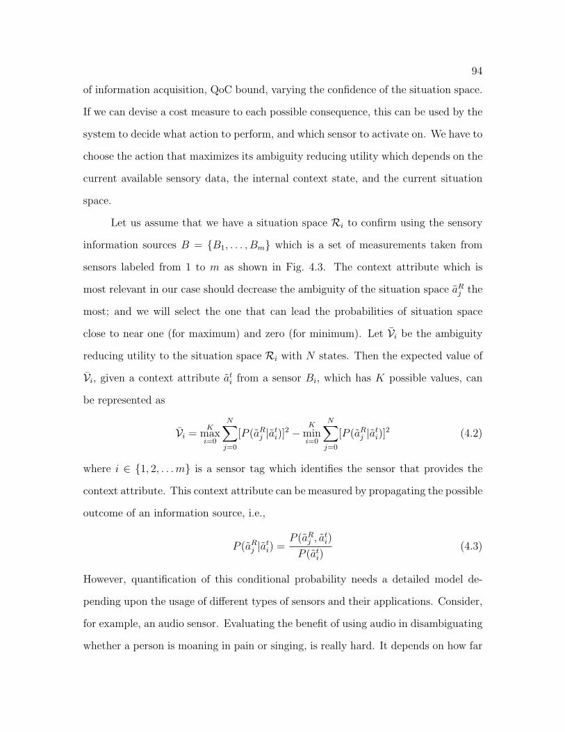
94

of information acquisition, QoC bound, varying the confidence of the situation space.

If we can devise a cost measure to each possible consequence, this can be used by the

system to decide what action to perform, and which sensor to activate on. We have to

choose the action that maximizes its ambiguity reducing utility which depends on the

current available sensory data, the internal context state, and the current situation

space.

Let us assume that we have a situation space Ri to confirm using the sensory

information sources B = B1, . . . , Bm which is a set of measurements taken from

sensors labeled from 1 to m as shown in Fig. 4.3. The context attribute which is

most relevant in our case should decrease the ambiguity of the situation space aRj the

most; and we will select the one that can lead the probabilities of situation space

close to near one (for maximum) and zero (for minimum). Let Vi be the ambiguity

reducing utility to the situation space Ri with N states. Then the expected value of

Vi, given a context attribute ati from a sensor Bi, which has K possible values, can

be represented as

Vi =K

maxi=0

N∑

j=0

[P (aRj |at

i)]2 −

K

mini=0

N∑

j=0

[P (aRj |at

i)]2 (4.2)

where i ∈ 1, 2, . . .m is a sensor tag which identifies the sensor that provides the

context attribute. This context attribute can be measured by propagating the possible

outcome of an information source, i.e.,

P (aRj |at

i) =P (aR

j , ati)

P (ati)

(4.3)

However, quantification of this conditional probability needs a detailed model de-

pending upon the usage of different types of sensors and their applications. Consider,

for example, an audio sensor. Evaluating the benefit of using audio in disambiguating

whether a person is moaning in pain or singing, is really hard. It depends on how far

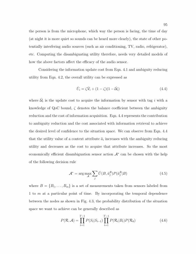
95

the person is from the microphone, which way the person is facing, the time of day

(at night it is more quiet so sounds can be heard more clearly), the state of other po-

tentially interfering audio sources (such as air conditioning, TV, radio, refrigerator),

etc. Computing the disambiguating utility therefore, needs very detailed models of

how the above factors affect the efficacy of the audio sensor.

Considering the information update cost from Eqn. 4.1 and ambiguity reducing

utility from Eqn. 4.2, the overall utility can be expressed as

Ui = ζVi + (1− ζ)(1− Ui) (4.4)

where Ui is the update cost to acquire the information by sensor with tag i with a

knowledge of QoC bound, ζ denotes the balance coefficient between the ambiguity

reduction and the cost of information acquisition. Eqn. 4.4 represents the contribution

to ambiguity reduction and the cost associated with information retrieval to achieve

the desired level of confidence to the situation space. We can observe from Eqn. 4.4

that the utility value of a context attribute ai increases with the ambiguity reducing

utility and decreases as the cost to acquire that attribute increases. So the most

economically efficient disambiguation sensor action A∗ can be chosen with the help

of the following decision rule

A∗ = arg maxA

∑

j

U(B, aRj )P (aR

j |B) (4.5)

where B = B1, . . . , Bm is a set of measurements taken from sensors labeled from

1 to m at a particular point of time. By incorporating the temporal dependence

between the nodes as shown in Fig. 4.3, the probability distribution of the situation

space we want to achieve can be generally described as

P (R,A) =T−1∏

t=1

P (St|St−1)T−1∏

t=1

P (Rt|Bt)P (R0) (4.6)

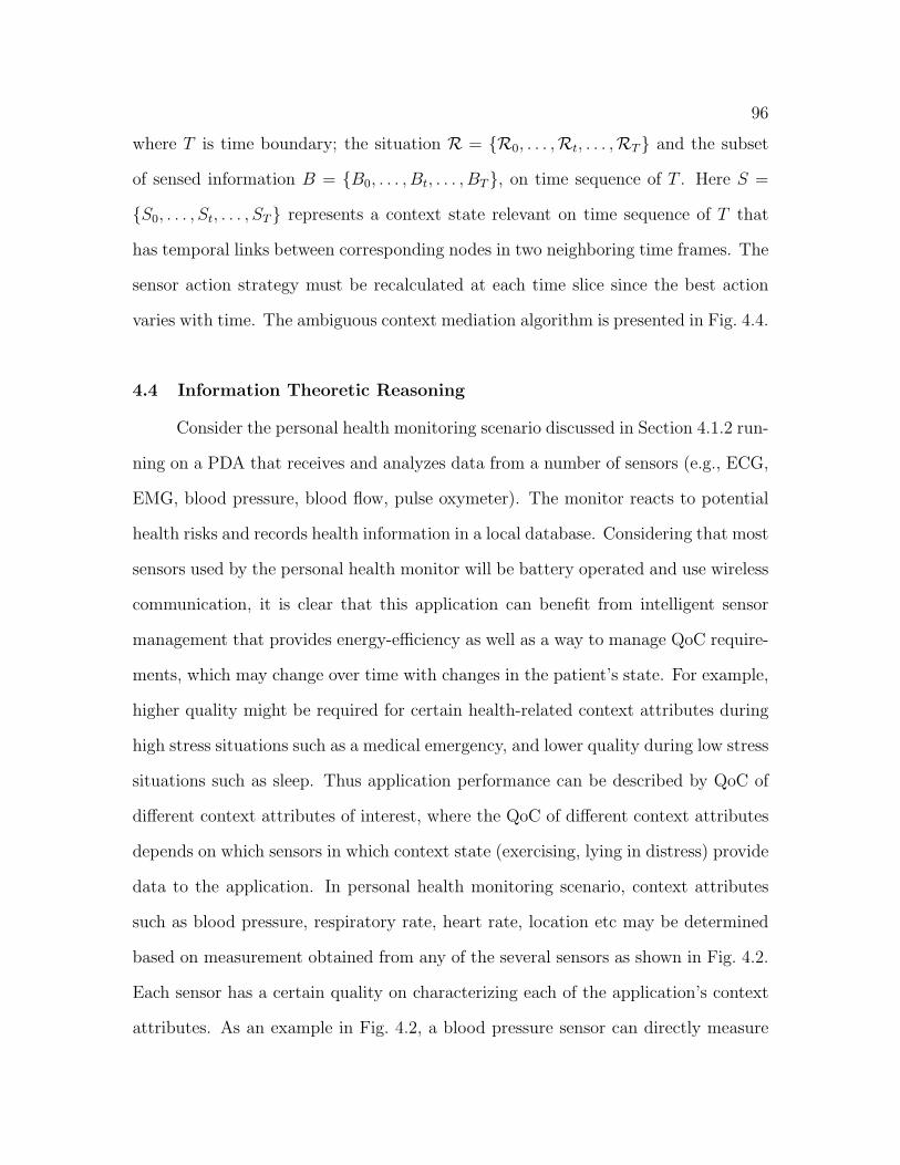
96

where T is time boundary; the situation R = R0, . . . ,Rt, . . . ,RT and the subset

of sensed information B = B0, . . . , Bt, . . . , BT, on time sequence of T . Here S =

S0, . . . , St, . . . , ST represents a context state relevant on time sequence of T that

has temporal links between corresponding nodes in two neighboring time frames. The

sensor action strategy must be recalculated at each time slice since the best action

varies with time. The ambiguous context mediation algorithm is presented in Fig. 4.4.

4.4 Information Theoretic Reasoning

Consider the personal health monitoring scenario discussed in Section 4.1.2 run-

ning on a PDA that receives and analyzes data from a number of sensors (e.g., ECG,

EMG, blood pressure, blood flow, pulse oxymeter). The monitor reacts to potential

health risks and records health information in a local database. Considering that most

sensors used by the personal health monitor will be battery operated and use wireless

communication, it is clear that this application can benefit from intelligent sensor

management that provides energy-efficiency as well as a way to manage QoC require-

ments, which may change over time with changes in the patient’s state. For example,

higher quality might be required for certain health-related context attributes during

high stress situations such as a medical emergency, and lower quality during low stress

situations such as sleep. Thus application performance can be described by QoC of

different context attributes of interest, where the QoC of different context attributes

depends on which sensors in which context state (exercising, lying in distress) provide

data to the application. In personal health monitoring scenario, context attributes

such as blood pressure, respiratory rate, heart rate, location etc may be determined

based on measurement obtained from any of the several sensors as shown in Fig. 4.2.

Each sensor has a certain quality on characterizing each of the application’s context

attributes. As an example in Fig. 4.2, a blood pressure sensor can directly measure

97

blood pressure with a quality of 1.0 2 in determining this context attribute, where as

heart rate measured by this sensor can have quality less than 1.0. But the quality of

the heart rate measurement could be improved through high-level fusion of the blood

pressure measurements with data from additional sensors such as blood flow sensor

depending upon the context state. Fig. 4.5 shows the context attributes requirement

graph for personal health monitor which includes multiple states for each vital signs

that can be monitored depending upon the context state of the patient. For example,

the Fig. 4.5 shows that when a patient is in lying in distress state and the blood

pressure is low, the blood oxygen level must be monitored with a quality of .7 and

the blood pressure must be monitored with a quality of .8. So the problem here is

to decide what type of information each sensor should send to the fusion center to

estimate the best current state of the patient while satisfying the application QoC

requirements for each context attribute.

We introduce a formalism for optimal sensor parameter selection for state esti-

mation. The optimality is defined in terms of reduction in ambiguity or error in state

estimation process. The main assumption is that state estimation becomes more re-

liable and accurate if the ambiguity/error in the underlying state estimation process

can be minimized. We investigate this from an information theoretic perspective [26]

where information about the context attribute is made available to the fusion center

by a set of smart sensors. The fusion center produces an estimate of the state of the

situation based on the intelligent analysis on the received data. We assume that the

noisy observation across sensors are independent and identically distributed (i.i.d)

random variable conditioned on the binary situation R (assume situation R here as

binary for ease of modeling). Now each sensor attribute has a source entropy rate

H(ai). Any sensor wishing to report this attribute must send H(ai) bits per unit

2Quality with 1.0 corresponds to 100% reliability

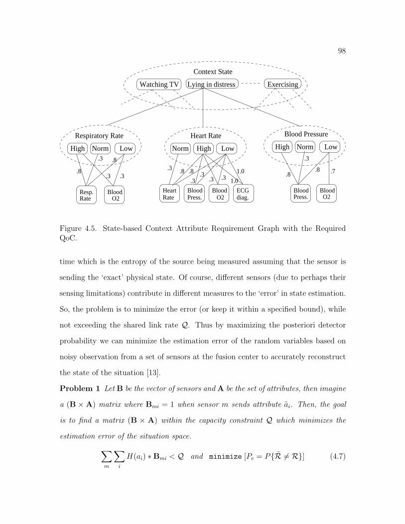
98

Watching TV Lying in distress

Heart Rate Blood PressureRespiratory Rate

High Norm Low High Norm LowNorm LowHigh

Resp.Rate O2

Blood HeartRate

BloodPress.

Blood O2

ECGdiag.

BloodPress.

Blood O2

.8

.8.3

.3 .3 .8.8

.3

.7.3 .8 .8 .3.3 .3 .3

1.0

1.0

Exercising

Context State

Figure 4.5. State-based Context Attribute Requirement Graph with the RequiredQoC.

time which is the entropy of the source being measured assuming that the sensor is

sending the ‘exact’ physical state. Of course, different sensors (due to perhaps their

sensing limitations) contribute in different measures to the ‘error’ in state estimation.

So, the problem is to minimize the error (or keep it within a specified bound), while

not exceeding the shared link rate Q. Thus by maximizing the posteriori detector

probability we can minimize the estimation error of the random variables based on

noisy observation from a set of sensors at the fusion center to accurately reconstruct

the state of the situation [13].

Problem 1 Let B be the vector of sensors and A be the set of attributes, then imagine

a (B ×A) matrix where Bmi = 1 when sensor m sends attribute ai. Then, the goal

is to find a matrix (B × A) within the capacity constraint Q which minimizes the

estimation error of the situation space.

∑

m

∑

i

H(ai) ∗Bmi < Q and minimize [Pe = PR 6= R] (4.7)

99

where Bmi is an indicator function taking on the value 1 only if the sensor m actually

sends attribute ai, H(ai) is the source entropy rate of the attribute ai and R is an

estimate of the original state R,

4.4.1 Problem Explanation

We assumeR be the random variable drawn from the binary alphabet R0,R1

with prior probabilities p0 and p1, respectively. In our case each sensor needs to

determine a sequence of context attributes for a sequence of context state Sm,t :

∀t = 1, 2, . . . , T about the value of situation R. We assume that random variable

Sm,t are i.i.d., given R, with conditional distribution pS|R(.|Ri). The sensors could

construct a summary Zm,t = πm(Sm,t) of their own observation to a fusion center at

discrete time t. The fusion center produces an estimate R of the original situation

R, upon reception of the data. Thus we need to find out an admissible strategy for

an optimal sensor-attribute mapping matrix (B×A) that minimizes the probability

of estimation error Pe = PR 6= R

Definition 8 A set of decision rules πm for an observation X → 1, 2, . . . am where

am is the number of attribute admissible to sensor Bm with the admissible strategy

denoted by π, consists of an integer M in (B×A) matrix, such that

M∑

m=1

∑

i

H(am.ai) ∗Bmi < Q

Evaluation of message zm,t = πm(sm,t) by sensor Bm is forwarded to the fusion center

at time t. Since we are interested in a continuous monitoring scheme here we consider

the observation intervals T tends to ∞. But the associated probability of error at

the fusion center goes to zero exponentially fast as T grows unbounded. Thus we can

100

compare the transmission scheme through the error exponent measure or Chernoff

information

E(π) = − limT→∞

1

TlogP (T )

e (π) (4.8)

where P(T )e (π) denotes the probability of error at the fusion center for strategy π

considering maximum posteriori detector probability. We use Π(Q) to capture all

admissible strategies corresponding to a multiple access channel with capacity Q and

redefine our problem as follows:

Problem 2 Find an admissible strategy π ∈ Π(Q) that maximizes the Chernoff in-

formation

E(π) = − limT→∞

1

TlogP (T )

e (π) (4.9)

4.4.2 Results

Let us consider an arbitrary admissible strategy π = (π1, π2, . . . , πM) and denote

the space of received information corresponding to this strategy by

γ = 1, 2, . . . , a1 × 1, 2, . . . , a2 × . . .× 1, 2, . . . , aM (4.10)

where

(π1(x1), π2(x2), . . . , πM(xM)) ∈ γ (4.11)

for all observation vectors (x1, x2, . . . , xM) ∈ XM . Since the maximization of pos-

teriori detector is basically the minimization of the probability of estimation error

at the fusion center, we could just approximate this probability of error for a finite

observation interval T and can measure the error exponent corresponding to strategy

π by using the Chernoff’s theorem [26].

101

Next we consider pZ|R(.|R0) and pZ|R(.|R1) as the conditional probability mass

functions on γ, given situation R0 and R1. Now for z = (z1, z2, . . . zM) and i ∈ 0, 1

pZ|R(z|Ri) = Pi x : (π1(x1), π2(x2), . . . , πM(xM)) = z

=M∏

m=1

Piπm(um) (4.12)

where the probability of event W is PiW under situation Ri, and πm(um) = x :

πm(x) = zm

Theorem 3 [26] Using the Chernoff’s theorem, the best achievable exponent in the

probability of error at the fusion center is given by

E(π) = − min0≤k≤1

log

[∑

z∈γ

(pZ|R(z|R0))k(pZ|R(z|R1))

1−k

]

where π ∈ Π(Q) is given. Using Theorem 3 we can restate our original problem

as follows

Problem 3 Maximized the Chernoff information

E(π) = − min0≤k≤1

log

[∑

z∈γ

(pZ|R(z|R0))k(pZ|R(z|R1))

1−k

]

corresponding to an admissible strategy π ∈ Π(Q).

The problem of finding the optimal decision rules π = (π1, π2, . . . , πM) is hard even

when the assignment vector (a1, a2, . . . , aM) is fixed a priori. Hence we try to derive a

set of simplified conditions for Problem 3. Thus we state the following Lemma, where

we upper bound the contribution of a single sensor to the Chernoff information and

find sufficient conditions for which having Q sensors in (B×A) matrix, each sending

one bit of information is optimal.

102

Lemma 1 For strategy π, the contribution EBm(π) from a single sensor Bm to the

Chernoff information E(π) is bounded above by the Chernoff information E∗ con-

tained in one context state S,

EBm(π) ≤ E∗ ≡ −min

0≤k≤1log

[∫

X

(pS|R(x|R0))k.(pS|R(x|R1))

1−kdx

](4.13)

Proof: Considering the contribution of sensor Bm, the Chernoff information for

strategy π = (π1, π2, . . . , πM) is given by

E(π) = − min0≤k≤1

log

[∑

z∈γ

(pZ|R(z|R0))k(pZ|R(z|R1))

1−k

]

= − log

[M∏

m=1

(am∑

zm=1

(P0πm(um))k∗

(P1πm(um))1−k∗

)]

= −M∑

m=1

log

[am∑

zm=1

(P0πm(um))k∗

(P1πm(um))1−k∗

]

= − log

[a1∑

z1=1

(P0πm(um))k∗

(P1πm(um))1−k∗

]

−M∑

m=2

log

[am∑

zm=1

(P0πm(um))k∗

(P1πm(um))1−k∗

](4.14)

where the Chernoff information E(π) is maximized at k∗. So we can conclude that

contribution of sensor Bm to the Chernoff information E(π) can not exceed

− min0≤k≤1

log

[am∑

zm=1

(P0πm(um))k(P1πm(um))1−k

](4.15)

which in turn is upper bounded by the Chernoff information contained in one context

state S. So, the Lemma 1 confirms that the contribution of a single sensor to the

total Chernoff information is no way greater than the information contained in each

observation. Hence we derive the sufficient condition based on the Lemma 1 where

having Q binary sensors is optimal.

103

Let us represent E1(πm) as the Chernoff information corresponding to a single sensor

with decision rule πm, i.e.,

E1(πm) = −min0≤k≤1

log

[am∑

zm=1

(P0πm(um))k(P1πm(um))1−k

](4.16)

and let Πb be the set of binary functions on the observation space X.

Lemma 2 Consider a binary function πb ∈ Πb such that E1(πb) ≥ E∗

2then having Q

identical sensors, each sending one bit of information is optimal.

Proof: Let strategy π = (π1, π2, . . . , πM) ∈ Π(Q) and rate Q be given. We construct

an admissible strategy π′ ∈ Π(Q) such that E(π′) ≥ E(π). We divide the collection

of decision rules π1, π2, . . . , πM into two sets, a first set contains all the binary

functions, whereas the other is composed of the remaining decision rules. We also

consider Ib to be the set of integers for which the function πm is a binary decision rule

Ib = m : 1 ≥ m ≥M,πm ∈ Πb (4.17)

Similarly, we define Inb = 1, 2, . . . ,M − Ib. Considering binary decision rule

πb ∈ Πb, we express

E1(πb) ≥ maxmaxm∈Ib

E1(πb),E∗

2 (4.18)

Since by assumption πb ∈ Πb and E1(πb) ≥ E∗

2, we could infer that such a function

πb always exits. Observing that m ∈ Inb implies that am ≥ 2, which in turn yields

H(am.ai) ≥ 2. Hence without exceeding the capacity (Q bits per unit time) of the

multiple access channel, we can replace each sensor with index in Inb by two binary

sensors. Considering the alternative scheme π′, where π′ is an admissible strategy,

we replace every sensor with index in Inb by two binary sensors with decision rule πb.

This new scheme outperforms the original strategy π as shown in Equation 4.19.

104

E(π′) = (| Ib | +2|Inb|)E1(πb) ≥ |Ib|E1(πb) + |Inb|E∗

≥M∑

m=1

[−min0≤k≤1

log

[am∑

zm=1

(P0πm(um))k(P1πm(um))1−k

]]

≥−min0≤k≤1

log

[∑

z∈γ

(M∏

m=1

(P0πm(um))k(P1πm(um))1−k

)]

= E(π) (4.19)

This proof is based upon the noisy observations across sensors which are independent

and identically distributed random variable conditioned on situation R. We also

observe that the Chernoff information at the fusion center is monotonically increasing

in the number of sensors for a fixed decision rule πb. State estimation error can be

minimized by augmenting the number of sensors in π′ until the capacity constraint

Q is met with equality. The strategy π being arbitrary, we conclude that having Q

identical sensors in (B×A) matrix, each sending one bit of information is optimal in

terms of reducing the state estimation error. This configuration also conveys that the

gain offered through multiple sensor fusion exceeds the benefits of getting detailed

information from each individual sensor.

4.5 Rule Based Model

Unambiguous context can be realized to some extent if we can directly involve

the user action as one of the input to the model to mediate the current associated

ambiguity with the context. We have used Bayesian network and information theo-

retic reasoning to deal with imperfect contexts. However, it is next to impossible to

make the sensed data as completely free from ambiguity, leaving it up to the context-

aware environment programmer and the inhabitants to deal with. An application can

choose to ignore the ambiguity and just take some action (e.g., act on the most likely

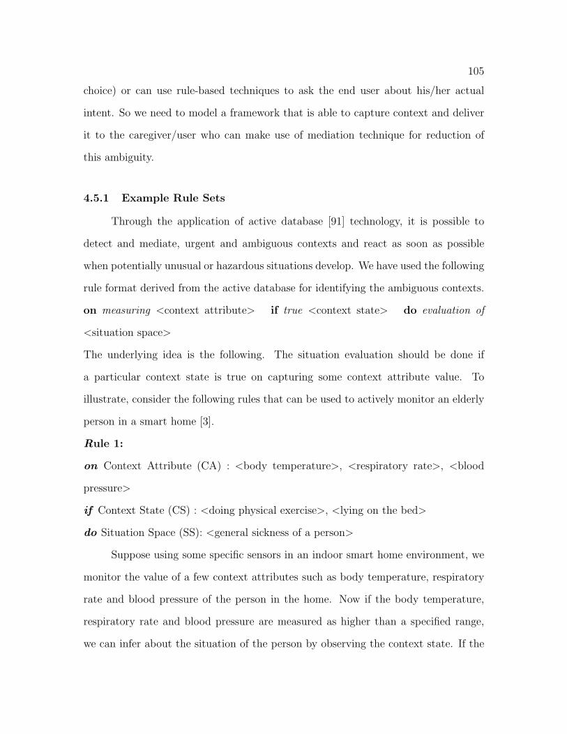
105

choice) or can use rule-based techniques to ask the end user about his/her actual

intent. So we need to model a framework that is able to capture context and deliver

it to the caregiver/user who can make use of mediation technique for reduction of

this ambiguity.

4.5.1 Example Rule Sets

Through the application of active database [91] technology, it is possible to

detect and mediate, urgent and ambiguous contexts and react as soon as possible

when potentially unusual or hazardous situations develop. We have used the following

rule format derived from the active database for identifying the ambiguous contexts.

on measuring <context attribute> if true <context state> do evaluation of

<situation space>

The underlying idea is the following. The situation evaluation should be done if

a particular context state is true on capturing some context attribute value. To

illustrate, consider the following rules that can be used to actively monitor an elderly

person in a smart home [3].

Rule 1:

on Context Attribute (CA) : <body temperature>, <respiratory rate>, <blood

pressure>

if Context State (CS) : <doing physical exercise>, <lying on the bed>

do Situation Space (SS): <general sickness of a person>

Suppose using some specific sensors in an indoor smart home environment, we

monitor the value of a few context attributes such as body temperature, respiratory

rate and blood pressure of the person in the home. Now if the body temperature,

respiratory rate and blood pressure are measured as higher than a specified range,

we can infer about the situation of the person by observing the context state. If the

106

context state is doing physical exercise, then the situation is normal. Otherwise, if

the context state is lying on the bed, then the situation is abnormal. Let us consider

another rule where we consider the context attribute as time instant, time span and

location of the inhabitant in the home.

Rule 2:

on CA: <time instant>, <time span>, <location>

if CS: <doing morning/evening walk>, <talking with neighbors>, <sleeping>

do SS: <normal behavior>

If it is 2am at morning and the location of the person is outside the home

where the context state is walking, then we can conclude that the behavior of the

person is not normal. But if it is 6am in the morning and the location of the person

is outside the home where the context state is walking, then we can conclude that

the behavior of the person is normal. We can make different variants of this rule by

considering different context attributes with a different context state. Thus detecting

that a person has been engaged in a specific activity for an unusual time may be an

indicator of a health problem or a potentially hazardous domiciliary situation.

Rule 3:

on CA: <time>, <frequency for getting up from the bed>

if CS: <watching the television>, <going to restroom>

do SS: <sickness of a person>

We can frame another rule where the context attribute are time and frequency

for getting up from the bed. If the time is late night and frequency is too high we

have to take a look at the context state. If the context state is watching the television

then we don’t need to comment regarding the person situation but if it’s going to

restroom then might be there is a need for taking care of the person (measuring the

blood sugar level, blood pressure etc.).

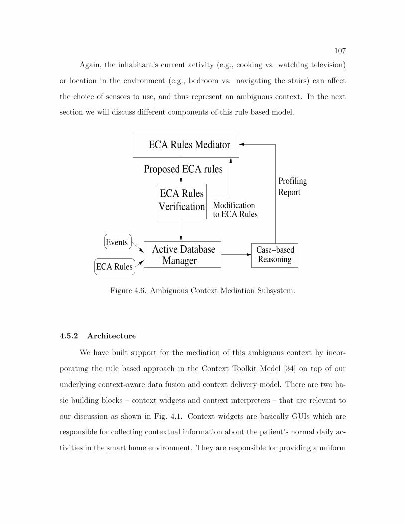
107

Again, the inhabitant’s current activity (e.g., cooking vs. watching television)

or location in the environment (e.g., bedroom vs. navigating the stairs) can affect

the choice of sensors to use, and thus represent an ambiguous context. In the next

section we will discuss different components of this rule based model.

ECA Rules

Verification

Active Database Manager

Proposed ECA rules

Events

ECA Rules

Case−basedReasoning

Modificationto ECA Rules

Profiling

Report

ECA Rules Mediator

Figure 4.6. Ambiguous Context Mediation Subsystem.

4.5.2 Architecture

We have built support for the mediation of this ambiguous context by incor-

porating the rule based approach in the Context Toolkit Model [34] on top of our

underlying context-aware data fusion and context delivery model. There are two ba-

sic building blocks – context widgets and context interpreters – that are relevant to

our discussion as shown in Fig. 4.1. Context widgets are basically GUIs which are

responsible for collecting contextual information about the patient’s normal daily ac-

tivities in the smart home environment. They are responsible for providing a uniform

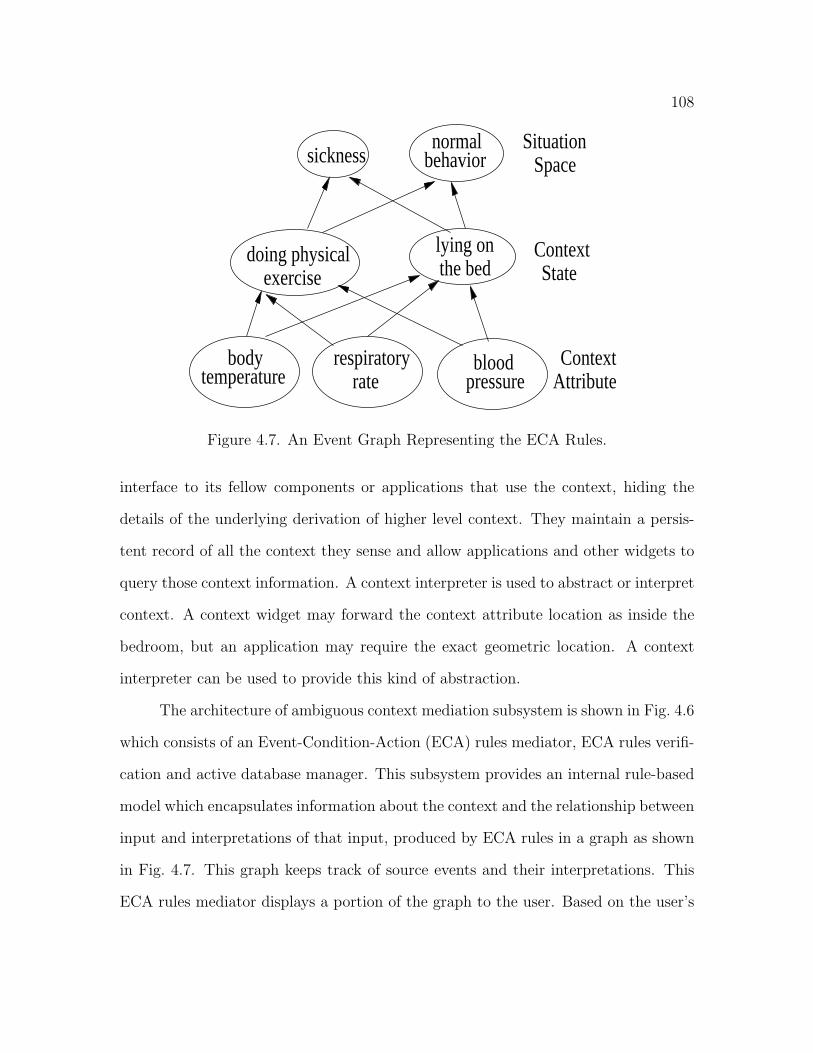
108

body temperature pressure

blood

doing physical exercise

lying onthe bed

sicknessnormal

behavior

Context

Situation

ContextAttribute

State

Space

raterespiratory

Figure 4.7. An Event Graph Representing the ECA Rules.

interface to its fellow components or applications that use the context, hiding the

details of the underlying derivation of higher level context. They maintain a persis-

tent record of all the context they sense and allow applications and other widgets to

query those context information. A context interpreter is used to abstract or interpret

context. A context widget may forward the context attribute location as inside the

bedroom, but an application may require the exact geometric location. A context

interpreter can be used to provide this kind of abstraction.

The architecture of ambiguous context mediation subsystem is shown in Fig. 4.6

which consists of an Event-Condition-Action (ECA) rules mediator, ECA rules verifi-

cation and active database manager. This subsystem provides an internal rule-based

model which encapsulates information about the context and the relationship between

input and interpretations of that input, produced by ECA rules in a graph as shown

in Fig. 4.7. This graph keeps track of source events and their interpretations. This

ECA rules mediator displays a portion of the graph to the user. Based on the user’s

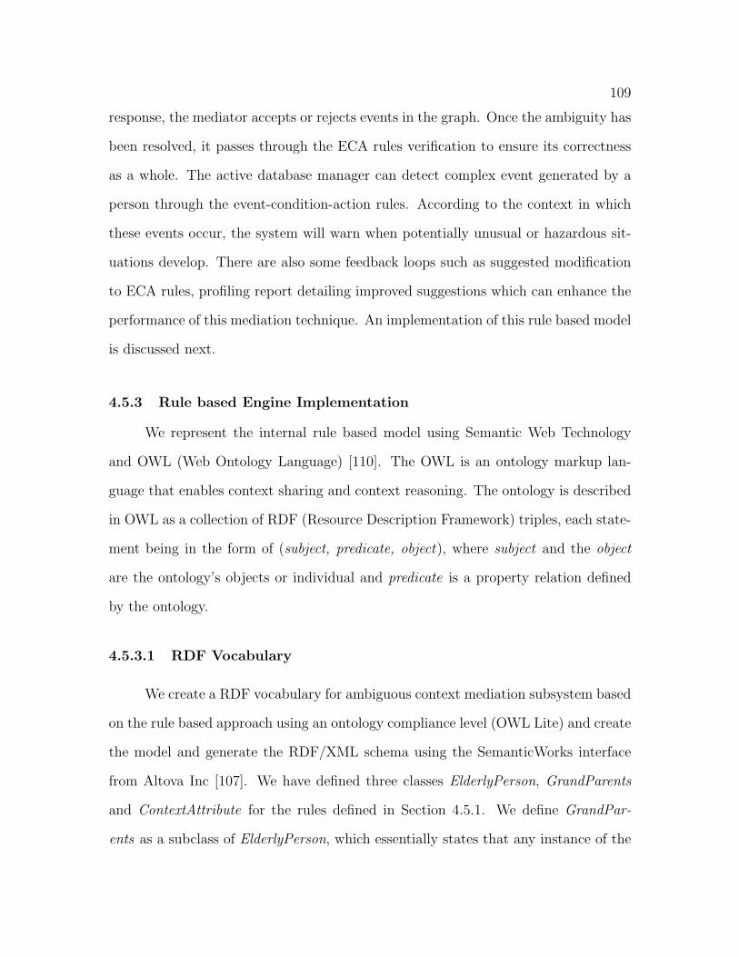
109

response, the mediator accepts or rejects events in the graph. Once the ambiguity has

been resolved, it passes through the ECA rules verification to ensure its correctness

as a whole. The active database manager can detect complex event generated by a

person through the event-condition-action rules. According to the context in which

these events occur, the system will warn when potentially unusual or hazardous sit-

uations develop. There are also some feedback loops such as suggested modification

to ECA rules, profiling report detailing improved suggestions which can enhance the

performance of this mediation technique. An implementation of this rule based model

is discussed next.

4.5.3 Rule based Engine Implementation

We represent the internal rule based model using Semantic Web Technology

and OWL (Web Ontology Language) [110]. The OWL is an ontology markup lan-

guage that enables context sharing and context reasoning. The ontology is described

in OWL as a collection of RDF (Resource Description Framework) triples, each state-

ment being in the form of (subject, predicate, object), where subject and the object

are the ontology’s objects or individual and predicate is a property relation defined

by the ontology.

4.5.3.1 RDF Vocabulary

We create a RDF vocabulary for ambiguous context mediation subsystem based

on the rule based approach using an ontology compliance level (OWL Lite) and create

the model and generate the RDF/XML schema using the SemanticWorks interface

from Altova Inc [107]. We have defined three classes ElderlyPerson, GrandParents

and ContextAttribute for the rules defined in Section 4.5.1. We define GrandPar-

ents as a subclass of ElderlyPerson, which essentially states that any instance of the

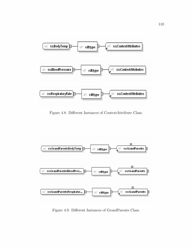
110

Figure 4.8. Different Instances of ContextAttribute Class.

Figure 4.9. Different Instances of GrandParents Class.

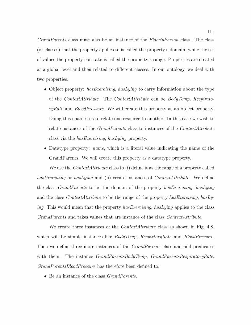
111

GrandParents class must also be an instance of the ElderlyPerson class. The class

(or classes) that the property applies to is called the property’s domain, while the set

of values the property can take is called the property’s range. Properties are created

at a global level and then related to different classes. In our ontology, we deal with

two properties:

• Object property: hasExercising, hasLying to carry information about the type

of the ContextAttribute. The ContextAttribute can be BodyTemp, Respirato-

ryRate and BloodPressure. We will create this property as an object property.

Doing this enables us to relate one resource to another. In this case we wish to

relate instances of the GrandParents class to instances of the ContextAttribute

class via the hasExercising, hasLying property.

• Datatype property: name, which is a literal value indicating the name of the

GrandParents. We will create this property as a datatype property.

We use the ContextAttribute class to (i) define it as the range of a property called

hasExercising or hasLying and (ii) create instances of ContextAttribute. We define

the class GrandParents to be the domain of the property hasExercising, hasLying

and the class ContextAttribute to be the range of the property hasExercising, hasLy-

ing. This would mean that the property hasExercising, hasLying applies to the class

GrandParents and takes values that are instance of the class ContextAttribute.

We create three instances of the ContextAttribute class as shown in Fig. 4.8,

which will be simple instances like BodyTemp, RespirtoryRate and BloodPressure.

Then we define three more instances of the GrandParents class and add predicates

with them. The instance GrandParentsBodyTemp, GrandParentsRespiratoryRate,

GrandParentsBloodPressure has therefore been defined to:

• Be an instance of the class GrandParents,

112

• Have object property hasExercising, hasLying that takes the instance Contex-

tAttribute as its object, and

• Have a datatype property name that takes the string as its literal value.

4.5.3.2 Demonstration

To validate our work and to demonstrate the expressiveness of the model we

implemented a reasoning component, which implements this rule model. The java

based reasoning component gets RDF-information about these classes, available con-

text state, context attribute, and can then trigger actions and provide prioritiza-

tion information about situation space. Jena 2.5.3, an open source Semantic Web

Toolkit [62] is utilized within the reasoning component for parsing the RDF descrip-

tions. We implemented demonstration software, which can be used for experimenting

with the reasoning component. The demonstration software includes the RDF vo-

cabulary. This vocabulary has been converted to java class file using the schemagen

utility from Jena API which helps to get access to different properties of RDF graph

based model. A RDF metadatabase is developed which contains several datavalue

used for querying context. We use SPARQL [111], a query language which can select

RDF triples from this database. Applications based on our ambiguous context medi-

ation subsystem can query contexts by specifying a SPARQL query. The queries are

executed directly with Jena’s SPARQL support for querying RDF models. Variables

in the rules present the resources (users, situations), which are to be found with the

SPARQL query. The RDF descriptions and rules in the demonstration were written

by using an XML/RDF definition for presenting RDF models. Here is an example of

a statement from a rule, which is supported by our implementation:

string rules = “[ Rule1: (?GrandParentsBodyTemp ss:hasLying ?BodyTemp) ∧

(?BodyTemp ss:hasGreaterThan ?TempValue) ∧ (?GrandParentsBloodPressure

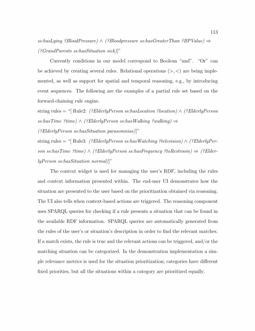
113

ss:hasLying ?BloodPressure) ∧ (?Bloodpressure ss:hasGreaterThan ?BPValue) ⇒

(?GrandParents ss:hasSituation sick)]”

Currently conditions in our model correspond to Boolean “and”. “Or” can

be achieved by creating several rules. Relational operations (>,<) are being imple-

mented, as well as support for spatial and temporal reasoning, e.g., by introducing

event sequences. The following are the examples of a partial rule set based on the

forward-chaining rule engine.

string rules = “[ Rule2: (?ElderlyPerson ss:hasLocation ?location) ∧ (?ElderlyPerson

ss:hasTime ?time) ∧ (?ElderlyPerson ss:hasWalking ?walking) ⇒

(?ElderlyPerson ss:hasSituation parasomnias)]”

string rules = “[ Rule3: (?ElderlyPerson ss:hasWatching ?television) ∧ (?ElderlyPer-

son ss:hasTime ?time) ∧ (?ElderlyPerson ss:hasFrequency ?toRestroom) ⇒ (?Elder-

lyPerson ss:hasSituation normal)]”

The context widget is used for managing the user’s RDF, including the rules

and context information presented within. The end-user UI demonstrates how the

situation are presented to the user based on the prioritization obtained via reasoning.

The UI also tells when context-based actions are triggered. The reasoning component

uses SPARQL queries for checking if a rule presents a situation that can be found in

the available RDF information. SPARQL queries are automatically generated from

the rules of the user’s or situation’s description in order to find the relevant matches.

If a match exists, the rule is true and the relevant actions can be triggered, and/or the

matching situation can be categorized. In the demonstration implementation a sim-

ple relevance metrics is used for the situation prioritization; categories have different

fixed priorities, but all the situations within a category are prioritized equally.

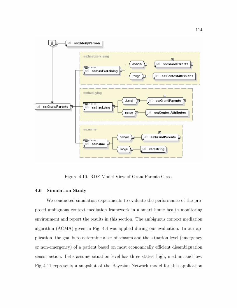
114

Figure 4.10. RDF Model View of GrandParents Class.

4.6 Simulation Study

We conducted simulation experiments to evaluate the performance of the pro-

posed ambiguous context mediation framework in a smart home health monitoring

environment and report the results in this section. The ambiguous context mediation

algorithm (ACMA) given in Fig. 4.4 was applied during our evaluation. In our ap-

plication, the goal is to determine a set of sensors and the situation level (emergency

or non-emergency) of a patient based on most economically efficient disambiguation

sensor action. Let’s assume situation level has three states, high, medium and low.

Fig 4.11 represents a snapshot of the Bayesian Network model for this application

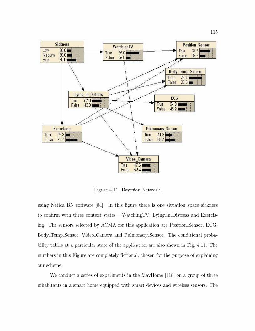
115

Figure 4.11. Bayesian Network.

using Netica BN software [84]. In this figure there is one situation space sickness

to confirm with three context states – WatchingTV, Lying in Distress and Exercis-

ing. The sensors selected by ACMA for this application are Position Sensor, ECG,

Body Temp Sensor, Video Camera and Pulmonary Sensor. The conditional proba-

bility tables at a particular state of the application are also shown in Fig. 4.11. The

numbers in this Figure are completely fictional, chosen for the purpose of explaining

our scheme.

We conduct a series of experiments in the MavHome [118] on a group of three

inhabitants in a smart home equipped with smart devices and wireless sensors. The

116

inhabitants wear radio frequency identification (RFID) tags and are tracked by RFID-

readers. The house is equipped with explicit monitoring of inhabitants’ activities and

locations to get the context attribute values for performing a trace-driven simulation.

We have developed an object-oriented discrete-event simulation platform for generat-

ing context attribute values, deriving context state and inferring the situation space

using the DBN model. In order to collect the test data associated with the inhabi-

tants’ life-style as shown in Table 4.1, the appliances in the MavHome are equipped

with X10 ActiveHome kit and HomeSeer [117], thus allowing the inhabitants to auto-

matically control the appliances. The identity of the inhabitants, their locations and

activities are captured by wireless sensors placed inside the home. The inhabitants

wear the RF-tags, which are sensed by the RF-readers to gather their identities. The

raw data [119] as shown in Table 4.1 is first parsed using parsing tools like Perl and

Tcl to remove unnecessary information. The different column headings in Table 4.1

have the following meanings: Mark as the data and time stamp; Zone and Number

as unique sensor zone identifier and sensor number within it; State as binary ‘on’

or ‘off’ of the sensor; Level as specific value if the sensor is on. Subsequently, we

use these data to effectively select the set of sensors for an application performing

context-aware data fusion and decision making.

4.6.1 Performance Results

The sensors used for our application are classified according to their numbers

such as Sensor-1 (Position Sensor), Sensor-2 (Body Temp Sensor), Sensor-3 (ECG),

Sensor-4 (Pulmonary Sensor), Sensor-5 (Video Camera), Sensor-21 (RFID 1) and

Sensor-23 (RFID 2) as shown in Table 4.1. We have calculated the utility value for

different combination of sensors with varying set size through the successive iteration

of the ambiguous context mediation algorithm. The balance coefficient α is set to 1

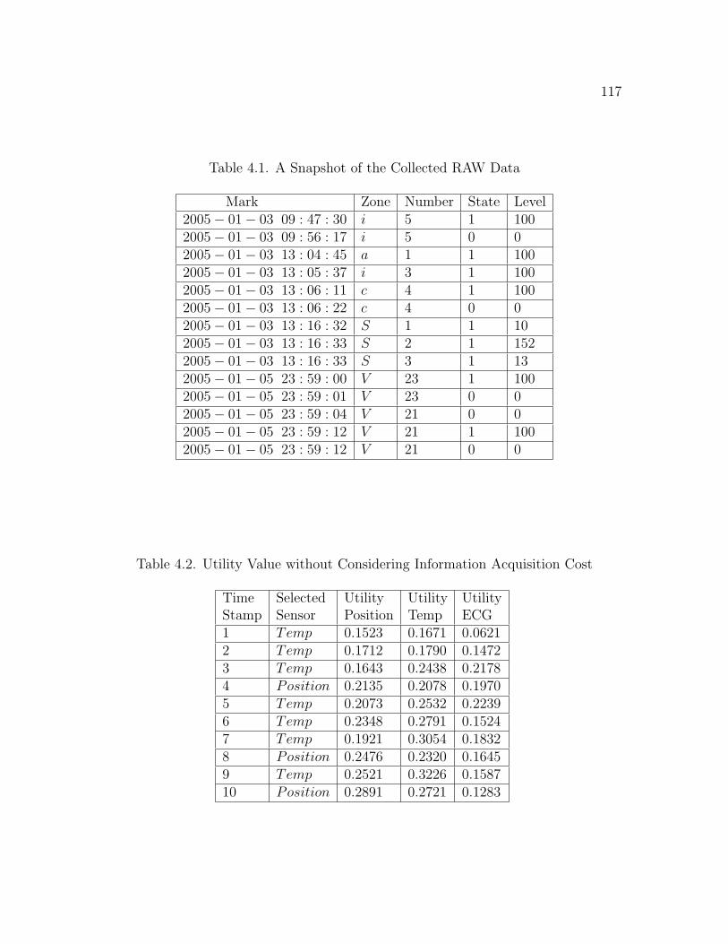
117

Table 4.1. A Snapshot of the Collected RAW Data

Mark Zone Number State Level2005− 01− 03 09 : 47 : 30 i 5 1 1002005− 01− 03 09 : 56 : 17 i 5 0 02005− 01− 03 13 : 04 : 45 a 1 1 1002005− 01− 03 13 : 05 : 37 i 3 1 1002005− 01− 03 13 : 06 : 11 c 4 1 1002005− 01− 03 13 : 06 : 22 c 4 0 02005− 01− 03 13 : 16 : 32 S 1 1 102005− 01− 03 13 : 16 : 33 S 2 1 1522005− 01− 03 13 : 16 : 33 S 3 1 132005− 01− 05 23 : 59 : 00 V 23 1 1002005− 01− 05 23 : 59 : 01 V 23 0 02005− 01− 05 23 : 59 : 04 V 21 0 02005− 01− 05 23 : 59 : 12 V 21 1 1002005− 01− 05 23 : 59 : 12 V 21 0 0

Table 4.2. Utility Value without Considering Information Acquisition Cost

Time Selected Utility Utility UtilityStamp Sensor Position Temp ECG1 Temp 0.1523 0.1671 0.06212 Temp 0.1712 0.1790 0.14723 Temp 0.1643 0.2438 0.21784 Position 0.2135 0.2078 0.19705 Temp 0.2073 0.2532 0.22396 Temp 0.2348 0.2791 0.15247 Temp 0.1921 0.3054 0.18328 Position 0.2476 0.2320 0.16459 Temp 0.2521 0.3226 0.158710 Position 0.2891 0.2721 0.1283

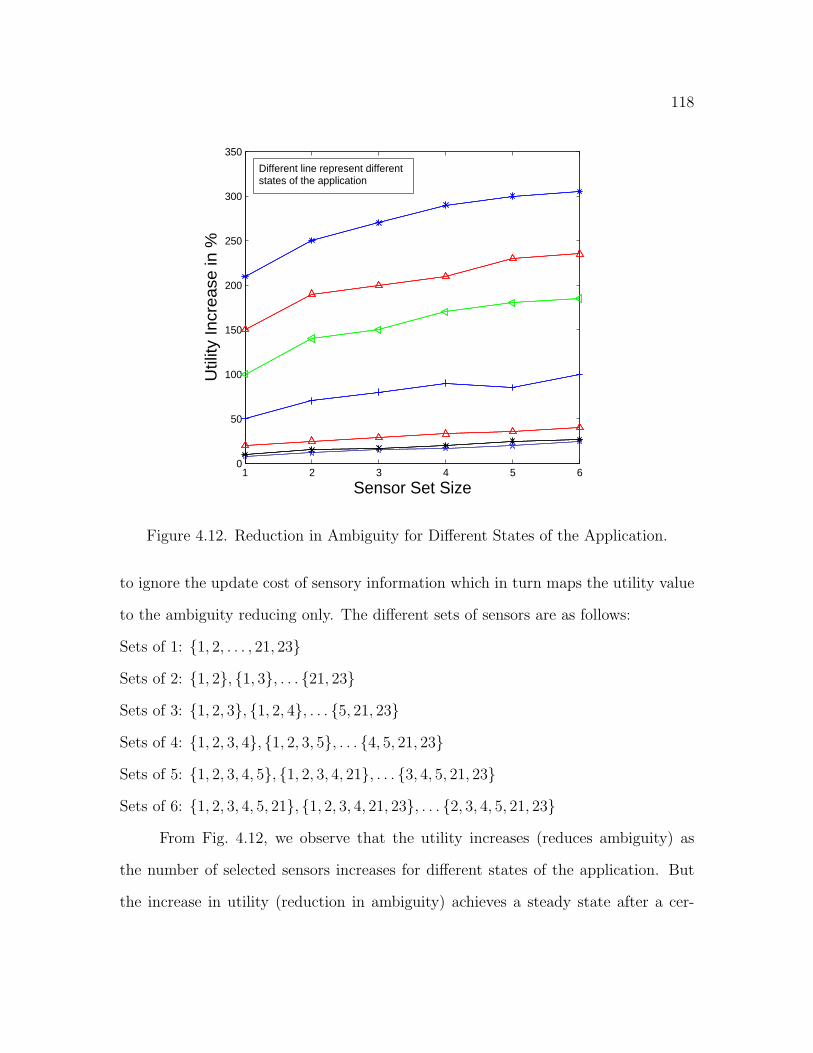
118

1 2 3 4 5 60

50

100

150

200

250

300

350

Sensor Set Size

Util

ity In

crea

se in

%

Different line represent differentstates of the application

Figure 4.12. Reduction in Ambiguity for Different States of the Application.

to ignore the update cost of sensory information which in turn maps the utility value

to the ambiguity reducing only. The different sets of sensors are as follows:

Sets of 1: 1, 2, . . . , 21, 23

Sets of 2: 1, 2, 1, 3, . . . 21, 23

Sets of 3: 1, 2, 3, 1, 2, 4, . . . 5, 21, 23

Sets of 4: 1, 2, 3, 4, 1, 2, 3, 5, . . . 4, 5, 21, 23

Sets of 5: 1, 2, 3, 4, 5, 1, 2, 3, 4, 21, . . . 3, 4, 5, 21, 23

Sets of 6: 1, 2, 3, 4, 5, 21, 1, 2, 3, 4, 21, 23, . . . 2, 3, 4, 5, 21, 23

From Fig. 4.12, we observe that the utility increases (reduces ambiguity) as

the number of selected sensors increases for different states of the application. But

the increase in utility (reduction in ambiguity) achieves a steady state after a cer-

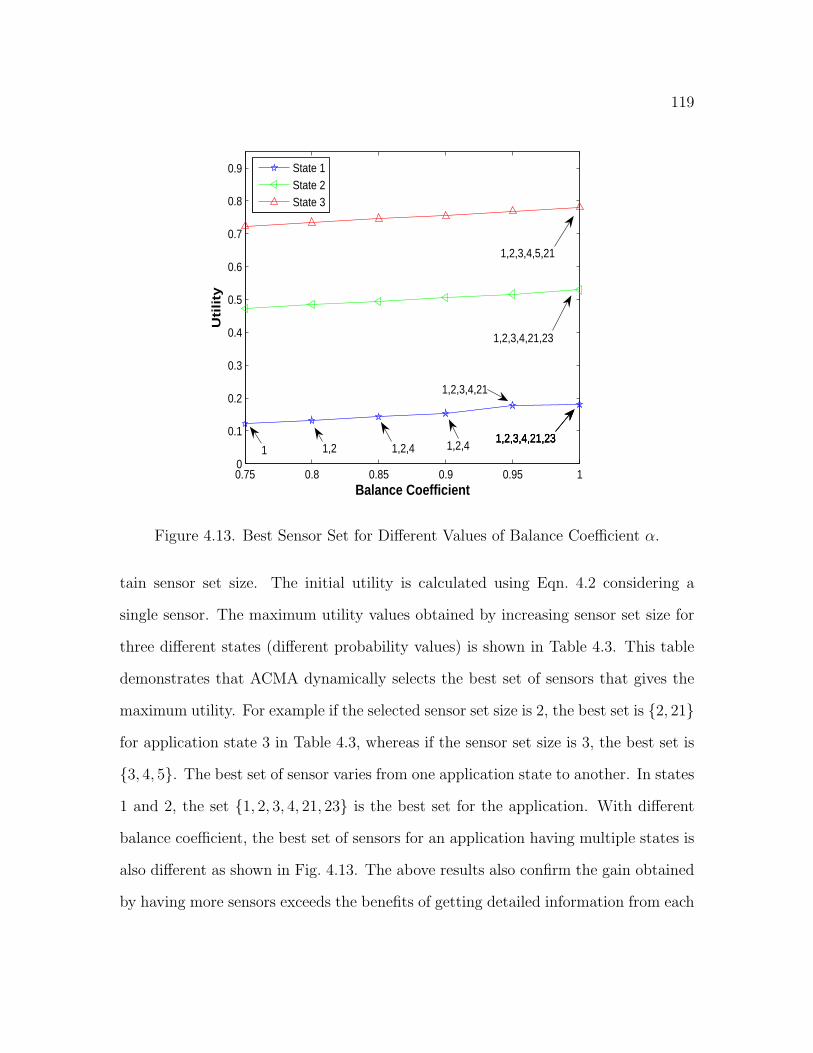
119

0.75 0.8 0.85 0.9 0.95 10

0.1

0.2

0.3

0.4

0.5

0.6

0.7

0.8

0.9

Balance Coefficient

Uti

lity

State 1State 2State 3

1 1,21,2,3,4,21,231,2,3,4,21,231,2,3,4,21,23

1,2,3,4,21,23

1,2,3,4,5,21

1,2,4 1,2,4

1,2,3,4,21

Figure 4.13. Best Sensor Set for Different Values of Balance Coefficient α.

tain sensor set size. The initial utility is calculated using Eqn. 4.2 considering a

single sensor. The maximum utility values obtained by increasing sensor set size for

three different states (different probability values) is shown in Table 4.3. This table

demonstrates that ACMA dynamically selects the best set of sensors that gives the

maximum utility. For example if the selected sensor set size is 2, the best set is 2, 21

for application state 3 in Table 4.3, whereas if the sensor set size is 3, the best set is

3, 4, 5. The best set of sensor varies from one application state to another. In states

1 and 2, the set 1, 2, 3, 4, 21, 23 is the best set for the application. With different

balance coefficient, the best set of sensors for an application having multiple states is

also different as shown in Fig. 4.13. The above results also confirm the gain obtained

by having more sensors exceeds the benefits of getting detailed information from each

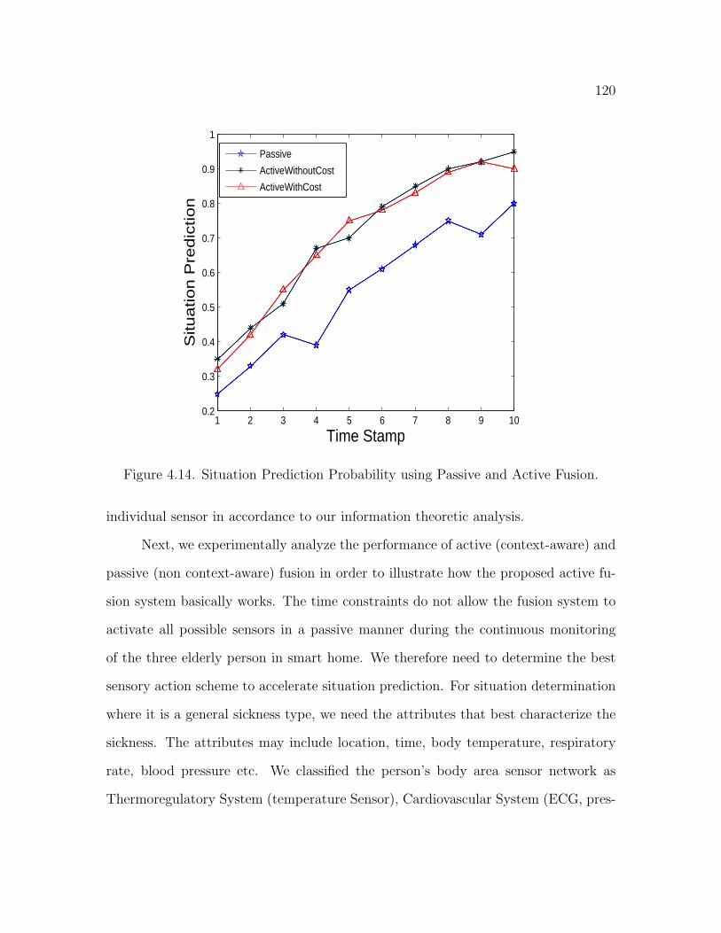
120

1 2 3 4 5 6 7 8 9 100.2

0.3

0.4

0.5

0.6

0.7

0.8

0.9

1

Time Stamp

Situ

atio

n P

red

ictio

n

Passive

ActiveWithoutCost

ActiveWithCost

Figure 4.14. Situation Prediction Probability using Passive and Active Fusion.

individual sensor in accordance to our information theoretic analysis.

Next, we experimentally analyze the performance of active (context-aware) and

passive (non context-aware) fusion in order to illustrate how the proposed active fu-

sion system basically works. The time constraints do not allow the fusion system to

activate all possible sensors in a passive manner during the continuous monitoring

of the three elderly person in smart home. We therefore need to determine the best

sensory action scheme to accelerate situation prediction. For situation determination

where it is a general sickness type, we need the attributes that best characterize the

sickness. The attributes may include location, time, body temperature, respiratory

rate, blood pressure etc. We classified the person’s body area sensor network as

Thermoregulatory System (temperature Sensor), Cardiovascular System (ECG, pres-

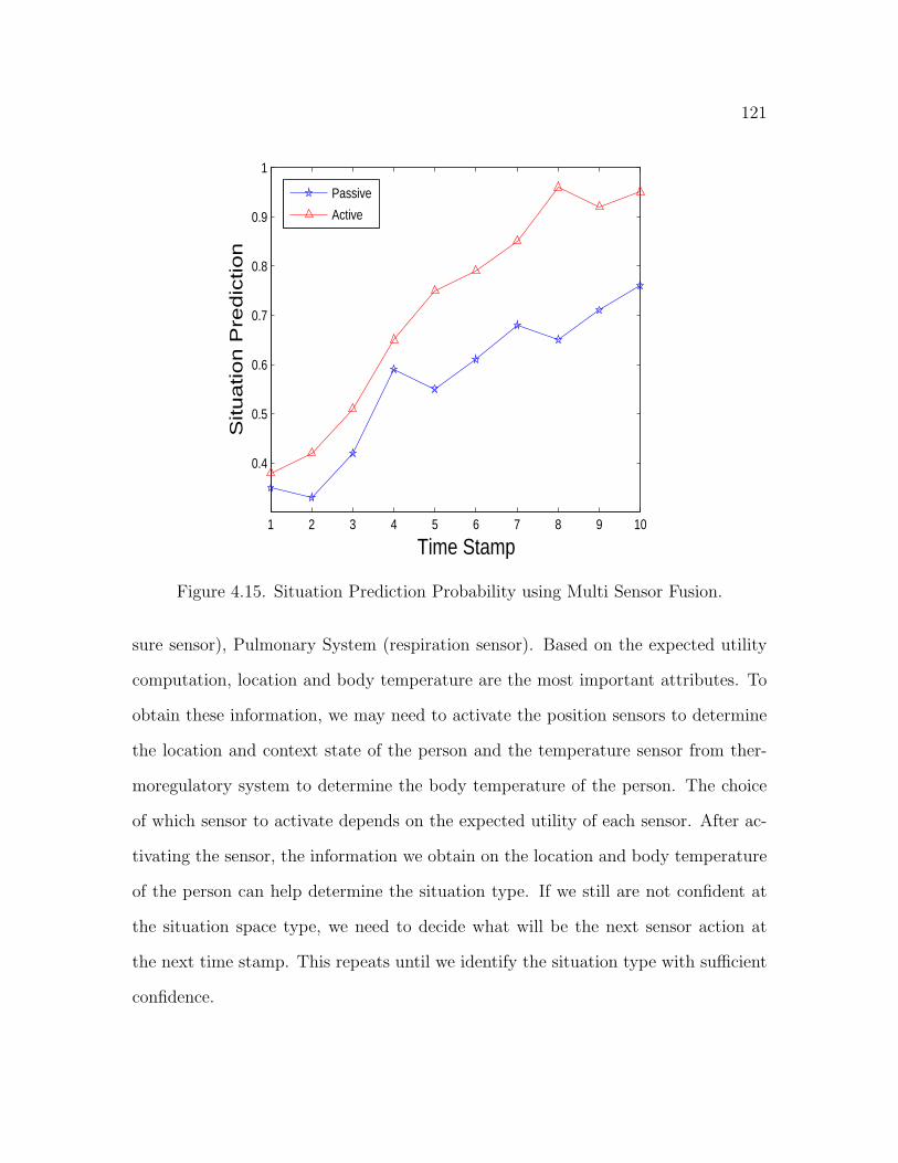
121

1 2 3 4 5 6 7 8 9 10

0.4

0.5

0.6

0.7

0.8

0.9

1

Time Stamp

Situ

atio

n P

red

ictio

n

Passive

Active

Figure 4.15. Situation Prediction Probability using Multi Sensor Fusion.

sure sensor), Pulmonary System (respiration sensor). Based on the expected utility

computation, location and body temperature are the most important attributes. To

obtain these information, we may need to activate the position sensors to determine

the location and context state of the person and the temperature sensor from ther-

moregulatory system to determine the body temperature of the person. The choice

of which sensor to activate depends on the expected utility of each sensor. After ac-

tivating the sensor, the information we obtain on the location and body temperature

of the person can help determine the situation type. If we still are not confident at

the situation space type, we need to decide what will be the next sensor action at

the next time stamp. This repeats until we identify the situation type with sufficient

confidence.

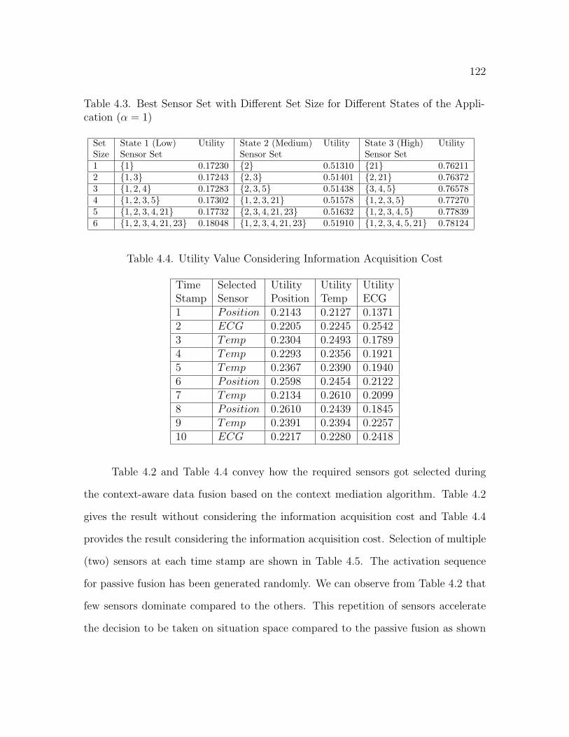
122

Table 4.3. Best Sensor Set with Different Set Size for Different States of the Appli-cation (α = 1)

Set State 1 (Low) Utility State 2 (Medium) Utility State 3 (High) UtilitySize Sensor Set Sensor Set Sensor Set1 1 0.17230 2 0.51310 21 0.762112 1, 3 0.17243 2, 3 0.51401 2, 21 0.763723 1, 2, 4 0.17283 2, 3, 5 0.51438 3, 4, 5 0.765784 1, 2, 3, 5 0.17302 1, 2, 3, 21 0.51578 1, 2, 3, 5 0.772705 1, 2, 3, 4, 21 0.17732 2, 3, 4, 21, 23 0.51632 1, 2, 3, 4, 5 0.778396 1, 2, 3, 4, 21, 23 0.18048 1, 2, 3, 4, 21, 23 0.51910 1, 2, 3, 4, 5, 21 0.78124

Table 4.4. Utility Value Considering Information Acquisition Cost

Time Selected Utility Utility UtilityStamp Sensor Position Temp ECG1 Position 0.2143 0.2127 0.13712 ECG 0.2205 0.2245 0.25423 Temp 0.2304 0.2493 0.17894 Temp 0.2293 0.2356 0.19215 Temp 0.2367 0.2390 0.19406 Position 0.2598 0.2454 0.21227 Temp 0.2134 0.2610 0.20998 Position 0.2610 0.2439 0.18459 Temp 0.2391 0.2394 0.225710 ECG 0.2217 0.2280 0.2418

Table 4.2 and Table 4.4 convey how the required sensors got selected during

the context-aware data fusion based on the context mediation algorithm. Table 4.2

gives the result without considering the information acquisition cost and Table 4.4

provides the result considering the information acquisition cost. Selection of multiple

(two) sensors at each time stamp are shown in Table 4.5. The activation sequence

for passive fusion has been generated randomly. We can observe from Table 4.2 that

few sensors dominate compared to the others. This repetition of sensors accelerate

the decision to be taken on situation space compared to the passive fusion as shown

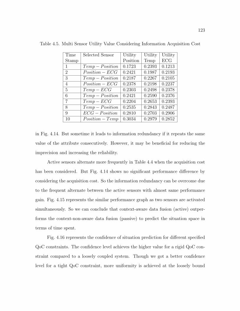
123

Table 4.5. Multi Sensor Utility Value Considering Information Acquisition Cost

Time Selected Sensor Utility Utility UtilityStamp Position Temp ECG1 Temp− Position 0.1723 0.2393 0.12132 Position− ECG 0.2421 0.1987 0.21933 Temp− Position 0.2187 0.2267 0.21054 Position− ECG 0.2378 0.2198 0.22375 Temp− ECG 0.2303 0.2498 0.23786 Temp− Position 0.2421 0.2590 0.23767 Temp− ECG 0.2204 0.2653 0.23938 Temp− Position 0.2535 0.2843 0.24879 ECG− Position 0.2810 0.2703 0.290610 Position− Temp 0.3034 0.2979 0.2852

in Fig. 4.14. But sometime it leads to information redundancy if it repeats the same

value of the attribute consecutively. However, it may be beneficial for reducing the

imprecision and increasing the reliability.

Active sensors alternate more frequently in Table 4.4 when the acquisition cost

has been considered. But Fig. 4.14 shows no significant performance difference by

considering the acquisition cost. So the information redundancy can be overcome due

to the frequent alternate between the active sensors with almost same performance

gain. Fig. 4.15 represents the similar performance graph as two sensors are activated

simultaneously. So we can conclude that context-aware data fusion (active) outper-

forms the context-non-aware data fusion (passive) to predict the situation space in

terms of time spent.

Fig. 4.16 represents the confidence of situation prediction for different specified

QoC constraints. The confidence level achieves the higher value for a rigid QoC con-

straint compared to a loosely coupled system. Though we got a better confidence

level for a tight QoC constraint, more uniformity is achieved at the loosely bound

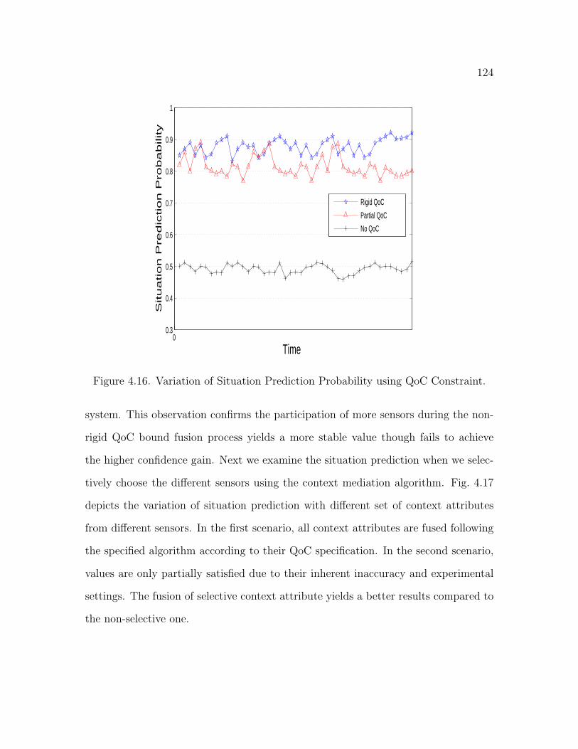
124

00.3

0.4

0.5

0.6

0.7

0.8

0.9

1

Time

Situ

atio

n P

red

ictio

n P

rob

ab

ility

Rigid QoC

Partial QoC

No QoC

Figure 4.16. Variation of Situation Prediction Probability using QoC Constraint.

system. This observation confirms the participation of more sensors during the non-

rigid QoC bound fusion process yields a more stable value though fails to achieve

the higher confidence gain. Next we examine the situation prediction when we selec-

tively choose the different sensors using the context mediation algorithm. Fig. 4.17

depicts the variation of situation prediction with different set of context attributes

from different sensors. In the first scenario, all context attributes are fused following

the specified algorithm according to their QoC specification. In the second scenario,

values are only partially satisfied due to their inherent inaccuracy and experimental

settings. The fusion of selective context attribute yields a better results compared to

the non-selective one.

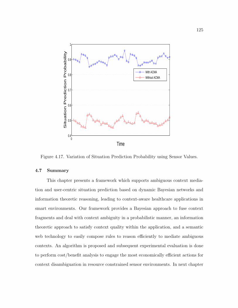
125

0 0.4

0.5

0.6

0.7

0.8

0.9

1

Time

Situ

atio

n P

red

ictio

n P

rob

ab

ility

With ACMA

Without ACMA

Figure 4.17. Variation of Situation Prediction Probability using Sensor Values.

4.7 Summary

This chapter presents a framework which supports ambiguous context media-

tion and user-centric situation prediction based on dynamic Bayesian networks and

information theoretic reasoning, leading to context-aware healthcare applications in

smart environments. Our framework provides a Bayesian approach to fuse context

fragments and deal with context ambiguity in a probabilistic manner, an information

theoretic approach to satisfy context quality within the application, and a semantic

web technology to easily compose rules to reason efficiently to mediate ambiguous

contexts. An algorithm is proposed and subsequent experimental evaluation is done

to perform cost/benefit analysis to engage the most economically efficient actions for

context disambiguation in resource constrained sensor environments. In next chapter

126

we discuss an efficient Quality-of-Inference (QoINF)-Aware context determination in

pervasive care environments.

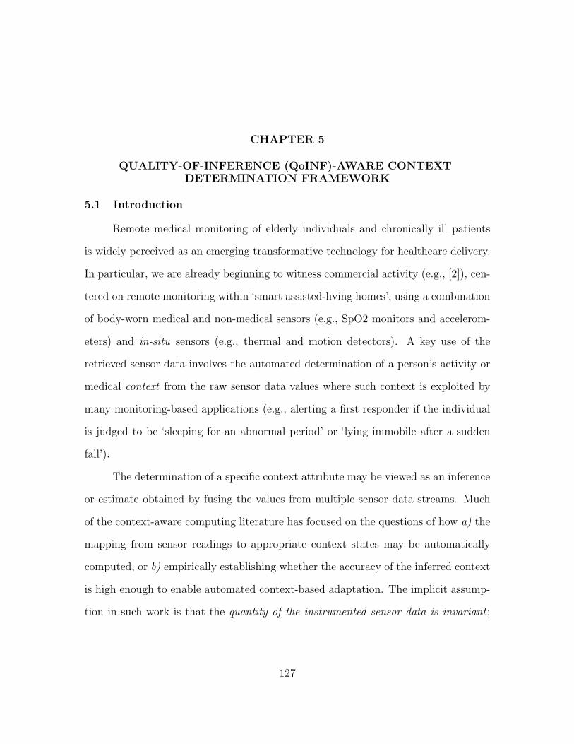
CHAPTER 5

QUALITY-OF-INFERENCE (QoINF)-AWARE CONTEXTDETERMINATION FRAMEWORK

5.1 Introduction

Remote medical monitoring of elderly individuals and chronically ill patients

is widely perceived as an emerging transformative technology for healthcare delivery.

In particular, we are already beginning to witness commercial activity (e.g., [2]), cen-

tered on remote monitoring within ‘smart assisted-living homes’, using a combination

of body-worn medical and non-medical sensors (e.g., SpO2 monitors and accelerom-

eters) and in-situ sensors (e.g., thermal and motion detectors). A key use of the

retrieved sensor data involves the automated determination of a person’s activity or

medical context from the raw sensor data values where such context is exploited by

many monitoring-based applications (e.g., alerting a first responder if the individual

is judged to be ‘sleeping for an abnormal period’ or ‘lying immobile after a sudden

fall’).

The determination of a specific context attribute may be viewed as an inference

or estimate obtained by fusing the values from multiple sensor data streams. Much

of the context-aware computing literature has focused on the questions of how a) the

mapping from sensor readings to appropriate context states may be automatically

computed, or b) empirically establishing whether the accuracy of the inferred context

is high enough to enable automated context-based adaptation. The implicit assump-

tion in such work is that the quantity of the instrumented sensor data is invariant ;

127

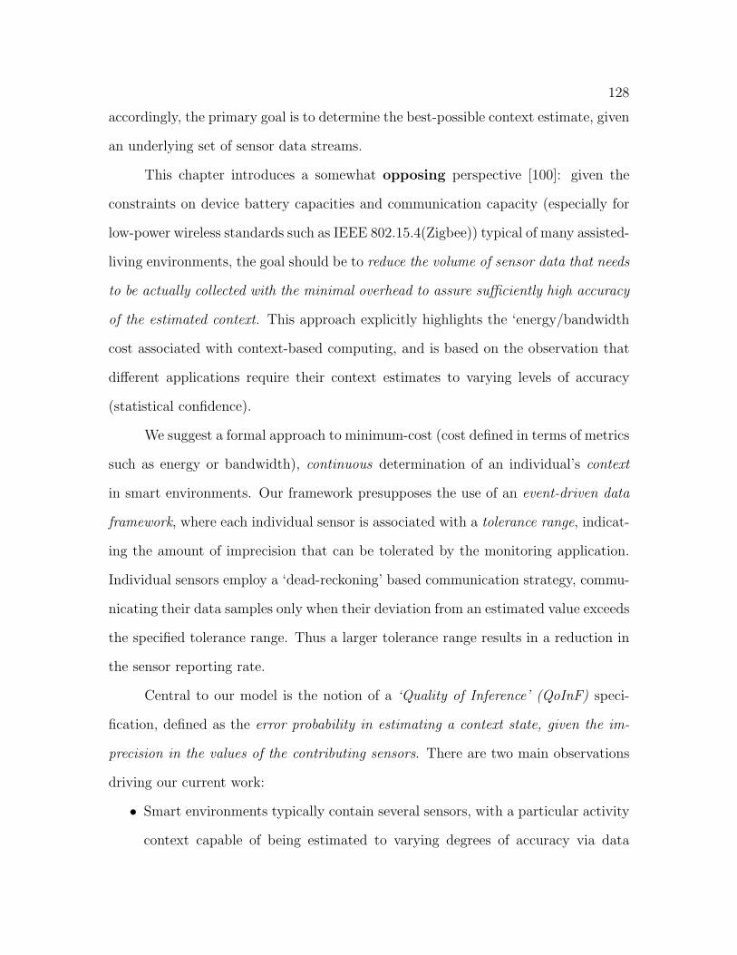
128

accordingly, the primary goal is to determine the best-possible context estimate, given

an underlying set of sensor data streams.

This chapter introduces a somewhat opposing perspective [100]: given the

constraints on device battery capacities and communication capacity (especially for

low-power wireless standards such as IEEE 802.15.4(Zigbee)) typical of many assisted-

living environments, the goal should be to reduce the volume of sensor data that needs

to be actually collected with the minimal overhead to assure sufficiently high accuracy

of the estimated context. This approach explicitly highlights the ‘energy/bandwidth

cost associated with context-based computing, and is based on the observation that

different applications require their context estimates to varying levels of accuracy

(statistical confidence).

We suggest a formal approach to minimum-cost (cost defined in terms of metrics

such as energy or bandwidth), continuous determination of an individual’s context

in smart environments. Our framework presupposes the use of an event-driven data

framework, where each individual sensor is associated with a tolerance range, indicat-

ing the amount of imprecision that can be tolerated by the monitoring application.

Individual sensors employ a ‘dead-reckoning’ based communication strategy, commu-

nicating their data samples only when their deviation from an estimated value exceeds

the specified tolerance range. Thus a larger tolerance range results in a reduction in

the sensor reporting rate.

Central to our model is the notion of a ‘Quality of Inference’ (QoInF) speci-

fication, defined as the error probability in estimating a context state, given the im-

precision in the values of the contributing sensors. There are two main observations

driving our current work:

• Smart environments typically contain several sensors, with a particular activity

context capable of being estimated to varying degrees of accuracy via data

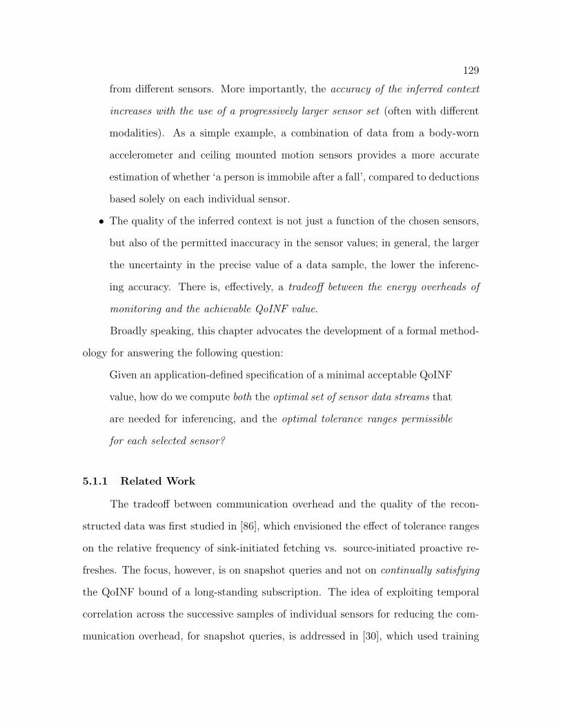
129

from different sensors. More importantly, the accuracy of the inferred context

increases with the use of a progressively larger sensor set (often with different

modalities). As a simple example, a combination of data from a body-worn

accelerometer and ceiling mounted motion sensors provides a more accurate

estimation of whether ‘a person is immobile after a fall’, compared to deductions

based solely on each individual sensor.

• The quality of the inferred context is not just a function of the chosen sensors,

but also of the permitted inaccuracy in the sensor values; in general, the larger

the uncertainty in the precise value of a data sample, the lower the inferenc-

ing accuracy. There is, effectively, a tradeoff between the energy overheads of

monitoring and the achievable QoINF value.

Broadly speaking, this chapter advocates the development of a formal method-

ology for answering the following question:

Given an application-defined specification of a minimal acceptable QoINF

value, how do we compute both the optimal set of sensor data streams that

are needed for inferencing, and the optimal tolerance ranges permissible

for each selected sensor?

5.1.1 Related Work

The tradeoff between communication overhead and the quality of the recon-

structed data was first studied in [86], which envisioned the effect of tolerance ranges

on the relative frequency of sink-initiated fetching vs. source-initiated proactive re-

freshes. The focus, however, is on snapshot queries and not on continually satisfying

the QoINF bound of a long-standing subscription. The idea of exploiting temporal

correlation across the successive samples of individual sensors for reducing the com-

munication overhead, for snapshot queries, is addressed in [30], which used training

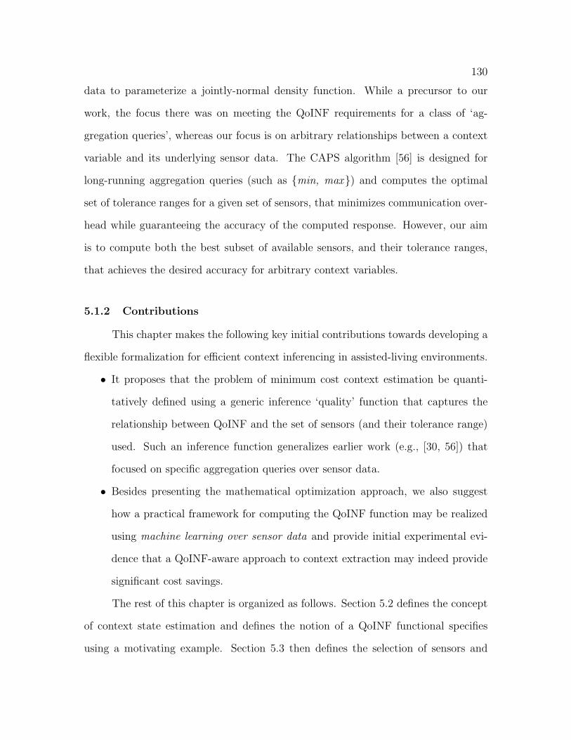
130

data to parameterize a jointly-normal density function. While a precursor to our

work, the focus there was on meeting the QoINF requirements for a class of ‘ag-

gregation queries’, whereas our focus is on arbitrary relationships between a context

variable and its underlying sensor data. The CAPS algorithm [56] is designed for

long-running aggregation queries (such as min, max) and computes the optimal

set of tolerance ranges for a given set of sensors, that minimizes communication over-

head while guaranteeing the accuracy of the computed response. However, our aim

is to compute both the best subset of available sensors, and their tolerance ranges,

that achieves the desired accuracy for arbitrary context variables.

5.1.2 Contributions

This chapter makes the following key initial contributions towards developing a

flexible formalization for efficient context inferencing in assisted-living environments.

• It proposes that the problem of minimum cost context estimation be quanti-

tatively defined using a generic inference ‘quality’ function that captures the

relationship between QoINF and the set of sensors (and their tolerance range)

used. Such an inference function generalizes earlier work (e.g., [30, 56]) that

focused on specific aggregation queries over sensor data.

• Besides presenting the mathematical optimization approach, we also suggest

how a practical framework for computing the QoINF function may be realized

using machine learning over sensor data and provide initial experimental evi-

dence that a QoINF-aware approach to context extraction may indeed provide

significant cost savings.

The rest of this chapter is organized as follows. Section 5.2 defines the concept

of context state estimation and defines the notion of a QoINF functional specifies

using a motivating example. Section 5.3 then defines the selection of sensors and

131

associated tolerance ranges as a non-linear optimization problems and presents a

Lagrangian-based optimization algorithm. Subsequently, Section 5.4 describes how

a QoINF function may be computed in practice, by employing past observations.

Section 5.5 presents early results using SunSPOT sensors to investigate the sort of

accuracy vs. overhead tradeoffs that may be realized. While Section 5.6 summarizes

this chapter.

5.2 Context Inference and the QoINF Model

An important component of automated and proactive health monitoring tech-

nologies is the computation of specific context variables, based on an underlying set

of sensor samples. To precisely quantify the concepts, we assume an underlying set

of S sensors; let vi(t) represent the ‘value’ of the ith sensor at time t. Also, let Λi

represent the range of feasible values of sensor si. The act of determining the value of

a context variable C may be viewed as a multi-dimensional mapping function fC(.),

that takes as input the values from a set of sensors θ : θ ⊂ S and maps them onto

the state space (denoted by ΛC) of the output context. Mathematically:

fC(Υ) :∏

i∈θ

Λi ⇒ x : x ∈ ΛC . (5.1)

Different values of the same context may be inferred to varying degrees of

‘accuracy’ by employing different sets of sensors. In general, one may thus associate

an accuracy function QoINFC(θ(S)), representing the average accuracy in estimating

the context C based on the values for the sensors in the θ(S). To make our definitions

more specific, we define QoINF (.) to be the ‘one minus the average estimation error

resulting from the inferencing function fC(θ(S)), i.e.,

QoINFC(θ(S)) = 1−∑

x∈ΛC

p(i) ∗ errC(x, si ∈ θ(S)), (5.2)

132

where errC(x, si ∈ θ(S))) is the probability of error, given accurate sensor readings

from the sensor set θ(S), when the individual’s value for context variable C is actually

x. In general, alternative definitions of accuracy (e.g., estimation error subject to

maximal ‘false alarm’ rates) are possible; such definitions may, for our purposes, be

viewed merely as alternative definitons of QoINF (.). If the state space of context

C is discrete (e.g., a choice between the values walking, sitting, sleeping, then the

estimation error is computed by the normalized number of wrong inferences made by

the ‘best possible estimator’.1

Figure 5.1 illustrates this notion of multiple sensors and the accuracy (or QoINF)

value associated with different context variables. For example, as shown in Fig. 5.1,

the activity state of an individual may be computed with an inferencing accuracy of

0.9 (i.e., with 10% error rate) using data from a respiratory sensor, but only with

0.8 accuracy using data from a low-quality ECG sensor. However, by fusing the

data available from respiratory, ECG and accelerometer sensors, we can achieve an

inferencing accuracy of 0.95 (i.e., only a 5% error rate).

5.2.1 Role of Tolerance Ranges in Context Estimation Errors

The model above, illustrated in Figure 5.1, can capture the relationship be-

tween context inferencing quality and the choice of sensors. Such a model does not,

however, completely capture the continuous event-driven remote monitoring scenario,

where the value of a sensor sample may be known to different degrees of precision

1In contrast, if the context state space is continuous, the error function also depends on the

tolerance in the computed output state (e.g., it may be acceptable for an inferred location context

to be inaccurate by ±3 feet). Due to reasons of space, we do not delve into these technicalities, which

all relate to the precise specification of the err(.) function. Our focus here is on how to exploit a

given function err(.); for the actual determination of err(.); it suffices to note that there exists an

extensive body of literature on optimal estimators and the resulting lowest possible error bounds.

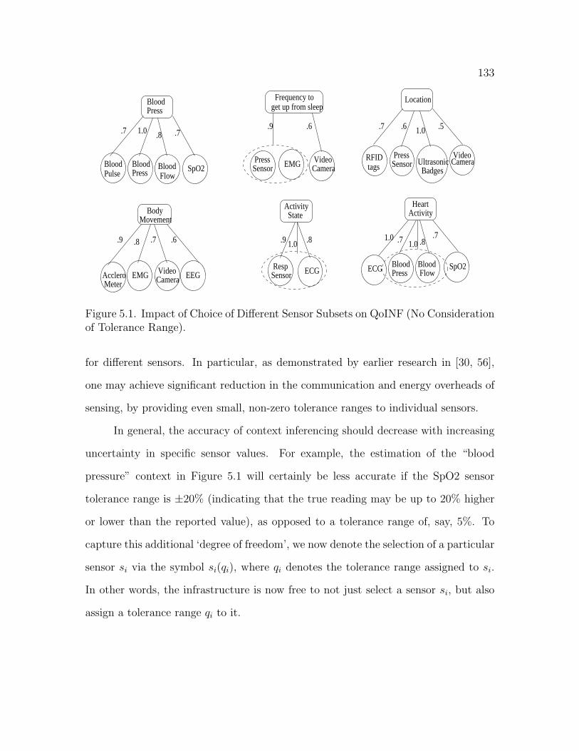
133

BloodPulse

Blood Press

Blood Press

Blood Flow

.7 1.0 .8 .7

get up from sleepFrequency to

Press VideoSensor CameraEMG

.9 .6

RFID tags

PressSensor

VideoCameraUltrasonic

Badges

Location

.7 .6 1.0 .5

MovementBody

MeterAcclero EMG Camera EEGVideo

.9 .8 .7 .6

SensorResp ECG

Heart

ECG Blood Press

Blood Flow

1.0 .7 .7.9 .81.0 1.0 .8

ActivityState Activity

SpO2

SpO2

Figure 5.1. Impact of Choice of Different Sensor Subsets on QoINF (No Considerationof Tolerance Range).

for different sensors. In particular, as demonstrated by earlier research in [30, 56],

one may achieve significant reduction in the communication and energy overheads of

sensing, by providing even small, non-zero tolerance ranges to individual sensors.

In general, the accuracy of context inferencing should decrease with increasing

uncertainty in specific sensor values. For example, the estimation of the “blood

pressure” context in Figure 5.1 will certainly be less accurate if the SpO2 sensor

tolerance range is ±20% (indicating that the true reading may be up to 20% higher

or lower than the reported value), as opposed to a tolerance range of, say, 5%. To

capture this additional ‘degree of freedom’, we now denote the selection of a particular

sensor si via the symbol si(qi), where qi denotes the tolerance range assigned to si.

In other words, the infrastructure is now free to not just select a sensor si, but also

assign a tolerance range qi to it.

134

We can then represent the error associated with a specific choice of sensors s(C)

through the modified dependency relationship:

QoINFC(θ, qθ) = 1−∑

x∈ΛC

p(i) ∗ errC(x, (si, qi) : si ∈ θ(S))

The above equation expresses the fact the accuracy of context sensing is a function

of both the sensors chosen and the tolerated amount of inaccuracy in each sensor’s

value.

5.2.2 Context Sensing Architecture

Figure 5.2 shows our vision of the high-level functional components of a context-

determination service. External applications (e.g., activity monitoring applications

deployed by stakeholders such as wellness professionals) subscribe to a specific context

C, indicating a minimally acceptable QoINF value, QoINFmin. (Of course, monitor-

ing applications may change their QoINFmin specification in response to external

‘situational awareness’, thereby triggering another optimization cycle). The Con-

text Optimizer component must then determine the best (least-cost) combination of

sensors and tolerance ranges that can meet this QoINF threshold. To perform this

optimization, it requires the QoINFC(.) function that is computed by the Context

Modeler component. Finally, the transmitted sensor data samples are received by the

Context Estimator component, which provides continuous updates on the subscribed

context variable.

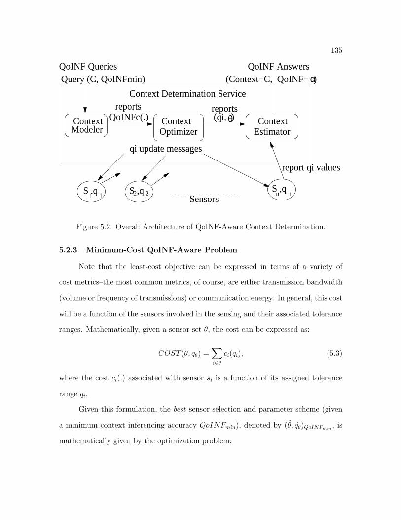
135

1S ,q

1S ,q2 2

S ,qn n

ModelerContext Context

Optimizer

QoINFc(.)reports reports

EstimatorContext

Context Determination Service

QoINF AnswersQuery (C, QoINFmin)QoINF Queries

Sensors

qi update messages

report qi values

(qi, )

(Context=C, QoINF= )α

θ

Figure 5.2. Overall Architecture of QoINF-Aware Context Determination.

5.2.3 Minimum-Cost QoINF-Aware Problem

Note that the least-cost objective can be expressed in terms of a variety of

cost metrics–the most common metrics, of course, are either transmission bandwidth

(volume or frequency of transmissions) or communication energy. In general, this cost

will be a function of the sensors involved in the sensing and their associated tolerance

ranges. Mathematically, given a sensor set θ, the cost can be expressed as:

COST (θ, qθ) =∑

i∈θ

ci(qi), (5.3)

where the cost ci(.) associated with sensor si is a function of its assigned tolerance

range qi.

Given this formulation, the best sensor selection and parameter scheme (given

a minimum context inferencing accuracy QoINFmin), denoted by (θ, qθ)QoINFmin, is

mathematically given by the optimization problem:

136

MIN-COST-INFERENCE:

(θ, qθ)QoINFmin=

arg minθ ⊂ S, qθ COST (θ, qθ)

such that QoINFC(θ, qθ) ≥ QoINFmin (5.4)

5.3 QoINF Cost Optimization

Our computing infrastructure consists of a declarative query processing engine

that takes application bounds on QoINFmin as input and optimally ‘tasks’ the in-

dividual sensors to provide the necessary inputs to a context estimator engine. The

actual optimal parameters will depend on the specific cost (e.g., energy or reporting

frequency) that we seek to minimize and the structure of the QoINF (.) function. In

this section, for specificity, we focus on minimizing a measure of the average commu-

nication overhead and provide insights into the resulting algorithms.

5.3.1 Average Reporting Cost Optimization

One natural cost to optimize is the communication overhead incurred by the

sensor in reporting its values to the Context Estimator component. Let us denote the

average update cost (communication overhead) of sensor si, given a tolerance range

qi as ci(qi). Intuitively, ci is a decreasing function of qi, since the communication cost

would be higher (more frequent reports) for smaller tolerance ranges. In a setting

where the sensor data traverses multiple hops to get to the Context Estimator Engine,

the update cost is also proportional to hi, the length of the uplink path from sensor si

to the Aggregation Engine.2 As shown in [56], if the underlying data samples evolve

2It is easy to generalize the model to other cost formulations–e.g., where the cost for si is weighted

inversely proportional to its residual battery capacity.

137

as a random-walk model, we have ci(qi) ∝ hi

q2

i

. In this case, the resulting cumulative

cost function is given by:

COST (θ, qθ) = κ ∗∑

i∈θ

hi

q2i

(5.5)

where κ is a scaling constant and hi is the hop count.

If the set of sensors to be used, i.e., the set θ is given, then the problem of

optimally computing the qis can be represented by the Lagrangian:

minimize∑

i∈θ

hi

q2i

+ λ× [QoINFC(q1, q2, . . . , qθ)−QoINFmin] . (5.6)

Finding an exact solution to Equation 5.4, for any arbitrary QoINF (.) is an NP-

complete problem [30]. For the general case of a function QoINF (.), the only solution

to determine the most optimal set of sensors (i.e., θ) is to iterate over all the 2S − 1

elements of the power-set of S.

5.3.2 Suggested Optimization Heuristic

While a completely arbitrary QoINF (.) function requires a brute-force search,

there are certain forms of QoINF (.) that prove to be more tractable and lend them-

selves to more efficient optimization heuristics. In particular, a particularly attractive

case occurs when the ith sensor’s individual qoinf(.) is represented by an ‘Inverse-

Exponential’ distribution of the form

qoinf(i) = 1− 1

νi

exp(−1

ηiqi), (5.7)

where ηi and νi are sensitivity constants for sensor si. A larger value of νi indicates

a lower contribution from sensor si to the inference of context C. Moreover, for a

selection of θ sensors, the resulting QoINF (.) function is modeled as:

QoINFC(θ) = 1−∏

i∈θ

(1− qoinfC(i)) (5.8)

138

The above equation satisfies three of the key properties a QoINF (.) function must

have: a) 0 < QoINFC(.) < 1 ∀θ, b) QoINFC() is non-decreasing in θ (in other

words, incorporating data from an additional sensor should not lead to a reduced

QoINF value, the other sensors’ qi values remaining the same, and c) qoinfC(i) → 0

as qi →∞.

Now, the first-level optimization problem is to choose the values of q1, q2, . . . , qθ,

given a set θ, such that we minimize the total update cost while ensuring that the

minimum accuracy level is achieved. Mathematically,

min COST (θ, qθ) subject to: QoINFC(θ) ≥ QoINFmin. (5.9)

We solve this by taking the Lagrangian form of the constraints, i.e, solve for

minimize∑

i∈θ

hi

q2i

+ λ

[1−

∏

i∈θ

[1

νi

exp(−1

ηiqi)]−QoINFmin

]. (5.10)

Lemma 3 If the QoINF (.) function for any set of sensors θ follows the form specified

by Equations 5.7 and 5.8, then the optimal choices of the qis that minimize the cost

function follow the relationship:

2 ∗ η1 ∗ h1

q1=

2 ∗ η2 ∗ h2

q2= . . . =

2 ∗ ηθ ∗ hθ

qθ, (5.11)

and the optimal value of qi, denoted by qi is given by:

qi =hi ∗ ηi ∗

[∑i∈θ

1hi∗η2

i

]

log(1−QoINFmin) +∑

i∈θ νi

(5.12)

Moreover, for a given θ, the minimal cost to achieve the specified inference accuracy

is given by:

COST (θ) =

[log(1−QoINFmin) +

∑i∈θ νi

]2∑

i∈θ1

hi∗η2

i

(5.13)

Proof: The above expression follows immediately by taking partial derivatives of the

Lagrangian in Equation 5.10 and setting them to 0. The details are omitted here due

to space constraints.

139

5.3.2.1 Search Heuristic for the Best θ

In addition to finding the minimum cost for a given θ, we also need to determine

the ‘best’ θ (i.e., the subset that minimizes the overall update cost). Clearly, one

solution is to iterate through all possible combinations, computing COST (.) for each

combination of sensors. However, for efficient operation, we now propose a selection

heuristic that is only linear in the number of sensors.

The heuristic is based on the observation that the ‘additional cost (increase

or decrease)’ (based on Equation 5.13) in adding a sensor sx to an existing set θ

is, roughly speaking, dependent on the term log(νx) ∗ hx ∗ η2x; this can be more

rigorously derived by considering the limiting case when QoINFmin → 1. A lower

value of this term indicates a greater preference for selecting a sensor (ideally, a

sensor has a small hi (small update cost)) and small η, ν terms (indicating a smaller

degradation in QoINF with increasing qi). Accordingly, the selection heuristic sorts

the available sensor set S in ascending order of this term, and keeps adding additional

sensors until the overall cost either increases or the percentage decrease in cost falls

below a specified threshold. Figure 5.3 shows the pseudocode for our proposed search

heuristic.

5.4 Techniques for Deriving QoINFC(.)

One of the main challenges in the application of our suggested formalism is

the establishment of appropriate QoINFC(.) functions for specific context variables.

Indeed, much of the work on utility-based context models has failed to achieve the

desired impact due to the difficulty of computing useful utility functions. To overcome

this challenge, we propose to employ statistical learning or regression techniques to

construct the QoINF (.) functions from the empirically observed data. Such statis-

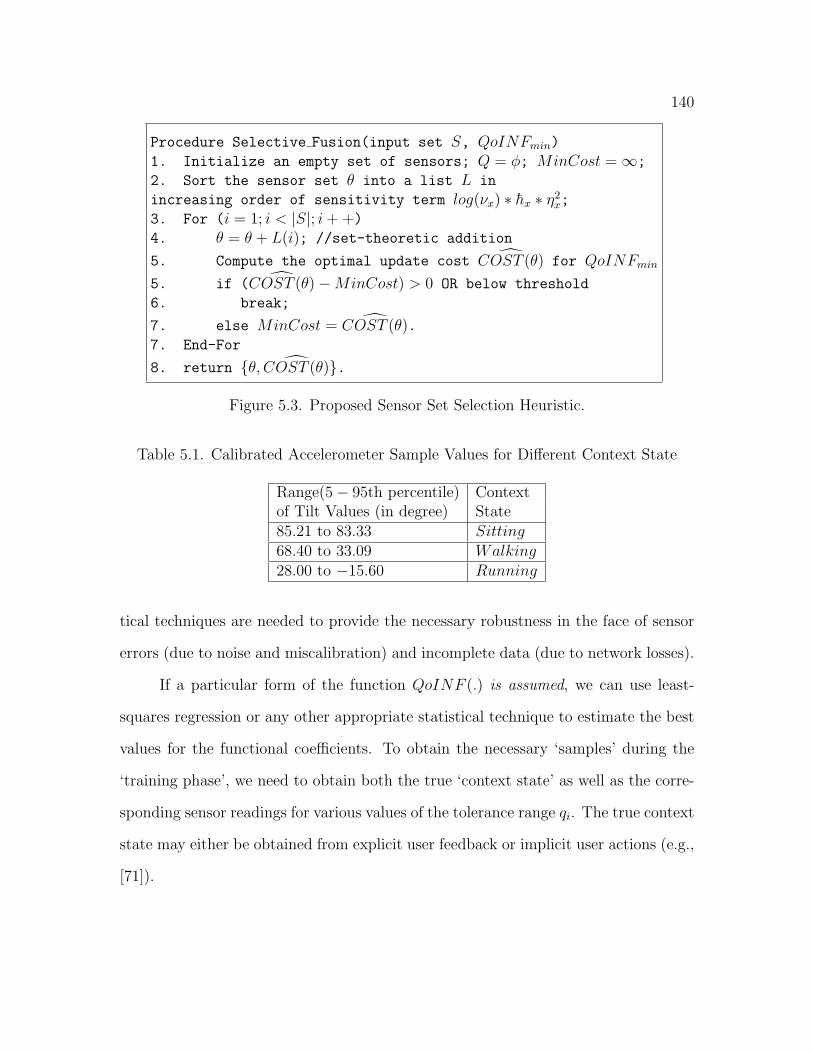
140

Procedure Selective Fusion(input set S, QoINFmin)

1. Initialize an empty set of sensors; Q = φ; MinCost =∞;

2. Sort the sensor set θ into a list L in

increasing order of sensitivity term log(νx) ∗ hx ∗ η2x;

3. For (i = 1; i < |S|; i+ +)

4. θ = θ + L(i); //set-theoretic addition

5. Compute the optimal update cost COST (θ) for QoINFmin

5. if ( COST (θ)−MinCost) > 0 OR below threshold

6. break;

7. else MinCost = COST (θ).7. End-For

8. return θ, COST (θ).

Figure 5.3. Proposed Sensor Set Selection Heuristic.

Table 5.1. Calibrated Accelerometer Sample Values for Different Context State

Range(5− 95th percentile) Contextof Tilt Values (in degree) State85.21 to 83.33 Sitting68.40 to 33.09 Walking28.00 to −15.60 Running

tical techniques are needed to provide the necessary robustness in the face of sensor

errors (due to noise and miscalibration) and incomplete data (due to network losses).

If a particular form of the function QoINF (.) is assumed, we can use least-

squares regression or any other appropriate statistical technique to estimate the best

values for the functional coefficients. To obtain the necessary ‘samples’ during the

‘training phase’, we need to obtain both the true ‘context state’ as well as the corre-

sponding sensor readings for various values of the tolerance range qi. The true context

state may either be obtained from explicit user feedback or implicit user actions (e.g.,

[71]).

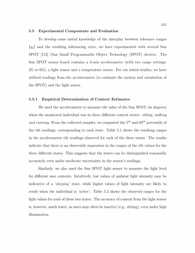
141

5.5 Experimental Components and Evaluation

To develop some initial knowledge of the interplay between tolerance ranges

qi and the resulting inferencing error, we have experimented with several Sun

SPOT [112] (Sun Small Programmable Object Technology (SPOT) devices. The

Sun SPOT sensor board contains a 3-axis accelerometer (with two range settings:

2G or 6G), a light sensor and a temperature sensor. For our initial studies, we have

utilized readings from the accelerometer (to estimate the motion and orientation of

the SPOT) and the light sensor.

5.5.1 Empirical Determination of Context Estimates

We used the accelerometer to measure tilt value of the Sun SPOT (in degrees)

when the monitored individual was in three different context states: sitting, walking

and running. From the collected samples, we computed the 5th and 95th percentile of

the tilt readings, corresponding to each state. Table 5.1 shows the resulting ranges

in the accelerometer tilt readings observed for each of the three states. The results

indicate that there is an observable separation in the ranges of the tilt values for the

three different states. This suggests that the states can be distinguished reasonably

accurately even under moderate uncertainty in the sensor’s readings.

Similarly, we also used the Sun SPOT light sensor to measure the light level

for different user contexts. Intuitively, low values of ambient light intensity may be

indicative of a ‘sleeping’ state, while higher values of light intensity are likely to

result when the individual is ‘active’. Table 5.2 shows the observed ranges for the

light values for each of these two states. The accuracy of context from the light sensor

is, however, much lower, as users may often be inactive (e.g., sitting), even under high

illumination.

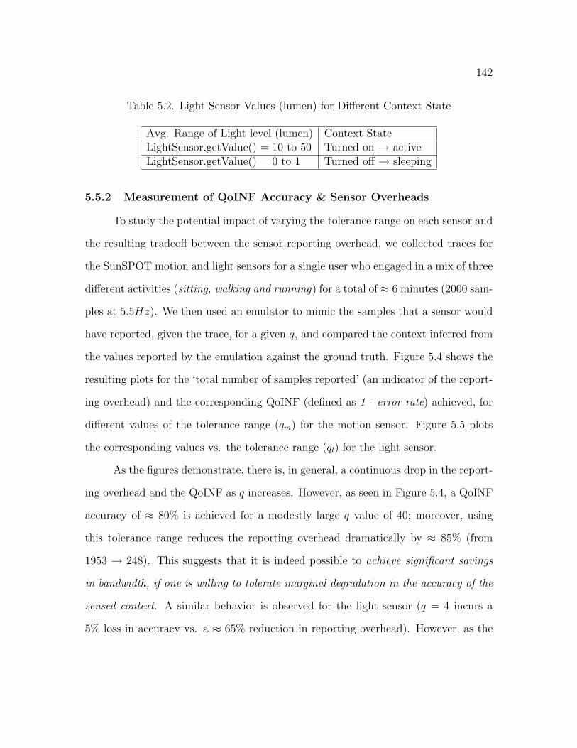
142

Table 5.2. Light Sensor Values (lumen) for Different Context State

Avg. Range of Light level (lumen) Context StateLightSensor.getValue() = 10 to 50 Turned on → activeLightSensor.getValue() = 0 to 1 Turned off → sleeping

5.5.2 Measurement of QoINF Accuracy & Sensor Overheads

To study the potential impact of varying the tolerance range on each sensor and

the resulting tradeoff between the sensor reporting overhead, we collected traces for

the SunSPOT motion and light sensors for a single user who engaged in a mix of three

different activities (sitting, walking and running) for a total of ≈ 6 minutes (2000 sam-

ples at 5.5Hz). We then used an emulator to mimic the samples that a sensor would

have reported, given the trace, for a given q, and compared the context inferred from

the values reported by the emulation against the ground truth. Figure 5.4 shows the

resulting plots for the ‘total number of samples reported’ (an indicator of the report-

ing overhead) and the corresponding QoINF (defined as 1 - error rate) achieved, for

different values of the tolerance range (qm) for the motion sensor. Figure 5.5 plots

the corresponding values vs. the tolerance range (ql) for the light sensor.

As the figures demonstrate, there is, in general, a continuous drop in the report-

ing overhead and the QoINF as q increases. However, as seen in Figure 5.4, a QoINF

accuracy of ≈ 80% is achieved for a modestly large q value of 40; moreover, using

this tolerance range reduces the reporting overhead dramatically by ≈ 85% (from

1953 → 248). This suggests that it is indeed possible to achieve significant savings

in bandwidth, if one is willing to tolerate marginal degradation in the accuracy of the

sensed context. A similar behavior is observed for the light sensor (q = 4 incurs a

5% loss in accuracy vs. a ≈ 65% reduction in reporting overhead). However, as the

143

difference between the lumen ranges for Active vs. Sleeping is only ≈ 10 (Table 5.2),

increasing q beyond ≈ 10 leads to a sharp fall in the QoINF.

0 20 40 60 80 1000

500

1000

1500

2000

Re

po

rtin

g F

req

ue

ncy

Tolerance Range (qi) in degrees

Motion Sensor: Communication Overhead and Inferencing Accuracy

0 20 40 60 80 1000

10

20

30

40

50

60

70

80

90

100

Qo

INF

(%)

Figure 5.4. Communication Overhead & Inferencing Accuracy vs. Tolerance Rangeusing Motion Sensor.

5.5.3 The Benefit of Joint Sensing

We also investigated how the use of readings jointly from both sensors affects

the inferencing accuracy vs. tolerance ranges. We consider the individual to be in a

sitting, walking or running state whenever the motion sensor tilt values lie within the

corresponding range AND the light sensor values indicate an active state. Figure 5.6

uses a three-dimensional plot to illustrate the observed inferencing accuracy when

the tuple (qm, ql) is jointly varied; we see how the QoINF is now less susceptible to

144

0 10 20 30 40 500

1000

2000

Re

po

rtin

g F

req

ue

ncy

Tolerance Range (qi) in lumen

Light Sensor: Communication Overhead and Inferencing Accuracy

0 10 20 30 40 500

5

10

15

20

25

30

35

40

Qo

INF

(%

)

Figure 5.5. Communication Overhead & Inferencing Accuracy vs. Tolerance Rangeusing Light Sensor.

individual q variations. Figure 5.7 confirms this benefit by plotting the QoINF vs. q

obtained using just the light sensor against that obtained by using both sensors (the q

ranges of both being identical). Clearly, the QoINF obtainable from the combination

of the two sensors is much higher than that of a single sensor.

5.5.4 Next Steps and Ongoing Work

The initial results above provide preliminary evidence that significant savings

that may be achieved, by relaxing the tolerance range for each sensor, without com-

promising the accuracy of context estimation. However, significant work remains to

validate and quantify the benefits of our proposed approach. To apply these results

to our proposed, formal QoINF model, we are now working to fit the QoINF (.) vs

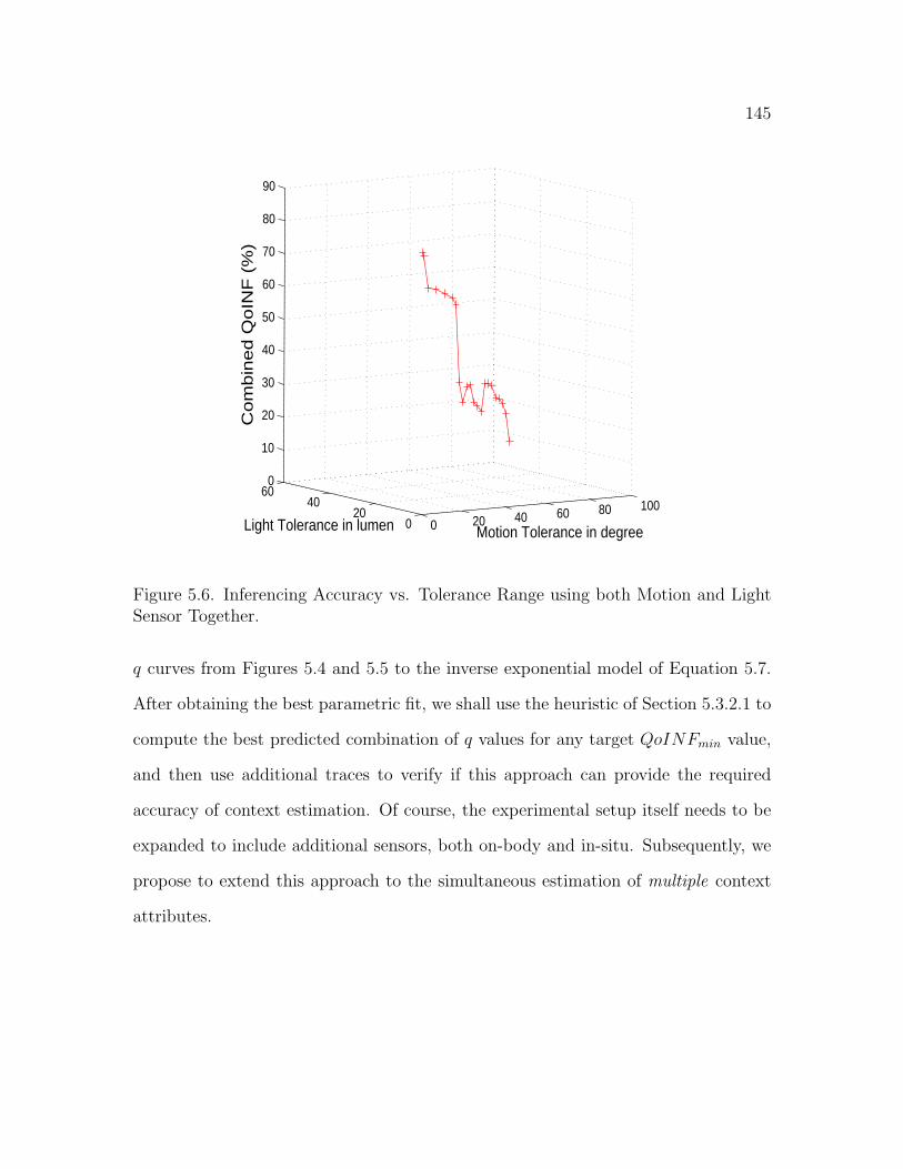
145

0 20 40 60 80 1000

2040

600

10

20

30

40

50

60

70

80

90

Motion Tolerance in degreeLight Tolerance in lumen

Co

mb

ine

d Q

oIN

F (

%)

Figure 5.6. Inferencing Accuracy vs. Tolerance Range using both Motion and LightSensor Together.

q curves from Figures 5.4 and 5.5 to the inverse exponential model of Equation 5.7.

After obtaining the best parametric fit, we shall use the heuristic of Section 5.3.2.1 to

compute the best predicted combination of q values for any target QoINFmin value,

and then use additional traces to verify if this approach can provide the required

accuracy of context estimation. Of course, the experimental setup itself needs to be

expanded to include additional sensors, both on-body and in-situ. Subsequently, we

propose to extend this approach to the simultaneous estimation of multiple context

attributes.

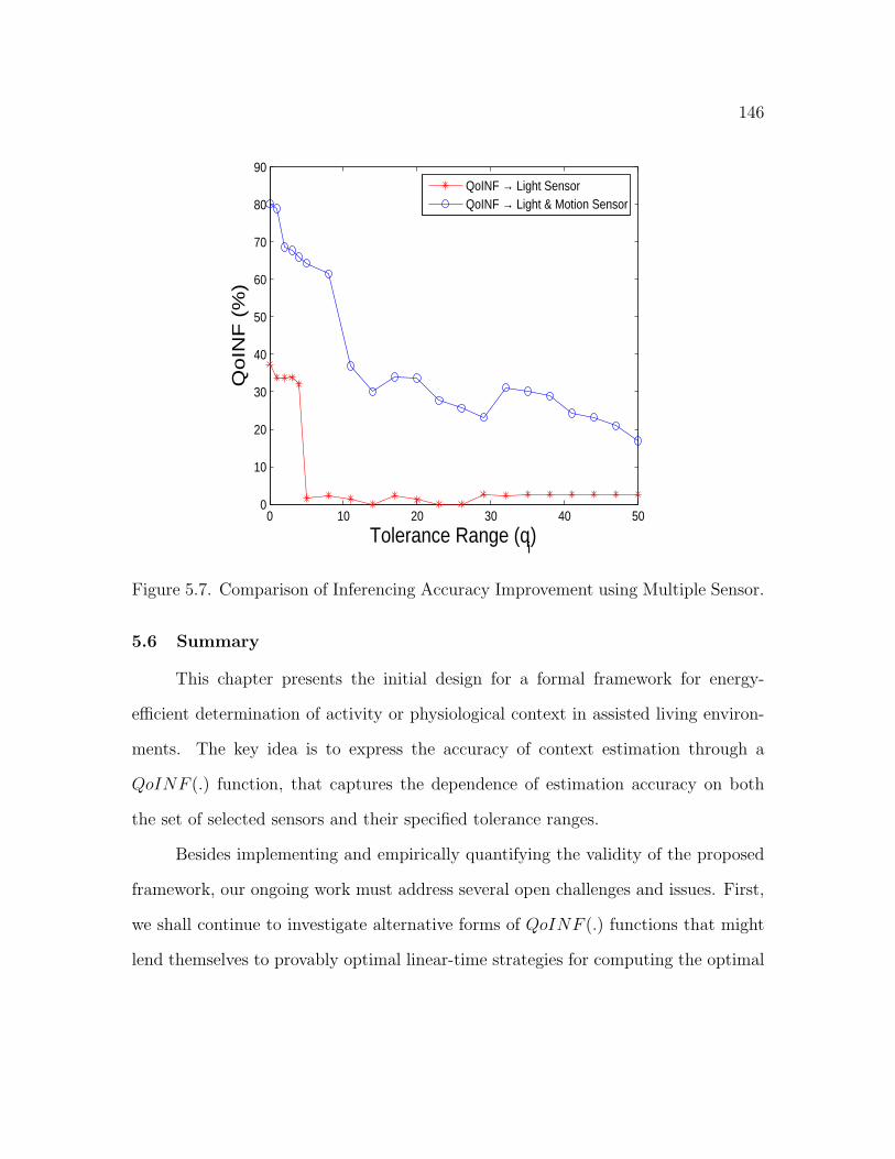
146

0 10 20 30 40 500

10

20

30

40

50

60

70

80

90

Tolerance Range (qi)

Qo

INF

(%

)

QoINF → Light SensorQoINF → Light & Motion Sensor

Figure 5.7. Comparison of Inferencing Accuracy Improvement using Multiple Sensor.

5.6 Summary

This chapter presents the initial design for a formal framework for energy-

efficient determination of activity or physiological context in assisted living environ-

ments. The key idea is to express the accuracy of context estimation through a

QoINF (.) function, that captures the dependence of estimation accuracy on both

the set of selected sensors and their specified tolerance ranges.

Besides implementing and empirically quantifying the validity of the proposed

framework, our ongoing work must address several open challenges and issues. First,

we shall continue to investigate alternative forms of QoINF (.) functions that might

lend themselves to provably optimal linear-time strategies for computing the optimal

147

(θ, qθ) combination. Similarly, for our initial choice of the ‘inverse exponential

function’, the quality of the proposed sensor selection heuristic requires evaluation.

CHAPTER 6

RELATED WORK

6.1 Introduction

This chapter presents recent research projects and groups which are related to

context awareness in general or more specifically to context learning and prediction.

The most important pioneering projects which helped to define the notion of context

awareness and/or had great influence on the development of this field are briefly listed

in section 6.3. Other related works regarding specific steps in our architecture or used

methods and algorithms is mentioned in section 6.4. The term context prediction itself

has been used by different research groups, but, as explained in more detail for the

related projects, most predictions are performed for lower-level location information.

We aim to predict high-level context identifiers, i.e., classes of situations a user or

device usually is in [81].

6.2 Projects and Groups

Context awareness is still being defined by different research groups and in dif-

ferent projects. The following list of projects is non-exhaustive and by no means com-

plete, as there have been too many publications to list which were dealing with context

awareness in some way during the last few years. We present those publications that

are more closely related to the main parts of this thesis: general frameworks and

middleware for context awareness, work on context learning and prediction and char-

acterizing uncertainty/ambiguity/error on sensor-driven decision process with limited

resources.

148

149

Georgia Institute of Technology

The “Aware Home” is built as a living laboratory for empirical research on

ubiquitous computing, with the goal to sense contextual information about itself and

its inhabitants [66]. One of the motivations for this project is to enable support for

elderly to be built into their homes. Kidd et.al. reported about the status of this

project, which should also learn user’s habits. The Context Toolkit [34] has been

developed to support work on the Aware Home project. Consequently, it is a very

flexible framework for abstracting context sensing from applications in a distributed,

heterogeneous network environment. Aimed towards context sensing embedded into

the infrastructure, it uses HTTP and XML for communication between sensors (rep-

resented by their “context widgets”) and higher-level components (named “aggrega-

tors” or “servers” and “interpreters”). It is not directly addressing context prediction

targeted at embedded systems; we aim to implement context recognition and pre-

diction locally at each device, without the need for infrastructure components, while

the Context Toolkit intentionally is an infrastructure approach for context sensing.

There are some limitations of the context toolkit, described in [34]. It does not sup-

port continuous context and does not deal with unreliable/unavailable sensor data.

MIT Media Lab

In [19], Brian Clarkson et.al. describe a wearable system with a video camera

and a microphone, capable of distinguishing coarse locations (although it is stated

that the approach is not restricted to location). Similar to their previous work [18],

they used Hidden Markov Models (HMMs), which are a well-known technique for

recognizing time series, as a basic model for recognizing context. After feature ex-

traction, they used unsupervised clustering to distinguish between user contexts.

MavHome

150

The MavHome project [25] by Diana J. Cook et.al. aims to create an agent-

based intelligent home with a vision in the spirit of the Aware Home. Their multi-layer

architecture consists of a “physical” (i.e. sensors), a “communication” (i.e. network),

an “information” (i.e. database) and a “decision” layer and is based on CORBA

for remote method invocation. This architecture is similar to the one used in this

thesis, as it is also a bottom-up structure for recognizing context. The distinguishing

factor of MavHome is its use of different prediction methods to automate actions

within the house. Although the Neural Network Home also applies machine learning

to predict inhabitant actions, there is a more detailed examination of prediction in

the MavHome project. They have developed different algorithms for categorical time

series prediction, a simple sequence-match algorithm, Active LeZi [42], a prediction

by partial match algorithm based on Markov models, a Markov model based on

higher-level action sequences and Episode Discovery [48] [27], which uses data-mining

techniques and the minimum description length principle to predict periodic patterns.

Those different prediction algorithms are used to forecast user actions, but parts of

the prediction seem to rely on database support and batch training, i.e., it does not

seem to be possible to use them in an online manner.

University of Washington

In [90], high-level user behavior is inferred from low-level sensor data by adding

knowledge of real-world constraints to user location data. A variant of Dynamic

Bayesian Networks (DBN) is used in an unsupervised way to predict transport routes

based on GPS data. By adding constraints on the routes that could be learned by the

training algorithm, the prediction accuracy was significantly improved. However, as

we aim to perform prediction at the middleware, independent of the application area,

we do not see a general way of incorporating real-world knowledge (that is not learned

automatically from the sensor data) a priori into our framework. In the “Activity

151

Compass” application, this was possible because the work was restricted to location

prediction with map material being available. Although it might improve context

prediction accuracy, this approach does currently not seem applicable to our work on

general, application-independent context.

Owl

The Owl context service supports heterogeneous context sources, privacy and

meta information like age, i.e., the time since the sensor was last sampled, and con-

fidence of context data [35]. It is one of the earlier works that already mentions the

possibility of inferring future user behavior from learned habits. To this end, their

context service was designed to manage context history in addition to the current

context. It is also one of the few projects that explicitly deal with the issue of pri-

vacy by implementing access control measures. However, it was still developed as

a centralized service with a database system as back end and thus requires a per-

sistent connection between clients and infrastructure components and faces issues of

fault-tolerance.

SOCAM

At the National University of Singapore, a “Service-Oriented Context-Aware

Middleware” (SOCAM) has very recently been developed [43]. It is based on an

ontology-oriented approach, i.e., on a vocabulary for representing context, and its

model of context is defined using the Web Ontology Language (OWL), allowing to

share context between different entities and giving rise to reasoning about context.

Their middleware provides the standard services of acquiring, interpreting and dis-

seminating context, but also takes steps towards deriving high-level context from

low-level context, which they call “context reasoning” and which can be performed

in description logic and first-order logic. To cope with limited resources in mobile

devices, the authors divide possible situations into sub-domains (e.g. home domain,

152

office domain) and switch between the ontologies defined for these sub-domains. How-

ever, this middleware is also a service- and infrastructure-oriented approach with a

service registry, which might make its use in infrastructure-independent embedded

systems difficult. Adapting applications to changed context is performed via the

standard way of predefined rules and triggers. The described implementation of the

context interpreter, which performs the reasoning process within the OWL model, is

suitable for infrastructure-based context services, but not for resource-limited devices.

In recent work, the authors proposed a probabilistic extension to OWL and added a

Bayesian Network approach to deal with uncertainty in sensor data [44]. Although

the ontology-based approach and its automatic transformation to a Bayesian Network

to deal with uncertainty could offer distinct advantages, currently there does not seem

to be a method for automatically deriving this structure of the ontology from sensor

data.

6.3 Pioneering Projects

In this section, the most important pioneering or initiating projects that had an

influence on the development of context awareness are listed. They describe an im-

portant part of the history of context awareness and help to understand how research

on context awareness evolved.

Active Badge

The Active Badge system [115] is a wearable, personal badge equipped with a

microprocessor, an infrared sender and a button. Every 15 seconds, it sends a beacon

containing its unique id to receivers distributed in the environment, allowing to gather

location information at a central server. It used infrared as primary communication

medium, which can be embedded in small devices with limited battery life. These

badges have been used at ORL for pioneering applications in pervasive computing,

153

like a building-wide notification system, and have since then been deployed at the

University of Kent, Imperial College, London, Lancaster University, the University

of Twente, Xerox PARC, DEC research laboratories, Bellcore and MIT Media Lab.

The largest system is still in use at Cambridge, with over 200 badges and 300 sensors

in the environment. As one of the first building-wide location system that can be

said to be unobtrusive (the badges are small enough to be worn comfortably), the

Active Badge system had a significant influence on the development of subsequent

location systems and already defined upper boundaries regarding the size and power

consumption of worn devices. With the early Active Badge installations, even issues

like privacy in practical applications or acceptance by test subjects could be tackled

due to the large number of badges in use.

Smart Badge system

Inspired by and building upon the experiences with the Active Badge System,

the Smart Badge system has been developed [5]. Similar to the Active Badge, a Smart

Badge has an infrared transceiver and can be worn, but it additionally integrates tilt

and heading sensors. Because infrared receivers are also available in addition to

infrared senders, the Smart Badge can sense its environment (the spatial proximity of

other Smart Badges) and transmit this sensor information bundled with its unique id

to the infrastructure, where it is gathered at a network server. This usage of spatial

proximity was one of the first in the pervasive computing research field.

Xerox ParcTab

At the Xerox Palo Alto Research Center (PARC), the ParcTab system has been

developed, which is a palm-sized PDA with touch screen, complemented by an in-

frared communication infrastructure with room-sized cells. Most of its applications

are executed on remote hosts and thus depend on the communication infrastructure,

which also handles location tracking. One of the applications that have been imple-

154

mented on the ParcTab is a remote control system to control lights and temperature

for the current location, others include the better known Forget-me-not system [76].

The ParcTab can be seen as a more complicated version of the Active Badge that

includes a limited user interface for arbitrary applications. As for the Active Badge,

infrastructure support is necessary, but this project still inspired many subsequent

publications focusing on context aware handheld devices.

Cooltown

The Cooltown project in Palo Alto [67] is still one of the most prominent perva-

sive computing installations. Its main goal is to provide a “web presence” for people,

places and things. To this end, things (i.e. devices) are equipped with web servers and

URLs are used as the primary way of addressing information throughout the systems.

By periodically sending URLs in infrared beacons and sensing those URLs, location

awareness is provided to users in the form of location-aware web services. Their use

of HTTP as communication protocol and WLAN for physical communication links

allows arbitrary clients to access the infrastructure and thus make use of the web

presence of other people, places and things. Example applications that have been

implemented include the Cooltown museum and bookstore, which allow to retrieve

information about real-world items that broadcast URLs, or the Cooltown confer-

ence room, which gives access to projectors, printers or whiteboards via URLs. This

project has affected research on context awareness in two areas: Firstly, its distinction

of physical entities into people, places and things has become one of the most often

cited classifications of context aspects, although newer definitions are less location-

specific. Secondly, the usage of HTTP and URLs as principles for referencing and

sensing shifts the focus in research from applications to protocols. Using standard,

well-known and established Internet protocols and only enhancing them by dynamic

sensing technology might be an important direction for future context-aware systems.

155

Neural Network House

Learning user’s habits has previously been explored in The Neural Network

House [82], which is able to predict occupancy of rooms, hot water usage and likeli-

hood that a zone is entered the next few seconds using trained feed-forward neural

networks. The context information in the project was again mainly comprised of

location, but additional state information from rooms like the status of lights or the

temperature set by inhabitants were used. While this project is one of many “smart

house” projects, it was one of the first to include prediction of user actions. It showed

that prediction of user locations can help to save resources and support users by learn-

ing their behavior and automating simple tasks which is one of the main contribution

of this thesis.

6.4 Summary

In this thesis we try to build an intelligent, pervasive computing and commu-

nication platform which can determine the inhabitants’ important contexts through

the autonomous and pro-active interaction of smart devices. “Context awareness”

is indeed a key to build such a smart environment and associated applications. For

example, the embedded pressure sensors in the Aware Home [87] capture inhabitants’

footfalls, and the system (i.e., smart home) uses these data for position tracking and

pedestrian recognition. The Neural Network House [82], the Intelligent Home [77], the

Intelligent House n [57] and the MavHome [27, 118] projects focus on the development

of adaptive control of home environments by also anticipating the location, routes and

activities of the inhabitants. The Active Badge [45] and Active Bat [46] takes the

help of infra-red and ultrasonic time-of-flight techniques to provide indoor location

tracking framework. On the other hand, MIT’s Cricket Location Support System [92]

delegates the responsibility of location reporting to the mobile object itself. RADAR

156

[4], another RF-based indoor location support system uses signal strength and signal-

to-noise ratio to compute 2-D positioning. Microsoft’s Easy-living and Microsoft

Home [72] projects use real-time 3D cameras to provide stereo-vision positioning ca-

pability in an indoor environment. Intelligent prediction of these contexts helps in

efficient triggering of mobility-aware services.

This ubiquitous computing paradigm [121] implies smart (i.e., pro-active) in-

teraction of computing and communication devices with their peers and surrounding

networks, often without explicit operator control. Hence, such devices need to be

imbued with an inherent sentience [54] about their important contexts that can auto-

matically or implicitly sense information about their state and the presence of users

(inhabitants) in order to take action on those contexts. This concept has led to various

projects smart homes or environments in general [22, 23]. Existing work such as the

Reactive Room [24], Neural Network House [82], Intelligent Room [21] and House n

[60] do not provide explicit reusable support for users to manage or correct uncertainty

in the sensed data and their interpretations, and thereby assume that the sensed con-

texts are unambiguous. The work reported in [34] provided a toolkit to enable the

integration of context data into applications, however, no mechanism is provided for

sensor fusion or reasoning about contexts to deal with ambiguity. Although other

works such as [61] proposed mechanisms for reasoning about contexts, yet they do

not provide well defined context-aware data fusion model nor address the challenges

associated with context ambiguity and users’ situation prediction. Distributed medi-

ation of ambiguous contexts in aware environments was discussed in [31] that allow

the user to correct ambiguity in the sensed input. Multimodal Maps [15] for travel

planning addresses ambiguity by using multimodal fusion to combine different inputs

and then prompting the user for more information to remove the remaining ambiguity

157

as much as possible. Remembrance Agent [93] uses context to retrieve information

relevant to the user and explicitly addresses ambiguity in its manual interface.

Alongside, significant efforts have been made to develop middleware systems

that can effectively support context-aware applications in the presence of resource

constraints (e.g., sensor networks), also considering requirements for sensory data or

information fusion from middleware perspective [1]. For example, DFuse [73] is a data

fusion framework that facilitates dynamic transfer of different application level infor-

mation fusion into the network in order to save power. In adaptive middleware [55] for

context-aware applications in smart home setups, the application’s quality of context

(QoC) requirements is matched with the QoC attributes of the sensors with the help

of a utility function. Similarly, in MiLAN [49], application’s quality of service (QoS)

requirements are matched with the QoS provided by the sensor networks. However,

in this scheme, the QoS requirements of the applications are assumed to be prede-

termined, which the applications should know in advance in addition to the quality

associated with the type of sensors it can make use of. Given that in ubiquitous

computing environments, the nature (number, types and cost off usage, and benefits)

of such sensors available to the applications usually vary, it is impractical to include

a priori knowledge about them. The selection of right sensor with right information

at the right moment was originally introduced in [114], while the structure of an opti-

mal sensor configuration constrained by the wireless channel capacity was investigated

in [13]. By eliminating the simplifying assumption that all contexts are certain we

designed a context-aware data fusion algorithm based on dynamic Bayesian network

to mediate ambiguous context. But an intelligent sensor management that provides

energy-efficiency as well as a way to manage quality of context requirements, which

may change over time with changes in patient’s state, has not been considered before.

An information theoretic approach is taken to decide an optimal sensor configuration

158

to determine the best current state of the patient while satisfying the application QoC

requirements. For end user an ontological rule based approach using semantic web

technology is proposed for further reduction of context ambiguity with applications

to context-aware healthcare services.

Energy-efficient determination of an individual’s context (both physiological

and activity) is also an important technical challenge for assisted living environments.

Given the expected availability of multiple sensors, context determination may be

viewed as an estimation problem over multiple sensor data streams. This thesis de-

velops a formal, and practically applicable, model to capture the tradeoff between the

accuracy of context estimation and the communication overheads of sensing. But the

tradeoff between communication overhead and the quality of the reconstructed data

was first studied in [86], which envisioned the effect of tolerance ranges on the relative

frequency of sink-initiated fetching vs. source-initiated proactive refreshes. The focus,

however, is on snapshot queries and not on continually satisfying the QoINF bound of

a long-standing subscription. The idea of exploiting temporal correlation across the

successive samples of individual sensors for reducing the communication overhead,

for snapshot queries, is addressed in [30], which used training data to parameterize a

jointly-normal density function. While a precursor to our work, the focus there was

on meeting the QoINF requirements for a class of ‘aggregation queries’, whereas our

focus is on arbitrary relationships between a context variable and its underlying sen-

sor data. The CAPS algorithm [56] is designed for long-running aggregation queries

(such as min, max) and computes the optimal set of tolerance ranges for a given set

of sensors, that minimizes communication overhead while guaranteeing the accuracy

of the computed response. However, our aim is to compute both the best subset of

available sensors, and their tolerance ranges, that achieves the desired accuracy for

arbitrary context variables. In summary the distinguishing aspects of the work pre-

159

sented in this thesis are context learning, prediction, mediation and the combination

of an open, cross-platform middleware framework with the concentration on limited

resources, unobtrusiveness and quality of information.

CHAPTER 7

CONCLUSION AND FUTURE WORK

In this thesis, we have developed a novel mobility-aware resource management

framework in a multi-inhabitant smart home. Characterizing the mobility of inhabi-

tants as a stationary, ergodic, stochastic process, the framework uses the information

theoretic measure to estimate the uncertainty associated with all the inhabitants in

the house. It has also been shown that the direct use of per-inhabitant location track-

ing fails to capture the correlation among multiple inhabitants’ locations or activities.

We have proved that the multi-inhabitant location tracking is an NP-hard problem.

We also formulated a non-cooperative learning paradigm based on stochastic game

theory, which learns and estimates the inhabitants’ most likely location (route) pro-

files by minimizing the overall entropy associated with them. The convergence and

worst-case performance bounds of this framework are also derived. Automated ac-

tivation of devices along the predicted locations/routes provide the inhabitants with

necessary comfort while minimizing energy consumption and cost.

We also presented a framework which supports ambiguous context mediation

and user-centric situation prediction based on dynamic Bayesian networks and in-

formation theoretic reasoning, leading to context-aware healthcare applications in

smart environments. Our framework provides a Bayesian approach to fuse context

fragments and deal with context ambiguity in a probabilistic manner, an information

theoretic approach to satisfy context quality within the application, and a semantic

web technology to easily compose rules to reason efficiently to mediate ambiguous

contexts. An algorithm is proposed and subsequent experimental evaluation is done

160

161

to perform cost/benefit analysis to engage the most economically efficient actions for

context disambiguation in resource constrained sensor environments.

At the end we developed a formal, and practically applicable, model to cap-

ture the tradeoff between the accuracy of context estimation and the communication

overheads of sensing. In particular, we proposed the use of tolerance ranges to reduce

an individual sensor’s reporting frequency, while ensuring acceptable accuracy of the

derived context. In our vision, applications specify their minimally acceptable value

for a Quality-of Inference (QoINF) metric. We introduced an optimization technique

allowing the Context Service to compute both the best set of sensors, and their as-

sociated tolerance values, that satisfy the QoINF target at minimum communication

cost. Early experimental results with SunSPOT sensors are presented to attest to

the promise of this approach.

REFERENCES

[1] H. Alex, M. Kumar and B. Shirazi, “MidFusion: An adaptive middleware for in-

formation fusion in sensor network applications”, Elsevier Journal of Information

Fusion, 2005

[2] Aperion Inspiration Communities, http://aperion.typepad.com/aperion compa-

nies weblog/aperion health news/index.html

[3] J. C. Augusto, C. D. Nugent and N. D. Black, “Management and Analysis of

Time-Related Data in Smart Home Environments”, Proceedings of Mediterranean

Conference on Medical and Biological Engineering (Medicon’04).

[4] P. Bahl and V. Padmanabhan, “RADAR: An In-Building RF-based User Location

and Tracking System,” Proc. IEEE Infocom, IEEE CS Press, Los Alamitos, CA,

2000, pp. 775-784.

[5] H. W. P. Beadle, B. Harper, G. Q. Maguire, and J. Judge, “Location aware

mobile computing”, Proceedings of the IEEE/IEE International Conference on

Telecommunications (ICT97), April 1997, pp. 13191324.

[6] M. Beigl, H.-W. Gellersen, and A. Schmidt, “Mediacups: experience with design

and use of computer-augmented everyday artifacts”, Computer Networks (Ams-

terdam, Netherlands) 35 (2001), no. 4, 401409.

[7] A. Bhattacharya and S. K. Das, “LeZi-update: An information-theoretic approach

for personal mobility tracking in PCS networks,” ACM/Kluwer Wireless Net-

works, vol. 8, no. 2, pp.121-137, Mar-May 2002.

162

163

[8] M. Bowling and M. Velso, “Rational and Convergent Learning in Stochastic

Games”, In Proceedings of the Seventeenth International Joint Conference on Ar-

tificial Intelligence, Seattle, WA, Aug. 2001.

[9] P. J. Brown and G. J. F. Jones, “Exploiting contextual change in context-aware

retrieval”, Proceedings of the 2002 ACM Symposium on Applied Computing, ACM

Press, 2002, pp. 650656.

[10] S. B. H. Bruder, M. Farooq, and M. M. Bayoumi, “A feature-level approach to

multisensor integration; emphasizing robotic applications”,Proceedings of IEEE

Conference on Multisensor Fusion and Integration for Intelligent Systems, Octo-

ber 1994, pp. 477484.

[11] S. B. H. Bruder, “An information centric approach to heterogeneous multi-

sensor integration for robotic applications”, Robotics and Autonomous Systems

26 (1999), no. 4, 255280.

[12] C. J. C. Burges, “A tutorial on support vector machines for pattern recognition”,

Data Mining and Knowledge Discovery 2 (1998), 121167.

[13] J. Chamberland and V. Verravalli, “Decentralized detection in sensor networks”,

IEEE Transactions on Signal Processing, 51(2), Feb 2003. 10

[14] G. Chen and D. Kotz, “Solar: A pervasive-computing infrastructure for context-

aware mobile applications”, Tech. Report TR2002-421, Dept. of Computer Sci-

ence, Dartmouth College, February 2002.

[15] A. Cheyer and L. Julia, “Multimodal Maps: An Agent-based Approach”, In

Proc. of the International Conference on Cooperative Multimodal Communication,

pp.103-113, Netherlands, May. 1995.

[16] G. Chen, M. Li and D. Kotz,“Design and implementation of a large-scale context

fusion network”, Proceedings of the First Annual International Conference on

164

Mobile and Ubiquitous Systems: Networking and Services (MobiQuitous), Aug.

2004.

[17] B. Clarkson and A. Pentland, “Unsupervised clustering of ambulatory audio and

video”, Tech. Report 471, MIT Media Lab, Perceptual Computing Group, 1998.

[18] B. Clarkson, N. Sawhney, and A. Pentland, “Auditory context awareness via

wearable computing”, Proceedings of the 1998 Workshop on Perceptual User In-

terfaces (PUI98) (San Francisco, CA, USA), November 1998.

[19] B. Clarkson, K. Mase, and A. Pentland, “Recognizing user context via wearable

sensors”, Proceedings of the 4th International Symposium onWearable Computers

(ISWC 2000), 2000, pp. 6976.

[20] C. Claus and C. Boutilier, “The Dyanamics of Reinforcement Learning in Co-

Operative Multiagent System”, Proceedings of the Tenth Innovative Applications

of Arti cial Intelligence Conference, Madison, WI, July 1998, pp. 746-752.

[21] M. Coen,“The future of human-computer interaction or how I learned to stop

worrying and love my intelligent room”, IEEE Intelligent Systems 14, 2 (1999),

8-10.

[22] D. J. Cook and S. K. Das, “Smart Environments: Technology, Protocols and

Applications,” John Wiley & Sons, Nov 2004.

[23] D. J. Cook and S. K. Das, “How Smart Are Our Environments? An Updated

Look at the State of the Art,” Pervasive and Mobile Computing (Special Issue on

Smart Environments), Vol. 3, No. 2, pp. 53-73, Mar 2007.

[24] J. Cooperstock et al., “Reactive environments: Throwing away your keyboard

and mouse”, CACM 40, 9 (1997), 65-73.

[25] D. J. Cook, M. Youngblood, III E. O. Heierman, K. Gopalratnam, S. Rao, A.

Litvin, and F. Khawaja, “MavHome: An agent-based smart home”, Proceedings

165

of the 1st IEEE International Conference on Pervasive Computing and Commu-

nications (PerCom03), IEEE Computer Society Press, March 2003, pp. 521524.

[26] T. M. Cover and J. A. Thomas, Elements of Information Theory, John Wiley,

1991.

[27] S. K. Das, D. J. Cook, A. Bhattacharya, E. Hierman, T. Y. Lin, “The Role

of Prediction Algorithms in the MaVHome Smart Home Architecture”, IEEE

Wireless Communications, Special Issue Smart Homes, Dec. 2002.

[28] S. K Das, N. Roy and A. Roy “Context-Aware Resource Management in Multi-

Inhabitant Smart Homes: A Framework based on Nash H-Learning”, Pervasive

and Mobile Computing (PMC) Journal, pp. 372-404, Vol. 2, Issue 4, Nov. 2006

[29] Datamonitor: The Changing Role of Consumers in Healthcare, Health Data Man-

agement Report, Aug. 2006.

[30] A. Deshpande, C. Guestrin, S. Madden, J. M. Hellerstein, W. Hong, “Model-

based Approximate Querying in Sensor Networks”, Int’l Journal on Very Large

Data Bases (VLDB Journal), 2005

[31] A. K. Dey, J. Mankoff, G. D. Abowd and S. Carter, “Distributed Mediation

of Ambiguous Context in Aware Environments”, Proceedings of the 15th Annual

Symposium on User Interface Software and Technology (UIST 2002), Oct. 2002.

pp. 121-130.

[32] A. K. Dey, G. D. Abowd, and D. Salber, “A context-based infrastructure for

smart environments”, Proceedings of the 1st International Workshop on Managing

Interactions in Smart Environments (MANSE 99), 1999, pp. 114128.

[33] A. K. Dey and G. D. Abowd, “Towards a better understanding of context and

contextawareness”, Proceedings of the CHI 2000 Workshop on The What, Who,

Where, When, and How of Context-Awareness, April 2000.

166

[34] A. K. Dey, D. Salber and G. D. Abowd, “A Conceptual Framework and a Toolkit

for Supporting the Rapid Prototyping of Context-Aware Applications”, Human-

Computer Interaction (HCI) Journal, Vol. 16 (2-4), pp. 97-166, 2001.

[35] M. R. Ebling, G. D. H. Hunt, and H. Lei, “Issues for context services for pervasive

computing”, Proceedings of the Middleware 2001 Workshop on Middleware for

Mobile Computing, 2001.

[36] T. D. Estop, Applied Thermodynamics for Engineering Technologists: S.I. Units,

Longman Publishers, 1978.

[37] M. R. Garey and D. S. Johnson, Computers and Intractability: A Guide to the

Theory of NP-Completeness, W. H. Freeman Publishers, 1979.

[38] D. Garlan, D. Siewiorek, A. Smailagic, and P. Steenkiste, “Project Aura:

Towards distraction-free pervasive computing”, IEEE Pervasive Computing 21

(2002), no. 2, 22 31.

[39] H.W. Gellersen, A. Schmidt, and M. Beigl, “Multi-sensor context-awareness in

mobile devices and smart artefacts”, Mobile Networks and Applications 7 (2002),

341351.

[40] K. Gopalratnam and D. J. Cook, “Active LeZi: An Incremental Parsing Algo-

rithm for Sequential Prediction”, International Journal of Artificial Intelligence

Tools, vol. 14, no.(1-2), pp. 917-930, 2004.

[41] G. R. Grimmet and D. R. Stirzaker, Probability and Random Processes, 2nd Ed.,

Oxford University Press, 1992.

[42] K. Gopalratnam and D. J. Cook, “Active Lezi: An incremental parsing algo-

rithm for sequential prediction”, Proceedings of the Florida Artificial Intelligence

Research Symposium, 2003.

167

[43] T. Gu, H. K. Pung, and D. Q. Zhang, “A middleware for building context-aware

mobile”,Proceedings of the IEEE Vehicular Technology Conference (VTC-Spring

2004), May 2004.

[44] T. Gu, H. K. Pung, and D. Q. Zhang, “A bayesian approach for dealing with

uncertain contexts”, Advances in Pervasive Computing (A. Ferscha, H. Hrtner,

and G. Kotsis, eds.), vol. 176, Austrian Computer Society (OCG), April 2004, part

of the Second International Conference on Pervasive Computing (PERVASIVE

2004), pp. 205210.

[45] A. Harter and A. Hopper, “A distributed location system for the active office,”

IEEE Network, vol. 8, no. 1 January/February 1994, pp. 62-70.

[46] A. Harter, A. Hopper, P. Steggles, A. Ward and P. Webster, “The anatomy

of a context-aware application,” Proc. 5th Annual Int’l Conference on Mobile

Computing and Networking, August 1999, pp. 59-68.

[47] R. Headon, “Movement awareness for a sentient environment”, Proceedings of the

1st IEEE International Conference on Pervasive Computing and Communications

(PerCom03), IEEE Computer Society Press, March 2003, pp. 99106.

[48] E. Heierman and D. J. Cook, “Improving home automation by discovering regu-

larly occurring device usage patterns”, Proceedings of the International Conference

on Data Mining, IEEE Computer Society Press, November 2003, pp. 537540.

[49] W. Heinzelman, A.L. Murphy, H.S. Carvalho and M.A. Perillo, “Middleware to

Support Sensor Network Applications”, IEEE Network 18, pp. 6-14, Feb. 2004.

[50] K. Hisazumi, T. Nakanishi, T. Kitasuka, and A. Fukuda, “Campus: A context-

aware middleware”, Proceedings of the 2nd CREST Workshop on Advanced Com-

puting and Communicating Techniques for Wearable Information Playing, May

2003, pp. 4249.

[51] X10 web resources available at http://www.x10.com.

168

[52] A. Hopper, “Sentient computing,” The Royal Society Clifford Patterson Lecture,

1999.

[53] E. Horvitz, P. Koch, C. M. Kadie, and A. Jacobs, “Coordinate: Probabilistic

forecasting of presence and availability”, Proceedings of the 18th Conference on

Uncertainty and Artificial Intelligence, Morgan Kaufmann Publishers, July 2002,

pp. 224233.

[54] A. Hopper, “Sentient computing,” The Royal Society Clifford Patterson Lecture,

1999.

[55] M. C. Huebscher and J.A. McCann, “Adaptive Middleware for Context-aware

Applications in Smart Homes”, Proc. of the 2nd Workshop on Middleware for

Pervasive and Ad-hoc Computing, Oct. 2004, pp. 111-116.

[56] W. Hu, A. Misra and R. Shorey, “CAPS: Energy-Efficient Processing of Contin-

uous Aggregate Queries in Sensor Networks”, Fourth IEEE International Confer-

ence on Pervasive Computing and Communications (PerCom), 2006, pp. 190-199

[57] “House n Living Laboratory Introduction”, web resource available at

http://architecture.mit.edu/house n/web/publications.

[58] J. Hu and M. P. Wellman, “Nash Q-Learning for General-Sum Stochastic

Games”, Journal of Machine Learning, vol. 4, pp.1039-1069, 2003.

[59] 802-11: IEEE standards for information technology telecommunications and

information exchange between systems local and metropolitan area networks

specific requirements part 11: Wireless LAN medium access control (MAC) and

physical layer (PHY) specifications, 1999.

[60] S.S. Intille, “The goal: smart people, not smart homes,” Proceedings of the

International Conference on Smart Homes and Health Telematics, IOS Press, 2006

[61] D. L. de Ipina, “An ECA Rule-Matching Service for Simpler Development of

Reactive Applications”, Middleware, Vol. 2, No. 7, Nov. 2001.

169

[62] Jena Semantic Web Toolkit: http://www.hpl.hp.com/semweb/jena2.htm

[63] F.V. Jensen, “Bayesian Networks and Decision Graphs”, Springer-Verlag, New

York, 2001

[64] W.P. Jones, “Air Conditioning Engineering”, Arnold Publishers, 1995.

[65] G. Judd and P. Steenkiste, “Providing contextual information to pervasive com-

puting applications”, Proceedings of the 1st IEEE International Conference on

Pervasive Computing and Communications (PerCom03), IEEE Computer Soci-

ety Press, March 2003, pp. 133142

[66] C. D. Kidd, R. Orr, G. D. Abowd, C. G. Atkeson, I. A. Essa, B. MacIntyre,

E. D.Mynatt, T. Starner, and W. Newstetter, “The Aware Home: A living

laboratory for ubiquitous computing research”, Proceedings of the Cooperative

Buildings, Integrating Information, Organization, and Architecture, Second Inter-

national Workshop, CoBuild99, Lecture Notes in Computer Science, vol. 1670,

Springer, 1999, pp. 191198.

[67] T. Kindberg, H. Morris, J. Schettino, B. Serra, M. Spasojevic, J. Barton, J.

Morgan, G. Becker, D. Caswell, P. Debaty, G. Gopal, M. Frid, and V. Krishnan,

“People, places, things: Web presence for the real world”, Proceedings of the 3rd

IEEE Workshop on Mobile Computing Systems and Applications (WMCSA00),

IEEE Computer Society Press, December 2000, pp. 1930.

[68] Y. Korilis and A. Lazer, “On the existance of equilibria in noncooperative optimal

flow control”, Journal of the ACM vol. 42, no. 3, pp. 584–613, 1995.

[69] P. Korpip, M. Koskinen, J. Peltola, S.-M. Mkel, and T. Seppnen, “Bayesian

approach to sensor-based context awareness”, Personal and Ubiquitous Computing

7 (2003), no. 2, 113124.

[70] E. Koutsoupias and C. Papadimitriou, “Worst-case Equilibria”, 16th Annual

Symposium on Theoretical Aspects of Computer Science, pp. 404–413, 1999.

170

[71] A. Krause, A. Smailagic, D. Siewiorek, “Context-Aware Mobile Computing:

Learning Context-Dependent Personal Preferences from a Wearable Sensor Ar-

ray,” IEEE Transactions on Mobile Computing, pp. 113-127, Feb 2006.

[72] J. Krumm, S. Harris, B. Meyers, B. Brumitt, M. Hale, S. Shafer “Multi-Camera

Multi-Person Tracking for Easy Living,” Proceedings of 3rd IEEE International

Workshop on Visual Surveillance, IEEE Press, Piscataway, NJ, 2000, pp. 3-10.

[73] R. Kumar, M. Wolenetz, B. Agarwalla, J. Shin, P. Hutto, A. Paul and U. Ra-

machandran, “DFuse: a Framework for Distributed Data Fusion”, Proc. of the

1st International Conference on Embedded Networked Sensor Systems, Nov. 2003,

pp. 114-125.

[74] K. Van Laerhoven, “On-line adaptive context awareness starting from low-level

sensors”, Masters thesis, Free University of Brussels, 1999.

[75] K. Van Laerhoven, “Combining the Self-Organizing Map and K-Means clustering

for on-line classification of sensor data”, Proceedings of the International Confer-

ence on Artificial Neural Networks (ICANN), Springer, 2001, pp. 464469.

[76] M. Lamming and M. Flynn, “Forget-me-not: Intimate computing in support of

human memory”, Proceedings of FRIEND2194, The International Symposium on

Next Generation Human Interface, Feb. 1994.

[77] Lesser et al., “The Intelligent Home Testbed”, Proc. of Autonomy Control Soft-

ware Workshop, Jan 1999.

[78] P. Lukowicz, H. Junker, M. Stger, T. von Bren, and G. Trster, “WearNET:

A distributed multi-sensor system for context aware wearables”, Proceedings of

the 4th International Conference on Ubiquitous Computing (UbiComp02) Lecture

Notes in Computer Science, vol. 2498, September 2002, pp. 361370.

[79] P. Lukowicz, J. A. Ward, H. Junker, M. Stger, G. Trester, A. Atrash, and

T. Starner, “Recognizing workshop activity using body worn microphones and

171

accelerometers”, Proceedings of the 2nd International Conference on Pervasive

Computing (PERVASIVE 2004) Lecture Notes in Computer Science, vol. 3001,

Springer, April 2004, pp. 1832.

[80] H. Luo, Y. Liu and S. K. Das, “Routing Correlated Data with Fusion Cost in

Wireless Sensor Networks,” IEEE Transactions on Mobile Computing, Vol. 5, No.

11, pp. 1620-1632, Nov. 2006.

[81] Rene Mayrhofer, “An Architecture for Context Prediction,” PhD Thesis, 2004

[82] M. C. Mozer, “The Neural Network House: An Environment that Adapts to its

Inhavitants”, Proc. of the American Association for Artificial Intelligence Spring

Symposium on Intelligent Environments, pp. 110-114, 1998.

[83] John F. Nash. “Non-cooperative games”, Annals of Mathematics, 54: 286295,

1951.

[84] Netica Bayesian Network Software http://www.norsys.com

[85] D. A. Norman, “The invisible computer”, MIT Press, Cambridge, 1998.

[86] C. Olston and J. Widom, “Offering a precision performance tradeoff for aggre-

gation queries over replicated data”, In Proceedings of VLDB. Margan Kaufmann

Publishers Inc., 2000, pp.144 -155.

[87] R. J. Orr and G. D. Abowd, “The Smart Floor: A Mechanism for Natural User

Identification and Tracking,” Proceedings of Conference on Human Factors in

Computing Systems (CHI 2000), ACM Press, NY, 2000.

[88] G. Owen,“Game Theory”, Second Edition,Academic Press,1982

[89] S. Padovitz, W. Loke, A. Zaslavsky, C. Bartolini and B. Burg, “An approach

to Data Fusion for Context Awareness”, 5th International and Interdisciplinary

Conference, CONTEXT 2005, pp. 353-367

[90] D. J. Patterson, L. Liao, D. Fox, and H. Kautz, “Inferring high-level behavior

from lowlevel sensors”, Proceedings of the 5th International Conference on Ubiq-

172

uitous Computing (UbiComp03) Lecture Notes in Computer Science, vol. 2864,

Springer, October 2003, pp. 7389.

[91] N. Paton and O. Diaz, “Active Databse Systems” ACM Computing Surveys,

31(1): 63-103 (1999)

[92] N. Priyantha, A. Chakraborty and H. Balakrishnan, “The Cricket location sup-

port system,” Proc. 6th Ann. Int’l Conference on Mobile Computing and Net-

working, August 2000, pp. 32-43.

[93] B. Rhodes, “The Wearable Remembrance Agent: a System for Augmented Mem-

ory”, Personal Technologies Journal Special Issue on Wearable Computing, 1:218-

224, 1997.

[94] A. Roy, S. K. Das Bhaumik, A. Bhattacharya, K. Basu, D. J. Cook and S. K.

Das, “Location Aware Resource Management in Smart Homes”, Proc. of IEEE

Int’l Conf. on Pervasive Computing and Communications (PerCom), pp. 481-488,

Mar 2003.

[95] N. Roy, S. K. Das , K. Basu and M. Kumar, “Enhancing Availability of

Grid Computational Services to Ubiquitous Computing Application”, IEEE

International Conference on Parallel and Distributed Processing Symposium

(IPDPS’2005), Denver, Colorado, USA, Apr. 2005.

[96] N. Roy, A. Roy, S. K. Das and K. Basu, “A Reinforcement Learning Framework

for Location-Aware Resource Management in Multi-Inhabitant Smart Homes”,

Proc. of 3rd International Conference on Smart Homes and Health Telematic

(ICOST), pp. 180-187, July 2005.

[97] N. Roy, A. Roy, K. Basu and S. K. Das “A Cooperative Learning Framework for

Mobility-Aware Resource Management in Multi-Inhabitant Smart Homes ”, Proc.

of IEEE International Conference on Mobile and Ubiquitous Systems: Networking

and Services (MobiQuitous), pp. 393-403, July 2005.

173

[98] N. Roy, A. Roy and S. K. Das, “Context-Aware Resource Management in Multi-

Inhabitant Smart Homes: A Nash H-learning based Approach”, Proc. of IEEE

Int’l Conf. on Pervasive Computing and Communications (PerCom), pp. 148-158,

Mar 2006. (Mark Weiser Best Paper Award).

[99] N. Roy, G. Pallapa and S. K. Das,“A Middleware Framework for Ambiguous

Context Mediation in Smart Healthcare Application”, Proc. of IEEE Int’l Conf.

on Wireless and Mobile Computing, Networking and Communications (WiMob),

Oct 2007.

[100] N. Roy, A. Misra and S. K. Das, “Efficient Long-Term Quality-of-Inference

(QoINF)-Aware Context Determination in Pervasive Care Environments”, Proc.

of ACM SIGMOBILE Workshop on Systems and Networking Support for Health-

care and Assisted Living Environments (HealthNet 2008) in conjunction with

MobiSys 2008.

[101] N. Roy, G. Pallapa and S. K. Das, “An Ontology-Driven Ambiguous Contexts

Mediation Framework for Smart Healthcare Applications”, Proc. of Int’l Conf. on

PErvasive Technologies Related to Assistive Environments (PETRA 2008).

[102] M. Schneps-Schneppe and V. B. Iverson “Service Level Agreement as an issue

of Teletraffic”, Proceedings of the ITC, Berlin, Sept 2003.

[103] C. R. Shelton, “Balancing Multiple Sources of Reward in Reinforcement Learn-

ing”, Advances in Neural Information Processing Systems, pp. 1082-1088, 2000.

[104] A. Schmidt, M. Beigl, and H.-W. Gellersen, “There is more to context than

location”, Computers and Graphics 23 (1999), no. 6, 893901.

[105] A. Schmidt, “Ubiquitous computing computing in context”, Ph.D. thesis, Lan-

caster University, November 2002.

[106] B. N. Schilit, “A system architecture for context-aware mobile computing”,

Ph.D. thesis, Columbia University, May 1995.

174

[107] SemanticWorks: http://www.altova.com/products/semanticworks/semantic web rdf

owl editor.html

[108] C. R. Shelton, “Balancing Multiple Sources of Reward in Reinforcement Learn-

ing”, Advances in Neural Information Processing Systems, pp. 1082-1088, 2000.

[109] S. Singh, T. Jaakkola, M. L. Littman and C. Szepesvari, “Convergence Results

for Single-Step On-Policy Reinforcement-Laerning Algorithms”, Machine Learn-

ing 38, no. 3, 2000, pp. 287-290

[110] M. K. Smith, C. Welty, and D.L. McGuinness, “OWL Web Ontology Language

Reference,” World Wide Web Consortium (W3C) recommendation, Feb. 2004;

www. w3.org/TR/owl-ref.

[111] SPARQL tutorial: http://www.w3.org/TR/rdf-sparql-query/

[112] SunSpotWorld-Home of Project Sun SPOT: www.sunspotworld.com

[113] E. M. Tapia, S. S. Intille, and K. Larson, “Activity recognition in the home using

simple and ubiquitous sensors”, Proceedings of the 2nd International Conference

on Pervasive Computing (PERVASIVE 2004) Lecture Notes in Computer Science,

vol. 3001, Springer, April 2004, pp. 158175.

[114] R. R. Tenney and N. R. Sandell, Jr., “Detection with distributed sensors,” IEEE

Trans. Aerosp. Electron. Syst., vol. AES-17, pp. 501-510, 1981.

[115] R. Want, A. Hopper, V. Falco, and J. Gibbons, “The active badge location

system”, ACM Transactions on Information Systems (TOIS) 10 (1992), 91102.

[116] M. Weiser, “The Computer for the 21st Century,” Scientific American, vol. 265,

no. 3, pp. 94-104, Sept. 1991.

[117] X10 web resources available at http://www.x10.com.

[118] M. Youngblood, D. J. Cook, and L. B. Holder. “Managing Adaptive Versatile

Environments.” Proc. of IEEE Int’l Conf. on Pervasive Computing and Commu-

nications (PerCom), pp. 351-360; Mar 2005.

175

[119] M. Youngblood, “MavPad Inhabitant 2 Trial 2 Data Set.” The MavHome

Project. Computer Science and Engineering Department, The University of Texas

at Arlington, 2005. http://mavhome.uta.edu

[120] Watkins, C. J. C. H., “Learning from delayed rewards”, PhD thesis, King’s

College, Cambridge, UK, 1989

[121] M. Weiser, “The computer for the 21st century,” Scientific American, vol. 265,

no. 3, pp. 94-104, Sept. 1991.

[122] Y. Zhang, Q. Ji and C. G. Looney, “Active Information Fusion For Decision

Making Under Uncertainty”, Proceedings of the Fifth International Conference on

Information Fusion, 2002, vol. 1, pp. 643- 650.

[123] J. Ziv and A. Lempel, “Compression of individual sequences via variable-rate

coding,” IEEE Transactions on Information Theory, vol. 24, no. 5, pp. 530-536,

Sept 1978.

BIOGRAPHICAL STATEMENT

Nirmalya Roy received a Bachelor of Engineering degree in Computer Science

and Engineering from Jadavpur University, Calcutta, India, in 2001. He began his

graduate studies in the Department of Computer Science and Engineering at The

University of Texas at Arlington in Fall 2002. He received his Master of Science degree

in Computer Science and Engineering from The University of Texas at Arlington in

May 2004.

176