
Recommender Systems - Stellenbosch University
186
Recommender Systems by Bronwyn Catherine Dumbleton Thesis presented in partial fulfilment of the requirements for the degree of Master of Science (Mathematical Statistics) in the Faculty of Science at Stellenbosch University Supervisor: Dr. S. Bierman December 2019
-
Upload
khangminh22 -
Category
Documents
-
view
2 -
download
0
Transcript of Recommender Systems - Stellenbosch University

Recommender Systems
by
Bronwyn Catherine Dumbleton
Thesis presented in partial fulfilment of the requirements for the degree of
Master of Science (Mathematical Statistics) in the Faculty of Science at
Stellenbosch University
Supervisor: Dr. S. Bierman
December 2019

Declaration
By submitting this thesis electronically, I declare that the entirety of the work contained therein is my
own, original work, that I am the sole author thereof (save to the extent explicitly otherwise stated), that
reproduction and publication thereof by Stellenbosch University will not infringe any third party rights
and that I have not previously in its entirety or in part submitted it for obtaining any qualification.
December 2019Date: . . . . . . . . . . . . . . . . . . . . . . . . . . . . . . . . . . . . . . . . . . . .
Copyright © 2019 Stellenbosch University
All rights reserved.
i
Stellenbosch University https://scholar.sun.ac.za

Abstract
Recommender Systems
B.C. Dumbleton
Thesis: MSc
December 2019
A Recommender System (RS) is a particular type of information filtering system used to propose relevant
items to users. Their successful application in online retail is reflected in increased customer satisfaction
and sales revenue, with further application in entertainment, e-commerce and services, and content.
Hence it may be argued that recommender systems currently present some of the most successful and
widely used machine learning algorithms in practice.
We provide an overview of both standard and more modern approaches to recommender systems, includ-
ing content-based and collaborative filtering, as well as latent factor models for collaborative filtering.
A limitation of standard latent factor models is that their input is typically restricted to a set of item
ratings. In contrast, general purpose supervised learning algorithms allow more flexible inputs, but are
typically not able to handle the degree of data sparsity prevalent in recommendation problems. Factor-
isation machines, which are supervised learning methods, are able to incorporate more flexible inputs
and are well suited to deal with the effects of data sparsity. We therefore study the use of factorisation
in recommender problems and report an empirical study in which we compare the effects of data sparsity
on latent factor models, as well as on factorisation machines.
Currently in RS research, emphasis is placed on the advantages of recommender systems that yield
recommendations that are simple to explain to users. Such recommender systems have been shown to be
much more trustworthy than more complex, unexplainable systems. Towards a proposal for explainable
recommendations, we also provide an overview of the connection between the recommender problem and
Multi-Label Classification (MLC). Since some of the recent MLC approaches facilitate the interpretation
of predictions, we conduct an empirical study in order to evaluate the use of various MLC approaches in
the context of recommender problems.
ii
Stellenbosch University https://scholar.sun.ac.za

Opsomming
Aanbevelingstelsels
(“Recommender Systems”)
B.C. Dumbleton
Tesis: MSc
Desember 2019
’n Aanbevelingstelsel (ABVS) is ’n spesifieke tipe inligting-siftingstelsel wat gebruik word om relevante
items aan gebruikers voor te stel. Die suksesvolle toepassing van hierdie stelsels in aanlyn-aankope word
gereflekteer in hoër gebruikersatisfaksie en wins, met verdere toepassings in die vermaaklikheidswêreld,
e-handel, dienste, en inhoud. Derhalwe sou ’n mens kon argumenteer dat aanbevelingstelsels huidiglik
van die suksesvolste en algemeenste masjienleer-algoritmes in die praktyk is.
Hierdie tesis gee ’n oorsig oor beide die standaard-, en ook oor die moderner benaderings tot aanbe-
velingstelsels, insluitend inhoudsgebaseerde- en samewerkingsifting, sowel as latente faktor modelle vir
samewerkingsifting. ’n Beperking van standaard latente faktor modelle is dat hulle invoer tipies slegs in
die vorm van ’n versameling itemgraderings kan wees. In teenstelling hiermee, laat algemene ondertoesig
leer-algoritmes buigsamer invoer toe, maar is hulle nie instaat om die graad van dataskaarsheid te hanteer
wat in aanbevelingsprobleme aanwesig is nie. Faktoriserings-algoritmes, as ondertoesig leer-algoritmes,
is daartoe instaat om buigsamer invoere te inkorporeer, en is geskik om die gevolge van dataskaarsheid
to hanteer. Die gebruik van faktoriserings-algoritmes in aanbevelingsprobleme word derhalwe in hierdie
tesis bestudeer, en die gevolge van dataskaarsheid op latente faktor modelle, sowel as op faktoriserings-
algoritmes, word empiries vergelyk.
Huidiglik in ABVS navorsing, word die voordele van stelsels wat aanbevelings lewer wat makliker is om aan
gebruikers te verduidelik, beklemtoon. Dit is bewys dat sulke stelsels meer betroubaar as ingewikkelder,
onverduidelikbare stelsels is. In aanloop tot ’n voorstel vir meer verklaarbare aanbevelings, word ’n oorsig
gegee oor die verband tussen die aanbevelingsprobleem en meervuldige-Y klassifikasie (MYK). Aangesien
sommige van die onlangse meervuldige-Y klassifikasie benaderings die interpretasie van vooruitskattings
iii
Stellenbosch University https://scholar.sun.ac.za

OPSOMMING iv
fasiliteer, word ’n empiriese studie gedoen ten einde die gebruik van ’n aantal MYK benaderings in
aanbevelingsprobleme te evalueer.
Stellenbosch University https://scholar.sun.ac.za

Acknowledgements
I would like to express my sincere gratitude to the following people and organisations:
• Dr. S. Bierman for her patience, enthusiasm and motivation over the entire duration of this thesis.
• My friends and family for their unfailing support and encouragement throughout my studies.
• The National Research Foundation (NRF) for their financial assistance. Opinions expressed and
conclusions arrived at, are those of the author and are not necessarily to be attributed to the NRF.
v
Stellenbosch University https://scholar.sun.ac.za

Contents
Declaration i
Abstract ii
Opsomming iii
Acknowledgements v
Contents vi
List of Figures x
List of Tables xii
1 Introduction 1
1.1 Concepts, Terminology and Notation . . . . . . . . . . . . . . . . . . . . . . . . . . . . . . 3
1.2 Data Representation . . . . . . . . . . . . . . . . . . . . . . . . . . . . . . . . . . . . . . . 4
1.3 Types of Recommender Systems . . . . . . . . . . . . . . . . . . . . . . . . . . . . . . . . 5
1.4 Properties of Recommender Systems . . . . . . . . . . . . . . . . . . . . . . . . . . . . . . 7
1.5 Evaluation of Recommender Systems . . . . . . . . . . . . . . . . . . . . . . . . . . . . . . 8
1.6 Purpose of the Study . . . . . . . . . . . . . . . . . . . . . . . . . . . . . . . . . . . . . . . 9
1.6.1 Motivation . . . . . . . . . . . . . . . . . . . . . . . . . . . . . . . . . . . . . . . . 9
1.6.2 Objectives . . . . . . . . . . . . . . . . . . . . . . . . . . . . . . . . . . . . . . . . . 10
1.7 Thesis Overview . . . . . . . . . . . . . . . . . . . . . . . . . . . . . . . . . . . . . . . . . 10
2 Content-based Recommenders 12
2.1 Introduction . . . . . . . . . . . . . . . . . . . . . . . . . . . . . . . . . . . . . . . . . . . . 12
2.2 The Architecture of Content-based Recommenders . . . . . . . . . . . . . . . . . . . . . . 13
2.3 Item Representation in Content-based Recommenders . . . . . . . . . . . . . . . . . . . . 16
2.4 Learning A Profile . . . . . . . . . . . . . . . . . . . . . . . . . . . . . . . . . . . . . . . . 18
2.5 Advantages of Content-based Recommenders . . . . . . . . . . . . . . . . . . . . . . . . . 19
vi
Stellenbosch University https://scholar.sun.ac.za

CONTENTS vii
2.6 Limitations of Content-based Recommenders . . . . . . . . . . . . . . . . . . . . . . . . . 20
2.7 Summary . . . . . . . . . . . . . . . . . . . . . . . . . . . . . . . . . . . . . . . . . . . . . 20
3 Collaborative Filtering Recommender Systems 21
3.1 Introduction . . . . . . . . . . . . . . . . . . . . . . . . . . . . . . . . . . . . . . . . . . . . 21
3.2 Memory-based Collaborative Filtering . . . . . . . . . . . . . . . . . . . . . . . . . . . . . 23
3.2.1 User-based Filtering . . . . . . . . . . . . . . . . . . . . . . . . . . . . . . . . . . . 23
3.2.2 Item-based Filtering . . . . . . . . . . . . . . . . . . . . . . . . . . . . . . . . . . . 25
3.2.3 Comparison of Item-based and User-based Models . . . . . . . . . . . . . . . . . . 25
3.3 Model-based Collaborative Filtering . . . . . . . . . . . . . . . . . . . . . . . . . . . . . . 26
3.4 Memory-based versus Model-based Collaborative Filtering . . . . . . . . . . . . . . . . . . 27
3.5 Content-based versus Collaborative Filtering . . . . . . . . . . . . . . . . . . . . . . . . . 28
3.6 Summary . . . . . . . . . . . . . . . . . . . . . . . . . . . . . . . . . . . . . . . . . . . . . 29
4 Latent Factor Models 31
4.1 Introduction . . . . . . . . . . . . . . . . . . . . . . . . . . . . . . . . . . . . . . . . . . . . 31
4.2 Singular Value Decomposition . . . . . . . . . . . . . . . . . . . . . . . . . . . . . . . . . . 32
4.3 Factorisation Models . . . . . . . . . . . . . . . . . . . . . . . . . . . . . . . . . . . . . . . 34
4.3.1 Matrix Factorisation . . . . . . . . . . . . . . . . . . . . . . . . . . . . . . . . . . . 34
4.3.2 Tensor Factorisation . . . . . . . . . . . . . . . . . . . . . . . . . . . . . . . . . . . 37
4.4 Factorisation Machines . . . . . . . . . . . . . . . . . . . . . . . . . . . . . . . . . . . . . . 38
4.4.1 The Factorisation Machine Model . . . . . . . . . . . . . . . . . . . . . . . . . . . 39
4.4.2 Learning Factorisation Machines . . . . . . . . . . . . . . . . . . . . . . . . . . . . 42
4.4.3 Matrix Factorisation versus Factorisation Machines . . . . . . . . . . . . . . . . . . 42
4.5 Advances in Factorisation Machines . . . . . . . . . . . . . . . . . . . . . . . . . . . . . . 43
4.5.1 Higher Order Factorisation Machines . . . . . . . . . . . . . . . . . . . . . . . . . . 44
4.5.2 Field-Aware Factorisation Machines . . . . . . . . . . . . . . . . . . . . . . . . . . 45
4.5.3 Field-Weighted Factorisation Machines . . . . . . . . . . . . . . . . . . . . . . . . . 47
4.5.4 Attentional Factorisation Machines . . . . . . . . . . . . . . . . . . . . . . . . . . . 48
4.6 Summary . . . . . . . . . . . . . . . . . . . . . . . . . . . . . . . . . . . . . . . . . . . . . 49
5 Recommendations using Multi-Label Classification 50
5.1 Introduction . . . . . . . . . . . . . . . . . . . . . . . . . . . . . . . . . . . . . . . . . . . . 50
5.2 The Context Recommendation Problem . . . . . . . . . . . . . . . . . . . . . . . . . . . . 52
5.3 Multi-Label Classification . . . . . . . . . . . . . . . . . . . . . . . . . . . . . . . . . . . . 53
5.4 Established MLC Learning Methods . . . . . . . . . . . . . . . . . . . . . . . . . . . . . . 54
5.4.1 Problem Transformation Methods . . . . . . . . . . . . . . . . . . . . . . . . . . . 55
Stellenbosch University https://scholar.sun.ac.za

CONTENTS viii
5.4.2 Algorithm Adaptation Methods . . . . . . . . . . . . . . . . . . . . . . . . . . . . . 55
5.4.3 Ensemble Methods . . . . . . . . . . . . . . . . . . . . . . . . . . . . . . . . . . . . 56
5.5 Regression Approaches to MLC . . . . . . . . . . . . . . . . . . . . . . . . . . . . . . . . . 57
5.5.1 Extensions to Multivariate Linear Regression . . . . . . . . . . . . . . . . . . . . . 57
5.5.2 Thresholding the Regression Output . . . . . . . . . . . . . . . . . . . . . . . . . . 58
5.5.3 Interpretation of Predictions . . . . . . . . . . . . . . . . . . . . . . . . . . . . . . 59
5.6 MLC Performance Measures . . . . . . . . . . . . . . . . . . . . . . . . . . . . . . . . . . . 59
5.7 Summary . . . . . . . . . . . . . . . . . . . . . . . . . . . . . . . . . . . . . . . . . . . . . 62
6 The Impact of Data Sparsity on Recommender Systems 63
6.1 Introduction . . . . . . . . . . . . . . . . . . . . . . . . . . . . . . . . . . . . . . . . . . . . 63
6.2 Related Work . . . . . . . . . . . . . . . . . . . . . . . . . . . . . . . . . . . . . . . . . . . 64
6.3 Exploratory Data Analysis . . . . . . . . . . . . . . . . . . . . . . . . . . . . . . . . . . . . 65
6.3.1 The MovieLens Dataset . . . . . . . . . . . . . . . . . . . . . . . . . . . . . . . . . 65
6.3.2 The LDOS-CoMoDa Dataset . . . . . . . . . . . . . . . . . . . . . . . . . . . . . . 66
6.4 Experimental Design . . . . . . . . . . . . . . . . . . . . . . . . . . . . . . . . . . . . . . . 67
6.4.1 Generating a Dense Ratings Matrix . . . . . . . . . . . . . . . . . . . . . . . . . . 67
6.4.2 Sampling a Sparse Ratings Matrix . . . . . . . . . . . . . . . . . . . . . . . . . . . 68
6.4.3 Algorithms . . . . . . . . . . . . . . . . . . . . . . . . . . . . . . . . . . . . . . . . 70
6.4.4 Evaluation . . . . . . . . . . . . . . . . . . . . . . . . . . . . . . . . . . . . . . . . 70
6.5 Results . . . . . . . . . . . . . . . . . . . . . . . . . . . . . . . . . . . . . . . . . . . . . . . 71
6.5.1 The MovieLens Dataset . . . . . . . . . . . . . . . . . . . . . . . . . . . . . . . . . 71
6.5.2 The LDOS-CoMoDa Dataset . . . . . . . . . . . . . . . . . . . . . . . . . . . . . . 74
6.6 Summary . . . . . . . . . . . . . . . . . . . . . . . . . . . . . . . . . . . . . . . . . . . . . 77
7 Multi-Label Classification for Context Recommendation 79
7.1 Introduction . . . . . . . . . . . . . . . . . . . . . . . . . . . . . . . . . . . . . . . . . . . . 79
7.2 Datasets . . . . . . . . . . . . . . . . . . . . . . . . . . . . . . . . . . . . . . . . . . . . . . 80
7.2.1 The LDOS-CoMoDa Dataset . . . . . . . . . . . . . . . . . . . . . . . . . . . . . . 80
7.2.2 The TripAdvisor Dataset . . . . . . . . . . . . . . . . . . . . . . . . . . . . . . . . 80
7.3 Experimental Design . . . . . . . . . . . . . . . . . . . . . . . . . . . . . . . . . . . . . . . 80
7.4 Results . . . . . . . . . . . . . . . . . . . . . . . . . . . . . . . . . . . . . . . . . . . . . . . 82
7.4.1 Baseline Algorithms . . . . . . . . . . . . . . . . . . . . . . . . . . . . . . . . . . . 84
7.4.2 MLC Algorithms . . . . . . . . . . . . . . . . . . . . . . . . . . . . . . . . . . . . . 87
7.4.3 Regression Algorithms . . . . . . . . . . . . . . . . . . . . . . . . . . . . . . . . . . 89
7.5 Summary . . . . . . . . . . . . . . . . . . . . . . . . . . . . . . . . . . . . . . . . . . . . . 92
Stellenbosch University https://scholar.sun.ac.za

CONTENTS ix
8 Conclusion 93
8.1 Summary . . . . . . . . . . . . . . . . . . . . . . . . . . . . . . . . . . . . . . . . . . . . . 93
8.2 Future Research . . . . . . . . . . . . . . . . . . . . . . . . . . . . . . . . . . . . . . . . . 94
Appendices 96
A Source Code: Chapter 6 97
A.1 Required Python Packages . . . . . . . . . . . . . . . . . . . . . . . . . . . . . . . . . . . . 97
A.2 Functions Needed To Generate A Sparse Matrix . . . . . . . . . . . . . . . . . . . . . . . 97
A.3 Functions Needed To Run Collaborative Filtering Algorithms . . . . . . . . . . . . . . . . 100
A.4 Functions Needed To Run Factorisation Machine Algorithms . . . . . . . . . . . . . . . . 109
A.5 Example . . . . . . . . . . . . . . . . . . . . . . . . . . . . . . . . . . . . . . . . . . . . . . 116
B Chapter 6: Model Parameters 120
C Source Code: Chapter 7 122
C.1 Python Code For Pre-processing Data . . . . . . . . . . . . . . . . . . . . . . . . . . . . . 122
C.1.1 LDOS-CoMoDa Pre-processing Functions . . . . . . . . . . . . . . . . . . . . . . . 122
C.1.2 TripAdvisor Pre-processing Functions . . . . . . . . . . . . . . . . . . . . . . . . . 129
C.2 Java Code For MLC Algorithms . . . . . . . . . . . . . . . . . . . . . . . . . . . . . . . . 134
C.3 R Code For Regression Techniques . . . . . . . . . . . . . . . . . . . . . . . . . . . . . . . 139
C.3.1 Functions Needed To Apply Regression Techniques . . . . . . . . . . . . . . . . . . 139
C.4 Example . . . . . . . . . . . . . . . . . . . . . . . . . . . . . . . . . . . . . . . . . . . . . . 152
Bibliography 159
Stellenbosch University https://scholar.sun.ac.za

List of Figures
1.1 An example of a product review on Amazon . . . . . . . . . . . . . . . . . . . . . . . . . . . . 5
2.1 The input of the Content Analyser. . . . . . . . . . . . . . . . . . . . . . . . . . . . . . . . . . 13
2.2 The output of the Content Analyser. . . . . . . . . . . . . . . . . . . . . . . . . . . . . . . . . 14
2.3 The input of the Profile Learner. . . . . . . . . . . . . . . . . . . . . . . . . . . . . . . . . . . 14
2.4 The output of the Profile Learner. . . . . . . . . . . . . . . . . . . . . . . . . . . . . . . . . . 15
2.5 The input of the Filtering Component. . . . . . . . . . . . . . . . . . . . . . . . . . . . . . . . 15
2.6 Architecture of a Content-based Recommender System. . . . . . . . . . . . . . . . . . . . . . 16
3.1 Collaborative Filtering Process. . . . . . . . . . . . . . . . . . . . . . . . . . . . . . . . . . . . 21
3.2 Collaborative Filtering Approaches. . . . . . . . . . . . . . . . . . . . . . . . . . . . . . . . . 22
3.3 Data entries in a classification and collaborative filtering setting. . . . . . . . . . . . . . . . . 27
4.1 Example of movie input data for a factorisation machine. . . . . . . . . . . . . . . . . . . . . 40
5.1 Performance measures for multi-label classification. . . . . . . . . . . . . . . . . . . . . . . . . 60
5.2 Confusion Matrix. . . . . . . . . . . . . . . . . . . . . . . . . . . . . . . . . . . . . . . . . . . 61
6.1 Frequency barplot of the MovieLens 100K ratings. . . . . . . . . . . . . . . . . . . . . . . . . 66
6.2 Frequency barplot of the LDOS-CoMoDa ratings. . . . . . . . . . . . . . . . . . . . . . . . . . 67
6.3 Boxplots of the RMSE and the MAE obtained by different algorithms on sparsity level 99%
and 98% on the MovieLens dataset. . . . . . . . . . . . . . . . . . . . . . . . . . . . . . . . . 71
6.4 The mean and the standard error of the RMSE and the MAE obtained by different algorithms
on sparsity level 99% and 98% on the MovieLens dataset. The bars indicate the mean while
the dots indicate the standard error. . . . . . . . . . . . . . . . . . . . . . . . . . . . . . . . . 72
6.5 Boxplots of the RMSE and the MAE for algorithms having either the lowest RMSE, MAE or
run time on sparsity level 99% and 98% on the MovieLens dataset. . . . . . . . . . . . . . . . 74
6.6 Boxplots of the RMSE and the MAE obtained by different algorithms on sparsity level 99%,
98% and 95% on the LDOS-CoMoDa dataset. . . . . . . . . . . . . . . . . . . . . . . . . . . . 75
x
Stellenbosch University https://scholar.sun.ac.za

LIST OF FIGURES xi
6.7 The mean and the standard error of the RMSE and the MAE obtained by different algorithms
on sparsity level 99%, 98% and 95% on the LDOS-CoMoDa dataset. The bars indicate the
mean while the dots indicate the standard error. . . . . . . . . . . . . . . . . . . . . . . . . . 75
6.8 Boxplots of the RMSE and MAE for algorithms having either the lowest RMSE, MAE or run
time on sparsity level 99%, 98% and 95% on the LDOS-CoMoDa dataset. . . . . . . . . . . . 77
7.1 Prediction performance of the MLC algorithms on LDOS-CoMoDa and TripAdvisor datasets. 83
7.2 LDOS-CoMoDa: Boxplot of performance measures for the different baseline recommenders. . 85
7.3 TripAdvisor: Boxplot of performance measures for the different baseline recommenders. . . . 86
7.4 Prediction performance of baseline algorithms. Precision, recall, accuracy and F1 values are
read off the left axis, while Hamming loss is read off the right axis. . . . . . . . . . . . . . . . 87
7.5 Prediction performance of all algorithms. Precision, recall, accuracy and F1 values are read
off the left axis, while Hamming loss is read off the right axis. . . . . . . . . . . . . . . . . . . 88
Stellenbosch University https://scholar.sun.ac.za

List of Tables
1.1 Application Domains of Recommender Systems. . . . . . . . . . . . . . . . . . . . . . . . . . 1
1.2 A book database. . . . . . . . . . . . . . . . . . . . . . . . . . . . . . . . . . . . . . . . . . . . 4
1.3 Users’ ratings of books. . . . . . . . . . . . . . . . . . . . . . . . . . . . . . . . . . . . . . . . 5
4.1 An artificial movie dataset. . . . . . . . . . . . . . . . . . . . . . . . . . . . . . . . . . . . . . 46
4.2 Observation from an artificial movie dataset. . . . . . . . . . . . . . . . . . . . . . . . . . . . 46
4.3 Number of parameters in various factorisation machines models. . . . . . . . . . . . . . . . . 48
5.1 Multi-label dataset represented as a matrix. . . . . . . . . . . . . . . . . . . . . . . . . . . . . 54
6.1 Description of the two datasets: MovieLens and LDOS-CoMoDa. . . . . . . . . . . . . . . . . 65
6.2 Format of the MovieLens rating file. . . . . . . . . . . . . . . . . . . . . . . . . . . . . . . . . 66
6.3 Format of the LDOS-COMODA rating file. . . . . . . . . . . . . . . . . . . . . . . . . . . . . 66
6.4 Proportions of user ratings in the original MovieLens dataset. . . . . . . . . . . . . . . . . . . 69
6.5 Selecting users for different sparse matrices. . . . . . . . . . . . . . . . . . . . . . . . . . . . . 69
6.6 Algorithms used in experiments. . . . . . . . . . . . . . . . . . . . . . . . . . . . . . . . . . . 70
6.7 The mean and standard error of the RMSE and MAE obtained by different algorithms on
sparsity level 99% and 98% on the MovieLens data. The average time (in seconds) it took the
algorithms to run is given in the last column. . . . . . . . . . . . . . . . . . . . . . . . . . . . 73
6.8 The mean and standard deviation of the RMSE and MAE obtained by different algorithms
on sparsity level 99%, 98% and 95% on the LDOS-CoMoDa dataset. The average time (in
seconds) it took the algorithms to run is given in the last column. . . . . . . . . . . . . . . . 76
7.1 Description of the context-aware datasets: LDOS-CoMoDa and TripAdvisor. The values in
brackets next to the context variables indicate the number of dimensions that each context has. 81
7.2 Hamming Loss values for each regression algorithm. . . . . . . . . . . . . . . . . . . . . . . . 90
7.3 F-measure values for each regression algorithm. . . . . . . . . . . . . . . . . . . . . . . . . . . 90
7.4 Accuracy values for each regression algorithm. . . . . . . . . . . . . . . . . . . . . . . . . . . . 91
xii
Stellenbosch University https://scholar.sun.ac.za

LIST OF TABLES xiii
B.1 Algorithm parameters used for the models on the MovieLens dataset at sparsity level 99%
and 98%. . . . . . . . . . . . . . . . . . . . . . . . . . . . . . . . . . . . . . . . . . . . . . . . 120
B.2 Algorithm parameters used for the models on the LDOS-CoMoDa dataset at sparsity level
99%, 98% and 95%. . . . . . . . . . . . . . . . . . . . . . . . . . . . . . . . . . . . . . . . . . 121
Stellenbosch University https://scholar.sun.ac.za

List of Abbreviations
AFM Attentional Factorisation Machine
ALS Alternating Least Squares
BP-MLL Back-Propagation Multi-Label Learning
BR Binary Relevance
BR-kNN Binary Relevance k-nearest Neighbours
CARS Context-Aware Recommender System
CB Content-based
CC Classifier Chains
CF Collaborative Filtering
CTR Click Through Rate
CW Curds-and-Whey
FM Factorisation Machine
FFM Field-Aware Factorisation Machine
FICYREG Filtered Canonical Y-variate Regression
FwFM Field-Weighted Factorisation Machine
GP Global Popular
HOFM Higher-Order Factorisation Machine
IDF Inverse Document Frequency
IFS Information Filtering System
IMDb Internet Movie Database
xiv
Stellenbosch University https://scholar.sun.ac.za

LIST OF TABLES xv
IP Item Popular
LFM Latent Factor Model
LP Label Powerset
MAE Mean Absolute Error
MF Matrix Factorisation
MLC Multi-Label Classification
ML-RBF Multi-Label Radial Basis Function
ML-kNN Multi-label k-nearest Neighbours
NMF Non-Negative Matrix Factorisation
OLS Ordinary Least Squares
PCA Principal Component Analysis
PITF Pairwise Interaction Tensor Factorisation
RAkEL Random k-labelsets
RARS Remedial Actions Recommender System
RMSE Root Mean Squared Error
RR Reduced Rank
RS Recommender System
SGD Stochastic Gradient Descent
SPTF Scalable Probabilistic Tensor Factorisation
SVD Singular Value Decomposition
SVM Support Vector Machine
TF Term Frequency
TF-IDF Term Frequency Inverse Document Frequency
UP User Popular
VSM Vector Space Model
Stellenbosch University https://scholar.sun.ac.za

Chapter 1
Introduction
Since its invention by Tim Berners-Lee in 1989 (Berners-Lee, 1989), the growth of the World Wide
Web has facilitated the ease with which knowledge may nowadays be shared. However, the resulting
abundance of information may quickly cause web users to experience information overload (Mak et al.,
2003). When presented with any form of information, humans tend to naturally filter out details that
are irrelevant to them. Consider, for example, the decision to buy a magazine. We expect a person to
buy a magazine that is particular to his/her interest, such as travel or cookery. Furthermore, within that
magazine, an individual would only take note of articles that he/she finds appealing. An Information
Filtering System (IFS) does this on a much larger scale. More specifically, the objective of an IFS is to
narrow the amount of information shown to a user, based on their preferences, in an automatic way.
A Recommender System (RS) is a particular type of information filtering system. It aims to reduce the
volume of information presented to an individual, by suggesting items (for example books, movies, or
websites) that correspond to their specific interests and requirements (Burke, 2002). According to the
taxonomy of recommender systems described by Montaner et al. (2003), recommender systems may be
organised into four general domains, depending on the type of content that they recommend. These
domains, which by far the majority of recommender systems focus on, are entertainment, content, e-
commerce and services. More recently, some research has been devoted to recommendations during data
exploration, data visualisation, and work-flow design. These areas are explored by Drosou and Pitoura
(2013), Ehsan et al. (2016) and Jannach et al. (2016), respectively. The items that may be recommended
in the aforementioned domains are named in Table 1.1.
Table 1.1: Application Domains of Recommender Systems.
Entertainment Movies, musicContent Documents, web pages, newspapersE-commerce Products to purchase, such as fashion, books, furnitureServices Accommodation, beauty salons, travel services, restaurantsDatabases Data exploration, data visualisation, work-flow design
1
Stellenbosch University https://scholar.sun.ac.za

CHAPTER 1. INTRODUCTION 2
The simplest type of recommendations are given by non-personalised recommenders, which are not unique
to an individual or user. Non-personalised recommenders suggest items that may be interesting to all
users. Certain events may acquire a large amount of attention in a short period of time, causing them to
appear in a ‘trending’ section, such as on the video streaming site YouTube. The most popular product
might be recommended on an e-commerce website, while a magazine might list the top ten bestselling
books of the month. Since non-personalised recommenders generally recommend the most sought-after
items, they are very straightforward to implement.
On the other hand, personalised recommenders guide users to items that are most likely to meet their
particular needs. Therefore, the recommendations provided by a personalised RS will differ greatly
between users. In this study, we focus on personalised recommenders (as does most research in this field).
Personalised recommenders are useful not only to the users of the system, but to the service provider
(Ricci et al., 2011). E-commerce websites which make use of personalised recommendations have been
shown to have a huge positive impact on sales revenue. These websites display items particular to users’
interests, and therefore user satisfaction is improved. As users are more likely to purchase products that
appeal to their needs, the number of items sold by the provider is likely to increase. An example of such
a recommender is Netflix, the well-known online movie and TV show streaming service. Netflix provides
recommendations that are based on users’ past preferences, thereby allowing a user to easily select a new
movie to watch. By providing reliable recommendations, Netflix was able to save approximately $1 billion
dollars by preventing customer churning (Gomez-Uribe and Hunt, 2015). The online store Amazon also
experienced an improved turnover from implementing a recommender system. It was estimated that 35%
of the sales on Amazon emanate from accurate recommendations (MacKenzie et al., 2013). Thus, we
can see that personalised recommenders have an added advantage over non-personalised recommender
systems. In our study, we focus on two types of personalised recommendations. In the first type of
recommendation, we consider the typical problem of recommending a new item to a user that they are
most likely to enjoy. The second type of recommendation that we consider is suggesting the best context
in which an item should be consumed by the user.
In the remainder of this chapter, we discuss the general ideas underlying recommender systems. The
notation which is commonly used in an RS context, and based largely on the notation utilised by Lops
et al. (2011) and Desrosiers and Karypis (2011), is also established. We introduce the notation, along
with concepts and terminology that are fundamental to the study of recommender systems in Section 1.1.
The format in which data may be stored in an RS database is discussed in Section 1.2, while the most
common types of recommender systems are introduced in Section 1.3. In Section 1.4 we describe key
factors that need to be considered when designing an RS. Following this, common metrics used for the
evaluation of recommenders are discussed in Section 1.5. The purpose of our study is given in Section 1.6
and we close this chapter with an overview of the thesis, given in Section 1.7.
Stellenbosch University https://scholar.sun.ac.za

CHAPTER 1. INTRODUCTION 3
1.1 Concepts, Terminology and Notation
The terms users and items are continually used when discussing recommender systems. Objects to
be recommended by the system, such as movies, clothing, or books, are generally referred to as items.
Individuals who make use of the system in order to find items to their liking, are called users.
Let U = {u1, u2, . . . , un} and I = {i1, i2, . . . , im} respectively denote the set of n users and m items in a
system. Let also the recorded ratings in the system be denoted by the set R, and the values that these
ratings may assume be contained in the set S.
We assume that each user is allowed to rate a particular item only once, and let the rating given by a
user u ∈ U to an item i ∈ I be denoted by rui. The subset of items rated by user u is denoted by Iu,
and similarly, the subset of users that have rated item i is given by Ui. To denote the exclusion of a set
Iu from a set I, we use the notation I \ Iu. Also, note that we usually use the notation |X | to denote
the number of elements in the set X . When we need to avoid confusion with the absolute value sign, we
use the notation n(X ) instead. Typically, when referring to a specific user under consideration, he/she
is called the active user, represented by ua.
Based on users’ feedback, an RS aims to determine which items a particular user is likely to enjoy. An
RS may obtain feedback in an implicit or explicit manner. Alternatively, implicit and explicit feedback
may be combined. Explicit feedback entails users directly evaluating objects, while implicit feedback is
obtained in an indirect manner, for example by monitoring users’ activity on the system.
Explicit feedback is incredibly useful since it allows the system to learn exactly how the user perceives
an object (Levinas, 2014). Although rating objects seems to be a simple task, it may happen that users
interpret rating scales differently. For example, two users may in fact both like an item, but one may
be more generous in their rating than the other. A further drawback of explicit ratings is that they are
difficult to acquire. Users may find it tedious and inconvenient to rate items after consuming them, or
they might simply forget. Thus no rating is obtained for that user regarding the item.
In contrast to explicit feedback, implicit feedback does not require the user to actively state their prefer-
ences. Instead, the system attaches relevance scores to users’ actions in order to decide if a specific user
values a particular acquired object (Lops et al., 2011). Implicit feedback tends to be less biased. For
example, there is no need for the user to rate an item highly simply because it seems to be popular at
the moment. There are, however, drawbacks to this form of feedback. The system will assess a user’s
actions, such as browsing time or purchase history, and base recommendations on these. Whereas an
item purchased by a user should imply that the user likes the item, he/she may have purchased it for
someone else, or the account could be shared among individuals.
One may of course use different scales in order to determine whether or not a user appreciates an item
Stellenbosch University https://scholar.sun.ac.za

CHAPTER 1. INTRODUCTION 4
(Schafer et al., 2007). These include binary, ordinal, numerical, and unary rating scales. Since some scales
are more suited to certain contexts, the type of rating scale utilised typically depends on the RS domain.
When a binary rating scale is implemented, a user is simply asked to decide whether an item is good or
bad. An example is the ‘thumbs up’ and ‘thumbs down’ feature on YouTube. Surveys or questionnaires
generally make use of ordinal scales, where the user selects the level to which they agree with a statement.
For example, a user will select from the list {strongly agree, agree, neutral, disagree, strongly disagree}.
One of the most well-known rating scales is the numerical scale, where a user expresses his/her interest by
a 1-to-N rating, where 1 indicates complete disinterest or dislike, andN indicates that the user thoroughly
enjoyed the item. Finally, unary ratings are typically associated with the situation where there is only
an option for ‘liking’ the item, and not for ‘disliking’ it. An example of unary ratings may be found on
the social media platform Facebook, where users can ‘like’ a post, but not ‘dislike’ it (Aggarwal, 2016).
Note that unary ratings may also be collected as part of a user’s implicit feedback, where the time spent
viewing an item, or purchasing it, would convey to the system that a user is interested in the item.
1.2 Data Representation
A database is used to store information concerning items that may be recommended to a user. The
database can take on either a structured or an unstructured format. In the case of a structured database,
a set of features or attributes are used to describe the items. The features remain the same for all items,
and each feature can assume a known set of values. For example, consider Table 1.2, which depicts the
first five entries in a very simple database concerning books. Each row represents a book, while the
columns represent the features. A unique ID is assigned to each book in order to ensure that books can
be distinguished from each other, should there be more than one book with the same title.
Table 1.2: A book database.
Item ID Title Author Year Genrei01 Jane Eyre Charlotte Bronte 1847 Social Romancei02 Pride and Prejudice Jane Austen 1813 Romancei03 Dune Frank Herbert 1965 Science fictioni04 Ender’s Game Orson Scott Card 1985 Military science fictioni05 The Hobbit J. R. R. Tolkien 1937 Fantasy
On the other hand, unstructured data do not contain observations with clearly defined features. Therefore,
unstructured data cannot be arranged in row and column format as seen in Table 1.2. An example of an
unstructured database would be an audio or video file, or a collection of product reviews.
Figure 1.1 is an excerpt of a product review taken from Amazon. Each review is different in terms of style,
length and language, and therefore has no structure. Typically, a mixture of structured and unstructured
data are used in recommender systems, thereby causing RS databases to be semi-structured.
Stellenbosch University https://scholar.sun.ac.za

CHAPTER 1. INTRODUCTION 5
Figure 1.1: An example of a product review on Amazon
Source: Amazon [Online].
An RS database will also store the ratings that a user has given items. Consider again the book database
in Table 1.2. The ratings that users u01 and u03 have given to the different books are shown in Table 1.3.
From Table 1.2 and Table 1.3 we can deduce that u01 is likely to enjoy romance books, while u03 would
rather read science fiction.
Table 1.3: Users’ ratings of books.
User ID Item ID Ratingu01 i01 4u01 i02 3u03 i02 1u03 i03 5u03 i04 4
1.3 Types of Recommender Systems
Most frequently in the literature, personalised recommender systems are categorised into three main
classes, viz. content-based, collaborative filtering, and hybrid approaches. There are, however, also more
extensive taxonomies, as given for example in Burke (2002). Thereby, recommender systems may be
partitioned into content-based, collaborative filtering, knowledge-based, demographic and hybrid systems.
When deciding between these recommenders, there are a number of factors that should be taken into
consideration. The type of information available, the domain in which the recommendations are to be
made, as well as the algorithms to be used, can play a role in selecting the type of recommender system
to implement (Montaner et al., 2003).
We focus in this section on the way in which the type of data used by an RS determines the way in which
it may be categorised. In the RS context, it is possible that the only available data is the ratings given
by users to items. In certain domains, external knowledge, such as attribute information associated with
sets of users and items, may also be available. Keeping the above data scenarios in mind, we provide
brief descriptions of the five different recommender strategies identified in Burke (2002).
Stellenbosch University https://scholar.sun.ac.za

CHAPTER 1. INTRODUCTION 6
In Content-based (CB) systems, the item features and the ratings that a user gave to items are used
to recommend new items. Content-based recommendation is based on the idea that the user is likely
to enjoy new items that have similar features to the ones that they have enjoyed in the past. Since
only the items that an active user has rated in the past are considered when making recommendations,
content-based recommendation is user-specific. By not exploiting interactions between different users in
the system, clearly CB methods are severely limited. A news recommender system, called NewsWeeder,
is an example of one of the earliest content-based recommenders (Lang, 1995).
Collaborative Filtering (CF) systems find users that have rated items similarly to the active user, and
make recommendations based on these similar users. In other words, recommendations are based on the
idea that the active user should enjoy items that users with a similar taste to them have enjoyed. The first
implementation of this type of recommender is attributed to Goldberg et al. (1992). The two types of CF
algorithms are memory- and model-based. The former is further divided into user- and item-based CF.
The latter is based on using typical regression or classification models to make a recommendation. The
main drawback of a CF system is that an item needs to have been rated before it can be recommended,
or a user has to have rated an item before they can receive recommendations. In other words, a sufficient
amount of information is needed regarding the items and/or users before recommendations can be made.
Scenarios where this is not the case, i.e. if there is no information available regarding certain users’
preferences, or on certain item ratings, are referred to as occurrences of the cold-start problem. If many
item ratings are missing, the data to be used to in the RS can become very sparse. Several model-based
algorithms have been proposed in an attempt to alleviate the data sparsity problem, such as latent factor
models, which are based on Singular Value Decomposition (SVD).
A knowledge-based system aims to meet users’ requirements by using domain knowledge about the items,
as well as information on user preferences. Knowledge-based systems are useful for recommending items
that are seldom purchased, and therefore associated with either a limited number of ratings, or no ratings
at all. An example of such a system is the online classified advertisement website, Gumtree1, where users
input certain requirements they need from an item, and the recommender determines which items best
match these needs.
In a demographic RS, rather than only relying on ratings or item information, the available demographic
information of a user is used to make a recommendation. Users are grouped together according to the
demographic information that they have provided, such as age, gender or location, and based on the
group or niche into which a user falls, a recommendation is made. The drawback of this method is that
demographic data is generally difficult to acquire due to privacy concerns, therefore the applications are
often limited. In the paper by Wang et al. (2012), they consider the recommendation of tourist attractions
using this approach on data from TripAdvisor. Different machine learning algorithms are considered to1https://www.gumtree.co.za/
Stellenbosch University https://scholar.sun.ac.za

CHAPTER 1. INTRODUCTION 7
group users according to their demographic information. A recommendation is made to the active user
by identifying to which class they belong, and then suggesting an attraction based on the ratings of the
users in the identified class.
When various forms of inputs are available, it is possible to use different types of recommender systems.
Hybrid recommender systems, as the name suggests, are mixtures of the above mentioned techniques.
They allow for the incorporation of the useful qualities of one system to be used in conjunction with an-
other system that lacks these qualities. For example, content-based recommenders do not suffer from the
new item problem as they rely on the content of items. Collaborative filtering systems, however, cannot
recommend an item that has no ratings. Thus, by combining these two techniques, the performance of a
RS is no longer impaired by not being able to suggest new items (Ricci et al., 2011).
1.4 Properties of Recommender Systems
One of the most desirable properties of an RS is that it provides accurate suggestions to users. The
accuracy is typically measured using one of several evaluation metrics, to be discussed in Section 1.5.
However, there are a number of other factors that should also be considered when designing an RS.
Common properties to be considered include scalability, robustness, diversity, novelty and serendipity.
While we provide a brief description of each of these factors, a more extensive examination may be
found in Aggarwal (2016) and in Shani and Gunawardana (2011). Moreover, metrics used to evaluate
recommender systems based on a number of these factors can be found in Kaminskas and Bridge (2016).
• Scalability. As the number of users and items in an RS increases, the volume of data in the form of
explicit and implicit ratings also increases. This means that the size of a database for recommender
systems continues to grow over time. An important consideration therefore is whether an RS is able
to provide good recommendations in an efficient and effective manner, even on very large datasets.
The scalability of an RS is typically assessed in terms of training time, prediction time and memory
requirements.
• Robustness. A recommender system is said to be ‘under attack’ when false or fake ratings are
purposefully entered into the system. This is generally done in order to skew the popularity of an
item. For example, a restaurant owner might create false profiles to leave positive reviews for their
restaurant, while leaving negative ones for the surrounding restaurants. An RS is said to be robust
when its recommendations remain stable and unaffected by such fake ratings.
• Diversity. Consider the top five recommendations provided by a book recommender. If the
recommender suggests books written by only one author, its recommendations are very similar. If
the active user does not like the first recommendation, it is very likely that he/she will not enjoy
Stellenbosch University https://scholar.sun.ac.za

CHAPTER 1. INTRODUCTION 8
any of the remaining books. Hence, in such a case, no useful recommendations were provided. It
therefore seems sensible to require an RS to provide recommendations that are diverse in nature.
Diversity can be measured using the similarity between items.
• Novelty. When an RS recommends items that the active user was previously unaware of, the
recommendation is said to be novel. An easy way to ensure novelty is to remove items that the user
has rated from the list of recommended items. A user-study can be conducted in order to determine
the novelty of an RS. The users will be asked to explicitly state whether or not they have seen the
items before.
• Serendipity. A recommendation which is new and unexpected, but enjoyed by a user, may be
regarded as a serendipitous recommendation. Serendipitous recommendations are novel, however
novel recommendations are not necessarily serendipitous. This is because the only requirement of a
novel recommendation is that the user should previously have been unaware of the item. Ge et al.
(2010) and Kotkov et al. (2016) discuss methods to evaluate the serendipity of an RS.
1.5 Evaluation of Recommender Systems
In this section we consider common metrics used for the evaluation of recommender systems. This
discussion is based largely on Desrosiers and Karypis (2011).
One may view the item recommendation task to be either a prediction or ranking task (Han and Karypis,
2005). In a prediction setup, the aim is to obtain the single (best) item deemed most likely to be of
interest to the active user. This means that for user ua, a single, unseen item i ∈ I \ Iuais proposed. In
other words, we aim to either predict a numerical rating for an unseen item, or to classify an unseen item
according to, for example, a binary or ordinal scale. This formulation of the recommendation problem
clearly fits into a regression or a (multi-class) classification framework.
In order to evaluate a best item recommender, before the recommender is built, the set of ratings R are
divided into a training set Rtrain and a test set Rtest. Let f be a function such that f : U × I → S.
Using Rtrain, we then learn the model f , and for each item i ∈ I \ Iua, the rating that user ua would
give to the item is predicted via the function f(u, i). The item i∗ with the highest rating is shown to the
user, where
i∗ = arg max f(ua, j)j∈I\Iua
. (1.1)
When ratings are predicted, the accuracy measures commonly used to evaluate the system are the Mean
Absolute Error (MAE) or the Root Mean Squared Error (RMSE). These are given by Equations 1.2
Stellenbosch University https://scholar.sun.ac.za

CHAPTER 1. INTRODUCTION 9
and 1.3, respectively.
MAE(f) =1
n(Rtest)
∑rui∈Rtest
|f(u, i)− rui|, and (1.2)
RMSE(f) =
√1
n(Rtest)
∑rui∈Rtest
(f(u, i)− rui)2. (1.3)
When explicit ratings are unavailable, and only the purchase history of the active user is available, for
example, we have a ranking setup. This is commonly used in content-based recommendation, where the
system recommends items that are similar to the items previously purchased by the user. Here, a list
L(ua) of N items that a user ua would most likely enjoy are displayed. The value of N is typically a
small value decided before recommendations are made.
For evaluation purposes, before the recommender is built, the items I are split into a training and test
set, denoted by Itrain and Itest, respectively. Additionally, a test user is selected and the subset of test
items that the user has purchased is denoted by T (u) ⊂ Iu ∩ Itest. The two most common measures to
assess the performance of an RS that recommends a list of items are precision (Equation 1.4) and recall
(Equation 1.5). Whereas precision is the proportion of items predicted to be relevant that are in fact
relevant, recall is the proportion of actual relevant items that have been suggested.
Precision(L) =1
|U|∑u∈U
1
|L(u)||L(u) ∩ T (u)|, and (1.4)
Recall(L) =1
|U|∑u∈U
1
|T (u)||L(u) ∩ T (u)|. (1.5)
Using the method of displaying a list of N recommendations means that the user is inconvenienced by
the fact that all items are regarded as being equally applicable (Desrosiers and Karypis, 2011). In other
words, no specific item is presented as being more likely to be enjoyed by the user, and so the user would
still have to determine this for himself from the given list L.
It is also possible that the goal of the recommender is not to suggest items to users, but rather, for example,
tags associated with items or even the context in which the item should be used. The formulation clearly
fits into a mulit-label classification framework. The metrics used for the evaluation of the recommender
may also be precision and recall.
1.6 Purpose of the Study
1.6.1 Motivation
With the exponential growth of information being readily available to individuals, recommender systems
are proving to be crucial in reducing information overload. A number of studies have been conducted
Stellenbosch University https://scholar.sun.ac.za

CHAPTER 1. INTRODUCTION 10
comparing the performance of recommender algorithms. A comparative study of algorithms was con-
ducted by Stomberg (2014), however only user-based, item-based and SVD algorithms were considered.
Furthermore, the effect of data sparsity on the algorithms was not considered. Cremonesi et al. (2010)
present a similar comparison of non-personalised algorithms, neighbourhood methods and latent factor
models on two movie datasets. The methods are evaluated based on top-N recommendation, therefore
the metrics used are precision and recall. As in Stomberg (2014), sparsity is not considered.
As the field of recommender systems is ever-expanding, there is scope for an extended comparison of
recommender algorithms, beyond that of the traditional approaches considered in the above mentioned
papers. In order to understand the state-of-the-art approaches, a thorough study of the traditional
approaches is necessary and is therefore also included in this study. Furthermore, the task of recom-
mendation typically focuses on the recommendation of an item to a user, and does not consider recom-
mending appropriate contexts in which to consume the item. This leads to a further avenue of research,
namely recommendation via the use of multi-label classification methods. Some recently proposed multi-
variate regression approaches to MLC assist with the interpretability of MLC output. As explainable
recommender systems is an important topic of interest in RS research, we believe the use of MLC in
recommender systems to be a promising research direction.
1.6.2 Objectives
The aim of this thesis is to provide an overview of both the traditional and more recent, state-of-the-art
algorithms used for recommender systems. We aim to:
• Demonstrate the construction and properties of different types of recommender algorithms.
• Empirically investigate the effects of data sparsity on their performance.
• Test the validity of the use of various MLC approaches for the recommendation problem.
1.7 Thesis Overview
The remainder of the thesis may conceptually be partitioned into two main sections. Chapters 2 to 5
provide an overview of the various recommendation techniques, while in Chapters 6 and 7 we report on
our empirical work.
In the first part of the thesis, we start with an overview of content-based recommender systems in
Chapter 2. The architecture and data pre-processing steps for this class of recommender systems are
described, and augmented with a discussion of the advantages and disadvantages of content-based recom-
menders. In Chapter 3 we consider the most popular method of recommendation, namely collaborative
filtering. The two CF approaches and their main drawbacks are discussed. This leads us to an overview
Stellenbosch University https://scholar.sun.ac.za

CHAPTER 1. INTRODUCTION 11
of more advanced CF methods in Chapter 4, where we we consider extensions to model-based CF, known
as Latent Factor Models (LFMs). The latter class of models aim to address the data sparsity problem.
For an overview of an entirely different perspective on the recommendation problem, in Chapter 5 we
approach the recommender problem from a multi-label classification point of view. Both established and
more recently proposed (regression) approaches to MLC are described. Performance measures deemed
relevant in an MLC context, are also given.
The second part of the thesis is devoted to a discussion of the two empirical studies undertaken during
the study. The first empirical study, with the aim of evaluating the impact of data sparsity on various
CF and LFM algorithms, is described in Chapter 6. The second empirical study was carried out in order
to investigate the use of MLC algorithms in the context of recommender systems. The MLC experiments
and results are discussed in Chapter 7. We conclude the thesis in Chapter 8, with a summary, and with
a few suggestions regarding avenues for further research.
Stellenbosch University https://scholar.sun.ac.za

Chapter 2
Content-based Recommenders
2.1 Introduction
The focus of this chapter is on one of the two main approaches to personalised recommenders, namely
content-based recommendation. Based on items that a given user has previously liked or rated, a Content-
based (CB) recommender systems suggests similar items to a user. The idea underlying CB recommender
systems is that a user should enjoy new items that have features in common with items that they
previously enjoyed. For example, a movie recommender might suggest new movies that have the same
genre as the movies that the user enjoyed in the past. In order to make these recommendations, the
content of the active user’s rated items are examined, thereby creating a unique user profile (Balabanović
and Shoham, 1997).
Therefore, in content-based recommendation, descriptive profiles are needed for the users. These profiles
often rely on external information regarding the items. For example, in the case of a movie recommender,
commonly used item information include movie genre and actors, or tags used to describe the movie. In
this way, Magnini and Strapparava (2001) developed a movie recommender by analysing movie synopses
available from Internet Movie Database (IMDb). Another successful implementation of content-based fil-
tering is a book recommender called Learning Intelligent Book Recommending Agent, or LIBRA (Mooney
and Roy, 2000). Here, product descriptions, available from the online store Amazon, were analysed and
a bag-of-words naive Bayesian text classifier was used to learn a user profile.
The remainder of this chapter is structured as follows. The architecture of a CB recommender system is
discussed in Section 2.2, followed by an overview of a regularly employed technique which is used by CB
recommender systems in order to represent items in a meaningful way. This overview may be found in
Section 2.3. As a simple illustration, we discuss how linear regression can be used to learn a user profile
in Section 2.4. A discussion of the advantages and common problems that may be expected when using
a CB recommender system may be found in Sections 2.5 and 2.6, respectively. We conclude the chapter
12
Stellenbosch University https://scholar.sun.ac.za

CHAPTER 2. CONTENT-BASED RECOMMENDERS 13
with a summary in Section 2.7.
2.2 The Architecture of Content-based Recommenders
The main components of a CB recommender are the Content Analyser, the Profile Learner and the
Filtering Component. Each component is responsible for a different step in the recommendation process.
In short, the Content Analyser receives the items and converts them into a usable format. The Profile
Learner aims to use feedback in order to discover the preferences of a user, whereafter the Filtering
Component uses the learned profile to recommend new items to an active user.
Figure 2.1: The input of the Content Analyser.
Source: Desrosiers and Karypis (2011).
The Content Analyser is responsible for the first step in the recommendation process. As seen in Fig-
ure 2.1, this component receives items from some information source. Examples of information sources
are web pages, journals, and social media platforms. An information source contains descriptions of the
items, which the Content Analyser may then convert into a usable format.
In the case of structured data, the CB recommender is said to be feature-based, while in the case of un-
structured data, the CB recommender is described as text categorisation-based (Mooney and Roy, 2000).
Difficulties arise when incorporating unstructured data (such as unrestricted text) into a recommender
system. Unrestricted text can include product descriptions, item tags, movie synopses or news articles,
to name a few. So-called Vector Space Models (VSMs) were developed for the purpose of semantic text
processing, and may successfully be used in order to transform unstructured text into a structured data
matrix. The use of VSMs in text analysis is a very specialised field. Hence, in Section 2.3 we only briefly
discuss the use of VSMs in order to shed some light on the way in which text can be used as input in a
CB recommender.
After converting unstructured data to a structured item representation, as shown in Figure 2.2, the
resulting data matrix may be passed on to the Profile Learner component. Consider an active user ua.
Using items Iuarated by ua, an initial user profile may be constructed. In more detail, for a given user
Stellenbosch University https://scholar.sun.ac.za

CHAPTER 2. CONTENT-BASED RECOMMENDERS 14
Figure 2.2: The output of the Content Analyser.
Source: Desrosiers and Karypis (2011).
Figure 2.3: The input of the Profile Learner.
Source: Desrosiers and Karypis (2011).
ua we have available a training set consisting of ratings on K items. That is, we have the item-rating
pairs Tak = {(iak, rak), k = 1, 2, . . . ,K}, where K is the total number of items rated by ua.
A user’s preference may be inferred based upon items he/she has previously rated. The Profile Learner
receives represented items that have been rated by a given user (Figure 2.3), and applies supervised
learning techniques to build a predictive profile (or model) for the user. These techniques include, but
are not limited to, linear classifiers, Naive Bayes classifiers, decision trees, k-nearest neighbour algorithms,
and relevance feedback. In Section 2.4, we consider how the user profile is learned using a linear classifier.
Once complete, the learned profile is stored in the Profiles Archive, as depicted in Figure 2.4.
The user profiles, together with items that have not yet been rated by the active user ua, are finally
passed to the Filtering Component (Figure 2.5). This component is used to suggest items to the user
that he/she may find interesting. This is done by comparing the learned profile to features of the new
represented items, and by determining which of the new items are the most similar to the learned profile.
A list of items is suggested to the user, ordered according to their preference, as deduced by the Filtering
Component.
Stellenbosch University https://scholar.sun.ac.za

CHAPTER 2. CONTENT-BASED RECOMMENDERS 15
Figure 2.4: The output of the Profile Learner.
Source: Desrosiers and Karypis (2011).
Figure 2.5: The input of the Filtering Component.
Source: Desrosiers and Karypis (2011).
Of course the taste of a user may change over time. Therefore, in order to ensure that recommendations
are as accurate as possible, the user profile should continually be updated. For this purpose, feedback
may (either implicitly or explicitly) be acquired and used by the Profile Learner in order to update the
profiles.
Finally in this section, the individual components of a content-based recommender system are combined
in Figure 2.6, thereby conveying its general architecture.
Stellenbosch University https://scholar.sun.ac.za

CHAPTER 2. CONTENT-BASED RECOMMENDERS 16
Figure 2.6: Architecture of a Content-based Recommender System.
Source: Desrosiers and Karypis (2011).
2.3 Item Representation in Content-based Recommenders
Given a set of items, together with a user, a content-based recommender system needs to find similar (or
other relevant) items for the user. As mentioned, it is often the case with content-based recommenders
that items are not represented by a defined set of features, but rather by textual descriptions. Therefore,
the Content Analyser needs to convert the textual features into a usable format. In this section, we
describe how this process may be carried out.
A traditional feature extraction technique used in information retrieval to achieve a structured repres-
entation of textual data is a vector space model. A VSM is an algebraic model that is used to spatially
represent a set of items, and can assist an RS in determining the similarity between items. This is
achieved in two steps, viz. a pre-processing step, followed by the calculation of term weights.
Phrases, keywords or single words used to describe an item are referred to as ‘terms’. During the
preliminary processing of items, all punctuation, special characters and stop-words in the item descriptions
are removed. A so-called bag-of-words representation is then used to represent the items, and each unique
word used to describe the items is used as a feature. In other words, each item is subsequently represented
as a vector of words (terms). For each item, the presence or absence of a particular word can then be
indicated either by the number of times that it appears in the item description, or by a Boolean value.
Next, the term vectors are converted into a usable numerical format, known as a vector of term weights.
These term weights indicate how closely each term is related to an item. The frequency distribution of
terms within an item description, as well as within the entire collection of terms used to describe all the
items, plays an import role in determining how meaningful a term is.
Stellenbosch University https://scholar.sun.ac.za

CHAPTER 2. CONTENT-BASED RECOMMENDERS 17
A commonly used method for calculating term weights is Term Frequency Inverse Document Frequency
(TF-IDF) (Turney and Pantel, 2010). As explained by Lops et al. (2011), TF-IDF is based on the
characteristics of text documents. A frequently occurring word in an item description (Term Frequency
(TF)) is more closely related to the item if it occurs infrequently throughout all the item descriptions
(Inverse Document Frequency (IDF)). Before expanding on how term weights are calculated in TF-IDF,
we first import some notation, following the notation introduced by Lops et al. (2011).
Let the set of item descriptions be denoted by I = {i1, i2, . . . , im}, and let the entire set of unique
terms found in I after pre-processing the item descriptions be given by T = {t1, t2, . . . , t|T |}. The n-
dimensional item vectors are denoted by ij = {w1j , w2j , . . . , wnj}, where wkj indicates the weight for
term tk, k = 1, 2, . . . , |T |, in item ij , j = 1, 2, . . . ,m. Additionally, let fkj be the number of times that
term tk appears in the description of item ij . Note that fkj is referred to as the raw count of term tk.
The term frequency of an item may take on a number of forms. The simplest form is to directly use the
raw count as the term frequency. The standard term frequency of item ij is calculated by dividing the
raw count fkj by the number of terms in the item description, as is given in Equation 2.1.
TF(tk, ij) =fkj∑
z∈ij fzj. (2.1)
However, using Equation 2.1 alone allows for the possibility of items with shorter descriptions being ig-
nored in favour of items with longer ones. This is because longer descriptions will contain a larger number
of words, potentially allowing a particular word to have a higher count, regardless of its importance in the
item description. Subsequently, we may want to rather make use of the so-called augmented frequency,
given by Equation 2.2.
TF(tk, ij) = 0.5 + 0.5 · fkjmaxz fzj
. (2.2)
Intuitively, a term that occurs repeatedly throughout all item descriptions is uninformative. Therefore we
want small weights to be associated with frequently occurring terms, and large weights to be associated
with rare terms. In order to achieve this, we scale the TF using the IDF. Let nk denote the number of
item descriptions in which the term tk appears at least once. Thus it follows that
IDF(tk) =N
nk, (2.3)
where N is the total number of item descriptions. Scaling the TF by the factor in Equation 2.3 is,
however, quite severe. In order to dampen the effect of the IDF terms, we instead take the logarithm
of the IDF term. Since the logarithmic function is a monotonically increasing function, we have that
log( Nnk
) is non-negative whenever Nnk
is non-negative. To rephrase, Nnk≥ 1 implies that log( N
nk) ≥ 0.
Therefore, the TF-IDF function is given by
TF-IDF(tk, ij) = TF(tk, ij)log(N
nk
). (2.4)
Stellenbosch University https://scholar.sun.ac.za

CHAPTER 2. CONTENT-BASED RECOMMENDERS 18
As a term occurs more frequently in the set of item descriptions (i.e. as nk increases), Nnk
will tend to
one. This will in turn cause the IDF (and thus also the TF-IDF) to approach zero.
When using Equation 2.2 to compute term frequency, it is possible that the frequency fkj of term tk in
item ij is such that fkj = maxz fzj . In this case,
TF-IDF(tk, ij) = log(N
nk)
= IDF(tk). (2.5)
Equation 2.4 is often used to directly obtain the term weights. However, it is not uncommon to go one
step further and normalise this equation. Normalisation ensures that wij ∈ [0, 1] for all i = 1, 2, . . . , n,
and j = 1, 2, . . . , N . Thus the final weight wkj for term tk in item ij is calculated using Equation 2.6,
where |T | is the total number of words in set of item descriptions.
wkj =TF-IDF(tk, ij)√∑|T |s=1 TF-IDF(ts, ij)2
. (2.6)
A large value for wkj indicates that the word tk is a particularly important distinguishing word in the
description of item ij . That is, the word tk occurs frequently in ij , but not throughout the entire collection
of item descriptions. Small values imply that the word tk appears frequently throughout the collection
of item descriptions, and is therefore not a distinguishing word in the item description.
2.4 Learning A Profile
Recall that in a CB recommender system, each user profile is learned in isolation. That is, the learning
process does not exploit similarities between users to assist in the recommendation process. As mentioned
in Section 2.2, various supervised machine learning algorithms can be employed in order to construct a
user profile, based on the contents of items rated by the user. When items are rated by users using a
numeric scale, we view the recommendation process as a regression task. A user’s interests are modelled
by a function learned by a machine learning algorithm. Once learned, the model (or user profile) is used
to predict the user’s ratings of unseen items. Items are sorted according to their predicted ratings, and
the items with the highest predicted ratings are recommended to the user. In this section, for a simple
explanation, we focus our attention on linear regression as a means of learning a user profile.
In Section 2.3, we saw how item descriptions may be represented as vectors of word frequencies. The
underlying assumption of using linear regression to predict ratings is that the ratings can be modelled as
a function of the word frequency. Suppose we have a set of items I, as well was the entire set of terms
T found in I after pre-processing the item descriptions. Let Iu be an n × |T | matrix representing the
n training items rated by user u. The ratings given to these n items by user u are represented in the
Stellenbosch University https://scholar.sun.ac.za

CHAPTER 2. CONTENT-BASED RECOMMENDERS 19
n-dimensional vector y. The linear model relating the word frequency to the user ratings is given by
y ≈ IuwT , (2.7)
where w is a |T |-dimensional row vector representing the coefficient (weight) of each word, and needs
to be estimated. The n-dimensional vector of prediction errors for the model can be calculated using
Equation 2.8.
PE = IuwT − y. (2.8)
The linear model achieves maximum predictive performance when Equation 2.8 is minimised or, equival-
ently, when the squared norm of the prediction errors are minimised. Therefore, we need to find w that
minimises
OF = ||IuwT − y||2 + λ||w||2, (2.9)
where λ > 0 is regularisation parameter. The regularisation parameter λ ensures that the model does
not overfit to the training data, and the optimal value of λ can be determined via cross-validation. The
weight vector w is obtained by taking the gradient of Equation 2.9 with respect to w and setting it equal
to zero. Let I be a |T | × |T | identity matrix, then we have that
IuT (Iuw
T − y) + λwT = 0
=⇒ (ITu Iu + λI)wT = ITuy (2.10)
=⇒ wT = (ITu Iu + λI)−1ITuy. (2.11)
Since (ITu Iu + λI) is a positive definite matrix, it is invertible. Therefore, Equation 2.11 follows from
Equation 2.10.
Let Xu be an m× |T | matrix representing the m test items for user u. Furthermore, let wu be estimated
weight vector for user u. The ratings of these items can be predicted via Equation 2.12. The user model
can then be evaluated using, for example, the RMSE.
y = XuwTu . (2.12)
Since a model is needed for each user in content-based recommendation, this process will be repeated for
each user in the system.
2.5 Advantages of Content-based Recommenders
We have seen that content-based recommenders rely on the content of items rated by a user in order to
learn a profile for that user. Each item is described by the same set of features, and recommendations
Stellenbosch University https://scholar.sun.ac.za

CHAPTER 2. CONTENT-BASED RECOMMENDERS 20
are made based on the similarity between items. This is advantageous in the sense that the RS can
recommend items that have not been rated by any user before.
The user profile is based on items rated by the user, therefore the user knows exactly why an item is
recommended to them. Thus, CB systems are transparent in their recommendations and users are more
likely to trust the recommendations given to them. Another advantage of using only the active user’s
ratings when creating a profile is user independence, meaning that the system does not need to rely on
information from other users. In other words, even in the case of an item that has never been rated
before, if that item’s features match those in the user profile, it may be recommended to the active user.
2.6 Limitations of Content-based Recommenders
One of the most common issues of recommender systems is the so-called new user or cold-start problem
(Burke, 2002). In order for the learned profile to accurately represent the user’s preferences, a sufficient
number of items need to have been rated by the user. A new user will not have any rated items, and is
therefore often prompted by the RS to give initial ratings to a set of initial items. However, due to the
lack of training data, initial suggestions by the RS may not be applicable to the user.
Since the features of items are used in learning techniques employed by CB recommenders, the quality
of the features is essential (Burke et al., 2011). A learned profile will only be representative of the user if
the items are described by detailed, key attributes. However, it is often difficult to acquire attributes for
items. Furthermore, since a user profile has to be learned for each user in a CB system, content-based
recommenders do not scale well with the number of users. Finally, a CB recommender can be subject to
over-specialisation. This means that items are only recommended if they are very similar to ones already
rated by a user (Iaquinta et al., 2008). Therefore, content-based recommenders tend to only present
a narrow selection of recommendations to the user, and generally do not perform well in terms of the
novelty and diversity of recommended items.
2.7 Summary
In this chapter, we discussed the way in which content-based recommenders aim to identify items with
equivalent features to the items that a user has previously enjoyed. The architecture of a CB system, and
the steps taken to make recommendations, were described. These steps include embedding unstructured
features into a vector space, creating a user profile and finding items that are similar to a user profile.
In terms of the advantages and limitations of CB recommender systems, it was noted that while these
systems are transparent in terms of their recommendations and do not suffer from the new item problem,
they generally do not supply novel or diverse recommendations.
Stellenbosch University https://scholar.sun.ac.za

Chapter 3
Collaborative Filtering Recommender Systems
3.1 Introduction
Unlike a content-based recommender system, a collaborative filtering recommender system does not make
use of the content of items to make suggestions to a user. Instead, CF systems take advantage of a given
user’s available rating history, together with the history of other users in the system, to determine the
relevance of an item to an active user. CF recommender systems are based on the assumption that if two
users have purchased or rated the same item, they are likely to share similar interests (Jannach et al.,
2010). In other words, CF systems use the ‘wisdom of crowds’, or collaboration among users to make
predictions for an active user.
The idea of CF was presented by Goldberg et al. (1992), the authors of the first commercial recom-
mender system called Tapestry. In this system, documents are recommended to users from a collection
of electronic documents. The documents are sourced from email or news wire stories, for example. Users
annotate the documents, which then allow the documents to be filtered according to preferences.
Figure 3.1: Collaborative Filtering Process.
Source: Sarwar et al. (2002).
A high-level overview of the way in which a collaborative filtering system can make recommendations
21
Stellenbosch University https://scholar.sun.ac.za

CHAPTER 3. COLLABORATIVE FILTERING RECOMMENDER SYSTEMS 22
is depicted in Figure 3.1. The input to a CF system is a data matrix consisting of ratings allocated by
the users to items which they have bought or viewed. These inputs in a so-called ratings matrix R, are
illustrated in the left part of Figure 3.1. Note that the rows {Ci, i = 1, 2, . . . ,m} represent users (or
customers), and the columns {Pj , j = 1, 2, . . . , n} represent items (or products in this application). The
black square indicates that we are attempting to predict the rating Pj that user Ca would give to the
item j. An algorithm can be applied to the data to acquire this prediction, and outputs a recommendation
(or a list of recommendations) to the user. In other words, given a ratings matrix R, a collaborative
filtering system aims to estimate the two-dimensional rating function hR given by
hR : U × I → S, (3.1)
where U is the set of users, where I is the set of items, and where S is the set of possible values for the
ratings.
In this chapter, we explore the two approaches that CF recommender systems can apply to make pre-
dictions, namely the memory-based (or neighbourhood-based) approach and the model-based approach
(see Figure 3.2). In the former approach, the objective is to directly predict the relevance of an item to
a user based on stored ratings. Since no assumptions regarding the functional form of hR are made, the
memory-based approach is a non-parametric approach. The two methods that can be used to do this
(called user-based and item-based recommendation) form the focus of Section 3.2. On the other hand, in
a model-based approach, we make an assumption regarding the functional form of hR. Therefore, a model
that is able to accurately predict missing item ratings needs to be learned. This approach is introduced in
Section 3.3, and we continue the discussion in more detail in Chapter 4. Memory-based and model-based
CF are compared in Section 3.4, followed by a comparison of content-based and collaborative filtering in
Section 3.5. We summarise the chapter in Section 3.6.
Figure 3.2: Collaborative Filtering Approaches.
Stellenbosch University https://scholar.sun.ac.za

CHAPTER 3. COLLABORATIVE FILTERING RECOMMENDER SYSTEMS 23
3.2 Memory-based Collaborative Filtering
Similarities between items or users play a pertinent role in memory-based CF recommender systems.
In the memory-based approach, similar items (or users) are identified. The rating function hR, given in
Equation 3.1, is typically estimated using the k-nearest neighbour algorithm. Therefore the memory-based
approach is often referred to as a neighbourhood-based approach and, as the name suggests, similarities
are calculated in-memory (Levinas, 2014).
Su and Khoshgoftaar (2009) separates the memory-based CF algorithm into three steps. The similarity
between users (or items) are first calculated. Using these similarities, the ratings of new items are then
predicted for an active user. This is followed by producing the recommended items that the user is
most likely to enjoy. Depending on whether similarities between users or items are obtained, one may
distinguish between user-based or item-based collaborative filtering. Stated very simply, the explanations
associated with a recommendation from each method are:
User-based: "Similar users to you also liked..."
Item-based: "Users who liked this item also liked..."
In other words, the goal of the user-based filtering is to identify users with similar preferences to the
active user and to base the rating prediction on the ratings provided by these users, while item-based
filtering finds similar items to the target item and bases the rating prediction on these item ratings.
A well-known example of a user-based CF system is the music recommender Ringo, which employs the
user-based technique to make recommendations (Shardanand and Maes, 1995). More recently, the CF
approach Effective Trust (Guo et al., 2015), extends the user-based method to allow users to specify other
users that they trust. This extension resulted in improved recommendation performance over that of a
user-based recommender system. An example of an item-based CF approach is the Slope One approach
(Lemire and Maclachlan, 2005). This method considers the differences between the ratings of items for
users when predicting a new item.
3.2.1 User-based Filtering
In user-based filtering, we assume that users can be clustered into groups based on their preferences
(Deshpande and Karypis, 2004). Similarities of users are based on the items they have consumed, as
well as on how they have responded to them. To recommend items to the active user, his or her nearest
neighbours (that is, the group of users he or she is most similar to) are identified. Based on the ratings
given to items by the active user’s neighbours, new items are suggested by predicting the rating the active
user would give to these items.
Stellenbosch University https://scholar.sun.ac.za

CHAPTER 3. COLLABORATIVE FILTERING RECOMMENDER SYSTEMS 24
More formally, consider an m × n ratings matrix R, wherein the rating rui is missing since item i has
not yet been experienced by user u. Our aim is therefore accurate prediction of rating rui. We start by
identifying the k users most similar to user u, and denote this set of neighbours by N k(u). The value of
k can either be pre-specified, or an optimal value can be determined by means of a grid-search. Next, we
make use of the ratings for item i, given by the neighbours of user u, in order to estimate rui. That is,
we base the prediction of rui on the set of ratings {rui, u ∈ N k(u)}.
In order to obtain N k(u) for each user, of course some similarity measure is needed. There are many
options in this regard. Arguably, two of the most frequently used similarity measures are the cosine
similarity or the Pearson correlation. Let suv denote the similarity between user u and user v. Then, the
suv-value according to the Pearson correlation is given by
suv = PC(u, v) =
∑i∈Iuv
(rui − ru)(rvi − rv)√∑i∈Iuv
(rui − ru)2∑
i∈Iuv(rvi − rv)2
. (3.2)
In Equation 3.2, Iuv indicates the items rated by both users u and v. Also, the mean rating of user u is
defined as
ru =1
|Iu|∑k∈Iu
ruk, u = 1, 2, . . . , n, (3.3)
where |Iu| denotes the number of items rated by user u. Since Pearson correlation takes into account
the differences in mean and variance of the ratings given by the users u and v, the effects of users having
different rating habits are reduced. By subtracting the mean ratings, and by dividing by the standard
deviations, the potential of some users rating items more generously than other users, does not influence
the similarities between users as much.
In a regression setting, once the similarities between user u and all other users have been obtained, the
predicted rating rui is calculated quite simply as the average rating given to item i by the users in N k(u).
That is,
rui =1
|N ki (u)|
∑v∈Nk
i (u)
rvi, (3.4)
where N ki (u) ⊆ N k(u) denotes the subset of neighbours of u who have rated item i. A variation of
Equation 3.4 is a weighted rating which takes the similarity between user u and user v into account. This
implies that a rating given to item i by a user who is very similar to u will be weighted more heavily than
a rating given to i by a user with dissimilar interests to u (Schafer et al., 2007). The weighted rating is
calculated as follows:
rui =
∑v∈Nk
i (u) rvisuv∑v∈Nk
i (u) |suv|. (3.5)
Stellenbosch University https://scholar.sun.ac.za

CHAPTER 3. COLLABORATIVE FILTERING RECOMMENDER SYSTEMS 25
As discussed in Section 1.1, ratings can be categorical, in which case we would use classification to predict
the ratings. In this setting, we predict the rating rui by
rui = arg maxr∈S
∑v∈Nk
i (u)
δ(rvi = r)suv, (3.6)
where
δ(rvi = r) =
1 rvi = r
0 otherwise,(3.7)
and where S is the set of possible (categorical) ratings.
Once the ratings rui have been predicted for all items i ∈ I \ Iu, new items may be recommended to
the user. In either the regression or classification setting, the items recommended to user u are those for
which the predicted ratings rui have the highest values.
3.2.2 Item-based Filtering
Item-based filtering and user-based filtering are very much alike. However, instead of finding other users
who are similar to user u, the recommender system distinguishes items that are similar to the items rated
by user u. The idea of item-based filtering is to predict the rating rui that user u would give to a target
item i, based on the ratings that user u gave to items that that are similar to item i. Hence, whereas user-
based filtering is based upon similarities between users (or rows of the ratings matrix), item-based filtering
is based upon similarities between items (or columns of the ratings matrix). Therefore, similarities in
item-based filtering can be determined using Equation 3.2, modified to calculate the similarity between
two items, i and j, instead of between two users. In this case, the Pearson correlation is thus given by
sij = PC(i, j) =
∑u∈Uij (rui − ri)(ruj − rj)√∑
u∈Uij (rui − ri)2∑
u∈Uij (ruj − rj)2, (3.8)
where Uij indicates the set of users that have rated both items i and j. The mean rating of item i and
item j is given by ri and rj respectively, and can be computed using a similar equation to Equation 3.3.
The k items rated by user u that have the highest similarity sij to item i, form a neighbourhood, denoted
by N ku (i). These similarities are used to determine a weighted prediction rui for item i, and then items
with the largest ratings are recommended. The predicted ratings are evaluated using Equation 3.4 or
Equation 3.5, where both are adjusted in order to determine similar items rather than similar users.
3.2.3 Comparison of Item-based and User-based Models
In constructing a memory-based collaborative filtering system, the choice between user-based and item-
based filtering depends largely on the stability of the system. As noted by Aggarwal (2016), the stability of
Stellenbosch University https://scholar.sun.ac.za

CHAPTER 3. COLLABORATIVE FILTERING RECOMMENDER SYSTEMS 26
a recommender system is dependent on the amount by which the number of users and items in the system
changes, as well as how on often these changes occur. A user-based method would be more beneficial in
the situation where the number of items changes, while the number of users remains relatively constant.
This is due to the fact that user similarities would not have to continually be recomputed. Contrarily,
when the number of users frequently changes, an item-based approach is desirable (Levinas, 2014).
3.3 Model-based Collaborative Filtering
In Section 3.2 we discussed memory-based collaborative filtering, and the two approaches thereof. To
make recommendations, these techniques require that all of the information regarding users and items be
stored in-memory. All of the available data cases are utilised each time a prediction is made, and hence
these methods are often known as instance-based algorithms.
Model-based CF differs from memory-based CF in the sense that the available data is encapsulated in a
model. Each time a prediction is made, this previously learned model is applied. This is comparable with
machine learning approaches for classification (or regression) problems, and accordingly, we can consider
model-based CF as a generalisation of these problems. In the remainder of this section, we describe the
relationship between model-based CF and machine learning approaches. In Chapter 4 we present some
of the well known model-based CF approaches, as well as more advanced techniques.
With reference to Figure 3.3, the classification setting and collaborative filtering setting can be compared
and contrasted. Figure 3.3 (a) depicts the data for a standard task of classification, which consists of
a matrix of dimension m × (p + 1). We see that the features (independent variables) are specified by
the first p columns, and that there are no missing entries. Observations of the response (or dependent
variable) is contained in column (p+1). Since it is a classification task, the response will specify the class
to which the object belongs. Typically, before modelling, the dataset is split into a training and test set,
as shown. The grey blocks indicate that the response values for the test cases are missing. Once a model
has been established from determining patterns in the training data, the missing response values of the
test data can be predicted.
We noted in the beginning of Chapter 3 that we use a ratings matrixR as input for a collaborative filtering
recommender system. This m × p matrix is represented in Figure 3.3 (b), with rows indicating users,
and columns indicating the ratings given to items viewed/experienced by the users. Since users have not
rated all possible items, there are missing values throughout the matrix. We do not wish to predict the
class to which the user belongs, but the value the user might give to an item. The implication is that we
do not have distinct dependent and independent variables. Furthermore, as indicated in Figure 3.3 (b),
there is no clear demarcation between the training and test data as in the traditional classification setup.
Based on these observations, we clearly see that the model-based CF approach is a generalisation of the
Stellenbosch University https://scholar.sun.ac.za

CHAPTER 3. COLLABORATIVE FILTERING RECOMMENDER SYSTEMS 27
Figure 3.3: Data entries in a classification and collaborative filtering setting.
Source: Aggarwal (2016).
classification (or regression) problem, thus the machine learning algorithms used in the latter task can
be modified to estimate the rating function hr given in Equation 3.1. Some of the common approaches
to model-based CF are decision trees, SVD or matrix factorisation (which we discuss in Chapter 4), as
well as neural networks. The performance of the models can be evaluated using, among others, RMSE,
MAE, precision and recall (cf. Section 1.1).
3.4 Memory-based versus Model-based Collaborative Filtering
Memory-based and model-based collaborative filtering techniques were discussed in Section 3.2 and Sec-
tion 3.3, respectively. We now examine the limitations, as well as the merits, of each of these methods.
Memory-based techniques are deemed to be more simple than model-based techniques. Memory-based
methods are not only intuitive, but they are also relatively uncomplicated to implement. When using this
type of collaborative filtering approach, the only “parameter” that needs to be specified is the number of
users (or items) to consider when forming neighbourhoods. Furthermore, unlike model-based techniques,
there is no training aspect. This reduces the cost of memory-based methods, since machine learning
models generally need to be retrained as more data becomes available, rendering them less efficient
(Levinas, 2014).
If the dataset is small, it is possible for memory-based techniques to provide virtually instantaneous
recommendations. The neighbours can be pre-determined offline and, since they do not require large
amounts of memory, they can be stored. Typically, a user-based method will have O(n2) space complexity,
where n is the number of users, and an item-based method will have O(m2) space complexity, where m
is the number of items. Thus, when the dataset increases in size, there is a much greater memory
Stellenbosch University https://scholar.sun.ac.za

CHAPTER 3. COLLABORATIVE FILTERING RECOMMENDER SYSTEMS 28
usage, accompanied by a decrease in performance. It can therefore be argued that although model-based
techniques may take longer to train, they have a much lower memory requirement. This is because the
learned model summarises the data, and is much smaller than the ratings matrix.
Data sparsity can have a significant impact on collaborative filtering systems in terms of the difficulty of
generating predictions, and in terms of the accuracy of the resulting recommendations. Herlocker et al.
(2004) define coverage to be the proportion of items for which an RS is able to generate predictions for. In
the situation where the number of available items is large and the number of users is small, it is unlikely
that any given user has rated all items, or even a large majority of them. This data sparsity means that
the coverage of the system is reduced. In a memory-based CF system, the number of common items
between users is therefore limited, and similar users may be overlooked. In a model-based CF system,
the lack of ratings means that there is not a sufficient amount of information for an effective model to
be learned. For both memory-based and model-based CF, data sparsity is highly likely to negatively
impact the accuracy of recommendations, and user satisfaction may be diminished. Thus, one of the
main challenges of CF is the fact that the ratings matrix is often sparse. In Chapter 4, we explore latent
factor models for collaborative filtering. These dimensionality reduction methods can be used to represent
sparse data in a more favourable manner, and as a result, more accurate predictions can be made in the
case of sparse data.
An increase in the number of items and users in a system directly affects the scalability of the system.
Neighbourhood methods especially do not scale well with an increase in the dimension of the ratings
matrix. Linden et al. (2003) propose addressing the scalability problem by reducing the size of the
dataset. This can be done by randomly sampling users, or by removing users who have not provided
a satisfactory number of ratings. Further dimension reduction techniques include SVD and Principal
Component Analysis (PCA).
3.5 Content-based versus Collaborative Filtering
We have already examined a number of drawbacks to content-based recommender systems in Section 2.6.
These included over-specialisation, the scalability problem, as well as poor feature quality. In this section,
we highlight some ways in which collaborative filtering recommender systems can overcome the drawbacks
of CB systems. Scenarios in which a CB system may be preferred are also mentioned.
While a CB systems relies on the content of items, a CF system completely ignores any content that
may be available. Instead, CF system make use of the ratings provided by users. This means that a CF
system is able to recommend items even when features are poorly described. CF recommenders also have
the potential to be applied to a very wide variety of domains (Felfernig and Burke, 2008). Furthermore,
items can still be recommended even when the content differs from previously seen items, or when content
Stellenbosch University https://scholar.sun.ac.za

CHAPTER 3. COLLABORATIVE FILTERING RECOMMENDER SYSTEMS 29
is not available. However, the dependence of collaborative filtering systems on the ratings matrix can be
detrimental. As a result of this reliance, recommendations given by a CF recommender can be unreliable
in situations where there is not a substantial amount of ratings data available, and therefore when the
ratings matrix is sparse. As noted by Felfernig and Burke (2008), the cold-start problem often hinders
the success of more advanced machine learning methods. The acquisition of user feedback therefore forms
a crucial step in the recommendation process. Users, however, often find the task of providing feedback
tedious. Furthermore, Resnick and Varian (1997) note that it may cause concern for privacy as users do
not want their preferences and habits tracked.
Content-based systems would be preferred to collaborative filtering systems in situations where the opin-
ion density of the items is low. For example, not many people have owned multiple cars or houses in order
to give their opinion on them, and therefore the rating matrix in these situations would be very sparse.
Another issue with memory-based CF systems is that neighbourhoods cannot be formed between users
unless they have rated very similar items (Balabanović and Shoham, 1997). CB systems do not have this
issue since they have access to the content of items. However, the recommendations provided by a CB
recommender do become noisy when a user has given feedback on only a small number of items (Burke
et al., 2011), and when, as a consequence, the user profile cannot accurately learn the users’ preferences.
Contrary to content-based recommenders, collaborative filtering systems cannot recommend an item to
a user unless some other user has rated it in the past. CB recommenders avoids the cold-start problem
by studying the content of an item and comparing it to the learned user profile. The disassociation
from other users in content-based systems can be advantageous. This is because it is easier for users to
understand the recommendations that have been made as they are based only on their own preferences,
independent of others.
Finally, we note that an active user whose tastes are vastly different to the other users in the system
will not receive meaningful recommendations in a collaborative filtering system. The lack of similarities
between users leads to a small neighbourhood and in turn a limited number of items to recommend.
3.6 Summary
In this chapter, we explored how collaborative filtering systems examine the rating history of users to
make recommendations. The two approaches through which collaborative filtering can be carried out,
namely memory-based and model-based filtering, were discussed. Additionally, we described the two
subdivisions of memory-based filtering known as user-based and item-based filtering.
In our discussion, we compared and contrasted content-based and collaborative filtering recommender
systems. From this, we noted that one of the key issues of CF is that the sparsity of the ratings matrix
severely impacts the accuracy of the recommendations. Thus, dimensionality reduction on the ratings
Stellenbosch University https://scholar.sun.ac.za

CHAPTER 3. COLLABORATIVE FILTERING RECOMMENDER SYSTEMS 30
matrix may serve to improve prediction accuracy. We therefore consider some of these techniques, known
as latent factor models, in Chapter 4.
Stellenbosch University https://scholar.sun.ac.za

Chapter 4
Latent Factor Models
4.1 Introduction
The two most prominent methods of recommendation were discussed in Chapter 2 and Chapter 3, namely
content-based and collaborative filtering, the latter being the most successful (Ricci et al., 2011). The
CF techniques capture relationships between either users or between items, based on ratings that users
provide. Since these techniques do not rely on the the content of items (as in content-based recommend-
ation), they are not restricted to specific domains. However, as discussed in Chapter 3, collaborative
filtering suffers from the cold-start problem since the ratings matrix is typically sparse.
An extension to model-based CF which aims to address the data sparsity problem is the use of latent factor
models. By applying these factorisation models to the observed ratings matrix, a latent representation of
the users and items, based on the provided ratings, may be found. Hence, the foundation of latent factor
models is the assumption that the relationship between users and items can accurately be encapsulated
by representing users and items in a lower dimensional space (Sammut and Webb, 2010). Following
an LFM approach, essential information regarding the users and items is preserved, while reducing the
dimension of the data. In this way, latent factor models are comparable to dimensionality reduction
methods such as singular value decomposition. However, there is a fundamental difference between LFMs
and dimensionality reduction techniques. Methods such as SVD are typically employed as precursors to
model-based methods that are used to predict missing ratings (Aggarwal, 2016). Latent factor models,
on the other hand, aim to directly predict the missing ratings in the ratings matrix by means of the
determined latent factors. This is advantageous as it eliminates the need to apply further learning
methods in order to predict the ratings. This chapter is dedicated to various model-based approaches
used in CF to alleviate the data sparsity problem.
Dimensionality reduction is a common method used to diminish the sparsity problem (Shani and Gun-
awardana, 2011). Therefore, in Section 4.2, we present a brief discussion of SVD as a well-known dimen-
31
Stellenbosch University https://scholar.sun.ac.za

CHAPTER 4. LATENT FACTOR MODELS 32
sionality reduction technique. Since SVD can only be applied to dense matrices (that is, matrices with
no missing values), missing ratings must first be estimated in order to render this technique applicable
to the recommendation problem (Shani and Gunawardana, 2011). A few methods that have been used
to estimate the missing values, are discussed.
In Section 4.3, we then move on to established LFMs that are used to directly estimate missing ratings,
thereby addressing the data sparsity problem of the ratings matrix. We start with a discussion of Matrix
Factorisation (MF) and of tensor factorisation models. MF is a direct extension of SVD and the most basic
latent factor model (Shani and Gunawardana, 2011). Tensor factorisation models are further extensions
of MF that allow for the inclusion of additional ratings information.
Factorisation Machines (FMs) are described in Section 4.4. An FM is a supervised learning algorithm
that not only provides more accurate results than the basic latent factor models, but that can also be
modified in order to mimic them (Rendle, 2010). One of the main advantages that FMs have over LFMs
is that they allow for the easy incorporation of additional user and item information. Advancements of
factorisation machines are discussed in Section 4.5, followed by a summary of the chapter in Section 4.6.
4.2 Singular Value Decomposition
In the previous chapter we have seen that the most commonly used feedback or information in a CF
system is in the form of explicit ratings, stored in the ratings matrix, with the users and items representing
different dimensions. SVD is a well-established dimensionality reduction technique used in information
retrieval (Dhumal and Deshmukh, 2016). In recommender systems, SVD can be used to represent users
and items in terms of a specified number k of latent factors.
Suppose that we have a fully specified matrix of ratings R of size n×m, where n indicates the number
of users and m indicates the number of items in a recommender system. SVD can be used to decompose
R into an n× r matrix P, an r × r diagonal matrix λ, and an m× r matrix Q, as follows:
R = PλQT . (4.1)
The diagonal matrix λ contains non-negative singular values λi, i = 1, 2, . . . , r, arranged in decreasing
order. Additionally, the columns of P and Q are constrained to be mutually orthogonal. By only
considering the first k < r singular values (that is, by setting λi = 0 for i = k+ 1, k+ 2, . . . , r), R can be
approximated by
Rk = PλkQT . (4.2)
The matrix Pλk in Equation 4.2 represents the reduced, original n× r ratings matrix R in the reduced
basis Q. Therefore, Rk is a lower-dimensional representation of R, known as the truncated SVD or the
Stellenbosch University https://scholar.sun.ac.za

CHAPTER 4. LATENT FACTOR MODELS 33
rank-k approximation of R, providing the minimum Frobenius norm between R and Rk (Hastie et al.,
2015).
However, when the ratings matrix contains missing information, SVD is undefined. In an RS, each user
will have rated only a limited number of all the available items, or new items will not yet have any ratings.
Due to this, the ratings matrix is sparse, and SVD (as well as its truncated form) cannot directly be
applied (Koren et al., 2009).
A number of methods exist to alleviate the data sparsity problem, such as using information obtained
from crowd-sourcing (Hwang et al., 2014; and Jang et al., 2016), from a trust network (Chang et al.,
2016; and Lee et al., 2013), or by means of data imputation (Hwang et al., 2016; and Hastie et al., 2015).
Since no additional information is needed for data imputation, it is considered a relatively simple way to
address the sparsity problem. In this approach, the missing ratings are estimated and inserted into the
ratings matrix. Once the missing values have been estimated, SVD can be applied.
A straightforward method of data imputation, suggested by Sarwar et al. (2001), is to first form a
new matrix consisting of non-personalised ratings. This is done using the average rating of an item,
normalised by subtracting the average user rating. Then, a complete matrix is obtained by adding
together the original sparse matrix and the matrix of non-personalised ratings. More complex data
imputation techniques include a smoothing-based approached proposed by Xue et al. (2005), and a
method that uses both user and item information to obtain the values to impute (Ma et al., 2007).
The former approach uses a combination of memory-based and model-based techniques to group similar
individuals into clusters. These clusters are used to predict the unrated items of users with similar
interests to users in their cluster, thereby filling in the missing values.
The approach by Ma et al. (2007) is based upon a neighbourhood of similar users, and a neighbourhood
of similar items. A neighbourhood S(u) of similar users to user u is formed, containing users whose
similarity to user u lies above a pre-specified threshold η. Similarly, a neighbourhood S(i) of similar
items to item i contains items whose similarity to item i lies above a pre-specified threshold θ. Then,
when a missing rating rui is predicted, four conditions are considered. Depending on which condition
is applicable to user u and item i, a different formula is used to calculate the predicted value of rui.
The benefit of this approach is that missing values are only estimated if it is deemed that it will have a
positive influence on the resulting recommendation. The interested reader should consult the paper by
Ma et al. (2007) for details regarding the conditions and corresponding formulae.
While data imputation methods are advantageous in the sense that no additional information is required,
the method has two significant drawbacks (Koren and Bell, 2011; Lee et al., 2018). Firstly, since imputa-
tion increases the amount of data, it is memory intensive. Secondly, SVD is prone to over-fitting if the
missing values are not carefully and accurately imputed, resulting in a loss of generality. Therefore, in-
Stellenbosch University https://scholar.sun.ac.za

CHAPTER 4. LATENT FACTOR MODELS 34
stead of relying on data imputation, factorisation models can be used. These models, which are discussed
in the following section, make use of only the observed ratings in order to directly estimate the missing
values.
4.3 Factorisation Models
A users’ rating pattern is indicative of their item preferences. Therefore, it can be said that the ob-
served ratings matrix captures the correlation between users and items. By exploiting these correlations,
factorisation models (or latent factor models) simultaneously describe users and items using k latent
factors, where k is pre-specified. The latent factors can subsequently be used to make recommendations.
In other words, in contrast to neighbourhood based methods that use statistical similarity measures to
generate recommendations, latent factor models assume that the data can be represented in a lower
dimensional space. This space contains hidden factors, indicative of user preferences, which facilitate
recommendations (Srebro and Jaakkola, 2003).
Unlike SVD, data imputation is not required before applying factorisation models. Therefore, an advant-
age of LFMs is that they can be directly applied to sparse matrices. Matrix factorisation forms the basis
of latent factor models. Two factorisation models that we consider are the basic matrix factorisation
model and a tensor factorisation model known as SVD++. These discussions are largely based on the
papers by Koren et al. (2009) and Koren and Bell (2011).
4.3.1 Matrix Factorisation
For the sake of simplicity, we first describe the basic matrix factorisation model, under the assumption
that all ratings are present. In this case, matrix factorisation is comparable to SVD. We then show
how one may modify the model in order to accommodate sparsity, as well as how to introduce bias into
the model. Finally, in this section, we describe a commonly used method to learn latent factor model
parameters, namely Stochastic Gradient Descent (SGD).
A key idea underlying matrix factorisation is that a user’s preferences are influenced by only a small
number of factors. Therefore, it is presumed that a preference vector for each user can be created, where
each element describes the way in which a factor relates to the user. Suppose we have a ratings matrix
R : n×m, then matrix factorisation maps R to a lower dimensional latent space. That is:
R = PQT , (4.3)
where P : d × k, where Q : n × k, and where k is an integer that needs to be pre-specified. The main
difference between SVD and matrix factorisation is that the latter is unconstrained, which means that
the columns of P and Q do not have to be orthogonal (Aggarwal, 2016).
Stellenbosch University https://scholar.sun.ac.za

CHAPTER 4. LATENT FACTOR MODELS 35
Equation 4.3 indicates that inner products can be used to express the interactions between users and
items. Each user u is related to an user factor pTu ∈ Rk, given by a row of P, and each item i is related
to an item factor qi ∈ Rk, given by a column of Q. The elements in vector qi indicate the degree to
which item i is associated with each of the k factors. Similarly, the elements in vector pTu indicate the
preference of user u towards items that are related to the corresponding factors. From Equation 4.3, it
is clear that the rating of item i by user u can be approximated by
rui = pTuqi. (4.4)
That is, a user’s interest in an item can be expressed as the dot product between latent vectors and latent
factors.
Of course, Equations 4.3 and 4.4 are only comparable to SVD when there are no missing values in the
ratings matrix. Fortunately, there is a way to learn pu and qi when the ratings matrix is sparse. In this
case, we can apply matrix factorisation on the observed ratings only. Thus, if we have available a set of
training observations K with known ratings, the model parameters pu and qi are given by the vectors
that minimise the regularised squared error loss in Equation 4.5. That is, we need to find p∗ and q∗ that
minimise
1
2
∑(u,i)∈K
[(rui − pT
uqi)2 + λ(||pu||2 + ||qi||2)
], (4.5)
where || · ||2 denotes the squared Frobenius norm. Two methods that are commonly used to minimise
Equation 4.5 are Stochastic Gradient Descent (SGD) or Alternating Least Squares (ALS).
A regularisation parameter λ > 0 is included in Equation 4.5 to avoid over-fitting. The value of the
regularisation parameter may be determined using cross-validation. Regularisation is important as the
ratings matrix is typically very sparse, which means that there are only a small number of observed ratings
and therefore over-fitting is highly likely. The regularisation parameter discourages large elements in p
and q. This means that less complex solutions are preferred since large elements are penalised. The
larger the value of λ, the greater the penalisation for large elements in p and q. Therefore, regularisation
may produce a more stable model.
Given a specific user u, their interest in an item i is approximated by Equation 4.4. In other words, rui
models the interaction between users and items. It is, however, possible that independent user or item
biases have an effect on the observed rating. For example, consider a user u and a movie i, and let the
average rating of all the movies in the system be denoted by µ. If i is a popular movie, it is likely to,
on average, be rated higher than other movies. Let the deviation of item i from the average rating µ is
denoted by bi. Suppose also that user u is a critical thinker, therefore u tends to rate movies lower than
average. Let the deviation of user u from the average rating be denoted by bu. Thus, incorporating the
Stellenbosch University https://scholar.sun.ac.za

CHAPTER 4. LATENT FACTOR MODELS 36
biases bi and bu, the predicted rating is given by
rui = bui + pTuqi
= µ+ bu + bi + pTuqi, (4.6)
and the model parameters bu, bi, pu and qi can be learned by minimising the following regularised
objective function:
1
2
∑(u,i)∈K
[(rui − µ− bu − bi − pT
uqi)2 + λ(b2u + b2i + ||pu||2 + ||qi||2)
]. (4.7)
As with Equation 4.5, Equation 4.7 can be minimised using either stochastic gradient descent or altern-
ating least squares. SGD is generally faster and easier to implement than ALS, and therefore it is more
commonly used (Koren et al., 2009). Thus, in the remainder of this section, we describe how SGD can
be used to solve Equation 4.7.
Towards this end, note that the error between the observed rating and the predicted rating is defined as
eui = rui − rui
= rui − bu − bi − pTuqi. (4.8)
Hence, the first term in Equation 4.7, denoted below by J , is the sum of squared errors. That is:
J =1
2
∑(u,i)∈K
[(rui − µ− bu − bi − pT
uqi)2 + λ(b2u + b2i + ||pu||2 + ||qi||2)
]=
1
2
∑(u,i)∈K
[e2ui + λ(b2u + b2i + ||pu||2 + ||qi||2)
]. (4.9)
The first step of stochastic gradient descent is to compute the gradient of J with respect to the unknown
parameters that need to be learned. Then, for each observed training case, the parameters are increment-
ally updated by moving in the opposite direction to the gradient. This process is terminated as soon as
the objective function J converges to a small enough value. To illustrate, we show how the parameter bu
can be updated using SGD, noting that all other parameters can be updated similarly.
To update bu, we use
bu ← bu − αδJ
δbu, (4.10)
where α is the rate of convergence (or the learning rate), typically chosen to be small. Taking the partial
derivative of Equation 4.9 with respect to bu and setting this to zero, we obtain
δJ
δbu= −(rui − bu − bi − pT
uqi) + λbu
= −eui + λbu. (4.11)
Stellenbosch University https://scholar.sun.ac.za

CHAPTER 4. LATENT FACTOR MODELS 37
Thus, Equation 4.10 may now be rewritten as
bu ← bu + α(eui − λbu). (4.12)
Following a similar procedure, all the parameters values minimising the objective function in Equation 4.9
may be obtained as follows:
bi ← bi + α(eui − λbi) (4.13)
qi ← qi + α(euipu − λqi) (4.14)
pu ← pu + α(euiqi − λpu). (4.15)
Before closing this section on matrix factorisation, we would like to mention a special instance of MF
known as Non-Negative Matrix Factorisation (NMF) (Lee and Seung, 1999). In NMF, the ratings matrix
R is also decomposed as in Equation 4.3. However, matrices R, P and Q are constrained to have
non-negative entries. This is useful in situations where the underlying latent vectors can be regarded
as non-negative, for example in topic modelling. Xu et al. (2003) used an NMF based model in order
to cluster documents according to topics. This method was shown to be an improvement over previous
approaches used for topic modelling. The interested reader should consult Lee and Seung (1999), where
they describe how NMFs can be used for the representation of facial images and for semantic analysis of
text documents.
4.3.2 Tensor Factorisation
From the previous section, it is clear that the interaction between two categorical variables (users and
items in the case of an RS) can be modelled by means of matrix factorisation. Tensor factorisation allows
for the interaction of several categorical variables to be modelled, and therefore they are considered
extensions to MF (Rendle, 2012). Two successful tensor factorisation methods are Tucker Decomposition
(Malik and Becker, 2018) and Pairwise Interaction Tensor Factorisation (PITF) (Rendle and Lars, 2010)
where the latter method is often used for tag recommendation.
The most well-known tensor factorisation model is SVD++ (Koren, 2008). Consequently, we discuss
this approach in more detail. This method is used to introduce implicit feedback into the system. As
implicit feedback provides additional information with regards to user preferences, it has been shown to
offer greater accuracy than the traditional matrix factorisation approach.
Suppose we have access to unary implicit feedback. Then, for each user u there is a set of items I∗(u) for
which the user’s preference is indicated in an implicit way. To incorporate this information into the model
in Equation 4.6, an additional set of item factors is imported. That is, each item j ∈ I∗(u) is associated
with a factor vector aj ∈ Rk. Based on the set of items I∗(u) that a user u expressed interest in, this
Stellenbosch University https://scholar.sun.ac.za

CHAPTER 4. LATENT FACTOR MODELS 38
user can be described with the new item factors in the vector∑
j∈I∗(u) aj . The model for predicting the
rating rui is now given by
rui = µ+ bi + bu + (pu + |I∗(u)|− 12
∑j∈I∗(u)
aj)Tqu. (4.16)
From Equation 4.16, it can be seen that by incorporating implicit feedback into the model, a user is now
modelled by pu + |I∗(u)|− 12
∑j∈I∗(u) aj . As was the case with traditional MF, the explicit ratings are
used to determine the free vector pu. Note that the vector∑
i∈I∗(u) ai is normalised in order to decrease
its variance. As with MF, the parameters can be learned using stochastic gradient descent. Additionally,
following the above described procedure, further types of implicit feedback can be incorporated into the
model.
Besides SVD++, there are also a number of specialised factorisation models, such as timeSVD++ and
Scalable Probabilistic Tensor Factorisation (SPTF), that are able to incorporate non-categorical variables.
The timeSVD++ model is a tensor factorisation model which takes the effects of time on ratings into
account. If we consider a user’s movie genre preferences, for example, his/her taste is likely to change
over time. Therefore it is useful to take time into consideration to ensure that recommendations remain
accurate.
A domain in which a large amount of implicit feedback is available, is that of e-commerce websites. Here,
implicit feedback is available from at least four sources, namely whether or not a user purchased an
item, whether or not an item was ‘added-to-cart’, ‘added-to-favourite’, or whether or not the item link
was clicked on. This type of data is known as heterogeneous behaviour data, and is indicative of user
interests. The SPTF model was proposed by Yin et al. (2017), which allows all user behaviours to be
modelled. Here, the user, item and behaviour type are each represented as a latent vector, and shown to
improve prediction accuracy.
4.4 Factorisation Machines
Proposed by Rendle (2010), factorisation machines belong to the class of supervised learning algorithms.
They are not restricted to a specific domain, and can be applied in both regression and classification
setups. Therefore, FMs are more general models than the typical factorisation models used in col-
laborative filtering. Furthermore, in contrast to other prediction algorithms, such as Support Vector
Machines (SVMs), they are able to operate under sparsity. There are a number of libraries available that
allow for the implementation of FMs, the earliest being LibFM, which was written by Rendle (2010).
Other FM libraries include xLearn (Ma, 2017) and tffm (Trofimov and Novikov, 2016), where the latter
allows for the implementation of arbitrary order FMs in Tensorflow. Also note that FMs have been
implemented in the machine learning library environment known as Amazon Sagemaker1 (Loni, 2018).1https://docs.aws.amazon.com/sagemaker/latest/dg/fact-machines.html
Stellenbosch University https://scholar.sun.ac.za

CHAPTER 4. LATENT FACTOR MODELS 39
Factorisation models used in collaborative filtering have proven to produce accurate predictions. A prime
example is its successful application in the Netflix Prize competition (Bennett et al., 2007; and Koren
et al., 2009). However, the drawback of factorisation models is the requirement of the input variables to
be categorical variables (Rendle, 2012). In situations where the data cannot be described by categorical
variables, the application of factorisation models will not yield a unique solution. Hence, for data with
non-categorical input variables, new models and learning algorithms need to be developed. This is not only
time consuming, but also requires sufficient knowledge of factorisation models and model development
to ensure that the new models do not produce poor results (Rendle, 2012). FMs are more advantageous
than factorisation models in the sense that they are able to take real-valued features as input. This is
comparable to general predictive machine learning algorithms, such as linear regression and SVMs. For
example, both FMs and SVMs are good at modelling interaction between pairs of input variables.
Despite the fact that there exists a connection between FMs and SVMs, importantly note that SVMs are
known to fail in the face of sparse data. Therefore, SVMs cannot be used for collaborative filtering. In
contrast, since FMs factorise parameters, they are suitable to be used when data are sparse.
From the above description, we see that factorisation machines are able to take real-valued input fea-
tures (as with SVMs) and produce accurate predictions in sparse settings by factorising interactions
between variables (as with factorisation models). Additionally, Rendle (2010) showed that by using fea-
ture engineering, FMs are able to imitate a number of factorisation models (including those discussed in
Section 4.3.1 and Section 4.3.2), thereby alleviating the need for a proficiency of factorisation models.
Based on Rendle (2010) and Rendle (2012), in Sections 4.4.1 to 4.4.2 we describe the factorisation
machine model, as well as the way in which the FM model parameters may be learned. We also compare
factorisation machines to methods for matrix factorisation.
4.4.1 The Factorisation Machine Model
An n ×m matrix is generally used to denote the input data for factorisation models, where n indicates
the number of users, and where m indicates the number of items. For factorisation machines, however,
each observation is represented as a real-valued feature vector xi ∈ Rp, where i = 1, 2, . . . , n. A feature
vector specifies the user, and the item that the user interacted with, and every xi has a corresponding
target value yi. For example, Figure 4.1 shows the input data to a factorisation machine when creating
a movie recommender. Here we see that the blue block specifies the active user, whereas the red block
specifies the active item. Note the one-hot encoded form of the user and item IDs. Moreover, for each
observation, there is exactly one active user and one active item.
The advantage of representing the input data in terms of feature vectors is that if any additional in-
formation about the items or users becomes available, it may easily be incorporated. For example, from
Stellenbosch University https://scholar.sun.ac.za

CHAPTER 4. LATENT FACTOR MODELS 40
Figure 4.1: Example of movie input data for a factorisation machine.
Source: Rendle (2010)
Figure 4.1, the other movies that a user interacted with (orange block), the time (measured in months)
since the rating was given (green block), as well as the last movie that the user rated (brown block), can
easily be incorporated into the model. This property, facilitated by the form of the data matrix, of course
renders factorisation machines to be highly flexible models.
Generalising the above, let the input data for a factorisation machine be described by the n × p matrix
X, where the i-th row xi is the p-dimensional real-valued input vector associated with user i. Each row
is associated with a corresponding target value yi. Then the degree d = 2 factorisation machine model is
given by
yFM (x) = w0 +
p∑i=1
wixi +
p−1∑i=1
p∑j=i+1
wijxixj , (4.17)
where
wij = 〈vi,vj〉
=k∑
f=1
vifvjf . (4.18)
Extending the notation in Equation 4.17, define V ∈ Rp×k as the matrix with rows equal to the latent
vectors associated with each variable. That is, the rows of V are the k-dimensional vectors vj , j =
1, 2, . . . , p. The hyper-parameter k ∈ N+0 indicates the dimension of the factorisation. This leaves the
bias w0 ∈ R, the weight vector w ∈ Rp, and the latent factor matrix V ∈ Rp×k to be estimated.
Clearly in the degree d = 2 model, w ∈ Rp models all main effects, while pairwise interaction are modelled
by the wij parameters. Importantly, the interaction between input variables Xi and Xj is captured by
the inner product between two low-dimensional latent vectors vi and vj . Consequently, interaction
parameters are not independent, and data for one interaction is used to estimate the parameters for
Stellenbosch University https://scholar.sun.ac.za

CHAPTER 4. LATENT FACTOR MODELS 41
other interactions. This allows the FM to obtain good parameter estimates even in sparse situations
(Rendle et al., 2011).
Rendle (2012) shows that given a large enough k, any pairwise interaction can be expressed by a factor-
isation machine. This is because for a symmetric, positive semi-definite matrix W, there exists a matrix
V such that W can be decomposed as W = VVT . In a factorisation machine, the pairwise interactions
between variables are represented in the matrix W. Thus, W is clearly symmetric. W is also positive
definite since i 6= j in the third term of Equation 4.17. Therefore the diagonal elements of W are not
needed in the model, and may assume any values. Of course the expressiveness of the FM is controlled
by k. In sparse settings Rendle (2010) notes that a small k should be used to ensure the the modelled
can generalise well.
In a factorisation machine, all pairwise interactions need to be computed, therefore the complexity of the
estimation process is O(kp2). Fortunately, via the reformulation of Equation 4.17, the estimation time
can be shown to be linear (Rendle, 2012).
p−1∑i=1
p∑j=i+1
〈vi,vj〉xixj
=1
2
p∑i=1
p∑j=1
〈vi,vj〉xixj −1
2
p∑i=1
〈vi,vi〉xixi
=1
2
p∑i=1
p∑j=1
k∑f=1
vifvjfxixj −p∑
i=1
k∑f=1
vifvifxixi
=
1
2
k∑f=1
( p∑i=1
vifxi
) p∑j=1
vjfxj
− p∑i=1
v2ifx2i
=
1
2
k∑f=1
( p∑i=1
vifxi
)2
−p∑
i=1
v2ifx2i
. (4.19)
Since Equation 4.19 is linear in both k and p, we see that the model complexity reduces to O(kp). In
sparse situations, there is of course a further decrease in model complexity: many of the elements in a
row vector x will be zero, and the sums in Equation 4.19 need only to be computed over a much smaller
set of non-zero elements. Therefore, if we let m be the average number of non-zero elements of all the
vectors x in X, then the model complexity of the resulting FM, given in Equation 4.20, is O(km). That
is:
yFM (x) = w0 +
p∑i=1
wixi +1
2
k∑f=1
( p∑i=1
vifxi
)2
−p∑
i=1
v2ifx2i
. (4.20)
Higher-order variable interactions can be factorised in order to extend the factorisation model in Equa-
tion 4.17 to a higher-order model. We discuss this extension of a degree d = 2 FM to a higher-order FMs
in Section 4.5.1.
Stellenbosch University https://scholar.sun.ac.za

CHAPTER 4. LATENT FACTOR MODELS 42
4.4.2 Learning Factorisation Machines
In Section 4.4.1 we have seen that the FM model may be estimated in linear time. Therefore, the
parameters w0, w and V in Equation 4.17 can efficiently be estimated by means of stochastic gradient
descent. It is, however, also possible to use other learning methods, such as alternating least squares
(Rendle et al., 2011) or Markov Chain Monte Carlo inference (Freudenthaler et al., 2011). The original
implementation of FMs by Rendle (2010) in the library LibFM (Python) contains these three methods.
Common loss functions that are minimised when determining the optimal model parameters include
squared-, logit- or hinge loss functions.
We proceed with a brief discussion of the use of stochastic gradient descent to optimise the FM parameter
values. We start by restating Equation 4.20:
yFM (x) = w0 +
p∑i=1
wixi +1
2
k∑f=1
( p∑i=1
vifxi
)2
−p∑
i=1
v2ifx2i
.It is easy to see that the gradient of the factorisation machine is given by
δ
δθyFM (x) =
1 if θ = w0
xi if θ = wi
xi∑p
j=1 vj,fxj − vifx2i if θ = vif ,
(4.21)
where each gradient can generally be computed in constant time. Let
1
n
n∑i=1
l(yFM (xi), yi) + 2(β1||w||2 + β2||V||2) (4.22)
be the objective function to be minimised, where β1 > 0 and β2 > 0 are regularisation parameters learned
via cross-validation. Using stochastic gradient descent, the model parameters are incrementally updated
until the objective function is minimised. If we denote the learning rate by α, then, at each step of the
SGD estimation process, the updates of the model parameters can be computed as follows:
θ ← θ − α(δ
δθl(y(x), y) + 2(β1||w||2 + β2||V||2)
). (4.23)
A more detailed description of using SGD or ALS to learn the model parameters of a factorisation machine
can be found in Rendle (2012).
4.4.3 Matrix Factorisation versus Factorisation Machines
It is easy to show how factorisation machines are related to matrix factorisation. Indeed, with specific
inputs, the model equations of an FM and of MF are exactly the same.
The standard input for the basic matrix factorisation model are the ratings given by a set of users U
to the set of available items I. In the previous section we have seen that instead of letting the users
Stellenbosch University https://scholar.sun.ac.za

CHAPTER 4. LATENT FACTOR MODELS 43
and items form the rows and columns of the ratings matrix respectively, they can be encoded as binary
variables, where each variable represents one level of the users and items. There will now be a total
of |U ∪ I| features, depicted by the blue and red blocks in Figure 4.1. Each observation will have two
non-zero entries that correspond to the user and the item in question. Thus, the factorisation model in
Equation 4.17 simplifies to
yFM (x) = w0 + wu + wi + 〈vu,vi〉. (4.24)
Recall from Section 4.3.1 that the matrix factorisation model for predicting the rating of user u for item
i was given by
rui = µ+ bu + bi + pTuqi.
Relating Equation 4.6 to Equation 4.25, clearly the parameters w0 and µ are used to the model global
bias, wu and bu are used to the model user bias, wi and bi are used to model the item bias, and 〈vu,vi〉
and pTuqi are used to model the interaction between users and items in terms of latent vectors.
4.5 Advances in Factorisation Machines
Several enhancements of FMs have been proposed in the literature. The main focus of research in this
line is to improve the underlying FM learning model (Loni, 2018). The purpose of this section is to
provide an overview of work that has been done in order to propose advanced FM models. We start
with an outline of the main directions of research in this context, and proceed with a discussion of key
methods from each direction.
In terms of the way in which interaction terms are modelled, Nguyen et al. (2014) propose using Gaussian
kernels, whereas Blondel et al. (2016a) introduce the first efficient algorithm for training Higher-Order
Factorisation Machines (HOFMs). A third contribution in this regard is the interesting proposal by Tay
et al. (2019), called holographic factorisation machines, where the inner products in FMs are replaced
with so-called ‘holographic reduced representations’, viz. circular convolution and correlation. These
operators were first proposed by Plate (1995), as encoding and decoding operations used to ‘emulate
storage and retrieval in holography’.
In terms of grouping together features in the input matrix, Juan et al. (2016) propose learning interactions
depending on the group (or field) to which a feature belongs to. Their proposal is called a Field-
Aware Factorisation Machine (FFM). A more efficient algorithm, called Field-Weighted Factorisation
Machines (FwFMs), is proposed in the paper by Pan et al. (2018). Along similar lines, Loni (2018)
proposes the use of weighted factorisation machines, where each group of features is assigned a weight
parameter that needs to be learned.
Stellenbosch University https://scholar.sun.ac.za

CHAPTER 4. LATENT FACTOR MODELS 44
Other contributions include extending the use of FMs to RS ranking (Loni et al., 2019), speeding up
recommendation with FMs (Loni et al., 2015), ways of enhancing FMs by making fuller use of the
available data (Loni et al., 2014), the use of neural networks to filter out relevant FM interactions in
so-called Attentional Factorisation Machines (AFMs) (Xiao et al., 2017), and ensemble learning with
FMs (Yuan et al., 2017).
With regard to an alternative approach to handling interaction terms, we focus in this section on HOFMs,
whereas in terms of modelling interactions between groups of features, we discuss FFMs and FwFMs. We
also single out AFMs as a recent state-of-the-art procedure.
4.5.1 Higher Order Factorisation Machines
In Section 4.4, we discussed how a second-order FMmodels the matrix containing the pairwise interactions
between variables by a low-rank matrix. The consequence of this lower-dimensional representation is
two-fold. Rendle et al. (2011) showed that FMs are not only able to produce results that are equal to
those produced by SVMs, but are able to do so with much more efficiency. This is particularly true in
highly sparse situations where SVMs fail. The other advantage is that in sparse settings, weights can be
determined even for feature combinations not occurring in the training data since the weights are not
independent.
Rendle et al. (2011) extend the second-order factorisation model given in Equation 4.17 to an arbitrary-
order factorisation model that allows for higher-order feature combinations. The d-order FM model is
given by
yHOFM (x) = w0 +
p∑i=1
wixi +d∑
l=2
p∑i1=1
. . .
p∑il=il−1+1
l∏j=1
xij
kl∑f=1
l∏j=1
v(l)ijf
, (4.25)
where the model parameters to be estimated are w0 ∈ R, w ∈ Rp and V(l) ∈ Rp×kl , and where l ∈
{2, 3, . . . , d} is the degree of feature combinations considered. Since a unique matrix containing the
latent vectors associated with each variable is used for each degree, a large number of parameters need
to be estimated.
The objective function of an HOFM, defined similarly to the objective function of a second-order FM, is
given by
1
n
n∑i=1
l(yHOFM (xi), yi) + 2(β1||w||2 +d∑
l=2
βl||V(l)||2), (4.26)
where β1, β2, . . . , βd > 0 are hyper-parameters. Blondel et al. (2016a) suggests setting β1 = β2 = . . . = βd
and k2 = k3 = . . . = kd in order to reduce the computation time needed to search all possible hyper-
parameter combinations.
Stellenbosch University https://scholar.sun.ac.za

CHAPTER 4. LATENT FACTOR MODELS 45
In the original paper by Rendle et al. (2011), no training algorithm was given for HOFMs. Due to this,
Blondel et al. (2016a) proposed two linear-time learning algorithm for HOFMs, one using stocatishic
gradient descent, the other using coordinate descent. To use these algorithms, Equation 4.25 needs to
be expressed in terms of the so-called ANOVA kernel (Blondel et al., 2016b). The multi-linearity of the
ANOVA kernel is exploited in the derivation of the proposed learning algorithms. The interested reader
should consult Blondel et al. (2016a) for the full derivation of the linear-time learning algorithms.
The ANOVA kernel of degree 2 ≤ d ≤ p is given by
Ad(v,x) =∑
id>...>i1
d∏l=1
vilxil . (4.27)
In order to see how the HOFM model can be expressed in terms of Equation 4.27, we first reformulate
Equation 4.25. Let v(l)i be the ith row of V(l) and let 〈v(l)
i1, . . . , v
(l)il〉 be the sum of element-wise products.
Then the HOFM model can expressed as
yHOFM (x) = w0 + 〈w,x〉+∑i′>i
〈v(2)i , v
(2)i′ 〉xixi′ + . . .+
∑id>...>i1
〈v(d)i1, . . . , v
(d)il〉xi1xi2 . . . xid . (4.28)
Following this, the HOFM can be written in terms of the ANOVA kernel as follows
yHOFM (x) = w0 + 〈w,x〉+
k2∑f=1
A2(vf(2),x) + . . .+
kd∑f=1
Ad(vf(d),x). (4.29)
As mentioned previously, different matrices V2,V3, . . . ,Vd are used to model each degree, resulting in
a complex model that is time-consuming to evaluate. In their paper, Blondel et al. (2016a) also propose
two new kernels that allow parameters to be shared between degrees, thereby reducing computation cost.
4.5.2 Field-Aware Factorisation Machines
A recent variant of factorisation machines are field-aware factorisation machines, proposed by Juan et al.
(2016). In their paper, FFMs where shown to be successful in the prediction of Click Through Rate (CTR),
which is essential for determining whether or not an online advertisement will be successful. Zhang et al.
(2018) reformulate FFMs in terms of recommender systems, and we follow a similar procedure in our
discussion of FFMs.
Pan et al. (2018) note three challenges that need to be addressed when designing a model for predicting
CTR, which can be carried over to the prediction of ratings by recommender systems. Firstly, the
interactions between features need to be accounted for by the model. Secondly, it is possible that the
feature interactions across fields differ. And thirdly, because there may be a large number of features,
model complexity needs to be minimised. From our discussion in Section 4.4, the first challenge is easily
addressed by factorisation machines. In this section, we review FFMs in the context of recommender
systems, and show how they are able to address the second problem.
Stellenbosch University https://scholar.sun.ac.za

CHAPTER 4. LATENT FACTOR MODELS 46
For our discussion, consider the artificial movie dataset depicted in Table 4.1, adapted from Figure 4.1.
There are a total of eight categorical features in this dataset, namely Titanic (T), Notting Hill (NH),
Star Wars (SW), Star Trek (ST), Home Alone (AL), Romance (R), Sci-Fi (SF) and Comedy (C). These
features can be grouped according to which field they belong to, namely User, Item or Genre. Therefore,
this type of data is known as multi-field categorical data. Since each feature belongs to only one field,
multi-filed categorical data are typically very sparse.
Table 4.1: An artificial movie dataset.
User Item Genre RatingA Titanic Romance 5A Notting Hill Romance 3A Star Wars Sci-Fi 1B Star Wars Sci-Fi 4B Home Alone Comedy 5C Titanic Romance 1C Star Wars Sci-Fi 5D Star Trek Sci-Fi 4D Home Alone Comedy 4
Referring to the dataset described in Table 4.1, suppose that we obtain a new observation, depicted in
Table 4.2. The vector representation of this observation is given in Equation 4.30.
Table 4.2: Observation from an artificial movie dataset.
User Movie GenreD Star Wars Sci-Fi
x = (xA, xB , xC , xD, xT , xNH , xSW , xHA, xST , xR, xSF , xC)
= (0, 0, 0, 1, 0, 0, 1, 0, 0, 0, 1, 0). (4.30)
The difference between FMs and FFMs is the number of latent vectors used to describe the interaction
between features. In FMs, a single latent vector is used to represent a feature and learn the interaction
effects between other features. Referring to Table 4.2, suppose we wanted to predict the rating that user
D would give to the movie Star Wars using a d = 2 factorisation machine. The effect of the interactions
between features would be described by the FM model as follows:
φFM =
p−1∑i=1
p∑j=i+1
wijxixj
=
p−1∑i=1
p∑j=i+1
〈vi,vj〉xixj
= 〈vD,vSW 〉+ 〈vD,vSF 〉+ 〈vSW ,vSF 〉. (4.31)
Stellenbosch University https://scholar.sun.ac.za

CHAPTER 4. LATENT FACTOR MODELS 47
If features belong to different fields, the latent effects of the features may in fact be different. Therefore,
the interaction between features may not be accurately captured by the factorisation model in Equa-
tion 4.31. Here, the same latent vector vD is used to learn the effects of the interaction between the
features D and Star Wars, and between D and Sci-Fi, even though these effects may be different.
FFMs aim to rectify this problem by using the fact that features can be grouped into fields. Instead
of learning a single latent vector for a feature, several latent vectors with k factors are learned for each
feature. The latent vectors will correspond to the field into which the feature falls. This is shown in
Equation 4.32, where fi indicates the field to which feature i belongs. Thus, when the latent effects with
other features are learned, different latent vectors are used.
φFFM =
p−1∑i=1
p∑j=i+1
〈vi,fj ,vj,fi〉xixj
= 〈vD,Item,vSW,User〉+ 〈vD,Genre,vSF,User〉+ 〈vSW,Genre,vSF,Movie〉. (4.32)
From the above example, the degree d = 2 field-aware factorisation machine model is as follows:
y(x) = w0 +
p∑i=1
wixi +
p−1∑i=1
p∑j=i+1
〈vi,fj ,vj,fi〉xixj , (4.33)
where w0 is the global bias and wi indicates the strength of the i-th feature. Also, the interaction between
the i-th and the j-th variable is represented by 〈vi,fjvj,fi〉. The interaction between the feature xi and
the feature xj (belonging to field fj) is given by the latent vector vi,fj . As with FMs, stochastic gradient
decent can be used to learn the model parameters of FFMs.
Suppose that there are total of p features and F different fields, and the latent vectors have k factors.
Then the number of parameters to be learned by the FFM is p+kp(F −1), which is more than the p+kp
parameters of the FM model. If m is the average number of non-zero elements of all the observations x,
then it can be shown that the complexity of an FFM is O(km).
4.5.3 Field-Weighted Factorisation Machines
In Section 4.5.2, we saw how multiple latent vectors are learned for each feature in order to model the
interaction effects of features belonging to different fields. Therefore, FFMs resolve the second challenge
noted by Pan et al. (2018). The third challenge is rectified by FwFMs, by determining the degree to
which different field pairs are associated with one another.
In FMs, there is no discrimination between the importance of field interactions. This means that interac-
tions that are in fact not very useful to the prediction of ratings are treated the same as the interactions
that are important. This lack of differentiation between the importance of field interactions in FMs may
be detrimental to the resulting prediction. Therefore, Pan et al. (2018) proposed the introduction of
weights into the FM model in order to capture the importance of field interactions. Bare in mind that
Stellenbosch University https://scholar.sun.ac.za

CHAPTER 4. LATENT FACTOR MODELS 48
FwFMs are applicable only to data containing categorical variables, and therefore have been used for
improved CTR prediction, rather than for general recommendation problems.
The FwFM model extends the FM model with the addition of a weight, and is given by
y(x) = w0 +
p∑i=1
wixi +
p−1∑i=1
p∑j=i+1
〈vi,vj〉xixjrfi,fj , (4.34)
where w0 is the global bias and wi indicates the strength of the i-th feature. The field of feature i is
denoted by fi. The various strengths of the different field pairs interactions is expressed by the weight
rfi,fj . Pan et al. (2018) suggest using mutual information to validate the importance of different field
pair interactions, thereby determining the weights rfi,fj .
Table 4.3 shows the number of parameters in the three factorisation machine models discussed in this
chapter. The number of features and number of fields are denoted by p and F respectively, while the
number of latent factors used is k. Generally we have that F � p, which means that the number of
parameters in an FwFM is smaller than the number of parameters in an FFM. Therefore, FwFMs have
a model complexity that is smaller than that of FMs.
Table 4.3: Number of parameters in various factorisation machines models.
Model Number of ParametersFM p+ kpFFM p+ kp(F − 1)
FwFM p+ pk + F (F−1)2
4.5.4 Attentional Factorisation Machines
Attentional factorisation machines are similar models to FwFMs, allowing for the interaction between
features to have different levels of importance in the prediction of a rating. However, there are two key
differences between the models. Firstly, AFMs are not restricted to binary inputs, and can therefore
be applied to a wider range of problems. Secondly, since a neural network model is used for AFMs,
the interaction weights are learned in an automatic way, unlike FwFMs where they are determined using
mutual information (Pan et al., 2018). We briefly discuss the architecture of the neural network for AFMs
here, though a detailed description can be found in the paper by Xiao et al. (2017).
The input to the neural network is a sparse p-dimensional vector x. This vector is passed to the embedding
layer, where each non-zero element in x is projected onto an embedding vector v. Therefore, letting X
denote the set of non-zero features in x, the output of the embedding layer is E = {vixi}i∈X .
Each of the embedding vectors are then passed to a pairwise interaction layer, denoted by PI, where
the element-wise product (vi � vj) between all non-zero embedded feature vectors are computed. The
Stellenbosch University https://scholar.sun.ac.za

CHAPTER 4. LATENT FACTOR MODELS 49
output of this layer is
fPI(E) = {(vi � vj)xixj}(i,j)∈Rx, (4.35)
whereRx = {(i, j)i∈X ,j∈X ,j>i}. The computed interaction features are then passed to the attention-based
pooling layer, denoted by Att, in which the attention score aij for each interaction feature (vi � vj)〉 is
computed. This attention score signifies the importance of the interaction feature. The output of this
layer is given by
fAtt(fPI(E)) =∑
(i,j)∈Rx
aij(vi � vj)xixj . (4.36)
Finally, the prediction layer consists of a fully connect layer which projects the output of the attention-
based pooling layer to the predicted score. The AFM model is given by
yAFM (x) = w0 +
p∑i=1
wixi + pT
p−1∑i=1
p∑j=i+1
aij(vi � vj)xixj , (4.37)
where w0 is the global bias, wi indicates the strength of the i-th feature, and p ∈ Rk represents the weights
computed in the prediction layer. The model parameters of an AFM can be learned by minimising an
objective function using stochastic gradient descent.
4.6 Summary
In this chapter we explored various techniques of representing sparse data in a low-dimensional space. The
original approach used to do this was singular value decomposition. However, due to the fact that missing
values first needed to be imputed, a variant of SVD, known as matrix factorisation, was developed. This
allowed for the correlation between users and items to be represented by latent factors. From this, tensor
factorisation models where proposed that permit the inclusion of other sources of information into the
model.
Following these techniques, the factorisation machine model was described. We saw that the FM model
improved on the basic MF models by incorporating feature interactions. Further modifications of the
FM gave way to state-of-the-art models that allow for higher-order interactions, for allocating different
weights to features belonging to different fields, or for the incorporation of feature importance into the
model.
Stellenbosch University https://scholar.sun.ac.za
Chapter 5
Recommendations using Multi-Label
Classification
5.1 Introduction
Our topic of the preceding chapters was traditional recommender systems, where the aim was to recom-
mend the most relevant item(s) to a specific user. In this chapter, in addition to traditional recommender
systems, we also turn our attention to the problem of context recommendation, which may be regarded
as a smaller theme in research on recommender systems. In context recommendation, the aim is to
recommend the most relevant context in which particular items are expected to be appreciated by the
active user. Context recommendation should not be confused with context-aware recommendation, which
constitutes a much broader area of research than context recommendation.
In order to appreciate the differences between context-aware recommendation and context recommend-
ation, we start with a brief overview of the former. Recall that traditional recommender systems only
consider user and item data, ignoring any detail providing context to a user or event (such as location or
time). Intuitively, the exploitation of such contextual user information may improve the performance of
recommender systems. For example, during weekend evenings, users might prefer watching movies, while
during week nights, users might favour watching the news. It is clear that users’ preferences depend on
their contexts, and in this example, if an RS is aware of the type of day on which a user watches TV, more
appropriate items may be suggested. Therefore, briefly, a Context-Aware Recommender System (CARS)
aims to address a short-coming of traditional recommender systems by taking users’ contexts into account
when making a recommendation.
Context-aware recommender systems may be applied in a broad area of domains. Rosenberger and
Gerhard (2018) explore a use case of CARS in an industrial application. Here they consider the daily tasks
of workers in a company that produces automotive parts. Workers can be divided into different groups,
50
Stellenbosch University https://scholar.sun.ac.za

CHAPTER 5. RECOMMENDATIONS USING MULTI-LABEL CLASSIFICATION 51
depending on the information that they require relating to the products, machinery and other workers.
A CARS system is proposed that will assist the workers by giving them the appropriate information,
depending on the workers’ context. In a multi-dimensional approach by Adomavicius et al. (2005), it
is shown that the use of contextual information, coupled with the typical user and item information,
improves recommendations in e-commerce personalisation. The incorporation of contextual information
in recommender systems may also be advantageous in the case of location-based services on mobile
phones. For example, tourists may share their travels with remote users through photographs, location
and voice feedback using the system George Square (established by Brown et al. 2005).
From the above findings it is clear that the inclusion of contextual information into the recommendation
process allows for recommended items to be more applicable. In contrast, and in order to introduce the
context recommendation problem, often recommendation of the contexts in which an item is expected to
be appreciated by a particular user, is of primary interest. For example, when a user is shopping online
for a jacket, he or she might not know if it is more appropriate for everyday wear or rather to be worn
in the snow. Thus, recommending contexts in which the jacket can be worn, may aid the user’s final
decision. Or, a user might be unsure with regard to the best situation in which to watch a particular
movie. A context recommender could then suggest settings most suited to the movie. These could include
the best location (home or theatre), companion (child or partner), or time (weekday or weekend), among
other possible contexts.
In contrast to context-aware recommendation, little attention has been paid to context recommendation
in the literature. In order to predict the best context for a user to listen to a music track, a kNN-
based model was suggested by Baltrunas et al. (2010). Benmansour et al. (2015) use context prediction
in pervasive computing for smart home systems, where the difference between context prediction and
context recommendation is that in the former, the aim is to predict the upcoming context.
The objective of our work in this chapter, and of the accompanying empirical study in Chapter 7, is to
explore the potential of MLC procedures to address the context recommendation problem. This topic has
been investigated for the recommendation of movies and travel destinations in the paper by Zheng et al.
(2014). For the broader application of recommendation, but not specifically for context recommendation,
the use of MLC was also studied in the papers by Rivolli et al. (2017 and 2018). Our unique contribution
is extending the exploration of the use of MLC in recommender systems to include the recently proposed
use of regression approaches for MLC (Bierman, 2019).
The remainder of the chapter is structured as follows. We provide further information regarding the
context recommendation problem in Section 5.2, which is largely based on the paper by Zheng et al.
(2014). Since our focus is on context recommendation by means of multi-label classification, the MLC
framework and established MLC models are discussed in Sections 5.3 and 5.4, respectively. The more
Stellenbosch University https://scholar.sun.ac.za

CHAPTER 5. RECOMMENDATIONS USING MULTI-LABEL CLASSIFICATION 52
recently proposed use of multivariate linear regression in an MLC context is discussed in Section 5.5.
We conclude the chapter with a discussion of frequently used performance measures in a multi-label
classification framework in Section 5.6, and with a summary in Section 5.7.
5.2 The Context Recommendation Problem
Time, location, companion(s) and weather are some attributes that may be thought of when referring
to context. With regard to context recommender systems, these variables are known as contextual
dimensions. The values that contextual dimensions may assume are called contextual conditions. For
example, the contextual dimension ‘companion(s)’ may have the contextual conditions ‘alone’, ‘family’,
‘friends’, ‘partner’, or ‘other’.
In a traditional RS, users U and items I are taken as input and the ratings R are predicted. Therefore,
we have a two-dimensional rating function hR given by
hR : U × I → R. (5.1)
As in traditional systems, we also have a two-dimensional function in a context recommender. However,
instead of predicting ratings, the outputs to be estimated are contexts. That is, we have the mapping
hC : U × I → C. (5.2)
Note that contexts may be predicted in either a direct, or in an indirect manner. For indirect context
recommendation, customary algorithms proposed for context-aware recommender systems, may be used
to obtain a rating. The procedure involves fixing the user and item pair, changing the context values
and predicting the corresponding rating. In this way, all possible contexts for a user and item pair are
ranked based on the predicted rating. The context values that achieved the highest predicted rating are
deemed to be the most relevant, and are then recommended to the user.
For direct context recommendation, the rating function defined in Equation 5.3 is used. Here each unique
combination of contexts are represented as context labels. Therefore this method may be implemented
using classification methods.
hC : U × I × R → C. (5.3)
In context recommendation, the contexts also need to be filtered in order to determine the relevant
contexts. Contexts are often domain-specific, and therefore some contexts may be more valuable in
certain scenarios. Determining the appropriate contexts to use is important, since it may influence
the final results from the model (Adomavicius and Tuzhilin, 2011). For example, consider a system
recommending the best contexts for a restaurant. Contexts such as ‘time’ or ‘companion’ would be useful,
while a context such as the current price of petrol might be less useful in recommending a restaurant.
Stellenbosch University https://scholar.sun.ac.za

CHAPTER 5. RECOMMENDATIONS USING MULTI-LABEL CLASSIFICATION 53
Determining relevant contexts can be done either before or after predicting the contexts, respectively
know as pre- or post-filtering.
Pre-filtering entails selecting particular contexts prior to prediction, and only considering those when
making predictions. Different pre-filtering methodologies exist in order to determine relevant contexts,
such as consulting domain experts (Adomavicius et al., 2005). Other methods that may assist in selecting
contexts include user studies and statistical analyses. For example, Baltrunas et al. (2012) conducted a
user study in order to deduce which contextual features influence the decisions users make with regard
to particular items. Examples of statistical analyses toward selecting contexts are χ2-tests (Liu et al.,
2010), while Adomavicius et al. (2005) use t-tests to determine the most appropriate context variables.
Briefly, we consider how a t-test may be carried out.
Consider items with the contextual dimension ‘Time’, which has two contextual conditions ‘Weekend’
and ‘Weekday’. In order to establish whether or not this dimension affects the ratings, we would need to
determine if ‘Time = Weekend’ and ‘Time = Weekday’ have the same distribution of ratings. In other
words, we have a hypothesis test with the null hypothesis that the distribution of ratings for ‘Time =
Weekend’ is the same as the distribution of ratings for ‘Time = Weekday’. To conduct a t-test, the item
ratings are partitioned according to these contextual conditions, and the average rating received by each
condition is computed. The difference in mean ratings between the two conditions is used to calculate
the t-statistic and the associated p-value.
In post-filtering, all available contexts are considered when making predictions. After the predictions
have been made for all contexts, the contexts that are deemed irrelevant are removed, or a list of the
top-N contexts are selected. To implement this, it is necessary to evaluate the ranking of these pre-
dicted contexts. Users’ preferences, obtained either implicitly or explicitly, with regard to the contextual
dimensions are needed in order to conduct the evaluation.
5.3 Multi-Label Classification
Since our objective in this chapter (and in Chapter 7) is to explore the use of multi-label classification
methods as part of recommendation systems, in this section we introduce the multi-label classification
setup.
Consider a set of training data {(xi,yi), i = 1, 2, . . . , n}, where xi, i = 1, 2, . . . , n, denotes a p-dimensional
vector of observations of the input variables X1 up to Xp, and where the K-dimensional vector yi,
i = 1, 2, . . . , n represents the observations of a set of output variables Y1 up to YK . Here the output
variables (or labels) may assume a value of 0 or 1. In order to contrast multi-label classification with
the better known problems of binary and multi-class classification, recall that in binary classification,
all data observations may be categorised into one of two disjoint groups (or classes). This implies that
Stellenbosch University https://scholar.sun.ac.za

CHAPTER 5. RECOMMENDATIONS USING MULTI-LABEL CLASSIFICATION 54
Y ∈ {0, 1}, and K = 1. In multi-class classification, we have K > 1, and each data observation may
belong to one of the K possible classes presented by the binary labels Y1 up to YK . That is, the sum of
the observed values for Y1 up to YK has to equal 1.
It is clear that in both binary and multi-class classification, data observations are allowed to only belong
to a single class. In contrast, in multi-label classification, observations may simultaneously belong to
several categories. That is, we have K > 1 and Yk ∈ {0, 1}, k = 1, 2, . . . ,K, where the sum of the
observed values for Y1 up to YK may be be greater than 1. Here the different response classes are referred
to as labels, and each observation may be associated with multiple labels. Note also that the collection
of unique label combinations is known as the labelset.
A multi-label dataset may be represented in matrix notation as [XY], where X denotes the predictors
and where Y denotes the responses, or labels. A typical multi-label dataset of size n×(p+K) is depicted
in Table 5.1 below.
Table 5.1: Multi-label dataset represented as a matrix.
X1 X2 . . . Xp Y1 Y2 . . . YK1 x1,1 x1,2 . . . x1,p 1 0 . . . 02 x2,1 x2,2 . . . x2,p 0 1 . . . 1...
......
. . ....
......
. . ....
n xn,1 xn,2 . . . xn,p 0 0 . . . 1
Given an observation x, which was unseen during training, the goal of multi-label classification is to
assign the corresponding biniary outcomes of the K labels as accurately as possible. MLC has a wide
scope of applications, including tag annotation (Katakis et al., 2008), the classification of music by the
emotion it evokes (Trohidis et al., 2011), and image annotation (Nasierding et al. 2009; and Chong et al.
2009).
5.4 Established MLC Learning Methods
There are three main types of methods available for performing multi-label classification, viz. problem
transformation-, algorithm adaptation-, and ensemble methods. We provide a brief overview of these
three approaches here. The interested reader may also want to refer to a comprehensive exposition and
comparative study of them, as provided in the paper by Madjarov et al. (2012). Since an important part
of our work in this chapter is the exploration of the use of regression approaches to MLC in recommender
systems, note that regression for MLC (which may be categorised as an algorithm adaptation approach)
will also be discussed.
Stellenbosch University https://scholar.sun.ac.za
CHAPTER 5. RECOMMENDATIONS USING MULTI-LABEL CLASSIFICATION 55
5.4.1 Problem Transformation Methods
Problem transformation methods work by converting the multi-label classification problem into several
single-label problems. This is done by transforming the data in such a way that a single-label classifier
can be implemented. Thus, any classification algorithm can be applied to the transformed data in order
to predict the binary outcomes of the K labels. Three well-known problem transformation methods are
Binary Relevance (BR) (Tsoumakas and Katakis, 2007), Label Powerset (LP) (Modi and Panchal, 2012;
Sorower, 2010) and Classifier Chains (CC) (Read et al., 2011).
Binary relevance is the simplest problem transformation method. Each label is considered to represent
a separate binary classification problem. Therefore in binary relevance, K binary classifiers are learned
- one for each of the labels. A potential disadvantage of binary relevance stems from the fact that the K
classifiers are learned separately: thereby informative dependencies among labels cannot be taken into
account.
Label powerset methods attempt to rectify the potential disadvantage of binary relevance mentioned
above. This is done by viewing each unique set of labels as a single class, whereby any multi-class
classifier may then be applied. In other words, the multi-label classification problem is transformed into
a multi-class classification problem. A disadvantage of label powerset methods is that the transformation
of the MLC problem typically leads to a large number of classes, and only a small number of observations
per class. In order to alleviate this problem, a pruned problem transformation method was proposed by
Read (2008). In this approach, observations corresponding to labels that appear less than a predetermined
threshold are removed from the training data. To prevent the loss of too much information, some of these
observations are reintroduced under a new label. A further complication of the LP method is that by
combing the label combinations into a single class, no new label combinations are allowed. This means
that a new, unseen observation will not be correctly classified if the label combination never appeared in
the training set.
Classifier chains are similar to binary relevance in the sense that K binary classifiers are also learned.
However, in the CC approach, a way is found to exploit potential information in the form of label
dependencies. By finding a way to link the binary classifiers, correlations among labels are incorporated
in the learning process. Therefore classifier chains take the form of a sequence of classifiers, where the
labels predicted by the previous classifier in the sequence are integrated into the feature space of the
current classifier.
5.4.2 Algorithm Adaptation Methods
In a sense, algorithm adaptation methods take an opposite approach to that of problem transformation
methods. Instead of transforming the data, algorithm adaptation methods transform the algorithms for
Stellenbosch University https://scholar.sun.ac.za

CHAPTER 5. RECOMMENDATIONS USING MULTI-LABEL CLASSIFICATION 56
single-label classifiers in order to be applied in the MLC setting.
Examples of algorithms that have been extended to multi-label classification, are decision trees and
nearest neighbour averaging. Clare and King (2001) adapted the C4.5 tree algorithm to allow mul-
tiple labels in the leaves of the trees. Two common extensions of the nearest neighbour algorithm are
Multi-label k-nearest Neighbours (ML-kNN) (Zhang and Zhou, 2007), and Binary Relevance k-nearest
Neighbours (BR-kNN) (Spyromitros et al., 2008). In ML-kNN, to classify a new observation to a la-
belset, a neighbourhood consisting of the new observation’s k-nearest neighbours in the training set is
first identified. The frequency of each label in this neighbourhood is then determined, as well as the
prior and posterior probability corresponding to the frequency of each label. Using the frequencies and
the corresponding probabilities for each label, the maximum a posterior principle is utilised to determ-
ine the labelset of the new observation. In other words, ML-kNN combines the kNN algorithm and
Bayesian inference to decide on the labelset of an unseen instance. In BR-kNN, the k-nearest neighbours
of a new observation are also first identified. Following this, a classifier is learned for each label in the
neighbourhood, as in binary relevance.
Adaptations have also been made to neural networks in order to handle multi-label data. Zhang and
Zhou (2006) modify the back propagation algorithm to make it applicable to mutli-label problems. Their
proposed algorithm, Back-Propagation Multi-Label Learning (BP-MLL), is able to ascertain that labels
associated with an observation should be deemed more important than the labels not associated with the
observation. This is done with a unique error function. Another algorithm, named Multi-Label Radial
Basis Function (ML-RBF), was introduced by Zhang (2009). The first step in the algorithm is to apply
k-means clustering so that observations that correspond to the same label are grouped together. The
centroids of these clusters, known as prototype vectors, form the first layer of the neural network. These
prototype vectors are used as input to the radial basis functions. Then, the sum-of-squared-errors loss
function is minimised in order to learn the weights of the second layer.
5.4.3 Ensemble Methods
Ensemble methods combine the predictions of several classifiers into a single prediction. Typically the
predictions from each classifier is averaged, leading to an ensemble classifier with smaller variance than
that of the individual classifiers. The individual classifiers may be obtained using either problem trans-
formation or algorithm adaptation algorithms. Well-known ensemble methods for MLC are Random
k-labelsets (RAkEL) (Tsoumakas and Vlahavas, 2007) and ensembles of classifier chains (Read et al.,
2011).
Stellenbosch University https://scholar.sun.ac.za

CHAPTER 5. RECOMMENDATIONS USING MULTI-LABEL CLASSIFICATION 57
5.5 Regression Approaches to MLC
A more recent proposal toward MLC is to make use of multivariate linear regression. Whereas it is well-
known that ordinary multivariate linear regression of K labels onto p predictors simply fits K separate
linear functions, there are extensions to multivariate linear regression which take potential dependence
structures among the labels into account. The use of these regression approaches in an MLC context
was proposed by Bierman (2019). While in the past, most MLC research focused on advancements in
terms of classification performance alone, there has recently been a shift toward obtaining interpretable
MLC models. This was also the main focus in the Bierman (2019) paper. In an empirical study on
a set of benchmark datasets it was found that the regression approaches are competitive with current
state-of-the-art MLC methods. The regression approaches have the additional advantage of yielding
interpretable output in terms of estimated regression coefficients. Developed further, such output may
facilitate variable selection for MLC, and additional improvements in classification performance. The
following discussion is largely based on the work in Bierman (2019).
5.5.1 Extensions to Multivariate Linear Regression
Suppose that we have a set of training data as defined in the beginning of Section 5.3. The multivariate
linear regression model is well-known, viz.
Y = XB + E , (5.4)
where X is the n × p matrix containing the observations on the input variables, and Y is the n × K
matrix of observations on the K labels, as defined earlier on in Section 5.3. E is the n × K matrix of
error terms, and B is the p ×K matrix of regression coefficients which needs to be estimated. We may
use Ordinary Least Squares (OLS) to estimate B, yielding
BOLS = (XTX)−1XTY. (5.5)
As stated before, the BOLS matrix will contain the estimated regression coefficients when each label
is modelled separately. Therefore, in predicting each label, information contained in the other labels
cannot be used. To address this problem, extensions to ordinary multivariate linear regression have been
proposed. Note that these proposals have more general applications in mind, and were not developed for
MLC. The following discussion summarises the fundamental design of these extensions to multivariate
regression. One starts by transforming the data to canonical coordinates. The first pair of canonical
coordinates is the linear combinations∑K
k=1 akYk and∑p
j=1 bjXj , maximising the correlation between
any two such linear combinations. Further coordinates, up to a maximum of q = min(p,K) are defined
similarly, subject to orthogonality restrictions. Coordinates with small canonical correlations are then
Stellenbosch University https://scholar.sun.ac.za

CHAPTER 5. RECOMMENDATIONS USING MULTI-LABEL CLASSIFICATION 58
shrunk towards zero, whereafter the canonical coordinates are transformed back to the original coordinate
system. The above steps may be achieved by means of the following matrix multiplication:
B = BOLSADA−1, (5.6)
where the columns of the q× q matrix A contain the response canonical coordinates and D is a diagonal
matrix. Different methods to shrink the canonical coordinates imply different D matrices, and lead to
different regression approaches. Izenman (1975) proposed Reduced Rank (RR) regression, where the
diagonal entries in D are specified as follows:
di =
1 if i ≤ m
0 otherwise,(5.7)
where m is a tuning parameter that needs to be specified. Van Der Merwe and Zidek (1980) proposed
Filtered Canonical Y-variate Regression (FICYREG). In FICYREG, the diagonal entries in D are given
by
di =c2i − w/nc2i (1− w/n)
, (5.8)
where c21 ≥ c22 ≥ . . . ≥ c2q denote the squared canonical correlations, and where w = p −K − 1. Finally
in this section, (Breiman and Friedman, 1997) proposed so-called Curds-and-Whey (CW) multivariate
regression procedure, where
di =(1− r)(c2i − r)
(1− r)2c2i + r2(1− c2i ), (5.9)
and where r = pn .
5.5.2 Thresholding the Regression Output
In the regression approaches discussed in the previous section, of course we obtain real valued predictions
via the function f(x) = BTx. Given an input vector x, in order to predict the corresponding binary
label vector y(x), we need to threshold the prediction output by the estimated regression function. Let
t1, t2, . . . , tK denote values such that
yk(x) = I(fk(x) > tk), (5.10)
where k = 1, 2, . . . ,K and where I(.) denotes the indicator function. That is, for every label, a different
threshold value tk is allowed.
In Bierman (2019), three approaches for data-dependent specification of label-specific thresholds are
considered. The first approach is based upon the idea that the distribution of 0’s and 1’s in the training
data should be similar to the distribution of 0’s and 1’s in the test data. The other two approaches
Stellenbosch University https://scholar.sun.ac.za

CHAPTER 5. RECOMMENDATIONS USING MULTI-LABEL CLASSIFICATION 59
are both based upon the optimisation of a performance measure. The performance measure considered
for this purpose during training, is the same as the performance measure used during test time. More
specifically, in one of these two approaches, threshold values are found that optimise a performance
measure on the training data. Therefore, the threshold values used to convert the real-valued output
obtained for the test data are the same values that was used to convert the real-valued output obtained
for the training data. In the other approach (also based upon the optimisation of a performance measure
on the training data), the threshold value obtained during training is first converted to a quantile value.
The corresponding quantile is then found on the test data. Hence, the threshold values used to convert
the real-valued output obtained for the test data are not the same as the threshold values used for the
training data.
In the empirical study in the Bierman (2019) paper, the performance of the above three thresholding
approaches were also compared. Although differences among the separate approaches were not always
very large, overall, the third approach was found to perform the best.
5.5.3 Interpretation of Predictions
The multivariate regression output includes a p×K matrix consisting of estimated regression coefficient
values. An interpretation of the multi-label classifier can be achieved with the assistance of the information
contained in the estimated coefficients. In the case of OLS regression, it is straightforward to obtain
the standard errors of these coefficients. In the Bierman (2019) paper, heatmaps of standardised OLS
coefficients were displayed, and interpreted in terms of the importance of features to the different labels.
By means of resampling, it should be possible to also obtain estimated standard errors of the CW,
FICYREG and RR coefficients, and to in a similar fashion, be able to interpret the regression coefficients
obtained from these methods.
5.6 MLC Performance Measures
The multi-label data structure in MLC causes the usual classification performance measures, such as
0− 1 loss, not to be applicable in this context. Therefore, in MLC, a unique set of performance measures
may be used in order to evaluate MLC models (Tsoumakas et al., 2010). These measures may be divided
into so-called example-based and label-based measures. Example-based measures apply a performance
measure to each data observation (therefore row-wise in the Y matrix). The average performance over
the n data cases is then reported as the final performance measure. In contrast, label-based measures
apply a metric to each label (therefore column-wise in the Y matrix), and then obtains an average of
these K performance values. Thus, these two kinds of performance metrics yield different information.
There are many proposed performance metrics for MLC since the performance of a learning algorithm
Stellenbosch University https://scholar.sun.ac.za

CHAPTER 5. RECOMMENDATIONS USING MULTI-LABEL CLASSIFICATION 60
Figure 5.1: Performance measures for multi-label classification.
will vary from metric to metric (Wu and Zhou, 2017). Figure 5.1 gives examples of common performance
measures used in multi-label classification. In the remainder of this section, we provide the formulae for
five of the most frequently used example-based MLC performance measures. We also show how to extend
binary classification evaluation measures to a multi-label setup. The label-based classification metrics,
namely the macro- and micro-averaging metrics, are also defined.
Consider a test dataset, given by {(xi, yi), i = 1, 2, . . . , n}, where xi denotes the unseen observations
of the inputs X1, X2, . . . , Xp and where yi are the respective test labels of Y1, Y2, . . . Yk. This gives an
n × (p + K) matrix [X Y]. Using a multi-label classification procedure, denote the obtained predicted
label vectors for the test data by y1, y2, . . . , yn. Then the accuracy measure is given by
Accuracy =1
n
n∑i=1
{ ∑Kk=1 yikyik
K −∑K
k=1(1− yik)(1− yik)
}. (5.11)
Precision is the average proportion of predicted labels that are correct. That is,
Precision =1
n
n∑i=1
{∑Kk=1 yikyik∑Kk=1 yik
}. (5.12)
The average proportion of true values (Y = 1) that are correctly predicted is known as the recall, and is
given by
Recall =1
n
n∑i=1
{∑Kk=1 yikyik∑Kk=1 yik
}. (5.13)
The harmonic mean of recall and precision is the F-measure, defined by
F -measure =2× precision× recallprecision+ recall
. (5.14)
Finally in this section, the fraction of incorrectly predicted labels is computed using the Hamming Loss
measure, defined as
HL =1
nK
n∑i=1
K∑k=1
I(yik 6= yik). (5.15)
Stellenbosch University https://scholar.sun.ac.za

CHAPTER 5. RECOMMENDATIONS USING MULTI-LABEL CLASSIFICATION 61
Predicted
Y = 1 Y = 0
Actua
l
Y = 1 tp fn
Y = 0 fp tn
Figure 5.2: Confusion Matrix.
In a multi-label classification problem, it is possible to make two types of incorrect classifications, namely
false positive (fp) and false negative (fn). A false positive classification occurs when the label is not
present (Y = 0), but the classifier predicts the label to be present (Y = 1). A false negative classification
occurs when the label is present (Y = 1), however the classifier predicts that the label is not present
(Y = 0). A multi-label classifier can also make two types of correct classifications which are known as
true positive (tp) and true negative (tn) classifications. If a label is present (Y = 1) and the classifier
correctly predicts that the label is present (Y = 1), a true positive classification is made. Similarly, a
true negative classification is made when the label is not present (Y = 0) and the classifier predicts that
it is not present (Y = 0). Figure 5.2 depicts these errors in a confusion matrix. The receiver operating
characteristic or ROC curve can be constructed using the tp and fp values. The larger the area under
the curve, the better the performance of the classifier.
The evaluation measures that are used for binary classification can be extended for multi-label classifica-
tion, and make use of the four types of classifications defined in Figure 5.2 (Giraldo-Forero et al., 2015).
Let B(.) be a binary classification metric, and let tpk, tnk, fpk and fnk be the number of true positives,
true negatives, false positives and false negatives, respectively, for a label k after a binary evaluation.
Then, we can define the so-called macro- and micro-averaged label-based measures. The macro-averaged
metric is given by
Bmacro = B
(K∑
k=1
tpk,K∑
k=1
fpk,K∑
k=1
tnk,K∑
k=1
fnk
), (5.16)
and the micro-averaged metric is given by
Bmicro =1
K
K∑k=1
B (tpk, fpk, tnk, fnk) . (5.17)
From Equation 5.16 it can be seen that the macro-averaged metric is calculated locally over each label.
Therefore, it is more influenced by the performance of the classifier on minority labels. On the other
hand, the micro-averaged metric is more influenced by the performance on commonly occurring labels.
This is because it is calculated globally over all labels, as seen in Equation 5.17. Thus, label-based
metrics are well suited to imbalanced MLC problems. However, as noted by Giraldo-Forero et al. (2015),
the label dependencies are not represented by label-based metrics since the performance of each label is
determined separately. Therefore, in our empirical analysis we will only make use of the example-based
measures.
Stellenbosch University https://scholar.sun.ac.za

CHAPTER 5. RECOMMENDATIONS USING MULTI-LABEL CLASSIFICATION 62
5.7 Summary
In this chapter, the idea of context recommendation was explored. We considered both pre- and post-
filtering methods in order to determine which contexts are relevant for a domain in question. We focused
on direct context recommendation, whereby combinations of contexts are represented as labels. There-
fore, traditional recommendation methods were not considered for the recommendation of context, but
rather multi-label classification procedures. Consequently, a large portion of this chapter was dedicated
to a discussion regarding multi-label classification techniques. Three established MLC methods where
described, as well as the recent multivariate regression approaches to MLC. The advantage of the mul-
tivariate regression approaches is that they assist with the interpretation of the multi-label classifier.
Finally in this chapter, we described the two types of performance measures used in MLC problems,
namely exampled-based and label-based measures.
Stellenbosch University https://scholar.sun.ac.za

Chapter 6
The Impact of Data Sparsity on Recommender
Systems
6.1 Introduction
One of the biggest issues in recommender systems is that only a small proportion of all available items have
been rated by each user. Therefore the ratings matrix contains a large number of missing ratings, which
causes a number of problems, and which potentially may have a very negative impact of the quality
of recommendations. More specially, the cold-start problem, the reduced coverage problem and the
neighbour transitivity problem are all consequences of sparse ratings matrices in recommender systems.
As discussed in Chapter 3, CF systems suffer from the cold-start problem as they cannot recommend an
item to a user if it has never received a rating before. Furthermore, a large number of unrated items
diminishes the coverage of the system, implying that the RS is only able to produce predictions for a
very small number of items. In sparse settings, memory-based CF suffers severely from the neighbour
transitivity problem. This problem arises since the neighbourhood of common items between users is
small, therefore the system often fails to recognise similar users.
In this chapter, we consider the problem of data sparsity and the effect it has on various recommendation
techniques. We compare the performance of some of the traditional collaborative filtering methods
(discussed in Chapter 3), with the performance of some of the more advanced latent factor models
(discussed in Chapter 4) using simulated datasets with varying levels of sparsity. We hereby aim to show
that in sparse settings, latent factor models (in particular factorisation machines) produce higher quality
predictions than the simpler collaborative filtering approaches (Rendle, 2012). Moreover, we provide a
guide as to which recommender models to use, depending on the level of sparsity of the dataset.
The remainder of this chapter is organised as follows. In Section 6.2, we provide an overview of related
work. In Section 6.3, an overview of a brief exploratory analysis of the data to be used, is given. The
63
Stellenbosch University https://scholar.sun.ac.za

CHAPTER 6. THE IMPACT OF DATA SPARSITY ON RECOMMENDER SYSTEMS 64
experimental design of our study is discussed in Section 6.4, followed by a discussion of the results in
Section 6.5. We close the chapter with a summary in Section 6.6.
6.2 Related Work
Three recent contributions with respect to specifically investigating the impact of data sparsity on re-
commender systems are the papers by Hwangbo and Kim (2017) and da Silva et al. (2018), as well as
the master’s study by Strömqvist (2018). In the paper by da Silva et al. (2018), it is stated that the
effects of sparsity on recent recommendation methods are still unclear. Focusing on non-negative mat-
rix factorisation, singular value decomposition and stacked autoencoders in deep learning, the authors
investigate the effects of data sparsity on the RMSE and MAE measures. The empirical work in this
study is based upon the MovieLens 100K dataset. In the paper by Hwangbo and Kim (2017), the authors
investigate the impact of various levels of data sparsity and degrees of data overlap on the performance of
recommender systems based upon cross-domain collaborative filtering. In their paper, the performance
measures considered were precision and recall. The authors make use of Korean fashion retail datasets in
order to conduct their analyses. In the Strömqvist (2018) study, the focus is specifically on the impact
of data sparsity in the case of matrix factorisation methods for recommender systems. In the analysis,
Strömqvist makes use of the MovieLens 100K dataset, and of the RMSE as a performance metric.
In the literature, a few papers may be found where the aim is to propose recommender techniques that
are not prone to suffer the negative consequences of data sparsity (cf. for example Huang et al., 2004; and
Alqadah et al., 2015). From the nature of the objective of these papers, they include empirical evaluations
of the effects of sparsity on the proposed methods, and on the methods with which they are compared.
Note that these contributions mainly focus on remedies to collaborative filtering methods. Finally, in this
section, in the paper by Lee et al. (2012), a comprehensive comparative study of collaborative filtering
algorithms is reported. The CF algorithms included in the study are matrix factorisation-based and
memory-based CF, and the CF proposals by Lemire and Maclachlan (2005), Yu et al. (2009), and Sun
et al. (2011). Importantly, note that in their study, Lee et al. (2012) take cognisance of the effects of the
number of users and items, as well as of the effects of sparsity on each CF algorithm considered.
Motivated by the above studies, and our discussions in Chapter 4, we recognise that there is scope for an
extended investigation of the effects of data sparsity on recommender systems. That is, the evaluation
of CF algorithms on varying levels of sparsity, as well as the evaluation of the more recent factorisation
machines.
Stellenbosch University https://scholar.sun.ac.za

CHAPTER 6. THE IMPACT OF DATA SPARSITY ON RECOMMENDER SYSTEMS 65
6.3 Exploratory Data Analysis
We consider two datasets in our analysis, viz. the MovieLens dataset (Harper and Konstan, 2015) and the
LDOS-CoMoDa dataset (Kosir et al., 2011). Table 6.1 provides a comparison of the descriptive statistics
of both datasets.
Table 6.1: Description of the two datasets: MovieLens and LDOS-CoMoDa.
MovieLens LDOS-CoMoDaNumber of users 610 121Number of items 9742 1232Number of ratings 100836 2296Sparsity 98.3% 98.4%Rating scale 0.5 - 5 1 - 5
6.3.1 The MovieLens Dataset
The Department of Computer Science and Engineering at the University of Minnesota has a research
lab called GroupLens. Recommender systems, among other areas of research, have been intensively
studied by GroupLens data scientists. The MovieLens website is a site run by GroupLens, offering movie
recommendations to its users. The MovieLens data is publicly available from the website, and contains
both user ratings and user tags. Note that there are four different sizes of MovieLens datasets available,
viz. 100K, 1M, 10M and 20M datasets.
In order to limit computation time, we focus on the MovieLens 100K dataset, which was collected
between 29 March 1996 and 24 September 2018, and was generated on 26 September 2018. As indicated
in Table 6.1, it contains 100836 ratings and 3683 tags provided by n = 610 users, related to m = 9742
movies. The data are contained in four files, and in this chapter, we focus only on one of them, that is
on the ratings.csv file. Table 6.2 shows the format of the ratings file. The users represented in the
dataset were randomly selected, however note that a user had to have rated at least 20 movies. Each
user is represented by a unique ID, and no other information (age, gender, race etc.) regarding the user
is available. A movie was included in the dataset if it had at least one rating or at least one tag. Each
movie is also assigned a unique ID. Each row represents a user’s rating of a movie. The ratings are based
on a 10-star scale, ranging from 0.5 stars to 5 stars, in increments of 0.5, with a higher value indicating a
better rating. The ratings are ordered by User ID, and and within each user, by Movie ID. A timestamp
of the rating indicates the number of seconds since midnight of 1 January 1970 (Coordinated Universal
Time or UTC).
A frequency barplot of the ratings in the MovieLens 100K dataset is given in Figure 6.1. Clearly, the
most common ratings are 3 and 4 stars.
Stellenbosch University https://scholar.sun.ac.za

CHAPTER 6. THE IMPACT OF DATA SPARSITY ON RECOMMENDER SYSTEMS 66
Table 6.2: Format of the MovieLens rating file.
User ID Movie ID Rating Timestamp1 1 4.0 9649827031 3 4.0 9649812471 6 4.0 9649822241 47 5.0 9649838151 50 5.0 964982931
Figure 6.1: Frequency barplot of the MovieLens 100K ratings.
6.3.2 The LDOS-CoMoDa Dataset
The LDOS-CoMoDa dataset also contains user ratings of movies. From Table 6.1 it can be seen that this
dataset, with 2296 ratings from n = 121 users on m = 1232 items, is much smaller than the MovieLens
dataset. However, the level of sparsity of the two dataset is very similar, viz. 98.3% and 98.4%. As in the
case of the MovieLens data, we will focus on the LDSO-CoMoDa ratings, although it should be noted
that the LDOS-CoMoDa dataset also contains additional features capturing contextual information. The
LDOS-CoMoDa dataset will feature again in Chapter 7.
Table 6.3: Format of the LDOS-COMODA rating file.
User ID Movie ID Rating15 178 415 4101 515 250 515 249 515 248 5
Users were included in the LDOS-CoMoDa dataset if they made use of the web application designed by
Kosir et al. (2011), and were subsequently assigned a unique ID. Movies where included if they received a
Stellenbosch University https://scholar.sun.ac.za

CHAPTER 6. THE IMPACT OF DATA SPARSITY ON RECOMMENDER SYSTEMS 67
Figure 6.2: Frequency barplot of the LDOS-CoMoDa ratings.
rating from a user and each movie was also assigned a unique ID. The ratings are based on a 5-star scale,
ranging from 1 stars to 5 stars, in increments of 1, with a higher value indicating a better rating. The
format of the data is given in Table 6.3, while the distribution of the ratings is displayed in Figure 6.2,
showing that the most common rating given to a movie is a 4, followed by a rating of 5.
6.4 Experimental Design
Parts of our experimental design is based upon the settings chosen in Lee et al. (2012) and Strömqvist
(2018). Similarities to their experimental design, and departures from it, will be pointed out where
appropriate. Note that we discuss flow of our empirical work in four parts. We start with a discussion of
the creation of dense matrices from existing datasets, followed by the way in which to sample matrices
to have varying pre-specified levels of sparsity. The algorithms to be evaluated and compared are then
given, and finally, their predictive performance on the varying levels of sparsity is evaluated. Also note
that all programming code relating to this chapter may be found in Appendix A.
We proceed with a more detailed description of our experimental setup in Sections 6.4.1-6.4.4. The gen-
eration of dense matrices is detailed in Section 6.4.1, while the sampling step is discussed in Section 6.4.2.
The algorithms to be considered, and their evaluation, is described in Sections 6.4.3 and 6.4.4 respectively.
6.4.1 Generating a Dense Ratings Matrix
In order to compare the performance of different algorithms on varying levels of data sparsity, a dense
rating matrix is first required. The datasets that we consider in this study (and in general in recommender
systems) are of course far from dense. The MovieLens and LDOS-CoMoDa datasets have sparsity levels
Stellenbosch University https://scholar.sun.ac.za

CHAPTER 6. THE IMPACT OF DATA SPARSITY ON RECOMMENDER SYSTEMS 68
98.3% and 98.4%, respectively, where the sparsity level of an n×m ratings matrix R is defined as
sparsity level = 1− r
nm. (6.1)
Here r is the number of observed ratings in R, n is the total number of users and m is the total number
of items (Lee et al., 2012). Therefore, prior to our experimental analysis, we need to first transform these
sparse datasets into dense datasets.
To create a dense matrix, we use a similar method as in Strömqvist (2018). The matrix factorisation
model, given in Equation 4.6, is used to estimate the missing ratings. To ensure that as much information
is retained in the approximation, we chose the number of latent factors to be k = 100. The dense matrices
may subsequently be used to generate sparse datasets by means of sampling user-item pairs, which is
described in Section 6.4.2.
6.4.2 Sampling a Sparse Ratings Matrix
Strömqvist (2018) considers four sparsity levels (95%, 97%, 98% and 99%) on the MovieLens 100K
dataset, while Lee et al. (2012) considers a range of sparsity levels from 95% to 99.5% on the Netflix
dataset. From this, we chose to consider two levels of sparsity for the MovieLens data, namely 98% and
99%, and three levels of sparsity for the LDOS-CoMoDa data, namely 95%, 98% and 99%. For each
sparsity level, and for each of the created dense matrices, five sparse matrices are obtained by sampling
the required number of user and item pairs from the corresponding dense matrix.
As noted by Strömqvist (2018), when creating sparse matrices, an important consideration is the un-
derlying structure of the original dataset. For example, popular items are more likely to have a higher
number of ratings than less popular items. There also may be some users who rate many more items
than others. If we randomly sample user-item pairs from the dense matrix, these characteristics of the
original will not be preserved. Therefore, we need to sample user-item pairs in such as way as to capture
these properties.
One way in which the underlying properties of the original data can be preserved is to consider the
proportion of ratings given by each user, as well as the proportions of ratings received by each item,
as observed in the original dataset. Sampling user and item pairs from the created dense matrix may
subsequently be guided by these proportions, by using them as sampling probabilities.
For each sparsity level, five sparse matrices are generated. Each time a new sparse matrix is generated,
the proportions are permuted. This is done to ensure that the same user and item are not selected with
the same probability for each sparse matrix. In other words, we are concerned with preserving the rating
proportions of the users and items as observed in the original data. We definitely do not want to select the
Stellenbosch University https://scholar.sun.ac.za

CHAPTER 6. THE IMPACT OF DATA SPARSITY ON RECOMMENDER SYSTEMS 69
same user and item pairs for each matrix. For illustration purposes, we consider the following example
based upon the MovieLens 100K dataset.
Example 6.1. As noted previously, the original MovieLens 100K dataset, consists of n = 610 users,
m = 9742 items and 100836 observed ratings. Using matrix factorisation, a dense matrix may be created.
This matrix consists of 610 × 9724 = 5931640 ratings. Suppose that we wish to generate two matrices,
both having a sparsity level of 99%. This implies that we need to sample 5931640× (1− 0.99) ≈ 59316
user-items pairs from the dense matrix. Before sampling, we need to record the user rating proportions
observed in the original MovieLens matrix. These are given in Table 6.4.
Table 6.4: Proportions of user ratings in the original MovieLens dataset.
User ID Number of ratings Rating proportion0 323 0.00231 29 0.00032 39 0.0004...
......
608 37 0.0004609 1302 0.0129
The proportions given in Table 6.4 are used to sample users for the sparse matrices. Table 6.5 demon-
strates how the user proportions are permuted before a new matrix is generated. It can be seen that for
the first matrix, the original user proportions given in Table 6.4 may be used. User 0 will be selected for
the sparse matrix, according to the rating proportion, with probability 0.0023. For the second matrix,
the rating proportion of User 0 is 0.0013, and therefore the probability of selecting this user for the second
matrix has decreased. Additionally, since the rating proportions are permuted, User 608 will be selected
for the second matrix with probability 0.0023, which is the same probability of selecting User 0 for the
first matrix.
Table 6.5: Selecting users for different sparse matrices.
Matrix 1 Matrix 2
User ID Rating proportion User ID Rating proportion
0 0.0023 0 0.00131 0.0003 1 0.00022 0.0004 2 0.0005...
......
...608 0.0004 608 0.0023609 0.0129 609 0.0003
4
Stellenbosch University https://scholar.sun.ac.za

CHAPTER 6. THE IMPACT OF DATA SPARSITY ON RECOMMENDER SYSTEMS 70
6.4.3 Algorithms
We consider a total of ten algorithms in our study. These are presented in Table 6.6, grouped according
to category. Some of the algorithms in the categories ‘memory-based’ and ‘factorisation models’ were
also considered by Lee et al. (2012). We take into consideration an additional category, namely ‘advanced
methods’, which include factorisation machines and field-aware factorisation machines. The third column
indicates the Python library used for the algorithm implementation. The names given to the algorithms
in Table 6.6 are based on the names given in the respective libraries. Therefore, the reader should keep
in mind that the SVD (unbiased) algorithm and the SVD (biased) algorithm are in fact the unbiased and
biased matrix factorisation models discussed in Section 4.3.1.
Although not indicated in Table 6.6, both memory-based models and the NMF model did not include
user and item bias for computational purposes. Additionally, since we are only making use of the ratings
as inputs to the algorithms in this study, the FM and FFM models are mimicking the SVD models, as
noted by Rendle et al. (2011).
Table 6.6: Algorithms used in experiments.
Category Algorithm LibraryBaseline Baised rating
Surprise
Memory-based CF (user-based)CF (item-based)
Factorisation Models
SVD (unbiased)SVD (biased)SVD++NMF
Advanced Methods FM xLearnFFM
6.4.4 Evaluation
The evaluation of the algorithms in Table 6.6 comprises three steps: splitting a sparse matrix into
training and test sets, hyper-parameter tuning via cross-validation, and the evaluation of the predictive
performance of the trained model. This process is discussed below.
As previously mentioned, five sparse matrices, which may be denoted byMi, i = 0, 1, . . . , 4, are generated
for each sparsity level. To explain our method of evaluation, we consider the CF (user-based) algorithm
on sparsity level 99%.
Consider the first sparse matrix M0. This matrix is first split into a training set Tr0 and test set Te0,
which contain 90% and 10% of the observations in M0, respectively. Next, the training set Tr0 is used
to tune the hyper-parameter of the algorithm. The only hyper-parameter of the CF algorithm is the
number of neighbours (k). The values considered for k are k = 5 , 15 , 25 and 50.
Stellenbosch University https://scholar.sun.ac.za

CHAPTER 6. THE IMPACT OF DATA SPARSITY ON RECOMMENDER SYSTEMS 71
Starting with k = 5, we evaluate the CF model by means of three-fold cross-validation using Tr0. For each
fold, the algorithm is evaluated based on the RMSE. The predictive performance of the CF algorithm
with k = 5 is the average RMSE over the three folds. This process is repeated for all values of k. The
value of k that gave the lowest average RMSE during cross-validation is the chosen number of neighbours.
The algorithm is then refit with the chosen k value on the entire training set Tr0. The test set Te0 is used
to compute the predictive performance of the algorithm. We make use of RMSE and MAE to evaluate
the predictions on the test set.
The above process is repeated for the remaining sparse matricesMi, i = 1, 2, 3, 4. The reported metrics for
the sparsity level are the averaged RMSE and MAE across the five matrices. The hyper-parameters that
achieved the best RMSE during cross-validation are reported in Appendix B. We repeat the procedures
described for each level of sparsity, as well as for each of the algorithms in Table 6.6.
6.5 Results
6.5.1 The MovieLens Dataset
Figure 6.3: Boxplots of the RMSE and the MAE obtained by different algorithms on sparsity level 99%and 98% on the MovieLens dataset.
Consider Figure 6.3, which displays the boxplots of the RMSE and MAE under varying levels of sparsity,
grouped by algorithm, for the MovieLens dataset. Due to the unbiased SVD and NMF algorithms
attaining significantly different results compared to the remaining algorithms under evaluation, the spread
Stellenbosch University https://scholar.sun.ac.za

CHAPTER 6. THE IMPACT OF DATA SPARSITY ON RECOMMENDER SYSTEMS 72
Figure 6.4: The mean and the standard error of the RMSE and the MAE obtained by different algorithmson sparsity level 99% and 98% on the MovieLens dataset. The bars indicate the mean while the dotsindicate the standard error.
of these remaining algorithms cannot clearly be seen in Figure 6.3. Therefore, while still displaying all
algorithms for comparative purposes, we include Figure 6.4. This shows the mean attained for the metrics
under different levels of sparsity (bars) and the standard error thereof (dots). Clearly, apart from the
unbiased SVD algorithm and the NMF algorithm, all the algorithms perform very similarly. The unbiased
SVD algorithm and the NMF algorithm are the two worst performing algorithms in terms of both metrics
(and both levels of sparsity). Interestingly, the spread of the RMSE and MAE for both these models
under a sparsity level of 98% is significantly larger compared to the a sparsity level of 99%. This may
indicate unstable models. Since both the unbiased SVD and NMF algorithms perform worse than the
simple baseline algorithm, an important conclusion can be drawn: incorporating user and item bias does
play a large role in producing accurate results. This is made evident by the fact that the biased SVD
attains a much lower average RMSE and average MAE value than the former two models.
Table 6.7 contains the mean and standard error values of the RMSE and MAE obtained by each algorithm
under the different levels of sparsity. It also includes the average times (in seconds) taken for the models
to run (including hyper-parameter tuning, training and testing). The bold values indicate the lowest
mean RMSE and mean MAE. We also highlight the algorithm with the shortest run time.
Based on Table 6.7, we observe that all models perform better at a lower level of sparsity. This is to be
expected since at a lower level of sparsity, there are more ratings present and therefore more information
is available for the models to learn from. The simple models, such as the baseline and CF models, perform
surprisingly well at high sparsity levels. Based on the average RMSE, the best performing model at a
Stellenbosch University https://scholar.sun.ac.za

CHAPTER 6. THE IMPACT OF DATA SPARSITY ON RECOMMENDER SYSTEMS 73
Table 6.7: The mean and standard error of the RMSE and MAE obtained by different algorithms onsparsity level 99% and 98% on the MovieLens data. The average time (in seconds) it took the algorithmsto run is given in the last column.
Sparsity: 99%
RMSE MAE
Algorithm Mean SE Mean SE Time
Baseline 0.1483 0.0024 0.1112 0.0015 29.0973CF (user) 0.1529 0.0024 0.1146 0.0015 25.4242CF (item) 0.1484 0.0024 0.1113 0.0015 90.4452SVD (unbiased) 0.4662 0.0083 0.2945 0.0018 204.2183SVD (biased) 0.1504 0.0024 0.1131 0.0015 208.6893SVD++ 0.1504 0.0024 0.1132 0.0014 7290.0472NMF 1.0264 0.0159 0.9829 0.0141 337.8787FM 0.1480 0.0024 0.1106 0.0015 16.3066FFM 0.1480 0.0024 0.1480 0.0015 15.9468
Sparsity: 98%
RMSE MAE
Algorithm Mean SE Mean SE Time
Baseline 0.1449 0.0006 0.1088 0.0005 55.7826CF (user) 0.1419 0.0010 0.1048 0.0011 62.1334CF (item) 0.1370 0.0020 0.1012 0.0020 256.8961SVD (unbiased) 0.2132 0.0344 0.1390 0.0153 412.0770SVD (biased) 0.1459 0.0006 0.1097 0.0005 421.1836SVD++ 0.1460 0.0006 0.1098 0.0006 29686.9596NMF 0.5130 0.1845 0.4787 0.1853 625.5833FM 0.1446 0.0009 0.1085 0.0006 33.3736FFM 0.1446 0.0009 0.1085 0.0006 31.9338
sparsity level of 98% is the item-based collaborative filtering model, with an average RMSE of 0.1370,
closely followed by the user-based CF model having an average RMSE of 0.1419. The FM model and
FFM model are tied for third best model, both having an average RMSE of 0.1446. The same conclusions
are drawn from the average MAE. At a sparsity level of 99%, according to the average RMSE, the best
performing models are the FM and the FFM models, both having an average RMSE of 0.1480. Studying
the average MAE, we see that the best performing model is the FM. For both levels of sparsity, the
fastest algorithm to implement was the FFM, followed by the FM.
Consider Figure 6.5, which displays the four best performing algorithms together with the baseline for
comparative purposes. Clearly all models perform similarly, even in terms of variability. However, while
the user- and item-based models perform better at a lower level of sparsity, they take considerably longer
to run than the latent factor models, with the item-based model taking over four minutes to complete.
The RMSE and MAE of the FM and FFM are only marginally worse than those obtained by the item-
based CF at a sparsity level of 98%. Furthermore, as the sparsity of the matrix increases, the FM and
FFM model outperforms the simpler models, both in terms of accuracy and run time. Therefore, the
latent factor models are clearly the top performers.
Stellenbosch University https://scholar.sun.ac.za

CHAPTER 6. THE IMPACT OF DATA SPARSITY ON RECOMMENDER SYSTEMS 74
Figure 6.5: Boxplots of the RMSE and the MAE for algorithms having either the lowest RMSE, MAEor run time on sparsity level 99% and 98% on the MovieLens dataset.
6.5.2 The LDOS-CoMoDa Dataset
The LDOS-CoMoDa dataset is significantly smaller than the MovieLens dataset. Due to this, the run
times of the algorithms are significantly reduced and we were therefore able to apply the algorithms to
an additional level of sparsity.
We first consider Figure 6.6, which displays the boxplots of the RMSE and MAE under varying levels of
sparsity, grouped by algorithm, for the LDOS-CoMoDa dataset. We can draw similar conclusions as we
did from the results on the MovieLens dataset. The unbiased SVD algorithm and the NMF algorithm
are the two worst performing algorithms in terms of both metrics (and at all levels of sparsity). On
the LDOS-CoMoDa dataset, however, the spread of the RMSE and MAE for the unbiased SVD under a
sparsity level of 99% is significantly larger compared to the lower levels of sparsity. This reinforces the
suggestion that this algorithm has high variability. Again we see that incorporating user and item bias
does play a large role in producing accurate results, since the biased SVD attains a much lower average
RMSE and average MAE value than the former two models.
For all algorithms, we see from Figure 6.7 that as sparsity decreases, there is a small decrease in the mean
RMSE and mean MAE (as well as the standard error) indicating that there is less variability in accuracy
as sparsity decreases. For its simplicity, the baseline algorithm achieves surprisingly good results at a
high level of sparsity, however the standard errors are marginally larger than is the case with the FM
and the FFM.
Despite not taking biases into account, both user- and item-based collaborative filtering algorithms pro-
Stellenbosch University https://scholar.sun.ac.za

CHAPTER 6. THE IMPACT OF DATA SPARSITY ON RECOMMENDER SYSTEMS 75
Figure 6.6: Boxplots of the RMSE and the MAE obtained by different algorithms on sparsity level 99%,98% and 95% on the LDOS-CoMoDa dataset.
Figure 6.7: The mean and the standard error of the RMSE and the MAE obtained by different algorithmson sparsity level 99%, 98% and 95% on the LDOS-CoMoDa dataset. The bars indicate the mean whilethe dots indicate the standard error.
duce relatively small RMSE and MAE values. However, the top performing algorithms are the FM and
FFM, having a lower mean for both metrics compared to remaining algorithms, suggesting that they are
able to perform better under high levels of sparsity.
Stellenbosch University https://scholar.sun.ac.za

CHAPTER 6. THE IMPACT OF DATA SPARSITY ON RECOMMENDER SYSTEMS 76
Table 6.8: The mean and standard deviation of the RMSE and MAE obtained by different algorithms onsparsity level 99%, 98% and 95% on the LDOS-CoMoDa dataset. The average time (in seconds) it tookthe algorithms to run is given in the last column.
Sparsity: 99%
RMSE MAE
Algorithm Mean SE Mean SE Time
Baseline 0.1139 0.0025 0.0905 0.0019 0.8938CF (user) 0.1337 0.0022 0.1015 0.0018 0.6369CF (item) 0.1218 0.0018 0.0965 0.0015 1.1211SVD (unbiased) 0.4434 0.0436 0.3877 0.0369 5.2274SVD (biased) 0.1196 0.0032 0.0955 0.0021 5.1171SVD++ 0.1220 0.0029 0.0962 0.0021 36.6128NMF 0.3548 0.0126 0.3054 0.0106 14.9847FM 0.1116 0.0014 0.0872 0.0009 3.5420FFM 0.1116 0.0014 0.0871 0.0010 1.3415
Sparsity: 98%
RMSE MAE
Algorithm Mean SE Mean SE Time
Baseline 0.1100 0.0021 0.0868 0.0014 1.8313CF (user) 0.1286 0.0025 0.0998 0.0022 1.5300CF (item) 0.1132 0.0025 0.0892 0.0015 2.8243SVD (unbiased) 0.5218 0.0591 0.4745 0.0516 10.7751SVD (biased) 0.1125 0.0016 0.0887 0.0012 11.7862SVD++ 0.1153 0.0021 0.0911 0.0013 146.2609NMF 0.4008 0.0210 0.3691 0.0211 29.1378FM 0.1072 0.0013 0.0849 0.0010 1.8558FFM 0.1067 0.0011 0.0843 0.0009 1.7620
Sparsity: 95%
RMSE MAE
Algorithm Mean SE Mean SE Time
Baseline 0.1152 0.0022 0.0894 0.0011 3.2661CF (user) 0.1206 0.0018 0.0917 0.0013 3.1894CF (item) 0.1164 0.0024 0.0903 0.0012 8.4866SVD (unbiased) 0.4166 0.0120 0.3380 0.0077 19.0467SVD (biased) 0.1176 0.0021 0.0910 0.0011 19.2490SVD++ 0.1168 0.0022 0.0906 0.0012 627.7266NMF 0.5445 0.0285 0.5270 0.0283 32.4978FM 0.1124 0.0020 0.0872 0.0013 3.8477FFM 0.1124 0.0020 0.0872 0.0013 3.1105
Table 6.8 contains the mean and standard error values of the RMSE and MAE obtained by each algorithm
under the different levels of sparsity. It also includes the average times (in seconds) taken for the models
to run. The bold values indicate the lowest mean RMSE and mean MAE. We also highlight the algorithm
with the shortest run time. Based on this table, we deduce that the top performing algorithms in terms of
the mean metrics are the FFM, FM and the baseline models. Based on time, the best performing models
are a mixture of the FFM, both user and item CF models, as well as the baseline model. Therefore,
based on these results, and for further comparisons, we constructed Figure 6.8.
Stellenbosch University https://scholar.sun.ac.za
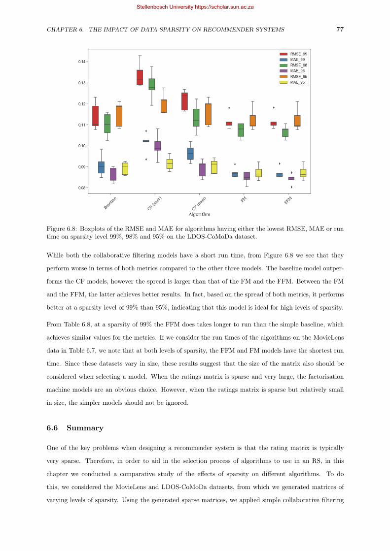
CHAPTER 6. THE IMPACT OF DATA SPARSITY ON RECOMMENDER SYSTEMS 77
Figure 6.8: Boxplots of the RMSE and MAE for algorithms having either the lowest RMSE, MAE or runtime on sparsity level 99%, 98% and 95% on the LDOS-CoMoDa dataset.
While both the collaborative filtering models have a short run time, from Figure 6.8 we see that they
perform worse in terms of both metrics compared to the other three models. The baseline model outper-
forms the CF models, however the spread is larger than that of the FM and the FFM. Between the FM
and the FFM, the latter achieves better results. In fact, based on the spread of both metrics, it performs
better at a sparsity level of 99% than 95%, indicating that this model is ideal for high levels of sparsity.
From Table 6.8, at a sparsity of 99% the FFM does takes longer to run than the simple baseline, which
achieves similar values for the metrics. If we consider the run times of the algorithms on the MovieLens
data in Table 6.7, we note that at both levels of sparsity, the FFM and FM models have the shortest run
time. Since these datasets vary in size, these results suggest that the size of the matrix also should be
considered when selecting a model. When the ratings matrix is sparse and very large, the factorisation
machine models are an obvious choice. However, when the ratings matrix is sparse but relatively small
in size, the simpler models should not be ignored.
6.6 Summary
One of the key problems when designing a recommender system is that the rating matrix is typically
very sparse. Therefore, in order to aid in the selection process of algorithms to use in an RS, in this
chapter we conducted a comparative study of the effects of sparsity on different algorithms. To do
this, we considered the MovieLens and LDOS-CoMoDa datasets, from which we generated matrices of
varying levels of sparsity. Using the generated sparse matrices, we applied simple collaborative filtering
Stellenbosch University https://scholar.sun.ac.za

CHAPTER 6. THE IMPACT OF DATA SPARSITY ON RECOMMENDER SYSTEMS 78
algorithms as well as the more complex latent factors models, the latter of which included the more
recent factorisation machines. The predictive performance of these algorithms were compared using the
accuracy metrics RMSE and MAE, as well as the run time of the algorithm.
According to our results, we can conclude that the FFM and the FM models are the better choice at a
higher level of sparsity. Simpler models perform competitively with these more advanced models as more
information becomes available, as well as when the size of the dataset is small. Therefore, at lower levels
of sparsity, simpler models should not be ignored.
Stellenbosch University https://scholar.sun.ac.za

Chapter 7
Multi-Label Classification for Context
Recommendation
7.1 Introduction
This chapter is devoted to empirical work in a rather niche area of research on recommender systems. As
noted in Chapter 5, both context recommendation and the use of multi-label classification approaches
in an RS setup are topics which, in our opinion, have not yet fully been explored in the literature.
For example, with regard to work on context recommendation, we could find only the contributions by
Baltrunas et al. (2010) and Benmansour et al. (2015). In terms of work on the use of MLC approaches
in general recommender problems, the reader may refer to the papers by Rivolli et al. (2017 and 2018).
Most relevant to our work, however, is the paper by Zheng et al. (2014), wherein the authors investigate
the use of MLC for recommending appropriate contexts for movies and travel destinations.
The objective of the empirical study reported in this chapter, is to expand upon the work in the latter pa-
per. Specifically, we extend the algorithms considered to also include modifications to multivariate linear
regression. In these modifications, potential dependencies among the labels are exploited, and typically
leads to improvements in prediction accuracy. An important advantage of the regression approaches is
that their output includes estimated regression coefficients which may provide valuable information for
feature selection, or for more explainable recommendations. Since in the literature, some work is being
done on finding recommender systems that are easily explainable to users, we regard investigation of the
use of regression for MLC in an RS context to be a worthwhile endeavour.
The performances of the MLC algorithms in Chapter 5 are compared on two real world datasets, viz. the
already encountered LDOS-CoMoDa dataset (Kosir et al., 2011), and the so-called TripAdvisor dataset
(Zheng et al., 2012). Note that both these datasets may be considered as so-called context-aware datasets.
The remainder of the chapter is structured as follows. A description of the LDOS-CoMoDa and TripAd-
79
Stellenbosch University https://scholar.sun.ac.za

CHAPTER 7. MULTI-LABEL CLASSIFICATION FOR CONTEXT RECOMMENDATION 80
visor datasets is provided in Section 7.2. A discussion of the experimental design of our study follows in
Section 7.3. Our empirical results are reported and briefly discussed in Section 7.4. We also compare our
results to those obtained in the paper by Zheng et al. (2014). We conclude the chapter in Section 7.5,
with a summary of our main findings.
7.2 Datasets
7.2.1 The LDOS-CoMoDa Dataset
The LDOS-CoMoDa dataset is a relatively small context-aware dataset relating to movies rated by users.
The data was collected by Kosir et al. (2011) using web surveys, and is freely available1. Several versions
of the LDOS-CoMoDa dataset may be found on the internet. The version of the dataset that was used
in our study contains 121 users, 1232 items (movies) and 2296 ratings. The ratings range from 1 to 5,
in one step increments. There are 30 variables in total, consisting of user information, movie content, as
well as contextual information. There are a total of 12 contextual variables which describe the context in
which the user watched the movie. A detailed description of all available variables can be found in Kosir
et al. (2011).
7.2.2 The TripAdvisor Dataset
This is a context-aware dataset containing information of hotel reviews. The data was complied by
Zheng et al. (2012) after scraping the travel website TripAdvisor. There are a total of 14175 hotel
ratings. These ratings also range from 1 to 5, in one step increments. The dataset contains ratings on
7269 hotels, provided by 2371 users. There are 6 variables, describing user location (state and timezone)
and the hotel location (state, city and timezone). The remaining variable is the contextual variable,
TripType, which describes the type of trip the user was on. As users tend not to stay in the same hotel
under different contexts, or leave a review each time they stay in a hotel, note that the dataset is sparse
with respect to the context.
7.3 Experimental Design
In our analysis, not all variables in the LDOS-CoMoDa dataset were considered. We based the selection
of variables on those chosen by Zheng et al. (2014). Therefore, four context variables are used, namely
time, location, daytype and social, together with a number of content features. The content features
are user gender, movie country, movie year, genre and movie language. For the TripAdvisor dataset,
however, we do make use of all available content and context variables.
1http://212.235.187.145/spletnastran/raziskave/um/comoda/comoda.php
Stellenbosch University https://scholar.sun.ac.za

CHAPTER 7. MULTI-LABEL CLASSIFICATION FOR CONTEXT RECOMMENDATION 81
In the LDOS-CoMoDa dataset, a number of observations had missing values for the context variables.
Since we are trying to predict the appropriate context for a user to watch a movie, these observations are
not useful and were removed. One observation had missing values for both genre and movie language.
There were three other observations that had either missing values for genre or for movie language.
These four observations were removed. The TripAdvisor dataset did not contain any missing values, and
therefore no observations were removed.
Recommendation of appropriate contexts for an item is based on the assumption that the user would
enjoy the item. Therefore, the datasets were split into positive and negative ratings. Ratings above 3
were considered positive, while ratings less than and equal to 3 were considered negative. Furthermore,
in both datasets, there were nominal input variables. It was necessary to label-encode these variables.
Table 7.1 provides a description of the datasets. The values in brackets next to the context variables
indicate the number of dimensions that each context has. For example, for the TripAdvisor dataset,
there are five possible trip types that a user can take, namely ‘solo’, ‘business’, ‘family’, ‘couples’, and
‘friends’. Note that also the context variables were one-hot encoded. Therefore, each dimension of a
context variable represents a label that the MLC algorithm is required to predict.
Table 7.1: Description of the context-aware datasets: LDOS-CoMoDa and TripAdvisor. The values inbrackets next to the context variables indicate the number of dimensions that each context has.
LDOS-CoMoDa TripAdvisorNumber of users 118 2371Number of items 1205 7269Number of ratings 2150 12175Number of positives 1419 11264Contexts time (4), location (3), day (3) trip type (5)
social (7)Contents user gender, movie country, user country, user timezone,
movie year, genre hotel city, hotel state,movie language hotel country, hotel timezone
Following Zheng et al. (2014), we evaluate the performance of the respective MLC algorithms using five-
fold cross-validation. The five sets of training observations, and the five sets of validation observations
are obtained in the following manner. All observations corresponding to positive ratings are split into
five folds of roughly equal size. Each of these positive folds are in turn used as a validation set. The
remaining four positive folds, together with all observations corresponding to negative ratings, are in turn
used as training set. Therefore note that the data observations corresponding to negative ratings form
part of all five training sets.
In order to compare the results of the MLC algorithms, we make use of three baseline recommendation
methods, viz. Global Popular (GP), Item Popular (IP) and User Popular (UP). These methods are based
on popularity. The most popular contexts that occur throughout the training set are recommended in
Stellenbosch University https://scholar.sun.ac.za

CHAPTER 7. MULTI-LABEL CLASSIFICATION FOR CONTEXT RECOMMENDATION 82
the global popular recommendation. The contexts that occur most frequently for a specific item are
recommended by the item popular baseline. Finally, the user popular baseline recommends the context
that occurs the most frequently for a given user. Since the GP method does not provide personalised
recommendations, it represents by far the simplest form of recommendation. The other two baselines, IP
and UP, provide simple personalised recommendations to users.
Note that we evaluate and compare the performance of six MLC algorithms in our experiments. Under
MLC adaptation algorithms we compare ML-kNN and BR-kNN, while CCs, LP and BR represent the
class of MLC transformation algorithms. We also include RAkEL as MLC ensemble method. After
transforming the data, of course any traditional classifier may be implemented by each of the MLC
transformation algorithms. In this regard, note that we considered the use of Bayesian nets, decision
trees and kNN classifiers.
The multi-label classification was preformed in Java, using the MLC library Mulan (version 1.5) (Tsou-
makas et al., 2011). For the classifiers used by the transformation MLC algorithms, we made use of Weka
(version 3.7.10), which is a Java based platform containing machine learning algorithms (Hall et al.,
2009). The classifiers used from Weka are Bayesnet for Bayesian nets, J48 for decision tress, and Ibk for
kNN classifier. As in Zheng et al. (2014), we used unpruned trees. Cross-validation was used in order to
determine the number of neighbours to use for the kNN classifiers.
The format of the data used by Weka is an ARFF file. In this file format, the user may specify the type of
data used. We found that for the LDOS-CoMoDa dataset, the MLC algorithms performed better when
the data was treated as nominal, while the algorithms on the TripAdvisor dataset performed better when
the data was treated as numeric.
The code relating to this chapter may be found in Appendix C.
7.4 Results
Since we follow a similar experimental setup to the setup described in Zheng et al. (2014), we start by
presenting the results from their study in Figure 7.1 below.
With respect to the results displayed in Figure 7.1, first note that we chose not to include the three
baseline kNN algorithms (proposed by Baltrunas et al. (2010)) in our analysis. These baselines are called
the Ratings-based (RB), Best Context Vector-based (BCVB), and Best Context-based (BCB) procedures
in the study by Zheng et al. (2014). For computation reasons, the SVM classifier (Ibk) was also omitted.
Note also that in Figure 7.1, and in our further discussion, the transformation algorithms will be denoted
by ‘Algorithm-Classifier’. Thus ‘BR-kNN’, for example, refers to the binary relevance algorithm used in
combination with a kNN classifier.
Stellenbosch University https://scholar.sun.ac.za

CHAPTER 7. MULTI-LABEL CLASSIFICATION FOR CONTEXT RECOMMENDATION 83
(a) LDOS-CoMoDa
(b) TripAdvisor
Figure 7.1: Prediction performance of the MLC algorithms on LDOS-CoMoDa and TripAdvisor datasets.
Source: Zheng et al. (2014).
Zheng et al. (2014) evaluate all baseline and MLC procedures using precision, recall, accuracy and
Hamming Loss. These measures were obtained using five-fold cross validation and a very specific way
of obtaining the five training- and test folds (described in the previous section). Note that the average
precision, recall and accuracy values are summarised using bar plots, whereas the average Hamming Loss
values are depicted using line graphs.
Considering the results in Figure 7.1, it is evident that for both datasets, the MLC algorithms generally
outperform the baseline algorithms. Exceptions, however, occur in the case of BR-J48 (for both datasets),
as well as in the case of BR-kNN and the two adaptation algorithms (for the TripAdvisor data). Zheng
et al. (2014) note that GP would perform better than a personalised algorithm in cases where a user
visited more than one hotel on a single trip, meaning that the trip type for those ratings would be the
same.
Since the F-measure combines recall and precision, we chose to also report the F-measure in our empirical
work. We proceed with a more detailed comparison between the results in Zheng et al. (2014), and the
results from our empirical evaluation. This is done first for the set of baseline algorithms (in Section 7.4.1),
Stellenbosch University https://scholar.sun.ac.za

CHAPTER 7. MULTI-LABEL CLASSIFICATION FOR CONTEXT RECOMMENDATION 84
subsequently also for the standard MLC algorithms (in Section 7.4.2), and finally for the MLC regression
approaches (in Section 7.4.3).
7.4.1 Baseline Algorithms
The performance measures of the baseline algorithms, as obtained in our empirical analysis, are sum-
marised in terms of boxplots in Figures 7.2 and 7.3. The former figure displays the LDOS-CoMoDa
results, whereas the latter figure is used to depict the TripAdvisor results. Note that the values of the
performance measures on each fold were used to produce the boxplots. The narrowness of the boxes
indicates that there is not much variation from one fold to the next with regards to the obtained metrics.
First consider the results for the LDOS-CoMoDa dataset in Figure 7.2. Clearly, GP and IP perform
very similarly. For both, the average F-measure value is about 0.58, and the average Hamming Loss
value is close to 0.20. In terms of average performance measures, we see that UP does slightly better,
with an average F-measure of approximately 0.65, and with an average Hamming Loss value of about
0.18. Interestingly, in terms of the variance of performance measures, note that the IP approach yields
measures with a much smaller variance than in the case of GP and UP.
Next consider the results for the TripAdvisor dataset in Figure 7.3. Here GP and IP perform much worse
than UP. The average F-measure values for GP and IP are about 0.32 and 0.4, respectively, compared
to about 0.6 for UP. In terms of Hamming Loss, differences between the baseline algorithms are far less
pronounced: UP achieves about 0.18, compared to approximately 0.27, achieved by both GP and IP.
The baseline results reported in Zheng et al. (2014), and those obtained in our empirical analysis (cf.
Figures 7.1 and 7.4) are found to be very similar. Zheng et al. (2014) also finds that UP outperforms both
GP and IP. For the TripAdvisor dataset in particular, our baseline algorithms achieve slightly better
results. For example, the average accuracies for GP, UP and IP in Zheng et al. (2014) are 0.3, 0.58, and
0.34. In our analysis, we obtained average accuracies of 0.33, 0.6 and 0.37.
In summary in this section, if one takes the simplicity of the baseline algorithms into account, their
performance seems to be very reasonable. Also, since in both applications, UP is shown to outperform
GP and IP, user personalisation seems to be an important aspect.
Stellenbosch University https://scholar.sun.ac.za

CHAPTER 7. MULTI-LABEL CLASSIFICATION FOR CONTEXT RECOMMENDATION 85
(a)GP
baselin
e(b)UP
baselin
e(c)IP
baselin
e
Figure7.2:
LDOS-CoM
oDa:
Boxplot
ofpe
rforman
cemeasuresforthediffe
rent
baselin
erecommenders.
Stellenbosch University https://scholar.sun.ac.za

CHAPTER 7. MULTI-LABEL CLASSIFICATION FOR CONTEXT RECOMMENDATION 86
(a)GP
baselin
e(b)UP
baselin
e(c)IP
baselin
e
Figure7.3:
TripA
dvisor:Boxplot
ofpe
rforman
cemeasuresforthediffe
rent
baselin
erecommenders.
Stellenbosch University https://scholar.sun.ac.za

CHAPTER 7. MULTI-LABEL CLASSIFICATION FOR CONTEXT RECOMMENDATION 87
(a) LDOS-CoMoDa
(b) TripAdvisor
Figure 7.4: Prediction performance of baseline algorithms. Precision, recall, accuracy and F1 values areread off the left axis, while Hamming loss is read off the right axis.
7.4.2 MLC Algorithms
The performance measures of the MLC algorithms, as obtained in our empirical analysis, are summarised
in terms of bar plots in Figure 7.5. In the case of both datasets, the baseline UP method is found to
outperform all MLC approaches.
For the LDOS-CoMoDa dataset, the MLC approaches perform very similarly. Only two adaption al-
gorithms (ML-kNN and BR-kNN) are found to show some potential: we obtain an average Hamming
Stellenbosch University https://scholar.sun.ac.za

CHAPTER 7. MULTI-LABEL CLASSIFICATION FOR CONTEXT RECOMMENDATION 88
(a) LDOS-CoMoDa
(b) TripAdvisor
Figure 7.5: Prediction performance of all algorithms. Precision, recall, accuracy and F1 values are readoff the left axis, while Hamming loss is read off the right axis.
Loss value of approximately 0.2 in the case of both these algorithms. Additionally, the average precision
values are above 0.6, which is significantly higher than that obtained by the other algorithms. However,
in terms of the other measures reported, these two approaches do not perform well.
Next consider the MLC results for the TripAdvisor dataset. Here we do observe some variation between
Stellenbosch University https://scholar.sun.ac.za

CHAPTER 7. MULTI-LABEL CLASSIFICATION FOR CONTEXT RECOMMENDATION 89
performances. In terms of Hamming Loss, BR-J48, BR-BN, CC-BN, and once again ML-kNN and
BR-kNN seem to have the most potential. For these methods, the average Hamming Loss values are
once again close to 0.2. However, as was the case for the LDOS-CoMoDa dataset, in terms of the other
performance measures, these approaches do not perform well.
We observe significant differences between our MLC results, and the MLC results reported in Zheng et al.
(2014) (cf. Figures 7.1 and 7.5). Across all performance measures and in the case of both datasets, our
MLC results are generally 20% to 30% lower than the reported results. There is, however, an exception of
this phenomenon that is perhaps worth mentioning. For the TripAdvisor data, in the case of the BR-J48,
CC-J48 and BR-kNN algorithms, we achieve very similar values to all reported performance values.
Several potential reasons for inconsistencies between our results and the reported results may further be
explored. Firstly, the format of the data, as well as the chosen variables, could be influential. It may
well be that we have used different encoding techniques, or selected different variables to form part of the
models considered. Another discrepancies might occur with hyper-parameter specifications. For example,
the number of nearest neighbours used in the kNN classifiers may differ from the parameter value used
in the study by Zheng et al. (2014).
7.4.3 Regression Algorithms
Recall from Section 5.5 that the regression approaches to MLC involve a method to specify label-specific
threshold values. Therefore note that on each fold, we obtain the Hamming Loss, F-measure and accuracy
measures for each combination of regression- and threshold methods. We number and label the threshold
methods as follows: 1 indicates the quantile method, 2 indicates thresholding on the performance measure,
and 3 indicates thresholding on the performance measure and subsequently converting the value to a
quantile. Thus, ‘CW-1’ indicates the curds-and-whey regression approach used in combination with the
quantile threshold method. Note that the other regression approaches are named similarly. The average
results from the five-fold cross-validation procedure are presented in Tables 7.2 to 7.4. Note that all best
performing methods are indicated in bold font.
Consider first the Hamming Loss values in Table 7.2. It is interesting to note that the results pertaining
to the LDOS-CoMoDa data are far less variable than in the case of the TripAdvisor data. Overall, it is
very difficult to identify an overall winner in terms of the regression approaches. Indeed, depending on the
application, the best performing regression approach is found to differ. In the case of the LDOS-CoMoDa
data, FICYREG performs the best, while in the case of the TripAdvisor data, RR outperforms the other
approaches. We also see that exploiting label dependencies has a greater positive impact in the case of
the TripAdvisor data than in the case of the LDOS-CoMoDa dataset. In terms of the performance of the
various threshold methods, the second threshold method seems to be the best choice.
Stellenbosch University https://scholar.sun.ac.za

CHAPTER 7. MULTI-LABEL CLASSIFICATION FOR CONTEXT RECOMMENDATION 90
Table 7.2: Hamming Loss values for each regression algorithm.
Approach LDOS-CoMoDa TripAdvisorCW-1 0.2380 0.3198CW-2 0.2246 0.3292CW-3 0.2259 0.3292FICY-1 0.2335 0.3171FICY-2 0.2221 0.3387FICY-3 0.2224 0.3387OLS-1 0.2352 0.3173OLS-2 0.2244 0.3756OLS-3 0.2253 0.3756RR-1 0.2355 0.3055RR-2 0.2260 0.3114RR-3 0.2257 0.3114
Consider next the F-measure values in Table 7.3. For both datasets, these values are very similar. For
the LDOS-CoMoDa data, FICYREG performs the best. For the TripAdvisor data, the performances
of CW and RR are tied for first place. In terms of a choice between threshold methods, in the case of
the LDOS-CoMoDa dataset, the first threshold method seems to be the best, while the second threshold
method is the best choice in the case of the TripAdvisor dataset.
Table 7.3: F-measure values for each regression algorithm.
Approach LDOS-CoMoDa TripAdvisorCW-1 0.5133 0.3139CW-2 0.4663 0.3553CW-3 0.4650 0.3503FICY-1 0.5201 0.3213FICY-2 0.4529 0.3547FICY-3 0.4553 0.3494OLS-1 0.5178 0.3431OLS-2 0.4705 0.3440OLS-3 0.4694 0.3464RR-1 0.5173 0.3154RR-2 0.4662 0.3553RR-3 0.4649 0.3499
The average accuracy values are reported in Table 7.4. For the LDOS-CoMoDa data, we observe the
same pattern as in the case of the Hamming Loss and F-measure, with FICYREG emerging as the best
regression approach. As was the case with results based on the F-measure, the first threshold procedure
is preferred in the case of all regression approaches. For the TripAdvisor dataset, the best accuracy across
the regression approaches is achieved using the first threshold technique. Somewhat surprisingly, here
OLS outperforms the other approaches.
A comparison between the performances of the regression approaches and the standard MLC algorithms
is of particular interest to us. We base our comparison on all three performance measures considered,
starting with the F-measure. Therefore, first consider Table 7.3 and Figure 7.5. For the LDOS-CoMoDa
Stellenbosch University https://scholar.sun.ac.za

CHAPTER 7. MULTI-LABEL CLASSIFICATION FOR CONTEXT RECOMMENDATION 91
Table 7.4: Accuracy values for each regression algorithm.
Approach LDOS-CoMoDa TripAdvisorCW-1 0.3829 0.2743CW-2 0.3229 0.2309CW-3 0.3220 0.2266FICY-1 0.3912 0.2814FICY-2 0.3116 0.2300FICY-3 0.3135 0.2256OLS-1 0.3903 0.3004OLS-2 0.3273 0.2204OLS-3 0.3135 0.2256RR-1 0.3895 0.2889RR-2 0.3234 0.2315RR-3 0.3135 0.2256
data, the regression approaches is found to perform similarly to the standard MLC algorithms. FICY-1
yields an F-measure of approximately 0.52, which is almost identical to the F-measure corresponding
to the best performing MLC algorithm (LP-BN). This is also true in the for the TripAdvisor data: the
average F-measure corresponding to the best regression approach (RR-2) is approximately 0.35, while the
average F-measure corresponding to the best MLC algorithms (LP-J48 and RAkEL-J48) is approximately
0.37.
In terms of average Hamming Loss values, we reconsider Table 7.2 and Figure 7.5. In the case of the
LDOS-CoMoDa data, once again the regression results are very similar to the MLC results. In the case
of the TripAdvisor data, the regression results are slightly worse than the MLC results. The average
Hamming Loss value is approximately 0.3 across all approaches, whereas the MLC algorithms produce
an average Hamming Loss below 0.3.
In terms of average accuracy values, we compare Table 7.4 to Figure 7.5. For the LDOS-CoMoDa dataset,
with exception of the first threshold method, the regression approaches perform consistently worse than
the MLC algorithms. The best regression approach is found to be FICY-1, achieving an accuracy of 0.39,
which is the same accuracy obtained by LP-BN. The regression approaches also perform significantly
worse in the case of the TripAdvisor dataset. The best accuracy of 0.30 (OLS-1) is approximately 7%
lower than the best performing MLC method (LP-J48).
In summary of this section, while the regression methods do not necessarily provide better results than
the MLC methods, they are at least somewhat similar. The best performing regression approach on the
LDOS-CoMoDa dataset across all performance measures is FICYREG. On the TripAdvisor dataset, the
best Hamming Loss and F-score is achieved by RR, whereas OLS yields the best accuracy.
Stellenbosch University https://scholar.sun.ac.za

CHAPTER 7. MULTI-LABEL CLASSIFICATION FOR CONTEXT RECOMMENDATION 92
7.5 Summary
In this chapter, an empirical study was conducted in order to evaluate the predictive performance of MLC
algorithms for context recommendation against simple baseline methods. We also considered various
regression approaches to multi-label classification.
Compared to the standard MLC algorithms that we considered, the simple baseline methods perform
much better than the more complex methods. In particular, the User Popular baseline achieves the best
results on both datasets. This indicates that user personalistion is necessary in order to recommend
the best contexts associated with an item. The fact that the simple baseline algorithms have a better
predictive performance than the more complex algorithms, and that our results differ from that of Zheng
et al. (2014) is reason to do additional future empirical studies on this topic. Alternative designs were
also explored, however these did not yield improved results.
In our experiments, it was shown that the MLC regression approaches are unable to outperform the
standard MLC methods. However, most of the results were found to be comparable, thereby not entirely
discouraging an interest in the topic.
Stellenbosch University https://scholar.sun.ac.za

Chapter 8
Conclusion
The main objective of this thesis was to investigate various algorithms for recommender systems. We
focused on two traditional types of recommender systems, as well as on recent improvements thereof.
An overview of the algorithms that typically form part of recommender systems was provided. Towards
explainable recommender systems, we considered the connection between multi-label classification and
recommender systems.
We conducted two empirical studies. In the first study, our aim was to evaluate the performance of latent
factor models and factorisation machines using varying levels of data sparsity. In the second study, in
addition to standard MLC approaches, we also evaluated the use of extensions to multivariate linear
regression in an MLC context. In the following two sections, we proceed with a summary of the thesis,
and conclude with suggested avenues for further research.
8.1 Summary
Chapters 2 to 5 were devoted to a literature review of related RS algorithms. We started by describing
the more standard approaches of content-based recommendation and collaborative filtering in Chapters 2
and 3, and proceeded with a discussion of more recent collaborative filtering approaches in Chapter 4.
A different perspective to the design of an RS was explored in Chapter 5. This entails casting recom-
mendation in terms of a multi-label classification problem. Chapters 6 and 7 were devoted to the two
empirical studies that formed part of the research. We proceed with a more detailed description of each
chapter below.
In Chapter 2 the focus was on content-based recommender systems. The design of these systems was
described, which included using vector space models to represent items in a usable format, as well as
using machine learning algorithms to learn user profiles. While these systems do not suffer from the cold-
start problem, without well described items, their performance is generally poor. Therefore, collaborative
filtering systems, discussed in Chapter 3, are typically preferred. The two types of CF algorithms, viz.
93
Stellenbosch University https://scholar.sun.ac.za

CHAPTER 8. CONCLUSION 94
memory- and model-based, were discussed. Memory-based algorithms are simpler than model-based al-
gorithms and can perform well on small datasets, however they do not scale well. Recommendations from
both types of CF methods are severely impacted in sparse data settings. Since model-based CF methods
scale reasonably well, extensions which aim to alleviate the impact of data sparsity on the recommend-
ations were discussed in Chapter 4. These extensions included well-known latent factor models, such
as matrix and tensor factorisation, as well as the more state-of-the-art factorisation machines. We con-
cluded our literature review in Chapter 5, with an overview of recommendation by means of multi-label
classification. More specifically, we considered the use of well-known MLC approaches, and extensions to
multivariate linear regression in an MLC context, in order to recommend the context in which to use an
item.
Our first empirical study was discussed in Chapter 6. The aim of this study was to investigate the impact
of data sparsity on the predictive performance of recommender systems. The experimental design of
the study was based upon the experimental frameworks considered in related work, although necessary
modifications were made. We compared the performance of memory-based CF models, latent factor
models and factorisation machines on two recommendation datasets, using generated datasets of varying
levels of sparsity. In summary, the results showed that factorisation machines are able to provide improved
recommendations at high levels of data sparsity. Furthermore, in the case of large datasets, factorisation
machines are faster to implement than the simpler methods.
Chapter 7 was devoted to our second empirical study. The purpose of this study was to explore the use
of multi-label classification algorithms in recommender problems. Since related work focused on the use
of MLC algorithms in context recommendations, we also attempted to make use of MLC methods in
order to recommend the contexts in which users are more likely to appreciate items of interest. With a
view to a contribution in terms of explainable recommender systems, we extended our study to include
the more recently proposed MLC regression approaches. Our results indicated that an MLC approach is
suboptimal in an RS setting, however it is important to note that our results differ from those of Zheng
et al. (2014), therefore further investigation is necessary.
8.2 Future Research
Several options for further research in the recommender systems field are worth mentioning. Since Zheng
et al. (2014) report promising results for the use of MLC methods in an RS setting, there is some
evidence that improvement of the performance of MLC methods in this context is within reach. Several
pre-processing steps (such as using sampling to correct class imbalances, and considering different data
formats) may be worth investigating.
Recommender systems that produce explainable output can improve user satisfaction as well as trust
Stellenbosch University https://scholar.sun.ac.za

CHAPTER 8. CONCLUSION 95
in the system. Recommendations produced by simple memory-based CF models are easy to explain,
however they typically have a low accuracy. On the other hand, latent factor models produce highly
accurate results, but these are difficult to interpret and explain. Therefore, it is desirable to have a
recommender system that is not only accurate, but explainable. A recent review of the currently used
methods towards explainable recommendation may be found in the survey by Zhang and Chen (2019).
If the regression approaches to MLC can be shown to perform as well as the MLC methods investigated
in Zheng et al. (2014), we believe that there is a contribution to be made in this research field.
In our discussion in Chapter 4, we have touched upon the use of factorisation machines in the hidden layers
of neural networks. Studies investigating the use of neural networks towards improving the predictive
performance of recommender systems can be found in the literature. For example, Covington et al.
(2016) make use of deep learning to improve YouTube recommendations, and van den Oord et al. (2013)
investigate the use of convolutional neural networks for music recommendation. A review of the use of
deep learning for recommender systems may be found in the paper by Batmaz et al. (2018). From this
paper it is clear that deep learning for recommender systems is a specialised field, and one which seems
to be a natural direction for further study.
Stellenbosch University https://scholar.sun.ac.za

Appendices
96
Stellenbosch University https://scholar.sun.ac.za

Appendix A
Source Code: Chapter 6
A.1 Required Python Packages
1 import pandas as pd
2 import os
3 import matp lo t l i b . pyplot as p l t
4 from sc ipy import spar s e
5 import numpy as np
6 import random
7 import time
8 from ppr int import ppr int
9 import x l ea rn as x l
10
11 from su r p r i s e import NMF, SVD, KNNBasic
12 from su r p r i s e import pred i c t i on_a lgor i thms
13 from su r p r i s e import Reader , Dataset
14 from su r p r i s e . mode l_se lect ion import t r a i n_te s t_sp l i t
15 from su r p r i s e . mode l_se lect ion import GridSearchCV
16 from su r p r i s e import accuracy
17 from su r p r i s e . mode l_se lect ion import KFold
A.2 Functions Needed To Generate A Sparse Matrix
1 de f ca l cu late_data f rame_spars i ty ( rat ings_df ) :
2 n_users = len ( rat ings_df [ ’ userId ’ ] . unique ( ) )
3 n_movies = len ( rat ings_df [ ’ movieId ’ ] . unique ( ) )
4 n_ratings = len ( rat ings_df )
5 s p a r s i t y = 100 .0 − ( 100 . 0 ∗ n_ratings / ( n_users ∗ n_movies ) )
6
7 r e turn (" u s e r s : " , n_users ,
8 "movies : " , n_movies ,
9 " r a t i n g s : " , n_ratings ,
97
Stellenbosch University https://scholar.sun.ac.za
APPENDIX A. SOURCE CODE: CHAPTER 6 98
10 " s p a r s i t y : " , s p a r s i t y )
11
12 de f sparsity_of_an_array ( a ) :
13 n_elements = np . prod ( a . shape )
14 r e turn ( ( n_elements − np . count_nonzero ( a ) ) /n_elements )
15
16 de f label_encode_ids ( rat ings_df ) :
17
18 from sk l e a rn import p r ep ro c e s s i ng
19 l e = pr ep ro c e s s i ng . LabelEncoder ( )
20
21 # encode u s e r i d s
22 l e . f i t ( rat ings_df [ ’ userId ’ ] . unique ( ) )
23 rat ings_df [ ’ userId ’ ] = l e . trans form ( rat ings_df [ ’ userId ’ ] )
24
25 # encode movie ids
26 l e . f i t ( rat ings_df [ ’ movieId ’ ] . unique ( ) )
27 rat ings_df [ ’ movieId ’ ] = l e . trans form ( rat ings_df [ ’ movieId ’ ] )
28
29 r e turn ( rat ings_df )
30
31 de f user_and_item_proportions ( df ) :
32 ’ ’ ’
33 Parameters :
34 − df : dataframe with columns " use r Id " , "movieId " , " r a t i ng " .
35 Returns :
36 Dataframe s p e c i f y i n g user p ropor t i on s and a dataframe s p e c i f i y i n g item
propor t i on s .
37 ’ ’ ’
38 import numpy as np
39
40 unique_user id = np . array ( df [ ’ userId ’ ] . unique ( ) )
41 unique_itemid = np . array ( df [ ’ movieId ’ ] . unique ( ) )
42 total_number_of_ratings = len ( df )
43
44 # number o f r a t i n g s per user
45 n_user_ratings = df . drop ( columns=["movieId " ] )
46 n_user_ratings = n_user_ratings . groupby ( [ " use r Id " ] ) . count ( ) . reset_index ( )
47 n_user_ratings = n_user_ratings . rename ( columns={" ra t i ng " : " n_ratings "})
48
49 # proport ion o f r a t i n g s f o r each user
50 n_user_ratings [ ’ user_prop ’ ] = n_user_ratings [ ’ n_ratings ’ ] / total_number_of_ratings
51
52 # number o f r a t i n g s per item
Stellenbosch University https://scholar.sun.ac.za

APPENDIX A. SOURCE CODE: CHAPTER 6 99
53 n_item_ratings = df . drop ( columns=[" use r Id " ] )
54 n_item_ratings = n_item_ratings . groupby ( [ " movieId " ] ) . count ( ) . reset_index ( )
55 n_item_ratings = n_item_ratings . rename ( columns={" ra t i ng " : " n_ratings "})
56
57 # proport ion o f r a t i n g s f o r each item
58 n_item_ratings [ ’ item_prop ’ ] = n_item_ratings [ ’ n_ratings ’ ] / total_number_of_ratings
59
60 r e turn ( n_user_ratings , n_item_ratings )
61
62 de f create_dense_matrix ( df , mf_technique = ’SVD’ , k = 100 , b i a s = ’ False ’ , s c a l e = ( 0 . 5 ,
5) ) :
63 ’ ’ ’
64 Paramters :
65 − df : dataframe with columns " use r Id " , "movieId " , " r a t i ng " .
66 − mf_technique : matrix f a c t o r i s a t i o n techn ique to be used , e i t h e r "SVD" or "NMF" .
67 − k : number o f l a t e n t f a c t o r s .
68 − b ia s : whether to use b a s e l i n e s ( boolean ) .
69 − s c a l e : min and max ra t i ng va lue s .
70 Returns :
71 Dense matrix , user l a t e n t vector , item l a t e n t vec to r .
72 ’ ’ ’
73
74 from su r p r i s e import NMF, SVD
75 from su r p r i s e import pred i c t i on_a lgor i thms
76 from su r p r i s e import Reader , Dataset
77 import numpy as np
78
79 r eader = Reader ( ra t ing_sca l e = s c a l e )
80 data = Dataset . load_from_df ( df , r eader )
81 temp = data . bu i l d_ fu l l_ t r a i n s e t ( )
82
83 i f mf_technique == "SVD" :
84 a lg = SVD( n_factors = k , b iased = bias , random_state = 1)
85 e l s e :
86 a lg = NMF( n_factors = k , b iased = bias , random_state = 1)
87
88 a lg . f i t ( temp)
89 pu = a lg . pu
90 q i = a lg . q i
91 R_hat = np . dot (pu , q i .T)
92
93 r e turn (R_hat , pu , q i )
94
95 de f number_of_ratings_needed_for_a_level_of_spasrsity ( total_number_of_ratings ,
Stellenbosch University https://scholar.sun.ac.za

APPENDIX A. SOURCE CODE: CHAPTER 6 100
s p a r s i t y_ l e v e l ) :
96 r e turn ( i n t ( total_number_of_ratings∗(1− s p a r s i t y_ l e v e l ) ) )
97
98 de f create_sparse_matrix (mat , user_prop , item_prop , s p a r s i t y_ l e v e l ) :
99 import random
100 import pandas as pd
101 import numpy as np
102
103 np . random . seed (2 )
104 i , u = mat . shape
105 x = number_of_ratings_needed_for_a_level_of_spasrsity (u∗ i , s p a r s i t y_ l e v e l )
106
107 unique_user id = np . array ( user_prop [ ’ userId ’ ] . unique ( ) )
108 unique_itemid = np . array ( item_prop [ ’ movieId ’ ] . unique ( ) )
109
110 random . s h u f f l e ( unique_user id )
111
112 sparse_df = pd . DataFrame ( columns = [ ’ userId ’ , ’ movieId ’ , ’ ra t ing ’ ] )
113
114 f o r j in range (0 , x ) :
115 s e l e c t ed_use r = in t (np . random . cho i c e ( unique_userid , 1 , p = user_prop [ ’ user_prop
’ ] , r e p l a c e = True ) )
116 se l ected_item = in t (np . random . cho i c e ( unique_itemid , 1 , p = item_prop [ ’ item_prop
’ ] , r e p l a c e = True ) )
117 s e l e c t ed_ra t i ng = mat [ se l ec ted_user , se l ected_item ]
118 sparse_df = sparse_df . append ({ ’ userId ’ : s e l ec ted_user ,
119 ’ movieId ’ : se lected_item , ’ rat ing ’ : s e l e c t ed_ra t i ng
} , ignore_index =True )
120
121
122 convert_dict = { ’ userId ’ : int , ’ movieId ’ : int , ’ ra t ing ’ : f l o a t }
123 sparse_df = sparse_df . astype ( convert_dict )
124 r e turn ( sparse_df )
A.3 Functions Needed To Run Collaborative Filtering Algorithms
1 de f get_data ( f i le_name ) :
2 import pandas as pd
3 from su r p r i s e import Reader , Dataset
4 import numpy as np
5 import random
6 import csv
7
8 R_100_s = pd . DataFrame (np . l oadtx t ( file_name , dtype=f l o a t ) , columns = [ ’ userId ’ , ’
itemId ’ , ’ ra t ing ’ ] )
Stellenbosch University https://scholar.sun.ac.za

APPENDIX A. SOURCE CODE: CHAPTER 6 101
9 R_100_s = R_100_s . astype ({ ’ userId ’ : int , ’ itemId ’ : int , ’ ra t ing ’ : f l o a t })
10
11 # Load the f u l l da ta se t .
12 r eader = Reader ( ra t ing_sca l e=(min (R_100_s [ ’ ra t ing ’ ] ) , max(R_100_s [ ’ ra t ing ’ ] ) ) )
13 data = Dataset . load_from_df (R_100_s [ [ ’ userId ’ , ’ itemId ’ , ’ ra t ing ’ ] ] , r eader )
14 raw_ratings = data . raw_ratings
15
16 # s h u f f l e r a t i n g s i f you want
17 random . s h u f f l e ( raw_ratings )
18
19 with open ( f i le_name + ’_raw ’ , ’w’ ) as out :
20 csv_out=csv . wr i t e r ( out )
21 f o r row in raw_ratings :
22 csv_out . writerow ( row )
23
24 # A = 90% of the data , B = 10% of the data
25 th r e sho ld = in t ( . 9 ∗ l en ( raw_ratings ) )
26 pr in t ( th r e sho ld )
27 A_raw_ratings = raw_ratings [ : th r e sho ld ]
28 B_raw_ratings = raw_ratings [ th r e sho ld : ]
29
30 data . raw_ratings = A_raw_ratings # data i s now the s e t A
31 t r a i n s e t = data . bu i l d_ fu l l_ t r a i n s e t ( )
32 t e s t s e t = data . c on s t ru c t_te s t s e t ( B_raw_ratings ) # t e s t s e t i s now the s e t B
33
34 r e turn ( data , t r a i n s e t , t e s t s e t , raw_ratings , th r e sho ld )
35
36 ######## BASIC METHODS
37
38 de f get_baseline_only_model ( gs_data , train_data ) :
39 from su r p r i s e . mode l_se lect ion import GridSearchCV
40 from su r p r i s e import accuracy
41 from su r p r i s e import Base l ineOnly
42 from su r p r i s e import pred i c t i on_a lgor i thms
43
44 bs l_opt ions = { ’method ’ : [ ’ sgd ’ ] , ’ l earn ing_rate ’ : [ 0 . 0 0 7 , 0 . 009 , 0 . 0 1 ] , ’ n_epochs ’ :
[ 5 , 1 0 ] }
45 param_grid = { ’ bs l_options ’ : bs l_opt ions }
46
47 base l ine_gs = GridSearchCV ( Basel ineOnly , param_grid , measures =[ ’ rmse ’ ] , cv=3, n_jobs
=5)
48 base l ine_gs . f i t ( gs_data )
49
50 best_params_basel ineonly = base l ine_gs . best_params
Stellenbosch University https://scholar.sun.ac.za

APPENDIX A. SOURCE CODE: CHAPTER 6 102
51 pr in t ( best_params_basel ineonly )
52 ba s e l i n e on l y = base l ine_gs . best_est imator [ ’ rmse ’ ]
53
54 # re t r a i n on the whole t r a i n s e t
55 model_BaselineOnly = ba s e l i n e on l y . f i t ( train_data )
56
57 r e turn ( model_BaselineOnly )
58
59 ######## KNN METHODS
60
61 de f get_best_CF_userbased_model ( gs_data , train_data ) :
62 from su r p r i s e . mode l_se lect ion import GridSearchCV
63 from su r p r i s e import accuracy
64 from su r p r i s e import KNNBasic
65 from su r p r i s e import pred i c t i on_a lgor i thms
66
67 sim_options = { ’name ’ : [ ’ cos ine ’ ] ,
68 ’ user_based ’ : [ True ]
69 }
70 param_grid = { ’k ’ : [ 5 , 15 , 25 , 50 ] , ’ sim_options ’ : sim_options }
71
72 knnbasic_gs = GridSearchCV (KNNBasic , param_grid , measures =[ ’ rmse ’ ] , cv=3, n_jobs=5)
73 knnbasic_gs . f i t ( gs_data )
74
75 best_params_CF_user = knnbasic_gs . best_params
76 pr in t ( best_params_CF_user )
77 knn_users = knnbasic_gs . best_est imator [ ’ rmse ’ ]
78
79 # re t r a i n on the whole t r a i n s e t
80 model_CF_userbased = knn_users . f i t ( train_data )
81
82 r e turn (model_CF_userbased )
83
84 de f get_best_CF_itembased_model ( gs_data , train_data ) :
85 from su r p r i s e . mode l_se lect ion import GridSearchCV
86 from su r p r i s e import accuracy
87 from su r p r i s e import KNNBasic
88 from su r p r i s e import pred i c t i on_a lgor i thms
89
90 sim_options = { ’name ’ : [ ’ cos ine ’ ] ,
91 ’ user_based ’ : [ Fa l se ]
92 }
93 param_grid = { ’k ’ : [ 5 , 15 , 25 , 50 ] , ’ sim_options ’ : sim_options }
94
Stellenbosch University https://scholar.sun.ac.za

APPENDIX A. SOURCE CODE: CHAPTER 6 103
95 knnbasic_gs = GridSearchCV (KNNBasic , param_grid , measures =[ ’ rmse ’ ] , cv=3, n_jobs=5)
96 knnbasic_gs . f i t ( gs_data )
97
98 best_params_CF_item = knnbasic_gs . best_params
99 pr in t ( best_params_CF_item)
100 knn_item = knnbasic_gs . best_est imator [ ’ rmse ’ ]
101
102 # re t r a i n on the whole t r a i n s e t
103 model_CF_itembased = knn_item . f i t ( train_data )
104
105 r e turn (model_CF_itembased )
106
107 ######## MATRIX FACTORISATION METHODS
108
109 de f get_best_svd_model ( gs_data , train_data ) :
110 ’ ’ ’
111 Does a g r id search to determining the best parameters ( based on rmse ) , and r e tu rn s
the model f i t t e d on t r a i n i n g data .
112
113 Parameters :
114 − data : g r id s each data
115 − t r a i n : data to t r a i n model
116 Returns :
117 − model : t r a in ed model
118 ’ ’ ’
119
120 from su r p r i s e . mode l_se lect ion import GridSearchCV
121 from su r p r i s e import accuracy
122 from su r p r i s e import SVD
123 from su r p r i s e import pred i c t i on_a lgor i thms
124
125 param_grid = { ’ n_factors ’ : [ 2 0 , 50 , 100 ] , ’ n_epochs ’ : [ 5 , 1 0 ] , ’ l r_a l l ’ : [ 0 . 0 0 7 ,
0 . 009 , 0 . 0 1 ] ,
126 ’ reg_al l ’ : [ 0 . 0 2 , 0 . 04 , 0 . 0 6 ] }
127
128 gr id_search = GridSearchCV (SVD, param_grid , measures =[ ’ rmse ’ ] , cv=3)
129 gr id_search . f i t ( gs_data )
130
131 best_params_svd = grid_search . best_params
132 pr in t ( best_params_svd )
133 algo_svd = grid_search . best_est imator [ ’ rmse ’ ]
134
135 # re t r a i n on the whole t r a i n s e t
136 model_svd = algo_svd . f i t ( train_data )
Stellenbosch University https://scholar.sun.ac.za

APPENDIX A. SOURCE CODE: CHAPTER 6 104
137
138 r e turn (model_svd )
139
140 de f get_best_svd_unbiased_model ( gs_data , train_data ) :
141 ’ ’ ’
142 Does a g r id search to determining the best parameters ( based on rmse ) , and r e tu rn s
the model f i t t e d on t r a i n i n g data .
143
144 Parameters :
145 − data : g r id s each data
146 − t r a i n : data to t r a i n model
147 Returns :
148 − model : t r a in ed model
149 ’ ’ ’
150
151 from su r p r i s e . mode l_se lect ion import GridSearchCV
152 from su r p r i s e import accuracy
153 from su r p r i s e import SVD
154 from su r p r i s e import pred i c t i on_a lgor i thms
155
156 param_grid = { ’ n_factors ’ : [ 2 0 , 50 , 100 ] , ’ n_epochs ’ : [ 5 , 1 0 ] , ’ l r_a l l ’ : [ 0 . 0 0 7 ,
0 . 009 , 0 . 0 1 ] ,
157 ’ reg_al l ’ : [ 0 . 0 2 , 0 . 04 , 0 . 0 6 ] , ’ b iased ’ : [ Fa l se ] }
158
159 gr id_search = GridSearchCV (SVD, param_grid , measures =[ ’ rmse ’ ] , cv=3)
160 gr id_search . f i t ( gs_data )
161
162 best_params_svd = grid_search . best_params
163 pr in t ( best_params_svd )
164 algo_svd = grid_search . best_est imator [ ’ rmse ’ ]
165
166 # re t r a i n on the whole t r a i n s e t
167 model_svd = algo_svd . f i t ( train_data )
168
169 r e turn (model_svd )
170
171 de f get_best_svdpp_model ( gs_data , train_data ) :
172 ’ ’ ’
173 Does a g r id search to determining the best parameters ( based on rmse ) , and r e tu rn s
the model f i t t e d on t r a i n i n g data .
174
175 Parameters :
176 − data : g r id s each data
177 − t r a i n : data to t r a i n model
Stellenbosch University https://scholar.sun.ac.za

APPENDIX A. SOURCE CODE: CHAPTER 6 105
178 Returns :
179 − model : t r a in ed model
180 ’ ’ ’
181
182 from su r p r i s e . mode l_se lect ion import GridSearchCV
183 from su r p r i s e import accuracy
184 from su r p r i s e import SVDpp
185 from su r p r i s e import pred i c t i on_a lgor i thms
186
187 param_grid = { ’ n_factors ’ : [ 2 0 , 5 0 ] , ’ n_epochs ’ : [ 5 , 1 0 ] , ’ l r_a l l ’ : [ 0 . 0 0 7 , 0 . 009 ,
0 . 0 1 ] ,
188 ’ reg_al l ’ : [ 0 . 0 4 , 0 . 0 6 ] }
189
190 gr id_search = GridSearchCV (SVDpp, param_grid , measures =[ ’ rmse ’ ] , cv=3)
191 gr id_search . f i t ( gs_data )
192
193 best_params_svdpp = gr id_search . best_params
194 pr in t ( best_params_svdpp )
195 algo_svdpp = grid_search . best_est imator [ ’ rmse ’ ]
196
197 # re t r a i n on the whole t r a i n s e t
198 model_svdpp = algo_svdpp . f i t ( train_data )
199
200 r e turn (model_svdpp )
201
202 de f get_best_nmf_model ( gs_data , train_data ) :
203 ’ ’ ’
204 Does a g r id search to determining the best parameters ( based on rmse ) , and r e tu rn s
the model f i t t e d on t r a i n i n g data .
205
206 Parameters :
207 − data : g r id s each data
208 − t r a i n : data to t r a i n model
209 Returns :
210 − model : t r a in ed model
211 ’ ’ ’
212
213 from su r p r i s e . mode l_se lect ion import GridSearchCV
214 from su r p r i s e import accuracy
215 from su r p r i s e import NMF
216 from su r p r i s e import pred i c t i on_a lgor i thms
217 param_grid = { ’ n_factors ’ : [ 2 0 , 50 , 100 ] , ’ n_epochs ’ : [ 5 , 1 0 ] , ’ reg_qi ’ : [ 0 . 0 2 , 0 . 04 ,
0 . 0 6 ] ,
218 ’ reg_pu ’ : [ 0 . 0 2 , 0 . 04 , 0 . 0 6 ] }
Stellenbosch University https://scholar.sun.ac.za

APPENDIX A. SOURCE CODE: CHAPTER 6 106
219
220 gr id_search = GridSearchCV (NMF, param_grid , measures =[ ’ rmse ’ ] , cv=3)
221 gr id_search . f i t ( gs_data )
222
223 best_params_nmf = gr id_search . best_params
224 pr in t ( best_params_nmf )
225 algo_nmf = gr id_search . best_est imator [ ’ rmse ’ ]
226
227 # re t r a i n on the whole t r a i n s e t
228 model_nmf = algo_nmf . f i t ( train_data )
229
230 r e turn (model_nmf )
231
232 ############## PREDICTION MODELS
233
234 de f ba s e l i n e_pred i c t (model , t ra in , t e s t ) :
235 from su r p r i s e import accuracy
236 from su r p r i s e import pred i c t i on_a lgor i thms
237
238 # Compute b iased accuracy on t r a i n
239 pred i c t i on s_b ia s = model . t e s t ( t r a i n . bu i l d_te s t s e t ( ) )
240 bias_rmse = accuracy . rmse ( p r ed i c t i on s_b ia s )
241 bias_mae = accuracy .mae( p r ed i c t i on s_b ia s )
242
243 # Compute unbiased accuracy on t e s t
244 pred i c t i ons_unb ias = model . t e s t ( t e s t )
245 unbias_rmse = accuracy . rmse ( pred i c t i ons_unb ias )
246 unbias_mae = accuracy . mae( pred i c t i ons_unb ias )
247
248 r e turn ( bias_rmse , bias_mae , unbias_rmse , unbias_mae )
249
250 de f c f_users_pred ict (model , t ra in , t e s t ) :
251 from su r p r i s e import accuracy
252 from su r p r i s e import pred i c t i on_a lgor i thms
253 from su r p r i s e import Reader , Dataset
254
255 # Compute b iased accuracy on t r a i n
256 predict ions_bias_knn_users = model . t e s t ( t r a i n . bu i l d_te s t s e t ( ) )
257 bias_rmse_knn_users = accuracy . rmse ( predict ions_bias_knn_users )
258 bias_mae_knn_users = accuracy .mae( predict ions_bias_knn_users )
259
260 # Compute unbiased accuracy on t e s t
261 predict ions_unbias_knn_users = model . t e s t ( t e s t )
262 unbias_rmse_knn_users = accuracy . rmse ( predict ions_unbias_knn_users )
Stellenbosch University https://scholar.sun.ac.za

APPENDIX A. SOURCE CODE: CHAPTER 6 107
263 unbias_mae_knn_users = accuracy .mae( predict ions_unbias_knn_users )
264
265 r e turn ( bias_rmse_knn_users , bias_mae_knn_users , unbias_rmse_knn_users ,
unbias_mae_knn_users )
266
267 de f cf_item_predict (model , t ra in , t e s t ) :
268 from su r p r i s e import accuracy
269 from su r p r i s e import pred i c t i on_a lgor i thms
270
271 # Compute b iased accuracy on t r a i n
272 predictions_bias_knn_item = model . t e s t ( t r a i n . bu i l d_te s t s e t ( ) )
273 bias_rmse_knn_item = accuracy . rmse ( predictions_bias_knn_item )
274 bias_mae_knn_item = accuracy .mae( predictions_bias_knn_item )
275
276 # Compute unbiased accuracy on t e s t
277 predictions_unbias_knn_item = model . t e s t ( t e s t )
278 unbias_rmse_knn_item = accuracy . rmse ( predictions_unbias_knn_item )
279 unbias_mae_knn_item = accuracy .mae( predictions_unbias_knn_item )
280
281 r e turn ( bias_rmse_knn_item , bias_mae_knn_item , unbias_rmse_knn_item ,
unbias_mae_knn_item)
282
283 de f svd_predict (model , t ra in , t e s t ) :
284 from su r p r i s e import accuracy
285 from su r p r i s e import pred i c t i on_a lgor i thms
286
287 # Compute b iased accuracy on t r a i n
288 predict ions_bias_svd = model . t e s t ( t r a i n . bu i l d_te s t s e t ( ) )
289 biased_rmse_svd = accuracy . rmse ( pred ict ions_bias_svd )
290 biased_mae_svd = accuracy . mae( pred ict ions_bias_svd )
291
292 # Compute unbiased accuracy on t e s t
293 predict ions_unbias_svd = model . t e s t ( t e s t )
294 unbiased_rmse_svd = accuracy . rmse ( predict ions_unbias_svd )
295 unbiased_mae_svd = accuracy .mae( predict ions_unbias_svd )
296
297 r e turn ( biased_rmse_svd , biased_mae_svd , unbiased_rmse_svd , unbiased_mae_svd )
298
299 de f svd_unbiased_predict (model , t ra in , t e s t ) :
300 from su r p r i s e import accuracy
301 from su r p r i s e import pred i c t i on_a lgor i thms
302
303 # Compute b iased accuracy on t r a i n
304 predict ions_bias_svd = model . t e s t ( t r a i n . bu i l d_te s t s e t ( ) )
Stellenbosch University https://scholar.sun.ac.za

APPENDIX A. SOURCE CODE: CHAPTER 6 108
305 biased_rmse_svd = accuracy . rmse ( pred ict ions_bias_svd )
306 biased_mae_svd = accuracy . mae( pred ict ions_bias_svd )
307
308 # Compute unbiased accuracy on t e s t
309 predict ions_unbias_svd = model . t e s t ( t e s t )
310 unbiased_rmse_svd = accuracy . rmse ( predict ions_unbias_svd )
311 unbiased_mae_svd = accuracy .mae( predict ions_unbias_svd )
312
313 r e turn ( biased_rmse_svd , biased_mae_svd , unbiased_rmse_svd , unbiased_mae_svd )
314
315 de f svpp_predict (model , t ra in , t e s t ) :
316 from su r p r i s e import accuracy
317 from su r p r i s e import pred i c t i on_a lgor i thms
318
319 # Compute b iased accuracy on t r a i n
320 predict ions_bias_svdpp = model . t e s t ( t r a i n . bu i l d_te s t s e t ( ) )
321 biased_rmse_svdpp = accuracy . rmse ( predict ions_bias_svdpp )
322 biased_mae_svdpp = accuracy .mae( predict ions_bias_svdpp )
323
324 # Compute unbiased accuracy on t e s t
325 predict ions_unbias_svdpp = model . t e s t ( t e s t )
326 unbiased_rmse_svdpp = accuracy . rmse ( predict ions_unbias_svdpp )
327 unbiased_mae_svdpp = accuracy .mae( predict ions_unbias_svdpp )
328
329 r e turn ( biased_rmse_svdpp , biased_mae_svdpp , unbiased_rmse_svdpp , unbiased_mae_svdpp )
330
331 de f nmf_predict (model , t ra in , t e s t ) :
332 from su r p r i s e import accuracy
333 from su r p r i s e import pred i c t i on_a lgor i thms
334
335 # Compute b iased accuracy on t r a i n
336 predict ions_biased_nmf = model . t e s t ( t r a i n . bu i l d_te s t s e t ( ) )
337 biased_rmse_nmf = accuracy . rmse ( predict ions_biased_nmf )
338 biased_mae_nmf = accuracy .mae( predict ions_biased_nmf )
339
340 # Compute unbiased accuracy on t e s t
341 predictions_unbias_nmf = model . t e s t ( t e s t )
342 unbias_rmse_nmf = accuracy . rmse ( predictions_unbias_nmf )
343 unbias_mae_nmf = accuracy . mae( predictions_unbias_nmf )
344
345 r e turn ( biased_rmse_nmf , biased_mae_nmf , unbias_rmse_nmf , unbias_mae_nmf )
Stellenbosch University https://scholar.sun.ac.za

APPENDIX A. SOURCE CODE: CHAPTER 6 109
A.4 Functions Needed To Run Factorisation Machine Algorithms
The function convert_ratings_to_fm is modified from Punia (2018).
1 de f convert_ratings_to_fm ( f in , fout , feature_index , rating_index , _model = "fm") :
2 ’ ’ ’
3 Input : r a t i n g s f i l e with columns in the f o l l ow i n g order
4 1) user_id
5 2) movie_id
6 3) r a t i ng
7 4) timestamp − Ignor ing t h i s column f o r now
8
9 Arguments : f i n : input r a t i n g s f i l e
10 f out : output f i l e name − column i nd i c e s to be inc luded
11 column index conta in ing the r a t i ng
12 _model : ffm/fm
13
14 Output :
15 r a t i n g s matrix transformed to l ibsvm
16
17 ’ ’ ’
18 r a t_ f i l e = open ( f in , ’ r ’ ) #input f i l e
19 t e x t_ f i l e = open ( fout , ’w’ ) #output f i l e
20
21 i f _model=="ffm " :
22 add_f ie ld = 1
23 e l s e :
24 add_f ie ld = 0
25
26 #I n i t i a l i z e : :
27 l i n e s=r a t_ f i l e . r e a d l i n e s ( )
28 va l0 = l i n e s [ 0 ]
29 spl i t_row0 = val0 . s p l i t ( ’ , ’ )
30 da ta s t r i ng = "" #s t o r e s the f i n a l s t r i n g
31 indx_cntr = 0
32 d_f i e ld = {}
33
34 ###User
35 d_f i e ld [ feature_index [ 0 ] ] = { spl i t_row0 [ 0 ] : indx_cntr }
36 indx_cntr = indx_cntr + 1
37 ###movie
38 d_f i e ld [ feature_index [ 1 ] ] = { spl i t_row0 [ 1 ] : indx_cntr }
39 indx_cntr = indx_cntr + 1
40 ###f i r s t s t r i n g
41 ###rat i ng
Stellenbosch University https://scholar.sun.ac.za

APPENDIX A. SOURCE CODE: CHAPTER 6 110
42 da ta s t r i ng += spl it_row0 [ rat ing_index ]
43 ###user
44 da ta s t r i ng += " ," + ("0" + " : " ) ∗ add_f ie ld + s t r ( d_f i e ld [ 0 ] [ sp l i t_row0 [ 0 ] ] ) + " :" +
"1"
45 ###movie
46 da ta s t r i ng += " ," + ("1" + " : " ) ∗ add_f ie ld + s t r ( d_f i e ld [ 1 ] [ sp l i t_row0 [ 1 ] ] ) + " :" +
"1"
47
48 da ta s t r i ng += "\n"
49 t e x t_ f i l e . wr i t e ( da t a s t r i ng )
50
51 #i t e r a t e over a l l the l i n e s
52 f o r va l in l i n e s [ 1 : l en ( l i n e s ) ] :
53
54 #s p l i t each row
55 spl i t_row = val . s p l i t ( ’ , ’ )
56 #rat i ng
57 da ta s t r i ng = spl i t_row [ rat ing_index ] . r ep l a c e ( ’\n ’ , ’ ’ )
58 f o r c o l in feature_index : #igno r ing timestamp , r a t i ng
59
60 #i f a new user /movie found , add i t to d i c t i ona ry
61 i f d_f i e ld [ c o l ] . get ( spl i t_row [ c o l ] , None ) == None :
62 d_f i e ld [ c o l ] [ sp l i t_row [ i n t ( c o l ) ] ] = indx_cntr
63 indx_cntr += 1
64
65 da ta s t r i ng += " ," + ( s t r ( c o l ) + " : " ) ∗ add_f ie ld + s t r ( d_f i e ld [ c o l ] [ sp l i t_row
[ c o l ] ] ) + " :" + "1"
66 da ta s t r i ng += "\n"
67 t e x t_ f i l e . wr i t e ( da t a s t r i ng )
68
69 t e x t_ f i l e . c l o s e ( )
70
71 de f tra in_test_spl i t_for_fm ( fi le_name ) :
72 # s p l i t s the spar s e matrix in to a t r a i n and t e s t s e t . 90/10 s p l i t .
73 # se t seed be f o r e running t h i s to ensure th r e sho ld i s the same
74
75 import csv
76
77 al l_data = open ( file_name , ’ r ’ )
78 l i n e s = al l_data . r e a d l i n e s ( )
79
80 th r e sho ld = in t ( . 9 ∗ l en ( l i n e s ) )
81 pr in t ( th r e sho ld )
82
Stellenbosch University https://scholar.sun.ac.za

APPENDIX A. SOURCE CODE: CHAPTER 6 111
83 t r a i n = l i n e s [ : th r e sho ld ]
84 t e s t = l i n e s [ th r e sho ld : ]
85
86 with open ( f i le_name + ’ _train ’ , ’w’ ) as out :
87 csv_out=csv . wr i t e r ( out )
88 f o r row in t r a i n :
89 r = row . r ep l a c e ( ’ \n ’ , ’ ’ )
90 r = r . s p l i t ( ’ , ’ )
91 csv_out . writerow ( r )
92
93 with open ( f i le_name + ’ _test ’ , ’w’ ) as out :
94 csv_out=csv . wr i t e r ( out )
95 f o r row in t e s t :
96 r = row . r ep l a c e ( ’ \n ’ , ’ ’ )
97 r = r . s p l i t ( ’ , ’ )
98 csv_out . writerow ( r )
99
100 de f create_cv_train_test_spl its_for_fm ( fi le_name ) :
101 # s p l i t s the t r a i n i n g data in to 3 f o l d s . Each o f the three f o l d s i s s p i l t i n to a
102 # tra i n and t e s t s e t . These t r a i n i n g and t e s t i n g s e t s are saved .
103 # se t seed be f o r e running t h i s to ensure th r e sho ld i s the same
104
105 import csv
106
107 al l_data = open ( file_name , ’ r ’ )
108 l i n e s = al l_data . r e a d l i n e s ( )
109
110 th r e sho ld = in t ( l en ( l i n e s ) /3)
111
112 f o l d 1 = l i n e s [ : th r e sho ld ]
113 f o l d 2 = l i n e s [ th r e sho ld : th r e sho ld ∗2 ]
114 f o l d 3 = l i n e s [ th r e sho ld ∗ 2 : ]
115
116 sp l i t_fo ld_into_tra in_tes t ( fo ld1 , " fold_1 ")
117 sp l i t_fo ld_into_tra in_tes t ( fo ld2 , " fold_2 ")
118 sp l i t_fo ld_into_tra in_tes t ( fo ld3 , " fold_3 ")
119
120 de f sp l i t_fo ld_into_tra in_tes t ( fo ld , f i le_name ) :
121 # s p l i t s a f o l d in to t r a i n and t e s t s e t . 90/10 s p l i t .
122
123 import csv
124
125 th r e sho ld = in t ( . 9 ∗ l en ( f o l d ) )
126
Stellenbosch University https://scholar.sun.ac.za

APPENDIX A. SOURCE CODE: CHAPTER 6 112
127 t r a i n = f o l d [ : th r e sho ld ]
128 t e s t = f o l d [ th r e sho ld : ]
129
130 with open ( f i le_name + ’ _train_cv ’ , ’w’ ) as out :
131 csv_out=csv . wr i t e r ( out )
132 f o r row in t r a i n :
133 r = row . r ep l a c e ( ’ \n ’ , ’ ’ )
134 r = r . s p l i t ( ’ , ’ )
135 csv_out . writerow ( r )
136
137 with open ( f i le_name + ’ _test_cv ’ , ’w’ ) as out :
138 csv_out=csv . wr i t e r ( out )
139 f o r row in t e s t :
140 r = row . r ep l a c e ( ’ \n ’ , ’ ’ )
141 r = r . s p l i t ( ’ , ’ )
142 csv_out . writerow ( r )
143
144 de f cv_for_FM( fo ld_dict , params , is_fm = True ) :
145 ’ ’ ’
146 Performs 3 f o l d cros s−va l i d a t i o n .
147 Ca l cu l a t e s the rmse on each fo ld , and average rmse ac r o s s the f o l d s
148
149 Parameters
150 −−−−−−−−−−−−
151 f o ld_d i c t : d i c t i ona ry s p e c i f i y i n g the f i l e paths f o r the t r a i n i n g and t e s t i n g
f o l d s
152 params : parameters to be used f o r the model
153 is_fm : bool , FM or FFM
154
155 Returns
156 −−−−−−−−−−−−
157 Average rmse o f the three f o l d s
158 ’ ’ ’
159
160 import x l ea rn as x l
161
162 aggr_rmse = 0
163 f o r f o l d in fo ld_d i c t :
164 i f is_fm :
165 model = x l . create_fm ( )
166 e l s e :
167 model = x l . create_ffm ( )
168
169 model . s e tTra in ( f o ld_d i c t [ f o l d ] [ 0 ] ) # ( ’ train1_fi le_name ’ , " test1_fi le_name ")
Stellenbosch University https://scholar.sun.ac.za

APPENDIX A. SOURCE CODE: CHAPTER 6 113
170 model . s e tTes t ( f o ld_d i c t [ f o l d ] [ 1 ] ) # ( ’ train1_fi le_name ’ , " test1_fi le_name ")
171 model . f i t ( params , " . / save_model_path" + f o l d + " . out ")
172 model . p r ed i c t ( " . / save_model_path" + f o l d + " . out " , " . / output_" +f o l d +". txt ")
173
174 rmse ,_ = ca l cu l a t e_met r i c s ( f o ld_d i c t [ f o l d ] [ 1 ] , " . / output_" +f o l d +". txt ")
175 aggr_rmse += rmse
176
177 # aggr_mae += mae
178 # update aggregate
179 avg_rmse = aggr_rmse/ l en ( f o ld_d i c t )
180
181 r e turn ( avg_rmse )
182
183 de f GridSearchFM( tra in_f i l ename , l_rates , regs , n_factors , fm=True ) :
184 ’ ’ ’
185 Performs a g r id search ac ro s s s e p c i f i e d parameters by means o f 3− f o l d cros s−
va l i d a t i o n .
186 The parameters r e s u l t i n g in the lowest rmse are returned .
187
188 Paramters
189 −−−−−−−−−−−
190 t ra in_f i l ename : s t r i n g s p e c i f i y i n g the t r a i n f i l e path
191 l_rate s : array , l e a rn i ng r a t e s
192 r eg s : array , r e g u l a r i s a t i o n
193 n_factors : array , number o f l a t e n t ve c t o r s
194 Returns
195 best_rmse : lowest obta ined average rmse
196 best_params : paramters that r e s u l t e d in the lowest rmse
197 ’ ’ ’
198
199 import csv
200 import x l ea rn as x l
201 import numpy as np
202
203 # s p l i t s the data in to 3 f o l d s , then s p l i t s each f o l d in to a t r a i n and t e s t s e t
204 create_cv_train_test_spl its_for_fm ( tra in_f i l ename )
205
206 # fo ld_d ic t : d i c t i ona ry conta in ing f o l d s to use f o r cv
207 f o ld_d i c t = { ’ fo ld1 ’ : ( ’ fold_1_train_cv ’ , " fold_1_test_cv ") ,
208 ’ f o ld2 ’ : ( ’ fold_2_train_cv ’ , " fold_2_test_cv ") ,
209 ’ f o ld3 ’ : ( ’ fold_3_train_cv ’ , " fold_3_test_cv ") }
210
211 best_params = [ 0 , 0 , 0 ]
212 best_rmse = np . i n f
Stellenbosch University https://scholar.sun.ac.za

APPENDIX A. SOURCE CODE: CHAPTER 6 114
213
214 # Grid Search
215 f o r l r in l_rate s :
216 f o r reg in r eg s :
217 f o r k in n_factors :
218 pr in t ( [ l r , reg , k ] )
219 param = { ’ task ’ : ’ reg ’ ,
220 ’ l r ’ : l r ,
221 ’ lambda ’ : reg ,
222 ’ metric ’ : ’ rmse ’ ,
223 ’ f o ld ’ : 3 ,
224 ’ opt ’ : ’ sgd ’ ,
225 ’ k ’ : k}
226
227 # Cross v a l i d a t i o n
228 avg_rmse = cv_for_FM( fo ld_dict , param , is_fm = fm)
229
230 i f avg_rmse < best_rmse :
231 best_rmse = avg_rmse
232 best_params = [ l r , reg , k ]
233 r e turn ( best_rmse , best_params )
234
235 de f FM_predict ( train_fi le_name , test_fi le_name , params , fm = True ) :
236 ’ ’ ’
237 Fi t s model to the t r a i n i n g data . Returns the b iased and unbiased rmse and mae
238
239 Parameters
240 −−−−−−−−−−−−
241 train_fi le_name : s t r i ng , t r a i n f i l e path
242 test_fi le_name : s t ing , t e s t f i l e path ,
243 params : d i c t i onary , s p e c i f y paramters to use
244 fm : bool , FM or FFM
245
246 Returns
247 −−−−−−−−
248 biased_rmse
249 biased_mae
250 unbiased_rmse
251 unbiased_mae
252
253 ’ ’ ’
254 import x l ea rn as x l
255
256 i f fm :
Stellenbosch University https://scholar.sun.ac.za
APPENDIX A. SOURCE CODE: CHAPTER 6 115
257 model = x l . create_fm ( )
258 e l s e :
259 model = x l . create_ffm ( )
260
261 model . s e tTra in ( train_fi le_name )
262 model . f i t ( params , " . / model . out ")
263
264 model . s e tTes t ( train_fi le_name )
265 model . p r ed i c t ( " . / model . out " , " . / output_biased . txt ")
266 biased_rmse , biased_mae = ca l cu l a t e_met r i c s ( train_fi le_name , " . / output_biased . txt ")
267
268 model . s e tTes t ( test_fi le_name )
269 model . p r ed i c t ( " . / model . out " , " . / output_unbiased . txt ")
270 unbiased_rmse , unbiased_mae = ca l cu l a t e_met r i c s ( test_fi le_name , " ./ output_unbiased .
txt ")
271
272 r e turn ( biased_rmse , biased_mae , unbiased_rmse , unbiased_mae )
273
274 de f ca l cu l a t e_met r i c s ( test_fname , predict_fname ) :
275 ’ ’ ’
276 Reads p r e d i c t i o n s and t e s t data from f i l e and c a l c u l a t e s
277 RMSE and MAE.
278
279 Parameters
280 −−−−−−−−−−−−−−−
281 test_fname − St r ing
282 Test data f i l e name
283 predict_fname − St r ing
284 Pred i c t i on s f i l e name
285
286 Returns
287 −−−−−−−−−−−−−−−
288 RMSE − f l o a t
289 Root mean squared e r r o r
290 MAE − f l o a t
291 Mean Absolute Error
292 ’ ’ ’
293 from sk l e a rn . met r i c s import mean_squared_error , mean_absolute_error
294 import math
295 import csv
296 import numpy as np
297
298 t rue = open ( test_fname , ’ r ’ )
299 l i n e s_t rue = true . r e a d l i n e s ( )
Stellenbosch University https://scholar.sun.ac.za

APPENDIX A. SOURCE CODE: CHAPTER 6 116
300
301 y_true = np . z e r o s ( l en ( l i n e s_t rue ) )
302
303 f o r i in range (0 , l en ( l i n e s_t rue ) ) :
304 ob = l ine s_t rue [ i ]
305 ob = ob . s p l i t ( ’ , ’ ) [ 0 ]
306 ob = f l o a t ( ob )
307 y_true [ i ] = f l o a t ( ob )
308
309 pred = open ( predict_fname , ’ r ’ )
310 l ines_pred = pred . r e a d l i n e s ( )
311
312 y_pred = np . z e r o s ( l en ( l ines_pred ) )
313
314 f o r i in range (0 , l en ( l ines_pred ) ) :
315 ob = l ines_pred [ i ]
316 ob = ob . r ep l a c e ( ’ \n ’ , ’ ’ )
317 ob = f l o a t ( ob )
318 y_pred [ i ] = f l o a t ( ob )
319
320 mse = mean_squared_error ( y_true , y_pred )
321 rmse = math . s q r t (mse )
322 mae = mean_absolute_error ( y_true , y_pred )
323
324 r e turn rmse , mae
A.5 Example
For ease of use, we provide an example demonstrating the creation of a dense matrix and the subsequent
generation of a matrix with a sparsity level of 99%. This is followed by applying the algorithms described
in Chapter 6.
1 # Load data
2 dataset_path = " f i l e_path "
3 rat ings_df = pd . read_csv ( os . path . j o i n ( dataset_path , " r a t i n g s . csv ") , sep =" ,")
4 rat ings_df . drop ( columns=[" timestamp " ] , i np l a c e=True )
5
6 # Determine s p a r s i t y o f matrix
7 ca l cu late_data f rame_spars i ty ( rat ings_df )
8
9 # Label encode us e r s and items so that the IDs s t a r t at 0
10 rat ings_df = label_encode_ids ( rat ings_df )
11
12 # User and item propor t i on s o f o r i g i n a l matrix
Stellenbosch University https://scholar.sun.ac.za
APPENDIX A. SOURCE CODE: CHAPTER 6 117
13 user_props , item_props = user_and_item_proportions ( rat ings_df )
14
15 # Estimate miss ing r a t i n g s us ing Surp r i s e package . That i s , c r e a t e a dense matrix
16 K = 100
17 R_hat , p , q = create_dense_matrix ( rat ings_df , k = K)
18 np . save txt ( ’R_hat_’ + s t r (K) , R_hat , fmt=’%f ’ )
19 np . save txt ( ’p_’ + s t r (K) , p , fmt=’%f ’ )
20 np . save txt ( ’ q ’ + s t r (K) , q , fmt=’%f ’ )
21
22 # Create 5 spar s e matr i ce s ( Spar s i t y : 99\%)
23 R_100 = np . l oadtx t ( ’R_hat_100 ’ , dtype=f l o a t )
24 s t = time . time ( )
25 f o r i in range (0 , 5 ) :
26 pr in t ( i )
27 R_100_s99 = create_sparse_matrix (R_100 , user_props , item_props , . 9 9 )
28 np . save txt ( ’R_100_s99_ ’ + s t r ( i ) , R_100_s99 , fmt=’%f ’ )
29 et = time . time ( )
30 pr in t ( et−s t )
31
32 # Fit CF a lgor i thms on f i r s t matrix o f s p a r s i t y 99 . Repeat f o r reaming matr i ce s .
33 data0 , t r a i n s e t 0 , t e s t s e t 0 = get_data ( ’R_100_s99_0 ’ )
34
35 models = {
36 " ba s e l i n e " : {
37 " t r a i n " : get_baseline_only_model ,
38 " p r ed i c t " : ba s e l i n e_pred i c t
39 } ,
40 "CF_userbased_model " : {
41 " t r a i n " : get_best_CF_userbased_model ,
42 " p r ed i c t " : c f_users_pred ic t
43 } ,
44 "CF_itembased_model " : {
45 " t r a i n " : get_best_CF_itembased_model ,
46 " p r ed i c t " : cf_item_predict
47 } ,
48 "svd " : {
49 " t r a i n " : get_best_svd_model ,
50 " p r ed i c t " : svd_predict
51 } ,
52 " svd_unbiases " : {
53 " t r a i n " : get_best_svd_unbiased_model ,
54 " p r ed i c t " : svd_unbiased_predict
55 } ,
56 "svdpp " : {
Stellenbosch University https://scholar.sun.ac.za

APPENDIX A. SOURCE CODE: CHAPTER 6 118
57 " t r a i n " : get_best_svdpp_model ,
58 " p r ed i c t " : svpp_predict
59 } ,
60 "nmf " : {
61 " t r a i n " : get_best_nmf_model ,
62 " p r ed i c t " : nmf_predict
63 }
64
65 }
66
67 f o r model_name , model_functions in models . i tems ( ) :
68 pr in t ("Working with " ,model_name)
69 pr in t (" Finding best model + t r a i n i n g : " )
70 model = model_functions [ " t r a i n " ] ( data0 , t r a i n s e t 0 )
71
72 pr in t ("Done t r a i n i n g . Pred i c t i ng : " )
73 model_functions [ " p r ed i c t " ] ( model , t r a i n s e t 0 , t e s t s e t 0 )
74 pr in t (model_name , " completed ")
75
76 # Fit FM algor i thms on f i r s t matrix o f s p a r s i t y 99 . Repeat f o r reaming matr i ce s .
77 random . seed (2 )
78
79 # get the data to work with
80 _, _, _,_, thre sho ld0 = get_data ( ’R_100_s99_0 ’ )
81
82 # transform the data in to the r equ i r ed format f o r fms
83 convert_ratings_to_fm ("R_100_s99_0_raw" , "s99_0_fm" , [ 0 , 1 ] , 2 , _model = "fm")
84
85 # s p l i t the data in to a t r a i n and t e s t s e t
86 tra in_test_spl i t_for_fm ("s99_0_fm")
87
88 random . seed (2 )
89 #create_cv_train_test_spl its_for_fm (" s99_0_fm_train ")
90 s = time . time ( )
91 best_rmse , best_params = GridSearchFM(" s99_0_fm_train " , l_rate s = np . l i n s p a c e ( 0 . 001 ,
0 . 002 , 5) ,
92 r eg s = np . l i n s p a c e ( 0 . 5 , 0 . 65 , 5) , n_factors = [20 , 40 , 5 0 ] , fm =False )
93
94 param = { ’ task ’ : ’ reg ’ ,
95 ’ l r ’ : best_params [ 0 ] ,
96 ’ lambda ’ : best_params [ 1 ] ,
97 ’ metric ’ : ’ rmse ’ ,
98 ’ f o ld ’ : 3 ,
99 ’ opt ’ : ’ sgd ’ ,
Stellenbosch University https://scholar.sun.ac.za

APPENDIX A. SOURCE CODE: CHAPTER 6 119
100 ’ k ’ : best_params [ 2 ] }
101 pred = FM_predict (" s99_0_fm_train " , "s99_0_fm_test " , params = param , fm = True )
102
103 e = time . time ( )
104
105
106 # Fit FFM algor i thms on f i r s t matrix o f s p a r s i t y 99 . Repeat f o r reaming matr i ce s .
107 random . seed (2 )
108 # get the data to work with
109 _, _, _,_, thre sho ld0 = get_data ( ’R_100_s99_0 ’ )
110
111 # transform the data in to the r equ i r ed format f o r fms
112 convert_ratings_to_fm ("R_100_s99_0_raw" , "s99_0_ffm" , [ 0 , 1 ] , 2 , _model = " ffm ")
113
114 # s p l i t the data in to a t r a i n and t e s t s e t
115 tra in_test_spl i t_for_fm (" s99_0_ffm")
116
117 random . seed (2 )
118 #create_cv_train_test_spl its_for_fm (" s99_0_fm_train ")
119 s = time . time ( )
120 best_rmse , best_params = GridSearchFM(" s99_0_ffm_train " , l_rate s = np . l i n s p a c e ( 0 . 0 01 ,
0 . 002 , 5) ,
121 r eg s = np . l i n s p a c e ( 0 . 5 , 0 . 65 , 5) , n_factors = [20 , 40 , 5 0 ] , fm =False )
122
123 param = { ’ task ’ : ’ reg ’ ,
124 ’ l r ’ : best_params [ 0 ] ,
125 ’ lambda ’ : best_params [ 1 ] ,
126 ’ metric ’ : ’ rmse ’ ,
127 ’ f o ld ’ : 3 ,
128 ’ opt ’ : ’ sgd ’ ,
129 ’ k ’ : best_params [ 2 ] }
130 pred = FM_predict (" s99_0_ffm_train " , "s99_0_ffm_test " , params = param , fm = True )
131 e = time . time ( )
Stellenbosch University https://scholar.sun.ac.za

Appendix B
Chapter 6: Model Parameters
The model parameters used in the models in Chapter 6 are given in this section. If not stated, the default
parameters for the model where used. For the collaborative filtering models, a cosine similarity measure
was used. Stochastic gradient descent is used to minimise objective functions. We use λ to denote a
regularisation parameter and we use γ to denote the learning rate. The number of epochs is specified by
nepochs and the number of latent factors is denoted by nfactors.
Table B.1: Algorithm parameters used for the models on the MovieLens dataset at sparsity level 99%and 98%.
Algorithm Parametersat Sparsity 99%
Parametersat Sparsity 98%
Baised rating γ = 0.007nepochs = 5
γ = 0.007nepochs = 5
CF (user-based) k = 15 k = 25CF (item-based) k = 50 k = 50
SVD (unbiased)
γall = 0.01λall = 0.02nepochs = 10nfactors = 20
γall = 0.009λall = 0.06nepochs = 10nfactors = 20
SVD (biased)
γall = 0.01λall = 0.06nepochs = 10nfactors = 20
γall = 0.009λall = 0.06nepochs = 10nfactors = 20
SVD++
γall = 0.007λall = 0.06nepochs = 10nfactors = 20
γall = 0.007λall = 0.06nepochs = 10nfactors = 20
NMF
λqi = 0.06λpu
= 0.06nepochs = 20nfactors = 10
λqi = 0.04λpu
= 0.06nepochs = 10nfactors = 50
FMγ = 0.00125λ = 0.5nfactors = 20
γ = 0.001λ = 0.5375nfactors = 20
FFMγ = 0.001λ = 0.65nfactors = 20
γ = 0.00175λ = 0.65nfactors = 50
120
Stellenbosch University https://scholar.sun.ac.za

APPENDIX B. CHAPTER 6: MODEL PARAMETERS 121
Table B.2: Algorithm parameters used for the models on the LDOS-CoMoDa dataset at sparsity level99%, 98% and 95%.
Algorithm Parametersat Sparsity 99%
Parametersat Sparsity 98%
Parameters
at Sparsity 95%
Baised rating γ = 0.007nepochs = 5
γ = 0.007nepochs = 5
γ = 0.007nepochs = 5
CF (user-based) k = 5 k = 5 k = 5CF (item-based) k = 15 k = 50 k = 50
SVD (unbiased)
γall = 0.007λall = 0.02nepochs = 5nfactors = 20
γall = 0.01λall = 0.02nepochs = 10nfactors = 100
γall = 0.01λall = 0.02nepochs = 10nfactors = 20
SVD (biased)
γall = 0.01λall = 0.04nepochs = 10nfactors = 20
γall = 0.009λall = 0.06nepochs = 10nfactors = 20
γall = 0.01λall = 0.06nepochs = 10nfactors = 20
SVD++
γall = 0.009λall = 0.06nepochs = 10nfactors = 20
γall = 0.009λall = 0.06nepochs = 10nfactors = 20
γall = 0.007λall = 0.06nepochs = 10nfactors = 20
NMF
λqi = 0.02λpu = 0.02nepochs = 5nfactors = 20
λqi = 0.06λpu = 0.06nepochs = 10nfactors = 20
λqi = 0.06λpu = 0.06nepochs = 10nfactors = 20
FMγ = 0.002λ = 0.65nfactors = 40
γ = 0.002λ = 0.65nfactors = 50
γ = 0.001λ = 0.575nfactors = 50
FFMγ = 0.00175λ = 0.575nfactors = 50
γ = 0.002λ = 0.65nfactors = 40
γ = 0.002λ = 0.6125nfactors = 40
Stellenbosch University https://scholar.sun.ac.za

Appendix C
Source Code: Chapter 7
C.1 Python Code For Pre-processing Data
C.1.1 LDOS-CoMoDa Pre-processing Functions
1 ’ ’ ’
2 Generate data
3 ’ ’ ’
4 de f mulan_sparse ( ) :
5 import pandas as pd
6 import numpy as np
7 import s c ipy
8 num_folds = 5
9
10 data = get_og_data ( )
11 data = remove_rows_with_minus_one_missing_values ( data )
12 data = rating_to_pos_and_neg ( data )
13 c o l s = l i s t ( data . columns )
14 c o l s . remove (" r a t i ng ")
15 data = make_one_hot_specific_columns ( data , c o l s = co l s , drop = False )
16 data [ " r a t i ng " ] = data [ " r a t i ng " ] . astype (" u int8 ")
17
18 s p l i t = pos_neg_split ( data , f o l d s=num_folds , seed=2)
19
20 f o r i in range ( num_folds ) :
21 t r a i n = s p l i t [ i ] [ 0 ]
22 t e s t = s p l i t [ i ] [ 1 ]
23 t ra in_labe l s_df = keep_columns ( get_one_hot_labels ( ) , t r a i n )
24 train_data_df = t r a i n . drop ( get_one_hot_labels ( ) , ax i s = 1) . reset_index ( drop=True )
25 t e s t_labe l s_df = keep_columns ( get_one_hot_labels ( ) , t e s t )
26 test_data_df = t e s t . drop ( get_one_hot_labels ( ) , ax i s = 1) . reset_index ( drop=True )
122
Stellenbosch University https://scholar.sun.ac.za

APPENDIX C. SOURCE CODE: CHAPTER 7 123
27 save_to_arf f ( s c ipy . spa r s e . csr_matrix ( test_data_df . va lue s ) , s c ipy . spa r s e .
csr_matrix ( t e s t_labe l s_df . va lue s ) , f i l ename="t e s t"+s t r ( i )+". a r f f ")
28 save_to_arf f ( s c ipy . spa r s e . csr_matrix ( train_data_df . va lue s ) , s c ipy . spa r s e .
csr_matrix ( t ra in_labe l s_df . va lue s ) , f i l ename="t r a i n"+s t r ( i )+". a r f f ")
29
30 de f com_generate_pos_neg_5_nominal_folds_for_mulan ( save_type="a r f f " , save = False ) :
31 i f save_type != " a r f f " and save_type != " csv " :
32 pr in t (" Save type must be ’ a r f f ’ or ’ csv ’ " )
33 r e turn
34 import pandas as pd
35 import numpy as np
36 num_folds = 5
37 data = get_og_data ( )
38 data = remove_rows_with_minus_one_missing_values ( data )
39 data = rating_to_pos_and_neg ( data )
40 data = make_one_hot_specific_columns ( data , c o l s = get_og_labels ( ) , drop = False )
41 s p l i t = pos_neg_split ( data , f o l d s=num_folds , seed=2)
42 f o r i in range ( num_folds ) :
43 t r a i n = s p l i t [ i ] [ 0 ]
44 t e s t = s p l i t [ i ] [ 1 ]
45 i f save :
46 i f save_type == " a r f f " :
47 t r = convert_df_to_arf f_str ing ( t ra in , s t r ( i )+"_train ")
48 with open ("com_pos_neg_"+s t r ( i )+"_train . a r f f " , "w") as t e x t_ f i l e :
49 t e x t_ f i l e . wr i t e ( t r )
50
51 te = convert_df_to_arf f_str ing ( t e s t , s t r ( i )+"_train ")
52 with open ("com_pos_neg_"+s t r ( i )+"_test . a r f f " , "w") as t e x t_ f i l e :
53 t e x t_ f i l e . wr i t e ( te )
54
55 e l i f save_type == " csv " :
56 save_df_as_csv ( t ra in , " csv /com_pos_neg_"+s t r ( i )+"_train . csv ")
57 save_df_as_csv ( t e s t , " csv /com_pos_neg_"+s t r ( i )+"_test . csv ")
58
59 de f generate_og_data ( save ) :
60 import pandas as pd
61 raw = get_og_raw_data ( )
62 df = keep_columns ( get_og_cols ( ) , raw )
63 i f save :
64 save_df_as_csv ( df , " base l ine_processed_data . csv ")
65 r e turn df
66
67 de f com_generate_pos_neg_5_folds_regression ( save = False ) :
68 import pandas as pd
Stellenbosch University https://scholar.sun.ac.za

APPENDIX C. SOURCE CODE: CHAPTER 7 124
69 import numpy as np
70 num_folds = 5
71 data = get_og_data ( )
72 data = remove_rows_with_minus_one_missing_values ( data )
73 data = rating_to_pos_and_neg ( data )
74 data = make_one_hot_specific_columns ( data , c o l s = get_og_labels ( ) , drop = True )
75 s p l i t = pos_neg_split ( data , f o l d s=num_folds , seed=2)
76 f o r i in range ( num_folds ) :
77 t r a i n = s p l i t [ i ] [ 0 ]
78 t e s t = s p l i t [ i ] [ 1 ]
79 X_train , y_train = get_X_y_one_hot_labels ( t r a i n )
80 X_test , y_test = get_X_y_one_hot_labels ( t e s t )
81 i f save :
82 save_df_as_csv ( X_train , "com_pos_neg_reg_"+s t r ( i )+"_X_train . csv ")
83 save_df_as_csv (X_test , "com_pos_neg_reg_"+s t r ( i )+"_X_test . csv ")
84 save_df_as_csv ( y_train , "com_pos_neg_reg_"+s t r ( i )+"_y_train . csv ")
85 save_df_as_csv ( y_test , "com_pos_neg_reg_"+s t r ( i )+"_y_test . csv ")
86
87 de f com_generate_pos_neg_5_folds ( save = False ) :
88 import pandas as pd
89 import numpy as np
90 num_folds = 5
91 data = get_og_data ( )
92 data = remove_rows_with_minus_one_missing_values ( data )
93 data = rating_to_pos_and_neg ( data )
94 data = make_one_hot_specific_columns ( data , c o l s = get_og_labels ( ) )
95 s p l i t = pos_neg_split ( data , f o l d s=num_folds , seed=2)
96 f o r i in range ( num_folds ) :
97 t r a i n = s p l i t [ i ] [ 0 ]
98 t e s t = s p l i t [ i ] [ 1 ]
99 X_train , y_train = get_X_y_one_hot_labels ( t r a i n )
100 X_test , y_test = get_X_y_one_hot_labels ( t e s t )
101 i f save :
102 save_df_as_csv ( X_train , "com_pos_neg_"+s t r ( i )+"_X_train . csv ")
103 save_df_as_csv (X_test , "com_pos_neg_"+s t r ( i )+"_X_test . csv ")
104 save_df_as_csv ( y_train , "com_pos_neg_"+s t r ( i )+"_y_train . csv ")
105 save_df_as_csv ( y_test , "com_pos_neg_"+s t r ( i )+"_y_test . csv ")
106 # return X_train , y_train , X_test , y_test
107
108 de f com_generate_pos_neg_5_folds_one_hot ( save = False ) :
109 import pandas as pd
110 import numpy as np
111 num_folds = 5
112 data = get_og_data ( )
Stellenbosch University https://scholar.sun.ac.za

APPENDIX C. SOURCE CODE: CHAPTER 7 125
113 c o l s = s e t ( data . columns )
114 data = remove_rows_with_minus_one_missing_values ( data )
115 data = rating_to_pos_and_neg ( data )
116 data = make_one_hot_specific_columns ( data , l i s t ( c o l s − s e t ( [ ’ ra t ing ’ ] ) ) )
117 s p l i t = pos_neg_split ( data , f o l d s=num_folds , seed=2)
118 f o r i in range ( num_folds ) :
119 t r a i n = s p l i t [ i ] [ 0 ]
120 t e s t = s p l i t [ i ] [ 1 ]
121 X_train , y_train = get_X_y_one_hot_labels ( t r a i n )
122 X_test , y_test = get_X_y_one_hot_labels ( t e s t )
123 i f save :
124 save_df_as_csv ( X_train , "com_pos_neg_one_hot_"+s t r ( i )+"_X_train . csv ")
125 save_df_as_csv (X_test , "com_pos_neg_one_hot_"+s t r ( i )+"_X_test . csv ")
126 save_df_as_csv ( y_train , "com_pos_neg_one_hot_"+s t r ( i )+"_y_train . csv ")
127 save_df_as_csv ( y_test , "com_pos_neg_one_hot_"+s t r ( i )+"_y_test . csv ")
128 # return X_train , y_train , X_test , y_test
129
130 de f com_generate_pos_neg_5_folds_with_missing_values ( save = False ) :
131 import pandas as pd
132 import numpy as np
133 num_folds = 5
134 data = get_og_data ( )
135 data = rating_to_pos_and_neg ( data )
136 data = remove_obs_with_missing_values_in_labels ( data )#
137 data = replace_missing_values_with_question_mark ( data )#
138 data = make_one_hot_specific_columns ( data , c o l s = get_og_labels ( ) )
139 s p l i t = pos_neg_split ( data , f o l d s=num_folds , seed=2)
140 f o r i in range ( num_folds ) :
141 t r a i n = s p l i t [ i ] [ 0 ]
142 t e s t = s p l i t [ i ] [ 1 ]
143 X_train , y_train = get_X_y_one_hot_labels ( t r a i n )
144 X_test , y_test = get_X_y_one_hot_labels ( t e s t )
145 i f save :
146 save_df_as_csv ( X_train , "com_pos_neg_"+s t r ( i )+"_X_train . csv ")
147 save_df_as_csv (X_test , "com_pos_neg_"+s t r ( i )+"_X_test . csv ")
148 save_df_as_csv ( y_train , "com_pos_neg_"+s t r ( i )+"_y_train . csv ")
149 save_df_as_csv ( y_test , "com_pos_neg_"+s t r ( i )+"_y_test . csv ")
150
151 de f generate_entire_data_set_with_missing_values ( save = False ) :
152 # removes miss ing va lue s from the response v a r i a b l e s
153 # conver t s miss ing va lue s in p r e d i c t o r s to ’ ? ’
154 import pandas as pd
155 import numpy as np
156 num_folds = 5
Stellenbosch University https://scholar.sun.ac.za

APPENDIX C. SOURCE CODE: CHAPTER 7 126
157 data = get_og_data ( )
158 data = rating_to_pos_and_neg ( data )
159 data = remove_obs_with_missing_values_in_labels ( data )#
160 data = replace_missing_values_with_question_mark ( data )#
161 data = make_one_hot_specific_columns ( data , c o l s = get_og_labels ( ) )
162 i f save :
163 save_df_as_csv ( data , "all_data_with_question_marks . csv ")
164
165 de f generate_simple_one_hot_spilt ( save = False ) :
166 import pandas as pd
167 import numpy as np
168 data = get_og_data ( )
169 data = remove_rows_with_minus_one_missing_values ( data )
170 data = rating_to_pos_and_neg ( data )
171 data = one_hot_all_cols ( data )
172 t ra in , t e s t = simple_20_80_split ( data )
173 X_train , y_train = get_X_y_one_hot_labels ( t r a i n )
174 X_test , y_test = get_X_y_one_hot_labels ( t e s t )
175 i f save :
176 save_df_as_csv ( X_train , " simple_X_train . csv ")
177 save_df_as_csv (X_test , " simple_X_test . csv ")
178 save_df_as_csv ( y_train , " simple_y_train . csv ")
179 save_df_as_csv ( y_test , " simple_y_test . csv ")
180 r e turn X_train , y_train , X_test , y_test
181
182 de f generate_s imple_sp l i t ( save = False ) :
183 import pandas as pd
184 import numpy as np
185 data = get_og_data ( )
186 data = remove_rows_with_minus_one_missing_values ( data )
187 data = rating_to_pos_and_neg ( data )
188 data = make_one_hot_specific_columns ( data , c o l s = get_og_labels ( ) )
189 t ra in , t e s t = simple_20_80_split ( data )
190 X_train , y_train = get_X_y_one_hot_labels ( t r a i n )
191 X_test , y_test = get_X_y_one_hot_labels ( t e s t )
192 i f save :
193 save_df_as_csv ( X_train , " simple_X_train . csv ")
194 save_df_as_csv (X_test , " simple_X_test . csv ")
195 save_df_as_csv ( y_train , " simple_y_train . csv ")
196 save_df_as_csv ( y_test , " simple_y_test . csv ")
197 r e turn X_train , y_train , X_test , y_test
198
199 de f save_df_as_csv ( df , f i l ename ) :
200 df . to_csv ( f i l ename , index = False )
Stellenbosch University https://scholar.sun.ac.za

APPENDIX C. SOURCE CODE: CHAPTER 7 127
201
202 de f convert_df_to_numeric_arff_string ( df , r e l ) :
203 import a r f f
204 xor_dataset = {
205 ’ d e s c r i p t i on ’ : ’ ’ ,
206 ’ r e l a t i o n ’ : r e l ,
207 ’ a t t r i bu t e s ’ : get_ta_numeric_attributes ( ) ,
208 ’ data ’ : d f . va lue s
209 }
210 r e turn a r f f . dumps( xor_dataset )
211
212 de f convert_df_to_arf f_str ing ( df , r e l ) :
213 import a r f f
214 xor_dataset = {
215 ’ d e s c r i p t i on ’ : ’ ’ ,
216 ’ r e l a t i o n ’ : r e l ,
217 ’ a t t r i bu t e s ’ : get_nominal_attr ibutes ( df ) ,
218 ’ data ’ : d f . va lue s
219 }
220 r e turn a r f f . dumps( xor_dataset )
221
222 ’ ’ ’
223 Get data and columns
224 ’ ’ ’
225
226 de f get_og_data ( ) :
227 import pandas as pd
228 r e turn pd . read_csv (" base l ine_processed_data . csv ")
229
230 de f get_og_raw_data ( ) :
231 import pandas as pd
232 r e turn pd . read_csv ( " . . /Raw/CoMoDa data/LDOS−CoMoDa. csv ")
233
234 de f get_og_cols ( ) :
235 r e turn [ ’ userID ’ , ’ itemID ’ , ’ ra t ing ’ , ’ sex ’ , ’ time ’ , ’ daytype ’ , ’ l o ca t i on ’ , ’ s o c i a l ’ ,
236 ’ movieCountry ’ , ’ movieLanguage ’ , ’ movieYear ’ , ’ genre1 ’ ]
237
238 de f get_og_labels ( ) :
239 r e turn [ ’ time ’ , ’ daytype ’ , ’ l o ca t i on ’ , ’ s o c i a l ’ ]
240
241 de f get_one_hot_labels ( ) :
242 r e turn [ ’ time_4 ’ , ’ time_1 ’ , ’ time_2 ’ , ’ time_3 ’ , ’ daytype_3 ’ , ’ daytype_1 ’ , ’ daytype_2
’ , ’ locat ion_3 ’ , ’ locat ion_1 ’ , ’ locat ion_2 ’ , ’ soc ia l_7 ’ , ’ soc ia l_1 ’ , ’ soc ia l_2 ’ , ’
soc ia l_3 ’ , ’ soc ia l_4 ’ , ’ soc ia l_5 ’ , ’ soc ia l_6 ’ ]
Stellenbosch University https://scholar.sun.ac.za

APPENDIX C. SOURCE CODE: CHAPTER 7 128
243
244 ’ ’ ’
245 Process data
246 ’ ’ ’
247 de f keep_columns ( keep_columns , df ) :
248 keep_cols = s e t ( keep_columns )
249 c o l s = s e t ( df . columns )
250 df = df . drop ( l i s t ( c o l s − keep_cols ) , ax i s = 1) . reset_index ( drop=True )
251
252 i f ( l en ( df . columns ) != l en ( keep_cols ) ) :
253 pr in t (" Something went wrong . Not a l l keep c o l s are pre sent in dataframe . " )
254 pr in t (" Missmatch c o l s : " , s e t ( keep_columns )−s e t ( df . columns ) )
255 r e turn df
256
257 de f remove_rows_with_minus_one_missing_values ( df ) :
258 r ep laced = df . r ep l a c e ({−1: None})
259 r e turn rep laced . dropna ( ) . reset_index ( drop = True )
260
261 de f replace_missing_values_with_question_mark ( df ) :
262 r ep laced = df . r ep l a c e ({−1: ’ ? ’ } )
263 r e turn rep laced . reset_index ( drop = True )
264
265 de f remove_obs_with_missing_values_in_labels ( df ) :
266 f o r l a b e l in get_og_labels ( ) :
267 df [ l a b e l ] = df [ l a b e l ] . r e p l a c e ({−1: None})
268
269 r e turn df . dropna ( ) . reset_index ( drop = True )
270
271 de f make_one_hot_specific_columns ( df , co l s , drop = False ) :
272 import pandas as pd
273 r e turn pd . get_dummies ( df , columns = co l s , d rop_f i r s t=drop )
274
275 de f rating_to_pos_and_neg ( df ) :
276 df [ ’ ra t ing ’ ] [ d f [ ’ ra t ing ’ ] < 4 ] = 0
277 df [ ’ ra t ing ’ ] [ d f [ ’ ra t ing ’ ] > 3 ] = 1
278 r e turn df
279
280 de f one_hot_all_cols ( df ) :
281 import pandas as pd
282 c o l s = l i s t ( df . columns )
283 r e turn pd . get_dummies ( df , columns = c o l s )
284
285 de f get_X_y_one_hot_labels ( df ) :
286 y_labe ls = get_og_labels ( )
Stellenbosch University https://scholar.sun.ac.za

APPENDIX C. SOURCE CODE: CHAPTER 7 129
287 one_hot_cols = l i s t ( df . columns )
288 y_one_hot_labels = [ x f o r x in one_hot_cols i f any (x . s t a r t sw i t h (y ) f o r y in y_labe ls )
]
289 X_one_hot_labels = l i s t ( s e t ( one_hot_cols ) − s e t ( y_one_hot_labels ) )
290 i f l en ( y_one_hot_labels ) + len ( X_one_hot_labels ) != l en ( one_hot_cols ) :
291 pr in t (" Something went wrong . " )
292 r e turn keep_columns ( X_one_hot_labels , d f ) , keep_columns ( y_one_hot_labels , d f )
293
294 de f jo in_dfs ( df1 , df2 ) :
295 import pandas as pd
296 r e turn pd . concat ( [ df1 , df2 ] ) . reset_index ( drop=True )
297
298 de f pos_neg_split ( df , f o l d s =5, seed=1) :
299 import pandas as pd
300 import numpy as np
301 from sk l e a rn . u t i l s import s h u f f l e
302 s h u f f l e d = s h u f f l e ( df , random_state = seed )
303 pos = shu f f l e d [ s h u f f l e d [ " r a t i ng " ] == 1 ]
304 neg = shu f f l e d [ s h u f f l e d [ " r a t i ng " ] == 0 ]
305 fo ld_data = [ ]
306 N = pos . shape [ 0 ]
307 f o l d_s i z e = in t (N/ f o l d s )
308 f o r i in range ( f o l d s ) :
309 start_ind = i ∗ f o l d_s i z e
310 end_ind = ( i +1)∗ f o l d_s i z e
311 t e s t_ fo ld = pos . i l o c [ s tart_ind : end_ind ] . reset_index ( drop=True )
312 t r a in_fo ld = jo in_dfs ( pos . i l o c [ 0 : s tart_ind ] , pos . i l o c [ end_ind :N] )
313 t r a in_fo ld = jo in_dfs ( t ra in_fo ld , neg )
314 fo ld_data . append ( ( t ra in_fo ld , t e s t_ fo ld ) )
315 r e turn fold_data
C.1.2 TripAdvisor Pre-processing Functions
1 ’ ’ ’
2 Generate data
3 ’ ’ ’
4 de f ta_get_one_hot_labels ( ) :
5 r e turn [ ’ TripType_BUSINESS ’ , ’TripType_COUPLES ’ , ’TripType_FAMILY ’ , ’TripType_FRIENDS
’ , ’TripType_SOLO ’ ]
6
7 de f ta_generate_pos_neg_5_numeric_folds_for_mulan ( save_type="a r f f " , save = False ) :
8 i f save_type != " a r f f " and save_type != " csv " :
9 pr in t (" Save type must be ’ a r f f ’ or ’ csv ’ " )
10 r e turn
11 import pandas as pd
Stellenbosch University https://scholar.sun.ac.za

APPENDIX C. SOURCE CODE: CHAPTER 7 130
12 import numpy as np
13 from u t i l s import convert_df_to_numeric_arff_string , save_df_as_csv , keep_columns
14 from sk l e a rn . p r ep ro c e s s i ng import LabelEncoder
15 num_folds = 5
16 data = ta_get_raw_data ( )
17 data = ta_rating_to_pos_and_neg ( data )
18 data = ta_make_one_hot_specific_columns ( data , [ " TripType " ] )
19 f o r c o l in data . columns :
20 l e = LabelEncoder ( )
21 data [ c o l ] = l e . f i t_trans fo rm ( data [ c o l ] )
22 s p l i t = ta_pos_neg_split ( data , f o l d s=num_folds , seed=2)
23 f o r i in range ( num_folds ) :
24 t r a i n = s p l i t [ i ] [ 0 ]
25 t e s t = s p l i t [ i ] [ 1 ]
26 i f save :
27 i f save_type == " a r f f " :
28 t r = convert_df_to_numeric_arff_string ( t ra in , s t r ( i )+"_train ")
29 with open (" ta_pos_neg_"+s t r ( i )+"_train . a r f f " , "w") as t e x t_ f i l e :
30 t e x t_ f i l e . wr i t e ( t r )
31
32 te = convert_df_to_numeric_arff_string ( t e s t , s t r ( i )+"_train ")
33 with open (" ta_pos_neg_"+s t r ( i )+"_test . a r f f " , "w") as t e x t_ f i l e :
34 t e x t_ f i l e . wr i t e ( te )
35
36 e l i f save_type == " csv " :
37 save_df_as_csv ( t ra in , " csv /ta_pos_neg_"+s t r ( i )+"_train . csv ")
38 save_df_as_csv ( t e s t , " csv /ta_pos_neg_"+s t r ( i )+"_test . csv ")
39
40
41 de f ta_generate_pos_neg_5_nominal_folds_for_mulan ( save_type="a r f f " , save = False ) :
42 i f save_type != " a r f f " and save_type != " csv " :
43 pr in t (" Save type must be ’ a r f f ’ or ’ csv ’ " )
44 r e turn
45 import pandas as pd
46 import numpy as np
47 from u t i l s import convert_df_to_arf f_str ing , save_df_as_csv , keep_columns
48 from sk l e a rn . p r ep ro c e s s i ng import LabelEncoder
49 num_folds = 5
50 data = ta_get_raw_data ( )
51 data = ta_rating_to_pos_and_neg ( data )
52 data = ta_make_one_hot_specific_columns ( data , [ " TripType " ] )
53 f o r c o l in data . columns :
54 l e = LabelEncoder ( )
55 data [ c o l ] = l e . f i t_trans fo rm ( data [ c o l ] )
Stellenbosch University https://scholar.sun.ac.za

APPENDIX C. SOURCE CODE: CHAPTER 7 131
56 s p l i t = ta_pos_neg_split ( data , f o l d s=num_folds , seed=2)
57 f o r i in range ( num_folds ) :
58 t r a i n = s p l i t [ i ] [ 0 ]
59 t e s t = s p l i t [ i ] [ 1 ]
60 i f save :
61 i f save_type == " a r f f " :
62 t r = convert_df_to_arf f_str ing ( t ra in , s t r ( i )+"_train ")
63 with open (" ta_pos_neg_"+s t r ( i )+"_train . a r f f " , "w") as t e x t_ f i l e :
64 t e x t_ f i l e . wr i t e ( t r )
65
66 te = convert_df_to_arf f_str ing ( t e s t , s t r ( i )+"_train ")
67 with open (" ta_pos_neg_"+s t r ( i )+"_test . a r f f " , "w") as t e x t_ f i l e :
68 t e x t_ f i l e . wr i t e ( te )
69
70 e l i f save_type == " csv " :
71 save_df_as_csv ( t ra in , " csv /ta_pos_neg_"+s t r ( i )+"_train . csv ")
72 save_df_as_csv ( t e s t , " csv /ta_pos_neg_"+s t r ( i )+"_test . csv ")
73
74 de f ta_generate_pos_neg_5_folds_for_regression ( save = False ) :
75 import pandas as pd
76 import numpy as np
77 from u t i l s import save_df_as_csv , keep_columns
78 from sk l e a rn . p r ep ro c e s s i ng import LabelEncoder
79 num_folds = 5
80 data = ta_get_raw_data ( )
81 data = ta_rating_to_pos_and_neg ( data )
82 data = ta_make_one_hot_specific_columns ( data , [ " TripType " ] , drop=True )
83 f o r c o l in data . columns :
84 l e = LabelEncoder ( )
85 data [ c o l ] = l e . f i t_trans fo rm ( data [ c o l ] )
86 s p l i t = ta_pos_neg_split ( data , f o l d s=num_folds , seed=2)
87 f o r i in range ( num_folds ) :
88 t r a i n = s p l i t [ i ] [ 0 ]
89 t e s t = s p l i t [ i ] [ 1 ]
90 X_train , y_train = ta_get_X_y_one_hot_labels ( t r a i n )
91 X_test , y_test = ta_get_X_y_one_hot_labels ( t e s t )
92
93 i f save :
94 save_df_as_csv ( X_train , "ta_pos_neg_reg_"+s t r ( i )+"_X_train . csv ")
95 save_df_as_csv (X_test , "ta_pos_neg_reg_"+s t r ( i )+"_X_test . csv ")
96 save_df_as_csv ( y_train , "ta_pos_neg_reg_"+s t r ( i )+"_y_train . csv ")
97 save_df_as_csv ( y_test , "ta_pos_neg_reg_"+s t r ( i )+"_y_test . csv ")
98
99 ’ ’ ’
Stellenbosch University https://scholar.sun.ac.za

APPENDIX C. SOURCE CODE: CHAPTER 7 132
100 Get data and columns
101 ’ ’ ’
102 de f ta_get_raw_data ( ) :
103 import pandas as pd
104 r e turn pd . read_csv ( " . . /Raw/Data_TripAdvisor_v2 . csv ")
105 ’ ’ ’
106 Process data
107 ’ ’ ’
108 de f remove_columns ( remove_cols , d f ) :
109 df = df . drop ( remove_cols , ax i s = 1) . reset_index ( drop=True )
110 r e turn df
111
112 de f ta_rating_to_pos_and_neg ( df ) :
113 df [ ’ Rating ’ ] [ d f [ ’ Rating ’ ] < 4 ] = 0
114 df [ ’ Rating ’ ] [ d f [ ’ Rating ’ ] > 3 ] = 1
115 r e turn df
116
117 de f ta_make_one_hot_specific_columns ( df , co l s , drop=False ) :
118 import pandas as pd
119 r e turn pd . get_dummies ( df , columns = co l s , d rop_f i r s t=drop )
120
121 de f ta_get_X_y_one_hot_labels ( df ) :
122 from u t i l s import keep_columns
123 y_labe ls = [ ’ TripType ’ ]
124 one_hot_cols = l i s t ( df . columns )
125 y_one_hot_labels = [ x f o r x in one_hot_cols i f any (x . s t a r t sw i t h (y ) f o r y in y_labe ls )
]
126 X_one_hot_labels = l i s t ( s e t ( one_hot_cols ) − s e t ( y_one_hot_labels ) )
127 i f l en ( y_one_hot_labels ) + len ( X_one_hot_labels ) != l en ( one_hot_cols ) :
128 pr in t (" Something went wrong . " )
129 r e turn keep_columns ( X_one_hot_labels , d f ) , keep_columns ( y_one_hot_labels , d f )
130
131 de f jo in_dfs ( df1 , df2 ) :
132 import pandas as pd
133 r e turn pd . concat ( [ df1 , df2 ] ) . reset_index ( drop=True )
134
135 de f ta_pos_neg_split ( df , f o l d s =5, seed=1) :
136 import pandas as pd
137 import numpy as np
138 from sk l e a rn . u t i l s import s h u f f l e
139 s h u f f l e d = s h u f f l e ( df , random_state = seed )
140 pos = shu f f l e d [ s h u f f l e d [ " Rating " ] == 1 ]
141 neg = shu f f l e d [ s h u f f l e d [ " Rating " ] == 0 ]
142 fo ld_data = [ ]
Stellenbosch University https://scholar.sun.ac.za

APPENDIX C. SOURCE CODE: CHAPTER 7 133
143 N = pos . shape [ 0 ]
144 f o l d_s i z e = in t (N/ f o l d s )
145 f o r i in range ( f o l d s ) :
146 start_ind = i ∗ f o l d_s i z e
147 end_ind = ( i +1)∗ f o l d_s i z e
148 t e s t_ fo ld = pos . i l o c [ s tart_ind : end_ind ] . reset_index ( drop=True )
149 t r a in_fo ld = jo in_dfs ( pos . i l o c [ 0 : s tart_ind ] , pos . i l o c [ end_ind :N] )
150 t r a in_fo ld = jo in_dfs ( t ra in_fo ld , neg )
151 fo ld_data . append ( ( t ra in_fo ld , t e s t_ fo ld ) )
152 r e turn fold_data
Stellenbosch University https://scholar.sun.ac.za

APPENDIX C. SOURCE CODE: CHAPTER 7 134
C.2 Java Code For MLC Algorithms
1 import java . u t i l . ArrayList ;
2 import java . u t i l . HashMap ;
3 import java . u t i l . L i s t ;
4 import java . u t i l .Map;
5
6 import mulan . c l a s s i f i e r . Mult iLabelLearner ;
7 import mulan . c l a s s i f i e r . l a zy .BRkNN;
8 import mulan . c l a s s i f i e r . l a zy .MLkNN;
9 import mulan . c l a s s i f i e r . meta .RAkEL;
10 import mulan . c l a s s i f i e r . t rans fo rmat ion . BinaryRelevance ;
11 import mulan . c l a s s i f i e r . t rans fo rmat ion . C l a s s i f i e rCha i n ;
12 import mulan . c l a s s i f i e r . t rans fo rmat ion . LabelPowerset ;
13 import mulan . data . Inval idDataFormatException ;
14 import mulan . data . Mul t iLabe l Ins tances ;
15 import mulan . eva lua t i on . Evaluat ion ;
16 import mulan . eva lua t i on . Evaluator ;
17 import mulan . eva lua t i on . measure . ExampleBasedAccuracy ;
18 import mulan . eva lua t i on . measure . ExampleBasedPrecis ion ;
19 import mulan . eva lua t i on . measure . ExampleBasedRecall ;
20 import mulan . eva lua t i on . measure . HammingLoss ;
21 import mulan . eva lua t i on . measure . Measure ;
22 import weka . c l a s s i f i e r s . bayes . BayesNet ;
23 import weka . c l a s s i f i e r s . f un c t i on s .SMO;
24 import weka . c l a s s i f i e r s . l a zy . IBk ;
25 import weka . c l a s s i f i e r s . t r e e s . J48 ;
26
27 import java . i o . F i l eWr i t e r ;
28 import java . i o . IOException ;
29 import java . u t i l . Arrays ;
30
31 pub l i c c l a s s Experiments2 {
32 pub l i c s t a t i c L i s t<Measure> getMeasures ( i n t numLabels ) {
33 List<Measure> measuresLi s t = new ArrayList<Measure >() ;
34 measuresLi s t . add (new ExampleBasedPrecis ion ( ) ) ;
35 measuresLi s t . add (new ExampleBasedRecall ( ) ) ;
36 measuresLi s t . add (new ExampleBasedAccuracy ( ) ) ;
37 measuresLi s t . add (new HammingLoss ( ) ) ;
38 r e turn measuresLi s t ;
39 }
40
41 pub l i c s t a t i c J48 getJ48 ( ) throws Exception {
42 St r ing [ ] opt ions = { "−U" } ;
43 J48 j48 = new J48 ( ) ;
Stellenbosch University https://scholar.sun.ac.za

APPENDIX C. SOURCE CODE: CHAPTER 7 135
44 j 48 . setOpt ions ( opt ions ) ;
45 r e turn j48 ;
46 }
47
48 pub l i c s t a t i c IBk getKnn ( ) {
49 IBk knn = new IBk ( ) ;
50 knn . s e tCro s sVa l ida t e ( t rue ) ;
51 r e turn knn ;
52 }
53
54 pub l i c s t a t i c Map<Str ing , Mult iLabelLearner> getLearner s ( ) throws Exception {
55 Map<Str ing , Mult iLabelLearner> map = new HashMap<Str ing , Mult iLabelLearner >() ;
56
57 map . put ("BR−KNN" , new BinaryRelevance ( getKnn ( ) ) ) ;
58 map . put ("BR−J48 " , new BinaryRelevance ( getJ48 ( ) ) ) ;
59 map . put ("BR−BN" , new BinaryRelevance (new BayesNet ( ) ) ) ;
60
61 map . put ("CC−KNN" , new C l a s s i f i e rCha i n ( getKnn ( ) ) ) ;
62 map . put ("CC−J48 " , new C l a s s i f i e rCha i n ( getJ48 ( ) ) ) ;
63 map . put ("CC−BN" , new C l a s s i f i e rCha i n (new BayesNet ( ) ) ) ;
64
65 map . put ("LP−KNN" , new LabelPowerset ( getKnn ( ) ) ) ;
66 map . put ("LP−J48 " , new LabelPowerset ( getJ48 ( ) ) ) ;
67 map . put ("LP−BN" , new LabelPowerset (new BayesNet ( ) ) ) ;
68
69 map . put ("RAkEL−KNN" , new RAkEL(new LabelPowerset ( getKnn ( ) ) ) ) ;
70 map . put ("RAkEL−J48 " , new RAkEL(new LabelPowerset ( getJ48 ( ) ) ) ) ;
71 map . put ("RAkEL−BN" , new RAkEL(new LabelPowerset (new BayesNet ( ) ) ) ) ;
72
73 map . put ("MLkNN" , new MLkNN() ) ;
74 map . put ("BRkNN" , new BRkNN( ) ) ;
75 r e turn map ;
76 }
77
78 pub l i c s t a t i c void writeToCsv ( St r ing f i l ename , Li s t<Str ing> headers , L i s t<List<Str ing>>
rows ) throws IOException {
79 Fi l eWr i t e r wr i t e r = new Fi l eWr i t e r ( f i l ename ) ;
80 CSVUtils . wr i t eL ine ( wr i te r , headers ) ;
81
82 f o r ( L i s t<Str ing> row : rows ) {
83 CSVUtils . wr i t eL ine ( wr i te r , row , ’ , ’ , ’ " ’ ) ;
84 }
85 wr i t e r . f l u s h ( ) ;
86 wr i t e r . c l o s e ( ) ;
Stellenbosch University https://scholar.sun.ac.za

APPENDIX C. SOURCE CODE: CHAPTER 7 136
87 }
88
89 pub l i c s t a t i c void main ( St r ing [ ] a rgs ) throws Exception {
90 St r ing xmlFilename = " ta . xml " ;
91 i n t num_folds = 5 ;
92 i n t numMeasures = 4 ;
93 St r ing dataType = "nominal " ; // nominal or numeric or OneHot
94 St r ing dataSource = "TripAdvisor " ; // COM or TripAdvisor
95
96 // St r ing xmlFilename = "comoda . xml " ;
97 // i n t num_folds = 5 ;
98 // i n t numMeasures = 4 ;
99 // St r ing dataType = "nominal " ; // nominal or numeric or OneHot
100 // St r ing dataSource = "COM" ; // COM or TripAdvisor
101
102 f o r ( S t r ing key : ge tLearner s ( ) . keySet ( ) ) {
103 t ry {
104 Mult iLabelLearner l e a r n e r = getLearner s ( ) . get ( key ) ;
105 System . out . p r i n t l n ( key ) ;
106 List<Str ing> headers = new ArrayList<Str ing >() ;
107 List<List<Str ing>> rows = new ArrayList<List<Str ing >>() ;
108 List<Double> average = new ArrayList<Double >() ;
109 f o r ( i n t i = 0 ; i < numMeasures ; i++) {
110 average . add ( 0 . 0 ) ;
111 }
112 f o r ( i n t i = 0 ; i < num_folds ; i++) {
113 // St r ing t e s tAr f fF i l ename = "com_nominal/com_pos_neg_" + i + "_test . a r f f " ;
114 // St r ing t ra inAr f fF i l ename = "com_nominal/com_pos_neg_" + i + "_train . a r f f " ;
115 St r ing t e s tAr f fF i l ename = " ta_arff_nominal /ta_pos_neg_"+i+"_test . a r f f " ;
116 St r ing t ra inAr f fF i l ename = " ta_arff_nominal /ta_pos_neg_"+i+"_train . a r f f " ;
117
118 Mult iLabe l Ins tances t ra inDatase t = new Mult iLabe l Ins tances ( t ra inAr f fF i l ename ,
xmlFilename ) ;
119 Mult iLabe l Ins tances t e s tData s e t = new Mult iLabe l Ins tances ( te s tAr f fF i l ename ,
xmlFilename ) ;
120
121 l e a r n e r . bu i ld ( t ra inDatase t ) ;
122
123 Evaluator eva l = new Evaluator ( ) ;
124 Evaluat ion r e s u l t s ;
125 r e s u l t s = eva l . eva luate ( l ea rne r , t e s tDataset , getMeasures (40) ) ;
126 i f ( i == 0) {
127 headers = new ArrayList<Str ing >() ;
128 f o r ( i n t j = 0 ; j < numMeasures ; j++) {
Stellenbosch University https://scholar.sun.ac.za

APPENDIX C. SOURCE CODE: CHAPTER 7 137
129 headers . add ( r e s u l t s . getMeasures ( ) . get ( j ) . getName ( ) ) ;
130 }
131
132 System . out . p r i n t l n ( r e s u l t s . getMeasures ( ) . get (0 ) . getName ( ) + " ,"
133 + r e s u l t s . getMeasures ( ) . get (1 ) . getName ( ) + " ," + r e s u l t s . getMeasures ( ) .
get (2 ) . getName ( )
134 + " ," + r e s u l t s . getMeasures ( ) . get (3 ) . getName ( ) ) ;
135 }
136 List<Str ing> row = new ArrayList<Str ing >() ;
137 f o r ( i n t j = 0 ; j < numMeasures ; j++) {
138 row . add ( r e s u l t s . getMeasures ( ) . get ( j ) . getValue ( ) + "") ;
139
140 average . s e t ( j , ( average . get ( j )+r e s u l t s . getMeasures ( ) . get ( j ) . getValue ( ) ) ) ;
141
142 }
143
144 rows . add ( row ) ;
145 System . out . p r i n t l n ( r e s u l t s . getMeasures ( ) . get (0 ) . getValue ( ) + " ,"
146 + r e s u l t s . getMeasures ( ) . get (1 ) . getValue ( ) + " ," + r e s u l t s . getMeasures ( ) . get
(2 ) . getValue ( )
147 + " ," + r e s u l t s . getMeasures ( ) . get (3 ) . getValue ( ) ) ;
148 }
149 List<Str ing> l i n e = new ArrayList<Str ing >() ;
150 f o r ( i n t j = 0 ; j < numMeasures ; j++) {
151 l i n e . add("−") ;
152 }
153 System . out . p r i n t l n ("− − − −") ;
154 List<Str ing> averageAsStr ing = new ArrayList<Str ing >() ;
155 f o r ( i n t j = 0 ; j < numMeasures ; j++) {
156 averageAsStr ing . add ( average . get ( j ) /( num_folds ) + "") ;
157 }
158 System . out . p r i n t l n ( averageAsStr ing . get (0 ) + " ,"
159 + averageAsStr ing . get (1 ) + " ," + averageAsStr ing . get (2 )
160 + " ," + averageAsStr ing . get (3 ) ) ;
161 rows . add ( l i n e ) ;
162 rows . add ( averageAsStr ing ) ;
163 writeToCsv (" r e s u l t s /"+dataSource+"/" + dataType + "/" + key + " . csv " , headers ,
rows ) ;
164 } catch ( Exception e ) {
165 System . out . p r i n t l n (" Fa i l ed f o r the f o l l ow i ng reason : " ) ;
166 System . out . p r i n t l n ( e . getMessage ( ) ) ;
167 }
168 System . out . p r i n t l n ("\n\n") ;
169 }
Stellenbosch University https://scholar.sun.ac.za

APPENDIX C. SOURCE CODE: CHAPTER 7 138
170 }
171 }
Stellenbosch University https://scholar.sun.ac.za

APPENDIX C. SOURCE CODE: CHAPTER 7 139
C.3 R Code For Regression Techniques
C.3.1 Functions Needed To Apply Regression Techniques
1 fAcc <− f unc t i on ( y l abe l s , z l a b e l s )
2 {
3 ymaalz = y l a b e l s ∗ z l a b e l s
4 y i n t e r s e k s i e z = sum( ymaalz )
5 ny l abe l s=sum( y l a b e l s )
6 nz l ab e l s=sum( z l a b e l s )
7 yveren igz = ny l abe l s+nz l abe l s−y i n t e r s e k s i e z
8 proport ion5 = y i n t e r s e k s i e z / yveren igz
9 r e turn (" acc"=proport ion5 )
10 }
11
12 fF12 <− f unc t i on ( y l abe l s , z l a b e l s )
13 {
14 ymaalz = y l a b e l s ∗ z l a b e l s
15 y i n t e r s e k s i e z = sum( ymaalz )
16 nz l ab e l s = sum( z l a b e l s )
17 proport ion2 = y i n t e r s e k s i e z / n z l a b e l s
18 p r e c i s i o n = proport ion2
19 ny l abe l s = sum( y l a b e l s )
20 proport ion3 = y i n t e r s e k s i e z / ny l abe l s
21 r e c a l l = proport ion3
22 F12 = 1/mean( c (1/ p r e c i s i on ,1/ r e c a l l ) )
23 output=l i s t ("F12"=F12 )
24 r e turn ( output )
25 }
26
27 fH l o s s <− f unc t i on ( y l abe l s , z l a b e l s )
28 {
29 yminz = y labe l s−z l a b e l s
30 yde l taz = sum( abs ( yminz ) )
31 r e turn ( yde l taz )
32 }
33
34 Pmeasures_com <− f unc t i on ( y l abe l s , z l a b e l s ) {
35
36
37 # This program computes var i ous measures o f c l a s s i f i c a t i o n accuracy .
38 # The input to the program i s :
39 # 1. y l a b e l s : an i nd i c a t o r matrix conta in ing the t rue l a b e l s f o r a s e t o f Nnew new
cas e s
40 # 2. z l a b e l s : an i nd i c a t o r matrix conta in ing the pr ed i c t ed l a b e l s f o r the Nnew new
Stellenbosch University https://scholar.sun.ac.za

APPENDIX C. SOURCE CODE: CHAPTER 7 140
ca s e s
41
42 # The f o l l ow i ng measures are computed :
43
44 # Example−based measures :
45 # 1. Hamming l o s s ( Hloss )
46 # 2. C l a s s i f i c a t i o n accuracy ( c l a c c )
47 # 3. Pr e c i s i on ( p r e c i s i o n )
48 # 4. Reca l l ( r e c a l l )
49 # 5. F−one , f i r s t v e r s i on (F11 )
50 # 6. F−one , second ve r s i on (F12 )
51 # 7. Accuracy ( accuracy )
52 # ∗∗ Note that p r e c i s i o n and r e c a l l was a c c i d e n t a l l y swopped
53
54 # Remove rows in the y l a b e l s and z l a b e l s matr i ce s where e i t h e r one o f the matr i ce s
conta in no ones
55
56 # somy=apply ( y l abe l s , 1 , sum)
57 # somz=apply ( z l ab e l s , 1 , sum)
58 # indy=which ( somy==0)
59 # indz=which ( somz==0)
60 # indweg=c ( indy , indz )
61 # y l ab e l s=y l a b e l s [− indweg , ]
62 # z l a b e l s=z l a b e l s [− indweg , ]
63
64
65 # We next do some bookkeeping .
66 M <− nrow ( z l a b e l s )
67 time_1 <− rep (0 , M)
68 daytype_1 <− rep (0 , M)
69 locat ion_1 <− rep (0 , M)
70 soc ia l_1 <− rep (0 , M)
71
72 f o r ( i in 1 :M) {
73 i f (sum( z l a b e l s [ i , 1 : 3 ] ) == 0) {
74 time_1 [ i ] <− 1
75 }
76 i f (sum( z l a b e l s [ i , 4 : 5 ] ) == 0) {
77 daytype_1 [ i ] <− 1
78 }
79 i f (sum( z l a b e l s [ i , 6 : 7 ] ) == 0) {
80 locat ion_1 [ i ] <− 1
81 }
82 i f (sum( z l a b e l s [ i , 8 : 1 3 ] ) == 0) {
Stellenbosch University https://scholar.sun.ac.za

APPENDIX C. SOURCE CODE: CHAPTER 7 141
83 soc ia l_1 [ i ] <− 1
84 }
85 }
86
87 z l a b e l s <− cbind ( z l ab e l s , time_1 , daytype_1 , locat ion_1 , soc ia l_1 )
88
89 Nnew = nrow ( y l a b e l s )
90 q = nco l ( y l a b e l s )
91
92 # Fir s t , compute the example−based measures .
93
94
95 yminz = y labe l s−z l a b e l s
96 ymaalz = y l a b e l s ∗ z l a b e l s
97 yde l taz = apply ( yminz , 1 , f unc t i on (x ) sum( abs (x ) ) )
98 ny l abe l s = apply ( y l abe l s , 1 , sum)
99 nz l ab e l s = apply ( z l ab e l s , 1 , sum)
100 #pr in t ( ny l abe l s )
101 #pr in t ( n z l a b e l s )
102
103 proport ion1 = yde l taz /q
104 Hloss = mean( proport ion1 )
105 c l a c c = sum( yde l taz==0)/Nnew
106
107 y i n t e r s e k s i e z = apply ( ymaalz , 1 , sum)
108 yveren igz = ny l abe l s+nz l abe l s−y i n t e r s e k s i e z
109
110 proport ion2 = y i n t e r s e k s i e z / n z l a b e l s
111 proport ion3 = y i n t e r s e k s i e z / ny l abe l s
112 proport ion4 = y i n t e r s e k s i e z /( ny l abe l s+nz l a b e l s )
113 proport ion5 = y i n t e r s e k s i e z / yveren igz
114
115 p r e c i s i o n = mean( proport ion2 )
116 r e c a l l = mean( proport ion3 )
117 F11 = 2∗mean( proport ion4 )
118 F12 = 1/mean( c (1/ p r e c i s i on ,1/ r e c a l l ) )
119 accuracy = mean( proport ion5 )
120
121 a fvoe r = l i s t ( Hloss=Hloss , c l a c c=c lacc , p r e c i s i o n=pr e c i s i on , r e c a l l=r e c a l l , F11=F11 , F12=F12
, accuracy=accuracy )
122 r e turn ( a fvoe r )
123 }
124
125 Pmeasures_ta <− f unc t i on ( y l abe l s , z l a b e l s ) {
Stellenbosch University https://scholar.sun.ac.za

APPENDIX C. SOURCE CODE: CHAPTER 7 142
126
127 # This program computes var i ous measures o f c l a s s i f i c a t i o n accuracy .
128 # The input to the program i s :
129 # 1. y l a b e l s : an i nd i c a t o r matrix conta in ing the t rue l a b e l s f o r a s e t o f Nnew new
cas e s
130 # 2. z l a b e l s : an i nd i c a t o r matrix conta in ing the pr ed i c t ed l a b e l s f o r the Nnew new
cas e s
131
132 # The f o l l ow i ng measures are computed :
133 # Example−based measures :
134 # 1. Hamming l o s s ( Hloss )
135 # 2. C l a s s i f i c a t i o n accuracy ( c l a c c )
136 # 3. Pr e c i s i on ( p r e c i s i o n )
137 # 4. Reca l l ( r e c a l l )
138 # 5. F−one , f i r s t v e r s i on (F11 )
139 # 6. F−one , second ve r s i on (F12 )
140 # 7. Accuracy ( accuracy )
141 # ∗∗ Note that p r e c i s i o n and r e c a l l was a c c i d e n t a l l y swopped
142
143
144 # Remove rows in the y l a b e l s and z l a b e l s matr i ce s where e i t h e r one o f the matr i ce s
conta in no ones
145
146 # somy=apply ( y l abe l s , 1 , sum)
147 # somz=apply ( z l ab e l s , 1 , sum)
148 # indy=which ( somy==0)
149 # indz=which ( somz==0)
150 # indweg=c ( indy , indz )
151 # y l ab e l s=y l a b e l s [− indweg , ]
152 # z l a b e l s=z l a b e l s [− indweg , ]
153
154 # We next do some bookkeeping .
155 M <− nrow ( z l a b e l s )
156
157 TripType_BUSINESS <− rep (0 , M)
158
159 f o r ( i in 1 :M) {
160 i f (sum( z l a b e l s [ i , ] ) == 0) {
161 TripType_BUSINESS [ i ] <− 1
162 }
163 }
164 z l a b e l s <− cbind ( z l ab e l s , TripType_BUSINESS)
165
166 Nnew = nrow ( y l a b e l s )
Stellenbosch University https://scholar.sun.ac.za

APPENDIX C. SOURCE CODE: CHAPTER 7 143
167 q = nco l ( y l a b e l s )
168
169 # Fir s t , compute the example−based measures .
170
171 yminz = y labe l s−z l a b e l s
172 ymaalz = y l a b e l s ∗ z l a b e l s
173 yde l taz = apply ( yminz , 1 , f unc t i on (x ) sum( abs (x ) ) )
174 ny l abe l s = apply ( y l abe l s , 1 , sum)
175 nz l ab e l s = apply ( z l ab e l s , 1 , sum)
176 #pr in t ( ny l abe l s )
177 #pr in t ( n z l a b e l s )
178
179 proport ion1 = yde l taz /q
180 Hloss = mean( proport ion1 )
181 c l a c c = sum( yde l taz==0)/Nnew
182
183 y i n t e r s e k s i e z = apply ( ymaalz , 1 , sum)
184 yveren igz = ny l abe l s+nz l abe l s−y i n t e r s e k s i e z
185
186 proport ion2 = y i n t e r s e k s i e z / n z l a b e l s
187 proport ion3 = y i n t e r s e k s i e z / ny l abe l s
188 proport ion4 = y i n t e r s e k s i e z /( ny l abe l s+nz l a b e l s )
189 proport ion5 = y i n t e r s e k s i e z / yveren igz
190
191 p r e c i s i o n = mean( proport ion2 )
192 r e c a l l = mean( proport ion3 )
193 F11 = 2∗mean( proport ion4 )
194 F12 = 1/mean( c (1/ p r e c i s i on ,1/ r e c a l l ) )
195 accuracy = mean( proport ion5 )
196 a fvoe r = l i s t ( Hloss=Hloss , c l a c c=c lacc , p r e c i s i o n=pr e c i s i on , r e c a l l=r e c a l l , F11=F11 , F12=F12
, accuracy=accuracy )
197
198 r e turn ( a fvoe r )
199 }
200
201 Pregress ion_enron <− f unc t i on ( ydata , f t r a inda ta , f t e s t d a t a ) {
202
203 # This program takes 2 matr i ce s as input :
204 # 1. A matrix o f t r a i n i n g data l a b e l s .
205 # 2. A matrix o f f−va lue s to th r e sho ld .
206 # I t then employs d i f f e r e n t th r e sho ld ing approaches to trans form the f−va lue s to l a b e l s
.
207
208 tyd1=proc . time ( )
Stellenbosch University https://scholar.sun.ac.za

APPENDIX C. SOURCE CODE: CHAPTER 7 144
209 ymat = as . matrix ( ydata )
210 f t ra inmat = as . matrix ( f t r a i nda t a )
211 f t e s tmat = as . matrix ( f t e s t d a t a )
212 Ntrain = nrow (ymat )
213 Ntest = nrow ( f t e s tmat )
214 Kval = nco l ( f t e s tmat )
215
216 # y lab e l s 1 = matrix (0 , Ntest , Kval )
217
218
219 # Quanti le th r e sho ld procedure
220
221 # thre sho ld1 = rep (0 , Kval )
222 # de n s i t i e s = apply (ymat , 2 ,mean)
223 # fo r (k in 1 : Kval ) {
224 # vecto r = f t e s t d a t a [ , k ]
225 # thre sho ld1 [ k ] = quan t i l e ( vector ,1− d e n s i t i e s [ k ] , names=FALSE)
226 # fo r ( i in 1 : Ntest ) {
227 # y lab e l s 1 [ i , k ] = as . numeric ( f t e s t d a t a [ i , k]> thre sho ld1 [ k ] )
228 # }
229 # }
230 #
231 # vRowsNeed1 = ( 1 : nrow ( y l ab e l s 1 ) ) [ apply ( y l abe l s1 , 1 , sum) == 0 ]
232 #
233 # fo r ( i in vRowsNeed1 ) {
234 # posNeed1 = which .max( f t r a i nda t a [ i , ] )
235 # y lab e l s 1 [ i , posNeed1 ]=1
236 # }
237
238 # Minimum measure−quan t i l e th r e sho ld procedure
239 waarde = 1500
240 y l ab e l s 2 . h l = matrix (0 , Ntest , Kval )
241 y l ab e l s 2 . f = matrix (0 , Ntest , Kval )
242 y l ab e l s 2 . acc = matrix (0 , Ntest , Kval )
243 th re sho ld2 . h l = rep (0 , Kval )
244 th re sho ld2 . f = rep (0 , Kval )
245 th re sho ld2 . acc = rep (0 , Kval )
246 ylab = rep (0 , Ntrain )
247 numvCut=i f e l s e ( Ntrain ∗Kval>waarde , 150 , Ntrain −1)
248 onder = min ( f t r a i nda t a )
249 bo = max( f t r a i nda t a )
250 stap = (bo−onder ) /numvCut
251 vCut = seq ( from=onder , to=bo , by=stap )
252
Stellenbosch University https://scholar.sun.ac.za

APPENDIX C. SOURCE CODE: CHAPTER 7 145
253 f o r ( k in 1 : Kval ) {
254 vec to r = f t r a i nda t a [ , k ]
255 vHloss=NULL
256 vF12=NULL
257 vAcc=NULL
258 f o r ( i in vCut ) {
259 f o r ( i i in 1 : Ntrain ) ylab [ i i ]=as . numeric ( f t r a i nda t a [ i i , k]> i )
260 h l o s s=fH lo s s ( y l a b e l s=ymat [ , k ] , z l a b e l s=ylab )
261 f 12=fF12 ( y l a b e l s=ymat [ , k ] , z l a b e l s=ylab )
262 acc=fAcc ( y l a b e l s=ymat [ , k ] , z l a b e l s=ylab )
263 vHloss=append ( vHloss , h l o s s )
264 vF12=append (vF12 , f12 )
265 vAcc=append (vAcc , acc )
266 }
267
268 indexmin . h l = which . min ( vHloss )
269 indexmax . f = which .max( vF12 )
270 indexmax . acc = which .max( vAcc )
271
272 th re sho ld2 . h l [ k ] = vCut [ indexmin . h l ]
273 th re sho ld2 . f [ k ] = vCut [ indexmax . f ]
274 th re sho ld2 . acc [ k ] = vCut [ indexmax . acc ]
275
276 Fn=ecd f ( f t r a i nda t a [ , k ] )
277 prob . h l=Fn( thre sho ld2 . h l [ k ] )
278 prob . f=Fn( thre sho ld2 . f [ k ] )
279 prob . acc=Fn( thre sho ld2 . acc [ k ] )
280
281 thr . h l=quan t i l e ( f t e s t d a t a [ , k ] , probs=prob . h l )
282 thr . f=quan t i l e ( f t e s t d a t a [ , k ] , probs=prob . f )
283 thr . acc=quan t i l e ( f t e s t d a t a [ , k ] , probs=prob . acc )
284
285 f o r ( i in 1 : Ntest ) {
286 y l ab e l s 2 . h l [ i , k]=as . numeric ( f t e s t d a t a [ i , k]> thr . h l )
287 y l ab e l s 2 . f [ i , k]=as . numeric ( f t e s t d a t a [ i , k]> thr . f )
288 y l ab e l s 2 . acc [ i , k]=as . numeric ( f t e s t d a t a [ i , k]> thr . acc )
289 }
290 }
291
292 vRowsNeed1 = NULL
293 vRowsNeed1 = ( 1 : nrow ( y l ab e l s 2 . h l ) ) [ apply ( y l ab e l s 2 . hl , 1 , sum) == 0 ]
294
295 f o r ( i in vRowsNeed1 ) {
296 posNeed1 = which . min ( abs ( f t e s t d a t a [ i , ]− th re sho ld2 . h l ) )
Stellenbosch University https://scholar.sun.ac.za

APPENDIX C. SOURCE CODE: CHAPTER 7 146
297 y l ab e l s 2 . h l [ i , posNeed1 ]=1
298 }
299
300 vRowsNeed1 = NULL
301 vRowsNeed1 = ( 1 : nrow ( y l ab e l s 2 . f ) ) [ apply ( y l ab e l s 2 . f , 1 , sum) == 0 ]
302
303 f o r ( i in vRowsNeed1 ) {
304 posNeed1 = which . min ( abs ( f t e s t d a t a [ i , ]− th re sho ld2 . f ) )
305 y l ab e l s 2 . f [ i , posNeed1 ]=1
306 }
307
308 vRowsNeed1 = NULL
309 vRowsNeed1 = ( 1 : nrow ( y l ab e l s 2 . acc ) ) [ apply ( y l ab e l s 2 . acc , 1 , sum) == 0 ]
310
311 f o r ( i in vRowsNeed1 ) {
312 posNeed1 = which . min ( abs ( f t e s t d a t a [ i , ]− th re sho ld2 . acc ) )
313 y l ab e l s 2 . acc [ i , posNeed1 ]=1
314 }
315
316 tyd2=proc . time ( )
317
318 # Return the output .
319
320 Output = l i s t (" h l"=y l ab e l s 2 . hl , " f12"=y l ab e l s 2 . f , " acc"=y l ab e l s 2 . acc , " t1"=tyd1 , " t2"=tyd2 )
321 r e turn (Output )
322 }
323
324 Pregres s ion1<−f unc t i on ( r , xdata , ydata , xdata t e s t )
325 {
326 # In t h i s program var i ous r e g r e s s i o n based approaches to ML c l a s s i f i c a t i o n are
i n v e s t i g a t e d .
327 # This i s combined with d i f f e r e n t ways o f th r e sho ld ing the f i t t e d va lue s .
328 #
329 # 1. OLS; 2 . CW; 3 . RR; 4 . FICYREG
330
331 xmat = xdata
332 ymat = ydata
333 xmattest = xdata te s t
334
335 N = nrow (xmat )
336 Ntest = nrow ( xmattest )
337 p = nco l (xmat )
338 Kval = nco l (ymat )
339
Stellenbosch University https://scholar.sun.ac.za

APPENDIX C. SOURCE CODE: CHAPTER 7 147
340 f t r a i n 1 = matrix (0 ,N, Kval )
341 f t e s t 1 = matrix (0 , Ntest , Kval )
342 yt ra in1 = matrix (0 ,N, Kval )
343 yt e s t 1 = matrix (0 , Ntest , Kval )
344
345 f t r a i n 2 = matrix (0 ,N, Kval )
346 f t e s t 2 = matrix (0 , Ntest , Kval )
347 yt ra in2 = matrix (0 ,N, Kval )
348 yt e s t 2 = matrix (0 , Ntest , Kval )
349
350 f t r a i n 3 = matrix (0 ,N, Kval )
351 f t e s t 3 = matrix (0 , Ntest , Kval )
352 yt ra in3 = matrix (0 ,N, Kval )
353 yt e s t 3 = matrix (0 , Ntest , Kval )
354
355 f t r a i n 4 a = matrix (0 ,N, Kval )
356 f t r a i n 4 = matrix (0 ,N, Kval )
357 f t e s t 4 a = matrix (0 , Ntest , Kval )
358 f t e s t 4 = matrix (0 , Ntest , Kval )
359 yt ra in4 = matrix (0 ,N, Kval )
360 yt e s t 4 = matrix (0 , Ntest , Kval )
361
362 f t r a i n 5 = matrix (0 ,N, Kval )
363 f t e s t 5 = matrix (0 , Ntest , Kval )
364 yt ra in5 = matrix (0 ,N, Kval )
365 yt e s t 5 = matrix (0 , Ntest , Kval )
366
367 f t r a i n 6 = matrix (0 ,N, Kval )
368 f t e s t 6 a = matrix (0 , Ntest , Kval )
369 f t e s t 6 = matrix (0 , Ntest , Kval )
370 yt ra in6 = matrix (0 ,N, Kval )
371 yt e s t 6 = matrix (0 , Ntest , Kval )
372
373 # We f i r s t s c a l e the data .
374
375 # xstd = apply (xmat , 2 , sd )
376 # ystd = apply (ymat , 2 , sd )
377 #
378 # pr in t (" These p r e d i c t o r s have a standard dev i a t i on o f 0")
379 # zero_sd <− which ( xstd == 0)
380 # pr in t ( zero_sd )
381 #
382 # pr in t (dim(xmat ) )
383 # xmat <− xmat [ , −as . vec to r ( zero_sd ) ]
Stellenbosch University https://scholar.sun.ac.za

APPENDIX C. SOURCE CODE: CHAPTER 7 148
384 # xmattest <− xmattest [ , −as . vec to r ( zero_sd ) ]
385 # pr in t (dim(xmat ) )
386
387 #xstd = apply (xmat , 2 , sd )
388 #ystd = apply (ymat , 2 , sd )
389 #xaverage = apply (xmat , 2 ,mean)
390 #yaverage = apply (ymat , 2 ,mean)
391
392 #xmatstd = s c a l e (xmat , c en t e r=xaverage , s c a l e=xstd )
393 #ymatstd = s c a l e (ymat , c en t e r=yaverage , s c a l e=ystd )
394 #xmatteststd = s c a l e ( xmattest , c en t e r=xaverage , s c a l e=xstd )
395
396 xmatstd = as . matrix ( xdata )
397 ymatstd = as . matrix ( ydata )
398 xmatteststd = as . matrix ( xdata te s t )
399
400 # Ordinary mul t ip l e l i n e a r r e g r e s s i o n i s used as base c l a s s i f i e r .
401
402 f i t 1 = lm( ymatstd ~ xmatstd−1)
403 # pr in t (" c o e f s na ")
404 #pr in t ( f i t 1 $ c o e f f i c i e n t s [ 1 , ] )
405 # pr in t (sum( i s . na ( f i t 1 $ c o e f f i c i e n t s ) ) )
406 f o r ( i in 1 :N) f t r a i n 1 [ i , ] = xmatstd [ i ,]%∗% f i t 1 $ c o e f f i c i e n t s
407 f o r ( i in 1 : Ntest ) f t e s t 1 [ i , ] = xmatteststd [ i ,]%∗% f i t 1 $ c o e f f
408 # pr in t ( f t r a i n 1 )
409 # pr in t ( f t e s t 1 )
410
411 # Curds and whey r e g r e s s i o n i s used as c l a s s i f i e r .
412 # Now we compute the canon i ca l c o e f f i c i e n t s and trans form the response data .
413 # Note that the columns o f the output matr i ce s from func t i on cancor d e f i n e the
canon i ca l v a r i a b l e s .
414
415 canoncor = cancor ( xmatstd , ymatstd )
416 Tmat = t ( canoncor$ycoe f )
417 ccor = canoncor$cor
418 ccor2 = ccor^2
419
420 # Now we f i t the transformed response v a r i a b l e s s epa r a t e l y to the p r ed i c t o r data , us ing
OLS.
421 # We a l s o compute the shr inkage f a c t o r s .
422
423 f i t cw = lm( ymatstd ~ xmatstd−1)
424 f o r ( i in 1 :N) f t r a i n 4 a [ i , ] = xmatstd [ i ,]%∗% f i t c w $ c o e f f i c i e n t s
425 f o r ( i in 1 : Ntest ) f t e s t 4 a [ i , ] = xmatteststd [ i ,]%∗% f i t c w $ c o e f f i c i e n t s
Stellenbosch University https://scholar.sun.ac.za

APPENDIX C. SOURCE CODE: CHAPTER 7 149
426
427 rva lue = p/N
428 d t i l d e = ((1− rva lue ) ∗( ccor2−rva lue ) ) /((1− rva lue )^2∗ ccor2+( rva lue ^2)∗(1− ccor2 ) )
429 f o r ( i in 1 : l ength ( d t i l d e ) ) i f ( d t i l d e [ i ]<0) d t i l d e [ i ]=0
430
431 i f ( nrow (Tmat)>length ( d t i l d e ) ) d t i l d e=c ( d t i l d e , rep (0 , nrow (Tmat)−l ength ( d t i l d e ) ) )
432
433 Dmat = diag ( d t i l d e )
434 Bmat = so l v e (Tmat)%∗%Dmat%∗%Tmat
435 f t r a i n 4 = f t r a i n 4 a%∗%t (Bmat)
436 f t e s t 4 = f t e s t 4 a%∗%t (Bmat)
437 betakap .CW=f i t 1 $ c o e f f i c i e n t s%∗%t (Bmat)
438
439 # We now f i t a reduced rank r e g r e s s i o n model to the data .
440 # The number o f canon i ca l v a r i a b l e s to r e t a i n i s a parameter , r , which i s input to the
func t i on .
441
442 Dmat .RR = diag ( c ( rep (1 , r ) , rep (0 , Kval−r ) ) )
443 Bmat .RR = so l v e (Tmat)%∗%Dmat .RR%∗%Tmat
444 f t r a i n 5 = f t r a i n 4 a%∗%t (Bmat .RR)
445 f t e s t 5 = f t e s t 4 a%∗%t (Bmat .RR)
446 betakap .RR=f i t 1 $ c o e f f i c i e n t s%∗%t (Bmat .RR)
447
448 # We now f i t the FICYREG procedure .
449 # We use the r e c i p e de s c r ibed on page 15 o f the Breiman and Friedman paper .
450
451 d t i l d e .FICYREG = ( ccor2 −(p−Kval−1)/N) /( ccor2 ∗(1−(p−Kval−1)/N) )
452 f o r ( i in 1 : l ength ( d t i l d e .FICYREG) ) i f ( d t i l d e .FICYREG[ i ]<0) d t i l d e .FICYREG[ i ]=0
453 i f ( nrow (Tmat)>length ( d t i l d e .FICYREG) ) d t i l d e .FICYREG=c ( d t i l d e .FICYREG, rep (0 , nrow (Tmat)−
l ength ( d t i l d e .FICYREG) ) )
454
455 Dmat .FICYREG = diag ( d t i l d e .FICYREG)
456 Bmat .FICYREG = so l v e (Tmat)%∗%Dmat .FICYREG%∗%Tmat
457 f t r a i n 6 = f t r a i n 4 a%∗%t (Bmat .FICYREG)
458 f o r ( i in 1 : Ntest ) f t e s t 6 a [ i , ] = xmatteststd [ i ,]%∗% f i t c w $ c o e f f i c i e n t s
459 f t e s t 6 = f t e s t 6 a%∗%t (Bmat .FICYREG)
460 betakap .FICYREG=f i t 1 $ c o e f f i c i e n t s%∗%t (Bmat .FICYREG)
461
462 # Return the output .
463
464 Output = l i s t (" o l s . t r a i n"=f t r a i n1 , " r i dg e . t r a i n"=f t r a i n2 , " l a s s o . t r a i n"=f t r a i n3 , "CW. t r a i n
"=f t r a i n4 , "RR. t r a i n"=f t r a i n5 ,
465 "FICYREG. t r a i n"=f t r a i n6 , " o l s . t e s t"=f t e s t 1 , " r i dg e . t e s t"=f t e s t 2 , " l a s s o . t e s t
"=f t e s t 3 , "CW. t e s t"=f t e s t 4 , "RR. t e s t"=f t e s t 5 ,
Stellenbosch University https://scholar.sun.ac.za
APPENDIX C. SOURCE CODE: CHAPTER 7 150
466 "FICYREG. t e s t"=f t e s t 6 , " o l s . betakap"= f i t 1 $ c o e f f i c i e n t s , " cw . betakap"=
betakap .CW," r r . betakap"=betakap .RR,
467 " f i c y r e g . betakap"=betakap .FICYREG)
468 r e turn (Output )
469 }
470 Preg r e s s i on2 <− f unc t i on ( ydata , f t r a inda ta , f t e s t d a t a ) {
471
472 # This program takes 2 matr i ce s as input :
473 # 1. A matrix o f t r a i n i n g data l a b e l s .
474 # 2. A matrix o f f−va lue s to th r e sho ld .
475 # I t then employs d i f f e r e n t th r e sho ld ing approaches to trans form the f−va lue s to l a b e l s
.
476
477 tyd1=proc . time ( )
478 ymat = as . matrix ( ydata )
479 f t ra inmat = as . matrix ( f t r a i nda t a )
480 f t e s tmat = as . matrix ( f t e s t d a t a )
481 Ntrain = nrow (ymat )
482 Ntest = nrow ( f t e s tmat )
483 Kval = nco l ( f t e s tmat )
484
485 y l ab e l s 1 = matrix (0 , Ntest , Kval )
486
487 # Quanti le th r e sho ld procedure
488
489 th re sho ld1 = rep (0 , Kval )
490 d e n s i t i e s = apply (ymat , 2 ,mean)
491
492 f o r ( k in 1 : Kval ) {
493 vec to r = f t e s t d a t a [ , k ]
494 th re sho ld1 [ k ] = quan t i l e ( vector ,1− d e n s i t i e s [ k ] , names=FALSE, na . rm = TRUE)
495 f o r ( i in 1 : Ntest ) {
496 y l ab e l s 1 [ i , k ] = as . numeric ( f t e s t d a t a [ i , k]> thre sho ld1 [ k ] )
497 }
498 }
499 vRowsNeed1 = ( 1 : nrow ( y l ab e l s 1 ) ) [ apply ( y l abe l s 1 , 1 , sum) == 0 ]
500 f o r ( i in vRowsNeed1 ) {
501 posNeed1 = which .max( f t r a i nda t a [ i , ] )
502 y l ab e l s 1 [ i , posNeed1 ]=1
503 }
504
505 # Minimum measure th r e sho ld procedure
506
507 waarde = 1500
Stellenbosch University https://scholar.sun.ac.za

APPENDIX C. SOURCE CODE: CHAPTER 7 151
508 y l ab e l s 2 . h l = matrix (0 , Ntest , Kval )
509 y l ab e l s 2 . f = matrix (0 , Ntest , Kval )
510 y l ab e l s 2 . acc = matrix (0 , Ntest , Kval )
511 th re sho ld2 . h l = rep (0 , Kval )
512 th re sho ld2 . f = rep (0 , Kval )
513 th re sho ld2 . acc = rep (0 , Kval )
514 ylab = rep (0 , Ntrain )
515 numvCut=i f e l s e ( Ntrain ∗Kval>waarde , 150 , Ntrain −1)
516 onder = min ( f t r a i nda t a )
517 bo = max( f t r a i nda t a )
518 stap = (bo−onder ) /numvCut
519 vCut = seq ( from=onder , to=bo , by=stap )
520
521 f o r ( k in 1 : Kval ) {
522 vec to r = f t r a i nda t a [ , k ]
523 #pr in t ( k )
524 vHloss=NULL
525 vF12=NULL
526 vAcc=NULL
527 f o r ( i in vCut ) {
528 f o r ( i i in 1 : Ntrain ) ylab [ i i ] = as . numeric ( f t r a i nda t a [ i i , k]> i )
529 h l o s s=fH lo s s ( y l a b e l s=ymat [ , k ] , z l a b e l s=ylab )
530 f 12=fF12 ( y l a b e l s=ymat [ , k ] , z l a b e l s=ylab )
531 acc=fAcc ( y l a b e l s=ymat [ , k ] , z l a b e l s=ylab )
532 vHloss=append ( vHloss , h l o s s )
533 vF12=append (vF12 , f12 )
534 vAcc=append (vAcc , acc )
535 }
536
537 indexmin . h l = which . min ( vHloss )
538 indexmax . f = which .max( vF12 )
539 indexmax . acc = which .max( vAcc )
540
541 th re sho ld2 . h l [ k ] = vCut [ indexmin . h l ]
542 th re sho ld2 . f [ k ] = vCut [ indexmax . f ]
543 th re sho ld2 . acc [ k ] = vCut [ indexmax . acc ]
544
545 f o r ( i in 1 : Ntest ) {
546 y l ab e l s 2 . h l [ i , k ] = as . numeric ( f t e s t d a t a [ i , k]> thre sho ld2 . h l [ k ] )
547 y l ab e l s 2 . f [ i , k ] = as . numeric ( f t e s t d a t a [ i , k]> thre sho ld2 . f [ k ] )
548 y l ab e l s 2 . acc [ i , k ] = as . numeric ( f t e s t d a t a [ i , k]> thre sho ld2 . acc [ k ] )
549 }
550 }
551
Stellenbosch University https://scholar.sun.ac.za

APPENDIX C. SOURCE CODE: CHAPTER 7 152
552 vRowsNeed1 = NULL
553 vRowsNeed1 = ( 1 : nrow ( y l ab e l s 2 . h l ) ) [ apply ( y l ab e l s 2 . hl , 1 , sum) == 0 ]
554
555 f o r ( i in vRowsNeed1 ) {
556 posNeed1 = which . min ( abs ( f t e s t d a t a [ i , ]− th re sho ld2 . h l ) )
557 y l ab e l s 2 . h l [ i , posNeed1 ]=1
558 }
559
560 s h l=length (vRowsNeed1 )
561
562 vRowsNeed1 = NULL
563 vRowsNeed1 = ( 1 : nrow ( y l ab e l s 2 . f ) ) [ apply ( y l ab e l s 2 . f , 1 , sum) == 0 ]
564
565 f o r ( i in vRowsNeed1 ) {
566 posNeed1 = which . min ( abs ( f t e s t d a t a [ i , ]− th re sho ld2 . f ) )
567 y l ab e l s 2 . f [ i , posNeed1 ]=1
568 }
569
570 s f=length (vRowsNeed1 )
571
572 vRowsNeed1 = NULL
573 vRowsNeed1 = ( 1 : nrow ( y l ab e l s 2 . acc ) ) [ apply ( y l ab e l s 2 . acc , 1 , sum) == 0 ]
574
575 f o r ( i in vRowsNeed1 ) {
576 posNeed1 = which . min ( abs ( f t e s t d a t a [ i , ]− th re sho ld2 . acc ) )
577 y l ab e l s 2 . acc [ i , posNeed1 ]=1
578 }
579
580 sacc=length (vRowsNeed1 )
581
582 tyd2=proc . time ( )
583
584 # Return the output .
585
586 Output = l i s t ("q"=y labe l s1 , " h l"=y l ab e l s 2 . hl , " f12"=y l ab e l s 2 . f , " acc"=y l ab e l s 2 . acc , " sh l"=
shl ,
587 " s f "=s f , " sacc"=sacc , "vRN1"=vRowsNeed1 , " t1"=tyd1 , " t2"=tyd2 )
588 r e turn (Output )
589 }
C.4 Example
Example demonstrating how to apply regression techniques to LDOS-CoMoDa data. First generate data
in Python as follows
Stellenbosch University https://scholar.sun.ac.za

APPENDIX C. SOURCE CODE: CHAPTER 7 153
1 com_generate_pos_neg_5_folds_regression ( save = False )
In R, run the following.
1 CW_HL <− matrix (0 , 3 , 7)
2 colnames (CW_HL) <− c ( ’ sp l i t_0 ’ , ’ sp l i t_1 ’ , ’ sp l i t_2 ’ , ’ sp l i t_3 ’ , ’ sp l i t_4 ’ , ’mean ’ , ’ se ’ )
3 rownames (CW_HL) <− c ( ’ q ’ , ’ hl ’ , ’ hl2 ’ )
4 CW_F <− matrix (0 , 3 , 7)
5 colnames (CW_F) <− c ( ’ sp l i t_0 ’ , ’ sp l i t_1 ’ , ’ sp l i t_2 ’ , ’ sp l i t_3 ’ , ’ sp l i t_4 ’ , ’mean ’ , ’ se ’ )
6 rownames (CW_F) <− c ( ’ q ’ , ’ hl ’ , ’ hl2 ’ )
7 CW_A <− matrix (0 , 3 , 7)
8 colnames (CW_A) <− c ( ’ sp l i t_0 ’ , ’ sp l i t_1 ’ , ’ sp l i t_2 ’ , ’ sp l i t_3 ’ , ’ sp l i t_4 ’ , ’mean ’ , ’ se ’ )
9 rownames (CW_A) <− c ( ’ q ’ , ’ hl ’ , ’ hl2 ’ )
10 FICY_HL <− matrix (0 , 3 , 7)
11 colnames (FICY_HL) <− c ( ’ sp l i t_0 ’ , ’ sp l i t_1 ’ , ’ sp l i t_2 ’ , ’ sp l i t_3 ’ , ’ sp l i t_4 ’ , ’mean ’ , ’ se
’ )
12 rownames (FICY_HL) <− c ( ’ q ’ , ’ hl ’ , ’ hl2 ’ )
13 FICY_F <− matrix (0 , 3 , 7)
14 colnames (FICY_F) <− c ( ’ sp l i t_0 ’ , ’ sp l i t_1 ’ , ’ sp l i t_2 ’ , ’ sp l i t_3 ’ , ’ sp l i t_4 ’ , ’mean ’ , ’ se
’ )
15 rownames (FICY_F) <− c ( ’ q ’ , ’ f ’ , ’ f2 ’ )
16 FICY_A <− matrix (0 , 3 , 7)
17 colnames (FICY_A) <− c ( ’ sp l i t_0 ’ , ’ sp l i t_1 ’ , ’ sp l i t_2 ’ , ’ sp l i t_3 ’ , ’ sp l i t_4 ’ , ’mean ’ , ’ se
’ )
18 rownames (FICY_A) <− c ( ’ q ’ , ’ acc ’ , ’ acc2 ’ )
19 OLS_HL <− matrix (0 , 3 , 7)
20 colnames (OLS_HL) <− c ( ’ sp l i t_0 ’ , ’ sp l i t_1 ’ , ’ sp l i t_2 ’ , ’ sp l i t_3 ’ , ’ sp l i t_4 ’ , ’mean ’ , ’ se
’ )
21 rownames (OLS_HL) <− c ( ’ q ’ , ’ hl ’ , ’ hl2 ’ )
22 OLS_F <− matrix (0 , 3 , 7)
23 colnames (OLS_F) <− c ( ’ sp l i t_0 ’ , ’ sp l i t_1 ’ , ’ sp l i t_2 ’ , ’ sp l i t_3 ’ , ’ sp l i t_4 ’ , ’mean ’ , ’ se ’ )
24 rownames (OLS_F) <− c ( ’ q ’ , ’ f ’ , ’ f2 ’ )
25 OLS_A <− matrix (0 , 3 , 7)
26 colnames (OLS_A) <− c ( ’ sp l i t_0 ’ , ’ sp l i t_1 ’ , ’ sp l i t_2 ’ , ’ sp l i t_3 ’ , ’ sp l i t_4 ’ , ’mean ’ , ’ se ’ )
27 rownames (OLS_A) <− c ( ’ q ’ , ’ acc ’ , ’ acc2 ’ )
28 RR_HL <− matrix (0 , 3 , 7)
29 colnames (RR_HL) <− c ( ’ sp l i t_0 ’ , ’ sp l i t_1 ’ , ’ sp l i t_2 ’ , ’ sp l i t_3 ’ , ’ sp l i t_4 ’ , ’mean ’ , ’ se ’ )
30 rownames (RR_HL) <− c ( ’ q ’ , ’ hl ’ , ’ hl2 ’ )
31 RR_F <− matrix (0 , 3 , 7)
32 colnames (RR_F) <− c ( ’ sp l i t_0 ’ , ’ sp l i t_1 ’ , ’ sp l i t_2 ’ , ’ sp l i t_3 ’ , ’ sp l i t_4 ’ , ’mean ’ , ’ se ’ )
33 rownames (RR_F) <− c ( ’ q ’ , ’ f ’ , ’ f2 ’ )
34 RR_A <− matrix (0 , 3 , 7)
35 colnames (RR_A) <− c ( ’ sp l i t_0 ’ , ’ sp l i t_1 ’ , ’ sp l i t_2 ’ , ’ sp l i t_3 ’ , ’ sp l i t_4 ’ , ’mean ’ , ’ se ’ )
36 rownames (RR_A) <− c ( ’ q ’ , ’ acc ’ , ’ acc2 ’ )
37 LS_CW <− l i s t ( )
Stellenbosch University https://scholar.sun.ac.za

APPENDIX C. SOURCE CODE: CHAPTER 7 154
38 LS_FICY <− l i s t ( )
39 LS_OLS <− l i s t ( )
40 LS_RR <− l i s t ( )
41
42 f o r ( s p l i t in 0 : 4 ) {
43
44 pr in t ( s p l i t )
45 # Data
46 data . t r a i n . x <− read . csv ( paste ("com_pos_neg_reg_" , t oS t r i ng ( s p l i t ) ,"_X_train . csv " , sep
="") )
47 data . t r a i n . y <− read . csv ( paste ( com_pos_neg_reg_" , t oS t r i ng ( s p l i t ) ," _y_train . csv " , sep
="") )
48 data . t e s t . x <− read . csv ( paste ( com_pos_neg_reg_" , t oS t r i ng ( s p l i t ) ,"_X_test . csv " , sep
="") )
49 data . t e s t . y <− read . csv ( paste ("com_pos_neg_reg_" , t oS t r i ng ( s p l i t ) ," _y_test . csv " , sep
="") )
50
51 M <− nrow ( data . t e s t . y )
52 time_1 <− rep (0 , M)
53 daytype_1 <− rep (0 , M)
54 locat ion_1 <− rep (0 , M)
55 soc ia l_1 <− rep (0 , M)
56
57 f o r ( i in 1 :M) {
58 i f (sum( data . t e s t . y [ i , 1 : 3 ] ) == 0) {
59 time_1 [ i ] <− 1
60 }
61 i f (sum( data . t e s t . y [ i , 4 : 5 ] ) == 0) {
62 daytype_1 [ i ] <− 1
63 }
64 i f (sum( data . t e s t . y [ i , 6 : 7 ] ) == 0) {
65 locat ion_1 [ i ] <− 1
66 }
67 i f (sum( data . t e s t . y [ i , 8 : 1 3 ] ) == 0) {
68 soc ia l_1 [ i ] <− 1
69 }
70 }
71
72 data . t e s t . y <− cbind ( data . t e s t . y , time_1 , daytype_1 , locat ion_1 , soc ia l_1 )
73 # 1. The r e g r e s s i o n step on Sp l i t s
74 data_out <− Preg r e s s i on1 ( r=6, data . t r a i n . x ,
75 data . t r a i n . y , data . t e s t . x )
76
77 LS_CW[ [ s p l i t + 1 ] ] <− data_out$cw . betakap
Stellenbosch University https://scholar.sun.ac.za

APPENDIX C. SOURCE CODE: CHAPTER 7 155
78 LS_FICY [ [ s p l i t + 1 ] ] <− data_out$ f i cyreg . betakap
79 LS_OLS [ [ s p l i t + 1 ] ] <− data_out$ols . betakap
80 LS_RR[ [ s p l i t + 1 ] ] <− data_out$rr . betakap
81
82 # Approach : CW
83
84 data_threshold_cw <− Preg r e s s i on2 ( data . t r a i n . y , data_out$CW . tra in , data_out$CW . t e s t )
85 data_threshold_cw2 <− Pregress ion_enron ( data . t r a i n . y , data_out$CW . tra in , data_out$CW .
t e s t )
86 data_cw_measures_q <− Pmeasures_com( data . t e s t . y , data_threshold_cw$q )
87
88 # Hamming Loss
89 pr in t ("CW: Hamming Loss ")
90 data_cw_measures_hl <− Pmeasures_com( data . t e s t . y , data_threshold_cw$hl )
91 data_cw_measures_hl2 <− Pmeasures_com( data . t e s t . y , data_threshold_cw2$hl )
92
93 CW_HL[1 , s p l i t +1] <− data_cw_measures_q$Hloss
94 CW_HL[2 , s p l i t +1] <− data_cw_measures_hl$Hloss
95 CW_HL[3 , s p l i t +1] <− data_cw_measures_hl2$Hloss
96
97 # F measure
98 pr in t ("CW: F meausre ")
99 data_cw_measures_f <− Pmeasures_com( data . t e s t . y , data_threshold_cw$f )
100 data_cw_measures_f2 <− Pmeasures_com( data . t e s t . y , data_threshold_cw2$f )
101
102 CW_F[1 , s p l i t +1] <− data_cw_measures_q$F12
103 CW_F[2 , s p l i t +1] <− data_cw_measures_f$F12
104 CW_F[3 , s p l i t +1] <− data_cw_measures_f2$F12
105
106 # Accuracy
107 pr in t ("CW: Accuracy ")
108 data_cw_measures_acc <− Pmeasures_com( data . t e s t . y , data_threshold_cw$acc )
109 data_cw_measures_acc2 <− Pmeasures_com( data . t e s t . y , data_threshold_cw2$acc )
110
111 CW_A[1 , s p l i t +1] <− data_cw_measures_q$acc
112 CW_A[2 , s p l i t +1] <− data_cw_measures_acc$acc
113 CW_A[3 , s p l i t +1] <− data_cw_measures_acc2$acc
114
115 # Approach : FICYREG
116
117 data_threshold_f icy <− Preg r e s s i on2 ( data . t r a i n . y , data_out$FICYREG . t ra in ,
data_out$FICYREG . t e s t )
118 data_threshold_f icy2 <− Pregress ion_enron ( data . t r a i n . y , data_out$FICYREG . t ra in ,
data_out$FICYREG . t e s t )
Stellenbosch University https://scholar.sun.ac.za

APPENDIX C. SOURCE CODE: CHAPTER 7 156
119 data_ficy_measures_q <− Pmeasures_com( data . t e s t . y , data_threshold_ficy$q )
120
121 # Hamming Loss
122 pr in t ("FICY : Hamming Loss ")
123 data_ficy_measures_hl <− Pmeasures_com( data . t e s t . y , data_thresho ld_f icy$hl )
124 data_ficy_measures_hl2 <− Pmeasures_com( data . t e s t . y , data_thresho ld_f icy2$hl )
125
126 FICY_HL[ 1 , s p l i t +1] <− data_ficy_measures_q$Hloss
127 FICY_HL[ 2 , s p l i t +1] <− data_ficy_measures_hl$Hloss
128 FICY_HL[ 3 , s p l i t +1] <− data_ficy_measures_hl2$Hloss
129
130 # F measure
131 pr in t ("FICY : F measure ")
132 data_ficy_measures_f <− Pmeasures_com( data . t e s t . y , data_thresho ld_f icy$ f )
133 data_ficy_measures_f2 <− Pmeasures_com( data . t e s t . y , data_thresho ld_f icy2$ f )
134
135 FICY_F[ 1 , s p l i t +1] <− data_ficy_measures_q$F12
136 FICY_F[ 2 , s p l i t +1] <− data_ficy_measures_f$F12
137 FICY_F[ 3 , s p l i t +1] <− data_ficy_measures_f2$F12
138
139 # Accuracy
140 pr in t ("FICY : Accuracy ")
141 data_ficy_measures_acc <−Pmeasures_com( data . t e s t . y , data_thresho ld_f icy$acc )
142 data_ficy_measures_acc2 <− Pmeasures_com( data . t e s t . y , data_threshold_f icy2$acc )
143
144 FICY_A[1 , s p l i t +1] <− data_ficy_measures_q$acc
145 FICY_A[2 , s p l i t +1] <− data_ficy_measures_acc$acc
146 FICY_A[3 , s p l i t +1] <− data_ficy_measures_acc2$acc
147
148 # Approach : OLS
149
150 data_threshold_ols <− Preg re s s i on2 ( data . t r a i n . y , data_out$ols . t ra in , data_out$ols .
t e s t )
151 data_threshold_ols2 <− Pregress ion_enron ( data . t r a i n . y , data_out$ols . t ra in ,
data_out$ols . t e s t )
152 data_ols_measures_q <− Pmeasures_com( data . t e s t . y , data_threshold_ols$q )
153
154 # Hamming Loss
155 pr in t ("OLS: Hamming Loss ")
156 data_ols_measures_hl <− Pmeasures_com( data . t e s t . y , data_threshold_ols$hl )
157 data_ols_measures_hl2 <− Pmeasures_com( data . t e s t . y , data_threshold_ols2$hl )
158
159 OLS_HL[ 1 , s p l i t +1] <− data_ols_measures_q$Hloss
160 OLS_HL[ 2 , s p l i t +1] <− data_ols_measures_hl$Hloss
Stellenbosch University https://scholar.sun.ac.za

APPENDIX C. SOURCE CODE: CHAPTER 7 157
161 OLS_HL[ 3 , s p l i t +1] <− data_ols_measures_hl2$Hloss
162
163 # F measure
164 pr in t ("OLS: F measure ")
165 data_ols_measures_f <− Pmeasures_com( data . t e s t . y , data_thresho ld_ols$ f )
166 data_ols_measures_f2 <− Pmeasures_com( data . t e s t . y , data_threshold_ols2$f )
167
168 OLS_F[ 1 , s p l i t +1] <− data_ols_measures_q$F12
169 OLS_F[ 2 , s p l i t +1] <− data_ols_measures_f$F12
170 OLS_F[ 3 , s p l i t +1] <− data_ols_measures_f2$F12
171
172 # Accuracy
173 pr in t ("OLS: Accuracy ")
174 data_ols_measures_acc <−Pmeasures_com( data . t e s t . y , data_threshold_ols$acc )
175 data_ols_measures_acc2 <− Pmeasures_com( data . t e s t . y , data_threshold_ols2$acc )
176
177 OLS_A[1 , s p l i t +1] <− data_ols_measures_q$acc
178 OLS_A[2 , s p l i t +1] <− data_ols_measures_acc$acc
179 OLS_A[3 , s p l i t +1] <− data_ficy_measures_acc2$acc
180
181 # Approach : RR
182
183 data_threshold_rr <− Preg r e s s i on2 ( data . t r a i n . y , data_out$RR . t ra in , data_out$RR . t e s t )
184 data_threshold_rr2 <− Pregress ion_enron ( data . t r a i n . y , data_out$RR . t ra in , data_out$RR .
t e s t )
185 data_rr_measures_q <− Pmeasures_com( data . t e s t . y , data_threshold_rr$q )
186
187 # Hamming Loss
188 pr in t ("RR: Hamming Loss ")
189 data_rr_measures_hl <− Pmeasures_com( data . t e s t . y , data_threshold_rr$hl )
190 data_rr_measures_hl2 <− Pmeasures_com( data . t e s t . y , data_threshold_rr2$hl )
191
192 RR_HL[ 1 , s p l i t +1] <− data_rr_measures_q$Hloss
193 RR_HL[ 2 , s p l i t +1] <− data_rr_measures_hl$Hloss
194 RR_HL[ 3 , s p l i t +1] <− data_rr_measures_hl2$Hloss
195
196 # F measure
197 pr in t ("RR: F measure ")
198 data_rr_measures_f <− Pmeasures_com( data . t e s t . y , data_threshold_rr$f )
199 data_rr_measures_f2 <− Pmeasures_com( data . t e s t . y , data_threshold_rr2$f )
200
201 RR_F[ 1 , s p l i t +1] <− data_rr_measures_q$F12
202 RR_F[ 2 , s p l i t +1] <− data_rr_measures_f$F12
203 RR_F[ 3 , s p l i t +1] <− data_rr_measures_f2$F12
Stellenbosch University https://scholar.sun.ac.za

APPENDIX C. SOURCE CODE: CHAPTER 7 158
204
205 # Accuracy
206 pr in t ("RR: Accuracy ")
207 data_rr_measures_acc <−Pmeasures_com( data . t e s t . y , data_threshold_rr$acc )
208 data_rr_measures_acc2 <− Pmeasures_com( data . t e s t . y , data_threshold_rr2$acc )
209
210 RR_A[1 , s p l i t +1] <− data_rr_measures_q$acc
211 RR_A[2 , s p l i t +1] <− data_rr_measures_acc$acc
212 RR_A[3 , s p l i t +1] <− data_ficy_measures_acc2$acc
213 }
214 CW_HL[ , 6 ] <− t ( apply (CW_HL[ , 0 : 5 ] , 1 , mean) )
215 CW_HL[ , 7 ] <− t ( apply (CW_HL[ , 0 : 5 ] , 1 , sd ) )
216 CW_F[ , 6 ] <− t ( apply (CW_F[ , 0 : 5 ] , 1 , mean) )
217 CW_F[ , 7 ] <− t ( apply (CW_F[ , 0 : 5 ] , 1 , sd ) )
218 CW_A[ , 6 ] <− t ( apply (CW_A[ , 0 : 5 ] , 1 , mean) )
219 CW_A[ , 7 ] <− t ( apply (CW_A[ , 0 : 5 ] , 1 , sd ) )
220 FICY_HL[ , 6 ] <− t ( apply (FICY_HL[ , 0 : 5 ] , 1 , mean) )
221 FICY_HL[ , 7 ] <− t ( apply (FICY_HL[ , 0 : 5 ] , 1 , sd ) )
222 FICY_F[ , 6 ] <− t ( apply (FICY_F[ , 0 : 5 ] , 1 , mean) )
223 FICY_F[ , 7 ] <− t ( apply (FICY_F[ , 0 : 5 ] , 1 , sd ) )
224 FICY_A[ , 6 ] <− t ( apply (FICY_A[ , 0 : 5 ] , 1 , mean) )
225 FICY_A[ , 7 ] <− t ( apply (FICY_A[ , 0 : 5 ] , 1 , sd ) )
226 OLS_HL[ , 6 ] <− t ( apply (OLS_HL[ , 0 : 5 ] , 1 , mean) )
227 OLS_HL[ , 7 ] <− t ( apply (OLS_HL[ , 0 : 5 ] , 1 , sd ) )
228 OLS_F[ , 6 ] <− t ( apply (OLS_F[ , 0 : 5 ] , 1 , mean) )
229 OLS_F[ , 7 ] <− t ( apply (OLS_F[ , 0 : 5 ] , 1 , sd ) )
230 OLS_A[ , 6 ] <− t ( apply (OLS_A[ , 0 : 5 ] , 1 , mean) )
231 OLS_A[ , 7 ] <− t ( apply (OLS_A[ , 0 : 5 ] , 1 , sd ) )
232 RR_HL[ , 6 ] <− t ( apply (RR_HL[ , 0 : 5 ] , 1 , mean) )
233 RR_HL[ , 7 ] <− t ( apply (RR_HL[ , 0 : 5 ] , 1 , sd ) )
234 RR_F[ , 6 ] <− t ( apply (RR_F[ , 0 : 5 ] , 1 , mean) )
235 RR_F[ , 7 ] <− t ( apply (RR_F[ , 0 : 5 ] , 1 , sd ) )
236 RR_A[ , 6 ] <− t ( apply (RR_A[ , 0 : 5 ] , 1 , mean) )
237 RR_A[ , 7 ] <− t ( apply (RR_A[ , 0 : 5 ] , 1 , sd ) )
Stellenbosch University https://scholar.sun.ac.za

Bibliography
Adomavicius, G., Sankaranarayanan, R., Sen, S. and Tuzhilin, A. (2005). Incorporating contextual information in
recommender systems using a multidimensional approach. ACM Trans. Inf. Syst., vol. 23, no. 1, pp. 103–145.
ISSN 1046-8188.
Available at: http://doi.acm.org/10.1145/1055709.1055714
Adomavicius, G. and Tuzhilin, A. (2011). Context-aware recommender systems. In: Ricci, F., Rokach, L., Shapira,
B. and Kantor, P.B. (eds.), Recommender Systems Handbook, chap. 7. Springer. ISBN 978-0-387-85819-7.
Aggarwal, C.C. (2016). Recommender Systems: The Textbook. Springer.
Alqadah, F., Reddy, C.K., Hu, J. and Alqadah, H.F. (2015). Biclustering neighborhood-based collaborative
filtering method for top-n recommender systems. Knowledge and Information Systems, vol. 44, no. 2, pp.
475–491. ISSN 0219-3116.
Available at: https://doi.org/10.1007/s10115-014-0771-x
Amazon [Online] (2017). Available at: https://www.amazon.com/gp/customer-reviews/R3JOA2LIFQIBI6/ref=
cm_cr_getr_d_rvw_ttl?ie=UTF8&ASIN=B071G3X2GF.
Balabanović, M. and Shoham, Y. (1997). Fab: Content-based, collaborative recommendation. Commun. ACM,
vol. 40, no. 3, pp. 66–72. ISSN 0001-0782.
Available at: http://doi.acm.org/10.1145/245108.245124
Baltrunas, L., Ludwig, B., Peer, S. and Ricci, F. (2012). Context relevance assessment and exploitation in mobile
recommender systems. Personal Ubiquitous Comput., vol. 16, no. 5, pp. 507–526. ISSN 1617-4909.
Available at: http://dx.doi.org/10.1007/s00779-011-0417-x
Baltrunas, L., Rokach, L., Kaminskas, M., Shapira, B., Ricci, F., Luke, K.-H. and Ag, D.T. (2010). Best usage
context prediction for music tracks. In: Proceedings of the 2nd Workshop on Context Aware Recommender
Systems.
Batmaz, Z., Yürekli, A., Bilge, A. and Kaleli, C. (2018). A review on deep learning for recommender systems:
challenges and remedies. Artificial Intelligence Review, vol. 52, pp. 1–37.
Benmansour, A., Bouchachia, A. and Feham, M. (2015). Multioccupant activity recognition in pervasive smart
home environments. ACM Comput. Surv., vol. 48, no. 3, pp. 1–34. ISSN 0360-0300.
Available at: http://doi.acm.org/10.1145/2835372
159
Stellenbosch University https://scholar.sun.ac.za

BIBLIOGRAPHY 160
Bennett, J., Lanning, S. and Netflix, N. (2007). The netflix prize. In: KDD Cup and Workshop in conjunction
with KDD.
Berners-Lee, T. (1989). Information management: A proposal. W3C.
Bierman, S. (2019). Interpretable multi-label classification by means of multivariate linear regression. South
African Statistical Journal, vol. 53, no. 1, pp. 1–13.
Available at: https://journals.co.za/content/journal/10520/EJC-14af67f7cb
Blondel, M., Fujino, A., Ueda, N. and Ishihata, M. (2016a). Higher-order factorization machines. In: Proceedings
of the 30th International Conference on Neural Information Processing Systems, NIPS’16, pp. 3359–3367.
Curran Associates Inc., USA. ISBN 978-1-5108-3881-9.
Blondel, M., Ishihata, M., Fujino, A. and Ueda, N. (2016b). Polynomial networks and factorization machines: New
insights and efficient training algorithms. In: Proceedings of the 33rd International Conference on International
Conference on Machine Learning, vol. 48 of ICML’16, pp. 850–858. JMLR.org.
Breiman, L. and Friedman, J. (1997). Predicting multivariate responses in multiple linear regression. Journal of
the Royal Statistical Society: Series B (Statistical Methodology), vol. 59, pp. 3–54.
Brown, B., Chalmers, M., Bell, M., Hall, M., MacColl, I. and Rudman, P. (2005). Sharing the square: Collabor-
ative leisure in the city streets. In: Gellersen, H., Schmidt, K., Beaudouin-Lafon, M. and Mackay, W. (eds.),
ECSCW 2005, pp. 427–447. Springer Netherlands, Dordrecht. ISBN 978-1-4020-4023-8.
Burke, R. (2002). Hybrid recommender systems: Survey and experiments. User Modeling and User-Adapted
Interaction, vol. 12, no. 4, pp. 331–370. ISSN 0924-1868.
Available at: http://dx.doi.org/10.1023/A:1021240730564
Burke, R.D., Felfernig, A. and Göker, M.H. (2011). Recommender systems: An overview. AI Magazine, vol. 32,
pp. 13–18.
Available at: https://www.aaai.org/ojs/index.php/aimagazine/article/view/2361
Chang, S., Harper, F.M. and Terveen, L.G. (2016). Crowd-based personalized natural language explanations for
recommendations. In: Proceedings of the 10th ACM Conference on Recommender Systems, RecSys ’16, pp.
175–182. ACM, New York, NY, USA. ISBN 978-1-4503-4035-9.
Available at: http://doi.acm.org/10.1145/2959100.2959153
Chong, W., Blei, D. and Li, F. (2009). Simultaneous image classification and annotation. In: 2009 IEEE
Conference on Computer Vision and Pattern Recognition, pp. 1903–1910. ISSN 1063-6919.
Clare, A. and King, R.D. (2001). Knowledge discovery in multi-label phenotype data. In: De Raedt, L. and
Siebes, A. (eds.), Principles of Data Mining and Knowledge Discovery, pp. 42–53. Springer Berlin Heidelberg,
Berlin, Heidelberg. ISBN 978-3-540-44794-8.
Covington, P., Adams, J. and Sargin, E. (2016). Deep neural networks for youtube recommendations. In:
Proceedings of the 10th ACM Conference on Recommender Systems, RecSys ’16, pp. 191–198. ACM, New
Stellenbosch University https://scholar.sun.ac.za

BIBLIOGRAPHY 161
York, NY, USA. ISBN 978-1-4503-4035-9.
Available at: http://doi.acm.org/10.1145/2959100.2959190
Cremonesi, P., Koren, Y. and Turrin, R. (2010). Performance of recommender algorithms on top-n recommenda-
tion tasks. In: Proceedings of the Fourth ACM Conference on Recommender Systems, RecSys ’10, pp. 39–46.
New York, NY, USA.
Available at: http://doi.acm.org/10.1145/1864708.1864721
da Silva, J.F.G., de Moura Junior, N.N. and Calôba, L.P. (2018). Effects of data sparsity on recommender systems
based on collaborative filtering. In: 2018 International Joint Conference on Neural Networks, IJCNN. IEEE.
ISBN 978-1-5090-6014-6.
Available at: http://ieeexplore.ieee.org/xpl/mostRecentIssue.jsp?punumber=8465565
Deshpande, M. and Karypis, G. (2004). Item-based top-N recommendation algorithms. ACM Trans. Inf. Syst.,
vol. 22, no. 1, pp. 143–177.
Available at: https://doi.org/10.1145/963770.963776
Desrosiers, C. and Karypis, G. (2011). A comprehensive survey of neighborhood-based recommendation methods.
In: Ricci, F., Rokach, L., Shapira, B. and Kantor, P.B. (eds.), Recommender Systems Handbook, chap. 4.
Springer. ISBN 978-0-387-85819-7.
Dhumal, P. and Deshmukh, S. (2016). Survey on information retrieval and pattern matching for compressed data
size using the svd technique on real audio dataset. International Journal of Computer Applications, vol. 133,
no. 16, pp. 10–12.
Drosou, M. and Pitoura, E. (2013). Ymaldb: Exploring relational databases via result-driven recommendations.
The VLDB Journal, vol. 22, no. 6, pp. 849–874. ISSN 1066-8888.
Available at: http://dx.doi.org/10.1007/s00778-013-0311-4
Ehsan, H., Sharaf, M.A. and Chrysanthis, P.K. (2016). Muve: Efficient multi-objective view recommendation for
visual data exploration. In: IEEE 32nd International Conference on Data Engineering (ICDE), pp. 731–742.
Felfernig, A. and Burke, R. (2008). Constraint-based recommender systems: Technologies and research issues.
In: Proceedings of the 10th International Conference on Electronic Commerce, ICEC ’08, pp. 3:1–3:10. ACM,
New York, NY, USA. ISBN 978-1-60558-075-3.
Available at: http://doi.acm.org/10.1145/1409540.1409544
Freudenthaler, C., Schmidt-Thieme, L. and Rendle, S. (2011). Bayesian factorization machines. In: Proceedings
of the NIPS Workshop on Sparse Representation and Low-rank Approximation.
Ge, M., Delgado-Battenfeld, C. and Jannach, D. (2010). Beyond accuracy: Evaluating recommender systems by
coverage and serendipity. In: Proceedings of the Fourth ACM Conference on Recommender Systems, RecSys10,
pp. 257–260. ACM, New York, NY, USA. ISBN 978-1-60558-906-0.
Available at: http://doi.acm.org/10.1145/1864708.1864761
Stellenbosch University https://scholar.sun.ac.za

BIBLIOGRAPHY 162
Giraldo-Forero, A.F., Jaramillo-Garzón, J.A. and Castellanos-Domínguez, C.G. (2015). Evaluation of example-
based measures for multi-label classification performance. In: Ortuño, F. and Rojas, I. (eds.), Bioinformatics
and Biomedical Engineering, pp. 557–564. Springer International Publishing, Cham. ISBN 978-3-319-16483-0.
Goldberg, D., Nichols, D., Oki, B.M. and Terry, D. (1992). Using collaborative filtering to weave an information
tapestry. Commun. ACM, vol. 35, no. 12, pp. 61–70. ISSN 0001-0782.
Available at: http://doi.acm.org/10.1145/138859.138867
Gomez-Uribe, C.A. and Hunt, N. (2015). The netflix recommender system: Algorithms, business value, and
innovation. ACM Trans. Manage. Inf. Syst., vol. 6, no. 4, pp. 13:1–13:19. ISSN 2158-656X.
Available at: http://doi.acm.org/10.1145/2843948
Guo, Y., Huang, M. and Lou, T. (2015). A collaborative filtering algorithm of selecting neighbors based on user
profiles and target item. In: Proceedings of the 2015 12th Web Information System and Application Conference
(WISA), WISA ’15, pp. 9–14. IEEE Computer Society, Washington, DC, USA. ISBN 978-1-4673-9372-0.
Available at: http://dx.doi.org/10.1109/WISA.2015.51
Hall, M., Frank, E., Holmes, G., Pfahringer, B., Reutemann, P. and Witten, I.H. (2009). The WEKA data mining
software: an update. SIGKDD Explorations, vol. 11, no. 1, pp. 10–18.
Han, E.-H.S. and Karypis, G. (2005). Feature-based recommendation system. In: Proceedings of the 14th ACM
International Conference on Information and Knowledge Management, CIKM ’05, pp. 446–452. ACM, New
York, NY, USA. ISBN 1-59593-140-6.
Available at: http://doi.acm.org/10.1145/1099554.1099683
Harper, F.M. and Konstan, J.A. (2015). The movielens datasets: History and context. ACM Trans. Interact.
Intell. Syst., vol. 5, no. 4, pp. 19:1–19:19. ISSN 2160-6455.
Available at: http://doi.acm.org/10.1145/2827872
Hastie, T., Tibshirani, R. and Wainwright, M. (2015). Statistical Learning with Sparsity: The Lasso and Gener-
alizations. Chapman & Hall. ISBN 1498712169, 9781498712163.
Herlocker, J.L., Konstan, J.A., Terveen, L.G. and Riedl, J.T. (2004). Evaluating collaborative filtering recom-
mender systems. ACM Trans. Inf. Syst., vol. 22, no. 1, pp. 5–53. ISSN 1046-8188.
Available at: http://doi.acm.org/10.1145/963770.963772
Huang, Z., Chen, H. and Zeng, D. (2004). Applying associative retrieval techniques to alleviate the sparsity
problem in collaborative filtering. ACM Trans. Inf. Syst., vol. 22, no. 1, pp. 116–142. ISSN 1046-8188.
Available at: http://doi.acm.org/10.1145/963770.963775
Hwang, W., Li, S., Kim, S. and Lee, K. (2014). Data imputation using a trust network for recommendation. In:
Proceedings of the 23rd International Conference on World Wide Web, WWW ’14 Companion, pp. 299–300.
ACM, New York, NY, USA. ISBN 978-1-4503-2745-9.
Available at: http://doi.acm.org/10.1145/2567948.2577363
Stellenbosch University https://scholar.sun.ac.za

BIBLIOGRAPHY 163
Hwang, W., Parc, J., Kim, S., Lee, J. and Lee, D. (2016). ‘told you i didn’t like it’: Exploiting uninteresting
items for effective collaborative filtering. In: 2016 IEEE 32nd International Conference on Data Engineering
(ICDE), pp. 349–360.
Hwangbo, H. and Kim, Y. (2017). An empirical study on the effect of data sparsity and data overlap on cross
domain collaborative filtering performance. Expert Syst. Appl., vol. 89, pp. 254–265.
Iaquinta, L., de Gemmis, M., Lops, P., Semeraro, G., Filannino, M. and Molino, P. (2008). Introducing serendipity
in a content-based recommender system. In: Eighth International Conference on Hybrid Intelligent Systems,
pp. 168–173.
Izenman, A.J. (1975). Reduced-rank regression for the multivariate linear model. Journal of Multivariate Analysis,
vol. 5, no. 2, pp. 248–264.
Available at: http://www.sciencedirect.com/science/article/pii/0047259X75900421
Jang, M., Faloutsos, C., Kim, S., Kang, U. and Ha, J. (2016). Pin-trust: Fast trust propagation exploiting
positive, implicit, and negative information. In: Proceedings of the 2016 ACM Conference on Information and
Knowledge Management, pp. 629–38.
Jannach, D., Jugovac, M. and Lerche, L. (2016). Supporting the design of machine learning workflows with a
recommendation system. ACM Trans. Interact. Intell. Syst., vol. 6, no. 1. ISSN 2160-6455.
Available at: http://doi.acm.org/10.1145/2852082
Jannach, D., Zanker, M., Felfernig, A. and Friedrich, G. (2010). Recommender Systems: An Introduction. 1st
edn. Cambridge University Press, New York, NY, USA. ISBN 0521493366, 9780521493369.
Juan, Y., Zhuang, Y., Chin, W. and Lin, C. (2016). Field-aware factorization machines for ctr prediction. In:
Proceedings of the 10th ACM Conference on Recommender Systems, RecSys ’16, pp. 43–50. ACM, New York,
NY, USA. ISBN 978-1-4503-4035-9.
Available at: http://doi.acm.org/10.1145/2959100.2959134
Kaminskas, M. and Bridge, D. (2016). Diversity, serendipity, novelty, and coverage: A survey and empirical
analysis of beyond-accuracy objectives in recommender systems. ACM Trans. Interact. Intell. Syst., vol. 7,
no. 1, pp. 2:1–2:42. ISSN 2160-6455.
Available at: http://doi.acm.org/10.1145/2926720
Katakis, I., Tsoumakas, G. and Vlahavas, I. (2008). Multilabel text classification for automated tag suggestion.
In: Proceedings of the ECML/PKDD 2008 Discovery Challenge.
Koren, Y. (2008). Factorization meets the neighborhood: A multifaceted collaborative filtering model. In:
Proceedings of the 14th ACM SIGKDD International Conference on Knowledge Discovery and Data Mining,
KDD ’08, pp. 426–434. ACM, New York, NY, USA. ISBN 978-1-60558-193-4.
Available at: http://doi.acm.org/10.1145/1401890.1401944
Koren, Y. and Bell, R. (2011). Advances in collaborative filtering. In: Ricci, F., Rokach, L., Shapira, B. and
Kantor, P.B. (eds.), Recommender Systems Handbook, chap. 8. Springer. ISBN 978-0-387-85819-7.
Stellenbosch University https://scholar.sun.ac.za

BIBLIOGRAPHY 164
Koren, Y., Bell, R. and Volinsky, C. (2009). Matrix factorization techniques for recommender systems. Computer,
vol. 42, no. 8, pp. 30–37. ISSN 0018-9162.
Available at: http://dx.doi.org/10.1109/MC.2009.263
Kosir, A., Odić, A., Kunaver, M., Tkalvcivc, M. and F Tasivc, J. (2011 01). Database for contextual personaliz-
ation. Elektrotehnivski vestnik, vol. 78, pp. 270–274.
Kotkov, D., Veijalainen, J. and Wang, S. (2016). Challenges of serendipity in recommender systems. In: Proceed-
ings of the 12th International conference on web information systems and technologies, vol. 2, pp. 251–256.
Lang, K. (1995). Newsweeder: Learning to filter netnews. In: Proceedings of the Twelfth International Conference
on International Conference on Machine Learning, ICML’95, pp. 331–339. Morgan Kaufmann Publishers Inc.,
San Francisco, CA, USA. ISBN 1-55860-377-8.
Available at: http://dl.acm.org/citation.cfm?id=3091622.3091662
Lee, D. and Seung, H. (1999). Learning the parts of objects by non-negative matrix factorization. Nature, vol.
401, no. 6755, pp. 788–791. ISSN 0028-0836.
Lee, J., Jang, M., Lee, D., Hwang, W., Hong, J. and Kim, S. (2013). Alleviating the sparsity in collaborative
filtering using crowdsourcing. In: Workshop on Crowdsourcing and Human Computation for Recommender
Systems (CrowdRec).
Lee, J., Sun, M. and Lebanon, G. (2012). A comparative study of collaborative filtering algorithms. CoRR, vol.
abs/1205.3193. 1205.3193.
Available at: http://arxiv.org/abs/1205.3193
Lee, Y., Kim, S., Park, S. and Xie, X. (2018). How to impute missing ratings?: Claims, solution, and its
application to collaborative filtering. In: Proceedings of the 2018 World Wide Web Conference, WWW ’18, pp.
783–792. International World Wide Web Conferences Steering Committee, Republic and Canton of Geneva,
Switzerland. ISBN 978-1-4503-5639-8.
Available at: https://doi.org/10.1145/3178876.3186159
Lemire, D. and Maclachlan, A. (2005). Slope one predictors for online rating-based collaborative filtering. In:
Proceedings of the 2005 SIAM International Conference on Data Mining, vol. 5, pp. 471–475.
Levinas, C.A. (2014). An Analysis of Memory Based Collaborative Filtering Recommender Systems with Improve-
ment Proposals. Master’s thesis, Polytechnic University of Catalonia.
Linden, G., Smith, B. and York, J. (2003). Amazon.com recommendations: Item-to-item collaborative filtering.
Internet Computing, IEEE, vol. 7, pp. 76–80.
Liu, L., Lecue, F., Mehandjiev, N. and Xu, L. (2010). Using context similarity for service recommendation. In:
2010 IEEE Fourth International Conference on Semantic Computing, ICSC ’10, pp. 277–284. IEEE Computer
Society, Washington, DC, USA. ISBN 978-0-7695-4154-9.
Available at: http://dx.doi.org/10.1109/ICSC.2010.39
Stellenbosch University https://scholar.sun.ac.za

BIBLIOGRAPHY 165
Loni, B. (2018). Advanced Factorization Models for Recommender Systems. Master’s thesis, Delft University of
Technology.
Loni, B., Larson, M., Karatzoglou, A. and Hanjalic, A. (2015). Recommendation with the right slice: Speeding
up collaborative filtering with factorization machines. In: Poster Proceedings of the 9th ACM Conference on
Recommender Systems, RecSys 2015.
Loni, B., Pagano, R., Larson, M. and Hanjalic, A. (2019). Top-n recommendation with multi-channel positive
feedback using factorization machines. ACM Trans. Inf. Syst., vol. 37, no. 2. ISSN 1046-8188.
Loni, B., Said, A., Larson, M. and Hanjalic, A. (2014). Free lunch enhancement for collaborative filtering with
factorization machines. In: RecSys 2014 - Proceedings of the 8th ACM Conference on Recommender Systems,
pp. 281–284.
Lops, P., de Gemmis, M. and Semeraro, G. (2011). Content-based recommender systems: State of the art and
trends. In: Ricci, F., Rokach, L., Shapira, B. and Kantor, P.B. (eds.), Recommender Systems Handbook, chap. 3.
Springer. ISBN 978-0-387-85819-77.
Ma, C. (2017). xlearn. https://github.com/aksnzhy/xlearn.
Ma, H., King, I. and Lyu, M.R. (2007). Effective missing data prediction for collaborative filtering. In: Proceed-
ings of the 30th Annual International ACM SIGIR Conference on Research and Development in Information
Retrieval, SIGIR ’07, pp. 39–46. ACM, New York, NY, USA. ISBN 978-1-59593-597-7.
Available at: http://doi.acm.org/10.1145/1277741.1277751
MacKenzie, I., Meyer, C. and Noble, S. (2013). How retailers can keep up with consumers.
Available at: https://www.mckinsey.com/industries/retail/our-insights/
how-retailers-can-keep-up-with-consumers
Madjarov, G., Kocev, D., Gjorgjevikj, D. and Deroski, S. (2012). An extensive experimental comparison of
methods for multi-label learning. Pattern Recogn., vol. 45, no. 9, pp. 3084–3104. ISSN 0031-3203.
Available at: http://dx.doi.org/10.1016/j.patcog.2012.03.004
Magnini, B. and Strapparava, C. (2001). Improving user modelling with content-based techniques. In: Proceed-
ings of the 8th International Conference on User Modeling 2001, UM ’01, pp. 74–83. Springer-Verlag, Berlin,
Heidelberg. ISBN 3-540-42325-7.
Available at: http://dl.acm.org/citation.cfm?id=647664.733419
Mak, H., Koprinska, I. and Poon, J. (2003). Intimate: a web-based movie recommender using text categorization.
In: Proceedings IEEE/WIC International Conference on Web Intelligence (WI 2003), pp. 602–605.
Malik, O.A. and Becker, S. (2018). Low-rank tucker decomposition of large tensors using tensorsketch. In:
Proceedings of the 32Nd International Conference on Neural Information Processing Systems, NIPS’18, pp.
10117–10127. Curran Associates Inc., USA.
Available at: http://dl.acm.org/citation.cfm?id=3327546.3327674
Stellenbosch University https://scholar.sun.ac.za

BIBLIOGRAPHY 166
Modi, H. and Panchal, M. (2012). Experimental comparison of different problem transformation methods for
multi-label classification using meka. International Journal of Computer Applications, vol. 59, no. 15, pp.
10–15.
Montaner, M., López, B. and de la Rosa, J.L. (2003). A taxonomy of recommender agents on the internet.
Artificial Intelligence Review, vol. 19, no. 4, pp. 285–330.
Mooney, R.J. and Roy, L. (2000). Content-based book recommending using learning for text categorization. In:
Proceedings of the Fifth ACM Conference on Digital Libraries, DL ’00, pp. 195–204. ACM, New York, NY,
USA. ISBN 1-58113-231-X.
Available at: http://doi.acm.org/10.1145/336597.336662
Nasierding, G., Tsoumakas, G. and Kouzani, A.Z. (2009). Clustering based multi-label classification for image
annotation and retrieval. In: 2009 IEEE International Conference on Systems, Man and Cybernetics, pp.
4514–4519. ISSN 1062-922X.
Nguyen, T.V., Karatzoglou, A. and Baltrunas, L. (2014). Gaussian process factorization machines for context-
aware recommendations. In: Proceedings of the 37th International ACM SIGIR Conference on Research &
Development in Information Retrieval, SIGIR ’14, pp. 63–72. ACM, New York, NY, USA. ISBN 978-1-4503-
2257-7.
Pan, J., Xu, J., Ruiz, A.L., Zhao, W., Pan, S., Sun, Y. and Lu, Q. (2018). Field-weighted factorization machines for
click-through rate prediction in display advertising. In: Proceedings of the 2018 World Wide Web Conference,
WWW ’18, pp. 1349–1357. International World Wide Web Conferences Steering Committee, Republic and
Canton of Geneva, Switzerland. ISBN 978-1-4503-5639-8.
Available at: https://doi.org/10.1145/3178876.3186040
Plate, T.A. (1995). Holographic reduced representations. IEEE Transactions on Neural Networks, vol. 6, no. 3,
pp. 623–641. ISSN 1045-9227.
Punia, A. (2018). Movielens recommender system. https://github.com/AkhilPunia/
Movielens-Recommender-System.
Read, J. (2008). A pruned problem transformation method for multi-label classification. In: In: Proc. 2008 New
Zealand Computer Science Research Student Conference (NZCSRS, pp. 143–150.
Read, J., Pfahringer, B., Holmes, G. and Frank, E. (2011). Classifier chains for multi-label classification. Mach.
Learn., vol. 85, no. 3, pp. 333–359. ISSN 0885-6125.
Available at: http://dx.doi.org/10.1007/s10994-011-5256-5
Rendle, S. (2010). Factorization machines. In: Proceedings of the 2010 IEEE International Conference on Data
Mining, ICDM ’10, pp. 995–1000. IEEE Computer Society, Washington, DC, USA. ISBN 978-0-7695-4256-0.
Available at: http://dx.doi.org/10.1109/ICDM.2010.127
Stellenbosch University https://scholar.sun.ac.za

BIBLIOGRAPHY 167
Rendle, S. (2012). Factorization machines with libfm. ACM Trans. Intell. Syst. Technol., vol. 3, no. 3, pp. 57:1–
57:22. ISSN 2157-6904.
Available at: http://doi.acm.org/10.1145/2168752.2168771
Rendle, S., Gantner, Z., Freudenthaler, C. and Lars, S. (2011). Fast context-aware recommendations with factoriz-
ation machines. In: Proceedings of the 34th International ACM SIGIR Conference on Research and Development
in Information Retrieval, SIGIR ’11, pp. 635–644. ACM, New York, NY, USA. ISBN 978-1-4503-0757-4.
Available at: http://doi.acm.org/10.1145/2009916.2010002
Rendle, S. and Lars, S. (2010). Pairwise interaction tensor factorization for personalized tag recommendation.
In: Proceedings of the Third ACM International Conference on Web Search and Data Mining, WSDM ’10, pp.
81–90. ACM, New York, NY, USA. ISBN 978-1-60558-889-6.
Available at: http://doi.acm.org/10.1145/1718487.1718498
Resnick, P. and Varian, H.R. (1997). Recommender systems. Communications of the ACM, vol. 40, no. 3, pp.
56–58. ISSN 0001-0782.
Available at: http://doi.acm.org/10.1145/245108.245121
Ricci, F., Rokach, L. and Shapira, B. (2011). Introduction to recommender systems handbook. In: Ricci, F.,
Rokach, L., Shapira, B. and Kantor, P.B. (eds.), Recommender Systems Handbook, chap. 1. Springer. ISBN
978-0-387-85819-77.
Rivolli, A., Parker, L.C. and de Carvalho, A.C.P.L.F. (2017). Food truck recommendation using multi-label clas-
sification. In: Oliveira, E., Gama, J., Vale, Z. and Lopes Cardoso, H. (eds.), Progress in Artificial Intelligence,
vol. 10423, pp. 585–596. Springer International Publishing. ISBN 978-3-319-65340-2.
Rivolli, A., Soares, C. and de Carvalho, A.C.P.L.F. (2018). Enhancing multilabel classification for food truck
recommendation. Expert Systems, vol. 35, no. 4.
Available at: https://onlinelibrary.wiley.com/doi/abs/10.1111/exsy.12304
Rosenberger, P. and Gerhard, D. (2018). Context-awareness in industrial applications: definition, classification
and use case. Procedia CIRP, vol. 72, pp. 1172 – 1177. ISSN 2212-8271.
Available at: http://www.sciencedirect.com/science/article/pii/S2212827118304128
Sammut, C. and Webb, G.I. (eds.) (2010). Latent Factor Models and Matrix Factorizations, pp. 571–571. Springer
US, Boston, MA. ISBN 978-0-387-30164-8.
Available at: https://doi.org/10.1007/978-0-387-30164-8_887
Sarwar, B.M., Karypis, G., Konstan, J.A. and Riedl, J. (2001). Application of dimensionality reduction in
recommender system - a case study. In: 10th International Conference on the World Wide Web, pp. 285–295.
Sarwar, B.M., Karypis, G., Konstan, J.A. and Riedl, J.T. (2002). Recommender systems for large-scale e-
commerce : Scalable neighborhood formation using clustering. In: 5th International Conference on Computer
Information Technology (ICCIT).
Stellenbosch University https://scholar.sun.ac.za

BIBLIOGRAPHY 168
Schafer, J., Frankowski, D., Herlocker, J. and Sen, S. (2007). Collaborative Filtering Recommender Systems.
Springer Berlin.
Shani, G. and Gunawardana, A. (2011). Advances in collaborative filtering. In: Ricci, F., Rokach, L., Shapira,
B. and Kantor, P.B. (eds.), Recommender Systems Handbook, chap. 5. Springer. ISBN 978-0-387-85819-7.
Shardanand, U. and Maes, P. (1995). Social information filtering: Algorithms for automating “word of
mouth”. In: Proceedings of the SIGCHI Conference on Human Factors in Computing Systems, CHI ’95,
pp. 210–217. ACM Press/Addison-Wesley Publishing Co., New York, NY, USA. ISBN 0-201-84705-1.
Available at: http://dx.doi.org/10.1145/223904.223931
Sorower, M.S. (2010). A literature survey on algorithms for multi-label learning. Oregon State University,
Corvallis, vol. 18, pp. 1–25.
Spyromitros, E., Tsoumakas, G. and Vlahavas, I. (2008). An empirical study of lazy multilabel classification
algorithms. In: Proc. 5th Hellenic Conference on Artificial Intelligence (SETN 2008).
Srebro, N. and Jaakkola, T. (2003). Weighted low-rank approximations. In: Proceedings of the Twentieth Inter-
national Conference on International Conference on Machine Learning, ICML’03, pp. 720–727. AAAI Press.
ISBN 1-57735-189-4.
Available at: http://dl.acm.org/citation.cfm?id=3041838.3041929
Stomberg, J.C. (2014). A Comparative Study and Evaluation of Collaborative Recommendation Systems. Master’s
thesis, Michigan Technological University.
Strömqvist, Z. (2018). Matrix factorization in recommender systems. Master’s thesis, Uppsala University.
Su, X. and Khoshgoftaar, T.M. (2009). A survey of collaborative filtering techniques. Advances in Artificial
Intelligence, vol. 2009, pp. 4:2–4:2. ISSN 1687-7470.
Available at: http://dx.doi.org/10.1155/2009/421425
Sun, M., Lebanon, G. and Kidwell, P. (2011). Estimating probabilities in recommendation systems. In: Gordon,
G., Dunson, D. and DudÃk, M. (eds.), Proceedings of the Fourteenth International Conference on Artificial
Intelligence and Statistics, vol. 15 of Proceedings of Machine Learning Research, pp. 734–742. PMLR, Fort
Lauderdale, FL, USA.
Available at: http://proceedings.mlr.press/v15/sun11a.html
Tay, Y., Zhang, S., Luu, A.T., Hui, S.C., Yao, L. and Vinh, T.D.Q. (2019). Holographic factorization machines
for recommendation. In: The Thirty-Third AAAI Conference on Artificial Intelligence, pp. 5143–5150.
Trofimov, M. and Novikov, A. (2016). tffm: Tensorflow implementation of an arbitrary order factorization
machine. https://github.com/geffy/tffm.
Trohidis, K., Tsoumakas, G., Kalliris, G. and Vlahavas, I. (2011). Multi-label classification of music by emotion.
EURASIP Journal on Audio, Speech, and Music Processing, vol. 2011, no. 1, p. 4. ISSN 1687-4722.
Available at: https://doi.org/10.1186/1687-4722-2011-426793
Stellenbosch University https://scholar.sun.ac.za

BIBLIOGRAPHY 169
Tsoumakas, G. and Katakis, I. (2007). Multi-label classification: An overview. International Journal of Data
Warehousing and Mining (IJDWM), vol. 2007, pp. 1–13.
Tsoumakas, G., Katakis, I. and Vlahavas, I. (2010). Mining Multi-label Data, pp. 667–685. Springer US, Boston,
MA. ISBN 978-0-387-09823-4.
Available at: https://doi.org/10.1007/978-0-387-09823-4_34
Tsoumakas, G., Spyromitros-Xioufis, E., Vilcek, J. and Vlahavas, I. (2011). Mulan: A java library for multi-label
learning. Journal of Machine Learning Research", vol. 12, pp. 2411–2414.
Available at: http://mulan.sourceforge.net/
Tsoumakas, G. and Vlahavas, I. (2007). Random k-labelsets: An ensemble method for multilabel classification. In:
Proceedings of the 18th European Conference on Machine Learning, ECML ’07, pp. 406–417. Springer-Verlag,
Berlin, Heidelberg. ISBN 978-3-540-74957-8.
Available at: http://dx.doi.org/10.1007/978-3-540-74958-5_38
Turney, P.D. and Pantel, P. (2010). From frequency to meaning: Vector space models of semantics. Journal of
Artificial Intelligence Research, vol. 37, no. 1, pp. 141–188. ISSN 1076-9757.
van den Oord, A., Dieleman, S. and Schrauwen, B. (2013). Deep content-based music recommendation. In:
Burges, C.J.C., Bottou, L., Welling, M., Ghahramani, Z. and Weinberger, K.Q. (eds.), Advances in Neural
Information Processing Systems 26, pp. 2643–2651. Curran Associates, Inc.
Available at: http://papers.nips.cc/paper/5004-deep-content-based-music-recommendation.pdf
Van Der Merwe, A. and Zidek, J.V. (1980). Multivariate regression analysis and canonical variates. Canadian
Journal of Statistics, vol. 8, no. 1, pp. 27–39.
Available at: https://onlinelibrary.wiley.com/doi/abs/10.2307/3314667
Wang, Y., Chan, S.C. and Ngai, G. (2012). Applicability of demographic recommender system to tourist attrac-
tions: A case study on trip advisor. In: 2012 IEEE/WIC/ACM International Conferences on Web Intelligence
and Intelligent Agent Technology, vol. 3, pp. 97–101.
Wu, X. and Zhou, Z. (2017). A unified view of multi-label performance measures. In: Proceedings of the 34th
International Conference on Machine Learning, vol. 70.
Xiao, J., Ye, H., He, X., Zhang, H., Wu, F. and Chua, T. (2017). Attentional factorization machines: Learning the
weight of feature interactions via attention networks. In: Proceedings of the 26th International Joint Conference
on Artificial Intelligence, IJCAI’17, pp. 3119–3125.
Xu, W., Liu, X. and Gong, Y. (2003). Document clustering based on non-negative matrix factorization. In: Pro-
ceedings of the 26th Annual International ACM SIGIR Conference on Research and Development in Informaion
Retrieval, SIGIR ’03, pp. 267–273. ACM, New York, NY, USA. ISBN 1-58113-646-3.
Available at: http://doi.acm.org/10.1145/860435.860485
Stellenbosch University https://scholar.sun.ac.za

BIBLIOGRAPHY 170
Xue, G., Lin, C., Yang, Q., Xi, W., Zeng, H., Yu, Y. and Chen, Z. (2005). Scalable collaborative filtering
using cluster-based smoothing. In: Proceedings of the 28th Annual International ACM SIGIR Conference on
Research and Development in Information Retrieval, SIGIR ’05, pp. 114–121. ACM, New York, NY, USA.
ISBN 1-59593-034-5.
Available at: http://doi.acm.org/10.1145/1076034.1076056
Yin, H., Chen, H., Sun, X., Wang, H., Wang, Y. and Nguyen, Q.V.H. (2017). Sptf: A scalable probabilistic tensor
factorization model for semantic-aware behavior prediction. In: 2017 IEEE International Conference on Data
Mining (ICDM), pp. 585–594. ISSN 2374-8486.
Yu, K., Zhu, S., Lafferty, J. and Gong, Y. (2009). Fast nonparametric matrix factorization for large-scale collabor-
ative filtering. In: Proceedings of the 32Nd International ACM SIGIR Conference on Research and Development
in Information Retrieval, SIGIR ’09, pp. 211–218. ACM, New York, NY, USA. ISBN 978-1-60558-483-6.
Available at: http://doi.acm.org/10.1145/1571941.1571979
Yuan, F., Guo, G., Jose, J.M., Chen, L., Yu, H. and Zhang, W. (2017). Boostfm: Boosted factorization machines
for top-n feature-based recommendation. In: Proceedings of the 22Nd International Conference on Intelligent
User Interfaces, IUI ’17, pp. 45–54. ACM, New York, NY, USA.
Zhang, M. and Zhou, Z. (2006). Multilabel neural networks with applications to functional genomics and text
categorization. IEEE Transactions on Knowledge and Data Engineering, vol. 18, no. 10, pp. 1338–1351.
Zhang, M.-L. (2009 04). Ml-rbf: Rbf neural networks for multi-label learning. Neural Processing Letters, vol. 29,
pp. 61–74.
Zhang, M.-L. and Zhou, Z.-H. (2007). Ml-knn: A lazy learning approach to multi-label learning. Pattern
Recognition, vol. 40, pp. 2038–2048.
Zhang, Y. and Chen, X. (2019). Explainable recommendation: A survey and new perspectives. CoRR.
Zhang, Z., Liu, Y. and Zhang, Z. (2018). Field-aware matrix factorization for recommender systems. IEEE Access,
vol. 6, pp. 45690–45698.
Zheng, Y., Burke, R. and Mobasher, B. (2012). Differential context relaxation for context-aware travel recom-
mendation. In: E-Commerce and Web Technologies, vol. 123, pp. 88–99. ISBN 9783642322723.
Zheng, Y., Mobasher, B. and Burke, R. (2014). Context recommendation using multi-label classification. In:
Proceedings of the 2014 IEEE/WIC/ACM International Joint Conferences on Web Intelligence and Intelligent
Agent Technologies, vol. 2, pp. 288–295. IEEE Computer Society, Washington, DC, USA. ISBN 978-1-4799-
4143-8.
Available at: http://dx.doi.org/10.1109/WI-IAT.2014.110
Stellenbosch University https://scholar.sun.ac.za