
Recent trends in design and analysis of Rotman‐type lens for multiple beamforming
18
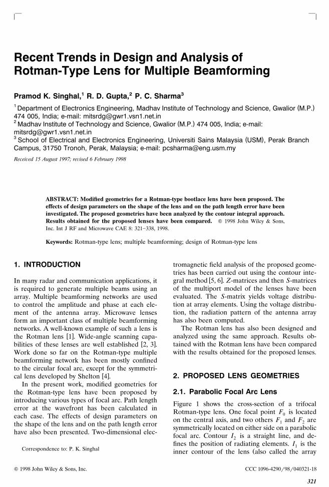
} } < < Recent Trends in Design and Analysis of Rotman-Type Lens for Multiple Beamforming Pramod K. Singhal, 1 R. D. Gupta, 2 P. C. Sharma 3 1 ( ) Department of Electronics Engineering, Madhav Institute of Technology and Science, Gwalior M.P. 474 005, India; e-mail: [email protected] 2 ( ) Madhav Institute of Technology and Science, Gwalior M.P. 474 005, India; e-mail: [email protected] 3 ( ) School of Electrical and Electronics Engineering, Universiti Sains Malaysia USM , Perak Branch Campus, 31750 Tronoh, Perak, Malaysia; e-mail: [email protected] Recei ¤ ed 15 August 1997; re¤ ised 6 February 1998 ABSTRACT: Modified geometries for a Rotman-type bootlace lens have been proposed. The effects of design parameters on the shape of the lens and on the path length error have been investigated. The proposed geometries have been analyzed by the contour integral approach. Results obtained for the proposed lenses have been compared. Q 1998 John Wiley & Sons, Inc. Int J RF and Microwave CAE 8: 321]338, 1998. Keywords: Rotman-type lens; multiple beamforming; design of Rotman-type lens 1. INTRODUCTION In many radar and communication applications, it is required to generate multiple beams using an array. Multiple beamforming networks are used to control the amplitude and phase at each ele- ment of the antenna array. Microwave lenses form an important class of multiple beamforming networks. A well-known example of such a lens is wx the Rotman lens 1 . Wide-angle scanning capa- w x bilities of these lenses are well established 2, 3 . Work done so far on the Rotman-type multiple beamforming network has been mostly confined to the circular focal arc, except for the symmetri- wx cal lens developed by Shelton 4 . In the present work, modified geometries for the Rotman-type lens have been proposed by introducing various types of focal arc. Path length error at the wavefront has been calculated in each case. The effects of design parameters on the shape of the lens and on the path length error have also been presented. Two-dimensional elec- Correspondence to: P. K. Singhal tromagnetic field analysis of the proposed geome- tries has been carried out using the contour inte- w x gral method 5, 6 . Z-matrices and then S-matrices of the multiport model of the lenses have been evaluated. The S-matrix yields voltage distribu- tion at array elements. Using the voltage distribu- tion, the radiation pattern of the antenna array has also been computed. The Rotman lens has also been designed and analyzed using the same approach. Results ob- tained with the Rotman lens have been compared with the results obtained for the proposed lenses. 2. PROPOSED LENS GEOMETRIES 2.1. Parabolic Focal Arc Lens Figure 1 shows the cross-section of a trifocal Rotman-type lens. One focal point F is located 0 on the central axis, and two others F and F are 1 2 symmetrically located on either side on a parabolic focal arc. Contour I is a straight line, and de- 2 fines the position of radiating elements. I is the 1 Ž inner contour of the lens also called the array Q 1998 John Wiley & Sons, Inc. CCC 1096-4290r98r040321-18 321
-
Upload
independent -
Category
Documents
-
view
1 -
download
0
Transcript of Recent trends in design and analysis of Rotman‐type lens for multiple beamforming
} }< <
Recent Trends in Design and Analysis ofRotman-Type Lens for Multiple Beamforming
Pramod K. Singhal,1 R. D. Gupta,2 P. C. Sharma3
1 ( )Department of Electronics Engineering, Madhav Institute of Technology and Science, Gwalior M.P.474 005, India; e-mail: [email protected] ( )Madhav Institute of Technology and Science, Gwalior M.P. 474 005, India; e-mail:[email protected] ( )School of Electrical and Electronics Engineering, Universiti Sains Malaysia USM , Perak BranchCampus, 31750 Tronoh, Perak, Malaysia; e-mail: [email protected]
Recei ed 15 August 1997; re¨ised 6 February 1998
ABSTRACT: Modified geometries for a Rotman-type bootlace lens have been proposed. Theeffects of design parameters on the shape of the lens and on the path length error have beeninvestigated. The proposed geometries have been analyzed by the contour integral approach.Results obtained for the proposed lenses have been compared. Q 1998 John Wiley & Sons,Inc. Int J RF and Microwave CAE 8: 321]338, 1998.
Keywords: Rotman-type lens; multiple beamforming; design of Rotman-type lens
1. INTRODUCTION
In many radar and communication applications, itis required to generate multiple beams using anarray. Multiple beamforming networks are usedto control the amplitude and phase at each ele-ment of the antenna array. Microwave lensesform an important class of multiple beamformingnetworks. A well-known example of such a lens is
w xthe Rotman lens 1 . Wide-angle scanning capa-w xbilities of these lenses are well established 2, 3 .
Work done so far on the Rotman-type multiplebeamforming network has been mostly confinedto the circular focal arc, except for the symmetri-
w xcal lens developed by Shelton 4 .In the present work, modified geometries for
the Rotman-type lens have been proposed byintroducing various types of focal arc. Path lengtherror at the wavefront has been calculated ineach case. The effects of design parameters onthe shape of the lens and on the path length errorhave also been presented. Two-dimensional elec-
Correspondence to: P. K. Singhal
tromagnetic field analysis of the proposed geome-tries has been carried out using the contour inte-
w xgral method 5, 6 . Z-matrices and then S-matricesof the multiport model of the lenses have beenevaluated. The S-matrix yields voltage distribu-tion at array elements. Using the voltage distribu-tion, the radiation pattern of the antenna arrayhas also been computed.
The Rotman lens has also been designed andanalyzed using the same approach. Results ob-tained with the Rotman lens have been comparedwith the results obtained for the proposed lenses.
2. PROPOSED LENS GEOMETRIES
2.1. Parabolic Focal Arc Lens
Figure 1 shows the cross-section of a trifocalRotman-type lens. One focal point F is located0on the central axis, and two others F and F are1 2symmetrically located on either side on a parabolicfocal arc. Contour I is a straight line, and de-2fines the position of radiating elements. I is the1
Žinner contour of the lens also called the array
Q 1998 John Wiley & Sons, Inc. CCC 1096-4290r98r040321-18
321

Singhal, Gupta, and Sharma322
Figure 1. Cross-section of parabolic focal arc lens.
.contour . The inner and outer contours are con-Ž .nected by TEM mode transmission lines W n .
Two off-axis focal points F and F are located1 2on the focal arc, and make angles a and ya withthe X-axis. It is required that the lens be de-signed in such a way that the outgoing beammakes angles ya , 0, and a with the X-axis whenfeeds are placed at F , F , and F , respectively.1 0 2
A ray originating from F may reach the wave-1Ž .front through a general point P X, Y on the
Ž .inner contour I , transmission line W n , and1Ž .point Q n on the outer contour, and then trace a
straight line at an angle ya , and terminate per-pendicular to the wavefront. Also, the ray fromF may reach the wavefront from F to point O ,1 1 1
Ž .and then through transmission line W 0 to thewavefront. Similarly, rays from other feed pointsmay reach their respective wavefront.
Inner contour and transmission lines are de-signed from the design equations which are de-rived using the fact that, at the wavefront, all ofthese rays must be in phase independent of thepath they travel. This requires that the total phaseshift in traversing the path to reach the wavefrontin each case be equal. Referring to Figure 1 andusing the path length comparison approach as
w xsuggested in 1 , the following design equations
are written:
Ž . Ž . Ž .F P q W n q N sin a s W 0 q F 11
Ž . Ž . Ž .F P q W n y N sin a s W 0 q F 22
Ž . Ž . Ž .F P q W n s W 0 q G 30
where:
Ž .2 Ž .2 Ž .2F P s X y c q Y y d1Ž .2 Ž .2 Ž .2F P s X y c q Y q d2Ž .2 Ž .2 Ž .2F P s X q Y0
F s distance from point O to F , called1 1the off-axis focal length
G s distance from point O to F , called1 0the on-axis focal length
Ž .d s F sin a Y-coordinate of point F1Ž .c s G y F cos a X-coordinate of point F1
Ž .2 Ž .2 Ž .2F s G y c q dŽ . Ž .X, Y s coordinates of general point P X, Y
Length N indicates the position of the radiatingelements, and is called the lens aperture.
Algebraic manipulation of the above equationsgives:
Ž . 2 2 Ž .X s W F y G rc q G y N sin ar2c 4
Ž . Ž .Y s F y W N sin ard 52 Ž .AW q BW q C s 0 6
Design Concepts for Rotman-Type Lens 323
where:
2 2 2 2 2Ž .A s F y G rc q N sin ard y 1
Ž .Ž 2 2 .B s 2 F y G G y N sin ar2c rc
y 2 FN 2 sin2 ard2 q 2G22 2Ž .C s G y N sin ar2c
y G2 q F 2N 2 sin2 ard2
Ž . Ž .W s W n y W 0
For given values of design parameters a , G,and F, W can be calculated as a function of N
Ž .using eq. 6 . These values of W and N can beŽ . Ž .substituted in eqs. 4 and 5 to calculate X and
Y. This completes the design of a trifocal parabolicfocal arc bootlace lens.
The coordinates of the focal arc are given bythe relations:
2 Ž .Y s 4aX 7
2 2 Ž .where a s F sin ar4 G y F cos a .
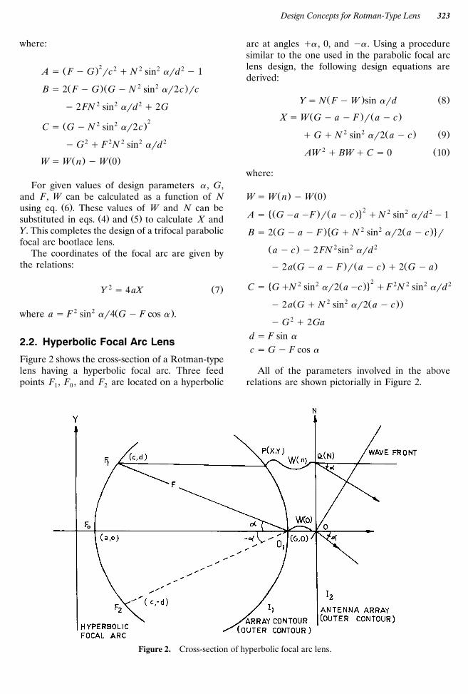
2.2. Hyperbolic Focal Arc Lens
Figure 2 shows the cross-section of a Rotman-typelens having a hyperbolic focal arc. Three feedpoints F , F , and F are located on a hyperbolic1 0 2
arc at angles qa , 0, and ya . Using a proceduresimilar to the one used in the parabolic focal arclens design, the following design equations arederived:
Ž . Ž .Y s N F y W sin ard 8
Ž . Ž .X s W G y a y F r a y c2 2 Ž . Ž .q G q N sin ar2 a y c 9
2 Ž .AW q BW q C s 0 10
where:
Ž . Ž .W s W n y W 02 2 2 2� Ž . Ž .4A s G ya yF r a y c qN sin ard y1
Ž . � 2 2 Ž .4B s 2 G y a y F G q N sin ar2 a y c r
Ž . 2 2 2a y c y 2 FN sin ard
Ž . Ž . Ž .y 2 a G y a y F r a y c q 2 G y a22 2 2 2 2 2� Ž .4C s GqN sin ar2 ayc qF N sin ard
Ž 2 2 Ž ..y 2 a G q N sin ar2 a y c
y G2 q 2Gad s F sin a
c s G y F cos a
All of the parameters involved in the aboverelations are shown pictorially in Figure 2.
Figure 2. Cross-section of hyperbolic focal arc lens.
Singhal, Gupta, and Sharma324
The coordinates of the hyperbolic focal arc aregiven by:
2 2 2 2 Ž .X ra y Y rb s 1 11
where:
2 2 Ž 2 .b s a e y 12 � 2 Ž 2 2 . 4e s d r c y a q 1
e is the eccentricity. The center of the hyperbolicfocal arc is located at the origin.
2.3. Elliptical Focal Arc Lens
In this case, the equations to design the arraycontour and transmission lines will be exactly the
w xsame as for the Rotman lens as described in 1 .The only difference will be in the focal arc. Thefocal arc is given by the following equation:
2 2 2 2 Ž .X ra q Y rb s 1 12
where:
2 2 Ž 2 .b s a 1 y e2 2 � Ž 2 2 . Ž 2 .4a s F 1 y e cos a r 1 y e
e is the eccentricity of the elliptical focal arc. Thecenter of the elliptical focal arc is located at the
Ž .origin 0, 0 . F is the off-axis focal length, and ais the focal angle.
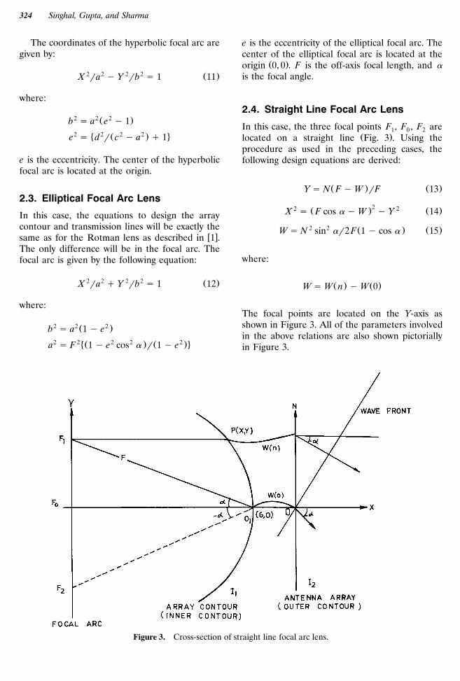
2.4. Straight Line Focal Arc Lens
In this case, the three focal points F , F , F are1 0 2Ž .located on a straight line Fig. 3 . Using the
procedure as used in the preceding cases, thefollowing design equations are derived:
Ž . Ž .Y s N F y W rF 13
22 2Ž . Ž .X s F cos a y W y Y 14
2 2 Ž . Ž .W s N sin ar2 F 1 y cos a 15
where:
Ž . Ž .W s W n y W 0
The focal points are located on the Y-axis asshown in Figure 3. All of the parameters involvedin the above relations are also shown pictoriallyin Figure 3.
Figure 3. Cross-section of straight line focal arc lens.
Design Concepts for Rotman-Type Lens 325
3. EFFECTS OF DESIGN PARAMETERS
3.1. Effects on the Shape of the Lens
The Rotman-type lenses discussed so far havefour basic design parameters: off-axis focal lengthF, focal angle a , normalized lens aperture hŽ .h s NrF , and on-axis to off-axis focal length
Ž .ratio g g s GrF . This section describes thedependence of the shape of the lens on the de-
Žsign parameters a , h, g, and F except for the.straight line focal arc lens . The lens shape deter-
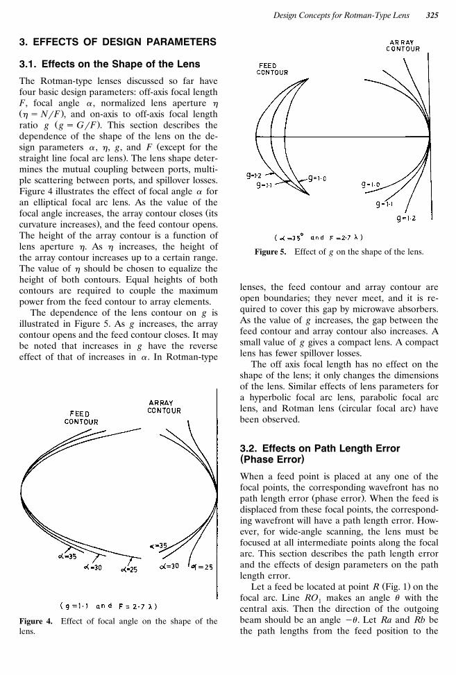
mines the mutual coupling between ports, multi-ple scattering between ports, and spillover losses.Figure 4 illustrates the effect of focal angle a foran elliptical focal arc lens. As the value of the
Žfocal angle increases, the array contour closes its.curvature increases , and the feed contour opens.
The height of the array contour is a function oflens aperture h. As h increases, the height ofthe array contour increases up to a certain range.The value of h should be chosen to equalize theheight of both contours. Equal heights of bothcontours are required to couple the maximumpower from the feed contour to array elements.
The dependence of the lens contour on g isillustrated in Figure 5. As g increases, the arraycontour opens and the feed contour closes. It maybe noted that increases in g have the reverseeffect of that of increases in a . In Rotman-type
Figure 4. Effect of focal angle on the shape of thelens.
Figure 5. Effect of g on the shape of the lens.
lenses, the feed contour and array contour areopen boundaries; they never meet, and it is re-quired to cover this gap by microwave absorbers.As the value of g increases, the gap between thefeed contour and array contour also increases. Asmall value of g gives a compact lens. A compactlens has fewer spillover losses.
The off axis focal length has no effect on theshape of the lens; it only changes the dimensionsof the lens. Similar effects of lens parameters fora hyperbolic focal arc lens, parabolic focal arc
Ž .lens, and Rotman lens circular focal arc havebeen observed.
3.2. Effects on Path Length Error( )Phase Error
When a feed point is placed at any one of thefocal points, the corresponding wavefront has no
Ž .path length error phase error . When the feed isdisplaced from these focal points, the correspond-ing wavefront will have a path length error. How-ever, for wide-angle scanning, the lens must befocused at all intermediate points along the focalarc. This section describes the path length errorand the effects of design parameters on the pathlength error.
Ž .Let a feed be located at point R Fig. 1 on thefocal arc. Line RO makes an angle u with the1central axis. Then the direction of the outgoingbeam should be an angle yu . Let Ra and Rb bethe path lengths from the feed position to the
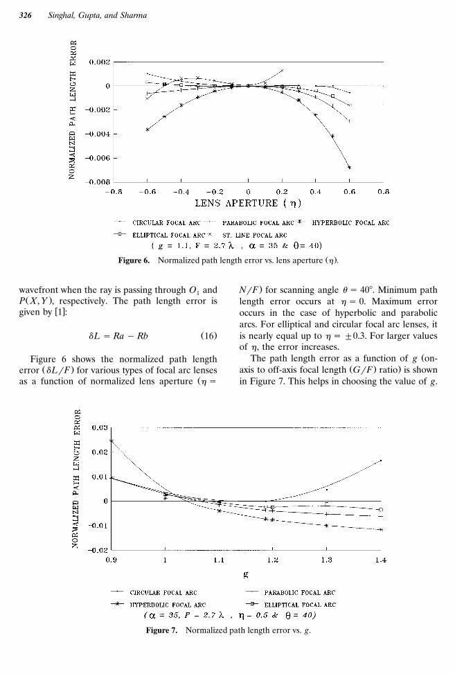
Singhal, Gupta, and Sharma326
Ž .Figure 6. Normalized path length error vs. lens aperture h .
wavefront when the ray is passing through O and1Ž .P X, Y , respectively. The path length error is
w xgiven by 1 :
Ž .dL s Ra y Rb 16
Figure 6 shows the normalized path lengthŽ .error dLrF for various types of focal arc lenses
Žas a function of normalized lens aperture h s
.NrF for scanning angle u s 408. Minimum pathlength error occurs at h s 0. Maximum erroroccurs in the case of hyperbolic and parabolicarcs. For elliptical and circular focal arc lenses, itis nearly equal up to h s "0.3. For larger valuesof h, the error increases.
ŽThe path length error as a function of g on-Ž . .axis to off-axis focal length GrF ratio is shown
in Figure 7. This helps in choosing the value of g.
Figure 7. Normalized path length error vs. g.
Design Concepts for Rotman-Type Lens 327
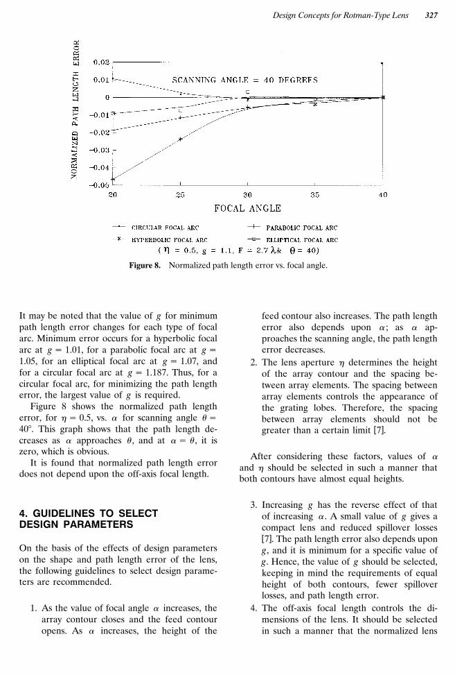
Figure 8. Normalized path length error vs. focal angle.
It may be noted that the value of g for minimumpath length error changes for each type of focalarc. Minimum error occurs for a hyperbolic focalarc at g s 1.01, for a parabolic focal arc at g s1.05, for an elliptical focal arc at g s 1.07, andfor a circular focal arc at g s 1.187. Thus, for acircular focal arc, for minimizing the path lengtherror, the largest value of g is required.
Figure 8 shows the normalized path lengtherror, for h s 0.5, vs. a for scanning angle u s408. This graph shows that the path length de-creases as a approaches u , and at a s u , it iszero, which is obvious.
It is found that normalized path length errordoes not depend upon the off-axis focal length.
4. GUIDELINES TO SELECTDESIGN PARAMETERS
On the basis of the effects of design parameterson the shape and path length error of the lens,the following guidelines to select design parame-ters are recommended.
1. As the value of focal angle a increases, thearray contour closes and the feed contouropens. As a increases, the height of the
feed contour also increases. The path lengtherror also depends upon a ; as a ap-proaches the scanning angle, the path lengtherror decreases.
2. The lens aperture h determines the heightof the array contour and the spacing be-tween array elements. The spacing betweenarray elements controls the appearance ofthe grating lobes. Therefore, the spacingbetween array elements should not be
w xgreater than a certain limit 7 .
After considering these factors, values of aand h should be selected in such a manner thatboth contours have almost equal heights.
3. Increasing g has the reverse effect of thatof increasing a . A small value of g gives acompact lens and reduced spillover lossesw x7 . The path length error also depends upong, and it is minimum for a specific value ofg. Hence, the value of g should be selected,keeping in mind the requirements of equalheight of both contours, fewer spilloverlosses, and path length error.
4. The off-axis focal length controls the di-mensions of the lens. It should be selectedin such a manner that the normalized lens
Singhal, Gupta, and Sharma328
aperture h is less than 0.6 since the pathlength error increases as h increases.
Repetitive iteration may be made to select theproper values of lens design parameters.
5. ANALYSIS APPROACH
In a microstrip or stripline configuration, theheight of the lens is much smaller than the wave-length at the operating frequencies, and conse-quently, there is no variation of the field alongthe height of the substrate. This type of planarcircuit may be considered a two-dimensional cir-cuit. Because of the arbitrary geometrical shape
w xof the lens, the contour integral method 5 hasbeen adopted to analyze the proposed lens geom-etry. More details of the contour integral tech-
w xnique have been given in 5, 6, 8 .
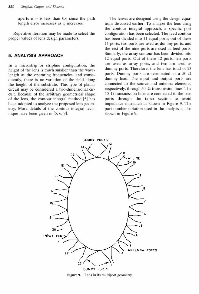
The lenses are designed using the design equa-tions discussed earlier. To analyze the lens usingthe contour integral approach, a specific portconfiguration has been selected. The feed contourhas been divided into 11 equal ports; out of these11 ports, two ports are used as dummy ports, andthe rest of the nine ports are used as feed ports.Similarly, the array contour has been divided into12 equal ports. Out of these 12 ports, ten portsare used as array ports, and two are used asdummy ports. Therefore, the lens has total of 23ports. Dummy ports are terminated at a 50 V
dummy load. The input and output ports areconnected to the source and antenna elements,respectively, through 50 V transmission lines. The50 V transmission lines are connected to the lensports through the taper section to avoidimpedance mismatch as shown in Figure 9. Theport number notation used in the analysis is alsoshown in Figure 9.
Figure 9. Lens in its multiport geometry.
Design Concepts for Rotman-Type Lens 329
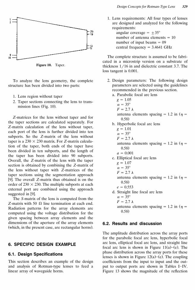
Figure 10. Taper.
To analyze the lens geometry, the completestructure has been divided into two parts:
1. Lens region without taper2. Taper sections connecting the lens to trans-
Ž .mission lines Fig. 10 .
Z-matrices for the lens without taper and forthe taper sections are calculated separately. ForZ-matrix calculation of the lens without taper,each port of the lens is further divided into tensubports. So the Z-matrix of the lens withouttaper is a 230 = 230 matrix. For Z-matrix calcula-tion of the taper, both ends of the taper havebeen divided in ten subports, and the length ofthe taper has been divided into 90 subports.Overall, the Z-matrix of the lens with the tapersection is obtained by combining the Z-matrix ofthe lens without taper with Z-matrices of thetaper sections using the segmentation approachw x9 . The overall Z-matrix thus obtained is on theorder of 230 = 230. The multiple subports at eachexternal port are combined using the approach
w xsuggested in 9 .The S-matrix of the lens is computed from the
Z-matrix with 50 V line termination at each end.Radiation patterns for the array elements arecomputed using the voltage distribution for thegiven spacing between array elements and thedimensions of the aperture of the array elementsŽ .which, in the present case, are rectangular horns .
6. SPECIFIC DESIGN EXAMPLE
6.1. Design Specifications
This section describes an example of the designand analysis of Rotman-type lenses to feed alinear array of waveguide horns.
1. Lens requirements: All four types of lensesare designed and analyzed for the followingrequirements:
angular coverage s "358number of antenna elements s 10number of input beams s 09central frequency s 3.4641 GHz
The complete structure is assumed to be fabri-cated in a microstrip version on a substrate ofthickness 1r16 in and dielectric constant 3.7. Theloss tangent is 0.001.
2. Design parameters: The following designparameters are selected using the guidelinesrecommended in the previous section.a. Parabolic focal arc lens
g s 1.05a s 358F s 2.7 l
Žantenna elements spacing s 1.2 in h s.0.58
b. Hyperbolic focal arc lensg s 1.01a s 358F s 2.7 l
Žantenna elements spacing s 1.2 in h s.0.58
a s 0.001c. Elliptical focal arc lens
g s 1.07a s 358F s 2.7 l
Žantenna elements spacing s 1.2 in h s.0.58
e s 0.553d. Straight line focal arc lens
a s 358F s 2.7 l
Žantenna elements spacing s 1.2 in h s.0.58
6.2. Results and discussion
The amplitude distribution across the array portsfor the parabolic focal arc lens, hyperbolic focalarc lens, elliptical focal arc lens, and straight line
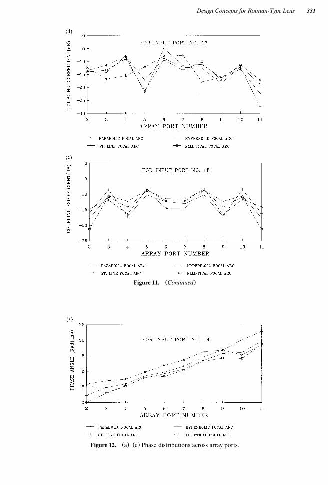
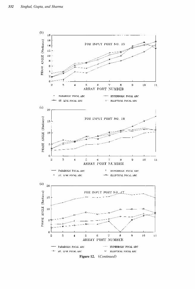
Ž . Ž .focal arc lens is shown in Figure 11 a ] e . Thephase distribution across the array ports for these
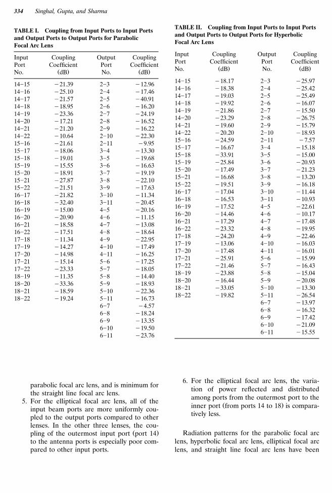
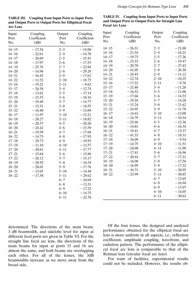
Ž . Ž .lenses is shown in Figure 12 a ] e . The couplingcoefficients from the input to input and the out-put to output ports are shown in Tables I]IV.Figure 13 shows the magnitude of the reflection

Singhal, Gupta, and Sharma330
Ž . Ž .Figure 11. a ] e Amplitude distributions across array ports.
Design Concepts for Rotman-Type Lens 331
Ž .Figure 11. Continued
Ž . Ž .Figure 12. a ] e Phase distributions across array ports.
Singhal, Gupta, and Sharma332
Ž .Figure 12. Continued

Design Concepts for Rotman-Type Lens 333
Ž .Figure 12. Continued
coefficients for the input ports. In view of thegeometrical symmetry of the lens amplitude dis-tribution, the phase distribution and reflectioncoefficients for only half of the input ports areshown. The minimum reflection coefficient occur-ring for port 18 of the parabolic focal arc lens andthe maximum for port 14 of the hyperbolic focalarc lens have been observed. The reflection co-efficients obtained for all of the input ports of theelliptical focal arc lens are uniform compared tothose for other lenses.
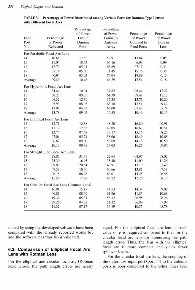
The percentage of power distributed amongvarious ports for all of the lenses are given inTable V. This table reveals the following.
1. The percentage of power coupled back tothe feed ports may be considered as almostequal for all of the ports. However, it isslightly large for the elliptical focal arc lens.
2. The power lost in the dummy ports is maxi-mum for the straight line arc lens since thewidths of the dummy ports are maximumfor this lens, and for other lenses it is nearlyequal.
3. The power lost in the lens is minimum forthe parabolic focal arc lens, and for otherlenses it is nearly the same.
4. The percentage of power coupled to theantenna elements is maximum for the
Figure 13. Reflection coefficients at input ports.
Singhal, Gupta, and Sharma334
TABLE I. Coupling from Input Ports to Input Portsand Output Ports to Output Ports for ParabolicFocal Arc Lens
Input Coupling Output CouplingPort Coefficient Port Coefficient
Ž . Ž .No. dB No. dB
14]15 y21.39 2]3 y12.9614]16 y25.10 2]4 y17.4614]17 y21.57 2]5 y40.9114]18 y18.95 2]6 y16.2014]19 y23.36 2]7 y24.1914]20 y17.21 2]8 y16.5214]21 y21.20 2]9 y16.2214]22 y10.64 2]10 y22.3015]16 y21.61 2]11 y9.9515]17 y18.06 3]4 y13.3015]18 y19.01 3]5 y19.6815]19 y15.55 3]6 y16.6315]20 y18.91 3]7 y19.1915]21 y27.87 3]8 y22.1015]22 y21.51 3]9 y17.6316]17 y21.82 3]10 y11.3416]18 y32.40 3]11 y20.4516]19 y15.00 4]5 y20.1616]20 y20.90 4]6 y11.1516]21 y18.58 4]7 y13.0816]22 y17.51 4]8 y18.6417]18 y11.34 4]9 y22.9517]19 y14.27 4]10 y17.4917]20 y14.98 4]11 y16.2517]21 y15.14 5]6 y17.2517]22 y23.33 5]7 y18.0518]19 y11.35 5]8 y14.4018]20 y33.36 5]9 y18.9318]21 y18.59 5]10 y22.3618]22 y19.24 5]11 y16.73
6]7 y4.576]8 y18.246]9 y13.356]10 y19.506]11 y23.76
parabolic focal arc lens, and is minimum forthe straight line focal arc lens.
5. For the elliptical focal arc lens, all of theinput beam ports are more uniformly cou-pled to the output ports compared to otherlenses. In the other three lenses, the cou-
Ž .pling of the outermost input port port 14to the antenna ports is especially poor com-pared to other input ports.
TABLE II. Coupling from Input Ports to Input Portsand Output Ports to Output Ports for HyperbolicFocal Arc Lens
Input Coupling Output CouplingPort Coefficient Port Coefficient
Ž . Ž .No. dB No. dB
14]15 y18.17 2]3 y25.9714]16 y18.38 2]4 y25.4214]17 y19.03 2]5 y25.4914]18 y19.92 2]6 y16.0714]19 y21.86 2]7 y15.5014]20 y23.29 2]8 y26.7514]21 y19.60 2]9 y15.7914]22 y20.20 2]10 y18.9315]16 y24.59 2]11 y7.5715]17 y16.67 3]4 y15.1815]18 y33.91 3]5 y15.0015]19 y25.84 3]6 y20.9315]20 y17.49 3]7 y21.2315]21 y16.68 3]8 y13.2015]22 y19.51 3]9 y16.1816]17 y17.04 3]10 y11.4416]18 y16.53 3]11 y10.9316]19 y17.52 4]5 y22.6116]20 y14.46 4]6 y10.1716]21 y17.29 4]7 y17.4816]22 y23.32 4]8 y19.9517]18 y24.20 4]9 y22.4617]19 y13.06 4]10 y16.0317]20 y17.48 4]11 y16.0117]21 y25.91 5]6 y15.9917]22 y21.46 5]7 y16.4318]19 y23.88 5]8 y15.0418]20 y16.44 5]9 y20.0818]21 y33.05 5]10 y13.3018]22 y19.82 5]11 y26.54
6]7 y13.976]8 y16.326]9 y17.426]10 y21.096]11 y15.55
6. For the elliptical focal arc lens, the varia-tion of power reflected and distributedamong ports from the outermost port to the
Ž .inner port from ports 14 to 18 is compara-tively less.
Radiation patterns for the parabolic focal arclens, hyperbolic focal arc lens, elliptical focal arclens, and straight line focal arc lens have been
Design Concepts for Rotman-Type Lens 335
TABLE III. Coupling from Input Ports to Input Portsand Output Ports to Output Ports for Ellipitical FocalArc Lens
Input Coupling Output CouplingPort Coefficient Port Coefficient
Ž . Ž .No. dB No. dB
14]15 y17.54 2]3 y15.0014]16 y22.61 2]4 y14.7814]17 y28.69 2]5 y15.4114]18 y17.97 2]6 y17.5514]19 y25.76 2]7 y22.8414]20 y14.94 2]8 y29.2014]21 y16.45 2]9 y17.6214]22 y11.52 2]10 y18.7515]16 y19.21 2]11 y8.6215]17 y26.58 3]4 y12.7415]18 y13.62 3]5 y17.1415]19 y15.53 3]6 y18.1615]20 y19.49 3]7 y14.7715]21 y15.31 3]8 y14.5515]22 y16.40 3]9 y13.6916]17 y11.97 3]10 y13.2116]18 y20.27 3]11 y18.8216]19 y20.37 4]5 y20.2016]20 y24.42 4]6 y15.5916]21 y19.58 4]7 y17.6816]22 y14.73 4]8 y17.9317]18 y29.73 4]9 y19.9317]19 y11.10 4]10 y13.5717]20 y20.61 4]11 y17.7717]21 y15.64 5]6 y13.8617]22 y26.12 5]7 y13.1718]19 y28.92 5]8 y16.3418]20 y20.01 5]9 y17.7618]21 y13.65 5]10 y14.4818]22 y17.58 5]11 y29.62
6]7 y10.696]8 y13.316]9 y17.236]10 y14.756]11 y22.76
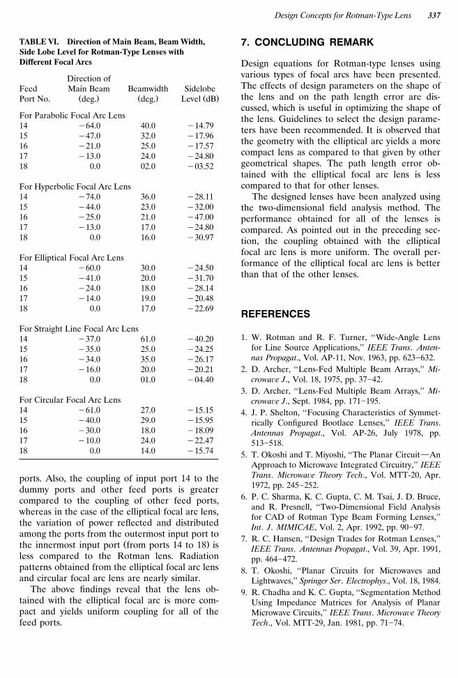
determined. The directions of the main beam,3 dB beamwidth, and sidelobe level for input atdifferent feed ports are given in Table VI. For thestraight line focal arc lens, the directions of themain beams for input at ports 15 and 16 arealmost the same, and both beams are overlappingeach other. For all of the lenses, the 3dBbeamwidths increase as we move away from thebroad side.
TABLE IV. Coupling from Input Ports to Input Portsand Output Ports to Output Ports for Straight LineFocal Arc Lens
Input Coupling Output CouplingPort Coefficient Port Coefficient
Ž . Ž .No. dB No. dB
14]15 y26.31 2]3 y21.0014]16 y21.54 2]4 y16.2114]17 y19.73 2]5 y17.2614]18 y23.55 2]6 y19.4714]19 y20.78 2]7 y27.4314]20 y41.05 2]8 y26.3014]21 y24.43 2]9 y11.1214]22 y12.74 2]10 y10.2515]16 y17.32 2]11 y9.7615]17 y21.80 3]4 y11.2815]18 y16.52 3]5 y11.0615]19 y17.66 3]6 y14.3315]20 y19.24 3]7 y14.2015]21 y15.24 3]8 y21.6215]22 y24.95 3]9 y11.7816]17 y14.43 3]10 y13.0016]18 y16.79 3]11 y10.3416]19 y23.46 4]5 y12.3616]20 y14.81 4]6 y16.3416]21 y19.41 4]7 y13.3716]22 y41.33 4]8 y18.3117]18 y16.09 4]9 y9.5417]19 y14.75 4]10 y11.5117]20 y24.08 4]11 y11.9017]21 y17.41 5]6 y16.9617]22 y20.44 5]7 y17.2118]19 y16.08 5]8 y17.5618]20 y16.99 5]9 y17.3218]21 y16.71 5]10 y20.9518]22 y23.99 5]11 y30.85
6]7 y12.656]8 y16.946]9 y13.076]10 y14.056]11 y30.63
Of the four lenses, the designed and analyzedperformance obtained for the elliptical focal arclens is more uniform in all aspects, i.e., reflectioncoefficient, amplitude coupling, wavefront, andradiation pattern. The performance of the ellipti-cal focal arc lens is comparable to that of the
Ž .Rotman lens circular focal arc lens .For want of facilities, experimental results
could not be included. However, the results ob-
Singhal, Gupta, and Sharma336
TABLE V. Percentage of Power Distributed among Various Ports for Rotman-Type Lenseswith Different Focal Arcs
Percentage Percentageof Power of Power Percentage Percentage
Feed Percentage Lost in Going to of Power of PowerPort of Power Dummy Antenna Coupled to Lost inNo. Reflected Ports Array Feed Ports Lens
For Parabolic Focal Arc Lens14 10.65 17.55 57.91 13.84 0.0515 11.04 18.63 64.16 6.08 0.0916 17.72 05.91 63.89 07.17 0.3117 07.14 05.30 71.45 15.76 0.3518 0.94 05.03 74.04 19.89 0.13Average 09.49 10.48 66.29 12.54 0.18
For Hyperbolic Focal Arc Lens14 34.44 10.04 34.82 08.41 12.2715 08.23 09.85 61.39 09.41 11.1316 06.32 12.39 57.35 13.73 10.2017 05.93 08.03 63.10 13.51 09.4218 13.98 04.83 66.00 07.43 07.74Average 13.78 09.02 56.53 10.49 10.15
For Elliptical Focal Arc Lens14 12.71 12.38 48.20 16.80 09.9115 11.12 12.65 49.05 16.67 10.5116 13.74 07.68 55.17 15.16 08.2517 07.06 05.71 58.06 18.49 10.6818 06.62 09.00 59.69 14.18 10.50Average 10.10 09.48 54.03 16.26 09.97
For Straight Line Focal Arc Lens14 28.87 31.49 22.64 08.97 08.0315 25.30 16.95 35.40 11.09 11.2616 09.87 20.54 48.91 13.19 07.4917 07.53 10.46 60.66 13.81 07.5318 06.18 06.98 66.01 14.25 06.58Average 15.50 17.28 46.72 12.26 08.17
Ž .For Circular Focal Arc Lens Rotman Lens14 16.81 15.17 44.53 14.34 09.0215 06.81 08.69 61.96 11.85 10.6916 19.36 05.31 58.12 08.95 08.2617 29.26 04.32 51.32 06.99 07.9918 11.32 07.17 56.19 10.55 08.78
tained by using the developed software have beenw xcompared with the already reported works 6 ,
and the software has thus been validated.
6.3. Comparison of Elliptical Focal ArcLens with Rotman Lens
ŽFor the elliptical and circular focal arc Rotman.lens lenses, the path length errors are nearly
equal. For the elliptical focal arc lens, a smallvalue of g is required compared to that for thecircular focal arc lens for minimizing the pathlength error. Thus, the lens with the ellipticalfocal arc is more compact and yields fewerspillover losses.
For the circular focal arc lens, the coupling ofŽ .the outermost input port port 14 to the antenna
ports is poor compared to the other inner feed
Design Concepts for Rotman-Type Lens 337
TABLE VI. Direction of Main Beam, Beam Width,Side Lobe Level for Rotman-Type Lenses withDifferent Focal Arcs
Direction ofFeed Main Beam Beamwidth Sidelobe
Ž . Ž . Ž .Port No. deg. deg. Level dB
For Parabolic Focal Arc Lens14 y64.0 40.0 y14.7915 y47.0 32.0 y17.9616 y21.0 25.0 y17.5717 y13.0 24.0 y24.8018 0.0 02.0 y03.52
For Hyperbolic Focal Arc Lens14 y74.0 36.0 y28.1115 y44.0 23.0 y32.0016 y25.0 21.0 y47.0017 y13.0 17.0 y24.8018 0.0 16.0 y30.97
For Elliptical Focal Arc Lens14 y60.0 30.0 y24.5015 y41.0 20.0 y31.7016 y24.0 18.0 y28.1417 y14.0 19.0 y20.4818 0.0 17.0 y22.69
For Straight Line Focal Arc Lens14 y37.0 61.0 y40.2015 y35.0 25.0 y24.2516 y34.0 35.0 y26.1717 y16.0 20.0 y20.2118 0.0 01.0 y04.40
For Circular Focal Arc Lens14 y61.0 27.0 y15.1515 y40.0 29.0 y15.9516 y30.0 18.0 y18.0917 y10.0 24.0 y22.4718 0.0 14.0 y15.74
ports. Also, the coupling of input port 14 to thedummy ports and other feed ports is greatercompared to the coupling of other feed ports,whereas in the case of the elliptical focal arc lens,the variation of power reflected and distributedamong the ports from the outermost input port to
Ž .the innermost input port from ports 14 to 18 isless compared to the Rotman lens. Radiationpatterns obtained from the elliptical focal arc lensand circular focal arc lens are nearly similar.
The above findings reveal that the lens ob-tained with the elliptical focal arc is more com-pact and yields uniform coupling for all of thefeed ports.
7. CONCLUDING REMARK
Design equations for Rotman-type lenses usingvarious types of focal arcs have been presented.The effects of design parameters on the shape ofthe lens and on the path length error are dis-cussed, which is useful in optimizing the shape ofthe lens. Guidelines to select the design parame-ters have been recommended. It is observed thatthe geometry with the elliptical arc yields a morecompact lens as compared to that given by othergeometrical shapes. The path length error ob-tained with the elliptical focal arc lens is lesscompared to that for other lenses.
The designed lenses have been analyzed usingthe two-dimensional field analysis method. Theperformance obtained for all of the lenses iscompared. As pointed out in the preceding sec-tion, the coupling obtained with the ellipticalfocal arc lens is more uniform. The overall per-formance of the elliptical focal arc lens is betterthan that of the other lenses.
REFERENCES
1. W. Rotman and R. F. Turner, ‘‘Wide-Angle Lensfor Line Source Applications,’’ IEEE Trans. Anten-nas Propagat., Vol. AP-11, Nov. 1963, pp. 623]632.
2. D. Archer, ‘‘Lens-Fed Multiple Beam Arrays,’’ Mi-crowa¨e J., Vol. 18, 1975, pp. 37]42.
3. D. Archer, ‘‘Lens-Fed Multiple Beam Arrays,’’ Mi-crowa¨e J., Sept. 1984, pp. 171]195.
4. J. P. Shelton, ‘‘Focusing Characteristics of Symmet-rically Configured Bootlace Lenses,’’ IEEE Trans.Antennas Propagat., Vol. AP-26, July 1978, pp.513]518.
5. T. Okoshi and T. Miyoshi, ‘‘The Planar Circuit}AnApproach to Microwave Integrated Circuitry,’’ IEEETrans. Microwa e Theory Tech., Vol. MTT-20, Apr.1972, pp. 245]252.
6. P. C. Sharma, K. C. Gupta, C. M. Tsai, J. D. Bruce,and R. Presnell, ‘‘Two-Dimensional Field Analysisfor CAD of Rotman Type Beam Forming Lenses,’’Int. J. MIMICAE, Vol. 2, Apr. 1992, pp. 90]97.
7. R. C. Hansen, ‘‘Design Trades for Rotman Lenses,’’IEEE Trans. Antennas Propagat., Vol. 39, Apr. 1991,pp. 464]472.
8. T. Okoshi, ‘‘Planar Circuits for Microwaves andLightwaves,’’ Springer Ser. Electrophys., Vol. 18, 1984.
9. R. Chadha and K. C. Gupta, ‘‘Segmentation MethodUsing Impedance Matrices for Analysis of PlanarMicrowave Circuits,’’ IEEE Trans. Microwa e TheoryTech., Vol. MTT-29, Jan. 1981, pp. 71]74.
Singhal, Gupta, and Sharma338
BIOGRAPHIES
Pramod K. Singhal was born in 1965. Hereceived the B.E. degree in electronicsengineering from Jiwaji University,Gwalior, in 1987, the M.Tech. degree inmicrowave electronics from the Univer-sity of Delhi, Delhi, in 1989, and thePh.D. degree in electronics engineeringin 1997 from Jiwaji University, Gwalior.At present, he is working as a Reader in
the Department of Electronics Engineering, Madhav Instituteof Technology & Science, Gwalior. He has about 25 publica-tions to his credit at the national and international level. He isa Life Member of ISTE, a Life Member of CSI, a member of
Ž .IE India , and an Associate Member of IETE. His researchinterests include electromagnetics, communication systems,microwave circuits, and antennas.
R. D. Gupta is the Director of the Madhav Institute ofTechnology & Science, Gwalior, India. He received the B.Sc.Ž .Engg. degree from B.H.U., Varanasi, India, the M.E. degreefrom B.I.T.S. Plani, and the Ph.D. degree from Queens Uni-versity, Canada. He has guided a number of projects. He is amember of the IEEE and ISTE. His interests include system
Žengineering, microwave antennas, and control systems. Photo.not available .
P. C. Sharma was born in 1947. He re-ceived the B.E. and M.E. degrees fromthe University of Indore in 1969 and 1972,respectively, and the Ph.D. degree inelectrical engineering in 1982 from I.I.T.
Ž .Kanpur India . In 1972, he joined SGSInstitute of Technology and Science, In-dore, India, as a Lecturer in ElectricalEngineering, and became a Professor in
1986 in the Department of Electronics and Telecommunica-tion. Dr. Sharma has been a Visiting Scientist with the MIMI-CAD Center, Department of Electrical and Computer Engi-neering, University of Colorado at Boulder, during the period1989]91. In 1991, he rejoined SGS Institute of Technologyand Science, Indore, as Professor and Head of the Electronicsand Telecommunications Department. During 1995]96, heworked as a Visiting Scientist with the School of Electrical
Ž .and Electronic Engineering, Universiti Sains Malaysia USM .In 1996, he was elevated to the position of Director, SGSInstitute of Technology and Science, Indore. Dr. Sharma ispresently with the Faculty of School of Electrical and Elec-
Ž .tronic Engineering, Universiti Sains Malaysia USM . Dr.Sharma has published over 100 research papers. He has also
Žauthored a book, Networks, Filters and Transmission Lines in.Hindi . He is the recipient of the National Anna University
Award, 1987 for outstanding academics, awarded by I.S.T.E.New Delhi, in recognition of the best teacher of the year. The
Ž .Government of the State of Madhya Pradesh India has alsoawarded him the ‘‘Pandit Lajja Shankar Jha Award, 1986 for
Ž .outstanding research contributions to engineering and tech-nology. Dr. Sharma also received the Dr. RadhakrishnanAward, 1992 from the State University Grants Commission of
Ž .the State of Madhya Pradesh India for the best researchpublication in the year. Dr. Sharma has done extensive workin the area of microwave engineering, instrumentation, andapplications of computers. His current research interests in-clude microwave circuits and antennas. In addition to beingactive in the field of engineering and technology, Dr. Sharma
Ž .is an authorized teacher Preceptor of the SRC Mission toimpart spiritual training to aspirants through transmission ofdivine energy. Dr. Sharma is a Senior Member of the IEEE, a
Ž .Fellow of the IETE India , a Life Member of the ISTEŽ . Ž .India , and a Life Member of AAFAS India .