Recent Progress in Image Deblurring

Ruxin Wang Dacheng Tao

Centre for Quantum Computation & Intelligent Systems

Faculty of Engineering & Information Technology

University of Technology Sydney

81-115 Broadway, Ultimo, NSW

Australia

Email: Ruxin.Wang@student.uts.edu.au, dacheng.tao@uts.edu.au

11 August 2014

Abstract

This paper comprehensively reviews the recent development of image deblurring, including non-blind/blind, spatially invariant/variant deblurring techniques. Indeed, these techniques share the sameobjective of inferring a latent sharp image from one or several corresponding blurry images, while theblind deblurring techniques are also required to derive an accurate blur kernel. Considering the criticalrole of image restoration in modern imaging systems to provide high-quality images under complexenvironments such as motion, undesirable lighting conditions, and imperfect system components, imagedeblurring has attracted growing attention in recent years. From the viewpoint of how to handle the ill-posedness which is a crucial issue in deblurring tasks, existing methods can be grouped into five categories:Bayesian inference framework, variational methods, sparse representation-based methods, homography-based modeling, and region-based methods. In spite of achieving a certain level of development, imagedeblurring, especially the blind case, is limited in its success by complex application conditions whichmake the blur kernel hard to obtain and be spatially variant. We provide a holistic understanding anddeep insight into image deblurring in this review. An analysis of the empirical evidence for representativemethods, practical issues, as well as a discussion of promising future directions are also presented.

1 Introduction

Modern imaging sciences, such as consumer photography, astronomical imaging, medical imaging, and mi-croscopy, have been well developed in recent years and a large number of progressive techniques have emerged.These developments have enabled the acquisition of images that are of both higher speed and higher res-olution (also referred to as high-definition). However, intrinsic or extrinsic factors behind such fast andhigh-resolution techniques may lead to degradation in the quality of the acquired image, of which blur is oneexample and is the focus of this paper. From an artistic viewpoint, image blur in photography is sometimesintentional, but in the most common imaging situations, the blur effect corrupts valuable image informationand produces visually unattractive images. For example,1) A fast moving car captured by a surveillance system might exhibit significant blurriness in the video orimage, leading to difficulty in the license-plate recognition (motion blur).2) It is often difficult for photographers to stabilize hand-held cameras for a long period, especially whenthey are taking pictures in dim lighting conditions which require long exposure times, resulting in blurredimages (camera shake blur).

1

arX

iv:1

409.

6838

v1 [

cs.C

V]

24

Sep

2014

3) Since most imaging systems have only one focus, the resultant images usually have at most one regionthat is focused while the others remain blurred (defocus blur).4) When capturing a long distance scene, atmospheric particulate matter sometimes prevents photons frommoving directly to the sensor, which produces a blurred image (atmospheric turbulence blur).5) When a lens has a different refractive index for different wavelengths of light, the lens can fail to focus allcolors to the same convergence point which also results in a blurred image (intrinsic physical blur).

These blurry image data are a nuisance in a variety of high-quality image-based applications, e.g. imagecontent recognition (Nishiyama et al 2011), medical diagnosis and surgery (Tzeng et al 2010), surveillancemonitoring, remote sensing (Ma and Le Dimet 2009), and astronomy. Therefore, reducing such blur, which isknown as image deblurring or image deconvolution, is a crucial step in improving the resolution and contrastof high-quality images.

Image deblurring is a traditional inverse problem whose aim is to recover a sharp image from the corre-sponding degraded (blurry and/or noisy) image. Over the years, numerous methods have been proposed totackle the non-blind deblurring problems or the blind deblurring problems, in which classic and well-knownclassification schemes are employed. The former case, non-blind deblurring, indicates that the blur kernel isassumed to be known and a sharp image can be induced from both the blurry image and the kernel. Typi-cal methods include the Richardson-Lucy method (Richardson 1972; Lucy 1974) and Wiener filter (Wiener1949). By contrast, the blind deblurring problem, which is more practical, means that the blur kernel isunknown, and the task therefore becomes one of estimating the sharp image and/or the kernel from thedegraded image. This kind of method dates back to the 1970s (Stockham Jr et al 1975; Cannon 1976). Inrecent years, many novel approaches have been presented to handle both the non-blind and blind deblur-ring problem, driven by a variety of motivations. The above simple classification scheme is not sufficientlycompetent to discover the connections and details of modern image deblurring methods, thus we intend inthis survey to manage the organization of this domain through an analysis of ill-posedness. Ill-posednessis the most severe problem in image deblurring. In the non-blind case, the observed blurry image does notuniquely and stably determine the sharp image due to the ill-conditioned nature of the blur operator (Bert-ero and Boccacci 1998). This means that if the assumed/given blur kernel and the true kernel are slightlymismatched, or if the blurry image is also corrupted by noise, the recovered image may be much worse thanthe underlying sharp image. In the blind case, even if the blur operator is not ill-conditioned, the deblurringproblem will still be inherently ill-posed since there is an infinite set of image-blur pairs that can synthesizethe observed blurry image.

Contemporary researchers have been devoted to developing new models and new prototypes, or improvingthe efficiency of optimization methods, to deal with ill-posedness. From the model construction perspective,most methods can be grouped into the following five categories: Bayesian inference framework, variationalmethods, sparse representation-based methods, homography-based modeling, and region-based methods. In theBayesian inference framework, priors are introduced to impose uncertainty attributes on either the unknownsharp image or the unknown blur kernel, or both. This operation is intended to reduce the volume of thesearch space, where the problem’s solution lies, to suppress the ill-posedness. Variational methods renderthe solution unique and stable through the incorporation of regularization techniques whose role is similar tothe prior’s in Bayesian inference, i.e. regularizing the solution into a constraint space. Sparse representation,a progressive topic in recent years, benefits from the fact that natural images are intrinsically sparse insome domains. The sparse property of the natural images in these domains is well suited to tackle theill-posedness of the deblurring problem. The homography-based modeling and region-based methods areintentionally proposed for spatially variant deblurring (see Section 2). Since spatially variant blur cannot bemodeled by a single blur kernel with limited support, researchers usually approximate the blurry effect byusing a union of multiple kernels or homographies. Due to the growing number of unknowns, this type ofmethod lead to a worse situation in the inverse problem. To overcome this issue, homography-based methodsderive the spatially variant kernel as an integration of ”temporal” homographies whose continuity is furtherconstrained according to the properties of the blur effects in the image. Meanwhile, region-based methodsfocus on the restriction of spatial variations of the blur kernels. Other methods which do not fall into theabove frameworks include Projection-based method, kernel regression, stochastic deconvolution, and spectralanalysis.

Besides the above mathematical viewpoint, a progressive direction in deblurring concerns the developmentof hardware prototype systems. Traditional camera systems are generally equipped with a single lens, single

2

focus, and single consecutive exposure. Using these systems, a blurred image is the only achievable resource,and a large amount of useful information is lost during imaging (Wehrwein and Scharstein 2010). However,by using hardware modifications, additional observations or principles can be easily accessed to help thederivation of either the sharp image or the blur kernel, resulting in reduced ill-posedness.

In reviewing the literatures on image deblurring, we have been attracted by a number of interestingdiscoveries. The one such discovery is that more and more approaches have been proposed to use multipleimages to jointly deblur, or at least to assist the deblurring of a target image. These images may beeither correlated or uncorrelated. Multiple image deblurring is possible because a set of common patternsexist behind natural scenes which could be used to generate all kinds of natural structures. One option toincorporate multiple images is to learn the deblurring functions or subspaces by using the acquirable sharp-blurry image pairs from additional datasets. Another option is hardware modification, as noted earlier.In terms of single image deblurring, another concern claims that the global solutions of certain models donot necessarily correspond to the true solution of the problem, and a more appropriate model should bediscovered. Considering these findings, the possible future directions in the image deblurring field may besummarized as learning-based methods and hardware modifications. In fact, research in these areas hasstarted and is flourishing. As well, new single image deblurring models are necessary yet challenging to beexploited to complement the drawbacks of existing models.

The rest of this paper is organized as follows: The formulation of image deblurring is first introducedin Section 2. Five classes of modeling methods are described and comprehensively analyzed in Sections3-7 and other methods are listed in Section 8. Section 9 discusses several issues usually encountered indesigning deblurring methods. Insights to promising future directions in this field are given in Section 10.The experimental analyses and evaluations are given in Section 11, and concluding remarks are made inSection 12.

2 Image Blur Formulation

The blur kernel, also known as (aka) point spread function (PSF), causes an image pixel to record lightphotons from multiple scene points. Many factors can extrinsically or intrinsically cause image blur. Asbriefed above, blur is generally one of five types: object motion blur, camera shake blur, defocus blur,atmospheric turbulence blur, and intrinsic physical blur.1 These types of blur degrade an image in differentways. An accurate estimation of the sharp image and the blur kernel requires an appropriate modeling ofthe digital image formation process. Hence before introducing the blur types, we first focus on analyzing theimage formation model.

Recall that image formation encompasses the radiometric and geometric processes by which a 3D worldscene is projected onto a 2D focal plane. In a typical camera system2, light rays passing through a lens’sfinite aperture are concentrated onto the focal point. This process can be modeled as a concatenation of theperspective projection and the geometric distortion. Due to the non-linear sensor response, the photons aretransformed into an analog image, from which the final digital image is formed by discretization (Delbracioet al 2012).

Mathematically, the above process can be formulated as

y = S(f(D(P(s) ∗ hex) ∗ hin)) + n, (2.1)

where y is the observed blurry image plane, s is the real planar scene, P(·) denotes the perspective projection,D(·) is the geometric distortion operator, f(·) denotes the nonlinear camera response function (CRF) thatmaps the scene irradiance to intensity, hex is the extrinsic blur kernels caused by external factors such asmotion, hin denotes the blur kernels determined by intrinsic elements such as imperfect focusing, ∗ is themathematical operation of convolution, S(·) denotes the sampling operator due to the sensor array, and nmodels the noise.

1Strictly speaking, both the object motion blur and the camera shake blur belong to motion blur, while the defocus blur isan instance of the intrinsic physical blur. Here we separate them to highlight the focus of different approaches.

2Different imaging systems correspond to different image formulation models. Here, we start with the camera system andend with the most common formulation for other systems: see equation (2.3).

3

The above process explicitly describes the mechanism of blur generation. However, what we are interestedhere is the recovery of a sharp image having no blur effect, rather than the geometry of the real scene. Hence,focusing on the image plane and ignoring the sampling errors, we obtain

y ≈ f(x ∗ h) + n, (2.2)

where x is the latent sharp image induced from D(P(s)), and h is an approximated blur kernel combining hexand hin, as assumed by most approaches. The effect of the CRF in this formulation, which will be discussedin Section 2.2, will have a significant influence on the deblurring process if it is not appropriately addressed.For simplification, most researchers neglect the effect of the CRF, or explore it as a preprocessing step. Letus remove the effect of the CRF to obtain a further simplified formulation:

y = x ∗ h+ n. (2.3)

This equation is the most commonly-used formulation in image deblurring.Given the above formulation, the general objective is to recover an accurate x (non-blind deblurring), or

to recover x and h (blind deblurring), from the observation y, while simultaneously removing the effects ofnoises n. Taking into account a whole image, equation (2.3) is often represented as a matrix-vector form:

y = Hx + n, (2.4)

where y, x and n are lexicographically ordered column vectors representing y, x and n, respectively. H is aBlock Toeplitz with Toeplitz Blocks (BTTB) matrix derived from h.

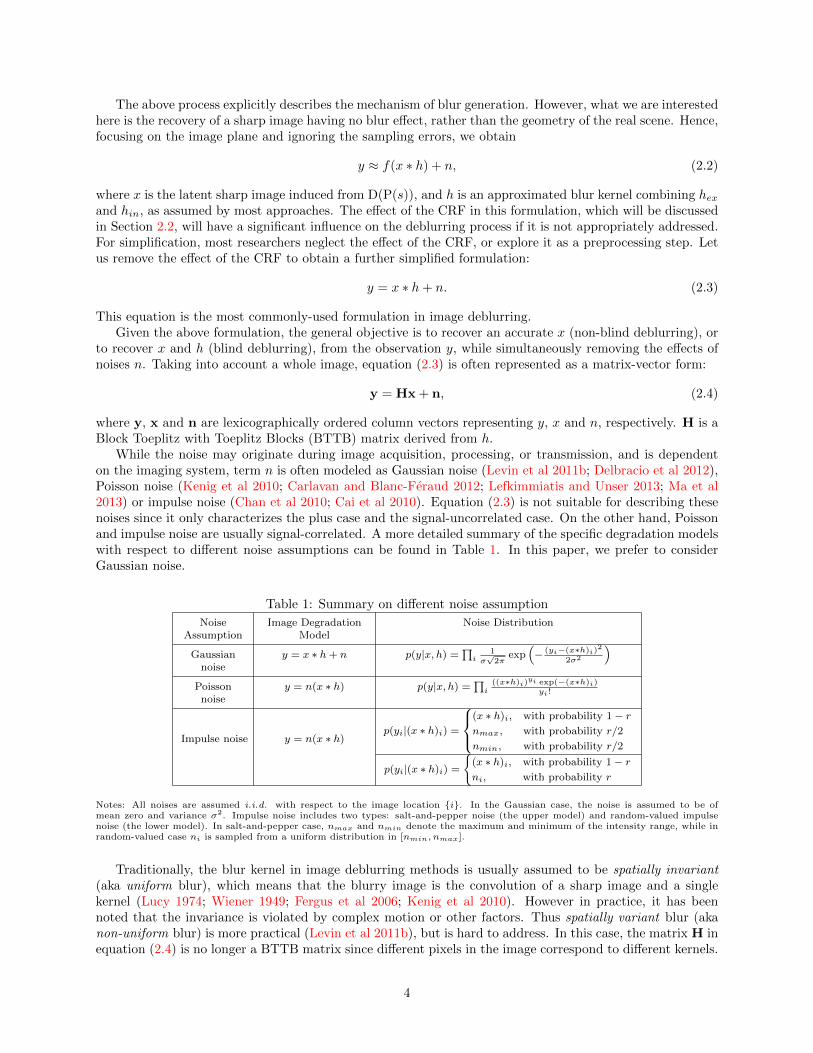
While the noise may originate during image acquisition, processing, or transmission, and is dependenton the imaging system, term n is often modeled as Gaussian noise (Levin et al 2011b; Delbracio et al 2012),Poisson noise (Kenig et al 2010; Carlavan and Blanc-Feraud 2012; Lefkimmiatis and Unser 2013; Ma et al2013) or impulse noise (Chan et al 2010; Cai et al 2010). Equation (2.3) is not suitable for describing thesenoises since it only characterizes the plus case and the signal-uncorrelated case. On the other hand, Poissonand impulse noise are usually signal-correlated. A more detailed summary of the specific degradation modelswith respect to different noise assumptions can be found in Table 1. In this paper, we prefer to considerGaussian noise.

Table 1: Summary on different noise assumption

NoiseAssumption

Image DegradationModel

Noise Distribution

Gaussiannoise

y = x ∗ h+ n p(y|x, h) =∏i

1σ√2π

exp(− (yi−(x∗h)i)2

2σ2

)Poissonnoise

y = n(x ∗ h) p(y|x, h) =∏i((x∗h)i)yi exp(−(x∗h)i)

yi!

Impulse noise y = n(x ∗ h)p(yi|(x ∗ h)i) =

(x ∗ h)i, with probability 1− rnmax, with probability r/2

nmin, with probability r/2

p(yi|(x ∗ h)i) =

{(x ∗ h)i, with probability 1− rni, with probability r

Notes: All noises are assumed i.i.d. with respect to the image location {i}. In the Gaussian case, the noise is assumed to be ofmean zero and variance σ2. Impulse noise includes two types: salt-and-pepper noise (the upper model) and random-valued impulsenoise (the lower model). In salt-and-pepper case, nmax and nmin denote the maximum and minimum of the intensity range, while inrandom-valued case ni is sampled from a uniform distribution in [nmin, nmax].

Traditionally, the blur kernel in image deblurring methods is usually assumed to be spatially invariant(aka uniform blur), which means that the blurry image is the convolution of a sharp image and a singlekernel (Lucy 1974; Wiener 1949; Fergus et al 2006; Kenig et al 2010). However in practice, it has beennoted that the invariance is violated by complex motion or other factors. Thus spatially variant blur (akanon-uniform blur) is more practical (Levin et al 2011b), but is hard to address. In this case, the matrix H inequation (2.4) is no longer a BTTB matrix since different pixels in the image correspond to different kernels.

4

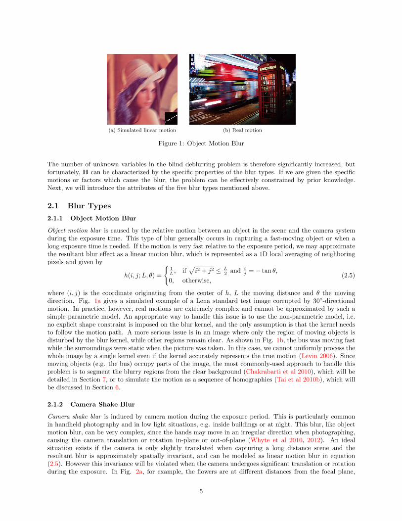
(a) Simulated linear motion (b) Real motion

Figure 1: Object Motion Blur

The number of unknown variables in the blind deblurring problem is therefore significantly increased, butfortunately, H can be characterized by the specific properties of the blur types. If we are given the specificmotions or factors which cause the blur, the problem can be effectively constrained by prior knowledge.Next, we will introduce the attributes of the five blur types mentioned above.

2.1 Blur Types

2.1.1 Object Motion Blur

Object motion blur is caused by the relative motion between an object in the scene and the camera systemduring the exposure time. This type of blur generally occurs in capturing a fast-moving object or when along exposure time is needed. If the motion is very fast relative to the exposure period, we may approximatethe resultant blur effect as a linear motion blur, which is represented as a 1D local averaging of neighboringpixels and given by

h(i, j;L, θ) =

{1L , if

√i2 + j2 ≤ L

2 and ij = − tan θ,

0, otherwise,(2.5)

where (i, j) is the coordinate originating from the center of h, L the moving distance and θ the movingdirection. Fig. 1a gives a simulated example of a Lena standard test image corrupted by 30◦-directionalmotion. In practice, however, real motions are extremely complex and cannot be approximated by such asimple parametric model. An appropriate way to handle this issue is to use the non-parametric model, i.e.no explicit shape constraint is imposed on the blur kernel, and the only assumption is that the kernel needsto follow the motion path. A more serious issue is in an image where only the region of moving objects isdisturbed by the blur kernel, while other regions remain clear. As shown in Fig. 1b, the bus was moving fastwhile the surroundings were static when the picture was taken. In this case, we cannot uniformly process thewhole image by a single kernel even if the kernel accurately represents the true motion (Levin 2006). Sincemoving objects (e.g. the bus) occupy parts of the image, the most commonly-used approach to handle thisproblem is to segment the blurry regions from the clear background (Chakrabarti et al 2010), which will bedetailed in Section 7, or to simulate the motion as a sequence of homographies (Tai et al 2010b), which willbe discussed in Section 6.

2.1.2 Camera Shake Blur

Camera shake blur is induced by camera motion during the exposure period. This is particularly commonin handheld photography and in low light situations, e.g. inside buildings or at night. This blur, like objectmotion blur, can be very complex, since the hands may move in an irregular direction when photographing,causing the camera translation or rotation in-plane or out-of-plane (Whyte et al 2010, 2012). An idealsituation exists if the camera is only slightly translated when capturing a long distance scene and theresultant blur is approximately spatially invariant, and can be modeled as linear motion blur in equation(2.5). However this invariance will be violated when the camera undergoes significant translation or rotationduring the exposure. In Fig. 2a, for example, the flowers are at different distances from the focal plane,

5

(a) Camera translation (b) Camera rotation

Figure 2: Camera Shaken Blur

implying that during the camera’s translation, the nearer flowers undergo a large shift with respect to thefocal plane, while the distant flowers experience a slight shift. Camera rotation is a more complicated casewhich includes in-plane rotation and out-of-plane rotation in terms of focal plane. In the case of in-planerotation, the blur kernel varies significantly across the image, especially for the regions far from the axisalong which the camera is rotated, as shown in Fig. 2b. For out-of-plane rotation, the degree of spatialvariance across the image is dependent on the focal length of the camera (for more detail see (Whyte et al2012)). Clearly, the spatially variant blur is more suitable to explain all cases mentioned above than thespatially invariant blur. Fortunately, as Harmeling et al (2010) point out, it is reasonable to expect that theblur kernel will vary smoothly across the whole image if the depth of the scene varies smoothly, in spite ofthe fact that this is not true when the objects have very different distances from the focal plane.

2.1.3 Defocus Blur

As a result of imperfect focusing by the imaging system or different depths of scene, the fields outside thefocus field are defocused, giving rise to defocus blur, or out of focus blur. This blur is familiar in our everydayphotos. For example, it is often hard for a photography beginner to focus on the target object by hand. Also,when a camera is equipped with only one lens, scenes outside the depth of field (DOF, which is the rangecovered by all objects in a scene that appear acceptably sharp in an image) are all blurred in the resultantimage, e.g. Fig. 3b. Traditionally, a crude approximation of a defocus blur is made as a uniform circularmodel:

h(i, j) =

{1

πR2 , if√i2 + j2 ≤ R,

0, otherwise,(2.6)

where R is the radius of the circle. This is valid if the depth of scene does not have significant variation andR is properly selected. A simulated instance is shown in Fig. 3a. Practically, focusing on a target objectis not difficult for modern consumer cameras since most of them are equipped with an auto-focus function;however, due to the limited DOF, it is not always possible to make the entire image sharp, as illustrated inFig. 3b. To recover a full-focused image, the focus sweep technique is usually utilized to sweep the planeof focus through a desired depth range during exposure, so that the depth of field is enlarged (Bando et al2013). An alternative way of handling this limit is to use coded aperture pairs (Zhou et al 2011), by whichthe depth of the scene can be also recovered.

2.1.4 Atmospheric Turbulence Blur

Atmospheric turbulence blur generally happens in long-distance imaging systems such as remote sensing andaerial imaging. This is mainly because of the randomly varying refractive index along the optical transmissionpath. For long-term exposure through the atmosphere, the blur kernel can be described by a fixed Gaussianmodel (Zhu and Milanfar 2010), i.e.

h(i, j) = Z · exp

(− i

2 + j2

2σ2

), (2.7)

6

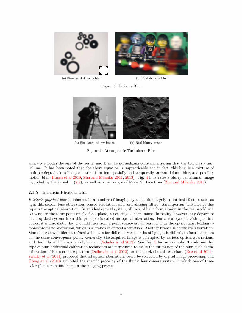
(a) Simulated defocus blur (b) Real defocus blur

Figure 3: Defocus Blur

(a) Simulated blurry image (b) Real blurry image

Figure 4: Atmospheric Turbulence Blur

where σ encodes the size of the kernel and Z is the normalizing constant ensuring that the blur has a unitvolume. It has been noted that the above equation is impracticable and in fact, this blur is a mixture ofmultiple degradations like geometric distortion, spatially and temporally variant defocus blur, and possiblymotion blur (Hirsch et al 2010; Zhu and Milanfar 2011, 2013). Fig. 4 illustrates a blurry cameraman imagedegraded by the kernel in (2.7), as well as a real image of Moon Surface from (Zhu and Milanfar 2013).

2.1.5 Intrinsic Physical Blur

Intrinsic physical blur is inherent in a number of imaging systems, due largely to intrinsic factors such aslight diffraction, lens aberration, sensor resolution, and anti-aliasing filters. An important instance of thistype is the optical aberration. In an ideal optical system, all rays of light from a point in the real world willconverge to the same point on the focal plane, generating a sharp image. In reality, however, any departureof an optical system from this principle is called an optical aberration. For a real system with sphericaloptics, it is unrealistic that the light rays from a point source are all parallel with the optical axis, leading tomonochromatic aberration, which is a branch of optical aberration. Another branch is chromatic aberration.Since lenses have different refractive indexes for different wavelengths of light, it is difficult to focus all colorson the same convergence point. Generally, the acquired image is corrupted by various optical aberrations,and the induced blur is spatially variant (Schuler et al 2012). See Fig. 5 for an example. To address thistype of blur, additional calibration techniques are introduced to assist the estimation of the blur, such as theutilization of Poisson noise pattern (Delbracio et al 2012), or the checkerboard test chart (Kee et al 2011).Schuler et al (2011) proposed that all optical aberrations could be corrected by digital image processing, andTzeng et al (2010) exploited the specific property of the fluidic lens camera system in which one of threecolor planes remains sharp in the imaging process.

7

Figure 5: Optical Aberration

(a) Input image

0 0.2 0.4 0.6 0.8 10

0.1

0.2

0.3

0.4

0.5

0.6

0.7

0.8

0.9

1

The Estimated CRF with Single ImageThe Estimated CRF with multiple ImagesInverse Gamma-Correction

Ground Truth

(b) Estimated CRF (c) Deblurred imagewithout CRF correction

(d) Deblurred imagewith CRF correction

Figure 6: Effects of the nonlinear CRF on deblurring results (Kim et al 2012b)

2.2 Effects of the CRF f(·)Recall that the camera response function f(·) in equation (2.2) is a nonlinear model mapping the sceneirradiance to image intensity. The purpose of this design is to mimic the response of the human visualsystem or to compress the dynamic range of scenes, or for aesthetic consideration (Grossberg and Nayar2004; Lin and Zhang 2005). However, inappropriate processing of CRF leads to severe ringing artifacts indeblurring problems. Chen et al (2012) have theoretically pointed out three kinds of CRF effects on blurinconsistency ∆ = f(x ∗ h)− x ∗ h. Here x is the sharp irradiance image corresponding to x. These effectsare:1) The nonlinear CRF has no influence on the intensity of the uniform regions, i.e. ∆ = 0;2) In low-frequency regions, the irradiance is approximately equal to its corresponding intensity, i.e. ∆ ≈ 0,under the condition of small kernel h and smooth function f(·);3) In high-frequency high contrast regions, the nonlinearity of f(·) can significantly damage the blur consis-tency, particularly when the local minimum and maximum pixel intensities are very different.

From these claims, we readily find that even if a spatially invariant blur h is assumed to be in irradiance,f(·) could turn h into a spatially variant case in the intensity domain (Kim et al 2012a). To estimate thefunction, given a blurry/sharp image pair, Chen et al (2012) exploited Generalized Gamma Curve Model(GGCM) to fit f(·). Kim et al (2012a) and Tai et al (2013) addressed the estimation in two ways, one ofwhich is based on a least-squares formulation when the blur kernel is known, while the other is solved viarank minimization without the need for a known kernel. Fig. 6 illustrates a result of (Kim et al 2012a,b),indicating that large number of artifacts remain in the selected regions of the deblurred image without theCRF correction.

In summary, each of the five blur types discussed in this section has specific properties, inspiring re-searchers to develop effective and efficient algorithms for deblurring. Needless to say, a good deblurringmodel should be suitable for all blur types which, however, is difficult to be explored. Fortunately, in thedeblurring community, there have been many progressive methods proposed in recent years. In the followingsections, we will discuss the five categories of existing methods from the modeling perspective in detail. Firstlet us focus on Bayesian inference framework.

8

3 Bayesian Inference Framework

In statistics, Bayesian inference updates the states of a probability hypothesis by exploiting additionalevidence. Bayes’ rule is the critical foundation of Bayesian inference and can be expressed as

p(A|B) =p(B|A)p(A)

p(B), (3.1)

where A stands for the hypothesis set and B corresponds to the evidence set. This rule states that thetrue posterior probability p(A|B) is based on our prior knowledge of the problem, i.e. p(A), and is updatedaccording to the compatibility of the evidence and the given hypothesis, i.e. the likelihood p(B|A). In ourscenario for the non-blind deblurring problem, A is then the underlying sharp image x to be estimated, whileB denotes the blurry observation y. For the blind case, a slight difference is that A means the pair of (x, h)since h is also a hypothesis in which we are interested. Explicitly (3.1) can be written for both cases as

Non-blind: p(x|y, h) =p(y|x, h)p(x)

p(y), (3.2)

Blind: p(x, h|y) =p(y|x, h)p(x)p(h)

p(y). (3.3)

Note that either x or y and h are usually assumed to be uncorrelated. Irrespective of case, the likelihoodp(y|x, h) is dependent on the noise assumption, as listed in Table 1. How to further infer the equation (3.1)in the literatures inspires us to explore three directions: maximum a posteriori, minimum mean square error,and variational Bayesian methods.

3.1 Maximum a Posteriori

The most commonly-used estimator in a Bayesian inference framework is the maximum a posteriori (MAP).This strategy attempts to find the optimal solution A∗ which maximizes the distribution of the hypothesisset A given the evidence set B in (3.1). In the blind case,

(x∗, h∗) = argmaxx,h

p(x, h|y)

= argmaxx,h

p(y|x, h)p(x)p(h), (3.4)

while in the non-blind scenario, the term p(h) is discarded according to equation (3.2). Fig. 7 shows adiagram of this type of method.

3.1.1 Maximum Likelihood Estimation

We start with the introduction of a classic non-blind algorithm, Richardson-Lucy (RL) deconvolution(Richardson 1972; Lucy 1974), which is widely used in astronomical imaging and medical imaging.3 As-suming that the prior p(x) takes the form of a uniform distribution, the MAP estimator then becomes amaximum likelihood estimator (MLE), i.e.

x∗ = argmaxx

p(y|x, h)

= argminx− log p(y|x, h), (3.5)

where in the second equation the minimized equation is known as negative log-likelihood. Under the noiseassumption of Poisson distribution (Shepp and Vardi 1982), (3.5) is derived as

x∗ = argminx

∑i

((x ∗ h)i − yi log(x ∗ h)i) . (3.6)

3In the standard RL, no specific noise assumption is assumed. Here, we introduce RL from the MLE perspective underPoisson noise assumption to facilitate the ongoing analysis.

9

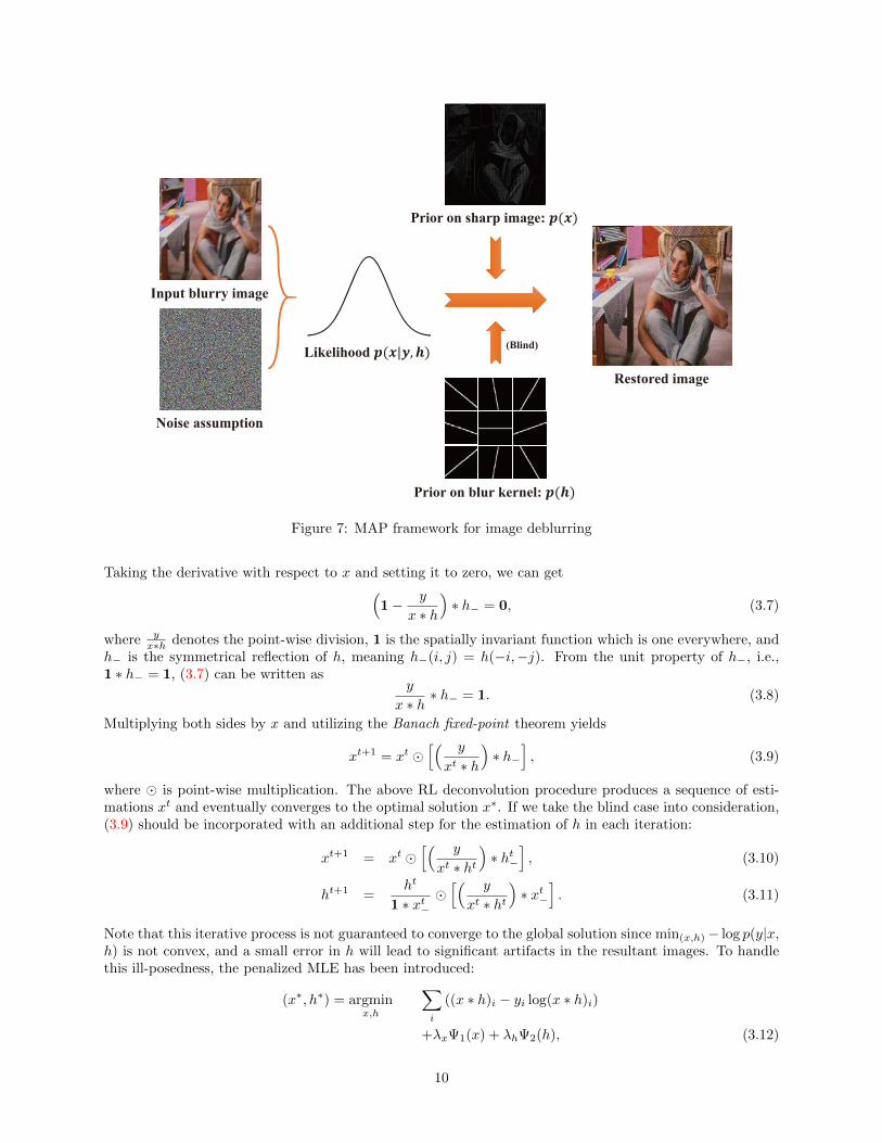
Input blurry image

Noise assumption

Likelihood

Prior on sharp image:

Prior on blur kernel:

(Blind)

Restored image

Figure 7: MAP framework for image deblurring

Taking the derivative with respect to x and setting it to zero, we can get(1− y

x ∗ h

)∗ h− = 0, (3.7)

where yx∗h denotes the point-wise division, 1 is the spatially invariant function which is one everywhere, and

h− is the symmetrical reflection of h, meaning h−(i, j) = h(−i,−j). From the unit property of h−, i.e.,1 ∗ h− = 1, (3.7) can be written as

y

x ∗ h∗ h− = 1. (3.8)

Multiplying both sides by x and utilizing the Banach fixed-point theorem yields

xt+1 = xt �[( y

xt ∗ h

)∗ h−

], (3.9)

where � is point-wise multiplication. The above RL deconvolution procedure produces a sequence of esti-mations xt and eventually converges to the optimal solution x∗. If we take the blind case into consideration,(3.9) should be incorporated with an additional step for the estimation of h in each iteration:

xt+1 = xt �[( y

xt ∗ ht)∗ ht−

], (3.10)

ht+1 =ht

1 ∗ xt−�[( y

xt ∗ ht)∗ xt−

]. (3.11)

Note that this iterative process is not guaranteed to converge to the global solution since min(x,h)− log p(y|x,h) is not convex, and a small error in h will lead to significant artifacts in the resultant images. To handlethis ill-posedness, the penalized MLE has been introduced:

(x∗, h∗) = argminx,h

∑i

((x ∗ h)i − yi log(x ∗ h)i)

+λxΨ1(x) + λhΨ2(h), (3.12)

10

where Ψ1(·) and Ψ1(·) are the penalty functions on x and h, respectively. Direct derivation leads to theiterations for the penalized version, i.e.,

xt+1 = xt �(

yxt∗ht

)∗ ht−

1 + λx∂Ψ1(xt)∂xt

, (3.13)

ht+1 = ht �(

yxt∗ht

)∗ xt−

1 ∗ xt− + λh∂Ψ2(ht)∂ht

. (3.14)

Under this formula, Temerinac-Ott et al (2012) utilized the total variation (TV) regularization for Ψ1(x)and derived a multi-view RL algorithm. In their method, the underlying sharp 3D image is composedof images observed from multiple viewpoints, each of which is corrupted by a different blur kernel. Themultiple blurry images are integrated in a unified formulation from which the sharp image is jointly deduced.Lefkimmiatis and Unser (2013) employed the Schatten norms of Hessian matrix on each image pixel as theregularization on x. This kind of regularizer is based on the second-order derivatives instead of the first-orderderivatives, thus favoring piecewise-smooth solutions, as opposed to TV which produces piecewise-constantsolutions.

Regarding Ψ2(h), Keuper et al (2013) discovered a specific property of the wide-field fluorescence mi-croscopy (WFFM) system, which suggests that the optical transfer function (OTF), i.e. the Fourier transformof the kernel h, is well localized and smooth. They proposed imposing the TV constraint on both x to pre-serve edges, and OTF to ensure the smoothness of the kernel. Kenig et al (2010) developed a novel approachto restrict h to a kernel subspace which was produced by either linear or kernel principal component analysis(PCA) based on the general forms of the WFFM PSF. This is easily integrated into the iterative RL decon-volultion procedure. Additionally, the residual denoising operation is employed to avoid over-smoothing theuseful high-frequency details, which is also used in (Keuper et al 2013).

Most of the above methods are based on the assumption of a spatially invariant kernel. Tai et al (2011)developed the projective motion RL algorithm to tackle the spatially variant case. Under the proposedprojective motion blur model, the operations of convolution and correlation in the conventional RL algorithmare replaced by a sequence of forward projective motions and their inverses via homographies, which will bediscussed in Section 6. Various regularizers are applicable in their framework.

3.1.2 Priors for MAP

The penalized MLE in equation (3.12) is exactly the MAP since the penalty functions act as the priors in thatp(x) = exp(−λxΨ1(x)) and p(h) = exp(−λhΨ2(h)). Various MAP based methods focus on the developmentof priors to obtain attractive deblurring results.

It is commonly agreed that for a natural image, the gradients of the sharp image tend to obey a heavy-tailed distribution, meaning that the distribution of gradients has most of its mass on small values but assignssignificantly more probability to large values than a Gaussian distribution (Field 1994; Fergus et al 2006).Thus natural images often contain large regions of constant intensity or gentle intensity whose gradients areinterrupted by occasional large changes at the edges or occlusion boundaries. To express such a prior, variousapproximations of the heavy-tailed distribution are used to describe the gradients. One classic method is toinform a Laplace distribution on the magnitude of the gradients:

pLap(∇x) =∏i

1

2bexp

(−‖∇xi‖1

b

), (3.15)

where ∇ is the gradient operator, ‖ · ‖1 is the `1 norm, and b denotes the scale parameter. Additionally,for computation efficiency, a generalized Gaussian model is used by Levin et al (2007) in their design of anoptimal aperture filter, and a Gaussian prior is imposed on the gradient patches instead of gradient pixelsby Hu et al (2012). The autocorrelation function of the blur kernel is shown in relation to the covariancematrix of the Gaussian distribution. Through the Fourier transform of the autocorrelation matrix and anadditional phase retrieval stage, the blur kernel can be easily recovered. Unlike the MAP methods involvingrepeated reconstructions of the sharp image, this approach directly relies on basic statistics of the blurryimage and is therefore efficient.

11

Due to the imperfect fitness of the above priors to the real gradient distribution of sharp natural images,these methods tend to remove mid-frequency textures, even though structures such as edges can be preserved.To improve the fitness to the heavy-tailed distribution, Fergus et al (2006) proposed using a Gaussian mixturemodel (GMM) having finite mixture numbers. Chakrabarti et al (2010) extended this to Gaussian scalemixture (GSM) which is a mixture of infinite Gaussian models with a continuous range of variances. Theform of the corresponding zero-mean GMM and GSM are respectively

pGMM (∇x) =∏i

C∑c=1

N (∇xi|0, ξc), (3.16)

pGSM (∇x) =∏i

∫ξ

N (∇xi|0, ξ)p(ξ)dξ, (3.17)

where ξ is the standard derivation of the Gaussian distribution, c and C in GMM is the index and the totalnumber of mixtures, and p(ξ) in GSM is a probability distribution on ξ. In terms of GSM, a critical issue isthe infinite selection of ξ, which makes it computationally expensive. According to the theoretical analysisby Palmer et al (2005), equation (3.17) can be derived from the variational perspective as

p(∇x) =∏i

supξi>0N (∇xi|0, ξi)p(ξi), (3.18)

where p(ξ) takes the form of exp(f( ξ2 )). This theoretical convenience is directly utilized by (Chakrabartiet al 2010) and further investigated by Zhang et al (2013a); Zhang and Wipf (2013). In (Zhang et al 2013a),authors proposed an adaptive sparse prior based on (3.18). They coupled multiple blurry observations in ajoint deblurring procedure by assuming that the parameters {ξi} in (3.18) are shared across all images. Intheir subsequent work (Zhang and Wipf 2013), the idea of the shared parameter is extended to the singleimage deblurring problem by additionally assuming the homography expression of blur kernels. In bothworks, the sparse regularizer is adaptively adjusted according to the noise level estimated in each iteration.

Another question raises: even though the assumed prior coincides perfectly with the gradient distributionof the sharp image, is the recovered gradient distribution able to fit our prior as we expected? A recentresearch by Cho et al (2012c) responded in the negative. According to their analysis, the above heavy-tailed priors are generally independently forced on each pixel or each local patch, failing to capture theglobal statistics of gradients. Thus the reconstructed image favors flat regions, resulting in the gradientdistribution of the MAP estimates failing to match that of the original sharp image. To address this issue,the authors proposed penalizing the Kullback-Leibler (KL) divergence between the gradient distribution ofthe estimated image pe(∇x) and a reference distribution pr(∇x),

KL(pe||pr) =

∫∇x

pe(∇x) ln

(pe(∇x)

pr(∇x)

)d∇x, (3.19)

which induces a constraint and can be combined with (3.4). The reference distribution is characterized asthe generalized Gaussian model and immediately estimated from the blurry image by using the approach of(Cho et al 2010a). Taking the same idea, Zhuo et al (2010) presented a more direct method which forces thegradients of the deblurred image close to those of the reference image. It is direct because: 1) a Lorentzianerror norm is imposed on the difference of the two gradients rather than the difference of their distributions,i.e.

ρ(∇xe,∇xr) = log

(1 +

1

2

(∇xe −∇xr

%

)2), (3.20)

where % is a predefined constant; and 2) the reference image is a flash image of the same scene which is sharpbut corrupted by a degraded illumination.

Besides the priors on image gradients, the knowledge on image intensities or transformed domains isextremely helpful in specific applications. For example, Chen et al (2011) developed a content-aware priorfor document image deblurring in which the histogram of the whole image is the weighted sum of thehistogram of the foreground (dark pixels) and of the background (white pixels). Additionally, a local upper-bound constraint together with TV is imposed to restrain the artifacts in the resultant images. Similarly,

12

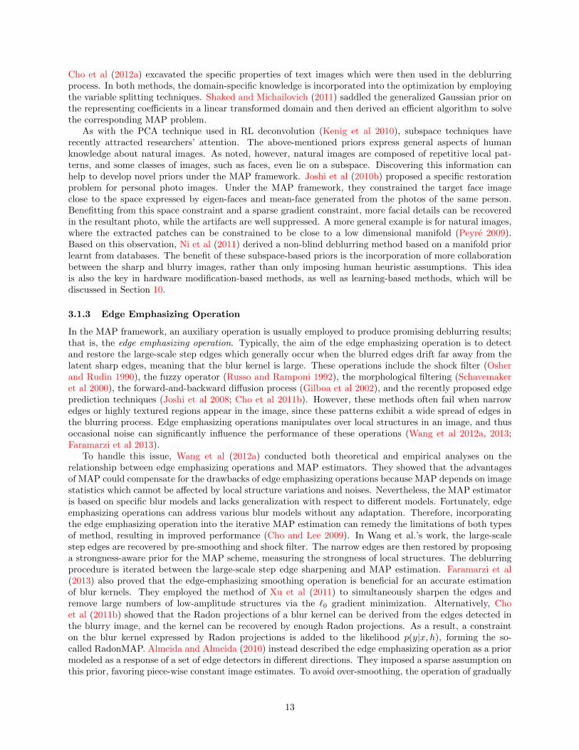
Cho et al (2012a) excavated the specific properties of text images which were then used in the deblurringprocess. In both methods, the domain-specific knowledge is incorporated into the optimization by employingthe variable splitting techniques. Shaked and Michailovich (2011) saddled the generalized Gaussian prior onthe representing coefficients in a linear transformed domain and then derived an efficient algorithm to solvethe corresponding MAP problem.

As with the PCA technique used in RL deconvolution (Kenig et al 2010), subspace techniques haverecently attracted researchers’ attention. The above-mentioned priors express general aspects of humanknowledge about natural images. As noted, however, natural images are composed of repetitive local pat-terns, and some classes of images, such as faces, even lie on a subspace. Discovering this information canhelp to develop novel priors under the MAP framework. Joshi et al (2010b) proposed a specific restorationproblem for personal photo images. Under the MAP framework, they constrained the target face imageclose to the space expressed by eigen-faces and mean-face generated from the photos of the same person.Benefitting from this space constraint and a sparse gradient constraint, more facial details can be recoveredin the resultant photo, while the artifacts are well suppressed. A more general example is for natural images,where the extracted patches can be constrained to be close to a low dimensional manifold (Peyre 2009).Based on this observation, Ni et al (2011) derived a non-blind deblurring method based on a manifold priorlearnt from databases. The benefit of these subspace-based priors is the incorporation of more collaborationbetween the sharp and blurry images, rather than only imposing human heuristic assumptions. This ideais also the key in hardware modification-based methods, as well as learning-based methods, which will bediscussed in Section 10.

3.1.3 Edge Emphasizing Operation

In the MAP framework, an auxiliary operation is usually employed to produce promising deblurring results;that is, the edge emphasizing operation. Typically, the aim of the edge emphasizing operation is to detectand restore the large-scale step edges which generally occur when the blurred edges drift far away from thelatent sharp edges, meaning that the blur kernel is large. These operations include the shock filter (Osherand Rudin 1990), the fuzzy operator (Russo and Ramponi 1992), the morphological filtering (Schavemakeret al 2000), the forward-and-backward diffusion process (Gilboa et al 2002), and the recently proposed edgeprediction techniques (Joshi et al 2008; Cho et al 2011b). However, these methods often fail when narrowedges or highly textured regions appear in the image, since these patterns exhibit a wide spread of edges inthe blurring process. Edge emphasizing operations manipulates over local structures in an image, and thusoccasional noise can significantly influence the performance of these operations (Wang et al 2012a, 2013;Faramarzi et al 2013).

To handle this issue, Wang et al (2012a) conducted both theoretical and empirical analyses on therelationship between edge emphasizing operations and MAP estimators. They showed that the advantagesof MAP could compensate for the drawbacks of edge emphasizing operations because MAP depends on imagestatistics which cannot be affected by local structure variations and noises. Nevertheless, the MAP estimatoris based on specific blur models and lacks generalization with respect to different models. Fortunately, edgeemphasizing operations can address various blur models without any adaptation. Therefore, incorporatingthe edge emphasizing operation into the iterative MAP estimation can remedy the limitations of both typesof method, resulting in improved performance (Cho and Lee 2009). In Wang et al.’s work, the large-scalestep edges are recovered by pre-smoothing and shock filter. The narrow edges are then restored by proposinga strongness-aware prior for the MAP scheme, measuring the strongness of local structures. The deblurringprocedure is iterated between the large-scale step edge sharpening and MAP estimation. Faramarzi et al(2013) also proved that the edge-emphasizing smoothing operation is beneficial for an accurate estimationof blur kernels. They employed the method of Xu et al (2011) to simultaneously sharpen the edges andremove large numbers of low-amplitude structures via the `0 gradient minimization. Alternatively, Choet al (2011b) showed that the Radon projections of a blur kernel can be derived from the edges detected inthe blurry image, and the kernel can be recovered by enough Radon projections. As a result, a constrainton the blur kernel expressed by Radon projections is added to the likelihood p(y|x, h), forming the so-called RadonMAP. Almeida and Almeida (2010) instead described the edge emphasizing operation as a priormodeled as a response of a set of edge detectors in different directions. They imposed a sparse assumption onthis prior, favoring piece-wise constant image estimates. To avoid over-smoothing, the operation of gradually

13

decreasing the regularization parameter was used to produce a promising result. Xu and Jia (2010) pointedout that not all strong edges are profitable for kernel estimation. They proposed a new metric to measurethe usefulness of the image edges. The selected edges according to this metric are then used to induce thekernel formation. What follows is an adaptive kernel refinement procedure which is to ensure the sparsenessof the estimated kernel without damaging its large-valued elements.

3.1.4 Marginalization Techniques

Even though appropriate priors or suitable edge emphasizing operations have been utilized in the MAPframework and have resulted in improved performance, intrinsic problems remain. A recent outstandingresearch by Levin et al (2009, 2011b) comprehensively analyzes the failure of the MAP scheme and pointsout how to make the MAP estimation successfully recover the true blur kernel. The MAPx,h scheme forblind deconvolution in (3.4) can be rewritten as

(x∗, h∗) = argminx,h

‖y − x ∗ h‖2 + λ(∑i

|∇hxi|α + |∇vxi|α) (3.21)

under the Gaussian noise assumption and a sparse derivative prior or heavy-tailed prior on image gradients.∇h and ∇v are horizontal and vertical derivatives of the image. According to Levin et al.’s conclusions,the solution of (3.21) under the sparse prior usually favors a blurry result rather than a sharp result, eventhough y is generated up to infinitely large image samples from the perfect prior. This observation is alsoknown as the no-blur explanation or delta effect of MAP, which means that the solution of (3.21) has ahigher probability of being {

x∗ = y

h∗ = δ(3.22)

than the true solution. From the estimation theory perspective, it is evident that we cannot gather sufficientmeasurements for the MAPx,h problem since the number of unknown variables grows with the image size,even to infinity.

As noted by Levin et al (2009, 2011b), the strong asymmetry between the dimensionality of x and hprovides a favorable property for handling the blind deconvolution. This means that while the dimensionalityof x increases with the image size, the support of h remains fixed and is small relative to the image size.From this viewpoint, h can achieve an increased number of measurements when the image size becomeslarge. Thus, estimation theory tells us through sufficient measurements on h that the recovered blur kernelunder MAPh can be arbitrarily close to the true kernel. Mathematically, the MAPh is

h∗ = argmaxh

p(h|y)

= argmaxh

∫p(x, h|y)dx, (3.23)

where h∗ is the true kernel, as stated in Claim 3 of (Levin et al 2011b). Once the kernel is estimated, x canthen be solved in a non-blind deblurring scheme. In their subsequent work (Levin et al 2011a), Levin et al.noted that MAPh is generally complex and hard to directly compute because the marginalization in (3.23)involves all possible x explanations, which is computationally intractable. An approximation method wasproposed to derive the MAPh. To estimate the blur kernel, they assumed the i.i.d. Gaussian imaging noiseand the GMM prior on image derivatives, as well as a uniform distribution on h. Equation (3.23) can thenbe written as

h∗ = argmaxh

p(y|h)

= argmaxh

∫p(x, y|h)dx. (3.24)

The above problem is solved by the expectation-maximization (EM) framework that alternates between theestimation of p(x|y, h) which is still a Gaussian (E-step), and the computation of h under the minimum

14

mean square error (M-step). In the E-step, however, calculating the mean and covariance of p(x|y, h) undera sparse prior is generally hard, so the authors proposed approximating the conditional distribution by usingvariational inference, which will be discussed in Section 3.3.

Wang et al (2013) have discovered several intrinsic issues between edge emphasizing operations and imagestatistics through a large number of experiments on ImageNet (Deng et al 2009) composed of 1.2 millionimages in total. Their research points out that the limited number of large scale step edges within a naturalimage cannot ensure a robust estimation of the blur kernel. Additionally, due to the diversity of naturalimages, the sparse derivative priors are not consistent across them and it is almost impossible to find a robustmeasurement that favors sharp explanations for all of them. Different from their previous work (Wang et al2012a) which uses MAPx,h, they adopted the marginalization scheme in (3.23) and developed an adaptivesparse prior composed of two components to ensure robustness. The first component is the commonly-usedsparse derivative prior, while the second encodes the edge emphasizing operation.

3.2 Minimum Mean Square Error

The Bayesian framework aims to estimate x or h from the posterior p(x, h|y) and a loss function L((x∗, h∗), (x,h)). The expected loss is computed over all unknown variables,

L((x∗, h∗), (x, h)|y) =

∫L((x∗, h∗), (x, h))p(x, h|y)dxdh, (3.25)

which is called Bayesian expected loss (Brainard and Freeman 1997). The optimal solution (x∗, h∗) isthen chosen to minimize L((x∗, h∗), (x, h)). If we take L((x∗, h∗), (x, h)) as a Dirac delta loss function,i.e. L((x∗, h∗), (x, h)) = 1 − δ((x∗, h∗) − (x, h)), (3.25) becomes the MAPx,h problem. Alternatively, ifL((x∗, h∗), (x, h)) is the square error loss, we can obtain the minimum mean square error (MMSE) formula-tion:

(x∗, h∗) = argminx,h

∫‖x− x‖2‖h− h‖2p(x, h|y)dxdh

= argminx,h

E{x, h|y}. (3.26)

For the non-blind deblurring case, the above equation turns into

x∗ = argminx

∫‖x− x‖2p(x|y, h)dx

= argminx

E{x|y, h}. (3.27)

The equivalence between MMSE and MAP has been proved by Levin et al (2011b), that is if p(h|y) hasa unique maxima, then for large images, the MAPh estimator followed by an MMSEx image estimation isequivalent to a simultaneous MMSEx,h estimation of both x and h.

In spite of this, the empirical demonstrations on image denoising have shown the advantages of MMSEover MAP approaches (Schmidt et al 2010). MAP solutions usually exhibit piecewise constant regions andresult in incorrect statistics of the output image, as previously noted, whereas MMSE can achieve the desiredstatistics by exploiting the uncertainty of the model. Furthermore, the image restoration performance of theMMSE estimator is highly correlated with the generative quality of the model. This observation is particu-larly useful since MMSE benefits from a powerful learnt generative model even without any regularizationweight. As is well known, the regularization parameter is related to the noise level of the degraded image.By taking the above superiority of MMSE, Schmidt et al (2011) integrated the noise estimation process intothe MMSE framework by treating the noise standard deviation as a variable of the posterior, i.e., given hand y,

p(x|y, h) =

∫p(x, σ|y, h)dσ. (3.28)

Compared with MAP, one problem in MMSE remains. Due to the lack of complete knowledge on thejoint distribution (p(x, h|y) and p(x|y, h)) in real applications, it is difficult to take expectation in (3.26) and

15

(3.27) over all possible explanations. To handle this problem, Schmidt et al (2010, 2011) proposed to usethe Gibbs sampling method to alternatively generate the sequence of the variable samples, e.g. in deblurring{(x1, z1, σ1), ..., (xT , zT , σT )} where z is a latent variable. Another way to address the above issue is toabandon the full optimality requirements and use a particular class of estimators to approximate MMSE,such as linear MMSE:

E{A|B} = WB + v, (3.29)

where A and B are as those in (3.1), and W and v are the parameters encoding the deblurring process.Minimizing E{‖A−WB − v‖2} with respect to W and v can result in the optimal W and v expressed as{

W = CABC−1B ,

v = E{A} −WE{B},(3.30)

where CAB denotes the cross-covariance matrix between A and B, CB is the auto-covariance matrix of B.Thus the linear MMSE estimator is given by

A∗ = CABC−1B (B − E{B}) + E{A}. (3.31)

Clearly, the linear MMSE estimator is dependent on the first- and second-order moments of A and B.In a multi-image deblurring setting, the underlying sharp image is generally interrupted by different

degradation operations, yielding multiple observations. A typical case is a pair of blurry/noisy images.These two images are correlated with each other and can be restored simultaneously. To be clear, the noisyimage can first be denoised to produce a nearly sharp image which can then be used as a guideline or aconstraint in the deblurring process. A recent approach by Michaeli et al (2012) has exploited this strategy byproposing the partially linear MMSE (PLMMSE) estimator. Denoting the denoised image C as a constrainton the estimation of W and v in (3.29), PLMMSE is

E{A|B,C} = W (C)B + v(C), (3.32)

where W (C) and v(C) are functions of C. However, the above estimator is not applicable since it needs theknowledge of the conditional covariance CAB|C which is difficult to acquire (Michaeli et al 2012). Thereforea relaxation of the restriction is conducted, resulting in a separable partially linear MMSE:

E{A|B,C} = WB + v(C). (3.33)

In this case, the PLMMSE estimator is given by

A∗ = CABC−1

BB + E{A|C}, (3.34)

whereB = B − E{B|C}. (3.35)

For more details of the derivation, please see the Appendix in (Michaeli et al 2012). The superiority ofPLMMSE over LMMSE lies in the fact that PLMMSE only requires the knowledge of the second-orderstatistics of A and B, and this estimator can reach the lowest worst-case MSE among all estimators whichdepend solely on the second-order statistics of A and B.

3.3 Variational Bayesian methods

Variational Bayesian methods approximate the intractable integrals arising in a Bayesian inference frame-work. This situation occurs when there are unknown variables and latent variables over which we want tomarginalize without explicitly computing them, such as the marginalization over x in the above MAPh prob-lem. This type of method, on one hand, provides an analytical approximation of the posterior probabilityof the unobserved variables to deduce the statistical properties of these variables (Fergus et al 2006). Onthe other hand, it derives a lower bound for the marginal likelihood of the observed data, which can be usedto model selection (Levin et al 2011a) and high-order statistics analysis on the likelihood of the unobservedvariables (Zhang et al 2010).

16

Variational Bayesian methods have recently been applied to image deblurring. Levin et al (2011b) havemade the important comment that the variational Bayes approximation experimentally outperforms allexisting methods with a different estimation strategy in motion deblurring tasks.

The most frequently-used type of variational Bayes is known as mean-field variational Bayes. Recall thatthe posterior distribution p(A|B) is over the set of unobserved variables A given the observed data B. Herewe try to approximate p(A|B) by finding a variational distribution q(A) that is restricted to a family ofdistributions with a simpler form than p(A|B), i.e. q(A) ≈ p(A|B). The mean-field variational Bayes utilizesthe KL divergence to measure the difference between the two distributions,

L(q) := DKL(q||p) =

∫q(A) log

q(A)

p(A|B)dA. (3.36)

To apply this strategy to the deblurring task, Miskin and MacKay (2000) developed an ensemble learningstrategy. In their method, the unobserved set A is an ensemble of the sharp image x, the blur kernel h andthe noise variance σ2 if the Gaussian noise is assumed. The addition of σ2 frees the user from tuning thisparameter, as well as adaptively balancing the data-fidelity term and the prior term. For simplification, aseparable factorization of the q distribution is employed, which corresponds to the mean field theory (Bishop2006),

q(x, h, σ2) = q(x)q(h)q(σ2). (3.37)

This leads to

L(q) = Eq(x)

{log

q(x)

p(x|y)

}+ Eq(h)

{log

q(h)

p(h|y)

}+Eq(σ2)

{log

q(σ2)

p(σ2|y)

}. (3.38)

The variable B in (3.36) is the observed blurry image y. Our goal is to minimize L(q) with respect toq(x, h, σ2). By taking the convenience of the above factorization, we can take an alternating update procedureof coordinate descent to solve (3.38), that is: minimizing one factor (for example q(x)) while marginalizingout the other factors (q(h) and q(σ2)). The updates are performed by computing the closed-form optimalparameter updates, and performing line-search along the direction of these updated values. According to(Bishop 2006), the optimal factors obtained from the corresponding sequential updates are given by theexpectation of the joint distribution with respect to all unobserved variables except the one of interest, andthus

log q∗(x) = Eq(h),q(σ2){log p(x, h, σ2, y)}+ const

= Eq(h){log p(y|x, h)}+ log p(x) + const,

(3.39)

log q∗(h) = Eq(x),q(σ2){log p(x, h, σ2, y)}+ const

= Eq(x){log p(y|x, h)}+ log p(h) + const,

(3.40)

log q∗(σ2) = Eq(x),q(h){log p(x, h, σ2, y)}+ const

= log p(σ2) + const,

(3.41)

Following the calculation of the above equations, the final estimates of the sharp image x, the blur kernelh and the noise variance σ2 are taken as the mean values of the distributions q∗(x), q∗(h) and q∗(σ2),respectively.

Using this framework, Fergus et al (2006) and Whyte et al (2010, 2012) operated the variational for-mulation on the gradient domain, i.e., x in the above equations is replaced by the image gradients ∇x, tofacilitate the statistical assumption on model priors, such as sparse gradients. Babacan et al (2012)] proposeda super-Gaussian prior over the image intensities and treated the parameter of this prior as a latent variablein the variational inference. The optimal solutions are similar to equations (3.39-3.41).

17

Levin et al (2011a) employed the variational inference to handle the marginalization problem in MAPh.By re-arranging the equation (3.36), a free energy is defined as

F(q) =

∫q(x, z) log q(x, z)dzdx

−∫q(x, z) log p(y, x, z|h)dzdx

= DKL(q(x, z)||p(x, z|y, h))− log p(y|h), (3.42)

where z is an auxiliary latent variable specifying the prior distribution. Due to the non-negativeness ofthe KL-divergence, minimizing F(q) is equivalent to maximizing the lower bound of the likelihood p(y|h)which is the goal of MAPh. Following an iterative optimization procedure, the optimal distribution can besolved. Levin et al.’s method differs from Fergus et al (2006) and Whyte et al (2010, 2012) in that thetarget distribution to be approximated is p(x|y, h) rather than p(x, h|y). However, Fergus et al.’s approachselects h∗ from the estimated q(x, h) distribution by marginalizing out all possible x’s, and thus belongs tothe MAPh approach.

Rather than applying variational inference for deblurring tasks, Zhang et al (2010) explored a differentapplication that compares the reliability of two restoration tasks in the camera shake situation: one is toestimate from a blurry image (deblurring) and the other addresses a sequence of noisy images (denoising).The posterior probabilities of these two tasks are pb = p(x|yb, σ2

b ) and pn = p(x|{ykn}Nk=1, σ2n), respectively,

where yb is the blurry image, ykn is the k-th noisy image, σ2b and σ2

n are the noise variance in two types ofimage. Since the Hessian matrices of log pb and log pn with respect to x provide an uncertainty measurementassociated with the estimation of x, the authors applied the variational distributions over the hidden variables(here, the motion paths) to approximate the posterior, i.e. Lb(q) = DKL(q||pb) and Ln(q) = DKL(q||pn).The comparison result between the Hessian matrix of Lb(q) and that of Ln(q) reveals that restoration bydenoising multiple images is generally more reliable than deblurring a single image.

4 Variational Methods

Variational methods stem from the calculus of variations and are typically used as approximation methodsin a wide variety of settings, such as quantum mechanics, classical mechanics, finite element analysis, andstatistics. Such approximations are engaged to convert an ill-posed problem into a well-posed problemwhich is characterized by exploring additional constraints to reduce the size of the solution space of theunknown variables (Jordan et al 1999). To approximate the problem, a typical setting involves the extremum(maximum or minimum) of a functional composing a function and the associated constraints:

minA

Φ(A;B) + λΨ(A), (4.1)

where A is the undetermined variables and B is the observations. In variational principle, Φ(A;B) is calledthe data-fidelity function, Ψ(A) is the regularization function, and λ denotes the regularization parameter.Under this formulation, the non-blind image deblurring problem can be written as

minx

Φ(x; y, h) + λxΨx(x), (4.2)

while the blind case isminx,h

Φ(x, h; y) + λxΨx(x) + λhΨh(h). (4.3)

The term Φ is determined according to the noise assumptions listed in Table 1. In this section, we generallyassume the Gaussian noise model, and the corresponding Φ is given by

Φ = ‖y − x ∗ h‖22. (4.4)

The discussion of the variational methods is organized from three aspects: regularization, optimization, andanalysis/synthesis reformulation.

18

4.1 Regularization Techniques

Similar to the character of the prior in the Bayesian inference framework, the regularizers in a variationalframework express human knowledge on the interested blurry images. Such knowledge can constrain thesolution space such that the deblurred images are favored by human sense.

4.1.1 Regularization in Single-image Deblurring

Classically, to stabilize the deblurring result, it is expected the solution to have a small norm, and thus theTikhonov-Miller regularizer (Tikhonov 1963) is imposed on the sharp image:

Ψx(x) = ‖x‖2. (4.5)

However, this choice is rarely used in modern deblurring tasks because of the property whereby the resultantimages will have over-smoothed edges. With this regard, the development of the first-order regularizerswhich maximally preserve the significant details is more frequently adopted. A typical example is the totalvariation (TV) proposed by Rudin et al (1992)

TVi(x) = ‖√|∇hx|2 + |∇vx|2‖1, (4.6)

where the subscript i means it is the isotropic version. Complementarily, the anisotropic TV is

TVa(x) = ‖|∇hx|+ |∇vx|‖1. (4.7)

Both TVi and TVa enhance the visualization of edges in the resultant images. They mainly differ fromeach other in their sensitivity to edge directions. From the formulations, we can see that TVi enforces thesame strength on the edges with different directions, whereas TVa favors certain directions. Both methodshave proven to be useful in numerous applications, such as image denoising, decomposition, super-resolution,inpainting, and non-blind deblurring. Nevertheless, when applied to blind deblurring problems, some failuresoccur.

Note that TV is intrinsically an `1 norm of the image gradients, and thus induces sparsity over imagegradients. According to the delta-effect of MAP mentioned in Section 3, simultaneously estimating x and hwill result in a blurry image. Another perspective from the `1 properties can assist the understanding of TVfailure. For a sharp image of natural scenes, the gradient magnitude is typically sparse, meaning that mostvalues are either zero or very small, but may occasionally be large. If a blur kernel is operated on this image,the high-frequency bands will be attenuated, leading to the magnitudes being un-sparse. To recover theoriginal sparsity, a natural choice is the `0 measure, an important property of which is the scale-invariance,i.e., min `0(∇x) = min `0(a · ∇x) for any positive values of a. Minimizing `0 will only lead to a sparse effect,without destroying the magnitudes of large values, thus preserving the energy of original gradients. However,`0 is difficult to optimize because of the lack of derivative information everywhere, and then `1 is utilizedas an alternative to approximate `0. Unfortunately, the blurring process in itself reduces the `1 norm of thegradients. Minimizing `1 fails to preserve or recover the energy of the original gradients. Additionally, thescale variant property makes `1 sensitive to the setting of the regularization parameter λ. Therefore, variousmethods of approximating the `0 norm while maintaining the scale-invariance property are proposed.

Krishnan et al (2011) recently extended the `1 norm to a normalized version:

Ψ(∇x) =‖∇x‖1‖∇x‖2

. (4.8)

To understand this regularizer, let us focus on the denominator, `2 norm. The blurring process reduces the`2 norm of the gradients as well. Fortunately, `2 is reduced more than the numerator `1 norm, leading to anincreased ratio of the two terms. Fig. 8c illustrates that the minimum of this ratio is along the axes. Theblurry effect will drive the ratio away from the axes. Therefore, minimizing this regularizer will deduce theblurry effect in the image without destroying the magnitude of the true gradient because `1/`2 is evidentlyscale invariant, just as we expected.

Another example of the approximation is the unnatural `0 regularizer which is proposed by Xu et al (2013).The unnaturalness stems from the observation that in most iterative deblurring methods, the intermediate

19

−3 −2 −1 0 1 2 3 4

3

2

1

0

−1

−2

−3

−4−4

4

(a) `0

−3 −2 −1 0 1 2 3 4

3

2

1

0

−1

−2

−3

−4−4

4

(b) `1

−3 −2 −1 0 1 2 3 4

3

2

1

0

−1

−2

−3

−4−4

4

(c) `1/`2

−3 −2 −1 0 1 2 3 4

3

2

1

0

−1

−2

−3

−4−4

4

(d) Unnatural `0 (ε = 0.4)

−3 −2 −1 0 1 2 3 4

3

2

1

0

−1

−2

−3

−4−4

4

(e) Unnatural `0 (ε = 0.1)

−3 −2 −1 0 1 2 3 4

3

2

1

0

−1

−2

−3

−4−4

4

(f) Unnatural `0 (ε = 0.1)

Figure 8: Visualization of different measures

image results only contain high-contrast and step-like structures while suppressing others. These imagesare different from natural scenes, and hence the term ’unnatural’ is exploited. To incorporate the step-edgeproperties in an unnatural representation, the authors utilized the unnatural `0 scheme to preserve the salientchanges (i.e., the gradients) in the image. The resultant regularizer is formulated as

Ψ(∇hx) =∑i

ψ(∇hxi), (4.9)

where

ψ(z) =

{1ε2 |z|

2, if |z| ≤ ε,1, otherwise.

(4.10)

The definition on the vertical derivative ∇vxi is similar. Depending on the formulation, the gradient mag-nitudes smaller than ε are penalized by ψ(·) while the larger values result in a constant 1 in the objectivefunction. Minimizing this regularizer will remove fine structures and keep useful salient details in the result.Fig. 8d-8f illustrates three plots under different values of ε. When ε approaches to zero, this regularizer canbe fitted perfectly to the `0 norm. Another property ensuring the unnatural `0 superior to `1 is its scaleinvariance property, as previously stated. By using this regularization technique in the estimation of blurkernels, the deblurring performance has been notably improved.

While the above regularizers are all based on first-order derivatives, second-order regularization techniqueshave also proven to be useful in image denoising tasks, and have recently been introduced to deblurringimages. Lefkimmiatis et al (2012) extended the first-order TV functional to two second-order cases bydefining the mixed norms including `1 − `∞ and `1 − `2. These regularizers maintain favorable properties ofTV (such as convexity, homogeneity, rotation and translation invariance) well, and can effectively suppressthe staircase effect. To solve the resultant variational problem, an efficient algorithm is proposed basedon the majorization-minimization approach. Rather than only enforcing the second-order regularization indeblurring tasks, Papafitsoros and Schonlieb (2014) handled the combined problem involving both first- andsecond-order functionals. The benefit is that the first-order term recovers the step-edges as well as possible,while the second-order term eliminates the artifacts of the staircase produced by the first-order regularizer,without introducing any serious blur in the reconstructed image. Further, the existence and uniqueness of

20

the solution to the combined problem is proved, and numerical solutions are provided based on the splitBregman iteration (Goldstein and Osher 2009).

A limitation of most regularizers is noted to be based on the local principle, i.e. regularizing the localstructures, which can be overcome by the nonlocal ideas. Inspired by the development of nonlocal TV (Gilboaand Osher 2007, 2008) in the image deblurring task (Lou et al 2010), Jung et al (2011) derived a nonlocalMumford-Shah (MS) regularizer by applying the nonlocal operators to the multichannel approximations ofthe MS regularizer. Due to the repetitiveness of the textures in nature, this regularizer performs better thanthe local counterpart in various image applications.

4.1.2 Regularization in Multi-image Deblurring

In the case of multi-image deblurring, the regularizers should not only express human knowledge but alsoexhibit mutual constraints among different images. In this setting, we need to involve a multiple blurringmodel:

yk = x ∗ hk + nk, for k = 1, 2, ... (4.11)

Different observation yk is obtained by convolving the same latent image x with a different kernel hk,interrupted by specific noise nk. Given equation (4.11), the blind deblurring process can be written as ajoint variational formulation:

(x∗, {h∗k}) = argminx,{hk}

∑k

‖yk − x ∗ hk‖22 + λxΨx(x)

+λh∑k

Ψh(hk). (4.12)

Detailed discovery of the relationship among the kernels {hk} can help us handle the above inverse prob-lem. Specifically in terms of two-image deblurring, Li et al (2011a) presented a theory of Coprime BlurredParis (CBP). CBP means that in the blurry image pair, the z-transforms of the two kernels are coprime.Mathematically, the equations in (4.11) are transformed into{

y1(z1, z2) = x(z1, z2) · h1(z1, z2) + n1(z1, z2)

y2(z1, z2) = x(z1, z2) · h2(z1, z2) + n2(z1, z2), (4.13)

where y, x, h and n are the z-transform of y, x, h and n, respectively. The coprimeness between h1(z1, z2)and h2(z1, z2) will theoretically lead to an approximation of the optimal solution x∗, that is

x∗ = GCD{y1(z1, z2), y2(z1, z2)}, (4.14)

where GCD is the abbreviation of the greatest common divisor (Pillai and Liang 1999), a classic method inNumber Theory. However, computing (4.14) requires great computation power and system memory, makingGCD impractical in deblurring tasks. To address this issue, the authors suggested recovering the sharp imageby factoring the Bezout Matrix of y1 and y2 to determine the coprimality and can be efficiently solved.

With the assistance of additional hardware, Li et al (2011b) captured two images of the same scenedisturbed by camera shake blur. These two images are correlated according to a mapping g, and can beformulated as {

y1 = x ∗ h+ n1

y2 = g(x) ∗ h+ n2

. (4.15)

The mapping g, as expected, needs to be bijective isometry, and satisfies that g−1(a ∗ b) = g−1(a) ∗ g−1(b)for all a, b ∈ Rn. Imposing the inverse mapping of g to the second equation of (4.15), we obtain

g−1(y2) = x ∗ g−1(h) + n2 = x ∗ h′ + n2, (4.16)

21

where h′ = g−1(h). Substituting these two observation models into equation (4.12), the two-step optimizationis

h∗ = argminh‖y1 − x ∗ h‖22 + ‖y2 − g(x) ∗ h‖22

+λhΨh(h),

x∗ = argminx‖y1 − x ∗ h‖22 + ‖g−1(y2)− x ∗ g−1(h)‖22

+λxΨx(x).

(4.17)

In practice, the mapping g is instantiated as rot90, i.e. an image is the 90◦-rotated version of the other.This is achieved by employing a beam splitter in the consumer camera. An advantage of this method is theavoidance of the blurry image alignment which, if not properly processed, brings serious artifacts into therestored images.

Even though the alignment problem is crucial in multi-image deblurring, it is possible to handle with-out an accurate alignment. Hacohen et al (2013) addressed the deblurring task by discovering the densecorrespondence (HaCohen et al 2011) between a blurry image and a sharp reference image. The referenceimage acts as a regularizer such that the blurry information can be restored from the corresponding sharpinformation. An assumption in this method is that the two images are required to share the same contentbut undergo non-rigid geometric transformations; and there is no need to construct an alignment betweenthem.

4.2 Optimization Methods

In a variational framework, as well as in other related schemes, a good optimization algorithm can achievea fast convergence rate and produce an accurate solution. For the problem of deblurring, the generalformulation is

minx

1

2‖y −Hx‖2 + λΨ(x), (4.18)

where we utilize the matrix-vector expression in (2.4). Even though this is for the non-blind deblurringproblem, we can see from the discussion in previous sections that the blind case is generally decomposedinto a two-step procedure, in which the blur kernel is first estimated by a similar function to (4.18) and thesharp image is then calculated according to (4.18).

A standard algorithm for solving the problem of (4.18) is the so-called iterative shrinkage/thresholding(IST) algorithm, which depends on the shrinkage/thresholding function. For example, if we set the Ψ as the`0 norm on x, the corresponding shrinkage/thresholding function is the hard-threshold function (Donohoand Johnstone 1994):

Tλ`0(w) = w � 1w≥√

2λ, (4.19)

where w is the observation to be approximated, 1w≥√

2λ is the indicator function determined by the condition

of the subscript. If Ψ is `1 norm, the soft-threshold function (Donoho and Johnstone 1994) is then utilized:

Tλ`1(w) = sign(w)�max(|w| − λ, 0). (4.20)

For solving (4.18), the IST iteration is given by

xt+1 = TλΨ

(xt − 1

γH∗(Hxt − y)

), (4.21)

where H∗ is the adjoint of the matrix H, and 1γ is the step size. The convergence rate of IST is determined

by the parameter λ and the matrix H. Small values of λ and/or the ill-condition of H results in slowconvergence. To accelerate IST, variants have been proposed including the two-step IST algorithm (Bioucas-Dias and Figueiredo 2007), fast IST algorithm (Beck and Teboulle 2009), and sparse reconstruction byseparable approximation (Wright et al 2009b). Michailovich (2011) worked on a more general version of TVwhich is based on multidirectional gradients rather than only the horizontal and vertical derivatives in TVi

and TVa, and then derived an IST-type algorithm to solve the model.

22

Another popular scheme for solving the problem (4.18) is the alternating direction method of multipliers(ADMM), a variant of the augmented Lagrangian Method (ALM). Formally, (4.18) can be transformed intothe following constrained problem by introducing an auxiliary variable z:

minx,z

f1(x) + f2(z),

s.t. x = z, (4.22)

where f1(x) = 12‖y−Hx‖2 and f2(z) = λΨ(z). This procedure is called variable splitting. By incorporating

the ALM techniques, (4.22) can be further written as

minx,z,β

Lµ(x, z,β) = f1(x) + f2(z) +µ

2‖x− z‖22 − βT (x− z), (4.23)

where µ ≥ 0 is the penalty parameter and β is a vector of Lagrange multipliers. Then ADMM alternativelyoptimizes x and z (Boyd et al 2011), associated with an additional step to estimate the Lagrange parameters

xt+1 = argminxLµ(x, zt,βt), (4.24)

zt+1 = argminzLµ(xt+1, z,βt), (4.25)

βt+1 = βt + µ(xt+1 − zt+1). (4.26)

If a transformed signal (say the gradients) of x is regularized, the constraint in (4.22) is replaced by thecorresponding equations (Gx = z where G is the matrix expression of the derivatives). Under this framework,Afonso et al (2010) recently proposed a so-called SALSA (split augmented Lagrangian shrinkage algorithm)to tackle the problem (4.18) with a non-smooth regularizer (e.g. TV or `1 norm on wavelet coefficients).Carlavan and Blanc-Feraud (2012) used the same scheme to deblur Poisson noisy images. Yang et al (2013)presented the multidimensional anisotropic TV problem which is then solved by ADMM. To accelerate thealgorithm, it is recommended to decompose the original multidimensional problem into a set of independent1D TV problems, which can be processed in parallel, thus reducing the time cost. Ng et al (2013) unifiedthe image deblurring, decompositioin and inpainting problem into one formulation, and recommended analgorithm based on ADMM to solve it.

Newton’s method and its variants are also used to solve (4.18). Barbero and Sra (2011) developed aNewton-type method under the dual formulation of the TV-proximity problem to solve the `2-TV problem.Similarly, in Chan et al (2010)’s work, Fenchel-duality and semi-smooth Newton techniques are utilized tohandle a `1-TV problem.

A crucial issue in solving the variational problem is the determination of the regularization parameter. Agood selection of the parameter will result in a promising deblurring result, whereas a bad choice may lead toslow convergence as well as the existence of severe artifacts in the results. Generally, when the degradationin the blurry image is significant, the value of λ needs to be set large, to reduce the blur as much as possible.However, in the continuing iterations, the blurry effect is decreased gradually. In this case, small value ofλ is required since a large value will damage the fine detail in the image. By considering these effects, adirect implementation is to set λ from large to small according to an empirical reduction rule (Tai et al 2011;Almeida and Almeida 2010; Faramarzi et al 2013):

λt+1 = max(λt · r, λmin), (4.27)

which depends on the initial value λ0, the minimal value λmin and the reduction factor r ∈ (0, 1). Usually,r = 0.5. This setting ensures the improvement of the convergence speed of the algorithm if, at each step inthe outer iteration, the optimal solution of its immediate predecessor is used as a starting point for the inneriterative steps (warm start). The adaptive adjustment of the parameter by considering the intermediateimages in each iteration is more favorable. For example, Montefusco and Lazzaro (2012) proposed an updaterule based on the values of the loss function in two previous iterations. If we define the loss function in (4.18)as L(x, λ), we then have

λt+1 = λt · L(xt, λt)

L(xt−1, λt−1). (4.28)

23

If the penalty in (4.18) is `1-based functional, the utilization of this adaptive rule can guarantee the con-vergence of the forward-backward splitting algorithm. Almeida and Figueiredo (2013b) suggested using theresidual whiteness measure as a guideline for the parameter selection and the stopping criterion. The ratio-nale is that if the restored image is well-estimated, the residual image is spectrally white. Their strategy isexperimentally demonstrated in both blind and non-blind deblurring tasks.

4.3 Analysis & Synthesis

There are two different kinds of formulation for modelling the variational image restoration problem, whichare called analysis and synthesis respectively (Elad 2010; Elad et al 2007). In the analysis formulation, theimage x is associated with an analysis operator U by which x is effectively decomposed in a transformeddomain, forming the analysis representation Ux. Constraining this representation and merging it with theGaussian noise assumption, the problem is formalized as

x∗ = argminx‖y −Hx‖22 + λ‖Ux‖p, (4.29)

where ‖ · ‖p is the `p norm. The TV problem is an instance of the above formulation by setting U as thegradient operator and p = 1. For different forms of U and p, we can find various examples of the analysisrepresentation in Section 4.1, and iterative optimization methods in Section 4.2.

The synthesis formulation indicates that the vectorized image x ∈ RN is to be represented as a linearcombination of atoms taken from the columns of a full-rank matrix D ∈ RN×M , where N ≤ M . Thesynthesis representation is then taken as x = Dα, where α ∈ RM is expected to be sparse. Under the samenoise assumption as in the analysis case, the synthesis formulation is given by

α∗ = argminα‖y −HDα‖22 + λ‖α‖p, (4.30)

and the optimal solution x∗ = Dα∗. Synthesis-based methods stem from the basis pursuit method by Chenet al (1998) and have been well developed in the past years. A particularly popular synthesis representationis sparse representation, which will be detailed in the next section. Curvelet (Candes and Donoho 2000),contourlet (Do and Vetterli 2005), ridgelet (Candes and Donoho 1999) and their variants are all excellentworks under this framework and most of them are focused on the denoising problem. In terms of deblurring,Tzeng et al (2010) recently exploited the collaborative property of multiband deblurring in the fluid lenscamera system. Since the green plane of the image remains sharp in the image formation process, thissharp information can be used to recover the contourlet coefficients of other blurry planes. Zhang andHirakawa (2013) proposed the double discrete wavelet transform (DDWT) whose coefficients possess near-blur-invariant properties, thus enabling the identity of the blur kernel in the DDWT domain. Under thetight wavelet frame system, Ji and Wang (2012a) derived a deblurring scheme by considering the kernel errorin a unified formulation, whereas Cai et al (2012) used framelet decomposition to derive an analysis-basedsparse prior rather than the synthesis-based prior.

Analysis and synthesis modeling share a similar structure in their formulation, but the resultant x fromthem are not necessarily equal, and may even be significantly different from each other in most cases.According to (Elad et al 2007), the equivalence between the two solutions occurs in anyone of the followingthree situations: 1) if U takes as a square and non-singular analyzing operator and D = U−1; 2) if H = I,U ∈ RL×N (L ≤ N) is a full-rank operator, and D = U+; or 3) if p = 2, U ∈ RL×N (L > N) is a full-rank operator, and D = U+. Even if one of these equivalences exist, the difference between the analysisscheme and the synthesis scheme suggests each has merits and demerits in specific tasks. For example, theredundancy of the operators U and D has a different effect on the analysis approach and the synthesisapproach, respectively. While a redundant D enables the synthesis scheme to describe more complex signals,redundant U in the analysis case makes the signal inconsistent. On the other hand, in the synthesis scheme,considering the dependence among the atoms in D, the incorrect selection of one atom can propagate tothe others; in contrast, for the analysis scheme, considering each pixel is related to its neighbor pixels, thisdependence is significantly reduced, which ensures the imprecise estimation of one pixel will not seriouslyaffect the estimation of the other pixels (Elad et al 2007).

The above analysis is based on a single analysis formulation or a single synthesis formulation. Never-theless, a recent state-of-the-art work (Danielyan et al 2012, 2010) suggested a combined scheme to address

24

the deblurring problem, i.e. block-matching 3-D (BM3D) image modeling (originally proposed for the im-age denoising task (Dabov et al 2007)). Danielyan et al (2012, 2010) deduced the BM3D modeling fromboth the analysis formulation and the synthesis formulation, proposing the so-called BM3D frames. Withinthe formulations of (4.29) and (4.30), the authors extended BM3D modeling to modern variational imagerestoration techniques. Furthermore, a combination of analysis/synthesis is formulated as a generalized Nashequilibrium (GNE) problem including two objective functions, which arex∗ = argmin

x‖y −Hx‖22, s.t. ‖x−Dα∗‖22 ≤ ε1,

α∗ = argminα

λ‖α‖p, s.t. ‖α−Ux∗‖22 ≤ ε2,(4.31)

where ε1, ε2 > 0 and p = 0, 1. The optimization algorithm iteratively solves the two functions. As noted bythe authors, simultaneously minimizing the two functions cannot be achieved since minimization of eitherone of them will lead to an increase of the other. This effect is called the Nash equilibrium and provides abalance between the fit of the restoration x to observation y and the complexity of the model ‖α‖p. Thisbalance plays a vital role in the image restoration.

Xie and Rahardja (2012) and Shen et al (2011) worked on the balanced formulation:

minα‖y −HDα‖22 + γ‖(I−DTD)α‖22 + λT |α|, (4.32)

where D and α are same as those in (4.30), I is the identity matrix, γ > 0, λ is a given nonnegative weightvector, and | · | denotes the element-wise absolute operator. This formulation can be viewed as a combinationof the analysis formulation and the synthesis formulation. Specifically, when γ = 0, the problem (4.32) isturned into the synthesis scheme, and while γ =∞, (4.32) is then reduced as the analysis problem. Therefore,by taking 0 < γ < ∞, this formulation balances the sparsity of the coefficients α and the smoothness ofthe reconstructed image. To solve (4.32),Xie and Rahardja (2012) proposed a fast ADMM-type algorithmby exploiting the special structures of H and D. In Shen et al (2011)’s work, it is noted that the problemin (4.32) is not strictly convex, and thus the optimal solution is not unique. The authors addressed thisissue by adding an additional regularizer ‖α‖22 to constrain the solution space, and an accelerated proximalgradient algorithm was developed to solve the problem.

5 Sparse Representation-based Methods

Sparse representation accounts for a decomposition that represents a signal x ∈ RN as a sparse linearcombination of basis atoms Dm ∈ RN (m = 1, ...,M). Given an over-complete dictionary D = [D1, ...,DM ]where N �M , the underlying sharp image x in (2.4) is sparsely represented as follows

x = Dα,

s.t. ‖α‖0 � N,

‖y −Hx‖2 < ε, (5.1)

where α ∈ RM , ε > 0 and the second constraint stems from the Gaussian noise assumption. Taking intoconsideration the noise and the representation error, the above problem can be formulated as

minα‖y −HDα‖22 + λ‖α‖0. (5.2)

Since solving this `0 regularized problem is NP-hard and computationally prohibitive (Bruckstein et al 2009),approximation algorithms are usually considered. A general scheme is to replace the `0 with an `1 norm,leading to a reformulation of (5.2) as

minα‖y −HDα‖22 + λ‖α‖1, (5.3)

which can be solved by basis-pursuit (BP) (Chen et al 1998) or LASSO (Tibshirani 1996). More generaloptimization methods for (5.3) are reviewed in (Zibulevsky and Elad 2010).

25

5.1 Smooth Enhancement

The sparse representation framework has been successfully applied to various image processing tasks, suchas denoising (Elad and Aharon 2006), deblurring (Cai et al 2009), inpainting (Elad et al 2005), and super-resolution (Yang et al 2010). In these approaches, the sign x in the above equations typically represents apatch in the image. Mathematically, the minimization over the whole image can be written as

minα

∑i

‖Riy −HDαi‖22 + λ∑i

‖αi‖1, (5.4)

where α = [α1, ...,αK ], K is the total number of patches, Ri denotes the extraction of the patch at locationi, and the patch xi = Dαi. To reconstruct the sharp image, the estimated patches need to be fused. Ageneral operation is to chop the image into overlapping patches, which are then averaged to calculate eachpixel’s value. However, as noted by Cai et al (2012), a crude fusing scheme in the synthesis approach oftenleads to visible artifacts along the image edges, exhibiting less smoothness in the reconstructed image.

To suppress the artifacts and enhance the smoothness, additional constraints have been proposed thatinvolve kinds of formations. For example, Ma et al (2013) added a TV regularizer about the estimatedimage into the sparse formulation, since the TV regularization in the analysis approaches has the effect ofenhancing edges and restraining the changes in non-edge regions. Based on the Poisson noise assumption,the objective (5.4) changes to

minα,x,D

γ < Hx− y logHx,1 > +∑i

‖Rix−Dαi‖22

+∑i

µi‖αi‖0 + η‖∇x‖1, (5.5)

where γ and η balance the corresponding terms, and < ·, · > denotes the inner product. An algorithm basedon the variable splitting method is also proposed to iteratively solve different unknown variables.

Inspired by the superiority of nonlocal strategy over the local estimation strategy, Dong et al (2011b)introduced a combination of two adaptive regularizers, one of which involves a set of auto-regression (AR)models {a1, ...,aL} characterizing the local structures, while the other encodes the nonlocal similarity. Theresultant formulation is

minα

∑i

‖Riy −HDαi‖22 +∑i

λi‖αi‖1

+ γ∑i

‖xi − aTl x\i‖22︸ ︷︷ ︸AR regularization

+ η∑i

‖xi − bTi βi‖22︸ ︷︷ ︸Nonlocal regularization

, (5.6)

where {λi}, γ, η are regularization parameters. For the i-th patch, xi and x\i are the central pixel and thenon-central pixels respectively, al denotes the parameters of the selected l-th AR model, βi collects the centralpixels of similar patches searched across the whole image, and bi lists the corresponding nonnegative weights.The elements of bi are required to sum to 1, i.e.

∑j bi,j = 1. This scheme considers both local smoothness

and nonlocal structure similarity, which in cooperation with sparse representation, will provide an accurateestimation of the pixel by excavating as much of the information in the image as possible. In Dong et al(2011a, 2013)’s subsequent work, the same idea of nonlocal regularization is employed. Rather than directlyestimating the central pixel according to the nonlocal similarity, the authors impose this regularization ontothe sparse codes α by replacing the last term in (5.6) with∑

i

‖αi −Aiωi‖p, (5.7)

where p = 1 or 2, the columns of Ai correspond to the sparse codes of the similar patches which are collectedvia block matching over all extracted patches, and ωi is the same weight vector as bi in (5.6). The resultantmodel is named centralized sparse representation. The rationale behind this nonlocal regularization comesfrom an empirical investigation, showing that the sparse codes αe calculated according to (5.4) usually have

26

sparse coding noise with respect to the true codes αt, i.e. αe = αt + nα where nα is the noise that canbe approximately characterized by Laplace distribution. The authors proposed using Aiωi to approximateαt, and thus minimizing the regularization in (5.7) would restrain the noise emerging in the optimizationprocedure.

5.2 Dictionary Learning

The selection of the dictionary D is crucial in the sparse representation-based methods, since a suitableD will result in low reconstruction error, otherwise high error will be caused. A classic selection is thepredefined regular dictionary, such as the redundant discrete cosine transform (DCT) (Guleryuz 2006a,b)and the overcomplete Haar dictionary. These dictionaries can be pre-calculated before the optimization ofproblem (5.2) or (5.3), saving a large amount of computational source, but these choices provide limitedperformance due to the ignoring of the real data.

Alternatively, a task-specific dictionary learning strategy has been proven to be advantageous. A typicalexample is the K-SVD (Elad and Aharon 2006; Aharon et al 2006), in which the redundant dictionary isleaned from a training set of high quality images or the currently processed degraded images. In this method,the optimization alternates between solving the sparse codes α and the dictionary D, thus increasing thecomputational cost compared with using a predefined regular dictionary. Fortunately, the performance ofK-SVD is enhanced, and it is also shown that the scheme in which the dictionary is learned from the currentlyprocessed image is superior to other schemes that utilize a training set to learn the dictionary. This highlightsthe importance of task-specificity.

The K-SVD algorithm is utilized by Ma et al (2013) to update the dictionary in each iteration fordebluring. Besides, Perrone et al (2012) used a dictionary D composed of two parts, one of which consistsof blurry patches extracted from the current processed image y, denoted as Dy, while another collects thepatches from a sharp dataset and corrupts them using the known blur kernel, denoted as Dd. Thus we canwrite D = [Dy,Dd], corresponding to the self-similarity-based and dataset-based dictionaries, respectively.Instead of solving the `1 optimization problem, the authors computed the representation of the blurry imageon D by employing the nonlocal mean method and a subsequent refinement. This representation, denotedas αnlm, is then regarded in a variational formulation as a constraint on the sharp image. The problem iswritten as

minx,n,e

1

2‖x−Dαnlm‖22 + λ‖∇x‖2 +

η

2‖n‖22 + γ‖e‖1,

s.t. y = Hx + n + e, (5.8)

where λ, η, γ balance the different terms, and e denotes the error introduced by the inaccurate blur kernel.The effectiveness of this formulation is experimentally demonstrated when a noisy blur kernel is assumed.

Generally, the local structures of the natural images exhibit a certain level of correlations and can besynthesized by similar atoms in a redundant dictionary. By intentionally arranging the dictionary atoms, theestimated sparse patterns will be constrained to a specific subset of atoms. This is the so-called structuredsparse representation. By exploring structured sparse representation, Dong et al (2011a,b, 2013) introduceda PCA-based dictionary learning method. In the training phase, a large number of patches are extractedfrom an additional dataset of natural images, followed by a clustering procedure to create a set of clusters(say K clusters), each of which encodes a certain type of local structure. Then PCA is applied to each cluster(denoted by its centroid µk, 1 ≤ k ≤ K), in which all the affiliated patches are vectorized. The calculatedprincipal components, which encode the structural information, are utilized as the subdictionary (denotedas Dk) for the corresponding cluster. Thus the final dictionary is a concatenation of all subdictionaries, i.e.D = [D1, ...,DK ]. In the sparse coding phase, a patch x is adaptively assigned a subdictionary whose indexis

k∗ = argmink ‖Dkx− Dkµk‖2, (5.9)

where Dk collects the first several most significant components in Dk. Following the selection of the sub-dictionary, the sparse codes of x are solved by optimizing (5.3). Since x is degraded by blur and noise, theselection in (5.9) may be not optimal. The authors proposed to iteratively implement (5.9) and (5.3) untilthe estimation of x converged. This PCA-based structured sparsity is shown to be equivalent to piecewise

27

linear estimation (PLE) under the GMM assumption (Yu et al 2012). By contrast, a MAP-EM algorithm isproposed in (Yu et al 2012) to solve the PLE problem instead of using PCA, showing that PLE can stabilizeand improve traditional nonlinear sparse inverse problems.

5.3 Combined Tasks under Sparse Representation

Image deblurring is a low-level task aiming to produce high quality images for the subsequent high-levelvision tasks. Several recent sparse representation-based methods combine the deblurring problem and otherelements, such as compressed sensing (Amizic et al 2013; Rostami et al 2012) and object recognition (Zhanget al 2011), into a unified scheme. In Amizic et al (2013)’s work, the blind image deconvolution techniqueis integrated into the compressed sensing (CS)-based imaging system. In this system, a blurry image isrepresented as

y = Mx + n = MHx + n, (5.10)

where M is the CS measurement matrix, and x = Hx. To sample the signal x, CS involves the followingoptimization problem:

minα‖y −MWα‖22 + τ‖α‖1, (5.11)

which is similar to (5.3), and W denotes the redundant transformation by which x = Wα can be sparselyrepresented. Combined with the variational framework for blind image deblurring in (4.3), a unified objectivefunction can be obtained

minx,H,α

‖y −MWα‖22 + τ‖α‖1 + λxΨx(x) + λhΨh(H),

s.t. Hx = Wα. (5.12)

As noted, the advantage of (5.12) compared to the sequential approach (a two-step approach in which CSis followed by blind image deblurring) is the capacity of imposing an additional structural constraint on thesparse codes α because in the sequential case, α is determined when completing CS and cannot be changedin the subsequent deblurring procedure. Rostami et al (2012) introduced a derivative compressed sensing(DCS) technique to derive the generalized pupil function (GPF) of the short-exposure optical system, wherethe GPF can uniquely determine the PSF introduced by air turbulence. Once the estimation of PSF viaDCS is completed, a non-blind deconvolution procedure under the variational framework is conducted toproduce the restored optical images.

The performance of face recognition heavily depends on the quality of the captured face images. Whenimages are degraded by blur or noise, the extracted features may be significantly disturbed. To addressthis issue, Zhang et al (2011) proposed a framework to simultaneously blind-restore the face images andrecognize the face labels. The whole framework stems from the sparse representation-based classification(SRC) (Wright et al 2009a) which assumes that the data samples belonging to the same class lie in the samelow-dimensional subspace. Different from SRC, the target image to be labeled in this method is a blurryface image, and the results include an estimated kernel, a restored image and its associated label. Formally,the proposed objective function is

minx,H,α,c

‖y −Hx‖22 + η‖x−Dα‖22 + τ‖α‖1

+λxΨx(x) + λhΨh(H), (5.13)

where the dictionary D includes a set of C subdictionaries, each of which contains the training face imagesof one specific class, i.e. D = [D1, ...,DC ], and c is the class label embedded in D and α. In the aboveformulation, x, H, α, c are optimized alternatively. It should be noted that D is realized as the collectionof sharp training images when optimizing x and H, whereas in the estimation of α and c, D is corruptedby the intermediate estimation of H to generate the blurry dictionary Db, i.e. Db = HD. Compared withthe state-of-the-art blind deblurring algorithms and SRC, this framework obtains a significant performanceimprovement.

28

6 Homography-based Methods

In this section and the next section, our discussion will mainly focus on the modeling and associated pro-cessing of the spatial variant blur effect.

Homography-based modeling is generally proposed to simulate the blur effect induced by the camera’segomotion or camera shake. Recall that in the image formation process, a 3D scene point (u, v,m) is mappedto a 2D image plane point (i, j), which can be formulated in the homogeneous coordinates as

(it, jt, 1)T = Pt(u, v,m, 1)T , (6.1)

where t denotes the time index. In the case of camera motion, Pt may vary with time as a function of cameratranslation and rotation, causing a fixed point in the scene to be projected onto different locations in theimage plane at each time. As is well-known, when using a pinhole camera, all views seen by the camera areprojectively equivalent except for the boundaries (Whyte et al 2010; Joshi et al 2010a). This means thatfor a static scene with constant depth, the 2D images projected at different instances of time are related viaa homography. Denoting the image point at time t = 0 as (i0, j0), the homography and projected point attime t are modeled as

Ht(d) = K

(Rt +

1

dTtN

T

)K−1, (6.2)

(it, jt, 1)T = Ht(d)(i0, j0, 1)T , (6.3)

for a particular depth d, where K is the camera’s internal calibration matrix, Rt and Tt are the rotationmatrix and translation vector at time t, and N is the unit vector orthogonal to the image plane. Based onthis formulation, the image captured at any time is expressed by the initial image x0, i.e.

xt(i, j) = x0(Ht(d)(i, j, 1)T ). (6.4)

For simplicity, we express the coordinates as a column vector i and the homography as Ht, and then (6.4)can be rewritten as

xt(i) = x0(Hti). (6.5)

Thus we can define the blurry image y as the accumulated result over the exposure duration τ , which isgiven by

y(i) =

∫ τ

t=0

x0(Hti)dt, (6.6)

where we omit the noise term. We rewrite (6.5) in the matrix-vector form as

xt = Htx0, (6.7)

where Ht is a sparse resampling matrix that implements the image warping and resampling due to thehomography, and then (6.6) becomes

y =

∫ τ

t=0

Htx0dt. (6.8)

However, due to the successive duration [0, τ ] in (6.6) and (6.8), infinite instantiations of Ht will be created,causing the ill-posedness of the problem. To handle this issue, two methods can be employed: one whichdiscretizes the time duration and one which decomposes Ht into the basis transformations.

6.1 Time Discretization

If we suppose that the duration τ is segmented to N equivalent periods, in each of which the homographyH is approximately consistent, the equation (6.6) becomes

y(i) ≈ 1

N

N∑t=1

x0(Hti). (6.9)

29

The left hand side of (6.9) is equal to the right hand side when N →∞. If N is set to a limited value, theunknown variables in {Ht} will be well-constrained, reducing the ill-posedness of the problem. Equation (6.9)is nothing but the projective motion blur model proposed by Tai et al (2011). To estimate each homography,the motion is assumed to be uniform in the exposure time. Each Ht can therefore be computed directlyaccording to the whole homography generated from t = 0 to τ , i.e. Ht = N

√H[0,τ ]. Based on this formulation,

Tai et al (2011) also developed the projective motion Richardson-Lucy algorithm which has been mentionedin Section 3.1.1. Following this model, Tai et al (2010b) proposed a coded exposure technique to introducediscontinuities during the exposure period for the purpose of reducing the discretization error existing inequation (6.9), while at the same time preserving the high-frequency spatial information. The capturedimage provides more details for the recovery of the blur kernel. In conjunction with the matting technique,the moving object in the image is isolated and deblurred appropriately.

A strong assumption in equation (6.9) is the consistent homography in each equivalent period, whichmay not fit to the reality. A more general formulation is

y(i) ≈N∑t=1

wtx0(Hti), (6.10)

where wt denotes the proportion of the period occupied by Ht, and∑t wt = 1. Under this model, Cho et al

(2012b) proposed a registration-based method to estimate the homographies {Ht} and the weights {wt} byusing the Lucas-Kanade algorithm (Szeliski and Shum 1997). This estimation method is extended into amultiple image deblurring scheme.

6.2 Homography Decomposition

This strategy decomposes the homography into a set of basic operations, i.e. representing Ht in (6.7) and(6.8) as a weighted sum of predefined transformations or homographies. This leads to the formulation as

y =

L∑l=1

wlHlx0, (6.11)

where {Hl} denotes the basis set with cardinality of L, wl is the weight assigned to the l-th basis, and∑l wl = 1.A typical example is the transformation spread function (TSF)-based modeling proposed by Chan-

dramouli and Rajagopalan (2010). Their method focuses on the modeling of the camera’s translationsand in-plane rotations. {Hl} is assumed to be the set of possible geometric transformations the image pointscan undergo during the exposure. TSF w(Hl) is defined as

w(Hl) : {Hl} → R+, (6.12)

and (6.11) is rewritten as

y =

L∑l=1

w(Hl)xHl, (6.13)

where xHl= Hlx0 denotes the reference image x0 warped by the transformation Hl. A direct understanding

of this formulation is similar to that in (6.10), i.e. the transformed images are weighted according to theirexposure time. Depending on (6.13), Chandramouli et al. derived the relationship between TSF and thespatial variant PSF. Let h(i;u) denote the PSF where i is the location in the image plane and u is theposition in the 2D PSF. Then

h(i;u) =

L∑l=1

w(Hl)δ(u− (i− il)), (6.14)

in which δ(·) is the Kronecker delta function, and il denotes the coordinate of the point projected from iaccording to Hl. Applying this model to the deblurring problem, TSFs w(·) are estimated by solving a least-squares problem. Vijay et al (2013) subsequently employed TSF-based modeling in the high dynamic range

30

(HDR) image reconstruction problem which involves blurry/noisy image pairs or multiple blurry images. Intheir formulation, the TV regularization and the image pair collaborative constraint are utilized to ensurethe smoothness and recoverability of fine details. Note that the equation (6.13) is limited to the situationof constant depth (Chandramouli and Rajagopalan 2010). If there are depth variations in the scene, theblurry effect cannot be modeled using (6.13) where only one TSF is involved. Paramanand and Rajagopalan(2013) proposed a method involving two TSFs to handle the blurry image by capturing a bilayer scene whichconsists of two dominant layers of different depths. The two TSFs, each of which corresponds to a certaindepth, are estimated as follows. Local blur kernels are first calculated at different image locations, followedby a grouping operation on the kernels according to the depth of each location. Each TSF is then estimatedfrom the blur kernels in the corresponding depth layer under a regularization framework.

Another scheme for setting the basis set {Hl} was proposed by Whyte et al (2010, 2012). Consideringall-directional rotation of the camera, the homographies are correlated with the camera’s orientation. Theresultant formulation is

y(i) =

∫Θ

w(θ)x0(Hθi)dθ, (6.15)

and its discretized version isy(i) =

∑θ

w(θ)x0(Hθi), (6.16)

where Hθ is the homography specifying the orientation θ of the camera rotation, and w(θ) denotes theweighting function of θ. By setting {Hθ} according to the rotations along the three Cartesian axes, thespatially variant blur kernel can be well-approximated. This model is applied to a single image deblurringproblem using the variational Bayesian method, as well as a blurry/noisy image pair deblurring problemunder the regularized least-squares formulation. Note that an integral over Θ implies a search over the fullorientation space, incurring a high computational cost when the camera rotates significantly. Instead, Hu andYang (2012a) proposed to constrain the camera poses by imposing an initial guess of the pose subspace andsearching the optimal solution within this subspace. This initialization of the pose subspace is implementedusing back-projection. Compared with the method in (Whyte et al 2010, 2012), Hu and Yang (2012a)’smethod produces more favorable results.

Motion density function (MDF) proposed by Gupta et al (2010) is similar to the above two schemes,and has the formulation of (6.11). Here the basis set {Hl} is called the motion response basis (MRB) while{wl} is called MDF. In the method, MRB is again pre-computed according to both camera translation androtation, while the sharp image x0 and the MDF {wl} are iteratively optimized using the proposed RANSAC(short for ”Random Sample consensus”)-based scheme. Zheng et al (2013) applied this type of method to amore practical scenario that is forward/backward motion blur removal.

7 Region-based Methods

The spatial variant blur kernel implies that the local kernels vary from region to region, or more strictly, frompoint to point. Region-based methods express the blur model in that each region, or ideally, each point isassigned to a local consistent kernel (Levin 2006). The local kernel at the location i of the image is denotedas hi, and the windowing operation extracting the fixed size patch whose center is located at i is denoted asωi. The blurry image is then modeled as

yi = c(hi ∗ (ωi � x)), (7.1)

where c(·) is a function to extract the center point of the patch. Thus the set {hi} forms the spatial variantblur model. Note that in equation (7.1), only the correspondence between yi and the center of the patchhi ∗ (ωi � x) is accessible due to the operation of c(·), and thus it is impractical to estimate x and all {hi}.By considering the redundancy information (in particular, the overlaps between sampled patches) in themodeling, the operator c(·) is generally replaced by the averaging of overlaps, which results in the efficientfilter flow (EFF) model proposed by Hirsch et al (2010) and Harmeling et al (2010),

y =∑{i}

hi ∗ (ωi � x). (7.2)

31

In (7.2), for computational efficiency, the overlapping patches are only extracted at the locations indicatedby the set {i} (not all locations in the image). ωi encodes not only the extracting operation, but also theaveraging operation. Thus its values are not necessarily 0 or 1 but in the range of [0, 1], and furthermorethe normalization constraint

∑{i} ωi = 1 should be satisfied. Thanks to the matrix-vector-multiplication

expression of convolution, equation (7.2) can be rewritten as y = Hx, where

H = ZTy∑{i}

CTi F

HDiag(FZhhi)FCiDiag(ωi). (7.3)

Here Diag(v) is a diagonal matrix that has vector v along its diagonal, Ci is the chopping matrix for the i-thpatch in the image, F and FH are respectively the Discrete Fourier Transform matrix and its Hermitian, Zhis the zero-padding matrix used to expand the hi by zero to the patch size, and ZTy chops out the valid partof the space-variant convolution. Regarding equation (7.2) as y = Xh, in which the vector h is obtained bystacking h1, ..., hR, X is given by

X = ZTy∑{i}

CTi F

HDiag(FCiDiag(ωi)x)FZhBi, (7.4)

where Bi denotes a matrix that chops the blur kernel hi from h. Equations (7.3) and (7.4) provide an efficientway to obtain H, HT , X and XT , which are essential to iteratively estimate {hi} and x. The experimentson processing of both atmospheric turbulence blur and camera shake blur show promising recovery accuracyand computational efficiency.

In their subsequent work, Schuler et al (2011) apply this framework to the problem of correcting opticalaberrations, which exploits three channels (i.e. RGB) of the captured image. The problem is formulated asa joint objective function that combines respective constraints on three channels. Additionally, by incorpo-rating the idea discussed in Section 6.2, Hirsch et al (2011) and Schuler et al (2012) reformulated (7.2) tomodel the camera rotation blur by representing the local blur kernel as the weighted sum of a set of bases,i.e.

y =∑{i}

(

K∑k=1

µkbk,i) ∗ (ωi � x), (7.5)

where {µk} are the weights assigned to the bases {bk,i}. It should be noted that µk is independent of thepatch with index i, whereas bk,i depends that patch. This is because when modeling the camera rotationblur, different locations in the sensor may undergo very different routes, i.e. the local kernel in a specificpoint is expressible only by the basis kernels at the same point, each of which is induced by different rotation.Specifically, for modeling the camera rotation blur, we need to first generate the kernel maps, each of whichconsists of the local kernel for all points in an image, for different rotations, and then extract the localkernels at the same point, say i, of all maps to constitute the bases {bk,i}. In such a situation, {µk} andx are unknown variables in equation (7.5), whose number is significantly decreased. By employing the edgeemphasizing operation in the pre-steps of optimization, the deblurring results on shaken blurred images andoptical aberrant images are impressive. Apart from modeling camera rotation blur, this scheme is applicableto modeling general camera shaken blur, air turbulence blur, as well as defocus blur.

In contrast to the above EFF methods, Ji and Wang (2012b) proposed an intuitive approach to estimatepoint-wise blur kernels. In camera egomotion, the sensor is forced to undergo rigid translation or rotation.This rigidness naturally implies that without the consideration of depth change, the variation of the localkernels between two adjacent points is limited, meaning that if we have two kernels located in nearbypositions, the other kernels located within the line between these two points can be recovered by a kernelinterpolation scheme. Based on this strategy, Ji and Wang (2012b)’s method initially estimates the localkernels for overlapping regions using existing spatially invariant blind deblurring methods. However, becausethe scene depth varies in reality, some of the estimated kernels are erroneous and should be correctedaccording to the affine relationship between the adjacent regions. The authors then presented a kernelinterpolation algorithm for transforming the region-wise kernels into point-wise kernels. Note that eitherkernel initialization or interpolation inevitably introduces errors to the kernel estimation. Based on (Ji andWang 2012a), the induced error term is considered in a non-blind deblurring model which is an analysisformulation (cf. equation (4.29) in Section 4.3).

32

Camera translational blur is spatially variant when capturing a scene with depth variation. Xu and Jia(2012) developed a model by discovering the depth information of the scene. The depth layers, each of whichcorresponds to a local region, are produced by a stereo-matching-based disparity estimation algorithm thatinvolves two blurry images of different views. In the estimation of the blur kernel for each layer, a treestructure is constructed over all depth layers, where the nodes for two layers having neighboring depths aremerged to form their parent node. The blur kernels are then estimated from the top-level of the tree to thebottom-level, in which the kernel refinement is operated to make the estimation robust. Once the kernelsare estimated, the two images are simultaneously deblurred in a unified formulation. To produce a pleasantresult, the whole process from disparity estimation to blur removal is required to repeat at least once.

In terms of object motion blur, the blurry image can typically be segmented into two regions, whereone is for the moving object inducing the blur and the other is generally the static background that hasprobably been corrupted by defocus blur. In this case, Chakrabarti et al (2010) determined the spatiallyvariant blur model by mining the statistics of the localized frequency representation, in which each localregion of the blurry image is independently transformed into the frequency domain. To reduce the numberof unknown parameters, pixels in one region correspond to a same local kernel. To handle the boundaryeffects in convolution, the statistics, in particular the first- and second-order moments, are involved in aMAPk formulation. Solving the MAPk provides the estimation of the blur kernel. What follows is a binarysegmentation of the motion-blurred foreground from the background via a Markov Random Field modelingstrategy. The non-blind deblurring procedure is conducted independently in each region. Similarly, Kimet al (2013) addressed to deblur an image which contains multiple moving objects. Each object occupies aregion and corresponds to a single kernel. In this method, the blur segmentation, the kernel estimation andthe image restoration are alternatively processed in a unified variational formulation (cf. equation (4.3) inSection 4).

8 Others

In this section, we will discuss several methods which cannot be grouped into the above categories.Projection-based method : The projection-based methods involve two terms, one of which concerns

knowledge about the true solution that can be incorporated into the prior constraint set, while the otherencodes the noisy blurry image that specifies the observation constraint set. Similar to the variationalframework, this type of method also has the objective of (4.1), containing the above two terms. Specifically,Li (2011) proposed the following weighted deblurring function:

minx

1

2

r∑i=0

‖Bi(y −Hx)‖22 + λΨ(x), (8.1)

where r is a positive integral parameter, and the operator Bi is defined as

Bi = (I− βHH∗)i, i = 0, ..., r, (8.2)

and 0 < β < 1. The first term in (8.1) forms a variant of the problem in the traditional Landweber-iterationalgorithm (Landweber 1951) which is used to deal with the ill-posed linear inverse problem, and can besolved by the r-times Landweber iteration. As noted by Li, the introduction of the r operators {Bi} hasthree advantages. The first is that in the variational framework, the estimated solution is sensitive to thesetting of the regularization parameter λ. However in (8.1), the degree of regularization is scaled by afactor of 1/r, because of the addition of {Bi}. Thus we can adjust r instead of λ to control the impactof regularization. Second, operators {Bi} generalize the definition of deblurring error which is determinedby r. When r = 0, the functional (8.1) reduces to the standard variational formulation. When r → ∞,(8.1) becomes the standard Landweber iteration without regularization. Therefore by setting r ∈ (0,∞),the global minimum can fall everywhere except the two extremes. The third advantage is that based on theeigenvalue analysis, {Bi} can be deemed as a weighting scheme for improving the numerical stability of theLandweber iteration. To solve (8.1), Li proved that the minimization can be realized by a concatenation of r-times Landweber iteration (projection on the observation constraint set) and regularized filtering (projectionon the prior constraint set). Formally, denoting the projection operator of r-times Landweber iteration as

33

Pl and the projection operator of regularized filtering as Pr, the optimization is then iterated betweenxk+1/2 = Plxk and xk+1 = Prxk+1/2 until convergence.

Kernel regression : Kernel regression techniques have been widely used in image denoising. However,for deblurring, this type of method has received relatively less attention. To understand how a kernelregression framework handles the ill-posedness, local similarity is conventionally investigated to ensure thesmoothness of local structures, whereas more recently, the focus has moved to non-local kernels that canefficiently exploit the repetitive patterns in the blurry image. Mathematically, kernel regression computesthe central pixel of a window as follows:

x∗i = argminxi

∑j∈N (i)

(yj − xi)2Ki(j − i), (8.3)

where i and j are the locations, xi and yj are the corresponding pixels, N (i) denotes the neighbors of locationi, and Ki(·) is a generic spatial kernel at i which typically assigns large weights to the nearby similar pixelswhile assigning small weights to the farther dissimilar pixels. To apply (8.3) to deblurring, Takeda et al(2008) derived a formulation for kernel-based deblurring through exploiting the Taylor expansion of localstructures. In their work, two types of locally adaptive kernel, i.e. bilateral kernel function and steeringkernel function, are utilized in the proposed framework. The bilateral kernel function considers both thesimilarity of pixel values and the distance of spatial locations, while the steering kernel function is adaptiveto the local gradients. Zhang et al (2013b) extended the local kernel regression to the nonlocal case, in whichthe kernel K(·) encodes the nonlocal similarity of high orders by searching similar patches across the wholeimage and calculating the zero-, first- and second-order similarities. In their formulation, both local kerneland nonlocal kernel are incorporated since the local structures regularize the noisy candidates found by thenonlocal similarity search, and nonlocal similarity provides the redundancy that prevents possible overfittingof the local kernel regression. In the application of deblurring, the authors pre-deconvolved the image usingWiener filtering, which amplifies the effect of the noise. The proposed nonlocal kernel regression is thenemployed to suppress the noise, resulting in a deblurred image.

Stochastic deconvolution : It is not easy to develop specific optimization algorithms to solve thedeblurring problems defined under the Bayesian framework (or the variational framework) due to the complexpriors (or the regularizers). To derive a general-purpose deconvolution algorithm, Gregson et al (2013)proposed stochastic deconvolution, which is not only capable of effectively handling arbitrary priors, but alsoof tackling the boundary conditions, saturated pixels and spatial variant kernels. Stochastic deconvolutionis based on the random walk optimization strategy from Stochastic Tomography (Gregson et al 2012), inwhich a stochastic coordinate-descent method employs a Metropolis-Hasting style heuristic for picking thenext coordinate axis to descend along. Specifically, this strategy picks a single pixel in each iteration andchecks whether the objective can be improved by adding (or removing) an energy quantum to (or from) thispixel. Any change will be recorded if the objective is improved, otherwise the process will jump to the nextpixel.

Spectral analysis: The power spectra of sharp natural images exhibit canonical behaviors expressingstrong regularities (Field 1987; Burton and Moorhead 1987):

|x(ω)|2 ∝ ‖ω‖−β , (8.4)

for ω 6= (0, 0), where x is the Fourier transform of the sharp image x, ω is the frequency coordinates.However, such behaviors will be disturbed by the degradation of the blur effect, which might display statisticalirregularities. Goldstein and Fattal (2012) derived the power spectrum of the blurry image y as

|y ∗ d(ω)|2 ≈ c|h(ω)|2, (8.5)

where d denotes the spectral whitening operation and c is a constant. Based on this relationship, the powerspectrum of the blur kernel h can be recovered from the statistics of the whitened spectrum of y (Goldstein

and Fattal 2012; Hu et al 2012). Further, recovering the kernel h given its power spectrum |h|2, requires

the estimation of the phase component of h(ω). This mission is generally accomplished by a phase retrievaltechnique. For example, Goldstein and Fattal (2012) proposed a robust version of the relaxed averagedalternating reflections (RAAR), which was originally developed by Luke (2005) for phase retrieval. Hu et al(2012) recovered the phase using the error-reduction phase retrieval algorithm (Fienup 1982).

34

9 Practical Issues

9.1 Boundary

In image deblurring tasks, pixels located around the boundary of the blurry image are dependent uponthe unknown pixels outside the observed region. Inappropriate processing on these pixels can bring severeartifacts. Typically, several kinds of boundary condition (BC) are utilized to formulize the boundary issue.For example, the periodic BC, which assumes a periodic convolution, is frequently used. This conditionfacilitates the implementation of fast Fourier transform (FFT) and thus speeds up the optimization. Alter-natively, two other ways to define the condition are zero BC and reflexive BC. The zero BC pads the externalregion with zero values, while the reflexive BC indicates that the pixels outside the image are a reflection ofthose near the boundary but in the image. Even though these BCs make the deblurring tasks addressableand computationally convenient, they are intrinsically an approximate procedure and do not correspond tothe real imaging systems. Deconvolution using these BCs could produce staircase artifacts in the deblurredimage. To properly handle the boundary issue, Almeida and Figueiredo (2013a) and Matakos et al (2013)proposed the integration of a masking scheme into the image blurring model, which can be formulated as

yM = MHx + n, (9.1)

where M is a masking matrix designed to select only the subset of pixels which do not depend on theboundary pixels, and yM = My. In this case, the assumed BC for the convolution is then irrelevant to thedeconvolution.

Note that the above model implies that the pixels around the boundary but inside the image cannotbe estimated. These pixels, however, are calculated in Ji and Wang (2012a)’s method and Sorel (2012)’smethod by extending the size of the mask to involve all the pixels of the observed image. This model canbe summarized as

y = MHx + n, (9.2)

which biasedly estimates the boundary pixels. In practice, the above models (defined by (9.1) and (9.2)) canbe accordingly employed by considering their specific properties.

9.2 Noise and Outliers

Noises in images are usually caused by insufficient exposure. The longer the exposure time is, the lower thenoise level will be exhibited. In general conditions, we can therefore expect that the noises in blurry imageshave not reached a sensitive level, and these noises can be effectively removed by appropriately choosingthe parameters of the noise model in the Bayesian inference framework (Section 3) or the regularizationparameters in variational methods (Sections 4 and 5). Nevertheless, noises should be carefully handled inextreme cases, such as in low-light conditions, or when capturing a very fast object. This is because deblurringan image with noticeable noise will produce ringing artifacts in the results. To handle this issue, Tai andLin (2012) applied an existing denoising algorithm as a preprocessing step, and successively conducted blinddeconvolution on the denoised image to estimate the blur kernel and the sharp image. However, a drawbackof this method has been noticed by Zhong et al (2013), i.e. the denoising operation can bias the accurateestimation of the kernel. Thus, Zhong et al. designed a set of denoising filters based on the directional filtersso that the denoising operation has no effect on the estimated kernel.

Another source of deblurring that should be adequately addressed is the outliers. According to Cho et al(2011a)’s definition, outliers include all factors which cannot be explained by the linear model (2.3), e.g.saturated/clipped pixels, non-Gaussian noise and nonlinear CRF. If these outliers are processed in the sameway as the inliers, the resultant image will show severe ringing artifacts. In Cho et al (2011a)’s method,the blurry image is classified into two parts, i.e. inliers and outliers. Different statistical assumptions arerespectively imposed on these two parts, and the estimation of the sharp image and the classification of theinlier/outlier are alternated until a reasonable result is obtained.

35

10 Promising Future Directions

Most of conventional methods for image deblurring process a single blurry image, in either non-blind or blindways. The non-blind methods try to suppress the artifacts in the resultant image, while the blind methodsare developed to recover an accuracy blur kernel. However, a single image has very limited information forthe deblurring task. Although the blur kernel is known in the non-blind case, the high frequency informationwhich is lost in the blurring process, is difficult to be restored from the degraded image. On the other hand,the deblurring problem is underdetermined in the blind case since the parameters to be estimated (i.e., x andh) outnumber the observations. In both cases, the performance of deblurring using single image is limited.

Effective options to resolve the above problem include 1) involving multiple images, each of which canprovide different information in recovering the sharp target image, and 2) improving the camera systems tocapture more detailed information that can be exploited in the recovering process. Regarding these options,two promising directions, learning-based deblurring and hardware modifications, have emerged in recent years,which are discussed in this section.

Another possible but difficult direction is to develop new models for single image deblurring, especiallyfor blind single image deblurring. The recent progresses in this area include the MAPh scheme, homography-based modeling, efficient filter flow modeling (please refer to Sections 3, 6, 7 respectively). However, theperformance of these methods are far from optimal, and potential techniques should be exploited.

10.1 Learning-based Deblurring

Learning-based deblurring methods explore machine learning techniques to learn how to restore a targetimage from additional images which can be easily obtained from other resources, e.g. the Internet. Sincedifferent images share similar local patterns, the images used for learning can provide both sharp informationand high frequency details that can be used to deduce the target image, even though they have differentcontents. This strategy has also been incorporated in various image processing tasks, such as image denoisingand image super-resolution.

The first type of learning-based method is to learn a subspace where the sharp image may be located. Byextracting the local patterns from multiple sharp images, a subspace can be constructed, in which the targetimage and the sharp images share similar details and thus details in the target image can be accuratelyrepresented. For example, Joshi et al (2010b) proposed to construct one person’s eigenfaces (which formthe subspace) by using this person’s multiple sharp facial images. To restore the same person’s blurry facialimage, these eigenfaces are employed to constrain the corresponding sharp image. Similarly, Dong et al(2011b) and Ni et al (2011) introduced to build the patch space or the patch manifold by first clusteringthe patches extracted from a sharp image database, and then applying PCA on each cluster to form itscorresponding subspace. The whole patch space is composed of the resultant subspaces, each of whichprovides specific local structural information, and can therefore constrain the local patterns of the targetimage. An alternative scheme to specify the subspace is to estimate the patch distribution from sharp imagedatabases, by assuming that the local patterns of different natural images should follow the common patchdistribution. A typical example was developed by Zoran and Weiss (2011), in which the GMM was learned tomodel the prior distribution of sharp patches. Straightforwardly using this prior under the MAP framework,however, could produce a deblurred image in which the restored patches might not follow the distributionof the patches sampled from the original sharp image. Thus, to reduce this problem, the authors proposed aregularization technique that minimizes the difference between the patch distribution of the target image andthat of the learned GMM. Sun et al (2013) developed a nonparametric method to model the distribution of theedge patches extracted from the BSDS500 dataset (Arbelaez et al 2011). In this method, the nonparametricdistribution is learned by clustering the extracted patches and then counting the percentage of the patchesfalling into each cluster.

The second type of learning-based method is to learn a restoring function which recovers the sharp targetimage from its blurry version. In this case, multiple sharp images together with their blurry correspondencesare generally utilized to train the parameters of the restoring function. For example, Schmidt et al (2013)employed the regression tree field (RTF) to model a non-linear regressor that specifies the local deblurringparameters. Before deblurring an image, RTFs are learned by maximizing a peak signal-to-noise ratio-based loss function. Rather than directly learning a deblurring function, Schuler et al (2013) estimated

36

the deblurred image by using direct deconvolution (Hirsch et al 2011) in the Fourier domain, and thenincorporated the multilayer perceptron (MLP) to remove the artifacts of that deblurred image. Note thatin both methods, RTF and MLP are trained based on a collection of sharp images and their correspondingsynthesized blurry counterparts.

Finally, the learning scheme has been employed to facilitate the blur-related tasks by exploiting additionalsharp information. For example, Hu and Yang (2012b) developed a novel strategy to determine which regionof the blurry image is good to deblur, or in other words, is good to estimate the blur kernel. To detect thegood regions, conditional random field is employed as the learning scheme from which the local structuralinformation can be well exploited. The regions are considered to be good if they could provide as manyinformative structures as possible. In addition, Couzinie-Devy et al (2013) presented a novel scheme tohandle the non-uniform blur such as defocus blur and linear motion blur. In this scheme, the kernel sizeis regarded as the class label indicating how large the blur kernel is for each blurry pixel. A multi-labelsegmentation method is introduced to estimate each pixel’s kernel size. Once the kernel sizes for all pixelsare obtained, the blurry image is restored within a variational framework.

The sharp information of additional images are beneficial not only for recovering the details of a bargetblurry image, such as in the cases of learning a subspace and learning a restoring function, but also forproviding assistant information for deblurring tasks, such as in the cases of specifying the good regions anddetermining the kernel sizes. As demonstrated by the attractive experimental results in these methods,learning-based delburring is a promising direction in this domain.

10.2 Hardware Modifications

Image deblurring has recently benefited from the development of imaging systems. A typical instance is thatmost camera systems have been integrated with the image stabilization modular, reducing the blur causedby slight shakes of the systems during exposure. However, this image stabilization technique has limitedperformance in some extreme conditions, such as when the captured object is moving fast, or in the low lightenvironments. Fortunately, more advanced techniques have been proposed to facilitate the image deblurringtask.

Computational photography, which is an emerging field, inspires many researchers to develop new tech-niques for deblurring. Coded exposure photography (Ding et al 2010; McCloskey et al 2012) is one kind oftechnique in computational photography. In conventional exposure technique, the camera records the pho-tons in a successive duration. In this technique, however, the camera’s shutter is fluttered open and closedduring the chosen exposure time, while the open-close period is determined by a binary pseudo-random shut-ter sequence. Its superiority is that the coded exposure photography can produce a blurry image preservingmore high-frequency spatial details than the conventional technique, especially when the image containslarge motions, textured backgrounds, or partially occluded regions. Considering this, the preserved detailscan make the deconvolution to be a well-posed problem. Additionally, the shutter sequence can be designedas velocity-dependent when capturing very fast moving object, such that the details of the moving object canbe retained (McCloskey 2010). Another kind of technique is the coded aperture photography. The apertureallows the light to go through it, and at the same time, can block the light with different wavelengths byreshaping itself. The rationale behind this technique is that the light through different shapes of aperturesprovides different information, because the light with different wavelengths has different optical character-istics. Using this property, Zhou et al (2011) derived a criterion for selecting a pair of coded apertures, bywhich the light through the two apertures can preserve the complementary information covering a broadband of scene frequencies. The third kind of computational photography is the coded flash technique, whichis specifically designed for low light conditions (McCloskey 2011). In traditional lighting technique, theflash is generally activated in a successive duration. In contrast, by coding the flash timing sequence, thistechnique can control the illuminance and the exposure time in photographing, which has a similar effectto the coded exposure. When capturing a moving object in low light environment, coded flash system canproduce a well-exposed image, and meanwhile can make the PSF estimation easier.

Besides the computational photography, constructing a multi-camera system can provide multiple imagesof the same scene, each of which carries different information that benefits deblurring tasks. For example,Cho et al (2010b) developed an orthogonal parabolic camera to capture two images of the scene by movingthe sensor with parabolic velocities and in two orthogonal directions. Tai et al (2010a) designed a hybrid

37

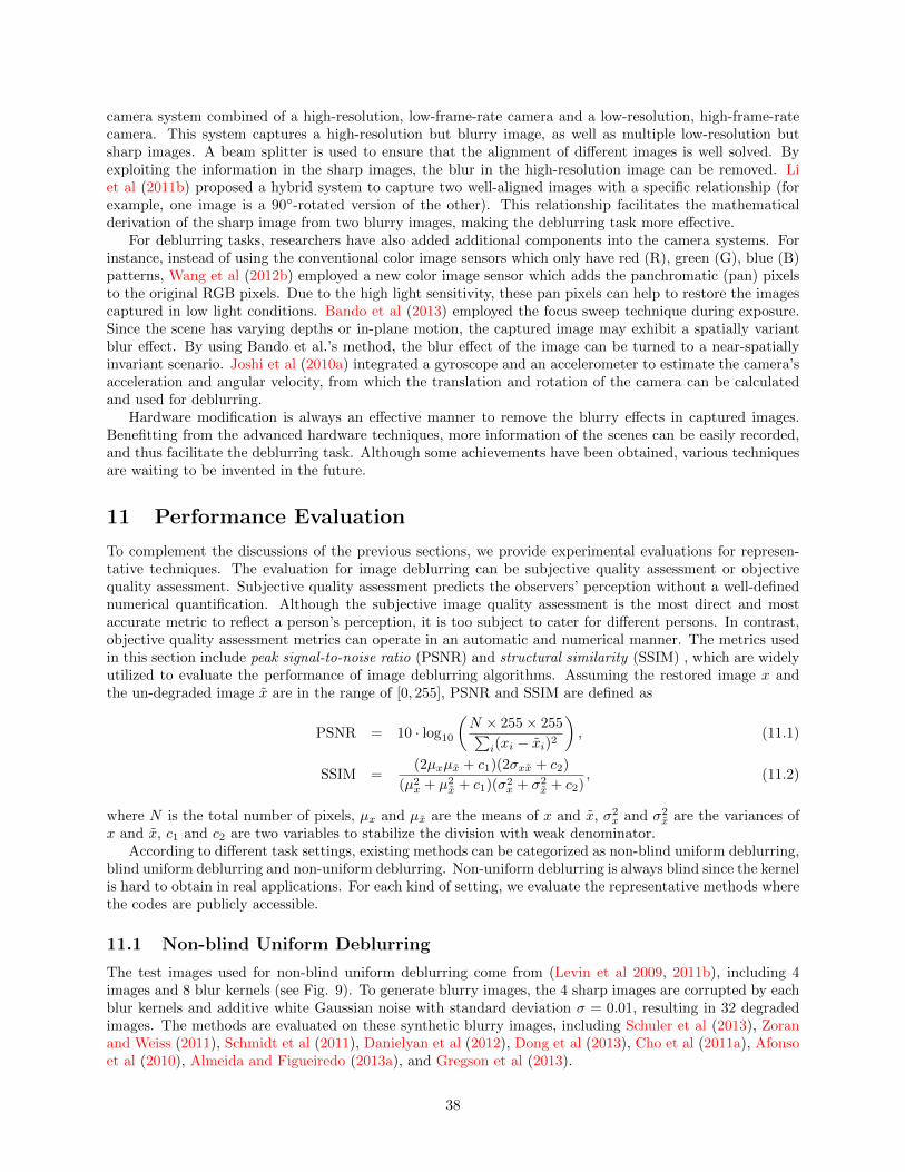
camera system combined of a high-resolution, low-frame-rate camera and a low-resolution, high-frame-ratecamera. This system captures a high-resolution but blurry image, as well as multiple low-resolution butsharp images. A beam splitter is used to ensure that the alignment of different images is well solved. Byexploiting the information in the sharp images, the blur in the high-resolution image can be removed. Liet al (2011b) proposed a hybrid system to capture two well-aligned images with a specific relationship (forexample, one image is a 90◦-rotated version of the other). This relationship facilitates the mathematicalderivation of the sharp image from two blurry images, making the deblurring task more effective.

For deblurring tasks, researchers have also added additional components into the camera systems. Forinstance, instead of using the conventional color image sensors which only have red (R), green (G), blue (B)patterns, Wang et al (2012b) employed a new color image sensor which adds the panchromatic (pan) pixelsto the original RGB pixels. Due to the high light sensitivity, these pan pixels can help to restore the imagescaptured in low light conditions. Bando et al (2013) employed the focus sweep technique during exposure.Since the scene has varying depths or in-plane motion, the captured image may exhibit a spatially variantblur effect. By using Bando et al.’s method, the blur effect of the image can be turned to a near-spatiallyinvariant scenario. Joshi et al (2010a) integrated a gyroscope and an accelerometer to estimate the camera’sacceleration and angular velocity, from which the translation and rotation of the camera can be calculatedand used for deblurring.

Hardware modification is always an effective manner to remove the blurry effects in captured images.Benefitting from the advanced hardware techniques, more information of the scenes can be easily recorded,and thus facilitate the deblurring task. Although some achievements have been obtained, various techniquesare waiting to be invented in the future.

11 Performance Evaluation

To complement the discussions of the previous sections, we provide experimental evaluations for represen-tative techniques. The evaluation for image deblurring can be subjective quality assessment or objectivequality assessment. Subjective quality assessment predicts the observers’ perception without a well-definednumerical quantification. Although the subjective image quality assessment is the most direct and mostaccurate metric to reflect a person’s perception, it is too subject to cater for different persons. In contrast,objective quality assessment metrics can operate in an automatic and numerical manner. The metrics usedin this section include peak signal-to-noise ratio (PSNR) and structural similarity (SSIM) , which are widelyutilized to evaluate the performance of image deblurring algorithms. Assuming the restored image x andthe un-degraded image x are in the range of [0, 255], PSNR and SSIM are defined as

PSNR = 10 · log10

(N × 255× 255∑

i(xi − xi)2

), (11.1)

SSIM =(2µxµx + c1)(2σxx + c2)

(µ2x + µ2

x + c1)(σ2x + σ2

x + c2), (11.2)

where N is the total number of pixels, µx and µx are the means of x and x, σ2x and σ2

x are the variances ofx and x, c1 and c2 are two variables to stabilize the division with weak denominator.

According to different task settings, existing methods can be categorized as non-blind uniform deblurring,blind uniform deblurring and non-uniform deblurring. Non-uniform deblurring is always blind since the kernelis hard to obtain in real applications. For each kind of setting, we evaluate the representative methods wherethe codes are publicly accessible.

11.1 Non-blind Uniform Deblurring

The test images used for non-blind uniform deblurring come from (Levin et al 2009, 2011b), including 4images and 8 blur kernels (see Fig. 9). To generate blurry images, the 4 sharp images are corrupted by eachblur kernels and additive white Gaussian noise with standard deviation σ = 0.01, resulting in 32 degradedimages. The methods are evaluated on these synthetic blurry images, including Schuler et al (2013), Zoranand Weiss (2011), Schmidt et al (2011), Danielyan et al (2012), Dong et al (2013), Cho et al (2011a), Afonsoet al (2010), Almeida and Figueiredo (2013a), and Gregson et al (2013).

38

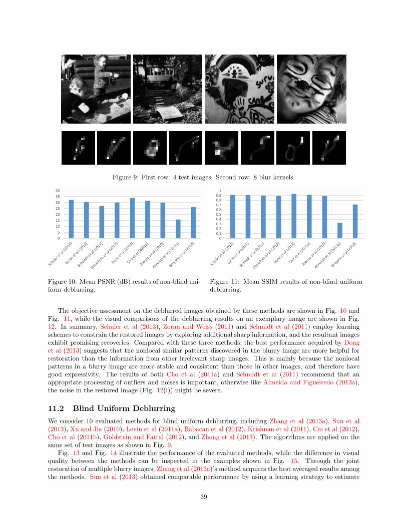
Figure 9: First row: 4 test images. Second row: 8 blur kernels.

05

10152025303540

Figure 10: Mean PSNR (dB) results of non-blind uni-form deblurring.

00.10.20.30.40.50.60.70.80.9

1

Figure 11: Mean SSIM results of non-blind uniformdeblurring.

The objective assessment on the deblurred images obtained by these methods are shown in Fig. 10 andFig. 11, while the visual comparisons of the deblurring results on an exemplary image are shown in Fig.12. In summary, Schuler et al (2013), Zoran and Weiss (2011) and Schmidt et al (2011) employ learningschemes to constrain the restored images by exploring additional sharp information, and the resultant imagesexhibit promising recoveries. Compared with these three methods, the best performance acquired by Donget al (2013) suggests that the nonlocal similar patterns discovered in the blurry image are more helpful forrestoration than the information from other irrelevant sharp images. This is mainly because the nonlocalpatterns in a blurry image are more stable and consistent than those in other images, and therefore havegood expressivity. The results of both Cho et al (2011a) and Schmidt et al (2011) recommend that anappropriate processing of outliers and noises is important, otherwise like Almeida and Figueiredo (2013a),the noise in the restored image (Fig. 12(i)) might be severe.

11.2 Blind Uniform Deblurring

We consider 10 evaluated methods for blind uniform deblurring, including Zhang et al (2013a), Sun et al(2013), Xu and Jia (2010), Levin et al (2011a), Babacan et al (2012), Krishnan et al (2011), Cai et al (2012),Cho et al (2011b), Goldstein and Fattal (2012), and Zhong et al (2013). The algorithms are applied on thesame set of test images as shown in Fig. 9.

Fig. 13 and Fig. 14 illustrate the performance of the evaluated methods, while the difference in visualquality between the methods can be inspected in the examples shown in Fig. 15. Through the jointrestoration of multiple blurry images, Zhang et al (2013a)’s method acquires the best averaged results amongthe methods. Sun et al (2013) obtained comparable performance by using a learning strategy to estimate

39

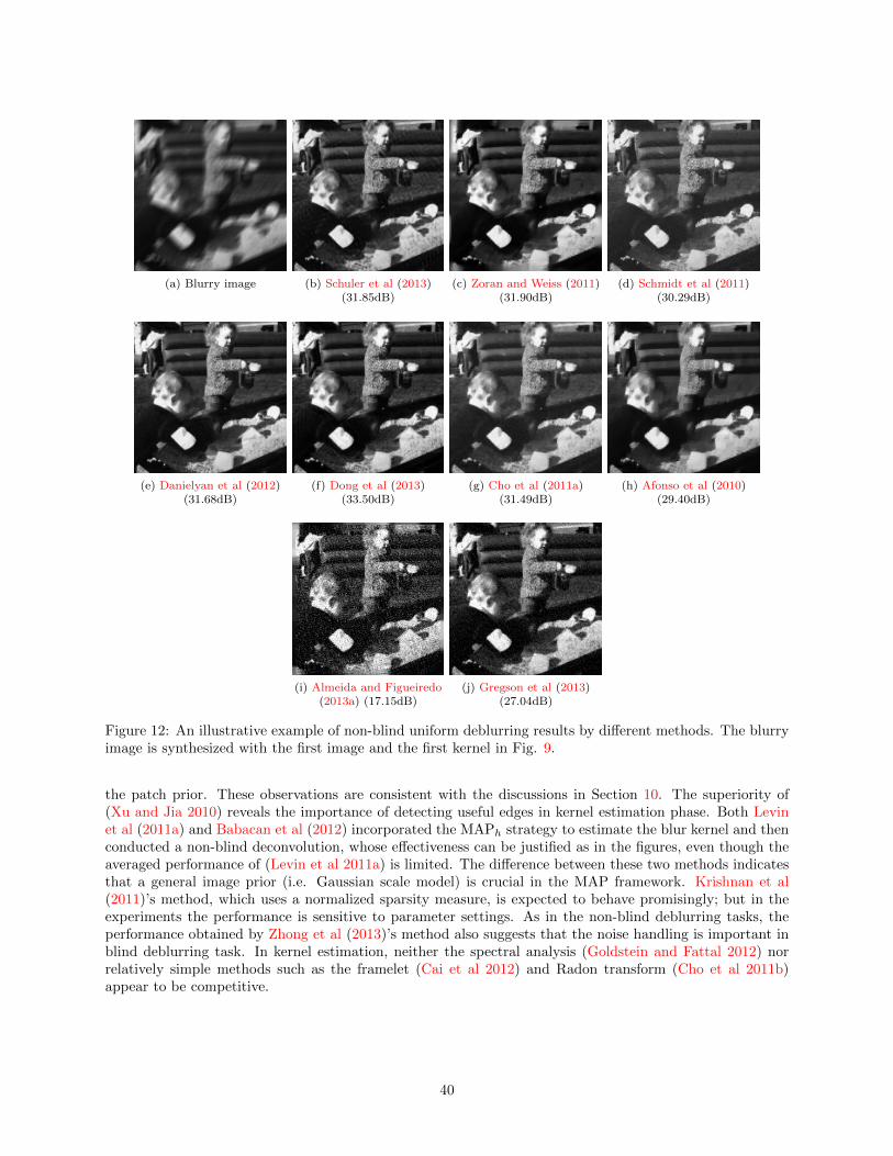
(a) Blurry image (b) Schuler et al (2013)(31.85dB)

(c) Zoran and Weiss (2011)(31.90dB)

(d) Schmidt et al (2011)(30.29dB)

(e) Danielyan et al (2012)(31.68dB)

(f) Dong et al (2013)(33.50dB)

(g) Cho et al (2011a)(31.49dB)

(h) Afonso et al (2010)(29.40dB)

(i) Almeida and Figueiredo(2013a) (17.15dB)

(j) Gregson et al (2013)(27.04dB)

Figure 12: An illustrative example of non-blind uniform deblurring results by different methods. The blurryimage is synthesized with the first image and the first kernel in Fig. 9.

the patch prior. These observations are consistent with the discussions in Section 10. The superiority of(Xu and Jia 2010) reveals the importance of detecting useful edges in kernel estimation phase. Both Levinet al (2011a) and Babacan et al (2012) incorporated the MAPh strategy to estimate the blur kernel and thenconducted a non-blind deconvolution, whose effectiveness can be justified as in the figures, even though theaveraged performance of (Levin et al 2011a) is limited. The difference between these two methods indicatesthat a general image prior (i.e. Gaussian scale model) is crucial in the MAP framework. Krishnan et al(2011)’s method, which uses a normalized sparsity measure, is expected to behave promisingly; but in theexperiments the performance is sensitive to parameter settings. As in the non-blind deblurring tasks, theperformance obtained by Zhong et al (2013)’s method also suggests that the noise handling is important inblind deblurring task. In kernel estimation, neither the spectral analysis (Goldstein and Fattal 2012) norrelatively simple methods such as the framelet (Cai et al 2012) and Radon transform (Cho et al 2011b)appear to be competitive.

40

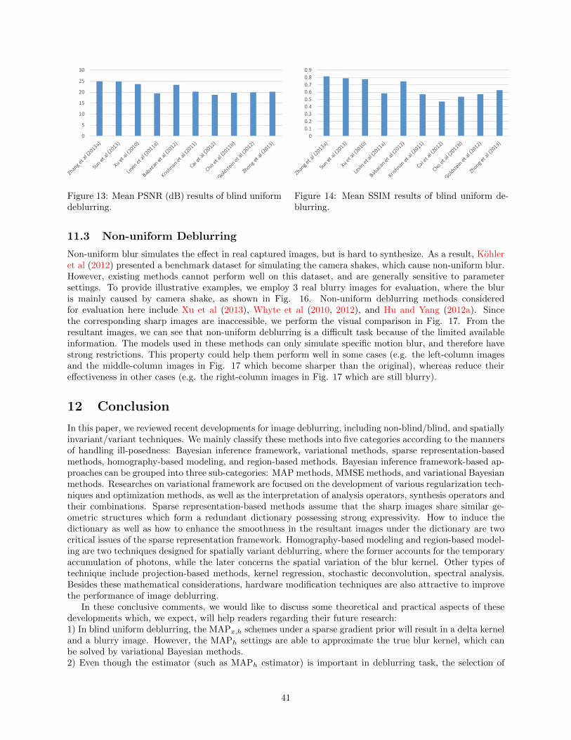
0

5

10

15

20

25

30

Figure 13: Mean PSNR (dB) results of blind uniformdeblurring.

00.10.20.30.40.50.60.70.80.9

Figure 14: Mean SSIM results of blind uniform de-blurring.

11.3 Non-uniform Deblurring

Non-uniform blur simulates the effect in real captured images, but is hard to synthesize. As a result, Kohleret al (2012) presented a benchmark dataset for simulating the camera shakes, which cause non-uniform blur.However, existing methods cannot perform well on this dataset, and are generally sensitive to parametersettings. To provide illustrative examples, we employ 3 real blurry images for evaluation, where the bluris mainly caused by camera shake, as shown in Fig. 16. Non-uniform deblurring methods consideredfor evaluation here include Xu et al (2013), Whyte et al (2010, 2012), and Hu and Yang (2012a). Sincethe corresponding sharp images are inaccessible, we perform the visual comparison in Fig. 17. From theresultant images, we can see that non-uniform deblurring is a difficult task because of the limited availableinformation. The models used in these methods can only simulate specific motion blur, and therefore havestrong restrictions. This property could help them perform well in some cases (e.g. the left-column imagesand the middle-column images in Fig. 17 which become sharper than the original), whereas reduce theireffectiveness in other cases (e.g. the right-column images in Fig. 17 which are still blurry).

12 Conclusion

In this paper, we reviewed recent developments for image deblurring, including non-blind/blind, and spatiallyinvariant/variant techniques. We mainly classify these methods into five categories according to the mannersof handling ill-posedness: Bayesian inference framework, variational methods, sparse representation-basedmethods, homography-based modeling, and region-based methods. Bayesian inference framework-based ap-proaches can be grouped into three sub-categories: MAP methods, MMSE methods, and variational Bayesianmethods. Researches on variational framework are focused on the development of various regularization tech-niques and optimization methods, as well as the interpretation of analysis operators, synthesis operators andtheir combinations. Sparse representation-based methods assume that the sharp images share similar ge-ometric structures which form a redundant dictionary possessing strong expressivity. How to induce thedictionary as well as how to enhance the smoothness in the resultant images under the dictionary are twocritical issues of the sparse representation framework. Homography-based modeling and region-based model-ing are two techniques designed for spatially variant deblurring, where the former accounts for the temporaryaccumulation of photons, while the later concerns the spatial variation of the blur kernel. Other types oftechnique include projection-based methods, kernel regression, stochastic deconvolution, spectral analysis.Besides these mathematical considerations, hardware modification techniques are also attractive to improvethe performance of image deblurring.

In these conclusive comments, we would like to discuss some theoretical and practical aspects of thesedevelopments which, we expect, will help readers regarding their future research:1) In blind uniform deblurring, the MAPx,h schemes under a sparse gradient prior will result in a delta kerneland a blurry image. However, the MAPh settings are able to approximate the true blur kernel, which canbe solved by variational Bayesian methods.2) Even though the estimator (such as MAPh estimator) is important in deblurring task, the selection of

41

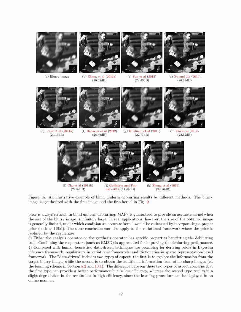
(a) Blurry image (b) Zhang et al (2013a)(26.35dB)

(c) Sun et al (2013)(28.40dB)

(d) Xu and Jia (2010)(26.09dB)

(e) Levin et al (2011a)(29.16dB)

(f) Babacan et al (2012)(28.39dB)

(g) Krishnan et al (2011)(22.71dB)

(h) Cai et al (2012)(22.12dB)

(i) Cho et al (2011b)(22.84dB)

(j) Goldstein and Fat-tal (2012)(21.47dB)

(k) Zhong et al (2013)(24.90dB)

Figure 15: An illustrative example of blind uniform deblurring results by different methods. The blurryimage is synthesized with the first image and the first kernel in Fig. 9.

prior is always critical. In blind uniform deblurring, MAPh is guaranteed to provide an accurate kernel whenthe size of the blurry image is infinitely large. In real applications, however, the size of the obtained imageis generally limited, under which condition an accurate kernel would be estimated by incorporating a properprior (such as GSM). The same conclusion can also apply to the variational framework where the prior isreplaced by the regularizer.3) Either the analysis operator or the synthesis operator has specific properties benefitting the deblurringtask. Combining these operators (such as BM3D) is appreciated for improving the deblurring performance.4) Compared with human heuristics, data-driven techniques are promising for deriving priors in Bayesianinference framework, regularizers in variational framework, and dictionaries in sparse representation-basedframework. The ”data-driven” includes two types of aspect: the first is to explore the information from thetarget blurry image, while the second is to obtain the additional information from other sharp images (cf.the learning scheme in Section 5.2 and 10.1). The difference between these two types of aspect concerns thatthe first type can provide a better performance but in low efficiency, whereas the second type results in aslight degradation in the results but in high efficiency, since the learning procedure can be deployed in anoffline manner.

42

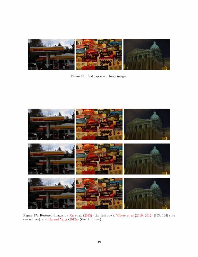
Figure 16: Real captured blurry images.

Figure 17: Restored images by Xu et al (2013) (the first row), Whyte et al (2010, 2012) [103, 104] (thesecond row), and Hu and Yang (2012a) (the third row).

43

5) For deblurring, since an images can be viewed as a composition of large amount of repetitive patterns,exploiting the repetitive nature of images, which is often termed as a non-local strategy, is an effective way toboost the deblurring performance. This has been already proven in various image processing tasks includingimage deblurring, image denoising, image super-resolution, etc. Besides, the conventional local strategiescan overcome a common issue of the non-local strategies that is the loss of local smoothness. Therefore, thecombination of local and non-local strategies is recommended.6) Spatially variant deblurring is a difficult task and the progress in this aspect is very limited. Incorporatinga certain physical model (such as the modeling of object motion and the modeling of camera motion) is anoption to improve the performance. However, this cannot satisfy the complex conditions in real applications.7) Benefitting from the massive high-quality images available on the Internet and the advanced technologiesof hardware, extra information can be recorded and employed for the subsequent deblurring as well asother restoration tasks. Learning-based deblurring and hardware modifications are therefore two promisingdirections to improve the performance of image deblurring.8) Image deblurring is a crucial step to produce high-quality images for high-level vision tasks. However,when limited information is accessible, the deblurring performance could be restricted. In this case, arecommended option is to combine image deblurring and high-level vision tasks into a unified problem, suchas classification of blurry images and detection of blurry objects. Then the deblurring task can benefit fromthe high-level vision tasks because they are generally human supervised. Therefore, the cross informationamong the images and among the tasks are worth to be exploited.

References

Afonso MV, Bioucas-Dias JM, Figueiredo MA (2010) Fast image recovery using variable splitting and con-strained optimization. IEEE Transactions on Image Processing 19(9):2345–2356

Aharon M, Elad M, Bruckstein A (2006) K-svd: An algorithm for designing overcomplete dictionaries forsparse representation. IEEE Transactions on Signal Processing 54(11):4311–4322

Almeida MS, Almeida LB (2010) Blind and semi-blind deblurring of natural images. IEEE Transactions onImage Processing 19(1):36–52

Almeida MS, Figueiredo MA (2013a) Deconvolving images with unknown boundaries using the alternatingdirection method of multipliers. IEEE Transactions on Image Processing 22(8):3074–3086

Almeida MS, Figueiredo MA (2013b) Parameter estimation for blind and non-blind deblurring using residualwhiteness measures. IEEE Transactions on Image Processing 22(7):2751–2763

Amizic B, Spinoulas L, Molina R, Katsaggelos AK (2013) Compressive blind image deconvolution. IEEETransactions on Image Processing 22(10):3994–4006

Arbelaez P, Maire M, Fowlkes C, Malik J (2011) Contour detection and hierarchical image segmentation.IEEE Transactions on Pattern Analysis and Machine Intelligence 33(5):898–916

Babacan SD, Molina R, Do MN, Katsaggelos AK (2012) Bayesian blind deconvolution with general sparseimage priors. In: Proceedings of European Conference on Computer Vision, pp 341–355

Bando Y, Holtzman H, Raskar R (2013) Near-invariant blur for depth and 2d motion via time-varying lightfield analysis. ACM Transactions on Graphics 32(2):13:1–13:15

Barbero A, Sra S (2011) Fast newton-type methods for total variation regularization. In: Proceedings ofInternational Conference on Machine Learning, pp 313–320

Beck A, Teboulle M (2009) A fast iterative shrinkage-thresholding algorithm for linear inverse problems.SIAM Journal on Imaging Sciences 2(1):183–202

Bertero M, Boccacci P (1998) Introduction to Inverse Problems in Imaging. CRC press

44

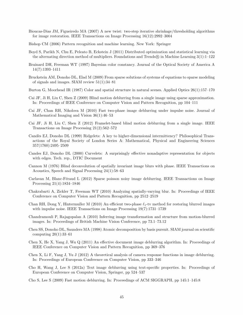
Bioucas-Dias JM, Figueiredo MA (2007) A new twist: two-step iterative shrinkage/thresholding algorithmsfor image restoration. IEEE Transactions on Image Processing 16(12):2992–3004

Bishop CM (2006) Pattern recognition and machine learning. New York: Springer

Boyd S, Parikh N, Chu E, Peleato B, Eckstein J (2011) Distributed optimization and statistical learning viathe alternating direction method of multipliers. Foundations and Trends R© in Machine Learning 3(1):1–122

Brainard DH, Freeman WT (1997) Bayesian color constancy. Journal of the Optical Society of America A14(7):1393–1411

Bruckstein AM, Donoho DL, Elad M (2009) From sparse solutions of systems of equations to sparse modelingof signals and images. SIAM review 51(1):34–81

Burton G, Moorhead IR (1987) Color and spatial structure in natural scenes. Applied Optics 26(1):157–170

Cai JF, Ji H, Liu C, Shen Z (2009) Blind motion deblurring from a single image using sparse approximation.In: Proceedings of IEEE Conference on Computer Vision and Pattern Recognition, pp 104–111

Cai JF, Chan RH, Nikolova M (2010) Fast two-phase image deblurring under impulse noise. Journal ofMathematical Imaging and Vision 36(1):46–53

Cai JF, Ji H, Liu C, Shen Z (2012) Framelet-based blind motion deblurring from a single image. IEEETransactions on Image Processing 21(2):562–572

Candes EJ, Donoho DL (1999) Ridgelets: A key to higher-dimensional intermittency? Philosophical Trans-actions of the Royal Society of London Series A: Mathematical, Physical and Engineering Sciences357(1760):2495–2509

Candes EJ, Donoho DL (2000) Curvelets: A surprisingly effective nonadaptive representation for objectswith edges. Tech. rep., DTIC Document

Cannon M (1976) Blind deconvolution of spatially invariant image blurs with phase. IEEE Transactions onAcoustics, Speech and Signal Processing 24(1):58–63

Carlavan M, Blanc-Feraud L (2012) Sparse poisson noisy image deblurring. IEEE Transactions on ImageProcessing 21(4):1834–1846

Chakrabarti A, Zickler T, Freeman WT (2010) Analyzing spatially-varying blur. In: Proceedings of IEEEConference on Computer Vision and Pattern Recognition, pp 2512–2519

Chan RH, Dong Y, Hintermuller M (2010) An efficient two-phase `1-tv method for restoring blurred imageswith impulse noise. IEEE Transactions on Image Processing 19(7):1731–1739

Chandramouli P, Rajagopalan A (2010) Inferring image transformation and structure from motion-blurredimages. In: Proceedings of British Machine Vision Conference, pp 73.1–73.12

Chen SS, Donoho DL, Saunders MA (1998) Atomic decomposition by basis pursuit. SIAM journal on scientificcomputing 20(1):33–61

Chen X, He X, Yang J, Wu Q (2011) An effective document image deblurring algorithm. In: Proceedings ofIEEE Conference on Computer Vision and Pattern Recognition, pp 369–376

Chen X, Li F, Yang J, Yu J (2012) A theoretical analysis of camera response functions in image deblurring.In: Proceedings of European Conference on Computer Vision, pp 333–346

Cho H, Wang J, Lee S (2012a) Text image deblurring using text-specific properties. In: Proceedings ofEuropean Conference on Computer Vision, Springer, pp 524–537

Cho S, Lee S (2009) Fast motion deblurring. In: Proceedings of ACM SIGGRAPH, pp 145:1–145:8

45

Cho S, Wang J, Lee S (2011a) Handling outliers in non-blind image deconvolution. In: Proceedings of IEEEInternational Conference on Computer Vision, pp 495–502

Cho S, Cho H, Tai YW, Lee S (2012b) Registration based non-uniform motion deblurring. Computer GraphicsForum 31(7):2183–2192

Cho TS, Joshi N, Zitnick CL, Kang SB, Szeliski R, Freeman WT (2010a) A content-aware image prior. In:Proceedings of IEEE Conference on Computer Vision and Pattern Recognition, pp 169–176

Cho TS, Levin A, Durand F, Freeman WT (2010b) Motion blur removal with orthogonal parabolic exposures.In: IEEE International Conference on Computational Photography, pp 1–8

Cho TS, Paris S, Horn BK, Freeman WT (2011b) Blur kernel estimation using the radon transform. In:Proceedings of IEEE Conference on Computer Vision and Pattern Recognition, pp 241–248

Cho TS, Zitnick CL, Joshi N, Kang SB, Szeliski R, Freeman WT (2012c) Image restoration by matchinggradient distributions. IEEE Transactions on Pattern Analysis and Machine Intelligence 34(4):683–694

Couzinie-Devy F, Sun J, Alahari K, Ponce J (2013) Learning to estimate and remove non-uniform imageblur. In: Proceedings of IEEE Conference on Computer Vision and Pattern Recognition, pp 1075–1082

Dabov K, Foi A, Katkovnik V, Egiazarian K (2007) Image denoising by sparse 3-d transform-domain col-laborative filtering. IEEE Transactions on Image Processing 16(8):2080–2095

Danielyan A, Katkovnik V, Egiazarian K (2010) Image deblurring by augmented lagrangian with bm3d frameprior. In: Workshop on Information Theoretic Methods in Science and Engineering, Tampere, Finland,pp 16–18

Danielyan A, Katkovnik V, Egiazarian K (2012) Bm3d frames and variational image deblurring. IEEETransactions on Image Processing 21(4):1715–1728

Delbracio M, Muse P, Almansa A, Morel JM (2012) The non-parametric sub-pixel local point spread functionestimation is a well posed problem. International journal of computer vision 96(2):175–194

Deng J, Dong W, Socher R, Li LJ, Li K, Fei-Fei L (2009) Imagenet: A large-scale hierarchical image database.In: Proceedings of IEEE Conference on Computer Vision and Pattern Recognition, pp 248–255

Ding Y, McCloskey S, Yu J (2010) Analysis of motion blur with a flutter shutter camera for non-linearmotion. In: Proceedings of European Conference on Computer Vision, pp 15–30

Do MN, Vetterli M (2005) The contourlet transform: an efficient directional multiresolution image represen-tation. IEEE Transactions on Image Processing 14(12):2091–2106

Dong W, Zhang L, Shi G (2011a) Centralized sparse representation for image restoration. In: Proceedingsof IEEE International Conference on Computer Vision, pp 1259–1266

Dong W, Zhang L, Shi G, Wu X (2011b) Image deblurring and super-resolution by adaptive sparse domainselection and adaptive regularization. IEEE Transactions on Image Processing 20(7):1838–1857

Dong W, Zhang L, Shi G, Li X (2013) Nonlocally centralized sparse representation for image restoration.IEEE Transactions on Image Processing 22(4):1620–1630

Donoho DL, Johnstone JM (1994) Ideal spatial adaptation by wavelet shrinkage. Biometrika 81(3):425–455

Elad M (2010) Sparse and redundant representations: from theory to applications in signal and imageprocessing. Springer

Elad M, Aharon M (2006) Image denoising via sparse and redundant representations over learned dictionaries.IEEE Transactions on Image Processing 15(12):3736–3745

Elad M, Starck JL, Querre P, Donoho DL (2005) Simultaneous cartoon and texture image inpainting usingmorphological component analysis (mca). Applied and Computational Harmonic Analysis 19(3):340–358

46

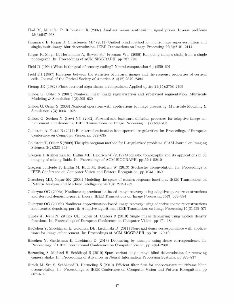
Elad M, Milanfar P, Rubinstein R (2007) Analysis versus synthesis in signal priors. Inverse problems23(3):947–968

Faramarzi E, Rajan D, Christensen MP (2013) Unified blind method for multi-image super-resolution andsingle/multi-image blur deconvolution. IEEE Transactions on Image Processing 22(6):2101–2114

Fergus R, Singh B, Hertzmann A, Roweis ST, Freeman WT (2006) Removing camera shake from a singlephotograph. In: Proceedings of ACM SIGGRAPH, pp 787–794

Field D (1994) What is the goal of sensory coding? Neural computation 6(4):559–601

Field DJ (1987) Relations between the statistics of natural images and the response properties of corticalcells. Journal of the Optical Society of America A 4(12):2379–2394

Fienup JR (1982) Phase retrieval algorithms: a comparison. Applied optics 21(15):2758–2769

Gilboa G, Osher S (2007) Nonlocal linear image regularization and supervised segmentation. MultiscaleModeling & Simulation 6(2):595–630

Gilboa G, Osher S (2008) Nonlocal operators with applications to image processing. Multiscale Modeling &Simulation 7(3):1005–1028

Gilboa G, Sochen N, Zeevi YY (2002) Forward-and-backward diffusion processes for adaptive image en-hancement and denoising. IEEE Transactions on Image Processing 11(7):689–703

Goldstein A, Fattal R (2012) Blur-kernel estimation from spectral irregularities. In: Proceedings of EuropeanConference on Computer Vision, pp 622–635

Goldstein T, Osher S (2009) The split bregman method for l1-regularized problems. SIAM Journal on ImagingSciences 2(2):323–343

Gregson J, Krimerman M, Hullin MB, Heidrich W (2012) Stochastic tomography and its applications in 3dimaging of mixing fluids. In: Proceedings of ACM SIGGRAPH, pp 52:1–52:10

Gregson J, Heide F, Hullin M, Rouf M, Heidrich W (2013) Stochastic deconvolution. In: Proceedings ofIEEE Conference on Computer Vision and Pattern Recognition, pp 1043–1050

Grossberg MD, Nayar SK (2004) Modeling the space of camera response functions. IEEE Transactions onPattern Analysis and Machine Intelligence 26(10):1272–1282

Guleryuz OG (2006a) Nonlinear approximation based image recovery using adaptive sparse reconstructionsand iterated denoising-part i: theory. IEEE Transactions on Image Processing 15(3):539–554

Guleryuz OG (2006b) Nonlinear approximation based image recovery using adaptive sparse reconstructionsand iterated denoising-part ii: Adaptive algorithms. IEEE Transactions on Image Processing 15(3):555–571

Gupta A, Joshi N, Zitnick CL, Cohen M, Curless B (2010) Single image deblurring using motion densityfunctions. In: Proceedings of European Conference on Computer Vision, pp 171–184

HaCohen Y, Shechtman E, Goldman DB, Lischinski D (2011) Non-rigid dense correspondence with applica-tions for image enhancement. In: Proceedings of ACM SIGGRAPH, pp 70:1–70:10

Hacohen Y, Shechtman E, Lischinski D (2013) Deblurring by example using dense correspondence. In:Proceedings of IEEE International Conference on Computer Vision, pp 2384–2391

Harmeling S, Michael H, Scholkopf B (2010) Space-variant single-image blind deconvolution for removingcamera shake. In: Proceedings of Advances in Neural Information Processing Systems, pp 829–837

Hirsch M, Sra S, Scholkopf B, Harmeling S (2010) Efficient filter flow for space-variant multiframe blinddeconvolution. In: Proceedings of IEEE Conference on Computer Vision and Pattern Recognition, pp607–614

47

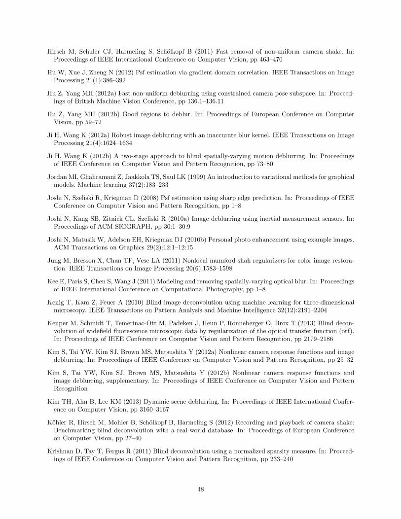
Hirsch M, Schuler CJ, Harmeling S, Scholkopf B (2011) Fast removal of non-uniform camera shake. In:Proceedings of IEEE International Conference on Computer Vision, pp 463–470

Hu W, Xue J, Zheng N (2012) Psf estimation via gradient domain correlation. IEEE Transactions on ImageProcessing 21(1):386–392

Hu Z, Yang MH (2012a) Fast non-uniform deblurring using constrained camera pose subspace. In: Proceed-ings of British Machine Vision Conference, pp 136.1–136.11

Hu Z, Yang MH (2012b) Good regions to deblur. In: Proceedings of European Conference on ComputerVision, pp 59–72

Ji H, Wang K (2012a) Robust image deblurring with an inaccurate blur kernel. IEEE Transactions on ImageProcessing 21(4):1624–1634

Ji H, Wang K (2012b) A two-stage approach to blind spatially-varying motion deblurring. In: Proceedingsof IEEE Conference on Computer Vision and Pattern Recognition, pp 73–80

Jordan MI, Ghahramani Z, Jaakkola TS, Saul LK (1999) An introduction to variational methods for graphicalmodels. Machine learning 37(2):183–233

Joshi N, Szeliski R, Kriegman D (2008) Psf estimation using sharp edge prediction. In: Proceedings of IEEEConference on Computer Vision and Pattern Recognition, pp 1–8

Joshi N, Kang SB, Zitnick CL, Szeliski R (2010a) Image deblurring using inertial measurement sensors. In:Proceedings of ACM SIGGRAPH, pp 30:1–30:9

Joshi N, Matusik W, Adelson EH, Kriegman DJ (2010b) Personal photo enhancement using example images.ACM Transactions on Graphics 29(2):12:1–12:15

Jung M, Bresson X, Chan TF, Vese LA (2011) Nonlocal mumford-shah regularizers for color image restora-tion. IEEE Transactions on Image Processing 20(6):1583–1598

Kee E, Paris S, Chen S, Wang J (2011) Modeling and removing spatially-varying optical blur. In: Proceedingsof IEEE International Conference on Computational Photography, pp 1–8

Kenig T, Kam Z, Feuer A (2010) Blind image deconvolution using machine learning for three-dimensionalmicroscopy. IEEE Transactions on Pattern Analysis and Machine Intelligence 32(12):2191–2204

Keuper M, Schmidt T, Temerinac-Ott M, Padeken J, Heun P, Ronneberger O, Brox T (2013) Blind decon-volution of widefield fluorescence microscopic data by regularization of the optical transfer function (otf).In: Proceedings of IEEE Conference on Computer Vision and Pattern Recognition, pp 2179–2186

Kim S, Tai YW, Kim SJ, Brown MS, Matsushita Y (2012a) Nonlinear camera response functions and imagedeblurring. In: Proceedings of IEEE Conference on Computer Vision and Pattern Recognition, pp 25–32

Kim S, Tai YW, Kim SJ, Brown MS, Matsushita Y (2012b) Nonlinear camera response functions andimage deblurring, supplementary. In: Proceedings of IEEE Conference on Computer Vision and PatternRecognition

Kim TH, Ahn B, Lee KM (2013) Dynamic scene deblurring. In: Proceedings of IEEE International Confer-ence on Computer Vision, pp 3160–3167

Kohler R, Hirsch M, Mohler B, Scholkopf B, Harmeling S (2012) Recording and playback of camera shake:Benchmarking blind deconvolution with a real-world database. In: Proceedings of European Conferenceon Computer Vision, pp 27–40

Krishnan D, Tay T, Fergus R (2011) Blind deconvolution using a normalized sparsity measure. In: Proceed-ings of IEEE Conference on Computer Vision and Pattern Recognition, pp 233–240

48

Landweber L (1951) An iteration formula for fredholm integral equations of the first kind. American Journalof Mathematics 73(3):615–624

Lefkimmiatis S, Unser M (2013) Poisson image reconstruction with hessian schatten-norm regularization.IEEE Transactions on Image Processing 22(11):4314–4327

Lefkimmiatis S, Bourquard A, Unser M (2012) Hessian-based norm regularization for image restoration withbiomedical applications. IEEE Transactions on Image Processing 21(3):983–995

Levin A (2006) Blind motion deblurring using image statistics. In: Proceedings of Advances in NeuralInformation Processing Systems, pp 841–848

Levin A, Fergus R, Durand F, Freeman WT (2007) Image and depth from a conventional camera with acoded aperture. In: Proceedings of ACM SIGGRAPH

Levin A, Weiss Y, Durand F, Freeman WT (2009) Understanding and evaluating blind deconvolution algo-rithms. In: Proceedings of IEEE Conference on Computer Vision and Pattern Recognition, pp 1964–1971

Levin A, Weiss Y, Durand F, Freeman WT (2011a) Efficient marginal likelihood optimization in blinddeconvolution. In: Proceedings of IEEE Conference on Computer Vision and Pattern Recognition, pp2657–2664

Levin A, Weiss Y, Durand F, Freeman WT (2011b) Understanding blind deconvolution algorithms. IEEETransactions on Pattern Analysis and Machine Intelligence 33(12):2354–2367

Li F, Li Z, Saunders D, Yu J (2011a) A theory of coprime blurred pairs. In: Proceedings of IEEE InternationalConference on Computer Vision, pp 217–224

Li W, Zhang J, Dai Q (2011b) Exploring aligned complementary image pair for blind motion deblurring. In:Proceedings of IEEE Conference on Computer Vision and Pattern Recognition, pp 273–280

Li X (2011) Fine-granularity and spatially-adaptive regularization for projection-based image deblurring.IEEE Transactions on Image Processing 20(4):971–983

Lin S, Zhang L (2005) Determining the radiometric response function from a single grayscale image. In:Proceedings of IEEE Conference on Computer Vision and Pattern Recognition, pp 66–73

Lou Y, Zhang X, Osher S, Bertozzi A (2010) Image recovery via nonlocal operators. Journal of ScientificComputing 42(2):185–197

Lucy LB (1974) An iterative technique for the rectification of observed distributions. The astronomicaljournal 79:745–754

Luke DR (2005) Relaxed averaged alternating reflections for diffraction imaging. Inverse Problems 21(1):37–50

Ma J, Le Dimet FX (2009) Deblurring from highly incomplete measurements for remote sensing. IEEETransactions on Geoscience and Remote Sensing 47(3):792–802

Ma L, Moisan L, Yu J, Zeng T (2013) A dictionary learning approach for poisson image deblurring. IEEETransactions on Medical Imaging 32(7):1277–1289

Matakos A, Ramani S, Fessler JA (2013) Accelerated edge-preserving image restoration without boundaryartifacts. IEEE Transactions on Image Processing 22(5):2019–2029

McCloskey S (2010) Velocity-dependent shutter sequences for motion deblurring. In: Proceedings of Euro-pean Conference on Computer Vision, pp 309–322

McCloskey S (2011) Temporally coded flash illumination for motion deblurring. In: Proceedings of IEEEInternational Conference on Computer Vision, pp 683–690

49

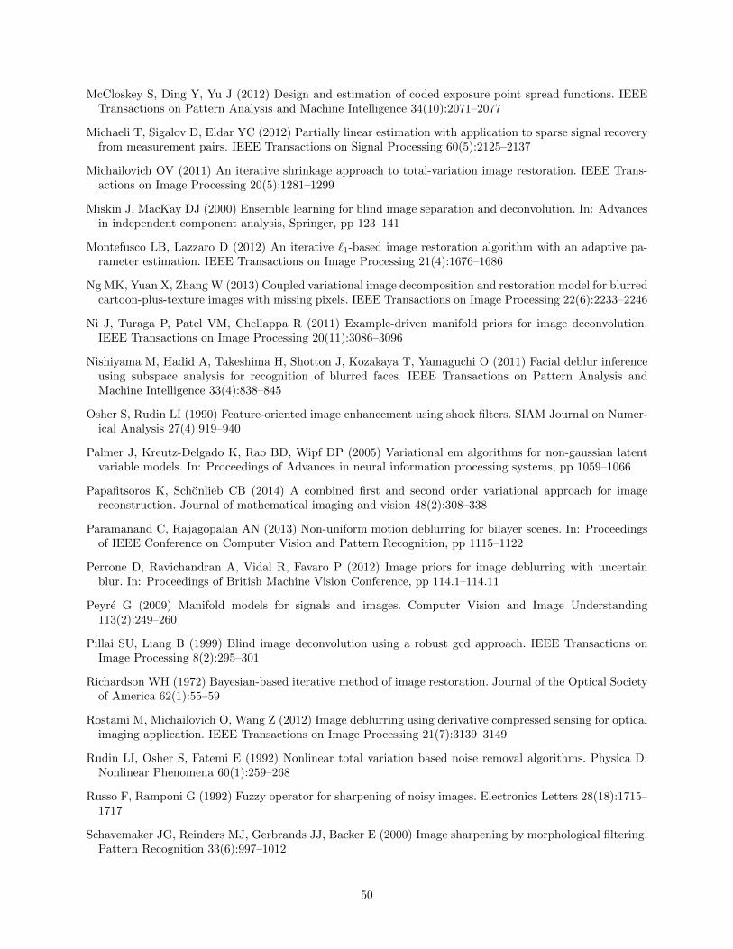
McCloskey S, Ding Y, Yu J (2012) Design and estimation of coded exposure point spread functions. IEEETransactions on Pattern Analysis and Machine Intelligence 34(10):2071–2077

Michaeli T, Sigalov D, Eldar YC (2012) Partially linear estimation with application to sparse signal recoveryfrom measurement pairs. IEEE Transactions on Signal Processing 60(5):2125–2137

Michailovich OV (2011) An iterative shrinkage approach to total-variation image restoration. IEEE Trans-actions on Image Processing 20(5):1281–1299

Miskin J, MacKay DJ (2000) Ensemble learning for blind image separation and deconvolution. In: Advancesin independent component analysis, Springer, pp 123–141

Montefusco LB, Lazzaro D (2012) An iterative `1-based image restoration algorithm with an adaptive pa-rameter estimation. IEEE Transactions on Image Processing 21(4):1676–1686

Ng MK, Yuan X, Zhang W (2013) Coupled variational image decomposition and restoration model for blurredcartoon-plus-texture images with missing pixels. IEEE Transactions on Image Processing 22(6):2233–2246

Ni J, Turaga P, Patel VM, Chellappa R (2011) Example-driven manifold priors for image deconvolution.IEEE Transactions on Image Processing 20(11):3086–3096

Nishiyama M, Hadid A, Takeshima H, Shotton J, Kozakaya T, Yamaguchi O (2011) Facial deblur inferenceusing subspace analysis for recognition of blurred faces. IEEE Transactions on Pattern Analysis andMachine Intelligence 33(4):838–845

Osher S, Rudin LI (1990) Feature-oriented image enhancement using shock filters. SIAM Journal on Numer-ical Analysis 27(4):919–940

Palmer J, Kreutz-Delgado K, Rao BD, Wipf DP (2005) Variational em algorithms for non-gaussian latentvariable models. In: Proceedings of Advances in neural information processing systems, pp 1059–1066

Papafitsoros K, Schonlieb CB (2014) A combined first and second order variational approach for imagereconstruction. Journal of mathematical imaging and vision 48(2):308–338

Paramanand C, Rajagopalan AN (2013) Non-uniform motion deblurring for bilayer scenes. In: Proceedingsof IEEE Conference on Computer Vision and Pattern Recognition, pp 1115–1122

Perrone D, Ravichandran A, Vidal R, Favaro P (2012) Image priors for image deblurring with uncertainblur. In: Proceedings of British Machine Vision Conference, pp 114.1–114.11

Peyre G (2009) Manifold models for signals and images. Computer Vision and Image Understanding113(2):249–260

Pillai SU, Liang B (1999) Blind image deconvolution using a robust gcd approach. IEEE Transactions onImage Processing 8(2):295–301

Richardson WH (1972) Bayesian-based iterative method of image restoration. Journal of the Optical Societyof America 62(1):55–59

Rostami M, Michailovich O, Wang Z (2012) Image deblurring using derivative compressed sensing for opticalimaging application. IEEE Transactions on Image Processing 21(7):3139–3149

Rudin LI, Osher S, Fatemi E (1992) Nonlinear total variation based noise removal algorithms. Physica D:Nonlinear Phenomena 60(1):259–268

Russo F, Ramponi G (1992) Fuzzy operator for sharpening of noisy images. Electronics Letters 28(18):1715–1717

Schavemaker JG, Reinders MJ, Gerbrands JJ, Backer E (2000) Image sharpening by morphological filtering.Pattern Recognition 33(6):997–1012

50

Schmidt U, Gao Q, Roth S (2010) A generative perspective on mrfs in low-level vision. In: Proceedings ofIEEE Conference on Computer Vision and Pattern Recognition, pp 1751–1758

Schmidt U, Schelten K, Roth S (2011) Bayesian deblurring with integrated noise estimation. In: Proceedingsof IEEE Conference on Computer Vision and Pattern Recognition, pp 2625–2632

Schmidt U, Rother C, Nowozin S, Jancsary J, Roth S (2013) Discriminative non-blind deblurring. In: Pro-ceedings of IEEE Conference on Computer Vision and Pattern Recognition, pp 604–611

Schuler CJ, Hirsch M, Harmeling S, Scholkopf B (2011) Non-stationary correction of optical aberrations. In:Proceedings of IEEE International Conference on Computer Vision, pp 659–666

Schuler CJ, Hirsch M, Harmeling S, Scholkopf B (2012) Blind correction of optical aberrations. In: Proceed-ings of European Conference on Computer Vision, pp 187–200

Schuler CJ, Burger HC, Harmeling S, Scholkopf B (2013) A machine learning approach for non-blind imagedeconvolution. In: Proceedings of IEEE Conference on Computer Vision and Pattern Recognition, pp1067–1074

Shaked E, Michailovich O (2011) Iterative shrinkage approach to restoration of optical imagery. IEEE Trans-actions on Image Processing 20(2):405–416

Shen Z, Toh KC, Yun S (2011) An accelerated proximal gradient algorithm for frame-based image restorationvia the balanced approach. SIAM Journal on Imaging Sciences 4(2):573–596

Shepp LA, Vardi Y (1982) Maximum likelihood reconstruction for emission tomography. IEEE Transactionson Medical Imaging 1(2):113–122

Sorel M (2012) Removing boundary artifacts for real-time iterated shrinkage deconvolution. IEEE Transac-tions on Image Processing 21(4):2329–2334

Stockham Jr TG, Cannon TM, Ingebretsen RB (1975) Blind deconvolution through digital signal processing.Proceedings of the IEEE 63(4):678–692

Sun L, Cho S, Wang J, Hays J (2013) Edge-based blur kernel estimation using patch priors. In: IEEEInternational Conference on Computational Photography, pp 1–8

Szeliski R, Shum HY (1997) Creating full view panoramic image mosaics and environment maps. In: Pro-ceedings of Annual Conference on Computer Graphics and Interactive Techniques, pp 251–258

Tai YW, Lin S (2012) Motion-aware noise filtering for deblurring of noisy and blurry images. In: Proceedingsof IEEE Conference on Computer Vision and Pattern Recognition, pp 17–24

Tai YW, Du H, Brown MS, Lin S (2010a) Correction of spatially varying image and video motion blur usinga hybrid camera. IEEE Transactions on Pattern Analysis and Machine Intelligence 32(6):1012–1028

Tai YW, Kong N, Lin S, Shin SY (2010b) Coded exposure imaging for projective motion deblurring. In:Proceedings of IEEE Conference on Computer Vision and Pattern Recognition, pp 2408–2415

Tai YW, Tan P, Brown MS (2011) Richardson-lucy deblurring for scenes under a projective motion path.IEEE Transactions on Pattern Analysis and Machine Intelligence 33(8):1603–1618

Tai YW, Chen X, Kim S, Kim SJ, Li F, Yang J, Yu J, Matsushita Y, Brown MS (2013) Nonlinear cameraresponse functions and image deblurring: Theoretical analysis and practice. IEEE Transactions on PatternAnalysis and Machine Intelligence 35(10):2498–2512

Takeda H, Farsiu S, Milanfar P (2008) Deblurring using regularized locally adaptive kernel regression. IEEETransactions on Image Processing 17(4):550–563

51

Temerinac-Ott M, Ronneberger O, Ochs P, Driever W, Brox T, Burkhardt H (2012) Multiview deblurringfor 3-d images from light-sheet-based fluorescence microscopy. IEEE Transactions on Image Processing21(4):1863–1873

Tibshirani R (1996) Regression shrinkage and selection via the lasso. Journal of the Royal Statistical SocietySeries B (Methodological) 58(1):267–288

Tikhonov A (1963) Solution of incorrectly formulated problems and the regularization method. In: SovietMath. Dokl., vol 5, pp 1035–1038

Tzeng J, Liu CC, Nguyen TQ (2010) Contourlet domain multiband deblurring based on color correlation forfluid lens cameras. IEEE Transactions on Image Processing 19(10):2659–2668

Vijay CS, Paramanand C, Rajagopalan AN, Chellappa R (2013) Non-uniform deblurring in hdr imagereconstruction. IEEE Transactions on Image Processing 22(10):3739–3750

Wang C, Sun L, Cui P, Zhang J, Yang S (2012a) Analyzing image deblurring through three paradigms. IEEETransactions on Image Processing 21(1):115–129

Wang C, Yue Y, Dong F, Tao Y, Ma X, Clapworthy G, Lin H, Ye X (2013) Nonedge-specific adaptive schemefor highly robust blind motion deblurring of natural imagess. IEEE Transactions on Image Processing22(3):884–897

Wang S, Hou T, Border J, Qin H, Miller RL (2012b) High-quality image deblurring with panchromaticpixels. ACM Transactions on Graphics 31(5):120:1–120:11

Wehrwein S, Scharstein AD (2010) Computational photography: Coded exposure and coded aperture imag-ing

Whyte O, Sivic J, Zisserman A, Ponce J (2010) Non-uniform deblurring for shaken images. In: Proceedingsof IEEE Conference on Computer Vision and Pattern Recognition, pp 491–498

Whyte O, Sivic J, Zisserman A, Ponce J (2012) Non-uniform deblurring for shaken images. Internationaljournal of computer vision 98(2):168–186

Wiener N (1949) Extrapolation, interpolation, and smoothing of stationary time series, vol 2. Cambridge,MA: MIT press

Wright J, Yang AY, Ganesh A, Sastry SS, Ma Y (2009a) Robust face recognition via sparse representation.IEEE Transactions on Pattern Analysis and Machine Intelligence 31(2):210–227

Wright SJ, Nowak RD, Figueiredo MA (2009b) Sparse reconstruction by separable approximation. IEEETransactions on Signal Processing 57(7):2479–2493

Xie S, Rahardja S (2012) Alternating direction method for balanced image restoration. IEEE Transactionson Image Processing 21(11):4557–4567

Xu L, Jia J (2010) Two-phase kernel estimation for robust motion deblurring. In: Proceedings of EuropeanConference on Computer Vision, pp 157–170

Xu L, Jia J (2012) Depth-aware motion deblurring. In: Proceedings of IEEE International Conference onComputational Photography, pp 1–8

Xu L, Lu C, Xu Y, Jia J (2011) Image smoothing via l0 gradient minimization. In: Proceedings of ACMSIGGRAPH, pp 174:1–174:12

Xu L, Zheng S, Jia J (2013) Unnatural l0 sparse representation for natural image deblurring. In: Proceedingsof IEEE Conference on Computer Vision and Pattern Recognition, pp 1107–1114

Yang J, Wright J, Huang TS, Ma Y (2010) Image super-resolution via sparse representation. IEEE Trans-actions on Image Processing 19(11):2861–2873

52

Yang S, Wang J, Fan W, Zhang X, Wonka P, Ye J (2013) An efficient admm algorithm for multidimensionalanisotropic total variation regularization problems. In: Proceedings of ACM SIGKDD, pp 641–649

Yu G, Sapiro G, Mallat S (2012) Solving inverse problems with piecewise linear estimators: From gaussianmixture models to structured sparsity. IEEE Transactions on Image Processing 21(5):2481–2499

Zhang H, Wipf D (2013) Non-uniform camera shake removal using a spatially-adaptive sparse penalty. In:Proceedings of Advances in Neural Information Processing Systems, pp 1556–1564

Zhang H, Yang J, Zhang Y, Nasrabadi NM, Huang TS (2011) Close the loop: Joint blind image restorationand recognition with sparse representation prior. In: Proceedings of IEEE International Conference onComputer Vision, pp 770–777

Zhang H, Wipf D, Zhang Y (2013a) Multi-image blind deblurring using a coupled adaptive sparse prior. In:Proceedings of IEEE Conference on Computer Vision and Pattern Recognition, pp 1051–1058

Zhang H, Yang J, Zhang Y, Huang TS (2013b) Image and video restorations via nonlocal kernel regression.IEEE Transactions on Cybernetics 43(3):1035–1046

Zhang L, Deshpande A, Chen X (2010) Denoising vs. deblurring: Hdr imaging techniques using movingcameras. In: Proceedings of IEEE Conference on Computer Vision and Pattern Recognition, pp 522–529

Zhang Y, Hirakawa K (2013) Blur processing using double discrete wavelet transform. In: Proceedings ofIEEE Conference on Computer Vision and Pattern Recognition, pp 1091–1098

Zheng S, Xu L, Jia J (2013) Forward motion deblurring. In: Proceedings of IEEE International Conferenceon Computer Vision, pp 1465–1472

Zhong L, Cho S, Metaxas D, Paris S, Wang J (2013) Handling noise in single image deblurring usingdirectional filters. In: Proceedings of IEEE Conference on Computer Vision and Pattern Recognition, pp612–619

Zhou C, Lin S, Nayar SK (2011) Coded aperture pairs for depth from defocus and defocus deblurring.International journal of computer vision 93(1):53–72

Zhu X, Milanfar P (2010) Image reconstruction from videos distorted by atmospheric turbulence. In: Pro-ceedings of SPIE, pp 75,430S–75,430S–8, DOI 10.1117/12.840127

Zhu X, Milanfar P (2011) Stabilizing and deblurring atmospheric turbulence. In: Proceedings of IEEEInternational Conference on Computational Photography, pp 1–8

Zhu X, Milanfar P (2013) Removing atmospheric turbulence via space-invariant deconvolution. IEEE Trans-actions on Pattern Analysis and Machine Intelligence 35(1):157–170

Zhuo S, Guo D, Sim T (2010) Robust flash deblurring. In: Proceedings of IEEE Conference on ComputerVision and Pattern Recognition, pp 2440–2447

Zibulevsky M, Elad M (2010) L1-l2 optimization in signal and image processing. IEEE Signal ProcessingMagazine 27(3):76–88

Zoran D, Weiss Y (2011) From learning models of natural image patches to whole image restoration. In:Proceedings of IEEE International Conference on Computer Vision, pp 479–486

53