Recent MILP advances CO@W2015 - CO@Work 2020

© 2015 IBM Corporation

Recent MILP advances CO@W2015

Domenico Salvagnin – CPLEX Optimization – IBM Italy 06/10/2015

© 2015 IBM Corporation‹#›

CPLEX TEAM

Andrea Lodi MIP/MINLP

Andrea Tramontani MIP

Bo Jensen LP

Christian Bliek Barrier/(MI)Q(C)P

Daniel Junglas MIP

Domenico Salvagnin MIP

Ed Klotz Product Expert

Jonas Schweiger MINLP

Kathleen Callaway Documentation

Laszlo Ladanyi MIP

Philippe Charman QA

Pierre Bonami MIP/MINLP

Roland Wunderling LP/MIP

Ryan Kersh Python

Xavier Nodet Product Manager


CPLEX Solver▪ Problem types that can be solved:

− LP: linear programs

− QP: quadratic programs (convex objective)

− QCP: quadratically constrained programs (convex constraints)

− MIP: mixed integer linear programs

− MIQP: mixed integer quadratic programs

− MIQCP: mixed integer quadratically constrained programs

− MINLP: mixed integer nonconvex quadratic objective programs

▪ Continuous algorithms (LP, QP, QCP):

− primal simplex

− dual simplex

− barrier


CPLEX Features

▪ Tools to improve solving MIP models: − parameter tuning tool

• find settings that work best for your problem class − polishing

• improve primal bound − solution pool

• get multiple solutions out of a solve − populate

• get more and diverse solutions − rich callback API

• try your research ideas inside state-of-the-art environment

▪ Tools to analyze MIP model issues: − FeasOpt (infeasible problems)

• find minimal relaxation of problem to make it feasible − Conflict Refiner (infeasible problems)

• extract a minimal infeasible subproblem to show the issue − Condition Number and MIP kappa (numerical issues)

• estimate the ill-conditioning and numerics of an LP/MIP solve


CPLEX Everywhere▪ Available on many platforms:

− Windows

− Linux

− Mac

− zOS/AIX/Solaris/Sparc/HPux

▪ Scalable to many scenarios:

− Sequential

− Shared-memory parallel

− Distributed-memory parallel

− Remote Object API

− Cloud

see Daniel’s talk


CPLEX keeps getting better everyday ☺

0

12.5

25

37.5

50

0

175

350

525

700

9.0 10.0 11.0 12.1 12.2 12.3 12.4 12.5.1 12.6.2


All the cool kids do MINLP these days…

…but this is supposed to be a MILP session!

(don’t worry, let’s just redefine “recent”…)


Recent advances in MILP

1) Parallel cut loop

2) Local implied bound cuts

3) Lift-and-project cuts


PARALLEL CUT LOOPexploiting performance variability

at root node


Performance Variability

▪ Performance variability is a well known phenomenon intrinsic to MIP: − Danna (MIP Workshop, 2008) − Koch et al. (Math. Prog. Comp., 2011) − Achterberg and Wunderling (Facets of Comb. Optimization, 2013) − Lodi and Tramontani (INFORMS 2013 Tutorial) − Fischetti and Monaci (Op. Res., 2014)

▪ MIP Solvers contain various ingredients: − Heuristics − Cutting planes − Criteria for branching variable selection − ...

▪ Seemingly performance neutral changes (in the platform, in the code, or in the parameter setting) may have a big impact − on all those ingredients (separated cuts, heuristic solution found, picked variable to

branch on) − and therefore on the whole solution process!


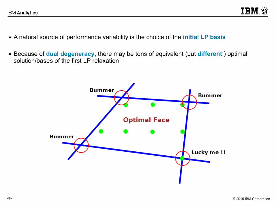
▪ A natural source of performance variability is the choice of the initial LP basis

▪ Because of dual degeneracy, there may be tons of equivalent (but different!) optimal solution/bases of the first LP relaxation


▪ Equivalent (but different) optimal solution/bases may lead to different: − cutting planes − heuristic solutions − ...

▪ Reoptimizing with different cutting planes amplifies the diversification

▪ The final root node could be very different in terms of: − Fractional solution − Dual and primal bounds − Cuts active in the LP

▪ Branching rules will take different decisions ▪ Branch-and-cut will then amplify the diversification again


Simulating Performance Variability: CPLEX random seed

▪ Use CPLEX random seed parameter CPXPARAM_RandomSeed to simulate a performance neutral change in the environment (very convenient!)

▪ Compare: − Solver A: CPLEX 12.6.0 with random seed 1 − Solver B: CPLEX 12.6.0 with random seed 2

▪ Test set: 3224 models classified according to their difficulty: − [0, 10k]: all models but the ones for which the solvers provide an inconsistent answer − [T, 10k]: all models for which one of the solver takes at least T seconds

▪ The comparison is fair because the difficulty of a given model is defined by all the compared solver: there is no bias against any of the compared solvers

▪ Comparison: (shifted) geometric mean of computing times


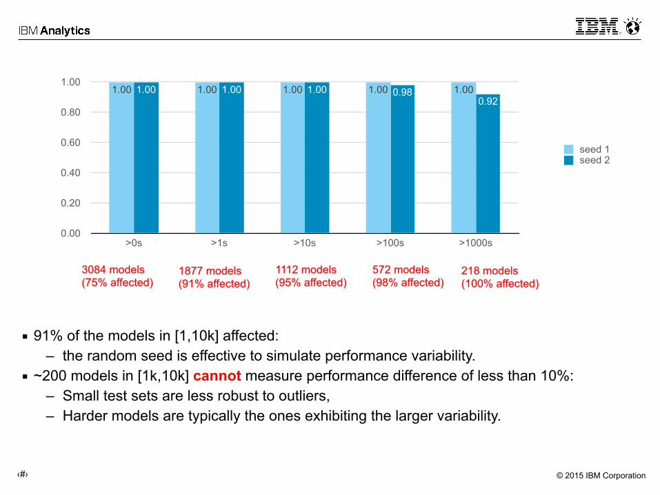
3084 models (75% affected)





▪ 91% of the models in [1,10k] affected: – the random seed is effective to simulate performance variability.

▪ ~200 models in [1k,10k] cannot measure performance difference of less than 10%: – Small test sets are less robust to outliers, – Harder models are typically the ones exhibiting the larger variability.

0.00

0.20

0.40

0.60

0.80

1.00

>0s >1s >10s >100s >1000s

0.920.981.001.001.00 1.001.001.001.001.00

seed 1seed 2


Can we take advantage of that?

0.00

0.20

0.40

0.60

0.80

1.00

>0s >1s >10s >100s >1000s

0.63

0.750.80

0.860.91 0.92

0.981.001.001.00 1.001.001.001.001.00

seed 1seed 2lucky

VIRTUAL BEST

ROCKS!!!


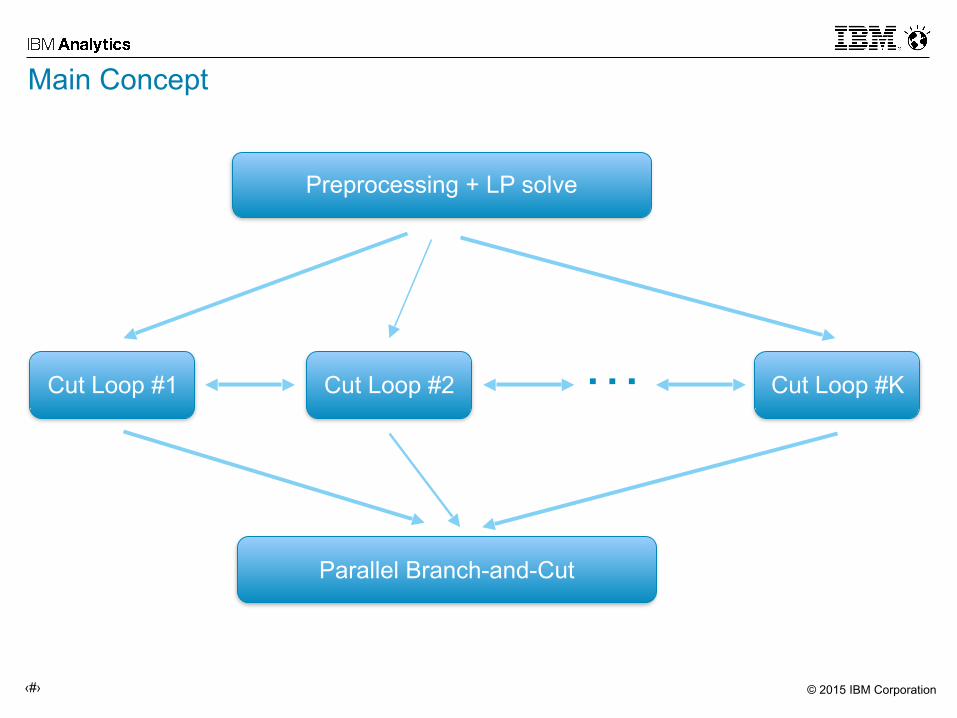
Main Concept

Preprocessing + LP solve

Parallel Branch-and-Cut

Cut Loop #1 Cut Loop #2 Cut Loop #K…


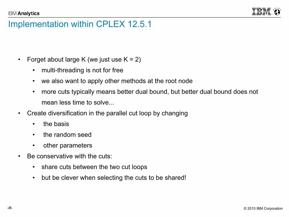
Implementation within CPLEX 12.5.1

• Forget about large K (we just use K = 2)

• multi-threading is not for free

• we also want to apply other methods at the root node

• more cuts typically means better dual bound, but better dual bound does not

mean less time to solve... • Create diversification in the parallel cut loop by changing

• the basis

• the random seed

• other parameters

• Be conservative with the cuts:

• share cuts between the two cut loops

• but be clever when selecting the cuts to be shared!


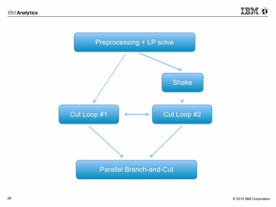
Preprocessing + LP solve

Cut Loop #1

Shake

Cut Loop #2

Parallel Branch-and-Cut


Parallel cut loop results (CPLEX 12.5.1)

0.00

0.20

0.40

0.60

0.80

1.00

>1s >10s >100s

0.980.980.98 0.970.980.990.86

0.920.95 0.940.960.98 0.950.970.98

seed 1seed 2seed 3seed 4seed 5

~1864 models ~1089 models ~565 models

1.02x 1.04x 1.05xAll Models

0.00

0.20

0.40

0.60

0.80

1.00

>1s >10s >100s

0.960.960.97 0.950.970.97

0.800.880.91 0.910.940.96 0.920.960.97



1.04x 1.06x 1.09xAffected Models


LOCAL IMPLIED BOUND CUTS


Implications and implied bound cuts

Discovered during presolve and probing


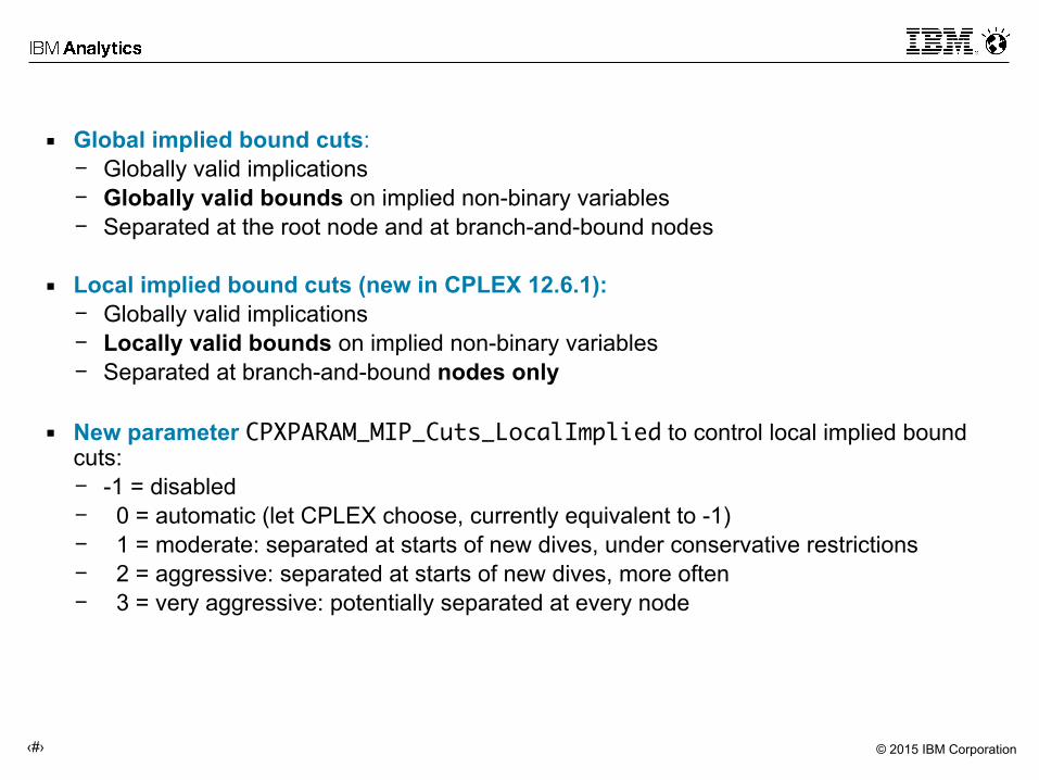
▪ Global implied bound cuts: − Globally valid implications − Globally valid bounds on implied non-binary variables − Separated at the root node and at branch-and-bound nodes

▪ Local implied bound cuts (new in CPLEX 12.6.1): − Globally valid implications − Locally valid bounds on implied non-binary variables − Separated at branch-and-bound nodes only

▪ New parameter CPXPARAM_MIP_Cuts_LocalImplied to control local implied bound cuts: − -1 = disabled − 0 = automatic (let CPLEX choose, currently equivalent to -1) − 1 = moderate: separated at starts of new dives, under conservative restrictions − 2 = aggressive: separated at starts of new dives, more often − 3 = very aggressive: potentially separated at every node


▪ Enabling moderate separation of local implied bound cuts: − 1-‐2% degradation (neutral?) on our test bed

▪ Key points to be investigated: − Cut strength versus cut applicability

• Local cuts are stronger, but global cuts applies to the whole tree − Interaction with other cut types − Cut filtering and cut selection

• Local cuts are violated more often than global cuts: special filtering rules?

▪ Disabled by default, but fundamental in some cases (e.g., to handle “big-‐M constraints”)


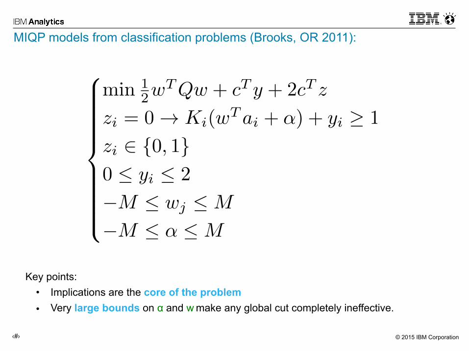
MIQP models from classification problems (Brooks, OR 2011):

Key points: • Implications are the core of the problem • Very large bounds on α and w make any global cut completely ineffective.


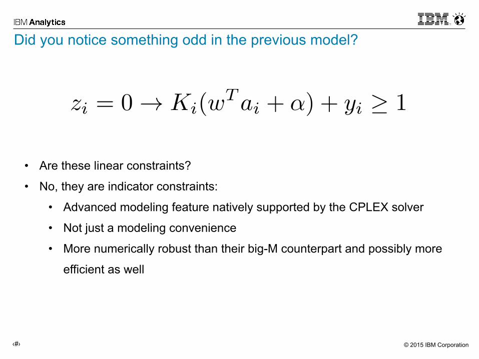
Did you notice something odd in the previous model?

• Are these linear constraints?

• No, they are indicator constraints:

• Advanced modeling feature natively supported by the CPLEX solver

• Not just a modeling convenience

• More numerically robust than their big-M counterpart and possibly more

efficient as well


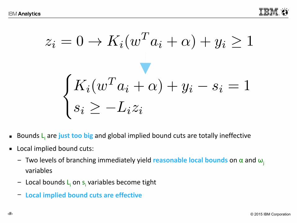
▪ Bounds Li are just too big and global implied bound cuts are totally ineffective

▪ Local implied bound cuts: − Two levels of branching immediately yield reasonable local bounds on α and ωj

variables − Local bounds Li on si variables become tight

− Local implied bound cuts are effective


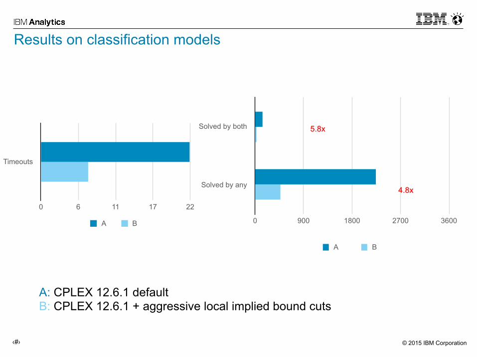
Results on classification models

Timeouts

0 6 11 17 22

A B

Solved by both

Solved by any

0 900 1800 2700 3600

A B

4.8x

5.8x

A: CPLEX 12.6.1 default B: CPLEX 12.6.1 + aggressive local implied bound cuts


LIFT & PROJECT CUTSCGLP magic


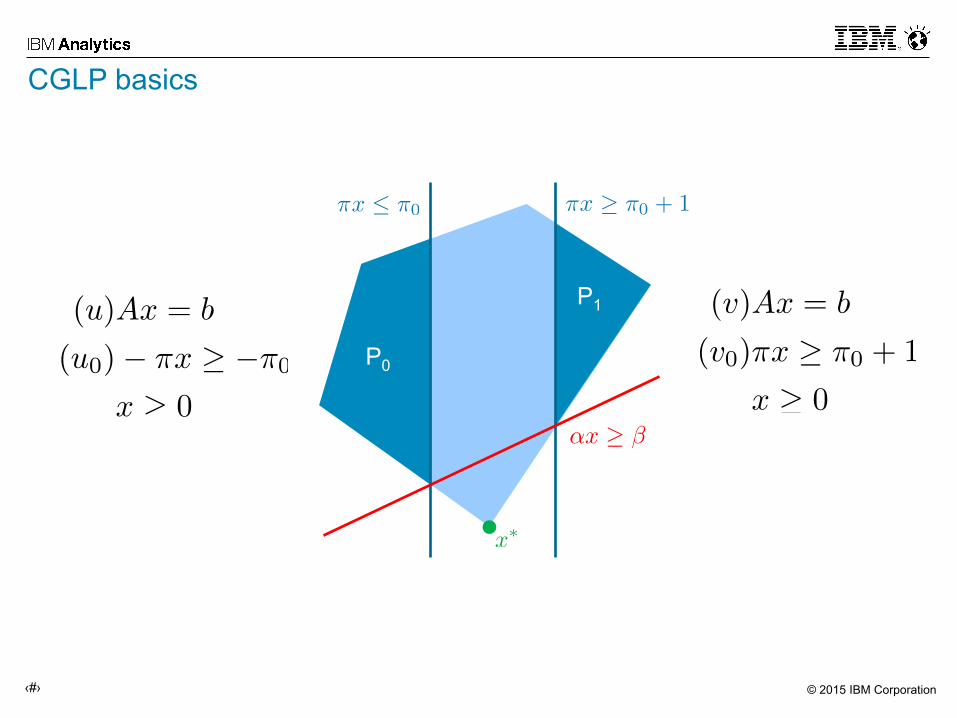
CGLP basics

P0

P1


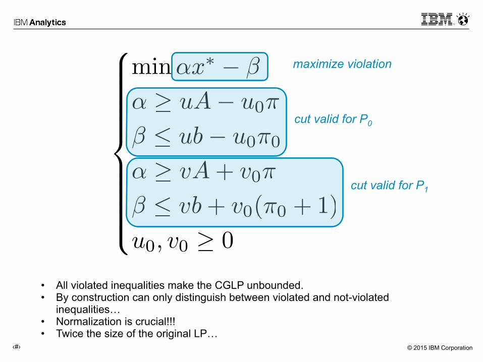
cut valid for P0

cut valid for P1

• All violated inequalities make the CGLP unbounded. • By construction can only distinguish between violated and not-violated

inequalities… • Normalization is crucial!!! • Twice the size of the original LP…

maximize violation


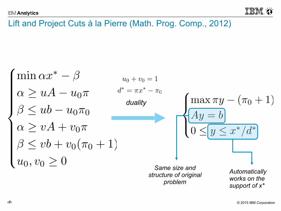
Lift and Project Cuts à la Pierre (Math. Prog. Comp., 2012)

duality

Same size and structure of original

problem

Automatically works on the support of x*


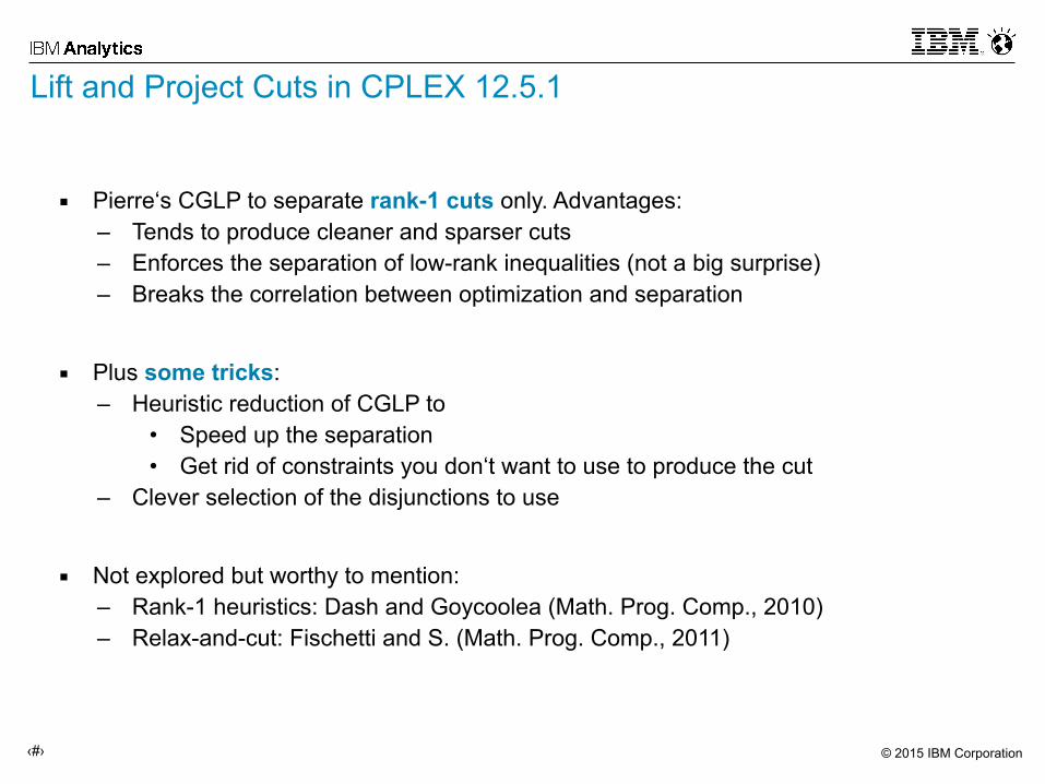
Lift and Project Cuts in CPLEX 12.5.1

▪ Pierre‘s CGLP to separate rank-1 cuts only. Advantages: – Tends to produce cleaner and sparser cuts – Enforces the separation of low-rank inequalities (not a big surprise) – Breaks the correlation between optimization and separation

▪ Plus some tricks: – Heuristic reduction of CGLP to

• Speed up the separation • Get rid of constraints you don‘t want to use to produce the cut

– Clever selection of the disjunctions to use

▪ Not explored but worthy to mention: – Rank-1 heuristics: Dash and Goycoolea (Math. Prog. Comp., 2010) – Relax-and-cut: Fischetti and S. (Math. Prog. Comp., 2011)


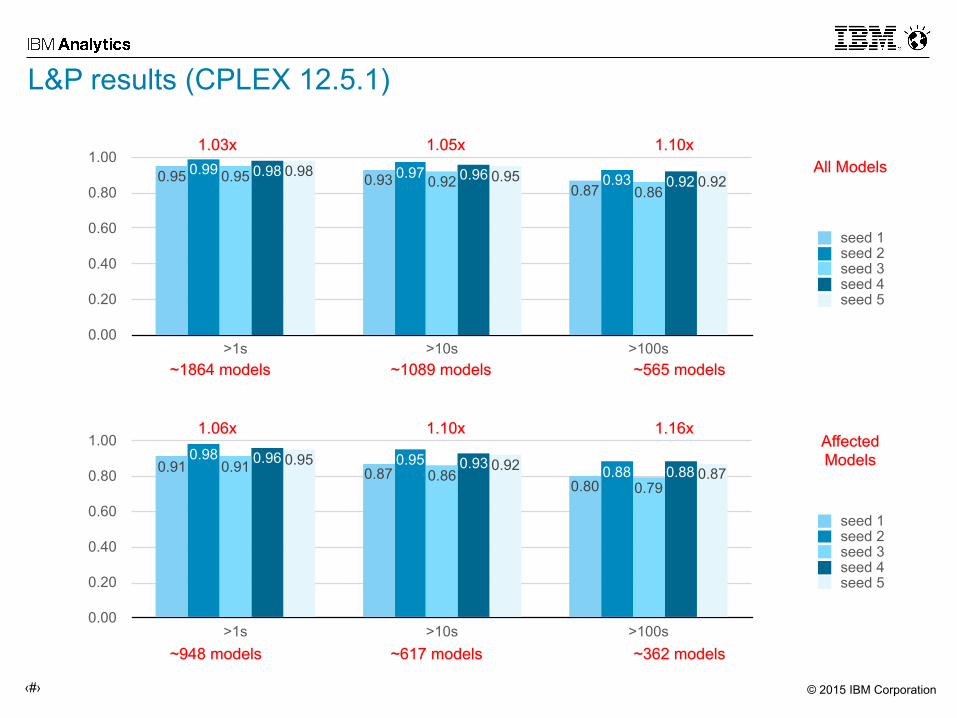
L&P results (CPLEX 12.5.1)

0.00

0.20

0.40

0.60

0.80

1.00

>1s >10s >100s

0.920.950.980.920.960.98

0.860.920.95 0.930.970.99

0.870.930.95



1.03x 1.05x 1.10xAll Models

0.00

0.20

0.40

0.60

0.80

1.00

>1s >10s >100s

0.870.920.950.880.930.96

0.790.860.91 0.88

0.950.98

0.800.870.91



1.06x 1.10x 1.16xAffected Models


Questions?


Legal Disclaimer • © IBM Corporation 2015. All Rights Reserved. • The information contained in this publication is provided for informational purposes only. While efforts were made to verify the completeness and

accuracy of the information contained in this publication, it is provided AS IS without warranty of any kind, express or implied. In addition, this information is based on IBM’s current product plans and strategy, which are subject to change by IBM without notice. IBM shall not be responsible for any damages arising out of the use of, or otherwise related to, this publication or any other materials. Nothing contained in this publication is intended to, nor shall have the effect of, creating any warranties or representations from IBM or its suppliers or licensors, or altering the terms and conditions of the applicable license agreement governing the use of IBM software.

• References in this presentation to IBM products, programs, or services do not imply that they will be available in all countries in which IBM operates. Product release dates and/or capabilities referenced in this presentation may change at any time at IBM’s sole discretion based on market opportunities or other factors, and are not intended to be a commitment to future product or feature availability in any way. Nothing contained in these materials is intended to, nor shall have the effect of, stating or implying that any activities undertaken by you will result in any specific sales, revenue growth or other results.

• Performance is based on measurements and projections using standard IBM benchmarks in a controlled environment. The actual throughput or performance that any user will experience will vary depending upon many factors, including considerations such as the amount of multiprogramming in the user's job stream, the I/O configuration, the storage configuration, and the workload processed. Therefore, no assurance can be given that an individual user will achieve results similar to those stated here.

• Microsoft and Windows are trademarks of Microsoft Corporation in the United States, other countries, or both. • Linux is a registered trademark of Linus Torvalds in the United States, other countries, or both. • Other company, product, or service names may be trademarks or service marks of others.

Recent MILP advances CO@W2015 - CO@Work 2020

Documents

Transcript of Recent MILP advances CO@W2015 - CO@Work 2020