Recent climate variation in the Bering and Chukchi Seas and its linkages to large-scale circulation...
15
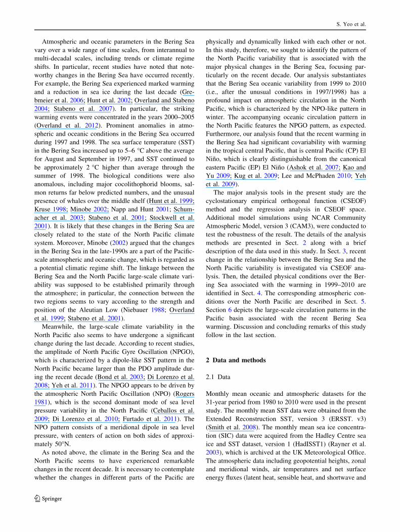
Recent climate variation in the Bering and Chukchi Seas and its linkages to large-scale circulation in the Pacific Sae-Rim Yeo • Kwang-Yul Kim • Sang-Wook Yeh • Baek-Min Kim • Taehyoun Shim • Jong-Ghap Jhun Received: 23 December 2012 / Accepted: 26 December 2013 Ó The Author(s) 2014. This article is published with open access at Springerlink.com Abstract The thermal state of the Bering Sea exhibits interdecadal variations, with distinct changes occurred in 1997–1998. After the unusual thermal condition of the Bering Sea in 1997–1998, we found that the recent climate variability (1999–2010) in the Bering Sea is closely related to Pacific basin-scale atmospheric and oceanic circulation patterns. Specifically, warming in the Bering and Chukchi Seas in this period involves sea ice reduction and stronger oceanic heat flux to the atmosphere in winter. The atmo- spheric response to the recent warming in the Bering and Chukchi Seas resembles the North Pacific Oscillation (NPO) pattern. Further analysis reveals that the recent cli- mate variability in the Bering and Chukchi Seas has strong covariability with large-scale climate modes in the Pacific, that is, the North Pacific Gyre Oscillation and the central Pacific El Nin ˜o. In this study, physical connections among the recent climate variations in the Bering and Chukchi Seas, the NPO pattern and the Pacific large-scale climate patterns are investigated via cyclostationary empirical orthogonal function analysis. An additional model experiment using the National Center for Atmospheric Research Community Atmospheric Model, version 3, is conducted to support the robustness of the results. Keywords Bering and Chukchi Seas North Pacific Oscillation North Pacific Gyre Oscillation Central Pacific El Nin ˜o 1 Introduction The Bering Sea, a northern extension of the North Pacific Ocean, is located between Russia and Alaska and is the third largest semi-enclosed sea in the world. The Bering Sea is connected to the Chukchi Sea, which is a marginal sea of the Arctic Ocean, through the Bering Strait. In a global sense, the Bering Sea acts as the Pacific gateway, through which the North Pacific and the Arctic Ocean exchange heat and water. The Bering Sea is one of the most productive marine resources in the world and provides nearly half of the US fisheries production (National Research Council 1996). For this reason, many oceano- graphers have tried to understand the variability of the marine ecosystem in the Bering Sea. In particular, its relationship with climate variability has long been the focus of attention (Grebmeier et al. 2006; Overland and Stabeno 2004; Hunt et al. 2002; Kruse 1998; Brodeur et al. 1999). Furthermore, the Bering Sea, as a marginal section of the North Pacific Ocean, is sensitive to Pacific large- scale climate phenomena such as the El Nin ˜o/Southern Oscillation (ENSO) (Niebauer 1988) and the Pacific Dec- adal Oscillation (PDO) (Hare and Mantua 2000; Overland et al. 1999). Understanding the oceanic and atmospheric variability over the Bering Sea, therefore, is essential from both ecological and climatological perspectives. S.-R. Yeo K.-Y. Kim (&) T. Shim J.-G. Jhun School of Earth and Environmental Sciences, Seoul National University, Seoul 151-747, Republic of Korea e-mail: [email protected] S.-W. Yeh Department of Environmental Marine Science, Hanyang University, Ansan 426-792, Republic of Korea B.-M. Kim T. Shim Korea Polar Research Institute, Incheon 406-840, Republic of Korea J.-G. Jhun Research Institute of Oceanography, Seoul National University, Seoul 151-747, Republic of Korea 123 Clim Dyn DOI 10.1007/s00382-013-2042-z
Transcript of Recent climate variation in the Bering and Chukchi Seas and its linkages to large-scale circulation...
Recent climate variation in the Bering and Chukchi Seasand its linkages to large-scale circulation in the Pacific
Sae-Rim Yeo • Kwang-Yul Kim • Sang-Wook Yeh •
Baek-Min Kim • Taehyoun Shim • Jong-Ghap Jhun
Received: 23 December 2012 / Accepted: 26 December 2013
� The Author(s) 2014. This article is published with open access at Springerlink.com
Abstract The thermal state of the Bering Sea exhibits
interdecadal variations, with distinct changes occurred in
1997–1998. After the unusual thermal condition of the
Bering Sea in 1997–1998, we found that the recent climate
variability (1999–2010) in the Bering Sea is closely related
to Pacific basin-scale atmospheric and oceanic circulation
patterns. Specifically, warming in the Bering and Chukchi
Seas in this period involves sea ice reduction and stronger
oceanic heat flux to the atmosphere in winter. The atmo-
spheric response to the recent warming in the Bering and
Chukchi Seas resembles the North Pacific Oscillation
(NPO) pattern. Further analysis reveals that the recent cli-
mate variability in the Bering and Chukchi Seas has strong
covariability with large-scale climate modes in the Pacific,
that is, the North Pacific Gyre Oscillation and the central
Pacific El Nino. In this study, physical connections among
the recent climate variations in the Bering and Chukchi
Seas, the NPO pattern and the Pacific large-scale climate
patterns are investigated via cyclostationary empirical
orthogonal function analysis. An additional model
experiment using the National Center for Atmospheric
Research Community Atmospheric Model, version 3, is
conducted to support the robustness of the results.
Keywords Bering and Chukchi Seas � North Pacific
Oscillation � North Pacific Gyre Oscillation � Central
Pacific El Nino
1 Introduction
The Bering Sea, a northern extension of the North Pacific
Ocean, is located between Russia and Alaska and is the
third largest semi-enclosed sea in the world. The Bering
Sea is connected to the Chukchi Sea, which is a marginal
sea of the Arctic Ocean, through the Bering Strait. In a
global sense, the Bering Sea acts as the Pacific gateway,
through which the North Pacific and the Arctic Ocean
exchange heat and water. The Bering Sea is one of the most
productive marine resources in the world and provides
nearly half of the US fisheries production (National
Research Council 1996). For this reason, many oceano-
graphers have tried to understand the variability of the
marine ecosystem in the Bering Sea. In particular, its
relationship with climate variability has long been the
focus of attention (Grebmeier et al. 2006; Overland and
Stabeno 2004; Hunt et al. 2002; Kruse 1998; Brodeur et al.
1999). Furthermore, the Bering Sea, as a marginal section
of the North Pacific Ocean, is sensitive to Pacific large-
scale climate phenomena such as the El Nino/Southern
Oscillation (ENSO) (Niebauer 1988) and the Pacific Dec-
adal Oscillation (PDO) (Hare and Mantua 2000; Overland
et al. 1999). Understanding the oceanic and atmospheric
variability over the Bering Sea, therefore, is essential from
both ecological and climatological perspectives.
S.-R. Yeo � K.-Y. Kim (&) � T. Shim � J.-G. Jhun
School of Earth and Environmental Sciences, Seoul National
University, Seoul 151-747, Republic of Korea
e-mail: [email protected]
S.-W. Yeh
Department of Environmental Marine Science,
Hanyang University, Ansan 426-792, Republic of Korea
B.-M. Kim � T. Shim
Korea Polar Research Institute, Incheon 406-840,
Republic of Korea
J.-G. Jhun
Research Institute of Oceanography, Seoul National University,
Seoul 151-747, Republic of Korea
123
Clim Dyn
DOI 10.1007/s00382-013-2042-z
Atmospheric and oceanic parameters in the Bering Sea
vary over a wide range of time scales, from interannual to
multi-decadal scales, including trends or climate regime
shifts. In particular, recent studies have noted that note-
worthy changes in the Bering Sea have occurred recently.
For example, the Bering Sea experienced marked warming
and a reduction in sea ice during the last decade (Gre-
bmeier et al. 2006; Hunt et al. 2002; Overland and Stabeno
2004; Stabeno et al. 2007). In particular, the striking
warming events were concentrated in the years 2000–2005
(Overland et al. 2012). Prominent anomalies in atmo-
spheric and oceanic conditions in the Bering Sea occurred
during 1997 and 1998. The sea surface temperature (SST)
in the Bering Sea increased up to 5–6 �C above the average
for August and September in 1997, and SST continued to
be approximately 2 �C higher than average through the
summer of 1998. The biological conditions were also
anomalous, including major cocolithophorid blooms, sal-
mon returns far below predicted numbers, and the unusual
presence of whales over the middle shelf (Hunt et al. 1999;
Kruse 1998; Minobe 2002; Napp and Hunt 2001; Schum-
acher et al. 2003; Stabeno et al. 2001; Stockwell et al.
2001). It is likely that these changes in the Bering Sea are
closely related to the state of the North Pacific climate
system. Moreover, Minobe (2002) argued that the changes
in the Bering Sea in the late-1990s are a part of the Pacific-
scale atmospheric and oceanic change, which is regarded as
a potential climatic regime shift. The linkage between the
Bering Sea and the North Pacific large-scale climate vari-
ability was supposed to be established primarily through
the atmosphere; in particular, the connection between the
two regions seems to vary according to the strength and
position of the Aleutian Low (Niebauer 1988; Overland
et al. 1999; Stabeno et al. 2001).
Meanwhile, the large-scale climate variability in the
North Pacific also seems to have undergone a significant
change during the last decade. According to recent studies,
the amplitude of North Pacific Gyre Oscillation (NPGO),
which is characterized by a dipole-like SST pattern in the
North Pacific became larger than the PDO amplitude dur-
ing the recent decade (Bond et al. 2003; Di Lorenzo et al.
2008; Yeh et al. 2011). The NPGO appears to be driven by
the atmospheric North Pacific Oscillation (NPO) (Rogers
1981), which is the second dominant mode of sea level
pressure variability in the North Pacific (Ceballos et al.
2009; Di Lorenzo et al. 2010; Furtado et al. 2011). The
NPO pattern consists of a meridional dipole in sea level
pressure, with centers of action on both sides of approxi-
mately 50�N.
As noted above, the climate in the Bering Sea and the
North Pacific seems to have experienced remarkable
changes in the recent decade. It is necessary to contemplate
whether the changes in different parts of the Pacific are
physically and dynamically linked with each other or not.
In this study, therefore, we sought to identify the pattern of
the North Pacific variability that is associated with the
major physical changes in the Bering Sea, focusing par-
ticularly on the recent decade. Our analysis substantiates
that the Bering Sea oceanic variability from 1999 to 2010
(i.e., after the unusual conditions in 1997/1998) has a
profound impact on atmospheric circulation in the North
Pacific, which is characterized by the NPO-like pattern in
winter. The accompanying oceanic circulation pattern in
the North Pacific features the NPGO pattern, as expected.
Furthermore, our analysis found that the recent warming in
the Bering Sea had significant covariability with warming
in the tropical central Pacific, that is central Pacific (CP) El
Nino, which is clearly distinguishable from the canonical
eastern Pacific (EP) El Nino (Ashok et al. 2007; Kao and
Yu 2009; Kug et al. 2009; Lee and McPhaden 2010; Yeh
et al. 2009).
The major analysis tools in the present study are the
cyclostationary empirical orthogonal function (CSEOF)
method and the regression analysis in CSEOF space.
Additional model simulations using NCAR Community
Atmospheric Model, version 3 (CAM3), were conducted to
test the robustness of the result. The details of the analysis
methods are presented in Sect. 2 along with a brief
description of the data used in this study. In Sect. 3, recent
change in the relationship between the Bering Sea and the
North Pacific variability is investigated via CSEOF ana-
lysis. Then, the detailed physical conditions over the Ber-
ing Sea associated with the warming in 1999–2010 are
identified in Sect. 4. The corresponding atmospheric con-
ditions over the North Pacific are described in Sect. 5.
Section 6 depicts the large-scale circulation patterns in the
Pacific basin associated with the recent Bering Sea
warming. Discussion and concluding remarks of this study
follow in the last section.
2 Data and methods
2.1 Data
Monthly mean oceanic and atmospheric datasets for the
31-year period from 1980 to 2010 were used in the present
study. The monthly mean SST data were obtained from the
Extended Reconstruction SST, version 3 (ERSST. v3)
(Smith et al. 2008). The monthly mean sea ice concentra-
tion (SIC) data were acquired from the Hadley Centre sea
ice and SST dataset, version 1 (HadISST1) (Rayner et al.
2003), which is archived at the UK Meteorological Office.
The atmospheric data including geopotential heights, zonal
and meridional winds, air temperatures and net surface
energy fluxes (latent heat, sensible heat, and shortwave and
S. Yeo et al.
123
longwave radiative fluxes) were taken from the NCEP/
DOE AMIP-2 reanalysis (Kanamitsu et al. 2002).
2.2 Methods
CSEOF analysis (Kim and North 1997; Kim et al. 1996) is
applied to the monthly atmospheric and oceanic datasets.
Physically evolving spatial patterns are extracted from
space-time data, T(r, t), through CSEOF analysis:
Tðr; tÞ ¼X
n
LVnðr; tÞPCnðtÞ ð1Þ
where LVn(r, t) is CSEOF loading vector, PCn(t) is the
corresponding principal component (PC) time series, and n,
r and t denote the mode number, space and time,
respectively. The CSEOF method is useful for describing
temporally evolving spatial patterns because the CSEOF
loading vectors, LVn(r, t), are time dependent and periodic:
LVnðr; tÞ ¼ LVnðr; t þ dÞ ð2Þ
where d is called the nested period. In this study, the nested
period is set to 12 months implying that the statistical
properties of each physical process do not vary from 1 year
to another. Thus, the physical evolution as represented by
LVn(r, t) is modulated over a longer time span by the PC
time series, PCn(t).
After CSEOF analysis is conducted on individual vari-
ables, regression analysis is performed in CSEOF space to
find physically consistent patterns among different vari-
ables. The PC time series of a predictor variable, PCPm(t),
is regressed onto the PC time series of the target variable,
PCn(t), as in (3):
PCnðtÞ ¼XM
m¼1
aðnÞm PCPmðtÞ þ eðnÞðtÞ ð3Þ
where am(n) and e(n)(t) are regression coefficients and regression
error time series, respectively. The regression coefficients are
determined such that the variance of the regression error time
series is minimized. Then, new loading vectors for the
predictor variable, LVPRn(r, t), are obtained as
LVPRnðr; tÞ ¼XM
m¼1
aðnÞm LVPmðr; tÞ ð4Þ
where LVPm(r, t) are the CSEOF loading vectors for the
predictor variable. The resulting regressed spatial patterns
of the predictor variables are considered physically and
dynamically consistent with the target patterns in that the
two loading vectors share the same amplitude time series
Tn(t). In the present study, SST in the Bering Sea is
selected as the target variable whereas other variables such
as SST and atmospheric variables in the Pacific basin are
regarded as the predictor variables.
Model experiments are conducted using CAM3, an
atmospheric general circulation model developed by the
National Center for Atmospheric Research (NCAR), to
further assess the atmospheric response over the North
Pacific to the changed physical conditions in the Bering
and Chukchi Seas in recent decade. The physical and
numerical methods used in CAM3 are documented in
Collins et al. (2006) and the references therein.
3 Changes in the relationship between the Bering Sea
and the North Pacific
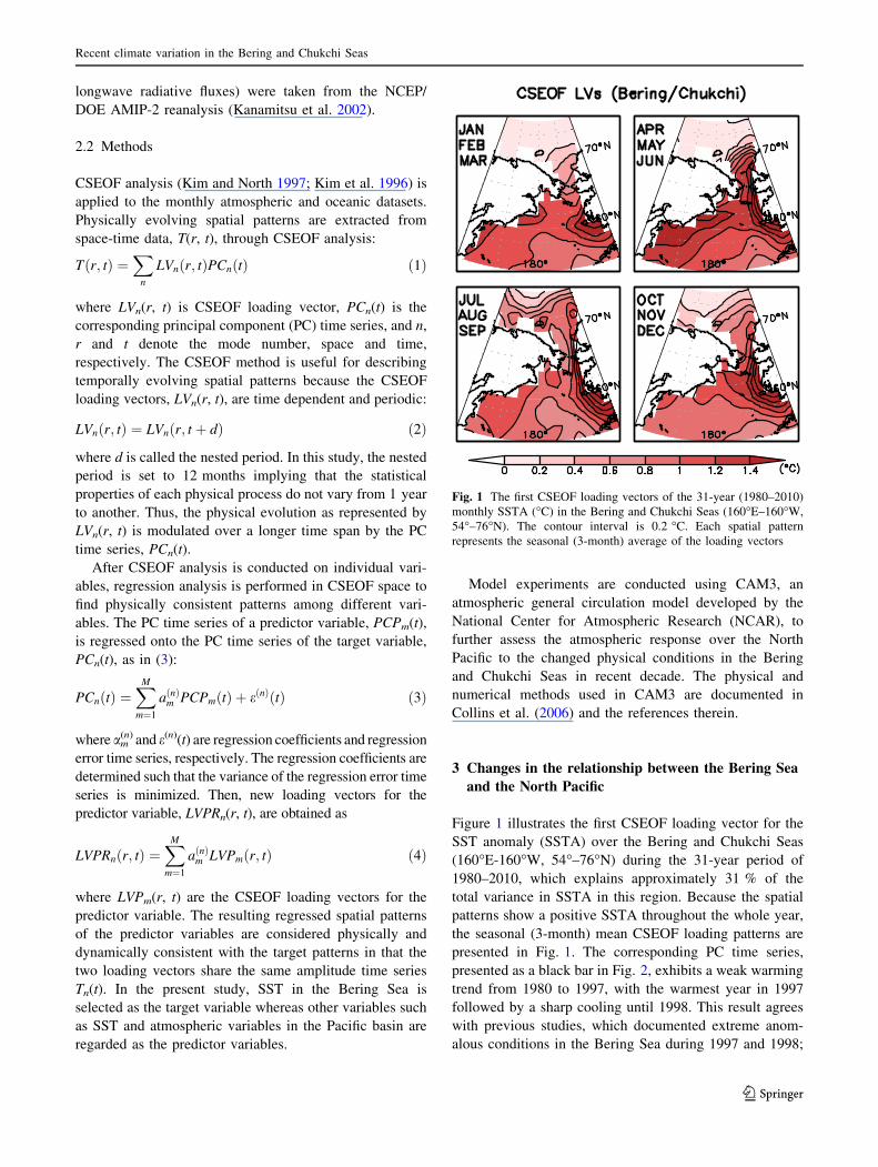
Figure 1 illustrates the first CSEOF loading vector for the
SST anomaly (SSTA) over the Bering and Chukchi Seas
(160�E-160�W, 54�–76�N) during the 31-year period of
1980–2010, which explains approximately 31 % of the
total variance in SSTA in this region. Because the spatial
patterns show a positive SSTA throughout the whole year,
the seasonal (3-month) mean CSEOF loading patterns are
presented in Fig. 1. The corresponding PC time series,
presented as a black bar in Fig. 2, exhibits a weak warming
trend from 1980 to 1997, with the warmest year in 1997
followed by a sharp cooling until 1998. This result agrees
with previous studies, which documented extreme anom-
alous conditions in the Bering Sea during 1997 and 1998;
Fig. 1 The first CSEOF loading vectors of the 31-year (1980–2010)
monthly SSTA (�C) in the Bering and Chukchi Seas (160�E–160�W,
54�–76�N). The contour interval is 0.2 �C. Each spatial pattern
represents the seasonal (3-month) average of the loading vectors
Recent climate variation in the Bering and Chukchi Seas
123
the warmest temperature ever observed before appeared in
1997, which is followed by rapid cooling until 1999 (Hunt
et al. 1999; Kruse 1998; Minobe 2002; Napp and Hunt
2001; Schumacher et al. 2003; Stabeno et al. 2001;
Stockwell et al. 2001). After an abrupt decline from 1998
to 1999, SST displayed a sharp increase from 1999 to 2003
and the summer of 2003 marked the warmest year in the
entire record (1980–2010). This result is consistent with the
recent studies suggesting warming in the Bering Sea in the
early 2000s (Grebmeier et al. 2006; Hunt et al. 2002;
Overland and Stabeno 2004; Overland et al. 2012; Stabeno
et al. 2007). Although there is no warming trend since
2003, SST over the Bering Sea has been warmer during
2003–2010 compared with the mean SST in 1980–2010.
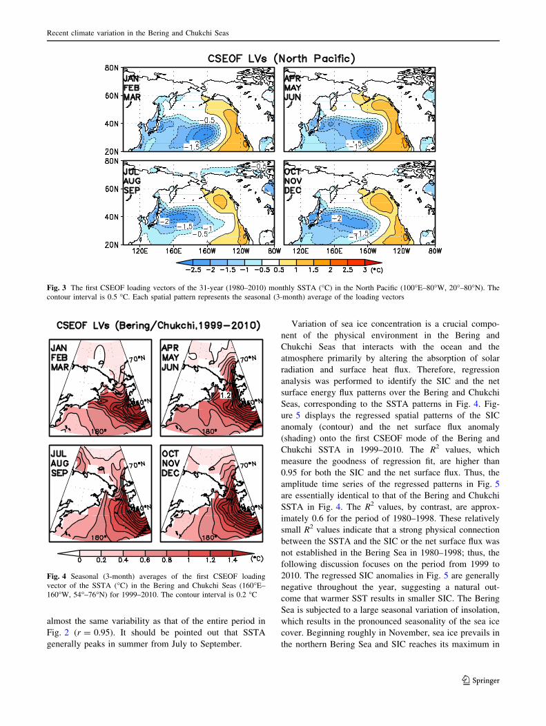
To identify any links between the Bering and Chukchi
Seas and climate variability in the North Pacific, North
Pacific (100�E–80�W, 20�–80�N) SSTA data were ana-
lyzed via CSEOF analysis. The seasonally (3-month)
averaged loading vector of the first CSEOF is presented in
Fig. 3; the first mode explains approximately 23 % of the
total variability. The corresponding PC time series is
shown in Fig. 2 as a blue curve. The spatial patterns in
Fig. 3 are similar to the structure of the PDO, which fea-
tures negative SSTA with an elliptical shape over the
western to central Pacific and positive SSTA along the
eastern North Pacific. Correlation between the first PC time
series of the North Pacific SSTA and the Mantua’s PDO
index (available at http://jisao.washington.edu/pdo/PDO.
latest) is 0.73 confirming the similarity between the first
CSEOF (Fig. 3) and the PDO patterns. On the other hand,
the strong meridional gradient of SSTA along approxi-
mately 40�N in Fig. 3 is more in line with the structure of
the NPGO than the PDO. Indeed, the NPGO index
(available at http://www.o3d.org/npgo) and the first PC
time series of the North Pacific SSTA are also significantly
correlated at -0.63. In terms of the spatial pattern and the
amplitude time series, the first CSEOF loading vector of
the North Pacific SSTA (Fig. 3) reflects both the PDO and
the NPGO features.
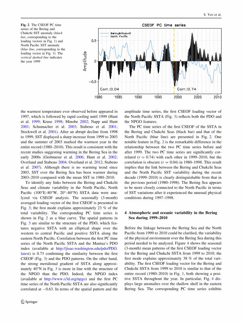
The PC time series of the first CSEOF of the SSTA in
the Bering and Chukchi Seas (black bar) and that of the
North Pacific (blue line) are presented in Fig. 2. One
notable feature in Fig. 2 is the remarkable difference in the
relationship between the two PC time series before and
after 1999. The two PC time series are significantly cor-
related (r = 0.74) with each other in 1999–2010, but the
correlation is obscure (r = 0.04) in 1980–1998. This result
implies that the link between the Bering and Chukchi Seas
and the North Pacific SST variability during the recent
decade (1999–2010) is clearly distinguishable from that in
the previous period (1980–1998). The Bering Sea appears
to be more closely connected to the North Pacific in terms
of SST variations after it experienced the unusual physical
conditions during 1997–1998.
4 Atmospheric and oceanic variability in the Bering
Sea during 1999–2010
Before the linkage between the Bering Sea and the North
Pacific from 1999 to 2010 could be clarified, the variability
of the physical environment over the Bering Sea during this
period needed to be analyzed. Figure 4 shows the seasonal
(3-month) mean patterns of the first CSEOF loading vector
for the Bering and Chukchi SSTA from 1999 to 2010; the
first mode explains approximately 38 % of the total vari-
ability. The first CSEOF loading vector for the Bering and
Chukchi SSTA from 1999 to 2010 is similar to that of the
entire record (1980–2010) in Fig. 1, both showing a posi-
tive SSTA throughout the year. In particular, Fig. 4 dis-
plays large anomalies over the shallow shelf in the eastern
Bering Sea. The corresponding PC time series exhibits
Fig. 2 The CSEOF PC time
series of the Bering and
Chukchi SST anomaly (black
bar, corresponding to the
loading vectors in Fig. 1) and
North Pacific SST anomaly
(blue line, corresponding to the
loading vector in Fig. 3). The
vertical dashed line indicates
the year 1999
S. Yeo et al.
123
almost the same variability as that of the entire period in
Fig. 2 (r = 0.95). It should be pointed out that SSTA
generally peaks in summer from July to September.
Variation of sea ice concentration is a crucial compo-
nent of the physical environment in the Bering and
Chukchi Seas that interacts with the ocean and the
atmosphere primarily by altering the absorption of solar
radiation and surface heat flux. Therefore, regression
analysis was performed to identify the SIC and the net
surface energy flux patterns over the Bering and Chukchi
Seas, corresponding to the SSTA patterns in Fig. 4. Fig-
ure 5 displays the regressed spatial patterns of the SIC
anomaly (contour) and the net surface flux anomaly
(shading) onto the first CSEOF mode of the Bering and
Chukchi SSTA in 1999–2010. The R2 values, which
measure the goodness of regression fit, are higher than
0.95 for both the SIC and the net surface flux. Thus, the
amplitude time series of the regressed patterns in Fig. 5
are essentially identical to that of the Bering and Chukchi
SSTA in Fig. 4. The R2 values, by contrast, are approx-
imately 0.6 for the period of 1980–1998. These relatively
small R2 values indicate that a strong physical connection
between the SSTA and the SIC or the net surface flux was
not established in the Bering Sea in 1980–1998; thus, the
following discussion focuses on the period from 1999 to
2010. The regressed SIC anomalies in Fig. 5 are generally
negative throughout the year, suggesting a natural out-
come that warmer SST results in smaller SIC. The Bering
Sea is subjected to a large seasonal variation of insolation,
which results in the pronounced seasonality of the sea ice
cover. Beginning roughly in November, sea ice prevails in
the northern Bering Sea and SIC reaches its maximum in
Fig. 3 The first CSEOF loading vectors of the 31-year (1980–2010) monthly SSTA (�C) in the North Pacific (100�E–80�W, 20�–80�N). The
contour interval is 0.5 �C. Each spatial pattern represents the seasonal (3-month) average of the loading vectors
Fig. 4 Seasonal (3-month) averages of the first CSEOF loading
vector of the SSTA (�C) in the Bering and Chukchi Seas (160�E–
160�W, 54�–76�N) for 1999–2010. The contour interval is 0.2 �C
Recent climate variation in the Bering and Chukchi Seas
123
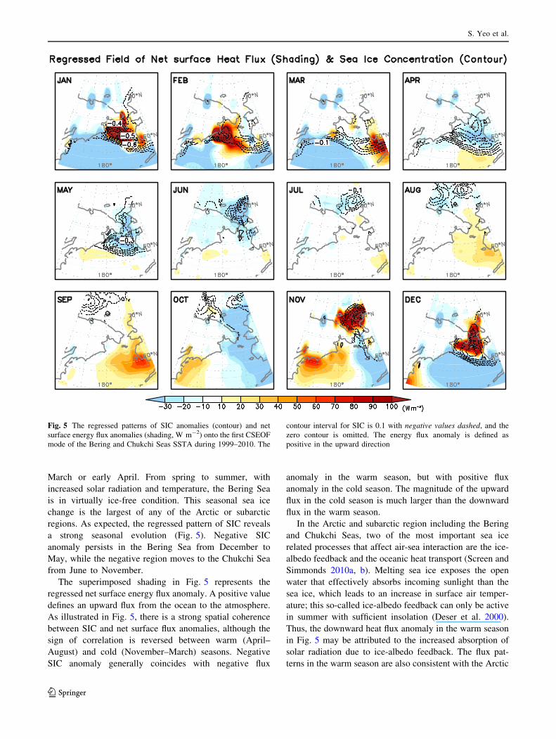
March or early April. From spring to summer, with
increased solar radiation and temperature, the Bering Sea
is in virtually ice-free condition. This seasonal sea ice
change is the largest of any of the Arctic or subarctic
regions. As expected, the regressed pattern of SIC reveals
a strong seasonal evolution (Fig. 5). Negative SIC
anomaly persists in the Bering Sea from December to
May, while the negative region moves to the Chukchi Sea
from June to November.
The superimposed shading in Fig. 5 represents the
regressed net surface energy flux anomaly. A positive value
defines an upward flux from the ocean to the atmosphere.
As illustrated in Fig. 5, there is a strong spatial coherence
between SIC and net surface flux anomalies, although the
sign of correlation is reversed between warm (April–
August) and cold (November–March) seasons. Negative
SIC anomaly generally coincides with negative flux
anomaly in the warm season, but with positive flux
anomaly in the cold season. The magnitude of the upward
flux in the cold season is much larger than the downward
flux in the warm season.
In the Arctic and subarctic region including the Bering
and Chukchi Seas, two of the most important sea ice
related processes that affect air-sea interaction are the ice-
albedo feedback and the oceanic heat transport (Screen and
Simmonds 2010a, b). Melting sea ice exposes the open
water that effectively absorbs incoming sunlight than the
sea ice, which leads to an increase in surface air temper-
ature; this so-called ice-albedo feedback can only be active
in summer with sufficient insolation (Deser et al. 2000).
Thus, the downward heat flux anomaly in the warm season
in Fig. 5 may be attributed to the increased absorption of
solar radiation due to ice-albedo feedback. The flux pat-
terns in the warm season are also consistent with the Arctic
Fig. 5 The regressed patterns of SIC anomalies (contour) and net
surface energy flux anomalies (shading, W m-2) onto the first CSEOF
mode of the Bering and Chukchi Seas SSTA during 1999–2010. The
contour interval for SIC is 0.1 with negative values dashed, and the
zero contour is omitted. The energy flux anomaly is defined as
positive in the upward direction
S. Yeo et al.
123
Ocean being more efficient in absorbing atmospheric heat
during summer (Screen and Simmonds 2010b).
In winter, on the other hand, the primary air–sea inter-
action mechanism is the oceanic heat transport, since the
albedo effect is suppressed due to the low insolation
(Screen and Simmonds 2010a, b). Screen and Simmonds
(2010b) proposed two explanations for the relationship
between SIC and net surface flux in winter season. As a
direct response to reductions in winter sea ice cover, heat is
released from the relatively warm ocean surface to the
colder atmosphere above. As an indirect response, sea ice
reduction in summer also facilitates increased heat transfer
from the ocean to the atmosphere in winter; sea ice cover
reduction in summer leads to heat storage in the ocean,
which is released in winter. Indeed, Fig. 5 exhibits striking
spatial coherence between the negative SIC and the upward
flux anomalies in the cold season, which supports that
melting sea ice facilitates increased oceanic heat loss. An
implication is that sea ice plays a significant role in forcing
the atmosphere above by regulating energy flux transfer.
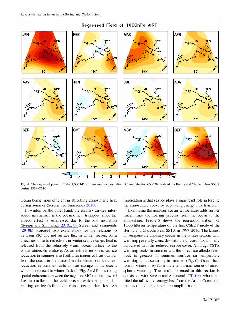
Examining the near-surface air temperature adds further
insight into the forcing process from the ocean to the
atmosphere. Figure 6 shows the regression pattern of
1,000-hPa air temperature on the first CSEOF mode of the
Bering and Chukchi Seas SSTA in 1999–2010. The largest
air temperature anomaly occurs in the winter season, with
warming generally coincides with the upward flux anomaly
associated with the reduced sea ice cover. Although SSTA
warming peaks in summer and the direct ice-albedo feed-
back is greatest in summer, surface air temperature
warming is not so strong in summer (Fig. 6). Ocean heat
loss in winter is by far a more important source of atmo-
spheric warming. The result presented in this section is
consistent with Screen and Simmonds (2010b), who iden-
tified the fall-winter energy loss from the Arctic Ocean and
the associated air temperature amplification.
Fig. 6 The regressed patterns of the 1,000-hPa air temperature anomalies (�C) onto the first CSEOF mode of the Bering and Chukchi Seas SSTA
during 1999–2010
Recent climate variation in the Bering and Chukchi Seas
123
5 North Pacific atmospheric circulation
5.1 Regression analysis
Atmospheric response to the recent thermal variability in
the Bering Sea does not seem confined to the Bering Sea
region, but also appear in the North Pacific. Henceforth,
large-scale atmospheric circulation over the North Pacific
is investigated in association with the recent thermal state
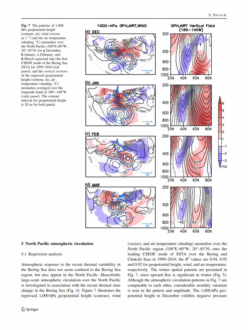
change in the Bering Sea (Fig. 4). Figure 7 illustrates the
regressed 1,000-hPa geopotential height (contour), wind
(vector), and air temperature (shading) anomalies over the
North Pacific region (100�E–80�W, 20�–85�N) onto the
leading CSEOF mode of SSTA over the Bering and
Chukchi Seas in 1999–2010; the R2 values are 0.94, 0.95
and 0.92 for geopotential height, wind, and air temperature,
respectively. The winter spatial patterns are presented in
Fig. 7, since upward flux is significant in winter (Fig. 5).
Although the atmospheric circulation patterns in Fig. 7 are
comparable to each other, considerable monthly variation
is seen in the pattern and amplitude. The 1,000-hPa geo-
potential height in December exhibits negative pressure
(a)
(b)
(c)
(d)
Fig. 7 The patterns of 1,000-
hPa geopotential height
(contour, m), wind (vector,
m s-1) and the air temperature
(shading, �C) anomalies over
the North Pacific (100�E–80�W,
20�–85�N) for a December,
b January, c February, and
d March regressed onto the first
CSEOF mode of the Bering Sea
SSTA for 1999–2010 (left
panel), and the vertical sections
of the regressed geopotential
height (contour, m), air
temperature (shading, �C)
anomalies averaged over the
longitude band of 180�–140�W
(right panel). The contour
interval for geopotential height
is 20 m for both panels
S. Yeo et al.
123
anomalies over the Bering Sea and the surrounding area
(Fig. 7a). In January, positive pressure anomalies dominate
to the north of 60�N and the negative pressure anomalies
shift southward, constituting a north-south dipole structure.
This dipole pattern resembles the NPO pattern, which is the
second leading mode of North Pacific sea level pressure
(Linkin and Nigam 2008; Rogers 1981). Similar dipole
patterns are found in February and March with weaker
amplitudes. In particular, a substantial fraction of the
Bering Sea region is covered by positive pressure anoma-
lies in January–March.
The accompanying air temperature anomalies, shown as
shading in Fig. 7, display warm air temperature anomalies
to the north of 50�N with centers in the Bering Sea region.
The vertical sections of temperature (shading) and geopo-
tential height anomalies (contour) averaged over the Bering
Sea region (180�–140�W) are shown in Fig. 7. Warming
over the Bering Sea is not confined to the lower tropo-
sphere but is also evident in the upper troposphere. In
December, positive temperature anomalies over the Bering
Sea region reach approximately 400 hPa and a baroclinic
geopotential height structure with a nodal point near
600 hPa is observed. The linear model result of Hoskins
and Karoly (1981) indicates that this baroclinic response is
forced by diabatic heating in the lower troposphere asso-
ciated with surface heat flux deriving from the imposed
boundary forcing. In January, on the other hand, an
equivalent barotropic structure is observed. The warm air
temperature anomaly over the Bering Sea reaches a mature
state in January, exhibiting amplification and expansion to
near the tropopause. As a result, the thickness of the
atmospheric layer increases further, and the atmospheric
circulation adjusts to the equivalent barotropic structure.
The adjustment process from an initial baroclinic structure
to an equivalent barotropic one was substantiated in
atmospheric general circulation models (Peng et al. 2003;
Deser et al. 2007). The barotropic dipole structure in Jan-
uary is maintained throughout winter, although the anom-
aly center varies in location and amplitude. The meridional
dipole structure is roughly characterized as an NPO-like
pattern. Although the NPO pattern is conventionally known
as an intrinsic mode of variability (e.g., Rogers 1981), an
NPO-like pattern seems to appear also as a result of an
atmospheric response to the recent thermal forcing in the
Bering Sea.
5.2 Comparison with the CAM3 model simulation
In order to confirm that the recent thermal condition in the
Bering Sea can produce the meridional dipole pattern (i.e.,
NPO-like response) in winter, two sets of experiments were
carried out using the CAM3 model—Clim_Run and
SIC_Run. In the Clim_Run experiment, the monthly SST
and SIC climatology data from the HadISST dataset for
1980–1998 are used to force CAM3. The SIC_Run
experiment is the same as Clim_Run, except over the
region of significant sea-ice reduction for 1999–2010; the
monthly SST and SIC climatology data for 1999–2010 are
used where SIC is reduced by 10 % or more compared to
1980–1998. For each set of experiments, the model is
integrated for 55 years, and the mean values over the last
50 years are analyzed to exclude the spin-up effect.
Assuming that each year is statistically independent, the
50-year mean is equivalent to an ensemble mean of 50
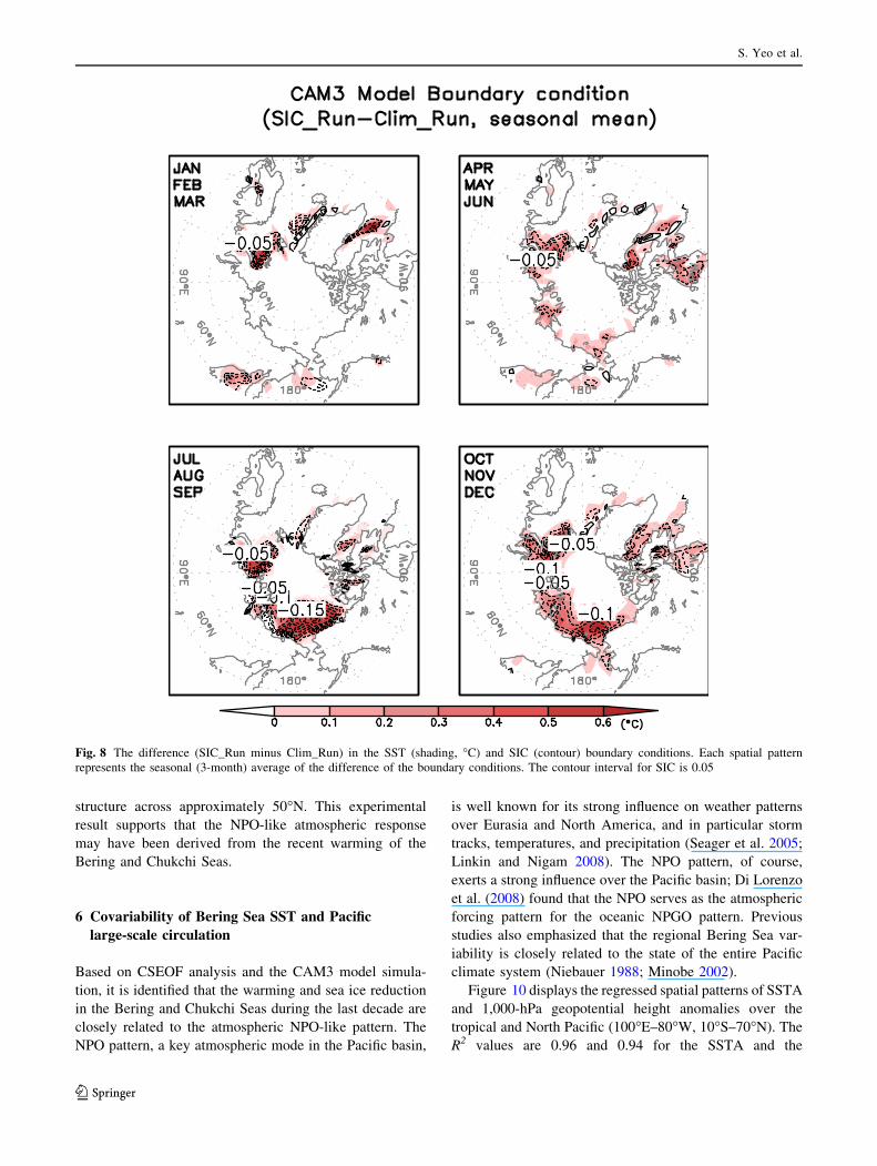
members. The seasonal (3-month) averages of the differ-
ences (SIC_Run minus Clim_Run) in the SST (shading)
and SIC (contour) boundary conditions are illustrated in
Fig. 8. SIC has declined more than 10 % over the Arctic
Ocean in the recent decade (1999–2010) compared to the
previous period of 1980–1998. Such a change has already
been pointed out in previous studies (Comiso et al. 2008;
Maslanik et al. 2007; Stroeve et al. 2007). The Bering and
Chukchi Sea ice has also declined except for the summer
season (July–September); the sea ice in this region retreats
completely in summer. By comparing SIC_Run and
Clim_Run experiments, therefore, an atmospheric response
to the recent change in the SST and SIC over the Arctic
Ocean can be identified. Of particular interest is the
atmospheric response over the North Pacific in the winter
season. Since the dipole structure is most pronounced in
January and February in the regression patterns (Fig. 7),
analysis for model result will also focus on January and
February.
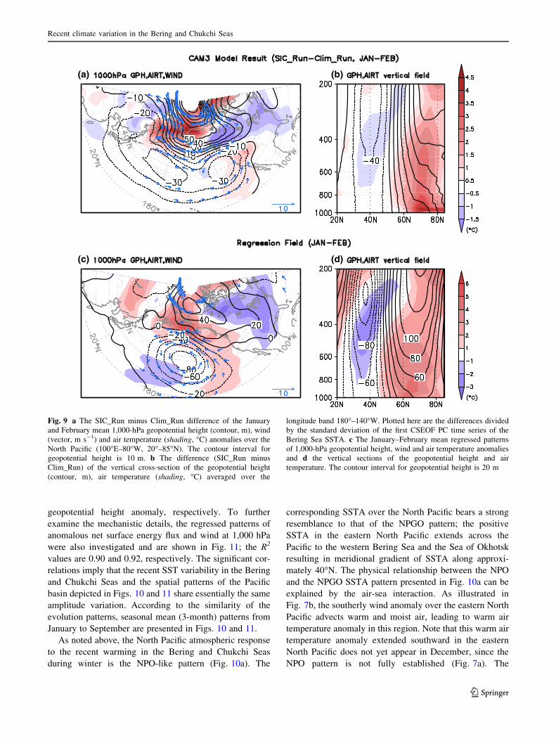
Figure 9a shows the difference in the January–February
mean of 1,000-hPa geopotential height (contour), wind
(vector), and air temperature (shading) between the two
simulations (SIC_Run minus Clim_Run) over the North
Pacific region (100�E–80�W, 20�–85�N). The vertical
cross-sections of the difference in geopotential height
(contour) and air temperature (shading) averaged over the
longitude band of 180�–140�W are illustrated in Fig. 9b.
The corresponding regression patterns in Fig. 7 are repro-
duced in the lower panel of Fig. 9. It is evident that CAM3
captures positive pressure anomaly over the Bering and
Chukchi Seas and negative pressure anomaly south of 50�N
in response to the warmer SST and reduced SIC. Spatial
correlation of the 1,000-hPa geopotential height anomaly
patterns (Fig. 9a, c) is 0.75, supporting that the atmo-
spheric response in winter over the North Pacific consists
of a meridional dipole structure, which resembles the NPO
pattern. In addition, the vertical structure of the response
(Fig. 9b) exhibits a striking similarity with the regression
result (Fig. 9d). They share common features of an
equivalent barotropic high over 60�–80�N in association
with warming in the entire troposphere and a barotropic
low over 30�–50�N, exhibiting a north-south dipole
Recent climate variation in the Bering and Chukchi Seas
123
structure across approximately 50�N. This experimental
result supports that the NPO-like atmospheric response
may have been derived from the recent warming of the
Bering and Chukchi Seas.
6 Covariability of Bering Sea SST and Pacific
large-scale circulation
Based on CSEOF analysis and the CAM3 model simula-
tion, it is identified that the warming and sea ice reduction
in the Bering and Chukchi Seas during the last decade are
closely related to the atmospheric NPO-like pattern. The
NPO pattern, a key atmospheric mode in the Pacific basin,
is well known for its strong influence on weather patterns
over Eurasia and North America, and in particular storm
tracks, temperatures, and precipitation (Seager et al. 2005;
Linkin and Nigam 2008). The NPO pattern, of course,
exerts a strong influence over the Pacific basin; Di Lorenzo
et al. (2008) found that the NPO serves as the atmospheric
forcing pattern for the oceanic NPGO pattern. Previous
studies also emphasized that the regional Bering Sea var-
iability is closely related to the state of the entire Pacific
climate system (Niebauer 1988; Minobe 2002).
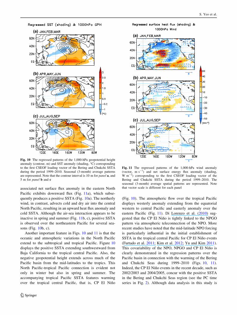
Figure 10 displays the regressed spatial patterns of SSTA
and 1,000-hPa geopotential height anomalies over the
tropical and North Pacific (100�E–80�W, 10�S–70�N). The
R2 values are 0.96 and 0.94 for the SSTA and the
Fig. 8 The difference (SIC_Run minus Clim_Run) in the SST (shading, �C) and SIC (contour) boundary conditions. Each spatial pattern
represents the seasonal (3-month) average of the difference of the boundary conditions. The contour interval for SIC is 0.05
S. Yeo et al.
123
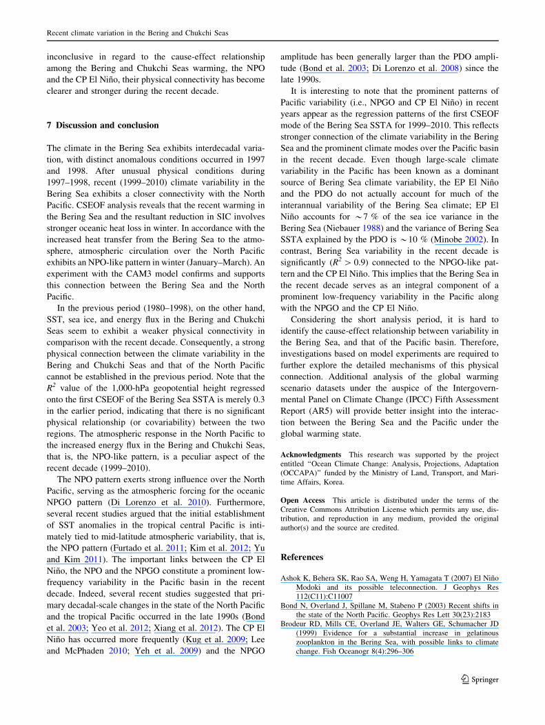
geopotential height anomaly, respectively. To further
examine the mechanistic details, the regressed patterns of
anomalous net surface energy flux and wind at 1,000 hPa
were also investigated and are shown in Fig. 11; the R2
values are 0.90 and 0.92, respectively. The significant cor-
relations imply that the recent SST variability in the Bering
and Chukchi Seas and the spatial patterns of the Pacific
basin depicted in Figs. 10 and 11 share essentially the same
amplitude variation. According to the similarity of the
evolution patterns, seasonal mean (3-month) patterns from
January to September are presented in Figs. 10 and 11.
As noted above, the North Pacific atmospheric response
to the recent warming in the Bering and Chukchi Seas
during winter is the NPO-like pattern (Fig. 10a). The
corresponding SSTA over the North Pacific bears a strong
resemblance to that of the NPGO pattern; the positive
SSTA in the eastern North Pacific extends across the
Pacific to the western Bering Sea and the Sea of Okhotsk
resulting in meridional gradient of SSTA along approxi-
mately 40�N. The physical relationship between the NPO
and the NPGO SSTA pattern presented in Fig. 10a can be
explained by the air-sea interaction. As illustrated in
Fig. 7b, the southerly wind anomaly over the eastern North
Pacific advects warm and moist air, leading to warm air
temperature anomaly in this region. Note that this warm air
temperature anomaly extended southward in the eastern
North Pacific does not yet appear in December, since the
NPO pattern is not fully established (Fig. 7a). The
(a) (b)
(c) (d)
Fig. 9 a The SIC_Run minus Clim_Run difference of the January
and February mean 1,000-hPa geopotential height (contour, m), wind
(vector, m s-1) and air temperature (shading, �C) anomalies over the
North Pacific (100�E–80�W, 20�–85�N). The contour interval for
geopotential height is 10 m. b The difference (SIC_Run minus
Clim_Run) of the vertical cross-section of the geopotential height
(contour, m), air temperature (shading, �C) averaged over the
longitude band 180�–140�W. Plotted here are the differences divided
by the standard deviation of the first CSEOF PC time series of the
Bering Sea SSTA. c The January–February mean regressed patterns
of 1,000-hPa geopotential height, wind and air temperature anomalies
and d the vertical sections of the geopotential height and air
temperature. The contour interval for geopotential height is 20 m
Recent climate variation in the Bering and Chukchi Seas
123
associated net surface flux anomaly in the eastern North
Pacific exhibits downward flux (Fig. 11a), which subse-
quently produces a positive SSTA (Fig. 10a). The northerly
wind, in contrast, advects cold and dry air into the central
North Pacific, resulting in an upward heat flux anomaly and
cold SSTA. Although the air-sea interaction appears to be
inactive in spring and summer (Fig. 11b, c), positive SSTA
is observed over the northeastern Pacific for several sea-
sons (Fig. 10b, c).
Another important feature in Figs. 10 and 11 is that the
oceanic and atmospheric variations in the North Pacific
extend to the subtropical and tropical Pacific. Figure 10
displays the positive SSTA extending southwestward from
Baja California to the tropical central Pacific. Also, the
negative geopotential height extends across much of the
Pacific basin from the mid-latitudes to the tropics. This
North Pacific-tropical Pacific connection is evident not
only in winter but also in spring and summer. The
accompanying tropical Pacific SSTA features warming
over the tropical central Pacific, that is, CP El Nino
(Fig. 10). The atmospheric flow over the tropical Pacific
displays westerly anomaly extending from the equatorial
western to central Pacific and easterly anomaly over the
eastern Pacific (Fig. 11). Di Lorenzo et al. (2010) sug-
gested that the CP El Nino is tightly linked to the NPGO
pattern via atmospheric teleconnection of the NPO. More
recent studies have noted that the mid-latitude NPO forcing
is particularly influential in the initial establishment of
SSTA in the tropical central Pacific for CP El Nino events
(Furtado et al. 2011; Kim et al. 2012; Yu and Kim 2011).
This covariability of the NPO, NPGO and CP El Nino is
clearly demonstrated in the regression patterns over the
Pacific basin in connection with the warming of the Bering
and Chukchi Seas during 1999–2010 (Figs. 10, 11).
Indeed, the CP El Nino events in the recent decade, such as
2002/2003 and 2004/2005, concur with the positive SSTA
in the Bering and Chukchi Seas region (see the PC time
series in Fig. 2). Although data analysis in this study is
(a)
(b)
(c)
Fig. 10 The regressed patterns of the 1,000-hPa geopotential height
anomaly (contour, m) and SST anomaly (shading, �C) corresponding
to the first CSEOF loading vector of the Bering and Chukchi SSTA
during the period 1999–2010. Seasonal (3-month) average patterns
are represented. Note that the contour interval is 10 m for panel a, and
5 m for panel b and c
(a)
(b)
(c)
Fig. 11 The regressed patterns of the 1,000-hPa wind anomaly
(vector, m s-1) and net surface energy flux anomaly (shading,
W m-2) corresponding to the first CSEOF loading vector of the
Bering and Chukchi SSTA during the period 1999–2010. The
seasonal (3-month) average spatial patterns are represented. Note
that vector scale is different for each panel
S. Yeo et al.
123
inconclusive in regard to the cause-effect relationship
among the Bering and Chukchi Seas warming, the NPO
and the CP El Nino, their physical connectivity has become
clearer and stronger during the recent decade.
7 Discussion and conclusion
The climate in the Bering Sea exhibits interdecadal varia-
tion, with distinct anomalous conditions occurred in 1997
and 1998. After unusual physical conditions during
1997–1998, recent (1999–2010) climate variability in the
Bering Sea exhibits a closer connectivity with the North
Pacific. CSEOF analysis reveals that the recent warming in
the Bering Sea and the resultant reduction in SIC involves
stronger oceanic heat loss in winter. In accordance with the
increased heat transfer from the Bering Sea to the atmo-
sphere, atmospheric circulation over the North Pacific
exhibits an NPO-like pattern in winter (January–March). An
experiment with the CAM3 model confirms and supports
this connection between the Bering Sea and the North
Pacific.
In the previous period (1980–1998), on the other hand,
SST, sea ice, and energy flux in the Bering and Chukchi
Seas seem to exhibit a weaker physical connectivity in
comparison with the recent decade. Consequently, a strong
physical connection between the climate variability in the
Bering and Chukchi Seas and that of the North Pacific
cannot be established in the previous period. Note that the
R2 value of the 1,000-hPa geopotential height regressed
onto the first CSEOF of the Bering Sea SSTA is merely 0.3
in the earlier period, indicating that there is no significant
physical relationship (or covariability) between the two
regions. The atmospheric response in the North Pacific to
the increased energy flux in the Bering and Chukchi Seas,
that is, the NPO-like pattern, is a peculiar aspect of the
recent decade (1999–2010).
The NPO pattern exerts strong influence over the North
Pacific, serving as the atmospheric forcing for the oceanic
NPGO pattern (Di Lorenzo et al. 2010). Furthermore,
several recent studies argued that the initial establishment
of SST anomalies in the tropical central Pacific is inti-
mately tied to mid-latitude atmospheric variability, that is,
the NPO pattern (Furtado et al. 2011; Kim et al. 2012; Yu
and Kim 2011). The important links between the CP El
Nino, the NPO and the NPGO constitute a prominent low-
frequency variability in the Pacific basin in the recent
decade. Indeed, several recent studies suggested that pri-
mary decadal-scale changes in the state of the North Pacific
and the tropical Pacific occurred in the late 1990s (Bond
et al. 2003; Yeo et al. 2012; Xiang et al. 2012). The CP El
Nino has occurred more frequently (Kug et al. 2009; Lee
and McPhaden 2010; Yeh et al. 2009) and the NPGO
amplitude has been generally larger than the PDO ampli-
tude (Bond et al. 2003; Di Lorenzo et al. 2008) since the
late 1990s.
It is interesting to note that the prominent patterns of
Pacific variability (i.e., NPGO and CP El Nino) in recent
years appear as the regression patterns of the first CSEOF
mode of the Bering Sea SSTA for 1999–2010. This reflects
stronger connection of the climate variability in the Bering
Sea and the prominent climate modes over the Pacific basin
in the recent decade. Even though large-scale climate
variability in the Pacific has been known as a dominant
source of Bering Sea climate variability, the EP El Nino
and the PDO do not actually account for much of the
interannual variability of the Bering Sea climate; EP El
Nino accounts for *7 % of the sea ice variance in the
Bering Sea (Niebauer 1988) and the variance of Bering Sea
SSTA explained by the PDO is *10 % (Minobe 2002). In
contrast, Bering Sea variability in the recent decade is
significantly (R2 [ 0.9) connected to the NPGO-like pat-
tern and the CP El Nino. This implies that the Bering Sea in
the recent decade serves as an integral component of a
prominent low-frequency variability in the Pacific along
with the NPGO and the CP El Nino.
Considering the short analysis period, it is hard to
identify the cause-effect relationship between variability in
the Bering Sea, and that of the Pacific basin. Therefore,
investigations based on model experiments are required to
further explore the detailed mechanisms of this physical
connection. Additional analysis of the global warming
scenario datasets under the auspice of the Intergovern-
mental Panel on Climate Change (IPCC) Fifth Assessment
Report (AR5) will provide better insight into the interac-
tion between the Bering Sea and the Pacific under the
global warming state.
Acknowledgments This research was supported by the project
entitled ‘‘Ocean Climate Change: Analysis, Projections, Adaptation
(OCCAPA)’’ funded by the Ministry of Land, Transport, and Mari-
time Affairs, Korea.
Open Access This article is distributed under the terms of the
Creative Commons Attribution License which permits any use, dis-
tribution, and reproduction in any medium, provided the original
author(s) and the source are credited.
References
Ashok K, Behera SK, Rao SA, Weng H, Yamagata T (2007) El Nino
Modoki and its possible teleconnection. J Geophys Res
112(C11):C11007
Bond N, Overland J, Spillane M, Stabeno P (2003) Recent shifts in
the state of the North Pacific. Geophys Res Lett 30(23):2183
Brodeur RD, Mills CE, Overland JE, Walters GE, Schumacher JD
(1999) Evidence for a substantial increase in gelatinous
zooplankton in the Bering Sea, with possible links to climate
change. Fish Oceanogr 8(4):296–306
Recent climate variation in the Bering and Chukchi Seas
123
Ceballos LI, Di Lorenzo E, Hoyos CD, Schneider N, Taguchi B
(2009) North Pacific gyre oscillation synchronizes climate
fluctuations in the eastern and western boundary systems.
J Climate 22(19):5163–5174
Collins WD, Rasch PJ, Boville BA, Hack JJ, McCaa JR, Williamson
DL, Briegleb BP, Bitz CM, Lin SJ, Zhang M (2006) The
formulation and atmospheric simulation of the community
atmosphere model version 3 (CAM3). J Climate
19(11):2144–2161
Comiso JC, Parkinson CL, Gersten R, Stock L (2008) Accelerated
decline in the Arctic sea ice cover. Geophys Res Lett
35(1):L01703
Deser C, Walsh JE, Timlin MS (2000) Arctic sea ice variability in the
context of recent atmospheric circulation trends. J Climate
13(3):617–633
Deser C, Tomas RA, Peng S (2007) The transient atmospheric
circulation response to North Atlantic SST and sea ice anom-
alies. J Climate 20(18):4751–4767
Di Lorenzo E, Schneider N, Cobb K, Franks P, Chhak K, Miller A,
McWilliams J, Bograd S, Arango H, Curchitser E (2008) North
Pacific Gyre Oscillation links ocean climate and ecosystem
change. Geophys Res Lett 35(8):L08607
Di Lorenzo E, Cobb K, Furtado J, Schneider N, Anderson B, Bracco
A, Alexander M, Vimont D (2010) Central Pacific El Nino and
decadal climate change in the North Pacific Ocean. Nat Geosci
3(11):762–765
Furtado JC, Di Lorenzo E, Anderson BT, Schneider N (2011)
Linkages between the North Pacific Oscillation and central
tropical Pacific SSTs at low frequencies. Clim Dyn. doi:10.1007/
s00382-011-1245-4
Grebmeier JM, Overland JE, Moore SE, Farley EV, Carmack EC,
Cooper LW, Frey KE, Helle JH, McLaughlin FA, McNutt SL
(2006) A major ecosystem shift in the northern Bering Sea.
Science 311(5766):1461–1464
Hare SR, Mantua NJ (2000) Empirical evidence for North Pacific
regime shifts in 1977 and 1989. Prog Oceanogr 47(2–4):103–145
Hoskins BJ, Karoly DJ (1981) The steady linear response of a
spherical atmosphere to thermal and orographic forcing. J Atmos
Sci 38(6):1179–1196
Hunt GL Jr, Baduini C, Brodeur R, Coyle K, Kachel N, Napp J, Salo
S, Schumacher J, Stabeno P, Stockwell D (1999) The Bering Sea
in 1998: the second consecutive year of extreme weather-forced
anomalies. EOS Trans AGU 80(47):561–566
Hunt GL Jr, Stabeno P, Walters G, Sinclair E, Brodeur RD, Napp JM,
Bond NA (2002) Climate change and control of the southeastern
Bering Sea pelagic ecosystem. Deep Sea Res Part II
49(26):5821–5853. doi:10.1016/S0967-0645(02)00321-1
Kanamitsu M, Ebisuzaki W, Woollen J, Yang SK, Hnilo J, Fiorino M,
Potter G (2002) Ncep-doe amip-ii reanalysis (r-2). Bull Am Met
Soc 83(11):1631–1644
Kao HY, Yu JY (2009) Contrasting eastern-Pacific and central-Pacific
types of ENSO. J Climate 22(3):615–632
Kim KY, North GR (1997) EOFs of harmonizable cyclostationary
processes. J Atmos Sci 54(19):2416–2427
Kim KY, North GR, Huang J (1996) EOFs of one-dimensional
cyclostationary time series: computations, examples, and sto-
chastic modeling. J Atmos Sci 53(7):1007–1016
Kim ST, Yu JY, Kumar A, Wang H (2012) Examination of the two
types of ENSO in the NCEP CFS model and its extratropical
associations. Mon Wea Rev 140:1908–1923
Kruse GH (1998) Salmon run failures in 1997–1998: a link to
anomalous ocean conditions? Alaska Fish Res Bull 5(1):55–63
Kug JS, Jin FF, An SI (2009) Two types of El Nino events: cold
tongue El Nino and warm pool El Nino. J Climate
22(6):1499–1515
Lee T, McPhaden MJ (2010) Increasing intensity of El Nino in the
central-equatorial Pacific. Geophys Res Lett 37(14):L14603
Linkin ME, Nigam S (2008) The north pacific oscillation-west Pacific
teleconnection pattern: mature-phase structure and winter
impacts. J Climate 21(9):1979–1997
Maslanik J, Fowler C, Stroeve J, Drobot S, Zwally J, Yi D, Emery W
(2007) A younger, thinner Arctic ice cover: increased potential
for rapid, extensive sea-ice loss. Geophys Res Lett
34(24):L24501
Minobe S (2002) Interannual to interdecadal changes in the Bering
Sea and concurrent 1998/99 changes over the North Pacific. Prog
Oceanogr 55(1–2):45–64
Napp JM, Hunt GL Jr (2001) Anomalous conditions in the south-
eastern Bering Sea 1997: linkages among climate, weather,
ocean, and Biology. Fish Oceanogr 10(1):61–68
National Research Council (1996) The Bering Sea ecosystem.
National Academy Press, Washington, DC
Niebauer H (1988) Effects of El Nino-Southern Oscillation and North
Pacific weather patterns on interannual variability in the
subarctic Bering Sea. J Geophys Res 93(C5):5051–5068
Overland JE, Stabeno PJ (2004) Is the climate of the Bering Sea
warming and affecting the ecosystem. EOS Trans AGU
85(33):309–316
Overland JE, Adams JM, Bond NA (1999) Decadal variability of the
Aleutian low and its relation to high-latitude circulation.
J Climate 12(5):1542–1548
Overland JE, Wang M, Wood KR, Percival DB, Bond NA (2012)
Recent Bering Sea warm and cold events in a 95-year contest.
Deep Sea Res Part II 65–70:6–13
Peng S, Robinson WA, Li S (2003) Mechanisms for the NAO
responses to the North Atlantic SST tripole. J Climate
16(12):1987–2004
Rayner N, Parker D, Horton E, Folland C, Alexander L, Rowell D,
Kent E, Kaplan A (2003) Global analyses of sea surface
temperature, sea ice, and night marine air temperature since the
late nineteenth century. J Geophys Res 108(D14):4407
Rogers JC (1981) The North Pacific oscillation. J Climatol 1(1):39–57
Schumacher J, Bond N, Brodeur R, Livingston P, Napp J, Stabeno P
(2003) Climate change in the southeastern Bering Sea and some
consequences for biota. Large Marine Ecosyst World Trends
Exploit Prot Res 17–40
Screen JA, Simmonds I (2010a) The central role of diminishing sea
ice in recent Arctic temperature amplification. Nature
464(7293):1334–1337
Screen JA, Simmonds I (2010b) Increasing fall-winter energy loss
from the Arctic Ocean and its role in Arctic temperature
amplification. Geophys Res Lett 37(16):L16707
Seager R, Harnik N, Robinson W, Kushnir Y, Ting M, Huang HP,
Velez J (2005) Mechanisms of ENSO-forcing of hemispherically
symmetric precipitation variability. Q J Roy Meteor Soc
131(608):1501–1527
Smith TM, Reynolds RW, Peterson TC, Lawrimore J (2008)
Improvements to NOAA’s historical merged land-ocean surface
temperature analysis (1880–2006). J Climate 21(10):
2283–2296
Stabeno P, Bond N, Kachel N, Salo S, Schumacher J (2001) On the
temporal variability of the physical environment over the south-
eastern Bering Sea. Fish Oceanogr 10(1):81–98
Stabeno P, Bond N, Salo S (2007) On the recent warming of the
southeastern Bering Sea shelf. Deep Sea Res Part II
54(23–26):2599–2618
Stockwell DA, Whitledge TE, Zeeman SI, Coyle KO, Napp JM,
Brodeur RD, Pinchuk AI, Hunt JRGL (2001) Anomalous
conditions in the south-eastern Bering Sea, 1997: nutrients,
phytoplankton and zooplankton. Fish Oceanogr 10(1):99–116
S. Yeo et al.
123
Stroeve J, Holland MM, Meier W, Scambos T, Serreze M (2007)
Arctic sea ice decline: faster than forecast. Geophys Res Lett
34(9):9501
Xiang B, Wang B, Li T (2012) A new paradigm for the predominance
of standing Central Pacific Warming after the late 1990s. Clim
Dyn. doi:10.1007/s00382-012-1427-8
Yeh SW, Kug JS, Dewitte B, Kwon MH, Kirtman BP, Jin FF (2009)
El Nino in a changing climate. Nature 461(7263):511–514
Yeh SW, Kang YJ, Noh Y, Miller AJ (2011) The North Pacific
climate transitions of the winters of 1976/77 and 1988/89.
J Climate 24:1170–1183
Yeo SR, Kim KY, Yeh SW, Kim WM (2012) Decadal changes in the
relationship between the tropical Pacific and the North Pacific.
J Geophys Res 117(D15):D15102
Yu JY, Kim ST (2011) Relationships between extratropical sea level
pressure variations and the central Pacific and eastern Pacific
types of ENSO. J Climate 24(3):708–720
Recent climate variation in the Bering and Chukchi Seas
123