Tellus (2010), 62A, 516–529 C© 2010 The AuthorsJournal compilation C© 2010 Blackwell Munksgaard

Printed in Singapore. All rights reserved

T E L L U S

The mid-depth circulation of the Nordic Seas derivedfrom profiling float observations

By G . VO ET 1∗, D . Q UA D FA SEL 1, K . A . M O R K 2 and H . SØ ILA N D 2, 1Institut fur Meereskunde,KlimaCampus, University of Hamburg, Bundesstr. 53, 20146 Hamburg, Germany; 2Institute of Marine

Research and Bjerknes Centre for Climate Research, Bergen, Norway

(Manuscript received 10 July 2009; in final form 10 March 2010)

A B S T R A C TThe trajectories of 61 profiling Argo floats deployed at mid-depth in the Nordic Seas—the Greenland, Lofoten andNorwegian Basins and the Iceland Plateau—between 2001 and 2009 are analysed to determine the pattern, strength andvariability of the regional circulation. The mid-depth circulation is strongly coupled with the structure of the bottomtopography of the four major basins and of the Nordic Seas as a whole. It is cyclonic, both on the large-scale and on thebasin scale, with weak flow (<1 cm s−1) in the interior of the basins and somewhat stronger flow (up to 5 cm s−1) attheir rims. Only few floats moved from one basin to another, indicating that the internal recirculation within the basinsis by far dominating the larger-scale exchanges. The seasonal variability of the mid-depth flow ranges from less than1 cm s−1 over the Iceland Plateau to more than 4 cm s−1 in the Greenland Basin. These velocities translate into internalgyre transports of up to 15 ± 10 × 106 m3 s−1, several times the overall exchange between the Nordic Seas and thesubpolar North Atlantic. The seasonal variability of the Greenland Basin and the Norwegian Basin can be adequatelymodelled using the barotropic vorticity equation, with the wind and bottom friction as the only forcing mechanisms.For the Lofoten Basin and the Iceland Plateau less than 50% of the variance can be explained by the wind.

1. Introduction

The Nordic Seas, comprising the area between Greenland, Spits-bergen, Norway, Iceland and the Faroe Islands, are a marginalsea with great importance for the Atlantic Meridional Overturn-ing Circulation. Atmospheric conditions in this area lead to atransformation of inflowing warm and buoyant surface waterinto cold and dense deep water masses (Mauritzen, 1996) thateventually feed the overflows across the Greenland–ScotlandRidge into the subpolar North Atlantic (Hansen and Østerhus,2000). The circulation within the Nordic Seas is essential for thedeep water formation as it transports the inflowing surface waternorthwards, redistributes the water within the Nordic Seas andsupplies the overflows with the dense water to be exported.

The near-surface circulation of the Nordic Seas was studiedwith drogued surface drifters by Poulain et al. (1996), Orvik andNiiler (2002) and Jakobsen et al. (2003). They find a generalcyclonic circulation with meridional boundary currents and ad-ditional cyclonic circulation patterns in the Greenland Basin, theNorwegian Basin and the Iceland Plateau. The surface drifters

∗Corresponding author.e-mail: gunnar.voet@zmaw.deDOI: 10.1111/j.1600-0870.2010.00444.x

confirm the tight link between surface circulation and bottom to-pography that was already noted by Helland-Hansen and Nansen(1909) in their fundamental study of the Nordic Seas.

Our knowledge about the mid-depth and deep circulation ofthe Nordic Seas stems mainly from water mass analyses, currentobservations with moored instrumentation and model studies.The basin structure of the Nordic Seas (Fig. 1) with closed f /Hcontours and the weak stratification leads to a strong topographicsteering of the flow field. This led Nøst and Isachsen (2003) todevelop a simplified diagnostic model for the Nordic Seas andthe Arctic Ocean that is driven by climatological wind forcingand a climatological density field. It solves for a bottom flowfield which compares well with available direct current obser-vations. The number of these direct current measurements atdepth is limited for the interior of the Nordic Seas as most cur-rent meter studies concentrated on the in- and outflows to andfrom the Nordic Seas. An exception is the study of Woodgateet al. (1999) who deployed moorings at the continental slopeeast of Greenland that extended into the deeper parts of theGreenland Basin. They find evidence for a recirculation internalto the Greenland Sea that is intensified towards the edge of thebasin.

Several studies show an intensification of the Nordic Seas’internal circulation in winter. This seasonal variability is found

516 Tellus 62A (2010), 4

P U B L I S H E D B Y T H E I N T E R N A T I O N A L M E T E O R O L O G I C A L I N S T I T U T E I N S T O C K H O L M

SERIES ADYNAMIC METEOROLOGYAND OCEANOGRAPHY

MID-DEPTH CIRCULATION OF THE NORDIC SEAS 517

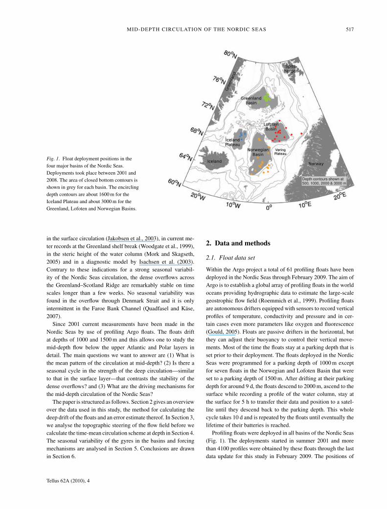
Fig. 1. Float deployment positions in thefour major basins of the Nordic Seas.Deployments took place between 2001 and2008. The area of closed bottom contours isshown in grey for each basin. The encirclingdepth contours are about 1600 m for theIceland Plateau and about 3000 m for theGreenland, Lofoten and Norwegian Basins.

in the surface circulation (Jakobsen et al., 2003), in current me-ter records at the Greenland shelf break (Woodgate et al., 1999),in the steric height of the water column (Mork and Skagseth,2005) and in a diagnostic model by Isachsen et al. (2003).Contrary to these indications for a strong seasonal variabil-ity of the Nordic Seas circulation, the dense overflows acrossthe Greenland–Scotland Ridge are remarkably stable on timescales longer than a few weeks. No seasonal variability wasfound in the overflow through Denmark Strait and it is onlyintermittent in the Faroe Bank Channel (Quadfasel and Kase,2007).

Since 2001 current measurements have been made in theNordic Seas by use of profiling Argo floats. The floats driftat depths of 1000 and 1500 m and this allows one to study themid-depth flow below the upper Atlantic and Polar layers indetail. The main questions we want to answer are (1) What isthe mean pattern of the circulation at mid-depth? (2) Is there aseasonal cycle in the strength of the deep circulation—similarto that in the surface layer—that contrasts the stability of thedense overflows? and (3) What are the driving mechanisms forthe mid-depth circulation of the Nordic Seas?

The paper is structured as follows. Section 2 gives an overviewover the data used in this study, the method for calculating thedeep drift of the floats and an error estimate thereof. In Section 3,we analyse the topographic steering of the flow field before wecalculate the time-mean circulation scheme at depth in Section 4.The seasonal variability of the gyres in the basins and forcingmechanisms are analysed in Section 5. Conclusions are drawnin Section 6.

2. Data and methods

2.1. Float data set

Within the Argo project a total of 61 profiling floats have beendeployed in the Nordic Seas through February 2009. The aim ofArgo is to establish a global array of profiling floats in the worldoceans providing hydrographic data to estimate the large-scalegeostrophic flow field (Roemmich et al., 1999). Profiling floatsare autonomous drifters equipped with sensors to record verticalprofiles of temperature, conductivity and pressure and in cer-tain cases even more parameters like oxygen and fluorescence(Gould, 2005). Floats are passive drifters in the horizontal, butthey can adjust their buoyancy to control their vertical move-ments. Most of the time the floats stay at a parking depth that isset prior to their deployment. The floats deployed in the NordicSeas were programmed for a parking depth of 1000 m exceptfor seven floats in the Norwegian and Lofoten Basin that wereset to a parking depth of 1500 m. After drifting at their parkingdepth for around 9 d, the floats descend to 2000 m, ascend to thesurface while recording a profile of the water column, stay atthe surface for 5 h to transfer their data and position to a satel-lite until they descend back to the parking depth. This wholecycle takes 10 d and is repeated by the floats until eventually thelifetime of their batteries is reached.

Profiling floats were deployed in all basins of the Nordic Seas(Fig. 1). The deployments started in summer 2001 and morethan 4100 profiles were obtained by these floats through the lastdata update for this study in February 2009. The positions of

Tellus 62A (2010), 4

518 G. VOET ET AL.

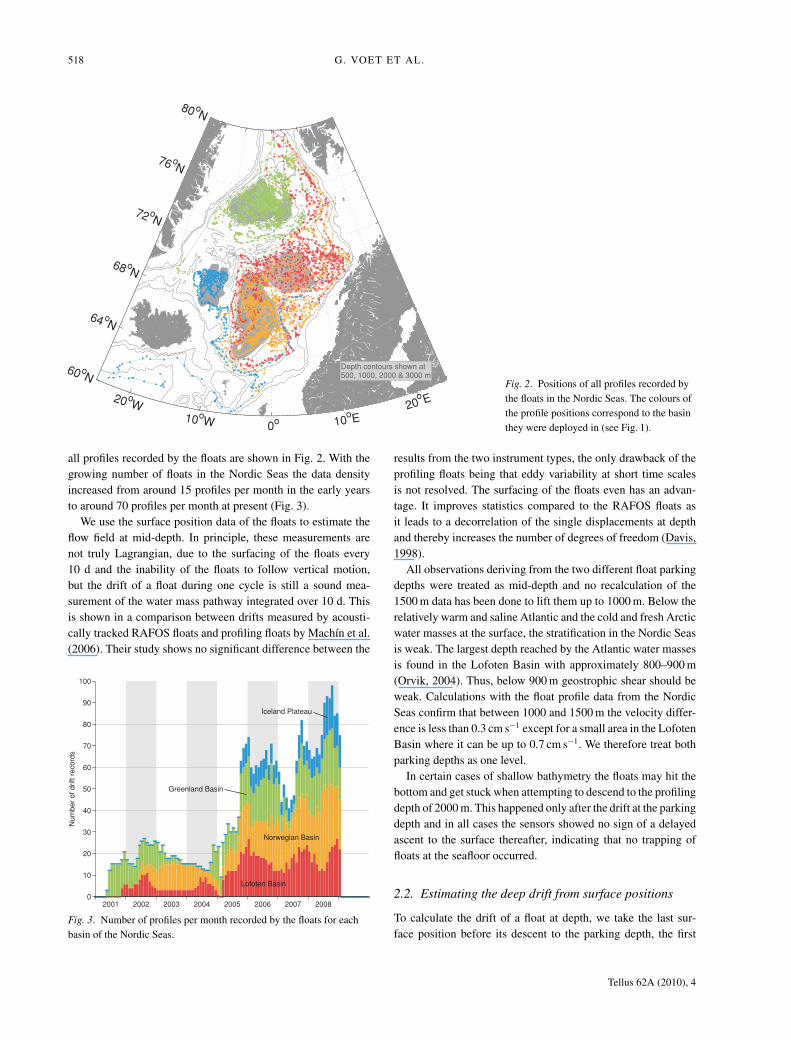
Fig. 2. Positions of all profiles recorded bythe floats in the Nordic Seas. The colours ofthe profile positions correspond to the basinthey were deployed in (see Fig. 1).

all profiles recorded by the floats are shown in Fig. 2. With thegrowing number of floats in the Nordic Seas the data densityincreased from around 15 profiles per month in the early yearsto around 70 profiles per month at present (Fig. 3).

We use the surface position data of the floats to estimate theflow field at mid-depth. In principle, these measurements arenot truly Lagrangian, due to the surfacing of the floats every10 d and the inability of the floats to follow vertical motion,but the drift of a float during one cycle is still a sound mea-surement of the water mass pathway integrated over 10 d. Thisis shown in a comparison between drifts measured by acousti-cally tracked RAFOS floats and profiling floats by Machın et al.(2006). Their study shows no significant difference between the

Fig. 3. Number of profiles per month recorded by the floats for eachbasin of the Nordic Seas.

results from the two instrument types, the only drawback of theprofiling floats being that eddy variability at short time scalesis not resolved. The surfacing of the floats even has an advan-tage. It improves statistics compared to the RAFOS floats asit leads to a decorrelation of the single displacements at depthand thereby increases the number of degrees of freedom (Davis,1998).

All observations deriving from the two different float parkingdepths were treated as mid-depth and no recalculation of the1500 m data has been done to lift them up to 1000 m. Below therelatively warm and saline Atlantic and the cold and fresh Arcticwater masses at the surface, the stratification in the Nordic Seasis weak. The largest depth reached by the Atlantic water massesis found in the Lofoten Basin with approximately 800–900 m(Orvik, 2004). Thus, below 900 m geostrophic shear should beweak. Calculations with the float profile data from the NordicSeas confirm that between 1000 and 1500 m the velocity differ-ence is less than 0.3 cm s−1 except for a small area in the LofotenBasin where it can be up to 0.7 cm s−1. We therefore treat bothparking depths as one level.

In certain cases of shallow bathymetry the floats may hit thebottom and get stuck when attempting to descend to the profilingdepth of 2000 m. This happened only after the drift at the parkingdepth and in all cases the sensors showed no sign of a delayedascent to the surface thereafter, indicating that no trapping offloats at the seafloor occurred.

2.2. Estimating the deep drift from surface positions

To calculate the drift of a float at depth, we take the last sur-face position before its descent to the parking depth, the first

Tellus 62A (2010), 4

MID-DEPTH CIRCULATION OF THE NORDIC SEAS 519

surface position after the ascent back to the surface and thetime interval between these two positions. The drift velocitythen is the distance between the two positions divided by thetime interval. We define the location and time of the velocityobservation as the mid-point between the diving and surfacingpoints. Two main error sources have to be considered when thesurface positions of the floats are used to infer the drift at depth.These are the uncertainty of the position fix and the velocityshear the float encounters on its passage between surface anddepth.

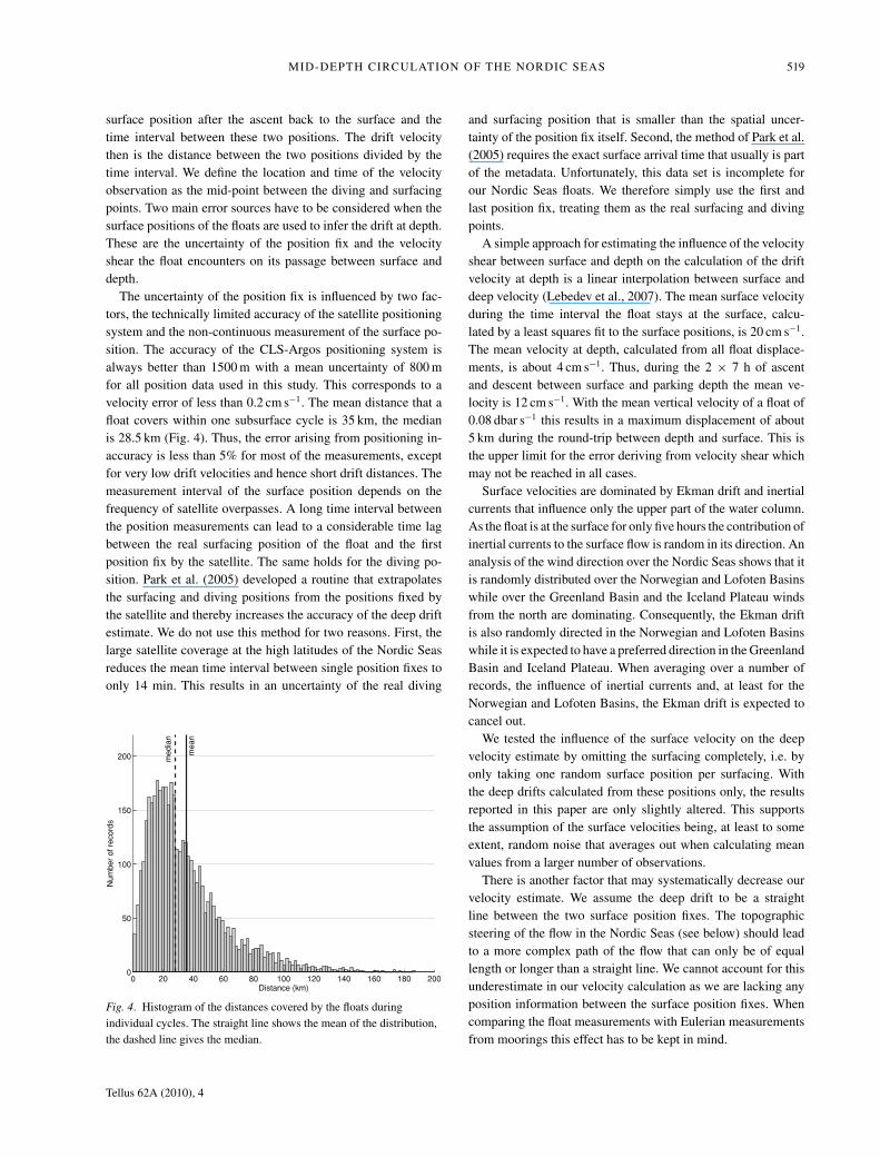
The uncertainty of the position fix is influenced by two fac-tors, the technically limited accuracy of the satellite positioningsystem and the non-continuous measurement of the surface po-sition. The accuracy of the CLS-Argos positioning system isalways better than 1500 m with a mean uncertainty of 800 mfor all position data used in this study. This corresponds to avelocity error of less than 0.2 cm s−1. The mean distance that afloat covers within one subsurface cycle is 35 km, the medianis 28.5 km (Fig. 4). Thus, the error arising from positioning in-accuracy is less than 5% for most of the measurements, exceptfor very low drift velocities and hence short drift distances. Themeasurement interval of the surface position depends on thefrequency of satellite overpasses. A long time interval betweenthe position measurements can lead to a considerable time lagbetween the real surfacing position of the float and the firstposition fix by the satellite. The same holds for the diving po-sition. Park et al. (2005) developed a routine that extrapolatesthe surfacing and diving positions from the positions fixed bythe satellite and thereby increases the accuracy of the deep driftestimate. We do not use this method for two reasons. First, thelarge satellite coverage at the high latitudes of the Nordic Seasreduces the mean time interval between single position fixes toonly 14 min. This results in an uncertainty of the real diving

Fig. 4. Histogram of the distances covered by the floats duringindividual cycles. The straight line shows the mean of the distribution,the dashed line gives the median.

and surfacing position that is smaller than the spatial uncer-tainty of the position fix itself. Second, the method of Park et al.(2005) requires the exact surface arrival time that usually is partof the metadata. Unfortunately, this data set is incomplete forour Nordic Seas floats. We therefore simply use the first andlast position fix, treating them as the real surfacing and divingpoints.

A simple approach for estimating the influence of the velocityshear between surface and depth on the calculation of the driftvelocity at depth is a linear interpolation between surface anddeep velocity (Lebedev et al., 2007). The mean surface velocityduring the time interval the float stays at the surface, calcu-lated by a least squares fit to the surface positions, is 20 cm s−1.The mean velocity at depth, calculated from all float displace-ments, is about 4 cm s−1. Thus, during the 2 × 7 h of ascentand descent between surface and parking depth the mean ve-locity is 12 cm s−1. With the mean vertical velocity of a float of0.08 dbar s−1 this results in a maximum displacement of about5 km during the round-trip between depth and surface. This isthe upper limit for the error deriving from velocity shear whichmay not be reached in all cases.

Surface velocities are dominated by Ekman drift and inertialcurrents that influence only the upper part of the water column.As the float is at the surface for only five hours the contribution ofinertial currents to the surface flow is random in its direction. Ananalysis of the wind direction over the Nordic Seas shows that itis randomly distributed over the Norwegian and Lofoten Basinswhile over the Greenland Basin and the Iceland Plateau windsfrom the north are dominating. Consequently, the Ekman driftis also randomly directed in the Norwegian and Lofoten Basinswhile it is expected to have a preferred direction in the GreenlandBasin and Iceland Plateau. When averaging over a number ofrecords, the influence of inertial currents and, at least for theNorwegian and Lofoten Basins, the Ekman drift is expected tocancel out.

We tested the influence of the surface velocity on the deepvelocity estimate by omitting the surfacing completely, i.e. byonly taking one random surface position per surfacing. Withthe deep drifts calculated from these positions only, the resultsreported in this paper are only slightly altered. This supportsthe assumption of the surface velocities being, at least to someextent, random noise that averages out when calculating meanvalues from a larger number of observations.

There is another factor that may systematically decrease ourvelocity estimate. We assume the deep drift to be a straightline between the two surface position fixes. The topographicsteering of the flow in the Nordic Seas (see below) should leadto a more complex path of the flow that can only be of equallength or longer than a straight line. We cannot account for thisunderestimate in our velocity calculation as we are lacking anyposition information between the surface position fixes. Whencomparing the float measurements with Eulerian measurementsfrom moorings this effect has to be kept in mind.

Tellus 62A (2010), 4

520 G. VOET ET AL.

2.3. Wind stress data

To estimate the atmospheric wind forcing over the Nordic Seas,NCEP/NCAR-reanalysis data (Kalnay et al., 1996) are used. TheNCEP/NCAR-reanalysis assimilates a multitude of observationsinto a model to produce a homogeneous data set of many atmo-spheric and oceanic variables. A comparison with QuikSCATwind fields, a data set derived from active radar measurementsof the sea surface roughness, has shown that the NCEP/NCAR-reanalysis data represents the surface winds over the Nordic Seaswell in terms of low- and high-frequency variability (Kolstad,2008). We use the 6-hourly momentum flux data set to calculatethe wind stress curl over the Nordic Seas.

2.4. Bottom topography

The ETOPO2 bathymetry with a resolution of two minutes isused to assign bottom depths and topographic gradients to thefloat displacements. For the region of the Nordic Seas, ETOPO2consists of the Smith and Sandwell bathymetry (Smith andSandwell, 1997) south of 64◦N and the International Bathy-metric Chart of the Arctic Ocean (IBCAO, Jakobsson et al.,2000) north of 64◦N. For the calculation of bottom gradients wesmoothed the topography at the length scale of the float displace-ments (Thomson and Freeland, 2003). The mean displacementfor all Nordic Seas floats is about 30 km and we remove scalessmaller than 40 km.

3. Topographically influenced mean flow

The floats have the tendency to stay in the basin where they weredeployed in (Fig. 2). On average 75% of all float positions stemfrom the deployment basin while the remaining 25% are locatedin one of the other basins. There is some organized exchangethrough the opening between the Norwegian and Lofoten Basinwith floats leaving the Norwegian Basin with the rim currentin the southern part of the opening. Floats only transfer fromthe Lofoten into the Norwegian Basin in the northern part of theopening. Furthermore, some floats leave the Lofoten Basin in therim current towards Fram Strait, one float leaves the GreenlandBasin southward in the rim current. The floats’ stay in the IcelandPlateau is rather short, and most of them escape towards thesoutheast into the Norwegian Basin within one to 2 yr. One floatfrom the Iceland Plateau even made its way through the FaroeBank Channel into the subpolar North Atlantic. However, theIceland Plateau is an exception and the floats mostly stay in thebasin they were deployed in.

In general the floats follow lines of constant bottom depth.Examples for single trajectories can be found in Gascard andMork (2008) and Søiland et al. (2008). In Fig. 2 the positionsof two floats above the only 1000–1500 m deep Vøring-Plateauoff the Norwegian coast between the Lofoten and NorwegianBasin show that they were trapped there. This indicates again

the topographic steering of the flow field as the floats and thusthe water cannot move away from the relatively shallow plateauinto deeper areas.

Given the strong topographic steering we project the mea-sured drift velocities onto the bathymetry. This gives us velocitycomponents along and across the local topography instead ofnorth and east components. The convention here is that for thealong bathymetry component, positive values have the shallowbottom on the left side irrespective of the basin.

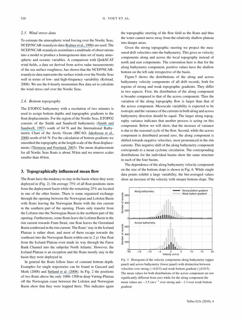
Figure 5 shows the distributions of the along and acrossbathymetry velocity components of all drift records, both forregions of strong and weak topographic gradients. They differin two aspects. First, the distribution of the along componentis broader compared to that of the across component. Thus thevariation of the along topography flow is larger than that ofthe across component. Mesoscale variability is expected to beisotropic and the variance of the currents in both along and acrossbathymetry direction should be equal. The larger along topog-raphy variance indicates that another process is acting on thiscomponent. Below we will show, that the increase of varianceis due to the seasonal cycle of the flow. Second, while the acrosscomponent is distributed around zero, the along component isshifted towards negative velocities, most pronounced in the rimcurrents. This negative shift of the along bathymetry componentcorresponds to a mean cyclonic circulation. The correspondingdistributions for the individual basins show the same structurein each of the four basins.

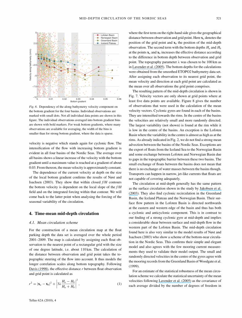
The dependence of the along bathymetry velocity componenton the size of the bottom slope is shown in Fig. 6. While singledata points exhibit a large variability, the bin-averaged valuesshow an increase of the velocity with steeper bottom slope. The

Fig. 5. Histogram of the velocity components along bathymetry (upperpanel) and across bathymetry (lower panel) with distinction betweenvelocities over strong (>0.015) and weak bottom gradient (≤0.015).The mean values for both distributions of the across component are notsignificantly different from zero while for the along component themean values are −3.5 cm s−1 over strong and −1.3 over weak bottomgradient.

Tellus 62A (2010), 4

MID-DEPTH CIRCULATION OF THE NORDIC SEAS 521

Fig. 6. Dependency of the along bathymetry velocity component onthe bottom gradient for the four basins. Individual observations aremarked with small dots. Not all individual data points are shown in thisfigure. The individual observations averaged into bottom gradient binsare shown with bold markers. For weak bottom gradients, where manyobservations are available for averaging, the width of the bins issmaller than for strong bottom gradient, where the data is sparse.

velocity is negative which stands again for cyclonic flow. Theintensification of the flow with increasing bottom gradient isevident in all four basins of the Nordic Seas. The average overall basins shows a linear increase of the velocity with the bottomgradient until a maximum value is reached at a gradient of about0.03. From thereon, the mean velocity is approximately constant.

The dependence of the current velocity at depth on the sizeof the local bottom gradient confirms the results of Nøst andIsachsen (2003). They show that within closed f /H contoursthe bottom velocity is dependent on the local slope of the f /Hfield and on the integrated forcing within that contour. We willcome back to the latter point when analysing the forcing of theseasonal variability of the circulation.

4. Time-mean mid-depth circulation

4.1. Mean circulation scheme

For the construction of a mean circulation map at the floatparking depth the data set is averaged over the whole period2001–2009. The map is calculated by assigning each float ob-servation to the nearest point of a rectangular grid with the sizeof one degree latitude, i.e. about 110 km. The calculation ofthe distance between observation and grid point takes the to-pographic steering of the flow into account. It thus models thelonger correlation scales along bottom topography. FollowingDavis (1998), the effective distance r between float observationand grid point is calculated as

r2 = |xa − xb|2 +∣∣∣∣3λ

Ha − Hb

Ha + Hb

∣∣∣∣2

, (1)

where the first term on the right-hand side gives the geographicaldistance between observation and grid point. Here xa denotes theposition of the grid point and xb the position of the mid-depthobservation. The second term with the bottom depths Ha and Hb

at the points xa and xb increases the effective distance accordingto the difference in bottom depth between observation and gridpoint. The topography parameter λ was chosen to be 100 km asin Lavender et al. (2005). The bottom depths for the calculationswere obtained from the smoothed ETOPO2 bathymetry data set.After assigning each observation to its nearest grid point, themean velocity and direction at each grid point are calculated asthe mean over all observations the grid point comprises.

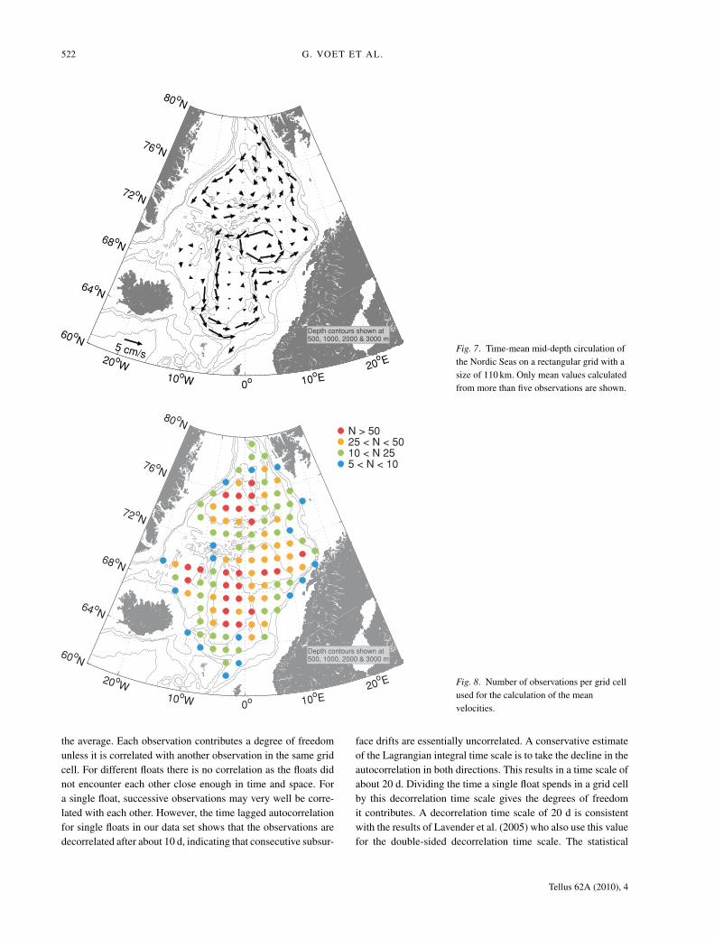
The resulting pattern of the mid-depth circulation is shown inFig. 7. Velocity vectors are only shown at grid points where atleast five data points are available. Figure 8 gives the numberof observations that were used in the calculation of the meanvelocity vectors. Cyclonic gyres are found in each of the basins.They are intensified towards the rims. In the centre of the basinsthe velocities are relatively small and more randomly directed.The largest variability (not shown) is found at the rim while itis low in the centre of the basins. An exception is the LofotenBasin where the variability in the centre is almost as high as at therims. As already indicated in Fig. 2, we do not find a strong meanadvection between the basins of the Nordic Seas. Exceptions arethe export of floats from the Iceland Sea to the Norwegian Basinand some exchange between Lofoten and Norwegian Basin dueto gaps in the topographic barrier between these two basins. Thesmall exchange of floats between the basins does not mean thatthere is no exchange of water masses between the basins though.Transports can happen in narrow, jet-like currents that floats arenot capable of covering adequately.

The circulation at mid-depth generally has the same patternas the surface circulation shown in the study by Jakobsen et al.(2003). They also find cyclonic recirculation in the GreenlandBasin, the Iceland Plateau and the Norwegian Basin. Their sur-face flow pattern in the Lofoten Basin is directed northwardsat the eastern and western edge of the basin and thus has botha cyclonic and anticyclonic component. This is in contrast toour finding of a strong cyclonic gyre at mid-depth and impliesa considerable shear between surface and mid-depth flow in thewestern part of the Lofoten Basin. The mid-depth circulationfound here is also very similar to the model results of Nøst andIsachsen (2003) who show a scheme of the bottom-near circula-tion in the Nordic Seas. This confirms their simple and elegantmodel and also agrees with the few mooring current measure-ments they used to validate their model output. The small andrandomly directed velocities in the centre of the gyres agree withthe mooring records from the Greenland Basin of Woodgate et al.(1999).

For an estimate of the statistical robustness of the mean circu-lation scheme we calculate the statistical uncertainty of the meanvelocities following Lavender et al. (2005) as the covariance ofeach average divided by the number of degrees of freedom in

Tellus 62A (2010), 4

522 G. VOET ET AL.

Fig. 7. Time-mean mid-depth circulation ofthe Nordic Seas on a rectangular grid with asize of 110 km. Only mean values calculatedfrom more than five observations are shown.

Fig. 8. Number of observations per grid cellused for the calculation of the meanvelocities.

the average. Each observation contributes a degree of freedomunless it is correlated with another observation in the same gridcell. For different floats there is no correlation as the floats didnot encounter each other close enough in time and space. Fora single float, successive observations may very well be corre-lated with each other. However, the time lagged autocorrelationfor single floats in our data set shows that the observations aredecorrelated after about 10 d, indicating that consecutive subsur-

face drifts are essentially uncorrelated. A conservative estimateof the Lagrangian integral time scale is to take the decline in theautocorrelation in both directions. This results in a time scale ofabout 20 d. Dividing the time a single float spends in a grid cellby this decorrelation time scale gives the degrees of freedomit contributes. A decorrelation time scale of 20 d is consistentwith the results of Lavender et al. (2005) who also use this valuefor the double-sided decorrelation time scale. The statistical

Tellus 62A (2010), 4

MID-DEPTH CIRCULATION OF THE NORDIC SEAS 523

uncertainties calculated with this integral time scale show thatmost mean velocities are significant. Only few mean velocitiesin the centre of the basins are smaller than their statistical un-certainty.

4.2. Topostrophy

It is instructive to study the topographical steering of the flowwith a single scalar parameter. Killworth (1992) introduced sucha parameter to measure the alignment of the flow with bottom to-pography. Holloway et al. (2007) termed this parameter topostro-phy. The topostrophy T is defined as the vertical component ofthe cross product of velocity vector and bottom gradient:

T = (�v × �∇H )z, (2)

Topostrophy is positive for cyclonic flow and negative for an-ticyclonic flow. It is zero for a current perpendicular to localisobaths. We define the normalised topostrophy T as

T = (�v × �∇H )z|�v| · | �∇H | . (3)

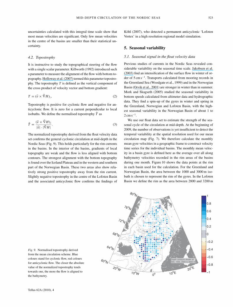
The normalized topostrophy derived from the float velocity dataset confirms the general cyclonic circulation at mid-depth in theNordic Seas (Fig. 9). This holds particularly for the rim currentsin the basins. In the interior of the basins, gradients of localtopography are weak and the flow is less aligned with bottomcontours. The strongest alignment with the bottom topographyis found over the Iceland Plateau and in the western and southernpart of the Norwegian Basin. These two areas also show rela-tively strong positive topostrophy away from the rim current.Slightly negative topostrophy in the centre of the Lofoten Basinand the associated anticyclonic flow confirms the findings of

Kohl (2007), who detected a permanent anticyclonic ‘LofotenVortex’ in a high resolution regional model simulation.

5. Seasonal variability

5.1. Seasonal signal in the float velocity data

Previous studies of currents in the Nordic Seas revealed con-siderable variability on the seasonal time scale. Jakobsen et al.(2003) find an intensification of the surface flow in winter of or-der of 5 cm s−1. Transports calculated from mooring records inthe Greenland Sea (Woodgate et al., 1999) and in the NorwegianBasin (Orvik et al., 2001) are stronger in winter than in summer.Mork and Skagseth (2005) studied the seasonal variability inbottom speeds calculated from altimeter data and hydrographicdata. They find a spin-up of the gyres in winter and spring inthe Greenland, Norwegian and Lofoten Basin, with the high-est seasonal variability in the Norwegian Basin of about 1 to2 cm s−1.

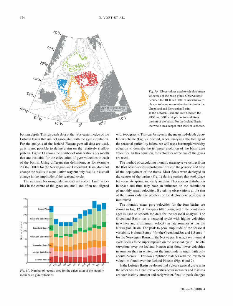
We use our float data set to estimate the strength of the sea-sonal cycle of the circulation at mid-depth. At the beginning of2009, the number of observations is yet insufficient to detect thetemporal variability at the spatial resolution used for our meancirculation map (Fig. 7). We therefore calculate the monthlymean gyre velocities in a geographic frame to construct velocitytime series for the individual basins. The monthly mean veloc-ity in a basin gyre is defined here as the average over all alongbathymetry velocities recorded in the rim areas of the basinsduring one month. Figure 10 shows the data points at the rimin each basin used for the calculation. For the Greenland andNorwegian Basin, the area between the 1000 and 3000 m iso-bath is chosen to represent the rim of the gyres. In the LofotenBasin we define the rim as the area between 2800 and 3200 m

Fig. 9. Normalised topostrophy derivedfrom the mean circulation scheme. Bluecolours stand for cyclonic flow, red coloursfor anticyclonic flow. The closer the absolutevalue of the normalized topostrophy tendstowards one, the more the flow is aligned tothe bathymetry.

Tellus 62A (2010), 4

524 G. VOET ET AL.

Fig. 10. Observations used to calculate meanvelocities of the basin gyres. Observationsbetween the 1000 and 3000 m isobaths werechosen to be representative for the rim in theGreenland and Norwegian Basin.In the Lofoten Basin the area between the2800 and 3200 m depth contours definesthe rim of the basin. For the Iceland Basinthe whole area deeper than 1000 m is chosen.

bottom depth. This discards data at the very eastern edge of theLofoten Basin that are not associated with the gyre circulation.For the analysis of the Iceland Plateau gyre all data are used,as it is not possible to define a rim on the relatively shallowplateau. Figure 11 shows the number of observations per monththat are available for the calculation of gyre velocities in eachof the basins. Using different rim definitions, as for example2000–3000 m for the Norwegian and Greenland Basin, does notchange the results in a qualitative way but only results in a smallchange in the amplitude of the seasonal cycle.

The rationale for using only rim data is twofold. First, veloc-ities in the centre of the gyres are small and often not aligned

Fig. 11. Number of records used for the calculation of the monthlymean basin gyre velocities.

with topography. This can be seen in the mean mid-depth circu-lation scheme (Fig. 7). Second, when analysing the forcing ofthe seasonal variability below, we will use a barotropic vorticityequation to describe the temporal evolution of the basin gyrevelocities. In this equation, the velocities at the rim of the gyresare used.

The method of calculating monthly mean gyre velocities fromthe float observations is problematic due to the position and timeof the deployment of the floats. Most floats were deployed inthe centres of the basins (Fig. 1) during cruises that took placebetween late spring and early autumn. This uneven distributionin space and time may have an influence on the calculationof monthly mean velocities. By taking observations at the rimof the basins only, the problem of the deployment positions isminimized.

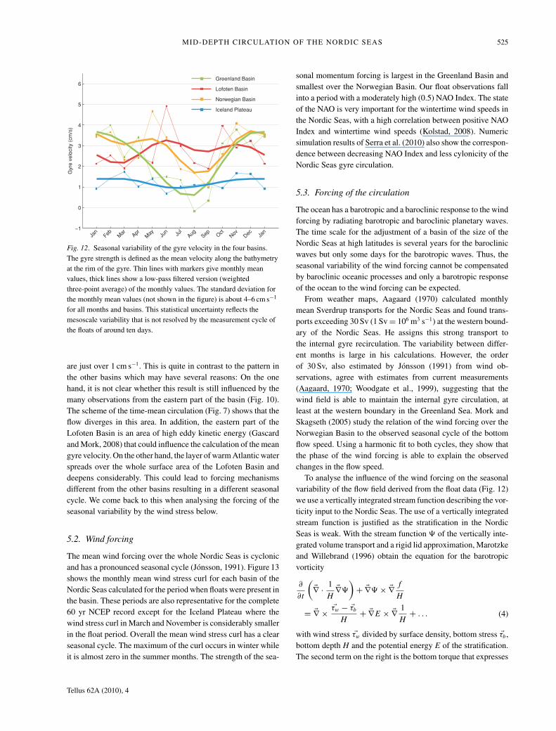
The monthly mean gyre velocities for the four basins areshown in Fig. 12. A low-pass filter (weighted three point aver-age) is used to smooth the data for the seasonal analysis. TheGreenland Basin has a seasonal cycle with higher velocitiesin winter and a minimum velocity in late summer as has theNorwegian Basin. The peak-to-peak amplitude of the seasonalvariability is about 3 cm s−1 for the Greenland Sea and 1.5 cm s−1

for the Norwegian Basin. In the Norwegian Basin, a semi-annualcycle seems to be superimposed on the seasonal cycle. The ob-servations over the Iceland Plateau also show lower velocitiesin summer than in winter, but the amplitude is small with onlyabout 0.5 cm s−1. This low amplitude matches with the low meanvelocities found over the Iceland Plateau (Figs 6 and 7).

In the Lofoten Basin we do not find a clear seasonal cycle as inthe other basins. Here low velocities occur in winter and maximaare seen in early summer and early winter. Peak-to-peak changes

Tellus 62A (2010), 4

MID-DEPTH CIRCULATION OF THE NORDIC SEAS 525

Fig. 12. Seasonal variability of the gyre velocity in the four basins.The gyre strength is defined as the mean velocity along the bathymetryat the rim of the gyre. Thin lines with markers give monthly meanvalues, thick lines show a low-pass filtered version (weightedthree-point average) of the monthly values. The standard deviation forthe monthly mean values (not shown in the figure) is about 4–6 cm s−1

for all months and basins. This statistical uncertainty reflects themesoscale variability that is not resolved by the measurement cycle ofthe floats of around ten days.

are just over 1 cm s−1. This is quite in contrast to the pattern inthe other basins which may have several reasons: On the onehand, it is not clear whether this result is still influenced by themany observations from the eastern part of the basin (Fig. 10).The scheme of the time-mean circulation (Fig. 7) shows that theflow diverges in this area. In addition, the eastern part of theLofoten Basin is an area of high eddy kinetic energy (Gascardand Mork, 2008) that could influence the calculation of the meangyre velocity. On the other hand, the layer of warm Atlantic waterspreads over the whole surface area of the Lofoten Basin anddeepens considerably. This could lead to forcing mechanismsdifferent from the other basins resulting in a different seasonalcycle. We come back to this when analysing the forcing of theseasonal variability by the wind stress below.

5.2. Wind forcing

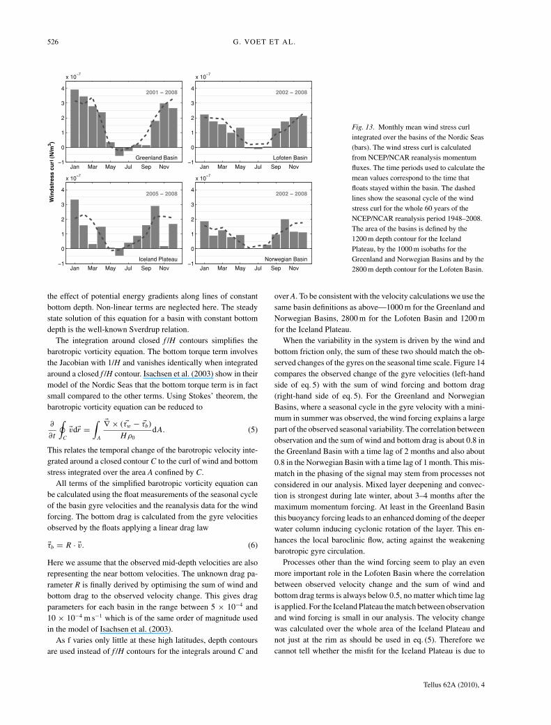
The mean wind forcing over the whole Nordic Seas is cyclonicand has a pronounced seasonal cycle (Jonsson, 1991). Figure 13shows the monthly mean wind stress curl for each basin of theNordic Seas calculated for the period when floats were present inthe basin. These periods are also representative for the complete60 yr NCEP record except for the Iceland Plateau where thewind stress curl in March and November is considerably smallerin the float period. Overall the mean wind stress curl has a clearseasonal cycle. The maximum of the curl occurs in winter whileit is almost zero in the summer months. The strength of the sea-

sonal momentum forcing is largest in the Greenland Basin andsmallest over the Norwegian Basin. Our float observations fallinto a period with a moderately high (0.5) NAO Index. The stateof the NAO is very important for the wintertime wind speeds inthe Nordic Seas, with a high correlation between positive NAOIndex and wintertime wind speeds (Kolstad, 2008). Numericsimulation results of Serra et al. (2010) also show the correspon-dence between decreasing NAO Index and less cylonicity of theNordic Seas gyre circulation.

5.3. Forcing of the circulation

The ocean has a barotropic and a baroclinic response to the windforcing by radiating barotropic and baroclinic planetary waves.The time scale for the adjustment of a basin of the size of theNordic Seas at high latitudes is several years for the baroclinicwaves but only some days for the barotropic waves. Thus, theseasonal variability of the wind forcing cannot be compensatedby baroclinic oceanic processes and only a barotropic responseof the ocean to the wind forcing can be expected.

From weather maps, Aagaard (1970) calculated monthlymean Sverdrup transports for the Nordic Seas and found trans-ports exceeding 30 Sv (1 Sv = 106 m3 s−1) at the western bound-ary of the Nordic Seas. He assigns this strong transport tothe internal gyre recirculation. The variability between differ-ent months is large in his calculations. However, the orderof 30 Sv, also estimated by Jonsson (1991) from wind ob-servations, agree with estimates from current measurements(Aagaard, 1970; Woodgate et al., 1999), suggesting that thewind field is able to maintain the internal gyre circulation, atleast at the western boundary in the Greenland Sea. Mork andSkagseth (2005) study the relation of the wind forcing over theNorwegian Basin to the observed seasonal cycle of the bottomflow speed. Using a harmonic fit to both cycles, they show thatthe phase of the wind forcing is able to explain the observedchanges in the flow speed.

To analyse the influence of the wind forcing on the seasonalvariability of the flow field derived from the float data (Fig. 12)we use a vertically integrated stream function describing the vor-ticity input to the Nordic Seas. The use of a vertically integratedstream function is justified as the stratification in the NordicSeas is weak. With the stream function � of the vertically inte-grated volume transport and a rigid lid approximation, Marotzkeand Willebrand (1996) obtain the equation for the barotropicvorticity

∂

∂t

(�∇ · 1

H�∇�

)+ �∇� × �∇ f

H

= �∇ × �τw − �τb

H+ �∇E × �∇ 1

H+ . . . (4)

with wind stress �τw divided by surface density, bottom stress �τb,bottom depth H and the potential energy E of the stratification.The second term on the right is the bottom torque that expresses

Tellus 62A (2010), 4

526 G. VOET ET AL.

Fig. 13. Monthly mean wind stress curlintegrated over the basins of the Nordic Seas(bars). The wind stress curl is calculatedfrom NCEP/NCAR reanalysis momentumfluxes. The time periods used to calculate themean values correspond to the time thatfloats stayed within the basin. The dashedlines show the seasonal cycle of the windstress curl for the whole 60 years of theNCEP/NCAR reanalysis period 1948–2008.The area of the basins is defined by the1200 m depth contour for the IcelandPlateau, by the 1000 m isobaths for theGreenland and Norwegian Basins and by the2800 m depth contour for the Lofoten Basin.

the effect of potential energy gradients along lines of constantbottom depth. Non-linear terms are neglected here. The steadystate solution of this equation for a basin with constant bottomdepth is the well-known Sverdrup relation.

The integration around closed f /H contours simplifies thebarotropic vorticity equation. The bottom torque term involvesthe Jacobian with 1/H and vanishes identically when integratedaround a closed f /H contour. Isachsen et al. (2003) show in theirmodel of the Nordic Seas that the bottom torque term is in factsmall compared to the other terms. Using Stokes’ theorem, thebarotropic vorticity equation can be reduced to

∂

∂t

∮C

�vd�r =∫

A

�∇ × ( �τw − �τb)

Hρ0dA. (5)

This relates the temporal change of the barotropic velocity inte-grated around a closed contour C to the curl of wind and bottomstress integrated over the area A confined by C.

All terms of the simplified barotropic vorticity equation canbe calculated using the float measurements of the seasonal cycleof the basin gyre velocities and the reanalysis data for the windforcing. The bottom drag is calculated from the gyre velocitiesobserved by the floats applying a linear drag law

�τb = R · �v. (6)

Here we assume that the observed mid-depth velocities are alsorepresenting the near bottom velocities. The unknown drag pa-rameter R is finally derived by optimising the sum of wind andbottom drag to the observed velocity change. This gives dragparameters for each basin in the range between 5 × 10−4 and10 × 10−4 m s−1 which is of the same order of magnitude usedin the model of Isachsen et al. (2003).

As f varies only little at these high latitudes, depth contoursare used instead of f /H contours for the integrals around C and

over A. To be consistent with the velocity calculations we use thesame basin definitions as above—1000 m for the Greenland andNorwegian Basins, 2800 m for the Lofoten Basin and 1200 mfor the Iceland Plateau.

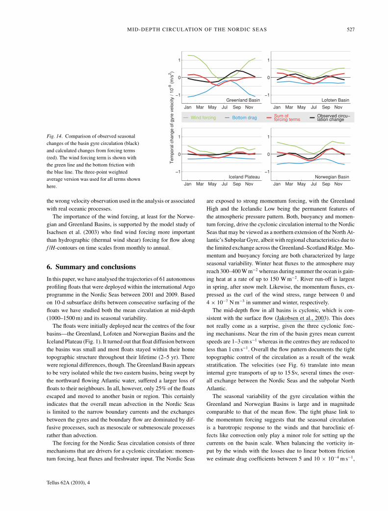
When the variability in the system is driven by the wind andbottom friction only, the sum of these two should match the ob-served changes of the gyres on the seasonal time scale. Figure 14compares the observed change of the gyre velocities (left-handside of eq. 5) with the sum of wind forcing and bottom drag(right-hand side of eq. 5). For the Greenland and NorwegianBasins, where a seasonal cycle in the gyre velocity with a mini-mum in summer was observed, the wind forcing explains a largepart of the observed seasonal variability. The correlation betweenobservation and the sum of wind and bottom drag is about 0.8 inthe Greenland Basin with a time lag of 2 months and also about0.8 in the Norwegian Basin with a time lag of 1 month. This mis-match in the phasing of the signal may stem from processes notconsidered in our analysis. Mixed layer deepening and convec-tion is strongest during late winter, about 3–4 months after themaximum momentum forcing. At least in the Greenland Basinthis buoyancy forcing leads to an enhanced doming of the deeperwater column inducing cyclonic rotation of the layer. This en-hances the local baroclinic flow, acting against the weakeningbarotropic gyre circulation.

Processes other than the wind forcing seem to play an evenmore important role in the Lofoten Basin where the correlationbetween observed velocity change and the sum of wind andbottom drag terms is always below 0.5, no matter which time lagis applied. For the Iceland Plateau the match between observationand wind forcing is small in our analysis. The velocity changewas calculated over the whole area of the Iceland Plateau andnot just at the rim as should be used in eq. (5). Therefore wecannot tell whether the misfit for the Iceland Plateau is due to

Tellus 62A (2010), 4

MID-DEPTH CIRCULATION OF THE NORDIC SEAS 527

Fig. 14. Comparison of observed seasonalchanges of the basin gyre circulation (black)and calculated changes from forcing terms(red). The wind forcing term is shown withthe green line and the bottom friction withthe blue line. The three-point weightedaverage version was used for all terms shownhere.

the wrong velocity observation used in the analysis or associatedwith real oceanic processes.

The importance of the wind forcing, at least for the Norwe-gian and Greenland Basins, is supported by the model study ofIsachsen et al. (2003) who find wind forcing more importantthan hydrographic (thermal wind shear) forcing for flow alongf /H-contours on time scales from monthly to annual.

6. Summary and conclusions

In this paper, we have analysed the trajectories of 61 autonomousprofiling floats that were deployed within the international Argoprogramme in the Nordic Seas between 2001 and 2009. Basedon 10-d subsurface drifts between consecutive surfacing of thefloats we have studied both the mean circulation at mid-depth(1000–1500 m) and its seasonal variability.

The floats were initially deployed near the centres of the fourbasins—the Greenland, Lofoten and Norwegian Basins and theIceland Plateau (Fig. 1). It turned out that float diffusion betweenthe basins was small and most floats stayed within their hometopographic structure throughout their lifetime (2–5 yr). Therewere regional differences, though. The Greenland Basin appearsto be very isolated while the two eastern basins, being swept bythe northward flowing Atlantic water, suffered a larger loss offloats to their neighbours. In all, however, only 25% of the floatsescaped and moved to another basin or region. This certainlyindicates that the overall mean advection in the Nordic Seasis limited to the narrow boundary currents and the exchangesbetween the gyres and the boundary flow are dominated by dif-fusive processes, such as mesoscale or submesoscale processesrather than advection.

The forcing for the Nordic Seas circulation consists of threemechanisms that are drivers for a cyclonic circulation: momen-tum forcing, heat fluxes and freshwater input. The Nordic Seas

are exposed to strong momentum forcing, with the GreenlandHigh and the Icelandic Low being the permanent features ofthe atmospheric pressure pattern. Both, buoyancy and momen-tum forcing, drive the cyclonic circulation internal to the NordicSeas that may be viewed as a northern extension of the North At-lantic’s Subpolar Gyre, albeit with regional characteristics due tothe limited exchange across the Greenland–Scotland Ridge. Mo-mentum and buoyancy forcing are both characterized by largeseasonal variability. Winter heat fluxes to the atmosphere mayreach 300–400 W m−2 whereas during summer the ocean is gain-ing heat at a rate of up to 150 W m−2. River run-off is largestin spring, after snow melt. Likewise, the momentum fluxes, ex-pressed as the curl of the wind stress, range between 0 and4 × 10−7 N m−3 in summer and winter, respectively.

The mid-depth flow in all basins is cyclonic, which is con-sistent with the surface flow (Jakobsen et al., 2003). This doesnot really come as a surprise, given the three cyclonic forc-ing mechanisms. Near the rim of the basin gyres mean currentspeeds are 1–3 cm s−1 whereas in the centres they are reduced toless than 1 cm s−1. Overall the flow pattern documents the tighttopographic control of the circulation as a result of the weakstratification. The velocities (see Fig. 6) translate into meaninternal gyre transports of up to 15 Sv, several times the over-all exchange between the Nordic Seas and the subpolar NorthAtlantic.

The seasonal variability of the gyre circulation within theGreenland and Norwegian Basins is large and in magnitudecomparable to that of the mean flow. The tight phase link tothe momentum forcing suggests that the seasonal circulationis a barotropic response to the winds and that baroclinic ef-fects like convection only play a minor role for setting up thecurrents on the basin scale. When balancing the vorticity in-put by the winds with the losses due to linear bottom frictionwe estimate drag coefficients between 5 and 10 × 10−4 m s−1,

Tellus 62A (2010), 4

528 G. VOET ET AL.

reasonable values that fall into the same range as those used innumerical model simulations. Estimated transport variability isup to 15 ± 10 Sv, a value confirmed by earlier direct currentmeasurements using moored instrumentation (Woodgate et al.,1999). Over the Iceland Plateau the seasonal wind forcing is lesspronounced compared to the Greenland Sea. Here the gyre cir-culation shows the smallest seasonal variations, consistent withthe forcing. Also, the topographic gradients are much weakerthan in the other basins and the flow may not be subject to asrigorous a topographic control as in the other regions. In addi-tion, our database here is smallest and it may not be sufficient todetect the variability.

The largest deviation from our simple barotropic responsemodel occurs in the Lofoten Basin. The gyre circulation herecontains a strong semi-annual component comparable in mag-nitude to the seasonal signal. The reason for this is not clear tous. The forcing, wind and bottom friction, is clearly seasonal,but the float exchange with the Norwegian Basin in the Southand the continental slope region in the West Spitsbergen Cur-rent in the North suggest a weaker topographic control of theflow. Results from a numerical model simulation confirm thisbehaviour (Serra et al., 2010). The Lofoten Basin is a regionof enhanced mesoscale variability generated by baroclinic in-stabilities of the flow, first described by Helland-Hansen andNansen (1909) as puzzling waves and also observed in drifterstudies (Poulain et al., 1996; Jakobsen et al., 2003; Rossby et al.,2009). These baroclinic effects may also play a role in setting upthe circulation, but our data set does not allow to explore suchmechanisms.

The Nordic Seas are a region of intense water mass transfor-mation. Here, through heat loss, freshwater input and meltingand freezing of sea ice, buoyant Atlantic Water is transformedinto buoyant (cold, low salinity) near surface waters and dense(cold, intermediate salinity) intermediate and deep waters. Thesurface waters leave the Nordic Seas via Denmark Strait and en-ter the subpolar North Atlantic as a narrow and shallow boundarycurrent (about 2 Sv, Sutherland and Pickart, 2008) on the EastGreenland shelf and continental slope. The dense waters exitinto the subpolar Atlantic in different pathways via the overflowsacross the Greenland–Scotland Ridge, mainly through DenmarkStrait and the Faroe Bank Channel. This exchange is limited bytopographic (hydraulic) control and presently the Nordic Seascontribute only about 6 Sv (Quadfasel and Kase, 2007) to theNorth Atlantic Deep Water.

Direct current measurements over the Greenland–ScotlandRidge show that the Nordic Loop of the Subpolar Gyre of theNorth Atlantic has a strength of about 8 Sv. Seasonal variabilityof these exchanges across the ridge is small and amounts to 1 Svat most (Hansen and Østerhus, 2007). In contrast, the internalhorizontal circulation cells in the Nordic Seas that are linked tothe four topographic basins are at least twice as strong as theoverall exchange, with their seasonal variability exceeding thatof the ridge exchanges by an order of magnitude.

The main role of the Nordic gyres thus is the transformationof buoyant surface water into dense deep and intermediate water.This process and the associated circulation set up and maintainfronts. Instabilities of the fronts then provide the energy formeso- and submesoscale stirring and mixing, transferring thetransformed water masses from the gyres’ interior to the bound-ary currents. These eventually feed the overflows into the NorthAtlantic.

7. Acknowledgments

Rolf Kase provided valuable comments on the first draftof this manuscript. The financial support for this study byDeutsche Forschungsgemeinschaft (SFB 512 E2) and theEuropean Commission (Euro-Argo and Mersea) is gratefully ac-knowledged. These funding agencies also provided most of theNordic Seas floats. Globally Argo data are collected and madefreely available by the International Argo Project and the na-tional programs that contribute to it (http://www.argo.ucsd.edu,http://argo.jcommops.org). Argo is a pilot program of the GlobalOcean Observing System.

References

Aagaard, K. and Coachman, L. K. 1968. The East Greenland Currentnorth of Denmark Strait. Part I. Arctic 21(3), 181–200.

Aagaard, K. 1970. Wind-driven transports in the Greenland and Norwe-gian Seas. Deep-Sea Res. 17, 281–291.

Davis, R. E. 1998. Preliminary results from directly measuring mid-depth circulation in the tropical and South Pacific. J. Geophys. Res.

103(C11), 24619–24639.Gascard, J.-C. and Mork, K. A. 2008. Climatic Importance of Large-

Scale and Mesoscale Circulation in the Lofoten Basin Deduced fromLagrangian Observations. In: Arctic-Subarctic Ocean Fluxes, (edsR. R., Dickson, J., Meincke and P., Rhines), Springer, Dordrecht,131–143.

Gould, W. J. 2005. From Swallow to Argo—the development ofneutrally buoyant floats. Deep-Sea Res. Part I 52, 529–543.

Hansen, B. and Østerhus, S. 2000. North Atlantic-Nordic Seas ex-changes. Prog. Oceanogr. 45, 109–208.

Hansen, B. and Østerhus, S. 2007. Faroe Bank Channel Overflow 1995-2005. Prog. Oceanogr. 75, 817–856.

Helland-Hansen, B. and Nansen, F. 1909. The Norwegian Sea: Its Phys-ical Oceanography based on Norwegian Researches. Report on Nor-wegian Fishery and Marine Investigations 11, 390 pp. + 25 plates.

Holloway, G., Dupont, F., Golubeva, E., Hakkinen, S., Hunke, E. andco-authors. 2007. Water properties and circulation in Arctic Oceanmodels. J. Geophys. Res. 112(C4), C04S03.

Isachsen, P. E., LaCasce, J. H., Mauritzen, C. and Hakkinen, S. 2003.Wind-driven variability of the large-scale recirculating flow in theNordic Seas and Arctic Ocean. J. Phys. Oceanogr. 33, 2534–2550.

Jakobsen, P. K., Ribergaard, M. H., Quadfasel, D., Schmith, T. andHughes, C. W. 2003. Near-surface circulation in the northern NorthAtlantic as inferred from Lagrangian drifters: variability from themesoscale to interannual. J. Geophys. Res. 108(C8), 3251.

Tellus 62A (2010), 4

MID-DEPTH CIRCULATION OF THE NORDIC SEAS 529

Jakobsson, M., Cherkis, N., Woodward, J., Coakley, B. and Macnab, R.2000. New grid of Arctic bathymetry aids scientists and mapmakers.EOS, Trans. Am. Geophys. Un. 81(9), 89.

Jonsson, S. 1991. Seasonal and interannual Variability of Wind StressCurl Over the Nordic Seas. J. Geophys. Res. 96(C2), 2649–2659.

Kalnay, E., Kanamitsu, M., Kistler, R., Collins, W., Deaven, D. andco-authors. 1996. The NCEP/NCAR 40-Year Reanalysis Project. B.

Am. Meteorol. Soc. 77(3), 437–472.Killworth, P. D. 1992. An equivalent-barotropic mode in the fine reso-

lution antarctic model. J. Phys. Oceanogr. 22, 1379–1387.Kohl, A. 2007. Generation and stability of a quasi-permanent vortex in

the Lofoten Basin. J. Phys. Oceanogr. 37, 2637–2651.Kolstad, E. W. 2008. A QuikSCAT climatology of ocean surface winds

in the Nordic seas: identification of features and comparison with theNCEP/NCAR reanalysis. J. Geophys. Res. 113, D11106.

Lavender, K. V., Owens, W. B. and Davis, R. E. 2005. The mid-depthcirculation of the subpolar North Atlantic Ocean as measured bysubsurface floats. Deep-Sea Res. Part I 52, 767–785.

Lebedev, K. V., Yoshinari, H., Maximenko, N. A. and Hacker, P. W.2007. YoMaHa’07: Velocity data assessed from trajectories of Argofloats at parking level and at the sea surface. IPRC Tech. Rep. 4(2),16 pp.

Machın, F., Send, U. and Zenk, W. 2006. Intercomparing drifts fromRAFOS and profiling floats in the deep western boundary currentalong the Mid-Atlantic Ridge. Sci. Mar. 70(1), 1–8.

Marotzke, J. and Willebrand, J. 1996. The North Atlantic mean circu-lation: combining data and dynamics. In: The Warm water sphere of

the North Atlantic Ocean (eds W. Krauss et al.), Borntraeger, Berlin,Stuttgart, 55–90.

Mauritzen, C. 1996. Production of dense overflow waters feeding theNorth Atlantic across the Greenland-Scotland Ridge. Part 1: evidencefor a revised circulation scheme. Deep-Sea Res. Part I 43, 769–806.

Mork, K. A. and Skagseth, Ø. 2005. Annual Sea Surface Height Vari-ability in the Nordic Seas and Arctic Ocean estimated from simplifieddynamics. In: The Nordic Seas: An Integrated Perspective (eds H.Drange, T. Dokken, T. Furevik, R. Gerdes and W. Berger), Geophys.Monogr. Ser. 158, AGU, Washington DC, 51–64.

Nøst, O. A. and Isachsen, P. E. 2003. The large-scale time-mean oceancirculation in the Nordic Seas and Arctic Ocean estimated from sim-plified dynamics. J. Mar. Res. 61, 175–210.

Orvik, K. A. 2004. The deepening of the Atlantic water in the LofotenBasin of the Norwegian Sea, demonstrated by using an active reducedgravity model. Geophys. Res. Lett. 31, L01306.

Orvik, K. A. and Niiler, P. 2002. Major pathways of Atlantic water inthe northern North Atlantic and Nordic Seas toward Arctic. Geophys.Res. Lett. 29, 1986.

Orvik, K. A., Skagseth, Ø. and Mork, M. 2001. Atlantic inflow to theNordic Seas: current structure and volume fluxes from moored cur-rent meters, VM-ADCP and SeaSoar-CTD observations, 1995–1999.Deep-Sea Res. Part I 48, 937–957.

Park, J. J., Kim, K., King, B. A. and Riser, S. 2005. An advanced methodto estimate deep currents from profiling floats. J. Atmos. Ocean. Tech.

22, 1294–1304.Poulain, P.-M., Warn-Varnas, A. and Niiler, P. P. 1996. Near-surface

circulation of the Nordic seas as measured by Lagrangian drifters. J.

Geophys. Res. 101(C8), 18237–18258.Quadfasel, D. and Kase, R. 2007. Present-Day Manifestation of the

Nordic Seas Overflows. In: Ocean Circulation: Mechanisms and Im-

pacts (eds A. Schmittner, J. C. H. Chiang and S. R. Hemmings),Geophys. Monogr. Ser. 173, AGU, Washington DC, 75–89.

Roemmich, D., Boebel, O., Desaubies, Y., Freeland, H., Kim, K. andco-authors. 1999. Argo: the global array of profiling floats. In: Ob-

serving the Oceans in the 21st Century (eds C. J. Koblinsky andN. R. Smith), GODAE Project Office and Bureau of Meteorology,Melbourne, 248–257.

Rossby, T., Prater, M. D. and Søiland, H. 2009. Pathways of inflow anddispersion of warm waters in the Nordic seas. J. Geophys. Res. 114,C04011.

Serra, N., Kase, R. H., Kohl, A., Stammer, D. and Quadfasel, D. 2010.On the low-frequency phase relation between the Denmark Strait andthe Faroe-Bank Channel overflows. Tellus 62A.

Smith, W. H. F. and Sandwell, D. T. 1997. Global sea floor topogra-phy from satellite altimetry and ship depth soundings. Science 277,1956–1962.

Søiland, H., Prater, M. D. and Rossby, T. 2008. Rigid topographiccontrol of currents in the Nordic Seas. Geophys. Res. Lett. 35,L18607.

Sutherland, D. A. and Pickart, R. S. 2008. The east Greenland coastalcurrent: structure, variability, and forcing. Prog. Oceanogr. 78, 58–77.

Thomson, R. E. and Freeland, H. J. 2003. Topographic steering of amid-depth drifter in an eddy-like circulation region south and east ofthe Hawaiian Ridge. J. Geophys. Res. 108(C11), 3341.

Woodgate, R. A., Fahrbach, E. and Rohardt, G. 1999. Structure andtransports of the East Greenland Current at 75◦N from moored currentmeters. J. Geophys. Res. 104(C8), 18059–18072.

Tellus 62A (2010), 4