Recent changes (1930s±1990s) in spatial patterns ofinterior northwest forests, USA

P.F. Hessburga,*, B.G. Smithb, R.B. Saltera, R.D. Ottmarc, E. Alvaradoc

aU.S.D.A. Forest Service, Paci®c Northwest Research Station, 1133 N. Western Ave., Wenatchee, WA 98801, USAbU.S.D.A. Forest Service, 1230 NE 3rd St., Suite 262, Bend, OR 97701, USA

cU.S.D.A. Forest Service, Paci®c Northwest Research Station, 4043 Roosevelt Way NE, Seattle, WA 98105, USA

Received 11 May 1999; accepted 5 September 1999

Abstract

We characterized recent historical and current vegetation composition and structure of a representative sample of

subwatersheds on all ownerships within the interior Columbia River basin and portions of the Klamath and Great Basins. For

each selected subwatershed, we constructed historical and current vegetation maps from 1932 to 1966 and 1981 to 1993 aerial

photos, respectively. Using the raw vegetation attributes, we classi®ed and attributed cover types, structural classes, and

potential vegetation types to individual patches within subwatersheds. We characterized change in vegetation spatial patterns

using a suite of class and landscape metrics, and a spatial pattern analysis program. We then translated change in vegetation

patterns to change in patterns of vulnerability to wild®res, smoke production, and 21 major forest pathogen and insect

disturbances. Results of change analyses were reported for province-scale ecological reporting units (ERUs). Here, we

highlight signi®cant ®ndings and discuss management implications.

Twentieth century management activities signi®cantly altered spatial patterns of physiognomies, cover types and structural

conditions, and vulnerabilities to ®re, insect, and pathogen disturbances. Forest land cover expanded in several ERUs, and

woodland area expanded in most. Of all physiognomic conditions, shrubland area declined most due to cropland expansion,

conversion to semi- and non-native herblands, and expansion of forests and woodlands. Shifts from early to late seral conifer

species were evident in forests of most ERUs; patch sizes of forest cover types are now smaller, and current land cover is more

fragmented. Landscape area in old multistory, old single story, and stand initiation forest structures declined with

compensating increases in area and connectivity of dense, multilayered, intermediate forest structures. Patches with medium

and large trees, regardless of their structural af®liation are currently less abundant on the landscape. Finally, basin forests are

now dominated by shade-tolerant conifers, and exhibit elevated fuel loads and severe ®re behavior attributes indicating

expanded future roles of certain defoliators, bark beetles, root diseases, and stand replacement ®res. Although well

intentioned, 20th-century management practices did not account for landscape-scale patterns of living and dead vegetation that

enable forest ecosystems to maintain their structure and organization through time, or for the disturbances that create and

maintain them. Improved understanding of change in vegetation spatial patterns, causative factors, and links with disturbance

processes will assist managers and policymakers in making informed decisions about how to address important ecosystem

health issues. # 2000 Elsevier Science B.V. All rights reserved.

Keywords: Change detection; Landscape assessment; Spatial patterns; Reference variation; Ecosystem health; Forest health; Fire exclusion;

Disturbance regimes

Forest Ecology and Management 136 (2000) 53±83

* Corresponding author.

0378-1127/00/$ ± see front matter # 2000 Elsevier Science B.V. All rights reserved.

PII: S 0 3 7 8 - 1 1 2 7 ( 9 9 ) 0 0 2 6 3 - 7

1. Introduction

Forest and rangeland ecosystems of the Interior

Northwest are remarkably diverse and productive

owing to great variety in climate, geology, landforms,

hydrology, ¯ora, fauna, and ecosystem processes

(Franklin and Dyrness, 1988; Bailey, 1995). Recurring

disturbances, such as those caused by ®res, insects,

pathogens, and weather are essential to maintaining

this diversity (Arno, 1976, 1980; Hall, 1976; Turner,

1987, 1989; Agee, 1993, 1994; Hessburg et al., 1994).

Terrestrial plant communities range from dry, short

grass prairies and sagebrush shrublands, to dry pon-

derosa pine and Douglas-®r forests, cool and moist

western hemlock and western redcedar forests, high

elevation whitebark pine and subalpine larch forests,

krummholz, and heath. Alpine tundras, rock barrens,

and glaciers occupy many of the highest elevations.

Vegetation spatial and temporal patterns and eco-

logical characteristics of forest-dominated landscapes

are closely related to their disturbance ecology. Broad-

scale landscape patterns of life forms and physiog-

nomic conditions arise from broad differences in

topography and physiography, lithology, geomorphic

processes, climate regime, and large-scale distur-

bances. Within the general framework of coarse pat-

terns, meso-scale patterns result from environmental

gradients, patch-scale and gap disturbances, stand

development, and succession processes.

Natural ®re regimes of forests range from frequent,

nonlethal surface ®res typical in dry ponderosa pine

and Douglas-®r forests to moderately infrequent,

mixed-severity ®res characteristic of moist grand ®r,

western hemlock, and western redcedar forests, and

infrequent, lethal, stand-replacing ®res typical in cold

subalpine forests (Agee, 1993, 1994). Likewise, native

insect and pathogen disturbance regimes are variable

in their frequency, severity, duration, and spatial

extent. Pandemic bark beetle and defoliator outbreaks

occur relatively infrequently in any given geographic

area, and outbreaks when occurring, often are syn-

chronous with climatic extremes and cycles of geo-

graphically dominant vegetation structure or

composition resulting from other major pattern-form-

ing trends or events. Insect or pathogen disturbance

associated with endemic populations blends seam-

lessly with other succession and stand-development

processes.

The declining health of forest ecosystems in the

Interior Northwest has been the subject of much recent

study, concern, and controversy (e.g., see Wickman,

1992; O'Laughlin et al., 1993; Everett et al., 1994;

Lehmkuhl et al., 1994; Harvey et al., 1995). Land-use

practices of this century have altered disturbance

regimes, spatial and temporal patterns of vegetation,

and reduced ecosystem resilience to native and human

disturbances (Covington et al., 1994). Fire suppression

and ®re exclusion, timber harvest, and domestic live-

stock grazing have contributed most to increased

forest ecosystem vulnerability to insect, pathogen,

and wild®re disturbance. Concern over declining `for-

est health' centers on the perception that management

activities have damaged forest ecosystem structure

and functioning. That perception is founded on a

strongly held social value that forest ecosystems

should appear `natural' and function `naturally.'

This paper presents results of a study conducted

under the aegis of the Interior Columbia Basin Eco-

system Management Project. We report on a meso-

scale (map scale � 1 : 24 000) scienti®c assessment of

vegetation change in terrestrial landscapes of the

interior Columbia River basin, associated change in

landscape vulnerability to ®re and related PM10 (par-

ticulate matter < 10 mm in diameter) smoke produc-

tion, and insect and pathogen disturbances, and we

discuss the management implications of those

changes. Our assessment area (58 million ha) included

the Columbia River basin east of the crest of the

Cascade Range and portions of the Klamath and Great

Basins in Oregon (`the basin', Fig. 1)

Our study had four objectives: (1) to characterize

current structure and composition of a representative

sample of forest (and rangeland) landscapes; (2) to

compare existing conditions to the oldest historical

vegetation conditions we could reconstruct at a com-

parable scale; (3) to link historical and current vegeta-

tion spatial patterns with patterns of vulnerability to

insect and pathogen disturbances; and (4) to link

historical and current landscape vegetation character-

istics throughout the basin with fuel conditions, poten-

tial ®re behavior, and related smoke production.

Linkages in objectives 3 and 4 would enable us to

better understand causal connections among historical

management activities and current conditions, and

assist in evaluating current air quality and human

health tradeoffs associated with wild and prescribed

54 P.F. Hessburg et al. / Forest Ecology and Management 136 (2000) 53±83

®res, and tradeoffs associated with alternative insect

and pathogen vulnerability scenarios.

2. Methods

In the mid-scale assessment, (Hessburg et al.,

1999a), we quanti®ed change in vegetation patterns

and landscape vulnerability to ®re, insect, and patho-

gen disturbances over the most recent 50±60 years.

Sampling design and change analysis methods were

adapted from Lehmkuhl et al. (1994). Our sample of

historical conditions corresponded well with the start

of the period of most intensive timber harvest, road

construction, and ®re suppression, and a period of

declining intensity in rangeland management. We

based our assessment on a strati®ed random sample

of 337 subwatersheds (10 000 ha average area) dis-

tributed in 43 subbasins (400 000 ha average area),

across all ownerships within the basin. Change ana-

lysis results were reported by ecological reporting

units (ERUs, Fig. 1). Ecological reporting units were

developed during the broad-scale assessment of the

basin (Quigley and Arbelbide, 1997) as statistical

pooling strata for generalizing results of various eco-

logical, social, economic, and integrated assessments.

The ERUs represent land areas that are broadly homo-

geneous in their biophysical and social ecosystem

characteristics.

Forest and rangeland composition and structure

were derived from raw data developed from aerial

photographs taken from 1932 to 1966 (historical), and

from 1981 to 1993 (current). Historical conditions of

most forested settings were represented by photogra-

phy from the 1930s to 1940s; while those of range-

lands were represented by 1950s and 1960s aerial

Fig. 1. Map of ecological reporting units (ERUs), and sampled subbasins and subwatersheds in the mid-scale assessment of the interior

Columbia River basin.

P.F. Hessburg et al. / Forest Ecology and Management 136 (2000) 53±83 55

photography. Areas with homogeneous vegetation

composition and structure were delineated as patches

to a minimum size of 4 ha. Vegetation cover types,

structural classes, and potential vegetation types were

classi®ed for each patch using the raw attributes, and

topographic or biophysical data from other digital

sources of comparable scale and image resolution.

Each patch was assigned a rating for three to seven

vulnerability factors associated with each of 21 dif-

ferent forest insects and pathogens, including defo-

liator, bark beetle, dwarf mistletoe, root disease, rust,

and stem decay disturbances. Vulnerability factors

were unique for each host±pathogen or host±insect

interaction modeled and included items such as site

quality, host abundance, canopy layers, host age or host

size, stand vigor, stand density, connectivity of host

patches, topographic setting, and type of visible

logging disturbance. Patch vulnerability factors were

taken fromthe literatureor werebased on theexperience

of ®eld pathologists and entomologists with expertise

in speci®c geographic areas (Hessburg et al., 1999b).

Resulting models represent substantial revisions of

early versions described by Lehmkuhl et al. (1994).

Similarly, historical and current vegetation patches

were matched to one of 192 fuel condition classes

(Ottmar et al., 1996; Schaaf, 1996) and assigned a fuel

loading. Fuel loads were used to compute fuel con-

sumption, particulate emissions production (PM10),

crown ®re potential, and ®re behavior attributes for an

average wild®re scenario using published procedures

(Huff et al., 1995; Ottmar et al., 1999). We also

modeled fuel consumption and related smoke produc-

tion for a current prescribed burn scenario. Algorithms

for estimating fuel consumption for both burn scenar-

ios were taken from the CONSUME (Ottmar et al.,

1993) and ®rst order ®re effects model (FOFEM,

Keane et al., 1994). Fire behavior attributes were rate

of spread, ¯ame length, and ®reline intensity. We

computed ®reline intensity (Byram's, Rothermel,

1983), rate of spread, and ¯ame length using the

published equations of the National Fire Danger Rat-

ing System (Rothermel, 1972; Deeming et al., 1977;

Cohen and Deeming, 1985).

2.1. Vegetation and landscape pattern analysis

This assessment was a map-based characterization

of landscape patterns and ecological processes across

space and time. We used the ARC/INFO (ESRI, 1995)

geographical information system (GIS) to manipulate

and analyze digital maps, and to develop and run

spatially explicit insect and pathogen vulnerability

(Hessburg et al., 1999b), and potential fuel consump-

tion and ®re behavior models (Ottmar et al., 1999).

Spatial and statistical analyses characterized

change in patterns and quanti®ed the signi®cance of

change. FRAGSTATS (McGarigal and Marks, 1995)

was used to compute class and landscape pattern

metrics directly from ARC/INFO data tables, and

we incorporated three additional metrics (N1, N2,

and R21, Table 1) into the source code. We used S-

PLUS (MathSoft Inc., 1993) to summarize and ana-

lyze ARC/INFO and FRAGSTATS outputs. Vegeta-

tion maps, raw and derived patch attributes formed the

basic data set for all analysis. For spatial pattern

analysis, a variety of unique vegetation maps were

derived in a GIS by dissolving on single or combined

data items. Patch types of a map submitted to analysis

could be de®ned by any raw attribute such as canopy

layers or total crown cover class, or by any derived

attribute such as cover type or structural class, either

singly or in combinations.

2.2. Raster size determination

To quantify change in individual patch types and

patterns of various patch types, we used raster versions

of current and historical vegetation maps where patch

types were physiognomic conditions, cover types,

structural classes, potential vegetation types, or com-

binations. A raster format was chosen because several

useful metrics were only available in FRAGSTATS for

raster maps. The appropriate cell size was determined

by calculating several class metrics in vector and raster

form, with cell sizes ranging from 10 to 100 m (1 ha),

in 10-m increments, and at 141 m (2.0 ha) and 224 m

(5.0 ha), and plotting each raster-derived metric value

against the vector value. When compared with vector

values, raster bias was insigni®cant with 30 m and

smaller cell sizes, and we used 30-m raster maps for all

pattern analysis.

2.3. Sample statistics

We used percentage of area, patch density, mean

patch size, edge density, and mean nearest neighbor

56 P.F. Hessburg et al. / Forest Ecology and Management 136 (2000) 53±83

metrics to describe change in area and connectivity of

patch types in subwatersheds of an ERU. We used 10

landscape metrics to describe changes in patch

type richness, evenness, diversity, dominance, conta-

gion, interspersion, juxtaposition, and edge contrast

(Tables 1 and 2). For each ERU, means, standard

errors, and con®dence intervals were estimated using

methods for simple random samples with subwater-

sheds as sample units. Signi®cant (p � 0.2) change

from historical to current conditions was determined

by examining the 80% con®dence interval (CI) around

the mean difference for the ERU. We used a moder-

ately conservative 80% CI because we wanted to be

able to detect changes in spatial patterns that were of

potential ecological importance. We reasoned that

with a more conservative CI, we might increase the

likelihood of type II error (false positive). When we

compared 90 and 95% CI estimates of mean difference

with 80% estimates, we noted that important changes

went undetected using the more conservative CIs. To

avoid increasing the likelihood of type I error (false

negative), we supplemented our signi®cance test with

Table 1

FRAGSTATS indices used to quantify spatial patterns of patch types in sampled subbasins in the mid-scale ecological assessment of the

interior Columbia River basin

Acronym Scale Index name Descriptiona

LAND (%) class percentage of landscape (%) percentage of a landscape composed of the corresponding patch type

PD class or landscape patch density (no. per 10 000 ha) number of patches in an area of 10 000 ha

MPS class or landscape mean patch size (hectare) average patch size

AWMECI class or landscape area-weighted mean edge

contrast index (%)

average patch edge contrast as a percentage of maximum contrast with

patch edge contrasts weighted by patch area; equals 100 when all edge

is maximum contrast; approaches 0 when all edge is minimum

contrast

SHDI landscape Shannon's diversity indexb measures proportional abundance of patch types and the equitable

distribution of patch type areas; increases with patch richness (PR)

and equitability of area

RPR landscape relative patch richness (%) observed number of patch types within a landscape over a realistic

potential maximum number of patch types

PR landscape patch richness observed number of patch types within a landscape boundary

MSIEI landscape modified Simpson's

evenness indexc

observed distribution of area of patch types within a landscape over

evenly distributed area of patch types

IJI class or landscape interspersion and juxtaposition

index (%)

observed interspersion of edge types over maximum possible

interspersion; IJI approaches 0 when patch types are clumped, IJI

approaches 100 when all patch types are equally adjacent to all other

patch types

CONTAG landscape contagion index (%) observed contagion over the maximum possible contagion for the

given number of patch types; approaches 0 when the distribution of

adjacencies among unique patch types becomes increasingly uneven;

approaches 100 when all patch types are equally adjacent to all other

patch types; measures patch type interspersion and patch dispersion

N1 landscape Hill's index N1d a transformation of SHDI, computed as eSHDI; rare patch types are

weighted less in the calculation than in pr

N2 landscape Hill's index N2d a transformation of sidi, computed as 1/(1 ÿ SIDI); rare patch types

are weighted less in the calculation than in n1

R21 landscape Alatalo's evenness indexe measures evenness of patch types; computed as (N2ÿ1)/(N1ÿ1),

where PR > 1; values approaching 0 indicate uneven distribution of

patch type areas; values approaching 1 indicate even distribution of

area for the given number of patch types

a See McGarigal and Marks (1995) for algorithms and complete descriptions of all indices except N1, N2, and R21.b Shannon and Weaver (1949).c Simpson (1949).d Hill (1973).e Alatalo (1981).

P.F. Hessburg et al. / Forest Ecology and Management 136 (2000) 53±83 57

two other tests. These enabled us to evaluate the

potential ecological importance of change in patch

area or connectivity, and the likelihood of error in

rejecting the null hypothesis. First, we estimated a

reference variation by calculating for each metric, the

75% range around the historical sample median, and

then compared the current sample median value with

this range. Second, we determined the largest changes

in absolute area of a patch type within a sample using

transition analysis. Transition analysis estimated the

percentage of sampled area in each unique historical to

current patch type transition.

We chose the median 75% range instead of the full

range as a meaningful measure of reference variation

to portray typical variation exclusive of extreme

observations. Historical (and current) data distribu-

tions were frequently right-skewed, and the sample

median value was the more accurate re¯ection of

central tendency. Most observations were clustered

within the median 75±80% range. We reasoned that

more extreme variation usually results from either

unique contexts or environments, or from rare events.

By imposing the contrast between current median

values and a typical range of historical conditions,

we retained the ability to detect conditions resulting

from management activities, chance events, or per-

haps climate change that were unique in some aspect.

3. Results

3.1. Trends in physiognomic conditions

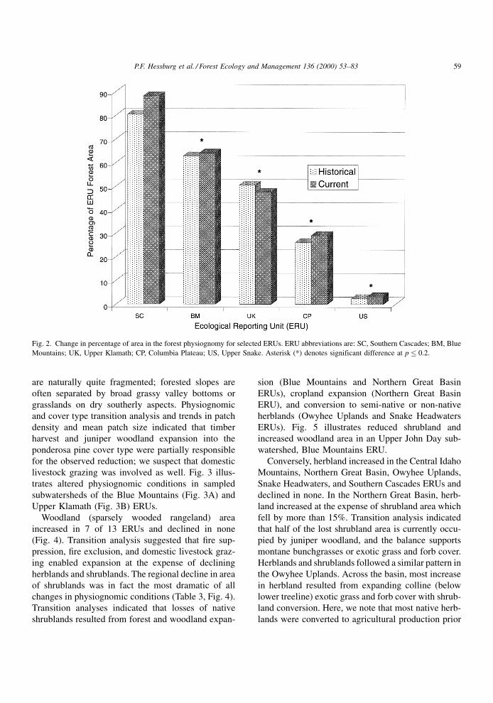
Signi®cant changes in physiognomies occurred

throughout the basin. Forest cover increased signi®-

cantly in the Blue Mountains, Columbia Plateau, and

Upper Snake ERUs (Fig. 2, Table 3) where our results

suggested that effective ®re prevention, suppression,

and exclusion resulted in expansion of forests into

areas that were previously bare ground or shrubland,

or into former herbland areas previously maintained

by ®re or created by early logging. Connectivity

(spatial aggregation) of forest increased in the

Central Idaho Mountains and Upper Snake ERUs

(see Hessburg et al., 1999a). Increased connectivity

of forests was the result of expansion of forest

cover types on former shrubland areas (Table 3).

The Central Idaho Mountains contains large wild

and roadless areas. Transition analysis of cover type

changes indicated that increased connectivity result

from effective ®re suppression and ®re exclusion. We

note that in a few subwatersheds increased forest

connectivity was associated with large scale stand

replacement ®res.

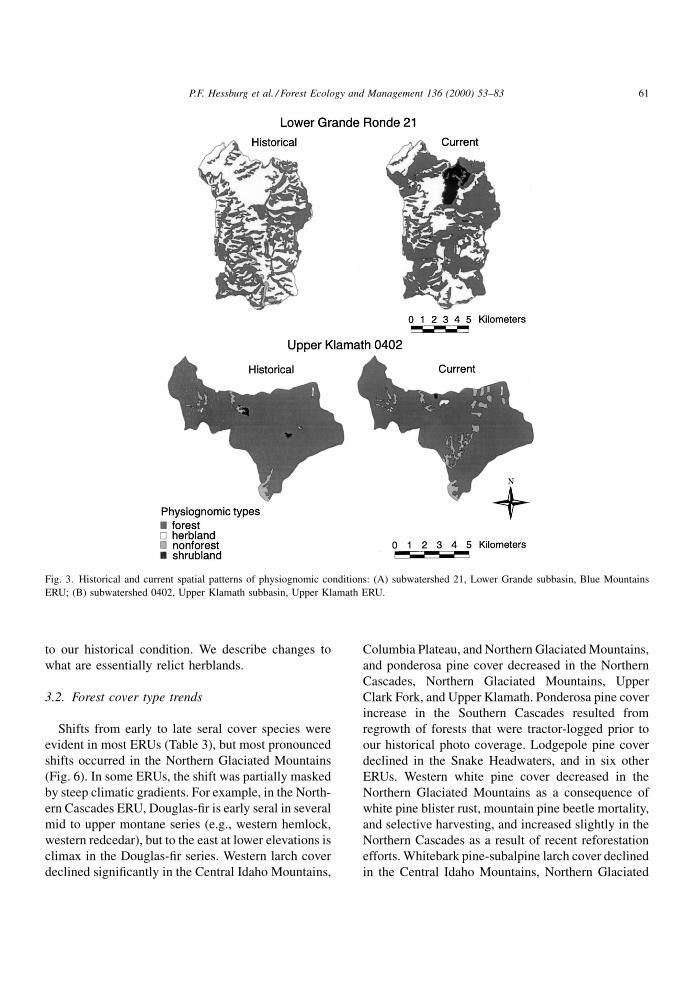
Area and connectivity of forest cover declined in the

Upper Klamath ERU (Fig. 2). Upper Klamath forests

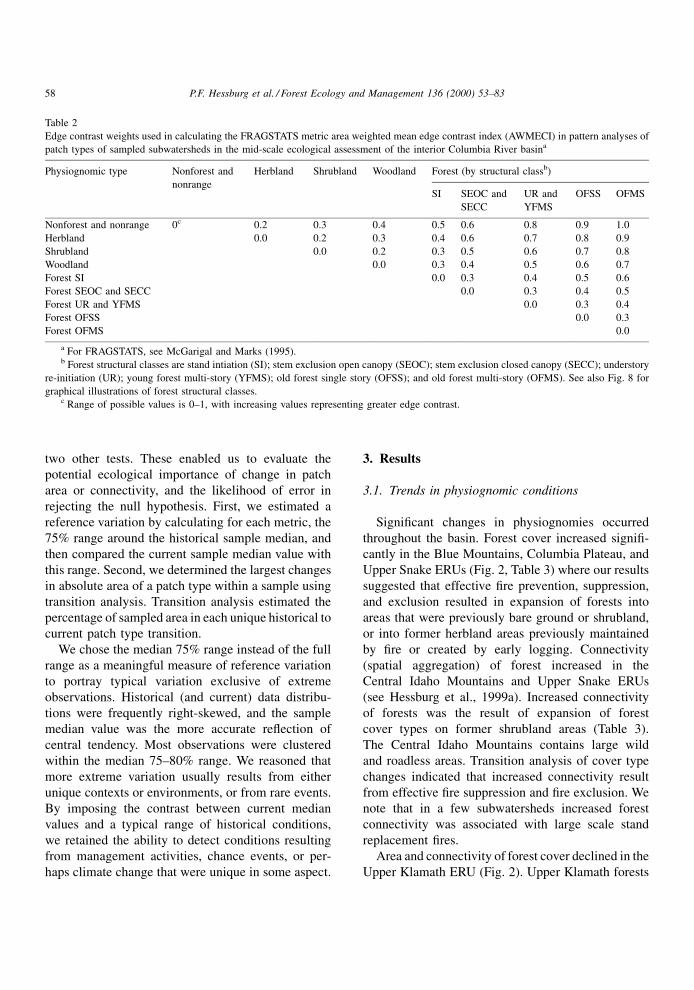
Table 2

Edge contrast weights used in calculating the FRAGSTATS metric area weighted mean edge contrast index (AWMECI) in pattern analyses of

patch types of sampled subwatersheds in the mid-scale ecological assessment of the interior Columbia River basina

Physiognomic type Nonforest and

nonrange

Herbland Shrubland Woodland Forest (by structural classb)

SI SEOC and

SECC

UR and

YFMS

OFSS OFMS

Nonforest and nonrange 0c 0.2 0.3 0.4 0.5 0.6 0.8 0.9 1.0

Herbland 0.0 0.2 0.3 0.4 0.6 0.7 0.8 0.9

Shrubland 0.0 0.2 0.3 0.5 0.6 0.7 0.8

Woodland 0.0 0.3 0.4 0.5 0.6 0.7

Forest SI 0.0 0.3 0.4 0.5 0.6

Forest SEOC and SECC 0.0 0.3 0.4 0.5

Forest UR and YFMS 0.0 0.3 0.4

Forest OFSS 0.0 0.3

Forest OFMS 0.0

a For FRAGSTATS, see McGarigal and Marks (1995).b Forest structural classes are stand intiation (SI); stem exclusion open canopy (SEOC); stem exclusion closed canopy (SECC); understory

re-initiation (UR); young forest multi-story (YFMS); old forest single story (OFSS); and old forest multi-story (OFMS). See also Fig. 8 for

graphical illustrations of forest structural classes.c Range of possible values is 0±1, with increasing values representing greater edge contrast.

58 P.F. Hessburg et al. / Forest Ecology and Management 136 (2000) 53±83

are naturally quite fragmented; forested slopes are

often separated by broad grassy valley bottoms or

grasslands on dry southerly aspects. Physiognomic

and cover type transition analysis and trends in patch

density and mean patch size indicated that timber

harvest and juniper woodland expansion into the

ponderosa pine cover type were partially responsible

for the observed reduction; we suspect that domestic

livestock grazing was involved as well. Fig. 3 illus-

trates altered physiognomic conditions in sampled

subwatersheds of the Blue Mountains (Fig. 3A) and

Upper Klamath (Fig. 3B) ERUs.

Woodland (sparsely wooded rangeland) area

increased in 7 of 13 ERUs and declined in none

(Fig. 4). Transition analysis suggested that ®re sup-

pression, ®re exclusion, and domestic livestock graz-

ing enabled expansion at the expense of declining

herblands and shrublands. The regional decline in area

of shrublands was in fact the most dramatic of all

changes in physiognomic conditions (Table 3, Fig. 4).

Transition analyses indicated that losses of native

shrublands resulted from forest and woodland expan-

sion (Blue Mountains and Northern Great Basin

ERUs), cropland expansion (Northern Great Basin

ERU), and conversion to semi-native or non-native

herblands (Owyhee Uplands and Snake Headwaters

ERUs). Fig. 5 illustrates reduced shrubland and

increased woodland area in an Upper John Day sub-

watershed, Blue Mountains ERU.

Conversely, herbland increased in the Central Idaho

Mountains, Northern Great Basin, Owyhee Uplands,

Snake Headwaters, and Southern Cascades ERUs and

declined in none. In the Northern Great Basin, herb-

land increased at the expense of shrubland area which

fell by more than 15%. Transition analysis indicated

that half of the lost shrubland area is currently occu-

pied by juniper woodland, and the balance supports

montane bunchgrasses or exotic grass and forb cover.

Herblands and shrublands followed a similar pattern in

the Owyhee Uplands. Across the basin, most increase

in herbland resulted from expanding colline (below

lower treeline) exotic grass and forb cover with shrub-

land conversion. Here, we note that most native herb-

lands were converted to agricultural production prior

Fig. 2. Change in percentage of area in the forest physiognomy for selected ERUs. ERU abbreviations are: SC, Southern Cascades; BM, Blue

Mountains; UK, Upper Klamath; CP, Columbia Plateau; US, Upper Snake. Asterisk (*) denotes significant difference at p � 0.2.

P.F. Hessburg et al. / Forest Ecology and Management 136 (2000) 53±83 59

Table 3

Historical (H) and current (C) percentage of areaa of physiognomic types, forest cover types, and structural classes of subwatersheds sampled in Ecological Reporting Units of the

mid-scale ecological assessment of the interior Columbia River basin

Patchtypes

Ecological reporting units

BlueMtns

CenralIdahoMtns.

ColumbiaPlateau

LowerClarkFork

NorthernCascades

NorthernGlaciatedMtns

NorthernGreatBasin

OwyheeUplands

SnakeHeadwtr

SouthernCascades

UpperClarkFork

UpperKlamath

UpperSnake

H C H C H C H C H C H C H C H C H C H C H C H C H C

Physiognomic typesForest 62.8 64.1 73.4 73.5 26.1 29.1 91.7 94.5 78.8 78.2 81.0 80.8 7.2 7.3 0.2 0.2 74.5 73.8 80.5 88.3 87.2 86.2 50.5 47.5 2.4 3.2Woodland 2.7 4.2 0.1 0.0 6.7 12.2 ± ± 0.3 0.7 ± ± 15.3 22.2 5.5 7.6 0.2 0.3 0.0 0.4 ± ± 8.4 12.8 3.0 2.9Shrubland 14.1 10.7 19.2 17.1 32.2 23.4 1.9 0.6 4.8 4.1 3.1 2.5 72.8 57.6 88.8 81.0 16.3 13.9 0.5 0.5 2.5 2.1 21.4 18.8 73.8 68.5Herbland 17.4 18.0 3.2 4.5 12.7 14.0 5.4 3.2 6.7 6.5 7.4 8.1 3.9 12.2 1.0 7.4 6.1 8.7 0.6 2.7 5.5 5.7 10.6 9.0 10.6 9.9Otherb 3.0 2.9 4.2 4.9 22.4 21.4 0.9 1.8 9.4 10.6 8.5 8.5 0.8 0.8 4.5 3.8 3.0 3.3 18.4 8.1 4.8 6.0 9.1 12.0 10.3 15.4Forest cover typesGF/WFc 15.3 8.4 9.6 10.2 1.1 0.4 40.4 42.5 1.0 2.2 0.0 1.2 ± ± ± ± ± ± 5.9 6.5 0.0 0.1 7.8 8.1 ± ±ES/SAF 6.3 4.4 22.7 24.1 ± ± 2.5 2.2 16.8 13.6 11.5 13.2 ± ± ± ± 24.3 31.4 0.0 0.2 14.2 17.3 0.1 0.1 ± ±ASP/COT 0.1 0.1 1.1 0.8 0.3 0.3 0.1 0.7 ± ± 0.3 1.9 8.4 7.7 0.2 0.2 8.8 5.7 ± ± 0.3 0.3 0.0 0.1 0.9 1.0JUN 2.7 4.2 0.1 0.0 6.5 12.0 ± ± ± ± ± ± 14.1 21.8 5.5 7.5 0.2 0.3 0.0 0.4 ± ± 8.4 12.8 2.6 2.5WL 2.6 2.2 0.5 0.3 1.0 0.1 0.8 2.6 1.0 1.0 14.8 11.4 ± ± ± ± ± ± ± ± 2.5 3.0 0.0 0.1 ± ±WBP/SAL 0.0 0.7 5.1 2.5 ± ± ± ± 3.3 4.7 0.3 0.2 ± ± ± ± 6.9 5.7 0.0 0.8 4.3 3.5 ± ± ± ±LPP 2.4 2.3 9.7 9.5 1.3 0.9 2.1 1.8 5.9 5.2 8.0 8.3 ± ± ± ± 15.6 11.3 19.4 20.6 20.9 19.5 1.4 1.7 0.1 0.2LP ± ± 0.4 0.4 ± ± ± ± ± ± ± ± ± ± ± ± 0.7 1.1 ± ± 0.0 0.4 ± ± ± ±PP 28.4 28.9 6.0 5.9 19.2 21.4 3.0 5.1 16.5 13.2 13.4 11.4 ± ± ± ± ± ± 22.7 28.1 12.3 9.5 26.7 23.5 ± ±DF 7.7 17.1 17.6 18.5 3.0 3.9 26.1 21.1 23.8 25.8 30.3 30.2 ± ± ± ± 18.2 18.6 1.5 1.7 32.7 32.5 2.1 1.2 1.4 2.1WH/WRC ± ± 0.9 1.3 0.4 2.2 14.7 17.3 3.0 2.4 0.7 2.8 ± ± ± ± ± ± ± ± ± ± ± ± ± ±MH ± ± 0.0 0.0 ± ± 1.3 0.6 1.3 1.2 0.1 0.0 ± ± ± ± ± ± 30.5 29.7 0.0 0.1 4.7 4.2 ± ±SP/WWP ± ± ± ± ± ± 0.3 0.6 0.1 0.3 1.5 0.0 ± ± ± ± ± ± 0.3 0.3 ± ± ± ± ± ±PSF ± ± ± ± ± ± ± ± 6.0 8.3 ± ± ± ± ± ± ± ± ± ± ± ± ± ± ± ±OWO ± ± ± ± ± ± ± ± 0.6 0.9 ± ± ± ± ± ± ± ± ± ± ± ± ± ± ± ±SRF ± ± ± ± ± ± ± ± ± ± ± ± ± ± ± ± ± ± 0.2 0.4 ± ± 7.8 8.5 ± ±PJ ± ± ± ± ± ± ± ± ± ± ± ± ± ± ± ± ± ± ± ± ± ± ± ± 0.4 0.5Forest structural classesSId 3.9 6.5 9.7 5.9 2.3 2.8 32.7 9.5 9.2 10.4 16.9 9.4 ± ± ± ± 6.4 7.0 9.1 9.9 15.9 11.1 1.9 3.6 0.8 0.3SEOC 14.3 9.6 18.4 17.7 6.7 7.8 15.7 9.2 13.2 13.2 11.8 11.6 6.5 6.0 0.0 0.1 19.1 15.3 12.3 14.3 18.5 18.2 11.3 10.9 0.4 1.0SECC 5.0 5.0 7.7 8.5 3.8 3.6 10.3 17.6 7.6 7.9 7.2 12.8 0.7 1.3 ± ± 7.9 4.8 0.5 4.8 16.7 21.1 1.2 1.6 0.1 0.1UR 13.6 11.2 16.0 21.4 3.1 3.3 16.3 37.7 17.5 19.5 18.4 23.3 ± ± 0.4 1.1 13.8 12.6 10.3 8.7 15.6 14.0 5.6 8.1 2.5 1.6YFMS 21.3 29.6 18.4 17.1 7.3 10.0 14.3 17.5 21.2 22.0 25.5 22.8 ± ± 0.1 0.1 22.0 30.9 46.0 45.6 19.7 21.1 21.1 16.4 0.6 1.1OFMS 2.2 1.0 1.4 1.2 2.3 1.3 0.2 0.5 5.8 2.7 0.5 0.4 ± ± ± ± 3.2 1.8 0.7 1.4 0.6 0.4 4.3 5.5 ± ±OFSS 2.7 0.9 1.8 1.7 1.1 1.0 2.2 2.5 4.3 2.4 0.7 0.6 ± ± ± ± 2.0 1.3 1.6 3.7 0.2 0.3 7.4 4.8 0.1 0.0

a Mean values shown in bold type are significantly different at p � 0.2.b `Other' includes anthropogenic cover types and other nonforest and nonrange types.c Forest cover types are: grand fir/white fir (GF/WF); Engelmann spruce/subalpine fir (ES/SAF); aspen/cottonwood/willow (ASP/COT); juniper (JUN); western larch (WL);

whitebark pine/subalpine larch (WBP/SAL); lodgepole pine (LPP); limber pine (LP); ponderosa pine (PP); Douglas-fir (DF); western hemlock/western redcedar (WH/WRC);

mountain hemlock (MH); sugar pine/western white pine (SP/WWP); Pacific silver fir (PSF); Oregon white oak (OWO); Shasta red fir (SRF); and pinyon/juniper (PJ).d Forest structural classes are stand intiation (SI); stem exclusion open canopy (SEOC); stem exclusion closed canopy (SECC); understory reinitiation (UR); young forest multi-

story (YFMS); old forest single story (OFSS); and old forest mult-story (OFMS).

60

P.F

.H

essbu

rget

al./F

orest

Eco

logy

and

Managem

ent

136

(2000)

53±83

to our historical condition. We describe changes to

what are essentially relict herblands.

3.2. Forest cover type trends

Shifts from early to late seral cover species were

evident in most ERUs (Table 3), but most pronounced

shifts occurred in the Northern Glaciated Mountains

(Fig. 6). In some ERUs, the shift was partially masked

by steep climatic gradients. For example, in the North-

ern Cascades ERU, Douglas-®r is early seral in several

mid to upper montane series (e.g., western hemlock,

western redcedar), but to the east at lower elevations is

climax in the Douglas-®r series. Western larch cover

declined signi®cantly in the Central Idaho Mountains,

Columbia Plateau, and Northern Glaciated Mountains,

and ponderosa pine cover decreased in the Northern

Cascades, Northern Glaciated Mountains, Upper

Clark Fork, and Upper Klamath. Ponderosa pine cover

increase in the Southern Cascades resulted from

regrowth of forests that were tractor-logged prior to

our historical photo coverage. Lodgepole pine cover

declined in the Snake Headwaters, and in six other

ERUs. Western white pine cover decreased in the

Northern Glaciated Mountains as a consequence of

white pine blister rust, mountain pine beetle mortality,

and selective harvesting, and increased slightly in the

Northern Cascades as a result of recent reforestation

efforts. Whitebark pine-subalpine larch cover declined

in the Central Idaho Mountains, Northern Glaciated

Fig. 3. Historical and current spatial patterns of physiognomic conditions: (A) subwatershed 21, Lower Grande subbasin, Blue Mountains

ERU; (B) subwatershed 0402, Upper Klamath subbasin, Upper Klamath ERU.

P.F. Hessburg et al. / Forest Ecology and Management 136 (2000) 53±83 61

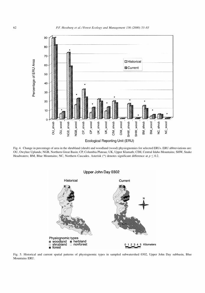
Fig. 4. Change in percentage of area in the shrubland (shrub) and woodland (wood) physiognomies for selected ERUs. ERU abbreviations are:

OU, Owyhee Uplands; NGB, Northern Great Basin; CP, Columbia Plateau; UK, Upper Klamath; CIM, Central Idaho Mountains; SHW, Snake

Headwaters; BM, Blue Mountains; NC, Northern Cascades. Asterisk (*) denotes significant difference at p � 0.2.

Fig. 5. Historical and current spatial patterns of physiognomic types in sampled subwatershed 0302, Upper John Day subbasin, Blue

Mountains ERU.

62 P.F. Hessburg et al. / Forest Ecology and Management 136 (2000) 53±83

Mountains, Snake Headwaters, and Upper Clark Fork

ERUs and increased in the Blue Mountains and North-

ern Cascades. Decline in whitebark pine-subalpine

larch cover resulted from ongoing blister rust and

mountain pine beetle mortality, and expanded area

of subalpine ®r and Engelmann spruce.

In contrast, Douglas-®r cover increased in the Blue

Mountains, Columbia Plateau, and Northern Cas-

cades; grand ®r cover increased in the Northern Cas-

cades and Northern Glaciated Mountains; Paci®c

silver ®r cover increased in the Northern Cascades;

Engelmann spruce±subalpine ®r cover increased in the

Northern Glaciated Mountains, Snake Headwaters,

Southern Cascades, and Upper Clark Fork; and wes-

tern hemlock-western redcedar cover increased in the

Columbia Plateau, and Northern Glaciated Mountains

(Table 3). Engelmann spruce±subalpine ®r cover

declined in the Blue Mountains, and Engelmann

spruce±subalpine ®r and western hemlock±western

redcedar cover both decreased in the Northern Cas-

cades. Results of transition analysis suggested that

noted increases in shade-tolerant cover types were best

explained by ®re suppression and exclusion, and

selective timber harvest activities.

Added to expanded area of late seral species, aver-

age patch sizes of most forest cover species are smaller

and current land cover is more fragmented (Fig. 7A

and B). In the historical condition, spatial patterns of

biophysical environments and disturbance regimes

created patches of land cover that were large, and

overall patterns were relatively simple. In the current

condition, simple patterns have been replaced by

highly fragmented landscape cover mosaics. In some

heavily-roaded subwatersheds (Fig. 7A), patch den-

sity and mean patch size analysis, and transition

analysis indicated that widely applied patterns of

small cutting units are responsible for the change.

In other roadless subwatersheds, ®ne to mid-scale

disturbance processes are responsible for reduced

connectivity of land cover. For example, subwatershed

55 of the Methow subbasin (Fig. 7B) resides in the

Pasayten Wilderness. Prior to the era of ®re suppres-

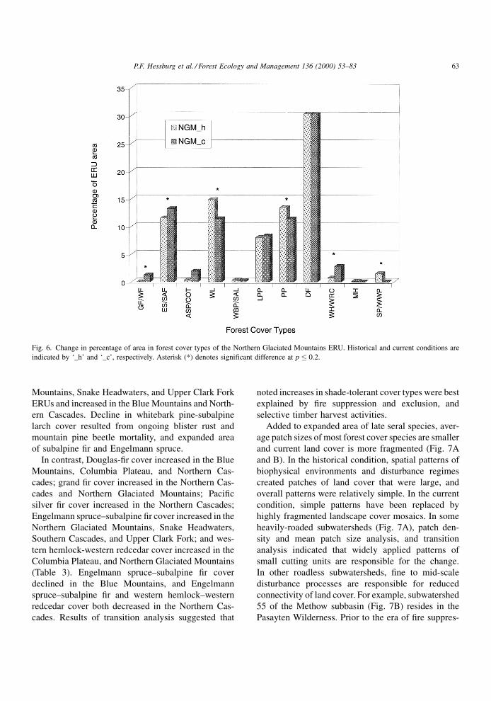
Fig. 6. Change in percentage of area in forest cover types of the Northern Glaciated Mountains ERU. Historical and current conditions are

indicated by `_h' and `_c', respectively. Asterisk (*) denotes significant difference at p � 0.2.

P.F. Hessburg et al. / Forest Ecology and Management 136 (2000) 53±83 63

sion (pre-1930s), large scale stand replacement ®res

would naturally occur on an infrequent basis resulting

in simple landscape cover mosaics consisting of a

relatively few large patches. Today, the Methow sub-

watershed exhibits reduced connectivity of land cover,

and causative factors were small ®res and bark beetle

outbreaks.

In Section 3.3, we discuss changes among forest

structural classes. Here, it will be important to keep in

mind the scale dependence of observations. Immedi-

ately above, we reported that landscape cover mosaics

exhibited increased pattern complexity in the current

condition. Below, we show that patterns of structural

classes have changed in a different way.

3.3. Trends among structural classes

In general, the vertical structure of individual forest

patches has become more complex, but the landscape

pattern of structural conditions is generally simpler

when compared with historical forests. Landscape

area in old forest structures (multi-story and single

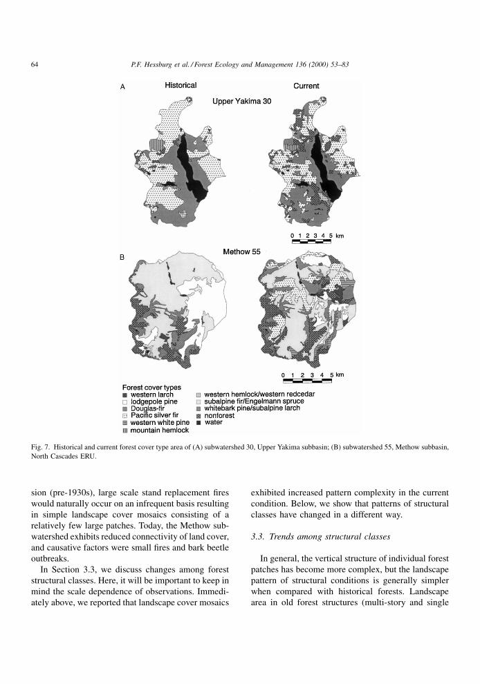
Fig. 7. Historical and current forest cover type area of (A) subwatershed 30, Upper Yakima subbasin; (B) subwatershed 55, Methow subbasin,

North Cascades ERU.

64 P.F. Hessburg et al. / Forest Ecology and Management 136 (2000) 53±83

story) declined in most forested ERUs (Fig. 8) , but the

most signi®cant declines occurred in the Blue Moun-

tains, Northern Cascades, Snake Headwaters, and

Upper Klamath ERUs (Fig. 9, Table 3). Landscape

area in stand initiation structures (new forest) declined

in ®ve of nine forest-dominated ERUs and increased in

one, the Blue Mountains. Area in stand-initiation

structures declined in the Central Idaho Mountains,

Lower Clark Fork, Northern Glaciated Mountains,

Upper Clark Fork, and Upper Snake ERUs (Fig. 10).

This stands to reason because stand replacement and

mixed severity ®res were historically dominant in

these ERUs across space and time.

Area and connectivity of intermediate (not new and

not old forest) structural classes (stem exclusion,

understory reinitiation, and young multistory) in-

creased in most forested ERUs. This change toward

landscape dominance by intermediate forest structures

was the general mechanism of pattern simpli®cation.

When viewed simplistically, there is currently less

Fig. 8. Graphical representation of forest structural classes used in the mid-scale assessment of the interior Columbia River basin; (A) stand

initiation, (B) open stem exclusion, (C) closed stem exclusion, (D) understory reinitiation, (E) young multi-story forest, (F) old multi-story

forest, (G) old single story forest. Refer to Oliver and Larson (1996) and O'Hara et al. (1996) for expanded descriptions of forest structural

classes.

P.F. Hessburg et al. / Forest Ecology and Management 136 (2000) 53±83 65

area in stand initiation and old forest structures, and

considerably more area and improved connectivity of

intermediate forest structures. The most notable

increases in intermediate structures occurred in the

Blue Mountains, Central Idaho Mountains, Columbia

Plateau, Lower Clark Fork, Northern Glaciated Moun-

tains, Snake Headwaters, Southern Cascades, and

Upper Clark Fork ERUs. Area in intermediate struc-

tural classes actually declined in the Upper Klamath

ERU, where transition analysis implicated extensive

past harvesting.

3.4. Other structural changes

Four additional ®ndings related to forest structural

change are worthy of brief mention: (1) In the histor-

ical condition, large (>63.5 cm DBH) and medium

(40.5±63.5 cm DBH) trees were once more widely

distributed in structures other than old forest as a

conspicuous remnant after stand-replacing wild®res.

Change analysis indicated that patches with medium

and large trees were targeted for timber harvest,

regardless of their structural af®liation. (2) Along with

other raw attributes interpreted from aerial photos, we

estimated dead tree and snag abundance in each forest

patch as: none, <10% , 10±39%, 40±70%, and >70%

of trees dead or as snags. Change analysis with these

data indicated that dead tree and snag abundance

increased signi®cantly in most forested ERUs, but

primarily in the pole and small tree (12.7±40.4 cm

DBH) size classes, because the medium and large trees

were depleted by timber harvest. (3) Current forest

patches have more canopy layers than were displayed

in the historical condition, and understory layers are

typically comprised of late seral species. (4) In the

historical condition, forest understories were often

absent or comprised of shrub and herbaceous species.

Current forest understories are less often grass or

Fig. 9. Change in percentage of area in of old forest and other structures for selected ERUs. Structural class abbreviations are: SI, stand

initiation, SE, stem exclusion (both open and closed canopy conditions), UR, understory reinitiation, YFMS, young multi-story forest, OF, old

multi-story and single story forest. Asterisk (*) denotes significant difference at p � 0.2.

66 P.F. Hessburg et al. / Forest Ecology and Management 136 (2000) 53±83

shrub and mostly coniferous. With livestock grazing

and the elimination of surface ®res, multi-layered

conifer understories developed.

3.5. Landscape spatial patterns

We conducted change analysis with cover type-

structural class couplets as patch types. In the sections

that follow, we discuss changes occurring across all

ERUs for a given subset of metrics (Table 1).

3.5.1. Richness, diversity, and evenness

Patch richness (PR), Shannon's (1949) diversity

index (SHDI), and the inverse of Simpson's l (N2,

Hill, 1973) provide different views of the diversity of

patch types of a landscape. While richness tallies the

number of patch types present regardless of their

abundance, the SHDI and N2 indices incorporate

abundance into the measurement of diversity, but

N2 responds to change in the abundance of dominant

patch types. Relative patch richness (RPR) relates PR

to the total number of patch types (192) present in the

basin. The SHDI (or its transformed equivalent N1,

Hill, 1973) is intermediate in responsiveness to abun-

dance changes between RPR and N2.

In general, for the ®ve measures of richness and

diversity (RPR and PR, SHDI and N1, and N2), all

ERUs displayed a positive mean difference with two

notable exceptions (Table 4): the Lower Clark Fork

and Upper Klamath ERUs exhibited minor declines in

PR. Using transition analysis, we attributed these

declines to a history of widespread timber harvest

activity. Five of 13 ERUs displayed change in PR

generally on the order of a 15±30% increase, while 8

of the 13 ERUs re¯ected both increased dominance

and diversity (N2). The PR values and transition

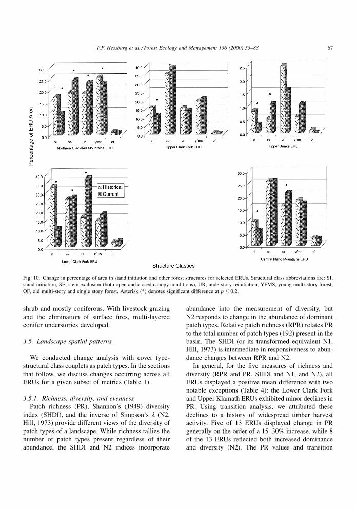
Fig. 10. Change in percentage of area in stand initiation and other forest structures for selected ERUs. Structural class abbreviations are: SI,

stand initiation, SE, stem exclusion (both open and closed canopy conditions), UR, understory reinitiation, YFMS, young multi-story forest,

OF, old multi-story and single story forest. Asterisk (*) denotes significant difference at p � 0.2.

P.F. Hessburg et al. / Forest Ecology and Management 136 (2000) 53±83 67

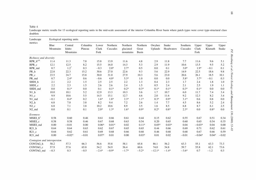
Table 4

Landscape metric results for 13 ecological reporting units in the mid-scale assessment of the interior Columbia River basin where patch types were cover type-structural class

doublets

Landscape

metrics

Ecological reporting units

Blue

Mountains

Central

Idaho

Mountains

Columbia

Plateau

Lower

Clark

Fork

Northern

Cascades

Northern

glaciated

mountains

Northern

Great

Basin

Owyhee

Uplands

Snake

Headwaters

Southern

Cascades

Upper

Clark

Fork

Upper

Klamath

Upper

Snake

Richness and diversity

RPR_ha,b 11.4 11.3 7.8 15.8 13.9 11.6 4.8 2.9 11.8 7.7 11.6 9.6 5.1

RPR_c 12.1 12.5 8.2 15.5 16.0 14.3 5.3 2.9 11.9 10.6 13.5 9.5 5.2

RPR_md 0.7 1.2* 0.3 ÿ0.3 2.0* 2.7* 0.5 0.0 0.1 3.0* 1.9* ÿ0.1 0.1

PR_h 22.8 22.3 15.2 30.6 27.0 22.6 9.3 5.6 22.9 14.9 22.5 18.6 9.8

PR_c 23.5 24.7 15.8 30.0 31.0 27.9 10.3 5.6 23.0 20.6 26.1 18.5 10.1

PR_md 0.7 2.4* 0.6 ÿ0.6 4.0* 5.3* 1.0 0.0 0.0 5.8* 3.7* ÿ0.1 0.3

SHDI_h 2.1 2.2 1.5 2.5 2.5 2.2 1.3 0.4 2.3 1.7 2.4 1.8 1.0

SHDI_c 2.2 2.3 1.5 2.6 2.6 2.4 1.5 0.5 2.4 2.1 2.5 1.9 1.1

SHDI_md 0.0 0.1* 0.0 0.1 0.1* 0.2* 0.3* 0.1* 0.1* 0.3* 0.1* 0.0 0.0

N1_h 10.0 10.1 5.2 12.9 13.3 10.3 3.6 1.7 10.7 6.0 11.7 7.4 3.4

N1_c 9.9 10.6 5.5 14.5 15.1 12.7 4.6 2.0 11.6 9.2 12.3 8.2 3.4

N1_md ÿ0.1 0.4* 0.2 1.6* 1.8* 2.3* 1.1* 0.3* 0.9* 3.1* 0.6 0.8 0.0

N2_h 6.8 7.0 3.8 8.2 9.4 7.2 2.6 1.4 7.7 4.5 8.6 5.2 2.4

N2_c 6.8 7.1 3.8 10.2 10.6 8.9 3.5 1.6 8.5 6.8 8.7 6.1 2.5

N2_md 0.0 0.1 0.1 2.0* 1.3* 1.6* 0.9* 0.2* 0.8* 2.3* 0.0 0.8* 0.0

Evenness

MSIEI_hc 0.58 0.60 0.46 0.61 0.66 0.61 0.44 0.15 0.62 0.55 0.67 0.51 0.34

MSIEI_c 0.58 0.58 0.46 0.67 0.68 0.63 0.54 0.20 0.65 0.60 0.65 0.54 0.35

MSIEI_md 0.00 ÿ0.01 0.00 0.06* 0.01* 0.02 0.11* 0.05* 0.03* 0.04 ÿ0.03* 0.04 0.00

R21_h 0.64 0.64 0.63 0.62 0.67 0.65 0.65 0.44 0.66 0.69 0.71 0.62 0.61

R21_c 0.64 0.62 0.61 0.69 0.68 0.66 0.68 0.46 0.68 0.68 0.67 0.66 0.59

R21_md 0.00 ÿ0.02* ÿ0.01 0.07* 0.01 0.00 0.03* 0.01 0.02 ÿ0.01 ÿ0.04* 0.04* ÿ0.02

Contagion and interspersion

CONTAG_h 58.2 57.3 66.3 56.6 55.8 58.1 65.8 86.1 56.2 63.3 55.1 63.3 73.3

CONTAG_c 57.9 57.6 65.8 54.2 54.9 56.4 60.6 74.0 54.8 59.7 55.8 62.1 73.6

CONTAG_md ÿ0.3 0.3 ÿ0.5 ÿ2.4* ÿ0.9* ÿ1.7* ÿ5.2* ÿ12.1* ÿ1.4* ÿ3.6* 0.7 ÿ1.2 0.3

68

P.F

.H

essbu

rget

al./F

orest

Eco

logy

and

Managem

ent

136

(2000)

53±83

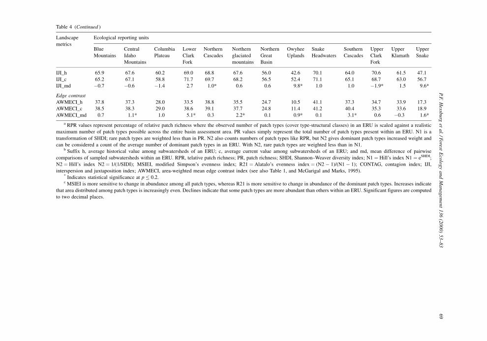
Table 4 (Continued )

Landscape

metrics

Ecological reporting units

Blue

Mountains

Central

Idaho

Mountains

Columbia

Plateau

Lower

Clark

Fork

Northern

Cascades

Northern

glaciated

mountains

Northern

Great

Basin

Owyhee

Uplands

Snake

Headwaters

Southern

Cascades

Upper

Clark

Fork

Upper

Klamath

Upper

Snake

IJI_h 65.9 67.6 60.2 69.0 68.8 67.6 56.0 42.6 70.1 64.0 70.6 61.5 47.1

IJI_c 65.2 67.1 58.8 71.7 69.7 68.2 56.5 52.4 71.1 65.1 68.7 63.0 56.7

IJI_md ÿ0.7 ÿ0.6 ÿ1.4 2.7 1.0* 0.6 0.6 9.8* 1.0 1.0 ÿ1.9* 1.5 9.6*

Edge contrast

AWMECI_h 37.8 37.3 28.0 33.5 38.8 35.5 24.7 10.5 41.1 37.3 34.7 33.9 17.3

AWMECI_c 38.5 38.3 29.0 38.6 39.1 37.7 24.8 11.4 41.2 40.4 35.3 33.6 18.9

AWMECI_md 0.7 1.1* 1.0 5.1* 0.3 2.2* 0.1 0.9* 0.1 3.1* 0.6 ÿ0.3 1.6*

a RPR values represent percentage of relative patch richness where the observed number of patch types (cover type-structural classes) in an ERU is scaled against a realistic

maximum number of patch types possible across the entire basin assessment area. PR values simply represent the total number of patch types present within an ERU. N1 is a

transformation of SHDI; rare patch types are weighted less than in PR. N2 also counts numbers of patch types like RPR, but N2 gives dominant patch types increased weight and

can be considered a count of the average number of dominant patch types in an ERU. With N2, rare patch types are weighted less than in N1.b Suffix h, average historical value among subwatersheds of an ERU; c, average current value among subwatersheds of an ERU; and md, mean difference of pairwise

comparisons of sampled subwatersheds within an ERU. RPR, telative patch richness; PR, patch richness; SHDI, Shannon±Weaver diversity index; N1 � Hill's index N1 � eSHDI;

N2 � Hill's index N2 � 1/(1/SIDI); MSIEI, modified Simpson's evenness index; R21 � Alatalo's evenness index � (N2 ÿ 1)/(N1 ÿ 1); CONTAG, contagion index; IJI,

interspersion and juxtaposition index; AWMECI, area-weighted mean edge contrast index (see also Table 1, and McGarigal and Marks, 1995).* Indicates statistical significance at p � 0.2.c MSIEI is more sensitive to change in abundance among all patch types, whereas R21 is more sensitive to change in abundance of the dominant patch types. Increases indicate

that area distributed among patch types is increasingly even. Declines indicate that some patch types are more abundant than others within an ERU. Significant figures are computed

to two decimal places.

P.F

.H

essbu

rget

al./F

orest

Eco

log

yand

Managem

ent

136

(2000)

53±83

69

analysis indicated that cover-structure patch types not

only increased in number, but new patch types occu-

pied considerable landscape area. The ERUs display-

ing increased dominance and diversity are shown in

Table 4.

Evenness measures assess how equitably area is

distributed among patch types. Both evenness mea-

sures (MSIEI and R21) index change in the distribu-

tion of area among patch types. Many ERUs displayed

increased diversity, richness, and dominance during

the sample period for the diversity measures we used.

Such increase typically results in a modest increase in

the values of the evenness measures, if any change

occurs. Our results con®rmed this relation; the MSIEI

and R21 indices increased in six of eight ERUs

displaying increased diversity and dominance. The

Upper Clark Fork and the Central Idaho Mountains

were the only two ERUs to decline in evenness; the

Upper Clark Fork declined in both evenness measures

(Table 4). To explain changes in evenness, it is helpful

to re-examine changes in the area relations of cover

types and structural classes. In the Central Idaho

Mountains, few cover type changes were signi®cant,

but distribution of area in forest structural classes

became increasingly uneven (Table 3, Fig. 10). Area

in stand-initiation structures declined from 9.7 to

5.9% of the ERU, and area in understory reinitiation

structures increased from an average of 16±21.4%

of the ERU. A similar pattern of change was evident

in the Upper Clark Fork; few cover type changes

were evident, but distribution of area in stand initia-

tion, closed canopy stem-exclusion, and young mul-

tistory forest structures became increasingly uneven

(Table 3).

Landscape metrics were averaged across sampled

subwatersheds, hence, values for all metrics in the

historical and current condition re¯ect the average per

subwatershed. But an examination of data in Table 4

prompts two additional questions: (1) What is the total

richness and diversity of patch types of each ERU, and

(2) Have total richness and diversity values for the

ERU changed during the sample period? Heltshe and

Forrester (1983) describe a `jackknife' estimator for

richness that attempts to estimate total richness for a

geographic area of interest. We applied this technique

and a related estimator for N2 (Burnham and Overton,

1979) to the historical and current data to estimate

difference in total richness and dominance for each

ERU (Table 5). The jackknife technique results in

estimates of the total and standard error. We used these

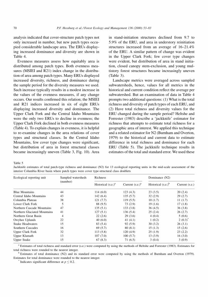
Table 5

Jackknife estimates of total patch-type richness and dominance (N2) for 13 ecological reporting units in the mid-scale assessment of the

interior Columbia River basin where patch types were cover type-structural class doublets

Ecological reporting unit Sampled watersheds

(number)

Richness Dominance (N2)

Historical (s.e.)a Current (s.e.)a Historical (s.e.)b Current (s.e.)

Blue Mountains 44 114 (6.0) 123 (4.3) 23 (3.5) 20 (2.4)

Central Idaho Mountains 43 142 (6.4) 135 (5.7) 32 (2.9) 29 (2.7)

Columbia Plateau 38 121 (7.7) 119 (5.5) 10 (1.7) 11 (1.7)

Lower Clark Fork 5 88 (9.5) 73 (2.9) 19 (1.6) 17 (1.8)

Northern Cascade Mountains 47 135 (5.1) 133 (3.8) 36 (4.5) 36 (3.8)

Northern Glaciated Mountains 41 127 (5.1) 136 (5.4) 25 (2.4) 26 (2.7)

Northern Great Basin 4 22 (2.6) 29 (3.6) 4 (0.4) 5 (0.6)

Owyhee Uplands 22 40 (6.0) 41 (4.1) 1 (0.2) 2 (0.3)*

Snake Headwaters 15 83 (5.4) 92 (5.9) 30 (3.2) 26 (3.1)

Southern Cascades 16 69 (5.7) 80 (8.1) 15 (1.3) 15 (2.6)

Upper Clark Fork 32 113 (5.8) 120 (4.9) 25 (1.9) 23 (2.2)

Upper Klamath 13 107 (7.0) 100 (5.7) 13 (3.9) 16 (3.0)

Upper Snake 15 67 (8.3) 71 (6.5) 3 (0.4) 3 (0.9)

a Estimates of total richness and standard error (s.e.) were computed by using the methods of Heltshe and Forrester (1983). Estimates for

total richness were rounded to the nearest integer.b Estimates of total dominance (N2) and its standard error were computed by using the methods of Burnham and Overton (1979).

Estimates for total dominance were rounded to the nearest integer.* Indicates significant difference at p � 0.2.

70 P.F. Hessburg et al. / Forest Ecology and Management 136 (2000) 53±83

statistics in simple two-way t-tests to evaluate sig-

ni®cant change in total richness or dominance. All

changes but one were insigni®cant, but eight ERUs

displayed nonsigni®cant increase in richness. Jack-

knife estimates of richness are sensitive to differences

in sample size and distribution. It is best in this

instance, not to make comparisons among ERUs,

but comparisons between current and historical values

are appropriate. Jackknife estimates for N2 are not

restricted in this way. The N2 values across ERUs

range from a low of 1 in the Owyhee Uplands to 36 in

the Northern Cascades. We expect forest-dominated

ERUs to display much larger values of total domi-

nance than rangeland-dominated ERUs because of

their greater patch richness and diversity.

3.5.2. Contagion and interspersion

Contagion (CONTAG) and interspersion±juxtapo-

sition (IJI) metrics quantify the extent to which pixels

of differing type intermix; IJI considers length of edge

between contrasting patch types, and CONTAG esti-

mates patch dispersion and interspersion for raster

maps. Seven of 13 ERUs displayed signi®cant

declines in CONTAG, and all signi®cant mean differ-

ences values were negative (Table 4). A negative

mean difference value of CONTAG indicated that

across a given ERU, patches became smaller and more

dispersed. Three of six ERUs with nonsigni®cant

mean difference values of CONTAG also exhibited

a negative sign. These results suggest a basinwide

decrease in contagion of cover-structure patch

types. With the exception of the Northern Great Basin

and Owyhee Uplands ERUs, the magnitude of

decrease was small relative to initial average historical

values.

Only 4 of 13 ERUs displayed signi®cant mean

difference values for IJI; two were positive and two

were negative (Table 4). The Owyhee Uplands and

Upper Snake ERUs were noteworthy because the

magnitude of the mean IJI difference for these two

ERUs was especially large. Unlike CONTAG, there

was no consistent pattern across ERUs for this metric,

and most changes were small. We conclude that

interspersion changes as measured by this metric

are minimal at this scale, but that changes in inter-

spersion and juxtaposition may be better observed at

smaller pooling scales where environmental variation

is controlled.

3.5.3. Edge contrast

The area-weighted mean edge contrast index

(AWMECI) uses a set of user-de®ned values ranging

from 0 to 1 to represent relative edge contrast (Table 2)

between patch types, weighted by area, to evaluate

change in edge contrast of a sample of landscapes. We

based edge contrast weights on physiognomic and

structural conditions in deference to edge-sensitive

and edge-dependent terrestrial species, and their sen-

sitivity to structural differences of edges. An increase

in area-weighted mean edge contrast was indicated as

the percentage of the total edge that was the equivalent

of maximum contrast edge. The greater the difference

in structure or physiognomic condition (e.g., an old

single-story forest patch adjacent to herbland), the

greater the edge contrast weight. Signi®cant increase

in AWMECI for a sample of landscapes indicated that

greater contrast in structural and physiognomic con-

dition was occurring at patch edges. Six of 13 ERUs

displayed such an increase. Most increases were rela-

tively modest except in the Lower Clark Fork where

increase in maximum contrast edge averaged 5.1% of

the total edge (Table 4).

3.6. Landscape vulnerability to disturbances

3.6.1. Insects and pathogens

Our analysis indicated that forest landscapes have

changed signi®cantly in their vulnerability to major

insect and pathogen disturbances. Absent frequent

®res, and in¯uenced by selective harvesting and

domestic livestock grazing, overstory and understory

Douglas-®r cover and that of most other shade-tolerant

species expanded, forest structures became more

layered, and grass and shrub understories were

replaced by coniferous understories. As a conse-

quence, insect and pathogen vulnerabilities that

increase with increased dominance and spatial aggre-

gation of shade-tolerant conifers were favored by the

changes in vegetation patterns. Conversely, because

patches with medium and large trees of early seral

species were primarily harvested, insect and pathogen

vulnerabilities favored by increasing dominance and

spatial aggregation of large trees of early seral species

declined. A few examples follow (see also Table 6).

In many ERUs, area vulnerable to western spruce

budworm increased, but most changes were not sig-

ni®cant at the scale of an ERU. To determine whether

P.F. Hessburg et al. / Forest Ecology and Management 136 (2000) 53±83 71

Table 6

Change in area (in %) highly vulnerable to insect and pathogen disturbance in 11 forested ecological reporting units in the mid-scale assessment of the interior Columbia River

basin (see also Hessburg et al., 1999b)

Disturb.

agentaEcological reporting units (ERU)

Blue

Mountains

Central

Idaho

Mountains

Columbia

Plateau

Lower

Clark

Fork

Northern

Cascades

Northern

Glaciated

Mountains

Snake

Headwaters

Southern

Cascades

Upper

Clark

Fork

Upper

Klamath

Upper

Snake

Hb C H C H C H C H C H C H C H C H C H C H C

WSB 38.2 38.9 49.4 51.1 9.3 12.0 56.8 65.0 51.5 50.4 44.5 47.9 45.0 51.8 10.1 12.3 59.1 55.9 14.6 15.9 1.6 2.1

DFB 5.2c 7.8 4.4 5.0 2.9 2.6 0.2 5.9 8.7 7.4 3.6 5.0 2.1 3.9 1.8 0.1 8.0 4.8 0.0 0.0 0.5 1.0

WPB1 2.5 2.5 1.0 1.3 4.6 2.9 0.0 0.6 3.7 1.8 1.2 0.9 34.6 29.2 5.2 5.1 2.9 0.5 5.7 4.5 ± ±

WPB2 17.8 19.7 3.3 3.3 14.9 17.1 1.5 3.8 9.8 8.2 7.9 7.3 ± ± 20.5 24.4 9.9 8.1 19.3 21.3 ± ±

MPB1 6.7 5.1 21.0 22.1 1.8 2.4 4.0 12.9 5.3 6.8 15.4 18.9 34.6 29.2 29.0 24.9 36.1 37.6 4.7 4.3 0.6 0.3

MPB2 17.8 19.7 3.3 3.3 14.9 17.1 1.5 3.8 9.8 8.2 7.9 7.3 ± ± 20.5 24.4 9.9 8.1 19.3 21.3 ± ±

FE 24.6 15.0 21.3 26.2 1.8 2.9 28.3 37.0 20.4 21.5 6.8 8.4 19.3 16.1 9.0 10.2 7.8 9.7 17.1 18.0 ± ±

SB 2.6 0.7 3.1 3.6 ± ± 0.1 0.5 6.0 5.3 3.0 4.5 8.3 7.6 0.1 0.1 6.9 5.6 ± ± ± ±

DFDM 10.1 16.5 10.7 10.5 6.9 6.4 6.0 7.9 18.6 17.9 13.1 14.3 4.1 6.4 2.3 0.5 16.2 13.2 0.8 0.2 0.6 1.5

PPDM 10.4 8.1 2.2 1.8 10.8 7.8 0.0 0.9 5.6 3.9 3.8 2.5 ± ± 12.9 17.9 5.0 2.3 17.8 15.5 ± ±

WLDM 1.3 0.8 0.5 0.1 0.0 0.1 0.2 0.2 0.5 0.4 6.9 4.2 ± ± ± ± 2.8 1.3 ± ± ± ±

LPDM 1.5 1.6 13.7 15.1 0.2 0.4 0.2 2.6 2.7 3.1 9.3 9.1 30.8 20.9 10.2 11.9 22.6 22.5 0.4 0.3 0.3 0.3

AROS 40.7 41.0 37.6 39.2 9.1 10.5 55.0 65.1 48.6 45.2 37.3 40.7 20.4 31.5 10.9 12.8 34.2 31.8 13.2 13.6 1.0 1.6

PHWE 34.5 37.0 29.3 27.8 10.4 9.7 59.4 62.0 41.7 39.2 27.8 31.0 10.9 12.8 31.1 35.4 21.6 20.8 18.5 17.7 1.0 1.6

HEANs 24.3 16.9 36.2 38.9 0.8 5.4 71.4 77.0 29.6 32.2 20.0 26.8 22.0 30.6 37.1 38.3 32.2 34.6 22.8 23.3 1.0 1.7

HEANp 11.6 10.4 2.1 1.7 11.8 11.2 0.0 0.2 7.5 5.9 3.1 4.0 ± ± 13.8 23.4 5.4 4.0 19.0 19.8 ± ±

TRBR 4.4 2.5 9.3 11.0 ± ± 1.0 1.5 11.4 9.9 7.1 9.0 13.1 15.1 0.8 0.8 9.9 10.3 ± ± ± ±

SRBR 46.7 52.1 57.1 56.2 17.2 15.4 56.2 52.3 61.2 57.2 66.9 65.8 49.9 48.6 25.6 29.4 60.6 59.0 26.4 17.9 1.5 2.1

WPBR1 ± ± 0.0 0.1 1.4 0.1 0.8 3.7 0.1 0.2 1.9 0.3 ± ± 0.2 0.3 2.5 1.4 0.0 0.0 ± ±

WPBR2 ± ± 0.7 0.6 ± ± ± ± 0.4 0.9 0.0 0.0 4.0 2.0 ± ± 2.9 2.4 ± ± ± ±

RRSR 1.1 0.8 0.1 0.3 0.0 0.1 1.0 1.7 0.6 1.1 0.0 0.2 ± ± 1.1 1.7 1.2 2.3 4.8 4.1 ± ±

a WSB, western spruce budworm; DFB, Douglas-fir beetle; WPB1, western pine beetle Ð type 1 attack of mature and old ponderosa pine; WPB2, western pine beetle Ð type 2

attack of immature and overstocked ponderosa pine; MPB1, mountain pine beetle Ð type 1 attack of overstocked lodgepole pine; MPB2, mountain pine beetle Ð type 2 attack of

immature and overstocked ponderosa pine; FE, fir engraver; SB, spruce beetle; DFDM, Douglas-fir dwarf mistletoe; PPDM, ponderosa pine dwarf mistletoe; WLDM, western larch

dwarf mistletoe; LPDM, lodgepole pine dwarf mistletoe; AROS, Armillaria root disease; PHWE, laminated root rot; HEANs, S-group annosum root disease; HEANp, P-group

annosum root disease; TRBR, tomentosus root and butt rot; SRBR, Schweintizii root and butt rot; WPBR1, white pine blister rust Ð type 1 on western white pine/sugar pine;

WPBR2, white pine blister rust Ð type 2 on whitebark pine; RRSR, rust-red stringy rot. See also Hessburg et al., 1999b.b H, Historical condition; C, Current condition.c Values shown in bold indicate significant increase or decrease (p � 0.2) from the historical to the current condition; `na' � not applicable.

72

P.F

.H

essbu

rget

al./F

orest

Eco

logy

and

Managem

ent

136

(2000)

53±83

the lack of observed signi®cant difference was scale

dependent, we summarized statistical results for bud-

worm (and other disturbances) by smaller scale pool-

ing strata. For example, we used 4th code watersheds

called `subbasins' and subregional aggregations of

subwatersheds based on similar climate and environ-

ments, and we were able to detect signi®cant change.

Results of these analyses suggested that ERUs were

too large, and that smaller pooling strata would be

more informative. In addition, we noted that the

conduciveness of conditions to widespread severe

budworm defoliation increased over the sample per-

iod. This was due to the increased dominance of

shade-tolerant conifers, increased abundance of

multi-layered host patches, and increased spatial

aggregation of host patches re¯ected in increased

average host patch size, and in some cases increased

host patch density.

Throughout the basin, area vulnerable to Douglas-

®r beetle and Douglas-®r dwarf mistletoe increased

because forest landscapes in the existing condition

exhibited increased cover and connectivity of Dou-

glas-®r, current stand densities are elevated from

historical conditions, and patches today tend to be

multi-layered, often with several layers of understory

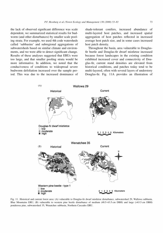
Douglas-®r. Fig. 11A provides an illustration of

Fig. 11. Historical and current forest area: (A) vulnerable to Douglas-fir dwarf mistletoe disturbance, subwatershed 29, Wallowa subbasin,

Blue Mountains ERU; (B) vulnerable to western pine beetle disturbance of medium (40.5±63.5 cm DBH) and large (>63.5 cm DBH)

ponderosa pine, subwatershed 35, Wenatchee subbasin, Northern Cascades ERU.

P.F. Hessburg et al. / Forest Ecology and Management 136 (2000) 53±83 73

increased forest area vulnerable to Douglas-®r dwarf

mistletoe in a subwatershed of the Wallowa subbasin

of the Blue Mountains ERU. Conversely, area vulner-

able to western pine beetle disturbance of mature and

old ponderosa pine (WPB1, Table 6) fell because

medium and large ponderosa pine were selectively

harvested from old forest patches and from other

structures (Fig. 11B).

3.6.2. Wildfires, prescribed fires, and smoke

production

Forest landscapes have been signi®cantly altered in

their vulnerability to wild®res, increasing the potential

for air quality degradation, as well. In general, the risk

of stand replacement ®re has increased throughout the

forest-dominated portion of the basin. Elevated risk is

indicated by increased ground fuel loads, crown ®re

potential, ¯ame length, rate of spread, ®reline inten-

sity, and smoke production (PM10), each of which are

consequences of change in spatial patterns of both

living and dead forest cover and structure. Changes in

vegetation patterns are the result of effective ®re

suppression, timber harvest, and ®re exclusion. Key

factors responsible for ®re exclusion were the wide-

spread elimination of ¯ashy fuels through extensive

domestic livestock grazing, especially in the ®rst half

of the 20th century (Wissmar et al., 1994; Skovlin and

Thomas, 1995; Hann et al., 1997, and references

therein); reduced connectivity of ®re-prone land-

scapes through placement of extensive road networks;

settlement of ®re-prone interior valleys and subse-

quent conversion to irrigated agriculture by European

immigrants; and movement of American Indians, who

used ®re as a management tool, onto reservations

(Robbins and Wolf, 1994).

A number of changes in fuel loading, PM10 smoke

production (Table 7), crown ®re potential, and ®re

behavior attributes (Table 8) were signi®cant at the

ERU scale; a few examples follow (see also Ottmar

et al., 1999). In the Central Idaho Mountains, fuel

loads (>45 Mg/ha), smoke production (>448 kg/ha),

and ¯ame length (>1.2 m) increased to high levels

or above on more than 5% of the area. In the Lower

Clark Fork ERU, fuel loads (>45 Mg/ha), PM10

smoke production (>448 kg/ha) during wild®res,

and ¯ame lengths >1.2 m during wild®res increased

to moderate levels or above on approximately one-

third of the ERU area. Crown ®re potential increased

to high levels or above on 29% of the ERU area. At

present, 82% of the area of the Lower Clark Fork ERU

exhibits moderate to severe crown ®re potential. In the

event of a wild®re today, it would be dif®cult to

suppress expected ¯ames on 94% of the current forest

and rangeland area. At present, over 81% of the ERU

would exhibit very low smoke production if pre-

scribed ®res were implemented in place of wild®res

for fuels reduction. Under a wild®re burn scenario

only 14% of the ERU area would exhibit very low

smoke production.

Finally, in the Southern Cascades fuel loads

(>45 Mg/ha) increased on nearly 5% of the ERU area,

rate of spread (>2.4 m/min) during wild®res increased

on more than 11% of the area, and extreme ®reline

intensity (>3459.2 kW/m) increased on nearly 8% of

the area. At present, 56% of the ERU area exhibits

moderate to extreme crown ®re potential, and 82% of

the forest and rangeland area would experience ¯ame

lengths in excess of 1.2 m during wild®res. In the

event of a wild®re, it would be dif®cult to suppress

¯ames on 8 of every 10 ha. At present, over 75% of the

ERU would exhibit very low smoke production if

prescribed ®res were implemented in place of wild-

®res for fuels reduction. Under a wild®re burn sce-

nario, 21% of the ERU area would exhibit very low

smoke production.

4. Discussion

The primary utility of landscape assessment is in

understanding the characteristics of ecosystems that

we manage (Morgan et al., 1994). Knowledge of

landscape pattern change at regional and subregional

scales provides critical context for forest-level plan-

ning, watershed analysis and project-level planning,

and valuable insight for ecosystem restoration, con-

servation, and monitoring decisions. Landscape

change analysis provides an empirical basis to eval-

uate the historical and current rarity of landscape

pattern features and aids in determining how repre-

sentative current patterns are compared with recent

historical conditions.

The basin assessment area is large, and we sum-

marized many changes in vegetation condition and

associated vulnerability to disturbance. Here we focus

on the most important generalities lest we lose them.

74 P.F. Hessburg et al. / Forest Ecology and Management 136 (2000) 53±83

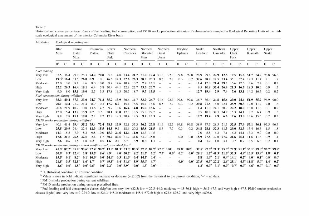
Table 7

Historical and current percentage of area of fuel loading, fuel consumption, and PM10 smoke production attributes of subwatersheds sampled in Ecological Reporting Units of the mid-

scale ecological assessment of the interior Columbia River basin

Attributes Ecological reporting unt

Blue

Mtns

Cenral

Idaho

Mtns.

Columbia

Plateau

Lower

Clark

Fork

Northern

Cascades

Northern

Glaciated

Mtns

Northern

Great

Basin

Owyhee

Uplands

Snake

Headwtr

Southern

Cascades

Upper

Clark

Fork

Upper

Klamath

Upper

Snake

Ha C H C H C H C H C H C H C H C H C H C H C H C H C

Fuel loading

Very low 37.5 36.4 29.0 28.3 74.2 70.8 5.8 4.8 23.4 21.7 21.0 19.4 91.6 92.3 99.8 99.8 28.9 29.6 22.9 12.8 19.5 15.6 51.7 54.9 96.8 96.6

Low 19.3b 16.4 31.5 26.0 8.9 10.1 46.5 17.3 22.6 26.3 28.2 23.3 8.5 7.7 0.3 0.2 37.6 28.2 17.5 23.4 35.1 37.4 12.3 11.4 2.1 1.7

Moderate 12.0 13.0 8.1 8.6 8.0 10.0 9.4 14.6 10.4 10.7 7.8 15.1 ± ± ± ± 11.4 12.0 21.4 29.5 16.6 17.6 3.6 7.2 0.1 0.2

High 22.2 26.3 16.4 18.1 6.4 5.8 20.4 44.1 22.9 22.7 33.3 26.7 ± ± ± ± 9.5 10.8 35.4 26.9 21.3 16.5 18.3 10.0 0.9 1.3

Very high 9.0 8.0 15.1 19.0 2.5 3.3 17.8 19.3 20.7 18.7 9.7 15.5 ± ± ± ± 12.7 19.4 2.9 7.4 7.6 13.1 14.2 16.5 0.2 0.2

Fuel consumption during wildfirese

Very low 38.3 40.4 37.3 33.0 74.7 71.2 35.2 13.9 30.6 31.7 33.9 26.7 91.6 92.3 99.8 99.8 36.7 36.4 24.8 15.6 29.0 24.4 51.9 55.2 96.9 90.0

Low 20.1 14.4 23.2 21.4 8.9 10.3 17.2 8.2 15.4 16.5 15.4 16.6 8.5 7.7 0.3 0.2 29.8 21.5 18.0 22.1 25.9 30.3 12.0 11.2 2.0 1.6

Moderate 20.8 21.9 10.7 10.8 13.6 14.7 9.7 19.6 16.4 14.8 15.2 18.6 ± ± ± ± 11.4 11.9 24.1 30.9 22.2 18.2 13.8 11.6 0.1 0.2

High 12.0 15.4 13.7 15.9 0.7 1.3 20.1 39.0 17.3 18.5 25.8 22.7 ± ± ± ± 9.5 10.8 30.1 24.9 15.3 14.1 8.7 6.4 0.9 1.3

Very high 8.8 7.8 15.1 19.0 2.2 2.7 17.8 19.3 20.4 18.5 9.7 15.3 ± ± ± ± 12.7 19.4 2.9 6.6 7.6 13.0 13.6 15.6 0.2 0.2

PM10 smoke production during wildfirese

Very low 40.1 41.4 39.4 35.2 75.4 72.4 38.5 13.9 32.1 33.3 36.2 27.8 91.6 92.3 99.8 99.8 38.9 37.5 28.5 21.3 32.5 27.9 53.1 56.1 97.5 96.7

Low 25.5 20.9 24.4 22.4 12.3 15.5 14.5 9.9 18.6 20.2 15.8 21.5 8.5 7.7 0.3 0.2 34.8 28.1 32.3 41.3 29.0 32.3 13.4 16.5 1.5 1.8

Moderate 14.3 15.5 7.9 8.2 9.8 10.0 15.0 24.6 12.4 11.0 13.3 14.5 ± ± ± ± 7.0 5.8 6.2 7.1 16.2 14.1 13.3 9.0 0.0 0.0

High 17.6 21.5 26.8 32.5 2.4 1.7 30.4 49.5 31.2 31.6 33.9 35.0 ± ± 0.0 0.0 18.9 27.5 32.0 27.2 21.6 25.1 11.6 11.8 0.9 1.4

Very high 2.6 0.6 1.5 1.8 0.2 0.5 1.6 2.2 5.7 3.9 0.8 1.3 ± ± ± ± 0.4 1.2 1.0 3.1 0.7 0.7 8.5 6.6 0.2 0.1

PM10 smoke production during current wildfires and prescribed firese

Very low 41.5c 87.2d 35.2c 95.6d 72.4c 90.7d 13.9c 81.3d 33.3c 85.5d 27.8c 87.7d 92.3c 100d 99.8c 100d 37.5c 97.5d 21.3c 75.5d 27.9c 91.1d 56.1c 79.0d 96.7c 99.8d

Low 20.9c 9.3d 22.4c 2.8d 15.5c 8.6d 9.9c 9.0d 20.2c 8.2d 21.5c 5.2d 7.7c 0.0d 0.2c 0.0d 28.1c 1.2d 41.3c 21.6d 32.3c 4.4d 16.5c 15.9d 1.8c 0.1d

Moderate 15.5c 0.1d 8.2c 0.1d 10.0c 0.0d 24.6c 0.3d 11.0c 0.4d 14.5c 0.4d ± ± ± ± 5.8c 1.0d 7.1c 0.4d 14.1c 0.2d 9.0c 0.1d 0.0c 0.0d

High 21.5c 3.5d 32.5c 1.6d 1.7c 0.7d 49.5c 9.4d 31.6c 5.9d 35.0c 6.7d ± ± 0.0c 0.0d 27.5c 0.3d 27.2c 2.6d 25.1c 4.3d 11.8c 5.0d 1.4c 0.2d

Very high 2.6c 0.6d 1.8c 0.0d 0.5c 0.0d 2.2c 0.0d 3.9c 0.0d 1.3c 0.0d ± ± ± ± 1.2c 0.0d 3.1c 0.0d 0.7c 0.0d 6.6c 0.0d 0.1c 0.0d

a H, Historical condition; C, Current condition.b Values shown in bold indicate significant increase or decrease (p � 0.2) from the historical to the current condition; `±' � no data.c PM10 smoke production during current wildfires.d PM10 smoke production during current prescribed fires.e Fuel loading and fuel consumption classes (Mg/ha) are: very low <22.5; low � 22.5±44.9; moderate � 45±56.1; high � 56.2±67.3; and very high > 67.3. PM10 smoke production

classes (kg/ha) are: very low � 0±224.2; low � 224.3±448.3; moderate � 448.4±672.5; high � 672.6±896.7; and very high >896.6.

Table 8

Historical (H) and current (C) percentage of area of fire behavior and crown fire potential attributes of subwatersheds sampled in Ecological Reporting Units of the mid-scale ecological

assessment of the interior Columbia River basin

Attributes Ecological reporting unit

Blue

Mountains

Central

Idaho

Mountains

Columbia

Plateau

Lower

Clark

Fork

Northern

Cascades

Northern

Glaciated

Mountains

Northern

Great

Basin

Owyhee

Uplsnds

Snake

Headwaters

Southern

Cascades

Upper

Clark

Fork

Upper

Klamath

Upper

Snake

H C H C H C H C H C H C H C H C H C H C H C H C H C

Fireline intensity during wildfiresa

Very low 26.4 27.4 14.9 14.9 50.2 51.1 4.0 3.6 21.5 19.9 19.6 18.3 19.6 35.7 16.2 25.0 18.2 20.1 25.4 15.6 19.4 15.2 32.2 38.3 31.0 33.6

Low 11.3b 7.9 15.4 15.3 24.3 19.9 2.4 1.7 2.9 4.0 2.4 2.8 78.7 62.5 83.8 74.9 18.6 13.3 0.1 0.2 3.2 3.9 20.1 17.4 67.0 63.6

Moderate 20.5 19.2 19.8 21.2 12.5 9.8 8.4 7.7 23.4 19.1 20.6 15.5 1.7 1.8 0.0 0.1 22.3 22.6 14.3 12.5 17.0 15.3 16.3 11.4 0.6 0.6

High 15.2 14.0 24.0 20.2 4.3 4.9 49.5 28.4 19.2 23.6 26.1 29.6 ± ± ± ± 29.2 29.4 20.3 18.1 35.3 36.7 6.3 7.2 0.5 0.8

Very high 18.0 20.5 23.7 26.0 5.0 5.7 27.4 48.1 24.0 23.4 29.2 29.4 ± ± 0.0 0.0 11.4 13.5 33.7 26.9 23.0 24.8 15.6 11.6 0.9 1.4

Severe 1.2 0.9 0.8 0.9 0.2 0.2 2.3 2.4 3.6 4.2 0.5 0.5 ± ± ± ± 0.1 0.4 1.8 1.9 0.4 0.5 3.1 3.2 ± ±

Extreme 7.3 7.9 1.4 1.6 3.6 6.2 6.0 8.1 5.3 5.8 1.5 4.0 ± ± ± ± 0.2 0.8 4.5 12.3 1.6 3.5 6.4 10.8 ± ±

Rate of spread during wildfires

Very low 24.4 24.0 26.1 28.9 37.0 36.4 4.8 5.0 30.0 27.1 24.9 24.1 13.0 19.3 6.6 14.0 33.6 35.3 25.4 17.6 24.8 23.2 21.8 24.1 21.7 26.5

Low 45.9 46.7 52.7 50.4 44.7 43.9 56.8 64.3 48.7 48.9 56.0 51.5 86.3 78.9 93.1 85.8 54.5 51.9 59.8 56.5 52.8 52.5 56.5 52.9 76.9 71.5

Moderate 29.7 29.3 21.2 20.6 18.3 19.6 38.4 30.5 21.2 23.6 19.1 24.1 0.7 1.9 0.3 0.2 11.9 12.8 14.8 25.8 22.4 24.2 21.7 22.9 1.5 2.0

High 0.0 0.0 0.0 0.0 0.0 0.0 0.0 0.3 0.0 0.4 0.1 0.3 ± ± ± ± 0.0 0.1 0.0 0.1 0.0 0.2 0.0 0.1 ± ±

Flame length during wildfires

Very low 24.0 26.0 12.8 12.6 43.1 47.5 3.8 3.6 20.5 19.1 19.4 17.9 19.6 35.7 13.1 22.6 12.8 15.5 22.9 12.8 17.7 13.5 29.8 35.6 22.4 28.5

Low 14.3 11.2 22.8 23.8 31.5 23.6 3.3 2.2 4.7 5.4 5.1 6.1 80.0 63.9 86.9 77.4 32.1 23.7 2.6 5.3 6.4 8.5 22.6 20.1 75.6 69.0

Moderate 18.5 18.3 13.5 14.2 11.6 9.7 7.4 7.2 20.3 15.9 17.5 11.9 0.4 0.5 ± ± 10.7 15.7 14.1 13.0 13.9 11.0 15.2 9.5 0.6 0.3

High 24.6 20.0 33.0 28.7 5.7 6.9 57.2 44.2 25.1 29.7 35.3 37.3 ± ± ± ± 35.4 35.1 32.2 34.9 44.0 44.3 9.2 10.9 1.1 1.7

Very high 16.3 21.3 16.6 19.5 7.1 10.2 22.3 35.1 26.7 26.1 21.3 24.8 ± ± ± ± 8.9 9.5 27.9 32.9 17.1 19.9 20.0 18.6 0.4 0.5

Severe 2.3 3.2 1.2 1.3 1.0 2.2 6.0 7.7 2.8 3.9 1.2 2.1 ± ± ± ± 0.1 0.6 0.4 1.2 0.9 2.8 3.2 5.3 ± ±

Crown fire potential during wildfires

None 35.3 31.8 30.9 30.4 68.2 60.2 10.1 6.8 24.0 23.6 24.9 22.2 85.9 78.3 94.1 92.6 38.0 33.7 22.5 16.5 19.1 18.9 54.3 56.0 96.9 95.9

Very low 7.1 9.4 4.6 3.9 11.0 16.5 1.4 0.2 5.8 4.9 8.4 3.9 14.1 21.8 5.9 7.4 4.7 3.1 8.0 7.7 8.7 6.7 11.3 13.5 1.7 1.8

Low 12.7 7.2 17.0 14.3 5.2 5.4 24.7 10.8 10.4 11.9 12.0 12.0 ± ± ± ± 15.4 18.6 19.7 20.1 15.0 14.3 6.1 6.3 0.3 0.6

Moderate 16.4 18.8 8.9 6.8 7.3 9.5 23.1 11.8 14.6 13.3 11.7 11.3 ± ± ± ± 5.5 6.3 15.4 19.7 12.2 11.1 16.6 11.1 0.1 0.1

High 5.4 3.8 9.7 9.7 0.4 0.6 0.7 2.7 6.6 7.6 11.0 13.8 ± ± ± ± 13.5 14.2 1.7 3.0 12.3 15.5 1.8 1.6 0.1 0.1

Very high 14.3 17.0 18.6 22.5 7.6 6.9 19.8 28.0 19.4 19.3 18.3 20.6 ± ± ± ± 18.4 18.8 23.1 24.3 21.0 23.7 5.3 6.1 0.3 0.4

Severe 8.9 9.9 10.4 12.5 0.4 0.9 20.3 39.7 19.3 19.5 13.7 14.5 ± ± ± ± 4.5 5.4 9.6 8.7 11.7 9.9 4.7 5.5 0.6 1.1

a Fireline intensity classes (kW/m) are: very low � 0.0±172.9; low � 173.0±345.9; moderate � 346.0±1037.8; high � 1037.9±1729.6; very high � 1729.7±2594.4; severe � 2594.5±

3459.2; and extreme >3459.2. Fire rate of spread classes (m/min) are: very low � 0.0±0.6; low � 0.7±2.4; moderate � 2.5±9.1; and high >9.1. Flame length classes (m) are: very low

<0.6; low � 0.7±1.2; moderate � 1.3±1.8; high � 1.9±2.4; very high � 2.5±3.4; and severe >3.4. Crown fire potential classes are a relativized index.b Values shown in bold indicate significant increase or decrease (p � 0.2) from the historical to the current condition; `±' � no data.

� The most dramatic change in physiognomic condi-

tions was the widespread decline in shrublands.

Losses resulted from forest, woodland, and crop-

land expansion, and conversion to semi- or non-

native herbland.

� Loss of historical herblands to agriculture was

equally dramatic but had already occurred by the

time of our historical sample.

� Shifts from early to late seral species were evident

in many ERUs. Change in ponderosa pine, western

larch, and Douglas-fir cover was associated with

reduced patch area with medium and large trees.

� We observed a precipitous decline in area and

connectivity of western white pine cover in northern

Idaho and northwestern Montana, the heart of the

historical range. Losses were attributed to early

selective harvesting, an introduced blister rust,

and mountain pine beetle mortality.

� Basin forests are now dominated by shade-tolerant

conifers. Lacking significant pattern restoration,

insects and pathogens favored by increased area

and contiguity of patches of shade-tolerant conifers

will continue to expand their role in shaping forest

patterns by their growth and mortality affects, and

by indirect influence on fire regimes.

� Patch area with old forest-structures declined shar-

ply in all ERUs where they historically occupied

more than a minor area. The same was true of

patches with remnant large trees.

� In several ERUs, area with medium and large trees

overshadowed or augmented losses to historical

old-forest area. Our results suggested that 20th-

century timber harvest activities targeted patches

with medium- and large-sized trees regardless of

their structural affiliation. There are at least two

important ramifications: First, it has been broadly

assumed that large trees are principally associated

with old forests, where they contribute important

living and dead structure. In some ERUs, old forest

abundance was historically quite minimal (Table 3),

but medium and large trees were distributed in other

forest structures as a remnant after stand-replacing

fires; in some cases, large trees comprised as much

as 24% of the crown cover of forest structures,

contributing important living and dead structure.

Hence, some non-old forest structures of historical

forest landscapes contributed a measure of late-

successional functionality and connectivity with

old forest. Second, where old forest area and area

with remnant large trees has been depleted, the

present and future supply of medium and large

dead trees as snags and down logs is substantially

diminished. This is especially true of snags and

down logs of early seral species. We propose that

terrestrial and aquatic species and processes requir-

ing large dead tree structure may be adversely

influenced by this reduction unless the shortfall is

remedied through recruitment.

� In several ERUs, we observed a marked reduction

in landscape vulnerability to dwarf mistletoes of

early seral species. Comparisons of historical and

current subwatersheds showed that timber harvest

reduced crown cover of large early seral trees while

one or more shade-tolerant understory strata devel-

oped. There are likely wildlife microhabitat rami-

fications.

� Area and mean patch size of stand-initiation struc-

tures dramatically declined where natural stand-

replacing fires have been excluded. Such reduction

was evident despite widespread timber harvest

activity. With recent emphasis on conserving

dwindling areas of late-successional and old forests

in the Interior Northwest, the role of stand initiation

structures on the landscape may have been under-

estimated. The immediate effect of stand replacing

fires is to simplify landscape patterns and restore

early seral conditions. After such a fire, forests are

regenerated with a new cohort of early seral seed-

lings, saplings, grasses and shrubs. Subsequently,

environmental and disturbance gradients interact

recreating some of the lost pattern complexity,

but expanses of interior forest emerge as a reminder

of prior disturbance. Absent disturbances of this

magnitude, where do the interior forests of the

future come from?

� The absence of wildfires has had profound effects

on forest and woodland area and connectivity at

subwatershed to regional scales. The history and

legacy of fire suppression and prevention programs

is well known, but fire exclusion effects have been

more difficult to pin down because many interacting

factors played a role. As a result, fire prevention

and suppression efficacy may have been overstated,

and the role of factors responsible for exclusion

of fire understated. Basic ecological studies are

needed that explore in greater detail effects of road

P.F. Hessburg et al. / Forest Ecology and Management 136 (2000) 53±83 77

networks and domestic livestock herbivory on

historical and current exclusion of fires and

accretion of trees.

� Patches of current forest cover types and structural

classes are more fragmented than before. Patch

densities are now higher, mean patch sizes are

smaller, the largest patch of any given cover or

structural class is smaller, and edge density is

greater. These combined outcomes point to reduced

landscape contagion as a consequence of timber

harvest and road construction. Landscape pattern

metrics confirmed the presence of highly fragmen-

ted landscapes in the current condition and pointed

to increased pattern complexity among patch types

in managed landscapes, and decreased complexity

in roadless and wilderness-dominated landscapes.

5. Management implications

Several important management implications

emerge from our assessment of basin conditions,

but before we discuss implications, we summarize

what was learned from assessment. First, we showed

that spatial patterns of historical landscapes were

indeed variable, and that those patterns re¯ected var-

iation resulting from patterns of environments and

natural disturbance regimes. Second, we showed that

ground fuel and ®re behavior conditions can be expli-

citly linked to vegetation conditions, that fuel and ®re

behavior conditions changed throughout the basin,

and that landscapes varied in the direction and mag-

nitude of changes. Finally, we showed that ®re, insect,

and pathogen disturbances were commonly associated

with historical landscapes, but that the area and pattern

of area that was highly vulnerable to disturbance, and

the degree of spatial isolation has changed. In the

section that follows, we highlight several key issues

surrounding current public land management of Inte-

rior Northwest forests and relevant implications

from this assessment.

5.1. Fuels and fire behavior Ð examining and

isolating the risks

Throughout the basin, there are currently many

large, spatially continuous areas that display elevated

ground fuel conditions and increased severity in ®re

behavior attributes. Prior to the 20th century period of

active resource management, areas that were normally

in¯uenced by infrequent lethal ®res and those of a

mixed lethal±nonlethal type, also displayed relatively

high fuel loads, crown ®re potential, rate of spread,

¯ame length, and ®reline intensity. Active manage-

ment has not made the entire landscape wild®re prone,

rather, it has removed the degree of spatial isolation

that patches prone to stand replacement once enjoyed

(Fig. 12A±H). A reasonable target of restoration

would be to restore a more typical pattern of isolation

to affected landscapes. To that end, a systematic

evaluation of forest susceptibility to stand replacement

®re would be helpful. Such an evaluation is now

possible using tools and analytical approaches devel-

oped during this assessment, and this information

would be useful for allocating monetary and man-

power resources.

5.2. The wildland±urban interface

Most people who live adjacent to National Forest

lands of the basin live on or adjacent to dry woodlands,

or dry to mesic forests. These speci®c settings have

been most altered by 20th century management activ-

ities. As a result, surface ®re regimes that once

affected lands of the current wildland±urban interface

have become lethal or at best mixed regimes, and

forest residents are at risk at each outbreak of ®re. In

the context of declining ®re suppression effectiveness,

public land managers might consider as a ®rst priority,

restoring vegetation and fuels patterns in the wild-

land±urban interface. In addition, managers might

consider working with local citizens and communities

to halt what is currently a rapidly expanding zone of

interface. The tacit assumption of citizens who take

up private residence in the forest is that the public

land manager will come to their aid at the outbreak of

®re. At some point, the rescue role of public land

managers must be clearly enunciated and the total

extent of a wildland±®re interface zone de®ned. The

safety and management implications of not doing so

are large.

5.3. Fire and smoke Ð how much and when

Stated simply, the question before public land

managers is not whether there will be ®re and smoke

78 P.F. Hessburg et al. / Forest Ecology and Management 136 (2000) 53±83

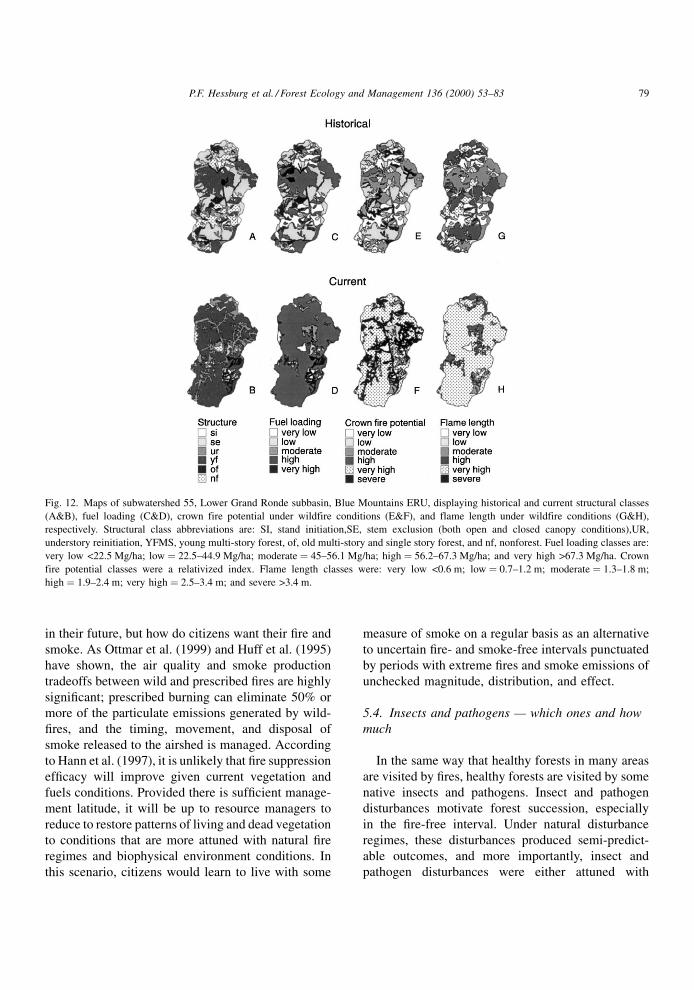
in their future, but how do citizens want their ®re and

smoke. As Ottmar et al. (1999) and Huff et al. (1995)

have shown, the air quality and smoke production

tradeoffs between wild and prescribed ®res are highly

signi®cant; prescribed burning can eliminate 50% or

more of the particulate emissions generated by wild-

®res, and the timing, movement, and disposal of

smoke released to the airshed is managed. According

to Hann et al. (1997), it is unlikely that ®re suppression

ef®cacy will improve given current vegetation and

fuels conditions. Provided there is suf®cient manage-

ment latitude, it will be up to resource managers to

reduce to restore patterns of living and dead vegetation

to conditions that are more attuned with natural ®re

regimes and biophysical environment conditions. In

this scenario, citizens would learn to live with some

measure of smoke on a regular basis as an alternative

to uncertain ®re- and smoke-free intervals punctuated

by periods with extreme ®res and smoke emissions of

unchecked magnitude, distribution, and effect.

5.4. Insects and pathogens Ð which ones and how

much

In the same way that healthy forests in many areas

are visited by ®res, healthy forests are visited by some

native insects and pathogens. Insect and pathogen

disturbances motivate forest succession, especially

in the ®re-free interval. Under natural disturbance

regimes, these disturbances produced semi-predict-

able outcomes, and more importantly, insect and

pathogen disturbances were either attuned with

Fig. 12. Maps of subwatershed 55, Lower Grand Ronde subbasin, Blue Mountains ERU, displaying historical and current structural classes

(A&B), fuel loading (C&D), crown fire potential under wildfire conditions (E&F), and flame length under wildfire conditions (G&H),

respectively. Structural class abbreviations are: SI, stand initiation,SE, stem exclusion (both open and closed canopy conditions),UR,

understory reinitiation, YFMS, young multi-story forest, of, old multi-story and single story forest, and nf, nonforest. Fuel loading classes are:

very low <22.5 Mg/ha; low � 22.5±44.9 Mg/ha; moderate � 45±56.1 Mg/ha; high � 56.2±67.3 Mg/ha; and very high >67.3 Mg/ha. Crown

fire potential classes were a relativized index. Flame length classes were: very low <0.6 m; low � 0.7±1.2 m; moderate � 1.3±1.8 m;

high � 1.9±2.4 m; very high � 2.5±3.4 m; and severe >3.4 m.

P.F. Hessburg et al. / Forest Ecology and Management 136 (2000) 53±83 79

biophysical environment conditions and natural ®re

regimes or recalibrated them. Such is not the case

today. Owing to effects of past management, current

patterns of forest vegetation are out of synchrony with

natural ®re regimes, and current insect and pathogen

disturbance regimes are anomalous.

There is no way to eliminate insect and pathogen

disturbances from basin landscapes, and we would

undoubtedly not wish to do so even if we were able.

The byproduct of most insect and pathogen distur-

bances is microhabitat (snags, down wood) of varying

quality and residence time essential to a variety of

terrestrial and aquatic species. But management, by

altering spatial and temporal patterns of vegetation

structure, composition, and growing conditions, can

in¯uence the suite of agents operating on a landscape,

but it cannot, and, from a purely ecological point of

view, should not attempt to eliminate these distur-

bances.

5.5. Dynamic and reserve systems

In the Paci®c Northwest, the northwest forest plan

(NWFP) de®nes a network of late-successional

reserves throughout the Cascade and Coast Ranges

of Oregon, Washington, and California. While these

lands are not explicitly set aside for custodial manage-

ment, that is how they are managed. It is likely that

such an approach is implementable west of the Cas-

cade crest where most ®re regimes are lethal, ®re-free

intervals may last 250±800 years or more, and the

most common disturbances which are caused by

native insects and pathogens result in canopy

gaps. But east of the Cascade crest where this assess-

ment has taken place, the picture is different. Wild®res

and large-scale insect outbreaks are relatively com-

mon, and escaped wild®re frequency is increasing as

a consequence of past management (Hann et al.,

1997).

Results from both the interior Columbia Basin

broad- (Hann et al., 1997) and mid-scale (Ottmar

et al., 1999; Hessburg et al., 1999a) assessments

suggest that in the interior, a two-pronged, dynamic

and reserve system management approach may be

needed to ensure recovery of the northern spotted

owl and associated species. In the short term (e.g.,

50±100 years), it is likely that areas currently func-

tioning as late-successional and old forest habitats will

be maintained with only limited success. Risk of

disturbance and uncertainty of outcomes will be high.

Over that period, some areas will be affected by stand-

replacement ®res, and will cease to function as late-

successional habitat. For example, since, 1994, 10 of

140±180 (6±7%) northern spotted owl nest stands and

neighborhoods were lost to uncontrolled wild®res on

the Wenatchee National Forest alone. Patterns of

structure and composition within the NWFP reserve

network will continue to change as a result of uncon-

trolled ®res, insect outbreaks, and other succession

processes. What may be needed is an approach that

marries a short term system of reserves with a long

term strategy to convert from a reserve system to a

continuous network of landscapes with dynamic

properties. In such a system, late-successional ele-

ments with semi-predictable environmental settings

(sensu Camp et al., 1997) are continuously recruited,

but shifting in landscape position across space and

time.

Indeed, the most signi®cant fallout associated with

20th century resource management activities has been

the effect of timber extraction and associated activities

on native species biodiversity. Hardest hit have

been late-successional and old forest communities

of the Paci®c and Interior Northwest. Old forest

area has been seriously depleted by past harvest

activity, and old forests of the future will be grown

from existing conditions. But spatial and temporal

patterns of interior forest vegetation and disturbance

are dynamic. Adaptive ecosystem management sce-

narios (sensu Walters and Hollings, 1990) for the

interior should therefore be informed by that insight,

including scenarios to conserve old forest-dependent

species.

Patches of late-successional and old forest structure

are ephemeral landscape elements; they have speci®c

contexts in space and across time. Future old forest

will grow from some other condition; current old

forests will become something else. Taking hold of

this notion enables one to identify the dilemma of

strategies that rely on a reserve system without

backup. Because of the unfortunate legacy of past

management actions, late-successional reserves must

represent a special case for management. But the

special case is an unforeseen consequence of past

events, and in the interior, the likelihood of success

in the long term is low.

80 P.F. Hessburg et al. / Forest Ecology and Management 136 (2000) 53±83

5.6. Healthy fish and healthy forests

Is there really an aquatic conservation strategy

separate from a landscape pattern restoration strategy?

One conclusion of the interior Columbia basin aquatic

(Lee et al., 1997) and landscape assessments (Hann

et al., 1997) is the notion that disturbance regimes and

succession processes associated with terrestrial and

aquatic environments are intertwined. For example, in

forested catchments hydrologic regimes are governed

by spatial and temporal patterns of vegetation and

disturbance. Wild®res and harvest activities have a

direct bearing on the timing and ¯ow of water through

a catchment. But disturbance in upland settings can

result in either positive or negative effects on aquatic

conditions: some amount of disturbance across space

and time results in the renewal and redistribution of

essential aquatic habitats; too much, too often, or even

too little disturbance, or the wrong kind in the wrong

place, may result in damage and loss. Likewise, aquatic

conservation strategies by specifying standardized buf-

fer zones and custodial management of riparian zones

of in¯uence have a direct bearing on spatial and

temporal patterns of vegetation in the catchment. But

in neither case are the effects of either strategy jointly

considered. While the tug-of-war between healthy

aquatic systems and healthy forests is to be expected

initially, reason suggests that as the debate comes of

age, scientists and managers would pursue strategies

that jointly consider long-term spatial and temporal

patterns of upland vegetation and disturbance, and con-

sequences to hydrologic regimes and aquatic habitats.

Acknowledgements

Financial support for this study was provided by the

US Department of Agriculture, Forest Service, the US

Department of Interior, Bureau of Land Management,

and the Paci®c Northwest, Rocky Mountain, and

Intermountain Research Stations. Special thanks to

John Lehmkuhl, Sandy Boyce, Ann Camp, and an

anonymous reviewer for helpful comments and sug-

gestions on an earlier draft.

References

Agee, J.K., 1993. Fire ecology of Pacific Northwest forests.

Washington, DC, Island Press, 493 pp.

Agee, J.K., 1994. Fire and weather disturbances in terrestrial

ecosystems of the eastern Cascades. Gen. Tech. Rep. PNW-

GTR-320. Portland, OR: USDA For. Serv., Pacific Northwest

Res. Sta, 52 pp.

Alatalo, R.V., 1981. Problems in the measurement of evenness in

ecology. Oikos 37, 199±204.

Arno, S.F., 1976. The historical role of fire on the Bitterroot

National Forest. Res. Pap. INT-187. Missoula, MT: USDA For.

Serv., Intermountain Res. Sta. 29 pp.

Arno, S.F., 1980. Forest fire history in the northern Rockies. J. For.

78, 460±465.

Bailey, R.G., 1995. Description of Ecoregions of the United States.

2d ed. Misc. Publ. 1391. Washington, DC, USDA, For. Serv.

108 pp.

Burnham, K.P., Overton, W.S., 1979. Robust estimation of

population size when capture probabilities vary among animals.

Ecology 60, 927±936.

Camp, A.E., Oliver, C.D., Hessburg, P.F., Everett, R.L., 1997.

Predicting late-successional fire refugia from physiography and

topography. For. Ecol. Manage. 95, 63±77.

Cohen, J.D., Deeming J.E., 1985. The National Fire Danger Rating

System: basic equations. Gen. Tech. Rep. PSW-82. Berkeley,

CA: USDA For. Serv., Pacific Southwest Res. Sta., 16 pp.

Covington, W.W., Everett, R.L., Steele, R., Irwin, L.L., Daer, T.A.,

Auclair, A.N., 1994. Historical and anticipated changes in

forest ecosystems of the Inland West of the United States. J.

Sus. For. 2, 13±63.

Deeming, J.E., Burgan, R.E., Cohen, J.D., 1977. The National Fire

Danger Rating System-1988. Gen. Tech. Rep. INT-19. Ogden,

UT, 63 pp.

ESRI, 1995. ARC/INFO version 7.0, User's manual. Redlands, CA:

Environmental Systems Research Institute.

Everett, R.L., Hessburg, P.F., Jensen, M.E., Bormann, B., 1994. vol.

I, Executive summary. Eastside Forest Ecosystem Health

Assessment. Gen. Tech. Rep. PNW-GTR-317. Portland, OR:

USDA For. Serv., Pacific Northwest Res. Sta., 61 pp.

Franklin, J.F., Dyrness, C.T., 1988. Natural Vegetation of Oregon

and Washington. OSU Press, Corvallis, OR, 452 pp.

Hall, F.C., 1976. Fire and vegetation in the Blue Mountains Ð

implications for land managers. In: Proc. 15th annual Tall

Timbers Fire Ecology Conf., 16±17 October 1974, Portland,

OR. Tallahassee, FL, Tall Timbers Res. Sta. 15, pp. 155±170.

Hann, W.J., Jones, J.L., Karl, M.G., Hessburg, P.F., Keane, R.E.,

Long, D.G., Menakis, J.P., McNicoll, C.H., Leonard, S.G.,

Gravenmeier, R.A., Smith, B.G., 1997. Landscape dynamics of

the basin. In: Quigley, T.M., Arbelbide, S.J. (Eds.), An

Assessment of Ecosystem Components in the Interior Colum-

bia Basin and Portions of the Klamath and Great Basins. Gen.

Tech. Rep. PNW-GTR-405. Portland, OR: USDA For. Serv.,

Pacific Northwest Res. Sta. Chp. 3, 2066 pp.

Harvey, A.E., Hessburg, P.F., Byler, J.W., McDonald, G.I.,

Weatherby, J.C., Wickman, B.E., 1995. Health declines in

western interior forests: symptoms and solutions. In: Everett,

R.L., Baumgartner, D.L. (Eds.), Proc. Symp. Ð Ecosystem

Management in Western Interior Forests, 3±5 May 1994,

Spokane, WA, Pullman, WA, Washington State University,

pp. 163±170.

P.F. Hessburg et al. / Forest Ecology and Management 136 (2000) 53±83 81

Heltshe, J.F., Forrester, N.E., 1983. Estimating species richness

using the jackknife procedure. Biometrics 39, 1±11.

Hessburg, P.F., Mitchell, R.G., Filip, G.M., 1994. Historical and

current roles of insects and pathogens in eastern Oregon and

Washington forested landscapes. Gen. Tech. Rep. PNW-GTR-

327. Portland, OR: USDA For. Serv., Pacific Northwest Res.

Sta., 72 pp.

Hessburg, P.F., Smith, B.G., Kreiter, S.G., Miller, C.A., Salter,

R.B., McNicoll, C.H., Hann, W.J., 1999a. Historical and current

forest and range landscapes in the Interior Columbia River

Basin and portions of the Klamath and Great Basins. Part I.

Linking vegetation patterns and landscape vulnerability to

potential insect and pathogen disturbances. Gen. Tech.

Rep. PNW-GTR-458. Portland, OR: USDA For. Serv., Pacific

Northwest Res. Sta., 357 pp.

Hessburg, P.F., Smith, B.G., Miller, C.A., Kreiter, S.G., Salter,

R.B., 1999b. Modeling change in potential landscape vulner-

ability to forest insect and pathogen disturbances: methods for

forested subwatersheds sampled in the mid-scale interior

Columbia River basin assessment. Gen. Tech. Rep. PNW-

GTR-454. Portland, OR: USDA For. Serv., Pacific Northwest

Res. Sta., 56 pp.

Hill, M.O., 1973. Diversity and evenness: a unifying notation and

its consequences. Ecology 54, 427±431.

Huff, M.H., Ottmar, R.D., Alvarado, E., Vihnanek, R.E., Lehm-

kuhl, J.F., Hessburg, P.F., Everett, R.L., 1995. Historical and

current forest landscapes of eastern Oregon and Washington.

Part II. Linking vegetation characteristics to potential fire

behavior and related smoke production. Gen. Tech. Rep. PNW-

GTR-355. Portland, OR: USDA For. Serv., Pacific Northwest

Res. Sta., 43 pp.

Keane, R.E., Reinhardt, E.D., Brown, J.K., 1994. FOFEM: A first

order fire effects model for predicting the immediate

consequences of wildland fire in the United States. In: Proc.

12th Conf. of Fire and Forest Meteorology, 26±28 October

1993, Jekyll Island, GA. Boston, MA; American Meteorologi-

cal Society, pp. 628±631.

Lee, D.C., Sedell, J.R., Rieman, B.E., Thurow, R.F., Williams,

J.E., 1997. Broadscale assessment of aquatic species and

habitats. In: Quigley, T.M., Arbelbide, S.J. (Eds.), An

assessment of ecosystem components in the interior

Columbia basin and portions of the Klamath and Great Basins.

Gen. Tech. Rep. PNW-GTR-405. Portland, OR: USDA

For. Serv., Pacific Northwest Res. Sta., pp. 1057±1496 (Chapter

4).

Lehmkuhl, J.F., Hessburg, P.F., Everett, R.L., Huff, M.H., Ottmar,

R.D., 1994. Historical and current forest landscapes of eastern

Oregon and Washington. Part I. Vegetation patterns and

insect and disease hazards. Gen. Tech. Rep. PNW-GTR-328.

Portland, OR: USDA For. Serv., Pacific Northwest Res. Sta., 88

pp.

MathSoft Inc., 1993. S-PLUS user's manual, version 3.2. Seattle:

StatSci, a Division of MathSoft, Inc.

McGarigal, K., Marks, B.J., 1995. FRAGSTATS: spatial pattern

analysis program for quantifying landscape structure. Gen.

Tech. Rep. PNW-GTR-351. Portland, OR: USDA For. Serv.,

Pacific Northwest Res. Sta., 122 pp.

Morgan, P., Aplet, G.H., Haufler, J.B., Humphries, H.C., Moore,

M.M., Wilson, W.D., 1994. Historical range of variability: a

useful tool for evaluating ecosystem change. In: Sampson,

R.N., Adams, D.L. (Eds.), Assessing forest ecosystem health in

the inland Northwest, New York (The Haworth Press), pp. 87±

111.

O'Hara, K.L., Latham, P.A., Hessburg, P.F., Smith, B.G., 1996. A

structural classification of inland Northwest forest vegetation.

West. J. Appl. For. 11 (3), 97±102.

O'Laughlin, J., MacCracken, J.G., Adams, D.L., Bunting, S.C.,

Blatner, K.A., Keegan, C.E., 1993. Forest health conditions in

Idaho. Rep. 11. Moscow, ID: U of I, Forest, Wildlife, and

Range Policy Analysis Group, 244 pp.

Oliver, C.D., Larson, B.C., 1996. Forest Stand Dynamics. New

York, Wiley, 520 pp.

Ottmar, R.D., Burns, M.F., Hall, J.N., Hanson, A.D., 1993.

CONSUME users guide. Gen. Tech. Rep. PNW-GTR-304.

Portland, OR: USDA For. Serv., Pacific Northwest Res. Sta.,

118 pp.

Ottmar, R.D., Schaaf, M.D., Alvarado, E., 1996. Smoke considera-

tions for using fire in maintaining healthy forest conditions. In:

Gen. Tech. Rep. INT-GTR-341. Ogden,UT: USDA For. Serv.,

Intermountain Res. Sta., pp. 2±28

Ottmar, R.D., Alvarado, E, Hessburg, P.F., Smith, B.G., Kreiter,

S.G., Miller, C.A., Salter, R.B., 1999. Historical and current

forest and range landscapes in the Interior Columbia River

Basin and portions of the Klamath and Great Basins. Part II.

Linking vegetation patterns and potential smoke production and

fire behavior. Gen. Tech. Rep. PNW-GTR-XXX. Portland, OR:

USDA For. Serv., Pacific Northwest Res. Sta., in press.

Quigley, T.M., Arbelbide, S.J. (Eds.), 1997. An assessment of

ecosystem components in the interior Columbia basin and

portions of the Klamath and Great Basins. Gen. Tech.

Rep. PNW-GTR-405. Portland, OR, USDA For. Serv., Pacific

Northwest Res. Sta. vol. 4, 2066 pp.

Robbins, W.G., Wolf, D.W., 1994. Landscape and the intermontane

Northwest: an environmental history. Gen. Tech. Rep. PNW-

GTR-319. Portland, OR, USDA For. Serv., Pacific Northwest

Res. Sta., 32 pp.

Rothermel, R.C., 1972. A mathematical model for predicting fire

spread in wildland fuels. Res. Pap. INT-115. Ogden, UT: USDA

For. Serv., Intermountain Res. Sta., 73 pp.

Rothermel, R.C., 1983. How to predict the spread and intensity of

forest and range fires. Gen. Tech. Rep. INT-143. Ogden, UT:

USDA For. Serv., Intermountain Res. Sta., 161 pp.

Schaaf, M.D., 1996. Development of the fire emission tradeoff

model (FETM) and application to the Grande Ronde River

basin, Oregon. CH2MHill Contract Report No. 53-82FT-03-2.

On file with: CH2MHill Co., 825 NE Multinomah Building,

Suite 1300, Portland, OR 97232.

Shannon, C., Weaver, W., 1949. The Mathematical Theory

of Communication. University of Illinois Press, Urbana, 117

pp.

Simpson, E.H., 1949. Measurement of diversity. Nature. 163,

688.

Skovlin, J.M., Thomas, J.W., 1995. Interpeting long-term trends in

Blue Mountains ecosystems from repeat photography. Gen.

82 P.F. Hessburg et al. / Forest Ecology and Management 136 (2000) 53±83

Tech. Rep. PNW-GTR-315. Portland, OR, USDA For. Serv.,

Pacific Northwest Res. Sta., 102 pp.

Turner, M.G., 1987. Landscape Heterogeneity and Disturbance.

Springer, New York, NY.

Turner, M.G., 1989. Landscape ecology: the effect of pattern on

process. Ann. Rev. Ecol. Syst. 20, 171±197.

Walters, C.J., Hollings, C.S., 1990. Large-scale management

experiments and learning by doing. Ecology 71, 2060±2068.

Wickman, B.E., 1992. Forest health in the Blue Mountains: the

influence of insects and diseases. Gen. Tech. Rep. PNW-GTR-

295. Portland, OR, USDA For. Serv., Pacific Northwest Res.

Sta., 15 pp.

Wissmar, R.C., Smith, J.E., McIntosh, B.A., Li, H.W., Reeves,

G.H., Sedell, J.R., 1994. A history of resource use and

disturbance in riverine basins of eastern Oregon and Washing-

ton (early 1800s±1990s). Northwest Sci. 68, 1±35.

P.F. Hessburg et al. / Forest Ecology and Management 136 (2000) 53±83 83