Recap: inferences about quality

1

Hypothesis test: type I and type II errors

2

Reject H0 NOT Reject H0

H0 is True Type I error(𝛼)

Confidence(1 𝛼)

H0 is NOT True Power(1 𝛽)

Type II error(𝛽)

Rea

lity 0

0

20 ZZ 20 ZZ

x

H0 H1

1

Rejection region

Rejection region

UL

/2 /2

0

Decision based on samples

Type I and type II errors

3

• Type I error (false reject/false alarm/false positive):– = Type I error rate = Pr{type I error}

= Pr{decide to reject H0 | H0 is true in reality} = Pr{test statistic falling in the rejection region | H0 is true}

• Type II error (misdetection/false negative):– = Type II error rate = Pr{type II error}

= Pr{fail to reject H0 | H0 is false}= Pr{test statistic NOT falling in the rejection region | H0 is NOT true}

• Power of the test (correct detection):– Power = 1 ̶   = P{reject H0 | H0 is NOT true}

x

H0 H1

1

Rejection region

Rejection region

UL

/2 /2

0

Note: The rejection limits (L & U) are based onH0 parameter and the user-specified

Type II Error: test mean of a normal population with known 𝜎

4

x

Rejection region

Rejection region

/2 /2

0

2Z 2Z

= P{test statistic NOT falling in rejection region | H0 is NOT true} can only be calculated for a given 𝜇

01

00

::

HH

)0(;: 011 H

0

0 / 2

0 / 2

Reject if

/

/

H

X L Z n

X U Z n

Note: • The rejection region is designed

using 𝐻 parameters!• is calculated based on the test

statistic following 𝐻 distribution!

1

21 1

0 / 2 0 / 2 1

0 / 2 1 1 0 / 2 1

/ 2 / 2

Pr{ NOT falling in rejection region | }

Pr{ | : ~ ( ,( / ) }

Pr{ / / | }

( / ) ( / )Pr/ / /

X H

L X U H X N n

Z n X Z n H

Z n X Z nn n n

n nZ Z

ExampleThe mean contents of coffee cans filled on a particular production line are being studied. Standards specify that the mean contents must be 16.0 oz, and from past experience it is known that the standard deviation of the can contents is 0.1 oz. The hypotheses are 

H0: μ = 16.0

H1: μ 16.0

A random sample of nine cans is to be used, and type I error probability is specified as α = 0.05.  What is the type II error rate if the true mean contents are μ1=16.1 oz or 𝛽(16.1)?

5

Note: This formula can only be used to test the mean of a normal distribution with pre-known variance and two sided error rate (mean shift without a variance change).

0 1 1 0

1/ 2 0.025

/ 2 / 2

Given 0.1, 16, 16.1, 0.1, 9, 0.05

(0.975) 1.96

0.1 9 0.1 91.96 1.960.1 0.1

( 1.04) ( 4.96) 0.1492 14.92%

n

Z Z

n nZ Z

Properties of type I & type II errors

• For a given sample size, one risk can only be reduced at the expense of increasing the other risk.

• For a given type I error rate, a desired type II error rate can be achieved by increasing the sample size at the price of an increased inspection cost.

6

ME 498 Manufacturing Data and Quality Systems

Methods and Philosophy of SPC

7

• Assignable causes/special causes– problems arise in somewhat unpredictable fashion

(operator errors, material defects, machine failures)

Basics of SPC

• SPC is about controlling variations in products.

8

• Chance causes/common causes– inherent variability (natural variation/background noise)

5 5.54.2 4.7 8 8.57.2 7.7

Generally small and unavoidable!

Generally large. Corrective actions are needed.

Assignable causes

9

Assignable cause 2:

worn tools

Assignable cause 1:

change setup

Assignable cause 3:

worn tools + shift

Q.C.

Time t

t1

t2

t3

Normal operation

USLLSL

1 0 0,

0 0,

0

0 1 0,

2 0 1 0,

Statistical in-control and out-of-control process

10

In-control process:

Out-of-control process:A process operating in the presence of assignable causes is said to be out-of-control

Chance causes In-control processDistribution is unchanged

(Both mean & variance are constant)

Assignable causes

Out-of-control process

Distribution is changed(Either mean or variance,

or both are changed)

A process operating with only chance causes is said to be in-control

Objectives of SPC

11

1.Monitoring the process and detecting process changes

2.Diagnosing the assignable causes

3.Providing corrective action plans

Process Measurements/Observation 1. SPC Monitoring

2. Find Root Causes3. Formulate Actions

Chance Causes

Assignable CausesTake

Action

“statistically in control”

“statisticallyout of control”

Process Variables

Output Product Quality Characteristic

Control charts

Analysis of process change patternsCause-effect analysis

Remove root causesSPC + APCRobust design

Implementing SPC: magnificent SEVEN tools

12

1. Histogram

2. Check Sheet 

3. Pareto Chart

4. Cause and Effect Diagram (Fishbone diagram)

5. Scatter Diagram

6. Defect Concentration Diagram 

7. Control Chart

Check sheet

13

• A simple tool for data collection• Give a time-oriented summary of historical data• Looking for trend and/or other meaningful patterns

Pareto chart

14

• Vilfredo Pareto (Economist) observed in 1906 that 80% of the land in Italy was owned by 20% of the population.

Pareto principle (a.k.a. 80‐20 rule, law of vital few):80% of the problems are caused by 20% of the causes

Another way to visualize data

Cause-and-effect diagram

15Cause-and-effect diagram for the tank defect problem

Cause-and-effect diagram

16

Scatter diagram

17

Showing inter-relationships between two different variables

Correlation does NOT imply the causal relationship between two variables

Defect concentration diagram

18

Identify particular locations and link with potential causes.

• Surface‐finish defects on a refrigerator.• Showing various types of defects drawn on 

different views.

• Engine surface measurement.• Showing the spatial distribution of out‐

of‐limit points.

Defect concentration diagram

19

• Rental car checklist• Visual inspection of 

surface damage

• Check sheet in shirt manufacturing

• Locations of defects are marked

Control charts: objectives

• Monitoring the process and detecting process changes.• Estimating the process mean and variance.• Guiding the decisions on adjusting the process mean and reducing process variation.

20

Process Measurements/Observation 1. SPC Monitoring

2. Find Root Causes3. Formulate Actions

Chance Causes

Assignable CausesTake

Action

“statistically in control”

“statisticallyout of control”

Process Variables

Output Product Quality Characteristic

Control charts: concepts

21

1 Out-of-control process

0 In-control process

Have we seen this before somewhere?

Control charts: concepts

22

• Control Chart: is a graphical display of a quality characteristic that has been measured or computed from a sample versus the sample number or time. – Center Line (CL) – represents the average value of the quality 

characteristic corresponding to the in‐control state (only chance causes are present). 

– Upper Control Limit (UCL), Lower Control Limit (LCL) – are chosen so that if the process is in control, nearly all of the sample points will fall between them.

Sample number / time201000

-3

-2

-1

0

1

2

3

CL

LCL

UCL

Quality characteristic

Out-of-control action plan (OCAP)• Out‐of‐control action plan: an OCAP is a flowchart or text‐based description of the sequence of activities that must take place following the occurrence of an out‐of‐control signal.

23Process improvement using control charts

OCAP

Announcements

• Homework 1 graded and returned. Solutions posted.• Homework 2 assigned.• Homework guidelines: A complete submission features the following items: (a) a brief 

written/typeset report including all figures and results, and explanations of necessary steps taken to obtain them; and (b) and the source code (Python is recommended).

Item (a) shall be submitted in hard copies, and Item (b) shall be submitted in a zipped folder, which is named as your_net_id_here.zip, through Compass. 

• Software: you are strongly suggested to use Python for homework.

24

Type II Error: test mean of a normal population with known 𝜎

25

x

Rejection region

Rejection region

/2 /2

0

2Z 2Z

= P{test statistic NOT falling in rejection region | H0 is NOT true} can only be calculated for a given 𝜇

01

00

::

HH

)0(;: 011 H

0

0 / 2

0 / 2

Reject if

/

/

H

X L Z n

X U Z n

Note: • The rejection region is designed

using 𝐻 parameters!• is calculated based on the test

statistic following 𝐻 distribution!

1

21 1

0 / 2 0 / 2 1

0 / 2 1 1 0 / 2 1

/ 2 / 2

Pr{ NOT falling in rejection region | }

Pr{ | : ~ ( ,( / ) }

Pr{ / / | }

( / ) ( / )Pr/ / /

X H

L X U H X N n

Z n X Z n H

Z n X Z nn n n

n nZ Z

error rate

26

/ 2 / 2n nZ Z

𝑝 𝑝

Construction of control charts

27

Let 𝑊 denote the monitoring statistic of a quality characteristic, and assume

𝑊~𝑁𝐼𝐷 𝜇 , 𝜎 when the process is in-control.

Shewhart Control Chart:w w

w

w w

UCL kCL

LCL k

• k is the distance of control limits from the center line, expressed in standard deviation units.

• k = 3 is usually used for control limits approximately 99.73% of the in-control data lies

within the 3-sigma limits (α = 0.0027)• k = 2 is usually used for warning limits increase the sensitivity of the control chart result in an increased risk of false alarms

Pr(x+)=68.26%Pr(2x+2)=95.46%Pr(3x+3)=99.73%

(K-sigma limits)

Example: piston ringsThe inner‐diameter of piston rings follows a normal distribution with mean = 75 mm, and variance = 9. a) What is the sampling distribution 

of sample average (denoted as X‐bar) with sample size n=5?

b) Construct  a monitoring chart on the sample average (called X‐bar control chart) with sample size n=5 and k=3.

28

Population

Sample

Individual observation

Example: piston rings

29

V - The cylinders are arranged in two banks set at an angle to one another

Example: piston ringsThe inner‐diameter of piston rings follows a normal distribution with mean = 75 mm, and variance = 9. a) What is the sampling distribution of sample average (denoted 

as X‐bar) with sample size n=5?b) Construct  a monitoring chart on the sample average (called X‐

bar control chart) with sample size n=5 and k=3.

30

20 0

21 0

0

) The th obervation of sample : ~ ,

Sample 's average : ~ ,

i

n

ijj

i

a j i X N

Xi X N

n n

0 0

00

) 75, 9 3, 5, 3

79.02375 370.98 control chart: 5

75

XX X

X

X X

b n kUCL

k kLCLX n

CL

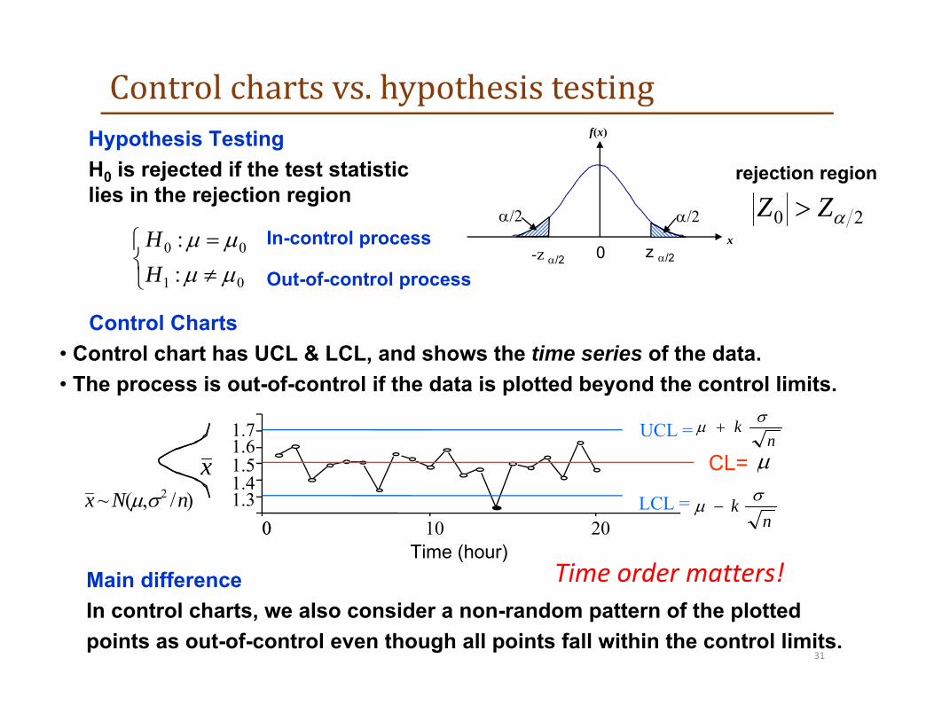
Control charts vs. hypothesis testing

31

f(x)

x0 z /2-z /2

/2/2

Hypothesis TestingH0 is rejected if the test statistic lies in the rejection region

20 ZZ rejection region

01

00

::

HH In-control process

Out-of-control process

1.31.41.51.61.7

Control Charts• Control chart has UCL & LCL, and shows the time series of the data.• The process is out-of-control if the data is plotted beyond the control limits.

201000Time (hour)

x CL=

LCL =

UCL = nk

nk )/,(~ 2 nNx

Main differenceIn control charts, we also consider a non-random pattern of the plotted points as out-of-control even though all points fall within the control limits.

Time order matters!

Why time order matters in control charts

32

1 2 3 4 5 6 7 8 9 1 0- 3

- 2

- 1

0

1

2

3

1 2 3 4 5 6 7 8 9 1 0- 3

- 2

- 1

0

1

2

3

(a) Non-random pattern, with assignable causes

(b) Non-random pattern disappears

Conclusion: Control chart showing the time sequence of sample data can reveal a non-random pattern for early detection of assignable causes, while the hypothesis testing of non-ordered samples cannot do this.

Type I and type II errors in hypothesis testing

33

Reject H0 NOT Reject H0

H0 is True Type I error(𝛼)

Confidence(1 𝛼)

H0 is NOT True Power(1 𝛽)

Type II error(𝛽)

Rea

lity 0

0

20 ZZ 20 ZZ

x

H0 H1

1

Rejection region

Rejection region

UL

/2 /2

0

Decision based on samples

Type I and type II errors in control charts

34

We Reject H0 We do NOT Reject H0

H0 is True Type I error(𝛼)

Confidence(1 𝛼)

H0 is NOT True Power(1 𝛽)

Type II error(𝛽)

Decision based on monitoring statisticR

ealit

y

0

/2

/2

UCL

CL

LCL

1

Shifted Mean

Process is in-control

Control chart states that the process is

out-of-control

Control chart states that the process is

in-control

Process isout-of-control

Type I error of control chart

35

= Pr{type I error}= Pr{Control chart states the process is out-of-control | Process is actually in-control} = Pr{A point is plotted beyond the control limits | Process is actually in-control}

x

UCLLCL

/2 /2

0

Example:Type I error of a X-bar chart with known

),(~ 200 NX

nkLCL

nkUCL

X

X

00

00

),(~

20

0 nNX

)](1[2)()(1Pr1/

)(//

)(Pr1

)/,(~Pr1

),(~Pr1),(~Pr

0

000

0

0

0

000

2000000

200

200

kkkkZknnk

nX

nnk

nNXnkXnk

NXUCLXLCLNXUCLXorLCLX

Note: For 𝑘-sigma control charts, type I error only depends on 𝑘.

0- 3 - 2 - 1 +1 +2 +3 z

k

/2

nXZ

/0

000

/2ZUCL k Z

Type II error of control chart

36

0

)0(;01 1

/2 /2

0 UCLLCL

= Pr{type II error}= Pr{Control chart states the process is in-control | Process is actually out-of-control} = Pr{A point is plotted within the control limits | Process is actually out-of-control}

Out-of-control

In-control

Example: Type II error in X-bar chart with known

01

2011

2000

),(~:

),(~:

NXH

NXH

nkLCL

nkUCL

00

00

Type II error depends on 𝑘, 𝛿, and 𝑛.

21 0

1 1 1

0 0 0

0 0 1 0 0 11

0 0 0

0 0 0 0

Pr ~ ( , / )

Pr/ / /

( ) ( )Pr/ / /

Pr/ / / /

LCL X UCL X N n

LCL X UCLn n n

k n k nXn n n

k Z k k kn n n n

K-sigma control limits

Example: piston rings

The inner‐diameter of piston rings follows a normal distribution with mean = 75 mm, and variance = 9. a) Construct a X‐bar Shewhart control chart with n = 16 and k = 3.b) If the mean of process changes to 78 mm, calculate the Type II error.c) What is the probability of detecting this mean shift before plotting the 

4th sample?

37

0 0 0 0

12

77.25) 75, 9 3, 16, 3; 75 3 3 / 16

72.75) 78

Pr{72.75 77.25 | ~ (78,3 /16}

72.75 78 78 77.25 78 Pr Pr{ 7 Z 1} ( 1) ( 7)3 / 4 3 / 4 3 / 4

UCLa n k k n

LCLb

X X N

X

3 3

[1 (1)] 0 1 0.8413 0.1587) Pr{detect the change before the 4th sample} 1- Pr{all three samples do not detect the change}

1 1 0.1587 0.996c

Probability limits

38

How to calculate p-probability limits (0<p<0.5):

x

UPLWLPLW

p p

0

pLPLWpUPLW

)Pr()Pr(

),(~: 20 wwNIDWH

UPL: Upper Probability Limit

LPL: Lower Probability Limit

p2

WpWWWWWW

W

W

W ZZkLCLUCL

LPLUPL

2/

Probability limits offer more flexibility than 𝑘𝜎 control limits.

Example: piston rings

• The inner‐diameter of piston rings follows a normal distribution with mean = 75 mm, and variance = 9. Calculate the 0.001 probability limits for individual observations (n = 1).

39

20

2

0.001

0.001

75, 9, 1

~ (75, 3 )84.27

75 3 75 3.09 365.73

(1 0.001) 3.09

WW p W

W

n

W X NUPL

z zLPL

z

Performance assessment of control charts

40

• Based on the probability in OC curves– Fix type I error rate and compare type II error rate (or detection 

power) 

• Based on average run length (ARL)

prob

abilit

y of N

OT re

ceivi

ng al

arm

Average run length

• Run length (RL): The number of samples/points that are plotted until a point is out of control limits.

RL is a random variable.

What is the distribution of RL?

What is the mean of RL?

41

Average run length

42

• The number of samples/points that are plotted until a point is out of control limits, follows a Geometric Distribution.

• ARL: The average number of samples/points that are plotted until a point is out of control limits.

• Example : for 3-sigma control limits (=0.0027)ARLin-control =ARL=ARL0 = 1/= 1/0.0027 = 370.

Comments: Even the process is in-control, an out-of-control sample will be generated every 370 samples on average.

11ARL

1ARL1ARL

1

0

p

If the process is actually in-control

If the process is actually out-of-control

Example

• Suppose that a control chart with 2‐sigma limits is used to control a process. If the process remains in control, find the average run length until a false out‐of‐control signal is observed. Compare this with the in‐control ARL for 3‐sigma limits.

• Solution: For K=2 sigma control limits, 

=2[1‐(k)]=2[1‐(2)]=0.0455

(2)=0.97725

ARL0=1/=22

43

0- 3 - 2 - 1 + 1 + 2 + 3z

k

/2

nXZ

/0

000

2/ZkULCZ

ExampleSuppose that a X‐bar control chart with 3‐sigma limits and n=4 is used to control a process. Assume the process mean is changed by 1 standard deviation.(a) What is the probability of detecting the change by the first sample after shift?(b) What is the probability of detecting the change before collecting the 5th sample? (c) What is the average number of points plotted on the chart until a signal is observed?

44

0 0

0 0 0 0

1 1( ) 3 3/ / / 4 / 4

(1) ( 5) 0.8413 0 0.8413 1 1 0.8413 0.1587

a k kn n

4( ) Prob 1 Pr(fail to detect based on all 4 samples) 1 0.4990b

1 1 out of control1( ) ARL ARL ARL 6.30

1c

Rules to signal: detect out-of-control status

Rules to signal: an out‐of‐control status• Rule 1: When one or more points fall beyond the control limits

• Rule 2: Sample points exhibit any nonrandom pattern of behaviors

(additional capability of control charts beyond hypothesis tests)

Description of nonrandom patterns• The location of the current point can be approximately predicted by previous points

Run up: a sequence of increasing observations

Run down: a sequence of decreasing observations

Cyclic pattern

etc.

45

Examples of nonrandom patterns

• Pattern is very nonrandom • 19 of 25 points plot below the center line, while only 6 plot 

above• Following 4th point, 5 points in a row increase in magnitude 

“run up”• There is also an unusually long run down beginning with 18th

point

46

Nonrandom patterns and common causes

• Jumps in process level1. New supplier2. New worker3. New machine4. New technology5. Change in method or process6. Change in inspection device or method

• High proportion of points near outer limits1. Over control2. Large difference in material quality and test method3. Control of 2 or more processes on one chart4. Mixtures of materials of different quality5. Multiple charters6. Improper subgrouping

47

Nonrandom patterns and common causes• Recurring cycles

1. Temperature and other cyclic environmental effects2. Worker fatigue3. Differences in measuring devices used in order4. Regular rotation of machines or operators5. Scheduled preventive maintenance (R chart)6. Tool wear (R chart)

• Trends1. Gradual equipment deterioration2. Worker fatigue3. Accumulation of waste products4. Improvement or deterioration of worker skill/effort (especially in R chart)5. Drift in incoming materials quality

• Stratification (lack of variability)1. Incorrect calculation of control limits2. Systematic sampling

48

Western electric rules (zone rules charts)

49

Rule 2Rule 3

More sensitizing rules

50

Combined type I error rate of multiple sensitizing rules

51

• Decision to signal: the process is concluded out of control if any one of the rules is applied.

k

ii

1

)1(1

𝛼 is type I error rate of using Rule 𝑖 alone

If all k rules are independent,

Control limits vs. specification limits

52

1.Control Limits are used to determine if a process is in-control (if any distribution parameters of process/product measurements’ are changed, e.g. mean or variance).

Statistical tests: determined based on collected samples from a process

Design requirement: determined by customer needs and standards

2.Specification Limits are used to determine if a product will function in the intended design fashion.

Out-of-controlIn-control

LCLW UCLW

NonconformityConformity

LSL USL

Monitoring statistic W (e.g. X-bar or R) for detecting process distribution change (mean or variance change for the normal distribution)

product qualitychar. for inspectingnonconformity of each part

Examples: true or false

53

• One of the main purpose of a control chart is to distinguish chance and assignable causes. (T)

• If we use k=2 instead of k=3 for k-sigma control limits, the type I error will decreases. (F)

• If the process consistently produces products outside of the engineering specification limits, the process is out of control. (F)

• When designing a process control chart, by increasing its type I error, we can always increase its detection power for a given mean shift. (T)

• A 3-sigma limits X-bar chart will always have a type I error rate equal to 0.27%. (T)

Example

A x‐bar control chart with 3‐sigma control limits is used to monitor process mean. Inspection decision is made based on two successive samples using the following rules: (n = 4)Rule 1: If one or two sample means exceed either the upper or lower control limitRule 2: If two sample means fall on the same side of the center line(1) What is type I error rate using Rule 1 alone?(2) What is type I error rate using Rule 2 alone?(3) What is the overall type I error rate based on the two rules given that 

the two rules are independent?(4) If the process has a mean shift of one process standard deviation, what 

is type II error rate using Rule 1?(5) If the process has a mean shift of one process standard deviation, what 

is type II error rate using Rule 2?

54

1 0

02

0

2

0

2

1

(1) Pr(any sample's mean exceeds control limits | )1 Pr(both sample means fall within LCL and UCL | )

1 Pr(a sample mean falls within LCL and UCL | )

1 Pr( | )

1 1

1 1

rule

sample

HH

H

LCL X UCL H

21

2 0

0

0.0027 0.0027 in 3-sigma limits control chart

0.0054(2) Pr(2 sample means fall on the same side of the center line | )

Pr(2 sample means above CL | ) Pr(2 sample means below CL |

sample

rule HH H

02 2

0 0

2 2

1 2

)

Pr( | ) Pr( | )

0.5 0.5 0.5(3) 1 (1 )(1 ) 1 (1 0.0054)(1 0.5) 0.5027overall rule rule

X CL H X CL H

55

56

1 12

1

21

1

21 1

(4) Pr(both sample means fall within LCL and UCL | )

Pr( | )

=

1 1( ) ( ) (3 ) ( 3 )/ / / 4 / 4

(1) ( 5) 0.84130

rule

sample

sample

rule sample

H

LCL X UCL H

k kn n

2

2 1

1 12 2

1 1

.8413 0.7079

(5) 1 Pr(2 sample means fall on the same side of the center line | )1 Pr(2 sample means above CL | ) Pr(2 sample means below CL | )

1 Pr( | ) Pr( | )

Pr( |

rule

L

HH H

X CL H X CL H

P X CL

1

0 1 0 010 1 0

1

0 1 0 0 1 0

2 22

)

( | ) ( ) ( ) ( 2) 0.02275/ / / 4

Pr( | )( | ) 1 ( | ) 1 ( 2) 0.97725

1 0.0445

U

rule L U

HXP X P

n nP X CL H

P X P X

P P