Recall:  Mo*va*on  Probability  distribu.on  (represented  by  tabular  form,  formula  or  graphs)  

à behavior  of  random  variable  

In  general,  observa.ons  generated  by  different  experiment  have  similar  type  of  behavior.    In  prac.ce,  several  life  random  phenomenon  can  be  described  by  some  commonly  used  distribu.on    In  this  lesson,  we  present  these  commonly  used  CONTINUOUS  distribu.ons  .  

Engineering Statistics

Probability  Distribu*ons:    Con*nuous  

         

Engineering Statistics Engineering Statistics

http://science.utm.my/norhaiza/

Recall  Random  Variable  

Discrete   Con.nuous  

Probability  Distribu.on  

 Probability  

Mass  Func*on  

Probability  Distribu.on  

 Probability  Density  

Func*on  

Special  Probability  Distribu*on  

Special  Probability  Distribu*on  

Outline   Con.nuous  R.V    

Con.nuous  Uniform   Normal   Exponen.al   Erlang  &  

Gamma   Weibull   Lognormal  

Outline  Con.nuous  R.V    

Con.nuous  Uniform   Normal   Exponen.al   Erlang  &  

Gamma   Weibull   Lognormal  

Normal  Distribu*ons  Characteris*cs  (draw  basic  normal)  

•   the  most  widely  used  probability  distribu.on  in  sta.s.cs    and    an  important  tool  in  analysis      •   also  called  the  Gaussian  Distribu*on  

Normal  Distribu*ons  r.v  X  with  p.d.f            is  a  normal  r.v  with  parameters  mean            and  variance                                    such  that                                                                      and      è    

∞<<∞=−

−

xexfx

- ,21)( 2

2

2)(

σµ

σπ

),(~ 2σµNX

∞<<∞− µ 0>σµ 2σ

Normal  Distribu*ons:    Mean  and  Variance  

If                                                                            then,                                                                                                                                        

)(XE=µ

)(2 XV=σ

),(~ 2σµNX

Normal  Distribu*ons  Characteris*cs  

•   Bell  Shape  Curve  and  is  Symmetric    •   Symmetric  around  the  mean:        Two  halves  of  the  curve  are  the  same  (mirror  images)    •   sketch      

Normal  Distribu*ons  Characteris*cs  

•     

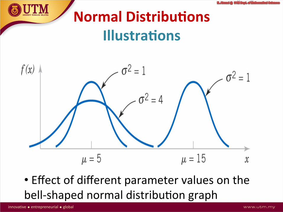
Normal  Distribu*ons  Illustra*ons  

 •     

•   Effect  of  different  parameter  values  on  the  bell-­‐shaped  normal  distribu.on  graph  

Normal  Distribu*ons  sketch  my  shape  

 •      )1,0(~ NX )25.6,100(~ NX

)4,50(~ NX )41,4(~ NX

Normal  Distribu*ons  Finding  probabili*es  

•     

 è    

•   Very  difficult  to  evaluate.  What  to  do?  • è  need  to  transform    • è  work  with  standard  normal  variable    

?)(),,(~ If 2

=≤≤ bXaPNX σµ

∫−

−

=≤≤b

a

x

dxebXaP 2

2

2)(

21)( σ

µ

σπ

ZX

Normal  Distribu*ons  Standard  Normal  Distribu*on  

•   Transform              to                i.e.  by  STANDARDIZING    

   è    

Then  

σµ

σµ−

=XZNX and ),,(~ If 2

ZX

σµ−

=XZ

X

)1,0(~ NZ

•   Given                                                    

•   Note:  For  con*nuous  r.v:  no  significant  difference  in  equality  signs    

1.0)(7.0)(1.0)(7.0)(1.0)0(

=>

=>

=<

=<

=<<

zZPzZPzZPzZPzZP

)1,0(~ NZ

Finding  probabili*es  :    standard  Normal  Distribu*on  

sketch  the  area  of  probability  

Finding  probabili*es  :  standard  Normal  Distribu*on  Cumula*ve  Distribu*on  Func*on  for  Z,    

•     

     

•   S.ll  difficult  to  evaluate.    •   Refer  tables  

∫∞−

−=≤=Φ

z zdzezZPz

2

21

21)()(π

)(zΦ

Finding  probabili*es:    Standard  Normal  Probability  Tables  

•   We  can  evaluate  the  probability  associated  to  a  standard  normal  distribu.on  either  using  a  scien.fic  calculator/computer  applica.on  such  as  MicrosoX  Excel  or  sta.s.cal  tables.  •   Sta.s.cal  table  –many  versions                                                                                            ß  H.Lee  stats  table  (given  z  value,  prob.?)                                                                                    ß  H.Lee  stats  table  (given  prob.                      ,  z  value?)  

 Note:  different  books  use  different  area  of  the  curve  to  calculate  std.normal  probability  dn.  Montgomery  et  al.    Cumula.ve  standard  normal  dn.    (given  z  value,  prob.?)   )( zZP ≤

)0( zZP ≤≤

α=≥ )( zZP α

Appendix  A.  Finding  probabili*es:    Standard  Normal  Probability  Tables  (Lee)  

?)0( =<< zZP α=≥ )( zZP

Given  z-­‐value,      Probability?  

Given  probability,      z-­‐value?  

α

z   0.00   ..   ..   0.09  

0.0   0.0000   ..   ..   0.0359  

.   .  

.   .  

.   .  

1.5   0.4332   ..   ..   0.4441  

Appendix  A.  Finding  probabili*es:    Cumula*ve  Standard  Normal  Distribu*on  Tables  (Lee),  P(0<Z  <z)  

)0( zZP <<

z0

)59.10( << ZP

59.10

Cumula*ve  Standard  Normal  Dn.  Probability  Tables,    

If  Z~  N(0,1),  find  from  tables  (sketch  it!)                                                                                                                                                    0.9162          

=≤ )377.1( (a) ZP

=−> )377.1( (b) ZP = 0.9162

=> )38.1( (d) ZP=−< )38.1( (c) ZP

0.5+P(0 < Z <1.38) =

0838.0 0.5−P(0 < Z <1.38) = 0.0838

Excel  note:    P(Z<z)  =normsdist(1.377)=0.9157  =normsdist(1.38)=0.9162    

If  Z~  N(0,1),  find  from  tables  (sketch  it!)                                                                            

)43.1()43.1()433.1|(|)()43.143.1()433.1|(|)(

)6.04.1()()865.1696.2()()751.1345.0((a)

−<+>=>

<<−=<

=−<<−

=<<−

=≤<

ZPZPZPeZPZPd

ZPcZPbZP 32311.0)35.00()75.10( =<<−<< ZPZP

9658.01935.0

Cumula*ve  Standard  Normal  Dn.  Probability  Tables  

Cumula*ve  Standard  Normal  Dn.    Probability  Tables  

If  Z~  N(0,1),  find  the  value  of  a  if                                                                              

9.0)|(|)(9693.0)()(0793.0)()(7818.0)()(

3802.0)( (a)

=<

=>

=<

=>

=>

aZPeaZPdaZPcaZPbaZP

Excel  note:P(Z<a)  P(Z>a)=0.3802  1-­‐P(Z<a)=0.3802  P(Z<a)=0.6198  à  =normsinv(0.6198)              =normsinv(0.3802)=0.3805  

Finding  Probabili*es  

If  X~  N(300,25),  find                                                                                                                                                                                                      

=> )305( (a) XP

=≤ )291( (b) XP

=< )312( (c) XP

=> )286( (d) XP

Excel  note:  P(X<x)  =normdist(1.377)=0.9157  =normsdist(1.38)=0.9162    

Normal  Distribu*ons:  Example  2    Suppose  the  current  measurements  in  a  strip  of  wire  are  assumed  to  follow  a  normal  distribu.on  with  a  mean  of  10  milliamperes  and  a  variance  of  4  mA2.      (a) What  is  the  probability  that  a  current  measurement  

will  exceed  13  milliamperes?  (0.067)  (b) What  is  the  probability  that  a  current  measurement  is  

between  9  and  11  milliamperes?  (0.383)  (c)  Determine  the  value  for  which  the  probability  that  a  

current  measurement  is  below  this  value  is  0.98?  (14.1mA)  

Exercise(Montgomery,  4th  ed.  Ex.4-­‐57)    The  speed  of  a  file  transfer  from  a  server  on  campus  to  a  personal  

computer  at  a  student’s  home  on  a  weekday  evening  is  normally  distributed  with  a  mean  of  60  kilobits  per  second  and  a  standard  devia.on  of  4  kilobits  per  second.    (a)  What  is  the  probability  that  the  file  will  transfer  at  a  speed  of  70  kilobits  per  second  or  more?    (b)  What  is  the  probability  that  the  file  will  transfer  at  a  speed  of  less  than  58  kilobits  per  second?    (c)  If  the  file  is  1  megabyte,  what  is  the  average  .me  it  will  take  to  transfer  the  file?  (Assume  eight  bits  per  byte.)  

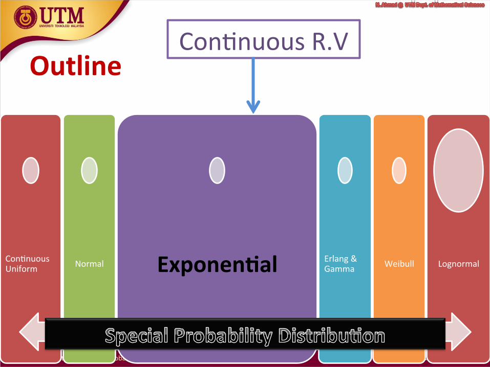
Outline  Con.nuous  R.V    

Con.nuous  Uniform   Normal   Exponen*al   Erlang  &  

Gamma   Weibull   Lognormal  

Recall:  Poisson  Process  

           

•   discrete  distribu.on  •   Poisson  dn.à  r.v    •   compute  probability  of  specific  number  of  events  during  an  interval  (.me  or  space)  

 è  The  interval,  (eg.  the  .me  period/span  of  space)    can  be  a  random  variable!  

Exponen*al  Distribu*on  

           

•   rela.onship  to  Poisson  process      •   Example    Ø   *me  between  arrivals  at  service  facili.es  Ø   *me  to  failure  of  components  

 •   Important  role  in  queuing  theory  &  reliability  problems  

Example  3:  Exponen*al  Distribu*on  

           

•   r.v  Y  ,  number  of  flaws  along  a  length  of  copper  wire  •   No.  of  flawà  Poisson  event  •   r.v  X,  length  from  any  point  on  the  copper  wire  un.l  a  flaw  is  detected                  distribu.on  of  X  depends  on  distribu.on  of  Y  è  In  general,  •     r.v  Y  ,  number  of  flaws  along  x  millimeters  of  wire  •     if                =  mean  number  of  flaw  per  millimeter,  then    •   r.v  X,  length  from  any  point  on  the  wire  un.l  a  flaw  is  detected  

λ

∴

X ~ Exp(λ)

Exponen*al  Distribu*ons  Defini*on  

 A  Con$nuous  r.v  X  having  a  prob.  density  func$on  where            Noteè                                                                                                                                                                                    

xexf λλ −=)(0for ≥x

)()|()(1)(1)()(

2121 tXPtXttXPexFxXPexFxXP

x

x

<=>+<

=−=>

−==<−

−

λ

λ

constant positive a is λ

Lack  of  memory  property  

Exponen*al  Uniform  Distribu*ons  Mean  and  Variance  

           

λµ

1)( == XE

22 1)(

λσ == XV

)exp(~ λXIf  

Exponen*al  Distribu*ons  Illustra*ons  

Exponen*al  Distribu*ons:    Example  4  

                   

In  a  large  corporate  computer  network,  user  log-­‐ons  to  the  system  can  be  modeled  as  a  Poisson  process  with  a  mean  of  25  log-­‐ons  per  hour.      (a)What  is  the  probability  that  there  are  no  logons  in  an  interval  of  6  minutes?  (b)  What  is  the  probability  that  the  .me  un.l  the  next  log-­‐on  is  between  2  and  3  minutes?    X,  .me  in  hours  from  the  start  of  the  interval  un.l  the  first  log-­‐on  X~exp(25)                      

082.025)1.0(0.1

25 ==> ∫∞

− dxeXP x

152.025)05.0033.0(05.0

0.033

25 ==<< ∫ − dxeXP x

Exponen*al  Distribu*ons:    Example  5:  Lack  of  memory  property  

                   

Let  X  denote  the  .me  between  detec.ons  of  a  par.cle  with  a  geiger  counter  and  assume  that  X  has  an  exponen.al  distribu.on  with  mean,  1.4  minutes.  What  is  the  probability  that  we  detect  a  par.cle  within  30  seconds  of  star.ng  the  counter    X,  .me  to  detect  a  par.cle  aXer  star.ng  the  counter  X~exp(1/1.4)        suppose  we  turn  on  the  geiger  counter  and  wait  3  minutes  without  detec*ng  a  par*cle.  What  is  the  probability  that  a  par.cle  is  detected  in  the  WITHIN  THE  next  30  seconds?*                      

3.01)5.0()5.0( 4.15.0

=−==<−

eFXP

3.0)3(1)3()5.3(

)3()5.33()3|5.3( =

−

−=

>

<<=><

FFF

XPXPXXP

Exponen*al  Distribu*ons:    Exercise  (crawshaw,eg.5.22,p.309)  

                   

The  life.me  in  years  of  a  TV  tube  is  a  r.v  T  and  its  p.d.f  ,  f(t)  is  given  by            Obtain  A  in  terms  of  k  (a)  If   the   manufacturer   finds   that   out   of   1000   such   tubes,   371   failed  

within  the  first  two  years  of  use,  es.mate  the  value  of  k.    (0.232,3sf)  (b)  Using   the   value  of   k   in   ques.on   (a)   correct   to   3   significant   figures,  

calculate   the  mean   and   variance   of   T,   giving   answers   correct   to   2  significant  figures.  (4.3;1.9)  

(c)  If   two   such   tubes  are  bought,  what   is   the  probability   that  one   fails  within  its  first  year  and  the  other  lasts  longer  than  six  years?  (0.103)  

   

Group  submission  

otherwise , 0 0,t0for ,)(

=

>∞≤≤= − kAetf kt

Other  Distribu*ons:    Erlang  &  Gamma  Weibull  Log-­‐normal    

                   

•  Strictly  non-­‐nega.ve  distribu.ons:  posi.ve  skewed  

38 Fundamental Topics

1.4.8 Other continuous distributions

Other distributions for continuous random variables include Erlang, Gamma, Weibulland log-normal distributions. Unlike normal distribution, these distributions assumethat the variables are strictly non-negative. The list of probability density functionsfor these distributions are listed below:

Distributions Probability Density Functions Mean & Variance

1. Erlang f(x) =µrxr�1e�µx

(r � 1)!for x > 0. E(X) = r

µ

and r = 1, 2, . . .

Note: If r = 1, then Erlang is simply V ar(X) = r

µ

2

an exponential distribution.

2. Gamma f(x) =µrxr�1e�µx

(r � 1)!for x > 0 and r > 0. E(X) = r

µ

Note: If r is an integer, then Gamma is V ar(X) = r

µ

2

simply an Erlang distribution.

3. Weibull f(x) =�

�

⇣x�

⌘��1

exp

�⇣x�

⌘�

�

for x > 0, � > 0 and � > 0. E(X) = ��

✓1 +

1

�

◆

Note: � and � are the shape and V ar(X) = �2�

✓1 +

2

�

◆�

the scale parameters respectively.

If � = 1 then Weibull is simply �2�

✓1 +

1

�

◆�2

an exponential distribution with µ = 1/�.

4. Log-normal f(x) =1

x!p2⇡

exp

� (lnx� ✓)2

2!2

�E(X) = e✓+!

2/2

for 0 < x < 1 and X = exp(W ) V ar(X) = e2✓+!

2(e!

2 � 1)

where W ⇠ N(✓,!2).

The shape of the above distributions for varying values of their parameters can be

investigated via computer software such as Matlab. Further information and examples

for these distributions can be found from Montgomery & Runger (2006).

•  Strictly  non-­‐nega.ve  distribu.ons  

•  Similarly  different  values  its  parameters  affect  the  shape  of  the  distribu$ons  

Figure 1. Univariate distribution relationships.

The American Statistician, February 2008, Vol. 62, No. 1 47

LEEMIS,  Lawrence  M.;  Jacquelyn  T.  MCQUESTON  (February  2008).  "Univariate  Distribu.on  Rela.onships"  (PDF).  American  Sta.s.cian.  62  (1):  45–53.  doi:10.1198/000313008x270448  

Rela.onships  between  

distribu.ons  

Simplified  rela.onships  between  distribu.ons    htps://upload.wikimedia.org/wikipedia/commons/thumb/6/69/Rela.onships_among_some_of_univariate_probability_distribu.ons.jpg/1920px-­‐Rela.onships_among_some_of_univariate_probability_distribu.ons.jpg  

Next:  Sampling  Distribu.ons