ARTICLE IN PRESS

0736-5845/$ - se

doi:10.1016/j.rc

�CorrespondE-mail addr

Robotics and Computer-Integrated Manufacturing 25 (2009) 483–496

www.elsevier.com/locate/rcim

Real world disassembly modeling and sequencing problem:Optimization by Algorithm of Self-Guided Ants (ASGA)

Mukul Tripathia, Shubham Agrawalb, Mayank Kumar Pandeyc,Ravi Shankard, M.K. Tiwaric,�

aDepartment of Metallurgy and Materials Engineering, National Institute of Foundry and Forge Technology, Ranchi 834003, IndiabDepartment of Operations Research and Industrial Engineering, University of Texas at Austin, Austin, TX 78705, USA

cDepartment of Industrial Engineering and Management, Indian Institute of Technology, Kharagpur 721302, IndiadDepartment of Management Studies, Indian Institute of Technology, Delhi 110016, India

Received 13 August 2007; received in revised form 18 December 2007; accepted 19 February 2008

Abstract

Decrease in product life along with the advent of stringent regulations and environmental consciousness have led to increased concern

for methodological product recovery through disassembly operations. This research proposes a fuzzy disassembly optimization model

(FDOM) and is aimed at determining the optimal disassembly sequence as well as the optimal depth of disassembly to maximize the net

revenue at the end-of-life (EOL) disposal of the product in the real world situations. In order to account for the uncertainty inherent in

quality of the returned products, fuzzy control theory is incorporated in the problem environment for modeling the expected value of the

recovered modules. Considering the computational complexity of the problem at hand, an innovative approach of Algorithm of Self-

Guided Ants (ASGAs) is proposed for the same. The performance of the proposed methodology is benchmarked against a set of test

instances that were generated using design of experiment techniques and analysis of variance is performed to determine the impact of

various factors on the objective. The robustness of proposed algorithm is authenticated against Ant Colony Optimization and Genetic

Algorithm over which it always demonstrated better results thereby proving its superiority on the concerned problem.

r 2008 Elsevier Ltd. All rights reserved.

Keywords: Disassembly; Ant colony optimization; Fuzzy logic; Product recovery

Contents

1. Introduction . . . . . . . . . . . . . . . . . . . . . . . . . . . . . . . . . . . . . . . . . . . . . . . . . . . . . . . . . . . . . . . . . . . . . . . . . . . . . . . 484

2. Literature review . . . . . . . . . . . . . . . . . . . . . . . . . . . . . . . . . . . . . . . . . . . . . . . . . . . . . . . . . . . . . . . . . . . . . . . . . . . . 484

3. The fuzzy disassembly optimization model (FDOM). . . . . . . . . . . . . . . . . . . . . . . . . . . . . . . . . . . . . . . . . . . . . . . . . . . 485

3.1. Model objectives . . . . . . . . . . . . . . . . . . . . . . . . . . . . . . . . . . . . . . . . . . . . . . . . . . . . . . . . . . . . . . . . . . . . . . . . 485

3.2. Model assumptions . . . . . . . . . . . . . . . . . . . . . . . . . . . . . . . . . . . . . . . . . . . . . . . . . . . . . . . . . . . . . . . . . . . . . . 485

3.3. The mathematical model . . . . . . . . . . . . . . . . . . . . . . . . . . . . . . . . . . . . . . . . . . . . . . . . . . . . . . . . . . . . . . . . . . 485

3.3.1. Objective function. . . . . . . . . . . . . . . . . . . . . . . . . . . . . . . . . . . . . . . . . . . . . . . . . . . . . . . . . . . . . . . . . 486

3.3.2. Constraints . . . . . . . . . . . . . . . . . . . . . . . . . . . . . . . . . . . . . . . . . . . . . . . . . . . . . . . . . . . . . . . . . . . . . 486

3.4. Disassembly modeling in fuzzy environment . . . . . . . . . . . . . . . . . . . . . . . . . . . . . . . . . . . . . . . . . . . . . . . . . . . . 486

4. Algorithm of Self-Guided Ants . . . . . . . . . . . . . . . . . . . . . . . . . . . . . . . . . . . . . . . . . . . . . . . . . . . . . . . . . . . . . . . . . . 487

4.1. The initialization criteria . . . . . . . . . . . . . . . . . . . . . . . . . . . . . . . . . . . . . . . . . . . . . . . . . . . . . . . . . . . . . . . . . . 488

4.2. The self-guided state transition rule . . . . . . . . . . . . . . . . . . . . . . . . . . . . . . . . . . . . . . . . . . . . . . . . . . . . . . . . . . 488

e front matter r 2008 Elsevier Ltd. All rights reserved.

im.2008.02.004

ing author.

ess: mkt09@hotmail.com (M.K. Tiwari).

ARTICLE IN PRESSM. Tripathi et al. / Robotics and Computer-Integrated Manufacturing 25 (2009) 483–496484

4.2.1. Tandem running rule . . . . . . . . . . . . . . . . . . . . . . . . . . . . . . . . . . . . . . . . . . . . . . . . . . . . . . . . . . . . . . 489

4.2.2. Social carrying rule . . . . . . . . . . . . . . . . . . . . . . . . . . . . . . . . . . . . . . . . . . . . . . . . . . . . . . . . . . . . . . . . 490

4.3. The pheromone update rules . . . . . . . . . . . . . . . . . . . . . . . . . . . . . . . . . . . . . . . . . . . . . . . . . . . . . . . . . . . . . . . 490

4.3.1. Dynamic pheromone evaporation and update rule . . . . . . . . . . . . . . . . . . . . . . . . . . . . . . . . . . . . . . . . . . 490

4.3.2. Global pheromone update rule . . . . . . . . . . . . . . . . . . . . . . . . . . . . . . . . . . . . . . . . . . . . . . . . . . . . . . . 490

5. Experimental design and results . . . . . . . . . . . . . . . . . . . . . . . . . . . . . . . . . . . . . . . . . . . . . . . . . . . . . . . . . . . . . . . . . 490

5.1. Test bed formulation. . . . . . . . . . . . . . . . . . . . . . . . . . . . . . . . . . . . . . . . . . . . . . . . . . . . . . . . . . . . . . . . . . . . . 490

5.2. The encoding schema . . . . . . . . . . . . . . . . . . . . . . . . . . . . . . . . . . . . . . . . . . . . . . . . . . . . . . . . . . . . . . . . . . . . 491

5.3. Parameter settings. . . . . . . . . . . . . . . . . . . . . . . . . . . . . . . . . . . . . . . . . . . . . . . . . . . . . . . . . . . . . . . . . . . . . . . 491

5.4. Performance comparison . . . . . . . . . . . . . . . . . . . . . . . . . . . . . . . . . . . . . . . . . . . . . . . . . . . . . . . . . . . . . . . . . . 492

5.5. Analysis of results. . . . . . . . . . . . . . . . . . . . . . . . . . . . . . . . . . . . . . . . . . . . . . . . . . . . . . . . . . . . . . . . . . . . . . . 493

5.6. A simulated example . . . . . . . . . . . . . . . . . . . . . . . . . . . . . . . . . . . . . . . . . . . . . . . . . . . . . . . . . . . . . . . . . . . . . 493

6. Conclusion . . . . . . . . . . . . . . . . . . . . . . . . . . . . . . . . . . . . . . . . . . . . . . . . . . . . . . . . . . . . . . . . . . . . . . . . . . . . . . . . 494

References . . . . . . . . . . . . . . . . . . . . . . . . . . . . . . . . . . . . . . . . . . . . . . . . . . . . . . . . . . . . . . . . . . . . . . . . . . . . . . . . 494

1. Introduction

Extraordinary rate of advancement in technology isseriously threatening the current state of environment.Recycling regulations are being framed for disposing offthe products in an environmentally conscious mannerwhich has put increased responsibilities on the manufac-turers for the competitive, economic and environmentalperformance of their products throughout its lifecycle [1].This has led to a promising field of research in theremanufacturing sector called as product recovery, whichrelies on disassembly of a scrapped product into separatecomponents for efficient and methodological part/compo-nent retrieval. The ease with which the parts can bedisassembled plays a vital role in determining thecommercial viability of the parts reuse [2] and thereby thedesign of fasteners, their location and number may have asubstantial bearing on the product disassembly and henceon its economic value after EOL (end-of-life). Therefore,disassembly planning is playing a significant role inremanufacturing. It entails the methodical and economicalseparation of malignant modules and environmentallybenign components from an assembly of modules [3].

In this research, an attempt has been made to maximizethe net profits associated with the product/part recoveryand thereby minimize the disassembly cost in a real worldenvironment where the knowledge related to the quality ofthe returned products as well as their constituent parts isvague. The technique of fuzzy logic is employed for controland modeling of complex systems where experience ofhuman operators is available in terms of qualitative rules[4]. This paper investigates and implements the perceivedadvantages of fuzzy control theory with reduced develop-ment time and simplicity in implementation to account forthe ambiguities in the structure of the returned productspertaining to different operating conditions.

The fuzzy disassembly optimization model (FDOM),proposed in this research belongs to the class ofcombinatorial optimization problems which are computa-tionally complex [5]. In this paper, an effective combina-torial optimization technique, Algorithm of Self-Guided

Ants (ASGAs) is proposed to solve the computationallyhard FDOM problem. In recent years, biologists andcomputer scientists have drifted their attention to studyingmore complex characteristics of real ants and utilizing themto enhance the performance of existing algorithms for theproblems concerning highly complex combinatorial deci-sion making [6,7]. In particular, the social behavior of antsnamed Temnothorax Albipennis (formerly Leptothorax

Albipennis) have been rigorously studied in the recent past[6,8–10]. The finding that is of particular interest in thisstudy is the quorum index governed speed and accuracytradeoffs in decision making shown by T. Albipennis ant[8]. This particularly ensures avoidance of the entrapmentof the results in the local optimum. The proposedmetaheuristic (ASGA) utilizes an interesting synergyarising between speed and accuracy tradeoff arisingbetween ants, to maintain a stringent balance between thetwo. Another feature of ASGA embodies simulation of realant phenomenon more closely and accordingly updatingthe pheromone trail levels with a dynamic pheromoneevaporation rule. For validating the efficacy and efficiencyof the proposed ASGA metaheuristic, a test bed isgenerated (with due considerations to Taguchi L8(2

7) array[11]) by selecting seven factors and varying them at twodifferent levels and the results were compared against theestablished metaheuristic approaches.Rest of the paper is organized as follows: Section 2

discusses the literature review while the problem formula-tion is carried out in Section 3 of the paper. Section 4provides the description of the proposed ASGA with theprocedure for its implementation on the underlyingproblem. Section 5 details the computational resultsobtained by the application of various algorithms on thegenerated test beds. Finally, Section 6 concludes the paper.

2. Literature review

The product data modeling, economic aspects associatedwith the process and finally the development of tools andsolution methodology is the research agenda of this paper.One of the famous methods for relational product data is

ARTICLE IN PRESSM. Tripathi et al. / Robotics and Computer-Integrated Manufacturing 25 (2009) 483–496 485

the generation of disassembly trees using the AND/ORgraphs proposed by Homem de Mello and Sanderson [12].An AND/OR graph [13] is a directed hypergraph with anode of this graph representing the subassembly and thearcs emanating from it point to the various modulescontained within it. Ishii et al. [14] suggested a hierarchicalnetwork representation scheme called LINKER thatprovided an efficient way of representing physical andgeometric connections and parts. Moorie et al. [15]proposed the automatic generation of disassembly Petrinets (DPNs) from the disassembly precedence matrix(DPM). Zussman and Zhou [16] used DPN for themodeling and adaptive planning of disassembly processes.DPNs have also been used in disassembly modeling byTiwari et al. [17], Rai et al. [18], Kumar et al. [19], etc. Sarinet al. [20] proposed a disassembly optimization model(DOM) and an innovative approach for network repre-sentation based upon the information derived directly fromthe Bill-of-Material (BOM).

The analysis of EOL alternatives is important for theeconomic consideration of disassembly process. Variousrecycling options for components were analyzed by Kriwetet al. [21]. Boothroyd and Alting [22] proposed the idea ofdesign for assembly and disassembly (DFAD). There alsoarises the need for the discipline of design for environment(DFE) [23] that encapsulates aspects for using cleantechnologies and recyclable materials.

In general, disassembly sequence optimization problemscan be broadly categorized into those where the sequencecosts are immaterial and where they are taken into account.The first set of problems lie in the category of linearprograms involving less complexity. These were addressedby Lambert [24], Penev and de Ron [25] and Kuo et al. [26].The problems lying in the second group involve integervariables and have been shown to be NP-hard [27]. Theunderlying disassembly problem was treated as PriceCollecting Traveling Salesman Problem (TSP) with simplevariations by Navin Chandra [28]. Gungor and Gupta [29]proposed a heuristic procedure for the determination of thedisassembly sequence. Lambert and Gupta [30] proposed atree network model for this problem that is based on thedisassembly graph approach and reverse BOM. Thedisassembly optimization problem was formulated as aprecedence-constrained asymmetric TSP by Sarin et al. [20]and was solved using Lagrangian relaxation with a three-stage iterative procedure. In recent times there has beenextensive use of artificial intelligence techniques fordisassembly optimization [2,31]. One such technique, antcolony optimization (ACO) [32] has been successfullyapplied to varied applications like quadratic assignmentproblem (QAP) [33] vehicle routing problem (VRP) [34],FMS scheduling problem [35], space planning problem[36], machine tool tardiness problem [37], multiple objec-tive JIT sequencing problem [38], and resource constraintproject scheduling problem (RCPSP) [39], etc. In essence,the performance of the ant algorithms has been found to befairly competitive in problems involving graphical struc-

ture. With the increasing quest for improvement, of courseinspired by the successful applications of ACO, the presentresearch focus is to devising further modifications that mayhelp increase the applicability and reliability of its variants.The base of all the prevailing variants has been the rules ofACO metaheuristic. Some of the successful variants ofACO can be summarized as follows [40]: Elitist ant system[41], Ant colony system (ACS) [42], Max–Min ant system(MMAS) [43] and Best–Worst Ant System [44]. The antalgorithms that do not rely over the basic principles ofACO metaheuristic are hybrid ant system (HAS) [45] andfast ant system (FANT) [46], etc. First use of antalgorithms to solve disassembly sequencing problem couldbe found in Failli and Dini [47]. Application of antalgorithms as optimization tools in disassembly operationshave also been utilized by McGovern and Gupta [48] whoemployed ACO for disassembly sequencing with multipleobjectives. In addition, Agrawal and Tiwari [1] also madeuse of a collaborative ant colony algorithm to solve astochastic mixed-model U-shaped disassembly line balan-cing problem.

3. The fuzzy disassembly optimization model (FDOM)

3.1. Model objectives

The proposed model is aimed at determining thedisassembly sequence and the depth of disassembly so asto maximize the net revenues obtained from the benefits ofthe recovery of components. Moreover, we included theidea of fuzziness in the available data with a view to mimicthe real world disassembly scenario. The objectives of theproposed model are:

1.

Maximization of the profits obtained from the optimaldisassembly sequencing.

2.

Incorporation of the previously accumulated knowledgeavailable in form of warranty/field service data in thevariables of problem domain.

3.2. Model assumptions

The FDOM problem assumptions include:

1.

The recovered value of any module is dependent upontwo input linguistic variables i.e., service area parameter

and recovered quality parameter (discussed in Section 3.4).

2. The depth of disassembly can have serious implications

on the objective value and is therefore assumed criticalto carry out partial disassembly instead of completedisassembly.

3.3. The mathematical model

In the proposed model, the term full assembly (FA)has been utilized to represent the product as a whole.

ARTICLE IN PRESSM. Tripathi et al. / Robotics and Computer-Integrated Manufacturing 25 (2009) 483–496486

Moreover, eight sets have been used to formulate theobjective function:

1.

P ¼ fp1; p2; . . . ; pnPg, the set of all the parts (within the

FA) and nP being the cardinality of the set P.

2. SA ¼ fsa1; sa2; . . . ; sanSAg, the set of all the subassemblies

and nSA being the cardinality of the set SA.

3. F ¼ ff 1; f 2; . . . ; f nF

g, the set of all the fasteners andjoints and nF being the cardinality of set F.

The sets P, SA, F are provided from the BOM of theproduct. The set SA is unique in the terms that it ishomogenous with both fasteners (when consideringprecedence relationships) and parts (when consideringrecovery of the subassembly).

4.

FB ¼ ffb1; fb2; . . . ; fbnFBg, the set of fasteners broken andnFB being the number of elements of the set FB. By theterm ‘broken’ we mean that the joint or the fastener isunfastened by certain mechanisms available for thepurpose and corresponds to the joint breaking costs.

5.

PR ¼ fpr1; pr2; . . . ; prnPRg, the set of parts recovered afterdisassembly operation and nPR being the cardinality ofset PR.

6.

SB ¼ fsb1; sb2; . . . ; sbnSBg, the set of subassemblies bro-

ken and nSB being the cardinality of set SB.

7. SR ¼ fsr1; sr2; . . . ; srnSRg, the set of subassemblies recov-

ered and nSR being the cardinality of set SR. PR and SR

form total parts and subassemblies recovered. The SR isactually obtained by the set operation (SA–SB). Asubassembly is recovered if it is not broken.

8.

SOL ¼ fsol1; sol2; . . . ; solnFBþnSBg, a set formed of aparticular feasible sequence from numerous possiblepermutations of FB[SB.

Consider PR ¼ {1,3,7,8,9,12}, then nPR ¼ 6 and pr1 ¼ 1,pr2 ¼ 3, pr3 ¼ 7, pr4 ¼ 8, pr5 ¼ 9, pr6 ¼ 12. Similar reason-ing stands for elements of other sets.

3.3.1. Objective function

The aim of this research is to determine the optimaldisassembly sequence which maximizes the net profitattained from disassembly operations and is mathemati-cally represented as

MaximizeZP ¼XnPRþnSR

i¼1

RCpsai�

XðnPþnSAÞ�ðnPRþnSRÞ

i0¼1

DCpsai0

�XnFBþnSB

j¼1

BCsolj �XnFBþnSB�1

k¼1

W solk ;solkþ1 (1)

where psaiAP[SA, psai0 2 ðP [ SAÞ � ðPR [ SRÞ, soljA-SOL, solk 2 ðSOL� fsolnFBþnSBgÞ

Thus, the focus of this research is on determining the setSOL such that an optimal/near optimal (maximized) valueof ZP is obtained. In other words, the purpose is tomaximize the net profit represented by objective functionvalue ZP. Further, the sets FB, PR, SB and SR can beobtained from the sets SOL, P, SA, F. RCpsai

is the

composite recovered value of part/subassembly psai,DCpsai0

is the disposal cost of part/subassembly psai0 ,BCsolj is the breaking cost of joint/subassembly solj andW solk ;solkþ1 is the setup cost incurred if the joint/subassem-bly solk is broken immediately before solk+1.The first term of the objective function symbolizes the

composite recovered value of all the parts/subassembliesrecovered and constitutes the only positive contribution tothe profit ZP. The second term represents the cost fordisposal of uneconomical or unrecoverable parts. The thirdterm corresponds to the costs involved in breaking of jointsand subassemblies where as the final term represents thesetup costs incurred due to sequence in which the jointshave to be broken. Last three terms decrease the net profitattained during the disassembly operation and hence aresubtracted from the objective function value. Here, it is tobe noted that an integer programming formulation of theaforementioned problem has not been done as themetaheuristic techniques applied to resolve the problemcan work well without the comprehensive integer modelingas is done in this research.

3.3.2. Constraints

3.3.2.1. Precedence constraints. Certain precedence rela-tionships may exist between the joints of a product. Thus,while determining the optimal disassembly sequence, anyviolation of precedence relations must be checked. We haveutilized a DPM which is constructed based upon the BOMof the product. It is represented as R where

R ¼ ½rij�; where i; j 2 f1; 2; :::; ðnF þ nSAÞg (2a)

and

rij ¼1 if ‘j’ predeeds ‘i’

0 otherwise

�(2b)

Here rij is a variable that takes the value of 1 when thejoint (or subassembly) ‘j’ precedes joint (or subassembly) ‘i’and 0 otherwise.

3.3.2.2. Depth of disassembly. Further, our aim is tomaximize the net profits associated with the disassemblyoperations keeping in mind the partial disassembly. Thuswe have following constraint:

nFB þ nSBpnF þ nSA (3)

In Eq. (3), equality holds good for complete disassembly.

3.4. Disassembly modeling in fuzzy environment

Application of fuzzy set theory to represent non-statistical uncertainty and approximate reasoning in reallife situations are abundant in literature [49,50]. At the endof the useful life of a product, its parts and subassembliesget deteriorated as some function of time. These deteriora-tions, in turn, depend upon the parts and subassembliesunder consideration and vary according to the use of themodules within the product and the product as a whole

ARTICLE IN PRESS

z1% z2%

mc (z2) = 0.7

mc (z1) = 0.3

x

y↑

→

~

~

Fig. 1. Illustration of the weighted average mean method for symmetrical

and triangular membership functions and two input variables z̄1 and z̄2(on x-axis) having membership function value 0.3 and 0.7 (on y-axis),

respectively.

M. Tripathi et al. / Robotics and Computer-Integrated Manufacturing 25 (2009) 483–496 487

during its lifecycle. In this research, a fuzzy logic controller(FLC) is structured as multiple-input–single-output(MISO) for making relevant decisions based upon thetwo input linguistic variables as discussed below.

In general, the product lifecycle management (PLM) isdivided primarily into three phases—design, manufactur-ing and warranty/field service phase. The key concern ofthis research is to effectively and efficiently include theinformation obtained from the last phase of PLM into theproblem domain of variables associated with disassemblysequencing operation. Analysis of the warranty/fieldservice data reveals vital information related to thecondition of the returned product from different marketingand distribution areas based on the expected way of itsusage. Such information can be categorized in terms oflinguistic variables and comprises the first input for ourFLC and is termed as the service area parameter.

Apart from this, exhaustive use of any single module orthe higher degree of sophistication required for its use maylead to its early failure and, as such, the failure of theproduct as a whole while keeping other modules inrelatively very good condition. For example, muchfrequent use of a panel on the television set may lead toits early degradation as compared to other internalcircuitry of the product. Besides, expected life of anyproduct depends upon the minimum life expectancy of allthe modules constituting it. Thus, we define a new attributeassociated with the module, recovered quality parameter,which defines the quality of the modules at EOL of theproduct. This parameter has been expressed in terms oflinguistic variables and thus acts as a second input for ourFLC. These two inputs and the output for our FLC havebeen summed up in Table 1.

A FLC has been designed for the underlying disassemblysequencing problem that works in accordance with the rulebase for the fuzzy parameters. The general fuzzy statementfor our problem states that ‘‘If the service area parameter

for the product is good and the recovered quality parameter

for a module under consideration is high then the expected

value of that module is high’’. Likewise we develop thefuzzy rule base for solving the problem. This constitutes arealistic approach based on the concept of fuzzy systemsand developed to approximate the revenue generated bythe recovered modules within the product.

After formulation of the rule base, the next step is todetermine the membership functions of the input and

Table 1

Inputs and output for FLC

Name Input/

output

Minimum

value

Maximum

value

Service area parameter Input 1 10

Recovered quality

parameter

Input 1 10

Recovered value Output RCpsai=10 RCpsai

output parameters. In this research, the inputs are fuzzifiedusing the triangular membership functions distributedsymmetrically across the universe of discourse. Three fuzzysets (high, medium and low) are used in each case with anoverlapping of about 15–25% in each case. If–Then rules,which are derived from the rule base, are used to computethe fuzzified output that is ready for defuzzification. In thispaper, we have used the weighted average mean methodol-ogy where the outputs can be defuzzified using thealgebraic function as

Z� ¼

Pmcð~zÞ~zPmcð~zÞ

(4a)

Here, mcð~zÞ is the output membership value of thefuzzified quantity ~z and Z* is the output defuzzified value.This methodology weighs each membership function in theoutput by its respective membership value. This approachof defuzzification is applied only to the symmetric outputmembership functions and thus suits our case.For instance, the two functions shown in Fig. 1 would

result in following general form of the defuzzified value:

Z� ¼z̄1ð0:3Þ þ z̄2ð0:7Þ

0:3þ 0:7(4b)

Thus, the information from fuzzy theory based upon theservice area parameter and the recovered quality parameter

is used to obtain the expected value of a module and it helpsin mapping real attributes into the proposed optimizationmodel.

4. Algorithm of Self-Guided Ants

Determination of optimal solution in the disassemblysequence optimization problem is a computationallycomplex process which requires the analysis of all possiblepermutations of the sequences in which the joints can bebroken. In essence, increase in the instance size leads to anexponential growth of the feasible solution space [2]. Thus,deterministic methods become almost impractical even inslightly larger problem instances. In this paper, the fuzzy

ARTICLE IN PRESSM. Tripathi et al. / Robotics and Computer-Integrated Manufacturing 25 (2009) 483–496488

disassembly sequence optimization problem has beenmapped as a TSP. Due to its NP-hard nature [51,52], andwide range of applicability, TSP has been one of the mostintriguing combinatorial optimization problems. In recentyears, intelligent search algorithms utilizing some analogieswith the natural or social systems have been applied toobtain optimal/near optimal results in the problems of typedefined above. A few of such techniques found in theliterature include Simulated Annealing [53], Genetic Algo-rithm [54], ACO [42,55], Evolutionary programming [56],Elastic Net method [57] and Particle Swarm Optimization[58].

Considering the computational complexity involved, thisresearch proposes a new meta-heuristic coined as ASGAswhich utilizes a speed versus accuracy tradeoff in collectivedecision making demonstrated by T. Albipennis ants [8].Here we mathematically model and simulate the househunting behavior of these ants and map it with theselection of the edges joining two nodes by utilizing anew state transition rule. An interesting phenomenonoccurring in colonies of such ants corresponds to theirquick decision making in harsh environmental conditionsthan benign ones. However, it was observed that the quickdecision making generally leads the ants to an erroneouschoice (i.e., making choice of comparatively weaker nest).Recent researches over T. Albipennis ant have empiricallyestablished that this error in decision making is primarilydue to the judgment error and not due to the omissionerror as ants have discovered almost all alternative nestsbefore making a choice for initiating an emigration [7].Thus, this error in accuracy is mostly due to the strict timeconstraints imposed during the need for urgent decisionmaking in harsh environmental conditions. By incorporat-ing similar idea in foraging behavior of ants, convergencetrends of the proposed ant algorithm can be controlledmaking an apposite tradeoff in solution quality.

The choice of an appropriate nest is a highly structuredprocess involving following stages; exploration, decisionmaking and migration. These stages are characterized bymultifaceted options, high stakes and involvement ofnumerous individuals [7]. The crisis management and rapidachievement of consensus over optimal location of nestfrom amongst a large set of probabilities are simulta-neously taken care of by these ants. For this purpose, theants utilize the concept of quorum threshold (detailed inSection 4.2) while choosing whether to give emphasis tospeed or to move for accuracy.

Moreover, to simulate the ant colonies more realistically,this paper presents an idea of self-guided ants and utilizesan innovative and effective strategy for selecting the nextnode in the ant’s tour. The underlying idea behind thisselection strategy resides on the fact that while making atransition to the next node, the ants take into account onlythe pheromone concentration. Therefore, in ASGA, theconsideration for distance between the two nodes isomitted from the criteria of the probabilistic selection ofthe nodes. However, this heuristic information has been

implicitly merged with pheromone concentration by utiliz-ing some appropriate dynamic pheromone evaporationrule during the tour construction. Based upon this, theASGAs is first discussed in terms of a TSP and thereafterits application on the FDOM problem is detailed.Mathematically, structure the ASGA is as follows.

4.1. The initialization criteria

This research assumes the path between any two nodesas an arc with an integrated collection of infinite discretepoints. Simulating the actual environment of ant move-ment, the initial pheromone count at each arc is assumed tobe equal. Therefore, the pheromone concentration on thepath between the two nodes is calculated by computingthe ratio of the net pheromone content on the arcs and thelength of that arc. If l(r,s) denotes the length of the pathbetween the nodes r and s then the initial pheromoneconcentration t0(r,s) between the same two paths ismodeled by the following equation:

t0ðr; sÞ ¼Q0

lðr; sÞ(5)

In Eq. (5), Q0 is a fixed pheromone content assumed tobe distributed uniformly over each arc. Computationally, itis a model dependent parameter. For initialization, ants arerandomly positioned on the feasible nodes. In order tosimulate real ant’s motion in forward direction only, a datastructure called tabu-list is associated with each ant formaintaining the feasibility constraint.

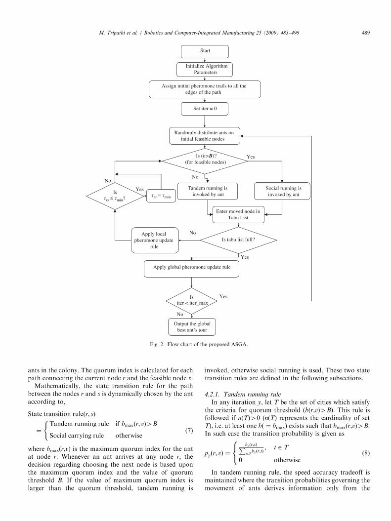
4.2. The self-guided state transition rule

In the proposed ASGA (Fig. 2), the artificial ants utilizea concept similar to quorum threshold [7] as shown by theT. Albipennis ants. For this purpose, a quorum index isdefined whose values determine whether to use probabil-istic model to select the next nodes in the path or to simplyfollow the pheromone trail intensity. If there is an urgentneed for speedy convergence (harsh environment), thequorum threshold is low, otherwise it is high (benignenvironment). Therefore, before making a move, the antdecides its behavior for running—tandem running or social

carrying.The scout first assesses the quorum size (or the quorum

index), which is compared with the context sensitivethreshold quorum ‘B’. If the threshold is low, tandemrunning is preferred, whereas social running is used in theother case. The probabilistic model simulates the tandemrunning where as the mechanism to follow pheromone trailintensity is used for social carrying. The quorum index foran ant positioned at node r is defined as

brv ¼Nrv

N(6)

where Nrv is the number of ants that have passed throughthe nodes (r,v) in the last iteration; N is the total number of

ARTICLE IN PRESS

Start

Initialize Algorithm Parameters

Assign initial pheromone trails to all theedges of the path

Set iter = 0

Randomly distribute ants oninitial feasible nodes

Apply global pheromone update rule

Enter moved node in Tabu List

Is tabu list full?No

Yes

Is (b>B)?(for feasible nodes)

Tandem running is invoked by ant

Yes

No

Isiter < iter_max

Output the global best ant’s tour

Yes

No

Apply local pheromone update

rule

IsSocial running is invoked by ant

Yes

No

�rs ≤ �min?�rs = �min

Fig. 2. Flow chart of the proposed ASGA.

M. Tripathi et al. / Robotics and Computer-Integrated Manufacturing 25 (2009) 483–496 489

ants in the colony. The quorum index is calculated for eachpath connecting the current node r and the feasible node v.

Mathematically, the state transition rule for the pathbetween the nodes r and s is dynamically chosen by the antaccording to,

State transition ruleðr; sÞ

¼Tandem running rule if bmaxðr; vÞ4B

Social carrying rule otherwise

((7)

where bmax(r,v) is the maximum quorum index for the antat node r. Whenever an ant arrives at any node r, thedecision regarding choosing the next node is based uponthe maximum quorum index and the value of quorumthreshold B. If the value of maximum quorum index islarger than the quorum threshold, tandem running is

invoked, otherwise social running is used. These two statetransition rules are defined in the following subsections.

4.2.1. Tandem running rule

In any iteration y, let T be the set of cities which satisfythe criteria for quorum threshold (b(r,v)4B). This rule isfollowed if n(T)40 (n(T) represents the cardinality of setT), i.e. at least one b( ¼ bmax) exists such that bmax(r,v)4B.In such case the transition probability is given as

pyðr; vÞ ¼

byðr;sÞPt2T

byðr;tÞ; t 2 T

0 otherwise

8<: (8)

In tandem running rule, the speed accuracy tradeoff ismaintained where the transition probabilities governing themovement of ants derives information only from the

ARTICLE IN PRESSM. Tripathi et al. / Robotics and Computer-Integrated Manufacturing 25 (2009) 483–496490

quorum index and the quorum threshold value. Such amodification maintains fast convergence of the algorithmin addition to keeping the explorative structure in cases oflocal convergence.

4.2.2. Social carrying rule

This rule is followed if n(T) ¼ 0, i.e., if no b exists forwhich the criteria for quorum threshold (b(r,v)4B) issatisfied. In this case, the transition probability is mathe-matically modeled as

pyðr; vÞ ¼

tyðr;vÞPu2Jy ðrÞ

tyðr;uÞif v 2 JyðrÞ

0 otherwise

8<: (9)

Thus, in any iteration y, an ant positioned on node r

chooses to move to a feasible node v (i.e., a node lying inthe list of feasible nodes Jy(r)), according to Eq. (9).

4.3. The pheromone update rules

Two pheromone update rules are utilized to update thepheromone concentration lying between the paths of thenodes.

4.3.1. Dynamic pheromone evaporation and update rule

Immediately, after the choice of the next node has beenmade by an ant, the content of its tabu-list is updated and alocal pheromone update rule is applied. First the pher-omone level of all the paths is allowed to evaporate equally

tnewði; jÞ ¼ ð1� rlÞtoldði; jÞ (10)

where rl is the local pheromone evaporation parameter.Now, additional pheromone is given to the paths overwhich each ant has passed by. The study of real antphenomenon states that the ants reside for lesser time onthe shorter paths than on the longer paths. Thus,evaporation on the shorter paths occurs for a lesser timewhich indirectly leads to higher pheromone concentrationover these paths than on the longer ones. To simulate thisphenomenon, cumulative pheromone added to each path isgoverned by the following equation:

tnewðr; sÞ ¼ toldðr; sÞ þ rl � ðQl=lðr; sÞÞ (11)

where Ql is the model dependent positive quantity. Thisdynamic pheromone evaporation and update rule impli-citly merges the greedy heuristic information with thepheromone information by logically relating it with theactual evaporation phenomenon that occurs in movementof real ants.

4.3.2. Global pheromone update rule

Moreover, at the tour completion by all the ants, the N

ants which correspond to the best N tours till the currentiteration are rewarded according to the global update rule.The purpose of this rule is to search in the vicinity of thebest N tours found so far.

tnewði; jÞ ¼ toldði; jÞ þ rDtði; jÞ (12)

In Eq. (12), the term tnew(i,j) represents the newpheromone concentration and is obtained by incrementingthe original pheromone value by rDt(i,j). The factor Dt(i,j)represents the accumulated increment by each of the N antswhich are ranked best till the current iteration as depictedin

Dtði; jÞ ¼XN

k¼1

Dtkði; jÞ (13)

Dtkði; jÞ ¼Q 1

Lklði;jÞ

� �ifði; jÞ 2 kth ant’s tour

0 otherwise

((14)

Parameter Q is the positive model dependent constantand Lk is the tour length by the global best ant. Dtk(i,j) is adynamic quantity that is added to all the paths after thetour completion. Eq. (14) is designed such that Dtk(i,j)obtains a non-zero value only for paths that are traversedby the global best ant.After global pheromone update, all the ants are

reinitialized and their tabu-lists are emptied. Algorithm isiterated in this fashion till certain terminating criterion(Maximum number of iterations or functional evaluations)is met.For the maximization of profits in FDOM problem

discussed in this paper, we applied the proposed ASGA toobtain the near optimal results. For this purpose, followingmodifications are made: number of cities and the numberof ants are both set equal to nt. The length of the tour ismodified as Lk ¼ 50+(5000/ZP) for all the probleminstances. The path length between two cities is definedby the sequence dependent setup cost matrix such that,l(r,v) ¼W(r,v). The precedence constraint is maintainedwith the help of a tabu-list and the list Jy(r) such that thelist Jy(r) consists of only those cities which satisfy thefeasibility criteria.

5. Experimental design and results

5.1. Test bed formulation

Many designed experiments use multi-level matricescalled orthogonal arrays for determining the combinationsof factor levels to use for each experimental run and foranalyzing the data thereafter [11,59]. The problem dis-cussed in this paper involves numerous factors, out ofwhich, seven factors were identified that can have majorimpact on the results. These factors were varied at twodifferent levels (low and high) and their effect on theobjective function value has been studied. The test bed isgenerated with due considerations to the Taguchi’s L8(2

7)orthogonal arrays [11] and thereby the resulting eightexperiments serve as the balanced combination of the levelsof the factors selected.

ARTICLE IN PRESSM. Tripathi et al. / Robotics and Computer-Integrated Manufacturing 25 (2009) 483–496 491

The factors considered for this study are:

1.

Number of parts (nP): This factor directly reflects thetotal number of parts that could be separated out of theworn out products. This includes the parts containedeither directly within the FA or within any subassemblylying underneath it. The factor is varied at two levels of20 and 40 parts.

2.

Number of subassemblies (nSA): The problem instancesare varied at two different level of this factor, i.e., 3(low) and 6 (high).

3.

Number of joints (nF): The total number of jointsobtained by the union of joints within all the sub-assemblies as well as those within the FA constitutes theparameter nF. This term forms a deciding factor for thedetermination of problem size and is kept at 20 for low,and 40 for high level.

4.

Setup costs ðW solk ;solkþ1Þ: The sequence dependent costsbetween the two joints are randomly generated in aninterval of (1, 5) for low and (5, 10) for high level.

5.

Joint breaking costs ðBCsolj Þ: The costs for breaking thejoints are usually dissimilar for different joints and aregenerated uniformly in the interval (15, 20) for low and(20, 30) for high level.

6.

Recovery value ðRCpsaiÞ: It is the actual value of the part

or subassembly after recovery from the FA at its EOLand is assumed to be uniformly distributed over therange of (70–80) and (80–90) for the two levels duringthe analysis.

7.

Disposal costs ðDCpsai0Þ: It represents the costs involved

in the disposal of unextracted or unrecovered parts/components. In the experimental design utilized, thesecosts are generated at two different levels in the uniforminterval of (5, 10) and (10, 15).

5.2. The encoding schema

The first step in the implementation of a searchtechnique to any problem is the representation of searchspace in terms of algorithmic parameters. For disassemblyof a product containing nF and nSA subassemblies, theknowledge based string is nt-tuple where nt represents thenumber of segments of the string and is defined as

nt ¼ nF þ nSA þ 1 (15)

Each string segment denotes a joint or subassembly andis represented as a node in ASGA. The precedencepreservation in ASGA has been done by selecting onlythat node as the next probable node which did not belongto a node within the tabu list and had no precedenceconstraint with any of the nodes contained within the tabulist. One extra segment is reserved for saving a specialnumber say ‘0’ that determines the depth of disassembly.Integer coding is done for the string representations suchthat each joint and subassembly is assigned the value of aunique positive integer. This string representation isinterpreted as:

1.

The joints and subassemblies are broken according tothe sequence of their appearance in the solution string.

2.

Depth of disassembly is ascertained by using theanalogy behind the special number ‘0’ which states thatonly those subassemblies and joints that lie before ‘0’ inthe solution string are allowed to be broken down forfurther disassembly.

Moreover, in any network representation, if there are nFjoints and nSA subassemblies, the first subassembly hasbeen referred as the (nF+1)th joint, the second subassem-bly as (nF+2)th joint and so on. This was done in anattempt to simplify the coding schema. Thus, if (nF+4)thjoint is encountered within the coding scheme, it isunderstood that it refers to the fourth subassembly.As an example, consider the following 9-tuple string

representation, /2 3 1 4 8 0 7 6 5S, where integers from 1 to8 represents joints/subassemblies to be broken while ‘0’identifies the depth of disassembly. Thus from theaforementioned discussion, the final sequence of joints tobe broken are those that lie ahead of ‘0’, i.e., /2 3 1 4 8S.Based upon the joints broken, the associated subassembliesand parts recovered can be determined. Similarly, if therewere six joints and two subassemblies in this exampleproduct configuration, then ‘7’ represents the subassembly‘1’, and ‘8’ represents the subassembly ‘2’.

5.3. Parameter settings

The proposed algorithm is coded in C++ and compiledon GNU C++ Compiler (GCC) using KDevelop on aLinux platform. Further, the compiled program is run on asystem specification of 1.5GHz Pentium IV processor and768MB RAM. Numerous preliminary experiments areperformed to determine the optimal parameter setting. Thenumber of cities and the ants in the AGSA are both positedto be equal to nt. The value of Q0 is set equal to 30, Ql is setequal to 10 and Q to 50. The dynamic evaporation rategoverning parameter rl is equal to 0.05 and the parameter ris set equal to 0.5. However, the primary proposal of thepaper is to show the efficiency of the introduced quorum

threshold concept. It is evident that the introduction ofquorum threshold enhances the performance in few cases,whereas its excessive low or high values tend to trap thesearch in local optima or degenerate the quality ofsolutions. The proposal works better, if the values arekept in the range [0.3–0.7]. Thus selection of quorumthreshold B is crucial for rate of convergence towards theglobal optimum. Greater scope for exploration is prefer-able in the early stages of the algorithm progress (to avoidentrapment in the local optima) where as large exploitationwill be preferable in the last stage of the algorithm (tosearch in the neighborhood of the obtained best solution).Due to the fact that the proposed metaheuristic is anintrinsically dynamic and adaptive search technique, anadaptive parameter handling strategy is suggested [60]. Theparameter B is adaptively handled by the algorithm during

ARTICLE IN PRESS

Table 4

Comparisons of time taken by ASGA, ACO and GA (in s)

Instance no. ASGA ACO GA

Table 3

Comparisons of average results obtained from ASGA, ACO and GA

ASGA ACO GA

455.017 430.028 397.507

296.413 283.309 245.710

64.202 56.385 47.983

�273.134 �269.651 �248.588

463.804 442.599 385.383

857.103 834.347 752.368

1349.922 1263.216 1196.062

889.878 828.425 741.123

M. Tripathi et al. / Robotics and Computer-Integrated Manufacturing 25 (2009) 483–496492

the course of its progress using following equation:

B ¼

0:7 if 1� logðyÞlog y_maxð Þ

� �40:7

0:3 if 1� logðyÞlog y_maxð Þ

� �o0:3

1� logðyÞlogðy_maxÞ

otherwise

8>>>><>>>>:

(16)

This adaptive parameter handling strategy refers to thegradual transition of the environmental conditions frombenign (high quorum threshold in the beginning) to harshones (low quorum threshold towards the end). Maximumnumber of fitness evaluations is taken as terminatingcriteria for all the algorithms and its value is set to 5000fitness evaluations for small problem instances and 10 000for comparatively larger problem instances.

For evaluation of performance, we have compared theresults obtained from ASGA with the results fromtraditional ACO [42] and Genetic Algorithm [54]. Initially,we choose similar parameter settings for ACO as were forASGA. But for tuned performance (after conductingnumerous preliminary runs) we obtained the value ofb ¼ 2 and a ¼ 0.5. Moreover, initial pheromone level oneach path was set equal to t0 ¼ 0.5. q0 was taken to be 0.4.In case of GA we utilized a population size of 50. A twopoint crossover operator with probability 0.7 and bitwisemutation operator with probability 0.05 gave best results.The terminating criteria for each of these two algorithmswas also set as the same as that for ASGA.

1 380.12 459.94 273.68

2 345.66 449.72 300.72

3 680.34 1074.93 564.68

4 720.76 980.23 655.89

5 692.29 768.44 470.75

6 643.54 978.18 469.78

7 291.43 396.34 273.94

8 322.49 432.13 264.44

750

800

850

900

n Va

lue

5.4. Performance comparison

Eight problem instances were generated with dueconsiderations to the Taguchi’s L8 (27) orthogonal arraysas shown in Table 2 [11]. The characteristic and searchcapability of ASGA is compared with that of ACO andGA and the results are provided in Table 3 for detailedanalysis. The results clearly reveal that ASGA outperformsthe other two algorithms in terms of maximizing the netprofits associated with the disassembly operation in 7 outof 8 designed experiments. The success of the algorithm liesin the fact that the proposed metaheuristic adapts itself tomaintain a balance between exploitation and explorationthroughout the run of the algorithm.

Table 2

L8 orthogonal array

Experiment no. nP nSA nF W solk ;solkþ1 BCsolj RCpsaiDCpsai0

1 1 1 1 1 1 1 1

2 1 1 1 2 2 2 2

3 1 2 2 1 1 2 2

4 1 2 2 2 2 1 1

5 2 1 2 1 2 1 2

6 2 1 2 2 1 2 1

7 2 2 1 1 2 2 1

8 2 2 1 2 1 1 2

Further, the computational times required by the variousalgorithms have been reported in Table 4. From the sametable, it can be observed that the GA required theminimum time in producing the results as compared toASGA and ACO in all the cases. However, ASGA wasagain seen to outperform ACO in terms of the computa-tional times involved.Further, to provide detailed insights, the best fitness

values obtained from ASGA, ACO, and GA were plotted

0 1000 2000 3000 4000 5000 6000 7000 8000 9000 10000500

550

600

650

700

No. of Fitness Evaluations

Obj

ectiv

e Fu

nctio

ASGAACOGA

Fig. 3. Convergence trends for ASGA and ACO and GA. X-axis

represents the number of fitness evaluations and Y-axis represents

objective function value.

ARTICLE IN PRESSM. Tripathi et al. / Robotics and Computer-Integrated Manufacturing 25 (2009) 483–496 493

against total number of generations (Fig. 3) in order toestimate the convergence trends of the algorithms. It isevident in Fig. 3 that ASGA significantly outperforms bothACO and GA thus validating its supremacy over the othertwo approaches on the concerned problem.

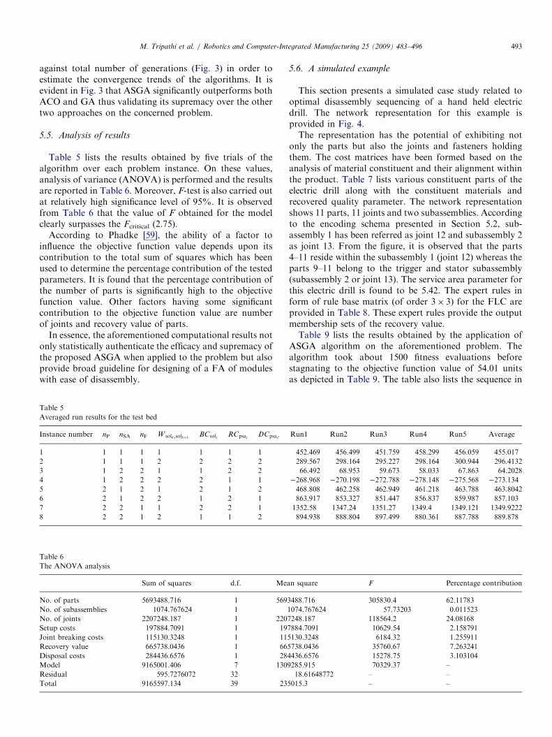
5.5. Analysis of results

Table 5 lists the results obtained by five trials of thealgorithm over each problem instance. On these values,analysis of variance (ANOVA) is performed and the resultsare reported in Table 6. Moreover, F-test is also carried outat relatively high significance level of 95%. It is observedfrom Table 6 that the value of F obtained for the modelclearly surpasses the Fcritical (2.75).

According to Phadke [59], the ability of a factor toinfluence the objective function value depends upon itscontribution to the total sum of squares which has beenused to determine the percentage contribution of the testedparameters. It is found that the percentage contribution ofthe number of parts is significantly high to the objectivefunction value. Other factors having some significantcontribution to the objective function value are numberof joints and recovery value of parts.

In essence, the aforementioned computational results notonly statistically authenticate the efficacy and supremacy ofthe proposed ASGA when applied to the problem but alsoprovide broad guideline for designing of a FA of moduleswith ease of disassembly.

Table 5

Averaged run results for the test bed

Instance number nP nSA nF W solk ;solkþ1 BCsolj RCpsaiDCpsai0

1 1 1 1 1 1 1 1

2 1 1 1 2 2 2 2

3 1 2 2 1 1 2 2

4 1 2 2 2 2 1 1

5 2 1 2 1 2 1 2

6 2 1 2 2 1 2 1

7 2 2 1 1 2 2 1

8 2 2 1 2 1 1 2

Table 6

The ANOVA analysis

Sum of squares d.f. Mea

No. of parts 5693488.716 1 569

No. of subassemblies 1074.767624 1

No. of joints 2207248.187 1 220

Setup costs 197884.7091 1 19

Joint breaking costs 115130.3248 1 11

Recovery value 665738.0436 1 66

Disposal costs 284436.6576 1 28

Model 9165001.406 7 130

Residual 595.7276072 32

Total 9165597.134 39 23

5.6. A simulated example

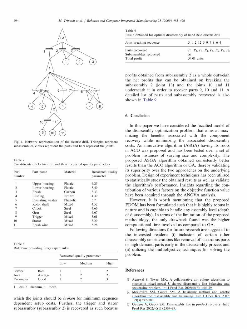
This section presents a simulated case study related tooptimal disassembly sequencing of a hand held electricdrill. The network representation for this example isprovided in Fig. 4.The representation has the potential of exhibiting not

only the parts but also the joints and fasteners holdingthem. The cost matrices have been formed based on theanalysis of material constituent and their alignment withinthe product. Table 7 lists various constituent parts of theelectric drill along with the constituent materials andrecovered quality parameter. The network representationshows 11 parts, 11 joints and two subassemblies. Accordingto the encoding schema presented in Section 5.2, sub-assembly 1 has been referred as joint 12 and subassembly 2as joint 13. From the figure, it is observed that the parts4–11 reside within the subassembly 1 (joint 12) whereas theparts 9–11 belong to the trigger and stator subassembly(subassembly 2 or joint 13). The service area parameter forthis electric drill is found to be 5.42. The expert rules inform of rule base matrix (of order 3� 3) for the FLC areprovided in Table 8. These expert rules provide the outputmembership sets of the recovery value.Table 9 lists the results obtained by the application of

ASGA algorithm on the aforementioned problem. Thealgorithm took about 1500 fitness evaluations beforestagnating to the objective function value of 54.01 unitsas depicted in Table 9. The table also lists the sequence in

Run1 Run2 Run3 Run4 Run5 Average

452.469 456.499 451.759 458.299 456.059 455.017

289.567 298.164 295.227 298.164 300.944 296.4132

66.492 68.953 59.673 58.033 67.863 64.2028

�268.968 �270.198 �272.788 �278.148 �275.568 �273.134

468.808 462.258 462.949 461.218 463.788 463.8042

863.917 853.327 851.447 856.837 859.987 857.103

1352.58 1347.24 1351.27 1349.4 1349.121 1349.9222

894.938 888.804 897.499 880.361 887.788 889.878

n square F Percentage contribution

3488.716 305830.4 62.11783

1074.767624 57.73203 0.011523

7248.187 118564.2 24.08168

7884.7091 10629.54 2.158791

5130.3248 6184.32 1.255911

5738.0436 35760.67 7.263241

4436.6576 15278.75 3.103104

9285.915 70329.37 –

18.61648772 – –

5015.3 – –

ARTICLE IN PRESS

Table 7

Constituents of electric drill and their recovered quality parameters

Part

number

Part name Material Recovered quality

parameter

1 Upper housing Plastic 4.25

2 Lower housing Plastic 5.49

3 Brush Carbon 3.33

4 Bushing Bronze 4.39

5 Insulating washer Phenolic 5.7

6 Rotor shaft Mixed 4.52

7 Chuck Steel 4.66

8 Gear Steel 4.67

9 Trigger Mixed 3.61

10 Stator Mixed 3.29

11 Brush wire Mixed 5.28

FA

1 2 3

1 2 3

1

45 6 7 8 9

7 862

54

10 11

9 10 11

Fig. 4. Network representation of the electric drill. Triangles represent

subassemblies, circles represent the parts and bars represent the joints.

Table 8

Rule base providing fuzzy expert rules

Recovered quality parameter

Low Medium High

Service Bad 1 1 2

Area Average 1 2 2

Parameter Good 1 2 3

1—less, 2—medium, 3—more.

Table 9

Result obtained for optimal disassembly of hand held electric drill

Joint breaking sequence 3_1_2_12_5_9_7_8_6_4

Parts recovered P1, P2, P3, P4, P5, P6, P7, P8

Subassemblies recovered S2

Total profit 54.01 units

M. Tripathi et al. / Robotics and Computer-Integrated Manufacturing 25 (2009) 483–496494

which the joints should be broken for minimum sequencedependent setup costs. Further, the trigger and statorsubassembly (subassembly 2) is recovered as such because

profits obtained from subassembly 2 as a whole outweighthe net profits that can be obtained on breaking thesubassembly 2 (joint 13) and the joints 10 and 11underneath it in order to recover parts 9, 10 and 11. Adetailed list of parts and subassembly recovered is alsoshown in Table 9.

6. Conclusion

In this paper we have considered the fuzzified model ofthe disassembly optimization problem that aims at max-imizing the benefits associated with the componentrecovery while minimizing the associated disassemblycosts. An innovative algorithm (ASGA) having its rootsin ACO was proposed and has been tested over a set ofproblem instances of varying size and complexity. Theproposed ASGA algorithm obtained consistently betterresults than the ACO algorithm or GA, thereby validatingits superiority over the two approaches on the underlyingproblem. Design of experiment techniques has been utilizedto statistically study the obtained results as well as validatethe algorithm’s performance. Insights regarding the con-tribution of various factors on the objective function valuehave been acquired through the ANOVA analysis.However, it is worth mentioning that the proposed

FDOM has been formulated such that it is highly robust innature and is capable to handle any assembly level (depthof disassembly). In terms of the limitation of the proposedmethodology, the only drawback found was the highercomputational time involved as compared to GA.Following directions for future research are suggested to

the interested readers: (i) inclusion of certain otherdisassembly considerations like removal of hazardous partsor high demand parts early in the disassembly process and(ii) utilizing the multiobjective techniques for solving theproblem.

References

[1] Agarwal S, Tiwari MK. A collaborative ant colony algorithm to

stochastic mixed-model U-shaped disassembly line balancing and

sequencing problem. Int J Prod Res 2008;46(6):1405–29.

[2] McGovern SM, Gupta SM. A balancing method and genetic

algorithm for disassembly line balancing. Eur J Oper Res 2007;

179(3):692–708.

[3] Gungor A, Gupta SM. Disassembly line in product recovery. Int J

Prod Res 2002;40(11):2569–89.

ARTICLE IN PRESSM. Tripathi et al. / Robotics and Computer-Integrated Manufacturing 25 (2009) 483–496 495

[4] Chipperfield AJ, Bica B, Fleming PJ. Fuzzy scheduling control of a

gas turbine aero-engine: a multiobjective approach. IEEE Trans Ind

Electron 2002;49(3):536–48.

[5] Lambert ADJ, Gupta SM. Disassembly modeling for assembly,

maintenance, reuse, and recycling. USA: CRC Press; 2005.

[6] James ARM, Anna D, Nigel RF, Tim K. Noise, cost and speed-

accuracy trade-offs: decision-making in a decentralized system. J R

Soc Interface 2006;3:243–54.

[7] Franks NR, Dornhaus A, Fitzsimmons JP, Stevens M. Speed versus

accuracy in collective decision making. Proc R Soc Lond Ser B

2003;270:2457–63.

[8] Franks NR, Richardson T. Teaching in tandem-running ants. Nature

2006;439:153.

[9] Pratt SC, Mallon EB, Sumpter DJT, Franks NR. Quorum sensing,

recruitment, and collective decision-making during colony emigration

by the ant Leptothorax albipennis. Behav Ecol Sociobiol 2002;

52:117–27.

[10] James ARM, Tim K, Anna RD, Nigel RF. Simulating the evolution

of ant behaviour in evaluating nest sites. In: Advances in artificial

life—proceedings of the seventh European conference on artificial life

(ECAL). Berlin: Springer; 2003. p. 643–50.

[11] Taguchi G. System of experimental design, vol. 1&2. US: UNIPUB/

Kraus International Publications; 1987.

[12] Homem de Mello LS, Sanderson AC. AND/OR graph representation

of assembly plans. IEEE Trans Robotics Automat 1990;6(2):188–98.

[13] Lambert AJD. Determining optimum disassembly sequences in

electronic equipment. Comput Ind Eng 2002;43(3):553–75.

[14] Ishii K, Eubanks CF, Di Marco P. Design for product retirement and

material life-cycle. Mater Des 1994;15(4):225–33.

[15] Moorie KE, Gungor A, Gupta SM. A Petrinet approach to

disassembly process planning. Comput Ind Eng 1998;35(1):165–8.

[16] Zussman E, Zhou M. A methodology for modeling and adaptive

planning of disassembly processes. IEEE Trans Robotics Automat

1999;15(1):190–4.

[17] Tiwari MK, Sinha N, Kumar S, Rai R, Mukhopadhyay SK. A Petri

Net based approach to determine the disassembly strategy of a

product. Int J Prod Res 2001;40(5):1113–29.

[18] Rai R, Rai V, Tiwari MK, Allada V. Disassembly sequence

generation: a Petri net based heuristic approach. Int J Prod Res

2002;40(13):3183–98.

[19] Kumar S, Kumar R, Shankar R, Tiwari MK. Expert enhanced

coloured stochastic Petri Net and its application in assembly/

disassembly. Int J Prod Res 2003;41(12):2727–62.

[20] Sarin SC, Sherali HD, Bhootra A. A precedence-constrained

asymmetric traveling salesman model for disassembly optimization.

IIE Trans 2006;38:223–37.

[21] Kriwet A, Zussman E, Seliger G. Systematic integration of design-

for-recycling into product design. Int J Prod Econ 1995;38(1):15–32.

[22] Boothroyd G, Alting L. Design for assembly and disassembly. Ann

CIRP 1992;41(2):625–36.

[23] Hill B. Industry’s integration of environmental product design. IEEE

Int Symp Electron Environ 1993:64–8.

[24] Lambert AJD. Linear programming in disassembly/cluster sequence

generation. Comput Ind Eng 1999;36:723–38.

[25] Penev KD, de Ron AJ. Determination of a disassembly strategy. Int J

Prod Res 1996;34(2):495–506.

[26] Kuo TC, Zhang HC, Huang SH. Disassembly analysis for electro-

mechanical products: a graph-based heuristic approach. Int J Prod

Res 2000;38(5):903–1007.

[27] Moyer L, Gupta SM. Environmental concerns and recycling/

disassembly efforts in the electronics industry. J Electron Manuf

1997;7(1):1–22.

[28] Navin-Chandra D. The recovery problem in product design. J Eng

Des 1994;5(1):65–86.

[29] Gungor A, Gupta SM. An evaluation methodology for disassembly

processes. Comput Ind Eng 1997;33(1/2):329–32.

[30] Lambert AJD, Gupta SM. Demand-driven disassembly optimization

for electronic products. J Electron Manuf 2002;11(19):121–35.

[31] Konkar E, Gupta SM. A genetic algorithm for disassembly process

planning. In: Proceedings of 2001 SPIE international conference on

environmentally conscious manufacturing II, Newton, Massachu-

setts; 2001. p. 28–9, 54–62.

[32] Dorigo M, Gambardella LM. Ant colonies for the travelling

salesman problem. Bio Systems 1997;43:73–81.

[33] Maniezzo V, Colorni A, Dorigo M. The ant system applied to the

quadratic assignment problem. IEEE Trans Knowl Data Eng

1999;11(50):769–78.

[34] Bell JE, McMullen PR. Ant colony optimization techniques for the

vehicle routing problem. Adv Eng Inf 2004;18(1):41–8.

[35] Kumar R, Tiwari MK, Shankar R. Scheduling of flexible manufac-

turing systems: an ant colony optimization approach. I Mech E

2003:1443–53.

[36] Bland JA. Space planning by ant colony optimisation. Int J Comput

Appl Technol 1999;6:320–8.

[37] Baucr A, Bullnhcimer B, Hartl RF, Strauss C. An ant colony

optimization approach for the single machine tool tardiness problem.

In: Proceedings of the 1999 congress on evolutionary computation;

1999. p. 1445–50.

[38] McMullen PR. An ant colony optimization approach to addressing a

JIT sequencing problem with multiple objectives. Artif intell Eng

2001;15:309–17.

[39] Brucker P, Drexel A, Mohring R, Neumann K, Pesch E. Resource

constraint project scheduling problem. Eur J Oper Res 1999;112:3–41.

[40] Stutzle T, Linke S. Experiments with variants of ant algorithms.

Matheware Soft Comput 2000;7.

[41] Dorigo M, Di Caro G. The ant colony optimization metaheuristic.

In: Corne D, et al., editors. New ideas in optimization. Maidenhead,

UK: Mc-Graw Hill; 1999. p. 11–32.

[42] Dorigo M, Gambardella LM. Ant colony system: a cooperative

learning approach to the travelling salesman problem. IEEE Trans

Evol Comput 1997;1(1):53–66.

[43] Stutzle T, Hoos HH. Max–Min ant system. Future Generation

Comput Systems 2000;16:889–914.

[44] Cordon O, Fernandez de Viana I, Herrera F, Moreno L. A new ACO

model integrating evolutionary computation concepts: the best–worst

ant system. In: Dorigo M, Middendorf M, Stutzle T, editors.

Proceedings of Ants’2000; 2000. p. 22–9.

[45] Gambardella LM, Taillard ED, Dorigo M. Ant colonies for the

quadratic assignment problem. J Oper Res Soc 1999;50(2):167–76.

[46] Taillard ED, Gambardella LM. Adaptive memories for the quadratic

assignment problem. Technical report IDSIA, Lugano, Switzerland;

1997. p. 87–97.

[47] Failli F, Dini G. Optimization of disassembly sequences for recycling

of end-of-life products by using a colony of ant-like agents. Lecture

Notes in Computer Science, vol. 2070. 2001. p. 632–9.

[48] McGovern SM, Gupta SM. Ant colony optimization for disassembly

sequencing with multiple objectives. Int J Adv Manuf Technol

2006;30(5–6):481–96.

[49] Gen M, Tsujimura Y, Li Y. Fuzzy assembly line balancing using

genetic algorithms. Comput Ind Eng 1996;31(3/4):631–4.

[50] Mierswa I. Incorporating fuzzy knowledge into fitness: multiobjective

evolutionary 3D design of process plants. In: Genetic and evolu-

tionary computation conference, proceedings of the 2005 conference

on genetic and evolutionary algorithm. New York: ACM Press; 2005.

p. 1985–92.

[51] Lawler EL, Lenstra JK, Rinnoy-Kan AGH, Shmoys DG, editors.

The traveling salesman problem: a guided tour of combinatorial

optimization. Chichester: Wiley; 1985.

[52] Reinelt G. The traveling salesman problem: computational solutions

for TSP applications. Berlin: Springer; 1994.

[53] Lin FT, Kao CY, Hsu CC. Applying the genetic approach to

simulated annealing in solving some NP hard problems. IEEE Trans

Systems Man Mach Cybernet 1993;23:1752–67.

[54] Goldberg DE. Genetic algorithms in search, optimization and

machine learning. Boston, MA, USA: Addison-Wesley Longman

Publishing Co., Inc.; 1989.

ARTICLE IN PRESSM. Tripathi et al. / Robotics and Computer-Integrated Manufacturing 25 (2009) 483–496496

[55] Dorigo M. Optimization, learning and natural algorithms. PhD

thesis, Politecnico di Milano, Italy, 1992 [in Italian].

[56] Fogel DB. Applying evolutionary programming to selected traveling

salesman problem. Cybernet System Int J 1993;24:27–36.

[57] Durbin R, Willshaw D. An analogue approach to the traveling

salesman problem using an elastic net method. Nature 1987;

326(6114):689–91.

[58] Onwubolu GC, Clerc M. Optimal path for automated operations by

a new heuristic approach using particle swarm optimization. Int J

Prod Res 2004;42:473–91.

[59] Phadke MS. Quality engineering using robust design. Englewood

Cliffs, NJ: Prentice-Hall; 1989.

[60] Eiben AE, Hinterding R, Michalewicz Z. Parameter control in evolu-

tionary algorithms. IEEE Trans Evolutionary Comput 1999;3(2):124–41.