Real time assimilation of HF radar currents into a coastal ocean model

Ž .Journal of Marine Systems 28 2001 161–182www.elsevier.nlrlocaterjmarsys

Real time assimilation of HF radar currents into a coastalocean model

Øyvind Breivik a,), Øyvind Sætra b

a Department of Modelling and Data Assimilation, Nansen EnÕironmental and Remote Sensing Centre, EdÕ. Griegs. 3A,5059 Bergen, Norway

b The Norwegian Meteorological Institute, Oslo, Norway

Received 4 September 2000; accepted 18 December 2000

Abstract

A real time assimilation and forecasting system for coastal currents is presented. The purpose of the system is to delivercurrent analyses and forecasts on based on assimilation of high-frequency radar surface current measurements. The localVessel Traffic Service monitoring the ship traffic to two oil terminals on the coast of Norway received the analyses andforecasts in real time.

A new assimilation method based on optimal interpolation is presented where spatial covariances derived from an oceanmodel are used instead of simplified mathematical formulations. An array of high frequency radar antennae provides thecurrent measurements. A suite of nested ocean models comprises the model system. The observing system is found to yieldgood analyses and short range forecasts that are significantly improved compared to a model twin without assimilation. Thesystem is fast, analysis and 6-h forecasts are ready at the Vessel Traffic Service 45 min after acquisition of radarmeasurements. q 2001 Elsevier Science B.V. All rights reserved.

Keywords:

Subject keywords: Data assimilation, Ocean modelling, Current sensors, Ocean currents

Regional terms: Europe, Norway, Bergen, Fedje

Ž . Ž .Bounding coordinates: 48E, 608N , 58E, 618N

1. Introduction

Operational forecasting of the ocean is still in itsinfancy. Unlike the atmospheric weather, ocean cur-

) Corresponding author. Tel.: q47-55-29-72-88; fax: q47-55-20-00-50.

Ž .E-mail address: [email protected] Ø. Breivik .

rents do not pose an immediate threat to everydaylife. Our daily goings-on may indeed never be af-fected by the strength of the ocean currents in nearbywaters. This explains in part why forecasting thestate of the atmosphere was a science and a craft asearly as in the 1920s while at the turn of the mille-nium the same can still not be said about the oceansŽsee the account of the first, failed attempt at numeri-

0924-7963r01r$ - see front matter q 2001 Elsevier Science B.V. All rights reserved.Ž .PII: S0924-7963 01 00002-1

( )Ø. BreiÕik, Ø. SætrarJournal of Marine Systems 28 2001 161–182162

cally forecasting the atmosphere in Richardson,.1922 .

Another reason for this disparity may be thegeneral impression that the ocean is not as capriciousas the atmosphere. While this may be true on sometime scales and in some regions, it is certainly nottrue for the coastal surface currents that feed on thecontrast in temperature and salinity between neigh-bouring water masses. When such baroclinic currentsare further enforced by the wind field and join upwith the tidal motion, the result can be surface

Ž .currents up to 2 mrs 4 knots that loosely followthe coastline. These currents vary in width andstrength and can quickly break into whorls and ed-

Ždies of various sizes typically less than 80 km, see.Johannessen et al., 1989; Ikeda et al., 1989 . Such a

chaotic dynamical system is unpredictable overlonger periods; hence, data assimilation of observa-tions is vital when trying to forecast coastal currents.

The complexity of coastal current fields tells usthat the pertinent horizontal length scale of ocean

Ždynamics, the Rossby radius of deformation see.Gill, 1982 , which in turn dictates the required hori-

zontal resolution of the numerical models, is vastlydifferent from that of the atmosphere. In the atmo-sphere, this scale determines the horizontal extent of

Žlow- and high-pressure systems the good and the.bad weather , which is in the range of several hun-

dred kilometers. The equivalent scale in the ocean isonly a few tens of kilometers. Hence, resolvingeddies in ocean models is only done at an enormouscomputational cost, which seriously limits the hori-zontal extent of the model domain.

When trying to forecast coastal currents with theaid of data assimilation, the Rossby length scalebecomes an acute problem. In weather forecasting,observations of the density field are made with adense network of radio soundings that resolves thevertical structure of the atmospheric fronts. The den-sity fronts associated with a mesoscale ocean cy-clone may be less than a kilometer in horizontalextent. Hence, to achieve the same forecast skill formesoscale activity in the ocean as in the atmosphere,the vertical and horizontal density structure of theocean eddies and their associated fronts must beresolved using an extremely dense network of verti-cal density profilers. Although technically possibleŽusing salinity–temperature–depth meters, CTD, or

.expendable bathythermographs, XBT , it is neitherfinancially nor operationally feasible to build such adense coastal real time observation network.

We see that there are numerical, instrumental, andsocioeconomic reasons why operational forecastingof the coastal ocean is lagging behind its atmo-spheric counterpart. However, the appearance of hugeoil tankers has caused currents to become a factor toreckon. A tanker moves almost unaffected throughbad weather and rough seas, but coastal currents canseriously deflect its bearing. While aiming towardnarrow sounds, or maneuvering through channelsand straits, it is imperative to know the strength anddirection of the currents. Fortunately, there is now agrowing awareness of the threat that coastal currentspose to ship traffic and the ensuing pollution andpotential loss of lives that such disasters may cause.

There exists, however, an inexpensive alternativeto in situ sampling of oceanographic data. Shore-

Ž .based high-frequency HF radars provide high-reso-lution surface current coverage in near real time onan extensive observation grid at a very low cost.Although surface currents do not provide a completepicture of a coastal current, it does provide valuableinformation on its extent, direction, and magnitude.Using HF radars to map coastal currents is by now a

Žwell-tested technique see Barrick et al., 1977; Bar-.rick, 1978 for early accounts of the methodology

which has matured over the years into reliable instru-ments.

One of the aims of the project EuroROSEŽ .European Radar Ocean Sensing is to combine realtime radar observations of surface currents witha suite of ocean forecast models using an assimila-tion scheme to deliver real time analyses and fore-casts of coastal currents to the Vessel Traffic ServicesŽ .VTS in dangerous regions with extensive shiptraffic. The net site http:rrifmaxp1.ifm.uni-ham-burg.derEuroROSE provides more information onthe project as a whole.

Assimilating HF radar surface currents into mod-els of the coastal ocean is a relatively new approachto improving coastal current forecasts. The authorsare only aware of two other similar efforts. Oke et al.Ž .2000 describe a data assimilation system which

Žutilizes a CODAR HF radar see Barrick et al., 1977.for a description of an early version of the radar and

the Princeton Ocean Model to produce forecasts of

( )Ø. BreiÕik, Ø. SætrarJournal of Marine Systems 28 2001 161–182 163

the wind-driven, mesoscale shelf circulation off theOregon coast. The results are promising, includingthe vertical impact of the surface currents. However,this system is only used for hindcast studies. TheRutgers University has an ongoing assimilation ef-fort associated with their underwater laboratory

Ž .LEO-15, Glenn et al., 2000 off the coast of NewJersey. During 5-week campaigns in the summermonths, they perform real time assimilation of CO-DAR radar data into their Regional Ocean Model

ŽSystem ROMS, see Song and Haidvogel, 1994 for a.description of an early version of the model and

produce forecasts of coastal currents. More details ofthe system can be found at http:rrmarine.rutgers.edurmrsr.

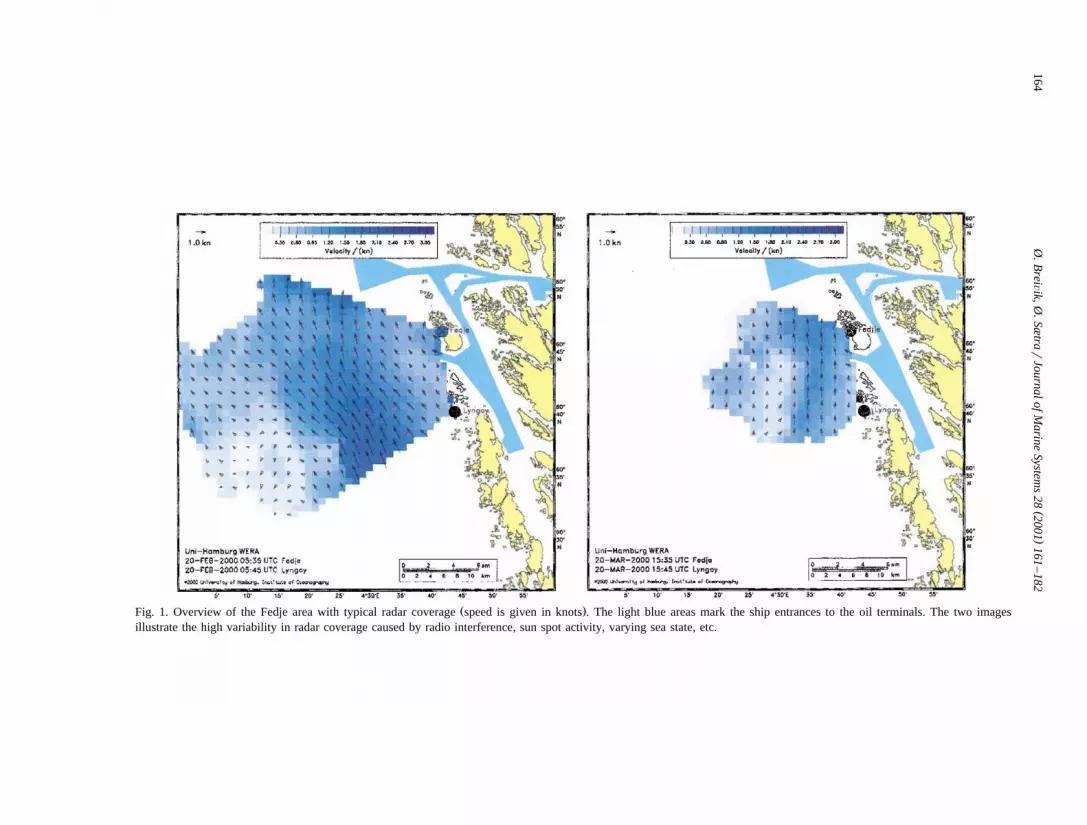
The first realization of the EuroROSE observingsystem was focussed on the island Fedje off the westcoast of Norway. This area is bustling with tankersand other ships that serve the petroleum terminalsSture and Mongstad, together one of the busiestpetroleum harbours in the world. The ship entrancesare narrow and the coastal current is strong andrapidly changing in location and direction. Fig. 1provides an overview of the area and typical radarcoverage during the experiment.

As the main objective of the project was todemonstrate the potential of such an ocean monitor-ing and forecasting system for coastal security, theinformation was transmitted in real time to the local

Ž .vessel traffic service VTS where observations,analyses, and forecasts were presented automatically.

In this paper, we present the theory behind theassimilation scheme together with its implementationand performance in the real time monitoring andforecasting system, which was developed for theregion around Fedje. The radar system and the nu-merical model are also described in some detail.

2. Sequential data assimilation

Data assimilation methods have been used rou-tinely by the major weather prediction centres for the

Ž .past two decades Daley, 1991 . These methods varyin complexity from simple Newtonian nudgingschemes through optimal interpolation schemes andall the way up to four-dimensional variational assim-

ilation schemes and sequential Kalman filtering tech-niques. The latter method has also been demon-

Žstrated for simplified models the Lorenz equationsand quasi-geostrophic models, see Evensen, 1994,

.1997 .The fundamental equation in sequential data as-

similation is

c asc fqK dyHc f . 1Ž .Ž .

Here, cgR n is the n-dimensional model state vec-tor, with superscripts AaB and AfB denoting analysisand forecast. Further, KgR n=m is the gain matrix,

m Ž .and dgR is the data vector the m observations .Finally, H is the observation operator, which mapsthe model state onto the observation space.

As an explanation to the observation operator,consider a 3D-ocean model yielding horizontal cur-rent vectors at certain vertical levels. The data pro-vided are surface currents measured with a radarfacility. Unless the models and the radar yield data inthe exact same locations, some kind of interpolationis needed to make modelled and observed fieldscomparable.

The gain K is a matrix of weights that determineseach observation’s influence on the final analysis.

ŽUsing a minimum variance principle see Daley,.1991 , we can argue that K should be

y1f T f TKsP H H P H qR , 2Ž . Ž .

where P fgR n=n is the error variance–covariancematrix of the numerical model, and RgRm=m is theerror variance–covariance matrix of the observa-tions.

Let indices i and j denote model variables and kf � f4and l denote observations, i.e., c ' c , is1, . . . ,i

� 4n, and d' d , ks1, . . . , m. The model statek

vector mapped to observation space can then bewritten

� 4Hcs c , ks1, . . . ,m ,k

and the model error variance–covariance matrix is

P fs Cov cX ,c X , i , js1, . . . ,n. 3Ž .� 4Ž .i j

Here and throughout, primes indicate zero-meanŽ .quantities deviations from the mean .

()

Ø.B

reiÕik,Ø

.Sætra

rJournalof

Marine

Systems

282001

161–

182164

Ž .Fig. 1. Overview of the Fedje area with typical radar coverage speed is given in knots . The light blue areas mark the ship entrances to the oil terminals. The two imagesillustrate the high variability in radar coverage caused by radio interference, sun spot activity, varying sea state, etc.


Ž .The gain matrix in Eq. 2 can be made moreunderstandable by first noting that

P fH Ts Cov cX ,c X , is1, . . . ,n , ks1, . . . ,m ,� 4Ž .i k

is simply the error covariance between model vari-able i and observation k. Secondly, the purpose of

Ž .the inverse weight matrix in Eq. 2 is to weightobservations according to their importance. Hence,in a cluster of observations, one more data point willnormally not add much information as the internalcorrelation between the observations will be high.Conversely, a solitary observation in a critical loca-tion may be heavily weighted. The inverse weightmatrix achieves this by balancing the error covari-ances between observation locations k and l aspredicted by the numerical model,

H P fH Ts Cov cX ,c X , k ,ls1, . . . ,m ,� 4Ž .k l

against the AinstrumentalB quality of the observa-tions and internal covariance, which is contained inthe observation error variance–covariance matrix,

Rs Cov dX ,dX , k ,ls1, . . . ,m. 4� 4Ž . Ž .k l

( )2.1. Statistical optimal interpolation

Ž .Statistical or optimal interpolation OI is a se-quential data assimilation method using predefinedŽ .time invariant error statistics. Hence, the assimila-

Ž .tion analysis is variance minimizing only if theerror statistics are correct and do not change with

Ž .time see Daley, 1991 .OI schemes normally assume either that correla-

tions between two variables u and Õ, say, in differ-ent locations are functions of distance and direction,

Corr uX x ,ÕX x fCorr X X r ,f ,Ž . Ž . Ž .Ž .1 2 u ,Õ

or even isotropic functions of distance only,

Corr uX x ,ÕX x fCorr X X r .Ž . Ž . Ž .Ž .1 2 u ,Õ

< <Here, r is the radial distance x yx and f is the1 2

direction from x to x relative to north. These1 2

simplifications can sometimes be adequate, but if thecovariances display a more complex spatial structurethen this formulation may lead to serious errors inthe assimilation update.

2.2. The Ensemble Kalman filter

A much more advanced sequential method is theŽso-called Ensemble Kalman filter EnKF, see

.Evensen, 1994, 1997; Burgers et al., 1998 . Themethod is based on the Kalman filter approach, butcircumvents the closure problem of nonlinearity inthe model by calculating the covariances from anensemble of evolving model states. This approachalso avoids forecasting the n=n covariance matrixP f, which becomes intractable for 3D oceanic andatmospheric models of realistic dimensions.

An ensemble of N initial model states

c 0 , ns1, . . . , N ,� 4n

is generated and integrated forward in time, yieldingan ensemble of forecasts at a later time t ,1

c f , ns1, . . . , N.� 4n

The ensemble average isN1

cs c , 5Ž .Ý nNns1

and the deviations from the mean are denoted c X'n

c yc .n

The zero mean ensemble can also be viewed as acollection of column vectors, illustrated by the fol-lowing tableau,

X X Xw x w x w xA s c , . . . , c . 6Ž .1 N

The model error covariance matrix can be approxi-mated by the outer product of the ensemble,

1X XTfP f A A . 7Ž .

Ny1

At each update, the Kalman gain K must be foundŽ .from Eq. 2 by first integrating N numerical modelŽ Ž ..realizations where N is typically OO 250 and then

f Ž .computing P using Eq. 7 . Clearly, this method iscomputationally very expensive, and it would bedesirable to find a middle ground between the over-simplification of standard OI and the enormous costof running N sibling models.

2.3. A A quasi-ensembleB assimilation scheme

We propose to exchange the ensemble of modelsused to compute the Ensemble Kalman Filter with an


ensemble of model states. This can be any collectionof model states taken from a representative modelrun. Whereas an ensemble of models will pick upperiods of high and low variance, our covarianceswill remain fixed throughout the assimilation period.This means that an assimilation scheme employingthese statistics will formally belong to the class ofpreviously discussed optimal interpolation schemes.

In order to generate this quasi-ensemble, we needto run the model for a representative period. Modelstates are sampled from the model run. This refer-ence period should be selected carefully. Ideally, itshould pick up the correlations relevant for ourspecific time period. However, this may be impossi-ble to do in advance, as is the case for a real timeobserving system. For a hindcast experiment, oneshould naturally choose the reference run to coverthe period of interest. The next best thing will be tochoose a reference run that covers a similar periodŽsimilar climatology, e.g., a different year but same

.time of year .A final caveat regarding the sampling is to choose

a sampling frequency that captures the relevantphysics. This is especially critical for the tidal mo-tion with its well-defined frequencies. This is mosteasily achieved by choosing a sampling period D tthat is smaller than the dominant tidal period, but

Žnot an integer fraction of it to avoid capturing only.high tides or only low tides .

An EnKF will find the AcorrectB error statisticsunder the assumptions that the ensemble is suffi-ciently large and the errors are normally distributed.The proposed quasi-ensemble will not, in general,find the correct error variances for the model sinceits statistics do not vary with time. However, thecorrelations may be satisfactory. This means thatalthough the relative weight between data and modelmay be off, the spatial correlations between, say,surface currents in one point and the salinity inanother point, may be quite alright.

The formulation of the quasi-ensemble filter isanalogous to the derivation of the EnKF and makesno assumptions on the spatial shape of the covari-ances. In theory, cross-correlations between all perti-nent model variables may be used to make full useof the data; hence, model grid points well outside thearea covered by observations may experience correc-tions based on their covariance with variables in

points closer to the observations. Likewise, verticalcorrections can be made to the different model vari-ables. The full equation reads

1X XTa f Tc sc q A A H

Ny1

=

y11X XT T fHA A H qR dyHc .Ž .ž /Ny1

8Ž .

ŽHere, we have substituted the ensemble of sampled. f Ž .model states for P using Eq. 7 .

3. The EuroROSE current assimilation and fore-casting system

3.1. The numerical model

Ž .We used the Princeton Ocean Model POM asimplemented and modified by The Norwegian Mete-

Ž .orological Institute DNMI . The lateral hydrody-namic equations are solved on an Arakawa C-gridŽsee Mesinger and Arakawa, 1976; Kowalik and

.Murty, 1993, p. 170 . Terrain following s-coordi-nates resolve the vertical, which means that thevertical resolution is high in shallow areas and coarsein deeper areas. In addition, the levels are not dis-tributed linearly over the depth as the mixed layernear the surface requires higher resolution than thedeeper parts of the ocean. Surface elevation and thevertical component of the current vector, w, aresolved on the surface. Through the water column, uand Õ are staggered one half grid cell with respect tow. Hence, the horizontal velocities of the uppermostlayer are found one half grid cell from the surface.

The model contains a second-order moment turbu-Ž .lence closure sub-model Mellor and Yamada, 1982 ,

which provides vertical mixing coefficients. Themodel solves the conservation equations for momen-tum and mass using an explicit finite differencescheme in the horizontal, and an implicit scheme forthe vertical terms to eliminate the time-step con-straints caused by fine resolution of the surface layer.The model has a free surface and uses mode-splittingfor the time-stepping. In the external mode, themodel is two-dimensional and uses a time-step based


on the CFL-criterion for internal wave speed. Aleapfrog scheme is used for the advection terms. The

model version developed at DNMI has a Flow Re-Ž .laxation Scheme FRS implemented at the lateral

Fig. 2. The 1-km high-resolution model domain is shown as a small square superposed on the bathymetry of the 4-km intermediate modelcovering parts of the North Sea, Skagerrak, Kattegat, and the coastal waters around southern Norway. The projection is polar stereographic,north is toward the upper right-hand corner of the map.


Ž .open boundaries Martinsen and Engedahl, 1987 ,where forcing from eight tidal constituents is also

Ž .included Engedahl, 1995 . A thorough descriptionof the basic model setup can be found in Blumberg

Ž .and Mellor 1987 . For further information on themodifications made to the DNMI version of the

Ž .model, please refer to Engedahl 1995 .

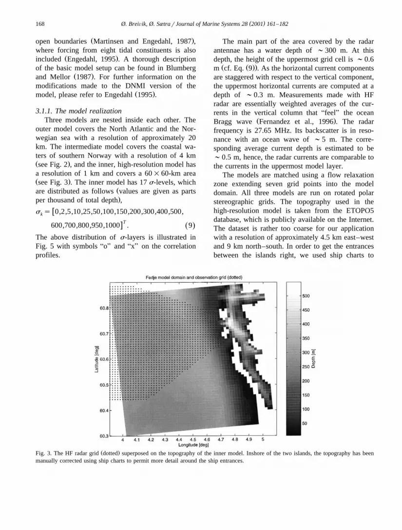
3.1.1. The model realizationThree models are nested inside each other. The

outer model covers the North Atlantic and the Nor-wegian sea with a resolution of approximately 20km. The intermediate model covers the coastal wa-ters of southern Norway with a resolution of 4 kmŽ .see Fig. 2 , and the inner, high-resolution model hasa resolution of 1 km and covers a 60=60-km areaŽ .see Fig. 3 . The inner model has 17 s-levels, which

Žare distributed as follows values are given as parts.per thousand of total depth ,

ws s 0,2,5,10,25,50,100,150,200,300,400,500,k

Tx600,700,800,950,1000 . 9Ž .The above distribution of s-layers is illustrated inFig. 5 with symbols AoB and AxB on the correlationprofiles.

The main part of the area covered by the radarantennae has a water depth of ;300 m. At thisdepth, the height of the uppermost grid cell is ;0.6

Ž Ž ..m cf. Eq. 9 . As the horizontal current componentsare staggered with respect to the vertical component,the uppermost horizontal currents are computed at adepth of ;0.3 m. Measurements made with HFradar are essentially weighted averages of the cur-rents in the vertical column that AfeelB the ocean

Ž .Bragg wave Fernandez et al., 1996 . The radarfrequency is 27.65 MHz. Its backscatter is in reso-nance with an ocean wave of ;5 m. The corre-sponding average current depth is estimated to be;0.5 m, hence, the radar currents are comparable tothe currents in the uppermost model layer.

The models are matched using a flow relaxationzone extending seven grid points into the modeldomain. All three models are run on rotated polarstereographic grids. The topography used in thehigh-resolution model is taken from the ETOPO5database, which is publicly available on the Internet.The dataset is rather too coarse for our applicationwith a resolution of approximately 4.5 km east–westand 9 km north–south. In order to get the entrancesbetween the islands right, we used ship charts to

Ž .Fig. 3. The HF radar grid dotted superposed on the topography of the inner model. Inshore of the two islands, the topography has beenmanually corrected using ship charts to permit more detail around the ship entrances.


manually correct the topography of the inner model.This explains why Fig. 3 exhibits rather more detailin the estuary than along the coast. Tides are in-cluded in the intermediate model and are propagatedas a barotropic signal into the nested model. No icemodel is included, as we are in a permanently ice-freepart of the Norwegian Sea. Monthly mean values forriver runoff are included in all three models. Thewind fields and boundary values are updated every 3h. The outer models are forced with 50-km resolu-tion winds from a limited area atmospheric modelŽ .LAM . The inner model is forced using winds froma 10-km resolution atmospheric model to includetopographic effects near the coast. Both atmosphericmodels and the two outer ocean models are runroutinely by DNMI.

3.1.2. The model error statisticsAs explained in Section 2.3, the assimilation

scheme requires a reference run to compute themodel error covariance matrix. In our case, the modelperiod was Feb.–Mar. 2000, and consequently weran the model for the same period in 1999 with asampling period D ts5.5 h, assuming that Aon theaverageB this model run would pick up the importantcorrelations inherent to the model state. The choiceof D t is guided by the observations made in Section2.3 that integer multiples of the major tidal con-stituents should be avoided. A period of 5.5 h willmarch slowly through the tidal cycle and thus avoidsampling only, say, the high tide and the ebb.

The result of this reference run was then scruti-nized and found to yield sensible results. The fullcorrelation matrix of the model can be seen as asix-dimensional object,

Corr cX x ,c X x , 10Ž . Ž . Ž .Ž .1 2

XŽ . XŽ .where c x and c x may assume all model1 2

variables in all different grid points in the modeldomain.

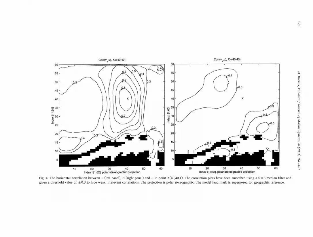
In Fig. 4, a slice through the model correlationmatrix has been made by freezing x at grid point2Ž .40,40,1 , marked with an AXB. This point waschosen because it lies in the centre of the radarcoverage. The model grid orientation is such that uis the alongshore current and Õ the across-shorecurrent. The across-shore current correlation showsthe expected behaviour of decorrelation with radial

distance. Further, the cross-correlation between uand Õ is found to be quite strong. Its maximum isshifted away from the location X, meaning that themaximum cross-correlation does not occur on thespot.

The vertical correlation structure with the surfaceŽ .current in point X 40,40,1 is shown in Fig. 5. The

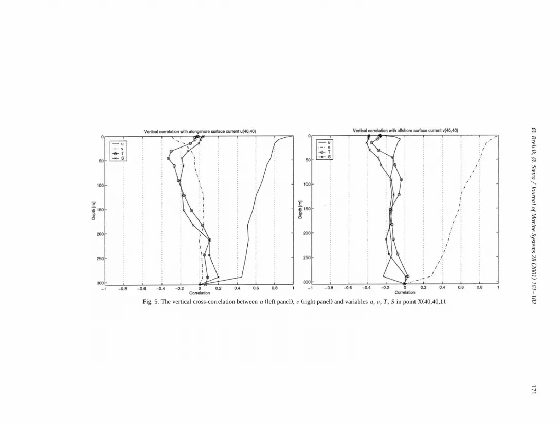
model layer depths are indicated with symbols AoBand AxB in the cross-correlation with T and S. Asseen, the model resolves very well the upper 50 m ofthe ocean. This is necessary to capture the influenceof the atmosphere on the oceanic mixed layer. Ingeneral, the surface currents do not correlate stronglywith the hydrography of the underlying water masses.The strongest correlations are of the order of y0.4.

The across-shore current exhibits a slightlystronger correlation with the hydrography than thealong-shore current. Negative correlation indicatesthat across-shore currents advect fresh and cold

Žcoastal waters away from the coast remember thatŽ .the location of the point X 40,40 is quite far from

.shore . The along-shore surface current u is com-pletely detached from the hydrography and only atabout 50-m depth does the correlation rise above anabsolute value of 0.2.

The model statistics reveal a strong surface cur-rent to deeper current correlation, but a significantlyweaker cross correlation between current compo-nents. Note also the immediate drop in correlation atthe surface to about 0.8 at 20-m depth. This illus-trates how the wind energy is distributed in the upperwater column.

3.2. The data

Our observations are taken from a beam formingphased array HF radar called AWellen RadarBŽ .WERA . The radar is operated by the University ofHamburg and was temporarily mounted on the is-lands Lyngøy and Fedje. Each radar array measuresthe radial component of the surface current. For awalk through the theoretical underpinnings of thecurrent measurements, please refer to Essen et al.Ž . Ž .1999 , Gurgel and Antonischki 1997 and Gurgel et

Ž .al. 1999 . The radar range is affected by the seastate, atmospheric disturbances, radio interferenceand sun spot activity. Fig. 1 illustrates the variabilityin radar coverage.

()

Ø.B

reiÕik,Ø

.Sætra

rJournalof

Marine

Systems

282001

161–

182170

Ž . Ž . Ž .Fig. 4. The horizontal correlation between Õ left panel , u right panel and Õ in point X 40,40,1 . The correlation plots have been smoothed using a 6=6-median filter andgiven a threshold value of "0.3 to hide weak, irrelevant correlations. The projection is polar stereographic. The model land mask is superposed for geographic reference.

()

Ø.B

reiÕik,Ø

.Sætra

rJournalof

Marine

Systems

282001

161–

182171

Ž . Ž . Ž .Fig. 5. The vertical cross-correlation between u left panel , Õ right panel and variables u, Õ, T , S in point X 40,40,1 .


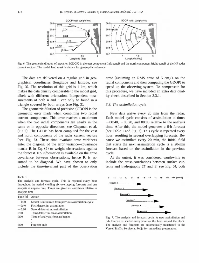
Ž . Ž . Ž .Fig. 6. The geometric dilution of precision GDOP in the east component left panel and the north component right panel of the HF radarcurrent vectors. The model land mask is shown for geographic reference.

The data are delivered on a regular grid in geo-Žgraphical coordinates longitude and latitude, see

.Fig. 3 . The resolution of this grid is 1 km, whichmakes the data density comparable to the model grid,albeit with different orientation. Independent mea-surements of both u and Õ can only be found in a

Ž .triangle covered by both arrays see Fig. 3 .Ž .The geometric dilution of precision GDOP is the

geometric error made when combining two radialcurrent components. This error reaches a maximumwhen the two radial components are nearly in thesame or in opposite directions, see Chapman et al.Ž .1997 . The GDOP has been computed for the eastand north components of the radar current vectorsŽ .see Fig. 6 . These time-invariant error variancesenter the diagonal of the error variance–covariance

Ž .matrix R in Eq. 2 to weight observations againstthe forecast. No information is available on the errorcovariance between observations, hence R is as-sumed to be diagonal. We have chosen to onlyinclude the time-invariant part of the observation

Table 1The analysis and forecast cycle. This is repeated every hourthroughout the period yielding six overlapping forecasts and oneanalysis at anyone time. Times are given as lead times relative toanalysis time

w xTime h Action

y1:00 Model is initialized from previous assimilation cycley0:40 First dataset in, assimilationy0:20 Second dataset in, assimilation0:00 Third dataset in, final assimilation0:00 Time of analysis, forecast begins. .. .. .6:00 Forecast ends

Žerror assuming an RMS error of 5 cmrs on the.radial components and then computing the GDOP to

speed up the observing system. To compensate forthis procedure, we have included an extra data qual-ity check described in Section 3.3.1.

3.3. The assimilation cycle

New data arrive every 20 min from the radar.Each model cycle consists of assimilation at timesy00:40, y00:20, and 00:00 relative to the analysistime. After this, the model generates a 6-h forecastŽ .see Table 1 and Fig. 7 . This cycle is repeated everyhour, resulting in several overlapping forecasts. Be-cause we assimilate every 20 min, the initial fieldthat starts the next assimilation cycle is a 20-minforecast based on the assimilation in the previouscycle.

At the outset, it was considered worthwhile toinclude the cross-correlations between surface cur-

Ž .rents and hydrography T and S, see Fig. 5 , both

Fig. 7. The analysis and forecast cycle. A new assimilation and6-h forecast is started every hour on the hour around the clock.The analysis and forecasts are automatically transferred to theVessel Traffic Service at Fedje for immediate presentation.


horizontally and vertically. This way the densityfield could be corrected to make it consistent withthe observed velocity field. However, even aftersmoothing the analysis using a second order Shapiro

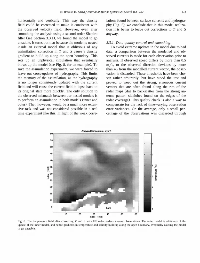
Ž .filter see Section 3.3.1 , we found the model to gounstable. It turns out that because the model is nestedinside an external model that is oblivious of anyassimilation, correction in T and S cause a densitygradient to build up along the open boundary. Thissets up an unphysical circulation that eventually

Ž .blows up the model see Fig. 8, for an example . Tosave the assimilation experiment, we were forced toleave out cross-updates of hydrography. This limitsthe memory of the assimilation, as the hydrographyis no longer consistently updated with the currentfield and will cause the current field to lapse back toits original state more quickly. The only solution tothe observed mismatch between our nested models is

Žto perform an assimilation in both models inner and.outer . That, however, would be a much more exten-

sive task and was not considered possible in a realtime experiment like this. In light of the weak corre-

lations found between surface currents and hydrogra-Ž .phy Fig. 5 , we conclude that in this model realiza-

tion it is better to leave out corrections to T and Sanyway.

3.3.1. Data quality control and smoothingTo avoid extreme updates in the model due to bad

data, a comparison between the modelled and ob-served currents is made for each observation prior toanalysis. If observed speed differs by more than 0.5mrs, or the observed direction deviates by morethan 45 from the modelled current vector, the obser-vation is discarded. These thresholds have been cho-sen rather arbitrarily, but have stood the test andproved to weed out the strong, erroneous currentvectors that are often found along the rim of the

Žradar maps due to backscatter from the strong an-tenna pattern sidelobes found on the edges of the

.radar coverage . This quality check is also a way tocompensate for the lack of time-varying observationerror variances. On the average, only a small per-centage of the observations was discarded through

Fig. 8. The temperature field after correcting T and S with HF radar surface current observations. The outer model is oblivious of theupdate of the inner model, and hence gradients in temperature and salinity build up along the open boundary, eventually causing the modelto go unstable.


Ž .this procedure less than 5% . However, in situationswhere the radar performed poorly, larger amounts ofdata were discarded.

Further, the assimilation sometimes adds too muchfine structure to the model fields. To remove this butretain the longer wavelengths, we chose to run aShapiro second-order nine-point filter after each

Žanalysis. It has been shown see Shapiro, 1970 or.Haltiner and Williams, 1980 that the Shapiro filter

Žremoves the A2D xB wave completely the shortestwave that can be represented, dictated by the Nyquist

.frequency , while the longer wavelengths are notŽmuch dampened zero damping for infinite wave-

.length . The A10D xB wave is attenuated by less than10%.

3.3.2. Restarting the modelThe ocean model uses centered differences in

Ž .space and time leapfrog scheme for the integrationof the horizontal momentum equations.

As a demonstration of the scheme, we take theone-dimensional advection equation

Eu Euqc s0, 11Ž .

Et Ex

Ž .where c is the constant advection velocity. Appliedto this equation, the leapfrog scheme becomes

D tnq1 ny1 n nu su qc u yu . 12Ž .Ž .i i iq1 iy1

D x

Here, i is the spatial index and n the temporal index.Further, D x and D t represent the spatial and tempo-ral resolution, respectively.

The assimilation scheme is invoked at time t ,n

which is incompatible with the above scheme be-cause it involves t , and hence the correctionsny1

introduced by the assimilation would not be propa-Žgated forward in time as the scheme AleapfrogsB

.past time n from time ny1 to nq1 . To circum-

Fig. 9. The assimilation skill measured in level of kinetic energy. The ratio of modelled kinetic energy to the observed kinetic energy isŽ . Ž .plotted for the free run model leftmost box-plot , the analysis, and the forecasts, numbered in forecast lead time 1 to 6 . The box-plots

Ž .consist of a box covering the middle 50% of the data quartile to quartile , the median line dividing the box, and whiskers indicating theextent of the remaining data. Outliers are plotted as individual crosses.


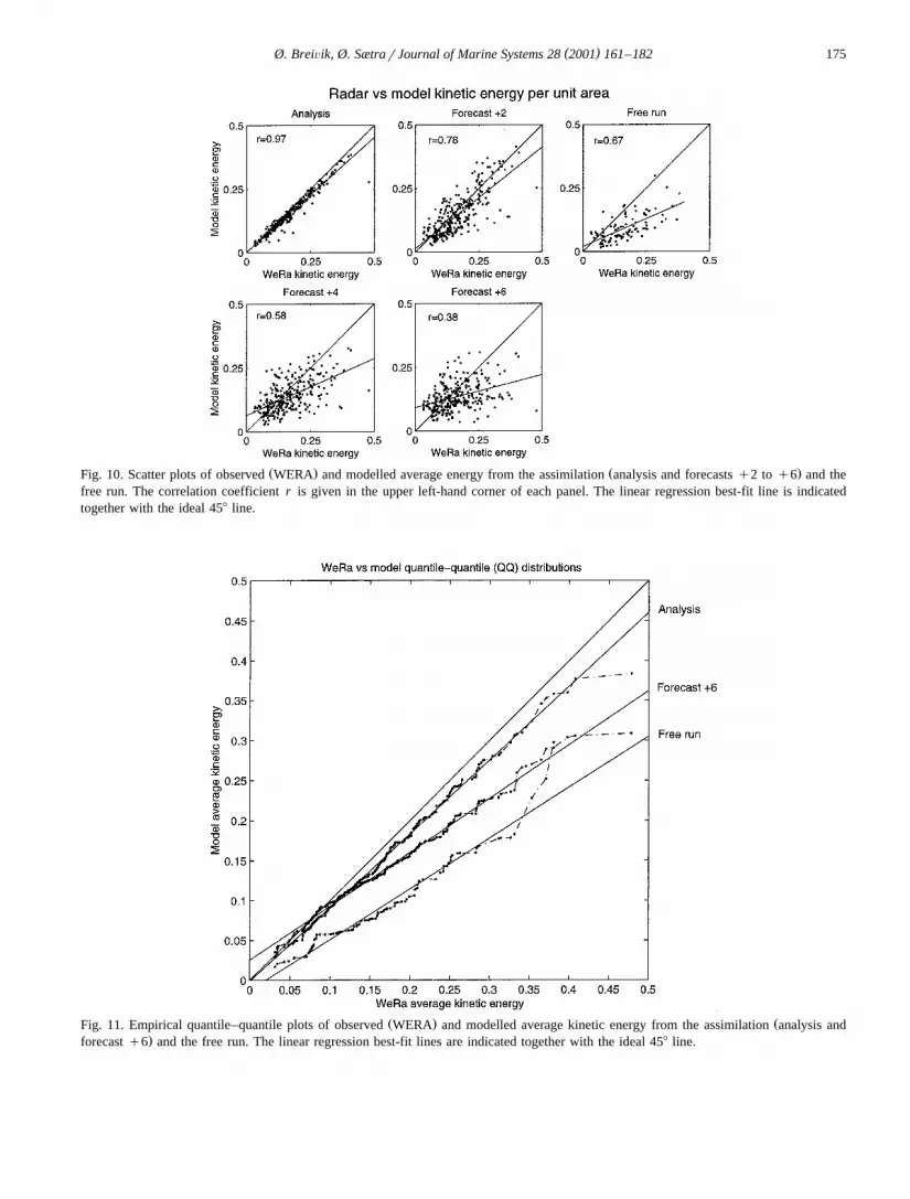
Ž . Ž .Fig. 10. Scatter plots of observed WERA and modelled average energy from the assimilation analysis and forecasts q2 to q6 and thefree run. The correlation coefficient r is given in the upper left-hand corner of each panel. The linear regression best-fit line is indicatedtogether with the ideal 458 line.

Ž . ŽFig. 11. Empirical quantile–quantile plots of observed WERA and modelled average kinetic energy from the assimilation analysis and.forecast q6 and the free run. The linear regression best-fit lines are indicated together with the ideal 458 line.


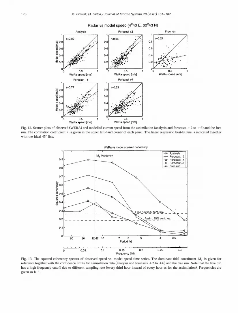
Ž . Ž .Fig. 12. Scatter plots of observed WERA and modelled current speed from the assimilation analysis and forecasts q2 to q6 and the freerun. The correlation coefficient r is given in the upper left-hand corner of each panel. The linear regression best-fit line is indicated togetherwith the ideal 458 line.

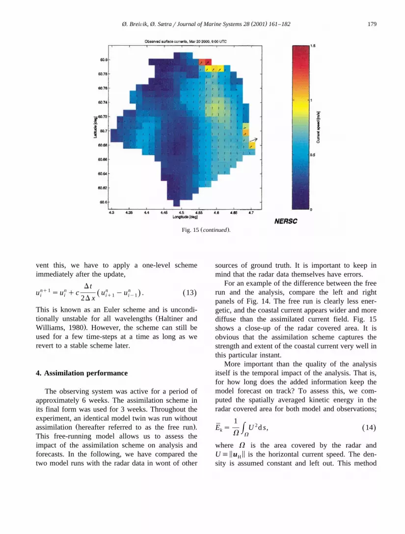
Fig. 13. The squared coherency spectra of observed speed vs. model speed time series. The dominant tidal constituent M is given for2Ž .reference together with the confidence limits for assimilation data analysis and forecasts q2 to q6 and the free run. Note that the free run

Ž .has a high frequency cutoff due to different sampling rate every third hour instead of every hour as for the assimilation . Frequencies aregiven in hy1.


Ž . ŽFig. 14. Upper panel: analysed surface current field assimilation . Lower panel: surface current field of the free-running model no.assimilation .


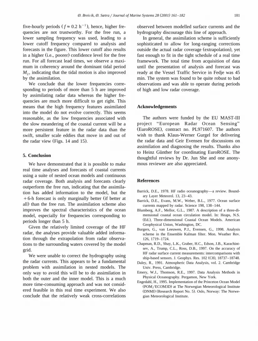
Fig. 15. Same as previous figure zoomed in on the area covered by the radar. Radar data are shown in the third panel for comparison.Arrows are only indicative of direction, colour scale gives speed.


Ž .Fig. 15 continued .

vent this, we have to apply a one-level schemeimmediately after the update,

D tnq1 n n nu su qc u yu . 13Ž .Ž .i i iq1 iy12D x

This is known as an Euler scheme and is uncondi-Žtionally unstable for all wavelengths Haltiner and

.Williams, 1980 . However, the scheme can still beused for a few time-steps at a time as long as werevert to a stable scheme later.

4. Assimilation performance

The observing system was active for a period ofapproximately 6 weeks. The assimilation scheme inits final form was used for 3 weeks. Throughout theexperiment, an identical model twin was run without

Ž .assimilation hereafter referred to as the free run .This free-running model allows us to assess theimpact of the assimilation scheme on analysis andforecasts. In the following, we have compared thetwo model runs with the radar data in wont of other

sources of ground truth. It is important to keep inmind that the radar data themselves have errors.

For an example of the difference between the freerun and the analysis, compare the left and rightpanels of Fig. 14. The free run is clearly less ener-getic, and the coastal current appears wider and morediffuse than the assimilated current field. Fig. 15shows a close-up of the radar covered area. It isobvious that the assimilation scheme captures thestrength and extent of the coastal current very well inthis particular instant.

More important than the quality of the analysisitself is the temporal impact of the analysis. That is,for how long does the added information keep themodel forecast on track? To assess this, we com-puted the spatially averaged kinetic energy in theradar covered area for both model and observations;

12E s U d s, 14Ž .Hk

V V

where V is the area covered by the radar and5 5U' u is the horizontal current speed. The den-H

sity is assumed constant and left out. This method


has the advantage of appreciating a corrected currentŽ .field typically the coastal current even when the

current maximum is slightly dislocated by the modelyet still improved over the free run.

Fig. 9 shows the ratio of the model fields to themod obsobserved fields, E rE . As can be seen, the freek k

run underestimates the energy level of the coastalŽ .current roughly by 50% . The analysis is a signifi-

Ž .cant improvement over the free run same figure ,with an energy level on a par with what is observed.After analysis, the forecasts spread out quickly, butretain an average energy level well above that for thefree-running model even after a 6-h forecast.

The scatter plot is a more conventional way tocompare datasets. Fig. 10 shows how the energylevel decorrelates as the forecast time increases. At

Ž .the time of analysis the assimilation itself , thefields match up almost perfectly. Two hours fromanalysis, the correlation is still good, but as thebox-plots also suggested, there is a lot more spread.Another observation is that the best fit linear regres-sion line dips down compared to the ideal 458 line,which means that the energy level drops off withforecast lead time. Compared to the free run, itseems that forecasts up to 3 h correlate better withobservations.

The probability distributions of two datasets canbe compared with an empirical quantile–quantile

Žplot EQQ, see Kleiner and Graedel, 1980 or Wilks,. Ž .1995 . The cumulative distribution function CDF

of a dataset X is

t X XP t ' p t d t . 15Ž . Ž . Ž .HX Xy`

The CDF is a monotonically increasing function,hence its inverse Q 'Py1 may be found. TheX X

Ž . Ž . y1 Ž .median mid point is t sQ 0.5 sP 0.5 ,0.5 X Xy1 Ž .the upper quartile is P 0.75 , and so forth.X

Plotting these values against each other reveal differ-ences in the underlying probability distributions. If apopulation Y is a linear transform of X, i.e., YsaXqb, the quantiles will fall on straight line.

Fig. 11 shows the QQ-plots of average kineticenergy of the analysis, the q6-h forecast, and thefree run vs. radar data. The distribution of the analy-sis is almost identical to the radar data, with a slopeclose to unity. The q6-h forecast has a weakerslope, again suggesting that the forecasts are not able

to keep up the coastal current. However, the underly-ing distribution seems to be of the same form as theradar data. Finally, the free run displays an evenweaker energy field and stronger deviations from theradar distribution. All three datasets display somedeviations in the upper extreme tail.

Time series of current speed were extracted fromthe radar data and the model grid point nearest the

Ž X X .position 4840 E, 60843 N . This point was chosenbecause it is in the central area of interest for theVTS, and always covered by the radar, even insituations with very low radar coverage. Fig. 12shows the correlation between observed and mod-elled current speed. The free-running model corre-lates extremely poorly with observations in this par-ticular point and is clearly not able to capture theintensity of the coastal current.

Finally, the spectral characteristics of the mod-elled currents were studied. Time series of analysed

Ž .speed, forecasted speed at different lead times , andforecasts from the free run were compared to theradar data. The time series were subjected to acoherency analysis. The squared coherency spectrumbetween two time series is defined as

< < 2G fŽ .122g f ' , 16Ž . Ž .G f G fŽ . Ž .11 22

where G and G denote the power spectral den-11 22Ž .sity variance spectra of the observed and modelled

time series, and G is the complex cross-spectral12Ž .density see Emery and Thomson, 1997 . Confidence

limits based on the number of equivalent degrees offreedom n are computed following ThompsonŽ .1979 ,

c2s1ya 1rŽny1. . 17Ž .ŽHere, a indicates confidence level as0.05 means

. 2a 95% confidence interval . The limiting value cgives the level up to which squared coherency values

Ž .may occur by chance Emery and Thomson, 1997 .Fig. 13 shows the squared coherency for the analy-sis, the free run, and forecast lead times q2, q4,and q6 h. Good coherency is found for the analysis.The coherency then drops regularly with forecastlead time until it becomes barely distinguishablefrom the free run at 6 h from the analysis time. Theforecasts cross the confidence limit at approximately


Ž y1 .five-hourly periods ff0.2 h , hence, higher fre-quencies are not trustworthy. For the free run, alower sampling frequency was used, leading to alower cutoff frequency compared to analysis andforecasts in the figure. This lower cutoff also results

Ž .in a higher i.e., poorer confidence level for the freerun. For all forecast lead times, we observe a maxi-mum in coherency around the dominant tidal periodM , indicating that the tidal motion is also improved2

by the assimilation.We conclude that the lower frequencies corre-

sponding to periods of more than 5 h are improvedby assimilating radar data whereas the higher fre-quencies are much more difficult to get right. Thismeans that the high frequency features assimilatedinto the model do not evolve correctly. This seemsreasonable, as the low frequencies associated withthe slow meandering of the coastal current will be amore persistent feature in the radar data than theswift, smaller scale eddies that move in and out of

Ž .the radar view Figs. 14 and 15 .

5. Conclusion

We have demonstrated that it is possible to makereal time analyses and forecasts of coastal currentsusing a suite of nested ocean models and continuousradar coverage. Both analysis and forecasts clearlyoutperform the free run, indicating that the assimila-tion has added information to the model, but the

Žq6-h forecast is only marginally better if better at.all than the free run. The assimilation scheme also

improves the spectral characteristics of the oceanmodel, especially for frequencies corresponding toperiods longer than 5 h.

Given the relatively limited coverage of the HFradar, the analyses provide valuable added informa-tion through the extrapolation from radar observa-tions to the surrounding waters covered by the modelgrid.

We were unable to correct the hydrography usingthe radar currents. This appears to be a fundamentalproblem with assimilation in nested models. Theonly way to avoid this will be to do assimilation inboth the outer and the inner model. This is a muchmore time-consuming approach and was not consid-ered feasible in this real time experiment. We alsoconclude that the relatively weak cross-correlations

observed between modelled surface currents and thehydrography discourage this line of approach.

In general, the assimilation scheme is sufficientlysophisticated to allow for long-ranging corrections

Ž .outside the actual radar coverage extrapolation , yetfast enough to fit in the tight schedule of a real timeframework. The total time from acquisition of datauntil the presentation of analysis and forecast wasready at the Vessel Traffic Service in Fedje was 45min. The system was found to be quite robust to badobservations and was able to operate during periodsof high and low radar coverage.

Acknowledgements

The authors were funded by the EU MAST-IIIproject AEuropean Radar Ocean SensingBŽ .EuroROSE , contract no. PL971607. The authorswish to thank Klaus-Werner Gurgel for deliveringthe radar data and Geir Evensen for discussions onassimilation and diagnosing the results. Thanks alsoto Heinz Gunther for coordinating EuroROSE. The¨thoughtful reviews by Dr. Jun She and one anony-mous reviewer are also appreciated.

References

Barrick, D.E., 1978. HF radio oceanography—a review. Bound-ary Layer Meteorol. 13, 23–43.

Barrick, D.E., Evans, M.W., Weber, B.L., 1977. Ocean surfacecurrents mapped by radar. Science 198, 138–144.

Blumberg, A.F., Mellor, G.L., 1987. A description of a three-di-mensional coastal ocean circulation model. In: Heaps, N.S.Ž .Ed. , Three-dimensional Coastal Ocean Models. AmericanGeophysical Union, Washington, DC.

Burgers, G., van Leeuwen, P.J., Evensen, G., 1998. Analysisscheme in the Ensemble Kalman filter. Mon. Weather Rev.126, 1719–1724.

Chapman, R.D., Shay, L.K., Graber, H.C., Edson, J.B., Karachint-sev, A., Trump, C.L., Ross, D.B., 1997. On the accuracy ofHF radar surface current measurements: intercomparisons with

Ž .ship-based sensors. J. Geophys. Res. 102 C8 , 18737–18748.Daley, R., 1991. Atmospheric Data Analysis, vol. 2. Cambridge

Univ. Press, Cambridge.Emery, W.J., Thomson, R.E., 1997. Data Analysis Methods in

Physical Oceanography. Pergamon, New York.Engedahl, H., 1995. Implementation of the Princeton Ocean Model

Ž .POMrECOM3D at The Norwegian Meteorological InstituteŽ . Ž .DNMI Research Report No. 5 . Oslo, Norway: The Norwe-gian Meteorological Institute.


Essen, H.-H., Gurgel, K.-W., Schlick, T., 1999. On the accuracyof current measurements by means of HF radar. IEEE J.Oceanic Eng. 1–10, Submitted for publication.

Evensen, G., 1994. Sequential data assimilation with a nonlinearquasi-geostrophic model using Monte Carlo methods to fore-

Ž .cast error statistics. J. Geophys. Res. 99 C5 , 10143–10162.Evensen, G., 1997. Advanced data assimilation for strongly non-

linear dynamics. Mon. Weather Rev. 125, 1342–1354.Fernandez, D.M., Vesecky, J.F., Teague, C.C., 1996. Measure-

ments of upper ocean surface current shear with high-frequencyŽ .radar. J. Geophys. Res. 101 C12 , 28615–28625.

Gill, A.E., 1982. Atmosphere–Ocean Dynamics, vol. 30. Aca-demic Press, San Diego, CA.

Glenn, S.M., Boicourt, W., Parker, B., Dickey, T.D., 2000. Opera-tional observation networks for ports, a large estuary and an

Ž .open shelf. Oceanography 13 1 , 12–23.Gurgel, K.-W., Antonischki, G., 1997. Measurements of surface

current fields with high spatial resolution by the HF radarWERA. Proceedings of the IGARSS ’97 Conference, pp.1820–1822.

Gurgel, K.-W., Antonischki, G., Essen, H.H., Schlick, T., 1999.Ž .Wellen Radar WERA : a new ground-wave HF radar for

Ž .ocean remote sensing. Coastal Eng. 37 3–4 , 219–234.Haltiner, G.J., Williams, R.T., 1980. Numerical Prediction and

Dynamic Meteorology. Wiley, New York.Ikeda, M., Johannessen, J.A., Lygre, K., Sandven, S., 1989. A

process study of mesoscale meanders and eddies in the Norwe-gian Coastal Current. J. Phys. Oceanogr. 19, 20–35.

Johannessen, J.A., Svendsen, E., Sandven, S., Johannessen, O.M.,Lygre, K., 1989. Three-dimensional structure of mesoscale

eddies in the Norwegian Coastal Current. J. Phys. Oceanogr.19, 3–19.

Kleiner, B., Graedel, T.E., 1980. Exploratory data analysis in thegeophysical sciences. Rev. Geophys. Space Phys. 18, 699–717.

Kowalik, Z., Murty, T.S., 1993. Numerical Modeling of OceanDynamics, vol. 4. World Scientific Publishing, New York.

Martinsen, E.A., Engedahl, H., 1987. Implementation and testingof a lateral boundary scheme as an open boundary condition ina barotropic ocean model. Coastal Eng. 11, 603–627.

Mellor, G.L., Yamada, T., 1982. Development of a turbulentclosure model for geophysical fluid problems. Rev. Geophys.Space Phys. 20, 851–875.

Mesinger, F., Arakawa, A., 1976. Numerical Methods Used inŽ .Atmospheric Models GARP Publications Series No. 17 .

World Meteorological Organization.Oke, P.R., Allen, J.S., Miller, R.N., Egbert, G.D., Kosro, P.M.,

2000. Assimilation of surface velocity data into a primitiveŽ .equation coastal ocean model. J. Geophys. Res. Oceans ,

Submitted for publication.Richardson, L.F., 1922. Weather Prediction by Numerical Process.

Cambridge Univ. Press, Cambridge, reprinted Dover, 1965.Shapiro, R., 1970. Smoothing, filtering, and boundary effects.

Rev. Geophys. Space Phys. 8, 359–387.Song, Y., Haidvogel, D.B., 1994. A semi-implicit ocean circula-

tion model using a generalized topography following coordi-nate system. J. Comput. Phys. 115, 228–244.

Thompson, R.O.R.Y., 1979. Coherence significance levels. J.Atmos. Sci. 36, 2020–2021.

Wilks, D.S., 1995. Statistical Methods in the Atmospheric Sci-ences. Academic Press, London.

Real time assimilation of HF radar currents into a coastal ocean model

Documents

Transcript of Real time assimilation of HF radar currents into a coastal ocean model