Real estate portfolio diversification by property type and region

Real estateportfolio

diversification

39

Real estate portfoliodiversification by property

type and regionPiet M.A. Eichholtz

Limburg Institute of Financial Economics, University of Limburg,The Netherlands,Martin Hoesli

Haute Ecole de Commerce, University of Geneva, Switzerland, andBryan D. MacGregor and Nanda Nanthakumaran

Centre for Property Research, Department of Land Economy, University of Aberdeen, UK

IntroductionThe top-down approach to portfolio allocation involves first, the decision as tohow much to allocate to each broad asset category; and second, a decision on anoptimal strategy within each asset category. In part, this involves themanagement of risk through diversification within the asset category.

For real estate portfolios, the conventional approach to defining diver-sification categories is to use property type and geographical region. Returnson different property types are believed to be driven by different economicfactors: for example, offices by office employment, shops by retail sales andindustrial properties by manufacturing output. Similarly, there should bedifferential performance across regions within each property type. However, theconventional approach to regional diversification is not without problems. Theregions normally used in the UK are administrative (that is, geographical)rather than functional. Both MacGregor[1] and McNamara[2] suggest that analternative approach to real estate portfolio construction may be to groupregions by economic base. In this way the economies underlying the propertymarkets within the unit of analysis will be more homogeneous. These ideas arerelated to work done in the USA, of which Hartzell et al.[3,4], Shulman andHopkins[5], Mueller and Ziering[6] and Mueller[7] are examples. There is also anextensive literature in economic geography which challenges the appropri-ateness of the geographic region as a unit of analysis.

In the USA, the issue of homogeneity of the spatial units has led to theconsideration of non-contiguous spatial groupings which combine areas ofsimilar economic base. Shulman and Hopkins[5], Mueller and Ziering[6] andMueller[7] all look at cities with similar dominant industry employment basessuch as manufacturing, transportation, government services, and so on. This islinked to the issue of “scale”: the larger the spatial unit, the less homogeneous

Journal of Property Finance,Vol. 6 No. 3, 1995, pp. 39-59.

MCB University Press, 0958-868X

Journal ofPropertyFinance6,3

40

will be its economic parts and the greater the scope for real estate portfoliodiversification within the region. Despite the associated problems, a propertytype/region classification using geographical regions has been used widely forreal estate portfolio construction in both the USA and the UK. Given the verydifferent sizes of the two countries, the size of these spatial units varies greatly.

Investors in real estate, typically through a process of naïve diversification,have constructed diversified portfolios, although in many cases more effectivestrategies could be adopted. One question which arises is, starting from oneproperty type in one region, whether it is more efficient to diversify acrossregions within a single property type or across property types within a region.That is to say, should investors remain in one region and seek diversification byproperty type within the region, or diversify across regions but remain withinthe property type. Another issue of importance is whether diversification byproperty type or region alone produces significantly worse results than fulldiversification by both property type and region.

This problem is relevant specifically to domestic investors, either British orAmerican, who have not yet entered the real estate market or have entered it onlymarginally, or international investors seeking exposure to a country and unlikelyto have sufficient investment funds to construct a portfolio diversified both byproperty type and region. A further practical consideration is that a morerestricted diversification strategy is likely to be less expensive to implement.

The remainder of this study is as follows. In the next section, UK and USproperty returns data are presented. This is followed by a review of the relevantliterature. In each of the next three sections the issue of property diversificationis approached with a different method. Each section starts with an outline of themethod used, and proceeds with the results for the UK and the USA. The firstanalysis involves the construction of correlation matrices for the returnsdisaggregated by property type and the matrices for returns disaggregated bygeographic region. These matrices are subsequently compared with a formaltest. In the second analysis, efficient frontiers for the USA and the UK areconstructed and studied. Finally, principal components analysis is undertakento investigate the similarities and differences between the returns for thedifferent property types and regions. The article ends with conclusions andsuggestions for further research.

DataThe US data used in this study come from the Russell NCREIF (RN) PropertyIndex. This index is available from 1978, but the breakdowns by both regionand property are only available from 1983. This article uses 40 quarterlyobservations for the period 1983-1992. The four property types which comprisethe commercial real estate market (office; research and development/ office;warehouse; and retail) are used for each of the four geographical regions (East,Mid-west, West and South)[8].

The UK data are from the Investors Chronicle Hillier Parker (ICHP) Index andcomprise 32 semi-annual observations from 1977 to 1993[9]. The UK data are


diversification

41

available disaggregated by three property types (offices; industrial; and retail)and by 11 regions (London, South East, South West, East Anglia, EastMidlands, West Midlands, Wales, Yorkshire and Humberside, North, NorthWest, Scotland). The data exclude shopping centres, mixed use buildings, andbusiness space. Data for the UK 11 regions were also aggregated to producethree “super” regions as suggested by Key et al.[10]. These regions are London,South and North.

There are a number of limitations with these data sources. First, the timeseries are relatively short. Second, both are appraisal based and there is agrowing literature on the problems of such indices as measures of marketmovement (see [11-16]). Third, the UK data are not from actual properties inactual portfolios, but rather hypothetical properties of a particularspecification. The rents quoted are not provable rent or actual rent but a valuer’sview of open market rent based on market knowledge[17]. Finally, differentindices can give different measures of the market[18]. However, whatever thelimitations, these indices probably give a reasonable view of market movementsand should be reasonably robust for analyses within the real estate market.Caution is required for cross-national comparisons, not least as the RN data arequarterly and the ICHP data biannual.

Literature reviewAs suggested above, two dimensions have traditionally been used fordiversification within real estate: property type and the geographical location ofthe properties. Miles and McCue[19], for example, used a sample of real estateinvestment trusts (REITs) and regressed the return to risk ratio againstvariables representing the extent of diversification by property type andgeographic region. They found evidence that diversification by property typeproduces higher risk-adjusted cash yields than geographic diversification. In alater study, Miles and McCue[20] used property-specific data from a largecommingled real estate fund. They found that correlations among returns onportfolios of properties differentiated by property type were significantly lessthan correlations among portfolios differentiated by region. Property type wasa more efficient means of diversification.

A contrary view comes from Hartzell et al.[3] who considered five ways ofdiversifying a real estate portfolio by: geographic region, property type,property size, metropolitan statistical area (MSA) and lease maturity. Thegeographical areas considered by these authors were the very broad areas ofthe USA used in this study (East, Mid-west, West and South). On the basis ofappraisal-based data on properties for the period from 1973-1983, they foundthat correlations between returns in the four regions were usually low. Theypointed, however, to the need for more detailed diversification categories.

A study by Grissom et al.[21], using the standard four regions (East, West,Mid-west and South), showed evidence for the existence of regional marketsfor industrial real estate. This suggests the importance of regional divers-ification. This was undertaken in an arbitrage pricing theory (APT) framework.


42

The authors showed that the risk premiums associated with common system-atic risk attributes vary for properties located in different regions. Also, thenumber of relevant factors was found to differ across regions.

On the premiss that there should be more diversification potential acrossregions with different economic bases than across purely political or geographicboundaries, several authors have suggested the segmentation of the marketaccording to economic factors. Such an approach has been used for some time bygeographers considering industrial diversification[22,23]. For real estate,Hartzell et al.[4] have used a hybrid of the geographic and economic approaches.They divided the USA into eight contiguous regions based on similar underlyingeconomic fundamentals (New England, Mid-Atlantic corridor, Old South,Industrial Mid-west, Farm belt, Mineral extraction area, Southern California andNorthern California). Their results show that eight-region diversificationprovides benefits that cannot be achieved from the traditional four-regiondiversification. This was confirmed by Malizia and Simons[24] who used“demand” variables of population, income and employment rather than realestate returns and found that the eight-region classification used by Hartzell etal.[4] in 1987 offered better diversification than either the traditional fourgeographical regions or an alternative eight-region geographical classification.

Shulman and Hopkins[5] broadened the concept of economic diversificationby analysing 60 MSAs, which they classified into homogeneous portfoliosbased on employment characteristics. These authors concluded that thisclassification should be superior to four- or eight-region diversification but didnot provide a test of this hypothesis. An approach based on economic factorswas also adopted by Corgel and Gay[25] who investigated whether repaymentrisks of mortgages could be reduced. They divided employment data for the 30largest standard metropolitan areas (SMAs) in the USA into eight industrygroups, and did mean-variance portfolio analysis on the thus obtained timeseries. This analysis was found to outperform other diversification strategiesnot based on economic characteristics.

For Europe, these findings were confirmed by Hartzell et al.[26] whocharacterized 74 commonly recognized European regions as diversified, or asspecialized in one out of nine industrial categories. The regions with a commonspecialization were scattered throughout Europe, so regionally diverseinvestments were not necessarily economically diverse.

A formal test of the superiority of economic-based diversification strategiesfor real estate portfolio diversification was undertaken by Mueller[7]. Hecompared the appropriateness of using the four-region classification, theclassification of Hartzell et al.[4] and his own classification. This latter comprisesnine economic categories based on one digit SIC codes: mining; government;manufacturing; finance, insurance and real estate; services; transportation;military; farm; and diversified. Each of the 316 MSAs of the USA wascategorized in one of these groups. Mueller reported that the four-regionclassification was least efficient in terms of diversification. The eight-regionclassification gave much better diversification results. He further showed that a


diversification

43

diversification strategy based on his own classification, which relies solely oneconomic base, provided even greater risk-adjusted return possibilities.

Stock market researchers have considered a similar question to the oneaddressed by this study, that is, whether diversification should be undertakenaccording to type of industry or according to country. Authors who haveexamined this issue used data for the individual stocks, which is a differentapproach from that used here. The conclusions of these studies are mixed.Roll[27], for example, found that each country’s industrial structure plays amajor role in explaining stock price behaviour. A contrary view is found inHeston and Rouwenhorst[28] who concluded that diversification acrosscountries within an industry is a much more effective tool for risk reductionthan industry diversification within a country.

Of the studies outlined above, only Miles and McCue[19] suggested thatdiversification by property type should be preferred to diversification byregion. Since that study was conducted, however, several researchers haveshown that economic rather than purely geographic regions should be used. Asa consequence, the conclusion by Miles and McCue probably stems from theinappropriateness of the large scale geographic classification they used whichdilutes differences between regions. Moreover, the time series on which theirstudy was based were relatively short. In this study, the use of UK real estatedata allows the issue of diversification by property type and region to beconsidered at a spatial scale not possible using US data. The results of threeseparate analyses are now considered.

Analysis of the correlation matricesMarkowitz[29,30] showed that the opportunities for risk reduction ininvestment portfolios are negative functions of the correlations between assetreturns. This implies that the benefits of geographic diversification can bedetermined by measuring the correlations between time series of real estatereturns aggregated by region. Similarly, correlating real estate returnsaggregated by property type can give information about the usefulness ofdiversification by property type. Deciding which one of the two approaches toreal estate diversification is more effective can be done by comparing thecorrelations of both approaches: the lower correlations imply whichdiversification strategy would be best.

One way to compare the property type and regional correlations is todetermine which of the two correlation matrices is lower. A formal andstraightforward approach to this was developed by Jennrich[31,32]. However, itcan only be used to compare two correlation matrices of equal dimension. Thus,it is only possible to compare the regional and property type correlationmatrices when the numbers of regional and property type classifications areequal. For the USA, a four-region by four-property type disaggregation is usedand for the UK a three-region by three-property type disaggregation.

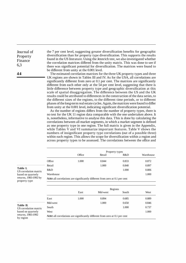
The correlation matrices for the four US property types and four US regionsare shown in Tables I and II. All correlations are significantly different fromzero at 0.1 per cent. The matrices are significantly different from each other at


44

the 7 per cent level, suggesting greater diversification benefits for geographicdiversification than for property type diversification. This supports the resultsfound in the US literature. Using the Jennrich test, we also investigated whetherthe correlation matrices differed from the unity matrix. This was done to see ifthere was significant potential for diversification. The matrices were found tobe different from unity at the 0.001 level.

The estimated correlation matrices for the three UK property types and threeUK regions are shown in Tables III and IV. As for the USA, all correlations aresignificantly different from zero at 0.1 per cent. The matrices are significantlydifferent from each other only at the 54 per cent level, suggesting that there islittle difference between property type and geographic diversification at thisscale of spatial disaggregation. The difference between the US and the UKresults could be attributed to differences in the construction of the data series, tothe different sizes of the regions, to the different time periods, or to differentphases of the long-term real estate cycles. Again, the matrices were found to differfrom unity at the 0.001 level, indicating significant diversification potential.

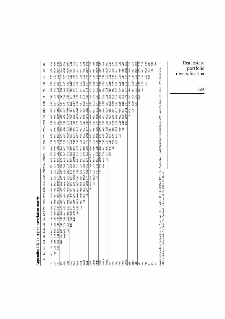
As the number of regions differs from the number of property types, there isno test for the UK 11 region data comparable with the one undertaken above. Itis, nonetheless, informative to analyse this data. This is done by calculating thecorrelations between all market segments, in which a market segment is definedas one property type in one region. The full matrix is given in the Appendix,while Tables V and VI summarize important features. Table V shows thenumbers of insignificant property type correlations (out of a possible three)within each region. This allows the scope for diversification within a region andacross property types to be assessed. The correlations between the office and

Table I.US correlation matrixbased on quarterlyreturns, 1983-1992 byproperty type

Property typesOffice Retail R&D Warehouse

Office 1.000 0.844 0.833 0.872

Retail 1.000 0.840 0.897

R&D 1.000 0.806

Warehouse 1.000

Note: all correlations are significantly different from zero at 0.1 per cent

Table II.US correlation matrixbased on quarterlyreturns, 1983-1992by region

RegionsEast Mid-west South West

East 1.000 0.894 0.685 0.889

Mid-west 1.000 0.650 0.846

South 1.000 0.737

West 1.000



diversification

45

industrial markets are always significant but the correlations between retail andthe other two property types are weakest the further the region is from London,suggesting greater scope for within region diversification.

When the insignificant correlations are grouped by property type (Table VI),it is clear that there are strong correlations within property types and acrossregions, particularly within retail. There are also strong correlations betweenthe industrial and office property types and less significant correlationsbetween retail property and the other two property types. These correlationsare to be expected as both the industrial and office markets are driven by profitsin the economy and the retail market is driven by wages; thus shocks to profitswill affect the office and industrial markets and shocks to wages will affect theretail market[1].

Table V shows the percentage of significant correlations for each marketsegment with all other market segments. There are two striking features: first,the percentage of significant correlations is high in the office and industrialmarkets and relatively much lower for the retail market; and second, thepercentage of significant correlations decreases with the distance from Londonand the South East (the region around London).

In the UK it is a conventional wisdom that retail property offers least scopefor regional diversification: retail sales tend not to have strong regionaldifferences and the supply response of the retail property market does not differsignificantly across regions. This is consistent with the results presented inTables V and VI. In contrast, in the office market, as the London market isdriven by the financial sector and has a strong international dimension,opportunities should exist for regional diversification within the office market.

Table III.UK correlation matrixbased on semi-annualreturns, 1977-1993 by

property type

Property typesIndustrial Office Retail

Industrial 1.000 0.848 0.622

Office 1.000 0.702

Retail 1.000


Table IV.UK correlation matrixbased on semi-annualreturns, 1977-1993 by

region

RegionsLondon South North

London 1.000 0.847 0.732

South 1.000 0.841

North 1.000



46

There is no evidence here to support this: the London market is highlycorrelated with the other regional office markets. This result may be aconsequence of the level of aggregation which does not treat the main financialcentre in the City of London separately from the other London office marketswhich are less specialized. The results for industrial property also show strongregional correlations within the property type.

In summary, the results show that the scope for diversification within aregion varies from region to region and is greatest the further from London,while the diversification within property type is generally limited but is betterfor office and industrial property. Retail property is poorly correlated witheither industrials or offices. Thus, full diversification by both property type andregion is to be preferred.

Table VI.Insignificantcorrelations betweenmarket segments byproperty type, based onsemi-annual returns,UK, 1977-1993

Industrial Office Retail

Industrial 4 6 62

Office 3 84

Retail 0

Note:A market segment is defined as one property type in one geographic region. Since three propertytypes and 11 regions are examined, there are 33 market segments.The insignificant correlationcoefficients (at 5 per cent) between one property type/region and another are grouped, for allregions, according to the two property types involved

Table V.UK correlations basedon semi-annual returnsfor 11 regions and threeproperty types,1977-1993

RegionL SE EA SW EM WM W NW YH N S Total

Insignificant property type correlations within regions a

Number 0 0 1 1 1 1 1 2 2 2 2 13

Significant correlations between market segments bIndustrial 93.8 96.9 90.6 93.8 87.5 75.0 84.4 68.8 68.8 65.6 37.5 78.4Office 90.6 93.8 62.5 71.9 62.5 87.5 68.8 65.6 65.6 65.6 65.6 72.7Retail 53.1 62.5 65.6 59.4 62.5 62.5 75.0 65.6 46.9 40.6 50.0 58.5Total 79.2 84.4 72.9 75.0 70.8 75.0 76.0 66.7 60.4 57.3 51.0 69.9

Notes:a Within each region there are three property type correlation coefficients. The number in each

cell in the table represents the number of correlations which are insignificant at 5 per cent. Otherthings being equal, the larger the number, the greater the scope for property type diversificationwithin the region

b A market segment is defined as one property type in one geographic region. Since threeproperty types and 11 regions are examined, there are 33 markets segments. The number ineach cell represents the percentage of correlations between the row (property type/column(region) and all other property type regions which are significant at 5 per cent


diversification

47

Analysis of the efficient frontiersWhile correlation matrices of asset returns provide information on one aspectof diversification, they do not consider the asset risks which, together with thecorrelations, determine portfolio risk. Nor do they consider the trade-offbetween risk and return and so do not give insights into the link between aninvestor’s relative risk aversion and an optimal diversification strategy. These,however, can be gained by comparing the efficient frontiers of the differentdiversification strategies. Three types of efficient frontiers are constructed:

(1) The four efficient frontiers for diversification within each property typebut across all regions.

(2) The four efficient frontiers for diversification within each region butacross all property types.

(3) The efficient frontier for full diversification across all property types andregions.

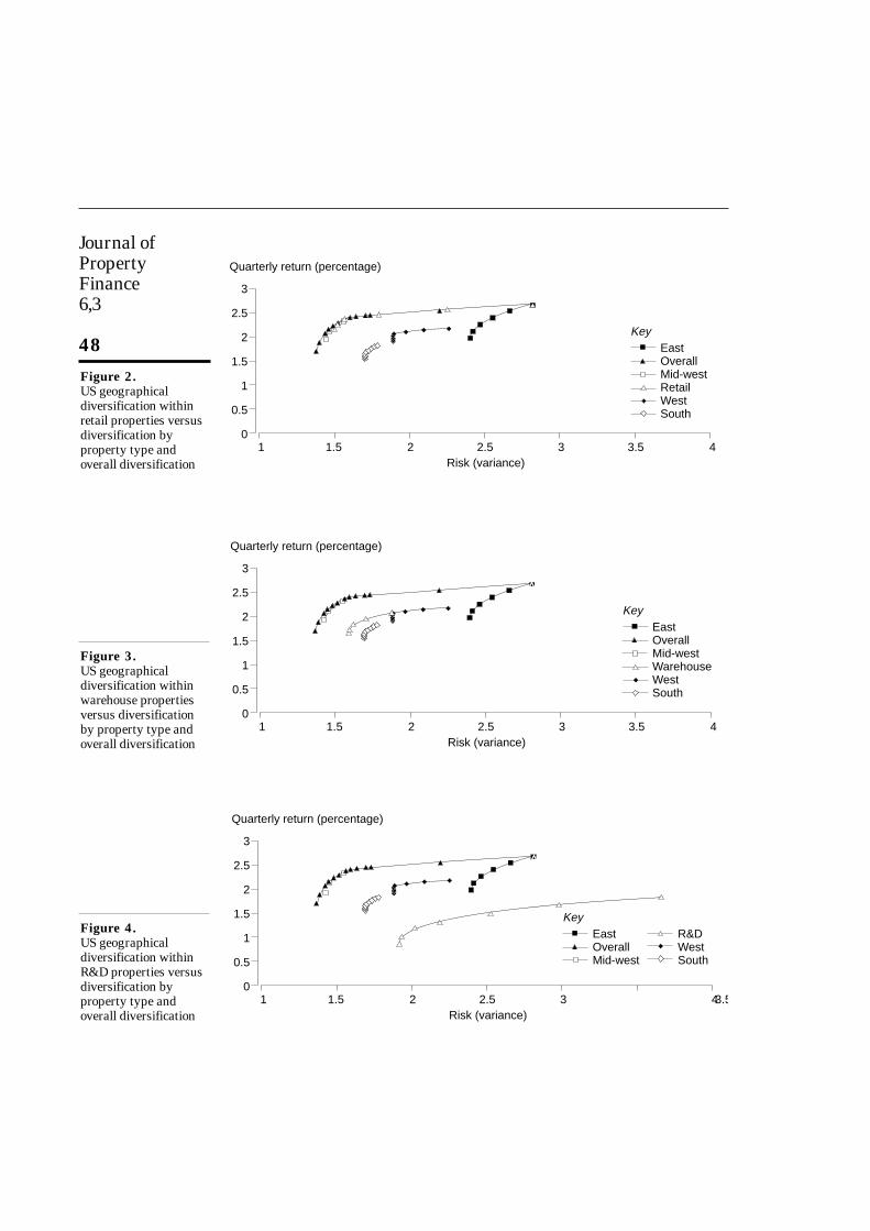
The results for the USA and the UK are shown in Figures 1 to 7. For eachcountry, a separate graph is presented for each property type showing: thefrontier for diversification within that one property type and across regions; thefour frontiers for diversification within each region and across property types;and the full diversification frontier. These graphs can be compared to see whichstrategy gives the best possible risk/return trade-off for different levels of riskaversion of the real estate investor.

US resultsThe efficient frontiers for the USA are provided in Figures 1 to 4. Figure 1shows clearly that for office and R&D/office properties the best strategy wouldhave been to diversify across property types within one region. Indeed, theregional frontiers, that is those frontiers which contain portfolios of differenttypes of real estate, all lie well above the property type frontier, which containsportfolios of geographically diversified properties of one type. This resultsuggests that an effective geographical diversification could not have beenachieved in office and R&D/office properties. These exhibits also show that for

3

2.5

2

1.5

1

0.5

01 1.5 2 2.5 3 3.5 4

Quarterly return (percentage)

Risk (variance)

KeyEastOverallMid-westOfficeWestSouth

Figure 1.US geographical

diversification withinoffice properties versus

diversification byproperty type and

overall diversification


48

Figure 2.US geographicaldiversification withinretail properties versusdiversification byproperty type andoverall diversification

3

2.5

2

1.5

1

0.5

01 1.5 2 2.5 3 3.5 4


Risk (variance)

KeyEastOverallMid-westRetailWestSouth

Figure 3.US geographicaldiversification withinwarehouse propertiesversus diversificationby property type andoverall diversification

3

2.5

2

1.5

1

0.5

01 1.5 2 2.5 3 3.5 4


Risk (variance)

KeyEastOverallMid-westWarehouseWestSouth

Figure 4.US geographicaldiversification withinR&D properties versusdiversification byproperty type andoverall diversification

3

2.5

2

1.5

1

0.5

01 1.5 2 2.5 3 3.54


Risk (variance)

KeyEastOverallMid-west

R&DWestSouth


diversification

49

office and R&D/office properties much of the diversification benefits have beenexploited when diversification within the property type has been undertaken:the overall frontier does not lie far above the regional frontiers.

For retail properties, there seems to exist more diversification potentialacross regions than within regions, as can be seen in Figure 2. Most of thediversification benefits are used when geographical diversification isundertaken. For warehouses, the conclusion is mixed: the property type frontierlies in between the geographic frontiers (Figure 3). Thus, diversification shouldhave taken place according to both property type and region. However, for eachproperty type, for very risk-averse investors in the Mid-west, diversificationacross property types within the region would have sufficed.

The results do not fully support the conclusion of the correlation matrixanalysis as they suggest that for two of the property types a between propertytypes and within region diversification strategy is better than a betweenregions and within property type diversification strategy. However, thecorrelation matrix analysis did not address precisely the same issue: it merelycompared correlations between property types and regions. It is clear fromthese results that there are property type differences contained within theaverage. Thus, the picture is mixed for the USA: no compelling evidence hasbeen found to suggest that in all cases a regional strategy should have beenpreferred to a property type strategy. Indeed, on balance, the oppositeconclusion might be suggested.

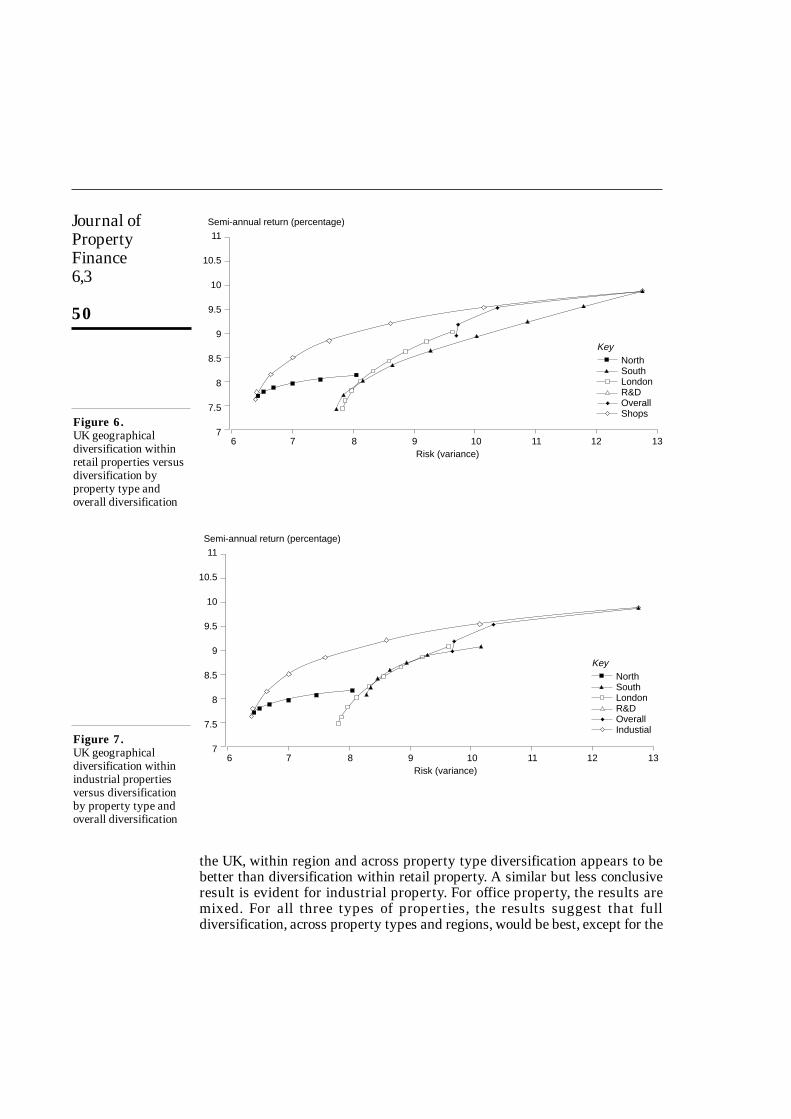
UK resultsThe efficient frontiers for the UK are provided in Figures 5 to 7. Since the UKregions are much smaller than the US regions, it is reasonable to expect thatthere should be greater opportunities for economic diversity across regions andso for diversification within each property type and across regions. However, in

Figure 5.UK geographical

diversification withinoffice properties versus

diversification byproperty type and

overall diversification

KeyNorthSouthLondon

OverallOffice

11

10.5

10

9.5

9

8.5

8

7.5

76 7 8 9 10 11 12

Semi-annual return (percentage)

Risk (variance)13


50

the UK, within region and across property type diversification appears to bebetter than diversification within retail property. A similar but less conclusiveresult is evident for industrial property. For office property, the results aremixed. For all three types of properties, the results suggest that fulldiversification, across property types and regions, would be best, except for the

11

10.5

10

9.5

9

8.5

8

7.5

76 7 8 9 10 11 12


Risk (variance)13

KeyNorthSouthLondonR&DOverallShops

11

10.5

10

9.5

9

8.5

8

7.5

76 7 8 9 10 11 12


Risk (variance)13

KeyNorthSouthLondonR&DOverallIndustial

Figure 6.UK geographicaldiversification withinretail properties versusdiversification byproperty type andoverall diversification

Figure 7.UK geographicaldiversification withinindustrial propertiesversus diversificationby property type andoverall diversification


diversification

51

most risk-taking and most risk-averse investors. As for the USA, this analysisdisaggregates the correlation matrix analysis. It confirms the earlier results.

Principal components analysisAnother way to analyse the benefits of the two diversification strategies isoffered by the arbitrage pricing theory (APT) as developed by Ross[33].Contrary to the capital asset pricing model (CAPM), where the only factorinfluencing returns is the market, the basic idea of the APT is that asset returnsare determined by a set of orthogonal factors, instead of just one factor.Although Ross does not indicate what these factors are, they most probably willbe related to economic activity. Chen et al.[34], for example, show that variablessuch as unexpected inflation, changes in the term structure of interest rates andchanges in industrial production explain stock returns. For real estate, Chan etal.[35] have used a similar approach and also found promising results.

Using the APT model diversification is based on the idea that risk reductioncan be obtained by investing across factors, instead of investing within factors.After all, if a portfolio is exposed to only one factor, it is not very welldiversified. An optimally diversified portfolio should be exposed to allimportant factors. The question is, then, to identify which factors areimportant. For this study this translates into the question: are property typeand/or geographic region important factors in generating real estate returns? Ifthey both are, one would have to diversify across both dimensions to obtainoptimal diversification. However, if only one dimension is found to beimportant, then that would be the dimension to keep in mind when building areal estate portfolio.

The analysis comprises two stages. The first stage involves the extraction ofa set of orthogonal factors from the real estate returns matrix. This is an (l × m× T ) matrix, where l is the number of property types, m is the number ofregions, and T is the number of observations. Each element of this matrixreflects the real estate return in market segment l, m at time t. The number offactors extracted is (l × m). For the factor extraction, one can use factor analysis,but Chamberlain and Rothschild[36] have found that principal componentsanalysis can be used to establish an approximate factor structure. This methodis computationally and conceptually simpler than factor analysis. Therefore,principal components analysis is used to extract common factors from the realestate returns matrix.

In this first stage of the analysis, the factors are just vectors of returns,without any clear relationship to economic variables. This stems directly fromRoss[33], who gives no indication as to what these factors might be. Establishingthe relationship between the factors and the property returns is the key to thesecond stage of the analysis. This is done simply by correlating the factors withthe original (l × m) individual property type/region real estate return series. Thecorrelation pattern provides information on whether the factors have thedimension of property type or geographic area. For example, if it is observedthat correlations show similar patterns among real estate returns for the same


52

property type across regions, it can be concluded that diversification is mostuseful across property types. On the other hand, similar correlation patternswithin a region for the different property types would imply that risk reductioncan be accomplished best by investing across different regions.

It is likely that one dominant factor and several less important ones will befound (this kind of result is typical in the empirical APT literature[34]). In thisstudy, this dominant factor can be thought of as the national real estate marketfactor. As the main interest of this study is within real estate diversificationrather than mixed-asset diversification, this national real estate market factor isnot a main concern. Therefore, the analysis is repeated to exclude the marketinfluence. This is done using two separate approaches. In the first, principalcomponents analysis is undertaken on the real estate returns in excess of thenational real estate market; in the second, in order to examine the robustness ofthe first approach, real estate returns are regressed on the real estate marketand principal components analysis is undertaken on the regression residuals.The resulting factors should provide a clearer picture of the dimensions of realestate returns.

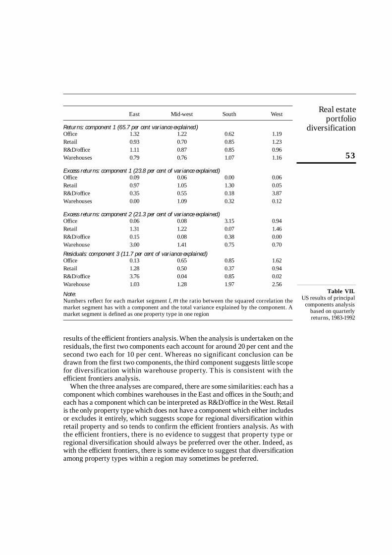
The relationship to be considered is that between factors (the components)and the return for the real estate market in each property type/region. Thus, thesquare of each correlation between the property type/region and the componentsis calculated. This gives the explanatory power of the components over the realestate return in each property type/region. However, this power is particularlyinteresting in relative terms. Therefore, the ratio between the squared correlationand the total variance explained by the component is calculated for each marketsegment l, m. This is a simple way to summarize and compare the structures ofthe components. This part of the analysis uses data for the US four propertytypes and regions and the UK three property types and regions.

US resultsThe results of the principal components analysis for the USA are shown inTable VII. As expected, for returns, the first component is dominant, accountingfor 65.7 per cent of the variance. As none of the other components accounts formore than 10 per cent of the variance, only the first is considered. None of thecomponents has a clear or pronounced dimension which is either property typeor region. The correlations with the market are generally high, particularly foroffices; there are relatively lower figures for warehouses and retail. This tends toconfirm the earlier results that there is limited scope for diversification acrossregions within offices and R&D/offices, some within warehouses and rathermore within retail. However, the comparison is far from conclusive.

The first two components of the excess returns each account for around 20per cent and the second two each for 10 per cent of the total variance. The firsttwo components are presented for illustration. Again the results show no clearregional or property type dimension and are open to various interpretations.The first and second components suggest little scope for diversification withinthe office and R&D/office property types respectively. This tends to confirm the


diversification

53

results of the efficient frontiers analysis. When the analysis is undertaken on theresiduals, the first two components each account for around 20 per cent and thesecond two each for 10 per cent. Whereas no significant conclusion can bedrawn from the first two components, the third component suggests little scopefor diversification within warehouse property. This is consistent with theefficient frontiers analysis.

When the three analyses are compared, there are some similarities: each has acomponent which combines warehouses in the East and offices in the South; andeach has a component which can be interpreted as R&D/office in the West. Retailis the only property type which does not have a component which either includesor excludes it entirely, which suggests scope for regional diversification withinretail property and so tends to confirm the efficient frontiers analysis. As withthe efficient frontiers, there is no evidence to suggest that property type orregional diversification should always be preferred over the other. Indeed, aswith the efficient frontiers, there is some evidence to suggest that diversificationamong property types within a region may sometimes be preferred.

Table VII.US results of principal

components analysisbased on quarterlyreturns, 1983-1992

East Mid-west South West

Returns: component 1 (65.7 per cent variance explained)Office 1.32 1.22 0.62 1.19Retail 0.93 0.70 0.85 1.23R&D/office 1.11 0.87 0.85 0.96Warehouses 0.79 0.76 1.07 1.16

Excess returns: component 1 (23.8 per cent of variance explained)Office 0.09 0.06 0.00 0.06Retail 0.97 1.05 1.30 0.05R&D/office 0.35 0.55 0.18 3.87Warehouses 0.00 1.09 0.32 0.12

Excess returns: component 2 (21.3 per cent of variance explained)Office 0.06 0.08 3.15 0.94Retail 1.31 1.22 0.07 1.46R&D/office 0.15 0.08 0.38 0.00Warehouse 3.00 1.41 0.75 0.70

Residuals: component 3 (11.7 per cent of variance explained)Office 0.13 0.65 0.85 1.62Retail 1.28 0.50 0.37 0.94R&D/office 3.76 0.04 0.85 0.02Warehouse 1.03 1.28 1.97 2.56

Note:Numbers reflect for each market segment l, m the ratio between the squared correlation themarket segment has with a component and the total variance explained by the component. Amarket segment is defined as one property type in one region


54

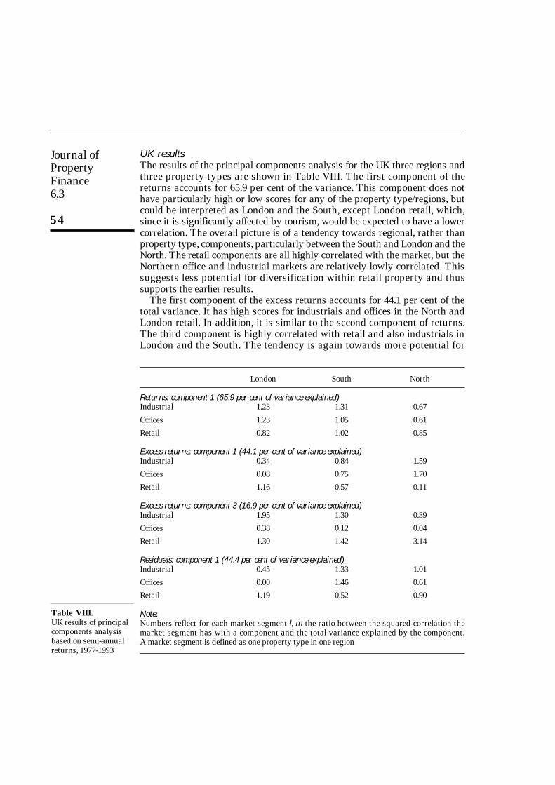
UK resultsThe results of the principal components analysis for the UK three regions andthree property types are shown in Table VIII. The first component of thereturns accounts for 65.9 per cent of the variance. This component does nothave particularly high or low scores for any of the property type/regions, butcould be interpreted as London and the South, except London retail, which,since it is significantly affected by tourism, would be expected to have a lowercorrelation. The overall picture is of a tendency towards regional, rather thanproperty type, components, particularly between the South and London and theNorth. The retail components are all highly correlated with the market, but theNorthern office and industrial markets are relatively lowly correlated. Thissuggests less potential for diversification within retail property and thussupports the earlier results.

The first component of the excess returns accounts for 44.1 per cent of thetotal variance. It has high scores for industrials and offices in the North andLondon retail. In addition, it is similar to the second component of returns.The third component is highly correlated with retail and also industrials inLondon and the South. The tendency is again towards more potential for

Table VIII.UK results of principalcomponents analysisbased on semi-annualreturns, 1977-1993

London South North

Returns: component 1 (65.9 per cent of variance explained)Industrial 1.23 1.31 0.67

Offices 1.23 1.05 0.61

Retail 0.82 1.02 0.85

Excess returns: component 1 (44.1 per cent of variance explained)Industrial 0.34 0.84 1.59

Offices 0.08 0.75 1.70

Retail 1.16 0.57 0.11

Excess returns: component 3 (16.9 per cent of variance explained)Industrial 1.95 1.30 0.39

Offices 0.38 0.12 0.04

Retail 1.30 1.42 3.14

Residuals: component 1 (44.4 per cent of variance explained)Industrial 0.45 1.33 1.01

Offices 0.00 1.46 0.61

Retail 1.19 0.52 0.90

Note:Numbers reflect for each market segment l, m the ratio between the squared correlation themarket segment has with a component and the total variance explained by the component.A market segment is defined as one property type in one region


diversification

55

regional diversification within a property type, rather than property typediversification within a region. For the residual returns, the first componentaccounts for 44.4 per cent of the variance. It has high correlations with allmarket segments except for London offices. The pattern is more mixed than forother analyses, suggesting potential for both regional and property typediversification.

When the three analyses are compared, there are some similarities: Londonretail and London offices are dissimilar from other property type/regions; andNorthern industrials and offices are different from the other office and industrialmarkets. Retail is the only property type which highly correlates with thecomponents but these explain little of the variance. The UK results suggest thatdiversification within property types and across regions is most effective, whilethe US results tend to suggest more scope for diversification across propertytypes within regions.

Conclusion and suggestions for further researchThe sections above have considered diversification within a real estate portfolio.Three forms of analysis and three data sets covering the USA and the UK atdifferent levels of geographical aggregation were used. The central researchissue was whether, starting from one property type in one region, it is moreeffective to diversify across regions within a single property type or acrossproperty types within a region. In general, it is possible to obtain a cleareranswer to this question in the USA than in the UK, although the answer variesfrom property type to property type. For retail property investments,diversification across regions is more effective, while this does not hold foroffice and office/R&D properties. For the UK, the opposite result was obtainedfor retail property and diversification across both property types and regionswas to be preferred for the other two property types.

The results for the USA suggest that office and office/R&D properties havesimilar performance across regions, whereas the retail sector has greaterdiversification across regions. In the UK, for the riskiest portfolios, diver-sification within London is almost as effective as countrywide diversification.

The results offer some insights into real estate performance and may offersome input into the determination of a diversification strategy for a real estateportfolio. There are two major qualifications on the results. The first is that theyare historical results and they may not be a good proxy for the futurecorrelations. Historical returns are unlikely to be a good proxy for futurereturns and that probably also holds for the correlations calculated betweenreal estate categories. Investigating sub-samples would be a good way todetermine the importance of this problem, but more observations are needed todo this properly.

The second qualification is that investors have objectives which are morecomplex than just the trade-off between the level of period return and thevolatility of period return. This is particularly true when the periods, as in this


56

analysis, are three and six months. Investors may well have longer horizonsthan that, or may have liabilities to which they must match their assets.

In the review of previous work at the beginning of this study, reference wasmade to the work undertaken in the USA to devise groupings based on theeconomic base rather than geographic regions, which would result in greaterscope for location diversification. In the UK such work is much less developedin real estate and has focused on the classification of towns. This work has notyet made full use of the research available in economic base theory.

Behind the analysis of regional economic base is the reasonablepresumption that similarity in economic structure and performance shouldlead to similarity in real estate performance. However, such analyses whichfocus on demand proxies ignore supply or, at best, assume no differences insupply responses across property type or region. Testing the economic baseideas with highly disaggregated returns data is therefore very important.The UK data allow comparisons of the economic similarity of regions and thesimilarity of property performance. It could be undertaken at three spatialscales: the three regions; the 11 regions; and at town level. It would then bepossible to infer from the UK results whether the proxying of real estateperformance with economic performance is valid and perhaps at whatspatial scale.

Notes and references1. MacGregor, B.D., “Risk and return: constructing a property portfolio”, Journal of

Valuation, Vol. 8 No. 3, 1990, pp. 233-42.2. McNamara, P.F., “The problems of forecasting rental growth at the local level”, in Venmore-

Rowland, P., Brandon P. and Mole, T. (Eds), Investment Procurement and Performance inConstruction, E. & F.N. Spon, London, 1992, pp. 64-78.

3. Hartzell, D.J., Hekman, J. and Miles, M., “Diversification categories in investment realestate”, AREUEA Journal, 1986, Vol. 14 No. 2, pp. 230-54.

4. Hartzell, D.J., Shulman, D.G. and Wurtzebach, C.H., “Refining the analysis of regionaldiversification for income-producing real estate”, Journal of Real Estate Research, Vol. 2No. 2, 1987, pp. 85-95.

5. Shulman, D. and Hopkins, R.E., “Economic diversification in real estate portfolios”, BondMarket Research: Real Estate, Salomon Brothers Inc., November 1988.

6. Mueller, G.R. and Ziering, B.A., “Real estate portfolio diversification using economicdiversification”, Journal of Real Estate Research, Vol. 7 No. 4, 1992, pp. 375-86.

7. Mueller, G.R., “Refining economic diversification strategies for real estate portfolios”,Journal of Real Estate Research, Vol. 8 No. 1, 1993, pp. 55-68.

8. Ideally, it would have been preferable to use data for the economic regions proposed in theliterature reviewed in the article but such data do not exist. The use of 11 relatively smallregions for the UK goes some way to overcoming this problem.

9. As the US data are quarterly and the UK data are biannual, other things being equal, itwould be reasonable to expect higher variation and lower correlations for the former.However, this article looks at the benefits of different diversification strategies withincountries, and does not compare directly the UK and the USA. Therefore, the difference indata frequency is not very important here.


diversification

57

10. Key, T., MacGregor, B.D., Nanthakumaran, N. and Zarkesh, F., Understanding the PropertyCycle, RICS, London, 1994.

11. Geltner[12] estimates real estate’s systematic risk from appraisal data. Geltner[13]considers temporal aggregation in real estate indices, both appraisal and transaction-based. Geltner et al.[14] address the issue of appraisal error. MacGregor andNanthakumaran[15] and Barkham and Geltner[16] for the UK, and Geltner[13] for the USAconsider unsmoothing real estate series.

12. Geltner, D., “Estimating real estate’s systematic risk from aggregate level appraisal-basedreturns”, AREUEA Journal, Vol. 17 No. 4, 1989, pp. 463-81.

13. Geltner, D., “Estimating market values from appraised values without assuming anefficient market”, The Journal of Real Estate Research, Vol. 8 No. 3, 1993, pp. 325-45.

14. Geltner, D., Graft, R.A. and Young, M.S., “Random disaggregate appraisal error incommercial property: evidence from the Russell-NCREIF database”, The Journal of RealEstate Research, Vol. 9 No. 4, 1994, pp. 403-19.

15. MacGregor, B.D. and Nanthakumaran, N., “The allocation to property in the multi-assetportfolio: the evidence and theory reconsidered”, Journal of Property Research, Vol. 9 No. 1,1992, pp. 5-32.

16. Barkham, R. and Geltner, D., “Unsmoothing British valuation-based returns withoutassuming an efficient market”, Journal of Property Research, Vol. 11 No. 2, 1994, pp. 81-95.

17. The rents and yields from the Investors Chronicle Hillier Parker database are not from“actual” properties but rather from “hypothetical” properties of a particular specification(generally modern standard properties on institutional leases) in a specified location. Thus,each observation is meant to be representative of a particular type of property rather thanan actual property. An appraiser assesses the rent and yield on the basis of marketknowledge and available comparables. The data cover all significant centres and a sampleof smaller towns. The indices are weighted using the actual rents as weights. Rents andyields are combined to produce total returns. The index is used widely in the UK.

18. Gordon, J.N., “Property performance indices in the United Kingdom and the US”,unpublished paper, New York, September 1990.

19. Miles, M. and McCue, T., “Historic returns and institutional real estate portfolios”,AREUEA Journal, Vol. 10 No. 2, 1982, pp. 184-99.

20. Miles, M. and McCue, T., “Commercial real estate returns”, AREUEA Journal, Vol. 12 No. 3,1984, pp. 355-77.

21. Grissom, T.V., Hartzell, D.J. and Liu, C.H., “An approach to industrial real estate marketsegmentation and valuation using the Arbitrage Pricing paradigm”, AREUEA Journal,Vol. 15 No. 3, 1987, pp. 199-219.

22. Bahl, R.W., “Industrial diversification in urban areas: alternative measures ofintermetropolitan comparisons”, Economic Geography, July 1971, pp. 414-25.

23. Clemente, F. and Sturgis, R., “Population size and industrial diversification”, UrbanStudies, August 1971, pp. 65-8.

24. Malizia, E.E. and Simons, R.A., “Comparing regional classifications for real estate portfoliodiversification”, Journal of Real Estate Research, Vol. 6 No. 1, 1991, pp. 53-77.

25. Corgel, J.B. and Gay, G.D., “Local economic base, geographic diversification and riskmanagement of mortgage portfolios”, AREUEA Journal, Vol. 15 No. 3, 1987, pp. 256-67.

26. Hartzell, D.J., Eichholtz, P. and Selender, A., “Economic diversification in European realestate portfolios”, Journal of Property Research, Vol. 10 No. 1, 1993, pp. 5-25.

27. Roll, R., “Industrial structure and the comparative behaviour of international stock marketindices”, Journal of Finance, Vol. 47 No. 1, 1992, pp. 3-41.


58

28. Heston, S.L. and Rouwenhorst, K.G., “Does industrial structure explain the benefits ofinternational diversification?”, Working Paper, Yale University, 1993.

29. Markowitz, H., “Portfolio selection”, Journal of Finance, Vol. 7, 1952, pp. 77-91.30. Markowitz, H., Portfolio Selection: Efficient Diversification of Investment, Wiley, New York,

NY, 1959.31. Jennrich, R.I., “An asymptotic chi-square test for the equality of two correlation matrices”,

Journal of the American Statistical Association, Vol. 65, 1970, pp. 904-12.32. The Jennrich[31] chi-square test statistic for equality tests of correlation matrices has

p(p–1)/2 degrees of freedom, where p is the dimension of the correlation matrix. Thestatistic is:

χ2 = 0.5 × tr(Z 2) – diag’(Z)S–1diag(Z),

where Z = c1⁄2R–1(R1–R2), with R1 and R2 the correlation matrices to be compared;

R = (n1R1+n2R2)/(n1+n2), with n1 and n2 the number of observations on which the matrices are based;

c = n1n2/(n1+n2); and

S = (δij+rijrij), with δij the Kronecker delta, rij the elements of R, and rij the

elements of R–1.33. Ross, S.A., “Arbitrage theory of capital asset pricing”, Journal of Economic Theory, Vol. 13,

1976, pp. 341-60.34. Chen, N.F., Roll, R. and Ross, S.A., “Economic forces and the stock market: testing the APT

and alternative asset pricing theories”, Journal of Business, Vol. 59, 1986, pp. 383-403.35. Chan, K.C., Hendershott, P.H. and Sanders, A.B., “Risk and return of real estate: evidence

from equity REITs”, AREUEA Journal, Vol. 18, 1990, pp. 431-52.36. Chamberlain, G. and Rothschild, M., “Arbitrage, factor structure, and mean variance

analysis on large asset markets”, Econometrica, Vol. 51, 1983, pp. 1281-304.


diversification

59

App

endi

x: U

K 1

1 r

egio

n co

rrel

atio

n m

atri

x

LILO

LRSE

ISE

OSE

RE

AI

EA

OE

AR

SWI

SWO

SWR

EM

IE

MO

EM

RW

MI

LI1.

000.

770.

550.

930.

780.

670.

860.

430.

590.

890.

610.

540.

850.

410.

530.

71LO

1.00

0.62

0.80

0.74

0.68

0.63

0.47

0.60

0.79

0.59

0.57

0.65

0.34

0.69

0.59

LR1.

000.

540.

480.

680.

430.

180.

630.

490.

210.

650.

380.

000.

650.

27SE

I1.

000.

810.

730.

860.

570.

640.

900.

720.

590.

870.

460.

570.

75SE

O1.

000.

710.

740.

620.

610.

720.

770.

540.

700.

460.

510.

59SE

R1.

000.

500.

290.

850.

590.

380.

830.

480.

040.

790.

32E

AI

1.00

0.62

0.48

0.83

0.74

0.49

0.91

0.57

0.43

0.76

EA

O1.

000.

280.

520.

770.

330.

610.

690.

300.

56E

AR

1.00

0.56

0.33

0.86

0.44

0.07

0.84

0.38

SWI

1.00

0.67

0.49

0.88

0.45

0.54

0.75

SWO

1.00

0.34

0.74

0.67

0.33

0.73

SWR

1.00

0.37

0.08

0.85

0.28

EM

I1.

000.

600.

390.

89E

MO

1.00

0.13

0.67

EM

R1.

000.

35W

MI

1.00

WM

OW

MR

WI

WO

WR

NW

IN

WO

NW

RY

HI

YH

OY

HR

NI

NO

NR

SI SO SR Not

es: I

talic

s in

dica

te in

sign

ific

ance

at

5 pe

r ce

nt –

L =

Lon

don,

SE

= S

outh

Eas

t, E

A =

Eas

tY

H =

Yor

kshi

re a

nd H

umbe

rsid

e, N

= N

orth

, S =

Sco

tland

, I =

Indu

stri

al, O

= O

ffice

, R =

Ret

ail

WM

OW

MR

WI

WO

WR

NW

IN

WO

NW

RY

HI

YH

OY

HR

NI

NO

NR

SISO

SR

056

0.47

0.70

0.48

0.64

0.61

0.51

0.51

0.69

0.50

0.48

0.61

0.54

0.26

0.20

0.36

0.38

0.55

0.48

0.62

0.40

0.66

0.47

0.46

0.64

0.55

0.43

0.64

0.40

0.43

0.43

–0.1

00.

340.

500.

180.

480.

300.

050.

640.

270.

080.

550.

300.

000.

730.

280.

110.

420.

000.

270.

490.

650.

520.

790.

460.

640.

620.

530.

590.

700.

530.

430.

620.

530.

350.

260.

440.

470.

680.

480.

670.

470.

560.

420.

500.

580.

500.

470.

500.

390.

440.

470.

000.

300.

390.

390.

740.

420.

200.

770.

250.

100.

760.

290.

060.

730.

260.

090.

650.

000.

200.

660.

680.

440.

820.

600.

510.

670.

680.

520.

790.

640.

310.

710.

680.

190.

450.

540.

310.

620.

330.

630.

550.

180.

380.

530.

470.

460.

550.

170.

340.

390.

340.

190.

450.

190.

420.

740.

380.

210.

850.

270.

160.

770.

230.

080.

680.

210.

150.

710.

000.

430.

720.

560.

370.

750.

430.

620.

610.

570.

510.

710.

540.

370.

600.

570.

270.

290.

440.

380.

840.

370.

790.

600.

340.

520.

720.

460.

600.

700.

220.

480.

570.

300.

250.

460.

340.

360.

870.

430.

260.

750.

080.

170.

830.

150.

060.

730.

070.

110.

68–0

.10

0.27

0.73

0.69

0.33

0.82

0.56

0.52

0.77

0.71

0.43

0.86

0.71

0.22

0.80

0.75

0.15

0.53

0.57

0.29

0.57

0.14

0.51

0.89

0.09

0.52

0.85

0.12

0.62

0.91

0.02

0.49

0.78

0.18

0.35

0.55

0.08

0.38

0.73

0.38

0.30

0.81

0.26

0.25

0.79

0.26

0.15

0.78

0.22

0.19

0.64

0.00

0.34

0.68

0.73

0.32

0.79

0.60

0.48

0.82

0.79

0.33

0.84

0.80

0.19

0.77

0.82

0.16

0.50

0.67

0.31

1.00

0.49

0.74

0.61

0.42

0.68

0.63

0.59

0.71

0.68

0.25

0.59

0.59

0.30

0.31

0.46

0.49

1.00

0.45

0.36

0.67

0.22

0.22

0.86

0.21

0.17

0.69

0.15

0.18

0.74

0.00

0.23

0.65

1.00

0.46

0.47

0.59

0.61

0.57

0.71

0.60

0.22

0.63

0.60

0.18

0.31

0.47

0.30

1.00

0.21

0.50

0.83

0.29

0.61

0.83

0.23

0.46

0.76

0.33

0.36

0.49

0.20

1.00

0.40

0.23

0.71

0.39

0.17

0.68

0.39

0.26

0.59

0.00

0.41

0.59

1.00

0.59

0.28

0.92

0.66

0.15

0.92

0.70

0.05

0.59

0.60

0.25

1.00

0.19

0.70

0.93

0.16

0.58

0.93

0.16

0.47

0.60

0.21

1.00

0.32

0.14

0.70

0.24

0.17

0.67

0.00

0.30

0.65

1.00

0.76

0.16

0.92

0.80

0.03

0.63

0.59

0.27

1.00

0.00

0.62

0.91

0.09

0.47

0.53

0.19

1.00

0.10

0.12

0.65

–0.3

00.

210.

521.

000.

69–0

.10

0.65

0.55

0.17

1.00

0.08

0.56

0.61

0.18

1.00

–0.2

00.

320.

491.

000.

430.

021.

000.

301.

00

Ang

lia, S

W =

Sou

th W

est,

EM

= E

ast M

idla

nds,

WM

= W

est M

idla

nds,

W =

Wal

es, N

W =

Nor

th W

est,

Real estate portfolio diversification by property type and region

Documents

Transcript of Real estate portfolio diversification by property type and region