
Read the Docs
306
InVEST User’s Guide, Release 3.8.4.post0+ug.g3516a47.d20201118 InVEST User’s Guide Integrated Valuation of Ecosystem Services and Tradeoffs Version 3.8.4.post0+ug.g3516a47.d20201118 Editors: Richard Sharp, Rebecca Chaplin-Kramer, Spencer Wood, Anne Guerry, Heather Tallis, Taylor Ricketts. Contributing Authors: Erik Nelson, Driss Ennaanay, Stacie Wolny, Nasser Olwero, Kari Vigerstol, Derric Penning- ton, Guillermo Mendoza, Juliann Aukema, John Foster, Jessica Forrest, Dick Cameron, Katie Arkema, Eric Lonsdorf, Christina Kennedy, Gregory Verutes, Chong-Ki Kim, Gregory Guannel, Michael Papenfus, Jodie Toft, Matthew Mar- sik, Joey Bernhardt, Robert Griffin, Kathryn Glowinski, Nicholas Chaumont, Adam Perelman, Martin Lacayo, Lisa Mandle, Perrine Hamel, Adrian L. Vogl, Lauren Rogers, Will Bierbower, Douglas Denu, James Douglass. Citation: Sharp, R., Tallis, H.T., Ricketts, T., Guerry, A.D., Wood, S.A., Chaplin-Kramer, R., Nelson, E., Ennaanay, D., Wolny, S., Olwero, N., Vigerstol, K., Pennington, D., Mendoza, G., Aukema, J., Foster, J., Forrest, J., Cameron, D., Arkema, K., Lonsdorf, E., Kennedy, C., Verutes, G., Kim, C.K., Guannel, G., Papenfus, M., Toft, J., Marsik, M., Bernhardt, J., Griffin, R., Glowinski, K., Chaumont, N., Perelman, A., Lacayo, M.Mandle, L., Hamel, P., Vogl, A.L., Rogers, L., Bierbower, W., Denu, D., and Douglass, J. 2020, InVEST 3.8.4.post0+ug.g3516a47.d20201118 User’s Guide. The Natural Capital Project, Stanford University, University of Minnesota, The Nature Conservancy, and World Wildlife Fund. 1
-
Upload
khangminh22 -
Category
Documents
-
view
3 -
download
0
Transcript of Read the Docs

InVEST User’s Guide, Release 3.8.4.post0+ug.g3516a47.d20201118
InVEST User’s GuideIntegrated Valuation of Ecosystem Services and Tradeoffs
Version 3.8.4.post0+ug.g3516a47.d20201118
Editors: Richard Sharp, Rebecca Chaplin-Kramer, Spencer Wood, Anne Guerry, Heather Tallis, Taylor Ricketts.
Contributing Authors: Erik Nelson, Driss Ennaanay, Stacie Wolny, Nasser Olwero, Kari Vigerstol, Derric Penning-ton, Guillermo Mendoza, Juliann Aukema, John Foster, Jessica Forrest, Dick Cameron, Katie Arkema, Eric Lonsdorf,Christina Kennedy, Gregory Verutes, Chong-Ki Kim, Gregory Guannel, Michael Papenfus, Jodie Toft, Matthew Mar-sik, Joey Bernhardt, Robert Griffin, Kathryn Glowinski, Nicholas Chaumont, Adam Perelman, Martin Lacayo, LisaMandle, Perrine Hamel, Adrian L. Vogl, Lauren Rogers, Will Bierbower, Douglas Denu, James Douglass.
Citation: Sharp, R., Tallis, H.T., Ricketts, T., Guerry, A.D., Wood, S.A., Chaplin-Kramer, R., Nelson, E., Ennaanay,D., Wolny, S., Olwero, N., Vigerstol, K., Pennington, D., Mendoza, G., Aukema, J., Foster, J., Forrest, J., Cameron,D., Arkema, K., Lonsdorf, E., Kennedy, C., Verutes, G., Kim, C.K., Guannel, G., Papenfus, M., Toft, J., Marsik,M., Bernhardt, J., Griffin, R., Glowinski, K., Chaumont, N., Perelman, A., Lacayo, M. Mandle, L., Hamel, P., Vogl,A.L., Rogers, L., Bierbower, W., Denu, D., and Douglass, J. 2020, InVEST 3.8.4.post0+ug.g3516a47.d20201118User’s Guide. The Natural Capital Project, Stanford University, University of Minnesota, The Nature Conservancy,and World Wildlife Fund.
1

InVEST User’s Guide, Release 3.8.4.post0+ug.g3516a47.d20201118
2

CONTENTS
1 Introduction 51.1 Data Requirements and Outputs Summary Table . . . . . . . . . . . . . . . . . . . . . . . . . . . . 51.2 Why we need tools to map and value ecosystem services . . . . . . . . . . . . . . . . . . . . . . . . 5
1.2.1 Introduction . . . . . . . . . . . . . . . . . . . . . . . . . . . . . . . . . . . . . . . . . . . 51.2.2 Who should use InVEST? . . . . . . . . . . . . . . . . . . . . . . . . . . . . . . . . . . . 51.2.3 Introduction to InVEST . . . . . . . . . . . . . . . . . . . . . . . . . . . . . . . . . . . . . 101.2.4 Using InVEST to Inform Decisions . . . . . . . . . . . . . . . . . . . . . . . . . . . . . . 121.2.5 A work in progress . . . . . . . . . . . . . . . . . . . . . . . . . . . . . . . . . . . . . . . 151.2.6 This guide . . . . . . . . . . . . . . . . . . . . . . . . . . . . . . . . . . . . . . . . . . . . 15
1.3 Getting Started . . . . . . . . . . . . . . . . . . . . . . . . . . . . . . . . . . . . . . . . . . . . . . 151.3.1 Installing InVEST and sample data on your Windows computer . . . . . . . . . . . . . . . 151.3.2 Using sample data . . . . . . . . . . . . . . . . . . . . . . . . . . . . . . . . . . . . . . . . 161.3.3 Formatting your data . . . . . . . . . . . . . . . . . . . . . . . . . . . . . . . . . . . . . . 171.3.4 Running the models . . . . . . . . . . . . . . . . . . . . . . . . . . . . . . . . . . . . . . . 171.3.5 Support and Error Reporting . . . . . . . . . . . . . . . . . . . . . . . . . . . . . . . . . . 181.3.6 Working with the DEM . . . . . . . . . . . . . . . . . . . . . . . . . . . . . . . . . . . . . 191.3.7 Installing InVEST and sample data on your Mac . . . . . . . . . . . . . . . . . . . . . . . 20
2 InVEST Models 232.1 Supporting Ecosystem Services: . . . . . . . . . . . . . . . . . . . . . . . . . . . . . . . . . . . . . 23
2.1.1 Habitat Quality . . . . . . . . . . . . . . . . . . . . . . . . . . . . . . . . . . . . . . . . . 232.1.2 Habitat Risk Assessment . . . . . . . . . . . . . . . . . . . . . . . . . . . . . . . . . . . . 352.1.3 Pollinator Abundance: Crop Pollination . . . . . . . . . . . . . . . . . . . . . . . . . . . . 57
2.2 Final Ecosystem Services: . . . . . . . . . . . . . . . . . . . . . . . . . . . . . . . . . . . . . . . . 662.2.1 Forest Carbon Edge Effect . . . . . . . . . . . . . . . . . . . . . . . . . . . . . . . . . . . 662.2.2 Carbon Storage and Sequestration . . . . . . . . . . . . . . . . . . . . . . . . . . . . . . . 712.2.3 Coastal Blue Carbon . . . . . . . . . . . . . . . . . . . . . . . . . . . . . . . . . . . . . . 852.2.4 Annual Water Yield . . . . . . . . . . . . . . . . . . . . . . . . . . . . . . . . . . . . . . . 1022.2.5 Nutrient Delivery Ratio . . . . . . . . . . . . . . . . . . . . . . . . . . . . . . . . . . . . . 1182.2.6 Sediment Delivery Ratio . . . . . . . . . . . . . . . . . . . . . . . . . . . . . . . . . . . . 1332.2.7 Unobstructed Views: Scenic Quality Provision . . . . . . . . . . . . . . . . . . . . . . . . 1502.2.8 Visitation: Recreation and Tourism . . . . . . . . . . . . . . . . . . . . . . . . . . . . . . . 1562.2.9 Wave Energy Production . . . . . . . . . . . . . . . . . . . . . . . . . . . . . . . . . . . . 1632.2.10 Offshore Wind Energy Production . . . . . . . . . . . . . . . . . . . . . . . . . . . . . . . 1772.2.11 Marine Finfish Aquacultural Production . . . . . . . . . . . . . . . . . . . . . . . . . . . . 1962.2.12 Fisheries . . . . . . . . . . . . . . . . . . . . . . . . . . . . . . . . . . . . . . . . . . . . . 2082.2.13 Crop Production . . . . . . . . . . . . . . . . . . . . . . . . . . . . . . . . . . . . . . . . . 2352.2.14 Seasonal water yield . . . . . . . . . . . . . . . . . . . . . . . . . . . . . . . . . . . . . . 239
3

InVEST User’s Guide, Release 3.8.4.post0+ug.g3516a47.d20201118
2.3 Urban Ecosystem Services: . . . . . . . . . . . . . . . . . . . . . . . . . . . . . . . . . . . . . . . 2532.3.1 Urban Cooling Model . . . . . . . . . . . . . . . . . . . . . . . . . . . . . . . . . . . . . . 2532.3.2 Urban Flood Risk Mitigation model . . . . . . . . . . . . . . . . . . . . . . . . . . . . . . 261
2.4 Tools to Facilitate Ecosystem Service Analyses: . . . . . . . . . . . . . . . . . . . . . . . . . . . . 2662.4.1 Coastal Vulnerability Model . . . . . . . . . . . . . . . . . . . . . . . . . . . . . . . . . . 2662.4.2 InVEST GLOBIO Model . . . . . . . . . . . . . . . . . . . . . . . . . . . . . . . . . . . . 284
2.5 Supporting Tools . . . . . . . . . . . . . . . . . . . . . . . . . . . . . . . . . . . . . . . . . . . . . 2942.5.1 RouteDEM . . . . . . . . . . . . . . . . . . . . . . . . . . . . . . . . . . . . . . . . . . . 2942.5.2 DelineateIt . . . . . . . . . . . . . . . . . . . . . . . . . . . . . . . . . . . . . . . . . . . 2962.5.3 Scenario Generator: Proximity Based . . . . . . . . . . . . . . . . . . . . . . . . . . . . . 2982.5.4 InVEST Scripting Guide and API . . . . . . . . . . . . . . . . . . . . . . . . . . . . . . . 303
3 Acknowledgements 3053.1 Acknowledgements . . . . . . . . . . . . . . . . . . . . . . . . . . . . . . . . . . . . . . . . . . . 305
3.1.1 Data sources . . . . . . . . . . . . . . . . . . . . . . . . . . . . . . . . . . . . . . . . . . . 3053.1.2 Individuals and organizations . . . . . . . . . . . . . . . . . . . . . . . . . . . . . . . . . . 305
4 CONTENTS

CHAPTER
ONE
INTRODUCTION
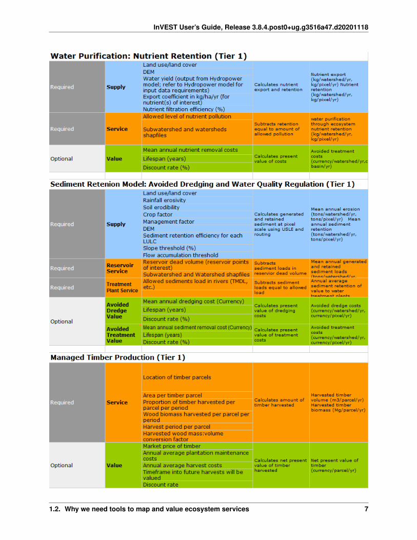
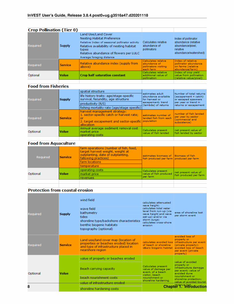
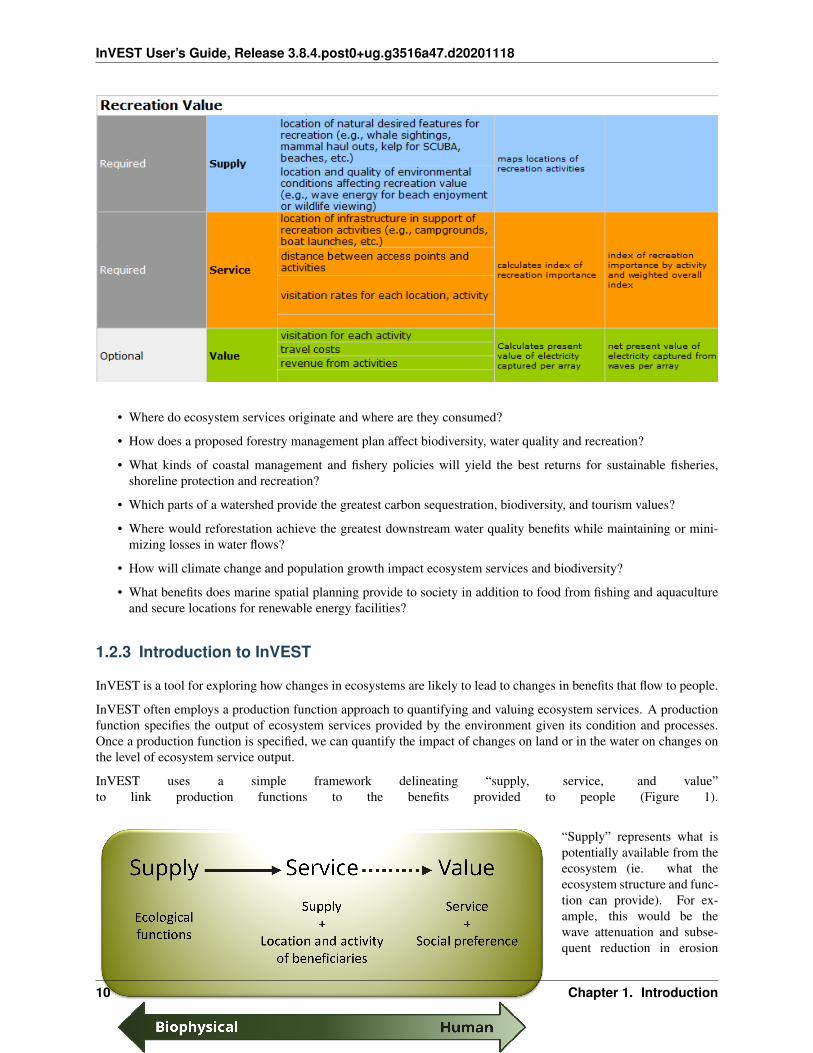
1.1 Data Requirements and Outputs Summary Table
1.2 Why we need tools to map and value ecosystem services
1.2.1 Introduction
Ecosystems, if properly managed, yield a flow of services that are vital to humanity, including the production of goods(e.g., food), life support processes (e.g., water purification), and life fulfilling conditions (e.g., beauty, recreationopportunities), as well as the conservation of options (e.g., genetic diversity for future use). Despite its importance,this natural capital is poorly understood, scarcely monitored, and—in many cases—undergoing rapid degradation anddepletion. To bring understanding of nature’s values into decisions, the Natural Capital Project is developing modelsthat quantify and map the values of ecosystem services. The modeling suite is best suited for analyses of multipleservices and multiple objectives. The current models, which have low data requirements relative to more complextools, can identify areas where investment may enhance human well-being and nature. We are continuing to refineexisting models and to develop new ones.
We use the Millennium Ecosystem Assessment (2005) definition of the term ecosystem services: “the benefits peopleobtain from ecosystems.” Ecosystems incorporate both biotic and abiotic components and we thus consider “ecosys-tem services” and “environmental services” to be equivalent. Natural capital is the living and non-living componentsof ecosystems that contribute to the provision of ecosystem services. Capital assets take many forms including man-ufactured capital (e.g., buildings and machines), human capital (knowledge, experience, and health), social capital(relationships and institutions), as well as natural capital.
1.2.2 Who should use InVEST?
InVEST is designed to inform decisions about natural resource management. Essentially, it provides informationabout how changes in ecosystems are likely to lead to changes in the flows of benefits to people. Decision-makers,from governments to non-profits to corporations, often manage lands and waters for multiple uses and inevitably mustevaluate trade-offs among these uses. InVEST’s multi-service, modular design provides an effective tool for exploringthe likely outcomes of alternative management and climate scenarios and for evaluating trade-offs among sectors andservices. For example, government agencies could use InVEST to help determine how to manage lands, coasts, andmarine areas to provide a desirable range of benefits to people or to help design permitting and mitigation programsthat sustain nature’s benefits to society. Conservation organizations could use InVEST to better align their missions toprotect biodiversity with activities that improve human livelihoods. Corporations, such as consumer goods companies,renewable energy companies, and water utilities, could also use InVEST to decide how and where to invest in naturalcapital to ensure that their supply chains are sustainable and secure.
InVEST can help answer questions like:
5

InVEST User’s Guide, Release 3.8.4.post0+ug.g3516a47.d20201118
6 Chapter 1. Introduction
InVEST User’s Guide, Release 3.8.4.post0+ug.g3516a47.d20201118
1.2. Why we need tools to map and value ecosystem services 7
InVEST User’s Guide, Release 3.8.4.post0+ug.g3516a47.d20201118
8 Chapter 1. Introduction

InVEST User’s Guide, Release 3.8.4.post0+ug.g3516a47.d20201118
1.2. Why we need tools to map and value ecosystem services 9
InVEST User’s Guide, Release 3.8.4.post0+ug.g3516a47.d20201118
• Where do ecosystem services originate and where are they consumed?
• How does a proposed forestry management plan affect biodiversity, water quality and recreation?
• What kinds of coastal management and fishery policies will yield the best returns for sustainable fisheries,shoreline protection and recreation?
• Which parts of a watershed provide the greatest carbon sequestration, biodiversity, and tourism values?
• Where would reforestation achieve the greatest downstream water quality benefits while maintaining or mini-mizing losses in water flows?
• How will climate change and population growth impact ecosystem services and biodiversity?
• What benefits does marine spatial planning provide to society in addition to food from fishing and aquacultureand secure locations for renewable energy facilities?
1.2.3 Introduction to InVEST
InVEST is a tool for exploring how changes in ecosystems are likely to lead to changes in benefits that flow to people.
InVEST often employs a production function approach to quantifying and valuing ecosystem services. A productionfunction specifies the output of ecosystem services provided by the environment given its condition and processes.Once a production function is specified, we can quantify the impact of changes on land or in the water on changes onthe level of ecosystem service output.
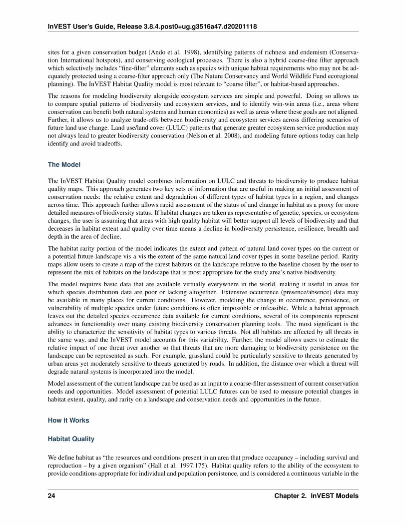
InVEST uses a simple framework delineating “supply, service, and value”to link production functions to the benefits provided to people (Figure 1).
Fig. 1: The ecosystem service supply chain, linking ecological function to ecosystemservices and the benefits provided to people
“Supply” represents what ispotentially available from theecosystem (ie. what theecosystem structure and func-tion can provide). For ex-ample, this would be thewave attenuation and subse-quent reduction in erosion
10 Chapter 1. Introduction

InVEST User’s Guide, Release 3.8.4.post0+ug.g3516a47.d20201118
and flooding onshore pro-vided by a particular loca-tion and density of man-grove forest. “Service” in-corporates demand and thususes information about bene-ficiaries of that service (e.g.,where people live, importantcultural sites, infrastructure,etc.). “Value” includes socialpreference and allows for the
calculation of economic and social metrics (e.g., avoided damages from erosion and flooding, numbers of peopleaffected).
The InVEST toolset described in this guide includes models for quantifying, mapping, and valuing the benefits pro-vided by terrestrial, freshwater, and marine systems. We group models in InVEST into four primary categories: 1)supporting services, 2) final services, 3) tools to facilitate ecosystem service analyses and 4) supporting tools. Support-ing services underpin other ecosystem services, but do not directly provide benefits to people. Final services providedirect benefits to people. For final services, we split the services into their biophysical supply and the service to peoplewherever possible. For some final services, we model the service directly, without modeling the supply separately.Supporting tools include helping to create watersheds, do hydrological processing on a digital elevation model andcreate scenarios that can be used as inputs to InVEST.
Supporting Ecosystem Services:
• Habitat Risk Assessment
• Habitat Quality
• Pollinator Abundance: Crop Pollination
Final Ecosystem Services:
• Forest Carbon Edge Effect
• Carbon Storage and Sequestration
• Coastal Blue Carbon
• Annual Water Yield
• Nutrient Delivery Ratio
• Sediment Delivery Ratio
• Unobstructed Views: Scenic Quality Provision
• Visitation: Recreation and Tourism
• Wave Energy Production
• Offshore Wind Energy Production
• Marine Finfish Aquacultural Production
• Fisheries
• Crop Production
• Seasonal Water Yield
1.2. Why we need tools to map and value ecosystem services 11

InVEST User’s Guide, Release 3.8.4.post0+ug.g3516a47.d20201118
Tools to Facilitate Ecosystem Service Analyses:
• Overlap Analysis
• Coastal Vulnerability
• InVEST GLOBIO
Supporting tools:
• RouteDEM
• DelineateIT
• Scenario Generator
• Scenario Generator: Proximity Based
1.2.4 Using InVEST to Inform Decisions
Information about changes in ecosystem services is most likely to make a difference when questions are driven bydecision-makers and stakeholders, rather than by scientists and analysts. We have found that InVEST is most effec-tive when used within a decision-making process. The Natural Capital Project has used InVEST in over 60 coun-tries worldwide. See the Where We Work section of the NatCap website (https://naturalcapitalproject.stanford.edu/how-do-we-know-it-works/where-we-work/) for the latest map and description of our projects. Through our experi-ence applying InVEST and helping to shape decisions, we have seen how the InVEST tool fits within the larger contextof a natural capital approach.
Our approach (Figure 2) starts with a series of stakeholder consultations. Through discussion, questions of interest topolicy makers, communities and conservation groups are identified. These questions may concern service delivery ona landscape today and how these services may be affected by new programs, policies, and conditions in the future. Forquestions regarding the future, stakeholders develop scenarios to explore the consequences of expected changes onnatural resources. These scenarios typically include a map of future land use and land cover or, for the marine models,a map of future coastal and ocean uses and coastal/marine habitats. These scenarios that are assessed for ecosystemservice value by biophysical and economic models that produce several types of outputs. Following stakeholderconsultations and scenario development, InVEST can estimate the amount of ecosystem services that are providedon the current landscape or under future scenarios. InVEST models are spatially explicit, using maps as informationsources and producing maps as outputs. InVEST returns results in either biophysical terms, whether absolute quantitiesor relative magnitudes (e.g., tons of sediment retained or % of change in sediment retention) or economic terms (e.g.,value of carbon sequestration.)
The spatial extent of analyses is also flexible, allowing users to address questions at the local, regional or global scale.InVEST results can be shared with the stakeholders and decision makers who created the scenarios to inform upcomingdecisions. Using InVEST is an iterative process, and stakeholders may choose to create new scenarios based on theinformation revealed by the models until suitable solutions for management action are identified.
Figure 3 below provides some concrete examples of how the general approach can be used to inform different typesof decisions.
12 Chapter 1. Introduction

InVEST User’s Guide, Release 3.8.4.post0+ug.g3516a47.d20201118
Fig. 2: Stages of a natural capital approach to informing decision making.
1.2. Why we need tools to map and value ecosystem services 13

InVEST User’s Guide, Release 3.8.4.post0+ug.g3516a47.d20201118
Fig. 3: Examples of how the Natural Capital Project has used an ecosystem services approach to inform decisionsacross a variety of contexts. The columns in this table map onto the stages of the natural capital approach illustratedin Figure 2 above.
14 Chapter 1. Introduction

InVEST User’s Guide, Release 3.8.4.post0+ug.g3516a47.d20201118
1.2.5 A work in progress
InVEST is a free of cost software product licensed under the BSD open source license.
The development of InVEST is an ongoing effort of the Natural Capital Project. We release updated versions of thetoolkit approximately every three months that can include updated science, performance and feature enhancements,bug fixes, and/or new models. As a historical note, the original InVEST models were built within ArcGIS but nowall models exist in a standalone form directly launchable from the Windows or Mac perating system with no othersoftware dependencies.
A note on InVEST versioning: Integer changes will reflect major changes. For example, the transition from 2.6.0to 3.0.0 indicates a transition from the Arc-GIS modules to standalone version. An increment in the digit after theprimary decimal indicates major new features (e.g, the addition of a new model) or major revisions. The third decimalreflects minor feature revisions or bug fixes with no new functionality.
1.2.6 This guide
This guide will help you understand the basics of the InVEST models and start using them. The next chapter leadsyou through the installation process and provides general information about the tool and interface.
The remaining chapters present the ecosystem service models. Each chapter:
• briefly introduces a service and suggests the possible uses for InVEST results;
• explains how the model works, including important simplifications, assumptions, and limitations;
• describes the data needed to run the model, which is crucial because the meaning and value of InVEST resultsdepend on the input data;
• provides step-by-step instructions for how to input data and interact with the tool;
• offers guidance on interpreting InVEST results;
• includes an appendix of information on relevant data sources and data preparation advice (this section is variableamong chapters, and will improve over time from user input).
Much of the theory related to the scientific foundation of many of these models can be found in the book NaturalCapital: The Theory & Practice of Mapping Ecosystem Services (Oxford University Press). The models applied anddiscussed in that book are not identical to those presented in the InVEST toolset, however, and this user guide providesthe most up-to-date description of the current versions of the models. .. primerend
1.3 Getting Started
For assistance with installing InVEST on a Mac, see the section Installing InVEST and sample data on your Macbelow.
1.3.1 Installing InVEST and sample data on your Windows computer
Download the InVEST installer from http://www.naturalcapitalproject.org. The executable will be called “In-VEST_<version>_Setup.exe”. Double-click on this .exe to run the installer.
After clicking through the first screen and agreeing to the Licence Agreement, the Choose Components screen willappear. The installer will always install the InVEST Tools and HTML and PDF versions of the InVEST User’s Guide.Optionally, sample datasets may also be installed, and by default they are all selected. Note that these datasets aredownloaded over the internet, and some are very large (particularly the Marine Datasets), so they make take a longtime to install. If you do not wish to install all or some of the sample datasets, uncheck the corresponding box(es).
1.3. Getting Started 15

InVEST User’s Guide, Release 3.8.4.post0+ug.g3516a47.d20201118
Next, choose the folder where the InVEST toolsets and sample data will be installed. The installer shows how muchspace is available on the selected drive. Click Install to begin the installation.
Once installed, the InVEST install folder will contain the following:
• A documentation folder, containing the InVEST User Guide in HTML format.
• An invest-3-x86 folder, containing the compiled Python code that makes up the InVEST toolset.
• InVEST_<version>_Documentation.pdf, the InVEST User Guide in PDF format.
• Uninstall_<version>.exe, which will uninstall InVEST.
• HISTORY.rst, lists of all of the updates included in each new version.
• If you chose to also install sample data, they will be located in the folder sample_data, with a sub-folder foreach model’s data.
Additionally, shortcuts for all InVEST standalone applications will be added to your Windows start menu under AllPrograms -> InVEST |version|
Advanced Installation
The InVEST windows installer has a number of installation options for several use cases, including silent installationand the use of local sample data. To view the available options, download the installer, open a CMD prompt to thedirectory that contains the downloaded installer and type:
.\InVEST_<version>_x86_Setup.exe /?
Standalone InVEST Tools
All of the InVEST models run on an entirely open-source platform, where historically the toolset was a collection ofArcGIS scripts. The new interface does not require ArcGIS and the results can be explored with any GIS tool includingArcGIS, QGIS, and others. As of InVEST 2.3.0, the toolset has had standalone versions of the models available fromthe Windows start menu after installation, under All Programs -> InVEST |version|. Standalone versions are currentlyavailable for all models. The ArcGIS versions of InVEST models are no longer supported.
Older InVEST Versions
Older versions of InVEST can be found at http://data.naturalcapitalproject.org/invest-releases/deprecated_models.html. Note that many models were deprecated due to critical unsolved science issues, and we strongly encourageyou to use the latest version of InVEST.
1.3.2 Using sample data
InVEST comes with sample data as a guide for formatting your data, and starting to understand how the models work.For instance, in preparation for analysis of your data, you may wish to test the models by changing input valuesin the sample data to see how the output responds. For the terrestrial/freshwater models it is particularly importantthat their sample data is only used for testing and example, do not use the spatial data or table values for your ownanalysis, because their source and accuracy is not documented. Some of the marine models come with global datasetsthat may be used for your own application - please see the individual User Guide chapters for these models for moreinformation.
Sample data are found in separate sub-folders within the InVEST install folder. For example, the sample datasetsfor the Pollination model are found in \{InVEST install directory}\sample_data\pollination\, and those for the Carbon
16 Chapter 1. Introduction

InVEST User’s Guide, Release 3.8.4.post0+ug.g3516a47.d20201118
model in \{InVEST install directory}\sample_data\carbon. For testing the models, you may make a Workspace foldercalled “output” within the sample data folders for saving model results. Once you are working with your own data,you will need to create a workspace and input data folders to hold your own input and results. You will also need toredirect the tool to access your data and workspace.
1.3.3 Formatting your data
Before running InVEST, it is necessary to format your data. Although subsequent chapters of this guide describe howto prepare input data for each model, there are several formatting guidelines common to all models:
• Data file names should not have spaces (e.g., a raster file should be named ‘landuse.tif’ rather than ‘land use.tif’).
• For raster data, TIFFs are preferred for ease of use, but you may also use IMG or ESRI GRID.
• If using ESRI GRID format rasters, their dataset names cannot be longer than 13 characters and the first charactercannot be a number. TIFF and IMG rasters do not have the file name length limitation. When using ESRI GRIDas input to the model interface, use the file “hdr.adf”.
• Spatial data must be in a projected coordinate system (such at UTM), not a geographic coordinate system (suchas WGS84), and all input data for a given model run must be in the same projected coordinate system. If yourdata is not projected, InVEST will give errors or incorrect results.
• While the InVEST 3.0 models are now very memory-efficient, the amount of time that it takes to run the modelsis still affected by the size of the input datasets. If the area of interest is large and/or uses rasters with small cellsize, this will increase both the memory usage and time that it takes to run the model. If they are too large, amemory error will occur. If this happens, try reducing the size of your area of interest, or using coarser-resolutioninput data.
• Similarly, the amount of disk space that is used by the model is in proportion to the resolution of the input data.If the area of interest is large and/or uses rasters with small cell size, this will increase the amount of disk spacerequired to store intermediate and final model results. If not enough disk space is available, the model will returnan error.
• Running the models with the input data files open in another program can cause errors. Ensure that the data filesare not in use by another program to prevent data access issues.
• Regional and Language options: Some language settings cause errors while running the models. For examplesettings which use comma (,) for decimals instead of period (.) cause errors in the models. To solve this changethe computer’s regional settings to English.
• As the models are run, it may be necessary to change values in the input tables. This is usually done with aspreadsheet program like Excel or text editor like Notepad++. Input tables are required to be in CSV (comma-separated value) format, where the values are separated by commas, not semicolons or any other character. Ifworking in Excel, you cannot see the separator, so double-check in Notepad or another text editor. When savingthe CSV file, be sure to save the file using one of the following encodings: ASCII, UTF-8 or Signed UTF-8.Using any other encoding (such as Latin-1) will result in incorrect text rendering in output files and could causemodels to fail with an error.
• Some models require specific naming guidelines for data files (e.g., Habitat Quality model) and field (column)names, which are defined in the User Guide chapter for each model. Follow these carefully to ensure yourdataset is valid, or the model will give an error.
• Remember to use the sample datasets as a guide to format your data.
1.3.4 Running the models
You are ready to run an InVEST model when you have prepared your data according to the instructions in the relevantmodel chapter and have installed the latest version of InVEST.
1.3. Getting Started 17

InVEST User’s Guide, Release 3.8.4.post0+ug.g3516a47.d20201118
To begin:
• Review your input data. View spatial data in a GIS, make sure that the values look correct, there are no areas ofmissing data where it should be filled in, that all layers are in the same projected coordinate system, etc. Viewtable data in a spreadsheet or text editor, make sure that the values look correct, the column names are correct,and that it is saved in CSV format.
• Select the model you wish to run (e.g., Carbon) from the Windows Start menu, and add your input data to eachfield in the user interface. You may either drag and drop layers into the field, or click the File icon to the rightof each field to navigate to your data.
• Inputs for which the entered path leads to a non-existent file or a file that is incorrectly formatted will be markedwith a red “X” to the left of the name of the input. If you click the red X, it will give an idea of what is wrongwith the data. The model will not run if there are any red Xs.
• Note that each tool has a place to enter a Suffix, which is a string that will be added to the output filenames as<filename>_Suffix. Adding a unique suffix prevents overwriting files produced in previous iterations. This isparticularly useful if you are running multiple scenarios, so each file name can indicate the name of the scenario.
• When all required fields are filled in, and there are no red Xs, click the Run button on the interface.
• Processing time will vary depending on the script and the resolution and extent of your input datasets. Everymodel will open a window showing the progress of the script. Be sure to scan the output window for usefulmessages and errors. This progress information will also be written to a file in the Workspace called <modelname>-log-<timestamp>.txt. If you need to contact NatCap for assistance with errors, always send this log file,it will help with debugging. Also see Support and Error Reporting below for more information.
• Results from the model can be found in the Workspace folder. Main outputs are generally in the top level of theWorkspace. There is also an ‘intermediate’ folder which contains some of the additional files generated whiledoing the calculations. While it’s not usually necessary to look at the intermediate results, it is sometimes usefulwhen you are debugging a problem, or trying to better understand how the model works. Reading the modelchapter and looking at the corresponding intermediate files can be a good way to understand and critique yourresults. Each model chapter in this User Guide provides a description of these output files.
After your script completes successfully, you can view the spatial results by adding them from the Workspace to yourGIS. It is important to look closely and critically at the results. Do the values make sense? Do the patterns make sense?Do you understand why some places have higher values and others lower? How are your input layers and parametersdriving the results?
1.3.5 Support and Error Reporting
Several training workshops on InVEST may be offered annually, subject to funding and demand. Information on thesetrainings will be announced on the support page and can be found at the Natural Capital Project website. This site isalso a good source of general information on InVEST, related publications and use cases and other activities of theNatural Capital Project.
If you encounter any issues when running the models, or have questions about their theory, data, or application, pleasevisit the user support forum at http://forums.naturalcapitalproject.org. First, please use the Search feature to see if asimilar question has already been asked. Many times, your question or problem has already been answered. If youdon’t find existing posts related to your question or issue, or they don’t solve your issue, you can log in and create anew post.
If you are reporting an error when running a model, please include the following information in the forum post:
• InVEST model you’re asking about
• InVEST version you’re using
• What you have already tried to solve the issue, and hasn’t worked
18 Chapter 1. Introduction

InVEST User’s Guide, Release 3.8.4.post0+ug.g3516a47.d20201118
• The entire log file produced by the model, located in the output Workspace folder - <model name>-log-<timestamp>.txt
1.3.6 Working with the DEM
For the freshwater models SDR, NDR and Seasonal Water Yield, having a well-prepared digital elevation model(DEM) is critical. It must have no missing data (holes of NoData values), and should correctly represent the surfacewater flow patterns over the area of interest in order to get accurate results.
Here are some tips for working with the DEM and creating a hydrologically-correct DEM. Included is informationon using built-in functions from ArcGIS and QGIS. There are other options for DEM processing as well, includingArcHydro, ArcSWAT, AGWA, and BASINS, which are not covered here. This is only intended to be a brief overviewof the issues and methods involved in DEM preparation, not a GIS tutorial.
• Use the highest quality, finest resolution DEM that is appropriate for your application. This will reduce thechances of there being sinks and missing data, and will more accurately represent the terrain’s surface waterflow, providing the amount of detail that is required for making informed decisions at your scale of interest.
• Mosaic tiled DEM data
If you have downloaded DEM data for your area that is in multiple, adjacent tiles, they will need to first bemosaicked together to create a single DEM file. In ArcToolbox, use Data Management -> Raster -> Mosaic toNew Raster. Look closely at the output raster to make sure that the values are correct along the edges where thetiles were joined. If they are not, try different values for the Mosaic Method parameter to the Mosaic to NewRaster tool.
In QGIS, you can use the Raster -> Miscellaneous -> Merge function to combine the tiles.
• Clipping the DEM to your study area
We generally recommend that the DEM be clipped to an area that is slightly larger than your area of interest.This is to ensure that the hydrology around the edge of the watershed is captured. This is particularly importantif the DEM is of coarse resolution, as clipping to the area of interest will lead to large areas of missing dataaround the edge. To do this, create a buffer around your area of interest (or watershed) shapefile, and clip theDEM to that buffered polygon. Make sure that the buffer is at least the width of one DEM pixel.
• Reprojecting DEMs
When reprojecting a DEM in either ArcGIS (Project Raster tool) or QGIS (Warp tool), it is important to selectBILINEAR or CUBIC for the “Resampling Technique” in ArcGIS or “Resampling method” in QGIS. SelectingNEAREST (or Near in QGIS) will produce a DEM with an incorrect grid pattern across the area of interest,which might only be obvious when zoomed-in or after Flow Direction has been run. This will create a badstream network and flow pattern and lead to bad model results.
• Check for missing data
After getting (and possibly mosaicking) the DEM, make sure that there is no missing data, represented byNoData cells within the area of interest. If there are NoData cells, they must be assigned values.
For small holes, one way to do this is to use the ArcGIS Focal Mean function within Raster Calculator (orConditional -> CON). For example, in ArcGIS 10.x:
Con(IsNull("theDEM"),FocalStatistics("theDEM",NbrRectangle(3,3),"MEAN"),"theDEM")
Interpolation can also be used, and can work better for larger holes. Convert the DEM to points using ConversionTools -> From Raster -> Raster to Point, interpolate using Spatial Analyst’s Interpolation tools, then use CONto assign interpolated values to the original DEM:
Con(isnull([theDEM]), [interpolated_grid], [theDEM])
1.3. Getting Started 19

InVEST User’s Guide, Release 3.8.4.post0+ug.g3516a47.d20201118
In QGIS, try the Fill Nodata tool, or the GRASS r.neighbors tool. r.neighbors provides different statistics types,including Mean.
• Identify sinks in the DEM and fill them
From the ESRI help on “How Sink works”: “A sink is a cell or set of spatially connected cells whose flowdirection cannot be assigned one of the eight valid values in a flow direction raster. This can occur when allneighboring cells are higher than the processing cell or when two cells flow into each other, creating a two-cellloop.”
Sinks are usually caused by errors in the DEM, and they can produce an incorrect flow direction raster. Thiscan lead to several problems with hydrology processing, including creating a discontinuous stream network.Filling the sinks assigns new values to the anomalous processing cells, such that they are better aligned withtheir neighbors. But this process may create new sinks, so an iterative process may be required.
We have found that the QGIS Wang and Liu Fill tool does a good job of filling sinks, and is recommended. Youcan also use ArcGIS by using the Hydrology -> Fill tool. Multiple runs of Fill may be needed.
• Verify the stream network
The stream network generated by the model from the DEM should closely match the streams on a known correctstream map. Several of the InVEST hydrology models and the supporting InVEST tool RouteDEM output astream network (usually called stream.tif.) These tools create streams by first generating a Flow Accumulationraster, then applying the user input ‘threshold flow accumulation’ (TFA) value to select pixels that should bepart of the stream network. For example, if a TFA value of 1000 is given, this says that 1000 pixels must draininto a particular pixel before it’s considered part of a stream. This is the equivalent of saying that streams aredefined by having a flow accumulation value >= 1000.
Use these stream.tif outputs to evaluate how well the modelled streams match reality, and adjust the thresholdflow accumulation accordingly. Larger values of TFA will produce coarser stream networks with fewer tribu-taries, smaller values of TFA will produce more tributaries. There is no one “correct” value for TFA, it will bedifferent for each area of interest and DEM. A good value to start with for testing is 1000.
To create flow accumulation and stream maps without needing to run a whole hydrology model, you can use theInVEST tool RouteDEM, which is specifically for processing the DEM. See the RouteDEM chapter of the UserGuide for more information.
• Creating watersheds
It is recommended to create watersheds from the DEM that you will be using in the analysis. If a watershed mapis obtained from elsewhere, the boundaries of the watershed(s) might not line up correctly with the hydrologycreated from the DEM, leading to incorrect aggregated results.
There are a variety of tools that can create watersheds, including the ArcGIS Watershed tool and QGIS Water-shed basins or r.basins.fill. InVEST also provides a tool called DelineateIt, which works well, is simple to use,and is recommended. It has the advantage of being able to create watersheds that overlap, such as when thereare several dams along the same river. See the DelineateIt section of the User Guide for more information.
After watersheds are generated, verify that they represent the catchments correctly and that each watershed isassigned a unique integer ID in the field “ws_id” (or “subws_id”, depending on the model - see the Data Needssection of the hydrology model you’re using to find out what’s required.)
1.3.7 Installing InVEST and sample data on your Mac
Note: In Mac OS 10.13 “High Sierra”, InVEST 3.4.0 or later is required.
Numerical results of the Mac binaries may differ slightly (usually within 1e-4) from the results of the Windows bina-ries. For this reason, we consider InVEST binaries “unstable”, but they should still provide reasonable results. As al-
20 Chapter 1. Introduction

InVEST User’s Guide, Release 3.8.4.post0+ug.g3516a47.d20201118
ways, if something does not seem to be working, please let us know on the forums: http://forums.naturalcapitalproject.org
Download the InVEST zip file from http://www.naturalcapitalproject.org/invest. The archive will be called “InVEST-<version>.zip”. This archive contains a compressed copy of the InVEST executable and this User’s Guide.
To install:
1. Double-click the zip archive to uncompress it.
2. Drag the folder labeled “InVEST-<version>” to your Applications folder.
3. Open the InVEST folder you just copied to your Applications folder in a new finder window.
4. The first time you run InVEST, you’ll need to do the following:
1. Right-click on InVEST.app, and in the context menu, select Open.
2. In the dialog that pops up, click Open once again.
5. In the launcher dialog, select the model you’d like to run and click Launch.
The mac distribution includes the executable models and documentation, but unlike the Windows installer does notinclude sample data. These can be found online at http://naturalcapitalproject.org/invest by following the link to“Individual Sample Datasets for InVEST”.
1.3. Getting Started 21

InVEST User’s Guide, Release 3.8.4.post0+ug.g3516a47.d20201118
22 Chapter 1. Introduction

CHAPTER
TWO
INVEST MODELS
2.1 Supporting Ecosystem Services:
2.1.1 Habitat Quality
Summary
Biodiversity is intimately linked to the production of ecosystem services. Patterns in biodiversity are inherently spatial,and as such, can be estimated by analyzing maps of land use and land cover (LULC) in conjunction with threats tospecies’ habitat. InVEST models habitat quality and rarity as proxies for biodiversity, ultimately estimating the extentof habitat and vegetation types across a landscape, and their state of degradation. Habitat quality and rarity are afunction of four factors: each threat’s relative impact, the relative sensitivity of each habitat type to each threat, thedistance between habitats and sources of threats, and the degree to which the land is legally protected. The modelassumes that the legal protection of land is effective and that all threats to a landscape are additive.
Introduction
A primary goal of conservation is the protection of biodiversity, including the range of genes, species, populations,habitats, and ecosystems in an area of interest. While some consider biodiversity to be an ecosystem service, here wetreat it as an independent attribute of natural systems, with its own intrinsic value (we do not monetize biodiversityin this model). Natural resource managers, corporations and conservation organizations are becoming increasinglyinterested in understanding how and where biodiversity and ecosystem services align in space and how managementactions affect both.
Evidence from many sources builds an overwhelming picture of pervasive biodiversity decline worldwide (e.g., Vi-tousek et al. 1997; Wilcove et al 1998; Czech et. al 2000). This evidence has prompted a wide-ranging responsefrom both governments and civil society. Through the Rio Convention on Biodiversity, 189 nations have committedthemselves to preserving the biodiversity within their borders. Yet, there is scant research on the overlap betweenopportunities to protect biodiversity and to sustain the ecosystem services so critical to these countries’ economicwell-being. This is precisely the type of challenge that InVEST has been designed to address.
For managers to understand the patterns of distribution and richness across a landscape, individually and in aggregate,it is necessary to map the range or occurrences of elements (e.g. species, communities, habitats). The degree to whichcurrent land use and management affects the persistence of these elements must also be assessed in order to designappropriate conservation strategies and encourage resource management that maximizes biodiversity in those areas.
There are a variety of approaches to identifying priorities for conservation with various trade-offs among them. Each ofthese approaches focuses on different facets of biodiversity attributes and dynamics, including habitat or vegetation-based representation (i.e., a coarse filter), maximizing the number of species “covered” by a network of conserved
23
InVEST User’s Guide, Release 3.8.4.post0+ug.g3516a47.d20201118
sites for a given conservation budget (Ando et al. 1998), identifying patterns of richness and endemism (Conserva-tion International hotspots), and conserving ecological processes. There is also a hybrid coarse-fine filter approachwhich selectively includes “fine-filter” elements such as species with unique habitat requirements who may not be ad-equately protected using a coarse-filter approach only (The Nature Conservancy and World Wildlife Fund ecoregionalplanning). The InVEST Habitat Quality model is most relevant to “coarse filter”, or habitat-based approaches.
The reasons for modeling biodiversity alongside ecosystem services are simple and powerful. Doing so allows usto compare spatial patterns of biodiversity and ecosystem services, and to identify win-win areas (i.e., areas whereconservation can benefit both natural systems and human economies) as well as areas where these goals are not aligned.Further, it allows us to analyze trade-offs between biodiversity and ecosystem services across differing scenarios offuture land use change. Land use/land cover (LULC) patterns that generate greater ecosystem service production maynot always lead to greater biodiversity conservation (Nelson et al. 2008), and modeling future options today can helpidentify and avoid tradeoffs.
The Model
The InVEST Habitat Quality model combines information on LULC and threats to biodiversity to produce habitatquality maps. This approach generates two key sets of information that are useful in making an initial assessment ofconservation needs: the relative extent and degradation of different types of habitat types in a region, and changesacross time. This approach further allows rapid assessment of the status of and change in habitat as a proxy for moredetailed measures of biodiversity status. If habitat changes are taken as representative of genetic, species, or ecosystemchanges, the user is assuming that areas with high quality habitat will better support all levels of biodiversity and thatdecreases in habitat extent and quality over time means a decline in biodiversity persistence, resilience, breadth anddepth in the area of decline.
The habitat rarity portion of the model indicates the extent and pattern of natural land cover types on the current ora potential future landscape vis-a-vis the extent of the same natural land cover types in some baseline period. Raritymaps allow users to create a map of the rarest habitats on the landscape relative to the baseline chosen by the user torepresent the mix of habitats on the landscape that is most appropriate for the study area’s native biodiversity.
The model requires basic data that are available virtually everywhere in the world, making it useful in areas forwhich species distribution data are poor or lacking altogether. Extensive occurrence (presence/absence) data maybe available in many places for current conditions. However, modeling the change in occurrence, persistence, orvulnerability of multiple species under future conditions is often impossible or infeasible. While a habitat approachleaves out the detailed species occurrence data available for current conditions, several of its components representadvances in functionality over many existing biodiversity conservation planning tools. The most significant is theability to characterize the sensitivity of habitat types to various threats. Not all habitats are affected by all threats inthe same way, and the InVEST model accounts for this variability. Further, the model allows users to estimate therelative impact of one threat over another so that threats that are more damaging to biodiversity persistence on thelandscape can be represented as such. For example, grassland could be particularly sensitive to threats generated byurban areas yet moderately sensitive to threats generated by roads. In addition, the distance over which a threat willdegrade natural systems is incorporated into the model.
Model assessment of the current landscape can be used as an input to a coarse-filter assessment of current conservationneeds and opportunities. Model assessment of potential LULC futures can be used to measure potential changes inhabitat extent, quality, and rarity on a landscape and conservation needs and opportunities in the future.
How it Works
Habitat Quality
We define habitat as “the resources and conditions present in an area that produce occupancy – including survival andreproduction – by a given organism” (Hall et al. 1997:175). Habitat quality refers to the ability of the ecosystem toprovide conditions appropriate for individual and population persistence, and is considered a continuous variable in the
24 Chapter 2. InVEST Models

InVEST User’s Guide, Release 3.8.4.post0+ug.g3516a47.d20201118
model, ranging from low to medium to high, based on resources available for survival, reproduction, and populationpersistence, respectively (Hall et al 1997). Habitat with high quality is relatively intact and has the structure andfunction within the range of historic variability. Habitat quality depends on a habitat’s proximity to human land usesand the intensity of these land uses. Generally, habitat quality is degraded as the intensity of nearby land-use increases(Nelleman 2001, McKinney 2002, Forman et al. 2003).
The model runs using raster data, where each cell in the raster is assigned an LULC class, which can be a natural(unmanaged) class or a managed class. LULC types can be given at any level of classification detail. For example,grassland is a broad LULC definition that can be subdivided into pasture, restored prairie, and residential lawn typesto provide much more habitat classification detail. While the user can submit up to 3 raster maps of LULC, one eachfor a baseline, current, and future period, at a minimum the current LULC raster map must be provided.
The user defines which LULC types can provide habitat for the conservation objective (e.g., if forest breeding birds arethe conservation objective then forests are habitat and non-forest covers are not habitat). Let 𝐻𝑗 indicate the habitatsuitability of LULC type 𝑗.
Which LULC types should be considered habitat? If considering biodiversity generally or if data on specificbiodiversity-habitat relationships are lacking, you can take a simple binary approach to assigning habitat to LULCtypes. A classic example would be to follow an island-ocean model and assume that the managed land matrix sur-rounding remnant patches of unmanaged land is unusable from the standpoint of species (e.g., MacArthur and Wilson1967). In this case a 0 would be assigned to managed LULC types in the matrix (i.e., non-habitat) and a 1 to unman-aged types (i.e., habitat). Under this modeling scheme habitat quality scores are not a function of habitat importance,rarity, or suitability; all habitat types are treated equally. Model inputs are assumed to not be specific to any particularspecies or species guild, but rather apply to biodiversity generally.
More recent research suggests that the matrix of managed land that surrounds patches of unmanaged land can signifi-cantly influence the “effective isolation” of habitat patches, rendering them more or less isolated than simple distanceor classic models would indicate (Ricketts 2001, Prugh et al. 2008). Modification of the matrix may provide opportu-nities for reducing patch isolation and thus the extinction risk of populations in fragmented landscapes (Franklin andLindenmayer 2009). To model this, a relative habitat suitability score can be assigned to an LULC type ranging from0 to 1 where 1 indicates the highest habitat suitability. A ranking of less than 1 indicates habitat where a species orfunctional group may have lower survivability. Applying this second approach greatly expands the definition of habitatfrom the simple and often artificial binary approach (e.g., “natural” versus “unnatural”) to include a broad spectrum ofboth managed and unmanaged LULC types. By using a continuum of habitat suitability across LULC types, the usercan assess the importance of land use management on habitat quality holistically or consider the potential importanceof “working” (or managed) landscapes.
If a continuum of habitat suitability is relevant, weights with a roster of LULC on a landscape must be applied inreference to a particular species guild of group. For example, grassland songbirds may prefer a native prairie habitatabove all other habitat types (the habitat score for the LULC prairie (𝐻𝑝𝑟𝑎𝑟𝑖𝑒 equals 1), but will also make use of amanaged hayfield or pasture if prairie is not available (the habitat score for the LULC hayfield (𝐻ℎ𝑎𝑦𝑓𝑖𝑒𝑙𝑑) and pasture(𝐻𝑝𝑎𝑠𝑡𝑢𝑟𝑒) equals 0.5). However, mammals such as porcupines will find prairie unsuitable for breeding and feeding.Therefore, if specific data on species group-habitat relationships are used, the model output refers to habitat extent andquality for the species or group in the modeled set only.
Besides a map of LULC and data that relates LULC to habitat suitability, the model also requires data on habitat threatdensity and its effects on habitat quality. In general, we consider threats to be human-modified LULC types that causehabitat fragmentation, edge, and degradation in neighboring habitat. For example, the conversion of a habitat LULCto non-habitat LULC reduces the size and continuity of neighboring habitat patches. Edge effects refer to changesin the biological and physical conditions that occur at a patch boundary and within adjacent patches. For example,adjacent degraded non-habitat LULC parcels impose “edge effects” on habitat parcels and can have negative impactswithin habitat parcels by, for example, facilitating entry of predators, competitors, invasive species, or toxic chemicalsand other pollutants. Another example: in many developing countries roads are a threat to forest habitat quality on thelandscape because of the access they provide to timber and non-timber forest harvesters.
Each threat source needs to be mapped on a raster grid. A grid cell value on a threat’s map can either indicate intensityof the threat within the cell (e.g., road length in a grid cell or cultivated area in a gird cell) or simply a 1 if the grid cell
2.1. Supporting Ecosystem Services: 25

InVEST User’s Guide, Release 3.8.4.post0+ug.g3516a47.d20201118
contains the threat in a road or crop field cover and 0 otherwise. Let 𝑜𝑟𝑦 indicate threat 𝑟’s “score” in grid cell 𝑦 where𝑟 = 1, 2, . . . , 𝑅 indexes all modeled degradation sources.
All mapped threats should be measured in the same scale and metric. For example, if one threat is measured in densityper grid cell then all degradation sources should be measured in density per grid cell where density is measured withthe same metric unit (e.g., km and km2). Or if one threat is measured with presence/absence (1/0) on its map then allthreats should be mapped with the presence/absence scale.
The impact of threats on habitat in a grid cell is mediated by four factors.
1. The first factor is the relative impact of each threat. Some threats may be more damaging to habitat, all elseequal, and a relative impact score accounts for this (see Table 1 for a list of possible threats). For instance, urbanareas may be considered to be twice as degrading to any nearby habitats as agricultural areas. A degradationsource’s weight, 𝑤𝑟, indicates the relative destructiveness of a degradation source to all habitats. The weight 𝑤𝑟
can take on any value from 0 to 1. For example, if urban area has a threat weight of 1 and the threat weight ofroads is set equal to 0.5 then the urban area causes twice the disturbance, all else equal, to all habitat types. Toreiterate, if we have assigned species group-specific habitat suitability scores to each LULC then the threats andtheir weights should be specific to the modeled species group.
2. The second mitigating factor is the distance between habitat and the threat source and the impact of thethreat across space. In general, the impact of a threat on habitat decreases as distance from the degradationsource increases, so that grid cells that are more proximate to threats will experience higher impacts. Forexample, assume a grid cell is 2 km from the edge of an urban area and 0.5 km from a highway. The impact ofthese two threat sources on habitat in the grid cell will partly depend on how quickly they decrease, or decay,over space. The user can choose either a linear or exponential distance-decay function to describe how a threatdecays over space. The impact of threat 𝑟 that originates in grid cell 𝑦, 𝑟𝑦 , on habitat in grid cell 𝑥 is given by𝑖𝑟𝑥𝑦 and is represented by the following equations:
𝑖𝑟𝑥𝑦 = 1 −(︂
𝑑𝑥𝑦𝑑𝑟 max
)︂if linear (2.1)
𝑖𝑟𝑥𝑦 = 𝑒𝑥𝑝
(︂−(︂
2.99
𝑑𝑟 max
)︂𝑑𝑥𝑦
)︂if exponential (2.2)
where 𝑑𝑥𝑦 is the linear distance between grid cells 𝑥 and 𝑦 and 𝑑𝑟 max is the maximum effective distance of threat𝑟’s reach across space. Figure 1 illustrates the relationship between the distance-decay rate for a threat based on themaximum effective distance of the threat (linear and exponential). For example, if the user selects an exponentialdecline and the maximum impact distance of a threat is set at 1 km, the impact of the threat on a grid cell’s habitat willdecline by ~ 50% when the grid cell is 200 m from 𝑟’s source. If 𝑖𝑟𝑥𝑦 > 0 then grid cell 𝑥 is in degradation source 𝑟𝑦’sdisturbance zone. (If the exponential function is used to describe the impact of degradation source 𝑟 on the landscapethen the model ignores values of 𝑖𝑟𝑥𝑦 that are very close to 0 in order to expedite the modeling process.) To reiterate, ifwe have assigned species group-specific habitat suitability scores to each LULC then threat impact over space shouldbe specific to the modeled species group.
Figure 1. An example of the relationship between the distance-decay rate of a threat and the maximum effectivedistance of a threat.
3. The third landscape factor that may mitigate the impact of threats on habitat is the level of legal / institutional/ social / physical protection from disturbance in each cell. Is the grid cell in a formal protected area? Or is itinaccessible to people due to high elevations? Or is the grid cell open to harvest and other forms of disturbance?
26 Chapter 2. InVEST Models

InVEST User’s Guide, Release 3.8.4.post0+ug.g3516a47.d20201118
The model assumes that the more legal / institutional / social / physical protection from degradation a cell has,the less it will be affected by nearby threats, no matter the type of threat. Let 𝛽𝑥 ∈ [0, 1] indicate the level ofaccessibility in grid cell 𝑥 where 1 indicates complete accessibility. As accessibility decreases the impact thatall threats will have in grid cell 𝑥 decreases linearly. It is important to note that while legal / institutional / social/ physical protections often do diminish the impact of extractive activities in habitat such as hunting or fishing, itis unlikely to protect against other sources of degradation such as air or water pollution, habitat fragmentation,or edge effects. If the threats considered are not mitigated by legal / institutional / social / physical propertiesthen you should ignore this input or set 𝛽𝑥 = 1 for all grid cells 𝑥. To reiterate, if we have assigned speciesgroup-specific habitat suitability scores to each LULC then the threats mitigation weights should be specific tothe modeled species group.
4. The relative sensitivity of each habitat type to each threat on the landscape is the final factor used whengenerating the total degradation in a cell with habitat. (In Kareiva et al. (2010), habitat sensitivity is referred toby its inverse, “resistance”.) Let 𝑆𝑗𝑟 ∈ [0, 1] indicate the sensitivity of LULC (habitat type) 𝑗 to threat 𝑟 wherevalues closer to 1 indicate greater sensitivity. The model assumes that the more sensitive a habitat type is toa threat, the more degraded the habitat type will be by that threat. A habitat’s sensitivity to threats should bebased on general principles from landscape ecology for conserving biodiversity (e.g., Forman 1995; Noss 1997;Lindenmayer et al 2008). To reiterate, if we have assigned species group-specific habitat suitability scores toeach LULC then habitat sensitivity to threats should be specific to the modeled species group.
Therefore, the total threat level in grid cell 𝑥 with LULC or habitat type 𝑗 is given by 𝐷𝑥𝑗 ,
𝐷𝑥𝑗 =
𝑅∑︁𝑟=1
𝑌𝑟∑︁𝑦=1
(︃𝑤𝑟∑︀𝑅𝑟=1 𝑤𝑟
)︃𝑟𝑦𝑖𝑟𝑥𝑦𝛽𝑥𝑆𝑗𝑟 (2.3)
where 𝑦 indexes all grid cells on 𝑟’s raster map and 𝑌𝑟 indicates the set of grid cells on 𝑟’s raster map. Note that eachthreat map can have a unique number of grid cells due to variation in raster resolution. If 𝑆𝑗𝑟 = 0 then 𝐷𝑥𝑗 is not afunction of threat 𝑟. Also note that threat weights are normalized so that the sum across all threats weights equals 1.
By normalizing weights such that they sum to 1 we can think of 𝐷𝑥𝑗 as the weighted average of all threat levels ingrid cell 𝑥. The map of 𝐷𝑥𝑗 will change as the set of weights we use change. Please note that two sets of weights willonly differ if the relative differences between the weights in each set differ. For example, set of weights of 0.1, 0.1,and 0.4 are the same as the set of weights 0.2, 0.2, and 0.8.
A grid cell’s degradation score is translated into a habitat quality value using a half saturation function where the usermust determine the half-saturation value. As a grid cell’s degradation score increases its habitat quality decreases. Letthe quality of habitat in parcel 𝑥 that is in LULC 𝑗 be given by 𝑄𝑥𝑗 where,
𝑄𝑥𝑗 = 𝐻𝑗
(︃1 −
(︃𝐷𝑧
𝑥𝑗
𝐷𝑧𝑥𝑗 + 𝑘𝑧
)︃)︃(2.4)
and 𝑧 (we hard code 𝑧 = 2.5) and 𝑘 are scaling parameters (or constants). 𝑄𝑥𝑗 is equal to 0 if 𝐻𝑗 = 0. 𝑄𝑥𝑗 increasesin 𝐻𝑗 and decreases in 𝐷𝑥𝑗 . 𝑄𝑥𝑗 can never be greater than 1. The 𝑘 constant is the half-saturation constant and is
2.1. Supporting Ecosystem Services: 27

InVEST User’s Guide, Release 3.8.4.post0+ug.g3516a47.d20201118
set by the user. The parameter 𝑘 is equal to the 𝐷 value where 1 −(︁
𝐷𝑧𝑥𝑗
𝐷𝑧𝑥𝑗+𝑘𝑧 = 0.5
)︁. For example, if 𝑘 = 5 then
1 −(︁
𝐷𝑧𝑥𝑗
𝐷𝑧𝑥𝑗+𝑘𝑧
)︁= 0.5 when 𝐷𝑥𝑗 = 5. By default, you can set 𝑘 = 0.5 (see note in Data Needs section). If you are
doing scenario analyses, whatever value you chose for 𝑘 for the first landscape you ran the model on, that same 𝑘 mustbe used for all alternative scenarios on the same landscape. Similarly, whatever spatial resolution you chose the firsttime you ran the model on a landscape use the same value for all additional model runs on the same landscape. If youwant to change your choice of 𝑘 or the spatial resolution for any model run then you have to change the parametersfor all model runs, if you are comparing multiple scenarios on the same landscape.
Table 1. Possible degradation sources based on the causes of endangerment for American species classified as threat-ened or endangered by the US Fish and Wildlife Service. Adapted from Czech et al. 2000.
Habitat Rarity
While mapping habitat quality can help to identify areas where biodiversity is likely to be most intact or imperiled, itis also critical to evaluate the relative rarity of habitats on the landscape regardless of quality. In many conservationplans, habitats that are rarer are given higher priority, simply because options and opportunities for conserving themare limited and if all such habitats are lost, so too are the species and processes associated with them.
The relative rarity of an LULC type on a current or projected landscape is evaluated vis-a-vis a baseline LULC pattern.A rare LULC type on a current or projected map that is also rare on some ideal or reference state on the landscape (thebaseline) is not likely to be in critical danger of disappearance, whereas a rare LULC type on a current or projectedmap that was abundant in the past (baseline) is at risk.
In the first step of the rarity calculation we take the ratio between the current or projected and past (baseline) extents ofeach LULC type 𝑗. Subtracting this ratio from one, the model derives an index that represents the rarity of that LULCclass on the landscape of interest.
𝑅𝑗 = 1 − 𝑁𝑗
𝑁𝑗baseline
(2.5)
where 𝑁𝑗 is the number of grid cells of LULC 𝑗 on the current or projected map and 𝑁𝑗baseline gives the number of gridcells of LULC 𝑗 on the baseline landscape. The calculation of 𝑅𝑗 requires that the baseline, current, and/or projectedLULC maps are all in the same resolution. In this scoring system, the closer to 1 a LULC’s 𝑅 score is, the greaterthe likelihood that the preservation of that LULC type on the current or future landscape is important to biodiversityconservation. If LULC 𝑗 did not appear on the baseline landscape then we set 𝑅𝑗 = 0.
Once we have a 𝑅𝑗 measure for each LULC type, we can quantify the overall rarity of habitat type in grid cell 𝑥 with:
𝑅𝑥 =
𝑋∑︁𝑥=1
𝜎𝑥𝑗𝑅𝑗 (2.6)
where 𝜎𝑥𝑗 = 1 if grid cell x is in LULC 𝑗 on a current or projected landscape and equals 0 otherwise.
Limitations and Simplifications
In this model all threats on the landscape are additive, although there is evidence that, in some cases, the collectiveimpact of multiple threats is much greater than the sum of individual threat levels would suggest.
28 Chapter 2. InVEST Models

InVEST User’s Guide, Release 3.8.4.post0+ug.g3516a47.d20201118
2.1. Supporting Ecosystem Services: 29
InVEST User’s Guide, Release 3.8.4.post0+ug.g3516a47.d20201118
Because the chosen landscape of interest is typically nested within a larger landscape, it is important to recognizethat a landscape has an artificial boundary where the habitat threats immediately outside of the study boundary havebeen clipped and ignored. Consequently, threat intensity will always be less on the edges of a given landscape. Thereare two ways to avoid this problem. One, you can choose a landscape for modeling purposes whose spatial extentis significantly beyond the boundaries of your landscape of interest. Then, after results have been generated, youcan extract the results just for the interior landscape of interest. Or you can limit your analysis to landscapes wheredegradation sources are concentrated in the middle of the landscape.
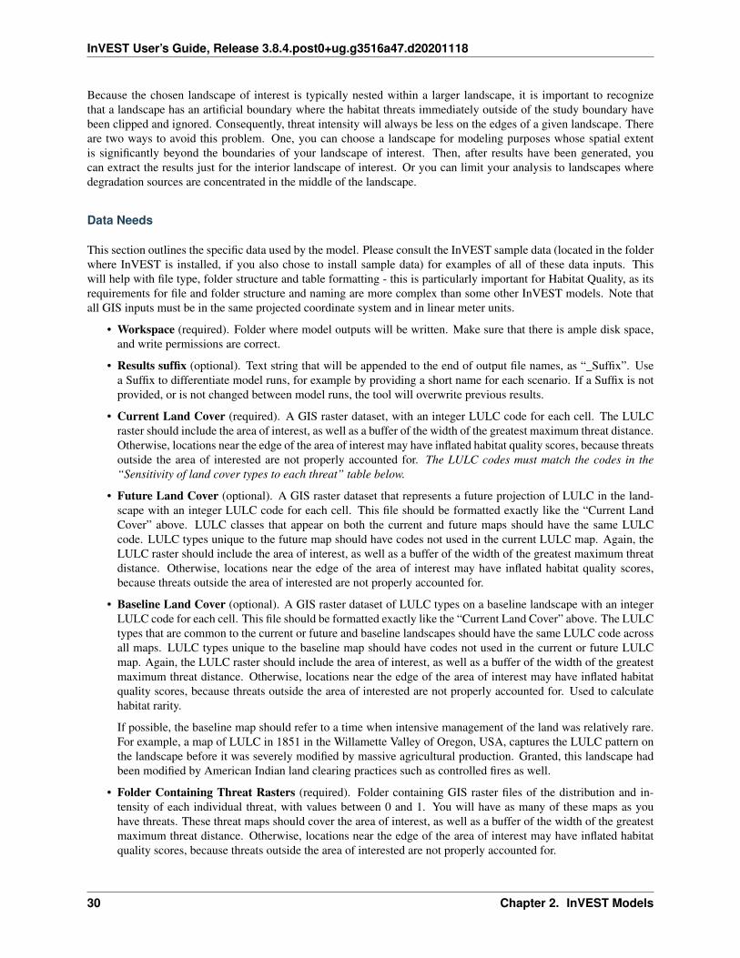
Data Needs
This section outlines the specific data used by the model. Please consult the InVEST sample data (located in the folderwhere InVEST is installed, if you also chose to install sample data) for examples of all of these data inputs. Thiswill help with file type, folder structure and table formatting - this is particularly important for Habitat Quality, as itsrequirements for file and folder structure and naming are more complex than some other InVEST models. Note thatall GIS inputs must be in the same projected coordinate system and in linear meter units.
• Workspace (required). Folder where model outputs will be written. Make sure that there is ample disk space,and write permissions are correct.
• Results suffix (optional). Text string that will be appended to the end of output file names, as “_Suffix”. Usea Suffix to differentiate model runs, for example by providing a short name for each scenario. If a Suffix is notprovided, or is not changed between model runs, the tool will overwrite previous results.
• Current Land Cover (required). A GIS raster dataset, with an integer LULC code for each cell. The LULCraster should include the area of interest, as well as a buffer of the width of the greatest maximum threat distance.Otherwise, locations near the edge of the area of interest may have inflated habitat quality scores, because threatsoutside the area of interested are not properly accounted for. The LULC codes must match the codes in the“Sensitivity of land cover types to each threat” table below.
• Future Land Cover (optional). A GIS raster dataset that represents a future projection of LULC in the land-scape with an integer LULC code for each cell. This file should be formatted exactly like the “Current LandCover” above. LULC classes that appear on both the current and future maps should have the same LULCcode. LULC types unique to the future map should have codes not used in the current LULC map. Again, theLULC raster should include the area of interest, as well as a buffer of the width of the greatest maximum threatdistance. Otherwise, locations near the edge of the area of interest may have inflated habitat quality scores,because threats outside the area of interested are not properly accounted for.
• Baseline Land Cover (optional). A GIS raster dataset of LULC types on a baseline landscape with an integerLULC code for each cell. This file should be formatted exactly like the “Current Land Cover” above. The LULCtypes that are common to the current or future and baseline landscapes should have the same LULC code acrossall maps. LULC types unique to the baseline map should have codes not used in the current or future LULCmap. Again, the LULC raster should include the area of interest, as well as a buffer of the width of the greatestmaximum threat distance. Otherwise, locations near the edge of the area of interest may have inflated habitatquality scores, because threats outside the area of interested are not properly accounted for. Used to calculatehabitat rarity.
If possible, the baseline map should refer to a time when intensive management of the land was relatively rare.For example, a map of LULC in 1851 in the Willamette Valley of Oregon, USA, captures the LULC pattern onthe landscape before it was severely modified by massive agricultural production. Granted, this landscape hadbeen modified by American Indian land clearing practices such as controlled fires as well.
• Folder Containing Threat Rasters (required). Folder containing GIS raster files of the distribution and in-tensity of each individual threat, with values between 0 and 1. You will have as many of these maps as youhave threats. These threat maps should cover the area of interest, as well as a buffer of the width of the greatestmaximum threat distance. Otherwise, locations near the edge of the area of interest may have inflated habitatquality scores, because threats outside the area of interested are not properly accounted for.
30 Chapter 2. InVEST Models

InVEST User’s Guide, Release 3.8.4.post0+ug.g3516a47.d20201118
Each cell in the raster contains a value that indicates the density or presence of a threat within it (e.g., areaof agriculture, length of roads, or simply a 1 if the grid cell is a road or crop field and 0 otherwise). Allthreats should be measured in the same scale and units (i.e., all measured in density terms or all measured inpresence/absence terms) and not some combination of metrics. The extent and resolution of these raster datasetsdoes not need to be identical to that of the input LULC maps. In cases where the threats and LULC mapresolutions vary, the model will use the resolution and extent of the LULC map. Do not leave any area on thethreat maps as ‘No Data’. If pixels do not contain that threat set the pixels’ threat level equal to 0.
InVEST will not prompt you for these rasters in the tool interface. It will instead automatically find each one inthe user-specified Folder, based on names in the Threats data table.
Raster naming requirements: The name of each raster file must exactly match the name of a degradationsource in the rows of the Threats data table. File names cannot be longer than 7 characters if using ESRI GRIDformat (so TIFFs are recommended.) If you are analyzing habitat quality for more than one LULC scenario (e.g.,a current and future map or a baseline, current, and future map) then you need a set of threat layers for eachmodeled scenario. Add “_c” at the end of the raster name for all “current” threat layers, “_f” for all future threatlayers, and “_b” for all “baseline” threat layers. For example, a raster corresponding to a THREAT of agriculture(called “Agric” in the Threats data table below) in the current scenario should be named “Agric_c.tif”, named“Agric_f.tif” in the future scenario and “Agric_b.tif” in the baseline scenario. If you do not use such endingsthen the model assumes the degradation source layers correspond to the current map. If a threat noted in theThreats data table is inappropriate for the LULC scenario that you are analyzing (e.g., industrial developmenton a Willamette Valley pre-settlement map from 1851) then enter a threat map for that time period that has all 0values. If you do not include threat maps for an input LULC scenario then the model will not calculate habitatquality on the scenario LULC map.
Finally, note that we assume that the relative weights of threats and sensitivity of habitat to threats do not changeover time, so we only submit one Threat data table and one Habitat sensitivity data table. If you want to changethese over time then you will have to run the model multiple times.
In the sample datasets, threat rasters are called the following: crp_c; crp_f; rr_c; rr_f; urb_c; urb_f; rot_c; rot_f;prds_c; prds_f; srds_c; srds_f; lrds_c; lrds_f. By using these sets of inputs we are running a habitat qualityanalysis for the current (_c) and future (_f) LULC scenario maps. A habitat quality map will not be generatedfor the baseline map because we have not provided any threat layers for the baseline map. The name ‘crp’ refersto cropland, ‘rr’ to rural residential, ‘urb’ to urban, ‘rot’ to rotation forestry, ‘prds’ to primary roads, ‘srds’ tosecondary roads, and ‘lrds’ to light roads.
• Threats data (required). A CSV (comma-separated value, .csv) table of all threats you want the model toconsider. The table contains information on the each threat’s relative importance or weight and its impact acrossspace.
Each row in the Threats data CSV table is a degradation source, and columns must be named as follows:
– THREAT. The name of the specific threat. Threat names must not exceed 8 characters.
– MAX_DIST. The maximum distance over which each threat affects habitat quality (measured in kilome-ters). The impact of each degradation source will decline to zero at this maximum distance.
– WEIGHT. The impact of each threat on habitat quality, relative to other threats. Weights can range from 1at the highest impact, to 0 at the lowest.
– DECAY. The type of decay over space for the threat. Can have the value of either “linear” or “exponential”.
Example: Hypothetical study with three threats. Agriculture (Agric in the table) degrades habitat overa larger distance than roads do, and has a greater overall magnitude of impact. Further, paved roads(Paved_rd) attract more traffic than dirt roads (Dirt_rd) and thus are more destructive to nearby habitatthan dirt roads.
2.1. Supporting Ecosystem Services: 31

InVEST User’s Guide, Release 3.8.4.post0+ug.g3516a47.d20201118
THREAT MAX_DIST WEIGHT DECAYDirt_rd 2 0.1 linearPaved_rd 4 0.4 exponentialAgric 8 1 linear
• Accessibility to Threats (optional): A GIS polygon shapefile containing data on the relative protection thatlegal / institutional / social / physical barriers provide against threats. Polygons with minimum accessibility(e.g., strict nature reserves, well protected private lands) are assigned some number less than 1, while polygonswith maximum accessibility (e.g., extractive reserves) are assigned a value 1. These polygons can be landmanagement units or a regular array or hexagons or grid squares. Any cells not covered by a polygon will beassumed to be fully accessible and assigned values of 1.
In the shapefile’s attribute table, each row is a specific polygon on the landscape, and columns must be namedas follows:
– ID: Unique identifying integer code for each polygon.
– ACCESS: Values between 0 and 1 for each polygon, as described above.
• Sensitivity of Land Cover Types to Each Threat (required): A CSV (comma-separated value, .csv) table ofLULC types, whether or not they are considered habitat, and, for LULC types that are habitat, their specificsensitivity to each threat.
Each row in the Sensitivity CSV table is an LULC type, and columns must be named as follows:
– LULC: Numeric integer code for each LULC type. Values must match the codes used in the current, futureand baseline LULC rasters. All LULC types that appear in the current, future, or baseline maps must havea row in this table.
– NAME: The name of each LULC
– HABITAT: Each LULC type is assigned a habitat score (𝐻𝑗 in the equations above), from 0 to 1. If youwant to simply classify each LULC as habitat or not without reference to any particular species group thenuse 0s and 1s where a 1 indicates habitat. Otherwise, if sufficient information is available on a speciesgroup’s habitat preferences, assign the LULC a relative habitat suitability score between 0 and 1 where1 indicates the highest habitat suitability. For example, a grassland songbird may prefer a native prairiehabitat above all other habitat types (prairie is given a “HABITAT” score of 1 for grassland birds), but willalso use a managed hayfield or pasture if prairie is not available (managed hayfield and pasture are given a“HABITAT” score of 0.5 for grassland birds).
– L_THREAT1, L_THREAT2, etc.: The relative sensitivity of each habitat type to each threat. You will haveas many columns named like this as you have threats, and the “_THREAT1”, “_THREAT2” etc portionsof the column names must match row names in the “Threat data” table noted above. Values range from 0to 1, where 1 represents high sensitivity to a threat and 0 represents no sensitivity. Note: Even if the LULCis not considered habitat, do not leave its sensitivity to each threat as Null or blank, instead enter a 0 andthe model will convert it to NoData.
Example: A hypothetical study with four LULC types and three threats. In this example we treat ClosedWoodland and Forst Mosaic as (absolute) habitat and Bare Soil and Cultivation as (absolute) non-habitat. Forestmosaic is the most sensitive (least resistant) habitat type, and is more sensitive to dirt roads (L_DIRT_RD, value0.9) than paved roads (L_PAVED_RD, value 0.5) or agriculture (L_AGRIC value 0.8). We enter 0s across allthreats for the two developed land covers, Bare Soil and Cultivation, since they are not habitat.
32 Chapter 2. InVEST Models

InVEST User’s Guide, Release 3.8.4.post0+ug.g3516a47.d20201118
LULC NAME HABITAT L_AGRIC L_PAVED_RD L_DIRT_RD1 Bare Soil 0 0 0 02 Closed Woodland 1 0.5 0.2 0.43 Cultivation 0 0 0 04 Forest Mosaic 1 0.8 0.8 0.5
• Half-saturation constant (required): This is the value of the parameter 𝑘 in equation (4). By default it is setto 0.5 but can be set equal to any positive floating point number. In general, you want to set 𝑘 to half of thehighest grid cell degradation value on the landscape. To perform this model calibration you will have to the runthe model once to find the highest degradation value and set 𝑘 for your landscape. For example, if a preliminaryrun of the model generates a degradation map where the highest grid-cell degradation level is 1 then setting 𝑘at 0.5 will produce habitat quality maps with the greatest variation on the 0 to 1 scale (this helps with visualrepresentation of heterogeneity in quality across the landscape). It is important to note that the rank order ofgrid cells on the habitat quality metric is invariant to your choice of 𝑘. The choice of 𝑘 only determines thespread and central tendency of habitat quality scores. It is important to use the same value of 𝑘 for all runs thatinvolve the same landscape. If you want to change your choice of 𝑘 for any model run then you must changethe parameters for all model runs.
Running the Model
To launch the Habitat Quality model navigate to the Windows Start Menu -> All Programs -> InVEST [version] ->Habitat Quality. The interface does not require a GIS desktop, although the results will need to be explored with anyGIS tool such as ArcGIS or QGIS.
Interpreting Results
The following is a short description of each of the outputs from the Habitat Quality model. Final results are foundwithin the user defined Workspace specified for this model run. “Suffix” in the following file names refers to theoptional user-defined Suffix input to the model.
• [Workspace] folder:
– Parameter log: Each time the model is run, a text (.txt) file will be created in the Workspace. The file willlist the parameter values and output messages for that run and will be named according to the service, thedate and time. When contacting NatCap about errors in a model run, please include the parameter log.
• [Workspace]\output folder:
– deg_sum_out_c_[Suffix].tif – Relative level of habitat degradation on the current landscape. A high scorein a grid cell means habitat degradation in the cell is high relative to other cells. Grid cells with non-habitat land cover (LULC with 𝐻𝑗 = 0) get a degradation score of 0. This is a mapping of degradationscores calculated with equation (3).
– deg_sum_out_f_[Suffix].tif – Relative level of habitat degradation on the future landscape. A high scorein a grid cell means habitat degradation in the cell is high relative to other cells. This output is only createdif a future LULC map is given as input. Grid cells with non-habitat land cover (LULC with 𝐻𝑗 = 0) get adegradation score of 0. This is a mapping of degradation scores calculated with equation (3).
– quality_out_c_[Suffix].tif – Relative level of habitat quality on the current landscape. Higher numbersindicate better habitat quality vis-a-vis the distribution of habitat quality across the rest of the landscape.Areas on the landscape that are not habitat get a quality score of 0. This quality score is unitless and does
2.1. Supporting Ecosystem Services: 33

InVEST User’s Guide, Release 3.8.4.post0+ug.g3516a47.d20201118
not refer to any particular biodiversity measure. This is a mapping of habitat qulaity scores calculated withequation (4).
– quality_out_f_[Suffix].tif – Relative level of habitat quality on the future landscape. Higher numbersindicate better habitat quality vis-a-vis the distribution of habitat quality across the rest of the landscape.This output is only created if a future LULC map is given as input. Areas on the landscape that are nothabitat get a quality score of 0. This quality score is unitless and does not refer to any particular biodiversitymeasure. This is a mapping of habitat qulaity scores calculated with equation (4).
– rarity_c_[Suffix].tif – Relative habitat rarity on the current landscape vis-a-vis the baseline map. Thisoutput is only created if a baseline LULC map is given as input. This map gives each grid cell’s value of𝑅𝑥 (see equation (6)). The rarer the habitat type in a grid cell is vis-a-vis its abundance on the baselinelandscape, the higher the grid cell’s value in rarity_c.tif.
– rarity_f_[Suffix].tif – Relative habitat rarity on the future landscape vis-a-vis the baseline map. Thisoutput is only created if both baseline and future LULC maps are given as input. This map gives each gridcell’s value of 𝑅𝑥 (see equation (6)). The rarer the habitat type in a grid cell is vis-a-vis its abundance onthe baseline landscape, the higher the grid cell’s value in rarity_f.tif.
• [Workspace]\intermediate folder:
This folder contains some of the intermediate files created during the model run. Usually you donot need to work with these files, unless you are trying to better understand how the model works, ordebugging a model run. They include maps of habitats (habitat__[b,c,f].tif), threats layers processedwith Threats data table attributes ([threat]_filtered_[b,c,f].tif), sensitivity applied to different threats(sens_[threat]_[b,c,f].tif), and a rasterized version of the Access input (access_layer.tif).
Modifying Output and Creating a Landscape Biodiversity Score
The model output does not provide landscape-level quality and rarity scores for comparing the baseline, current,and future LULC scenarios. Instead the user must summarize habitat extent and quality and rarity scores for eachlandscape. At the simplest level, a habitat quality landscape score for an LULC scenario is simply the aggregateof all grid cell-level scores under the scenario. In other words, we can sum all grid-level quality scores from thequality_out_c.tif, quality_out_b.tif (if available), and quality_out_f.tif (if available) maps and then compare scores.A map may have a higher aggregate quality score for several reasons. For one, it may just have more habitat area.However, if the amount of habitat across any two scenarios is approximately the same then a higher landscape qualityscore is indicative of better overall quality habitat.
Scores for certain areas on a landscape could also be compared. For example, we could compare aggregate habitatquality scores in areas of the landscape that are known to be in the geographic ranges of species of interest. Forexample, suppose we have geographic range maps of 9 species and have provided current and future LULC scenariomaps to the Habitat Quality model. In this case we would determine 18 aggregate habitat quality scores, once foreach modeled species under each scenario (current and future). Let 𝐺𝑠cur indicate the set of grid cells on the currentlandscape that are in 𝑠’ range. Then the average habitat quality score in species 𝑠’ range on the current landscape isgiven by,
𝑄𝑠cur =
∑︀𝐺𝑠cur
𝑥=1 𝑄𝑥𝑗cur
𝐺𝑠cur(2.7)
where 𝑄𝑥𝑗𝑐𝑢𝑟 indicates the habitat quality score on pixel 𝑥 in LULC 𝑗 on the current landscape and 𝑄𝑥𝑗𝑐𝑢𝑟 = 0 ifquality_out.tif for pixel 𝑥 is “No Data”. The average range-normalized habitat quality score for all 9 species on thecurrent landscape would be given by,
𝑅𝑥 =
𝑋∑︁𝑥=1
𝜎𝑥𝑗𝑅𝑗 (2.8)
Then we would repeat for the future landscape with the grid cells in set 𝐺𝑠fut for each species 𝑠 and the set of 𝑄𝑥𝑗𝑓𝑢𝑡.
34 Chapter 2. InVEST Models

InVEST User’s Guide, Release 3.8.4.post0+ug.g3516a47.d20201118
References
Ando, A, J. Camm, S. Polasky, and A. Solow. 1998. Species distributions, land values, and efficient conservation.Science 279:2126-2128.
Czech, B., P. R. Krausman, and P. K. Devers. 2000. Economic Associations among Causes of Species Endangermentin the United States. Bioscience 50:593-601.
Forman, R. 1995. Land Mosaics: The Ecology of landscapes and regions. Cambridge Univ Press. New York.
Forman, R. 2003. Road ecology: science and solutions. Island Press. New York, New York.
Franklin, J.F. and D. B. Lindenmayer. 2009. Importance of matrix habitats in maintaining biological diversity. Pro-ceedings of the National Academy of Sciences 106:349-350.
Hall, L.S., Krausman, P.R. and Morrison, M.L. 1997. The habitat concept and a plea for standard terminology. WildlifeSociety Bulletin 25(1):173-182.
Lindenmayer, D., Hobbs, R., Montague-Drake, R., Alexandra, J., Bennett, A., Burgman, M., Cae, P., Calhoun, A.,Cramer, V., Cullen, P. 2008. A checklist for ecological management of landscapes for conservation. Ecology Letters11:78-91.
MacArthur, R., E. 0. Wilson. 1967. The theory of island biogeography. Princeton University Press, Princeton, NJ.
Mckinney, M.L. 2002. Urbanization, biodiversity, and conservation. BioScience 52:883-890.
Nelleman C, Kullered L, Vistnes I, Forbes B, Foresman T, Husby E, Kofinas G, Kaltenborn B, Rouaud J, MagomedovaM, Bobiwash R, Lambrechts C, Schei P, Tveitdal S, Gron O, Larsen T. 2001. GLOBIO. Global methodology formapping human impacts on the biosphere. UNEP/DEWA/TR.01-3.
Nelson, E., S. Polasky, D. J. Lewis, A. J. Plantinga, E. Lonsdorf, D. White, D. Bael & J. J. Lawler. 2008. Efficiencyof incentives to jointly increase carbon sequestration and species conservation on a landscape. Proc. Nat. Acad. Sci.105: 9471-9476.
Noss, R. F., M. A. Connell, and D. D. Murphy. 1997. The science of conservation planning: habitat conservationunder the endangered species act. Island Press. Prugh, L., K. Hodges, A. Sinclair, and J. Brashares. 2008. Effectof habitat area and isolation on fragmented animal populations. Proceedings of the National Academy of Sciences105:20770.
Ricketts, T. H. 2001. The Matrix Matters: Effective Isolation in Fragmented Landscapes. American Naturalist 158:87-99.
Vitousek, P. M., H. A. Mooney, J. Lubchenco, and J. M. Melillo. 1997. Human Domination of Earth’s Ecosystems.Science 277:494.
Wilcove, D. S., D. Rothstein, J. Dubow, A. Phillips, and E. Losos. 1998. Quantifying Threats to Imperiled Species inthe United States. Bioscience 48:607-615.
2.1.2 Habitat Risk Assessment
Summary
The InVEST Habitat and Species Risk Assessment (HRA/SRA) model allows users to assess the cumulative risk posedto habitats and species by human activities and to explore consequences for the delivery of ecosystem services andbiodiversity. The condition of a habitat is a key determinant of the ecosystem services it can provide; for example,degraded coastal mangroves are less able to attenuate waves and reduce coastal exposure. Risk to species may indicatereduced sustainability through time. As anthropogenic stressors continue to diversify and intensify, so too does theneed for quick, clear and repeatable ways of assessing risks to habitats and species, now and under future manage-ment scenarios. HRA/SRA utilizes a well-supported exposure-consequence framework to assess spatial variation incumulative risk from multiple human activities across a land- or seascapes.
2.1. Supporting Ecosystem Services: 35

InVEST User’s Guide, Release 3.8.4.post0+ug.g3516a47.d20201118
Outputs from the model include an ecosystem risk map, risk maps for each individual habitat or species, risk plotsthat display the contribution of exposure and consequence to overall risk, and summary tables of risk by subregionand habitat or species. These outputs can be used to identify areas at the greatest relative risk of degradation as wellas the primary causes of risk within a study region and among alternative future scenarios. Model outputs can helpidentify areas where human activities may create trade-offs among ecosystem services by posing risk high enough tocompromise habitat structure and function or species persistence or recovery. The model can help to prioritize areasfor conservation, evaluate management strategies, and inform the design and configuration of spatial plans for bothmarine and terrestrial systems.
Introduction
Habitats and species provide essential benefits for people, including regulating, material, and non-material services(Pascual et al. 2017, Díaz et al. 2018). For example, nearshore habitats such as kelp forests and eelgrass meadowsprotect shorelines from storms, provide nursery habitat for fisheries, and store and sequester carbon. Terrestrial habi-tats like riparian forests absorb excess nutrients and sediment, provide habitat for riverine fish species, and mitigateinland flooding after rain events. As these habitats (or species) become degraded by human activities, the ecosystemservices they provide are threatened. Recent global analyses have revealed that almost no area of the world’s oceansis untouched by human impacts (Halpern et al. 2008). Thus, an understanding of the location and intensity of hu-man impacts on nearshore ecosystems is an essential component of informed and successful terrestrial, coastal, andocean management. The InVEST HRA model allows users to assess the threat of human activities to the health ofthese ecosystems and species. The model has been successfully applied in numerous locations across the world (e.g.Arkema et al. 2014, Cabral et al. 2015, Chung et al. 2015, Duggan et al. 2015, Ma et al. 2016, Elliff et al. 2017,Wyatt et al. 2017).
The HRA model is a quantitative approach to evaluating the cumulative influence of stressors associated with humanactivities on habitats and species (Arkema et al. 2014, Arkema et al. 2015). HRA uses a well-established approachfrom the risk literature that originates from fisheries vulnerability assessments (Astles et al. 2006, Patrick et al. 2010,Hobday et al. 2011, Samhouri and Levin 2012).
The model incorporates two dimensions of information to calculate risk or impact to ecosystem components (figure1; Halpern et al. 2008, Patrick et al. 2010, Samhouri and Levin 2012, Arkema et al. 2014). These dimensions areexposure and consequence.
Exposure is the degree to which a habitat or species experiences a stressor, given the effectiveness of managementpractices.
Consequence is the habitat (or species)-specific response to that exposure. Consequence incorporates the sensitivityof each habitat or species to the effects of a stressor, and the habitat’s resilience, or the ability of the habitat or speciesto resist or recover from a stressor to which it is exposed.
Informing decision-making processes
The outputs of the HRA model allow users to identify areas of high ecosystem risk, investigate which habitats orspecies are at the greatest risk and where, determine the primary causes of that risk, and understand how risk maychange under future scenarios. HRA results can be used in an array of decision contexts:
• Areas of high risk can be used to prioritize management or restoration efforts, as NOAA’s Office for CoastalManagement has done in New Hampshire’s Great Bay (NOAA OCM 2016).
• Areas of high risk can be used to constrain the decision space when siting additional uses (e.g. where to sitewind energy as shown in Wyatt et al. 2017)
• Risk plots can provide insight into which activities are the most impactful and what types of managementstrategies will be most effective (E.g. Duggan et al. 2015).
36 Chapter 2. InVEST Models

InVEST User’s Guide, Release 3.8.4.post0+ug.g3516a47.d20201118
Fig. 1: Habitats with high exposure to human activities and high consequence of that exposure are at high risk. Plottingexposure and consequence like this allows assessments of which components of risk are most significant and revealsrisk-reduction strategies. Risks driven by exogenous human factors (top right region of the risk space) might bemitigated by management interventions, while risk driven by endogenous habitat-specific factors (top-left region ofrisk space) may be better addressed through monitoring and preparedness. (Adapted from Dawson et al. 2011).
• When used in conjunction with models that estimate habitat-induced changes in ecosystem services, such asstorm protection or tourism revenue, HRA can help to evaluate trade-offs among human activities and benefitsthat ecosystems provide to people (see :ref:‘ Connecting Habitat Risk Assessment Results to InVEST EcosystemService Models‘; Guerry et al. 2012, Clarke et al. 2016, Arkema et al. 2015).
• Repeated applications of HRA can be used together to assess and compare alternative scenarios (Arkema et al.2014).
The Model
How it Works
To assess the exposure of ecosystems and habitats or species to human activities, and the consequence of that expo-sure, HRA synthesizes information about interactions between multiple human activities (or “stressors”), and multiplehabitats or species using both spatial and non-spatial data from the peer-reviewed literature, grey literature, and expertopinion.
The model is spatially-explicit, calculating exposure, consequence, and risk scores on a continuous raster surfaceacross the study area, at a spatial resolution chosen by the user. All geospatial data inputs are rasterized at thisresolution, and operations described below occur at the pixel-scale.
Users provide geospatial data including habitat or species distributions, the spatial extent of human activities or stres-sors, and tabular data about the nature of the interaction between habitats or species and these stressors. Informationabout these interactions are included in the form of multiple exposure and consequence criteria scores (typically 1-3,with 0 = no score). The specific criteria can be defined by the user, or suggested by the model. Scores are specificto each habitat (or species)-stressor interaction. For example, scores from 1-3 would be assigned to each of theseitalicized criteria, for each habitat-stressor pair:
2.1. Supporting Ecosystem Services: 37

InVEST User’s Guide, Release 3.8.4.post0+ug.g3516a47.d20201118
Exposure criteria might include, the extent of geographic overlap between a habitat-stressor pair, the duration oftime that the stressor and habitat overlap, the intensity of the stressor, and the degree to which management strategiesmitigate impact.
Consequence criteria might include the degree of habitat loss as a result of exposure to a stressor, change in habitatstructure, and the ability of habitats to recover from these effects (i.e., through life history traits such as recruitmentand regeneration rates).
For each criterion, the user scores the interaction from low to high. The model is flexible and can accommodate data-poor and data-rich situations. Data may come from a combination of sources, from peer-reviewed data at the globalscale and locally available fine-scale data. Model inputs and results can be updated as better information becomesavailable.
Cumulative Risk to Habitats or Species from Multiple Stressors
The risk of human activities to habitats or species is modeled in five steps.
1. Calculate the exposure and consequence scores for each habitat-stressor pair.
2. Combine the exposure and consequence values into a risk score, for each habitat-stressor pair.
3. Accumulate the risk from all stressors to each habitat/species, at each pixel location.
4. Categorize risk to each habitat or species as low, medium, or high.
5. Summarize pixel-scale results to larger subregions of interest.
Step 1. The first step involves determining the degree of exposure of the habitat or species to the stressor, and theconsequence of this exposure. Exposure (E) and consequence (C) are both determined by assigning a rating (typically1-3, with 0 = no score) to a set of criteria, such as those described above, which are used frequently in the scientificliterature. However, any criteria may be added or removed. Guidelines for scoring the default criterion are summarizedbelow (Default Exposure Criteria and Default Consequence Criteria). Note that “spatial overlap” is a special exposurecriteria that is always included, and does not need to be defined or scored by the user like other criteria. For each gridcell in the study area, if a stressor and a habitat or species are both present, then spatial overlap = 1 and the modelcalculates E and C using the information about the other criteria and the equations below. If a stressor and a habitator species do not overlap in a particular grid cell, Exposure, Consequence, and Risk are 0 in that cell. The scores forall the other criteria are inputs to the model provided by the user. For each score assigned, you may also indicate thequality of the data used to determine the score, and the weighted importance of the criteria relative to other criteria.This allows you to assign greater weight to criteria where scoring confidence was higher, or to criteria which contributemore to risk in the system. Thus, the overall exposure 𝐸 and consequence 𝐶 scores are calculated as weighted averagesof the exposure values 𝑒𝑖 and consequence values 𝑐𝑖 for each criterion i, from habitat j and stressor k
𝐸𝑗𝑘𝑙 =
∑︀𝑁𝑖=1
𝑒𝑖𝑗𝑘𝑙
𝑑𝑖𝑗𝑘𝑙·𝑤𝑖𝑗𝑘𝑙∑︀𝑁𝑖=1
1𝑑𝑖𝑗𝑘𝑙·𝑤𝑖𝑗𝑘𝑙
(2.9)
𝐶𝑗𝑘𝑙 =
∑︀𝑁𝑖=1
𝑐𝑖𝑗𝑘𝑙
𝑑𝑖𝑗𝑘𝑙·𝑤𝑖𝑗𝑘𝑙∑︀𝑁𝑖=1
1𝑑𝑖𝑗𝑘𝑙·𝑤𝑖𝑗𝑘𝑙
(2.10)
where 𝐸𝑗𝑘𝑙 is the exposure score specific to habitat j, from stressor k in location l; 𝐶𝑗𝑘𝑙 is the consequence score, 𝑒𝑖𝑗𝑘𝑙is the exposure rating criterion i, specific to habitat j and stressor k and location l; 𝑐𝑖𝑗𝑘𝑙 is the consequence rating. 𝑑𝑖𝑗𝑘𝑙represents the data quality rating, 𝑤𝑖𝑗𝑘𝑙 represents the importance weighing for criterion. N is the number of criteriaevaluated for each habitat.
Step 2. The second step combines the exposure and response values to produce a risk value for each stressor-habitatcombination in each grid cell. There are two options for risk calculation.
38 Chapter 2. InVEST Models

InVEST User’s Guide, Release 3.8.4.post0+ug.g3516a47.d20201118
For Euclidean Risk calculation, risk to habitat j caused by stressor k in each location (i.e. cell) l is calculated as theEuclidean distance from the origin in the exposure-consequence space, where average exposure (eq1) is on one axisand the average consequence score (eq2) is on the other.
𝑅𝑗𝑘𝑙 =√︁
(𝐸𝑗𝑘𝑙 − 1)2 + (𝐶𝑗𝑘𝑙 − 1)2 (2.11)
The model maps this habitat-stressor specific risk score where the habitat and stressor overlap in space
For Multiplicative Risk calculation, risk to habitat j caused by stressor k in cell l is calculated as the product of theexposure (eq1) and consequence scores (eq2).
𝑅𝑖𝑗𝑘𝑙 = 𝐸𝑗𝑘𝑙 · 𝐶𝑗𝑘𝑙 (2.12)
Note: The user has the option of choosing which risk function to use. Different studies have combined exposure andconsequence in different ways: Cumulative impact mapping studies tend to use a multiplicative approach to estimaterisk (Halpern et al 2008, Selkoe et al 2009, Ban et al 2010), whereas ecosystem risk assessment studies tend to estimaterisk as the Euclidean distance for a specific habitat (or species)-activity combination in risk plots (Patrick et al 2010,Hobday et al 2011, Samhouri and Levin 2012, Arkema et al. 2014).
Initial sensitivity testing suggests that, overall, the two approaches agree on the highest and lowest risk habitats orregions, although intermediate risk results may differ (Stock et al. 2015). Empirical testing of an extensive HRAanalysis in Belize using a Euclidean approach found good agreement between calculated risk and measures of habitatfragmentation and health (Arkema et al. 2014 supplement). In general, the Euclidean approach may provide moreconservative, higher overall estimates than the multiplicative approach. If E and C values are widely different, thenthe Euclidean approach will produce relatively higher risk results. In contrast, the multiplicative approach will tend toproduce relatively lower, less conservative values for risk and associate similarity in E and C with higher risk. If yoursystem contains habitats for which there is a very high consequence of risk but low exposure (e.g., coral and shrimptrawling zones that currently avoid coral reefs) and you want to adopt the precautionary principle, then choosing theEuclidean approach is advised.
2.1. Supporting Ecosystem Services: 39

InVEST User’s Guide, Release 3.8.4.post0+ug.g3516a47.d20201118
Step 3. In this step, the model quantifies the cumulative risk to each habitat or species from all stressors, at each gridcell. Cumulative risk for habitat or species j in cell l is the sum of all risk scores for each habitat or species,
𝑅𝑗𝑙 =
𝐾∑︁𝑘=1
𝑅𝑗𝑘𝑙 (2.13)
Step 4. Each grid cell for each habitat or species is classified as LOW< MED, or HIGH risk based on risk posed by thecumulative effects of multiple stressors. A classification of HIGH is assigned to grid cells meeting one of two criteria:
1) Cumulative risk in the grid cell is >66% of the maximum risk score for any individual habitat (or species)-stressor combination. For example, if exposure and consequence are ranked on a scale of 1-3, then the maximumrisk score for an individual habitat (or species)-stressor combination is 2.83 (using the Euclidean approach); allcells with a risk score greater than 1.87 (66% of 2.83) would be classified as HIGH risk. This criterion addressesthe issue that in instances where a stressor is particularly destructive (e.g. clear cutting that removes all treesor dredging that removes all coral), additional stressors (e.g. hiking trails or recreation fishing) will not furtherincrease the risk of habitat degradation.
2) Cumulative risk in the grid cell is >66% of the total possible cumulative risk. Total possible cumulative riskis based on both the maximum risk score for an individual habitat (or species)-stressor combination and themaximum number of stressors that can occupy a particular grid cell in the study area (see next paragraph).Maximum number of overlapping stressors = 3 if, in the entire study region, no more than 3 stressors (e.g.,agriculture run-off, marine aquaculture and marine transportation) are likely to occur in a single grid cell. Totalpossible cumulative risk in this case would be 8.49 (based on the Euclidean approach; the maximum risk scorefor a single habitat (or species)-stressor combination X the maximum number of overlapping stressors = 2.83 x3 = 8.49). This criterion addresses the issue that even when a single stressor is not particularly detrimental thecumulative effect of multiple stressors causes is high.
Cells are classified as MED if they have individual stressor or cumulative risk scores between 33%-66% of the totalpossible cumulative risk score. Cells are classified as LOW risk if they have individual or cumulative risk scores of0-33% of the total possible risk score for a single stressor or multiple stressors, respectively.
The maximum number of overlapping stressors is determined by the model. It is the total number of stressors in thestudy area; however, it is unlikely that all stressors will ever realistically overlap in a single grid cell. The modelexamines overlap in stressors to get the highest number of overlapping stressors.
Step 5. In the final step, risk is summarized in any number of subregions within the sudy area. In a spatial planningprocess, subregions are often units of governance (i.e., coastal planning regions, states or provinces) within the bound-aries of the planning area. At the subregional scale, score for spatial overlap (a default exposure criteria) is basedon the fraction of habitat area in a subregion that overlaps with a human activity (see below for more detail). Thesubregional score for all other E and C criteria are the average E and C score across all grid cells in the subregion.Risk is estimated either using the Euclidean distance or multiplicative approach (see above).
Cumulative Risk to the Ecosystem from Multiple Stressors
To provide an integrative index of risk across all habitats or species in a grid cell, the model also calculates ecosystemrisk. Ecosystem risk for each grid cell l is the sum of habitat or species risk scores in that cell.
𝑅𝑙 =
𝐽∑︁𝑗=1
𝑅𝑗𝑙 (2.14)
Ecosystem risk will increase with an increasing number of co-occurring habitats or species.
Exposure and Consequence Criteria in More Detail
The model allows for any number of criteria to be used when evaluating the risk to habitat areas. As a default, themodel provides a set of typical considerations for evaluating risk of stressors to habitats. With the exception of spatial
40 Chapter 2. InVEST Models

InVEST User’s Guide, Release 3.8.4.post0+ug.g3516a47.d20201118
overlap at a grid cell scale, these criteria are rated on a scale of 1-3, with 0 = no score. However, the user is notconstrained to the 1-3 scale. As long as there is consistency across the rating scores within a single model run, otherscales (e.g. 1-5, 1-10) may be used. In all cases higher numbers represent greater exposure or consequence and resultin higher risk scores. Using a score of 0 will always indicate that the given criteria should be excluded fromExposure & Consequence equations.
For technical guidance on how to prepare this input data, see Criteria Scores CSV . For
Default Exposure Criteria
1. Spatial overlap . To assess spatial overlap in the study area, the model uses maps of the distribution of habitatsor species and stressors.
Habitat maps can represent biotic (e.g. eelgrass or kelp) or abiotic (e.g. hard or soft bottom) habitat types, orspecies. The user defines the detail of habitat classification. For example, habitats can be defined as biotic orabiotic, by taxa (e.g., coral, seagrass, mangrove), by species (e.g., red, black mangroves) or in whatever schemethe user desires. In a species risk assessment, we recommend specifying a single species, but the user could alsoindicate a taxa. In order for additional detail or specificity to be useful and change the outcome of the model,these habitat classifications should correspond with differences between how habitats or species respond to thestressors.
Stressor maps represent the footprint, or spatial extent, of the stressor activity. In addition, a “zone of influence”or “buffer” can be assigned to each stressor, representing the distance over which the effects of the stressor spreadbeyond its actual footprint in the input map. For some stressors, such as foot trails through a forest, this distancewill be small. For other stressors, such as finfish aquaculture pens where nutrients spread 300-500m or forestclearcutting where edge effects can extend up to 1km, this distance may be large. The user can specify whetherthe impacts of the stressor decay linearly or exponentially from the footprint of the stressor to the outer extent ofthe zone of influence. The model uses the distance of the zone of influence of a stressor to create an intermediateoutput that is a map of the stressor footprint buffered by the zone of influence (rounding down to the nearestpixel unit; e.g., a buffer distance of 600m will round down to 500m if the resolution of analysis is 250m).
For each grid cell, if the habitat or species overlaps with a stressor, then spatial overlap = 1 and the modelcalculates exposure, consequence and risk using scores for the other criteria (below). If a habitat or species doesnot overlap with a stressor in a particular grid cell, then the model sets exposure, consequence and risk = 0 inthat particular grid cell.
At the subregional scale, the model calculates spatial overlap scores as follows. For each subregion, the fractionof area of each habitat that overlaps with each stressor is the percentage_overlap. Then, the spatial overlap scorefollows this equation:
maximum_criteria_score * percentage_overlap + minimum_criteria_score * (1 - percentage_overlap)
For example, if 50% of a habitat’s area is overlapped by a stressor, and our criteria scale is 1-3, then: 3 * 0.5 +1 * (1 - 0.5) = 2. Lastly, the model averages the spatial overlap score with the average exposure score for thesubregion. If there is no spatial overlap between the habitat and stressor at the subregional scale, then exposure= 0, consequence = 0 and risk = 0. If there are no exposure scores for that habitat-stressor combination, butspatial overlap does exist, the score will be entirely the spatial overlap.
2. Overlap time rating. Temporal overlap is the duration of time that the habitat or species and the stressorexperience spatial overlap. Some stressors, such as permanent structures, are present year-round. Other stresorsare seasonal, such as certain fishing practices or recreational activities. Similarly, some habitats (e.g. mangroves)or species are present year round, while others are more ephemeral (e.g. some seagrasses or perennial understoryvegetation).
If criteria are scored on a 1-3 scale, the following is a suggestion for scoring temporal overlap:
2.1. Supporting Ecosystem Services: 41

InVEST User’s Guide, Release 3.8.4.post0+ug.g3516a47.d20201118
Score: 1 (low) 2 (medium) 3 (high) 0 (noscore)
Tem-poraloverlap
Habitat and stressor co-occur for 0-4 months of theyear
Habitat and stressor co-occur for 4-8 months of theyear
Habitat and stressor co-occur for 8-12 months ofthe year
N/A
Choose “0” to exclude this criterion from your assessment.
3. Intensity rating. Exposure depends not only on whether the habitat and stressor overlap in space and time,but also on the intensity of the stressor. Some examples: The intensity of nutrient-loading stress associatedwith netpen salmon aquaculture is related to the number of salmon in the farm and how much waste is releasedinto the surrounding environment. The intensity of destructive shellfish harvesting is related to the number ofharvesters and the harvest practices. You can use this intensity criteria to explore how changes in the intensity ofone stressor might affect risk to habitats. For example, one could change the intensity score to represent changesin the stocking density of a salmon farm in a future scenario. One can also use this ranking to incorporate relativedifferences in the intensity of different stressors within the study region. For example, different types of marinetransportation may have different levels of intensity. For example, cruise ships may be a more intense stressorthan water taxis because they release more pollutants than the taxis do.
If criteria are scored on a 1-3 scale, the following is a suggestion for scoring intensity:
Score 1 2 3 0Intensity Low intensity Medium intensity High intensity N/A
Choose “0” to exclude this criterion from your assessment.
4. Management strategy effectiveness rating. Management can limit the negative impacts of human activitieson habitats. For example, regulations that require a minimum height for overwater structures reduce the shadingimpacts of overwater structures on submerged aquatic vegetation. Thus, effective management strategies willreduce the exposure from stressors to habitats or species. The effectiveness of management of each stressoris scored relative to other stressors in the region. So if there is a stressor that is very well managed suchthat it imparts much less stress on the system than other stressors, classify management effectiveness as “veryeffective.” In general, however, the management of most stressors is likely to be “not effective.” After all, youare including them as stressors because they are having some impact on habitats. You can then use this criterionto explore changes in management between scenarios, such as the effect of changing development from highimpact (which might receive a score of “not effective”) to low impact (which might receive a score of “veryeffective).” As with all criteria, higher numbers represent greater exposure and result in higher risk scores.
If criteria are scored on a 1-3 scale, the following is a suggestion for scoring management effectiveness:
Score 1 2 3 0Management effectiveness Very effective Somewhat effective Not effective, poorly managed N/A
Choose “0” to exclude this criterion from your assessment.
5. Other exposure criteria may be used in addition to, or instead of, the criteria listed above.
Default Consequence Criteria
The risk of a habitat or species being degraded by a stressor depends on the consequence of exposure. Consequence isdetermined by both the sensitivity of a habitat to a specific stressor and the resilience of a habitat to resist and recoverfrom disturbance in general. As a default, the model includes three specific measures of sensitivity (change in area,change in structure, and frequency of similar natural disturbance) and four measures of resilience (natural mortalityrate, recruitment rate, age at maturity, and connectivity). Each is described below.
42 Chapter 2. InVEST Models

InVEST User’s Guide, Release 3.8.4.post0+ug.g3516a47.d20201118
1. Change in area rating. Change in area is measured as the percent change in extent of a habitat or species whenexposed to a given stressor and is a measure of sensitivity of the habitat or species to the stressor. Habitats orspecies that lose a high percentage of their areal extent when exposed to a given stressor are highly sensitive,while those habitats that lose little area are less sensitive.
If criteria are scored on a 1-3 scale, the following is a suggestion for scoring change in area:
Score 1 2 3 0Change inarea
Low loss in area (0-20%)
Medium loss in area (20-50%)
High loss in area (50-100%)
N/A
Choose “0” to exclude this criterion from your assessment.
2. Change in structure rating. For biotic habitats, the change in structure is the percentage change in structuraldensity of the habitat when exposed to a given stressor. For example, change in structure would be the changein tree density (or vertical or horizontal complexity) for forest systems or change in polyp density for corals.Habitats that lose a high percentage of their structure when exposed to a given stressor are highly sensitive,while habitats that lose little structure are less sensitive. For abiotic habitats, the change in structure is theamount of structural damage sustained by the habitat. Sensitive abiotic habitats will sustain complete or partialdamage, while those that sustain little to no damage are more resistant. For example, gravel or muddy bottomswill sustain partial or complete damage from bottom trawling while hard bedrock bottoms will sustain little tono damage. For species, change in structure can be used to capture changes to population structure, for examplein age or gender distribution
If criteria are scored on a 1-3 scale, the following is a suggestion for scoring change in structure:
Score 1 2 3 0Changeinstruc-ture
Low loss in structure (for bi-otic habitats, 0-20% loss indensity, for abiotic habitats,little to no structural damage)
Medium loss in structure (forbiotic habitats, 20-50% lossin density, for abiotic habi-tats, partial structural dam-age)
High loss in structure (forbiotic habitats, 50-100%loss in density, for abiotichabitats, total structuraldamage)
N/A
Choose “0” to exclude this criterion from your assessment.
3. Frequency of natural disturbance rating. If a habitat or species is naturally frequently perturbed in a waysimilar to the anthropogenic stressor, it may be more resistant to comparable anthropogenic stress. For example,habitats in areas that experience periodical delivery of nutrient subsidies (i.e. from upwelling or allocthonousinputs such as delivery of intertidal plant material to subtidal communities) are adapted to variable nutrientconditions and may be more resistant to nutrient loading from netpen salmon aquaculture. Similarly, forests withhistorical wind-throw events may be better adapted to selective logging. This criterion is scored separately foreach habitat or species-stressor combination, such that being adapted to variable nutrient conditions increasesresistance to nutrient loading from salmon aquaculture but not destructive fishing. However, an alternativenaturally occurring stress like high storm frequency may increase resistance to destructive fishing, because bothstressors impact habitats in similar ways. High rates of comparable natural disturbance imply greater resilienceand are therefore scored lower.
If criteria are scored on a 1-3 scale, the following is a suggestion for scoring natural disturbance frequencies:
Score 1 2 3 0Frequency of similar nat-ural disturbance
Frequent (dailyto weekly)
Intermediate frequency (sev-eral times per year)
Rare (annually orless often)
N/A
Choose “0” to exclude this criterion from your assessment.
2.1. Supporting Ecosystem Services: 43

InVEST User’s Guide, Release 3.8.4.post0+ug.g3516a47.d20201118
Note: The following consequence criteria are Resilience Attributes. These include life history traits such as regen-eration rates and recruitment patterns that influence the ability of habitats or species to recover from disturbance. Wetreat recovery potential as a function of natural mortality, recruitment, age of maturity, and connectivity.
4. Natural mortality rate rating (biotic habitats only). Habitats or species with high natural mortality rates aregenerally more productive and more capable of recovery and therefore scored as less impacted by a disturbance(i.e. higher mortality rates are given lower scores). As with all criteria, higher numbers represent greaterexposure or consequence and result in higher risk scores.
If criteria are scored on a 1-3 scale, the following is a suggestion for scoring natural mortality rates:
Score 1 2 3 0Natural mortal-ity rate
High mortality (e.g.80% orhigher)
Moderate mortality (e.g.20-50%)
Low mortality (e.g.0-20%)
N/A
Choose “0” to exclude this criterion from your assessment.
5. Recruitment rating (biotic habitats only). Frequent recruitment increases recovery potential by increasing thechance that incoming recruits can re-establish a population in a disturbed area. I.e. Higher recruitment confersgreater resilience and is therefore scored lower. As with all criteria, higher numbers represent greater exposureor consequence and result in higher risk scores.
If criteria are scored on a 1-3 scale, the following is a suggestion for scoring natural recruitment rate:
Score 1 2 3 0Natural recruitment rate Annual or more often Every 1-2 yrs Every 2+ yrs N/A
Choose “0” to exclude this criterion from your assessment.
6. Age at maturity/recovery time. Biotic habitats or species that reach maturity earlier are likely to be able torecover more quickly from disturbance than those that take longer to reach maturity. For habitats, we refer tomaturity of the habitat as a whole (i.e., a mature kelp or temperate forest) rather than reproductive maturity ofindividuals. For abiotic habitats, shorter recovery times for habitats such as mudflats decrease the consequencesof exposure to human activities. In contrast, habitats made of bedrock will only recover on geological timescales, greatly increasing the consequences of exposure.
If criteria are scored on a 1-3 scale, the following is a suggestion for scoring maturity/recovery time:
Score 1 2 3 0Age at maturity/recovery time Less than 1 yr 1-10yrs More than 10 yrs N/A
Choose “0” to exclude this criterion from your assessment.
7. Connectivity rating (biotic habitats only). Close spacing of habitat patches or population subgroups increasesthe recovery potential of a habitat or species by increasing the chance that incoming recruits can re-establish apopulation in a disturbed area. Connectivity is relative to the distance a recruit can travel. For example, patchesthat are 10km apart may be considered poorly connected for a species whose larvae or seeds can only travelhundreds of meters and well connected for a species whose larvae or seeds can travel hundreds of kilometers.As with all criteria, higher numbers represent greater exposure or consequence and result in higher risk scores.
If criteria are scored on a 1-3 scale, the following is a suggestion for scoring connectivity:
Score 1 2 3 0Connec-tivity
Highly connected relative to dis-persal distances
Medium con-nectivity
Low connectively relative to dis-persal distances
N/A
44 Chapter 2. InVEST Models

InVEST User’s Guide, Release 3.8.4.post0+ug.g3516a47.d20201118
Choose “0” to exclude this criterion from your assessment.
Using Spatially Explicit Criteria
As an alternative to assigning a single rating to a criterion that is then applied to the whole study region, the modelallows for spatially explicit criteria to be used as an input. Spatially explicit criteria ratings can be used for any of theexposure or consequence criteria. For example, the user could differentiate between areas of high and low recruitmentfor a particular habitat or species within the study area. As another example, the user may have information on spatialvariation in a human activity, such as alternative tinning and logging plans, which could influence the intensity ratingof this stressor. The spatially explicit criteria are vector or raster layers, where each feature or raster value may containa separate rating for that particular area. (See the Preparing Spatially Explicit Criteria Layers section for technicaldetails on how to prepare and use spatially explicit criteria.)
Guidelines for Scoring Data Quality and Weights
Risk assessment is an integrative process, which requires a substantial amount of data on many attributes of humanand ecological systems. It is likely that some aspects of the risk assessment will be supported by high quality data andother aspects will be subject to limited data availability and high uncertainty. The user has the option of scoring dataquality to put greater weight on the criteria for which confidence is higher in the calculation of risk (eq. 2 and 3). Wehope that by including the option to rate data quality in the model, users will be aware of some sources of uncertaintyin the risk assessment, and will therefore be cautious when using results derived from low quality data. In addition, theinformation generated from this rating process can be used to guide research and monitoring effects to improve dataquality and availability. We suggest the users first run the model with the same data quality score (e.g., 2) for all thecriteria to determine if the overall patterns make sense based just on relationships between the stressors and habitats.Next, if users have excellent data quality for a given criteria, they should then re-run the model using a 1 to indicatehigh data quality, and if they do not have verified information on the data quality of specify a 3 to indicate lower anddata quality.
For each exposure and consequence score, users can indicate the quality of the data that were used to determine thescore on a sliding scale where 1 indicates the highest quality data and anything above that is increasingly untrustworthy.
Best data (1) Adequate data (2) Limited data (3)Substantial information is availableto support the score and is based ondata collected in the study region (ornearby) for the species in question.
Information is based on data collectedoutside the study region, may be based onrelated species, may represent moderateor insignificant statistical relationships.
No empirical literature ex-ists to justify scoring for thespecies but a reasonable in-ference can be made by theuser.
Similarly, the user can adjust the importance or “weight” of each criterion. Each ecological system is unique anddifferent criteria may be more important for some habitats or species than others. For example, the recovery potentialof a habitat or species may be more strongly dictated by recruitment rate than connectivity to other habitat patches. Wesuggest the users first run the model with the same weight score (e.g., 2) for all the criteria to determine if the overallpatterns make sense based on known relationships between the stressors and habitats or species. Next, if users haveverified information on the importance of a given criteria, they should then re-run the model using a 1 or 3 to indicatehigher or lower importance, respectively.
Most important (1) Moderately important(2)
Least important (3)
Relativeimpor-tance ofcriterion
Criterion is especiallyimportant in determiningthe impact of the stressor
Criterion is somewhatimportant in determiningthe impact of the stressor
Criterion is less important, rela-tive to other criterion, in deter-mining the impact of the stres-sor
2.1. Supporting Ecosystem Services: 45

InVEST User’s Guide, Release 3.8.4.post0+ug.g3516a47.d20201118
Limitations and Assumptions
Limitations
1. Results are limited by data quality: The accuracy of the model results is limited by the availability andquality of input data. Especially in the case of crtieria scores, using high quality data such as those from recentlocal assessments replicated at several sites within the study region for the species in question will yield moreaccurate results than using lower quality data that are collected at a distant location with limited spatial ortemporal coverage. In most cases, users will need to use information from other geographic locations for someof the stressor-habitat or species combinations because most of the data on the effects of some stressors haveonly been collected in a limited number of locations worldwide. To overcome these data limitations, we includea data quality score in the analysis. This score allows users to down-weight criteria for which data quality islow.
2. Results should be interpreted on a relative scale: Due to the nature of the scoring process, results can be usedto compare the risk of several human activities among several habitats or species within the study region (whichcan range in size from small local scales to a global scale), but should not be used to compare risk calculationsfrom separate analyses. Uncertainty analysis has shown broad qualitative trends in this type of impact mappingto be robust (Stock 2016). Empirical testing of HRA elsewhere has shown strong relationships between modeledrisk and habitat fragmentation and health (Arkema et al. 2014). As empirical data become available locally, agreat avenue of future work would be to validate and relate regional risk scores to conditions of habitat quality(e.g., density, fragmentation, etc.).
3. Results do not reflect the effects of past human activities. The HRA model does not explicitly account forthe effects of historical human activities on the current risk. Exposure to human activities in the past may affectthe consequence of human activities in the present and future. For example, habitats or species may still berecovering from more destructive past fishing or land-use practices. If users have historical data on the exposureof habitats to human activities (e.g. spatial and temporal extent), and information on how this affects currentconsequence scores, they may include this information in the analysis for more accurate results.
4. Results are based on equal weighting of criteria unless the user weights the criteria by importance or dataquality. The model calculates the exposure and consequence scores assuming that the effect of each criterion(i.e. spatial overlap and recruitment pattern) is of equal importance in the relative components of exposureand consequence. The relative importance of each of the criteria is poorly understood, so we assume equalimportance. However, the user has the option to weight the importance of each criterion in determining overallrisk.
5. The model only assesses the risk of stressors that directly impact habitat by overlapping in space. Stressorsmay impact habitats in other more indirect ways, but this model is not designed to incorporate those indirecteffects.
Assumptions
1. Ecosystems around the world respond in similar ways to any given stressor. Often information in theliterature about the effect stressors have on habitats or species comes from only a few locations. If usingglobally available data or data from other locations, users make the assumption that ecosystems around theworld respond in similar ways to any given stressor (i.e. eelgrass in the Mediterranean responds to netpenaquaculture in the same way as eelgrass in British Columbia). To avoid making this assumption, users shoulduse local data whenever possible.
2. Cumulative risk is additive (vs. synergistic or antagonistic). The interaction of multiple stressors on marineecosystems and species is poorly understood (see Crain et al. 2008, Teichert eta l. 2016) for more information).Interactions may be additive, synergistic or antagonistic. However, our ability to predict the type of interactionthat will occur is limited. Due to the absence of reliable information on the conditions that determine additivity,synergism or antagonism, the model assumes additivity because it is the simplest approach. In some cases, the
46 Chapter 2. InVEST Models
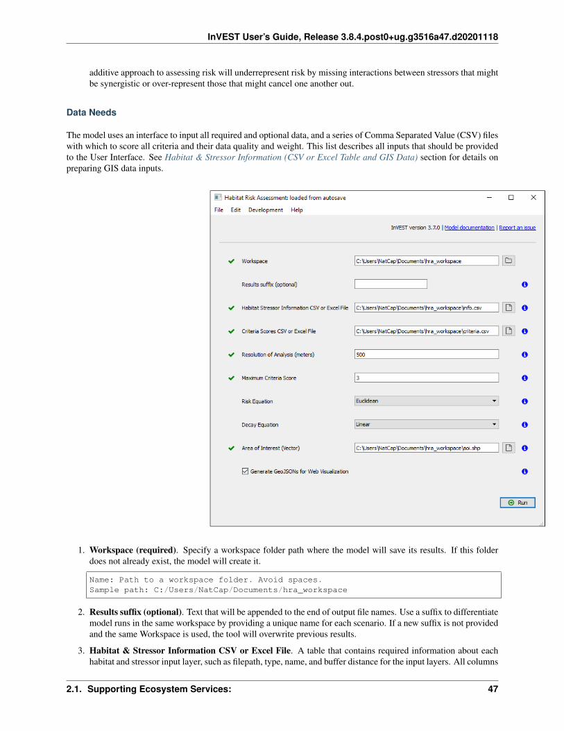
InVEST User’s Guide, Release 3.8.4.post0+ug.g3516a47.d20201118
additive approach to assessing risk will underrepresent risk by missing interactions between stressors that mightbe synergistic or over-represent those that might cancel one another out.
Data Needs
The model uses an interface to input all required and optional data, and a series of Comma Separated Value (CSV) fileswith which to score all criteria and their data quality and weight. This list describes all inputs that should be providedto the User Interface. See Habitat & Stressor Information (CSV or Excel Table and GIS Data) section for details onpreparing GIS data inputs.
1. Workspace (required). Specify a workspace folder path where the model will save its results. If this folderdoes not already exist, the model will create it.
Name: Path to a workspace folder. Avoid spaces.Sample path: C:/Users/NatCap/Documents/hra_workspace
2. Results suffix (optional). Text that will be appended to the end of output file names. Use a suffix to differentiatemodel runs in the same workspace by providing a unique name for each scenario. If a new suffix is not providedand the same Workspace is used, the tool will overwrite previous results.
3. Habitat & Stressor Information CSV or Excel File. A table that contains required information about eachhabitat and stressor input layer, such as filepath, type, name, and buffer distance for the input layers. All columns
2.1. Supporting Ecosystem Services: 47

InVEST User’s Guide, Release 3.8.4.post0+ug.g3516a47.d20201118
must be filled, except that buffer distance is required only for stressor layers. (See more in the Habitat & StressorInformation (CSV or Excel Table and GIS Data) section):
Name: File can be named anything, but avoid spaces.File Type: A CSV (.csv) or an Excel (.xlsx, .xls) file.Sample path: C:/Users/NatCap/Documents/hra_workspace/info.csv
4. Criteria Scores CSV or Excel File (required). A table that contains the criteria scores for all habitats andstressors. The rating column on the table can also store the filepath to the optional spatially explicit criteria files.The Rating Instruction column is optional, used as a reference for filling out scores on the Rating column. (Seemore in the Criteria Scores CSV section):
Name: File can be named anything, but avoid spaces.File Type: A CSV (.csv) or an Excel (.xlsx, .xls) file.Sample path: C:/Users/NatCap/Documents/hra_workspace/criteria.csv
5. Resolution of Analysis (required). The grid cell size, in meters, that is desired for the analysis. This mustbe a whole number. The model will convert any vector-based habitat and stressor inputs into rasters with pixelwidth and height equal to this value. Any occurrence of a habitat or stressor within a cell will result in the cellregistering as containing that habitat or stressor.
Note: The resolution of analysis should reflect the resolution of the habitat and stressor data that is available. Forexample, if input data includes small patches of seagrasses and kelp resolved at 100-200 meters, then choose a similarvalue for the model’s reslution. If the input habitat data are coarse, then choose a larger value. We recommend runningthe model for the first time at a low resolution (1000m or 5000m) to verify that the model is running properly and thenuse a higher resolution in subsequent runs as needed.
6. Maximum Criteria Score (required) The maximum criteria score is the highest integer value assigned to anycriteria rating within the assessment. This will be used as the upper bounded value against which all ratingscores will be compared. For example, in a model run where the ratings scores vary from 0-3, this would be a3. If the user chooses to use a different scale for ratings, however, this should be the highest value that could bepotentially assigned to a criterion.
7. Risk Equation (required). This selection chooses the equation that will be used when calculating risk to agiven habitat. (See the Cumulative Risk to Habitats or Species from Multiple Stressors section.) The user maychoose either a Euclidean risk model, or a Multiplicative risk model.
8. Decay Equation (required) This selection influences how the “zone of influence” (i.e., buffer distance) of astressor will be applied to risk. The stressor buffer distance in the Information CSV or excel file can bedegraded to provide a more accurate depiction of the influence of a stressor beyond its footprint. The decayequation decays the overall exposure rating. The options for decay are as follows. “None” will apply the fullexposure to the full range of the stressor footprint plus buffer, without any decay. “Linear” and “Exponential”will use the stated equation as a model for decay from the edges of the footprint to the extent of the bufferdistance.
8. Area of Interest (Vector) (required). The model will use a vector file to generate a summary statistics table ofaveraged exposure, consequence, and risk values within each feature of this AOI, by habitat and stressor. If theAOI vector contains more than one feature, there MUST be a ‘Name’ attribute with a unique name for eachfeature.
Name: File can be named anything, but avoid spaces.File Type: A valid vector file such as shapefile, GeoJSON, or Geopackage.Sample path: C:/Users/NatCap/Documents/hra_workspace/aoi.shp
9. Generate GeoJSONs for Web Visualization (optional). If this option is enabled, the model will generateGeoJSON files that can be visualized on the HRA web application at http://marineapps.naturalcapitalproject.org/
48 Chapter 2. InVEST Models

InVEST User’s Guide, Release 3.8.4.post0+ug.g3516a47.d20201118
after the model run.
Habitat & Stressor Information (CSV or Excel Table and GIS Data)
This table (item 3 in Data Needs) instructs the model where to find the GIS data inputs for habitat and stressor layers.GIS data may be either raster or vector format. See the image below for an example. The following columns arerequired:
• NAME: choose a unique name for each input. These names must exactly match those apearing the CriteriaScores CSV.
• PATH: the file path of the input dataset. These can be absolute filepaths (e.g.C:/InVEST_3.7.0/HabitatRiskAssess/Input/habitat_layers/eelgrass.shp) or a path that is relative to thelocation of this CSV file.
• TYPE: either “habitat” or “stressor”
• STRESSOR_BUFFER: The desired buffer distance (meters) to be used to expand a given stressor’s influence,or footprint. This should be left blank for habitats, but must not be blank for stressors. Enter 0 if no bufferingis desired for a given stressor. The model will round down this buffer distance to the nearest cell unit. e.g., abuffer distance of 600m will buffer a stressor’s footprint by two grid cells if the resolution of analysis is 250m.
Raster inputs: If a raster file is used, it should contain only values of 0 and 1, where 1 represents the presence of ahabitat or a stressor, and 0 represents absence of a habitat or a stressor. Any values other than 0 or 1 will be treated as0.
Vector inputs: If a vector file is used, all the features in that vector are considered to represent the presence of thehabitat or a stressor.
Fig. 2: The table should have columns NAME, PATH, TYPE, and STRESSOR BUFFER (meters). The column namesare case insensitive, but the path names are case sensitive.
Criteria Scores CSV
The Criteria Scores CSV (or Excel) file will provide all the criteria information for the run of the Habitat and SpeciesRisk Assessment model. This file contains information about the effect of each stressor on each habitat (i.e. theexposure and consequence scores) for the habitats and stressors in your analysis. A template for the criteria CSV filecan be found in the sample data folder. Users should feel free to add or remove specific criteria, and fill in ratings ona scale of 1 to 3, or 1 to any other value, so long as the scale is the same for all criteria
The template CSVs will contain no numerical ratings, only guidance on how each rating might be filled out. The usershould use the best available data sources in order to obtain rating information. The columns of information includethe following:
2.1. Supporting Ecosystem Services: 49

InVEST User’s Guide, Release 3.8.4.post0+ug.g3516a47.d20201118
• Rating- This is a measure of a criterion’s impact on a particular habitat or species, with regards to the overallecosystem. The rating can be an integer or a path to a spatially explicit file (see Preparing Spatially ExplicitCriteria Layers). Ratings may come from a combination of peer-reviewed sources at the global scale and locallyavailable fine-scale data sources. Model inputs and results can be updated as better information becomes avail-able. We provide guidance for well-known criteria on a scale of 1-3, but it should be noted that if information isavailable on a different scale, this can also be used. It is important to note, however, that all rating informationacross all CSVs should be on one consistent scale, regardless of what the upper bound is. A rating score of 0will tell the model to ignore that particular criteria.
• DQ- This column represents the data quality of the score provided in the Rating column. Here the model givesthe user a chance to down-weight less-reliable data sources, or up-weight particularly well-studied criteria. Alow DQ (e.g. 1) indicates best data quality, while a high DQ (e.g. 3) indicates limited data quality. While weprovide guidance for a scoring system of 1-3, the user should feel free to use any upper bound they feel practical,as long as the scale is consistent. The lower bound, however, should ALWAYS be 1, unless the user wishes toremove the entire criteria score by entering 0.
• Weight- Here the user is given the opportunity to up-weight criteria which they feel are particularly importantto the system, independent of the data quality. A low Weight (e.g. 1) indicates more important criteria, while ahigh Weight (e.g. 3) indicates less important criteria. While we provide guidance for a scoring system from 1-3,the user should feel free to use any upper bound they feel practical, as long as the scale is consistent. The lowerbound, however, should ALWAYS be 1 unless the user wishes to remove the entire criteria score by entering 0.
• E/C- This column indicates whether the given criteria are being applied to the exposure or the consequenceportion of the chosen risk equation. We do not recommend changing these values for the default criteria, butif a new criterion is added, a value of E or C should be entered. By default, any criteria in the Sensitivity orResilience categories will be assigned to Consequence (C) within the risk equations, and any criteria within theExposure category will be assigned to Exposure (E) within the risk equation.
50 Chapter 2. InVEST Models

InVEST User’s Guide, Release 3.8.4.post0+ug.g3516a47.d20201118
Note: Which criteria are required? - An accurate risk assessment should include information about all of the keycomponents of risk (i.e., spatial overlap along with other relevant exposure and consequence criteria). Nevertheless,the model will produce estimates for risk so long as there is at least one Exposure and one Consequence criteria.Spatial overlap counts as an Exposure criteria, and it does not require a row in this table, it is always calculated.
Note: Specifying No Interaction Between Habitat and Stressor - As of InVEST 3.7.0 the HRA model will allowusers to indicate that a habitat-stressor pair should have no interaction. This essentially means that the model willconsider the habitat and stressor have no spatial overlap. To set a habitat - stressor pair to no overlap, simply fill ineach criterion’s “Rating” column with a 0 value for the given pair. ALL “Rating” values for that pair must be set to 0for the model to consider the pair to have no interaction / overlap.
Preparing Spatially Explicit Criteria Layers
For any of the criteria listed in the Criteria Scores CSV, instead of entering a single number for the Rating, a pathto a GIS file may be entered instead, allowing the Rating for that criterion to vary across space. The Rating will beextracted from the spatial data as follows. If a raster file is used, its pixel values will be used as the Rating and thereforepixel values must be between 0 and the Maximum Criteria Score. If a vector file is used, the Rating value will beextracted from the attributes of the features. An attribute field “rating” must be present with values between 0 and theMaximum Criteria Score.
Interpreting Results
Risk assessment results can be used to explore strategies that would reduce the exposure of a particular habitat toa particular activity, such as reducing the extent or changing the location of an activity. The model produces risksummaries for each habitat that compare the consequence and exposure scores for all activities at a subregional scale(SUMMARY_STATISTICS.CSV). These help the user to understand if reducing exposure of particular activitiesthrough management actions is likely to reduce risk or if risk is driven by consequence, which is harder to perturbthrough management actions (see Figure 1 above).
Model Outputs
Upon successful completion of the model, you will see new folders in your Workspace called “intermediate_outputs”and “outputs”. These two folders will hold all outputs, both temporary and final that are used in a complete run of themodel. While most users will be interested only in the Output folder data, we will describe all outputs below.
Output Folder
Each of these output files is saved in the “outputs” folder that is saved within the user-specified workspace directory:
• TOTAL_RISK_habitat.tif
– This raster layer depicts the habitat-specific cumulative risk from all the stressors in a grid cell. Forexample, “TOTAL_RISK_eelgrass” depicts the cumulative risk from all stressors on habitat “eelgrass”. Itis calculated on a cell-by-cell basis, where risk is calculated only where the habitat or species occurs andvaries spatially based on the distribution (and scores) of stressors that affect that habitat or species (seeCumulative Risk to Habitats or Species from Multiple Stressors). This layer is informative for users whowant to know how cumulative risk for a given habitat varies across a study region (e.g. identify hotspots
2.1. Supporting Ecosystem Services: 51

InVEST User’s Guide, Release 3.8.4.post0+ug.g3516a47.d20201118
where eelgrass or kelp is at high risk from multiple stressors). Hotspots of high cumulative risk may betargeted for restoration or monitoring.
• TOTAL_RISK_Ecosystem.tif
– This raster layer depicts the sum of habitat cumulative risk scores divided by the number of habitatsoccurring in each cell. It is best interpreted as an average risk across all habitats in a grid cell. Forexample, in a nearshore grid cell that contains some coral reef, mangrove and soft bottom habitat, theecosystem risk value reflects the sum of risk to all three habitats in the cell.
• RECLASS_RISK_habitat.tif
– This raster layer depicts the reclassified habitat-specific risk from all the stressors in a grid cell into fourcategories, where 0 = No Risk, 1 = Low Risk, 2 = Medium Risk, and 3 = High Risk. Cells are classified ashigh risk if they have cumulative risk scores of 66%-100% of the total possible cumulative risk score. Cellsare classified as medium risk if they have cumulative risk scores between 33%-66% of the total possiblecumulative risk score. Cells are classified as low risk if they have cumulative risk scores of 0-33% of thetotal possible risk score for a single stressor or multiple stressors, respectively. If there’s no stressor on ahabitat cell, it is classified as no risk.
• RECLASS_RISK_Ecosystem.tif
– This raster layer depicts the reclassified ecosystem risk in each cell. It is best interpreted as a reclassifiedaverage index of risk across all habitats in a grid cell. The reclassification technique is similar to the onedescribed above.
• SUMMARY_STATISTICS.csv
– This CSV file contains mean, minimum, and maximum exposure, consequence, and risk scores for eachhabitat-stressor pair, as well as habitat-specific scores in each subregion. If the “name” field is not givenin the AOI vector, a “Total Region” value will be used to represent the entire AOI extent in the “SUB-REGION” column on the table. Additionally, there are three columns “R_%HIGH”, “R_%MEDIUM”,“R_%LOW”, indicating the percentage of high, medium, and low risk areas, respectively.
• InVEST-Habitat-Risk-Assessment-log-YYYY-MM-DD–HH_MM_SS.txt
– Each time the model is run a text file will appear in the workspace folder. The file will list the parametervalues for that run and be named according to the date and time.
– Parameter log information can be used to identify detailed configurations of each of scenario simulation.
Visualization Outputs Folder (optional)
Each of these output files is saved in the “visualization_outputs” folder that is saved within the user-specifiedworkspace directory. You may upload this folder to a web application that will visualize your results. See “Habi-tat Risk Assessment” at http://marineapps.naturalcapitalproject.org/.
• RECLASS_RISK_habitat.geojson
– This vector layer allows users to visualize reclassified habitat-specific risk from all the stressors into fourcategories, where 0 = No Risk, 1 = Low Risk, 2 = Medium Risk, and 3 = High Risk, in gradient color fromwhite to red on a map.
• RECLASS_RISK_Ecosystem.tif
– This vector layer allows users to visualize reclassified ecosystem risk in each cell into four categories,where 0 = No Risk, 1 = Low Risk, 2 = Medium Risk, and 3 = High Risk, in gradient color from white tored on a map.
• STRESSOR_stressor.geojson
52 Chapter 2. InVEST Models

InVEST User’s Guide, Release 3.8.4.post0+ug.g3516a47.d20201118
– This vector layer allows users to visualize stressor extent with orange color on a map.
• SUMMARY_STATISTICS.csv
– This is the same file from one in the Output Folder. It is copied here so users can just upload the visualiza-tion outputs folder to the HRA web application, with all the files in one place.
Intermediate Folder
The Intermediate folder contains files that were generated to support the final output calculations. All rasters withinthis file use the pixel size that the user specifies in the “Resolution of Analysis” text field of the Data Needs section.
• \aligned_raster.tif
– A raster file aligned with all the other input layers, so they share the same projection, pixel size, dimensions,and bounding box.
• \base_raster.tif
– If an input layer is a vector file, it will be converted to a raster file. If it’s a habitat or stressor raster, a valueof 1 on a pixel indicates the existence of the habitat or stressor, where 0s indicate non-existence. If it’s aspatially explicit criteria file, a “Rating” column must exist on the attribute table, in order for the values tobe converted to the raster grid.
• \C_habitat_stressor.tif
– A raster file representing the calculated consequence scores on each pixel for the particular habitat-stressorcombination.
• \C_num_habitat_stressor.tif
– A raster file representing the calculated consequence numerator scores on each pixel for the particu-lar habitat-stressor combination. The numerator scores are calculated by summing up all the valid rat-ing/(dq*weight) for the habitat-stressor pair of type C.
• \dist_stressor.tif
– A raster file where each pixel value indicates the nearest Euclidean distance from that pixel to a stressor.
• \E_habitat_stressor.tif
– A raster file representing the calculated exposure scores on each pixel for the particular habitat-stressorcombination.
• \E_habitat_stressor.tif
– A raster file representing the calculated exposure numerator scores on each pixel for the particular habitat-stressor combination. The numerator scores are calculated by summing up all the valid rating/(dq*weight)for the habitat-stressor pair of type E.
• \RECOV_num_habitat.tif
– A raster file indicating the recovery numerator scores for a habitat, calculated from summing all the validrating/(dq*weight) of the habitat’s recovery attribute on the criteria table.
• \RECOV_habitat.tif
– A raster file depicting the resilience or recovery potential for the given habitat or species for each cell.Recovery potential is based on natural mortality rate, recruitment rate, age at maturity/recovery time andconnectivity, though these can be altered by the user on the criteria table. Recovery potential is usefulto those who are interested in identifying areas where habitats or species are more resilient to humanstressors, and therefore may be able to withstand increasing stress. Habitats or species with low recoverypotential are particularly vulnerable to intensifying human activities.
2.1. Supporting Ecosystem Services: 53

InVEST User’s Guide, Release 3.8.4.post0+ug.g3516a47.d20201118
• \RISK_habitat_stressor.tif
– A raster file indicating the risk score for a habitat-stressor pair.
• \simplified_vector.gpkg
– A GeoPackage file generated from an input vector layer, with simplified geometries and a tolerance basedon the desired resolution. This will make rasterization process less time consuming.
• \TOTAL_C_habitat.tif
– A raster file representing the overall consequence scores for a habitat from all the stressors.
• \TOTAL_E_habitat.tif
– A raster file representing the overall exposure scores for a habitat from all the stressors.
Appendix
Connecting Habitat Risk Assessment Results to Ecosystem Service Models
In addition to providing management tools and insight, HRA/SRA is an integral step in connecting the multitude ofstressors to changes in ecosystem services. InVEST ecosystem service models include the location and/or quality ofhabitat as a factor in determining the delivery of services and this input to service models can be modified based onrisk results. For example, coastal vulnerability depends on the presence of coastal habitats and the ability of thosehabitats to attenuate waves. If these coastal habitats are at high risk, they may be less capable of attenuating waves.Demonstrating the possibility of linking HRA and ecosystem service models, the Belize Coastal Zone ManagementAuthority and Institute (CZMAI) and Natural Capital Project scientists used HRA and three InVEST ecosystem servicemodels to design an Integrated Coastal Zone Management Plan for the country. To estimate spatial variation andchange in ecosystem services, they first quantified change in the distribution, abundance, and other characteristicsof three habitats: coral reefs, mangrove forests, and seagrass beds. They began with an HRA analysis to determinewhich habitats and where were most at risk for degradation from the cumulative impacts of human activities currentlyand three future scenarios (Arkema et al. 2014). This analysis produced maps of high, medium, and low risk ofhabitat degradation in the coastal zone and marine waters. Arkema et al. 2015 used these maps to estimate thearea of functional habitat capable of providing ecosystem services in each scenario. In high and medium areas, theyassumed that 0% and 50%, respectively, of the existing habitat was capable of providing services; in low-risk areas,they considered all habitat to be functional (Arkema et al. 2015).
In another example that did not use InVEST ecosystem service models, in New Hampshire’s Great Bay, NOAA’sOffice for Coastal Management and others (Pinsky et al. 2013), related current and estimated future risk to eelgrass,saltmarsh, and oyster beds as determined in an HRA analysis to losses in recreational fishing, recreational oysterharvesting, and commercial aquaculture using a benefits-transfer approach with implications for restoration planningand aquaculture siting. When used in conjunction with models that estimate habitat-induced changes in ecosystemservices, HRA can help to evaluate trade-offs among human activities and benefits that ecosystems provide to people.
Comparison to InVEST Habitat Quality Model
The InVEST HRA/SRA model is similar to the InVEST Habitat Quality model in that both models allow users toidentify regions on a landscape or seascape where human impacts are highest. While the Habitat Quality model isintended to be used to assess how human activities impact biodiversity, the HRA model is better suited to screeningthe risk of current and future human activities to prioritize management strategies that best mitigate risk.
A primary goal of conservation is the protection of biodiversity; biodiversity is intricately linked to the productionof ecosystem services. While some people and institutions consider biodiversity itself to be an ecosystem service,the InVEST Habitat Quality model treats it as an independent attribute of natural systems, with its own intrinsicvalue (InVEST does not monetize biodiversity). InVEST includes a habitat quality model because natural resource
54 Chapter 2. InVEST Models
InVEST User’s Guide, Release 3.8.4.post0+ug.g3516a47.d20201118
managers, corporations and conservation organizations are becoming increasingly interested in understanding how andwhere biodiversity and ecosystem services align in space and how management actions affect both. The biodiversitymodel uses habitat quality and rarity as a proxy for diversity.
When developing a similar model with marine systems in mind (as was the case for HRA/SRA), differences in dataavailability (e.g., the lack of an analog to land-use/land-cover maps in marine systems) and differences in thinking(e.g., the prevalence of a risk-assessment framework in fisheries science) led us to the development of the habitat (andspecies) risk assessment model described in this chapter. Both the Habitat Quality and the Habitat Risk Assessmentmodels can be used across systems to identify areas on a landscape or seascape where the risk posed by humanactivities is highest. However, the modeling approaches differ in several ways. First, the exposure-consequenceframework of the HRA/SRA model allows model results to be interpreted in a manner that helps users explore whichtypes of management strategies are likely to most effectively reduce risk (Figure 1). For example, ecosystems withhigh exposure and high consequence may be targeted for intense active management, while effective strategies forecosystems with low exposure to human stressors but high consequence may include close monitoring but little activeintervention unless exposure increases. Second, the transparent flexible structure, in addition to the ability to rankdata quality and importance, facilitate HRA/SRA’s use in both data-rich and data-poor situations. Finally, the HabitatQuality model is better suited for terrestrial applications than marine applications because it requires a land use landcover map as an input. The HRA/SRA model can be used in both marine and terrestrial systems.
References
Arkema, K. K., Verutes, G., Bernhardt, J. R., Clarke, C., Rosado, S., Maritza Canto, . . . Zegher, J. de. (2014).Assessing habitat risk from human activities to inform coastal and marine spatial planning: a demonstration in Belize.Environmental Research Letters, 9(11), 114016. https://doi.org/10.1088/1748-9326/9/11/114016
Arkema, K. K., Verutes, G. M., Wood, S. A., Clarke-Samuels, C., Rosado, S., Canto, M., . . . Guerry, A. D. (2015).Embedding ecosystem services in coastal planning leads to better outcomes for people and nature. Proceedings of theNational Academy of Sciences, 112(24), 7390–7395. https://doi.org/10.1073/pnas.1406483112
Astles, K. L., Holloway, M. G., Steffe, A., Green, M., Ganassin, C., & Gibbs, P. J. 2006. An ecological methodfor qualitative risk assessment and its use in the management of fisheries in New South Wales, Australia. FisheriesResearch, 82: 290-303.
Burgman, M. 2005. Risks and decisions for conservation and environmental management. Cambridge UniversityPress, Cambridge, UK.
Cabral, P., Levrel, H., Schoenn, J., Thiébaut, E., Le Mao, P., Mongruel, R., . . . Daures, F. (2015). Marine habitatsecosystem service potential: A vulnerability approach in the Normand-Breton (Saint Malo) Gulf, France. EcosystemServices, 16(Supplement C), 306–318. https://doi.org/10.1016/j.ecoser.2014.09.007
Chung, M. G., Kang, H., & Choi, S.-U. (2015). Assessment of Coastal Ecosystem Services for Conservation Strategiesin South Korea. PLOS ONE, 10(7), e0133856. https://doi.org/10.1371/journal.pone.0133856
Clarke C, Canto M, Rosado S. Belize Integrated Coastal Zone Management Plan. Coastal Zone Management Authorityand Institute (CZMAI); 2013.
Coastal Zone Management Authority and Institute. Belize Integrated Coastal Zone Manage-ment Plan (2016). Retrieved from https://www.coastalzonebelize.org/wp-content/uploads/2015/08/BELIZE-Integrated-Coastal-Zone-Management-Plan.pdf
Crain, C. M., Kroeker, K., & Halpern, B. S. 2008. Interactive and cumulative effects of multiple human stressors inmarine systems. Ecology Letters, 11: 1304-1315.
Dawson, T. P., Jackson, S. T., House, J. I., Prentice, I. C., & Mace, G. M. 2011. Beyond Predictions: BiodiversityConservation in a Changing Climate. Science, 332: 53-58.
Díaz, S., Pascual, U., Stenseke, M., Martín-López, B., Watson, R. T., Molnár, Z., . . . Shirayama, Y. (2018). Assessingnature’s contributions to people. Science, 359(6373), 270–272. https://doi.org/10.1126/science.aap8826
2.1. Supporting Ecosystem Services: 55

InVEST User’s Guide, Release 3.8.4.post0+ug.g3516a47.d20201118
Duggan, J. M., Eichelberger, B. A., Ma, S., Lawler, J. J., & Ziv, G. (2015). Informing management of rare species withan approach combining scenario modeling and spatially explicit risk assessment. Ecosystem Health and Sustainability,1(6), 1–18. https://doi.org/10.1890/EHS14-0009.1
Elliff, C. I., & Kikuchi, R. K. P. (2017). Ecosystem services provided by coral reefs in a Southwestern AtlanticArchipelago. Ocean & Coastal Management, 136(Supplement C), 49–55. https://doi.org/10.1016/j.ocecoaman.2016.11.021
Halpern, B. S., Walbridge, S., Selkoe, K. A., Kappel, C. V., Micheli, F., D’Agrosa, C., Bruno, J. F., et al. 2008. AGlobal Map of Human Impact on Marine Ecosystems. Science, 319: 948-952.
Halpern BS, Frazier M, Potapenko J, Casey KS, Koenig K, Longo C, et al. Spatial and temporal changes in cumulativehuman impacts on the world’s ocean. Nat Commun. 2015;6: 7615. doi:10.1038/ncomms8615
Hobday, A. J., Smith, A. D. M., Stobutzki, I. C., Bulman, C., Daley, R., Dambacher, J. M., Deng, R. A., et al. 2011.Ecological risk assessment for the effects of fishing. Fisheries Research, 108: 372-384.
Ma, S., Duggan, J. M., Eichelberger, B. A., McNally, B. W., Foster, J. R., Pepi, E., . . . Ziv, G. (2016). Valuation ofecosystem services to inform management of multiple-use landscapes. Ecosystem Services, 19, 6–18. https://doi.org/10.1016/j.ecoser.2016.03.005
NOAA OCM 2016. How people benefit from New Hampshire’s Great Bay estuary. A collaborative assessment of thevalue of ecosystem services and how our decision might affect those values in the future. [Internet]. NOAA Officefor Coastal Management, New Hampshire Department of Environmental Services Coastal Program, and Eastern Re-search Group, Inc.; 2016. Available: https://www.des.nh.gov/organization/divisions/water/wmb/coastal/documents/greatbayesa-final-report-201611.pdf
Pascual, U., Balvanera, P., Díaz, S., Pataki, G., Roth, E., Stenseke, M., . . . Yagi, N. (2017). Valuing nature’scontributions to people: the IPBES approach. Current Opinion in Environmental Sustainability, 26–27, 7–16.https://doi.org/10.1016/j.cosust.2016.12.006
Pinsky ML, Worm B, Fogarty MJ, Sarmiento J, Levin SA. Marine taxa track local climate velocities. Science.2013;341: 1239–1242.
Samhouri, J. F., and P. S. Levin. Linking Land- and Sea-Based Activities to Risk in Coastal Ecosystems. 2012.Biological Conservation 145(1): 118–129. doi:10.1016/j.biocon.2011.10.021.
Stock A, Micheli F. Effects of model assumptions and data quality on spatial cumulative human impact assessments.Glob Ecol Biogeogr. 2016;25: 1321–1332. doi:10.1111/geb.12493
Verutes, G. M., Arkema, K. K., Clarke-Samuels, C., Wood, S. A., Rosenthal, A., Rosado, S., . . . Ruckelshaus, M.(2017). Integrated planning that safeguards ecosystems and balances multiple objectives in coastal Belize. Inter-national Journal of Biodiversity Science, Ecosystem Services & Management, 13(3), 1–17. https://doi.org/10.1080/21513732.2017.1345979
Teck, S. J., Halpern, B. S., Kappel, C. V., Micheli, F., Selkoe, K. A., Crain, C. M., Martone, R., et al. 2010. Usingexpert judgement to estimate marine ecosystem vulnerability in the California Current. Ecological Applications 20:1402-1416.
Teichert N, Borja A, Chust G, Uriarte A, Lepage M. Restoring fish ecological quality in estuaries: Implication ofinteractive and cumulative effects among anthropogenic stressors. Sci Total Environ. 2016;542, Part A: 383–393.doi:10.1016/j.scitotenv.2015.10.068
Williams, A., Dowdney, J., Smith, A. D. M., Hobday, A. J., & Fuller, M. 2011. Evaluating impacts of fishing onbenthic habitats: A risk assessment framework applied to Australian fisheries. Fisheries Research, In Press.
Wyatt, K. H., Griffin, R., Guerry, A. D., Ruckelshaus, M., Fogarty, M., & Arkema, K. K. (2017). Habitat riskassessment for regional ocean planning in the U.S. Northeast and Mid-Atlantic. PLOS ONE, 12(12), e0188776.https://doi.org/10.1371/journal.pone.0188776
56 Chapter 2. InVEST Models

InVEST User’s Guide, Release 3.8.4.post0+ug.g3516a47.d20201118
2.1.3 Pollinator Abundance: Crop Pollination
Summary
The InVEST pollination model focuses on wild bees as a key animal pollinator. It uses estimates of the availabilityof nest sites and floral resources within bee flight ranges to derive an index of the abundance of bees nesting on eachcell on a landscape (i.e., pollinator supply). It then uses floral resources, and bee foraging activity and flight rangeinformation to estimate an index of the abundance of bees visiting each cell. If desired, the model then calculates asimple index of the contribution of these bees to agricultural production, based on bee abundance and crop dependenceon pollination. The results can be used to understand changes in crop pollination and crop yield with changes inland use and agricultural management practices. Required inputs include a land use and land cover map, land coverattributes, guilds or species of pollinators present, and their flight ranges. To estimate wild pollinator contributionsto crop production requires information on farms of interest, the crops grown there, and the abundance of managedpollinators. The model’s limitations include not accounting for pollinator persistence over time or the effects of landparcel size.
Introduction
Crop pollination by bees and other animals is a potentially valuable ecosystem service in many landscapes of mixedagricultural and natural habitats (Allen-Wardell et al. 1998, Free 1993). Pollination can increase the yield, quality,and stability of fruit and seed crops as diverse as tomato, canola, watermelon, coffee, sunflower, almond, and cacao.Indeed, Klein et al. (2007) found that 87 of 115 globally important crops benefit from animal pollination, a servicevalued variously in the billions to tens of billions per year globally (Costanza et al. 1997, Losey and Vaughan 2006,Nabhan and Buchmann 1997, Southwick and Southwick 1992).
Despite these numbers, it is important to realize that not all crops need animal pollination. Some crop plants arewind pollinated (e.g., staple grains such as rice, corn, wheat) or self pollinated (e.g., lentils and other beans), needingno animal pollinators to successfully produce fruits or seeds. Klein et al. (2007) provides a list of crops and theirpollination requirements that can help identify whether crops in a region of interest may benefit from wild animalpollinators.
Decision-makers can use information on crop pollinators, their abundance across a landscape, and the pollinationservices they provide to crops in several ways. First, with maps of pollinator abundance and crops that need them,land use planners could predict consequences of different policies on pollination services and income to farmers(for an example, see Priess et al. 2007). Second, farmers could use these maps to locate crops intelligently, giventheir pollination requirements and predictions of pollinator availability. Third, conservation organizations or landtrusts could use the tool to optimize conservation investments that benefit both biodiversity and farmers. Finally,governments or others proposing payment schemes for ecosystem services could use the results to estimate whoshould pay whom, and how much.
The Model
A wide range of animals can be important pollinators (e.g., birds, bats, moths and flies), but bees are the most importantgroup for most crops (Free 1993). As a result, the InVEST Pollination model focuses on the resource needs andflight behaviors of wild bees. Many people think of honeybees, managed in artificial hives, when they think ofpollinators, but wild bees also contribute to crop pollination. In fact, for several important crops (e.g., blueberries),native species are more efficient and effective pollinators than honeybees (Cane 1997). These native bees, in additionto feral honeybees living in the wild, can benefit crops without active management of captive hives. This is thepollination service associated with habitat conservation.
This model is adapted from Lonsdorf et al. (2009). For bees to persist on a landscape, they need two things: suitableplaces to nest, and sufficient food (provided by flowers) near their nesting sites. If provided these resources, pollinatorsare available to fly to nearby crops and pollinate them as they collect nectar and pollen. The model translates landcover into an index of suitability (0-1) for bees to create a pollinator source map. Higher scores indicate sources of
2.1. Supporting Ecosystem Services: 57

InVEST User’s Guide, Release 3.8.4.post0+ug.g3516a47.d20201118
greater relative bee abundance. To calculate the index, the model assumes that bees require two types of limitingresources to persist on a landscape - nesting substrates and floral resources. Given an input of land cover that describesthe landscape, various suitability values of each land cover type are assigned based on their ability to provide theseresources.
The Pollination model then uses the nest supply index to estimate the pollinators visiting crop fields. It assumes thesupply from nearby parcels contributes more than those farther away. We use insights from Olsson et al. (2015) andweight bee visitation by the floral quality of the parcel to reflect the central place foraging behavior that bees are knownto follow. In other words, the visitation rates to two parcels equally distant from a nest are proportional to the floralqualities of the parcels.
Additionally, this model incorporates the potential use of managed bees into a yield index. With information on thelocation of crops and their dependence on pollinators, the model uses a simple yield function to project how wildpollinator abundance in agricultural areas and the use of managed bees contributes to an index of crop yields. Theinclusion of managed bees reflects guidance from recent work by the USDA-Funded Integrated Crop PollinationProject (icpbees.org) to integrate the combined benefits of managed and wild bees.
These steps are described formally below.
How it Works
The model is an index-based model, and requires the following biophysical data:
• a land use / land cover (LULC) map;
• a biophysical table paired with the LULC raster to map LULC types to nesting suitability and floral resourcesacross seasons;
• a pollinator guild table with properties about active seasons, nesting preferences, mean flight distances, andrelative abundances for each species or group of wild pollinators;
• a farm shapefile indicating the geospatial location of farms, crop type, dependence on pollinators, abundance ofmanaged pollinators, as well as on-farm nesting sites and floral resources.
Because bees are proficient fliers, they integrate over several elements of a landscape, moving between nesting habitatsand foraging habitats (Ricketts et al. 2006). The distances they typically fly affect both their persistence and the levelof service they deliver to farms. The model therefore requires a typical foraging distance for each pollinator species.These data can be supplied from quantitative field estimates (e.g., Roubik and Aluja 1983), proxies such as body size(Greenleaf et al. 2007), or from expert opinion.
Pollinator Supply and Abundance
Using these data, the model first estimates pollinator supply for every cell in the landscape, based on the availablenesting sites in that cell, the floral resources (i.e., food) in surrounding cells, and the relative abundance of that pol-linator species. Floral resources in cells near nesting sites are given more weight than distant cells, according to thespecies’ average foraging range.
𝑃𝑆(𝑥, 𝑠) is the pollinator supply index at pixel 𝑥 for species 𝑠 defined as:
𝑃𝑆(𝑥, 𝑠) = 𝐹𝑅(𝑥, 𝑠)𝐻𝑁(𝑥, 𝑠)𝑠𝑎(𝑠) (2.15)
where 𝐹𝑅(𝑥, 𝑠) is the accessible floral resources index at pixel 𝑥 for species 𝑠 defined as:
𝐹𝑅(𝑥, 𝑠) =
∑︀𝑥′∈𝑋 exp(−𝐷(𝑥, 𝑥′)/𝛼𝑠)
∑︀𝑗∈𝐽 𝑅𝐴(𝑙(𝑥′), 𝑗)𝑓𝑎(𝑠, 𝑗)∑︀
𝑥′∈𝑋 exp(−𝐷(𝑥, 𝑥′)/𝛼𝑠)(2.16)
58 Chapter 2. InVEST Models

InVEST User’s Guide, Release 3.8.4.post0+ug.g3516a47.d20201118
𝐻𝑁(𝑥, 𝑠) is the habitat nesting suitability at pixel 𝑥 for species 𝑠
𝐻𝑁(𝑥, 𝑠) = max𝑛∈𝑁
[𝑁(𝑙(𝑥), 𝑛)𝑛𝑠(𝑠, 𝑛)] (2.17)
and where
• 𝑠𝑎(𝑠) is the relative species abundance index for species 𝑠 in the range [0.0, 1.0],∑︀
𝑠∈𝑆 𝑠𝑎(𝑠) = 1, and 𝑆 is theset of all species,
• 𝑁(𝑙, 𝑛) is the nesting substrate index for landcover type 𝑙 for substrate type 𝑛 in the range [0.0, 1.0],
• 𝑙(𝑥) is the landcover type at pixel 𝑥,
• 𝑗 is the season,
• 𝑅𝐴(𝑙, 𝑗) index of relative abundance of floral resources on landcover 𝑙 during season 𝑗,
• 𝑓𝑎(𝑠, 𝑗) is the relative foraging activity for pollinator species 𝑠 during season 𝑗.
• 𝐷(𝑥, 𝑥′) is the Euclidean distance between cells 𝑥 and 𝑥′,
• 𝑛𝑠(𝑠, 𝑛) is the nesting suitability preference for species 𝑠 in nesting type 𝑛 (and 𝑁 is the set of all nesting types),
• and 𝛼𝑠 is the expected foraging distance for the pollinator 𝑠 (Greenleaf et al. 2007).
Pollinator supply is an indicator of where pollinators originate from on the landscape. Pollinator abundance indicateswhere pollinators are active on the landscape. Pollinator abundance depends on the floral resources that attract polli-nators to a cell, and the supply of pollinators that can access that cell. The pollinator abundance for species 𝑠 indexon cell 𝑥, during season 𝑗, 𝑃𝐴(𝑥, 𝑠, 𝑗), is the product of available floral resources on a cell during a given season,weighted by a pollinator’s relative activity during that season with the pollinator supply and normalized by the floralresources index in surrounding cells such that:
𝑃𝐴(𝑥, 𝑠, 𝑗) =
(︂𝑅𝐴(𝑙(𝑥), 𝑗)𝑓𝑎(𝑠, 𝑗)
𝐹𝑅(𝑥, 𝑠)
)︂ ∑︀𝑥′∈𝑋 𝑃𝑆(𝑥′, 𝑠) exp(−𝐷(𝑥, 𝑥′)/𝛼𝑠)
exp(−𝐷(𝑥, 𝑥′)/𝛼𝑠)(2.18)
See the Table of Variables Appendix for all variable definitions and properties.
On-Farm Abundance and Yield
Next, using the indices of pollinator abundance across the landscape, the location of farms, and information about eachfarm (availability of managed pollinators, crop dependence on pollination), the model can calculate an index of totalyield attained and the contribution of wild pollinators to that yield.
First, the model calculates an index of total pollinator abundance by season in agricultural areas that might benefitfrom pollination services. On-farm pollinator abundance is given as:
𝑃𝐴𝑇 (𝑥, 𝑗) =∑︁𝑠∈𝑆
𝑃𝐴(𝑥, 𝑠, 𝑗) (2.19)
The potential contribution of on-farm pollinator abundance to pollinator-dependent crop yield is calculated using atunable half-sigmoid function as:
𝐹𝑃 (𝑥) =𝑃𝐴𝑇 (𝑥, 𝑗(𝑓(𝑥)))(1 − ℎ(𝑓(𝑥)))
ℎ(𝑓(𝑥))(1 − 2𝑃𝐴𝑇 (𝑥, 𝑗(𝑓(𝑥))) + 𝑃𝐴𝑇 (𝑥, 𝑗(𝑓(𝑥))(2.20)
where ℎ(𝑓(𝑥)) is the half saturation constant for farm 𝑓 at pixel 𝑥 indicating the abundance of wild pollinators neededto reach half of the total potential pollinator-dependent yield.
The actual contribution of wild pollinators to pollinator-dependent yield depends on the degree to which pollinationneeds are already being met by managed pollinators. The total pollinator-dependent yield, from both wild and managedpollinators, is given as:
𝑃𝑌 𝑇 (𝑥) = min(𝑚𝑝(𝑓(𝑥)) + 𝐹𝑃 (𝑥), 1) (2.21)
2.1. Supporting Ecosystem Services: 59
InVEST User’s Guide, Release 3.8.4.post0+ug.g3516a47.d20201118
assuming a value of 0 indicates 0% of pollinator-dependent yield is achieved, and 1.0 indicates 100% of pollinator-dependent yield is achieved. Note the max/min notation constrains the value of 𝑃𝑌 𝑇 to 0..1 where 𝑚𝑝(𝑓(𝑥)) is theproportion of pollination needs met by managed pollinators available at pixel 𝑥 within farm polygon 𝑓 .
The proportion of pollinator-dependent yield attributable to wild pollinators is given as
𝑃𝑌𝑊 (𝑥) = max(0, 𝑃𝑌 𝑇 (𝑥) −𝑚𝑝(𝑓(𝑥))) (2.22)
Thus, in cases where managed pollinators are sufficiently abundant, i.e, 𝑚𝑝(𝑓(𝑥)) = 1, there is no additional yieldattributable to wild pollinators.
Total crop yield attained is a function of the crop’s dependence on pollination and the degree to which its pollinationneeds are met. Some crop species are self-compatible or wind-pollinated and yield is less dependent on animalpollinators while other species obligately require pollinators to generate any yield (Klein et al. 2007). Total crop yieldis calculated per farm as
𝑌 𝑇 (𝑓) = 1 − 𝜈(𝑓)
⎛⎝1 −∑︁
𝑥∈𝑋(𝑓)
𝑃𝑌 𝑇 (𝑥)/|𝑋(𝑓)|
⎞⎠ (2.23)
where 𝑓 is a particular farm, 𝑋(𝑓) are the set of pixels covering farm 𝑓 , and |𝑋(𝑓)| is the count of pixels covered byfarm 𝑓 . The function 𝜈(𝑓) is a scalar ∈ [0, 1] representing what proportion of yield for the crop grown on farm 𝑓 isdependent on pollinators.
The proportion of total crop yield attributable to wild pollinators is given as
𝑌𝑊 (𝑓) = 𝜈(𝑓)
⎛⎝ ∑︁𝑥∈𝑋(𝑓)
𝑃𝑌𝑊 (𝑥)/|𝑋(𝑓)|
⎞⎠ (2.24)
Limitations and Simplifications
This model is an index-based model and only estimates relative patterns of pollinator abundance and pollinationcontribution to crop yields. This is because absolute estimates of nest density, resource availability, and pollinatorabundance are rarely available, and yield functions (including pollinator abundance) for many crops are poorly defined.Relying on relative indices limits our ability to estimate absolute economic values to better inform land-use planningdecision-making, often based on cost-benefit analyses.
The use of central place foraging in the model’s pollinator abundance index has yet to be tested empirically, so wecaution against using the model to make economic projections without empirical verification. The same applies to theintegration of managed bees in the yield function.
As an index-based model, it is well-suited for making qualitative comparisons among scenarios representing marginalchanges in land use/land cover, farm management practices or crop types. On-farm pollinator abundance 𝑃𝐴𝐹 (𝑥, 𝑗)will be affected by the number of pollinator guilds being modeled and so cannot be used to compare different pollinatorcommunities even on the same landscape. Similarly, because relative species abundance indices 𝑠𝑎(𝑠) are specified asan input, the model will not yield accurate results for scenarios in which a rare species becomes common or vice versadue to large changes in nesting habitat or floral resource availability.
The model does not include the dynamics of bee populations over time, and therefore cannot evaluate whether thesepopulations are sustainable given the current landscape. Instead, the model simply provides a static snapshot ofthe number of pollinators on each cell in the landscape, given simple estimates of nesting sites and food resources.Some of the factors that influence bee populations, like habitat disturbances and typical population fluctuations, arenot captured. In addition, the model calculates pollinator supply based on the average of available floral resourcesweighted by pollinator activity across seasons during which the pollinator is active. It does not account for the order ofseasons or the dependence of pollinator abundance in one season on the resources available in the season directly prior.The model does not account for variation in the effectiveness of different pollinator species or guilds at pollinating
60 Chapter 2. InVEST Models

InVEST User’s Guide, Release 3.8.4.post0+ug.g3516a47.d20201118
different crop types. All species are assumed to contribute equally based on their relative abundance and the half-saturation constant specified for each farm/crop.
The model does not account for the sizes of habitat patches in estimating abundance. For many species, there is aminimum patch size, under which a patch cannot support that species over the long term. There is some evidence thatsmall patches support fewer species of bees (Kremen et al. 2004), but bees can also survive in small areas of suitablehabitat (Ricketts 2004).
Pollinators are likely to be influenced by fine-scale features in the landscape, which are difficult to capture in typicalland-cover data with typical resolutions of 30m. For example, small patches of flower resources in an otherwise hostilehabitat for bees can provide important food resources, but will not be detected by typical land cover maps. Some beesare also able to nest in small but suitable areas (a single suitable roadside or tree hollow). Using average values ofnesting site or flower availability for each land cover type, along with 30m pixels or larger, will therefore not capturethese fine scale but important areas of resources.
Data Needs
This section outlines the specific data used by the model. See the Appendix for additional information on data sourcesand pre-processing. Please consult the InVEST sample data (located in the folder where InVEST is installed, if youalso chose to install sample data) for examples of all of these data inputs. This will help with file type, folder structureand table formatting. Note that all GIS inputs must be in the same projected coordinate system and in linear meterunits.
• Workspace (required). Folder where model outputs will be written. Make sure that there is ample disk space,and write permissions are correct.
• Suffix (optional). Text string that will be appended to the end of output file names, as “_Suffix”. Use a Suffix todifferentiate model runs, for example by providing a short name for each scenario. If a Suffix is not provided,or changed between model runs, the tool will overwrite previous results.
• Land Cover Map (required). Raster of land use/land cover (LULC) for each pixel, where each unique integerrepresents a different land use/land cover class. All values in this raster MUST have corresponding entries inthe Land Cover Biophysical Table. This coverage must be of fine enough resolution (i.e., sufficiently small cellsize) to capture the movements of bees on a landscape. If bees fly 800 meters on average and cells are 1000meters across, the model will not fully capture the movement of bees from their nesting sites to neighboringfarms.
• Land Cover Biophysical Table (required). A .csv (Comma Separated Value) table containing model infor-mation corresponding to each of the land use classes in the Land Cover Map. All LULC classes in the LandCover raster MUST have corresponding values in this table. Data needed are relative indices (0-1). Data can besummarized from field surveys, or obtained by expert assessment if field data is unavailable. Each row is a landuse/land cover class and columns must be named and defined as follows:
• lucode: Land use/land cover class code. LULC codes must match the ‘value’ column in the Land Cover Mapraster and must be integer or floating point values, in consecutive order, and unique.
• nesting_[SUBSTRATE]_availability_index: Relative index of the availability of the given nesting type withineach LULC type, on a floating point scale of 0-1. The SUBSTRATE name must exactly match a substrate givenin the Guild Table.
• floral_resources_[SEASON]_index: Relative abundance (floating point value 0-1) of flowers in each LULC classfor the given season. There are two aspects to consider when estimating the relative floral abundance of eachLULC class: % floral abundance or % floral coverage, as well as the duration of flowering during each season.For example, a land cover type comprised 100% of a mass flowering crop that flowers the entire season with anabundance cover of 80% would be given a suitability value of 0.80. A land cover type that flowers only half ofthe season at 80% floral coverage would be given a floral suitability value of 0.40. The SEASON name mustexactly match a season given in the Guild Table.
2.1. Supporting Ecosystem Services: 61

InVEST User’s Guide, Release 3.8.4.post0+ug.g3516a47.d20201118
Table 1: Example Biophysical Tablelu-code
nest-ing_cavity_availability_index
nest-ing_ground_availability_index
flo-ral_resources_spring_index
flo-ral_resources_summer_index
1 0.3 0.2 0.7 0.52 0.3 0.2 0.7 0.53 0.3 0.2 0.7 0.54 0.3 0.2 0.7 0.56 0.3 0.2 0.7 0.57 0.3 0.2 0.7 0.58 0.3 0.2 0.7 0.5
• Guild Table (required). A .csv (Comma Separated Value) table containing information on each species or guildof pollinator to be modeled. ‘Guild’ refers to a group of bee species that show the same nesting behavior,whether preferring to build nests in the ground, in tree cavities, or other habitat features. If multiple species areknown to be important pollinators, and if they differ in terms of flight season, nesting requirements, or flightdistance, provide data on each separately. If little or no data are available, create a single ‘proto-pollinator’ withdata taken from average values or expert opinion about the whole pollinator community. Each row is a uniquespecies or guild of pollinator and columns must be named and defined as follows:
Note: The [SUBSTRATE] and [SEASON] strings in column names should be customized for meaning,but must be consistent with column names in the Land Cover Biophysical Table.
• species: Name of species or guild (Species names can be numerical codes or strings.)
• Any number of nesting_suitability_[SUBSTRATE]_index columns, one for each SUBSTRATE de-fined: Values must be entered as a floating point number between 0 and 1, with 1 indicating a nestingsubstrate that is fully utilized and 0 indicating a nest substrate that is not utilized at all. Substratesare user defined, but might include ground nests, tree cavities, etc. The SUBSTRATE string mustmatch a nesting_[SUBSTRATE]_availability_index in the Land Cover Biophysical Table.
• Any number of foraging_activity_[SEASON]_index columns, one for each SEASON defined: Polli-nator activity by floral season (i.e., flight season). Values must be entered as a floating point numberbetween 0 and 1, with 1 indicating the season of greatest activity for the guild or species, and 0indicating a season of no activity. Seasons are user defined but might include spring, summer, fall;wet, dry, etc. The SEASON string must match a floral_resources_[SEASON]_index column in theLand Cover Biophysical Table.
• alpha: Average distance each species or guild travels to forage on flowers, specified in integermeters. The model uses this estimated distance to define the neighborhood of available flowersaround a given cell, and to weight the sums of floral resources and pollinator abundances on farms.This value can be determined by typical foraging distance of a bee species based on an allometricrelationship (see Greenleaf et al. 2007).
• relative_abundance: A floating point value indicating the weighted relative abundance of thespecies’ contribution to pollinator abundance. Setting this value to the same value for each specieswill result in each species being weighted equally.
Example: A hypothetical Guilds Table with two species. There are two main SUBSTRATEs, “cavity”and “ground.” Species “Apis” uses both cavity and ground nesting types, and species “Bombus” onlyuses cavity nests. There are two SEASONs, “spring” and “summer”. Typical flight distances, specifiedin meters (alpha), vary widely between species. The relative_abundance of Bombus is higher than Apis,indicating that there are more Bombus pollinators than Apis.
62 Chapter 2. InVEST Models

InVEST User’s Guide, Release 3.8.4.post0+ug.g3516a47.d20201118
Table 2: Example Guild Tablespeciesnest-
ing_suitability_cavity_indexnest-ing_suitability_ground_index
forag-ing_activity_spring_index
forag-ing_activity_summer_index
al-pha
rela-tive_abundance
Apis 1 1 1 1 500 0.75Bom-bus
1 0 0.8 1 1500 1
• Farm Vector (optional): In order to calculate information related to crop yields, the model uses a polygon vectorlayer (shapefile) to indicate farm areas, and the attribute table of that shapefile provides information specific toeach farm. The Farm Vector shapefile’s attribute table must include the following fields:
• crop_type (string): Name of the crop grown on that polygon, ex. “blueberries”, “almonds”, etc. For farmsgrowing multiple overlapping crops, or crops in multiple seasons, a separate overlapping polygon must beincluded for each crop.
• half_sat (floating point): The half saturation coefficient for the crop grown on that farm. This is the value of thewild pollinator abundance index that results in 50% of pollinator-dependent crop yield being attained. This is atunable parameter that may be most useful to adjust following an initial run of the model and an examination ofthe results.
• season (string): the season in which the crop is pollinated. This season must match a SEASON provided in theGuilds Table.
• fr_[SEASON] (floating point value in the range [0.0, 1.0]): The floral resources available at this farm for thegiven season. The SEASON string must exactly match one of the seasons provided in the Guild Table.
• n_[SUBSTRATE] (floating point value in the range [0.0, 1.0]): The nesting substrate suitability for the farm forthe given substrate. The SUBSTRATE string must exactly match one of the substrates provided in the GuildTable.
• p_dep (floating point value in the range [0.0, 1.0]): The proportion of crop dependent on pollinators. See Kleinet al. (2007) for estimates for common crops.
• p_managed (floating point value in the range [0.0, 1.0]): The proportion of pollination required on the farmprovided by managed pollinators. This can be estimated as the proportion of the recommended hive density orstocking rate. See Delaplane & Mayer (2000) for recommended stocking rates in the United States. Agriculturalextension offices are also a good source of this information.
Running the model
To launch the Crop Pollination model navigate to the Windows Start Menu -> All Programs -> InVEST [version] ->Pollination. The interface does not require a GIS desktop, although the results will need to be explored with any GIStool such as ArcGIS or QGIS.
Interpreting Results
Final Results
The following is a short description of each of the outputs from the Pollination model. Final results are found withinthe user defined Workspace specified for this model run. “Suffix” in the following file names refers to the optionaluser-defined Suffix input to the model.
2.1. Supporting Ecosystem Services: 63

InVEST User’s Guide, Release 3.8.4.post0+ug.g3516a47.d20201118
• Parameter log: Each time the model is run, a text (.txt) file will be created in the Workspace. The file will listthe parameter values and output messages for that run and will be named according to the service, the date andtime. When contacting NatCap about errors in a model run, please include the parameter log.
• farm_results_[Suffix].shp: A copy of the input farm polygon vector file with the following additional fields:
• p_abund: average pollinator abundance on the farm for the active season
• y_tot: total yield index, including wild and managed pollinators and pollinator independent yield.
• pdep_y_w: index of potential pollination dependent yield attributable to wild pollinators.
• y_wild: index of the total yield attributable to wild pollinators.
• pollinator_abundance_[SPECIES]_[SEASON]_[Suffix].tif: Per-pixel abundance of pollinator SPECIES inseason SEASON.
• pollinator_supply_[SPECIES]_[Suffix].tif: Per-pixel index of pollinator [SPECIES] that could be on a pixelgiven its arbitrary abundance factor from the table, multiplied by the habitat suitability for that species at thatpixel, multiplied by the available floral resources that a pollinator could fly to from that pixel. (Eqn. 1)
• total_pollinator_abundance_[SEASON]_[Suffix].tif: Per-pixel total pollinator abundance across all speciesper season.
• total_pollinator_yield_[Suffix].tif: Per-pixel total pollinator yield index for pixels that overlap farms, includingwild and managed pollinators.
• wild_pollinator_yield_[Suffix].tif: Per-pixel pollinator yield index for pixels that overlap farms, for wild-pollinators only.
Intermediate Results
You may also want to examine the intermediate results. These files can help determine the reasons for the patternsin the final results, and can also be used to better understand the model, and troubleshoot. They are found in theintermediate_outputs folder within the Workspace directory defined for the model run, and most of them have filenames that give a good idea of what the layer represents.
Appendix: Table of Variables
• 𝑥 - a pixel coordinate.
• 𝑋 - set of all pixels in the landcover map.
• 𝑓(𝑥) - farm at pixel x.
• 𝐹 - set of all pixels that are located in farms.
• 𝑠 - bee species.
• 𝑛 - nesting type (ground, cavity).
• 𝑁 - set of all nesting types.
• 𝑗 - season (fall, spring, etc).
• 𝐽 - set of all seasons (ex: {fall, spring}).
• 𝑓𝑗(𝑓, 𝑥) - active pollination season for farm 𝑓 at pixel 𝑥.
• 𝛼𝑠 - mean foraging distance for species s.
• 𝑛𝑠(𝑠, 𝑛) - nesting suitability preference for species 𝑠 in nesting type 𝑛.
64 Chapter 2. InVEST Models

InVEST User’s Guide, Release 3.8.4.post0+ug.g3516a47.d20201118
• 𝐻𝑁(𝑥, 𝑠) - habitat nesting suitability at pixel 𝑥 for species 𝑠 [0.0, 1.0].
• 𝑁(𝑙, 𝑛) - the nesting substrate index for landcover type 𝑙 for substrate type 𝑛 in the range [0.0, 1.0].
• 𝑅𝐴(𝑙, 𝑗) - index of relative abundance of floral resources on landcover type 𝑙 during season 𝑗. [0.0, 1.0]
• 𝑓𝑎(𝑠, 𝑗) - relative foraging activity for species 𝑠 during season 𝑗.
• 𝐹𝑅(𝑥, 𝑠) - accessible floral resources index at pixel 𝑥 for species 𝑠.
• 𝐷(𝑥, 𝑥′) - euclidean distance between the centroid of pixel 𝑥 and 𝑥′.
• 𝑃𝑆(𝑥, 𝑠) - pollinator supply index at pixel 𝑥 for species 𝑠.
• 𝑃𝐴(𝑥, 𝑠, 𝑗) - pollinator abundance at pixel 𝑠 for species 𝑠.
• 𝑃𝐴𝑇 (𝑥, 𝑗) - total on-farm pollinator abundance at pixel 𝑥 in season 𝑗, accounting for all species
• 𝐹𝑃 (𝑥) - the potential contribution of on-farm pollinator abundance to pollinator-dependent crop yield at a farmpixel during the season in which pollination is needed for that farm.
• 𝑚𝑝(𝑓) - abundance of managed pollinators on farm 𝑓 relative to the recommended stocking rate.
• ℎ(𝑓) - half saturation coefficient for farm 𝑓 .
• 𝑃𝑌 𝑇 (𝑥) - total pollinator-attributable yield at pixel x for season 𝑗, accounting for wild and managed pollinators.
• 𝑃𝑌𝑊 (𝑥) - wild-pollinator-attributable yield at pixel x for season 𝑗.
• 𝑠𝑎(𝑠) - relative species abundance index for species 𝑠.
• 𝑌 𝑇 (𝑓) - average farm yield for farm parcel 𝑓 accounting for pollinator dependency of crop.
• 𝑌𝑊 (𝑓) - proportion of average farm yield for farm parcel 𝑓 attributable to wild pollinators, accounting forpollinator dependency of crop.
• 𝜈(𝑓) - proportion of crop yield dependent on pollination.
Appendix: Data Sources
List of globally important crops and their dependence on animal pollinators: (Klein et al. 2007).
References
Allen-Wardell, G., P. Bernhardt, R. Bitner, A. Burquez, S. Buchmann, J. Cane, PA Cox, V. Dalton, P. Feinsinger,M. Ingram, D. Inouye, CE Jones, K. Kennedy, P. Kevan, and H. Koopowitz. 1998. The potential consequences ofpollinator declines on the conservation of biodiversity and stability of food crop yields. Conservation Biology 12:8-17.
Cane, JH. 1997. Lifetime monetary value of individual pollinators: the bee habropoda laboriosa at rabbiteye blueberry(vaccinium ashei reade). Acta Horticulturae 446: 67-70.
Costanza, R., R. d’Arge, R. de Groot, S. Farber, M. Grasso, B. Hannon, K. Limburg, S. Naeem, RV O’Neill, J. Paruelo,RG Raskin, P. Sutton, and M. van den Belt. 1997. The value of the world’s ecosystem services and natural capital.Nature 387: 253-260.
Delaplane, KS, and DF Mayer. 2000. Crop pollination by bees. CABI Publishing, New York.
Free, JB. 1993. Insect pollination of crops. Academic Press, London.
Greenleaf, SS, NM Williams, R. Winfree, and C. Kremen. 2007. Bee foraging ranges and their relationship to bodysize. Oecologia 153: 589-596.
2.1. Supporting Ecosystem Services: 65

InVEST User’s Guide, Release 3.8.4.post0+ug.g3516a47.d20201118
Greenleaf, SS, and C. Kremen. 2006. Wild bee species increase tomato production and respond differently to sur-rounding land use in Northern California. Biological Conservation 133:81-87.
Klein, AM, BE Vaissiere, JH Cane, I. Steffan-Dewenter, SA Cunningham, C. Kremen, and T. Tscharntke. 2007.Importance of pollinators in changing landscapes for world crops. Proceedings of the Royal Society B-BiologicalSciences 274: 303-313.
Kremen, C., NM Williams, RL Bugg, JP Fay, and RW Thorp. 2004. The area requirements of an ecosystem service:crop pollination by native bee communities in California. Ecology Letters 7: 1109-1119.
Lonsdorf, E., C. Kremen, T. Ricketts, R. Winfree, N. Williams, and SS Greenleaf. 2009. Modelling pollinationservices across agricultural landscapes. Annals of Botany 1: 12. online [http://aob.oxfordjournals.org/content/103/9/1589.abstract?sid=b0f6fc9e-bd52-4bec-8248-50e56b78344d]
Lonsdorf, E., TH Ricketts, CM Kremen, NM Williams, and S. Greenleaf. in press. Pollination services in P. Kareiva,TH Ricketts, GC Daily, H. Tallis, and S. Polasky, eds. The theory and practice of ecosystem service valuation.
Losey, JE, and M. Vaughan. 2006. The economic value of ecological services provided by insects. Bioscience 56:311-323.
Nabhan, GP, and SL Buchmann. 1997. Services provided by pollinators. Pages 133-150 in GC Daily, ed. Nature’sservices. Island Press, Washington, D.C.
Olsson, O. A. Bolin, H. Smith, and E. Lonsdorf. 2015. Modeling pollinating bee visitation rates in heterogeneouslandscapes from foraging theory. Ecological Modelling 316: 133-143.
Priess, JA, M. Mimler, AM Klein, S. Schwarze, T. Tscharntke, and I. Steffan-Dewenter. 2007. Linking deforestationscenarios to pollination services and economic returns in coffee agroforestry systems. Ecological Applications 17:407-417.
Ricketts, TH. 2004. Tropical forest fragments enhance pollinator activity in nearby coffee crops. Conservation Biology18: 1262-1271.
Ricketts, TH, NM Williams, and MM Mayfield. 2006. Connectivity and ecosystem services: crop pollination inagricultural landscapes. Pages 255-289 in M. Sanjayan and K. Crooks, eds. Connectivity for Conservation. CambridgeUniversity Press, Cambridge, UK.
Roubik, DW, and M. Aluja. 1983. Flight ranges of Melipona and Trigona in tropical forest. Journal of the KansasEntomological Society 56: 217-222.
Southwick, EE, and L. Southwick. 1992. Estimating the economic value of honey-bees (Hymenoptera; Apidae) asagricultural pollinators in the United States. Journal of Economic Entomology 85: 621-633.
Winfree, R., J. Dushoff, EE Crone, CB Schultz, RV Budny, NM Williams, and C. Kremen. 2005. Testing simpleindices of habitat proximity. American Naturalist 165(6): 707-717.
2.2 Final Ecosystem Services:
2.2.1 Forest Carbon Edge Effect
Summary
The InVEST carbon edge effect model extends the approach of the InVEST carbon model to account for forest carbonstock degradation due to the creation of forest edges. It applies known relationships between carbon storage and dis-tance from forest edge to calculate edge effects in carbon storage, and combines these estimates with carbon inventorydata to construct the overall carbon map. The model for edge effects pertains to above-ground carbon only, becauseedge effects have not been documented for the other carbon pools (below-ground, soil and dead matter). For all other
66 Chapter 2. InVEST Models

InVEST User’s Guide, Release 3.8.4.post0+ug.g3516a47.d20201118
carbon pools, and for non-tropical forest classes, or if the model is run without edge effects, it follows the IPCC (2006)inventory approach to assigning carbon storage values by land cover class.
Introduction
The effects of future land-use change on carbon storage or sequestration can be modeled by applying carbon storageestimates found in the literature for different habitat types to each habitat found in a landscape (e.g., Nelson et al.2010). However, this approach assumes that all habitat is equivalent in its quality of carbon storage, regardless ofwhere it occurs, despite the fact that there is substantial evidence that fragmentation can play a dramatic role inaltering carbon storage and sequestration rates in tropical forests (Broadbent et al. 2008, Dantas et al 2011, Lauranceet al. 1997, 2000, 2001, 2002). For example, core forest has been shown to store more than three times the carbon ofedge forest in Brazilian Atlantic forests (Dantas et al. 2011). Chaplin-Kramer et al. (2015) investigated this patternfor the entire pantropics using remotely sensed data on biomass (Baccini et al 2012) and associated land cover (Friedlet al. 2011) and found a continuous relationship of carbon storage degrading gradually toward a forest edge, whichvaries substantially from region to region. This model accounts for these documented edge effects in tropical forests,assigning carbon storage based on the distance of a pixel to the nearest forest edge. This can improve the overallaccuracy of carbon storage estimates by 20% relative to forest inventory approaches, and better captures the impactsof forest degradation from fragmentation, beyond merely the area of habitat lost.
The model
The InVEST carbon edge effect model is an update to the InVEST carbon model, which incorporates the degradationof carbon storage that occurs due to edge effects in tropical forests. The user designates which land cover classesare forest, and then the model uses pre-generated regression results to predict the carbon throughout a forest parcelbased on its distance to the nearest forest edge. These results are combined with the carbon assigned to non-forestclasses through traditional inventory methods (IPCC 2006) used in the InVEST carbon model, to generate a map ofabove-ground carbon storage for all land cover classes. The InVEST carbon edge effect model can be run to calculateonly above ground carbon or all carbon pools, and it can be run with or without edge effects. It is important to note thatthe edge effects regression only pertains to above-ground carbon stocks because edge effects have only been detectedfor above-ground biomass. To include the other three carbon pools (below-ground, soil, and standing dead matter),carbon density (Mg/ha) should be included for each land cover class in the biophysical table.
How it works
This model follows the methodology described in Chaplin-Kramer et al. (2015), which constructs a series of regres-sion models between forest biomass density (Mg/ha) and distance from forest edge (km) for 100 km x 100 km gridcells throughout the pantropics. In grid cells where the majority of pixels were from forest biomes, three candidateregression models are considered to represent the relationship between biomass density and distance to forest edge:
1. Asymptotic: Biomass = 𝜃1 − 𝜃2 · exp(−𝜃3 · Distance)
2. Logarithmic: Biomass = 𝜃1 + 𝜃2 · 𝑙𝑛(Distance)
3. Linear: Biomass = 𝜃1 + 𝜃2 · Distance
Then, for each grid cell, the candidate with the highest r2 value is used to best represent the relationship betweendensity and distance to forest edge. Models (2) and (3) were deemed as suitable (and more simplistic) alternatives incells where higher distances were generally not observed and as a result the forest core was not firmly established. Inthe vast majority of grid cells, model (1) was optimal.
The results of these regressions can be found in the carbon edge regression parameter shapefile(core_data/forest_carbon_edge_regression_model_parameters.shp) in the sample dataset that is provided for the In-VEST carbon edge effect model. For any forest pixel within the study region, the model calculates the distance ofthat pixel from forest edge then calculates biomass to a predefined number of nearest regression models which is then
2.2. Final Ecosystem Services: 67

InVEST User’s Guide, Release 3.8.4.post0+ug.g3516a47.d20201118
aggregated to a single result using a distance linear interpolation scheme. The model then converts biomass to carbonwith a user provided conversion factor, defaulted to 0.47 (IPCC 2006). The user can designate the number of localmodels used in the interpolation scheme which is defaulted to 10 but can range anywhere from 1 (only closest point)to 2635 (every regression model on the planet). Note that a selection of 1 may result in artificially large differencesin carbon when moving from one pixel to the next where they fall in different regression grid cells. The higher thenumber of regression grid cells selected, the smoother the transition from one pixel to the next. The user may wish toselect the number of grid cells overlapping the entire study region in order to eliminate any artifacts of model selection.This can be determined by examining the intermediate_outputslocal_carbon_shape.shp geometry overlaid on the areaof interest. The linear interpolation scheme for biomass b on pixel p is given below
𝑏𝑝 =
∑︀𝑖∈𝑛
1𝑑𝑖𝑏′
𝑖∑︀1𝑑𝑖
Where,
• 𝑏𝑝is the interpolated biomass on pixel p
• n is the number of nearest models to interpolate from, a value provided by the user
• i is the ith nearest biomass model from pixel p
• di is the distance from pixel p to the centroid of the ith biomass model.
The carbon calculated for non-forest classes follows the methodology from the InVEST carbon model, assigningvalues based on forest carbon inventory data designated in the biophysical table. The carbon maps following thisinventory approach and the edge effects approach are merged into the final carbon map, such that the forest landcovers exhibit edge effects and all other land covers will not.
Data needs
This section outlines the specific data used by the model. See the Appendix for the Carbon Storage model for additionalinformation on data sources and pre-processing of non-forest or non-tropical LULC classes. Please consult the InVESTsample data (located in the folder where InVEST is installed, if you also chose to install sample data) for examples ofall of these data inputs. This will help with file type, folder structure and table formatting. Note that all GIS inputsmust be in the same projected coordinate system and in linear meter units.
• Workspace (required). Folder where model outputs will be written. Make sure that there is ample disk space,and write permissions are correct.
• Suffix (optional). Text string that will be appended to the end of output file names, as “_Suffix”. Use a Suffix todifferentiate model runs, for example by providing a short name for each scenario. If a Suffix is not provided,or changed between model runs, the tool will overwrite previous results.
• Land use/land cover (required). A GIS raster dataset, with an integer LULC code for each cell. These LULCcodes must match lucode values in the Biophysical table.
• Biophysical table (required). A CSV (Comma-Separated Value) table providing information about whichclasses in the land-use/land-cover map are considered forest and should have the edge effect regression ap-plied, and carbon density (Mg per hectare) for the land cover classes that are not forest. If “all carbon pools”is selected for “carbon pools to calculate” in the user interface for the model, columns 3-6 must be included(although 0’s can be placed for any pools that you do not wish to calculate); if “above ground only” is selected,columns 4-6 can be excluded.
The biophysical table columns must be named as follows:
1. lucode (required). Unique integer for each LULC class. Every value in the LULC raster MUST have a corre-sponding lucode value in the Biophysical table.
2. is_tropical_forest (required). Integer value of 1 if the LULC class is tropical forest, 0 if it is not tropical forest.
68 Chapter 2. InVEST Models

InVEST User’s Guide, Release 3.8.4.post0+ug.g3516a47.d20201118
3. c_above (required for non-tropical forest). Carbon density value for the aboveground carbon pool. Units:megagrams per hectare (Mg/ha). See the Carbon Storage model chapter for more information.
4. c_below (optional). Carbon density value for the belowground carbon pool. Units: megagrams per hectare(Mg/ha). See the Carbon Storage model chapter for more information.
5. c_soil (optional). Carbon density value for the soil carbon pool. Units: megagrams per hectare (Mg/ha). Seethe Carbon Storage model chapter for more information.
6. c_dead (optional). Carbon density value for the dead matter carbon pool. Units: megagrams per hectare(Mg/ha). See the Carbon Storage model chapter for more information.
7. Description (optional). Text description of each LULC class.
Example biophysical table (data for Brazil):
lucode Is_tropical_forest c_above c_below c_soil c_dead Description0 0 0 0 0 0 Water1 1 n/a 16.8 60 14.4 Evergreen Needleleaf Forest2 1 n/a 22.4 60 10.2 Evergreen Broadleaf Forest3 1 n/a 12.8 60 11 Deciduous Needleleaf Forest4 1 n/a 15.6 60 13.4 Deciduous Broadleaf Forest5 1 n/a 14.1 60 12.1 Mixed Forest6 0 10.51 6.7 60.1 1.3 Closed Shrublands7 0 4.51 7.3 65.5 1.1 Open Shrublands8 0 20.12 23.6 151.4 2.6 Woody Savannas9 0 4.42 7.1 211 1.5 Savanna10 0 31 7.9 71 0.9 Grasslands12 0 0.253 0.5 50.8 2.4 Croplands13 0 0 0 0 0 Urban/Built-up16 0 0 0 0 0 Barren or sparsely vegetated
Source: (1) Miranda, Sabrina do Couto, et al. Regional variations in biomass distribution in Brazilian savanna wood-land. Biotropica 46.2 (2014): 125-138. (2) Saatchi, Susan S., et al. Distribution of aboveground live biomass inthe Amazon basin. Global Change Biology 13.4 (2007): 816-837. (3) Fearnside, Philip M. Greenhouse gases fromdeforestation in Brazilian Amazonia: net committed emissions. Climatic Change 35.3 (1997): 321-360.
• Carbon Pools to Calculate (required, select from menu). Select either “all carbon pools” or “above groundonly”.
• Compute forest edge effects (optional). Check this box if edge effects on above-ground biomass should beincluded.
• Global forest carbon edge regression models (required if computing forest edge effects, included in sampledata). This shapefile was derived from a pantropical analysis of the relationship between forest biomass and dis-tance from forest edge (Chaplin-Kramer et al. 2015). The rows contain the coefficients of the unique parametersfor each 100 x 100 km subregion across the tropics. This information need not be altered unless you have run aseparate regression for your region and have better or updated information.
• Number of nearest model point to average (required if computing forest edge effects). Integer number usedwhen calculating the biomass in a pixel. This value determines the number of closest regression models thatare used when calculating the total biomass. Each local model is linearly weighted by distance such that thebiomass in the pixel is a function of each of these points with the closest point having the highest effect. Defaultvalue is 10. Higher values smooth the variation in the edge effect detected in the different grid cells (seen in thecarbon edge regression parameter shapefile) to a greater degree.
• Forest Edge Biomass to Carbon Conversion Factor (required if computing forest edge effects). The float-ing point number by which to multiply forest above-ground biomass to convert to carbon. Default value is
2.2. Final Ecosystem Services: 69

InVEST User’s Guide, Release 3.8.4.post0+ug.g3516a47.d20201118
0.47 (according to IPCC 2006). This pertains to the edge-effects regression parameters only; all values in theBiophysical Table should already be in terms of carbon, not biomass.
• Service areas of interest (optional). If a summary of the carbon value is desired, a shapefile containing thearea(s) of interest, either as a region area or partitioned into subregions (e.g., ecoregions, districts, etc.) can beincluded. Carbon values will be aggregated within these region/subregion polygons and a single value will beoutput for each.
Running the model
To launch the Forest carbon edge effect model navigate to the Windows Start Menu -> All Programs -> InVEST[version] ->Forest Carbon Edge Effect. The interface does not require a GIS desktop, although the results will need tobe explored with any GIS tool such as ArcGIS or QGIS.
Interpreting Results
The following is a short description of each of the outputs from the Forest carbon edge effects model. Final results arefound within the user defined Workspace specified for this model run. “Suffix” in the following file names refers tothe optional user-defined Suffix input to the model.
• Parameter log. Each time the model is run, a text (.txt) file will appear in the Workspace. The file will listthe parameter values for that run and will be named according to the service, the date and time. Whencontacting NatCap about errors in a model run, please include the parameter log.
• carbon_map_[Suffix[.tif. A map of carbon stock per pixel, with the amount in forest derived from the re-gression based on distance to forest edge, and the amount in non-forest classes according to the biophysi-cal table. Note that because the map displays carbon (Mg) per pixel, coarser resolution maps should havehigher values for carbon, because the pixel areas are larger.
• aggregated_carbon_stocks_[Suffix].shp: If service areas of interest are provided by the user, this outputshapefile summarizes the total carbon (column c_sum) and mean carbon per ha (column c_ha_mean) inthe area polygons defined. Values are in Mg.
Intermediate Results
You may also want to examine the intermediate results. These files can help determine the reasons for the patterns inthe final results. They are found in the intermediate_outputs folder within the Workspace specified for this module.
• intermediate_outputs\c_above_carbon_stocks_[Suffix].tif. Carbon stored in the aboveground biomass car-bon pool.
• intermediate_outputs\c_below_carbon_stocks_[Suffix].tif. Carbon stored in the belowground biomass car-bon pool.
• intermediate_outputs\c_dead_carbon_stocks_[Suffix].tif. Carbon stored in the dead matter biomass carbonpool.
• intermediate_outputs\c_soil_carbon_stocks_[Suffix].tif. Carbon stored in the soil biomass carbon pool.
• intermediate_outputs\**local_carbon_shape.shp. The regression parameters reprojected to match yourstudy area**
• intermediate_outputs\edge_distance_[Suffix].tif. The distance of each forest pixel to the nearest forest edge
• intermediate_outputs\tropical_forest_edge_carbon_stocks_[Suffix].tif. A map of carbon in the forest only,according to the regression method
70 Chapter 2. InVEST Models

InVEST User’s Guide, Release 3.8.4.post0+ug.g3516a47.d20201118
References
Baccini, A., S. J. Goetz, W. S. Walker, N. T. Laporte, M. Sun, D. Sulla-Menashe, J. Hackler, P. S. A. Beck, R. Dubayah,M. A. Friedl, S. Samanta, and R. A. Houghton. 2012. Estimated carbon dioxide emissions from tropical deforestationimproved by carbon-density maps. Nature Climate Change 2:182–185.
Chaplin-Kramer, R., I. Ramler, R. Sharp, N. M. Haddad, J. S. Gerber, P. C. West, L. Mandle, P. Engstrom, A. Baccini,S. Sim, C. Mueller, and H. King. (2015). Degradation in carbon stocks near tropical forest edges. Nature Communi-cations.
Dantas de Paula, M., Alves-Costa, C., Tabarelli, M., 2011. Carbon storage in a fragmented landscape of Atlanticforest: the role played by edge-affected habitats and emergent trees. Tropical Conservation Science 4, 349–358.
Friedl, M. A., D. Sulla-Menashe, B. Tan, A. Schneider, N. Ramankutty, A. Sibley, and X. Huang. 2010. MODISCollection 5 global land cover: Algorithm refinements and characterization of new datasets. Remote Sensing ofEnvironment 114:168–182.
Intergovernmental Panel on Climate Change (IPCC). 2006. IPCC Guidelines for National Greenhouse Gas Inventories.Volume 4: Agriculture, Forestry and Other Land Use.
Laurance, W. F., 1997. Biomass Collapse in Amazonian Forest Fragments. Science 278, 1117–1118.
Laurance, W.F., 2000. Do edge effects occur over large spatial scales? Trends in ecology & evolution 15, 134–135.
Laurance, William F., Williamson, G.B., 2001. Positive Feedbacks among Forest Fragmentation, Drought, and Cli-mate Change in the Amazon. Conservation Biology 15, 1529–1535.
Laurance, W., Lovejoy, T., Vasconcelos, H., Bruna, E., Didham, R., Stouffer, P., Gascon, C., Bierregaard, R., Laurance,S., Sampaio, E., 2002. Ecosystem decay of Amazonian forest fragments: a 22-year investigation. ConservationBiology 16, 605–618.
Nelson, E., et al. 2010. Projecting global land-use change and its effect on ecosystem service provision and biodiver-sity with simple models. PLOS One 5: e14327
2.2.2 Carbon Storage and Sequestration
Summary
Terrestrial ecosystems, which store more carbon than the atmosphere, are vital to influencing carbon dioxide-drivenclimate change. The InVEST Carbon Storage and Sequestration model uses maps of land use along with stocks in fourcarbon pools (aboveground biomass, belowground biomass, soil and dead organic matter) to estimate the amount ofcarbon currently stored in a landscape or the amount of carbon sequestered over time. Additional data on the market orsocial value of sequestered carbon and its annual rate of change, and a discount rate can be used to optionally estimatethe value of this ecosystem service to society. Limitations of the model include an oversimplified carbon cycle, anassumed linear change in carbon sequestration over time, and potentially inaccurate discounting rates.
Introduction
Ecosystems regulate Earth’s climate by adding and removing greenhouse gases (GHG) such as CO2 from the atmo-sphere. Forests, grasslands, peat swamps, and other terrestrial ecosystems collectively store much more carbon thandoes the atmosphere (Lal 2002). By storing this carbon in wood, other biomass, and soil, ecosystems keep CO2 out ofthe atmosphere, where it would contribute to climate change. Beyond just storing carbon, many systems also continueto accumulate it in plants and soil over time, thereby “sequestering” additional carbon each year. Disturbing thesesystems with fire, disease, or vegetation conversion (e.g., land use / land cover (LULC) conversion) can release largeamounts of CO2. Other management changes, like forest restoration or alternative agricultural practices, can lead tothe storage of large amounts of CO2. Therefore, the ways in which we manage terrestrial ecosystems are critical toregulating our climate.
2.2. Final Ecosystem Services: 71

InVEST User’s Guide, Release 3.8.4.post0+ug.g3516a47.d20201118
Terrestrial-based carbon sequestration and storage is perhaps the most widely recognized of all ecosystem services(Stern 2007, IPCC 2006, Canadell and Raupach 2008, Capoor and Ambrosi 2008, Hamilton et al. 2008, Pagiola2008). The social value of a sequestered ton of carbon is equal to the social damage avoided by not releasing the tonof carbon into the atmosphere (Tol 2005, Stern 2007). Calculations of social cost are complicated and controversial(see Weitzman 2007 and Nordhaus 2007b), but have resulted in value estimates that range from USD $9.55 to $84.55per metric ton of CO2 released into the atmosphere (Nordhaus 2007a and Stern 2007, respectively).
Managing landscapes for carbon storage and sequestration requires information about how much and where carbon isstored, how much carbon is sequestered or lost over time, and how shifts in land use affect the amount of carbon storedand sequestered over time. Since land managers must choose among sites for protection, harvest, or development,maps of carbon storage and sequestration are ideal for supporting decisions influencing these ecosystem services.
Such maps can support a range of decisions by governments, NGOs, and businesses. For example, governments canuse them to identify opportunities to earn credits for reduced (carbon) emissions from deforestation and degradation(REDD). Knowing which parts of a landscape store the most carbon would help governments efficiently target incen-tives to landowners in exchange for forest conservation. Additionally, a conservation NGO may wish to invest in areaswhere high levels of biodiversity and carbon sequestration overlap (Nelson et al. 2008). A timber company may alsowant to maximize its returns from both timber production and REDD carbon credits (Plantinga and Birdsey 1994).
The Model
Carbon storage on a land parcel largely depends on the sizes of four carbon pools: aboveground biomass, belowgroundbiomass, soil, and dead organic matter. The InVEST Carbon Storage and Sequestration model aggregates the amountof carbon stored in these pools according to land use maps and classifications provided by the user. Abovegroundbiomass comprises all living plant material above the soil (e.g., bark, trunks, branches, leaves). Belowground biomassencompasses the living root systems of aboveground biomass. Soil organic matter is the organic component of soil,and represents the largest terrestrial carbon pool. Dead organic matter includes litter as well as lying and standing deadwood.
Using maps of land use and land cover types and the amount of carbon stored in carbon pools, this model estimatesthe net amount of carbon stored in a land parcel over time and the market value of the carbon sequestered in remainingstock. Limitations of the model include an oversimplified carbon cycle, an assumed linear change in carbon sequestra-tion over time, and potentially inaccurate discounting rates. Biophysical conditions important for carbon sequestrationsuch as photosynthesis rates and the presence of active soil organisms are also not included in the model.
How it Works
The model maps carbon storage densities to land use/land cover (LULC) rasters which may include types such asforest, pasture, or agricultural land. The model summarizes results into raster outputs of storage, sequestration andvalue, as well as aggregate totals.
For each LULC type, the model requires an estimate of the amount of carbon in at least one of the four fundamentalpools described above. If you have data for more than one pool, the modeled results will be more complete. The modelsimply applies these estimates to the LULC map to produce a map of carbon storage in the carbon pools included.
If you provide both a current and future LULC map, then the net change in carbon storage over time (sequestrationand loss) and its social value can be calculated. To estimate this change in carbon sequestration over time, the modelis simply applied to the current landscape and a projected future landscape, and the difference in storage is calculated,pixel by pixel. If multiple future scenarios are available, the differences between the current and each alternate futurelandscape can be compared.
Additionally if you provide a REDD scenario landcover map, the model will treat that raster as an additional futurescenario, calculate storage and sequestration and summarize results.
Outputs of the model are expressed as Mg of carbon per pixel, and if desired, the value of sequestration in currencyunits per pixel. We strongly recommend using the social value of carbon sequestration if you are interested in express-
72 Chapter 2. InVEST Models

InVEST User’s Guide, Release 3.8.4.post0+ug.g3516a47.d20201118
ing sequestration in monetary units. The social value of a sequestered ton of carbon is the social damage avoided bynot releasing the ton of carbon into the atmosphere.
The valuation model estimates the economic value of sequestration (not storage) as a function of the amount of carbonsequestered, the monetary value of each unit of carbon, a monetary discount rate, and the change in the value of carbonsequestration over time. Thus, valuation can only be done in the carbon model if you have a future scenario. Valuationis applied to sequestration, not storage, because market prices relate only to carbon sequestration. Discount rates aremultipliers that typically reduce the value of carbon sequestration over time. The first type of discounting, the standardeconomic procedure of financial discounting, reflects the fact that people typically value immediate benefits more thanfuture benefits due to impatience and uncertain economic growth. The second discount rate adjusts the social valueof carbon sequestration over time. This value will change as the impact of carbon emissions on expected climatechange-related damages changes. If we expect carbon sequestered today to have a greater impact on climate changemitigation than carbon sequestered in the future this second discount rate should be positive. On the other hand, if weexpect carbon sequestered today to have less of an impact on climate change mitigation than carbon sequestered in thefuture this second discount rate should be negative.
REDD Scenario Analysis
The carbon model can optionally perform scenario analysis according to a framework of Reducing Emissions fromForest Degradation and Deforestation (REDD) or REDD+. REDD is a scheme for emissions reductions under whichcountries that reduce emissions from deforestation can be financially compensated. REDD+ builds on the originalREDD framework by also incorporating conservation, sustainable forest management, and enhancement of existingcarbon stocks.
To perform REDD scenario analysis, the model requires three LULC maps: one for the current scenario, one for afuture baseline scenario, and one for a future scenario under a REDD policy. The future baseline scenario is usedto compute a reference level of emissions against which the REDD scenario can be compared. Depending on thespecifics on the desired REDD framework, the baseline scenario can be generated in a number of different ways; forinstance, it can be based on historical rates of deforestation or on projections. The REDD policy scenario map reflectsfuture LULC under a REDD policy to prevent deforestation and enhance carbon sequestration.
Based on these three LULC maps for current, baseline, and REDD policy scenarios, the carbon biophysical modelproduces rasters for total carbon storage for each of the three LULC maps, and two sequestration rasters for future andREDD scenarios.
Limitations and Simplifications
The model simplifies the carbon cycle which allows it to run with relatively little information, but also leads to impor-tant limitations. For example, the model assumes that none of the LULC types in the landscape are gaining or losingcarbon over time. Instead it is assumed that all LULC types are at some fixed storage level equal to the average ofmeasured storage levels within that LULC type. Under this assumption, the only changes in carbon storage over timeare due to changes from one LULC type to another. Therefore, any pixel that does not change its LULC type will havea sequestration value of 0 over time. In reality, many areas are recovering from past land use or are undergoing naturalsuccession. The problem can be addressed by dividing LULC types into age classes (essentially adding more LULCtypes), such as three ages of forest. Then, parcels can move from one age class to the other in scenarios and changetheir carbon storage values as a result.
A second limitation is that because the model relies on carbon storage estimates for each LULC type, the resultsare only as detailed and reliable as the LULC classification used and carbon pool values supplied. Carbon storageclearly differs among LULC types (e.g., tropical forest vs. open woodland), but often there can also be significantvariation within an LULC type. For example, carbon storage within a “tropical moist forest” is affected by temperature,elevation, rainfall, and the number of years since a major disturbance (e.g., clear-cut or forest fire). The variety ofcarbon storage values within coarsely defined LULC types can be partly recovered by using an LULC classificationsystem and related carbon pool table which stratifies coarsely defined LULC types with relevant environmental and
2.2. Final Ecosystem Services: 73
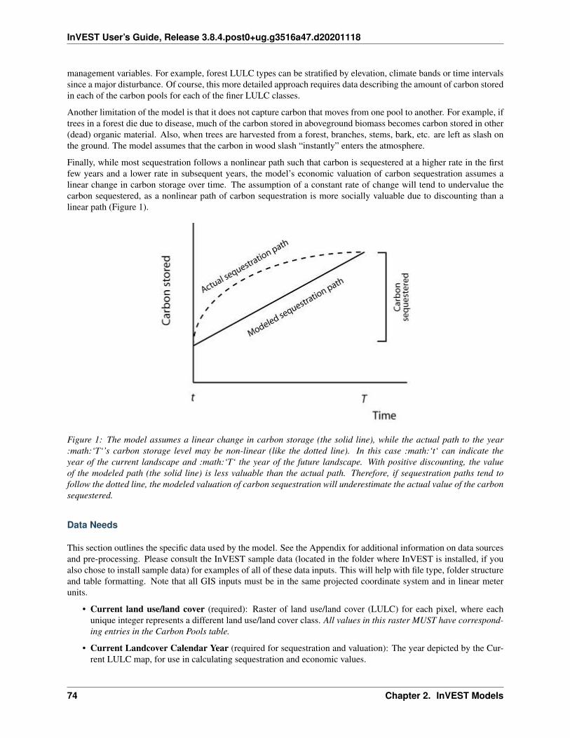
InVEST User’s Guide, Release 3.8.4.post0+ug.g3516a47.d20201118
management variables. For example, forest LULC types can be stratified by elevation, climate bands or time intervalssince a major disturbance. Of course, this more detailed approach requires data describing the amount of carbon storedin each of the carbon pools for each of the finer LULC classes.
Another limitation of the model is that it does not capture carbon that moves from one pool to another. For example, iftrees in a forest die due to disease, much of the carbon stored in aboveground biomass becomes carbon stored in other(dead) organic material. Also, when trees are harvested from a forest, branches, stems, bark, etc. are left as slash onthe ground. The model assumes that the carbon in wood slash “instantly” enters the atmosphere.
Finally, while most sequestration follows a nonlinear path such that carbon is sequestered at a higher rate in the firstfew years and a lower rate in subsequent years, the model’s economic valuation of carbon sequestration assumes alinear change in carbon storage over time. The assumption of a constant rate of change will tend to undervalue thecarbon sequestered, as a nonlinear path of carbon sequestration is more socially valuable due to discounting than alinear path (Figure 1).
Figure 1: The model assumes a linear change in carbon storage (the solid line), while the actual path to the year:math:‘T‘’s carbon storage level may be non-linear (like the dotted line). In this case :math:‘t‘ can indicate theyear of the current landscape and :math:‘T‘ the year of the future landscape. With positive discounting, the valueof the modeled path (the solid line) is less valuable than the actual path. Therefore, if sequestration paths tend tofollow the dotted line, the modeled valuation of carbon sequestration will underestimate the actual value of the carbonsequestered.
Data Needs
This section outlines the specific data used by the model. See the Appendix for additional information on data sourcesand pre-processing. Please consult the InVEST sample data (located in the folder where InVEST is installed, if youalso chose to install sample data) for examples of all of these data inputs. This will help with file type, folder structureand table formatting. Note that all GIS inputs must be in the same projected coordinate system and in linear meterunits.
• Current land use/land cover (required): Raster of land use/land cover (LULC) for each pixel, where eachunique integer represents a different land use/land cover class. All values in this raster MUST have correspond-ing entries in the Carbon Pools table.
• Current Landcover Calendar Year (required for sequestration and valuation): The year depicted by the Cur-rent LULC map, for use in calculating sequestration and economic values.
74 Chapter 2. InVEST Models

InVEST User’s Guide, Release 3.8.4.post0+ug.g3516a47.d20201118
• Carbon pools (required): A CSV (comma-separated value) table of LULC classes, containing data on carbonstored in each of the four fundamental pools for each LULC class. If information on some carbon pools is notavailable, pools can be estimated from other pools, or omitted by leaving all values for the pool equal to 0. Thetable must contain the following columns:
– lucode: Unique integer for each LULC class (e.g., 1 for forest, 3 for grassland, etc.) Every value in theLULC map MUST have a corresponding **lucode* value in the Carbon Pool table.*
– c_above: Carbon density in aboveground biomass [units: megagrams/hectare]
– c_below: Carbon density in belowground biomass [units: megagrams/hectare]
– c_soil: Carbon density in soil [units: megagrams/hectare]
– c_dead: Carbon density in dead matter [units: megagrams/hectare]
Example: Hypothetical study with five LULC classes. Class 1 (Forest) contains the most carbon in allpools. In this example, carbon stored in above- and below-ground biomass differs strongly among landuse classes, but carbon stored in soil varies less dramatically.
lucode LULC_name C_above C_below C_soil C_dead1 Forest 140 70 35 122 Coffee 65 40 25 63 Pasture/grass 15 35 30 44 Shrub/undergrowth 30 30 30 135 Open/urban 5 5 15 2
• Future landcover (required for sequestration and valuation): Raster of land use/land cover (LULC) for eachpixel, where each unique integer represents a different land use/land cover class. All values in this raster MUSThave corresponding entries in the Carbon Pools table.
• Future Landcover Calendar Year (required for sequestration and valuation): The year depicted by the FutureLULC map, for use in calculating sequestration and economic values.
• REDD Policy (required for REDD sequestration and valuation): Raster of land use/land cover (LULC) for eachpixel, where each unique integer represents a different land use/land cover class. All values in this raster MUSThave corresponding entries in the Carbon Pools table.
• Economic data (required for valuation):
– Price/Metric ton of carbon (𝑉 in the equation below): Price given in currency per metric ton of elementalcarbon (not CO:sub:‘2‘). For applications interested in estimating the total value of carbon sequestration,we recommend value estimates based on damage costs associated with the release of an additional ton ofcarbon - the social cost of carbon (SCC). Stern (2007), Tol (2009), and Nordhaus (2007a) present estimatesof SCC. For example, two SCC estimates we have used from Tol (2009) are $66 and $130 (in 2010 USdollars) (Polasky et al. 2010).
– Market discount in Price of Carbon (𝑟 in the equation below): An integer percentage value which reflectssociety’s preference for immediate benefits over future benefits. One default value is 7% per year, whichis one of the market discount rates recommended by the U.S. government for cost-benefit evaluation ofenvironmental projects. However, this rate will depend on the country and landscape being evaluated, andshould be selected based on local requirements. Philosophical arguments have been made for using a lowerdiscount rate when modeling climate change related dynamics, which users may consider using. If the rateis set equal to 0% then monetary values are not discounted.
– Annual rate of change in the price of carbon (𝑐 in the equation below): An integer percentage valuewhich adjusts the value of sequestered carbon as the impact of emissions on expected climate change-related damages changes over time. Setting this rate greater than 0% suggests that the societal value ofcarbon sequestered in the future is less than the value of carbon sequestered now. It has been widely arguedthat GHG emissions need to be curtailed immediately to avoid crossing a GHG atmospheric concentration
2.2. Final Ecosystem Services: 75

InVEST User’s Guide, Release 3.8.4.post0+ug.g3516a47.d20201118
threshold that would lead to a 3 degree Celsius or greater change in global average temperature by 2105.Some argue that such a temperature change would lead to major disruptions in economies across the world(Stern et al. 2006). Therefore, any mitigation in GHG emissions that occurs many years from now mayhave no effect on whether or not this crucial concentration threshold is passed. If this is the case, Csequestration in the far future would be relatively worthless and a carbon discount rate greater than zerois warranted. Alternatively, setting the annual rate of change less than 0% (e.g., -2%) suggests that thesocietal value of carbon sequestered in the future is greater than the value of carbon sequestered now (thisis a separate issue than the value of money in the future, a dynamic accounted for with the market discountrate). This may be the case if the damages associated with climate change in the future accelerate as theconcentration of GHGs in the atmosphere increases.
The value of carbon sequestration over time for a given parcel x is:
𝑣𝑎𝑙𝑢𝑒_𝑠𝑒𝑞𝑥 = 𝑉𝑠𝑒𝑞𝑢𝑒𝑠𝑡𝑥
𝑦𝑟_𝑓𝑢𝑡− 𝑦𝑟_𝑐𝑢𝑟
𝑦𝑟_𝑓𝑢𝑡−𝑦𝑟_𝑐𝑢𝑟−1∑︁𝑡=0
1(︀1 + 𝑟
100
)︀𝑡 (︀1 + 𝑐
100
)︀𝑡 (2.25)
Running the Model
To launch the Carbon model navigate to the Windows Start Menu -> All Programs -> InVEST [version] -> Carbon.The interface does not require a GIS desktop, although the results will need to be explored with any GIS tool such asArcGIS or QGIS.
This model supports avoided re-computation. This means the model will detect intermediate and final results from aprevious run in the specified workspace and it will avoid re-calculating any outputs that are identical to the previousrun. This can save significant processing time for successive runs when only some input parameters have changed.
Interpreting Results
The following is a short description of each of the outputs from the Carbon model. These results are found within themodel’s Workspace specified in the user interface. In the file names below, “Suffix” refers to the optional user-definedSuffix input to the model.
• [Workspace] folder:
– Parameter log: Each time the model is run, a text (.txt) file will be created in the Workspace. The file willlist the parameter values and output messages for that run and will be named according to the service, thedate and time. When contacting NatCap about errors in a model run, please include the parameter log.
– report_[Suffix].html: This file presents a summary of all data computed by the model. It also includesdescriptions of all other output files produced by the model, so it is a good place to begin exploring andunderstanding model results. Because this is an HTML file, it can be opened with any web browser.
– tot_c_cur_[Suffix].tif/tot_c_fut_[Suffix].tif/tot_c_redd_[Suffix].tif: Rasters showing the amount of car-bon stored in Mg in each pixel for the current, future and REDD scenarios. It is a sum of all of the carbonpools provided by the biophysical table.
– delta_cur_fut_[Suffix].tif/delta_cur_redd_[Suffix].tif: Rasters showing the difference in carbon storedbetween the future/REDD landscape and the current landscape. The values are in Mg per pixel. In thismap some values may be negative and some positive. Positive values indicate sequestered carbon, negativevalues indicate carbon that was lost.
– npv_fut_[Suffix].tif/npv_redd_[Suffix].tif:** Rasters showing the economic value of carbon sequesteredbetween the current and the future/REDD landscape dates. The units are in currency per pixel.
• [Workspace]\intermediate_outputs folder:
76 Chapter 2. InVEST Models

InVEST User’s Guide, Release 3.8.4.post0+ug.g3516a47.d20201118
– c_above_[Suffix].tif: Raster of aboveground carbon values, mapped from the Carbon Pools table to theLULC.
– c_below_[Suffix].tif: Raster of belowground carbon values, mapped from the Carbon Pools table to theLULC.
– c_dead_[Suffix].tif: Raster of dead carbon values, mapped from the Carbon Pools table to the LULC.
– c_soil_[Suffix].tif: Raster of soil carbon values, mapped from the Carbon Pools table to the LULC.
– _tmp_work_tokens: This directory stores metadata used iternally to enable avoided re-computation. Nomodel results are stored here.
Appendix: Data Sources
This is a rough compilation of data sources and suggestions for finding, compiling, and formatting data. This sectionshould be used for ideas and suggestions only. This section is updated as new data sources and methods becomeavailable.
Land use/land cover
Global land use data is available from:
• NASA: https://lpdaac.usgs.gov/dataset_discovery/modis/modis_products_table/mcd12q1 (MODIS multi-yearglobal landcover data provided in several classifications)
• The European Space Agency: https://www.esa-landcover-cci.org (Three global maps for the 2000, 2005 and2010 epochs)
• The University of Maryland?s Global Land Cover Facility: http://glcf.umd.edu/data/landcover/ (data availablein 1 degree, 8km and 1km resolutions).
Data for the U.S. is provided by the USGS and Department of the Interior via the National Land Cover Database:https://www.mrlc.gov/finddata.php
The simplest categorization of LULCs on the landscape involves delineation by land cover only (e.g., cropland, tem-perate conifer forest, prairie). Several global and regional land cover classifications are available (e.g., Anderson et al.1976), and often detailed land cover classification has been done for the landscape of interest.
A slightly more sophisticated LULC classification could involve breaking relevant LULC types into broad age cate-gories (e.g., forest of age 0-10 years, 11-20, 21-40, etc.). This would allow separate estimates of carbon storage fordifferent ages. In scenarios, parcels can move from one age class to the next, crudely capturing changes in carbonstorage over time. This approach requires more information, however, including carbon storage estimates for each ageclass for all modeled pools of carbon.
A still more detailed classification could stratify LULC types by variables known to affect carbon storage within agiven LULC type (e.g., montane forest 800-1000m, montane forest 1001-1200m, etc.). Rainfall, temperature, andelevation all typically influence carbon storage and sequestration (e.g., Jenny 1980, Coomes et al. 2002, Raich etal. 2006). If data are available to estimate carbon storage at different elevations, or at different levels of rainfall,temperature or other climate variables, model results will be substantially more accurate. This will typically take alarge sample of plot estimates of carbon storage.
Carbon pools
Carbon storage data should be set equal to the average carbon storage values for each LULC class. The ideal datasource for all carbon stocks is a set of local field estimates, where carbon storage for all relevant stocks has been
2.2. Final Ecosystem Services: 77
InVEST User’s Guide, Release 3.8.4.post0+ug.g3516a47.d20201118
directly measured. These can be summarized to the LULC map, including any stratification by age or other variable.If these data are not available, however, there are several general data sources that can be used.
Note that several sources, including IPCC (2006), report in units of biomass, while InVEST uses mass of elementalcarbon. To convert metric tons of biomass to metric tons of C, multiply by a conversion factor, which varies typicallyfrom 0.43 to 0.51. Conversion factors for different major tree types and climatic regions are listed in Table 4.3 on page4.48 of IPCC (2006).
Carbon stored in aboveground biomass
A good but very general source of data for carbon storage is the Intergovernmental Panel on Climate Change’s(IPCC) 2006 methodology for determining greenhouse gas inventories in the Agriculture, Forestry and OtherLand Use (AFOLU) sector (http://www.ipcc-nggip.iges.or.jp/public/2006gl/pdf/4_Volume4/V4_02_Ch2_Generic.pdf, IPCC 2006). To use this set of information from the IPCC, you must know your site’s climate domainand region; use data from Table 4.1 on page 4.46 and a digital copy of the Food and Agriculture Organiza-tion of the United Nations’ (FAO) eco-region map (http://www.fao.org/geonetwork/srv/en/main.home) to figure thatout. Tables 5.1 through 5.3 (p. 5.9) of IPCC (2006) give estimates for aboveground biomass in agriculture landwith perennial woody biomass (e.g., fruit orchards, agroforestry, etc.). Tables 4.7, 4.8, and 4.12 give above-ground biomass estimates for natural and plantation forest types. Ruesch and Gibbs (2008) mapped the IPCC(2006) aboveground biomass carbon storage data given year 2000 land cover data, which can be accessed here:https://cdiac.ess-dive.lbl.gov/epubs/ndp/global_carbon/carbon_documentation.html.
Other general sources of carbon storage estimates can be found. For example, Grace et al. (2006) estimate the averageaboveground carbon storage (leaf + wood) for major savanna ecosystems around the world (Table 1). Houghton(2005) gives aboveground carbon storage for natural and plantation forest types, by continent (Tables 1 and 3). Brownet al. (1989) give aboveground biomass estimates for tropical broadleaf forests as a function of land-use: undisturbed,logged and nonproductive (Table 7). Region-specific sources of carbon storage data are also available. Those we’vefound include:
• Latin America: Malhi et al. (2006) report aboveground biomass volumes for 227 lowland forest plots in Bolivia,Brazil, Colombia, Ecuador, French Guinea, Guyana, Panama, Peru, and Venezuela. Nascimento and Laurance(2002) estimate aboveground carbon stocks in twenty 1-ha plots of Amazonian rainforest. Tiessen et al. (1998)find aboveground carbon stocks for the Brazilian savanna types Caatingas and Cerrados.
• Africa: Zhang and Justice (2001) report aboveground carbon stocks for major forest and shrub LULC types forcentral African countries. Tiessen et al. (1998) estimates total aboveground biomass of degraded savanna inSenegal. Makundi (2001) reports mean annual incremental growth for three forest plantation types in Tanzania.Malimbwi et al. (1994) estimates aboveground carbon stocks in the miombo woodlands of Kitungalo ForestReserve Tanzania. Munishi and Shear (2004) report aboveground carbon stocks in the Afromontane rain forestsof the Eastern Arc Mountains of Tanzania. Glenday (2006) estimates aboveground carbon stocks for 3 foresttypes in the Kakamega National Forest of western Kenya.
• North America: Smith et al. (2006) estimate aboveground carbon stocks for all major forest types in the US.
• The Carbon On Line Estimator (http://www.ncasi2.org/COLE/) is a tool for calculating carbon characteristicsin U.S. forests based on USDA Forest Service Forest Inventory & Analysis and Resource Planning Assessmentdata. With this tool, carbon characteristics can be examined at the scale of counties. Using the variables tab,aboveground, belowground, soil, or dead wood carbon pools can be selected.
• Coomes et al. (2002) estimate aboveground carbon stocks for native shrubland and forest types in New Zealand.
Aboveground biomass (and therefore carbon stocks) can also be calculated from timber inventories, which are oftendone by forestry ministries on a set of plots. Use the following formula to estimate the aboveground carbon stock ina forest stand that has been inventoried for its merchantable volume where VOB is the per-hectare volume of trees incubic meters measured from tree stump to crown point (the merchantable portion of the tree), WD is the wood densityof trees (dry biomass per unit of tree volume), BEF is the ratio of total aboveground dry biomass to dry biomass ofinventoried volume, and CF is the ratio of elemental carbon to dry biomass, by mass (Brown 1997). The biomass
78 Chapter 2. InVEST Models

InVEST User’s Guide, Release 3.8.4.post0+ug.g3516a47.d20201118
expansion factor (BEF) accounts for C stored in all other portions of the tree aboveground (e.g., branches, bark, stems,foliage, etc; the non-merchantable portions of the tree). In most cases WD for a plot is approximated with values fordominant species. Brown (1997) provides a table of WD values for many tree species in Appendix 1 of section 3 anda method for calculating BEF (Equation 3.1.4). See ECCM (2007) for an application of this FAO method to forestinventory data from eastern Tanzania. IPCC (2006) also presents estimates of ( ) where BEF values for hardwood,pine, conifer, and natural forest stands by eco-region are given in Table 4.5 and WD values for many species are givenin Tables 4.13 and 4.14. (Use the BCEF values in Table 4.5 that are subscripted by S.) Finally, Brown et al. (1989)give BEF for tropical broadleaf forests under three land uses: undisturbed, logged, and nonproductive.
Brown (1997) attaches several caveats to the use of the above equation. First, the equation is designed for inventoriedstands that are closed as opposed to open (forests with sparser canopy coverage such as oak savanna). Second, VOBestimates should be a function of all tree species found in the stand, not just the economically most valuable wood.Third, trees with diameters as low as 10 centimeters at breast height (DBH = 10) need to be included in the inventoryif this aboveground biomass carbon equation is to be as accurate as possible. Brown (2002) also notes that the use ofa single BEF value is a simplification of the actual biomass growth process.
These caveats lead Brown (2002) to recommend the use of allometric biomass equations to estimate woody above-ground biomass if available. These equations give the estimated relationship between a stand’s distribution of different-sized trees and the stand’s aboveground biomass. Brown (1997) and Brown and Schroeder (1999) provide generalaboveground biomass allometric equations for all global eco-regions and the eastern US, respectively. Cairns et al.(2000) provide aboveground biomass allometric equations for LULC types in southern Mexico. Nascimento and Lau-rance (2002) estimate Amazonian rainforest aboveground biomass using allometric curves. The use of these equationsrequires knowledge of the distribution of tree size in a given stand.
Some researchers have made use of these equations a bit easier by first relating a stand’s distribution of different-sizedtrees to its age and then mapping the relationship between age and aboveground biomass (i.e., ). For example, Silver etal. (2000) have estimated aboveground biomass as a function of stand age (i.e., years since afforestation/reforestation)or previous LULC for native forest types in tropical ecosystems. Smith et al. (2006) take the transformation ofallometric equations one step further by relating age to total biomass carbon (belowground plus aboveground) directlyfor various US forests.
When using IPCC data or other similar broad data sources, one final issue to consider is how the level of anthropogenicdisturbance affects carbon stocks. The aboveground C stock of highly disturbed areas will likely be lower than thestocks of undisturbed areas. It is not clear what type of disturbance levels IPCC or other such sources assume whenreporting aboveground biomass estimates. If forest disturbance is an issue in the demonstration site, LULC typesshould be stratified by levels of disturbance. For an example of such stratification see Table 2.5, page 14 of ECCM(2007).
Finally, we generally do not treat aboveground herbaceous material as a carbon pool (e.g., grass, flowers, non-woodycrops). Our working assumption is that this material does not represent a potential source of long-term storage likewoody biomass, belowground biomass, and soil. Herbaceous material in general recycles its carbon too quickly.
Carbon stored in belowground biomass
For LULC categories dominated by woody biomass, belowground biomass can be estimated roughly with the “root toshoot” ratio of belowground to aboveground biomass. Default estimates of the root to shoot ratio are given in Table4.4 on p. 4.49 of IPCC (2006) by eco-region. Broad estimates of this ratio are also given in Section 3.5 of Brown(1997).
Some LULC types contain little to no woody biomass but substantial belowground carbon stocks (e.g., naturalgrasslands, managed grasslands, steppes, and scrub/shrub areas). In these cases the root to shoot ratio describedabove does not apply. Belowground estimates for these LULC types are best estimated locally, but if local dataare not available some global estimates can be used. The IPCC (2006) lists total biomass (aboveground plus be-lowground) and aboveground biomass for each climate zone in table 6.4 (p. 6.27). The difference between thesenumbers is a crude estimate of belowground biomass. . Recently, Ruesch and Gibbs (2008) mapped the IPCC
2.2. Final Ecosystem Services: 79

InVEST User’s Guide, Release 3.8.4.post0+ug.g3516a47.d20201118
(2006) aboveground biomass carbon storage data given year 2000 land cover data, which can be accessed here:https://cdiac.ess-dive.lbl.gov/epubs/ndp/global_carbon/carbon_documentation.html.
Several studies have compiled estimates of belowground biomass or root-to-shoot ratios for different habitat types.Among those we found:
• Grace et al. (2006) estimate the total average woody and herbaceous root biomass for major savanna ecosystemsaround the world (Table 1). Baer et al. (2002) and Tilman et al. (2006) estimate the C stored in the roots ofplots restored to native C4 grasses in Nebraska and Minnesota, U.S. respectively, as a function of years sincerestoration (see Table 2 in Baer et al. (2002) and Figure 1D in Tilman et al. (2006)).
• Cairns et al. (1997) survey root-to-shoot ratios for LULC types across the world. Munishi and Shear (2004)use a ratio of 0.22 for Afromontane forests in the Eastern Arc forests of Tanzania. Malimbwi et al. (1994) use0.20 for miombo woodlands in the same area of Tanzania. Coomes et al. (2002) use 0.25 for shrublands in NewZealand. Gaston et al. (1998) report a root-to-shoot ratio of 1 for African grass / shrub savannas.
Carbon stored in soil
If local or regional soil C estimates are not available, default estimates can be looked up from IPCC (2006) foragricultural, pasture, and managed grasslands. Table 2.3 of IPCC (2006) contains estimates of soil carbon stocks bysoil type, assuming these stocks are at equilibrium and have no active land management. For cropland and grasslandLULC types, this default estimate can be multiplied by management factors, listed in Tables 5.5 and 6.2 of IPCC(2006). For all other LULC types and their related management schemes, the IPCC (2006) assumes no managementfactors.
There are alternative global-level sources of soil carbon data. Post et al. (1982) report carbon stocks in the first meter ofsoil by Holdridge Life Zone Classification System (GIS map of these Zones available at http://www.arcgis.com/home/item.html?id=f3ec7241777f4c56a69ae14d2a98e44b). Silver et al. (2000) have estimated soil carbon as a function ofyears since afforestation/reforestation for native forest types in tropical ecosystems. Grace et al. (2006) estimate thesoil carbon for major savanna types around the world (Table 1). Detwiler (1986) lists soil carbon for tropical forestsoils in Table 2.
Several region-specific studies also report soil carbon stocks. Those we’ve found include:
• North America: Smith et al. (2006) estimate soil C for every 5-year increment up to 125 years since afforesta-tion/reforestation for all major forest types and forest management practices in each region of the U.S. Othersinclude McLauchlan et al. (2006); Tilman et al. (2006); Fargione et al (2008); Schuman et al. (2002); and Lal(2002).
• Africa: Houghton and Hackler (2006) give soil C for 5 LULC forest types (Rain Forest; Moist Forest Dry;Forest; Shrubland; and Montane Forest) in sub-Saharan Africa that have retained their natural cover and forforest areas that have been converted to croplands, shifting cultivation, and pasture. Vagen et al. (2005) providessoil C estimates for various LULC types in sub-Saharan Africa.
• South America: Bernoux et al. (2002) estimated soil C stocks to a depth of 30 cm for different soil type-vegetation associations in Brazil. For example, the soil C stock in HAC soils under 14 different land covercategories, including Amazon forest and Brazilian Cerrado, range from 2 to 116 kg C m-2.
Important Note: In most research that estimates carbon storage and sequestration rates on a landscape, soil poolmeasures only include soil organic carbon (SOC) in mineral soils (Post and Kwon 2000). However, if the ecosystembeing modeled has a lot of organic soils (e.g. wetlands or paramo), it is critical to add this component to the mineralsoil content. In landscapes where the conversion of wetlands into other land uses is common, carbon releases fromorganic soils should also be tracked closely (IPCC 2006).
80 Chapter 2. InVEST Models

InVEST User’s Guide, Release 3.8.4.post0+ug.g3516a47.d20201118
Carbon stored in dead organic matter
If local or regional estimates of carbon stored in dead organic matter aren’t available, default values from the IPCC(2006) can be assigned. Table 2.2 (p. 2.27) gives default carbon stocks for leaf litter in forested LULC types. Fornon-forested types, litter is close to 0. Grace et al. (2006) estimate the average carbon stored in litter for majorsavanna ecosystems around the world (Table 1). It is not clear if their total “above-ground biomass” estimates includedeadwood or not. Deadwood stocks are more difficult to estimate in general, and we have located no default datasources.
Regional estimates:
• United States: Smith et al. (2006) estimate carbon storage in litter (referred to as “Forest Floor” C in thedocument) and dead wood (the aggregate of C pools referred to as “Standing Dead Trees” and “Down DeadWood” in the document) for all major forest types and forest management practices in each region of the U.S.as a function of stand age.
• South America: Delaney et al. (1998) estimate carbon stored in standing and down dead wood in 6 tropicalforests of Venezuela. According to the authors, deadwood is typically 1/10 the amount of biomass as above-ground vegetation.
Economic inputs: carbon price and discount rates
Recent estimates suggest that the social cost of carbon (SCC), or the marginal damage associated with the release ofan additional Mg of C into the atmosphere, ranges from $32 per metric ton of C (Nordhaus 2007a) to $326 per metricton of C (Stern 2007) in 2010 US dollars. The value of this damage can also be considered the monetary benefit of anavoided release. Tol (2009) provides a comprehensive survey of SCC estimates, reporting median values of $66 and$130 per metric ton in 2010 US dollars (values differ because of different assumptions regarding discounting of time).Other estimates can be found in Murphy et al. (2004), Stainforth et al. (2005), and Hope (2006).
An alternative method for measuring the cost of an emission of a metric ton of C is to set the cost equal to the leastcost alternative for sequestering that ton. The next best alternative currently is to capture and store the C emitted fromutility plants. According to Socolow (2005) and Socolow and Pacala (2007), the cost of this technology per metric toncaptured and stored is approximately $100.
Finally, while we do not recommend this approach, market prices can be used to set the price of sequestered carbon.We do not recommend the use of market prices because they usually only apply to “additional” carbon sequestration;sequestration above and beyond some baseline sequestration rate. Further, carbon credit values from carbon marketsare largely a function of various carbon credit market rules and regulations and do not necessarily reflect the benefit tosociety of a sequestered ton of carbon. Therefore, correct use of market prices would require estimating a baseline ratefor the landscape of interest, mapping additional sequestration, and then determining which additional sequestrationis eligible for credits according to market rules and regulations.
We discount the value of future payments for carbon sequestration to reflect society’s preference for payments thatoccur sooner rather than later. The U.S. Office of Management and Budget recommends a 7% per annum marketdiscount rate for US-based projects (OMB 1992). Discount rates vary for other parts of the world. Canada and NewZealand recommend 10% for their projects (Abusah and de Bruyn 2007). It is best to look for the recommendeddiscount rate for your country.
Some economists believe that a market or consumption discount rate of 7% to 12% is too high when dealing with theclimate change analysis. Because climate change has the potential to severely disrupt economies in the future, thepreference of society to consume today at the expense of both climate stability in the future and future generations’economic opportunities is seen as unethical by some (Cline 1992, Stern 2007). According to this argument, analyses ofthe effects of climate change on society and policies designed to reduce climate change should use low discount ratesto encourage greater GHG emission mitigation and therefore compensate for the potentially severe damages incurredby future generations (e.g., r = 0.014 in Stern (2007)). Recent government policies in several countries have supportedthe use of a very low discount rate for certain long-term projects (Abusah and de Bruyn 2007).
2.2. Final Ecosystem Services: 81

InVEST User’s Guide, Release 3.8.4.post0+ug.g3516a47.d20201118
The carbon discount rate, which reflects the greater climatic impact of carbon sequestered immediately over carbonsequestered in the future, is discussed in Adams et al. (1999), Plantinga et al. (1999), Feng 2005, and Nelson et al.(2008).
References
Abusah, Sam and Bruyn, Clinton de. 2007. Getting Auckland on Track: Public Transport and New Zealand’s Eco-nomic. Ministry of Economic Development Working Paper. Accessed at <http://s3.amazonaws.com/zanran_storage/www.med.govt.nz/ContentPages/4013253.pdf>.
Adams, DM, RJ Alig, BA McCarl, et al. 1999. Minimum cost strategies for sequestering carbon in forests. Land Econ75: 360-374.
Anderson, JR, EE Hardy, JT Roach, RE Witmer. A Land Use and Land Cover Classification System for Use with Re-mote Sensor Data. Washington, DC: United States Government Printing Office; 1976. Geological Survey ProfessionalPaper 964.
Antle, JM, and B. Diagana. 2003. Creating Incentives for the Adoption of Sustainable Agricultural Practices inDeveloping Countries: The Role of Soil Carbon Sequestration. American Journal of Agricultural Economics 85:1178-1184.
Baer, SG, DJ Kitchen, JM Blair, and CW Rice. 2002. Changes in Ecosystem Structure and Function along a Chronose-quence of Restored Grasslands. Ecological Applications 12:1688-1701.
Bernoux, M., MDS Carvalho, B. Volkoff, and CC Cerri. 2002. Brazil’s soil carbon stocks. Soil Science Society ofAmerica Journal 66:888-896.
Brown, SL, PE Schroeder and JS Kern. Spatial distribution of biomass in forests of the eastern USA.Forest Ecologyand Management 123 (1999) 81-90.
Brown, S. 2002. Measuring carbon in forests: current status and future challenges. Environmental Pollution 116:363-372.
Brown, S. Estimating Biomass and Biomass Change of Tropical Forests: a Primer. FAO Forestry Department; 1997.Report for FAO Forestry Paper 134.
Brown, S. and PE Schroeder. 1999. Spatial patterns of aboveground production and mortality of woody biomass foreastern US forests. Ecological Applications 9:968-980.
Cairns, MA, PK Haggerty, R. Alvarez, BHJ De Jong, and I. Olmsted. 2000. Tropical Mexico’s recent land-use change:A region’s contribution to the global carbon cycle. Ecological Applications 10:1426-1441.
Cairns, MA, S. Brown, EH Helmer, and GA Baumgardner. 1997. Root biomass allocation in the world’s uplandforests. Oecologia 111:1-11.
Canadell, JG and MR Raupach. 2008. Managing Forests for Climate Change Mitigation. Science 320:1456-1457.
Cline, WR. 1992. The economics of global warming. Instuitute for International Economics, Washington, D.C.
Coomes, DA, RB Allen, NA Scott, C. Goulding, and P. Beets. 2002. Designing systems to monitor carbon stocks inforests and shrublands. Forest Ecology and Management 164:89-108.
Conte, MN and MJ Kotchen. 2010. Explaining the price of voluntary carbon offsets. Climate Change Economics 1(2):93-111.
Capoor, K., and P. Ambrosi. State and Trends of the Carbon Market 2008. Washington, D.C.: World Bank Institute,2008 May.
Delaney, M., S. Brown, AE Lugo, A. Torres-Lezama, and NB Quintero. 1998. The quantity and turnover of deadwood in permanent forest plots in six life zones of Venezuela. Biotropica 30:2-11.
82 Chapter 2. InVEST Models

InVEST User’s Guide, Release 3.8.4.post0+ug.g3516a47.d20201118
Detwiler, RP. 1986. Land Use Change and the Global Carbon Cycle: The Role of Tropical Soils. Biogeochemistry2:67-93.
Edinburgh Centre for Carbon Management. The Establishing Mechanisms for Payments for Carbon EnvironmentalServices in the Eastern Arc Mountains, Tanzania; 2007 May 2007.
Fargione, J., J. Hill, D. Tilman, S. Polasky, and P. Hawthorne. 2008. Land Clearing and the Biofuel Carbon Debt.Science 319:1235-1238.
Feng, H. 2005. The dynamics of carbon sequestration and alternative carbon accounting, with an application to theupper Mississippi River Basin. Ecological Economics 54:23-35.
Gaston, G., S. Brown, M. Lorenzini, and KD Singh. 1998. State and change in carbon pools in the forests of tropicalAfrica. Global Change Biology 4:97-114.
Glenday, J. 2006. Carbon storage and emissions offset potential in an East African tropical rainforest. Forest Ecologyand Management 235:72-83.
Grace, J., J. San Jose, P. Meir, HS Miranda, and RA Montes. 2006. Productivity and carbon fluxes of tropical savannas.Journal of Biogeography 33:387-400.
Gibbs, HK, S Brown, JO Niles, and JA Foley. 2007. Monitoring and estimating tropical forest carbon stocks: makingREDD a reality. Environmental Research Letters 2:045023.
Hamilton, K., M Sjardin, T Marcello, and G Xu. Forging a Frontier: State of the Voluntary Carbon Markets 2008.Washington, D.C.: Ecosystem Marketplace and New Carbon Finance; 2008.
Hope, CW. 2006. The social cost of carbon: what does it actually depend on? Climate Policy 6: 565–572
Houghton, RA. 2005. Tropical deforestation as a source of greenhouse gas emissions. In: Tropical Deforestation andClimate Change, Moutinho and Schwartzman [eds.]. Instituto de Pesquisa Ambiental da Amazonia and EnvironmentalDefense, Belem, Brazil.
Houghton, RA, and JL Hackler. 2006. Emissions of carbon from land use change in sub-Saharan Africa. Journal ofGeophysical Research 111.
The Intergovernmental Panel on Climate Change (IPCC). 2006. 2006 IPCC Guidelines for National GreenhouseGas Inventories, Volume 4: Agriculture, Forestry and Other Land Use. Prepared by the National Greenhouse GasInventories Programme, Eggleston, HS, L. Buendia, K. Miwa, T. Ngara, and K. Tanabe (eds). Institute for GlobalEnvironmental Strategies (IGES), Hayama, Japan. <http://www.ipcc-nggip.iges.or.jp/public/2006gl/vol4.html>.
Jenny, H. 1980. The Soil Resource. Springer, New York.
Lal, R. 2004. Soil Carbon Sequestration Impacts on Global Climate Change and Food Security. Science 304:1623-1627.
Mackey, B, Keith H, Berry S.L, Lindenmayer DB. Green carbon: the role of natural forests in carbon storage. Part1, A green carbon account of Australia’s Southeastern Eucalypt forest, and policy implications. Canberra, Australia:ANU E Press, 2008.
Makundi, WR. 2001. Carbon mitigation potential and costs in the forest sector in Tanzania. Mitigation and AdaptationStrategies for Global Change 6:335-353.
Malhi, Y., D. Wood, TR Baker, et al. 2006. The regional variation of aboveground live biomass in old-growthAmazonian forests. Global Change Biology 12:1107-1138.
Malimbwi, RE, B. Solberg, and E. Luoga. 1994. Estimation of biomass and volume in miombo woodland at KitungaloForest Reserve Tanzania. Journal of Tropical Forest Science 7:230-242.
McLauchlan, KK., SE Hobbie, and WM Post. 2006. Conversion From Agriculture To Grassland Builds Soil OrganicMatter On Decadal Timescales. Ecological Applications 16:143-153.
2.2. Final Ecosystem Services: 83

InVEST User’s Guide, Release 3.8.4.post0+ug.g3516a47.d20201118
Mollicone D., F. Achard, S. Federici, H. Eva, G. Grassi, A. Belward, F. Raes, G. Seufert, H. Stibig, G. Matteucci, andE. Schulze. 2007. An incentive mechanism for reducing emissions from conversion of intact and non-intact forests.Climatic Change 83:477-493.
Munishi, PKT and TH Shear. 2004. Carbon Storage in Afromontane Rain Forests of the Eastern Arc Mountains ofTanzania: their Net Contribution to Atmospheric Carbon. Journal of Tropical Forest Science 16:78-93.
Murphy, JM et al. 2004. Quantification of modelling uncertainties in a large ensemble of climate change simulations.Nature 430, 768-772.
Murray, B., B. Sohngen, and M. Ross. 2007. Economic consequences of consideration of permanence, leakage andadditionality for soil carbon sequestration projects. Climatic Change 80:127-143.
Nascimento, HEM, and WF Laurance. 2002. Total aboveground biomass in central Amazonian rainforests: alandscape-scale study. Forest Ecology and Management 168:311-321.
Nelson, E., G. Mendoza, J. Regetz, S. Polasky, H. Tallis, D. Cameron, K. Chan, G. Daily, J. Goldstein, P. Kareiva, E.Lonsdorf, R. Naidoo, TH Ricketts, and R. Shaw. 2009. Modeling multiple ecosystem services, biodiversity conserva-tion, commodity production, and tradeoffs at landscape scales. Frontiers in Ecology and the Environment.
Nordhaus, W. 2007a. Critical Assumptions in the Stern Review on Climate Change. Science 317 (5835): 201–202.
Nordhaus, W. 2007b. A Review of the Stern Review on the Economics of Global Warming. Journal of EconomicLiterature 45: 686-702.
Pagiola, S. 2008. Payments for environmental services in Costa Rica. Ecological Economics 65 (4): 712-724.
Plantinga, AJ, and RA Birdsey. 1994. Optimal Forest Stand Management When Benefits are Derived from Carbon.Natural Resource Modeling 8(4): 373-387.
Polasky, S, E Nelson, D Pennington, and K Johnson. 2010. The Impact of Land-Use Change on Ecosystem Services,Biodiversity and Returns to Landowners: A Case Study in the State of Minnesota. Environmental and ResourceEconomics 48:219-242
Post, WM, WR Emanuel, PJ Zinke, and AG Stangenberger. 1982. Soil carbon pools and world life zones. Nature298:156-159.
Post, WM, KC Kwon. 2000. Soil carbon sequestration and land-use change: processes and potential. Global ChangeBiology 6:317-327.
Raich, JW, AE Russell, K. Kitayama, WJ Parton, and PM Vitousek. 2006. Temperature influences carbon accumula-tion in moist tropical forests. Ecology 87:76-87.
Ruesch A, and HK Gibbs. 2008. New IPCC tier-1 global biomass carbon map for the year 2000.Available:https://cdiac.ess-dive.lbl.gov/epubs/ndp/global_carbon/carbon_documentation.html.
Schuman, GE, HH Janzen, and JE Herrick. 2002. Soil carbon dynamics and potential carbon sequestration by range-lands. Environmental Pollution, 116:391-396.
Sedjo, RA and B. Sohngen. Carbon Credits for Avoided Deforestation. Washington, DC: Resources for the Future;2007 October 2007. Report for RFF DP 07-47.
Silver, WL, R. Ostertag, and AE Lugo. 2000. The potential for carbon sequestration through reforestation of aban-doned tropical agricultural and pasture lands. Restoration Ecology 8:394-407.
Socolow, RH. 2005. Can We Bury Global Warming? Scientific American 293: 49-55.
Socolow, RH and SW Pacala. 2006. A Plan to Keep Carbon in Check. Scientific American 295: 50-57.
Sohngen, Brent, RH Beach, and Kenneth Andrasko. 2008. Avoided Deforestation as a Greenhouse Gas MitigationTool: Economic Issues. Journal of Environmental Quality 37: 1368-1375.
Stainforth, DA et al., 2005. Uncertainty in predictions of the climate response to rising levels of greenhouse gases.Nature 433, 403–406.
84 Chapter 2. InVEST Models

InVEST User’s Guide, Release 3.8.4.post0+ug.g3516a47.d20201118
Stern, N. 2007. The Economics of Climate Change: The Stern Review. Cambridge and New York: CambridgeUniversity Press.
Tiessen, H., C. Feller, EVSB Sampaio, and P. Garin. 1998. Carbon Sequestration and Turnover in Semiarid Savannasand Dry Forest. Climatic Change 40:105-117.
Tilman, D., J. Hill, and C. Lehman. 2006. Carbon-Negative Biofuels from Low-Input High-Diversity GrasslandBiomass. Science 314:1598-1600.
Tol, RSJ. 2005. The marginal damage costs of carbon dioxide emissions: an assessment of the uncertainties. EnergyPolicy 33:2064-2074.
Tol, RSJ. 2009. The Economic Effects of Climate Change.Journal of Economic Perspectives 23:29-51.
USOMB (US Office of Management and Budget). 1992. Guidelines and Discount Rates for Benefit-Cost Analy-sis of Federal Programs Circular No. A-94 (Revised). Transmittal Memo No. 64. Washington DC: US Office ofManagement and Budget.
Vagen, TG, R Lal, and BR Singh. 2005. Soil carbon sequestration in sub-Saharan Africa: A review. Land Degradation& Development 16:53-71.
Weitzman, ML. 2007. A review of the Stern Review on the Economics of Climate Change. Journal of EconomicLiterature 45:703-724.
Zhang, Q, and CO Justice. 2001. Carbon Emissions and Sequestration Potential of Central African Ecosystems.AMBIO 30:351-355.
2.2.3 Coastal Blue Carbon
Summary
Marine and terrestrial ecosystems help regulate Earth’s climate by adding and removing greenhouse gases (GHGs)such as carbon dioxide (CO2) to and from the atmosphere. Coastal marshes, mangroves, and seagrasses, in partic-ular, store large amounts of carbon in their sediments, leaves, and other forms of biomass. In addition to storingcarbon, marine ecosystems continually accumulate carbon in their sediments, creating large reservoirs of long-termsequestered carbon. By storing and sequestering carbon, marine ecosystems keep CO2 out of the atmosphere where itwould otherwise contribute to climate change.
Management activities that change the cover of coastal vegetation, such as the restoration of seagrass beds and theclearing of mangrove forests, change the ability of coastal and marine areas to store and sequester carbon.
The InVEST Coastal Blue Carbon model attempts to predict the amount of carbon stored and sequestered over acoastal zone at particular points in time due to changes in land cover. Using an estimate of the monetary social value,or where available, a market price for stored and sequestered carbon, the InVEST Coastal Blue Carbon model alsoquantifies the marginal value of storage and sequestration.
Results of the InVEST Coastal Blue Carbon model can be used to compare current and future scenarios of carbonstock and net sequestration, as well as identify locations within the landscape where degradation of coastal ecosystemsshould be avoided and restoration of coastal ecosystems should be prioritized in order to preserve and enhance thesecarbon storage and sequestration services.
Introduction
This model makes use of a variety of information, including:
• The distribution and abundance of coastal vegetation
• Habitat-specific carbon stock data
2.2. Final Ecosystem Services: 85

InVEST User’s Guide, Release 3.8.4.post0+ug.g3516a47.d20201118
• Impact characteristics of various land-cover disturbances to biomass and soil carbon stock pools to predictcarbon emission rates
• Carbon accumulation rates to estimate carbon stock, net sequestration and value across a land or seascape
• Estimates of the monetary social value or market price of carbon
To quantify the value of carbon storage and sequestration, the model focuses on changes in atmospheric carbon dioxideand other greenhouse gases as a result of changes caused by human activities that can affect marine ecosystems whichstore and sequester carbon. Changes to the composition of the atmosphere have wide-ranging effects on naturalsystems that can result in changes to agricultural productivity, air quality, sea levels, and more.
The Model
Modeling Considerations
Mapping and modeling changes in carbon storage and sequestration for coastal and marine habitats can present chal-lenges. The types of spatial inputs and available information about the carbon cycle vary by location. Some studyareas have high-quality data available for a detailed analysis while other locations do not have the information neces-sary to model changes in the position and function of coastal vegetation. Salt marsh, for example, is often studied inthe context of migration due to sea-level rise. The combination of natural (e.g. sea-level rise) and anthropogenic (e.g.salt marsh migration blocked by roads) factors should be included in scenario maps and subsequent carbon modelingwhere possible. When exploring future land cover scenarios, land cover map outputs produced by the SLAMM model(Sea Level Affecting Marshes Model, developed by Warren Pinnacle) can be useful inputs to the InVEST CoastalBlue Carbon model (Clougheet et al. 2010). However, because not all sites have the detailed elevation and habitatinformation required to run SLAMM, this InVEST model provides a flexible approach that allows users to provideeither detailed land use/land cover maps or maps indicating the presence of coastal and marine vegetation that cansequester carbon.
How it Works
InVEST Coastal Blue Carbon models the carbon cycle through a bookkeeping-type approach (Houghton, 2003). Thisapproach simplifies the carbon cycle by accounting for storage in three main pools (biomass, sediment carbon (i.e.soil), and standing dead carbon (i.e. litter) see Figure 1). Accumulation of carbon in coastal habitats occurs primarilyin sediments (Pendleton et al., 2012). The model requires users to provide maps of coastal ecosystems that storecarbon, such as mangroves and seagrasses. Users must also provide data on the amount of carbon stored in the threecarbon pools and the rate of annual carbon accumulation in the biomass and sediments. If local information is notavailable, users can draw upon the global database of values for carbon stocks and accumulation rates sourced fromthe peer-reviewed literature that is included in the model. If data from field studies or other local sources are available,these values should be used instead of those in the global database. The model requires land cover maps, whichrepresent changes in human use patterns in coastal areas or changes to sea level, to estimate the amount of carbon lostor gained over a specified period of time. The model quantifies carbon storage across the land or seascape by summingthe carbon stored in these three carbon pools.
Figure 1. Three carbon pools for marine ecosystems included in the InVEST blue carbon model (mangrove example).
Carbon Storage
The carbon stored in a grid cell 𝑥 at time 𝑡, given by 𝑆𝑥𝑡 and measured in Megatonnes of CO2 equivalent, is equal tothe sum of the carbon stored in each pool in the grid cell at any time (𝑡),
𝑆𝑡𝑜𝑡𝑎𝑙 = 𝑆𝑏𝑖𝑜𝑚𝑎𝑠𝑠 + 𝑆𝑠𝑜𝑖𝑙 + 𝑆𝑙𝑖𝑡𝑡𝑒𝑟
86 Chapter 2. InVEST Models

InVEST User’s Guide, Release 3.8.4.post0+ug.g3516a47.d20201118
where 𝑆𝑏𝑖𝑜𝑚𝑎𝑠𝑠, 𝑆𝑠𝑜𝑖𝑙, 𝑆𝑙𝑖𝑡𝑡𝑒𝑟 indicate the respective Megatonnes of CO2 equivalent stored in the biomass, soil, andlitter pools in a grid cell of a particular coastal blue carbon habitat.
Coastal blue carbon habitats can simply indicate the dominant vegetation type (e.g., eelgrass, mangrove, etc), or theycan be based on details that affect pool storage values such as plant species, vegetation density, temperature regime,or vegetation age (e.g., time since restoration or last major disturbance).
For the sake of the carbon storage estimation, each coastal blue carbon habitat is assumed to be in storage equilibriumat any point in time (accumulation of carbon will be accounted for in the sequestration component of the model).
Carbon Accumulation
We model accumulation as the rate of carbon retained in the soil in organic form after the first year of decomposition.In relation to the annual ecosystem budget, this pool has not been remineralized, so it represents net accumulation.This carbon is usually derived from belowground production, and residence time can range from decades to millennia(Romero et al. 1994, Mateo et al. 1997). This accumulation contributes to the development of carbon “reservoirs”which are considered virtually permanent unless disturbed. Thus, even in the absence of a land-use or land-coverchange, carbon continues to be sequestered naturally.
We estimate accumulation by multiplying habitat specific rates of carbon accumulation by the given cell area. Thecarbon accumulated in a grid cell 𝑥 at time 𝑡 in carbon pool 𝑝, given by 𝐴𝑝𝑡 and measured in Megatonnes of CO2equivalent per year, is equal to the rate of carbon accumulation in the sediments at time 𝑡.
Loss of carbon from the soil pool (sediments) upon disturbance is more nuanced than sequestration because differenttypes of human uses and/or stasis may cause varied disruption of the soils and the carbon stored below. For example,high impact activities such as the clearing of mangroves for a shrimp pond or sediment dredging may result in a largersoil carbon disturbance than other activities such as commercial fishing or oil exploration. The impacts from coastaldevelopment on carbon storage vary since some types of development may involve paving over the soil, which oftenkeeps a large percentage of the carbon stored intact. Alternatively, dredging could remove seagrasses and disturb thesediments below, releasing carbon into the atmosphere.
Carbon Emissions
When coastal ecosystems are degraded by human activities, the carbon stored in the living plant material (above andbelow the ground) and the soil may be emitted to the atmosphere. The magnitude of post-conversion CO2 releasedepends on the type of vegetation disturbed and the level of disturbance. The type of disturbance will determine theamount of aboveground biomass loss and depth to which the soil profile will be altered. The deeper the effects ofthe disturbance, the more soil carbon that will be exposed to oxygen, oxidized and consequently emitted in the formof CO2. Some disturbances will only disturb the top soil layers while the deeper layers remain inundated and theircarbon intact. Other disturbances may affect several meters of the soil profile. To estimate the extent of the impactof various disturbances, we classify disturbances into three categories of impact: high, medium and low. Examples
2.2. Final Ecosystem Services: 87

InVEST User’s Guide, Release 3.8.4.post0+ug.g3516a47.d20201118
of high impact disturbances include mangrove conversion to shrimp farms and draining or diking salt marshes forconversion to agriculture. Low impact disturbance examples include recreational boating or float home marinas.
Magnitude and Timing of Loss
We model the release of carbon from the biomass and soil pools by estimating the fraction of carbon lost from eachpool’s total stock at the time of disturbance. The fraction of carbon lost is determined by the original coastal bluecarbon habitat and the level of impact resulting from the disturbance (see Table 1).
The InVEST Coastal Blue Carbon model allows users to provide details on the level of disturbance that occurs during atransition from a coastal blue carbon habitat to a non-coastal blue carbon habitat. This information can be provided tothe model through a pre-processor tool (See “Transition Storage” section) and further clarified with an input transitiontable.
In general, carbon stock pools emit carbon at different rates: most emissions from the biomass pool take place withinthe first year, whereas emissions from the soil pool may take much longer. The model assigns exponential decayfunctions and half-life values to the biomass and soil carbon pools of each habitat type (Table 1; Murray et al. 2011).
Carbon emitted at time 𝑡 due to a disturbance:
𝐸𝑝 = 𝐷𝑝 · (0.5𝑡−(𝑟+1)
𝐻𝑝 − 0.5𝑡−𝑟𝐻𝑝 )
where 𝑝 is the carbon pool (biomass and soil), 𝐷𝑝 represents the amount of carbon stock disturbed as time approachesinfinity, 𝐻𝑝 represents the half-life of the disturbance event, and 𝐸𝑝 represents the share of carbon released from thetotal disturbed carbon stock at time 𝑡.
Table 1: Percent carbon loss and habitat-specific decay rates as a result of low (LI), medium (MI) and high (HI)impact activities disturbing salt marsh, mangrove, and seagrass ecosystems. These default values can be adjusted bymodifying the input CSV tables.
References (numbers in parentheses above):
1. Donato, D. C., Kauffman, J. B., Murdiyarso, D., Kurnianto, S., Stidham, M., & Kanninen, M. (2011). Man-groves among the most carbon-rich forests in the tropics. Nature Geoscience, 4(5), 293-297.
2. Murray, B. C., Pendleton, L., Jenkins, W. A., & Sifleet, S. (2011). Green payments for blue carbon: Economicincentives for protecting threatened coastal habitats. Nicholas Institute for Environmental Policy Solutions,Report NI, 11, 04.
3. Crooks, S., Herr, D., Tamelander, J., Laffoley, D., & Vandever, J. (2011). Mitigating climate change throughrestoration and management of coastal wetlands and near-shore marine ecosystems: challenges and opportuni-ties. Environment Department Paper, 121, 2011-009.
4. Krithika, K., Purvaja, R., & Ramesh, R. (2008). Fluxes of methane and nitrous oxide from an Indian mangrove.Current Science (00113891), 94(2).
Valuation of Net Sequestered Carbon
The valuation option for the blue carbon model estimates the economic value of sequestration (not storage) as afunction of the amount of carbon sequestered, the monetary value of each ton of sequestered carbon, a discount rate,and the change in the value of carbon sequestration over time. The value of sequestered carbon is dependent on whois making the decision to change carbon emissions and falls into two categories: social and private. If changes incarbon emissions are due to public policy, such as zoning coastal areas for development, then decision-makers shouldweigh the benefits of development against the social losses from carbon emissions. Because local carbon emissionsaffect the atmosphere on a global scale, the social cost of carbon (SCC) is commonly calculated at a global scale(USIWGSCC, 2010). Efforts to calculate the social cost of carbon have relied on multiple integrated assessmentmodels such as FUND (http://www.fund-model.org/), PAGE (Hope, 2011), DICE and RICE (https://sites.google.com/
88 Chapter 2. InVEST Models
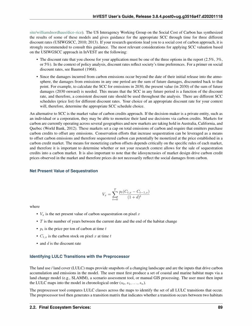
InVEST User’s Guide, Release 3.8.4.post0+ug.g3516a47.d20201118
site/williamdnordhaus/dice-rice). The US Interagency Working Group on the Social Cost of Carbon has synthesizedthe results of some of these models and gives guidance for the appropriate SCC through time for three differentdiscount rates (USIWGSCC, 2010; 2013). If your research questions lead you to a social cost of carbon approach, it isstrongly recommended to consult this guidance. The most relevant considerations for applying SCC valuation basedon the USIWGSCC approach in InVEST are the following:
• The discount rate that you choose for your application must be one of the three options in the report (2.5%, 3%,or 5%). In the context of policy analysis, discount rates reflect society’s time preferences. For a primer on socialdiscount rates, see Baumol (1968).
• Since the damages incurred from carbon emissions occur beyond the date of their initial release into the atmo-sphere, the damages from emissions in any one period are the sum of future damages, discounted back to thatpoint. For example, to calculate the SCC for emissions in 2030, the present value (in 2030) of the sum of futuredamages (2030 onward) is needed. This means that the SCC in any future period is a function of the discountrate, and therefore, a consistent discount rate should be used throughout the analysis. There are different SCCschedules (price list) for different discount rates. Your choice of an appropriate discount rate for your contextwill, therefore, determine the appropriate SCC schedule choice.
An alternative to SCC is the market value of carbon credits approach. If the decision-maker is a private entity, such asan individual or a corporation, they may be able to monetize their land use decisions via carbon credits. Markets forcarbon are currently operating across several geographies and new markets are taking hold in Australia, California, andQuebec (World Bank, 2012). These markets set a cap on total emissions of carbon and require that emitters purchasecarbon credits to offset any emissions. Conservation efforts that increase sequestration can be leveraged as a meansto offset carbon emissions and therefore sequestered carbon can potentially be monetized at the price established in acarbon credit market. The means for monetizing carbon offsets depends critically on the specific rules of each market,and therefore it is important to determine whether or not your research context allows for the sale of sequestrationcredits into a carbon market. It is also important to note that the idiosyncrasies of market design drive carbon creditprices observed in the market and therefore prices do not necessarily reflect the social damages from carbon.
Net Present Value of Sequestration
𝑉𝑥 =
𝑇∑︁𝑡=0
𝑝𝑡(𝐶𝑡,𝑥 − 𝐶𝑡−1,𝑥)
(1 + 𝑑)𝑡
where
• 𝑉𝑥 is the net present value of carbon sequestration on pixel 𝑥
• 𝑇 is the number of years between the current date and the end of the habitat change
• 𝑝𝑡 is the price per ton of carbon at time 𝑡
• 𝐶𝑡,𝑥 is the carbon stock on pixel 𝑥 at time 𝑡
• and 𝑑 is the discount rate
Identifying LULC Transitions with the Preprocessor
The land use / land cover (LULC) maps provide snapshots of a changing landscape and are the inputs that drive carbonaccumulation and emissions in the model. The user must first produce a set of coastal and marine habitat maps via aland change model (e.g., SLAMM), a scenario assessment tool, or manual GIS processing. The user must then inputthe LULC maps into the model in chronological order (𝑠0, 𝑠1, . . . , 𝑠𝑛).
The preprocessor tool compares LULC classes across the maps to identify the set of all LULC transitions that occur.The preprocessor tool then generates a transition matrix that indicates whether a transition occurs between two habitats
2.2. Final Ecosystem Services: 89

InVEST User’s Guide, Release 3.8.4.post0+ug.g3516a47.d20201118
(e.g. salt marsh to developed dry land) and whether carbon accumulates, is disturbed, or remains unchanged once thattransition occurs.
Land Cover Transition Types:
• Other LULC Class ⇒ Coastal Blue Carbon Habitat (Carbon Accumulation in Succeeding Years of TransitionEvent Until Next Bounding Year)
• Coastal Blue Carbon Habitat ⇒ Coastal Blue Carbon Habitat (Carbon Accumulation in Succeeding Years ofTransition Event Until Next Bounding Year)
• Coastal Blue Carbon Habitat ⇒ Other LULC Class (Carbon Disturbance in Succeeding Years of TransitionEvent Until End of Time Series Forecast)
• Other LULC Class ⇒ Other LULC Class (No Carbon Change in Succeeding Years of Transition Event UntilNext Bounding Year)
This transition matrix produced by the coastal blue carbon preprocessor, and subsequently edited by the user, allowsthe model to identify where human activities and natural events disturb carbon stored by vegetation. If a transitionfrom one LULC class to another does not occur during any of the time steps, the cell will be left blank. For cells inthe matrix where transitions occur, the tool will populate a cell with ‘accum’ in the cases where a non-coastal bluecarbon habitat transitions to a coastal blue carbon habitat or a coastal blue carbon habitat transitions to another coastalblue carbon habitat, ‘disturb’ in the case where a coastal blue carbon habitat transitions to a non-coastal blue carbonhabitat, or ‘NCC’ (for “no carbon change”) in the case where a non-coastal blue carbon habitat transitions to anothernon-coastal blue carbon habitat. For example, if a salt marsh pixel in 𝑡0 is converted to developed dry land in 𝑡1 thenthe cell will be populated with ‘disturb’. On the other hand, if a mangrove remains a mangrove over this same timeperiod then this cell in the matrix will be populated with ‘accum’. It is likely that a mangrove that remains a mangrovewill accumulate carbon in its soil and biomass.
The user will then need to modify the ‘disturb’ cells with either ‘low-impact-disturb’, ‘med-impact-disturb’ or ‘high-impact-disturb’ depending on the level of disturbance that occurs as the transition occurs between LULC types. Thisgives the user more fine-grained control over emissions due to disturbance. For example, rather than provide onlyone development type in an LULC map, a user can separate out the type into two development types and update thetransition matrix accordingly so that the model can more accurately quantify and map changes in carbon as a result ofnatural and anthropogenic factors. Similarly, different species of mangroves may accumulate soil carbon at differentrates. If this information is known, it can improve the accuracy of the model to provide this species distinction (twodifferent classes in the LULC input maps) and then the associated accumulation rates in the Carbon Pool TransientValues CSV table.
Model Math
Dimensions
• 𝑥, 𝑦: Position
• 𝑡: Timestep (Years Ahead of Baseline Year)
• 𝑠: Snapshot Year (Year in which a Snapshot is Provided)
• 𝑟: Transition Year (Year in which a Transition Event Begins)
• 𝑎: Analysis Year (Final Year of the Time Series Forecast)
• 𝑏: Bounding Year (Year that Bounds a Transition Event)
• 𝑝: Carbon Pool
90 Chapter 2. InVEST Models

InVEST User’s Guide, Release 3.8.4.post0+ug.g3516a47.d20201118
Multidimensional Matrices
• 𝐶𝑠,𝑥,𝑦: LULC Map (unitless)
• 𝑆𝑏,𝑝,𝑥,𝑦: Carbon Stock for Biomass and Soil Pools (Megatonnes CO2e)
• 𝐿𝑠,𝑥,𝑦: Litter Pool Carbon Stock (Megatonnes CO2e)
• 𝑇𝑏,𝑥,𝑦: Total Carbon Stock (Megatonnes CO2e)
• 𝑌𝑟,𝑝,𝑥,𝑦: Yearly Accumulated Carbon (Megatonnes CO2e / Year)
• 𝐴𝑡,𝑝,𝑥,𝑦: Accumulated Carbon (Megatonnes CO2e / Year)
• 𝐴𝑟,𝑝,𝑥,𝑦: Accumulated Carbon (Megatonnes CO2e / Transition)
• 𝐷𝑟,𝑝,𝑥,𝑦: Carbon Stock Disturbed (Megatonnes CO2e)
• 𝐻𝑟,𝑝,𝑥,𝑦: Disturbed Carbon Stock Emissions Half-life (Years)
• 𝐸𝑡,𝑝,𝑥,𝑦: Emitted Carbon (Megatonnes CO2e / Year)
• 𝐸𝑟,𝑝,𝑥,𝑦: Emitted Carbon (Megatonnes CO2e / Transition)
• 𝑁𝑡,𝑥,𝑦: Net Sequestered Carbon (Megatonnes CO2e / Year)
• 𝑁𝑟,𝑥,𝑦: Net Sequestered Carbon (Megatonnes CO2e / Transition)
• 𝑉𝑥,𝑦: Net Present Value of Net Sequestered Carbon ($ at Baseline Year)
Initial Conditions
• 𝑆0,𝑝,𝑥,𝑦, 𝐿0,𝑥,𝑦, 𝑇0,𝑥,𝑦 ⇐ reclass(𝐶0,𝑥,𝑦 , cell_size, lulc_carbon_stock_initial_conditions)
Time Series Forecast
• 𝑌𝑟,𝑝,𝑥,𝑦, 𝐷𝑟,𝑝,𝑥,𝑦, 𝐻𝑟,𝑝,𝑥,𝑦, 𝐿𝑠,𝑥,𝑦 ⇐ reclass(𝐶𝑠,𝑥,𝑦 , 𝑆𝑏,𝑥,𝑦 cell_size, lulc_carbon_stock_transient_conditions)
• 𝐴𝑡,𝑝,𝑥,𝑦 ⇐ compute_timestep_accumulation(𝑌𝑟,𝑝,𝑥,𝑦 , 𝑡)
• 𝐸𝑡,𝑝,𝑥,𝑦 ⇐ compute_timestep_emissions(𝐷𝑟,𝑝,𝑥,𝑦 , 𝐻𝑟,𝑝,𝑥,𝑦 , 𝑡)
• 𝑁𝑡,𝑝,𝑥,𝑦 ⇐ compute_timestep_net_sequestration(𝐴𝑡,𝑝,𝑥,𝑦 , 𝐸𝑡,𝑝,𝑥,𝑦 , 𝑡)
• 𝐴𝑟,𝑝,𝑥,𝑦 ⇐ compute_transition_period_total_accumulation(𝑌𝑟,𝑝,𝑥,𝑦 , 𝑟)
• 𝐸𝑟,𝑝,𝑥,𝑦 ⇐ compute_transition_period_total_emissions(𝐸𝑡,𝑝,𝑥,𝑦 , 𝑟)
• 𝑁𝑟,𝑝,𝑥,𝑦 ⇐ compute_transition_period_net_sequestration(𝐴𝑟,𝑝,𝑥,𝑦 , 𝐸𝑟,𝑝,𝑥,𝑦 , 𝑟)
• 𝑆𝑏,𝑝,𝑥,𝑦 ⇐ compute_carbon_stock(𝑆𝑏,𝑝,𝑥,𝑦 , 𝑁𝑟,𝑝,𝑥,𝑦 , 𝑏)
• 𝑇𝑏,𝑥,𝑦 ⇐ compute_carbon_stock_with_litter(𝑆𝑏,𝑝,𝑥,𝑦 , 𝐿𝑠,𝑥,𝑦 , 𝑏)
• 𝑉𝑥,𝑦 ⇐ compute_net_present_value(𝑁𝑡,𝑝,𝑥,𝑦 , 𝑝𝑟𝑖𝑐𝑒𝑡, 𝑑𝑖𝑠𝑐𝑜𝑢𝑛𝑡_𝑟𝑎𝑡𝑒)
Time Series Forecast Functions in Detail
compute_timestep_accumulation(𝑌𝑟,𝑝,𝑥,𝑦 , 𝑡)
• 𝐴𝑡,𝑝,𝑥,𝑦 ⇐ 𝑌𝑟,𝑝,𝑥,𝑦
compute_timestep_emissions(𝐷𝑟,𝑝,𝑥,𝑦 , 𝐻𝑟,𝑝,𝑥,𝑦 , 𝑡)
2.2. Final Ecosystem Services: 91

InVEST User’s Guide, Release 3.8.4.post0+ug.g3516a47.d20201118
• 𝐸𝑡,𝑝,𝑥,𝑦 ⇐∑︀
𝑟𝑝𝑟𝑒𝑣
(︂𝐷𝑟,𝑝,𝑥,𝑦 · (0.5
𝑡−(𝑟+1)𝐻𝑟,𝑝,𝑥,𝑦 − 0.5
𝑡−𝑟𝐻𝑟,𝑝,𝑥,𝑦 )
)︂compute_timestep_net_sequestration(𝐴𝑡,𝑝,𝑥,𝑦 , 𝐸𝑡,𝑝,𝑥,𝑦 , 𝑡)
• 𝑁𝑡,𝑥,𝑦 ⇐ 𝐴𝑡,𝑥,𝑦 − 𝐸𝑡,𝑥,𝑦
compute_transition_period_total_accumulation(𝑌𝑟,𝑝,𝑥,𝑦 , 𝑟)
• 𝐴𝑟,𝑝,𝑥,𝑦 ⇐ (𝑡𝑏_𝑛𝑒𝑥𝑡 − 𝑡𝑏_𝑝𝑟𝑒𝑣) · 𝑌𝑟,𝑝,𝑥,𝑦
compute_transition_period_total_emissions(𝐸𝑡,𝑝,𝑥,𝑦 , 𝑟)
• 𝐸𝑟,𝑝,𝑥,𝑦 ⇐∑︀𝑡𝑏_𝑛𝑒𝑥𝑡
𝑡𝑏_𝑝𝑟𝑒𝑣𝐸𝑡,𝑝,𝑥,𝑦
compute_transition_period_net_sequestration(𝐴𝑟,𝑝,𝑥,𝑦 , 𝐸𝑟,𝑝,𝑥,𝑦 , 𝑟)
• 𝑁𝑟,𝑝,𝑥,𝑦 ⇐ 𝐴𝑟,𝑝,𝑥,𝑦 − 𝐸𝑟,𝑝,𝑥,𝑦
compute_carbon_stock(𝑆𝑏,𝑝,𝑥,𝑦 , 𝑁𝑟,𝑝,𝑥,𝑦 , 𝑏)
• 𝑆𝑏𝑛𝑒𝑥𝑡,𝑝,𝑥,𝑦 ⇐ 𝑆𝑏𝑝𝑟𝑒𝑣,𝑝,𝑥,𝑦 + 𝑁𝑟,𝑝,𝑥,𝑦
compute_carbon_stock_with_litter(𝑆𝑏,𝑝,𝑥,𝑦 , 𝐿𝑠,𝑥,𝑦 𝑏)
• 𝑇𝑏,𝑥,𝑦 ⇐ 𝐿𝑠,𝑥,𝑦 +∑︀
𝑝 𝑆𝑏,𝑝,𝑥,𝑦
compute_net_present_value(𝑁𝑡,𝑝,𝑥,𝑦 , 𝑝𝑟𝑖𝑐𝑒𝑡, 𝑑𝑖𝑠𝑐𝑜𝑢𝑛𝑡_𝑟𝑎𝑡𝑒)
• 𝑉𝑥,𝑦 ⇐∑︀
𝑡
(︁𝑝𝑟𝑖𝑐𝑒𝑡
(1+𝑑𝑖𝑠𝑐𝑜𝑢𝑛𝑡_𝑟𝑎𝑡𝑒)𝑡 ·𝑁𝑡,𝑥,𝑦
)︁
Results
• 𝑇𝑏,𝑥,𝑦: Total Carbon Stock (Megatonnes CO2e per Hectare)
• 𝐴𝑟,𝑥,𝑦: Carbon Accumulation (Megatonnes CO2e per Hectare)
• 𝐸𝑟,𝑥,𝑦: Carbon Emissions (Megatonnes CO2e per Hectare)
• 𝑁𝑟,𝑥,𝑦: Net Carbon Sequestration (Megatonnes CO2e per Hectare)
• 𝑉𝑥,𝑦: Net Present Value at Baseline Year ($ per Hectare)
Limitations and Simplifications
In the absence of detailed knowledge on the dynamics of the carbon cycle in coastal and marine systems, we takethe simplest accounting approach and draw on published carbon stock datasets from neighboring coastlines. We usecarbon estimates from the most extensive and up-to-date published global datasets of carbon storage and accumulationrates (e.g., Fourqurean et al. 2012 & Silfeet et al. 2011).
• We assume all storage and accumulation occurs in the biomass and soil pools.
• We ignore increases in stock and accumulation with growth and aging of habitats.
• We assume that carbon is stored and accumulated linearly through time between the current and future scenarios.
• We assume that, after a disturbance event occurs, the disturbed carbon is emitted over time at an exponentialdecay rate.
• We assume that some human activities that may degrade coastal ecosystems do not disturb carbon in the sedi-ments.
92 Chapter 2. InVEST Models

InVEST User’s Guide, Release 3.8.4.post0+ug.g3516a47.d20201118
Data Needs and Running the Model
The Coastal Blue Carbon model is run in two steps, and using two tools - first, the Coastal Blue Carbon Preprocessorand second, the main Coastal Blue Carbon model. The main model requires several outputs from the Preprocessor, sothe tools must be run in order. The inputs for both of these two steps/tools are listed here.
Please consult the InVEST sample data (located in the folder where InVEST is installed, if you also chose to installsample data) for examples of all of these data inputs. This will help with file type, folder structure and table formatting.Note that all GIS inputs must be in the same projected coordinate system and in linear meter units.
Step 1. Preprocessing - Coastal Blue Carbon Preprocessor
The preprocessor tool compares LULC classes across the maps to identify the set of all LULC transitions that occur.It generates a transition matrix that indicates whether a transition occurs between two habitats (e.g. salt marsh todeveloped dry land) and whether carbon accumulates, is disturbed, or remains unchanged once that transition occurs.It also produces an initial carbon pool table for the LULC classes and a carbon pool transition table with informationquantifying carbon change due to LULC transitions. These three tables must be further edited by the user, and theedited tables are required inputs to the second step, the main Coastal Blue Carbon model. See the Identifying LULCTransitions with the Preprocessor section above for more information.
Inputs
• Workspace (required): The selected folder is used as the workspace where all intermediate and final output fileswill be written. If the selected folder does not exist, it will be created. If datasets already exist in the selectedfolder, they will be overwritten.
• Results suffix (optional): This text string will be appended to the end of the result file names to help distinguishoutputs from multiple runs.
• LULC Lookup Table (required): A CSV (.csv, Comma Separated Value) table used to map LULC classes totheir values in a raster, as well as to indicate whether or not the LULC class is a coastal blue carbon habitat. Thetable format is as follows:
lulc-class code is_coastal_blue_carbon_habitat<string> <int> <TRUE or FALSE>. . . . . . . . .
Where all columns are required and are defined as follows:
• lulc-class: Text string description of each land use/land cover (LULC) class
• lulc-class: Text string description of each land use/land cover (LULC) class
• code: Unique integer value for each LULC class. These integer values must match values in theuser-supplied Land Use/Land Cover Rasters, and all LULC classes in the Land Use/Land CoverRasters must be included in this LULC Lookup Table.
• is_coastal_blue_carbon_habitat: Enter a value of TRUE if the LULC type is coastal blue carbonhabitat (e.g. mangroves, sea grass) and enter a value of FALSE if the LULC type is not blue carbonhabitat (e.g. urban, agriculture.)
• Land Use/Land Cover Rasters (required): One or more GDAL-supported land use/land cover rasters repre-senting the land/seascape at particular points in time. The values for this raster are unique integers representingeach LULC class, and must have matching values in the code column of the LULC Lookup Table. The LandUse/Land Cover Rasters must be entered into the user interface in chronological order. All pixel stacks acrossall timesteps must have valid pixels in order for calculations to take place.
2.2. Final Ecosystem Services: 93

InVEST User’s Guide, Release 3.8.4.post0+ug.g3516a47.d20201118
Outputs
Output files for the preprocessor are located in the folder Workspace/outputs_preprocessor. “Suffix” in the followingfile names refers to the optional user-defined Suffix input to the model.
• Parameter log: Each time the model is run, a text (.txt) file will be created in the main Workspace folder. Thefile will list the parameter values and output messages for that run and will be named according to the service,the date and time. When contacting NatCap about errors in a model run, please include this parameter log.
• transitions_[Suffix].csv: CSV (.csv, Comma Separated Value) format table, which is a transition matrix indi-cating whether disturbance or accumulation occurs in a transition from one LULC class to another. If the cellis left blank, then no transition of that kind occurs between the input Land Use/Land Cover Rasters. The left-most column (lulc-class) represents the source LULC class, and the top row (<lulc1>, <lulc2>. . . ) representsthe destination LULC classes. Depending on the transition type, a cell will be pre-populated with one of thefollowing: empty if no such transition occurs, ‘NCC’ (for no carbon change), ‘accum’ (for accumulation) or‘disturb’ (for disturbance). You must edit the ‘disturb’ cells with the degree to which disturbance occurs due tothe LULC change. This is done by changing ‘disturb’ to either ‘low-impact-disturb’, ‘med-impact-disturb’, or‘high-impact-disturb’.
The edited table is used as input to the main Coastal Blue Carbon model as the LULC Transition Effectof Carbon Table.
lulc-class <lulc1> <lulc2> . . .<lulc1> <string> <string> . . .<lulc2> <string> <string> . . .. . . . . . . . . . . .
• carbon_pool_initial_template_[Suffix].csv: CSV (.csv, Comma Separated Value) format table mapping eachLULC type to carbon pool values. You must fill in the ‘biomass’, ‘soil’, and ‘litter’ columns with an amount ofcarbon initially stored in each pool of the LULC class in units of Megatonnes CO2 e/ hectare. See Step 2. TheMain Model for more information on these carbon pools.
The edited table is used as input to the main Coastal Blue Carbon model as the Carbon Pool InitialVariables Table
code lulc-class biomass soil litter<int> <string> <float> <float> <float>. . . . . . . . . . . . . . .
• carbon_pool_transient_template_[Suffix].csv: CSV (.csv, Comma Separated Value) format table, mappingeach LULC type to impact and accumulation information. You must fill in all columns of this table exceptthe ‘lulc-class’ and ‘code’ columns, which will be pre-populated by the model. See Step 2. The Main Modelfor more information. Accumulation units are (Megatonnes of CO2 e/ha-yr), half-life is in integer years, anddisturbance is in integer percent.
The edited table is used as input to the main Coastal Blue Carbon model as the Carbon Pool TransientVariables Table.
code lulc-class
biomass-half-life
biomass-low-impact-disturb
biomass-med-impact-disturb
biomass-high-impact-disturb
biomass-yearly-accumulation
soil-half-life
soil-low-impact-disturb
soil-med-impact-disturb
soil-high-impact-disturb
soil-yearly-accumulation
<int> <lulc1><int> <lulc2>. . . . . .
94 Chapter 2. InVEST Models

InVEST User’s Guide, Release 3.8.4.post0+ug.g3516a47.d20201118
• aligned_lulc_[#]_[Suffix].tif: Rasters that are the result of aligning all of the input LULC rasters with eachother. You generally don’t need to do anything with these files.
Step 2. The Main Model - Coastal Blue Carbon
The main Coastal Blue Carbon model calculates carbon stock and sequestration over time, based on the transitionand carbon pool information generated by the preprocessor and edited by the user. It can also calculate the value ofsequestration if economic data is provided.
Inputs
• Workspace (required): The selected folder is used as the workspace where all intermediate and final output fileswill be written. If the selected folder does not exist, it will be created. If datasets already exist in the selectedfolder, they will be overwritten.
• Results suffix (optional): This text string will be appended to the end of the result file names to help distinguishoutputs from multiple runs.
• LULC Lookup Table (required): The same LULC Lookup Table used as input to the preprocessor, which mapsLULC classes to their values in a raster and indicates whether or not the LULC class is a coastal blue carbonhabitat.
lulc-class code is_coastal_blue_carbon_habitat<string> <int> <TRUE or FALSE>. . . . . . . . .
Where all columns are required and are defined as follows:
• lulc-class: Text string description of each land use/land cover (LULC) class
• code: Unique integer value for each LULC class. These integer values must match values in theuser-supplied Land Use/Land Cover rasters, and all LULC classes in the Land Use/Land Coverrasters must be included in this LULC Lookup Table.
• is_coastal_blue_carbon_habitat: Enter a value of TRUE if the LULC type is coastal blue carbonhabitat (e.g. mangroves, sea grass) and enter a value of FALSE if the LULC type is not blue carbonhabitat (e.g. urban, agriculture.)
• LULC Transition Effect of Carbon Table (required): CSV (.csv, Comma Separated Value) table, based on thetransitions_[Suffix].csv table generated by the preprocessor. You must edit transitions_[Suffix].csv as describedin Step 1 Preprocessing Outputs before it can be used by the main model. The left-most column (lulc-class)represents the source LULC class, and the top row (<lulc1>, <lulc2>. . . ) represents the LULC classes that ittransitions to.
lulc-class <lulc1> <lulc2> . . .<lulc1> <str> <str> . . .<lulc2> <str> <str> . . .. . . . . . . . . . . .
• Carbon Pool Initial Variables Table (required): CSV (.csv, Comma Separated Value) table, based onthe carbon_pool_initial_template_[Suffix].csv table generated by the preprocessor. You must edit car-bon_pool_initial_template_[Suffix].csv as described in Step 1 Preprocessing Outputs before it can be used bythe main model. This table contains information related to the initial conditions of the carbon stock within thethree pools of each LULC class. Biomass includes carbon stored above and below ground. All non-coastal blue
2.2. Final Ecosystem Services: 95

InVEST User’s Guide, Release 3.8.4.post0+ug.g3516a47.d20201118
carbon habitat LULC classes are assumed to contain no carbon. The values for ‘biomass’, ‘soil’, and ‘litter’should be given in units of Megatonnes CO2 e/ ha.
code lulc-class biomass soil litter<int> <string> <float> <float> <float>. . . . . .
• Carbon Pool Transient Variables Table (required): CSV (.csv, Comma Separated Value) table, basedon the carbon_pool_transient_template_[Suffix].csv generated by the preprocessor. You must edit car-bon_pool_transient_template_[Suffix].csv as described in Step 1 Preprocessing Outputs before it can be usedby the main model. This table contains information related to the transition of carbon into and out of coastalblue carbon pools. All non-coastal blue carbon habitat LULC classes are assumed to neither sequester nor emitcarbon as a result of change. The ‘yearly-accumulation’ values should be given in units of Megatonnes of CO2e/ha-yr. The ‘half-life’ values must be given in integer years. The ‘disturbance’ values must be given as adecimal percentage of stock disturbed when a transition occurs away from a particular LULC class.
code lulc-class
biomass-half-life
biomass-low-impact-disturb
biomass-med-impact-disturb
biomass-high-impact-disturb
biomass-yearly-accumulation
soil-half-life
soil-low-impact-disturb
soil-med-impact-disturb
soil-high-impact-disturb
soil-yearly-accumulation
<int> <lulc1><int> <lulc2>. . . . . .
• Baseline LULC Raster (required): A raster representing the baseline landscape/seascape, for example a currentLULC map. Sequestration will be calculated relative to this baseline.
• Year of baseline LULC raster (required): The integer year corresponding to the Baseline LULC Raster. Thisvalue will be used for naming output files and calculating sequestration.
• LULC Transition (“Snapshot”) Rasters (optional, at least one is required for calculating sequestration): Oneor more GDAL-supported rasters representing the landscape/seascape at particular points in time. If you areonly interested in the standing stock of carbon at 𝑡1, then this input is optional. Click the “Add Another” link inthe user interface to add each transition raster. These must be added in chronological order.
• LULC Transition (“Snapshot”) Years (optional, one is required for each LULC Transition (“Snapshot”) Rasterentered): One or more years (integer values) that respectively correspond to the provided LULC Transition(“Snapshot”) Rasters. The model uses these years to determine length of time (number of years; (𝑡2 - 𝑡1)) of theanalysis and multiplies this value by the user-specified accumulation rates (Megatonnes of CO2 e/ha/yr). If youare only interested in the standing stock of carbon at 𝑡1, then this input is optional. These years must also beadded in chronological order.
• Analysis Year (optional): An integer year value that may be used to extend the analysis for longer than theSnapshot Years. For example, carbon will continue to accumulate after the last Snapshot Year, until the AnalysisYear. This value must be further in the future than the LULC Transition (“Snapshot”) Years.
• Calculate Net Present Value of Sequestered Carbon (optional): If you want the model to calculate the mon-etary value of sequestration, check this box. You have the choice to model the value of carbon sequestrationusing a price schedule (using the input Price Table), or by supplying a base year carbon price (input Price) andan annual rate of interest (input Interest Rate). In both cases, an appropriate discount rate is necessary.
The value of carbon sequestration over time is given by:
• Value of a sequestered ton of carbon: This user’s guide assumes carbon is measured in tons ofCO2. If you have prices in terms of tons of elemental carbon, these need to be converted to pricesper ton of CO2. This requires dividing the price by a factor of 3.67 to reflect the difference in
96 Chapter 2. InVEST Models

InVEST User’s Guide, Release 3.8.4.post0+ug.g3516a47.d20201118
the atomic mass between CO2 and elemental carbon. Again, this value can be input using a priceschedule over the appropriate time horizon, or by supplying a base year carbon price and an annualrate of inflation.
• Discount rate: (𝑑 in the net present value equation), which reflects time preferences for immediatebenefits over future benefits. If the rate is set equal to 0% then monetary values are not discounted.
If the Calculate Net Present Value of Sequestered Carbon box is checked, you must also provide thefollowing valuation information.
• Use Price Table (optional): If you want to provide a table of carbon prices for different years, checkthis box. If the box is checked, you must also provide the Price Table input.
• Price (required for valuation if Price Table is not used): The price per Megatonne CO2 e at thebaseline year. Floating point value, may be in any currency.
• Interest Rate (required for valuation if Price Table is not used): The interest rate on the price perMegatonne CO2 e, compounded yearly. Floating point percentage (%) value. For example, aninterest rate of 3% would be entered as “3”.
• Price Table (optional): CSV (.csv, Comma Separated Value) table that can be used in place of thePrice and Interest Rate inputs. This table contains the price per Megatonne CO2 e sequestered fora given year, for all years from the original Snapshot Year to the Analysis Year, if provided. Yearis an integer value; price is a floating point value, may be in any currency, but must be in the samecurrency for all years.
year price<int> <float><int> <float>. . . . . .
• Discount Rate (required): The discount rate on future valuations of sequestered carbon, com-pounded yearly. Floating point value.
Outputs
The output files for the main Coastal Blue Carbon model are located in the folder Workspace/outputs_core, andintermediate files in Workspace/intermediate. “Suffix” in the following file names refers to the optional user-definedSuffix input to the model.
• Parameter log: Each time the model is run, a text (.txt) file will be created in the main Workspace folder. Thefile will list the parameter values and output messages for that run and will be named according to the service,the date and time. When contacting NatCap about errors in a model run, please include this parameter log.
Workspace/outputs_core
• carbon_accumulation_between_[year]_and_[year]_[Suffix].tif. Amount of carbon accumulated between thetwo specified years. Units: Megatonnes CO2 e per Hectare
• carbon_emissions_between_[year]_and_[year]_[Suffix].tif. Amount of carbon lost to disturbance betweenthe two specified years. Units: Megatonnes CO2 e per Hectare
• carbon_stock_at_[year]_[Suffix].tif. Sum of the 3 carbon pools for each LULC for the specified year. Units:Megatonnes CO2 e per Hectare
• net_carbon_sequestion_between_[year]_and_[year]_[Suffix].tif. Total carbon sequestration between the twospecified years, based on accumulation minus emissions during that time period. Units: Megatonnes CO2 e perHectare
2.2. Final Ecosystem Services: 97

InVEST User’s Guide, Release 3.8.4.post0+ug.g3516a47.d20201118
• total_net_carbon_sequestration_[Suffix].tif. Total carbon sequestration over the whole time period betweenthe Baseline and either the latest Snapshot Year or the Analysis Year, based on accumulation minus emissions.Units: Megatonnes CO2 e per Hectare
• net_present_value_[Suffix].tif. Monetary value of carbon sequestration. Units: (Currency of provided Prices)per Hectare
Workspace/intermediate
This folder contains input rasters that have all been resampled and aligned to the same bounding box, as intermediatesteps in the modeling process. Numbers in the file names correspond to the Baseline and Snapshot Years. Generally,you don’t need to do anything with these files.
Example Use-Case
Freeport, Texas
Summary
Over the next 100 years, the US Gulf coast has been identified as susceptible to rising sea levels. The use of theInVEST blue carbon model serves to identify potential changes in the standing stock of carbon in coastal vegetationthat sequester carbon. This approach in Freeport, TX was made possible with rich and resolute elevation and LULCdatasets. We used a 10-meter DEM with sub-meter vertical accuracy to model marsh migration and loss over time asa result of sea level rise (SLR) using Warren Pinnacle’s SLAMM (Sea Level Affected Marsh Model). Outputs fromSLAMM serve as inputs to the InVEST Coastal Blue Carbon model which permits the tool to map, measure, and valuecarbon sequestration and emissions resulting from changes to coastal land cover over a 94-year period.
The Sea Level Affecting Marshes Model (SLAMM: http://www.warrenpinnacle.com/prof/SLAMM/) models changesin the distribution of 27 different coastal wetland habitat types in response to sea-level rise. The model relies on therelationship between tidal elevation and coastal wetland habitat type, coupled with information on slope, land use,erosion and accretion to predict changes or loss of habitat. SLAMM outputs future habitat maps for user-defined timesteps and sea-level rise scenarios. These future habitat maps can be utilized with InVEST service models to evaluateresultant changes in ecosystem services under various sea-level rise scenarios (e.g. 1 meter SLR by 2100).
For example, SLAMM was used to quantify differences in carbon sequestration over a range of sea-level rise projec-tions in Galveston Bay, Texas, USA. First, SLAMM was used to map changes in the distribution of coastal wetlandhabitat over time under different sea-level rise projections. Then, the InVEST Coastal Blue Carbon model was used toevaluate changes in carbon sequestration associated with predicted changes in habitat type. The 27 land-cover classesmodeled by SLAMM were condensed into a subset relevant to carbon sequestration and converted from ASCII to rasterformat for use with InVEST. SLAMM results produced LULC maps of future alternative scenarios over 25-year timeslices beginning in 2006 and ending in 2100. The following figure depicts 2006 LULC and a table of disaggregatedland class types.
Figure CS1. Current (2006) LULC map of Freeport, Texas
Carbon stored in the sediment (‘soil’ pool) was the focus of this analysis. The vast majority of carbon is sequestered inthis pool by coastal and marine vegetation. See the case study limitations for additional information. To produce mapsof carbon storage at the different 25-year time steps, we used the model to perform a simple “look-up” to determine theamount of carbon per 10-by-10 meter pixel based on known storage rates from sampling in the Freeport area (Chmuraet al. 2003).
Next, we provide the InVEST model with a transition matrix in order to identify the amount of carbon gained orlost over each 25-year time step. Annual accumulation rates in the salt marsh were also obtained from Chmura et al.(2003). When analyzing the time period from 2025 to 2050, we assume 𝑡2 = 2025 and 𝑡3 = 2050. We identify all thepossible transitions that will result in either accumulation or loss of carbon. The model compares the two LULC maps(𝑡2 and 𝑡3) to identify any pixel transitions from one land cover type to another. We apply these transformations tothe standing stock of carbon which is the running carbon tally at 𝑡2 (2025). Once these adjustments are complete, we
98 Chapter 2. InVEST Models
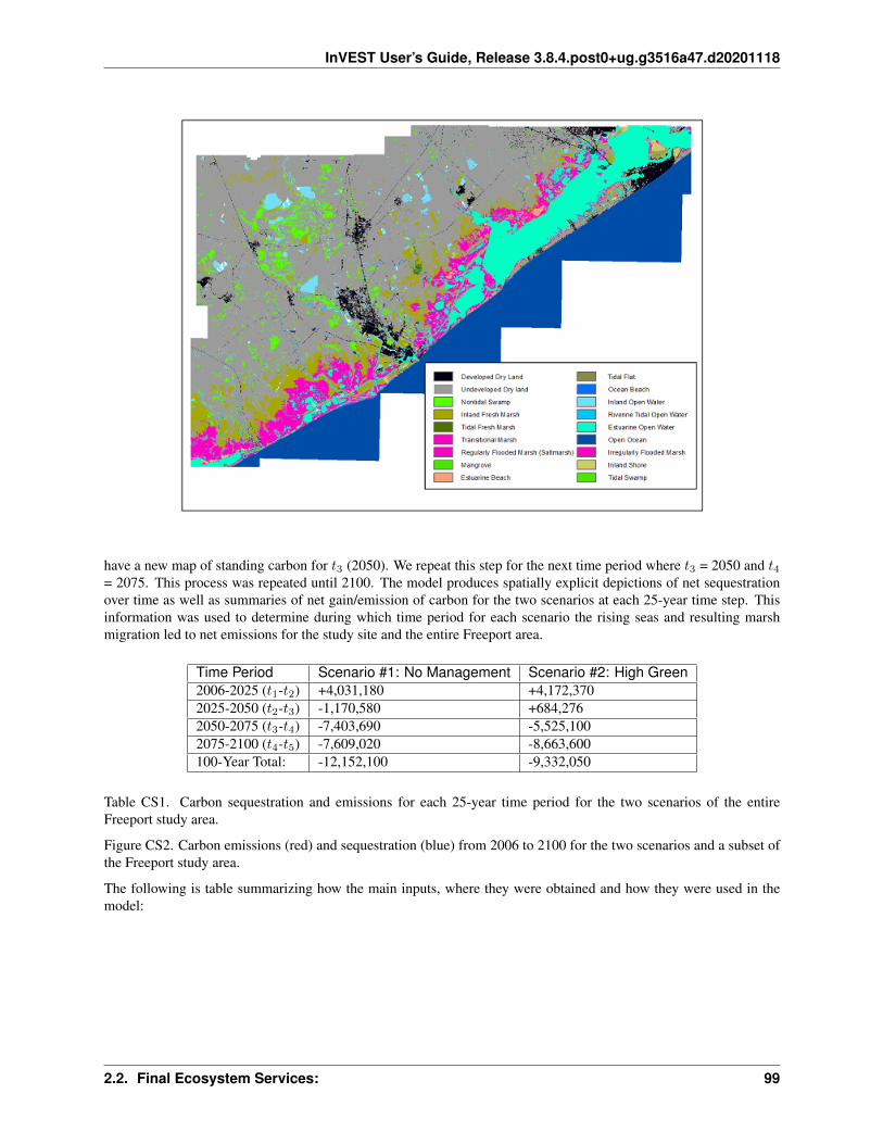
InVEST User’s Guide, Release 3.8.4.post0+ug.g3516a47.d20201118
have a new map of standing carbon for 𝑡3 (2050). We repeat this step for the next time period where 𝑡3 = 2050 and 𝑡4= 2075. This process was repeated until 2100. The model produces spatially explicit depictions of net sequestrationover time as well as summaries of net gain/emission of carbon for the two scenarios at each 25-year time step. Thisinformation was used to determine during which time period for each scenario the rising seas and resulting marshmigration led to net emissions for the study site and the entire Freeport area.
Time Period Scenario #1: No Management Scenario #2: High Green2006-2025 (𝑡1-𝑡2) +4,031,180 +4,172,3702025-2050 (𝑡2-𝑡3) -1,170,580 +684,2762050-2075 (𝑡3-𝑡4) -7,403,690 -5,525,1002075-2100 (𝑡4-𝑡5) -7,609,020 -8,663,600100-Year Total: -12,152,100 -9,332,050
Table CS1. Carbon sequestration and emissions for each 25-year time period for the two scenarios of the entireFreeport study area.
Figure CS2. Carbon emissions (red) and sequestration (blue) from 2006 to 2100 for the two scenarios and a subset ofthe Freeport study area.
The following is table summarizing how the main inputs, where they were obtained and how they were used in themodel:
2.2. Final Ecosystem Services: 99

InVEST User’s Guide, Release 3.8.4.post0+ug.g3516a47.d20201118
Input Source Use in the InVEST blue carbon modelDEM USGS DEM was needed to produce the future LULC maps using the SLAMM tool.Landuse /landcover(LULC)
USGS/NOAASalt marshes store carbon in biomass and soils. We utilized maps showing the current distributionof salt marshes to establish a baseline coverage of marshes from which we estimate abovegroundbiomass and soil carbon.
Car-bonstockinsaltmarshsys-tems
Nat-uralCap-italProjectliter-aturere-view
Carbon storage was calculated by summing the carbon stored in biomass and sediments. Carbonstocks were calculated for all of the areas of functional salt marsh in the study region (Chmuraet al. 2003).
So-cialvalueofcar-bonin2006US $
USI-WGSCC2010
The “social cost of carbon” (SCC) is an estimate of the monetized damages associated with anincremental increase in carbon emissions in a given year. It is intended to include (but is notlimited to) changes in net agricultural productivity, human health, property damages from in-creased flood risk, and the value of ecosystem services. The social cost of carbon is useful forallowing institutions to incorporate the social benefits of reducing carbon dioxide (CO2) emis-sions into cost benefit analyses of management actions that have small, or “marginal,” impactson cumulative global emissions.
Dis-countrate
USI-WGSCC2010
This discount rate reflects society’s preferences for short run versus long term consumption.Since carbon dioxide emissions are long-lived, subsequent damages occur over many years. Weuse the discount rate to adjust the stream of future damages to its present value in the year whenthe emissions were changed.
100 Chapter 2. InVEST Models

InVEST User’s Guide, Release 3.8.4.post0+ug.g3516a47.d20201118
Table CS2. Input summary table for using InVEST blue carbon model in Freeport, Texas
Limitations
• This analysis did not model change in carbon resulting from growth or loss of aboveground biomass of coastaland marine vegetation.
• While the spatial resolution of the LULC maps produced by SLAMM was very high (10 meters), the temporalresolution provided by SLAMM was quite coarse (25-year time steps). The carbon cycle is a dynamic process.By analyzing change over 25-year time periods, we ignore any changes that are not present at the start and endof each time step.
References
Baumol, W. J. (1968). On the social rate of discount. The American Economic Review, 788-802.
Bouillon, S., Borges, A. V., Castañeda-Moya, E., Diele, K., Dittmar, T., Duke, N. C., . . . & Twilley, R. R. (2008).Mangrove production and carbon sinks: a revision of global budget estimates. Global Biogeochemical Cycles, 22(2).
Chmura, G. L., Anisfeld, S. C., Cahoon, D. R., & Lynch, J. C. (2003). Global carbon sequestration in tidal, salinewetland soils. Global biogeochemical cycles, 17(4).
Clough, J. S., Park, R., and Fuller, R. (2010). “SLAMM 6 beta Technical Documentation.” Available at http://warrenpinnacle.com/prof/SLAMM.
Fourqurean, J. W., Duarte, C. M., Kennedy, H., Marbà, N., Holmer, M., Mateo, M. A., . . . & Serrano, O. (2012).Seagrass ecosystems as a globally significant carbon stock. Nature Geoscience, 5(7), 505-509.
Hope, Chris. (2011) “The PAGE09 Integrated Assessment Model: A Technical Description.” Cambridge JudgeBusiness School Working Paper No. 4/2011 (April). Available at https://www.jbs.cam.ac.uk/fileadmin/user_upload/research/workingpapers/wp1104.pdf.
Houghton, R. A. (2003). Revised estimates of the annual net flux of carbon to the atmosphere from changes in landuse and land management 1850–2000. Tellus B, 55(2), 378-390.
Pendleton, L., Donato, D. C., Murray, B. C., Crooks, S., Jenkins, W. A., Sifleet, S., . . . & Baldera, A. (2012).Estimating global “blue carbon” emissions from conversion and degradation of vegetated coastal ecosystems. PLoSOne, 7(9), e43542.
Rosenthal, A., Arkema, K., Verutes, G., Bood, N., Cantor, D., Fish, M., Griffin, R., and Panuncio, M. (In press).Identification and valuation of adaptation options in coastal-marine ecosystems: Test case from Placencia, Belize.Washington, DC: InterAmerican Development Bank. Technical Report.
Sifleet, S., Pendleton, L., and B. Murray. (2011). State of the Science on Coastal Blue Carbon. Nicholas InstituteReport, 1-43.
United States, Interagency Working Group on Social Costs of Carbon. (2010) “Technical Support Document: SocialCost of Carbon for Regulatory Impact Analysis Under Executive Order 12866.” Available at https://www.epa.gov/sites/production/files/2016-12/documents/scc_tsd_2010.pdf.
United States, Interagency Working Group on Social Costs of Carbon. (2013) “Technical Update of the Social Cost ofCarbon for Regulatory Impact Analysis Under Executive Order 12866.” Available at https://environblog.jenner.com/files/technical-update-of-the-social-cost-of-carbon-for-regulatory-impact-analysis-under-executive-order-12866.pdf.
World Bank. (2012). State and Trends of the Carbon Market 2012. Washington DC: The World Bank, 133.
2.2. Final Ecosystem Services: 101
InVEST User’s Guide, Release 3.8.4.post0+ug.g3516a47.d20201118
2.2.4 Annual Water Yield
Summary
Hydropower accounts for twenty percent of worldwide energy production, most of which is generated by reservoirsystems. InVEST estimates the annual average quantity and value of hydropower produced by reservoirs, and identifieshow much water yield or value each part of the landscape contributes annually to hydropower production. The modelhas three components: water yield, water consumption, and hydropower valuation. The biophysical models do notconsider surface – ground water interactions or the temporal dimension of water supply. The valuation model assumesthat energy pricing is static over time.
Introduction
The provision of fresh water is an ecosystem service that contributes to the welfare of society in many ways, includingthrough the production of hydropower, the most widely used form of renewable energy in the world. Most hydropowerproduction comes from watershed-fed reservoir systems that generally deliver energy consistently and predictably. Thesystems are designed to account for annual variability in water volume, given the likely levels for a given watershed,but are vulnerable to extreme variation caused by land use and land cover (LULC) changes. LULC changes can alterhydrologic cycles, affecting patterns of evapotranspiration, infiltration and water retention, and changing the timingand volume of water that is available for hydropower production (World Commission on Dams 2000; Ennaanay 2006).
Changes in the landscape that affect annual average water yield upstream of hydropower facilities can increase ordecrease hydropower production capacity. Maps of where water yield used for hydropower is produced can helpavoid unintended impacts on hydropower production or help direct land use decisions that wish to maintain powerproduction, while balancing other uses such as conservation or agriculture. Such maps can also be used to informinvestments in restoration or management that downstream stakeholders, such as hydropower companies, make inhopes of improving or maintaining water yield for this important ecosystem service. In large watersheds with multiplereservoirs for hydropower production, areas upstream of power plants that sell to a higher value market will have ahigher value for this service. Maps of how much value each parcel contributes to hydropower production can helpmanagers avoid developments in the highest hydropower value areas, understand how much value will be lost orgained as a consequence of different management options, or identify which hydropower producers have the largeststake in maintaining water yield across a landscape.
The Model
The InVEST Water Yield model estimates the relative contributions of water from different parts of a landscape,offering insight into how changes in land use patterns affect annual surface water yield and hydropower production.
Modeling the connections between landscape changes and hydrologic processes is not simple. Sophisticated modelsof these connections and associated processes (such as the WEAP model) are resource and data intensive and requiresubstantial expertise. To accommodate more contexts, for which data are readily available, InVEST maps and modelsthe annual average water yield from a landscape used for hydropower production, rather than directly addressingthe effect of LULC changes on hydropower, as this process is closely linked to variation in water inflow on a dailyto monthly timescale. Instead, InVEST calculates the relative contribution of each land parcel to annual averagehydropower production and the value of this contribution in terms of energy production. The net present value ofhydropower production over the life of the reservoir also can be calculated by summing discounted annual revenues.
How it Works
The model runs on a gridded map. It estimates the quantity and value of water used for hydropower production fromeach subwatershed in the area of interest. It has three components, which run sequentially. First, it determines the
102 Chapter 2. InVEST Models
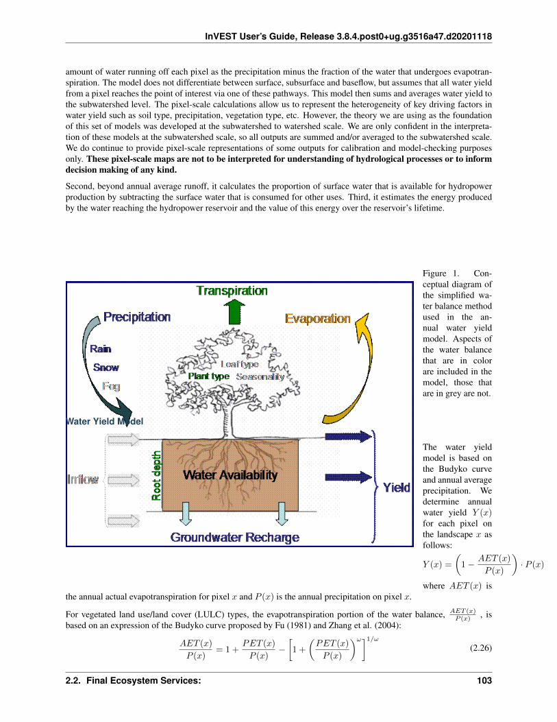
InVEST User’s Guide, Release 3.8.4.post0+ug.g3516a47.d20201118
amount of water running off each pixel as the precipitation minus the fraction of the water that undergoes evapotran-spiration. The model does not differentiate between surface, subsurface and baseflow, but assumes that all water yieldfrom a pixel reaches the point of interest via one of these pathways. This model then sums and averages water yield tothe subwatershed level. The pixel-scale calculations allow us to represent the heterogeneity of key driving factors inwater yield such as soil type, precipitation, vegetation type, etc. However, the theory we are using as the foundationof this set of models was developed at the subwatershed to watershed scale. We are only confident in the interpreta-tion of these models at the subwatershed scale, so all outputs are summed and/or averaged to the subwatershed scale.We do continue to provide pixel-scale representations of some outputs for calibration and model-checking purposesonly. These pixel-scale maps are not to be interpreted for understanding of hydrological processes or to informdecision making of any kind.
Second, beyond annual average runoff, it calculates the proportion of surface water that is available for hydropowerproduction by subtracting the surface water that is consumed for other uses. Third, it estimates the energy producedby the water reaching the hydropower reservoir and the value of this energy over the reservoir’s lifetime.
Figure 1. Con-ceptual diagram ofthe simplified wa-ter balance methodused in the an-nual water yieldmodel. Aspects ofthe water balancethat are in colorare included in themodel, those thatare in grey are not.
Water Yield Model
The water yieldmodel is based onthe Budyko curveand annual averageprecipitation. Wedetermine annualwater yield 𝑌 (𝑥)for each pixel onthe landscape 𝑥 asfollows:
𝑌 (𝑥) =
(︂1 − 𝐴𝐸𝑇 (𝑥)
𝑃 (𝑥)
)︂· 𝑃 (𝑥)
where 𝐴𝐸𝑇 (𝑥) isthe annual actual evapotranspiration for pixel 𝑥 and 𝑃 (𝑥) is the annual precipitation on pixel 𝑥.
For vegetated land use/land cover (LULC) types, the evapotranspiration portion of the water balance, 𝐴𝐸𝑇 (𝑥)𝑃 (𝑥) , is
based on an expression of the Budyko curve proposed by Fu (1981) and Zhang et al. (2004):
𝐴𝐸𝑇 (𝑥)
𝑃 (𝑥)= 1 +
𝑃𝐸𝑇 (𝑥)
𝑃 (𝑥)−[︂1 +
(︂𝑃𝐸𝑇 (𝑥)
𝑃 (𝑥)
)︂𝜔]︂1/𝜔(2.26)
2.2. Final Ecosystem Services: 103

InVEST User’s Guide, Release 3.8.4.post0+ug.g3516a47.d20201118
where 𝑃𝐸𝑇 (𝑥) is the potential evapotranspiration and 𝜔(𝑥) is a non-physical parameter that characterizes the naturalclimatic-soil properties, both detailed below.
Potential evapotranspiration 𝑃𝐸𝑇 (𝑥) is defined as:
𝑃𝐸𝑇 (𝑥) = 𝐾𝑐(ℓ𝑥) · 𝐸𝑇0(𝑥)
where, 𝐸𝑇0(𝑥) is the reference evapotranspiration from pixel 𝑥 and 𝐾𝑐(ℓ𝑥) is the plant (vegetation) evapotranspirationcoefficient associated with the LULC ℓ𝑥 on pixel 𝑥. 𝐸𝑇0(𝑥) reflects local climatic conditions, based on the evapotran-spiration of a reference vegetation such as grass or alfalfa grown at that location. 𝐾𝑐(ℓ𝑥) is largely determined by thevegetative characteristics of the land use/land cover found on that pixel (Allen et al. 1998). 𝐾𝑐 adjusts the 𝐸𝑇0 valuesto the crop or vegetation type in each pixel of the land use/land cover map.
𝜔(𝑥) is an empirical parameter that can be expressed as linear function of 𝐴𝑊𝐶*𝑁𝑃 , where N is the number of rain
events per year, and AWC is the volumetric plant available water content (see Appendix 1 for additional details). Whilefurther research is being conducted to determine the function that best describe global data, we use the expressionproposed by Donohue et al. (2012) in the InVEST model, and thus define:
𝜔(𝑥) = 𝑍𝐴𝑊𝐶(𝑥)
𝑃 (𝑥)+ 1.25
where:
• 𝐴𝑊𝐶(𝑥) is the volumetric (mm) plant available water content. The soil texture and effective rooting depthdefine 𝐴𝑊𝐶(𝑥), which establishes the amount of water that can be held and released in the soil for use bya plant. It is estimated as the product of the plant available water capacity (PAWC) and the minimum of rootrestricting layer depth and vegetation rooting depth:
𝐴𝑊𝐶(𝑥) = 𝑀𝑖𝑛(𝑅𝑒𝑠𝑡.𝑙𝑎𝑦𝑒𝑟.𝑑𝑒𝑝𝑡ℎ, 𝑟𝑜𝑜𝑡.𝑑𝑒𝑝𝑡ℎ) · 𝑃𝐴𝑊𝐶
Root restricting layer depth is the soil depth at which root penetration is inhibited because of physical or chemicalcharacteristics. Vegetation rooting depth is often given as the depth at which 95% of a vegetation type’s rootbiomass occurs. PAWC is the plant available water capacity, i.e. the difference between field capacity andwilting point.
• 𝑍 is an empirical constant, sometimes referred to as “seasonality factor”, which captures the local precipitationpattern and additional hydrogeological characteristics. It is positively correlated with N, the number of rainevents per year. The 1.25 term is the minimum value of 𝜔(𝑥), which can be seen as a value for bare soil (whenroot depth is 0), as explained by Donohue et al. (2012). Following the literature (Yang et al., 2008; Donohue etal. 2012), values of 𝜔(𝑥) are capped to a value of 5.
For other LULC types (open water, urban, wetland), actual evapotranspiration is directly computed from referenceevapotranspiration 𝐸𝑇0(𝑥) and has an upper limit defined by precipitation:
𝐴𝐸𝑇 (𝑥) = 𝑀𝑖𝑛(𝐾𝑐(ℓ𝑥) · 𝐸𝑇0(𝑥), 𝑃 (𝑥)) (2.27)
where 𝐸𝑇0(𝑥) is reference evapotranspiration, and 𝐾𝑐(ℓ𝑥) is the evaporation factor for each LULC.
The water yield model generates and outputs the total and average water yield at the subwatershed level.
Realized Supply
The Realized Supply option of the model (called Water Scarcity in the tool interface) calculates the water inflow to areservoir based on calculated water yield and water consumptive use in the watershed(s) of interest. The user inputshow much water is consumed by each land use/land cover type in a table format. Examples of consumptive use include
104 Chapter 2. InVEST Models
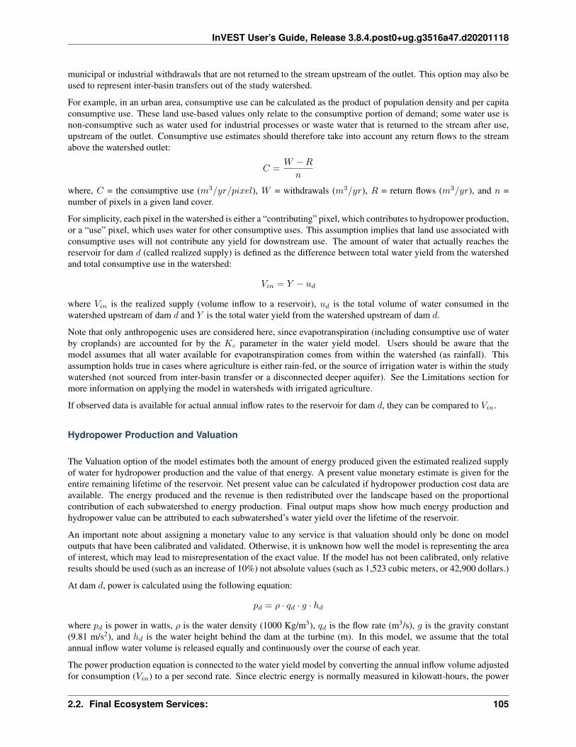
InVEST User’s Guide, Release 3.8.4.post0+ug.g3516a47.d20201118
municipal or industrial withdrawals that are not returned to the stream upstream of the outlet. This option may also beused to represent inter-basin transfers out of the study watershed.
For example, in an urban area, consumptive use can be calculated as the product of population density and per capitaconsumptive use. These land use-based values only relate to the consumptive portion of demand; some water use isnon-consumptive such as water used for industrial processes or waste water that is returned to the stream after use,upstream of the outlet. Consumptive use estimates should therefore take into account any return flows to the streamabove the watershed outlet:
𝐶 =𝑊 −𝑅
𝑛
where, 𝐶 = the consumptive use (𝑚3/𝑦𝑟/𝑝𝑖𝑥𝑒𝑙), 𝑊 = withdrawals (𝑚3/𝑦𝑟), 𝑅 = return flows (𝑚3/𝑦𝑟), and 𝑛 =number of pixels in a given land cover.
For simplicity, each pixel in the watershed is either a “contributing” pixel, which contributes to hydropower production,or a “use” pixel, which uses water for other consumptive uses. This assumption implies that land use associated withconsumptive uses will not contribute any yield for downstream use. The amount of water that actually reaches thereservoir for dam 𝑑 (called realized supply) is defined as the difference between total water yield from the watershedand total consumptive use in the watershed:
𝑉𝑖𝑛 = 𝑌 − 𝑢𝑑
where 𝑉𝑖𝑛 is the realized supply (volume inflow to a reservoir), 𝑢𝑑 is the total volume of water consumed in thewatershed upstream of dam 𝑑 and 𝑌 is the total water yield from the watershed upstream of dam 𝑑.
Note that only anthropogenic uses are considered here, since evapotranspiration (including consumptive use of waterby croplands) are accounted for by the 𝐾𝑐 parameter in the water yield model. Users should be aware that themodel assumes that all water available for evapotranspiration comes from within the watershed (as rainfall). Thisassumption holds true in cases where agriculture is either rain-fed, or the source of irrigation water is within the studywatershed (not sourced from inter-basin transfer or a disconnected deeper aquifer). See the Limitations section formore information on applying the model in watersheds with irrigated agriculture.
If observed data is available for actual annual inflow rates to the reservoir for dam 𝑑, they can be compared to 𝑉𝑖𝑛.
Hydropower Production and Valuation
The Valuation option of the model estimates both the amount of energy produced given the estimated realized supplyof water for hydropower production and the value of that energy. A present value monetary estimate is given for theentire remaining lifetime of the reservoir. Net present value can be calculated if hydropower production cost data areavailable. The energy produced and the revenue is then redistributed over the landscape based on the proportionalcontribution of each subwatershed to energy production. Final output maps show how much energy production andhydropower value can be attributed to each subwatershed’s water yield over the lifetime of the reservoir.
An important note about assigning a monetary value to any service is that valuation should only be done on modeloutputs that have been calibrated and validated. Otherwise, it is unknown how well the model is representing the areaof interest, which may lead to misrepresentation of the exact value. If the model has not been calibrated, only relativeresults should be used (such as an increase of 10%) not absolute values (such as 1,523 cubic meters, or 42,900 dollars.)
At dam 𝑑, power is calculated using the following equation:
𝑝𝑑 = 𝜌 · 𝑞𝑑 · 𝑔 · ℎ𝑑
where 𝑝𝑑 is power in watts, 𝜌 is the water density (1000 Kg/m3), 𝑞𝑑 is the flow rate (m3/s), 𝑔 is the gravity constant(9.81 m/s2), and ℎ𝑑 is the water height behind the dam at the turbine (m). In this model, we assume that the totalannual inflow water volume is released equally and continuously over the course of each year.
The power production equation is connected to the water yield model by converting the annual inflow volume adjustedfor consumption (𝑉𝑖𝑛) to a per second rate. Since electric energy is normally measured in kilowatt-hours, the power
2.2. Final Ecosystem Services: 105

InVEST User’s Guide, Release 3.8.4.post0+ug.g3516a47.d20201118
𝑝𝑑 is multiplied by the number of hours in a year. All hydropower reservoirs are built to produce a maximum amountof electricity. This is called the energy production rating, and represents how much energy could be produced if theturbines are 100% efficient and all water that enters the reservoir is used for power production. In the real world,turbines have inefficiencies and water in the reservoir may be extracted for other uses like irrigation, retained in thereservoir for other uses like recreation, or released from the reservoir for non-power production uses like maintainingenvironmental flows downstream. To account for these inefficiencies and the flow rate and power unit adjustments,annual average energy production 𝜀𝑑 at dam 𝑑 is calculated as follows:
𝜀𝑑 = 0.00272 · 𝛽 · 𝛾𝑑 · ℎ𝑑 · 𝑉𝑖𝑛
where 𝜀𝑑 is hydropower energy production (KWH), 𝛽 is the turbine efficiency coefficient (%), 𝛾𝑑 is the percent ofinflow water volume to the reservoir at dam 𝑑 that will be used to generate energy.
To convert 𝜀𝑑, the annual energy generated by dam 𝑑, into a net present value (NPV) of energy produced (point of usevalue) we use the following,
𝑁𝑃𝑉𝐻𝑑 = (𝑝𝑒𝜀𝑑 − 𝑇𝐶𝑑) ×𝑇−1∑︁𝑡=0
1
(1 + 𝑟)𝑡
where 𝑇𝐶𝑑 is the total annual operating costs for dam 𝑑, 𝑝𝑒 is the market value of electricity (per kilowatt hour)provided by the hydropower plant at dam 𝑑, 𝑇𝑑 indicates the number of years present landscape conditions are expectedto persist or the expected remaining lifetime of the station at dam 𝑑 (set 𝑇 to the smallest value if the two time valuesdiffer), and 𝑟 is the market discount rate. The form of the equation above assumes that 𝑇𝐶𝑑, 𝑝𝑒, and 𝜀𝑑, are constantover time.
Energy production over the lifetime of dam 𝑑 is attributed to each subwatershed as follows:
𝜀𝑥 = (𝑇𝑑𝜀𝑑) × (𝑐𝑥/𝑐𝑡𝑜𝑡)
where the first term in parentheses represents the electricity production over the lifetime of dam 𝑑. The second termrepresents the proportion of water volume used for hydropower production that comes from subwatershed 𝑥 relativeto the total water volume for the whole watershed. The value of each subwatershed for hydropower production overthe lifetime of dam 𝑑 is calculated similarly:
𝑁𝑃𝑉𝐻𝑥 = 𝑁𝑃𝑉𝐻𝑑 × (𝑐𝑥/𝑐𝑡𝑜𝑡)
Limitations and Simplifications
The model has a number of limitations. First, it is not intended for devising detailed water plans, but rather forevaluating how and where changes in a watershed may affect hydropower production for reservoir systems. It isbased on annual averages, which neglect extremes and do not consider the temporal dimensions of water supply andhydropower production.
Second, the model does not consider the spatial distribution of land use/land cover. The empirical model used for thewater balance (based on the Budyko theory) has been tested at larger scales than the pixel dimensions used in InVEST(Hamel & Guswa, in review). Complex land use patterns or underlying geology, which may induce complex waterbalances, may not be well captured by the model.
Third, the model does not consider sub-annual patterns of water delivery timing. Water yield is a provisioning function,but hydropower benefits are also affected by flow regulation. The timing of peak flows and delivery of minimumoperational flows throughout the year determines the rate of hydropower production and annual revenue. Changes inlandscape scenarios are likely to affect the timing of flows as much as the annual water yield, and are of particularconcern when considering drivers such as climate change. Modeling the temporal patterns of overland flow requiresdetailed data that are not appropriate for our approach. Still, this model provides a useful initial assessment of howlandscape scenarios may affect the annual delivery of water to hydropower production.
106 Chapter 2. InVEST Models

InVEST User’s Guide, Release 3.8.4.post0+ug.g3516a47.d20201118
Fourth, the model greatly simplifies consumptive demand. For each LULC, a single variable (𝛾𝑑) is used to representmultiple aspects of water resource allocation, which may misrepresent the complex distribution of water among usesand over time. In reality, water demand may differ greatly between parcels of the same LULC class. Much of thewater demand may also come from large point source intakes, which are not represented by an LULC class at all. Themodel simplifies water demand by distributing it over the landscape. For example, the water demand may be large foran urban area, and the model represents this demand by distributing it over the urban LULC class. The actual watersupply intake, however, is likely further upstream in a rural location. Spatial disparity in actual and modeled demandpoints may cause an incorrect representation in the realized supply output grid. The distribution of consumption isalso simplified in the reallocation of energy production and hydropower value since it is assumed that water consumedalong flow paths is drawn equally from every pixel upstream. As a result, water scarcity, energy production patterns,and hydropower values may be incorrectly estimated.
Fifth, water transfers for irrigation, either between subbasins or between seasons, are not well captured by the model.When applying the empirical approach to cropland, irrigation patterns should be considered, which typically fall intoone of the following cases:
1) If there is no irrigation other than direct rain, it can be assumed that croplands respond to climate forcing in asimilar way to natural vegetation (i.e. the theory behind the eco-hydrological model used in the InVEST model,linking plant available water and climate forcing, applies, cf. Donohue et al. 2012)
2) If small reservoirs store water during the wet season to irrigate crops during the dry season, the AET shouldequal PET during the irrigation season. However, the model predicts AET<PET due to limited water retentionin undisturbed catchments (where there is no other reservoir except soil storage). This likely results in theunderestimation of evapotranspiration, and therefore the overestimation of yields. To avoid this issue, you canuse the alternative equation for AET (equation 2), which sets AET directly as a function of ETo. (In thatcase, remember that AET is capped by P to avoid predicting negative water yields, which may result in anoverestimation of yields).
3) If the study area contains croplands that are irrigated with water from outside the catchment (either throughinter-basin transfer or pumping from a disconnected groundwater source), then AET also equals PET during theirrigation season. Because the model assumes that evapotranspiration is sourced from rainfall, the water yieldoutput is likely overestimated. This situation can also be represented by using the alternative equation for AET(equation 2). Assuming that crops are being irrigated efficiently (i.e. the total volume of imported water is equalto the water deficit, or PET – P, for crop pixels), then the known volume of water irrigated may be added to themodeled water yield to give a better picture of actual yield.
4) Because seasonality can play a significant role in irrigation water use, use caution when applying the annualmodel in catchments with large irrigated fields. For options that are not covered above or where complexwater transfers may substantially affect the water balance, users are encouraged to use alternative models thatwill better represent the spatial and temporal water transfers. In particular, great caution should be used whencalibrating the model without good data on the different water balance components within your study area (i.e.rainfall, streamflow, irrigation rates and timing).
Finally, the model assumes that hydropower production and pricing remain constant over time. It does not account forseasonal variation in energy production or fluctuations in energy pricing, which may affect the value of hydropower.Even if sub-annual production or energy prices change, however, the relative value between parcels of land in the samedrainage area should be accurate.
Data Needs
This section outlines the specific data used by the model. See the Appendix for additional information on data sourcesand pre-processing. Please consult the InVEST sample data (located in the folder where InVEST is installed, if youalso chose to install sample data) for examples of all of these data inputs. This will help with file type, folder structureand table formatting. Note that all GIS inputs must be in the same projected coordinate system and in linear meterunits.
2.2. Final Ecosystem Services: 107

InVEST User’s Guide, Release 3.8.4.post0+ug.g3516a47.d20201118
• Workspace (required). Folder where model outputs will be written. Make sure that there is ample disk space,and write permissions are correct.
• Suffix (optional). Text string that will be appended to the end of output file names, as “_Suffix”. Use a Suffix todifferentiate model runs, for example by providing a short name for each scenario. If a Suffix is not provided,or changed between model runs, the tool will overwrite previous results.
• Precipitation (required). A GIS raster dataset with a non-zero value for average annual precipitation for eachcell. [units: millimeters]
• Average Annual Reference Evapotranspiration (required). A GIS raster dataset, with an annual averageevapotranspiration value for each cell. Reference evapotranspiration is the potential loss of water from soilby both evaporation from the soil and transpiration by healthy alfalfa (or grass) if sufficient water is available.[units: millimeters]
• Root restricting layer depth (required). A GIS raster dataset with an average root restricting layer depth valuefor each cell. Root restricting layer depth is the soil depth at which root penetration is strongly inhibited becauseof physical or chemical characteristics. [units: millimeters]
• Plant Available Water Content (required). A GIS raster dataset with a plant available water content value foreach cell. Plant Available Water Content fraction (PAWC) is the fraction of water that can be stored in the soilprofile that is available for plants’ use. [fraction from 0 to 1]
• Land use/land cover (required). A GIS raster dataset, with an integer LULC code for each cell. These LULCcodes must match lucode values in the Biophysical table.
• Watersheds (required). A shapefile, with one polygon per watershed. This is a layer of watersheds such thateach watershed contributes to a point of interest where hydropower production will be analyzed. An integerfield named ws_id is required, with a unique integer value for each watershed.
• Subwatersheds (required). A shapefile, with one polygon per subwatershed within the main watersheds spec-ified in the Watersheds shapefile. An integer field named subws_id is required, with a unique integer value foreach subwatershed.
• Biophysical Table (required). A .csv (Comma Separated Value) table containing model information corre-sponding to each of the land use classes in the LULC raster. All LULC classes in the LULC raster MUST havecorresponding values in this table. Each row is a land use/land cover class and columns must be named anddefined as follows:
– lucode (required): Unique integer for each LULC class (e.g., 1 for forest, 3 for grassland, etc.) Everyvalue in the LULC map MUST have a corresponding lucode value in the biophysical table.
– LULC_desc (optional): Descriptive name of land use/land cover class
– LULC_veg (required): Specifies which AET equation to use (Eq. 1 or 2). Values must be 1 for vegetatedland use except wetlands, and 0 for all other land uses, including wetlands, urban, water bodies, etc.
– root_depth (required): The maximum root depth for vegetated land use classes, given in integer millime-ters. This is often given as the depth at which 95% of a vegetation type’s root biomass occurs. For landuses where the generic Budyko curve is not used (i.e. where evapotranspiration is calculated from Eq. 2),rooting depth is not needed. In these cases, the rooting depth field is ignored, and may be set as a valuesuch as -1 to indicate the field is not used.
– Kc (required): Plant evapotranspiration coefficient for each LULC class, used to calculate potential evapo-transpiration by using plant physiological characteristics to modify the reference evapotranspiration, whichis based on alfalfa. The evapotranspiration coefficient is a decimal in the range of 0 to 1.5 (some cropsevapotranspire more than alfalfa in some very wet tropical regions and where water is always available).
• Z parameter (required). Floating point value on the order of 1 to 30 corresponding to the seasonal distributionof precipitation (see the Appendix for more information).
108 Chapter 2. InVEST Models

InVEST User’s Guide, Release 3.8.4.post0+ug.g3516a47.d20201118
• Demand Table (required if calculating Water Scarcity or Valuation). A table of LULC classes, with consumptivewater use for each landuse/landcover type. Consumptive water use is that part of water used that is incorporatedinto products or crops, consumed by humans or livestock, or otherwise removed from the watershed waterbalance. Each row is a land use/land cover class, and columns must be named and defined as follows:
– lucode (required): Unique integer for each LULC class (e.g., 1 for forest, 3 for grassland, etc.), must matchthe LULC raster above.
– demand (required): The estimated average consumptive water use for each landuse/landcover type. De-mand must be given in cubic meters per year per pixel in the land use/land cover map. Note that accountingfor pixel area is important since larger pixels will consume more water for the same land cover type.
• Hydropower valuation table (required if doing Valuation). A table of hydropower stations (which are theoutlets of the input Watersheds) with associated model values. Each row is a hydropower station, and columnsmust be named and defined as follows:
– ws_id (required): Unique integer value for each hydropower station, which must correspond to values inthe Watersheds layer.
– station_desc (optional): Name of hydropower station
– efficiency (required): Turbine efficiency, obtained from the hydropower plant manager. Floating pointvalues (generally 0.7 to 0.9).
– fraction (required): The fraction of inflow water volume that is used to generate energy, obtained from thehydropower plant manager. Managers can release water without generating electricity to satisfy irrigation,drinking water or environmental demands. Floating point value.
– height (required): The head, measured as the average annual effective height of water behind each dam atthe turbine intake. Floating point value in meters.
– kw_price (required): The price of one kilowatt-hour of power produced by the station, in any currency (butmust match the currency used for cost.) Floating point value.
– cost (required): Annual cost of running the hydropower station (maintenance and operations costs), in anycurrency (but must match the currency used for kw_price.) Floating point value.
– time_span (required): Either the expected lifespan of the hydropower station or the period of time of theland use scenario of interest, expressed as number of years. Used in net present value calculations. Integervalue.
– discount (required): The discount rate over the time span, used in net present value calculations. Percent-age - for example, if the discount rate is 5%, enter the value 5.
Running the Model
To launch the Water Yield model navigate to the Windows Start Menu -> All Programs -> InVEST [version] -> WaterYield. The interface does not require a GIS desktop, although the results will need to be explored with any GIS toolsuch as ArcGIS or QGIS. By default, only the biophysical (water yield) portion of the model will be run. If you wantto also use Water Scarcity and Valuation, check the box next to these options and fill in the additional data. WaterScarcity may be run alone, but if running Valuation, Water Scarcity must also be run.
This model supports avoided re-computation. This means the model will detect intermediate and final results from aprevious run in the specified workspace and it will avoid re-calculating any outputs that are identical to the previousrun. This can save significant processing time for successive runs when only some input parameters have changed.
2.2. Final Ecosystem Services: 109

InVEST User’s Guide, Release 3.8.4.post0+ug.g3516a47.d20201118
Interpreting Results
The following is a short description of each of the outputs from the Water Yield model. Final results are found withinthe user defined Workspace specified for this model run. “Suffix” in the following file names refers to the optionaluser-defined Suffix input to the model.
The resolution of the output rasters will be the same as the resolution of the Land use/land cover raster provided asinput.
• Parameter log: Each time the model is run, a text (.txt) file will be created in the Workspace. The file will listthe parameter values and output messages for that run and will be named according to the service, the date andtime. When contacting NatCap about errors in a model run, please include the parameter log.
• Outputs in the per_pixel folder can be useful for intermediate calculations but should NOT be interpreted at thepixel level, as model assumptions are based on processes understood at the subwatershed scale.
– output\per_pixel\fractp_[Suffix].tif (fraction): Estimated actual evapotranspiration fraction of precipi-tation per pixel (Actual Evapotranspiration / Precipitation). It is the mean fraction of precipitation thatactually evapotranspires at the pixel level.
– output\per_pixel\aet_[Suffix].tif (mm): Estimated actual evapotranspiration per pixel.
– output\per_pixel\wyield_[Suffix].tif (mm): Estimated water yield per pixel.
• output\subwatershed_results_wyield_[Suffix].shp and output\subwatershed_results_wyield_[Suffix].csv:Shapefile and table containing biophysical output values per subwatershed, with the following attributes:
– precip_mn (mm): Mean precipitation per pixel in the subwatershed.
– PET_mn (mm): Mean potential evapotranspiration per pixel in the subwatershed.
– AET_mn (mm): Mean actual evapotranspiration per pixel in the subwatershed.
– wyield_mn (mm): Mean water yield per pixel in the subwatershed.
– wyield_vol (m3): Volume of water yield in the subwatershed.
• output\watershed_results_wyield_[Suffix].shp and output\watershed_results_wyield_[Suffix].csv: Shape-file and table containing output values per watershed, with the following attributes:
– precip_mn (mm): Mean precipitation per pixel in the watershed.
– PET_mn (mm): Mean potential evapotranspiration per pixel in the watershed.
– AET_mn (mm): Mean actual evapotranspiration per pixel in the watershed.
– wyield_mn (mm): Mean water yield per pixel in the watershed.
– wyield_vol (m3): Volume of water yield in the watershed.
If the Water Scarcity option is run, the following attributes will also be included for watersheds andsubwatersheds:
– consum_vol (m3): Total water consumption for each watershed.
– consum_mn (m3/ha): Mean water consumptive volume per hectare per watershed.
– rsupply_vl (m3): Total realized water supply (water yield – consumption) volume for eachwatershed.
– rsupply_mn (m3/ha): Mean realized water supply (water yield – consumption) volume perhectare per watershed.
If the Valuation option is run, the following attributes will also be included for watersheds, but notfor subwatersheds:
110 Chapter 2. InVEST Models

InVEST User’s Guide, Release 3.8.4.post0+ug.g3516a47.d20201118
– hp_energy (kw/timespan): The amount of ecosystem service in energy production terms. Thisshows the amount of energy produced by the hydropower station over the specified timespanthat can be attributed to each watershed based on its water yield contribution.
– hp_val (currency/timespan): The amount of ecosystem service in economic terms. This showsthe value of the landscape per watershed according to its ability to yield water for hydropowerproduction over the specified timespan.
• intermediate: This directory contains data that represent intermediate steps in calculations of the final datain the output folder. It also contains subdirectories that store metadata used internally to enable avoided re-computation.
The application of these results depends entirely on the objective of the modeling effort. Users may be interested inall of these results or a select one or two. If valuation information is not available or of interest, you may choose tosimply run the water yield model and compare biophysical results.
The first several model results provide insight into how water is distributed throughout the landscape. aet_mn describesthe actual evapotranspiration depth of the hydrologic cycle, showing how much water (precipitation) is lost annuallyto evapotranspiration across the watershed or subwatershed.
The wyield_vol field contains the estimated annual average water volume that is ‘yielded’ from each subwatershedwithin the watershed of interest. This value can be used to determine which subwatersheds are most important tototal annual water yield – although at this step the user still will not know how much of that water is benefitingdownstream users of any type. The consumptive use (consum_vol) field then shows how much water is used forconsumptive activities (such as drinking, bottling, etc.) each year across the landscape per watershed. The realizedsupply (rsupply_vl) field contains the difference between cumulative water yield and cumulative consumptive use.This value demonstrates where the water supply for hydropower production is abundant and where it is most scarce.Remember that the consumptive use value may not truly represent where water is taken, only where it is demanded.This may cause some misrepresentation of the scarcity in certain locations, but this value offers a general sense of thewater balance and whether there is a lack of or abundance of water in the watershed of interest.
The hp_energy and hp_val values are the most relevant model outputs for prioritizing the landscape for investmentsthat wish to maintain water yield for hydropower production. The hp_val field contains the most information for thispurpose as it represents the revenue attributable to each watershed over the expected lifetime of the hydropower station,or the number of years that the user has chosen to model. This value accounts for the fact that different hydropowerstations within a large river basin may have different customers who pay different rates for energy production. Ifthis is the case, this result will show which watersheds contribute the highest value water for energy production. Ifenergy values do not vary much across the landscape, the hp_energy outputs can be just as useful in planning andprioritization. Comparing any of these values between landuse scenarios allows you to understand how the role of thelandscape may change under different management plans.
Appendix 1: Data Sources
This is a rough compilation of data sources and suggestions about finding, compiling, and formatting data, providinglinks to global datasets that can get you started. It is highly recommended to look for more local and accurate data(from national, state, university, literature, NGO and other sources) and only use global data for final analyses ifnothing more local is available.
Average annual precipitation
Average Annual Precipitation may be interpolated from existing rain gage point data, and global data sets from remotesensing models to account for remote areas. Precipitation as snow is included. When considering rain gage data, makesure that they provide good coverage over the area of interest, especially if there are large changes in elevation thatcause precipitation amounts to be heterogeneous within the study area. Ideally, the gauges will have at least 10 yearsof continuous data, with no large gaps, around the same time period as the land use/land cover map used as input.
2.2. Final Ecosystem Services: 111

InVEST User’s Guide, Release 3.8.4.post0+ug.g3516a47.d20201118
If field data are not available, you can use coarse data from the freely available global data sets developed by theClimatic Research Unit: http://www.cru.uea.ac.uk or WorldClim: http://www.worldclim.org/.
Within the United States, the PRISM group at Oregon State University provides free precipitation data at a 30-arcsecond resolution. See their website at http://www.prism.oregonstate.edu/ and navigate to ‘800m Normals’ todownload data.
Average annual reference evapotranspiration (𝐸𝑇0)
Reference evapotranspiration, 𝐸𝑇0, is the energy (expressed as a depth of water, e.g. mm) supplied by the sun (andoccasionally wind) to vaporize water. Reference evapotranspiration varies with elevation, latitude, humidity, and slopeaspect. There are many methodologies, which range in data requirements and precision.
CGIAR provides a global map of potential evapotranspiration, based on WorldClim climate data, which may be usedfor reference ET: https://cgiarcsi.community/data/global-aridity-and-pet-database/.
You can calculate reference ET by developing monthly average grids of precipitation, and maximum and minimumtemperatures. These data can come from weather stations, where you can follow the same process as the developmentof the average annual precipitation grid, including incorporating the effects of elevation when interpolating betweenstations. Or, both WorldClim and CRU provide monthly temperature data already in grid format. These monthly gridscan be used as input to the equations listed below.
A simple way to determine reference evapotranspiration is the ‘modified Hargreaves’ equation (Droogers and Allen,2002), which generates superior results than the Pennman-Montieth when information is uncertain.
𝐸𝑇0 = 0.0013 × 0.408 ×𝑅𝐴× (𝑇𝑎𝑣 + 17) × (𝑇𝐷 − 0.0123𝑃 )0.76
The ‘modified Hargreaves’ method uses the average of the mean daily maximum and mean daily minimum tem-peratures for each month (Tavg in degrees Celsius), the difference between mean daily maximum and mean dailyminimums for each month (TD), RA is extraterrestrial radiation (RA in MJm−2d−1 and precipitation (P in mm permonth), all of which can be relatively easily obtained. Temperature and precipitation data are often available fromregional charts, direct measurement or national or global datasets. Radiation data, on the other hand, is far moreexpensive to measure directly but can be reliably estimated from online tools, tables or equations. FAO IrrigationDrainage Paper 56 provides monthly radiation data in Annex 2.
The reference evapotranspiration can also be calculated monthly and annually using the Hamon equation (Hamon1961, Wolock and McCabe 1999):
𝑃𝐸𝐷𝐻𝑎𝑚𝑜𝑛 = 13.97𝑑𝐷2𝑊𝑡
where d is the number of days in a month, D is the mean monthly hours of daylight calculated for each year (in unitsof 12 hours), and Wt is a saturated water vapor density term calculated by:
𝑊𝑡 =4.95𝑒0.062𝑇
100
where T is the monthly mean temperature in degrees Celsius. Reference evapotranspiration is set to zero when meanmonthly temperature is below zero. Then for each year during the time period analyzed, the monthly calculated PETvalues at each grid cell are summed to calculate a map of the annual PET for each year.
A final method to assess ETo, when pan evaporation data are available, is to use the following equation: ETo = (panET)*0.7 (Allen et al., 1998)
Root restricting layer depth
Root restricting layer depth is the soil depth at which root penetration is strongly inhibited because of physical orchemical characteristics. Root restricting layer depth may be obtained from some soil maps. If root restricting layer
112 Chapter 2. InVEST Models

InVEST User’s Guide, Release 3.8.4.post0+ug.g3516a47.d20201118
depth or rootable depth by soil type is not available, soil depth can be used as a proxy. If several soil horizons aredetailed, the root restricting layer depth is the sum of the depths of non-restrictive soil horizons.
Global soil data are available from the Soil and Terrain Database (SOTER) Programme (http://data.isric.org). Theyprovide some area-specific soil databases, as well as SoilGrids globally (https://www.isric.org/index.php/explore/soilgrids.)
The FAO also provides global soil data in their Harmonized World Soil Database: http://www.iiasa.ac.at/Research/LUC/External-World-soil-database/HTML/, but it is rather coarse.
In the United States free soil data is available from the U.S. Department of Agriculture’s NRCS SSURGO database:http://www.nrcs.usda.gov/wps/portal/nrcs/detail/soils/survey/?cid=nrcs142p2_053627
The Soil Data Viewer (http://www.nrcs.usda.gov/wps/portal/nrcs/detailfull/soils/home/?cid=nrcs142p2_053620) con-tains an ArcGIS extention that helps with pre-processing and downloading of the data. Highly recommended if youuse ArcGIS and need to process U.S. soil data.
Plant available water content (PAWC)
Plant available water content is a fraction obtained from some standard soil maps. It is defined as the differencebetween the fraction of volumetric field capacity and permanent wilting point. Often plant available water contentis available as a volumetric value (mm). To obtain the fraction divide by soil depth. Soil characteristic layers areestimated by performing a weighted average from all horizons within a soil component. If PAWC is not available,raster grids obtained from polygon shape files of weight average soil texture (%clay, %sand, %silt) and soil porositywill be needed. See ‘Root Restricting Layer Depth’ above for a description of where to find and how to processsoil data. https://www.ars.usda.gov/research/software/download/?softwareid=492 has software to help you estimatePAWC when you have soil texture data.
Land use/land cover
A key component for all water models is a spatially continuous land use/land cover (LULC) raster, where all pixelsmust have a land use/land cover class defined. Gaps in data will create missing data (holes) in the output layers.Unknown data gaps should be approximated.
Global land use data is available from:
• NASA: https://lpdaac.usgs.gov/dataset_discovery/modis/modis_products_table/mcd12q1 (MODIS multi-yearglobal landcover data provided in several classifications)
• The European Space Agency: https://www.esa-landcover-cci.org (Three global maps for the 2000, 2005 and2010 epochs)
• The University of Maryland’s Global Land Cover Facility: http://glcf.umd.edu/data/landcover/ (data availablein 1 degree, 8km and 1km resolutions).
Data for the U.S. is provided by the USGS and Department of the Interior via the National Land Cover Database:https://www.mrlc.gov/finddata.php
The simplest categorization of LULCs on the landscape involves delineation by land cover only (e.g., cropland, forest,grassland). Several global and regional land cover classifications are available (e.g., Anderson et al. 1976), and oftendetailed land cover classification has been done for the landscape of interest.
A slightly more sophisticated LULC classification involves breaking relevant LULC types into more meaningful types.For example, agricultural land classes could be broken up into different crop types or forest could be broken up intospecific species. The categorization of land use types depends on the model and how much data is available for eachof the land types. You should only break up a land use type if it will provide more accuracy in modeling. For instance,
2.2. Final Ecosystem Services: 113

InVEST User’s Guide, Release 3.8.4.post0+ug.g3516a47.d20201118
only break up ‘crops’ into different crop types if you have information on the difference in evapotranspiration rates(Kc) and root depth between crop values.
Sample Land Use/Land Cover Table
lucode Land Use/Land Cover1 Evergreen Needleleaf Forest2 Evergreen Broadleaf Forest3 Deciduous Needleleaf Forest4 Deciduous Broadleaf Forest5 Mixed Cover6 Woodland7 Wooded Grassland8 Closed Shrubland9 Open Shrubland10 Grassland11 Cropland (row Crops)12 Bare Ground13 Urban and Built-Up14 Wetland15 Mixed evergreen16 Mixed Forest17 Orchards/Vineyards18 Pasture
Root depth
A valuable review of plant rooting depths was done by Schenk and Jackson (2002). Root depth values should be basedon depth at which 90% of root biomass occurs, not the maximum depth of the longest tap root. Other rooting depthvalues for crops and some tree plantations can be found in the FAO 56 guidelines by Allen et al. (1998).
The model determines the minimum of root restricting layer depth and rooting depth for an accessible soil profile forwater storage. Values must be integer, converted to mm. For non-vegetated LULCs (e.g. urban), for which Equation 2above is used, the model will not use the root depth value so any value can be inserted into the table.
Evapotranspiration coefficient Kc
Evapotranspiration coefficient ( 𝐾𝑐) values for crops are readily available from irrigation and horticulture handbooks.FAO has an online resource for this: http://www.fao.org/docrep/X0490E/x0490e0b.htm. The FAO tables list coeffi-cients by crop growth stage (𝐾𝑐 ini, 𝐾𝑐 mid, 𝐾𝑐 end), which need to be converted to an annual average 𝐾𝑐. Thisrequires knowledge about the phenology of the vegetation in the study region (average green-up, die-down dates) andcrop growth stages (when annual crops are planted and harvested). Annual average 𝐾𝑐 can be estimated as a functionof vegetation characteristics and average monthly reference evapotranspiration using the following equation:
𝐾𝑐 =
∑︀12𝑚=1 𝐾𝑐𝑚 × 𝐸𝑇𝑜𝑚∑︀12
𝑚=1 𝐸𝑇𝑜𝑚
where 𝐾𝑐𝑚 is an average crop coefficient of month 𝑚 (1-12) and 𝐸𝑇𝑜𝑚 is the corresponding reference evapotranspi-ration. These values can also be calculated using the following spreadsheet: https://naturalcapitalproject.stanford.edu/sites/g/files/sbiybj9321/f/kc_calculator.xlsx. Values for 𝐾𝑐 should be decimals between 0-1.5.
Values for other vegetation types can be estimated using Leaf Area Index (LAI) relationships. LAI characterizes thearea of green leaf per unit area of ground surface and can be obtained by satellite imagery products derived from
114 Chapter 2. InVEST Models

InVEST User’s Guide, Release 3.8.4.post0+ug.g3516a47.d20201118
NDVI analysis. A typical LAI - 𝐾𝑐 relationship is as follows (Allen et al., 1998, Chapter 6: http://www.fao.org/docrep/x0490e/x0490e0b.htm):
𝐾𝑐 =
{︂𝐿𝐴𝐼3 when 𝐿𝐴𝐼 ≤ 3
1
𝐾𝑐 estimates for non-vegetated LULC are based on (Allen et al., 1998). Note that these values are only approximate,but unless the LULC represents a significant portion of the watershed, the impact of the approximation on modelresults should be minimal.
• Kc for <2m open water can be approximated by Kc=1;
• Kc for >5m open water is in the range of 0.7 to 1.1;
• Kc for wetlands can be assumed in the range of 1 to 1.2;
• Kc for bare soil ranges from 0.3 to 0.7 depending on climate (in particular rainfall frequency). It can be estimatedat Kc=0.5 (see Allen 1998, Chapter 11). Additional information for determining Kc for bare soil can be foundin (Allen et al., 2005).
• Kc for built areas can be set to f*0.1 +(1-f)*0.6 where f is the fraction of impervious cover in the area. Here,evapotranspiration from pervious areas in built environments is assumed to be approximately 60% of referenceevapotranspiration (i.e. the average between lawn grass and bare soil). In addition, evaporation from impervioussurface is assumed at 10% of PET. Should local data be available, the user may compute an annual averageestimate of Kc, using the method described for crop factors.
No zero values are allowed.
Consumptive water use
The consumptive water use for each land use/land cover class is the water that is removed from the water balance. Itshould be estimated based on knowledge of local water transfers (e.g. extraction from groundwater or surface water forurban water supply) in consultation with local professionals in these fields. The value used in the table is an averagefor each land use type. For agricultural areas, water used by cattle or agricultural processing that is not returned tothe watershed must be considered. In urban areas, water use may be calculated based on an estimated water use perperson and multiplied by the approximate population area per raster cell. Industrial water use or water exports to otherwatersheds must also be considered where applicable. For all of these calculations, it is assumed that the agriculturalwater demand, people, etc. are spread evenly across each land use class.
Watersheds / subwatersheds
To delineate watersheds, we provide the InVEST tool DelineateIT, which is relatively simple yet fast and has theadvantage of creating watersheds that might overlap, such as watersheds draining to several dams on the same river.See the User Guide chapter for DelineateIt for more information on this tool. Watershed creation tools are alsoprovided with GIS software, as well as some hydrology models. It is recommended that you delineate watershedsusing the DEM that you are modeling with, so the watershed boundary corresponds correctly to the topography.
Alternatively, a number of watershed maps are available online, e.g. HydroBASINS: http://hydrosheds.org/. Note thatif watershed boundaries are not based on the same DEM that is being modeled, results that are aggregated to thesewatersheds are likely to be inaccurate.
Exact locations of specific structures, such as drinking water facility intakes or reservoirs, should be obtained from themanaging entity or may be obtained on the web:
• The U.S. National Inventory of Dams: http://nid.usace.army.mil/
• Global Reservoir and Dam (GRanD) Database: http://www.gwsp.org/products/grand-database.html
2.2. Final Ecosystem Services: 115

InVEST User’s Guide, Release 3.8.4.post0+ug.g3516a47.d20201118
• World Water Development Report II dam database: http://wwdrii.sr.unh.edu/download.html
Some of these datasets include the catchment area draining to each dam, which should be compared with the area ofthe watershed(s) generated by the delineation tool to assess accuracy.
Hydropower Station Information
Detailed information about each hydropower station may only be available from the owner or managing entity of thestations. Some information may be available through public sources, and may be accessible online. In particular, ifthe hydropower plant is located in the United States some information may be found on the internet.
Exact locations of specific structures, such as reservoirs, should be obtained from the managing entity or may beobtained on the web:
• The U.S. National Inventory of Dams: http://nid.usace.army.mil/
• Global Reservoir and Dam (GRanD) Database: http://www.gwsp.org/products/grand-database.html
• World Water Development Report II dam database: http://wwdrii.sr.unh.edu/download.html
• Calibration: For calibration, data are needed on how much water actually reaches the (sub)watershed outlets,which can be a hydropower station, on an average annual basis. Data should be available from the managingentity of the hydropower plant. In absence of information available directly from the hydropower operators, datamay be available for a stream gage just upstream of the hydropower station. Gages in the U.S. may be managedby the USGS, the state fish and wildlife agency, the state department of ecology or by a local university.
• Time_period: The design life span of each hydropower station can be obtained from the station owner or opera-tor. Alternative sources may be available online as described above. This value may instead represent the timeperiod of a scenario of interest, which should be equal to or smaller than the life span of the station.
• Discount_rate: This rate is defined as how much value the currency loses per year, which reflects society’spreference for immediate benefits over future benefits.
Z parameter
Z is an empirical constant that captures the local precipitation pattern and hydrogeological characteristics, with typicalvalues ranging from 1 to 30. Several studies have determined 𝜔 empirically (e.g. Xu et al. 2013, Fig. 3; Liang and Liu2014; Donohue et al. 2012) and can be used to estimate Z. The relationship between 𝜔 and Z is:
𝑍 =(𝜔 − 1.25)𝑃
𝐴𝑊𝐶
where P and AWC should be average values of Precipitation and Available Water Capacity, respectively, in the studyarea. 𝐴𝑊𝐶 is the volumetric (mm) plant available water content. The soil texture and effective rooting depth define𝐴𝑊𝐶, which establishes the amount of water that can be held and released in the soil for use by a plant. It isestimated as the product of the plant available water capacity (PAWC) and the minimum of root restricting layer depthand vegetation rooting depth:
𝐴𝑊𝐶 = 𝑀𝑖𝑛(𝑅𝑒𝑠𝑡.𝑙𝑎𝑦𝑒𝑟.𝑑𝑒𝑝𝑡ℎ, 𝑟𝑜𝑜𝑡.𝑑𝑒𝑝𝑡ℎ) × 𝑃𝐴𝑊𝐶
Root restricting layer depth is the soil depth at which root penetration is inhibited because of physical or chemicalcharacteristics. Vegetation rooting depth is often given as the depth at which 95% of a vegetation type’s root biomassoccurs. PAWC is the plant available water capacity, i.e. the difference between field capacity and wilting point.
Alternatively, following a study by Donohue et al. (2012) encompassing a range of climatic conditions in Australia,Z could be estimated as 0.2*N, where N is the number of rain events per year. The definition of a rain event is theone used by the authors of the study, characterized by a minimum period of 6 hours between two storms. Calibrationof the Z coefficient may also be used by comparing modeled and observed data. Note that the Budyko curve theory
116 Chapter 2. InVEST Models

InVEST User’s Guide, Release 3.8.4.post0+ug.g3516a47.d20201118
suggests that the sensitivity of the model to Z is lower when Z values are high, or in areas with a very low or very higharidity index (𝐸𝑇0
𝑃 ; see Fig. 5 in Zhang et al. 2004).
Appendix 2: Calibration of Water Yield Model
The water yield model is based on a simple water balance where it is assumed that all water in excess of evaporativeloss arrives at the outlet of the watershed. The model is an annual average time step simulation tool applied at thepixel level but reported at the subwatershed level. If possible, calibration of the model should be performed using longterm average streamflow. As a rule of thumb, a 10-year period should be used to capture some climate variability, andthis 10-year period should coincide with the date of the LULC map. Gauge data is often provided in flow units (suchas m3/s). Since the model calculates water volume, the observed flow data should be converted into units of m3/year.Climate data (total precipitation and potential evapotranspiration) should also match the date of the land use map. Theother inputs, root restricting layer depth and plant available water content are less susceptible to temporal variabilityso any available data for these parameters may be used.
As with all models, model uncertainty is inherent and must be considered when analyzing results for decision mak-ing. Before starting the calibration process, we highly recommend conducting a sensitivity analysis. The sensitivityanalysis will define the parameters that influence model outputs the most (see for example Hamel and Guswa 2015;Sanchez-Canales et al., 2012). The calibration can then focus on highly sensitive parameters.
References
Allen, R.G., Pereira, L.S., Raes, D. and Smith, M., 1998. “Crop evapotranspiration. Guidelines for computing cropwater requirements.” FAO Irrigation and Drainage Paper 56. Food and Agriculture Organization of the United Nations,Rome, Italy. Available at: http://www.fao.org/docrep/x0490e/x0490e00.htm
Allen, R., Pruitt, W., Raes, D., Smith, M. and Pereira, L., 2005. “Estimating Evaporation from Bare Soil and the CropCoefficient for the Initial Period Using Common Soils Information.” Journal of Irrigation and Drainage Engineering,131(1): 14-23.
Donohue, R. J., M. L. Roderick, and T. R. McVicar (2012), Roots, storms and soil pores: Incorporating key ecohydro-logical processes into Budyko’s hydrological model, Journal of Hydrology, 436-437, 35-50
Droogers, P. & Allen, R.G. 2002. “Estimating reference evapotranspiration under inaccurate data conditions.” Irriga-tion and Drainage Systems, vol. 16, Issue 1, February 2002, pp. 33–45
Ennaanay, Driss. 2006. Impacts of Land Use Changes on the Hydrologic Regime in the Minnesota River Basin. Ph.D.thesis, graduate School, University of Minnesota.
Fu, B. P. (1981), On the calculation of the evaporation from land surface (in Chinese), Sci. Atmos. Sin., 5, 23– 31.
Hamel, P., & Guswa, A. (2015). Uncertainty analysis of a spatially-explicit annual water-balance model: case studyof the Cape Fear catchment, NC. Hydrology and Earth System Sciences. doi:10.5194/hess-19-839-2015
Liang, L., & Liu, Q. (2014). Streamflow sensitivity analysis to climate change for a large water-limited basin. Hydro-logical Processes, 28(4), 1767–1774. doi:10.1002/hyp.9720
Sánchez-Canales, M., López Benito, A., Passuello, A., Terrado, M., Ziv, G., Acuña, V., Elorza, F. J. (2012). Sensitivityanalysis of ecosystem service valuation in a Mediterranean watershed. Science of the Total Environment, 440, 140–53.doi:10.1016/j.scitotenv.2012.07.071
Schenk, H. J., & Jackson, R. B. (2002). Rooting depths, lateral root spreads and below-ground/above-groundallometries of plants in water-limited ecosystems. Journal of Ecology, 90(3), 480–494. doi:10.1046/j.1365-2745.2002.00682.x
World Commission on Dams (2000). Dams and development: A new framework for decision- making. The Report ofthe World Commission on Dams. Earthscan Publications LTD, London.
2.2. Final Ecosystem Services: 117

InVEST User’s Guide, Release 3.8.4.post0+ug.g3516a47.d20201118
Xu, X., Liu, W., Scanlon, B. R., Zhang, L., & Pan, M. (2013). Local and global factors controlling water-energy bal-ances within the Budyko framework. Geophysical Research Letters, 40(23), 6123–6129. doi:10.1002/2013GL058324
Yang, H., Yang, D., Lei, Z., & Sun, F. (2008). New analytical derivation of the mean annual water-energy balanceequation. Water Resources Research, 44(3), n/a–n/a. doi:10.1029/2007WR006135
Zhang, L., Hickel, K., Dawes, W. R., Chiew, F. H. S., Western, A. W., Briggs, P. R. (2004) A rational function approachfor estimating mean annual evapotranspiration. Water Resources Research. Vol. 40 (2)
2.2.5 Nutrient Delivery Ratio
Summary
The objective of the InVEST nutrient delivery model is to map nutrient sources from watersheds and their transportto the stream. This spatial information can be used to assess the service of nutrient retention by natural vegetation.The retention service is of particular interest for surface water quality issues and can be valued in economic or socialterms, such as avoided treatment costs or improved water security through access to clean drinking water.
Introduction
Land use change, and in particular the conversion to agricultural lands, dramatically modifies the natural nutrient cycle.Anthropogenic nutrient sources include point sources, e.g. industrial effluent or water treatment plant discharges, andnon-point sources, e.g. fertilizer used in agriculture and residential areas. When it rains or snows, water flows overthe landscape carrying pollutants from these surfaces into streams, rivers, lakes, and the ocean. This has consequencesfor people, directly affecting their health or well-being (Keeler et al., 2012), and for aquatic ecosystems that have alimited capacity to adapt to these nutrient loads.
One way to reduce non-point source pollution is to reduce the amount of anthropogenic inputs (i.e. fertilizer man-agement). When this option fails, ecosystems can provide a purification service by retaining or degrading pollutantsbefore they enter the stream. For instance, vegetation can remove pollutants by storing them in tissue or releasingthem back to the environment in another form. Soils can also store and trap some soluble pollutants. Wetlands canslow flow long enough for pollutants to be taken up by vegetation. Riparian vegetation is particularly important in thisregard, often serving as a last barrier before pollutants enter a stream.
Land-use planners from government agencies to environmental groups need information regarding the contributionof ecosystems to mitigating water pollution. Specifically, they require spatial information on nutrient export andareas with highest filtration. The nutrient delivery and retention model provides this information for non-point sourcepollutants. The model was designed for nutrients (nitrogen and phosphorous), but its structure can be used for othercontaminants (persistent organics, pathogens etc.) if data are available on the loading rates and filtration rates of thepollutant of interest.
The Model
Overview
The model uses a simple mass balance approach, describing the movement of a mass of nutrient through space. Unlikemore sophisticated nutrient models, the model does not represent the details of the nutrient cycle but rather representsthe long-term, steady-state flow of nutrients through empirical relationships. Sources of nutrient across the landscape,also called nutrient loads, are determined based on a land use/land cover (LULC) map and associated loading rates.Nutrient loads can then be divided into sediment-bound and dissolved parts, which will be transported through surfaceand subsurface flow, respectively, stopping when they reach a stream. Note that modeling subsurface flow is optional;the user can choose to model surface flow only. In a second step, delivery factors are computed for each pixel based on
118 Chapter 2. InVEST Models

InVEST User’s Guide, Release 3.8.4.post0+ug.g3516a47.d20201118
the properties of pixels belonging to the same flow path (in particular their slope and retention efficiency of the landuse). At the watershed/subwatershed outlet, the nutrient export is computed as the sum of the pixel-level contributions.
Fig. 3: Conceptual representation of the NDR model. Each pixel i is characterized by its nutrient load, loadi, andits nutrient delivery ratio (NDR), which is a function of the upslope area, and downslope flow path (in particular theretention efficiencies of LULC types on the downslope flow path). Pixel-level export is computed based on these twofactors, and the sediment export at the watershed level is the sum of pixel-level nutrient exports.
Nutrient Loads
Loads are the sources of nutrients associated with each pixel of the landscape. Consistent with the export coefficientliterature (California Regional Water Quality Control Board Central Coast Region, 2013; Reckhow et al., 1980), loadvalues for each LULC class are derived from empirical measures of nutrient export (e.g. nutrient export running offurban areas, crops, etc.). If information is available on the amount of nutrient applied (e.g. fertilizer, livestock waste,atmospheric deposition), it is possible to use it by estimating the on-pixel nutrient use, and apply this correction factorto obtain the load parameters.
Next, each pixel’s load is modified to account for the local runoff potential. The LULC-based loads defined aboveare averages for the region, but each pixel’s contribution will depend on the amount of runoff transporting nutrients(Endreny and Wood, 2003; Heathwaite et al., 2005). As a simple approximation, the loads can be modified as follows:
𝑚𝑜𝑑𝑖𝑓𝑖𝑒𝑑.𝑙𝑜𝑎𝑑𝑥𝑖= 𝑙𝑜𝑎𝑑𝑥𝑖
·𝑅𝑃𝐼𝑥𝑖 (2.28)
where 𝑅𝑃𝐼𝑖 is the runoff potential index on pixel 𝑖. It is defined as: 𝑅𝑃𝐼𝑖 = 𝑅𝑃𝑖/𝑅𝑃𝑎𝑣 , where 𝑅𝑃𝑖 is the nutrientrunoff proxy for runoff on pixel 𝑖, and 𝑅𝑃𝑎𝑣 is the average 𝑅𝑃 over the raster. This approach is similar to that
2.2. Final Ecosystem Services: 119

InVEST User’s Guide, Release 3.8.4.post0+ug.g3516a47.d20201118
developed by Endreny and Wood (2003). In practice, the raster RP is defined either as a quickflow index (e.g. fromthe InVEST Seasonal Water Yield model) or as precipitation.
For each pixel, modified loads can be divided into sediment-bound and dissolved nutrient portions. Conceptually,the former represents nutrients that are transported by surface or shallow subsurface runoff, while the latter representnutrients transported by groundwater. Because phosphorus particles are usually sediment bound and less likely to betransported via subsurface flow, the model uses the subsurface option only for nitrogen (designated by _n) The ratiobetween these two types of nutrient sources is given by the parameter 𝑝𝑟𝑜𝑝𝑜𝑟𝑡𝑖𝑜𝑛_𝑠𝑢𝑏𝑠𝑢𝑟𝑓𝑎𝑐𝑒_𝑛 which quantifiesthe ratio of dissolved nutrients over the total amount of nutrients. For a pixel i:
𝑙𝑜𝑎𝑑𝑠𝑢𝑟𝑓,𝑖 = (1 − 𝑝𝑟𝑜𝑝𝑜𝑟𝑡𝑖𝑜𝑛_𝑠𝑢𝑏𝑠𝑢𝑟𝑓𝑎𝑐𝑒𝑖) ·𝑚𝑜𝑑𝑖𝑓𝑖𝑒𝑑.𝑙𝑜𝑎𝑑_𝑛𝑖 (2.29)
𝑙𝑜𝑎𝑑𝑠𝑢𝑏𝑠𝑢𝑟𝑓,𝑖 = 𝑝𝑟𝑜𝑝𝑜𝑟𝑡𝑖𝑜𝑛_𝑠𝑢𝑏𝑠𝑢𝑟𝑓𝑎𝑐𝑒𝑖 ·𝑚𝑜𝑑𝑖𝑓𝑖𝑒𝑑.𝑙𝑜𝑎𝑑_𝑛𝑖 (2.30)
If no information is available on the partitioning between the two types, the recommended default value of𝑝𝑟𝑜𝑝𝑜𝑟𝑡𝑖𝑜𝑛_𝑠𝑢𝑏𝑠𝑢𝑟𝑓𝑎𝑐𝑒_𝑛 is 0, meaning that all nutrients are reaching the stream via surface flow. (Note that surfaceflow can, conceptually, include shallow subsurface flow). However, users should explore the model’s sensitivity to thisvalue to characterize the uncertainty introduced by this assumption.
Nutrient Delivery
Nutrient delivery is based on the concept of nutrient delivery ratio (NDR), an approach inspired by the peer-reviewedconcept of sediment delivery ratio (see InVEST SDR User’s Guide chapter and Vigiak et al., 2012). The concept issimilar to the risk-based index approaches that are popular for nutrient modeling (Drewry et al., 2011), although itprovides quantitative values of nutrient export (e.g. the proportion of the nutrient load that will reach the stream). Twodelivery ratios are computed, one for nutrient transported by surface flow, the other for subsurface flow.
Fig. 4: Conceptual representation of nutrient delivery in the model. If the user chooses to represent subsurface flow,the load on each pixel, load_n, is divided into two parts, and the total nutrient export is the sum of the surface andsubsurface contributions.
120 Chapter 2. InVEST Models

InVEST User’s Guide, Release 3.8.4.post0+ug.g3516a47.d20201118
Surface NDR
The surface NDR is the product of a delivery factor, representing the ability of downstream pixels to transport nutrientwithout retention, and a topographic index, representing the position on the landscape. For a pixel i:
𝑁𝐷𝑅𝑖 = 𝑁𝐷𝑅0,𝑖
(︂1 + exp
(︂𝐼𝐶𝑖 − 𝐼𝐶0
𝑘
)︂)︂−1
(2.31)
where 𝐼𝐶0 and 𝑘 are calibration parameters, 𝐼𝐶𝑖 is a topographic index, and 𝑁𝐷𝑅0,𝑖 is the proportion of nutrient thatis not retained by downstream pixels (irrespective of the position of the pixel on the landscape). Below we providedetails on the computation of each factor.
𝑁𝐷𝑅0,𝑖 is based on the maximum retention efficiency of the land between a pixel and the stream (downslope path, inFigure 1):
𝑁𝐷𝑅0,𝑖 = 1 − 𝑒𝑓𝑓 ′𝑖 (2.32)
Moving along a flow path, the algorithm computes the additional retention provided by each pixel, taking into accountthe total distance traveled across each LULC type. Each additional pixel from the same LULC type will contributea smaller value to the total retention, until the maximum retention efficiency for the given LULC is reached (Figure2). The total retention is capped by the maximum retention value that LULC types along the flow path can provide,𝑒𝑓𝑓𝐿𝑈𝐿𝐶𝑖
.
In mathematical terms:
𝑒𝑓𝑓 ′𝑖 =
⎧⎪⎨⎪⎩𝑒𝑓𝑓𝐿𝑈𝐿𝐶𝑖 · (1 − 𝑠𝑖) if 𝑑𝑜𝑤𝑛𝑖 is a stream pixel
𝑒𝑓𝑓 ′𝑑𝑜𝑤𝑛𝑖
· 𝑠𝑖 + 𝑒𝑓𝑓𝐿𝑈𝐿𝐶𝑖 · (1 − 𝑠𝑖) if 𝑒𝑓𝑓𝐿𝑈𝐿𝐶𝑖 > 𝑒𝑓𝑓 ′𝑑𝑜𝑤𝑛𝑖
𝑒𝑓𝑓 ′𝑑𝑜𝑤𝑛𝑖
𝑜𝑡ℎ𝑒𝑟𝑤𝑖𝑠𝑒
(2.33)
Where:
• 𝑒𝑓𝑓 ′𝑑𝑜𝑤𝑛𝑖
is the effective downstream retention on the pixel directly downstream from 𝑖,
• 𝑒𝑓𝑓𝐿𝑈𝐿𝐶𝑖is the maximum retention efficiency that LULC type 𝑖 can reach, and
• 𝑠𝑖 is the step factor defined as:
𝑠𝑖 = exp
(︂−5ℓ𝑖𝑑𝑜𝑤𝑛
ℓ𝐿𝑈𝐿𝐶𝑖
)︂(2.34)
With:
• ℓ𝑖𝑑𝑜𝑤𝑛is the length of the flow path from pixel 𝑖 to its downstream neighbor
• ℓ𝐿𝑈𝐿𝐶𝑖is the LULC retention length of the landcover type on pixel 𝑖
Notes:
Since 𝑒𝑓𝑓 ′𝑖 is dependent on the pixels downstream, calculation proceeds recursively starting at pixels that flow directly
into streams before upstream pixels can be calculated.
In equation [6], the factor 5 is based on the assumption that maximum efficiency is reached when 99% of its value isreached (assumption due to the exponential form of the efficiency function, which implies that the maximum valuecannot be reached with a finite flow path length).
2.2. Final Ecosystem Services: 121
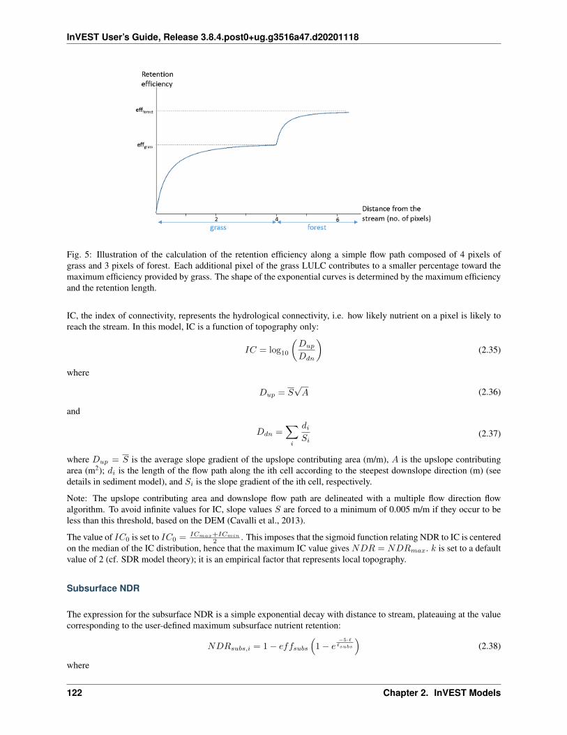
InVEST User’s Guide, Release 3.8.4.post0+ug.g3516a47.d20201118
Fig. 5: Illustration of the calculation of the retention efficiency along a simple flow path composed of 4 pixels ofgrass and 3 pixels of forest. Each additional pixel of the grass LULC contributes to a smaller percentage toward themaximum efficiency provided by grass. The shape of the exponential curves is determined by the maximum efficiencyand the retention length.
IC, the index of connectivity, represents the hydrological connectivity, i.e. how likely nutrient on a pixel is likely toreach the stream. In this model, IC is a function of topography only:
𝐼𝐶 = log10
(︂𝐷𝑢𝑝
𝐷𝑑𝑛
)︂(2.35)
where
𝐷𝑢𝑝 = 𝑆√𝐴 (2.36)
and
𝐷𝑑𝑛 =∑︁𝑖
𝑑𝑖𝑆𝑖
(2.37)
where 𝐷𝑢𝑝 = 𝑆 is the average slope gradient of the upslope contributing area (m/m), 𝐴 is the upslope contributingarea (m2); 𝑑𝑖 is the length of the flow path along the ith cell according to the steepest downslope direction (m) (seedetails in sediment model), and 𝑆𝑖 is the slope gradient of the ith cell, respectively.
Note: The upslope contributing area and downslope flow path are delineated with a multiple flow direction flowalgorithm. To avoid infinite values for IC, slope values 𝑆 are forced to a minimum of 0.005 m/m if they occur to beless than this threshold, based on the DEM (Cavalli et al., 2013).
The value of 𝐼𝐶0 is set to 𝐼𝐶0 = 𝐼𝐶𝑚𝑎𝑥+𝐼𝐶𝑚𝑖𝑛
2 . This imposes that the sigmoid function relating NDR to IC is centeredon the median of the IC distribution, hence that the maximum IC value gives 𝑁𝐷𝑅 = 𝑁𝐷𝑅𝑚𝑎𝑥. 𝑘 is set to a defaultvalue of 2 (cf. SDR model theory); it is an empirical factor that represents local topography.
Subsurface NDR
The expression for the subsurface NDR is a simple exponential decay with distance to stream, plateauing at the valuecorresponding to the user-defined maximum subsurface nutrient retention:
𝑁𝐷𝑅𝑠𝑢𝑏𝑠,𝑖 = 1 − 𝑒𝑓𝑓𝑠𝑢𝑏𝑠
(︁1 − 𝑒
−5·ℓℓ𝑠𝑢𝑏𝑠
)︁(2.38)
where
122 Chapter 2. InVEST Models

InVEST User’s Guide, Release 3.8.4.post0+ug.g3516a47.d20201118
Fig. 6: Relationship between NDR and the connectivity index IC. The maximum value of NDR is set to 𝑁𝐷𝑅0 = 0.8.The effect of the calibration is illustrated by setting 𝑘 = 1 and 𝑘 = 2 (solid and dashed line, respectively), and𝐼𝐶0 = 0.5 and 𝐼𝐶0 = 2 (black and gray dashed lines, respectively).
2.2. Final Ecosystem Services: 123

InVEST User’s Guide, Release 3.8.4.post0+ug.g3516a47.d20201118
• 𝑒𝑓𝑓𝑠𝑢𝑏𝑠 is the maximum nutrient retention efficiency that can be reached through subsurface flow (i.e. retentiondue to biochemical degradation in soils),
• ℓ𝑠𝑢𝑏𝑠 is the subsurface flow retention length, i.e. the distance after which it can be assumed that soil retainsnutrient at its maximum capacity,
• ℓ𝑖 is the distance from the pixel to the stream.
Nutrient export
Nutrient export from each pixel i is calculated as the product of the load and the NDR:
𝑥𝑒𝑥𝑝𝑖= 𝑙𝑜𝑎𝑑𝑠𝑢𝑟𝑓,𝑖 ·𝑁𝐷𝑅𝑠𝑢𝑟𝑓,𝑖 + 𝑙𝑜𝑎𝑑𝑠𝑢𝑏𝑠,𝑖 ·𝑁𝐷𝑅𝑠𝑢𝑏𝑠,𝑖 (2.39)
Total nutrient at the outlet of each user-defined watershed is the sum of the contributions from all pixels within thatwatershed:
𝑥𝑒𝑥𝑝𝑡𝑜𝑡 =∑︁𝑖
𝑥𝑒𝑥𝑝𝑖 (2.40)
Limitations
The model has a small number of parameters and outputs generally show a high sensitivity to inputs. This implies thaterrors in the empirical load parameter values will have a large effect on predictions. Similarly, the retention efficiencyvalues are based on empirical studies, and factors affecting these values (like slope or intra-annual variability) are av-eraged. These values implicitly incorporate information about the dominant nutrient dynamics, influenced by climateand soils. The model also assumes that once nutrient reaches the stream it impacts water quality at the watershedoutlet, no in-stream processes are captured. Finally, the effect of grid resolution on the NDR formulation has not beenwell studied.
Sensitivity analyses are recommended to investigate how the confidence intervals in input parameters affect the studyconclusions (Hamel et al., 2015).
Also see the “Biophysical model interpretation” section for further details on model uncertainties.
Options for Valuation
Nutrient export predictions can be used for quantitative valuation of the nutrient retention service. For example,scenario comparison can serve to evaluate the change in purification service between landscapes. The total nutrientload can be used as a reference point, assuming that the landscape has 0 retention. Comparing the current scenarioexport to the total nutrient load provides a quantitative measure of the retention service of the current landscape.
An important note about assigning a monetary value to any service is that valuation should only be done on modeloutputs that have been calibrated and validated. Otherwise, it is unknown how well the model is representing the areaof interest, which may lead to misrepresentation of the exact value. If the model has not been calibrated, only relativeresults should be used (such as an increase of 10%) not absolute values (such as 1,523 kg, or 42,900 dollars.)
Data Needs
This section outlines the specific data used by the model. See the Appendix for additional information on data sourcesand pre-processing. Please consult the InVEST sample data (located in the folder where InVEST is installed, if youalso chose to install sample data) for examples of all of these data inputs. This will help with file type, folder structure
124 Chapter 2. InVEST Models
InVEST User’s Guide, Release 3.8.4.post0+ug.g3516a47.d20201118
and table formatting. Note that all GIS inputs must be in the same projected coordinate system and in linear meterunits.
You may choose to run the model with either Nitrogen or Phosphorus or both at the same time. If only one of theseis chosen, then all inputs must match. For example, if running Nitrogen, you must provide load_n, eff_n, crit_len_n,Subsurface Critical Length (Nitrogen) and Subsurface Maximum Retention Efficiency (Nitrogen).
• Workspace (required). Folder where model outputs will be written. Make sure that there is ample disk space,and write permissions are correct.
• Suffix (optional). Text string that will be appended to the end of output file names, as “_Suffix”. Use a Suffix todifferentiate model runs, for example by providing a short name for each scenario. If a Suffix is not provided,or changed between model runs, the tool will overwrite previous results.
• Digital elevation model (DEM) (required). Raster dataset with an elevation value for each pixel, given inmeters. Make sure the DEM is corrected by filling in sinks, and compare the output stream maps with hydro-graphic maps of the area. To ensure proper flow routing, the DEM should extend beyond the watersheds ofinterest, rather than being clipped to the watershed edge.
• Land use/land cover (required). Raster of land use/land cover (LULC) for each pixel, where each uniqueinteger represents a different land use/land cover class. All values in this raster MUST have correspondingentries in the Biophysical table.
• Nutrient runoff proxy (required). Raster representing the spatial variability in runoff potential, i.e. the capacityto transport nutrient downstream. This raster can be defined as a quickflow index (e.g. from the InVESTSeasonal Water Yield model) or simply as annual precipitation. The model will normalize this raster (by dividingby its average value) to compute the runoff potential index (RPI, see Eq. 1).
• Watersheds (required). Shapefile delineating the boundary of the watershed to be modeled. Results will beaggregated within each polygon defined. The column ws_id is required, containing a unique integer value foreach polygon.
• Biophysical Table (required). A .csv (Comma Separated Value) table containing model information corre-sponding to each of the land use classes in the LULC raster. All LULC classes in the LULC raster MUST havecorresponding values in this table. Each row is a land use/land cover class and columns must be named anddefined as follows:
• lucode (required): Unique integer for each LULC class (e.g., 1 for forest, 3 for grassland, etc.) Everyvalue in the LULC map MUST have a corresponding lucode value in the biophysical table.
• LULC_desc (optional): Descriptive name of land use/land cover class
• load_n (and/or load_p) (at least one is required): The nutrient loading for each land use class, givenas floating point values with units of kilograms per hectare per year. Suffix “_n” stands for nitrogen,and “_p” for phosphorus, and the two compounds can be modeled at the same time or separately.
Note 1: Loads are the sources of nutrients associated with each LULC class. If you wantto represent different levels of fertilizer application, you will need to create separate LULCclasses, for example one class called “crops - high fertilizer use” a separate class called“crops - low fertilizer use” etc.
Note 2: Load values may be expressed either as the amount of nutrient applied (e.g. fertil-izer, livestock waste, atmospheric deposition); or as “extensive” measures of contaminants,which are empirical values representing the contribution of a parcel to the nutrient budget(e.g. nutrient export running off urban areas, crops, etc.) In the latter case, the load shouldbe corrected for the nutrient retention from downstream pixels of the same LULC. For ex-ample, if the measured (or empirically derived) export value for forest is 3 kg.ha-1.yr-1 andthe retention efficiency is 0.8, users should enter 15(kg.ha-1.yr-1) in the n_load column ofthe biophysical table; the model will calculate the nutrient running off the forest pixel as15*(1-0.8) = 3 kg.ha-1.yr-1.
2.2. Final Ecosystem Services: 125

InVEST User’s Guide, Release 3.8.4.post0+ug.g3516a47.d20201118
• eff_n (and/or eff_p) (at least one is required): The maximum retention efficiency for each LULCclass, a floating point value between zero and 1. The nutrient retention capacity for a given vegetationtype is expressed as a proportion of the amount of nutrient from upstream. For example, highvalues (0.6 to 0.8) may be assigned to all natural vegetation types (such as forests, natural pastures,wetlands, or prairie), indicating that 60-80% of nutrient is retained. Like above, suffix “_n” standsfor nitrogen, and “_p” for phosphorus, and the two compounds can be modeled at the same time orseparately.
• crit_len_n (and/or crit_len_p) (at least one is required): The distance after which it is assumedthat a patch of a particular LULC type retains nutrient at its maximum capacity, given in meters. Ifnutrients travel a distance smaller than the retention length, the retention efficiency will be less thanthe maximum value eff_x, following an exponential decay (see Nutrient Delivery section).
• proportion_subsurface_n (optional): The proportion of dissolved nutrients over the total amountof nutrients, expressed as floating point value (ratio) between 0 and 1. By default, this value shouldbe set to 0, indicating that all nutrients are delivered via surface flow.
Example biophysical table (only to be used as an example, your LULC classes and corresponding valueswill be different):
lucode LULC_desc load_n eff_n crit_len_n proportion_subsurface_n1 Agriculture 100 0.5 25 0.52 Grass 8 0.75 150 03 Forest 2.8 0.8 300 04 Wetland 2.8 0.8 10 05 Urban 10 0.05 10 0
• Threshold flow accumulation (required): The number of upstream cells that must flow into a cell before it isconsidered part of a stream, which is used to classify streams from the DEM. This threshold directly affectsthe expression of hydrologic connectivity and the nutrient export result: when a flow path reaches the stream,nutrient retention stops and the nutrient exported is assumed to reach the catchment outlet. It is important tochoose this value carefully, so modeled streams come as close to reality as possible. See Appendix 1 for moreinformation on choosing this value. Integer value, with no commas or periods - for example “1000”.
• Borselli k parameter (required): Calibration parameter that determines the shape of the relationship betweenhydrologic connectivity (the degree of connection from patches of land to the stream) and the nutrient deliveryratio (percentage of nutrient that actually reaches the stream; cf. Figure 2). The default value is 2.
• Subsurface Critical Length (Nitrogen or Phosphorus) (required): The distance (traveled subsurface anddownslope) after which it is assumed that soil retains nutrient at its maximum capacity, given in meters. Ifdissolved nutrients travel a distance smaller than Subsurface Critical Length, the retention efficiency will belower than the Subsurface Maximum Retention Efficiency value defined. Setting this value to a distance smallerthan the pixel size will result in the maximum retention efficiency being reached within one pixel only.
• Subsurface Maximum Retention Efficiency (Nitrogen or Phosphorus) (required): The maximum nutrientretention efficiency that can be reached through subsurface flow, a floating point value between 0 and 1. Thisfield characterizes the retention due to biochemical degradation in soils.
Running the Model
To launch the Nutrient model navigate to the Windows Start Menu -> All Programs -> InVEST [version] -> NDR.The interface does not require a GIS desktop, although the results will need to be explored with any GIS tool such asArcGIS or QGIS.
126 Chapter 2. InVEST Models

InVEST User’s Guide, Release 3.8.4.post0+ug.g3516a47.d20201118
Interpreting results
The following is a short description of each of the outputs from the Nutrient Delivery model. Final results are foundwithin the user defined Workspace specified for this model run. In the file names below, “x” stands for either n(nitrogen) or p (phosphorus), depending on which nutrients were modeled. And “Suffix” refers to the optional user-defined Suffix input to the model.
The resolution of the output rasters will be the same as the resolution of the DEM provided as input.
• Parameter log: Each time the model is run, a text (.txt) file will be created in the Workspace. The file will listthe parameter values and output messages for that run and will be named according to the service, date and time.When contacting NatCap about errors in a model run, please include the parameter log.
• [Workspace] folder:
– watershed_results_ndr_[Suffix].shp: Shapefile which aggregates the nutrient model results per water-shed, with “x” in the field names below being n for nitrogen, and p for phosphorus. The .dbf table containsthe following information for each watershed:
* surf_x_ld: Total nutrient loads (sources) in the watershed, i.e. the sum of the nutrient contributionfrom all surface LULC without filtering by the landscape. [units kg/year]
– sub_x_ld: Total subsurface nutrient loads in the watershed. [units kg/year]
* **x_exp_tot*: Total nutrient export from the watershed.[units kg/year] (Eq. 13)
– x_export_[Suffix].tif : A pixel level map showing how much load from each pixel eventually reaches thestream. [units: kg/pixel] (Eq. 12)
• [Workspace]\intermediate_outputs folder:
– crit_len_x: Retention length values, crit_len, found in the biophysical table
– d_dn: Downslope factor of the index of connectivity (Eq. 10)
– d_up: Upslope factor of the index of connectivity (Eq. 9)
– eff_n: Retention efficiencies, eff_x, found in the biophysical table
– dist_to_channel: Average downstream distance from a pixel to the stream
– eff_x: Raw per-landscape cover retention efficiency for nutrient x.
– effective_retention_x: Effective retention provided by the downslope flow path for each pixel (Eq. 6)
– flow_accumulation: Flow accumulation created from the DEM
– flow_direction: Flow direction created from the DEM
– ic_factor: Index of connectivity (Eq. 8)
– load_x: Loads (for surface transport) per pixel [units: kg/year]
– modified_load_x: Raw load scaled by the runoff proxy index. [units: kg/year]
– ndr_x: NDR values (Eq. 4)
– runoff_proxy_index: Normalized values for the Runoff Proxy input to the model
– s_accumulation and s_bar: Slope parameters for the IC equation found in the Nutrient Delivery section
– stream: Stream network created from the DEM, with 0 representing land pixels, and 1 representing streampixels. Compare this layer with a real-world stream map, and adjust the Threshold Flow Accumulation sothat stream.tif matches real-world streams as closely as possible.
– sub_crit_len_n: Critical distance value for subsurface transport of nitrogen (constant over the landscape)
2.2. Final Ecosystem Services: 127

InVEST User’s Guide, Release 3.8.4.post0+ug.g3516a47.d20201118
– sub_eff_n: Subsurface retention efficiency for nitrogen (constant over the landscape)
– sub_effective_retention_n: Subsurface effective retention for nitrogen
– surface_load_n: Above ground nutrient loads [units: kg/year]
– sub_load_n: Nitrogen loads for subsurface transport [units: kg/year]
– sub_ndr_n: Subsurface nitrogen NDR values
– thresholded_slope: Raster with slope values thresholded for correct calculation of IC.
Biophysical Model Interpretation for Valuation
Some valuation approaches, such as those relying on the changes in water quality for a treatment plant, are verysensitive to the model absolute predictions. Therefore, it is important to consider the uncertainties associated with theuse of InVEST as a predictive tool and minimize their effect on the valuation step.
Model parameter uncertainties
Uncertainties in input parameters can be characterized through a literature review (e.g. examining the distribution ofvalues from different studies). One option to assess the impact of parameter uncertainties is to conduct local or globalsensitivity analyses, with parameter ranges obtained from the literature (Hamel et al., 2015).
Model structural uncertainties
The InVEST model computes a nutrient mass balance over a watershed, subtracting nutrient losses (conceptually rep-resented by the retention coefficients), from the total nutrient sources. Where relevant, it is possible to distinguishbetween surface and subsurface flow paths, adding three parameters to the model. In the absence of empirical knowl-edge, modelers can assume that the surface load and retention parameters represent both transport process. Testingand calibration of the model is encouraged, acknowledging two main challenges:
• Knowledge gaps in nutrient transport: although there is strong evidence of the impact of land use change onnutrient export, modeling of the watershed scale dynamics remains challenging (Breuer et al., 2008; Scanlon etal., 2007). Calibration is therefore difficult and not recommended without in-depth analyses that would provideconfidence in model process representation (Hamel et al., 2015)
• Potential contribution from point source pollution: domestic and industrial waste are often part of the nutrientbudget and should be accounted for during calibration (for example, by adding point-source nutrient loads tomodeled nutrient export, then comparing the sum to observed data).
Comparison to observed data
Despite the above uncertainties, the InVEST model provides a first-order assessment of the processes of nutrient reten-tion and may be compared with observations. Time series of nutrient concentration used for model validation shouldspan over a reasonably long period (preferably at least 10 years) to attenuate the effect of inter-annual variability. Timeseries should also be relatively complete throughout a year (without significant seasonal data gaps) to ensure compari-son with total annual loads. If the observed data is expressed as a time series of nutrient concentration, they need to beconverted to annual loads (LOADEST and FLUX32 are two software facilitating this conversion). Additional detailson methods and model performance for relative predictions can be found in the study of Hamel and Guswa 2015.
128 Chapter 2. InVEST Models

InVEST User’s Guide, Release 3.8.4.post0+ug.g3516a47.d20201118
Appendix: Data sources
This is a rough compilation of data sources and suggestions about finding, compiling, and formatting data, providinglinks to global datasets that can get you started. It is highly recommended to look for more local and accurate data(from national, state, university, literature, NGO and other sources) and only use global data for final analyses ifnothing more local is available.
Digital elevation model
DEM data is available for any area of the world, although at varying resolutions.
Free raw global DEM data is available from:
• The World Wildlife Fund - http://worldwildlife.org/pages/hydrosheds
• NASA: https://asterweb.jpl.nasa.gov/gdem.asp (30m resolution); and easy access to SRTM data: http://dwtkns.com/srtm/
• USGS: https://earthexplorer.usgs.gov/
Alternatively, it may be purchased relatively inexpensively at sites such as MapMart (www.mapmart.com).
The DEM resolution may be a very important parameter depending on the project’s goals. For example, if decisionmakers need information about impacts of roads on ecosystem services then fine resolution is needed. The hydrologicalaspects of the DEM used in the model must be correct. Most raw DEM data has errors, so it’s likely that the DEM willneed to be filled to remove sinks. Multiple passes of the ArcGIS Fill tool, or QGIS Wang & Liu Fill algorithm (SAGAlibrary) have shown good results. Look closely at the stream network produced by the model (stream.tif). If streamsare not continuous, but broken into pieces, the DEM still has sinks that need to be filled. If filling sinks multiple timesdoes not create a continuous stream network, perhaps try a different DEM. If the results show an unexpected gridpattern, this may be due to reprojecting the DEM with a “nearest neighbor” interpolation method instead of “bilinear”or “cubic”. In this case, go back to the raw DEM data and reproject using “bilinear” or “cubic”.
Land use/land cover
A key component for all water models is a spatially continuous land use/land cover (LULC) raster, where all pixelsmust have a land use/land cover class defined. Gaps in data will create missing data (holes) in the output layers.Unknown data gaps should be approximated.
Global land use data is available from:
• NASA: https://lpdaac.usgs.gov/dataset_discovery/modis/modis_products_table/mcd12q1 (MODIS multi-yearglobal landcover data provided in several classifications)
• The European Space Agency: https://www.esa-landcover-cci.org (Three global maps for the 2000, 2005 and2010 epochs)
• The University of Maryland’s Global Land Cover Facility: http://glcf.umd.edu/data/landcover/ (data availablein 1 degree, 8km and 1km resolutions).
Data for the U.S. is provided by the USGS and Department of the Interior via the National Land Cover Database:https://www.mrlc.gov/finddata.php
The simplest categorization of LULCs on the landscape involves delineation by land cover only (e.g., cropland, forest,grassland). Several global and regional land cover classifications are available (e.g., Anderson et al. 1976), and oftendetailed land cover classification has been done for the landscape of interest.
A slightly more sophisticated LULC classification involves breaking relevant LULC types into more meaningful types.For example, agricultural land classes could be broken up into different crop types or forest could be broken up into
2.2. Final Ecosystem Services: 129

InVEST User’s Guide, Release 3.8.4.post0+ug.g3516a47.d20201118
specific species. The categorization of land use types depends on the model and how much data is available for eachof the land types. You should only break up a land use type if it will provide more accuracy in modeling. For instance,only break up ‘crops’ into different crop types if you have information on the difference in nutrient export and retentionbetween crop management values.
Sample Land Use/Land Cover Table
lucode Land Use/Land Cover1 Evergreen Needleleaf Forest2 Evergreen Broadleaf Forest3 Deciduous Needleleaf Forest4 Deciduous Broadleaf Forest5 Mixed Cover6 Woodland7 Wooded Grassland8 Closed Shrubland9 Open Shrubland10 Grassland11 Cropland (row Crops)12 Bare Ground13 Urban and Built-Up14 Wetland15 Mixed evergreen16 Mixed Forest17 Orchards/Vineyards18 Pasture
Nutrient runoff proxy
Either the quickflow index (e.g. from the InVEST Seasonal Water Yield or other model) or average annual precipitationmay be used. Average annual precipitation may be interpolated from existing rain gages, and global data sets fromremote sensing models to account for remote areas. When considering rain gage data, make sure that they provide goodcoverage over the area of interest, especially if there are large changes in elevation that cause precipitation amountsto be heterogeneous within the AOI. Ideally, the gauges will have at least 10 years of continuous data, with no largegaps, around the same time period as the land use/land cover map used.
If field data are not available, you can use coarse annual precipitation data from the freely available global data setsdeveloped by World Clim (http://www.worldclim.org/) or the Climatic Research Unit (http://www.cru.uea.ac.uk).
Watersheds / subwatersheds
To delineate watersheds, we provide the InVEST tool DelineateIT, which is relatively simple yet fast and has theadvantage of creating watersheds that might overlap, such as watersheds draining to several dams on the same river.See the User Guide chapter for DelineateIt for more information on this tool. Watershed creation tools are alsoprovided with GIS software, as well as some hydrology models. It is recommended that you delineate watershedsusing the DEM that you are modeling with, so the watershed boundary corresponds correctly to the topography.
Alternatively, a number of watershed maps are available online, e.g. HydroBASINS: http://hydrosheds.org/. Note thatif watershed boundaries are not based on the same DEM that is being modeled, results that are aggregated to thesewatersheds are likely to be inaccurate.
Exact locations of specific structures, such as drinking water facility intakes or reservoirs, should be obtained from themanaging entity or may be obtained on the web:
130 Chapter 2. InVEST Models

InVEST User’s Guide, Release 3.8.4.post0+ug.g3516a47.d20201118
• The U.S. National Inventory of Dams: http://nid.usace.army.mil/
• Global Reservoir and Dam (GRanD) Database: http://www.gwsp.org/products/grand-database.html
• World Water Development Report II dam database: http://wwdrii.sr.unh.edu/download.html
Some of these datasets include the catchment area draining to each dam, which should be compared with the area ofthe watershed(s) generated by the delineation tool to assess accuracy.
Threshold flow accumulation
There is no one “correct” value for the threshold flow accumulation (TFA). The correct value for your application isthe value that causes the model to create a stream layer that looks as close as possible to the real-world stream networkin the watershed. Compare the model output file stream.tif with a known correct stream map, and adjust the TFAaccordingly - larger values of TFA will create a stream network with fewer tributaries, smaller values of TFA willcreate a stream network with more tributaries. A good value to start with is 1000, but note that this can vary widelydepending on the resolution of the DEM, local climate and topography. Note that generally streams delineated froma DEM do not exactly match the real world, so just try to come as close as possible. If the modelled streams are verydifferent, then consider trying a different DEM. This is an integer value, with no commas or periods - for example“1000”.
A global layer of streams can be obtained from HydroSHEDS: http://hydrosheds.org/, but note that they are generallymore major rivers and may not include those in your study area, especially if it has small tributaries. You can also trylooking at streams in Google Earth if no more localized maps are available.
Nutrient load
For all water quality parameters (nutrient load, retention efficiency, and retention length), local literature should beconsulted to derive site-specific values. The NatCap nutrient parameter database provides a non-exhaustive list of lo-cal references for nutrient loads and retention efficiencies: https://www.naturalcapitalproject.org/wp-content/uploads/2016/04/Nutrient_DB_0212.xlsx. Parn et al. (2012) and Harmel et al. (2007) provide a good review for agriculturalland in temperate climate.
Examples of export coefficients (“extensive” measures, see Data needs) for the US can be found in the EPA PLOADUser’s Manual and in a review by Lin (2004). Note that the examples in the EPA guide are in lbs/ac/yr and must beconverted to kg/ha/yr.
Retention efficiency
This value represents, conceptually, the maximum nutrient retention that can be expected from a given LULC type.Natural vegetation LULC types (such as forests, natural pastures, wetlands, or prairie) are generally assigned highvalues (>0.8). A review of the local literature and consultation with hydrologists is recommended to select the mostrelevant values for this parameter. The NatCap nutrient parameter database provides a non-exhaustive list of local ref-erences for nutrient loads and retention efficiencies: https://www.naturalcapitalproject.org/wp-content/uploads/2016/04/Nutrient_DB_0212.xlsx. Parn et al. (2012) provide a useful review for temperate climates. Reviews of riparianbuffers efficiency, although a particular case of LULC retention, can also be used as a starting point (Mayer et al.,2007; Zhang et al., 2009).
Retention length
This value represents the typical distance necessary to reach the maximum retention efficiency. It was introduced inthe model to remove any sensitivity to the resolution of the LULC raster. The literature on riparian buffer removal
2.2. Final Ecosystem Services: 131

InVEST User’s Guide, Release 3.8.4.post0+ug.g3516a47.d20201118
efficiency suggests that retention lengths range from 10 to 300 m (Mayer et al., 2007; Zhang et al., 2009). In theabsence of local data for land uses that are not forest or grass, you can simply set the retention length constant, equalto the pixel size: this will result in the maximum retention efficiency being reached within a distance of one pixel only.
Subsurface parameters: proportion_subsurface_n, eff_sub, crit_len_sub
These values are used for advanced analyses and should be selected in consultation with hydrologists. Parn et al.(2012) provide average values for the partitioning of N loads between leaching and surface runoff. From Mayer etal. (2007), a global average of 200m for the retention length, and 80% for retention efficiency can be assumed forvegetated buffers.
References
Breuer, L., Vaché, K.B., Julich, S., Frede, H.-G., 2008. Current concepts in nitrogen dynamics for mesoscale catch-ments. Hydrol. Sci. J. 53, 1059–1074.
California Regional Water Quality Control Board Central Coast Region, 2013. Total Maximum Daily Loads for Nitro-gen Compounds and Orthophosphate for the Lower Salinas River and Reclamation Canal Basin , and the Moro CojoSlough Subwatershed , Monterey County, CA. Appendix F. Available at: http://www.waterboards.ca.gov/centralcoast/water_issues/programs/tmdl/docs/salinas/nutrients/index.shtml
Endreny, T.A., Wood, E.F., 2003. Watershed weighting of export coefficients to map critical phosphorous loadingareas. J. Am. Water Resour. Assoc. 08544, 165–181.
Hamel, P., Chaplin-Kramer, R., Sim, S., Mueller, C., 2015. A new approach to modeling the sediment retention service(InVEST 3.0): Case study of the Cape Fear catchment, North Carolina, USA. Sci. Total Environ. 166–177.
Hamel, P., Guswa A.J. 2015. Uncertainty Analysis of the InVEST 3.0 Nutrient Model: Case Study of the CapeFear Catchment, NC. Hydrology and Earth System Sciences Discussion 11:11001-11036. http://dx.doi.org/10.5194/hessd-11-11001-2014
Harmel, D., Potter, S., Casebolt, P., Reckhow, K., 2007. Compilation of measured nutrient load data for agriculturalland uses in the United States 76502, 1163–1178.
Heathwaite, A.L., Quinn, P.F., Hewett, C.J.M., 2005. Modelling and managing critical source areas of diffuse pollutionfrom agricultural land using flow connectivity simulation. J. Hydrol. 304, 446–461.
Keeler, B.L., Polasky, S., Brauman, K.A., Johnson, K.A., Finlay, J.C., Neill, A.O., 2012. Linking water quality andwell-being for improved assessment and valuation of ecosystem services 109, 18629–18624.
Lin, J.., 2004. Review of published export coefficient and event mean concentration (EMC) data, WRAP TechnicalNotes Collection (ERDC TN-WRAP-04-3). Vicksburg, MS.
Mayer, P.M., Reynolds, S.K., Mccutchen, M.D., Canfield, T.J., 2007. Meta-Analysis of Nitrogen Removal in RiparianBuffers 1172–1180.
Pärn, J., Pinay, G., Mander, Ü., 2012. Indicators of nutrients transport from agricultural catchments under temperateclimate: A review. Ecol. Indic. 22, 4–15.
Reckhow, K.H., Beaulac, M.N., Simpson, J.T., 1980. Modeling Phosphorus loading and lake response under uncer-tainty: A manual and compilation of export coefficients. EPA 440/5-80-011. US-EPA, Washington, DC.
Scanlon, B.R., Jolly, I., Sophocleous, M., Zhang, L., 2007. Global impacts of conversions from natural to agriculturalecosystems on water resources: Quantity versus quality. Water Resour. Res. 43.
Tarboton, D., 1997. A new method for the determination of flow directions and upslope areas in grid digital elevationmodels. Water Resour. Res. 33, 309–319.
132 Chapter 2. InVEST Models
InVEST User’s Guide, Release 3.8.4.post0+ug.g3516a47.d20201118
Vigiak, O., Borselli, L., Newham, L.T.H., Mcinnes, J., Roberts, A.M., 2012. Comparison of conceptual landscapemetrics to define hillslope-scale sediment delivery ratio. Geomorphology 138, 74–88.
Zhang, X., Liu, X., Zhang, M., Dahlgren, R. a, Eitzel, M., 2009. A review of vegetated buffers and a meta-analysis oftheir mitigation efficacy in reducing nonpoint source pollution. J. Environ. Qual. 39, 76–84.
2.2.6 Sediment Delivery Ratio
Summary
The objective of the InVEST Sediment Delivery Ratio (SDR) model is to map overland sediment generation anddelivery to the stream. In the context of global change, such information can be used to study the service of sedimentretention in a catchment. This is of particular interest for reservoir management and instream water quality, both ofwhich may be economically valued.
Introduction
Erosion and overland sediment retention are natural processes that govern the sediment concentration in streams. Sed-iment dynamics at the catchment scale are mainly determined by climate (in particular rain intensity), soil properties,topography, and vegetation; and anthropogenic factors such as agricultural activities or dam construction and opera-tion. Main sediment sources include overland erosion (soil particles detached and transported by rain and overlandflow), gullies (channels that concentrate flow), bank erosion, and mass erosion (or landslides; see Merrit 2003 for areview). Sinks include on-slope, floodplain or instream deposition, and reservoir retention, as summarized in Figure 1.Conversion of land use and changes in land management practices may dramatically modify the amount of sedimentrunning off a catchment. The magnitude of this effect is primarily governed by: i) the main sediment sources (landuse change will have a smaller effect in catchments where sediments are not primarily coming from overland flow);and ii) the spatial distribution of sediment sources and sinks (for example, land use change will have a smaller effectif the sediment sources are buffered by vegetation).
Increases in sediment yield are observed in many places in the world, dramatically affecting water quality and reservoirmanagement (UNESCO 2009). The sediment retention service provided by natural landscapes is of great interest towater managers. Understanding where the sediments are produced and delivered allow managers to design improvedstrategies for reducing sediment loads. Changes in sediment load can have impacts on downstream irrigation, watertreatment, recreation and reservoir performance.
Outputs from the sediment model include the sediment load delivered to the stream at an annual time scale, as well asthe amount of sediment eroded in the catchment and retained by vegetation and topographic features. Note that SDRonly creates biophysical results. For valuation of the sediment retention service, appropriate valuation approaches willbe highly dependent on the particular application and context, and need to be implemented independently of InVEST.
The Model
Sediment Delivery
The sediment delivery module is a spatially-explicit model working at the spatial resolution of the input digital eleva-tion model (DEM) raster. For each pixel, the model first computes the amount of annual soil loss from that pixel, thencomputes the sediment delivery ratio (SDR), which is the proportion of soil loss actually reaching the stream. Once
2.2. Final Ecosystem Services: 133
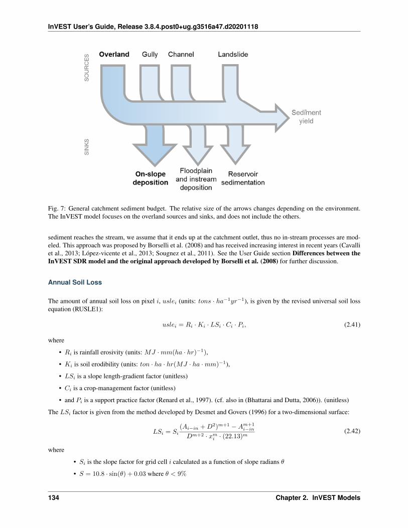
InVEST User’s Guide, Release 3.8.4.post0+ug.g3516a47.d20201118
Fig. 7: General catchment sediment budget. The relative size of the arrows changes depending on the environment.The InVEST model focuses on the overland sources and sinks, and does not include the others.
sediment reaches the stream, we assume that it ends up at the catchment outlet, thus no in-stream processes are mod-eled. This approach was proposed by Borselli et al. (2008) and has received increasing interest in recent years (Cavalliet al., 2013; López-vicente et al., 2013; Sougnez et al., 2011). See the User Guide section Differences between theInVEST SDR model and the original approach developed by Borselli et al. (2008) for further discussion.
Annual Soil Loss
The amount of annual soil loss on pixel 𝑖, 𝑢𝑠𝑙𝑒𝑖 (units: 𝑡𝑜𝑛𝑠 · ℎ𝑎−1𝑦𝑟−1), is given by the revised universal soil lossequation (RUSLE1):
𝑢𝑠𝑙𝑒𝑖 = 𝑅𝑖 ·𝐾𝑖 · 𝐿𝑆𝑖 · 𝐶𝑖 · 𝑃𝑖, (2.41)
where
• 𝑅𝑖 is rainfall erosivity (units: 𝑀𝐽 ·𝑚𝑚(ℎ𝑎 · ℎ𝑟)−1),
• 𝐾𝑖 is soil erodibility (units: 𝑡𝑜𝑛 · ℎ𝑎 · ℎ𝑟(𝑀𝐽 · ℎ𝑎 ·𝑚𝑚)−1),
• 𝐿𝑆𝑖 is a slope length-gradient factor (unitless)
• 𝐶𝑖 is a crop-management factor (unitless)
• and 𝑃𝑖 is a support practice factor (Renard et al., 1997). (cf. also in (Bhattarai and Dutta, 2006)). (unitless)
The 𝐿𝑆𝑖 factor is given from the method developed by Desmet and Govers (1996) for a two-dimensional surface:
𝐿𝑆𝑖 = 𝑆𝑖
(𝐴𝑖−𝑖𝑛 + 𝐷2)𝑚+1 −𝐴𝑚+1𝑖−𝑖𝑛
𝐷𝑚+2 · 𝑥𝑚𝑖 · (22.13)𝑚
(2.42)
where
• 𝑆𝑖 is the slope factor for grid cell 𝑖 calculated as a function of slope radians 𝜃
• 𝑆 = 10.8 · sin(𝜃) + 0.03 where 𝜃 < 9%
134 Chapter 2. InVEST Models

InVEST User’s Guide, Release 3.8.4.post0+ug.g3516a47.d20201118
• 𝑆 = 16.8 · sin(𝜃) − 0.50, where 𝜃 ≥ 9%
• 𝐴𝑖−𝑖𝑛 is the contributing area (𝑚2) at the inlet of a grid cell which is computed from the MultipleFlow Direction method
• 𝐷 is the grid cell linear dimension (𝑚)
• 𝑥𝑖 is the mean of aspect weighted by proportional outflow from grid cell 𝑖 determined by theMultiple-Flow Direction method. It is calculated by
∑︀𝑑∈{0,7}
𝑃𝑖(𝑑)𝑥𝑑
where 𝑥𝑑 = | sin𝛼(𝑑)| +
| cos𝛼(𝑑)| where 𝛼(𝑑) is the radian angle for direction 𝑑 and 𝑃𝑖(𝑑) is the proportion of total outflowat cell 𝑖 in direction 𝑑.
• 𝑚 is the RUSLE length exponent factor.
To avoid overestimation of the LS factor in heterogeneous landscapes, long slope lengths are capped to a value of333m (Desmet and Govers, 1996; Renard et al., 1997).
The value of 𝑚, the length exponent of the LS factor, is based on the classical USLE, as discussed in (Oliveira et al.,2013):
• 𝑚 = 0.2 for slope <= 1%:
• 𝑚 = 0.3 for 1% < slope <= 3.5%
• 𝑚 = 0.4 for 3.5% < slope <= 5%
• 𝑚 = 0.5 for 5% < slope <= 9%
• 𝑚 = 𝛽/(1 + 𝛽) where 𝛽 = sin 𝜃/0.0986/(3 sin 𝜃0.8 + 0.56) for slope >= 9%
Sediment Delivery Ratio
Step 1. Based on the work by Borselli et al. (2008), the model first computes the connectivity index (𝐼𝐶) for eachpixel. The connectivity index describes the hydrological linkage between sources of sediment (from the landscape)and sinks (like streams.) Higher values of 𝐼𝐶 indicate that source erosion is more likely to make it to a sink (i.e. ismore connected), which happens, for example, when there is sparse vegetation or higher slope. Lower values of 𝐼𝐶(i.e. lower connectivity) are associated with more vegetated areas and lower slopes.
𝐼𝐶 is a function of both the area upslope of each pixel (𝐷𝑢𝑝) and the flow path between the pixel and the neareststream (𝐷𝑑𝑛). If the upslope area is large, has lower slope, and good vegetative cover (so a low USLE C factor), 𝐷𝑢𝑝
will be low, indicating a lower potential for sediment to make it to the stream. Similarly, if the downslope path betweenthe pixel and the stream is long, has lower slope and good vegetative cover, 𝐷𝑑𝑛 will be low.
𝐼𝐶 is calculated as follows:
𝐼𝐶 = log10
(︂𝐷𝑢𝑝
𝐷𝑑𝑛
)︂(2.43)
Figure 2. Conceptual approach used in the model. The sediment delivery ratio (SDR) for each pixel is a function ofthe upslope area and downslope flow path (Equations 3, 4, 5).
𝐷𝑢𝑝 is the upslope component defined as:
𝐷𝑢𝑝 = 𝐶𝑆√𝐴 (2.44)
2.2. Final Ecosystem Services: 135

InVEST User’s Guide, Release 3.8.4.post0+ug.g3516a47.d20201118
where 𝐶 is the average 𝐶 factor of the upslope contributing area, 𝑆 is the average slope gradient of the upslopecontributing area (𝑚/𝑚) and 𝐴 is the upslope contributing area (𝑚2). The upslope contributing area is delineatedfrom the D-infinity flow algorithm (Tarboton, 1997).
The downslope component 𝐷𝑑𝑛 is given by:
𝐷𝑑𝑛 =∑︁𝑖
𝑑𝑖𝐶𝑖𝑆𝑖
(2.45)
where 𝑑𝑖 is the length of the flow path along the ith cell according to the steepest downslope direction (𝑚) (see Figure2), 𝐶𝑖 and 𝑆𝑖 are the 𝐶 factor and the slope gradient of the ith cell, respectively. Again, the downslope flow path isdetermined from the D-infinity flow algorithm (Tarboton, 1997).
To avoid infinite values for 𝐼𝐶, slope values 𝑆 are forced to a minimum of 0.005 m/m if they occur to be less thanthis threshold, and an upper limit of 1 m/m to limit bias due to very high values of 𝐼𝐶 on steep slopes. (Cavalli et al.,2013).
Step 2. The SDR ratio for a pixel 𝑖 is then derived from the conductivity index 𝐼𝐶 following (Vigiak et al., 2012):
𝑆𝐷𝑅𝑖 =𝑆𝐷𝑅𝑚𝑎𝑥
1 + exp(︀𝐼𝐶0−𝐼𝐶𝑖
𝑘
)︀ (2.46)
where 𝑆𝐷𝑅𝑚𝑎𝑥 is the maximum theoretical SDR, set to an average value of 0.8 (Vigiak et al., 2012), and 𝐼𝐶0 and𝑘 are calibration parameters that define the shape of the SDR-IC relationship (which is an increasing function). Theeffect of 𝐼𝐶0 and 𝑘 on the SDR is illustrated below:
Figure 3. Relationship between the connectivity index IC and the SDR. The maximum value of SDR is set to𝑆𝐷𝑅𝑚𝑎𝑥 = 0.8. The effect of the calibration are illustrated by setting 𝑘𝑏 = 1 and 𝑘𝑏 = 2 (solid and dashedline, respectively), and 𝐼𝐶0 = 0.5 and 𝐼𝐶0 = 2 (black and grey dashed lines, respectively).
136 Chapter 2. InVEST Models
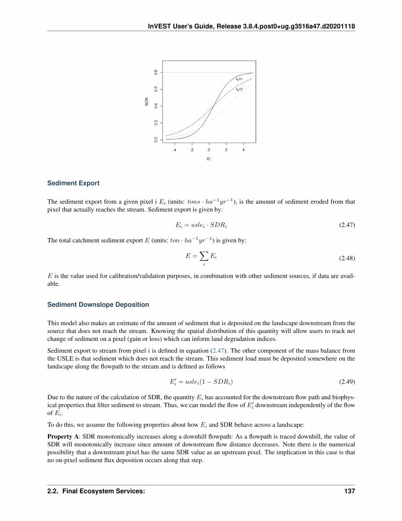
InVEST User’s Guide, Release 3.8.4.post0+ug.g3516a47.d20201118
Sediment Export
The sediment export from a given pixel i 𝐸𝑖 (units: 𝑡𝑜𝑛𝑠 · ℎ𝑎−1𝑦𝑟−1), is the amount of sediment eroded from thatpixel that actually reaches the stream. Sediment export is given by:
𝐸𝑖 = 𝑢𝑠𝑙𝑒𝑖 · 𝑆𝐷𝑅𝑖 (2.47)
The total catchment sediment export 𝐸 (units: 𝑡𝑜𝑛 · ℎ𝑎−1𝑦𝑟−1) is given by:
𝐸 =∑︁𝑖
𝐸𝑖 (2.48)
𝐸 is the value used for calibration/validation purposes, in combination with other sediment sources, if data are avail-able.
Sediment Downslope Deposition
This model also makes an estimate of the amount of sediment that is deposited on the landscape downstream from thesource that does not reach the stream. Knowing the spatial distribution of this quantity will allow users to track netchange of sediment on a pixel (gain or loss) which can inform land degradation indices.
Sediment export to stream from pixel 𝑖 is defined in equation (2.47). The other component of the mass balance fromthe USLE is that sediment which does not reach the stream. This sediment load must be deposited somewhere on thelandscape along the flowpath to the stream and is defined as follows
𝐸′𝑖 = 𝑢𝑠𝑙𝑒𝑖(1 − 𝑆𝐷𝑅𝑖) (2.49)
Due to the nature of the calculation of SDR, the quantity 𝐸𝑖 has accounted for the downstream flow path and biophys-ical properties that filter sediment to stream. Thus, we can model the flow of 𝐸′
𝑖 downstream independently of the flowof 𝐸𝑖.
To do this, we assume the following properties about how 𝐸𝑖 and SDR behave across a landscape:
Property A: SDR monotonically increases along a downhill flowpath: As a flowpath is traced downhill, the value ofSDR will monotonically increase since amount of downstream flow distance decreases. Note there is the numericalpossibility that a downstream pixel has the same SDR value as an upstream pixel. The implication in this case is thatno on-pixel sediment flux deposition occurs along that step.
2.2. Final Ecosystem Services: 137

InVEST User’s Guide, Release 3.8.4.post0+ug.g3516a47.d20201118
Property B: All non-exporting sediment flux on a boundary stream pixel is retained by that pixel: If pixel 𝑖 drainsdirectly to the stream there is no opportunity for further downstream filtering of 𝐸𝑖. Since 𝐸𝑖 is the inverse of Ei, theimplication is that the upstream flux (defined as Fi below) must have been deposited on the pixel.
Given these two properties, we see that the amount of 𝐸𝑖 retained on a pixel must be a function of:
• the absolute difference in SDR values from pixel 𝑖 to the downstream pixel(s) drain, and
• how numerically close the downstream SDR value is to 1.0 (the stream pixel).
These mechanics can be captured as a linear interpolation of the difference of pixel i’s SDR value with its downstreamSDR counterpart with respect to the difference of pixel i’s difference with a theoretical maximum downstream SDRvalue 1.0. Formally,
𝑑𝑅𝑖 =
∑︀𝑘∈{𝑑𝑖𝑟𝑒𝑐𝑡𝑙𝑦 𝑑𝑜𝑤𝑛𝑠𝑡𝑟𝑒𝑎𝑚 𝑓𝑟𝑜𝑚 𝑖} 𝑆𝐷𝑅𝑘 · 𝑝(𝑖, 𝑘) − 𝑆𝐷𝑅𝑖
1.0 − 𝑆𝐷𝑅𝑖
(2.50)
The 𝑑 in 𝑑𝑅𝑖 indicates a delta difference and 𝑝(𝑖, 𝑘) is the proportion of flow from pixel 𝑖 to pixel 𝑗. This notation ismeant to invoke the intution of a derivative of 𝑅𝑖. Note the boundary conditions are satisfied:
• In the case of Property A (downstream 𝑆𝐷𝑅𝑘 = 𝑆𝐷𝑅𝑖), the value of 𝑑𝑅𝑖 = 0 indicating no 𝐹𝑖 will be retainedon the pixel.
• In the case of Property B (downstream 𝑆𝐷𝑅𝑘 = 1 because it is a stream) the value of 𝑑𝑅𝑖 = 1 indicating theremaining 𝐹𝑖 is retained on the pixel.
Now we define the amount of sediment flux that is retained on any pixel in the flowpath using 𝑑𝑅𝑖 as a weighted flowof upstream flux:
𝑅𝑖 = 𝑑𝑅𝑖 ·
⎛⎝ ∑︁𝑗∈{𝑝𝑖𝑥𝑒𝑙𝑠 𝑡ℎ𝑎𝑡 𝑑𝑟𝑎𝑖𝑛 𝑡𝑜 𝑖}
𝐹𝑗𝑝(𝑖, 𝑗) + 𝐸′𝑖
⎞⎠ (2.51)
where 𝐹𝑗 is the amount of sediment-export-that-does-not-reach-the stream “flux”, defined as:
𝐹𝑖 = (1 − 𝑑𝑅𝑖) ·
⎛⎝ ∑︁𝑗∈{𝑝𝑖𝑥𝑒𝑙𝑠 𝑡ℎ𝑎𝑡 𝑑𝑟𝑎𝑖𝑛 𝑡𝑜 𝑖}
𝐹𝑗𝑝(𝑖, 𝑗) + 𝐸′𝑖
⎞⎠ (2.52)
Optional Drainage Layer
In some situations, the index of connectivity defined by topography does not represent actual flow paths, which maybe influenced by artificial connectivity instead. For example, sediments in urban areas or near roads are likely to beconveyed to the stream with little retention. The (optional) drainage raster identifies the pixels that are artificiallyconnected to the stream, irrespective of their geographic position (e.g. their distance to the stream network). Pixelsfrom the drainage layer are treated similarly to pixels of the stream network; in other words, the downstream flowpath will stop at pixels of the drainage layer (and the corresponding sediment load will be added to the total sedimentexport).
Limitations
• Among the main limitations of the model is its reliance on the USLE (Renard et al., 1997). This equation iswidely used but is limited in scope, only representing rill/inter-rill erosion processes. Other sources of sedimentinclude gully erosion, streambank erosion, and mass erosion. A good description of the gully and streambankerosion processes is provided by Wilkinson et al. 2014, with possible modeling approaches. Mass erosion(landslide) is not represented in the model but can be a significant source in some areas or under certain landuse change, such as road construction.
138 Chapter 2. InVEST Models

InVEST User’s Guide, Release 3.8.4.post0+ug.g3516a47.d20201118
• A corollary is that the descriptions of the impact on ecosystem services (and any subsequent valuation) shouldaccount for the relative proportion of the sediment source from the model compared to the total sediment budget(see the section on Evaluating sediment retention services).
• In addition, as an empirical equation developed in the United States, the USLE has shown limited performancein other areas – even when focusing on sheet and rill erosion. Based on local knowledge, users may modifythe soil loss equation implemented in the model by altering the R, K, C, P inputs to reflect findings from localstudies (Sougnez et al., 2011).
• The model is very sensitive to the k and IC0 parameters, which are not physically based. The emerging literatureon the modeling approach used in the InVEST model (Cavalli et al., 2013; López-vicente et al., 2013; Sougnezet al., 2011; Vigiak et al., 2012) provides guidance to set these parameters, but users should be aware of thislimitation when interpreting the model’s absolute values.
• Given the simplicity of the model and low number of parameters, outputs are very sensitive to most input param-eters. Errors in the empirical parameters of the USLE equations will therefore have a large effect on predictions.Sensitivity analyses are recommended to investigate how the confidence intervals in input parameters affect thestudy conclusions.
Differences between the InVEST SDR model and the original approach developed by Borselli et al.(2008)
The InVEST SDR model is based on the concept of hydrological connectivity, as parameterized by Borselli et al.(2012). This approach was selected since it requires a minimal number of parameters, uses globally available data,and is spatially explicit. In a comparative study, Vigiak et al. (2012) suggested that the approach provides: “(i) largeimprovement in predicting specific sediment yields, (ii) ease of implementation, (iii) scale-independency; and (iv) aformulation capable of accounting for landscape variables and topology in line with sedimentological connectivityconcepts”. The approach has also been used to predict the effect of land use change (Jamshidi et al., 2013).
The following points summarize the differences between InVEST and the Borselli model:
• The weighting factor is directly implemented as the USLE C factor (other researchers have used a differentformulation, e.g. roughness index based on a high-resolution DEM (Cavalli et al., 2013))
• The 𝑆𝐷𝑅𝑚𝑎𝑥 parameter used by Borselli et al. is set to 0.8 by default to reduce the number of parameters.Vigiak et al. (2012) propose to define 𝑆𝐷𝑅𝑚𝑎𝑥 as the fraction of topsoil particles finer than coarse sand (<1mm).
Evaluating Sediment Retention Services
Sediment Retention Services
Translating the biophysical impacts of altered sediment delivery to human well-being metrics depends very much onthe decision context. Soil erosion, suspended sediment and deposited sediment can have both negative and positiveimpacts on various users in a watershed (Keeler et al, 2012). These include, but are not limited to:
• Reduced soil fertility and reduced water and nutrient holding capacity, impacting farmers
• Increase in treatment costs for drinking water supply
• Reduced lake clarity diminishing the value of recreation
• Increase in total suspended solids impacting health and distribution of aquatic populations
• Increase in reservoir sedimentation diminishing reservoir performance or increasing sediment control costs
• Increase in harbor sedimentation requiring dredging to preserve harbor function
2.2. Final Ecosystem Services: 139

InVEST User’s Guide, Release 3.8.4.post0+ug.g3516a47.d20201118
Sediment Retention Index
An index of sediment retention is computed by the model as follows:
𝑅𝑖 ·𝐾𝑖 · 𝐿𝑆𝑖(1 − 𝐶𝑖𝑃𝑖)𝑆𝐷𝑅𝑖 (2.53)
which represents the avoided soil loss by the current land use compared to bare soil, weighted by the SDR factor. Thisindex underestimates retention since it does not account for the retention from upstream sediment flowing throughthe given pixel. Therefore, this index should not be interpreted quantitatively. We also note that in some situations,index values may be counter-intuitive: for example, urban pixels may have a higher index than forest pixels if they arehighly connected to the stream. In other terms, the SDR (second factor) can be high for these pixels, compensatingfor a lower service of avoided soil loss (the first factor): this suggests that the urban environment is already providinga service of reduced soil loss compared to an area of bare soil.
Quantitative Valuation
An important note about assigning a monetary value to any service is that valuation should only be done on modeloutputs that have been calibrated and validated. Otherwise, it is unknown how well the model is representing the areaof interest, which may lead to misrepresentation of the exact value. If the model has not been calibrated, only relativeresults should be used (such as an increase of 10%) not absolute values (such as 1,523 tons, or 42,900 dollars.)
Sediment retention at the subwatershed level From a valuation standpoint, an important metric is the difference inretention or yield across scenarios. For quantitative assessment of the retention service, the model uses as a benchmarka hypothetical scenario where all land is cleared to bare soil: the value of the retention service is then based on thedifference between the sediment export from this bare soil catchment and that of the scenario of interest. This output istermed “sed_retent” in the watershed summary table and sed_retention.tif in the raster outputs. Similarly, the sedimentretention provided by different user-provided scenarios may be compared with the baseline condition (or each other)by taking the difference in sediment export between scenario and baseline. This change in export can represent thechange in sediment retention service due to the possible future reflected in the scenario.
Additional sources and sinks of sediment As noted in the model limitations, the omission of some sources and sinksof sediment (gully erosion, stream bank erosion, and mass erosion) should be considered in the valuation analyses. Insome systems, these other sources of sediment may dominate and large changes in overland erosion may not make adifference to overall sediment concentrations in streams. In other words, if the sediment yields from two scenariosdiffer by 50%, and the part of rill/inter-rill erosion in the sediment budget in 60%, then the actual change in erosionthat should be valued for avoided reservoir sedimentation is 30% (50% x .6).
One complication when calculating the total sediment budget is that changes in climate or land use result in changesin peak flow during rain events, and are thus likely to affect the magnitude of gully and streambank erosion. While themagnitude of the change in other sediment sources is highly contextual, it is likely to be in the same direction as thechange in overland erosion: a higher sediment overland transport is indeed often associated with higher flows, whichlikely increase gully and bank erosion. Therefore, when comparing across scenarios, the absolute change may serveas a lower bound on the total impact of a particular climate or land use change.
Appendix 2 summarizes options to represent the additional sources and sinks of erosion in the model.
Replacement and avoided cost frameworks, versus willingness to pay approaches With many ecosystem serviceimpacts, and sediment impacts in particular, monetary valuation is relatively simple if an avoided mitigation cost orreplacement cost method is deemed appropriate. In this situation, beneficiaries are assumed to incur a cost that is afunction of the biophysical metric (e.g., suspended sediment increases treatment costs). However, it is important torecognize that the avoided cost or replacement cost approaches assume the mitigating actions are worthwhile for theactor undertaking them. For example, if a reservoir operator deems that the costs associated with dredging deposited
140 Chapter 2. InVEST Models

InVEST User’s Guide, Release 3.8.4.post0+ug.g3516a47.d20201118
sediment are not worth the benefits of regaining lost storage capacity, it is not appropriate to value all depositedsediment at the unit cost of dredging. Similarly, an increase in suspended sediment for drinking water supplies may bemet by increasing treatment inputs or switching to an alternate treatment technology. Avoiding these extra costs couldthen be counted as economic benefits. However, in some contexts, private water users may decide that the increase insediment content is acceptable, rather than incur additional treatment expenses. They are economically worse off, butby not paying for additional treatment, the replacement cost approach becomes an upper bound on their economic loss.Their economic loss is also no longer captured by their change in financial expenditures, which further complicatesthe analysis.
Note, however, that this bounding approach may be entirely appropriate for initial assessment of the significance ofdifferent benefit streams, i.e. if the most expensive approach does not have a significant impact, then there is no needto refine the analysis to utilize more detailed approaches such as willingness-to-pay (for consumers) or impacts on netrevenues (for producers). However, if the impact is large and there is no good reason to believe that the relevant actorswill undertake the mitigating activities, then a willingness-to-pay framework is the appropriate path to take. For anintroduction to the techniques available, see http://ecosystemvaluation.org/dollar_based.htm.
Time considerations Generally, economic and financial analysis will utilize some form of discounting that recognizesthe time value of money, benefits, and use of resources. Benefits and costs that accrue in the future “count for less”than benefits and costs that are borne close to the present. It is important that any economic or financial analysis becognizant of the fact that the SDR model represents only average annual impacts under steady state conditions. Thishas two implications for valuation. First, users must recognize that the impacts being valued may take some time tocome about: It is not the case that the full steady state benefits would begin accruing immediately, even though manyof the costs might. Second, the annual averaging means that cost or benefit functions displaying nonlinearities onshorter timescales should (if possible) be transformed, or the InVEST output should be paired with other statisticalanalysis to represent important intra- or inter-annual variability.
Data Needs
This section outlines the specific data used by the model. See the Appendix for additional information on data sourcesand pre-processing. Please consult the InVEST sample data (located in the folder where InVEST is installed, if youalso chose to install sample data) for examples of all of these data inputs. This will help with file type, folder structureand table formatting. Note that all GIS inputs must be in the same projected coordinate system and in linear meterunits.
• Workspace (required). Folder where model outputs will be written. Make sure that there is ample disk space,and write permissions are correct.
• Suffix (optional). Text string that will be appended to the end of output file names, as “_Suffix”. Use a Suffix todifferentiate model runs, for example by providing a short name for each scenario. If a Suffix is not provided,or changed between model runs, the tool will overwrite previous results.
• Digital elevation model (DEM) (required). Raster dataset with an elevation value for each cell. Make surethe DEM is corrected by filling in sinks, and compare the output stream maps with hydrographic maps of thearea. To ensure proper flow routing, the DEM should extend beyond the watersheds of interest, rather than beingclipped to the watershed edge. [units: meters]
• Rainfall erosivity index (R) (required). Raster dataset, with an erosivity index value for each cell. This variabledepends on the intensity and duration of rainfall in the area of interest. The greater the intensity and duration ofthe rain storm, the higher the erosion potential. The erosivity index is widely used, but in case of its absence,there are methods and equations to help generate a grid using climatic data. [units: 𝑀𝐽 ·𝑚𝑚 · (ℎ𝑎 · ℎ · 𝑦𝑟)−1]
• Soil erodibility (K) (required). Raster dataset, with a soil erodibility value for each cell. Soil erodibility, K,is a measure of the susceptibility of soil particles to detachment and transport by rainfall and runoff. [units:𝑡𝑜𝑛𝑠 · ℎ𝑎 · ℎ · (ℎ𝑎 ·𝑀𝐽 ·𝑚𝑚)−1]
• Land use/land cover (LULC) (required). Raster dataset, with an integer LULC code for each cell. All valuesin this raster MUST have corresponding entries in the Biophysical table.
2.2. Final Ecosystem Services: 141
InVEST User’s Guide, Release 3.8.4.post0+ug.g3516a47.d20201118
• Watersheds (required). A shapefile of polygons. This is a layer of watersheds such that each watershed con-tributes to a point of interest where water quality will be analyzed. Format: An integer field named ws_id isrequired, with a unique integer value for each watershed.
• Biophysical table (required). A .csv (Comma Separated Value) table containing model information corre-sponding to each of the land use classes in the LULC raster. All LULC classes in the LULC raster MUST havecorresponding values in this table. Each row is a land use/land cover class and columns must be named anddefined as follows:
– lucode: Unique integer for each LULC class (e.g., 1 for forest, 3 for grassland, etc.) Every value in theLULC map MUST have a corresponding lucode value in the biophysical table.
– usle_c: Cover-management factor for the USLE, a floating point value between 0 and 1.
– usle_p: Support practice factor for the USLE, a floating point value between 0 and 1.
• Threshold flow accumulation (required). The number of upstream cells that must flow into a cell before it isconsidered part of a stream, which is used to classify streams from the DEM. This threshold directly affectsthe expression of hydrologic connectivity and the sediment export result: when a flow path reaches the stream,sediment deposition stops and the sediment exported is assumed to reach the catchment outlet. It is important tochoose this value carefully, so modeled streams come as close to reality as possible. See Appendix 1 for moreinformation on choosing this value. Integer value, with no commas or periods - for example “1000”.
• 𝑘𝑏 and 𝐼𝐶0 (required): Two calibration parameters that determine the shape of the relationship between hy-drologic connectivity (the degree of connection from patches of land to the stream) and the sediment deliveryratio (percentage of soil loss that actually reaches the stream; cf. Figure 3). The default values are 𝑘𝑏 = 2 and𝐼𝐶0 = 0.5.
• SDRmax (required): The maximum SDR that a pixel can reach, which is a function of the soil texture. Morespecifically, it is defined as the fraction of topsoil particles finer than coarse sand (1000 𝜇m; Vigiak et al. 2012).This parameter can be used for calibration in advanced studies. Its default value is 0.8.
• Drainage layer (optional) A raster with 0s and 1s, where 1s correspond to pixels artificially connected to thestream (by roads, stormwater pipes, etc.) and 0s are assigned to all other pixels. The flow routing will stopat these “artificially connected” pixels, before reaching the stream network, and the corresponding sedimentexported is assumed to reach the catchment outlet.
Running the Model
To launch the Sediment model navigate to the Windows Start Menu -> All Programs -> InVEST [version] -> SDR.The interface does not require a GIS desktop, although the results will need to be explored with any GIS tool such asArcGIS or QGIS.
Interpreting Results
The following is a short description of each of the outputs from the SDR model. Final results are found within the userdefined Workspace specified for this model run. “Suffix” in the following file names refers to the optional user-definedSuffix input to the model.
The resolution of the output rasters will be the same as the resolution of the DEM provided as input.
• [Workspace] folder:
– Parameter log: Each time the model is run, a text (.txt) file will be created in the Workspace. This filewill list the parameter values and output messages for that run and will be named according to the service,the date and time, and the suffix. When contacting NatCap about errors in a model run, please include theparameter log.
142 Chapter 2. InVEST Models
InVEST User’s Guide, Release 3.8.4.post0+ug.g3516a47.d20201118
– rkls_[Suffix].tif (type: raster; units: tons/pixel): Total potential soil loss per pixel in the original landcover without the C or P factors applied from the RKLS equation. Equivalent to the soil loss for bare soil.
– sed_export_[Suffix].tif (type: raster; units: tons/pixel): The total amount of sediment exported from eachpixel that reaches the stream.
– sediment_deposition_[Suffix].tif (type: raster; units: tons/pixel): The total amountof sediment depositedon the pixel due to retention from upstream sources.
– stream_[Suffix].tif (type: raster): Stream network generated from the input DEM and Threshold FlowAccumulation. Values of 1 represent streams, values of 0 are non-stream pixels. Compare this layer with areal-world stream map, and adjust the Threshold Flow Accumulation so that stream.tif matches real-worldstreams as closely as possible.
– stream_and_drainage_[Suffix].tif (type: raster): If a drainage layer is provided, this raster is the unionof that layer with the calculated stream layer.
– usle_[Suffix].tif (type: raster; units: tons/pixel): Total potential soil loss per pixel in the original landcover calculated from the USLE equation.
– sed_retention_[Suffix].tif (type:raster; units: tons/pixel): Map of sediment retention with reference to awatershed where all LULC types are converted to bare ground.
– sed_retention_index_[Suffix].tif (type: raster; units: tons/pixel, but should be interpreted as relative val-ues, not absolute): Index of sediment retention, used to identified areas contributing more to retention withreference to a watershed where all LULC types are converted to bare ground. This is NOT the sedimentretained on each pixel (see Section on the index in “Evaluating Sediment Retention Services” above).
– watershed_results_sdr_[Suffix].shp: Table containing biophysical values for each watershed, with fieldsas follows:
* sed_export (units: tons/watershed): Total amount of sediment exported to the stream per watershed.This should be compared to any observed sediment loading at the outlet of the watershed. Knowl-edge of the hydrologic regime in the watershed and the contribution of the sheetwash yield into totalsediment yield help adjust and calibrate this model.
* usle_tot (units: tons/watershed): Total amount of potential soil loss in each watershed calculated bythe USLE equation.
* sed_retent (units: tons/watershed): Difference in the amount of sediment delivered by the currentwatershed and a hypothetical watershed where all land use types have been converted to bare ground.
* sed_dep (units: tons/watershed): Total amount of sediment deposited on the landscape in each water-shed, which does not enter the stream.
• [Workspace]\intermediate_outputs folder:
– slope, thresholded_slope, flow_direction, flow_accumulation: hydrologic rasters based on the DEM usedfor flow routing (outputs from RouteDEM, see corresponding chapter in the User’s Guide)
– ls_[Suffix].tif -> LS factor for USLE (Eq. (2.42))
– w_bar_[Suffix].tif -> mean weighting factor (C factor) for upslope contributing area
– s_bar_[Suffix].tif -> mean slope factor for upslope contributing area
– d_up_[Suffix].tif (and bare_soil) -> upslope factor of the index of connectivity (Eq. (2.44))
– w_[Suffix].tif -> denominator of the downslope factor (Eq. (2.45))
– d_dn_[Suffix].tif (and bare_soil) -> downslope factor of the index of connectivity (Eq. (2.45))
– ic_[Suffix].tif (and bare_soil) -> index of connectivity (Eq. (2.43))
– sdr_factor_[Suffix].tif (and bare_soil) -> sediment delivery ratio (Eq. (2.46))
2.2. Final Ecosystem Services: 143

InVEST User’s Guide, Release 3.8.4.post0+ug.g3516a47.d20201118
– weighted_avg_flow_[Suffix].tif -> the mean proportional flow weighted by the flow length for all neighborpixels.
Comparison with Observations
The sediment yield (sed_export) predicted by the model can be compared with available observations. These can takethe form of sediment accumulation in a reservoir or time series of Total Suspended Solids (TSS) or turbidity. In theformer case, the units are the same as in the InVEST model (tons per year). For time series, concentration data needto be converted to annual loads (LOADEST and FLUX32 are two software facilitating this conversion).
A global database of sediment yields for large rivers can be found on the FAO website: http://www.fao.org/nr/water/aquastat/sediment/index.stm Alternatively, for large catchments, global sediment models can be used to estimate thesediment yield. A review of such models was performed by de Vente et al. (2013).
A key thing to remember when comparing modeled results to observations is that the model represents rill-inter-rillerosion only. As indicated in the Introduction three other sources of sediment may contribute to the sediment budget:gully erosion, stream bank erosion, and mass erosion. The relative importance of these processes in a given landscapeneeds to be determined to ensure appropriate model interpretation.
For more detailed information on comparing with observations, and associated calibration, see Hamel et al (2015).
Appendix 1: Data Sources
This is a rough compilation of data sources and suggestions about finding, compiling, and formatting data, providinglinks to global datasets that can get you started. It is highly recommended to look for more local and accurate data(from national, state, university, literature, NGO and other sources) and only use global data for final analyses ifnothing more local is available.
Digital Elevation Model (DEM)
DEM data is available for any area of the world, although at varying resolutions.
Free raw global DEM data is available from:
• The World Wildlife Fund - http://worldwildlife.org/pages/hydrosheds
• NASA: https://asterweb.jpl.nasa.gov/gdem.asp (30m resolution); and easy access to SRTM data: http://dwtkns.com/srtm/
• USGS: https://earthexplorer.usgs.gov/
Alternatively, it may be purchased relatively inexpensively at sites such as MapMart (www.mapmart.com).
The DEM resolution may be a very important parameter depending on the project’s goals. For example, if decisionmakers need information about impacts of roads on ecosystem services then fine resolution is needed. The hydrologicalaspects of the DEM used in the model must be correct. Most raw DEM data has errors, so it’s likely that the DEMwill need to be filled to remove sinks. The QGIS Wang & Liu Fill algorithm (SAGA library) or ArcGIS Fill toolhave shown good results. Look closely at the stream network produced by the model (stream.tif.) If streams are notcontinuous, but broken into pieces, the DEM still has sinks that need to be filled. If filling sinks multiple times does notcreate a continuous stream network, perhaps try a different DEM. If the results show an unexpected grid pattern, thismay be due to reprojecting the DEM with a “nearest neighbor” interpolation method instead of “bilinear” or “cubic”.In this case, go back to the raw DEM data and reproject using “bilinear” or “cubic”.
144 Chapter 2. InVEST Models

InVEST User’s Guide, Release 3.8.4.post0+ug.g3516a47.d20201118
Rainfall Erosivity Index (R)
R should be obtained from published values, as calculation is very tedious. For calculation, R equals the annualaverage of EI values, where E is the kinetic energy of rainfall (in 𝑀𝐽 · ℎ𝑎−1) and I30 is the maximum intensity ofrain in 30 minutes (in mm.hr-1). A review of relationships between precipitation and erosivity index around the worldis provided by Renard and Freimund (1994).
General guidance to calculate the R index can be found in the FAO Soils bulletin 70 (Roose, 1996): http://www.fao.org/docrep/t1765e/t1765e0e.htm. It is also possible that area- or country-specific equations for R have been derived,so it is worth doing a literature search for these.
In the United States, national maps of the erosivity index can be found through the United States Department ofAgriculture (USDA) and Environmental Protection Agency (EPA) websites. The USDA published a soil loss handbook(http://www.epa.gov/npdes/pubs/ruslech2.pdf ) that contains a hard copy map of the erosivity index for each region.Using these maps requires creating a new line feature class in GIS and converting to raster. Please note that conversionof units is also required: multiplication by 17.02 is needed to convert from US customary units to MJ.mm.(ha.h.yr)-1,as detailed in Appendix A of the USDA RUSLE handbook (Renard et al., 1997).
The EPA has created a digital map that is available at https://archive.epa.gov/esd/archive-nerl-esd1/web/html/wemap_mm_sl_rusle_r_qt.html. The map is in a shapefile format that needs to be converted to raster, along with an adjustmentin units.
Soil Erodibility (K)
Texture is the principal factor affecting K, but soil profile, organic matter and permeability also contribute. It variesfrom 70/100 for the most fragile soil to 1/100 for the most stable soil (in US customary units). Erodibility is typicallymeasured on bare reference plots, 22.2 m-long on 9% slopes, tilled in the direction of the slope and having receivedno organic matter for three years.
Global soil data are available from the Soil and Terrain Database (SOTER) Programme (http://data.isric.org). Theyprovide some area-specific soil databases, as well as SoilGrids globally (https://www.isric.org/index.php/explore/soilgrids.)
The FAO also provides global soil data in their Harmonized World Soil Database: http://www.iiasa.ac.at/Research/LUC/External-World-soil-database/HTML/, but it is rather coarse.
In the United States free soil data is available from the U.S. Department of Agriculture’s NRCS SSURGO database:http://www.nrcs.usda.gov/wps/portal/nrcs/detail/soils/survey/?cid=nrcs142p2_053627. The Soil Data Viewer (http://www.nrcs.usda.gov/wps/portal/nrcs/detailfull/soils/home/?cid=nrcs142p2_053620) contains an ArcGIS extention thathelps with pre-processing and downloading of the data. Highly recommended if you use ArcGIS and need to processU.S. soil data.
Please note that conversion of units may be required: multiplication by 0.1317 is needed to convert from US customaryunits to 𝑡𝑜𝑛 · ℎ𝑎 · ℎ𝑟 · (ℎ𝑎 ·𝑀𝐽 ·𝑚𝑚)−1, as detailed in Appendix A of the USDA RUSLE handbook (Renard et al.,1997).
Alternatively, the following equation can be used to calculate K (Renard et al., 1997):
𝐾 =2.1 · 10−4(12 − 𝑎)𝑀1.14 + 3.25(𝑏− 2) + 2.5(𝑐− 3)
759(2.54)
In which K = soil erodibility factor (𝑡 ·ℎ𝑎 ·ℎ𝑟 · (𝑀𝐽 ·𝑚𝑚 ·ℎ𝑎)−1; M = (silt (%) + very fine sand (%))(100-clay (%)) a= organic matter (%) b = structure code: (1) very structured or particulate, (2) fairly structured, (3) slightly structuredand (4) solid c = profile permeability code: (1) rapid, (2) moderate to rapid, (3) moderate, (4) moderate to slow, (5)slow and (6) very slow.
When profile permeability and structure are not available, soil erodibility can be estimated based on soil textureand organic matter content, based on the work of Wischmeier, Johnson and Cross (reported in Roose, 1996). The
2.2. Final Ecosystem Services: 145

InVEST User’s Guide, Release 3.8.4.post0+ug.g3516a47.d20201118
OMAFRA fact sheet summarize these values in the following table (http://www.omafra.gov.on.ca/english/engineer/facts/12-051.htm):
Average OMC OMC<2% OMC>2%Clay 0.22 0.24 0.21Clay loam 0.3 0.33 0.28Coarse sandy loam 0.07 0.07 0.07Fine sand 0.08 0.09 0.06Fine sandy loam 0.18 0.22 0.17Heavy clay 0.17 0.19 0.15Loam 0.3 0.34 0.26Loamy fine sand 0.11 0.15 0.09Loamy sand 0.04 0.05 0.04Loamy very fine sand 0.39 0.44 0.25Sand 0.02 0.03 0.01Sandy clay loam 0.2 0.2 0.2Sandy loam 0.13 0.14 0.12Silt loam 0.38 0.41 0.37Silty clay 0.26 0.27 0.26Silty clay loam 0.32 0.35 0.3Very fine sand 0.43 0.46 0.37Very fine sandy loam 0.35 0.41 0.33
The soil erodibility values (K) in this table are in US customary units, and require the 0.1317 conversion men-tioned above. Values are based on the OMAFRA Fact sheet. Soil textural classes can be derived from the FAOguidelines for soil description (FAO, 2006, Figure 4).
A special case is the K value for water bodies, for which soil maps may not indicate any soil type. A value of 0 can beused, assuming that no soil loss occurs in water bodies.
Sometimes, soil maps may also have holes in places that aren’t water bodies (such as glaciers.) Here, look at a landcover map to see what is happening on the landscape. If it is a place where erosion is unlikely to happen (such as rockoutcrops), a value of 0 may be used. However, if the area seems like it should have soil data, you can use a nearestneighbor GIS function, or manually set those areas to the dominant soil type that surrounds the missing data.
Land Use/Land Cover
A key component for all water models is a spatially continuous land use/land cover (LULC) raster, where all pixelsmust have a land use/land cover class defined. Gaps in data will create missing data (holes) in the output layers.Unknown data gaps should be approximated.
Global land use data is available from:
• NASA: https://lpdaac.usgs.gov/dataset_discovery/modis/modis_products_table/mcd12q1 (MODIS multi-yearglobal landcover data provided in several classifications)
• The European Space Agency: https://www.esa-landcover-cci.org (Three global maps for the 2000, 2005 and2010 epochs)
• The University of Maryland’s Global Land Cover Facility: http://glcf.umd.edu/data/landcover/ (data availablein 1 degree, 8km and 1km resolutions).
146 Chapter 2. InVEST Models

InVEST User’s Guide, Release 3.8.4.post0+ug.g3516a47.d20201118
Data for the U.S. is provided by the USGS and Department of the Interior via the National Land Cover Database:https://www.mrlc.gov/
The simplest categorization of LULCs on the landscape involves delineation by land cover only (e.g., cropland, forest,grassland). Several global and regional land cover classifications are available (e.g., Anderson et al. 1976), and oftendetailed land cover classification has been done for the landscape of interest. Many countries have national LULCmaps that can be used.
A slightly more sophisticated LULC classification involves breaking relevant LULC types into more meaningful types.For example, agricultural land classes could be broken up into different crop types or forest could be broken up intospecific species. The categorization of land use types depends on the model and how much data is available for eachof the land types. You should only break up a land use type if it will provide more accuracy in modeling. For instance,only break up ‘crops’ into different crop types if you have information on the difference in USLE C values betweencrops.
Sample Land Use/Land Cover Table
lucode Land Use/Land Cover1 Evergreen Needleleaf Forest2 Evergreen Broadleaf Forest3 Deciduous Needleleaf Forest4 Deciduous Broadleaf Forest5 Mixed Cover6 Woodland7 Wooded Grassland8 Closed Shrubland9 Open Shrubland10 Grassland11 Cropland (row Crops)12 Bare Ground13 Urban and Built-Up14 Wetland15 Mixed evergreen16 Mixed Forest17 Orchards/Vineyards18 Pasture
P and C Coefficients
The support practice factor, P, accounts for the effects of contour plowing, strip-cropping or terracing relative tostraight-row farming up and down the slope. The cover-management factor, C, accounts for the specified crop andmanagement relative to tilled continuous fallow. These values will need to be obtained from a literature search.Several references on estimating these factors can be found online:
• USDA: RUSLE handbook (Renard et al., 1997)
• OMAFRA: USLE Fact Sheet http://www.omafra.gov.on.ca/english/engineer/facts/12-051.pdf
• U.N. Food and Agriculture Organization http://www.fao.org/docrep/T1765E/t1765e0c.htm
Watersheds / Subwatersheds
To delineate watersheds, we provide the InVEST tool DelineateIT, which is relatively simple yet fast and has theadvantage of creating watersheds that might overlap, such as watersheds draining to several dams on the same river.
2.2. Final Ecosystem Services: 147

InVEST User’s Guide, Release 3.8.4.post0+ug.g3516a47.d20201118
See the User Guide chapter for DelineateIt for more information on this tool. Watershed creation tools are alsoprovided with GIS software, as well as some hydrology models. It is recommended that you delineate watershedsusing the DEM that you are modeling with, so the watershed boundary corresponds correctly to the topography.
Alternatively, a number of watershed maps are available online, e.g. HydroBASINS: http://hydrosheds.org/. Note thatif watershed boundaries are not based on the same DEM that is being modeled, results that are aggregated to thesewatersheds are likely to be inaccurate.
Exact locations of specific structures, such as reservoirs, should be obtained from the managing entity or may beobtained on the web:
• The U.S. National Inventory of Dams: http://nid.usace.army.mil/
• Global Reservoir and Dam (GRanD) Database: http://www.gwsp.org/products/grand-database.html
• World Water Development Report II dam database: http://wwdrii.sr.unh.edu/download.html
Some of these datasets include the catchment area draining to each dam, which should be compared with the area ofthe watershed(s) generated by the delineation tool to assess accuracy.
Threshold flow accumulation
There is no one “correct” value for the threshold flow accumulation (TFA). The correct value for your application isthe value that causes the model to create a stream layer that looks as close as possible to the real-world stream networkin the watershed. Compare the model output file stream.tif with a known correct stream map, and adjust the TFAaccordingly - larger values of TFA will create a stream network with fewer tributaries, smaller values of TFA willcreate a stream network with more tributaries. A good value to start with is 1000, but note that this can vary widelydepending on the resolution of the DEM, local climate and topography. Note that generally streams delineated froma DEM do not exactly match the real world, so just try to come as close as possible. If the modelled streams are verydifferent, then consider trying a different DEM. This is an integer value, with no commas or periods - for example“1000”.
A global layer of streams can be obtained from HydroSHEDS: http://hydrosheds.org/, but note that they are generallymore major rivers and may not include those in your study area, especially if it has small tributaries. You can also trylooking at streams in Google Earth if no more localized maps are available.
Calibration Parameters 𝐼𝐶0 and 𝑘𝑏
𝐼𝐶0 and 𝑘𝑏 are calibration parameters that define the relationship between the index of connectivity and the sedimentdelivery ratio (SDR). Vigiak et al. (2012) suggest that 𝐼𝐶0 is landscape independent and that the model is moresensitive to 𝑘𝑏 . Advances in sediment modeling science should refine our understanding of the hydrologic connectivityand help improve this guidance. In the meantime, following other authors (Jamshidi et al., 2013), we recommendsetting these parameters to their default values ( 𝐼𝐶0 =0.5 and 𝑘𝑏 =2), and using 𝑘𝑏 only for calibration (Vigiak et al.,2012).
For more detailed information on sensitivity analysis and calibration, see Hamel et al (2015).
Appendix 2: Representation of Additional Sources and Sinks of Sediment
The InVEST model predicts the sediment delivery only from sheetflow erosion, thus neglecting other sources andsinks of sediment (e.g. gully erosion, streambank, landslides, stream deposition, etc.), which can affect the valuationapproach. Adding these elements to the sediment budget requires good knowledge of the sediment dynamics of the areaand is typically beyond the scope of ecosystem services assessments. General formulations for instream depositionor gully formation are still an area of active research, with modelers systematically recognizing large uncertaintiesin process representation (Hughes and Prosser, 2003; Wilkinson et al., 2014). Consultation of the local literature to
148 Chapter 2. InVEST Models

InVEST User’s Guide, Release 3.8.4.post0+ug.g3516a47.d20201118
estimate the relative importance of additional sources and sinks is a more practical approach to assess their effect onthe valuation approach.
Typeof ero-sion
Process Representation
Gullyerosion(con-nectedto thestream)
If the gully is connected to the stream, it isessentially a small stream tributary and itscontribution may therefore be consideredas streambank erosion.
The optional drainage layer can be used to represent thisdirect connection of the gully to the stream. To obtainthe total sediment export, gully contribution (known fromother studies) is added to the subwatershed level output.
Gullyerosion(dis-con-nectedfromthestream)
If the gully is disconnected, eroded soil isdeposited on land and may eventually reachthe stream together with rill-inter-rill sedi-ment.
The additional soil loss can be added in post-processing.If a map of gullies and their estimated contribution isavailable (e.g. Vigiak 2011, Wilkinson 2014), it may beused with the SDR layer to compute the sediment export.
Stream-bankerosion
Bank erosion is a function of soil erodibil-ity and shear stress, i.e. the hydraulic forcesapplied to the channel. Detailed knowl-edge the bank height, and soil resistanceto friction are necessary to inform a simpleprocess-based model of these process.
The additional soil loss can be added in post-processing.If local information is available on the magnitude ofstreambank erosion (e.g. per unit length of stream), userscan compute this values for each subwatershed based onthe stream layer generated by the model, and then add thevalue to the InVEST sediment export values.
Land-slides
Landslides occur in areas of high rainfallintensity and unstable slopes.
The additional soil loss can be added in post-processing.
In-streamdeposi-tion
Larger particles tend to be deposited in thestream before reaching the catchment outlet
A simple method based on the Rouse number is proposedby Pelletier (2012), which relates deposition probabilityto the channel slope and settling velocity.
References
Bhattarai, R., Dutta, D., 2006. Estimation of Soil Erosion and Sediment Yield Using GIS at Catchment Scale. WaterResour. Manag. 21, 1635–1647.
Borselli, L., Cassi, P., Torri, D., 2008. Prolegomena to sediment and flow connectivity in the landscape: A GIS andfield numerical assessment. Catena 75, 268–277.
Cavalli, M., Trevisani, S., Comiti, F., Marchi, L., 2013. Geomorphometric assessment of spatial sediment connectivityin small Alpine catchments. Geomorphology 188, 31–41.
Desmet, P.J.J., Govers, G., 1996. A GIs procedure for automatically calculating the USLE LS factor on topographicallycomplex landscape units. J. Soi 51, 427–433.
De Vente J, Poesen J, Verstraeten G, Govers G, Vanmaercke M, Van Rompaey, A., Boix-Fayos C., 2013. Predictingsoil erosion and sediment yield at regional scales: Where do we stand? Earth-Science Rev. 127 16–29
FAO, 2006. Guidelines for soil description - Fourth edition. Rome, Italy.
Hamel, P., Chaplin-Kramer, R., Sim, S., Mueller, C. 2015. A new approach to modeling the sediment retention service(InVEST 3.0): Case study of the Cape Fear catchment, North Carolina, USA. Science of the Total Environment524–525 (2015) 166–177.
2.2. Final Ecosystem Services: 149

InVEST User’s Guide, Release 3.8.4.post0+ug.g3516a47.d20201118
Hughes, A.O., Prosser, I.P., 2003. Gully and Riverbank erosion mapping for the Murray-Darling Basin. Canberra,ACT.
Jamshidi, R., Dragovich, D., Webb, A.A., 2013. Distributed empirical algorithms to estimate catchment scale sedimentconnectivity and yield in a subtropical region. Hydrol. Process.
Lopez-vicente, M., Poesen, J., Navas, A., Gaspar, L., 2013. Predicting runoff and sediment connectivity and soilerosion by water for different land use scenarios in the Spanish Pre-Pyrenees. Catena 102, 62–73.
Oliveira, A.H., Silva, M.A. da, Silva, M.L.N., Curi, N., Neto, G.K., Freitas, D.A.F. de, 2013. Development of To-pographic Factor Modeling for Application in Soil Erosion Models, in: Intechopen (Ed.), Soil Processes and CurrentTrends in Quality Assessment. p. 28.
Pelletier, J.D., 2012. A spatially distributed model for the long-term suspended sediment discharge and delivery ratioof drainage basins 117, 1–15.
Renard, K., Foster, G., Weesies, G., McCool, D., Yoder, D., 1997. Predicting Soil Erosion by Water: A Guide toConservation Planning with the revised soil loss equation.
Renard, K., Freimund, J., 1994. Using monthly precipitation data to estimate the R-factor in the revised USLE. J.Hydrol. 157, 287–306. Roose, 1996. Land husbandry - Components and strategy. Soils bulletin 70. Rome, Italy.
Sougnez, N., Wesemael, B. Van, Vanacker, V., 2011. Low erosion rates measured for steep , sparsely vegetatedcatchments in southeast Spain. Catena 84, 1–11.
Tarboton, D., 1997. A new method for the determination of flow directions and upslop areas in grid digital elevationmodels. Water Resour. Res. 33, 309–319.
Vigiak, O., Borselli, L., Newham, L.T.H., Mcinnes, J., Roberts, A.M., 2012. Comparison of conceptual landscapemetrics to define hillslope-scale sediment delivery ratio. Geomorphology 138, 74–88.
Wilkinson, S.N., Dougall, C., Kinsey-Henderson, A.E., Searle, R.D., Ellis, R.J., Bartley, R., 2014. Development of atime-stepping sediment budget model for assessing land use impacts in large river basins. Sci. Total Environ. 468-469,1210–24.
2.2.7 Unobstructed Views: Scenic Quality Provision
Summary
The natural and scenic views of marine and coastal seascapes can contribute to the well-being of local communitiesin a number of ways. Scenic amenities play an important role in augmenting local economies by attracting visitorswho support local businesses. The value of local property partially depends on attributes of its location and scenicviews often increase local property values (Sanders and Polasky 2009, Bourassa et al. 2004, Benson et al. 2004).Local communities and their residents often become strongly attached to views and show fervent opposition to newdevelopment that has the potential to threaten the integrity of existing views and diminish the benefits drawn from thoseviews (Ladenburg and Dubgaard 2009, Haggett 2011). The InVEST scenic quality model allows users to determinethe locations from which new nearshore or offshore features can be seen. It generates viewshed maps that can beused to identify the visual footprint of new offshore development and calculates the value of the impacted visibility.Inputs to the viewshed model include: topography and bathymetry, locations of offshore facilities of interest, and thelocations of viewers (e.g. population centers or areas of interest such as parks or trails). The model does not quantifyeconomic impacts of altering the viewshed, but it can be adapted to compute viewshed metrics for use in a moredetailed valuation study. A key limitation of the model is that it does not currently account for the ways in whichvegetation or land-based infrastructure may constrain land areas that are visually affected by offshore development.
150 Chapter 2. InVEST Models

InVEST User’s Guide, Release 3.8.4.post0+ug.g3516a47.d20201118
Introduction
Coastal ecosystems are increasingly dominated by human activities. This rise in human activities can compromisethe unique scenic qualities associated with coastal and marine areas. The coastline and ‘seascape’ is an importanteconomic asset that attracts visitors for tourism and recreation and contributes to the general quality of life for peo-ple living near the coast. Near and offshore development projects often raise considerable concern within the localcommunities that value the natural seascape for its inherent beauty. Visual impacts are external effects that unless mea-sured and accounted for, do not factor into the calculus of weighing the costs and benefits of new coastal development.Applications using viewshed analysis range from the siting of aquaculture facilities to minimize spatial competitionwith tourism activities (Perez 2003) to seascape and shoreline visibility assessment of offshore wind projects (Envi-ronmental Design and Research 2006). Because scenic beauty is an attribute generally considered to be importantto people living near the coast and for those who visit coastal areas to enjoy the ocean and the marine environment,coastal planners can incorporate measures of visual amenities and/or disamenities into broader policy deliberationsand planning exercises. Because most applications of viewshed analysis involve examining the negative impacts ofnew facilities, language within the InVEST scenic quality model assumes the objects viewed have a negative impact onviews. However, positive interpretation of viewing these objects can be included with interpretation of model results.
The InVEST scenic quality model provides users with a simple way to provide information about potential tradeoffsbetween nearshore and offshore development proposals and the visual impacts of those projects. The viewshed mapsproduced by the model can be used to identify coastal areas that are most likely to be directly affected by additions tothe seascape. They can serve as valuable input into broader analyses that consider a range of services provided by themarine environment.
This model can be used to compute the costs associated with offshore visual impacts, these costs are likely to decreaseas the location of facilities moves further offshore, while the costs of installing and operating offshore facilities gen-erally increase with distance from the shoreline. The few valuation studies that explore the economic magnitude ofvisual disamenities resulting from offshore development projects show a complex picture. One recent study found thatindividuals living along the coast have external costs ranging from $27 to $80 resulting from the visual disamenity ofan offshore wind project (Krueger et al. 2010). In contrast, Firestone et al. (2009) found that public acceptance foroffshore renewable energy projects is growing and may be less contentious than previously anticipated.
The Model
The scenic quality model provides information about the visibility of offshore objects from the surrounding landscapeor seascape. Offshore and nearshore development projects, such as renewable wave energy facilities or aquaculturefacilities, have the potential to impact the visual amenities that are an important feature of many coastal areas. Theresults of viewshed analysis will be useful for decision-makers who would like to identify areas where visual impactsmay be an important factor to incorporate into planning.
The model inputs are divided into two groups: General has all the entries necessary to run the viewshed computationsuch as the location of a DEM and a point vector that identifies the locations of sites that contribute to visual impacts.Valuation allows the user to select the functional form of the valuation function and its parameters. The viewshedanalysis is then computed over a user-defined area of interest (AOI).
The model will create three outputs that can be used to assess the visible impact of any type of facility added to themarine environment:
• vshed.tif is a raster containing the sum of how many viewpoints are visible from each pixel. If a WEIGHTcolumn is provided in the structures/viewpoints vector, the visibility sum is weighted. If the valuation andweights are all set to 1, this raster reduces to merely a count of the number of sites that are visible from a pixel.
• vshed_value.tif is the sum of all individual valuation rasters calculated for each site. If a WEIGHT column isprovided in the sites vector, the values will be weighted accordingly.
• vshed_qual.tif is a raster representing the visual quality of a given pixel. The cells of vshed_Value.tif areclassified according to the following percentile breaks:
2.2. Final Ecosystem Services: 151

InVEST User’s Guide, Release 3.8.4.post0+ug.g3516a47.d20201118
1. Unaffected
2. Low visual impact / High visual quality (< 25th percentile)
3. Moderate visual impact / Medium visual quality (25-50th percentile)
4. High visual impact / Low visual quality (50-75th percentile)
5. Very high visual impact / Poor visual quality (> 75th percentile)
Additional files are created for each feature X at each step of the computation:
• visibility_X.tif indicates which pixels are visible from feature X
• auxiliary_X.tif is an intermediate raster written as part of the viewshed algorithm. Pixel values indicate theminimum height that must be reached for a pixel to be visible.
• value_X.tif is the value of the viewshed, weighted (if a WEIGHT column is provided), and in terms of thedistance (in meters) between pixels and feature X.
How it Works
The InVEST scenic quality model computes the visual impact of features in the landscape in several steps:
1. For each structure site:
1. Calculate the visibility for each point feature X (intermediate\visibility_X.tix) based on the Wang et alreference-plane viewshed algorithm.
2. From the visibility, determine the value of the visibility amenity/disamenity by weighting the visibility andapplying the valuation function defined in the user interface (intermediate\value_X.tif ).
2. Sum the valuation rasters to create a weighted aggregate (output\vshed_value.tif )
3. Divide the weighted, aggregate valuation raster into quartiles to create a raster representing visual quality (out-put\vshed_qual.tif )
4. Weight and sum the visibility rasters from all structures points to create a weighted sum of the number of visiblepoints (output\vshed.tif )
Valuation can take one of these forms:
Linear:
𝑓(𝑥) = 𝑎 + 𝑏 · 𝑥 (2.55)
Logarithmic:
𝑓(𝑥) = 𝑎 + 𝑏 · 𝑙𝑛(𝑥) (2.56)
Exponential:
𝑓(𝑥) = 𝑎 · 𝑒(−𝑏·𝑥) (2.57)
Where x is the distance in meters from the cell center to a point feature, and a and b are user-defined coefficients.With the default parameter values (a=1, b=0), the model computes an aggregate viewshed. The valuation function iscomputed up to a maximum valuation radius that defaults to 8000 meters.
152 Chapter 2. InVEST Models

InVEST User’s Guide, Release 3.8.4.post0+ug.g3516a47.d20201118
Limitations and Simplifications
The global DEM included with the scenic quality model does not account for trees, buildings, or other structures thatcan obscure the view. If users have a raster layer that represents the locations of trees, buildings, or other obstructions(and their heights) this information can be incorporated into the DEM to create a more realistic surface to obscure orallow views. The model accounts for the curvature of the earth in limiting visibility but it does not limit the distanceat which objects of varying size and quality may be visible to the human eye in the default settings. As long as thereis a straight-line vector that can be computed from a particular DEM grid cells to any offshore point, that grid cell willbe counted as visible. This should be carefully considered when interpreting viewshed impact maps from facilitieslocated far offshore when default settings are used. However, users can provide an outer radius that limits the searchdistance when identifying areas visible from each offshore development site.
Data Needs
The model’s interface is composed of two groups of inputs, General and Valuation. The former contains all the inputsnecessary to run the basic viewshed analysis. The latter tab contains the valuation-related inputs. Here we describeeach option in more detail.
General
1. Workspace (required). Users are required to specify a workspace folder path. It is recommend that the user cre-ate a new folder for each run of the model. For example, by creating a folder called “runBC” within the “Scenic-Quality” folder, the model will create “intermediate” and “output” folders within this “runBC” workspace. The“intermediate” folder will compartmentalize data from intermediate processes. The model’s final outputs willbe stored in the “output” folder.
Name: Path to a workspace folder. Avoid spaces.Sample path: \InVEST\ScenicQuality\runBC
2. Results suffix (optional). This string, if provided, will be appended to all outputs of the model while maintain-ing the directory structure of the workspace. This allows multiple runs to be stored alongside one another withinthe same workspace.
Name: Results suffixSample suffix: 100m
3. Area of Interest (AOI) (required). An AOI instructs the model where to clip the input data and the extent ofanalysis. Users will create a polygon feature layer that defines their area of interest. The AOI must intersect theDigital Elevation Model (DEM).
File type: polygon shapefile (.shp)Sample path: \InVEST\ScenicQuality\AOI_WCVI.shp
4. Features Impacting Scenic Quality (required). The user must specify a point feature layer that indicates loca-tions of objects that contribute to negative scenic quality, such as aquaculture netpens or wave energy facilities.Users wish to including polygons (e.g. clear-cuts) in their analysis must convert the polygons to a grid of evenlyspaced points.
File type: point shapefile (.shp)Sample path: \InVEST\ScenicQuality\AquaWEM_points.shp
The model will compute a viewshed for each feature separately and aggregate them into a combined viewshed. Theuser can specify up to three fields (all fields are optional) to assign a maximum viewing distance, a viewshed impor-tance coefficient, or a viewpoint height to each feature:
2.2. Final Ecosystem Services: 153

InVEST User’s Guide, Release 3.8.4.post0+ug.g3516a47.d20201118
• Maximum viewing distance: Integer field named either “RADIUS” (preferred, case insensitive) or “RADIUS2”(kept for backwards compatibility) specifying the maximum length of the line of sight in meters originatingfrom a viewpoint. The value can either be positive (preferred) or negative (kept for backwards compatibility),but is converted to a positive number. If the field doesn’t exist, the model will include all pixels in the DEM inthe visibility analysis.
• Viewshed importance coefficient: The user can assign an importance to each viewshed by scaling them with areal number (either positive or negative) stored in the field “WEIGHT”. The model assumes a weight of 1.0 ifthe field doesn’t exist.
• Viewpoint height: Each feature elevation above the ground can be specified as a positive real number in the field“HEIGHT”. The default value is 0.0 if the field doesn’t exist.
5. Digital Elevation Model (DEM) (required). A raster layer is required to conduct viewshed analysis. Elevationdata allows the model to determine areas within the AOI’s land-seascape where features from input #4 arevisible. The model runs at the resolution of this raster.
Format: standard GIS raster file (e.g., ESRI GRID or IMG), with elevation valuesSample data set: \InVEST\ScenicQuality\Base_Data\Marine\DEMs\claybark_dem
6. Refractivity Coefficient (required). The earth curvature correction option corrects for the curvature of theearth and refraction of visible light in air. Changes in air density curve the light downward causing an observerto see further and the earth to appear less curved. While the magnitude of this effect varies with atmosphericconditions, a standard rule of thumb is that refraction of visible light reduces the apparent curvature of the earthby one-seventh. By default, this model corrects for the curvature of the earth and sets the refractivity coefficientto 0.13.
Format: A string of numeric text with a value between 0 and 1Sample (default): 0.13
Valuation
9. Valuation function. Type of economic function the user wishes to use to quantify the visual impact of dis-amenities. The coefficients for each function can be specified in the following inputs.
Format: An item selected from a drop-down menuDefault: linear: a + bx
10. ‘a’ coefficient. Coefficient used by the valuation function. It is set to 1.0 by default.
Format: A string of numeric text (direct input to the interface)Default: 1.0
11. ‘b’ coefficient. Coefficient used by the valuation function. It is set to 0.0 by default.
Format: A string of numeric text (direct input to the interface)Default: 0.0
14. Maximum valuation radius. Valuation will only be computed for cells that fall within the maximum valuationradius. The maximum radius is a positive number in meters.
Format: A string of numeric text (direct input to the interface)Default: 8000.0
154 Chapter 2. InVEST Models

InVEST User’s Guide, Release 3.8.4.post0+ug.g3516a47.d20201118
Running the Model
The model is available as a standalone application accessible from the Windows start menu. For Windows, this canbe found under All Programs -> InVEST |version| -> Scenic Quality. The standalone can also be found directly in theInVEST install directory under the subdirectory invest-3_x86/invest_scenic_quality.exe.
Viewing Output from the Model
Upon successful completion of the model, a file explorer window will open to the output workspace specified in themodel run. This directory contains an output folder holding files generated by this model. Those files can be viewedin any GIS tool such as ArcGIS, or QGIS. These files are described below in Section Interpreting Results.
Final Results
Output Folder
• Output\vshed_qual.tif
– This raster layer contains a field that classifies based on quartiles the visual quality within the AOI. Thevisual quality classes include: unaffected (no visual impact), high (low visual impact), medium (moderatevisual impact), low (high visual impact), and very low (very high visual impact).
• Output\vshed.tif
– This raster layer contains the weighted sum of all visibility rasters. If no weight column is provided in thestructures point vector, this raster will represent a count of the number of structure points that are visiblefrom each pixel.
– In order to compare scenario runs, use this layer rather than vshed_qual. By calculating the differencebetween “vshed” outputs from multiple runs, a user can assess changes in visual quality across scenarios.
• Output\vshed_value.tif
– This raster layer contains the weighted sum of the valuation rasters created for each point.
Intermediate Folder
• intermediate\dem_clipped.tif
– This raster layer is a version of the DEM that has been clipped and masked to the AOI and tiled. This isthe DEM file that is used for the viewshed analysis.
• intermediate\aoi_reprojected.shp
– This vector is the AOI, reprojected to the DEM’s spatial reference and projection.
• intermediate\structures_clipped.shp
– This vector contains all viewpoints that intersect with the AOI.
• intermediate\structures_reprojected.shp
– This is the structures vector, reprojected to the DEM’s spatial reference and projection.
• intermediate\visibility_*.tif
– The visibility raster for a given structures viewpoint. This raster has pixel values of 0 (not visible), 1(visible), or nodata (where the DEM is nodata).
2.2. Final Ecosystem Services: 155

InVEST User’s Guide, Release 3.8.4.post0+ug.g3516a47.d20201118
• intermediate\auxiliary_*.tif
– An intermediate raster created while calculating the viewshed for the given structures viewpoint. Thevalues of this raster represent the minimum height that the DEM must have in order for the terrain to bevisible at that pixel.
• intermediate\value_*.tif
– The calculated value of the viewshed amenity/disamenity given the distances (in meters) of pixels fromthe structures viewpoint, the weight of the viewpoint, the valuation function, and the a and b coefficients.The viewshed’s value is only evaluated for visible pixels. If an underlying DEM pixel is undefined (has anodata value), so does the valuation raster.
References
Benson E., Hansen, J., Schwartz, A., and Smersh, G., 1998. Pricing residential amenities: the value of a view. Journalof Real Estate Research, 16: 55-73.
Bourassa, S., Hoesli, M. and Sun, J. 2004. What’s in a view? Environment and Planning A. 36(8): 1427-1450.
Center for International Earth Science Information Network (CIESIN), Columbia University; International Food Pol-icy Research Institute (IFPRI); The World Bank; and Centro Internacional de Agricultura Tropical (CIAT). 2004.Global Rural-Urban Mapping Project (GRUMP), Alpha Version: Population Grids. Palisades, NY: SocioeconomicData and Applications Center (SEDAC), Columbia University. Available at http://sedac.ciesin.columbia.edu/gpw.(downloaded on 1/6/2011).
Environmental Design and Research, P.C. 2006. Seascape and shoreline visibility assessment. Cape Wind EnergyProject. Cape Cod, Martha’s Vineyard, and Nantucket, Massachusetts. Prepared for Cape Wind Associates, L.L.C.Boston, Mass. Syracuse, N.Y. July 2006.
Firestone, J., Kempton, W. & Krueger, A., 2009. Public acceptance of offshore wind power projects in the USA. WindEnergy, 12(2):183-202.
Haggett, C. 2011. Understanding public responses to offshore wind power. Energy Policy. 39: 503-510.
Krueger, A., Parson, G., and Firestone, J., 2010. Valuing the visual disamenity of offshore wind power at varyingdistances from the shore: An application of on the Delaware shoreline. Working paper. Available at: http://works.bepress.com/george_parsons/doctype.html.
Ladenburg, J. & Dubgaard, A., 2009. Preferences of coastal zone user groups regarding the siting of offshore windfarms. Ocean & Coastal Management, 52(5): 233-242.
Perez, O.M., Telfer, T.C. & Ross, L.G., 2005. Geographical information systems-based models for offshore floatingmarine fish cage aquaculture site selection in Tenerife, Canary Islands. Aquaculture Research, 36(10):946-961.
Sander, H.A. & Polasky, S., 2009. The value of views and open space: Estimates from a hedonic pricing model forRamsey County, Minnesota, USA. Land Use Policy, 26(3):837-845.
Wang, J., Robertson, G.J., White, K., 2000. Generating viewsheds without using sightlines. Photogrammetric Engi-neering & REmote Sensing, 66(1):87-90
2.2.8 Visitation: Recreation and Tourism
Summary
Recreation and tourism are important components of many national and local economies and they contribute in innu-merable ways to quality of life, sense of place, social connection, physical wellbeing, learning, and other intangibles.To quantify the value of natural environments, the InVEST recreation model predicts the spread of person-days ofrecreation, based on the locations of natural habitats and other features that factor into people’s decisions about where
156 Chapter 2. InVEST Models

InVEST User’s Guide, Release 3.8.4.post0+ug.g3516a47.d20201118
to recreate. The tool estimates the contribution of each attribute to visitation rate in a simple linear regression. In theabsence of empirical data on visitation, we parameterize the model using a proxy for visitation: geotagged photographsposted to the website flickr. Using photo-user-day estimates, the model predicts how future changes to natural fea-tures will alter visitation rates. The tool outputs maps showing current patterns of recreational use and maps of futurepatterns of use under alternate scenarios.
The Recreation model is designed to answer these basic questions:
1) What are the relative visitation rates across a landscape or across a set of sites?
2) Which features of the natural/built environment influence the spatial pattern of the visitation rates, and what arethe relative levels of influence of those features?
3) Given a new scenario where the spatial patterns of the natural/built features have changed, how will the visitationrates change in response?
Introduction
Recreation and tourism are important components of many national and local economies and they contribute in innu-merable ways to quality of life, sense of place, social connection, physical wellbeing, learning, and other intangibles.A key reason for studying patterns of recreation or tourism is the economic significance of this industry. The totalcontribution of travel and tourism to the world’s gross domestic product (GDP) in 2011 was approximately $6 B USD(9% of GDP), with expected growth to $10 B USD by 2022 (World Travel and Tourism Council 2012). Of course,economic impacts are only one way of measuring the importance of recreation and tourism. These activities are criticalcontributors to diverse aspects of human wellbeing (Russell et al. 2013). For example, outdoor recreation is a spiritualexperience for many people (eg Trainor and Norgaard 1999), and social interactions in nature contribute to building asense of place (e.g. Willox et al. 2012).
A major and growing portion of recreation is “nature-based”, involving interactions with or appreciation of the naturalenvironment (Balmford et al. 2009). For these types of activities, characteristics of the environment influence people’sdecisions about where, when, and how to recreate. SCUBA divers, for example, select destinations based on thewater clarity, water temperature, and diversity of marine life (Williams and Polunin 2000, Uyarra et al. 2009). Bird-watchers are drawn to the best places to see target species (Naidoo and Adamowicz 2005), which inevitably are placeswhere natural systems support populations of desirable birds (Puhakka et al. 2011). Some recreation depends onenvironmental attributes such as species richness (Loureiro et al. 2012), the diversity of habitats (Neuvonen et al.2010, Loureiro et al. 2012), precipitation (Loomis and Richardson 2006), and temperature (Richardson and Loomis2005), as well as to other attributes such as infrastructure and cultural attractions (Mills and Westover 1987, Hill andCourtney 2006).
The Model
The purpose of the InVEST recreation model is to predict the spread of person-days of recreation and tourism, basedon the locations of natural habitats, accessibility, and built features that factor into people’s decisions about where torecreate (Adamowicz et al. 2011). The tool outputs maps showing current patterns of recreational use and, optionally,maps of future use under alternative scenarios.
How it Works
The model displays rate of visitation across landscapes (grid cells) or in discrete areas (polygons) and optionally buildsa regression model to estimate the contribution of attributes of the landscape to the visitation rate, using a simple linearregression:
𝑦𝑖 = 𝛽0 + 𝛽1𝑥𝑖1 + ... + 𝛽𝑝𝑥𝑖𝑝 for 𝑖 = 1...𝑛,
2.2. Final Ecosystem Services: 157

InVEST User’s Guide, Release 3.8.4.post0+ug.g3516a47.d20201118
where 𝑥𝑖𝑝 is the coverage of each attribute in each cell or polygon (hereafter called ‘cell’), 𝑖, within an Area of Interest(AOI) containing 𝑛 cells. In the absence of empirical data on visitation for 𝑦𝑖, we parameterize the model using acrowdsourced measure of visitation: geotagged photographs posted to the website flickr (see Photo User Days sectionfor more information). Stated again, the InVEST recreation model predicts the spread of person-days of recreation inspace. It does this using attributes of places, such as natural features (eg habitat distributions), built features (eg roads),and human uses (eg industrial activities), among others.
The tool begins by log-transforming all 𝑦𝑖 values, by taking the natural log of average photo-user-days per cell + 1.Then, a simple linear regression is performed to estimate the effect of each attribute on log-transformed visitation ratesacross all grid cells within the study region. These estimates (the 𝛽𝑝 values) can be used for an additional scenario, topredict how future changes to the landscape will alter visitation rate. The model uses ordinary least squares regression,performed by the linalg.lstsq function in python’s numpy library (van der Walt et al. 2011).
Photo User Days
Since fine-scale data on numbers of visitors is often only collected at a few specific locations in any study region,we assume that current visitation can be approximated by the total number of annual person-days of photographsuploaded to the photo-sharing website flickr. Many of the photographs in flickr have been assigned to a specificlatitude/longitude. Using this location, along with the photographer’s user-name and date that the image was taken,the InVEST model counts the total photo-user-days for each grid cell or polygon. One photo-user-day at a locationis one unique photographer who took at least one photo on a specific day. For each cell, the model sums the numberof photo-user-days for all days from 2005-2014 (or a user-defined range within those years), and returns the averageannual number of photo-user-days (PUD_YR_AVG). PUD_YR_AVG is 𝑦𝑖 in the equation above.
We have observed that the number of recreators who visit a location annually is related to the number of photographstaken in the same area and uploaded to the flickr database at 836 visitor attractions worldwide (Wood et al. 2013). Thedensity of photographs varies spatially, and this has ramifications for the cell-size that can be chosen for analysis (seeData Needs: Cell size). PUD calculations are computed on a remote server on an extensive global dataset curated andmaintained by The Natural Capital Project.
Predictor Variables
In the regression equation above, photo-user-days are the 𝑦𝑖 variable and all the 𝑥 variables on the right side arepredictor variables. These are features in the Area of Interest that are likely to influence the visitation patterns acrossspace. Users may provide any number of predictor variables and the model will compute a regression that estimates𝛽𝑝 values for each predictor. 𝛽𝑝 indicates the relationship between a predictor variable and the visitation rate, afteraccounting for all other predictor variables included in the regression.
We find that it often helps to consider at least one predictor variable from several main categories: natural capital (eghabitats, lakes), built capital (eg roads, hotels), industrial activities, and access or cost (eg distance to major airport).Often, single variables representing each of these categories can explain the majority of variation in photo-user-days.This tool allows users to provide predictor variables in GIS formats and to process those layers in a variety of ways(described in the Data Needs section).
Scenario Analysis
If a regression is computed, the model can optionally estimate visitation rates given a set of modified predictors thatrepresent a future or alternative scenario. Scenario predictors should represent the same features that were selectedas Predictor Variables, but may represent modified versions of those features (e.g. modified road networks, additionalhotel points, altered habitat distributions, etc). Scenario predictions are made using the regression equation above.First, coefficients for each predictor variable are estimated as described in How it Works, then those coefficients areapplied to the values of each predictor that has been modified for a scenario. See Data Needs section for more detailson preparing scenario data.
158 Chapter 2. InVEST Models
InVEST User’s Guide, Release 3.8.4.post0+ug.g3516a47.d20201118
Limitations and Simplifications
The model does not presuppose that any predictor variable has an effect on visitation. Instead, the tool estimates themagnitude of each predictor’s effect based on its spatial correspondence with current visitation in the area of interest.The values of photo-person-days per cells are taken as a measure of visitation and are regressed against the valuesof the predictor variables across all cells. When a Scenario Predictor Table is provided, the tool uses the 𝛽𝑝 valuescomputed for the Predictor Table, and applies them to the future scenario predictors. This step requires the assumptionthat people’s responses to attributes that serve as predictors in the model will not change over time. In other words, inthe future, people will continue to be attracted to, or repelled by, the predictors in the same way they are currently.
Data Needs
The following outlines the options presented to the user after opening the InVEST application, and details the contentand format of the data required by the model.
1. Workspace (required). Users must specify a path to the workspace folder where the tool will save its results:
Name: Path to a workspace folder. Avoid spaces.Sample path: \InVEST\Recreation\
2. Results Suffix (optional). Optionally enter a text string that will be used as a suffix on all output filenames.
3. Area of Interest (required). This input should be a polygon shapefile which represents the geographic area ofinterest (AOI) for a model run. It is recommended that this shapefile be projected into linear units, especially ifit is used to calculate a regression and scenario. UTM coordinate systems are a good choice. The AOI shapefilemay contain one single polygon, or multiple polyogn features. Results are aggregated to those polygons. Usingthe “Grid the AOI” checkbox, an AOI may be divided into grid cells.:
Name: File can be named anything, but no spaces in the nameFile type: polygon shapefile (.shp)
4. Start Year and End Year (required). Photo user-day calculations are based on geotagged photos taken betweenthe years 2005 and 2017. Users may select this full year span, or may define a smaller range of years within2005-2017. The average annual photo-user-days calculated by the model will be based on the number of yearsin the selected range.
5. Compute Regression (optional). If this box is not checked, the results will be limited to a map of currentvisitation rates in the AOI polygons or grid cells. If Compute Regression is checked, a “Predictor Table” mustbe provided and the regression model (described in How it Works) will be computed.
6. Predictor Table (required if Compute Regression is checked). A CSV table that specifies a set of GIS layersto use as predictors (for 𝑥𝑖𝑝 values described in How it Works). The Predictor Table must have the headers “id”,“path”, and “type”. See below for an example table.
• id is a 10 character or less text string used to uniquely describe the predictor.
• path is the location and filename of a GIS layer. In the example below, the files listed in the path column arelocated in the same folder as the Predictor_Table.csv file. GIS layers may be located in other places, but eitherthe full path to them must be included in this table (e.g. “C:/Documents/Rec/airport.shp”) or the path relative tothis CSV file.
• type is one of the predictor metric modes described below.
– raster_mean: Predictor is a raster. Metric is the mean of the non-nodata values of the raster that intersectthe AOI grid cell or polygon.
– raster_sum: Predictor is a raster. Metric is the sum of the non-nodata values of the raster that intersect theAOI grid cell or polygon.
2.2. Final Ecosystem Services: 159

InVEST User’s Guide, Release 3.8.4.post0+ug.g3516a47.d20201118
– point_count: Predictor is a point shapefile. Metric is the count of those points in each AOI grid cell orpolygon.
– point_nearest_distance: Predictor is a point shapefile. Metric is the euclidean distance between the centerof each AOI grid cell and the nearest point in this predictor layer.
– line_intersect_length: Predictor is a line shapefile. Metric is the total length of the lines intersecting eachAOI grid cell.
– polygon_area_coverage: Predictor is a polygon shapefile. Metric is the area of overlap between the pre-dictor and each AOI grid cell.
– polygon_percent_coverage: Predictor is a polygon shapefile. Metric is the percent (0-100) of area ofoverlap between the predictor and each AOI grid cell.
Warning: All GIS data referenced in the Predictor Table must be in the same projected coordinate systemas the Area of Interest shapefile. All distance, length, and area calculations use the same units as the AOIcoordinate system.
Table 3: Example Predictor Tableid path typeports dredged_ports.shp point_countairdist airport.shp point_nearest_distancebeaches beaches.shp line_intersect_lengthbonefish bonefish.shp polygon_percent_coverageroads roads_simple_buf.shp polygon_percent_coverageelevation dem90m.tif raster_mean
7. Scenario Predictor Table (optional). A CSV table that specifies a set of GIS layers to use as predictors in ascenario. The “id” and “type” columns of this table should be identical to the “id” and “type” columns in thePredictor Table (see above). However, the “path” will often point to a different GIS file. See above, PredictorTable for more details.:
Name: Path to a csv file. Avoid spaces.Sample path: \InVEST\Recreation\data\BC\scenario_A.csv
8. Grid the AOI (optional). Check this box to divide the polygons in the AOI shapefile into equal-sized grid cells.Results are computed for those grid cells instead of the original AOI polygons.
9. Grid type (required if Grid the AOI is checked). This input specifies the shape of the grid cells. Choosebetween square or hexagonal grid cell shapes.
10. Cell size (required if Grid the AOI is checked). This input specifies the size of grid cells. The cell size is inthe same linear units as the AOI. For example, if the AOI is in a UTM projection with units of meters, thecell size parameter will also be in meters. If cells are square, the size defines the length of a side. If cells arehexagonal, the size defines the length of the diameter.
Note: The number of grid cells greatly affects processing time. If you are unsure what cell size to specify,choose a very large size the first time (10 km or more), and then re-run the model with smaller sizes ifnecessary. The appropriate size and number of cells depends on several factors, including the goals ofthe study and the density of photographs, which varies from region to region. In order for the model tocompute the effects of predictor variables (as described in the How it Works section), users must select asufficiently large cell size such that the majority of cells contain photographs. We recommend that usersbegin by running the model with cell sizes ranging between 10-100 km, depending on the total area of the
160 Chapter 2. InVEST Models

InVEST User’s Guide, Release 3.8.4.post0+ug.g3516a47.d20201118
AOI. Then, iteratively assess the model outputs (described in Interpreting Results) and re-run the modelto determine an appropriate cell size.
Running the Model
Warning: The recreation model requires a connection to the internet.
The model uses an interface to input all required and optional data (see Data Needs). The AOI shapefile is sent to aserver managed by the Natural Capital Project, where photo-user-day computations are performed. Consequently, thismodel requires a connection to the internet. The model may be run with three configurations:
1. Get a map of visitation rates in your Area of Interest. Provide a “Workspace” and “Area of Interest”, do notcheck “Compute Regression”. Results include “pud_results.shp” (Interpreting Results).
2. Get a map of visitation rates and compute a regression with one set of predictors. Provide a “Workspace” and“Area of Interest”, check “Compute Regression” and provide “Predictors Table” Data Needs. Results include“pud_results.shp”, “predictor_data.shp”, and “regression_coefficients.txt” (Interpreting Results).
3. Estimate visitation rates for a Scenario. Provide a “Workspace” and “Area of Interest”, check “ComputeRegression” and provide “Predictors Table” and “Scenario Predictors Table” (Data Needs). Results include“pud_results.shp”, “predictor_data.shp”, “regression_coefficients.txt”, and “scenario_results.shp” (InterpretingResults).
The time required to run the model varies depending on the extent of the AOI, the number grid cells, and the numberand size of predictor layers. We advise users to run the model first without computing a regression, and to start with alarge cell size if gridding the AOI.
Please note, the server performing the analysis also records the IP address of each user.
This model supports avoided re-computation. This means the model will detect intermediate and final results from aprevious run in the specified workspace and it will avoid re-calculating any outputs that are identical to the previousrun. This can save significant processing time for successive runs when only some input parameters have changed.For example, if the same AOI and cell size are provided, the model can re-use the “pud_results.shp” from a previousrun and avoid communicating with the server entirely.
Interpreting Results
Model Outputs
The following is a short decription of each of the outputs from the Recreation model. Each of these output files issaved in the workspace directory specified by the user.
• pud_results.shp: The features of this polygon shapefile match the original AOI shapefile, or the gridded versionof the AOI if the “Grid the AOI” option was selected. The attributes include all attribute columns present in theoriginal AOI shapefile, along with these:
– PUD_YR_AVG is the average photo-user-days per year (Photo User Days). This corresponds to theaverage PUD described in Wood et al. (2013).
– PUD_JAN, PUD_FEB, . . . . PUD_DEC is the average photo-user-days for each month. For example, ifthe date range is the default 2005-2014, then PUD_JAN is the average of all ten January’s photo-user-days.
• monthly_table.csv:
2.2. Final Ecosystem Services: 161

InVEST User’s Guide, Release 3.8.4.post0+ug.g3516a47.d20201118
– This table contains the total photo-user-days counted in each cell for each month of the chosen date range.Each row in this table is a unique AOI grid cell or polygon. Columns represent months (“2005-1” isJanuary 2005, “2014-12” is December 2014).
• predictor_data.shp (output if Compute Regression is selected):
– This shapefile has polygons matching those in “pud_results.shp” and it has fields defined by the ids givenin the Predictor Table. The values of those fields are the metric calculated per response feature (DataNeeds: Predictor Table).
• regression_coefficients.txt (output if Compute Regression is selected):
– This is a text file output of the regression analysis. It includes 𝛽𝑝 estimates for each predictor variable (seeHow it Works). It also contains a “server id hash” value which can be used to correlate the PUD result withthe data available on the PUD server. If these results are used in publication this hash should be includedwith the results for reproducibility.
• scenario_results.shp (output if Scenario Predictor Table is provided):
– This shapefile matches “predictor_data.shp”, but its fields come from the predictors defined in the ScenarioPredictor Table and there is an additional field “PUD_EST” which is the estimated PUD_YR_AVG perpolygon.
• natcap.invest. . . client-log. . . txt
– This text file is the log automatically produced any time the model is run. It can be useful for troubleshoot-ing errors. At the top of the log is also a record of all the input values selected for that model run.
References
Adamowicz, WL, R Naidoo, E Nelson, S Polasky, J Zhang. 2011. Nature-based tourism and recreation. In: Kareiva P,G Daily, T Ricketts, H Tallis, S Polasky (eds) Natural Capital: Theory and Practice of Mapping Ecosystem Services.Oxford University Press, New York.
Balmford, A, J Beresford, J Green, R Naidoo, M Walpole, A Manica. 2009. A global perspective on trends innature-based tourism. PLoS Biology 7: e1000144.
Hill, GW, PR Courtney. 2006. Demand analysis projections for recreational visits to countryside woodlands in GreatBritain. Forestry 79: 18-200.
Loomis, JB, RB Richardson. 2006. An external validity test of intended behavior: comparing revealed preference andintended visitation in response to climate change. Journal of Environmental Planning and Management 49: 621-630.
Loureiro, ML, F Macagno, PA Nunes, R Tol. 2012. Assessing the impact of biodiversity on tourism flows: an econo-metric model for tourist behaviour with implications for conservation policy. Journal of Environmental Economicsand Policy 1: 174-194.
Mills, AS, TN Westover. 1987. Structural differentiation: a determinant of park popularity. Annals of TourismResearch 14: 486-498.
Naidoo, R, WL Adamowicz. 2005. Biodiversity and nature-based tourism at forest reserves in Uganda. Environmentand Development Economics 10: 159-178.
Neuvonen, M, E Pouta, J Puustinen, T Sievänen. 2010. Visits to national parks: effects of park characteristics andspatial demand. Journal for Nature Conservation 18: 224-229.
Puhakka, L, M Salo, IE Sääksjärvi. 2011. Bird diversity, birdwatching tourism and conservation in Peru: a geographicanalysis. PLoS One 6: e26786.
Richardson, R, JB Loomis. 2005. Climate change and recreation benefits in an alpine national park. Journal of LeisureResearch 37: 307-320.
162 Chapter 2. InVEST Models

InVEST User’s Guide, Release 3.8.4.post0+ug.g3516a47.d20201118
Russell, R, AD Guerry, P Balvanera, RK Gould, X Basurto, KM Chan, S Klain, J Levine, J Tam. 2013. Humans andnature: how knowing and experiencing nature affect well-being. Annual Review of Environment and Resources 38:in press.
Trainor, SF, RB Norgaard. 1999. Recreation fees in the context of wilderness values. Journal of Park and RecreationAdministration 17: 100-115.
Uyarra, MC, AR Watkinson, IM Côté. 2009. Managing dive tourism for the sustainable use of coral reefs: validatingdiver perceptions of attractive site features. Environmental Management 43: 1-16.
van der Walt, Stéfan, S. Chris Colbert, and Gaël Varoquaux. 2011. The NumPy Array: A Structure for EfficientNumerical Computation. Computing in Science & Engineering 13 (2): 22–30.
Williams, ID, NV Polunin. 2000. Differences between protected and unprotected reefs of the western Caribbean inattributes preferred by dive tourists. Environmental Conservation 27: 382-391.
Willox, AC, SL Harper, JD Ford, K Landman, K Houle, V Edge. 2012. “From this place and of this place:” climatechange, sense of place, and health in Nunatsiavut, Canada. Social Science and Medicine 75: 538-547.
Wood, SA, AD Guerry, JM Silver, M Lacayo. 2013. Using social media to quantify nature-based tourism and recre-ation. Scientific Reports 3: 2976.
World Travel and Tourism Council. 2012. Travel and Tourism: Economic Impact.
2.2.9 Wave Energy Production
Summary
Decision-makers and the public are increasingly interested in converting wave energy into electricity, with the hopethat ocean waves will be a source for clean, safe, reliable, and affordable energy. The goals of the InVEST waveenergy model (WEM) are to map and value the energy provisioning service provided by ocean waves and to allowfor the evaluation of trade-offs that might arise when siting wave energy conversion (WEC) facilities. The WEMassesses potential wave power and harvested wave energy based on wave conditions (e.g., significant wave heightand peak wave period) and technology-specific information of WEC devices (e.g., performance table and maximumcapacity). The model then evaluates the net present value (NPV) of building and operating a WEC facility over itslife span using economic parameters (e.g., price of electricity, discount rate, as well as installation and maintenancecosts). Obtaining accurate input data and parameters for the economic valuation portion of the model is a significantchallenge because there have been no commercial-scale wave energy facilities implemented to date. We recommendusing the NPV values of a wave energy facility computed with the default values be used to only to make relativecomparisons between sites. The outputs of the WEM provide spatially explicit information, showing potential areasfor siting WEC facilities with the greatest energy production and value. This site- and device-specific informationfor the WEC facilities can then be used to identify and quantify potential trade-offs that may arise when siting WECfacilities. Decision-makers and stakeholders can use the WEM to better understand where to install a WEC facilitywith greatest harvested wave energy and least effect on coastal and ocean ecosystems and other human uses.
Wave Energy 3.0 Beta
Wave Energy has a 3.0 prototype which can be found in the InVEST 3.x.x folder. New features to the 3.0 versioninclude:
• Parameters from previous runs are automatically loaded into the user interface.
• Runtime of the model has been improved.
• The projection input is no longer required and we calculate distances from the projection given by the area ofinterest polygon layer.
• All table inputs are now given in CSV format rather than Excel files - see sample data for correct format.
2.2. Final Ecosystem Services: 163

InVEST User’s Guide, Release 3.8.4.post0+ug.g3516a47.d20201118
If you encounter any issues please post to the user’s support forum at http://forums.naturalcapitalproject.org/
Introduction
Wave energy has many characteristics important to the efficient generation of electricity and is considered a poten-tially significant contributor to the effort to meet growing human energy demands (Barstow et al. 2008). Amongvarious renewable energy resources, wave energy has the greatest power density and provides relatively continuousand predictable power-significant advantages for electrical grid operation (Bedard et al. 2005). The cost of electricitygenerated by wave energy has decreased since the 1980s and is likely to decrease further as the technology devel-ops and the wave energy industry expands (Thorpe 1999). Considering the increasing cost of fossil fuel energy andconcomitant interest in renewable energy sources, wave energy may be economically feasible in the near feature. Asa consequence, decision-makers and the public are increasingly interested in converting wave energy into electricitywith the hope that ocean waves will be a source for clean, safe, reliable, and affordable energy source without signifi-cant greenhouse gas emissions. With this increasing interest in wave energy as a renewable energy resource, there is agrowing need for a framework to help decision-makers site wave energy facilities. The WEM we articulate here willprovide planners with information that can be used to balance the harvesting of energy from waves with existing usesof marine and coastal ecosystems.
Globally, exploitable wave energy resources are approximately equal to 20% of current world electricity consumption,but their potential varies considerably by location (Cornett 2008). In addition, in areas close to the shore, “hot spots”(characterized by condensed wave energy) provide the highest potential for wave energy harvesting (Cornett andZhang 2008; Iglesias and Carballo 2010). Therefore, indentifying wave-power-rich areas is the first step in siting awave energy conversion (WEC) facility.
A variety of technologies for WEC devices have been proposed to capture the energy from waves, and the particularcharacteristics of these devices play a critical role in quantifying the amount of energy that can be captured. Therefore,the choice of WEC device is also an essential component in efficiently harvesting wave energy under different waveconditions by location.
The economic valuation of a wave energy facility can be used to compare the net benefits across sites and device-specific technologies. As with most renewable energy projects, many different factors can be included in the economicvaluation. These include: the value of energy provided to the electricity grid, reduction in pollution associated withwave energy projects as compared to traditional sources, costs to those who lose access to coastal and marine locations,and environmental costs associated with the construction and operation of these facilities. In practice, including all therelevant benefits and costs, particularly those related to environmental benefits and costs, can be difficult to measureand include in a formal cost-benefit analysis. Rather than ignoring these potential impacts, we have taken a simpleapproach to incorporating some of this information in a framework that can be used in parallel to a formal cost-benefitanalysis.
While wave energy may provide clean and renewable energy without significant greenhouse gas emissions, waveenergy projects may conflict with existing ocean uses or conservation strategies for protecting marine species andhabitats. WEC facilities have the potential to impact fishing opportunities, pelagic and benthic habitat, recreationalactivities, aesthetic views, hydrodynamic and wave environments, navigation, and the bioaccumulation of toxic ma-terials (Boehlert et al. 2007; Nelson et al. 2008; Thorpe 1999). The severity of these potential impacts is likely tobe site specific. Also, given limited experience with wave energy projects to date, there is little empirical evidencedescribing impacts. Therefore, identifying and evaluating the potential trade-offs associated with siting WEC facili-ties is an essential component of marine spatial planning and other forms of decision-making in marine and coastalenvironments.
The WEM presented here assesses: 1) potential wave power, 2) harvested wave energy, and 3) the net present valueof a WEC facility. The outputs of the WEM provide spatially explicit information, showing potential areas for sitingWEC facilities with the greatest energy production and benefits. This site- and facility-specific information then canbe used to evaluate how siting a WEC facility might influence and/or change existing coastal and marine uses. Forexample, the WEM allows users to explore potential trade-offs by mapping and quantifying spatial competition withexisting ocean uses for commercial and recreational activities (e.g., fishing, navigation, whale watching, kayaking,etc.).
164 Chapter 2. InVEST Models

InVEST User’s Guide, Release 3.8.4.post0+ug.g3516a47.d20201118
The Model
The objective of the WEM is to help facilitate marine spatial planning in the context of wave energy projects byexploring potential costs and benefits of siting wave energy facilities. The model can run using default input data setsthat are globally and regionally available or with local input data.
How it works
Potential Wave Power Resource Assessment
Wave power per unit width of wave crest length transmitted by irregular waves can be approximated as
𝑃𝑛 =𝜌 * 𝑔16
𝐻2𝑠𝐶𝑔(𝑇𝑒, ℎ) (2.58)
where, 𝑃𝑛 is wave power (kW/m), 𝜌 is sea water density (1,028 kg m-3), 𝑔 is gravitational acceleration (9.8 m s-2), 𝐻𝑠
is significant wave height (m), and 𝐶𝑔 is wave group velocity (m s-1) as a function of wave energy period, 𝑇𝑒 (sec),and water depth ℎ (m) (Cornett 2008). 𝐶𝑔 can be estimated as
𝐶𝑔 =
(︁1 + 2𝑘ℎ
sinh(2𝑘ℎ)
)︁√︀𝑔𝑘 tanh(𝑘ℎ)
2(2.59)
where the wave number 𝑘 is calculated using a dispersion relationship expressed as a function of wave frequency(𝑤 = 2𝜋/𝑇𝑒) and water depth ℎ:
𝑤2 = 𝑔𝑘 * tanh(𝑘ℎ) (2.60)
An iterative numerical solution scheme can be applied to solve Equation (2.11) with initial estimates of 𝑘 =𝑤2/(𝑔 ·
√︀𝑡𝑎𝑛ℎ(𝑤2 · ℎ/𝑔)). The wave period of measured or modeled sea states are rarely expressed as 𝑇𝑒, rather,
they are often specified as peak wave period, 𝑇𝑝. Therefore, the peak energy period is estimated as 𝑇𝑒 = 𝛼 · 𝑇𝑝.Where, 𝛼 is constant determining the shape of a wave spectrum. We use 𝛼 = 0.90 as a default value assuming standardJONSWAP spectrum, which works well when sea state is dominated by waves from a single source and the spectrumis unimodal (Cornett 2008). The same assumption was also applied to global wave power resource estimation (Cornett2008) and wave power calculations in the west coast of Canada (Cornett and Zhang 2008; Dunnett and Wallace 2009).
We prepared globally and regionally available input data layers for the potential wave power resources calculation.We used NOAA WAVEWATCH III (NWW3) model hindcast reanalysis results (version 2.22) to obtain wave charac-teristics defined by 𝐻𝑠 and 𝑇𝑝. NWW3 spatial resolution ranges from 4 to 60 minutes depending on the global andregional grid systems. We used ETOPO1 to obtain the water depth (ℎ), which provides 1 arc-minute global oceanbathymetry information (Amante and Eakins 2009). When using the default input data layers, model results providethe first approximation of potential wave power resources for any target area in the world. However, the spatial reso-lution of the model results may not be fine enough to assess wave power resources near coastal areas. So, this modulewill allow users to add their own wave input based on local studies (e.g., nearshore wave model results) in the nextversion.
Captured Wave Energy Assessment
Captured wave energy can be estimated as a function of sea states and the wave energy absorption performance ofa WEC device (Previsic 2004a, Previsic 2004b). A seastate is the general condition of the ocean surface and oftencharacterized by two parameters, a significant wave height 𝐻𝑠 and a peak period 𝑇𝑝. Long-term wave time-series datacan be used to calculate the number of hours that each seastate occurs over a particular time period. We preparedglobally and regionally available seastate tables using 3-hour interval NWW3 model results over a period of 5 years.Table 3.1 is an example of yearly occurrence of hours at each seastate bin in the west coast of Vancouver Island. Inthis example, a seastate with 𝐻𝑠 = 2.5 m and 𝑇𝑝 = 10.0 sec is most dominant, occurring 115 hours per year.
2.2. Final Ecosystem Services: 165

InVEST User’s Guide, Release 3.8.4.post0+ug.g3516a47.d20201118
Fig. 8: Occurrence of hours (hr/yr) in each seastate bin in the west coast of Vancouver Island.
The ability of a WEC device to harvest wave energy can be expressed by wave energy absorption performance that isavailable from WEC device manufacturers. We have conducted a literature review of WEC devices for which there ispublic information and prepared wave energy absorption performance tables. While these devices are technologicallydated in the fast-changing offshore wave energy industry, they have undergone full-scale testing and verification in theocean. Currently, the InVEST WEM includes as default input parameters performance tables for:
• PWP-Pelamis (Pelamis Wave Power Ltd 2010; Previsic 2004b)
• Energetech-OWC (Previsic 2004a)
• AquaBuOY (Dunnett and Wallace 2009)
• WaveDragon (Dunnett and Wallace 2009)
Fig. 9: Wave energy absorption performance (kW) in each seastate bin for Pelamis.
By multiplying each cell in the annual occurrence of hours table by each corresponding cell of the wave energyabsorption performance table, captured wave energy is calculated for each sea state bin. The annual captured waveenergy (kWh/yr) per WEC device is calculated by summing up all the captured wave energy in each seastate bin. SomeWEC devices have an ability to optimize their performance in response to site-specific conditions (Previsic 2004b) andusers may need to adjust the default parameters of a WEC device or apply their own machine-dependent values formore accurate assessments of harvested wave energy.
166 Chapter 2. InVEST Models

InVEST User’s Guide, Release 3.8.4.post0+ug.g3516a47.d20201118
Net Present Value Assessment
We used a cost-benefit analysis framework to evaluate the construction and operation of a wave energy facility. Wecombined the most relevant measures of benefits (𝐵𝑡) and costs (𝐶𝑡) to compute the NPV for a wave energy facilitylocated at a specific location in marine space. The NPV of a particular wave energy facility is:
𝑇∑︁𝑡=1
(𝐵𝑡 − 𝐶𝑡)(1 + 𝑖)−𝑡 (2.61)
and is evaluated over a life span, 𝑇 , of a WEC facility. To discount the value of future benefits and costs, a discountrate, 𝑖 is required. Annual benefits are computed as the product of the price of electricity per kWh and annual capturedwave energy in kWh1. We assume no revenue in the initial year of the project. Refer to the valuation section of theInVEST offshore wind energy model for discussion on appropriate choice of a discount rate and energy prices.
The annual costs can be broken down into initial installation costs and annual operating and maintenance costs. Theinitial costs of installing the wave energy devices include the following costs: 1) capital cost per installed kW, which isdevice dependent, 2) cost of mooring lines, 3) cost of underwater transmission cables, 4) cost of overland transmissioncables2. Because the total costs of underwater and overland transmission cables depend on the distance of the facilityto the nearest grid connection point, calculation of NPV allows users to evaluate the tradeoff between locating a facilityin a particular location for its wave energy resources and the distance-dependent costs of installing the devices at thatlocation. We provide default economic parameters tables for economic valuation of wave energy using three of thefour machines described in the previous section: PWP-Pelamis, AquaBuOY and WaveDragon. All costs are expressedin 2006 US dollars and should be inflated to your study’s base year of analysis. See Kim et al. (2012) and Plummerand Feist (2016) for further guidance on parameterizing the economic portion of the model.
Limitations and Simplifications
Some words of caution about limitations and simplifications of the model and guidance on model interpretation:
1. The quality of wave input data determines the accuracy of model results. So, a user needs to understand thequality of wave input data for proper interpretation of the WEM results. For example, the default wave inputdata are more appropriate for global and regional scale applications at 4 or 60 minutes spatial resolution. For amore detailed analysis of wave power in a region of interest, the user may want to provide wave model resultsobtained at a finer spatial resolution.
2. Captured wave energy indicates the yearly averaged energy absorbed per WEC device. For estimation of actualenergy production from a WEC device, users may need to consider additional technology-specific information,such as device availability, power conversion efficiency, and directional factors. For some WEC devices, anincrease in performance is possible without significant changes in the device structure and users may applyadjustment factors to the performance table. Please consult Previsic (2004a, 2004b) for further discussion aboutthe estimation of actual wave energy production from a WEC facility.
3. Because there have been no commercial-scale wave energy facilities implemented to date, obtaining accuratecost data is a challenge. We provide default values for several wave energy devices that are publicly available.Because these costs may be inaccurate and/or out of date, we recommend that NPV values of a wave energyfacility computed with the default values be used to only to make relative comparisons between sites. Theserelative comparisons will highlight that potential wave power resources and distance to the grid will have a sig-nificant influence on the estimated project cost. The magnitude of the NPV computations should be interpretedwith caution.
1 Both the discount rate and the wholesale price of electricity are user-defined inputs for which we provide example values. In many cases, fixedtariff or feed-in tariffs are being discussed to help promote development of renewable energy projects.
2 We do not consider the costs of additional land-based infrastructure that may be required to connect an offshore facility to the grid, nor do weconsider the costs of permitting a wave energy project. Costs estimates for different wave energy conversion devices were derived from Dunnettand Wallace (2009) and are given in 2006 USD$.
2.2. Final Ecosystem Services: 167

InVEST User’s Guide, Release 3.8.4.post0+ug.g3516a47.d20201118
4. The cost estimates provided are scaled for a small to moderately sized wave farm3. Larger farms would likelyexperience some cost savings from having to produce more machines, but might also require higher capacityand/or additional transmission cables. If you want to simulate the amount of energy harvested or the costsassociated with a larger farm, you should carefully evaluate these factors.
5. The distance measure from a WEC facility to an underwater cable landing point is based on Euclidean metricand does not recognize any landmass within two target points. Users should be careful about distance estimationin regions with complex bathymetry.
Data Needs
The model uses an interface to input all required and optional model data. Here we outline the options presented to theuser via the interface as well as the maps and data tables used by the model. See the appendix for detailed informationon data sources and pre-processing.
Required Inputs
First we describe required inputs. The required inputs are the minimum data needed to run this model. The minimuminput data allows the model to run globally without conducting economic analysis.
1. Workspace (required). Users are required to specify a workspace folder path. It is recommended that theuser create a new folder for each run of the model. For example, by creating a folder called “runBC” within the“WaveEnergy” folder, the model will create “intermediate” and “output” folders within this “runBC” workspace.The “intermediate” folder will compartmentalize data from intermediate processes. The model’s final outputswill be stored in the “output” folder.:
Name: Path to a workspace folder. Avoid spaces.Sample path: \InVEST\WaveEnergy\runBC
2. Wave Base Data Folder (required). Users are required to specify the path on their system to the folder withinput data for the Wave Energy model. When installing InVEST, about 1GB of global Wave Watch III wavedata will be included.:
Name: Path to a workspace folder. Avoid spaces.Sample path (default): \InVEST\WaveEnergy\Input\WaveData\
3. Analysis Area (required). This drop down box allows users to select the scale of their analysis and instructsthe model as to the appropriate wave input data. Users will also have the option of selecting an area of interest(AOI, input #7, see optional inputs below). The AOI input serves to clip these larger areas in order to performmore detailed, local analysis. If an AOI is not specified, the model will conduct wave energy calculations forthe entire analysis area. There are four preset areas: West Coast of North America and Hawaii, East Coast ofNorth America and Puerto Rico, Global (Eastern Hemisphere), and Global (Western Hemisphere):
File type: drop down optionsSample (default): West Coast of North America and Hawaii
4. Machine Performance Table (required). This table indicates a machine’s “performance”, or its ability tocapture wave energy given seastate conditions. The first row indicates wave period bins (Tp) in seconds whilethe first column indicates wave height bins (Hs) in meters. The remaining numbers in the table indicates capturedwave energy for the given seastate condition defined by wave height (Hs) and period (Tp).:
3 Wallace and Dunnett (2009) model 24 devices in their application.
168 Chapter 2. InVEST Models

InVEST User’s Guide, Release 3.8.4.post0+ug.g3516a47.d20201118
Table Names: File can be named anything, but no spaces in the nameFile type: *.csvSample data set: \InVEST\WaveEnergy\Input\Machine_Pelamis_Performance
5. Machine Parameters Table (required). This table indicates a machine’s maximum capacity and limits (waveheight and period) to capturing wave energy given seastate conditions.:
Table Names: File can be named anything, but no spaces in the nameFile type: *.csvSample data set: \InVEST\WaveEnergy\Input\Machine_Pelamis_Parameter
6. Global Digital Elevation Model (DEM) (required). A bathymetric raster layer is required to calculate oceandepths in meters. This information is incorporated into potential wave power calculation and the economicanalysisvaluation to determine the cost to send mooring cables to the ocean floor before running them to landingpoints. If the user specifies a raster input that doesn’t cover the entire AOI, then wave output results outsidethis coverage will not include wave power calculations. To ensure the model runs properly, make sure this inputcovers the analysis area specified in input #2 and #7. The default bathymetry data, global_dem, provides 1arc-minute global bathymetry data. If you are using wave input data coarser than 1arc1 arc-minute resolution,we recommend using the global demDEM data.:
Name: File can be named anything, but no spaces in the name and less than 13→˓charactersFormat: GIS raster file (e.g., ESRI GRID or IMG) with depth information in metersSample data set (default): \InVEST\Base_Data\Marine\DEMs\global_dem
Optional Inputs
The next series of inputs are optional, but may be required depending on other decision inputs.
2.2. Final Ecosystem Services: 169
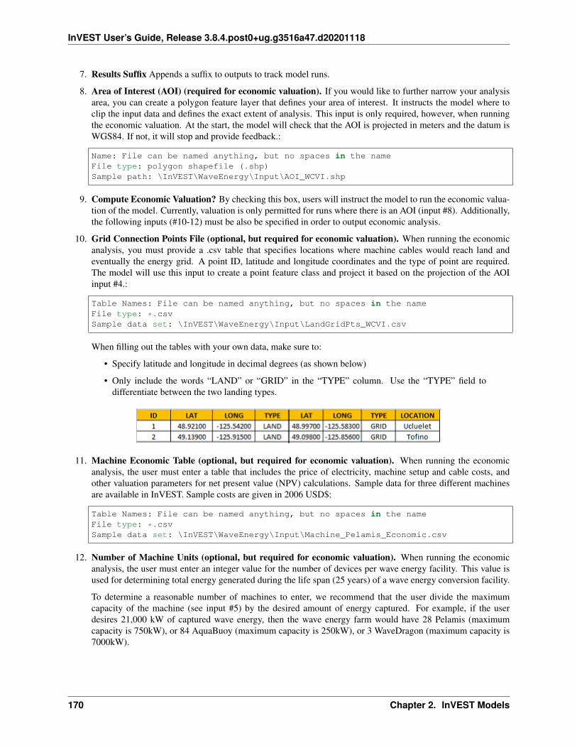
InVEST User’s Guide, Release 3.8.4.post0+ug.g3516a47.d20201118
7. Results Suffix Appends a suffix to outputs to track model runs.
8. Area of Interest (AOI) (required for economic valuation). If you would like to further narrow your analysisarea, you can create a polygon feature layer that defines your area of interest. It instructs the model where toclip the input data and defines the exact extent of analysis. This input is only required, however, when runningthe economic valuation. At the start, the model will check that the AOI is projected in meters and the datum isWGS84. If not, it will stop and provide feedback.:
Name: File can be named anything, but no spaces in the nameFile type: polygon shapefile (.shp)Sample path: \InVEST\WaveEnergy\Input\AOI_WCVI.shp
9. Compute Economic Valuation? By checking this box, users will instruct the model to run the economic valua-tion of the model. Currently, valuation is only permitted for runs where there is an AOI (input #8). Additionally,the following inputs (#10-12) must be also be specified in order to output economic analysis.
10. Grid Connection Points File (optional, but required for economic valuation). When running the economicanalysis, you must provide a .csv table that specifies locations where machine cables would reach land andeventually the energy grid. A point ID, latitude and longitude coordinates and the type of point are required.The model will use this input to create a point feature class and project it based on the projection of the AOIinput #4.:
Table Names: File can be named anything, but no spaces in the nameFile type: *.csvSample data set: \InVEST\WaveEnergy\Input\LandGridPts_WCVI.csv
When filling out the tables with your own data, make sure to:
• Specify latitude and longitude in decimal degrees (as shown below)
• Only include the words “LAND” or “GRID” in the “TYPE” column. Use the “TYPE” field todifferentiate between the two landing types.
11. Machine Economic Table (optional, but required for economic valuation). When running the economicanalysis, the user must enter a table that includes the price of electricity, machine setup and cable costs, andother valuation parameters for net present value (NPV) calculations. Sample data for three different machinesare available in InVEST. Sample costs are given in 2006 USD$:
Table Names: File can be named anything, but no spaces in the nameFile type: *.csvSample data set: \InVEST\WaveEnergy\Input\Machine_Pelamis_Economic.csv
12. Number of Machine Units (optional, but required for economic valuation). When running the economicanalysis, the user must enter an integer value for the number of devices per wave energy facility. This value isused for determining total energy generated during the life span (25 years) of a wave energy conversion facility.
To determine a reasonable number of machines to enter, we recommend that the user divide the maximumcapacity of the machine (see input #5) by the desired amount of energy captured. For example, if the userdesires 21,000 kW of captured wave energy, then the wave energy farm would have 28 Pelamis (maximumcapacity is 750kW), or 84 AquaBuoy (maximum capacity is 250kW), or 3 WaveDragon (maximum capacity is7000kW).
170 Chapter 2. InVEST Models

InVEST User’s Guide, Release 3.8.4.post0+ug.g3516a47.d20201118
Running the Model
The model is available as a standalone application accessible from the Windows start menu. For Windows 7 or earlier,this can be found under All Programs -> InVEST |version| -> Wave Energy. Windows 8 users can find the applicationby pressing the windows start key and typing “wave” to refine the list of applications. The standalone can also befound directly in the InVEST install directory under the subdirectory invest-3_x86/invest_wave_energy.exe.
Viewing Output from the Model
Upon successful completion of the model, a file explorer window will open to the output workspace specified in themodel run. This directory contains an output folder holding files generated by this model. Those files can be viewedin any GIS tool such as ArcGIS, or QGIS. These files are described below in Section Interpreting Results.
Interpreting Results
Model Outputs
The following is a short description of each of the outputs from the Wave Energy model. Each of these output filesis automatically saved in the “Output” & “Intermediate” folders that are saved within the user-specified workspacedirectory:
Output Folder
• Output\wp_kw & Output\wp_rc
– These raster layers depict potential wave power in kW/m for the user-specified extent. The latter (“_rc”) isthe former reclassified by quantiles (1 = < 25%, 2 = 25-50%, 3 = 50-75%, 4 = 75-90%, 5 = > 90%). The(“_rc”) raster is also accompanied by a csv file that shows the value ranges for each quantile group as wellas the number of pixels for each group.
– The potential wave power map indicates wave power resources based on wave conditions. These oftenprovide the first cut in the siting process for a wave energy project.
• Output\capwe_mwh & Output\capwe_rc
– These raster layer depict captured wave energy in MWh/yr per WEC device for the user-specified extent.The latter (“_rc”) is the former reclassified by quantiles (1 = < 25%, 2 = 25-50%, 3 = 50-75%, 4 = 75-90%, 5 = > 90%). The (“_rc”) raster is also accompanied by a csv file that shows the value ranges for eachquantile group as well as the number of pixels for each group.
2.2. Final Ecosystem Services: 171

InVEST User’s Guide, Release 3.8.4.post0+ug.g3516a47.d20201118
– The captured wave energy map provides useful information to compare the performance of different WECdevices as a function of site-specific wave conditions.
• Output\npv_usd & Output\npv_rc
– These raster layers depict net present value in thousands of $ over the 25 year life-span of a WEC facilityfor the user-specified extent. The latter (“_rc”) is positive values of the former reclassified by quantiles (1= < 25%, 2 = 25-50%, 3 = 50-75%, 4 = 75-90%, 5 = > 90%). The (“_rc”) raster is also accompanied by acsv file that shows the value ranges for each quantile group as well as the number of pixels for each group.
– The NPV map indicates the economic value of a WEC facility composed of multiple devices. A positivevalue indicates net benefit; a negative value indicates a net loss. Such information can be used to locatepotential areas where a wave energy facility may be economically feasible.
– These are only an output if you have chosen to run economic valuation.
• Output\LandPts_prj.shp and GridPt_prj.shp
– These feature layers contain information on underwater cable landing location and power grid connectionpoints.
– The landing and grid connection points provide useful information for interpreting the NPV map.
– It is only an output if the user chooses to run the economic valuation.
• Parameters_[yr-mon-day-min-sec].txt
– Each time the model is run a text file will appear in the workspace folder. The file will list the parametervalues for that run and be named according to the date and time.
– Parameter log information can be used to identify detailed configurations of each of scenario simulation.
Intermediate Folder
• intermediate\WEM_InputOutput_Pts.shp
– These point layers from the selected wave data grid are based on inputs #2-4.
– They contain a variety of input and output information, including:
* I and J – index values for the wave input grid points
* LONG and LAT – longitude and latitude of the grid points
* HSAVG_M – wave height average [m]
* TPAVG_S – wave period average [second]
* DEPTH_M – depth [m]
* WE_KWM – potential wave power [kW/m]
* CAPWE_MWHY – captured wave energy [MWh/yr/WEC device]
* W2L_MDIST – Euclidean distance to the nearest landing connection point [m]
* LAND_ID – ID of the closest landing connection point that is closest
* L2G_MDIST – Euclidean distance from LAND_ID to the nearest power grid connection point [m]
* UNITS – number of WEC devices assumed to be at this WEC facility site
* CAPWE_ALL – total captured wave energy for all machines at site [MWh/yr/WEC facility]
* NPV_25Y – net present value of 25 year period [thousands of $]
172 Chapter 2. InVEST Models

InVEST User’s Guide, Release 3.8.4.post0+ug.g3516a47.d20201118
– The model outputs in raster format are interpolated results based on these point data. So, you can usethis point information to explore the exact values of essential inputs and outputs at wave input data pointlocations.
• intermediate\GridPt.txt and LandPts.txt + These text files log records of the grid and landing point coordinates.+ This is only an intermediate output if you choose to run economic valuation.
Case Example Illustrating Results
The following example illustrates the application of the wave energy model to the west coast of Vancouver Island(WCVI). The figures and maps are for example only, and are not necessarily an accurate depiction of WCVI. In thisexample, we use input data layers including:
1. Wave base data = West Coast of North America with 4-minute resolution 2. Area of Interest = AOI_WCVI.shp3. WEC device = Pelamis 4. Digital Elevation Model = global_dem 5. Landing and Power Grid ConnectionPoints = LandGridPts_WCVI.shp 6. Number of Machine Units = 28 7. Projection = WGS 1984 UTM Zone10N.prj
In order to generate a grid-scale power producing facility, it is necessary to capture a minimum of 10 kW/m of wavepower (Spaulding and Grilli 2010). Along the WCVI, this threshold is generally met, with the annual mean wavepower >10 kW/m in most areas. Wave power gradually increases offshore. Approximately 20 kW/m wave power isavailable within 10 km of the shore, but the maximum wave power, 30-40 kW/m, is available 20-60 km offshore wheredepth is > 150 m.
Fig. 10: Wave power potential (kW/m) in the west coast of Vancouver Island.
Captured wave energy in this example is calculated based on Pelamis devices with 750 kW power rating. The overallpatterns of the captured wave energy are similar to those of potential wave power. A Pelamis device located at the50-70 m depth contour produces approximately 2,000-2,300 MWh/yr of energy. Assuming 15 MWh/yr energy use perhousehold in the WCVI (Germain 2003), each Pelamis unit produces enough energy to support 133-153 households.
For the economic valuation of harvested wave energy, we calculate and map NPV over the 25-yr life-span of a WECfacility. For this example model run, each of the WEC facilities is composed of 28 Pelamis devices. We used anestimate of $100,000 for the underwater cable cost and 20 cents/kW for the price of electricity. Positive NPV occursfrom 5-10 km offshore from the shoreline. It increases offshore and the highest NPV (the top 20% of all calculatedNPV values ($4668k - $7307k)) occurs between 25-90 km from the shore.
2.2. Final Ecosystem Services: 173
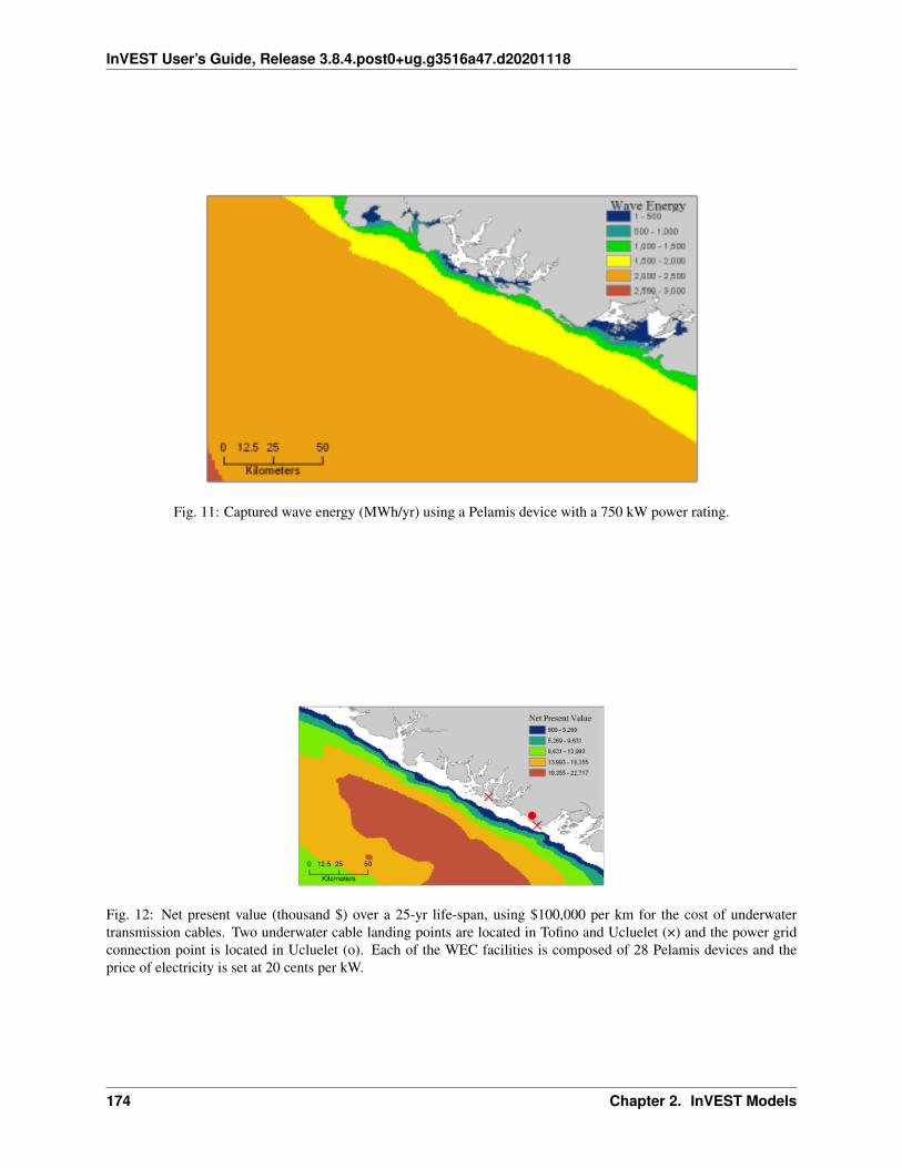
InVEST User’s Guide, Release 3.8.4.post0+ug.g3516a47.d20201118
Fig. 11: Captured wave energy (MWh/yr) using a Pelamis device with a 750 kW power rating.
Fig. 12: Net present value (thousand $) over a 25-yr life-span, using $100,000 per km for the cost of underwatertransmission cables. Two underwater cable landing points are located in Tofino and Ucluelet (×) and the power gridconnection point is located in Ucluelet (o). Each of the WEC facilities is composed of 28 Pelamis devices and theprice of electricity is set at 20 cents per kW.
174 Chapter 2. InVEST Models

InVEST User’s Guide, Release 3.8.4.post0+ug.g3516a47.d20201118
Because there have been no commercial-scale wave energy facilities implemented to date, large uncertainties exist inthe economic parameters. In particular, the cost of underwater transmission cables is highly uncertain, ranging from$100,000 to $1,000,000 per km. The NPV uses a lower bound of $100,000 per km for the cable cost. When we usea median cost of underwater transmission cables ($500,000 per km), the area with a positive NPV is significantlyreduced.
In this example, positive NPV only occurs within a 50 km radius around the two underwater cable landing points inTofino and Ucluelet. The upper 20% NPV exists between 10-40 km distances from the two landing points. When theupper bound ($1,000,000 per km) of transmission cable costs is used, no positive NPV exist in the WCVI. Consid-ering uncertainties in economic parameters, users should be cautious in interpreting the magnitude of the NPV. Werecommend that the NPV of a wave energy facility computed with the default values be used only to make relativecomparisons between sites.
Fig. 13: Net present value (thousand $) over a 25-yr life-span, using $500,000 per km for the cost of underwatertransmission cables. Two underwater cable landing points are located in Tofino and Ucluelet (×) and power gridconnection point is located in Ucluelet (o). Each of the WEC facilities is composed of 28 Pelamis devices. The priceof electricity is set at 20 cents per kW.
Appendix A
Data Sources
This is a rough compilation of data sources and suggestions for finding, compiling, and formatting data. This sectionshould be used for ideas and suggestions only. We will continue to update this section as we learn about new datasources and methods.
• Wave data: significant wave height (𝐻𝑠) and peak wave period (𝑇𝑝)
– Global ocean wave buoy data are available from NOAA’s National Data Buoy Center (http://www.ndbc.noaa.gov/). Although ocean wave buoy provides the most accurate wave time series data, their spatialresolution is very coarse and it may not be appropriate for local scale analysis.
– NOAA’s National Weather Service provides WAVEWATCH III model hindcast reanalysis results (http://polar.ncep.noaa.gov/waves/index2.shtml). The spatial resolution of the model results ranges from 4 to 60minutes depending on the global and regional grid systems. The model outputs have been saved at 3-hourinterval from 1999 to the present. The model results have been validated with ocean buoy data at manylocations and provide good quality wave information.
• Water depth
– NOAA’s National Geophysical Data Center (NGDC) provides global bathymetry data with various spatialresolutions at http://www.ngdc.noaa.gov/mgg/bathymetry/relief.html.
– ETOPO1 is a 1 arc-minute global relief model of Earth’s surface that integrates land topography and oceanbathymetry. It was built from numerous global and regional data sets, and is available in “Ice Surface”
2.2. Final Ecosystem Services: 175

InVEST User’s Guide, Release 3.8.4.post0+ug.g3516a47.d20201118
(top of Antarctic and Greenland ice sheets) and “Bedrock” (base of the ice sheets) versions. NGDC alsoprovides regional and other global bathymetry datasets.
• Wave energy absorption performance
– EPRI wave energy conversion project provides a review of several WEC devices: http://oceanenergy.epri.com/waveenergy.html
– Recent updates on technology may be available from the WEC device manufactures.
* PWP-Pelamis: http://www.pelamiswave.com/
* AquaBuOY: http://www.finavera.com/
* WaveDragon: http://www.wavedragon.net/
* DEXAWAVE: http://www.dexawave.com/
References
Amante, C., and B. W. Eakins. 2009. ETOPO1 1 Arc-minute global relief model: procedures, data sources andanalysis, p. 19. NOAA Technical Memorandum NESDIS NGDC-24.
Barstow, S., G. Mørk, D. Mollison, and J. Cruz. 2008. The wave energy resource, p. 94-131. In J. Cruz [ed.], OceanWave Energy: current status and future prepectives. Springer.
Bedard, R., G. Hagerman, M. Previsic, O. Siddiqui, R. Thresher, and B. Ram. 2005. Offshore wave power feasibilitydemonstration project: final summary report, p. 34. Electric Power Research Institute Inc.
Boehlert, G. W., G. R. Mcmurray, and C. E. Tortorici. 2007. Ecological effects of wave energy development in thePacific Nothwest, p. 174. U.S. Dept. Commerce, NOAA Tech. Memo.
Cornett, A., and J. Zhang. 2008. Nearshore wave energy resources, Western Vancouver Island, B.C., p. 68. CanadianHydraulics Centre.
Cornett, A. M. 2008. A global wave energy resource assessment. Proc. ISOPE 2008.
Dunnett, D., and J. S. Wallace. 2009. Electricity generation from wave power in Canada. Renewable Energy 34:179-195.
Germain, L. A. S. 2003. A case study of wave power integration into the Ucluelet area electrical grid. Master Thesis.University of Victoria.
Iglesias, G., and R. Carballo. 2010. Wave energy and nearshore hot spots: the case of the SE Bay of Biscay. RenewableEnergy 35: 2490-2500.
Kim, C.K.
Kim, C.K., J. Toft, M. Papenfus, G. Verutes, A. Guerry, M. Ruckelshaus, K. Arkema et al. 2012. Catching the rightwave: evaluating wave energy resources and potential compatibility with existing marine and coastal uses. PloS one7, no. 11: e47598.
Nelson, P. A. and others 2008. Developing wave energy in coastal California: potential socio-economic and environ-mental effects, p. 182. California Energy Commission, PIER Energy-Related Environmental Research Program, andCalifornia Ocean Protection Council.
Pelamis Wave Power Ltd. 2010. Pelamis Wave Power. http://www.pelamiswave.com/.
Plummer, M. and B. Feist. 2016. Capturing energy from the motion of the ocean in a crowded sea. Coastal Manage-ment 44, no. 5: 1-22.
Previsic, M. 2004a. System level design, performance and costs - San Francisco California Energetech offshore wavepower plant. EPRI.
176 Chapter 2. InVEST Models

InVEST User’s Guide, Release 3.8.4.post0+ug.g3516a47.d20201118
—. 2004b. System level design, performance and costs for San Francisco California Pelamis offshore wave powerplant, p. 73. EPRI.
Spaulding, M. L., and A. Grilli. 2010. Application of technology development index and principal component analysisand cluster methods to ocean renewable energy facility siting. Marine Technology Society Journal 44: 8-23.
Thorpe, T. W. 1999. A brief review of wave energy, p. 186. The UK department of trade and industry.
Wilson, J. H., and A. Beyene. 2007. California wave energy resource evaluation. Journal of coastal research 23:679-690.
2.2.10 Offshore Wind Energy Production
Summary
Offshore wind energy is gaining interest worldwide, with 5,400megawatts (MW) installed as of January 2013 and a growth ratearound 25% per year (GWEC, 2013). Consistently higher off-shore winds and proximity to coastal load centers serve as two ofthe major reasons wind energy developers are looking offshore.The goal of the InVEST offshore wind energy model is to providespatial maps of energy resource availability, energy generationpotential, and (optionally) energy generation value to allow usersto evaluate siting decisions, use tradeoffs, and an array of othermarine spatial planning questions. The model was developed toallow maximum flexibility for the user, in that it can be run withdefault data and parameters, but it can just as easily be updatedwith new turbine and foundation information, grid connection in-formation, and parameter values that fit the user’s context. Modeloutputs include wind power potential, energy generation, offsetcarbon emissions, net present value, and levelized cost of energy,all given at the farm level.
Peer-reviewed references for this model are http://dx.doi.org/10.1016/j.aquaculture.2014.10.035 for the financial portion ofthe model and http://dx.doi.org/10.1016/j.marpol.2015.09.024for the physical portion.
Introduction
This wind energy model provides an easily replicable interfaceto assess the viability of wind energy in your region under dif-ferent farm design scenarios. The outputs are raster maps, whosepoint values represent the aggregate value of a farm centered atthat point. This allows for detailed analysis of siting choices ata fine scale, though it comes at the cost of assuming that condi-tions are sufficiently symmetric around the center point so thatthe center point represents the median conditions of all turbinesin the farm. Since the user can select the number of turbines forthe farm, and the raster maps do not give an indication of farmsize, the model also outputs a representative polyline polygon ata randomly selected wind data point that indicates the size of thefarm.
2.2. Final Ecosystem Services: 177

InVEST User’s Guide, Release 3.8.4.post0+ug.g3516a47.d20201118
To run the model, you are asked to supply information into thegraphical user interface. This includes information about windenergy conditions, the type of turbine, number of turbines, thearea of interest, etc. To make the model easier to run, it includesdefault data in .csv tables on two common offshore wind turbines:3.6 MW and 5.0 MW. We also include two wind speed datasets:a global dataset and a dataset covering the Northwest Atlantic.Finally, it includes a table of less commonly changed default val-ues used to parameterize various parts of the model, called the“Global Wind Energy Parameters” file. These .csv files are re-quired inputs, and may be modified if alternate values are desiredby directly editing the files using a text editor or Microsoft Ex-cel. When modifying these files, it is recommended that the usermake a copy of the default .csv file so as not to lose the originaldefault values.
The Model
Wind Energy Potential
The wind energy model estimates wind power density (windpower potential) to identify offshore areas with high energy po-tential. The wind power density 𝑃𝐷(𝑊𝑚−2) at a certain loca-tion can be approximated as a function of wind statistics (Elliottet al., 1986)
1
2𝜌
𝑐∑︁𝑗=1
𝑓(𝑉𝑗)𝑉3𝑗 (2.62)
where, 𝜌 is mean air density (𝑘𝑔𝑚−3), 𝑗 is the index of windspeed class, 𝑐 is the number of wind speed classes, 𝑉𝑗 is windspeed of the jth class (𝑚𝑠−1), and 𝑓(𝑉𝑗) is probability densityfunction of 𝑉𝑗 . Two probability distributions are commonly usedin wind data analysis: 1) the Rayleigh and 2) the Weibull distribu-tions (Manwell et al. 2009). The Weibull distribution can betterrepresent a wider variety of wind regimes (Celik 2003; Manwellet al. 2009), and is given as
𝑓(𝑉𝑗) =𝑘
𝜆
(︂𝑉𝑗
𝜆
)︂𝑘−1
𝑒−(︁
𝑉𝑗𝜆
)︁𝑘
(2.63)
where, 𝑘 and 𝜆 are the shape and scale factors, respectively. The shape factor, 𝑘, determines the shape of theWeibull probability density function (Figure 14). The probability density function shows a sharper peak as 𝑘 in-creases, indicating that there are consistent wind speeds around the mean wind speed. On the other hand, the functionbecomes smoother as k decreases, indicating more variation in wind speed and more frequent low and high windspeeds. The model requires wind speed inputs to be in terms of the estimated Weibull parameters, versus takingin raw wind speed data. For our sample data we used a MATLAB function, wblfit, to estimate 𝑘 and 𝜆 at thewind speed reference height (height at which wind speeds were observed or estimated), which returns the maxi-mum likelihood estimates of the parameters of the Weibull distribution given the values in the wind time series data.This was done for each wind speed observation point. The model For more details of wblfit function, please con-sult http://www.mathworks.co.kr/kr/help/stats/wblfit.html. This can also be accomplished in R (see here for tutorial:http://stats.stackexchange.com/questions/60511/weibull-distribution-parameters-k-and-c-for-wind-speed-data).
Wind power density is calculated at the hub height 𝑍 (m) ofa wind turbine (Figure 14), which means all variables in (2.9)
178 Chapter 2. InVEST Models

InVEST User’s Guide, Release 3.8.4.post0+ug.g3516a47.d20201118
Fig. 14: Example of Weibull probability density function with various shape factors (𝑘), where mean wind velocity =6𝑚𝑠−1 (Manwell et al., 2009).
and (2.10) need to be converted into the appropriate value at hubheight. Mean air density 𝜌 was estimated as 𝜌 = 1.225− (1.194 ·10−4)𝑍, which approximates the U.S. Standard Atmosphere pro-file for air density (National Oceanic and Atmospheric Adminis-tration, 1976). We applied the wind profile power law to estimatewind speed (𝑉 ) at hub height 𝑍 (Elliott et al., 1986).
𝑉
𝑉𝑟=
(︂𝑍
𝑍𝑟
)︂𝛼
(2.64)
where 𝑉 is wind speed (𝑚𝑠−1) at the hub height 𝑍 (m) of a windturbine, and 𝑉𝑟𝑖𝑠 wind speed (𝑚𝑠−1) at the reference height 𝑍𝑟
(m) where wind data are obtained. 𝛼 is power law exponent,which is an empirically derived coefficient and varies with thestability of the atmosphere. For neutral stability condition, 𝛼 isapproximately 1/7 (0.143) for land surfaces, which is widely ap-plicable to adjust wind speed on land (Elliott et al., 1986). Thepower law exponent has different value on ocean surfaces. Hsuet al. (1994) found that 𝛼 = 0.11 ± 0.03 for ocean surface under near-neutral atmospheric stability conditions. Thewind energy model uses 𝛼 = 0.11 as a default value to adjust wind speed on the ocean surface. The wind profile of theatmospheric boundary layer can be approximated more accurately using the log wind profile equation that accountsfor surface roughness and atmospheric stability (Manwell et al. 2009).
Wind power density (PD) outputs provide suitability informationfor a wind energy development project in terms of wind resource.Pacific Northwest Laboratories categorized wind power densityand wind speed into seven classes based on United States windatlas (Figure 16) (Manwell et al. 2009). Areas designated as class4 or greater are considered to be suitable for most wind energydevelopment. Class 3 areas are suitable for wind energy develop-
2.2. Final Ecosystem Services: 179

InVEST User’s Guide, Release 3.8.4.post0+ug.g3516a47.d20201118
Fig. 15: A schematic diagram of a wind turbine (http://www.daviddarling.info/encyclopedia/H/AE_hub_height.html)
ment if large turbines are used. Class 1 and 2 are rarely consid-ered as suitable areas for wind energy development in terms ofenergy potential. Wind resources vary considerably over spaceand a more detailed categorization of wind power density forfive topographical conditions was developed in Europe, whichincludes sheltered terrain, open plain, sea coast, open sea, hillsand ridges (Figure 16) (Manwell et al. 2009). The wind resourceclassification for sea coast and open sea may provide better infor-mation on the suitability of offshore wind energy projects.
Fig. 16: Wind power density (PD) and wind speed classes based on European wind atlas (Modified from Table 2.6 inManwell et al. 2009).
180 Chapter 2. InVEST Models

InVEST User’s Guide, Release 3.8.4.post0+ug.g3516a47.d20201118
Energy Generation
The amount of energy harvestable from a wind turbine in a par-ticular location depends on the characteristics of the wind turbineas well as wind conditions (Pallabazzer 2003; Jafarian & Ran-jbar 2010). The wind energy model quantifies the harvestableenergy based on the output power curve of a wind turbine andwind speed statistics. Figure 17 shows an output power curveof a wind turbine (pitch control type). The wind turbine starts togenerate power at the cut-in wind speed (𝑉𝑐𝑖𝑛). The output powerincreases up to the rated power (Prate) as wind speed increases tothe rated wind speed (𝑉𝑟𝑎𝑡𝑒). The wind turbine keeps produc-ing the maximum power (i.e., Prate) until wind speed reaches thecut-out wind speed (𝑉𝑐𝑜𝑢𝑡). If wind speed increases beyond thecut-out wind speed, the wind turbine stops generating power forsafety purposes. Currently, more than 74 offshore wind farmsare operating globally and technology specific information of thewind turbine at each wind farm are available at LORC Knowl-edge (2012).
Fig. 17: Output power (P) curve of a wind turbine (pitch control type) as a function of wind speed (V) (Modified fromFig.1 in Pallabazzer 2003)
To provide flexibility for a variety of different turbine types with-out requiring the user to manually enter a power curve, we esti-mate the output power 𝑃 (kW) of a wind turbine using a polyno-mial modeling approach (Jafarian & Ranjbar 2010):
𝑃 (𝑉 ) =
⎧⎨⎩ 0 𝑉 < 𝑉𝑐𝑖𝑛 or 𝑉 > 𝑉𝑐𝑜𝑢𝑡
𝑃𝑟𝑎𝑡𝑒 𝑉𝑟𝑎𝑡𝑒 < 𝑉 < 𝑉𝑐𝑜𝑢𝑡
(𝑉 𝑚 − 𝑉 𝑚𝑖𝑛 )/(𝑉 𝑚
𝑟𝑎𝑡𝑒 − 𝑉 𝑚𝑖𝑛 ) 𝑉𝑐𝑖𝑛 ≤ 𝑉 ≤ 𝑉𝑟𝑎𝑡𝑒
(2.65)
where, 𝑚 is an exponent of the output power curve (usually 1 or2). Using this approach, the energy output, O (MWh), generated
2.2. Final Ecosystem Services: 181

InVEST User’s Guide, Release 3.8.4.post0+ug.g3516a47.d20201118
by a wind turbine can be calculated using
𝑂 = 𝑛𝑑𝑎𝑦 · 𝜌
𝜌0𝑃𝑟𝑎𝑡𝑒
(︃∫︁ 𝑉𝑟𝑎𝑡𝑒
𝑉𝑐𝑖𝑛
𝑉 𝑚 − 𝑉 𝑚𝑐𝑖𝑛
𝑉 𝑚𝑟 − 𝑉 𝑚
𝑐𝑖𝑛
𝑓(𝑉 )𝑑𝑉 +
∫︁ 𝑉𝑐𝑜𝑢𝑡
𝑉𝑟𝑎𝑡𝑒
𝑓(𝑉 )𝑑𝑉
)︃(1 − 𝑙𝑜𝑠𝑠𝑟𝑎𝑡𝑒)
(2.66)
where, 𝑛𝑑𝑎𝑦 is the number of days for energy output (e.g.𝑛𝑑𝑎𝑦 = 365 days for annual energy output), 𝜌0 is air density ofstandard atmosphere (e.g. 1.225𝑘𝑔𝑚−3 for U.S. standard atmo-sphere air density at sea level), and 𝑙𝑜𝑠𝑠𝑟𝑎𝑡𝑒 is a decimal valuewhich represents energy losses due to a combination of down-time, power conversion efficiency, and electrical grid losses (de-fault value is .05). All of these parameters are included in the global parameters .csv file and may be changed by theuser from their defaults. Total farm energy output is equal to the individual turbine output multiplied by the numberof turbines, 𝑛,
𝐸 = 𝑛𝑂 (2.67)
The InVEST software comes with default technical and financial information about two common turbine sizes, the3.6 MW and 5.0 MW turbines. The information for each turbine is given in .csv files in the Input directory and isa required input into the model. The user can use the default data, edit a file, or create a new file to assess differentturbine sizes or update specific characteristics. The files must retain the same format - only parameter values maysafely be modified. It is recommended to save edits as new .csv files rather than overwriting the default data.
Offset Carbon
Since wind turbines create no greenhouse gasses when generat-ing energy, the user may be interested in assessing the amount ofcarbon dioxide emissions avoided by building a wind farm ver-sus a conventional energy generation plant. To translate carbon-free wind power to a representative amount of annual avoidedCO2 emissions, we use the following default conversion factor:6.8956 · 10−4metric tons CO2/𝑘𝑊ℎ
This is obtained from the EPA (http://www.epa.gov/cleanenergy/energy-resources/refs.html) and is based on 2007 data. See theirwebsite for limitations of this approach. The parameter is rep-resentative of the carbon emitted by the energy portfolio of theUnited States and may not be appropriate for your context. Thisvalue is changeable in the global parameters .csv file.
Value of Power
The value of wind power is measured as the discounted pre-taxnet revenue from power generation that would accrue to a windpower developer/operator over the expected lifetime of a windfarm. The Net Present Value (http://en.wikipedia.org/wiki/Net_present_value) (NPV) of energy for a given wind farm is:
𝑁𝑃𝑉 =
𝑇∑︁𝑡=1
(𝑅𝑡 − 𝐶𝑡)(1 + 𝑖)−𝑡 (2.68)
182 Chapter 2. InVEST Models

InVEST User’s Guide, Release 3.8.4.post0+ug.g3516a47.d20201118
Where 𝑅𝑡 is the gross revenue collected in year 𝑡, and 𝐶𝑡 arethe aggregate costs in year 𝑡. 𝑇 represents the expected life-time of the facility, and 𝑖 represents the discount rate (http://en.wikipedia.org/wiki/Discount_rate) or weighted average cost ofcapital (WACC, http://en.wikipedia.org/wiki/Weighted_average_cost_of_capital). Both 𝑇 and 𝑖 can be changed by the user; 𝑇can be found in the global parameters .csv file and 𝑖 is enteredin the valuation section of the user interface. For projects thatare financed by both debt and equity and where there is a signifi-cant amount of risk associated with establishing and maintainingthe projected stream of revenues, WACC is a more appropriatemethod for establishing the time value of money. As this parameter enters into the calculation in the same way asa discount rate would, if you prefer you can input an appropriate discount rate and interpret the results accordingly.We do not supply a default value, but Levitt et al. (2011) suggest a WACC value of .116 based on a comprehensiveanalysis of industry specific discount rates and different debt/equity structures in Europe and the U.S. This is higherthan discount rates typically used elsewhere, such as in standard cost benefit analysis, so you may find your applicationjustifies a different rate.
Annual gross revenue is calculated by multiplying the price perkWh, 𝑠, by the annual amount of kWh supplied to the grid by awind farm, 𝐸𝑡, thus 𝑅𝑡 = 𝑠𝐸𝑡. It is assumed that energy is notcollected in the first year during the construction phase.
Costs can be separated into one-time capital costs and ongo-ing operations and management costs. During the constructionphase, expenditures are made on turbines, foundations, electricaltransmission equipment, and other miscellaneous costs associ-ated with development, procurement, and engineering. At the endof the farms usable lifetime, the firm must remove their equip-ment. The default information supplied is based on an extensivereview of peer-reviewed publications, industry reports, and pressreleases. This information is summarized below.
Turbines
Turbines and foundations are modeled with unit costs. We havesupplied cost data on 3.6 MW and 5.0 MW class turbines aswell as monopile and jacketed foundations, though you may en-ter your own turbine- or foundation-specific information. Noteall default costs below are given in 2012 US dollars. Assumingone foundation per turbine, the total cost of turbines and founda-tions is simply the number of wind turbines multiplied by the unitcost. Table 1 gives a summary of existing turbine costs.
Farm Location Capacity # of Turbines Total MW Unit Cost ($mil)Riffgat UK 3.6 30 108 6.3Sheringham Shoal UK 3.6 88 317 5.65Greater Gabbard UK 3.6 140 504 6.03Butendiek Germany 3.6 80 288 5.54London Array UK 3.6 175 630 6.29Amrumbank Germany 3.6 80 288 6.41Global Tech 1 Germany 5 80 400 10.4Borkum 2 Germany 5 40 200 10.6
2.2. Final Ecosystem Services: 183

InVEST User’s Guide, Release 3.8.4.post0+ug.g3516a47.d20201118
Table 1: Turbine costs.
Foundations
This model can flexibly include valuation for both foundation-based and floating turbine designs. This is accomplished by let-ting the user enter the appropriate unit cost information for theirfarm design. Outputs are constrained by user-editable depth anddistance parameters, so it is important to adjust these to reflectthe appropriate technological constraints of your design choice.Foundation-based turbines have conventionally been limited to adepth of around 60 meters.
Foundation cost information is relatively difficult to come by.Monopile foundations are the most common foundation type andare typically mated to 3.6 MW turbines. Ramboll, a major foun-dation manufacturer, estimates that monopile foundations with a3.6 MW turbine are $2 million per foundation. Monopile costs atBurbo and Rhyl Flats in the UK were given in press releases as$1.9 million $2.2 million respectively. Jacketed foundations aremore robust than monopile foundations and are typically usedwith 5.0 MW turbines and/or in deep water. Two press releasesfor Nordsee Ost (Germany) and Ormonde (UK) put the unit costsfor this type of foundation at $2.74 million and $2.43 million re-spectively. A 2012 release by the European Energy Programmefor Recovery put the cost of deepwater (40 meters) gravity foun-dations at Global Tech 1 (Germany) as $6.65 million per founda-tion.
All foundations should feature an increasing cost with depth asmaterial costs will necessarily be higher; however, this is not cap-tured in this model currently due to the paucity of project costdata to estimate such a relationship. Jacquemin et al. (2011) usedfield data to estimate foundation weight as a function of waterdepth; however the data and functions are not given making itimpossible to replicate their work. Nonetheless, this source doesprovide a means to approximate different foundation technologycosts including floating foundation technology. Samoteskul et al.(2014) demonstrate how the data from Jacquemin et al. (2011)can be used in this way.
Electricity Transmission
Electricity transmission equipment is much harder to model atthe component level because the optimal transmission system de-sign varies considerably with local conditions and wind farm de-sign. Depending on the size of the farm and its distance fromshore, offshore platforms with voltage transformers, converters,and switchgear may be needed. Additionally, there is a criti-cal point where a wind farm’s distance from the grid requires aswitch from alternating current (AC) power to direct current (DC)power to overcome line losses which reduce the amount of energydelivered. Given design variation across different contexts, we
184 Chapter 2. InVEST Models

InVEST User’s Guide, Release 3.8.4.post0+ug.g3516a47.d20201118
utilized a top-down modeling approach for transmission costs toallow the model to be used broadly without the need for exhaus-tive system modeling and unit cost information. We collectedinformation about electricity transmission costs (including instal-lation) from 20 wind farms and used it to estimate a relationshipbetween total costs and farm characteristics. This data was col-lected from the U.K. Ofgem tender process (http://www.ofgem.gov.uk/Networks/offtrans/Pages/Offshoretransmission.aspx) andis shown in Table 2.
Farm Cost (2012$Million)
MW Depth(m)
DC Land Cable(km)
Sea Cable(km)
Tot Cable(km)
Barrow 52.73 90 14 0 3 27 30Robin Rigg 93.25 180 6 0 1.8 12.5 14.3Gunfleet Sands 1& 2
75.8 173 6.5 0 3.8 9.3 13.1
SheringhamShoal
285.08 315 18.5 0 21.5 22.4 43.9
Ormonde 158.27 150 19 0 2.8 43 45.8Greater Gabbard 495.64 504 20.5 0 0.6 45.5 46.1Thanet 255.34 300 18.5 0 2.4 26.3 28.7Walney 1 173.56 183 21 0 2.7 45.3 48Walney 2 164.38 183 27 0 5 43.7 48.7Gwynt y Mor 449.38 576 27.5 0 11 41.4 52.4Lincs 456.44 250 9.5 0 12 48 60London ArrayPhase 1
699.28 630 11.5 0 0.8 54 54.8
Nordergrunde 89.82 111 7 0 4 28 32Dolwin 1 1221.81 800 30.5 1 90 75 165Dolwin 2 1021.5 900 29 1 90 45 135Helwin 2 817.51 690 28.5 1 45 85 130Sylwin 1 1393.38 864 26 1 45 160 205Helwin 1 718.71 576 23 1 45 85 130Borwin 2 718.71 800 40 1 75 120 195Borwin 1 598.83 400 40 1 75 125 200
Table 2: Offshore energy transmission infrastructure.
Using an ordinary least squares regression, we estimated the fol-lowing equation that relates total transmission costs to farm ca-pacity and total transmission cable distance:
𝑇𝑟𝑎𝑛𝑠𝐶𝑜𝑠𝑡 = 𝛽0𝑀𝑊 + 𝛽1𝑇𝑜𝑡𝐶𝑎𝑏𝑙𝑒 + 𝜖 (2.69)
To capture the effect of transmission losses due to resistance,we estimated this separately for each current type (AC and DC).Since our data suggest a critical threshold of greater than 54.8kmfor DC transmission, we adopt 60km as the transition point. Thisis also consistent with published figures regarding the cost effec-tiveness of transitioning from AC to DC transmission (CarbonTrust, 2008; UMaine, 2011); see Table 3
2.2. Final Ecosystem Services: 185

InVEST User’s Guide, Release 3.8.4.post0+ug.g3516a47.d20201118
Costs if ≤ 60km (AC) Costs if > 60km (DC)MW .81*** 1.09**
-0.15 -0.37Cables (km) 1.36 0.89
-1.19 -1.61Adj 𝑅2 0.937 0.951
Table 3, AC DC transmission costs. *p<.10, **p<.05, ***p<.01
These results provide a predictive model of transmission costs asa function of current type, total farm capacity in MW, and thetotal length of transmission cable in km. To calculate the totallength of transmission cable from any given offshore location,the model requires some information about the onshore grid. Theprovided options are meant to provide the user flexibility basedon data availability and common analysis questions. The user hastwo options:
• Create a .csv table that includes latitude and longitude details forall grid connection points in the area of interest
• Use a fixed parameter to model grid location
The table option gives the user the ability to indicate both land-ing points on the coastline and grid connection points. For eachpotential wind farm site (each ocean pixel that fits the other con-straints of the model and is in the AOI), the model identifies theclosest specified land point and calculates the straight-line dis-tance to that point. It then finds the closest grid connection pointand calculates the straight-line distance to that point. Summingthese two distances yields the total length of the transmission ca-bles used in the calculation for transmission costs in Table 3. Theuser can optionally omit landing points from the table and onlyinclude grid points: in this case the model simply calculates totallength of the transmission cable as the straightline distance fromeach potential wind farm location to the nearest grid point.
The fixed parameter option specifies a mean distance inland alongthe entire coast that represents the expected distance that overlandcables may have to travel to reach a grid connection. Since gridconnection points for large farms are very opportunistic and rep-resent a relatively small portion of capital costs, it is not unrealis-tic to model grid connection this way in the absence of a detailedgrid connection scheme. The default parameter included, 5.5 km,is the mean overland cable distance from the UK from the trans-mission infrastructure table above.
Above and beyond the cost of sending the energy to shore, windfarms also require cables which connect turbines to each other,called array cables. We estimated a simple linear relationshipbetween array cables and the number of turbines based on thedata given below:
186 Chapter 2. InVEST Models

InVEST User’s Guide, Release 3.8.4.post0+ug.g3516a47.d20201118
Farm Location # of Turbines km of cable Total Cost ($mil)Nordsee Ost Germany 48 63 14.3Amrumbank Germany 80 86 27.1Gwynt y Mor UK 160 148 34.7Anholt Denmark 111 160 41.4Baltic 2 Germany 80 80 32.5Sheringham Shoal UK 88 88 17.7
Table 4. Array cabling
The data above suggest that .91km of cable is required per turbineat a cost of $260,000 per km. This establishes a relationship ofarray cable to wind turbines which can retrieve the total cost ofarray cable based only on the number of turbines in the farm.
Other Costs
There are a variety of additional costs associated with the con-struction phase, such as those for development, engineering, pro-curement, and royalties. AWS Truewind (2010) estimate thesecosts to amount to 2% of total capital expenditures; Blanco(2009) indicates it could be as high as 8%. We adopt their methodof using a ratio of capital costs for calculating these costs and usethe mean value of 5% as the default .
Installation of foundations, turbines, and transmission gear (ca-bles and substations) comprises its own cost category. Kaiser andSnyder (2012) take a comprehensive view of installation costsand find that installation costs make up approximately 20% ofcapital expenditures in European offshore wind farms. Accord-ingly, this model treats installation costs as a fixed percentage oftotal capital costs and uses the default value suggested by Kaiserand Snyder (2012).
Decommissioning the facility at the end of its useful life (𝑡 =𝑇 ) enters into the model in a similar way as installation costs,in that it is a fixed fraction of capital expenditures. Kaiser andSnyder (2012) put this one-time cost at 2.6% to 3.7% of initialexpenditures (net of scrap value) for the Cape Wind farm using asophisticated decommissioning model. The default value used inthis model is 3.7%.
Most of the costs of an offshore wind energy farm are related tothe initial capital costs; however, there are ongoing costs relatedto maintenance and operations (O&M) as well. Boccard (2010)uses a methodology consistent with the rest of our modeling bycalculating annual O&M cost as a % of original capital costs, andputs the costs somewhere between 3 and 3.5. The default valueused in this model is 3.5%, and can be changed along with all theother costs in this section by editing the global parameters .csvfile.
2.2. Final Ecosystem Services: 187
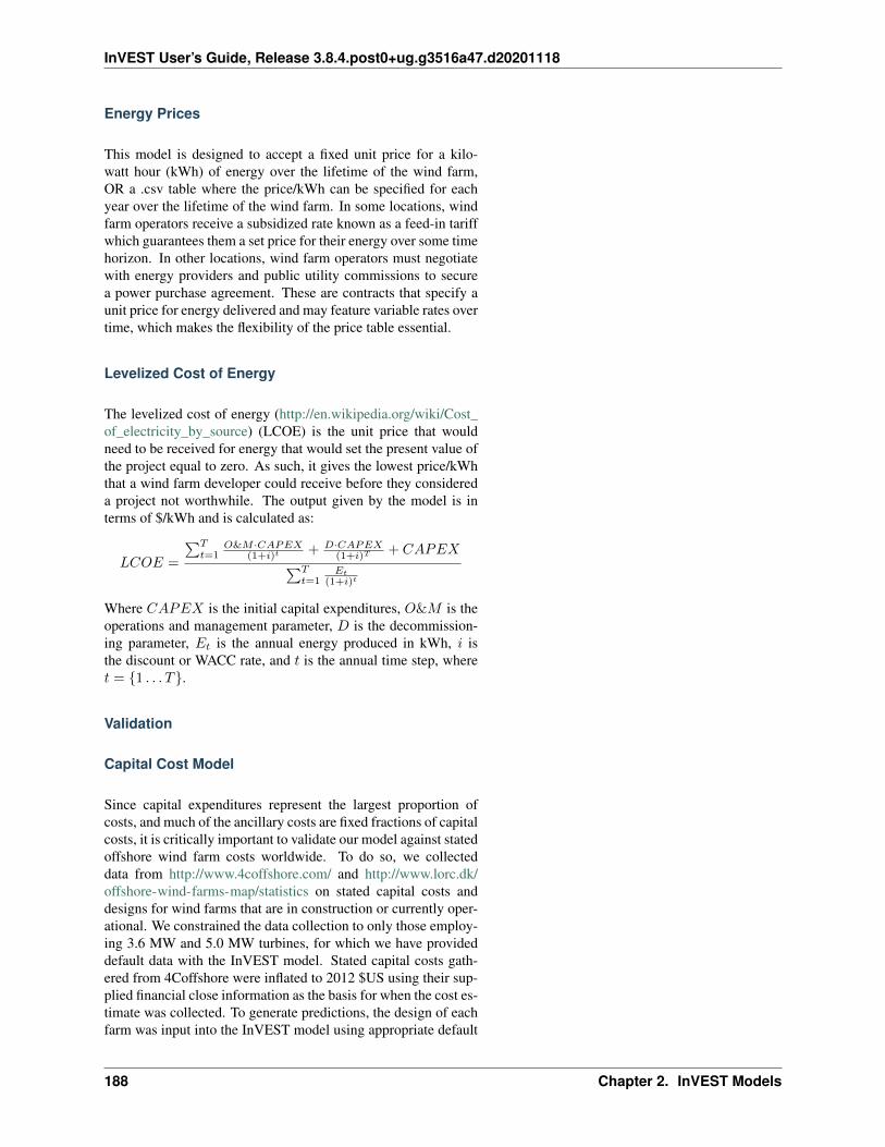
InVEST User’s Guide, Release 3.8.4.post0+ug.g3516a47.d20201118
Energy Prices
This model is designed to accept a fixed unit price for a kilo-watt hour (kWh) of energy over the lifetime of the wind farm,OR a .csv table where the price/kWh can be specified for eachyear over the lifetime of the wind farm. In some locations, windfarm operators receive a subsidized rate known as a feed-in tariffwhich guarantees them a set price for their energy over some timehorizon. In other locations, wind farm operators must negotiatewith energy providers and public utility commissions to securea power purchase agreement. These are contracts that specify aunit price for energy delivered and may feature variable rates overtime, which makes the flexibility of the price table essential.
Levelized Cost of Energy
The levelized cost of energy (http://en.wikipedia.org/wiki/Cost_of_electricity_by_source) (LCOE) is the unit price that wouldneed to be received for energy that would set the present value ofthe project equal to zero. As such, it gives the lowest price/kWhthat a wind farm developer could receive before they considereda project not worthwhile. The output given by the model is interms of $/kWh and is calculated as:
𝐿𝐶𝑂𝐸 =
∑︀𝑇𝑡=1
𝑂&𝑀 ·𝐶𝐴𝑃𝐸𝑋(1+𝑖)𝑡 + 𝐷·𝐶𝐴𝑃𝐸𝑋
(1+𝑖)𝑇+ 𝐶𝐴𝑃𝐸𝑋∑︀𝑇
𝑡=1𝐸𝑡
(1+𝑖)𝑡
Where 𝐶𝐴𝑃𝐸𝑋 is the initial capital expenditures, 𝑂&𝑀 is theoperations and management parameter, 𝐷 is the decommission-ing parameter, 𝐸𝑡 is the annual energy produced in kWh, 𝑖 isthe discount or WACC rate, and 𝑡 is the annual time step, where𝑡 = {1 . . . 𝑇}.
Validation
Capital Cost Model
Since capital expenditures represent the largest proportion ofcosts, and much of the ancillary costs are fixed fractions of capitalcosts, it is critically important to validate our model against statedoffshore wind farm costs worldwide. To do so, we collecteddata from http://www.4coffshore.com/ and http://www.lorc.dk/offshore-wind-farms-map/statistics on stated capital costs anddesigns for wind farms that are in construction or currently oper-ational. We constrained the data collection to only those employ-ing 3.6 MW and 5.0 MW turbines, for which we have provideddefault data with the InVEST model. Stated capital costs gath-ered from 4Coffshore were inflated to 2012 $US using their sup-plied financial close information as the basis for when the cost es-timate was collected. To generate predictions, the design of eachfarm was input into the InVEST model using appropriate default
188 Chapter 2. InVEST Models

InVEST User’s Guide, Release 3.8.4.post0+ug.g3516a47.d20201118
cost parameters for all components. Most farms have their ownelectrical transmission equipment, though some deepwater farmsare beginning to used centralized offshore substations that aggre-gate energy for transport from multiple farms. To predict elec-trical transmission costs for these farms, it was first necessary toestimate the cost of the entire offshore substation and then attribute a prorated capital cost to each farm based on theirrelative contribution to exported energy capacity. For example, an offshore substation with a 800 MW export capacitythat is connected to Farm A (200 MW) and Farm B (600 MW) would contribute 25% of capital costs to Farm A and75% to Farm B. The results of our validation show a very strong correlation between predictions and stated capitalcosts for 3.6 MW and 5.0 MW turbines using the default data (see Figure 5.6).
Fig. 18: Predicted capital costs versus stated capital costs.
Since this model was released in early 2013, it has been testedagainst other modeling approaches. They are noted below forreference:
1. The InVEST model was compared alongside model estimatesfrom the National Renewable Energy Laboratory (NREL) anda consulting firm in a report out of the University of Califor-nia, Santa Barbara, that measured the levelized cost of windenergy in Bermuda. InVEST was within 3% of the NRELestimate and 12% of the estimate made by the consultingfirm. http://www.bren.ucsb.edu/research/2014Group_Projects/documents/BermudaWind_Final_Report_2014-05-07.pdf
Limitations and Simplifications
2.2. Final Ecosystem Services: 189

InVEST User’s Guide, Release 3.8.4.post0+ug.g3516a47.d20201118
Energy Production
The quality of wind input data determines the accuracy of modelresults. So, users need to understand the quality of wind inputdata for proper interpretation of the model results. The defaultwind input data are more appropriate for global and regional scaleapplications at 4 or 60 minutes spatial resolution.
Harvested wind energy indicates the averaged energy output fora given period based on the output power curve of a wind tur-bine. Users may want to consider additional technology-specificinformation, such as device availability, power conversion effi-ciency, and directional factors by applying adjustment factors tothe harvested energy output.
Energy Valuation
As the validation section demonstrates, the model and the defaultdata reliably predict capital costs using the supplied inputs. Rev-enues are linked to energy production and a user-entered price.More reliable cost projections over space could likely be attainedby:
• Creating a foundation cost function that accounts for higher costsin deeper waters
• Having installation costs vary as a function of bottom geology
These are features that are being explored for subsequent modelupdates conditional on data availability.
The model is amenable to producing valuation outputs for float-ing turbines, but was not designed specifically for this task. Toproduce outputs, the user needs to input reasonable values fordepth and distance constraints as well as “foundation” costs equalto the unit cost of the aggregate equipment needed to float a tur-bine. The electrical transmission cost model was derived usingtechnologies that are suitable to roughly 60 meters depth and 200kilometers distance from shore and will likely produce less accu-rate cost projections outside of those bounds.
Data Needs
Inputs
1. Workspace Select a folder to be used as your workspace. If thefolder you select does not exist, a new one will be created. Thisfolder will contain the rasters produced by this model. If datasetsalready exist in this folder, they will be overwritten. The outputwill be contained in an folder named output inside the workspacedirectory.
2. Results Suffix (Optional) A string that will be added to the endof the output file paths.
190 Chapter 2. InVEST Models

InVEST User’s Guide, Release 3.8.4.post0+ug.g3516a47.d20201118
3. Wind Data Points A .csv file that represents the wind input data(Weibull parameters). The column headers are: LONG, LATI,LAM, K, REF. LAM is the Weibull scale factor at the referencehub height. K is the Weibull shape factor. REF is the referenceheight at which wind speed data was collected and LAM was es-timated at. Sample data files are found in the WindEnergyinputdirection inside the InVEST installation directory.
• Global Data: GLobal_EEZ_WEBPAR_90pct_100ms.csv
• East Coast of the US: ECNA_EEZ_WEBPAR_Aug27_2012.csv
4. Area Of Interest (Optional) An optional polygon shapefile thatdefines the area of interest. The AOI must be projected with lin-ear units equal to meters. If the AOI is provided it will clip andproject the outputs to that of the AOI. The distance inputs aredependent on the AOI and will only be accessible if the AOI isselected. If the AOI is selected and the distance parameters areselected, then the AOI should also cover a portion of the landpolygon to calculate distances correctly. An AOI is required forvaluation.
5. Bathymetric DEM A raster dataset for the elevation values inmeters of the area of interest. The DEM should cover at least theentire span of the area of interest and if no AOI is provided thenthe default global DEM should be used.
6. Land Polygon for Distance Calculation A polygon shapefilethat represents the land and coastline that is of interest. For thisinput to be selectable the AOI must be selected. The AOI shouldalso cover a portion of this land polygon to properly calculate dis-tances. This coastal polygon, and the area covered by the AOI,form the basis for distance calculations for wind farm electricaltransmission. This input is required for masking by distance val-ues and for valuation.
7. Global Wind Energy Parameters A .csv file that holds windenergy model parameters for both the biophysical and valuationmodules. These parameters are defaulted to values that are re-viewed in the The Model section of this guide. We recommendcareful consideration before changing these values.
Turbine Properties
8. Turbine Type A .csv file that contains parameters correspondingto a specific turbine type. The InVEST package comes with twoturbine model options, 3.6 MW and 5.0 MW. You may create anew turbine class (or modifying existing classes) by using the ex-isting file format conventions and filling in your own parameters.It is recommended that you do not overwrite the existing default.csv files. These files are found in the WindEnergyinput directioninside the InVEST installation directory and named
• 3.6 MW: 3_6_turbine.csv
• 5.0 MW: 5_0_turbine.csv
2.2. Final Ecosystem Services: 191

InVEST User’s Guide, Release 3.8.4.post0+ug.g3516a47.d20201118
9. Number Of Turbines An integer value indicating the number ofwind turbines per wind farm.
10. Minimum Depth for Offshore Wind Farm Installation (m) Afloating point value in meters for the minimum depth of the off-shore wind farm installation.
11. Maximum Depth for Offshore Wind Farm Installation (m)A floating point value in meters for the maximum depth of theoffshore wind farm installation.
12. Minimum Distance for Offshore Wind Farm Installation (m)A floating point value in meters that represents the minimum dis-tance from shore for offshore wind farm installation. Requiredfor valuation.
13. Maximum Distance for Offshore Wind Farm Installation (m)A floating point value in meters that represents the maximum dis-tance from shore for offshore wind farm installation. Requiredfor valuation.
Valuation
14. Cost of the Foundation Type (millions of dollars) A floatingpoint number for the unit cost of the foundation type (in millionsof dollars). The cost of a foundation will depend on the type offoundation selected, which itself depends on a variety of factorsincluding depth and turbine choice.
15. Discount Rate The discount rate reflects preferences for imme-diate benefits over future benefits. Enter in decimal form (Ex: 1%as 0.01, 100% as 1.0).
16. Grid Connection Points An optional .csv file with grid and landpoints to determine energy transmission cable distances from.Each point location is represented as a single row with columnsbeing ID, TYPE, LATI, and LONG. The LATI and LONG columnsindicate the coordinates for the point. The TYPE column relatesto whether it is a land or grid point. The ID column is a simpleunique integer. The shortest distance between respective pointsis used for calculations. An example:
ID TYPE LATI LONG1 GRID 42.957 -70.7862 LAND 42.632 -71.1433 LAND 41.839 -70.394
17. Average Shore to Grid Distance (km) A number in kilome-ters that is only used if grid points are NOT used in valuation.When running valuation using the land polygon to compute dis-tances, the model uses an average distance to the onshore gridfrom coastal cable landing points instead of specific grid connec-tion points.
18. Use Price Table If selected, then the model uses a price table tovalue energy produced over the lifetime of the farm. If not, the
192 Chapter 2. InVEST Models

InVEST User’s Guide, Release 3.8.4.post0+ug.g3516a47.d20201118
model uses a constant price/kWh (with potential inflation).
19. Wind Energy Price Table A .csv file that indicates the price re-ceived for each annual time period over the life of the wind farm.See sample price table “price_table_example.csv” for proper for-matting.
20. Price of Energy per Kilowatt Hour ($/kWh) The price of en-ergy per kilowatt hour. This is only available if “Use Price Table”is unchecked.
21. Annual Rate of Change in the Price of Wind Energy This rep-resents the inflation rate for the price of wind energy and refers tothe price entered directly above. Enter in decimal form (Ex: 1%as 0.01, 100% as 1.0). This is only available if “Use Price Table”is unchecked.
Interpreting Results
All output resolutions are based on the resolution of the supplieddigital elevation model raster. When the resolution of the DEMexceeds the resolution of the wind data layers, pixel values aredetermined by using bilinear interpolation.
• carbon_emissions_tons.tif : a GeoTIFF raster file that representstons of offset carbon emissions for a farm built centered on a pixelper year.
• density_W_per_m2.tif : a GeoTIFF raster file that representspower density (W/m^2) centered on a pixel.
• example_size_and_orientation_of_a_possible_wind_farm.shp:an ESRI shapefile that represents the outer boundary of a samplewindfarm. The position of this polygon is random and is meantto give the user a sense of scale of the potential wind farm.
• harvested_energy_MWhr_per_yr.tif : a GeoTIFF raster file thatrepresents the annual harvested energy from a farm centered onthat pixel.
• levelized_cost_price_per_kWh.tif : a GeoTIFF raster file that rep-resents the unit price of energy that would be required to set thepresent value of the farm centered at that pixel equal to zero.
• npv_US_millions.tif : a GeoTIFF raster file that represents the netpresent value of a farm centered on that pixel.
• wind_energy_points.shp: an ESRI Shapefile that summarizes theabove outputs for each point. . .
Data Sources
Energy Output Data
• Default wind time series data: NOAA’s National Weather Ser-vice provides hindcast reanalysis results for wind time series;
2.2. Final Ecosystem Services: 193

InVEST User’s Guide, Release 3.8.4.post0+ug.g3516a47.d20201118
http://polar.ncep.noaa.gov/waves/index2.shtml. The spatial res-olution of the model results ranges from 4 to 60 minutes depend-ing on the global and regional grid systems. The model outputshave been saved at 3-hour interval from 1999 to the present. Themodel results have been validated with ocean buoy data at manylocations and provide good quality wind information.
• Water depth: NOAA’s National Geophysical Data Center(NGDC) provides global bathymetry data with various spatialresolutions at http://www.ngdc.noaa.gov/mgg/bathymetry/relief.html.
– ETOPO1 is a 1 arc-minute global relief model of Earth’s sur-face that integrates land topography and ocean bathymetry. It wasbuilt from numerous global and regional data sets, and is avail-able in “Ice Surface” (top of Antarctic and Greenland ice sheets)and “Bedrock” (base of the ice sheets) versions. NGDC also pro-vides regional and other global bathymetry datasets.
• LORC knowledge provides the parameter information of off-shore wind turbines that are currently operating in the world.http://www.lorc.dk/offshore-wind-farms-map/list?sortby=InstalledCapacity&sortby2=&sortorder=desc
Valuation
Data sources are largely cited above, except for figures that werederived from press releases. Press releases were found by an ex-haustive Google keyword search on “offshore wind energy” con-tract and several variants of that theme. All costs were recordedand inflated in their original currency and exchanged to $US atthe spot rate on March 30th, 2012.
This file (https://www.dropbox.com/s/p4l36pbanl334c2/Wind_Sources.zip?dl=0) contains an archive of the sources sited forcosts and a spreadsheet that links each cost figure to the relevantpress release, conference proceeding, etc.
Running the Model
To run the wind energy model, navigate to the “Wind Energy” ap-plication under the windows Start Menu found in All Programs->InVEST{version}. The user interface will indicate the requiredand optional input arguments as described in the Data Needs sec-tion above. Click the Run button to start the model. A successfulrun will be indicated in the window and a file explorer will opencontaining the results.
If you encounter any issues please post to the user’s support fo-rum at http://forums.naturalcapitalproject.org/
194 Chapter 2. InVEST Models

InVEST User’s Guide, Release 3.8.4.post0+ug.g3516a47.d20201118
References
AWS Truewind. 2010. New York’s Offshore Wind Energy De-velopment Potential in the Great Lakes. Feasibility Study forNew York State Energy Research and Development Authority.
Blanco, M. 2009. The Economics of Wind Energy. Renewableand Sustainable Energy Reviews, 13, 1372-82. http://dx.doi.org/10.1016/j.rser.2008.09.004
Boccard, N. 2010. Economic Properties of Wind Power: AEuropean Assessment. Energy Policy, 38, 3232-3244. http://dx.doi.org/10.1016/j.enpol.2009.07.033
Carbon Trust. 2008. Offshore Wind Power: Big Challenge, BigOpportunity. Report on behalf of the Government of the UnitedKingdom.
Celik, A. N. 2003. A statistical analysis of wind power den-sity based on the Weibull and Rayleigh models at the southernof Turkey. Renewable Energy 29:509-604. http://dx.doi.org/10.1016/j.renene.2003.07.002
Elliott, D. L., C. G. Holladay, W. R. Barchet, H. P. Foote, andW. F. Sandusky. 1986. Wind energy resource atlas of the UnitedStates. DOE/CH 10093-4. Solar Technical Information Program,Richland, Washington.
Global Wind Energy Council (GWEC). 2013. Global WindStatistics, 2012. Accessed at: http://www.gwec.net/wp-content/uploads/2013/02/GWEC-PRstats-2012_english.pdf
Griffin, R., Buck, B., and Krause, G. 2015a. Private incentivesfor the emergence of co-production of offshore wind energy andmussel aquaculture. Aquaculture, 346, 80-89. http://dx.doi.org/10.1016/j.aquaculture.2014.10.035
Griffin, R., Chaumont, N., Denu, D., Guerry, A., Kim, C., andRuckelshaus, M. 2015b. Incorporating the visibility of coastalenergy infrastructure into multi-criteria siting decisions. MarinePolicy, 62, 218-223. http://dx.doi.org/10.1016/j.marpol.2015.09.024
Hsu, S. A., E. A. Meindl, and D. B. Gilhousen. 1994. Determin-ing the power-law wind-profile exponent under near-neutral sta-bility conditions at sea. Journal of applied meteorology 33:757-765. http://dx.doi.org/10.1175/1520-0450(1994)033%3C0757:DTPLWP%3E2.0.CO;2
Jacquemin, J., Butterworth, D., Garret, C., Baldock, N.,and A. Henderson. 2011. Inventory of location specificwind energy cost. WP2 Report D2.2. Spatial deploy-ment of offshore wind energy in Europe (Wind-Speed). Gar-rad Hassan & Partners Ltd. Supported by Intelligent En-ergy Europe. Available at: http://www.windspeed.eu/media/publications/WINDSPEED_D2_2_revised_May_2011.pdf
Jafarian, M., and A. M. Ranjbar. 2010. Fuzzy modeling tech-niques and artificial neural networks to estimate annual energy
2.2. Final Ecosystem Services: 195

InVEST User’s Guide, Release 3.8.4.post0+ug.g3516a47.d20201118
output of a wind turbine. Renewable Energy 35:2008-2014.http://dx.doi.org/10.1016/j.renene.2010.02.001
Kaiser, M. and B. Snyder. 2012. Offshore wind capital cost es-timation in the U.S. Outer Continental Shelf: A reference classapproach. Marine Policy, 36, 1112-1122. http://dx.doi.org/10.1016/j.marpol.2012.02.001
Levitt, A., Kempton, W., Smith, A., Musial, W., and J. Firestone.2011. Pricing offshore wind energy. Energy Policy, 39, 6408-6421. http://dx.doi.org/10.1016/j.enpol.2011.07.044
Lorc Knowledge. 2012. List of offshore wind farms. http://www.lorc.dk/offshore-wind-farms-map/list Accessed at December 31,2012.
Manwell, J. F., J. G. Mcgowan, and A. L. Rogers. 2009. Windenergy explained: Theory, design and application. John Wiley &Sons Ltd., West Sussex, United Kingdom.
National Oceanic and Atmospheric Administration. 1976. U. S.Standard Atmosphere. NOAA- S/T76-1562, Washington, DC.
Pallabazzer, R. 2003. Provisional estimation of the energy outputof wind generators. Renewable Energy, 29, 413-420. http://dx.doi.org/10.1016/S0960-1481(03)00197-6
Samoteskul, K., Firestone, J., Corbett, J., and J. Callahan. 2014.Changing vessel routes could significantly reduce the cost of fu-ture offshore wind projects. Journal of Environmental Manage-ment, 141, 146-154. http://dx.doi.org/10.1016/j.jenvman.2014.03.026
UMaine. 2011. Maine deepwater offshore wind report. http://www.deepcwind.org/docs/OfficialOffshoreWindReport-22311.pdf
2.2.11 Marine Finfish Aquacultural Produc-tion
Summary
Supporting the production of aquacultured fish and shellfish isan important service provided by coastal and marine environ-ments. Because salmon is one of the two most important fin-fish in aquaculture worldwide, the current version of the InVESTaquaculture model analyzes the volume and economic value ofAtlantic salmon (Salmo salar) grown in netpen aquaculture facili-ties based on farming practices, water temperature, and economicfactors. Inputs for the present model include farm location, man-agement practices at the facilities, water temperature, economicdata for valuation, and the time period over which results are ofinterest. This model is best used to evaluate how human activ-ities (e.g., the addition or removal of farms or changes in har-vest management practices) and climate change (e.g., change insea surface temperature) may affect the production and economicvalue of aquacultured Atlantic salmon. Limitations of the model
196 Chapter 2. InVEST Models

InVEST User’s Guide, Release 3.8.4.post0+ug.g3516a47.d20201118
include assumptions that harvest practices, prices, and costs ofproduction of aquacultured fish are constant for the selected timeperiod. Additionally, risk of disease outbreaks and variability be-tween individual salmon within a farm are not included in themodel.
Introduction
Human demand for protein from the ocean has rapidly increasedand is projected to continue to do so in coming decades (Delgadoet al. 2003, Halwart et al. 2007, Soto et al. 2008). In recent years,the scales, previously tilted towards provisioning of protein fromcapture fisheries, have shifted toward aquaculture (Griffin et al.,2015). In particular, finfish aquaculture, primarily for Atlanticsalmon, has intensified in coastal areas over the past two decades(FAO 2004, Goldburg and Naylor 2004, Naylor and Burke 2005).In 2002, farmed salmon production, over 90% of which was forAtlantic salmon, was 68% higher than the volume of wild capture(FAO 2004). Atlantic salmon farming, conducted in floating net-pens in low energy, nearshore areas, is a well-established, consol-idated industry that operates in the temperate waters of Norway,Chile, the United Kingdom and Canada.
Commercial operations for Atlantic salmon use the marine en-vironment to produce a valuable commodity, which generatesrevenue and is a source of employment. Yet salmon farmingis controversial due to potentially adverse impacts to marineecosystems and, thereby, people who derive their livelihoodsfrom those ecosystems (e.g., commercial fishermen, tourism op-erators). Concerns about the effects of Atlantic salmon aquacul-ture on the marine ecosystem involve debate about the impactsof emission of dissolved and solid wastes to water quality andliving habitats, degradation of water quality due to use of antibi-otics, mixing and competition of escaped farmed salmon with en-demic species (e.g., Pacific salmon), increased risk of parasitismand disease, and depletion of forage fish resources harvested fromother ecosystems for use as Atlantic salmon feed.
Regulations for the Atlantic salmon aquaculture industry vary re-gionally, from the most stringent requirements for locating andoperating facilities in Norwegian waters, to fewer constraints forfarms in Chilean waters. For all operations, there are regulatorylimits on where and how aquaculture can be conducted and re-quirements for monitoring and regulating the amount of wastegenerated at different facilities, and in some cases, mitigation re-quirements.
Weighing the economic benefits of Atlantic salmon aquacultureagainst the environmental costs involves quantifying both. TheInVEST model presented here does the former by quantifyingthe volume and economic value of the commodity.
2.2. Final Ecosystem Services: 197

InVEST User’s Guide, Release 3.8.4.post0+ug.g3516a47.d20201118
The Model
The model is designed to address how the production and eco-nomic value of farmed Atlantic salmon at individual aquaculturefacilities and across a user-defined study area change dependingon farm operations and changes in water temperature. Temporalshifts in price, costs or harvest management practices are not dy-namically modeled, but can be represented by running the modelsequentially, where each run uses different information on prices,costs and farm operations. The risk of disease outbreaks and vari-ability between individual salmon within a farm are not includedin the model. The model will yield the most accurate outputswhen parameterized with site-specific temperature and farm op-erations data. If site-specific data are unavailable, the providedranges of default values can be used to yield first approximationsof results (see Data Needs section).
The model is run simultaneously for all Atlantic salmon farmsidentified by the user. Each farm can have a user-defined set ofoperations and management practices. The volume of fish pro-duced on a farm depends on water temperature (which affectsgrowth), the number of fish on the farm, the target harvest weightrange, and the mortality rate. Fish growth is modeled on a dailytime-step until the fish reach the target harvest weight range, afterwhich they are harvested. After a user-defined fallowing period,the farm is restocked and this initiates the next production cy-cle. Production cycles continue for each farm until the end of thetime period of interest (e.g., 2 years, 10 years). Outputs includethe harvested weight of fish and net revenue per cycle for eachindividual farm. In addition, the model yields a map of the totalharvested weight, total net revenue, and net present value overthe time period of interest.
How it Works
The model runs on a vector GIS dataset that maps individualaquaculture facilities for Atlantic salmon that are actively farmedover a user-defined time period. The map can be based on currentfarming (the “status quo” or “baseline” scenario), or on scenar-ios of projected expansion or contraction of the industry or onprojected changes in water temperature.
In each farm we model the production of fish in three steps. (1)We model the growth of individual fish to harvest weight. (2)We calculate the total weight of fish produced in each farm as thenumber of fish remaining at harvest, multiplied by their harvestedweight, less the weight removed during processing (gutting, etc.)and the weight of fish lost to natural mortality. (3) Lastly, allthe fish in a farm are harvested at the same time, and the farmis restocked after a user-defined fallowing period. Valuation ofprocessed harvest is an optional fourth step in the model.
198 Chapter 2. InVEST Models

InVEST User’s Guide, Release 3.8.4.post0+ug.g3516a47.d20201118
Growth of the Individual Fish to Harvest Weight
Atlantic salmon weight (kg) is modeled from size at outplant-ing to target harvest weight. Weight is a function of growth rateand temperature (Stigebrandt 1999). Outplanting occurs whenAtlantic salmon have been reared beyond their freshwater lifestages. The model runs on a daily time step. Fine resolutiontemporal data are more appropriate for the seasonal evaluation ofenvironmental impacts (e.g., seasonal eutrophication).
Weight 𝑊𝑡 at time 𝑡 (day), in year 𝑦, and on farm 𝑓 is modeledas:
𝑊𝑡,𝑦,𝑓 = (𝛼𝑊 𝛽𝑡−1,𝑦,𝑓 · 𝑒𝑇𝑡−1,𝑓𝜏 ) + 𝑊𝑡−1,𝑦,𝑓 (2.70)
where 𝛼 (g1-bday-1) and 𝛽 (non-dimensional) are growth param-eters, 𝑇𝑡,𝑓 is daily water temperature (C) at farm 𝑓 , and 𝜏 (C-1)represents the change in biochemical rates in fishes with an in-crease in water temperature. The value for Atlantic salmon (0.08)indicates a doubling in growth with an 8-9 C increase in tempera-ture. Daily water temperatures can be interpolated from monthlyor seasonal temperatures. The growing cycle for each farm be-gins on the user-defined date of outplanting (𝑡 = 0). The out-planting date is used to index where in the temperature time se-ries to begin. The initial weight of the outplanted fish for eachfarm is user-defined. An individual Atlantic salmon grows untilit reaches its target harvest weight range, which is defined by theuser as a target harvest weight.
Total Weight of Fish Produced per Farm
To calculate the total weight of fish produced for each farm, weassume that all fish on a farm are homogenous and ignore vari-ability in individual fish growth. This assumption, though ofcourse incorrect, is not likely to affect the results significantlybecause 1) netpens are stocked so as to avoid effects of densitydependence and 2) aquaculturists outplant fish of the same weightto netpens for ease of feeding and processing. We also assumethat when fish reach a certain size, all fish on the farm are har-vested. In practice, farms consist of several individual netpens,which may or may not be harvested simultaneously. If a user hasinformation about how outplanting dates and harvest practicesvary between netpens on a farm, the user can define each netpenas an individual “farm.”
The total weight of processed fish 𝑇𝑃𝑊 on farm 𝑓 in harvestcycle 𝑐:
𝑇𝑃𝑊𝑓,𝑐 = 𝑊𝑡ℎ,ℎ,𝑓 · 𝑑 · 𝑛𝑓𝑒−𝑀 ·(𝑡ℎ−𝑡0) (2.71)
where 𝑊𝑡ℎ,ℎ,𝑓 is the weight at date of harvest 𝑡ℎ, 𝑦 on farm 𝑓from Equation (2.9), 𝑑 is the processing scalar which is the frac-tion of the fish in the farm that remains after processing (e.g.,weight of headed/gutted or filleted fish relative to harvest weight),
2.2. Final Ecosystem Services: 199

InVEST User’s Guide, Release 3.8.4.post0+ug.g3516a47.d20201118
𝑛𝑓 is the user-defined number of fish on farm 𝑓 , and 𝑒−𝑀 ·(𝑡ℎ−𝑡𝑜)
is the daily natural mortality rate 𝑀 experienced on the farm fromthe date of outplanting (𝑡0) to date of harvest (𝑡ℎ).
Restocking
The previous 2 steps describe how fish growth is mdoeled forone production cycle. However, the user may want to evaluateproduction of fish over a series of production cycles. The pri-mary decision to be made when modeling multiple harvest cyclesis if (and if so, how long) a farm will be left to lie fallow afterharvest and before the next production cycle begins (initiated byoutplanting).
If used, fallowing periods are considered hard constraints in themodel such that a farm cannot be restocked with fish until ithas lain fallow for the user-defined number of days. This is be-cause fallowing periods are often used to meet regulatory require-ments, which can be tied to permitting, and thus provide incen-tive for compliance. Once fish are harvested from a farm andafter the user-defined fallowing period, new fish are outplantedto the farm. The model estimates the harvested weight of At-lantic salmon for each farm in each production cycle. The totalharvested weight for each farm over the time span of the entiremodel run is the sum of the harvested weights for each productioncycle.
Valuation of Processed Fish (Optional)
The aquaculture model also estimates the value of that harvest foreach farm in terms of net revenue and net present value (NPV) ofthe harvest in each cycle. The net revenue is the harvest weightfor each cycle multiplied by market price, where costs are ac-counted for as a fraction of the market price for the processedfish. Fixed and variable costs, including costs of freshwater rear-ing, feed, and processing will be more explicitly accounted for inthe next iteration of this model. The NPV of the processed fishon a farm in a given cycle is the discounted net revenue such that:
𝑁𝑃𝑉𝑓,𝑐 = 𝑇𝑃𝑊𝑓,𝑐[𝑝(1 − 𝐶)] · 1
(1 + 𝑟)𝑡 (2.72)
where 𝑇𝑃𝑊𝑓,𝑐 is the total weight of processed fish on farm 𝑓 inharvest cycle 𝑐, 𝑝 is the market price per unit weight of processedfish, 𝐶 is the fraction of 𝑝 that is attributable to costs, 𝑟1 is thedaily market discount rate, and 𝑡 is the number of days since thebeginning of the model run.
Note: The beginning of the model run is the initial outplanting date for the very first farm (of all the farms in thestudy area) to receive fish. Thus, the net revenue for each farm in each harvest cycle is discounted by the number of
1 The daily discount rate is computed as the annual discount rate divided by 365. For an annual discount rate of 7%, the daily discount rate is0.00019178.
200 Chapter 2. InVEST Models

InVEST User’s Guide, Release 3.8.4.post0+ug.g3516a47.d20201118
days since the very first farm was initially stocked. The total NPV for each farm over the duration of the model run isthe discounted net revenue from each harvest cycle summed over all harvest cycles 𝑐.
The discount rate reflects society’s preference for immediate ben-efits over future benefits (e.g., would you rather receive $10 todayor $10 five years from now?). The default annual discount rate is7% per year, which is one of the rates recommended by the U.S.government for evaluation of environmental projects (the other is3%). However, this rate can be set to reflect local conditions orcan be set to 0%.
Uncertainty Analysis (Optional)
Optionally, if the fish growth parameters are not known with cer-tainty, the model can perform uncertainty analysis. This uncer-tainty analysis is done via a Monte Carlo simulation. In this sim-ulation, the growth parameters (𝛼 and 𝑏) are repeatedly sampledfrom a given normal distribution, and the model is run for eachrandom sampling.
The results for each run of the simulation (harvested weight, netpresent value, and number of completed cycles per farm) are col-lected and then analyzed. Uncertainty results are output in twoways: first, the model outputs numerical results, displaying themean and the standard deviation for all results across all runs.Second, the model creates histograms to help visualize the rela-tive probability of different outcomes. (After version 3.8.0, his-tograms are no longer generated by the model due to instabilityin the plotting library.)
Limitations and Simplifications
Limitations of the model include assumptions that harvest prac-tices, prices, and costs of production of aquacultured fish areconstant over the selected time period. Additionally, risk of dis-ease outbreaks and variability between individual salmon withina farm are not included in the model.
The current model operates at a daily time step (requiring dailytemperature data).
Uncertainty in input data is currently supported only for fishgrowth parameters. There is currently no support for uncertaintyin input data such as water temperature.
Growth is assumed to be exponential up to the point of harvesting.Survival and growth do not depend on density. The assumption isthat aquaculturists are optimizing the stocking density such thatthere is not excess mortality due to over-crowding.
Data Needs
2.2. Final Ecosystem Services: 201
InVEST User’s Guide, Release 3.8.4.post0+ug.g3516a47.d20201118
Data Sources
Here we outline the specific data and inputs used by the modeland identify potential data sources and default values. Four datalayers are required, and one is optional (but required for valua-tion).
1. Workspace Location (required). Users are required to specifya workspace folder path. It is recommended that the user createa new folder for each run of the model. For example, by creat-ing a folder called “runBC” within the “Aquaculture” folder, themodel will create “intermediate” and “output” folders within this“runBC” workspace. The “intermediate” folder will compart-mentalize data from intermediate processes. The model’s finaloutputs will be stored in the “output” folder.:
Name:→˓Path to a workspace folder. Avoid spaces.Sample path: \InVEST\Aquaculture\runBC
2. Finfish Farm Location (required). A GIS polygon or pointdataset, with a latitude and longitude value and a numerical iden-tifier for each farm.:
Names: File can→˓be named anything, but no spaces in the nameFile type: polygon shapefile or .gdbRows: each row is→˓a specific netpen or entire aquaculture farmColumns: columns contain attributes→˓about each netpen (area, location, etc.).Sample data set:→˓\InVEST\Aquaculture\Input\Finfish_Netpens.shp
Note: The user must ensure that one field contains unique integers. This field name (i.e. “FarmID” in the sampledata) must be chosen by the user for input #3 as the “farm identifier name”.
Note: The model checks to ensure that the finfish farm location shapefile is projected in meters. If it is not, the usermust re-project it before running the model.
3. Farm Identifier Name (required). The name of a column head-ing used to identify each farm and link the spatial informationfrom the GIS features (input #2) to subsequent table input data(farm operation and daily water temperature at farm tables, inputs# 6-7). Additionally, the numbers underneath this farm identifiername must be unique integers for all the inputs (#2, 6, & 7).:
Names: A string→˓of text identifying a column in the Finfish→˓Farm Location shapefile's attribute tableFile type: Drop-down optionSample: FarmID
202 Chapter 2. InVEST Models

InVEST User’s Guide, Release 3.8.4.post0+ug.g3516a47.d20201118
4. Fish growth parameters (required, defaults provided). De-fault a (0.038 g/day), b (0.6667 dimensionless units), and 𝜏 (0.08C-1) are included for Atlantic salmon, but can be adjusted by theuser as needed. If the user chooses to adjust these parameters, werecommend using them in the simple growth model (Equation(2.9)) to determine if the time taken for a fish to reach a targetharvest weight typical for the region of interest is accurate.:
Names:→˓A numeric text string (floating point number)File type: text→˓string (direct input to the ArcGIS interface)Sample (default): 0.038 for a / 0.6667 for b
5. Uncertainty analysis data (optional). These parameters are re-quired only if uncertainty analysis is desired. Users must providethree numbers directly through the tool interface.:
• Standard deviation for fish growth parameter a. This representsuncertainty in the estimate for the value of a.
• Standard deviation for fish growth parameter b. This representsuncertainty in the estimate for the value of b.
• Number of Monte Carlo simulation runs. This controls the num-ber of times that the parameters are sampled and the model is run,as part of a Monte Carlo simulation. A larger number will in-crease the reliability of results, but will also increase the runningtime of the model. Monte Carlo simulations typically involveabout 1000 runs.
6. Daily Water Temperature at Farm Table (required). Usersmust provide a time series of daily water temperature (C) foreach farm in data input #1. When daily temperatures are notavailable, users can interpolate seasonal or monthly temperaturesto a daily resolution. Water temperatures collected at existingaquaculture facilities are preferable, but if unavailable, users canconsult online sources such as NOAA’s 4 km AVHRR PathfinderData and Canada’s Department of Fisheries and Oceans Oceano-graphic Database. The most appropriate temperatures to use arethose from the upper portion of the water column, which are thetemperatures experienced by the fish in the netpens.:
Table Names: File can→˓be named anything, but no spaces in the nameFile type: *.xls or→˓.xlsx (if user has MS Office 2007 or newer)Rows: There are 365 rows (rows 6-370),→˓ each corresponding to a day of the year.Columns: The first two columns contain the→˓number for that year (1-365) and day-month.Sample: \InVEST\Aquaculture\Input\Temp_→˓Daily.xls\WCVI$
Note: For clarification on rows, please refer to the sample temperature dataset in the InVEST package(Temp_Daily.xls).
2.2. Final Ecosystem Services: 203

InVEST User’s Guide, Release 3.8.4.post0+ug.g3516a47.d20201118
Note: Column “C” and then all others to its right contain daily temperature data for a specific farm, where the numbersfound in row 5 must correspond to the numbers underneath the farm identifier name found in input #2’s attribute table.
7. Farm Operations Table (required). A table of general andfarm-specific operations parameters. Please refer to the sampledata table for reference to ensure correct incorporation of data inthe model. If you would like to use your own dataset, you canmodify values for farm operations (applied to all farms) and/oradd new farms (beginning with row 32). However, do not modifythe location of cells in this template. If for example, you chooseto run the model for three farms only, they should be listed inrows 10, 11 and 12 (farms 1, 2, and 3, respectively). Severaldefault values that are applicable to Atlantic salmon farming inBritish Columbia are also included in the sample data table. Themajority of these values can be found by talking to aquaculturistsin the study area or through regional industry reports from ma-jor aquaculture companies (e.g. Panfish, Fjord Seafood, Cermaq,Marine Harvest, Mainstream Canada, and Grieg).
The General Operation Parameters of the input table includesthe following inputs that apply to all farms: + Fraction of the fishweight (in the farm) remaining after processing (e.g., weight ofheaded/gutted fish relative to harvest weight) + Natural mortalityrate on the farm (daily) + Duration of simulation (in years)
The Farm-Specific Operation Parameters of the input table in-cludes the following inputs:
• Rows: Each row in this table (table begins at row #10) containsthe input data for a specific farm.
• Columns: Each column contains values and should be named asfollows:
– Farm #: a series of consecutive integers (beginning with “1” inrow 10) that identifies each farm and must correspond to theunique integers underneath the farm identifier name found in in-put #2’s attribute table.
– Weight of fish at start (kg): this is the weight of fish when they areoutplanted, which occurs when Atlantic salmon have been rearedbeyond their freshwater life stages.
– Target weight of fish at harvest (kg)
– Number of fish in farm (absolute)
– Start day for growing (Julian day of the year): this is the dateof the initial outplanting at the start of the model run. Outplant-ing date will differ in subsequent cycles depending on lengths ofgrowth and fallowing periods.
– Length of fallowing period (number of days): if there is no fal-lowing period, set the values in this column to “0”.
204 Chapter 2. InVEST Models

InVEST User’s Guide, Release 3.8.4.post0+ug.g3516a47.d20201118
Table Names: File can→˓be named anything, but no spaces in the nameFile type: *.xls or→˓.xlsx (if user has MS Office 2007 or newer)Sample: \InVEST\Aquaculture\Input\Farm_→˓Operations.xls\WCVI$
8. Run Valuation? (optional). By checking this box, users requestvaluation analysis.
9. Valuation parameters (required for valuation, defaults pro-vided).:
Names: A numeric text string→˓(positive integer or floating point number)File type: text→˓string (direct input to the ArcGIS interface)Sample (default):a.
→˓ Market price per kilogram of processed fish.Default value is 2.25 $/kilogram(Urner-Berry monthly fresh sheet
→˓reports on price of farmed Atlantic salmon)b. Fraction of market price
→˓that accounts for costs rather than profit.Default value is 0.3 (30%).
c. Daily market discount rate.We use a
→˓7% annual discount rate, adjusted to a daily→˓rate of 0.000192 for 0.0192% (7%/365 days).
Note: If you change the market price per kilogram, you should also change the fraction of market price that accountsfor costs to reflect costs in your particular system.
Running the Model
The model is available as a standalone application accessiblefrom the Windows start menu. For Windows 7 or earlier, thiscan be found under All Programs -> InVEST |version| -> Fin-fish Aquaculture. Windows 8 users can find the application bypressing the windows start key and typing “finfish” to refine thelist of applications. The standalone can also be found directlyin the InVEST install directory under the subdirectory invest-3_x86/invest_pollination.exe.
Viewing Output from the Model
Upon successful completion of the model, a file explorer windowwill open to the output workspace specified in the model run.This directory contains an output folder holding files generatedby this model. Those files can be viewed in any GIS tool such
2.2. Final Ecosystem Services: 205

InVEST User’s Guide, Release 3.8.4.post0+ug.g3516a47.d20201118
as ArcGIS, or QGIS. These files are described below in SectionInterpreting Results.
Interpreting Results
Model Outputs
The following is a short description of each of the outputs fromthe Aquaculture tool. Each of these output files is automati-cally saved in the “Output” folder that is saved within the user-specified workspace directory:
Final results are found in the output folder of the workspace forthis model. The model produces two main output files:
• Output\Finfish_Harvest.shp: Feature class (copy of input 2)containing three additional fields (columns) of attribute data.
– Tot_Cycles – The number of harvest cycles each farm completedover the course of the simulation (duration in years)
– Hrvwght_kg – Total processed weight (in kg, Eqn. 2,) for eachfarm summed over the time period modeled
– NPV_USD_1k – The discounted net revenue from each harvestcycle summed over all harvest cycles (in thousands of $). Thisvalue will be a “0” if you did not run the valuation analysis.
• Output\HarvestResults_[date and time].html: An HTML doc-ument containing tables that summarize the inputs and outputs ofthe model.
– Farm Operations – a summary of the user-provided input dataincluding: Farm ID Number, Weight of fish at start, Weight offish at harvest, Number of fish in farm, start day for growing andLength of fallowing period
– Farm Harvesting – a summary table of each harvest cycle foreach farm including: Farm ID Number, Cycle Number, DaysSince Outplanting Date, Harvested Weight, Net Revenue, NetPresent Value, Outplant Day, Year
– Farm Result Totals – a summary table of model outputs for eachfarm including: Farm ID Number, Net Present Value, Number ofcompleted harvest cycles, Total volume harvested
– Uncertainty Analysis Results – this section will be includedonly if uncertainty analysis was performed. It includes two parts:
* Numerical Results – a table summarizing mean and standard de-viation for model outputs such as harvested weight, net presentvalue, and number of completed harvest cycles.
* Histograms – After version 3.8.0, histograms are no longer gen-erated by the model due to instability in the plotting library.
206 Chapter 2. InVEST Models

InVEST User’s Guide, Release 3.8.4.post0+ug.g3516a47.d20201118
Fig. 19: First few rows of a sample Farm Operations table in HTML output
Fig. 20: First few rows of a sample Farm Harvesting table in HTML output
Fig. 21: First few rows of a sample Farm Result Totals table in HTML output
2.2. Final Ecosystem Services: 207
InVEST User’s Guide, Release 3.8.4.post0+ug.g3516a47.d20201118
Parameter Log
• Each time the model is run a text file will appear in the workspacefolder. The file will list the parameter values for that run and benamed according to the date and time.
References
Delgado, C., N. Wada, M. Rosegrant, S. Meijer, and M. Ahmed.2003. Outlook for Fish to 2020: Meeting Global Demand. Wash-ington, DC: Int. Food Policy Res. Inst.
FAO. 2004. Fishstat Plus. Universal software for fishery statis-tical series. Capture production 1950 - 2004. FAO Fish. Aqua.Dept., Fish. Inf., Data, Stat. Dep.
Goldburg R., and R. Naylor. 2004. Future seascapes, fishing, andfish farming. Front. Ecol. 3:21–28.
Griffin, R., Buck, B., and Krause, G. 2015. Private incentivesfor the emergence of co-production of offshore wind energy andmussel aquaculture. Aquaculture, 346, 80-89.
Halwart, M., D. Soto, and J.R. Arthur, J.R. (eds.) 2007. Cageaquaculture – Regional reviews and global overview. FAO Fish-eries Technical Paper. No. 498. Rome, FAO. 241 pp.
Naylor, R., and M. Burke. 2005. Aquaculture and Ocean Re-sources: Raising Tigers of the Sea. Ann. Rev. Envtl. Res.30:185-218.
Soto, D., J. Aguilar-Manjarrez, and N. Hishamunda (eds). 2008.Building an ecosystem approach to aquaculture. FAO/Universitatde les Illes Balears Expert Workshop. 7–11 May 2007, Palma deMallorca, Spain. FAO Fisheries and Aquaculture Proceedings.No. 14. Rome, FAO. 221p.
Stigebrandt, A., 1999. Turnover of energy and matter by fish—ageneral model with application to salmon. Fisken and Havet No.5, Institute of Marine Research, Norway. 26 pp.
2.2.12 Fisheries
Summary
Wild capture fisheries provide a significant source of protein forhuman consumption and directly employ nearly 40 million fishersworldwide (FAO 2014). However, poor harvesting practices andhabitat loss and degradation can reduce the ability of ecosystemsto support healthy, productive fisheries. The InVEST FisheriesProduction model produces estimates of harvest volume and eco-nomic value of single-species fisheries. The model is an age- orstage-structured population model, and is presented as a generic
208 Chapter 2. InVEST Models
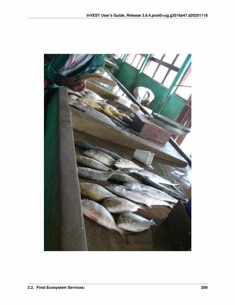
InVEST User’s Guide, Release 3.8.4.post0+ug.g3516a47.d20201118
2.2. Final Ecosystem Services: 209

InVEST User’s Guide, Release 3.8.4.post0+ug.g3516a47.d20201118
model that can be adapted to most species and geographies. In-puts to the model include parameters for life history character-istics (e.g., age at maturity, recruitment, migration and naturalmortality rates), behavior of the fishery (e.g., fishing pressure),habitat dependencies (e.g., importance and availability of nurseryhabitat), and, optionally, economic valuation (e.g., price per unitbiomass). The model outputs the volume and economic valueof harvest within the area(s) designated by the user. It is bestto compare outputs from multiple runs of the model, where eachrun represents different scenarios of habitat extent, environmen-tal conditions and/or fishing pressure. A library of four samplemodels is provided, which the user can adapt to their own species or region, or the user can choose to build a modelfrom scratch.
Introduction
Marine and aquatic ecosystems provide habitat for fish and shell-fish, which in turn provide food and livelihoods for millions ofpeople worldwide (FAO 2014). The ability of ecosystems to sup-port fisheries depends on having intact habitat for fish, and onmaintaining harvests at sustainable levels. A consideration ofhow changes in habitat or harvesting practices will impact theproduction of wild fish is thus important when weighing deci-sions which impact marine or aquatic ecosystems.
The status and ecology of fish stocks are often assessed by com-piling multiple types of data into a single model that gives es-timates of production under different scenarios. Unfortunately,such complex stock assessments are often not possible due to alack of data and/or resources. In addition, traditional stock as-sessments generally do not take into account habitat dependen-cies or spatial dynamics, both of which are essential for under-standing how local or regional fisheries production might respondunder different scenarios. Therefore, a tool is needed that is flexi-ble enough so that it can be adapted to different species, localities,and qualities of data, and which can be used to assess the poten-tial consequences of decisions on the production of wild capturefisheries.
The Model
The InVEST model of ecosystem services from fisheries isan age- or stage-structured, deterministic, population dynamicsmodel for an individual species. The model uses life-history in-formation and survival parameters provided by the user to esti-mate the volume of harvest. The model can then be used to ex-plore how the amount of harvest (and, optionally, value) respondsto changes in the amount of habitat (e.g., seagrass, mangrove,coral reef), environmental conditions (e.g., temperature, salinity),and/or fishing pressure. It is best to compare outputs from mul-tiple runs of the model, where each run represents different sce-narios of habitat extent, environmental conditions, and/or fishingpressure. Fish population dynamics are notoriously variable and
210 Chapter 2. InVEST Models

InVEST User’s Guide, Release 3.8.4.post0+ug.g3516a47.d20201118
difficult to predict. This model is not intended to give a preciseprediction of harvest amounts, but rather to be used as a tool toexplore the consequences of different decisions which could im-pact fisheries production.
Parameter sets for four sample models are provided, representingthe following species and geographies: (1) Caribbean spiny lob-ster (Panulirus argus) in Belize; (2) Dungeness crab (Metacarci-nus magister) in Hood Canal, Washington; (3) blue crab (Call-inectes sapidus) in Galveston Bay, Texas; and (4) white shrimp(Litopenaeus setiferus) in Galveston Bay, Texas. We chose thesecombinations of species and geographies because they were ofinterest to our partners in different NatCap application sites. Theexisting models, and others that will be added as they are devel-oped, capture a range of life history types and exploitation pat-terns such that users can choose an existing model and modify itfor their own region and species (e.g., modify the Galveston Baywhite shrimp model for brown shrimp in the South Atlantic). Al-ternatively, the model is formulated such that a user with more ad-vanced knowledge of fisheries science and modeling techniquescan start from scratch and parameterize the generic model to suitany species (or guild) of interest.
How it Works
The underlying mechanics of the model are an age-structured orstage-structure population dynamics model. The model interfaceguides users through a series of decisions about the model’s struc-ture:
• Are populations structured by age or by stage?
• Should males and females be modeled separately (sex-specific)or together?
• Are there multiple subregions?
• Is there migration between subregions?
• How is recruitment (i.e. the production of offspring) determined?
• For how many time steps should the model run?
The user supplies the necessary parameters, which describe thesurvival rates, maturation schedule, recruitment function, migra-tion patterns, and vulnerability to harvest. The model then runsfor a user-specified number of time steps with the intention ofthe population reaching a state of equilibrium. Primary modeloutputs are estimates of harvest and value (optional) for the pop-ulation at the final time step of the run. Valuation is optional andreflects revenue earned from the sale of processed catch.
After generating a baseline model run, the user can then alter as-pects of the model to compare fisheries production under differ-ent scenarios. Scenarios feed into the model by altering survivalrates at certain life stages or in certain locations, for instance inresponse to changes in habitat extent, environmental variables,
2.2. Final Ecosystem Services: 211
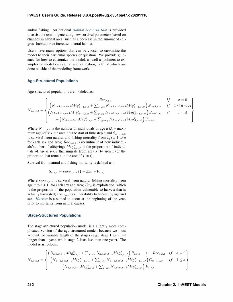
InVEST User’s Guide, Release 3.8.4.post0+ug.g3516a47.d20201118
and/or fishing. An optional Habitat Scenario Tool is providedto assist the user in generating new survival parameters based onchanges in habitat area, such as a decrease in the amount of eel-grass habitat or an increase in coral habitat.
Users have many options that can be chosen to customize themodel to their particular species or question. We provide guid-ance for how to customize the model, as well as pointers to ex-amples of model calibration and validation, both of which aredone outside of the modeling framework.
Age-Structured Populations
Age-structured populations are modeled as:
𝑁𝑎,𝑠,𝑥,𝑡 =
⎧⎪⎪⎪⎪⎪⎨⎪⎪⎪⎪⎪⎩
𝑅𝑒𝑐𝑠,𝑥,𝑡 𝑖𝑓 𝑎 = 0(︁𝑁𝑎−1,𝑠,𝑥,𝑡−1𝑀𝑖𝑔𝑥𝑎−1,𝑠,𝑥 +
∑︀𝑥′ ̸=𝑥 𝑁𝑎−1,𝑠,𝑥′,𝑡−1𝑀𝑖𝑔𝑥𝑎−1,𝑠,𝑥′
)︁𝑆𝑎−1,𝑠,𝑥 𝑖𝑓 1 ≤ 𝑎 < 𝐴(︁
𝑁𝐴−1,𝑠,𝑥,𝑡−1𝑀𝑖𝑔𝑥𝐴−1,𝑠,𝑥 +∑︀
𝑥′ ̸=𝑥 𝑁𝐴−1,𝑠,𝑥′,𝑡−1𝑀𝑖𝑔𝑥𝐴−1,𝑠,𝑥′
)︁𝑆𝐴−1,𝑠,𝑥 𝑖𝑓 𝑎 = 𝐴
+(︁𝑁𝐴,𝑠,𝑥,𝑡−1𝑀𝑖𝑔𝑥𝐴,𝑠,𝑥 +
∑︀𝑥′ ̸=𝑥 𝑁𝐴,𝑠,𝑥′,𝑡−1𝑀𝑖𝑔𝑥𝐴,𝑠,𝑥′
)︁𝑆𝐴,𝑠,𝑥
⎫⎪⎪⎪⎪⎪⎬⎪⎪⎪⎪⎪⎭Where 𝑁𝑎,𝑠,𝑥,𝑡 is the number of individuals of age a (A = maxi-mum age) of sex s in area x at the start of time step t; and 𝑆𝑎−1,𝑠,𝑥
is survival from natural and fishing mortality from age a-1 to afor each sex and area; 𝑅𝑒𝑐𝑠,𝑥,𝑡 is recruitment of new individu-als/number of offspring; 𝑀𝑖𝑔𝑥𝑎,𝑠,𝑥′ is the proportion of individ-uals of age a sex s that migrate from area x’ to area x (or theproportion that remain in the area if x’ = x).
Survival from natural and fishing mortality is defined as:
𝑆𝑎,𝑠,𝑥 = 𝑠𝑢𝑟𝑣𝑎,𝑠,𝑥 (1 − 𝐸𝑥𝑥 * 𝑉𝑎,𝑠)
Where 𝑠𝑢𝑟𝑣𝑎,𝑠,𝑥 is survival from natural fishing mortality fromage a to a + 1. for each sex and area; 𝐸𝑥𝑥 is exploitation, whichis the proportion of the population vulnerable to harvest that isactually harvested; and 𝑉𝑎,𝑠 is vulnerability to harvest by age andsex. Harvest is assumed to occur at the beginning of the year,prior to mortality from natural causes.
Stage-Structured Populations
The stage-structured population model is a slightly more com-plicated version of the age-structured model, because we mustaccount for variable length of the stages (e.g., stage 1 may lastlonger than 1 year, while stage 2 lasts less than one year). Themodel is as follows:
𝑁𝑎,𝑠,𝑥,𝑡 =
⎧⎪⎪⎪⎨⎪⎪⎪⎩(︁𝑁𝑎,𝑠,𝑥,𝑡−1𝑀𝑖𝑔𝑥𝑎,𝑠,𝑥 +
∑︀𝑥′ ̸=𝑥 𝑁𝑎,𝑠,𝑥′,𝑡−1𝑀𝑖𝑔𝑥𝑎,𝑠,𝑥′
)︁𝑃𝑎,𝑠,𝑥 + 𝑅𝑒𝑐𝑠,𝑥,𝑡 𝑖𝑓 𝑎 = 0(︁
𝑁𝑎−1,𝑠,𝑥,𝑡−1𝑀𝑖𝑔𝑥𝑎−1,𝑠,𝑥 +∑︀
𝑥′ ̸=𝑥 𝑁𝑎−1,𝑠,𝑥′,𝑡−1𝑀𝑖𝑔𝑥𝑎−1,𝑠,𝑥′
)︁𝐺𝑎−1,𝑠,𝑥 𝑖𝑓 1 ≤ 𝑎
+(︁𝑁𝑎,𝑠,𝑥,𝑡−1𝑀𝑖𝑔𝑥𝑎,𝑠,𝑥 +
∑︀𝑥′ ̸=𝑥 𝑁𝑎,𝑠,𝑥′,𝑡−1𝑀𝑖𝑔𝑥𝑎,𝑠,𝑥′
)︁𝑃𝑎,𝑠,𝑥
⎫⎪⎪⎪⎬⎪⎪⎪⎭
212 Chapter 2. InVEST Models

InVEST User’s Guide, Release 3.8.4.post0+ug.g3516a47.d20201118
Where 𝑁𝑎,𝑠,𝑥,𝑡, 𝑅𝑒𝑐𝑠,𝑥,𝑡, 𝑀𝑖𝑔𝑥𝑎,𝑠,𝑥 are the same as in the for-mulation for the age-structured model. Note that there is no A(maximum age) for stage-structured models because the modelsare designed to capture all of the life stages. 𝐺𝑎,𝑠,𝑥 is the proba-bility of surviving from natural and fishing mortality and growinginto the next stage for each sex and area; and 𝑃𝑎,𝑠,𝑥 is the proba-bility of surviving from natural and fishing mortality and stayingin the same stage for each sex and area.
𝐺𝑎,𝑠,𝑥 is a function of survival from natural and fishing mortality(𝑆𝑎,𝑠,𝑥 as defined above, except now expressed as per unit time(e.g. day) rather than per year) and stage duration, 𝐷𝑎:
𝐺𝑎,𝑠,𝑥 =𝑆𝑎,𝑠,𝑥
𝐷𝑎 (1 − 𝑆𝑎,𝑠,𝑥)
1 − 𝑆𝑎,𝑠,𝑥𝐷𝑎
𝑃𝑎,𝑠,𝑥 is also a function of survival from natural and fishing mor-tality and stage duration; it is defined as:
𝑃𝑎,𝑠,𝑥 = 𝑆𝑎,𝑠,𝑥1 − 𝑆𝑎,𝑠,𝑥
𝐷𝑎−1
1 − 𝑆𝑎,𝑠,𝑥𝐷𝑎
Recruitment
Recruitment (i.e. the production of offspring) can be modeled inone of four different ways. The Beverton-Holt and Ricker func-tions assume different forms of density-dependence in the recruit-ment function (i.e. the number of offspring per adult decreases asadult abundance or biomass increases). The Fecundity functionassumes a constant reproductive rate for adults (i.e. no densitydependence). The Fixed Recruitment function assumes that re-cruitment is constant and not dependent on the number of adults.The parameterization of each function is shown below. See theGuidance section for advice on choosing and parameterizing therecruitment function.
Beverton-Holt
𝑅𝑒𝑐𝑠,𝑥,𝑡 =𝐿𝑎𝑟𝑣𝑎𝑙𝐷𝑖𝑠𝑝𝑒𝑟𝑠𝑎𝑙𝑥
𝑆𝑒𝑥𝑆𝑝𝑒𝑐𝑖𝑓𝑖𝑐· (𝛼 · 𝑆𝑝𝑡)
(𝛽 + 𝑆𝑝𝑡)
Ricker
𝑅𝑒𝑐𝑠,𝑥,𝑡 =𝐿𝑎𝑟𝑣𝑎𝑙𝐷𝑖𝑠𝑝𝑒𝑟𝑠𝑎𝑙𝑥
𝑆𝑒𝑥𝑆𝑝𝑒𝑐𝑖𝑓𝑖𝑐·(︀𝛼 · 𝑆𝑝𝑡 · 𝑒−𝛽·𝑆𝑝𝑡
)︀
2.2. Final Ecosystem Services: 213

InVEST User’s Guide, Release 3.8.4.post0+ug.g3516a47.d20201118
Fecundity
𝑅𝑒𝑐𝑠,𝑥,𝑡 =𝐿𝑎𝑟𝑣𝑎𝑙𝐷𝑖𝑠𝑝𝑒𝑟𝑠𝑎𝑙𝑥
𝑆𝑒𝑥𝑆𝑝𝑒𝑐𝑖𝑓𝑖𝑐·
(︃∑︁𝑎,𝑠,𝑥
𝑁𝑎,𝑠,𝑥,𝑡−1𝑀𝑎𝑡𝑢𝑟𝑖𝑡𝑦𝑎,𝑠𝐹𝑒𝑐𝑢𝑛𝑑𝑖𝑡𝑦𝑎,𝑠
)︃
Fixed Recruitment
𝑅𝑒𝑐𝑠,𝑥 =𝐿𝑎𝑟𝑣𝑎𝑙𝐷𝑖𝑠𝑝𝑒𝑟𝑠𝑎𝑙𝑥
𝑆𝑒𝑥𝑆𝑝𝑒𝑐𝑖𝑓𝑖𝑐·𝑅𝑒𝑐𝑟𝑢𝑖𝑡𝑚𝑒𝑛𝑡
Fig. 22: Illustration of the four recruitment functions available within the InVEST Fisheriesmodel.
If the modelis sex-specific,𝑆𝑒𝑥𝑆𝑝𝑒𝑐𝑖𝑓𝑖𝑐 = 2, or ifthe sexes are aggregated,𝑆𝑒𝑥𝑆𝑝𝑒𝑐𝑖𝑓𝑖𝑐 = 1. Insex-specific mod-els, recruits aresplit evenly betweenmales and females.𝐿𝑎𝑟𝑣𝑎𝑙𝐷𝑖𝑠𝑝𝑒𝑟𝑠𝑎𝑙𝑥gives the proportionof larvae that settle inarea x for models withsubregions. Spawners(𝑆𝑝𝑡) can be expressedas either number orbiomass. The numberof spawners is theproduct of the numberof individuals in eachage (or stage) class forthe entire study regionand the proportion thatare mature by age (orstage):
𝑆𝑝𝑡 =∑︁𝑎,𝑠,𝑥
𝑁𝑎,𝑠,𝑥,𝑡−1𝑀𝑎𝑡𝑢𝑟𝑖𝑡𝑦𝑎,𝑠
The biomass of spawn-ers is the product ofnumber of individuals ineach age (or stage) classfor the entire study re-gion, the proportion thatare mature at each age(or stage) AND theirweight at a given age (or stage):
𝑆𝑝𝑡 =∑︁𝑎,𝑠,𝑥
𝑁𝑎,𝑠,𝑥,𝑡−1𝑀𝑎𝑡𝑢𝑟𝑖𝑡𝑦𝑎,𝑠𝑊𝑎,𝑠
214 Chapter 2. InVEST Models

InVEST User’s Guide, Release 3.8.4.post0+ug.g3516a47.d20201118
Where 𝑊𝑎,𝑠 is weight or biomass by age and sex.
Migration
If multiple subregions are specified, the user can choose to include migration from one subregion to another. Migrationmay occur at one or multiple ages/stages, and for each age/stage at which migration occurs the user specifies whichproportion of fish from each subregion move to each other subregion. These proportions may depend on habitat quality,habitat quantity, known oceanographic dispersal patterns, etc. Within subregion migrations (for instance, shifts fromone habitat type to another) should not be specified in this way. See Migration section in the Guidance section formore information.
Harvest
Harvest (𝐻𝑥,𝑡) from each subregion in the final (equilibrated) time step is calculated based on the user-defined ex-ploitation rate(s) and vulnerability. Harvest can be output by numbers or by weight. Choosing the appropriate outputmetric depends on how catch is normally processed and sold.
Numbers (e.g. Dungeness crab: 𝐻𝑡,𝑥 =∑︀
𝑎,𝑠,𝑥 𝑁𝑎,𝑠,𝑥,𝑡𝐸𝑥𝑥𝑉𝑎,𝑠
By Weight (e.g. Spiny lobster, White shrimp): 𝐻𝑡,𝑥 =∑︀
𝑎,𝑠,𝑥 𝑁𝑎,𝑠,𝑥,𝑡𝐸𝑥𝑥𝑉𝑎,𝑠𝑊𝑎,𝑠
Where 𝐸𝑥𝑥 is exploitation, which is the proportion of the population vulnerable to harvest that is actually harvested,𝑉𝑎,𝑠 is vulnerability to harvest for age a and sex s, and 𝑤𝑎,𝑠 is weight for age and sex.
Valuation
Valuation, 𝑉𝑥,𝑡 is optional and reflects the earnings from the sale of harvest. It is intended to give a rough idea of thecurrent market value for an equilibrated population based on user-defined price parameters. It is simply:
𝑉𝑡,𝑥 = 𝐻𝑡,𝑥 * 𝐹𝑟𝑎𝑐𝑡𝑖𝑜𝑛𝑃𝑟𝑜𝑐𝑒𝑠𝑠𝑒𝑑 * 𝑃𝑟𝑖𝑐𝑒
Where 𝑃𝑟𝑖𝑐𝑒 is the value in price per units (where units match those given by 𝐻𝑥,𝑡), and 𝐹𝑟𝑎𝑐𝑡𝑖𝑜𝑛𝑃𝑟𝑜𝑐𝑒𝑠𝑠𝑒𝑑 is theproportion of each harvest unit that remains to be sold after processing.
Initial Conditions
The user supplies the initial number of recruits for both age- and stage-structured models. To initialize the age-structured models the following is done (i.e., at 𝑡 = 0):
𝑁𝑎,𝑠,𝑥,𝑡=0 =
⎧⎨⎩𝑅𝑒𝑐𝑠,𝑥,𝑡=0 𝑖𝑓 𝑎 = 0
𝑁𝑎−1,𝑠,𝑥,𝑡=0𝑆𝑎,𝑠,𝑥 𝑖𝑓 1 ≤ 𝑎 < 𝐴𝑁𝐴−1,𝑠,𝑥,𝑡=0𝑆𝐴−1,𝑠,𝑥
(1−𝑆𝐴,𝑠,𝑥)𝑖𝑓 𝑎 = 𝐴
⎫⎬⎭For stage-structured models, we set the youngest stage as the initial recruitment, and then all other stages to 1 (asbelow). This is appropriate for the stage-structured models because each stage has a different duration, so we allowthe model to redistribute the initial recruits (i.e., members of the youngest stage) over time instead of specifying themat the outset as in the age-structured model.
𝑁𝑎,𝑠,𝑥,𝑡=0 =
{︂𝑅𝑒𝑐𝑠,𝑥,𝑡=0 𝑖𝑓 𝑎 = 0
1 𝑖𝑓 1 ≤ 𝑎
}︂Because the population model is run to equilibrium, the initial number of recruits will not affect the model results, butmay affect the number of time steps required before the population reaches equilibrium.
2.2. Final Ecosystem Services: 215

InVEST User’s Guide, Release 3.8.4.post0+ug.g3516a47.d20201118
Scenarios
The InVEST Fisheries model is best suited for comparing fisheries production under different scenarios. A scenariocould be a change in the amount of juvenile habitat, a change in the harvest rate in a particular subregion, or a changein survival due to other causes such as climate change. Results from running scenarios can then be compared tobaseline model runs to evaluate the consequences of such changes for fisheries production. To facilitate the analysisof scenarios, we provide a preprocessor tool for calculating how changes in habitat extent translate into changes inage/stage-specific survival.
Habitat Dependency
For ages/stages that depend on certain habitats (for instance, mangroves), a change in habitat coverage within a regioncan result in a change in the survival rate of ages/stages which depend on that habitat. The option to model thisdependency is included as a Habitat Scenario Tool with InVEST, whereby new survival parameters are generatedbased on the baseline survival parameters and the amount of change in habitat. Users may choose to use the functionalform provided in the tool, or use their own methods to calculate changes in survival. Currently, the tool is only suitedfor use with age-structured (not stage-structured) models.
Using the Habitat Scenario Tool, changes in the area of critical habitats are linked to changes in survival as follows:
𝑆𝑎,𝑥 = 𝑠𝑢𝑟𝑣𝑎,𝑥
⎛⎜⎝∑︀
𝑑𝑎,ℎ>0
(︁1 +
𝐻ℎ,𝑥,𝑆𝐶𝐸𝑁−𝐻ℎ,𝑥,𝐵𝐿
𝐻ℎ,𝑥,𝐵𝐿
)︁𝑑𝑎,ℎ𝛾
𝑛𝑎
⎞⎟⎠𝑇𝑎
Where 𝑠𝑢𝑟𝑣𝑎,𝑥 is baseline survival from natural mortality from age a-1 to a in subregion x: 𝑠𝑢𝑟𝑣0 = 1, 𝑠𝑢𝑟𝑣𝑎 = 𝑒−𝑀
if a > 0, and 𝑀𝑎 is the natural mortality rate from a - 1 to a. 𝑇𝑎 indicates if a transition to a new habitat happens from a -1 to a, which is used so that changes in habitat coverage only affect survival during the transition to that habitat, but notonce settled in the habitat. 𝐻ℎ,𝑥 is the amount of habitat h (e.g. coral, mangrove, seagrass) in the region in the baseline(BL; i.e. status quo) system or under the scenario being evaluated (SCEN). 𝑑𝑎,ℎ is the degree to which survival duringthe transistion from a-1 to a depends upon availability of ℎ, 𝑦 is a shape parameter which describes the relationshipbetween a change in habitat and a change in survival, and 𝑛𝑎 is the number of non-zero habitat-dependency values forage a. If 𝑛𝑎 = 0, 𝑆𝑎,𝑥 = 𝑠𝑢𝑟𝑣𝑎,𝑥. 𝑆𝑎,𝑥 is restricted to a maximum of 1.
Limitations and Simplifications
The InVEST Fisheries model is best suited for exploring how different scenarios of habitat change, harvesting, orchanging environmental conditions may result in changes to fisheries production. It is not intended to be a stockassessment tool, nor should the output be interpreted as predictions of future catches. Fish populations are notoriouslyvariable, both from year to year as well as over long time scales. In the InVEST Fisheries model, as with any model,the quality of the output will be determined by the quality of the parameters supplied. Key assumption of the modelinclude:
• Fishing is assumed to take place at the start of the year, before natural mortality.
• After recruitment, survival is not density-dependent (i.e. does not depend on population size).
• Harvest rates and selectivity are fixed through time, such that technological improvements to gear or changes infishing practices are not modeled.
• Market operations are fixed, such that they do not vary in response to the amount of harvest, shifts in market orconsumer preference.
Key assumptions of the Habitat Scenario Tool include:
• Habitat dependencies are obligatory (i.e., habitat substitutability is not explicitly represented).
216 Chapter 2. InVEST Models

InVEST User’s Guide, Release 3.8.4.post0+ug.g3516a47.d20201118
• The population responds to change in habitat quantity (e.g., areal extent of mangrove, seagrass, or coral reef),not quality of those habitats.
• A change in habitat area affects survival only during the first life stage which depends on that habitat.
• Habitat availability is a limiting factor for survival. This means that an increase or decrease in the amount ofhabitat will always result in an increase or decrease in survival for the first life stage dependent on that habitat.
• The effect of a change in habitat on survival does not depend on the population density. In other words, a 50%reduction in juvenile habitat will have the same effect on survival rates regardless of the number of juveniles.
Model Details and Guidance
Customing the Model
Four sample models are included with the InVEST Fisheries model as parameter sets the user can input to InVEST.However, it is expected that users will customize the model to suit their own species or region as needed. The followingsections provide guidance on how to customize the model and give examples from the four sample models. For moreinformation on the parameterization of the Dungeness crab model, as well as an application of the model, see Toft etal. 2013. For the Spiny lobster model used in the Belize case study, see Arkema et al. in review and Toft et al. in prep(available upon request).
Most of the parameters required for customizing the model may be found in scientific literature or reports, or basedon local knowledge (e.g., maturation age or migration patterns). However, some parameters will likely need to beestimated from data (e.g., recruitment parameters). For instance, the Spiny lobster model was parameterized by fittingto time-series of catch and catch-per-unit-effort (CPUE) from Belize (see Arkema et al. in review). This must be doneoutside InVEST and requires a user to be familiar with fitting models to data to estimate parameters. Some fisheriesscience expertise is also necessary.
As additional models are developed for particular applications, parameter sets, and relevant files will be made publiclyavailable and highlighted on the NatCap forum. User-developed models may be shared in the same way, with thevision of a growing library of InVEST Fisheries models from around the globe.
Guidance
Age or Stage-Structured
An age-structured model is simply a stage-structured model where all stages are the same length (typically one year).If multiple important life-history transitions happen within a year which should be captured in the model (e.g., multipletransitions from one habitat to another, or multiple migration events between regions), then a stage-structured modelmay be most appropriate.
All of the sample models are age-structured models, aside from shrimp, which is stage-structured. The stage-structuredmodel accounts for variable lengths of the stages (e.g., stage 1 may last longer than a year, while stage 2 may last lessthan a year). Stage duration, 𝐷𝑎, must be specified for each stage, but is assumed to be constant (and typically 1 year)for age-structured models.
Time Step Units
For age-structured models, the time step is assumed to be one year, and parameters are therefore based on annualrates and the model progresses in one-year increments. For stage-structured models, the user determines the timestep. For instance, in the white shrimp model time steps are interpreted as days because ‘Duration’ values in thepopulation_params.csv are number of days. The time step unit (days, months, years) will be the same as used for the“number of time steps for model run,” which is specified by the user.
2.2. Final Ecosystem Services: 217

InVEST User’s Guide, Release 3.8.4.post0+ug.g3516a47.d20201118
Number of Time Steps for Model Run
The number of time steps should be sufficiently large for the population to reach equilibrium. For age-structuredmodels, a reasonable starting place is between 100-300 time steps, but will depend on the population parameters. Forstage-structured models, more time steps may be needed. It is recommended that the user starts with an interme-diate number of time steps and check the model output to determine whether more time steps are needed to reachequilibrium.
Number of Age or Stage Classes
The model should capture the major points through adulthood– larval, juvenile/rearing, spawning, harvest. This isfairly straightforward for stage-structured models, as stages will span larval to adult stages, with some in between.For white shrimp, for instance, the intermediate stages are post-larval, marsh and bay. For age-structured models,the maximum age should be set to be old enough for the species to have reached full maturity and to be subjected tomaximum harvest. The oldest age class will be a ‘plus’ class meaning that it includes that age and all older ages. Thereis no maximum age for stage-structured models because the models are designed to capture all of the life stages.
Spiny Lobster (8 age classes): 0 (larval), 1, 2, 3, 4, 5, 6, 7+
Dungeness Crab (5 age classes): 0 (larval), 1, 2, 3, 4+
Blue Crab (4 age classes): 0 (larval), 1, 2, 3+
White Shrimp (5 stage classes): eggs/larvae, post-larval, marsh, bay, adult (based on Baker et al. 2008)
Sex-Specific or Not
A sex-specific model can be used if the biology (e.g., migration, size at age) or harvest practices differ substantiallyby sex. Different parameters can be given to each sex. Of the sample models, Dungeness crab is the only example of asex-specific model. Males and females are separate in the Dungeness crab model because regulations prohibit harvestof female crabs. The population model could have been combined for both sexes, but we deemed it easier to keepthem separate to reflect the harvest practices.
Areas(s) of Interest
The model can encompass one area—that is, be completely spatially aggregated (i.e. the population is consideredhomogenous throughout the study area)—or the area can be divided into subregions. In the sample models, we havemade our decisions about how to include space in each model based on the policy questions and data availability forparameterizing the model.
Spiny Lobster: Project partners separated Belizean coastal and marine waters into 9 planning regions of differentsizes, which we use for the lobster model (Clarke et al. 2013).
Dungeness Crab: Six boxes of irregular shape/size to match output from an ecosystem model (Toft et al. 2013).
Blue Crab and White Shrimp: A single bay-wide region (Guannel et al. 2014).
Larval Dispersal
For models with subregions (e.g., Spiny Lobster, Dungeness Crab), we assume that adults from each subregion con-tribute to a common larval pool. Larvae are then distributed across subregions. The proportion of larvae that go to eachsubregion is user-defined, in the main parameters CSV file. In the spiny lobster default model, larvae are dispersed tothe subregions according to the distribution of suitable habitat (e.g. mangroves and seagrasses) among the subregions
218 Chapter 2. InVEST Models

InVEST User’s Guide, Release 3.8.4.post0+ug.g3516a47.d20201118
(Arkema et al. in review). In the Dungeness crab default model, larvae are dispersed proportional to the surface areaof each subregion (Toft et al. 2013). The models represent closed populations, meaning we do not allow for any larvalrecruitment from outside of the study area. However, if recruitment is modeled using the Fixed Recruitment function,this could implicitly represent an external source of larvae.
Migration
If there are multiple subregions in the model, the user defines the degree of migration between subregions and at whatages/stages this migration occurs. In deciding how to include migration in a model, the user should answer questionssuch as: Does a portion of each age-class emigrate each year? Or does emigration only occur for specific classes asthey migrate between habitats? What portion of each class emigrates (e.g., 10% or 50%)? Where do they go (e.g.,distribute equally to all other subregions regardless of distance from subregion of origin, or distribute based on adistance decay from subregion of origin)?
To specify migration, the user includes a separate matrix for each age (or stage) when migration occurs (e.g., in thelobster model, lobster migrate between ages 2 and 3 only, so only 1 migration matrix is included). These matrices,stored within a single folder, are selected under “migration matrix CSV folder” in the model interface. Note thatmovements within subregions (for instance, ontogenetic shifts between different habitat types) may be implicitlyincluded in the model by altering age-specific survival rates to reflect availability of recipient habitat (see habitatdependency section). Within subregion movements do not require a migration matrix.
Spiny lobster is the only sample model that includes migration, which occurs as lobster move from mangroves andseagrasses to corals between ages 2 and 3. The proportion of age 2s that migrates from one subregion to another isdetermined by a distance decay function weighted by the amount of coral habitat in each subregion. For example, ifthere are 2 subregions and one is replete with coral, more of the age 2 lobster will migrate to that subregion than theother (for details see Arkema et al. in review).
Survival from Natural Mortality
Each year, a proportion of each age-class or stage succumbs to natural mortality due to a variety of causes, includingpredation, disease, or competition. Survival from natural mortality is the proportion of individuals that continues onto the next age/stage. Often, survival from natural mortality is calculated from instantaneous natural mortality rates(𝑀𝑎), which are frequently available from peer-reviewed literature and/or stock assessments: 𝑆𝑎 = 𝑒−𝑀𝑎𝑡, where t isthe length of the time step over which survival is calculated (typically 1 year for Age-Structured Populations).
Within the model, natural mortality may vary by age/stage, sex, and subregion, but it may not vary by time step.
Spiny Lobster: survival from natural mortality is the same across all ages (0.698), as calculated from a naturalmortality rate of 𝑀 = 0.36𝑦−1 (Puga et al. 2005).
Dungeness Crab: we use 4 survival parameters, which were the same for males and females (see Higgins et al. 1997,Toft et al. 2013, and references therein). The survival of eggs to age 1 crab involves survival through two phasesof Dungeness crab development—egg, and megalopae—for which we each had estimates of survival (5.41x10⁻⁶ and0.29, respectively). We multiplied these together to generate the survival term from eggs through megalopae to age 1.Survival was the same for ages 2 and 3 of both sexes, and age 4+ females (0.725); age 4+ males are harvested and thesurviving males have been shown to have a lower survival than other adult Dungeness crab (0.526).
Survival from Fishing Mortality
Mortality from fishing depends on the exploitation fraction and the age- or stage-specific vulnerability to harvest (seebelow).
2.2. Final Ecosystem Services: 219

InVEST User’s Guide, Release 3.8.4.post0+ug.g3516a47.d20201118
Exploitation Fraction
This is the proportion of the population vulnerable to harvest that is actually harvested. This may vary by subregion.
Vulnerability to Harvest
Not all ages or stages are equally likely to be harvested. Vulnerability to harvest (also called selectivity) may dependon size, life-stage specific behavior (for instance spawning aggregations), habitat use, or regulations, and may changedepending on the gear and fishing strategies employed. A value of 1.0 indicates that the age or stage is fully vulnerableto harvest, whereas values less than one indicate the vulnerability relative to the fully-vulnerable age or stage. Forinstance, if all individuals age 4+ are fully vulnerable, whereas age 3 individuals are only half as likely to be caughtgiven the same fishing pressure, age-3 would have a vulnerability of 0.5. The most vulnerable age/stage should havea value of 1.0. Vulnerability is assumed to be the same across subregions.
Different functional forms may be used to describe vulnerability. These are examples intended to help the user con-struct the population parameters CSV file, but other functional forms are possible (for instance, a dome-shaped func-tion would imply the highest vulnerability for medium-aged individuals).
Binary: each age or stage is either not vulnerable or fully vulnerable (0 or 1).
Logistic function: assumes that vulnerability increases with age/stage, where 𝑎50 is the age at which individuals havea 50% vulnerability to harvest, and 𝛿 determines the slope of the logistic function.
Spiny Lobster: We model vulnerability-at-age by using the logistic function above, with 𝑎50 set to 2.5 years and 𝛿 setto 10. A 𝛿 of 10 gives the shape of the logistic function a near knife-edge selectivity, meaning that very few lobsteryounger than 2.5 years are vulnerable to fishing, whereas almost all lobster older than 2.5 years are vulnerable tofishing. This cutoff was chosen as this is the age when a lobster reaches the minimum legal size for harvest of 75mm.A smaller delta would soften the knife-edge selectivity, resulting in higher vulnerability (and harvest) of youngerlobster. Exploitation (𝐸𝑥𝑥) for this model is set to 31% based on historical harvest rates.
Dungeness Crab: Vulnerability and exploitation are set more simply in this model. Only age 4 males are assumedto be vulnerable to harvest (V = 1 for age 4 males, and V = 0 for all other ages and females). 𝐸𝑥𝑥 is set to 0.47,meaning 47% of age-4 males are harvested in each region. This was estimated by adjusting an average harvest ratefor California, Oregon, and Washington to include only tribal and recreational catch since commercial harvesting doesnot occur in Hood Canal, WA (details in Toft et al. 2013)
Recruitment
Beverton-Holt: The Beverton-Holt model represents a situation where the total number of recruits increases withspawners abundance up to an asymptote. This recruitment function also has two parameters: alpha and beta. ForBeverton-Holt, alpha represents the maximum number of recruits produced (i.e. the asymptote), whereas beta rep-resents the number of spawners needed to produce recruitment equal to half the maximum (alpha/2). In this form,alpha/beta represents the recruits per spawner at low spawner levels.
Ricker: The Ricker model represents a situation where the total number of recruits increases up to intermediatespawner levels and then decreases at very high spawner levels. This function has two parameters: alpha and beta. Inthe Ricker model, alpha gives the maximum recruits per spawner at low spawner levels (i.e., the initial slope of thestock-recruit curve), while beta is the rate of decline in recruits as there are more spawners or the degree to which thecurve bends downwards as spawner abundance increases.
For both Ricker and Beverton-Holt, spawners may be measured in numbers of individuals or in biomass, and theparameters should be specified appropriately.
Fecundity: For the fecundity-based recruitment function, only age- or stage-specific fecundity values are needed,representing the number of offspring per mature individual. Caution is urged when selecting this option as age-based
220 Chapter 2. InVEST Models

InVEST User’s Guide, Release 3.8.4.post0+ug.g3516a47.d20201118
models must be carefully parameterized in order to reach equilibrium. Most parameter sets will result in a continuouslyincreasing or decreasing population. We do not recommend this option for stage-based models.
Fixed: In the fixed recruitment function, recruitment is time-invariant. A value for the fixed number of recruits mustbe given. Recruitment, therefore, does not depend on the abundance of mature individuals.
Note: Choosing which recruitment function to use will depend on data availability as well as ecological knowledgeabout the species and region. Density-dependent recruitment functions such as the Ricker and Beverton-Holt aremost common in fisheries models, as they recognize that a population depends on finite resources and cannot growinfinitely large. A model with the Fecundity function must be parameterized carefully or it is not guaranteed to reachan equilibrium. The Fixed recruitment may be appropriate in cases where the region of interest is small relative tothe range or distribution of the fished population, for instance, when recruits may drift into the region of interest fromnearby spawning areas.
The Ricker function is used for the blue crab and Dungeness crab models. The lobster model uses the Beverton-Holt function. The white shrimp model assumes fixed recruitment. In all cases, stock-recruitment parameters wereestimated by fitting the model to available data. For instance, the spiny lobster model was fit to three time-seriesof catch-per-unit-effort (CPUE) data, which allowed the estimation of alpha and beta. In the white shrimp model,recruitment was estimated by fitting the model to catch data.
If the user would like to create their own recruitment function for the Fisheries Model, an optional parameter has beencreated in the InVEST Fisheries python module (but not in the User Interface) to allow for this. See the FisheriesModel page of the InVEST API Reference for more information.
Initial Recruitment
Because the model is an equilibrium model, the value chosen for Initial Recruitment is not critical. It should be in areasonable range in order to ensure the model reaches equilibrium without too many time steps.
Maturity at Age/Stage
Maturity at age or stage is used to determine the abundance of spawners if you choose Beverton-Holt or Ricker for therecruitment function. These parameters may be taken from other studies, or estimated from data using, for instance,the equation below. If local data are not available, www.fishbase.org provides basic life history information for manyspecies of fish.
Maturity-at-age, 𝑚𝑎, may be calculated using a maturity ogive governed by a logistic function:
𝑚𝑎 = (1 + 𝑒𝑥𝑝 (−𝜑 (𝐿𝑎 − 𝐿50)))−1
where:
• 𝜑 determines the slope of the logistic function
• 𝐿50 is the length-at-50% maturity
• 𝐿𝑎 is the length-at-age, defined according to a von Bertalanffy growth equation.
See the length/weight section below.
Weight at Age (Optional)
It is optional to include a length-weight relationship in the model. We have done so for the lobster model becauseharvest and sale of lobster is recorded by volume of meat, not number of lobsters, which means any model validation
2.2. Final Ecosystem Services: 221

InVEST User’s Guide, Release 3.8.4.post0+ug.g3516a47.d20201118
needed to be a comparison of weight, not just numbers of lobster. For Dungeness crab, however, we validated themodel against numbers of crab landed and had no need to transform numbers of crab to volume of crab. It may also beuseful to include weight when recruitment depends strongly on total biomass of spawners, rather than total numbersof spawners.
For Lobster, we use a von Bertalanffy growth equation and a length-weight relationship to transform numbers-at-ageto weight-at-age, 𝑤𝑎:
𝑤𝑎 = 𝑒𝐿𝑎𝑓
where:
• 𝑒, 𝑓 are parameters of the von Bertalanffy growth equation
• 𝐿𝑎 is length-at-age
𝐿𝑎 is defined as:
𝐿𝑎 = 𝑙∞ (1 − 𝑒𝑥𝑝 (−𝜅 (𝑎− 𝑡0)))
where:
• 𝐼∞ is the asymptotic maximum length
• 𝜅 is curvature parameter, which is proportional to rate at which 𝐼∞ is reached
• 𝑡0 is the age at which the fish has 0 length, therefore, is non-negative, or zero.
Parameters for these equations may be estimated from data prior to running InVEST, or taken from www.fishbase.orgfor many fish species. Alternatively, estimates of weight-at-age may be taken directly from fish measurements withoutusing a model.
Valuation (Optional)
Valuation is intended to reflect the earnings from the sale of harvest. Unit Price gives the price per unit of harvest(either weight or numbers) that fishers receive from buyers. This information should be obtainable in reports, fromnational statistics, or by surveying fishers and buyers. Fraction Kept After Processing gives the proportion of eachunit of harvest that remains to be sold after processing, or if harvest is specified in numbers, gives the proportion ofindividuals which are sold.
Currently, the spiny lobster model is the only sample model with valuation. See Arkema et al. in review and Toft et al.in prep (available upon request) for a description of how valuation parameters were estimated.
Habitat Dependency and the Habitat Scenario Tool (Optional)
Habitat dependencies are not explicitly included within the InVEST Fisheries Production model. However, a HabitatScenario Tool is included which can be used to generate updated survival parameters based on changes in habitat. Inorder to use the tool, the user must already have a baseline set of population parameters, particularly survival rates.The tool takes information on changes in habitat area (expressed as a percent change from the baseline habitat area),age/stage specific habitat dependencies (i.e. age-0 lobster depend on mangroves and seagrass), and a user-specifiedshape parameter describing the relative response rate, or how a change in habitat corresponds to a change in survival.The tool outputs a new population parameters file with updated survival rates. Note that this tool cannot be used togenerate an initial set of survival parameters, but is only used to update baseline survival parameters based on habitatchange scenarios.
In using this tool, the user should have information on which life stages depend on which habitat types.
The user needs to specify:
222 Chapter 2. InVEST Models

InVEST User’s Guide, Release 3.8.4.post0+ug.g3516a47.d20201118
1. Habitat changes, represented as a percent change in the area of each habitat type by subregion (if applicable).Changes in habitat area can represent different scenarios of conservation, restoration, or development, for in-stance as output from the Habitat Risk Assessment model.
2. Age- or stage-specific habitat dependencies, ranging from 0 (no dependency) to 1 (fully dependency). If an ageor stage depends on multiple habitats, each habitat-stage dependency value can range from 0 to 1. However, ifhabitats are interchangable with regards to species dependency (in other words, if a species can use either habitattype, or if an increase in one habitat can compensate for a decrease in the other), we recommend modeling themas a single habitat type in the Habitat Scenario Tool. Information on habitat dependencies can often be found inthe scientific literature.
3. A gamma value. A gamma value of 1 means that a 50% increase in habitat area will correspond to a 50%increase in survival. A gamma value of 0.2 means that a 50% increase in habitat area will correspond to only a10% increase in survival.
Data Needs
Many types of data may and should be used to estimate inputs for the model parameters. For instance, data about aspecies’ length, weight, maturity, or fecundity at a given age/stage are important for specifying how the populationreproduces. Historical data on prices can be used to estimate the value of harvests. Survival rates may be estimatedfrom data or taken from literature values. Because the types of data available for each fishery may vary drastically,the model is designed to allow the user full flexibility in how these inputs are estimated. In cases where parametersare highly uncertain, we recommend the user to run the model multiple times with a range of parameter values todetermine how sensitive the model’s results are to uncertainty in parameters. For more details on the definitions of theinput data, please see the How it Works and Guidance sections.
Running the Model
Core Model
Upon opening the Fisheries program, the user is presented with an interface containing a set of parametersthrough which to submit inputs. Information about each parameter is provided below. Once the user has en-tered all necessary inputs, the user can start the model run by pressing ‘Run’. If any errors occur, InVESTwill stop the model run and provide feedback to the user about what caused the error through a message screen.
Fig. 23: Example User Interface for Core Model
General Parameters
1.Workspace(re-quired).These-lectedfolderisusedastheworkspacewhere
2.2. Final Ecosystem Services: 223

InVEST User’s Guide, Release 3.8.4.post0+ug.g3516a47.d20201118
allin-ter-me-di-ateandout-putfileswillbewrit-ten.Ifthese-lectedfolderdoesnotex-ist,itwillbecre-ated.Ifdatasetsal-readyex-istinthese-lectedfolder, they will be overwritten.
Naming Conventions: Any alphanumeric string of characters. Best to avoid whitespace characters.
Example Filepath: \InVEST\Fisheries\
2.Area(s)ofIn-ter-est(op-tional).Thepro-vided
224 Chapter 2. InVEST Models

InVEST User’s Guide, Release 3.8.4.post0+ug.g3516a47.d20201118
shape-fileisusedtodis-playout-putswithinthesub-re-gion(s)ofin-ter-est.Thelayershouldcon-tainonefea-tureforev-erysub-re-gionofin-ter-est,eachfea-tureofwhichshouldhavea‘Name’at-tribute(case-sensitive)match-ingacor-re-
2.2. Final Ecosystem Services: 225

InVEST User’s Guide, Release 3.8.4.post0+ug.g3516a47.d20201118
spond-ingsub-re-gioninthePop-u-la-tionPa-ram-e-tersCSVFile.The‘Name’at-tributevaluecanbenu-mericoral-pha-betic,butmustbeuniquewithinthegivenfile.
Filetype: Polygon Shapefile (SHP)
Example Filepath: \InVEST\Fisheries\Input\lobster_subregions.shp
Requirement: must have a ‘Name’ attribute in the shapefile’s attribute table.
3.NumberofTimeStepsforModelRun(re-quired).The
226 Chapter 2. InVEST Models

InVEST User’s Guide, Release 3.8.4.post0+ug.g3516a47.d20201118
num-beroftimestepsthesim-u-la-tionshallex-e-cutebe-forecom-ple-tion.Mustbeapos-i-tivein-te-ger.Thetimestepcanuseanyunitoftimerel-e-vanttothepop-u-la-tion.Con-sultTimeStepUnitsforad-vice
2.2. Final Ecosystem Services: 227

InVEST User’s Guide, Release 3.8.4.post0+ug.g3516a47.d20201118
onse-lect-ingtimestepdu-ra-tion.
Population Parameters
4. Population Model Type (required). Specifies whether the classes provided in the Population Parameters CSVfile represent ages or stages. Age-based models (e.g. Spiny Lobster, Dungeness Crab) are separated by uniform,fixed-length time steps (usually representing a year). Stage-based models (e.g. White Shrimp) allow stages tohave non-uniform durations based on the assumed resolution of the provided time step. If the stage-based modelis selected, the Population Parameters CSV File must include a ‘Duration’ vector alongside the survival matrixthat contains the number of time steps that each stage lasts.
5. Population Classes are Sex-Specific (required). Specifies whether or not the population classes provided inthe Population Parameters File are distinguished by sex.
6. Harvest by Individuals or Weight (required). Specifies whether the harvest output values are calculatedin terms of number of individuals or in terms of biomass (weight). If ‘Weight’ is selected, the PopulationParameters CSV File must include a ‘Weight’ vector alongside the survival matrix that contains the weight ofeach age/stage, as well as sex if the model is sex-specific.
7. Batch Processing. Specifies whether the program will perform a single model run or a batch (set) of modelruns. For single model runs, users submit a filepath pointing to a single Population Parameters CSV file. Forbatch model runs, users submit a folder path pointing to a set of Population Parameters CSV files. The name ofeach CSV file will serve as the prefix of the outputs created by the model run.
8. Population Parameters CSV File. The provided CSV file should contain all necessary parameters for popula-tion groups based on age/stage, sex, and subregion - excluding possible migration parameters.
Naming Conventions: Any alphanumeric string of characters. Best to avoid whitespace characters.
Filetype: Comma Separated Values (CSV)
Example Filepath: \InVEST\Fisheries\Inputs_Lobster\population_params.csv
• Classes (required)- The leftmost column should contain the age/stage names of the given specieslisted in chronological order. Each name can be an alphanumeric string. If the population classesare sex-specific, all age/stage names of one sex must be listed first, followed below by the age/stagenames of the other sex.
• Subregions (required)- The top-most row should contain the subregion names considered by themodel. Each name can be an alphanumeric string. If the AOI shapefile is to be provided, thesubregion entries must each match a corresponding ‘Name’ attribute value in a feature of the AOIshapefile. An entry must be provided even if the model is considering only one subregion.
• Survival Rates from Natural Mortality Matrix (required)- Each unique pair of age/stage andsubregion should contain a survival rate from natural mortality, expressed as a decimal fraction.
Subregion-specific Attributes: Rows placed directly below the survival matrix with at least one emptyrow placed in-between as a buffer.
• ExploitationFraction (required)- A row starting in the first column with the label ‘Exploitation-Fraction’. The exploitation fraction is the proportion of the vulnerable population in each subregion
228 Chapter 2. InVEST Models
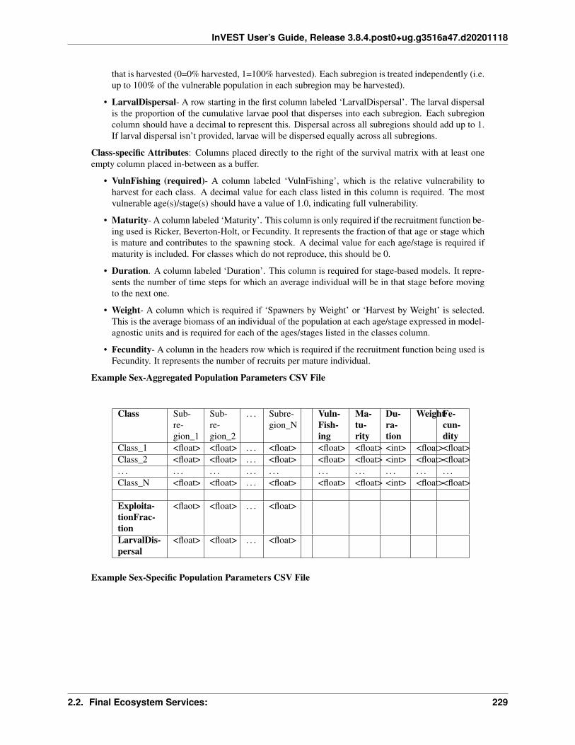
InVEST User’s Guide, Release 3.8.4.post0+ug.g3516a47.d20201118
that is harvested (0=0% harvested, 1=100% harvested). Each subregion is treated independently (i.e.up to 100% of the vulnerable population in each subregion may be harvested).
• LarvalDispersal- A row starting in the first column labeled ‘LarvalDispersal’. The larval dispersalis the proportion of the cumulative larvae pool that disperses into each subregion. Each subregioncolumn should have a decimal to represent this. Dispersal across all subregions should add up to 1.If larval dispersal isn’t provided, larvae will be dispersed equally across all subregions.
Class-specific Attributes: Columns placed directly to the right of the survival matrix with at least oneempty column placed in-between as a buffer.
• VulnFishing (required)- A column labeled ‘VulnFishing’, which is the relative vulnerability toharvest for each class. A decimal value for each class listed in this column is required. The mostvulnerable age(s)/stage(s) should have a value of 1.0, indicating full vulnerability.
• Maturity- A column labeled ‘Maturity’. This column is only required if the recruitment function be-ing used is Ricker, Beverton-Holt, or Fecundity. It represents the fraction of that age or stage whichis mature and contributes to the spawning stock. A decimal value for each age/stage is required ifmaturity is included. For classes which do not reproduce, this should be 0.
• Duration. A column labeled ‘Duration’. This column is required for stage-based models. It repre-sents the number of time steps for which an average individual will be in that stage before movingto the next one.
• Weight- A column which is required if ‘Spawners by Weight’ or ‘Harvest by Weight’ is selected.This is the average biomass of an individual of the population at each age/stage expressed in model-agnostic units and is required for each of the ages/stages listed in the classes column.
• Fecundity- A column in the headers row which is required if the recruitment function being used isFecundity. It represents the number of recruits per mature individual.
Example Sex-Aggregated Population Parameters CSV File
Class Sub-re-gion_1
Sub-re-gion_2
. . . Subre-gion_N
Vuln-Fish-ing
Ma-tu-rity
Du-ra-tion
WeightFe-cun-dity
Class_1 <float> <float> . . . <float> <float> <float> <int> <float><float>Class_2 <float> <float> . . . <float> <float> <float> <int> <float><float>. . . . . . . . . . . . . . . . . . . . . . . . . . . . . .Class_N <float> <float> . . . <float> <float> <float> <int> <float><float>
Exploita-tionFrac-tion
<flaot> <float> . . . <float>
LarvalDis-persal
<float> <float> . . . <float>
Example Sex-Specific Population Parameters CSV File
2.2. Final Ecosystem Services: 229

InVEST User’s Guide, Release 3.8.4.post0+ug.g3516a47.d20201118
Class Sub-re-gion_1
Sub-re-gion_2
. . . Subre-gion_N
Vuln-Fish-ing
Ma-tu-rity
Du-ra-tion
WeightFe-cun-dity
Class_1(Female)
<float> <float> . . . <float> <float> <float> <int> <float><float>
Class_2 <float> <float> . . . <float> <float> <float> <int> <float><float>. . . . . . . . . . . . . . . . . . . . . . . . . . . . . .Class_N <float> <float> . . . <float> <float> <float> <int> <float><float>Class_1(Male)
<float> <float> . . . <float> <float> <float> <int> <float><float>
Class_2 <float> <float> . . . <float> <float> <float> <int> <float><float>. . . . . . . . . . . . . . . . . . . . . . . . . . . . . .Class_N <float> <float> . . . <float> <float> <float> <int> <float><float>
Exploita-tionFrac-tion
<float> <float> . . . <float>
LarvalDis-persal
<float> <float> . . . <float>
9. Population Parameters CSV Folder. The provided CSV folder should contain a set of Population ParametersCSV files with all necessary attributes for population classes based on age/stage, sex, and subregion – excludingpossible migration information. The name of each file will serve as the prefix of the outputs created by themodel run.
Recruitment Parameters
10. Initial Number of Recruits (required). The initial number of recruits in the population model at time equalto zero. If the model contains multiple subregions of interest or is distinguished by sex, this value will befirst divided into subregions using the LarvalDispersal vector and then further divided evenly by sex of eachsubregion.
11. Recruitment Function Type (required). This equation will be used to calculate recruitment into each subre-gion in the area of interest. For a detailed explanation of each equation, please refer to the Recruitment section.Each equation requires a different set of recruitment parameters. Be sure that the required parameters for thedesired equation are included.
12. Spawners by Individuals or Weight. Specifies whether the spawner abundance used in the recruitment functionshould be calculated in terms of number of individuals or in terms of biomass (weight). If ‘Weight’ is selected,the user must provide a ‘Weight’ vector alongside the survival matrix in the Population Parameters CSV File.The ‘Alpha’ and ‘Beta’ parameters provided by the user should correspond to the selected choice.
13. Alpha. Specifies the shape of the stock-recruit curve. Used only for the Beverton-Holt and Ricker recruitmentfunctions.
14. Beta. Specifies the shape of the stock-recruit curve. Used only for the Beverton-Holt and Ricker recruitmentfunctions.
15. Recurring Number of Recruits. Specifies the total number of recruits that come into the population at eachtime step (a fixed number). Used only for the Fixed Recruitment function.
230 Chapter 2. InVEST Models

InVEST User’s Guide, Release 3.8.4.post0+ug.g3516a47.d20201118
Migration Parameters
For a species which migrates, this option will include source/sink population dynamics in the model. The migration isdone on a class basis, so there is an opportunity for each age/stage to have separate migratory patterns.
16. Migration Matrix CSV Folder (optional). If migration is checked, the selected folder should contain CSVmigration matrices to be used in the simulation. Each CSV file contains a single migration matrix correspondingto the age/stage that migrates. Not all ages/stages require migration matrices, only those ages/stages that migrate.
Naming Conventions: Any alphanumeric string of characters. Best to avoid whitespace characters.
Example Filepath: \InVEST\Fisheries\Inputs_Lobster\Migrations\
Migration Matrix CSV Files. For each age/stage where migration occurs, there should be a single CSVwithin the migration directory. The name of the CSV can be anything, but MUST end with an underscorefollowed by the name of the age or stage. This MUST correspond to an age or stage within the PopulationParameters CSV File. For migration from the ‘adult’ class for example, a migration file might be named‘migration_adult.csv’. The CSV should contain nothing besides subregion names and migration values.The first row and first column should be the names of the subregions in the Population Parameters CSVFile, listed in the same order. The columns represent the sources — the subregions FROM which themigration occurs; each column should therefore sum to 1. The rows represent the sinks — the subregionsTO which the migration occurs. The cells within the matrix should be a DECIMAL REPRESENTATIONof percentage of the source’s population which will migrate to the sink.
Naming Conventions: Any alphanumeric string of characters. Best to avoid whitespace char-acters. Must end with the age/stage name, such as ‘_ageName.csv’
Filetype: Comma Separated Values (CSV)
Example Filepath: \InVEST\Fisheries\Inputs_Lobster\Migrations\migration_adult.csv
Example Migration CSV File
Migration Subregion_1 (Src) Subregion_2 . . . Subregion_NSubregion_1 (Sink) <float> <float> . . . <float>Subregion_2 <float> <float> . . . <float>. . . . . . . . . . . . . . .Subregion_N <float> <float> . . . <float>
Valuation Parameters
17. Fraction of Harvest Kept After Processing (required). This is the decimal representation of the percentageof harvested catch remaining after post-harvest processing is complete. (Either by weight or by number ofindividuals, as set in the Recruitment Parameters)
18. Unit Price (required). Specifies the price per harvest unit. Valuation is intended to give a rough idea of thecurrent market value for an equilibrated population based on user-defined price parameters. If ‘Harvest byIndividuals or Weight’ was set to ‘Individuals’, this should be the price per individual. If set to ‘Weight’, thisshould be the price per unit weight. Weight units should agree with the units implied by the Weight column ofthe Population Parameters CSV file.
Habitat Scenario Tool
The goal of the Habitat Scenario Tool is to calculate new survival rates from the natural mortality rates of a baselinepopulation given the dependencies of certain classes on certain habitats and the change in the area of those habitatsover certain subregions.
2.2. Final Ecosystem Services: 231

InVEST User’s Guide, Release 3.8.4.post0+ug.g3516a47.d20201118
Upon opening the Habitat Scenario Tool, the user is presented with an interface containing a set of parameters throughwhich to submit inputs. Information about each parameter is provided below. Once the user has entered all necessaryinputs, the user can start the model run by pressing ‘Run’. If any errors occur, InVEST will stop the model run andprovide feedback to the user about what caused the error through a message screen.
Fig. 24: Example User Interface for Habitat Scenario Tool
General Parameters
1. Workspace (required). The selected folder is used as the workspace where all intermediate and output fileswill be written. If the selected folder does not exist, it will be created. If datasets already exist in the selectedfolder, they will be overwritten.
Naming Conventions: Any alphanumeric string of characters. Best to avoid whitespace characters.
Example Filepath: \InVEST\Fisheries\
Population Parameters
2. Population Parameters File (CSV) (required). The provided CSV file should contain all necessary parametersfor population classes based on age/stage, sex, and subregion - excluding possible migration parameters. Seethe Population Parameters CSV File description in the Core Model section for information about the file format.
232 Chapter 2. InVEST Models

InVEST User’s Guide, Release 3.8.4.post0+ug.g3516a47.d20201118
Naming Conventions: Any alphanumeric string of characters. Best to avoid whitespace characters.
Filetype: Comma Separated Values (CSV)
Example Filepath: \InVEST\Fisheries\Input\Habitat_Scenario_Tool\pop_params.csv
3. Population Classes are Sex-Specific (required). Specifies whether or not the population classes provided inthe Population Parameters CSV File are distinguished by sex.
Habitat Parameters
4. Habitat Dependency Parameters File (CSV). The provided CSV file should contain the habitat dependencies(0-1) for each age/stage for each habitat type that is also provided in the Habitat Change CSV File.
Naming Conventions: Any alphanumeric string of characters. Best to avoid whitespace characters.
Filetype: Comma Separated Values (CSV)
Example Filepath: \InVEST\Fisheries\Input\Habitat_Scenario_Tool\habitat_dep_params.csv
Example Habitat Dependency Parameters CSV File
Habitats Class_1 Class_2 . . . Class_NHabitat_1 <float> <float> . . . <float>Habitat_2 <float> <float> . . . <float>. . . . . . . . . . . . . . .Habitat_N <float> <float> . . . <float>
5. Habitat Area Change File (CSV). The provided CSV file should contain the percent changes in habitat area bysubregion (if applicable). The habitats included should be those that the population depends on at any age/stage.
Name: Any alphanumeric string, avoid spaces.
Filetype: Comma Separated Values (CSV)
Example Filepath: \InVEST\Fisheries\Input\Habitat_Scenario_Tool\habitat_chg_params.csv
Example Habitat Area Change File (CSV)
Habitats Subregion_1 Subregion_2 . . . Subregion_NHabitat_1 <float> <float> . . . <float>Habitat_2 <float> <float> . . . <float>. . . . . . . . . . . . . . .Habitat_N <float> <float> . . . <float>
6. Gamma. Describes the relationship between the change in habitat area and a change in survival of age/stagedependent on that habitat. Specify a value between 0 and 1.
Interpreting Results
Core Model Results
Upon successful completion of the model, the workspace folder will contain ‘intermediate’ and ‘output’ sub-folders.These two folders hold the data generated by the model. Most users will primarily be interested in data containedwithin the ‘output’ folder.
2.2. Final Ecosystem Services: 233

InVEST User’s Guide, Release 3.8.4.post0+ug.g3516a47.d20201118
Intermediate Outputs Folder
The intermediate folder contains information used for final calculations. Intermediate outputs provide a more compre-hensive look at how the final outputs were generated.
1. Population Breakdown. The output CSV file details the number of individuals within each class in eachsubregion, for every time step.
Example Filepath: \intermediate\<pop_params_name>_population_by_time_step.csv
Final Outputs Folder
1. HTML Summary of Results. A page which displays the final harvest after equilibration, and the cumulativeharvest across the entire area of interest per time step up to the equilibrated time step. The second table, ‘FinalHarvest by Subregion After XX Time Steps’, shows the final harvest (by individuals or weight, depending oninputs) for each subregion. If valuation of the harvest was selected in the inputs, this will also include a columnfor the valuation of each subregion harvest (in the input currency). The bottom table, ‘Time Step Breakdown’,shows the cumulative harvest across all subregions for each time step before the model equilibrates. If valuationof the harvest was selected in the inputs, this will also include a column for valuation of the subregion harvestusing the input currency. The ‘Equilibrated?’ column indicates whether the model reached equilibrium for eachgiven time step (N=No, Y=Yes).
Example Filepath: \output\<pop_params_name>_results_page.html
2. CSV Summary of Results. A summary of results formatted as a CSV file.
Example Filepath: \output\<pop_param_name>_results_table.csv
3. Modified AOI. A copy of the AOI layer, but with either one or two additional attributes. The layer will alwayscontain ‘Hrv_Total’, which is the final harvest (in either number of individuals or weight, depending on inputs)within that subregion at the final time step. Additionally, if the valuation parameter was checked, the layer willalso contain ‘Val_Total’, the total value of the harvest within that subregion using the currency from the inputs.
Example Filepath: \output\<aoi_name>_results_aoi.shp
Habitat Scenario Tool Results
Upon completion of a successful model run, the workspace folder will contain an ‘output’ sub-folder. No intermediatefiles are created.
Final Outputs Folder
1. Modified Population Parameters CSV File A new population parameters file with an adjusted survival matrixbased on the Habitat Scenario equation.
Example Filepath: \output\<pop_params>_modified.csv
References
Arkema, K.K., G. Verutes, S.A. Wood, C. Clarke, S. Rosado, M. Canto, A. Rosenthal, M. Ruckelshaus, G. Guannel,J. Toft, J. Fariesa, J.M. Silver, R. Griffin, A.D. Guerry. Improving the margins: Modeling ecosystem services leads tobetter coastal plans. In review
234 Chapter 2. InVEST Models

InVEST User’s Guide, Release 3.8.4.post0+ug.g3516a47.d20201118
Baker, R., P. Levin, and T. Minello. 2008. The link between coastal wetlands and white shrimp fishery production inthe northern Gulf of Mexico. ICES CM 2008/M:11
Clarke, C., M. Canto, and S. Rosado. 2013. Belize Integrated Coastal Zone Management Plan. Coastal Zone Man-agement Authority and Institute, Belize City. 423 p.
Food and Agriculture Organization of the United Nations. 2014a. The State of World Fisheries and Aquaculture 2014:Opportunities and Challenges. Food and Agriculture Organization of the United Nations. Rome
Guannel, G., A. Guerry, J. Brenner, J. Faries, M. Thompson, J. Silver, R. Griffin, J. Proft, M. Carey, J. Toft, G. Verutes.2014. Changes in the delivery of ecosystem services in Galveston Bay, TX, under a sea-level rise scenario. Reportavailable upon request.
Higgins, K., A. Hastings, J.N. Sarvela, and L.W. Botsford. 1997. Stochastic dynamics and deterministic skeletons:population behavior of Dungeness crab. Science 276: 1431-1435
Puga, R., S. Hernández, J. López and M.E. de León. 2005. Bioeconomic modeling and risk assessment of the Cubanfishery for spiny lobster Panulirus argus. Fisheries Research 75: 149–163
Toft, J.E., J.L. Burke, M.P. Carey, C.K. Kim, M. Marsik, D.A. Sutherland, K.K. Arkema, A.D. Guerry, P.S. Levin,T.J. Minello, M. Plummer, M.H. Ruckelshaus and H.M. Townsend. 2013. From mountains to sound: modelling thesensitivity of Dungeness crab and Pacific oyster to land-sea interactions in Hood Canal, WA. ICES J. Mar. Sci. 71(3):725-738
2.2.13 Crop Production
Summary
The Crop Production Percentile and Crop Production Regression models estimate crop yield and nutrient value for afixed set of crops, derived from user-supplied landcover information. Crop yield is primarily driven by climate, and iffertilizer rates are available, they may also be taken into account with the Regression model.
Introduction
Expanding agricultural production and closing yield gaps is a key strategy for many governments and developmentagencies focused on poverty alleviation and achieving food security. However, conversion of natural habitats to agri-cultural production impacts other ecosystem services that are key to sustaining the economic benefits that agricultureprovides to local communities. Intensive agricultural practices can add to pollution loads in water sources, often neces-sitating future costly water purification methods. Overuse of water also threatens the supply available for hydropoweror other services. Still, crop production is essential to human well-being and livelihoods. The InVEST crop productionmodel allows detailed examination of the costs and benefits of this vital human enterprise, including exploration ofquestions such as:
• How would a different arrangement or selection of cropping systems compare to current systems in terms oftotal production? Could switching crops yield higher economic returns or nutritional value?
• What are the impacts of crop intensification on ecosystem services? If less land is used to produce equal amountsof food by increasing intensification, is the net result on ecosystem services production positive or negative?
• How can we evaluate different strategies for meeting increasing food demand while minimizing the impact onecosystem services?
The Model
The InVEST crop production model is divided into a percentile based yield model, covering 175 crops worldwide, anda regression based model that accounts for fertilization rates on 12 crops. These models are deployed to the end user
2.2. Final Ecosystem Services: 235

InVEST User’s Guide, Release 3.8.4.post0+ug.g3516a47.d20201118
as the “percentile” and “regression” models.
All results are paried with observed results from the same region for quality control checks as well as nutrition infor-mation for 33 macro and micronutrients.
Percentile Model
The InVEST Crop Production Percentile model produces estimates of 175 crops’ yield from existing data, percentilesummaries, and observed yields. These observations are based on FAO and sub-national datasets for 175 crops, astons/ha (Monfreda et al. 2008) and nutrition information. The percentile yields are useful for exploring a range ofintenstification levels, listing the yield for the 25th, 50th, 75th, and 95th percentiles, amongst observed yield data ineach of the crop’s climate bins.
Regression Model
For 12 staple crops for which yields have been modeled globally by Mueller et al. (2011), the Crop ProductionRegression model can provide estimates of yields given fertilizer inputs. These crops include barley, maize, oil palm,potato, rapeseed, rice, rye, soybean, sugar beet, sugar cane, sunflower, and wheat. To run this model, the user mustprovide an additional table that corresponds crops with nitrogen, phosphate, and potash application rates (kg/ha) percrop. The model produces modeled and observed crop yields, as well as nutritional value.
How it Works
Percentile Model
The Percentile model’s algorithm is as follows:
1. Reclass landcover to climate bin per crop type
2. Look up percentile yield per crop type in percentile table associated with climate bin and crop
3. Calculate nutrient valuation per crop
4. Fetch observed yield per crop.
5. (optional) Aggregating total production and nutrient covering the query polygon. Including per-centiles/observed.
6. Output yield maps, percentile production table - observed, and nutrient information.
Regression Model
The Regression model’s algorithm is as follows:
1. Reclass landcover to climate bin per crop type
2. Reclass landcover to all the various regression parameters which are a function of crop type andclimate bin
3. Calculate yield per crop type on map using the supplied fertilization rates (kg/ha for K, N, and Pot)
4. Calculate nutrient valuation per crop
5. Fetch observed per crop
236 Chapter 2. InVEST Models

InVEST User’s Guide, Release 3.8.4.post0+ug.g3516a47.d20201118
6. Output yield maps, production table - observed, and nutrient information.
The crop regression itself comes from Mueler et. al 2012 and has the form
𝑌𝑚𝑜𝑑𝐺𝐶= min(𝑌𝑚𝑎𝑥(1 − 𝑏𝑁𝑃 exp(−𝑐𝑁𝑁𝐺𝐶)), 𝑌𝑚𝑎𝑥(1 − 𝑏𝑁𝑃 exp(−𝑐𝑃𝑃𝐺𝐶)), 𝑌𝑚𝑎𝑥(1 − 𝑏𝐾 exp(−𝑐𝐾𝐾𝐺𝐶)))
Where 𝑁𝐺𝐶 , 𝑃𝐺𝐶 ,𝐾𝐺𝐶 are the user supplied fertilization rates (N = nitrogen, P = phosphorus, K = potassium), andthe other regression parameters are provided as global data to the model.
Limitations and Simplifications
The current version of the model is a coarse global model driven mostly by climate and optionally by management.This model is therefore not able to capture the variation in productivity that occurs across heterogeneous landscapes.A rocky hill slope and a fertile river valley, if they share the same climate, would be assigned the same yield in thecurrent model. This is a problem if the question of interest is where to prioritize future habitat conversion, or wherefarming is most productive and least destructive.
Data Needs
There are two InVEST crop production models available, a Percentile based observation model that operates on 175crops, and a Regression model for exploring fertilziation rates that operates on 12 crops. The arguments below are forboth models unless otherwise specified.
Important: You need to download the InVEST dataset for Crop Production, to get the Monfreda Dataset required asinput to the models. If you choose to install the Crop Production sample data when you install InVEST, there will bea folder called sample_data\CropProduction in the installation folder for InVEST, where this data may befound. Or, you can download it from http://releases.naturalcapitalproject.org/?prefix=invest/, after going to that link,clicking on the target version, then navigating into the data directory and selecting CropProduction.zip.
Please also consult the Crop Production dataset for examples of all of these data inputs. This will help with file type,folder structure and table formatting. Note that all GIS inputs must be in the same projected coordinate system and inlinear meter units.
• Workspace Folder (required). The selected folder is used as the workspace where all intermediate and finaloutput files will be written. If the selected folder does not exist, it will be created. Make sure that there is ampledisk space, and write permissions are correct.
• Results Suffix (optional). Text string that will be appended to the end of output file names, as “_Suffix”. Usea Suffix to differentiate model runs, for example by providing a short name for each scenario. If a Suffix is notprovided, or changed between model runs, the tool will overwrite previous results.
• Directory to model data (required). Both the percentile and regression models require the baseMonfreda Dataset which will be installed if you choose to install sample data along with the In-VEST tools, or download the dataset directly as explained above. Once installed, the model folder issample_data\CropProduction\model_data in the InVEST data installation directory.
• Land-Use/Land-Cover Map (required). Raster of land use/land cover (LULC) for each pixel, where eachunique integer represents a different land use/land cover class. These integers are used in the Landcover toCrop Table to map landcover classes to specific crops. This raster must have a projected coordinate systemwith units of meters (e.g. UTM) because pixel areas are divided by 10000 in order to report some results inhectares.
• Landcover to Crop Table (required). A .csv (Comma Separated Value) table that maps aLand-Use/Land-Cover integer code (column lucode) to a crop name (column name crop_name).The crop name must be one of the accepted 175 crops for the percentile model, or 12for the regression model. Accepted crop names for the percentile model can be found
2.2. Final Ecosystem Services: 237
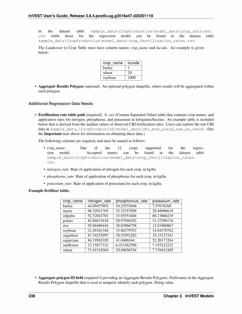
InVEST User’s Guide, Release 3.8.4.post0+ug.g3516a47.d20201118
in the dataset table sample_data\CropProduction\model_data\crop_nutrient.csv while those for the regression model can be found in the dataset tablesample_data\CropProduction\model_data\crop_fertilization_rates.csv.
The Landcover to Crop Table must have column names crop_name and lucode. An example is givenbelow:
crop_name lucodebarley 1wheat 20soybean 1000
• Aggregate Results Polygon (optional). An optional polygon shapefile, where results will be aggregated withineach polygon.
Additional Regression Data Needs
• Fertilization rate table path (required). A .csv (Comma Separated Value) table that contains crop names, andapplication rates for nitrogen, phosphorus, and potassium in kilograms/hectare. An example table is includedbelow that is derived from the median values of observed CBI fertilization rates. Users can explore the raw CBIdata in sample_data_\CropProduction\model_data\cbi_mod_yield_use_as_check. (Seethe Important note above for information on obtaining these data.)
The following columns are required, and must be named as follows:
• crop_name: One of the 12 crops supported for the regres-sion model. Accepted names can be found in the dataset tablesample_data\CropProduction\model_data\crop_fertilization_rates.csv.
• nitrogen_rate: Rate of application of nitrogen for each crop, in kg/ha
• phosphorus_rate: Rate of application of phosphorus for each crop, in kg/ha
• potassium_rate: Rate of application of potassium for each crop, in kg/ha
Example fertilizer table:
crop_name nitrogen_rate phosphorous_rate potassium_ratebarley 44.89457693 16.23535846 7.57676268maize 96.32921765 25.33357058 20.48986618oilpalm 52.32043701 15.95551604 68.13866219potato 82.80431618 29.97946392 31.27596176rice 92.04486444 28.03866758 12.01960867soybean 21.49161346 33.86379707 34.84370762sugarbeet 87.34252997 30.55592282 35.15127241sugarcane 84.19565105 41.0406544 52.20177264sunflower 23.15877332 6.413182596 7.155222222wheat 71.91518364 29.49656744 7.739412485
• Aggregate polygon ID field (required if providing an Aggregate Results Polygon). Field name in the AggregateResults Polygon shapefile that is used to uniquely identify each polygon. String value.
238 Chapter 2. InVEST Models

InVEST User’s Guide, Release 3.8.4.post0+ug.g3516a47.d20201118
Advanced Usage
These models support avoided re-computation. This means the model will detect intermediate and final results froma previous run in the specified workspace and it will avoid re-calculating any outputs that are identical to the previousrun. This can save significant processing time for successive runs when only some input parameters have changed.
Running the model
To launch the Crop Production model navigate to the Windows Start Menu -> All Programs -> InVEST [version] ->Crop Production (Percentile) or Crop Production (Regression). The interface does not require a GIS desktop, althoughthe results will need to be explored with any GIS tool such as ArcGIS or QGIS.
Interpreting Results
The following is a short description of each of the outputs from the Crop Production model. Final results are foundwithin the user defined Workspace specified for this model run. “Suffix” in the following file names refers to theoptional user-defined Suffix input to the model.
• aggregate_results_[Suffix].csv: If an Aggregate Results Polygon shapefile is provided, a table is produced thatsummarizes total observed/percentile/modeled production and nutrient information within each polygon.
• Crop Production Rasters: For each crop modeled, there will be a raster (.tif) corresponding to that crop nameand the type of modeling - “observed”, “regression”, or “yield” plus percentile number (25th/50th/75th/95th),and the user-supplied Suffix. These rasters represent the production rate of that crop per pixel in metric tons perpixel per year.
• result_table_[Suffix].csv: Table listing all of the crops modeled in the run, the area covered, percentile ormodeled production, observed production, and nutrient information for each crop. It is the primary output of themodel.
There is also an intermediate_output folder, containing many files that represent intermediate steps in the calculationsof the final results. Usually, you don’t need to work with these files, but they may be of interest if you are debugging amodel run or want to understand the intermediate steps better. It also contains a subdirectory that stores metadata usedinternally to enable avoided re-computation.
References
“Farming the planet: 2. Geographic distribution of crop areas, yields, physiological types, and net primary pro-duction in the year 2000.”” C. Monfreda N. Ramankutty, J. Foley. Biogeochemical Cycles, Vol.22, GB1022,doi:10.1029/2007GB002947. 2008
“Closing yield gaps through nutrient and water management” N Mueller, J. Gerber, M. Johnston, D. Ray, N. Ra-mankutty, J. Foley. Nature. 2012 Oct 11;490(7419):254-7. doi: 10.1038/nature11420. Epub 2012 Aug 29.
2.2.14 Seasonal water yield
Summary
There is a high demand for tools estimating the effect of landscape management on the water supply service, for useslike irrigation, domestic consumption and hydropower production. While the InVEST Annual Water Yield modelprovides an estimate of total water yield for a catchment, many applications require knowledge of seasonal flows, es-pecially during the dry season. This requires the understanding of hydrological processes in a catchment, in particularthe partitioning between quick flow (occurring during or shortly after rain events) and baseflow (occurring during dry
2.2. Final Ecosystem Services: 239

InVEST User’s Guide, Release 3.8.4.post0+ug.g3516a47.d20201118
weather). In highly seasonal climates, baseflow is likely to provide greater value than quick flow, unless significantstorage (e.g., a large reservoir) is available. The InVEST Seasonal Water Yield model seeks to provide guidance re-garding the contribution of land parcels to the generation of both baseflow and quick flow. The model computes spatialindices that quantify the relative contribution of a parcel of land to the generation of both baseflow and quick flow.Currently, there are no quantitative estimates of baseflow, only the relative contributions of pixels; a separate tool is indevelopment to address this question.
Introduction
Understanding the effect of landscape management on seasonal flow is of critical importance for watershed man-agement. The contribution of a given parcel to streamflow depends on a number of environmental factors includingclimate, soil, vegetation, slope, and position along the flow path (determining if the pixel may receive water fromupslope or if water recharged may later be evapotranspired).
Water flowing across the landscape is either evaporated, transpired, withdrawn by a well, or leaves the watershed asdeep groundwater flow or streamflow. If we consider an individual pixel, and its value with respect to water yield, wecan consider two approaches:
• The first gives credit to the net amount of water generated on a pixel as equal to the incoming precipitationminus the losses to evapotranspiration on that pixel. In this scheme, it is possible for actual evapotranspirationto be greater than precipitation if water is supplied to the site from upslope. Thus, the net generation could benegative. This approach pays no heed to the eventual disposition of that water generated on that pixel; that is, itdoes not consider whether the water actually shows up as streamflow or is evaporated or withdrawn somewherealong its path.
• The second approach gives credit to the water from a parcel that actually shows up as streamflow. Thus, if aparcel generates water that is later evaporated, the contribution is considered to be nil.
The former approach puts greater emphasis on the land-use and land-cover of a site, since the focus is on net generationfrom that pixel. It accounts for the subsidy of water from upslope pixels, but does not consider downslope effects. Itrepresents the potential to generate streamflow (not an actual generation of flow).
The second approach puts more emphasis on the topographic position of a pixel, as that will determine the potentialfor water generated on that pixel to be consumed before becoming streamflow. It represents the actual streamflowgenerated by a pixel. Since actual streamflow cannot be less than zero, this approach, unlike the first, will result inindices that are greater than or equal to zero.
We use both of these concepts to develop a set of three indices, one for quickflow, one for recharge (which representsthe ‘potential baseflow’), and one for actual baseflow. Here, baseflow is defined as the generation of streamflow withwatershed residence times of months to years, while quick flow represents the generation of streamflow with watershedresidence times of hours to days.
The Model
Quickflow
Quickflow (QF) is calculated with a Curve Number (CN)-based approach. Monthly rain events cause precipitationto fall on the landscape. Soil and land cover properties determine how much of the rain runs off of the land surfacequickly (producing quickflow) versus infiltrating into the soil (producing local recharge.) The curve number is a simpleway of capturing these soil + land cover properties - higher values of CN have higher runoff potential (for example,clay soils and low vegetation cover), lower values are more likely to infiltrate (for example, sandy soils and densevegetation cover.)
To calculate quickflow, we use the mean event depth, 𝑃𝑖,𝑚
𝑛𝑖,𝑚and assume an exponential distribution of daily precipitation
240 Chapter 2. InVEST Models

InVEST User’s Guide, Release 3.8.4.post0+ug.g3516a47.d20201118
depths on days with rain,
𝑓 (𝑝) =1
𝑎𝑖,𝑚𝑒𝑥𝑝
(︂− 𝑝
𝑎𝑖,𝑚
)︂Where 𝑎𝑖,𝑚 =
𝑃𝑖,𝑚
𝑛𝑚/25.4 and
• 𝑎𝑖,𝑚 is the mean rain depth on a rainy day at pixel i on month m [in],
• 𝑛𝑖,𝑚 is the number of events at pixel i in month m [-],
• 𝑃𝑖,𝑚 is the monthly precipitation for pixel i at month m [mm].
Quickflow for pixels located in streams is set to the precipitation on that pixel, which assumes no infiltration, onlyrunoff.
QF𝑠𝑡𝑟𝑒𝑎𝑚,𝑚 = 𝑃𝑠𝑡𝑟𝑒𝑎𝑚,𝑚
otherwise it can be shown from the exponential distribution that the monthly runoff QF𝑖,𝑚 is
QF𝑖,𝑚 = 𝑛𝑚 ×(︂
(𝑎𝑖,𝑚 − 𝑆𝑖) exp
(︂−0.2𝑆𝑖
𝑎𝑖,𝑚
)︂+
𝑆2𝑖
𝑎𝑖,𝑚exp
(︂0.8𝑆𝑖
𝑎𝑖,𝑚
)︂𝐸1
(︂𝑆𝑖
𝑎𝑖,𝑚
)︂)︂×(︁
25.4[︁mm
in
]︁)︁(2.73)
where
• 𝑆𝑖 = 1000CN𝑖
− 10 [in]
• CN𝑖 is the curve number for pixel i [in-1], tabulated as a function of the local LULC, and soil type (see AppendixI for a template of this table),
• 𝐸1 is the exponential integral function, 𝐸1(𝑥) =∫︀∞1
𝑒−𝑥𝑡
𝑡 dt.
• and 25.4 is a conversion factor from inches (used by the equation) to millimeters (used by the model)
Thus the annual quick flow QF𝑖, can be calculated from the sum of monthly QF𝑖,𝑚 values,
QF𝑖 =
12∑︁𝑚=1
𝑄𝐹𝑖,𝑚 (2.74)
Local recharge
The local recharge, or potential contribution to baseflow, of a pixel is computed from the local water balance. Precip-itation that does not run off as quickflow, and is not evapotranspired by the vegetation on a pixel, can infiltrate the soilto become local recharge. Local recharge can be negative if a pixel does not receive enough of its own water to satisfyits vegetation requirements (determined by its crop factor Kc), so it uses water generated upslope of the pixel as well(referred to as an “upslope subsidy”.) The local recharge index is computed on an annual time scale, but uses valuesderived from monthly water budgets.
For a pixel i, the local recharge derived from the annual water budget is (Figure 1):
𝐿𝑖 = 𝑃𝑖 − QF𝑖 − AET𝑖 (2.75)
Where annual actual evapotranspiration AET is the sum of monthly AET:
AET𝑖 =∑︁
months
AET𝑖,𝑚 (2.76)
For each month, AET𝑖,𝑚 is either limited by the demand (potential evapotranspiration - PET) or by the available water(from Allen et al. 1998):
AET𝑖,𝑚 = 𝑚𝑖𝑛(PET𝑖,𝑚 ; 𝑃𝑖,𝑚 − QF𝑖,𝑚 + 𝛼𝑚𝛽𝑖𝐿𝑠𝑢𝑚.𝑎𝑣𝑎𝑖𝑙,𝑖) (2.77)
2.2. Final Ecosystem Services: 241

InVEST User’s Guide, Release 3.8.4.post0+ug.g3516a47.d20201118
Where PET𝑖,𝑚 is the monthly potential evapotranspiration,
PET𝑖,𝑚 = 𝐾𝑐,𝑖,𝑚 × 𝐸𝑇0,𝑖,𝑚 (2.78)
𝐿𝑠𝑢𝑚.𝑎𝑣𝑎𝑖𝑙,𝑖 is recursively defined by (Figure 2),
𝐿𝑠𝑢𝑚.𝑎𝑣𝑎𝑖𝑙,𝑖 =∑︁
𝑗∈{𝑛𝑒𝑖𝑔ℎ𝑏𝑜𝑟 𝑝𝑖𝑥𝑒𝑙𝑠 𝑑𝑟𝑎𝑖𝑛𝑖𝑛𝑔 𝑡𝑜 𝑝𝑖𝑥𝑒𝑙 𝑖}
𝑝ij · (𝐿𝑎𝑣𝑎𝑖𝑙,𝑗 + 𝐿𝑠𝑢𝑚.𝑎𝑣𝑎𝑖𝑙,𝑗) (2.79)
where 𝑝ij ∈ [0, 1] is the proportion of flow from cell i to j, and 𝐿𝑎𝑣𝑎𝑖𝑙,𝑖 is the available recharge to a pixel, which is 𝐿𝑖
whenever 𝐿𝑖 is negative, and a proportion 𝛾 of 𝐿𝑖 when it is positive (see below for definition of 𝛾):
𝐿𝑎𝑣𝑎𝑖𝑙,𝑖 = 𝑚𝑖𝑛(𝛾𝐿𝑖, 𝐿𝑖) (2.80)
In the above:
• 𝑃𝑖 and 𝑃𝑖,𝑚 are the annual and monthly precipitation, respectively [mm]
• QF𝑖 and QF𝑖,𝑚 are the quickflow indices, defined above [mm]
• 𝐸𝑇0,𝑖,𝑚 is the reference evapotranspiration for month m [mm]
• 𝐾𝑐,𝑖,𝑚 is the monthly crop factor for the pixel’s LULC
• 𝛼𝑚 is the fraction of upslope annual available recharge that is available in month m (default is 1/12)
• 𝛽𝑖 is the fraction of the upslope subsidy that is available for downslope evapotranspiration (default is 1; seeAppendix II for more information)
• 𝛾 is the fraction of pixel recharge that is available to downslope pixels (default is 1)
Attribution of recharge
The total baseflow, 𝑄𝑏 (in mm), is the average of the contributing local recharges (negative or positive) in the catch-ment,
𝑄𝑏 =
∑︀𝑘∈{pixels in catchment} 𝐿𝑘
𝑛pixels in catchment(2.81)
Attribution value to a pixel is the relative contribution of local recharge 𝐿 on that pixel to the baseflow 𝑄𝑏:
𝑉𝑅,𝑖 =𝐿𝑖
𝑄𝑏 × 𝑛pixels in catchment(2.82)
Figure 1. Water balance at the pixel scale to compute thelocal recharge (Eq. 3).
Figure 2. Routing at the hillslope scale to compute ac-tual evapotranspiration (based on each pixel’s climatevariables and the upslope contribution, see Eq. 5) andbaseflow (based on Bsum, the flow actually reaching thestream, see Eq. 11-14)
242 Chapter 2. InVEST Models
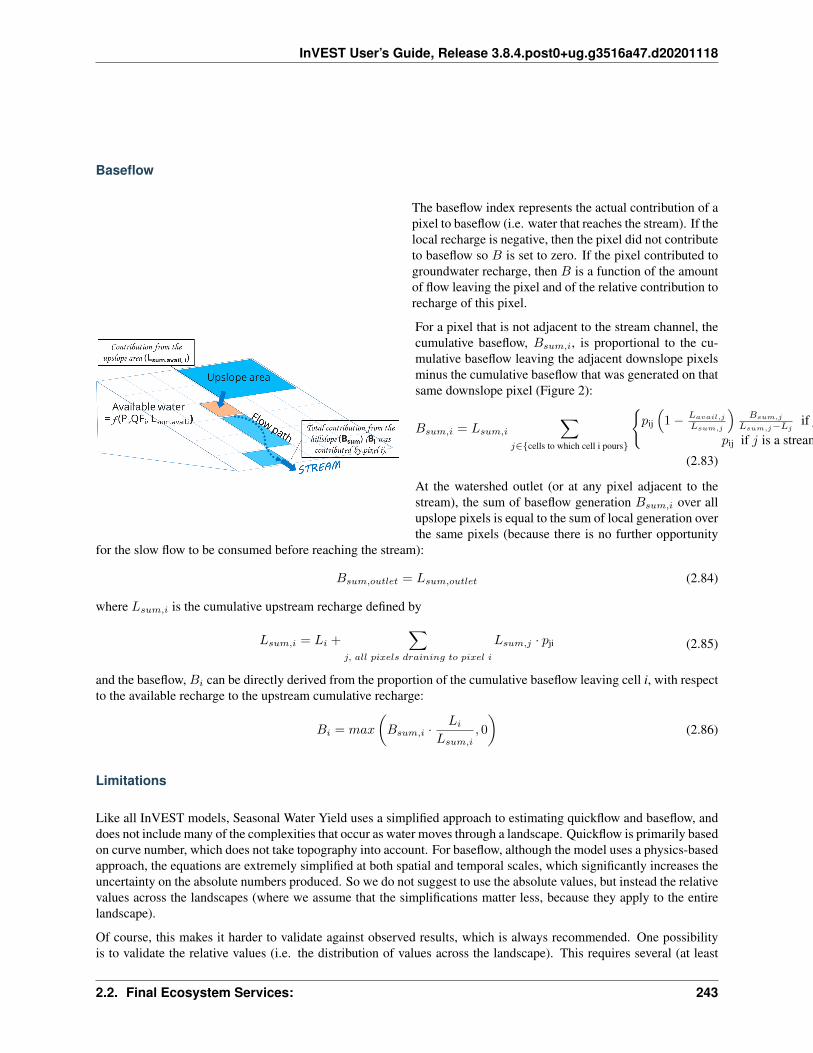
InVEST User’s Guide, Release 3.8.4.post0+ug.g3516a47.d20201118
Baseflow
The baseflow index represents the actual contribution of apixel to baseflow (i.e. water that reaches the stream). If thelocal recharge is negative, then the pixel did not contributeto baseflow so 𝐵 is set to zero. If the pixel contributed togroundwater recharge, then 𝐵 is a function of the amountof flow leaving the pixel and of the relative contribution torecharge of this pixel.
For a pixel that is not adjacent to the stream channel, thecumulative baseflow, 𝐵𝑠𝑢𝑚,𝑖, is proportional to the cu-mulative baseflow leaving the adjacent downslope pixelsminus the cumulative baseflow that was generated on thatsame downslope pixel (Figure 2):
𝐵𝑠𝑢𝑚,𝑖 = 𝐿𝑠𝑢𝑚,𝑖
∑︁𝑗∈{cells to which cell i pours}
{︃𝑝ij
(︁1 − 𝐿𝑎𝑣𝑎𝑖𝑙,𝑗
𝐿𝑠𝑢𝑚,𝑗
)︁𝐵𝑠𝑢𝑚,𝑗
𝐿𝑠𝑢𝑚,𝑗−𝐿𝑗if 𝑗 is a nonstream pixel
𝑝ij if 𝑗 is a stream pixel
}︃(2.83)
At the watershed outlet (or at any pixel adjacent to thestream), the sum of baseflow generation 𝐵𝑠𝑢𝑚,𝑖 over allupslope pixels is equal to the sum of local generation overthe same pixels (because there is no further opportunity
for the slow flow to be consumed before reaching the stream):
𝐵𝑠𝑢𝑚,𝑜𝑢𝑡𝑙𝑒𝑡 = 𝐿𝑠𝑢𝑚,𝑜𝑢𝑡𝑙𝑒𝑡 (2.84)
where 𝐿𝑠𝑢𝑚,𝑖 is the cumulative upstream recharge defined by
𝐿𝑠𝑢𝑚,𝑖 = 𝐿𝑖 +∑︁
𝑗, 𝑎𝑙𝑙 𝑝𝑖𝑥𝑒𝑙𝑠 𝑑𝑟𝑎𝑖𝑛𝑖𝑛𝑔 𝑡𝑜 𝑝𝑖𝑥𝑒𝑙 𝑖
𝐿𝑠𝑢𝑚,𝑗 · 𝑝ji (2.85)
and the baseflow, 𝐵𝑖 can be directly derived from the proportion of the cumulative baseflow leaving cell i, with respectto the available recharge to the upstream cumulative recharge:
𝐵𝑖 = 𝑚𝑎𝑥
(︂𝐵𝑠𝑢𝑚,𝑖 ·
𝐿𝑖
𝐿𝑠𝑢𝑚,𝑖, 0
)︂(2.86)
Limitations
Like all InVEST models, Seasonal Water Yield uses a simplified approach to estimating quickflow and baseflow, anddoes not include many of the complexities that occur as water moves through a landscape. Quickflow is primarily basedon curve number, which does not take topography into account. For baseflow, although the model uses a physics-basedapproach, the equations are extremely simplified at both spatial and temporal scales, which significantly increases theuncertainty on the absolute numbers produced. So we do not suggest to use the absolute values, but instead the relativevalues across the landscapes (where we assume that the simplifications matter less, because they apply to the entirelandscape).
Of course, this makes it harder to validate against observed results, which is always recommended. One possibilityis to validate the relative values (i.e. the distribution of values across the landscape). This requires several (at least
2.2. Final Ecosystem Services: 243

InVEST User’s Guide, Release 3.8.4.post0+ug.g3516a47.d20201118
>3, more realistically >5) stream gauges, which can be compared with the baseflow generation output of the model.Alternatively, results may be compared to a different spatially-explicit model, if it is available.
Data needs
This section outlines the specific data used by the model. See the Appendix for additional information on data sourcesand pre-processing. Please consult the InVEST sample data (located in the folder where InVEST is installed, if youalso chose to install sample data) for examples of all of these data inputs. This will help with file type, folder structureand table formatting. Note that all GIS inputs must be in the same projected coordinate system and in linear meterunits.
• Workspace (required). Folder where model outputs will be written. Make sure that there is ample disk space,and write permissions are correct.
• Suffix (optional). Text string that will be appended to the end of output file names, as “_Suffix”. Use a Suffix todifferentiate model runs, for example by providing a short name for each scenario. If a Suffix is not provided,or changed between model runs, the tool will overwrite previous results.
• Precipitation Directory (required). Folder containing 12 rasters of monthly precipitation for each pixel. Rasterfile names must end with the month number (e.g. Precip_1.tif for January.) Only .tif files should be in this folder(no .tfw, .xml, etc files). [units: millimeters]
• ET0 directory (required). Folder containing 12 rasters of monthly reference evapotranspiration for each pixel.Raster file names must end with the month number (e.g. ET0_1.tif for January.) Only .tif files should be in thisfolder (no .tfw, .xml, etc files). [units: millimeters]
• Digital Elevation Model (required). Raster of elevation for each pixel. Floating point or integer values. [units:meters]
• Land use/land cover (required). Raster of land use/land cover (LULC) for each pixel, where each uniqueinteger represents a different land use/land cover class. All values in this raster MUST have correspondingentries in the Biophysical table.
• Soil group (required). Raster of SCS soil hydrologic groups (A, B, C, or D), used in combination with theLULC map to compute the curve number (CN) raster. This is a raster of integers where values are entered asnumbers 1, 2, 3, and 4, corresponding to soil groups A, B, C, and D, respectively.
• AOI/Watershed (required). Shapefile delineating the boundary of the watershed to be modeled. Results will beaggregated within each polygon defined. The column ws_id is required, containing a unique integer value foreach polygon.
• Biophysical table (required). A .csv (Comma Separated Value) table containing model information corre-sponding to each of the land use classes in the LULC raster. All LULC classes in the LULC raster MUST havecorresponding values in this table. Each row is a land use/land cover class and columns must be named anddefined as follows:
– lucode (required). Unique integer for each LULC class (e.g., 1 for forest, 3 for grassland, etc.) Every valuein the LULC map MUST have a corresponding lucode value in the biophysical table.
– CN_A, CN_B, CN_C, CN_D (required). Integer curve number (CN) values for each combination of soiltype and lucode class. No 0s (zeroes) are allowed.
– Kc_1, Kc_2. . . Kc_11, Kc_12 (required). Floating point monthly crop/vegetation coefficient (Kc) valuesfor each lucode. Kc_1 corresponds to January, Kc_2 February, etc.
• Rain events table (either this or a Climate Zone table is required). CSV (comma-separated value, .csv) table with12 values of rain events, one per month. A rain event is defined as >0.1mm. The following fields are required:
– month (required). Values are the integer numbers 1 through 12, corresponding to January (1) throughDecember (12)
244 Chapter 2. InVEST Models

InVEST User’s Guide, Release 3.8.4.post0+ug.g3516a47.d20201118
– events (required). The number of rain events for that month, which are floating point or integer values
• Threshold flow accumulation (required). The number of upstream cells that must flow into a cell before itis considered part of a stream, which is used to create streams from the DEM. Smaller values create moretributaries, larger values create fewer. Integer value. See Appendix 1 for more information on choosing thisvalue. Integer value, with no commas or periods - for example “1000”.
• alpha_m, beta_i, gamma (required). Model parameters used for research and calibration purposes. Defaultvalues are: alpha_m = 1/12, beta_i = 1, gamma = 1. alpha_m is type string; beta_i and gamma are type floatingpoint.
Advanced model options
One model input is the number of rain events per month, which is entered as a .csv table with one number for eachmonth of the year. This assumes that there is one such number for the whole watershed, which may not be true forlarge areas or areas with very spatially variable precipitation.
To represent variability in the number of rain events, it is possible to enter a map of climate zones, and associatednumber of rain events for each zone.
Inputs
• Climate zone table (either this or a Rain Events table is required). CSV (comma-separated value, .csv) tablewith the number of rain events per month and climate zone, with the following required fields:
– cz_id. Climate zone numbers, integers which correspond to values found in the Climate zone raster
– jan feb mar apr may jun jul aug sep oct nov dec. 12 fields corresponding to each month of the year. Thesecontain the number of rain events that occur in that month in that climate zone. Floating point.
• Climate zone. Raster of climate zones, each uniquely identified by an integer (i.e. all pixels that are part of oneclimate zone should have the same integer value.) Must match cz_id values in the Climate zone table.
The model computes sequentially the local recharge layer, and then the baseflow layer from local recharge. Instead ofInVEST calculating local recharge, this layer could be obtained from a different model (e.g, RHESSys.) To computebaseflow contribution based on your own recharge layer, it is possible to bypass the first part of the model and directlyenter a map of local recharge.
Inputs
• Local recharge. Raster with the local recharge obtained from a different model (in mm). Floating point values.
The alpha parameter represents the temporal variability in the contribution of upslope available water to evapotranspi-ration on a pixel. In the default parameterization, its value is set to 1/12, assuming that the soil buffers water releaseand that the monthly contribution is exactly 1\12th of the annual contribution.
To allow upslope subsidy to be temporally variable instead, the user can enter monthly alpha values, in the same tableas the rain events table.
Inputs
2.2. Final Ecosystem Services: 245

InVEST User’s Guide, Release 3.8.4.post0+ug.g3516a47.d20201118
• Rain events table. The rain events table is a CSV (comma-separated value, .csv) model input (see above).Along with the required month field, one additional column named alpha is required to run this advanced option.Values for alpha are floating point.
Running the model
To launch the Seasonal Water Yield model navigate to the Windows Start Menu -> All Programs -> InVEST [version]-> Seasonal Water Yield. The interface does not require a GIS desktop, although the results will need to be exploredwith any GIS tool such as ArcGIS or QGIS.
Interpreting outputs
The following is a short description of each of the outputs from the Seasonal Water Yield model. Final results arefound within the user defined Workspace specified for this model run. “Suffix” in the following file names refers tothe optional user-defined Suffix input to the model.
The resolution of the output rasters will be the same as the resolution of the DEM that is provided as input.
• [Workspace] folder:
• Parameter log: Each time the model is run, a text (.txt) file will be created in the Workspace. The file will listthe parameter values and output messages for that run and will be named according to the service, the date andtime. When contacting NatCap about errors in a model run, please include the parameter log.
• B_[Suffix].tif (type: raster; units: mm, but should be interpreted as relative values, not absolute): Map ofbaseflow 𝐵 values, the contribution of a pixel to slow release flow (which is not evapotranspired before itreaches the stream)
• B_sum_[Suffix].tif (type: raster; units: mm, but should be interpreted as relative values, not absolute): Map of𝐵sumvalues, the flow through a pixel, contributed by all upslope pixels, that is not evapotranspirated before itreaches the stream
• CN_[Suffix].tif (type: raster): Map of curve number values
• L_avail_[Suffix].tif (type: raster; units: mm, but should be interpreted as relative values, not absolute): Map ofavailable local recharge 𝐿avail , i.e. only positive L values
• L_[Suffix].tif (type: raster; units: mm, but should be interpreted as relative values, not absolute): Map of localrecharge 𝐿 values
• L_sum_avail_[Suffix].tif (type: raster; units: mm, but should be interpreted as relative values, not absolute):Map of 𝐿sum.avail values, the available water to a pixel, contributed by all upslope pixels, that is available forevapotranspiration by this pixel
• L_sum_[Suffix].tif (type: raster; units: mm, but should be interpreted as relative values, not absolute): Map of𝐿sum values, the flow through a pixel, contributed by all upslope pixels, that is available for evapotranspirationto downslope pixels
• QF_[Suffix].tif (type: raster; units: mm): Map of quickflow (QF) values
• Vri_[Suffix].tif (type: raster; units: mm): Map of the values of recharge (contribution, positive or negative), tothe total recharge
• aggregated_results_[Suffix].shp: Table containing biophysical values for each watershed, with fields as fol-lows:
– qb (units: mm, but should be interpreted as relative values, not absolute): Mean baseflow value within thewatershed
• [Workspace]\intermediate_outputs folder:
246 Chapter 2. InVEST Models

InVEST User’s Guide, Release 3.8.4.post0+ug.g3516a47.d20201118
• aet_[Suffix].tif (type: raster; units: mm): Map of actual evapotranspiration (AET)
• qf_1_[Suffix].tif. . . qf_12_[Suffix].tif (type: raster; units: mm): Maps of monthly quickflow (1 = January. . . 12= December)
• stream_[Suffix].tif (type: raster): Stream network generated from the input DEM and Threshold Flow Accu-mulation. Values of 1 represent streams, values of 0 are non-stream pixels.
Appendix 1: Data sources and guidance for parameter selection
This is a rough compilation of data sources and suggestions about finding, compiling, and formatting data, providinglinks to global datasets that can get you started. It is highly recommended to look for more local and accurate data(from national, state, university, literature, NGO and other sources) and only use global data for final analyses ifnothing more local is available.
Monthly precipitation
Global monthly precipitation data can be obtained from the WorldClim dataset: http://www.worldclim.org/ or ClimaticResearch Unit: http://www.cru.uea.ac.uk.
Alternatively, rasters can be interpolated from rain gauge points with long-term monthly data. When considering raingage data, make sure that they provide good coverage over the area of interest, especially if there are large changesin elevation that cause precipitation amounts to be heterogeneous within the study area. Ideally, the gauges will haveat least 10 years of continuous data, with no large gaps, around the same time period as the land use/land cover mapused.
Monthly reference evapotranspiration
Reference evapotranspiration, 𝐸𝑇0, is the energy (expressed as a depth of water, e.g. mm) supplied by the sun (andoccasionally wind) to vaporize water. Reference evapotranspiration varies with elevation, latitude, humidity, and slopeaspect. There are many methodologies, which range in data requirements and precision.
Global monthly reference evapotranspiration may be obtained from the CGIAR CSI dataset (based on WorldClimdata): http://www.cgiar-csi.org/data/global-aridity-and-pet-database.
It is important that the precipitation data used for calculating reference evapotranspiration is the same as the precipita-tion data used as input to the model.
You can calculate reference ET by developing monthly average grids of precipitation, and maximum and minimumtemperatures (also available from WorldClim and CRU) which need to incorporate the effects of elevation wheninterpolating from observation stations. Data to develop these monthly precipitation and temperature grids follow thesame process in the development of the ‘Monthly Precipitation’ grids.
A simple way to determine reference evapotranspiration is the ‘modified Hargreaves’ equation (Droogers and Allen,2002), which generates superior results than the Pennman-Montieth when information is uncertain.
𝐸𝑇0 = 0.0013 × 0.408 ×𝑅𝐴× (𝑇𝑎𝑣𝑔 + 17) × (𝑇𝐷 − 0.0123𝑃 )0.76
The ‘modified Hargreaves’ uses the average of the mean daily maximum and mean daily minimum temperatures(𝑇𝑎𝑣𝑔 in degrees Celsius), the difference between mean daily maximum and mean daily minimums (𝑇𝐷), 𝑅𝐴 isextraterrestrial radiation (𝑅𝐴 in MJm−2d−1 and precipitation (𝑃 in mm per month), all of which can be relativelyeasily obtained. Temperature and precipitation data are often available from regional charts or direct measurement.Radiation data, on the other hand, is far more expensive to measure directly but can be reliably estimated from onlinetools, tables or equations. FAO Irrigation Drainage Paper 56 provides radiation data in Annex 2.
2.2. Final Ecosystem Services: 247

InVEST User’s Guide, Release 3.8.4.post0+ug.g3516a47.d20201118
The reference evapotranspiration could be also calculated using the Hamon equation (Hamon 1961, Wolock andMcCabe 1999):
𝑃𝐸𝐷𝐻𝑎𝑚𝑜𝑛 = 13.97𝑑𝐷2𝑊𝑡
where 𝑑 is the number of days in a month, 𝐷 is the mean monthly hours of daylight calculated for each year (in unitsof 12 hours), and 𝑊𝑡 is a saturated water vapor density term calculated by:
𝑊𝑡 =4.95𝑒0.062𝑇
100
where 𝑇 is the monthly mean temperature in degrees Celsius. Reference evapotranspiration is set to zero when meanmonthly temperature is below zero.
A final method to assess ETo, when pan evaporation data are available, is to use the following equation.
𝐸𝑇𝑜 = 𝑝𝑎𝑛𝐸𝑇 * 0.7 (Allen et al., 1998)
Digital elevation model
DEM data is available for any area of the world, although at varying resolutions.
Free raw global DEM data is available from:
• The World Wildlife Fund - http://worldwildlife.org/pages/hydrosheds
• NASA: https://asterweb.jpl.nasa.gov/gdem.asp (30m resolution); and easy access to SRTM data: http://dwtkns.com/srtm/
• USGS: https://earthexplorer.usgs.gov/
Alternatively, it may be purchased relatively inexpensively at sites such as MapMart (www.mapmart.com).
The DEM resolution may be a very important parameter depending on the project’s goals. For example, if decisionmakers need information about the impacts of roads on ecosystem services then fine resolution is needed. The hydro-logical aspects of the DEM used in the model must be correct. Most raw DEM data has errors, so it’s likely that theDEM will need to be filled to remove sinks. The QGIS Wang & Liu Fill algorithm (SAGA library) or ArcGIS Fill toolhave shown good results. Look closely at the stream network produced by the model (stream.tif.) If streams are notcontinuous, but broken into pieces, the DEM still has sinks that need to be filled. If filling sinks multiple times does notcreate a continuous stream network, perhaps try a different DEM. If the results show an unexpected grid pattern, thismay be due to reprojecting the DEM with a “nearest neighbor” interpolation method instead of “bilinear” or “cubic”.In this case, go back to the raw DEM data and reproject using “bilinear” or “cubic”.
Land use/land cover
A key component for all water models is a spatially continuous land use/land cover (LULC) raster, where all pixelsmust have a land use/land cover class defined. Gaps in data will create missing data (holes) in the output layers.Unknown data gaps should be approximated.
Global land use data is available from:
• NASA: https://lpdaac.usgs.gov/dataset_discovery/modis/modis_products_table/mcd12q1 (MODIS multi-yearglobal landcover data provided in several classifications)
• The European Space Agency: https://www.esa-landcover-cci.org (Three global maps for the 2000, 2005 and2010 epochs)
• The University of Maryland’s Global Land Cover Facility: http://glcf.umd.edu/data/landcover/ (data availablein 1 degree, 8km and 1km resolutions).
248 Chapter 2. InVEST Models

InVEST User’s Guide, Release 3.8.4.post0+ug.g3516a47.d20201118
Data for the U.S. is provided by the USGS and Department of the Interior via the National Land Cover Database:https://www.mrlc.gov/finddata.php
The simplest categorization of LULCs on the landscape involves delineation by land cover only (e.g., cropland, forest,grassland). Several global and regional land cover classifications are available (e.g., Anderson et al. 1976), and oftendetailed land cover classification has been done for the landscape of interest.
A slightly more sophisticated LULC classification involves breaking relevant LULC types into more meaningful types.For example, agricultural land classes could be broken up into different crop types or forest could be broken up intospecific species. The categorization of land use types depends on the model and how much data is available for eachof the land types. You should only break up a land use type if it will provide more accuracy in modeling. For instance,only break up ‘crops’ into different crop types if you have information on the difference in evapotranspiration rates(Kc) and soil characteristics (CN) between crop management values.
Sample Land Use/Land Cover Table
lucode Land Use/Land Cover1 Evergreen Needleleaf Forest2 Evergreen Broadleaf Forest3 Deciduous Needleleaf Forest4 Deciduous Broadleaf Forest5 Mixed Cover6 Woodland7 Wooded Grassland8 Closed Shrubland9 Open Shrubland10 Grassland11 Cropland (row Crops)12 Bare Ground13 Urban and Built-Up14 Wetland15 Mixed evergreen16 Mixed Forest17 Orchards/Vineyards18 Pasture
Soil group
Two global layers of hydrologic soil group are available, 1) from FutureWater (available at: http://www.futurewater.eu/2015/07/soil-hydraulic-properties/) and 2) ORNL-DAAC’s HYSOGs250m (available at https://daac.ornl.gov/SOILS/guides/Global_Hydrologic_Soil_Group.html.)
The FutureWater raster provides numeric group values 1-4 14, 24 and 34. The Seasonal Water Yield model requiresonly values of 1/2/3/4, so you need to convert any values of 14, 24 or 34 into one of the allowed values.
HYSOGs250m provides letter values A-D, A/D, B/D, C/D and D/D. For use in this model, these letter values must betranslated into numeric values, where A = 1, B = 2, C = 3 and D = 4. Again, pixels with dual values like A/D, B/D etcmust be converted to a value in the range of 1-4.
If desired, soil groups may also be determined from hydraulic conductivity and soil depths. FutureWater’s Soil Hy-draulic Properties dataset also contains hydraulic conductivity, as may other soil databases. Table 1 below can be usedto convert soil conductivity into soil groups.
2.2. Final Ecosystem Services: 249

InVEST User’s Guide, Release 3.8.4.post0+ug.g3516a47.d20201118
Table 1: Criteria for assignment of hydrologic soil groups (NRCS-USDA, 2007 Chap. 7)
GroupA
GroupB
GroupC
Group D
Saturated hydraulic conductivity of the least transmissivelayer when a water impermeable layer exists at a depth be-tween 50 and 100 centimeters
>40𝜇m/s
[40;10]𝜇m/s
[10;1]𝜇m/s
<1 𝜇m/s (or depth to imper-meable layer<50cm or wa-ter table<60cm)
Saturated hydraulic conductivity of the least transmissivelayer when any water impermeable layer exists at a depthgreater than 100 centimeters
>10𝜇m/s
[4;10]𝜇m/s
[0.4;4]𝜇m/s
<0.4 𝜇m/s
Watersheds / subwatersheds
To delineate watersheds, we provide the InVEST tool DelineateIT, which is relatively simple yet fast and has theadvantage of creating watersheds that might overlap, such as watersheds draining to several dams on the same river.See the User Guide chapter for DelineateIt for more information on this tool. Watershed creation tools are alsoprovided with GIS software, as well as some hydrology models. It is recommended that you delineate watershedsusing the DEM that you are modeling with, so the watershed boundary corresponds correctly to the topography.
Alternatively, a number of watershed maps are available online, e.g. HydroBASINS: http://hydrosheds.org/. Note thatif watershed boundaries are not based on the same DEM that is being modeled, results that are aggregated to thesewatersheds are likely to be inaccurate.
Exact locations of specific structures, such as reservoirs, should be obtained from the managing entity or may beobtained on the web:
• The U.S. National Inventory of Dams: http://nid.usace.army.mil/
• Global Reservoir and Dam (GRanD) Database: http://www.gwsp.org/products/grand-database.html
• World Water Development Report II dam database: http://wwdrii.sr.unh.edu/download.html
Some of these datasets include the catchment area draining to each dam, which should be compared with the area ofthe watershed(s) generated by the delineation tool to assess accuracy.
Biophysical table
It is recommended to do a literature search to look for values for CN and Kc that are specific to the area you’reworking in. If these are not available, look for values that correspond as closely as possible to the same types of landcover/soil/climate. If none of these more local values are available, several general sources are recommended.
• Curve numbers (fields CN_A, CN_B, CN_C, CN_D) can be obtained from the USDA handbook: (NRCS-USDA,2007 Chap. 9)
• Monthly Kc values (fields Kc_1 through Kc_12) can be obtained from the FAO guidelines: (Allen et al., 1998)
For water bodies and wetlands that are connected to the stream, CN can be set to 99 (i.e. assuming that those pixelsrapidly convey quickflow.)
When the focus is on potential flood effects, CN may be selected to reflect wet antecedent runoff conditions: CNvalues should then be converted to ARC-III conditions, as per Chapter 10 in NRCA-USDA guidelines (2007).
250 Chapter 2. InVEST Models
InVEST User’s Guide, Release 3.8.4.post0+ug.g3516a47.d20201118
Rain events table
The average number of monthly rain events can be obtained from local climate statistics (Bureau of Meteorology) oronline resources:
• http://www.yr.no/
• http://wcatlas.iwmi.org
• The World Bank also provides maps with precipitation statistics: http://data.worldbank.org/developers/climate-data-api
Climate zones are available from: http://koeppen-geiger.vu-wien.ac.at/present.htm
Threshold flow accumulation
There is no one “correct” value for the threshold flow accumulation (TFA). The correct value for your application isthe value that causes the model to create a stream layer that looks as close as possible to the real-world stream networkin the watershed. Compare the model output file stream.tif with a known correct stream map, and adjust the TFAaccordingly - larger values of TFA will create a stream network with fewer tributaries, smaller values of TFA willcreate a stream network with more tributaries. A good value to start with is 1000, but note that this can vary widelydepending on the resolution of the DEM, local climate and topography. Also note that streams delineated from a DEMgenerally do not exactly match the real world, so just try to come as close as possible. If the modelled streams are verydifferent, then consider trying a different DEM. This is an integer value, with no commas or periods - for example“1000”.
A global layer of streams can be obtained from HydroSHEDS: http://hydrosheds.org/, but note that they are generallymore major rivers and may not include those in your study area, especially if it has small tributaries. You can also trylooking at streams in Google Earth if no more localized maps are available.
alpha_m
Default=1/12. See Appendix 2
beta_i
Default=1. See Appendix 2
gamma
Default =1. See Appendix 2
Appendix 2: 𝛼, 𝛽i,and 𝑔𝑎𝑚𝑚𝑎 parameters definition and alternative values
𝛼 and 𝛽𝑖 represent the fraction of annual recharge from upslope pixels that is available to a downslope pixel forevapotranspiration in a given month. The product 𝛼× 𝛽𝑖 is expected to be <1 since some water from upslope may be
2.2. Final Ecosystem Services: 251

InVEST User’s Guide, Release 3.8.4.post0+ug.g3516a47.d20201118
unavailable, either when it follows deep flowpaths or when the timing of supply and (evapotranspiration) demand isnot right.
𝛼 is a function of precipitation seasonality: recharge from a given month can be used by downslope areas during latermonths, depending on the subsurface travel times. In the default parameterization, its value is set to 1/12, assumingthat the soil buffers water release and that the monthly contribution is exactly one 12th of the annual contribution. Analternative assumption is to set values to the antecedent monthly precipitation values, relative to the total precipitation:Pm-1/Pannual
𝛽𝑖 is a function of local topography and soils: for a given amount of upslope recharge, the amount of water used bya pixel is a function of the storage capacity. It also depends on the characteristics of the upslope area: the use of theupslope subsidy is conditioned by the shape and area of the contribution area (i.e. the recharge from the pixel justabove the pixel of interest is less likely to be lost than the pixels much further away)
In the default parameterization, 𝛽 is set to 1 for all pixels. One alternative is to set 𝛽𝑖 as TI, the topographic wetnessindex for a pixel, defined as 𝑙𝑛( 𝐴
tan𝛽 ) (or other formulation including soil type and depth).
𝛾 represents the fraction of pixel recharge that is available to downslope pixels. It is a function of soil properties andpossibly topography. In the default parameterization, 𝛾 is constant over the landscape and plays a role similar to 𝛼.
In practice
The options above are provided mainly for research purposes. In practice, we suggest that for highly seasonal climates,alpha should be set to the antecedent monthly precipitation values, relative to the total precipitation: Pm-1/Pannual
Then, we offer two options to address the uncertainty around the parameter values:
1. Verification of actual evapotranspiration with observations
The model outputs the actual evapotranspiration at the annual time scale: users can adjust parameters to meet observedactual evapotranspiration (e.g. from MODIS, http://www.ntsg.umt.edu/project/mod16). In the following, “_mod”stands for modeled AET, “_obs” stands for observed AET.
• If AET_mod > AET_obs, the model overpredicts evapotranspiration, which can be corrected by: reducing Kcvalues, or reducing gamma values, and/or beta values (so less water is available for each pixel).
• If AET_mod < AET_obs, the model underpredicts evapotranspiration, which can be corrected by: increasingKc values (and increasing gamma or beta values if they are not at their maximum of 1).
If monthly values of AET are available, a finer calibration can be performed by changing the seasonal parameter alpha.
2. Ensemble modeling
The model can be run under different assumptions and the outputs compared to estimate the effect of parameter error.Parameter ranges can be determined from assumptions about the proportion of upslope subsidy available to a givenpixel; they can be set to the maximum bounds (0 and 1) for preliminary results.
References
Allen, R.G., Pereira, L.S., Raes, D., Smith, M., 1998. Crop evapotranspiration - Guidelines for computing crop waterrequirements, FAO Irrigation and drainage paper 56. Rome, Italy.
NRCS-USDA, 2007. National Engineering Handbook. United States Department of Agriculture, http://www.nrcs.usda.gov/wps/portal/nrcs/detailfull/national/water/?cid=stelprdb1043063.
252 Chapter 2. InVEST Models

InVEST User’s Guide, Release 3.8.4.post0+ug.g3516a47.d20201118
2.3 Urban Ecosystem Services:
2.3.1 Urban Cooling Model
Summary
Urban heat mitigation is a priority for many cities that have undergone heat waves in recent years. Vegetation canhelp reduce the urban heat island by providing shade, modifying thermal properties of the urban fabric, and increasingcooling through evapotranspiration. This has consequences for health and wellbeing of citizens through reducedmortality and morbidity, increased comfort and productivity, and reduced need for air conditioning (A/C). The InVESTurban cooling model calculates an index of heat mitigation based on shade, evapotranspiration, and albedo, as wellas distance from cooling islands (e.g. parks). The index is used to estimate a temperature reduction by vegetation.Finally, the model estimates the value of the heat mitigation service using two (optional) valuation methods: energyconsumption and work productivity.
Introduction
The urban heat island effect affects many cities around the world, with major consequences on human health andwellbeing: high mortality or morbidity during heat waves, high A/C consumption, and reduced comfort or workproductivity. The urban heat island effect, i.e. the difference between rural and urban temperatures, is caused by achange in the energy balance in cities due to two main factors: the thermal properties of materials used in urban areas(e.g. concrete, asphalt), which store more heat, and the reduction of the cooling effect of vegetation (through shade andevapotranspiration). Natural infrastructure therefore plays a role in reducing the urban heat island in cities. Using therapidly-growing literature on urban heat modeling (Deilami et al., 2018), the InVEST urban cooling model estimatesthe cooling effect of vegetation based on commonly available data on climate, land use/ land cover, and (optionally)A/C use.
The Model
How it works
Cooling capacity index
The model first computes the cooling capacity index for each pixel based on local shade, evapotranspiration, andalbedo. This approach is based on the indices proposed by Zardo et al. 2017 and Kunapo et al. 2018, to which weadd albedo, an important factor for heat reduction. The shade factor (‘shade’) represents the proportion of tree canopy(for trees >2m) associated with each LULC category. Its value is comprised between 0 and 1. The evapotranspirationindex represents a normalized value of potential evapotranspiration, i.e. the evapotranspiration from vegetation (orevaporation from soil, for unvegetated areas). It is calculated for each pixel by multiplying the reference evapotran-spiration (𝐸𝑇0, provided by the user) and the crop coefficient (𝐾𝑐 , associated with the LULC type), and dividing bythe maximum value of the 𝐸𝑇0 raster in the area of interest, 𝐸𝑇𝑚𝑎𝑥.:
𝐸𝑇𝐼 =𝐾𝑐 · 𝐸𝑇0
𝐸𝑇𝑚𝑎𝑥(2.87)
Note that this equation assumes that vegetated areas are sufficiently irrigated (although Kc values can be reduced torepresent water-limited evapotranspiration).
The albedo factor is a value between 0 and 1 representing the proportion of solar radiation reflected by the LULC type(Phelan et al. 2015).
2.3. Urban Ecosystem Services: 253

InVEST User’s Guide, Release 3.8.4.post0+ug.g3516a47.d20201118
The model combines the three factors in the cooling capacity (CC) index:
𝐶𝐶𝑖 = 0.6 · 𝑠ℎ𝑎𝑑𝑒 + 0.2 · 𝑎𝑙𝑏𝑒𝑑𝑜 + 0.2 · 𝐸𝑇𝐼 (2.88)
The default weighting (0.6; 0.2; 0.2) is based on empirical data and reflects the higher impact of shading compared toevapotranspiration. For example, Zardo et al. (2017) report that “in areas smaller than two hectares [evapotranspira-tion] was assigned a weight of 0.2 and shading of 0.8. In areas larger than two hectares the weights were changed to0.6 and 0.4, for [evapotranspiration] and shading respectively”. In the present model, we propose to disaggregate theeffect of shade and albedo in Eq. 2, and give albedo equal weight to ETI based on the results by Phelan et al. (2015)(see Table 2 in their study showing that vegetation and albedo have similar coefficients).
Note: alternative weights can be manually entered by the user for testing the sensitivity of the model outputs to thisparameter (or if local knowledge is available).
Optionally, the model can consider another factor, intensity (𝑏𝑢𝑖𝑙𝑑𝑖𝑛𝑔.𝑖𝑛𝑡𝑒𝑛𝑠𝑖𝑡𝑦 for a given landcover classifcation),which captures the vertical dimension of built infrastructure. Building intensity is an important predictor of night-time temperature since heat stored during the day is released by buildings during the night. To predict night-timetemperatures, users need to provide the building intensity factor for each land use type in the Biophysical Table andthe model will change equation (2.88) to:
𝐶𝐶𝑖 = 1 − 𝑏𝑢𝑖𝑙𝑑𝑖𝑛𝑔.𝑖𝑛𝑡𝑒𝑛𝑠𝑖𝑡𝑦 (2.89)
Urban heat mitigation index (effect of large green spaces)
To account for the cooling effect of large green spaces (>2 ha) on surrounding areas (see discussion in Zardo et al.,2017 and McDonald et al. 2016), the model calculates the urban heat mitigation (HM) index: HM is equal to CC ifthe pixel is unaffected by a large green spaces, and otherwise set to a distance-weighted average of the CC values fromthe large green space and the pixel of interest.
To do so, the model first computes the amount of green areas within a search distance 𝑑𝑐𝑜𝑜𝑙 around each pixel (𝐺𝐴𝑖),and the cooling capacity provided by each park (𝐶𝐶𝑝𝑎𝑟𝑘𝑖
):
𝐺𝐴𝑖 = 𝑐𝑒𝑙𝑙𝑎𝑟𝑒𝑎 ·∑︁
𝑗∈ 𝑑 𝑟𝑎𝑑𝑖𝑢𝑠 𝑓𝑟𝑜𝑚 𝑖
𝑔𝑗 (2.90)
𝐶𝐶𝑝𝑎𝑟𝑘𝑖=
∑︁𝑗∈ 𝑑 𝑟𝑎𝑑𝑖𝑢𝑠 𝑓𝑟𝑜𝑚 𝑖
𝑔𝑗 · 𝐶𝐶𝑗 · 𝑒(︁
−𝑑(𝑖,𝑗)𝑑𝑐𝑜𝑜𝑙
)︁(2.91)
where 𝑐𝑒𝑙𝑙𝑎𝑟𝑒𝑎 is the area of a cell in ha, 𝑔𝑗 is 1 if pixel 𝑗 is green space, 0 otherwise, 𝑑(𝑖, 𝑗) is the distance betweenpixel 𝑖 and 𝑗, 𝑑𝑐𝑜𝑜𝑙 is the distance over which a green space has a cooling effect, and 𝐶𝐶𝑝𝑎𝑟𝑘𝑖
is the distance weightedaverage of the CC values from green spaces. Note that LULC that count as “green area” are determined by the userwith the parameter ‘green_area’ in the biophysical table, see Input table in Section 3. Then, the HM index is calculatedas:
𝐻𝑀𝑖 =
{︂𝐶𝐶𝑖 𝑖𝑓 𝐶𝐶𝑖 ≥ 𝐶𝐶𝑝𝑎𝑟𝑘𝑖 𝑜𝑟 𝐺𝐴𝑖 < 2ℎ𝑎
𝐶𝐶𝑝𝑎𝑟𝑘𝑖𝑜𝑡ℎ𝑒𝑟𝑤𝑖𝑠𝑒
}︂(2.92)
Air temperature estimates
To estimate heat reduction throughout the city, the model uses the (city-scale) UHI magnitude, UHI_max. Users canobtain UHI values from local literature or global studies: for example, the Global surface UHI explorer developedby the university of Yale, provides estimates of annual, seasonal, daytime, and nighttime UHI (https://yceo.users.earthengine.app/view/uhimap). Note that UHI magnitude is defined for a specific period (e.g. current or future climate)and time (e.g. nighttime or daytime temperatures). The selection of period and time will affect the service valuation.
254 Chapter 2. InVEST Models

InVEST User’s Guide, Release 3.8.4.post0+ug.g3516a47.d20201118
Air temperature without air mixing 𝑇𝑎𝑖𝑟𝑛𝑜𝑚𝑖𝑥 is calculated for each pixel as:
𝑇𝑎𝑖𝑟𝑛𝑜𝑚𝑖𝑥,𝑖 = 𝑇𝑎𝑖𝑟,𝑟𝑒𝑓 + (1 −𝐻𝑀𝑖) · 𝑈𝐻𝐼𝑚𝑎𝑥 (2.93)
Where 𝑇𝑎𝑖𝑟,𝑟𝑒𝑓 is the rural reference temperature and 𝑈𝐻𝐼𝑚𝑎𝑥 is the magnitude of the UHI effect for the city.
Due to air mixing, these temperatures average spatially. Actual air temperature (with mixing), 𝑇𝑎𝑖𝑟, is derived from𝑇𝑎𝑖𝑟𝑛𝑜𝑚𝑖𝑥
using a Gaussian function with kernel radius 𝑟, defined by the user.
For each area of interest (vector provided by the user), we calculate average temperature and temperature anomaly(𝑇𝑎𝑖𝑟,𝑖 − 𝑇𝑎𝑖𝑟,𝑟𝑒𝑓 ).
Value of heat reduction service
The value of temperature reduction can be assessed in at least three ways:
i) energy savings from reduced electricity consumption, when A/C is prevalent;
ii) gain in work productivity for outdoor workers;
iii) decrease in heat-related morbidity and mortality.
The model provides estimates of the first two, energy savings and work productivity, based on global regressionanalyses or local data.
Energy savings: the model uses a relationship between energy consumption and temperature (e.g. summarized bySantamouris et al., 2015), to calculate energy savings and associated costs for a building 𝑏:
𝐸𝑛𝑒𝑟𝑔𝑦.𝑠𝑎𝑣𝑖𝑛𝑔𝑠(𝑏) = 𝑐𝑜𝑛𝑠𝑢𝑚𝑝𝑡𝑖𝑜𝑛.𝑖𝑛𝑐𝑟𝑒𝑎𝑠𝑒(𝑏) · (𝑇𝑎𝑖𝑟,𝑀𝐴𝑋 − 𝑇𝑎𝑖𝑟,𝑖) (2.94)
Where:
• 𝑐𝑜𝑛𝑠𝑢𝑚𝑝𝑡𝑖𝑜𝑛.𝑖𝑛𝑐𝑟𝑒𝑎𝑠𝑒(𝑏) (kWh/degree) is the local estimate of the energy consumption increase per eachdegree of temperature, for building category 𝑏.
• 𝑇𝑎𝑖𝑟,𝑀𝐴𝑋 (degC) is the maximum temperature over the landscape (𝑇𝑎𝑖𝑟,𝑟𝑒𝑓 + 𝑈𝐻𝐼𝑚𝑎𝑥);
• 𝑇𝑎𝑖𝑟,𝑀𝐴𝑋 − 𝑇𝑎𝑖𝑟,𝑖 (degC) is the average difference in air temperature for building 𝑏, with 𝑇𝑎𝑖𝑟,𝑖 modeled in theprevious steps.
If costs are provided for each building category, equation (2.94) is replaced by equation (2.95)
𝐸𝑛𝑒𝑟𝑔𝑦.𝑠𝑎𝑣𝑖𝑛𝑔𝑠(𝑏) = 𝑐𝑜𝑛𝑠𝑢𝑚𝑝𝑡𝑖𝑜𝑛.𝑖𝑛𝑐𝑟𝑒𝑎𝑠𝑒(𝑏) · (𝑇𝑎𝑖𝑟,𝑀𝐴𝑋 − 𝑇𝑎𝑖𝑟,𝑖) · 𝑐𝑜𝑠𝑡(𝑏) (2.95)
Where:
• 𝑐𝑜𝑠𝑡(𝑏) is the estimate of energy cost per kWh for building category 𝑏. Note that this is very likely to be equalfor all buildings.
To calculate total energy savings, we sum the pixel-level values over the area of interest.
Work Productivity: To calculate impacts of heat on work productivity, the model converts air temperature into WetBulb Globe Temperature (WBGT). This temperature takes into account humidity, and can be estimated from standardmeteorological data in the following way (Source: American College of Sports Medicine, Prevention of thermalinjuries during distance running - Position Stand. Med.J.Aust. 1984 Dec. 876 - see here):
𝑊𝐵𝐺𝑇𝑖 = 0.567 · 𝑇𝑎𝑖𝑟,𝑖 + 0.393 · 𝑒𝑖 + 3.94 (2.96)
Where:
• 𝑇𝑎𝑖𝑟 = temperature provided by the model (Dry bulb temperature (𝑇𝐶 ))
2.3. Urban Ecosystem Services: 255

InVEST User’s Guide, Release 3.8.4.post0+ug.g3516a47.d20201118
• 𝑒𝑖 = Water vapour pressure (hPa) [humidity]
The vapour pressure is calculated from the temperature and relative humidity using the equation:
𝑒𝑖 =𝑅𝐻
100· 6.105 · 𝑒
(︁17.27·
𝑇𝑎𝑖𝑟,𝑖(237.7+𝑇𝑎𝑖𝑟,𝑖)
)︁(2.97)
Where:
• 𝑅𝐻 = average Relative Humidity [%] provided by the user
For each pixel, the model computes the estimated loss in productivity, in %, for two work intensities: “light work” and“heavy work” (based on rest time needed at different work intensities, as per Table 2 in Kjellstrom et al., 2009):
𝐿𝑜𝑠𝑠.𝑙𝑖𝑔ℎ𝑡.𝑤𝑜𝑟𝑘𝑖 =
⎧⎪⎪⎨⎪⎪⎩0 𝑖𝑓 𝑊𝐵𝐺𝑇 < 31.525 𝑖𝑓 31.5 ≤ 𝑊𝐵𝐺𝑇 < 32.050 𝑖𝑓 32.0 ≤ 𝑊𝐵𝐺𝑇 < 32.575 𝑖𝑓 32.5 ≤ 𝑊𝐵𝐺𝑇
⎫⎪⎪⎬⎪⎪⎭ (2.98)
𝐿𝑜𝑠𝑠.ℎ𝑒𝑎𝑣𝑦.𝑤𝑜𝑟𝑘𝑖 =
⎧⎪⎪⎨⎪⎪⎩0 𝑖𝑓 𝑊𝐵𝐺𝑇 < 27.525 𝑖𝑓 27.5 ≤ 𝑊𝐵𝐺𝑇 < 29.550 𝑖𝑓 29.5 ≤ 𝑊𝐵𝐺𝑇 < 31.575 𝑖𝑓 31.5 ≤ 𝑊𝐵𝐺𝑇
⎫⎪⎪⎬⎪⎪⎭ (2.99)
Here, “light work” corresponds to approx. 200 Watts metabolic rate, i.e. office desk work and service industries,and “heavy work” corresponds to 400 W, i.e. construction or agricultural work. If city-specific data on distributionof gross labor sectors is not available, the user can estimate the working population of the city in 3 sectors (service,industry, agriculture) using national-level World Bank data (e.g. “employment in industry, male (%)” and similar).Given the resting times in Table 2, and the proportion of working population in different sectors, loss of work time canbe calculated for a given temperature. If local data on average hourly salaries for the different sectors are available,these losses in work time can be translated to monetary losses.
Finally, for “light work”, note that A/C prevalence can play a role. If most office buildings are equipped with A/C, theuser might want to reduce the loss of work time for the service sector by the same proportion as A/C prevalence.
Limitations and simplifications
Due to the simplifications presented above, the model presents a number of limitations which we summarize below:
Cooling capacity index: the CC index relies on empirical weights, derived from a limited number of case studies,which modulate the effect of key factors contributing to the cooling effect (Eq. 2). This weighting step compriseshigh uncertainties, as reviewed in Zardo et al. (2017). To characterize and reduce this uncertainty, users can testthe sensitivity of the model to these parameters or conduct experimental studies that provide insights into the relativeeffect of shade, albedo, and evapotranspiration.
Effect of large parks and air mixing: two parameters capture the effect of large green spaces and the air mixing(d_cool and r). The value of these parameters is difficult to derive from the literature, as it varies with the vegetationproperties, climate (effect of large green spaces) and wind patterns (air mixing). Similar to CC, users can characterizeand reduce these uncertainties by testing the sensitivity of the model to these parameters and comparing spatial patternsof temperature estimated by the model with observed or modeled data (see Bartesaghi et al., 2018 and Deilami et al.,2018 for additional insights into such comparisons) Valuation options: the valuation options currently supported bythe model are related to the A/C energy consumption and the outside work productivity. For A/C energy consumption,users need to assess A/C prevalence, and reduce estimates accordingly (i.e. reduce energy consumption proportionallyto actual use of A/C).
Valuation of the health effects of urban heat is currently not included in the model, despite their importance (McDonaldet al. 2016). This is because these effects vary dramatically across cities and it is difficult to extrapolate currentknowledge based predominantly in the global North (Campbell et al. 2018). Possible options to obtain health impactestimates include: using global data from McMichael et al. (2004, WHO report), who use a linear relationship above
256 Chapter 2. InVEST Models

InVEST User’s Guide, Release 3.8.4.post0+ug.g3516a47.d20201118
a threshold temperature to estimate the annual attributable fraction of deaths due to hot days for applications in theUS, a methodology was developed based on national-scale relationships between mortality and temperature change:see Mc Donald et al. (in review)
Gasparrini et al. (2014) break down the increase in mortality attributable to heat for 384 cities in 13 countries. T_airoutput from the InVEST model could be used to determine the mortality fraction attributable to heat (first determinein which percentile T_air,i falls, then use Table S3 or Table S4 in the appendix).
Data needs
• Workspace (required): Folder where model outputs will be written. Make sure that there is ample disk space,and write permissions are correct.
• Suffix (optional): Text string that will be appended to the end of output file names, as “_Suffix”. Use a Suffix todifferentiate model runs, for example by providing a short name for each scenario. If a Suffix is not provided,or changed between model runs, the tool will overwrite previous results.
• Land Cover Map (required): Raster of land use/land cover (LULC) for each pixel, where each unique integerrepresents a different land use/land cover class. All values in this raster MUST have corresponding entries inthe Land Cover Biophysical Table. The model will use the resolution of this layer to resample all outputs.The resolution should be small enough to capture the effect of green areas in the landscape, although LULCcategories can comprise a mix of vegetated and non-vegetated covers (e.g. “residential”, which may have 30%canopy cover)
• Biophysical Table (required): A .csv (Comma Separated Value) table containing model information correspond-ing to each of the land use classes in the Land Cover Map. All LULC classes in the Land Cover raster MUSThave corresponding values in this table. Each row is a land use/land cover class and columns must be namedand defined as follows:
– lucode: Required. Land use/land cover class code. LULC codes must match the ‘value’ column in theLand Cover Map raster and must be integer or floating point values, in consecutive order, and unique.
– Shade: a value between 0 and 1, representing the proportion of tree cover (0 for no tree; 1 for full treecover; with trees>2m). Required if using the weighted factor approach to Cooling Coefficient calculations.
– Kc: Required. Crop coefficient, a value between 0 and 1 (see Allen et al. 1998).
– Albedo: a value between 0 and 1, representing the proportion of solar radiation directly reflected by theLULC type. Required if using the weighted factor approach to Cooling Coefficient calculations.
– Green_area: Required. A value of 0 or 1, 1 meaning that the LULC is counted as a green area (green areas>2ha have an additional cooling effect)
– Building_intensity: A floating-point value between 0 and 1. This is calculated by dividing the floor areaby the land area, standardized between 0 and 1. Required if using the weighted factor approach to CoolingCoefficient calculations.
• Ref. evapotranspiration: a raster representing reference evapotranspiration (in mm) for the period of interest(could be a specific date or monthly values can be used as a proxy)
• Areas of interest: vector delineating areas of interest (city boundaries or neighborhoods boundaries). Resultswill be aggregated within each shape contained in this vector
• Green Area Maximum Cooling Distance (𝑑𝑐𝑜𝑜𝑙) : Distance (in m) over which large urban parks (> 2 ha) willhave a cooling effect
• Reference Air Temperature (𝑇𝑟𝑒𝑓 ): Rural reference temperature (where the urban heat island effect is not ob-served) for the period of interest. This could be nighttime or daytime temperature, for a specific date or anaverage over several days. The results will be given for the same period of interest).
2.3. Urban Ecosystem Services: 257

InVEST User’s Guide, Release 3.8.4.post0+ug.g3516a47.d20201118
• Magnitude of the UHI Effect (𝑈𝐻𝐼𝑚𝑎𝑥) : Magnitude of the urban heat island effect, in degC, i.e. the differencebetween the rural reference temperature and the maximum temperature observed in the city.
• Air Temperature Maximum Blending Distance: Search radius (in m) used in the moving average to account forair mixing (default value: 2000m)
• Cooling capacity calculation method: Either “Weighted Factors” or “Building Intensity”. The method selectedhere determines the predictor used for air temperature. If “Weighted Factors” is selected, the Cooling Capacitycalculations will use the weighted factors for shade, albedo and ETI as a predictor for daytime temperatures.Alternatively, if “Building Intensity” is selected, building intensity will be used as a predictor for nighttimetemperature instead of shade, albedo and ETI.
• Building Footprints Vector (Required if doing valuation): vector with built infrastructure footprints. The at-tribute table must contain a column ‘Type’, with integers referencing the building type (e.g. 1=residential,2=office, etc.)
• Average relative humidity (0-100%) (Required if doing valuation): The average relative humidity (0-100%) overthe time period of interest.
• Energy_consumption (Required if doing valuation): A .csv (Comma Separated Value) table containing information on energy consumption for each building type, in kWh/degC. The table must contain the following columns:
– “Type”: building type defined in the vector above
– “Consumption”: energy consumption per building type, in kWh/degC
– “RH” (optional): Average Relative Humidity [%] during the period of interest, which is used tocalculate the wet bulb globe temperature for the work productivity module.
– “cost” (optional): The cost per kWh ($/𝑘𝑊ℎ) of electricity for each building type. If this col-umn is provided in the Energy Consumption table, the energy_sav field in the output vectorbuildings_with_stats.shp will be in monetary units rather than kWh. This column is verylikely to be the same for all building types.
• Cooling capacity: adjust shade weight. The relative weight to apply to shade when calculating the cooling index.Default value: 0.6.
• Cooling capacity: adjust albedo weight. The relative weight to apply to albedo when calculating the coolingindex. Default value: 0.2.
• Cooling capacity: adjust evapotranspiration weight. The relative weight to apply to ETI when calculating thecooling index. Default value: 0.2.
Interpreting outputs
The following is a short description of each of the outputs from the urban cooling model. Final results are found withinthe user defined Workspace specified for this model run. “Suffix” in the following file names refers to the optionaluser-defined Suffix input to the model. Parameter log: Each time the model is run, a text (.txt) file will be created inthe Workspace. The file will list the parameter values and output messages for that run and will be named accordingto the service, the date and time. When contacting NatCap about errors in a model run, please include the parameterlog.
• hm_[Suffix].tif: The calculated Heat Mitigation (HM) Index.
• uhi_results_[Suffix].shp: A copy of the input vector with areas of interest with the following additional fields:
– “avg_cc” - Average CC value (-)
– “avg_tmp_v” - Average temperature value (degC)
– “avg_tmp_an” - Average temperature anomaly (degC)
258 Chapter 2. InVEST Models

InVEST User’s Guide, Release 3.8.4.post0+ug.g3516a47.d20201118
– “avd_eng_cn” - (Optional) Avoided energy consumption ($)
– “avg_wbgt_v” - (Optional) Average WBGT (degC)
– “avg_ltls_v” - (Optional) Loss.light.work (%)
– “avg_hvls_v” - (Optional) Loss.heavy.work (%)
– “energy_sav” - (Optional) energy savings. This is in units of kWh. If the optional cost column isprovided in the Energy Consumption CSV, units will instead be monetary units.
• buildings_with_stats[suffix].shp: A copy of the input vector with buildings with the following additional fields
– “energy_sav” - Energy savings value ($)
– “mean_T_air” - Average temperature value in building (degC)
In the intermediate folder, additional model outputs can be found:
• cc_[Suffix].tif: raster with values of the cooling capacity (CC)
• T_air_[Suffix].tif: raster with estimated temperature values
• T_air_nomix_[Suffix].tif: raster with estimated temperature values prior to air mixing (i.e. before applying themoving average algorithm)
• eti_[Suffix].tif: raster with values of actual evapotranspiration (reference evapotranspiration times crop coeffi-cient Kc)
• wbgt_[Suffix].tif: The calculated Wet Bulb Globe Temperature (WBGT)
• reprojected_aoi_[Suffix].shp: The user-defined Area of Interest, reprojected to the Spatial Reference of theLULC.
• reprojected_buildings_[Suffix].shp: The user-defined buildings vector, reprojected to the Spatial Reference ofthe LULC.
Appendix: Data sources and guidance for parameter selection
The following table summarizes possible data sources for inputs specific to the urban cooling model. Additionalinformation on common InVEST inputs (e.g. LULC, evapotranspiration) can be found in the annual water yieldmodel documentation.
2.3. Urban Ecosystem Services: 259

InVEST User’s Guide, Release 3.8.4.post0+ug.g3516a47.d20201118
Name SourceAlbedo (inBiophysicaltable)
Albedo for urban built infrastructure can be found in local microclimate literature. Deilami et al.(2018) and Bartesaghi et al. (2018) provide a useful review.
Stewart and Oke (2012) provide value ranges for typical land use/ land cover categories.dcool Distance (in m) over which large urban parks (> 2 ha) will have a cooling effect. See a short review
in Zardo et al. (2017), including a study that report a cooling effect at a distance five times the treesheight. In the absence of local studies, an estimate of 100 m can be used.
Tref Rural reference temperature can be obtained from local temperature stations or global climate data.UHImax Magnitude of the UHI effect, i.e. the difference between the maximum temperature in the city and
the reference temperature. In the absence of local studies, users can obtain values from a globalstudy conducted by Yale: https://yceo.users.earthengine.app/view/uhimap
r Search radius (in m) used in the moving average to account for air mixing. A default value of 500mcan be used based on preliminary tests in pilot cities (Minneapolis-St Paul, Paris). This parametercan be used as a calibration parameter if observed or modeled temperature data are available.
Buildings The built infrastructure shapefile may be obtained from the City or open source data such as OpenStreet Map. https://www.openstreetmap.org
Energyconsump-tion /deg C(optional)
Energy consumption varies widely across countries and cities. Santamouris et al., 2015 provideestimates of the energy consumption /degC for a number of cities worldwide.
Note: If A/C prevalence is low, this valuation metric should not be used as it assumes that energycosts will increase with higher temperatures (and higher A/C use). A/C prevalence data for the UScan be obtained from the American Housing Survey: https://www.census.gov/programs-surveys/ahs.html
RH (op-tional)
Average Relative Humidity [%] during heat waves can be obtained from local temperature stationsor global climate data
FAQs
• What is the output resolution?
Model outputs are of two types: rasters and vectors. Rasters will have the same resolution as theLULC input (all other raster inputs will be resampled to the same resolution).
• Why aren’t the health impacts calculated by the model?
Effects of heat on human health vary dramatically across cities and it is difficult to develop a genericmodel within InVEST. See the point Valuation of the health effects in the Model limitations sectionfor additional details and pathways to assess the health impacts of urban heat mitigation.
References
Allen, R. G., Pereira, L. S., Raes, D., & Smith, M. (1998). Crop evapotranspiration - Guidelines for computing cropwater requirements - FAO Irrigation and drainage paper 56. FAO, Rome, Italy.
Bartesaghi, C., Osmond, P., & Peters, A. (2018). Evaluating the cooling effects of green infrastructure : A systematicreview of methods , indicators and data sources. Solar Energy, 166(February), 486-508. https://doi.org/10.1016/j.solener.2018.03.008
Campbell, S., Remenyi, T. A., White, C. J., & Johnston, F. H. (2018). Heatwave and health impact research: A globalreview. Health & Place, 53, 210-218. https://doi.org/https://doi.org/10.1016/j.healthplace.2018.08.017
260 Chapter 2. InVEST Models

InVEST User’s Guide, Release 3.8.4.post0+ug.g3516a47.d20201118
Deilami, K., Kamruzzaman, M., & Liu, Y. (2018). Urban heat island effect: A systematic review of spatio-temporalfactors, data, methods, and mitigation measures. International Journal of Applied Earth Observation and Geoinforma-tion, 67, 30-42. https://doi.org/https://doi.org/10.1016/j.jag.2017.12.009
Kjellstrom, T., Holmer, I., & Lemke, B. (2009). Workplace heat stress, health and productivity - an increasing chal-lenge for low and middle-income countries during climate change. Global Health Action, 2, 10.3402/gha.v2i0.2047.https://doi.org/10.3402/gha.v2i0.2047
Kunapo, J., Fletcher, T. D., Ladson, A. R., Cunningham, L., & Burns, M. J. (2018). A spatially explicit framework forclimate adaptation. Urban Water Journal, 15(2), 159-166. https://doi.org/10.1080/1573062X.2018.1424216
McDonald, R. I., Kroeger, T., Boucher, T., Wang, L., & Salem, R. (2016). Planting Healthy Air: A global analysis ofthe role of urban trees in addressing particulate matter pollution and extreme heat. Arlington, VA.
Phelan, P. E., Kaloush, K., Miner, M., Golden, J., Phelan, B., Iii, H. S., & Taylor, R. A. (2015). Urban Heat Island: Mechanisms , Implications , and Possible Remedies. Annual Review of Environment and Resources, 285-309.https://doi.org/10.1146/annurev-environ-102014-021155
Santamouris, M., Cartalis, C., Synnefa, A., & Kolokotsa, D. (2015). On the impact of urban heat island and globalwarming on the power demand and electricity consumption of buildings - A review. Energy & Buildings, 98, 119-124.https://doi.org/10.1016/j.enbuild.2014.09.052
Stewart, I. D., & Oke, T. R. (2012). Local climate zones for urban temperature studies. American MeteorologicalSociety. https://doi.org/10.1175/BAMS-D-11-00019.1
Zardo, L., Geneletti, D., Prez-soba, M., & Eupen, M. Van. (2017). Estimating the cooling capacity of green infras-tructures to support urban planning. Ecosystem Services, 26, 225-235. https://doi.org/10.1016/j.ecoser.2017.06.016
2.3.2 Urban Flood Risk Mitigation model
Introduction
Flood hazard comes from different sources, including: riverine (or fluvial) flooding, coastal flooding, and stormwater(or urban) flooding - the focus of this InVEST model. Natural infrastructure can play a role for each of these floodhazards. Related to stormwater flooding, natural infrastructure operates mainly by reducing runoff production, slowingsurface flows, and creating space for water (in floodplains or basins).
The InVEST model calculates the runoff reduction, i.e. the amount of runoff retained per pixel compared to the stormvolume. For each watershed, it also calculates the potential economic damage by overlaying information on floodextent potential and built infrastructure.
The model
How it works
Runoff production and runoff attenuation index
For each pixel i, defined by a land use type and soil characteristics, we estimate runoff Q (mm) with the Curve Numbermethod:
𝑄𝑝,𝑖 =(𝑃 − 𝜆𝑆𝑚𝑎𝑥,𝑖)
2
𝑃 + (1 − 𝜆)𝑆𝑚𝑎𝑥,𝑖𝑖𝑓 > 𝜆𝑆𝑚𝑎𝑥,𝑖;𝑄 = 0 𝑜𝑡ℎ𝑒𝑟𝑤𝑖𝑠𝑒. (2.100)
Where P is the design storm depth in mm, 𝑆𝑚𝑎𝑥,𝑖 is the potential retention in mm, and 𝜆𝑆𝑚𝑎𝑥 is the rainfall depthneeded to initiate runoff, also called the initial abstraction (=0.2 for simplification).
2.3. Urban Ecosystem Services: 261

InVEST User’s Guide, Release 3.8.4.post0+ug.g3516a47.d20201118
𝑆𝑚𝑎𝑥 is a function of the curve number, CN, an empirical parameter that depends on land use and soil characteristics(NRCS 2004):
𝑆𝑚𝑎𝑥,𝑖 =25400
𝐶𝑁𝑖− 254 (𝑆𝑚𝑎𝑥 𝑖𝑛 𝑚𝑚) (2.101)
The model then calculates runoff retention as:
𝑅𝑖 = 1 − 𝑄𝑝,𝑖
𝑃(2.102)
And runoff retention volume as:
𝑅_𝑚3𝑖 = 𝑅𝑖 · 𝑃 · 𝑝𝑖𝑥𝑒𝑙.𝑎𝑟𝑒𝑎 · 10−3
With pixel.area in m2.
Runoff volumes are also calculated as:
𝑄_𝑚3𝑖 = 𝑄𝑖 · 𝑃 · 𝑝𝑖𝑥𝑒𝑙.𝑎𝑟𝑒𝑎 · 10−3
Calculate potential service (optional)
The service is the monetary valuation of avoided damage to built infrastructure and number of people at risk. As ofthis version of InVEST, the population metrics described here are not yet implemented.
For each watershed (or sewershed) with flood-prone areas, compute:
• Affected.Pop : total potential number of people affected by flooding (could focus on vulnerable groups only, e.g.related to age, language, etc. see Arkema et al., 2017, for a review of social vulnerability metrics). This metricis calculated by summing the population in the intersection of the two shapefiles (watershed and flood-pronearea)
• Affected.Build : sum of potential damage to built infrastructure in $, This metric is calculated by multiplyingbuilding footprint area and potential damage values in $/m2).
Aggregation of runoff retention and potential service values at the watershed scale:
For each watershed, compute the following indicators of the runoff retention service:
𝑆𝑒𝑟𝑣𝑖𝑐𝑒.𝑝𝑜𝑝 = 𝐴𝑓𝑓𝑒𝑐𝑡𝑒𝑑.𝑃𝑜𝑝∑︁
𝑤𝑎𝑡𝑒𝑟𝑠ℎ𝑒𝑑
0.001(𝑃 −𝑄𝑝,𝑖) · 𝑝𝑖𝑥𝑒𝑙.𝑎𝑟𝑒𝑎
𝑆𝑒𝑟𝑣𝑖𝑐𝑒.𝑏𝑢𝑖𝑙𝑡 = 𝐴𝑓𝑓𝑒𝑐𝑡𝑒𝑑.𝐵𝑢𝑖𝑙𝑑∑︁
𝑤𝑎𝑡𝑒𝑟𝑠ℎ𝑒𝑑
0.001(𝑃 −𝑄𝑝,𝑖) · 𝑝𝑖𝑥𝑒𝑙.𝑎𝑟𝑒𝑎
where pixel.area is the pixel area (𝑚2), Service.pop is expressed in ppl.m3 and Service.built in $/m3
Limitations and simplifications
Runoff production: the model uses a simple approach (SCS-Curve Number), which introduces highuncertainties. However, the ranking between different land uses is generally well captured by such anapproach, i.e. that the effect of natural infrastructure will be qualitatively represented in the model outputs.Future work will aim to include a routing over the landscape: ideas include TOPMODEL (there is an Rpackage), UFORE (used in iTree), CADDIES, etc
Valuation approaches: Currently, a simple approach to value flood risk retention is implemented, valuingflood risk as the avoided damage for built infrastructure. Alternative approaches (e.g. related to mortality,morbidity, or economic disruption) could be implemented.
262 Chapter 2. InVEST Models

InVEST User’s Guide, Release 3.8.4.post0+ug.g3516a47.d20201118
Data needs
• Workspace (required): Folder where model outputs will be written. Make sure that there is ample disk space,and write permissions are correct.
• Suffix (optional). Text string that will be appended to the end of output file names, as “_Suffix”. Use a Suffix todifferentiate model runs, for example by providing a short name for each scenario. If a Suffix is not provided,or changed between model runs, the tool will overwrite previous results.
• Watershed Vector (required). shapefile delineating areas of interest, which should be hydrologic units: water-sheds or sewersheds.
• Depth of rainfail in mm (required). This is 𝑃 in equation 1. Also see Table 1 in Appendix, below.
• Land Cover Map (required). Raster of land use/land cover (LULC) for each pixel, where each unique integerrepresents a different land use/land cover class. All values in this raster MUST have corresponding entries inthe Land Cover Biophysical Table. The model will use the resolution of this layer to resample all outputs.The resolution should be small enough to capture the effect of green areas in the landscape, although LULCcategories can comprise a mix of vegetated and non-vegetated covers (e.g. “residential”, which may have 30%canopy cover, and have biophysical table parameters that change accordingly)
• Soils Hydrological Group Raster (required). Raster of categorical hydrological groups. Pixel values must belimited to 1, 2, 3, or 4, which correspond to soil hydrologic group A, B, C, or D, respectively (used to derive theCN number)
• Biophysical Table (required). A .csv (Comma Separated Value) table containing model information correspond-ing to each of the land use classes in the Land Cover Map. All LULC classes in the Land Cover raster MUSThave corresponding values in this table. Each row is a land use/land cover class and columns must be namedand defined as follows:
– lucode: and use/land cover class code. LULC codes must match the ‘value’ column in the Land CoverMap raster and must be integer or floating point values, in consecutive order, and unique.
– Curve number (CN) values for each LULC type and each hydrologic soil group. Column names shouldbe: CN_A, CN_B, CN_C, CN_D, which the letter suffix corresponding to the hydrologic soil group
• Built Infrastructure Vector (optional): shapefile with built infrastructure footprints. The attribute table mustcontain a column ‘Type’, with integers referencing the building type (e.g. 1=residential, 2=office, etc.)
• Damage Loss Table (optional): Table with columns “Type” and “Damage” with values of built infrastructuretype (see above) and potential damage loss (in $/m2)
Interpreting outputs
The following is a short description of each of the outputs from the urban flood risk mitigation model. Final resultsare found within the user defined Workspace specified for this model run. “Suffix” in the following file names refersto the optional user-defined Suffix input to the model.
• Parameter log: Each time the model is run, a text (.txt) file will be created in the Workspace. The file will listthe parameter values and output messages for that run and will be named according to the service, the date andtime. When contacting NatCap about errors in a model run, please include the parameter log.
• R.tif: raster with runoff retention values (no unit, relative to precipitation volume)
• R_m3.tif: raster with runoff retention values (in m3)
• cn_raster.tif: raster with CN values
• q_p.tif: raster with runoff values (mm)
• s_max.tif: raster with S_max values
2.3. Urban Ecosystem Services: 263

InVEST User’s Guide, Release 3.8.4.post0+ug.g3516a47.d20201118
• flood_risk_service.shp: shapefile with results in the attribute table:
– rnf_rt_idx: average of runoff retention values per watershed
– rnf_rt_m3: sum of runoff retention volumes, in m3, per watershed
– aff_bld: potential damage to built infrastructure in $, per watershed
– serv_bld: spatial indicator of the importance of the runoff retention service (product of potential damageto built infrastructure by runoff retention)
Appendix: Data sources and guidance for parameter selection
The following table summarizes possible data sources for inputs specific to the urban flood risk mitigation model.Additional information on common InVEST inputs (e.g. LULC, evapotranspiration) can be found in the annual wateryield model documentation.
264 Chapter 2. InVEST Models
InVEST User’s Guide, Release 3.8.4.post0+ug.g3516a47.d20201118
Table 1
Name DescriptionDepthofrain-faill
Depth of rainfall event of interest (mm). To calculate the design storm, users can look up intensity-frequency-duration (IFD) tables available for their city. The storm duration is equal to the average timeof concentration of the studied watersheds. Time of concentration can be derived from existing studies orfrom web tools: eg. https://www.lmnoeng.com/Hydrology/TimeConc.php. See Balbi et al. (2017) for adetailed description of these methods.
SoilHy-dro-log-icalGroup
Two global layers of hydrologic soil group are available, 1) from FutureWater (available at: http://www.futurewater.eu/2015/07/soil-hydraulic-properties/) and 2) ORNL-DAAC’s HYSOGs250m (avail-able at https://daac.ornl.gov/SOILS/guides/Global_Hydrologic_Soil_Group.html.)The FutureWater raster provides numeric group values 1-4 14, 24 and 34. The Urban Flood Risk modelrequires only values of 1/2/3/4, so you need to convert any values of 14, 24 or 34 into one of the allowedvalues.HYSOGs250m provides letter values A-D, A/D, B/D, C/D and D/D. For use in this model, these lettervalues must be translated into numeric values, where A = 1, B = 2, C = 3 and D = 4. Again, pixels withdual values like A/D, B/D etc must be converted to a value in the range of 1-4.If desired, soil groups may also be determined from hydraulic conductivity and soil depths. FutureWater’sSoil Hydraulic Properties dataset also contains hydraulic conductivity, as may other soil databases. Table2 below can be used to convert soil conductivity into soil groups.
Bio-phys-icaltable
It is recommended to do a literature search to look for values for that are specific to the area you’reworking in. If these are not available, look for values that correspond as closely as possible to the sametypes of land cover/soil/climate. If none of these more local values are available, several general sourcesare recommended. Curve numbers (fields CN_A, CN_B, CN_C, CN_D) can be obtained from the USDAhandbook: (NRCS-USDA, 2007 Chap. 9) For water bodies and wetlands that are connected to the stream,CN can be set to 99 (i.e. assuming that those pixels rapidly convey quickflow.) Since the focus is onpotential flood effects, CN can be selected to reflect wet antecedent runoff conditions: CN values shouldthen be converted to ARC-III conditions, as per Chapter 10 in NRCA-USDA guidelines (2007).
Ar-easof in-terest(Sub-wa-ter-shedsorsew-er-sheds)
Subwatershed can be delineated from the digital elevation model using the InVEST RouteDEM tool. Sew-ershed data may be available from local municipalities.
Builtin-fras-truc-ture(op-tional)
Built infrastructure may be obtained from local municipalities or OpenStreetMap data
Po-ten-tialdam-agelossforeachbuild-ingtype(op-tional)
In the US, HAZUS provides damage data. For rest of the world, a recent report from the EuropeanCommission provides useful data: http://publications.jrc.ec.europa.eu/repository/bitstream/JRC105688/global_flood_depth-damage_functions__10042017.pdf
2.3. Urban Ecosystem Services: 265

InVEST User’s Guide, Release 3.8.4.post0+ug.g3516a47.d20201118
Table 2
GroupA
GroupB
GroupC
Group D
Saturated hydraulic conductivity of the least transmissivelayer when a water impermeable layer exists at a depth be-tween 50 and 100 centimeters
>40?m/s
[40;10]?m/s
[10;1]?m/s
<1 ?m/s (or depth to imper-meable layer<50cm or wa-ter table<60cm)
Saturated hydraulic conductivity of the least transmissivelayer when any water impermeable layer exists at a depthgreater than 100 centimeters
>10?m/s
[4;10]?m/s
[0.4;4]?m/s
<0.4 ?m/s
2.4 Tools to Facilitate Ecosystem Service Analyses:
2.4.1 Coastal Vulnerability Model
Summary
Faced with an intensification of human activities and a changing climate, coastal communities need to better under-stand how modifications of the biological and physical environment (i.e. direct and indirect removal of natural habitatsfor coastal development) can affect their exposure to storm-induced erosion and flooding (inundation). The InVESTCoastal Vulnerability model produces a qualitative estimate of such exposure in terms of a vulnerability index, whichdifferentiates areas with relatively high or low exposure to erosion and inundation during storms. By coupling theseresults with global population information, the model can show areas along a given coastline where humans are mostvulnerable to storm waves and surge. The model does not take into account coastal processes that are unique to aregion, nor does it predict long- or short-term changes in shoreline position or configuration.
Model inputs, which serve as proxies for various complex shoreline processes that influence exposure to erosionand inundation, include: a polyline with attributes about local coastal geomorphology along the shoreline, polygonsrepresenting the location of natural habitats (e.g., seagrass, kelp, wetlands, etc.), rates of (observed) net sea-levelchange, a depth contour that can be used as an indicator for surge level (the default contour is the edge of the continentalshelf), a digital elevation model (DEM) representing the topography of the coastal area, a point shapefile containingvalues of observed storm wind speed and wave power, and a raster representing population distribution.
Outputs can be used to better understand the relative contributions of these different model variables to coastal ex-posure and highlight the protective services offered by natural habitats to coastal populations. This information canhelp coastal managers, planners, landowners and other stakeholders identify regions of greater risk to coastal hazards,which can in turn better inform development strategies and permitting. The results provide a qualitative representationof coastal hazard risks rather than quantifying shoreline retreat or inundation limits.
Introduction
Coastal regions, which are constantly subject to the action of ocean waves and storms, naturally experience erosion andinundation over various temporal and spatial scales. However, coastal erosion and inundation pose a threat to humanpopulations, activities and infrastructure, especially within the context of a changing climate and increasing coastalpopulations. Moreover, these increases in anthropogenic pressure can lead to the loss and degradation of coastalecosystems and their ability to provide protection for humans during storms. Thus, it is important to understandthe role of various biological and geophysical factors in increasing or decreasing the threat of coastal erosion andinundation in order to better plan for future development. In particular, it is important to know how natural habitatscan mitigate the forces responsible for coastal erosion and inundation so that management actions might best preservethe protective services provided by coastal ecosystems.
266 Chapter 2. InVEST Models

InVEST User’s Guide, Release 3.8.4.post0+ug.g3516a47.d20201118
A number of models estimate the vulnerability of coastal regions to long-term sea level rise, erosion and inundationbased on geophysical characteristics (Gornitz et al. 1991, Hammar-Klose and Thieler 2001, Cooper and McLaughlin1998). There are also methods to qualitatively estimate the relative role natural habitats play in reducing the riskof erosion and inundation of particular areas (WRI 2009, Bush et al. 2001). However, few models map the relativevulnerability of coastal areas to erosion and inundation based on both the geophysical and natural habitat characteristicsof a region. It is our aim to fill that gap with the Coastal Vulnerability model.
The Coastal Vulnerability model produces a qualitative index of coastal exposure to erosion and inundation as well assummaries of human population density in proximity to the coastline. The model does not value directly any ecoystemservice, but ranks sites as having a relatively low, moderate or high risk of erosion and inundation. It is relativelysimple to use and quick to run, and it can be applied in most regions of the world with data that are, for the most part,relatively easy to obtain.
Model outputs are geospatial datasets, with a spatial resolution defined by the modeler, and can be overlaid with otherspatial information for users to perform further analysis as they see fit. By highlighting the relative role of naturalhabitat at reducing exposure and showing the areas where coastal populations are threatened, the model can be used toinvestigate how some management action or land use change can affect the exposure of human populations to erosionand inundation.
The Model
The InVEST Coastal Vulnerability model produces an exposure index rank for each point along a coastline at aninterval specified by the user. The exposure index represents the relative exposure of different coastline segmentsto erosion and inundation caused by storms within the region of interest. The coastal population raster shows thedistribution of human population density within the coastal region of interest. The index is constructed using upto seven bio-geophysical variables. These variables represent the variations in natural biological and geomorphiccharacteristics across the region, the rate or amount of sea-level rise, the local bathymetry and topography, and therelative wind and wave forcing associated with storms. The model assesses the exposure of each shore segment withinthe domain of interest, relative to all other shore segments. Model outputs are potentially relevant at a variety of scalesand extents, depending on the resolution of the input data. The model is suitable for wide, exposed, uniform coastlinesand for complex, heterogenous, sheltered coastlines. Finally, the model also summarizes the coastal population densityat the same scale as the exposure index, which can be used to create maps that show the relative vulnerability of humanpopulations to coastal storms.
How it Works
The model calculates the exposure index and coastal population density using a spatial representation of the followingbio-geophysical variables:
1. Relief
2. Natural habitats (biotic and abiotic)
3. Wind Exposure
4. Wave Exposure
5. Surge potential depth contour
6. Geomorphology (optional)
7. Sea level change (optional)
The primary output of the model is a geospatial dataset (points) that are plotted at user-defined interval along theshoreline in the coastal region of interest. This point dataset includes a table wioth a number of indices and rankingsof input variables (described below) and can be used to the create maps that fit the user’s needs. Below are detailsdescribing the model variables and how the outputs are created.
2.4. Tools to Facilitate Ecosystem Service Analyses: 267

InVEST User’s Guide, Release 3.8.4.post0+ug.g3516a47.d20201118
Exposure Index
The model computes the coastal exposure index by combining the ranks of up to seven biological and physical vari-ables at each shoreline point. Ranks vary from very low exposure (rank=1) to very high exposure (rank=5), basedon a mixture of user- and model-defined criteria (see Table 4.1). This ranking system is based on methods proposedby Gornitz et al. (1990) and Hammar-Klose and Thieler (2001).
Table 4.1
Table 4: Example Ranking SystemRank 1 (very low) 2 (low) 3 (moderate) 4 (high) 5 (very high)Geo-mor-phol-ogy
Rocky; highcliffs; fjord;fiard; seawalls
Medium cliff; in-dented coast; bulk-heads and smallseawalls
Low cliff; glacial drift;alluvial plain; revet-ments; rip-rap walls
Cobblebeach; estu-ary; lagoon;bluff
Barrier beach;sand beach;mud flat; delta
Relief 81 to 100 Per-centile
61 to 80 Percentile 41 to 60 Percentile 21 to 40 Per-centile
0 to 20 Per-centile
Nat-uralHabi-tats
Coral reef;mangrove;coastal forest
High dune; marsh Low dune Seagrass;kelp
No habitat
SeaLevelChange
0 to 20 Per-centile
21 to 40 Percentile 41 to 60 Percentile 61 to 80 Per-centile
81 to 100 Per-centile
WaveExpo-sure
0 to 20 Per-centile
21 to 40 Percentile 41 to 60 Percentile 61 to 80 Per-centile
81 to 100 Per-centile
SurgePoten-tial
0 to 20 Per-centile
21 to 40 Percentile 41 to 60 Percentile 61 to 80 Per-centile
81 to 100 Per-centile
Table 4.1: List of Bio-Geophysical Variables and Ranking System for Coastal Exposure.
The model calculates the exposure index 𝐸𝐼 for each shoreline point as the geometric mean of all the variable ranks:
𝐸𝐼 = (𝑅𝐺𝑒𝑜𝑚𝑜𝑟𝑝ℎ𝑜𝑙𝑜𝑔𝑦𝑅𝑅𝑒𝑙𝑖𝑒𝑓𝑅𝐻𝑎𝑏𝑖𝑡𝑎𝑡𝑠𝑅𝑆𝐿𝑅𝑅𝑊𝑖𝑛𝑑𝐸𝑥𝑝𝑜𝑠𝑢𝑟𝑒𝑅𝑊𝑎𝑣𝑒𝐸𝑥𝑝𝑜𝑠𝑢𝑟𝑒𝑅𝑆𝑢𝑟𝑔𝑒)1/7 (2.103)
or more generally:
𝐸𝐼 =
(︃𝑛∏︁
𝑖=1
𝑅𝑖
)︃1/𝑛
(2.104)
where 𝑅𝑖 represents the ranking of the 𝑖𝑡ℎ bio-geophysical variable to calculate 𝐸𝐼 .
Additionally, we provide tabular output of all intermediate results computed by the model so users can, for example,compute an 𝐸𝐼 using a different subset of 𝑅 variables, or even a different equation.
In the remainder of this section, we first describe how the area of interest and shoreline points are defined, and thenwe provide a more detailed description of the variables presented in Table 4.1.
268 Chapter 2. InVEST Models

InVEST User’s Guide, Release 3.8.4.post0+ug.g3516a47.d20201118
Shore Points and Area of Interest
Users can model coastal exposure at any scale and for any coastline on the globe within latitudes -65 degrees south and77 degrees north (see Wind Exposure for details on this limitation). The model requires a polygon vector representinglandmasses within the area of interest. From this landmass, the model plots points along the coastline at a distanceinterval specified by the user as the model resolution. For all the variables described in sections below, the modelassigns a value for each shore point. Model runtime is highly dependent on the level of detail in the landmass polygon,which along with the model resolution, influences the number of total shoreline points.
Shore points will be plotted along all line segments of the landmass polygon that are within the area of interestpolygon. Users may wish to exclude small uninhabited offshore features where it does not make sense to evaulatecoastal hazard exposure. Such features will still be present for processes that assess wind and wave exposure to theother shore points.
Geomorphology
Rocky cliffs are less prone to erosion and inundation than bluffs, beaches or deltas. Consequently, a relative rankingof exposure scheme based on geomorphology similar to the one proposed by Hammar-Klose and Thieler (2001) hasbeen adopted. Supplied in Appendix A is a definition of the terms used in this classification, which applies mostly tothe North American continent.
The Geomorphology input should be a polyline vector with segments that categorize – in an attribute fieldcalled ‘RANK’ – the shoreline geomorphology based on the scheme presented in Table 4.1. The model joinsthe geomorphology ranks to shore points by searching around each point with a radius of half the model res-olution and then taking the average of all the ranks found in the search. If no geomorphology segments arefound in the search, the rank chosen for geomorphology fill value is assigned to the point. In this instancethe shore points that received the geomorphology fill value are saved to an intermediate output file (intermedi-ate/geomorphology/shore_points_missing_geomorphology.gpkg) for convenience. If very many points are missingdata, it might be explained by spatial inaccuracy of either the geomorphology or landmass polygon inputs. Editing thegeometory of one or both in GIS could help resolve this.
If the user’s geomorphology data source has more categories than the ones presented in Table 4.1, it is left to the user’sdiscretion to reclassify their data to match the provided ranking system, as explained in the Data Needs section, andin Appendix B.
It is recommend that the user include shore parallel hard structures (seawalls, bulkheads, etc.) in this classificationand that they apply a low to moderate rank (1-3), depending on their characteristics. For example, a large, concreteseawall should be assigned a rank 1 as they are typically designed to prevent inundation during storm events and aredesigned to withstand damage or failure during the most powerful storms. It is recommended that low revetments orriprap walls be assigned a rank of 3 as they do not prevent inundation and may fail during extreme events.
The ranking presented in the above table is only a suggestion. Users should change the ranking of different shorelinetypes as they see fit, based on local research and knowledge, and by following directions presented in the Data Needssection.
Relief
Sites that are, on average, at greater elevations above Mean Seal Level (MSL) are at a lower risk of being inundatedthan areas at lower elevations. Relief is defined in the model as the average elevation of the coastal land area that iswithin a user-defined elevation averaging radius around each shore point. For this variable, the model requires aDigital Elevation Model (DEM) that covers the area of interest and extends beyond the AOI by at least the distance ofthe elevation averaging radius.
If there are no valid DEM pixels within the search radius of a shore point, that point will not receive a relief rankand the final Exposure Index at that point will not be calculated since a key variable (R_relief ) of equation (2.103) is
2.4. Tools to Facilitate Ecosystem Service Analyses: 269

InVEST User’s Guide, Release 3.8.4.post0+ug.g3516a47.d20201118
missing. These missing values will be evident in the coastal_exposure.csv and intermediate_exposure.csv outputfiles. If there are many missing values, users may wish to increase the elevation averaging radius or confirm that theDEM and landmass polygon inputs are well aligned with each other.
Natural Habitats
Natural habitats (marshes, seagrass beds, mangroves, coastal dunes, or others) play a vital role in decreasing theimpacts of coastal hazards that can erode shorelines and harm coastal communities. For example, large waves breakon coral reefs before reaching the shoreline, mangroves and coastal forests dramatically reduce wave heights in shallowwaters, and decrease the strength of wave- and wind-generated currents, seagrass beds and marshes stabilize sedimentsand encourage the accretion of nearshore beds as well as dissipate wave energy. On the other hand, beaches with littleto no biological habitats or sand dunes offer little protection against erosion and inundation.
To compute a Natural Habitat exposure rank for a given shoreline point, the model determines whether a certain classof natural habitat (Table 4.1) is within a user-defined search radius from the point. (See Section 2 and Appendix B fora description of how the model processes natural habitat input layers.) When all 𝑁 habitats in proximity to that pointhave been identified, the model creates an array R that contains all the ranks 𝑅𝑘, 1 ≤ 𝑘 ≤ 𝑁 , associated with thesehabitats, as defined in Table 4.1. Using those rank values, the model computes a final Natural Habitat exposure rankfor that point with the following formula:
𝑅𝐻𝑎𝑏 = 4.8 − 0.5
⎯⎸⎸⎷(1.5𝑁
max𝑘=1
(5 −𝑅𝑘))2 +
𝑁∑︁𝑘=1
(5 −𝑅𝑘)2 − (𝑁
max𝑘=1
(5 −𝑅𝑘))2 (2.105)
where the habitat that has the lowest rank is weighted 1.5 times higher than all other habitats that are present near asegment. This formulation allows us to maximize the accounting of the protection services provided by all naturalhabitats that front a shoreline segment. In other words, it ensures that segments that are fronted or have only one typeof habitat (e.g., high sand dune) are more exposed than segments with more than one habitat (e.g., coral reefs and highsand dune). See Appendix B for a detailed account of all possible final rank values that can be obtained with equation(2.105).
To include this variable in the exposure index calculation, the model requires separate polygon shapefiles representingeach natural habitat type, the rank, or level of protection offered by the habitat, and a protection distance, beyondwhich the habitat does not protect the coastline. All of these parameters are specified in the Habitats Table (CSV)(see Habitats Table section under Data Needs).
The ranking proposed in Table 4.1 is based on the fact that fixed and stiff habitats that penetrate the water column(e.g., coral reefs, mangroves) and sand dunes are the most effective in protecting coastal communities. Flexible andseasonal habitats, such as seagrass, reduce flows when they can withstand their force, and encourage accretion ofsediments. Therefore, these habitats receive a lower ranking than fixed habitats. It is left to the user’s discretion toseparate sand dunes into high and low categories. It is suggested, however, that since category 4 hurricanes can create a5m surge height, 5m is an appropriate cut-off value to separate high (>5m) and low (<5m) dunes. If the user has localknowledge about which habitats and dune elevations provide better protection in their area of interest, they shouldadjust the values in Table 4.1 accordingly.
Wind Exposure
Strong winds can generate high surges and/or powerful waves if they blow over an area for a sufficiently long periodof time. The wind exposure variable is an output that ranks shoreline segments based on their relative exposure tostrong winds. We compute this variable as the Relative Exposure Index (REI) defined in Keddy, 1982. This index iscomputed by taking the highest 10% wind speeds from a long record of measured wind speeds, dividing the compassrose (or the 360 degrees compass) into 16 equiangular sectors and combining the wind and fetch characteristics in
270 Chapter 2. InVEST Models
InVEST User’s Guide, Release 3.8.4.post0+ug.g3516a47.d20201118
these sectors as:
𝑅𝐸𝐼 =
16∑︁𝑛=1
𝑈𝑛𝑃𝑛𝐹𝑛 (2.106)
where:
• 𝑈𝑛 is the average wind speed, in meters per second, of the highest 10% wind speeds in the 𝑛𝑡ℎ equiangularsector
• 𝑃𝑛 is the percent of all wind speeds in the record of interest that blow in the direction of the 𝑛𝑡ℎ sector
• 𝐹𝑛 is the fetch distance (distance over which wind blows over water), in meters, in the 𝑛𝑡ℎ sector
To estimate fetch distance for a given shore point, the model casts rays outward in 16 directions and measures themaxium length of a ray before it intersects with a landmass. The maxiumum fetch distance parameter is used toavoid casting rays across an entire ocean.
Note: Data on wind speed and direction, which is also used to compute the Wave Exposure variable, comes fromthe Wave Watch III dataset and is provided in the sample data that comes with the InVEST installation. The spatialcoverage of this dataset is what limits the Coastal Vulnerability model to applications within latitudes -65 degreessouth and 77 degrees north. However, it is possible for a user to substitute their own wind speed and direction data,instead of relying the Wave Watch III dataset. Note that, in this model, wind direction is the direction winds areblowing FROM, and not TOWARDS. If users provide their own data, they must ensure that the data matches thisconvention before applying those data to this model. See also Appendix B for the data format requirements if you wishto supply your own dataset.
Wave Exposure
The relative exposure of a reach of coastline to storm waves is a qualitative indicator of the potential for shorelineerosion. A given stretch of shoreline is generally exposed to either oceanic waves or locally-generated, wind-drivenwaves. Also, for a given wave height, waves that have a longer period have more power than shorter waves. Coaststhat are exposed to the open ocean generally experience a higher exposure to waves than sheltered regions becausewinds blowing over a very large distance, or fetch, generate larger waves. Additionally, exposed regions experiencethe effects of long period waves, or swells, that were generated by distant storms.
The model estimates the relative exposure of a shoreline point to waves 𝐸𝑤 by assigning it the maximum of theweighted average power of oceanic waves, 𝐸𝑜
𝑤 and locally wind-generated waves, 𝐸𝑙𝑤:
𝐸𝑤 = max(𝐸𝑜𝑤, 𝐸
𝑙𝑤) (2.107)
For oceanic waves, the weighted average power is computed as:
𝐸𝑜𝑤 =
16∑︁𝑘=1
𝐻[𝐹𝑘]𝑃 𝑜𝑘𝑂
𝑜𝑘 (2.108)
where 𝐻[𝐹𝑘] is a heaviside step function for all of the 16 wind equiangular sectors k. It is zero if the fetch in thatdirection is less than max fetch distance, and 1 if the fetch is equal to max fetch distance:
𝐻[𝐹𝑘] =
{︃0 if 𝐹𝑘 < 𝑚𝑎𝑥𝑓𝑒𝑡𝑐ℎ𝑑𝑖𝑠𝑡𝑎𝑛𝑐𝑒
1 if 𝐹𝑘 = 𝑚𝑎𝑥𝑓𝑒𝑡𝑐ℎ𝑑𝑖𝑠𝑡𝑎𝑛𝑐𝑒(2.109)
In other words, this function only accumulates oceanic wave exposure at a shore point for sectors where the fetchdistance equals max fetch distance. For example, if a point is sheltered in an embayment and none of the fetch
2.4. Tools to Facilitate Ecosystem Service Analyses: 271
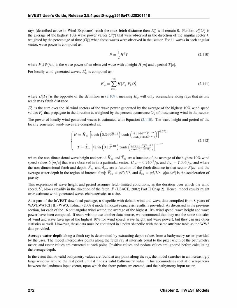
InVEST User’s Guide, Release 3.8.4.post0+ug.g3516a47.d20201118
rays (described avove in Wind Exposure) reach the max fetch distance then 𝐸𝑜𝑤 will remain 0. Further, 𝑃 𝑜
𝑘𝑂𝑜𝑘 is
the average of the highest 10% wave power values (𝑃 𝑜𝑘 ) that were observed in the direction of the angular sector k,
weighted by the percentage of time (𝑂𝑜𝑘) when those waves were observed in that sector. For all waves in each angular
sector, wave power is computed as:
𝑃 =1
2𝐻2𝑇 (2.110)
where 𝑃 [𝑘𝑊/𝑚] is the wave power of an observed wave with a height 𝐻[𝑚] and a period 𝑇 [𝑠].
For locally wind-generated waves, 𝐸𝑙𝑤 is computed as:
𝐸𝑙𝑤 =
16∑︁𝑘=1
𝐻[𝐹𝑘]𝑃 𝑙𝑘𝑂
𝑙𝑘 (2.111)
where 𝐻[𝐹𝑘] is the opposite of the definition in (2.109), meaning 𝐸𝑙𝑤 will only accumulate along rays that do not
reach max fetch distance.
𝐸𝑙𝑤 is the sum over the 16 wind sectors of the wave power generated by the average of the highest 10% wind speed
values 𝑃 𝑙𝑘 that propagate in the direction k, weighted by the percent occurrence 𝑂𝑙
𝑘 of these strong wind in that sector.
The power of locally wind-generated waves is estimated with Equation (2.110). The wave height and period of thelocally generated wind-waves are computed as:⎧⎪⎪⎨⎪⎪⎩
𝐻 = ̃︀𝐻∞
[︁tanh
(︁0.343̃︀𝑑1.14)︁ tanh
(︁4.41·10−4 ̃︀𝐹 0.79
tanh(0.343̃︀𝑑1.14)
)︁]︁0.572𝑇 = ̃︀𝑇∞
[︁tanh
(︁0.1̃︀𝑑2.01)︁ tanh
(︁2.77·10−7 ̃︀𝐹 1.45
tanh(0.1̃︀𝑑2.01)
)︁]︁0.187 (2.112)
where the non-dimensional wave height and period ̃︀𝐻∞ and ̃︀𝑇∞ are a function of the average of the highest 10% windspeed values 𝑈 [𝑚/𝑠] that were observed in in a particular sector: ̃︀𝐻∞ = 0.24𝑈2/𝑔, and ̃︀𝑇∞ = 7.69𝑈/𝑔, and wherethe non-dimensional fetch and depth, ̃︀𝐹∞ and ̃︀𝑑∞, are a function of the fetch distance in that sector 𝐹 [𝑚] and theaverage water depth in the region of interest 𝑑[𝑚]: ̃︀𝐹∞ = 𝑔𝐹/𝑈2, and ̃︀𝑑∞ = 𝑔𝑑/𝑈2. 𝑔[𝑚/𝑠2] is the acceleration ofgravity.
This expression of wave height and period assumes fetch-limited conditions, as the duration over which the windspeed, 𝑈 , blows steadily in the direction of the fetch, 𝐹 (USACE, 2002; Part II Chap 2). Hence, model results mightover-estimate wind-generated waves characteristics at a site.
As a part of the InVEST download package, a shapefile with default wind and wave data compiled from 8 years ofWAVEWATCH III (WW3, Tolman (2009)) model hindcast reanalysis results is provided. As discussed in the previoussection, for each of the 16 equiangular wind sector, the average of the highest 10% wind speed, wave height and wavepower have been computed. If users wish to use another data source, we recommend that they use the same statisticsof wind and wave (average of the highest 10% for wind speed, wave height and wave power), but they can use otherstatistics as well. However, these data must be contained in a point shapefile with the same attribute table as the WW3data provided.
Average water depth along a fetch ray is determined by extracting depth values from a bathymetry raster providedby the user. The model interpolates points along the fetch ray at intervals equal to the pixel width of the bathymetryraster, and raster values are extracted at each point. Positive values and nodata values are ignored before calculatingthe average depth.
In the event that no valid bathymetry values are found at any point along the ray, the model searches in an increasinglylarge window around the last point until it finds a valid bathymetry value. This accomodates spatial discrepanciesbetween the landmass input vector, upon which the shore points are created, and the bathymetry input raster.
272 Chapter 2. InVEST Models

InVEST User’s Guide, Release 3.8.4.post0+ug.g3516a47.d20201118
Surge Potential
Storm surge elevation is a function of wind speed and direction, but also of the amount of time wind blows overrelatively shallow areas. In general, the longer the distance between the coastline and the edge of the continental shelfat a given area during a given storm, the higher the storm surge. The model estimates the relative exposure to stormsurges by computing the distance from the shore point to the edge of the continental shelf (or to another user-specifiedbathymetry contour). For hurricanes in the Gulf of Mexico, a better approximation of surge potential than the distanceto the continental shelf contour might be the distance between the coastline and the 30 meters depth contour (Irish andResio 2010).
The model assigns a distance to all shore points, even points that seem sheltered from surge because they are too farinland, protected by a significant land mass, or on a side of an island that is not exposed to the open ocean.
Sea-Level Change
If the region of interest is large enough, some parts of the coastline may be exposed to more or less sea level rise(SLR), both in terms of the rate of rise or fall and the net amount of rise or fall that has been observed over time isexpected in the future. Spatial variation in SLR is an optional parameter in the Coastal Vulnerability model.
To include this variable in the exposure index calculation, the model takes a point vector with an attribute field con-taining a relevant SLR metric (rate, net rise, or any other variable that may be relevant to coastal inundation). The SLRvalues are joined to the shore points by taking a weighted average of the values at the two nearest SLR points, for eachshore point. The weights are the inverted distances from shore point to SLR point.
Population
When estimating the exposure of coastlines to erosion and inundation due to storms, it is important to consider thepopulation of humans that will be subject to those coastal hazards. Based on an input population raster, The CoastalVulnerability model reports the average population density (people per square kilometer) in a user-defined radiusaround each shore point. Specifically, the model takes the average of all the non-nodata population pixels within theradius, and divides by the area (in sq. km) of one population pixel.
The input population raster may contain any relevant demographic population metric of interest, not strictly totalpopulation. For example, it may be important to summarize the population density of only a vulnerable portion of thepopulation, such as eldery or children.
Limitations and Simplifications
Beyond technical limitations, the exposure index also has theoretical limitations. One of the main limitations is thatthe dynamic interactions of complex coastal processes occurring in a region are overly simplified into the geometricmean of seven variables and exposure categories. We do not model storm surge or wave field in nearshore regions.More importantly, the model does not take into account the amount and quality of habitats, and it does not quantifythe role of habitats are reducing coastal hazards. Also, the model does not consider any hydrodynamic or sedimenttransport processes: it has been assumed that regions that belong to the same broad geomorphic exposure class behavein a similar way. Additionally, the scoring of exposure is the same everywhere in the region of interest; the modeldoes not take into account any interactions between the different variables in Table 4.1. For example, the relativeexposure to waves and wind will have the same weight whether the site under consideration is a sand beach or a rockycliff. Also, when the final exposure index is computed, the effect of biogenic habitats fronting regions that have a lowgeomorphic ranking are still taken into account. In other words, we assume that natural habitats provide protection toregions that are protected against erosion independent of their geomorphology classification (i.e. rocky cliffs). Thislimitation artificially deflates the relative vulnerability of these regions, and inflates the relative vulnerability of regionsthat have a high geomorphic index.
2.4. Tools to Facilitate Ecosystem Service Analyses: 273

InVEST User’s Guide, Release 3.8.4.post0+ug.g3516a47.d20201118
The other type of model limitations is associated with the computation of the wind and wave exposure. Because ourintent is to provide default data for users in most regions of the world, we had to simplify the type of input requiredto compute wind and wave exposure. For example, we computed storm wind speeds in the WW3 wind database thatwe provide by taking the average of winds speeds above the 90th percentile value, instead of using the full time seriesof wind speeds. Thus we do not represent fully the impacts of extreme events. Also, we estimate the exposure tooceanic waves by assigning to a coastal segment a weighted average of the wave statistics of the nearest three WW3grid points. This approach neglects any 2D processes that might take place in nearshore regions and that might changethe exposure of a region.
Consequently, model outputs cannot be used to quantify the exposure to erosion and inundation of a specific coastallocation; the model produces qualitative outputs and is designed to be used at a relatively large scale. More importantly,the model does not predict the response of a region to specific storms or wave field and does not take into account anylarge-scale sediment transport pathways that may exist in a region of interest.
Data Needs
The model uses a graphical interface to input all required and optional data. Below, we outline the options offered tousers in this interface, and the content and format of the required and optional input data.
1. Workspace (required). The user is required to specify a workspace directory path. It is recommended tocreate a new directory for each run of the model. The model will create all output data in this directory. If theworkspace folder does not already exist, the model will create it.
Name: Path to a workspace directory. Avoid spaces.Sample path: \InVEST\coastal_vulnerability
2. Area of Interest (required). This file must be a polygon vector that has a ‘projected’ coordinate system ratherthan a ‘geographic’ coordinate system and the chosen coordinate system must have units of meters (the ModelResolution input value will inherit the units of this coordinate system).
Name: File can be named anything, but no spaces in the nameFile type: polygon vector (e.g. .shp, .gpkg, .geojson)Sample path: \InVEST\CoastalVulnerability\aoi_grandbahama_utm.shp
Note: Further guidance on creating an AOI: The AOI instructs the model to plot shore points on all Land-mass coastline within this AOI polygon. When drawing the AOI polygon, make sure to exclude any part of thelandmass that should not be analyzed.
When preparing other input data, it is not recommended to clip GIS datasets to the exact boundary of theAOI. Many of the model functions require searching for the presence of layers at certain distances around thecoastline, and that requires having data coverage extend beyond the AOI. The model will appropriately handleall clipping and projecting of larger datasets as needed. The model uses the AOI’s projection to transform theprojection of other input data as needed.
3. Model resolution (required). This numeric value determines the spacing between shore points as they areplotted along the landmass coastline. The value has units of meters. A larger value will yield fewer shore pointsbut a faster computation time.
Name: A numeric text string (positive integer)File type: text string (direct input to the interface)Sample (default): 1000
4. Landmass (required). This polygon input provides the model with a map of all landmasses in the region ofinterest. A global land mass polygon shapefile is provided as default (Wessel and Smith, 1996), but other layerscan be substituted. It is not recommended to clip this landmass to the AOI polygon because some functions in
274 Chapter 2. InVEST Models

InVEST User’s Guide, Release 3.8.4.post0+ug.g3516a47.d20201118
the model require searching for landmass around shore points up to the distance defined in Maximum FetchDistance, which likely extends beyond the AOI polygon.
Name: File can be named anything, but no spaces in the nameFile type: polygon vector (e.g. .shp, .gpkg, .geojson)Sample path (default): \InVEST\CoastalVulnerability\landmass_polygon.shp
5. WaveWatchIII (required). This vector contains a grid points as well as wave and wind variables that representstorm conditions at that location. These variables are used to compute the Wind and Wave Exposure ranking ofeach shoreline segment (see Wind Exposure and Wave Exposure) (Table 4.1). If users would like to create sucha file from their own data, instructions are provided in Appendix B.
Name: File can be named anythingFormat: point shapefile where each point has information about wind and wave→˓measurements.Sample data set (default): \InVEST\CoastalVulnerability\WaveWatchIII_global.shp
6. Maximum Fetch Distance (required). A numeric value in meters used to determine the degree to which shorepoints are exposed to oceanic waves or local wind-driven waves (see Wind Exposure for details). A shore pointis only exposed to oceanic wave energy if, in some direction around the point, no landmass is intersected whencasting a ray the length of this max fetch distance.:
Name: A numeric text string (positive integer)File type: text string (direct input to the interface)Sample (default): 12000
7. Bathymetry (required). This raster input is used to find average water depths required for wave height andperiod calculations ((2.112)). Bathymetry values should be negative and in units of meters. The raster shouldcover the entire offshore area extending beyond the AOI by at least the distance of the Maximum Fetch Dis-tance. All nodata and positive values are masked before calculating the average depth along a fetch ray. So it isokay if this raster also includes onshore elevation data.:
Name: File can be named anything, but no spaces in the nameFile type: raster datasetSample path: \InVEST\CoastalVulnerability\bathymetry.tif
8. Digital Elevation Model (required). This raster input is used to compute the Relief ranking of each shorelinesegment (Table 4.1). It should consist of elevation information covering the entire land polygon and extendingbeyond the AOI by at least the distance of the Elevation averaging radius. Any negative values in this inputare truncated to 0 before calculating the average elevation around a shore point. Nodata pixels are ignored.:
Name: File can be named anything, but no spaces in the nameFile type: raster datasetSample path: \InVEST\CoastalVulnerability\dem_srtm_grandbahama.tif
9. Elevation averaging radius (required). This numeric input determines the radius in meters around each shorepoint within which to compute the average elevation.
Name: A numeric text string (positive integer)File type: text string (direct input to the interface)Sample (default): 5000
10. Continental Shelf Contour (required). This is a polyline input that represents the location of the continentalmargin or other locally-important bathymetry contour. It must be within 1500 km of the coastline in the area ofinterest.
2.4. Tools to Facilitate Ecosystem Service Analyses: 275

InVEST User’s Guide, Release 3.8.4.post0+ug.g3516a47.d20201118
Names: File can be named anything, but no spaces in the nameFile type: polyline vector (e.g. .shp, .gpkg, .geojson)Sample path: \InVEST\CoastalVulnerability\continental_shelf_polyline_global.shp
11. Habitats Table (CSV) (required).. Users must provide a table to instruct the model on habitat layer inputs andparameters. The table must have headers “id”, “path”, “rank”, “protection distance (m)”.
• id is a text string (no spaces allowed) used to uniquely describe the habitat.
• path is the location and filename of the habitat GIS layer. GIS layers should be polygon format andrepresent the presence of the habitat. In the example below, the files listed in the path column are locatedin the same folder as this Habitat Table CSV file. GIS layers may be located in other places, but either thefull path must be included in this table (e.g. “C:/Documents/CV/kelp.shp”) or the path relative to this CSVfile.
• rank is a value from 1 to 5, as described in Table 4.1.
• protection distance (m) is the distance in meters beyond which this habitat will provide no protection tothe coastline.
More information on how to fill this table is provided in Appendix B.
Table Names: File can be named anything, but no spaces in the nameFile type: *.csvSample: InVEST\CoastalVulnerability\GrandBahama_Habitats\Natural_Habitats.csv
Table 5: Example Habitat Tableid path rank protection distance (m)kelp kelp.shp 4 1500eelgrass eelgrass.shp 4 500high dune HighDunes.shp 2 300low dune LowDunes.shp 3 300
12. Geomorphology (Vector) (optional). This polyline input is used to assign the Geomorphology ranking of eachshoreline point (Table 4.1). The attribute table must have a field called “RANK” that identifies the variousshoreline type ranks with a number from 1-5. More information on how to fill in this table is provided inAppendix B.
Names: File can be named anything, but no spaces in the nameFile type: polyline vector (e.g. .shp, .gpkg, .geojson)Sample path: \InVEST\CoastalVulnerability\geomorphology_grandbahama.shp
13. Geomorphology fill value (optional). Integer value between 1 and 5. If no geomorphology segments from thevector input are found in proximity to a shore point, this value will be assigned as the geomorphology rank forthat shore point. This is useful if the geomorphology type has only been mapped for a portion of the coastlinein the AOI.:
Name: A positive integer between 1 and 5.File type: text string (direct input to the interface)Sample (default): 3
14. Human Population (Raster) (optional). If provided, a raster of population is used to summarize the popula-tion density in proximity to each shore point. A global population raster file is provided as default, but otherpopulation raster layers can be substituted.
276 Chapter 2. InVEST Models

InVEST User’s Guide, Release 3.8.4.post0+ug.g3516a47.d20201118
Name: File can be named anything, but no spaces in the nameFormat: standard GIS raster file (.tiff, ESRI GRID), with population valuesSample data set (default): \InVEST\CoastalVulnerability\population_grandbahama.tif
15. Population search radius (meters) (optional). This numeric input determines the radius in meters around eachshore point within which to compute the population density.
Name: A numeric text string (positive integer)File type: text string (direct input to the interface)Sample (default): 5000
16. Sea Level Rise (Vector) (optional). This point input must have a field with numeric values representing a sealevel rise metric of interest (e.g. rate, net rise/fall) Table 4.1.
Name: File can be named anything, but no spaces in the name File type: point vector (e.g. .shp,.gpkg, .geojson) Sample path: InVESTCoastalVulnerabilitysea_level_rise.shp
17. Sea Level Rise fieldname (optional). The field in Sea Level Rise (Vector) that contains numeric values thatshould be assigned to shore points based on proximity.
Running the Model
The model uses a graphical interface to input all required and optional data and parameters (see Data Needs). Choosethe Workspace carefully, all model results will be located in that folder.
To load the model with default sample data, go to:
File > Load Parameters > Load Datastack . . . and browse to C:/InVEST_3.8.0_x86/coastal_vuln_grandbahama.invs.json
When preparing new data with which to run the model, it may be useful to view these sample datasets in a GIS, oropen a sample CSV file in order to see the expected formatting.
The runtime of this model is highly dependent on the number of shore points that are created and the level of detailin the Landmass polygon. The number of shore points created is dependent on the extent of the AOI and the modelresolution. Generally, it is wise to start modeling with a simple landmass, a large model resolution, and/or a smallAOI in order to have quick runtimes and catch other errors quickly. Then adjust these parameters as needed.
Advanced Usage
This model supports avoided re-computation. This means the model will detect intermediate and final results from aprevious run in the same workspace and it will avoid re-calculating any outputs that will be identical to the previousrun. This can save significant processing time for successive runs when only some input parameters have changed.For example, if the same AOI, landmass, model resolution, and WaveWatchIII datasets are used, the model can re-usethe time-consuming intermediate wind and wave calculations from a previous run and only spend time computingvariables that have changed.
This model also supports parallel processing. If multiple CPUs are available, users can select the number to use byselecting from the dropdown menu in File > Settings > taskgraph_n_workers_parameter. The Coastal Vulnerabilitymodel has many operations that can run in parallel, the optimal number of CPUs to use is dependent on the inputdatasets.
Interpreting results
2.4. Tools to Facilitate Ecosystem Service Analyses: 277

InVEST User’s Guide, Release 3.8.4.post0+ug.g3516a47.d20201118
Model outputs
All output files are created in the user-defined Workspace. Many files are located in an intermediate subfolder withinthe workspace.
Workspace directory
• InVEST-Coastal-Vulnerability-log-2019. . . .txt
– This is the logfile produced during every run of InVEST. It details the input parameters that were usedfor the run, and it logs all errors that may have occurred. If posting a question about a model run tocommunity.naturalcapitalproject.org, be sure to attach this logfile to your post!
• coastal_exposure.gpkg
– This point vector file contains the final outputs of the model. The points are created based on the inputmodel resolution, landmass, and AOI. The columns in this table are as follows:
* exposure - this is the final exposure index (EI in exposure-index)
* R_ - all other variables in exposure-index are columns in this table prefixed with R_. These are theranked (1 - 5) versions of these variables. Intermediate products for these variables, before valueswere binned into the 1 - 5 ranks, can be found in the intermediate folder. See below.
* exposure_no_habitats - this is the same exposure index as in exposure, except it is calculated as ifR_hab is always 5. In other words, it is the coastal exposure if no protective habitats were presentnear that point.
* habitat_role - the difference between exposure_no_habitats and exposure.
* population - (people per square kilometer) if a human population input raster was used, this is theaverage population density around each point.
• coastal_exposure.csv
– This is an identical copy of the attribute table of coastal_exposure.gpkg provided in csv format for conve-nience. Users may wish to modify or add to the columns of this table in order to calculate exposure indicesfor custom scenarios.
Intermediate directory
• intermediate_exposure.gpkg
– This point vector contains the same shore points as in coastal_exposure.gpkg, but the attribute tablecontains the intermediate values of variables before these values were binned into the 1 - 5 ranks. This ismainly useful for debugging unexpected values in the final outputs. The variables include: wind, wave,surge, relief.
• habitats/habitat_protection.csv
– This CSV file within the intermediate/habitats subfolder contains results of the habitat layer processing.Each row represents a shore point (the shore_id column can be used to link this table to other tabularoutputs). Each habitat has a column. A value of 5 indicates that habitat was not found within the habitat’sprotection distance from the shore point. A value less than 5 means the habitat was present in proximityto the shore point, and the value is the rank defined in the Habitats Table input. The R_hab column is theresult of equation (2.105).
• wind_wave/fetch_rays.gpkg
278 Chapter 2. InVEST Models

InVEST User’s Guide, Release 3.8.4.post0+ug.g3516a47.d20201118
– This line vector represents the rays that were cast in 16 directions around each shore point (see WindExposure). Viewing these rays can be helpful to understand the process behind the wind and wave exposurecalculations, and to select an appropriate Maximum Fetch Distance.
• wind_wave/wave_energies.gpkg
– This point vector contains all the shore points. The attributes include some of the intermediate values inthe Wave Exposure calculations (see Wave Exposure).
* E_ocean : from equation (2.108)
* E_local : from equation (2.111)
* Eo_El_diff : E_ocean - E_local
* max_E_type : “ocean” or “local”: A label indicating whether E_ocean or E_local has the larger value.
* maxH_local : the maximum of the wave heights across the 16 rays ( equation (2.112))
* minH_local : the minimum of the wave heights across the 16 rays (equation (2.112))
* maxT_local : the maximum of the wave periods across the 16 rays (equation (2.112))
* minT_local : the minimum of the wave periods across the 16 rays (equation (2.112))
– The wave value returned in intermediate_exposure.csv is the maximum of E_ocean and E_local at eachshore point.
• wind_wave/fetch_points.gpkg
– This point vector contains all the shore points. The attributes include the WaveWatchIII values used in theWind and Wave Exposure calculations.
– Also included are 16 columns each for fdist_ and fdepth_ which are, respectively, the fetch ray distanceand the average water depth along the ray for each compass direction.
• geomorphology/shore_points_missing_geomorphology.gpkg
– This vector stores the shore points that received the geomorphology fill value because no geomorphologysegments were found within the search radius of the point. If very many points are missing data, it mightbe explained by spatial inaccuracy of either the geomorphology or landmass polygon inputs. Editing thegeometory of one or both in GIS could help resolve this.
• other subdirectories
– Other subdirectories within the intermediate folder contain intermediate data processing steps. A couple ofthe intermediate products are highlighted above, in general the others are not particularly useful to explore,but could be useful for debugging errors.
• _taskgraph_working_dir
– This directory contains a database of previous model run parameters and enables the avoided re-computation discussed in Running the Model.
Appendix A
In this appendix, definitions for the terms presented in the geomorphic classification in Table 4.1 are presented. Someof these are from Gornitz et al. (1997) and USACE (2002).
Alluvial Plain A plain bordering a river, formed by the deposition of material eroded from areas of higher elevation.
Barrier Beach Narrow strip of beach with a single ridge and often foredunes. In its most general sense, a barrierrefers to accumulations of sand or gravel lying above high tide along a coast. It may be partially or fullydetached from the mainland.
2.4. Tools to Facilitate Ecosystem Service Analyses: 279

InVEST User’s Guide, Release 3.8.4.post0+ug.g3516a47.d20201118
Beach A beach is generally made up of sand, cobbles, or boulders and is defined as the portion of the coastal areathat is directly affected by wave action and that is terminated inland by a sea cliff, a dune field, or the presenceof permanent vegetation.
Bluff A high, steep backshore or cliff
Cliffed Coasts Coasts with cliffs and other abrupt changes in slope at the ocean-land interface. Cliffs indicate marineerosion and imply that the sediment supply of the given coastal segment is low. The cliff’s height depends uponthe topography of the hinterland, lithology of the area, and climate.
Delta Accumulations of fine-grained sedimentary deposits at the mouth of a river. The sediment is accumulatingfaster than wave erosion and subsidence can remove it. These are associated with mud flats and salt marshes.
Estuary Coast The tidal mouth of a river or submerged river valley. Often defined to include any semi-enclosedcoastal body of water diluted by freshwater, thus includes most bays. The estuaries are subjected to tidal influ-ences with sedimentation rates and tidal ranges such that deltaic accumulations are absent. Also, estuaries areassociated with relatively low-lying hinterlands, mud flats, and salt marshes.
Fiard Glacially eroded inlet located on low-lying rocky coasts (other terms used include sea inlets, fjard, and firth).
Fjord A narrow, deep, steep-walled inlet of the sea, usually formed by the entrance of the sea into a deep glacialtrough.
Glacial Drift A collective term which includes a wide range of sediments deposited during the ice age by glaciers,melt-water streams and wind action.
Indented Coast Rocky coast with headland and bays that is the result of differential erosion of rocks of differenterodibility.
Lagoon A shallow water body separated from the open sea by sand islands (e.g., barrier islands) or coral reefs.
Mud Flat A level area of fine silt and clay along a shore alternately covered or uncovered by the tide or covered byshallow water.
Appendix B
The model requires large-scale geophysical, biological, atmospheric, and population data. Most of this informationcan be gathered from past surveys, meteorological and oceanographic devices, and default databases provided withthe model. In this section, various sources for the different data layers that are required by the model are proposed,and methods to fill out the input interface discussed in the Data Needs section are described.
Geo-physical data layer
To estimate the Exposure Index of the AOI, the model requires an outline of the coastal region. As mentioned in theData Needs Section, we provide a default global land mass polygon file. This default dataset, provided by the U.S.National Oceanic and Atmospheric Administration (NOAA) is named GSHHS, or a Global Self-consistent, Hierar-chical, High-resolution Shoreline (for more information, visit http://www.ngdc.noaa.gov/mgg/shorelines/gshhs.html).It should be sufficient to represent the outline of most coastal regions of the world. However, if this outline is notsufficient, we encourage that users substitute it with another layer.
To compute the Geomorphology ranking, users must provide a geomorphology layer (Data Needs Section) with clas-sified line segments. This map should provide the location and type of geomorphic features that are located in thecoastal area of interest. For some parts of the United States, users can consult the Environmental Sensitivity Indexwebsite. If such a database is not available, it is recommend that a database from site surveys information, aerialphotos, geologic maps, or satellites images (using Google or Bing Maps, for example) is digitized. State, county, orother local GIS departments may have these data, freely available, as well.
280 Chapter 2. InVEST Models

InVEST User’s Guide, Release 3.8.4.post0+ug.g3516a47.d20201118
In addition, users must have a field in the geomorphology layer’s attribute table called “RANK”. This is used by themodel to assign a geomorphology exposure ranking based on the different geomorphic classes identified. Assign theexposure ranks based on the classification presented in Table 4.1. All ranks should be numeric from 1 to 5.
Habitat data layer
The natural habitat maps (see Data Needs Habitats Table) should provide information about the location and types ofcoastal habitats described in Table 4.1. The habitat layers in the default sample data directory have been built froma database called Shorezone. Dune data from an unpublished dataset provided by Raincoast Applied Ecology wasalso used. If such data layers are not available for your area of interest, it may be possible to digitize them from sitesurveys, aerial photos or satellites images (using Google or Bing Maps, for example).
Guidance for the protection distance (m) parameter in the Habitats Table CSV input:
Ideally this distance is based on empirical study and literature review. Absent of published findings on the distance atwhich a habitat will protect a coastline from waves, you may estimate this parameter by the following method. Viewhabitat layers in GIS along with the Landmass in your study area. Using a “distance” or “measurement” tool, measurethe distance between the shoreline and habitats that you judge to be close enough to have an effect on nearshore coastalprocesses. It is best to take multiple measurements and develop a sense of an average acceptable distance across yourregion that can serve as input. Please keep in mind that this distance is reflective of the local bathymetry conditions(a seagrass bed can extend for kilometers seaward in shallow nearshore regions), but also of the quality of the spatialreferencing of the input layer.
As mentioned in the Natural Habitats section, the model computes the natural habitat exposure ranking for a shorelinesegment using equation (2.105).
This equation is applied to various possible combinations of natural habitats, and the results of this exercise arepresented in the table and figure below:
Wind and Wave data
Wind and Wave data required by the model are included with the InVEST installation in In-VEST_3.6.0_x86CoastalProtectionInputWaveWatchIII.shp. Below is documentation on how this dataset wascreated.
To estimate the importance of wind exposure and wind-generated waves, wind statistics measured in the vicinity ofthe AOI are required. From at least 5 years of data, the model requires the average in each of the 16 equiangularsectors (0deg, 22.5deg, etc.) of the wind speeds in the 90th percentile or greater observed near the segment of interestto compute the Relative Exposure Index (REI; Keddy, 1982). In other words, for computation of the REI, sort windspeed time series in descending order, and take the highest 10% values, and associated direction. Sort this sub-seriesby direction: all wind speeds that have a direction centered around each of the 16 equiangular sectors are assigned tothat sector. Then take the average of the wind speeds in each sector. If there is no record of time series in a particularsector because only weak winds blow from that direction, then average wind speed in that sector is assigned a value ofzero (0). Please note that, in the model, wind direction is the direction winds are blowing FROM, and not TOWARDS.
For the computation of wave power from wind and fetch characteristics, the model requires the average of the windspeeds greater than or equal to the 90th percentile observed in each of the 16 equiangular sectors (0deg, 22.5deg, etc.).In other words, for computation of wave power from fetch and wind, sort the time series of observed wind speed bydirection: all wind speeds that have a direction centered on each of the 16 equiangular sectors are assigned to thatsector. Then, for each sector, take the average of the highest 10% observed values.
If users would like to provide their own wind and wave statistics, instead of relying on WW3 data, you must create apoint shapefile with the following columns:
• 16 columns named REI_VX, where X=[0,22,45,67,90,112,135,157,180,202,225,247,270,292,315,337] (e.g.,REI_V0). These wind speed values are computed to estimate the REI of each shoreline segment. These values
2.4. Tools to Facilitate Ecosystem Service Analyses: 281

InVEST User’s Guide, Release 3.8.4.post0+ug.g3516a47.d20201118
282 Chapter 2. InVEST Models

InVEST User’s Guide, Release 3.8.4.post0+ug.g3516a47.d20201118
are the average of the highest 10% wind speeds that were allocated to the 16 equiangular sectors centered on theangles listed above.
• 16 columns named REI_PCTX, where X has the same values as listed above. These 16 percent values (whichsum to 1 when added together) correspond to the proportion of the highest 10% wind speeds which are centeredon the main sector direction X listed above.
• 16 columns named WavP_X, where X has the same values as listed above. These variables are used to estimatewave exposure for sites that are directly exposed to the open ocean. They were computed from WW3 data byfirst estimating the wave power for all waves in the record, then splitting these wave power values into the 16fetch sectors defined earlier. For each sector, we then computed WavP by taking the average of the top 10%values (see Section The Model).
• 16 columns named WavPPCTX, where X has the same values as listed above. These variables are used incombination with WavP_X to estimate wave exposure for sites that are directly exposed to the open ocean. Theycorrespond to the proportion of the highest 10% wave power values which are centered on the main sectordirection X (see Section The Model).
• 16 columns named V10PCT_X, where X has the same values as listed above. These variables are used toestimate wave power from fetch. They correspond to the average of the highest 10% wind speeds that arecentered on the main sector direction X.
Sea level change
Sea level rise is often measured with tide gauges. A good global source of data for tide gauge measurements to beused in the context of sea level rise is the Permanent Service for Sea Level. This site has corrected, and sometimesuncorrected, data on sea-level variation for many locations around the world. To use this in the Coastal Vulnerability
2.4. Tools to Facilitate Ecosystem Service Analyses: 283

InVEST User’s Guide, Release 3.8.4.post0+ug.g3516a47.d20201118
Model, you must create a point dataset in GIS representing the location of the tide gauge, and the attribute table mustinclude at least one numeric field of values where larger values indicate a higher level of risk.
References
Arkema, Katie K., Greg Guannel, Gregory Verutes, Spencer A. Wood, Anne Guerry, Mary Ruckelshaus, Peter Kareiva,Martin Lacayo, and Jessica M. Silver. 2013. Coastal Habitats Shield People and Property from Sea-Level Rise andStorms. Nature Climate Change 3 (10): 913–18. https://doi.org/10.1038/nclimate1944.
Bornhold, B.D., 2008, Projected sea level changes for British Columbia in the 21st century, report for the BC Ministryof Environment.
Bush, D.M.; Neal, W.J.; Young, R.S., and Pilkey, O.H. (1999). Utilization of geoindicators for rapid assessment ofcoastal-hazard risk and mitigation. Oc. and Coast. Manag., 42.
Center for International Earth Science Information Network (CIESIN), Columbia University; and Centro Interna-cional de Agricultura Tropical (CIAT) (2005). Gridded Population of the World Version 3 (GPWv3). Palisades, NY:Socioeconomic Data and Applications Center (SEDAC), Columbia University.
Cooper J., and McLaughlin S. (1998). Contemporary multidisciplinary approaches to coastal classification and envi-ronmental risk analysis. J. Coastal Res. 14(2):512-524
Gornitz, V. (1990). Vulnerability of the east coast, U.S.A. to future sea level rise. JCR, 9.
Gornitz, V. M., Beaty, T.W., and R.C. Daniels (1997). A coastal hazards database for the U.S. West Coast.ORNL/CDIAC-81, NDP-043C: Oak Ridge National Laboratory, Oak Ridge, Tennessee.
Hammar-Klose and Thieler, E.R. (2001). Coastal Vulnerability to Sea-Level Rise: A Preliminary Database for theU.S. Atlantic, Pacific, and Gulf of Mexico Coasts. U.S. Geological Survey, Digital Data Series DDS-68, 1 CD-ROM
Irish, J.L., and Resio, D.T., “A hydrodynamics-based surge scale for hurricanes,” Ocean Eng., Vol. 37(1), 69-81, 2010.
Keddy, P. A. (1982). Quantifying within-lake gradients of wave energy: Interrelationships of wave energy, substrateparticle size, and shoreline plants in Axe Lake, Ontario. Aquatic Botany 14, 41-58.
Short AD, Hesp PA (1982). Wave, beach and dune interactions in south eastern Australia. Mar Geol 48:259-284
Tolman, H.L. (2009). User manual and system documentation of WAVEWATCH III version 3.14, Technical Note,U. S. Department of Commerce Nat. Oceanic and Atmosph. Admin., Nat. Weather Service, Nat. Centers forEnvironmental Pred., Camp Springs, MD.
U.S. Army Corps of Engineers (USACE). 2002. U.S. Army Corps of Engineers Coastal Engineering Manual (CEM)EM 1110-2-1100 Vicksburg, Mississippi.
Wessel, P., and W. H. F. Smith (1996). A Global Self-consistent, Hierarchical, High-resolution Shoreline Database, J.Geophys. Res., 101, #B4, pp. 8741-8743.
World Resources Institute (WRI) (2009). “Value of Coral Reefs & Mangroves in the Caribbean, Economic ValuationMethodology V3.0”.
2.4.2 InVEST GLOBIO Model
Summary
The GLOBIO model provides an index of biodiversity according to mean species abundance (MSA), the averagepopulation-level response across a range of species, to different stressors, including land-use change, fragmentation,and infrastructure. The model can be used as a static assessment of how far below a pristine state the current environ-ment is or to estimate how a change in any of the stressors would lead to a stress in biodiversity or ecosystem integrity,as indicated by MSA.
284 Chapter 2. InVEST Models

InVEST User’s Guide, Release 3.8.4.post0+ug.g3516a47.d20201118
Introduction
The GLOBIO methodology was developed by the United Nations Environmental Programme (UNEP, Alkemade etal. 2009) to model human impacts on biodiversity, measured by mean species abundance (MSA). Mean SpeciesAbundance is an improvement over the more traditional species-area curve approach for two reasons. First, it givesaggregate estimates of species densities, not just species presence, which is important to represent true diversity sincepresence alone gives limited information about population viability (Balmford et al 2012). Second, it relates morethan habitat area to changes in biodiversity by including information about the impact of fragmentation and threatsfrom infrastructure (and climate change and nitrogen deposition if the full version of GLOBIO were implemented).
The model
The GLOBIO method consists of a set of equations linking environmental drivers to biodiversity impact, tables ofparameters to estimate the above equations, based on a broad literature review, and suggested methodologies forinputting and processing the spatial data required. We have extended the GLOBIO methodology to downscale theirglobal approach to a landscape level.
How it works
The GLOBIO approach is based on mean species abundance (MSA, see Schwartz et al. 2003 for an example usage ofMSA). An MSA estimation ranges from 0 to 1, indicating the average proportional change in abundance of individualspecies in a location against that same location being pristine vegetation. An MSA of 1.0 implies that on average,species abundances are the same as in pristine land while an MSA of 0.0 implies that average species abundance iszero. Comparing MSA values of different scenarios identifies how anthropogenic changes affect biodiversity (e.g.,changing from a scenario with a mean MSA of 0.6 to a new scenario with 0.5 implies that, on average, individualspecies’ abundances declined 16.6% due to the land use change). In GLOBIO, an MSA value is defined for everygrid-cell within a geospatial extent.
Stressors decrease MSA in a multiplicative way. In the GLOBIO3 paper, the stressors included land use/land cover(LU), excess atmospheric nitrogen deposition (N), proximity of infrastructure (mainly roads; I), fragmentation (F) andclimate change (CC), as in the following equation to calculate MSA per pixel (i):
MS𝐴𝑖 = 𝑀𝑆𝐴𝐿𝑈𝑖∙𝑀𝑆𝐴𝑁𝑖
∙𝑀𝑆𝐴𝐼𝑖 ∙𝑀𝑆𝐴𝐹𝑖∙𝑀𝑆𝐴𝐶𝐶𝑖
To consider changes in land-use, we ignore the nitrogen deposition term and climate change terms; since neither ofthese terms change with each land-change scenario, they will cancel out when percent change in total (summed) MSAis calculated.
We refine the GLOBIO methodology for MSA change due to infrastructure, fragmentation, and land-use in order tomake use of higher resolution land-use/land-cover data (500 m pixels from MODIS rather than 50 km pixels usedby UNEP) needed to detect finer-scale ecological response that may include nonlinearities. Downscaling requiresnew methods for assigning land management regime sub-classes with more precision based on high-resolution datarather than continent-wide aggregates, and a more sophisticated approach for quantifying fragmentation than applyingoverall averages of patch size for different habitats.
Calculating MSA Impact from Infrastructure
Table 1 provides the data from Alkemade et al. (2009) for MSA values of different buffers around infrastructure thatimpact different ecosystems. The impact of infrastructure on MSA is determined solely by distance, not by the natureof the intervening vegetation. An area of cropland that is 5 km from a road will have its MSA reduced by a factor of0.9 regardless of whether the area between the cropland and the road is tropical forest or more cropland. All sourcesof infrastructure are aggregated into a “man-made” land use/land cover class. The remaining land cover classes, which
2.4. Tools to Facilitate Ecosystem Service Analyses: 285

InVEST User’s Guide, Release 3.8.4.post0+ug.g3516a47.d20201118
can then be considered vegetative or “natural” are split into three basic types: tropical forest, temperate or borealforest, and grassland or cropland. The distance of these different habitat classes from infrastructure is used to calculatethe impact zone for determining MSA from infrastructure, using Table 1.
Table 1: Effect of infrastructure impact zones on MSA, source: Alkemade et al. (2009)
Im-pactZone
Tropical Forest Dis-tance to infrastruc-ture (m)
Temperate Forest Dis-tance to infrastruc-ture (m)
Grassland & CroplandDistance to infrastruc-ture (m)
MSA_IStan-dardError
HighImpact
<1000 <300 <500 0.4 0.22
MediumImpact
1000-4000 300-1200 500-2000 0.8 0.13
LowImpact
4000-14,000 1200-4200 2000-7000 0.9 0.06
No Im-pact
>14,000 >4200 >7000 1.0 0.02
Calculating MSA Impact from Fragmentation
We augment the standard GLOBIO approach to fragmentation analysis by using a fragmented forest quality index(FFQI). The FFQI is similar to methods used in the forestry literature, and is calculated by considering how manyof a forest’s neighboring cells are also forested. Rather than identifying the expected MSA impact from patch-size(as in GLOBIO), the FFQI estimates the relative effect of fragmentation with a Gaussian smoothing function. Thistreats habitat patches that are separated by only very small patches of infrastructure or non-habitat as less fragmentedthat habitat patches separated by wider distances. We convert the FFQI values on our map to km2 to match the zonesdefined in Table 2 (according to Alkemade 2009) by taking the square root of the area to convert it to the width/heightof the patch. Although the method is different from how UNEP defined patches, comparisons to the literature showedFFQI to be an accurate approximation of more cumbersome patch-based approach.
Table 2: Fragmentation effect on MSA under varying patch sizes, source: Alkemade et al. (2009)
FFQI Area (km^2) MSA_F Standard Error< 0.43 < 1 0.3 0.150.43 – 0.58 <10 0.6 0.190.58 – 0.90 <100 0.7 0.190.90 – 0.98 <1,000 0.9 0.200.98 – 0.99 <10,000 0.95 0.200.99 – 1 >10,000 1.0 0.20
Calculating MSA Impact from Land Use Change
The most difficult aspect of GLOBIO to implement is assigning different land-use/land-cover categories that relate tointensity of management or human use, since this information is often absent in remotely-sensed global land-coverdatasets. To assist with this classification, we developed simple rules for reclassifying the MODIS or other satelliteland-use/land-cover maps into the management categories for which MSA is quantified by GLOBIO’s broad literaturereviews. Table 3 presents the rule-based categorization used to convert MODIS data to GLOBIO-compatible classes.LULC types that are mapped to more than one GLOBIO type are then split according to other auxiliary datasetsdescribed below.
286 Chapter 2. InVEST Models

InVEST User’s Guide, Release 3.8.4.post0+ug.g3516a47.d20201118
Forests:
To distinguish between primary forest and other forest, including secondary (replanted) forests or forests with someextractive use and plantation forests, we analyze fragmentation in forest cover using FFQI and assign different usecategories based on FFQI, with primary forest above a certain user-defined threshold. This approach assumes thatpristine forests are more likely to be found in large, unfragmented tracts of forest, and that secondary or lightly usedforests are more likely to be found in the most highly fragmented patches of forest. The threshold can be calibratedsuch that the aggregate amount of primary and secondary or lightly-used forests match estimates at the national orcontinental scale (documented in Alkemade et al. 2009).
Shrubland and Grassland:
To distinguish between primary vegetation (more pristine) grasslands, grazed grasslands, and man-made pastures(deforested areas used for pasture), we compare the potential vegetation map generated by Ramankutty and Foley(1999) described above to actual vegetation determined by MODIS land-cover data. If a particular pixel is designatedforest according to the potential vegetation map, but is listed as grassland in MODIS, it has likely forest that has beencleared for grazing, in this case the pixel is reclassified as “man-made pasture.” If a pixel is grassland according tothe potential vegetation map and is listed as grassland in the MODIS data, a separate dataset is utilized, quantifyingthe proportional pasture area at ~10 km resolution developed by Ramankutty et al. (2008). This pixel is defined as“livestock grazing” if the proportion of the grid-cell in pasture is greater than a user-defined threshold. The thresholdcan be chosen such that aggregate totals of livestock grazing match national and provincial data, as described abovefor forests. If the grassland pixel is lower than the grazing threshold, it will be defined as primary vegetation.
Cropland:
Because cropland intensification is only calculated in the MSALU and does not affect the configuration of primaryhabitat and thus the fragmentation calculated for MSAF, the spatial location of intensification is not necessary todefine. The user only needs to designate the proportion of agriculture in the landscape that is intensified (i.e., notlow-input agriculture). This can be found in the regional datasets cited by Alkemade et al. (2009) or available throughFAO, or can be derived a dataset developed by Foley et al. (2011) that maps yield gaps for all major commoditycrops globally at ~10 km resolution. This methodology compares agricultural production in similar climates (basedon precipitation and growing degree days) and rates crop yield in different regions according to the maximum yieldsattained for its particular climate. The difference between actual and maximum attainable yield is defined as the “yieldgap.” The yield gap can serve as a surrogate for (lack of) intensification, and the user can examine the yield gap mapsfor their region of interest to determine what proportion of the landscape falls below a certain level of yield gap.
Table 3: MODIS to GLOBIO cover class conversion and MSA affected by land use
2.4. Tools to Facilitate Ecosystem Service Analyses: 287
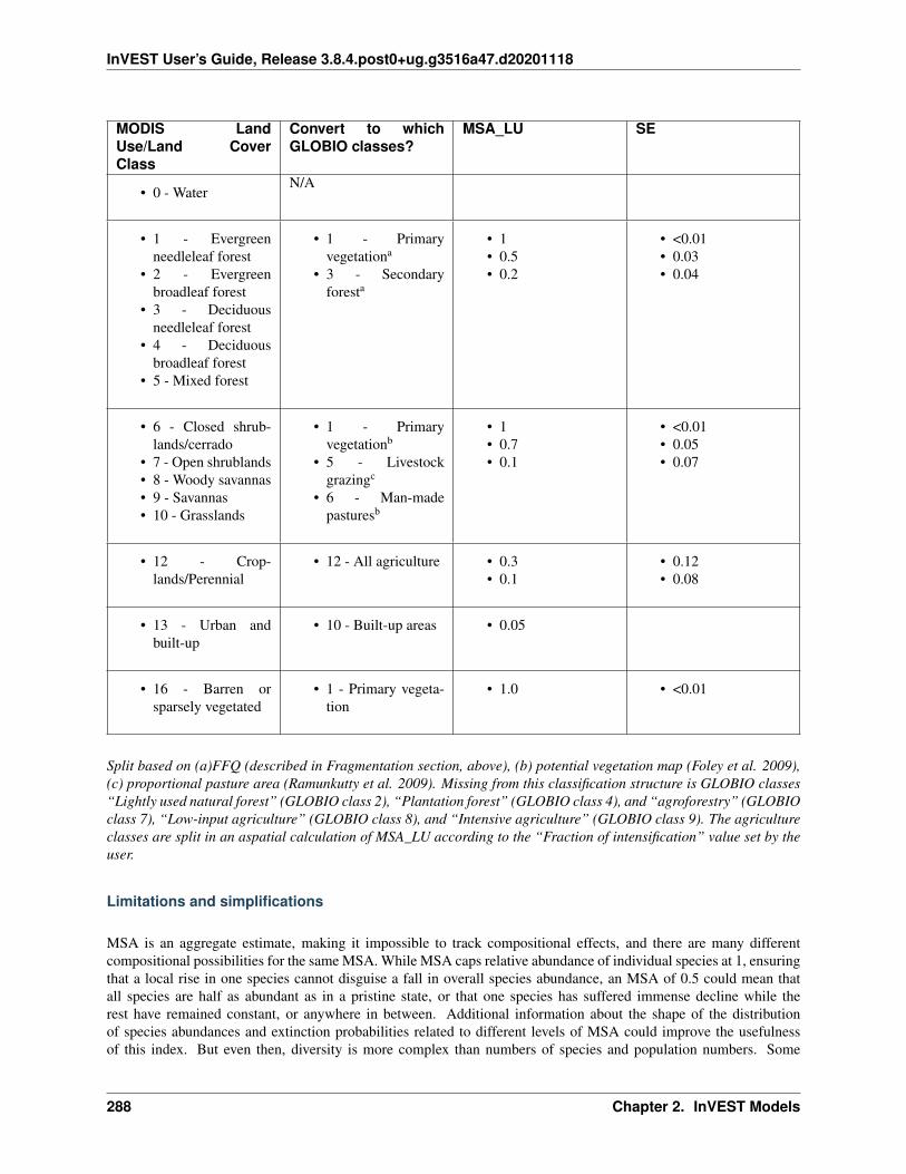
InVEST User’s Guide, Release 3.8.4.post0+ug.g3516a47.d20201118
MODIS LandUse/Land CoverClass
Convert to whichGLOBIO classes?
MSA_LU SE
• 0 - WaterN/A
• 1 - Evergreenneedleleaf forest
• 2 - Evergreenbroadleaf forest
• 3 - Deciduousneedleleaf forest
• 4 - Deciduousbroadleaf forest
• 5 - Mixed forest
• 1 - Primaryvegetationa
• 3 - Secondaryforesta
• 1• 0.5• 0.2
• <0.01• 0.03• 0.04
• 6 - Closed shrub-lands/cerrado
• 7 - Open shrublands• 8 - Woody savannas• 9 - Savannas• 10 - Grasslands
• 1 - Primaryvegetationb
• 5 - Livestockgrazingc
• 6 - Man-madepasturesb
• 1• 0.7• 0.1
• <0.01• 0.05• 0.07
• 12 - Crop-lands/Perennial
• 12 - All agriculture • 0.3• 0.1
• 0.12• 0.08
• 13 - Urban andbuilt-up
• 10 - Built-up areas • 0.05
• 16 - Barren orsparsely vegetated
• 1 - Primary vegeta-tion
• 1.0 • <0.01
Split based on (a)FFQ (described in Fragmentation section, above), (b) potential vegetation map (Foley et al. 2009),(c) proportional pasture area (Ramunkutty et al. 2009). Missing from this classification structure is GLOBIO classes“Lightly used natural forest” (GLOBIO class 2), “Plantation forest” (GLOBIO class 4), and “agroforestry” (GLOBIOclass 7), “Low-input agriculture” (GLOBIO class 8), and “Intensive agriculture” (GLOBIO class 9). The agricultureclasses are split in an aspatial calculation of MSA_LU according to the “Fraction of intensification” value set by theuser.
Limitations and simplifications
MSA is an aggregate estimate, making it impossible to track compositional effects, and there are many differentcompositional possibilities for the same MSA. While MSA caps relative abundance of individual species at 1, ensuringthat a local rise in one species cannot disguise a fall in overall species abundance, an MSA of 0.5 could mean thatall species are half as abundant as in a pristine state, or that one species has suffered immense decline while therest have remained constant, or anywhere in between. Additional information about the shape of the distributionof species abundances and extinction probabilities related to different levels of MSA could improve the usefulnessof this index. But even then, diversity is more complex than numbers of species and population numbers. Some
288 Chapter 2. InVEST Models

InVEST User’s Guide, Release 3.8.4.post0+ug.g3516a47.d20201118
conservation biologists argue that species composition is as important as any other measure of diversity, and trackingspecific species is essential to estimating impacts on threatened or endangered species or culturally valuable species(Phalan et al. 2011 Food Policy). To achieve this level of specificity, the impacts of different land-use strategies wouldneed to be evaluated for each species individually and then combined across species for summary results, which maynot be possible in many regions of the world with low data availability and high agricultural and other developmentpressure. In such cases, MSA provides a quick and easy to use index for biodiversity change in decision contexts.
In our application of GLOBIO, we use the mean parameter values and their standard errors to estimate the impactsof infrastructure, land-use, and fragmentation at new locations, which assumes that these values represent a randomsample of species and geographic locations. However, limited data availability for certain taxonomic groups andgeographic regions mean that there are potential biases in the parameter estimates that add an unquantifiable degree ofuncertainty to predictions based on our application of GLOBIO.
The estimates of the impact of infrastructure are based on a meta-analysis of ~75 studies, predominately of bird andmammal populations in Europe and North America, with some information on insects and plants (Alkemade et al.2009; Benítez-López et al 2010). Whether the impacts of infrastructure are similar for other taxonomic groups orgeographic areas is unknown.
Estimates of the impacts of land use are based on a slightly greater number of studies, with 89 identified in the initialpublication of GLOBIO (Alkemade et al. 2009) and 195 identified in a final published meta-analysis (de Baan etal. 2013). The parameter estimate for all artificial surfaces/built-up areas was based on expert opinion, representingdensely populated cities, and without quantification of uncertainty (Alkemade et al. 2009). Datasets come largelyfrom tropical regions, with fewer from temperate regions and none from boreal zones (de Baan et al. 2013). Datawere available for 9 out of 14 biomes, and for many biomes, information was only available for some land use types.For example, information on permanent crops, agroforestry and artificial areas came only from two biomes. For threebiomes, information was only available for pastures, but not for other land use types. As is common, data were alsotaxonomically biased towards vertebrate and plant species (de Baan et al. 2013). Arthropods were under-represented,and bacteria and fungi were not included at all in the database.
Furthermore, our assignment of satellite land-cover (e.g., forest or grassland) to the different GLOBIO land-use classes(e.g., primary vs. secondary forest or pristine vs. grazed grassland) introduce additional error that is not incorporatedinto the analysis. While we can ensure that our assignments aggregate up to national or regional level statistics, wecannot ground-truth our classification system to quantify the level of accuracy or uncertainty.
The impacts of fragmentation on mean species abundance (MSA) are based on six datasets from 3 publications. Theproportion of species with a viable population was used as a proxy for MSA (Alkemade et al. 2009), and it is unclearhow much additional uncertainty in the parameters that adds. Taxonomic and geographic biases are again a limitation.Two studies focus exclusively on mammals, including ~30 mammal species in Florida (Allen et al. 2001) and 10species of carnivores from around the world (Woodroffe & Ginsberg 1998). The third study is limited exclusively toEurope, of which half of the 202 species included are birds (Bouwma et al. 2002).
Data needs
The model uses 11 forms of input data. 3 are required and 8 are optional. NOTE: All spatial data must be pro-jected in meters (i.e., a local, not a global or lat-long projection), to ensure accurate distance to infrastructurecalculations. The model will not execute without a defined projection.
1. Land-use/cover map (required), following one of two options:
a. Vegetation-specific (not management-specific) land-cover. This is the type of land-cover you may acquirefrom MODIS or other remotely-sensed data sources. It distinguishes between forest, grassland, savanna,cropland, and other vegetation types. It does NOT distinguish between the differences in managementdefined by GLOBIO, such as primary vs. secondary vegetation, or grassland vs. pasture. If this option ischosen, several helper datasets (listed as required for option 1a, below) will be required.
b. Management-specific land-cover, following the classification scheme established by GLOBIO (see Table3, above). If this option is chosen, tick the box for “Predefined land use map for GLOBIO” and enter the
2.4. Tools to Facilitate Ecosystem Service Analyses: 289

InVEST User’s Guide, Release 3.8.4.post0+ug.g3516a47.d20201118
map there. All other data inputs will turn grey except for the other required data set, the infrastructuredirectory, and the optional AOI input.
Name: file can be named anything (lulc_2008.tif in the sample data)
Format: standard GIS raster file (e.g., ESRI GRID or IMG), with a column labeled ‘value’ that designatesthe LULC class code for each cell (integers only; e.g., 1 for forest, 10 for grassland, etc.) The LULC‘value’ codes must either match the LULC class codes used in the Land-cover to GLOBIO land-covertable described below (if choosing option 1a) or the GLOBIO land-cover specified in Table 3 (if choosing1b). The table can have additional fields, but the only field used in this analysis is one for LULC classcode.
2. Infrastructure directory (required). This is a folder containing maps of any forms of infrastructure you wish toconsider in the calculation of MSAI. These data may be in either raster or vector format.
Name: folder can be named anything (infrastructure_dir in the sample data)
Format: the files within the folder can be either raster or vector
3. Land-cover to GLOBIO land-cover table (required for option 1a). This is a table that translates the land-coverof option (a) in (1) above to intermediate GLOBIO classes, from which they will be further differentiated usingthe additional data below.
Name: file can be named anything (lulc_conversion_table.csv in the sample data)
File type: *.csv
Rows: each row is a different LULC class.
Columns: the columns must be named as follows:
i. lucode: Land use and land cover class code of the dataset used. LULC codes match the ‘values’ column in theLULC raster of (1a) and must be numeric and unique.
ii. globio_lucode: The LULC code corresponding to the GLOBIO class to which it should be converted, usingintermediate codes described in the example below.
Example: On the left is MODIS land-cover data, using the UMD classification, as defined in Table 3. On theright is the GLOBIO land-cover translation, which lumps the forest classes (1-5 in MODIS) into 130, grass-land/shrubland (6-10 in MODIS) into 131, and agriculture (12 in MODIS) into 132. Urban land-use (13 inMODIS) maps directly onto built-up lands (10 in GLOBIO). Barren or sparsely vegetated (16 in MODIS) canbe treated primary vegetation (1 in GLOBIO). The subsequent datasets and/or user inputs will help determinehow to split up the 130, 131, and 132 into primary and secondary vegetation, rangelands and pasture, andintensified and unintensified agriculture, respectively.
lucode globio_lucode0 01 1302 1303 1304 1305 1306 1317 1318 1319 13110 13112 13213 1016 1
290 Chapter 2. InVEST Models

InVEST User’s Guide, Release 3.8.4.post0+ug.g3516a47.d20201118
4. Pasture map (required for option 1a). The proportional pasture area, as developed by Ramankutty et al. (2008).See explanation in Shrubland and grassland under How it Works, above.
Name: file can be named anything (pasture.tif in the sample data)
Type: standard GIS raster file (e.g., ESRI GRID or IMG), with a column labeled ‘value’ that designates theproportion of the pixel that is in pasture (restricted to floats between 0 and 1).
5. Potential vegetation map (required for option 1a). This should be the potential vegetation map generated byRamankutty and Foley (1999), or similar approach. It is important to use either this exact map or if using adifferent method for mapping potential vegetation, convert the land cover classifications to match those of thismap. See explanation in Shrubland and grassland under How it Works, above.
Name: file can be named anything (potential_vegetation.tif in the sample data)
Type: standard GIS raster file (e.g., ESRI GRID or IMG), with a column labeled ‘value’ that designates the landcover class (integers only) according to Ramankutty and Foley (1999).
6. Primary Threshold (required for option 1a): a value between 0 and 1 that will determine the FFQI (forestfragmentation quality index) at which a cell should be assigned to primary or secondary forest, which can beadjusted such that the aggregate land-use matches regional statistics.
7. Pasture Threshold (required for option 1a): a value between 0 and 1 that will determine the proportion of pasturewithin a cell (in the pasture map, input #4) in order for that cell to be assigned to grassland or livestock grazing,which can be adjusted such that the aggregate land-use matches regional statistics.
8. Proportion of Agriculture Intensified (required for option 1a): a value between 0 and 1 denoting the proportionof total agriculture that should be classified as “Intensive agriculture” or GLOBIO class 8 (with 1 – Proportionof Agriculture Intensified being the proportion classified as “Low-input agriculture”, GLOBIO class 9) in thecomputation of MSALU.
9. MSA parameter table (required). This table sets the values for MSA that should be used for the different impacts(infrastructure, fragmentation and land-use) to compute MSAI, MSAF, and MSALU. The example below (and inthe sample data) gives the mean values and standard errors provided in Alkemade et al. (2009). This table canbe altered to put high and low estimates from confidence intervals in the msa_x column, to aid in uncertaintyassessment.
Name: file can be named anything (msa_parameters.csv in sample data)
Type: *.csv
Columns: the columns must be named as follows:
i. MSA_type: either msa_i_primary, msa_i_other, msa_f, or msa_lu. The values for msa_i are taken fromTable 1 above, and msa_i_primary in the example below corresponds to the values used for tropical forestand msa_i_other corresponds to values used for grassland and cropland.
ii. Measurement: the metric by which the value in the subsequent column is measured.
iii. Value: the level of impact from which the MSA value is derived (e.g., m of distance from infrastructurefor msa_i, the FFQI
iv. MSA_x: the MSA set by Alkemade et al. (2009) for different types of impacts
v. SE: the standard error associated with each MSA value, according to the meta-analysis in Alkemade et al.(2009). These values are not used by the model but are recorded here in this sample data set so that theuser can adjust the MSA_x values according to the confidence interval.
Example:
2.4. Tools to Facilitate Ecosystem Service Analyses: 291

InVEST User’s Guide, Release 3.8.4.post0+ug.g3516a47.d20201118
MSA_type Measurement Value MSA_x SEmsa_i_primary Distance (m) <1000 0.4 0.22msa_i_primary Distance (m) 1000-4000 0.8 0.13msa_i_primary Distance (m) 4000-14000 0.9 0.06msa_i_primary Distance (m) >14000 1 0.02msa_i_other Distance (m) <500 0.4 0.22msa_i_other Distance (m) 500-2000 0.8 0.13msa_i_other Distance (m) 2000-7000 0.9 0.06msa_i_other Distance (m) >7000 1 0.02msa_f FFQI < 0.43 0.3 0.15msa_f FFQI 0.43 - 0.58 0.6 0.19msa_f FFQI 0.58 - 0.90 0.7 0.19msa_f FFQI 0.90 - 0.98 0.9 0.2msa_f FFQI 0.98 - 0.99 0.95 0.2msa_f FFQI 0.99 - 1 1 0.2msa_lu Land Cover Class 0 0msa_lu Land Cover Class 1 1 <0.01msa_lu Land Cover Class 2 0.7 0.07msa_lu Land Cover Class 3 0.5 0.03msa_lu Land Cover Class 4 0.2 0.04msa_lu Land Cover Class 5 0.7 0.05msa_lu Land Cover Class 6 0.1 0.07msa_lu Land Cover Class 7 0.5 0.06msa_lu Land Cover Class 8 0.3 0.12msa_lu Land Cover Class 9 0.1 0.08msa_lu Land Cover Class 10 0.05 na
10. AOI – Area of Interest (optional). If a summary of the MSA value is desired for the region, click the box nextto AOI and enter a vector dataset containing the area(s) of interest, either as a region area or partitioned intosubregions (e.g., ecoregions, districts, etc.).
Name: file can be named anything (sub_aoi.shp in the sample data)
Type: polygon (vector) data
Running the model
The model is available as a standalone application accessible from the install directory of InVEST (under the subdi-rectory invest-3_x86/invest_globio.exe).
Advanced Usage
The GLOBIO model supports avoided re-computation. This means the model will detect intermediate and final resultsfrom a previous run in the specified workspace and it will avoid re-calculating any outputs that are identical to theprevious run. This can save significant processing time for successive runs when only some input parameters havechanged.
Viewing Output from the Model
Upon successful completion of the model, a file explorer window will open to the output workspace specified in themodel run. This directory contains an output folder holding files generated by this model. Those files can be viewed
292 Chapter 2. InVEST Models

InVEST User’s Guide, Release 3.8.4.post0+ug.g3516a47.d20201118
in any GIS tool such as ArcGIS, or QGIS. These files are described below in Section Interpreting Results.
Interpreting Results
Final Results
Final results are found within the Workspace specified for this module.
• globio-log: Each time the model is run, a text (.txt) file will appear in the Output folder. The file will list theparameter values for that run and will be named according to the service, the date and time, and the suffix.
• aoi_summary_<suffix>: A shapefile summarizing the average MSA for each zone defined in the area of in-terest.
• msa_<suffix>.tif: A raster of the overall MSA (mean species abundance) value, defined as “the averageabundances of originally occurring species relative to their abundance in the original, pristine or maturestate as the basis.” This index is on a scale of 0 to 1, with 1 being the pristine condition, calculated as theproduct of the MSALU, MSAF, and MSAI below.
• msa_lu_<suffix>.tif: A raster of MSA calculated for impacts of land-use only.
• msa_f_<suffix>.tif: A raster of MSA calculated for impacts of fragmentation only.
• msa_i_<suffix>.tif: A raster of MSA calculated for impacts of infrastructure only.
Intermediate Results
You may also want to examine the intermediate results. These files can help determine the reasons for the patterns inthe final results. They are found in the intermediate_outputs folder within the Workspace specified for this module.
• **distance_to_infrastructure_<suffix>.tif: A map coding each pixel by its distance to the nearest infras-tructure, used to compute MSAI. Distance in this raster is measured as number of pixels, which is convertedto meters in the model using the defined projection.**
• **globio_lulc_<suffix>.tif: The final land use map converted to GLOBIO classification, as outlined in Ta-ble 3. If desired, this map (or any altered version of this map) could be used to run the model using option1b, above. This is used to compute MSALU.**
• **primary_veg_smooth_<suffix>.tif: A Gaussian-filtered (“smoothed”) map of primary vegetation (identi-fied in globio_lulc), used to compute MSAF.**
• **tmp/ffqi_<suffix>.tif: A map of the forest fragmentation quality index (ffqi), used to differentiate be-tween primary and secondary forest in the GLOBIO land use classification.**
• **tmp/combined_infrastructure_<suffix>.tif: A map joining all the infrastructure files in the infrastructuredirectory (input 2 above). If there is only one file in that directory, it should be identical to that file.**
• **tmp/: Other files in this directory represent intermediate steps in calculations of the final data in the out-put folder.**
• _taskgraph_working_dir: This directory stores metadata used internally to enable avoided re-computation.
References
Alkemade, Rob, Mark van Oorschot, Lera Miles, Christian Nellemann, Michel Bakkenes, and Ben ten Brink. “GLO-BIO3: a framework to investigate options for reducing global terrestrial biodiversity loss.” Ecosystems 12, no. 3(2009): 374-390.
2.4. Tools to Facilitate Ecosystem Service Analyses: 293

InVEST User’s Guide, Release 3.8.4.post0+ug.g3516a47.d20201118
Allen, C. R., Pearlstine, L. G., & Kitchens, W. M. (2001). Modeling viable mammal populations in gap analyses.Biological Conservation, 99(2), 135–144. doi:10.1016/S0006-3207(00)00084-7
Balmford A., R. Green, B. Phalan. 2012 What conservationists need to know about farming. Proc. R. Soc. B 279:2714–2724.
Benítez-López, A., Alkemade, R., & Verweij, P. a. (2010). The impacts of roads and other infras-tructure on mammal and bird populations: A meta-analysis. Biological Conservation, 143(6), 1307–1316.doi:10.1016/j.biocon.2010.02.009
Bouwma, I. M., Jongman, R. H. G., & Butovsky, R. O. (2002). Indicative map of the Pan-European EcologicalNetwork - technical background document. Tilburg, The Netherlands/Budapest, Hungary.
de Baan, L., Alkemade, R., & Koellner, T. (2013). Land use impacts on biodiversity in LCA: a global approach.International Journal of Life Cycle Assessment, 18, 1216–1230. doi:10.1007/s11367-012-0412-0
Foley , J.A., et al. 2005. Global consequences of land use. Science 305: 570-574.
Foley, J.A., et al. 2011. Solutions for a cultivated planet. Nature 478: 337-342.
Mueller, N., et al. 2012. Closing yield gaps through nutrient and water management. Nature 490: 254-257.
Phalan, B., A. Balmford, R.E. Green, J.P.W. Scharlemann. 2011. Minimising the harm to biodiversity of producingmore food globally. Food Policy 36: S62-S71.
Ramankutty, N. and J.A. Foley. 1999. Estimating Historical Changes in Global Land Cover: Croplands from 1700 to1992, Global Biogeochemical Cycles, 13 (4), 997-1027
Ramankutty, N., et al. 2008. Farming the planet: 1. Geographic distribution of global agricultural lands in the year2000. Global Biogeochemical Cycles, Vol. 22, GB1003
Woodroffe, R., & Ginsberg, J. R. (1998). Edge Effects and the Extinction of Populations Inside Protected Areas.Science, 280(5372), 2126–2128. doi:10.1126/science.280.5372.2126
2.5 Supporting Tools
2.5.1 RouteDEM
Summary
Introduction
The freshwater models in InVEST are routed across a DEM. In the course of developing InVEST we’ve found existingimplementations of flow direction and flow accumulation algorithms to be lacking. To address this need, we have de-veloped our own high performance implementations of the D8 flow direction algorithm and fractional flow (“MultipleFlow Direction”), combined with a plateau resolution algorithm to route across flat areas (Garbrecht and Martz) thatoutperforms TauDEM and GRASS implementations. We feel these implementations are useful enough that we offerthem as a standalone tool that can calculate:
• Filling hydrological sinks.
• Resolving flat areas in a DEM so that all regions drain to some point.
• Compute flow direction across an arbitrary DEM.
• Compute flow accumulation across a DEM.
• Stream thresholding of the flow accumulation algorithm.
294 Chapter 2. InVEST Models

InVEST User’s Guide, Release 3.8.4.post0+ug.g3516a47.d20201118
After installing InVEST, this tool can be found in the start menu under the InVEST folder as a utility called RouteDEM.
RouteDEM will always resolve sinks and plateaus before routing flow.
Tool Inputs
1. Workspace: This is the folder that will contain outputs from RouteDEM after it is run.
2. Results Suffix: If provided, this suffix will be appended to all files created by the tool.
3. Digital Elevation Model: A GIS DEM raster input. Hydrological sinks and flat plateau regions will be auto-matically resolved by RouteDEM.
4. Band Index: The band index to use from the DEM raster. If not provided, band index 1 will be used.
5. Calculate Slope: Whether to calculate slope from the provided DEM. If checked, the slope raster will be writtento slope.tif in the workspace.
6. Routing Algorithm: Select the routing algorithm desired.
7. Calculate Flow Direction: Whether to calculate flow direction from the pit-filled, plateau-resolved DEM. Ifchecked, the flow direction raster will be written to flow_direction.tif in the workspace.
8. Calculcate Flow Accumulation: Whether to claculate flow accumulation from the flow direction outputs. Ifchecked, the flow accumulation raster will be written to flow_accumulation.tif in the workspace.
9. Calculate Stream Thresholds: Whether to calculate stream thresholds from the flow accumulation output. Ifchecked, the flow accumulation raster will be thresholded by the limit defined by Threshold Flow AccumulationLimit and written to stream_mask.tif.
10. Threshold Flow Accumulation Limit: The number of pixels that must flow into a pixel before it is considereda stream. Used when thresholding streams and creating the stream mask output.
11. Calculate Distance to Stream: Whether to calculate the distance to the stream. If checked, the distance-to-stream raster will be written to downstream_distance.tif in the workspace.
2.5. Supporting Tools 295
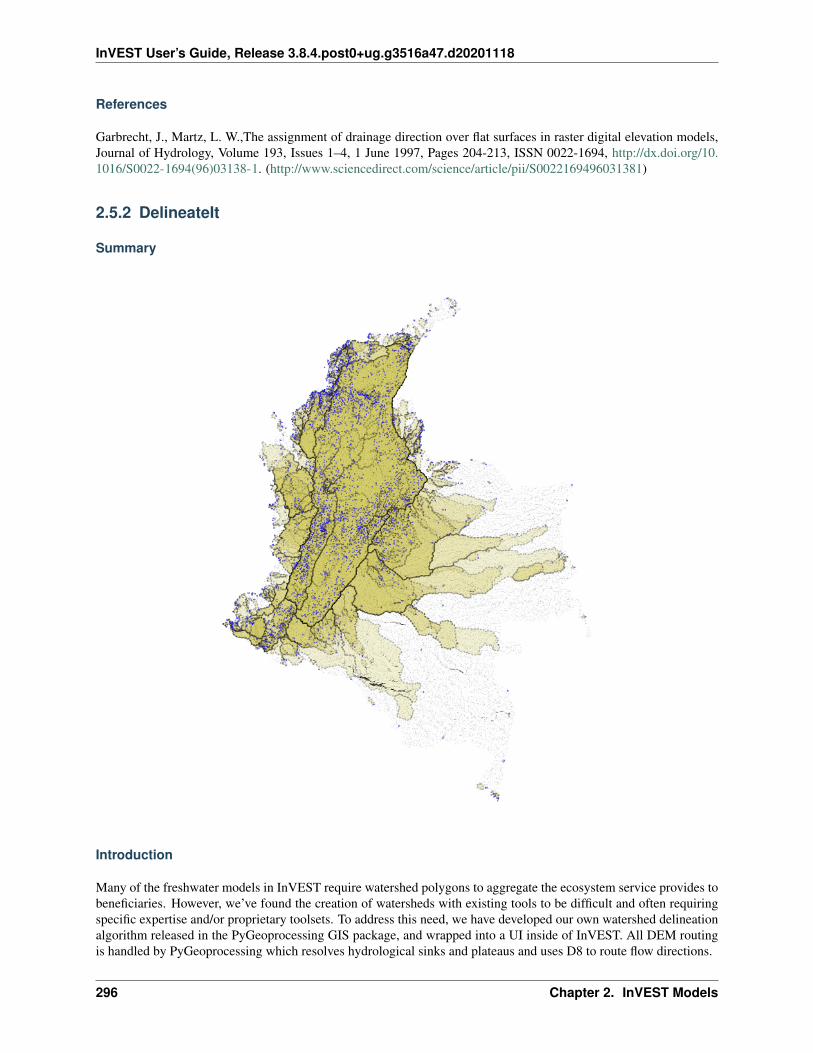
InVEST User’s Guide, Release 3.8.4.post0+ug.g3516a47.d20201118
References
Garbrecht, J., Martz, L. W.,The assignment of drainage direction over flat surfaces in raster digital elevation models,Journal of Hydrology, Volume 193, Issues 1–4, 1 June 1997, Pages 204-213, ISSN 0022-1694, http://dx.doi.org/10.1016/S0022-1694(96)03138-1. (http://www.sciencedirect.com/science/article/pii/S0022169496031381)
2.5.2 DelineateIt
Summary
Introduction
Many of the freshwater models in InVEST require watershed polygons to aggregate the ecosystem service provides tobeneficiaries. However, we’ve found the creation of watersheds with existing tools to be difficult and often requiringspecific expertise and/or proprietary toolsets. To address this need, we have developed our own watershed delineationalgorithm released in the PyGeoprocessing GIS package, and wrapped into a UI inside of InVEST. All DEM routingis handled by PyGeoprocessing which resolves hydrological sinks and plateaus and uses D8 to route flow directions.
296 Chapter 2. InVEST Models

InVEST User’s Guide, Release 3.8.4.post0+ug.g3516a47.d20201118
After installing InVEST, this tool can be found in the start menu under the InVEST folder as a utility called DelinateIt.
Tool Inputs
1. Workspace: This is the folder that will contain outputs from RouteDEM after it is run.
2. Suffix: If provided, this string will be appended to the filenames of all files created by DelineateIt.
3. Digital Elevation Model: A GIS digital elevation model (DEM) raster input. Hydrological sinks and flat plateauregions will be automatically resolved by PyGeoprocessing.
4. Outlet Features: A vector that is used to specify areas from which the watersheds should be delineated. Thesemay be stream intake points, population centers, roads, municipality boundaries or other features of interest.Any fields associated with this vector will be copied to the watershed vector as it is constructed.
5. Skip invalid geometries: If this box is checked, the model will log a WARNING and will skip delineation forthat invalid feature. If this box is unchecked and an invalid geometry if found in the outlet vector, the model willcrash with an informative error. DelineateIt can only delineate watersheds from valid geometries, so it is up tothe user to ensure that all geometries are valid.
6. Threshold Flow Accumulation: If an outlet feature does not lie directly on a stream, a very small watershedwill be generated which is usually not correct. So DelineateIt can snap outlet features with point geometry to thenearest stream to make more robust watersheds. To do this, the tool constructs a stream layer by thresholdingany pixels whose flow accumulation values exceed this parameter. Smaller values of this threshold producestreams with more tributaries, larger values produce streams with fewer tributaries.
7. Pixel Distance to Snap Outlet Points: If an outlet point does not lie directly on a stream, a very small watershedwill be generated which is usually not correct. During watershed construction, DelineateIt will search withina radius of the defined number of pixels around each outlet point to find the nearest stream pixel. Streams aredefined by the threshold flow accumulation value listed above. Pixel distance is given as the number of pixels,which is unitless. It is not an actual distance (such as meters.) So if you give it a value of 3, DelineateIt willsearch within a radius of 3 pixels around each outlet point looking for a stream. Note that if the cell size is small,the actual distance searched will be small, if the cell size is large, the actual distance searched will be large. Alsonote that this snap distance will only be applied to point geometries. Any other geometric types provided in theoutlet features vector will be used as they are.
Tool Outputs
All outputs can be found in the Workspace directory given previously. They include:
• watersheds.gpkg A GeoPackage vector defining the areas that are upstream from the snapped outlet points,where upstream area is defined by the D8 flow algorithm implementation in PyGeoprocessing.
• snapped_outlets.gpkg A vector that indicates where outlet points (point geometries only) were snapped tobased on the values of Threshold Flow Accumulation and Pixel Distance to Snap Outlet Points. Any non-pointgeometries will also have been copied over to this vector, but will not have been altered.
• preprocessed_geometries.gpkg A vector containing only those geometries that the model can verify are valid.The geometries appearing in this vector will be the ones passed to watershed delineation.
• streams.tif The raster stream layer used to snap outlet points, produced from the DEM and Threshold FlowAccumulation value.
• filled_dem.tif The DEM, but with hydrological sinks filled.
• flow_direction.tif The D8 flow direction raster, created from the filled DEM.
• flow_accumulation.tif The D8 flow accumulation raster, created from flow_direction.tif.
2.5. Supporting Tools 297

InVEST User’s Guide, Release 3.8.4.post0+ug.g3516a47.d20201118
References
PyGeoprocessing https://bitbucket.org/natcap/pygeoprocessing
2.5.3 Scenario Generator: Proximity Based
Summary
The proximity-based scenario generator creates a set of contrasting land use change maps that convert habitat indifferent spatial patterns. The user determines which habitat can be converted and what they are converted to, as wellas type of pattern, based on proximity to the edge of a focal habitat. In this manner, an array of land-use changepatterns can be generated, including pasture encroaching into forest from the forest edge, agriculture expanding fromcurrently cropped areas, forest fragmentation, and many others. The resulting land-use maps can then be used as inputsto InVEST models, or other models for biodiversity or ecosystem services that are responsive to land use change.
Introduction
In order to understand the change in biodiversity and ecosystem services (BES) resulting from change in land-use, itis often helpful to start with a scenario or a set of scenarios that exhibit different types of land-use change. Becausemany of the relationships between landscapes and BES are spatially-explicit, a different pattern of habitat conversionfor the same total area of habitat converted can lead to very different impacts on BES. This proximity-based scenariogenerator creates different patterns of conversion according to user inputs designating focal habitat and convertedhabitat, in contrast to but potentially complementing the InVEST rule-based scenario generator that creates maps ofland-use change according to user-assigned probabilities that certain transitions will occur. Thus, the intent of theInVEST proximity-based scenario generator is not to forecast actual predicted patterns of expansion, but rather todevelop different patterns of land use change in order to examine the relationship between land-use change and BES,and how the relationship may differ depending on land use change assumptions.
The model
The tool can generate two scenarios at once (nearest to the edge and farthest from the edge of a focal habitat), for aconversion to particular habitat type for a given area. To convert to different habitat types, different habitat amounts,or to designate different focal habitats or converted habitats, the tool can be run multiple times in sequence.
How it works
Three types of landcover must be defined: 1) Focal landcover is the landcover(s) that set the proximity rules fromwhich the scenarios will be determined. The scenario generator will convert habitat from the edge or toward theedge of patches of these types of landcover. This does not mean it will convert these land-covers, only that it willmeasure distance to or from the edges in designating where the conversion will happen. 2) Convertible landcover isthe landcover(s) that can be converted. These could be the same as the focal landcover(s), a subset, or completelydifferent. 3) Replacement landcover is the landcover type to which the convertible landcovers will be converted. Thiscan only be one landcover type per model run.
Two scenarios can then be run at a time: 1) Nearest to edge means that convertible landcover types closest to the edgesof focal landcovers will be converted to the replacement landcover. 2) Farthest from edge means that convertiblelandcover types furthest from the edges of focal landcover types will be converted to the replacement landcover. If thisscenario is chosen, the user can designate in how many steps the conversion should occur. This is relevant if the focallandcover is the same as the convertible land cover because the conversion of the focal landcover will create new edgesand hence will affect the distance calculated from the edge of that landcover. If desired, the conversion can occur inseveral steps, each time converting the farthest from the edge of the focal landcover, causing a fragmentary pattern.
298 Chapter 2. InVEST Models

InVEST User’s Guide, Release 3.8.4.post0+ug.g3516a47.d20201118
Below are some examples of the types of scenarios that can be generated by manipulating these basic inputs, using theland-cover in the sample data that ship with this model. This landcover is from MODIS, using the UMD classification(Friedl et al. 2011), which follows the following scheme: 1 – Evergreen needleleaf forest; 2 – Evergreen broadleafforest; 3 – Deciduous needleleaf forest; 4 – Deciduous broadleaf forest; 5 – Mixed forest; 6 – Closed shrublands; 7 –Open shrublands; 8 – Woody savannas; 9 – Savannas; 10 – Grasslands; 12 – Croplands; 13 – Urban and built-up; 16 –Barren or sparsely vegetated.
Expand agriculture from forest edge inwards:
focal landcover codes: 1 2 3 4 5
convertible landcover codes: 1 2 3 4 5
replacement landcover code: 12
check “Convert From Edge”
number of steps toward conversion: 1
Expand agriculture from forest core outwards:
focal landcover codes: 1 2 3 4 5
convertible landcover codes: 1 2 3 4 5
replacement landcover code: 12
check “Convert Toward Edge”
number of steps toward conversion: 1
Expand agriculture by fragmenting forest:
focal landcover codes: 1 2 3 4 5
convertible landcover codes: 1 2 3 4 5
replacement landcover code: 12
check “Convert Toward Edge”
number of steps toward conversion: 10 (or as many steps as desired; the more steps, the more finely fragmented it willbe and the longer the simulation will take)
Expand pasture into forest nearest to existing agriculture:
focal landcover codes: 12
convertible landcover codes: 1 2 3 4 5
replacement landcover code: 10
check “Convert From Edge”
number of steps toward conversion: 1
Data needs
The only required input data to run the proximity-based scenario generator is a base land-use/land-cover map anduser-defined land cover codes pertaining to this base map to designate how the scenarios should be computed.
1. Base land-use/cover map (required). This is the map that will be modified in the generation of the desiredscenarios. All pixels in this map (that overlap with the area of interest, if included) other than the pixels that areconverted will remain the same.
2.5. Supporting Tools 299

InVEST User’s Guide, Release 3.8.4.post0+ug.g3516a47.d20201118
Name: file can be named anything (scenario_proximity_lulc.tif in the sample data)
Format: standard GIS raster file (e.g., ESRI GRID or IMG), with a column labeled ‘value’ that designatesthe LULC class code for each cell (integers only; e.g., 1 for forest, 10 for grassland, etc.)
2. AOI – Area of Interest (optional). If change is only desired in a subregion of the broader land-use/land-covermap, the user may designate this area of interest. Prior to scenario generation, the map will be clipped to theextent of this vector.
Name: file can be named anything (scenario_proximity_aoi.shp in the sample data)
Format: vector (polygon) file
3. Max area to convert (ha): enter the maximum numbers of hectares to be converted to agriculture. This is themaximum because due to the discretization of area of pixels, the number of pixels closest to but not exceedingthis number will be converted.
4. Focal Landcover Codes: enter the LULC code(s) for the land cover types from which distance from edge shouldbe calculated. If multiple values, they should be separated by spaces.
5. Convertible Landcover Codes: enter the LULC code(s) for the land cover types that are allowed to be convertedto agriculture in the simulation. If multiple values, they should be separated by spaces.
6. Replacement Landcover Code: enter an integer that corresponds to the LULC code to which habitat will beconverted. If there are multiple LULC types that are of interest for conversion, this tool should be run insequence, choosing one type of conversion each time. A new code may be introduced if it is a novel land-usefor the region or if it is desirable to track the expanded land-use as separate from historic land-use.
7. Check boxes: types of scenarios to generate
i. Convert farthest from edge: land cover type(s) designated as “convertible” that are farthest from the edgeof any land cover type designated as “focal” will be converted. Convertible land covers and habitat ofinterest land-covers may be the same, or a subset of one another, or they can be different. If they are thesame, the number of steps for conversion should be specified, because the conversion of habitat withinthe focal land cover will create new habitat edge, resulting in a completely different pattern of conversiondepending on how many steps are chosen.
ii. Convert nearest to edge: land cover type(s) designated as “convertible” that are nearest to the edge of anyland cover type designated as “focal” will be converted. As for the previous scenario, convertible landcovers and habitat of interest land-covers may be the same, or a subset of one another, or they can bedifferent.
8. Number of Steps in Conversion: enter an integer for the number of steps the simulation should take to fragmentthe habitat of interest in the fragmentation scenario. Entering a 1 means that all of the habitat conversion willoccur in the center of the patch of the habitat of interest. Entering 10 will be fragmented according to a patternof sequentially converting the pixels furthest from the edge of that habitat, over the number of steps specified bythe user.
Running the model
The model is available as a standalone application accessible from the install directory of InVEST (under the subdi-rectory invest-3_x86/invest_scenario_gen_proximity.bat).
Advanced Usage
This model supports avoided re-computation. This means the model will detect intermediate and final results from aprevious run in the specified workspace and it will avoid re-calculating any outputs that are identical to the previousrun. This can save significant processing time for successive runs when only some input parameters have changed.
300 Chapter 2. InVEST Models

InVEST User’s Guide, Release 3.8.4.post0+ug.g3516a47.d20201118
Viewing Output from the Model
Upon successful completion of the model, a file explorer window will open to the output workspace specified in themodel run. This directory contains an output folder holding files generated by this model. Those files can be viewedin any GIS tool such as ArcGIS, or QGIS. These files are described below in Section Interpreting Results.
Interpreting Results
Final Results
Final results are found in the Workspace folder within the specified for this module.
• InVEST. . . .log. . . txt: Each time the model is run, a text (.txt) file will appear in the Output folder. The file willlist the parameter values for that run and will be named according to the model, the date and time, and the suffix.
• nearest_to_edge _<suffix>.tif: LULC raster for the scenario of conversion nearest to the edge of the focalhabitat
• farthest_from_edge_<suffix>.tif: LULC raster for the scenario of conversion farthest from the edge of thefocal habitat
• nearest_to__edge_<suffix>.csv: table listing the area (in hectares) and number of pixels for different landcover types converted for the scenario of conversion nearest to the edge of the focal habitat
• farthest_from_edge _<suffix>.csv: table listing the area (in hectares) and number of pixels for differentland cover types converted for the scenario of conversion nearest to the edge of the focal habitat
Intermediate Results
You may also want to examine the intermediate results. These files can help determine the reasons for the patterns inthe final results. They are found in the intermediate_outputs folder within the Workspace specified for this module.
• **{farthest_from_/nearest_to}_edge_distance_<suffix>.tif: map of This raster shows the distance (in num-ber of pixels) of each pixel to the nearest edge of the focal landcover**
• _tmp_work_tokens: This directory stores metadata used internally to enable avoided re-computation.
Sample Script
The following script is provided to demonstrate how the scenarios described in Section “How It Works” can be com-posed into a single script that’s callable from the InVEST Python API:
import natcap.invest.scenario_generator_proximity_based
edge_args = {u'aoi_path': u'C:/Users/Rich/Documents/svn_repos/invest-sample-data/scenario_
→˓proximity/scenario_proximity_aoi.shp',u'area_to_convert': u'20000.0',u'base_lulc_path': u'C:/Users/Rich/Documents/svn_repos/invest-sample-data/
→˓scenario_proximity/scenario_proximity_lulc.tif',u'convert_farthest_from_edge': False,u'convert_nearest_to_edge': True,u'convertible_landcover_codes': u'1 2 3 4 5',u'focal_landcover_codes': u'1 2 3 4 5',u'n_fragmentation_steps': u'1',
(continues on next page)
2.5. Supporting Tools 301

InVEST User’s Guide, Release 3.8.4.post0+ug.g3516a47.d20201118
(continued from previous page)
u'replacment_lucode': u'12',u'results_suffix': 'edge',u'workspace_dir': u'C:\\Users\\Rich/Documents/scenario_proximity_workspace',
}
core_args = {u'aoi_path': u'C:/Users/Rich/Documents/svn_repos/invest-sample-data/scenario_
→˓proximity/scenario_proximity_aoi.shp',u'area_to_convert': u'20000.0',u'base_lulc_path': u'C:/Users/Rich/Documents/svn_repos/invest-sample-data/
→˓scenario_proximity/scenario_proximity_lulc.tif',u'convert_farthest_from_edge': True,u'convert_nearest_to_edge': False,u'convertible_landcover_codes': u'1 2 3 4 5',u'focal_landcover_codes': u'1 2 3 4 5',u'n_fragmentation_steps': u'1',u'replacment_lucode': u'12',u'results_suffix': 'core',u'workspace_dir': u'C:\\Users\\Rich/Documents/scenario_proximity_workspace',
}
frag_args = {u'aoi_path': u'C:/Users/Rich/Documents/svn_repos/invest-sample-data/scenario_
→˓proximity/scenario_proximity_aoi.shp',u'area_to_convert': u'20000.0',u'base_lulc_path': u'C:/Users/Rich/Documents/svn_repos/invest-sample-data/
→˓scenario_proximity/scenario_proximity_lulc.tif',u'convert_farthest_from_edge': True,u'convert_nearest_to_edge': False,u'convertible_landcover_codes': u'1 2 3 4 5',u'focal_landcover_codes': u'1 2 3 4 5',u'n_fragmentation_steps': u'10',u'replacment_lucode': u'12',u'results_suffix': 'frag',u'workspace_dir': u'C:\\Users\\Rich/Documents/scenario_proximity_workspace',
}
ag_args = {u'aoi_path': u'C:/Users/Rich/Documents/svn_repos/invest-sample-data/scenario_
→˓proximity/scenario_proximity_aoi.shp',u'area_to_convert': u'20000.0',u'base_lulc_path': u'C:/Users/Rich/Documents/svn_repos/invest-sample-data/
→˓scenario_proximity/scenario_proximity_lulc.tif',u'convert_farthest_from_edge': False,u'convert_nearest_to_edge': True,u'convertible_landcover_codes': u'12',u'focal_landcover_codes': u'1 2 3 4 5',u'n_fragmentation_steps': u'1',u'replacment_lucode': u'12',u'results_suffix': 'ag',u'workspace_dir': u'C:\\Users\\Rich/Documents/scenario_proximity_workspace',
}if __name__ == '__main__':
natcap.invest.scenario_generator_proximity_based.execute(edge_args)natcap.invest.scenario_generator_proximity_based.execute(core_args)natcap.invest.scenario_generator_proximity_based.execute(frag_args)natcap.invest.scenario_generator_proximity_based.execute(ag_args)
302 Chapter 2. InVEST Models

InVEST User’s Guide, Release 3.8.4.post0+ug.g3516a47.d20201118
2.5.4 InVEST Scripting Guide and API
Summary
Introduction
While there is a user interface for all the InVEST models, we also provide a python application programming interface(API) for more advanced usage of the models. Full documentation for the natcap.invest python package isavailable here: http://invest.readthedocs.io/en/latest/
Additionally, our core geoprocessing routines have been open sourced as a separate python package,pygeoprocessing. Documentation for pygeoprocessing is available here: http://pythonhosted.org/pygeoprocessing/
This documentation will be updated in more detail in the future. Programming support is also available on our userforums: http://forums.naturalcapitalproject.org/.
2.5. Supporting Tools 303

InVEST User’s Guide, Release 3.8.4.post0+ug.g3516a47.d20201118
304 Chapter 2. InVEST Models

CHAPTER
THREE
ACKNOWLEDGEMENTS
3.1 Acknowledgements
3.1.1 Data sources
The Marine InVEST development team would like to acknowledge the following sources for data that are providedwith the models:
WAVEWATCH III model hindcast reanalysis results are from NOAA’s National Weather Service
ETOPO1 was developed by and is available from NOAA’s National Geophysical Data Center (NGDC). (Amante,C. and B. W. Eakins, ETOPO1 1 Arc-Minute Global Relief Model: Procedures, Data Sources and Analysis. NOAATechnical Memorandum NESDIS NGDC-24, 19 pp, March 2009).
The Global Self-consistent, Hierarchical, High-resolution Shoreline Database (GSHHS) is developed and main-tained by Paul Wessel, SOEST, University of Hawai’i, Honolulu, and Walter H.F. Smith, NOAA Geosciences Lab, Na-tional Ocean Service, Silver Spring, MD. It can be accessed via NOAA’s National Geophysical Data Center (NGDC).(Wessel, P., and W. H. F. Smith, A Global Self-consistent, Hierarchical, High-resolution Shoreline Database, J. Geo-phys. Res., 101)
British Columbia Shorezone Data are provided courtesy of the Province of British Columbia, Ministry of NaturalResource Operations, GeoBC Division. The data used for this model is a snapshot in time. For the most current coastalresource and shorezone data please visit http://www.geobc.gov.bc.ca.
Gridded Population of the World Version 3 (GPWv3) data are provided courtesy of the Center for InternationalEarth Science Information Network (CIESIN), Columbia University; and Centro Internacional de Agricultura Tropical(CIAT). 2005. Gridded Population of the World Version 3 (GPWv3): Population Grids. Palisades, NY: SocioeconomicData and Applications Center (SEDAC), CIESIN, Columbia University. Available at http://sedac.ciesin.columbia.edu/gpw.
Department of Fisheries and Oceans Canada provides commercial fishery data layers (groundfish trawl and long-line, salmon troll, and shrimp trawl) collected from 1993-95 through interviews with fisheries officers for the WestCoast of Vancouver Island, British Columbia. Data are publicly available through GeoBC, the geographic informationclearinghouse for British Columbia Canada.
Habitat layers are available through British Columbia Marine Conservation Analysis (BCMCA) and GeoBC.
3.1.2 Individuals and organizations
We would also like to thank the following individuals and organizations for support, guidance, great collaborations,and fun! This is not an exhaustive list.
The Gordon and Betty Moore Foundation
305

InVEST User’s Guide, Release 3.8.4.post0+ug.g3516a47.d20201118
The West Coast Aquatic Management Board
NOAA Fisheries, Northwest Fisheries Science Center
Gretchen Daily, Peter Kareiva, Taylor Ricketts, Steve Polasky, and Jon Foley
Our Technical Working Group: Mary Ruckelshaus, Anne Guerry, Katie Arkema, Greg Guannel, CK Kim, MikePapenfus, Jodie Toft, Gregg Verutes, Joey Bernhardt, Apollo Qi, Jeremy Davies, Heather Tallis, Steve Polasky, MarkPlummer, Phil Levin, Bill Labiosa, Francis Chan, Guy Gelfenbaum, Peter Ruggiero, Andre Punt, Melanie McField,Ben Halpern, Sarah Lester, Malin Pinsky, Mike Beck, Barry Gold, Kai Chan
Others: Matt Marsik, Spencer Wood, Dave Sutherland, Andrew Day, Laura Loucks, Trudy Warner, Kevin Head, RogerBedard, Jim Regetz, Dan Holland, Jameal Samhouri .. primerend
306 Chapter 3. Acknowledgements