TARDIS Documentation - Read the Docs

TARDIS DocumentationRelease 0.9.dev642

TARDIS team

January 21, 2014

Contents

i

TARDIS Documentation, Release 0.9.dev642

This is the documentation for the TARDIS package.

Warning: Currently TARDIS only works on 64-bit python installations. We’re working on making it work on32-bit python distributions.

Contents 1


2 Contents

CHAPTER 1

Introduction

TARDIS is a package that creates

3


4 Chapter 1. Introduction

CHAPTER 2

Installation

2.1 Requirements

Warning: Currently TARDIS only works on 64-bit python installations. We’re working on making it work on32-bit python distributions.

TARDIS has the following requirements:

• Python 2.6, 2.7, 3.1 or 3.2

• Numpy 1.5 or later

• Scipy 0.10 or later

• Astropy 0.2.4 or later

• h5py 2.0.0 or later

• pandas 0.12.0 or later

• pyyaml 3.0 or later

Most of these requirements are easy to install using package managers like OS X’s macports or normal linux packagemanagers

2.2 Installing TARDIS

2.2.1 On Ubuntu (13.10)

We use a clean install of Ubuntu 13.10 as one of our testing grounds. Here’s how we get TARDIS to run:

sudo apt-get install python-dev python-pip python-numpy python-scipy python-h5py python-pandas python-yaml

We now need to install the newest astropy and we will install everything into our users directory:

pip install astropy --user

Once astropy is installed, install TARDIS:

pip install tardis-sn --user --pre

5

http://www.python.org/

http://www.numpy.org/

http://www.scipy.org/

http://www.astropy.org/

http://www.h5py.org/

http://pandas.pydata.org/

http://pyyaml.org/


Add a –pre to install the latest development version (currently no stable version is available).

Note:pip often tries to take care of many of the dependencies, this might be annoying as they already exist. Adding –

no-deps will help with this problem.

2.3 Building from source

2.3.1 Prerequisites

You will need a compiler suite and the development headers for Python and Numpy in order to build TARDIS. OnLinux, using the package manager for your distribution will usually be the easiest route, while on MacOS X you willneed the XCode command line tools.

The instructions for building Numpy from source are also a good resource for setting up your environment to buildPython packages.

You will also need Cython installed to build from source, unless you are installing a numbered release. (The releasespackages have the necessary C files packaged with them, and hence do not require Cython.)

Note: If you are using MacOS X, you will need to the XCode command line tools. One way to get them is to installXCode. If you are using OS X 10.7 (Lion) or later, you must also explicitly install the command line tools. You can dothis by opening the XCode application, going to Preferences, then Downloads, and then under Components, click onthe Install button to the right of Command Line Tools. Alternatively, on 10.7 (Lion) or later, you do not need to in-stall XCode, you can download just the command line tools from https://developer.apple.com/downloads/index.action(requires an Apple developer account).

6 Chapter 2. Installation

http://docs.scipy.org/doc/numpy/user/install.html

http://cython.org/

https://developer.apple.com/xcode/

https://developer.apple.com/downloads/index.action

CHAPTER 3

Running TARDIS

To run TARDIS requires two files. The atomic database (for more info refer to Atomic Data) and a configuration file(more info at Configuration File).

3.1 Simple Example

After installing TARDIS just download the example directory https://www.dropbox.com/s/svvyr5i7m8ouzdt/tardis_example.tar.gzand run TARDIS with:

tar zxvf tardis_example.tar.gzcd tardis_exampletardis tardis_example.yml output_spectrum.dat

Then plot the output_spectrum.dat with your favourite plotting program. Here’s an example how to do this withpython. (The only thing you need to install is ipython and matplotlib - in addition to TARDIS’s requirements)

3.2 Scripting TARDIS

from tardis import config_reader, model_radial_oned, simulation

tardis_config = config_reader.TARDISConfiguration.from_yaml(’myconfig.yml’)radial1d_mdl = model_radial_oned.Radial1DModel(tardis_config)simulation.run_radial1d(radial1d_mdl)

7

https://www.dropbox.com/s/svvyr5i7m8ouzdt/tardis_example.tar.gz


8 Chapter 3. Running TARDIS

CHAPTER 4

Graphical User Interface

TARDIS uses the PyQt4 framework for its cross-platform interface.

The GUI runs through the IPython Interpreter which should be started with the command ipython-2.7--pylab=qt, so that it has acess to pylab.

Creating an instance of the ModelViewer-class requires that PyQt4 has already been initialized in IPython. Theabove command to start IPython accomplishes this.

4.1 GUI Layout and Features

9

http://www.riverbankcomputing.com/software/pyqt/download

http://ipython.org/install.html


10 Chapter 4. Graphical User Interface

CHAPTER 5

Configuration File

TARDIS uses the YAML markup language for its configuration files. There are several sections which allow differentsettings for the different aspects of the TARDIS calculation. An example configuration file can be downloaded here.

Warning: One should note that currently floats in YAML need to be specified in a special format: any pure floatsneed to have a +/- after the e e.g. 2e+5

Every configuration file begins with the most basic settings for the model:

---#Currently only simple1d is allowedconfig_type: simple1d

#luminosity any astropy.unit convertible to erg/s#special unit log_lsun(log(luminosity) - log(L_sun)luminosity: 9.44 log_lsun

#time since explosiontime_explosion: 13 day

atom_data: ../atom_data/kurucz_atom_chianti_many.h5

The config_type currently only allows simple1d, but might be expanded in future versions of TARDIS. Manyparameters in the TARDIS configuration files make use of units. One can use any unit that is supported by astropy unitsas well as the unit log_lsun which is log(𝐿) − log(𝐿⊙). Time since explosion just takes a normal time quantity.atom_data requires the path to the HDF5 file that contains the atomic data (more information about the HDF5 filecan be found here Atomic Data).

5.1 Plasma

The next configuration block describes the plasma parameters:

plasma:initial_t_inner: 10000 Kinitial_t_rad: 10000 Kdisable_electron_scattering: noplasma_type: nebular#radiative_rates_type - currently supported are lte, nebular and detailedradiative_rates_type: detailed#line interaction type - currently supported are scatter, downbranch and macroatom

11

https://en.wikipedia.org/wiki/YAML

http://docs.astropy.org/en/stable/units/index.html


line_interaction_type : macroatomw_epsilon : 1.0e-10

inital_t_inner is temperature of the black-body on the inner boundary. initial_t_rad is the radiation tem-perature for all cells. For debugging purposes and to compare to synapps calculations one can disable the electronscattering. TARDIS will issue a warning that this is not physical. There are currently two plasma_type optionsavailable: nebular and lte which tell TARDIS how to run the ionization equilibrium and level population calcu-lations (see Plasma for more information). The radiative rates describe how to calculate the 𝐽blue needed for the nltecalculations and macroatom calculations. There are three options for radiative_rates_type: 1) lte in which𝐽blue = Blackbody(𝑇rad), 2) nebular in which 𝐽blue = 𝑊 × Blackbody(𝑇rad), 3) detailed in which the 𝐽blue arecalculated using an estimator (this is described in ??????).

TARDIS currently supports three different kinds of line interaction: scatter - a resonance scattering implementa-tion, macroatom - the most complex form of line interaction described in macroatom and downbranch a simplifiedversion of macroatom in which only downward transitions are allowed.

Finally, w_epsilon describes the dilution factor to use to calculate 𝐽blue that are 0, which causes problem with thecode (so 𝐽blue are set to a very small number).

NLTE:

nlte:coronal_approximation: Trueclassical_nebular: False

The NLTE configuration currently allows setting coronal_approximation which sets all 𝐽blue to 0. This isuseful for debugging with chianti for example. Furthermore one can enable ‘classical_nebular’ to set all 𝛽Sobolev to 1.Both options are used for checking with other codes and should not be enabled in normal operations.

5.2 Model

The next sections, describing the model, are very hierarchical. The base level is model and contains two subsections:structure and abundances. Both sections can either contain a file subsection which specifies a file and filetype where the information is stored or a number of other sections.

model:structure:

no_of_shells : 20

velocity:type : linearv_inner : 1.1e4 km/sv_outer : 2e4 km/s

density:#showing different configuration options separated by comments#simple uniform:#---------------

# type : uniform# value : 1e-12 g/cm^3

#---------------

#branch85_w7 - fit of seven order polynomial to W7 (like Branch 85):#---------------type : branch85_w7

12 Chapter 5. Configuration File


#value : 1e-12# default, no need to change!#time_0 : 19.9999584 s# default, no need to change!#density_coefficient : 3e29#---------------

# file:# type : artis# name : artis_model.dat# v_lowest: 10000.0 km/s# v_highest: 20000.0 km/s

In the structure section, one can specify a file section containing a type parameter (currently only artisis supported‘‘) and a name parameter giving a path top a file. For the artis type, one can specify the inner andoutermost shell by giving a v_lowest and v_highest parameter. This will result in the selection of certain shellswhich will be obeyed in the abundance section as well if artis is selected there as well.

Warning: If a file section is given, all other parameters and sections in the structure section are ignored!

If one doesn’t specify a file section, the code requires two sections (velocities and densities) and a pa-rameter no_of_shells. no_of_shells is the requested number of shells for a model. The velocity sectionrequires a type. Currently, only linear is supported and needs two parameters v_inner and v_outer withvelocity values for the inner most and outer most shell.

In the densities section the type parameter again decides on the parameters. The type uniform only needs avalue parameter with a density compatible quantity. The type branch85_w7 uses a seven order poly-nomial fit to the W7 model and is parametrised by time since explosion. The parameters time_0 anddensity_coefficient are set to sensible defaults and should not be changed.

#-- continued from model block before --abundances:

#file:# type : artis# name : artis_abundances.dat

nlte_species : [Si2]C: 0.01O: 0.01Ne: 0.01Mg: 0.01Si: 0.45S: 0.35Ar: 0.04Ca: 0.03Fe: 0.07Co: 0.01Ni: 0.01

The abundance section again has a possible file parameter with type (currently only artis is allowed) and aname parameter giving a path to a file containing the abundance information.

Warning: In contrast to the structure section, the abundance section will not ignore abundances set in therest of the section, but merely will overwrite the abundances given in the file section.

In this section we also specify the species that will be calculated with our nlte formalism using the nlte_species

5.2. Model 13


parameter (they are specified in a list using astrophysical notation, e.g. [Si2, Ca2, Mg2, H1]). The rest of the sectioncan be used to configure uniform abundances for all shells, by giving the atom name and a relative abundance fraction.If it does not add up to 1., TARDIS will warn - but normalize the numbers.

5.3 MonteCarlo

The montecarlo section describes the parameters for the MonteCarlo radiation transport and convergence criteria:

montecarlo:seed: 23111963171620no_of_packets : 2.e+4iterations: 100

convergence_criteria:type: specificdamping_constant: 0.5threshold: 0.05fraction: 0.8hold: 3

# convergence_criteria:# type: damped# damping_constant: 0.5# t_inner:# damping_constant: 0.7

The seed parameter seeds the random number generator first for the creation of the packets (𝜈 and 𝜇) and thenthe interactions in the actual MonteCarlo process. The no_of_packets parameter can take a float numberfor input convenience and gives the number of packets normally used in each MonteCarlo loop. The parameterslast_no_of_packets and no_of_virtual_packets influence the last run of the MonteCarlo loop whenthe radiation field should have converged. last_no_of_packets is normally higher than no_of_packets tocreate a less noisy output spectrum. no_of_virtual_packets can also be set to greater than 0 to use the VirtualPacket formalism (reference missing ?????). The iterations parameter describes the maximum number of Mon-teCarlo loops executed in a simulation before it ends. Convergence criteria can be used to make the simulation stopsooner when the convergence threshold has been reached.

The convergence_criteria section again has a type keyword. Two types are allowed: damped andspecific. All convergence criteria can be specified separately for the three variables for which convergence can bechecked (t_inner, t_rad, ws) by specifying subsections in the convergence_criteria of the same name.These override then the defaults.

1. damped only has one parameter damping-constant and does not check for convergence.

2. specific checks for the convergence threshold specified in threshold. For t_rad and w only a givenfraction (specified in fraction) has to cross the threshold. Once a convergence threshold is read,the simulation needs to hold this state for hold number of iterations.

5.4 Spectrum

The spectrum section defines the

spectrum:start : 500 angstromend : 20000 angstrombins : 1000



sn_distance : lum_density#sn_distance : 10 Mpc

Start and end are given as Quantities with units. If they are given in frequency space they are switched around ifnecessary. The number of bins is just an integer. Finally the sn_distance can either be a distance or the special

parameter lum_density which sets the distance to√︁

14𝜋 to calculate the luminosity density.

5.5 Config Reader

The YAML file is read by using a classmethod of the from_yaml().

5.5. Config Reader 15

CHAPTER 6

Atomic Data

The atomic data for tardis is stored in hdf5 files. TARDIS ships with a relatively simple atomic dataset which onlycontains silicon lines and levels. TARDIS also has a full atomic dataset which contains the complete Kurucz dataset(http://kurucz.harvard.edu/LINELISTS/GFALL/). This full dataset also contains recombination coefficients from theground state (𝜁− factor used in Calculating Zeta) and data for calculating the branching or macro atom line interaction(macroatom).

6.1 HDF5 Dataset

As mentioned previously, all atomic data is stored in hdf5 files which contain tables that include mass, ionization,levels and lines data. The atom data that ships with TARDIS is located in data/atom

The dataset basic_atom_set contains the Atomic Number, Symbol of the elements and average mass of theelements.

6.1.1 Basic Atomic Data

Name Description Unitatomic_number Atomic Number (e.g. He = 2) zsymbol Symbol (e.g. He, Fe, Ca, etc.) Nonemass Average mass of atom u

The ionization data is stored in ionization_data.

6.1.2 Ionization Data

Name Description Unitatomic_number(z) Atomic Number 1ion_number Ion Number 1ionization_energy Ionization Energy of atom eV

The levels data is stored in levels_data.

17


http://kurucz.harvard.edu/LINELISTS/GFALL/



6.1.3 Levels Data

Name Description Unitatomic_number(z) Atomic Number 1ion_number Ion Number 1level_number Level Number 1energy Energy of a particular level eVg 1metastable bool

All lines are stored in lines_data.

6.1.4 Lines Data

Name Description Unitwavelength Waveslength angstromatomic_number(z) Atomic Number 1ion_number Ion Number 1f_ul Upper level probability 1f_lu Lower level probability 1level_id_lower Upper level id 1level_id_upper Lower level id 1

The next three datasets are only contained in the full dataset available upon request from the authors.

The factor correcting for photo-ionization from excited levels (needed in Calculating Zeta) is stored in the datasetzeta_data. The data is stored in a special way as one large numpy.ndarray where the first two columns areAtomic Number and Ion Number. All further columns are the 𝜁− factors for different temperatures. The temperaturesare stored in the attribute t_rads.

Name Description Unitatomic_number(z) Atomic Number 1ion_number Ion Number 1T_XXXX Temperature for column K... ... ...T_XXXX Temperature for column K

There are two datasets for using the macro atom and branching line interactions. The macro_atom_data andmacro_atom_references:

The macro_atom_data contains blocks of transition probabilities, several indices and flags. The Transition Typeflag has three states -1 for downwards emitting, 0 for downwards internal and 1 for upwards internal (for more expla-nations please refer to macroatom)

6.1.5 Macro Atom Data

Name Description Unitatomic_number(z) Atomic Number 1ion_number Ion Number 1source_level_number Source Level Number 1destination_level_number Destination Level Number 1transition_type Transition Type 1transition_probability Transition Probability 1transition_line_id Transition Line ID 1

18 Chapter 6. Atomic Data

http://docs.scipy.org/doc/numpy/reference/generated/numpy.ndarray.html#numpy.ndarray


Here’s the structure of the probability block. The atomic number, ion number and source level number are the samewithin each block, the destination level number the transition type and transition probability are changing. The tran-sition probabilities are only part of the final probability and will be changed during the calculation. For details on themacro atom please refer to macroatom.

AtomicNumber

IonNumber

Source LevelNumber

DestinationLevel Number

TransitionType

Transitionprobabilities

TransitionLine ID

Z1 I1 i1 j1 -1 Pemission down 1 k1Z1 I1 i1 j2 -1 Pemission down 2 k2... ... ... ... ... ... ...Z1 I1 i1 jn -1 Pemission down n knZ1 I1 i1 j1 0 Pinternal down 1 k1Z1 I1 i1 j2 0 Pinternal down 2 k2... ... ... ... ... ... ...Z1 I1 i1 jn 0 Pinternal down n knZ1 I1 i1 j1 1 Pinternal up 1 k1Z1 I1 i1 j2 1 Pinternal up 2 k2... ... ... ... ... ... ...Z1 I1 i1 jn 1 Pinternal up n kn

The macro_references dataset contains the numbers for each block:

6.1.6 Macro Atom References

Name Description Unitatomic_number(z) Atomic Number 1ion_number Ion Number 1source_level_number Source Level Number 1count_down Number of down transitions 1count_up Number of up transitions 1count_total Total number of transitions 1

6.2 The Atom Data Class

Atom Data is stored inside TARDIS in the AtomData-class. The class method AtomData.from_hdf5() willinstantiate a new AtomData-class from an HDF5 file. If none is given it will automatically take the default HDF5-dataset shipped with TARDIS. A second function AtomData.prepare_atom_data() will cut the levels andlines data to only the required atoms and ions. In addition, it will create the intricate system of references needed bymacro atom or branching line interactions.

6.3 Indexing fun

The main problem with the atomic data is indexing. Most of these references require multiple numbers, e.g. atomicnumber, ion number and level number. The :py:module:‘pandas‘-framework provides the ideal functions to accom-plish this. In TARDIS we extensively use pandas.MultiIndex, pandas.Series and pandas.DataFrame

TO BE BETTER DOCUMENTED ...

6.2. The Atom Data Class 19

http://pandas.pydata.org/pandas-docs/dev/generated/pandas.Series.html#pandas.Series

http://pandas.pydata.org/pandas-docs/dev/generated/pandas.DataFrame.html#pandas.DataFrame


20 Chapter 6. Atomic Data

CHAPTER 7

Plasma

This module calculates the ionization balance and level populations in the BasePlasma, give a abundance fraction,temperature and density. After calculating the state of the plasma, these classes are able to calculate 𝜏sobolev for thesupernova radiative transfer. The simplest BasePlasma (BasePlasma) only calculates the atom number densities,but serves as a base for all BasePlasma classes. The next more complex class is LTEPlasma which will calculatethe aforementioned quantities in Local Thermal Equilibrium conditions (LTE). The NebularPlasma-class inheritsfrom LTEPlasma and uses a more complex description of the BasePlasma (for details see nebular_plasma).

Note: In this documentation we use the indices 𝑖, 𝑗, 𝑘 to mean atomic number, ion number and level number respec-tively.

All plasma calculations follow the same basic procedure in calculating the plasma state. This is always accomplishedwith the function update_radiationfield. This block diagram shows the basic procedure

7.1 Base Plasma

BasePlasma serves as the base class for all plasmas and can just calculate the atom number densities for a given inputof abundance fraction.

𝑁𝑎𝑡𝑜𝑚 = 𝜌total × Abundance fraction/𝑚atom

In the next step the line and level tables are purged of entries that are not represented in the abundance fractions aresaved in BasePlasma.levels and BasePlasma.lines. Finally, the function BasePlasma.update_t_rad is called at the endof initialization to update the plasma conditions to a new 𝑇radiation field (with the give t_rad). This function is the samein the other plasma classes and does the main part of the calculation. In the case of BasePlasma this is only settingBasePlasma.beta_rad to 1

𝑘B𝑇rad.

Here’s an example how to instantiate a simple base plasma:

>>> from tardis import atomic, plasma>>> atom_data = atomic.AtomData.from_hdf5()>>> my_plasma = plasma.BasePlasma({’Fe’:0.5, ’Ni’:0.5}, 10000, 1e-13, atom_data)>>> print my_plasma.abundancesatomic_number abundance_fraction number_density------------- ------------------ --------------

28 0.5 513016973.93626 0.5 539183641.472

21


7.2 Plasma Types

7.2.1 LTE Plasma

The LTEPlasma plasma class is the child of BasePlasma but is the first class that actually calculates plasma conditions.After running exactley through the same steps as BasePlasma, LTEPlasma will start calculating the partition functions.

𝑍𝑖,𝑗 =

𝑚𝑎𝑥(𝑘)∑︁𝑘=0

𝑔𝑘 × 𝑒−𝐸𝑘/(𝑘b𝑇 )

, where Z is the partition function, g is the degeneracy factor, E the energy of the level and T the temperature of theradiation field.

The next step is to calculate the ionization balance using the Saha ionization equation. and then calculating the Numberdensity of the ions (and an electron number density) in a second step. First 𝑔𝑒 =

(︀2𝜋𝑚𝑒𝑘B𝑇rad

ℎ2

)︀3/2is calculated (in

LTEPlasma.update_t_rad), followed by calculating the ion fractions (LTEPlasma.calculate_saha).

𝑁𝑖,𝑗+1 ×𝑁𝑒

𝑁𝑖,𝑗= Φ𝑖,(𝑗+1)/𝑗

Φ𝑖,(𝑗+1)/𝑗 = 𝑔𝑒 ×𝑍𝑖,𝑗+1

𝑍𝑖,𝑗𝑒−𝜒𝑗→𝑗+1/𝑘B𝑇

In the second step (LTEPlasma.calculate_ionization_balance), we calculate in an iterative process the electron densityand the number density for each ion species.

𝑁(𝑋) = 𝑁1 + 𝑁2 + 𝑁3 + . . .

𝑁(𝑋) = 𝑁1 +𝑁2

𝑁1𝑁1 +

𝑁3

𝑁2

𝑁2

𝑁1𝑁1 +

𝑁4

𝑁3

𝑁3

𝑁2

𝑁2

𝑁1𝑁1 + . . .

𝑁(𝑋) = 𝑁1(1 +𝑁2

𝑁1+

𝑁3

𝑁2

𝑁2

𝑁1+

𝑁4

𝑁3

𝑁3

𝑁2

𝑁2

𝑁1+ . . . )

𝑁(𝑋) = 𝑁1 (1 +Φ𝑖,2/1

𝑁𝑒+

Φ𝑖,2/2

𝑁𝑒

Φ𝑖,2/1

𝑁𝑒+

Φ𝑖,4/3

𝑁𝑒

Φ𝑖,3/2

𝑁𝑒

Φ𝑖,2/1

𝑁𝑒+ . . . )⏟ ⏞

𝛼

𝑁1 =𝑁(𝑋)

𝛼

Initially, we set the electron density (𝑁𝑒) to the sum of all atom number densities. After having calculated the ionspecies number densities we recalculated the electron density by weighting the ion species number densities with theirion number (e.g. neutral ion number densities don’t contribute at all to the electron number density, once ionizedcontribute with a factor of 1, twice ionized contribute with a factor of two, ....).

Finally we calculate the level populations (LTEPlasma.calculate_level_populations), by using the calculated ionspecies number densities:

𝑁𝑖,𝑗,𝑘 =𝑔𝑘𝑍𝑖,𝑗

×𝑁𝑖,𝑗 × 𝑒−𝛽rad𝐸𝑘

This concludes the calculation of the plasma. In the code, the next step is calculating the 𝜏Sobolev using the quantitiescalculated here.

22 Chapter 7. Plasma

http://en.wikipedia.org/wiki/Partition_function_(statistical_mechanics)

http://en.wikipedia.org/wiki/Saha_ionization_equation


Example Calculations

import osfrom matplotlib import pyplot as pltfrom matplotlib import colorsfrom tardis import atomic, plasma_array, utilimport numpy as npimport pandas as pdfrom astropy import units as u

#Making 2 Figures for ionization balance and level populations

plt.figure(1).clf()ax1 = plt.figure(1).add_subplot(111)


# expanding the tilde to the users directoryatom_fname = os.path.join(os.path.dirname(atomic.__file__), ’data’, ’atom_data.h5’)

# reading in the HDF5 Fileatom_data = atomic.AtomData.from_hdf5(atom_fname)

#The atom_data needs to be prepared to create indices. The Class needs to know which atomic numbers are needed for the#calculation and what line interaction is needed (for "downbranch" and "macroatom" the code creates special tables)atom_data.prepare_atom_data([14], ’scatter’)

#Initializing the NebularPlasma class using the from_abundance class method.#This classmethod is normally only needed to test individual plasma classes#Usually the plasma class just gets the number densities from the model classlte_plasma = plasma_array.BasePlasmaArray.from_abundance({’Si’:1.0}, 1e-14*u.g/u.cm**3, atom_data, 10*u.day)lte_plasma.update_radiationfield([10000], [1.0])

#Initializing a dataframe to store the ion populations and level populations for the different temperaturesion_number_densities = pd.DataFrame(index=lte_plasma.ion_populations.index)level_populations = pd.DataFrame(index=lte_plasma.level_populations.ix[14, 1].index)t_rads = np.linspace(2000, 20000, 100)

#Calculating the different ion populations and level populuatios for the given temperaturesfor t_rad in t_rads:

lte_plasma.update_radiationfield([t_rad], ws=[1.0])#getting total si number densitysi_number_density = lte_plasma.number_densities.get_value(14, 0)#Normalizing the ion populationsion_density = lte_plasma.ion_populations / si_number_densityion_number_densities[t_rad] = ion_density

#normalizing the level_populations for Si IIcurrent_level_population = lte_plasma.level_populations[0].ix[14, 1] / lte_plasma.ion_populations.get_value((14, 1), 0)

#normalizing with statistical weightcurrent_level_population /= atom_data.levels.ix[14, 1].g

level_populations[t_rad] = current_level_population

ion_colors = [’b’, ’g’, ’r’, ’k’]

7.2. Plasma Types 23


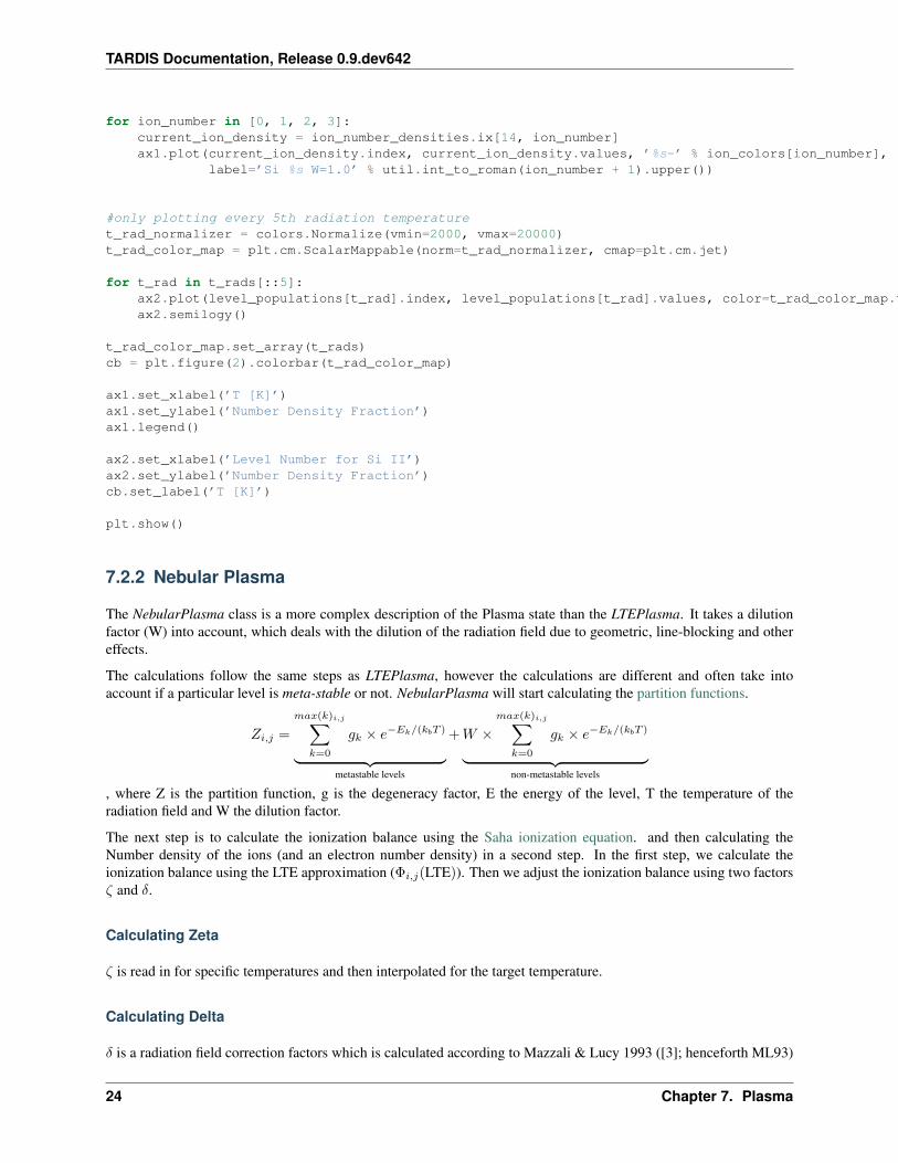
for ion_number in [0, 1, 2, 3]:current_ion_density = ion_number_densities.ix[14, ion_number]ax1.plot(current_ion_density.index, current_ion_density.values, ’%s-’ % ion_colors[ion_number],

label=’Si %s W=1.0’ % util.int_to_roman(ion_number + 1).upper())

#only plotting every 5th radiation temperaturet_rad_normalizer = colors.Normalize(vmin=2000, vmax=20000)t_rad_color_map = plt.cm.ScalarMappable(norm=t_rad_normalizer, cmap=plt.cm.jet)

for t_rad in t_rads[::5]:ax2.plot(level_populations[t_rad].index, level_populations[t_rad].values, color=t_rad_color_map.to_rgba(t_rad))ax2.semilogy()

t_rad_color_map.set_array(t_rads)cb = plt.figure(2).colorbar(t_rad_color_map)

ax1.set_xlabel(’T [K]’)ax1.set_ylabel(’Number Density Fraction’)ax1.legend()

ax2.set_xlabel(’Level Number for Si II’)ax2.set_ylabel(’Number Density Fraction’)cb.set_label(’T [K]’)

plt.show()

7.2.2 Nebular Plasma

The NebularPlasma class is a more complex description of the Plasma state than the LTEPlasma. It takes a dilutionfactor (W) into account, which deals with the dilution of the radiation field due to geometric, line-blocking and othereffects.

The calculations follow the same steps as LTEPlasma, however the calculations are different and often take intoaccount if a particular level is meta-stable or not. NebularPlasma will start calculating the partition functions.

𝑍𝑖,𝑗 =

𝑚𝑎𝑥(𝑘)𝑖,𝑗∑︁𝑘=0


⏟ ⏞ metastable levels

+𝑊 ×𝑚𝑎𝑥(𝑘)𝑖,𝑗∑︁

𝑘=0


⏟ ⏞ non-metastable levels

, where Z is the partition function, g is the degeneracy factor, E the energy of the level, T the temperature of theradiation field and W the dilution factor.

The next step is to calculate the ionization balance using the Saha ionization equation. and then calculating theNumber density of the ions (and an electron number density) in a second step. In the first step, we calculate theionization balance using the LTE approximation (Φ𝑖,𝑗(LTE)). Then we adjust the ionization balance using two factors𝜁 and 𝛿.

Calculating Zeta

𝜁 is read in for specific temperatures and then interpolated for the target temperature.

Calculating Delta

𝛿 is a radiation field correction factors which is calculated according to Mazzali & Lucy 1993 ([3]; henceforth ML93)


http://en.wikipedia.org/wiki/Partition_function_(statistical_mechanics)

http://en.wikipedia.org/wiki/Saha_ionization_equation


In ML93 the radiation field correction factor is denoted as 𝛿 and is calculated in Formula 15 & 20

The radiation correction factor changes according to a ionization energy threshold 𝜒T and the species ionization thresh-old (from the ground state) 𝜒0.

For 𝜒T ≥ 𝜒0

𝛿 =𝑇e

𝑏1𝑊𝑇Rexp(

𝜒T

𝑘𝑇R− 𝜒0

𝑘𝑇e)

For 𝜒T < 𝜒0

𝛿 = 1 − exp(𝜒T

𝑘𝑇R− 𝜒0

𝑘𝑇R) +

𝑇e

𝑏1𝑊𝑇Rexp(

𝜒T

𝑘𝑇R− 𝜒0

𝑘𝑇e),

where 𝑇R is the radiation field Temperature, 𝑇e is the electron temperature and W is the dilution factor.

Now we can calculate the ionization balance using equation 14 in [3]:

Φ𝑖,𝑗 =𝑁𝑖,𝑗+1𝑛𝑒

𝑁𝑖,𝑗

Φ𝑖,𝑗 = 𝑊 × [𝛿𝜁 + 𝑊 (1 − 𝜁)]

(︂𝑇e

𝑇R

)︂1/2

Φ𝑖,𝑗(LTE)

In the last step, we calculate the ion number densities according using the methods in LTEPlasma

Finally we calculate the level populations (NebularPlasma.calculate_level_populations()), by usingthe calculated ion species number densities:

𝑁𝑖,𝑗,𝑘(not metastable) = 𝑊𝑔𝑘𝑍𝑖,𝑗


𝑁𝑖,𝑗,𝑘(metastable) =𝑔𝑘𝑍𝑖,𝑗


This concludes the calculation of the nebular plasma. In the code, the next step is calculating the 𝜏Sobolev using thequantities calculated here.

Example Calculations

import os

from matplotlib import colorsfrom tardis import atomic, plasma, utilfrom matplotlib import pyplot as plt

import numpy as npimport pandas as pd

#Making 2 Figures for ionization balance and level populations



7.2. Plasma Types 25


# expanding the tilde to the users directoryatom_fname = os.path.expanduser(’~/.tardis/si_kurucz.h5’)

# reading in the HDF5 Fileatom_data = atomic.AtomData.from_hdf5(atom_fname)

#The atom_data needs to be prepared to create indices. The Class needs to know which atomic numbers are needed for the#calculation and what line interaction is needed (for "downbranch" and "macroatom" the code creates special tables)atom_data.prepare_atom_data([14], ’scatter’)

#Initializing the NebularPlasma class using the from_abundance class method.#This classmethod is normally only needed to test individual plasma classes#Usually the plasma class just gets the number densities from the model classnebular_plasma = plasma.NebularPlasma.from_abundance(10000, 0.5, {’Si’: 1}, 1e-13, atom_data, 10.)

#Initializing a dataframe to store the ion populations and level populations for the different temperaturesion_number_densities = pd.DataFrame(index=nebular_plasma.ion_populations.index)level_populations = pd.DataFrame(index=nebular_plasma.level_populations.ix[14, 1].index)t_rads = np.linspace(2000, 20000, 100)

#Calculating the different ion populations and level populuatios for the given temperaturesfor t_rad in t_rads:

nebular_plasma.update_radiationfield(t_rad, w=1.0)#getting total si number densitysi_number_density = nebular_plasma.number_density.get_value(14)#Normalizing the ion populationsion_density = nebular_plasma.ion_populations / si_number_densityion_number_densities[t_rad] = ion_density

#normalizing the level_populations for Si IIcurrent_level_population = nebular_plasma.level_populations.ix[14, 1] / nebular_plasma.ion_populations.ix[14, 1]#normalizing with statistical weightcurrent_level_population /= atom_data.levels.ix[14, 1].g


ion_colors = [’b’, ’g’, ’r’, ’k’]

for ion_number in [0, 1, 2, 3]:current_ion_density = ion_number_densities.ix[14, ion_number]ax1.plot(current_ion_density.index, current_ion_density.values, ’%s-’ % ion_colors[ion_number],


#only plotting every 5th radiation temperaturet_rad_normalizer = colors.Normalize(vmin=2000, vmax=20000)t_rad_color_map = plt.cm.ScalarMappable(norm=t_rad_normalizer, cmap=plt.cm.jet)

for t_rad in t_rads[::5]:ax2.plot(level_populations[t_rad].index, level_populations[t_rad].values, color=t_rad_color_map.to_rgba(t_rad))ax2.semilogy()

#Calculating the different ion populations for the given temperatures with W=0.5ion_number_densities = pd.DataFrame(index=nebular_plasma.ion_populations.index)for t_rad in t_rads:

nebular_plasma.update_radiationfield(t_rad, w=0.5)#getting total si number density



si_number_density = nebular_plasma.number_density.get_value(14)#Normalizing the ion populationsion_density = nebular_plasma.ion_populations / si_number_densityion_number_densities[t_rad] = ion_density

#normalizing the level_populations for Si IIcurrent_level_population = nebular_plasma.level_populations.ix[14, 1] / nebular_plasma.ion_populations.ix[14, 1]#normalizing with statistical weightcurrent_level_population /= atom_data.levels.ix[14, 1].g


#Plotting the ion fractions

for ion_number in [0, 1, 2, 3]:print "w=0.5"current_ion_density = ion_number_densities.ix[14, ion_number]ax1.plot(current_ion_density.index, current_ion_density.values, ’%s--’ % ion_colors[ion_number],


for t_rad in t_rads[::5]:ax2.plot(level_populations[t_rad].index, level_populations[t_rad].values, color=t_rad_color_map.to_rgba(t_rad),

linestyle=’--’)ax2.semilogy()

t_rad_color_map.set_array(t_rads)cb = plt.figure(2).colorbar(t_rad_color_map)

ax1.set_xlabel(’T [K]’)ax1.set_ylabel(’Number Density Fraction’)ax1.legend()

ax2.set_xlabel(’Level Number for Si II’)ax2.set_ylabel(’Number Density Fraction’)cb.set_label(’T [K]’)

plt.show()

7.3 Sobolev optical depth

This function calculates the Sobolev optical depth 𝜏Sobolev

𝐶Sobolev =𝜋𝑒2

𝑚𝑒𝑐

𝜏Sobolev = 𝐶Sobolev 𝜆 𝑓lower→upper 𝑡explosion 𝑁lower(1 − 𝑔lower

𝑔upper

𝑁upper

𝑁lower)

7.4 Macro Atom

The macro atom is described in detail in [1]. The basic principal is that when an energy packet is absorbed thatthe macro atom is on a certain level. Three probabilities govern the next step the Pup, Pdown and Pdown emission beingthe probability for going to a higher level, a lower level and a lower level and emitting a photon while doing thisrespectively (see Figure 1 in [1] ).

7.3. Sobolev optical depth 27


The macro atom is the most complex idea to implement as a data structure. The setup is done in ~tardisatomic, but wewill nonetheless discuss it here (as ~tardisatomic is even less documented than this one).

For each level we look at the line list to see what transitions (upwards or downwards are possible). We create a twoarrays, the first is a long one-dimensional array containing the probabilities. Each level contains a set of probabili-ties, The first part of each set contains the upwards probabilities (internal upward), the second part the downwardsprobabilities (internal downward), and the last part is the downward and emission probability.

each set is stacked after the other one to make one long one dimensional ~numpy.ndarray.

The second array is for book-keeping it has exactly the length as levels (with an example for the Si II level 15):

Level ID Probability index Nup Ndown Ntotal

14001015 ??? 17 5 17 + 5*2 = 27

We now will calculate the transition probabilites, using the radiative rates in Equation 20, 21, and 22 in [1]. Then wecalculate the downward emission probability from Equation 5, the downward and upward internal transition probabil-ities in [2].

𝑝emission down = ℛi→lower (𝜖upper − 𝜖lower)/𝒟𝑖

𝑝internal down = ℛi→lower 𝜖lower/𝒟𝑖

, 𝑝internal up = ℛi→upper 𝜖𝑖/𝒟𝑖

,

where 𝑖 is the current level, 𝜖 is the energy of the level, and ℛ is the radiative rates.

We ignore the probability to emit a k-packet as TARDIS only works with photon packets. Next we calculate theradidative rates using equation 10 in [2].

ℛupper→lower = 𝐴upper→lower𝛽Sobolev𝑛upper

ℛlower→upper = (𝐵lower→upper𝑛lower −𝐵upper→lower𝑛upper)𝛽Sobolev𝐽𝑏𝜈

,

with 𝛽Sobolev = 1𝜏Sobolev

(1 − 𝑒−𝜏Sobolev) .

using the Einstein coefficients

𝐴upper→lower =8𝜈2𝜋2𝑒2

𝑚𝑒𝑐3𝑔lower

𝑔upper𝑓lower→upper

𝐴upper→lower =4𝜋2𝑒2

𝑚𝑒𝑐⏟ ⏞ 𝐶Einstein

2𝜈2

𝑐2𝑔lower


𝐵lower→upper =4𝜋2𝑒2

𝑚𝑒ℎ𝜈𝑐𝑓lower→upper

𝐵lower→upper =4𝜋2𝑒2


1

ℎ𝜈𝑓lower→upper

𝐵upper→lower =4𝜋2𝑒2

𝑚𝑒ℎ𝜈𝑐𝑓lower→upper

𝐵upper→lower =4𝜋2𝑒2


1

ℎ𝜈

𝑔lower




we get

ℛupper→lower = 𝐶Einstein2𝜈2

𝑐2𝑔lower

𝑔upper𝑓lower→upper𝛽Sobolev𝑛upper

ℛlower→upper = 𝐶Einstein1

ℎ𝜈𝑓lower→upper(𝑛lower −

𝑔lower

𝑔upper𝑛upper)𝛽Sobolev𝐽

𝑏𝜈

This results in the transition probabilities:

𝑝emission down = 𝐶Einstein2𝜈2

𝑐2𝑔lower

𝑔i𝑓lower→i𝛽Sobolev𝑛i (𝜖i − 𝜖lower)/𝒟𝑖

𝑝internal down = 𝐶Einstein2𝜈2

𝑐2𝑔lower

𝑔i𝑓lower→i𝛽Sobolev𝑛i 𝜖lower/𝒟𝑖

𝑝internal up = 𝐶Einstein1

ℎ𝜈𝑓i→upper(𝑛i −

𝑔i

𝑔upper𝑛upper)𝛽Sobolev𝐽

𝑏𝜈 𝜖𝑖/𝒟𝑖

,

and as we will normalise the transition probabilities numerically later, we can get rid of 𝐶Einstein, 1𝒟𝑖

and num-ber densities.

𝑝emission down =2𝜈2

𝑐2𝑔lower

𝑔i𝑓lower→i𝛽Sobolev (𝜖i − 𝜖lower)

𝑝internal down =2𝜈2

𝑐2𝑔lower

𝑔i𝑓lower→i𝛽Sobolev 𝜖lower

𝑝internal up =1

ℎ𝜈𝑓i→upper (1 − 𝑔i

𝑔upper

𝑛upper

𝑛𝑖)⏟ ⏞

stimulated emission

𝛽Sobolev𝐽𝑏𝜈 𝜖𝑖

,

There are two parts for each of the probabilities, one that is pre-computed by ~tardisatomic and is in the HDF5 File,and one that is computed during the plasma calculations:

𝑝emission down =2𝜈2

𝑐2𝑔lower

𝑔i𝑓lower→i(𝜖i − 𝜖lower)⏟ ⏞

pre-computed

𝛽Sobolev

𝑝internal down =2𝜈2

𝑐2𝑔lower

𝑔i𝑓lower→i𝜖lower⏟ ⏞

pre-computed

𝛽Sobolev

𝑝internal up =1

ℎ𝜈𝑓i→upper⏟ ⏞

pre-computed

𝛽Sobolev𝐽𝑏𝜈 (1 − 𝑔i

𝑔upper

𝑛upper

𝑛𝑖) 𝜖𝑖.

7.5 NLTE treatment

NLTE treatment of lines is available both in ~LTEPlasma and the ~NebularPlasma class. This can be enabled byspecifying which species should be treated as NLTE with a simple list of tuples (e.g. [(20,1)] for Ca II).

7.5. NLTE treatment 29


First let’s dive into the basics:

There are two rates to consider from a given level.

𝑅upper→lower = 𝐴𝑢𝑙𝑛𝑢⏟ ⏞ spontaneous emission

+ 𝐵𝑢𝑙𝑛𝑢𝐽𝜈⏟ ⏞ stimulated emission

+ 𝐶𝑢𝑙𝑛𝑢𝑛𝑒⏟ ⏞ collisional deexcitation

= 𝑛𝑢 (𝐴𝑢𝑙 + 𝐵𝑢𝑙𝐽𝜈 + 𝐶𝑢𝑙𝑛𝑒)⏟ ⏞ 𝑟𝑢𝑙

𝑅lower→upper = 𝐵𝑙𝑢𝑛𝑙𝐽𝜈⏟ ⏞ stimulated absorption

+ 𝐶𝑙𝑢 𝑛𝑙 𝑛𝑒⏟ ⏞ collisional excitation

= 𝑛𝑙 (𝐵𝑙𝑢𝐽𝜈 + 𝐶𝑢𝑙𝑛𝑒)⏟ ⏞ 𝑟𝑙𝑢

,

where 𝐽𝜈 (in LTE this is 𝐵(𝜈, 𝑇 )) denotes the mean intensity at the frequency of the line and 𝑛𝑒 the number densityof electrons.

Next, we calculate the rate of change of a level by adding up all outgoing and all incoming transitions from level 𝑗.

𝑑𝑛𝑗

𝑑𝑡=

∑︁𝑖 ̸=𝑗

𝑅𝑖𝑗⏟ ⏞ incoming rate

−∑︁�̸�=𝑗

𝑅𝑗𝑖⏟ ⏞ outgoing rate

In a statistical equilibrium all incoming rates and outgoing rates add up to 0 (𝑑𝑛𝑗

𝑑𝑡 = 0). We use this to calculate thelevel populations using the rate coefficients (𝑟𝑖𝑗, 𝑟𝑗𝑖).⎛⎜⎝−(ℛ∞∈ + · · · + ℛ∞|) . . . ℛ|∞

.... . .

...ℛ∞| . . . −(ℛ|∞ + · · · + ℛ|,|−∞)

⎞⎟⎠⎛⎜⎝𝑛1

...𝑛𝑗

⎞⎟⎠ =

⎛⎝000

⎞⎠with the additional constrained that all the level number populations need to add up to the current ion population $N$we change this to ⎛⎜⎝ 1 1 . . .

.... . .

...ℛ∞| . . . −(ℛ|∞ + · · · + ℛ|,|−∞)

⎞⎟⎠⎛⎜⎝𝑛1

...𝑛𝑗

⎞⎟⎠ =

⎛⎝𝑁00

⎞⎠For a three level atom we have:

𝑑𝑛1

𝑑𝑡= 𝑛2𝑟21 + 𝑛3𝑟31⏟ ⏞

incoming rate

− (𝑛1𝑟12 + 𝑛1𝑟13)⏟ ⏞ outgoing rate

= 0

𝑑𝑛2

𝑑𝑡= 𝑛1𝑟12 + 𝑛3𝑟32⏟ ⏞

incoming rate

− (𝑛2𝑟21 + 𝑛2𝑟23)⏟ ⏞ 𝑜𝑢𝑡𝑔𝑜𝑖𝑛𝑔𝑟𝑎𝑡𝑒

= 0

𝑑𝑛3

𝑑𝑡= 𝑛1𝑟13 + 𝑛2𝑟23⏟ ⏞

incoming rate

− (𝑛3𝑟32 + 𝑛3𝑟31)⏟ ⏞ outgoing rate

= 0,

which can be written in matrix from:⎛⎝−(𝑟12 + 𝑟13) 𝑟21 𝑟31𝑟12 −(𝑟21 + 𝑟23) 𝑟32𝑟13 𝑟23 −(𝑟31 + 𝑟32)

⎞⎠⎛⎝𝑛1

𝑛2

𝑛3

⎞⎠ =

⎛⎝000

⎞⎠



To solve for the level populations we need an additional constraint: 𝑛1 + 𝑛2 + 𝑛3 = 𝑁 . By setting 𝑁 = 1: we canget the relative rates: ⎛⎝ 1 1 1

𝑟12 −(𝑟21 + 𝑟23) 𝑟32𝑟13 𝑟23 −(𝑟31 + 𝑟32)

⎞⎠⎛⎝𝑛1

𝑛2

𝑛3

⎞⎠ =

⎛⎝100

⎞⎠Now we go back and look at the rate coefficients used for a level population - as an example 𝑑𝑛2

𝑑𝑡 :

𝑑𝑛2

𝑑𝑡= 𝑛1𝑟12 − 𝑛2(𝑟21 + 𝑟23) + 𝑛3𝑟32

= 𝑛1𝐵12𝐽12 + 𝑛1𝐶12𝑛𝑒 − 𝑛2𝐴21 − 𝑛2𝐵21𝐽21 − 𝑛2𝐶21𝑛𝑒

−𝑛2𝐵23𝐽23 − 𝑛2𝐶23𝑛𝑒 + 𝑛3𝐴32 + 𝑛3𝐵32𝐽32 + 𝑛3𝐶32𝑛𝑒,

+𝑛3𝐴32 + 𝑛3𝐶32𝑛𝑒,

Next we will group the stimulated emission and stimulated absorption terms as we can assume 𝐽12 = 𝐽21:

𝑑𝑛2

𝑑𝑡= 𝑛1(𝐵12𝐽12 (1 − 𝑛2

𝑛1

𝐵21

𝐵12)⏟ ⏞

stimulated emission term

+𝐶12𝑛𝑒) − 𝑛2(𝐴21 + 𝐶23𝑛𝑒 + 𝑛2𝐵23𝐽23 (1 − 𝑛3

𝑛2

𝐵32

𝐵23)⏟ ⏞

stimulated emission term

) + 𝑛3(𝐴32 + 𝐶32𝑛𝑒)

7.5. NLTE treatment 31

CHAPTER 8

Radiative Monte Carlo

The radiative monte carlo is initiated once the model is constructed.

Different line interactions

line_interaction_id == 0: scatter line_interaction_id == 1: downbranch line_interaction_id == 2: macro

8.1 Radiationfield estimators

During the monte-carlo run we collect two estimators for the radiation field:

𝐽estimator =∑︁

𝜖𝑙

𝜈estimator =∑︁

𝜖𝜈𝑙,

where 𝜖, 𝜈 are comoving energy and comoving frequency of a packet respectively.

To calculate the temperature and dilution factor we first calculate the mean intensity in each cell ( 𝐽 = 14𝜋Δ𝑡 𝑉 𝐽estimator

)., [2].

The weighted mean frequency is used to obtain the radiation temperature. Specifically, the radiation temperature ischosen as the temperature of a black body that has the same weighted mean frequency as has been computed in thesimulation. Accordingly,

ℎ𝜈

𝑘𝐵𝑇𝑅=

ℎ

𝑘𝐵𝑇𝑅

𝜈estimator

𝐽estimator= 24𝜁(5)

15

𝜋4,

where the evaluation comes from the mean value of

�̄� =

∫︀∞0

𝑥4/(exp𝑥− 1)𝑑𝑥∫︀∞0

𝑥3/(exp𝑥− 1)𝑑𝑥= 24𝜁(5)

15

𝜋4= 3.8322 . . .

and so

𝑇𝑅 =1

�̄�

ℎ

𝑘𝐵

𝜈estimator

𝐽estimator

= 0.260945ℎ

𝑘𝐵

𝜈estimator

𝐽estimator.

With the radiation temperature known, we can then obtain our estimate for for the dilution factor. Our radiation fieldmodel in the nebular approximation is

𝐽 = 𝑊𝐵(𝑇𝑅) = 𝑊𝜎𝑆𝐵

𝜋𝑇 4𝑅,

33


i.e. a dilute blackbody. Therefore we use our value of the mean intensity derrived from the estimator (above) to obtainthe dilution factor

𝑊 =𝜋𝐽

𝜎𝑆𝐵𝑇 4𝑅

=1

4𝜎𝑆𝐵𝑇 4𝑅 ∆𝑡 𝑉

𝐽estimator.

There endeth the lesson.

34 Chapter 8. Radiative Monte Carlo

CHAPTER 9

Glossary

meta-stable A level is considered meta-stable if there’s no line that has this level as the upper state. This means thatthese levels can not be reached by absorbing a photon and are only reached when decaying.

synapps simple radiative transport code for supernovae. Please refer to Synapps for more information

35

https://c3.lbl.gov/es/


36 Chapter 9. Glossary

CHAPTER 10

References

37


38 Chapter 10. References

CHAPTER 11

Credits

11.1 Core Team

• Wolfgang Kerzendorf

• Stuart Sim

• Michael Klauser

• Markus Kromer

11.2 Contributers

• Maryam Patel (documentation, test environment)

• Adam Suban-Loewen (GUI, profiling and parallelization)

• Chris Sasaki and Mike Reid (Logo)

• Knox Long (recombination coefficient)

• Erik Bray (help with incorporating Astropy’s setuphelpers)

39


40 Chapter 11. Credits

Bibliography

[1] L. B. Lucy. Monte Carlo transition probabilities. \aap, 384:725–735, March 2002.

[2] L. B. Lucy. Monte Carlo transition probabilities. II.. \aap, 403:261–275, May 2003.

[3] P. A. Mazzali and L. B. Lucy. The application of Monte Carlo methods to the synthesis of early-time supernovaespectra. \aap, 279:447–456, November 1993.

41

TARDIS Documentation - Read the Docs

Documents

Transcript of TARDIS Documentation - Read the Docs