Rapid and Automatic Localization of the Anteriorand Posterior Commissure Point Landmarks in MR

Volumetric Neuroimages1

K.N. Bhanu Prakash, Qingmao Hu, Aamer Aziz, Wieslaw L. Nowinski

Rationale and Objective. Accurate identification of the anterior commissure (AC) and posterior commissure (PC) iscritical in neuroradiology, functional neurosurgery, human brain mapping, and neuroscience research. Moreover, majorstereotactic brain atlases are based on the AC and PC. Our goal is to provide an algorithm for a rapid, robust, accurateand automatic identification of AC and PC.

Materials and Method. The method exploits anatomical and radiological properties of AC, PC and surrounding struc-tures, including morphological variability. The localization is done in two stages: coarse and fine. The coarse stage locatesthe AC and PC on the midsagittal plane by analyzing their relationships with the corpus callosum, fornix, and brainstem.The fine stage refines the AC and PC in a well-defined volume of interest, analyzing locations of lateral and third ventri-cles, interhemispheric fissure, and massa intermedia.

Results. The algorithm was developed using simple operations, like histogramming, thresholding, region growing, 1D pro-jections. It was tested on 94 diversified T1W and SPGR datasets. After the fine stage, 71 (76%) volumes had an error be-tween 0–1 mm for the AC and 55 (59%) for the PC. The mean errors were 1.0 mm (AC) and 1.0 mm (PC). The accuracyhas improved twice due to fine stage processing. The algorithm took about 1 second for coarse and 4 seconds forfine processing on P4, 2.5 GHz.

Conclusion. The use of anatomical and radiological knowledge including variability in algorithm formulation aids inlocalization of structures more accurately and robustly. This fully automatic algorithm is potentially useful in clinicalsetting and for research.

Key Words. Anterior commissure; posterior commissure; midsagittal plane; corpus callosum; brainstem; fornix; localiza-tion; brain atlas.©

AUR, 2006

Acad Radiol 2006; 13:36–54

1 From the Biomedical Imaging Lab, Agency for Science Technology andResearch, 30 Biopolis Street, #07-01 Matrix Singapore 138671 (K.N.B.,H.Q., A.A., W.L.N.). Received May 27, 2005; revision received and ac-cepted August 2. Supported by Biomedical Research Council, Agency forScience, Technology and Research, Singapore. We are grateful to our col-leagues Ihar Volkau for valuable discussions and Guoyu Qian for the imple-mentation of the algorithm in VC��. The authors thank all the hospitals,Brainweb and Internet Brain Segmentation Repository for the datasetsused in the study. Address correspondence to: K.N.B. e-mail:bhanu@sbic.a-star.edu.org

©

AUR, 2006doi:10.1016/j.acra.2005.08.023

36

INTRODUCTION

The human cerebrum comprises of two hemispheres thatexchange information with each other through axons ar-ranged in specific bundles called commissures. The ante-rior commissure (AC) and posterior commissure (PC) aretwo such structures. Identification of AC and PC is criti-cal not only because they are important brain structures,but also as their location is crucial in stereotactic andfunctional neurosurgery (1), localization analysis in hu-man brain mapping (2), medical image analysis (3), struc-

ture segmentation and labeling in neuroradiology (4) as

Academic Radiology, Vol 13, No 1, January 2006 LOCALIZATION OF ANTERIOR AND POSTERIOR COMMISSURES

well as in registration to reduce the number of degrees offreedom. Major stereotactic brain atlases, such as the Ta-lairach and Tournoux (TT) atlas (5), Referentially Ori-ented Talairach-Tournoux atlas (6) and Schaltenbrand-Wahren atlas (7), are based on the AC and PC. The Ta-lairach transformation based on the AC and PC is alsowidely used in human brain mapping for brain compari-son across subjects (8). In addition, the number of refer-ences to the TT atlas has been growing exponentially (9).

The AC and PC structures are often hard to detect dueto their small size, variability in intensity properties, lowdata resolution in comparison to their size, presence ofneighboring structures with similar appearance (e.g., thefornix, blood vessels) and noise. For neuroanatomy ex-perts, an interactive identification of AC and PC isstraightforward for high quality data. Automation is re-quired not only in research but also in clinical practice toincrease confidence when identified by a non-neuroradi-ologist or resident (e.g., in urgent cases) or to save sub-stantial amount of time when processing numerous scans.

A few papers only address automatic identification ofAC and PC. Some earlier attempts limited to PET images(10,11) were not fully automatic when applied to MRimages (12). Verard et al (13) proposed a method foridentification of landmarks automatically on the MSP byscene analysis. The method extracts the MSP, binarizes itby using the threshold estimated from the histogram, andthe regions are evaluated for the corpus callosum (CC)and brainstem (BS) using shape features. First the PC andsubsequently the AC are identified using edge enhance-ment and template matching masks, and TT atlas infor-mation. The authors used high resolution, good qualityMR images for identification. For routine scans, in whichthe commissures are not well defined and have the partialvolume effect, their method may not be able to pinpointthe landmarks accurately. Han and Park (14) proposed theidentification of AC and PC based on two-step shapematching technique. An edge-enhanced CC template con-taining the AC and PC region is used to locate the ap-proximate region of the AC and the PC on the MSP. Inthe second step, edge-enhanced AC and PC templates areused to locate the final positions of AC and PC. The finalpositions of AC and PC are defined where the correlationcoefficient between the edge enhanced region and edgeenhanced template is maximum. The method works wellif data have no (or little) noise. When structures are notwell defined due to the partial volume effect, the edgemap gives a thick edge boundary and an accurate local-

ization may not be possible. The existence of multiple

points giving the same value of correlation coefficientwith the templates is also a source of inaccuracies. More-over as structures can have high variability in shape, ob-taining a suitable template is questionable.

Our ultimate objective is to automate the Talairachtransformation and to make it rapid, robust, and accuratesuch that it can be used easily in neuroradiology, humanbrain mapping, stereotactic functional neurosurgery, andneuroscience research. Therefore, the algorithm for ACand PC localization formulated here meets the same re-quirements. The major challenge was to capture anatomi-cal and radiological properties and formulate the algo-rithm in terms of relatively simple operations to make itrobust and rapid. This is achieved by employing simpleoperations, such as thresholding, histogramming, 1D in-tensity projections, region growing, and basic morphologi-cal operations. These operations are limited to small, ana-tomically well-defined regions of interests. An additionaladvantage of our approach is that it can be more under-standable by clinicians (as opposed to complicated “blackbox” solutions), which potentially will increase its clinicalacceptance.

Our algorithm is based on anatomical knowledge andradiological properties of images. The novelty of ourmethod is in the use of anatomy surrounding the AC andPC, particularly that of third ventricle (V3). To our bestknowledge, there is no study using features of V3 and 3Dprocessing for localization of AC and PC. Our method isfully automatic (i.e., requires no user interaction) andworks in two stages. In the first coarse stage it processes2D data (MSP) to obtain the initial positions of commis-sures. The second stage refines these initial positions byprocessing a 3D well-defined volume of interest (VOI).

MATERIAL AND METHOD

ConceptThe method is based on the anatomical facts that CC,

fornix (Fo), AC and PC are WM structures and the BS isa mixture of white and gray matters. Though, the inten-sity distributions of these structures overlaps their ana-tomical positions are different. Therefore, localization ofAC and PC is handled in an anatomical multi-scale man-ner in which the major structures surrounding the AC andPC are localized first in well-defined regions of interest(ROIs). The CC, Fo and BS are prominently visible onthe MSP and identification of these structures guides lo-

calizing the positions of the commissures. At each step a

37

BHANUPRAKASH ET AL Academic Radiology, Vol 13, No 1, January 2006

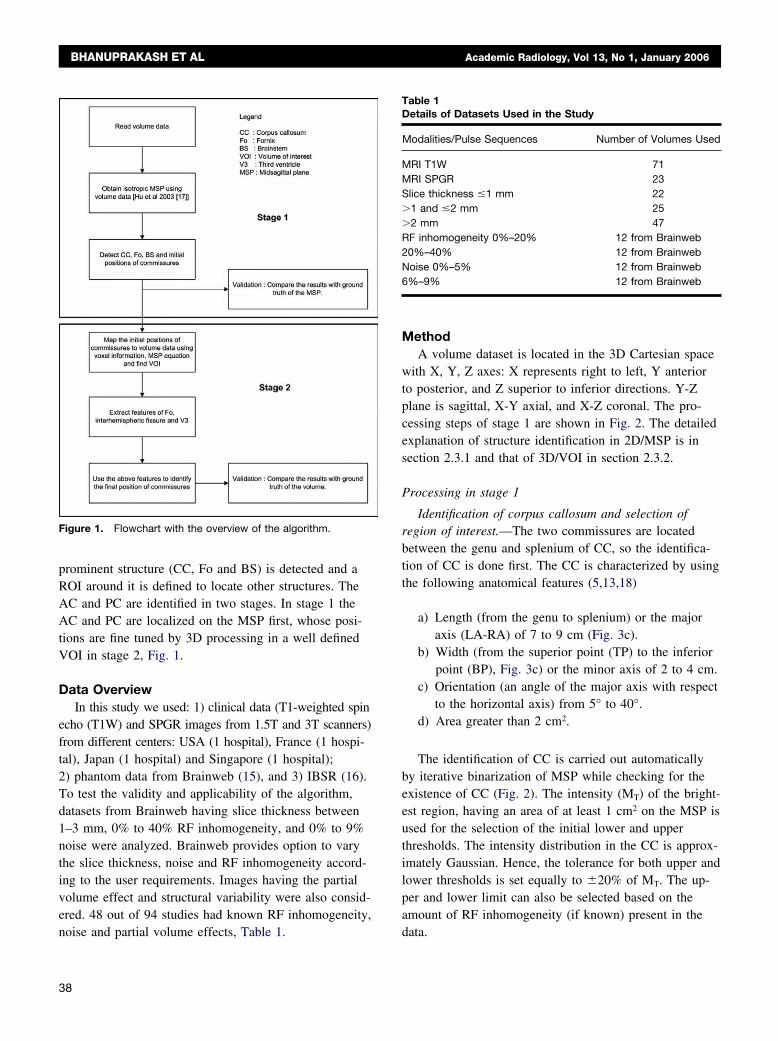
prominent structure (CC, Fo and BS) is detected and aROI around it is defined to locate other structures. TheAC and PC are identified in two stages. In stage 1 theAC and PC are localized on the MSP first, whose posi-tions are fine tuned by 3D processing in a well definedVOI in stage 2, Fig. 1.

Data OverviewIn this study we used: 1) clinical data (T1-weighted spin

echo (T1W) and SPGR images from 1.5T and 3T scanners)from different centers: USA (1 hospital), France (1 hospi-tal), Japan (1 hospital) and Singapore (1 hospital);2) phantom data from Brainweb (15), and 3) IBSR (16).To test the validity and applicability of the algorithm,datasets from Brainweb having slice thickness between1–3 mm, 0% to 40% RF inhomogeneity, and 0% to 9%noise were analyzed. Brainweb provides option to varythe slice thickness, noise and RF inhomogeneity accord-ing to the user requirements. Images having the partialvolume effect and structural variability were also consid-ered. 48 out of 94 studies had known RF inhomogeneity,

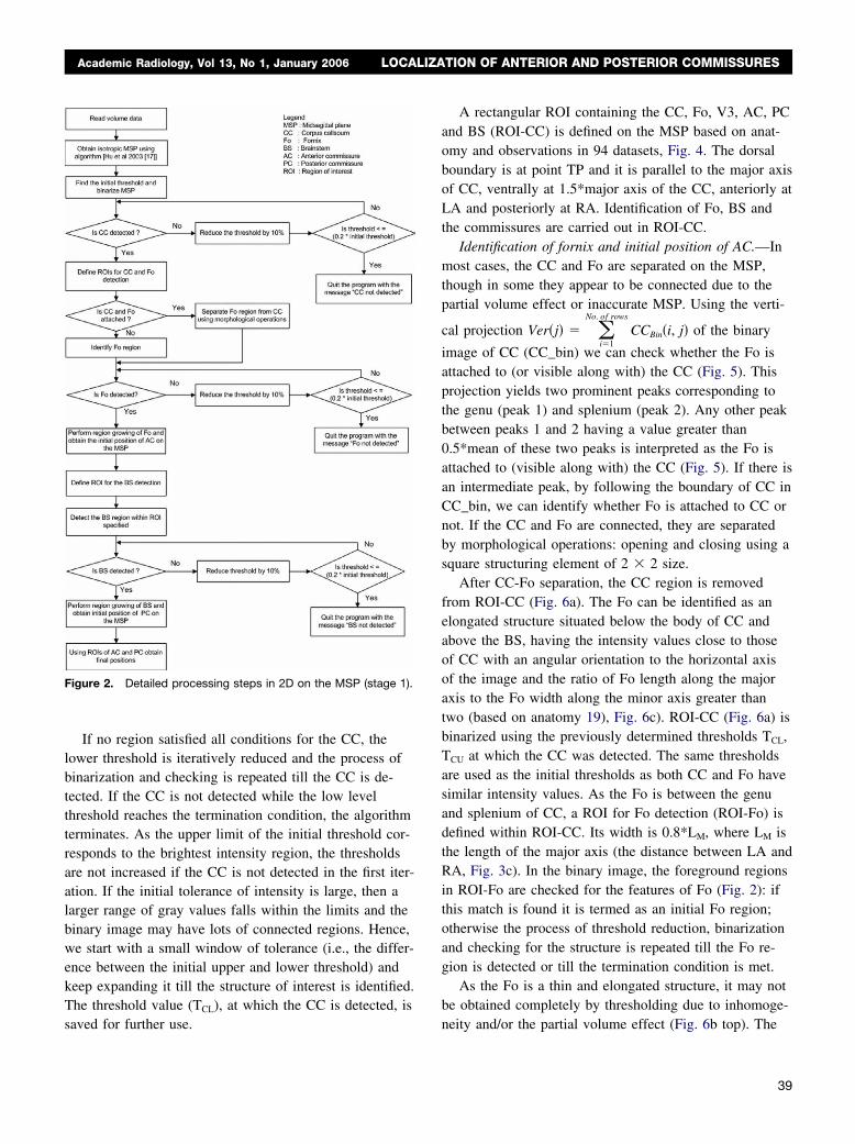
Figure 1. Flowchart with the overview of the algorithm.

noise and partial volume effects, Table 1.

38

MethodA volume dataset is located in the 3D Cartesian space

with X, Y, Z axes: X represents right to left, Y anteriorto posterior, and Z superior to inferior directions. Y-Zplane is sagittal, X-Y axial, and X-Z coronal. The pro-cessing steps of stage 1 are shown in Fig. 2. The detailedexplanation of structure identification in 2D/MSP is insection 2.3.1 and that of 3D/VOI in section 2.3.2.

Processing in stage 1

Identification of corpus callosum and selection ofregion of interest.—The two commissures are locatedbetween the genu and splenium of CC, so the identifica-tion of CC is done first. The CC is characterized by usingthe following anatomical features (5,13,18)

a) Length (from the genu to splenium) or the majoraxis (LA-RA) of 7 to 9 cm (Fig. 3c).

b) Width (from the superior point (TP) to the inferiorpoint (BP), Fig. 3c) or the minor axis of 2 to 4 cm.

c) Orientation (an angle of the major axis with respectto the horizontal axis) from 5° to 40°.

d) Area greater than 2 cm2.

The identification of CC is carried out automaticallyby iterative binarization of MSP while checking for theexistence of CC (Fig. 2). The intensity (MT) of the bright-est region, having an area of at least 1 cm2 on the MSP isused for the selection of the initial lower and upperthresholds. The intensity distribution in the CC is approx-imately Gaussian. Hence, the tolerance for both upper andlower thresholds is set equally to �20% of MT. The up-per and lower limit can also be selected based on theamount of RF inhomogeneity (if known) present in the

Table 1Details of Datasets Used in the Study

Modalities/Pulse Sequences Number of Volumes Used

MRI T1W 71MRI SPGR 23Slice thickness �1 mm 22�1 and �2 mm 25�2 mm 47RF inhomogeneity 0%–20% 12 from Brainweb20%–40% 12 from BrainwebNoise 0%–5% 12 from Brainweb6%–9% 12 from Brainweb

data.

Academic Radiology, Vol 13, No 1, January 2006 LOCALIZATION OF ANTERIOR AND POSTERIOR COMMISSURES

If no region satisfied all conditions for the CC, thelower threshold is iteratively reduced and the process ofbinarization and checking is repeated till the CC is de-tected. If the CC is not detected while the low levelthreshold reaches the termination condition, the algorithmterminates. As the upper limit of the initial threshold cor-responds to the brightest intensity region, the thresholdsare not increased if the CC is not detected in the first iter-ation. If the initial tolerance of intensity is large, then alarger range of gray values falls within the limits and thebinary image may have lots of connected regions. Hence,we start with a small window of tolerance (i.e., the differ-ence between the initial upper and lower threshold) andkeep expanding it till the structure of interest is identified.The threshold value (TCL), at which the CC is detected, is

Figure 2. Detailed processing steps in 2D on the MSP (stage 1).

saved for further use.

A rectangular ROI containing the CC, Fo, V3, AC, PCand BS (ROI-CC) is defined on the MSP based on anat-omy and observations in 94 datasets, Fig. 4. The dorsalboundary is at point TP and it is parallel to the major axisof CC, ventrally at 1.5*major axis of the CC, anteriorly atLA and posteriorly at RA. Identification of Fo, BS andthe commissures are carried out in ROI-CC.

Identification of fornix and initial position of AC.—Inmost cases, the CC and Fo are separated on the MSP,though in some they appear to be connected due to thepartial volume effect or inaccurate MSP. Using the verti-

cal projection Ver�j� � �i�1

No. of rows

CCBin�i, j� of the binary

image of CC (CC_bin) we can check whether the Fo isattached to (or visible along with) the CC (Fig. 5). Thisprojection yields two prominent peaks corresponding tothe genu (peak 1) and splenium (peak 2). Any other peakbetween peaks 1 and 2 having a value greater than0.5*mean of these two peaks is interpreted as the Fo isattached to (visible along with) the CC (Fig. 5). If there isan intermediate peak, by following the boundary of CC inCC_bin, we can identify whether Fo is attached to CC ornot. If the CC and Fo are connected, they are separatedby morphological operations: opening and closing using asquare structuring element of 2 � 2 size.

After CC-Fo separation, the CC region is removedfrom ROI-CC (Fig. 6a). The Fo can be identified as anelongated structure situated below the body of CC andabove the BS, having the intensity values close to thoseof CC with an angular orientation to the horizontal axisof the image and the ratio of Fo length along the majoraxis to the Fo width along the minor axis greater thantwo (based on anatomy 19), Fig. 6c). ROI-CC (Fig. 6a) isbinarized using the previously determined thresholds TCL,TCU at which the CC was detected. The same thresholdsare used as the initial thresholds as both CC and Fo havesimilar intensity values. As the Fo is between the genuand splenium of CC, a ROI for Fo detection (ROI-Fo) isdefined within ROI-CC. Its width is 0.8*LM, where LM isthe length of the major axis (the distance between LA andRA, Fig. 3c). In the binary image, the foreground regionsin ROI-Fo are checked for the features of Fo (Fig. 2): ifthis match is found it is termed as an initial Fo region;otherwise the process of threshold reduction, binarizationand checking for the structure is repeated till the Fo re-gion is detected or till the termination condition is met.

As the Fo is a thin and elongated structure, it may notbe obtained completely by thresholding due to inhomoge-

neity and/or the partial volume effect (Fig. 6b top). The

39

BHANUPRAKASH ET AL Academic Radiology, Vol 13, No 1, January 2006

intensity distribution in the possible Fo region is approxi-mately Gaussian (Fig. 6d, R2 � 0.971). Hence, the toler-ance for both upper and lower thresholds is set equally to�20% of TFL and the region growing is carried out inROI-Fo as a post-processing step using 8-neighborhood.The inferior tip of the Fo region is taken as the initial ACpoint (Fig. 6b).

Identification of BS and computation of initial PCposition.—The BS is located infero-posteriorly to the CC.The ROI for BS detection (ROI-BS, Fig. 7a) is definedwithin ROI-CC as a region between the initial AC pointand point RB (Fig. 3c) with the CC and Fo subtracted.Similar to Fo identification, the initial BS region is de-tected using iterative thresholding. The threshold at whichthe BS region is identified is defined as TBS. Subse-

Figure 3. Illustration of a typical MSP andest labeled; b) binarized MSP; and c) CC anor axes (LA: most anterior point of genu,most posterior point of splenium, RB: mossuperior point of the minor axis on the bodthe minor axis).

Figure 4. Anatomy in the region of interest of CC (ROI-CC)showing the CC, Fo, BS, AC and PC. The width of ROI-CC isequal to the major axis of CC and the height is 1.5 times the ma-jor axis.

quently, region growing is performed for extraction. The

40

BS is composed of GM and WM, having a higher vari-ance in intensity values than in the CC and Fo (Fig. 7b)due to the presence of the basilar artery in ROI-BS, Fig7a. GM and WM in the BS cause the intensity distribu-tion in ROI-BS to be skewed around the mean, Fig. 7b.The intensity of basilar artery is brighter than the BS inT1 and SPGR images. This produces a longer tail towardsthe higher intensity which influences the mean of the dis-tribution. To accommodate for the lower intensities, in theregion growing, the lower threshold is at 0.7*mean valueand the upper threshold at 1.2*mean value. The mostsupero-posterior point of BS is taken as the initial PCpoint, Fig. 7a.

Refinement of AC and PC positions on theMSP.—Refinement of AC and PC positions is carried outin two ROIs of AC (ROI-AC) and PC (ROI-PC).ROI-AC is centered at the initial AC point with a sizelarge enough (e.g., 12 � 12 mm2) to include surroundingstructures for processing. The construction of ROI-PC isbased on information about AC-PC variability derivedfrom about two hundred datasets studied in (20) that thePC is situated at a distance of 17–36 mm posterior to theAC. The initial PC point is checked for the above condi-tion of distance in an area large enough (e.g., 16 � 16mm2) to include the initial PC point and its surroundingstructures.

The AC landmark is located below the inferior tip ofFo and can be identified as the bright spot in T1W andSPGR images. In many routine scans, however, the ACcannot be distinguished clearly from the inferior tip of Fodue to limited spatial and contrast resolutions and partialvolume effect. To localize the final AC point of stage 1(AC2D), we binarize ROI-AC and perform region growingof the foreground pixels. The most infero-anterior pointof the largest region is considered as the initial AC point.Around it we check for a point, which has the highest

: a) MR image with the structures of inter-bounding ellipse with the major and mi-ost anterio-inferior point of genu, RA:

terio-inferior point of splenium, TP: mostthe CC, and BP: most inferior point on

CCnd itsLB: mt posy of

intensity in a reduced ROI of 5 � 5 pixels. If such a

wing

Academic Radiology, Vol 13, No 1, January 2006 LOCALIZATION OF ANTERIOR AND POSTERIOR COMMISSURES

point exists, it is taken as the AC2D; otherwise the initialAC point is taken as the AC2D.

The initial PC point is identified using the row-wise

projection, Pr oj�i� � �j�1

No. of columns

PC�i, j� of ROI of PC,

Fig. 8. The first point, at which the slope changes fromnegative to positive, indicates the row where the PC canbe identified. The row is designated as initial PC_row.

Figure 5. Detection of fornix existence on the MSP. The biand without fornix (right).

Figure 6. Illustration of features of Fo: a) anatomy in ROI-CC aftec) ROI-Fo showing the major and minor axes of Fo after region gro

Figure 7. Illustration of region growing in ROI-BS: a) BS before(top) and after (bottom) region growing; b) histograms of BS be-fore (dash line) and after region growing (solid line).

The pixel with maximum intensity (Fig. 8 right) in the

PC_row is considered as an initial PC point. If there isany other pixel having higher intensity than the currentpixel in the 8 neighborhood, it is considered as the finalPC point of stage 1 (PC2D); otherwise the initial PC pointitself is considered as PC2D.

Processing in stage 2

Volume of interest processing.—The locations of ACand PC may be inaccurate on the MSP, if its equation isnot accurate or structures like the Fo and superior collicu-lus are not well defined due to low resolution, partial vol-ume effect, and/or noise. Hence, 3D VOI processing mayenhance the accuracy of locating the commissures. 3Dprocessing is done in two steps, Fig. 9. In the first step,an initial VOI based on the MSP is formed. A thresholdfor binarization of VOI is calculated using the Gaussianmixture modeling (GMM) and Expectation-Maximization(EM) algorithm (21). Using the binarized VOI, the meanventricular plane (MVP) i.e. the sagittal symmetry planeof V3 is calculated. The VOI is realigned with the MVP

CC image and its vertical projection with the fornix (left)

subtraction; b) Fo before (top) and after (bottom) region growing;; d) Plot confirming the normal distribution of Fo intensities.

nary

r CC

to eliminate the errors of asymmetrical distribution of V3

41

ich t

BHANUPRAKASH ET AL Academic Radiology, Vol 13, No 1, January 2006

on the MSP. In the second step, the features of V3, inter-hemispheric fissure (IF), and lateral ventricles (LV) areextracted from VOI to locate the final positions of ACand PC.

Mapping of AC and PC coordinates from the MSP tovolume data and formulation of volume of interest.—The2D coordinates of AC (ACx, ACy) and PC (PCx, PCy)obtained by processing the MSP are mapped to the vol-ume data using the MSP equation. A cuboidal VOIaround the AC2D and PC2D (termed VOI-AC-PC to em-phasis that it encompasses the AC and PC together) isformed as follows. In the axial direction: min (ACz,PCz) � 5 mm to max (ACz, PCz) � 5 mm, in the sagit-tal direction: MSP � 10 mm to MSP � 10 mm, and inthe coronal direction: ACy � 10 mm to PCy � 10 mm.

The intensity distribution in VOI-AC-PC is modeled asa sum of two Gaussian distributions corresponding toCSF and GM�WM regions. The Gaussian mixture modelparameters are calculated using the EM algorithm. Theinitial mean (�) and standard deviation (�) for the twodistributions are calculated by using the K-means algo-rithm (22). The threshold for binarization of VOI-AC-PCcan be selected as (23)

Thresh �(�CSF�(GM�WM) � �(GM�WM)�CSF)

(�CSF � �(GM�WM))(4)

The final threshold (Thresh) is overestimated by 10%to include the partial volume voxels of V3 and WM alongthe boundary of V3. During binarization, the ventricularand extra-ventricular CSF regions are set to one (fore-ground) and the GM�WM voxels to zero (background).The length and width of V3 along with their end pointsare obtained from the X and Y projections of binary axial

Figure 8. Features of ROI-PC: ROI-PCintensity profile of PC_row (right) from wh

slices.

42

From each axial slice the coordinates of voxel which isat the center of V3 are identified. The final MVP is theleast square error plane constructed from the coordinates

its row-wise projection (center), and thehe location of PC can be identified.

Figure 9. Detailed steps in 3D/VOI processing.

(left),

of all center voxels after removing the outlier voxels us-

.

n: a)

Academic Radiology, Vol 13, No 1, January 2006 LOCALIZATION OF ANTERIOR AND POSTERIOR COMMISSURES

ing the mean and standard deviation of distribution ofvoxels [Grubb’s test (24 or modified Thompson’s tau test,http://www.mne.psu.edu/me82/Learning/Stat_2/stat_2.html]If the angular difference between the projections of theMSP and MVP on any axial slice is greater than 1°, VOI-AC-PC is reformulated based on the MVP instead ofMSP as follows: axial direction: min (ACz, PCz) � 5 mmto max (ACz, PCz) � 5 mm; sagittal direction: MVP � 10mm to MVP � 10 mm; coronal direction: ACy � 10 mmto PCy � 10 mm.

Fig. 10 illustrates the formulation of VOI-AC-PC aswell as other landmark points and structures used forprocessing.

AC processing in VOI-AC-PC.—The anatomy in theVOI-AC-PC is described using Fig. 11. Anteriorly, V3extends to the lamina terminalis (LT) and interventricularforamina. Rostrally, V3 is bounded ventrally by the LT,which is the rostral end of neural tube. It is a thin struc-ture stretching from the dorsum of optic chiasm to therostrum of CC. Above this the anterior wall of V3 isformed by the diverging columns of fornices and thetransversely oriented AC, which crosses the midline ros-trally to the columns of Fo. There are two CSF regionsnear the AC. Anterior to the AC is the IF CSF region andposterior to the AC is the V3 CSF region separated bythe LT in VOI-AC-PC, Fig. 11a. The junction of thesetwo CSF regions can be located easily and accurately on

Figure 10. Illustration of boundaries of VOI-AC-PC o

Figure 11. Illustration of anatomy in Vthe roof of V3 and changes in the CSFthe AC.

coronal rather than on sagittal slices.

To localize the position of AC, each axial sliceVOI-AC-PC is evaluated for:

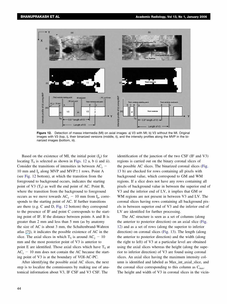
a. Presence of massa intermedia (MI) between the ini-tial AC and PC.

b. Length of V3 in between the initial AC and PC.c. End (the most posterior) point of V3.d. Presence of IF and its separation from V3.e. Starting point TS (the most anterior point) of V3.

The presence of MI in an axial slice conveys that theslice is located between the CC and BS. The presence ofIF and its separation from V3 give the boundary points ofAC on axial slices. The evaluation for presence of LVhelps in identifying the axial slices to be analyzed, as theAC lies in between the inferior tip of LV’s frontal hornand the roof of V3, Fig. 11b.

To obtain the above mentioned features (a–e), a binaryVOI-AC-PC is used. The presence or absence of MI isevaluated using the intensity profile transitions along theMVP and MVP�1 rows between the initial AC and PCpoints of a binary axial image. Figs. 12 a, b show an ax-ial slice with and without the MI and their correspondingbinary images and intensity profiles along the MVP. Theintensity transition from the foreground to backgroundbetween the AC2D and PC2D in an intensity profile indi-

axial, b) coronal, and c) sagittal slices.

-PC: a) in MSP showing changes ines (IF and V3), b) in a coronal plane at

OI-ACspac

cates the presence of MI.

43

BHANUPRAKASH ET AL Academic Radiology, Vol 13, No 1, January 2006

Based on the existence of MI, the initial point (Ip) forlocating TS is selected as shown in Figs. 12 a, b (i and ii).Consider the transitions of intensities in between ACy �10 mm and Ip along MVP and MVP�1 rows. Point A(see Fig. 12 bottom), at which the transition from theforeground to background occurs, indicates the startingpoint of V3 (TS) as well the end point of AC. Point B,where the transition from the background to foregroundoccurs as we move towards ACy � 10 mm from Ip, corre-sponds to the starting point of AC. If further transitionsare there (e.g. C and D, Fig. 12 bottom) they correspondto the presence of IF and point C corresponds to the start-ing point of IF. If the distance between points A and B isgreater than 2 mm and less than 5 mm (as by anatomythe size of AC is about 3 mm, the Schaltenbrand-Wahrenatlas [7]), it indicates the possible existence of AC in theslice. The axial slices in which TS is around ACy � 10mm and the most posterior point of V3 is anterior topoint E are identified. Those axial slices which have TS atACy � 10 mm does not contain the AC because the start-ing point of V3 is at the boundary of VOI-AC-PC.

After identifying the possible axial AC slices, the nextstep is to localize the commissures by making use of ana-

Figure 12. Detection of massa intermedia (MI) on aimages with V3 (top, i), their binarized versions (middnarized images (bottom, iii).

tomical information about V3, IF CSF and V3 CSF. The

44

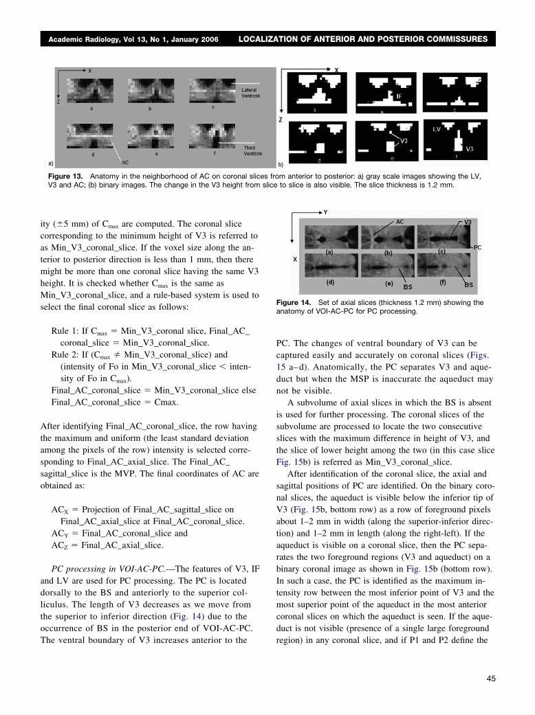
identification of the junction of the two CSF (IF and V3)regions is carried out on the binary coronal slices ofthe possible AC slices. The binarized coronal slices (Fig.13 b) are checked for rows containing all pixels withbackground value, which correspond to GM and WMregions. If a slice does not have any rows containing allpixels of background value in between the superior end ofV3 and the inferior end of LV, it implies that GM orWM regions are not present in between V3 and LV. Thecoronal slices having rows containing all background pix-els in between superior end of V3 and the inferior end ofLV are identified for further processing.

The AC structure is seen as a set of columns (alongthe anterior to posterior direction) on an axial slice (Fig.12) and as a set of rows (along the superior to inferiordirection) on coronal slices (Fig. 13). The length (alongthe anterior to posterior direction) and the width (alongthe right to left) of V3 at a particular level are obtainedusing the axial slices whereas the height (along the supe-rior to inferior direction) of V3 are found using coronalslices. An axial slice having the maximum intensity col-umn is identified and labeled as Max_int_axial_slice, andthe coronal slice corresponding to this column as Cmax.

ages: a) V3 with MI; b) V3 without the MI. Original, and the intensity profiles along the MVP in the bi-

xial imle, ii)

The height and width of V3 in coronal slices in the vicin-

slice

Academic Radiology, Vol 13, No 1, January 2006 LOCALIZATION OF ANTERIOR AND POSTERIOR COMMISSURES

ity (�5 mm) of Cmax are computed. The coronal slicecorresponding to the minimum height of V3 is referred toas Min_V3_coronal_slice. If the voxel size along the an-terior to posterior direction is less than 1 mm, then theremight be more than one coronal slice having the same V3height. It is checked whether Cmax is the same asMin_V3_coronal_slice, and a rule-based system is used toselect the final coronal slice as follows:

Rule 1: If Cmax � Min_V3_coronal slice, Final_AC_coronal_slice � Min_V3_coronal_slice.

Rule 2: If (Cmax � Min_V3_coronal_slice) and(intensity of Fo in Min_V3_coronal_slice � inten-sity of Fo in Cmax).

Final_AC_coronal_slice � Min_V3_coronal_slice elseFinal_AC_coronal_slice � Cmax.

After identifying Final_AC_coronal_slice, the row havingthe maximum and uniform (the least standard deviationamong the pixels of the row) intensity is selected corre-sponding to Final_AC_axial_slice. The Final_AC_sagittal_slice is the MVP. The final coordinates of AC areobtained as:

ACX � Projection of Final_AC_sagittal_slice onFinal_AC_axial_slice at Final_AC_coronal_slice.

ACY � Final_AC_coronal_slice andACZ � Final_AC_axial_slice.

PC processing in VOI-AC-PC.—The features of V3, IFand LV are used for PC processing. The PC is locateddorsally to the BS and anteriorly to the superior col-liculus. The length of V3 decreases as we move fromthe superior to inferior direction (Fig. 14) due to theoccurrence of BS in the posterior end of VOI-AC-PC.

Figure 13. Anatomy in the neighborhood of AC on coronal slicV3 and AC; (b) binary images. The change in the V3 height from

The ventral boundary of V3 increases anterior to the

PC. The changes of ventral boundary of V3 can becaptured easily and accurately on coronal slices (Figs.15 a– d). Anatomically, the PC separates V3 and aque-duct but when the MSP is inaccurate the aqueduct maynot be visible.

A subvolume of axial slices in which the BS is absentis used for further processing. The coronal slices of thesubvolume are processed to locate the two consecutiveslices with the maximum difference in height of V3, andthe slice of lower height among the two (in this case sliceFig. 15b) is referred as Min_V3_coronal_slice.

After identification of the coronal slice, the axial andsagittal positions of PC are identified. On the binary coro-nal slices, the aqueduct is visible below the inferior tip ofV3 (Fig. 15b, bottom row) as a row of foreground pixelsabout 1–2 mm in width (along the superior-inferior direc-tion) and 1–2 mm in length (along the right-left). If theaqueduct is visible on a coronal slice, then the PC sepa-rates the two foreground regions (V3 and aqueduct) on abinary coronal image as shown in Fig. 15b (bottom row).In such a case, the PC is identified as the maximum in-tensity row between the most inferior point of V3 and themost superior point of the aqueduct in the most anteriorcoronal slices on which the aqueduct is seen. If the aque-duct is not visible (presence of a single large foreground

m anterior to posterior: a) gray scale images showing the LV,to slice is also visible. The slice thickness is 1.2 mm.

Figure 14. Set of axial slices (thickness 1.2 mm) showing theanatomy of VOI-AC-PC for PC processing.

es fro

region) in any coronal slice, and if P1 and P2 define the

45

slice

BHANUPRAKASH ET AL Academic Radiology, Vol 13, No 1, January 2006

most inferior points of V3 in Min_V3_coronal_slice andits adjacent slice (in the anterior direction), then the PC isdefined as the row having the maximum intensity pixelsbetween P1 and P2. The X, Y and Z coordinates of thePC are defined by the positions of MVP,Min_V3_cornal_slice and the row, respectively.

Ground Truth Generation and Validation MethodThe ground truths for all 94 cases were provided inde-

pendently by two experts (WLN and AA) by marking thepositions of AC and PC on the MSP (2D) and in VOI-AC-PC (3D) on the originally acquired slices. The Eu-clidean distance in millimeters between the ground truthand the position obtained by the algorithm was the errormeasure. The mean and standard deviation of the estima-tion error of AC and PC landmarks against the groundtruth on the MSP and in the VOI were calculated.

The inter-observer variability analysis was carried outby finding the percentage difference in the markings bythe experts for both coarse (2D/MSP) and fine (3D/VOI)processing. To find the statistics of intra-observer vari-ability, a subset of 30 (easy and difficult) cases was eval-uated by each expert 10 times.

The data were grouped into subsets according to thelevels of noise, RF inhomogeneity, slice thickness andimaging sequence. The grouping was done to study theeffects of different parameters on the localization of ACand PC. All parameters, like thresholds, size of regions ofinterest (used to identify different structures) and featuresof structures, used in the algorithm (automatically withoutthe need of setting them by the user) were validatedquantitatively against all datasets. The algorithm was also

Figure 15. Anatomy of V3 showing the chalong the anterior to posterior direction, Msponding binary images (bottom row). The

tested against the effects of MSP rotation (clockwise and

46

counterclockwise) and volume data rotated around allthree axes (right-left, anterior-posterior, and superior-inferior).

RESULTS

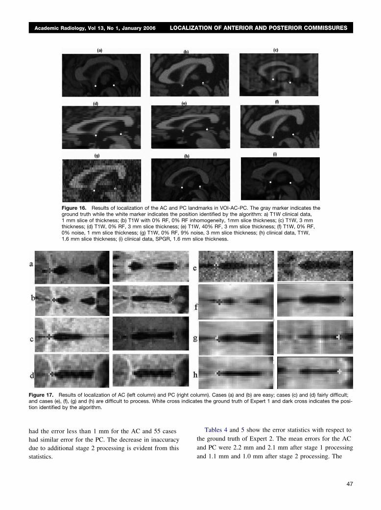
The algorithm was implemented initially in Matlab andtested on 94 cases used for getting the results and valida-tion. The algorithm was later translated to VC�� andincluded in an application for a fast analysis of brainscans, and demonstrated at recent major radiologicalmeetings with more than 200 datasets (25,26). The Mat-lab version takes about 4 seconds to process the MSP andbetween 10–50 seconds to process both MSP and VOI,depending on the volume size. The same algorithm inVC�� takes less than 1 second for MSP processing and2–4 seconds to process both MSP and VOI. The resultsof localization of AC and PC after stage 2 (3D/VOI) pro-cessing are shown in Fig. 16.

Fig. 17. shows more examples of AC and PC localiza-tion after the stage 2 (3D/VOI) processing for a variety ofcases ranging from the simplest to most difficult.

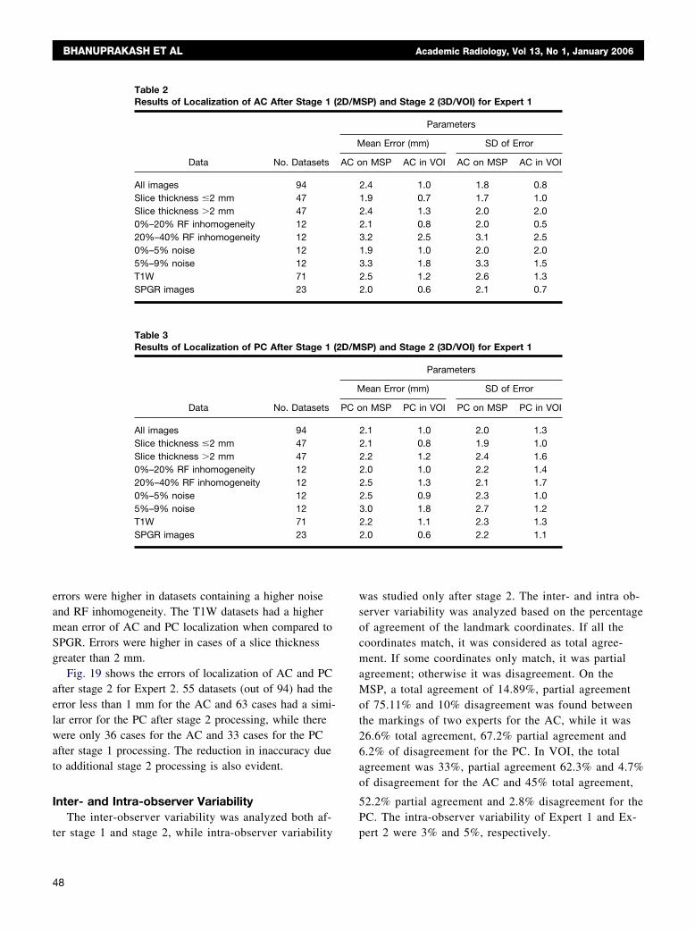
Accuracy of LocalizationTables 2 and 3 show the error statistics with respect to

the ground truth of Expert 1. The mean error for the ACand PC after stage 1 (2D/MSP) processing for all imageswas 2.4 and 2.1 mm, respectively, whereas after stage 2

(3D/VOI) processing the errors reduced to 1.0 and 1.0mm, respectively.

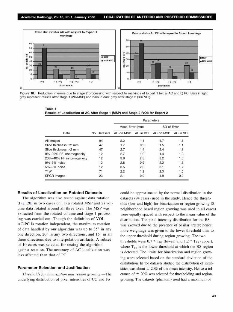
Fig. 18. shows the errors of localization of AC and

in height (coronal slices, top row a-d)d PC in the original image and its corre-thickness is 0.82 mm.

angeVP an

PC after stage 2 for Expert 1. 71 datasets (out of 94)

m sli

Academic Radiology, Vol 13, No 1, January 2006 LOCALIZATION OF ANTERIOR AND POSTERIOR COMMISSURES

had the error less than 1 mm for the AC and 55 caseshad similar error for the PC. The decrease in inaccuracydue to additional stage 2 processing is evident from this

Figure 16. Results of localization of the AC and PCground truth while the white marker indicates the po1 mm slice of thickness; (b) T1W with 0% RF, 0% Rthickness; (d) T1W, 0% RF, 3 mm slice thickness; (e)0% noise, 1 mm slice thickness; (g) T1W, 0% RF, 9%1.6 mm slice thickness; (i) clinical data, SPGR, 1.6 m

Figure 17. Results of localization of AC (left column) and PC (righand cases (e), (f), (g) and (h) are difficult to process. White cross intion identified by the algorithm.

statistics.

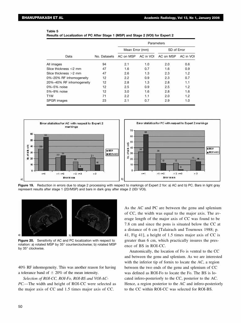
Tables 4 and 5 show the error statistics with respect tothe ground truth of Expert 2. The mean errors for the ACand PC were 2.2 mm and 2.1 mm after stage 1 processing

marks in VOI-AC-PC. The gray marker indicates theidentified by the algorithm: a) T1W clinical data,

omogeneity, 1mm slice thickness; (c) T1W, 3 mm, 40% RF, 3 mm slice thickness; (f) T1W, 0% RF,se, 3 mm slice thickness; (h) clinical data, T1W,ce thickness.

umn). Cases (a) and (b) are easy; cases (c) and (d) fairly difficult;es the ground truth of Expert 1 and dark cross indicates the posi-

landsitionF inh

T1Wnoi

t coldicat

and 1.1 mm and 1.0 mm after stage 2 processing. The

47

BHANUPRAKASH ET AL Academic Radiology, Vol 13, No 1, January 2006

errors were higher in datasets containing a higher noiseand RF inhomogeneity. The T1W datasets had a highermean error of AC and PC localization when compared toSPGR. Errors were higher in cases of a slice thicknessgreater than 2 mm.

Fig. 19 shows the errors of localization of AC and PCafter stage 2 for Expert 2. 55 datasets (out of 94) had theerror less than 1 mm for the AC and 63 cases had a simi-lar error for the PC after stage 2 processing, while therewere only 36 cases for the AC and 33 cases for the PCafter stage 1 processing. The reduction in inaccuracy dueto additional stage 2 processing is also evident.

Inter- and Intra-observer VariabilityThe inter-observer variability was analyzed both af-

Table 2Results of Localization of AC After Stage 1 (2

Data No. Datasets

All images 94Slice thickness �2 mm 47Slice thickness �2 mm 470%–20% RF inhomogeneity 1220%–40% RF inhomogeneity 120%–5% noise 125%–9% noise 12T1W 71SPGR images 23

Table 3Results of Localization of PC After Stage 1 (2

Data No. Datasets

All images 94Slice thickness �2 mm 47Slice thickness �2 mm 470%–20% RF inhomogeneity 1220%–40% RF inhomogeneity 120%–5% noise 125%–9% noise 12T1W 71SPGR images 23

ter stage 1 and stage 2, while intra-observer variability

48

was studied only after stage 2. The inter- and intra ob-server variability was analyzed based on the percentageof agreement of the landmark coordinates. If all thecoordinates match, it was considered as total agree-ment. If some coordinates only match, it was partialagreement; otherwise it was disagreement. On theMSP, a total agreement of 14.89%, partial agreementof 75.11% and 10% disagreement was found betweenthe markings of two experts for the AC, while it was26.6% total agreement, 67.2% partial agreement and6.2% of disagreement for the PC. In VOI, the totalagreement was 33%, partial agreement 62.3% and 4.7%of disagreement for the AC and 45% total agreement,

52.2% partial agreement and 2.8% disagreement for thePC. The intra-observer variability of Expert 1 and Ex-

SP) and Stage 2 (3D/VOI) for Expert 1

Parameters

ean Error (mm) SD of Error

n MSP AC in VOI AC on MSP AC in VOI

2.4 1.0 1.8 0.81.9 0.7 1.7 1.02.4 1.3 2.0 2.02.1 0.8 2.0 0.53.2 2.5 3.1 2.51.9 1.0 2.0 2.03.3 1.8 3.3 1.52.5 1.2 2.6 1.32.0 0.6 2.1 0.7

SP) and Stage 2 (3D/VOI) for Expert 1

Parameters

ean Error (mm) SD of Error

n MSP PC in VOI PC on MSP PC in VOI

2.1 1.0 2.0 1.32.1 0.8 1.9 1.02.2 1.2 2.4 1.62.0 1.0 2.2 1.42.5 1.3 2.1 1.72.5 0.9 2.3 1.03.0 1.8 2.7 1.22.2 1.1 2.3 1.32.0 0.6 2.2 1.1

D/M

M

AC o

D/M

M

PC o

pert 2 were 3% and 5%, respectively.

ay af

Academic Radiology, Vol 13, No 1, January 2006 LOCALIZATION OF ANTERIOR AND POSTERIOR COMMISSURES

Results of Localization on Rotated DatasetsThe algorithm was also tested against data rotation

(Fig. 20) in two cases on: 1) a rotated MSP and 2) vol-ume data rotated around all three axes. The MSP wasextracted from the rotated volume and stage 1 process-ing was carried out. Though the definition of VOI-AC-PC is rotation independent, the maximum rotationof data handled by our algorithm was up to 35° in anyone direction, 20° in any two directions, and 15° in allthree directions due to interpolation artifacts. A subsetof 10 cases was selected for testing the algorithmagainst rotation. The accuracy of AC localization wasless affected than that of PC.

Parameter Selection and Justification

Thresholds for binarization and region growing.—The

Figure 18. Reduction in errors due to stage 2 processing with rgray represent results after stage 1 (2D/MSP) and bars in dark gr

Table 4Results of Localization of AC After Stage 1 (M

Data No. Datasets

All images 94Slice thickness �2 mm 47Slice thickness �2 mm 470%–20% RF inhomogeneity 1220%–40% RF inhomogeneity 120%–5% noise 125%–9% noise 12T1W 71SPGR images 23

underlying distribution of pixel intensities of CC and Fo

could be approximated by the normal distribution in thedatasets (94 cases) used in the study. Hence the thresh-olds (low and high) for binarization or region growing (8neighborhood based region growing was used in all cases)were equally spaced with respect to the mean value of thedistribution. The pixel intensity distribution for the BSwas skewed due to the presence of basilar artery; hencemore weightage was given to the lower threshold than tothe upper threshold during region growing. The twothresholds were 0.7 * TBS (lower) and 1.2 * TBS (upper),where TBS is the lower threshold at which the BS regionis detected. The limits for binarization and region grow-

ing were selected based on the standard deviation of thedistribution. In the datasets studied the distribution of inten-sities was about � 20% of the mean intensity. Hence a tol-erance of � 20% was selected for thresholding and region

ct to markings of Expert 1 for: a) AC and b) PC. Bars in lightter stage 2 (3D/ VOI).

and Stage 2 (VOI) for Expert 2

Parameters

ean Error (mm) SD of Error

n MSP AC in VOI AC on MSP AC in VOI

2.2 1.1 1.7 1.11.7 0.9 1.5 1.12.7 1.4 2.4 1.12.7 1.0 1.4 1.03.8 2.3 3.2 1.62.8 0.9 2.2 1.33.5 2.0 3.1 1.72.2 1.2 2.3 1.02.1 0.9 1.9 0.9

espe

SP)

M

AC o

growing. The datasets (phantom) used had a maximum of

49

r sta

BHANUPRAKASH ET AL Academic Radiology, Vol 13, No 1, January 2006

40% RF inhomogeneity. This was another reason for havinga tolerance band of � 20% of the mean intensity.

Selection of ROI-CC, ROI-Fo, ROI-BS and VOI-AC-PC.—The width and height of ROI-CC were selected as

Figure 19. Reduction in errors due to stage 2 processing with resrepresent results after stage 1 (2D/MSP) and bars in dark gray afte

Figure 20. Sensitivity of AC and PC localization with respect torotation: a) rotated MSP by 35° counterclockwise; b) rotated MSPby 35° clockwise.

Table 5Results of Localization of PC After Stage 1 (M

Data No. Datasets

All images 94Slice thickness �2 mm 47Slice thickness �2 mm 470%–20% RF inhomogeneity 1220%–40% RF inhomogeneity 120%–5% noise 125%–9% noise 12T1W 71SPGR images 23

the major axis of CC and 1.5 times major axis of CC.

50

As the AC and PC are between the genu and spleniumof CC, the width was equal to the major axis. The av-erage length of the major axis of CC was found to be7.8 cm and since the pons is situated below the CC ata distance of 6 cm [Talairach and Tournoux 1988; p.41, Fig 41], a height of 1.5 times major axis of CC isgreater than 6 cm, which practically insures the pres-ence of BS in ROI-CC.

Anatomically, the location of Fo is ventral to the CCand between the genu and splenium. As we are interestedwith the inferior tip of fornix to locate the AC, a regionbetween the two ends of the genu and splenium of CCwas defined as ROI-Fo to locate the Fo. The BS is lo-cated infero-posteriorly to the CC, posterior to the AC.Hence, a region posterior to the AC and infero-posteriorly

to markings of Expert 2 for: a) AC and b) PC. Bars in light grayge 2 (3D/ VOI).

and Stage 2 (VOI) for Expert 2

Parameters

ean Error (mm) SD of Error

n MSP AC in VOI AC on MSP AC in VOI

2.1 1.0 2.0 0.61.6 0.7 1.6 0.92.6 1.3 2.3 1.22.2 0.9 2.3 0.72.8 1.3 2.8 1.12.5 0.9 2.5 1.23.0 1.6 2.8 1.62.2 1.1 2.0 1.22.1 0.7 2.9 1.0

pect

SP)

M

AC o

to the CC within ROI-CC was selected for ROI-BS.

Academic Radiology, Vol 13, No 1, January 2006 LOCALIZATION OF ANTERIOR AND POSTERIOR COMMISSURES

VOI-AC-PC was set based on our initial results of 2Dprocessing. Since the errors were less than 5 mm, the dor-sal and ventral limits of VOI were selected as min(AC_z, PC_z) � 5 mm to max (AC_z, PC_z) � 5 mm.The anterior, posterior and lateral limits were selectedbased on the measurements of V3 in the datasets.

Termination condition in 2D processing.—The termi-nation condition of 0.2*MT, where MT is the maximumintensity, was selected based on the observation in all thedatasets. The lower limit of intensity distribution of eachof CC, Fo and BS was above 0.2*MT.

Identification of BS.—Identification of the presenceof BS in any axial slice of VOI-AC-PC is found bychecking the lengths of V3. If L1, L2, . . . , LN is thelength of the V3 in axial slices and if the length of V3in any axial slice is less than 0.8 * max (L1, L2 . . . . LN),then the BS could be observed at the posterior end ofthe VOI-AC-PC. The value was selected based on theobservations from the various datasets used in thestudy. Moreover, all the above parameterswere additionally tested with more than 200 cases(25,26).

DISCUSSION

An accurate, automatic, rapid and robust algorithm forlocalization of AC and PC is critical in clinical and re-search applications. Our work contributes towards thisobjective. The novelty of the proposed algorithm is in theuse of anatomy and its variability (especially that of V3)along with image processing and analysis techniques. Theprocessing is not limited only to the AC and PC but alsoconsiders the neighboring structures. In our algorithm theprocessing is done in two stages. In the first (coarse)stage, the MSP is processed to obtain the initial positionsof the commissures, which are further tuned in the second(fine) stage where a well-defined VOI is processed. Arule-based system is developed based on the anatomy andimage characteristics. The incorporation of anatomicalinformation and variability of structures to the algorithmmakes it more robust in handling the variations in struc-ture and intensity. As the algorithm is developed based onsimple image processing techniques, like thresholding,region growing, histogramming, 1D profiling, and basicmorphological operations, it is rapid and simple in imple-mentation. The algorithm is fully automatic and does not

require any user interaction.

Accuracy of LocalizationThe zero estimation error for both AC and PC was

limited to anatomically well-defined regions of interest involumes with slice thickness of 1 mm and with low noiseand/or inhomogeneity. The errors were reduced by almosthalf when VOI processing was applied instead of onlyMSP processing. Twenty-eight volumes (30%) had theRMS error between 0 to 1 mm after stage 1 processingwhich increased to 71 (76%) (30 cases had zero error,32%) volumes after stage 2 processing for AC localiza-tion against the ground truth of Expert 1 (Fig. 18a). Thenumbers of datasets having the error between 1–2 mmafter stage 1 processing were 22 (23%) while after stage2 processing only 11 (12%). The numbers of data setshaving error between 2–3 mm and above 3 mm afterstage 1 processing were only 19 (20%) and 26 (28%),respectively, for the AC with respect to the ground truthof Expert 1. After stage 2 processing, these numbers wereonly 2 (2.12%) and 10 (10.63%). Only 10 (10.63%) caseshad an RMS error greater than or equal to 3 mm for theAC. The maximum error in the estimation of AC was ashigh as 4.12 mm (2 cases, 2.12%) and 3.46 mm (3 cases,3.19%) for the PC in a noisy volume with slice thicknessof 3 mm after stage 1 processing, whereas it reduced to3.46 mm and 3.31 mm for the AC and PC, respectively,after stage 2 processing.

The number of volumes which had an error between0–1 mm increased from 36 (38%) to 55 (59%) when VOIprocessing was applied compared to MSP processing only(Fig. 18b) for the PC. The SPGR images had a lower er-ror than the T1W images. The error was less than 1 mmin 36 (38) cases after stage 1 and in 55 (59%) cases afterstage 2 for Expert 2 for the AC, while for the PC it was33 (35%) and 63 (67%), respectively (Figs. 19 a, b).About 10 (11%) cases had the error greater than 3 mmfor the AC and 16 (17%) cases for the PC for Expert 2.There was also reduction in standard deviation of errorsdue to stage 2 processing. The errors reduced by morethan half due to stage 2 processing in datasets of slicethickness � �2 mm, RF inhomogeneity between 0–20%,noise 0–9% and SPGR volume for the AC and more thanhalf in most of the cases for the PC. There was no differ-ence between the experts’ markings and the algorithmresults in cases where the structure was composed of theodd number of voxels, as the midpoint was chosen with-out any ambiguity. The errors were mostly found in thecases where the structures were defined by the even num-ber of pixels where there are some ambiguity in defining

the landmark point.

51

BHANUPRAKASH ET AL Academic Radiology, Vol 13, No 1, January 2006

Inter- and Intra-observer VariabilityData resolution had a substantial impact on variability.

Datasets which had the width of V3, AC and PC equal tothe odd number rows, and only one axial slice passingthrough either AC or PC did not have any (intra- and inter-observer) variability. The values of intra-plane variabilityof the two experts were comparable [3%, 5%] whereasthere was a significant difference in the values of inter-plane variability [4%, 9%].

Influence of Noise, Partial Volume Effect,Resolution, and RF Inhomogeneity

The MSP may have limited accuracy due to variousfactors such as a high slice thickness, curvature of theinterhemispheric fissure, RF inhomogeneity, and noise.These factors will affect the MSP based detection of ACand PC. In such cases, processing of MSP alone may notbe sufficient and further analysis using VOI in the neigh-borhood of AC and PC is essential to accurately locatethe two commissures. As the percentage of noise in-creased, the errors were high due to not well delineatedstructures, especially, the PC. In the cases where the par-tial volume effect was high, the aqueduct was indistin-guishable and the PC was not well defined. In such casesthe errors were high. It is evident from Tables 2–5 thatnoise, RF inhomogeneity and partial volume effect (slicethickness) had an effect on the localization of the struc-tures. In the cases where a severe partial volume effectwas observed, the errors could not be brought down bymore than 20% even after stage 2 processing due to notwell delineated structures.

Influence of RotationThe algorithm was also tested against rotation in two

situations: 1) stage 1 processing was carried out on therotated MSP, while stage 2 processing was done on theunrotated original volume; 2) both stage 1 and 2 process-ing were carried out on the rotated volume. The AC andPC were identified on these rotated MSPs and the resultswere validated against ground truths. The algorithm wasable to localize the structures up to rotation of 35° inboth clockwise and counterclockwise for the MSP. Therotations are limited due to the orientation condition usedin the identification of CC and Fo. In cases where themajor axis of CC had an initial orientation (before rota-tion) with respect to the horizontal axis of the image, theupper limit of rotation could be less than 35°. The accuracy

of localization was low in cases, where there was the partial

52

volume effect, noise, RF inhomogeneity and the MSPs werefurther degraded after rotation due to interpolation.

In the second case, several datasets along with theirground truth ACs and PCs were rotated along all threeaxes and the ACs and PCs were localized on the rotateddatasets. There was severe degradation in the quality ofMSP in rotated volumes, which had more than 15° ofrotation along all three axes. The shape and intensity ofthe structures within VOI-AC-PC were also affected dueto interpolation after rotation.

Influence of Pulse SequenceThe imaging sequence (T1W and SPGR) had no influ-

ence on the accuracy of localization for slices up to 1 mmthickness. The percentage of noise contributed most to theerror in localization, especially that of PC. By stage 2processing the errors could not be reduced by more than15% of its value of stage 1 processing in the datasets(some volumes of IBSR) which were severely degradedby noise and inhomogeneity. These volumes affected theoverall error statistics, as they have been included in allcategories of data except of SPGR category. The error ismainly due to a poor delineation of structures on theMSP. The effect of partial volume influenced more onlocalization of AC than PC. The change in RF inhomoge-neity from 0 to 40% had less influence on the accuracy indata with slice thickness up to 2 mm; however, it contrib-uted to errors for a larger slice thickness. The change inpercentage of noise along with RF inhomogeneity reducedthe accuracy even further. Noise had a notable effect onthe accuracy for all cases. The maximum error for noisebetween 0–5% was 3.4 mm for the AC and 3.2 mm forthe PC after stage 1 processing, while it was 2.4 mm forthe AC and 2.1 mm for the PC after stage 2 processing.SPGR datasets had a better accuracy than T1W ones inslices with a larger thickness, as the contrast of SPGRimages is inherently better than that of T1W.

The additional features like the most anterior point ofV3, presence of IF, presence of LV, presence of MI, in-tensity values obtained from axial slices and Fo intensityaround the roof of V3 in coronal slices are used inmaking a decision about identification of AC and PC.Localization of AC and PC using additional anatomicaland radiological features has given more accurate resultsthan processing the volume with just intensity based fea-tures. The algorithm is designed to handle inhomogene-

ities up to 40% and noise up to 9% as it is taken into

Academic Radiology, Vol 13, No 1, January 2006 LOCALIZATION OF ANTERIOR AND POSTERIOR COMMISSURES

account as a tolerance band around the mean value whileselecting the thresholds for binarization and regiongrowing.

Despite intensive and long lasting research on thisproblem, our algorithm has still several drawbacks. It isnot applicable to modalities, which do not clearly delin-eate the CC, Fo, and/or BS, such as contrast enhancedT1W showing the CC connected to the sinuses. The re-sults may be erroneous if the slice thickness is greaterthan 3.5 mm and the pixel size is more than 2 � 2 mm.The features of V3 used in the algorithm may not be ex-haustive in detection of the commissures. Some of thethresholds and assumptions (orientation of CC and Fo, RFinhomogeneity, and noise) are made based on the experi-mental observations with the available data. Hence, fur-ther validations with even a higher number of datasetswill help in enhancing the current assumptions and cus-tomized them to other pulse sequences. Further explora-tions and studies are necessary to adapt the method forother imaging modalities.

Despite these limitations, the current results are en-couraging and the application for MRI image interpreta-tion which uses this algorithm is installed at several hos-pitals in the USA and Singapore for testing.

CONCLUSIONS

We have proposed a fast, accurate, robust, and auto-matic method to extract the AC and PC landmarks fromMRI volumetric data. Its features make it potentially use-ful for research and in clinical setting. The use of ana-tomical and radiological knowledge in the formulation ofthe algorithm is critical as it aids in localization of struc-tures more accurately and robustly. The proposed algo-rithm was tested on both T1W and SPGR datasets. Theaccuracy of the method doubled when the 3D/VOI pro-cessing was carried out. Noise, slice thickness and partialvolume effect have influence on landmark detection. Formost of the datasets with low noise (about 1–2%), inho-mogeneity (up to 10%) and slice thickness up to 1.86 mmthe error of localization was zero. The overall mean errorof the algorithmic results with respect to experts’ markingwas less than 1 mm for both AC and PC after 3D pro-cessing. The algorithm is computationally simple and effi-cient and takes less than 4 seconds on a P4 2.5 GHz

computer [17].

ACKNOWLEDGMENTS

This work was funded by the Biomedical ResearchCouncil, Agency for Science, Technology and Research,Singapore. We are grateful to our colleagues Ihar Volkaufor valuable discussions and Guoyu Qian for the imple-mentation of the algorithm in VC��. The authors thankall the hospitals, Brainweb and Internet Brain Segmenta-tion Repository for the datasets used in the study.

REFERENCES

1. Nowinski WL. Computerized brain atlases for surgery of movement dis-orders. Seminars in Neurosurgery 2001; 12(2):183–194.

2. Nowinski WL, Thirunavuukarasuu A. 2003. A locus-driven mechanismfor rapid and automated atlas assisted analysis of functional images byusing the Brain Atlas for Functional Imaging. Neurosurgical Focus,15(1), Article 3, 2003.

3. Lacerda ALT, Hardan AY, Yorbik O, et al. Measurement of the orbito-frontal cortex: a validation study of a new method. Neuroimage 2003;19: 665–673.

4. Nowinski WL. Electronic brain atlases: features and applications. In:3D Image Processing: Techniques and Clinical Applications (eds.Caramella D, Bartolozzi C). Medical Radiology series, Springer-Verlag,79–93, 2002.

5. Talairach J, Tournoux P. Coplanar Stereotactic Atlas of the HumanBrain. George Thieme/ Verlag/Thieme Medical Publishers, Stuttgart-New York, 1988.

6. Talairach J, Tournoux P. Referentially Oriented Cerebral MRI Anatomy.George Thieme/ Verlag/Thieme Medical Publishers, Stuttgart-NewYork, 1993.

7. Schaltenbrand G, Wahren W. Guide to the Atlas for Stereotaxy of theHuman Brain. Georg Thieme Publishers. Stuttgart, 1977.

8. Lancaster JL, Fox PT. Talairach space as a tool for intersubject stan-darization in the brain. Academic Press. San Diego. 555–567, 2000.

9. Fox PT, Parson LM, Lancaster JL. Beyond the single study: functional/location metanalysis in cognitive neuroimaging. Current Opinions inNeurobiology 1998; 8:178–187.

10. Friston KJ, Passingham RE, Nutt JG, et al. Localization in PET images:Direct fitting of the intercommissural (AC-PC) line. Journal of CerebralBlood Flow Metabolism 1989; 9:690–695.

11. Minoshima S. Automated detection of intercommissural (AC-PC) linefor stereotactic localization of functional brain images. Journal ofNuclear Medicine 1993; 34:322–329.

12. Collins DL, Neelin P, Peters TM, et al. Automatic 3-D inter-subject reg-istration of MR volumetric data in standardized Talairach space. Jour-nal of Computer assisted Tomography 1994; 18(2):192–205.

13. Verard L, Allain P, Travere JM, et al. Fully Automatic Identification ofAC and PC landmarks of the brain MRI using scene analysis. IEEETransactions on Medical Imaging 1997; 16(5):610–616.

14. Han Y, Park H. Automatic registration of brain magnetic resonance im-ages based on Talairach reference system. Journal of Magnetic Reso-nance Imaging 2004; 20(4):572–580.

15. Brainweb. http://www.bic.mni.mcgill.ca/brainweb/16. IBSR. http://neuro-www.mgh.harvard.edu/cma/ibsr/17. Hu QM, Nowinski WL. A rapid algorithm for robust and automatic ex-

traction of the midsagittal plane of the human cerebrum from neuroim-ages based on local symmetry and outlier removal. Neuroimage 2003;20(4): 2154–2166.

18. Patrick B, Robert JZ. Sexual dimorphism in the corpus callosum: Meth-odological considerations in MRI morphometry. Neuroimage 2001; 13:1121–1130.

19. Gray H. Gray’s Anatomy: LEA & FEBIGER, Philadelphia, New York:

Bartleby.Com, 2000.

53

BHANUPRAKASH ET AL Academic Radiology, Vol 13, No 1, January 2006

20. Nowinski WL, Belov D, Pollak P, Benabid AL. A probabilistic functionalatlas of the human subthalamic nucleus. Neuroinformatics, 2004: 2(4):381–398.

21. Blimes J. A gentle tutorial on the EM algorithm and its application toparameter estimation for Gaussian mixture and hidden Markovmodels. University of Berkeley Technical report ICSI-TR-97-021,1998.

22. Duda RO, Hart PE, Stork DG. Pattern Classification: John Wiley. 2001.

23. Gonzalez RC, Woods. RE. Digital Image Processing: Prentice Hall,

2002.

54

24. Barnett V, Lewis T. Outliers in Statistical Data: John Wiley and Sons,Chicester, 1994.

25. Nowinski WL, Hu QM, Bhanuprakash, et al. Automatic interpretation ofnormal brain scans. The Radiological Society of North America, 90thScientific Assembly and Annual Meeting Program; Chicago, Illinois,USA, 28 November–3 December 2004:710.

26. Nowinski WL, Hu QM, Bhanuprakash, et al. Atlas-assisted analysis ofbrain scans. Book of Abstracts of European Congress of Radiology

ECR 2005, 4–8 March 2005, Vienna, Austria. European Radiology,Supplement 1 to Volume 15, Feb 2005:572.