Railroads, Market Access, and Aggregate Productivity Growth∗

Richard HornbeckUniversity of Chicago

Martin RotembergNYU

March 2021

Abstract

We examine impacts of market integration on aggregate productivity growth in theUnited States, as railroads expanded in the 19th century. Using data from the Censusof Manufactures, we estimate relative increases in county manufacturing productivityfrom relative increases in county market access. In general equilibrium, we find that therailroads substantially increased economic activity in marginally productive counties.By allowing for factor misallocation, we estimate much larger aggregate economic gainsfrom the railroads than previous estimates. Our estimates highlight how broadly-usedinfrastructure or technologies can have much larger economic impacts when there areinefficiencies in the economy.

∗For helpful comments and suggestions, we thank many colleagues and seminar participants at: Berkeley,Brown, Census, Chicago Booth, Chicago Federal Reserve, Clemson, Columbia, Columbia-NYU, Duke, EHA,Florida State, Harvard, Hunter, Iowa State, Indiana, LSE, Montreal, MSU, NBER DAE, NBER DEV,New Economic School, Northwestern, NYU, OECD, Oxford, PERC, Princeton, Queens, Sciences Po, SED,SMU, Toronto, UCLA, UPF, Wharton, Williams, and Zurich. Andrea Cerrato, William Cockriel, andJulius Luettge provided extensive research assistance. This research was funded in part by the Initiativeon Global Markets at the University of Chicago Booth School of Business, the Neubauer Family FacultyFellowship, NBER Innovation Policy grant program, and PERC. This material is based upon work supportedby the National Science Foundation under Grant Number SES-1757050/1757051. Any opinions, findings, andconclusions or recommendations expressed in this material are those of the authors and do not necessarilyreflect the views of the National Science Foundation.

We estimate impacts on manufacturing from the expansion of the railroad network, which

integrated large domestic markets with vast land and commodity resources in the United

States over the latter half of the 19th century. The railroads represented a technological

improvement in the transportation sector, with modest direct benefits, but we estimate

that the railroads generated substantial indirect benefits through encouraging expansion

in manufacturing and other sectors. The railroads thereby generated much larger economic

gains than included in previous estimates (e.g., Fogel, 1964; Donaldson and Hornbeck, 2016),

highlighting how broadly-used technologies or infrastructure can more-substantially impact

economic growth.

Using data from the US Census of Manufactures, we measure counties’ manufacturing

revenue and costs for materials, labor, and capital. We define county productivity as its

aggregate surplus, county revenues minus costs, and estimate impacts on growth in counties’

revenues, costs, and productivity. To understand the sources of growth in county productiv-

ity, we use new county-by-industry data and decompose county manufacturing productivity

growth into two components (following Petrin and Levinsohn (2012)): growth in county

revenue total factor productivity or county TFPR (increased revenues for given input costs)

and growth in county reallocative efficiency or county RE (increased inputs when the value

marginal product of inputs exceeds their marginal cost).1

We measure how changes in the national railroad network affected county “market ac-

cess,” building on Donaldson and Hornbeck (2016), which captures how a county’s manu-

facturing establishments were affected by the railroads changing establishments’ access to

consumers, workers, and material inputs. While railroad construction is potentially endoge-

nous, and otherwise correlated with local growth in manufacturing, the estimated impacts

from changes in county market access are robust to controlling flexibly for local railroad

construction. The estimated impacts of county market access are thereby identified from

more-distant changes in the railroad network, and how a spreading railroad network com-

plemented or substituted for the previous transportation network.

We estimate that county manufacturing productivity increased substantially with relative

increases in county market access. A one standard deviation greater increase in county

1County productivity growth is equal to county TFPR growth when markets are efficient (Solow, 1957),but county productivity increases further when input-use increases and the value marginal product of inputsexceeds their marginal costs (e.g., due to firm markups (Hall, 1988) or input “frictions” (Hsieh and Klenow,2009)). For example, firms with market power generally produce too little, such that further increases ininput-use would increase revenues by more than input expenditures. If decreased transportation costs wereto encourage those firms to expand production, increased input usage by those firms would then increasethe total value of output by more than the total value of inputs (and thereby raise aggregate productivity).Similarly, shifting inputs from low-markup firms to high-markup firms would increase aggregate productivity.Note that transportation costs themselves are not “frictions” that would generate a gap between the valuemarginal product of inputs and marginal cost; rather, transportation is a component of costs.

1

market access, from 1860 to 1880, increased county manufacturing productivity by 20%.

This increase in county market access had similar percent effects on county revenue (19%)

and county expenditures on materials (18%), labor (20%), and capital (16%), which implies

little effect on counties’ revenue total factor productivity (TFPR) under the assumption

of constant returns to scale. The estimated increase in county productivity was thereby

driven by gains in reallocative efficiency (RE): county productivity (the difference between

county revenues and county input expenditures) increased because growth in county market

access increased manufacturing input-use in counties that were marginally productive (i.e.,

in counties where the value marginal product of inputs was greater than their marginal

cost, such that increases in input expenditures led to increases in revenues that exceeded

the increase in input expenditures).2 Increases in counties’ market access led to substantial

increases in economic activity and, because economic activity was inefficiently low due to

market distortions (e.g., firm markups or input frictions), this increase in economic activity

generated substantial economic gains. We do not estimate that increases in county market

access reduced these market distortions, however. We also do not find systematic changes

in local manufacturing industry concentration or a shift from agriculture to manufacturing;

rather, relative increases in county market access led to a general expansion of economic

activity in those counties.

We then explore aggregate productivity impacts from counterfactual transportation net-

works. The railroads may shift economic activity across counties, with large relative ben-

efits in growing counties but small aggregate effects on the US economy. Building on the

benchmark model (Eaton and Kortum, 2002; Donaldson and Hornbeck, 2016), we allow for

market distortions that drive a wedge between firms’ value marginal product of inputs and

their marginal cost. We use our estimates from the manufacturing sector to assign key pa-

rameters in the model, such as the county-specific gaps between the value marginal product

of inputs and their marginal cost.3

2We measure these county gaps between the value marginal product of inputs and their marginal cost usingthe difference between input cost shares and input revenue shares, which assumes Cobb-Douglas productionand constant returns to scale. Our estimated impacts on county productivity do not assume a particularproduction function, but the decomposition of county productivity into TFPR and RE does depend on theproduction function and, in particular, the output elasticities of inputs.

3We discuss below several challenges in measuring these market distortions, which motivate alternativeempirical estimates. For instance, firms make forward-looking investment decisions (Solomon, 1970; Fisherand McGowan, 1983; Fisher, 1987; Caplin and Leahy, 2010), such that apparent market distortions canreflect dynamically efficient input decisions (Asker, Collard-Wexler and De Loecker, 2014). Further, capital isparticularly difficult to measure, which may generate spurious measurement of misallocation across counties.Motivated by these issues, we use counties’ materials “wedges” to construct alternative proxies for countycapital expenditures (and labor expenditures), in the spirit of De Loecker and Warzynski (2012), restrictingmisallocation in capital inputs (and labor inputs) to that measured for materials inputs that are more-easilymeasured and less subject to dynamic issues. We also report alternative estimates when assuming that

2

Using this framework, we estimate that US aggregate productivity would have been

28% lower in 1890, in the absence of the railroads, with an associated annual loss of $3.4

billion or 28% of GDP. This annual economic loss, as a share of GDP, is much larger than

previous estimates of 3.2% (Donaldson and Hornbeck, 2016) or 2.7% (Fogel, 1964).4 We

estimate larger economic impacts of the railroads because we allow for changes in county

input-use to affect county productivity, due to county-level distortions in input-use, rather

than assuming zero input misallocation and thereby assuming that impacts of the railroads

are capitalized in county land values (Donaldson and Hornbeck, 2016) or reflected in savings

on transportation costs (Fogel, 1964).5 When including our estimated impacts on aggregate

productivity, we estimate a 50% annual social rate of return on the $8 billion of capital

invested in the railroads in 1890 (in 1890 dollars), and estimate that the railroads in 1890

privately captured 7% of this social return.

An important source of aggregate productivity growth in the United States was increases

in population, since we measure that the average US worker was marginally productive. If we

hold fixed worker utility (real wages), in the absence of the railroad network, then population

declines by 68%. This is similar to the 58% population decline estimated by Donaldson and

Hornbeck (2016), but in our analysis this generates much larger economic losses because

workers were often paid less than their marginal products.

Increases in population are not the only source of aggregate productivity growth, however,

as the railroads also reallocated inputs across counties. We estimate that if the aggregate

population of the United States had remained fixed in 1890, in the absence of the railroads,

worker utility (real wages) would have declined by 34%. Further, in this scenario, the reallo-

cation of workers across counties would have lowered aggregate productivity by 5.8%. This

estimated productivity impact of the railroads is in addition to direct gains in the trans-

portation sector, from reducing transportation costs (Fogel, 1964) or as capitalized in higher

land values (Donaldson and Hornbeck, 2016). Thus, even when holding population fixed,

our estimated aggregate productivity gains are roughly triple those of previous estimates.6

capital expenditure is efficient, with zero gap between value marginal product of capital and its marginalcost, and when assuming that county-level distortions are limited to the manufacturing sector. We alsoreport the estimates’ robustness to shrinking the dispersion in cross-county input wedges.

4For comparability to previous estimates, we use Fogel’s measure of GNP in 1890 ($12 billion).5Fogel (1964) and Donaldson and Hornbeck (2016) begin their analysis with the agricultural sector,

whereas we begin with the manufacturing sector, but our analyses then consider implications for the broadereconomy. The key conceptual difference in our approaches is that we allow for distortions in input-use, as wemeasure in the manufacturing sector, whereas Fogel (1964) and Donaldson and Hornbeck (2016) assume thatinput-use is efficient (such that in all counties the value marginal product of inputs is equal to their marginalcost). Notably, the estimated distortions in input-use are not larger in our historical data, on average, thanin data for the modern United States. We also estimate substantial aggregate productivity losses withoutthe railroads (17.4%) when assuming that the agricultural sector is efficient.

6Our estimated aggregate productivity effects also assume that the railroads did not increase county

3

In a more moderate counterfactual scenario, we estimate that US aggregate productivity

would have been 16% lower in 1890 if the railroad network had not expanded after 1860.

Additional canals might have been constructed in the absence of the railroads, as suggested

by Fogel (1964), but we estimate that replacing the railroad network with this extended

canal network would have lowered aggregate productivity by 25% (i.e., feasible extensions to

the canal network would have mitigated only 12% of the losses from removing the railroad

network). The railroads had a central role in enabling the substantial growth of the US

economy, and would not have been easily replaced.

Our paper draws on a large literature that highlights the presence of resource misalloca-

tion in generating income differences across countries (Restuccia and Rogerson, 2008; Hsieh

and Klenow, 2009; Ziebarth, 2013; Midrigan and Xu, 2014).7 A variety of market distortions

can drive a wedge between firms’ value marginal product and their marginal cost (e.g., firm

markups, capital constraints, taxes and regulation, or imperfect enforcement of property

rights).8

To understand the sources of aggregate productivity growth from the railroads and mar-

ket integration, we draw on a framework from the reallocation literature (Hulten, 1978;

Petrin and Levinsohn, 2012; Baqaee and Farhi, 2020). If the railroads shift economic activity

from one county to another, then aggregate productivity will increase or decrease depending

on the relative degree of resource misallocation in those counties. Further, aggregate in-

creases in input-use will increase aggregate productivity when the average marginal product

is higher than the average marginal cost. Factor misallocation can thereby heighten the

aggregate economic gains from new infrastructure or technologies that enable an expansion

of marginally-productive economic activity.

Our paper extends a literature on estimating the impacts of market access (Redding and

Venables, 2004; Hanson, 2005; Redding and Sturm, 2007; Head and Mayer, 2011; Donaldson

and Hornbeck, 2016; Yang, 2018; Balboni, 2019; Jaworski and Kitchens, 2019).9 We find

that resource misallocation creates a quantitatively important additional channel through

which increases in market access can generate economic gains (or losses). In doing so, our

work relates to a literature that considers how the efficiency of resource allocation is affected

“technical efficiency” or physical productivity, which is consistent with the estimated little effect of marketaccess on county TFPR, but considering only “reallocative efficiency” growth may understate aggregateproductivity gains from the railroads.

7See Baqaee and Farhi (2019b); Bigio and Lao (2020); and Liu (2019) for reviews of this literature, alongwith discussion of misallocation in environments with more complicated input-output linkages.

8We do not estimate that increases in county market access have a systematic effect on these county-levelwedges, which is consistent with the model in Section V in which firms would choose constant markups(given CES demand and Cobb-Douglas production with constant returns to scale) and face exogenous inputmarket frictions.

9Redding and Turner (2015) and Redding and Rossi-Hansberg (2017) review this literature.

4

by policies such as trade liberalization, financial regulations, and taxes.10 By bringing this

research on resource misallocation into a model of economic geography, we can explore

the spatial allocation of economic activity and especially how production expanded to use

new resources and attract additional workers. Our estimated increases in production are

associated with substantial increases in the number of establishments, with little change

in average establishment size, which relates to a literature highlighting the role of entry in

aggregate productivity growth (Foster, Haltiwanger and Krizan, 2001; Foster, Haltiwanger

and Syverson, 2008; Asturias et al., Forthcoming).

Our paper highlights an important limitation underlying a long tradition in economics,

back to at least Harberger (1964), of simplifying welfare analysis by assuming there is no

resource misallocation in secondary sectors or locations. Fogel (1964) implicitly adopts this

assumption in the “social savings” approach to calculating the economic gains from the

railroads, and much of the critique by David (1969) can be seen as calling attention to

Fogel’s implicit assumption that the social value marginal product of inputs is equal to their

marginal cost throughout the economy.11 Our larger estimated impacts of the railroads

are a reminder that resource misallocation can magnify the economic gains from widely

used infrastructure or technologies that encourage the expansion of marginally-productive

activities across other sectors of the economy (i.e., activities whose social value marginal

product exceeds their marginal cost).

Understanding the economic impacts of the railroads speaks to the potential for market

integration to drive economic growth and, more generally, for single technological advances

to generate large economic gains throughout the economy. If the impacts of railroads were

bounded above by the savings in transportation costs, then Fogel’s larger conclusion is that

10See, for example, papers on trade liberalization (Khandelwal, Schott and Wei, 2013; Swiecki, 2017; Bai,Jin and Lu, 2020; Berthou et al., 2020; Chung, 2019; Costa-Scottini, 2018; Singer, 2019; Tombe and Zhu,2019), financial regulations (Blattner, Farinha and Rebelo, 2020; Rotemberg, 2019), and taxes (Giroud andRauh, 2019), and see Sraer and Thesmar (2019) for a review of this literature. Asturias, Garcıa-Santanaand Ramos (2018) calibrate a model to consider how highway construction in India affects prices and theallocation of fixed aggregate inputs between firms with different markups. Firth (2019) and Zarate (2021)study the role of congestion in allocating factors to firms with potentially different marginal products.In contrast to previous work on resource misallocation, which generally holds aggregate inputs fixed andconsiders the gains or losses from their reallocation, an important feature of our analysis is how the railroadsencouraged growth in aggregate inputs in the economy. By drawing on the economic geography literature,we can consider changes in aggregate inputs along with the reallocation of fixed inputs, which is central tounderstanding the historical experience of the railroads and why the railroads had such large impacts on thedevelopment of the US economy.

11David (1969) focuses on increasing returns to scale, which would violate this assumption, and Fogel(1979) responds by making this assumption more explicit and disputing that there are increasing returns toscale at the economy-level. Crafts (2004) derives the Fogel upper-bound in partial equilibrium. Allen andArkolakis (2020) derive Fogel’s social savings calculation in general equilibrium, and show how it can breakdown with departures from benchmark models (in their case, in the presence of agglomeration economies).

5

any single technological advance is unlikely to generate transformative economic gains.12

Measured impacts on land values in the tradition of hedonic analyses, as in Donaldson and

Hornbeck (2016), can similarly understate economic impacts dramatically because substan-

tial economic surplus may not be paid out to land (or other factors). Resource misallocation

greatly magnifies the impacts of technologies or infrastructure that enable and encourage

other economic activities that are marginally productive. These economic gains are largest

when the economy is most inefficient; that is, with great problems come great possibilities.

I Data Construction

I.A Data on Manufacturing

We use data from the US Census of Manufactures (CMF), which published county-level

totals for 1860, 1870, 1880, 1890, and 1900 (Haines, 2010).13 We digitized county-by-industry

totals, published from 1860 to 1880 (see Appendix A).14

These manufacturing data include total annual revenue, total cost of raw materials,

total wages paid, and total value of capital invested. Revenues and materials costs are the

most easily measured variables, and least subject to adjustment costs and other dynamic

considerations.15 The measurement of labor costs raises more challenges, particularly in the

treatment of owner-operator labor, which motivate some later robustness exercises.

The measurement of capital is fraught with challenges, which motivate several robustness

exercises. The empirical results are not sensitive to these alternative approaches, however, in

part because the calculated annual cost of capital is the smallest of the input expenditures.

Our baseline approach calculates annual capital expenditures by multiplying the total value

of capital invested by a state-specific mortgage interest rate.16 Given concerns that fac-

12There is a persistent appeal to economic analysis, in the style of Fogel, that assigns value to sometechnology based on the cost of accommodating its absence. We highlight a problem with this intuitionwhen marginal activities have positive social returns, and those activities would in practice decline in theabsence of the technology.

13For 1850, only some of the variables we need were aggregated and published (revenue and capital),although the original establishment-level manuscripts mostly exist. Prior to 1850, there are greater concernsabout the comprehensiveness of the data collection and the Census data collection was professionalized in1850 (Atack and Bateman, 1999).

14Census enumerators were directed to collect data from each manufacturing establishment with morethan $500 in sales, which the census instructions refer to as capturing even basic manufacturing operationsthat might be run out of sheds or other part-time establishments. The Census then published aggregatedstatistics, including county-by-industry cells that contain only one manufacturing establishment (in 1860,1870, 1880).

15Revenues and materials costs were intended to reflect “factory-gate” prices, based on Census instructionsto enumerators: transportation costs were to be included in establishment expenditures on materials, whereasrevenue received by the manufacturing establishment would not include costs of shipping goods to customers.These factory-gate prices reflect what is directly paid or received by the manufacturing establishment, andare the natural choice for tracking manufacturing productivity.

16The Census of Manufactures reports the establishment’s estimated total value of “capital invested in

6

tor misallocation may be overstated by systematic mismeasurement of capital expenditures

and dynamic investments (e.g., Fisher and McGowan, 1983), we alternatively assume that

capital is allocated efficiently (and inflate capital expenditure such that its revenue share

is equal to its cost share) or assume that true capital misallocation is proxied by materials

misallocation.17

The empirical analysis is generally at the county-level, given county-level variation in

market access and the absence of a balanced panel at the county-by-industry level. We

use the county-by-industry data to allow for cross-county variation in production functions

due to cross-industry variation in production function elasticities (see Section II). We have

grouped the reported industries into 31 industry categories, though also report estimates

using 193 more-detailed industry categories.18 Appendix Table 1 reports information on 5

large industry groups, aggregating further, along with their share of national manufacturing

output in 1860, 1870, and 1880 (column 1). Columns 2 – 4 report industry cost shares in

each decade, which are mostly stable over time and vary more across industries.

In supplemental analysis, we use data from the Census of Manufactures on the number

of manufacturing establishments and the number of manufacturing workers. We also use

data from the Census of Agriculture to consider relative changes in the manufacturing and

agricultural sectors. The Census of Agriculture also includes data on the total value of home

manufactures, which we use to consider a potential shift from home manufacturing to more

formal manufacturing production.

I.B Data on Market Access

An expanding railroad network lowered county-to-county freight transportation costs. Figure

1, panel A, shows the network of waterway routes that includes canals, navigable rivers, lakes,

and oceans. Panel B shows the railroad network constructed by 1860, which then expanded

by 1870 (panel C) and 1880 (panel D).19 Railroads and waterways both provided low-cost

freight transportation routes, but the comparatively sparse waterway network required more

real and personal estate in the business” (United States Census Bureau, 1860a). To obtain an estimate ofannual capital expenditures, we multiply this total value by state-specific mortgage interest rates that variesbetween 5.5% and 11.4% , with an average value of 8% (Fogel, 1964).

17The goal of this latter exercise is both to take advantage of the relative ease in measuring materialsexpenditures and, because materials expenditures are flexible across time periods, deviations between ma-terials’ value marginal product and marginal cost may reflect markups or static input frictions that equallydistort each input (De Loecker and Warzynski, 2012).

18Starting in 1870, the county-by-industry data do not list some “neighborhood industries” or additionalindustries with less than $10,000 of output in total. We define a residual industry to capture the differencebetween county-level data and the summed county-by-industry data, and include this residual industry inour analysis. This residual “industry” includes less than 5% of manufacturing output in 1870 and 1880. Wealso created an “other” industry, representing less than 1% of output, reflecting named but small industries.

19Appendix Figure 1 shows the railroad network in 1890 and 1900.

7

wagon transportation that was much more expensive per ton mile. We calculate freight

transportation costs between each pair of counties using the available transportation routes

in each decade.20 We also calculate transportation costs under counterfactual scenarios that

remove the railroad network or replace the railroad network with an expanded canal network

proposed by Fogel (1964).

We focus on measuring county-to-county transportation costs because we consider how

the railroad network changes counties’ access to markets, rather than considering impacts

from the local presence of railroads themselves. This distinction is also particularly useful

for empirical identification, as we can examine the impacts of changes in market access after

controlling flexibly for changes in local railroad density.

We approximate the “market access” of county c, summing over that county’s cost of

transporting goods (τ) to or from each other county d with population L:

(1) MAc =∑d6=c

(τcd)−θLd.

County c has greater market access when it is cheaper to trade with other counties d that

have greater population.21 This approximation for county market access is derived from a

general equilibrium trade model (Eaton and Kortum, 2002; Donaldson and Hornbeck, 2016),

which we extend in Section V to include market frictions. We derive this same approximation

for county market access, under more general conditions, and so we defer those details until

Section V. Changes in counties’ market access summarize how changes in transportation

costs, due to expansion of the national railroad network, affect counties through interacting

goods markets and factor markets across counties.

For measuring county market access, as defined in equation 1, we need estimates of

θ and τcd. The parameter θ reflects the “trade elasticity,” which varies across empirical

contexts. The parameters τcd represent “iceberg trade costs,” which normalize the measured

county-to-county transportation costs tcd by the average price per ton of transported goods

20Following Donaldson and Hornbeck (2016), railroad rates are set at 0.63 cents per ton mile and waterwayrates are set at 0.49 cents per ton mile. Transshipment costs 50 cents per ton, incurred whenever transferringgoods to/from a railroad car, river boat, canal barge, or ocean liner. Wagon transportation costs 23.1 centsper ton mile, defined as the straight line distance between two points. Due to the wide dispersion in travelcosts by transportation method, the key features of the transportation network concern the required lengthof wagon transportation and the number of transshipment points. Donaldson and Hornbeck (2016) providefurther details on these cost calculations. In Section B.3, we report the robustness of our estimates toalternative assumptions in calculating county-to-county transportation costs.

21We calculate a county’s access to all other counties with reported population, including other countiesthat are excluded from our main regression sample (because they do not report manufacturing data in eachdecade) or counties that are excluded from the regression sample in particular robustness checks.

8

(τcd = 1 + tcd/P ). In Section V.E, we jointly estimate values for θ (2.79) and P (35.7).22 We

also report the robustness of our results to alternative parameter values.

Figure 2 shows in darker shades those counties that have relatively greater increases

in market access from 1860 to 1870 (panel A) and from 1870 to 1880 (panel B).23 Our

baseline empirical specification compares changes in darker shaded counties to changes in

lighter shaded counties within the same state, and within similar latitude and longitude.24

Comparing counties within nearby areas, there is substantial variation in changes in county

market access. Further, comparing across decades, it is often different counties that are

experiencing relatively larger or smaller changes in market access.

Figure 2 maps our main regression sample of 1,802 counties, which includes all counties

that report manufacturing inputs and revenues in 1860, 1870, and 1880.25 We focus on

manufacturing productivity growth along the intensive margin, in this balanced sample of

counties, but we also consider the extensive margin growth of manufacturing activity into

new counties.

II Defining and Decomposing County Productivity

Our empirical analysis focuses on the impacts of county market access on county productivity,

and its components, which we show below is related to the impacts of county market access

on county revenue and county input expenditures. The model in Section V predicts log-

linear impacts of county market access on these county-level outcomes, which guides our

analysis of relative changes in county market access before considering aggregate impacts

from counterfactual transportation networks.

This section defines our empirical measure of county productivity, and its decomposition

into county TFPR (revenue total factor productivity) and county RE (reallocative efficiency).

Appendix A.2 provides a concise reference for these formulas, along with further information

on the underlying data from the Census of Manufactures.26

22The estimated value of 35.7 for P is very close to the value of 35 assumed by Donaldson and Hornbeck(2016) based on data from Fogel (1964). The estimated value of 2.79 for θ is smaller than the estimated valueof 8.22 in Donaldson and Hornbeck (2016), due to differences in the model and sample period, although theestimated counterfactual impacts of the railroads are not sensitive to the value of θ.

23Appendix Figure 2 maps relative changes in market access from 1880 to 1890 (panel A) and from 1890to 1900 (panel B).

24We assign county “latitude” and “longitude” based on the x/y-coordinates of county centroids in thesefigures, which are based on an Albers equal-area projection of the United States.

25We have adjusted the data in each decade to maintain consistent geographic units (as in Hornbeck(2010)), which reflect county boundaries in 1890 and match to the network database of transportationroutes.

26We defer until Section V a discussion of aggregate productivity in the United States, which relates to aliterature that measures aggregate productivity from disaggregated components (Hulten, 1978; Petrin andLevinsohn, 2012; Baqaee and Farhi, 2020), where we estimate aggregate productivity consequences fromcounterfactual changes in county market access.

9

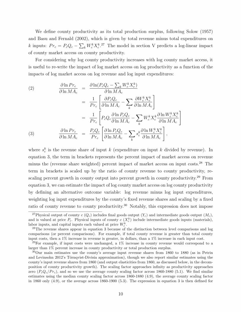
We define county productivity as its total production surplus, following Solow (1957)

and Basu and Fernald (2002), which is given by total revenue minus total expenditures on

k inputs: Prc = PcQc −∑

kWkc X

kc .27 The model in section V predicts a log-linear impact

of county market access on county productivity.

For considering why log county productivity increases with log county market access, it

is useful to re-write the impact of log market access on log productivity as a function of the

impacts of log market access on log revenue and log input expenditures:

∂ lnPrc∂ lnMAc

=∂ ln(PcQc −

∑kW

kc X

kc )

∂ lnMAc(2)

=1

Prc

[∂PcQc

∂ lnMAc−∑k

∂W kc X

kc

∂ lnMAc

]

=1

Prc

[PcQc

∂ lnPcQc

∂ lnMAc−∑k

W kc X

kc

∂ lnW kc X

kc

∂ lnMAc

]∂ lnPrc∂ lnMAc

=PcQc

Prc

[∂ lnPcQc

∂ lnMAc−∑k

skc∂ lnW k

c Xkc

∂ lnMAc

],(3)

where skc is the revenue share of input k (expenditure on input k divided by revenue). In

equation 3, the term in brackets represents the percent impact of market access on revenue

minus the (revenue share weighted) percent impact of market access on input costs.28 The

term in brackets is scaled up by the ratio of county revenue to county productivity, re-

scaling percent growth in county output into percent growth in county productivity.29 From

equation 3, we can estimate the impact of log county market access on log county productivity

by defining an alternative outcome variable: log revenue minus log input expenditures,

weighting log input expenditures by the county’s fixed revenue shares and scaling by a fixed

ratio of county revenue to county productivity.30 Notably, this expression does not impose

27Physical output of county c (Qc) includes final goods output (Yc) and intermediate goods output (Mc),and is valued at price Pc. Physical inputs of county c (Xk

c ) include intermediate goods inputs (materials),labor inputs, and capital inputs each valued at price W k

c .28The revenue shares appear in equation 3 because of the distinction between level comparisons and log

comparisons (or percent comparisons). For example, if total county revenue is greater than total countyinput costs, then a 1% increase in revenue is greater, in dollars, than a 1% increase in each input cost.

29For example, if input costs were unchanged, a 1% increase in county revenue would correspond to alarger than 1% percent increase in county productivity or total production surplus.

30Our main estimates use the county’s average input revenue shares from 1860 to 1880 (as in Petrinand Levinsohn 2012’s Tornqvist-Divisia approximation), though we also report similar estimates using thecounty’s input revenue shares from 1860 (and output elasticities from 1860, as discussed below, in the decom-position of county productivity growth). The scaling factor approaches infinity as productivity approacheszero (PcQc/Prc), and so we use the average county scaling factor across 1860-1880 (5.1). We find similarestimates using the median county scaling factor across 1860-1880 (4.9), the average county scaling factorin 1860 only (4.9), or the average across 1860-1900 (5.3). The expression in equation 3 is then defined for

10

assumptions about underlying production functions.

A main advantage of the expression in equation 3 is that we can use it to decompose

impacts on county productivity into two sources, given additional assumptions for calculating

production function elasticities. To do so, we add and subtract the growth in “expected

output” from the impact of market access on input expenditures: the sum over the growth

rate of each input multiplied by its respective output elasticity (αkc ).31 Rearranging terms:

∂ lnPrc∂ lnMAc

=PcQc

Prc

[∂ lnPcQc

∂ lnMAc−∑k

αkc∂ lnW k

c Xkc

∂ lnMAc

](TFPR)(4)

+PcQc

Prc

[∑k

(αkc − skc )∂ lnW k

c Xkc

∂ lnMAc

]. (RE)

The first term in brackets is the impact of county market access on county TFPR (revenue

total factor productivity). There are a number of considerations for interpreting TFPR, dis-

cussed below, but increases in TFPR represent increases in revenue above-and-beyond the

expected increases in revenue from increases in input expenditures. Increases in county

TFPR are equal to increases in county productivity, as defined above, if resources are al-

located efficiently and the value marginal product of inputs is equal to their marginal cost

(e.g., as assumed by Solow, 1957).

The second term in brackets represents an additional source of growth in county produc-

tivity. Holding county TFPR fixed, county productivity would increase when county inputs

increase if markups (Hall, 1988, 1990) or input frictions (Hsieh and Klenow, 2009) drive a

“wedge” between the value marginal product of inputs and their marginal costs (αkc/skc > 1).

In the decomposition, this wedge matters for county productivity because it leads to a “gap”

between measured production function elasticities and revenue shares (αkc − skc > 0), such

that increases in input-use would increase revenue by more than the increase in input ex-

penditures (and thereby increase county productivity).

We call this second term county RE (reallocative efficiency), following Petrin and Levin-

sohn (2012), which is also mechanically the residual between county productivity and county

TFPR.32 Increases in county RE do not reflect increased “efficiency” in the sense of reduc-

all counties, though the expression in equation 2 is only defined for counties with positive surplus. We alsoreport estimates of equation 3 using county-specific scaling factors, dropping counties with negative valuesand the top 1% of values.

31The output elasticity represents the expected log increase in physical output (Qc) from a log increase inphysical input k (Xk

c ), which is distinct from the relationship between log revenue and log input expenditure,though this decomposition still holds from adding and subtracting the same term (and we discuss below howthis affects the interpretation).

32Having used price deflators to convert nominal sales to real values, Petrin and Levinsohn (2012) call thefirst term “technical efficiency.”

11

tions in markups or input frictions. Instead, reallocative efficiency increases most when

input-use increases in counties with high markups or input frictions. Counties use too few

inputs when there are markups or input frictions, and so there are efficiency gains when

input-use increases.33 Increases in county RE reflect both “reallocation” of the same inputs

across counties and any growth in aggregate inputs. When there are positive gaps, county

RE increases with higher input-use but the implications for national aggregate productivity

depend on the cross-county variation in gaps and both relative and aggregate changes in

county inputs. We defer these details to Section V, in which the counterfactual analysis con-

siders impacts on national aggregate productivity from aggregate changes in county inputs

and reallocation of inputs across counties.

In practice, decomposing county productivity into these two separate components (county

TFPR and county RE) requires an estimate of the output elasticity (αkc ) for each input in each

county. For this, we assume that establishments have Cobb-Douglas production functions

with constant returns to scale, whereby cost minimization implies that each input’s output

elasticity is equal to its cost share. To allow for cross-industry variation in output elasticities,

we measure county-level cost shares by taking the revenue-weighted average of industry-level

cost shares for each industry in that county.34 We report estimates from alternative ways

of calculating the output elasticities, which in practice have little effect on the estimated

impacts of market access on county TFPR and county RE under constant returns to scale,

and mechanically do not affect the estimated impact of market access on county productivity.

Our regressions estimate relative changes in county productivity from relative changes

in county market access, but these estimated relative effects are not sufficient to estimate

aggregate productivity effects of the railroads. Section V.E makes further use of a general

equilibrium model to estimate these aggregate effects.

Our regressions estimate impacts of market access on values (county revenues and input

expenditures), along with associated impacts on county productivity/TFPR/RE, which differ

conceptually from impacts of market access on real quantities and physical productivity

(TFPQ). Section V models how county output prices and county input prices change with

33Regardless of the underlying source of inefficiency, whether due to markups or input frictions, if valuemarginal products are below marginal costs then input-use is inefficiently low and “reallocative efficiency”increases when input-use increases in that county.

34Our main estimates use the county’s average cost share from 1860 to 1880, as in the calculation ofrevenue shares, and we report similar estimates using the county’s cost shares from 1860. We measureindustry-level cost shares at the national level for each year, which reflect total industry expenditure oninput k divided by total industry expenditure on all inputs. We then calculate county-level cost sharesin each decade, weighting these industry-level cost shares by the share of county revenue in that industry.Alternative estimates use industry-level cost shares at the state level for each year, or industry-level costshares from the “most efficient” counties (i.e., those counties within one standard deviation of a total gap ofzero).

12

county market access, which reflect a combination of demand-side and supply-side influences,

and in that model declines in local prices would understate impacts of market access on

TFPQ and real county RE.35 While the regression analysis is limited to data on values, the

counterfactual analysis draws on the model to separate changes in quantities from changes

in prices.

In summary, we use data from the Census of Manufactures to define several outcome

variables for county c in year t. We start by showing effects on log revenue (ln(PctQct)), log

materials expenditures (ln(WMct X

Mct )), log labor expenditures (ln(WL

ctXLct)), and log capital

expenditures (ln(WKct X

Kct )), defined as the total values for county c in year t. We also show

effects on the log of total production surplus (ln(PctQct −

∑kW

kctX

kct

)), defined as the log

of total revenue minus total input expenditures for county c in year t.36 Our main outcome

variable is log productivity, in county c and year t, as discussed above:

(5)PcQc

Prc

[lnPctQct −

∑k

skc lnWkctX

kct

].

We then define two additional outcome variables that decompose the impacts of market

access on county productivity into the impacts through county TFPR growth

(6)PcQc

Prc

[lnPctQct −

∑k

αkc lnWkctX

kct

]

and the impacts through county RE growth

(7)PcQc

Prc

[∑k

(αkc − skc )lnWkctX

kct

].

35In the model, impacts of market access on TFPR would understate impacts on TFPQ because decreasesin transportation costs for output and inputs lower local output prices (with CES demand and Cobb-Douglasproduction with CRS), though TFPR is often correlated with TFPQ in settings when both are measured(Foster, Haltiwanger and Syverson, 2008; Haltiwanger, Kulick and Syverson, 2018). Reallocation of inputsacross industries or establishments, within a county, would also affect county TFPR without underlyingchanges in establishment TFPQ. In the model, impacts of market access on county RE would also understatereal productivity gains, because declining local input prices would cause the increases in input expendituresto understate increases in real inputs (though some local input prices could increase with county marketaccess, particularly for non-traded inputs like land).

36The analysis of log production surplus omits the 2% of county-year observations for which log productionsurplus is not defined because county revenue is less than county input expenditure.

13

III Estimating Equation

We regress outcome Y in county c and year t on log market access (MAct), county fixed

effects (γc), state-by-year fixed effects (γst), and a cubic polynomial in county latitude and

longitude interacted with year effects (γtf(xc, yc)):37

(8) Yct = β ln(MAct) + γc + γst + γtf(xc, yc) + εct.

The coefficient β reports the impact of county market access on outcome Y , comparing

changes in counties with relative increases in market access to other counties within the same

state and after adjusting for changes associated flexibly with county latitude and longitude.

The identification assumption is that counties with relative increases in market access would

otherwise have changed similarly to nearby counties.

The main identification concern is that railroad construction may have been targeted

toward counties that would otherwise have grown more over this period. We estimate impacts

of county market access, which depends in large part on more-distant changes in the railroad

network and its interaction with the existing transportation network. We report estimates

that control flexibly for changes in railroads within a county and within nearby areas. We

also use variation in counties’ access to more-distant counties.

The main regression sample is a balanced panel of 1,802 counties in 1860, 1870, and 1880

(Figure 2). We report standard errors that are clustered by state to adjust for correlation in

εct over time and within states.38

IV Estimated Impacts of County Market Access

IV.A Estimated Impacts on Productivity

Table 1 presents results from estimating equation 8. We estimate that county market access

has a substantial and statistically significant impact on county manufacturing revenue and

input expenditures. Column 1 reports that a one standard deviation greater increase in

market access from 1860 to 1880 leads to a 19.2% increase in revenue (panel A), 18.3%

increase in materials expenditure, 19.6% increase in labor expenditure, and 15.8% increase

37Note that we estimate equation 8 in levels, rather than in changes, but include county fixed effects thatfocus identification on county-level changes in market access. We also report separate estimates for pairs ofsample periods, where the estimation of equation 8 is equivalent in changes or in levels with county fixedeffects.

38If we instead adjust for spatial correlation across counties, following Conley (1999), we estimate standarderrors for our baseline specification that are 3-5% lower for distance cutoffs of 200 miles or 300 miles, 12-19%lower for distance cutoffs between 400 miles and 700 miles, and 19-30% lower for distance cutoffs between800 miles and 1000 miles. This method assumes that spatial correlation declines linearly up to the assumeddistance cutoff and is zero thereafter.

14

in capital expenditure.39 These estimated percent effects are similar in magnitude, which

imply little effect on county TFPR, but market access could still increase the total value of

county output by more than the total value of county inputs.

Indeed, we estimate substantial increases in county productivity from increases in county

market access. Panel E reports a 23.8% increase in log production surplus and Panel F

reports a 20.4% increase in log productivity, as defined in Section II.40 As county market

access increases, there is an increase in total county revenue that substantively exceeds the

increase in total county input expenditures; that is, there is increasingly more value of output

produced in excess of the value of inputs used.

Columns 2 and 3 report similar estimates when restricting the identifying variation in

county market access. For column 2, we calculate market access in each period holding

county populations fixed at 1860 levels, such that changes in county market access are only

due to changes in county-to-county transportation costs. For column 3, we calculate counties’

market access omitting other counties within 100 miles, such that changes in county market

access only reflect more-distant economic influences. Column 4 reports moderately larger

estimates from our baseline specification when extending the sample period, using available

county-level manufacturing data in 1890 and 1900.41 Column 5 reports similar estimated

impacts on county revenue and capital expenditures, using available county-level data in

1850 and restricting the sample to be a balanced panel back to 1850.

Table 2 shows that the above estimated impact of market access on log productivity (panel

A) is driven by growth in county RE (panel C) with less effect through growth in county

TFPR (panel B). This decomposition depends on production function assumptions (i.e.,

the calculation of counties’ output elasticities for each input, αkc ), but this decomposition

is not sensitive to alternative output elasticities (that sum to 1) because the estimated

percent effect of market access is similar for each input (from Table 1). Column 2 reports a

similar decomposition when defining counties’ output elasticities as a weighted average over

193 distinct industries, rather than 31 industries, which mechanically does not affect the

measurement of county productivity (in panel A). Column 3 reports similar estimates when

grouping all industries from 1860 to 1880, and Column 4 reports moderately larger estimates

39For ease of interpretation, we report the estimated impact of log market access in terms of standarddeviations (calculating changes in log market access from 1860 to 1880 and taking the standard deviation ofthose changes across counties). A one standard deviation greater increase in market access corresponds to a23% greater increase in market access from 1860 to 1880 for our baseline definition of market access.

40Appendix A.2 provides a reference on the formulas for these outcome variables. The sample for PanelE omits the 2% of county-year observations for which log production surplus is not defined because countyrevenue is less than county input expenditure.

41For comparability to columns 1 – 3, we continue to report the estimated impact of a 23% increase inmarket access (i.e., a one standard deviation greater increase in market access from 1860 to 1880).

15

when extending the sample through 1900 using the available aggregated county-level data

only.

For the estimated increases in county productivity to be driven by increases in county

RE, rather than county TFPR, it suggests that county market access is increasing input

expenditures in counties where the value marginal product of those inputs exceeds their

marginal cost. In that case, marginal additional expenditure on inputs would raise the total

value of output by more than the increase in total value of inputs used. By contrast, if the

value marginal product of inputs were equal to their marginal cost, then county productivity

would only increase with increases in county TFPR.

This interpretation raises important questions about whether mismeasurement of input

expenditures, particularly capital expenditures, may misstate counties’ gap between the value

marginal product of inputs and their marginal cost (Fisher and McGowan, 1983; Fisher,

1987; Hulten, 1991). Column 5 reports similar estimates when assuming zero misallocation

in capital, adjusting capital expenditures in each county such that its revenue share is equal

to its measured cost share. This adjustment scales down the level of county productivity,

but we estimate that increases in market access have a similar percent impact on that lower

level of productivity.42 Column 6 reports similar estimates from an alternative adjustment,

in which we use materials expenditures to infer county-level wedges (i.e., the ratio of the

cost share to the revenue share) and assign capital expenditures to counties such that capital

misallocation is the same as materials misallocation.43

Appendix B discusses a variety of additional specifications that find consistent effects of

market access on county productivity and its components. Appendix Table 2 further explores

the estimates’ sensitivity to the measurement of productivity, where we: use the materials

wedge to proxy for both capital and labor wedges; shrink the dispersion in cross-county

wedges; adjust for potential under-counting of labor or capital expenditures; define county

productivity based on 1860 county wedges (rather than average county wedges over the 1860

to 1880 period); and decompose productivity into TFPR and RE using alternative output

elasticities. Appendix Table 3 considers whether counties experiencing relative growth in

market access might otherwise have changed differently: estimating similar changes in coun-

ties prior to their relative growth in market access; controlling for time-varying effects of

42This adjustment has more effect on the aggregate counterfactual estimates in Section V.F, which dependon the level of counties’ productivity, but removing capital distortions does not have a large effect onthe counterfactual estimates because annual expenditures on capital are substantially smaller than annualexpenditures on materials and labor.

43This exercise is motivated by De Loecker and Warzynski (2012), who use materials expenditures to inferfirm-level markups. Here, we make the assumption that materials wedges reflect all sources of county-levelwedges that affect capital and that additional wedges for capital are not actually misallocation and insteadreflect measurement error, adjustment costs, and/or other dynamic issues.

16

county characteristics in 1860, including counties’ 1860 input wedges and input gaps; and

adjusting for potential differential effects of the Civil War. Appendix Table 4 focuses on the

measurement of county market access: calculating county-to-county transportation costs un-

der alternative assumptions; using different values for the trade elasticity θ or the average

price per ton of transported goods P ; and adjusting for the influence of international trade

and mismeasurement of population in the 1870 Census.

IV.B Endogeneity of Railroad Construction

An empirical concern when estimating the impacts of transportation infrastructure is that

infrastructure investment is generally directed toward areas that might otherwise change

differently over time. In particular, railroad construction may occur in counties that would

otherwise have experienced relative increases in manufacturing activity.

One of the advantages of analyzing changes in county market access, rather than directly

estimating impacts of local railroad construction, is that much variation in counties’ market

access is due to changes elsewhere in the railroad network and how the railroad network

interacts with other components of the transportation network. We can estimate the im-

pacts of county market access, controlling flexibly for railroad construction in the county

and nearby areas, which focuses the identifying variation on changes in county market ac-

cess from more-distant railroad construction and how railroad construction interacts with

waterways and the existing transportation network.44 Local railroad construction might also

directly impact local manufacturing activity, through increases in the demand for manufac-

tured construction materials, and so these controls also adjust for potential direct effects on

manufacturing from local railroad construction itself.

Table 3 reports similar estimated impacts of county market access when controlling flex-

ibly for local railroad construction. Column 1 reports baseline estimates from Table 2, as a

basis for comparison. Column 2 controls for whether the county has any railroad. Column

3 also controls for the county’s length of railroad track, and column 4 controls for a cubic

polynomial function of the county’s railroad track. Column 5 adds controls for a cubic poly-

nomial function of railroad track within 10 miles of the county’s borders, and column 6 adds

controls for separate cubic polynomial functions of railroad track within 20 miles, within

30 miles, and within 40 miles of the county’s borders. Local railroad construction predicts

44Other approaches sometimes focus on isolating some portion of new infrastructure placement that maybe more exogenous: because it followed historical plans or paths, because lines were built between particularlocations and inadvertently affected intermediate places, or because some lines were built for reasons lessassociated with local economic demand. Our approach is designed for contexts in which infrastructureplacement is potentially endogenous to local economic demand, and the transportation network is quite dense,such that there is not substantive variation in areas’ market access from particular known exogenously-placedconnections. A key feature of our context is that, after controlling flexibly for local railroad construction,there remains substantial residual variation in county market access.

17

increases in county market access, but Table 3 reports that the estimated impacts of county

market access are similar when identified from more-distant changes in the railroad network

and how railroad construction complemented or substituted for the previously established

waterway network.

As an alternative empirical approach, we can otherwise exploit changes in county market

access that are driven by how the existing waterway network interacts with changes in

the railroad network. As the railroad network expands throughout the country, counties

with cheap access to markets through waterways should generally experience less increase in

market access. We define county “water market access” in 1860, which reflects its measured

market access when excluding all railroads from the transportation network.

Table 4, column 1, reports that counties with greater water market access in 1860 ex-

perienced less increase in market access from 1860 to 1870 and from 1870 to 1880. Under

the identification assumption that counties with greater water market access would have

otherwise experienced similar changes in manufacturing productivity,45 we can instrument

for changes in county market access using county water market access in 1860 (and column

1 reports the first-stage results).46 Columns 2, 4, and 6 report the 2SLS estimated effects

of market access on productivity, county TFPR, and county RE, which are less precise but

similar in magnitude to the OLS estimates (columns 3, 5, and 7).

The waterway IV identification assumption would be violated if these counties with

greater water market access would have changed differently from 1860 through 1880, how-

ever, and a different empirical approach would estimate the effects of county market access

controlling for counties’ water market access in 1860 (interacted with decade, allowing these

places to change differently over time). Appendix Table 3 reports these estimates, which are

similar to those in Table 2, and also reports similar estimates when controlling for counties’

1860 market access (interacted with decade).

An expanding national railroad network affected different counties’ market access from

1860 to 1870 and from 1870 to 1880, and over each decade there were similar effects of market

access on county productivity. Splitting our baseline analysis by decade pair (1860 and

1870, 1870 and 1880, 1860 and 1880), increases in county market access lead to substantial

increases in county productivity that are more often driven by increases in county RE than

by increases in county TFPR (Appendix Table 3). We also estimate little serial correlation in

county market access, regressing changes in log market access from 1870 to 1880 on changes

in log market access from 1860 to 1870.47 Growth in county market access was also not

45Empirically, counties with better waterway access are not differentially likely to gain a connection to therailroad network by 1870 or by 1880.

46The first stage F-statistic is larger than the relevant critical value of 16.3 from Olea and Pflueger (2013).47Controlling for state fixed effects and latitude/longitude the point estimate (on a one percent increase

18

associated with differential trends in county manufacturing activity over the prior decade:

estimating the effects of county market access and counties’ future market access, controlling

for contemporaneous railroads and future railroads, Appendix Table 3 reports that county

market access has similar effects on county productivity (driven by growth in county RE)

and these outcomes are not associated with future market access (i.e., these outcomes were

changing similarly prior to growth in counties’ market access).48 Appendix Table 3 also

reports similar estimates when controlling for the share of counties’ 1860 revenue in each

industry, interacted with year, given the potential for relative changes in industry output

prices or other industry-specific shocks to differentially impact counties’ growth.

IV.C Sources of Growth in County RE

The estimated impact of market access on county productivity is largely driven by estimated

growth in county RE, with little estimated change in county TFPR, and this section explores

sources of growth in county RE along with other potentially associated changes in county

economic activity. We estimate that county RE growth is driven by increases in input

expenditures, in places where distortions lead to “gaps” between the value marginal product

of inputs and their marginal cost, but those gaps do not decrease with county market access.

We estimate little systematic change in the structure of the county economy itself, across a

range of outcomes; rather, there was a general expansion of county economic activity from

increases in counties’ market access.

Table 5, column 1, reports that the estimated increase in county RE (from Table 2)

is largely driven by increases in materials (panel C), followed by labor (panel B), with no

change from capital (panel A). Table 1 showed similar percent effects on expenditures for

each input, but average county gaps are largest for materials, followed by labor and then

capital (Appendix Table 5). Average county wedges are more similar across inputs, and even

moderately smaller for materials (Appendix Table 6), but materials expenditures are by far

the largest share of total input expenditures (Appendix Table 1). Input wedges represent

the degree of distortion (its output elasticity divided by its revenue share), but the impacts

on county RE from increased input expenditures depend on that input’s importance and the

resulting gap (its output elasticity minus its revenue share).

There is variation in input wedges across regions (Appendix Table 6), with associated

in market access from 1860 to 1870) is -0.02, with a standard error of 0.04. The estimate is 0.001 (0.04)when additionally controlling for contemporaneous and future growth in whether a county has any railroadand the length of its railroads.

48This specification controls for contemporaneous and future values for whether a county has any railroadand the length of its railroads, and the estimates are similar with additional cubic polynomial controls forcontemporaneous and future railroad length in the county and nearby areas.

19

differences in input gaps across regions (Appendix Table 5).49 Gaps greater than zero and

wedges greater than one may reflect a range of factors that would lower input use below

efficient levels (e.g., firm markups, capital constraints, taxes, insecure property rights).50

These regional differences in gaps and wedges are largely driven by differences in revenue

shares (Appendix Table 7), rather than differences in output elasticities (Appendix Table 8),

which means that the mix of industries across regions is not systematically more intensive

in particular inputs.

Cross-county variation in input gaps matters for how much national productivity would

decline without the railroads. County productivity increases as that county receives more

inputs, if that county’s input gaps are positive, but the impacts on national productivity

depend on how much that county input growth reflects inputs being shifted from another

county whose input gaps are relatively smaller or larger and, also, how much it reflects

aggregate input growth. Section V.F explores these effects on national productivity, based

on the cross-county variation in input gaps and the relative and aggregate changes in input-

use under counterfactual scenarios.51

Table 5, columns 2 and 3, report that county input gaps and wedges do not systematically

respond to increases in county market access. These estimates suggest that increases in

county market access are not systematically reducing input frictions or firm markups in

the county. We do not estimate the underlying sources of these county wedges, and how

much is driven by firm markups or input frictions, but the potential sources of wedges need

not decline with county market access. In the model in Section V, with CES demand and

Cobb-Douglas production with constant returns to scale, firms’ choice of markup would not

change as transportation costs decline for their output and materials inputs. Market access

also need not affect a variety of market distortions (e.g., borrowing constraints, implicit or

explicit taxes, contracting failures, imperfect property rights enforcement).52 Average gaps

49Appendix Figure 3 shows the cross-county dispersion in wedges by decade, where there is not much of asystematic pattern: the dispersion in the materials wedge decreased over time, increased for the labor wedge,and for the capital wedge stayed roughly the same.

50The calculated input gaps are equal to that input’s cost share minus its revenue share, and we report thesum of these gaps across inputs. The calculated input wedges are equal to that input’s cost share divided byits revenue share, and we report output-weighted averages of these county-level wedges by region and decade.The reported average input wedge reflects a simple unweighted average across the three inputs (materials,labor, capital).

51Section V clarifies that the percent impact of market access on input expenditures does not vary withcounty-level gaps, and even the percent impact on county productivity does not depend on county-level gaps,but the aggregate impact on national productivity depends on county-level gaps and how inputs change acrosscounties in the absence of the railroad network.

52There could also be some competing effects on input frictions, which cancel out in aggregate: borrowingor inventory management may become easier when there is more frequent and less costly movement of goodsor managers (see, e.g., Cronon (1991)), but input frictions may become more severe if local sources of fundsare slow to expand and meet increased demand. We report below that average establishment size is not

20

and wedges are declining over this time period, particularly in the Plains region, but we also

estimate little systematic effect of market access on gaps or wedges within regions (Appendix

Table 9).53

We have focused on county-level changes in input-use, though changes in county pro-

ductivity could also reflect within-county reallocation of inputs across industries. In our

decomposition of county productivity growth, this within-county reallocation of inputs across

county-industries would appear in county TFPR: if inputs shift from marginally less-productive

industries to marginally more-productive industries, within a county, then county revenue

would increase holding county input expenditures fixed (i.e., county TFPR growth). Our

previous estimates indicated little change in county TFPR, and column 4 of Table 5 reports

that county production did not systematically shift toward industries that are more capital-

intensive, labor-intensive, or materials-intensive. Column 5 reports there was little decline

in the standard deviation of wedges across industries within a county, as county market

access increased, which suggests that inputs did not shift from more-distorted industries to

less-distorted industries within counties.

Our main regressions are at the county level, aggregating county-industry data while al-

lowing for cross-county variation in output elasticities, because there is substantial industry

entry and exit that makes it difficult to interpret percent growth at the county-industry

level. Appendix Table 10 reports estimates from regressions at the county-industry level,

after aggregating industries to five more-consistently present categories: clothing, textiles,

and leather; food and beverage; lumber and wood products; metals and metal products; and

other industries. We extend our baseline specification by interacting the fixed effects with

industry.54 Column 1 reports estimated average impacts of market access on county-industry

productivity, county-industry RE, and county-industry TFPR that are similar to our county-

level estimates from Table 2, which is consistent with little cross-industry reallocation within

changing with increases in market access, which may be related to this absence of systematic change incounty wedges.

53One notable exception is a substantial decline in labor wedges with market access in the SouthernUnited States (Appendix Table 9), along with a sharp overall increase in labor wedges in the South in 1870following the emancipation of enslaved people (Appendix Table 6), which may be related. Our baselineestimates are not sensitive, though, to omitting the South or other robustness checks associated with theCivil War (Appendix Table 3). There is some indication of market access increasing input gaps in Westernareas, but these areas make up a small share of the overall sample and the baseline estimates are also notsensitive to omitting Western areas. We do not estimate systematic impacts of market access on gaps orwedges in “frontier areas” (Bazzi, Fiszbein and Gebresilasse, 2020), defined as counties with between twoand six people per square mile in 1860 and that are within 100km of the boundary where population densityfell below two people per square mile in 1860.

54The specification then includes county-industry fixed effects and state-year-industry fixed effects. Weomit county-industries that appear only once, but do not restrict the sample to county-industries that appearall three years.

21

counties that would appear as county TFPR growth in Table 2. Column 2 reports similar

average impacts when weighting county-industries by their 1860 share of county revenue.

Columns 3 – 6 report industry-specific effects of market access for each consistent industry

group, with some variation in effects across industries but no industry-specific effect is sta-

tistically different than the average over the other industries. Appendix Tables 11 and 12

report average gaps and wedges by industry group, and Appendix Table 13 reports little

systematic effect of market access on gaps and wedges within these industry groups.

Increases in county manufacturing activity appear to be a general expansion of existing

economic activity in the county. Column 1 of Table 6 reports little impact of county market

access on the number of industries in a county. Table 6 also reports little impact of market

access on the average size of establishments, measured as average revenue per establishment

(column 2) or average number of workers per establishment (column 3). Instead, increases

in county market access lead to a substantial increase in the number of manufacturing es-

tablishments (column 4), which is driving the overall increases in revenue and expenditures.

While county manufacturing activity increased substantially with increases in market

access, we do not estimate that increases in market access prompted an economic shift from

the agricultural sector toward the manufacturing sector within counties. Table 6, column 5,

reports little impact of market access on county manufacturing revenue as a share of total

manufacturing and agricultural revenue in the county. Similarly, columns 6, 7, and 8 report

little impact on county manufacturing value-added, surplus, or employment as a share of the

county total in manufacturing and agriculture.55 Further, we do not estimate that increases

in market access encouraged economic activity in counties to become specialized in either

manufacturing or agriculture.56 Appendix Table 14, panel A, reports little impact of market

access on sectoral specialization in terms of revenue (column 1), value-added (column 2),

surplus (column 3), or employment (column 4). Similarly, looking within the manufacturing

sector, panel B reports little impact of market access on specialization across manufacturing

industries. Using our county-by-industry data, however, we are unable to examine within-

industry specialization across product varieties.

These estimates highlight the broad expansion of manufacturing activity (and agricul-

55For agriculture, we define value-added as 92% of revenue, reflecting an assumed 8% materials share inagriculture (Towne and Rasmussen, 1960), and we define surplus as the value of land multiplied by the statemortgage interest rate. For manufacturing, we define value-added as revenue minus materials expenditures,and we define surplus as revenue minus all input expenditures.

56We define a county specialization index as the squared difference between a county’s manufacturing shareand the national manufacturing share, added to the squared difference between a county’s agricultural shareand the national agricultural share. This index increases as county production becomes more intensive in themanufacturing sector or agricultural sector, relative to the national shares in each decade. The estimatedeffects are similar for a Herfindahl index that reflects sector concentration (or industry concentration),whereas this specialization index reflects movement toward or away from “typical” production shares.

22

tural activity) in counties that experience relatively greater increases in market access, and

motivate several assumptions underlying the aggregate analysis in Section V. In particular,

we will assume in Section V that increases in county market access do not affect the county’s

production function elasticities (as in Tables 5 and 6). We also assume that county market

access does not directly affect county gaps or wedges (as in Table 5). The mechanism driv-

ing productivity growth is the change in counties’ input-use, combined with county-specific

gaps between the value marginal product of inputs and their marginal cost. Whereas the

regression analysis estimates relative growth in county productivity from relative increases

in county market access, the analysis in Section V.F considers the aggregate productivity

effects from aggregate changes in each counties’ input-use under counterfactual scenarios.

V Aggregate Counterfactual Analysis

We now examine how national aggregate productivity was affected by changes in county

market access due to the railroads. The regressions estimate that relative increases in county

productivity were driven by increased economic activity in counties with positive “gaps,”

where the value marginal product of inputs exceeded their marginal cost, but some of this

increase may reflect the shifting of inputs from other counties that also have positive gaps. By

drawing further on the model’s specification of county market access, we consider aggregate

economic impacts from the expansion of the railroad network and aggregate economic losses

under counterfactual transportation networks.

We extend a baseline model of economic geography (Eaton and Kortum, 2002; Donald-

son and Hornbeck, 2016) to include market distortions. Each county is affected by changes

in transportation costs due to expansion of the railroad network, through interacting goods

markets and factor markets across all counties, and these effects are summarized by changes

in a county’s market access. We show how the presence of market distortions causes there

to be aggregate productivity gains from reductions in transportation costs, which are not

captured by changes in land values (as in Donaldson and Hornbeck, 2016) or social sav-

ings calculations (as in Fogel, 1964). We then estimate the national aggregate productivity

losses from counterfactual transportation networks, such as removing the railroad network

or replacing the railroad network with an extended network of canals.

V.A Model Setup

Firms in each county have a Cobb-Douglas production function for good variety j, which

uses labor L, capital K, land T , and materials M .57 In county o, these inputs cost a wage

wo, interest rate ro, rental rate qo, and price index Po; alternatively, input k costs W ko in

57We now refer to “firms” for convenience, though note that the data is at the establishment-level and sothis refers to single-establishment “firms.”

23

county o. Firms use a continuum of good varieties as materials, with a constant elasticity of

substitution across varieties, and so Po is the CES price index over good varieties.58

Firm production functions vary across counties in their Hicks-neutral technical efficiency

zo(j). Following Eaton and Kortum (2002), each county has an exogenous technical efficiency

level zo(j), for each variety j, drawn from a Frechet distribution with CDF given by: Fo(z) =

1 − e−Aoz−θ

, with θ > 1.59 The parameter Ao captures average technical efficiency in county

o (absolute advantage), while the parameter θ captures the standard deviation of technical

efficiency across varieties (scope for comparative advantage). A smaller θ or “trade elasticity”

is associated with more-dispersed technical efficiency across varieties, larger incentives to

trade across counties, and a less elastic response of cross-county trade flows to trade costs. We

also allow for firm production functions to vary across counties in their exogenous production

function elasticities (αLo , αKo , α

To , α

Mo ). The marginal cost of producing variety j in county o

is:

(9) MCo (j) =(wo)

αLo (ro)αKo (qo)

αTo (Po)αMo

zo (j)=

∏k

(W ko

)αkozo (j)

.

Marginal costs are lower when input costs are lower and when firm technical efficiency is

higher.

The main addition in our model, as compared to Donaldson and Hornbeck (2016), is

that firms face input-specific frictions. These frictions are exogenous and represent market

inefficiencies that discourage further use of labor (ψL), capital (ψK), land (ψT ), or materials

(ψM). Given any positive friction, firms in county o reduce production of variety j such that

its price is greater than its marginal cost of production:

(10) po (j) =

∏k

((1 + ψko

)W ko

)αkoβo (j)

> MCo (j) .

Firm markups, due to market power, can be represented as a common component in each of

the ψ terms.60 Given a positive firm markup, or positive input-specific frictions, the value

created by firms increasing production would be greater than the value of resources used.

Firms are unable or unwilling to use more inputs, however, as reflected in the ψ terms.

We assume capital is mobile, such that interest rates are fixed exogenously, but this

58Po ≡[∫ n

0(po(j))

1−σdj]1/(1−σ)

, where σ is the elasticity of substitution across varieties j, n is the exoge-nous measure of varieties, and po(j) is the price of variety j in county o.

59This Frechet distribution reflects firms receiving levels of technical efficiency from various potentialdistributions and discarding all but the best for each variety.

60While the input-specific frictions are modeled as constants, the assumed CES demand for firm outputalso implies that firms would choose constant markups.

24

interest rate can vary across counties.61 We assume land is fixed in each county (i.e., the

total quantity of physical land in each county), and its price is endogenous.

Labor is supplied by workers, who consume good varieties j in the same manner that

firms use these varieties in roundabout production, and so workers pay the same CES price

index Po as firms (Redding and Venables, 2004). A worker living in county o, and receiving

a wage wo, receives indirect utility V (Po, wo) = wo/Po.62 We assume workers are perfectly

mobile across counties, such that worker utility is the same across counties at U . The local

wage rate is endogenous, however, and reflects local prices (wo = UPo) such that nominal

wages are higher in counties with higher goods prices. In assuming that workers are perfectly

mobile across counties, we focus on a long-run equilibrium in which workers can arbitrage

real wage differences over a decade.63

There is costly trade of good varieties across counties, for both final goods and intermedi-

ate goods (materials). Transporting goods from county o (origin) to county d (destination)

incurs a proportional “iceberg” trade cost τod.64 In county d, the price of good variety j

produced in county o is then given by: pod(j) = τodpoo(j), where poo(j) is the factory-gate

price in county o and τod > 1.

V.B Solving for Market Access

We begin by deriving the gravity equation for cross-county trade flows, allowing for input

frictions. When firms sell good varieties from county o in county d, the offered price in

county d reflects the factory-gate price in county o (equation 10) and the transportation

cost (τod). Consumers buy good varieties from their cheapest source, where “consumers”

includes workers buying goods and firms buying materials. Following Eaton and Kortum

(2002), with the addition of input frictions ψ, the value of total exports from county o to

county d is given by:65

(11) Eod = κ1Ao

(Πk

((1 + ψko

)W ko

)αko)−θ τ−θod YdP θd .

61In practice, given data constraints, we allow this interest rate to vary across states according to themeasured average mortgage interest rate in each state (Fogel, 1964).

62We assume workers spend their income in their home county, and that payments to land and capitalalong with any profits are also spent in each county in proportion to its share of aggregate revenues.

63In the counterfactual analysis we report estimates for different scenarios that assume a perfectly elasticsupply of immigrants from abroad, a perfectly inelastic supply of immigrants from abroad, as well as moreintermediate cases.

64We measure the cost per ton of transporting goods between counties (Section I.B), and express thisabsolute cost in proportional terms using the average value of transported goods (estimated below, alongwith the estimation of the trade elasticity θ).

65Here, κ1 =[Γ(θ+1−σ

θ

)]− θ1−σ , where Γ(·) is the Γ function defined by Γ(t) =

∫∞0xt−1e−xdx.

25

County o sends more goods to county d when county o has higher technical efficiency (Ao)

or lower “effective costs”(

Πk

((1 + ψko

)W ko

)αko), where “effective costs” reflect input prices

and input frictions. Higher input frictions have the same impact on trade flows as higher

input prices or lower technical efficiency. County o also sends more goods to county d when

bilateral transportation costs are lower (τod), when county d has higher income (Yd), and

when county d has a higher goods price index (Pd).

Consumer market access (CMA) in county d is an inverse transformation of the goods

price index (Redding and Venables, 2004; Donaldson and Hornbeck, 2016):

(12) CMAd = P−θd = κ1∑o

τ−θod Ao

(Πk

((1 + ψko

)W ko

)αko)−θ .Consumer market access is higher in county d when it has access to cheaper goods: when

there are lower costs of transporting goods from counties with higher technical efficiency and

lower “effective costs.” Input frictions in county o lower consumer market access in county

d because county d is not able to fully benefit from low marginal costs in county o.

Firm market access (FMA) in county o is a sum over firms’ access to all destination

counties, adjusting for those destination counties’ access to other sources of goods:

(13) FMAo =∑d

τ−θod YdCMA−1d .

Firm market access is higher in county o when it has access to more product demand: when

there are lower costs of transporting goods to counties with higher consumption, which have

less access to other sources of goods (CMAd). We can also represent consumer market access

in county d as a sum over consumers’ access to all origin counties:

(14) CMAd =∑o

τ−θod YoFMA−1o .

Similar to equation 13, consumer market access is higher in county d when it has access to

more product supply: when there are lower costs of transporting goods from counties with

higher production, which have less access to other destinations for goods (FMAo). Indeed,

equations 13 and 14 imply that a county’s firm market access and consumer market access are

exactly proportional: FMAo = ρCMAo, where ρ > 0.66 We therefore use a single measure

of “market access” (MA), which reflects the ideas underlying both firm market access and

consumer market access: MAo ≡ FMAo = ρCMAo. Given that workers receive a fixed

share of revenue (αL), we can then express market access in county o as a function of the

66For this result, we assume that trade costs are symmetric (τod = τdo), as constructed in Section I.B.

26

endogenous number of workers in each other county d:67

(15) MAo = κ2∑d

τ−θod LdMA−(1+θ)

θd

(1 + ψLd

)αLd

.

Market access is higher in county o when it is cheaper to trade with more-populated counties

that have less access to other markets, a greater labor cost share, and a higher labor input

friction. This equation for market access simplifies to the corresponding equation 9 in Don-

aldson and Hornbeck (2016), when there are zero labor input frictions and a homogeneous

labor cost share.68

Changes in county market access summarize how each county is impacted by changes

in transportation costs. In the model, changing transportation costs between two counties

has positive and negative spillover effects on other counties due to linked goods markets and

factor markets. Changes in county market access summarize these impacts from changes in

counties’ connectedness, capturing both “demand-side” and “supply-side” channels through

which counties are affected by changes in overall market integration.69 We solve for county

market access in each county and each decade, using: the N-by-N system of equations for

market access in each county (equation 15); data on county population and county-to-county

transportation costs; and parameter choices discussed below.

The calculated changes in county market access, as derived from the full model, are highly

correlated with the approximated changes in county market access used in the previous

regression analysis (equation 15 vs. equation 1). From 1860 to 1880, changes in log market

access derived from the model (equation 15) and changes in log market access based on

our approximation (equation 1) have a correlation coefficient of 0.9998. When estimating

equation 8, a one standard deviation greater increase in model-defined log market access is

estimated to increase log county productivity by 0.205 (s.e. of 0.051), which is driven by

increases in county RE (0.169 , s.e. of 0.051) rather than increases in county TFPR (0.036 ,

s.e. of 0.025). These estimates represent rounding differences from our estimates in Table 2

for approximated market access.70

Figure 3 shows approximately log-linear impacts of market access, as predicted in Section

V.C, on county productivity (panels A and B) and the contribution to county productivity

67Here, κ2 = Uρ1+θθ

68Note that other input frictions also affect equilibrium behavior but, conditional on the distribution ofpopulation, market access can be expressed as a function of labor, labor input frictions, and labor cost shares.

69One other effect, discussed below in the counterfactual analysis, is that worker welfare can also changeacross all counties.

70A one standard deviation greater change in model-defined log market access is 0.225, from 1860 to 1880,which is similar to that for approximated market access (0.231).

27

from county RE (panels C and D), and county TFPR (panels E and F).71 This figure shows

the local polynomial relationship between residual productivity and residual market access,

after partialling out the controls from estimating equation 8.

The approximated measure of county market access is sufficient for the regression analysis

of relative changes in market access, but the full model-defined expression for market access

is required for the aggregate counterfactual analysis. This is because we need to determine

not only relative changes in county market access but the absolute changes in counties’

market access under counterfactual scenarios.

V.C Predicted Impacts of Market Access

We now consider the predicted impacts of market access on county productivity and other

county-level outcomes. The impact of market access on productivity in county o is given by:

(16)d lnPRo

d lnMAo=PoQo

Pro

∑k

(αko − sko

) d lnXko

d lnMAo.

Market access increases county productivity by increasing real input usage ( d lnXko

d lnMAo), when

the value marginal product of that input exceeds its marginal cost (i.e., when the production

function elasticity α is greater than the revenue share s).72

Building on equation 16, as described in the Appendix, we show that changes in market

access have a log-linear impact on county productivity:

d lnPRo

d lnMAo=

PoQo

Pro

[ (αLo − sLo

) (1

θ+αMo + αLo + 1

1 + θαTo

)(17)

+(αMo − sMo

) (1

θ+αMo + αLo + 1

1 + θαTo

)+(αKo − sKo

) (αMo + αLo + 1

1 + θαTo

)].

Market access increases capital usage by αMo +αLo+11+θαTo

percent, which then increases county

productivity by PoQoPro

(αKo − sKo

)αMo +αLo+11+θαTo

percent. Market access has a larger impact on

labor and materials usage (in real values, but not in nominal values), with the additional

term(1θ

)reflecting that market access also decreases materials costs and nominal wages in

71These figures are for approximated market access (panels A, C, E) and model-defined market access(panels B, D, F).

72Note that county productivity is also increasing in its technical efficiency (Ao), though in the modelwe have assumed that technical efficiency is exogenous and not directly affected by market access. Asa consequence, we are now only considering productivity impacts of market access through increases inreallocative efficiency.

28

county o.73

This log-linear impact of market access on productivity can be re-written using the input

frictions (ψ):

d lnPRo

d lnMAo=

PoQo

Pro

[αLo

(ψLo

1+ψLo

) (1θ + αMo +αLo +1

1+θαTo

)(18)

+ αMo

(ψMo

1+ψMo

) (1θ + αMo +αLo +1

1+θαTo

)+ αKo

(ψKo

1+ψKo

) (αMo +αLo +1

1+θαTo

)].

Market access increases productivity by increasing input usage, when input usage is otherwise

below the efficient level due to input frictions (ψ). The Appendix derives the log-linear

impact of market access on each input and each input price. An interesting result is that

input frictions do not change the impact of market access on revenue or input expenditures,

in percentage terms, similar to how the impact of market access does not depend on local

technical efficiency. Input frictions do determine whether market access impacts productivity,

however, as captured in equations 17 and 18: the effect of market access on productivity, in

levels, goes to zero as the gaps or frictions go to zero.74

Input frictions on land do not affect the impact of market access on productivity (equa-

tions 17 and 18), as the model assumes land is in fixed supply and so the quantity of land

used is not below its efficient level. Market access does increase land expenditure, however,

as the price of land is log-linear in market access:

(19)d ln qo

d lnMAo=αMo + αLo + 1

1 + θαTo

Adding input frictions to the model does not affect the impact of market access on land value,

which is the main estimated impact in Donaldson and Hornbeck (2016). We obtain the same

predicted impact of market access on land value as Donaldson and Hornbeck (2016), when

replacing our county-specific sum of the labor share and materials share (αMo + αLo ) with

their average labor share of value-added (αL).75

73These input price effects are why the previous regression estimates are predicted to understate theimpact of market access on real county RE (as discussed in Section II), as the measured increase in inputexpenditures is predicted to understate the increase in real input usage.

74The impact of market access on productivity, in levels, is given by multiplying equations 17 and 18by the level of productivity (Pro). The resulting impact, in dollar terms, can be summed across counties.That sum, expressed relative to GDP, is equal to the Domar-weighted sum of percent changes in countyproductivity (see equations 20 and 21).

75Input frictions do affect land values in levels, just as unobserved technical efficiency affects land valuesin levels.

29

We define national aggregate productivity growth as the growth in total production

surplus, expressed in percent terms relative to national value-added (GDP). Under counter-

factual scenarios, the change in total production surplus is the sum of changes in county-level

production surplus:

APG =1

GDP

∑o

dPRo(20)

=1

GDP

∑o

Pro d lnPRo

=1

GDP

∑o

PoQo Σk

(αko − sko

)d lnXk

o

APG =∑o

Do Σk

(αko − sko

)d lnXk

o ,(21)

where Do is the Domar (1961) weight for county o (county revenue divided by national

value-added).76 These Domar weights sum to more than 1, and are the appropriate way

to aggregate county-level changes in settings with intermediate goods (Hulten, 1978) and

distortions that generate a gap between the value marginal product of inputs and their

marginal cost (Petrin and Levinsohn, 2012; Baqaee and Farhi, 2019a).77

V.D Model Interpretation and Discussion of Assumptions

Our model highlights the impact of market access on productivity, in the presence of market

distortions, which generates a separate source of economic gains from the railroads that are

in addition to the impacts on land values considered by Donaldson and Hornbeck (2016). In

that model without distortions, all economic gains from increased market access are captured

by the increase in land values.78 Increased land values reflect greater factor input payments,

but increased productivity reflects gains in output that are not paid to inputs. Thus, in

our model, the economic gains from the railroads are given by the increase in aggregate

productivity in addition to the increase in land values.

Our model extends the counterfactual analysis in Donaldson and Hornbeck (2016), and

is equivalent to that model when removing input frictions, removing intermediates, and

constraining the production function elasticities to be constant across counties. The most

76Our counterfactual analysis assigns each county the average of its factual and counterfactual Domarweight, though in both scenarios the sum of the Domar weights is approximately 1.57.

77Petrin and Levinsohn (2012) and Baqaee and Farhi (2019a) provide alternative derivations that simplifyto equation 21 for settings like ours in which technical efficiency is constant.

78There is also incidence on aggregate worker utility if there is not perfect labor mobility into the UnitedStates, which we discuss later. In principle, there could be gains to local workers (given some inelasticityto local labor supply) or gains to capital owners (given some inelasticity to capital supply), but we assumethose factors are supplied elastically and land is the only fixed factor and so it bears the total incidence.

30

important departure is the introduction of input frictions. We allow the output elasticities

to vary across counties so that we do not confound measured county-specific frictions with

county variation in output elasticities (e.g., cross-county variation in industry revenue shares

is also driven by different input intensities in production).

We make some important assumptions to maintain tractability in this general equilibrium

setting, while extending the model to include input frictions. In particular, we assume that

several features of the economy are exogenous and not impacted by changes in market access.

These assumptions are consistent, however, with the estimates in Section IV.

First, we assume that county input frictions are exogenous. This assumption is consistent

with estimates from Table 5, in which the measured “gaps” and “wedges” were not impacted

by changes in market access.79

Second, we assume that county production function elasticities are exogenous. This

assumption is consistent with estimates from Table 5, which show little impact of market

access on elasticities in manufacturing, and estimates from Table 1 that show similar percent

changes in expenditures on materials, labor, and capital. Further, Table 6 shows little impact

of market access on the county manufacturing share of revenue, value-added, surplus, or

employment.80

Third, we assume that county technical efficiency is exogenous. This assumption is con-

sistent with estimates from Table 2 that showed little impact of market access on TFPR,

which is often correlated with technical efficiency in data when both are observed (Foster,

Haltiwanger and Syverson, 2008; Haltiwanger, Kulick and Syverson, 2018). Our counter-

factual analysis then considers impacts on aggregate productivity only through changes in

reallocative efficiency, under the conservative assumption that technical efficiency does not

also decline in the absence of the railroads.

V.E Estimating the Model

Using our assumption that workers move across counties to equalize real wages, we use

data on county population to infer an “amenity” value for each county. This “amenity”

value reflects the quantity of fixed factors in each county, along with the county’s exoge-

79We do not identify the underlying sources of input frictions, but various sources of input frictions neednot vary with market access (e.g., borrowing constraints, contracting failures, implicit or explicit taxes orregulations, etc). To the extent that county input frictions reflect firm markups, the model’s assumptions(CES demand and Cobb-Douglas production with CRS) imply that firms choose constant markups that donot vary with market access.

80Note that the model allows for specialization in firms’ product varieties, within sectors or industries, asopposed to changes across sectors or industries that are associated with different elasticities. Appendix Table14 reports no impacts of county market access on cross-sector specialization or cross-industry specialization,but our data do not allow for estimating impacts on product variety specialization within sectors.

31

nous technical efficiency.81 Given our measured county-to-county transportation costs, the

county population data imply a unique vector of county amenity values (see Appendix for

details).82 Holding those amenity values fixed, and using counterfactual county-to-county

transportation costs, we can then calculate an implied counterfactual population in each

county and associated counterfactual changes in capital and materials usage. Using our es-

timated county-level input frictions, and the associated gap between inputs’ value marginal

product and marginal cost in each county, we then calculate the aggregate productivity

impact from removing the railroad network (or from other counterfactual transportation

networks).

The model describes total economic activity in each county, which corresponds to the

county’s total population and all goods consumption and production. We only have detailed

data for manufacturing industries, however, on the value of output and value of inputs. We

use these data to measure input frictions within the manufacturing sector in each county,

as in Section II and IV, and we begin by assuming these input frictions are constant across

sectors within each county.83 We also estimate production function elasticities for each

county in the manufacturing sector only, and so we calculate county-level elasticities also

using nationwide production function elasticities in agriculture.84

We jointly estimate values for the trade elasticity (θ) and the average price per ton of

transported goods (P ).85 For any given trade elasticity θ, the model predicts a matrix of

81These two variables are not separately identified, but we only need their combined value for the coun-terfactual analysis.

82The vector of county amenity values is unique up to a proportional constant, whose value does not affectthe analysis.

83As an alternative exercise, we consider counterfactual impacts when assuming there are lower inputfrictions outside the manufacturing sector.

84For the agricultural sector, we use value-added elasticities from Caselli and Coleman (2006) and thematerials input share from Towne and Rasmussen (1960), giving us production function elasticities of 0.552for labor, 0.1932 for capital, 0.1748 for land, and 0.08 for materials. We calculate county-level elasticities in1890 by weighting these agricultural sector elasticities by the fraction of 1890 county revenue in agriculture(or manufacturing). For economic activity outside the agricultural sector, we continue to assume a “fixedfactor” share of 0.1748 and assign county-specific elasticities for materials, labor, and capital by taking therevenue-weighted average of its manufacturing industry elasticities in 1880. The counterfactual sample is2,722 counties with positive population and positive agricultural or manufacturing revenue in 1890, of which309 sparsely-populated counties do not report manufacturing data in 1880 (which we assume reflects zeromanufacturing revenue). We use the 1880 county-by-industry data to calculate county-level wedges, as inSection II, when these data are available. We use 1890 county-level data to calculate wedges and elasticitiesfor 176 counties with no manufacturing data in 1880 (4% of US population in 1890), then use 1900 data tocalculate wedges for 69 counties with no manufacturing data in 1890 (1.5% of US population in 1890), andthen use state median wedges in 1880 for the remaining 64 counties (0.2% of US population in 1890). We thendivide the county-level elasticities by the county-level wedges to calculate county-level revenue shares (andthen calculate county-level gaps, defined as the difference between county-level elasticities and county-levelrevenue shares).

85We use this average price per ton of transported goods (P ) to calculate the iceberg trade costs (τcd)based on the measured county-to-county transportation costs: (τcd = 1 + tcd/P ).

32

county-to-county railroad shipments (in tons) and county output (in dollars), which we use

to generate a value for P that jointly maximizes closeness of fit with the Census data on

total manufacturing and agricultural output (in dollars), and total US railroad shipments

in 1890 in tons (Adams, 1895). Given that average price per ton P and trade elasticity θ,

we then estimate the impact of market access on agricultural land values (as in Donaldson

and Hornbeck, 2016), under the assumption that land markets are integrated across sectors

within counties. We choose the θ (and corresponding P ) that minimizes the residual sum of

squares from regressing the model-predicted change in land values (from equation 19) on the

observed change in land values. We estimate an average price of transported goods equal

to 35.7. We estimate a value of θ equal to 2.788 (95% confidence interval: 1.815 – 3.556),

which is moderately lower than (but within the general range of) estimates in the literature

(Costinot and Rodrıguez-Clare, 2014) and we report the robustness of our counterfactual

estimates to assuming alternative parameter values.

V.F Estimated Counterfactual Impacts

We estimate that national aggregate productivity would have been 28.0% lower in the United

States in 1890, if there were no railroad network and the economy had to rely on the existing

waterway network and high-cost wagon transportation (Table 7, panel A, column 1).86 This

28% decline in aggregate productivity reflects only decreases in reallocative efficiency, with

no decline in county technical efficiency or underlying physical productivity of firms, but

this decline in reallocative efficiency is equivalent to a 28% decline in aggregate real TFP or

roughly 50 years worth of technological innovation in this era.87

This 28% decrease in aggregate productivity is worth 28% of GDP annually, or $3.4

billion in 1890 dollars. As a comparison, the estimated cost of the railroad network in 1890

was $8 billion (Adams, 1895). We estimate that this investment in the railroads generated

an annual social return of 50%, and that the railroad sector privately captured only 7% of

its social return in 1890.88

86We focus on counterfactual estimates for 1890, following Fogel (1964) and Donaldson and Hornbeck(2016).

87For the 1855 to 1905 period, Abramovitz and David (1973) report an average of 0.50% annual growthin real value-added TFP.

88We estimate that the railroads generated an annual private return of 3.5% in 1890. For this calculation,based on numbers from Adams (1895), we sum the railroads’ reported net income ($145 million), debtinterest payments ($217 million), net capital expenditure ($5 million), and subtract losses not otherwisereflected from some companies ($30 million) along with subtracting income from other sources ($52 million).We then divide $285 million by the cost of the railroads including equipment ($8.041 billion) and value ofland ($80 million). Much of the railroads’ reported transportation expenses were maintenance costs (39%or $271 million), and we interpret the reported “permanent improvements” of $5 million as total capitalexpenditure minus depreciation. To calculate the annual social return, we sum the annual private return($285 million), our estimated annualized increase in agricultural land value ($425 million), and our estimatedincrease in annual productivity ($3.36 billion), divided by the cost of the railroads including equipment and

33

Figure 4 maps the county-level counterfactual changes in productivity, where darker

shaded counties represent larger counterfactual declines productivity in the absence of the

railroads. These declines in county-level productivity reflect counterfactual declines in mar-

ket access and production inputs, interacted with county-level “gaps” between the value

marginal product of inputs and their marginal cost, as in equation 17. Appendix Figure 4

maps the county-level counterfactual declines in market access, and Appendix Figure 5 maps

the county-level gaps.

In estimating the decline in aggregate productivity, we consider several scenarios for coun-

terfactual changes in US total population. Our baseline estimates reflect the counterfactual

decline in total population that holds fixed worker utility (real wages). We also consider

a scenario that holds fixed total population, and calculate the associated decline in worker

utility, along with scenarios that reflect intermediate declines in total population.

When holding fixed total population, we solve for counties’ population shares in the ab-

sence of the railroad network. We then calculate corresponding changes in other production

inputs, output, and the resulting change in aggregate productivity in the United States.

Panel B reports that productivity is estimated to fall by 5.8% in 1890, in the absence of

the railroad network, when maintaining the same total US population. Population and

other production inputs become condensed into limited geographic areas, decreasing labor

productivity, and so worker utility (real wages) falls by 34.4%.

When allowing for aggregate declines in population, the model predicts a substantial

decline in population in the United States. For worker utility (real wages) to be unchanged

in the counterfactual, the model predicts that the US population would need to be 68%

lower in 1890. This is moderately larger than the 58% counterfactual decline in population

estimated by Donaldson and Hornbeck (2016), but this population decline has much greater

economic impact in our analysis because the marginal product of inputs is allowed to be

greater than their marginal cost. If we instead assumed that total US population would

be lower by 33% in the absence of the railroads, reflecting the native-born population of

native-born parents in 1890, then we would estimate a 14% decline in productivity and a

24% decline in worker utility (real wages).89 By comparison, the US population was 37%

lower in 1870 and 73% lower in 1840 than in 1890 (United States Census Bureau, 1975).

Rather than removing the entire railroad network, we can also consider the counterfactual

economic losses if the railroad network had stopped expanding. For example, in 1890, we

estimate that productivity would have been 2.7% lower using only railroads that existed

land ($8.121 billion).89For this calculation, using the available Census tabulations, we reduce the total US population by

excluding foreign-born population in 1890 and the white native-born population in 1890 with foreign-bornparents.

34

in 1880, 10.4% lower using railroads from 1870, 16.4% lower using railroads from 1860, or

23.4% lower using railroads from 1850 (Table 7, panel A, columns 2 – 5).

Additional canals might have been constructed to mitigate productivity losses, in the

absence of the railroad network, but we find that these canals would have been an ineffective

substitute for the railroad network. We evaluate the system of feasible canals proposed by

Fogel (1964), estimating that productivity would have been lower by 24.7% in 1890 when

replacing the railroad network with these additional canals (Table 7, panel A, column 6).

That is, the additional canals would have mitigated only 12% of the losses from removing

the railroad network.90

By contrast, the railroads would have been “cheap at twice the price.” We estimate that

productivity would have been lower by 9.3% in 1890 if railroad rates were double (Table

7, panel A, column 7). Compared to losing access to the railroad network entirely, using

these more-expensive railroads would mitigate 67% of the productivity decline. Table 8

reports that our estimated counterfactual impacts on productivity vary moderately with

the estimated value of P (average price per ton of traded goods), which effectively re-scales

railroad rates, and the estimated counterfactual impacts are not sensitive to the estimated

value of θ (the trade elasticity).91

We would estimate zero dollar impact of the railroads on aggregate productivity, me-

chanically, if we assumed zero gaps between inputs’ value marginal product and marginal

cost. Our baseline counterfactual assumes the measured frictions in the manufacturing sector

also reflect frictions in the agricultural sector. Alternatively, we could assume zero gaps in

the agricultural sector, and only apply our estimated manufacturing wedges to the county’s

manufacturing share of combined revenue across manufacturing and agriculture.92 In this

case, we estimate that aggregate productivity would have declined by 17.4% in 1890 without

the railroad network (Table 8, column 7).

90Productivity falls by less when holding total population fixed (Table 7, panel B, column 6), but thenworker utility falls substantially when replacing the railroads with an extended canal network.

91Our point estimate for θ is 2.788, with a 95% confidence interval between 1.815 and 3.556. For alternativevalues of θ, we estimate that removing the railroad network would have lowered productivity in 1890 by 28.9%(θ = 1.815), 27.5% (θ = 3.556), or 24.5% (θ = 8.22). As in Donaldson and Hornbeck (2016), alternative valuesof θ effectively re-scale market access but have little effect on the estimated impacts. This is because we usethe observed distribution of population across counties to discipline the model, in estimating local amenitiesin each county, which effectively counteracts the change in θ. The estimated counterfactual impacts are moresensitive to the estimated value of the average price per ton of traded goods, P = 35.7, because alternativevalues of P effectively re-scale the baseline transportation rates (whereby lower values of P magnify differencesbetween the factual and counterfactual scenarios and higher values of P diminish differences between thefactual and counterfactual scenarios). For alternative values of P , we estimate counterfactual productivitydeclines of 36.4% (P = 20) and 23.3% (P = 50).

92We only measure revenue in manufacturing and agriculture, and so we are now effectively assuming thatwedges in other sectors are equal to the weighted average wedges across manufacturing (from Section IV)and agriculture (ψ = 0 for this alternative case only).

35

The estimated counterfactual impacts also become moderately smaller if we adjust coun-

ties’ measured input expenditures, as in Section IV, using counties’ measured materials

wedges as a proxy for capital wedges or labor wedges (due to potential measurement error

in county expenditures on capital or labor). We estimate that aggregate productivity would

have declined by 25.6% when assigning capital expenditures to counties such that counties’

capital wedge equals their materials’ wedge (Table 8, column 9).93 This aggregate produc-

tivity decline is 21.3% when also assigning labor expenditures to counties such that labor

wedges are the same as materials wedges (Table 8, column 10).94 We interpret these as

conservative estimates, given the potential for input frictions in labor or capital markets to

create greater distortions than for materials.

As a comparison for these estimates’ magnitudes, we consider an alternative counterfac-

tual that maintains the railroad network in 1890 but considers the aggregate productivity

gains from removing all distortions. In this case, aggregate productivity in 1890 would

increase by 101.9%.95 Holding aggregate population fixed, aggregate productivity would in-

crease by 27.9% and worker utility (real wages) would increase by 135% when removing all

distortions.

A back-of-the-envelope calculation helps to understand the magnitude of our baseline

28% counterfactual impact on aggregate productivity. This estimated impact on aggregate

productivity is driven by county-level gaps between the marginal value of inputs and their

marginal cost, multiplied by counterfactual changes in county-level production inputs. The

national revenue-weighted average gaps are 0.073 (for materials), 0.046 (for labor), and 0.012

(for capital), such that the sum of these gaps is 0.131. If we assume that the counterfactual

declines in production inputs were the same in each county (67% or 1.11 log points), this

corresponds to an aggregate productivity decline of 21.2% or 0.238 log points (0.131 times

1.11 times 1.64, where 1.64 is the sum of the county-level Domar weights in equation 21).

Our calculated counterfactual decline in national productivity is larger (28.0%), but this also

reflects cross-county heterogeneity in the gaps and input changes.

Productivity declines in the counterfactual scenarios because of gaps between the value

marginal product of inputs and their marginal cost, but the national aggregate gap in 1890

93The measurement of capital expenditures is particularly subject to measurement error, but capitalexpenditures are a small share of total input expenditures and assuming zero misallocation in capital (i.e.,fixing the capital wedge equal to 1 and adjusting capital expenditures in each county such that its revenueshare is equal to its measured cost share) reduces the estimated productivity loss from 28.0% to 24.6% (Table8, column 8).

94If we decrease the dispersion in capital wedges (or all input wedges) wedges by 5, 10, or 25 percent, asin Appendix Table 2, the counterfactual estimates are within one percentage point of our baseline estimate.

95In this counterfactual, further increases in inputs are no longer marginally productive, but the infra-marginal increases in input-use generate reallocative efficiency growth (multiplying the change in input-useby the Domar-weighted average of factual 1890 gaps and zero).

36

(0.13) is not especially large in comparison to other eras. For the United States, in 1997,

the manufacturing gap is around 0.3.96 Thus, the substantial impacts of the railroads on

aggregate productivity are not driven by especially large measured gaps in the historical

data.

VI Interpretation

We estimate substantially larger economic gains from the railroads, as a share of GDP,

than previous estimates of 3.2% (Donaldson and Hornbeck, 2016) or 2.7% (Fogel, 1964).

Our estimated impact on aggregate productivity (28%) also understates the total economic

gains because it supplements those previous estimates: our counterfactual estimates would

indicate no impact on aggregate productivity from the railroads if there were no differences

between counties’ value marginal product of inputs and their marginal cost (as assumed by

Fogel (1964) and Donaldson and Hornbeck (2016)), whereas the economy would still benefit

from railroad construction from decreasing resources spent on transportation (as in Fogel,

1964) or economic gains capitalized in land values (as in Donaldson and Hornbeck, 2016).97

Our analysis starts with the manufacturing sector and extends this analysis to the broader

economy, whereas Fogel (1964) and Donaldson and Hornbeck (2016) start with the agricul-

tural sector and extend their analyses to the broader economy. In considering impacts on

the broader economy, the key difference in our approaches is where those economic gains

will appear: for Fogel (1964), the benefits from railroads are confined to the transportation

sector through savings in transportation costs; for Donaldson and Hornbeck (2016), their

aggregate counterfactual analysis uses a one-sector model of the entire economy and total

population (not just the agricultural sector) and the aggregate impacts are capitalized in

land values.98

Donaldson and Hornbeck (2016) estimate that land values would have fallen by 60%

without the railroad network, which implies economic losses equal to 3.2% of GDP on an

96The modern calculations use the NBER-CES database (Becker, Gray and Marvakov, 2013) and assumethat the cost of capital is 8%.

97We also estimate an aggregate 67.0% counterfactual decline in land value, compared to the 58.2%estimate from Donaldson and Hornbeck (2016), which in our models would capture the total economicgains from the railroads if there were no market distortions (and counties’ value marginal product waseverywhere equal to their marginal cost). Fogel (1964) also considers the magnitude of other benefits to themanufacturing sector, based on ways in which the manufacturing sector was affected by the constructionand maintenance of the railroads themselves, and argues that these effects were small (as did Fishlow 1965.We set aside these potential impacts on manufacturing from supplying railroads.

98Donaldson and Hornbeck (2016) suggest that further research might explore impacts on the manufac-turing sector, through increases in technical efficiency, but the assumption of no market distortions (andperfectly elastic supply of capital and labor) focuses the economic incidence of the railroads on the value ofthe fixed factor (land). There are not data on the value of non-agricultural land or other fixed factors in thenon-agricultural sector, particularly without the cost of sunk investments, and so the calculated dollar lossescome from the value of agricultural land only.

37

annual basis. The largest annual economic loss that Donaldson and Hornbeck (2016) could

have estimated is 5.35%, from a 100% decline in agricultural land value, though land value

could not go to zero in the model without the whole economy going to zero.99 In our model

that allows for market distortions, the difference between output value and input costs is

not capitalized in land values, so there can be aggregate productivity gains or losses that are

not captured by changes in land values.

One general implication for measuring the economic incidence of new infrastructure or

new technologies is that increased payments to land (or labor or capital) do not include

all economic gains when there are market distortions (e.g., due to input frictions or market

power).100 We show that these additional economic gains can be substantively large, particu-

larly when new infrastructure or new technologies are broadly used and encourage substantial

expansion of economic activity. As in Baqaee and Farhi (2020), TFP growth in one sector

(transportation) can increase production in other sectors that were inefficiently small and

thereby generate larger aggregate productivity gains than implied by the Domar-weighted

increase in transportation sector TFP.101

99Similarly, Fogel’s calculations also use the total value of agricultural land in areas to bound the losteconomic value of those areas (more than 40 miles from a waterway), which would “at worst” be abandonedin the absence of the railroads, and then considers the increases in transportation costs without the railroadsfor areas within 40 miles of a waterway.100There are aggregate productivity gains when production is inefficiently low due to input frictions, but

also when those distortions are due to market power (i.e., markups): firms with market power keep their pricehigh by producing too little output and using too few inputs, and so policies that encourage a monopolistto grow can increase productivity (Boar and Midrigan, 2020). Market power leads to inefficiencies, but theinefficiency is that firms with market power are producing too little and so aggregate productivity increasesas inputs are reallocated to firms with more market power (even if that increases the average markup inthe economy). Even if high-markup firms are not especially productive, in a physical sense, their high pricemeans that consumers on the margin would value more of that good than the goods being produced withthose inputs by lower-markup firms. Increases in aggregate productivity do not depend on the averageproductivity of firms; rather, it depends on the marginal productivity of firms, and aggregate productivityincreases when inputs move to higher marginal productivity firms even if those firms are less productive onaverage.101Quantifying these direct gains from transportation sector TFP growth is effectively Fogel’s social savings

approach. The economic gains from decreasing resources spent on transportation can be measured directlyby calculating the decreases in transportation costs using the railroads instead of the waterways: this is thesocial savings calculation in Fogel (1964), which implies that our estimated impact on productivity is inaddition to Fogel’s estimate and that the social savings approach misses the broader impacts we consideron aggregate productivity. Allen and Arkolakis (2020) derive Fogel (1964)’s social savings calculation ingeneral equilibrium and show how it can break down with departures from the neoclassical model (in theircase, in the presence of agglomeration economies). This echoes the critique of (Fogel, 1964) by David (1969),who emphasizes increasing returns to scale as the reason for market inefficiencies. In response, Fogel (1979)makes this assumption more explicit: that in non-transportation sectors, firms’ value marginal product isequal to their marginal cost. Donaldson and Hornbeck (2016) maintain this assumption from Fogel (1964,1979). Our main departure from Fogel (1964, 1979) and Donaldson and Hornbeck (2016) is to allow forvarious distortions that can drive a wedge between the social benefit and private cost of firms expandingproduction (e.g., firm markups or input market frictions).

38

Our estimates highlight the importance of considering resource misallocation when quan-

tifying economic impacts of new technologies or infrastructure. One new technology may

appear to have small aggregate effects, when considering only productivity gains within

that particular sector, but may have much larger effects through induced changes in other

sectors that are producing too little (or too much) from society’s perspective. The rail-

roads decreased transportation costs, effectively subsidizing the expansion of economic ac-

tivities throughout the economy that had a positive social return (i.e., activities whose value

marginal product exceeded their marginal cost). The more that economic activity expands in

response to decreased transportation costs, the greater the aggregate economic gains, which is

opposite to the intuition of Fogel (1964, 1979) in which the railroads’ impacts were supposed

to be bounded above by assuming an inelastic demand for transportation.102 When there is

resource misallocation and other activities are under-provided (i.e., their social marginal re-

turn is greater than their private marginal cost), then new technologies or infrastructure can

generate much larger economic gains by encouraging the expansion of those other activities.

We estimate that the railroads substantially increased the scale of the US economy: in-

creasing the production and use of materials, spurring increased capital investment, and

encouraging population growth. The economic consequences of this expansion are sub-

stantially greater than previously considered because, in most counties, the value marginal

products of materials, capital, and labor were greater than their marginal costs. We do

not estimate that railroads reduced these market distortions, whether due to firm markups

or input frictions, but the railroads generated substantial aggregate productivity gains by

encouraging the expansion of an economy with market distortions. Market integration need

not decrease market distortions; indeed, estimated distortions in modern US data are gener-

ally larger than in this historical era, such that there continue to be large potential aggregate

productivity gains from further increases in input-use (e.g., through immigration, increased

infrastructure spending, or other capital investment).

We do not find that the railroads increased county TFPR, and we hold counties’ technical

efficiency fixed in our counterfactual estimates. Our estimated impacts on county TFPR

may understate impacts on physical productivity and technological innovation, as the model

102This issue is related to the seminal work of Harberger (1964), who simplifies the economic impacts of amarginal tax change by assuming there are no other distortions in the economy, but Harberger (1964) notesthe true impacts of the tax change are probably understated because of resulting changes in other activitiesthat are also distorted. In a similar spirit, Hulten (1978) presents a general motivation for focusing onlyon within-sector productivity improvements while a recent literature on production networks (Baqaee andFarhi, 2019b; Liu, 2019) has used general input-output models to move beyond this assumption. In Fogel’sapplication, when analyzing the impacts of a higher transportation cost (similar to a higher tax), the demandcurve for transported goods is used to capture the welfare effects, and the mistake is to not consider impactsfrom resulting changes in other activities.

39

predicts output prices decline with county market access, and future research can revisit

these potential effects with data on physical productivity and technological innovation.

Increases in aggregate productivity are not synonymous with increases in welfare, given

any social welfare function, but increases in the difference between total output value and

total input costs (aggregate productivity) represent additional resources that society may

consume and so are closely associated with increases in welfare (Solow, 1957; Basu and

Fernald, 2002). There is additional surplus in society when the value of output increases by

more than the cost of inputs, but we do not consider the distribution of that surplus across

people and how that might be weighted. Our main counterfactual analysis focuses on losses

in aggregate productivity without the railroads, holding fixed real wages (worker welfare),

but we also report substantial losses in worker welfare when total population is held fixed in

the counterfactual.

VII Conclusion

We estimate that the railroads drove substantial productivity growth in the United States,

playing a central role in the economy’s growth through the latter half of the 19th century. The

railroads integrated domestic markets within the United States, shifting economic activity

across counties and increasing aggregate economic activity. We estimate that increases in

county productivity were driven by increases in county RE (reallocative efficiency): input-use

increased substantially in counties where the value marginal product of inputs was greater

than their marginal cost, increasing the value of output more than the value of inputs even

holding fixed county TFPR (revenue total factor productivity).

We emphasize that new technologies or new infrastructure can be particularly impactful

when there are market distortions in the economy, such that economic activity increases in

places where the value marginal product of inputs is greater than their marginal cost. These

potential economic gains are largest when the economy is most inefficient; that is, with great

problems come great possibilities.

We find that the railroads generated large indirect economic gains, outside the transporta-

tion sector, by increasing marginally productive activities in the manufacturing sector and

other sectors. These indirect economic gains were substantially larger than the direct gains

from decreased resources spent on transportation itself (i.e., the “social savings” proposed by

Fogel (1964)). The railroads generated large indirect gains because they encouraged so much

expansion of economic activity in the United States, and this same mechanism would apply

to a variety of new technologies or infrastructure investments that encourage the substantial

expansion of other activities that have value marginal product greater than marginal cost.

Our counterfactual analysis does not include impacts of the railroads on physical pro-

40

ductivity (technical efficiency), or ways in which technological innovation might respond to

increases in market access. We estimate little effect of county market access on county TFPR

(revenue total factor productivity), which is often correlated with physical productivity, but

decreases in output prices would cause our estimated impacts on county TFPR to understate

increases in physical productivity.

We also do not consider a variety of other mechanisms through which railroads may

have impacted the US economy. Our analysis does not consider how the construction and

operation of the railroads may have directly affected the economy, such as through the

development of improved management practices (Chandler, 1965). We also do not consider

how the railroads may have impacted worker mobility, both across counties and within urban

areas. The railroads likely encouraged certain economic activities to agglomerate in major

urban centers, particularly wholesale trade, with effects highlighted by qualitative analyses

of individual major cities (e.g., Cronon, 1991). Our empirical analysis complements these

city histories, examining how a broad range of counties were induced to grow by the railroads

and increases in market access. The railroads shifted economic activity from some counties

to others, along with increasing aggregate economic activity in the country, and these effects

combined to generate substantial aggregate productivity gains.

41

References

Abramovitz, Moses, and Paul A David. 1973. “Reinterpreting economic growth: para-

bles and realities.” American Economic Review, 63(2): 428–439.

Adams, Henry C. 1895. Report on transportation business in the United States at the

eleventh census: 1890. Vol. 1, US GPO.

Allen, Treb, and Costas Arkolakis. 2014. “Trade and the Topography of the Spatial

Economy.” Quarterly Journal of Economics, 129(3): 1085–1140.

Allen, Treb, and Costas Arkolakis. 2020. “The welfare effects of transportation infras-

tructure improvements.”

Asker, John, Allan Collard-Wexler, and Jan De Loecker. 2014. “Dynamic inputs

and resource (mis) allocation.” Journal of Political Economy, 122(5): 1013–1063.

Asturias, Jose, Manuel Garcıa-Santana, and Roberto Ramos. 2018. “Competi-

tion and the welfare gains from transportation infrastructure: Evidence from the Golden

Quadrilateral of India.” Journal of the European Economic Association.

Asturias, Jose, Sewon Hur, Timothy J Kehoe, and Kim J Ruhl. Forthcoming. “Firm

Entry and Exit and Aggregate Growth.” American Economic Journal: Macroeconomics.

Atack, Jeremy. 1977. “Returns to scale in antebellum United States manufacturing.” Ex-

plorations in Economic History, 14(4): 337.

Atack, Jeremy, and Fred Bateman. 1999. “Nineteenth-century US industrial develop-

ment through the eyes of the Census of Manufactures.” Historical Methods, 32(4): 177–188.

Bai, Yan, Keyu Jin, and Dan Lu. 2020. “Misallocation under trade liberalization.”

Working Paper.

Balboni, Clare. 2019. “In Harm’s Way? Infrastructure Investments and the Persistence of

Coastal Cities.” Working Paper.

Baqaee, David, and Emmanuel Farhi. 2019a. “A Short Note on Aggregating Produc-

tivity.”

Baqaee, David Rezza, and Emmanuel Farhi. 2019b. “The macroeconomic impact of

microeconomic shocks: beyond Hulten’s Theorem.” Econometrica, 87(4): 1155–1203.

Baqaee, David Rezza, and Emmanuel Farhi. 2020. “Productivity and misallocation in

general equilibrium.” The Quarterly Journal of Economics, 135(1): 105–163.

42

Basu, Susanto, and John G Fernald. 2002. “Aggregate productivity and aggregate

technology.” European Economic Review, 46(6): 963–991.

Baylis, Patrick. 2020. “Temperature and temperament: Evidence from Twitter.” Journal

of Public Economics, 184: 104161.

Bazzi, Samuel, Martin Fiszbein, and Mesay Gebresilasse. 2020. “Frontier culture:

The roots and persistence of rugged individualism in the United States.” Econometrica,

88(6): 2329–2368.

Becker, Randy, Wayne Gray, and Jordan Marvakov. 2013. “NBER-CES manufac-

turing industry database: Technical notes.” NBER Working Paper, 5809.

Berthou, Antoine, Jong Hyun Chung, Kalina Manova, and Charlotte Sandoz Dit

Bragard. 2020. “Productivity, (mis)allocation and trade.”

Bigio, Saki, and Jennifer Lao. 2020. “Distortions in production networks.” The Quarterly

Journal of Economics, 135(4): 2187–2253.

Blattner, Laura, Luisa Farinha, and Francisca Rebelo. 2020. “When losses turn into

loans: the cost of undercapitalized banks.” Working Paper.

Boar, Corina, and Virgiliu Midrigan. 2020. “Markups and Inequality.” Working Paper.

Boberg-Fazlic, Nina, and Paul Richard Sharp. 2020. “Immigrant Communities and

Knowledge Spillovers: Danish-Americans and the Development of the Dairy Industry in

the United States.” CEPR Discussion Paper No. DP13757.

Caplin, Andrew, and John Leahy. 2010. “Economic Theory and the World of Practice:

A Celebration of the (S, s) Model.” Journal of Economic perspectives, 24(1): 183–202.

Caselli, Francesco, and Wilbur John Coleman. 2006. “The world technology frontier.”

American Economic Review, 96(3): 499–522.

Chandler, Alfred D. 1965. “The railroads: pioneers in modern corporate management.”

Business History Review, 39(1): 16–40.

Chung, Jong Hyun. 2019. “Firm heterogeneity, misallocation, and trade.” Working Paper.

Conley, Timothy G. 1999. “GMM estimation with cross sectional dependence.” Journal

of econometrics, 92(1): 1–45.

Costa-Scottini, Lucas. 2018. “Firm-level distortions, trade, and international productivity

differences.” Working Paper.

43

Costinot, Arnaud, and Andres Rodrıguez-Clare. 2014. “Trade theory with numbers:

Quantifying the consequences of globalization.” In Handbook of international economics.

Vol. 4, 197–261. Elsevier.

Crafts, Nicholas. 2004. “Social savings as a measure of the contribution of a new technology

to economic growth.” Working Paper.

Cronon, William. 1991. Nature’s metropolis: Chicago and the Great West.

David, Paul A. 1969. “Transport Innovation and Economic Growth: Professor Fogel on

and off the Rails.” Economic History Review, 22(3): 506–524.

De Chaisemartin, Clement, and Xavier d’Haultfoeuille. 2020. “Two-way fixed

effects estimators with heterogeneous treatment effects.” American Economic Review,

110(9): 2964–96.

De Loecker, Jan, and Frederic Warzynski. 2012. “Markups and firm-level export sta-

tus.” American Economic Review, 102(6): 2437–71.

Domar, Evsey D. 1961. “On the measurement of technological change.” Economic Journal,

71(284): 709–729.

Donaldson, Dave, and Richard Hornbeck. 2016. “Railroads and American economic

growth: A “market access” approach.” Quarterly Journal of Economics, 131(2): 799–858.

Eaton, Jonathan, and Samuel Kortum. 2002. “Technology, Geography and Trade.”

Econometrica, 70(5): 1741–1779.

Fajgelbaum, Pablo, and Stephen Redding. 2018. “Trade, Structural Transformation

and Development: Evidence from Argentina 1869-1914.” NBER WP, 20217.

Firth, John. 2019. “Ive Been Waiting on the Railroad: The Effects of Congestion on Firm

Production.” Working Paper.

Fisher, Franklin M. 1987. “On the misuse of the profits-sales ratio to infer monopoly

power.” The Rand Journal of Economics, 384–396.

Fisher, Franklin M, and John J McGowan. 1983. “On the misuse of accounting rates

of return to infer monopoly profits.” American Economic Review, 73(1): 82–97.

Fishlow, Albert. 1965. American Railroads and the Transformation of the Ante-bellum

Economy. Vol. 127, Harvard University Press.

44

Fogel, Robert W. 1964. Railroads and American Economic Growth: Essays in Econometric

History. Johns Hopkins University Press.

Fogel, Robert W. 1979. “Notes on the Social Saving Controversy.” Journal of Economic

History, 39: 1–54.

Foster, Lucia, John C Haltiwanger, and Cornell John Krizan. 2001. “Aggregate

productivity growth: lessons from microeconomic evidence.” In New developments in pro-

ductivity analysis. 303–372. University of Chicago Press.

Foster, Lucia, John Haltiwanger, and Chad Syverson. 2008. “Reallocation, firm

turnover, and efficiency: selection on productivity or profitability?” American Economic

Review, 98(1): 394–425.

Giroud, Xavier, and Joshua Rauh. 2019. “State taxation and the reallocation of busi-

ness activity: Evidence from establishment-level data.” Journal of Political Economy,

127(3): 1262–1316.

Gross, Daniel P. 2020. “Collusive Investments in Technological Compatibility: Lessons

from US Railroads in the Late 19th Century.” Management Science, 66(12): 5683–5700.

Hacker, J. David. 2013. “New estimates of census coverage in the United States, 1850–

1930.” Social Science History, 37(1): 71–101.

Haines, Michael R. 2010. “Historical, Demographic, Economic, and Social Data: The

United States, 1790–2002.” ICPSR, 2896.

Hall, Robert. 1988. “The relation between price and marginal cost in US industry.” Journal

of Political Economy, 96(5): 921–947.

Hall, Robert. 1990. “Invariance properties of Solows productivity residual.”

Growth/Productivity/Unemployment: Essays to Celebrate Bob Solows Birthday.

Haltiwanger, John, Robert Kulick, and Chad Syverson. 2018. “Misallocation mea-

sures: The distortion that ate the residual.”

Hanson, Gordon H. 2005. “Market potential, increasing returns and geographic concen-

tration.” Journal of International Economics, 67(1): 1–24.

Harberger, Arnold. 1964. “Taxation, resource allocation, and welfare.” In The role of

direct and indirect taxes in the Federal Reserve System. 25–80. Princeton University Press.

Head, Keith, and Thierry Mayer. 2011. “Gravity, market potential and economic de-

velopment.” Journal of Economic Geography, 11(2): 281–294.

45

Hornbeck, Richard. 2010. “Barbed wire: Property rights and agricultural development.”

Quarterly Journal of Economics, 125(2): 767–810.

Hsiang, Solomon M. 2010. “Temperatures and cyclones strongly associated with economic

production in the Caribbean and Central America.” PNAS, 107(35): 15367–15372.

Hsieh, Chang-Tai, and Peter J Klenow. 2009. “Misallocation and manufacturing TFP

in China and India.” Quarterly Journal of Economics, 124(4): 1403–1448.

Hulten, Charles R. 1978. “Growth accounting with intermediate inputs.” Review of Eco-

nomic Studies, 45(3): 511–518.

Hulten, Charles R. 1991. “The measurement of capital.” In Fifty years of economic mea-

surement: The jubilee of the conference on research in income and wealth. 119–158.

Jaworski, Taylor, and Carl T. Kitchens. 2019. “National Policy for Regional Develop-

ment: Historical Evidence from Appalachian Highways.” Review of Economics and Statis-

tics, 101(5): 777–790.

Kaldor, Nicholas. 1957. “A model of economic growth.” Economic Journal, 67(268): 591–

624.

Khandelwal, Amit K, Peter K Schott, and Shang-Jin Wei. 2013. “Trade liberal-

ization and embedded institutional reform: Evidence from Chinese exporters.” American

Economic Review, 103(6): 2169–95.

Liu, Ernest. 2019. “Industrial policies in production networks.” The Quarterly Journal of

Economics, 134(4): 1883–1948.

Margo, Robert A. 2014. “Economies of Scale in Nineteenth-Century American Manufac-

turing Revisited: A Resolution of the Entrepreneurial Labor Input Problem.” In Enterpris-

ing America: Businesses, Banks, and Credit Markets in Historical Perspective. 215–244.

University of Chicago Press.

Midrigan, Virgiliu, and Daniel Yi Xu. 2014. “Finance and misallocation: Evidence

from plant-level data.” American Economic Review, 104(2): 422–458.

Olea, Jose Luis Montiel, and Carolin Pflueger. 2013. “A robust test for weak instru-

ments.” Journal of Business & Economic Statistics, 31(3): 358–369.

Petrin, Amil, and James Levinsohn. 2012. “Measuring aggregate productivity growth

using plant-level data.” RAND Journal of Economics, 43(4): 705–725.

46

Redding, Stephen, and Anthony Venables. 2004. “Economic geography and interna-

tional inequality.” Journal of International Economics, 62(1): 53–82.

Redding, Stephen, and Daniel M. Sturm. 2007. “The Cost of Remoteness: Evidence

from German Division and Reunification.” American Economic Review, 98(5): 1766–1797.

Redding, Stephen, and Esteban Rossi-Hansberg. 2017. “Quantitative spatial eco-

nomics.” Annual Review of Economics, 9: 21–58.

Redding, Stephen, and Matthew Turner. 2015. “Transportation costs and the spatial

organization of economic activity.” In Handbook of regional and urban economics. Vol. 5,

1339–1398. Elsevier.

Restuccia, Diego, and Richard Rogerson. 2008. “Policy distortions and aggregate pro-

ductivity with heterogeneous establishments.” Review of Economic dynamics, 11(4): 707–

720.

Rotemberg, Martin. 2019. “Equilibrium Effects of Firm Subsidies.” American Economic

Review, 109(10): 3475–3513.

Rotemberg, Martin, and T Kirk White. 2020. “Measuring Cross-Country Differences

in Misallocation.” US Census Bureau Center for Economic Studies Paper, 16-50.

Singer, Gregor. 2019. “Endogenous markups, input misallocation and geographical sup-

plier access.”

Sokoloff, Kenneth L. 1984. “Was the transition from the artisanal shop to the nonmech-

anized factory associated with gains in efficiency? Evidence from the US Manufacturing

censuses of 1820 and 1850.” Explorations in Economic History, 21(4): 351–382.

Solomon, Ezra. 1970. “Alternative rate or return concepts and their implications for utility

regulation.” The Bell Journal of Economics and Management Science, 65–81.

Solow, Robert M. 1957. “Technical change and the aggregate production function.” Review

of Economics and Statistics, 312–320.

Sraer, David, and David Thesmar. 2019. “A sufficient statistics approach for aggregating

firm-level experiments.”

Swiecki, Tomasz. 2017. “Intersectoral distortions and the welfare gains from trade.” Jour-

nal of International Economics, 104: 138–156.

Tombe, Trevor, and Xiaodong Zhu. 2019. “Trade, migration, and productivity: A

quantitative analysis of china.” American Economic Review, 109(5): 1843–72.

47

Towne, Marvin, and Wayne Rasmussen. 1960. “Farm Gross Product and Gross Invest-

ment in the Nineteenth Century.” In Trends in the American Economy in the Nineteenth

Century. 255–316. NBER.

United States Census Bureau. 1860a. “Instructions to U.S. Marshals. Instructions to

Assistants.”

United States Census Bureau. 1860b. “Manufacturers of the United States in 1860.”

United States Census Bureau. 1870. “Volume 3. The Statistics of Wealth and Industry

of the United States.”

United States Census Bureau. 1880. “Report on the Manufactures of the United States

at the Tenth Census.”

United States Census Bureau. 1975. Historical Statistics of the United States, Colonial

Times to 1970. US Department of Commerce, Bureau of the Census.

Weeks, Joseph Dame. 1886. Report on the statistics of wages in manufacturing industries:

with supplementary reports on the average retail prices of necessaries of life, and on trades

societies, and strikes and lockouts. Vol. 20, US GPO.

Yang, Yang. 2018. “Transport infrastructure, city productivity growth and sectoral reallo-

cation: Evidence from China.” IMF Working Paper, 18(276).

Zarate, Roman David. 2021. “Factor Allocation, Informality and Transit Improvements:

Evidence from Mexico City.”

Ziebarth, Nicolas L. 2013. “Are China and India backward? Evidence from the 19th

century US Census of Manufactures.” Review of Economic Dynamics, 16(1): 86–99.

48

49

Figure 1. Waterways and Railroads, by Decade

A. Waterways

C. Waterways and 1870 Railroads

B. Waterways and 1860 Railroads

D. Waterways and 1880 Railroads

Notes: Panel A shows the waterway network: natural waterways (including navigable rivers, lakes, and oceans) and constructed canals. Panel B adds railroads

constructed by 1860, Panel C adds railroads constructed between 1860 and 1870, and Panel D adds railroads constructed between 1870 and 1880.

50

Figure 2. Calculated Changes in Log Market Access, by County

A. From 1860 to 1870

B. From 1870 to 1880

Notes: In each Panel, counties are shaded according to their calculated change in market access from 1860 to 1870

(Panel A) and from 1870 to 1880 (Panel B). Counties are divided into seven groups (with an equal number of

counties per group), and darker shades denote larger increases in market access. These maps include the 1,802

sample counties in the regression analysis, which are all counties that report non-zero manufacturing activity from

1860, 1870, and 1880. The excluded geographic areas are cross-hashed. County boundaries correspond to county

boundaries in 1890.

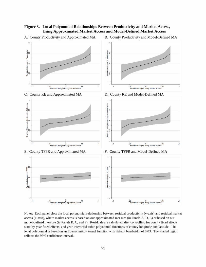
51

Figure 3. Local Polynomial Relationships Between Productivity and Market Access,

Using Approximated Market Access and Model-Defined Market Access

A. County Productivity and Approximated MA

C. County RE and Approximated MA

E. County TFPR and Approximated MA

B. County Productivity and Model-Defined MA

D. County RE and Model-Defined MA

F. County TFPR and Model-Defined MA

Notes: Each panel plots the local polynomial relationship between residual productivity (y-axis) and residual market

access (x-axis), where market access is based on our approximated measure (in Panels A, D, E) or based on our

model-defined measure (in Panels B, C, and F). Residuals are calculated after controlling for county fixed effects,

state-by-year fixed effects, and year-interacted cubic polynomial functions of county longitude and latitude. The

local polynomial is based on an Epanechnikov kernel function with default bandwidth of 0.03. The shaded region

reflects the 95% confidence interval.

52

Figure 4. Counterfactual Changes in Productivity, by County

Notes: This map shows counties shaded according to their change in productivity from 1890 to the baseline counterfactual scenario: darker shades denote larger

declines in productivity, and counties are divided into seven equal groups. This counterfactual sample includes all 2,722 counties that in 1890 report positive

population and positive revenue (agriculture and/or manufacturing). The excluded geographic areas are cross-hashed. County boundaries correspond to county

boundaries in 1890.

Table 1. Impacts of Market Access on Revenue, Input Expenditure, and Productivity

Baseline Fixed 1860 100-Mile Buffer

Specification Population Market Access 1860 to 1900 1850 to 1900

(1) (2) (3) (4) (5)

Panel A. Log Revenue

Log Market Access 0.192 0.185 0.185 0.258 0.236

(0.049) (0.047) (0.048) (0.060) (0.055)

Panel B. Log Capital Expenditure

Log Market Access 0.158 0.151 0.153 0.225 0.209

(0.053) (0.051) (0.052) (0.060) (0.054)

Panel C. Log Labor Expenditure

Log Market Access 0.196 0.188 0.188 0.293

(0.061) (0.059) (0.060) (0.068)

Panel D. Log Materials Expenditure

Log Market Access 0.183 0.176 0.176 0.243

(0.050) (0.048) (0.049) (0.061)

Panel E. Log Production Surplus

Log Market Access 0.238 0.228 0.229 0.303

(0.060) (0.057) (0.058) (0.069)

Panel F. Log Productivity

Log Market Access 0.204 0.196 0.196 0.280

(0.051) (0.049) (0.050) (0.057)

Number of Counties 1,802 1,802 1,802 1,802 1,437

County-Year Obs. 5,406 5,406 5,406 9,010 8,622

Notes: Column 1 reports estimates from equation 8: for the indicated outcome variable in each panel, we report the

estimated impacts of log market access (as defined in equation 1), controlling for county fixed effects, state-by-year

fixed effects, and year-interacted cubic polymials in county latitude and longitude. The sample is a balanced panel of

1,802 counties (1860, 1870, 1880).

The outcome variables are: the log of total county manufacturing annual revenue (Panel A); the log of total county

manufacturing annual expenditures on capital, labor, and materials (Panels B, C, D); the log of total county

manufacturing revenue minus total county manufacturing expenditures on capital, labor, and materials (Panel E); and the

log of total county manufacturing revenue minus the weighted logs of total county manufacturing expenditures on

capital, labor, and materials (where those weights are the county's average revenue share for that input, and the variable

is scaled by the ratio of average county revenue to average county surplus, as defined in equation 5).

In each column, we report the estimated impact of a one standard deviation greater change in market access from

1860 to 1880 (e.g., the coefficient in column 1, panel F, can be interpreted as a relative productivity increase of 20.4%

for counties with a one standard deviation greater change in market access from 1860 to 1880).

Column 2 reports estimates using a measure of counties' market access in each decade that holds counties' population

levels fixed at 1860 levels. Column 3 uses a measure of counties' market access only to counties beyond 100 miles of a

county. Columns 4 and 5 use county-level data only, rather than county-by-industry data, which only affects the

definition of Log Productivity in Panel F. Column 4 reports estimates for the 1860 to 1900 period, and Column 5

reports estimates for the 1850 to 1900 period using available data on county revenue and county capital expenditures in

1850.

Robust standard errors clustered by state are reported in parentheses.

County-level Data Only:

53

Table 2. Impacts on Productivity, Separated into TFPR and RE (Reallocative Efficiency)

Baseline Detailed

Specification Industry Groups 1860 to 1880 1860 to 1900 Zero Materials

(1) (2) (3) (4) (5) (6)

Panel A. Log Productivity

Log Market Access 0.204 0.204 0.204 0.280 0.207 0.206

(0.051) (0.051) (0.051) (0.057) (0.049) (0.049)

Panel B. TFPR (Revenue Total Factor Productivity)

Log Market Access 0.036 0.038 0.038 0.020 0.028 0.030

(0.025) (0.025) (0.026) (0.026) (0.028) (0.029)

Panel C. RE (Reallocative Efficiency)

Log Market Access 0.168 0.166 0.166 0.259 0.179 0.176

(0.051) (0.052) (0.054) (0.066) (0.052) (0.053)

Number of Counties 1,802 1,802 1,802 1,802 1,802 1,802

County-Year Obs. 5,406 5,406 5,406 9,010 5,406 5,406

Notes: Column 1, panel A, corresponds to the estimate reported in Panel F of Column 1 in Table 1. Column 1 reports

estimates from equation 8: for the indicated outcome variable in each panel, we report the estimated impacts of log market

access (as defined in equation 1), controlling for county fixed effects, state-by-year fixed effects, and year-interacted cubic

polymials in county latitude and longitude. The sample is a balanced panel of 1,802 counties (1860, 1870, 1880).

Panel A reports the estimated impacts on log county productivity (as in Panel F of Table 1), and Panels B and C report

the impacts on productivity through changes in county TFPR or revenue total factor productivity (as defined in equation 6)

and through changes in county RE or reallocative efficiency (as defined in equation 7).

In each column, we report the estimated impact of a one standard deviation greater change in market access from 1860 to

1880 (e.g., the coefficient in column 1, panel A, can be interpreted as a relative productivity increase of 20.4% for counties

with a one standard deviation greater change in market access from 1860 to 1880). The coefficients in panel B and panel C

imply 3.6% county productivity growth through increases in county TFPR and 16.8% county productivity growth through

increases in county RE.

Column 2 calculates the outcome variables using county-by-industry data based on 193 industry categories, rather than

the 31 industry categories used in column 1. Columns 3 and 4 calculate the outcome variables using county-level data,

rather than county-by-industry data, for the same period from 1860 to 1880 (in column 3) and an extended period from 1860

through 1900 (in column 4). Column 5 calculates county productivity and its components when assuming zero

misallocation in capital (such that the county's capital revenue share is equal to its cost share). Column 6 calculates county

productivity and its components when assuming that capital misallocation is equal to materials misallocation (such that the

county's capital revenue share is adjusted so the ratio of its cost share to revenue share is equal to the ratio of that county's

materials cost share to materials revenue share).

Robust standard errors clustered by state are reported in parentheses.

County-level Data Only Adjusted Capital Misallocation:

54

Table 3. Impacts of Market Access, Controlling Flexibly for Local Railroad Construction

(1) (2) (3) (4) (5) (6)

Panel A. Productivity

Log Market Access 0.204 0.218 0.199 0.197 0.175 0.142

(0.051) (0.056) (0.057) (0.058) (0.058) (0.056)

Panel B. TFPR (Revenue Total Factor Productivity)

Log Market Access 0.036 0.049 0.047 0.041 0.033 0.013

(0.025) (0.030) (0.031) (0.031) (0.032) (0.035)

Panel C. RE (Reallocative Efficiency)

Log Market Access 0.168 0.169 0.152 0.156 0.143 0.129

(0.051) (0.055) (0.056) (0.055) (0.055) (0.054)

Additional Controls for:

Any Railroad No Yes Yes Yes Yes Yes

Railroad Length No No Yes Yes Yes Yes

Railroad Length Polynomial No No No Yes Yes Yes

Railroads in Nearby Buffer No No No No Yes Yes

Railroads in Further Buffers No No No No No Yes

Number of Counties 1,802 1,802 1,802 1,802 1,802 1,802

County-Year Obs. 5,406 5,406 5,406 5,406 5,406 5,406

Notes: Column 1 reports the estimated impact of market access from the baseline specification (as in column 1 of Table

2). Column 2 includes an additional control for whether a county contains any railroad track. Column 3 also controls for

the length of railroad track in the county, and column 4 controls for a cubic polynomial function of the railroad track

mileage in a county. Column 5 includes additional controls for whether a county contains any railroad track within 10

miles of the county boundary, and a cubic polynomial function of the railroad track mileage within 10 miles of the

county boundary. Column 6 adds controls for separate cubic polymial functions of railroad track within 20 miles, within

30 miles, and within 40 miles of the county.

All regressions include county fixed effects, state-by-year fixed effects, and year-specific cubic polynomials in

county latitude and longitude. We continue to report the estimated impact of a one standard deviation greater change in

market access from 1860 to 1880. The sample is a balanced panel of 1,802 counties (1860, 1870, 1880). Robust

standard errors clustered by state are reported in parentheses.

55

Table 4. Impacts of Market Access, Instrumenting with Baseline Access through Waterways

Log

Market Access

OLS 2SLS OLS 2SLS OLS 2SLS OLS

(1) (2) (3) (4) (5) (6) (7)

Log Market Access 0.209 0.204 0.045 0.036 0.164 0.168

(0.118) (0.051) (0.109) (0.025) (0.103) (0.051)

Instruments:

Log Water Market Access -0.243

in 1860 X year=1870 (0.052)

Log Water Market Access -0.430

in 1860 X year=1880 (0.059)

Kleibergen-Paap F statistic 26.2 26.2 26.2

Number of Counties 1,802 1,802 1,802 1,802 1,802 1,802 1,802

County-Year Obs. 5,406 5,406 5,406 5,406 5,406 5,406 5,406

Productivity

Reallocative Efficiency

RE

Revenue Total Factor Productivity

TFPR

Notes: Column 1 reports the impact of log water market access in 1860 on changes in log market access from 1860 to 1870 and changes in log market access from

1870 to 1880: log market access is regressed on log water market access in 1860, interacted with year fixed effects for 1870 and 1880. Column 2 reports the

estimated impact of log market access on county productivity, instrumenting for log market access using the first-stage relationships reported in column 1. Columns 3,

5, and 7 reports the baseline estimates for comparison (from column 1 of Table 2). Columns 4 and 6 report corresponding 2SLS estimates for county TFPR and

county RE. For the 2SLS specifications, we report the Kleibergen-Paap F statistic from the first stage (in column 1).

All regressions include county fixed effects, state-by-year fixed effects, and year-interacted cubic polymials in county latitude and longitude. In columns 2 to 7,

we continue to report the estimated impact of a one standard deviation greater change in market access from 1860 to 1880. The sample is a balanced panel of 1,802

counties (1860, 1870, 1880). Robust standard errors clustered by state are reported in parentheses.

56

Table 5. Sources of Growth in County Reallocative Efficiency (RE)

Reallocative Efficiency

by Input

County Input

Gap

County Input

Wedge

County Input

Cost Share

County Std. Dev.

of Wedges

(1) (2) (3) (4) (5)

Panel A. Capital

Log Market Access -0.004 0.001 0.022 -0.0005 -0.015

(0.009) (0.002) (0.036) (0.0006) (0.044)

Panel B. Labor

Log Market Access 0.066 -0.001 -0.050 -0.0013 -0.022

(0.015) (0.005) (0.067) (0.0033) (0.044)

Panel C. Materials

Log Market Access 0.107 0.012 -0.027 0.0017 0.032

(0.049) (0.006) (0.039) (0.0037) (0.054)

Number of Counties 1,802 1,802 1,802 1,802 1,802

County/Year Obs. 5,406 5,406 5,406 5,406 5,406

Notes: For the indicated outcome variable, each column and panel reports the estimated impact of log market access from our baseline

specification (as in column 1 of Table 1). Column 1 reports impacts on county productivity through changes in county reallocative

efficiency (as in Table 2, panel C, column 1) through changes in capital (panel A), labor (panel B), and materials (panel C). Column 2

reports impacts on county-level input gaps (defined as the input's cost share minus its revenue share in that decade), Column 3 reports

impacts on county-level input wedges (defined as the input's cost share divided by its revenue share in that decade), and Column 4 reports

impacts on county-level cost shares (defined as the national industry-level cost shares in each decade multiplied by the share of county

revenue in each industry in that decade). Note that the county-level outcomes in columns 2 - 4 are defined in each decade, whereas our

baseline definition of county productivity (and county TFPR and county RE) uses counties' average values over the sample period (or, in

alternative specifications, counties' value in 1860 only). Column 5 reports impacts on counties' standard deviation of input wedges across

industries in that county and decade.

All regressions include county fixed effects, state-by-year fixed effects, and year-specific cubic polynomials in county latitude and

longitude. We continue to report the estimated impact of a one standard deviation greater change in market access from 1860 to 1880. The

sample is a balanced panel of 1,802 counties (1860, 1870, 1880). Robust standard errors clustered by state are reported in parentheses.

57

Table 6. Impacts of Market Access on County Industries, Establishments, and Sector Shares

Log Number of Log Number of

Industries Revenue / Estab. Workers / Estab. Establishments Revenue Value-Added Surplus Employment

(1) (2) (3) (4) (5) (6) (7) (8)

Log Market Access 0.029 0.021 0.025 0.171 0.0077 0.0002 -0.0017 0.0045

(0.021) (0.030) (0.043) (0.034) (0.0078) (0.0059) (0.0090) (0.0048)

Number of Counties 1,802 1,802 1,802 1,802 1,774 1,774 1,713 1,687

County/Year Obs. 5,406 5,406 5,406 5,406 5,322 5,322 5,139 5,061

Log Average Estab. Size: County Manufacturing Share of:

Notes: For the indicated outcome variable, each column reports the estimated impact of log market access from our baseline specification (as in column 1 of Table

1). In column 1, the outcome variable is the log number of manufacturing industries reporting positive output in the county. In columns 2 and 3, the outcome

variables are log average manufacturing establishment size in the county, based on revenue per establishment (column 2) or workers per establishment (column 3). In

column 4, the outcome variable is the log number of manufacturing establishments in the county. In columns 5 to 8, the outcome variables are the county's

manufacturing share of total values for manufacturing and agriculture: revenue (column 5); value-added (column 6), which for manufacturing is defined as revenue

minus materials expenditures and for agriculture is defined as 92% of revenue; surplus (column 7), which for manufacturing is defined as revenue minus all input

expenditures and for agriculture is defined as the value of land multiplied by the state mortgage interest rate; and employment (column 8).

All regressions include county fixed effects, state-by-year fixed effects, and year-interacted cubic polymials in county latitude and longitude. The samples are

drawn from our main balanced panel of 1,802 counties in 1860, 1870, and 1880, which for columns 5 to 8 is smaller due to missing data for some counties in some

years. We continue to report the estimated impact of a one standard deviation greater change in market access from 1860 to 1880 in the full sample of 1,802

counties. Robust standard errors clustered by state are reported in parentheses.

58

Table 7. Counterfactual Impacts on Productivity

Baseline: No Railroads, All Railroads,

No Railroads Only 1850 RRs Only 1860 RRs Only 1870 RRs Only 1880 RRs Extended Canals Twice the Cost

(1) (2) (3) (4) (5) (6) (7)

Panel A. Counterfactual scenario, holding utility constant

Change in Aggregate Productivity -28.0% -23.4% -16.4% -10.4% -2.7% -24.7% -9.3%

Panel B. Counterfactual scenario, holding total population constant

Change in Aggregate Productivity -5.8% -5.3% -4.3% -4.3% -0.7% -4.6% -4.6%

Change in Utility -34.4% -28.6% -19.3% -19.3% -3.1% -30.5% -30.5%

Notes: Each column reports the estimated change in aggregate productivity from counterfactual changes in the transportation network. Panel A reports estimates from

our baseline scenario, which holds worker utility constant in the counterfactual and allows for declines in total population. Panel B reports estimates from an alternative

scenario, which holds total population fixed, and so we also report the associated decline in worker utility. In all scenarios, population is allows to relocate endogenously

within the country. The sample includes all 2,722 counties that in 1890 report positive population and positive revenue (agriculture and/or manufacturing).

Column 1 reports impacts under our baseline counterfactual scenario, which removes all railroads in 1890. Columns 2 to 5 report impacts under more moderate

counterfactual scenarios, which restrict the railroad network to those railroads that had been constructed by 1850 (column 2), by 1860 (column 3), by 1870 (column 4), or

by 1880 (column 5). Column 6 reports impacts from replacing the railroads with feasible extensions to the canal network, as proposed by Fogel (1964). Column 7

reports impacts from maintaining the 1890 railroad network, but doubling the cost of transportation along all railroads.

Restricted Railroad Networks:

59

Table 8. Counterfactual Impacts on Productivity, Robustness

Baseline ϴ = 1.8 ϴ = 3.6 ϴ = 8.2 `P = 20 `P = 50

Efficient

Agriculture

Efficient

Capital Capital

Capital and

Labor

(1) (2) (3) (4) (5) (6) (7) (8) (9) (10)

Panel A. Fixed Utility

Change in Aggregate Productivity -28.0% -28.9% -27.5% -24.5% -36.4% -23.3% -17.4% -24.6% -25.6% -21.3%

Panel B. Fixed Total Population

Change in Aggregate Productivity -5.8% -6.0% -5.7% -4.1% -7.7% -4.7% -4.9% -4.3% -4.8% -6.5%

Change in Utility -34.4% -35.8% -33.5% -30.0% -43.9% -28.9% -34.6% -34.4% -34.4% -34.6%

Alternative Trade Elasticities: Alternative Average Prices: Use Materials Wedge for:

Notes: Each column reports impacts under our baseline counterfactual scenario that removes all railroads in 1890, as in column 1 of Table 7. Panel A reports estimates

from our baseline scenario, which holds worker utility constant in the counterfactual and allows for declines in total population. Panel B reports estimates from an

alternative scenario, which holds total population fixed, and so we also report the associated decline in worker utility. In all scenarios, population is allows to relocate

endogenously within the country. The sample includes all 2,722 counties that in 1890 report positive population and positive revenue (agriculture and/or

manufacturing).

Columns 2 to 10 report robustness of our baseline estimates (in column 1) under alternative parameters. Our baseline estimates use our estimated value for ϴ, the

trade elasticity, of 2.788 with a 95% confidence interval between 1.815 and 3.556. In columns 2 and 3, we alternatively impose values for ϴ of 1.815 or 3.556; in

column 4, we impose a value of 8.22 from Donaldson and Hornbeck (2016). Our baseline estimates also use our estimated value for `P of 35.7, the average price of

transported goods, which scales the assumed transportation costs into proportional costs. In Columns 5 and 6, we alternatively impose values for `P of 20 or 50. In

column 7, we reduce the estimated degree of resource misallocation in each county by assuming that the agricultural sector is efficient, and only apply our estimated

manufacturing wedges to the county's manufacturing share of combined output across manufacturing and agriculture. Column 8 assumes that capital-use is efficient,

such that there is zero gap for capital (or a wedge of 1). Columns 9 and 10 use the estimated materials wedge in each county to assign counties' capital wedge (Column

9) or capital wedge and labor wedge (Column 10).

60

For Online Publication:

Appendices

A Data Appendix

A.1 County-Industry Manufacturing Data

We have digitized manufacturing data, by county and industry, for 1860, 1870, and 1880

from the original published tabulations of the Census of Manufactures (United States Census

Bureau, 1860b, 1870, 1880). The county-industry data report many industries in each decade,

with some small variations, which we group together for our analysis.103 We homogenized

industry names from each county to the list of industry names from US-industry tabulations

in each decade: 331 names in 1880, 412 names in 1870, and 639 names in 1860. We then

grouped these industries into 193 categories that were more consistent across decades, and

further grouped these industries into 31 categories. Our estimates are not sensitive to these

industry groupings (Table 2), but our goal was to balance industry-level details against

statistical noise and to maintain comparability across decades and geographic areas.

These manufacturing data were collected by Census enumerators, who visited each man-

ufacturing establishment to solicit responses. The 1860 Census instructions to enumerators

discuss the data collection guidelines in useful detail, which we quote below, and there is

similar language in the instructions for other decades.

Our main variables of interest, from the manufacturing data, are:

Manufacturing Revenue (PQ). Total value of products, by county and industry from

1860, 1870, and 1880. These products were valued at the factory gate, excluding transporta-

tion costs to customers: “In stating the value of the products, the value of the articles at the

place of manufacture is to be given, exclusive of the cost of transportation to any market”

(emphasis original, United States Census Bureau, 1860a).

Manufacturing Materials Expenditure (WMXM). Total value of materials, by county

and industry from 1860, 1870, and 1880. These materials were valued at the factory gate,

including transportation costs from suppliers: “this value is always to represent the cost of

the article at the place where it is used” (emphasis original, United States Census Bureau,

1860a). Materials included fuel and “the articles used for the production of a manufacture,”

which the instructions noted might be manufactured by another establishment. Unused

materials (on June 1) were to be excluded.

Manufacturing Labor Expenditure (WLXL). Total amount paid in wages during the

year, by county and industry from 1860, 1870, and 1880. Reported wages were intended

103In 1860 only, the Census of Manufactures also collected information for sectors outside of manufacturing(fisheries and mining) that we drop from our analysis for consistency.

1

to reflect total labor costs, including boarding costs paid in kind and the proprietor’s own

labor. From the Census instructions: “In all cases when the employer boards the hands, the

usual charge of board is to be added to the wages, so that cost of labor is always to mean

the amount paid, whether in money or partly in money and partly in board...” (emphasis

original) and to be included was “the individual labor of a producer, working on his own

account” (United States Census Bureau, 1860a).

Manufacturing Capital Expenditure (WKXK). We impute annual capital expenditure by

multiplying the reported total value of capital invested, in each county and industry (1860,

1870, 1880), by a state-specific interest rate from Fogel (1964). The establishment’s capital

value was directed to include “capital invested in real and personal estate in the business”

(United States Census Bureau, 1860a).

Manufacturing Establishment Counts. The number of establishments in each county and

industry (1860, 1870, 1880) with at least $500 in annual sales. That is, the Census enu-

merators were instructed to survey every manufacturing establishment, except “household

manufactures or small mechanical operations where the annual productions do not exceed

five hundred dollars” (United States Census Bureau, 1860a). When multiple establishments

were owned by the same party, and operated jointly, then Census enumerators were in-

structed to obtain separate detailed on the operations of each establishment. If this were

impossible, particularly when one establishment manufactured the materials for the other

establishment, then enumerators were instructed to “return the last manufacture, giving the

raw materials for the first, and capital, fuel, and cost of labor, with the number of hands, in

both” (United States Census Bureau, 1860a).

Civil War Related Industries. We coded two sets of industries as being “Civil War

related.” Our strict classification includes: artificial limbs and surgical appliances; awnings

and tents; coffins; cutlery, edge tools, and axes; drugs; chemicals and medicines; explosives

and fireworks; flags and banners; gun- and lock-smithing; gunpowder; lead; military goods;

and ship and boat building. Our broad classification adds: bronze; canning and preserving;

carriage and wagon materials; carriages and wagons; clothing (general); cooperage; gloves

and mittens; and hats and caps.

A.2 Main Outcomes

The table below is a reference for the formulas used in calculating county productivity and

its components. We use an upper bar to denote averages over the sample period. County-

level values of revenue and input expenditures in each year reflect a sum of county-industry

values in that year.

2

Component Formula Notes

Output PctQct Gate value of revenue in the Census.

Capital WKct X

Kct Book value of capital in the Census,

multiplied by interest rate.

Labor WLctX

Lct Wage bill in the Census.

Materials WMct X

Mct Gate value of materials in the Census.

skctWkctX

kct

PctQctRevenue share of input k in county c in

year t

αkct∑

iPcitQcit∑j PcjtQcjt

∑cW

kcitX

kcit∑

c

∑`W

`citX

`cit

County-level revenue share weighted

sum of input’s national industry cost

share

ξ 1

1−( 1C

∑c

∑k s

kc)

Used for re-scaling percent growth in

county output into percent growth in

county productivity.

Production

Surplus

ln(PctQct −

∑kW

kctX

kct

)Undefined when total input costs are

larger than revenue.

Productivity ξ[PctQct −

∑k s

kc lnW k

ctXkct

]TFPR ξ

[PctQct −

∑k α

kc lnW k

ctXkct

]Reallocative

Efficiency (RE)

ξ[(αkc − skc

)lnW k

ctXkct

]Productivity

Robustness:

County Scalar

ξc

[PctQct −

∑k s

kc lnW k

ctXkct

]ξc = 1

1−(∑k s

kc)

Drop counties with negative scalar val-

ues and top 1% of values

Productivity

Robustness:

Median Scalar

ξ[PctQct −

∑k s

kc lnW k

ctXkct

]ξ = 1

1−(

1C

∑c

∑k s

k)

skc is the median revenue share for k in

county c, sk is its national median

Productivity

Robustness:

1860 Scalar

ξ[PctQct −

∑k s

kc1860 lnW k

ctXkct

]ξ = 1

1−( 1C

∑c

∑k s

kc1860)

We also use αkc1860 for the decomposi-

tion

3

A.3 Other County-Level Data

For some specifications using manufacturing data from 1890 and 1900, when county-industry

tabulations are unavailable, we use the corresponding county-level data (Haines, 2010).

Other county-level data are from the United States Censuses of Population and Agricul-

ture (Haines, 2010). Population is defined as the reported total population in each county.

For one robustness check, we inflate these population data due to potential undercounting

in the Census that is estimated to vary by region and year: undercounting in the South by

7.6% in 1860, 8.8% in 1870, and 5.2% in 1880, and undercounting in the North by 5.6% in

1860, 6.0% in 1870, and 4.4% in 1880 (Hacker, 2013). Agricultural land value is defined as

the total value of land in farms, including the value of farm buildings and improvements.104

We adjust county-level data to maintain consistent county definitions in each decade. We

adjust data from each decade to reflect county boundaries in 1890 following the procedure

outlined by Hornbeck (2010). Using historical United States county boundary files (from

NHGIS), county borders in each decade are intersected with county borders in 1890. When

counties in another decade fall within more than one 1890 county, data for each piece are

calculated by multiplying that decade’s county data by the share of its area in the 1890

county. For each other decade, each 1890 county is then assigned the sum of all pieces

falling within its area. This procedure assumes that data are evenly distributed across

county area, though for most counties in each decade there is little overlap with a second

1890 county. In three instances, we combine separately reported cities into a neighboring

county for consistency: Baltimore City is combined into Baltimore County; St. Louis City is

combined into St. Louis County; and Washington DC is combined into Montgomery County.

The regression sample is 1,802 counties that report county-industry manufacturing data

in 1860, 1870, and 1880 (see Figure 2). The counterfactual sample is 2,722 counties with

positive population and positive agricultural or manufacturing revenue in 1890 (see Figure

4).

104We follow Donaldson and Hornbeck (2016) in deflating these reported data, using Fogel’s state-levelestimates of the value of agricultural land only (Fogel, 1964, pp. 82-83).

4

B Results Appendix

B.1 Robustness: Measurement of Productivity

There may be various sources of measurement error in our calculation of county productivity

and its decomposition into county TFPR (revenue total factor productivity) and county RE

(reallocative efficiency). Appendix Table 2 shows how our regression estimates differ under a

variety of alternative approaches for calculating county productivity and its decomposition,

and in this section we describe the specifications in that table.

Table 2 showed that our estimates were similar when replacing the observed capital wedge

in each county with the materials wedge, motivated by De Loecker and Warzynski (2012)

who use the materials wedge to measure the common component of distortions across inputs.

In Row 2 of Appendix Table 2, we additionally replace the labor wedge with the materials

wedge and estimate similar percent effects of market access.

Given that the measurement of reallocation can be sensitive to the upper and lower tails

(Rotemberg and White, 2020), in rows 3–8 we test the sensitivity of our results to lowering

dispersion in input distortions. In rows 3–5, we shrink dispersion in the capital wedge by

5 percent, 10 percent, and 25 percent.105 While this adjustment mechanically lowers the

potential gains from reallocation in exercises like those in Hsieh and Klenow (2009), our

regression estimates are stable. In rows 6–8, we shrink dispersion in all of the input wedges,

which also has little effect on our regression estimates.106

Our main estimates hold fixed counties’ revenue shares and production function elastici-

ties (and therefore the wedges), using the observed average from 1860 to 1880 (as in Petrin

and Levinsohn 2012’s Tornqvist-Divisia approximation). In row 9, we instead hold these

values fixed at their 1860 levels (and correspondingly use those values to calculate the scal-

ing factor). In row 10, in addition to using these 1860 values in the measurement of county

productivity in each decade, based on county revenue and county input expenditures in each

decade, we hold county populations fixed at their 1860 values for calculating market access

(as in Table 1, column 2).

In rows 11 and 12, we use alternative scaling factors in the definition of county produc-

tivity. The percent impact of market access on county productivity reflects a scaled percent

impact of market access on revenue and input expenditures, as discussed in Section V.C,

and our baseline estimates define this scaling factor as the average ratio of county output

105In particular, we replace the observed wedge for capital with the weighted average of the observedcapital wedge and its national median, where the weights on the county’s observed values are respectively95 percent, 90 percent, and 75 percent. We then impute consistent values for capital (so the relationshipbetween imputed capital and observed output is consistent with the imputed wedge).106For the counterfactuals, replacing the observed wedges with their shrunk counterparts never affects the

welfare losses from removing the railroads by more than 1 percentage point.

5

to county productivity over the 1860-1880 period. Alternatively, in row 11, we define this

scaling factor based on the median ratio of county revenue to county productivity. In row

12, we use county-specific scaling factors instead of the national average (dropping counties

with negative values and the top 1% of values, as these scaling factors become undefined as

productivity approaches zero).

As an alternative approach to dealing with extreme values, we show similar impacts

of market access when excluding sample counties with the largest and smallest changes in

productivity from 1860 to 1880: row 13 excludes the top and bottom 1% of counties, and

row 14 excludes the top and bottom 5% of counties.

Establishment inputs may be under-reported in the Census of Manufactures, which would

over-state establishments’ productivity. For example, Census enumerators ask establish-

ments for their labor costs and these were intended to include in-kind boarding costs and

labor supplied by establishment owners working on their own account, but there has been

debate about whether establishment owner labor is fully reflected in these costs (Weeks,

1886; Atack, 1977; Sokoloff, 1984; Margo, 2014). Row 15 reports similar impacts of county

market access, though, when inflating labor costs to reflect potentially omitted labor costs.107

A similar concern is that establishments’ reported capital values may not reflect their en-

tire capital stock, such that annual capital expenditures are understated when multiplying

establishments’ capital value by an interest rate.108 Indeed, Appendix Table 1 shows that

national manufacturing capital expenditures are only 15% of total labor costs and capital

costs, which is below the typical range of a third (Kaldor, 1957). As an adjustment, in row

16, we double the assumed interest rate and re-calculate capital expenditures and county

productivity, and find similar impacts of market access on productivity.

Our measurement of county productivity does not depend on an assumed production

function, but we do assume Cobb-Douglas production with constant returns to scale for our

decomposition of county productivity into TFPR and RE. In row 17 we assume decreasing

returns to scale and re-scale the production function elasticities to add up to 0.90; and in

row 18 we assume the returns to scale are 0.95. In rows 19 and 20, we assume increasing

returns to scale and re-scale the production function elasticities to add up to 1.05 or 1.10.

Assuming decreasing returns to scale increases the impact on county productivity through

TFPR growth (column 2) and reduces the impact through RE growth (column 3), while

mechanically leaving unchanged the impact on county productivity (column 1).

107For this specification, we add to county-by-industry labor costs the number of establishments multipliedby the average wage in that county and industry.108Establishments’ reported book values of capital may also not reflect depreciation, which would overstate

their capital stock and calculated annual expenditure, but then depreciation should also be included in theirannual capital expenditure.

6

We also show the sensitivity of our results to alternative methods for calculating the

production function elasticities. These adjustments mechanically have no effect on the mea-

surement of county productivity (in column 1) and, in practice, have little substantive effect

on the estimated impacts through county TFPR (column 2) and county RE (column 3)

because market access had similar percent effects on each input. In row 21, we calculate

county-level elasticities averaging industry-level cost shares with weights equal to an in-

dustry’s share of total expenditure in that county, rather than an industry’s share of total

revenue in that county (which could over-weight the influence of high-markup sectors). In

row 22, we calculate production function elasticities only using the “most efficient” counties

for calculating each industry’s cost shares (specifically, those counties whose total input ex-

penditure gap is within one standard deviation of zero). In row 23, instead of using national

values for calculating industry cost shares, we leave out each specific county-industry when

calculating its production function elasticity. In row 24, we instead use only other counties

located in the same state to calculate industry-level cost shares, and in row 25 we leave out

that county in the calculation of state-level industry cost shares. In row 26, we use each

observed county-industry cost share as our measure of production function elasticities, which

imposes a constant wedge across inputs within the county.

If input frictions are consistently higher for one input than the others, then the measured

cost shares will understate the output elasticity for that input relative to the others. To

assess the sensitivity of our estimates, row 27 reports estimates when increasing the cost

share for labor by 5 percentage points and proportionally decreasing the cost shares for

materials and capital. Similarly, we increase the cost share for materials by 5 percentage

points (in row 28) or for capital by 5 percentage points (in row 29).

We measure manufacturing productivity using data from the Census of Manufactures,

though there may be additional manufacturing activity not included in the Census of Man-

ufactures. The Census of Manufactures reports a butter and cheese industry with only two

establishments in 1860 and $13 thousand of output, but reports 1195 establishments in 1870

with $16.5 million of output.109 If we exclude the butter and cheese industry in each decade,

though, we estimate similar impacts of market access (row 21).

The Census of Manufactures would have missed some manufacturing establishments,

particularly smaller establishments (United States Census Bureau, 1870). To the extent that

the Census coverage varies over time and geographic areas, this would be partly corrected

for by our inclusion of state-by-year fixed effects and year-interacted controls for county

109In 1880, the Census of Manufactures reports 3250 establishments with $30.4 million of output. Therewere also large technological changes in dairy manufacturing during the time period (Boberg-Fazlic andSharp, 2020). The Census of Agriculture reports quantities of butter and cheese produced, but does notreport data on their values or associated inputs.

7

longitude and latitude. The remaining concern is that changes in county market access

might be systematically correlated with changes in Census data coverage. While the general

concern is that smaller establishments are more likely to be missed by Census enumerators,

we report in Table 6 that changes in market access are not associated with changes in average

establishment size.

We can use data from the Census of Agriculture on the value of home manufactures to

expand our analysis of manufacturing beyond the Census of Manufactures.110 The national

value of home manufactures is only 1.2% of total manufacturing revenue in 1860 and 0.4% of

total manufacturing revenue in 1870, summing output values from the Census of Agriculture

and the Census of Manufacturing for our sample counties, though home manufactures are

substantively important in some counties. Among our sample counties, the median revenue

shares of home manufacturing are 3.6% in 1860 and 1.0% in 1870 and the average revenue

shares of home manufacturing are 11.8% in 1860 and 6.5% in 1870.111 The estimated im-

pact of county market access on the value of manufacturing output is 0.192 (0.049), using

only data from the Census of Manufactures, and the effect is 0.160 (0.043) when adding the

value of home manufactures to data from the Census of Manufactures. Data on home man-

ufactures also allow us to expand the balanced sample of counties to include 149 additional

counties that do not report manufacturing revenue in at least one decade of the Census

of Manufactures, but do report home manufactures in that decade. The estimated impact

of county market access on county manufacturing revenue increases to 0.269 (0.041) when

including these 149 additional counties and adding the value of home manufactures to data

from the Census of Manufactures.

Indeed, the United States itself expanded substantially from 1860 to 1880. Our baseline

estimates focus on a balanced sample of counties from 1860 to 1880, which includes 91%

of population and 99% of manufacturing revenue in 1880. When focusing on this balanced

panel, however, the analysis does not include impacts on the extensive margin of manufac-

turing growth in newly created counties. Over this period, from 1860 to 1880, we estimate

that a one standard deviation increase in market access leads to a 4 percentage point in-

crease in the probability that a county reports any manufacturing activity in the Census of

Manufactures. We cannot estimate what happened to manufacturing productivity in these

counties, which is not measured in the earlier periods, but increases in county market access

are leading to growth on the extensive margin along with our estimated productivity effects

110For this analysis, we assume that home manufactures are not already included in the Census of Manu-factures. Spot checks of the Census of Agriculture manuscripts show the values of home manufactures tendto be substantially less than the $500 threshold used by the Census of Manufactures.111The Census of Agriculture stopped asking this question in 1880, and we assume for our analysis here

that there was zero home manufacturing in 1880.

8

on the intensive margin.

B.2 Robustness: Regional Shocks

Our estimated effects of county market access on county productivity may be influenced

by other omitted sources of growth in county productivity that are correlated with relative

changes in county market access. In Appendix Table 3, we show how our regression estimates

differ under a variety of alternative specifications that look to control for these omitted

variables or adjust our sample definition.

An expanding national railroad network affected different counties’ market access from

1860 to 1870 and from 1870 to 1880, and over each decade there were similar effects of market

access on county productivity. Splitting our baseline analysis by decade pair (1860 and 1870,

1870 and 1880, 1860 and 1880), increases in county market access lead to substantial increases

in county productivity that are more often driven by increases in county RE than by increases

in county TFPR (Rows 2, 3, 4). These separate estimates also avoid potential issues with

interpreting two-way fixed effects models with multiple time periods (De Chaisemartin and

d’Haultfoeuille, 2020).

In row 5, we extend the specification from column 3 of Table 3 (controlling for any railroad

and railroad length) to include future values of market access and railroads. These additional

controls do not substantively change the measured effect of contemporaneous market access,

and there is no systematic effect of future market access on current outcomes (i.e., growth

in county market access was not associated with differential trends in county manufacturing

activity over the prior decade).112

Rows 6–17 control for county characteristics in 1860, interacted with year, to flexibly allow

for those characteristics to have time-varying influences on county productivity. Rows 6 and

7 control for 1860 market access without railroads and actual 1860 market access. Rows 8 and

9 control for the share of counties’ 1860 revenue in each industry, interacted with year, given

the potential for relative changes in industry output prices and input prices or other industry-

specific shocks to differentially impact counties’ growth. Rows 10 to 17 control for other

county characteristics in 1860: counties’ input-specific gaps in 1860 (the difference between

the output elasticities and the revenue shares), the 1860 production function elasticities; 1860

input revenue shares; 1860 input wedges (the ratio of the output elasticities to the revenue

shares); the 1860 HHIs of manufacturing industry revenue and employment; whether a county

was on the “frontier” in 1860 (following the definition from Bazzi, Fiszbein and Gebresilasse,

112From estimating this specification on an extended sample back to 1850, using the available county-leveldata on revenue from 1850, we also estimate no significant effect of future market access on manufactur-ing revenue growth from 1850 to 1860. Similarly, we estimate no significant effect on revenue growth (orproductivity growth) from 1860 to 1870 from market access growth from 1870 to 1880.

9

2020); and jointly controlling for the gaps, elasticities, wedges, HHIs, and frontier status.113

As the Civil War occurred within our sample period, and had substantially different

implications for different areas of the country, we explore the sensitivity of our results to

adjusting for differential impacts of the Civil War and the abolition of slavery. First, counties

that were initially concentrated in industries that produced more war-related goods may have

changed differently over this period even in the absence of changes in the railroad network.

For row 18, before calculating county productivity, we drop all industries strictly related to

war production and in row 19 we drop industries more broadly related to war production

(as defined in the Section A). Alternatively, in rows 20 and 21, we instead control for the

1860 share of revenue in war-related sectors under each definition. These adjustments do

not have large effects on the estimated coefficients. The Civil War itself may have had a

direct effect on outcomes, and row 22 controls for whether a county had a Civil War battle,

the number of battles (cubic polynomial), and the number of casualties (cubic polynomial),

all interacted with year fixed effects.114 Row 23 instead drops all counties with battles with

over 500 casualties, while row 24 drops all counties with any noted battle. Row 25 drops

counties on the border of the Union and the Confederacy. Row 26 drops Confederate states,

row 27 drops slave states, and row 28 drops the Southern region.115 The estimates are stable

across these sample changes.

Our baseline empirical specification estimates the impacts of market access, controlling

for county fixed effects and state-by-year fixed effects, such that the identifying variation is

within-state relative changes in counties’ market access. In rows 29 and 30, we report similar

estimates when also controlling for region-by-year fixed effects (20 regions) or subregion-

by-year fixed effects (106 subregions) that further restrict the analysis to relative changes

in county market access within nearby economic regions that cut across state and county

boundaries.116

Our baseline specification also adjusts for the general westward expansion of the United

States, even within states, by controlling for year-interacted cubic polynomial functions of

counties’ latitude and longitude. As alternative functional forms, we find similar estimates

when controlling for fifth-order polynomials (row 31) or linear functions of counties’ latitude

113The share of counties’ 1860 revenue in each industry, the HHIs, and frontier status are moderatelypredictive of 1860 county gaps (a within R-squared of 0.15, after conditioning on state fixed effects andlatitude/longitude, which mostly reflects the influence of the 31 industry shares).114Our battle data includes all battlefields identified as significant by the Civil War Sites Advisory Com-

mission’s Report on the Nations Civil War Battlefields.115When excluding areas from the regression sample, we continue to include them in the measurement of

other counties’ market access.116We assign each county the share of its area in each region or subregion, and control for those shares

interacted with year fixed effects.

10

and longitude (row 32). We also estimate similar impacts of market access when excluding

from our sample the Plains and West Coast regions of the United States in row 33.117

B.3 Robustness: Measurement of Market Access

Our measurement of county market access makes a number of simplifying assumptions that

can induce various sources of measurement error. In Appendix Table 4, we show how the

estimated effects of county market access on county productivity (and TFPR and RE) differ

under a variety of alternative approaches for calculating market access. In this section, we

describe the specifications in that table.

In rows 2 and 3, we show that the estimated impacts on county productivity are not

sensitive to omitting counties with the largest and smallest changes in market access. The

estimated impact on county productivity through TFPR growth becomes moderately larger

when omitting more counties (in row 3), but the estimates are not statistically different.

Measured changes in county market access reflect changes in county-to-county trans-

portation costs, which are based on assumed rates for transporting goods using railroads,

waterways, and wagons. Rows 4 and 5 report similar impacts of market access on county pro-

ductivity when decreasing the costs of waterways and wagons to the lowest values considered

by Fogel (1964). Row 6 reports similar estimates when removing the costs of transshipment

within the waterway network. Rows 7 – 9 report similar estimates when increasing the cost

of railroad transportation to reflect potential congestion, fragmented track ownership, or dif-

ferences in gauges that would require transshipment of goods or more indirect routes within

the railroad network (see, e.g., Gross (2020) on North-South gauge differences).

In calculating counties’ market access, the “iceberg trade costs” (τcd) reflect the measured

county-to-county transportation costs (tcd) scaled by the average price per ton of transported

goods (τcd = 1 + tcd/P ). Our baseline estimates use an average price of 35.7 that best fits

the data, but rows 10 and 11 report similar estimated effects of market access if we instead

use 20 or 50 dollars per ton.118

The impact of market access is also similar when using alternative values of θ, the trade

elasticity. Smaller values of θ compress the distribution of changes in market access, just as

for larger average prices, but increase the effect of gaining access such that there remains a

similar effect from a one standard deviation greater increase in market access. Rows 12 to 14

show similar results using the extremes of the 95% confidence interval around our baseline

estimate of θ (1.815 to 3.556) and a larger value of θ (8.22) from Donaldson and Hornbeck

117The West Coast sample states are California, Oregon, and Washington. The Plains sample states areKansas, Nebraska, and Texas.118We continue to focus on the estimated impact of a one standard deviation greater increase in county

market access, as market access itself is re-scaled when changing the transportation cost parameters.

11

(2016).

Our baseline measure of county market access reflects counties’ access to all other coun-

ties’ population, though we estimate similar impacts from a one standard deviation increase

in modified definitions of county market access. To incorporate the influence of access to in-

ternational markets, we inflate the population in 11 counties with major international ports

to reflect the value of imports and exports in each year divided by GDP per capita (row

15). The Census of Population is known to have undercounted population, especially in the

South in 1870, and so in row 16 we inflate counties’ population by year and region based on

the estimated degree of undercounting by Hacker (2013). Our baseline measure of market

access considers counties’ access to population, but we also replace counties’ population with

counties’ wealth as an alternative proxy for counties’ market size (row 17). The estimates

are also not sensitive to whether we include a county’s own population in its market access

(row 18), or omit counties’ access to other counties within 5 miles, 50 miles, or 200 miles

(rows 19 – 21).

12

C Theory Appendix

In this section, we provide some additional details on the model from Section V. These

details relate to deriving the log-linear relationship between market access and productivity,

and our estimation of counterfactuals.

C.1 Market Access and Productivity

As described in equation 11, trade flows follow a gravity equation:

(22) Eod = κ1Ao

(Πk

((1 + ψko

)W ko

)αko)−θ τ−θod YdP θd ,

where the price index in equation 12 is:

(23) CMAd = P−θd = κ1∑o

τ−θod Ao

(Πk

((1 + ψko

)W ko

)αko)−θ .Goods markets clear in general equilibrium, whereby demand in each county is equal to

supply. Production in each county is then equal to the sum of exports to all destinations

(including itself). Summing equation 22 over all counties and taking logs gives:119

(24) ln (Yo) = κ1 + κ1o +(αMo + αLo

)ln(P−θo

)− θαTo ln qo + ln

(∑d

(Pdτod

)θYd

).

Plugging P−θd from equation 23 into equation 24, and combining terms, gives:120

(25) lnYo = κ1 + κ2o +

(αMo + αLo + 1

1 + θαTo

)ln(P−θo

).

Once we have solved for output in each county, input quantities and input expenditures

in each county follow directly from our assumption that within-county revenue shares are

constant.

For estimating changes in productivity, what matters is changes in real output and real

inputs. Because markups and other distortions are constant in this environment, we can

convert from nominal output to real output using the changes in marginal costs. The price

of capital is independent of market access. The price of land (qo) is endogenous to market

119κ1 =(− θ

1−σ

)ln(Γ(θ+1−σ

θ

))and κ1o = ln (Ao) − θαLo ln

((1 + ψLo

)U)− θαKo ln

((1 + ψKo

)r)−

θαMo ln(1 + ψMo

)120κ2o =

κ1o+ln ξo−θαTo lnαToTo

1+θαTo

13

access, as described in equation 19:

(26)d ln qo

d lnMAo=αMo + αLo + 1

1 + θαTo.

The local prices for labor (wo) and materials (Po) are log-linear in market access, as described

by equation 23:

(27)d lnwod lnMAo

=d lnPod lnMAo

= −1

θ.

The impact of market access on productivity, equation 17, is then given by substituting

into equation 16 the impacts of log market access on log real inputs:

d lnPRo

d lnMAo=

PoQo

Pro

[ (αLo − sLo

) (1

θ+αMo + αLo + 1

1 + θαTo

)(28)

+(αMo − sMo

) (1

θ+αMo + αLo + 1

1 + θαTo

)+

(αKo − sKo

) (αMo + αLo + 1

1 + θαTo

)].

C.2 Counterfactual Estimation and Uniqueness

To estimate counterfactuals, we solve the model in the cross section. Some of the primitives

in the model, such as the production function elasticities, we estimate from our main county-

by-industry data. Other primitives, such as the the trade elasticity (θ) and the average price

of traded goods (P ), we estimate using supplemental data.

Our general approach to estimating counterfactuals is to rationalize the observed distri-

bution of population by estimating each county’s productivity (Ao) and quantity of fixed

factors (To). We start by noting that prices in any location can be expressed as a function

of prices and population in all locations:

(29) P−θd =∑o

τ−θod Po(1+ψLo )Lo

αLo∑i τ−θoi P

1+θi

(1+ψLi )LiαLi

.

This equation matches equation 15 in the appendix to Donaldson and Hornbeck (2016), with

two changes: we allow for market distortions(ψLo), and we allow variation across counties

in the production function elasticity for labor(αLo). As a result, many of the steps in our

derivation match those in Donaldson and Hornbeck (2016), which in turn rely on results

from Allen and Arkolakis (2014). Thus, we focus on describing where our new assumptions

14

require a new approach. For example, the first step is the same: there is a steady state

solution for prices (up to proportionality) that can be identified using the Fujimoto-Krause

algorithm.

Having solved for prices, we then solve for the fixed characteristics of each county (i.e.,

its productivity and quantity of fixed factors). We define Ci, such that:121

(30)

Ci ≡ AiTθαTii r

−θαKii αTi

−θαTi

[Γ

(θ + 1 − σ

θ

)]− θ1−σ (

1 + ψLi)−θαLi (1 + ψki)

−θαKi (1 + ψmi)−θαMi .

We can then rewrite equation 11 as

(31) Co∑i

τ−θoi P1+θi

(1 + ψLi

)Li

αLi= P

1+θ(αLo+αTo +αMo )o

((1 + ψLo

)Lo

αLo

)1+θαTo

U θ(αLo+αTo ),

and re-write equation 12 as

(32) P−θo =∑i

CiU−θ(αLi +αTi )P

−θ(αLi +αTi +αMi )i

((1 + ψLi

)Li

αLi

)−θαTiτ−θoi .

To solve this system above, we define:

(33) φo ≡(P−θo Co

)((1+ψLo )BLo

αLo

)1+θαToU θ(αLo+α

To )P

1+θ(αLo+αTo +α

Mo )

o

.

We solve the model up to a proportional constant for labor, which we denote B, as described

below.

We now have the equations:

(34) 1 =∑i

Co

P1+θ(αLo+α

To +α

Mo )

o

((1+ψLo )BLo

αLo

)1+θαToU θ(αLo+α

To )

τ−θoi P1+θi

(1 + ψLiαLi

)BLi

and

(35) φo =∑i

Co

P1+θ(αLo+α

To +α

Mo )

o

((1+ψLo )BLo

αLo

)1+θαToU θ(αLo+α

To )

τ−θoi P1+θi

(1 + ψLiαLi

)BLiφi.

Following Allen and Arkolakis (2014), we use the Perron-Frobenius theorem. The Perron-

121We will be able to solve for Ci using the factual data, our assumption on interest rates, and our estimatedvalue of θ.

15

Frobenius theorem says that for any matrix M , with all its elements positive, the equa-

tion φλ = Mφ has a unique eigenvalue λ and a unique (up to proportionality) eigen-

vector φ with all its elements positive. We define the matrix A with elements [Aod] =[Co

P1+θ(αLo +αTo +αMo )o L

1+θαToo

τ−θod P1+θd

(1+ψLdαLd

)Ld

]. For any possible values of Co, Po, No, and τod,

the matrix A has all of its elements positive. Perron-Frobenius therefore implies that, for

any values of Po, No, τod, the matrix A will have only one unique (up to proportionality)

eigenvector with all elements positive. In other words, when our system of equations 34 and

35 holds, we have two eigenvectors. The two eigenvectors are φo and 1, which therefore must

be proportional since the eigenvector is unique (up to proportionality) and so φo = φ−1 ∗ 1

for some constant φ−1. Thus, we know that

(36) P1+θ(1+αTo +αLo+αMo )o = φL

−(1+θαTo )o Co.

We then solve for Po in equation 36, and plug into equation 31 to get:

Co∑i

τ−θoi

φU−θ(αLi +αTi )

((1 + ψLi

)BLi

αLi

)−(1+θαTi )

Ci

1+θ

1+θ(1+αTi+αL

i+αM

i ) (1 + ψLi

)BLi

αLi=

φU−θ(αLo+αTo )

((1 + ψLo

)BLo

αLo

)−(1+θαTo )

Co

1+θ(αLo +αTo +αMo )

1+θ(1+αLo +αTo +αMo )

×

((1 + ψLo

)BLo

αLo

)1+θαTo

U θ(αLo+αTo )(37)

Rearranging and combining like terms, we get:

(φU−θ(α

Lo+α

To ))− 1+θ(αLo +αTo +αMo )

1+θ(1+αLo +αTo +αMo ) U−θ(αLo+α

To )C

θ

1+θ(1+αLo +αTo +αMo )o ∗

∑i

τ−θoi

(φU−θ(α

Li +α

Ti )Ci

) 1+θ

1+θ(1+αTi+αL

i+αM

i )

((1 + ψLi

)BLi

αLi

)1−(1+θαTi )(1+θ)

1+θ(1+αTi+αL

i+αM

i )

=

((1 + ψLo

)BLo

αLo

)(1+θαTo )(1−

1+θ(αLo +αTo +αMo )1+θ(1+αLo +αTo +αMo )

).(38)

We know that there is a unique combination of φ and B that solves equation 38. To find

that solution, we grid-search over the parameter space. For each initial guess, we use the

16

Fujimoto-Krause algorithm to solve for the distribution of population (Li) and we pick the

parameters for which equation 38 holds. As in Donaldson and Hornbeck (2016), we do not

separately identify Ao and To, but only their combined value is needed for estimating the

counterfactuals.

Given our estimated values of θ and P , we estimate how much production inputs would

have changed in each county given a different vector of costs τod (e.g., without the rail-

roads) and given a value of population (e.g., holding utility constant or holding population

constant), as in Donaldson and Hornbeck (2016) and Fajgelbaum and Redding (2018).122

The counterfactual impact on national aggregate productivity is then given by the Domar-

weighted sum of these counterfactual changes in county production inputs multiplied by the

county-level gap for that input (equation 21).

122Note that relative population levels are not independent of total population levels, unlike in Donaldsonand Hornbeck (2016), because the production function elasticities vary over space but quantitatively thiseffect is relatively small.

17

18

Appendix Figure 1. Waterways and Railroads, 1890 and 1900

A. Waterways and 1890 Railroads

B. Waterways and 1900 Railroads

Notes: Similar to Figure 1, Panel A shows the railroads constructed by 1890, as well as the natural waterways

(including navigable rivers, lakes, and oceans) and constructed canals. Panel B adds railroads constructed between

1890 and 1900.

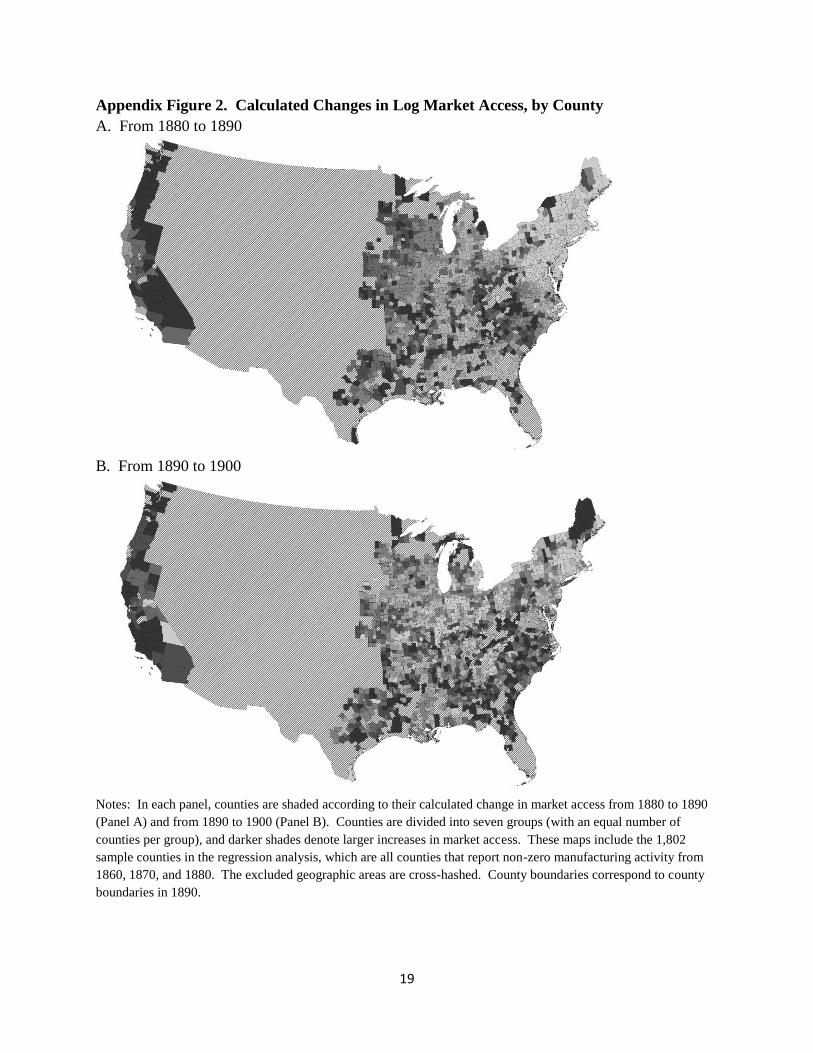
19

Appendix Figure 2. Calculated Changes in Log Market Access, by County

A. From 1880 to 1890

B. From 1890 to 1900

Notes: In each panel, counties are shaded according to their calculated change in market access from 1880 to 1890

(Panel A) and from 1890 to 1900 (Panel B). Counties are divided into seven groups (with an equal number of

counties per group), and darker shades denote larger increases in market access. These maps include the 1,802

sample counties in the regression analysis, which are all counties that report non-zero manufacturing activity from

1860, 1870, and 1880. The excluded geographic areas are cross-hashed. County boundaries correspond to county

boundaries in 1890.

20

Appendix Figure 3. Cross-County Dispersion in Input Wedges, by Decade

A. Cross-County Dispersion in Capital Wedges, by Decade

B. Cross-County Dispersion in Labor Wedges, by Decade

C. Cross-County Dispersion in Materials Wedges, by Decade

Notes: Each panel plots the cross-county dispersion in input wedges (output elasticity / revenue share), by decade.

21

Appendix Figure 4. Counterfactual Changes in Market Access, by County

Notes: This map shows counties shaded according to their change in market access from 1890 to the baseline counterfactual scenario: darker shades denote

larger declines in market access, and counties are divided into seven equal groups. This counterfactual sample includes all 2,722 counties that in 1890 report

positive population and positive revenue (agriculture and/or manufacturing). The excluded geographic areas are cross-hashed. County boundaries correspond to

county boundaries in 1890.

22

Appendix Figure 5. County-level Gaps in the Counterfactual Analysis

Notes: This map shows counties shaded according to their estimated sum of gaps between the output elasticity for each input (materials, labor, capital) and the

revenue share for that input: darker shades denote a larger sum of input gaps, and counties are divided into seven equal groups. This counterfactual sample

includes all 2,722 counties that in 1890 report positive population and positive revenue (agriculture and/or manufacturing). The excluded geographic areas are

cross-hashed. County boundaries correspond to county boundaries in 1890.

Appendix Table 1. Aggregated Industry Group Revenue Shares and Cost Shares

Revenue

Share Materials Labor Capital

(1) (2) (3) (4)

Panel A. All Industries

Total in 1860 1 0.72 0.24 0.04

Total in 1870 1 0.73 0.23 0.04

Total in 1880 1 0.76 0.20 0.04

Panel B. Aggregated Industry Groups

Clothing, Textiles, Leather in 1860 0.32 0.69 0.27 0.04

Clothing, Textiles, Leather in 1870 0.23 0.76 0.21 0.03

Clothing, Textiles, Leather in 1880 0.22 0.73 0.23 0.04

Food and Beverage in 1860 0.25 0.90 0.07 0.03

Food and Beverage in 1870 0.21 0.89 0.08 0.03

Food and Beverage in 1880 0.29 0.91 0.06 0.02

Lumber and Wood Products in 1860 0.17 0.59 0.36 0.05

Lumber and Wood Products in 1870 0.16 0.64 0.31 0.05

Lumber and Wood Products in 1880 0.14 0.68 0.27 0.05

Metals and Metal Products in 1860 0.15 0.63 0.32 0.05

Metals and Metal Products in 1870 0.18 0.66 0.29 0.05

Metals and Metal Products in 1880 0.13 0.68 0.27 0.05

Other Industries in 1860 0.12 0.66 0.29 0.05

Other Industries in 1870 0.22 0.66 0.30 0.04

Other Industries in 1880 0.22 0.64 0.29 0.07

Cost Shares:

Notes: Panel A reports aggregate statistics on manufacturing in the United States, by decade, from

summing the county-by-industry data: annual expenditures on materials (column 2), labor (column 3),

and capital (column 4) as a share of total annual expenditures. Panel B reports these statistics for

aggregated industry groups, along with that industry group's share of total revenue (column 1). The

"Clothing, Textiles, Leather" industry group contains: clothing; yarn, cloth, and other textiles; leather;

leather products; boots and shoes. The "Food and Beverage" industry group contains: flour and grist

mills; bread and bakery products; butter and cheese; tobacco; liquors and beverages. The "Lumber and

Wood Products" industry group contains: lumber; wood products; cooperage; carriages and wagons;

furniture; paper; printing and publishing; ship and boat building. The "Metals and Metal Products"

industry group contains: iron and steel; iron and steel products; brass and other metal products; tin,

copper, and sheet-iron ware; jewelry, pottery, and decorative work.

23

Appendix Table 2. Impacts of Market Access, Robustness (Measurement of Productivity)

Productivity TFPR RE

(1) (2) (3)

1. Baseline Specification 0.204 0.036 0.168

(0.051) (0.025) (0.051)

2. Use materials wedge for capital and labor wedges 0.202 0.052 0.149

(0.073) (0.064) (0.065)

3. Decrease dispersion of capital wedges by 5% 0.206 0.030 0.177

(0.049) (0.024) (0.050)

4. Decrease dispersion of capital wedges by 10% 0.205 0.026 0.179

(0.049) (0.023) (0.050)

5. Decrease dispersion of capital wedges by 25% 0.199 0.016 0.183

(0.049) (0.020) (0.051)

6. Decrease dispersion of all wedges by 5% 0.208 0.029 0.179

(0.049) (0.024) (0.050)

7. Decrease dispersion of all wedges by 10% 0.208 0.025 0.183

(0.049) (0.023) (0.051)

8. Decrease dispersion of all wedges by 25% 0.206 0.015 0.191

(0.050) (0.019) (0.051)

9. Using 1860 values for Wedges and Scaling Factor 0.204 0.045 0.159

(0.066) (0.022) (0.067)

10. Using 1860 values for Wedges and Scaling Factor, 0.196 0.043 0.153

and 1860 population for calculating market access (0.064) (0.021) (0.064)

11. Using Median Scaling Factor 0.225 0.028 0.197

(0.055) (0.023) (0.051)

12. Using County-Specific Scaling Factors 0.223 0.040 0.183

(0.055) (0.024) (0.052)

13. Dropping top/bottom centile, change in Productivity 0.190 0.043 0.147

(0.060) (0.030) (0.064)

14. Dropping top/bottom 5 centiles, change in Productivity 0.225 0.100 0.126

(0.081) (0.041) (0.087)

15. Inflating firm labor costs 0.184 0.039 0.144

(0.053) (0.031) (0.049)

16. Inflating firm capital costs 0.206 0.051 0.155

(0.052) (0.029) (0.051)

17. Decreasing returns to scale (0.90) 0.204 0.129 0.075

(0.051) (0.034) (0.032)

18. Decreasing returns to scale (0.95) 0.204 0.081 0.123

(0.051) (0.027) (0.042)

Estimated Impact of Market Access on:

24

19. Increasing returns to scale (1.05) 0.204 -0.014 0.218

(0.051) (0.030) (0.064)

20. Increasing returns to scale (1.10) 0.204 -0.062 0.266

(0.051) (0.038) (0.076)

21. Using elasticities weighted by costs instead of revenues 0.204 0.031 0.173

(0.051) (0.027) (0.053)

22. Using elasticities from most-efficient counties 0.204 0.035 0.169

(0.051) (0.028) (0.052)

23. Using national industry cost shares, omitting own county 0.204 0.034 0.171

(0.051) (0.025) (0.052)

24. Using state industry cost shares 0.204 0.042 0.162

(0.051) (0.026) (0.052)

25. Using state industry elasticities, omitting own state 0.204 0.038 0.167

(0.051) (0.029) (0.054)

26. Using local elasticities 0.204 0.045 0.159

(0.051) (0.021) (0.049)

27. Inflate labor cost share by 5 percentage points 0.204 0.030 0.174

(0.051) (0.023) (0.056)

28. Inflate materials cost share by 5 percentage points 0.204 0.035 0.169

(0.051) (0.032) (0.052)

29. Inflate capital cost share by 5 percentage points 0.204 0.041 0.163

(0.051) (0.022) (0.052)

30. Exclude butter and cheese industry 0.206 0.034 0.172

(0.049) (0.025) (0.050)

25

Notes: Row 1 reports our baseline estimates, from Table 2, for the impacts of market accesss on county productivity

(column 1) and the impacts through changes in county TFPR or revenue total factor productivity (column 2) and county

RE or reallocative efficiency (column 3). All regressions include county fixed effects, state-by-year fixed effects, and

year-interacted cubic polymials in county latitude and longitude. We continue to report the estimated impact of a one

standard deviation greater change in market access from 1860 to 1880. The sample is a balanced panel of 1,802 counties

(1860, 1870, 1880). Robust standard errors clustered by state are reported in parentheses.

Rows 2 to 30 report alternative estimates, which generally relate to adjusting our measurement of productivity and

its decomposition into TFPR and RE. Row 2 reports estimates when using counties' materials wedge to proxy for their

capital and labor wedges, adjusting county revenue shares for capital and labor to equal their output elasticities divided by

the materials wedge. Rows 3 to 5 report estimates when lowering the difference between measured county capital wedges

and the median county capital wedges by 5%, 10%, or 25%, and Rows 6 to 8 report estimates when lowering the cross-

county dispersion in all input wedges. Row 9 fixes county input wedges at their 1860 levels, rather than counties' average

wedges over the 1860-1880 sample period, and fixes the scaling factor at its 1860 level of 4.9 (the average of county

revenue divided by county productivity) and Row 10 does the same while also calculating counties' market access holding

counties' population fixed at 1860 levels. Row 11 uses the median county scaling factor (4.9), rather than the average

county scaling factor (5.1). Row 12 uses county-specific scaling factors, dropping counties with negative values and the

top 1% of values. Rows 13 and 14 drop counties with the largest and smallest changes in productivity from 1860 to 1880:

row 13 excludes the top and bottom 1% of counties, and row 14 excludes the top and bottom 5% of counties. Row 15

inflates firm labor costs, adding to county-by-industry labor costs the number of establishments multiplied by the average

wage in that county and industry. Row 16 inflates firm capital costs, doubling the assumed interest rate to calculate

annual capital expenditures. Rows 17 to 20 modify our baseline assumption of constant returns to scale, and re-scale the

cost shares to add up to 0.90 (row 17), 0.95 (row 18), 1.05 (row 19), 1.10 (row 20). Rows 21 to 26 adjust the

measurement of county output elasticities: averaging industry-level cost shares with weights equal to an industry's share

of total expenditure in that county (rather than revenue); averaging over industry-level cost shares from only the most

efficient counties (those with gaps within one standard deviation of zero); calculating leave-out elasticities based on

industry-level cost shares in other counties (omitting own industries); calculating state-specific industry-level cost shares;

and calculating county-industry cost shares (which imposes a constant wedge across inputs). Rows 27 to 29 modify the

relative cost shares for each factor, inflating by 5 percentage points the cost shares of labor (row 27), materials (row 28),

and capital (row 29), and proportionally reducing the cost shares of the other factors. Row 30 excludes the butter and

cheese industry from the analysis, for which coverage in the Census of Manufactures changes from 1860 to 1870.

26

Appendix Table 3. Impacts of Market Access, Robustness (Regional Shocks)

Productivity TFPR RE

(1) (2) (3)

1. Baseline Specification 0.204 0.036 0.168

(0.051) (0.025) (0.051)

2. Only 1860 and 1870 0.188 0.020 0.168

(0.078) (0.038) (0.079)

3. Only 1870 and 1880 0.199 0.121 0.078

(0.102) (0.059) (0.113)

4. Only 1860 and 1880 0.216 0.006 0.209

(0.067) (0.034) (0.057)

5. 0.177 0.043 0.134

(0.045) (0.025) (0.048)

0.037 0.013 0.024

(0.085) (0.066) (0.070)

6. Controlling for 1860 Waterway Access 0.202 0.032 0.170

(0.060) (0.047) (0.073)

7. Controlling for 1860 Market Access 0.253 0.058 0.195

(0.089) (0.050) (0.082)

8. Controls for Industry Shares 0.198 0.025 0.174

(0.056) (0.026) (0.058)

9. Controls for Detailed Industry Shares 0.162 0.037 0.125

(0.066) (0.023) (0.074)

10. Controls for County Gaps in 1860 0.182 0.003 0.179

(0.045) (0.025) (0.059)

11. Controls for County Elasticities in 1860 0.217 0.039 0.178

(0.052) (0.025) (0.055)

12. Controls for County Elasticities and Gaps in 1860 0.194 0.004 0.190

(0.049) (0.024) (0.063)

13. Controls for County Revenue Shares in 1860 0.195 0.002 0.194

(0.047) (0.023) (0.060)

14. Controls for County Wedges in 1860 0.207 0.065 0.142

(0.055) (0.023) (0.056)

15. Controls for County HHIs in 1860 0.190 0.046 0.144

(0.053) (0.026) (0.054)

16. Controls for Frontier in 1860 0.166 0.040 0.126

(0.049) (0.026) (0.046)

17. 0.163 0.035 0.127

(0.052) (0.020) (0.062)

Estimated Impact of Market Access on:

Controls for Gaps, Elasticities, Wedges, HHIs, and

Frontier in 1860

Market Access 10 Years in the Future, Controlling for

Current Market Access

Current Market Access, Controlling for Market Access

10 Years in the Future

27

18. Excludes Civil War related industries (strict) 0.209 0.037 0.172

(0.050) (0.026) (0.052)

19. Excludes Civil War related industries (broad) 0.221 0.047 0.174

(0.050) (0.027) (0.052)

20. Controls for share of War Related Industries (strict) 0.205 0.035 0.170

(0.051) (0.026) (0.052)

21. Controls for share of War Related Industries (broad) 0.223 0.035 0.188

(0.048) (0.025) (0.050)

22. Controls for Civil War battles and casualties 0.204 0.037 0.166

(0.052) (0.026) (0.051)

23. Drop Counties with battles, > 500 casualties 0.216 0.038 0.178

(0.054) (0.025) (0.053)

24. Drop Counties with Civil War battles 0.199 0.033 0.166

(0.050) (0.027) (0.054)

25. Drop Counties on Civil War Border 0.235 0.040 0.194

(0.056) (0.027) (0.054)

26. Drop Confederate states 0.210 0.010 0.201

(0.066) (0.037) (0.063)

27. Drop Slave states 0.172 -0.001 0.173

(0.077) (0.044) (0.077)

28. Drop Southern region 0.198 0.030 0.168

(0.064) (0.028) (0.061)

29. Fixed Effects for 20 "resource regions" 0.229 0.046 0.183

(0.054) (0.029) (0.052)

30. Fixed Effects for 106 "resource subregions" 0.185 0.038 0.147

(0.067) (0.049) (0.056)

31. Fifth Order Polynomial 0.207 0.027 0.180

(0.055) (0.029) (0.059)

32. First Order Polynomial 0.176 0.023 0.153

(0.047) (0.026) (0.042)

33. Drop Western region (Plains and West Coast) 0.204 0.016 0.188

(0.079) (0.035) (0.077)

28

Notes: Row 1 reports our baseline estimates, from Table 2, for the impacts of market accesss on county productivity

(column 1) and the impacts through changes in county TFPR or revenue total factor productivity (column 2) and county RE

or reallocative efficiency (column 3). All regressions include county fixed effects, state-by-year fixed effects, and year-

interacted cubic polymials in county latitude and longitude. We continue to report the estimated impact of a one standard

deviation greater change in market access from 1860 to 1880. The sample is a balanced panel of 1,802 counties (1860,

1870, 1880). Robust standard errors clustered by state are reported in parentheses.

Rows 2 to 33 report alternative estimates, which generally relate to controlling for other regional shocks. Rows 2, 3,

and 4 report estimates when restricting the sample period to two decades only, focusing on changes over that period only.

Row 5 reports the impacts of current market access along with the impacts of future market access (i.e., the 10-year pre-

trend), controlling for contemporaneous and future values for whether a county has any railroad and the length of its

railroads. Row 6 controls for counties' market access through waterways in 1860, interacted with decade. Row 7 controls

for counties' market access in 1860, interacted with decade. Row 8 controls for counties' 1860 share of revenue in each of 31

industries, interacted with decade. Row 9 controls for counties 1860 share of revenue in each of 193 industries, interacted

with decade. Rows 10 to 16 control for other county characteristics in 1860, interacted with decade: county gaps; county

elasticities; county elasticities and gaps; county revenue shares; county wedges; county employment concentration within

manufacturing and across sectors; and whether a county was on the "frontier." Row 17 controls for all of those variables,

interacted with decade. Rows 18 and 19 exclude from the data those industries most related to the Civil War or more

broadly related to the Civil War (see Data Appendix for the list of industries). Rows 20 and 21 instead control for counties'

revenue share in Civil War related production, interacted with decade. Row 22 controls for whether a county had a Civil

War battle, the number of battles (cubic polynomial), and the number of casualties (cubic polynomial), all interacted with

decade fixed effects. Row 23 excludes 99 counties with recorded Civil War battles that had more than 500 recorded

casualties, and Row 24 excludes 177 counties with recorded Civil War battles. Row 25 drops 93 counties on the North-

South border, Row 26 drops 745 counties in Confederate states, Row 27 drops 980 counties in slave states, and Row 28

drops 765 counties in the Southern region. Row 29 controls for region-by year fixed effects (20 regions), and row 30

controls for subregion-by-year fixed effects (106 subregions). Rows 31 and 32 modify the controls for county latitude and

longitude to be a fifth-order polynomial or first-order polynomial, respectively. Row 33 excludes 201 counties in the Plains

region and West Coast region of the sample.

29

Appendix Table 4. Impacts of Market Access, Robustness (Measurement of Market Access)

Productivity TFPR RE

(1) (3) (2)

1. Baseline Specification 0.204 0.036 0.168

(0.051) (0.025) (0.051)

2. Dropping top/bottom centile, change in market access 0.190 0.043 0.147

(0.060) (0.030) (0.064)

3. Dropping top/bottom 5 centiles, change in market access 0.225 0.100 0.126

(0.081) (0.041) (0.087)

4. Reduces the cost of water to 0.198 cents per ton mile 0.173 0.028 0.145

(0.050) (0.025) (0.045)

5. Reduces the cost of wagons to 14 cents per ton mile 0.220 0.037 0.183

(0.055) (0.028) (0.057)

6. No transshipment costs between waterways 0.202 0.033 0.169

(0.051) (0.025) (0.051)

7. Include transshipment between Northern and Southern RRs 0.205 0.036 0.168

(0.052) (0.026) (0.051)

8. Raise railroad cost to 0.735 cents per ton mile 0.201 0.034 0.167

(0.051) (0.025) (0.050)

9. Raise railroad cost to 0.878 cents per ton mile 0.193 0.032 0.162

(0.052) (0.025) (0.049)

10. Average price of goods,`P, set to 20 0.205 0.037 0.168

(0.051) (0.026) (0.051)

11. Average price of goods,`P, set to 50 0.203 0.035 0.168

(0.052) (0.025) (0.051)

12. Trade elasticity, ϴ, set to 1.815 0.204 0.036 0.168

(0.051) (0.025) (0.051)

13. Trade elasticity, ϴ, set to 3.556 0.205 0.036 0.169

(0.051) (0.025) (0.051)

Estimated Impact of Market Access on:

30

14. Trade elasticity, ϴ, set to 8.22 0.208 0.037 0.171

(0.051) (0.026) (0.051)

15. Include access to international markets 0.203 0.036 0.167

(0.051) (0.025) (0.051)

16. Adjustment for Census undercounting 0.204 0.036 0.168

(0.051) (0.025) (0.051)

17. Measure access to county wealth 0.197 0.033 0.164

(0.049) (0.025) (0.050)

18. Include access to own market 0.205 0.036 0.170

(0.051) (0.025) (0.051)

19. Limit access to counties beyond 5 miles 0.203 0.036 0.166

(0.051) (0.025) (0.051)

20. Limit access to counties beyond 50 miles 0.200 0.036 0.164

(0.051) (0.025) (0.051)

21. Limit access to counties beyond 200 miles 0.185 0.032 0.153

(0.048) (0.024) (0.049)

31

Notes: Row 1 reports our baseline estimates, from Table 2, for the impacts of market accesss on county productivity

(column 1) and the impacts through changes in county TFPR or revenue total factor productivity (column 2) and county

RE or reallocative efficiency (column 3). All regressions include county fixed effects, state-by-year fixed effects, and

year-interacted cubic polymials in county latitude and longitude. We continue to report the estimated impact of a one

standard deviation greater change in market access from 1860 to 1880. The sample is a balanced panel of 1,802 counties

(1860, 1870, 1880). Robust standard errors clustered by state are reported in parentheses.

Rows 2 to 21 report alternative estimates, which generally relate to adjusting our measurement of market access.

Rows 2 and 3 drop counties with the largest and smallest changes in market access from 1860 to 1880: row 2 excludes

the top and bottom 1% of counties, and row 3 excludes the top and bottom 5% of counties. Row 4 reduces the cost of

water transportation from 0.49 cents per ton mile to 0.198 cents per ton mile, and row 5 reduces the cost of wagon

transportation from 23.1 cents per ton mile to 14 cents per ton mile. Row 6 removes transshipment costs (50 cents) when

transfering goods within the waterway network. Row 7 adds transshipment costs between Northern and Southern

railroads, and rows 8 and 9 raise to cost of railroad transportation (from 0.63 cents per ton mile to 0.735 cents or 0.878

cents) to reflect general congestion or indirect routes along the railroad network (as considered in Donaldson and

Hornbeck 2016). Rows 10 and 11 replace our baseline estimated average price of transported goods (35.7) with

alternative assumed values of 20 or 50. Rows 12 and 13 replace our baseline estimated trade elasticity (2.788) with

alternative assumed values that reflect its estimated 95% confidence internal (1.815 to 3.556), and row 14 assumes a

value of 8.22 from Donaldson and Hornbeck (2016). Row 15 adjusts our measurement of counties' market access to

reflect access to international markets, inflating the population in counties with major international ports based on the

value of imports and exports (scaled by GDP per capita). Row 16 adjusts counties' population for different under-

enumeration rates in the Census of Population, by decade and region. Row 17 measures counties' market access based on

their access to other counties' wealth, rather than other counties' population. Row 18 includes counties' own population

in their market access, and Rows 19 to 21 measure counties' market access when excluding other counties within 5 miles,

50 miles, or 200 miles.

32

Appendix Table 5. Measured Manufacturing Gaps, by Decade and Region

National Plains West Coast Midwest Northeast South

(1) (2) (3) (4) (5) (6)

Panel A. Sum of Average Input Gaps

1860 0.22 0.33 0.23 0.21 0.22 0.21

[0.06] [0.18] [0.09] [0.06] [0.04] [0.09]

1870 0.19 0.24 0.22 0.21 0.19 0.22

[0.07] [0.09] [0.10] [0.08] [0.06] [0.08]

1880 0.15 0.16 0.15 0.15 0.15 0.17

[0.06] [0.06] [0.03] [0.04] [0.07] [0.06]

Panel B. Average Materials Gap

1860 0.15 0.27 0.26 0.16 0.14 0.16

[0.05] [0.11] [0.09] [0.05] [0.04] [0.07]

1870 0.14 0.20 0.21 0.15 0.13 0.16

[0.07] [0.09] [0.08] [0.08] [0.06] [0.10]

1880 0.11 0.13 0.10 0.10 0.11 0.13

[0.06] [0.06] [0.04] [0.05] [0.07] [0.07]

Panel C. Average Labor Gap

1860 0.06 0.05 -0.03 0.04 0.07 0.05

[0.04] [0.10] [0.05] [0.04] [0.03] [0.05]

1870 0.05 0.03 0.01 0.05 0.05 0.06

[0.03] [0.07] [0.04] [0.03] [0.03] [0.06]

1880 0.04 0.02 0.04 0.04 0.03 0.04

[0.03] [0.04] [0.03] [0.03] [0.02] [0.06]

Panel D. Average Capital Gap

1860 0.01 0.01 0.00 0.01 0.01 0.00

[0.01] [0.03] [0.06] [0.01] [0.01] [0.03]

1870 0.01 0.00 -0.01 0.00 0.01 0.01

[0.01] [0.02] [0.02] [0.01] [0.01] [0.02]

1880 0.01 0.01 0.01 0.01 0.00 0.01

[0.02] [0.04] [0.02] [0.02] [0.01] [0.03]

By Region:

Notes: This table reports measured gaps in the manufacturing sector, by decade, where the input gaps are equal to that

input's output elasticity minus its revenue share. Column 1 reports these gaps at the national level, and columns 2 to 6

report these gaps by region, which weight county-level gaps by county revenue in that decade. Panel A reports the sum

of these gaps across inputs, and panels B to D report gaps for materials, labor, and capital. Standard deviations are

reported in brackets.

33

Appendix Table 6. Measured Manufacturing Wedges, by Decade and Region

National Plains West Coast Midwest Northeast South

(1) (2) (3) (4) (5) (6)

Panel A. Average of Input Wedges

1860 1.36 1.80 1.30 1.30 1.37 1.33

[0.21] [1.02] [0.20] [0.27] [0.14] [0.28]

1870 1.31 1.38 1.14 1.29 1.30 1.49

[0.20] [0.40] [0.11] [0.18] [0.12] [0.59]

1880 1.24 1.27 1.24 1.31 1.21 1.31

[0.18] [0.28] [0.12] [0.18] [0.14] [0.33]

Panel B. Average Materials Wedge

1860 1.28 1.91 1.63 1.28 1.27 1.34

[0.23] [1.30] [0.45] [0.19] [0.10] [0.47]

1870 1.25 1.44 1.42 1.29 1.23 1.31

[0.21] [0.27] [0.21] [0.34] [0.11] [0.30]

1880 1.17 1.21 1.17 1.15 1.18 1.22

[0.09] [0.11] [0.08] [0.08] [0.08] [0.15]

Panel C. Average Labor Wedge

1860 1.35 1.62 0.91 1.32 1.37 1.35

[0.27] [1.07] [0.17] [0.38] [0.17] [0.38]

1870 1.32 1.43 1.10 1.39 1.27 1.73

[0.45] [1.04] [0.19] [0.33] [0.17] [1.58]

1880 1.23 1.19 1.21 1.29 1.20 1.35

[0.23] [0.53] [0.15] [0.22] [0.14] [0.66]

Panel D. Average Capital Wedge

1860 1.43 1.87 1.37 1.31 1.48 1.31

[0.40] [1.54] [0.47] [0.47] [0.31] [0.56]

1870 1.35 1.28 0.90 1.20 1.41 1.43

[0.34] [0.51] [0.24] [0.27] [0.29] [0.64]

1880 1.32 1.42 1.35 1.49 1.24 1.36

[0.44] [0.53] [0.30] [0.45] [0.41] [0.57]

By Region:

Notes: This table reports measured wedges in the manufacturing sector, by decade, where the input wedges are equal to

that input's output elasticity divided by its revenue share. Column 1 reports these wedges at the national level, and

columns 2 to 6 report these wedges by region, which weight county-level wedges by county revenue in that decade.

Panel A reports the unweighted average of these wedges across inputs, and panels B to D report wedges for materials,

labor, and capital. Standard deviations are reported in brackets.

34

Appendix Table 7. Measured Manufacturing Revenue Shares by Decade and Region

National Plains West Coast Midwest Northeast South

(1) (2) (3) (4) (5) (6)

Panel A. Average Materials Revenue Share

1860 0.56 0.46 0.48 0.60 0.55 0.57

[0.07] [0.18] [0.11] [0.08] [0.05] [0.12]

1870 0.59 0.52 0.54 0.59 0.59 0.58

[0.07] [0.11] [0.09] [0.08] [0.07] [0.11]

1880 0.64 0.66 0.61 0.68 0.63 0.63

[0.09] [0.08] [0.05] [0.07] [0.09] [0.07]

Panel B. Average Labor Revenue Share

1860 0.19 0.17 0.24 0.16 0.20 0.17

[0.05] [0.09] [0.07] [0.05] [0.04] [0.06]

1870 0.19 0.21 0.19 0.17 0.20 0.16

[0.05] [0.11] [0.05] [0.05] [0.04] [0.07]

1880 0.17 0.15 0.19 0.14 0.19 0.16

[0.05] [0.06] [0.03] [0.04] [0.04] [0.06]

Panel C. Average Capital Revenue Share

1860 0.03 0.04 0.05 0.03 0.03 0.04

[0.02] [0.03] [0.06] [0.02] [0.01] [0.03]

1870 0.03 0.03 0.05 0.03 0.03 0.03

[0.01] [0.02] [0.02] [0.01] [0.01] [0.02]

1880 0.04 0.04 0.04 0.03 0.04 0.04

[0.01] [0.03] [0.02] [0.02] [0.01] [0.02]

By Region:

Notes: This table reports measured revenue shares in the manufacturing sector, by decade, where the input revenue

shares are equal to county expenditure on that input divided by county revenue. Column 1 reports these revenue shares

at the national level, and columns 2 to 6 report these revenue shares by region, which weight county-level revenue

shares by county revenue in that decade. Panels A to C report revenue shares for materials, labor, and capital. Standard

deviations are reported in brackets.

35

Appendix Table 8. Measured Manufacturing Output Elasticities by Decade and Region

National Plains West Coast Midwest Northeast South

(1) (2) (3) (4) (5) (6)

Panel A. Average Materials Elasticity

1860 0.71 0.73 0.74 0.76 0.69 0.73

[0.05] [0.10] [0.06] [0.06] [0.04] [0.07]

1870 0.72 0.72 0.75 0.74 0.71 0.74

[0.04] [0.07] [0.03] [0.04] [0.03] [0.06]

1880 0.75 0.79 0.72 0.77 0.74 0.76

[0.05] [0.07] [0.05] [0.05] [0.05] [0.05]

Panel B. Average Labor Elasticity

1860 0.25 0.22 0.22 0.20 0.26 0.23

[0.05] [0.09] [0.05] [0.06] [0.04] [0.07]

1870 0.24 0.24 0.21 0.22 0.25 0.22

[0.04] [0.06] [0.03] [0.04] [0.03] [0.05]

1880 0.21 0.16 0.23 0.18 0.22 0.19

[0.05] [0.06] [0.04] [0.05] [0.04] [0.05]

Panel C. Average Capital Elasticity

1860 0.04 0.05 0.04 0.04 0.04 0.04

[0.01] [0.01] [0.01] [0.01] [0.00] [0.01]

1870 0.04 0.04 0.04 0.04 0.04 0.04

[0.00] [0.01] [0.01] [0.00] [0.00] [0.01]

1880 0.04 0.05 0.06 0.04 0.04 0.05

[0.01] [0.02] [0.01] [0.01] [0.01] [0.01]

By Region:

Notes: This table reports measured output elasticities in the manufacturing sector, by decade. County output

elasticities for each input in each decade are equal to: each national industry's expenditure on that input divided by total

industry expenditure, multiplied by the share of county revenue in that industry. Column 1 reports these elasticities at

the national level, and columns 2 to 6 report these elasticities by region, which weight county elasticities by county

revenue in that decade. Panels A to C report elasticities for materials, labor, and capital. Standard deviations are

reported in brackets.

36

Appendix Table 9. Impacts of Market Access on Input Gaps and Wedges, by Region

National Plains West Coast Midwest Northeast South

(1) (2) (3) (4) (5) (6) (7)

Panel A. Input Gaps

Materials 0.012 0.020 0.095 0.019 0.027 0.021 0.019

(0.006) (0.008) (0.009) (0.009) (0.025) (0.017) (0.013)

Labor -0.001 0.000 0.047 -0.015 0.004 -0.014 -0.003

(0.005) (0.009) (0.011) (0.003) (0.016) (0.009) (0.007)

Capital 0.001 0.000 0.006 0.004 0.000 0.002 0.001

(0.002) (0.002) (0.007) (0.004) (0.002) (0.002) (0.004)

Panel B. Input Wedges

Materials -0.027 0.021 -0.023 0.031 0.022 0.132 -0.097

(0.039) (0.021) (0.031) (0.039) (0.027) (0.089) (0.127)

Labor -0.050 0.062 0.101 -0.165 -0.038 -0.478 0.002

(0.067) (0.045) (0.074) (0.053) (0.147) (0.109) (0.065)

Capital 0.022 0.173 -0.097 -0.005 0.060 -0.006 0.145

(0.036) (0.115) (0.191) (0.064) (0.046) (0.112) (0.081)

Notes: Panels A and B report the estimated impacts of market access on county-level input gaps and county-level input wedges in

manufacturing. Column 1 reports estimates at the national level, as in Columns 2 and 3 of Table 5. Columns 2 to 6 report estimates

from separate regressions for each region, and Column 7 reports estimates in the sample of "Frontier Counties," defined following

Bazzi et al. (2020) as counties with between two and six people per square mile in 1860 and that are within 100km of the boundary

where population density fell below two people per square mile in 1860.

All regressions include county fixed effects, state-by-year fixed effects, and year-interacted cubic polymials in county latitude

and longitude. The sample is our main balanced panel of 1,802 counties in 1860, 1870, and 1880. We continue to report the

estimated impact of a one standard deviation greater change in market access from 1860 to 1880. Robust standard errors clustered

by state are reported in parentheses.

By Region: Frontier

Counties

37

Appendix Table 10. Impacts of Market Access, County-by-Industry Level Regressions

Pooled

Specification

Weighted by

1860 Revenue

Share

Clothing,

Textiles,

Leather

Food and

Beverage

Lumber and

Wood Products

Metals and

Metal Products

(1) (2) (3) (4) (5) (6)

Panel A. Log Productivity

Log Market Access 0.189 0.160 0.187 0.008 0.220 0.302

(0.058) (0.052) (0.096) (0.056) (0.148) (0.158)

Panel B. TFPR (Revenue Total Factor Productivity)

Log Market Access 0.056 0.044 0.060 -0.012 0.075 0.054

(0.023) (0.025) (0.073) (0.023) (0.038) (0.123)

Panel C. RE (Reallocative Efficiency)

Log Market Access 0.132 0.116 0.127 0.020 0.145 0.248

(0.058) (0.043) (0.089) (0.063) (0.139) (0.119)

Number of Counties 1,800 1,800 994 1,338 1,480 709

County-Year Obs. 5,400 5,400 2,640 3,665 3,984 1,860

Notes: this table reports estimates from regressions at the county-by-industry level, after aggregating the more-detailed

industries to five industry groups: clothing, textiles, leather; food and beverage; lumber and wood products; metals and

metal products; and other industries. We extend our baseline estimating equation 8, interacting the control variables with

industry group. The specification then includes: county-industry fixed effects, state-year-industry fixed effects, and year-

specific cubic polynomials in county latitude and longitude. The sample is drawn from our main balanced panel of 1,802

counties in 1860, 1870, and 1880, though each industry group is not reported in each county and decade. We omit county-

industries that appear only once, but do not restrict the sample to county-industries that appear all three years. We

continue to report the estimated impact of a one standard deviation greater change in market access from 1860 to 1880.

Robust standard errors clustered by state are reported in parentheses.

Column 1 reports estimated average impacts of market access on county-industry productivity, county-industry TFPR,

and county-industry RE. Column 2 reports estimates when weighting county-industries by their 1860 share of county

revenue. Columns 3 to 6 report industry-specific effects of market access from separate regressions for each consistent

aggregated industry group.

By Industry Group:

38

Appendix Table 11. Measured Manufacturing Gaps, by Decade and Industry

All

Industries

Clothing,

Textiles,

Leather

Food and

Beverage

Lumber and

Wood Products

Metals and

Metal Products

(1) (2) (3) (4) (5)

Panel A. Sum of Average Input Gaps

1860 0.22 0.22 0.26 0.26 0.23

[0.09] [0.06] [0.09] [0.09] [0.09]

1870 0.19 0.16 0.25 0.25 0.19

[0.16] [0.06] [0.09] [0.09] [0.08]

1880 0.15 0.16 0.18 0.18 0.17

[0.12] [0.04] [0.08] [0.08] [0.08]

Panel B. Average Materials Gap

1860 0.15 0.18 0.17 0.17 0.17

[0.09] [0.06] [0.09] [0.09] [0.10]

1870 0.11 0.08 0.12 0.12 0.12

[0.14] [0.07] [0.10] [0.10] [0.10]

1880 0.07 0.10 0.05 0.05 0.09

[0.12] [0.05] [0.11] [0.11] [0.10]

Panel C. Average Labor Gap

1860 0.06 0.04 0.08 0.08 0.05

[0.06] [0.05] [0.07] [0.07] [0.06]

1870 0.07 0.07 0.11 0.11 0.06

[0.07] [0.04] [0.06] [0.06] [0.06]

1880 0.07 0.06 0.13 0.13 0.07

[0.06] [0.04] [0.06] [0.06] [0.07]

Panel D. Average Capital Gap

1860 0.01 0.00 0.01 0.01 0.01

[0.02] [0.01] [0.02] [0.02] [0.04]

1870 0.01 0.00 0.01 0.01 0.01

[0.02] [0.01] [0.01] [0.01] [0.02]

1880 0.00 0.00 0.01 0.01 0.01

[0.03] [0.01] [0.02] [0.02] [0.02]

Notes: This table reports measured gaps in the manufacturing sector, by decade, where the input gaps

are equal to that input's output elasticity minus its revenue share. Column 1 reports these gaps at the

national level, and columns 2 to 5 report these gaps for consistent aggregated industry groups, which

weight county-industry gaps by county-industry revenue in that decade. Panel A reports the sum of

these gaps across inputs, and panels B to D report gaps for materials, labor, and capital. Standard

deviations are reported in brackets.

39

Appendix Table 12. Measured Manufacturing Wedges, by Decade and Industry

All

Industries

Clothing,

Textiles,

Leather

Food and

Beverage

Lumber and

Wood Products

Metals and

Metal Products

(1) (2) (3) (4) (5)

Panel A. Average Input Wedge

1860 1.47 1.29 1.46 1.46 1.36

[0.46] [0.23] [0.43] [0.43] [0.26]

1870 1.49 1.33 1.46 1.46 1.38

[0.58] [0.33] [0.40] [0.40] [0.88]

1880 1.47 1.25 1.38 1.38 1.34

[0.51] [0.22] [0.23] [0.23] [0.32]

Panel B. Average Materials Wedge

1860 1.34 1.35 1.48 1.48 1.42

[0.67] [0.27] [0.55] [0.55] [0.41]

1870 1.25 1.14 1.37 1.37 1.27

[0.43] [0.14] [0.80] [0.80] [0.32]

1880 1.14 1.18 1.12 1.12 1.21

[0.20] [0.10] [0.18] [0.18] [0.35]

Panel C. Average Labor Wedge

1860 1.62 1.26 1.43 1.43 1.29

[0.89] [0.42] [0.60] [0.60] [0.42]

1870 1.64 1.49 1.60 1.60 1.32

[0.91] [0.62] [0.59] [0.59] [0.61]

1880 1.76 1.38 1.76 1.76 1.46

[0.93] [0.54] [0.68] [0.68] [0.57]

Panel D. Average Capital Wedge

1860 1.45 1.26 1.48 1.48 1.37

[0.67] [0.51] [0.70] [0.70] [0.51]

1870 1.57 1.35 1.42 1.42 1.53

[1.17] [0.61] [0.59] [0.59] [2.18]

1880 1.52 1.18 1.28 1.28 1.35

[0.87] [0.41] [0.43] [0.43] [0.65]

Notes: This table reports measured wedges in the manufacturing sector, by decade, where the input

wedges are equal to that input's output elasticity divided by its revenue share. Column 1 reports these

wedges at the national level, and columns 2 to 5 report these wedges for consistent aggregated industry

groups, which weight county-industry wedges by county-industry revenue in that decade. Panel A

reports the unweighted average of these wedges across inputs, and panels B to D report wedges for

materials, labor, and capital. Standard deviations are reported in brackets.

40

Appendix Table 13. Impacts of Market Access on Input Gaps and Wedges, by Industry Group

All

Industries

Clothing, Textiles,

Leather

Food and

Beverage

Lumber and

Wood Products

Metals and Metal

Products

(1) (2) (3) (4) (5)

Panel A. Input Gaps

Materials 0.018 -0.001 -0.004 0.010 -0.021

(0.014) (0.008) (0.004) (0.004) (0.015)

Labor 0.010 0.015 0.002 0.000 0.026

(0.004) (0.005) (0.003) (0.006) (0.015)

Capital -0.001 0.001 0.000 0.005 0.004

(0.005) (0.003) (0.002) (0.003) (0.006)

Panel B. Input Wedges

Materials -0.004 -0.022 0.010 0.027 -0.071

(0.019) (0.035) (0.016) (0.040) (0.096)

Labor 0.050 0.092 -0.009 0.005 0.420

(0.029) (0.078) (0.078) (0.034) (0.259)

Capital 0.001 0.062 -0.068 0.071 -0.039

(0.038) (0.076) (0.049) (0.070) (0.105)

Notes: Panels A and B report the estimated impacts of market access on county-industry input gaps and county-industry

input wedges, where industry is defined using these four aggregated industry groups and other industries. Column 1

reports pooled estimates, from an unweighted regression, and Columns 2 to 5 allow the effect of market access to vary in

each consistent aggregated industry group.

These are county-industry regressions, as in Appendix Table 10. All regressions include county-industry fixed

effects, state-year-industry fixed effects, and year-specific cubic polymials in county latitude and longitude. The sample

is drawn from our main balanced panel of 1,802 counties in 1860, 1870, and 1880, though each industry group is not

reported in each county and decade. We omit county-industries that appear only once, but do not restrict the sample to

county-industries that appear all three years. We continue to report the estimated impact of a one standard deviation

greater change in market access from 1860 to 1880. Robust standard errors clustered by state are reported in

parentheses.

By Industry Group:

41

Appendix Table 14. Impacts of Market Access on County Specialization

Revenue

Shares

Value-Added

Shares

Surplus

Shares

Employment

Shares

(1) (2) (3) (4)

Panel A. Cross-Sector Specialization Index (Manufacturing vs. Agriculture)

Log Market Access -0.0103 0.0007 -0.0019 0.0016

(0.0111) (0.0062) (0.0119) (0.0053)

Number of Counties 1,774 1,774 1,713 1,687

County/Year Obs. 5,322 5,322 5,139 5,061

Panel B. Within-Manufacturing Specialization Index (Across Industries)

Log Market Access -0.0241 -0.0369 -0.0278 -0.0099

(0.0100) (0.0677) (0.0403) (0.0084)

Number of Counties 1,802 1,802 1,802 1,802

County/Year Obs. 5,406 5,406 5,406 5,406

Notes: For the indicated outcome variable, each column and panel reports the estimated impact of log market access from

our baseline specification (as in column 1 of Table 1). In panel A, the outcome variables reflect a cross-sector

specialization index: the share of county value in manufacturing minus its national share (squared) plus the share of county

value in agriculture minus its national share (squared), where those values are based on revenue (column 1), value-added

(column 2), surplus (column 3), and employment (column 4) as defined in Table 6. In panel B, the outcome variables

reflect a within-manufacturing specialization index: the share of county manufacturing value in each industry minus that

industry's national manufacturing share (squared and summed across each industry), where the values for manufacturing are

as defined in panel A.

All regressions include county fixed effects, state-by-year fixed effects, and year-interacted cubic polymials in county

latitude and longitude. The samples are drawn from our main balanced panel of 1,802 counties in 1860, 1870, and 1880,

which are sometimes smaller due to missing data for some counties in some years. We continue to report the estimated

impact of a one standard deviation greater change in market access from 1860 to 1880 in the full sample of 1,802 counties.

Robust standard errors clustered by state are reported in parentheses.

42