RABLE 2015 - Association for Biology Laboratory Education
368
Workshop 1 RABLE 2015 Regional Association for Biology Laboratory Educators Conference University of California - Irvine February 21, 2015
-
Upload
khangminh22 -
Category
Documents
-
view
1 -
download
0
Transcript of RABLE 2015 - Association for Biology Laboratory Education

Workshop 1RABLE 2015
Regional Association for Biology Laboratory Educators Conference
University of California - IrvineFebruary 21, 2015

1
RABLE 2015 Museum ecology: using fine art to reinforce ecological concepts
Mariëlle Hoefnagels
University of Oklahoma
RABLE participants: This is a slightly modified version of a worksheet I use for a lab in my nonmajors biology class. I have left in the rules, gallery maps, point values, and so forth so that you can see the handout as my students see it. If you have an art museum at your own campus, you would of course modify the worksheet to include your own instructions and maps. It should also be possible to modify the activity for an online collection of paintings. A few rules while you are here:
• No pens are allowed in the museum galleries – pencils only. • Do not touch any painting, ever. Do not even look as if you are going to touch any painting, ever
– the security guards and other museum personnel cringe whenever you come too close. • Do not lean on the walls, touch the walls, or use them as a “desk” for filling out your worksheets. • Museum galleries are typically places of quiet reflection. We don’t expect you to be silent while
you are here, but please talk quietly and try not to shout to your friends across the gallery.
Ground'floor'
For'part'I,'go'up'these'stairs'to'the'second'level.'Enter/meet'here'
For'part'II,'go'back'to'this'part'of'the'ground'floor.'

2
Part I – General Ecology Questions (7 points) Instructions: For part 1 of this lab, you will work with your group (no more than three students per group, please) to answer a series of ecology-related questions about paintings on the second floor of the museum. You must pick a different painting for each of the questions. POPULATION ECOLOGY 1. a. What is a population?
b. Find a painting that depicts a population of any species (plant or animal, including humans).
• Title:
• Artist:
• General description of subject:
c. Choose any species you can see in the painting. What is it? ___________________
• For the species you chose, describe the population’s density (high? low? somewhere in between?) and pattern of dispersion (random? clumped? a combination?)
• How are members of the species interacting with one another? (competition? mating? something else?)
• What is an example of a density-dependent control on the growth of this population? (It can be either evident in the painting or implied)
• What is an example of a density-independent control on the growth of this population? (It can be either evident in the painting or implied)

3
2. In lecture, you learned about the factors that determine whether a population grows or shrinks.
a. What are the events that cause a population’s size to increase?
b. What are the events that cause a population’s size to decrease?
c. Find a painting that depicts or implies one or more of the events you listed above.
• Title:
• Artist:
• General description of subject:
• Describe the event(s) that are affecting the population’s size.
COMMUNITY/ECOSYSTEM ECOLOGY 3. What is the difference between a community and an ecosystem? 4. Find any painting that shows a community with a large number of different species (that is,
high species diversity).
• Title:
• Artist:
• General description of subject: • Describe any of the autotrophs you can see in the painting:
• Describe any of the heterotrophs you can see in the painting:
• Which are more prominent in the painting, the heterotrophs or the autotrophs?
• Give an example of a type of organism that MUST be in the scene (because you know how ecosystems work) but that isn’t actually depicted.

4
5. Find any painting that shows a community with low species diversity.
• Title:
• Artist:
• General description of subject:
• Do you think the species diversity is “naturally” low, or is it low because of human alteration of the environment? How can you tell?
6. a. In class, you learned about three types of community interactions. Define each term:
• interspecific competition:
• symbiosis:
• predation:
b. Find a painting that shows (or implies) a community interaction of any type.
• Title:
• Artist:
• General description of subject:
• Describe the community interaction.
7. Find a painting that you think shows major human alteration of the environment.
• Title:
• Artist:
• General description of subject:
• How does this painting show human alteration of the environment?

5
8. Find a painting that you think shows minimal human alteration of the environment.
• Title: • Artist: • General description of subject: • What clues in the painting suggest that there are few human impacts on the environment?
9. What was your favorite piece in the gallery, and what did you like about it? Part II – Group Presentation (3 points) For this part of the exercise, return to the ground floor (see map on first page of this worksheet). Select any painting depicting an outdoor scene. Each group must choose a different painting. (RABLE note: For museums that do not have multiple collections, the “rules” for Part II can be modified to simply specify that each group must select a different painting and that no group may select a painting they already used in Part I. In fact, those are the rules we’re using for the RABLE.) 1. What are the names of the other people in your group? 2. What is the title of the painting you chose, and who is the artist?
Title: Artist:
3. Give a brief, general description of what is going on in the painting. 4. What can you infer about the weather or climate in the painting? Based on what clues? 5. What types of plants and non-human animals (if any) can you see in the painting? Is the painting
realistic enough for you to be able to see any of their adaptations to their climate? If so, what? 6. What does abiotic mean? Name three abiotic conditions that are either evident or implied in the
painting.

6
7. What can you infer about the people (if any) in the painting? (Their clothing, activities, posture, etc. may give you clues.)
8. What are three human impacts on the environment that this painting either depicts or implies? If you
can’t see three, think about the title and/or the subject and think about some other impacts that are implicit in the subject of the painting.
a.
b. c.
9. How does each of the three impacts you chose affect the living and/or nonliving environment?
a.
b. c.
10. Besides what you have already described, choose any other element of the painting that has
something to do with biology. How does it relate to something you have learned this semester about biology?
11. Do you see anything in your painting that is inconsistent with what you know about biology? If so,
what is it? How the group presentations will work. When everyone is done with this last set of questions, an instructor will call the class together. He or she will choose someone at random from your group to give a brief presentation about your painting to the rest of the class, explaining your answers to the questions. Each person in your group should be prepared to give the presentation, and everyone in your group will get the same grade based on that person’s presentation.
Be sure to turn this entire worksheet in to your TA before you leave!

Museum ecology: using fine art to reinforce ecological concepts
Mariëlle Hoefnagels University of Oklahoma Depts. of Biology and
Microbiology/Plant Biology
RABLE – February 2015 10:15 am -‐12:30 pm
Subscribe to my blog! nonmajorsbiology.wordpress.com

About My Class • Non-‐majors, gen-‐ed science with a lab; enrolls 70-‐80
• Each lab secBon enrolls 30-‐40 – This art museum acBvity takes ~1.5-‐2 hours
– Each student signs up for a slot • Half come to museum at 1:30
• The other half come at 2:45

About the Museum
Several CollecBons Are “Nature-‐y”

Thams CollecBon
• Lots of landscapes and images of NaBve American life, esp. in the Taos (N.M.) area

Tate CollecBon
More from the Taos Society of ArBsts

Fleischaker CollecBon
• Even more from the Taos Society of ArBsts.

An Art/Biology Partnership
• I got to thinking -‐-‐ could we use these incredible painBngs in a biology course?
• Answer: Yes!

Part I – Ecology QuesBons
• Please get into pairs. – Use the “painBngs” in the hall (not this room) to fill out Part I of your worksheets.
– Please don’t write on the painBngs or use the painBngs in this room.

Part II – One PainBng to Talk About • Focus on one of the 9 painBngs in this room – Each pair must choose a different one
– Answer the quesBons in Part II
– Again, please don’t write on the painBngs! – When you’re done, feel free to take a break; return by 11:30. Ager the break, we’ll have the group presentaBons and a discussion about the acBvity.

Part II – PresentaBons • I’ll show images of the 9 painBngs in this room. – When your painBng comes up, please come to the front and explain your answers to the Part II quesBons.

Overall student evaluaBons (all labs combined) = 7.2/10. Average student evaluaBon for this lab = 8.0/10.
It’s useful for learning ecological concepts … It’s something different … It’s the last lab of the semester … Oh, and it’s short!
What do students think of the museum lab?

Topics for Discussion • Could you modify this acBvity for online “art galleries” or for
your own campus situaBon? • Suggested changes to the quesBons on the worksheet? • AddiBonal concepts
to ask about? (e.g., relaBonship between ecology and evoluBon?)
• Ideas for followup assignments (e.g., write a paragraph for the museum display about the biology behind a painBng?)
• Others?

Workshop 2RABLE 2015

Microbial biodiversity in soil: A research-based introductory biology laboratory course
Regional ABLE Meeting Irvine CA | February 21, 2015
Stanley M. Lo ([email protected])
University of California, San Diego

Agenda for today
Stanley Lo | Regional ABLE | 02/21/2015 | 2
1. Research-based laboratory courses
2. Microbial biodiversity in soil
3. Data analysis in Excel and sequence alignment

Boyer Commission 1998 | PCAST 2012 3
National calls for research-based laboratory courses
Boyer Commission on Educating Undergraduate (1998) • Restructure undergraduate learning experience • Focus on inquiry- and research-based learning
President’s Council of Advisors for Science and Technology (2012) • Increase STEM-educated workforce • Engage students in authentic research in laboratory courses
Stanley Lo | Regional ABLE | 02/21/2015 |

4
Research-based courses in introductory biology: Two examples
Stand-alone laboratory course
Independent on-going research program
Shared experiments among all students
Single course in one quarter
Stand-alone laboratory courses
Connected to faculty research programs
Different experiments among groups
Sequence of two courses
Stanley Lo | Regional ABLE | 02/21/2015 |

Lave and Wenger (1991) Situated Learning | Wenger (1998) Communities of Practice 5
Design framework: Community of practice
Authentic research experience: Students perform the same tasks as scientists would in the same setting (i.e. legitimate), even though students’ level of competence may not be as sophisticated (i.e. peripheral)
Faculty and researchers
Participation Mentoring
Instructors and TAs
Students
Community of practice
Stanley Lo | Regional ABLE | 02/21/2015 |

6
UC San Diego: Longitudinal survey on soil microbiomes
Soil properties • How much moisture does the soil contain? • How acidic is the soil?
Functional biodiversity • What carbon sources are metabolized by
the microbial community?
Genetic biodiversity • What microorganisms are present?
Stanley Lo | Regional ABLE | 02/21/2015 |
7
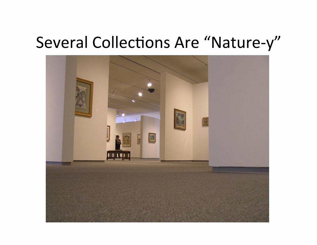
Specific research question for each quarter
Native plant species Invasive plant species
How do soil properties and microbiome biodiversity differ for native and invasive plant species?
Stanley Lo | Regional ABLE | 02/21/2015 |

8
Complementary laboratory project and research proposal
Soil microbiome project Research proposal • Asking questions • Making observations • Generating hypotheses • Designing and doing experiments • Collecting and analyzing data • Drawing conclusions • Communicating results and ideas
Stanley Lo | Regional ABLE | 02/21/2015 |

9
Course structure: Three hours of laboratory per week
Per laboratory section: • 32 students in 8 student groups • 1 undergraduate TA and 1 graduate TA
For all laboratory sections: • 1 faculty • Weekly 80-min “lecture”
Stanley Lo | Regional ABLE | 02/21/2015 |

10
Northwestern: Focus on experimental design
Design an experiment based on a defined model
Introduction to model via online lectures
Present results,
conclusions, and future directions
Create hypotheses and set up experiments
Collect, analyze, and interpret data
Repeat experiments if necessary
Stanley Lo | Regional ABLE | 02/21/2015 |

groups.molbiosci.northwestern.edu/morimoto/ 11
Research project: Protein-folding diseases in model organism
Wild-type worms Alzheimer’s model
Round worm C. elegans • Visible under standard dissecting scopes • Grow on agar plates with bacteria • Store indefinitely in -80°C
Stanley Lo | Regional ABLE | 02/21/2015 |

12
Course logistics: Parallel but different experiments
38 candidates genes that may have effects on toxicity: • Knockdown by RNAi
4 toxicity assays: • Thrashing, movement, longevity,
and egg laying
Stanley Lo | Regional ABLE | 02/21/2015 |

13
Course structure: Three hours of laboratory per week
24 students in 6 student groups per section
1 undergraduate TA and 1 graduate TA per section
1 faculty per 3 concurrent sections
Stanley Lo | Regional ABLE | 02/21/2015 |

Regional ABLE | 02/21/2015 | 14
Brainstorm: Can you do this at your institution?
Write down some ideas on the handout in relation to these questions: • What resources and support do you
need?
• What barriers and challenges do you anticipate?
• What potential solutions can you think of?

15
Microbial biodiversity in soil
Soil properties • How much moisture does the soil contain? • How acidic is the soil?
Functional biodiversity • What carbon sources are metabolized by
the microbial community?
Genetic biodiversity • What microorganisms are present?
Stanley Lo | Regional ABLE | 02/21/2015 |

16
Seven weeks of laboratory experimets
Week 2-3 4-8 9-10
Functional diversity
Genetic diversity
Project (poster)
Soil properties
Stanley Lo | Regional ABLE | 02/21/2015 |

17
How do we measure biodiversity?
More diverse
Less diverse
Richness Evenness Difference
Stanley Lo | Regional ABLE | 02/21/2015 |

18
Shannon diversity index: Richness and evenness
Shannon diversity index = H = -∑ pi × ln(pi)
Species Number pi ln (pi) pi × ln (pi)
1 40 0.200 -1.609 -0.322
2 40 0.200 -1.609 -0.322
3 40 0.200 -1.609 -0.322
4 40 0.200 -1.609 -0.322
5 40 0.200 -1.609 -0.322
Total 200 1.000 -1.609
H = 1.609
Stanley Lo | Regional ABLE | 02/21/2015 |

19
Shannon diversity index: Richness and evenness
Species Number pi ln (pi) pi × ln (pi)
1 1 0.005 -5.298 -0.026
2 1 0.005 -5.298 -0.026
3 196 0.980 -0.020 -0.019
4 1 0.005 -5.298 -0.026
5 1 0.005 -5.298 -0.026
Total 200 1.000 -0.126
H = 0.126
Shannon diversity index = H = -∑ pi × ln(pi)
Stanley Lo | Regional ABLE | 02/21/2015 |

20
Shannon diversity index (H)
Measures richness H = 0.69 H = 1.10 H = 1.39
Measures evenness H = 0.98 H = 1.39
Stanley Lo | Regional ABLE | 02/21/2015 |

21
Shannon evenness index
Shannon evenness index = E = H / Hmax = H / ln (S)
H = 0.98 Hmax = 1.39 E = 0.71
H = 1.39 Hmax = 1.39 E = 1.00
S = richness (number of species) ln (S) = maximum H given number of species ln (4) = 1.39
Stanley Lo | Regional ABLE | 02/21/2015 |

22
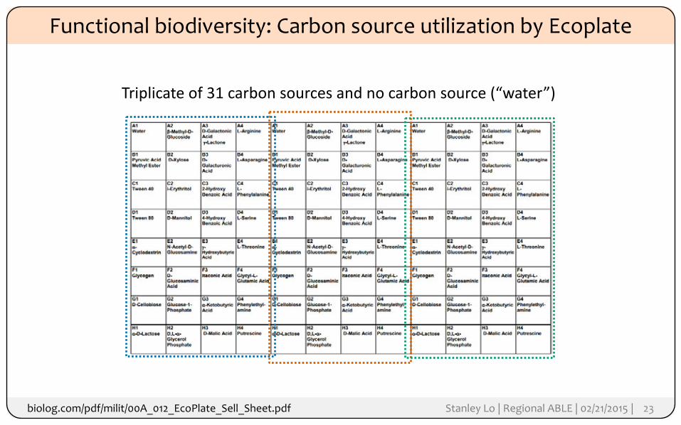
Functional biodiversity: Carbon source utilization by Ecoplate
Resuspend microbes in water
Test carbon source utilization in Ecoplate
50-mL conical tube
Stanley Lo | Regional ABLE | 02/21/2015 |
biolog.com/pdf/milit/00A_012_EcoPlate_Sell_Sheet.pdf 23
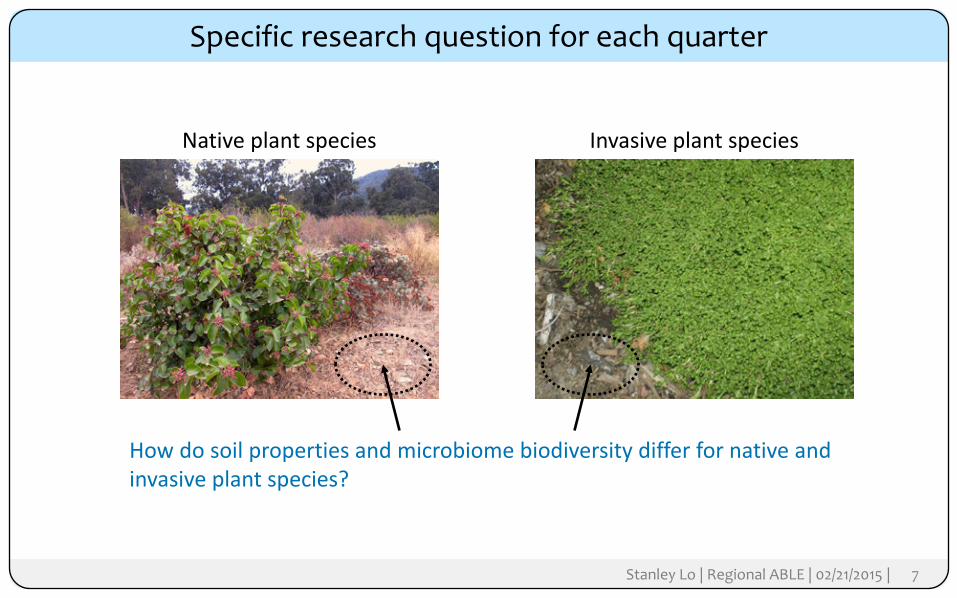
Functional biodiversity: Carbon source utilization by Ecoplate
Triplicate of 31 carbon sources and no carbon source (“water”)
Stanley Lo | Regional ABLE | 02/21/2015 |

biolog.com/pdf/milit/00A_012_EcoPlate_Sell_Sheet.pdf 24
How does Ecoplate work?
Colorless Purple and absorbs light at 590 nm
Indicator:
general
metabolism
Stanley Lo | Regional ABLE | 02/21/2015 |

25
Soil suspension with controls in Ecoplate
Water E. coli culture Soil suspension
Stanley Lo | Regional ABLE | 02/21/2015 |

26
Shared data on Google spreadsheet
Stanley Lo | Regional ABLE | 02/21/2015 |

27
Genetic biodiversity: 16S rDNA sequencing
Extract genomic DNA (Week 4)
Amplify 16S rDNA sequences by PCR (Week 5)
Ligate PRC product into plasmid (Week 6)
Stanley Lo | Regional ABLE | 02/21/2015 |

28
Genetic biodiversity: 16S rDNA sequencing
Bacterium E. coli
Bacterial chromosome
Plasmid
Transform into E. coli (Week 6)
Send bacterial colony to sequence plasmid insert (Week 7)
Analyze 16S rDNA sequence data (Week 8)
Stanley Lo | Regional ABLE | 02/21/2015 |

geospiza.com/Products/finchtv.shtml 29
Quality control in Finch TV
Good sequence
Bad sequence
Stanley Lo | Regional ABLE | 02/21/2015 |

30
Trimming sequences in Finch TV
Good sequence
1. Remove low quality bases at beginning 2. Remove low quality bases at the end 3. Export sequence in FASTA format (readable by
alignment algorithms) 4. Combine all sequences into one FASTA file
Stanley Lo | Regional ABLE | 02/21/2015 |

http://www.arb-silva.de/aligner/ 31
Classifying sequences into operational taxonomic units (OTUs)
Stanley Lo | Regional ABLE | 02/21/2015 |

http://www.arb-silva.de/aligner/ 32
SINA alignment and classification
1. Take input 16S sequence 2. Identify 10 closest matches in database
Stanley Lo | Regional ABLE | 02/21/2015 |

http://www.arb-silva.de/aligner/ 33
SINA alignment and classification
1. Take input 16S sequence 2. Identify 10 closest matches in database 3. Classify OTU for input sequence (common lowest classification)
Stanley Lo | Regional ABLE | 02/21/2015 |

34
Microbial biodiversity in soil
Native plant species
N I
Invasive plant species
Soil properties: moisture, pH Functional biodiversity: Ecoplate: AWCD, richness, Shannon H, Shannon E,
carbon source categories Genetic biodiversity: 16S sequencing: richness, Shannon H, Shannon E
Stanley Lo | Regional ABLE | 02/21/2015 |

sq.ucsd.edu 35
Lab reports in the format of research journal papers
Stanley Lo | Regional ABLE | 02/21/2015 |

36
Data analysis in Excel and sequence alignment
Ecoplate data • Week 3 handout • Data: http://goo.gl/OwuhJu • Excel datasheet: http://goo.gl/6lxhTE 16S data (already trimmed) • Week 8 handout • http://goo.gl/BDbIht
Stanley Lo | Regional ABLE | 02/21/2015 |

Workshop 3RABLE 2015

Ecological and Evolutionary Perspectives on a Tri-trophic System Dr. Jessica Pratt and Colleen Nell
Department of Ecology & Evolutionary Biology, UCI
2015 RABLE Workshop University of California, Irvine
Workshop Abstract: A tri-trophic system, one that incorporates three levels of a food chain, can be easily demonstrated using plants, aphids, and their predators (real or simulated) to teach a variety of ecological and evolutionary concepts in an interactive setting. A Plant-Aphid Study System is simple to set up in the classroom with minimal equipment and can be maintained by students in very little time each week. Aphids are exceptional study subjects for the classroom because they are very easy to keep, reproduce asexually with very fast generation times, have unique anatomical features, and interesting interactions with other organisms in nature. Many students are familiar with aphids as pests but have never examined them closely to determine what makes them successful. This workshop will cover the following topics: 1) selecting and obtaining a Plant-Aphid Study System, 2) materials and time needed to maintain a Plant-Aphid Study System, 3) examples of short-term and long-term lab activities using a Plant-Aphid Study System, and 4) outside resources for additional activities, background information, and interesting popular and formal science articles related to aphids and tri-trophic systems. This tri-trophic study system can be used for single lab investigations on a variety of topics including plant structure-function relationships, food chain interactions, evolutionary adaptations of plants and insects, aphid population growth and density dependence, and insect biology and ecology (among other topics). It is also ideal to use for a series of investigations that include those previously mentioned topics as well as long-term student-designed experiments that manipulate the plant-aphid environmental context and examine the effects on plant traits and aphid population growth. Workshop participants will complete two hands-on lab activities with aphids and plants during the workshop – Ecology, Behavior, and Adaptations of Aphids and Stop Poking Me! – An Aphid Predator Simulation Lab. All workshop materials will be provided in editable form for attendees to download. Workshop Schedule: 10:15 à Introduction to research using tri-trophic systems 10:25 à Selection and maintenance of Plant-Aphid study systems 10:35 à What is an aphid? Ecology, Behavior, and Adaptations of Aphids exercise. 10:55 à Discussion 11:05 à Aphid dissection video 11:15 à Break 11:30 à Overview of short and long-term activities using a Plant-Aphid study system 11:40 à Stop Poking Me! – An Aphid Predator Simulation exercise 12:00 à Presentation of results and discussion of data analysis with students 12:10 à Discussion of activities, assessment, and adapting to your classroom 12:25 à Wrap up

Ecological and Evolutionary Perspectives on a Tri-trophic System Dr. Jessica Pratt and Colleen Nell
Department of Ecology & Evolutionary Biology, UCI
2015 RABLE Workshop University of California, Irvine
Selecting and Obtaining a Plant-Aphid Study System: Pea plants and pea aphids are recommended by many websites including
http://insected.arizona.edu/home.htm, which provides a detailed description of how to obtain and maintain the pea aphid system. Pea plant seeds can be purchased at any greenhouse, nursery, or garden supply center. Pea aphids can be mail ordered from supply companies. A list of suppliers can be found here: http://insected.arizona.edu/gg/suppliers.html. Pea aphids are a common pest species, so care needs to be taken to not release pea aphids into the wild. Native plants and aphids should be fairly easy to come by with a simple trip to a local farm or arboretum, or chat with any gardener you know. Using local plants and aphids might be trickier, but more interesting to students. Keep in mind that many aphids are specialists and feed only on a particular type of plant. Some common Southern California native plant-aphid pairs that are fun to work with because they are big and brightly colored include the two below.
Uroleucon macolai on Baccharis salicifolia Aphis nerii on milkweed (Aesclepias spp.)
The Predators: Ladybird beetles (a.k.a. ladybugs) are one of the most common aphid predators. Ladybird beetles can be ordered online and are often found at local gardening centers as they are commonly used in gardens and farms to defend plants from pest aphids and other herbivorous insects. All students know what a ‘ladybug’ is but few recognize the important role they play as insect predators in natural systems. Of course, many exercises can also be completed using various tools to simulate a predator (e.g. paintbrush, forceps).
Materials Needed to Maintain a Plant-Aphid Study System: In the interest of not ‘reinventing the wheel’, please use the Resource Sheets found at http://insected.arizona.edu/gg/resource/default.html. These contain detailed and excellent lists of materials needed and links to suppliers and prices that will work for many lessons and activities. Acknowledgements- Many of the ideas and information included in this workshop resulted from conversations with Dr. Kailen Mooney (UC Irvine) and Catherine Prenot. Ms. Prenot developed an aphid lesson module for her high school classroom and we have included much of that information in this workshop.

Ecological and Evolutionary Perspectives on a Tri-trophic System Dr. Jessica Pratt and Colleen Nell
Department of Ecology & Evolutionary Biology, UCI
2015 RABLE Workshop University of California, Irvine
Stop Poking Me! – An Aphid Predator Simulation Lab Introduction: All organisms have adaptations that allow them to better survive in the environment in which they live. These adaptations can include both physical characteristics such as size, camouflage, bad-tasting or toxic chemicals, and behavioral characteristics. Some behavioral adaptations allow organisms to avoid being consumed by their predators. For example, some animals are active only at night to avoid potentially threatening predators that are awake during the day. In this activity we will examine anti-predator behavioral adaptations in aphids. Research Question: Do aphids demonstrate predator avoidance behaviors when their colonies are attacked? Experimental Design:
1. Each student group should obtain the following: • Two milkweed plants covered with aphids • A “predator” (paintbrush, straw, or forceps) • Two pieces of labeling tape • A stopwatch
2. Write a hypothesis about what will happen to the aphids when they are faced by a “predator”. IF aphids have behavioral adaptations to avoid predators THEN ____________ ________________________________________________________________ Based on your hypothesis write a prediction that could support your hypothesis Given the “predator” you chose. Predator:_____________ Prediction: _______________________________________________________ ________________________________________________________________
3. What are some possible behavioral adaptations aphids could exhibit to a predator?
________________________________________________________________ ________________________________________________________________
4. Follow the steps on the board for completing the experiment for your “predator” an
record your data in the table on the next page.

Ecological and Evolutionary Perspectives on a Tri-trophic System Dr. Jessica Pratt and Colleen Nell
Department of Ecology & Evolutionary Biology, UCI
2015 RABLE Workshop University of California, Irvine
Experimental Plant – Record the percent of aphids exhibiting each
behavior. Trial Wiggled Abdomen Walked Away Jumped off Plant Other (describe)
1
2
3
Control Plant – Record the percent of aphids exhibiting each behavior.
Trial Wiggled Abdomen Walked Away Jumped off Plant Other (describe)
1
2
3
Results and Conclusions
1. Were the results from all three trials the same? Yes or No 2. If not, why do you think this is? -
__________________________________________________________________
__________________________________________________________________
3. Based on your results do you support or reject the hypothesis? Support Reject
4. What can you conclude about aphid behavioral adaptations ?
__________________________________________________________________
__________________________________________________________________
Communication of Results:
1. Use the provided poster template to create a poster in powerpoint to communicate the results of your experiment to the rest of your class. Be sure to include background information, your hypothesis and predictions, your experimental design, and your results and conclusions.

Ecological and Evolutionary Perspectives on a Tri-trophic System Dr. Jessica Pratt and Colleen Nell
Department of Ecology & Evolutionary Biology, UCI
2015 RABLE Workshop University of California, Irvine
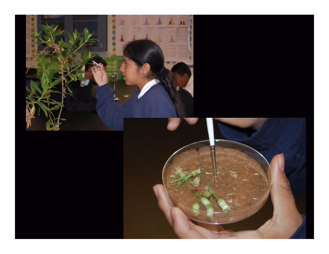
Ecology, Behavior, and Adaptations of Aphids In the following exercise you will observe aphids on their host plant and in a “Petri-‐dish habitat”. Record your observations of aphid anatomy and behavior and answer the questions below as you follow the directions. 1. Make a “Petri dish habitat” for your aphid: cut out one circular piece of paper towel, moisten it and place it in a Petri dish. 2. Cut a small leaf from the plant and place in your Petri dish on top of the paper towel. 3. Using a fine paint brush, nudge one large aphid until it moves from its location on the plant. Gently place the aphid on the leaf in your Petri dish. 4. Utilize hand lenses and dinolite microscopes to diagram your aphid as detailed and accurately as possible. 5. Watch the aphid for at least three minutes. What does it do? Describe. 5. Without the use of text books or other resources (except for your sizable craniums) name, describe, label and predict the function of at least three parts of the aphid’s anatomy. Be creative, but make sure that your reasoning makes sense in terms of what behaviors you see in your aphid. Name Description Predicted Function 1. 2. 3.

Ecological and Evolutionary Perspectives on a Tri-trophic System Dr. Jessica Pratt and Colleen Nell
Department of Ecology & Evolutionary Biology, UCI
2015 RABLE Workshop University of California, Irvine
Follow-‐up Questions: 1. If you were an aphid, what challenges might you face in your environment? 2. How do aphids move? 3. How do aphids eat? 4. Explain how the structure of an aphid may help it survive in its environment. 7. Define parthenogenesis and telescoping generations. 8. What adaptations or features of aphids might make them successful agricultural pests? 9. What questions are you left with at the end of this inquiry that you would like to investigate?

Teaching ecological and evolutionary perspectives on a tri-trophic system
Jessica Pratt & Colleen Nell RABLE Workshop February 21, 2015

Community Ecology Study of distribution, abundance, demography and interactions between co-occurring species

Research Focus Plant- Insect Interactions
• What is the relative importance of bottom-up vs. top-down controls over plant-insect interactions?
• How do plant-insect interactions change along environmental gradients?

Experimental Approaches
Tritrophic Interaction Studies

Research using a Plant-‐Aphid study system
• Aphids are a valuable bioassay agent
• Simple proxy for plant condi9on

Increase defense
Plant-‐plant communica9on
Research using a Plant-‐Aphid study system

A Tritrophic System The Plant -- Aphid -- Ladybug System
How can this system be used in the undergraduate classroom to teach a variety of ecological and evolutionary topics?

Selecting & Obtaining a Plant-Aphid Study System
• Pea plants/aphids are recommended by many websites including:
http://insected.arizona.edu/home.htm
• Native plants/aphids should be fairly easy to come by with a simple trip to a local farm or arboretum, or chat with any gardener you know!

Aphis nerii on milkweed
Uroleucon macolai on Baccharis spp.

Materials Needed: Plant Propagation • Two plastic containers or pots • Plastic plant trays • one large bucket or bowl for mixing soil • all-purpose potting soil • watering can • Sharpie and plant tags • Seeds • Fluorescent, full spectrum, or 'grow light' bulbs
and fixture • 24-hour appliance timer

Materials Needed: Aphid Rearing • Healthy plants • Fine-tipped paintbrushes • Mesh insect cage (optional)
• Bag or box of ladybugs
Materials Needed: Predators


Ecology, Behavior, and Adaptations of Aphids
• Follow the directions on your handout to do the following in your group: 1. Make a Petri-dish habitat for your aphids 2. Using a hand lens or dissecting scope, observe
the aphids in their Petri-dish habitat and on their host plants
3. While doing so complete the first side of the lab worksheet.
Aphid Initiation

What is an aphid?
• Herbivorous insects • Often considered pests • Important food source for
other insects & birds
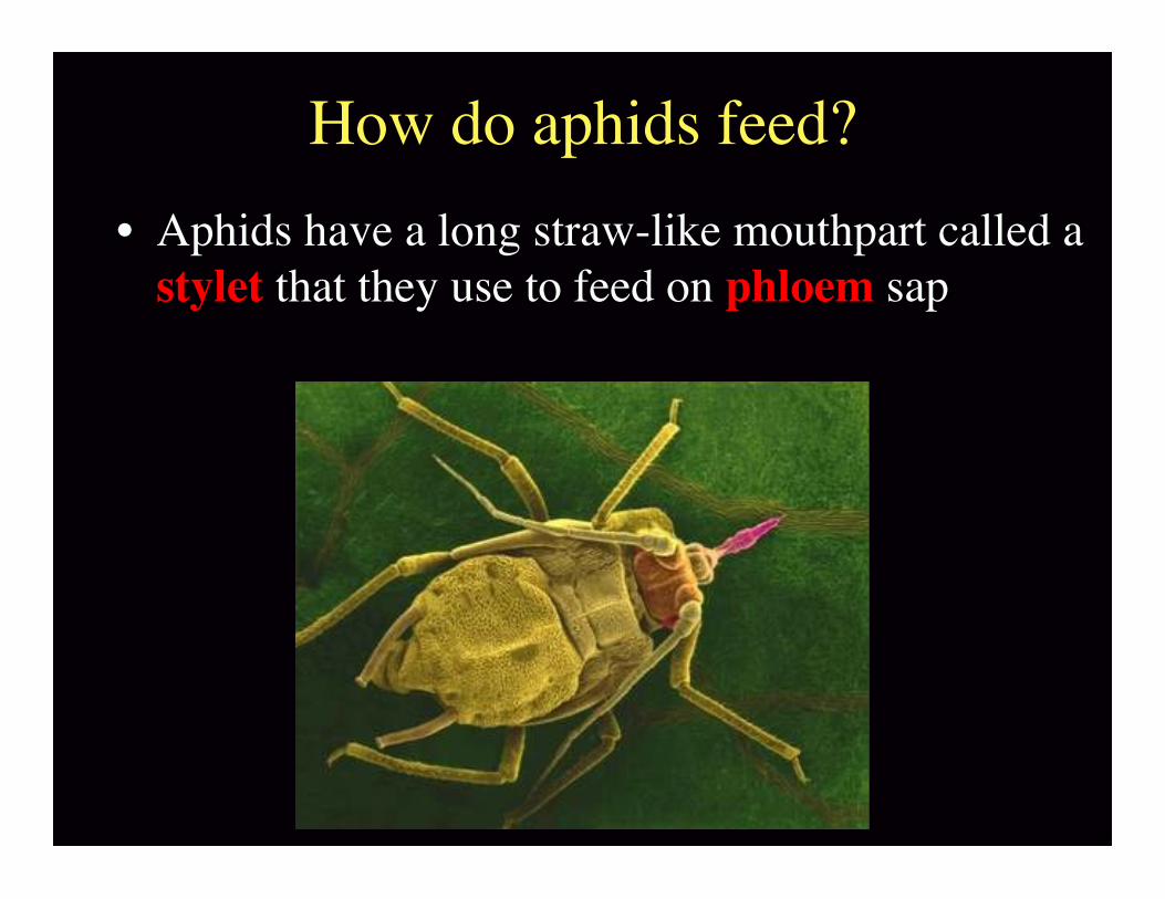
How do aphids feed? • Aphids have a long straw-like mouthpart called a
stylet that they use to feed on phloem sap

How do aphids feed?
• All aphids feed by inserting their mouth parts between plant cells to reach the phloem sap.

Aphids & their interactions….
…with plants Plants produce chemicals to defend
themselves from herbivores like aphids

Aphids & their interactions….
…with ants Many aphids have
a mutualism with ants

Aphids & their interactions….
…with ants Aphids secrete honeydew to feed the ants. The ants protect the aphids.

Aphids & their interactions….
…with predators Aphids secrete poisons from their cornicles to defend themselves

Aphid Reproduction • Give birth to live young via parthenogenesis • Have telescoping generations
– The baby aphid developing inside the mother already has its own babies developing inside it.

Complete Follow-up Questions on back side of worksheet

Discussion Questions
• What should students know beforehand? • What preparation is required? • What other questions related to aphids
would you be interested in investigating?

Aphid Dissection Video

15 minute break

Potential Classroom Activities
• Seed Structure & Function – Germination & Tissue Differentiation
• Student-directed Experiment – • Scientific Method, Experimental Design • Data Collection, Plant trait measurements • Analysis and presentation of data
• Aphid Initiation Activity – Aphid biology, plant-aphid interactions
• Population Explorations – of aphids in the classroom and in the field
• Plant-Aphid Systems Jigsaw Activity • Aphid-predator Simulation • Power of Predators


Stop Poking Me!���An Aphid Predator Simulation

Discussion Questions
• How could you adapt these activities for a class that you teach?
• How could you use this system in a large lecture hall / introductory bio or ecology class?
• What topics do you cover that could be taught using this system?

Thank You
NSF GK-12 Program at UCI (Grant DGE-0638751)
The Mooney Laboratory at UCI

Workshop 4RABLE 2015

4.1
LAB 3 Neurophysiology – Electrical Activity of Neurons
The following lab manuals were adapted and written by Veronique Boucquey, Derek Huffman, Joyce Lacy of the Dept. of Neurobiology and Behavior at the University of California Irvine. Presenters: Natalie Goldberg, Andre White, Veronique Boucquey, Julia Overman, Lauren Javier and Andrea Nicholas Summary In Lab 4, you will investigate the electrical properties of neurons experimentally using a classic preparation, the cockroach leg. Therefore, the exercise for Lab 3 will introduce you to cockroach anatomy, action potentials, and electrophysiology methodology. This week you will complete the cockroach leg preparation, listen for spontaneous and evoked activity, and use the recorded neural signal from one leg to modulate another leg’s neural activity. Goals
Complete the cockroach leg preparation
Listen to spontaneous and evoked neural activity
Use the recorded neural signal from one cockroach leg to modulate another leg’s activity Background Electrical Properties of Neurons
As you learned in Bio Sci N110, neurons are electrically active cells that rely on their electrical signaling capabilities to transmit information throughout the nervous system. The measure that is used to define the electrical state of a neuron is called the potential (short for transmembrane potential or membrane potential), which is the potential/voltage difference between the inside and the outside of the neuronal membrane. There are several different types of neuronal potentials, including resting potentials, synaptic potentials, receptor potentials and action potentials. These potentials all result from the differential distribution of ions on either side of the neuronal membrane, which sets up both concentration and electrical gradients across the membrane, and is affected by the opening and closing of particular ion channels. Please review your notes from Bio Sci N110 and/or the chapters on the electrical properties of neurons in any introductory neurobiology textbook and make sure that you understand the fundamentals of resting potentials and action potentials. Your understanding of these concepts is critical to your understanding of what you will be doing and the interpretation of your results in the next two laboratory exercises. TA Notes for Labs 3 & 4:

Lab 4
4.2
Make sure that all of the equipment is clean before class and that there is no residual Vaseline! Vaseline can act as an insulator and mess up the recordings/experiments!
Assign one student in each group to handle the Vaseline. Vaseline should only be placed on the exposed wound! Once this is completed, have this student change gloves!!
Make sure to pin along the midline of the leg! In most cases, there is a light (or dark) colored line runnig down part of the midline in the coxa part of the leg (find the trochanter). Usually pinning on there, gives great CAPs!

Electrical Properties of the Cockroach Leg Preparation
4.3
Methods for Recording the Electrical Activity of Neurons
There are four principal methods that are used to record the electrical activity of neurons:
Extracellular recording measures the voltage change along the outside of a cell, providing a “reflection” of what is happening on the inside of the cell. This technique measures the voltage difference between two recording electrodes placed outside of the cell. This is the method you will be using in the next two labs.
Intracellular recording measures the voltage difference between the inside and outside of the cell membrane. This technique is difficult and requires inserting one recording electrode into the cell, penetrating the cell membrane without compromising neuronal health, and placing the second recording electrode outside of the cell.
Patch-clamp recording measures electrical currents (ion flow) through single ion channels in a neuronal membrane. This very delicate technique involves isolating a patch of membrane small enough to contain only one or two ion channels. This patch of membrane can be pulled away from the cell, and ion flow through the isolated channels in the membrane patch can be measured.
Optical imaging allows direct visualization of the voltage difference across the cell membrane, providing both spatial and temporal resolution of the membrane potential. This technique involves application of certain voltage-sensitive dyes, which change color or other properties depending on voltage, followed by evaluation with microscopy.
Single Action Potential
The action potential (Fig. 3-1, steps 5-7: peak/trough), which appears as a biphasic (two-part) waveform (steps 6 & 7: peak/trough), is the rapid and brief depolarization that is conducted down the length of axons in order to convey information from one place to another in the nervous system. This fundamental neural signal results from a stereotyped pattern of opening and closing of voltage-gated Na+ and voltage-gated K+ channels. More detailed properties of the action potential will be addressed in the next lab.
1 & 2 Inhibitory hyperpolarization 3 & 4 Sub-threshold depolarization
5 Threshold depolarization
6 Action potential rising: V-gated Na+ channels open; recovery: V-gated K+ channels open
7 After-hyperpolarization (K+
channels still open)
The cockroach preparation
Figure 3-1. Potential Changes and the Action Potential in a Single Neuron

Lab 4
4.4
History of Cockroach Preparations: Cockroaches have been used for decades in neuroscience research—interestingly, many publications on the physiology of cockroach legs have come from investigations of the efficacy of pesticides (e.g., Cornwell, 1968). Cockroach legs live for many hours after being severed, providing a stable preparation to study many neuronal properties. For example, after being severed, cockroach legs exhibit spontaneous activity. Spontaneous activity refers to neuronal firing without external stimulation. By stimulating spines (hairs) on the leg, evoked activity (that is, activity evoked by external stimulation) can be observed. Evoked activity can often decrease as a result of prolonged stimulation. These changes are referred to as sensory adaptation. Sensory adaptation can be useful for signaling changes in the environment. For example, this morning when you put your watch on, you felt the cold of the metal and the pressure of the strap, but now you probably do not notice your watch is there. Listening for Spikes (Action Potentials): In the late 1950s Hubel and Wiesel performed a series of experiments in which they showed visual stimuli to cats while recording from visual cortex. The images were shown to cats on a projector using transparent slides. They amplified the output of the neuronal response through a speaker, thus allowing them to hear when a cell became highly active. Interestingly, they discovered that cells in primary visual cortex do not respond to large objects but rather to lines (e.g., Hubel & Wiesel, 1959). Their results were actually discovered by accident—they were attempting to get the cells to respond to the objects on the slides; however, they eventually heard spiking activity when the edge of their slides passed through the cell’s preferred line direction and spatial location. This only happened when they were removing the slides, so if they were only recording the spiking activity with an oscilloscope (without listening to the spiking activity as well), it is possible that they would have stopped recording in between stimulus presentations. Therefore, it is possible that if they were not listening to the neurons, they may have never discovered the properties of primary visual cortex. After hearing the neuronal behavior, they quantified it by recording the responses of neurons and showing increased evoked activity to very simple visual stimuli in the visual cortex. In today’s lab, you will be listening to spikes, much as Hubel and Wiesel did in their Nobel Prize winning experiments. Today you will be able to hear spontaneous and evoked activity, as well as possibly observing sensory adaptation.

Electrical Properties of the Cockroach Leg Preparation
4.5
From backyard brains: Cockroach Anatomy and Senses (http://www.backyardbrains.com, open source material)
Each segment of the cockroach contains a region of the Ventral Nerve Cord (VNC), a collection of neurons that send information to the muscles of the body, while receiving information from the sensory organs of the periphery. This information is relayed to and from the brain using action potentials and synapses.
When observed up close, you can see how the cockroach leg is covered with large spines along the tibia and femur. Each spine has a neuron wrapped around it, which sends action potentials (APs) to the VNC and eventually the brain. The pattern and frequency of APs sent will allow the VNC to distinguish a strong external stimulus from a weak one. Which hair cells are being stimulated will determine where the cockroach perceives the stimulation is located.
EXPERIMENT 1: Listening for spiking activity using the Spikerbox

Lab 4
4.6
Equipment: Spikerbox, stopwatch, dissecting tray, 2 sets of insect pins with wire attachment, blue pad, toothpick, Vaseline, scissors, amplifier, audio cable, plastic cup, cockroach Procedure
1. Obtain cockroach from bin (pick it up by gently pinching its sides with your thumb and middle finger- you can do it!)
2. Place cockroach in one of the cups. To anesthetize the cockroach, place in freezer for about 10 minutes, or until it stops moving. Use a stopwatch.
3. Place cockroach on its back on a paper towel on the dissecting tray.
4. Remove 4 legs (see diagram): REMOVE THE MESOTHORACIC (middle) LEGS FIRST
Gently pull the mesothoracic (middle) leg away from cockroach body. Cut the mesothoracic leg at the highest point possible (closest to the body, above the coxa- see dark line on diagram) so that you have all three segments of the leg intact (coxa, femur, tibia). Using the toothpick, place a pea-sized amount of Vaseline on the exposed wound of the leg. Make sure to place a good amount of Vaseline on the leg. If you do not, the leg will die. Repeat for other mesothoracic leg. Repeat for the metathoracic (hind) legs.
5. Sacrifice the cockroach: roll up cockroach in paper towel, tape, and place in freezer.
mesothoracic leg
metathoracic leg
coxa femur
tibia

Electrical Properties of the Cockroach Leg Preparation
4.7
6. Pin ONE of the metathoracic legs (see arrows in diagram below): Pin the leg using the insect pins with wire attachment. Pin in the femur and tibia (one pin in each). Try to pin down the midline of the leg segments. The pins CANNOT touch each other- this will create a short in the system. The pins will go through the leg and into the blue mat. These are your recording electrodes.
7. Plug the wire coming from the pins into the Spikerbox (green to green plug).
8. Plug the audio cable into the left plug on the Spikerbox (black plug). Plug the other end of the audio cable into the “input” plug on the amplifier.
9. Turn on Spikerbox (flip the switch).
10. Turn on amplifier.
11. Listen for spontaneous spiking (these will sounds like popcorn pops).
Tibia
Femur
Lab 4
4.8
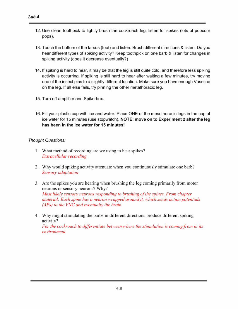
12. Use clean toothpick to lightly brush the cockroach leg, listen for spikes (lots of popcorn pops).
13. Touch the bottom of the tarsus (foot) and listen. Brush different directions & listen: Do you hear different types of spiking activity? Keep toothpick on one barb & listen for changes in spiking activity (does it decrease eventually?)
14. If spiking is hard to hear, it may be that the leg is still quite cold, and therefore less spiking activity is occurring. If spiking is still hard to hear after waiting a few minutes, try moving one of the insect pins to a slightly different location. Make sure you have enough Vaseline on the leg. If all else fails, try pinning the other metathoracic leg.
15. Turn off amplifier and Spikerbox.
16. Fill your plastic cup with ice and water. Place ONE of the mesothoracic legs in the cup of
ice water for 15 minutes (use stopwatch). NOTE: move on to Experiment 2 after the leg has been in the ice water for 15 minutes!
Thought Questions:
1. What method of recording are we using to hear spikes? Extracellular recording
2. Why would spiking activity attenuate when you continuously stimulate one barb?
Sensory adaptation
3. Are the spikes you are hearing when brushing the leg coming primarily from motor neurons or sensory neurons? Why? Most likely sensory neurons responding to brushing of the spines. From chapter material: Each spine has a neuron wrapped around it, which sends action potentials (APs) to the VNC and eventually the brain
4. Why might stimulating the barbs in different directions produce different spiking activity? For the cockroach to differentiate between where the stimulation is coming from in its environment

Electrical Properties of the Cockroach Leg Preparation
4.9
EXPERIMENT 2: Temperature effects on spiking activity Procedure
1. After the 1st mesothoracic leg has been in the ice water for 15 minutes, you will take it out of the ice water and pin it according to the steps in Experiment 1. Restart the stopwatch.
2. Un-pin the metathoracic leg that you were using in Experiment 1 and set aside for Experiment 3.
3. Using your second insect pin with wire attachment, pin the 2nd mesothoracic leg according
to the steps in Experiment 1.
4. Plug the 2nd mesothoracic leg (non-ice water) into the Spikerbox. Listen for spikes.
5. Plug the 1st mesothoracic leg (ice water) into the Spikerbox. Listen for spikes.
6. Turn off amplifier and Spikerbox.
Thought Question:
1. Do you notice a difference between the 1st and 2nd mesothoracic legs? If so, (a) characterize the difference(s), (b)what do you think causes the difference(s)? (a) The second leg has less spiking activity (b) The cold from the ice water decreased membrane fluidity of the cells (remember Bio93), so that for some of the cells (or all cells if you hear NO spikes) a low enough temperature is reached that the membrane has become rigid and therefore the membrane-bound ion channels cannot work properly.
EXPERIMENT 3: Neuroprosthetics

Lab 4
4.10
Use the recorded neural signal from one cockroach leg to modulate the other. Additional equipment: stimulation cable (lead with black and red grabbers), insect pins, 2nd metathoracic cockroach leg Procedure
1. Re-pin the original metathoracic leg (from Experiment 1). Check that your original leg (leg #1) is still producing spiking activity by turning on the amplifier and listening for spikes. This leg will be providing the neural signal to stimulate the other leg.
2. Now you will pin the 2nd metathoracic leg: (see diagram below) Pin the leg using the insect
pins WITHOUT wire attachment. Insert both pins into the coxa. Try to pin down the midline of the coxa. The pins CANNOT touch each other- this will create a short in the system. Make sure you have the tibia hanging off the blue mat- this is so that it can move without restriction! This leg will be stimulated by the neural signal from leg #1. The pins will go through the leg and into the blue mat.
3. Turn off the amplifier.
4. (See picture below) Attach the black and red grabbers to the insect pins in the 2nd leg. These are your stimulating electrodes. Attach the other end of the simulating cable to the “output” plug on the amplifier.
Coxa

Electrical Properties of the Cockroach Leg Preparation
4.11
5. Turn the amplifier on at lowest setting.
6. Brush leg #1. Observe leg #2 to see if there is any movement. Slowly increase amplification until you see movement of leg #2 when you brush leg #1.
7. Turn off amplifier and Spikerbox.
Thought Question:
1. Circle the correct answers: The signal coming from leg #1 is most likely from SENSORY/motor neurons, which is then used to stimulate leg #2. When you observe movement of leg #2, you are most likely observing sensory/MOTOR neuron spiking.

Lab 4
4.12
Electrical Properties of the Cockroach Leg Preparation
4.13
LAB 4 Neurophysiology – Electrical Properties of the Cockroach Leg Preparation
Summary In this lab, you will elucidate several electrical properties of a cockroach that relate to the conduction of action potentials along nerves. By analyzing compound action potentials, you will characterize many important properties of the cockroach leg, including excitability, movement, electrophysiological relationship, refractory period, and multiple fiber types.
Goals Become familiar with methods for generating and interpreting electrophysiology data
Characterize several electrophysiological properties of the cockroach leg
Utilize electrophysiological data to learn more about the organization of the cockroach leg
Background In order to understand the experiments in this lab exercise and interpret your data, you must understand the fundamentals of the action potential (i.e. single action potential). It is assumed that you are already familiar with these concepts, so not all important points will be covered here. Make sure you understand the diagram of the action potential in Figure 3-1 on p. 3.2 of the previous lab, including the mechanistic basis of each stage/electrical event indicated in the diagram (steps 1-7). In addition, make sure you understand what threshold means and why individual neurons have a threshold for firing an action potential; what is meant by the description all-or-none when referring to single action potentials; and what role different ions and ion channels play in the different parts of the action potential. You should also be comfortable with the terms depolarization and hyperpolarization.
Single Action Potential
Single action potentials are recorded by placing a single electrode into an axon with a second electrode placed outside of the axon. The voltage difference between these two electrodes is recorded; hence, resting potential reflects the voltage difference between the inside and outside of the axon. Resting potential is negative due to the Na+/K+ pump. The “all” portion of the all-or-none property of the single action potential refers to the fact that the height of the overshoot of the single action potential is physiologically determined and will not increase or decrease in size with varying strength of stimulation. The “none” portion simply states that the threshold serves as a binary operator for firing an action potential—that is, the cell will only fire an action potential if it reaches threshold. Figure 4-1 shows that it takes a finite amount of time for an individual cell to change from resting potential to threshold (this concept will be important later in today’s lab as we change the amount of time we stimulate the cockroach leg). The upstroke of the action potential is due to increased conductance to Na+ (more Na+ channels open) and the after hyperpolarization is due to increased conductance to K+ (more K+ channels open). Na+ channels

Lab 4
4.14
are quickly closed while K+ channels are slow to close, resulting in a relatively short depolarization followed by a relatively long hyperpolarization (See Figure 4-2).
Figure 4-1. Dynamics of the Single Action Potential. It takes a finite amount of time for a single axon to change voltage from resting potential (Vrest) to threshold (Vthresh). The x-axis here depicts change in time. The line notch that is raised above the line at the bottom of this figure depicts the amount of time to change voltage from resting potential to threshold. AHP=After Hyperpolarization. Figure from Bean, B.P. (2008). The action potential in mammalian central neurons. Nature Reviews Neuroscience(8): 451-465.

Electrical Properties of the Cockroach Leg Preparation
4.15
Figure 4-2. Components Underlying the Single Action Potential. Na+ channels close relatively quickly while K+ channels close relatively slowly, resulting in a quick upstroke of the action potential followed by a relatively long period of hyperpolarization. Figure and text from Hodgkin and Huxley (1952). A quantitative description of membrane current and its application to conduction and excitation in nerve. J. Physiol. 117: 500-544.
Compound Action Potential
Extracellular recordings from a nerve can be used to distinguish either single action potentials in single axons or the sum of multiple single action potentials firing simultaneously in many axons that comprise a nerve. This recorded sum is called a compound action potential (CAP). This week you will simultaneously stimulate many of the axons in a cockroach leg and observe the resulting compound action potential. It is important to note that compound action potentials are not all-or-none because they can increase size with increasing stimulus strength or duration of stimulus (violation of the “all” portion of the all-or-none property of the single action potential. See also the “Excitability” section below). While recording from more than one axon at once may seem like an indiscriminate technique, it is reliable and useful and offers the opportunity to explore many important aspects of action potential conduction. We will record the CAP through a differential amplifier. The amplifier is called a differential amplifier because it works by constantly comparing

Lab 4
4.16
signals from two recording electrodes (A) and (B), subtracting one from the other (A-B), and then sending the result to the computer. Here is an example of how a CAP is produced, step-by-step:
1. Initially, both electrodes are at rest, so the
display reads 0 µV as a result of the differential amplifier performing the following operation: A=B=0 µV, so A - B = 0 µV.
2. Now imagine that as the CAP crosses electrode A, the influx of positive Na+ ions caused by action potentials in the individual fibers causes a traveling wave of negativity on the outside of the fibers causing a voltage change of –1 µV when it is recorded by A. While recording electrode B still measures 0 µV. So A = -1 µV and B = 0 µV, so A - B = -1 µV
3. Eventually, the CAP travels so that it is
between the two electrodes or being recorded by both at the same time. Again, A=B=0 µV, so A-B = 0 µV.
4. When the CAP crosses over electrode B, the
value at B approaches –1 µV. With the value at recording electrode A now returned to 0 µV, the differential amplifier subtracts A-B and the monitor will display +1 µV. Note that the CAP is still a traveling wave of negativity.
5. The CAP then moves beyond the electrodes
and the display returns to zero. A=B=0 µV, so A-B=0 µV
!
! Femur of cockroach leg

Electrical Properties of the Cockroach Leg Preparation
4.17
Figure 3-3. Recording a Monophasic CAP Using a Differential Amplifier Other examples of CAPs: Consider if the positions of your recording electrodes A and B are reversed from the previous example. Now the traveling wave of negativity will reach B first, rather than A first. This produces a CAP that is reversed in sign from the previous example. (Remember, the subtraction is always A-B).
Consider if recording electrodes A and B are not recording from same fibers (Note: recording electrodes A and B are in the original locations). We will observe only half of the CAP, because the traveling wave of negativity will only pass one electrode. An example of this type of CAP can be observed on page 4.14.
!
B A
Femur of cockroach leg
1.
2.
3.
4.
5.
! Femur of cockroach leg

Lab 4
4.18
Stimulus Artifact Today, you will be recording and characterizing electrical responses in a cockroach leg. To get your leg to respond electrically, you will be stimulating the leg with a pulse of electrical current from the stimulator. Before you examine the neural response, however, you need to learn to recognize the stimulus artifact. Some of the electrical current from the stimulating pulse is conducted passively down the leg and is picked up as a signal by the recording electrodes. This signal is the stimulus artifact; it is merely a sort of “echo” of the original stimulus and is not related to the neural response.
Refractory Period
The refractory period is the period of time after an action potential fires, during which action potential generation cannot be similarly repeated in the same membrane region. The refractory period has two phases: the absolute refractory period during which no amount of stimulation can trigger an action potential; and the relative refractory period during which a second action potential can be generated, but it either takes greater stimulation (single action potential) or yields a lower-amplitude action potential upon stimulation at the same level (CAP). The absolute refractory period results from the inactivation of the voltage-gated Na+ channels responsible for the depolarizing phase of the action potential. About one millisecond after they open, they close in such a way that no amount of stimulation can open them again until the membrane repolarizes and they reactivate. This important property makes the single action potential unidirectional. If the voltage-gated Na+ channels can’t be opened, a neuron cannot fire an action potential and is therefore refractory. Since the compound action potential reflects the summed aggregate activity of individual axons, the absolute refractory period of a CAP is defined as the period of time when all axons within the nerve are in their absolute refractory periods, and no amount of stimulation can elicit a CAP of any size. The basis of the relative refractory period is different in a single action potential, which you are already familiar with, and the compound action potential, which you will be analyzing in this laboratory. After a single action potential, the voltage-gated Na+ channels recover at slightly different times. When some, but not all, of the voltage-gated Na+ channels have recovered and can be opened again, the neuron can fire another action potential if the stimulus intensity is increased. The relative refractory period of a compound action potential reflects the recovery of a subset of the axon fibers in the nerve. Since only some of the fibers have recovered and fire action potentials upon stimulation, the amplitude of the compound action potential is decreased during its relative refractory period.
Conduction We have said that an action potential “travels” down the axon, but to understand this better, we must discuss conduction or how the charge travels through the neuron.
Three Types of Conduction Used by Neurons

Electrical Properties of the Cockroach Leg Preparation
4.19
Electrotonic conduction refers to the passive spread of membrane potentials through the cell. There is no active participation on the part of the cell to maintain the amplitude (e.g., no voltage-gated Na+ channels opening, no action potential). Consequently these potentials decay over time and distance from their point of origin as current gradually leaks out of the cell. Electrotonic conduction is analogous to kicking a soccer ball across a grass field; if you kick it just once, the ball will travel forward, but it will slow down as it goes, ultimately petering out and stopping. Active conduction involves the active maintenance/rejuvenation of the membrane potential as it travels through the cell. It occurs in the axons of neurons where voltage-gated Na+ channels open as the membrane potential approaches threshold, thereby rejuvenating the membrane depolarization before it decays. The depolarization then spreads passively to the next patch of membrane, triggering the opening of its voltage-gated Na+ channels, and so forth, all the way down the length of the axon. This process allows the action potential to travel long distances without any loss of amplitude and is the means of action potential propagation in unmyelinated regions of axons. Active conduction is somewhat analogous to dribbling a soccer ball down the length of a grass field; the ball continually gets one little boost right after another to maintain its forward movement over long distances. Saltatory conduction is a combination of active and electrotonic conduction and is used in myelinated axons. Myelin is the insulating sheath that wraps around vertebrate axons. Along the length of a myelinated axon are periodic gaps in the sheath, called Nodes of Ranvier, where the majority of the voltage-gated Na+ and K+ channels are clustered. As the action potential travels down the axon, it advances electrotonically within the myelinated regions, and is actively rejuvenated by the activation of the voltage-gated channels at the Nodes. This process of saltatory conduction is analogous to passing a soccer ball from one person to another all the way down a grass field; one person kicks the ball, it rolls and begins to slow as it reaches the next person who then gives it another kick to get it to the next person, and so forth all the way down the field.
Properties Affecting Conduction Speed and Efficiency Two axon properties that influence conduction speed and efficiency are axon diameter and myelination. Larger diameter axons conduct electrical signals faster than smaller diameter axons. This is because increasing the diameter lowers the internal/axoplasmic resistance (Ri), thereby making it easier for signals to move forward along the axon. Myelin, which ensheathes vertebrate axons, does two things. First, it increases membrane resistance (Rm), thereby increasing the axon’s insulation and reducing leakage of the signal out of the cell as it travels. Second, it decreases membrane capacitance (Cm: the amount of charge captured and stored by a patch of membrane), thereby reducing the amount of time it takes to charge up myelinated regions of the membrane, and thus increasing the speed at which charge spreads through these portions of the axon. Invertebrate axons do not contain myelin. In order to have fast conduction velocities (important for survival), many invertebrate axons have evolved to have very large axons—squid and cockroach giant axons can get close to 1 mm in diameter! The large size of squid axons allowed researchers to readily study them, causing them to be extensively studied for their electrophysiological properties (e.g., Hodgkin and Huxley’s Nobel Prize winning research utilized the squid preparation). Vertebrates have myelin, which increases conduction velocity while minimizing the amount of volume required for each axon, thus allowing more axons to be packed into a smaller volume. Figure 4-2 shows the comparison between regular and giant axons in the squid as well as the cockroach. Notice that even though larger axons increase conduction

Lab 4
4.20
velocity, these axons are relatively slow compared to the cat’s myelinated axons (See also Table 4-1 for comparison of axon diameter between these species). Conduction in a Nerve and Multiple Components The cockroach leg contains axons of differing diameter. As discussed in the previous section (and as is evident in Figure 4-2) giant axons of the cockroach leg offer faster conduction velocity. The CAP is a summation of many axons which each fire single action potentials. Due to differing axon diameters, axons within the cockroach leg have differing conduction velocities. It is likely that you will view CAPs with multiple components (multiple deflections within the CAP) in today’s lab, which are likely due to differing size of axons in the leg.
Figure 4-3. Conduction velocity differences between vertebrate and invertebrate axons. Note that although larger axons allow faster conduction velocities, these axons are relatively slow compared with myelinated axons found in mammals. Data from Bullock, T. H. and G. A. Horridge 1965. Structure and function in the nervous sytems of invertebrates. Freeman: San Francisco. Figure from http://www.animalbehavioronline.com/myelin.html Table 4-1. Compare the conduction velocity of a small myelinated axon to a giant unmyelinated axon Nerve Tissue Temperature (°C) Fiber Diameter
(µm) Velocity (m/sec)
Cat (myelinated) 38 2-20 10-100
Squid (giant, unmyelinated) 20 500 25

Electrical Properties of the Cockroach Leg Preparation
4.21
Excitability The excitability of a nerve refers to how readily it generates an action potential, and this in turn is related to the nerve’s threshold for firing. In contrast to that for a single action potential, threshold for a compound action potential is the stimulation point at which you barely get a measurable response out of the nerve. The threshold for a nerve depends on two things: the strength and the duration of the stimulus. This is analogous to boiling water; you can either put it on very high heat for a short time, or on lower heat for a long time to reach a boil. Figure 4-1 shows that the change in voltage from resting to threshold takes a finite amount of time. Increasing the duration of the stimulus results in greater probability that an axon will have enough time to reach its threshold. In this experiment, you will generate a stimulus strength-duration curve for reaching threshold in order to determine two key properties that relate to nerve excitability:
Rheobase voltage: weakest stimulus that will elicit any response from the nerve (i.e., weakest stimulus that will bring the nerve to threshold).
Chronaxie time: stimulus duration required to elicit a response when stimulating at 2x the rheobase voltage. This is a measure of nerve excitability; lower chronaxie times reflect greater nerve excitability.
The relationship between these parameters and nerve strength-duration curves is illustrated in Figure 4-4 below. In any particular nerve, fibers are not identical in diameter or internal resistance and thus the relative excitability of these fibers varies. Fiber recruitment is the process in which increasing the amplitude or duration of a stimulus increases the number of fibers activated. Fibers with faster conduction velocities are more excitable. These fibers require less current (either a weaker stimulus intensity at a given duration or a shorter duration at a given stimulation intensity). Thus, fiber recruitment starts with the largest diameter axons first since they have the lowest internal resistance followed by the smallest diameter axons that have the highest internal resistance. For myelinated fibers in vertebrates, the greater membrane resistance results in higher efficiency by decreasing the leak of the charge; hence, myelinated fibers are more excitable than unmyelinated fibers. Today we will only be dealing with the non-myelinated case. Lastly, for a given stimulus strength (intensity), a longer stimulation duration would be needed to bring the fibers that have a slower conduction velocity to threshold. Figure 4-4. The Effects of Axon Diameter on Nerve Excitability. This figure depicts hypothetical fiber types. Rheobase voltage is equal to 1 (arbitrary units) in both figures (horizontal line). Chronaxie time (vertical line) is smaller for large diameter axons indicating that they are more excitable. This results from decreased Ri in the larger axons.

Lab 4
4.22
EXPERIMENT 1: Stimulating the cockroach leg using LabScribe Equipment: stimulator box, dissecting tray, insect pins, blue pad, toothpick, Vaseline, scissors, 3 white leads with red, black, and green alligator clips, red lead with red alligator clip, black lead with black alligator clip, cockroach Procedure
1. Obtain cockroach from bin (pick it up by gently pinching its sides with your thumb and middle finger—you can do it!)
2. Obtain jar. Place cockroach in the jar and screw on lid. To anesthetize the cockroach, place in freezer for about 10 minutes, or until it stops moving. Use a stopwatch.
3. Carefully get cockroach out of the jar and place on its back on the paper towel on the dissecting tray.
4. Remove 4 legs (see diagram): REMOVE THE MESOTHORACIC (middle) LEGS FIRST
Small Diameter Axons
0 2 4 6 8 10 12 14 16 18 20 22 240
1
2
3
4
5
Stimulus Duration(Arbitrary Units)
Stim
ulus
Inte
nsity
(Arb
itrar
y U
nits
)Large Diameter Axons
0 2 4 6 8 10 12 14 16 18 20 22 240
1
2
3
4
5
Stimulus Duration(Arbitrary Units)
Stim
ulus
Inte
nsity
(Arb
itrar
y U
nits
)
Electrical Properties of the Cockroach Leg Preparation
4.23
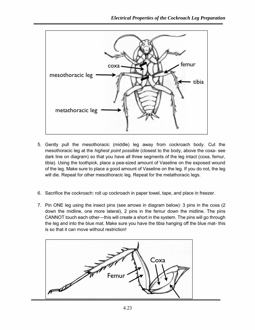
5. Gently pull the mesothoracic (middle) leg away from cockroach body. Cut the mesothoracic leg at the highest point possible (closest to the body, above the coxa- see dark line on diagram) so that you have all three segments of the leg intact (coxa, femur, tibia). Using the toothpick, place a pea-sized amount of Vaseline on the exposed wound of the leg. Make sure to place a good amount of Vaseline on the leg. If you do not, the leg will die. Repeat for other mesothoracic leg. Repeat for the metathoracic legs.
6. Sacrifice the cockroach: roll up cockroach in paper towel, tape, and place in freezer.
7. Pin ONE leg using the insect pins (see arrows in diagram below): 3 pins in the coxa (2 down the midline, one more lateral), 2 pins in the femur down the midline. The pins CANNOT touch each other—this will create a short in the system. The pins will go through the leg and into the blue mat. Make sure you have the tibia hanging off the blue mat- this is so that it can move without restriction!
mesothoracic leg
metathoracic leg
coxa femur
tibia
Coxa
Femur
Lab 4
4.24
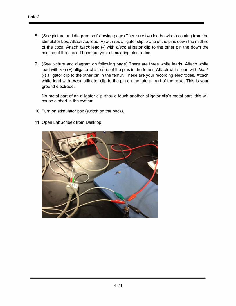
8. (See picture and diagram on following page) There are two leads (wires) coming from the
stimulator box. Attach red lead (+) with red alligator clip to one of the pins down the midline of the coxa. Attach black lead (-) with black alligator clip to the other pin the down the midline of the coxa. These are your stimulating electrodes.
9. (See picture and diagram on following page) There are three white leads. Attach white lead with red (+) alligator clip to one of the pins in the femur. Attach white lead with black (-) alligator clip to the other pin in the femur. These are your recording electrodes. Attach white lead with green alligator clip to the pin on the lateral part of the coxa. This is your ground electrode.
No metal part of an alligator clip should touch another alligator clip’s metal part- this will cause a short in the system.
10. Turn on stimulator box (switch on the back).
11. Open LabScribe2 from Desktop.

Electrical Properties of the Cockroach Leg Preparation
4.25
Labscribe2 screenshots

Lab 4
4.26
Eliciting a CAP
Measuring Cursers
Time between cursers
Voltage difference
between cursers
Time between pulses
Duration
# pulses
Amplitude (Intensity)
Hit “Apply” to update settings
Zoom in y-axis
Red plus sign to zoom in x-axis Zoom out x-axis

Electrical Properties of the Cockroach Leg Preparation
4.27
1. In LabScribe, under Settings, select Lab4_StimulationRep
2. Under View, click (or unclick—this is a toggle checkmark) Stimulator Panel. This is where
you can set the amplitude and duration of stimulation as well as the number of pulses. YOU MUST HIT APPLY AFTER EVERY CHANGE.
3. Initial settings: amplitude (Amp) = 0.5 # of pulses = 1 duration (W(ms)) = 0.1ms (See screenshots of how to use LabScribe)
4. Click Apply then Record.
5. This setting does 10 sweeps and averages the 10 sweeps as it goes. DO NOT HIT STOP DURING A SWEEP. LABSCRIBE WILL CRASH. YOU MUST WAIT UNTIL THE PROGRAM FINISHES—IT WILL STOP ITSELF. Example Traces:
Stimulus ArtifactStimulus Artifact
CAP
Stimulus Artifact
CAP
multiple
components
Stimulus Artifact
CAP
multiple
components

Lab 4
4.28
6. Use the blue cursers to zoom in on the x axis: move the two cursers to surround the area of interest (your stimulus artifact and CAP if you have one) and click on the red + sign to zoom in on the x-axis. To zoom in on the y-axis, double click on the y-axis or click the + sign next to ‘AutoScale’. (See Labscribe2 screenshots) To zoom out on the x-axis click the mountain symbol next to the red + sign. To zoom out on the y-axis, click the – sign next to ‘add function.’
7. WAIT 20 SECONDS before stimulating the leg again. Use a stopwatch.
8. If you have not seen a CAP, increase the amplitude to 1.0.
9. If you have not seen a CAP, increase the amplitude to 2.0.
10. If you have not seen a CAP, increase the amplitude to 3.0.
11. If you have not seen a CAP, increase the amplitude to 4.0.
12. If you do not see any CAP, try repining the stimulating electrodes and complete steps 1-9. It is possible neither electrode was near a nerve fiber. If this fails, pin another cockroach leg. ***ONCE YOU SEE A CAP DO NOT TOUCH/MOVE ELECTRODES***
Thought Questions:
1. Are the components that make up the first part of the CAP likely resulting from faster or slower fibers? Do you think they would have smaller or larger diameters?
Faster. Larger.
2. The CAP shows multiple downward and upward deflections, but sometimes the last deflection is much longer and has reduced amplitude compared to the others (see example traces on page 4.14. Observe the low amplitude curve at the tail end as it slowly returns to 0mV). What mechanism could be causing this? (hint: it has to do with channels)
K+ channels are slow to close to long hyperpolarization- see figure 4.2
EXPERIMENT 2: Amplitude-Duration Curve

Electrical Properties of the Cockroach Leg Preparation
4.29
Now that you have observed a CAP, DO NOT TOUCH OR MOVE ELECTRODES. You will now explore nerve excitability. Procedure
1. Initial settings: amplitude (Amp) = 0.5 # of pulses = 1 duration (W(ms)) = 0.1ms
2. Click Apply then Record
3. This setting does 10 sweeps and averages the 10 sweeps as it goes. DO NOT HIT STOP DURING A SWEEP. LABSCRIBE WILL CRASH. YOU MUST WAIT UNTIL THE PROGRAM FINISHES- IT WILL STOP ITSELF.
4. Gradually increase stimulus intensity (Amp) (HIT APPLY AFTER EACH CHANGE AND WAIT 20 SECONDS) until a CAP is observed. Record this stimulus intensity in the table below (this is the minimum stimulus intensity that is able to produce a CAP at a duration of 0.1ms).
5. Increase the duration by 0.1ms. Now decrease the stimulus intensity until you no longer see a CAP. Record, in the Table below, the lowest stimulus intensity at which you observed a CAP.
6. Repeat step (5) until you observe two subsequent durations (ex. Durations of 0.8ms and 0.9ms) that require the same intensity (ex. Amp = 0.54) to elicit a CAP.

Lab 4
4.30
Intensity (V)
Duration (ms)
0.1 0.2 0.3 0.4 0.5 0.6 0.7 0.8 0.9 1.0
7. Plot the intensity and duration on the graph below.
I N T E N S I T Y (V) Duration
8. Set the stimulus intensity (Amp) to the minimum stimulus intensity that is able to produce
a CAP at a duration of 0.1ms (from chart above). Set the stimulus duration to 0.1ms.
9. Click Apply then Record.
10. In your lab notebook record (describe or draw) the stimulus artifact and CAP.
11. Change the stimulus duration to 1.0ms. DO NOT change the stimulus intensity.
12. Click Apply then Record.
13. In your lab notebook record (describe or draw) the stimulus artifact and CAP.
Stimulus Artifact C. A.P.
Duration
0.1ms: 1.0ms:
0.1ms: 1.0ms:

Electrical Properties of the Cockroach Leg Preparation
4.31
Thought Questions:
1. In reference to step #13: Why does the stimulus artifact NOT increase in size vertically (i.e. why does it maintain the same intensity)?
Because the stimulus intensity is the same (only changing duration).
2. In reference to step #13: Why does the CAP increase in size vertically (i.e. why does the CAP increase in intensity)?
CAP amplitude is dependent on the number of axons firing. Increasing duration causes more axons to fire, increasing CAP size
3. What is the chronaxie time for your nerve fiber?
4. What is the rheobase voltage for your nerve fiber?
5. Why does increasing the duration of simulation allow for decreased intensity of stimulation to obtain the same CAP? (hint: see this chapter’s material) Specifically discuss the ideas of nerve excitability and fiber recruitment.
From chapter: Fiber recruitment is the process in which increasing the amplitude or duration of a stimulus increases the number of fibers activated. Fibers with faster conduction velocities are more excitable. These fibers require less current (either a weaker stimulus intensity at a given duration or a shorter duration at a given stimulation intensity). For a given stimulus strength (intensity), a longer stimulation duration would be needed to bring the fibers that have a slower conduction velocity to threshold.
6. You may notice your chronaxie time and rheobase voltage differ from other groups. Without dissecting the cockroach leg, we cannot know the distance between the stimulating electrodes and the nerve fiber. If your stimulating electrodes were far from the nerve, would your rheobase voltage be high or low? Why?
High because need greater intensity to bring nerve to threshold because voltage has to travel further to reach nerve (loses voltage along the way)

Lab 4
4.32
EXPERIMENT 3: Correlate CAP size with degree of movement For this experiment, one lab member will control the computer. The other three lab members must watch the cockroach leg- this will allow for greater reliability of measurement. Procedure
1. Initial settings: amplitude (Amp) = 0.5 # of pulses = 1 duration (W(ms)) = 0.1ms
2. Three lab members watch the cockroach leg closely. Click Apply then Record.
3. This setting does 10 sweeps and averages the 10 sweeps as it goes. DO NOT HIT STOP DURING A SWEEP. LABSCRIBE WILL CRASH. YOU MUST WAIT UNTIL THE PROGRAM FINISHES- IT WILL STOP ITSELF.
4. Record the CAP intensity and degree of leg movement in the table below. To make measurements: Use the blue cursers to zoom in on the x axis: move the two cursers to surround the area of interest (your stimulus artifact and CAP) and click on the red + sign to zoom in on the x-axis. To zoom in on the y-axis, double click on the y-axis or click the + sign next to ‘AutoScale’. Now place one blue vertical cursor just before the stimulus artifact. Place the other blue curser such that it intersects the highest (or lowest- whichever has greater magnitude) point of the CAP. In the upper right corner will be the difference along the y-axis (V2-V1) as well as the difference along the x-axis (T2-T1 or time) (See Labscribe2 screenshots). Remember the trace you are observing is represented as the change in voltage (y-axis) over time (x-axis).
5. If you do not see a CAP at Amp=0.5, gradually increase stimulus intensity (Amp) (HIT APPLY AFTER EACH CHANGE AND WAIT 20 SECONDS) until a CAP is observed.
6. Once you observe a CAP, record the stimulus intensity (Amp), CAP intensity, and degree of leg movement in the table below.
7. Increase stimulus intensity in small increments until you see the tarsus move. (HIT APPLY AFTER EACH CHANGE AND WAIT 20 SECONDS). Record the stimulus intensity (Amp), CAP intensity, and degree of leg movement in the table below. (If you immediately see both the tarsus and tibia moving, try smaller increments of stimulus intensity to see just the tarsus move).
1. Increase stimulus intensity in small increments until you see the tibia move. (HIT APPLY AFTER EACH CHANGE AND WAIT 20 SECONDS). Record the stimulus intensity (Amp), CAP intensity, and degree of leg movement in the table below.
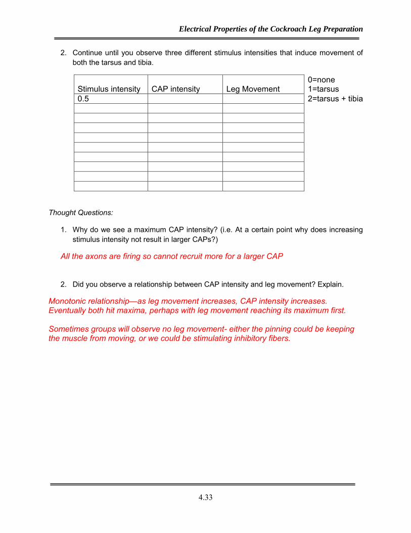
Electrical Properties of the Cockroach Leg Preparation
4.33
2. Continue until you observe three different stimulus intensities that induce movement of both the tarsus and tibia.
Stimulus intensity CAP intensity Leg Movement 0=none 1=tarsus
0.5 2=tarsus + tibia
Thought Questions:
1. Why do we see a maximum CAP intensity? (i.e. At a certain point why does increasing stimulus intensity not result in larger CAPs?)
All the axons are firing so cannot recruit more for a larger CAP
2. Did you observe a relationship between CAP intensity and leg movement? Explain.
Monotonic relationship—as leg movement increases, CAP intensity increases. Eventually both hit maxima, perhaps with leg movement reaching its maximum first. Sometimes groups will observe no leg movement- either the pinning could be keeping the muscle from moving, or we could be stimulating inhibitory fibers.

Lab 4
4.34
EXPERIMENT 4: Refractory Period Procedure
1. Initial settings: amplitude (Amp) = an intensity that evoked a moderately sized CAP # of pulses = 2
Toff (time between pulses) = 500ms duration (W(ms)) = 0.1ms
2. Click Apply then Record
3. This setting does 10 sweeps and averages the 10 sweeps as it goes. DO NOT HIT STOP DURING A SWEEP. LABSCRIBE WILL CRASH. YOU MUST WAIT UNTIL THE PROGRAM FINISHES- IT WILL STOP ITSELF. Example Trace:
Stimulus Artifacts
CAP1CAP2

Electrical Properties of the Cockroach Leg Preparation
4.35
4. Record intensity of first CAP (CAP1) and second CAP (CAP2) in table below:
Use the blue cursers to zoom in on the x-axis: move the two cursers to surround the area of interest (your stimulus artifact and CAP) and click on the red + sign to zoom in on the x-axis. To zoom in on the y-axis, double click on the y-axis or click the + sign next to ‘AutoScale’. Now place one blue vertical cursor just before the stimulus artifact of CAP1. Place the other blue curser such that it intersects the highest (or lowest- whichever has greater magnitude) point of CAP1. In the upper right corner will be the difference along the y-axis (V2-V1) as well as the difference along the x-axis (T2-T1 or time). Do the same for CAP2: Place one curser just before the 2nd stimulus artifact and the other curser at the highest (or lowest- whichever has greater magnitude) point of CAP2.
5. Change Toff to 300ms. Click Apply then Record. Record CAP1 and CAP2 intensities below.
6. Continue changing Toff according to the table below and record CAP intensities (HIT APPLY AFTER EACH CHANGE AND WAIT 20 SECONDS).
Toff CAP 1 intensity CAP 2 intensity 500ms 300ms 200ms 100ms 50ms 20ms 10ms 5ms 3ms
Thought Questions:
1. Why does CAP2 become smaller than CAP1 as you decrease the time between stimulations?
Reached the absolute refractory period for some axons, therefore reached the relative refractory period for the CAP (many axons, some of which have not reached the absolute refractory period)

4.36
EXPERIMENT 5: Visualize the stimulus artifact and the CAP
1. Initial settings: amplitude (Amp) = an intensity that evoked a moderately sized CAP # of pulses = 1 duration (W(ms)) = 0.1ms
2. Click Apply then Record
3. This setting does 10 sweeps and averages the 10 sweeps as it goes. DO NOT HIT STOP DURING A SWEEP. LABSCRIBE WILL CRASH. YOU MUST WAIT UNTIL THE PROGRAM FINISHES- IT WILL STOP ITSELF.
4. Record what the stimulus artifact and CAP look like in the “Before” area below:
5. Change the polarity of the stimulating electrodes: In the “Amp” box, change the Amp to -
(negative) (this effectively changes the stimulating electrode + to – and stimulating electrode – to +). In your lab notebook record (describe or draw) the effects of changing Polarity on the stimulus artifact and CAP in the “After” area below:
Stimulus Artifact C. A.P. Polarity
Before: After:
Before: After:
Thought Questions:
1. What is the difference between the way the stimulus artifact changed and the way the CAP changed when you switch the polarity?
Stimulus artifact flipped. CAP did not change. It is also possible that the CAP changes but it will not flip directions. If the CAP changes it is due to difference in the way it is being stimulated. SA flips because the charge flips.

Electrical Activity of Neurons
4.37
2. Based on what you have learned, why does the CAP not change the same way as the stimulus artifact?
The stimulus artifact is a reflection of the stimulus. Flipping the polarity of the stimulus will flip the stimulus artifact. Action potentials can only be caused by depolarization of the axons, therefore it does not matter which stimulating electrode is positive or negative – if the axons are stimulated enough to produce action potentials, they will always depolarize (in the case of CAP not changing) or the way they are being stimulated is different so CAP might disappear or change in size (in the case of CAP changing).

Flipping a Course: Electrical Properties of the Cockroach Leg Preparation
University of California at IrvineRABLE Conference
Presented by: L. Javier, A. White, V. Boucquey, N. Goldberg, A. Nicholas

Flipping a Classroom
• Flipped Classroom Design• Rocket Mix Modules• Lab Exercises and Data• Abstract Writing Assignment
http://www.washington.edu/

Experiment 1: Electrical Activity of Neurons
Experiment 2: Electrical Properties of theCockroach Leg Preparation
Lab Exercises

Course Organization
• Compliments in-class activities

Experiment 1: Electrical Activity of Neurons
Background:
• Methods used to generate and interpret electrophysiology data
• History of cockroach leg preparation
Experimental Goal:• Complete cockroach preparation (group work)• Listen to spontaneous and evoked activity• Use on cockroach to stimulate another leg• Thought Questions

Rocketmix Module
Rocketmix:https://my.rocketmix.com/InstructorHome.aspx

Experiment 2: Electrical Activity of Neurons
Background:
• Electrical properties of neurons
• Single action potential
• Compound Action potential (CAP)
• Use electrophysiology to learn about the organization of the cockroach leg preparation
Experimental Goal:• Record and measure CAP• Identify absolute and relative refractory period

Rocketmix
Advantages:-Students have easy access to dynamic video presentation
-Primes students before class and tests their own understanding of the material
-Allows instructors to evaluate student understanding and ease of material
Training video for future instructors

Rocketmix
Limitation:-Only as effective as the students utilization
-Rocketmix modules must be clear and precise

Workshop 5RABLE 2015

Inquiry-based investigation of ectothermic metabolism University of California, Irvine
Nancy Aguilar-Roca ([email protected]) Over the course a traditional physiology course, discussions of metabolism often focus on mammals which are endothermic homeotherms. Students may not be exposed to heterothermic ectotherms, which are the vast majority of all living organisms. In recent years, research on heterothermic ectotherms has surged because of their vulnerability to climate change. The goal of this lab exercise is to add an open-ended inquiry element to a traditional protocol for measuring the effect of temperature on an ectotherm (the Madagascar Hissing Cockroach, Gromphadorhina portentosa). Gromphadorhina colonies are easily maintained in small spaces, genders are easily distinguished, adults are large enough to be individually marked for tracking, and it’s possible to create custom diets with controlled quantities of supplements. Prior to this lab exercise, students will learn about metabolism and the differences between ectotherms and endotherms, and they will design their experiment. This system is flexible so that a multitude of different experimental designs are possible. The experimental treatments that have been used so far are the effects of chronic caffeine, green tea and a sports supplement on O2 consumption and CO2 production. For a class of 227 physiology students (in 11 lab sections), we set-up multiple colonies of Gromphadorhina with 2 replicate colonies of each supplement. Each lab section put the results of their experiments into a common database (a Google spreadsheet), and each TA was given the opportunity to structure a post-experiment activity for their own students. Potential Learning Goals
● compare and contrast endotherm, ectotherm, homeotherm and heterotherm. ● explain the relationship between environmental temperature and the metabolic rate of
an ectotherm (Madagascar Hissing Cockroach, Gromphadorhina portentosa). ● develop and test a hypothesis about the effect of a dietary or pharmacological
substance on metabolic rate Materials
● Madagascar Hissing cockroaches ● Metabolic chambers and gas analyzers or manometers ● Dry dog or cat food ● Coffee grinder or mortar & pestle ● Assorted supplements (liquid or powdered)
Cockroaches Madagascar hissing cockroaches are fairly easy to keep. They will thrive (and probably reproduce) in a container with a mix of foods (dog/cat food, small pieces of apples, lettuce, carrots), places to hide (egg cartons work well) and a heating pad or heat lamp (~25-30oC). http://www.petco.com/caresheets/invertebrates/Cockroach_MadagascarHissing.pdf http://agweb.okstate.edu/fourh/aitc/lessons/extras/cockroach.pdf
1

Cockroaches also need a water source. Water beads are a good option because they don’t spill and you can monitor how fast they are used. Potential suppliers of madagascar hissing cockroaches (and most of these also sell water beads/crystals)
New York Worms: http://www.nyworms.com/index.html Rainbow mealworms: http://rainbowmealworms.net Ken the Bug Guy: http://kenthebugguy.com West Coast Roaches: http://westcoastroaches.com
Cockroaches are large enough for marking individuals if students want to track weight changes. Students can create their own marking system with dots of acrylic paint on the carapace. Custom food for experiments The exact ratio of dried dog/cat food to liquid will vary with the brand of food so you may need to experiment a little to find a ratio that will work for you. We’ve been using 1g food plus 1 ml water or juice. Put your desired quantity of dried food into the coffee grinder (or mortar) and grind it. Add the appropriate amount of liquid to create a paste (roughly the same consistency as play-doh). Cut the tip off of a 10ml syringe and put the food into the syringe. You can extrude the paste from the syringe into regularly shaped pellets. (A pastry bag with a frosting tip would work too). Let the pellets dry out. If you are adding a powdered supplement, add a known quantity to the ground dog/cat food before making the paste. Students can change the ratio of supplement to ground food to generate dose-response curves. If you are adding a liquid supplement, add it to the water (or juice) for making the paste. Again, you can vary the ratio of water to supplement to generate dose-response curves. Before giving the roaches the supplemented food, they should be starved for 1 to 2 weeks (but with access to water beads). Deciding how long to feed the supplement to the roaches before measuring metabolic rate is a factor that students will have to decide on. Measuring metabolic rate The protocol described below can be accomplished in a 3-hr lab period. Glass jars are best for metabolic rate measurements (many plastics are oxygen permeable). I use 500ml glass canning jars.
2

In this set-up the lid of the jar has 2 holes: 1 has a tubing connector to attach to the gas analyzer and the second one is to allow for air-flow to the gas analyzer. (I put a magnet on top to prevent it from floating in the water bath). I put 2-3 similar sized cockroaches into the chamber, close the jar, and cover the openings with tape, so that the chamber is completely sealed and no fresh air can enter. Record the time at which the chamber was first sealed shut and put the chamber into a water bath. Let the sealed chambers incubate for at least 60 minutes at temperatures above 23oC, and at least 90 minutes at temperatures below 23oC. When ready, stop the timer and record the time to the nearest minute. Uncover both openings and attach the tube from the gas analyzers to the connector on the lid of the chamber. The other opening must be uncovered, to allow fresh air into the chamber as the analyzers remove the experimental air. Record the data from the gas analyzers. It should take about 2 minutes get these readings. Record the lowest %O2 and the highest %CO2. Disconnect your chamber, remove the lid, and return the roaches to their cages. Calculations Vo2 (ml O2/min) = 0.9 * (Fo2_Starting - Fo2_Ending) * (Chamber Volume) / min
Fo2_Starting = fraction of oxygen in the air = 0.2095 Fo2_Ending = what you measured (percent divided by 100). 0.9 is to convert from ATPS to STPD (assuming room temperature is 21oC and atmospheric pressure is 760mmHg)
Relative-Vo2 = Vo2 / mass Vco2 (ml O2/min) = 0.9 * (Fco2_Ending) * (Chamber Volume) / min
Fco2_Ending = what you measured (percent divided by 100). If you don’t have gas analyzers, you can use a manometer. Manometers can be made with varying levels of sophistication, but they all consist of a closed chamber with a piece of water filled-tubing attached. As the animal inside the chamber respires, Soda lime or (potassium hydroxide) absorbs CO2 and the volume of oxygen inside the chamber decreases. The water in the tubing will move as the gas volume in the chamber changes. The simplest version is below. It consists of a jar on its side and with a one-hole stopper with a 1-ml pipet (Hiebert and Noveral, 2007). The organism can be kept away from the soda lime with wire mesh. The volume of oxygen consumed is read directly from the movement of the
3

water. By removing the soda lime, you can measure CO2 produced (Vco2). This apparatus works best in an incubator because the volume of air in the chamber will change with variations in ambient temperature.
In the second manometer set-up shown below, the second chamber corrects for temperature-induced changes in air volume. As the animal consumes oxygen, the fluid in the manometer will shift towards the chamber with the organism. At set-time points, air (or pure oxygen) is injected into the chamber until the fluid in the manometer returns to its original position. The volume of air injected is the volume of oxygen consumed. As with the simple manometer above, you can determine CO2 production by removing the soda lime. http://sites.sinauer.com/animalphys3e/boxex07.04.html http://www.nuffieldfoundation.org/practical-biology/measuring-rate-metabolism Noveral, J. and S. Hiebert. 2007. Are chicken embryos endotherms or ectotherms? A laboratory exercise integrating concepts in thermoregulation and metabolism. Adv. Physiol. Ed. 31: 97-109. http://advan.physiology.org/content/31/1/97
4

Workshop 6RABLE 2015

BRINGING CHLAMYDIA AND CONFLICT TO THE CLASSROOM AN INTERACTIVE DISCUSSION ACTIVITY TO ASSESS STUDENTS' ABILITY TO READ PRIMARY LITERATURE
Bekah Le, Charles Yi, Vaishali Jayashankar, Seong Kim, and Rabi Murad University of California, Irvine Dept. of Developmental and Cell Biology GAANN Fellows
© 2015, UCI GAANN

How to read a science paper…?
• Rationale for this workshop: • The ability to read and analyze primary literature is a necessary
skill for students pursuing health science and research careers.
• Students don’t often get to practice this skill, especially in large classrooms.
• Students should learn about the “realities” of research and the process of discovery.
3/4/2014 Piled Higher and Deeper
http://www.phdcomics.com/comics/archive_print.php?comicid=974 1/1
Piled Higher and Deeper by Jorge Cham www.phdcomics.com
title: "We're all doomed" - originally published 2/6/2008
3/4/2014 Piled Higher and Deeper
http://www.phdcomics.com/comics/archive_print.php?comicid=974 1/1
Piled Higher and Deeper by Jorge Cham www.phdcomics.com
title: "We're all doomed" - originally published 2/6/2008
© 2015, UCI GAANN

D140: “How to read a science paper” • This workshop presents a module that stemmed from an
upper division elective course developed by three Ph.D. candidates.
• Small class size – 15 students per discussion.
• Modules consisting of: • Research seminar given by current graduate student. • “Journal Club” style discussion.
• Presentations, figure facts worksheet (Round, 2013) and pre- and post-module online quizzes.
• Class sessions devoted to Dev Bio techniques.
© 2015, UCI GAANN

Students self-reported increase in confidence
0
5
10
15
5 4 3 2 1
Generally, I feel confident about
working in a biological research laboratory*
5 4 3 2 1
I am sure I could conduct independent biological research*
5 4 3 2 1
I can handle reading and interpreting primary
scientific literature*
0
5
10
15
5 4 3 2 1
I generally feel confident explaining biological
research to non-scientists*
5 4 3 2 1 5 4 3 2 1
I generally feel confident explaining biological research to my PI*
I generally feel confident explaining biological
research to my peers in small groups*
Num
ber o
f Stu
dent
sN
umbe
r of S
tude
nts
Pre-Test Post-Test
Pre-Test Post-Test
Strongly
Agree AgreeNeutral
DisagreeStrongly
Disagree Strongly
Agree AgreeNeutral
DisagreeStrongly
Disagree Strongly
Agree AgreeNeutral
DisagreeStrongly
Disagree
Strongly
Agree AgreeNeutral
DisagreeStrongly
Disagree Strongly
Agree AgreeNeutral
DisagreeStrongly
Disagree Strongly
Agree AgreeNeutral
DisagreeStrongly
Disagree
* P-value ≤ 0.05 (Wilcoxon signed-rank test) © 2015, UCI GAANN

Structure of today’s workshop • Present a module that can be incorporated into an
existing course: • Introduction to the topic and basic techniques
• Individual reading of one of two papers (shortened for workshop)
• Discussion of same paper in small groups
• Discussion of both papers in combined groups
• Whole class discussion of both papers
• Closing discussion on module and modifications.
© 2015, UCI GAANN

• Most commonly reported notifiable disease in the U.S. (regular, frequent information about individual cases is necessary for prevention and control of disease)
Chlamydia trachomatis causes significant disease
Number of reported notifiable disease cases in the U.S. in 2012
Chlamydia trachomatis genital infections
Gonorrhea
Salmonellosis
Syphilis
Chicken Pox
AIDS
Other CDC, 2014
© 2015, UCI GAANN

The number of reported Chlamydia genital infections are increasing annually in the U.S.
CDC, 2009
© 2015, UCI GAANN

C. trachomatis relies on a host cell for survival
• Obligate intracellular bacterium
• Modulation of host cell pathways promotes bacterial growth • Avoidance of fusion with
lysosomal pathway • Acquisition of host lipids
and nutrients
• Host cell complements minimal chlamydial genome
J. Lee, UC Irvine
© 2015, UCI GAANN

Chlamydia induces specific host-pathogen interactions
Golgi reorganization Resistance to apoptosis Heuer et al., Nature, 2009 Fischer et al., J Exp Med, 2004
Intermediate filament re-organization
Kumar and Valdivia, Cell Host Microbe, 2008
Enhance lipid acquisition Preserve host cell and ensure bacterial
replication
Support the chlamydial inclusion
© 2015, UCI GAANN

How does Chlamydia induce host-pathogen interactions? • Secreted effectors
• Chlamydial proteins that can be translocated into the host cell cytoplasm
• Modulate normal cellular proteins and processes
• Others?
© 2015, UCI GAANN
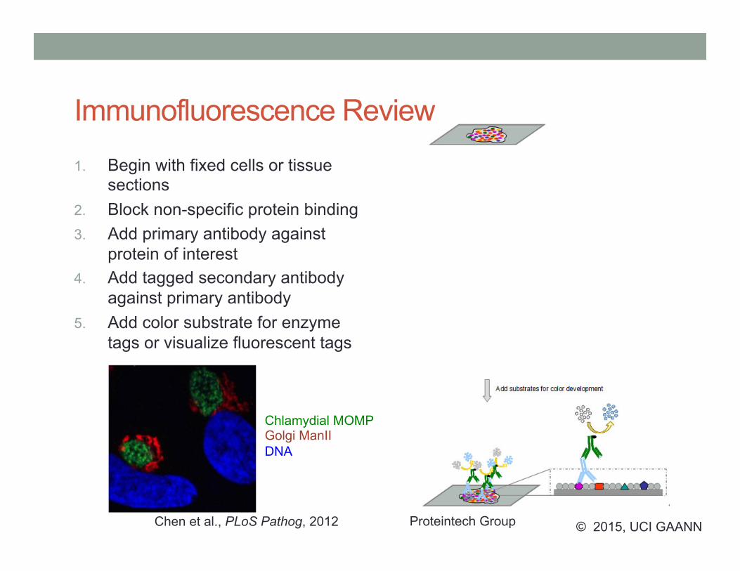
Immunofluorescence Review
1. Begin with fixed cells or tissue sections
2. Block non-specific protein binding 3. Add primary antibody against
protein of interest 4. Add tagged secondary antibody
against primary antibody 5. Add color substrate for enzyme
tags or visualize fluorescent tags
Chen et al., PLoS Pathog, 2012
Chlamydial MOMP Golgi ManII DNA
Proteintech Group © 2015, UCI GAANN

Western Blot Review Lyse Cells
Lysate containing proteins
C-Nap1
γ-Tubulin Non-specific band
Cleavage product
Loading control
1. Collect lysate from cells 2. Denature proteins 3. SDS-PAGE 4. Transfer to membrane 5. Blot with specific primary
antibodies to protein of interest 6. Blot with secondary antibodies
to visualize proteins 7. How do you control for loading
errors?
J. Lee, UC Irvine © 2015, UCI GAANN

Please read your assigned paper individually
Heuer et al
Chen et al
© 2015, UCI GAANN

Please form groups based on paper and color
Heuer et al Heuer et al
Chen et al Chen et al
Please discuss your responses to the questions with your
group members
© 2015, UCI GAANN

Please merge with a group that has the other paper
Please exchange the following information by comparing
the following information: hypothesis, key results and conclusions
Heuer et al Chen et al
Heuer et al Chen et al
+
+
© 2015, UCI GAANN

Questions addressing both papers • Please spend 10 minutes to answer the following
questions: • State the hypothesis being tested by the authors (one
sentence, do not copy from the authors’ text) • Based on the data presented, what conclusion can be
drawn from each individual paper? • From reading both of these papers, what conclusion did
you draw about the role of golgin-84 cleavage play in chlamydia infection?
• Can you think of an interpretation that will explain both sets of data?
© 2015, UCI GAANN

Whole group discussion • Can you think of an interpretation that will explain both
sets of data? • What are the significance of these papers? How do these
differing results impact the field? • What can you do to resolve different research findings in
literature?
A potential “end of activity” assignment for students: Write a paragraph on what you learned about critically reading
scientific literature.
© 2015, UCI GAANN

How could this module be implemented in lecture and lab courses?
© 2015, UCI GAANN

Suggestions for implementing this module
Choosing papers • Interesting biological or pathological problem
• Classic paper or current papers that are controversial/relevant • Paper could cover topics and techniques from lecture and
lab courses • Articles with straightforward techniques and clear
questions would be ideal
Other Modifications (please see our lesson plan) • Students can read the paper before coming to class • Assignment based on the paper could be assigned • When the questions are handed out can be varied
© 2015, UCI GAANN

Thank you for attending and please fill out the provided evaluation form!
© 2015, UCI GAANN

Workshop 7RABLE 2015

7.1
LAB 7 Behavioral Neuroscience- Habituation in C. elegans
Adapted and Written by Annie Ciernia, Drew Headley, Alex Pevzner, and Lauren Javier
Workshop presented by Julia Overman, Lauren Javier, Natalie Sashkin Goldberg, Andre White, Veronique Boucquey, and Dr. Andrea Nicholas
Summary Across generations evolutionary adaptation shapes species to better fit their environment, but within a single lifetime individuals can learn new behaviors that further enhance their chances of survival. To do this, organisms must internalize the current state of the environment so that they can anticipate and optimally respond to future conditions. Such relationships between stimuli and their consequences can be learned as the organism interacts with its environment. For example, a child might learn after getting stung by a bee to be wary of insects. In this example the child gains an understanding of the relationship between bees and their ability to sting and cause her pain, and can use this information to avoid bees in future situations. The neural basis of this type of phenomenon is largely the concern of behavioral neuroscience. For this exercise, we will focus on the role of the nervous system in mediating the learned behavior of C. elegans, a small worm that displays many of the same acquired behaviors as larger, more complex creatures, such as mammals. Towards this end, a framework for understanding learning and memory with respect to behavior will be explained. Goals
Introduce the fundamentals of behavioral neuroscience Become familiar with principles of experimental design for behavioral analyses
Investigate the link between genetics and behavior using a model organism, C. elegans
Characterize mechanosensory habituation in C. elegans through interpretation of experimental results
Figure 7.1. Ivan P. Pavlov, the discoverer of classical condition, with one of his dogs.
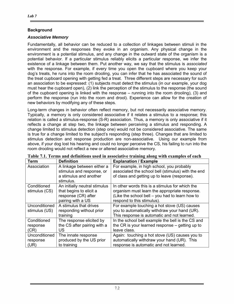
Lab 7
7.2
Background Associative Memory
Fundamentally, all behavior can be reduced to a collection of linkages between stimuli in the environment and the responses they evoke in an organism. Any physical change in the environment is a potential stimulus, and any change in the outward state of the organism is a potential behavior. If a particular stimulus reliably elicits a particular response, we infer the existence of a linkage between them. Put another way, we say that the stimulus is associated with the response. For example, if every time you open the cupboard where you keep your dog’s treats, he runs into the room drooling, you can infer that he has associated the sound of the treat cupboard opening with getting fed a treat. Three different steps are necessary for such an association to be expressed: (1) subjects must detect the stimulus (in our example, your dog must hear the cupboard open), (2) link the perception of the stimulus to the response (the sound of the cupboard opening is linked with the response – running into the room drooling), (3) and perform the response (run into the room and drool). Experience can allow for the creation of new behaviors by modifying any of these steps.
Long-term changes in behavior often reflect memory, but not necessarily associative memory. Typically, a memory is only considered associative if it relates a stimulus to a response; this relation is called a stimulus-response (S-R) association. Thus, a memory is only associative if it reflects a change at step two, the linkage between perceiving a stimulus and responding. A change limited to stimulus detection (step one) would not be considered associative. The same is true for a change limited to the subject’s responding (step three). Changes that are limited to stimulus detection and response production are non-associative. Using our example from above, if your dog lost his hearing and could no longer perceive the CS, his failing to run into the room drooling would not reflect a new or altered associative memory.
Table 7.1. Terms and definitions used in associative training along with examples of each Term Definition Explanation / Example Association A linkage between either a
stimulus and response, or a stimulus and another stimulus.
For example, in high school, you probably associated the school bell (stimulus) with the end of class and getting up to leave (response).
Conditioned stimulus (CS)
An initially neutral stimulus that begins to elicit a response (CR) after pairing with a US
In other words this is a stimulus for which the organism must learn the appropriate response. (Like the school bell – you had to learn how to respond to this stimulus).
Unconditioned stimulus (US)
A stimulus that drives responding without prior training
For example touching a hot stove (US) causes you to automatically withdraw your hand (UR). This response is automatic and not learned.
Conditioned response (CR)
The response elicited by the CS after pairing with a US
In the school bell example the bell is the CS and the CR is your learned response – getting up to leave class.
Unconditioned response (UR)
The innate response produced by the US prior to training
Again: touching a hot stove (US) causes you to automatically withdraw your hand (UR). This response is automatic and not learned.

As a side note, it is worth mentioning that current theories of associative memory argue that besides S-R associations, subjects also learn that one stimulus predicts another stimulus, which has been termed stimulus-stimulus (S-S) association. Psychologists and neuroscientists often have to infer S-S learning, because only the experimental stimulus and the animal's response are observable. A variety of tests have been developed to judge whether an associative memory reflects S-S or S-R learning. Frequently, including in this text, the observation of associative memory will be reported in S-R terms, while the psychological interpretation of the associative memory will be given in S-S terms. Given the previous example, the S-R interpretation is that the sound of opening the dog treat cabinet causes your dog to approach you and salivate. However, the S-S interpretation is that your dog has associated the sound of the cabinet opening with the dog treats, and thus the dog behaves as if anticipating the reward. In spite of these two different ways of viewing associative memory, both S-R and S-S require the change to occur between stimulus detection and response production. Ultimately, the same standardized protocols can be used to induce associative and non-associative memory, no matter whether associations are S-R or S-S.
Associative and Non-associative training protocols
To study how different training protocols produce associative or non-associative memories, we must establish a common vocabulary. Stimuli fall into two categories. Unconditioned stimuli (US) induce an innate response that does not depend on prior experience. Such stimuli are intrinsically motivating; subjects will either approach or avoid them without training. For instance, touching a hot stove will elicit a withdrawal response. The heat from the burner is sufficient to drive a response; you do not need to learn to withdraw your hand. In this case the hot stove is the US. The other class of stimuli is known as conditioned stimuli (CS). These are not intrinsically motivational, because subjects will eventually stop responding to them, unless they predict a US. The initial response to the CS is known as an orienting response (OR), and is driven by a sudden and unexpected change in the environment. Imagine a creaking noise you hear in your new apartment at night. At first you would notice it and become alert and concerned, but when enough nights had passed with the creaking noise, and nothing bad had happened you would get used to the noise and stop responding. The creaking is an example of a potential CS, if it predicted the arrival home of an upstairs neighbor that played really loud annoying music (a US) then you would continue to respond to the creaking.
Training subjects to learn that a CS predicts a US can be done with classical conditioning. Classical conditioning is a form of associative conditioning that involves pairing the CS with a US. During pairing the CS is presented and then shortly thereafter the US occurs. Each instance of presenting the CS and US is called a trial. Typically, the strength of the prediction will increase with the number of trials. Over time the CS will come to elicit a conditioned response (CR), the subject will respond to the CS as if anticipating the US. An iconic example is Pavlov’s dogs (Fig. 7.1), which were trained to associate the ringing of a bell with the presentation of beef. Upon hearing the bell, the dogs would begin salivating, as if anticipating the beef. If you then repeatedly present the bell without a food reward, the dog will learn that the CS no longer predicts the US. This form of new learning is called extinction. During extinction, a CS that was previously paired with a US is repeatedly presented alone (without the US). Thus, in extinction the previously acquired CS-US association is slowly "extinguished" after repeated CS only presentations (Fig. 7.2).

Lab 7
7.4
US
CS US
(A) Extinction
Figure 7.2. Extinction of Response (A) Classical conditioning repeatedly pairs the conditioned stimulus with an unconditioned stimulus (US). The acquired response to the CS is known as a conditioned response (CR). When the conditioned stimulus is presented repeatedly without the unconditioned stimulus, the subject learns that the CS does not predict the US. As a result, the subject’s conditioned response diminishes over trials, until finally, it no longer elicits a conditioned response. This is known as extinction.
Besides learning that one stimulus predicts another, such as in classical conditioning, in non-associative conditioning, subjects can also learn that stimuli are not predictive. Two commonly studied forms of non-associative learning are habituation and sensitization. During habituation, a novel stimulus (S) is repeatedly presented without a US. During repeated presentations the subject learns that the S does not predict another stimulus, and consequently the subject stops responding to the S (decrease in OR). Another form of non-associative learning is sensitization. During sensitization the presentation of a strong stimulus (S) enhances future responses to many different stimuli. For example, your dog will respond much more strongly to a normal pitch tone after it has been played a painfully loud tone. In this example, the dog has been sensitized by the loud tone (S) and will then respond much more strongly to otherwise innocuous stimuli (increase in OR).

Figure 7.3. Training protocols us to study memory.
(A) Classical conditioning repeatedly pairs the conditioned stimulus with an unconditioned stimulus. Stimuli, such as the CS and US, elicit several different responses. The first CS presentation evokes an orienting response (OR), which is driven by the novelty of the CS. US presentation evokes a strong innate response (UR), reflecting its inherent biological significance. Responding to the unconditioned stimulus remains the same throughout training, while responding to the conditioned stimulus increases across training trials. The acquired response to the CS is known as the conditioned response (CR). (B) Habituation training lacks an unconditioned stimulus, and the repeated presentations of the novel stimulus (S) leads to decreased responding. (C) Sensitization presents a strong stimulus (S) without a US resulting in an increase in the orienting response over repeated S presentations. Memory vs. performance distinction
The field of learning and memory is interested in understanding how the nervous system acquires, stores and recalls information for experiences (i.e. memory). Although intuitive, ‘memory’ cannot be easily defined or directly measured. Memory must be inferred from a change in the animal’s behavior. Therefore, our capacity to study memory is conditional, not only on the animal being able to perform the task, but our ability to detect a change in the

Lab 7
7.6
performance. Such an indirect measure of memory is problematic for neuroscientists, because in the course of conducting experiments they must differentiate between the animal’s memory for an experience and its ability to perform the appropriate action. This is known as the memory vs. performance distinction.
It is important to note that if the animal doesn’t display ‘memory’ when tested one cannot automatically conclude that the animal didn’t learn or that it forgot the events. Below is an example to illustrate this point. Rats will explore (i.e. sniff, rear, lick) the environment in which they are placed. However, if a mild foot shock is administered in that environment then the rats change their behavior from exploration to defensive freezing (immobility). This is a well- characterized fear response that is context specific. In an effort to understand the neurobiology supporting contextual fear, researchers decided to lesion specific brain regions and observe the rat’s behavior after the lesion. One particular brain region that resulted in a significant decrease of freezing was the basolateral amygdala (BLA). Thus, it was concluded that the memory for contextual fear was in this structure. However, the memory vs. performance distinction was not given proper attention. Subsequent research demonstrated that animals with BLA lesions in fact were capable of remembering the context in which they received the shock, although they were not able to freeze in that context. If other fear related behaviors were measured (e.g. defecation, active avoidance, heart rate) then the animals showed a clear fear response.1
This example illustrates not only the importance of distinguishing between memory and performance in a task, but also the significance of measuring appropriate behaviors and conducting necessary controls. If freezing was the only measure taken then one would falsely conclude that the rats did not have a fear memory for the context. It was only through multiple independent measures that researchers were able to observe that the animal did remember the association between the context and shock. A critical control that was used to bolster this conclusion was demonstrating that BLA lesions prevented unconditioned freezing (freezing to cat hair, something that is not learned but is innate to rats).
Experimental Analysis of Behavior Behavior is often difficult to quantify and may show a great deal of variability both between animals and within the same animal. To determine behavioral effects of a stimulus accurately, researchers must do their best to make objective, unbiased observations and measurements of the behavior. Several strategies can be used to achieve this, any of which may be employed in this laboratory exercise.
To eliminate bias, some studies blind various aspects of the experiment so that not everyone knows what variables are being tested at a given point. For example, the experimenter may not know the specific gene mutation in their experimental subjects.
Another strategy is to gather multiple data points for the same item and then determine statistical trends. This could mean that multiple individuals, each with his/her own biases and perspectives, score the same behaviors simultaneously, or that multiple subjects are used in the study.
A third strategy relies on a clearly defined set of criteria for scoring behaviors so that, for example, different degrees of a behavior can be distinguished systematically.
C. elegans as a Model Organism Caenorhabditis elegans are soil dwelling, bacteria eating nematodes (roundworms) that are approximately 1mm in length. C. elegans have a relatively short lifespan and reproduce quickly,

making them ideal experimental subjects. In the last forty years C. elegans has been used as a model experimental organism in neurobiology, developmental biology, and cell biology.
For neurobiologists, the adult worm’s nervous system is an attractive model system for linking neuronal and molecular function to behavior. The adult worm’s nervous system is composed of exactly 302 neurons, all of which have been identified and their interconnectivity mapped. Despite their relative simplicity, the components of the C. elegans nervous system are similar to more complex organisms such as humans. For example, over 5,000 genes in the C. elegans genome have corresponding human homologs, including important nervous system components.2 Neurobiologists have also taken advantage of the sequencing of the C. elegans genome. Using this genetic information, researchers have made thousands of mutant worm strains. By targeting a specific gene and either knocking out or over expressing it, researchers have begun to examine the function of individual proteins. Combining the known neuronal connectivity with genetic manipulations has allowed researchers to begin linking molecules, neurons and behavior.
Adult C. elegans fall into one of two sexes: hermaphrodites or males (no females). Hermaphrodites possess all the necessary components for self-fertilization and are the most common sex of worm (~50-99% depending on the environmental conditions).3 Hermaphrodite self-fertilization allows for the generation of genetically identical offspring while male mating (with hermaphrodites) produces greater genetic diversity. A single hermaphrodite worm can produce approximately 300 progeny by self-fertilization or 1200-1400 progeny by mating with a male. A single adult male can father about 3,000 progeny.3
Whether generated by self-fertilization or sexual reproduction, the resulting eggs hatch into the first larval stage (L1) in approximately 14 hours. Assuming favorable conditions, L1 larvae progress to become L2 larvae. L2 larvae then continue to L3, L4, and then adulthood. By 45-50 hours post hatching, an adult hermaphrodite lays its first eggs, completing its reproductive life cycle. Adult hermaphrodites continue to lay eggs for 3-4 days and then live for an additional 10-15 days.3 However, if there is limited food, extreme temperatures, over crowding or other environmental stressors, L1 worms arrest development and enter the dauer stage. In this dormant stage, worms no longer feed and locomotion is dramatically reduced. Worms can remain in the dauer stage for up to four months and exit only when environmental conditions become favorable. When this occurs, dauer stage worms can develop into L4 larvae and then adults.

Lab 7
7.8
Figure 7.3. C. elegans Life Cycle. a. C. elegans hermaphrodites undergo sexual or self-fertilization to produce eggs. In approximately 14 hours the egg hatch into L1 larvae which then develop into L2 larvae if food is present. L2 larvae will then develop into L3, L4 and finally adults. If conditions are not favorable, L1 larvae will arrest development and enter the dormant dauer stage until conditions improve. b. Male C. elegans. Note the lack of eggs (middle circle) and fanned tail (right circle) that distinguish the male from hermaphrodites. Adapted from WormAtlas.org.
Habituation in C. elegans In this lab you will perform a series of experiments to characterize mechanosensory habituation in C. elegans. C. elegans respond to vibrations (which can be induced by tapping the side of the plate they live in) by reversing their swimming direction. This tap-withdrawal response shows multiple forms of non-associative learning including habituation, dishabituation, and sensitization.4 In order to conclude that the decrease in the tap-withdrawal response with repeated stimulation is true habituation learning, you need to test for performance confounds. Sensory adaptation or sensory fatigue is evoked activity that can often decrease as a result of prolonged stimulation. Sensory fatigue is simply the inability of the animal to respond to a stimulus due to a deficit, not in memory, but in sensation. For example, suppose a specific set of sensory neurons are required for C. elegans to respond to a mechanosensory stimulation. Furthermore, suppose these neurons can only respond once every 15 sec or they stop firing. With our repeated tapping the worms would rapidly be unable to respond due to a sensory deficit independent of their memory for the stimulus. Similarly, motor fatigue, which is the lack of responding due to a deficit in the motor system underlying the measured behavior, can produce behavior similar to habituation.

To distinguish between sensory/motor fatigue and habituation, we will use dishabituation- the phenomenon in which a strong novel or noxious stimulus can result in the return of the habituated behavior to near its pre-training response level. Immediately, following training a strong novel or noxious stimulus is delivered and the worms are then given a set of test taps. Dishabituation is shown by an increased response above habituated levels observed at the end of the training trials. Dishabituation is performed immediately following the memory test, at a time point when sensory adaptation and motor fatigue are predicted to be maximal. Consequently, if habituated worms show strong dishabituation following the strong noxious stimulus, it can be concluded that the initial habituation was not due to sensory or motor fatigue and is likely true habituation learning. Dishabituation is similar to sensitization, except that dishabituation produces a recovery of the original response while sensitization produces a response that is stronger than the original.
Today’s exercise will examine tap-withdrawal habituation in C. elegans. Small groups of C. elegans will be placed in petri dishes for these experiments. For habituation, the dish will be repeatedly taped, and the tap withdrawal (swimming reversal) response will be measured across trials. The final habituated response is predicted to be much smaller in magnitude then the initial response. In other words, after enough experience with the tapping vibration stimulus, the worms will decrease their swimming reversal response. We will be using two blocks of training trials separated by a 10min rest period (Fig 7.4). There is predicted to be “savings” between the two blocks of training trials. Savings refers to an enhanced rate of learning (i.e. habituation) during subsequent training. For example, if you learn a list of words and then forget them, you will be able to relearn them faster the second time then you did the first time. This difference in learning rate is savings. Following training, your worms will be given a 10min break and then 10 additional test taps. These taps are considered a “memory test” to assess how well your worms remember the initial training. Immediately following testing, you will dishabituate your worms to test for a potential performance impairment. In the final experiment of this lab you will examine a mutant strain of C. elegans, compare the mutant strain’s habituation learning to wild type C. elegans, and look up the function of your mutant protein.
Fig 7.4. Timeline for training and testing procedures in Experiments 2 and 3.

Lab 7
7.10
LAB EXERCISE: Habituation in C. elegans Experiments:
Experiment 1: Basic Microscopy & C. elegans Lifecycle Identification.
Experiments 2: Habituation & Dishabituation in wild type C. elegans
Experiment 3: Genetic Manipulations in C. elegans
Experiment 1: Basic Microscopy and C. elegans Life Cycle Identification
You will observe your experiments through a dissecting microscope similar to the example in Figure 7.5. Using the focus knob, lower the microscope body all the way down and then place your specimen on the stage plate. Look through the eyepieces, which can be swiveled to accommodate variations in distance between the observers’ eyes, and turn the focus knob until the specimen comes into focus. You can then adjust the magnification with the zooming knob. The focus may need to be adjusted if you change the magnification significantly. If the focus is not sharp, you may need to adjust the diopter ring
on the eyepiece, which is similar to lenses used in eyeglasses to correct vision.
In this experiment you will be given a culture of C. elegans that are in various stages of their life cycle. You should identify at least one or two examples of each life cycle stage (except for male and daur stages) and take basic observations of worm behavior. Note the rough number of worms in each life cycle stage and how worm movement is dependent on stage. Refer the Fig 6.3 above and the hints below to identify each stage.
How to identify each life cycle stage (refer to Fig 7.3):
Eggs: small, ovular spheres, not moving L1: most recently hatched and smallest larvae L2 & L3: larger than L1 but smaller than adults and L4 Dauer: smaller than all but the L1 larvae, thinner and more pointed than L1 L4: almost as large as the adult hermaphrodite, lack internal embryos, clear crescent
shaped patch near its center Adult hermaphrodite: largest worms, embryos inside, whip-like tail, move more slowly
than the males, Male: slightly thinner and smaller body then the hermaphrodite, fan shaped tail, move
rapidly and tend to stroke other worms by doubling back on themselves *Note that under non-starvation conditions, wild type cultures will have only a few males and very few to no dauer stage worms.
Observations:
Experiment 2: Habituation
Figure 7.5. Dissecting microscope

In this experiment you will work in pairs to study habituation in C. elegans (nematodes) using 60 training trials. Training trials will be delivered in two blocks of 30 trials each separated by a 10min rest period (60 total trials). Each trial will consist of observing the worm’s initial behavior, delivering a tap stimulus, and recording any changes in the worm’s behavior following the tap. The training trials will be delivered 10 sec apart, so make sure you are prepared to record the worm’s behavior prior to beginning. One partner (Trainer) will deliver the tap stimulus and observe the worm’s behavior. The second partner (Recorder) will run the stopwatch, announce when to deliver the tap, and record their partner’s observations. For this experiment your TA or committee member will place 1-5 worms inside your petri dish. For this experiment you will be choosing one worm to observe. In response to each tap the worms are predicted to show a tap-withdrawal response –movement in the reverse direction following the tap (compared to the pre-tap movement). In this training scenario, the tap is a generic stimulus, neither CS nor quite US. The tap-withdrawal response is an orienting response.
In order to have a standardized set of scoring criteria, the worm’s movements will be scored as the following:
R: Reversal- worm moves in the opposite direction compared to the pre-tap movement
M: Movement- worm is in motion in the same direction compared to the pre-tap movement
I: Inactive- worm is not in motion in any direction
Thought Questions: 1. Based on your reading from this chapter, what type of behavior do you predict the
worms will show following the first training tap? Following the 10th tap? Following the 30th tap? Why?
Following the first training test the worms are predicted to show the tap withdrawal response (reversal swimming). This response is predicted to habituate during the course of training so that by the 10th trial there should be a decrease in the frequency of the withdrawal response and this response should be dramatically attenuated by the 30th tap. The “habituation” of the withdrawal response is thought to occur as the worms learn that the CS (tapping) does not predict a US (absent in this paradigm)
2. What advantage or disadvantage could tap-withdrawal response away from a tap confer to nematodes in their natural environment?
The withdrawal response to a novel stimulus such as a tap might confer an advantage to C. elegans by allowing them to avoid potentially harmful stimuli. For example, a vibration in the soil in which C. elegans live might signal the presence of a predator. A potential disadvantage of this response might result if environmental vibrations occurred near the source of food.
3. What advantage or disadvantage would habituation of this response confer to nematodes in their natural environment?
Learning to not respond to stimuli that do not predict a subsequent stimulus could confer a number of advantages in the wild. For example, if there is a constant drip of rainwater in an environment and this drip does not predict any subsequent events then there is no need for the worm to pay attention to it. Consequently, if the worm stops responding to the raindrops it can focus on other stimuli such as a potential predator or finding food. Without habituation, it would be difficult to distinguish biologically relevant from irrelevant stimuli, decreasing the organism’s likelihood of survival.
Procedure:

Lab 7
7.12
Acclimation 1. Have your TA or committee member transfer 1-5 worms to your petri dish. 2. Place your petri dish on the dissection scope. 3. Observe the nematodes as they swim normally across the agar. Allow your worms to
acclimate for 5 min while taking turns making observations. Note the directions of motion of the worms and approximately how often they turn and stop moving.
Observations:
Baseline Trials 1. The Trainer should choose one worm to observe for all the training trials. Based on the
worm’s baseline behavior, choose a worm that is moving frequently, is located near the center of the viewing field of the microscope, and is separated from other worms on the plate. Try to follow this worm throughout the procedure. If the worm swims out of the field of view choose another worm to score and make sure to note the change on your score sheet.
2. Conduct 5 baseline trials without tapping the side of the petri plate. These trials are designed to measure the baseline activity (prior to training) of your worm and to give you practice in observing and recording behavior.
3. For each Baseline Trial: a. Trainer: takes an observation of the worm’s movement prior to tapping. b. Recorder: says tap, (but no tap stimulus is delivered) and then times 10 sec
until the next baseline trial c. Trainer: takes a second observation immediately following the Recorder
saying tap d. Recorder: writes down the pre and post tap behaviors in under the Baseline
section of the Experiment 2 score sheet (found at the end of the lab).
**For each trial there will be two measurements: one prior to “tap” and one immediately following “tap”. NO taps will actually be given! To count as a Reversal, the worm must reverse directions relative to the pre-tap movement. Consequently, if the pre-tap behavior is inactive, the post tap behavior CANNOT be a Reversal.
Training Trials- Two Blocks of 30 trials separated by a 10min “rest” 1. Training trials are identical to the Baseline trials except that the Trainer will deliver a
single tap stimulus following the Recorder saying “tap.” 2. Give 30 training trials, while taking observations of your chosen worm. 3. Immediately following the last training trial of block one start the stopwatch. 4. Allow your worm to “rest” for 10 min without moving the plate from the microscope stage. 5. While waiting construct a histogram of the scored behavior.
a. Count the number of reversals in each set of 5 trials as shown on the score sheet. This gives you the frequency of reversals for each block of 5 training trials.
b. Graph the frequency of reversal for each block of 5 trials. Remember that to count as a Reversal, the pre-tap behavior must be a Movement.
6. After 10min have elapsed repeat steps 1-5 for the second block of 30 trials.

7. Immediately following the last training trial, start the time for a second 10min rest period. Leave the worm on the microscope stage for this period.
10min Memory Test & Dishabituation 1. Following the 10min period, test the memory of your worms by repeating 10 trials exactly
as was done during Training. 2. Record your results under the 10min test section of the score sheet. 3. Immediately following the memory test, dishabituate your worm by removing the petri
dish from the microscope stage 4. Carry the petri dish to the vortex, place the dish on the top of the vortex pedestal and
press firmly down so that the vortex activates. You should feel the plate vibrate. 5. Vortex the plate for 15 sec. 6. Following the dishabituation stimuli, immediately test your worm with 10 more trials
(performed the same way as the memory test trials). 7. Calculate the frequency of reversals for each test and add these data points to your
histogram.
Thought Questions: 1. Describe any general trends you notice in your in your histogram for the baseline and training
trials. Do you have “habituation”? If so, by what trial block does it first appear? “Habituation” would appear as a decrease in the frequency of the tap-withdrawal response over the course of the training trials. The onset of this decrease varies but should be noticeable by the end of the first training block.
2. Do you have “savings” in the rate of “habituation” between trials in block 1 and 2 (i.e. does the rate of “habituation” in block 2 appear greater than in block 1)?
Savings would be evident by an increased rate of habituation in block 2 compared to block 1. Savings can also occur for the first trial set (1-5) of block 2 (being lower than the first trial set (1-5) of block 1). The idea behind savings is that the worm “remembers” the habituation training from block 1 and hence habituates faster during the subsequent training trials. “Habituation” is in quotations here because without a control for performance there is no way to disambiguate true habituation learning from sensory/motor fatigue.
3. Compare the last block of training trials to the 10min memory test. Are the animals still showing a habituated response at test relative to training?
This is either yes or no depending on your data
4. Do your worms show dishabituation? How do your results from the dishabituation test influence your interpretation of the “habituation” observed during training and the memory test?
If the worms show dishabituation (withdrawal response above the habituated response levels at the memory test) then a decrease in the frequency of the withdrawal response can be attributed to true habituation learning and a habituated response during the memory test to true habituation memory. If there is not (or very little) dishabituation it is not possible to distinguish habituation learning/memory from sensory/motor fatigue in this experiment.
5. What other types of experiments could you use to determine if you have true habituation learning or sensory/motor fatigue?
In addition to dishabituation, other types of motor/sensory controls can be used. For example, training the worms with longer inter-trial intervals (60sec vs 10sec) has been used as a test for fatigue. Worms are trained with either 10 or 60 sec between trials. Animals with 10sec between trials habituate faster than 60 sec, but the rate of spontaneous recovery (return to pre-habituated levels) is also greater for short (10sec) interval. This rapid decrease in responding but faster recovery is opposite from what would be predicted by fatigue.
Experiment 3: Linking genetics and behavior.

Lab 7
7.14
In this experiment you will test a strain of worm with a single gene mutation- a change in the DNA sequence of one specific gene. Scientists often use mutations to try to understand a gene’s function by observing changes in worm behavior and appearance when the gene is absent or non-functional. Some mutations may cause obvious physical changes while others may produce more subtle effects on behavior. You will be given one of four different genetic mutants to test for deficits or enhancements in habituation. In order to further examine your mutant, you look up the mutated gene on WormBase, an online database that contains the sequence for the entire C. elegans genome and the locations of all its predicted genes. You will also compare your gene to its human homolog- genes with conserved sequences across species and with potentially similar functions. Each one of the mutants tested in this class is either a loss-of-function or a deletion mutation in one of three different genes involved in glutamate signaling. Glutamate is an important neurotransmitter that is critical for learning and memory (see Lab 8 for more details on glutamate’s role in long term potentiation). Your TA will give you the name of your worm’s mutant gene that you can use to look up the protein your mutant gene encodes, its potential function in glutamate signaling, and its human homolog.
Procedure: Examining your mutant worm 1. Obtain your mutant worms from your TA or committee member.
2. Observe your mutant worms under the dissecting scope. Note any differences between your mutant’s behavior and the behavior of the wild type worms you observed in Experiment 1. Pay particular attention to any differences in the mutant’s movements.
Observations:
3. Given your observations of your mutant’s behavior and the results of your habituation training and testing in the wild type C. elegans, develop a hypothesis about what type of gene/protein mutation your worm might have.
Hypothesis:
4. Repeat the habituation training protocol used in Experiment 2 to test your mutant’s response to the tap stimuli, habituation learning, habituation memory, and dishabituation performance. Record your results in the second score sheet and construct a histogram similar to that in Experiment 2.
5. Use Wormbase to find basic information about your gene. Go to http://www.wormbase.org and enter your gene name in the text box “search…” in the upper right hand corner. Click on the search (magnifying glass) button. Enter the strain you are interested in:
6. Examine the “Overview” section to answer the following Thought Questions.

Thought Questions:
1. What protein does your gene encode? a. Nmr-1 deletion mutation: human homolog is the NMDA receptor b. Glr-1 deletion mutation: human homolog is AMPA receptors c. Eat-4 loss of function mutation: human homolog is the sodium-dependent inorganic phosphate cotransporter that is required for glutamate synthesis
2. What are its known function(s)? a. Glr-1: glr-1 encodes an AMPA (non-NMDA)-type ionotropic glutamate receptor subunit; GLR-1 activity is required for mediating the behavioral response to light nose touch and the frequency with which animals change locomotory direction in response to sensory cues such as food; GLR-1 and GLR-2, a second AMPA-type ionotropic glutatmate receptor, can interact to form functional heteromeric channels; GLR-1 is expressed in motorneurons and interneurons, including four of the five pairs of command interneurons that are required for locomotory control; in the ventral nerve cord and nerve ring, GLR-1 localizes to perinuclear structures in cell bodies and to punctate structures that appear to be glutamatergic postsynaptic specializations; proper GLR-1 localization in the anterior ventral nerve cord of older larvae and adults requires activity of the class I PDZ protein LIN-10; GLR-1 is ubiquitinated in vivo and its abundance at postsynaptic elements, which may influence postsynaptic strength, is regulated by ubiquitination. b. Eat-4: eat-4 encodes an ortholog of the mammalian BNPI vesicular glutamate transporter that affects chemotaxis, feeding, foraging and thermotaxis; eat-4 is expressed in specific neurons, including M3L and M3R which are known to be glutamatergic. c. Nmr-1: nmr-1 encodes an NMDA-type ionotropic glutamate receptor subunit that affects the duration of forward movement which is important during foraging behavior, and also affects osmotic avoidance; the slow kinetics typical of NMDA-dependent currents are likely important for its effect on forward movement.
3. How might your protein’s function(s) contribute to your observations? How might it contribute to any changes you observed in habituation?
In general glutamate is a critical component of the neural circuitry underlying memory formation. Eat-4 is required for loading glutamate into vesicles for presynaptic release. Without it, glutamatergic signaling is predicted to be disrupted potentially disrupting both sensory and motor function as well as memory formation. Glr-1 and Nmr-1 are both glutamatergic receptors that are critical for glutamate to activate downstream signaling cascades required for memory formation. Homologous Proteins
7. Scroll down to the “Sequences” section. In the first column labeled “Transcript” click on the first entry. 8. View the “spliced + UTR” sequence. Select the entire sequence (from beginning of bracket until end of sequence) for your gene and click copy. 9. Open the website for the National Center for Biotechnology Information (NCBI) at http://www.ncbi.nlm.nih.gov/ 10. Click on BLAST under “Popular Resources” on the right side of the page. 11.Under Basic BLAST click on “blastx” (Search protein database using a translated nucleotide query). 12. Paste your gene’s DNA sequence from step 8 into the Search window. 13. Delete any non-nucleotide characters from the window. 14. In the Organism optional section type in “Homo sapiens (taxid:9606)” in the window. 15. Click on BLAST to send the query sequence to the NCBI database where the BLAST algorithm will attempt to find a match between your DNA sequence and a gene(s) in the human genome. This may take a few seconds or minutes. 16. Once the results window opens scroll down to Descriptions to see genes with homologous sequences to your mutant gene. The Query Coverage measure gives an approximate percent of homology.

Lab 7
7.16
In the Accession column, click on the link. Under the Summary section, is the information on that homolog’s function(s). Use this information to answer the following Thought Questions:.
Thought Questions 1. What type of gene (if any) is the human homolog to your C. elegans mutant gene?
Glr-1 = AMPA receptors; Nmr-1 = NMDA receptors; Eat-4 = BNPI vesicular glutamate transporter
2. Do the C. elegans and the human homolog encode proteins with similar types of functions?
Yes, Glr-1 and Nmr-1 function similarly to AMPA and NMDA receptors respectively. The Eat-4 protein functions as a critical component of the machinery responsible for loading glutamate into presynaptic vesicles.
3. Given the behavior of your mutant worm, do you think the homologous human gene would be important for learning and memory in humans? Why?
Yes, all three mutants are predicted to have deficits in learning/memory and/or performance and the homologous genes in humans perform similar functions. Consequently, it is strongly predicted that all three of these genes will be important in human learning and memory.
4. What are some possible limitations of linking a single gene mutation to a behavior? The function of any given protein is always a product of what other proteins are available to interact with it (the local environment). Consequently, manipulating a single protein can have dramatic effects on other proteins, which may or not result in a measurable behavioral change. For example, the loss of one protein product may be compensated for by a second protein and produce no measurable behavioral change even though it is involved in the behavior. Or under other conditions, the loss of one protein may further disrupt normal signaling of multiple processes producing a severe behavioral deficit. Removing a single piece of a very complex cascade of events may or may not disrupt behavior, but that doesn’t mean that that protein isn’t involved in memory or other processes. This is a very tricky topic for scientists to deal with.
5. What are some possible limitations of extrapolating a link between a gene and a behavior in animals to the same gene and a behavior in humans?
Even if a gene is homologous across species, that doesn’t mean that all of that protein’s functions are the same across species. In addition, behavior in animals compared to humans is often very different (think about the way we train and test habituation in worms compared to what you might do in humans). Therefore, scientists must exercise caution when extrapolating from animal work to humans.
Figure 7.6. Drawing done by Charlotte Anderson, a student in N113L Winter 2011
References

1. Vazdarjanova, A., & McGaugh, J.L. (1998). Basolateral amygdala is not critical for cognitive memory of contextual fear conditioning. PNAS, 95, 15003-15007.
2. Giles, A.C., & Rankin, C.H. (2009). Behavioral and genetic characterization of habituation using Caenorhabditis elegans. Neurobiology of Learning and Memory, 29, 139-146.
3. WormAtlas, Altun, Z.F., Herndon, L.A., Crocker, C., Lints, R. and Hall, D.H. (ed.s) 2002-2010. http://www.wormatlas.org.
4. Rankin, C.H., & Broster, B.S. (1992). Factors affecting habituation and recovery from habituation in the nematode Caenorhabditis elegans. Behavioral Neuroscience, 106(2), 239-249.
5. Portions of Experiment 3 were adapted from H, McGray & S. Groff. (2009). Model organism laboratory handbook. Caenorhabditis elegans in the classroom: Using worms to teach biology.

Lab 7
7.18
Testing Score Sheet 5 Trial Counts
Baseline
Trials
Pre Response Post Response Baseline 1-5 Notes
1
2
3
4
5
BLOCK 1 (30 training trials)
Training
Trials
Pre Tap
Response
Post Tap
Response
Trials 1-5
1
2
3
4
5
6 Trials 6-10
7
8
9
10
11 Trials 11-15
12
13
14
15
16 Trials 16-20
17
18
19
20
21 Trials 21-25
22
23
24
25
26 Trials 26-30
27
28
29
30

10min Break
BLOCK 2 (30 training trials)
Training
Trials
Pre Tap
Response
Post Tap
Response
Trials 31-35
31
32
33
34
35
36 Trials 36-40
37
38
39
40
41 Trials 41-45
42
43
44
45
46 Trials 46-50
47
48
49
50
51 Trials 51-55
52
53
54
55
56 Trials 56-60
57
58
59
60
10min Break
Testing
Trials
Pre Tap
Response
Post Tap
Response
10min Test Trials 1-5
1
2
3
4
5
6 10min Test Trials 6-10
7
8
9
10

Lab 7
7.20
Dishabituate!!!!
Testing
Trials
Pre Tap
Response
Post Tap
Response
Dishab Test Trials 1-
5
1
2
3
4
5
6 Dishab Test Trials 6-
10
7
8
9
10
0
1
2
3
4
5
Bas
elin
e
Trai
nin
g 1
-5
Trai
nin
g 6
-10
Trai
nin
g 1
1-1
5
Trai
nin
g 1
6-2
0
Trai
nin
g 2
1-2
5
Trai
nin
g 2
6-3
0
Trai
nin
g 3
1-3
5
Trai
nin
g 3
6-4
0
Trai
nin
g 4
1-4
5
Trai
nin
g 4
6-5
0
Trai
nin
g 5
1-5
5
Trai
nin
g 5
6-6
0
10
min
Te
st 1
-5
10
min
Te
st 6
-10
Dis
hab
Tes
t 1
-5
Dis
hab
Tes
t 6
-10
Fre
qu
en
cy o
f Ta
p-W
ith
dra
wal
Re
spo
nse
Histogram of C. elegans Tap-Withdrawal Response

Lab 7 Writing Assignment: Laboratory Report Your page limit is 6 pages of text (not including abstract, figures, legends or references), double-spaced in Times New Roman 12 pt font with 1” margins. I will not read or grade beyond 6 pages of text.
Turnitin.com AND hard copy Due Date: ____________Hard copy turn-in location: ____________
Compare course-wide data for the wild-type and ____ mutant only
Big Question: What role does the ______ receptor and its mutation play in non-associative learning?
The document should be separated into the following 7 Sections:
1) Cover page: Include your title, student ID#, due date, course name and number, TA and section. Each pagethereafter should have your ID # and page # in the top right hand corner (heading).
2) Abstract (max 250 words; on its own page): Follow the format in the guidelines I handed out for your first 2abstracts (still posted on class website).
3) Introduction: For this lab report, make sure you discuss the following (also feel free to include any othermaterial you think is relevant). These points should be discussed in reference to both the material in your labmanual and at least TWO outside literature sources pertaining to the topic. However, I recommend using moreas they may help to clarify certain topics: Discuss the importance of non-associative learning. This can be on a larger scale- like the need for this
learning for an organism’s survival- and also on a small scale- like daily activities. Make sure to include adefinition and description of non-associative learning.
How are we trying to measure memory in this experiment? Discuss the training protocols commonly usedin the field.
Discuss C. Elegans, why they are good/bad organism to study learning and memory. What type of behaviorare we measuring from them, and how does this correlate to memory? Might there be other reasons besideslearning and memory for their behavior?
Discuss the limitations of trying to measure memory and the memory versus performance distinction. Discuss how genetics can be used to help us understand more about the functions of different proteins in
learning and memory. End the introduction with your HYPOTHESIS.
4) Materials and Methods: Do not copy verbatim from the lab manual. Write in past tense the general set-up ofequipment, animals etc. Then describe each experiment including the timing of the stimulus and what types ofmeasurements were recorded. It may help to include a figure to describe the experimental paradigms.
5) Results: Report your results in the order of the experiments. Always start the paragraph for each experimentby telling what you were investigating, then go on to tell what you found. Include any formulas you used.
If you state that any relationship was significantly different (i.e., p<0.05 as discussed in Lab 5), you must citethe P value in parentheses.
Organize your data from the experiments into tables and figures that can be referenced here as “Table 1” or“Figure 4”. These tables and figures need to be cited throughout the Results text as you refer to them.
Include graphs/histograms that indicate the means and standard error of the mean for the reversal data fromeach experiment. Your table and figures belong in the Results Section with text as you would see in a journalarticle.

Lab 7
7.22
Analyze (statistics) and graph WT and ____ mutant data.** refer to Lab 5 Statistical Analysis (part 1-3, pages 5.8 – 5.9) for calculations**
All t-tests should be “paired” instead of “unpaired” as in Lab 5. This is because the same worms are re-tested throughout the experiment.
=TTEST(means for group A, means for group B, 2, 1) Savings: A significant decrease of the average number of reversals between the first training set of each block. Training Trials 1-5 vs. Training Trials 31-35 (t-test) Compare the results to determine if the concept of savings was demonstrated during the second block of training. Learning: Training Trails 1-5 vs. Training trials 56-60 (t-test) Perform t-test to determine if learning occurred between the first and last blocks of training trials. Dishabituation: Testing Trials 6-10 vs. Dishabituation Trials 1-5 (t-test) Perform t-test to determine if the worm dishabituated following vortexing.
How to make graphs in Excel: http://www.youtube.com/watch?v=jLW1A7j7r3Y How to make error bars on graphs in Excel: http://www.youtube.com/watch?v=RERSq5WbmRI
6) Discussion: Now you can begin to explain your results. Begin by restating your original hypothesis, and thendiscuss in detail each experiment and what your results mean. Talk about any trends you observed, anomalousresults (and possible explanations as to why), how your findings relate to other studies in the literature,whether the C. Elegans were a good model for studying non-associative memory, and how mutations can beused to link genetics to behavior. Make sure to address any performance problems, in addition to memorydeficits, that you observed in your mutants. You should also discuss how your experiments addressed thememory versus performance distinction. Also include potential future studies to further investigate yourhypothesis/anomalous results, etc. Be sure to reference other literature here!
Do not reference tables or figures in this section.
7) Literature Cited (max 1 page) Cite at least 4 relevant sources.
1 source can be the lab manual, 2 sources must be relevant journal articles that are NOT listed at theend of the lab. Find different sources to cite on Pubmed or Google Scholar.
You must cite articles referring to the _____ mutants! Use Pechenik Citation Style:
http://www.augustana.ualberta.ca/files/group/464/Pechenik%20Citation%20Style%20Quickguide.pdf
The first page of each of your 4 sources must be printed and turned in with your hard copy!
Reminders: 1. Do not make unqualified statements- if you make a statement, make sure you measured it directly, or you
back it up with a reference. All the inferences you make from the results belong in the discussion andshould be presented as inference only.
2. Along those same lines, we are only providing data that SUPPORT/SUGGEST/INDICATE our hypothesis,but in science we rarely ever PROVE our hypothesis.
3. If you use a pronoun such as “this”, “it”, “they” etc, be sure that I can tell what the pronoun is referring to.If you think it is unclear, replace the pronoun with a qualifying descriptor such as “this increase incompound action potential amplitude indicates….”
4. Use spell check, have a peer read your report for errors.5. Be clear and concise. The easier it is for me to understand, the better.

Laboratory Report Rubric Evaluation
Points
Earned
Title 2 Provides a specific indication of what the report is about 2 Abstract (200 words MAX!) 10 Background stated in 1 or 2 sentences 2 Clear statement of specific question addressed and/or hypothesis 2 Methods summarized in no more than 2 or 3 sentences 2 Major findings reported in no more than 3 or 4 sentences 2 Concluding sentence relates to statement of specific question addressed 2
Introduction 30 Includes relevant background information for an audience of your peers who have take the UCI Bio core 10 Follows a clear, logical progression 3 Contains an explicit statement of purpose or hypothesis 7 Explains the reasoning behind the hypothesis or significance of the purpose based on the published literature 10
Is not a materials and methods section minus
pts
Materials and Methods 15
Written in a descriptive style (not cookbook) in past tense minus
pts Contains sufficient detail for the audience to validate the experiments 9 Includes brief description of how data were analyzed (equations, calculations, etc) 6
Results 30 Clearly states the purpose of each experiment 5 Clearly states the results and conclusions of each experiment 5 Describes important trends or patterns in the data 5 Addresses the hypothesis in relation to the results 2
Includes no in-depth analysis minus
pts
All general statements supported with data &/or stats minus
pts Each figure and table makes an important and unique contribution 9 Figures and tables have titles and legends that are informative and complete (placed below each figure/table) 2
Figures and tables are presented to best allow reader to draw conclusions minus
pts Numbers of individuals and numbers or replicates are clearly indicated (if applicable) 2

Lab 7
7.24
Discussion 35 Briefly restates the results within the context of the study 5 States whether the data support the hypothesis 5 If present, addresses unexpected or anomalous results with specific ideas (not speculation) 10 Compares results to class data and provides specific explanations for similarities or differences (if applicable) Proposes future directions that are relevant (related to the data) and specific (briefly describes the experiment) 10 Addresses the overall purpose of the report discussed in the introduction 5 Literature Cited 14 References are relevant and strengthen the ideas and arguments made in the report 5
References are listed in alphabetical order by the first author's last name minus
pts
References are formatted as described in your lab manual or class website (Pechenik, 2007) minus
pts References are cited as directed by the lab manual or class website 2 All statements of fact or opinion (not already know by your audience) are supported with a citation/reference 5
Minimum 4 relevant primary research articles cited in both the introduction and discussion minus
pts
Paraphrases material from references (no quotes) minus
pts The first page of each cited reference is included with the final report 2 Holistic 14 Report contains little to no inaccurate statements 2 All information is presented in the appropriate section of the report 5
Language is precise and possesses a scientific tone minus
pts Writing is relatively free of grammar errors 2 Facts are carefully distinguished from speculation 5
Contains appropriate transitions between sections of the report and topics within each section minus
pts
Uses present and past tenses appropriately minus
pts Extra Credit 2
TOTAL 150

Common Lab Report Grading Rubric
Excellent Average Inadequate No Effort Title Provides a specific,
clear and concise indication of the report’s contents.
Lacking one element from the excellent category.
A vague or irrelevant title from which the reader is unable to determine the contents of the report.
No title
Abstract Demonstrates a command of the major concepts discussed in the report. Must clearly state the addressed question and hypothesis.
Clearly states the hypothesis and major findings but lacks information regarding the experimental background or methods.
Does not clearly state the hypothesis and major findings. Exhibits a rudimentary understanding of the background.
Contains unrelated material or no abstract is written.
Introduction The purpose or hypothesis is explicitly stated. Includes relevant background information that shows depth and complexity supported by relevant references.
Similar content as the excellent category but lacks the complexity of thought. Statements are often vague and lack specifics.
Contains a weakly written purpose or hypothesis but no clear or logical progression of thought. The reasoning behind the purpose or hypothesis is little to nonexistent.
No obvious purpose given. Composed mostly of generic statements that do not touch on the experimental specifics.
Methods Methods are consistent with the hypothesis or purpose of the experiment. Contains sufficient detail that can be used to validate the experiments and analyze the data.
Methods are consistent with the hypothesis or purpose of the experiment. Contains descriptions of the experimental procedure and data analysis conducted but is too vague for experiment validation.
Written in a “cook book” style narrative. Methods may not be consistent with the hypothesis or purpose of the experiment. May lack detail or proper instruction on how experiments are conducted or how data is analyzed.
Methods are essentially a copy of the protocol in the lab manual. No thought is given to the purpose or hypothesis.
Results The narrative includes the purpose, results and conclusion of each experiment and all statements are supported by the data. All tables or figures are properly labeled and include a title and legend. Data is presented in the context of the main purpose or hypothesis of the report.
The narrative includes the purpose, results and conclusion of each experiment and is supported by the data, but no clear relationship between the data and the hypothesis is given. Figures are properly labeled but figure titles and legends are lacking.
Minimal narrative. Figures are present but the data is inadequately organized and the figure legends are lacking or non-existent.
No narrative, no figure legends, and incorrectly labeled figures.
Discussion States the results within the context of the study, and describes in detail whether the data support the hypothesis. If present, unexpected results are explained with specific statements
Contains elements of the excellent category but fails to include sufficient statements that are relevant to the published literature for unexpected results or future directions.
Explanations for unexpected results and future directions are general and lack complex thought. Discussion is filled with pure speculation rather than concrete ideas supported
No attempt to address inaccuracies in a specific manner. Future directions beyond a version of “repeat the experiment” are

Lab 7
7.26
that are supported by appropriate references. Future directions are specific and relevant to the results.
by the literature. not included.
Literature Cited Minimum number of relevant references are included which strengthen the arguments made in the report.
Minimum number of references are included but some are not relevant.
Minimum number of references are included but some are not relevant. References are not cited with the proper format.
Minimum number of references are not included.
Holistic Contains all points addressed on rubric.
Lacking a few of the points addressed.
Lacking many of the points addressed.
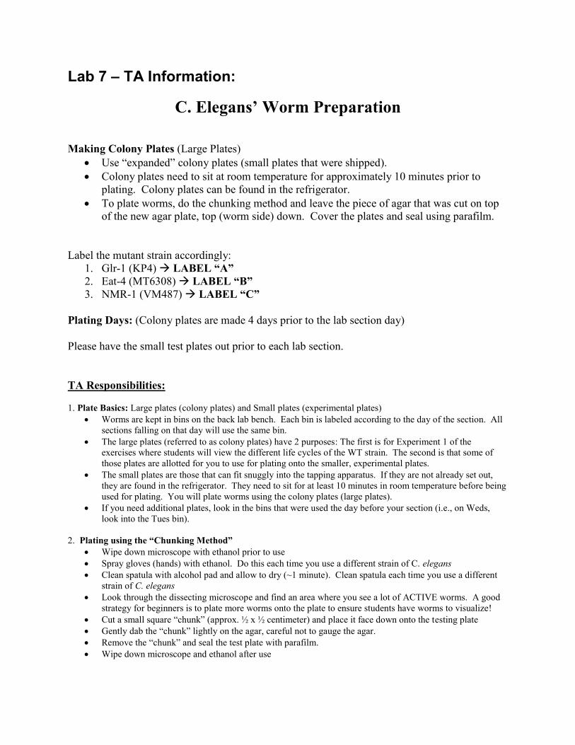
Lab 7 – TA Information:
C. Elegans’ Worm Preparation Making Colony Plates (Large Plates)
Use “expanded” colony plates (small plates that were shipped). Colony plates need to sit at room temperature for approximately 10 minutes prior to
plating. Colony plates can be found in the refrigerator. To plate worms, do the chunking method and leave the piece of agar that was cut on top
of the new agar plate, top (worm side) down. Cover the plates and seal using parafilm.
Label the mutant strain accordingly:
1. Glr-1 (KP4) LABEL “A” 2. Eat-4 (MT6308) LABEL “B” 3. NMR-1 (VM487) LABEL “C”
Plating Days: (Colony plates are made 4 days prior to the lab section day) Please have the small test plates out prior to each lab section. TA Responsibilities: 1. Plate Basics: Large plates (colony plates) and Small plates (experimental plates)
Worms are kept in bins on the back lab bench. Each bin is labeled according to the day of the section. All sections falling on that day will use the same bin.
The large plates (referred to as colony plates) have 2 purposes: The first is for Experiment 1 of the exercises where students will view the different life cycles of the WT strain. The second is that some of those plates are allotted for you to use for plating onto the smaller, experimental plates.
The small plates are those that can fit snuggly into the tapping apparatus. If they are not already set out, they are found in the refrigerator. They need to sit for at least 10 minutes in room temperature before being used for plating. You will plate worms using the colony plates (large plates).
If you need additional plates, look in the bins that were used the day before your section (i.e., on Weds, look into the Tues bin).
2. Plating using the “Chunking Method”
Wipe down microscope with ethanol prior to use Spray gloves (hands) with ethanol. Do this each time you use a different strain of C. elegans Clean spatula with alcohol pad and allow to dry (~1 minute). Clean spatula each time you use a different
strain of C. elegans Look through the dissecting microscope and find an area where you see a lot of ACTIVE worms. A good
strategy for beginners is to plate more worms onto the plate to ensure students have worms to visualize! Cut a small square “chunk” (approx. ½ x ½ centimeter) and place it face down onto the testing plate Gently dab the “chunk” lightly on the agar, careful not to gauge the agar. Remove the “chunk” and seal the test plate with parafilm. Wipe down microscope and ethanol after use

Lab 7
7.28
3. When do I plate my WT Strain? 1. You can plate during Experiment 1 while students are looking at the different stages of worms.
o A good thing to do is make sure you have all your materials ready. This can be done before class. Pre-cut Parafilm into strips Label test plates (i.e., WT, Mutant A, B, C)
2. If you are not confident in your plating, you can plate right before your lecture. Just make sure you time your lecture and do not go over 15 minutes!! (Students still need to do EXP 1)
3. Just a note that the smaller plates do not have any food! This is why the worms are more active once you plate them. They’re moving around looking for some grub! After 20 minutes, the worms travel to the end of the dish and crawl under the agar. With this, consider your lecture time and the amount of time you want students to spend on EXP 1.
4. When do I plate my Mutant Strains?
You can start plating during the 2nd break of their WT experiment When labeling the mutant plates, use A, B, and C, and keep note of which mutant corresponds to what
letter. Afterward, you can tell students what strain they have when they are looking up the genotype. That way they can do a "blind" experiment when they conduct the experiment on their mutant strain. **See table for how many groups are assigned to each mutant
o Glur-1 (KP4) LABEL “A” o Eat-4 (MT6308) LABEL “B” o NMR-1 (VM487) LABEL “C”
5. During Class
Have your students clean their lab bench with ethanol BEFORE and AFTER use! For Experiment 1, they just need to see that there are big worms and small ones. They do not need to
classify the different worm stages! For Experiment 2 and 3, have students observe an ACTIVE worm. If the worm students are focusing on
moves out of their viewing range, have them observe another worm. All worms on the plate are receiving the same tapping stimulus.
Make sure to add your students’ data on the Goggle document. o For the Google document, on the bottom left corner, there are different tabs for each section.
Select your name. o Fill in the answers for your section.
At the end of the day, return the colony plates back to the bins. Throw away the testing plates into the biohazard trash bin (gray lidded trash bin)—no gloves allowed in that bin! At the end of the week, we can throw everything out.

Sample Data:
Table 1. Table of P-values calculated using two-tailed paired t-test for trials comparing savings, learning and dishabituation. P- values< .05 were considered significant. Wild-type NMR-1 Mutant Number of worms 61 12 Savings (training trials 1-5 vs 31-35) .0038 .0086
Learning (training trials 1-5 vs 56-60) 9.56E-10 .0063
Dishabituation (testing trials 6-10 vs dishabituation trials 1-5) .0054 .0819
0
0.5
1
1.5
2
2.5
3
bas
elin
e
trai
nin
g1-5
trai
nin
g 6
-10
trai
nin
g 1
1-1
5
trai
nin
g 1
6-2
0
trai
nin
g 2
1-2
5
trai
nin
g 2
6-3
0
trai
nin
g 3
1-3
5
trai
nin
g 3
6-4
0
trai
nin
g 4
1-4
5
trai
nin
g 4
6-5
0
trai
nin
g 5
1-5
5
trai
nin
g 5
6-6
0
test
ing
1-5
test
ing
6-1
0
Dis
hab
te
st 1
-5
Dis
hab
te
st 6
-10
Ave
rage
nu
mb
er
of
tap
-wit
hd
raw
al
resp
on
se in
C. e
leg
an
s
0
0.5
1
1.5
2
2.5
bas
elin
e
trai
nin
g1-5
trai
nin
g 6
-10
trai
nin
g 1
1-1
5
trai
nin
g 1
6-2
0
trai
nin
g 2
1-2
5
trai
nin
g 2
6-3
0
trai
nin
g 3
1-3
5
trai
nin
g 3
6-4
0
trai
nin
g 4
1-4
5
trai
nin
g 4
6-5
0
trai
nin
g 5
1-5
5
trai
nin
g 5
6-6
0
test
ing
1-5
test
ing
6-1
0
Dis
hab
te
st 1
-5
Dis
hab
te
st 6
-10
Ave
rage
nu
mb
er
of
tap
wit
hd
raw
al
resp
on
se in
C. e
leg
na
s
Graph 2. NMR-1 mutant C. elegans average tap-withdrawal response. Graphic representation of average number of tap-withdrawal responses in training, testing and dishabituation trials for mutant C. elegans.N=12
Graph 1. Wild type C. elegans average tap withdrawal response. Graphic representation of average number of tap-withdrawal responses in training, testing and dishabituation trials for wild type C. elegans. N=61

Workshop 8RABLE 2015

1
Battle of the Bacteria: Characterizing the Evolutionary Advantage of Stationary Phase Growth Brian Sato University of California, Irvine 2238 McGaugh Hall MC 3900 Irvine, CA 92697 [email protected]
Karin E. Kram University of Southern California 1050 Child’s Way RRI 303 Los Angeles, CA 90089 [email protected]
Abstract:
Providing students with authentic research opportunities has been shown to enhance learning and increase retention in STEM majors. This workshop centers on an investigative microbiology lab module, which focuses on the molecular mechanisms of evolution in E. coli, by examining the growth advantage in stationary phase (GASP) phenotype. The GASP phenotype is illustrated by growing cells into long-term stationary phase (LTSP), and competing them against unaged cells in a fresh culture. This module includes learning goals related to improving student understanding of evolution and strengthening practical laboratory skills. In addition, the students generate novel data regarding the effects of different types of media on GASP and the relationship between evolution, genotypic change, and cell stress. Pairs of students are provided with the experimental background, select a specific aspect of the growth medium to modify, and generate a hypothesis regarding how this alteration will impact GASP. Students explore not only the growth competition between aged and fresh cells, but also how the different types of media impact cell stress and mutation frequency. From this module, we have demonstrated that students are able to achieve the established learning goals and have produced data currently being explored by a research lab.
Workshop attendees will be introduced to the GASP phenotype and get hands on experience with the techniques utilized to gather data regarding this phenomenon. We will discuss how to incorporate this module into the lab curriculum at attendees’ institutions, potential pitfalls for both students and instructs, and means to assess student learning.
Key words: E. coli, growth advantage in stationary phase (GASP), evolution, hypothesis construction,
Copyright 2014, Brian Sato and Karin Kram, University of California, Irvine

2
Introduction: Cells grown into long term stationary phase (LTSP – greater than 10 days) are better adapted to the environment, and thus are able to outcompete un-aged cells. This is the GASP phenomenon. This module is hypothesis driven, and allows the students to alter the culture medium in a manner of their choosing to uncover the variable’s impact on the GASP phenotype and its relationship with cell stress and frequency of genome mutation. In doing so, the students are capable of seeing evolution occur within this short module. While essential to life, student understanding of evolution can be lacking. One common criticism is that species evolution happens on such a large time scale, and that an inability to observe it in real-time makes it somehow less credible. This is clearly not the case with microorganisms though, which reproduce much more rapidly. Bacterial evolution has been demonstrated in many scenarios, one of the most famous being Luria and Delbruck’s fluctuation test with bacteriophages. This experiment demonstrated that mutations in a population can occur randomly and in the absence of a specific stress, as bacteriophage resistant cells arose whether or not the phages were present in the culture. Selection of these mutations and evolution of the population can then occur in the presence of the stress. This module begins with this premise of mutations occurring naturally and then leads to the ability to characterize the surviving population’s phenotype. Does the GASP population outcompete fresh cells only in the initial selective environment or does this apply to different types of media? Do we observe genetic or physiological changes in a major pathway responsible for survival in LTSP? Does the cell stress or mutation frequency change under various environments and does this impact the degree of the GASP phenotype? The goals of this lab module are two-fold. First, students can increase our knowledge concerning the GASP phenotype through novel experiments of their design. Secondly, this exercise will help students achieve the following learning objectives.
1. Describe the basis of evolution/survival of the fittest on a molecular level. 2. Describe the importance of the ingredients in microbial growth media. 3. Design a testable hypothesis. 4. Define and describe the use of a transcriptional reporter gene. 5. Differentiate between bacterial species and bacterial strains. 6. Differentiate between genotypic and phenotypic changes. 7. Use pipettors with accuracy/confidence. 8. Perform dilution calculations.
The module requires four weeks of the curriculum, including time for students to select a variable and develop a testable hypothesis and perform four different protocols to study various aspects of the phenotype. Based on a number of measures of assessment, students performing the lab module were able to achieve both goals. The class-generated experimental data agrees with published literature and contributes novel information, and the students attained the established learning outcomes. Questions, comments, want to do this experiment in your class? – Feel free to contact us!

3
Selected Student Handouts for Module
Evolution of populations occurs in two steps. First, organisms within those populations gain mutations as part of normal biological processes. Second, conditions in the environment allow a few organisms with beneficial mutations to survive longer than their non-mutated counterparts. Those organisms with beneficial mutations are more fit, and will be selected for over time.
Experiments conducted by scientists have shown that mutations arise in a population regardless of the environment. This is because there is a constant mutation rate simply due to mistakes made in DNA replication and repair. One example is the famous fluctuation test done by Luria and Delbruck (1943). The scientists demonstrated that mutations, which confer resistance to bacteriophage attack, occur randomly during growth of bacterial cultures, even when the bacteriophages are not present. This shows that mutations occur during growth with or without the selective environment. If, however, we place the bacteria into selective conditions, we can show that those mutations can be selected out of the population, which leads to evolution. These selective environments generate a number of interesting questions regarding the surviving mutant population. Are the mutations beneficial in other environments, what characteristics of the environment enhance this phenotype, etc?
In this experiment, we will be growing bacteria in a selective condition, and showing that selection causes the bacteria to be better adapted to their environment after merely a few days of exposure. The selective environment will be long-term stationary phase (LTSP), during which populations of bacteria must survive harsh conditions including low nutrients, basic pH, and high waste product levels.
Bacteria experience five phases of growth during their life cycle: lag phase, exponential phase, stationary phase, death phase, and LTSP.
Most often when we grow bacteria in the lab, we examine them during log phase or early stationary phase growth. However, in the natural environment, and in certain laboratory conditions, bacteria more often experience LTSP. Some strains of Escherichia coli can survive in LTSP without the addition of nutrients for years.
We can take bacterial populations that have been grown for over 10 days into LTSP, and compete them with un-aged bacteria in fresh media. The aged bacteria will be better adapted to the environment, and will therefore grow faster than the un-aged cells. We call this phenomenon growth advantage in stationary phase (GASP). Further, we will age our cells in a slightly different environment, which will change the conditions to which it will adapt, and determine whether or not those adaptations also help them in the original environment. Some conditions may select mutations that give the bacteria an advantage in a wide variety of environments, while other

4
conditions may select for mutations that only give an advantage to the bacteria in that specific environment. Using data from this experiment, we can determine what factors influence adaptation.
We will also characterize the GASP phenotype displayed by your cells. Are cells exhibiting the GASP phenotype surviving due to physiological adaptations or genetic mutations? Does increased environmental stress assist or hinder the growth advantage? Do GASP populations also experience a higher mutation frequency? With these experiments, we will illustrate that our aged strain is genetically different strain from the strain that began the experiment. We will see evolution occurring in real-time! Keep in mind that this is also novel work you will be conducting in collaboration with Dr. Steven Finkel’s lab at USC. You have a shot of identifying something that nobody has ever seen! Below is an outline of each experiment, and the specific questions that experiment will be answering. In addition, you will be examining how cells grow in LTSP when the media is altered. You and your group can choose one of the below variations of LB:
LB + 0.5% NaCl LB + 50mM CaCl or MgCl LB + 0.5% tryptone LB + 0.5% yeast extract LB + 0.2% glucose or fructose or sucrose

5
Assay I: Bacteria Growth Advantage in Stationary Phase (GASP) Assay We need to select for cells that exhibit the GASP phenotype, by first growing a culture of E. coli into long-term stationary phase and then adding the survivors to a fresh bacteria culture. We will then compare survival of the aged versus the un-aged cells using different antibiotic resistance markers to distinguish each (see diagram below). In addition, you will be modifying the culture media in a specific manner (by adding Variable X) to determine how it impacts the GASP phenotype. For this aspect of the experiment, we will need to make slight modifications to the general experimental protocol outlined below. Experimental Questions:
1. Does growth into long-term stationary phase select for certain mutations (existing or spontaneous) producing a culture with a growth advantage?
2. Does the addition of Variable X to the LB alter the growth advantage for long-term stationary phase cells?
3. Is the growth advantage observed in LB + Variable X specific for growth in LB + X or evident in regular LB as well?

6
Rough Protocol Start cultures for LTSP growth (Week 1) Materials: 1 test tube1, StrepR E. coli culture, LB medium
1. Set up 1 tube. 2. Add 5ml of LB and then 5μl of the overnight culture (the StrepR E. coli). 3. Place in your section’s rack for incubation at 37°C.
Start GASP assay (Week 3) Materials: 1 test tube, aged StrepR E. coli cultures, fresh NalR E. coli cultures, 2 LB + Strep plates, 2 LB + Nal plates You will now compete the StrepR E. coli against another strain of E. coli, which is resistant to nalidixic acid, but is otherwise identical to the strains you aged. To see whether the LTSP culture possesses the GASP phenotype, you will survey the mixed culture today, in discussion and next week in lab.
1. Set up 1 tube. Add 5ml of the NalR overnight culture. 2. Shake the tube to mix. 3. Now you need to add the aged StrepR bacteria. You will add only 5μl of the LTSP
culture. 4. Place in your section’s rack for incubation at 37°C.
Remember, the goal is to monitor how the LTSP StrepR bacteria grow compared to the fresh NalR bacteria. This will be determined by looking at growth on an LB + streptomycin plate (where only the StrepR bacteria will survive) versus growth on an LB + nalidixic acid plate. Each 1:10 dilution will involve adding 90μl media and 10μl cells. These dilutions will be performed using an empty petri dish (either the lid or the dish), where you add eight spots of 90μl LB. You will then transfer 10μl of your culture to the first spot, pipette up and down a few times and mix the drop with the pipette tip. The next spot will be made with 10μl of the first spot and 90μl LB, mixing by pipetting up and down and using the pipette tip. This will be repeated for all eight spots. Your TA will demonstrate this procedure for you.
1. Mix the tubes thoroughly before removing any liquid. You should plate one strain in its entirety before moving on to the next.
2. In an empty petri dish, you will make eight spots with 90μl each. Do not let the drops merge.
3. Take 10μl of your culture and add it into the first drop. Pipette up and down and stir the drop with the pipette tip to mix the dilution.
4. Using the same tip, pipette 10μl of the first drop onto your LB + Strep plate. You will use the grid below to keep track of your spots. Then pipette 10μl of the same drop onto your LB + Nal plate.
5. Take a new pipette tip and remove 10μl of the first drop and pipette into the second drop. Mix and pipette 10μl onto both plates.
6. Repeat for drops three through eight.
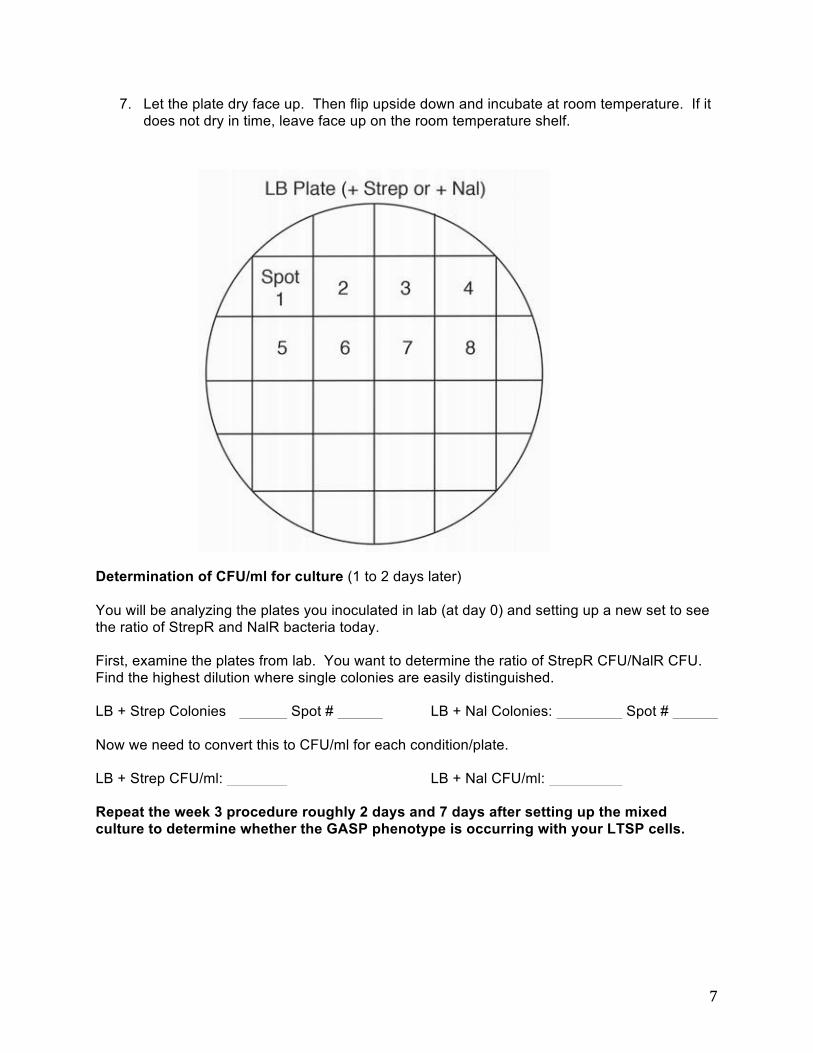
7
7. Let the plate dry face up. Then flip upside down and incubate at room temperature. If it does not dry in time, leave face up on the room temperature shelf.
Determination of CFU/ml for culture (1 to 2 days later) You will be analyzing the plates you inoculated in lab (at day 0) and setting up a new set to see the ratio of StrepR and NalR bacteria today. First, examine the plates from lab. You want to determine the ratio of StrepR CFU/NalR CFU. Find the highest dilution where single colonies are easily distinguished. LB + Strep Colonies Spot # LB + Nal Colonies: Spot # Now we need to convert this to CFU/ml for each condition/plate. LB + Strep CFU/ml: LB + Nal CFU/ml: Repeat the week 3 procedure roughly 2 days and 7 days after setting up the mixed culture to determine whether the GASP phenotype is occurring with your LTSP cells.

8
Assay II: Examination of rpoS Activity – Genotypic vs. Phenotypic for LTSP survival rpoS is a transcription factor that activates genes responsible for fighting cell stress and allowing cells to enter stationary phase. Surprisingly, rpoS activity appears to be detrimental to cell survival in long-term stationary phase, and many cells will downregulate rpoS in LTSP. In this part of the experiment, you will determine whether your LTSP cells have decreased rpoS activity. If so, this may be accomplished through one of two mechanisms, cellular downregulation of rpoS (through decreased transcription or increased protein degradation, for example) or through mutation, which results in chronically decreased rpoS levels. One of the targets of rpoS is catalase, and you will measure rpoS activity by examining hydrogen peroxide breakdown by your cells. By conducting this test at various intervals throughout the experiment, you will answer the following questions:
1. Does rpoS activity change in cultures that are grown to LTSP? 2. If rpoS is being downregulated in LTSP, is this due to a phenotypic or genotypic
modification of rpoS? 3. Do the answers to these questions differ for cells grown in LB + Variable X?
There are a few potential results you may see: 1. If catalase expression is similar on day 2, 14 and the following day 2, rpoS activity is unaltered by LTSP. 2. If catalase expression decreases on day 14, but is restored when the cells are added back to fresh media, rpoS activity is altered by LTSP conditions. This signifies a physiological, but not genomic change. 3. If catalase expression decreases on day 14 and remains decreased in fresh media, this signifies a genomic change to rpoS.

9
Rough protocol Examine rpoS activity in fresh cultures (week 1, roughly 2 days after starting cultures) Materials: Bacterial culture, microscope slide, H2O2 We want to measure catalase activity (and thus rpoS activity) before the cells reach LTSP.
1. Agitate tube if a pellet is at the bottom of the tube. 2. Remove 5μl of your cultures and add them to a glass slide. 3. Add one drop of H2O2 to each aliquot. 4. Note whether bubbles form (large/small, many/few, form immediately/after time, etc).
Repeat once cultures in long term stationary phase (roughly 2 weeks after starting culture) and again once the LTSP cells are added to fresh media (roughly 2 days after starting the second set of cultures).

10
Assay III: Cell Stress Measurement using a β-Galactosidase Assay Environmental stress can be a major factor in driving the evolution of organisms. Bacteria are equipped with cellular mechanisms to handle a variety of stresses, including elevated temperatures, oxidative stress, and low nutrient environments, among others. But in extreme scenarios, it is likely that the stress will overwhelm these pathways and the cells will be unable to survive. In rare cases, it is also possible that cells contain or acquire beneficial mutations that allow them to survive to a greater extent in these environments compared to the rest of the population. We will measure cell stress using a lacZ fusion protein, driven by the bolA promoter. bolA is part of the E. coli stress response and is upregulated under carbon starvation, increased osmolarity and oxidative stress. When stressed, the cell will transcribe from the bolA promoter, turning on the lacZ gene resulting in the production of β-galactosidase protein. We will measure β-galactosidase activity with the addition of its substrate, ortho-nitrophenyl-β-galactoside (ONPG), which is broken down to produce ortho-nitrophenol, a molecule with a yellow color. We can measure the amount of this molecule using the spectrophotometer. With this reporter protein, we can ask the following questions:
1. Does the amount of stress experienced by the cells correlate with the intensity of the GASP phenotype?
2. Does the addition of Variable X to the media alter cell stress?

11
Spectrophotometry allows one to measure the components in a solution. Different molecules are capable of absorption of specific wavelengths of light. This absorption can be measured with a spectrophotometer. A solution is added to a cuvette that is placed into the spectrophotometer. Light of a specific wavelength is directed at the cuvette and may be absorbed by specific molecules. The amount of light, which is not absorbed and passes through the cuvette, is read resulting in the calculation of an absorbance. More of that specific molecule results in more light absorbed and a higher absorbance value, known as the optical density (O.D.). Since we want to know the light absorbed by a specific molecule (in this case ortho-nitrophenol), we need to eliminate any light absorbed by the buffer. To eliminate the absorbance by any components in the buffer, we first “blank” the spectrophotometer with a cuvette containing only buffer. Thus, when we add the cuvette with ONPG and β-galactosidase, the resulting absorbance will be due only to ortho-nitrophenol. Below is the protocol for the spectrophotometer based β-galactosidase assay. The purpose of the experiment is to lyse the cells to expose the β-galactosidase protein to the ONPG substrate. In addition, you will need to determine the viable cell count in the population similarly to what you did the past week with the rifampicin assay. This is necessary because higher β-galactosidase activity could merely be due to a greater number of viable cells, and not necessarily greater bolA activation in each cell. Before you begin, familiarize yourself with the spectrophotometer.
1. On the screen, confirm that the wavelength is set at 550nm (not 600nm as above). 2. Next, add your blank cuvette (Z buffer only) to the spectrophotometer and hit “blank”. 3. After this is complete, you will add your cuvette containing your β-galactosidase assay. 4. Hit the green read sample button. This will generate an absorbance (OD) value.

12
Protocol (roughly 2-7 days after starting week 1 culture) Materials: Z buffer (60mM Na2HPO4, 40mM NaH2PO4, 10mM KCl, 1mM MgSO4, 50mM BME), phosphate buffer (60mM Na2HPO4, 40mM NaH2PO4), 0.1% SDS, 4mg/ml ONPG, 1M Na2CO3, spectrophotometer *For the RABLE workshop, you will be performing this protocol twice, once for a culture in LB and once for a culture in LB + NaCl.
1. Remove 0.5ml of your culture to a 1.5ml eppendorf tubes. 2. Centrifuge on full speed for 1 minute to pellet the cells. Pipette off the liquid but do not
disturb the pellet. This removes the media, which may contain molecules that impair β-galactosidase activity or light absorbance by the spectrophotometer.
3. Resuspend the pellet in 0.5ml chilled Z buffer. 4. In a new 2.0ml tube, add 900μl Z buffer and 100μl of cells (resuspended in Z buffer). 5. Add 50μl SDS and mix by inverting the tube a few times. SDS is a detergent, which will
lyse the cells. 6. Let the tubes sit on your bench for 5 minutes at room temperature. 7. Add 200μl ONPG to the tube and mix by inverting a few times. 8. Incubate the tube in the 28°C water bath until you see color (usually around 15 minutes). 9. Once you see yellow color in both tubes, stop the reaction by adding 0.5ml Na2CO3 and
mix by inverting a few times. The sodium carbonate raises the pH to 11, which inactivates the β-galactosidase protein.
10. Transfer 1ml of the solution to a new 1.5ml tube and centrifuge for 5 minutes at max speed.
11. Instructions for using the spectrophotometer are on the following page. Blank the spectrophotometer with 1ml Z buffer in a cuvette (at OD420).
12. Remove the supernatant from the centrifuged tubes to cuvettes.
13. Determine the OD of the tubes. LB only OD420: LB + X OD420: Determine CFU count for cells As mentioned above, to accurately measure the β-galactosidase activity, it is necessary to determine the viable cell count in the population. This will be accomplished by performing a dilution assay using LB plates. This would be performed similarly to the dilution plating described in the GASP assay. Mock results for this workshop are on the following page:

13
To determine the CFU/ml for viable cells, you will look at your dilution spots. The more concentrated spots are likely completely covered with growth and it is no longer possible to count individual colonies. Instead, select the spot with individual colonies. Colonies from LB only: Spot # Colonies from LB + NaCl: Spot # Now you need to determine the CFU/ml using the example from the previous class. Imagine you had 2 colonies on spot 5. The very first spot was created by adding 10μl of cells to 90μl LB and plating 10μl (1/10th) of this dilution. Since you plated 1/10th of that original 10μl (from the culture), you actually only added 1μl of the original culture. This means the growth in the first spot signifies the CFU/0.001ml or CFU/10-3 ml. Spot number two is a 1:10 dilution of the first, so growth in this spot signifies the CFU/10-4 ml.
This means the 2 colonies on spot 5 signify a value of 2 x 10 ____/ml or CFU/ml.
Now, based on this little tutorial, calculate your CFU/ml for all viable cells using the values you noted from your LB plates.
LB only CFU/ml: LB + X CFU/ml: And finally, you can calculate your cell stress:
OD420 CFU/ml
LB only OD420: LB + X OD420: (values from last week) LB only: LB + X:

14
Assay IV. Examination of Mutation Frequency by Rifampicin Survival Environmental stresses can promote the formation of mutations, for example through increased DNA alterations caused by base damage or decreased activity of DNA repair pathways. While most are likely detrimental or have no effect on the cell, it is also possible a cell will acquire a beneficial mutation. Normally your cells are sensitive to rifampicin, but it is possible for them to become antibiotic resistant. In this experiment, you will be measuring the mutation frequency in your bacterial culture to answer the following questions:
1. What is the frequency of mutations in the bacteria population? 2. Does this frequency change in LB + Variable X media? 3. Does the frequency of mutation correlate with the results of the GASP experiment?
Normally your bacteria are rifampicin sensitive. It is possible that they acquire a mutation that renders them rifampicin resistant. You will examine this by plating your cultures on an LB + Rif plate. In addition, you will plate them on an LB plate to determine the total viable cells in the population to calculate the percentage of the culture that is rifampicin resistant. Rough Protocol (roughly 2-7 days after starting week 1 culture) Materials: 1 LB plate, 1 LB + Rif plate, 1 empty petri dish, liquid LB To determine the frequency of rifampicin resistant cells in the population, you must identify how many cells are rifampicin resistant (by plating on LB + Rif) and comparing this to how many viable cells there are total (by plating on LB alone). We anticipate the frequency of rifampicin resistant cells to be low, so there will be no need to dilute the culture plated on LB + Rif.
1. Take 1 LB plate and 1 LB + Rif plate. Label the bottom of these as either LB or LB + Rif, along with your identifying information.
2. Prepare your LB plate first as described in the GASP assay dilution plate protocol. 3. Now prepare the LB + Rif plate. Because the number of rifampicin resistant cells will be
low, you will not need to do the above procedure. Instead, plate 100μl of your first culture (well-mixed) on an LB + Rif plate.
4. Spread the 100μl using the ethanol spreader (dip in ethanol, briefly flame, let cool by placing on a region on the plate where the cells are not).
5. Repeat this with your second culture using another LB + Rif plate.

15
Your mutation frequency will be based on counting colony forming units (CFU). CFU estimates the number of viable cells by assuming each viable cell is capable of cell division resulting in the formation of a colony. So CFU is determined by counting colony number on a plate. CFU/ml Rif Res Bacteria (on LB + Rif plate) The equation for the mutation frequency will be: CFU/ml Total Cells (on LB plate) 1. To determine the CFU/ml for Rif resistant bacteria you will count the colonies on the LB + Rif
plate. Note that number here: (LB only) (LB + X media) Remember, you plated 100μl of your original cultures onto the LB + Rif plate. So rather than identifying the CFU/ml, your values above represent the CFU/0.1ml. This means you need to multiply the numbers above by a factor of .
Your CFU/ml values for Rif resistance cells are: (LB) (LB + X) 2. To determine the CFU/ml for all viable cells (plated on the LB media), you will look at your dilution spots. This is to be performed as described in the cell stress assay.

16
Materials -Micropipettors (P20, P200, P1000) – one set per group of four -Bench top centrifuge – one per section of 20 students -Glass tubes (20mm x 150mm) -Spectrophotometer E. coli – both strains express the bolA-lacZ fusion protein -Naladixic acid resistant – SF2054 (W3110 deltalacU169 tna2 Nalr lambda-bolA::lacZ-Kan-r) -Streptomycin resistant – SF2055 (W3110 deltalacU169 tna2 Strr lambda-bolA::lacZ-Kan-r) More information can be found in Farrell and Finkel, 2003 . Lysogeny broth (LB) – for bacteria growth LB + Drug plates -Rifampicin - 100μg/ml (100mg/ml Rifampicin stock in DMSO) -Naladixic acid - 20μg/ml (20mg/ml Naladixic acid stock in water, add NaOH to get in
solution) -Streptomycin - 25μg/ml (25mg/ml Streptomycin stock in water) Reagents per experiment (per group of 4) -Experiment is performed in pairs, although 2 pairs (group of 4) will perform the identical experiment for repeatability purposes 25X Variable solutions (others can be used as well) – make in water, sterile filter before use -12.5% NaCl, 1.25M CaCl2,12.5% tryptone, 12.5% yeast extract, 5% glucose, 5% fructose Starting cultures to generate LTSP conditions -4 glass tubes, 25ml LB GASP Assay -Variable stock solutions, 10 glass tubes, 25ml LB -8 LB + Nal plates, 8 LB + Strep plates, and 8 empty petri dishes (4 for day 0, 4 for day 2) -5ml sterile water rpoS downregulation (catalase test) -a few drops of 3% H2O2, microscope slides Mutation frequency (Rifimpicin resistance) -2 LB plates, 4 LB + Rif plates, 2 empty plastic petri dishes, 5ml sterile water Cell Stress (β-galactosidase Assay) -Z buffer (must be made within a few days of use) – 8ml To make 150ml - 2.4g Na2HPO4•7H2O, 0.84g NaH2PO4•H2O, 1.5ml 1M KCl, 0.15ml 1M MgSO4, 0.405ml β-mercaptoethanol adjust pH to 7.0, then bring to 150ml with water, keep at 4°C (12 tubes per class, on ice) -ONPG solution (must be made within a few days of use) – 4mg/ml in water -0.1% SDS solution - 300μl -1M Na2CO3 – 2.5ml -2 LB plates, 2 empty plastic petri dishes -5ml sterile water

17
Example Student Data Comparison of GASP phenotype in LB versus LB + 50mM CaCl2 Figure 1. Competition assay comparing growth of aged versus un-aged cells grown in LB or LB + CaCl2. E. coli were aged in either LB or LB + CaCl2 and then diluted 1:1000 in a culture of fresh cells growing in either LB or LB + CaCl2. Aged cells grown in LB media for both conditions outcompeted the fresh cells. Cells aged in LB + CaCl2 were incapable of overtaking the fresh cells in the given time frame.
Figure 2. Example plates displaying results from competition assays comparing growth of aged versus un-aged cells grown in LB. Cells were plated at the indicated days following the addition of aged cells to the un-aged cultures on the appropriate media at ten-fold dilutions. Plates were grown at room temperature for 48 hours and photographed. Figure 3. Measuring catalase activity of cells grown in either LB or LB + CaCl2. E. coli were aged in either LB or LB + CaCl2 and then diluted 1:1000 in fresh cells growing in either LB or LB + CaCl2 (at day 14). Cells grown in CaCl2 experienced increased catalase activity both early on (day 2) and in LTSP (day 14). Upon re-addition to fresh media, the LTSP catalase phenotype is still present, illustrating that the lower rpoS activity is due to a genetic change in the cells. Growth in LB Growth in LB + CaCl2 Day 2 Few bubbles, appear after a
couple seconds Faster reaction, many bubbles, maintained for a longer time
Day 14 (LTSP culture) Took a very long time, very few small bubbles
Took a couple seconds, formed many bubbles
Day 16 (following re-addition to fresh media)
Took a very long time, very few small bubbles
Took a couple seconds, formed many bubbles

18
Figure 4. Measuring rifampicin resistance to determine the mutation frequency for cells grown in either LB or LB + CaCl2. Cells from day 2 cultures were plated on either LB (to determine CFU/ml) or LB + Rifampicin (to determine number of rifampicin resistant cells). Cells growing in LB + CaCl2 experienced a lower frequency of mutation relative to cells grown in LB. Growth in LB Growth in LB + CaCl2 CFU/ml 2.70E+09 1.90E+09 Rifamipcin resistant colonies 1010 290 Mutation Frequency 3.74E-07 1.53E-07 Figure 5. Measuring bolA activity as a gauge of cell stress for cells grown in either LB or LB + CaCl2. E. coli expressing β-galactosidase driven by the bolA promoter are lysed at day 7 of growth in the indicated media. CFU/ml are determined by growing cells on LB to normalize for the cell population. Cells grown in LB + CaCl2 exhibited higher stress levels compared to those grown in LB. Growth in LB Growth in LB + CaCl2 CFU/ml 2.50E+07 4.80E+08 OD420 (bolA expression) 0.14 0.32 β-gal units (CFU/ml / OD) 5.60E-09 6.67E-10

Battle of the Bacteria: Characterizing the Evolutionary Advantage of Stationary Phase
Growth!
Brian Sato, University of California, Irvine!Karin Kram, University of Southern California!

Welcome!!• Name!• Institution!• What labs do you teach?!

Workshop Outline!
• Evolution in the classroom!• What is the GASP phenotype?!• Description of Lab Module!• Hands-on time with Module !• Implementation at UC Irvine!• Adopting the module to your classroom!

Discuss: Why is evolution hard to teach?!

What is the GASP phenotype?!

4!
6!
8!
10!
5!
7!
9!
log 1
0 CFU
/mL!
Phases of Bacterial Growth in Batch Culture!
Finkel SE. Nature Reviews Microbiology. 2006 Feb;4(2):113-20.!
Days!Hours!0! 6! 12! 2! 6! 10! 14!
Months!12! 24! 36! 48! 60!
1!
2!
3!
4!
5!
Lag!
Log!
Stationary!
Death!
Long-Term Stationary Phase (LTSP)!

Growth Advantage in Stationary Phase (GASP)!
.
log
CFU/
ml
1296300
2
4
6
8
10
1-day-old
10-day-old
a
**
DayFinkel & Kolter, PNAS (1999)!
Aged Culture!
Un-Aged Culture!
10!
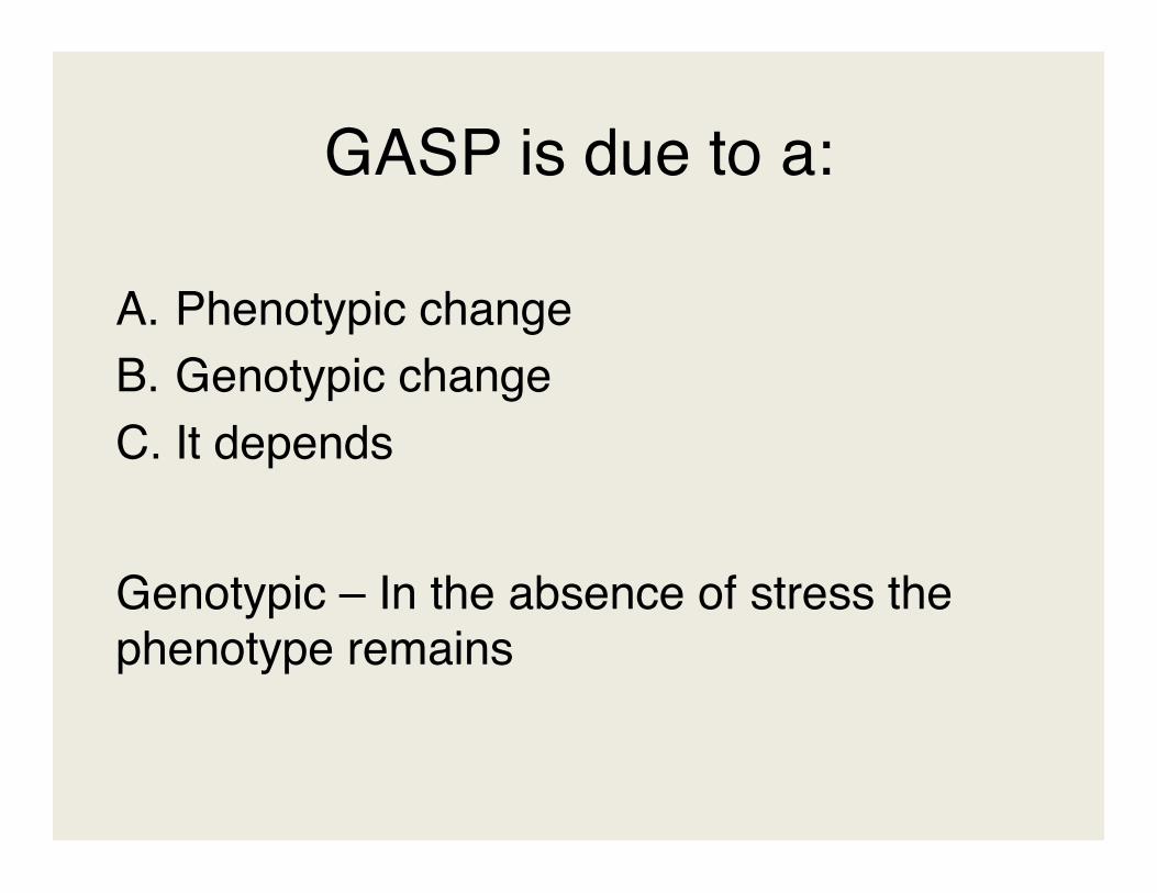
GASP is due to a:!
A. Phenotypic change!B. Genotypic change!C. It depends!
Genotypic – In the absence of stress the phenotype remains!!

Module Components!
GASP!
Do we observe the GASP phenotype?!Is the GASP phenotype environment specific?!
LB! LB + X!
Grow into LTSP!
Add aged cells to fresh media with un-aged cells!

Is the GASP phenotype environment specific?!
Module Components!
GASP!Real, novel data!

Module Components!
Mutation Frequency!
?!Does the frequency of bacterial mutation impact the GASP phenotype?!
LB! LB + X!
Measure frequency of antibiotic resistance!
GASP!

Module Components!
Mutation Frequency!
Cell Stress!
?! ?!
?!
Does the degree of cell stress correlate with mutation frequency and the strength of the GASP
phenotype?!
GASP!
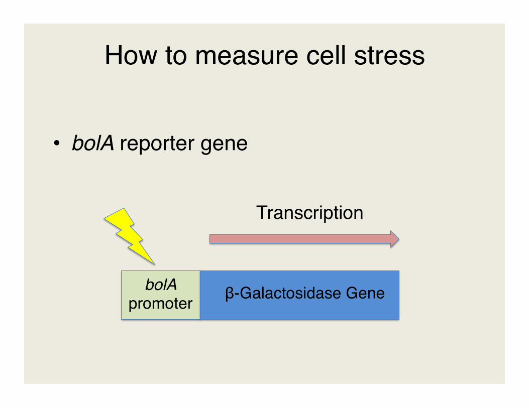
How to measure cell stress!
• bolA reporter gene!
bolA promoter! β-Galactosidase Gene!
Transcription!

How to measure cell stress!
• bolA reporter gene!
β-gal protein!
ONPG!Galactose!
Ortho-nitrophenol (yellow, absorbs
420nm light)!
+!

Module Components!
Mutation Frequency!
Cell Stress!
?! ?!
rpoS regulation!
?!
GASP!
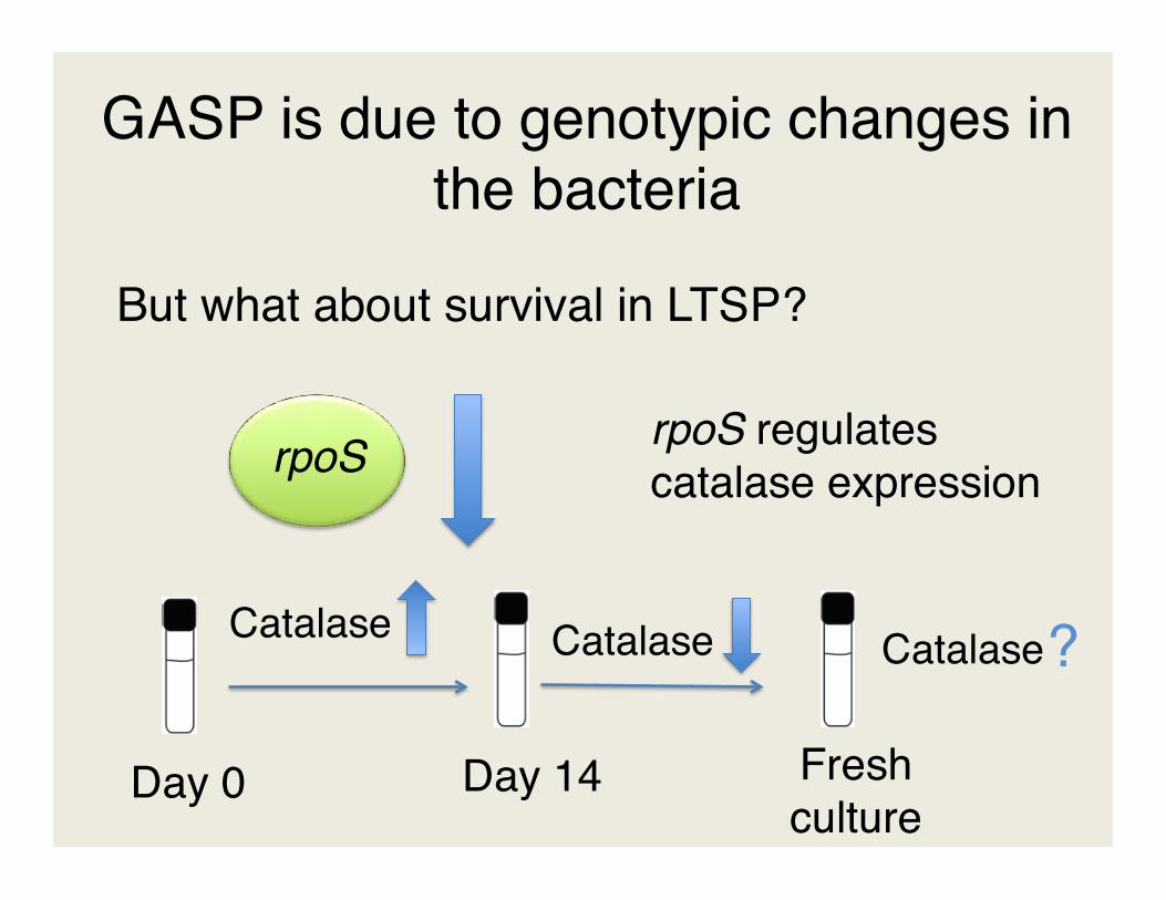
GASP is due to genotypic changes in the bacteria!
But what about survival in LTSP?!
rpoS! rpoS regulates catalase expression!
Day 0!
Catalase!
Day 14!
Catalase!
Fresh culture!
Catalase!?!

Module Components!
Mutation Frequency!
Cell Stress!
?! ?!
rpoS regulation!
Can choose to include any or all of these modules!
GASP!

Hands-On Time w/Module!
• (1) Catalase test (page 8 in handout)!– Compare old versus new cultures!
• (2) β-gal assay (page 10 in handout)!– Compare cells grown in 2 different
environments!– Which environment (LB or LB + NaCl) leads to
more cell stress?!– Analyze data on page 13!

Hands-On Time w/Module!
Page 13 in handout 2A 2B

What do we conclude?!
• rpoS is downregulated in culture 1A or 1B!
• Media 2A or 2B results in more cell stress!

Implementation at UCI!
• Fall 2014, Winter 2015!– Students select a variable to modify the media!– Hypothesize how this impacts GASP, mutation
frequency, cell stress, rpoS regulation!

Implementation at UCI!
Learning Goals!!1. Describe the basis of evolution/survival of the fittest on a
molecular level. !2. Describe the importance of the ingredients in microbial
growth media. !3. Design a testable hypothesis. !4. Define and describe the use of a transcriptional reporter
gene. !5. Differentiate between bacterial species and bacterial strains. !6. Differentiate between genotypic and phenotypic changes. !7. Use pipettors with accuracy/confidence. !
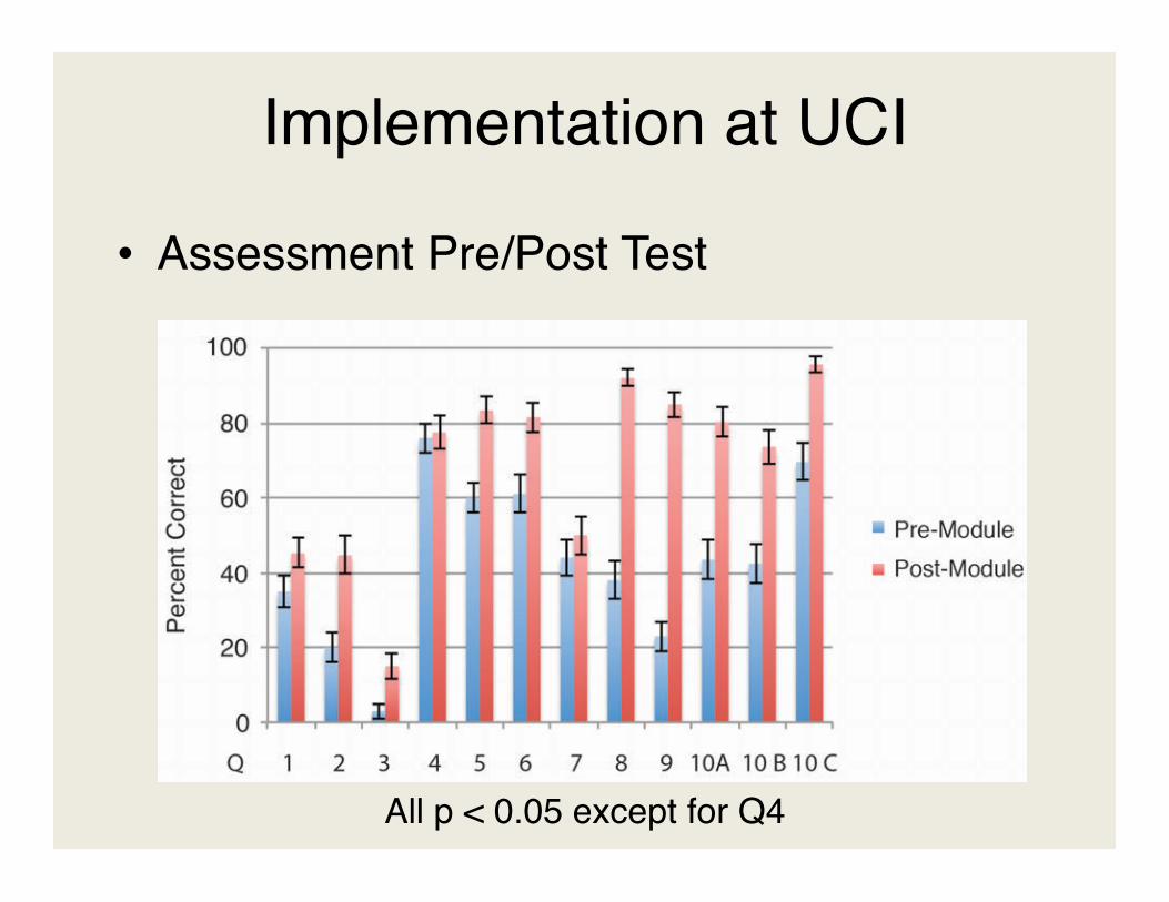
Implementation at UCI!
• Assessment Pre/Post Test!
All p < 0.05 except for Q4!

Implementation at UCI!• Pipetting Test!

Implementation at UCI!• Student Self-Assessment!
5 = strongly agree!!1 = strongly disagree!
*!*!
* p< 0.05!

Bringing this to your institution!
• What are the impediments?!

Questions?!


Data analysis!
• Using this data:!– Plot cell survival over time (page x)!– Is the GASP phenotype occurring?!– Is GASP impacted by environment?!

Microbiology Lab Course: Environmental Unknown Project Name: _________________________
1
Question/Hypothesis: Exercise 3
Sample:
Whole Colony Description Margin Elevation
Exercise 11 Streak plate unknown
Whole Colony Description Margin Elevation
Complete a subculture to nutrient agar plate. Exercise 5 Simple staining result
Morphology Arrangement
Complete a culture transfer to a nutrient broth. Exercise 7 Gram staining result
Gram result Morphology Arrangement
Complete a culture transfer from broth to a slant.
Exercise 12 Special Media results
EMB MSA Growth
Color
Exercise 14 Fermentation results
Glucose Growth
Color
Gas
Complete a culture transfer from the slant to broth.

Microbiology Lab Course: Environmental Unknown Project Name: _________________________
2
Exercise 25 Antibiotic resistance results
Antibiotic Disk code Diameter (mm) R, I, or S 1.
2.
3.
4.
5.
Complete a culture transfer to a nutrient agar plate. For Gram-negative sample: complete an Enterotube II Enterotube II results
Test Negative or Positive (±) Value Glucose Gas Lysine Ornithine H2S Indole Adonitol Lactose Arabinose Sorbitol VP Dulcitol PA Urea Citrate
Notes: Fermentation test (blue text)
ID code:

Microbiology Lab Course: Environmental Unknown Project Name: _________________________
3
For Gram-positive sample Catalase test:
Coagulase test:
Hemolysin test:
Identification of your unknown environmental sample: If a patient had an infection from the environmental microbe that you identified above, then what antibiotic(s)
could be used:

Workshop 9RABLE 2015

Welcome to Implementing Inquiry-based Microbial ProjectVeronica Ardi, PhD

Microbiology Laboratory Courses
CourseSmart: ebook resources http://instructors.coursesmart.com/

Microbiology Laboratory Courses• Traditional Lab Manual
• Individual experiments• Defined results• Post-lab questions with right answers
• Hypothesis-driven or Inquiry-based lab class• Creative• Critical thinking• Frustrating?

Microbiology Laboratory Courses
M. Hos‐McGrane. 2014.

Building on previous courses• General Biology, Genetics, Molecular biology, etc.• Scientific Method
NHS. 2009. http://web2.newtown-h.schools.nsw.edu.au/Science/CommonFolder/scienceindex.html

Microbial Techniques_____ Acid-fast stain_____ Aseptic Technique_____ Biochemical tests_____ Capsule stain_____ DNA isolation &
sequencing_____ Gram stain_____ Growth curve /
Spectrophotometer_____ Kirby-Bauer test_____ Microscope_____ Most probable number
_____ Motility_____ Negative stain_____ PCR_____ Pure culture isolation_____ Serial Dilution_____ Selective Media_____ Simple stain_____ Spread plating _____ Streak plating_____ Wet mount_____ Other: ____________

Sample Timeline• Does your order of
techniques aid in inquiry-based project?
• Johnson, T. and Case, C. Laboratory Experiments in Microbiology, 10 th
edition, 2012; Pearson, Benjamin Cummings, San Francisco, CA

Sample TimelineDate/ 2015
Laboratory Topics
General procedures, Lab Safety, Microscope Video, Turn in Safety Contract.Ex. 1: Parts of the Microscope & Oil immersion Ex. 3: Microbes in the Environment, Morphological unknownEx. 26: Effectiveness of Hand washing
Continue Ex. 3 & Isolate environmental sampleAseptic technique Ex. 11: Isolation of bacteria (& unknown environmental sample)Continue Ex. 11 & 26 (& unknown environmental sample)
Ex. 5: Smears & Simple Stains (& unknown environmental sample)
Ex. 7: Gram Staining (& unknown environmental sample)
Ex. 12: Special Media (& unknown environmental sample)Ex. 20: Bacterial Growth CurveContinue Ex.12Ex. 19: Oxygen & the growth of bacteria
Lab MIDTERM

Sample TimelineDate/ 2015
Laboratory Topics
Continue Ex.19Ex. 14: Fermentation (& unknown environmental sample)
Continue Ex. 14Ex. 24: Disinfectants & Antiseptics Continue Ex. 24Ex. 25: Antimicrobial drugs (& unknown environmental sample)Documentary: Nightmare Bacteria Continue Ex. 25Ex. 45: Bacteria of the Skin Unknown environmental sample / projectContinue Ex. 45Ex. 46: Bacteria of the Respiratory TractUnknown environmental sample / projectContinue Ex. 46Ex. 51: Enterotube ID unknown environmental sample
Continue Ex. 51 Unknown environmental sample / project
Final Lab Exam (Cumulative)Turn in Environmental Unknown Project

General Equipment for Microbiology Lab• Antibiotic disks (at least 5 different classes): ampicillin,
penicillin, streptomycin, tetracycline, & vancomycin[typically used in lab] or any that is typically used in clinics
• BD Enterotubes II API 20E• Blood agar, EMB, Mannitol salt agar (MSA), and Mueller-
Hinton agar plates• Bunsen burner Wire loops• Catalase test: H2O2 Coagulase test: rabbit plasma• Gram stain reagents• Glucose fermentation tube• Nutrient agar plates & slants• Personal protective equipment• Sterile cotton swabs & sterile saline solution (or broth)

Microorganisms in our world• In pairs, come up with hypothesis or inquiry.• How will you sample? [Design your method.]• Procedure (Exp. 3): inoculate 1 plate from the
environment using cotton swab (dip in saline first).

Microorganisms in our world• Go sampling!• Any problems during sampling?
• Incubate• Environmental samples
NOAA‐OE. 2007.

Results: variety of microbes

Results: Picking a colony• Students would describe all the colonies from the
sampling.• Guide students to select 1 colony
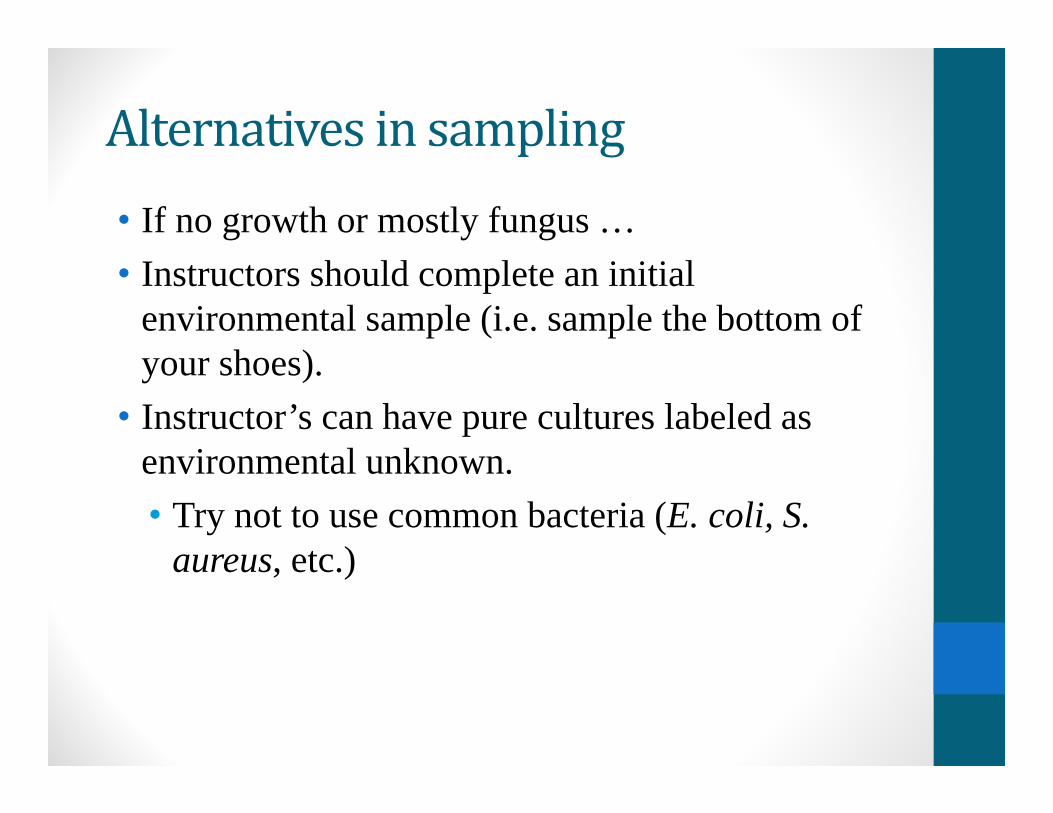
Alternatives in sampling• If no growth or mostly fungus …• Instructors should complete an initial
environmental sample (i.e. sample the bottom of your shoes).
• Instructor’s can have pure cultures labeled as environmental unknown.• Try not to use common bacteria (E. coli, S.
aureus, etc.)

TimelineDate/ 2015
Laboratory Topics
General procedures, Lab Safety, Microscope Video, Turn in Safety Contract.Ex. 1: Parts of the Microscope & Oil immersion Ex. 3: Microbes in the Environment, Morphological unknownEx. 26: Effectiveness of Hand washing
Continue Ex. 3 & Isolate environmental sampleAseptic technique Ex. 11: Isolation of bacteria (& unknown environmental sample)Continue Ex. 11 & 26 (& unknown environmental sample)
Isolate unknown environmental sample – pure culture
Ex. 5: Smears & Simple Stains (& unknown environmental sample)
Ex. 7: Gram Staining (& unknown environmental sample)

Collecting Data

Collecting Data

Collecting Data

Collecting Data• Enterotube II or API 20E
APIWeb: https://apiweb.biomerieux.com/servlet/Authenticate?action=prepareLogin

Collecting DataIdentification of your unknown environmental sample:
If a patient had an infection from the environmental microbe that you identified above, then what antibiotic(s) could be used:

Analyses • Identification of unknown – applying Bergey’s
Manual
Bergey’s Manual: https://archive.org/details/bergeysmanualofd1957amerhttp://www.uiweb.uidaho.edu/micro_biology/250/IDFlowcharts.pdf

Analyses • Identification of unknown – applying
dichotomous key

Analyses • Identification of unknown – applying
dichotomous key

Actual Student Results• What are the issues in identification of unknown?• What happens when student’s are absent?
• What if there is no identification?
• Motivation• Timing

Rubric• Establish a rubric to grade the project• Unknown Environmental Project: 5-15% of the
total grade• Example of rubric found in packet
Excellent Satisfactory Needs Improvement
Inadequate

Additional Assignments• Paper: write a 500-700 word paper about the
bacterial organism was identified. • Student presentation• What should the paper / presentation include?• A clinical case study, if applicable, should be
required in the writing or presentation assignment.
• Ecological significance of the bacterium should be part of the presentation or paper.
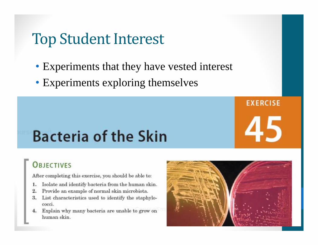
Top Student Interest• Experiments that they have vested interest• Experiments exploring themselves

Top Student Interest• Experiments that they have vested interest• Experiments exploring themselves

Limitations in Inquiry-based project• This workshop is limited to bacterial samples.• What if the students do not understand the
technique, how can they perform it?• How can they interpret the test?• Master the purpose of the test is key.
• How can they apply it to a project?

RABLE 2015 Sex in the Garden 01
Sex in the Garden: Pollen Germination Basic Protocols
Basic Background Information on Pollen Germination
Pollen germination occurs when a pollen grain develops a pollen tube. In nature, pollen germination occurs on the stigma of a flower and the pollen tube elongates towards the flower’s ovule. Sperm will travel through the pollen tube to fertilize the ovule. The evolution of pollen eliminated the dependence on standing water for fertilization in seed plants.
Pollen develops in the anthers of the stamen of the flower. The anther has four pollen sacs held together by connective tissue. Each pollen sac has microsporocytes (microscope mother cells) which divide by meiosis to produce microspores. Each microspore divides by mitosis to produce either a 2 cell microspore or a binucleated microspore. Each microspore differentiates into a pollen grain.
Pollen grains range from 6 to 100 micrometers and have species specific morphology. The wall of the pollen has three layers: the inner intine wall, the outer exine wall and the pollen coat. The pollen walls have modifications to allow for shrinking and swelling of the grain and thinner areas (apertures) where the pollen tube can break though the pollen wall.
Pollen germination and elongation is a dynamic process during which pollen must respond to different signals and develop a complex structure to deliver sperm cells for fertilization. Pollen germination can be visualized easily. This system is a simple model to study cell to cell interactions and environmental effects on development.

RABLE 2015 Sex in the Garden 01
Pollen Germination Assays Hanging Drop Method
Materials
Basic Germination Media (1mM KCl, 0.1 mM CaCl2, 1.6 mM H3B03, 10% Glucose) Regular glass slides Cover slips Petri dish
Filter paper (to fit into Petri dish) Pipette tips
Procedure A. Hanging Drop Procedure The hanging drop procedure is used to observe living organisms over time where desiccation could be an issue. The surface tension of the drop concentrates the cells to the edge of the drop. Oil immersion cannot be used with a hanging drop preparation.
1. Prepare humidity chamber by placing filter paper in Petri dish. 2. Moisten paper with water. 3. Clean microscope slides and cover slides using ethanol. Rinse with water and dry
using a Kimwipe. 4. Prepare a slide with a slide chamber where the hanging drop can be inverted onto. 5. Lightly grease the bottom of a gasket. Place the gasket onto a regular microscope
slide or a depression slide.
6. Determine the amount of media you will need to add to the cover slip to get a hanging drop (20 to 100 micrometers). The larger the drop, the less likely the drop
will evaporate. 7. Flip the coverslip over and place onto the
gasket.

RABLE 2015 Sex in the Garden 01
8. Observe the drop under the
low power objective. 9. Use the edge of the drop to
focus the microscope. 10. Change the objective lens
to 10X and refocus. You cannot use the 40X objective lens with this procedure.
B. Obtaining Pollen
1. Observe the flower. 2. Identify the different parts of the flower. 3. Find the anthers.
4. The best pollen to collect for germination comes from anthers that have burst or split open. The process is referred to as dehisce. You can quickly tell if the pollen is mature by gently brushing your finger across the anther. If you see a residue of pollen on your finger, the pollen is most likely mature.
5. Remove a pipette tip using the P2-- micropipettor. 6. Eject the tip into your hand. 7. Gently rub the anther with the pipette tip until a small amount of pollen is
transferred to the needle. 8. Transfer the pollen to the drop of media on the cover slip by tapping the tip with
your finger. 9. Invert the cover slip over your slide. 10. Record the time.
C. Observing Pollen Tube Growth
1. Observe the pollen under 100 x magnification (10 x objective lens and 10x ocular lens)
2. Record the shape, size and any unique features of the pollen grains. You may draw the pollen shape on a piece of paper and then take a photo to upload to your lab notebook.
3. Check the pollen every 30 minutes until the pollen tubes begin to grow. Keep the slide in the humidity chamber between observations. You may search through the fields of views until you find a field of pollen with a good density of pollen.
4. Once the pollen tubes have begun to germinate, record the time, percentage of pollen that has germinated and the length of five pollen tubes every 10 minutes for 30 minutes.

RABLE 2015 Sex in the Garden 01
Narcissus sp. (Daffodil) Pollen Germination
Agarose Method
Agarose gels are transparent, easy to make and can be made with a variety of buffers. 1. 1% molten agarose can be found at the back of the room in tubes in a hot plate. 2. Clean a microscope slide. 3. Warm the microscope slides by placing the slides on the edge of the hot plate. 4. Using a glass pipette, add 1 drop of agarose to the warm slide. 5. Allow the agarose to spread over the warm slide for 15 seconds. 6. Remove the slide from the hot plate and allow the slide to cool. 7. Prepare humidity chamber by placing filter paper in Petri dish. 8. Store your agarose slide in the humidity chamber when not in use. C. Observing Pollen Tube Growth 1. Remove the slide from the humidity chamber. 2. Dry the bottom of the slide using a Kimwipe. 3. Observe the pollen under 100X and 400X magnification 4. Record the shape, size and any unique features of the pollen grains. You may draw
the pollen shape on a piece of paper and then take a photo. 5. Continue to check the pollen.

Workshop 10RABLE 2015

RABLE 2015 Sex in the Garden
Pollen Germina:on
Medium Workshop 2 (3:30-4:50)

Narcissus jonquilla Common Trumpet Daffodil
Anthers
Stigma
Pollen

Tip: Pollen Make sure you can “brush off” some pollen with your finger

Hemerocallis sp. 40 min hanging drop
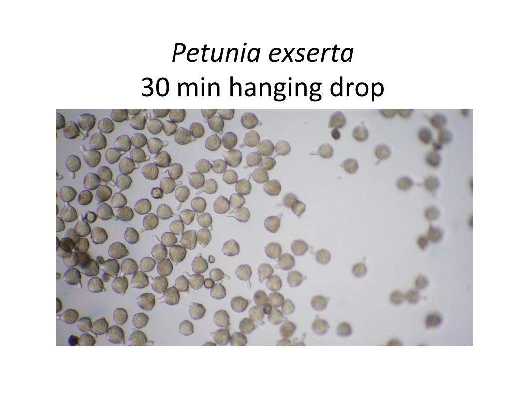
Petunia exserta 30 min hanging drop

Tulaghia violacea 75 min

Clivia sp. Agar 24 hr

Beaumon3a grandiflora Agar 20 hr Tpm B4

Rosa 90 min

Aloe agar 60 min

Ciona spp. • Translucent or yellowish solitary tunicate • Siphons are close together

Ascidia ceratodes • Yellow to orange solitary tunicate • Siphons are far apart and perpendicular to each other

Styela spp. • Brownish solitary tunicate (not common on our plates) • Some have a shorter stalk than others

Botrylloides violaceous • A colonial tunicate with irregularly arranged zooids • O@en enArely, orange, pink purple or red

Botrylloides diegensis • A colonial tunicate with irregularly arranged zooids • Always bi-‐color, o@en with orange zooids
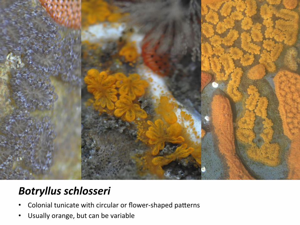
Botryllus schlosseri • Colonial tunicate with circular or flower-‐shaped paGerns • Usually orange, but can be variable
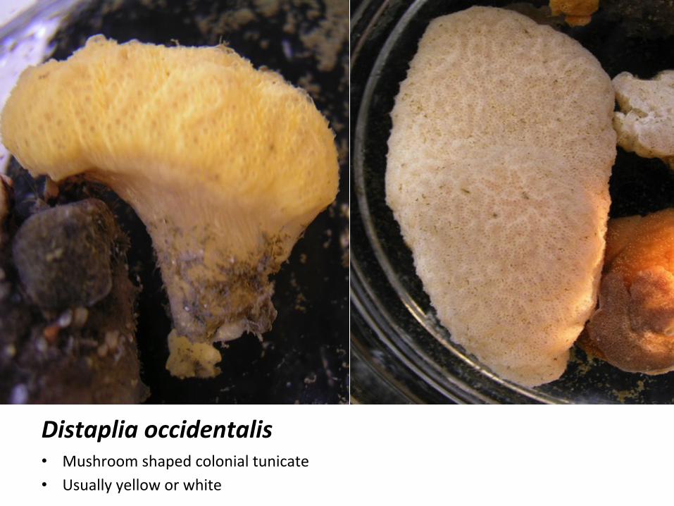
Distaplia occidentalis • Mushroom shaped colonial tunicate • Usually yellow or white

Didemnum sp. • Yellowish to cream colored colonial tunicate with irregularly arranged zooids • Larger colonies o@en have lobes that do not sit flat on the substrate

Diplosoma listerianum • Olive green to translucent colonial tunicate • Very thin and encrusAng with Any zooids

Bugula sp. • White arborescent bryozoan • Spiral branching polyps

Bugula neri9na • Purple to black arborescent bryozoan • Does not have spiral branches

Watersipora subtorquata • Bright encrusAng, reddish orange bryozoan with black dots • O@en rises up three dimensionally and is very briGle

Schizoporella unicornis • Bright orange encrusAng bryozoan • Always lays flat

Metridium senile • Small white or orange anemone • Tentacles can be white, orange or brown
closed

Obelia sp. • Branching colonial hydroid with Any white polyps at the Aps of branches • Polyps are o@en retracted
polyps

Spirorbid polychaete worms • Small spiral shaped calcareous tubes • Worms are o@en retracted when disturbed

Serpulid polychaete worms • Larger than spirorbid worms with irregular shaped calcareous tubes
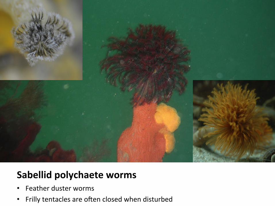
Sabellid polychaete worms • Feather duster worms • Frilly tentacles are o@en closed when disturbed

Terrebellid polychaete worms • Commonly called spagheP worms • Has a mud tube with small strands of tentacles searching for food.

Acorn barnacles • Small sessile crustacean that cements plates to a surface • Uses appendages (cirri) as a net to catch food

My9lus spp. • A common black or grey bivalve that aGaches using byssal threads • It usually has other organisms growing on its shell.

Workshop 11RABLE 2015

Succession in a Marine Fouling Community
Goals and ObjectivesAt the end of this laboratory you should be able to:
1. Estimatethedistributionandabundanceofspecieswithinacommunity.
2. Explainwhatresourcesaresharedamongcommunitymembers.
3. Predictthepossibleoutcomesofcompetitionforsharedresources.
4. Describethemechanismsbywhichresourcesarerenewed.
5. Analyzethechangeincommunityconstituentsovertime.
6. Proposemechanismstoaccountfortheobservedchanges.
7. Explaintheprocessofecologicalsuccessionandsuggestmechanismsunderlyingobservedchanges.
8. Describetheextenttowhichscientificstatementsarelimitedbydata.
Pre-lab Introduction for Lab 6Read and complete the pre-lab exercise before Monday 9 a.m. of lab week. Read the rest of the lab to get a general idea of what you will be doing.
Acommunityisacollectionofdifferentorganismslivinginaparticularplace.Recallthatthecommunitiesyouexaminedinthediversitylabdifferedfromeachotherinspeciesrichnessandabundance.Communityrichness and composition changes over time in a process called succession. Biologists have longwondered why communities differ in diversity and composition, so there are many hypothesizedexplanations,eachofwhichplacesdifferentamountsofemphasisonthearrivalofcolonists,availabilityofresources,andinteractionsamongresidents.Someofthesehypothesesarelistedbelow:
Community age—oldercommunitieshavehadmoretimetobecolonizedbyspeciesfromsurroundingareas(increasingdiversity)andforinteractionsamongspeciestohaveeffects(increasingordecreasingdiversity).
Energy inputs—allfoodwebsarebasedonprimaryproductivity(carbonfixation),soproductiveareas,suchasequatorialregionswithabundantlightandwarmtemperatures,shouldsupportmorespecies.
Resource availability—communitieswitharangeofresources(heterogeneoushabitats)shouldcontainmorespecies.
Lab 6
149

150 Lab6: SuccessioninaMarineFoulingCommunity
Competition—given sufficient time, a superior competitor may dominate a community, monopolizeresources,andexcludeotherspecies(reducesdiversity).
Predation—large or ecologically important predators reduce prey population sizes; this may reducecompetition,permittingmanydifferentspeciestopersist.
Facilitation or habitat modification—theactivitiesormerepresenceofsomespeciesmodifythephysicalenvironment in a way that enhances the success of other species, leading to changes in speciescomposition.
Access to colonists—isolated communities receive fewer colonists than less isolated communities, soisolatedcommunitiesmayhavelowerdiversity.
Rates of disturbance —frequentdisturbanceremovesbothindividualsandspecies,continuallyprovidingopen space and preventing dominance by superior competitors. This may lead to an increase indiversity.
The potential explanations for differences in diversity just presented are not mutually exclusive,meaningthatmorethanonecanbeacceptedastrue.Todistinguishamongpotentialexplanations,onemusthaveuniquetestablepredictionsforeach.Testsofahypothesiscanbemadeusingexperimentalorcomparativemethods.
Comparative methods are often used when experiments are very difficult to do. For example, if youwantedtoknowwhetherplantdiversitydeclinedasredwoodforestsaged,itwouldbedifficulttocreatereplicateforestsandfollowspeciesovertimebecauseredwoodtreesliveforsolong.However,itwouldbepossibletocomparethetreespeciespresent innaturalredwoodforestsofdifferentagesto lookatpatternsandcausesofsuccession.
Natural experiments are another useful tool for studies of community development and speciessuccession. As stated earlier, succession describes the pattern of change in species composition in acommunity. Succession often proceeds through “stages” characterized by different types of species.Sometimesthesestagesarequitedistinct,butmoreoftentheygradeintooneanother.Ecologistsstudysuccessionasawayofpredictingthetrajectoryofcommunityrecoveryafterahuman-causedornaturaldisturbance that creates free space. A natural experiment presents biologists with the opportunity tostudytheresultsofaneventthatcouldnotbeexperimentallyinduced.Forexample,thevolcaniceruptiononMountSt.Helenscreatedemptyhabitats,resultingintheperfectopportunityforanaturalsuccessionexperiment.Biologistswonderedwhetherplantswouldcolonizetheslopesofthemountaininaparticularorder.Theybegantostudythesiteimmediately.Lupineswereamongthefirstplantstocolonize,andsubsequentstudyrevealedthatlupinesmodifythesoilbyaddingnitrogentoit.Asymbioticassociationwithanα-proteobacterium(Rhizobium)permitslupinestofixatmosphericnitrogen;atfirstnitrogenisbound in plant tissues, but it later enters the soil when dead plant matter falls to the ground anddecomposes.Thisnitrogenadditionisvitaltolatercolonistswithoutsimilarsymbioticassociations.Bycombiningobservationsfromalargenaturalexperimentwithresultsfromdetailedexperimentalstudies,ecologists were able to show why certain plants were among the first colonists and how these plantsmodifiedtheenvironmentforspeciesthatarrivedlater.
©Stachowicz2008.Usedwithpermission.
Figure 6-1

Lab6: SuccessioninaMarineFoulingCommunity 151
In communities with long-lived organisms like trees, succession is often studied using comparativeapproaches in combination with natural experiments. For example, ecologists have developed anunderstanding of how forests regenerate by comparing the species composition of communities thatcurrentlyexistinareasthatwereoncefarmedbuthavesincebeenabandoned.Thesesitesareusuallycalled“oldfields.”Ecologistsusethetimesinceold-fieldabandonmentasasurrogatefortheageofthecommunityandarrangecommunitiesinorderofagetoinferthelikelysequenceofsuccession.AbandonedfieldsareshowninFigure6-1onthepreviouspage:movingfromlefttoright,thefirstfieldisonly2yearsold,thesecondisabout10yearsold,andthethirdhasbeenabandonedformorethan100years.Youwillnoticethatsuccessioncanbecharacterizedbydiscretestages,althoughthereis,ofcourse,considerableoverlapinspeciescompositionbetweenadjacentstagesasacommunitymovesfromonestagetoanother.
Noticetheopennessoftheyoungest“oldfield.”Thefirstcolonistsaregrassesandherbs.Thinkaboutseedproduction—dograssesmakemanyseedsorfew?Thinkaboutseedmovement—dograssesdispersewellorpoorly?Thinkaboutresourcessuchaslightornutrients—aretheylikelytobelimited,andwillresidentshavetocompeteforthem?
Noticethatthe10-year-oldfieldhasshrubs.Thinkaboutplantsize,density,andreproductiverates.Thinkaboutresourcecompetitionincomparisontothatintheyoungerfield.Isanewgrassplantlikelytoestablishitself(recruit)inthisfield?
Noticethatthe100-year-oldfieldhastreeswithlittleundergrowth.Theplantsthatarepresentintheundergrowthareferns—whatisthetypicallightregimeforafern?Noticethatthereissomeopenspacebeneaththetrees.Whyisthisspaceopen?Howhasthehabitatforpotentialcolonistschanged?Isitmorelikelythatpotentialcolonistscannotreachthehabitatorthattheycouldnotsurviveiftheydidreachit?
The rhetorical questions just posed were designed to help you think analytically about succession. Using the information and ideas outlined above, in conjunction with what you have learned in lecture, answer the numbered questions throughout the sections below:
Pre-lab Questions—Record Your Answers on the Online VersionSpeciesateachstageofsuccessionoftensharemanytraitsincommon.Recallfromearlierinthequarterourdiscussionofdifferentlife-historystrategies.
1. Wouldyouexpectearlysuccessionalspeciestober-selectedorK-selected?
2. Why?
3. Whataboutspecies thatdominate later insuccession?Wouldyouexpect themtober-selectedorK-selected?
Why do early successional species give way to later species? This is usually because they are poorcompetitors, and they either alter the environment in a way that reduces their own success oreventuallysuccumbtocompetitionfromotherspecies.Whydon’tlatesuccessionalspeciesdominatefromthestart?Thereareseveralpossibilities.Oneisthatitmaytakealongtimeforcolonizationbythesespeciestooccurbecauseofpoordispersalabilitiesandslowgrowthrates.Thisiscalledneutralor tolerance succession. In contrast, early successional species can either facilitate or inhibitsuccession.TheexampleofsuccessionofplantsonMountSt.Helensfollowingavolcaniceruptionisanexampleoffacilitativesuccessionbecauseearlycolonizersmodifytheirenvironmentbyaddingnitrogen,whichfacilitatesorenhancestheabilityofotherspeciestocolonize.Withoutlupines,latersuccessionalspecieswouldbecomeestablishedatamuchslowerrate.
Ininhibitionsuccession,earlysuccessionalspeciessuppresslatercolonistsandsuccessionproceedsonlywhensomeotheragentofmortality(suchaschangingphysicalconditions,orpredators)causesearlycoloniststodie.Underinhibitionsuccession,latesuccessionalspecieswouldbecomeabundantmore quickly in the absence of the early colonizing species. This occurs most often when earlycolonistspreemptresourcesbyoccupyingallavailablespace,light,orotherlimitingresource,thereby

152 Lab6: SuccessioninaMarineFoulingCommunity
inhibitingtheestablishmentorgrowthoflatersuccessionalspecies.Wewillseeexamplesofthisinlecture.
Inthefirstlabyouwereinterestedincharacterizingpatternsofspeciesdiversitywithinacommunity.Becauseofsuccession,communitycompositionchangesovertime.Howdoyouthinkthatspeciesdiversity changes over time as succession proceeds? From the list of potential causal hypothesesabove, you can see that making a prediction may not be straightforward. Early successionalcommunitiesmightbediversebecausefewspecieshavebeenexcludedandresourcesareabundant,ortheymightbespecies-poorbecauseconditionsaresufficientlystressfulandfewspeciescantoleratetheseconditions(asintheMountSt.Helensexample).Similarly,moretimemightallowmorespeciesto colonize,buton theotherhand, this alsomightallowmore time for competitive exclusion tohappen.Aresolutionofthesetwoideassuggeststhatdiversitymightbegreatestincommunitiesofintermediateagebecausethesehavesufficienttimeformanyspeciestobecomeestablishedbutnotenough for competitive exclusion to have resulted indeclinesindiversity.Lookbackatthephotographsofoldfields of different ages—can you see any evidence insupportofthishypothesis?
In the lab exercise for this week, you will look for elements of succession in a community of marine organisms that encrust hard surfaces in ocean waters.You will use the comparative method by examining thespeciespresentonhardsurfacesplaced intheoceanfordifferentlengthsoftime.Youwillseecommunitiesthatdiffer inage:approximately3months,6months,and9monthsold.
At firstglance,manyof theanimalsyouwill studymayremind you of plants. Many adult marine animals aresessile—they attach to hard surfaces and most cannotmoveoncetheyhavesettledintoaparticularplace.Somesessileanimalsareunitary—theygrowbyaddingnewcellstoanexistingindividual,butmostaremodular andgrowby copying feeding units of the body many times. Perhapsyou have seen a spider plant, Bermuda grass, or astrawberrygrowinthisway.
When the first strawberry plant is established, it sendsrunnersoutacrossthesoil(Figure6-2).
New plants develop when the runners put out roots (Figure6-3).
The new plants are attached to the first plant, but once they have roots, they can survive if therunnersbreak.
This modular growth strategy allows a single genetic individual to exploit a large area of thehabitat.
Fromlab#2,youknowsomethingaboutaplant’sphysiologicalneeds.Plantshavetocollectresourcesand compete with other plants for access to those resources. Imagine a modular plant, like astrawberry, grown in the same planting box with a unitary plant, like a daisy. Both start fromseedlings.Bothplantsneedlight,buttheirgrowthandcompetitivestrategiesdiffer.
©ThienMai2008.Usedwithpermission.
Figure 6-2
Figure 6-3
©ThienMai2008.Usedwithpermission.

Lab6: SuccessioninaMarineFoulingCommunity 153
4. Tworesourcesaregivenbelow.Addathirdofyourchoice,andbriefly discuss the relative costs and benefitsofhavingamodulargrowthstrategyforeachresource:
(a) Competitionforlight:
(b) Competitionforsoilnutrients:
(c) Competitionfor_____________________________________________.
5. Is a modular growth strategy better for capturing concentrated resources or widespread (dilute)resources?Brieflyexplainyourthinking.
Modular animals have some similarities to modular plants, but they also have some importantdifferencessuchastheabilitytofeedoncetheyareovergrown.Belowarethumbnailsketchesofafewcommontypesofencrustingmarineunitaryandmodularorganismsthatyouarelikelytoseeinlab.Youdonothavetomemorizeanytaxonomicterms,butapassingfamiliaritywithcommonnamesmaymakeiteasiertodiscusswhatyouseewithyourclassmates.
Aunitary(solitary)tunicate,alsocalledasea squirt isshowninFigure6-4.Theimportantthingtonoticeisthebloblikebodywithtwosiphonsatthetop.Theanimalfeedsbycollectingfoodparticlesfromthewateraroundit;waterentersthebodythroughonesiphon,passesthroughaninternalmeshbasketwhereparticlesarefilteredout,andexitsviatheothersiphon.Youmayseeseveralspecies.
Modular sea squirts develop as one animal buds to produce another.The buds remain attached to each other. Such animals are calledcolonial tunicates,andeachbuddedmoduleisusuallyverysmall.Thecolony has a firm, fleshy appearance and is covered with small poreswherethesiphonsofeachmoduleopentothecolonysurface (Figure6-5). The siphon openings are visible and are sometimes arranged inpathways or clusters. Many tunicate colonies have an extremely lowsurface pH; this might affect colonization or overgrowth by otherspecies?
Figure 6-4
©Santos2008.Usedwithpermission.
Figure 6-5Bryozoansarestiff,somewhatcrunchy,encrustinganimals.Theyhaveamodulargrowthpattern:thefirstorganismmakesaseriesofbuds,andeachbudmakesothers,untilacolonyisformed.Theshapeofthecolonycanbetreelike,aflatcrust,orsomethinginbetween(Figure6-6).Bryozoansfeedbycollectingtinyparticlesfromthesurroundingwateronaringoftentacles.
©S
anto
s20
08.U
sed
wit
hpe
rmis
sion
.
©Santos2008.Usedwithpermission. ©ThienMai2008.Usedwithpermission.

154 Lab6: SuccessioninaMarineFoulingCommunity
Some of the other unitary organisms you may encounter:
Tube-dwelling worms collect particles on a retractable crown of tentacles. The mouth is in thecenterofthetentaclecrown.Theanimal inFigure6-7hasaflexibletube(seearrow),whereastheanimalinFigure6-8hasahardtube(seearrow)madeofcalcium.
Barnaclescollectfoodbycombingafeatherystructurethroughthewaterabovetheirbodies.Thefeedingstructure,asetoflegs,canbepulledintothehardenedshell(asintheupperanimalinFigure6-9)orextendedthroughtheslitatthetopofthebody(loweranimal).
Mussels attachtohardsurfacesbyasetofstrongthreads(byssalthreads).Theyhavetwoshellswithasmallgape,oropening,betweenthem.Water,containingfoodandoxygen,entersviathegape(seearrowsinFigure6-10)betweenshellsandfoodparticlesarecollectedonaninternalgillcoveredwithmucus.
©ThienMai2008.Usedwithpermission.
Figure 6-7 Figure 6-8©ThienMai2008.Usedwithpermission.
©ThienMai2008.Usedwithpermission.
Figure 6-6©Santos2008.Usedwithpermission.
Youcannotseetheindividualmodulesinthesephotos.

Lab6: SuccessioninaMarineFoulingCommunity 155
6. Whatdomostsessileanimalseat?
7. Brieflydescribeonewayanimalscouldcompeteforthiskindoffoodsource.
Figure6-11depictsapanelsimilartothoseyouwillseeinlabthisweek.Thepanelishard,soanimalsdonotpenetrateitasrootsdowithsoil.Thispanelwasplacedintheoceanonlyashorttimeago,somuchofitisstillbare(thegrayarea).
8. Whatkindofanimalisthelargestorangecrust?
9. Forwhatresourcemightsessileanimalscompete?
ThepanelinFigure6-12hasbeenleftintheoceanformanymonths.
Barnacleswithfeedinglegsretractedandextended
©R
ando
lph
2008
.Use
dw
ith
perm
issi
on.
Figure 6-9 Figure 6-10©
Ran
dolp
h20
08.U
sed
wit
hpe
rmis
sion
.
©S
anto
s20
08.U
sed
wit
hpe
rmis
sion
.
Figure 6-11 Figure 6-12
©S
anto
s20
08.U
sed
wit
hpe
rmis
sion
.

156 Lab6: SuccessioninaMarineFoulingCommunity
10.Nametwokindsofanimalsthatarevisible:
(a)
(b)
SpaceisclearlyatapremiumontheolderpanelshowninFigure6-12.
11.Describeonegrowthstrategyyouseeherethatwasnotvisibleontheyoungerpanel:
12.Whatcanyouseethatindicatescompetitionamongorganisms?
13.Whymightitbeadvantageoustohaveamodulargrowthpatterninthissituation?
Haveyoustartedtowonderhowanimalsgetontothepanelsinthefirstplace?Animalscolonizethepanelsasfree-swimminglarvae.Somelarvaefeedintheswimmingstageandothersdonot.Thosethatdonotfeedhaveonlyashorttimeinwhichtofindasettlementsite—iftheydelaysettlement,theywillnothavesufficientenergyreserveslefttometamorphoseintoadultsaftertheysettle.
Allnewlyexposedpanelsareempty,sothedevelopmentofthecommunityisaffectedbywhichlarvaeareinthewateratthetimethepanelsareexposed.Thepresenceoflarvaeinthewaterdependsonwhichspeciesinthesurroundingcommunityarereproductivelyactiveatthetimespaceisavailable.Reproductiveactivityinanimalsvariesseasonallyinthesamewaythatsomewildflowersbloominlatewinterandothersbloominmid-summer.However,unlikeseedsthatcanremaindormantforsometime,thelarvaeofencrustingmarineorganismsbegingrowingassoonastheysettle.Oncetheblankpanelisfilled,thereisanopportunityfornewsettlerstolandontopofexistinganimalsandforcompetitionamongorganismstoaffectcommunitycomposition.
14.Listonefactorthatyouimaginewouldlimitsettlementontopoflivingorganisms.
Thepanelshangverticallyfromthesideofadock.Animalssuchascrabsandsnailsliveonthedockandcancrawlontothepanels.Theoceancanbestormyattimes,andheavyrainsmixfreshwaterintotheoceansurfacewaters.
15.Useyour imagination todescribe twoways inwhichdisturbanceof the sort justdescribedmightaffecttheanimalsthatliveonthepanelsandamountoffreespaceavailable.
(a)
(b)
16. Inwhatwaymightgrowth form(shape)ofthepanelinhabitantsaffectthelikelihoodofsurvivingonthepanels?
17.Aremodularorganismsmoreorlesslikelytobepartofthe long-termcommunitythanareunitaryorganisms?Explainyourthinking.
In lab this week you will need to observe patterns of species distribution and to develop testablemechanisticexplanationsforthesepatterns.Youmaywanttolookbackattheorganismsjustdescribedtorefreshyourmemoryontheirnaturalhistoryandlifestyles.
The laboratory exercise begins on the next page.

157
Lab 6: Succession in a Marine Fouling CommunityInlab,youandapartnerwillcatalogthenumberandrelativeabundancesofspeciesincommunitiesofthreedifferentageslivingon10cm×10cmpanels.Findatleastthreemorepairsofstudentstopoolyourdatawith.
Select a panel and place it in a large plastic tub filled with seawater. Be sure to randomize yourselectionusingthediceprovided.Usethestringgrid,similartotheoneinthepicturebelowtoestimatepercentcoverforthedifferentspecies.Donotcountanygrowththatextendsbeyondthepanel.Your grid will divide the panel surface into 25 squares each equal to 4% of the total surface area.Usethefractionofasquarefilledbyaparticularorganismtoestimatepercentcover.Forexample,thecolonialtunicateoutlinedinredintheupperrightofthepanelinFigure6-13coversabout100%ofthetotalareain4squares,orabout16%ofthetotalsurfacearea(4squares@4%each).
Usingwhatyoujustlearnedaboutthebasickindsofencrustinganimalsandthephotographickeyprovidedinlab,countthenumberofsessilespecieson one panel of each age.Youwilldistinguishbetweenthenumberofspeciesontheprimarysubstrate(thepanel)andthoseonsecondarysubstrate(growingonotherorganisms=overgrowth)oneachpanel.
Examinethepanelsatthelabbench;youcanputthemunderthedissectingmicroscopeifyouwish.Thismaybenecessary forpanels that lookbare—theyarenot!Begentlewiththeanimalsas theyaredelicateandwillbehandledbymanystudentsthisweek.Itisnotimportantthatyoucorrectlyidentifyeach species with its proper scientific name; the keys provided are meant only as a guide. What isimportantisthatyouareconsistentforallthepanelsyoucountandclearlydelineatethecharacteristics
©S
tach
owic
z20
08.U
sed
wit
hpe
rmis
sion
.
Figure 6-13

158 Lab6: SuccessioninaMarineFoulingCommunity
ofyourspecies.Forexample,theoutlinedcolonyinthefigureaboveisBotrylloides violaceous.Youwillhaveapicturekeyinlabthatwillclearlyidentifythis.However,whetheryoucallit“Botrylloides violaceous”or“orangeencrustingblob”onyourdatasheetdoesnotmattermuch,solongasyoualwaysidentifythisorganism in the same way. Meet with the other three partners in your group to standardize youridentifications. Your TA will give you some other hints on how to identify and operationally classify“species”forthislab.Useyourexperienceindelineating“operationaltaxonomicunits”foryoursurveyinlab#1asaguide.
Record Your Data on the Grids on Pages 159 to 161(1) Estimatetherelativeabundance(aspercentcover)ofeachspeciesoneachofthepanels;beconsistent
aboutwhatyoucallaspecies.First,recordthetotalcoverofeachspeciesonthepanel.Placethesedata in columnAof thedatagrid.Then record thepercent coverof each species that isgrowingdirectlyonprimarysubstrate(thepanel),ratherthanontopofotherorganisms.RecordthesedataincolumnBofthedatagrid.Thetotalareaoccupiedbyallspeciesmaybegreaterthan100%becauseofovergrowth,butthetotalamountofprimaryspaceoccupiedshouldnotexceed100%.
(2) Countthenumberofspeciesoneachpanel.
(3) Usenumberof speciesandpercentof totalcover tocalculate thediversityofeachpanelwiththeShannon-Wienerindexyoulearnedinlab#1.
(4) Calculatethepercent overgrowthforeachspeciesoneachpanelbysubtractingthepercentonprimarysubstrate(columnB)fromthepercentoftotalarea(columnA)foreachspecies.
Instructionsforfurthercalculationsandthelabreportfollowthedatasheetpages.Instruction (5) is on the top of page 162.
Whenyouhavefinishedwithapanel,putitbackintheflumeexactlywhereyoufoundit.

Lab6: SuccessioninaMarineFoulingCommunity 159
Data Collection in LabPanel Age
Totalnumberofspecies=
Total%cover=
Shannon-WienerIndexvalue=
Total%onprimarysurface=
Total%overgrowth=
Commonname %Coveron % or Total% panel Overgrowth Species identifier cover(A) Pi surface(B) (=A–B)

160 Lab6: SuccessioninaMarineFoulingCommunity
Data Collection in LabPanel Age
Totalnumberofspecies=
Total%cover=
Shannon-WienerIndexvalue=
Total%onprimarysurface=
Total%overgrowth=
Commonname %Coveron % or Total% panel Overgrowth Species identifier cover(A) Pi surface(B) (=A–B)

Lab6: SuccessioninaMarineFoulingCommunity 161
Data Collection in LabPanel Age
Totalnumberofspecies=
Total%cover=
Shannon-WienerIndexvalue=
Total%onprimarysurface=
Total%overgrowth=
Commonname %Coveron % or Total% panel Overgrowth Species identifier cover(A) Pi surface(B) (=A–B)

162 Lab6: SuccessioninaMarineFoulingCommunity
(5) Poolyourdatawith theother threepairsof students inyourgroup fora reasonable sample size.Calculate average values for number of species, total percent cover, the Shannon-Wiener index,percentcoveronpanel,andpercentovergrowthfor panels of each age.
Panel Numberof %coveron %coveras age species %cover H'value panelsfc overgrowth
3months
3months
3months
3months
Average:
SD
Panel Numberof %coveron %coveras age species %cover H'value panelsfc overgrowth
6months
6months
6months
6months
Average:
SD
Panel Numberof %coveron %coveras age species %cover H'value panelsfc overgrowth
9months
9months
9months
9months
Average:
SD

163
Laboratory Report(6) Ploteachofthefivevalues(numberofspecies,totalpercentcover,Shannon-Wienerindex,percent
coveronpanel,andpercentovergrowth)onthey-axisagainstpanelageonthex-axis(5plotstotal).YourTAwillprovidegraphpaper.Youcanmakeonesetofplotsperpairofstudentsandphotocopythem;otherwisemakeonesetperindividual.(½ point per plot)
(7) Describetheresultsshownineachplotinafewsentences.Writethesentencesonthesideofeach graph.(½ point per description)
(8) Selectoneresultthatinterestsyouandyourpartner.Developapotential explanationforthisresultthatisconsistentwiththeobservations.
Forexample,youmightobserveadeclineinthenumberofspeciesovertimebutnoticethatallthespeciesontheoldestpanelswerecolonialtunicates.Perhapsyouwouldliketoconsiderwhatfactor(s)are responsible for the decline in species richness and why colonial tunicates dominate latesuccessionalcommunities.Youmighthypothesizethatthepreponderanceoftunicateswasduetosuperiorcompetitiveability,orbetterfoodcapturerates,oragreatabundanceoftunicatelarvae,or...Thereareseveralpotentialexplanationsonpages149–150;weave these ideas together with information gained from the pre-lab text on succession.
Results: (½ point)
Proposed hypothesis to explain this result: (½ point)
Name: _______________________________ TA: __________________________ Date: ___________

164 Lab6: SuccessioninaMarineFoulingCommunity
(9) Developatestablepredictionofyourhypothesis.
Our hypothesis predicts: (½ point)
Our mathematical prediction: (½ point)
Brieflyoutline a feasible experimentthatwouldtestyourhypothesis.Outlinetheessentialfeaturesofthedesignbydescribingwhatyouwoulddoandwhichdatayouwouldcollect.
We could test our hypothesis by: (½ point)
(10) Describeoneexperimentaloutcomethatwouldsupport your hypothesis andone outcome that would refute your hypothesis.Remembertorefertoyourprediction.
Our hypothesis would be supported if the experimental outcome was: (½ point)

Lab6: SuccessioninaMarineFoulingCommunity 165
Our hypothesis would be refuted if the experimental outcome was: (½ point)
(11) Findanotherpairofstudentsandaskthemtoexplaintheresulttheyelectedtostudy.Listentotheirproposedexplanationfortheresult.Developanalternative explanationfortheresultthispairofstudentselectedtostudy.They will do the same thing for your hypothesis.
My classmates, ______________________________________________, observed: They hypothesized:
Their prediction was:

166 Lab6: SuccessioninaMarineFoulingCommunity
An alternate explanation and prediction for their result is: (½ point)
(12) Examinethealternateexplanationthattheotherpairofstudentshasdevelopedforyourresult.
My classmates thought my result could be explained by:
Their prediction was:
Would your planned experiment indicate that only one hypothesis was correct? (explain—couldyouruleouttheotherhypothesis?)(½ point)
(13) Assumethattheexperimentthatyou and your partneroutlinedwentasplanned.Whatconclusion(oneortwosentences)wouldyoubeabletodraw?Theconclusionmustbebasedonthedatayouintendedtocollect. (½ point)
If the experiment went as planned, I would conclude that:

Lab: Succession in a Marine Fouling Community
Course: BIS2B-‐-‐Introduc<on to Evolu<on and Ecology
University of California, Davis
Pat Randolph Dept of Evolu<on and Ecology

Big Questions (Lab Goals): What is succession? How can we determine if succession is occurring? How might we quantify a change in a community through time? What mechanisms can explain WHY there is a change in community structure? (develop a hypothesis) How would we test our hypothesis?
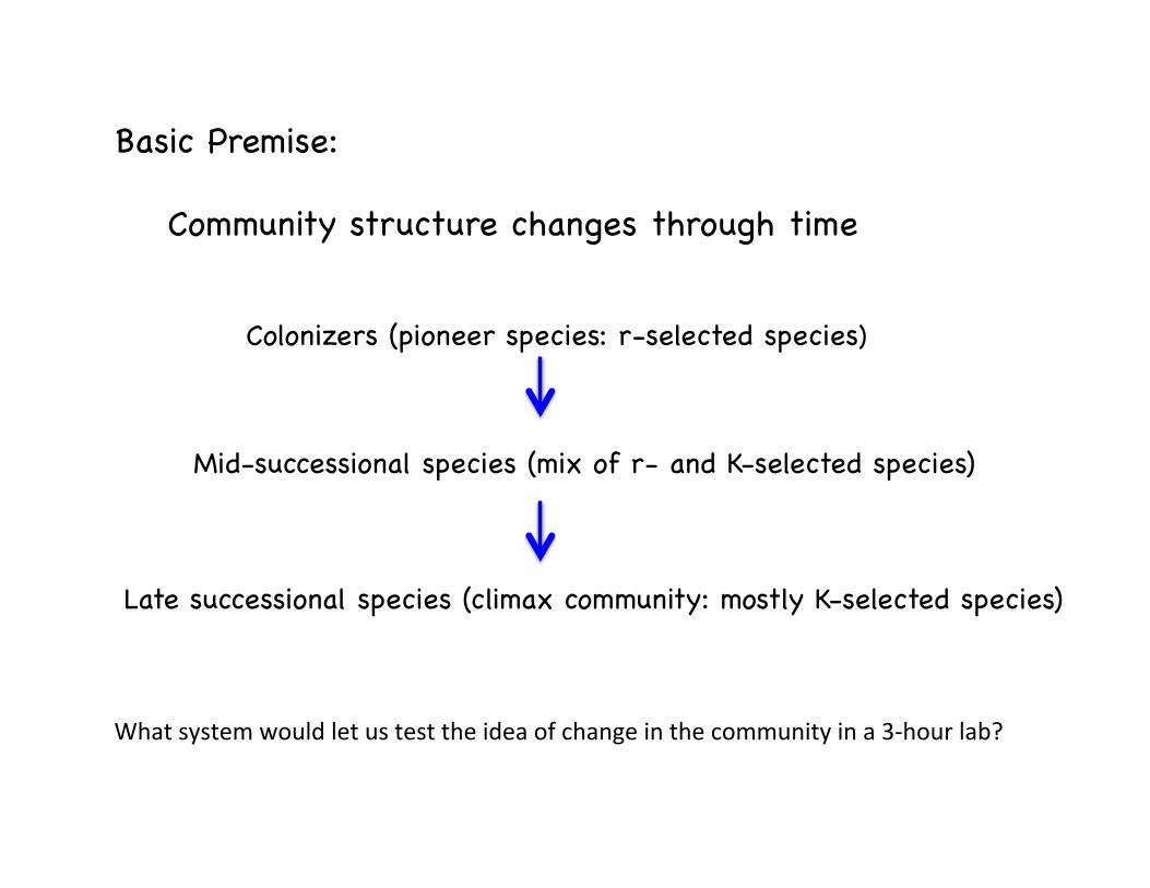
Basic Premise: Community structure changes through time
Colonizers (pioneer species: r-selected species)
Mid-successional species (mix of r- and K-selected species)
Late successional species (climax community: mostly K-selected species)
What system would let us test the idea of change in the community in a 3-‐hour lab?

Our System: Marine organisms growing on a floating dock in Bodega Bay
3 month old plate 9 month old plate
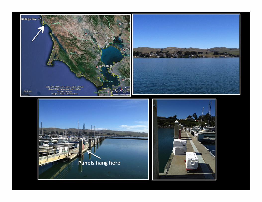
Panels hang here

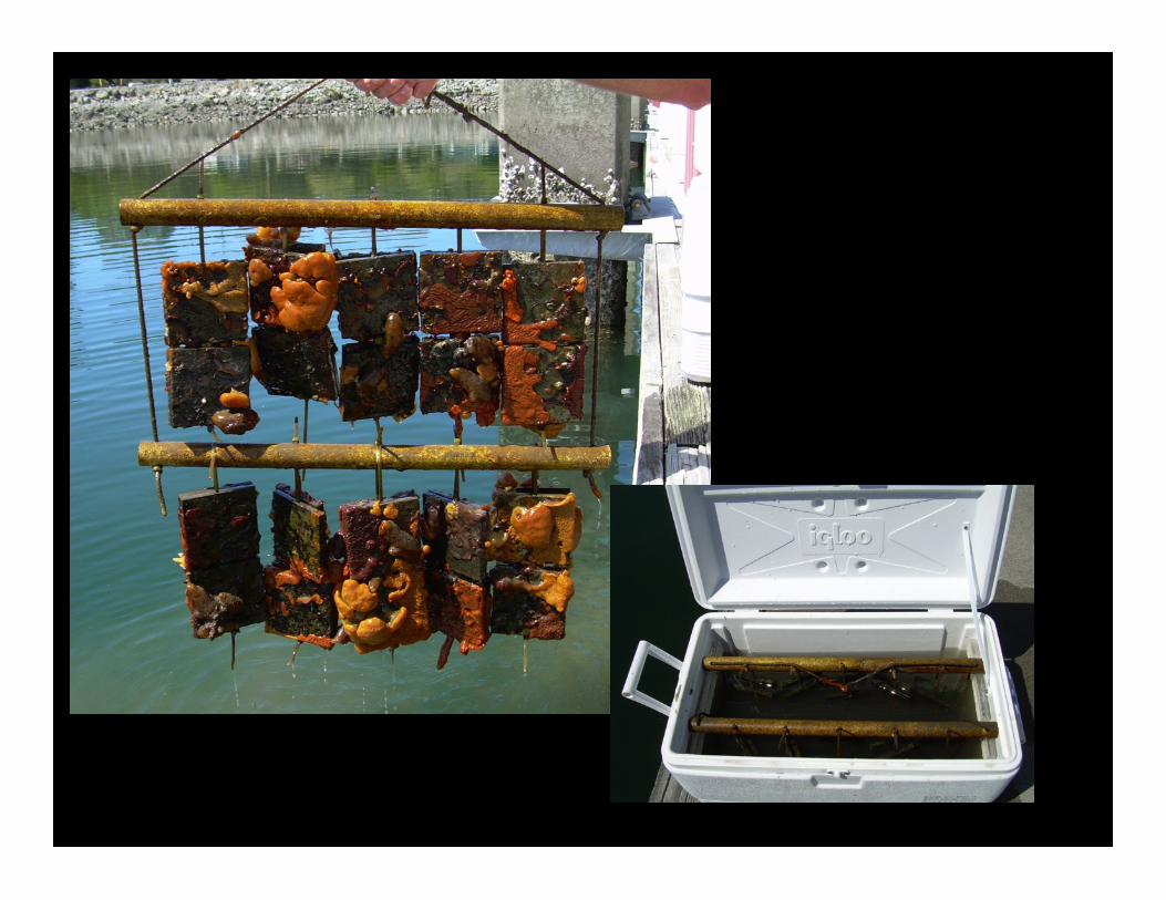

hKp://coursecontent.ucdavis.edu/BIS/2B/Lab06/player.html


The Lab—Part I Data Collection -Groups of 2 -Each group samples 3 plates (3 month, 6 month, 9 month). -Data collected: number of species percent cover for each species (includes overgrowth) percent of each species on the panel surface only -Calculations: Shannon Diversity Index Percent overgrowth

The Lab—Part I: Thinking Part Hypothesis Development: -pick a result (observation) that was interesting
-develop a mechanistic hypothesis to explain this result -include a prediction, mathematical prediction
-Outline an experiment to test hypothesis
-Exchange ideas with another group—are there other hypotheses that could explain the data?

Typical 3 month old panels
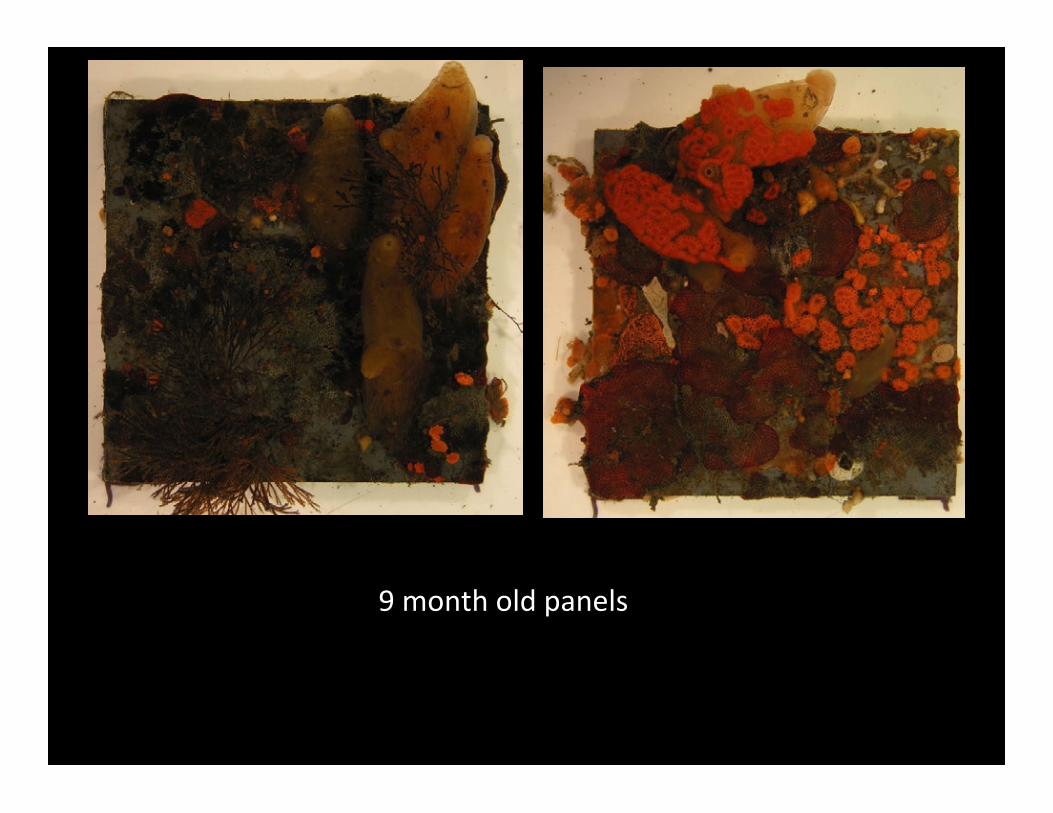
9 month old panels

Quick run through of some of the organisms

bryozoan
Mostly Modular Members
tunicates

Unitary animals
tunicate marine worms

SpagheU worm with a mud tube and foraging tentacles

Barnacles-‐unitary
Solitary tunicate

Sponge-‐gray area between modular and unitary

Plumose anemone-‐-‐unitary
closed

Workshop 12RABLE 2015

Justin Shaffer UCI RABLE [email protected] February 21, 2015
Insights and activities from a human anatomy lab without cadavers
Background • Bio Sci D170 (Applied Human Anatomy) is a six-unit upper-division elective targeted for
students that want to apply to health professional programs.• The pre-requisite for this course is a human physiology lecture with a C or better.• The majority of students that take the class are junior and senior biological sciences,
pharmaceutical sciences, or public health sciences majors. Sophomore level nursingscience students also enroll in the course.
• The course meets for three 50-minute lectures a week (in class size of 90 to 120students) and one three-hour lab section a week (in sections of 24 students).
• The course is taught with a systems anatomy approach (as compared to a regionalapproach used by medical schools) and covers all major organ systems of the body,including skeletal, muscular, nervous, cardiovascular, respiratory, digestive, urinary,reproductive, and integumentary.
Course materials • Bio Sci D170 is taught using the following materials:
o Textbook: Human Anatomy, 7e by Marieb et al.o MasteringA&P: an online learning management system that
provides students with opportunities for interactive assignmentsand quizzes, videos, tutorials, the eTextbook, and a study area
o Practice Anatomy Lab (PAL): PAL is a virtual cadaver thatstudents can use to see real human cadavers that can be“virtually dissected” to uncover deeper structures of the body.
o A variety of models used in lab (described below).
Course structure for the lecture component • Bio Sci D170 is taught as a highly structured course, meaning that students are actively
required to participate in the learning process before, during, and after each day of class.The breakdown for course activities and assignments is below:
o For each day of class, students are provided with an optional reading guide thatcontains a series of questions that can be answered by reading the textbook. Thereading guides are intended to help students focus on specific portions of thetextbook and to help them become active note-takers.
o Prior to each day of class, students are assigned a pre-class assignment onMasteringA&P that includes multiple choice, matching, and labeling activities.These assignments are intended to give students a chance to be familiar with thematerial prior to coming to class.
o During class, students work alone or in groups to answer a series of questions,including multiple-choice, matching, labeling, drawing, or short-answer. Lecture isminimal and is provided during transition points or to clarify studentmisconceptions or difficult material. The course is taught via active learning to getstudents to participate in the learning process and to give them chances topractice using their knowledge that they acquired from pre-class assignments.
o After class, students are required to complete weekly timed review quizzes onMasteringA&P. These quizzes are intended to model the exams in the courseand to keep students up-to-date with studying the course material.
o Major assessments include three midterm exams and a final exam, all of whichcontain cumulative portions.

Course structure for the lab component • This lab is taught without cadavers, so instead students gain hands-on experience with
plastic human anatomy models (whole skeletons, muscle limbs, torsos, hearts, etc), dissecting animal organs (sheep brain, heart, lung, eye, etc), and the virtual cadaver through PAL.
• During lab sessions, students work in groups of three to five to complete lab activities. Activities range from identifying and labeling models, making models, drawing anatomical structures, or feeling their own bodies to identify structures.
• Students turn in a worksheet or take a quiz at the end of each lab session. • Students also complete an online PAL assignment that is related to the organ systems
explored during that week of lab. • Major summative assessments include a midterm lab practical exam and a final lab
practical exam. During these exams, students rotate through ~25 stations to answer questions related to anatomical models.
Activities for this workshop
1. Epithelial and connective tissue identification • Students are exposed to tissues early in the course to give
them a foundation on the structure of organs in the body. • Students gain experience classifying types of tissues in the
body through the use of microscopic images from their textbook and also from PAL.
• In this activity, students work in groups to classify “unknown” images of epithelial and connective tissues. They also develop a flowchart that will help them organize their knowledge on tissue types.
2. Plotting cranial and spinal nerves through the body • Students often have difficulty transferring their knowledge of
organ systems in the body from 2-D textbook pages to 3-D models, and many studies have suggested that the nervous system is especially challenging.
• In this activity, students use string or other craft materials to plot the pathways that cranial and spinal nerves take through the human body. Students apply their “nerves” to human skeleton models to visualize how the nerves coarse through the body in three dimensions.
• NOTE: This activity has been published in CourseSource and can be accessed through the link below.
http://www.coursesource.org/courses/plotting-cranial-and-spinal-nerve-pathways-in-a-human-anatomy-lab

Activity 1 - Tissue identification • You should have a stack of five images for your group. Each image is a microscopic
image of a tissue from the human body. • As a group, determine which type of tissue each image is showing by filling in the
following table. You might not need / be able to fill in each column for each image. Use your textbook for help if you need it.
Image Number of cell layers
Types of cells
Shapes of cells Types of fibers
Other distinguishing
features
What tissue is this and how do you
know?
1
2
3
4
5
• Answer these questions below:
o In these images, what is colored blue (by hematoxylin)? What is colored pink (by eosin)? (Hint: see chapter 1 for help)
o How can you tell the difference between micrographs of elastic and dense regular connective tissues?
o The epithelium of the intestine needs to secrete lots of digestive enzymes and needs lots of surface area for molecular absorption to occur. What type of epithelium lines the intestine and what structures should the cells contain? Justify your answer.
Using the information from the above table, come up with a logical flowchart or guide to help you distinguish between the types of epithelial tissue and connective tissue proper. Draw this flowchart on a piece of paper and show your instructor before moving on.
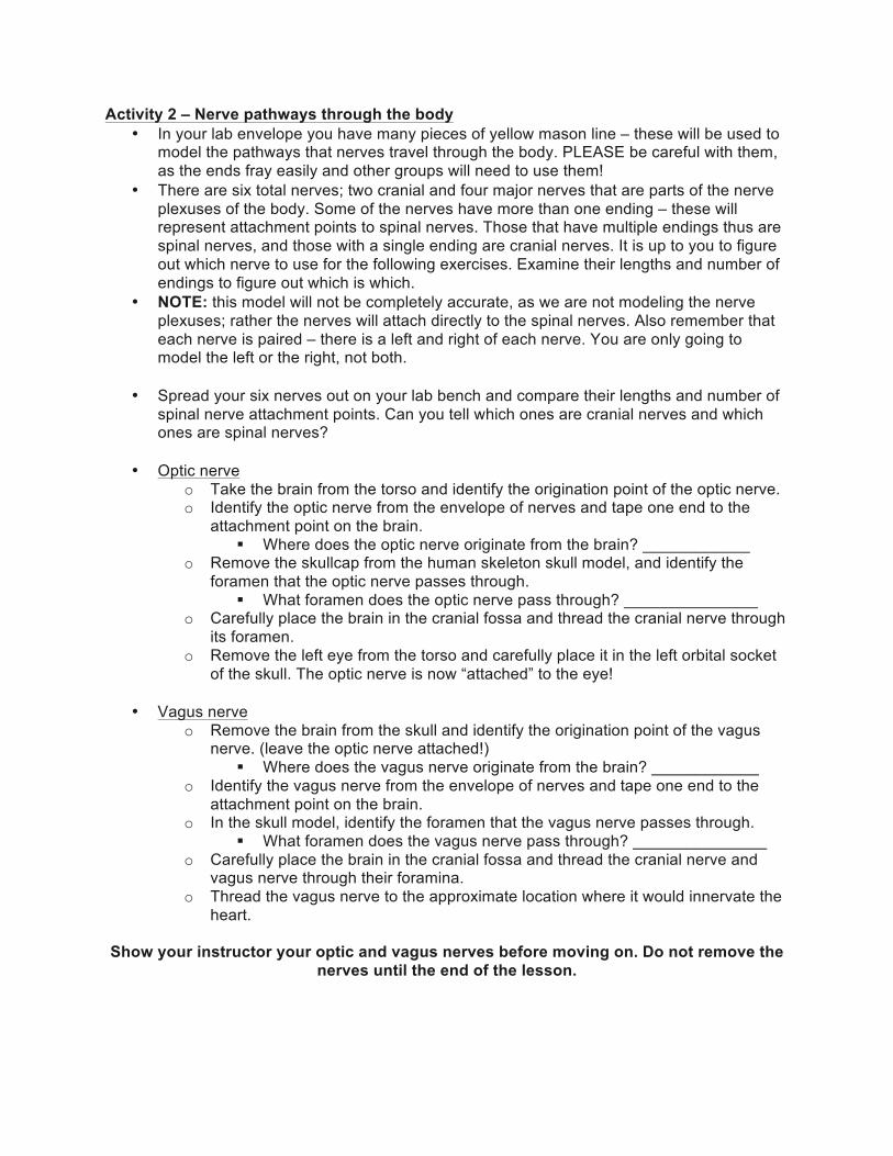
Activity 2 – Nerve pathways through the body • In your lab envelope you have many pieces of yellow mason line – these will be used to
model the pathways that nerves travel through the body. PLEASE be careful with them, as the ends fray easily and other groups will need to use them!
• There are six total nerves; two cranial and four major nerves that are parts of the nerve plexuses of the body. Some of the nerves have more than one ending – these will represent attachment points to spinal nerves. Those that have multiple endings thus are spinal nerves, and those with a single ending are cranial nerves. It is up to you to figure out which nerve to use for the following exercises. Examine their lengths and number of endings to figure out which is which.
• NOTE: this model will not be completely accurate, as we are not modeling the nerve plexuses; rather the nerves will attach directly to the spinal nerves. Also remember that each nerve is paired – there is a left and right of each nerve. You are only going to model the left or the right, not both.
• Spread your six nerves out on your lab bench and compare their lengths and number of spinal nerve attachment points. Can you tell which ones are cranial nerves and which ones are spinal nerves?
• Optic nerve o Take the brain from the torso and identify the origination point of the optic nerve. o Identify the optic nerve from the envelope of nerves and tape one end to the
attachment point on the brain. § Where does the optic nerve originate from the brain? ____________
o Remove the skullcap from the human skeleton skull model, and identify the foramen that the optic nerve passes through.
§ What foramen does the optic nerve pass through? _______________ o Carefully place the brain in the cranial fossa and thread the cranial nerve through
its foramen. o Remove the left eye from the torso and carefully place it in the left orbital socket
of the skull. The optic nerve is now “attached” to the eye!
• Vagus nerve o Remove the brain from the skull and identify the origination point of the vagus
nerve. (leave the optic nerve attached!) § Where does the vagus nerve originate from the brain? ____________
o Identify the vagus nerve from the envelope of nerves and tape one end to the attachment point on the brain.
o In the skull model, identify the foramen that the vagus nerve passes through. § What foramen does the vagus nerve pass through? _______________
o Carefully place the brain in the cranial fossa and thread the cranial nerve and vagus nerve through their foramina.
o Thread the vagus nerve to the approximate location where it would innervate the heart.
Show your instructor your optic and vagus nerves before moving on. Do not remove the
nerves until the end of the lesson.

• Phrenic nerve o Identify the phrenic nerve from the envelope of nerves.
§ Which spinal nerves make up the phrenic nerve? __________________ § What plexus does the phrenic nerve originate from? _______________
o On the human skeleton model, identify the spinal nerves that make up the phrenic nerve.
o Tape the ends of the phrenic nerve to its appropriate spinal nerves. o Thread the phrenic nerve from its attachment points at the spinal nerves to its
most distal point – use tape to help keep it in place.
• Ulnar nerve o Identify the ulnar nerve from the envelope of nerves.
§ Which spinal nerves make up the ulnar nerve? ____________________ § What plexus does the ulnar nerve originate from? _______________
o On the human skeleton model, identify the spinal nerves that make up the ulnar nerve.
o Tape the ends of the ulnar nerve to its appropriate spinal nerves. o Thread the ulnar nerve from its attachment points at the spinal nerves to its most
distal point – use tape to help keep it in place.
Show your instructor your phrenic and ulnar nerves before moving on. Do not remove the nerves until the end of the lesson.
• Obturator nerve
o Identify the obturator nerve from the envelope of nerves. § Which spinal nerves make up the obturator nerve? _________________ § What plexus does the obturator nerve originate from? _______________
o On the human skeleton model, identify the spinal nerves that make up the obturator nerve.
o Tape the ends of the obturator nerve to its appropriate spinal nerves. o Thread the obturator nerve from its attachment points at the spinal nerves to its
most distal point – use tape to help keep it in place.
• Tibial nerve o Identify the tibial nerve from the envelope of nerves.
§ Which spinal nerves make up the tibial nerve? __________________ § What plexus does the tibial nerve originate from? ________________
o On the human skeleton model, identify the spinal nerves that make up the tibial nerve.
o Tape the ends of the tibial nerve to its appropriate spinal nerves. o Thread the tibial nerve from its attachment points at the spinal nerves to its most
distal point – use tape to help keep it in place. Show your instructor your obturator and tibial nerves before moving on. Take a photo of
your completed skeleton model before removing your nerves.

• Answer the following questions about the nerves of the body: o What rami make up the plexuses? Dorsal or ventral or both or neither?
o What muscle(s) does the phrenic nerve innervate?
o What muscle groups does the ulnar nerve innervate? What cutaneous regions does it innervate?
o What muscle groups does the tibial nerve innervate? What cutaneous regions does it innervate?
o If you were to see the radial nerve on a skeleton in the final lab practical, how
would you know that it is the radial nerve?