R EPOR T RESUMES - ERIC

S

R EPOR T RESUMESED 012 069 'CG 000 225PEER ACCEPTANCE- REJECTION AND PERSONALITY DEVELOPMENT.BY- SELLS, S.B. AND OTHERSTEXAS CHRISTIAN UNIV., FORT WORTHREPORT NUMBER BR-5-0417 PUB DATE JAN 67MINNESOTA UNIV., MINNEAPOLIS, INST. OF CHILD DEV.CONTRACT °EC-2-10-051EDRS PRICE MF-$0.63 HC.418.91: 473P.

DESCRIPTORS- *PEER ACCEPTANCE, *PEER RELATIONSHIP, GROUPSTATUS, PARENTAL BACKGROUND, *FAMILY INFLUENCE, MINORITYGROUP CHILDREN, SIBLINGS, STATISTICAL DATA, POTENTIALDROPOUTS, DELINQUENCY CAUSES, *CULTURAL DISADVANTAGEMENT,FORT WORTH, MINNEAPOLIS, Z SCORES, MATRICES

THIS REPORT PRESENTS THE RESULTS OF A 5 -YEAR RESEARCHPROGRAM WHICH ANALYZED MANY OF THE CORRELATES OF PEERACCEPTANCE- REJECTION IN A SERIES OF STUDIES INVOLVING 37,913SCHOOL CHILDREN, AGES 9 TO 12 YEARS. PEERACCEPTANCE-REJECTION WAS INVESTIGATED THROUGH THE USE OF APEER RATING SCALE AND A TEACHER RATING SCALE. A NUMBER OFMETHODOLOGICAL STUDIES ON RELIABILITY AND STABILITY OF THEPEER STATUS AND TEACHER RATING SCORES AND INTERCORRELATIONSAMONG THESE SCORES ARE REPORTED. THE INFLUENCE OF FAMILYBACKGROUND ON PEER ACCEPTANCE-REJECTION IS SIGNIFICANTLYDEMONSTRATED IN DIFFERENT STUDIES INCLUDED IN THE REPORT.PEER REJECTION IS ALSO SIGNIFICANTLY RELATED TO CRITERIA OFEARLY DELINQUENCY AND EARLY SCHOOL DROPOUT IN TWO FOLLOWUPSTUDIES. AS THE REPORT DEMONSTRATES THE IMPORTANCE OF PEERSTATUS UPON SOCIALIZATION AND PERSONALITY DEVELOPMENT, ITSUGGESTS FURTHER STUDY ON MEASURES DESIGNED TO ATTACK CAUSESOF THE PROBLEMS. GENERALLY; PARENT EDUCATION AND THEERADICATION OF POVERTY WITH ITS ASSOCIATED SOCIAL ILLS APPEARTO SE THE MAJOR MODES OF INTERVENTION. (NS)

4t.

I

,

U.S. DEPARTMENT ur HEALTH, EDUCATION & WELFARE

OFFICE OF EDUCATION

THIS DOCUMENT HAS BEEN REPRODUCED EXACTLY AS RECEIVED FROM THE

PERSON OR ORGANIZATION ORIGINATING IT. POINTS OF VIEW OR OPINIONS

STATED DO NOT NECESSARILY REPRESENT OFFICIAL OFFICE OF EDUCATION

CI% POSITION OR POLICY..0 -CDCVM

C3LLJ

PEER ACCEPTANCE-REJECT/ON AND PERSONALITY DEVELOPMENT

Project No. OE 5-0417Contract No. OE 2-10-051

S. B. Sells, Ph.D. and Merrill Roff, Ph.D.

assisted by

S. Ho Cox, Ph.D. and Mary Mayer, M.A.

January, 1967

The research reported herein was performed pursuant to acontract with the Office of Education, U. S. Departmentof Haalth, Education, and Welfare. Contractors undertakingsuch projects under Government sponsorship are encouravidto express freely their professional judgment in the catv4uctof the project. Points of view or opinions state do not,therefore, necessarily represent official Office Educationposition or policy.

Institute of BehavioralResearch

Texas Christian University

and Institute of ChildDevelopment

University of Minnesota

sort Worth, Texas Minneapolis, Minnesota

,ry L 1 7 , 2.

72.19Far

ACKNOWLEDGEMENT

It is practically impossible to acknowledge individually

the significant contributions made to this study by the many

parents, teachers, and student assistants in the two co-

operating universities, who participated in various ways

in the research reported in this volume. A few assistants

were paid for specific work, but the largest shore of con.-

tributed time was voluntary and given graciously in the

belief that it might help acquire new information that would

improve the lives of children. This notice expresses deep

gratitude and profound appreciation to the school superin-

tendents, school coordinators, and project staff members

listed below whose roles were most conspicuous and whose

contributions were most prominent in permitting and perform-

ing the collection and analysis of the vast amount of data

involved. To the others, though not mentioned by name, go

our heartfelt thanks, as well.

PARTICIPATING SCHOOL DISTRICTS

Independent School

ARPRARIAiASIE District City

Mr. A. E. Wells Abilene Abilene, Texas

Mr. E. Hoover Azle Azle, Texas

ii

M

Superintendents

Mr. W. G. Thomas, Jr.

Mr. M. B. Nelson

Mr. T. A. Harbin

Mr. JO W. Culwell

Mrs. Irma Marsh

Mr. E. E. Guinn

Mr. H. W. Goodgion

Mr. T. P. Linam

Independent SchoolDistrit

Birdville

Bonham

Bowie

Breckenridge

Castleberry

Cleburne

Denison

Everman

Mr. B. D. Rutherford Everman

Mr. H. A. Hefner

Mr. P. T. Galiga

Mr. N. H. Odell

Mr. L. A. Moore

Mr. J. W. Harper

Mr. H. L. Irsfeld

Mr. Byron Davis

Mr. J. C. Helm, Jr.

Mr. A. R. Downing

isLiool Coordinators,

Mr. R. M. Hix

Mr. W. D. Lewis

Graham

Hillsboro

Hurst-Euless-Bedford

Jacksboro

McKinney

Mineral Wells

Sherman

Stephenville

Waco

SCZOOL COORDINATORS

Professiona n> Position

Elementary Supervisor Abilene

Counselor Azle

x-x-g-.2tumimmxpl..mla=m,

Fort Worth, Texas

Bonham, Texas

Bowie, Texas

Breckenridge, Texas

Port Worth, Texas

Cleburne, Texas

Denison, Texas

Everman, Texas

Everman, Texas

Graham, Texas

Hillsboro, Texas

Hurst, Texas

Jacksboro, Texas

McKinney, Texas

Mineral Wells, Texas

Sherman, Texas

Stephenville, Texas

Waco, Texas

IndependentSchool District

iii

alistwaSamAlpators

Mr. Jack Binion

Mx.. Thad E, Finley

Mr. Ray W. Taylor

IndependentProf^rrional Position School District

Principal Birdvilie

Elementary Principal Bonham

Junior High Principal Bonham

Mrs. Bonnie E. Brannon Counselor

Mr. L.B. Herring

Mrs. Muriel Keesee

Miss Jane Butler

Mrs. Jane P. Jones

Mr. O. C. Mulkey

Mr. Joe C. Bean

Mrs. H. Kind ley

Mr. Jack Elsom

Mrs. Billyelu Dunn

Mr. Howard Elenburg

Mrs. Johnnye MadgeWarden

Mrs. Christine Fustoa

Mrs. Dorothy Morris

Mr. G. W. York

Mrs. Ruth W. Ferguson

Mr. James R. W. Harper

Counselor

Bowie

Breckenridge

Supervisor, All levels Castleberry

Director of SpecialEducation

Counselor

Curriculum Director

Elementary Principal

Elementary Supervisor

Counselor

Director of Guidanceand Counseling

Elementary Principal

Castleberry

Cleburne

Denton

Everman

Graham

Hillsboro

Hurst

Jacksboro

Elementary Supervisor McKinney

Counselor



Elementary SchoolCoordinator

Liaison VisitingTeacher

Wra

iv

Mineral Wells

Sherman

Stephenville

Waco

Waco

COMPUT'e;r: NTER STAFF

Ctiai_i_gaz_____irectorTnuterCenter

Hoffman, A. A. J., Ph.D.

Programmers`_ gy Computer Center

Cox, S. H.., Jr. Of M.S.

Haughey, W. R., B.A.

McLean, John, B.A.

Mace, D., B.A.

Sconyers, W. B., B.A.

RESEARCH STAFF

Research Associate

Palmer, G. J., Ph.D., TCU, 1 September 61 - 31 August 62

Pro'ect Directors

Bostick, D., M.Ed., TCU, 1 September 61 - 31 August 62

Giesse, R., M.A., TCU, 1 September 62 - 31 August

jawarch,,Assistants

Greenmun, R., M.A., TCU, July 62 - September 66

Schroth, M., TCU, July 62 - September 62

Tracy, R., M.A., TCU, January 63 - June 63

Johnson, C. E., U. of Minn., January 63 - June 63

Edmunds, E. M., TCU, July 63 - June 64

Orloff, H., B.A., TCU, January 64 - June 64

Woodworth, J., M.A., TCU, Jilnn 6? - Sc.:if:ember 66

Rosecrans, Mary E., M.A., U. of Minn., July 64 - December 66

Mace, D., A.B., TCU, July 64 - June 65

Cox, Shirley B., B.A., TCU January 65 - September S5

Drown, S. T., B.A., TCU, September 65 - December 66

assetarial a d Administrative Personnel

McQuade, Louise

Lederer, Virginia

Haanan, Donna

Degan, Betty

CONTENTS

CHAPTER I. INTRODUCTION

CHAPTER II. PLAN OF THE INVESTIGATION

OBJECTIVES

MEASUREMENT OF PEER ACCEPTANCE-REJECTION

Page

1

6

7

12

PEER CHOICE MEASURES 14

TEACHER RATINGS 19

SAMPLING DESIGN 21

ANALYSIS OP SAMPLE 25

ORGANIZATION OF THE STUDY

APPENDIX

53

57

CHAPTER III. METHODOLOGICAL CONSIDERATIONS INTHE ESTIMATION OF PEER ACCEPTANCE-:IEJECTION 69

RELIABILITY STUDIES OF PEER ACCEPTANCE-REJECTION 79

SPLIT-HALF RELIABILITY OF PEER RATINGS 80

RELIABILITY OF TEACHER RATINGS 90

TEACHER RATING CHARACTERISTICS 99

AGREEMENT OF TEACHER RATINGS WITH PEER RATINGS 100

INFLUENCE OP SOCIOECONOMIC STATUS OF PUPILS

ON TEACHER RATINGS 105

INFLUENCE OF TEACHER CHARACTERISTIC:, TRAIN-

ING, AND BACKGROUND ON TEACHER RATINGS 107

4c1

STABILITY OF PEER AND TEACHER RATINGS OVERPOUR YEARS 117

INTERCORRELATIONS OF PEER SCORES 122

INTERCORRELATIONS WITHIN YEARS 123

INTERCORRELATXONS ACROSS YEARS 130

ANALYSIS OF MATRIX METtiODS OF ANALYZING SOCIO-METRIC (PEER RATING) SCORES: RELATIONS OFSOC/OMETRIC STATUS OF CHOOSER AND CHOSEN

CHAPTER IV. ANTECEDENT CORRELATES OF PEERACCEPTANCE- REJECTION

SIBLING AND TWIN RESEMBLANCE ON PEER SCORES

137

158

161

FAMILY INFLUENCE AS REFLECTED IN PEERACCEPTANCE-REJECTION RESEMBLANCE OF SIB-LINGS AS COMPARED WITH RANDOMLY ASSEMBLEDSETS OF SCHOOi CHILDREN 161

PEER ACCEPTANCE-REJECTION RESEMBLANCE OF TWINS 168

RELATION OF DEMOGRAPHIC AND FAMILY STRUCTUREVARIABLES TO PEER ACCEPTANCE-REJECTION 186

PEER ACCEPTANCE-REJECTION IN RELATION TOINTELLIGENCE AND SOCIOECONOMIC STATUS 186

PEER ACCEPTANCE-REJECTION AND SCHOOL GRADES 202

PEER ACCEPTANCE-REJECTION IN RELATION TOMINORITY ETHNIC STATUS, STUDY OF CHILDRENWITH SPANISH SURNAMES

PEER ACCEPTANCE-REJECTION, INTELLIGENCE,ANDSCHOOL GRADES AMONG NEGRO CHILDREN IN SEGRE-GATED SCHOOLS

206

225

PEER ACCEPTANCE-REJECTION AND BIRTH ORDER 239

viii

7::Z"" ZZEi4P-XILIM

FAMILY BACKGROUND STUDIES

AN CTENN-END QUESTIONNAIRE EXPLORING FAMILYSOCIAL PATHOLOGY

PEER STATUS AND FAMILY BACKGROUND. A QUALI...TAT IVE ANALYSIS

APPENDIX

CHAPTER V. FOLLOWUP STUDIES. LATER CORRELATESOF PEER ACC EPTANCE.41EJ ECT ION IN THE ELEMENTARY

GRADES

269

270

306

328

341

PEER STATUS AND EARLY DELINQUENCY 343

PEER STATUS AND EARLY SCHOOL DROPOUT 378

APPENDICES 398

CHAPTER VI. DEVELOPMENTAL PROCESSES ASSOCIATEDWITH PEER ACCEPTANCE - REJECTION 403

CHAPTER VII. SUMMARY AND CONCLUSIONS

CHAPTER VIII. REFERENCES

ix

445

456

CHAPTER I.

INTRODUCTION

SI.J, ,A.1, 17,

..11ratersiamimatftem.___

I. INTRODUCTION

r,-,017.,,,,,n7K,MIT,gfrrr,t. t

2

This programmatic, five-year study of the antecedent

and subsequent correlates of peer acceptance-rejection in

childhood was motivated by earlier research which presented

substantial evidence imputing the strategic significance of

peer relations in the processes of child development. In

view of the importance attached to early recognition of

potentially maladjusted youth, the linkage of peer rejection

in the elementary school period with several criteria of

young adult maladjustment, in Roff's large-scale longitudinal

studies (Roff, 1956, 1957, 1960, 1961a, 1963a) focused atten-

tion on early peer relations. However, identification of

cases is of limited value without understanding of their

etiology and without access to modes of intervention for

prevention or correction of the predicted outcomes. The

present investigation involved a search for factors leading

to peer rejection and the uncovering of processes associated

with peer acceptance and rejection that influence the

developing personality.

It may be noted that peer rejection, in Roff's pioneer-

ing studies, was obtained from the notes of psychiatrists,

psychologists, social workers, and teachers, retained in the

files of child guidance clinics, which were completed up to

,, .".T.,,,,,,, ,-,',75.747,TF7rArt,[4.1¢,,,,,,,,,,,,,,,,,,,,,,,,,,,,7514,4,,47477,..f.,,,,--,3NMany,,,,fan7,4MI,71,4',...5,,m7.7 ,F,

_

4

Texas and Minnesota. Both the large sample and this repli-

cation procedure enabled far more accurate assessment of

variability among subsamples than is customarily possible

in academic studies, while at the same time exploiting the

capability of the modern computer for high-speed, efficient,

and economical data processing. The possibility of immediate

cross-validation enabled evaluation of results without the

delays commonly observed in the literature. As a conse-

quence, the data reported in the following pages, which pro-

vide new insights concerning personality and social develop-

ment and child rearing concepts, are greatly enhanced in

credibility and generalizability.

This report is properly dedicated to the school board

members, administrators, supervisors, and teachers whose

generous cooperation and courageous commitment made it

possible. The study was carried out during a period in which

widespread official and public disapproval was expressed

toward psychological testing, "social research," and other

procedures involving alleged invasion of privacy. Peer

choices, such as those employed in this. research, were in

many cases singled out by hostile critics. It is perhaps a

tribute to the aims and procedures employed, as well as to

the judgment of the school people who helped carry it

through, that the work received constant and loyal support,

in many cases in the face of threatening criticism.

5

Whether or not the knowledge gained justifies the risks

taken will be determined by those who read and evaluate the

separate papers and this general report. The confidence of

the school personnel, families, and children who participated,

in the procedures for maintaining the anonymity of the

results and in the integrity of the investigators was a

trust that was accepted gravely and responsibly. The record

of the project shows that the bargain has been kept. Perhaps

this experience can contribute something to the resolution

of the dilemma which must be faced: how to study significant

human problems without violating the privaL7 of those from

whom critical information must be obtained. The inquiry was

stripped to the minimum essential information required and

the data were treated statistically by automatic equipment

in which identities were concealed behind identification

numbers filed in the offices of the project directors.

Policies followed throughout the study treated these lists

as confidential and not for release to unauthorized

personnel.

Otik,haeg,,,yay .1111,W,A

CHAPTER II.

PLAN OF THE INVESTIGATION

LL-

7

II. PLAN OF THE INVESTIGATION

OBJECTIVES

One of the major objectives of this investigation was

the verification of Roff's findings on peer rejection in a

design that would additionally permit analysis of antecedent

correlates of rejection, of effects on the individuals, and

provide insight into important developmental and behavioral

processes involved.

The decision to undertake a new study of a contemporary

sample was based on two considerations, mentioned above.

First, although qualitatively informative as to the manner

in which children designated here as "rejected" were per-

ceived by peers, namely, as "nasty, mean, and antagonizing,"

the information obtained from clinic files was difficult

to quantify on a scale of degree of rejection and did not

cover the full range of the continuum of acceptance-rejection

desired in correlational analysis. Second, Roff's samples

could be considered atypical in relation to selection (clinic

referrals) and not necessarily representative of the full

range of the population. In addition, Roff's studies, using

adult criterion information from military agencies, were

confined to boys, and the general applicability of the

hypothesis required inclusion of girls as well.

riaiiii;02:=401Zatz=7,7.si.. .

-.NILIZSZCL..4

8

In the context of the present study it was desired to

obtain a suitable measure of peer acceptance-rejection and

to apply this to a broad sample of elementary school children

in the United States for which access to correlative infor-

mation would be available. The selection of school organi-

zations, discussed below, was made with this need as one

criterion. Using this means of identifying peer-rejected

children in samples in which each child could be located on

an acceptance-rejection continuum, it would be possible to

correlate measures of peer status with other variables

hypothesized to be significantly related.

As mentioned above, the simultaneous replication design

was a second major, although methodological objective. In

view of the assumed importance of the problem, with the

possibilities of making a significant contribution relevant

to the understanding of personality development, child

rearing practices, parent education, school dropouts, delin-

quency, and mental health, some lessons of the past were

heeded. First, samples of sufficient size were planned to

assure adequate numbers when analyzed by grade, sex, socio-

economic level, ethnic group, and other relevant bases of

classification and to evaluate sampling fluctuations among

subgroups. And second, assuming that true cross-validation

requires a completely new and independent sample, exposed to

9

factors different from those of the initial sample on which

initial results were found, rather than additional cases

drawn essentially from the same original sample source, the

choice of two widely separated geographic areas, differing

in ethnic, social, and cultural backgrounds, was indicated.

We have found no large-scale studies of this kind which have

applied the same procedures to samples from differently

constituted populations. Finally, in order to avoid the

difficulties and delays of adequate replication, which is

rarely found in the literature, the simultaneous program in

the two selected areas assured the goals desired without loss

of valuable time.

Research Questions

The specific research questions to which answers were

sought in this study were as follows:

1. What is the optimal method of assessment of peer

acceptance-rejection in a large public school sample, with

appropriate consideration of validity, reliability, effects

on individual children, public policy regarding invasion of

privacy and related issues, and efficient, economical, and

high speed analysis of data? There is a substantial lite-

rature bearing on some of these problems, originally under

the heading of peer choices (Almack, 1922; Koch, 1933;

Mailer, 1929; Williams, 1923). _later under the heading

of sociometric status (Bonney, 1947; Gronlund, 1959; Lindzey

10

and Borgatta, 1954; Moreno, 1934; 1943; Mouton, Blake and

Fruchter, 1955a; 1955b) and still later under the heading of

peer choices or nominations again (Coleman, 1961; Hollander

and Webb, 1955; Hollander, 1964; Newcomb, 1961; Thompscn

and Powell, 1951).

2, What is the incidence of markedly antagonizing

behavior and peer rejection in the school population?

3. What factors in the backgrounds and life situations

of individual children are associated with peer acceptance

and rejection and account for significant variance in peer

status measures? The literature includes several references

to socioeconomic status (Brown, 1955; Cannon, 1957; Dahlke,

1953; Grossman and Wrighter, 1948; Loomis and Proctor, 1950;

Neugarten, 1946) and a few on the subject of actual family

situations, including birth order and/or number of siblings

(Lardy, 1937; Koch, 1956; Thorpe, 1955) and marital stability

or attitudes of the pareuts (Elkins, 1958; Winder and Rau,

1962).

4. What is the relation of peer rejection to subsequent

indices of maladjustment, such as school dropout, delinquency,

employment maladjustment, and mental illness? Again, there

is relatively little information relating peer group status

to subsequent adjustment status extending through any sub-

stantial period in the future (Cannon, 1958; Gronlund and

Holmlund, 1958)* There is a large literature on the perso-

r ,P0g17.7,

111111111111Y

11

nality characteristics exhibited concurrew%dy by well-liked

and poorly-liked children. The earliest study of this kind

that we have found is that of Terman (Terman, 1904), who

compared children rated by teachers as high and low in peer

status, and described in detail the characteristics of a

number of high and low individuals. Although he worked with

teachers' ratings, the correlation between these and children's

choices is about .60, he was able to give a picture of the

highly chosen as contrasted with the unliked child which

gives much of the information presented by later writers

(Baron, 1951; Bedoian, 1953; Bonney, 1947; Bonney, 1955;

Davis, 1957; Gronlund and Anderson, 1957; Kuhlen and Bretsch,

1947; Phillips and DeVault, 1955).

5. What are the developmental and behavior processes

involved in the pathognomonic sequellae of peer rejection

in childhood?

To a degree, some significant information has been

obtained in relation to each of these questions. Another

feature of the design has been provision for organization

of the files to facilitate further followup studies. During

the five years of the program the initial sample of children

in grades 3 through 6 has advanced to 6 through 9. Even

during this period, significant results related to school

dropout and delinquency have been obtained. It is hoped

that support may be made available for further followup

12

studies. The present report is more complete in relation

to the first four questions, but the results of the followup

studies enabled thus far are clearly in agreement with the

long-term findings reported by Roff (1956; 1957; 1960; 1961a;

1963a).

MEASUREMENT OF PEER ACCEPTANCE-REJECTION

Since no standard files on peer acceptance-rejection

are ordinarily maintained in schools, except perhaps for

the minority referred for psychological services, evidence

on this aspect of behavior could be obtained by essentially

three approaches: observation, rating (based on observation),

and self-report. Observational reports, by teachers or

project staff, are expc..sive, run the risk of disturbing

the "natural" social situation by the presence of strangers,

and must still be quantified, even when adequately recorded.

Observational reports were considered and rejected for these

reasons. Self-report instruments are of uncertain validity

(Kogan and Tagiuri, 1958; Saterlee, 1955) and were judged to

be of doubtful utility for the present purpose. Further,

objections were anticipated if such instruments were to be

employed. Nominations by peers and ratings by teachers, both

already familiar with the children in the group in which

choices or ratings are made, are direct and methods of deter-

mining peer-choice status, which, while somewhat different,

13

are quite highly correlated. The use of peer ratings to

obtain indications of well-liked and not-well-liked children

is essentially similar in principle to bio-assay methods in

the biological sciences, which are found superior to ether

procedures for determining certain kinds of information.

There is again a very substantial literature on both peer

ratings and ratings by teachers (Bonney, 1943a; Gronlund,

1950a; 1950b; 1955a; 1956; yers, 1961; Ullmann, 1957) .

In situations where enough time has elapsed to permit tho-

rough familiarity, these are unsurpassed, if not unequaled,

by any other form of rNsychological appraisal, for getting

a picture of peer status.

For the large-scale survey planned, the method devised

had also to meet criteria of economy, ease of handling, and

adaptability to an automatic data processing system. At the

time the study was planned, the most suitable procedure,

among those reviewed, was the IBM Nark Sense Card. Pre-

printed to facilitate correct marking, and providing enough

spaces to rate an entire class-group on a single card, the

Mark Sense Card was ideally adapted to the present study,

although more efficient optical scanning equipment has since

become commercially available. Once the ratings were marked

on cards, by pupils or teachers, providing the basic data

input, all subsequent counts, transformations, correlations,

and other analyses could be performed at high steed on the

automatic card machines and computers.

--7%15waiv-

j'''''''7,7Fgrrra7-77,i7r1757717777,77frprr=avrtwarark--xTm-mr,..

P....ER CHOICE MLASURLS

14

With the Mark Sense equipment in mind, a sociometric

choice procedure was designed which involved the following

significant features:

1. Peer choices were made directly on Mark Sense Cards,

using mimeographed rosters with identification numbers corre-

sponding to card columns. This procedure was compatible

with that for Teacher Ratings and enabled the use of auto-

mated analysis of data.

2. Pretests indicated that such ratings could be made

with ease by children in the third grade, but not in the

first or second grades. For this reason, primarily, the

lowest grade included in the study was grade 3. Interval

consistency data based on subsequent retests showed that the

third graders did as well as older children. It would have

been possible to include younger children, using more expen-

sive methods, including picture rosters, but this was not

practicable.

3. Class rosters were obtained from classroom teachers

a week to ten days prior to the arranged rating dates, per-

mitting the preparation of mimeographed class lists, used

for the ratings. The class rosters included the child's

birthdate in order to facilitate identification and to pro-

vide a record of the child's age.

15

4. Rating procedures were administered by classroom

teachers and returned to the project staff by school coordi-

nators who gathered them for the entire school. In small

communities, one coordinator served for an entire district.

To avoid contamination, teacher ratings were completed prior

to the peer choices.

5. Peer choices were separated by sex groups; boys

rated boys, only, and girls rated girls. Each set was desig-

nated a class-group. This procedure was adopted after consi-

deration of the social relations among boys and girls in the

early grades; boy and girl roles involve culturally focused

attitudes toward the opposite sex that might disturb the

assessment of peer acceptance-rejection. Cards for boys

and girls were of different color.

6. The peer choices were confined to nominations of

individuals, on the name lists furnished, that the rater

Liked Most (LM) and Liked Least (LL). In c'-ss-groups of

9 or more, pupils were instructed to make 4 Lm choices and

2 LL choices. Appropriate reductions in numbers chosen were

made for class-groups of smaller size. The choice procedure

required each pupil to cross out his own name and number on

the roster sheet before making his LM and LL nominations on

the Mark Sense Cards. This procedure required only about an

average of 15 minutes per class. After distributing the boy

lists to boys and the girl lists to girls, both class-groups

ti,51;V ;t111`,,V,7

recorded their nominations at the same time.

Determination of Rating Dimensions

The selection of Like Most and Like Least as the dimen-

sions on which the ratings were to be male was influenced

partly by the fact that these general, as opposed to specific,

phrases were closest to the original findings of the rela-

tions between childhood peer status and alult maladjustment

by Roff. It was based also on a review the literature

and some pretesting on our own. We can dzaw an analogy here

with IQ. An intelligence test is made up of items which are

imperfectly correlated, some of thich are more closely corre-

lated with total score than others; vocabulary characteris-

tically correlates very highly with total IQ. Similarly,

such commonly used questions as Who is your friend? and With

whom do you like to study? are in themselves intercorrelated

at least as highly as intelligence test items. The inter-

relations between these have been explored quite extensively

(Gronlund, 1955a; Mitchell, 1956). The results with these

different questions characteristically varies slightly from

question to question and there is no obvious basis for a

selection of a "best" one. The number of votes received by

the same individual indicated a high communality, despite

the fact that the choosers appeared to be responsive to the

specific nuances of each separate question. We thus decided

that the direct questions on Like Most and Like Least were

__L.A11111111MMEM.b....-

'i;

I6I

7+1,,, 1747,7,73,

17

most clearly related to our research problem, involved the

fewest assumptions semantically, and at the same time could

be defended in terms of their correlations with questions

related to specific activities.

Inclusion of Negative Ratings

As everyone with experience in sociometric investigation

knows, the negative nomination is a perennial problem.

People of all ages resist making publicly derogatory or even

mildly negative statements about their fellows. This is a

currently vexatious problem in American schools and objec-

tions have occasionally been aroused by the inclusion of

the negative ratings. Nevertheless both the literature

(Gronlund, 1959; Justman and Wrightstone, 1951) and the pre-

test results showed clearly that the choice status of chil-

dren might vary considerably on LM and LL ratings and that

LL was not a highly predictable opposite of LM. The median

correlation between the two is about .50, which accounts for

only about 25 per cent of their common variance. Although

a large number of LL votes received could be accepted as an

indicator of peer rejection, a small number of LM votes

received may not indicate the same status. It may reflect

only nonselection of uninteresting or sometimes newly arrived

individuals, who are also not selected in negative nomina-

tions. For this reason, and because Roff's prior studies

had emphasized the rejection end of the acceptance-rejection

VitilV . V

18

continuum, it was decided to insist on inclusion of the LL

ratings as a condition of the study in every school. In

spite of this policy, one Texas school district administered

only the LM ratings, as a result of objections raised after

the survey arrangements had been scheduled.

The decision to obtain 4 LM ratings and only 2 LL

ratings was a move toward accommodating to the e%:lerienced

antipathy against negative ratings. This was r.N.de After

much discussion and search for a means of making iha nega-

tive rating as palatable as possible without destroying its

validity. Choice of the term Like Least rather than Dislike

reflected the same thinking. In discussing the project with

school officials, PTA representatives, and teachers, it was

frequently apparent that Like Least was acceptable and could

be rationalized as not violating religious and ethical prin-

ciples, while Dislike would be considered objectionable.

Scores Derived

Rating cards were punched from the Mark Sense Cards,

using the IBM 514 Reproducing Punch. These were then run

through an IBM 1620 computer which counted the number of LM

and LL votes received by each member of each class-group and

then computed three z-scores, for LL, LM, and LM-LL. 'The LL

scores were reflected so that high (liked) peer choice status

was always the high extreme. The z-scores, which were com-

puted with a standard mean of 5 and standard deviation of 1,

c'a;,'Ataa'e,

ut-4,"rfrArx,r4.,, ri `-',91777CS,.ATIVIRTIRM7F,,,,,,,,,,, A-cte,n,

19

were adopted as a simple, but effective means of correcting

for variations in class-group size. Thus the scores reflected

deviation from class means in units of standard deviation

rather than absolute number of votes received, which could

vary widely on the basis of group size without reference to

sociometric status. The use of 5 as the mean, rather than 0,

eliminated negative scores and simplified computation.

The Mark Sense procedure worked almost perfectly

throughout the study. The processing of cards through the

reproducer and computer made the once prohibitive tasks of

visual inspection for double marks and other errors and of

manual counting an almost effortless, but vastly more

accurate process. The tabulations of votes and computation

of scores was accomplished rapidly, accurately, expedi-

tiously, and economically. Appendix 1 presents specimen

forms and instructions.

TEACHER RATINGS

Teacher Ratings were completed at the time that the

classroom teachers prepared the class-group rosters that were

used in the sociometric rating procedure. This assured

completion of Teacher Ratings ahead of pupil ratings and

removed any opportunity of direct influence on teachers'

ratings from that source.

zazwizagavAli IgimX4eiWakr

7.7.,7.777A7srr.

20

The initial Teacher Rating procedure employed a 4-step

scale, by means of which each teacher rated the peer rela-

tions of each pupil in his or her boy- and girl- class-

group individually as follows:

1. having exceptionally good peer relations

2. average - no negative indications or outstandingpositive indications

3. bOrderline rejection

4. clearly rejected by peers

Inspection of the distribution of first-year ratings

indicated a need for extension of the scale, since there was,

as predicted, a preponderance of 2 ratings, and suggested

the desirability of converting the ratings to z-scores, as

a partial correction for rater idiosyncracy. The Teacher

Rating scale adopted for year 2, and retained thereafter,

was a 7-point scale, as follows:

1. extremely high - outstanding peer relations

2. extremely high - superior peer relations

3. high acceptance among peers

4. moderate acceptance among peers

5. low peer relations

6. rejected generally by peers

7. rejected entirely by peers

Distributions of Teacher Ratings on the extended scale pro-

duced greater dispersion in the middle range. Correlations

on the same samples from year to year are discussed later.

CW:

21

These correlations and correlations of Teacher Ratings with

peer choice scores revealed substantial reliability of

Teacher Ratings as well as significant agreement with ratings

made by pupils. Variations among Teacher Ratings by men and

women teachers in rating boys and girls and relations with

teacher training and other background factors are also

discussed in a subsequent section.

Teacher Rating cards were also color-coded for boys and

girls, as shown in the exhibits in Appendix II. Programs for

conversion of ratings to z-scores, coordinated with those

for the Sociometric ratings, were developed. The integrated

program was rapid and efficient.

SAMPLING DESIGN

In the first year, 1961-2, this study included 37,913

pupils (19,422 boys and 18,491 girls) in grades 3 through 6,

and 1299 teachers, in 185 schools in 19 Texas school districts

and 2 metropolitan Minnesota cities. The pupils were assigned

to 1382 classes, which exceeds the number of teachers by 83.

The difference is accounted for by a practice, found occa-

sionally in both states, of assigning some teachers to split

home room classes, covering as many as three adjacent grades.

In such cases, the split class groups were accounted for as

separate classes. In Minnesota, where all testing was done

in elementary schools, combined classes were treated as one

class.

"'W2AtIt.'"

22

Following the large-scale initial-year survey, the

requirements for numbers of subjects were reviewed in relation

to the types of further studies planned. These involved

analysis of reliability and stability of peer status measures

over time, of measures of change in peer status over a four-

year period, and studies in depth of small, selected samples,

involving a wider spectrum of information collected from

family and other sources. Followup studies in relation to

school dropout, delinquency, and other outcomes, requiring

search of records, and correlational analyses involving

school grades, test scores, and other recorded school infor-

mation, could be made with the first-year sample end related

to similar analyses on smaller continuing samples. Hence

the decision was made to reduce the total sample for the

remaining three years in which data were gathered.

Basic Considerations

The general concept followed in sample selection

involved the following considerations:

(1) As far as possible, the research would be conducted

in entire grades within a school district; that is, if a

school district agreed to participate, one condition observed

was the inclusion of tae entire population of each grade

selected. Most of the districts that participated provided

all four grades requested. In Minneapolis, where the City

44.14"=-0AC'

23

was mapped by socioeconomic levels, the lower two of four

SES districts were included. All of these schools were

included, except for a few with prior commitments to other

research activities. In Waco, Texas, the survey was res-

tricted to three schools, However, in the remaining districts,

this rule was followed. The result was that for each popu-

lation segment included there was, with the exceptions noted,

a complete sample.

(2) In the interest of economy, the school districts

asked to participate were within close driving and telephone

range to the two University headquarters. In Texas, the

participating communities were within a 100-mile radius of

Fort Worth, or, if more distant (Abilene), on a main highway.

In Minnesota, the cities of Minneapolis and St. Paul were

within the principal metropolitan area of the University of

Minnesota.

(3) Each participating district was required, of

necessity, to make a substant.al contribution of staff time

and personnel skills to the study, In Texas, this involved

appointment of one or more (and in the larger cities, consi-

derably more) supervisory staff as local Coordinators, to

channel communications between University staffs and schools

and classroom teachers, to organize and insure that instruc-

tions were faithfully followed, to distribute, collect, and

ship all rating forms, and to adjust local problems, parti-

cularly special procedures for absentees, roster changes,

24

and large or small classes requiring special handling. It

also involved scheduling of teacher meetings, participation

of teachers, and use of class time for the ratings. The

importance of competent supervision and high-level admini-

strative support of the study was appreciated and these factors,

which were observed in arrangements for the initial survey,

were major determiners of selection for the followup years.

In Minnesota, where the cities of Minneapclis and St. Paul

are immediately adjacent, and contain the University, most

of the administrative work listed for Texas was done directly

by project personnel, in cooperation with the individual

schools. As mentioned in the first chapter, the work and

positive concern of all the school personnel who contributed

to this study was a massive contribution and the importance

of this generous cooperation cannot be overemphasized.

(4) School districts were favored which had a continuing

practice of research, testing, professional pupil record-

keeping, and pupil personnel services. Nevertheless, a

number of smaller districts, in which participation in this

study was viewed as a move toward greater professional

activity, were accepted because of the interest and coopera-

tion shown.

(5) Finally, with the one exception noted earlier, all

participating districts were expected to include the LL as

will as LM peer ratings.

25

ANALYSIS OF SAMPLE

Tables 1 through 4 give a broad picture of the sample,year by year. Of the nineteen Texas school districts parti-cipating in the first year, four remained in the study forall four years; nine participated only in the first year,five for two years, and one for three years. Minneapolisparticipated for four years, while St. Paul, the other Minne-sota city, was included only in year one. The numbers ofschooli, classes, teachers, and pupils in the continuingcities varied from year to year according to populationtrends and consequent school organization adjustments. As aresult, each year there were some cases lost and some addi-tions, as well as a large number of continuing pupils. Forsome analyses, the total year-samples were used, while forothers, such as year-to-year correlational studies, it wasnecessary to match names and include only the net sample.

The pupil samples were determined by the class-grouprosters as of the day on which the peer choices were made.Teachers added or deleted names reflecting roster changesbetween the day on which the rosters were made up for the pro-ject and the day on which the peer ',oices were made. Absentpupils were rated by their class-groups and z- scores, inthose cases, were computed on the basis of the number ofpupils present. Absentees were not followed to obtain their

26

Table 1. Teschool district,numbers of teachers

as, Minnesota, and Total samples, Year I, bynumbers of schools, numbers of pupils,

and numbers of classes by grade.

SchoolDistrict

No.Schools

No.Pu ils

No.eachers

No. Classes by Grade3 4 5 6

TEXAS

Abilene 11 3282 110 31 29 26 26

Azle 4 713 24 6 6 6 6

Birdsville 2 619 22 6 5 6 5

Bonham 3 532 18 4 5 4 5

Bowie 3 435 16 4 4 4 4

Breckenridge 4 586 22 6 7 5 6

Castleberry 2 1322 43 12 11 11 9

Cleburne 7 1336 49 12 14 11 12

Denison 7 1404 55 15 15 12 13

Everman 2 469 15 5 3 4 3

Graham 3 845 29 8 9 6 6

Hillsboro 5 577 21 5 5 5 6

Hurst 11 1778 57 1 22 19 17

Jacksboro 1 269 9 3 3 3 0

McKinney 6 1194 41 10 11 10 10

Mineral Wells 5 1129 41 11 10 10 10

Sherman 8 1636 65 19 15 15 15

Stephenville 2 543 17 5 4 4 4

Waco 3 948 37 10 10 8 9

Texas Total 89 19617 691 173 188 169 166

MINNESOTA

St. Paul 70 11633 392 112 119 116 104

Minneapolis 26 6663 216 60 58 58 59

Minnesota Total 96 18296 608 172 177 174 163

TEXAS AND MINNESOTACOMBINED 185 37913 1299 345 365 343 329

t

Table la.district,teachers

SchoolDistrict

27

Negroes in the Texas sample, Year I, by schoolnumbers of schools, numbers of pupils, numbers of

,__and numbers of classes by grade.

No No.Schools Pupils

Breckenridge

Cleburne

Hillsboro

Hurst

McKinney

Mineral Wells

Waco

Texas Total

1 23

1 114

1 109

1 47

1 128

1 72

1 327

7 820

No, No. Classes by GradeTeachers 3 4 5 6

1 1

4 1 1 1 1

6 2 2 2

2 1 1

4 1 1 1 1

4 1 1 1 1

12 3 3 3 3

33 6 9 8 10

011.111111111

28

Table 2, Texas, Minnesota and Total samples, Year II, by

school district, numbers of schools, numbers of pupils,

numbers of teachers, and numbers of classes by grade.

lAte-r=b

School No. No. No. No. Classes by Grade

District Schools Pupils Teachers

TEXAS

Abilene

Birdville

Bonham

Bowie

Breckenridge

Castleberry

Everman

Hillsboro

McKinney

Waco

Texas Total

MINNESOTA Total*

14 3000 93

1 415 14

2 544 18

4 476 16

5 575 21

2 1027 32

3 416 13

5 614 21

5 881 31

3 684 26

44 8632 285

27 4775 164

TEXAS AND MINNESOTACOMBINED 71 13407 449

4 5 6 7

35 27 28 18

5 4 5 0

4 4 5 5

4 4 4 4

6 6 5 6

11 11 10 0

4 4 5 0

5 5 6 5

7 7 6 11

8 10 8 0

89 82 82 49

54 52 58

143 134 140 49

* Minneapolis only

0:

'727775,,

29

Table 2a. Negroes in the Texas sample, Year XI, by schooldistrict, numbers of schools, numbers of pu:Als, numbers ofteachers and numbers of classes b rade

School No. No. No. No. Classes by Gradeistrict Schools Pu lls Teachers 4 5 6 7

Breckenridge 1 31 1 1

Hillsboro 1 140 4 1 1 1 1

McKinney 1 130 4 1 1 1 1

Waco 1 236 9 3 3 3

Texas Total 4 537 18 5 5 5 3

ro,u. e Art , er3,7.77,,,,,X727,74,,,,/,,,, 14,4,,mmw..,^4-44 4/ ;. ,...61#444

30

Table 3. Texas, Minnesota, and Total samples, Year III, byschool district, numbers of schools, numbers of pupils,numbers of to = chers and numbers of cla'ilses by_grade.

SchoolDistrict

No.Schools

TEXAS

Bonham 2

Castleberry 3

Everman 3

McKinney 4

Waco 3

Texas Total 15

MINNESOTA Total* 26

TEXAS AND MINNESOTACOMBINED 41

No.Pupils

No.Teachers

No. Classes by Grade4 5 6 7 8

581 19 4 5 5 5

1307 40 11 11 9 9

528 19 5 5 5 4

924 36 7 7 11 11

464 18 9 9 0 0

3804 132 36 37 30 29

3101 111 2 52 57

6905 243 2 88 94 30 29

* Minneapolis only

r.

.

31

Table 3a. Negroes in the Texas sample, Year III,district, numbers of pupils, numbers of teachers,of classes by grade.

by schooland numbers

School No.District Schools

No.Pu

No.s Teachers

No. Classes by Grade5 6 7 8

McKinney

Waco

Texas Total

1

1

2

125

159

284

4

6

10

1

3

4

1

3

4

1

1

1

1

P '1 m, 0^, e+, ri a.

Table 4. Texas,-Minnesota, and Total samples, Year IV, byschool district, numbers of schools, numbers of pupils,numbers of teachers and numbers of classes b rade.

SchoolDistrict

32

No. No. No. No. Classes by GradeSchools Pu ils Teachers

TEXAS

Bonham 2 580 20

Castleberry 3 1259 43

Everman 4 568 19

Waco 3 226 9

Texas Total 12 2697 91

MINNESOTA Total* 35 2227 80


6 7 8 9

5 5 5 5

10 11 10 12

6 4 4 5

9 0 0 0

30 20 19 22

80

110 20 19 22

* Minneapolis only

15

a ° w

f.

33

Table 4a. Negroes in the Texas sample, Year IV, by school

district, numbers of pupils, numbers of teachers, and numbers

of classes by grade.

SchoolDistrict

Waco

No. No. No. No. Classes by GradeSchools Pupils Teachers 6 7 8 9

1 80 3 3

1

34

choices later, although some teachers undoubtedly did this

before returning the cards to the coordinator.

Following this procedure, there were fewer Teacher

Ratings than peer choice scores. Teacher Ratings were made

at the time that rosters were furnished and teachers were not

requested to make subsequent ratings, first, because of the

burden, and second, because in many cases they would not have

had adequate time to observe the new child. As a result,

the loss of complete cases ranged from about 5 per cent, the

first year, to 1.5 per cent, in the third year.

Since completeness of data implied availability of LL

as well as LM and Teacher Ratings (TR) r there were also 1778

cases from the Texas community of Hurst in year one which

lacked LL ratings. This district did not participate in

subsequent years.

The total sample, by year, was as follows:

Year No. Districts No. Pupils No. Complete % Complete

I 19(Texas), 2(Minn.) 37,913 34,366 90.6II 10(Texas), 1(Minn.) 13,407 13,197 98.4III 5(Texas), l(Minn.) 6,905 6,801 98.5IV 4(Texas), 1(Minn.) 5,025 4,940 98.3

Table 5 presents the breakdown of completeness of data

in more detail, by year, grade, and sex. Tables 6 through 9

summarize, year by year, the numbers of boys and girls in

the sample, by district, by state, and for the total sample.

Tables 10 through 13 present comparable data on numbers of

cases on which complete peer and teacher rating data were

'Mall. P.M.:own

47,w ..Ws ..t.","7"4"C77S,PF,AYFF,I,T.177774=9.,N,,,

35

Table 5. Distribution of annual samples, showing numbers ofcases with com lete and missin data.

Missing Data Complete Data

Year Grade SexTotalSample

LL ScaleNot Admin.

Not Ratedby Teacher N Per cent

I 3 B 4563 232 4331 (94.9)

3 G 4301 191 4110 (95.6)

4 B 5097 348 248 4501 (88.3)

4 G 4764 311 200 4253 (89.3)

5 B 4700 297 207 4196 (89.3)

5 G 4647 288 192 3167 (89.7)6 B 5062 279 252 4531 (89.5)

6 G 4779 255 247 4277 (89.5)

Combined B 19422 924 939 17559 (90.4)

Combined G 18491 854 830 16807 (90.9)

Total 37913 1778 1769 34366 90.6II 4 B 2050 38 2012 (98.1)

4 G 2004 25 1979 (98.8)

5 B 1992 26 1966 (98.7)

5 G 1893 27 1866 (98.6)

6 B 1999 40 1959 (98.0)

6 G 2053 34 2019 (98.3)

7 B 750 12 738 (98.4)7 G 666 8 658 (98.8)

Combined B 6791 116 6675 (98.3)

Combined G 6616 94 6522 (98.6)

Total 13407 210 13197 (98.4)

II/ 4 B 27 1 26 (96.2)4 G 25 0 25 (100)

5 B 1261 22 1238 (98.2)5 G 1195 19 1176 (98.4)

6 B 1375 18 1357 (98.7)

6 G 1343 16 1327 (98.8)

7 B 450 10 440 (97.8)

7 3 421 5 416 (98.8)

8 B 420 9 411 (97.9)

8 G 389 4 385 (99.0)

Combined B 3532 60 3472 (98.3)

Combined G 3373 44 3329 (98.7)Total 6905 104 6801 (98.5)

IV 6 B 1626 16 1610 (99.0)

6 G 1599 15 1584 (99.1)

7 B 322 9 313 (97.0)

7 G 335 12 323 (96.4)

8 B 288 7 281 (97.6)

8 G 288 6 282 (97.9)

9 B 306 10 296 (96.7)

9 G 261 10 251 (96.2)

Combined B 2542 42 2500 (98.3)

Combined G 2483 43 2440 (98.3)

Total 5025 85

36

Table 6. Texas,pupils by_grade

and Minnesota samples, Year I,and by sex.

Grade3 4 5 6 Bovs

numbers of

SexGirls Total

SchoolDistrict

TEXAS

Abilene 938 820 754 770 1657 1625 3282

Azle 169 172 188 184 371 342 713

Birdville 154 149 172 144 325 294 619

Bonham 112 151 140 129 273 259 532

Bowie 116 91 111 117 236 199 435

Breckenridge 175 149 121 141 289 297 586

Castleberry 347 355 328 292 667 655 1322

Cleburne 321 340 335 340 690 646 1336

Denison 329 371 314 390 725 679 1404

Everman 128 108 126 107 256 213 469

Graham 228 273 165 179 474 371 845

Hillsboro 117 151 148 161 305 272 577

Hurst - 659 585 534 924 854 1778

Jacksboro 82 102 85 - 137 132 269

McKinney 296 326 287 285 603 591 1194

Mineral Wells 295 279 278 277 582 547 1129

Sherman 471 404 395 366 865 771 1636

Stephenville 153 136 133 121 288 255 543

Waco 245 257 216 230 471 477 948

Texas Total 4676 5293 4881 4767 10138 9479 19617

MINNESOTA

St. Paul (SES I) 631 706 756 793 1446 1440 2886

St. Paul (SES II) 512 842 648 786 1411 1377 2788

St. Paul (SES In) 772 757 761 707 1561 1436 2997

St. Paul (SES IV) 655 724 764 819 1486 1476 2962

Minneapolis(SES III) 900 777 857 1046 1842 1738 3580

Minneapolis(SES IV) 718 762 680 923 1538 1545 3083

Minnesota Total 4188 4568 4466 5074 9284 9012 18296


37

Table 6a. Texas sample, Year I, numbers of Negroes by grade

and by sex.

SchoolDistrict 3

Grade4 5 6

Breckenridge 23

Cleburne 28 21 27 38

Hillsboro 42 32 35

Hurst 24 23

McKinney 32 33 39 24

Mineral Wells 17 18 22 15

Waco 90 73 85 79

Texas Total 167 211 205 237

Boys

12

63

72

23

69

41

162

442

SexGirls Total

11 23

51 114

37 109

24 47

59 128

31 72

165 327

378 820

..1.1wwwwww...4114M.ftwEd==.1.11

38

Table 7. Texas and Minnesota samples,

pupils by grade and by sex.

Year II, number of

411MMIND^=IMINMI11.

TotalSchoolDistrict 4

Grade5 6 7 Boys

SexGirls

TEXAS

Abilene 980 729 777 514 1493 1507 3000

Birdville 144 127 144 - 217 198 415

Bonham 122 150 146 126 275 269 544

Bowie 129 103 109 135 254 222 476

Breckenridge 143 137 111 184 290 285 575

Castleberry 364 345 318 . 510 517 1027

Everman 120 134 162 . 225 191 416

Hillsboro 150 147 154 163 334 280 614

McKinney 186 214 187 294 452 429 881

Waco 232 '450 202 - 342 342 684

Texas Total 2570 2336 2310 1416 4392 4240 8632

MINNESOTA

Minneapolis(SES III) 824 829 979 1354 1278 2632

Minneapolis(SES IV) 660 720 763 1045 1098 2143

Minnesota Total 1484 1549 1742 2399 2376 4775


39

Table 7a.and b s x

Telas sample, Year II, numbers of Negroes by grade

SchoolDistrict 4

Grade5 6

SexBo s Girls Total

Breckenridge 31 19 12 31

Hillsboro 35 35 33 37 91 49 140

McKinney 34 34 36 26 72 58 130

Waco 86 73 77 116 120 236

Texas Total 155 142 146 94 298 249 537

'777707,r7"77475777FTWRTIMPIMMFFM,,,,r,i5,VPIA,,,,0 ,

40

Table 8. Texas and Minnesota samples.Year III, numbers of

DU ils b rade and b sex.

SchoolDistrict 4 5

Grade6

TEXAS

Bonham 153 154

Castleberry 336 350

Everman 133 123

McKinney 189 222

Waco 226 238

Texas Total 1037 1087

MINNESOTA

Minneapolis(SES III) 29 770 917

Minneapolis(SES IV) 23 648 714

Minnesota Total 52 1418 1631


7

144

319

143

265

-

871

-

-

-

871

Sex8 Boys Girls Total

130 300 281 581

302 671 636 1307

129 269 259 528

248 482 442 J24

. 231 233 464

809 1953 1851 3804

. 881 835 1716

- 698 687 1385

- 1579 1522 3101

809 3532 3373 6905

41

Table 8a.and by sex.

Texas sample, Year III, numbers of Negroes by grade

SchoolDistrict 5

Grade6 7 8

SexBoys Girls Total

McKinney

Waco

Texas Total

30

86

116

31

73

104

38

38

26

26

70

77

147

55

82

137

125

159

284

42

Table 9. Texas and Minnesota sample, Year IV, numbers o1 !pupils by grade and by sex.

SchoolDi trict

Grade7 8 9

SexBo s Gir s Total

TEXAS

Bonham 159 165 139 127 308 282 590

Castleberry 334 360 317 289 652 648 1300

Everman 177 132 120 151 302 278 580

Waco 227 - - - 126 101 227

Texas Total 897 657 576 567 1388 1309 2697

MINNESOTA

Minneapolis(SES III) 1490 . - - 741 749 1490

Minneapolis(SES IV) 838 . . - 413 425 838

Minnesota Total 2328 - - . 1154 1174 2328


aLt..%10

Table 9a. Texas sample, Year IV, numbers of Negroes by gradeand b sex

School Grade SexDistrict 6 7 8 9 Boys Girls Total

Waco 80 41 39 80

1181.4o,

44

Table- 10 . Texas and Minnesota samples, Year I, numbers of2,1:pils,bv grade and by sex, with om " data.

SchoolDistrict 3

Grade4 6

SexBo vs Girls Total

TEXAS

Abilene 891 778 721 730 1567 1553 3120Azle 163 172 184 178 362 335 697Birdville 152 147 169 142 320 290 610Bonham 112 150 140 127 272 257 529Bowie 116 73 110 116 234 181 415Breckenridge 172 147 119 135 282 291 573Castleberry 334 347 319 288 650 638 1288Cleburne 315 334 329 330 679 629 1308Denison 288 311 280 383 650 612 1262Everman 124 104 125 103 251 205 456Graham 227 271 164 178 472 368 840Hillsboro 117 151 148 160 305 271 576Jacksboro 81 99 84 . 134 130 264McKinney 290 316 276 281 588 575 1163Mineral Wells 288 273 275 273 572 537 1109Sherman 459 398 388 357 847 755 1602Stephenville 149 134 133 118 284 250 534Waco 243 257 215 230 469 476 945

Texas Total 4521 4462 4179 4129 8938 8353 17291

MINNESOTA

St. Paul (SES I) 630 704 756 790 1441 1439 2880St. Paul (SES II) 512 842 645 784 1407 1376 2783St. Paul (SES III) 772 755 743 686 1544 1412 2956St. Paul (SES IV) 645 700 762 819 1470 1456 2926Minneapolis(SES III) 758 677 724 876 1529 1506 3035

Minneapolis(SES IV) 603 614 554 724 1230 1265 2495

Minnesota Total 3920 4292 4184 4679 8621 8454 17075


Table 11. Texas and Minnesota samples, Year II, number of

u ils b rade and b sex with com lete ata

45

TotalSchoolDistrict 4

Grade Sex

5 6 7 Bo s Girls

TEXAS

Abilene 941 705 754 498 1441 1457 2898

Birdville 144 126 144 - 217 197 414

Bonham 122 150 146 126 275 269 544

Bowie 129 99 107 131 248 218 466

Breckenridge 137 136 109 184 284 282 566

Castleberry 358 340 308 . 498 508 1006

Everman 120 132 160 . 224 188 412

Hillsboro 150 146 154 163 333 280 613

McKinney 186 213 186 294 450 429 879

Waco 232 250 202 - 342 342 684

Texas Total 2519 2297 2270 1396 4312 4170 8482

MINNESOTA

Minneapolis(SES III) 817 821 975 1341 1272 2613

Minneapolis(SES IV) 655 714 733 1022 1080 2102

Minnesota Total 1472 1535 1708 2363 2352 4715


46

Table 12. Texas and Minnesota samples, Year /II, numbers of

,perils by rd a b

SchoolDistrict 4 5

TEXAS

Bonham 152

Castleberry 331

Everman 133

McKinney 180

Waco 208

Texas Total 1004

MINNESOTA

Minneapolis(SES III) 29 767

Minneapolis(SES IV) 22 643

Minnesota Total 51 1410

TEXAS AND MINNESOTACOMBINED 51 2414

e 74 th c m ete data

Grade Sex6 7 8 Bova Girls

154 144 130 300 280

341 311 298 658 623

122 140 128 264 259

213 261 240 461 433

235 221 222

1065 856 796 1904 1817

911 878 829

708 690 683

1619 1568 1512

2684 856 796 3472 3329

Total

580

1281

523

894

443

3721

1707

1373

3080

6801

9T.Wi R .

47

Table 13. Texas and Minnesota samples, Year IV, numbers of

ils b rade and b sex with con ete data.

SchoolDistrict 6

Grade Sex

7 8 9 Boys Girls Total

TEXAS

Bonham 157 163 135 125 304 276 580

Castleberry 329 345 312 273 633 626 1259

Everman 175 128 116 149 295 273 568

Waco 226 126 100 226

Texas Total 887 636 563 547 1358 1275 2633

MINNESOTA

Minneapolis(SES III) 1474 729 745 1474

Minneapolis(SES Iv) 833 413 420 833

Minnesota Total 2307 1142 1165 2307


.11111

i,m.atnnammu...,,,,Raeca.lems.wavo,s-acaratmaasnyvsvx galt...xmaRAR,v T.441,100.,

48

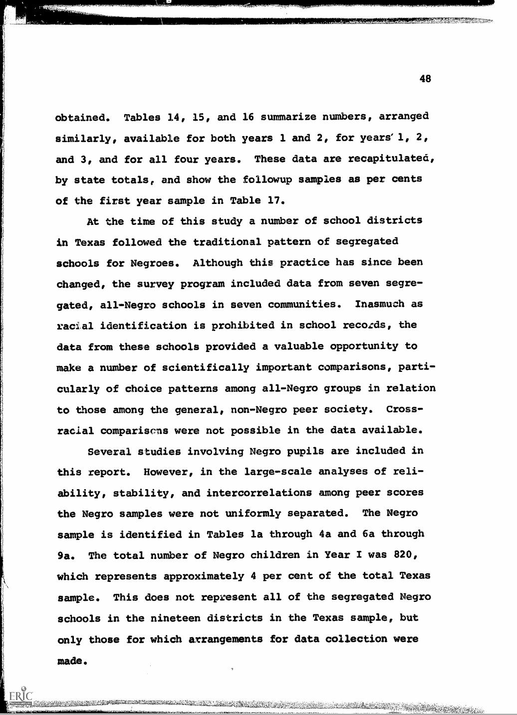
obtained. Tables 14, 15, and 16 summarize numbers, arranged

similarly, available for both years 1 and 2, for years' 1, 2,

and 3, and for all four years. These data are recapitulated,

by state totals, and show the followup samples as per cents

of the first year sample in Table 17.

At the time of this study a number of school districts

in Texas followed the traditional pattern of segregated

schools for Negroes. Although this practice has since been

changed, the survey program included data from seven segre-

gated, all-Negro schools in seven communities. Inasmuch as

racial identification is prohibited in school records, the

data from these schools provided a valuable opportunity to

make a number of scientifically important comparisons, parti-

cularly of choice patterns among all-Negro groups in relation

to those among the general, non-Negro peer society. Cross-

racial compariscns were not possible in the data available.

Several studies involving Negro pupils are included in

this report. However, in the large-scale analyses of reli-

ability, stability, and intercorrelations among peer scores

the Negro samples were not uniformly separated. The Negro

sample is identified in Tables la through 4a and 6a through

9a. The total number of Negro children in Year I was 820,

which represents approximately 4 per cent of the total Texas

sample. This does not represent all of the segregated Negro

schools in the nineteen districts in the Texas sample, but

only those for which arrangements for data collection were

made.

0...-7.A!,

49

Table 14. Texas and Minnesota Two-.Year samples, numbers ofu ils b rade and b sex with com lete data

SchoolDistrict 4

TEXAS

Abilene 640

Birdville 107

Bonham 102

Bowie 110

Breckenridge 124

Castleberry 265

Everman 88

Hillsboro 103

McKinney 156

Waco 180

Texas Total 1875

MINNESOTA

Minneapolis(SES III) 508

Minneapolis(SES IV) 402

Minnesota Total 910

TEXAS AND MINNESOTACOMBINED 2785

Grade Sex5 6 7 Boys Girls Total

526 534 285 982 1003 1985

105 126 177 161 338

133 123 114 237 235 472

61 96 107 207 167 374

120 89 112 216 229 445

281 252 399 399 798

91 131 177 133 310

132 133 134 266 236 502

181 160 248 375 370 745

202 167 273 276 549

1832 1811 1000 3309 3209 6518

526 606 810 830 1640

445 457 619 685 1304

971 1063 1429 1515 2944

2803 2874 1000 4738 4724 9462

50

Table 15. Texas and Minnesota Three-Year samples, numbers ofu ils b rade and b sex with com lete data.

SchoolDistrict

TEXAS

Grade5 6 7 8 Boys

Bonham 98 122 113 103 224

Castleberry 219 226 215 326

Everman 76 70 87 124

McKinney 133 159 133 187 310

Waco 144 172 161

Texas Total 670 749 548 290 1145

MINNESOTA

Minneapolis(SES III) 422 506 457

Minneapolis(SES IV) 324 368

Minnesota Total 746 874

TEXAS AND MINNESOTACOMBINED 1416 1623 548 290

334

791

1936

SexGirls Total

212 436

334 660

109 233

302 612

155 316

1112 2257

471 928

358 692

829 1620

1941 3877

Lrk-tiiv.ms,

51

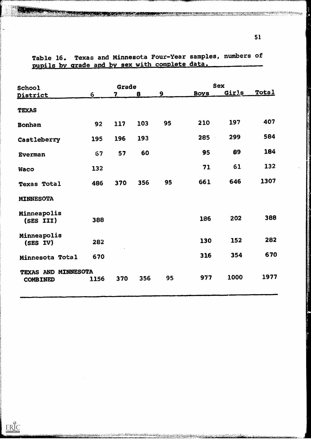
Table 16. Texas and Minnesota Four-Year samples, numbers of

Pupils by grade and by sex with complete data.

SchoolDistrict 6

Grade7 8 9

SexBo s Girls Total

TEXAS

Bonham 92 117 103 95 210 197 407

Castleberry 195 196 193 285 299 584

Everman 67 57 60 95 89 184

Waco 132 71 61 132

Texas Total 486 370 356 95 661 646 1307

MINNESOTA

Minneapolis(SES III) 388 186 202 388

Minneapolis(SES IV) 282 130 152 282

Minnesota Total 670 316 354 670


52

Table 17. Proportions of Year I sample (with complete data)

retained in the stud in subse tmLylasl Volawmi10=1111MMIIIM

Total Complete Proportions Retained Through:

Year I Sample Year II Year III Year I_VN N Per cent N Per cent Per cent

TEXAS

Boys 8938

Girls 8353

Total 17291

MINNESOTA

Boys 8621

Girls 8454

Total 17075

TEXAS ANDMINNESOTACOMBINED

Boys 17559

Girls 16807

Total 34366

3309 37.0 1145 12.8 661 7.4

3209 38.4 1112 13.3 646 7.7

6518 37.7 2257 13.1 1307 7.6

1429 15.6 791 9.2 316 3.7

1515 17.9 829 9.7 354 4.2

2944 17.2 1620 9.5 670 3.9

4738 26.9 1936 11.0 977 5.6

4724 28.1 1941 11.5 1000 5.9

9462 27.5 3877 11.3 1977 5.8

te,IIKSURE,*,;6

53

Data were collected on population parameters and socio-

economic status for all schools in the study and are reported

in relation to peer scores and associated variables in sub-

sequent sections. Socioeconomic and population parameters

of communities were not, however/ part of the sample design.

ORGANIZATION OF THE STUDY

The total study is reported under four major divisions,

which represent logical organization of substudies and

analysis, but not necessarily the chronological order of the

entire investigation. These major divisions, which identify

the heading of the next four chapters, are:

III. Methodological Problems in the Estimation ofPeer Acceptance-Rejection

IV. Antecedent Correlates of Peer Acceptance-Rejection

V. Followup Studies. Later Correlates of PeerAcceptance-Rejection in the Elementary Grades

VI. Analyses of Developmental Processes Associatedwith Peer Acceptance-Rejection

Methodological Problems

A preliminary report by the principal investigators

(Sells and Roff 1964a) discussed many of the methodological

issues in the estimation of peer acceptance-rejection in the

early grades. The present report includes a complete

analysis and supporting tables on intercorrelations among

the LM, LL, and TR scores, other scores derived from them,

such as LD (Lid -LL) and DT (2LD+TR), their reliability esti-

it's:AMU&

54

mated by split-half and retest methods, their stability from

year to year, and perturbing factors, such as class size,

teacher characteristics and school organization. Particular

attention has been paid, in addition to the basic analyses

of the peer choice scores, to the utility of matrix methods

in the analysis of sociometric data (Roff and Sells, 1967).

Antecedent Correlates of Peer Acce stance -Re ection

The peer status scores have been correlated with IQ,

socioeconomic status, birth order, family membership in

relation to like- and unlike-sex sibling or fraternal twin,

and identical twin, school achievement, personality measures,

and many indices of family background. In line with our

expectation of substantial family resemblance (Roff, 1950),

family influence emerged as a major factor in peer status.

The comparison of sibling and twin peer relations scores

with those of randomly matched controls confirmed this obser-

vation and led to more detailed investigations of family

background effects, including the study of 100 families in

the Castleberry School District, by Cox (1966) mentioned

below.

Followup Studies: Later Correlates of Peer Acceptance-ectionRe

Within the five years spanned by this study, the samples

measured in the first year advanced from the range of grades

3 to 6 to grades 6 to 9. On the basis of the earlier work

by Roff, it was expected that even during this period, there

7r7TX'arXrr,,,,,r,A,Tnr,

55

should be some measurable effects of peer rejection in the

adjustment of these children to school and society. More

extensive and detailed followup studies will be possible as

this sample matures. However, the hypothesis of subsequent

maladjustment related to peer rejection could be at least

minimally tested in relation to such criteria as school

dropout, as reflected in school records, and juvenile

delinquency, as reflected in county and city police and

juvenile bureau records. Some preliminary studies of this

type were carried out and are reported in this section.

Developmental Processes Associated with Peer Acceptance -Rejection

The consistent exposure of significant correlates of

peer acceptance-rejection related to family background and

the identification of peer-rejected children as "nasty, mean,

and antagonizing," led to some hypotheses concerning the

developmental processes associated with peer acceptance-

rejection and also with the subsequent maladjustment found

by Roff and in the present study as a predictable sequel to

early school peer rejection. To investigate these, Mr.

Samuel H. Cox, who functioned as Project Director of the

study at Texas Christian University, conducted an intensive

analysis of 100 volunteer families in the Castleberry School

District, a suburb of Fort Worth. These families were

invited to participate on the basis of having a child who

had been in the study for all four years and for whom

1,7

56

extensive data had already been collected. Cox visited each

home, administered a number of tests and questionnaires to

both parents, and also conducted further extensive testing

of the children. A condensed summary of his study appears

in this section.

APPENDIX XX

PEER CHOICE AND TEACHER RATING FORMS

AND INSTRUCTIONS

Negk."="-` TtM 1.

TEACHER'S NAME

SCHOOL SYSTEM

, :2:71,1rtEMDisrc,..f.S*An!"FM.M.=;;Z:M,...

CLASS ROLL (BOYS ONLY)

SCHOOL NAME

58

GRADE ROOM

(Please fill in the "nickname" column below if the student is known by otherthan his real name.)

FIRST MIDDLE LAST "NICKNAME" BIRTHDATE

1

3

5

6

7

8

9

10

11

12

13

14

15

16

17

18

...11101.111w

19

20 VI0110m

Form lb

CLASS ROLL (GIRLS ONLY)

TEACHER'S NAME SCHOOL 'NAME

SCHOOL SYSTEM GRADE ROOM

59

(Please fill in the "nickname" column below if the student is known by otherthan her real name.)

FIRST MIDDLE LAST

1

2

3

4

"NICKNAME" BIRTHDATE

.wams-woMr,

7

8

9

10

11

12

13

14

15

16

17

18

19

20

uekswAtrAogarY46.1.4-.1,4,g4gia-1014-.Riae-4,%`i.

kaLT,

Form 2

TEXAS CHRISTIAN UNIVERSITY -

THE UNIVERSITY OF MINNESOTA

PEER RELATIONS AND PERSONALITY STUDY

TEACHERS' RATINGS INSTRUCTIONS

60

The Peer Relations Study is concerned with the relations of Peer Accept-ance-and Peer Rejection to personality development and adjustment. Thisphase of the research involves teacher evaluation of yupils's peer relations.Previous research has indicated that teachers' judgments of pupils' peerrelations are generally one of the most valid sources of information. Pleasemake your ratings carefully, following the instructions below.

Peer group acceptance and rejection are defined differently from adjust-ment. Children classified as accepted are those who have frequent, non-conflictful relations with other children. This may range from popularity andleadership to followership, even in low status roles. As long as a child isincluded in play groups and remains in communication with the others, hemay be considered accepted to some degree.

Children who are disliked, ostracized, excluded, shunned and keptoutside of their peer group are classified as rejected. In some cases thesechildren may show no signs of maladjustment. However, if they are rejectedby their peers, they should be so classified.

Ratina Categories. Your ratings are to be made on the Teacher RatingCards, which are yellow colored for boys and green colored for girls. Inall other respects these cards are identical. Be careful to use the properlymarked cards for these ratings. Each student is to be rated in one of thefollowing seven categories which you think describes him or her best.

1. EXTREMELY HIGH - OUTSTANDING PEER RELATIONS. One of topboys (or girls) in class, an outstanding leader, best liked childin class, by both girls and boys, best accepted by other children.

2. EXTREMELY HIGH - SUPERIOR PEER RELATIONS. One of the mostpopular members of class, a strong leader, highly accepted byother children, well-liked by both boys and girls.

3. HIGH ACCEPTANCE AMONG PEERS. One of first chosen on play-ground, liked by most of the other children, has many friends,accepted by most of the children. .

u.

-2

61

4. MODERATE ACCEPTANCE AMONG PEERS. Chosen about the middleby other children, a follower, but others like him (her), generallyaccepted; Liked, but not to a high extent, not overly popular, butother children think he's ok.

5. LOW PEER RELATIONS. Merely tolerated, ignored by others, butnot rejected, accepted by some, rejected by others, no closefriends; not rejected but often overlooked, accepted by youngerchildren, but not by own age group.

6. REJECTED GENERALLY BY PEERS. Rejected by most other children,picked on, teased, blamed for everything, others don't want himon their side, pushed out of group activities.

7. REJECTED ENTIRELY BY PEERS. Actively disliked, laughed at,made a fool of, scapegoat, blamed for everything, rejected byall children, both boys and girls, never included in any groupactivities.

Rating Cards

1. Handling of the cards. The cards should be handled very care-fully. Bending or mutilating them in any way will interfere withmachine operations. In particular, the edges should not be muti-lated.

2. Marking. Make a long, heavy mark with the special pencil. Donot let the marks go outside the boxes.

Making the ratings. You have two name roster, one for Boys and onefor Girls. The numbers before the names correspond to the columns on thecard. Indicate your rating of each student by marking category 1 to 7 (thecategories are defined on page two) in the column corresponding to thestudent's number.

Do this for each boy on the yellow card, and for each girl on the greencard.

Number of Students in the Group. On the right end of the card are twocolumns labeled "No. of Students in This Group".

As an example, suppose there were 9 boys in your class. On the yellowcard, you would mark the "0" box in the first of these columns and the "9"box in the second column.

62

-3-

Teachers Comments. For every student that you rate in category 6 or7, please give an explanation comment on the attached Teacher's CommentsForm. In this comment try to describe the child's peer relations and explainyour rating.

If there are any other children, not in your class, whom you regard as

peer rejected, as described by categories 6 or 7, please add their namesand your comments concerning them. Be sure to give their teacher's nameand their grade.

Use extra sheets, if necessary, to complete your comments.

Form 3

TEXAS CHRISTIAN UNIVERSITYFORT WORTH 29, TEXAS

PEER RELATIONS STUDY

TEACHER'S COMMENTS

Date

Teacher's Name School

School System Grade

63

Class

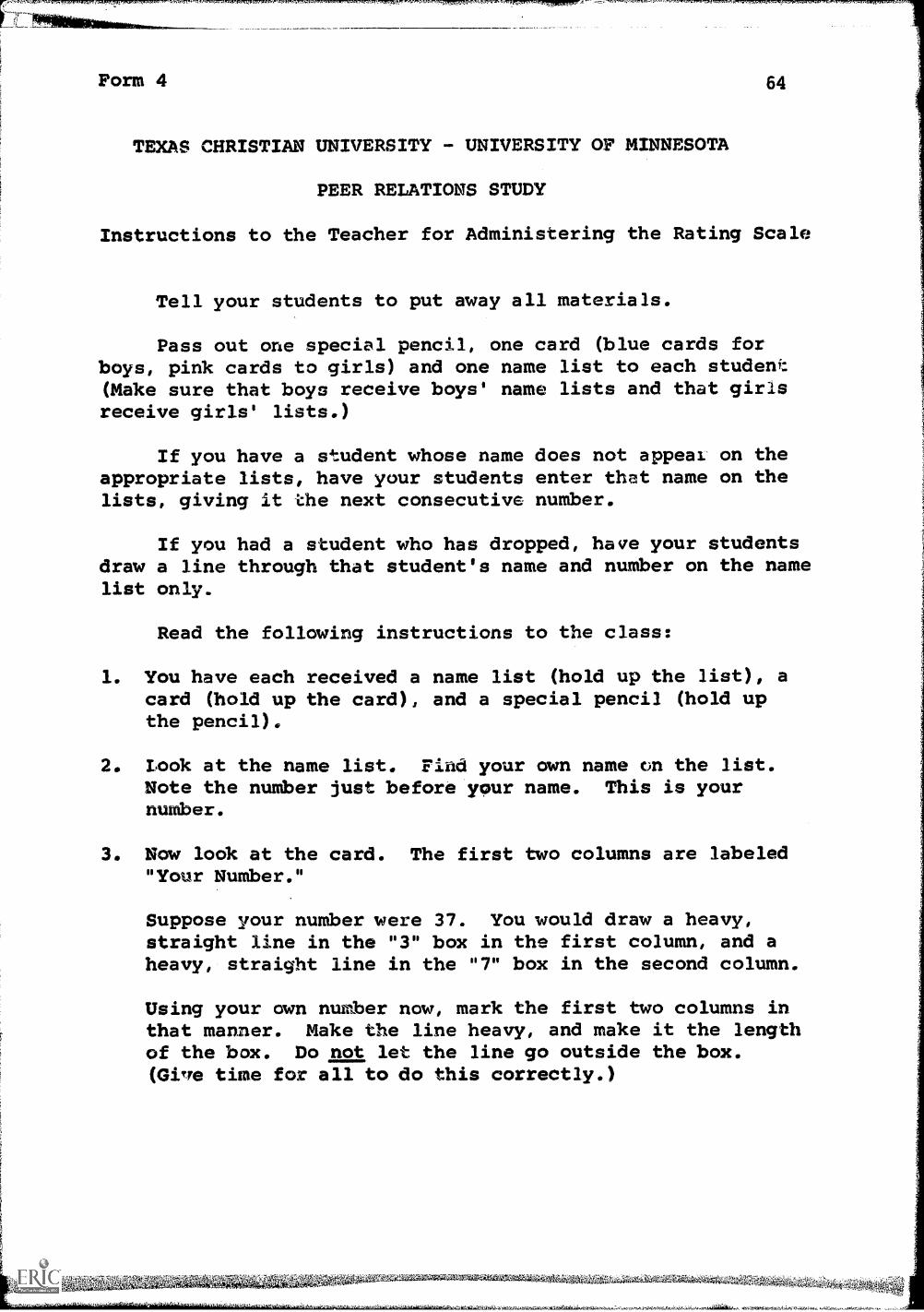
Form 4

TEXAS CHRISTIAN UNIVERSITY - UNIVERSITY OF MINNESOTA


Instructions to the Teacher for Administering the Rating Scale

Tell your students to put away all materials.

Pass out one special pencil, one card (blue cards forboys, pink cards to girls) and one name list to each student(Make sure that boys receive boys' name lists and that girlsreceive girls' lists.)

If you have a student whose name does not appeal on theappropriate lists, have your students enter that name on thelists, giving it the next consecutive number.

If you had a student who has dropped, have your studentsdraw a line through that student's name and number on the namelist only.

Read the following instructions to the class:

1. You have each received a name list (hold up the list), acard (hold up the card), and a special pencil (hold upthe pencil).

2. Look at the name list. Find your own name can the list.Note the number just before your name. This is yournumber.

3. Now look at the card. The first two columns are labeled"Your Number."

Suppose your number were 37. You would draw a heavy,straight line in the "3" box in the first column, and aheavy, straight line in the "7" box in the second column.

Using your own number now, mark the first two columns inthat manner. Make the line heavy, and make it the lengthof the box. Do not let the line go outside the box.(GiTre time for all to do this correctly.)

65

-2-

4. Look again at the name list. Draw a circle around your

name and number. This is to remind you that in the steps

to follow you are not to use your own number.

5. Now think of the person on the list whom you like most.

Find his or her number cn the list.

6. Find this number on the card: in the long row labeled

"Like Most". (Hold up the card and indicate the row to

the students.)

7. Put a heavy, straight, long line in the box just above

this number. (Give time for all to do this.)

8. Now do the same thing for the-next-thr.ee_peraons on the

list whom you like very much. (Give time for all to do

this.)

9. Do the same thing for the two persons on the list whom

you like least, but this time mark in the long row

labeled "Like Least".

10; Now look closely at the card. Make sure that you have

marked your number correctly.

11. Make sure that you have marked exactly four boxes in the

"Ilke Most" row.

12. Make sure that you have marked exactly two boxes in the

"Like Least" raw.

13. Make sure that there are no pencil marks anywhere else on

the card except for "Your Number", and "Like Most" and

"Like Least".

14: Turn the card over and write your name and your teacher's

name on the back.

End of instructions to students.

1"1141111111111111111110Mier ltee

66

Please take up all materials. Check the cards carefully

to make sure that each student's identification number iscorrect, that he has marked the correct number of responses onthe card, and that he has not marked a box for which there is

no student in your class.

Por each student who was absent during the administering

of this scale, please mark-sense his or her number on an

appropriately colored card. Include this card with the others.

Place the students cards in the properly marked envelope.Place this envelope and all other materials (except the pencils)

back in the large envelope.

Place the pencils in the specially marked container.

Follow the instructions given by your local coordinator

for turning in all materials.

,Aeate.4.

I

2

4

5

6

SYSTEM SCHOOL CRA TEACIInt

0111114A/4........

TEACHER RATING CARDS

...wee.

67

TREMELY HIGH-OUTSTANDING12 I3 14 15 16 17 18

XTREMELYC::=)

HIGH-SUPERIOR

REJECTED-GENERALLY

REJECTED-ENTIRELY

C;;;'

2

4

5

6

SYSTEM

tssMIIIS07

-4.,

SCHOOL TEACHER

FOR TEACHER RATING OF GIRLS

0c01Dcl,2Dc2

3c34c4

c5

c6.

c8 1

.

NO. OF STUDENTS

IN THIS CROUP

Lint *AEI a 1E3 IA 1111110.1 IIIIIEJEA W7[1 Evia8111.berawn. lIitlArt-47014111811C4.11.21.114.

ammo wool" sago

olo° sow, am.

woo woo

era. .0001

wow, .0100 moo.

.01001 memo arr.

sumo woo, wore

10

c="3

0311 NEM WM EMI NMI Kamm

MS111011 4

EXTREMELY HIGH-OUTSTANDING

woe*

12 13 14

F72:-)XTREMELY HIGH-SUPERIOR

16

4110011110

HIGH- .0/1010 0101110 a/0

frollo

11

MODERATE

LOW

REJECTED- GENERALLY

REJECTED ENTIRELYwooMEW

C:=D13 14 15 16

18 19 25

O

25

c.:(PcOp

c1aC1c2c2pc3pc3p

c4pc4p

FOR TEACHER RATING OF BOYS

c5p

c6

Cl.C8

C9NO OF STUDENTSIN .THIS GROUP

. sr&

imocrie -

68

PEER NOMINATION CARD

SYSTEM

YOUR NO.

c0c0

SCHOOL TEACHER Z L-5 T.R.

111111 11101111111111111111111111.11111111111111111'NUM WILE El t. f C11111011111111111F1 IMMO ILI III FM Fa 171. EZ.7 IFT1

411711.1113,r1I4 1

cPc112nc2::) (Pink - Girls)

3c3D

5c56:7c6

7c78c89 c9 c: = : ) c.")

1 2 3 4 5 6 7 9 10 11 12 13 14 15 14 17 1 19 20 21 22 23 24 25

LIKE LEAST

1012492!

YOUR NO.

cincPc2Pc2:7)

c3c3,citnc4

c5

Pc6cPc7,c8nc8n

c9c9

6611/416-1[11611r14611111611r111611,1111-1111I:

(Blue BOys

LIKE MOST

2 3 4 7 11101112MHMWWWW=21 222326

II BEM/ El x rm.:4 ra, El, FTIF:71

LIKE LEAST

1 2 3 .C:4i2C 7 ! 10 Ii 12 G3 K 15 111 i7 Cin y 5? 21 CF F:') 21 if h

151111201125.

""

CHAPTER III

METHODOLOGICAL CONSIDERATIONS IN THE ESTIMATION

OP PEER ACCEPTANCE - REJECTION

70

ildETHODOLOGICAL CONSIDERATIONS IN THE ESTIMATION OF

PEER ACCEPTENCE-REJECTION

The basic measures of peer acceptance-rejection employed

throughout this study were two peer choice scores, Like Most

(LM) and Like Least (LL) and a rating of peer-relations

effectiveness performed by teachers and referred to as the

Teacher Rating (TR). Detailed descriptions of these measures

and of scores derived from them have been presented in

Chapter II. The methodological studies reported in this

chapter provide further description of the measures in

relation to their reliability, stability over, the four years

of the Study, and their interrelations. This chapter also

inclndes reports of research on several methodological issues

related to the interpretation and combination of peer rela-

tions scores as well as an analysis of the incidence of peer

rejection in the elementary school population.

The studies included are reported in a logical organi-

zation which is different from the order in which the

analyses were performed. Some are based on the total

samples available, while others involved smaller samples,

employed when the stability of results, judged importance

rn".17,PrZrnk",,,,, . ,

71

of -the serticular analysis, or-cost indicated that such

sampling would be justified. While the major analyses were

replicated in the two states, a number of minor and explora-

tory studies were carried out with data from one area and

not replicated at the time of this report.

DISTRIBUTIONS OF PEER RATING AND TEACHER RATING SCORES

Distributions of the peer rating and teacher rating

scores for Year I data of the Texas sample and part of the

Minnesota sample (St. Paul) available at the time were pre-

sented by Sells and Roff at the 1963 meeting of the American

Educational Research Association (AERA) and published in

condensed form the following year (Sells and Roff, 1964a).

Subsequently, these tables were revised to include the 6616

Year I cases obtained in Minneapolis, where a revised 7-

point scale was used for TR, and the augmented distributions,

which are essentially unchanged except for TR, are pre-

sented here.

Tables 18 through 21 show the distributions for LM, LL,

LD, and TR, respectively. To facilitate their comprehension,

the combined distributions are summarized in Table 22 in

percentage form. These tables present the scores in intervals

of standard deviation from the mean, although in the

W2. Mc:ftiOitagaVilC*,'6AxeiP:40,4;;;;-+4,ILaq

P7ukerl at-14 a I4

Table 18. Frequency distributions of LM (Like Most)Peer Choice scores for Texas, Minnesota and CombinedYear I sam les

z -score

72

Obtained Prequenies Percentage Frequenciesinterval* ,Texas Minn., Total Texas, Minn. Total

3.0 3.4 19 27 46

2.5 2.9 117 133 250

2.0 2.4 553 496 1049

1.5 1.9 1224 1112 2336

1.0 1.4 1806 1557 3363

.5 .9 2097 2066 4163

0.0 .4 3284 3072 6356

-.1 -.5 3210 3095 6305

-.6 -1.0 4646 4304 8950

-1.1 -1.5 1905 1972 3877

-1.6 -2.0 184 208 392

-2.1 -2.5 9 7 16

TOTAL 19054 18049 37103

.10 .15 .12

.61 .74 .67

2.90 2.75 2.82

6.42 6.16 6.28

9.48 8.63 '9.05

11.00 11.45 11.20

17.24 17.02 17.10

16.85 17.15 16.96

24.38 23.84 24.08

9.99 10.92 10.43

.96 1.15 1.05

.05 .04 .04

*In units of standard deviation

.10

Table 19, Frequency distributions of LL (Like Least)

Peer Choice scores for Texas, Minnesota and Combined

Year I sam les.

z -scoreinterva 1*

Obtained FrequenciesTexas** Minn. Total

2.0 2.4 3 0 3

1.5 1.9 39 38 77

1.0 1.4 1191 1268 2459

.5 .9 6029 6162 12191

0.0 .4 4434 4362 8796

-.1 -.5 1752 2181 3933

-.6 -1.0 1308 1381 2689

-1.1 -1.5 925 951 1876

-1.6 -2.0 655 715 1370

-2.1 -2.5 537 707 1244

-2.6 -3.0 302 200 502

-3.1 -3.5 112 70 182

-3.6 -4,0 23 13 36

-4.1 -4.5 0 1 1

TOTAL 17310 18049 35359

Percentage FrequenciesTexas Minn. Total

.02 .00 .01

.22 .21 .22

6.88 7.02 6.94

34.82 34.14 34.38

25.62 24.17 24.80

10.12 12.08 11.09

7.56 7.65 7,58

5.34 5.27 5.29

3.78 3.96 3.86

3.10 3.92 3.51

1.74 1.11 1.42

.65 .39 .51

.13 .07 .10

.00 .01 .00

* In units of standard deviation**Like Least ratings were not available for 1778 pupils inone Texas city.

74

Table 20. Frequency distribution of LD (Like Most minus

Like Least) Peer Choice scores for Texas, Minnesota and

Combined Year I samples.

z-score Obtained Frequencies Percentage Frequencies

interval*

3.0 3.4

2.5 2.9

2.0 2.4

1.5 1.9

1.0 1.4

.5 .9

0.0 .4

-.1 -.5

-.6 -1.0

-1.1 -1.5

-1.6 -2.0

-2.1 -2.5

-2.6 -3.0

-3.1 -3.5

TOTAL

Texas** Minn. Total

1 1 2

19 26 45

159 194 353

855 881 1736

1960 1914 3874

2840 2977 5817

3844 3961 7805

3065 3254 6319

2142 2282 4424

1240 1359 2599

761 760 1521

337 391 728

80 44 124

7 5 12

17310 18049 35359

Texas

.01

.11

.92

4.94

11.32

16.41

22.21

17.71

12.37

7.16

4.40

1.95

.46

.04

Minn, Total

.01 .01

.14 .13

1.08 1.00

4.88 4.90

10.60 10.92

16.49 16.40

21.94 22.01

18.03 17.82

12.64 12.48

7.53 7.33

4.21 4.29

2.17 2.05

.24 .35

.03 .03

* In units of standard deviation**Like Least ratings were not available for 1778 pupils in

one Texas city.

75

Table 21. Frequency distribution of TR (Teacher Rating)

scores for Texas Minnesota and Combined Year I sam les

Obtained Frequency Minnea- Percentage Frequencies

St, polis St. Minnea-

z-score Texas Paul Total** 7-point Texas Paul Total** polis

interval* 4 -point scales AMU..

2.5 2.9 3

2.0 2.4 24 3 27 70 .13 .03 .19

1.5 1.9 251 219 740 329 2.73 1.92 2.43

1.0 1.4 2772 2038 4810 515 14.55 17.83 15.78

.5 .9 1709 598 2307 983 8.97 5.23 7.57

0.0 .4 4009 3755 7764 1207 21.04 32.84 25.47

-.1 -.5 6252 2115 8635 1915 34.22 18.50 28,32

-.6 -1.0 1582 1172 2754 949 8.30 10.25 9.03

-1.1 -1.5 1084 988 2072 479 5.69 8.64 6.80

-1.6 -2.0 532 401 933 143 2.79 3.51 3.06

-2.1 -2.5 216 127 343 23 1.13 1.11 1.13

-2.6 -3.0 73 12 85 .38 .10 .28

-3.1 -3.5 9 4 13 .05 .03 .04

-3.6 -4.0 3 1 4 .02 .01 .01

TOTAL 19054 11433 30487 6616

.05

1.10

4.97

7.7e

14.86

18.24

28.94

14.34

7.24

2.16

.35

* In units of standard deviation**Totals refer to Texas and St. Paul only; Minneapolis Teacher

Ratings were on a 7-point scale, Texas and St. Paul Teacher

Ratings were on a 4-point scale.

gig:-;114x.

76

Table 22. Percentage distributions of total sample for LM,

ID. and TR scores. Year sam le.

Teacher TeacherRatings Ratings

z -score Like Like Like Most- (4-point (7-point

,interval* Most Least Like Least scale scale)

3.0

2.5

2.0

1.5

1.0

.5

04

-.1

-.6

-1.1

-1.6

-2.1

-2.6

-3.1

-3.6

-4.1

3,4 ,12 .01

2,9 .67 .13 .05

2.4 2.82 .01 1.00 .19 1.10

1.9 6.28 .22 4.90 2.43 4.97

1.4 9.05 6.94 10.92 15.78 7.78

.9 11.20 34.38 16.40 7.57 14.86

.4 17 10 24.80 22.01 25.47 18.24

-.5 16.96 11.09 17.82 28.32 28.94

-1.0 24.08 7.58 12.48 9.03 14.34

-1.5 10.43 5.29 7.33 6.80 7.24

-2.0 1.05 3.86 4.29 3.06 2.16

-2.5 ,04 3.51 2.05 1.13 .35

-3,0 1.42 .35 .28

-3.5 .51 .03 .04

-4,0 .10 .01

-4.5 .00

3.4 18.94 7.17 16.96 18.40 13.90

.9 69.34 77.85 68.71 70.39 76.38

-4.5 11.52 14.69 14.05 11.32 9.75

*In units of standard deviation

MENI M INVINCVMORMMIPAWOMMMitl

77

computations a constant of 5 was added to all scores to

eliminate negative values. The distributions were designed

to have a mean of 5.0 and a standard deviation of 1.0.

The first four tables present obtained frequencies in

the columns at the left, for total Texas, Minnesota, and

combined samples, and relative frequencies in percentage

form, at the right. Breakdowns by grade and sex are not

included, but variations related to them are discussed in

the text. LL scores were reflected in sign to afford con-

sistent interpretation of all peer-score measures. Teacher

ratings on 4-point and 7-point scales are listed separately.

The z-score sets were designed to have a mean of 5.0

and standard deviation of 1.0 and an empirical check showed

that these were obtained within the limits of founding error

for approximate computation. However, it should be remembered

that whereas peer choices were made within class-groups of

like sex, Teacher Ratings were made for the entire class by

one rater, the teacher. Thus, while the means and standard

deviations of Teacher Ratings are 5.0 and 1.0, respectively,

for distributions of boys and girls combined, the means for

boys tend to be slightly lower and for girls, slightly higher

than the prescribed mean, as a result of sex-bias, discussed

later.

-i,oey*Aweia,-;?

78

Examination of Tables 18 through 22 reveals that the

Texas and Minnesota peer choice scores are distributed

nearly identically, but that this agreement does not hold

for the ratings by teachers. In view of the similarity of

the peer choice distributions, it is apparent that the Texas

and St. Paul teachers used different subjective judgment

scales in interpreting what were intended to be straight-

forward rating instructions. The Texas teachers reported

relatively less maladjustment in peer relations and this

must be taken into account in interpreting the results.

The four combined distributions are compared in Table

22, which summarizes the per cents of cases in each class

intervals. The variations among these distributions are

emphasized by the summary figures at the bottom of this

table, which report the per cents under the curve at inter-

vals of plus and minus one standard deviation from the mean.

In a normal distribution, these would be 15.87, 68.26, and

15.87 per cent, respectively. As Table 22 shows, high

liking (acceptance) is overestimated on the IM scale and

underestimated on the LL scale, while high "dislike" (rejec-

tion) is underestimated on both these scales, but only

slightly on the LL scale. The difference scale (LD) is

Tr:

0.,,,J,..11,01,

79

slightly skewed toward the negative eNtreme, but is more

symmetrical and approximates the normal distribution. The

TR distribution on the 4-point scale is skewed toward the

negative extreme and tends toward bimodality, while the

distribution on the 7-point scale is smoother and closer to

the normal curve.

RELIABILITY STUDIES OF PEER ACCEPTANCE-REJECTION SCORES

Split-half reliability coefficients, corrected by the

Spearman-Brown Prophecy Formula, were computed to estimate

the reliability of pe-r choice scores for each year, as

reported below. The sample in this study consisted of all

pupils in the districts of both states that participated

for four years. Reliability of Teacher Ratings was esti-

mated by correlating the ratings obtained at a regularly

scheduled rating period, for a sample of classes, with

repeat ratings of the same classes by the same teachers

several months later. The consistency of both peer scores

and teacher ratings, from year to year, which is reported

later in this Chapter, was estimated by correlating

corresponding scores of individuals who continued in the

study.

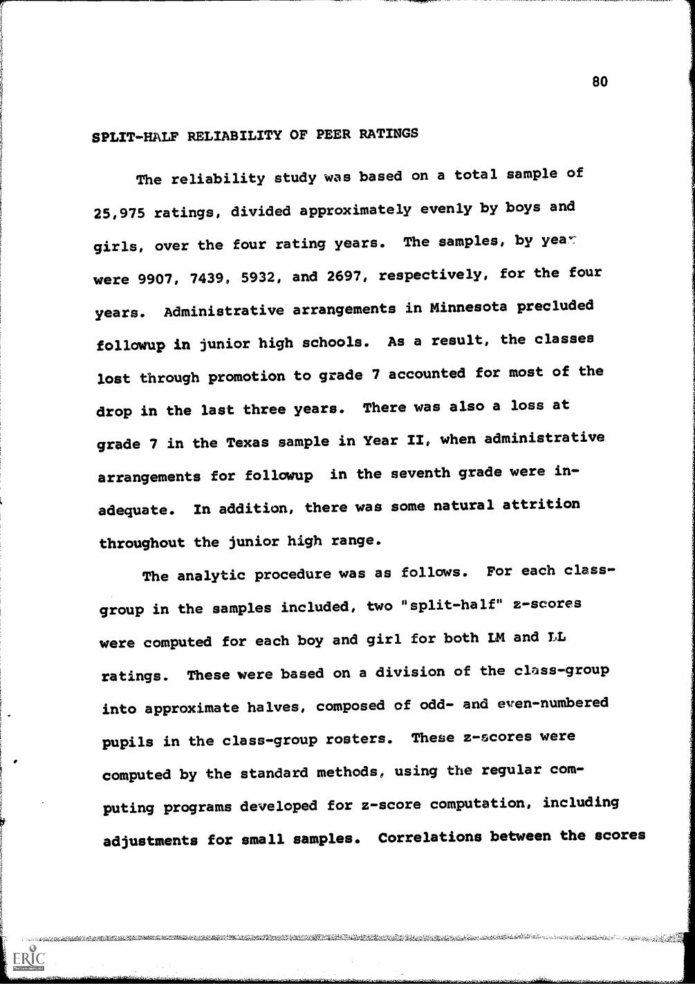
80

SPLIT-HALF RELIABILITY OF PEER RATINGS

The reliability study was based on a total sample of

25,975 ratings, divided approximately evenly by boys and

girls, over the four rating years. The samples, by yeas:

were 9907, 74394 5932, and 2697, respectively, for the four

years. Administrative arrangements in Minnesota precluded

follawup in junior high schools. As a result, the classes

lost through promotion to grade 7 accounted for most of the

drop in the last three years. There was also a loss at

grade 7 in the Texas sample in Year II, when administrative

arrangements for followup in the seventh grade were in-

adequate. In addition, there was some natural attrition

throughout the junior high range.

The analytic procedure was as follows. For each class-

group in the samples included, two "split-half" z-scores

were computed for each boy and girl for both LM and LL

ratings. These were based on a division of the class-group

into approximate halves, composed of odd- and even-numbered

pupils in the class-group rosters. These z-scores were

computed by the standard methods, using the regular com-

puting programs developed for z-score computation, including

adjustments for small samples. Correlations between the scores

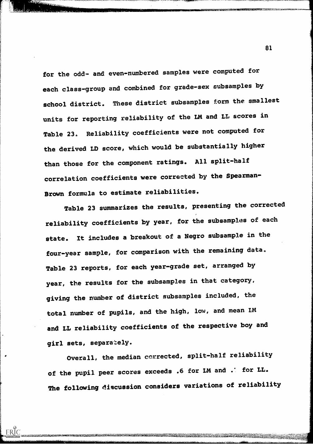
81

for the odd- and even-numbered samples were computed for

each class-group and combined for grade-sex subsamples by

school district. These district subsamples form the smallest

units for reporting reliability of the LM and LL scores in

Table 23. Reliability coefficients were not computed for

the derived LD score, which would be substantially higher

than those for the component ratings. All split-half

correlation coefficients were corrected by the Spearman-

Brown formula to estimate reliabilities.

Table 23 summarizes the results, presenting the corrected

reliability coefficients by year, for the subsamples of each

state. It includes a breakout of a Negro subsample in the

four-year sample, for comparison with the remaining data

Table 23 reports, for each year-grade set, arranged by

year, the results for the subsamples in that category,

giving the number of district subsamples included, the

total number of pupils, and the high, low, and mean LM

and LL reliability coefficients of the respective boy and

girl sets, separezely.

Overall, the median corrected, split-half reliability

of the pupil peer scores exceeds .6 for LM and .1 for LL.

The following discussion considers variations of reliability

82Table 23. Split-Half reliability estimates of LM and LL scoresby Grade Sex and Race.

No. Dist. No.

Reliability CoefficientsLM LL

.110,apxade Sex Subsamples Pupils Low High Aver. Low High Aver.

TEXAS NEGRO CHILDREN

I 3 B 1 47 .67 .781962 3 G 1 43 .57 .82

4 B 1 38 .73 .76

4 G 1 35 .70 .66

5 B 1 41 .72 .72

5 G 1 44 .67 .80

6 B 1 36 .76 .786 G 1 43 - - .49 .45

All B 1 162 .72 .76

All G 1 165 .61 .71

II 46 .67 .73

1964 4 1 40 .61 .82

5 B 1 35 .85 .58

5 G 1 38 - - .73 .63

6 B 1 35 .43 .68

6 1 42 .47 .56

All B 1 116 .68 .67

All G 1 120 .60 .68

III1964

5

5

BG

1

1

4244

.29

.30 alb

.39

.58

6 B 1 35 .76 .72

6 G 1 38 .73 .68

All B 1 77 .55 411111= .56rt

All G 1 82 .54 alb .62

IV 6 B 1 41 .69 .47

1965 6 G 1 39 .55 .14

..r..

NA, TaTegMFRF.,,,'^ 7X COT

Table 23 (cont )

No, Dist, No.

83

Reliability Coefficients

Leas Grade Sex Subsamples =ill Low Awl Am& Low Sic i Aver.

1962

II1963

III1964

IV1965

21-3AAWHIIESREEMER

3 B 4 380 .70 .81 .74 .32 .73 .633 G 4 362 .59 .68 .64 .31 .69 .614 B 4 418 .70 .81 .71 .68 .73 .754 G 4 380 .47 .73 .66 .69 .78 .745 B 4 349 .66 .82 .76 .12 .79 .705 4 361 .53 .70 .66 .75 .88 .796 B 4 343 .53 .81 .72 .73 .81 .766 G 4 336 .64 .75 .71 .51 .82 .70All B 4 1490 .68 .77 .73 .65 .76 .72All G 4 1439 .59 .71 .66 .59 .78 .71

4 13 4 391 .65 .79 .72 .63 .78 .714 G 4 361 .59 .78 .66 .64 .85 .725 B 4 414 .60 .81 .74 .58 .76 .715 G 4 396 .55 .78 .66 .66 .82 .746 B 4 371 .55 .73 .68 .55 .79 .736 G 4 382 .53 .58 .58 .57 .78 .737 B 1 64 .66 .717 G 1 62 .58 .67All B 4 1240 .63 .73 .71 .70 .71 .71All G 4 1201 .56 .67 .63 .67 .80 .73

5 B 4 399 .53 .72 .70 .51 .80 .745 G 4 363 .42 .71 .62 .40 .83 .716 B 4 395 .56 72 .66 .62 .80 .746 G 4 399 .49 05 .75 .58 .80 .767 B 3 306 .67 .71 .69 .72 .93 .817 G 3 301 .36 .64 .54 .78 .87 .828 B 3 296 .48 .62 .51 .55 .75 .718 G 3 265 .39 .58 .51 .74 .84 .81All B 4 1396 .61 .67 ,65 .61 .77 .76All G 4 1328 .52 .66 .61 .61 .81 .78

6 B 4 431 .63 .80 .71 .45 .80 .726 G 4 386 .55 .66 .60 .54 .77 .717 B 3 322 .65 .69 .66 .61 .90 .767 3 335 .59 .63 .60 .76 .83 .808 B 3 288 .61 .66 .64 .69 .83 .758 3 288 .32 .70 .59 .61 .83 .689 B 3 306 .57 .65 .60 .65 .74 .679 G 3 261 .12 .46 .38 .66 .73 .71All B 4 1347 .63 .70 .66 .45 .80 .72All G 4 1270 .49 .66 .55 .54 .75 .69

.',1t7Mare.g. Ziv.7.a%

Table 23 -front.;

No. Dist. No.

84

Reliability CoefficientsLM LL

Year Grade Sex Subsamples Pupils Low High MILL

1962

II1963

III1964

IV1965

TEXAS WHITE AND ITEGRO CHILDREN COMBINED

High Aver.

3 B 4 427 .70 .81 .73 .32 .73 .65

3 G 4 405 .59 .68 .64 .54 .69 .64

4 B 4 456 .70 .81 .71 .68 .73 .75

4 G 4 415 .47 .73 .66 .67 .73 .73

5 B 4 390 .69 .82 .76 .41 .79 .70

5 G 4 405 .53 .70 :66 .77 .88 .79

6 B 4 379 .53 .81 .72 .73 .81 .76

6 G 4 379 .59 .75 .69 .49 .82 .68

All B 4 1652 .68 .77 .73 .65 .76 .72

All G 4 1604 .59 .71 .66 .63 .78 .71

4 B 4 437 .65 .79 .72 .63 .78 .71

4 G 4 401 .59 .78 .66 .64 .85 .73

5 B 4 449 .60 .81 .75 .58 .76 .70

5 G 4 434 .55 .78 .67 .66 .82 .73

6 B 4 406 .55 .73 .66 .55 .79 .73

6 G 4 424 .53 .58 .57 .57 .78 .72

7 B 1 64 .66 IMO .717 G 1 62 .58 IMO .67

All E 4 1356 .63 .73 .71 .70 .71 .71

All G 4 1321 .56 .67 .63 .67 .80 .73

5 B 4 441 .56 .72 .67 .61 .80 .72

5 G 4 407 .50 .71 .59 .40 .83 .70

6 B 4 430 .56 .72 .67 .62 .80 .74

6 G 4 437 .49 .75 .70 .58 .80 .75

7 B 3 306 .67 .71 .69 .72 .93 .81

7 G 3 301 .36 .64 .55 .78 .87 .82

8 B 3 296 .48 .62 .51 .55 .75 .71

8 G 3 265 .39 .58 .51 .74 .84 .81

All B 4 1473 .61 .67 .65 .61 .77 .75

All G 4 1410 .52 .66 .61 .61 .81 .77

6 B 4 472 .60 .80 .71 .45 .80 .70

6 G 4 425 .55 .66 .59 .57 .77 .68

7 B 3 322 .65 .69 .66 .61 .90 .76

7 G 3 335 .59 .63 .60 .76 .83 .80

8 B 3 288 .61 .66 .64 .69 .83 .75

8 G 3 288 .32 .70 .59 .61 .83 .68

9 B 3 306 .57 .65 .60 .65 .74 .67

9 G 3 261 .12 .46 .38 .66 .73 .71

All B 4 1388 .63 .70 .66 .45 .80 .72

All G 4 1309 .49 .66 .55 .71 .75 .72

tiv

Wr1 't wm 4,1

Table 23 (cont.)85

Reliability CoefficientsNo. Dist. No. LM LL

em Grade Sex Subsamples bail& Lon ,High, Aver. Low mall Aver.

MINNESOTA SAMPLE

I 3 B 2 8391962 3 G 2 782

4 B 2 8064 G 2 742

5 B 2 7195 G 2 792

6 B 2 10126 G 2 959

All B 2 3376All G 2 3275

II 4 B 2 754

1963 4 G 2 715

5 B 2 8045 G 2 747

6 B 2 8416 G 2 901

All B 2 2399All G 2 2363

III 5 B 2 737

1964 5 G 2 702

6 B 2 8156 G 2 795

All B 2 1552All G 2 1497

.63 .63 .63 .56 .61 .59

.69 .72 .71 .67 .67 .67

.61 .66 .64 .65 .72 .69

.63 .74 .69 .68 .75 .72

.63 .G7 .65 .75 .75 .75

.65 .70 .67 .71 .75 .73

.60 .62 .61 .67 .80 .75

.59 .64 .60 .72 .73 .73

.62 .64 .63 .66 .73 .70

.64 .69 .67 .70 .72 .71

.61 .73 .68 .60 .66 .63

.67 .73 .71 .62 .65 .64

.73 .74 .74 .74 .76 .75

.65 .66 .66 .71 .75 .73

.63 .70 .67 .71 .78 .76

.61 .71 .66 .73 .80 .77

.67 .72 .70 .69 .74 .72

.64 .70 .68 .69 .74 .72

.54 .58 .56 .65 .72 .69

.54 .59 .56 .69 .69 .69

.62 .65 .65 .74 .75 .74

.56 .66 .62 .71 .84 .79

.57 .63 .61 .70 .73 .72

.58 .58 .58 .70 .77 .74

86

coefficients in relation to type of measure, region, grade,

race, and sex. Although the range of variation is not

great, the influence of these sources is quite interesting.

Reliability Variations Related to Measure

Although based on two nominations per class-group, as

compared with four for the LM ratings, the reliability of

the LL measures, across states, grades, and sexes, exceeds

that of LM in most comparisons, the only exception being for

small sample of Negro girls in the elementary grades (3 to 6),

in which the results appear to be atypical. It thus appears

that peer choice status or popularity based on negative,

Like Least choices, is determined somewhat more reliably

than such status based on positive, Like Most choices. In

other words, the population represented in this study tends

to agree somewhat more on the identification of disliked

than of liked persons. This difference appears to increase

with age and is most pronounced at the junior high level,

despite the fact that the organization of junior high classes

favors less reliable judgments, as discussed below.

Reliability Variations Related #o_ Reaion

Since the Minnesota sample covered only elementary

grades (3 through 6) and a Negro sample was not identified

iF

as such, the appropriate comparison is between the Texas White

sample and the Minnesota sample for the elementary grades.

The average reliability coefficients for this comparison are

as follows:

87

Texas Minnesota

Boys LM .71 .65

Boys LL .72 .71

Girls LM .65 .65

Girls LL .72 .71

These results are quite comparable, although the reliability

of the LM ratings is slightly higher for the Texas boys'

sample than for the comparable Minnesota group.

Reliability Variations Related to Sch,ooi Grade,

Junior high scores were available only in the Texas

sample. For this sample, the junior high reliabilities are

highest on LL, for both sexes and among the lowest on LM.

In the elementary grades, classes generally remain together

for the entire curriculum, while they are departmentalized

in junior high school. On the basis of amount of contact,

it might therefore be expected that peer choices among home

room class-groups would be less reliable in junior high than

in elementary classes. However, this was not the case, at

least for the LL reliabilities, which averaged .75 for junior

high girls and .74 for junior high boys, higher than for any

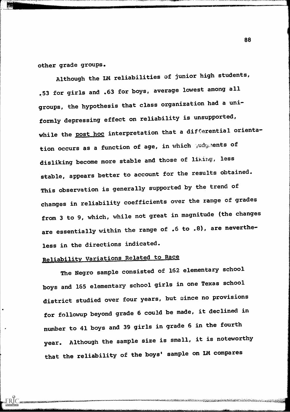
"5,1""1.^

1,

V434.11a,,'

88

other grade groups.

Although the LM reliabilities of junior high students,

.53 for girls and .63 for boys, average lowest among all

groups, the hypothesis that class organization had a uni-

formly depressing effect on reliability is unsupported,

while the post hoc interpretation that a differential orienta-

tion occurs as a function of age, in which udc),Ients of

disliking become more stable and those of liking, less

stable, appears better to account for the results obtained.

This observation is generally supported by the trend of

changes in reliability coefficients over the range of grades

from 3 to 9, which, while not great in magnitude (the changes

are essentially within the range of .6 to .8), are neverthe-

less in the directions indicated.

Reliability Variations Related to Race

The Negro sample consisted of 162 elementary school

boys and 165 elementary school girls in one Texas school

district studied over four years, but since no provisions

for followup beyond grade 6 could be made, it declined in

number to 41 boys and 39 girls in grade 6 in the fourth

year. Although the sample size is small, it is noteworthy

that the reliability of the boys' sample on LM compares

favorably with that of the Texas White and Minnesota samples,

while the reliability of the girls' LL score is higher than

that of White junior high girls. The average reliabilities

of Negro boys and girls on LL are lower than those of all

other groups, but these averages reflect the unusually low

coefficients for both sexes in grade 5 for 1964, which are

atypical and may be the result of an error in administration,

recording, or processing of the data. If these results were

omitted, no significant or systematic differences appear to

be present.

Reliability Variations Related to Sex

No systematic, significant sex differences related to

the reliability of the peer choice scores were found, although

girls had a greater number of coefficients exceeding .8 on U.

Summary

The median reliability of the peer choice scores, esti-

mated by split-half procedures and corrected by the Spearman-

Brawn formula, exceeds .6 for LM and .7 for LL. There is a

tendency for LM reliability to decline with grade (age) and

for LL reliability to increase. This trend was most marked

in the junior high grades, which were available only in the

Texas sample. No systematic, significant differences in

reliability were found to be related to region, race, or sex.

RELIABILITY OF TEACHER RATINGS

of Four -Point and Seven-Point Scales

As mentioned earlier, the four-point scale, employed

during the first year in the Texas and St. Paul surveys, was

abandoned in favor of a seven-point Teacher Rating scale

thereafter. The two scales were as follows:

Pour-Point Scale Seven-Point Scale

1. Exceptionally Good Peer 1. Extremely High-Outstand-Relations ing Peer Relations

2. Average, No Negative 2. Extremely High-SuperiorIndications 3. High

3. Borderline Rejection 4. Moderately Good4. Clearly Rejected Low

6.. Rejected Generally7. Rejected Entirely

After examination of raw score distributions of the

first-year, four-point scale ratings, it was felt that they

were not sufficiently differentiated and that greater

variability would be obtained with the new scale. Table 24

compares raw score distributions of 9676 Teacher Ratings

for ten Texas School Districts in Year I with 8467 comparable

ratings for the same districts in Year II. it may be noted

that in Year II five of the seven scale points were used

for at least five per cent of the ratings, whereas in Year I

- 7,74 ,n7,511MITINrrytfe

91

Table 24. Comparison of raw score distributions of Teacher

Ratings for 10 school districts: Year I and Year Ii, Texas

Mt- ..........10_ tumor,

Year I MsaIduzlis Scale)

Rating, N Per cent

1. Exceptionally good peer relations 2751 28.4

2. Average, no negative indications 5772 59.7

3, Borderline rejection 976 10.1

4. Clearly rejected 177 1.8

Total 9676 100.0

Mean 1.85

S.D. .66

Year // (Seven-Point Scale)

1. Extremely High-Outstanding 434 5.1

2. Extremely High-Superior 996 11.8

3. High 2183 25.8

4. Moderate 3511 41.5

5. Low 1198 14.1

6. Rejected-Generally 116 1.4

7. Rejected-Entirely 29 0.3

Total 8467 100.0

Mean 3.53

S.D. 1.09

0101 Improml Vow

,.n,y,1,7.5pwrzAgt...,,,,,,,,Z, ?Pim -6,(,..i74".,^1,1.,97. Ler, e'r

92

only three of the four scale points were effectively employed.,

fteDeat Anima

Since the seven-point scale was used following year one,

the reliability analysis of Teacher Ratings was based on

this scale. Each child received erply one TR in each year

and the only available method of assessing TR reliability

required repeat ratings after a period of time. Although

such ratings were an added burden to the classroom teachers,

arrangements were made in five Texas school districts for

second ratings, approximately five months after the regular

1964 survey, with a summer vacation intervening between

initial and repeat ratings.

In preparation for the second ratings a questionnaire

was sent to the 108 teachers participating and it was as-

certained, (a) that none of the teachers had employed socio-

metric devices in class that might have biased their ratings,

and (b) that all teachers felt that they knew the pupils on

their class lists well enough to rate them at the time of

the second rating, even though most of them were no longer

in these teachers' classes. Reratings were made on 377 boys

and 352 girls by 25 men teachers and on 1209 boys and 1114

girls by 78 women teachers.

93

For purposes of analysis, the data were divided into

eight groups, consisting of elementary and junior high boys

and girls rated by men teachers and by women teachers. One

man teacher and two women teachers rated junior high boys

only, three women teachers rated elementary boys only, and

two women teachers rated junior high girls only. The re-

maining 100 teachers, who rated both boys and girls, were

divided as follows: Men: elementary, 9 and junior high, 15;

Women: elementary, 48 and junior high, 28. Table 25 shows

the number of teachers rating each group and the number of

reliability coefficients computed for the eight groups, which

totaled 208. The distributions of these 208 coefficients

for the eight groups are shown in Table 26 and a breakdown

by school district is given in Table 27.

As might be expected, the range of individual teacher-

group reliability coefficients in Table 26 is great, although

entirely within the positive domain. However the pooled

results for teachers in each group, represented by the

weighted average and median coefficients, indicate substantial

reliability, comparable with that obtained for the peer

ratings, LM and LL. The range of coefficients reported by

group by district in Table 27 is not as great, reflecting

1' A

94

Table 25. Summary of teachers participating in the rerating

tud

Teacher CateL or

Elementary Men Rating Boysand Girls

Jr. High Men Rating Boysand Girls

Jr. High Men Rating Boys only

Subtotal Men Teachers

Number ofNumber of ReliabilityTeachers Coefficients,

9 18

15 30

1 1

25 49

Elementary Women Rating Boysand Girls 48 96

Elementary Women Rating Boys only 3 3

Jr. High Women Rating Boys and

Girls 28 56

Jr. High Women Rating Boys only 2 2

Jr. High Women Rating Girls only 2 2

Subtotal Women Teachers 83 159

Totals 108 208

iA',1

ryt- , 4 rZ, ..-01111M14r,C74404"4"-'','"' 7!R,4,774W/V771

40!

95

Table 26. Distribution of test-retest reliability coefficientsfor men and women teachers rating boys and girls in elementary

Ag..3012...gderhihscl

Elementary SchoolMen Women

Reliability Teachers Teachers Total

,Coefficient Bon Girls Boys Girls

Junior High SchoolMen WomenTeachers Teachers

Doze Girls Bou Girls r's

.9 - 1.0 1 1 3

.80 - .89 3. 3. 17

.70 - .79 1 1 8

.60 - .69 1 2 6

.50 - .59 3 1 6

.40 - .49 0 1 4

.30 - .39 1 0 3

.20 - .29 0 2 4

.10 - .19 1 0 0

below .1 0 0 0

Number ofCoefficients 9 9 51

AverageReliability .67 .66 .72

MedianReliability .58 .66 .72

2

17

14

3

5

1

0

3

2

1

48

.74

.75

,*WOUar,0.4z--" -1-V4ati

1 1 4 5 18

5 4 6 5 56

3 4 7 10 48

3 2 3 2 22

2 0 5 1 23

1 0 4 3 14

0 0 1 0 5

1 1 0 1 12

0 0 0 0 3

0 3 0 3 7

16 15 30 30 208

.74 .64 .72 .73 .72

.70 .70 .72 .75 .73

r FOVW91,`,57,. W7,,r ,

-

96

Table 27. Test-retest reliability of teacher ratings for men

and women teachers rating boys and girls by school district.

Texas Year III Sample.

Men Teachers Women Teachers

School Number of Number of Number of Number of

District 7 Boys r T Girls r T Boys r T Girls r

Junior 1.14,gh

Totals 16 244 .74

High Grades (7 and 8)

Everman 4 69 .61 4 56 .12 2 32 .72

Bonham 4 48 .72 4 46 .77 6 79 .54

McKinney 3 46 .55 2 18 .80 13 166 .73

Castleberry 5 81 .86 5 85 .63 9 171 .73

CombinedElementaryand Jr.High 25 377 .72

.7215 205 .64 30 448

24 352 .65 81 1209

4 63 .77

7 104 .73

12 159 .64

16 256 .67

9 115 .71

48 697 .74

2 24 .62

6 88 .64

14 193 .78

8 112 .69

30 417 .74

78 1114 .74

.72Junior 1.14,gh

Totals 16 244 .74

.72

CombinedElementaryand Jr.High 25 377 .72

4 63 .77

7 104 .73

12 159 .64

16 256 .67

9 115 .71

48 697 .74

2 24 .62

6 88 .64

14 193 .78

8 112 .69

30 417 .74

78 1114 .74.72

-

15 205 .64 30 448

24 352 .65 81 1209

97

the pooling of like-sex teacher ratings within districts.

The group averages in Table 26 are the same as the

totals in Table 27. These may be used to compare reliabili-

ties by grade level, sex of teacher, and sex of pupils. The

highest reliabilities were obtained by men teachers rating

junior high boys and by women teachers rating elementary

girls and junior high girls; these were all .74. Women

teachers' ratings of elementary and junior high boys were

next, with reliabilities of .72, while the reliabilities

of men teachers' ratings of elementary boys and of both

elementary and junior high girls were lowest, ranging from

.64 for junior high girls to .67 for elementary boys. In

general, the pooled ratings of boys and of girls by men and

women teachers cancelled out differences. However, the

results indicate that women teachers' ratings were signifi-

cantly more reliable than those of men, with those for men

rating girls lowest (.65) and those for women rating girls

highest (.74). No discriminable differences were found

attributable to pooled reliabilities of men and women teachers

by grade level.

The teacher sample included nine Negro teachers in

two school districts. These consisted of one male elementary

98

teacher with two class-groups, one of 13 boys and another

of 10 girls, six women elementary teachers with combined

groups of 88 boys and 84 girls, and two women junior high

teachers with 35 boys and 27 girls, jointly. The reliability

coefficients for these small groups follow the general pattern

described, and are as follows:

Elementary. 1 man teacher rating 13 boys: .58

rating 10 girls: .66

6 women teachers rating 88 boys: .83

rating 84 girls: .80

Junior High. 2 women teachers rating 35 boys: .60

rating 27 girls: .70.

The weighted mean reliability of the pooled ratings by

the 108 teachers of 3052 children was .72. This is somewhat

higher than the reliability reported earlier for LM and

about equal to that for LL. Although this was a relatively

small sample, compared to the numbers used in other parts

of the overall study, the consistency of the correlations

of Teacher Ratings, for the first year, four-point scale as

well as for the ratings on the seven-point scale, with other

variables throughout the study, supports the representa-

tiveness of these results.

514" ' ax; ,ralwiage141,44X4M

99

TEACHER RATING CHARACTERISTICS

Many reports in the literature (Bonney, 1943; 1947; Gron-

lund, 1950a; 1950b; 1954; 1956; 1959; Myers, 1961; Ullman 1957;

White and Harris, 1961) support the use of Teacher Ratings

as useful measures of peer relations. Teachers are in many

ways the best qualified adults to provide objective obser-

vational reports on the relative popularity, leadership,

influence and skill in interpersonal relations with peers of

the children in their classes. Yet objectivity itself is

relative, and various writers have reported or speculated on

the differential ability of men and women teachers to relate

with and to evaluate boys and girls. In general, women

teachers are believed to empathize with the problems of

young children better than men teachers, although some

believe that men relate better with boys and women with

girls. It has generally been observed that both men and

women evaluate girls more favorably than boys, but that men

are "softer" on girls. This section presents some empirical

data on these and related issues. In addition to examining

the effects of sex of teacher and pupil on teacher ratings,

data are presented relating a number of other teacher

characteristics to the accuracy of ratings by teachers.

r v c +7M17f53g 774,17R77,70A.7.7-377,7WW,,,,,,,,,,,,T,,,,,.1,,,,,),Y.,....T.W7,WeM,FtWiV.",I,,,,,i,..,,,,,,,,,,,g,7%",,,,,,,, ..1,,,7,113f,.-..,

-',...,......,

100

AGREEMENT OF TEACHER RATINGS WITH PEER RATINGS

1 -Correlation

As shown in Tables 37 through 45, below* Teacher Ratings

are indeed substantially correlated with the LM and LL

scores. For LM the correlations with TR range from .51 to

.54 for the Texas sample and from .54 to .59 for Minnesota,

in the four successive years of data collection. For LL,

they are lower; the Texas correlations vary from .34 to .44

and the comparable Minnesota correlations range from .41 to

.46. The corresponding correlations for the more repre-

sentative difference score, LD, range from .51 to .55 for

Texas and from .55 to .60 for Minnesota. These correlations

are about equal to those between the LM and LL scores and

support the confidence in teachers' judgments and observa-

tions reflected by the inclusion of Teacher Ratings in the

study. However, correlations reveal only the degree of rank

order covariation, and there is also a question concerning

agreement in terms of distance on a common scale. The next

analysis was undertaken to measure such agreement.

Distance Measures

A sample of 540 Texas teachers, 48 men and 492 women,

was selected individually from all districts participating

in the study in 1961 on the basis of having completed

questionnaires for a survey of teacher education conducted

by the Texas State Board of Examiners for Teacher Education

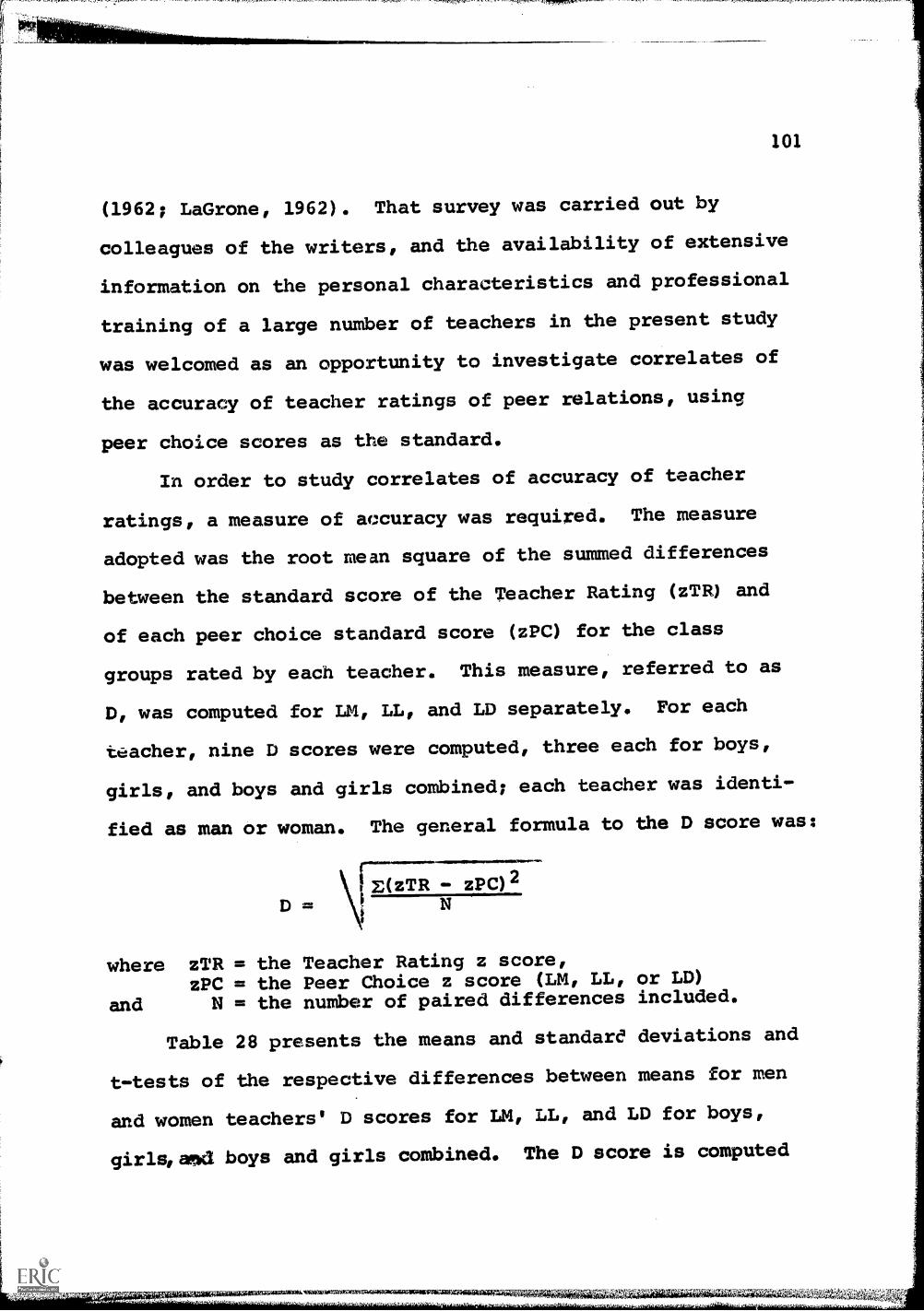
101

(1962; LaGrone, 1962). That survey was carried out by

colleagues of the writers, and the availability of extensive

information on the personal characteristics and professional

training of a large number of teachers in the present study

was welcomed as an opportunity to investigate correlates of

the accuracy of teacher ratings of peer relations, using

peer choice scores as the standard.

In order to study correlates of accuracy of teacher

ratings, a measure of accuracy was required. The measure

adopted was the root mean square of the summed differences

between the standard score of the Teacher Rating (zTR) and

of each peer choice standard score (zPC) for the class

groups rated by each teacher. This measure, referred to as

D, was computed for LM, LL, and LD separately. For each

teacher, nine D scores were computed, three each for boys,

girls, and boys and girls combined; each teacher was identi-

fied as man or woman. The general formula to the D score was

\\I E(zTR - zPC) 2

N

where zTR = the Teacher Rating z score,zPC = the Peer Choice z score (LM, LL, or LD)

and N = the number of paired differences included.

Table 28 presents the means and standare deviations and

t-tests of the respective differences between means for men

and women teachers' D scores for LM, LL, and LD for boys,

girls, aid boys and girls combined. The D score is computed

R1

.a ,47,7.77

102

Table 28. Comparison of Means and Standard Deviations of D

Scores for men and women teachers rating Boys, Girls, and

Boys and Girls Combined.

Men (N=48)Variable Mean S.D.

D LM boys 1.06 .39

D LL boys 1.12 .46

D LD boys 1.02 .44

D LM girls 1.27 .36

D LL girls 1.33 .43

D LD girls 1.24 .40

D LM both 1.18 .28

D LL both 1.28 .33

D LD both 1.18 .30

Women (N=492) MeanMean S.D. Difference t

1.04

1.15

1.02

1.02

1.12

1.01

1.05

1.16

1.04

.38 .02 .29

.45 -.03 .35

.42 0 0

.38 .25 3.62**

.46 .21 3.04**

.42 .23 3.69**

.31 .13 2.67**

.37 .12 2.03*

.35 .14 2.68**

* p<.05

**10.01

,r vn, n, 1"5-177ITIM. gfrrg,41,,, t

103

so that the smaller the D the greater the similarity

(accuracy) and the less the distance between sets of measures

compared. It is apparent that the differences between men

and women teachers are negligible for ratings of boys, but

that women are significantly more accurate than men in

rating girls. The teacher sex differences in agreement on

girls are so great that they account for the significant

differences found for boys and girls combined, as well. Not

only are women more accurate in general, but their mean D is

lowest for girls. The order of these differences matches

quite closely the pattern of reliability coefficients for

Teacher Ratings, reported above.

Table 29 shows the intercorrelations of the nine D

scores for the men and women teachers separately. This

table reveals two interesting sets of relationships. First,

it may be seen, both for men and women teachers, that the

accuracy of rating in relation to LM and LL is highly consis-

tent; the intercorrelations of LM, LL, and LD D scores,

respectively, for men are .89, .86, and .86, and for women

they are .86, .84, and .87. Second, the correlations

between accuracy of rating of boys and girls on all measures

are negative for men teachers and positive for women teachers.

The latter result suggests that men who are accurate in

rating boys tend to be inaccurate in rating girls, and vice

versa, while women tend to be consistent with both. These

104

Table 29. Intercorrelation of nine D Scores, LM, LL, and LID,for Boys (B), Girls (G) , and Boys Girls CoMbined (C), for;nen and women teachers. year I Texas sample. AMNON.

1 2Marial..oles LM-B LL-B

1 LM-B .892 LL-B3 LD-B4 LM--G5 LL-G6 LD-G7 LM-C8 LL-C

1 LM-B2 LL-B3 ID-B4 LM-G5 LL-G6 LD-G7 LM-C8 LL-C

.86

BelTeachers (pizAta3 4 5 6

LD-B LM -G, T.X.._:.QL.D-G,7

LM-C8

LL-C9

LD-C

.96 -.11 -.14 -.14 .70 .61 .68

.97 -.12 -.13 -.14 .63 .71 .70-.14 -.15 -,16 .67 .68 .71

.86 96 .60 .49 .54.97 .49 .59 .54

.55 .55 .55.86 .96

.97

(Women Teachers (N=492),

.96 .25 .23 .25 .80 .71 .78

.96 .21 .22 .22 .68 .78 .75.24 .23 .24 .76 .77 .79

.84 .96 .76 .66 .74.95 .65 .75 .72

.73 .73 .76.87 .97

.96

105

results support the belief in the greater empathy of women

teachers in their observation of children's peer relations.

INFLUENCE OF SOCIOECONOMIC STATUS (SES) OF PUPILS ON TEACHERRATINGS

In view of the widely mentioned opinion that teachers,

as members of the middle class, tend to evaluate middle

class pupils more favorably than those from lower classes, a

preliminary analysis was made of the ratings by 20 men and

20 women teachers in Minneapolis of 645 boys and 634 girls,

approximately evenly divided between the lowest and next to

lowest of four socioeconomic divisions of the population of

that city in 1963. Class III may he described as low-middle

and Class IV as low in socioeconomic status. Ratings were

reflected so that higher scores indicate positive peer

relations.

Table 30 compares means of boys and girls in the two

SES classes on the pooled ratings of men and women teachers,

separately and combined. No discriminable differences

appear, related to SES for boys, but the ratings of girls

are higher for SES III when rated by men and by women.

Further study of the relationships suggested by this analysis

is indicated.

106

Table 30. Raw teacher rating mean scores for 20 men

and 20 women elementary teachers in Minneapolis, 1963,

y sex of pupil_ and SES.

SES Subsamples Mean Teacher Ratings

SES III

Men Teachers 3.09 (171) 3.25 (158)

Women Teachers 3.21 (16C) 3.52 (162)

Combined 3.15 (339) 3.39 (320)

SES IV

Men Teachers 3.12 (153) 3.15 (152)

Women Teachers 3.14 (153) 3.34 (162)

Combined 3.13 (306) 3.25 (314)

. R..+ 47,4 ,

107

INFLUENCE OF TEACHER CHARACTERISTICS, TRAINING, AND BACKGROUNDON TEACHER RATINGS

Using the questionnaires completed by the 540 Texas

teachers who participated in the 1961 state survey mentioned

above, it was possible to examine a number of interesting

items reflecting personal characteristics of teachers, pro-

fessional training, and experience in relation to accuracy

of peer relations ratings, by means of the accurkcv (D)

scores described above.

Thirty-eight items in the Teachers' Questionnaire,

listed below, were examined in relation to accuracy of

Teacher Ratings of peer acceptance-rejection by Chi-square

analysis of contingency tables for each item. The tables

were uniformly constructed to provide category distributions

of response frequencies for the respective items, by sex of

pupil, sex of teacher, and range of D score, classified as

high, middle, or low by third, according to the following

intervals:

High Agreement Middle Agreement(16 male, (16 male,

Low Agreement(16 male,

Male Teachers

164 female) 164 female) 164 female)warsRating Boys .56 to .77 .78 to 1.07 1.08 to 2.54

Male TeachersRating Girls .52 to .96 .97 to 1.44 1.45 to 2.23

Female TeachersRating Boys .37 to .77 .78 to 1.08 1.09 to 2.50

Female TeachersRating Girls .37 to .77 .78 to 1.01 1.02 to 2.63

.;EiZER4,747e-

108

The items included were as follows:

1. Age (of teacher)

2. Race (White or Negro)

3. Teaching under emergency permit

4. Teaching under one-year permit

5. Teaching under special assignment permit

6. Interruption of undergraduate work to teach

7. Completion of requirements for teacher's certificate

at college graduation

8. If yes (on 7), was certificate permanent?

9. Attendance at junior college

10. Year of completion of most recent course forcollege credit

11. Was this course (10) in summer school?

12. Year awarded bachelors degree

13 Total undergraduate hours in student (practice)

teaching

14. Number of school systems attended duringelementary and junior high school

15. Number of undergraduate semester hours in profes-

sional education (excluding practice teaching)

16. Course taken in reading instruction

17. Course taken in arithmetic instruction

18. Was major part of teaching preparation in

traditional subjects?

19. Distance of present teaching position from high

school attended

20. Identification of first graduate major

21. Identification of first undergraduate major

nowt MAreZZUZAW,kMagrgagt.,,,,A.*.4.4.4WAI:.

r-777T7-mg. .77 74T47,4,77 .7,',V,4.777777T,,n93,,,,,,V.T7777.1,

109

22. Total semester hours completed abovebachelors degree

23. Type of masters degree held

24. Identification of college from which bachelorsdegree was received

25. Type of undergraduate degree received

26. Year of beginning first full-time teachingposition

27. Total years of full-time teaching experience

28. Years of full-time teaching experience inpresent school district

29. Number of different school systems in which youheld full-time teaching positions

30. If more than one school district, was last moveto smaller or larger school district?

31. Reason for most recent change (see 30)

. 32. If any change occurred in level of assignment,description of last change in terms of levelsinvolved, from and to

33. Number of one-year or greater breaks in full-timeteaching experience

34. Assignment for a semester or longer to teachingout of area of level of basic preparation

35. Primary reason for leaving teaching, in eventof previous breaks in service

36. Reason for returning to teaching, followingprevious breaks in service, if any

37. Whether college granting bachelors degree waschurch or state supported

38. General field classification of firstundergraduate major.

The complete tabulation of these data may be obtained

_-,,wlrrmmRrrnlMrm,,rwmpmTmm,,

110

upon request to the authors. 1 The net result of the analysis,

for all but four items for which tables are included below,

was random with respect to accuracy of Teacher Rating as

reflected by the D scores. The remaining tables would be of

interest only with respect to demographic and experience

background of a sample of Texas teachers, and, for t'iat

information, the Survey report (LaGrone, 1962) would be more

appropriate.

The Teacher Questionnaire items related significantly

to D score distributions were 2 (Race), 6 (Interruption of

undergraduate work to teach, 11 (Last college course for

credit taken in summer school), and 25' (Type of undergraduate

degree received).

Table 31 presents the data on Race (Item 2). There were

no male Negro teachers in the sample; hence, the analysis

applies only to female teachers. The results indicate signi-

ficantly higher agreement with pupil ratings by Negro women

teachers, as compared with White women teachers, for ratings

of both boys and girls. Since these data were obtained at a

time when Negro schools were segregated, it way be noted that

the Negro teachers were most likely segregated in living as

well as work conditions and were in a position to have closer

lAddress requests to Dr. S. B. Sells, Institute of BehavioralResearch, Texas Christian University, Fort Worth, Texas 76129.

111

Table 31. Relation of race of teacher to D Score measure

of accuracy of TR. Entires represent numbers of teachers

in each res onse cate or

Sex ofPupil Boys Girls

Sex ofTeacher Male Female Male Female

Race ofTeacher

High Mid LowAce. Acc.Acc

High Mid LowAcc. Am. Ace,

High Mid LowAcc. Acc. Aco

High Mid LowAce. Acc.Acc,

White

Negro

No Reply

16 16 16

0 0 0

0 0 0

151 156 161

12 6 3

1 2 0

16 16 16

0 0 0

0 0 0

149 157 162

13 6 2

2 1 0

Chi-Square = 6.27df = 2

13.05

.t...-.6W4.0.06Z.:.a&tagat,-=';iitat-ZIETCAVA:tetiair'

Chi-Square = 9.25df = 2X.01

112

personal knowledge of the lives of their pupils, as neighbors

in the minority settlement, than might be expected for White

teachers in the same school districts.

Item 6 asked, "If your undergraduate work was not conti-

nuous, was it interrupted to teach?" As shown in Table 32,

answers of No were received from 23 of the 48 men (48 per

cent) and from 164 of the 492 women (33 per cent), indicating

that 52 per cent of the men and 67 per cent of the women had

interruptions. The higher per cent for women reflects the

vulnerability of women to marriage, pregnancy, and other

socially determined factors that interfere with education.

No clear trend is observable for men teachers, but women

teachers whose educations were interrupted to teach tend to

be low in accuracy of ratings. This trend, which is signi-

ficant at the .05 level for women teachers rating girls,

most probably reflects the generally poorer training of

older teachers who began teaching in past years before

degrees were required. This analysis suggests further that

the present item-by-item analysis of the Teacher Question-

naire data may be overlooking more significant relationships

that might be extracted by a more sophisticated, multivariate

approach. However, this analysis was tangential to the Peer

Sutdy, and funds were not available within its framework to

undertake a more extensive analysis.

Table 33 complements the foregoing analysis by demon-

,

Table 32. Relation of interruption of undergraduateteach with the accuracy of teacher ratings. Entriesnumbers of teachers in each response category.

113

work torepresent

Sex ofpupil

Sex ofteacher

A. Inter-ruptedto teach

Male

Boys Girls

Female Male Female*

High Mid Low High Mid Law High Mid LowAcc. Acc.Acc. Acc. Acc.Acc. Acc. Acc.Acc.

1 3 3 74 65 78 2 3 2

High Mid LowAcc. Acc.Acc.

60 72 85

B. Inter-rupted notto teach 5 7 6 40 39 32 7 6 5

C. Not interrupted

42 39 30

10 6 7 50 60 54 7 7 9 62 53 49

*Chi-Square test of A vs B + C = 7.73, df = 2, p<.05 for womenteacher's accuracy in rating girls.

:mow"540::=141. 4 44v4.i.11V,..4..v.,$V4f.:';i2a24.1:,,$)

114

Table 33. The relation of responses to "Was the most recent

course taken in summer school?" to the accuracy of teacher

ratings. Entries represent numbers of teachers in each re-

s onse ate or

Sex ofpupils Boys

Girls

Sex o1teachers Male Female Male Female*

Response High. Mid LowAcc. Acc.Acc



High Mid LowAcc, Acc.Acc,

A. Yes

.......

B_ No

8 10 10 105 90 101 8 10 10 115 90 91

8 4 55 70 60 6 6 6 47 71 67

C. None

...........

0 2 0 4 4 3 2 0 0 2 3 g

*Chi-Square test of A vs B = 8.88, df = 2, p<.02 for women teachers'

accuracy in rating girls.

JO, 4tiasilW s.

115

strating that women teachers whose most recent college credit

course was taken in summer school, and who to that extent

may be considered motivated and professionally oriented

beyond their own peers, tend to be significantly high in

accuracy of rating. The trend is observable, but not signi-

ficant in ratings of boys; it is significant at the .02

level in ratings of girls.

The fourth item that produced a positive relations was

number 25, Type of undergraduate degree received. The three

highest-frequency categories reported by men and women were

BA, BS, and BS in Ed., summarized in Table 34. Here again,

no trend was observable for men, but for women, the academic,

BA degree ..s associated with high accuracy of rating, while

the professional, BS and BS in Ed. degrees are associated

with low accuracy. The results for women rating boys are

not significant, but for women rating girls they are signi-

ficant at the .05 level.

While the results for other items fail to reach signi-

ficance, the positive relations reported for items 6, 11,

and 25 suggest that further, more searching analysis of the

teacher background data might be profitable. Many of the

items, such as special permits (items 3, 4, 5) revealed

extreme divisions between those identified as in the special

category and the large majority of others. In most cases,

the distributions showed no differentiation related to D

AN,IF.1,11:4;3`.

116

Table 34. The relation of type undergraduate degree receivedto accuracy of teacher rating. Entries represent numbers ofteachers re ortin each t of de ree.

Sex ofpupil Boys Girls

Sex ofteacher Male Female Male Female*

Type ofdegree





A. BA 4 4 5 53 50 53 6 3 4 68 48 44

B. BS 8 8 7 46 54 43 .7 10 6 44 47 52

C. BS El.Ed. 2 2 3 60 50 62 3 1 3 49 63 60

*Chi-Square test of A vs B + C = 6.44, df = 2, p<.05 for womenteachers' accuracy in rating girls.

gReaaVcaaVrZeWata.YZYdtali=;,lm!--,,,,.y.at::-xlex.

117

score when tabulated independently, but the possibility of

joint effects with other items could not be explored in the

present univariate analysis. On the basis of the marginal

results obtained, these are indications that professional

training and motivation of teachers, as well as propinquity,

as in the case of the Negro women teachers, might be isolated

as significant contributing factors to accuracy of Teacher

Ratings.

STABILITY OF PEER AND TEACHER RATINGS OVER FOUR YEARS

The reliability estimates reported above for peer choice

scores were based on within-year data, and those for teachers

employed repeat ratings accomplished during the third year

of the study. The result of each analysis was an estimate

of the reproducibility of the ratings obtained within a

particular year. The present analysis focuses on another

facet related to the reliability of these measures, namely,

the stability of such ratings over longer time intervals.

The index of stability, involving the correlations of

identical measures on the same individuals from year to year,

is a gross estimate of the consistency of ratings under

conditions in which (a) the individuals rated advance in age

from year to year and change in various ways, (b) the raters

vary to some extent, for Peer Ratings, as class composition

'aWk4=',611, 1

77 7

118

changes and change, in the case of Teacher Ratings, and

(c) the school environment changes, most drastically in the

transition from elementary to junior high schocl, but subtly

in many respects from year to year.

No attempt has been made to allot responsibility to the

various sources of variance that may account fc r the level

of stability of the ratings, although this migtt be worth-

while. The principal emphasis in this analysis: is on the

comparison of the stability estimates over tim? with the

reliability estimates for a single year.

Table 35 summarizes the stability correlLtions over all

one-year intervals for the Texas and Minnesota total samples.

This table presents comparable data for a two-year sample

(Years I and II), which is the largest sample available, and

for the three- and four-year samples, which are smaller,

as explained earlier. The years compared are identified,

and ccrr:1-lati-m coefficients are presented for LM, LL, and

TR, the three independently defined variables, as well as

for the derived variables, LD and DT.

With the exception of the Texas coefficients for Years I

and II, which involve the largest sample and are highest of

all for peer choice scores, the stability coefficients for

one-year intervals are very homogeneous for all variables.

Although the reliability of LL (.7) was higher than that for

LM (.6), Table 35 shows that the LM scores are more stable

189

but beyond that it did not materially affect the selection-

rejection score" (1948, p. 354), This study is somewhat

unsatisfactory since the middle intelligence group was

defined so broadly as to leave few cases for the upper and

lower groups. it is of interest since an hypothesis of a

differential relation between intelligence level and socio-

metric status is stated.

The second of these studies, by Porterfield and

Schlichting (1961), compared reading achievement scores

obtained, using Test I, Paragraph Meaning, of the Stanford

Achievement Test with various pupil characteristics,

including sociometric scores. Their sample was drawn from

6th grade pupils in the Tulsa Public Schools; they had a

total of 981 pupils drawn about equally from schools of high,

middle, and low SES. As would be expected from the studies

of intelligence, they found a firm relationship between this

achievement test and sociometric status. When results by

socioeconomic levels were examined, they found a relationship

between achievement scores and social acceptability status

in the high and middle group, but the relation between test

scores and social acceptability was not significant in the

low SES schools, although it was in the expected direction.

This is similar to the Grossmann and Wrighter stully in

suggesting that the relationship between an intellectual

variable and sociometric status is different at various

190

levels, but data are opposing in the reported level at which

the difference occurred. It is possible to hypothesize in

either of these directions or in still other ways. In the

absence of clearer support from the literature than is

afforded by the studies reviewed here, an openly empirical

approach was taken. There was no compelling reason to hypo-

thesize that a difference would occur at any point in the

scale, or that no difference would appear at any level.

Minnesota Study

Sample. The sample was based on first year data and

included 4th grade children of both sexes from all schools

in one Minnesota city (2,800 cases). The 4th grade in this

city was employed because these children had been given the

Lorge-Thorndike Intelligence Test during the school year, and

because this city was the largest one ir the study for which

results were available for the entire city.

Socioeconomic level was determined on a census tract

basis, making use of a combination of adult income and

education from the 1960 census values. Separate classifi-

cations of census tracts on these two criteria gave highly

similar results. The entire set of schools in the city was

then divided into quartiles on the pasis of area in which

each was located. Other information indicates that this

classification of schools would correspond very closely to

that made with the use of any other relevant indices of

191

socioeconomic status, of which there are many. The diffe-

rence between the upper and lower socioeconomic levels on

the Large-Thorndike Intelligence Test was approximately the

same in IQ points as the difference between highest and

lowest socioeconomic levels of the Stanford-Binet when these

were classified according to occupational level of father

(McNemar, 1942). The differences found here are greater

than those reported by Anderson (1962) for the Lorge-

Thorndike Test for a partial sample from Syracuse, New York;

there SES was estimated on the basis of the Sims Social

Class Identification Scale.

Procedure. At each of our four SES levels, the group

of "high" girls and "high" boys was defined as consisting

of all those with standard scores 1 SD or more above the

mean on LD. A corresponding group of "low" girls and "low"

boys was defined as consisting of those with an LD standard

score 1 SD below the mean.

Results. When the mean IQ for each of these groups was

computed, the values shown in Table 55 and Fig. 1 were

obtained (mean IQ values for all 4th grade girls and all

4th grade boys by socioeconomic status are also presented

in Table 55).

There was a consistent sex difference of about 5 IQ

points in favor of the girls at all four socioeconomic

levels and for the total groups. This did not affect the

I5Z

17. 907W7Jt7vnc".'17:n,

GI A LS

111111111.111111.1.711".1111"71111114

*k,

192

HIGHCHOICESTATU S

LOWCHOICESTATUS

70 75 80 85 90 95 100 105 110 115 120 125MEAN IQ

BOYS

_°V-40,4.

rirrill,1111."1"1"'1'44"

HIGHCHOICE STATUS

LOWCHOICE STATUS

70 75 80 85 90 95 100 105 110 115 120125MEAN IQ

Fig. 1. The IQ and choice status of

girls and boys in relation to socioeconomic

background

r-

194

general pattern of differences between high and low choice

groups at the different socioeconomic levels. Inspection of

Fig. 1 shows the same pattern of results for girls and for

boys at different socioeconomic levels. At all four levels

the differences between the high and'low groups for both

sexes are about the same.

In terms of IQ points, there is a difference of about

15 to 20 points between the high aid low choice status

groups at various socioeconomic levels. The only exception

to this is in the top socioeconomic group where the diffe-

rences for girls and boys are only 11.5 and 14.3 points,

respectively. The smaller standard deviations of these

groups suggest that the test may not have had sufficient

ceiling for these groups.

This result is in line with the impressions obtained

from earlier work with childhood case histories. A child

of either sex with an IQ of 80 in a low socioeconomic group

is at a real social disadvantage. Similarly, a child with

an IQ of 100 in an upper socioeconomic group is also at a

disadvantage. An intelligence level above the average of

the peer group is an asset in a wide variety of groups.

Texas Study

The study of peer choice scores in relation to intelli-

gence and SES in the Texas sample followed a design quite

different from that in the Minnesota sample reported above.

195

Whereas a large sample in one grade (grade 4) from one

Minnesota city in which detailed SES analyses had already

been made permitted the type of comparison shown in Fig. le

no similar data were available for any subsample in Texas,

where the districts included ranged from small to medium

small in size and where schools frequently serve areas of

greater geographic extent and greater SES heterogeneity.

This report represents an effort to present the data

available from schools that continued in the second year of

the general study, using SES estimates obtained from 1960

Census reports for census tracts served by the respective

school:. SES differentiation of areas within communities

was not feasible, as in the Minnesota study. Instead, means

of districts varying in SES are presented.

As a result of the constraints experienced with the

Texas data, it was convenient to correlate peer scores with

IQ for a number of different tests used by different school

districts. These data are not pooled, but the comparisons

presented indicate trends generally in agreement with the

Minnesota data. Furthermore, the correlations, including

the entire sample, in each case, rather than only the

segments above and below one standard deviation from the

mean, permit estimates of fractions of variance in peer

scores accounted for by intelligence tests. Although a

wider range of grades is included than in the Minnesota

"sr

196

study, the use of age-independent IQ measures swards against

inflation of the correlation coefficients.

Results. Table 56 presents the means and standard

deviations of IQ for six school districts in relation to SES.

A seventh school district, Abilene, for which IQ data were

transcribed, was omitted because adequate data were not

available at the time to classify its eleven schools by SES,

and the composite was considered too heterogeneous for the

type of analysis required. The six districts are listed in

approximate order of SES, although a reversal occurs between

Castleberry and Breckenridge on Median Educational Level of

Adults. These six districts fall into discrete intervals

with Everman highest (median education, 12.8 years and

median family income, $7,797.), Castleberry and Breckenridge

in the middle (median education 10.4 to 11.8 years, median

income $4,752, to $5,300.), and Bonham, McKinney, and the

three schools from Waco forming the low group (median edu-

cation 8.3 to 9.3 years, median income $3,530. to $3,988.).

Six different test forms were used in the samples reported,

and the proportions of boys and girls in the subsamples

varied. The variation in mean IQ due to these factors is

not controlled. Nevertheless the results follow the general

pattern demonstrated in the Minnesota study and widely

reported in the literature, with the mean Ws generally

ordered in proportion to SES level.

9771,11,177.'57,07¢

197

Table 56. Mean and standard deviation of IQ for six schooldistricts varying in SES level, tests used, and proportionsof boys and girls. Texas....Year IY data.

MeasuresMedEduc.Adults

12.6

10.8

11.4

9.3

9.1

8.3

Medancome, School IntelligenceFamilies District Test

No,Cases Mean S.D.

$7797. Everman CTMM Prim. 47

$5300. Castleberry CTMM Elem. 586

$4752. Brecken-ridge*

Henmon-NelsonLorge-

145

Thorndike-C 223

$3988. Bonham Otis Alpha 208Henmon-Nelson 237

$3905. McKinney* CTMM Elem. 372CTMM Jr.H. 193

$3530. Waco* CTMM Prim. 102CTMM Elem. 466

117.8 14.93

112.2 14.50

106.2 15.90

103.7 11.02

103.4 12.03104.5 13.27

98.4 15.59104.2 14.31

92.5 14.3998.9 14.02

*Waco is represented in this study by three schools: these data donot depict the entire school population of this city. The Brecken-ridge, McKinney, and Waco samples each include one Negro schoolalong with the White school samples.

W3itiZ:"

198

Correlations of IQ with five peer status scores and

with school grades are shown in Table 57 for samples based on

four intelligence tests for boys and girls, separately and

combined. These data are based on five school districts,

Year II data, which had samples of sufficient size to provide

stable relationships. SES is not differentiated in Table 57.

Although there are variations related to test and other

factors affecting subsamples, the overall results are quite

similar for LM and LL. The average correlations are about

.24 for LM, .21 for LL, and .26 for LD. IQ accounts for 5,

4, and 7 per cent of the variance in LM, LL, and LD respec-

tively, in these samples, but these estimates are not consi-

dered independent. As might be expected from the earlier

discussion of the relationships between LM and LL among boys

and girls, the correlations of IQ with LM are higher for

girls than boys, and this relationship is reversed for LL,

although the differences are slight.

The correlations of IQ with TR are higher than with the

peer choice scores, averaging around .36, It may be assumed

that teachers have fairly stable impressions of the intel-

lectual levels of their pupils, even when they have not had

test scores available, and that these impressions are more

influential in their ratings than are similar factors in the

peer choices of their pupils. This observation gains some

support from the correlations of IQ with school grades,

199

Table 57. Correlations of 10's obtained from a number of testswith peer status scores and school grades, for boys and girlsseparately and combined. Data based on five Texas schooldistricts, Year II. Grade ran e 4-7

No.Test Cases L LD TR DT School Grades

BPX1

Corralation of I. with:

CTMM - Elem.

Henmon-Nelson

Lorge-Thorndike - A

Lorge-Thorndike - C

CTMM Elem.

Henmon-Nelson

Lorge-Thorndike - A

Lorge-Thorndike - C

CTMM - Elem.

Henmon-Nelson

Lorge-Thorndike A

Lorge-Thorndike - C

740 .21 .18 .23 .33 .29 .56

186 .21 .19 .22 .29 .27 .78

552 .22 .25 .27 .36 .32 .64

105 .23 .09 .20 .36 .28 .56

Girls

722 .28 .20 .28 .35 .34 .59

196 .13 .19 .18 .37 .27 .73

597 .26 .19 .26 .37 .31 .63

118 .34 .14 .29 .40 .33 .76

Combined

1462 .24 .19 .26 .34 .31 .57

382 .17 .18 .20 .32 .27 .75

1149 .24 .23 .26 .37 .32 .64

223 .28 .11 .24 .38 .30 .66

a4.

200

assigned by the same teachers, which are somewhat higher

than expected.

In Table 58, relations among IQ, SES, and school grades

are analyzed, using information from three school districts

in which the same intelligence test was administered. The

range of SES covers only the middle and low categories in

Table 56. However, the samples are .c;f good size for both

sexes and the data are comparable. This table presents

means and standard deviations for IQ and school grades,

correlations of both IQ and school grades with peer scores,

and the correlations of IQ with w7tool grades. The test on

which IQ's are based is the California Test of Mental

Maturity, Elementary Form.

These data follow generally the trends displayed in the

preceding two tables. With the exception of the Waco schools,

which are lowest in SES, the mean of girls are higher than

those of boys on IQ and grades. The correlations of school

grades with peer scores are higher than the corresponding

correlations with IQ, and the correlations of both with TR

are highest of all in their respective sets. In these three

districts, school grades are almost as good a measure of the

teachers' ratings of peer relations as they are of academic

performance. Although the correlation of TR with grades is

reduced when: the effect of IQ is partialled out (for example,

the correlation of TR with grades for boys in Castleberry,

'!"711M=MMma 77SMAMK4M7717" ,

201

Table 58. Means and standard deviations of IQ and school grades;

correlations of IQ and school grades with peer scores and each

other. Boys and girls separately for three Texas school districts

differin in SES

Mean and S.D. Ig and School Grades in Relation

No.Cases Sex

to SES MeasuresSchoolGradesSchool

District10=1W11

SES IndicatorsMedianEduc.

Med.Fam.Income Mean S.D. Mean S.D....=mw

Castleberry 10.8 $5300. 291 Boys 111.3 16.6 79.1 9.68

(2 schools)295 Girls 113.7 14.0 84.2 9.81

McKinney 9.1 $3905. 188 Boys 97.2 15.8 80.6 8.42

(5 schools)184 Girls 98.7 15.4 84.1 9.04

Waco 8.3 $3530. 237 Boys 98.9 14.8 75.2 8.83

(3 schools)229 Girls 98.9 13.7 77.7 9.74

Correlations of Peer Scores with I. and S hoof Grades

School Vari- LM LL LD TR DT

District abler Auve.Girls Boys Girls Boys Girls MogGirls Bays Girls

Castle-berry

McKinney

Waco

IQSch.Grades

IQSch.Grades

IQSch.Grades

.22 .34 .20 .20 .24 .32 .38 .39 .31 .38

. 35 .42 .33 .37 .40 .47 .53 .52 .47 .54

. 30 .39 .24 .32 .32 .44 .33 .45 .37 .50

.38 .46 .29 .31 .41 .45 .45 .51 .47 .52

.23 .35 .14 .27 .21 .36 .44 .49 .31 .43

.24 .26 .29 .29 .29 .32 .38 .44 .34 .36

Correlations of I with School GradesCastleberry McKinney Waco

Boys .62 .65 .50

Girls .66 .66 .48

ti

202

of .,53, is reduced to .40 when IQ is partialled out), the

resulting partial correlation coefficients are substantial.

_.....rSumaa. The Texas data on relations of peer scores to

IQ and SES, although not as manageable for the study of

joint effects as the Minnesota data analyzed in the preceding

section, nevertheless demonstrate confirmatory evidence that

peer acceptance-rejection is substantially related to both

variables. Correlations with SES measures were not possible.

Correlations with IQ measures on different tests suggest that

IQ accounts for about 7 per cent of the variance in LD,

although this is not believed to be an independent contri-

bution. Peer scores correlate more highly with school

grades than with IQ, and the data suggest that both IQ and

peer relations account for significant variance in school

grades.

PEER ACCEPTANCE-REJECTION AND SCHOOL GRADES

In the preceding section, in Table 58, data were pre-

sented on the relation of peer scores to school grades,

which are higher than the corresponding correlations with IQ.

The data in this section present additional correlations

between school grades and peer scores for a larger sample

from the seven Texas districts included in Year II and are

included primarily to demonstrate three relationships that

appear to deserve further study, although funds were not

203

bedgeted for this purpose in the present study. These three

relationships are: ..(1) The relative contributions of LM, LL,

and TR to school grades, (2) sex differences in contributions

of these variables to school grades, and (3) grade level

differences in correlations of these peer scores with school

grades.

Subjects. In 1963 it was possible, in conjunction with

other work, to transcribe from school records end-of-year

school grades of 3,774 pupils in grades 4 through 7 in seven

Texas school districts which had continued in the general

study through the second year. The letter grades were

converted to quantitative scores using the following numerical

equivalents: A 95, 13 85, C 75, D 65, and F 55. The average

grade scores were correlated with Year II peer scores.

Results. The means and standard deviations of average

school grades for boys and girls in the sample, by grade

level in school, and correlations of school grades with the

five peer scores, are presented in Table 59.

Relative Contributions of LH, LL, and TR to School

Grades. As shown in Table 59, the correlations of these

three variables with school grades follow a consistent

pattern across all grade levels. First, the LH correlations

exceed the LL correlations at all grade levels, suggesting

that to the limited extent to which such information may have

influence on grading, teachers appear to be more responsive

to liking patterns of children than to dislike patterns.

.140441;'"" .% .

WINSAMLiftiffisinamccrwm.

204

Table 59. The association of peer acceptance-rejection and

ashaOLAIAL12242920s SamRle, Year It. ,cMINOW111.1111111.11

Grade Sex N

School Gradesionsb of School

Grades withMean

aS.D. LM LL LD TR DT

4 Boys 648 81.6 9.32 .37 .34 .42 .52 .49

4 Girls 670 85.5 9.00 .41 .35 .44 .46 .49

5 Boys 627 79.9 9.88 .31 .26 .34 .39 .38

5 Girls 632 85.6 10.22 .31 .29 .34 .40 .38

6 Boys 286 80.4 9.84 .26 .21 .27 .31 .31

6 Girls 296 82.9 9.69 .25 .22 .27 .44 .37

7 Boys 309 80.8 9.60 .28 .15 .26 .28 .31

7 Girls 305 83.1 9.47 .29 .23 .29 .40 .34

Total Boys 1870 80.7 9.66 .32 .26 .34 .40 .39

Total Girls 1903 84.1 9.66 .33 .29 .35 .42 .41

CombinedTotal 3773 82.4 9.81 .33 .27 .35 .41 .40

A.1=11,1wwwwomm...m. ./..11NP*

aAt each grade level the means for girls are significantly greaterthan the means for boys, p<,01.

All correlations are significantly greater than zero, p<.01.

c

205

Second, the TR correlations uniformly equal (boys, grade 7) or

exceed (the other seven cases) the peer choice score correla-

tions at all grades. These results further suggest that peer

relations information may be related to grading practices.

Although the influence of intelligence, SES, ethnic, and

other factors is entangled in grading, the pattern of corre-

lations of peer scores with school grades suggests that peer

relations indices make a unique contribution that can be isolated.

Sex Differences in Correlations of Peer Scores with

School Grades. The interesting things about sex differences

in Table 59 is that they do not appear, except for the

correlations of TR with grades at grade levels 6 and 7, where

the girls' correlations are higher, as expected. No discri-

minable differences appear among the peer rating variables.

The higher mean grades of girls over boys are significant at

the .01 level at each grade level and for the total sample,

but, except for the exceptions noted, there are no differences

in correlation with peer scores.

Grade Level Differences in Correlati ns of Peer Scores

with School Grades. The trend of the correlations with

school grades in Table 59 is one of dropping off from the

earlier to later grades. For LD, the average correlations

of boys and girls with school grades are: grade 4, .43;

grade 5, .34; grade 6, .27; and grade 7, .28. The per cent

izw,mfta,1,44t:44f-

11.1Mu.

206

of common variance (r2) reflected by these correlations

reduces from 18 at grade 4 to 8 at grades 6 and 7.

Apparently, social relations, implicit in the measures of

peer acceptance-rejection, are most influential in grading

in the early grades and gradually lose influence as the

curriculum becomes more content-oriented. This factor needs

to be (Jonsidered in studies relating abilities and cognitive

performance measures to school grades.

aimmarz. Brief review of data relating prer scores to

school grades reveals the following relationships believed

worthy of further study. (1) The pattern of correlations of

peer scores with school grades suggests that peer relations

make a unique contribution to grades that can be isolated.

(2) Sex differences were almost totally absent in the corre-

lations, although mean grades for girls were significantly

higher than those for boys at every grade level. (3) The

correlations between peer scores and grades fall off con-

stantly from grade 4 to grade 7, suggesting that the

influence of peer relations on teacher grades is not constant,

but rather declines above the early elementary grades.

PEER ACCEPTANCE-REJECTION IN RELATION TO MINORITY ETHNICSTATUS, STUDY OF CHILDREN WITH SPANISH SURNAMES

With the exception of Negro children in segregated

schools in Texas, neither ethnic nor racial identifications

were available in the school records in either state, and

lPy0:025-We

207

such identifying data could not be incorporated in the forms

used routinely in the survey. However, it was possible, in

the Texas data, to identify a minority ethnic sample having

Spanish surnames, and a special study of this group is

reported in this section. A study of Negro children in

segregated schools appears in the following section,

Purpose

Traditionally, the Mexican-American has been a rejected

ethnic minority in the transitional areas along the Mexican

border. Differences in education and socioeconomic status

have magnified and colored the considerable cultural diffe-

rences between Anglo- and Latin-Americans in these areas.

Despite progress in many respects in recent years, prejudice

against Mexican-appearing individuals, who are commonly

identifiable by appearance, speech, area of residence, and

other indicia, is believed still to be widespread. The

purpose of this study was to evaluate the effect of such

prejudice among school children on the measures of peer

acceptance-rejection. Segregation of minorities in separate

schools was confined only to Negroes. Spanish-American

children attended the same public schools as Anglo- children,

the only segregation being by area of residence. Thus in

this study, Spanish- children were rated in mixed Anglo-

and Spanish- classes.

,

208

Subjects

This study is based on Year I peer ratings. Two

Spanish-speaking assistants reviewed independently the

entire Texas roster and checked all surnames that they

considered Spanish. Those on whom the two agreed were

retained for the purpose of this study. It is believed that

most of the children thus identified were of Mexican-

American parentage. However, for a variety of reasons, a

small number of errors must be expected. The number of

omissions is also believed to be small. The cost of going

back to the schools to check the classification was not

considered worth the additional accuracy to be gained by

this effort. Of the total sample of 72 schools in 19 school

districts, one district (Hurst), with 11 schools, was

excluded because LL nominations were not made, and two

districts had no children with Spanish surnames. The final

sample consisted of 640 children with Spanish surnames in

49 schools in the remaining 16 Texas school districts.

Demographic information, based on the 1960 U.S. Census,

was abstracted for the census tracts or county census divi-

sions in which the 49 schools were located. The 1960 Census

Reports included estimates, based on a 25 per cent sample,

of the per cent of families with Spanish surnames. For the

49 schools in the present study, these estimates range from

zero to 62 per cent for census units, with a median per cent

1

209

of 3.1. For the total Texas sample for Year I the median

value was 2.7 per cent. Based on the total number of 19,617

Texas children in the first -year survey, the 640 children

selected represent 3.26 per cent of the Texas sample. This

figure is close to the Census estimate.

Other demographic data derived from the 1960 Census

reports enable evaluation of the mean and range of socio-

economic level of the 49 schools in this study. As shown in

Table 60, the schools with Spanish surname children are..!

slightly below the total sample in socioeconomic level

measured by median income of families and by median educa-

tional level of adults.

Procedure

In order to control for socioeconomic background, each

child with a Spanish surname was paired with a randomly

selected classmate of the same sex, not in the "Spanish"

list. This procedure produced two paired samples, Spanish

and Anglo, each consisting of 640 children with data avail-

able on LM, LL, and LD. For these samples, teacher ratings

were not completed on 21 of the Spanish and 13 of the Anglo

children.

In addition to the peer scores, two additional variables

were recorded for each child. First, the 49 schools were

classified on the basis of location in or out of a metro-

politan area; this enabled a classification by large

.

210

Table 60. Comparison of measures of socioeconomic status

for 49 schools having children with Spanish surnames with

the 72 schools which comprise the Texas first-year sample.

Data from U.S. Censuses of Population and Housing112601...

SocioeconomicStatus_M'asure

Median Annual

Spanish Surname Total Texas

Sample (49 schools) Sample (72 schools)

Range 1Range1

Mean Low High Mean Low High

Income, Families $4566. $2935. $9250. $5118. $2733. $9250.

Median YearsEducation,Adults 10.1 8.3 13.2 10.6 8.0 13.2

NNW

.17.1-Manaitlw-

4,441,AT,T7MIM

211

community (in) or small community (out). Second, each child

received a code reflecting the number of Spanish surname

children iu his class. These variables were expected to have

analytic significance. The classification by size of

community was expected to relate to peer scores in the same

manner as SES and to suppliment the control for SES achieved

by the pairing of cases. The number of Spanish children in

a class was included in order to investigate the existence

and possible effects of minority or majority cliques in

classrooms.

Results

Gross Results. The mean peer scores of the paired

total groups and of subgroups representing large and small

communities are shown in Table 61. The Spanish children are

lower than the Anglo children on all comparisons and signi-

ficantly so on all but one, LL in the small-community sub-

sample. Except for that one case in which the Spanish sample

mean approaches closely to the corresponding Anglo-mean, the

differences between the large and small community subsamples

are insubstantial, and none are significant, including LL.

From Table 61, it is apparent that the Spanish-Anglo

comparisons on LM and LL are different. The order of means

and of mean differences between the two samples suggests that

the Spanish children are infrequently chosen (low on LH)

but also not strongly rejected (higher on LL). In both

, ,

212

Table 61. Comparison of peer and teacher rating scores of

Spanish surname and Anglo samples paired on SES, by small and

lar e communit sc ools and total sam le

Spanish Surname Paired AngloPeer Sample Sample Mean

Score N Mean S.D. N Mean S.D. Difference CR.

Small Communities (Located Outside Metro olitan Areas

LM 153 4.72 .80 153 5.14 1.04

LL 153 4.91 1.06 153 5.00 .94

LD 153 4.76 .91 153 5.08 .99

TR 149 4.78 .71 153 5.00 .76

DT 149 4.73 .88 153 5.06 .99

.42

.09

.32

.22

.33

Large Communitigsalooted in Metropolitan Areas)

3.96**.71

2.92**2.68 **

2.99**

LM 487 4.75 .87 487 5.16 1.00 .41 6.92**

LL 487 4.88 .98 487 5.06 .96 .18 2.89**

LD 487 4.77 .90 487 5.14 .99 .23 6.15**

TR 470 4.83 .73 474 5.14 .81 .31 6.34**

DT 470 4.74 .89 474 5.16 1.00 .42 6.89**

Total Sonia

LM 640 4.74 .85 640 5.16 1.01 .42 7.97**

LL 640 4.89 1.00 640 5.05 .95 .16 2.86**

LD 640 4.76 .90 640 5.12 .99 ..36 6.79**

TR 619 4.81 .72 627 5.11 .80 .30 6.81**

DT 619 4.74 .89 627 5.14 1m00 .40 7.58**

**p(.01

( ,ktia=1.4 aR:Nza-:,41,44

T7.214,1

213

subsamples, as well as the total sample, the means of LL

exceed those of LM for Spanish children, and the reverse

holds for Anglo children. As a result, the differences

between the Spanish and Anglo children are about three times

as great on LM as on LL. Further, the differences between

LM and LL are significantly greater than zero for the total

sample of Spanish surname children. Using 452 as an estimate

of the correlation between LM and LL as found for the total

first year sample, the computed tests of significance indi-

cate that the mean LM z-- scores are significantly lower than

the mean LL z-scores. For Spanish surname boys, the critical

ratio is 2.16 (p .05), and for girls it is 3.75 (p <41).

For the total Spanish surname sample, the critical ratio is

4.12 (p <Al). These data for boys and girls combined suggest

that children in this minority ethnic group are not strongly

rejected by their peers, but neither are they accepted in

the pee: group.

Teacher Rating Raw Scores. The inference that Spanish

children tend to be low in acceptance (LM) rather than

strongly rejected (LL) by peers is supported by the teachers'

estimates of peer acceptance-rejection. The distributions

of raw score teacher ratings on a four-point scale are shown

in Table 62.

The percentages of children rated as (3) Tends to be

Rejected or (4) Strongly Rejected, were 12 and 11 for the

Table 62.

Comparison of teachers

rating raw score frequency

distributions of Boys and

Girls

with Spanish surnames

and with Anglo surnames,

in the Texas Sample.

Teacher Rating

Boys

Girls

Spanish

Anglo

Spanish

Anglo

Cagegories (Year I)

N (Per cent

NPer cent

N (Per cent) N

Per cent

1 - Highly Accepted

56

(19)

89

(30)

33

(10)

100

(31)

2 - Accepted

213

(71)

173

(57)

241

(75)

200

(62)

3 - Tends to be

Rejected

21

(7)

34

(11)

37

(12)

21

(6)

4 - Strongly

Rejected

8(3)

7(2)

10

(3)3

(1)

Total

298

(100)

303

(100)

321

(100)

324

(100)

Mean

1.94a

1.86 b

2.07a

1.77b

S.D.

.60

.69

.58

.60

CR (Ethnic Groups)

1.38ns

6.55,

p<.01

Total Group

Spanish

Anglo

N Per cent) N

(Per cent)

89

(14)

189

(30)

454

(74)

373

(59)

58

(9)

55

(9)

18

(3)

10

(2)

619

(100)

627

(100)

2.01

1.82

.59

.65

5.39, p<.01

alndicates difference between means for Spanish

Surname Boys and

Spanish Surname Girls

is signifi-

cant,

CR = 2.95, p<.01.

bIndicates differences between means for Anglo Surname

Boys and Anglo Surname

Girls is significant,

CR

1.76, p<.05 (one tailed

test).

215

Spanish. and Anglo groups, respectively. Percentagewise,

fewer Spanish than Anglo boys received teacher ratings which

denote rejection, while fewer Anglo girls than Spanish girls

received ratings in these two categories. Teacher ratings

of Highly Accepted were awarded to Spanish children (14 per

cent) less frequently than to Anglo children (30 per cent).

These data agree with the peer ratings on LM and indicate

teacher agreement with the peer choice results.

Sex Differences. Significant differences between mean

scores of Spanish boys and Spanish girls on LM, LL, and TR

are reported in Tables 64 to 66. Since these variables

yielded significant sex differences, comparisons on LD and

DT are not needed. In each comparison, the data indicate

that Spanish boys tend to have more favorable relations with

their same-sex peers than do Spanish girls. In order to

investigate the presence of an interaction effect between

surnames and sex, a 2x2 unweighted means analysis of variance

was computed for LD which maximizes the joint effects of

LM and LL. The results, summarized in Table 63, show signi-

ficant main effects for ethnic group (Spanish vs Anglo

surname) and for sex (boy vs girl), but the interaction

between surname and sex was not significant.

Size of Communit . Tables 61 and 64 through 66 show no

significant mean differences on any of the peer scores

attributable to size of community. In order to determine

^ WfM, vr

216

Table 63. Analysis of variance on LD by surname (Spanishvs An

Source11111111111INNO111.1111MM

SS df

A (surname) 40.93 1

B (sex) 11.90 1

AB (surname x sex) 3.58 1

Within cells 2131.97 1276

MS F

40.93 24.5*

11.90 7.1*

3.58 2.14

1.67

*13<01

WPOVS..TAWAilltitat4 wsaax6rwro4A*s;i,ahgW4TiXtlNg.''''

Table 64.

Comparison of LM z-scores of boys and girls with Spanish and Anglo surnames.

-4'4Nolp

Span.

Surname

Pupils in

Spanish

Mean

S.D.

Boys

Anglo

Girls

Spanish

Anglo

Mean

S.D.

CR

NMean

S.D.

NMean

S.D.

CR

Small Communities (Located Outside Metropolitan Areas)

142

4.93

.79

42

5.09

.93

0.9

29

4.67

.96

29

5.32

.80

2.7**

214

4.67

.52

14

4.90

.99

0.8

22

4.68

.73

22

5.43

1.01

2.8 **

3 or 4

15

4.91

.92

15

5.14

1.28

0.6

20

4.32

.48

20

4.80

1.15

1.7*

5 or more

None

None

11

4.62

.79

11

5.15

1.05

1.3

Total

71

4.87

.87

71

5.06

1.03

1.2

82

4.58

.79

82

5.20

1.09

4.1**

Large Communities (Located in Metropolitan Areas)

156

4.92

.96

56

5.33

.98

2.2**

49

4.48

.68

49

5.28

1.09

4.3**

228

4.85

1.06

28

5.18

.95

1.1

40

4.45

.70

40

5.02

1.08

2.8**

3 or 4

70

4.92

.91

70

5.11

1.03

1.1

83

4.63

.78

83

5.10

,92

3.6**

5 or more

86

4.85

.89

86

5.23

.97

2.7**

75

4.75

.81

75

5.07

1.00

2.1**

Total

240

4.89

.94

240

5.21

.99

3.7**

247

4.61

.77

247

5.12

1.01

6.3**

Combined

Total

311

4.88a

.90

311

5.18

1.01

3.8**

329

4.60a

.77

329

5.14

1.01

7.6**

*p<.05

**p<.01

alndicatesdifference between means for Spanish Surname Boys and Spanish Surname Girls is signi-

ficant,

CR = 4.23, p<.01.

Table 65.

Comparison of LL z-scores of bo

coNo. Span.

Surname

Pupils in

Class-Grou

123 or 4

5 or more

Total

123 or 4

5 or more

Total

Combined

Total

s and iris with S anish and An lo surnames

Boys

Girls

Spanish

Anglo

CR

Spanish

An lo

CR

Mean

S.D

Mean

S.D.

Mean

S.D.

NMean

S.D.

Small Communities

Located Outside Metropolitan Areas)

42

5.23

.90

42

4.99

.86

0.0

29

4.58

1.27

29

5.05

.75

2.6 **

14

5.17

.62

14

4.88

1.06

0.0

22

4.67

1.22

22

5.16

.82

2.3**

15

4.83

1.15

15

5.25

.94

1.0

20

4.96

.95

20

4.GO

1.18

1.1

None

None

11

4.76

.82

11

5.07

.96

1.3

71

5.13

.92

71

5.02

.93

0,7

82

4.72

1.14

82

4.97

.94

1.5

Large Communities

(Located in Metropolitan Areas)

56

4.98

.89

56

5.15

.93

1.8*

49

4.91

.93

49

5.08

1.05

0.8

28

4.97

.89

28

5.09

1.00

1.0

40

4.55

1.33

40

5.01

.95

1.8*

70

5.08

.88

70

5.03

.99

0.8

83

4.78

.92

83

4.93

.92

1.0

86

4.84

1.03

86

5.17

.83

3.2**

75

4.90

.93

75

5.05

1.03

1.0

240

4.96

.95

240

5.12

1.03

1.7*

247

4.81

1.02

247

5.01

.97

2.2*

311

5.00a

.94

311

5.09

1,01

1.2

329

4.79a

1.04

329

5.00

.98

2.7**

*p<.05

**p<,01

alndicates

difference between means for

Spanish Surname Boys and Spanish Surname Girls is

signi-

ficant, CR = 2.73, p<.01.

Table 66.

Comparison of TR z-scores of boys and girls with Spanish and Anglo surnames.

rnr.4

"No.

Span.

Surname

Pupils in

Class- Group

Boys

Girls

Spanish

Anglo

CR

Spanish

Anglo

CR

Mean

S.D.

NMean

S.D.

NMean

S.D.

NMean

S.D.

Small Communities

Located Outside Metropolitan Areas

41

5.05

.67

42

4.89

.89

0.9

29

4.68

.79

29

5.13

.56

2.2*

4.94

.67

14

4.45

.62

1.7*

21

4.80

.76

22

5.21

.76

1.7*

14

4.70

.10

15

5.16

.78

2.2*

20

4.40

.54

20

4.98

.58

3.0**

None

None

11

4.48

.87

11

5.22

.67

2.2*

68

4.96

.62

71

4.86

.85

0.8

81

4.63

.75

82

5.13

.65

4.5**

Large Community ies

Located in Metropolitan Areas)

E4

4.78

.80

55

5.18

.81

2.5**

47

4.75

.71

48

5.27

.81

3.3**

26

5.01

.57

26

4.90

1.03

0.5

39

4.73

.57

39

5.05

.80

2.0*

68

4.94

.80

67

5.28

.75

2.5**

81

4.83

.56

81

5.18

.84

3.1**

82

4.86

.76

84

5.00

.73

1.2

73

4.75

.71

74

5.17

.75

3.4**

230

4.88

.77

232

5.11

.81

3.1**

240

4.77

.67

242

5.17

.80

5.9**

11

13

or 4

or more

Dotal

it.i

43 or 4

5 or more

Total

combined

Total

298

4.90a

.74

303

5.05b

.82

2.4**

321

4.74a

.70

324

5.16b

.77

7.4**

p<.05

t*X.01

indicates difference betweenmeans for Spanish Surname Boys and Spanish Surname Girls is

signi-

ficant, CR = 2.80, p<.01.

bIndicates difference betweenmeans for Anglo Surname Boys and Anglo Surname Girls is signifi-

cant, CR = 1.73, p<.05 (one tailed test).

220

whether-there was an effect attributable to the interaction

of ethnic group and community size, a two-way analysis of

variance with unweighted means was computed for boys and

girls separately, using the LD score. The results, summa-

rized in Table 67, show that only the main effect of ethnic

group (surnames) was significant.

Effects of "Cliques ". The data were next ordered and

analyzed in relation to the effects of the numbers of boys

or girls with Spanish surnames in the classes. The number

of Spanish children per class-group ranged from 1 to 8, and

class-groups were arbitrarily clustered as follows: 1, one

per class; 2, two per class; 3, three or four per class;

and 4, five to eight per class.

Analysis of the mean peer scores of the four categories

of class-group failed to reveal any consistent association

between peer status and the number of Spanish surname

children in the class-group. A two-way analysis of variance

with unweighted means produced no significant main effect

for this dimension, as shown in Table 68. Thus there was no

evidence that boys and girls with Spanish surnames vote as

"cliques" in making peer selections,

Correlation of Ethnic Group with Peer Status. Point

biserial correlations reported in Table 69 were computed in

order to evaluate the magnitude of the association between

ethnic group and peer status. The correlations on LM, LL,

152Y4f 7:;*

Table 67. Analysis of variance between surname(Spanish vs Anglo) and community size (large vs

small) on the LD peer score.

Source SS df MS

Hogs

221

A Surname 4.16 1 4.16 4,74*

B Community .15 1 .15 .18

AB Surname x Comm. 1.35 1 1.35 1.53

Within cells 542.93 618 .86

Girls

A Surname 25.48 1 25.48 29.35**

B Community .09 1 .09 .10

AB Surname x Comm. .19 1 .19 .22


* p <.05

"P<.01

3

41. fie

222

Table 68. Analysis of variance of Sex (boys Vs girls)and Density (Spanish surname children in classroom) ona sam le of 487 children with S anish surnames

Source SS df MS

A Sex 9.44 1 9.44 12.00*

B Density 2.09 3 .70 .88

AB (Sex x Density) 3.34 3 1.10 1.40


*EK,,01

223

Table 69. Point biserial correlations between Spanishvs Anglo ethnic group status and measures of peeracce tance-reection for Bo s and Girls

Variable

PointBiserial CorrelationsBoys Girls.

Per cent of VarianceAssociated with Ehtnic

NGroup Status

rp bis rp bis Boys Girls

LM 622 .l5 **

LL 622 .05

TR 601 .10*

658 .28** 2.3 7.9

658 .11** 0.2 1.1

645 .28** 1.0 7.6

* p<.05**p<.01

er,e, Ps'

224

and TR are all significant at the .01 level for girls. For

boys, the LL correlation is not significant, and the TR

correlation is marginally significant. These correlation

coefficients elaborate the information presented above in

the analysis of mean differences and make possible estimates

of variance fractions in peer scores accounted for by ethnic

status. These estimates appear in the right hand part of

Table 69 and range from .2 per cent (LL) to 2.3 per cent (LH)

for boys and from 1.1 per cent (LL) to a substantial 7.9 per

cent (LM) for girls. The lesser proportion of variance

accounted for by LL, as compared with 114, further helps to

characterize the nature of the "prejudice" against Mexican-

American children by Anglo children in the North Texas commu-

nities represented in this study. It is expressed mainly by

withholding of positive (LH) choices and is considerably

stronger in girls than in boys. The data for Teacher

Ratings in Table 69 show that the behavior reflecting these

attitudes among the Anglo children is clearly perceived by

teachers.

Summary

The results of this study support the expectation of

prejudice against the Mexican-American minority by Anglo

children as expressed in peer ratings. However, this

prejudice does not appear to take the form of outright

rejection, as is sometimes found, but rather the withholding

225

of positive choice. Translated into overt behavior, however,

this might be equivalent to "shunning," which is experienced

by its recipients as equivalent to rejection. This reaction

is conspicuous in girls' ratings of girls, but is comparatively

mild in boys', ratings of boys. No significant effects

attributable to size of community or to number of Spanish

children in class-groups were found.

PEER ACCEPTANCE-REJECTION, INTELLIGENCE, AND SCHOOL GRADESAMONG NEGRO CHILDREN IN SEGREGATED SCHOOLS

No data are available in this Study on interracial

rating, inasmuch as racial identification in integrated

schools could not be made from school records, and other

means of identification were not feasible in the communities

studied. However, data were available on peer choice and

teacher rating scores, intelligence test scores, and school

grades, for 334 Negro pupils in three Texas school districts

which maintained separate, segregated schools for Negroes at

the time of the Study. This section presents an analysis of

these data which demonstrates that relationships within the

all-Negro sample are patterned in essentially the same manner

as those already reported for the general (predominantly

White) school population. A comparison with White samples

from the three selected districts is included.

Subjects

This analysis is based on second-year data. Peer and

fj

Q-Y,- , ,

226

teacher rating scores were collected in May, 1963, near the

close of the 1962-1963 school year. The most recent intel-

ligence test scores and end of semester school grades were

transcribed from school records during the Summer of 1963.

One district with 22 Negro pupils used the Henmon-Nelson

Intelligence Test, Form A; the other two with a combined

total of 312 Negro pupils used various forms of the

California Test of Mental Maturity. In both districts, the

same tests had been administered to some grades in White

schools. A summary of the Negro and White samples in the

three districts appear in Table 70.

Procedure

For each test sample, separately, total IQ scores for

the combined White and Negro population available were

pooled and converted to standard scores with a mean of 100

and standard deviation of 20. Standard scores on the Henmon-

Nelson and California tests were used jointly in "high-low"

analyses. Teacher grades were converted to numerical scores

with the following equivalents and averaged: A 95, B85,

C 75, D 65, F 55.

High and low Negro and White children were identified

on the basis of peer status 2-scores. In each case, "high"

was identified as exceeding one standard deviation above the

mean of the LD scale and "low" as exceeding one standard

deviation below the mean. The "middle" group was then the

11.111.11:::

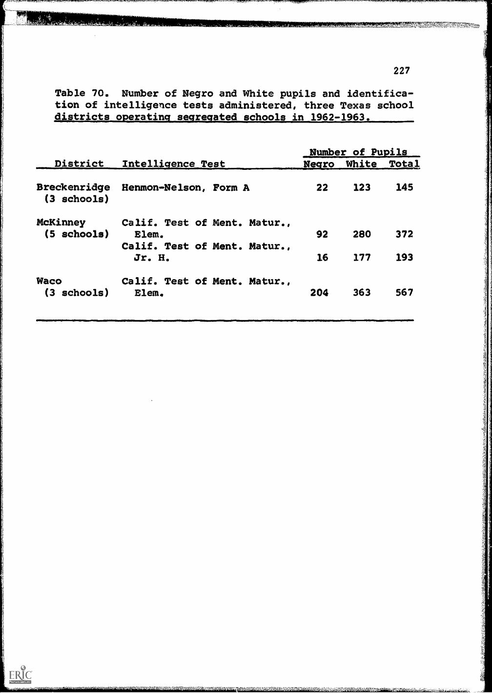
..,t, J. 1.4.i,

227

Table 70. Number of Negro and White pupils and identifica-tion of intelligence tests administered, three Texas schooldistricts o eratin se reated schools in 1962 -1963.

District Intelligence, TestNumber of PupilsNegro White Total

Breckenridge Henmon-Nelson, Form A 22 123 145(3 schools)

McKinney(5 schools)

Calif. Test of Ment. Matur.,Elem. 92 280 372

Calif. Test of Ment. Matur.,Jr. H. 16 177 193

Waco(3 schools)

Calif. Test of Ment. Matur.,Elem. 204 363 567

228

residual between one standard deviation above and below

the mean.

For comparison of peer status with other variables, the

LD and TR scores were used. Tables were constructed to

analyze effects of intelligence, peer acceptance-rejection,

sex, race, and school grade.

Results

The results presented in Tables 71 through 77 demon-

strate significant differences between Negro and White

pupils with respect to mean IQ, but almost identical

patterning among Negro and White pupils in respect to the

relationships of IQ and school grades to the peer status

measures.

Tables 71 and 72 summarize the relationships with

reference to intelligence. Means and standard deviations

are given in Table 71 and the tests of significance in Table

72. The rank order of mean IQ varies with peer status level

in the same direction for each race-sex group even though

the overall difference in mean standard score between the

Negro and White pupils is 10 points. As shown in Table 72,

however, the differences between the high and middle group

for Negro boys and between the middle and low groups for

Negro girls do not reach significance, while all differences

between peer status levels are significant for White boys

and girls. It should be noted, however, that the range of

nIVT4AAXMIWNI'M:Zgr,t4 NT411:a=a

r... a ,,V, -

Table 71. Comparison of Negro and White boys and girlsof High, Middle, and Low peer status on intelligencestandard scores.

NegroPeer No.Status Sex Pupils Mean

High Boys 31 97.9

Girls 31 99.9

Middle Boys 110 92.9

Girls 112 92.2

Boys 26 84.3

Girls 24 88.4

Low

Total Boys 167 92.5

Girls 167 93.1

229

White

S.D.No.Pupils Mean S.D.

17.2 94 106.6 21.3

16.1 91 111.4 16.0

18.6 306 10.5 19.5

16.2 306 103.1 17.3

20.1 77 96.3 24.2

20.4 69 89.7 17.8

18.0 477 102.9 17.8

17.1 466 102.7 18.5

4,4

230

Table 72. Eveluation of differences within and betweenrace, sex, and peer status groups on intelligence standardscores.

Between Peer Status Levels for Com arable Race and Sex Grou

Race Peer Status Grou-s

Negro High vs MiddleMiddle vs Low

White High vs MiddleMiddle vs Low

BoysCR

GirlsD CR

.0 1.40ns 7.78.6 1.99* 3.8

4.1 1.67* 8.36.2 2.09* 13.4

2.35**.86ns

4.26**5.68**

*p<.05, "P<.01, one tail test.

II. Between Sexes for Comparable Race and Peer Status Groups

Peer Status GrouTotal

Race D CR

Negro .6 .31ns

White -.2 .17ns

HighD CR

MiddleD CR

LowCR

2,0 .47ns -.7 0.30ns 4,1 .71ns

4.8 1.74ns .6 0.40ns -6.6 1.89ns

ns indicates p<.05, two tail test.

III. Between Races for Com arable Sex and Peer Status Grou s

Peer Status GrouTotal

.....,-Hi--Al......1 Middle LoeSex D CR D CR D CR D CR

Boys

Girls

*p.05, **p<.01, one tail test.

10.4 6.45** 8.7 2.29** 9.6 4.58** 12.0 2.50**

9.6 6.08** 11.5 3.44** 10.9 5.59** 1.3 .28ns

"

231

standard-score means from high to low groups is comparable

for Negro and White boys (13.6 and 10.3, respectively) and

the range for Negro girls is between these (11.5), while

that for White girls is double that for White boys (21.7).

The last mentioned result is accounted for by the unexpec-

tedly low mean for the 69 low status White girls, which is

89.7, only 1.3 points higher than the corresponding Negro

girl mean.

The second comparison in Table 72 shows that sex diffe-

rences are generally small and inconsistent in direction.

Although the mean IQ standard scores of girls exceed those

of boys in four of the six comparisons, the largest diffe-

rence for low status White pupils favors boys, and the

differences in the middle status group which are reversed

in sign for Negroes and Whites are virtually nonexistent.

The third comparison in Table 72 shows the results,

already mentioned, of the IQ differences between the racial

groups of comparable sex and peer status. Overall these

differences are highly significant, and they exceed the .01

level for all subgroups except low peer status girls. In

view of the results for Mexican-American girls in integrated

classes, presented in the preceding section, and of the

association of the variables studied here with minority

ethnic and low sociometric status, the results for "White"

girls in the Iow status group are believed not to be arti-

4yalisr, en a?5ki ;rya

"7,71,01T eM.3,7.57'y'AFEMT

Dui ,ibl

17.77,1.

232

factual but rather to be an over-representation of minority

ethnic group girls (with Spanish surnames) in that sample.

A check of the roster for that group gives some support to

this interpretation.

Tables 73 and 74 present comparable data for school

grades with essentially the same results, except that the

mean differences between Negro and White groups on school

grades were significant for only the middle status groups

of girls. The ordering of mean grades by peer status level

is the same as for IQ, and all differences between status

levels for comparable race-sex groups are significant

e %-lt that between middle and low status Negro girls. The

largest mean range, from high to low status groups, is for

White girls.

Tables 75 and 76 follow the format of the tables for

IQ and school grades, but compare Teacher Ratings of Negro

and White boys and girls ordered in peer status groups by LD.

The patterns of relationship in Table 75 are comparable

with those examined for IQ and school grades. It is of

interest that the highest group mean is that of high status

Negro girls, while the lowest is for low status White girls.

The intercorrelations of IQ standard scores, school

grades, TR, and LD scores are shown for the total Negro and

White samples separately in Table 77. It may be noted that

the pattern of correlations displayed in these two matrices

is very similar.

5

233

Table 73. Comparison of Negro and White boys and girls ofhi h middle and low eer status on school rades

PeerStatus Sex

Negro WhiteNo.Pu s Mean S.D.

No.Pu ils Mean S.D.

High Boys 31 82.1 7.7 94 82.7 8.9

Girls 31 87.1 6.7 91 86.6 7.8

Middle Boys 110 79.0 8.9 306 78.4 10.2

Girls 112 79.8 8.1 306 82.1 9.2

Low Boys 26 74.6 8.0 77 72.5 9.9

Girls 24 77.3 7.1 69 74.5 8.6

Total Boys 167 78.9 8.5 477 78.3 10.4

Girls 167 80.8 8.4 466 82.0 8.5IMION=MII1=11.10.1

'7E,LEif 41.7

234

Table 74. Evaluation of mean school grade differences withinand between race sex and eer status rou s

I. Between, Peer Status Levels for Comparable Race and Sex Groups.

Boys GirlsRace Peer Status Grou s D CR D CR

Negro High vs Middle 3.1 1.91* 7.3 5.12**Middle vs Low 4.4 2.48** 2.5 1.55ns

White High vs Middle 4.3 3.96** 4.5 4.61**Middle vs Low 5.9 4.64** 7.6 6.54**

II Between Sexes for Com arable Race and Peer Status Grou s

TotalPeer Status Grouxs

High Middle LawRace D CR D CR D CR D CR

Negro 1.9 2.06** 5.0 2.73** .8 .71ns 2.7 1.27ns

White 3.7 6.00** 3.9 3.17** 3.7 4.71** 2.0 1.30ns

/II, Between Races for Comparable Sex and Peer Status Groups,

ex

Boys

Girls

Peer Status Grou sTotal

D CR CRMiddle

CRLow

CR

-.6 .74ns .6 .36ns -.6 .59ns -'2.1

1.2 1.58ns -.5 .34ns 2.3 2.45** -2.8

1.09ns

1.57ns

*P<.05, **13.01, one tail test,

-16a06",ggWait.41

235

Table 75. Comparison of mean Teacher Ratings of Negro and

waill4LlisNALAAAAslatstitidu.114410A,and Low Peer Status.

PeerStatus Sex

White

No.Pupils Mean S.D.

No.Pupils Mean S.D...

High Boys 31 5.3 .79 94 5.7 .76

Girls 31 6.0 .79 91 5.7 .80

Middle Boys 110 5.1 .74 306 4.9 .70

Girls 112 5.0 .76 306 5.1 .74

Low Boys 26 4.5 .83 77 4.5 .61

Girls 24 4.6 .82 69 4.3 .62

IMINI111111111MI¢

Total Boys 167 5.0 .80 477 5.0 .78

Girls 167 5.1 .94 466 5.1 .84

'1.4750CT!'.!4r71%.*

Table 76. Evaluation of mean teacher rating differenceswithin and between race sex and eer status roue;..

Between Peer Status Levels for Com

BOYS

236

arable Race and Sex Groups

Race Peer Status Grou s D CRGirls

CR

Negro High vs MiddleMiddle vs Low

White High vs MiddleMiddle vs Low

.2 1.57ns

.6 3.17**

.8 8.58**

.4 4.86**

1,1 6.72**.4 1.94*

.6 6.91**

.7 8.79**

Between Sexes for Comparable Race and Peer Status Groups

RaceTotal

Hi........1111.--

D CRMiddle Low

D CR D CR D CR

Negro

White

.1

.1

1.04ns

1.83*

.7

.1

3,47**

.50ns

-.1

.2

.99ns

2.92**

.1

-.2

.43ns

1.83ns011.111MIE

*p<.05, **10.01, one tail test.

111111101.11Mialsaruka

Table 77. Intercorrelations of I( standard scores,school grades, TR, and LD scores for Negro and White,combined -sex) samples.

VariablesNegro2

N=334) White (N=943)

IQ Standard Score 1 .55 .32

School Grades 2 .49

TR 3

LD 4

Aisiganzubax ,

4 2 3 4

.23

.34

.43

.55 .36

.44

.26

.38

.54

tir

.4,

1M' "MITI Z,lit,',144.

238

Summary.

Although the Negro and White samples differed in socio-

economic background and other aspects which account for

significant differences in intellectual performance on tests,

the patterning of relationships between peer choice scores,

IQ, school grades, and teacher ratings is essentially the

same in both samples. It is concluded that the Negro sample

functions comparably to that of low SES Whites, and that

measures of peer acceptance-rejection for Negroes rated by

Negroes are equivalent to those of Whites rated by Whites

in psychological significance. In view of the "prejudice"

demonstrated in ratings of pupils with Spanish surnames by

other children in "White" school class-groups, presented in

the preceding section, the results reported here would not

be expected to show up in integrated class-groups in which

Negro children are a minority. On the contrary, the "pre-

judice" shown against Mexican-Americans suggests that dis-

tortion of ratings of Negroes might be even greater. However,

such distortion is not pure race prejudice, but reflects the

complex interaction of many factors associated with socio-

economic background, residence, intellectual level, and peer

attractiveness.

.r.

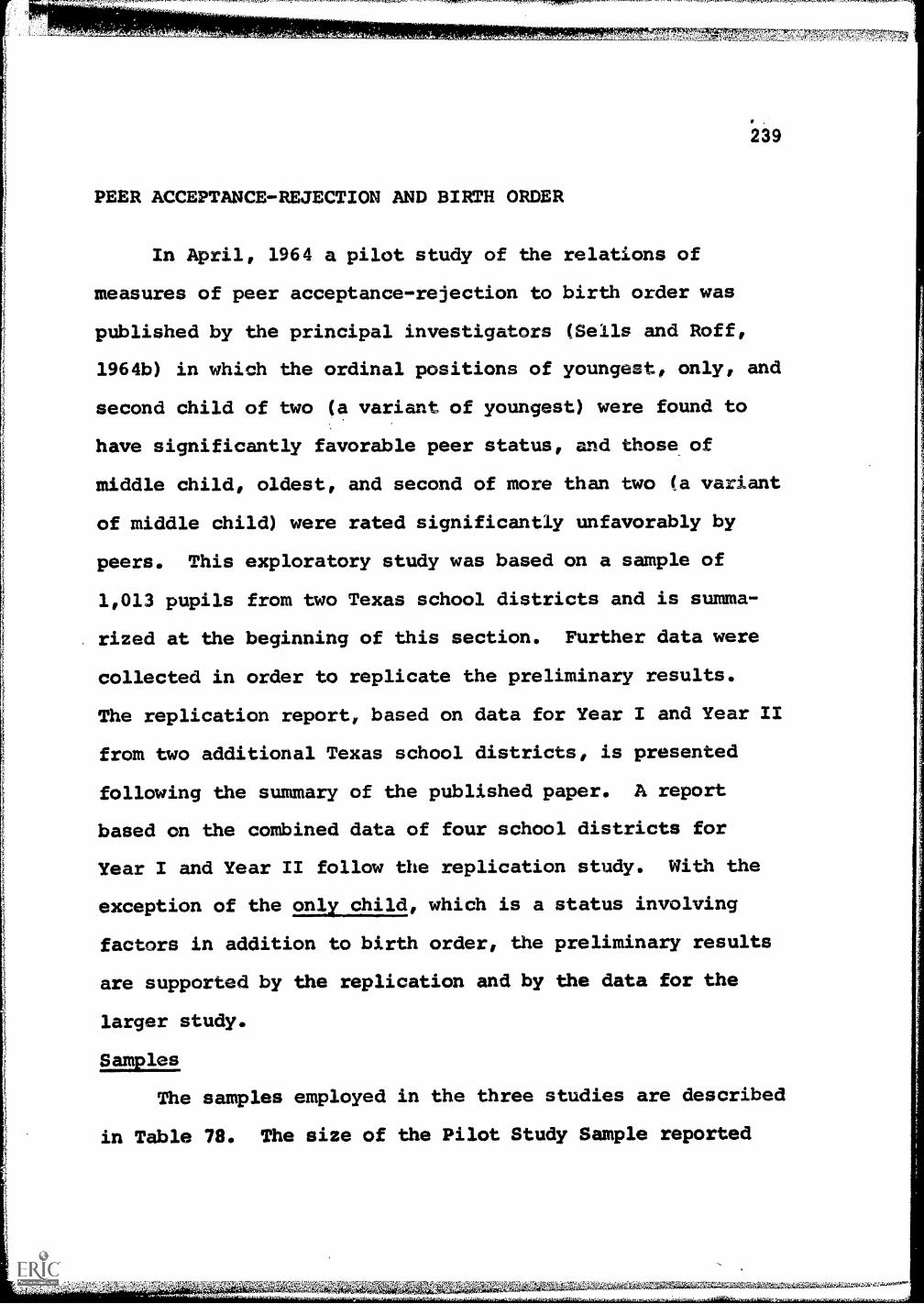
0

-V-4` ,,179=,74,

PEER ACCEPTANCE-REJECTION AND BIRTH ORDER

5

239

In April, 1964 a pilot study of the relations of

measures of peer acceptance-rejection to birth order was

published by the principal investigators (Sells and Roff,

1964b) in which the ordinal positions of youngest, only, and

second child of two (a variant of youngest) were found to

have significantly favorable peer status, and those of

middle child, oldest, and second of more than two (a variant

of middle child) were rated significantly unfavorably by

peers. This exploratory study was based on a sample of

1,013 pupils from two Texas school districts and is summa-

rized at the beginning of this section. Further data were

collected in order to replicate the preliminary results.

The replication report, based on data for Year I and Year II

from two additional Texas school districts, is presented

following the summary of the published paper. A report

based on the combined data of four school districts for

Year I and Year II follow the replication study. With the

exception of the only child, which is a status involving

factors in addition to birth order, the preliminary results

are supported by the replication and by the data for the

larger study.

Samples

The samples employed in the three studies are described

in Table 78. The size of the Pilot Study Sample reported

47-

e

240

in Table 78 disagrees slightly with that reported in Tables

79 through 82, for the Preliminary Study. The difference

resulted from excluding from the published study duplicate

data for seven cases. Recomputation of the corrected data

indicated that the published results were not affected.

The two school districts in the Pilot Study are located

outside metropolitan areas (in Census County Divisions) and

may be classified as small towns. One of the two districts,

Breckenridge, included a segregated Negro school. Compared

with the 82 schools in the Texas sample in Year I, the SES

level of Breckenridge, based on educational level and family

income reported in the 1960 census, was slightly above average.

The SES level for Hillsboro was in the lowest quartile. As

shown in Table 78, these two districts had 498 boys and 508

girls in grades 3, 4, 5, and 6, in 10 schools in Year I.

The two school districts in the replication study are

McKinney, located in the Dallas metropolitan area, and

Abilene, a metropolitan city, according to the 1960 U.S.

Census. McKinney is about 30 miles north of the city of

Dallas and might be classified as a small town. McKinney

included a segregated Negro school. Abilene did not provide

any Negro pupils. For McKinney, the Census Reports indicated

that the median adult educational levels for the five schools

ranged from 9.0 to 9.3, while median family income

:JAW 4,X,Stg,..ac

Table 78.

Description of the birth order

study samples by sex, grade, and school

district,

1.

Year Ia of the Texas

sam le

School

Districts

Number of

Schools

MAELb

MFIc

Boys

Girls

District

Total

Grade:

34

56

Total

34

56

Total

Pilot Study

Breckenridge

511.4

$4752

69

64

63

71

267

82

78

53

62

275

542

Hillsboro

59.0

$2935

50

57

64

60

231

67

51

51

64

233

464

Replication Study

McKinney

59.1

$3941

64

70

55 105

294

54

78

65

94

291

585

Abilene

11

11.4

$5309

225 212 143 109

689

233

203

171

112

719

1408

Combined Study

Combined

26

9.4

$4226

-

408 403 325 345

1481

436

410

340

332

1518

2999

aYear II Sample is identical to

Year I, except that TR'swere not available on 81 pupils, who

were dropped from the Year II

Sample.

bMedian Adult Educational

Level, source: 1960 U.S. Censuses of

Population and Housing.

cMedianFamily Income, source: 1960 U.S. Censuses of

Population and Housing.

242

ranged from $3,670. to $4,408. The respective ranges for

the 11 Abilene schools were 8.9 to 13.2 for educational

level and $3,435. to $9,250. for family income. As shown in

Table 70, these two districts had 983 boys and 1,010 girls

in grades 3, 4, 5, and 6 in 16 schools in Year I.

The combined study includes all four schoot districts

but it augmented by the inclusion of data for Year II as

well as Year I. The 2,999 cases in Year I were reduced to

2,918 in Year II because TR were not available on 81 pupils.

The SES level for the combined sample, as indicated in Table

78 (MAEL 9.4, and MFI $4,226.), was below the comparable

values for the total Year I Texas sample of 10.2 school

years completed and $4,515. annual family income.

Summary of preliminaryagdy (Sells and Roff, 1964b)

Backgrounds Murphy, Murphy, and Newcomb (1937), in

their pioneering book on experimental social psychology,

severely criticized a number of birth-order studies which

tended to be inconclusive or contradictory. They concluded

that the objective fact of ordinal position in the family

contributes little psychological insight into the operation

of social factors of family influence without consideration

of its meaning to the child, to the siblings, and to the

parents. Instead of "sheer comparison of children in terms

of birth order," they advocated more dynamic approaches,

such as of relations between various facets of parents'

243

attitudes and children's behavior, and supported their

position by citing numerous examples of such research which,

even today, would be regarded as productive.

Serious interest in the behavioral effects of birth

order has nevertheless persisted, and the writers have

counted over seventy researches, published since 1950,

dealing principally or in part with some aspect of this

topic. The principal difference between current formula-

tions and that criticized by Murphy, et al. appears to

reflect a change of research models between the 1930's and

the 1960's. The bivariate experiment, in which the relations

between a dependent and an independent variable were

observed while everything else was "held constant," has

gradually given way to a multivariate experimental model,

which provides more adequately for multiple determination

of behavior by recognizing the joint contributions of

multiple factors accounting individually for fractional

variances.

Many correlates of birth order have been investigated,

but few systematic studies of ordinal position have been

found. In general, the position of the oldest child has

been found to be somewhat vulnerable in relation to factors

related to social and emotional adjustment, while the

youngest child appears to be more favorably situated from

the standpoint of such influences. The only child, contrary

4,:.;&W

-7n1. ,

244

to widespread belief, appears to resemble the youngest

rather than the oldest in these respects (Hillinger, 1958;

Vuyk, 1959). There are, however, compensating influences.

For example, Rosen (1961) has shown that oldest children

tend to excel in need achievement.

The hypothesis tested in the present study is based on

the expected relation of ordinal position to the likelihood

of receiving solicitous, ego-satisfying attention from

parents, older persons, and siblings. It is believed that

certain ordinal positions are more conducive than others to

receiving such favorable attention, and that individuals who

are thus favored are likely to develop a greater poten-

tiality for positive, harmonious peer relations. In this

context, it was hypothesized that the youngest and only child

positions would tend to have the most favorable peer rela-

tions, while the oldest and middle positions, which tend to

be most prone to be superseded or "by-passed," and which

involve most sibling competition, would be the most vulne-

rable to peer rejection. Inasmuch as the second child of

two is also a youngest child, this position was expected to

resemble the youngest and only positions, while the second

child in larger families, who is, in effect, a middle child,

was expected to resemble more the middle and oldest

positions. There are, of course, other factors that inter-

act with birth order in influencing behavior, such as sex

riz .7.,,,,Krewrk,..xmol.,... nVte

245

of siblings, intervals between siblings, socioeconomic status,

and many aspects of parental behavior. Nevertheless,

assuming randomization of these in a large sample, it was

expected that the hypothesized relations would occur

significantly.

St n. Birth order data were obtained indepen-

dently for 1,013 pupils, constituting the complete samples

for two Texas school districts, through the cooperation of

the respective school counselors, who served as local coor-

dinators for the study. A card was prepared for each pupil,

indicating sex and date of birth of every sibling, and birth

order of the sample was coded according to the following

six categories, used in the analysis reported below:

1. Only child

2. Oldest child

3. Second child of two

4. Second child of more than two

5. Middle child (all positions between second andyoungest)

6. Youngest child

The relation of each of the four peer scores to the six

birth order categories was examined by analysis of variance,

using an adaptation of Winer's factorial design for un-

weighted means analysis of independent groups with unequal

cell frequencies (1962, p. 241). Three main effects, of

birth order, grade, and sex, three first-order interactions,

s.,

nS

245

of birth order with grade, birth order with sex, and grade

with sex, and one triple interactione of birth, grade, and

sex were tested for each of the four peer relations measures.

Results. The analysis of variance results are shown in

Tables 79 through 822. Only one main effect is significant

for the sociometric ratings. This is the variation in peer

acceptance-rejection associated with birth order. The F

tests for LM and LIB are significant beyond the .01 level,

while that for LL falls between the .10 and .05 levels. No

significant associations were found involving birth order

with grade or sex. The TR scores are not significantly

related to birth order or grade, but the variation between

means of TR's for sex groups approaches significance

(between .10 and .05), with girls rated higher than boys by

teachers, most of whom are female.

The rank order of the mean z-scores of birth order

groups in the TR data corresponds very closely to that for

the peer choices, even though the F test for birth order is

non-significant for TR. The overall means of birth order

2A complete summary of the frequencies, means, variances,

and marginal weighted means for the LMILL,LM-LL, and scores

by sex, grade, and birth order has been deposited as Documentnumber 7759 with the ADI Auxiliary Publications Project, Photo-duplication Service, Library of Congress, Washington 25, D.C.

A copy may be secured by citing the Document number and by re-

mitting $3.75 for photoprints, or $2.00 for 35mm. microfilm.Advance payment is required. Make checks or money orders pay-able to: Chief, Photoduplication Service, Library of Congress.

P-T

247

Table 79. Analysis of variance for LM peer scoresby birth order, sex and gradea.

Source df SS MS Fb

Birth Order (B) 5 22.84 4.57 4.91cSex (S) 1 .33 .33 .35Grade (G) 3 1.00 .33 .35BS 5 3.33 .67 .72SG 3 1.67 .56 .60BG 15 16.17 1.08 1.16BSG 15 17.17 1.14 1.22Within Cells 965 896.23 .93

Total 1012

aAn unweighted-means analysis of variance (Winer, 1962)

bAll effects' mean squares are evaluated with the withincells variance under a fixed effects model.

P<.01

t

248

Table 80. Analysis of variance for 7a4 peer scores

WATILSZA121i1042LIALIOdea-

Source SS MS Fb

Birth Order (B) 5 9.67 1.93 1.97cSex (s) 1 .17 .17 .17Grade (G) 3 1.17 .39 .40BS 5 2.17 .43 .44SG 3 .83 .28 .29BG 15 12.34 .82 .84BSG 15 14.01 .93 .95Within Cells 965 941.57 .98

my'011111.0

Total 1012



c0.10 <.05

TTT7nM-7n77Fx.y.w.-

249

Table 81. Analysis of variance for LD peer scoresb birth order 'rade and sexa.

Source df SS MS

Birth Order (8) 5 19.68 3.94 4.24cSex (S) 1 .50 .50 .54Grade (G) 3 1.17 .39 .42BS 5 1.17 .23 .25SG 3 1.67 .56 .60BG 15 15.01 1.00 1.08BSG 15 16.84 1.12 1.20Within Cells 965 900.63 .93

Total 1012

A=01...,aAn unweighted-means analysis of variance (Winer, 1962)


p(.01

250

Table 82. Analysis of variance for TR peer scoresb birth order sex and radea.

Source df SS MS Pb

Birth Order (B) 5 4.00 .80 1.25Sex (S) 1 2.17 2.17 3.39cGrade (G) 3 .83 .28 .44BS 5 1.33 .27 .42SG 3 .50 .17 .27BG 15 8.34 .56 .88BSG 15 15.51 1.03 1.61Within Celia 965 621.05 .64

Total 1012



cP>.10 <.05

251

groups, for all four variables, which are ranked identically

to the averages of the three peer choice variables, are as

follows:

1. Youngest child 5.19

2. Only child 5.13

3. Second of two 5.09

4. Second of more than two 4.98

5. Oldest child 4.91

6. Middle child 4.87

The line between the third and fourth ranks indicates

what appears to be a natural division between two clusters

on the acceptance-rejection dimension. The "accepted"

cluster, with means all above 5.00, includes youngest, only,

and second child of two (which is a special case of youngest

child), while the "rejected" cluster, with means all below

5.00, includes middle oldest, and second child of more than

two (which is a special case of middle child). The weighted

means of the two clusters for LD, the most stable of the

peer choice measures, are 5.17 and 4.89, respectively, and

the t test for this difference is significant beyond the

.001 level.

Discussion. Although the hypothesis concerning the

relation of peer acceptance-rejection to birth order is

supported, this study does not clarify the nature of the

behavior mechanisms involved. It was hoped that further

,

information concerning these would emerge as the peer rela-

tions study progresses. The emergence of the two clusters,

located in the positive and negative ranges of the acceptance-

rejection continuum, suggests a polarity related to ordinal

position that merits further consideration. To demonstrate

whether or not this does, in fact, reflect the effects of

attention and solicitous consideration on the child, it is

necessary to inquire more deeply into the family situation.

(In the published paper it was stated that such inquiry was in

progress, along with replication of the pilot study,and that

further answers to the questions raised here might be forth-

coming.)

The fact that birth order was the only significant main

effect, and that none of the interactions was significant is

interpreted as evidence of the consistency of the birth-

order-peer acceptance-rejection relationship for both sexes

and over the range of elementary grades included in this

study.

Replication Study

The replication study followed the procedure described

in the preliminary study and employed the same computer

programs for analysis of Year I data, except that separate

analyses were made for each of the two school districts,

McKinney and Abilene.

250

Results. The results are presented in Tables 83

through 87. These tables are similar in form to the analysis

of variance tables in the pilot study except that the results

are shown for each district separately.

For the Abilene sample no significant main effects or

interaction effects were found on any of the five measures

of per- acceptance-rejection.

The analyses of the McKinney data confirm those in the

pilot study. Only one main effect, that of birth order,

was significant on LM, LD, TR, and DT but not on LL.

The following tabulation compares the pilot and repli-

cation study results, presenting mean scores for the six

ordinal positions, averages across LM, LL, LD, and TR,

arrayed in rank order.

Pilot Study Replication StuckAbileneMcKinney

1. Youngest Child 5.19 5.19 5.022. Only Child 5.13 4.80 5.053. Second of Two 5.09 5.30 5.16

4. Second of More Than Two 4.98 5.08 5.025. Oldest Child 4.91 5.13 5.066. Middle Child 4.87 4.90 5.00

Discussion. McKinney, the community in which the results

support those of the pilot study, resembles Breckenridge and

Hillsboro, from which the pilot study sample was drawn, with

respect to community size, racial composition, and SES back-

ground, while Abilene, the community in which the birth

[1

,pr 461 e u'vWnri

254

Table 83. Analysis of variance for LM by birth order, sex,and rade for the two districts in the re licatirni.....qample,

Year I .

ounce df

Birth Order (B) 5

Sex (S) 1

Grade (G) 3

BS 5

SG 3

BG 15

BSG 15

Within Cells 1360

Total 1407

Abilene McKinney

SS-----c--

MS e6.67 1.33 1.35

.73 .73 .74

1.27 .42 .43

10.41 2.08 2.10

2.58 .86 .87

18.00 1.20 1.21

27.78 1.85 1.87

1343.17 .98

1410.65

df

5

1

3

5

3

15

15

537

584

SS MS Fb

13.97 2.79 3.02**

.79 .79 .85

.44 .14 .16

4.21 .84 .91

3.76 1.25 1.35

12.62 .84 .91

21.11 1.40 1.52

496.67 .92

553.61

**X.01


bAll effects' mean squares are evaluated with the within cells

variance under a fixed effects model.

255

Table 84. Analysis of variance for LL by birth order, sex,and grade for the two districts in the replication sample,Year /a.

Source df SS

Birth Order (B) 5 2.18

Sex (S) 1 .27

Grade (G) 3 .14

BS 5 7.62

SG 3 .48

BG 15 11.50

BSG 15 6,,19

Within cells 1360 1285.87

Total 1407 1314.28

MS F df SS MS Fib

.43

.27

.04

1.52

.16

.76

.41

.94

.46 5 7.37 1.47 1.65

.29 1 .45 .45 .51

.05 3 .34 .11 .12

1.61 5 1.00 .20 .22

.17 3 2.52 .84 .94

.81 15 17.64 1.17 1.32

.43 15 18.90 1.26 1.41

537 477.94 .89

584 526.21

AN ow ,M.....aAn unweighted-means analysis of variance (Winer, 1962)

All effects' mean squares are evaluated with the within cellsvariance under a fixed effects model.

Mall=110

Table 85. Analysis of variance for LD by birth order, sex,and grade for the two districts in the replication sample,Year

Source

Birth Order (B)

Sex (S)

Grade (G)

BS

SG

BG

BSG

Within cells

Total

AbileneA SS MS

5 4.97 .99

1 .20 .20

3 .63 .21

5 10.15 2.03

3 1.86 .62

15 18.78 1.25

15 19.92 1.32

1360 1318.48 .96

1407 1375.02

McEinagY4f SS MS Fb

1.02 5 11.73 2.34 2.57*

.21 1 .11 .11 .13

.21 3 .43 .14 .15

2.09 5 3.23 .64 .71

.64 3 4.14 1.38 1.51

1.29 15 12.39 .82 .90

1.36 15 23.08 1.53 1.69

*p<.05


bAll effects' mean squares are evaluated with the within cellsvariance under a fixed effects model.

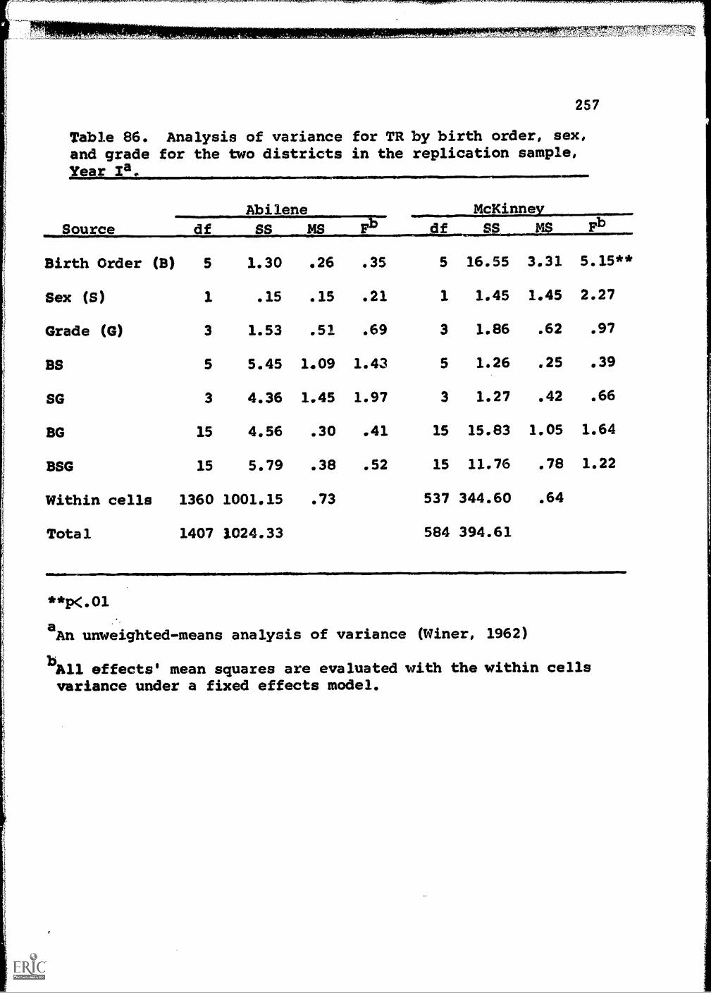
257

Table 86. Analysis of variance for TR by birth order, sex,and grade for the two districts in the replication sample,Year /a.

Source df

Birth Order (8) 5

Sex (S)

Grade (G)

BS

1

3

5

SG 3

BG 15

SSG 15

Within cells 1360

Total 1407

Abilene

SS MS

1.30 .26 .35

.15 .15 .21

1.53 .51 .69

5.45 1.09 1.43

4.36 1.45 1.97

4.56 .30 .41

5.79 .38 .52

1001.15 .73

1024.33

df

5

1

3

5

3

15

15

537

584

McKinneySS MS

16.55 3.31 5.15**

1.45 1.45 2.27

1.86 .62 .97

1.26 .25 .39

1.27 .42 .66

15.83 1.05 1.64

11.76 .78 1.22

344.60 .64

394.61

**p<.01



Table 87. Analysis of variance for DT by birth order, sex,and grade for the two districts in the replication sample,Year /a.

Abilene McKinneySource df SS MS Fn df SS MS

Birth Order (B) 5 5.06 1.01 1.00 5 19.16 3.83

Sex (S) 1 .01 .01 .01 1 .50 .50

Grade (G) 3 1.09 .36 .36 3 .82 .27

BS 5 10.01 2.00 1.98 5 2.73 .54

SG 3 2.56 .85 .84 3 1.85 .61

BG 15 14.69 .97 .97 15 13.59 .90

BSG 15 16.26 1.08 1.07 15 19.64 1.30

Within cells 1360 1373.03 1.00 537 495.66 .92

Total 1407 1422.74 584 553.98

4.15**

.54

.29

.59

.66

.98

1.41

**X.01aAn unweighted-means analysis of variance (Miner, 1962)


259

order results are negative, does not. Whether systematic

control of demographic and SES factors would help explain

the different results is an unanswered question. However,

even in Abilene, the results with respect to categories 3

(second of two), 4 (second of more than two), and 6 (middle

child) are in line with the pilot study results, while those

for 2 (only child) are inconsistent in both McKinney and

Abilene, The results of the replication study may be

regarded as furnishing support for the original findings for

the critical positions of youngest and middle child.

Combined Study

The combined study followed the procedure described

for the pilot and replication studies and employed the same

computer programs for analysis of the data, but, as noted

above, the four school districts were combined and the data

were augmented by including peer status measures for Year II.

Results. The results are presented in Tables 88

through 93. The first five tables are identical in form to

Tables 79 through 82 of the pilot study, one for each of

the five peer status scores. Table 93 shows the mean peer

scores, by year, for each of the six birth-order positions,

with t-tests comparing the pooled data for the more favored

and less favored positions determined in the pilot study.

The analysis of variance tables (88 through 92) examine for

the main effects of birth order, sex, and school grade, and

260

Table 88. Analysis of variance for LM by birth order, sex,and grade for Year I and Year /Ia. Combined sample of fourTexas districts. algaNINO1100

Source

Year I Year II

df SS MS F df SS MS

Birth Order (B) 5 22.74 4.54 4.75** 5 13.04 2.60 2.73*

Sex (S) 1 .04 .04 .04 1 .07 .07 .07

Grade (G) 3 .50 .16 .17 3 2.39 .79 .83

8S 5 7.42 1.48 1.55 5 2.37 .47 .49

SG 3 4.75 1.58 1.65 3 1.53 .51 .53

BG 15 14.84 .98 1.03 15 12.10 .80 .84

BSG 15 28.53 1.90 1.98* 15 14.99 .99 1.04

Within cells 2951 2825.46 .95 2870 2735.22 .95

Total 2998 2904.29 2917 2781.74

*P(.05**p<4.01


bAll effects' mean squares are evalmated with the within cellsvariance under a fixed effects model.

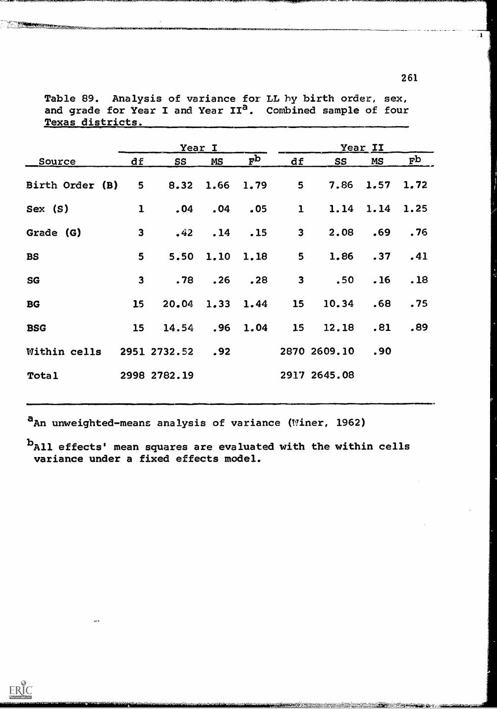
261

Table 89. Analysis of variance for LL by birth order, sex,and grade for Year I and Year IIa. Combined sample of fourTexas districts.

Source

Year I Year II

df SS MS Fb....

df SS MS Fb

Birth Order (B) 5 8.32 1.66 1.79 5 7.86 1.57 1.72

Sex (S) 1 .04 .04 .05 1 1.14 1.14 1.25

Grade (G) 3 .42 .14 .15 3 2.08 .69 .76

BS 5 5.50 1.10 1.18 5 1.86 .37 .41

SG 3 .78 .26 .28 3 .50 .16 .18

BG 15 20.04 1.33 1.44 15 10.34 .68 .75

BSG 15 14.54 .96 1.04 15 12.18 .81 .89

Within cells 2951 2732.52 .92 2870 2609.10 .90

Total 2998 2782.19 2917 2645.08



1.7r.

Table 90. Analysis of variance forand grade for Year I and Year IIa.Texas districts.

Year I

262

LD by birth order, sex,Combined sample of four

Year II

Birth Order (B) 5 19.19 3.83 4.07** 5 14.32 2.86 3.06**

Sex (S) 1 .05 .05 .06 1 .20 .20 .22

Grade (G) 3 .42 .14 .14 3 2.56 .85 .91

BS 5 7.89 1.57 1.67 5 2.22 .44 .47

SG 3 3.75 1.25 1.32 3 1.33 .44 .47

13G 15 16.46 1.09 1.16 15 9.43 .62 .67

BSG 15 24.68 1.64 1.74* 15 11.74 .78 .83

Within cells 2951 2783,61 .94 2870 2686.75 .93

Total 2998 2856.09 2917 2728.60

* P<.05**P<.01



263

Table 91. Analysis of variance for TR by birth order, sex,and grade for Year I and Year IIa. Combined sample of fourTexas districts.

Year I Year II

Source df SS MS Fb df SS

Birth Order (B) 5 6.51 1.30 1.88 5 19.47

Sex (S) 1 5.51 5.51 8.00** 1 11.16

Grade (G) 3 .74 .24 .35 3 2.26

BS 5 6.01 1.20 1.74 5 4.23

SG 3 .17 .05 .08 3 10.60

BG 15 7.17 .47 .69 15 11.53

BSG 15 11.66 .77 1.12 15 5.79

Within cells 2951 2034.64 .68 2870 1911.03

Total 2998 2072.46 2917 1976.11

MS Fb

3.89 5.84**

11.16 16.77**

3.53 5.30**

.76 1.15

.38 .58

.66



VarfirIMISTMEMAIMeghWOMAIT .....a,VNPAS=7:72373-2gras=mrstm-swrxrtg:m..-:,:q=ri

Table 92. Analysis of variance forand grade for Year I and Year IIa.

264

DT by birth order, sex,Combined sample of four

Texas districts

Source

Year I Year 11

df SS MS df SS MS =1101.m...M.11

Birth Order (B) 5 20,91 4.18 4.26** 5 19.04 3.80 3.82**

Sex (S) 1 1.24 1.24 1.26 1 2.71 2.71 2.73

Grade (G) 3 .44 .14 .15 3 4.71 1.57 1.57

BS 5 9.56 1.91 1.95 5 4.41 .88 .88

SG 3 1.85 .61 .63 3 4.14 1.38 1.38

BG 15 12.32 .82 .83 15 10.34 .68 .69

BSG 15 20.76 1.38 1.41 15 10.45 .69 .70

Within cells 2951 2894.12 .98 2870 2856.27 .99

Total 2998 2961.25 2917 2912.10

**p<.01


bAll effects' mean squares are evaluated with the within cells

variance under a fixed effects model.

4-44.4:41.%1Dil

1

Table 93.

Comparison of mean peer scores bybirth order for Year I and Year II.

Ccmbined

sam le of four Texas schooldistricts.

Birth Order

Position

Year I

MeanYear II

Mean Peer Scores

Peer Scores

NLM

LL

LD

TR

DT

NLM

LL

LD

TR

DT

1.

Youngest Child

389

5.17

5.06

5.14

5.09

5.14

392

5.08

5.05

5.08

5.05

5.07

2.

Only Child

316

5.06

5.06

5.08

5.00

5.05

308

5.01

5.00

5.00

5.01

4.99

3.

Second of Two

451

5.18

5.10

5.17

5.08

5.15

438

5.18

5.09

5.15

5.14

5.15

4.

Second of more

than Two

552

5.04

5.00

5.01

5.01

4.99

521

5.04

5.03

5.04

5.08

5.05

5.

Oldest Child

862

5.05

4.99

5.02

5.04

5.03

816

5.06

5.04

5.06

5.10

5.07

6.

Middle Child

429

4.89

4.92

4.90

4.95

4.88

443

4.91

4.90

4.89

4.87

4.86

IM1111111,

More Favored Posi-

tions (1,2,3)

1156

5.14

5.08

5.13

5.06

5.12

1138

5.10

5.05

5.08

5.07

5.08

Less Favored Posi-

tions (4,5,6)

1843

5.01

4.98

4.99

5.01

4.98

1780

5.02

5.00

5.01

5.03

5.01

Variance (pooled)

.96

.93

.95

.69

.98

.95

.91

.93

.68

1,00

Difference (more-

less favored)

.13

.10

.14

.05

.14

.08

.05

.07

.04

.07

t3.16**

2.77**

3.88**

1.58

3.74**

2.22*

1.39

1.94*

1.26

1.87*

* p<.05

**p<.01

reZZEZ-Z$7t,17:ERZUK7.?;.;:7.7A-.:.:77.7,-70:7

266

for three primary interactions among the main effect variables,

as well as the second-order interaction among the three.

For LM only one main effect, birth order, is signifia

cant, in both years as'in the pilot study, while the second-

order interaction is marginally significant for Year I and

second in rank, though not significant in Year II. For LL,

birth order approaches significance in both years and has

the highest F ratio, as in the pilot study. The joint

effects of LM and LL, relfected in LD, produce a highly

significant F ratio for birth order in Table 90, which also

shows a significant second-order interaction in Year I only.

As in the pilot study, the most significant effect for TR in

both years is on sex, reflecting the general tendency of

teachers to rate girls more favorably than boys. However,

the birth order effect for TR is significant in Year II and

marginal in Year I, showing a relationship in the larger

sample that was not significant in the pilot study. In

addition, the interaction of sex and grade shows a significant

F ratio for Year II. This corresponds well with the analysis

reported in an earlier section, in which differential

changes related to sex and grade were mentioned. Finally,

Table 86 shows a highly significant birth order effect for

DT in both years. Since DT summarizes information in both

the Peer and Teacher Ratings, this result may be accepted as

the most definitive confirmation of the relation of birth

order to peer acceptance-rejection in the study.

267

The nature of this relationship is illuminated in Table

93, which serves also as a test of the hypothesis developed

in the pilot study as to the identification of the presumed

most favored and least favored ordinal positions, from the

standpoint of peer status. Table 93 summarizes the means of

each of the five peer scores for each of the six birth order

positions in each year. It also presents pooled means for

the three favorable positions identified in the pilot study

(youngest, only, and second child of sets of two) and for

the three unfavorable positions (second of more than two,

oldest, and middle child) and t-tests of the differences

between these for each peer score in each year. The latter

comparisons are significant at the .01 level for Year I and

at the .05 level for Year II on all measures except TR. The

TR means fall in the expected direction, but the differences

are very small.

Examination of the mean scores by variable by birth

order position permits two conclusions. First, the combined

study upholds the overall validity of the pilot study

results, particularly with respect to the middle and youngest

ordinal positions. And second, the initial results with

regard to only child are not supported. The evidence for

these conclusions is summarized in the following tabulation

which compares the pilot and combined study results, pre-

senting mean scores for the six ordinal positions, averaged

?;,

268

across LM, LL, LD, and TR, arrayed in rank order as found in

the pilot study.

Pilot StudyCombined StudyYear I Year II

1. Youngest Child 5.19 5.12 5.072. Only Child 5.13 5.05 5.013. Second of Two 5.09 5.13 5.14

4. Second of More than Two 4.98 5,02 5.055. Oldest Child 4.91 5.03 5.076. Middle Child 4.87 4.92 4.89

Discussion. The birth order results that emerge as

most striking in this study are those related to categories

3 (second of two) and 6 (middle). Since two-sets of children

are the most common family size, and since the second of two

is a youngest child, the consistent results indicating the

favorable effects of this position on peer relations are

noteworthy. Similarly, the consistent results showing the

unfavorable effects of the middle child position on the peer

relations of the 429 subjects in this category tend to rein-

force the hypothesis offered in the interpretation of the

pilot study results with respect to alteration of family

structure and accompanying perceptions of parental rejection.

Apparently the middle child position is more traumatic than

that of the oldest child, who is given responsibility and

may receive rewards for successful role performance, despite

the perceived loss of love experienced with the introduction

of younger siblings into the family.

269

Despite the significance of th- results, it must be

noted that the effects of birth order on peer acceptance-

rejection are minor in terms of magnitude of relationship.

In terms of our interpretation they are also indirect and R.

mediated by interactions among parents and children as a

result of structural reorganizations of families requiring

changes in role relations.

FAMILY BACKGROUND STUDIES

The search for correlates of peer acceptance-rejection

produced information that repeatedly pointed to the family

as the mediator of various influences that appeared to

structure the nature of a child's peer relations. Several

attempts were made early in this Study to codify family

influence, using a variety of methodologies, including open-

end questionnaires sent to schools, tape-recorded interviews

with classroom teachers, and structured questionnaires sent

to classroom teachers through school coordinators. Later,

a more extensive study of family background in depth,

involved home visits and extensive data collection from

parents. This section reports three exploratory studies,

using teachers and other school personnel as sources. The

richness of the information obtained encouraged the investi-

gators to pursue the more ambitious study reported in Chapter

270

AN OPEN-END QUESTIONNAIRE EXPLORING VAMILY SOCIAL PATHOLOGY

The aim of this exploratory study was to search for

significant areas of family adjustment that discriminated

between acceptance and rejection by peers. After preliminary

negotiations, an open-end questionnaire inquiring concerning

nine general areas of family adjustment was mailed to school

coordinators in seven Texas school districts in 1963. This

questionnaire requested information concerning individual

pupils in a sample of 685, selected to provide a wide range

of peer relations status. The replies were coded and tabu-

lated in relation to peer scores.

Subjects

Initially it was intended to include an equal number of

high (beyond +1 standard deviation from the mean), middle

(between +1 and -1 standard deviation from the mean), and

low (beyond -1 standard deviation from the mean) children on

the basis of LD scores. However, since peer scores were

available for two years, cases were added from each district

which were high in one of the years and low in the other.

Using the DT average peer score for two years and splitting

at the mean of 5. (to distinguish "high" and "low" children),

there were 326 boys (96 high and 230 low) and 359 girls

(117 high and 242 low) in the sample of 685 pupils.

-,;s1geim=a4RMIXi

7.75r54-ji

271

Table 94 shows the composition o2 the sample in terms

of peer relations status, as defined above, socioeconomic

level, sex, race, and size of community where they attended

school. SES level was determined by ordering the 82 schools

participating in Year I on the basis of median number of

years of education completed by adults over 25 for the

appropriate census units in the 1960 Census. The schools

were divided in thirds and each pupil was classified as

high, middle, or low in SES according to the position of his

school. Most of the sample came from school districts in

large metropolitan communities, such as Fort Worth (Castle-

berry, Everman), Dallas (McKinney) , Abilene, and Waco. A

minority came from the smaller communities of Bonham and

Breckenridge.

Comparison with Census Data. While not directly

comparable, using assumptions outlined below several items in

this study can be related to statistics in the 1960 census

reports. Three pairs of conceptually related statistics are

shown in Table 95:

1. Per cent of Children Livin with Both Parents. The

census data report on numbers of children under 18 years of

age living with both parents. The children in the present

sample were estimated to be under 14 years of age, and an

approximation of this statistic was estimated for each SES

category by subtracting the per cent with disrupted parental

ca*

272

Table 94. Breakdown of sample by peer relations stai:.as,

SES sex race and size of comm1:nf.t7._

Socioeconomic StatusHigh Middle Low

Peer Relations Status H L H L H L

Raceand Sex

CommunitySize

White Large 22 49 22 59 24 54

BoysSmall 0 0 11 25 15 20

ara1011

Total 22 49 33 84 39 74

White Large 18 39 24 73 40 65

GirlsSmall 0 0 14 22 12 28

Total 18 39 38 95 52 93

Negro Large 0 0 0 0 21

BoysSmall 0 0 0 2 0 0

Total 0 0 0 2 2 21

Negro Large 0 0 0 0 9 15

GirlsSmall 0 0 0 0 0 0

Total 0 0 0 0 9 15

Total 40 88 71 181 102 203

Table 950

Comparison of Census population

indices with study sample

indices by community

size

and socioeconomic status.

CO

Number of

Schools in

Sample

WHITE

Median Per cent

Children Living

with Both

Parents

Census

Sample

Population

franile)

Median

Per cent

Income

<$1000

Census

Population

(range)

Median

Per cent

Receiving

Welfare

Sample

Median

Per cent

Adults

<5 yrs.

School

Census

Population

range)

Median Per

cent Low

Education of

Parents

Sample

High SES

594

94

1.7

00.2

1.6

(94 to 99)

(0.0 to 2.1)

(0.0 to 0.2)

Middle SES

993

91

1.7

2.8

0.2

1.1

(87 to 96)

(1.1 to 3.0)

(0.0 to 0.7)

Low SES

983

87

4.8

4.9

1.3

1.1

(71 to 86)

(0.5 to 9.3)

(1.0 to 2.2)

SmaLl Town

Middle SES

387

78

4.9

22.2

0.5

13.9

(87 to 87)

(4.9 to 4.9)

(0.5 to 0.5)

Low SES

267

76

6.5

12.0

1.4

14.7

(67 to 67)

(6.5 to 6.5)

(1.4 to 1.4)

NEGRO

Metropolitan

Low SES

1*65

51

9.9

10.2

2.2

2.0

rho = .94, p<.01

rho = .81, p<.06

rho = .39, ns

*Two Negro schools, located

in Small Towns, were excluded

from the population statistics only.

4

274

marital relations frcm 100, The rank order correlation

between the sample and the Census totals, of .94, was signi-

ficaat beyond the .01 level, indicating that the sample is

comparable with the general population on this statistic.

2. Welfare. The per cent of the population with

earnings of less than $1,000. per year income in the census

population was compared with the per cent receiving welfare

in the present sample. Except for the schools located in

small towns these statistics were comparable. The relatively

high proportion of comments from schools located in small

towns suggests that the number of families on welfare may be

over-represented in the study sample. The rank order corre-

lation between sample and population indices approaches

significance.

3. Parents Education. The census statistic for the

per cent of the adult population with less than 5 years of

schooling was selected as a standard. The per cent in the

population was compared with the per cent of the sample for

which comments were received concerning low educational

level of parents. Again, the two statistics agree reason-

ably well, except for the small towns.

The data in Table 95 suggest that the sample was repre-

sentative for Negroes and for Whites residing in metropolitan

areas, but that the adverse comments obtained from small

towns were over-represented for Education of Parents, as

well as for Welfare.

275

Procedure.

Arrangements were made with the school coordinators in

the seven school districts to obtain the family background

information. The coordinators were furnished individual forms

for the children in their respective samples and requested

to check records, files, and all available local resources

to determine the information requested. The peer status of

the children in this sample was not indicated on the forms.

The inquiry focused on whether or not each child's family

had a positive indication on any of the following items:

(1) Psychiatric history for any member.

(2) Welfare history; that is, known to any welfareagency.

(3) Criminal or deviant behavioral history.

(4) Significant medical history, including physicalhandicaps blindness, etc.

(5) Social history; that is, divorce, separation, orother major disruptive change in the child'sparental family.

(6) Excessive family mobility.

(7) Unusual or atypical occupational history; e.g.unemployment, marginal worker father travels,overseas, etc.

(8) Exceptional educational background, e.g. illi-terate, bilingual, etc,

(9) Any change in school status from 1962 to 1963(other than promotion).

The school coordinators were requested to include only

information that could be obtained through reliable sources

'14qa=LW: 5.14%"44WratigaW.A,===.,-EW7-44"*

ASA

A

276

or which could be verified. Followup interviews with the

school coordinators subsequently gave the impression that

they generally had made full and conscientious use of sources

available to provide the information sought in this inquiry.

The comments obtained in this manner were grouped into

categories. The major categories were retained, but several

subcategories were developed, and each comment was classi-

fied with respect to the family member principally involved

(father, mother, sibling, or subject). A brief description

illustrating typical comments classified under each of the

major categories is presented in Table 96.

Results

A total of 732 comments was received for the 685

children in the sample. In analyzing them, it was assumed

that (1) the teachers were reasonably good judges of children's

peer relations; (2) the teachers knew that they were parti-

cipating in an investigation of peer acceptance-rejection in

children; (3) the teachers' values and hypotheses concerning

peer relations might influence their comments; and (4)

teacher comments would probably reflect a bias in favor of

a larger number of adverse comments for children with low

peer relations, although the children's scores were not

included on the comment sheets. With full appreciation of

the possibilities of bias mentioned, the comments were never-

theless considered factual and verifiable and worthy of

cautious analysis.

'I-

fit

.-77rigmonmw=m17

277

Table 96. Family Backgroun'2 Study I: Examples of.9.2'111nts

1. Wchiatric histormforAny member of the familxe.

Whole family emotionally disturbed - possibly fromthe mother's instability.

There is evidence of psychiatric problem - father notwell balanced - father ran away, has been inmental institute.

Feeble mindedness is evident in father.

This pupil has mental troubles. The whole family isodd.

There is evidence of peculiar activity in mother's case.

Mother had a nervous breakdown last year.

Father has received psychiatric treatment - seems tohave recovered.

Mother has been hospitalized.

2. Welfare history.

This is a broken home - I understand the father leftthem some time ago. The mother and children areon welfare.

This child, a twin, has received help from the welfareagency. She has a speech defect and needs specialhelp. Her parents are divorced and her step fatheris unemployed.

The father is an invalid - the mother works part-time.

This is a relief family - school free lunch.

Family on relief since she was born.

This family has the record for longest term of reliefin the county.

taa rgaCartrizilikc

278

Table 96 (Continued)

3. Cr:;,T1, or bellaviorpl hfs!-.1ra

Some criminal history in father's past.

Father has been in penitentiary for theft.

Father has been in jail - mother and father separatedat present.

Mother has been arrested.

Peculiar behavior activities notes in the mother - shelives with one man awhile, then with another awhile.

Father arrested on more than one occasion. Behavior isnot good.

4. AisaitialmLimikaljAatatu.

Father injured, got deeply in debt, not able to supporthis large family.

Pupil has weak eyes - welfare agency purchased glassesfor him.

Father physically ill - veteran's aid. Illness ofmother prevents employment.

Father had injury two years ago - worked little since.

Physical handicap - poor speech - poor vision.

Father ill. Has been in and out of hospital. The pupiltakes care of his father - often misses 2 or 3 daysof school in succession waiting on father.

There has been separation in the family. Pupil liveswith grandparents and has almost total responsibilityof taking care of ill grandparents.

5. Social history, that is divorce, separation, or othermajor disruptive changes in the child's parental family.

Mother has not divorced all husbands, but has had 4 or 5.This is a real social problem. Two children andmother - 3 different names.

279


Parents have been separated and now living together.Mother married 5 times - drinks heavily.

Father and mother separated. Mother left home and nowlives in California. Child lives with her father.

Father deceased. On wcifare - free lunch at school.

Separation in family - mother has lived with 2 or 3different men.

There are three groups in this family - different names -different fathers - mother does not live with anyof these fathers - child born out of wedlock.

6. Excessive family mobility.

This family has moved a lot because the father is in theAir Force. Ronnie was in school - France.

(Father in Air Force is frequently indicated underthis item.)

Changes home address often and changes schools withinthe city.

Child has been in Three schools in city since 9-1-61.

The family moves often - 3 times the past 3 years.

The family moves to western Texas then back to Texasabout once a year.

The family moved 3 times the past year.

The father drives a truck - mother goes with him a lot -child stays with grandmother. The family movedfrom Breckenridge the past month.

7. Unusual or atypical occupational history.

Father overseas.

Father is in the Air Force

Father unemployed most of the time.

ttr2 14V trlia616

^A,17311747fM7,,,,,

if


7=771MMiMMz.

280

Father has no regular employment - he works irregularlyin oil fields.

Father unemployed for periods - little income.

Father is marginal worker - unemployed for longperiods - practically no income.

Low income - mother works and irons - tries to supportfour children.

8. .Lx,ceti.eduational backgrounds/ ea. illiterateu

Bilingual family.

Father and mother both almost illiterate.

Mother is illiterate.

Bilingual - poor mentality - poor attendance.

This family and this child are both misfits - non-conform-ists.

Mother is morally good, but the whole family is illiterate.

9. An chan e in school status 1962-1963 exce romotion

Retained in grade 7.

Retained in grade 7 - failed grade 5 also.

Pupil retained in 5th. grade.

Was retained in grade 3 - not able to keep up with groupnow, possibly should be retained this year, butage prevents.

Pupil has been retained in earlier years, but has droppedout of school this last 2 months.

Very slow with schoolwork - will be placed with an"opportunity group" another year.

Child was in Special Education in homebound unit fromAugust 1962 to January 1963.

rya

281

Demogx.aphic Factors and the Frequency of Comments.

Table 97 shows the absolute and relative frequency of

comments in each category by race, size of community, and

SES level. Since there are large differences in frequencies

of comments among cells in this table, comparisons are

difficult and Table 98 was prepared to facilitate interpre-

tation of these data. The index scores, or adjusted relative

frequencies, reported in Table 9S were obtained by the

formula:

Per cent of CommentsAdjusted Frequency by Category

of Comments Per cent of Childrenin the Subsample

Examination of the data in Table 98 suggested that

comments concerning serious illness in the family came from

White schools located in small towns and from Negro schools.

Comments concerning illness of the child appeared to be

associated with middle SES background in both large and

small communities. The psychiatric category was commented

on most frequently by teachers in the small town, middle

SES schools, but the Negro and high SES indices were above

the average value.

The Relation of Adverse Family Background Comments and

Peer Status. The relative frequencies of adverse comments

in the several family background categories were examined

in relation to SES and peer scores. The results, reported

11 .11:tagi

281

Demographic Factors and the Frequency of Comments.

Table 97 shows the absolute and relative frequency of

comments in eacn category by race, size of community, and

SES level. Since there are large differences in frequencies

of comments among cells in this table, comparisons are

difficult and Table 98 was prepared to facilitate interpre-

tation of these data. The index scores, or adjusted relative

frequencies, reported in Table 998 were obtained by the

formula:

Par cent of CommentsAdjusted Frequency b Cate or

of Commentsin the Subsample

Examination of the data in Table 98 suggested that

comments concerning serious illness in the family came from

White schools located in small towns and from Negro schools.

Comments concerning illness of the child appeared to be

associated with middle SES background in both large and

small communities. The psychiatric category was commented

on most frequently by teachers in the small town, middle

SES schools, but the Negro and high SES indices were above

the average value.

The Relation of Adverse Famil Back round Comments and

Peer Status. The relative frequencies of adverse comments

in the several family background categories were examined

in relation to SES and peer scores. The results, reported

,Km.0511:1=somug...wAparat,===4,7..,744=0#1,4=4WaWIltr valza:0 :0;44004

Table 97.

Summary of absolute and relative

frequency of comments by SES background

in

metro olitan areas and small towns forWhite and Nero children.

Race:

4

Metropolitan

High

Middle

f (Pct)

f (Pct)

White

Low

f (Pct

Small Town

Middle

Low

f (Pct)

f (Pct)

NegroTotal

Metropolitan

and Small

Low

f (Pct)

Metropolitan

and Small

f (Pet/

Community

Size:

SES:

Comment Catecom

Psychiatric

6(25)

3(12)

3(12)

7(29)

2(8)

3(12)

24(100)

Welfare

0(0)

5(11)

9(20)

16(36)

9(20)

5(11)

44(100)

Criminal History

Parent

1(10)

3(30)

4(40)

2(20)

10(100)

Child

2(20)

2(20)

3(30)

3(30)

10(100)

Medical History

Family

4(9)

11(25)

3(7)

7(16)

6(14)

13(30)

44(100)

Child

11(11)

32(31)

27(26)

16(16)

10(10)

6(6)

102(100)

Social History

8(8)

16(15)

24(23)

16(15)

18(17)

24(23)

106(100)

7`amily Mobility

J5(11)

10(23)

15(34)

9(20)

2(5)

3(7)

44(100)

Educational History

Parents

2(7)

2(7)

2(7)

10(36)

11(39)

1(4)

28(100)

Child

6(12)

15(29)

6(12)

17(33)

4(8)

3(6)

51(100)

Occupationa3 History

Employment

(Except Mil.)

2(4)

3(6)

10(19)

24(46)

10(19)

3(6)

52(100)

Father in

Military Serv.

8(19)

30(70)

1(2)

0(0)

1(2)

3(7)

43(100)

Number of Pupils

128(19)

178(26)

183(27)

72(11)

75(11)

49(7)

685

Table 98.

The relative frequency of comments

adjusted1for the proportion of children in

the subsample category by SES and

community size.

-Race :

White

Neer°

Total

Community

Size:

Metro olitan

Small Town

Metropolitan

and Small

Metropolitan

and Small

SES:

High

Middle

Law

Middle

Low

Low

Comment Category

Psychiatric

1.34

.48

.47

2.78

.76

1.75

1.00

Welfare

.00

.44

.77

3.46

1.87

1.59

1.00

Criminal History

Parents

.00

.38

1.11

3.64

1.82

.00

1.00

Child

.00

.77

.74

2.72

2.72

.00

1.00

Medical History

Family

.49

.96

.25

1.51

1.24

4.13

1.00

Child

.58

1.21

.99

1.49

.89

.82

1.00

Social History

.41

.58

.85

1.44

1.55

3.17

1.00

Family Mobility

.58

.88

1.26

1.82

.45

1.00

1.00

Educational History

Parents

.38

.27

.27

3.40

3.59

.50

1.00

Child

.63

1.13

.44

3.17

.72

.82

1.00

Occupational History

Employment

(Except Mil.)

.21

.22

.72

4.39

1.76

.81

1.00

Father in

Military Serv.

1.00

2.68

.09

.00

.21

.98

1.00

1Per cent of Comments by Category

Adjusted frequency of Comments =

Per cent of Children in the Subsample

284

in Table 9% show a consistent trend for adverse comments to

be associated with low peer status. These are discussed in

the following paragraphs.

Psychiatric. This category was associated with peer

status within high and middle, but not low, SES levels.

WellareHir. Comments on this item did not appear

at the high SES level, but were related to peer status at

the middle and low SES levels.

Criminal Histon. This category was associated with

low peer status in the middle and low SES levels,

Medical History. Serious illness in the family was

most highly related to low peer status in the low SES groups.

Adverse comments relating to health of the child were most

frequent in the middle SUS level. However, they tended to

be more highly associated with peer status within the high

and low SES groups.

Social Histo As noted above, this category was

related to SES. In Table 99 disrupted parental relations

occur almost twice as often for low than for high peer status

groups in the middle SES level, and nearly three times as

often for low peer status groups in the low SES level. At

the high SES level, the percentage difference between high

and low peer status children is only slight.

Family Mobility.. Comments on this category, like those

pertaining to Welfare and Educational History, were highly

associated with peer status.

MzuezwivMka=gia:li,.

9qppmrnr,TRp--....4n-r"cvvAmx-ta7!pgqm-Tr,r5,r.,--,

F.,

Table 99.

Summary of percentages of adverse family history by major category, distributed by

socioeconomic levels in metropolitan and rural areas and by race.

Year II DT scores.

co

Race;

White

Ne ro

Total

Community

Size:

Metro.olitan

Small Town

Met. and

Small

SES:

High

Middle

Low

Middle

Low

Low

High

Middle

Low

DT Classi-

fication

High LowHigh LowHigh Low

High Law.High LowHigh Low

High LawHigh LowHigh Low

Comment Category

Psychiatric

07

22

22

015

24

18

30

71

53

2Welfare

00

23

08

034

417

013

00

111

111

Criminal History

Parents

00

01

03

04

02

00

00

05

05

Child

00

02

02

03

03

00

00

05

05

Medical History

Family

23

47

22

413

013

932

23

48

210

Child

510

13

20

918

20

23

717

913

510

15

21

917

Social History

57

89

538

830

19

27

27

55

57

815

11

27

Family Mobility

06

27

013

019

42

08

06

110

19

Educational

History

Parents

02

02

02

021

023

03

02

07

07

Child

07

211

05

036

08

08

07

117

06

Occupational

History

Employment

(Except Mil.)

50

02

08

847

11

15

08

50

3141-

310

Father in

Military Serv,

09

620

01

00

02

18

30

94

15

21

Number of Pupils

40

88

46

132

64

119

25

47

27

48

11

38

40

88

71

179

102

205

286

Educational The relationship between adverse

comments concerning parents' education and peer status of

the child was consistent across SES levels in that no adverse

comments of this type were made on children with above

average peer scores. A similar pattern was prevalent for

comments concerning the child's educational problems.

Occupational History. Most frequently, comments

concerning the father's employment history came from schools

in small communities; the association with peer status was

consistent at the middle and low SES levels, but not for the

high SES group, In this study, most of the families with

the father in military service were in the middle and high

SES categories. Theoretically, two factors may contribute

to the relatively low peer status of children in this

situation. These are: (1) the periodic absence of fathers

from home and (2) the discrepancy between the social status

of the family and the SES level of the school that the child

attends.

Peer Scores and the FrEsuency of Comments, Frequency

distributions and cumulative percentages of adverse family,

history comments in relation to average DT scores for Years

I and II are presented in Table 100. The subcategories of

comments are described in detail. In this table, a single

family may be represented more than once in a single major

category.

287

Table 100. Frequency distribution and cumulative percentagesser_altzesse family history comments. Year I and Year II DT scores.

2.02.9

Distribution in sample: 76

Category of FamilyHistory Comment

DT Score Categories

MEDICAL HISTORYFamily Member InvolvedGeneral Medical

Father 5

Mother 0

Sibling 1

Child 16

Sub -total 22

Cum. per cent 16

PSYCHIATRIC HISTORYFather 6

Mother 2

Sibling 2

Child 1

Sub -tota 1 11Cum. per cent 46

AlcoholismFather 1

Mother 0

Sub-total 1

Cum. per cent 11

TotalsFather 12

Mother 2

Sibling 3

Child 17

Totals 34

Cum. per cent 20

3.0 4.0 5.0 6.0 7.03.9 4.9 5.9 6.9 7.9 Total Median165 262 27. 15 4 685 4.4_

6 2 0 0 0 13

0 5 1 0 0 6

0 3 0 0 0 4

40 43 2 16 0 117

46 53 3 16 0 14049 86 89 100 4.0

0 2 0 0 0

2 3 0 0 0 7

1 3 0 0 0 6

2 0 0 0 0 3

5 8 0 0 0 24

67 100 3.1

1 4 1 0 0 7

1 1 0 0 0 2

2 5 1 0 0 9

33 89 100 4.3

7 8 1 0 0 283 9 1 0 0 15

1 6 0 0 0 10

42 43 2 16 0 120

53 66 4 16 0 173

50 88 91 100 3.9

Table 100 (Continued)DT Score Cate cries

2.0 3.0 4.0 5.0 6.0 7.02.9 3.9 4.9 5.9 6.9 7.9 Total Median

istribution in Sam le: 76 165 262 2 151 4 685 4.4

288

WELFARE HISTORYChild Receives Charitythrough School (Lunches,Milk, Medical, Clothes)

Family has History ofWelfare Aid

Total Comments, WelfareHistory

Cum. per cent

DEVIANT BEHAVIORAL HISTORYParentSerious OffenseMinor Offense

Child DelinquentStealingOther

Total, History ofDeviency

Cum. per cent

SOCIAL HISTORYDeath of Family Member

Cum. per cent

Parents Separated, NotDivorced

Cum. per cent

Parental DivorcesNeither SpouseRemarriedMother only RemarriedFather only RemarriedBoth Parents Remarried

Sub -total, DivorcedParents

Cum. per cent

9 9

8 16

17 2530 75

2 0

3 3

2 5

2 0

9 8

45 85

5 5

20 40

11 12

29 60

2 2

5 7

0 2

0 2

7 13

17 49

6 24

8 32

14 56

100 3.5

3

100

11 1 3 0

84 88 100

11 0 4 089 89 100

4 0 4 0

8 1 2 0

2 0 0 00 0 0 0

14 1 6 0

83 85 100

3

7

7

3

20

3.0

254.2

383.7

12

234

2

414.0

Table 100 (Continued)DT Score Cate ories

289

2.02.9

3.03 9

4.04.9

5.05.9

6.06.9

7.07.9 Total Median

Distribution in Sample: 76 165 262 27 151 4 685 4.4

SOCIAL HISTORY (CONT.)Disrupted Parental Relations(Death, separation,divorce) 23 30 36 2 13 0 104

Cum. per cent 22 51 85 87 100 3.9

Parents with 3 or moremarriages 4 0 2 0 0 0 6

Cum. per cent 67 67 100 2.6

No Adult Male in theHome 3 3 2 0 1 0 9

Cum. per cent 33 67 89 89 100 3.1

Child Caretaker otherthan Parent 10 6 10 0 2 0 28

Cum. per cent 36 57 93 93 100 3.6

Children in the Homeother than natural siblings:Half-siblings 0 0 0 1 2 0 3

Step-siblings 0 0 1 1 0 0 2

Adopted siblings 3 1 3 0 1 0 8Combinations of above 4 3 6 0 0 0 13

Sub -total, other thannatural siblings 7 4 10 2 3 0 26

Cum. per cent 27 42 81 89 100 4.2

Child not born intoFamilyBorn out of Wedlock 1 1 0 0 2 0 4

Adopted 4 1 4 0 1 0 10

Sub-total 5 2 4 0 3 0 14

Cum. per cent 36 50 79 79 100 4.0

FAMILY MOBILITYChild Transferred AmongSchools 3 7 1 11

Family Moves Often 7 13 16 36

,...4.4. 7 1-4. %...,,,a;;:,-%....,4:,


2.02.9

Distribution in Sample:, 76

FAMILY MOBILITY (CONT.)Total Comments, FamilyMobility

Cum. per cent 2110

EDUCATIONAL HISTORYOf the Child:

Retained one or moregrades 8Social Promotion ofChild 3

Child Unable toDemonstrate Abilityto Achieve 3

Other EducationalProblems (Vision deaf) 1

Sub-total, EducationalDifficulties 15

Cum. per cent 25

Absenteeism from School 2Cum. per cent 10

Of the Parents:IlliterateLess than High SchoolEducation

Sub-total

2

2

4Cum. per cent 15

DT Score Categories3.0.9

4.04 9

165 262

20 17

64 100

14 11

4 .6

3 2

3 1

24 2064 97

6 13

38 100

5 12

2 5

7 17

41 100

Bilingual Home 4 9 13

Cum. per cent 14 46 93

Total Comments, EducationalHistory 25 46 63

Cum. per cent 18 52 97

- -V vowrxkwA000,,o.a4Wlag,b=:aara''-'

290

5.05.9

6.06.9

7.07.9 Total Median

27 151 4 685 4.4

473.6

1 1 35

13

8

5

1 1 6198 100 3.6

214.3

19

9

284.1

2 28100 4.1

3 1 13899 100 3.9

AtWOite:'

Table 100 (Continued)291

DT Score Cate ories2.0 3.02,9 3.9

OCCUPATIONAL OR WORK HISTORYItinerant WorkerFather frequentlyunemployed 4 10Father presentlyunemployed 1 1Father is marginal worker 3 3

Mother supports family 1 3

Mother takes in laundry,etc. 1 1

Sub -total 10 18Cum. per cent 15 42

Father in MilitaryService 13 13

Cum. per cent 30 59

TOTAL ADVERSE COMMENTS: 170 228Cum. per cent 23 54

Adverse Comment perChild 2.2 1.4

4.04,9

1

5.05.9

6,06.9

11 1 1

1

9

6 5 2

1

29 6 3

85 94 99

14 0 491 91 100

270 17 4691 94 99.9

1.0 0.6 0.3

7.07.9 Total Median

1

27

3

1 1617

3

1 67100 4.1

443.8

1 732100 3.9

0.2 1.1

292

The median DT scores were computed for the study sample

(N = 685) and for children receiving particular comments.

The total group median of 4.4 is below the defined mean of

5.0 for the population. The median DT score was computed

for children receiving comments for each of 18 different

categories. In every instance the median value of the DT

score was below the median value for the total sample.

The order of presentation of the comments was altered

slightly in order to compare the total comments related to

Medical History and Psychiatric History, including Alcoholism.

The number of adverse comments for children at each

class interval of DT score is reported at the bottom of

Table 100. The number of comments per child is perfectly

correlated (rho=-1.00, p.01) with the DT score.

Table 101 summarizes the data in Table 100. It is

adjusted to reflect the presence or absence of a comment

within each major category, in order to satisfy the assump-

tions of independence for a Chi-square test. The DT scores

were grouped into Low (2.0 to 3.9)# Middle (4.0 to 5.9), and

High (6.0 and above) peer status groups. Chi-squares were

computed for 3 x 2 tables using the three levels of peer

scores (DT, average for 2 years) and presence or absence of

the category comment. The category Criminal Behavior was

omitted because its frequency was too low to compute Chi-

square. Except for the Father's Employment History, the

293

Table 101. Summary of adverse family history comments by major

category and average DT scores.

LowPeer Status Group

4.0241

f(Pct)

Middle4.0 to5.9

.12911 611(Pct)Number in le

General Medical

Psychiatric (Incl.Alcoholic)

Welfare

Disrupted ParentalRelations

Family Mobility

64(27) 55(19)

16(7) 14(5)

30(12) 14(5)

High

.6.0

Total

15:(Pct)

16(10)

Chi Square

135(20) 15.8, p<.001

0(0) 30(4) 10.3, p<.01

0(0) 44(6) 26.3, p.001

48(20) 38(13) 13(8)

27(11) 17(6) 0(0)

Educational HistoryChild 31(13) 19(7)

Parent 11(5) 17(6)

Occupational HistoryEmployment (exceptMilitary Service) 21(9) 25(9)

Father in Military 26(11) 14(5)

1(1)

99(14) 10.9, p<.01

44(6) 19.8, p<.001

51(7) 21.1, p<.001

0(0) 28(4) 9.1, p<.02

6(4)4(3)

52(8)44(6)

3.4, p<.2013.9, p.01

Nr,+-1 o,

'4Lii-Allm 'Our d.

294

distributiondistribution of comments in all categories was significantly

associated with peer acceptance-rejection.

Summary. An open-end questionnaire concerning nine

general areas of family adjustment for a sample of 685 pupils

in seven Texas school districts identified areas of family

adjustment that discriminated between acceptance and rejec-

tion by peers. The data strongly suggest that factors

associated with poor adjustment in the family, or which

limit the opportunity to acquire enlightened parental atti-

tudes and practices, are related to peer rejection.

Follow Stud of Famil Pathology Using a StructuredQuestionnaire

The results of the preceding study were used as the

basis for construction of a questionnaire that could be used

in structured interviews with informants concerning family

background factors in the lives of school children, Instead

of the open-end inquiry, which had decided advantages for

exploratory reconnaissance, but was vulnerable to bias among

informants, the structured questionnaire required a definite

affirmative or negative reply to every item. The increased

precision implied also required skillful interviewing tech-

niques. In this followup study, professional persons,

principally school counselors, were employed as interviewers.

A copy of the questionnaire is appended to this section.

Subjects. The sample obtained included 59 families

involving 34 high peer status children and 25 low peer status

295

children, based on average DT score for the first two years.

These families were from the Breckenridge, Waco, and McKinney

School Districts. A detailed breakdown of the sample is

shown in Table102% A larger sample had been planned, but

the interviews proved to be very time-consuming, particularly

when it was necessary to consult five or six sources for

each child, and the compensation offered, within the con-

straints of a limited budget, was unattractive. Despite

these problems, the results obtained are quite impressive,

and all indications support the value of this approach in

further research.

Procedure. One of the advantages of conducting

personnel research in small communities is that individual

life histories are better known to the professional school

staff than they are in large cities. As long as such inves-

tigations are confined to appropriate professional persons,

provisions for anonymity of children and protection of

individual privacy are highly feasible.

The interviewers employed for this study were Mr. L. B.

Herring, School Counselor in the Breckenridge public schools,

Mr. J. R. W. Harper, Liaison Visiting Teachers Waco public

schools, and Mr. Scott Haynes, Elementary Teacher, McKinney

public schools. They obtained the information for various

parts of the questionnaire from teachers, clergymen,

physicians, mothers of the children, and other sources

''''_;i1;1".IN

4 1.

296

Table 102. Description of sample in the FamilyHistory Questionnaire Study, by age, race, andschool district. Year II Texas sample.

White NOCIZOSchool District Boys Girls Boys Girls,

Breckenridge 18

Waco 8

McKinney 1

Totals 27

17 1 3

7 2 2

0 0 0

24 3 5

4.-"7.'''''74:241-01gZUWZMWWWgRy :r

v-n. o-v- "' Wrq, ffp,

297

available to them, including school records. The results

were tabulated in relation to peer status as measured by the

two-year average DT scores.

Results. Table 103 presents item frequencies and per

cents, for high (above 5) and low (below 5) peer status

groups, and Chi-square tests for item discrimination of peer

status. Chi-squares were computed in 2 x 2 tables, using

Yate's correction for continuity. It is apparent that the

adverse family history comments summarized in this table are

associated with peer acceptance-rejection in much the same

manner as in the preceding study based on the open-end

questionnaire. Although a multivariate analysis of these

data would be appropriate with a larger sample, this was not

considered feasible in the present study. The data for each

category were adjusted to indicate presence or absence of

the response as required for the Chi-square analyses.

Parents' Health. A score on this item indicates the

presence of one or more of the serious illnesses listed in

paragraph la of the questionnaire. This item was scored for

the father and for the mother. The response frequencies

were in the expected direction, but none of these items was

significantly associated with peer acceptance-

rejection.

Child's Medical History,. Pour dichotomous scores

(1 or 0) were assigned for each child, for: (1) visual

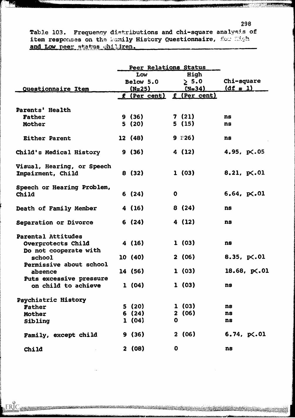
F

fi

298

Table 103. Frequency, diPtributions and chi-square analys3.s ofitem resporkses on tree ..'c roily History Questionnaire, 1!0:2

and Lowseerfltiktu.s.,.!.:hiliren.

Peer RelationsLow

Below 5.0Questionnaire Item (11=25)

Parents' HealthFatherMother

Either Parent

Child's Medical History

Visual, Hearing, or SpeechImpairment, Child

Speech or Hearing Problem,Child

Death of Family Member

Separation or Divorce

Parental AttitudesOverprotects ChildDo not cooperate with

schoolPermissive about school

absencePuts excessive pressure

on child to achieve

Psychiatric HistoryFatherMotherSibling

Family, except child

Child

StatusHigh5.0 Chi-square

(N=34) =(Per cent) f (Per cent)

9 (36)5 (20)

12 (48)

9 (36)

7 (21)5 (15)

9 D26)

4 (12)

8 (32) 1 (03)

6 (24)

4 (16)

6 (24)

4 (16)

10 (40)

14 (56)

1 (04)

5 (20)6 (24)1 (04)

9 (36)

2 (08)

0

8 (24)

4 (12)

1 (03)

2 (06)

1 (03)

1 (03)

1 (03)2 (06)0

2 (06)

0

nsns

ns

4.95, P<.05

8.21, p<.01

6.64, p<.01

ns

ns

ns

8.35, X.01

18.68, p<.01

ns

nsnsns

6.74, p<.01

ns


Welfare History

LowBelow 5.0f (Per cent)

Family or child 11 (44)

Criminal HistoryParent 6 (24)

Child 9 (36)

Personality Comments (Child)Lazy 15 (60)

Immature 14 (56)

Rebellious toward peers 10 (40)

Frequently fights withpeers 6 (24)

Takes property of peers 7 (28)

Lies excessively 10 (40)

Dishonest, cheats atgames 6 (24)

Bosses other children 1 (04)

Scared of Peers 2 (08)

Shy, withdrawn 7 (28)

Excessive daydreamer 5 (20)

Lacks self-confidence 14 (56)

Looses temper easily 7 (28)

Dirty appearance 5 (20)

Plays truant 7 (28)Rebellious toward teachers 7 (28)

AlcoholismFather 1 (04)

Mother 7 (28)

Family Mobility 6 (24)

Occupational HistoryFather unemployed, can'thold job, etc. 12 (48)

Educational HistoryChild retained in school 15 (60)

High School GraduateFather 4 (16)

Mother 3 (12)

High5.0

f (Per cent)

2 (06)

1 (03)I (03)

3 (09)1 (03)1 (03)

00

1 (03)

1 (03)2 (06)0003 (09)1 (03)2 (06)01 (03)

0

1 (03)

0

2 (06)

2 (06)

19 (56)19 (56)

299

10.07, p<.01

4.26, p<.058.96, p<.01

15.47, p<.0118.68, p<.0110.72, p<.01

6.65, p<.016.92, p<.0110.72, p<.01

4.26, p(.05nsns6.92, p<.015.07, p<.0513.42, p<.015.72, 10<.05ns6.92, p<.015.72, p<,05

ns5.72, p<.05

6.65, p<.01

11.89, p<.01

18.02, p<.01

8.03, p(.0115.18, 10.01

f.

200

impairment, (2) hearing impairment, (3) speech impairment,

and (4) a history of serious illness as indicated in para-

graph 2 of the questionnaire. None of the four item scores

occurred frequently enough to evaluate separately. Only six

children had histories of serious illness. Detailed analysis

of the item responses in this category showed a prevalence

of speech, hearing, and possibly vision problems, associated

with peer rejection. Since speech and hearing problems

affect intellectual functioning and social communication in

the peer setting, this finding is not a surprise.

Social Histsary of the Familx. Incidence of death

(item 3), separation, divorce and remarriage (item 4) were

included in this category. The item, Death of Family

Member, was the only one for which results consistent with

the open-end questionnaire were not found. However, none of

the items in this category discriminated significantly on

peer acceptance-rejection.

Family Constellation. None of the items under this

heading discriminated significantly on peer acceptance-

rejection, but the presence of half-sibs in the home was in

the expected direction.

Parental Attitudes. Discriminating response frequencies

were obtained for four of the six items included under this

heading. As shown in Table iO3, two school-related items

discriminated significantly on peer acceptance-rejection.

MN,

301

Psychiatric History.. This category included a variety

of psychiatric classifications, as well as one item which

indicated that in the judgment of the interviewer a family

member was in need of psychiatric examination. Thirty-six

per cent of the low children and six per cent of the high

children received positive family responses on this category.

The difference is statistically significant. (p<.01) .

Welfare History. Forty-four per cent of the families

in the low acid six per cent in the high sociometric groups

were reported to have received welfare aid. The difference

is significant (p<.01) .

Criminal History. This category included reports of

criminal behavior on the part of a parent or delinquent

behavior on the part of the child. The responses obtained

for both parents and children discriminate significantly

between low and high groups.

Personality Thirteen of 16 child

traits rated by school personnel were significantly associ-

ated with peer rejection. The most significant differences

reported described low peer status children as immature,

lazy, and lacking in self-confidence, which may be a reflec-

tion of low intellectual ability and achievement. Another

group of traits associated with peer rejection was charac-

terized by socially undesirable behaviors: rebellious

toward peers, rebellious toward teachers, frequently fights

Smi4J :f:

302

with peers, takes property of peers, lies excessively,

dishonest, cheats at games, loses temper easily, and plays

truant. Two other traits, shy, withdrawn, and excessive

day-dreamer, were also associated with low peer status scores.

Alcoholism. Of the six items in paragraph 11 of the

questionnaire, only Alcoholism received enough positive

responses to permit evaluation. Seven mothers and one

father were classified as alcoholic. The distribution with

respect to mothers was significantly associated with peer

acceptance-rejection.

Family Mobility. Twenty-four per cent of the families

with children in the low group and none in the high group

were reported as having moved often.

Occupational History. Responses indicating that the

father was unemployed, often unemployed, had difficulty

holding a job, and the like differentiated between low and

high groups at the .01 level. Although similar results were

not found in the preceding study, they are consistent with

the developing conceptualization of the correlates of social

acceptance in the peer group situation.

Educational History. Sixty per cent of the low children,

but only six per cent of the high group had been retained in

school for one or more grades. This difference was signi-

ficant at beyond the .01 level.

Over half of the fathers and mothers of the high status

303

children were reported to have graduated from high school,

while only 16 per cent of the fathers and 12 per cent of the

mothers of the low group had completed high school. The diffe-

rence for each parent was significant beyond the .01 level.

Grouped Item Scores. Theoretically, peer-rejected

children were expected to have a higher number of adverse

item responses than those accepted by peers. Three scores

based on combinations of groups of items were obtained for

each child. These were: (1) Family background, items 1 to 5,

7 to 9, and 11 to 16; (2) Parental attitudes based on the

six ratings in item 6; and (3) Child's personality based on

the 18 ratings in item 10. Responses concerning fathers and

mothers graduated from high school (item 14) were reflected

to represent parents not graduated from high school. The

proportions of scores above and below the median values for

the three scales are shown in Table 104.

These data suggested that the three scores shared

common variance representing the influence of the family on

the child's peer relations. The three scores and DT, the

measure of peer acceptance-rejection, were found to be

highly intercorrelated, as shown in Table 105.

The mean and standard deviation of the selection

variable, DT, indicated that the sample variance was consi-

derably larger than the defined population variance (1.00)

and led to the conclusion that the resulting correlations

Table 104. Proportions of high and law peer statuschildren with scores above dad below the me(3-thre...2.3 of the.7,:mily

Part I: FamilyBackground IIEBE

304

Peer Status_CategoryLow High

f (Per cent) f (Per cent)

Below Median 4 (16) 27(0 to 3)

Above Median 21 (84) 7(4 to 15)

=41=6..1. /WM.0Mii=1.=

Part I/: ParentalAttitudes

Below Median 7 (28) 31(0)

Above Medir4 18 (72) 3(1 to 4)

Part III: Child'sPe sonality Comments

Below Median 8 (32) 30(0 to 1)


Total (Sum ofabove)

Below Median 2 (8) 29(, to 4)


Number of cases 25 (100) 34

(79)

(21)

(100)

wa,anurozzosmaam,,,,,Avzmo.,.$4.4m-,-....mmesso...wrxr_kussmaxmaam=sarrEvittza",`,WaCaitq4AW,

.V7 ay M1T.'r

305

Table 105. Intercorrelations of three family backgroundscores with peer acceptance-rejection (DT) for 59 children.Correlation coefficients above the diagonal are the rawempirical results. Those below the diagonal are correctedor overexten ion of ra. :

Vtriable Mean S D.Correlations*

1 2 3 4

Background Items 4.19 3.81 - .69 .73 -.61

2.. Parent Attitudes .66 1.02 .46 - .62 -.66

3. Child Personality 2.37 1.19 .45 .32 - -.69

4. Peer Acceptance-Rejection (DT) 5.17 1.73 -.38 -.42 -.45

401,

Uncorrected: R4(123)

= 75

Corrected: R4(123) =

53

*All correlations are significantly greater than zero,P.05:

V, ,42

F17.1"Xn,,Phel

.11/0./X.C.ZZACM0111.11{71M.11.1.1.1L70,....1111wernklepo........*4

306

were inflated. In order to determine the levels of rela-

tionships expected if the sample had not been inflated on

DT, the data were corrected for over-extension in range.

The uncorrected correlations, shown above the main diagonal

in Table 105, may be compared with the corrected correlations

listed below the diagonal. The more conservative estimate

is that about 25 per cent of the variance in peer acceptance-

rejection is associated with the three scales derived from

the questionnaire.

Summary. This followup study of family pathology using

a structured questionnaire supported the results of the pre-

ceding study using the open-end inquiry. Although based on

a smaller sample, the quantitative analysis further suggests

a correspondence between the degree of family pathology and

the degree of peer rejection.

PEER STATUS AND FAMILY BACKGROUND. A QUALITATIVE ANALYSIS

In 1962, as a means of providing detailed qualitative

descriptions of representative children in the study to

relate to the quantitative measures, and as an exploratory

step toward the identification of relevant family back-

ground factors related to peer status, arrangements were

made to obtain interivew data concerning a portion of the

St. Paul sample. Similar interview data were collected

subsequently in Minneapolis.

n, ,44.1., L,r924114 044,1- (14 , az .MV

307

For a number of reasons, the interviews were held with

classroom teachers. The most important of these were:

(a) Teachers were regarded as qualified professional infor-

mants, situated in positions in which they could observe the

children and have some productive contacts with parents,

and (b) Arrangements for a limited number of teacher inter-

views could be made without difficulty, while negotiations

with families involved a problem of some magnitude. In

relation to the then exploratory nature of the inquiry, the

less intensive and less public approach seemed more

appropriate.

The interviews were conducted by visiting teachers on

the staff of the respective school systems, who were compen-

sated for the work which they completed during free time.

The visiting teachers followed a structured interview out-

line, shown below, and dictated the information obtained

using tape recorders. The tapes were later transcribed by

project personnel.

Interview Sample

It was not feasible to interview all children in the

total city sarples. For the purposes intended, it was

decided to obtain interviews on between 10 and 15 per cent

of the children. The final arrangement in St. Paul produced

1,600 interviews, for 800 boys and 800 girls, constituting

about 14 per cent of the city sample. In Minneapolis there

"9.7.TAZIljz9S-'

308

werewere 864 interviews, half for boys and half for girls. The

procedure was the same in both cities. Pour interviews were

held with every teacher in the sample. Two of these related

to the lowest boy and the lowest girl in peer relations

status. The third was based on the highest pupil in the

class, whether boy or girl, and the fourth related to the

middlemost pupil on the roster opposite in sex to the lighest

boy or girl. Thus it was intended to have an equal number

of boys and girls, half in the lowest status and the other

half approximately equally divided between middle and high

status.

Structured Interview Outline. The interview outline

given to the visiting teachers included four areas, as out-

lined below. The questions were specified, and the inter-

viewers were expected to cover all of them, in the order as

listed, in each interview.

I. Personal Characteristics of the Child.

1. Describe the child's physical appearance,

2. What individualizes this child? How is he likeor different from other children?

3. What are his particular strengths or weaknesses?

II. Child's Behavior.

1. Describe this child's behavior on the playground.

2. Describe this child's behavior in the classroomand in the building.

3. Describe this child's behavior in relation toother students.

rr.

,

309

4. Describe this child's behavior in relation to

his teacher.

5. Have you noticed any significant change in his

behavior this year?

III. Classmates' Reactions.

1. What do you consider to be typical reactions of

the other students toward this child?

2. What does he (or she) do to cause these reactions

in the other children?

IV. Family

1. What do you see as significant strengths andweaknesses present in this family?

Analysis of Family Background Information

The last question, concerning the teacher's impression

of particular strengths and weaknesses of the students'

families, was used to explore family background factors

related to peer status. It was realized that in many cases

the teachers would have had no significant interactions with

the families of their pupils, but it was considered desirable

to get whatever information resulted from this question.

Compared to the family descriptions present in the case

history of a good child guidance clinic, these are, of course,

brief. However, the analysis did yield a significant amount

of information from a substantial number of families for

every school studied in the two Minnesota cities. Thus the

family information obtained comes from a broader sample than

that of any study in which more intensive information is

available. Usable family information was obtained for over

iiJi

,AttMiti-4

.4/u44.- , 41,r _

310

half of the children for whom interviews were obtaiied; the

proportion of interviews with usable family information was

essentially the same at all socioeconomic levels.

Work with this family infe_:rmi.ition has consisted of

abstracting it from the interviews, developing categories

which would fit it, and placing the statements in these

categories in order to compare children who were high,

average, and low in choice status, from families who were in

different quartiles in socioeconomic division.

This sorting was done by workers who had no knowledge

i3f the choice-status scores of the pupils whose interviews

they were reading. (Of course, the interviews themselves

gave some indication as to whether a child was predominantly

liked-most or liked-least.) However, the initial placement

of comments was rechecked on the basis of the family infor-

mation alone, by still other workers who thus had no know-

ledge of either the choice-status score or the non-family

interview information.

These descriptions of the family have been characterized

as positive, neutral, and negative. As abstractly stated,

the categories are more or less in line with expectations

based on parental information in the general child literature.

To give these general terms some concrete meaning, sample

family descriptions abstracted from the interviews are

included in the discussion that follows. These offer in

7r, iai!,

2.

311

many cases a sharply contrasting picture of "good" and "poor"

parental practices as they relate to the social adjustment

of the children.

Results

Table 106 presents comparisons of high-, average-, and

low-child family information, broken down also by socio-

economic level. Since the primary interest in this analysis

was in the discrimination between high -, average-, and low-

child families, and since the full table, including the SES

breakdowns, contains some cells which are either blank or

contain a very small number of cases, the different SES

levels were combined for the purpose of testing significance.

With one exception, (economic deprivation) each "positive"

and "negative" category showed a difference among the

elements of the row being tested at the .01 level or better.

The economic deprivation category was significant at the

.05 level.

The differences among the "neutral" subcategories did

not show comparable levels of significance, pertly because

of the small numbers involved. In addition, Table 106

presents some factors having negative "trends," which did

not reach a satisfactory significance level, partly because

the frequencies were not large. These are mentioned because

of the attention they have sometimes received. "Parental

rejection" has here been counted only when it was obviously

wo,ammume

14.41, 1/4

312

Table 106. Positive, rnxtral, and negative family factorsfor low, average, ay:a cLoica-status cf'lildren -1= Cifferantsocioeccnomiccis*

Positive Factors

Per cent in each

Descriptive Cate c...a):Peer group

Low Average, }fiat

Family is stable, secure, cohesive,warm, happy, do things together, etc.

St. Paul SES 1 (high) 18 41 652 10 48 503 11 17 344 (low). 7 28 60

Minneapolis 3 & 4 7 25 35

Combined 10.3 31.1 48.0

Parents are active in PTAs cooperatewith school, come for conferences, etc.

St. Paul SES 1 31 43 402 14 39 433 15 22 394 10 36 55


Combined 15.8 32.8 39.7

Parents are concerned about children,interested in children, want childrento have advantages, care aboutchildren, etc.

St. Paul SES 1 21 45 472 16 48 473 19 19 364 10 23 52


Combined 16.1 33.8 42.3

*The percentages in the table show the proportions of the totalnumber of children whose teacher interviews contained eachparticular category of family information.

4?; ,MgtMgMMVAMICOZZ ,A4WW4.,


Descriptive Category:

Neutral Factors

Per cent in each

Low Average

313

Mother is employed full or parttime.

St. Paul SES 12

3

4Minneapolis 3 & 4

Combined

17161913

17

16.4

169

341822

20.0

2814

18

1819

19.2

Parents are separated or divorced.St. Paul SES 1

2

3

4Minneapolis 3 & 4

Combined

813182220

16.5

47

285

24

14.4

52

91520

10.7

Child lives with mother only(mother not remarried)

St. Paul SES 12

3

4Minneapolis 3 & 4

7

66

1414

44148

22

3

3

111010

Combined 9.6 11.4 7.6

Child lives with one parent and step-

parent.St. Paul SES 1 1 2 5

2 2 2 0

3 14 5 7

4 8 8 6

Minneapolis 3& 4 9 8 6

Combined 6.9 5.2 5.0

Table 106 (Continued)Net...atasa j'sCont

nascrigliyeCategory:

Parent or other person in home is

physically handicapped, seriously ill,

heart attacks, TB, cancer, etc.

314

Per cent in eachPeer group

Low Average High

St. Paul SES 12

3

4Minneapolis 3 & 4

Combined

2

3

2

47

3.6

67

2

2

4

5.3

2

2

5

4

2.5

Child lives with grandparents, relatives,

in a foster home (parents are not present

in the home).St. Paul SES 1

2 4 .5 2

3 4 3 2

4 3 5 -


Combined 4.,1 3.3 1.3

Parent is mentally ill, seeing apsychiatrist, had a nervous break-down, has been in a state hospital,

etc.St. Paul SES 1 1 WM

2 2 NMI OM

3 3 NIS 2

4 1 5


Combined 2.4 2.3 .6

Parent is of low intelligence, not

too bright, etc.St. Paul SES 1 2 INI

2 2 4

3 1

4 6 8 NO

Minneapolis 3 & 4 4

Combined 2.6 2.6 0

-

Table 106 (Continued)Negative Factors

Family is unstable, tense, unhappy, hasmany problems, conflict of authority,

315


,Low Average,"High

fighting, etc.St. Paul SES 1 (high) . 11 -

2 20 5

3 17 104 24 11

Minneapolis 3 & 4 17 8

Combined 20.3 7.5

Parents don't supervise, are indifferent,unconcerned, lack authority, lack control,too busy for children, children are leftalone frequently, don't care what childrendo, etc.

St. Paul SES 12

3

4Minneapolis 3 & 4

1412

102816

2

5

9

114

Combined 16.0 6.2

Parents uncooperative with the school,blame the teachers, critical, defensive,interfere with teachers, habitually failto keep conference appointments, etc.

St. Paul SES 1 17 2

2 14 2

3 15 84 27 6


Combined 16.4 4.2

5

2

-87

4.7

2

2

51

1.9

3

3

3

1

2.2

Table 106 (Continued)Negative Factors (Cont.)

Descriptive

316


Low Average High

Family is financially deprived, on relief,has a hard time making ends meet, aid todependent children, much below averagefor neighborhood, etc.

St. Paul SES

Minneapolis 3

Combined

1

2

3

4& 4

7

13

111013

11.0

2

7

9

3.9

2

5

4

2.2

Factors Showing Negative Trends

Parents are rejecting, want to put childin boarding home, resent the child,favor his siblings, ridicule child infront of teacher, etc.

St. Paul SES 1 (high) 7

2 5 1111111

3 2 2

4 (low) 7 2 111=


Combined 5.7 1.0 .3

Child is spoiled, overindulged, giveneverything he wants, etc.

St. Paul SES 1 3 2

2 4 1111111 qa

3 6

4 2 3 2

Minneapolis 3 & 4 3 1 1111111

Combined 3.3 1.3 .3

Table 106 (Continued)Factors Showing Negative Trends (Cont.)

Descriptive Category:

317


Average High

Parents are ambivalent, inconsistent, etc.St. Paul SES 1 3

2 1

3 7 3

4 1

Minneapolis 3 & 4 5

Combined 3.3 .7

Parents are overprotective, keep childrenhome for little reason, walk child toschool, child not allowed to leave his

block, etc.St. Paul SES 1

2

3

4

694

10

2

3

8


Combined 6.4 3.3

Parents are (were) in trouble with thelaw, in prison, ex-convict, etc.

St. Paul SES 1 - -

2 . -

3 3 2

4 4 3


Combined 2.4 1.3

0

2

3.8

.-

IMP

2

1

.6

indicated and was omitted when the indication was based only

on clinically-oriented interpretations, sometimes made, such

as "the mother shows so much overprotection that it is

rejection." So restricted, the term "rejection" as contrasted

with "neglect" did not occur frequently. Other items in the

"negative trends" group are "spoiled and over-indulged,"

"parents ambivalent or inconsistent," "parents have been in

serious trouble with the law," and "parents overprotective."

The total number of cases from which family information

was obtained was 581 for the low-choice children, 305 for

the average, and 317 for the high-choice children. Since

the total number of low-choice children was equal to the

number of average plus the number of high children, the pro-

portions yielding family information in the interview is

about the same for the three groups.

Positive Factors. Three discriminable sets of items

have been included under positive factors. These are

unquestionably correlated. The first of these relates to a

stable, secure family. The second indicates that the parents

are active in the PTA and cooperate with the school. The

third is that the parents are interested in their children,

want them to have advantages, and care about them. Typical

descriptions of families characterized predominantly by

positive factors are as follows.

319

A. gamily is stable, and so forth

FrankThis is a very supporting family. They do thingstogether, making frequent trips and having familyexperiences. They provide many opportunities forthe children. The standards of the family are high,and they do give freedom to Frank. There are noknown weaknesses in this family.

JaneThe mother is active in things that involve thechildren and gives good care. The mother givesassistance freely to Jane and her siblings. Shedoes show keen interest and insight in the childrenand involves them in many of the activities that aregood for them. There is a strength within thisfamily unit.

GloriaGloria comes from an excellent family. The parentsare completely thrilled with her. They have greatfun teasing each other. She has a little brotherin kindergarten, and they are a very close-knitfamily. They do many things together as a familywhich are cultural and they take trips and have books,magazines, and music together.

B. Parents concerned about and interested in children

PamThe mother came in for a conference. She is muchinterested in Pam's classroom achievement. Thefather went along on a trip with the group whenthey had an airplane ride. The mother took partin working with an immunization clinic this winter.

HerbertThe mother comes to school when Herbert has a partin a program and shows an interest in children.This is an Aid to Dependent Children family. Themother seems to manage well. The children arealways well cared for and well groomed.

C. Parents active in PTA and cooperative with school

RoxanneRoxanne comes from a very fine family as far ascooperation is concerned. Both parents come to

:::12;:;:fZ.

PTA and are very interested in the children'sschool achievement.

LarryLarry's parents are among the very best PTA members.His father has been president of the PTA, and hismother has been very helpful and willing oncommittees. They have good feelings toward school.

Neutral Factors. Descriptive characteristics included

in this category are those in which the differences in family

situation between low, average, and high choice status

children are either not significant or small: Most of these

refer to factual items such as the mother's employment,

separation or divorce, parent's physical handicap or illness,

and, in a very small number of cases, hospitalization for

mental illness. It is not necessary to give illustrative

comments for these. Although some of these might show a

technically significant difference if the sample were greatly

increased in size, assuming that they retained the same

proportions, they would still be rather ineffective items

in separating low, average, and high choice-status children.

Some of the differences in these items between the different

SES levels are more marked than the differences between low,

average, and high children.

Negative Factors. There were four main negative

factors: A. Family unstable, unhappy, conflict of authority,

etc. B. Parental neglect, marked indifference, or lack of

control over the children. C. Parents uncooperative with

the school, defensive, critical of teachers, etc. D. Family

321.

financially deprived. Concrete illustrations from the school

abstracts are as follows.

A. Family is unstable, etc.

JulieJulie's parents are separated, and have been for anumber of years. In fact, there have been twodivorces. Mother seems to love Julie but at timesis annoyed !:1, her demands for attention which themother is sometimes unable to handle.

VirginiaVirginia's mother should be hospitalized, accordingto teachero because she seems to be quite paranoic.She seems to project blame on others. This motheris the mother of one illegitimate child and has beenmarried on three different occasions, is definitelya walking paranoic person who is in constant troublewith the authorities, with ADC, and with the law,and on more than one occasion has been called downto court for possible child neglect, and has calledme on several occasions. It is an almost impossiblesituation with this mother. The current father isnothing but a vegetable in many ways. He seeks amother figure and he found it in this domineering,sick woman.

EdEd has a stormy home life. His mother has remarriedand now is having marital problems with the step-father. Ed has a lot of home responsibilities--babysitting etc. He seems concerned and interestedin his family. He is the third of six children.Ed has moved frequently. This is his sixth schoolin six years of elementary school. Ed does notmake his home difficulties known, and it is only oflate that the mother has admitted to real physicalabuses on the part of a drunken stepfather at times.

B. Parents unconcerned and uninterested in child..

GailGail's mother rules heavily on her boyfriend who ison the road during the week but is present on week-ends. Much of the disciplining is done by him.Mother finds it impossible to discipline and manageher boys.

322

JanetJanet and her siblings have been eating lunch at anearby high school cafeteria. Mother does not wantto fix lunch for them. The mother is not criticalof the school. She is rather indifferent to it.Her children have problems so she lives with these.This seems to be her attitude.

KayKay's mother seems to be slowly falling apart, andthe father has taken to spending a lot of time awayfrom home, drinking excessively. The neglect issuch that it is a real question whether there shouldbe removal from the family at this point.

RalphRalph's stepfather is engaged in politics, and atthe time of elections the youngster gets very littleattention as the mother is never in the home. Themother is extremely aggressive and seems to be moreinterested in her own needs and status than in theneeds of her kids. She pays lip service to wantingthe best for the youngster, but it not always ableto follow through.

JacobJacob comes from an extremely deprived familysituation where there seems to be very little con-cern about the children and almost complete lackof supervision. At the present time he is beingcared for by his grandmother. Jacob has often toldhis teacher of having never come home at night, andno one apparently has inquired about him.

JeanJean's mother is high strung, nervous, and on thedefensive. In addition to poor health, she had aback injury and had to have surgery. She has beenworking long hours, leaving her children unsuper-vised. This mother has not given Jean any helpwith her school work and appears to be a personinvolved in many personal problems.

C. Parents uncooperative with school.

LuanneMother seems to enjoy the fights at school morethan Luanne and her sister do. She usually saysthat there is prejudice, and she calls many namesand so forth. The girls seem to enjoy having mothersettle their difficulties.

323

DebbyDebby's mother does not do much to cooperate with

the school. She does not interfere, but she cer-tainly doesn't participate or give a great deal ofherself. Neither is she too careful about attendance.

CliftonThe parents project all of Clifton's problems uponthe school, using many excuses such as the fact that,

the school put him in an easy book when he shouldhave been in a hard one. The parents' attitudesince he started school was that he could do nowrong and that he was a very bright boy. In fact,

the parents have sabotaged the efforts of the school

to help Clifton. His parents have not allowed him

to like his teachers or to cooperate with the

school program.

BradBrad's mother is extremely antagonistic and hostile

to school. She feels that her children have been

picked on. She has not even been in a frame ofmind when she has talked to school personnel thatshe accepts any direction in regard to the children.In fact, she usually has a very intense temperdisplay, using foul language to school personnel.

D. Family financially deprived.

LolaMother receives Aid for Dependent Children for the

three oldest and social security for the youngest

three. She is a very poor manager and is always in

debt; consequently Lola and her family have moved

around a great deal.

HarryThere is a poor physical environment in Harry'shome; low economic conditions, improper diet, and

lack of food - -often no breakfast.

CarlCarl's father remains employed, which is a decided

family strength, but his livelihood is not reallysufficient for that many children. Guidance is

inconsistent. Actual physical surroundings are

bare and sparse. There is sometimes not enough food

and insufficient clothing.

The negative "trend" factors are all lower in frequency

of mention than the main negative factors. Illustrations of

the "rejection" and "overprotection" parents are as follows.

A. Rejection

LouieLouie's parents are separated. His mother has anextremely low opinion of him and refers to him asan "incorrigible monster."

PeterPeter's mother does not know how to cope with him,neither does the father. She ridicules the boyconstantly in front of the teacher, and evidentlythe parents whip him quite brutally with a belt.

MaryThe real father contacts the family on occasion--that is the other children--on birthdays and thatsort of occasion. However, he really ignores Maryand presents birthday gifts and the like to anolder sister who is more attractive.

B. Overprotection

MarthaThe grandparents appear to be very interested inMartha and provide good care for the children.However, there is an overprotection, and thechildren are not allowed to walk even severalblocks in the light of day. They are also encouragedto stay at home for minor ailments.

StanleyStanley's father often walks to school with him andchecks on the children near the school and on theplayground. He lives across the street from theschool.

Summary. The contrast between some of the positive and

negative families is very marked. It should be kept in mind

that in both cases there is the kind of variability in out-

come among their children which is indicated in the section

325

on sibling resemblance. Not all of the children from the

positive-category families came out high and not all of the

children from the negative-category families came out low.

The whole situation is a probabilistic one, and the data in

Table 106 give a preliminary picture of the probabilities

involved.

SUMMARY AND CONCLUSIONS

This Chapter has shown the complexity of the network of

relationships of the measures of peer acceptance-rejection

employed in this Study. Within the limits of the studies

reported, they focus on family background in the broadest

meaning of the term. The "family" was implicated by the

comparison of resemblance on peer choice scores of siblings

and unrelated classmates. This line of inquiry was extended

when fraternal and identical twins were included. Twins

were rated more alike than siblings even when they were in

different classes. However, unlike-sex fraternal twins were

less similar than like-sex fraternal twins, as were unlike-

and like-sex siblings, demonstrating the effect of sex role

as a source of variability.

These studies, as noted, implicated the family, but

did not explain how family influence occurred. This was

suggested by several exploratory studies, using questionnaires

326

and interviews with teachers. The results of these studies

indicated that almost every form of medical and social

family pathology is associated with peer rejection. Low

IQ, low socioeconomic status, family tensions, poverty, poor

parental education, illness, both medical and psychiatric,

neglect, and associated problems of conflict, prejudice, and

tension related to ethnic minority, and presumably racial

factors, appear to be involved. In addition, intrafamily

relations, associated with birth order, have their effects.

A general hypothesis that was tested in the study

reported in Chapter VI is that a complex of contributing

factors and chain of reactions is generated by experience

in the family which effects the child's personality in a

manner that antagonizes peers and leads to peer rejection.

This suggests such interpretations as the following.

(1) Parents with poor education and of low socioeconomic

status tend to provide their children with home environments

that abound in obstacles to effective adjustment and which

result in low self esteem and attitudes of hostility toward

them and the environment. (2) Such parents have little

opportunity to learn enlightened practices of child rearing

and their behaviors toward their children actually provide

guidance in self-effacement, self-depreciation, and hostility

toward others. (3) Peer rejection is the reaction of peers

to the backgrounds and personalities of disadvantaged

^1731rarlr 777,77M7MMPgz

327

children who appear poor, act hostile, and hold themselves

in as low esteem as they are accorded by their classmates.

, .

H

OH

a

Oter pGat 04 X

f'71.17777r7TrIRMRMWftWWW141=1::=77,...L 1 ,,,4e,..wi,am ,a,--.r;,..n..1=4,774,7rn"'M'e .

§910112SI:

FAMILY BACKGROUND QUESTIONNAIRE

Last Name First Name

UAL. of Study: I.D.:

329

Nickname

Home Address:Street and Number

Parents' Name:Last First

Father's Occupation:

City

Mother's Occupation:

1. PARENTS' HEALTH

a. Please circle Yes or No in the appropriate columns.

Father Mother

(1) Arthritic Yes No Yes No

(2) Cancer Yes No Yes No

(3) Cerebral palsy Yes No Yes No

(4) Diabetic Yes No Yes No

(5) Heart condition Yea No Yes No

(6) Tubercular Yes No Yes No

(7) Other chronic illness Yes No Yes No

(8) Physically disabled Yes No Yes No

(9) Injured in an auto accident Yes No Yes No

(10) Disabled veteran Yes No Yes No

(11) Hospitalized (bedbound) Yes No Yes No

"W.

g .-emngg,c,-g

(12) Other

Father

Yes No

330

Mother

Yes Ma

If yglo describe.

Total Father

Total Mother

b. Do any siblings have a physical handicap? Yes No

If yez what is the nature of the handicap? Describe

c. Is there an invalid living with the family? Yes No

If soo, what is relationship to child?

2. CHILD'S MEDICAL HISTORY

Please indicate by circling Yes or No as appropriate theSUBJECT'S (child's) medical history:

Was a premature baby (7 mo. or less) Yes No

Visual impairment Yes No

Hearing impairment Yes No

Speech impairment Yes No

History of: Asthma Yes No

Brain injury (traumatic) Yes No

Cerebral palsy Yes No

Convulsions Yes No

Diabetes Yes No

Heart condition Yes No

Meningitis Yes No

Polio Yes No

331

Respiratory ailments Yes No

Rheumatic fever Yes No

Thyroid condition Yes No

Other Yes No

If yes. to Other, describe.

Excessively overweight, obese Yes No

If yes, indicate height (in.). and weight (lbs.)

Underdeveloped for age, very small Yes No

If yes, indicate height (in.) and weight (ibs.)

Has observable birthmark which detractsfrom his appearance Yes No

Child is crippled: Finger missing Yes No

Arm missing Yes No

Leg missing Yes No

One leg shorter thanother Yes No

Other (specify) Yes No

3. DEATH OF MEMBER OF IMMEDIATE FAMILY

a. Circle to indicate death other than by suicide for anymember of immediate family.

(1) Brother Yes

(2) Sister Yes

(3) Mother Yes

(4) Father Yes

(5) Guardian Yes

(6) Step-parent Yes

No

No

No

No

No

No

332

c. Has any member c:Itimitted suicide? Yes No

If so, who?

d. If one parent is deceased, has the other

remarried? Yes No

4. PARENT

a.

RELATIONSHIP

If both parents are living, circle /a or no as to

No

No

No

parent relationship.

(1) Living together Yes

(2) Separated, not divorced Yes

(3) Divorced Yes

(4) Divorced, mother remarried Yes No

(5) Divorced, father remarried Yes No

b. Is there an adult male in the family? Yes No

If other than father, explain.

c.

d.

Has father deserted the family?

Does father leave home for prolonged

Yes No

periods of time other than for business? Yes No

e. Parent married more than twice? Father Yes No

Mother Yes No

5. FAMILY CONSTELLATION

a. Child is cared for by: (1) Parents athome

(2)

(3)

(4)

Relatives

Guardian

Foster home

(5) Institutionalhome or orphan-age

Yes No

Yes No

Yes No

Yes No

Yes No

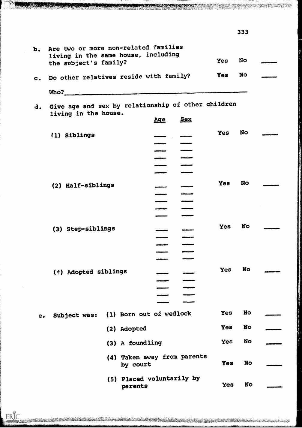
b. Are two or more non-related familiesliving in the same house, including

the subject's family?

c. Do other relatives reside with family?

Who?

333

Yes No

Yes No

d. Give age and sex by relationship of other children

living in the house.

(1) Siblings

(2) Half-siblings

(3) Step-siblings

(1) Adopted siblings

Ale Sex

1111111

..waswimas

MINNIMasfo

411111.11.11.11111.

Yes No

Yes No

Yes No

Yes No

e , Subject was: (1) Born out of wedlock Yes No

(2) Adopted Yes No

(3) A foundling Yes No

(4) Taken away from parentsby court Yes No

(5) Placed voluntarily byparents Yes No

,?Mr!,-21,70v

f. other children in the household were:No. of Each

(1) Born out of wedlock

(2) Adopted

(3) Foundlings

(4) Taken away from parentsby court

(5) Placed voluntarily byparents

g. Sister has had a baby born out of wedlock?

6. PARENTAL ATTITUDES

(1) Overprotects the child

(2) Do not cooperate with school

(3) Permissive about school absences

(4) Put excessive pressure on child to achieve

(5) Restrict child from engaging in schoolsocial activities

(6) Exercise no disciplinary control overthe child

Is there evidence of parental discord,i.e., fighting, friction, bickering?

Comment:

334

Yes No

Yes No

Yes No

Yes No

Yes No

Yes No

Yes No

Yes No

Yes No

Yes No

Yes No

Yes No

Yes No

7. PSYCHIATRIC HISTORYFather Mother Sibling Child

(1) Has been in mentalhospital Yes No Yes No Yes No Yes No

(2) Was hospitalized fornervous disorders Yes No Yes No Yes No Yes No

(3) Has received psycho-therapy Yes No Yes No Yes No Yes No

VA

Father

(4) Had a nervous break-down Yes No

(5) Has been underpsychiatric obser-vation Yes No

(6) Is emotionally ill Yes No

(7) Is febbleminded(mongoloid, hydro-cephalic, microcephalic,brain injury, etc.) Yes No

(8) Is judged to be in need

of psychiatric exami-

nation Yes No

8. WELFARE HISTORY

a. A welfare agency supplies (to

(1) Food

(2) Clothing

(3) Financial aid

b. Church contributes to support of family

c. Child receives aid such as:

(1) Free lunch at school

(2) Free milk at school

(3) Free medical care

(4) Free shoes or clothing

d. Child has missed school for lack of

clothing or shoes

e. Source of income is:

(1) Relief check

(2) Social security benefits

335

Mother Sibling Child

Yes No Yes No Yes No





family):

Yes No

Yes No

Yes No

Yes No

Yes No

Yes No

Yes No

Yes No

Yes No

Yes Uo

Yes No

MNINI1011111111111,

336

CRIMINAL HISTORY

a. Parent arrested for: (1) Bigamy Yes No

(2) Theft Yes No

(3) Rape Yes No

(4) Non-support Yes No

(5) Child neglect Yes No

(6) Other offense Yes No

Specify other offense if possible:

b. Child has history of: (1)

lir,

01.

Stealing (serious,cars, etc.)

Rape victim

Yes

Yes

No

No

Rape offense Yes No =10.

Petty theft Yes No

Vandalism Yes No0111INIMIIIMOIMr

Other offense Yes No

Specify other offense if possible.

Father Mother

c. Parent has jail record Yes No Yes No

d. Other family members have jailrecord Yes No Yes No

e. Parent is in penitentiary

10. PERSONALITY COMMENTS

Yes No Yes No

a. Circle either yes or no as to whether or not the item

is characteristic of the CHILD'S behavior.

(1) Immature

(a) Sucks thumb

(b) Lacks bowel control

ret,%;;A,1-4

Yes No

Yes No

11110manno

11112.1=Diaiagl

(c) Cries easily

(d) Emotionally immature

(2) Rebellious toward peers

(3) Rebellious toward teachers

(4) Frequently fights with peers

(5) Takes property of peers

(6) Bullies others

(7) Lies excessively

(8) Tells vulgar stories

(9) Exhibits lewd pictures

(10) Dishonest, cheats at games

(11) Bosses other children

(12) Scared of peers

(13) Shy, withdrawn

(14) Excessive daydreamer

(15) Lacks self-confidence

(16) Hyperactive

(17) Lazy

(18) Loses temper easily

337

Yes No

Yes No

Yes No

Yes No

Yes No

Yes No

Yes No

Yes No

Yes No

Yes No

Yes No

Yes No

Yes No

Yes No

Ye r; No

Yes No

Yes No

Yes No

Yes No

(19) Dirty appearance Yes No

(20) Plays truant Yes No

(21) A tattler Yes No

(22) Other (Specify ) Yes No

TOTAL

4-741t7.1, - =ALA-LIST!: .z-77=WWM

338

11. BEHAVIOR OF MEMBERS OF FAMILY OTHER THAN SUBJECT: MOTHER,FATHER, OR SIBLINGS

Mother Father Libljam,

(1) Alcoholic Yes No Yes No Yes No

(2) Delinquent Yes No Yes No Yes No

(3) Drug user Yes No Yes No Yes No

Is parents' (both father and mother) behaviorsuch as to cause gossip? Yes No

Is father's behavior such as to cause gossip? Yes No

Is mother's behavior such as to cause gossip? Yes No

If answer is xts to any of above, what is the nature of the

gossip?

12. FAMILY MOBILITY

(1) Members are itinerant workers Yes No

(2) Father in military, child moves often Yes No

(3) Father in military, leaves family behind Yes No

(4) Child has been transferred among severalschools Yes No

(5) This family moves often Yes No

Estimate number of moves in past 5 years.

13. OCCUPATIONAL HISTORY

(1) Father is unemployed now

(2) Father frequently unemployed

(3) Father can't hold a job

(4) Father is marginal worker

(5) Father, a laborer, is not regularly

employed

Yes No

Yes No

Yes No

Yes No

Yes No

.;:e..,4,4,1ve::tesiIteZ4:67'ziraittf441.^

00.0101MILSEINONI

(6) Father is crippled and can no longer

work at his usual trade

(7) Father has a traveling job and is not

home much of the time

(8) Father is overseas (Military?

(9) Mother supports family

(10) Mother takes in laundry, babysits

14, PARENTS' EDUCATION

a. Parent

(1) Is illiterate Yes No Yes No

(2) Educational level

(a) Lower than 8th grade Yes No Yes No

(b) 8th to llth grade Yes No Yes No

(c) High school graduate Yes No Yes No

(d) Some college Yes No Yes No

(e) Bachelor's degree Yes No Yes No

(f) Higher than bachelor degree Yes No Yes No

15. BILINGUAL HOME

a. Child is from bilingual home Yes No

b. Mother speaks English Yes No

c. Father speaks English Yes No

16, CHILD'S EDUCATIONAL STATUS

a. Has been retained: (1) One grade Yes No

339

Yes No

Yes No

Yes No

Yes No

Yes No

Father Mother

(2) Two grades Yes No

(3) More than twogrades Yes No

111111110ONIMINI

340

b . Child'-has received "social promotions" Yes No

c. Child is in an "opportunity group" Yes No

d. Child has been placed in or removed from(last occurrence) special educationclasses for:

(1) Visually handicapped Yes No

(2) Deaf Yes No

(3) Orthopedically handicapped Yes No

(4) Homebound Yes No

(5) Mentally retarded (educable) Yes No

e. Child has a history of absenteeism fromschool Yes No

f. Child has been unable to demonstrateability to achieve in school Yes No

1,1

CHAPTER V

FOLLOWUP STUDIES. LATER CORRELATES

OF PEER ACCEPTANCE-REJECTION IN THE

ELEMENTARY GRAMS

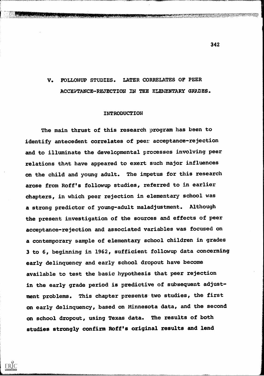
342

V. FOLLOWUP STUDIES. LATER CORRELATES OF PEER

ACCEPTANCE-REJECTION IN TEE ELEMENTARY GRADES.

INTRODUCTION

The main thrust of this research program has been to

identify antecedent correlates of peel: acceptance-rejection

and to illuminate the developmental processes involving peer

relations that have appeared to exert such major influences

on the child and young adult. The impetus for this research

arose from Roff's followup studies, referred to in earlier

chapters, in which peer rejection in elementary school was

a strong predictor of young-adult maladjustment. Although

the present investigation of the sources and effects of peer

acceptance-rejection and associated variables was focused on

a contemporary sample of elementary school children in grades

3 to 6, beginning in 1962, sufficient followup data concerning

early delinquency and early school dropout have become

available to test the basic hypothesis that peer rejection

in the early grade period is predictive of subsequent adjust-

ment problems. This chapter presents two studies, the first

on early delinquency, based on Minnesota data, and the second

on school dropout, using Texas data. The results of both

studies strongly confirm Roff's original results and lend

If 11,A,

343

substantial support and generality to the general assumptions

underlying this entire undertaking.

PEER STATUS AND EARLY DELINQUENCY

Juvenile delinquency is one of the socially significant

later behavior categories to which the measures of peer

acceptance-rejection collected in this study could be

expected to be related. Other criteria of this kind include

dropping out of school prematurely and being dealt with in

a child guidance clinic. It is known from Roff's earlier

work (1961b; 1963b; 1964) that a record of delinquency is

not inevitably predictive of adult criminal behavior; in fact,

the substantial majority of all juvenile delinquents even-

tually get along without serious difficulty. The problem of

delinquency is still, however, an important one from both a

theoretical and a practical point of view.

Definition of Delinquency. Although the term

"delinquency" has a definite sound, its actual definition

and the practices followed in dealing with it vary from place

to place and from time to time. One dictionary definition

is "a transgression of law....or offense. Or: a tendency

to commit such offenses." In practice, there are various

degrees of juvenile delinquency, and these are defined not

only in terms of the offenses but also in terms of the

apprehension and subsequent treatment of the offender.

:Wg44icaikaii-45

.41 C.74{7 4,, No, 5S"...,..7.1M"';'...'"'7.-

344

First is breaking the law without being observed; in terms

of frequency of occurrence, this would include practically

everyone. Another degree is being detected by a policeman

and verbally corrected, perhaps without even being known by

name to the officer involved. This may occur with juveniles,

as it may occur with adults for some minor traffic offenses.

It .is impossible to get accurate information on the frequency

with which this occurs. A degree above this is apprehension

and more formal admonition, either by an arresting officer

or at a juvenile department. A great many youngsters have

no history of delinquency after such an occurrence. A still

higher degree, following further trouble or a more serious

offense, consists in bringing the youngster into juvenile

court where he may be adjudicated delinquent and put under

supervision or on'probation.

Because it has a certain administrative definiteness,

the term "adjuicated delinquent" is probably the most

commonly used single criterion of delinquency, in studies in

this area. Like many other clear-cut administrative actions,

the frequency with which youngsters are "adjudicated" varies

from place to place, from judge to judge, and from probation

office to probation office, so that its definiteness as a

criterion is in practice more apparent than real, In any

case, many youngsters never proceed beyond this point. If

there is still further trouble, a decision may be reached to

345

take the youngster out of an unsatisfactory home and neigh-

borhood situation. In both the cities dealt with here, a

boy could be sent to a county training school. It is easily

possible to get a count of these individuals, and in this

Minnesota group, other work by Roff (1964) indicates that

about one out of five boys from the county training school

were later sent to the state training school. Later, as

they outgrow the juvenile age, a certain proportion of those

sent to the state training school appear as adult offenders.

Approach

This section describes the results of a partial followup

in terms or delinquency records for the two Minnesota cities.

A parallel study on the Texas sample has not yet been made.

Criterion information was collected in the probation offices

of these two cities during the summer of 1966.

For the first of these cities, followup was four years

after the initial choice-status scores were obtained. In

the second city, this interval was three years. Since all

those for whom data were initially obtained were in the

third through sixth grades, the oldest children in the first

city would have completed only the tenth grade, and in the

other city, the ninth grade. We thus refer to the results

presented here as relating to "early" delinquency.

The term "delinquency" as used here includes all cases

in each city who had contact with the juvenile authorities

ti

4.1 1:4 1'.1.4

346

formal enough to result in the preparation of a case file.

Most, but not all, of these were "adjudicated delinquents."

Almost all of their offenses occurred before they reached

the age of 16. One consequence of this is that the diffe-

rence in total frequency between different socioeconomic

levels is not quite so sharp as it usually is, if juvenile

delinquents of all ages are counted. Even if subsequent

work on this project should change the picture presented

here, were juvenile delinquents of all ages to be included,

any validity that the present study of early delinquents may

have will not be affected by such a change. This might

simply lead to the recognition of a difference between early

delinquency and later delinquency, which has received some,

but very little, attention (Neumeyer, 1961).

Subjects

For budgetary reasons, delinquency information was

obtained in the first city only for boys on whom teacher

interviews had been completed in the spring of 1962. These

structured teacher interviews were described earlier in

connection with the analysis of family background data.

In the first city, interviews were obtained regarding

800 boys. A search was made in this city for "interview"

boys in all four grades. In the second city, in view of

restricted time and funds, a search was made only for the

fifth and sixth grade boys. These seemed more likely to

347

have acquired a delinquency record than the original third

and fourth graders. Since delinquency occurs so much more

frequently among boys, a search of these records for the

comparable group of girls was postponed.

Of the 800 boys in City 1 for whom a search was made,

files were found for 87, or approximately 11 per cent. The

presence of a file meant that the boy had been apprehended,

and had gotten far enough beyond a preliminary stage of

consideration to have a file made for him, presenting the

circumstances of his misbehavior and indicating the steps

taken in an attempt to assist him. Allowing for the attri-

tion in the sample due to those lost as a result of moving

away from the city, the 87 found cases would be definitely

more than 11 per cent of those still present in the area.

It should also be remembered that those who were in the

third grade at the time of initial testing are far from

being through the delinquency period.

As mentioned earlier, the schools in each Minnesota

city were divided into quartiles on the basis of a combi-

nation of income and education of the adults in the school

district, based on the 1960 census figures. Try the first

city all four of these socioeconomic quartiles were used.

I, the second city, schools were obtained, only from the

third and fourth quartiles in socioeconomic status. That is,

they were drawn only from the lower socioeconomic half of

.19 44.

V 41

348

the city. This provided enough pupils to meet the pre =set

sample size, and by concentrating on the lower half of the

city, it was thought that the data would involve the area

with the greatest incidence of later problem behavior.

Results

Figure 2 shows the incidence of early delinquency in

City 1, broken down by the four socioeconomic quartiles for

the entire city, and by high, middle, or low choice status

at each of the four SES levels. This includes all the cases

for whom interviews had been obtained. Since the interviewed

cases included two low pupils per class, and only one high

and one middle pupil, the number of low-choice pupils has

been divided by two throughout this figure to make the

number of low cases equal to that of the high and of the

middle cases. With this exception, the frequencies shown

represent individual cases rather than percentages. (A more

comprehensive figure showing percentages is presented below

for a different sample.) It may be noted in Figure 2 that

the number of delinquents in the low/2 group consistently

exceeds the number in the high and the middle groups in the

upper three SES quartiles. This is in line with our expec-

tations. In the fourth quartiles, however, the number of

delinquents among the high-choice pupils was almost as high

as the number in the low-choice group. This was contrary to

our expectations and, taken by itself, might seem a chance

effect.

7'1

. a

Figure 2 349

LLL

..4.

_

vsANLISX- t - -

- I

.......

..r.i -;-111. .1.11:t...1:-.:ti _-1:-1..:{-i-iti-14'1.1.: ..; i-4:1*"; .-,1.44,-r-it'll-tI :

Hri.171,1.4-7i.,I.' _ I 1 :: -,.1 rt -t. ... . "'l.: ..;:rf I i-H-1

,..,,.......

.....,......._, ..... --1.. ,. ,

+. -4!-- 1 li . ... Ra..=1.,....mu. mi, ..".

4.4- .. aa .

, , - 4±- $.-

4-4

1'11r1tkreale''''4 L12ekit.1.0.!$11;IAAEL-40,MIASZ141.44VAN.41iT'1i=4V,k4-'4 .$7.1.-.11'; '1,-1111111k1:-1,kii;14144*I140Aliritt4

350

Figure 3 shows the results for early delinqLants in

City 2. Originally, each city was divided into SES quartiles,

on the assumption that this was a fine enough subdivision

socioeconomically for almcst any purpose. We decided,

however, that it would be more interesting, in looking at

the results in City 2, for which we had schools only in the

lower two SES quartiles, if each of these quartiles were

divided into upper and lower parts. Using the same criteria

on which the original division into quartiles had been made,

the third and fourth quartiles were each split into upper

and lower, and the results plotted. This sample includes

fifth and sixth grade boys only. They also differed from

the boys in City 1 in that three instead of four years had

elapsed since the scores were obtained.

Inspection of Figure 3 indicated that there were no

early delinquents at all among the high-choice or middle-

choice boys in SES groups III (upper) and III (lower), and

only one in group IV (upper). In group IV (lower) there are

at least as many high-choice boys as low-choice boys with

delinquency records, thus replicating the results of

Figure 2 almost exactly.

Since there was an observable difference between the

upper and lower, parts of the fourth SES quartile, we returned

to the data from City 1 and re-worked the third and fourth

quartiles by upper and lower parts. The results of this are

MAU

T " 1 .; --1,--1-'11.:--1:1:7FL7-14--H yr 1 t Fj1 i'4, -' 'jr/ L ;"T ; ,

; i; :

:

EARLY1.1

I -r II' t t--t

-i-tr -t 1--1- -Ft

-, -1 . . 1--"- -4-- -- -1--i-I1 4-7-! "t -: I

., I 1- !

. '

-r. I" 1 1' t"."' '1, .... `,

l- ' I ".I ` I " ,t1 -1-, 1 7-1-:-H- t

I. ir-- , : .... :-. I r

" : i .-: -i I 1 :ILIDLE. RAID 1.01AT CHOICE 86)':5 dr ,b i rrai-ii,l-tv',4_,..,---., :.:.... ..... . ..._,.. t T.

r-r- - t 1- r J . -..-i

i - i 1-4--, -t-..-{-; 4 . '

7 rl i WEk: qufiRTILL:5 5PLIT ,IN TINcs_,...t::. ;--11,44 , ,

7- -rt-t ; :- i.;-1.',_:-..1.1-, - '-', '''

- 1-- : , , ,

1 r ,t r-1--t-

4 4;1 7,1'; '± i-ERvIChil. 0/2565 ' F/Fril' 11/1/2) ! 5-.IXT11._:..4', It...7., ,,._ ,

,.. , , ,..i_iii..,,._,_., -I- J- ---

- .-. _. ..i..... ,..-1 -2.,...- ,- - -i. [..,, .. ..

_4:., y , .2. .. ...17_77- , , . -r -,--,--,-,, ..

:.F.t ;-:-T 1:;.1711-:..., ! ....., , :,.

.-, ,.. t7 ' 1 ""i 1 ..

' ',11:11- 71-1.--i-j- --rt.T.-4 1,..ilt i-: i ' 7 r, r j .

.1 :, r -; '. 11- 'I ; ' 1

r '''' ,-"- -rt - ' - -- -r--I.:,-f-r

---, -, .. 1..1._. --r

: .:.: I" . !

1 , .1, . i - -;---1- ; t 1 -I --,ti t; - -i---

H.) 6 .,.,,,.....,..,;,... t -4 1 1- ,--r

1--t-

4 '7-....--,

....'- -r-t--- i--- -r--

.., -1-2 .1 . .1_1_ 1 i _,-,_ ft ;:r 711jt:, , i -., . , , ! ! .

I-11-: ': I ',--, , I- -,1-1-

.1.. ,. _ --r-'-r-r-r._._ , . i : 4 I

I

...- - ,, ,--, I r; ' A .i L .

. ' 1 , , .,. 1

: -1", 1-r : i 1 tf i 11--11; t *frIIIIDDLE7,

,., , ., ...,..,

, i, ,

, I --t-,,..,,.., ... ......_,

i---Iii --.!."1-

.,. I-, -r t -1-1-t- r ,.--.,- -'-,-

,_ _,.i:. .

, r , ri :4--t14-"-- r -1 t : - , ' ' _ -,I ' -i- t- ,--f-rt-

r ,.1 .i.,.. 1 , . . ,1

1'7-17; :i- 4 4- .--

--r- - ' rt------- -,----i- I : 1. 11111,

! i

i I_VH--; ; , -1-, -L

-r :-- V . -1 1 H -4-.. i 13 ' . i - -,-T1 .-_,,

-;--- LO Ini d.: --i-,- ,--, I. -. 4

't r r ,I r1 ',1- r ' : J-I ; ,--1- -, er_. :-- -:-,-,,, : .,-,,- ,:. -::,-,-,-

7" i I l I 1I

' , I-71! 1

%If 7t41:4:

1'1

I I-

4,-1"-r.

I i-t-rt-r

,- 1-1-7-1 -1- -14

r

t 7: ;

, ..

-; 1'1

---'---r.

_-__

-

+"

01

I 1--`---1"- -

IV)'71

"'"

11*

I : 4-1*tirri I ,

111T-4.-;11-1- ; 1 r

I

.177.,r-r

,

j

Y! -/-t t- 1-tl -r I t t1-

/

-- r

- r;3--=1-.

-1-t7+-t-

-r r_

,-' t - '4"4-

77-7-7 ' ^' 7-7-1-: 1- 1---t,

- .-- 1-1.1, ; , -, r 1 - 4 r --, -1-- r- r- -' --'--1- 7--

11111.1111111M

I, : . -: I '.--,.' 11..-._-.4, ..; 1 ; 1 ;..1_11 ',. I--:_11:. I, 7--1-14---4-4--:-.1111---H-.7.7r --1---1-1-4- --7--I-;-"

---- i ; ' ; I I -,-1- -; I- t------1- --,- ----1--,-- --*--- I I- -9. t !-;,--t-I-i---

; ' '''' -I I 71.4T"1--"..1''.......1..;_7_14.:. ._.....7_ _i_t__l_. 1" _...----t-......_----

41--,--, .--1=

i.

7.21 7 i-.. .

: I ,

:-.1..-IT-T- il.r.t... 1 '.... .

- I

.' r ._ , i_t_.....__..1 ..y.H.. ,_,.y,.y....r4_,..!±_i__,*_,..7_1_,...1._-,_-_,___-.-_. . .

,,,4-i:Li-t-'1-'-t-1-4*---,-----,---- -*, , : 141- ..1_--7--; I. - -1+ - ...! ,--r-t,- t r,-4 t- r -------- --t -_

. , ...1.L...: - t ,. I t4.......1-4.-.1 i-4-1--j....- i ' - 4.'1 - .--- t- ..-t-r"'- -,-.....-.' r. ,..t...1.1.. -.4.1T .i. .,.1-4.-, . -i., -, .- , t ... ..I. -, ...._4 -t-t-,-----, r-f- -i- - '-'-1- --' !-'" -.-- I-1-r-/-7,--t- i- -1-1-1-r---ri- -i- 1- -- t , "----` t t " -1--,----i " ', .

i ' i -i- 1- '0 . t ..-i1- t,--- -; t t- -t- r-4 4- i i-t---t 41-1-,

-.4-

:7T-r,1. f:l E4-:, 1 ', :Ili" '-''' '; 1- r 1- '

...T.-. 44 4 I: 4, I 4 4 4'r

. L - ... I . ., :::1:17:I,;4 4, 4 4 4 ; 14 4 $ 444 ,-..L.,-

.

- J---.

-L ....-.. .. ; , .

f-'... ..

; 4

1

,..., .... .1-1..t+Ii-i-4-1.:-

: .., ! t ;

...- .,. .......-.-4-r. ..-.... .-t .1.

1 j- t t 1. , i r.

' t I I r- 4.

. , , . ; , 1- . . .1 , . ' ., 1. ',_:. 4..1 ....

11111.111111111111, , - -,---4--,

t t --1

t-t -- - --

.

,t., .

- 1 r-

'

';

fqokeOper

, I

'4 ,-

!1

1.:

I1 zi

11 l4 vi, g

'. k N, ,

tbaLe.:.-,

s-11' "" 7.1 1 P t I ! ,

. --r-t-- -

. ..,_.. ,lA -- . t

7 t:

3.....-.2

ILO W_.,-_..

:, : .n. , , ,_. ,.. . .. - .17 , .117i7C. . 1.4

T: 1 'II :. : ; 4. '.. '. I '.,1..r't ',-; ::', I -t

I

-4

; t tt, t--r -f- 4-1-1.-

j . -, . , - ii L ,-

i .. 1 . -,,i

I 1-, '. i l.1'1 ..:

i ! - :- -

t- f --:.-L. i 7.. :, . 1": '' , 1. L.+ i:1-.- ....,... .. ...._ ..... ..,... - .t' 1-1

. ,

: T-1. ! - r t t -r-t ,-,- 7' t'-.... - - .. . .

r, .1' -,1' '..---,-,-+-L 1_.:',.,_,:.:: , : jt!....,

kA,A, k.w\vWI4k, -,- y .

i , ,

. _LL.,...... ,1 L__. 7

i ' ' - . ' ; I ; 1

11...-`7.- ''..---7-" t I ' '4- t 4 ' ! - 1 ; t ! t

1-.1 1 ' 7 i .. ". -r- 1 4 t' ' r .

11 1..

I '

i t -

H 1. 1 tr ti 74: ." 1 ' '

'--1----

4- - ! ! I ! -! ' :'

.11* j

4

,.. .-, 1 7-141'

' 1 . I

-,..-.......... .............

----. 4 .

.

' 1.

... ...- . .

1 } TIT i. ; .,

I

4-; ' 11 i- ,-4--, ,..,--,. -. -:,.., . , .. 1 4, -t- 1-1 1- t* 1-1 L* - .! 7 -t.1-'

; 1 '4, H i ' ' 14--r :21 ;.* tl ' : 4' ' ! ' ' !-I '1. - - t 1---.4.."-

1 ,-- 7 - -,, , , i 1 . i -.-, - ,-,-; 7:7.1 ;._._ 7.;___..........1-4

!*- ; . 4 I - r - , ;.; . :. 4..... . .. A .......;........,r"li i. ,- '- - -..L.,... 14. -t ; . r -

I 1 ! .

i 1

. 1 r r . li 1.; Jr.It. L-1 1..1 :, ,. 1.1 1.1', ti..11.1 ..- .-1-' -,-.1. i . ,.. 4. '-'-...1-1:!: L

, !.t .,-:*-,, ,... 4-1',_ .: ; I:

I.

V, ',." 1;:.91--1_:; t -1-' I

11- ,', l_. H-1.-!-. -4.-}- .-- .. ..,....,

it-J-1. . -,-...-.7-1-"I'... - . i 1. , ,,

--r!"' 1

1

4-,

I

1 !,. ,

t. 1- ''1-:1.1;T:j !--1-- 1 t -.1r FT: +-741 4-1-1, .4-T-11" ---,..../: 71-7-.±.-...,..,

- - .., , y - ,- 1-. - r t .II.'" ' ''-'-1 ; "' ' I r1.--...1 .- _

-', 1 r I, ' 4/

,-U.1.mtt-:&;,44,!1g4i--aLtriA.r...kai4c,t.iAitLiLli:ei-tiL341Rtt'4.4,:iiii::'

;--t-, tt-1-1 1 1: r, -{-1+-/ t-1-1-71-141.,- 4444-irt1 11 I 4 .,.. t_ti..1 i

,.. rLL........L.L.L1 .-....1......I-. 11 IV ,n111, ntil .11.14' -11/

.,-:-.1 tilZVAwattla.,,, 7,,,,,,,...4... 4...1

I r r , I 4-1. , . ;

352

shown in Figure 4. For the III (upper?, III (lower) , and

IV (upper) SES groups, the results were approximately

according to our original expectation. For the IV (lower)

SES group, the number of delinquents among the high-choice

boys who were delinquent, in accordance with what was

becoming our new, revised expectation.

To fill in the omissions which resulted from the use of

high, middle, and low boys, for whom we had interviews,

information was obtained in City 2 for all the 1,729 fifth

and sixth grade boys for whom first-year scores had been

obtained. The total number found in the delinquency files

was 187, or 11 per cent. Figure 5 shows the percentage

delinquent for five standard score class intervals of choice

status, for the four SIP divisions of the schools of the lower

half of the city. Again our expectations were approximated

closely except for the boys with standard scores of 6.5 and

above in the lowest SES group. Here the proportion delin-

quent was almost exactly the same as in the low-choice group

with standard scores of 3.4 and below. The other standard

score groups for the IV (lower) schools showed the same sort

of patterning as did the schools in the other groups, and

the high and middle groups of Figures 2, 3, and 4.

.7"

Figure 4 353

rTr:_; .;I

E A R L: y:.

o L! I

L I LJ. __

L /Vb' LOW CkOIE 5óyS ,9T

qVI9TJLE5 /7j_/7

7iiw?) :I.,i

:

: I

J _1L1 LL z(Ie//c' O95Es Fr2/4 LO 1 5%1,49%,C Lr

:: ::: .: . .

- :-h:7_ :, H Hr1-TTh-I --i

I. ......t - .

I . ! ' . . .

1LJ ..v ii fl-u

I

I

Ii;- i rr 4 I4Trl--tL ti__Hi2_Jzj_L,T._

r .-. : :-...: ., .. .,. ........

T: 11:L-,-.- . k; . , "-.,. . r.-. .

i4,

I

I:

' 4ff'( e - t LL ,t- -

.. . .

:

...: ........ : ....

:

L' L ft I

F.T----r.-'-...1 ...... -1 f--1..H-...-t--r-...f .: . . . . ... H r f ....... 1 .i:--I -T-1-f-4-rH-

: i(,:ij .:_:::: :; : .

... :Jii_i) .:

:

[DI,i 1

I. .--- L_ ............................. -n-.:

4i I

H T;

1,.:-1 ii.H:ij

.: . .

f

I

-r jl

j ____

1

j1 .,. ..

....-

L. I ?Ti Ir- rL

H . H..: ..

t 1

.ti:-

.------

±1 k

ii_____________y

r r'-' -9tT41.t.

j_______T?TTH1T 7i I N\\\\\\\\\\\\\\\\ \\\\ \ \1

T..L4...

-:

:

. .,. 1--4_.4.4h ;14:Wh:1}rTTh

I lrf

:

IU:;-: .:;t4

:;H::::;:I : .i;.FEt1

LL 1 4

Fiqure 5 354

U1L T2JTI.flEfl Jt1LL 'CCfi_s _ J\ 440 Ce

Lf t1_ +i t r

F iL ttr L ' T i r 1tfp

-rTt' rfi j-

f;L L: 1i:ljt ftj:H.F -r I_! iI:Et

:iL t1r 1r

I

T H tiftiIi4 I±I o) !IoL:5L5 '.oJ.(a 4.jj_;:. .!; : : 4: : ;'; .;;' . :r: . ':h'.. :; jj r+T-1;-;

I:f... IcJ;4ITr4Fr

;;i :E

_:1. rt- .... : r4-- 1tL-.+..t

T: --T--f

fT::i7:r 4t i.k.t1 yr

r rr1.LLhJ4 L

I 1

E35Fr_&:Mi

-;4tr-\To1;2 LI

fT; tV

1:

--t- rFI

iriiT

- -rz4-ff; r-r-L.'

44Atft7 ;i

t+Er4 .. I JE:z -.fEfl:

ThL±

LF';Lt:

L i: ft ;T5i-{TF3T JFfTEL f ±- :r b(r' e4 rIto 4V ___

4L iM H '}-LI IiT 1--T

: ..

'T:: t 4r i11 i1 +; Lç :

.

r - -: L r

, . -: --k - fr--1.i..+.i ±

:i1:T

1'

L

49-i :FL.'

:L:t t:1L: L ,

L 6 ,_..+_f.

rL-' . ... ,.,-

:

;:j r1:,:

1 4--, ,

4. -'i _---.--.-..1--t

L4j

4

j.i:i:.:[1 1T14Ci

s7 ;9t q_1t51;5;

:; .:t: Lr 1:i.rff1:t : rirr:::., :::ii j) ]:i1:t 1

:E:.!t:L

zt:,t fEf 41"' ::fti# LT :.:t:ty1::: +ii:

r iL r:T -di: f T r9 ,t i: l_rrL::

. ---- --

355

ILLUSTRATIVE CASES

In the first year of the project, descriptions of

selected high, middle, and low children in each class were

obtained by interviews with teachers in order to provide a

more concrete picture of the individual children than was

given by the choice-status score alone. These descriptions

have been found useful in many ways. In the present context,

they give information about the cthildas seen by school

personnel, including various factors in his life situation

which may have had some relationship to his subsequent

behavior. Selected cases are presented here to illustrate

the way high and low-choice children at different socio-

economic levels were described.

Upper SES Quartiles. 'Is indicated in Figure 2, there

was only one high-choice delinquent in the two upper SES

quartiles in City 1. We can begin the illustration of the

described behavior characteristics of high and low-choice

youngsters with the single high-choice boy from the two

upper groups and the two low-choice boys of high SES status.

These are, respectively, Frank, who was high choice, and

Thomas and John who were low-choice boys.

FrankFrank (sixth grade) is a large, fat boy, extremely shy,

who always looks dirty and unkempt, his clothes messy andhis hair uncombed. Although he can do things all right, helooks awkward when doing them, particularly writing. Henever volunteers for anything. He has been absent a greatdeal, usually three or four days at a time, with stomachtrouble due to extreme nervousness. He is good at his work,

ral=ampmekads=.4072;434:

ti

356

tries hard, and when absent always makes an effort to do themakeup work so that he can keep up with the class. He isself-effacing: seems quite embarrassed when called on andshows much ambivalence in volunteering for things. On theother hand, he is beginning to take part in the teenageactivity; they do giggle and laugh about the other sex, buthe is quite upset when the teacher has to reprimand him.The teacher feels that in some ways this activity is animprovement and she would rather put up with much of hisplay with the other kids as long as he is doing what seemsmore natural and normal for him. She has had him for two yearsand has seen a decided change in his behavior, particularlyin his asserting himself more than he used to do.

On the whole, though, Frank is still a rather passiveindividual in class. On the playground, he is definitelyinterested, and he comes back all out of breath, having beenthoroughly active in the games. He speaks in an extremelytiny voice and seems afraid to make mistakes. He gives theimpression that he would die if he made another mistake.He does not demand much attention of the teacher, justaccepts her.

The other boys accept him well; he talks to them easily,they choose him on their sides when there is some sort ofcontest, and they give him much recognition when he doessomething well.

Little information on the family except that his motherwas divorced from his father and is now remarried. Frankreflects his stepfather's interest in him and talks aboutthe stepfather's experiences. The mother is cooperativetoward the school, and the teacher feels that Frankdefinitely reflects kindness from mother and stepfather.

Probation Information:Two years after testing, malicious destruction of

property. Referred to parents° About a year after this, themother became overtly psychotic. Soon after this, Frank wasarrested for auto theft and placed on probation.

ThomasAverage-size sixth grader, fairly good development.

He possesses average physical skills and generally can holdhis own on the playground. Teacher estimates that he hasabove average ability; however, achievement is not up towhat might be expected. Rather poor general adjustment.He is quite a problem. Has to be watched carefully. Majormisbehavior such as throwing stones at cars and lightingmatches on the school stairs. Untruthful and antagonistic,both toward teacher and classmates, so in general he is notwell liked by his peers. He has one other friend, a boy whois also known as a "troublemaker."

trzreaFAZZWATalSzywo...,41,

357

Tom is restless, constantly on the move. He appearsto be quite happy, is outgoing. The teacher believes thathe has good possibilities. He is able to reason in a fairlymature fashion and seems quite sensible when called upon todiscuss life in general. Both parents are working, and theboys (3) are left alone a good deal of the time. Theteacher knows the parents are in disagreement as to how tohandle the disciplinary problem. His father has ratherstrict standards, but the mother is on the other hand verypermissive and perhaps unconcerned.

Probation Information:Age 16 1/2: Possession of liquor and drunk. No

record of either social agency contact or contact with thelaw for any other member of the family.

JohnJohn is a very large fifth-grade boy, the largest in

the class. He is also one year older than the others,having failed one year. Last year he broke his leg and hewas somewhat lame; it is getting better now although he stillis not too well-coordinated and is somewhat awkward at times.

He is a bully. He picks on younger children and doesnot play well with the kids in his classroom.

He is an apple polisher; he tries very hard to workhis way into the group of children who are the most popular.

On the playground, John picks on the small participantsand he is one of the last chosen. In the classroom he isvery good, quiet, cooperative, and causes no disturbance.You hardly know he is in the room. Academically, he isbelow average, has a very difficult time getting his school-work done, but he works at his assignments.

His attitude toward other children is one of domineeringthem. He takes it out on smaller classmates and singles themout one at a time for picking on. He teases them, holdsthem down, takes their hats away, etc. His aggressivenessis not confined to overt fighting, but rather to some formof passive aggressiveness holding a child down tc say uncleand not letting him go, or teasing. His relationship to theteacher is very good. He does what he is told and causes notrouble in the classroom. He tries to please the teacherand he brings things from home to show the teacher and theclass. The trouble he is experiencing is all out-of-doors.

He has been doing better in school work, and there hasbeen some progress in his relationship with others. Thekids seem to accept him more now. He can now hit the balland, being the biggest in the class, he's somewhat moreaccepted on the playground in athletics.

Most of the students let him alone. The smaller onesdislike him intensely and fight him off..

,tiffs3a Y ;,

YS

L1,

,,,CitArwre.mr,475Ftlnyqg r+,,,,,,,,,,,,,,,,,v7,-,,A,F7477-7,77715.111,77.77,...7.41,7-4=137,57..,407,

:

358

The mother is described as being very good. She willgo to bat for the children. Whet... they are wrong, she willpunish them. John is the second youngest of five children,four of which are boys. At home there is a rather rough andtumble life, and John is picked on, being somewhat dullerthan his siblings.

Probation Information:At 15, burglary. Lives with father and stepmother.

There is no history of contact with any social agency, nor ofany contact with the law by any other member of his family.

Lower SES Quartiles. Space does not permit the presen-

tation of a case of this kind for all possible combinations

of SES and choice status. Typical low-choice boys from the

second and third quartiles are presented next (Paul and

Randy). For both of these SES groups, the number of high-

choice boys who became delinquent is very small.

PaulA very small, undernourished fourth grader who has a

cute face and is rather nice looking. He talks babytalk attimes. He has no marked strengths. He is often dishonestat games and he generally makes a poor adjustment withothers. Nevertheless, the teacher pointed out, there issome indescribable quality that makes this youngster likeableby adults.

On the playground, he is aggressive at times with otheryoungsters. He enters games and seems to enjoy them. Inthe classroom, he was described as sneaky. Sometimes in theclassroom he displays bad temper. He treats others in theclassroom in an aloof manner. He visits others occasionallybut seems not to become too personally involved in socialcontacts. The group in return for his aloofness also treatshim in an aloof, distant manner. A good relationship existsbetween the teacher and the pupil. She can correct and guidethis youngster when he is not behaving properly. He hasnever shown any strong feelings toward the teacher.

He is totally disliked. The girls dislike him and theboys dislike him. The girls dislike him because he beatsthem up, and the boys dislike him because he's sneaky andbecause he doesn't follow the group's standards of behavior.He disturbs them because he does not follow directions andhe is not fair.

359

The family is large and somewhat lower economicallythan their neighbors. The parents are not effective indirecting the youngster or his siblings. There are economicproblems that the family must face. The mother does notfollow through consistently on any plan concerning theyoungsters.

Probation Information:Whrn in second grade, picked up on three separate

occasions within one week once for burglary, twice forpetty larceny. No charge was placed. The following summer,he was arrested for burglary and put on probation for twoyears. Soon after school started, again caught for pettylarceny. In the spring when in the third grade, he wasarrested for burglary and sent to county training school.On release, again charged with burglary and prowling cars.Two months after this testing, burglary and arson, andagain sent to Detention Home.

The father has a history of five arrests for assaultand battery, drunkenness, and wife beating. About a yearafter testing, father hopitalized as psychotic. Oldest .

brother had history of six arrests, next brother had onearrest, oldest sister had six arrests, next brother hadthree arrests, and next sister had seven arrests. Motherdescribed as showing serious emotional disturbance.

Probation report while in second grade: quite percep-tive and capable of independent thinking and expressinghimself. Open negative feeling to father. Lives forpresent. Expect severe destructive aggression in future.Severe character disorder manifested by impulsive actingout, impaired ability to enter into meaningful relation withothers and considerable immature narcissism.

Mother and father divorced while Paul was in sixthgrade; they tried to give him some attention, but this wasdifficult with ten Children. Both drank too much.

RandyA small, wiry sixth-grade boy with flashing eyes, a big

smile, and usually neat appearance. Devil-may-care attitude.He doesn't seem to care if school keeps or not. Highlyself-seeking, self-pushing, egocentric. Seems to need tomake sure that everyone knows he is intelligent. He is veryverbal, loves to recite orally, but hates written work.Tremendous memory for facts which he acquires from reading,TV and radio. He is a complete individualist. He isn't atall like the other children except that he does seem to wanttheir approval. His answer to a list of offenses told himby the teacher was in the nature of debating style. "Now inthe first place, I did not...." and so forth. He counts

/41.314. ri.A;n1'ski.40..1.41e 1",

360

them off on his fingers. His strengths are his _: mindand witg and his ability to thin. something through, althoughan IQ test suggests his ability is less than teacher hadsupposed. Almost analytical in his thinking. He has theability to bluff. His greatest weakness is his completelack of motivation. He seems willing to be far less thanthe best academically, partly because he is unwilling toreveal his shortcomings. He is almost criminal-like in histendency to shift blame. Two juvenile officers came toschool to talk to him about vandalism in a closed store, andwith an innocent look he sent them to the junior high schoolto talk with his older brother, who was really just an on-looker. The officers soon returned.

On the playground, he wants to be a big leader, astrategist. He would have been a good Nazi. He is not out-right cruel to others, but he lacks understanding of theirfeelings and fears. No one else matters. He Is a goodcompetitor in class games, is not a poor loser, and is satis-factory in supervised play, but in unsupervised activityhe wants to be the supreme dictator.

In the classroom his behavior is not exceptionally bad.He has a tendency to be polite when he is criticized, and heseems to take it well even though he gives excuses. He getshis name on the board for little things, and he is constantlyreported by guides and patrols.

He has fairly normal relations with his peers, in spiteof his acting so superior, for he doesn't act superior withall the boys, nor all the time. He irritates the girlsbecause of his acting so smart, and because of his frequentinterruptions. He wants to be very frienCly with theteachers, but he has difficulty achieving this, for he feelsthat rules made for others don't apply to him. Rules arefor the ignorait ones. He doesn't outright defy the teacher,rather he seems to ignore. Sometimes he grins as though hehas to go along because it is necessary for the rest, but heseems to say that you know and I know that I really don'tneed these rules.

Most of the children pass Randy off. They have beenused to him a long time. His cuteness and sharpness can'thelp but impress some of these kids, even though he irritatesthem. His patronizing attitude of cutting in on others'recitations is one of the reasons why the children react tohim as they do. He is also too aggressive. He is really abully, even though he is small. He will try his bullying ona larger child even, but one who doesn't want to fight.

The parents are impressed by his factual knowledge, andthey and his older brother and sister think he is cute. Theyare not as sharp as Randy. He is so well accepted by hisfamily that he surely feels secure. A definite weakness isthat the parents are not realistic in their appraisal, and

361

they do not think the school appreciates their boy. They don'trealize that he does not do the writing work expected of him,even though they have been told many times.

Probation Information:During spring of sixth grade, he was arrested for

malicious destruction of property. There is no subsequentrecord.

Lower Half of Fourth SES Quartile. The SES level of

greatest interest here is the lower half of the fourth

quartile or approximately the lower eighth of the boys in

SES status, In this group, as indicated in all four charts,

2, 3, 4, and 5, there are as many high-choice delinquents as

there are low-choice delinquents. Our interviews indicate

that in general the high-choice boys were in tune not only

with the other boys, but also with the teacher and the school

in general. Insofar as both their peer status and the inter-

view materials are concerned, they do not seem to be "person-

ality problems." On the other hand, the low peer status

boys in this SES level are characteristically disliked by

the other boys and not so well in tune with the teacher and

the school. There has been a good deal of talk in the

literature about the "delinquent subculture." As a general

explanation of all delinquency at this level, this represents

an unproved assumption. It is closer to the facts to describe

these delinquent boys as coming from a bottom economic level,

which produces more than its share of delinquents, whether

as members of a delinquent subculture or through the

VM5411WX1.-

362

operation of other factors, such as family disorganization,

"improper" rearing, etc. Edward is typical of these.

EdwardEdward (fifth grade) sometimes looks very neat and

clean, and other times looks like he climbed out of a ragbag.Occasionally he doesn't even make it to school, apparentlybecause of insufficient clothing. Edward is slender andappears undernourished. He is an attractive boy with a lotof drive. He probably is a good deal more sophisticated inthe ways of the world than one would guess from his conver-sation. He's very nice and polite in school. Edward is agood student, but one handicap is that he rushes to get done.

Edward is a good ball player and a good sport and well-liked and one of the first to be chosen on any athletic team.In class the youngsters also like him very well and arequick to choose him. He's usually mannerly. He's no botherto anyone, would quickly reach out to help others. He'sdependable and is listed as the best-liked boy in class.Good average intelligence. The teacher said that he couldnot be nicer to her; he's cooperative and courteous, wantsto do well. He does not ask her for help. I think part ofthis comes from Nis being forced to be independent from hildisadvantaged family.

He does things well, is quiet, does not make himselfa pest.

A very unfortunate home situation. Mother apparentlydoes try to help work with the youngsters. Neither mothernor father make conferences.

The father and mother could perhaps be adequate parentsif they had one or two children, but with the extremelylarge family that they have, they are both overwhelmed. Asa result the youngsters do not get the proper care andemotional help that they should get. Father is frequentlyaway from home, separated from the mother; mother, in seekingcompanionship, is apt to reach out to other men and toentertain them and have them with her in her own home. Thisprobably has some adverse effects for the youngsters. I seeboth parents as being rather immature adults who are apt tosatisfy their own needs before satisfying the needs of theyoungsters. As a result, the youngsters are many times leftwithout the proper parental attention. Surprisingly enough,they seem to do quite well under these conditions. They areattractive, lovable, and likeable boys and girls. Whilethere has been some petty thievery, some truancy, and somelack of application on the part of these youngsters, by andlarge they are happy, fairly well organized boys and girls,who seemingly make the most of what little life has offered

363

them. Currently, there has been talk by the welfare agenciesof the possibility of removal of the youngsters from thisfamily. At this point, because again of the kind of adjust-ment made under these adverse circumstances, they have beenreluctant to see the older youngsters go; it's the smallerones that would be most hurt if they should have to leave,yet it's the small ones that perhaps would have the bestchance to move on and more fully develop their capacitieswith the chance to live somewhere else.

Probation Information:Edward had been arrested for malicious destruction of

property and referred to his parents about a year beforetesting. About a year and a half after testing, he wasarrested for shoplifting and put on probation for a year.Six months after this probation, he was arrested for bur-glary; at that time he admitted nine other burglaries. Hewas sent to the county training school, where he stayed forsix months and remained on probation for another six monthsafter that. This brings him almost up to the time of thefollowup.

The family was well known to various social agencies.An older brother was in an adult reformatory, and a secondolder brother was on probation at the time of followup. Thefamily was described as being unstable without the father.The mother seemed unable to supervise and had had an ille-gitimate child about two years before followup. The psycho-logical interview report said that there was nothing grosslyabnormal or unusual about him. Stable mood, emotionalreactions generally appropriate, though well-guarded; slightlyunhappy, has some poor opinion about himself, is fairlyenergetic--likes people. A normal person is indicated.

It may be noted that although the description of this

family situation seems to be adverse, apparently the boys

and girls get along surprisingly well. Of course, there has

been some petty thievery, truancy, etc., but both at the

time of the initial teacher interview and at the time of the

probation interview after he had gotten into trouble, he was

judged to be a "normal person" who was exhibiting some

misbehavior.

7fi

364

A somewhat similar picture is given by Joe, also a

high-choice boy from the bottom SES group.

JoeJoe (fifth grade) is small, short and stocky, very

handsome, with a sparkling eye and a bright alert-lookingface. He's very well coordinated. Distinguishing him fromother children, is his quick smile, his sense of humor, andhis tolerance and acceptance of others. He's extremely fairin all his dealings, seems to expect fairness in return and,generally, has a good, healthy outlook on life. Has leader-ship ability, accepts responsibility well, has an inquisitivemind, and is rather adult-like in conversation.

Joe does very well in playground participation, respectsthe rights of others and is a very good group member. Hehas athletic ability and is looked up to for this. He's oftenchosen as captain of a team, but this seems to be morebecause of his fairness in dealing with the other youngstersin a heated discussion than because of his athletic ability.

In the classroom he is very responsive. He participateswillingly, volunteers regularly, has a great deal of back-ground information. His tests indicate that he is over-achieving. Youngsters are anxious to have him on committeesand often look to him for leadership in class as well as onthe playground and in the halls. He has been a good policeboys He's very well liked by the children. He has an olderbrother who has been involved in a great deal of delinquentbehavior. The children have mentioned this to Joe, and helaughs and says, "Sometimes we are not all alike." Heresponds well to the teacher; he wants to please, but not inan anxious way. Joe accepts the teacher's role as a disci-plinarian and will respond to discipline. He comes from adisorganized family. His mother has been married three times.The whereabouts of his own father is unknown. He did notget along with his first stepfather but does relatively wellwith this one. He has one brother and several half-siblings.The mother and the current stepfather have been fairlycooperative with the school, coming for conferences. Themother feels that the youngsters are capable of caring forthemselves and has given them an undue amount of freedom.Joe has been able to use this very well, while other membersof the family have not. The mother has indicated there isa lack of discipline within the home, and this is evidencedvery clearly with other members but not with Joe. He isresponsive to adults, respects authority, and generally isa happy, well-dispositioned child.

365

Probation Information:About 18 months before the study, when he was nine

years old, he was arrested for petty larceny and referred tohis parents. Two and a half years after testing, he wasarrested for malicious destruction of property and referredto the school authorities. A year after that he was arrestedfor incorrigibility, truancy, and running away from homeand placed on prd3ation.

His older brother was sentenced to the penitentiary forseveral years, a few months prior to the time when Joe wastested.

It may be noted that the personality characteristics

described for him are generally very favorable ones. Neither

originally nor later was he considered a personality problem.

On the other hand, if we take a look at a pair of low-

choice boys in this bottom SES group, we find not only

indications of delinquency but also indications of perso-

nality difficulties. Jackie is one illustration of this,

and James is another.

JackieJackie (fifth grade) is of average height, has fair

hair, is fairly neat and clean--it varies. He is very loud,has a very mouthy, negative attitude. He can be caughtdoing something right in the middle of it, and he will denythat he had anything to do with it. He takes pins out ofthe bulletin boards, pulls the shades, throws the flowers onthe floor, pulls the bristles out of brooms, and he usuallythinks he is being very funny and he has six or sevenchildren egging him on. The teacher felt that he is entirelydifferent from everyone in her room. The assistant principalhas said that he is a "crazy nuts" He never works in theclassroom. He does no spelling, no arithmetic, no reading.The teacher doesn't have too much trouble with him, but sheis very dissatisfied with him. He is usually sent out ofthe room.

In the gym he is very uncooperative, not much coordi-nation. He has to be protected to see that he gets his turn.He is not chosen very often; he doesn't play fair. If thereis something that goes wrong he never says that it is hisfault. He always blames somebody else.

is,v4,-efc4t;v

.4"

366

The students do not like him because he creates problems.They thialbeis funny and they laugh, although he has no realfriends. His relationship with the teacher is not very good.He is very difficult to handle. The students laugh at himand try to encourage him to go on with this behavior, butbasically he is left out of the group.

The family background is not very good. The mother hasbeen caught for shoplifting, and there supposedly was a boy-friend with the mother. The father has a job once in awhile. Most of the time he is working on his car. Thereseem to be many family problems; they have been encouragedto go to family and children's service to get aid. Jackie'sbrother was sent through child study for a complete perso-nality check-up and testing; however, they found that heneeded status and this sort of thing. Jackie is showingsomewhat the same behavior. He did go to remedial reading,because of his inability to read, last year, but he wasabsent so many times that he was not taken back this year.He is being seen at the time by a special teacher on theaverage of two hours a day to help him gain some status bycatching up academically.

Probation Intonation:Truancy and incorrigibility about a year after testing.

Committed to the county training school for three months.Three months after that, violation of probation (truancy,absenteeing from home)-- committed to county training schoolfor an indefinite period. Within a week he ran away fromtraining school and was returned. Within another week,he ran away from training school again and was returned.Considered incorrigible and sent to state training school.He was the second of seven children.

JamesJames (sixth grade) is the youngest of three boys in his

family. He is overweight and self-conscious about it.The children tease him. He is lazy, slow moving, frequentlyavoids physical effort. He has dark skin and black hair.

His academic ability is better than his productionindicates. It is difficult for him to get to work; once he,starts, he will stay at it. In fact, on occasion he hasspent the entire day on arithmetic. He likes questions thatrequire thinking.

James will hit back, kick or swat anybody who walkspast his desk. At times when in difficulty, he looks to theteacher for protection.

On the playground his sportsmanship is better than mostof his teammates. His coordination is poor, but he likes toplay. His coordination has improved somewhat this year.

ua

.Ltd ti 11;

367

In his classroom behavior, he aggressively acts out against

the children and against the teacher. Teacher holds him

briefly in his more explosive moments. After he quiets down,

he will go to work. Limits have to be sot and firmly held

for him,He trf.es to buy friends through giving candy, gum, and

so on. He has one friend in the room, a boy who is quiteemotionally disturbed. When he does not strike out against

the children, some are apt to bring him to it. The children

seem to have cast him in a role that will be very difficult

for him to change, At the beginning of the school year, hescreamed, lashed out at or walked out on the teacher. Now

he still gets angry and will lash out at him, but he recoversfrom it more quickly and settles down more easily. There

has been a slow but fairly consistent growth in self-control.Children reject him. He almost demands this, despite

his wanting to be liked and trying to buy friends. He

starts many fights with children over petty things. The

children fight back. He is gradually withdrawing from this

kind of fighting. If children really start a fight with him,

he will fight it through.The teacher has only talked with his mother by tele-

phone. She is interested in James, overprotects him, andwill take his side against any other information that might

be offered.

Probation Information:In seventh grade, insubordinate in school; sent to

county training school for six months.Family had eight social agency contacts. Father

attempted to murder mother and committed suicide when James

was four years old. Mother was unstable, but willing to

help. Psychological interview found: Impulsive, aggressive,

seeks attention - -many somatic complaints--inner self-control

lacking. Marked dependency needs--poor peer relations- -

unresolved emotional conflicts (parents not desirous of

seeking help)- -not sociable.

Whereas Joe, above, was mentioned for his fairness,

Jackie was described as "he doesn't play fair." And whereas

Edward, above, was described as "very nice and polite in

school," James was described as "hitting anybody who walks

past his desk.° These pairs of boys seem at the extremes

of other continua besides that of peer status.

"q-

368

Negro Delinquents. Since there is a tendency in some

areas for low economic status to be confounded with race, it

was a matter of interest to see to what extent, if at all,

the phenomenon that we are discussing here was attributable

to race. Inspection of the abstracts, of which two are

presented here, indicate that delinquent youngsters with

both good and poor peer adjustment occurred in ttet Negro

group. In these cities, less than four per cen of the

entire grade-school population is Negro, and these aTe not

all confined within the lowest SES group. The pattern found

here may not fit other cities such as New York or Chicago

where the proportion of Negro students is so much larger.

It should fit a large number of cities where the ethnic

composition does not differ too markedly from that of the

present cities.

Of the two Negro cases presented here, Willy is not

only liked by the other boys, but he is also diligent in his

schoolwork, although his ability level is not high.

WillyA sixth-grade Negro boy, well coordinated and in good

physical condition. He is the number two boy in the schoolin control. The boys respect him and a great many are afraidof him. He seems to be a leader. A consistent good sporton the playground. At times he protects the underdog, buton occasion he may kick him.

Willy is a very dependable police boy. In school heworks hard. He is of dull normal ability. Even though heis slow in classwork, he does not want his assignments cutdown for him. His effort is great enough to complete hiswork. He is not always right, but he certainly tries.

4,e VLIvg..1

369

Teacher, a man, gives Willy responsibility in theclassroom, and he carries it out consistently. He does not

assume responsibility if it is not given to him. Boysrespect him and like him. There are several boys who wouldlike to take his crown as number two man away from him. He

is respectful, cooperative, and responsible. He is recog-nized by his pears for his leadership qualities. Strangelyenough, for the position he holds especially in the estimationof the boys, he is not an aggressive leader. He always holdshis own and gives an excellent account of himself whenchallenged. He rarely seems to challenge others.

There seems to be a gradual, consistent maturing inWilly this year. Children like his persistent trying, nomatter what the job assigned.

His mother is cooperative with the school. She is muchinterested in her son. She wants him to be a good studentand a good boy. Willy respects his mother and, on occasion,has told teacher of little things he has bought for hismother. They are a close family.

Probation Information:Two months after testing, charged with immoral conduct

and placed on informal probation. One month after that,auto theft and sent to county training school. In spring ofseventh grade, truancy and returned to county training school.The following summer, shoplifting. No further trouble untilninth grade when charged with driving without a license anddisorderly conduct; informal probation.

Has five older and two younger siblings; two olderbrothers have histories of delinquency. Father is deliveryman, mother is housewife. Probation interview notes "lacksstrong male influence - -quite close-knit family--good siblingrelationship."

On the other hand, Don is actively disliked and consis-

tently nonconforming in the classroom. He has twelve

siblings, some of whom also have records of delinquency.

He is not described as being a boy who is getting along well

within his own peer culture.

DonDon is a dirty, sloppy, well-built, apparently healthy

colored boy (fifth grade). He is a nonconformist with littleconsideration of others or of the situation. Athletics is

Tro

ors 7r1Z l7.

370

Don's only visible asset. His weaknesses are that hepresents no apparent reasoning ability, is greatly retardedacademically and is very inconsiderate of others.

On the playground Don tries to run the show, tends tobully, is quick with the fists. He has good athleticability and skills, but shows poor sportsmanship.

In the classroom he talks constantly. He is consis-tently nonconforming. Rules are made for everybody but him.With others he is inconsiderate of their feelings; he mayeven knock heads together. He delights in proving hisphysical strength, even in adverse ways. He himself is notinterested in others except by way of showing his strength.

With the teacher there is no communication either way.He may not answer at all; he often has an "I don't know"response, and there continues to be an impasse, no outrightconflict, but no real rapport possible. There has been nochange in Don's behavior during the year.

Others' reactions toward Don are that some fear himbecause of his size, some are disgusted with his behaviorand lack of cleanliness. Those who are fearful of himbecause of his size, he tends to intimidate. His tangleswith the law tend to appeal to some. Others may look to hisability in athletic skills. But even with the variety ofresponses, actual relationship with others is limited.

Don comes from a very large family. There are twelveor thirteen children. To observers there may appear to beparental apathy. However, there may be interests which areoverlooked because of the overwhelming responsibility heapedupon this family. There is a sweet compliance on the partof the parents but an inability to follow through withguidance and with real care. The father remains employed,which is a decided family strength, but his livelihood isnot really sufficient for that many children. Guidance isinconsistent. Actual physical surroundings are bare andsparse. There is sometimes not enough food and insufficientclothing. Many of Don's siblings are retarded, and severalare in a great deal of trouble with the law.

Probation Information:First delinquency recorded while in third grade,

breaking and entering and petty larceny. In two days duringfourth grades charged with four offenses, primarily shop-lifting and petty larceny; placed on probation for a year.In fifth grade, insubordinate in school and probationextended, In May of fifth-grade year, bicycle theft,insubordinate in school; committed to county training schoolfor an indefinite period. In fall of sixth grade, assault;probation continued. In spring of sixth grade, insubor-dinate in school; committed to state training school. r

Had twelve siblings, seven older than he. Two olderbrothers and an older sister had repeated records ofdelinquency.

SUMMARY OP RESULTS

The contrast is sharp between the high and low choice

boys in the bottom group. The interviews presented above

give a clear picture of some of the behavior of the low-choice

boys, who constitute one important group of delinquents;

they are obviously not well accepted by their peers. The

high-choice boys got along well, not only with their peers,

but also with the school. The interviewed teachers were not,

of course, totally unaware of the status of the boys that

they were describing. They had had an opportunity to see

some of the choices made, in the course of data collection,

a month or two before the interviews. More important than

this, they had opportunity to observe the younsters daily,

and interviews concerning both boys and girls are full of

comments such as "he (or she) is always the last to be

chosen," or, at the other end, "he is a leader and is usually

the first one chosen on the playground (or in the classroom)."

Choosing is a frequently occurring activity, and youngsters

who are not chosen can hardly fail to be aware that they are

not.

At all levels above the bottom one, delinquency is prog*

gressively less frequent as we go up the scale of choice

ZF

' ,

372

scores. In the bottom group, this is also true except for

'the highest status boys. From earlier work, we still expect

these high-choice boys of the bottom group to make better

adult adjustments than the low-choice boys.

DISCUSSION

This discussion has consistently referred to the delin-

quents followed up as "early". In the light of the emrhasis

placed upon gang activity in some discussions of delinquency

(Cohen, 1955; Short and Strodtbeck, 1965), this group may at

the time of the followup check still be too young for this

to be as prominent as it may be later. With this reservation,

it is of interest to compare the present findings with

currently prominent points of view on delinquency. The

literature on delinquency is very large, and space does not

permit a comprehensive review of it here. To place our

findings somewhat in the context of one particular part of

the literature, reference is made to a conference report from

the Children's Bureau in 1960, "Sociological Theories and

Their Implications for Juvenile Delinquency" (Bordua, 1960).

In an overall view, two theoretical positions quoted below

are most prominent, particularly in accounting for group

delinquency.

Theories of Delinquency

One of these sees the delinquent subculture as "arising

out of the socially structured gap between the aspirations

373

of lower-class boys and the means realistically available

to them to realize these aspirations. According to this view,

lower class socialization does not equip boys to perform

according to the requirements of middle-class dominated

institutions such as the school, and consequently the boys

suffer 'status deprivation' and low self-esteem.... The

delinquent subculture values precisely what middle-class

institutions devalue; e.g., 'hanging around' instead of

industriousness, aggressiveness instead of self-control."

"'Status deprivation,' then, provides the motivational

core for the lower-class male delinquent subculture....

Equally crucial is the fact that 'status punishment,' in an

institution such as the school, tends to be differentially

concentrated lower-class groups who are residentially

concentrated in certain parts of any city."

This simply does not fit the picture given above of the

present sample of boys at around the fifth or sixth grade

level.

The second point of view sees the "beliefs and values

of the street-corner group as arising, not from any situation

of status deprivation, but as simply the adolescent version

of 'lower-class culture.'....This position directly opposes

the notion that the street gang or groups' culture derives

from a reaction to the demands of middle-class culture.

Instead, it emphasizes the view that 'lower-class culture,'

4 iii

374

as a more or less systematized body of beliefs, values,

'focal concerns,' and even household forms, has existed in

its own right for generations and need not be considered as

a reaction to beliefs, values, and household patterns of

the middle class." One question that arose was "What is the

evidence that there is a lower-class culture which the

adolescents are considered to be reflecting?"

.....g.EDelinuegXaalea.LE_Bel-LELIJtetgEELAtEaaE

Our present results clearly support the second point of

view and offer clear-cut indications of a difference in the

pattern of delinquency at our upper and bottom social levels.

At our upper social levels, delinquency appears as primarily

a function of personality disturbance as reflected by low

peer-group status. Almost no high-choice status boys from

the upper levels were delinquent. At the bottom of our

eight social levels, there was still a marked trend for the

boys with low peer status to show delinquency more frequently

than the average boys. Here, however, the high peer status

boys exhibited delinquency almost exactly as frequently as

the low peer status boys. Qualitative information available

for these boys at the fifth and sixth grade levels indicates

quite clearly that they were not at that time in rebellion

against that so-called middle-class institution, the school.

They got along well with their associates and exhibited a

rensonable amount of ambition scholastically. In some cases

"S4

,

4ve

375

the boy had already shown some delinquency at the time of our

study, and the teacher sometimes mentioned this as casually

as he or she would mention the color of his hair. Some of

these boys gave a clear picture at this age of being "in tune"

with their associates, and with the school, and with the

teacher, although they sometimes came from highly pathological

family situations, Nowhere in the literature, have we found

anything yhich describes the total effect that is being

described here.

In the present study, social levels were divided in

terms of the education and income of the adults in the area.

It seems clear, and is replicated from one to another of the

two sample cities, that the lowest of the eight education -

income levels produces a substantial number of boys during

the pre-adolescent period who are not in any sense in

rebellion at that time, although they may exhibit some delin-

quency, then and later. On the other hand, there is also a

sizeable group, similar to that found more commonly at our

higher levels, where the delinquency is accompanied by

personality disturbance and a rebelliousness which seems to

be personally rather than class oriented.

Because of their natural preoccupation with cultures

and subcultures, discussions of delinquency by sociologists

have tended to center on the gang and on organized group

delinquency. Although adolescent gang activity is a

IT j.

frequently occurring phenomenon (which is recognized by soma

writers as occurring either in conjunction with, or inde-

pendent of, delinquency), it is unduly restrictive to limit

discussion of delinquency to gang activity. Psychological

or psychiatric discussions tend to focus more on the charac-

teristics of individuals which are associated with delin-

quency, whether the delinquency is on a group or individual

basis. Again, there is a large literature which cannot be

reviewed here in any detail. Mention must be made, however,

of Jenkins' distinction between the socialized and unso-

cialized delinquent (1949).

The studies of delinquency employing the Minnesota

Multiphasic Personality Inventory,, of Hathaway and Monachesi

(1953) and of Wirt and Briggs (1959), contribute important

information about differences in personality patterns between

delinquents and non-delinquents but do not break them down

in detail in relation to socioeconomic status. Kvaraceus

and Miller (1959)0 both of whom have worked intensively with

delinquents, have discussed some of the satisfactions which

delinquent behavior can bring to adolescent boys, particularly

in the lower class. Conger and Miller (1966), using a

sample of tenth-grade pupils in an entire city, studied

certain personality variables in relation to social class

and delinquency. With a social class criterion of per cent

of dilapidated bastes in an erect, they used a dichotomous

er-

-

377

division for social class. This would not have permitted

the differences found in the present study to appear, even

if they had been there. None of the factual information

from any of these sources is incompatible with the results

presented here, but none of these have combined the charac-

teristics of individuals with a detailed break-down of socio-

economic status.

The criterion of delinquency used here was that the

boy's behavior was serious enough to lead to a preparation

of a file for him. This definition was adopted in earlier

work where we were concerned with studying the later outcome

of delinquents and wanted to be sure we had a broad enough

definition to start with. Occasionally, someone argues that

"delinquency" is so vague a term as to be of no particular

utility in the behavioral sciences. As defined for the

present study, it proved to be precise enough to give very

meaningful relationships with the peer group phenomena which

we are studying.

CONCLUSION

The present results need replication with boys and

girls in the Texas sample, and in other areas, to find the

range of populations to which they can be generalized. It

is expected that they will be replicable in samples not too

much different from the ones used here. It may be possible

434

378

to find groups with different ethnic or racial proportions

in relation to socioeconomic level that will yield different

results. In the meantime, we have a more detailed picture

here than has been presented before of the relationship

between choice status, socioeconomic level, and delinquency.

PEER STATUS AND MOLY SCHOOL DROPOUT

Although Roff's longitudinal studies indicated a

relation between peer rejection in the elementary grades and

young adult maladjustment, the rationale of the present study

encouraged concern with more proximal criteria of maladjust-

ment subsequent to elementary school* Another such criterion

is school dropout.

In 1964, it appeared that a substantial number of

children who participated in the Study in the first year had

dropped out of school, and a formal inquiry was initiated.

First, all nineteen school superintendents were approached

and their cooperation was requested. On receipt of approval

and promises of cooperation from all nineteen, a questionnaire,

Report of School Dropout was prepared, and a quantity of

these sent to all school coordinators early in 1965. Follow -

up was restricted to eighteen districts; the district that

excluded LL ratings was dropped from this study. Because of

budgetary problems and personnel changes in the school

379

districts that discontinued participation after the first

year, it became necessary to send staff personnel to obtain

the information from some of the districts. The final

sample was assembled throughout 1965 and the spring of 1966.

It was made up about half of questionnaires received by mail

from part of the districts and the other half completed by

staff personnel from school records and interviews with

clerks, teachers, and Other available persons at school

district offices. One of the eighteen districts had no

dropouts. A copy of the questionnaire is included.

Sample

Information was obtained on 191 dropouts for whom LM,

LL, and LD scores were available. TR data were not available

for 7 of these, 4 boys and 3 girls. Although the question-

naire requested information on occupation of parents, IQ of

the child, reason for dropping out of school, and scholastic

record, which were considered relevant to the relation

between school dropout and peer status; this information was

not completely available, and the missing data required some

ingenuity in the analysis. Occupation of parents was pro-

vided for 122, or 63 per cent of the dropouts, IQ for 132,

or 69 per cent; some reported "reason for dropout" for 147,

og 76 per cent, and academic standing (passing or failing)

pr 103, or 54 per cent. Despite persistent efforts to

Otain the missing information, the combination of passage

of time and incomplete school ;words was an effective barrier.

380

Raci....2_Ase______2_anComosition. The sample of 191 early

dropouts included 100 boys, of whom 92 were White and 8

Negro, and 91 girls, of whom 8l were White and 11 Negro.

In relation to the total Year I sample for the 18 districts

followed up, these 191 dropouts represent 1 per cent of the

population, who dropped out of school within four years of

the first peer rating survey. Since the highest grade

included in Year I was grade 6, these early school dropouts

were not beyond grade 10 by the time they left school.

Although the statutory minimum age for dropping out of

school is 16, 47 of the 191 dropouts in this study were under

16. However, since they were reported as dropouts by the

schools, they must have come under an exception to the law,

the relevant portions of which are included in the Appendix

to this Chapter. The incidence of early dropout was the

same, 1 per cent, for total boys and for total girls. It

was higher for Negroes than for Whites, as shown in Table

107, although still very low for both groups. It should be

noted that the incidence statistics reported in this table

refer only to early school dropout of a sample, observed

initially in grades 3 through 6, after four years.

SES acid School Progress. Data on SES and scholastic

progress were considered essential for an understanding of

the problem. However, overall statistics on the dropout

sample could not be computed because of the large amount of

,F711711Xr. -rk

A

ST:MArnl.

381

Table 107, Incidence of early school dropout after 4years for a sample of 11839 school children observedAL4I4A112ALLaultaP throe h 6.

Number in

BoysWhite Negro

Girlsraksagro

TotalWhite Negro

sample 8795 419 354 17066 773

Number ofdropouts 92 8 80 11 172 19

Per cent ofdropouts 1.05 1.91 .97 3.11 1.01 2.46

4,24;40/a0rag

VI.

;SIZ ";* . j.

rrf

382

missing data. An estimate of SES was made on the basis of

census reports for the communities in which the schools

attended were located, and school progress was evaluated by

comparing the ages of the dropouts with age expectancies,

assuming normal entry and progress through school.

SES was determined on the basis of 1960 census reports

citing median years of schooling completed by adults over

age 25, for the census units appropriate to the schools

involved. These are expressed in quartiles computed for the

87 Texas schools in the Year I survey. As expected, the

majority (70 per cent) were from the two lower quartiles,

and only 10 per cent were from the top quartile. Fifteen of

the 19 Negro dropouts (6 boys and 9 girls) were from the

lowest quartile; they represent 79 per cent of the Negro

children, as compared with 20 per cent of Whites in the

lowest quartile. The distribution of Negro and White boy

and girl dropouts by SES quartile is shown in Table 108.

It is apparent that race and SES must be controlled in

examining the relation of school dropout to peer status.

School progress could not be evaluated by usual indices

because of incomplete information. A satisfactory analysis

was designed; however, which involved comparing age at time

of dropout with age expected, on_the assumption that each

child had entered school at age 6 and had progressed at the

rate of one grade per year up to the time of comparison.

383

Table 108. Distribution of dropout sample by SES level(median school grade completed by adults over 25 years ofa e

SES

Low HighLow Middle Middle High

(9.1 to (10.3 to(59.0 years) 10.2) .1101. (?.11.1 years) Totals

Boys 24 42 22 12 100

White 18 42 22 10 92

Negro 6 0 0 2 8

Girls 25 43 16 7 91

White 16 41 16 7 80

Negro 04 2 0 0 11

Total 49 85 38 19 191

White 34 83 38 17 172

Negro 15 2 0 2 19

WeagT42=W4W'

AM,

384

The birthdates were available for 170 of the 191 dropouts.

Of the remaining 21, 14 birthdates had been omitted from

class rolls and 7 were added to class rolls after initial

preparation, and their birthdates were omitted. Since

actual dropout date was not available, the comparison date

used was June 1, 1966, which was well beyond the date of the

last dropout reported. For each of the 170 dropouts, actual

age on this date was computed, as well as the age expected

on this date based on assumed normal entry and progress to

June 1, 1966, for his or her grade in the Year I survey.

For example, a pupil in grade 3 in June, 1962, would have

been 9 years old in June, 1962, and would be expected to be

13 on June 1, 1966, assuming normal age of entry and normal

progress. Similarly, a pupil in grade 6 in June, 1962, would

have been 12, and four years later, he would be expected to

be 16. Table 109 presents a scatter plot of the actual and

expected ages of the 170 dropouts included thus computed.

The range of expected ages extends from 13 to 16, to reflect

normal age of entry and school progress of pupils who four

years earlier were in grades 3 through 6. The range of

actual ages extends from 13 to 19, with a mean of 16.1 and

standard deviation of 1.17. It is of much interest that

five of the dropouts were only 13 years old.

The main diagonal, reflecting matched actual with

expected age, is enclosed in squares. Frequencies along the

.

VISNWINNIPMarrommeentrommersisowl?Kl

385

Table 109, Scatter Plot comparing expected age, based on

normal age of entry and normal school progress to June 1,

1966, from initial grade in the first year (1962) survey

with actual a e on June 1 1966 for 170 school dro uts

Expected Actual A e on June 1 1966

Age.. 13 14 15 16

13

14

15

16

I3

21 9

1

17 18

9 7 5

I12

2 9

14 3 2

I 33

19 Total

4

32

31

40 17 2 103

MatwOMENINWwWwwww...gie

Total 5 11 31 54 48 19 2 170

386

diagonal reflect normal school progress; those to the left

of the diagonal could be considered accelerated, while those

to the right could be considered retarded. Looking first at

the totals at the right which correspond to initial grades

3 to 6 in vertical order, it is apparent that this early

dropout sample includes the full range of the initial sample,

but that dropouts were more extensive in the higher grades.

It may be expected that, as these children move up, the

dropout statistics will increase. However, the most striking

information in this table is that which shows that although

dropout is associated with school retardation (100 of the

170, or 59 per cent) 13 (8 per cent) were younger than

expected, and the remaining 57 (28 per cent) were at their

expected ages. These results imply that while scholastic

aptitude must be accounted for, as well as SES, in evaluating

the relation of dropout to peer status, the hypothesis for

a residual relationship appears to have some merit.

A higher proportion of retarded among the early drop-

outs in this sample was obtained from the questionnaire item

on scholastic performance at the time of dropout. Eighty-

nine or 86 per cent of 103 pupils for whom this information

was provided were recorded as failing in school work at the

time of leaving school. It is difficult here to evaluate

bias due to nonreponse as for other incomplete items.

However, the preponderance of school failures among the

dropouts is not surprising.

4

387

Reasons Given for Dropping Out of School No reasons

for dropout were available for a fourth of the boys and a

fifth of the girls, but although those advanced for the

remainder are interesting, as shown in Table 110, they must

be viewed with caution. While these "reasons" may have some

value in identifying salient, precipitating factea when

known, it is believed that so complex an event as dropping

out of school must be the resultant of complex patterns of

antecedent factors, including, as already demonstrated, SES

and race, which are interdependent in the samples studied,

intellectual or scholastic aptitude, as well as other factors

such as peer status. The object of the present analysis

is to examine the unique relation of peer status to school

dropout. However, the items listed in Table 110 are

reported as representative of the apparent reasons as seen

by school personnel from whom this information was obtained.

It is worthy of mention that failure to perform

scholastic work is not mentioned. For a majority of boys in

this sample, the reasons advanced emphasize failure of the

school to challenge them; delinquency is relatively

infrequent. A major portion of the girls combine disinterest

in school with marriage, which is a socially acceptable

avenue of withdrawal. in the culture.

388

Table 110. Summary of reasons given for dropping out ofschool.

Reason Lcas Girls

1. Quit, non-attendance, not interested 48 26

2. Quit to go to work 12 2

3, Needed at home 1 1

4. Marriage 2

5. Pregnancy 0 8

6. Suspended 7 1

7. Illness 0 3

8. Sent to reform school 5 5

9. No reason given 25 19

Totals 100 91

-OM

389

Procedure

Samples of early dropouts from the total available

group of 191 were compared with matched samples of non-

dropouts on LM, LL, LD, and TR. Three comparisons were made,

with dropouts and controls matched as follows:

1. Each sample consisted of 132 children matched on:grade, sex, and IQ.

2. Each sample consisted of 122 children matched on:grade, sex, and SES (based on Warner's Social ClassIndex of parent's occupational level).

3. Each sample consisted of 102 children matched on:grade, sex, IQ, SES (as in 2).

In addition, the distribution of the total dropout sample

was compared with the total Year I Texas sample on LM, LL,

LD, and TR. Although not controlled for significant sus-

pected sources of variance, this comparison is of interest

to understand the general trend of relationship. In the

matched groups, race was not employed as a matching variable

because of the small number of Negro dropouts. Further work

on this problem should unquestionably take this into account.

However, in the present study, race and SES overlapped greatly.

Results

Table 111 compares the percentage frequency distribu-

tions of the total dropout sample with that of the Year I

total Texas sample on LM, LL, LD, and TR. It is apparent

that the dropout distribution is overrepresented in the

"rejected" range on all of the peer status measures. At the

Table 111. Comparison of percentage frequency distributions oftotal dropout sample OR al 191) and total Texas sample, Year I,on, LM, L LD and TR.

Percentage Frequencies

LM LL LD TRz-score Dropout Texas Dropout Texas Dropout Texas Dropout TexasintervaltAgrapleample Sample SamtleSAmple.ample Samell

7.5-7.9 .5 .7

7.0-7.4 1.1 2.9

6.5-6.9 2.7 6.4

6.0-6.4 2.7 9.5

5.5-5.9 7.4 11.0

5.0-5.4 10.1 17.2

4.5-4.9 17.0 16.9

4.0-4.4 36.6 24.4

3.5-3.9 22.3 10.0

3.0-3.4 1.1 1.0

2.5-2.9 .1

2.0-2.4

1.5-1.9

1.0-1.4

Per cent <5 77.0 52.4

.1

.5 .9

.2 1.6 4.9

4.8 6.9 3.7 11.3

21.2 34.8 11.1 16.4

18.0 25.6 12.7 22.2

15.9 10.1 20.7 17.7

11.1 7.6 20.1 12.4

8.0 5.3 11.7 7.2

10.1 3.8 12.7 4.4

5.8 3.1 5.3 2.0

4.2 1.7 1.1 .5

2.1 .7

.1

57.2 32.4 71.6 44.2

.5 .1

1.1 2.7

3.2 14.6

4.8 9.0

21.2 21.0

28.6 34.2

17.0 8.3

11.7 5.7

3.2 2.8

3.7 1.1

2.7 .4

.1

72.5* 52.6

*Adjusted for 3.7 per cent not rated.

"",,`cam; rzt171.6".-77,,"..2777rn7K.Pc-TATIRIFRIMM.77.07,,,-r-4,15,-,-47wmtwe,-7,

391

Bottom of this table is listed the per cents of the distri-

bution below a z-score of 5, These are over 70 for the

dropouts as compared with per cents in the 50's for the

total Texas sample for LM, LD, and TR. However, for LL,

while the group difference remains about the same, the per

cents below 5 are much lower. Table 111 shows a substantial

difference between dropouts and the general school population

in peer status but does not control for well-known sources of

variance that partially account for school dropout. The

following analyses were designed to take IQ and SES into

account.

Peer Score Comparisons of Groups Matched on Grade, Sex,

and IQ. It was possible to match 132 pairs of dropouts and

non-dropouts, drawn as far as possible from the same schools,

on grade, sex, and IQ. The male and female members of these

pairs were then assigned to samples for comparison on peer

scores. The male samples consisted of 71 boys each, and the

female samples of 61 girls each. Critical ratios, comparing

matched sample means on LM, LL, LA, TR, md also on IQ, are

shown in Table 112. As shown in the bottom part of this

table, the matching was imperfect although the differences

between means were small and nonsignificant.

Inspection of Table 112 shows that the dropout boys are

significantly lower than the non-dropout boys on LM and LD.

On LL, the means for' dropout boys are lower than those for

392

Table 112. Comparison of mean LM, LL, LD, TR scores and IQ's

of school dropouts with non-dropouts matched on grade, sex, and

:DD.

Variable

Dropouts Non-Dropouts

Sam le N Mean S D.

LM

LL

LD

TR

IQ

Boys

Girls

Total

71

61

132

4.54

4.58

4456

Boys 71 4.46

Girls 61 4.59

Total 132 4.52

Boys 71 4.43

Girls 61 4.50

Total 132 4.46

Boys 68 4.64

Girls 61 4.53

Total 129 4.59

Boys 71 84.4

Girls 61 87.8

Total 132 86.1

.72

.89

.80

.92

1.06

.99

.83

.92

.87

14.4

12.4

12.3

CriticalRatio (one-

Mean S D. tail testl.

71 4.89 .91

61 4.76 .80

132 4.83 .86

71 4.73 1.10

61 4.75 1.10

132 4.74* 1.10

71 4.78 .99

61 4.70* .92

132 4.74* .96

71 4.87 .72

61 4.73 .81

132 4.81* .77

71 86.5 13.4

61 88.4 12.5

132 87.5 13.0

2.50, p<.01

1.12 ns

2.58, p<,01

1.46 ns

.76 ns

1.58 ns

2.21, X.01

1.08 ns

2.34, p<.01

1.32 ns

1.24 ns

2.08, p<.01

0.9 ns

0.7 ns

0.8 ns

*Indicates means for Non-Dropout Group is significantly lower than

the population mean of 5.0 with S.D. of 1.0, one-tailed tests.

the non-dropouts, but not significantly so. The means of

girl dropouts are lower, as expected, than those of non-

dropouts on all peer variables, but none of the differences

is statistically significant at the .05 level. As a result

of the trend of the differences for boys and girls separately,

the differences do reach significance for three of the

variables, LM, LD, and TR when the samples are combined.

None of the differences on LL was significant.

Taken literally, the results shown in Table 112 suggest

that with IQ controlled by matching, dropouts are distin-

guished from non-dropouts on peer status measures. The discri-

mination is consistent in direction of differences for girls

but not significant in the samples used. However, when the

smaller girl samples are combined with the boy samples, the

discrimination is significant on 124, LD, and TR. The same

variables discriminate dropout boys significantly from non-

dropout boys. The reason for the failure of LL to discri-

minate in this analysis is not clear.

Peer Score Com arisons of Grou s Matched on Grade Sex,

and Parents' Occupational Level. The same four peer status

variables were similarly compared using four other groups,

overlapping the previous ones in composition. The new groups

were matched on grade, sex, and SES based on Warner's Social

Class Index scores for parents' occupational level ( Warner

et al, 1949). Although IQ was not a matching variable in

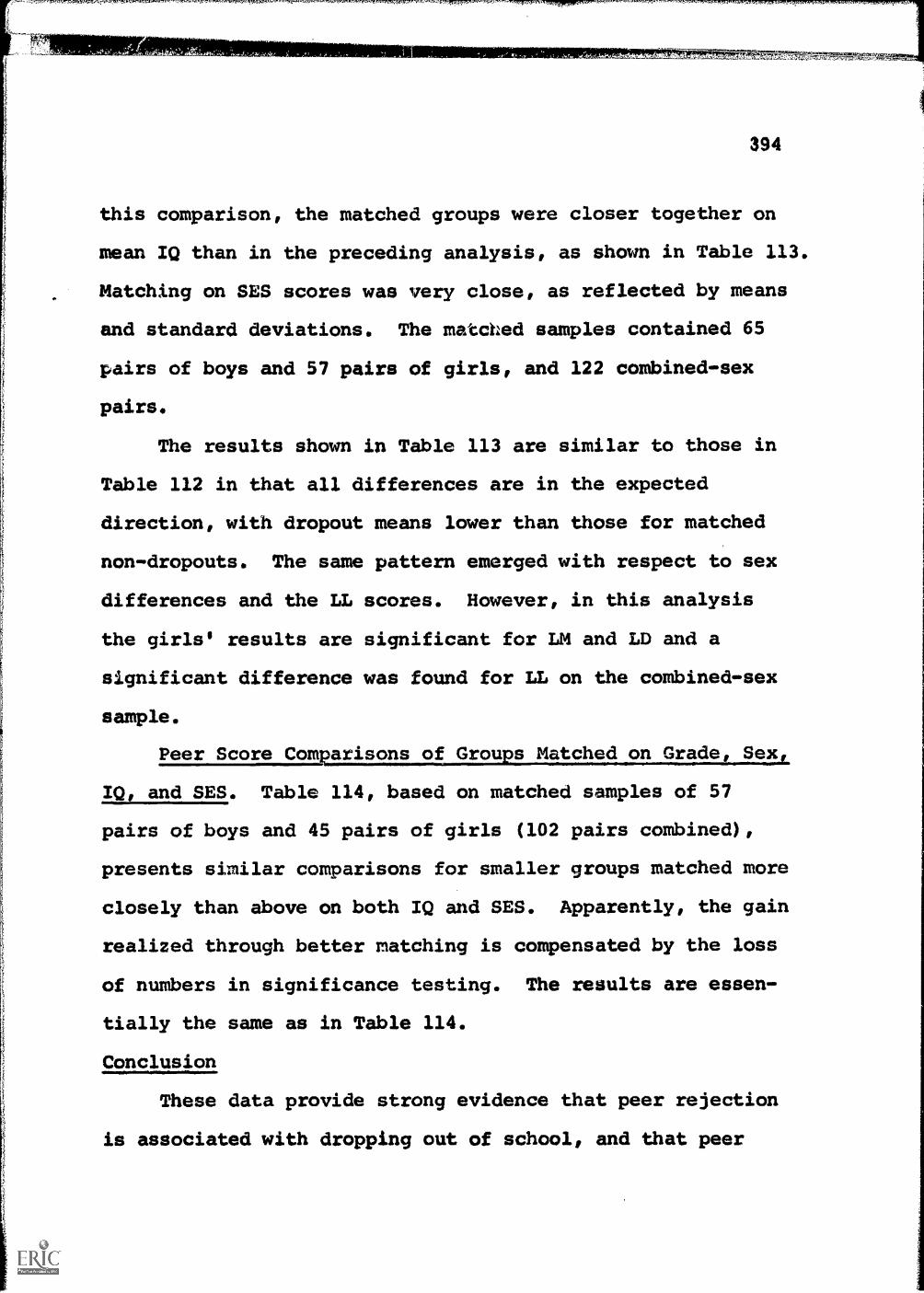
394

this comparison, the matched groups were closer together on

mean IQ than in the preceding analysis, as shown in Table 113.

Matching on SES scores was very close, as reflected by means

and standard deviations. The matched samples contained 65

pairs of boys and 57 pairs of girls, and 122 combined-sex

pairs.

The results shown in Table 113 are similar to those in

Table 112 in that all differences are in the expected

direction, with dropout means lower than those for matched

non-dropouts. The same pattern emerged with respect to sex

differences and the LL scores. However, in this analysis

the girls' results are significant for LM and LD and a

significant difference was found for LL on the combined-sex

sample.

Peer Score Comearisons of Grou s Matched on Grade, Sex

IQ, and SES. Table 114, based on matched samples of 57

pairs of boys and 45 pairs of girls (102 pairs combined),

presents similar comparisons for smaller groups matched more

closely than above on both IQ and SES. Apparently, the gain

realized through better matching is compensated by the loss

of numbers in significance testing. The results are essen-

tially the same as in Table 114.

Conclusion

These data provide strong evidence that peer rejection

is associated with dropping out of school, and that peer

395

Table 113. Comparison of mean sociometric scores of schooldropouts with non-dropout controls matched on socioeconomicstatu

Variable

LM

Sample

Boys

Girls

Total

N

65

57

122

IL Boys 65

Girls 57

Total 122

ID Boys 65

Girls 57

Total 122

TR Boys

Girls

Total

63

56

119

IQ Boys 57

Girls 45

Total 102

SES Boys

Girls

Total

65

57

122

1111111111111

Dropouts

S.D.

NortamoutsCriticalRatio (one-tail test)Mean N Mean S.D.

4.53 .80 65 4.98 .97 2.85, p<.01

4.56 .86 57 4.85 .80 1.80, p<.05

4.55 .83 122 4.92 .90 3.32, p<.01

4.45 1.16 65 4.76 1.17 1.54 ns

4.59 1.27 57 4.92 1.02 1.54 ns

4.51 1.21 122 4.84 1.10 2.17, p<.01

4.43 .96 65 4.86 1.07 2.44, p<.01

4.51 1.08 57 4.87 .90 1.94, p<.05

4.46 1.02 122 4.86 1.00 3.11, 13<.01

4.58 1.01 65 4.86 1.08 2.16, p<.01

4.58 .62 57 4.72 .75 1.03, ns

4.58 .84 122 4.81 .99 2.35, p<.01

85.4 13.21 57 85.9 13.06

87.4 11.46 45 87.1 11.13

86.3 12.51 102 86.5 12.32

6.14 .97 65 6.14 .97

5.98 .96 57 5.98 .96

6.07 .97 122 6.07 .97

k,`

396

Table 114. Comparison of mean sociometric scores of schooldropouts and non-dropout controls' matched on IQ and socio-economic status

Variable Sample

Dropouts Non-Dropouts

N Mean S.D. Mean S.D.

LM Boys 57 4.54 .70 57 4.99 .99

Girls 45 4.61 .92 45 4.86 .80

Total 102 4.57 .81 102 4.93 .91

LL Boys 57 4.45 1.14 57 4.72 1.17

Girls 45 4.59 1.30 45 4.92 1.06

Total 102 4.51 1.21 102 4.80 1.13

ID Boys 57 4.42 .91 57 4.86 1.05

Girls 45 4.52 1.13 45 4.86 .91

Total 102 4.46 1.01 102 4.86 .99

TR Boys 55 4.57 1.01 57 4.97 .68

Girls 44 4.65 .54 45 4.80 .74

Total 99 4.61 .83 102 4.89 .71

IQ Boys 57 85.4 13.21 57 85.9 13.06

Girls 45 87.4 11.47 45 87.1 11.13

Total 102 86.3 12.51 102 86.5 12.32

SES Boys 57 6.12 .99 57 6.12 .99

Girls 45 6.02 .91 45 6.02 .91

Total 102 6.08 .96 102 6.08 .96

CriticalRatio (one-tail test)

2.82, p<.01

1.40 ns

3.03, IX.01

1.24 ns

1.31 ns

1.801iP<.05

2.37, p<.01

1.58 ns

2.81, p<.01

2.48, IX.01

1.04 ns

2.75, p<.01

4:11A0Ailato,

397

rejection accounts for variance associated with dropping out

of school that is independent of intelligence and SES.

While the results were more substantial for boys than for

girls, the results for girls are in the same direction, and

all indications are that they would hold in larger samples.

The implications are that further, large-scale followup

studies of the relation of peer acceptance-rejection to

dropping out of school, involving longer elapsed time

between the initial peer survey data and time of dropout,

would yield even more fruitful results.

rsz

ag

H

g4a.

FAMILY BACKGROUND QUESTIONNAIRE

Sub'ect:Last Name

329

First Name Nickname

Xear of Study: I D

Home Address:Street and Number City

Parents' Name:Last First

Father's, Occu pation:

Mother's Occupation:

1. PARENTS' HEALTH

a. Please circle Yes or No in the appropriate columns.

Father Mother

(1) Arthritic Yes No Yes No

(2) Cancer Yes No Yes No

(3) Cerebral palsy Yes No Yes No

(4) Diabetic Yes No Yes No

(5) Heart condition Yes No Yes Nodale

(6) Tubercular Yes No Yes No

(7) Other chronic illness Yes No Yes NoSalliNIPINNMeows

(8) Physically disabled Yes No Yes No

(9) Injured in an auto accident Yes No Yes No

(10) Disabled veteran Yes No Yes No

(11) Hospitalized (bedbound) Yes No Yes No

330

Father Mother,

(12) Other Yes No Yes b73

If yel, describe.

Total Father

Total Mother

b. Do any siblings have a physical handicap? Yes No

If yes,, what is the nature of the handicap? Describe

c. Is there an invalid living with the family? Yes No

If so., what is relationship to child?

2. CHILD'S MEDICAL HISTORY

Please indicate by circling yes or No as appropriate theSUBJECT'S (child's) medical history:

Was a premature baby (7 mo. or less) Yes No

Visual impairment Yes No

Hearing impairment Yes No

Speech impairment Yes No

History of: Asthma Yes No

Brain injury (traumatic) Yes No

Cerebral palsy Yes No

Convulsions Yes No

Diabetes Yes No

Heart condition Yes No

Meningitis Yes No

Polio Yes No

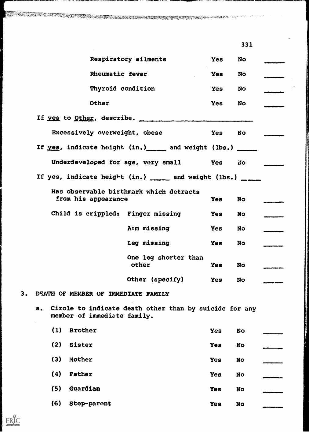
,47:777771WTAI !710-AVn-7,-

331

Respiratory ailments Yes No

Rheumatic fever Yes No

Thyroid condition Yes No

Other Yes No

If mta to Other, describe.

Excessively overweight, obese Yes No

If yes, indicate height (in.). and weight (ibs.)

Underdeveloped for age, very small Yes 110

If yes, indicate heig't (in.) and weight (lbs.)

Has observable birthmark which detractsfrom his appearance Yes No

Child is crippled: Finger missing Yes No

Aim missing Yes No

Leg missing Yes No

One leg shorter thanother Yes No

Other (specify) Yes No

3. DSATH OF MEMBER OF IMMEDIATE FAMILY

a. Circle to indicate death other than by suicide for anymember of immediate family.

(1) Brother Yes No

(2) Sister Yes No

(3) Mother Yes No

(4) Father Yes No

(5) Guardian Yes No

(6) Step-parent Yes No

c. Has any member c 'tumitted suicide?

If so, who?

332

Yes No

d. If one parent is deceased, has the other

remarried? Yes No

4. PARENT

a.

RELATIONSHIP

If both parents are living, circle Lei or no as to

parent relationship.

(1) Living together Yes No

(2) Separated, not divorced Yes No

(3) Divorced Yes No

(4) Divorced, mother remarried Yes No

(5) Divorced, father remarried Yes No

b. Is there an adult male in the family? Yes No

If other than father, explain.

c.

d.

Has father deserted the family?

Does father leave home for prolonged

Yes No

periods of time other than for business? Yes No

e. Parent married more than twice? Father Yes No

Mother Yes No

5. FAMILY CONSTELLATION

a. Child is cared for by: (1) Parents athome Yes No

(2) Relatives Yes No

(3) Guardian Yes No

(4) Foster home Yes No

(5) Institutionalhome or orphan-age Yes No

b. Are two or more non-related familiesliving in the same house, including

the subject's family?

c. Do other relatives reside with family?

Who?

d. Give ace and sex by relationship of other children

living in the house.

(1) Siblings

(2) Half-siblings

(3) Step-siblings

(1) Adopted siblings

333

Yes No

Yes No

ollEMMINOININ

011111111111M

0011M 111111/111111111.

101111111101111110

e. Subject was: (1) Born out of wedlock

(2) Adopted

(3) A foundling



Yes No

Yes No

Yes No

Yes No

Yes No

Yes No

Yes No

Yes No

Yes No

r,7i3.1 vroarrmiTIRAwn?-149g7,-, ,r74r,rVr'A

f. Other children in the household were:No. of Each,

(1) Born out of wedlock

(2) Adopted

(3) Foundlings



g. Sister has had a baby born out of wedlock?

6. PARENTAL ATTITUDES

(1) Overprotects the child

(2) Do not cooperate with school

(3) Permissive about school absences

(4) Put excessive pressure on child to achieve

(5) Restrict child from engaging in schoolsocial activities

(6) Exercise no disciplinary control overthe child

Is there evidence of parental discord,i.e., fighting, friction, bickering?

Comment:

334

Yes No

Yes No

Yes No

Yes No

Yes No

Yes No

Yes No

Yes No

Yes No

Yes No

Yes No

Yes No

Yes No

7. PSYCHIATRIC HICTORY

(1) Has been ia mentalhospital

Father

Yes No

Mother

Yes No

Sibling

Yes No

Child

Yes No

(2) Was hospitalized fornervous 'disorders Yes No Yes No Yes No Yes No

(3) Has received psycho-therapy Yes No Yes No Yes No Yes No

(4) Had a nervous break-down

(5) Has been underpsychiatric obser-vation

(6)

(7)

Is emotionally ill

TM%

Father Mother

Yes No Yes No

Yes No

Yes No

Is febbleminded(mongoloid, hydro -

cepha lic, microcephalic.brain injury, etc.) Yes No

(8) Is judged to be in need

of psychiatric exami-

nation Yes No

8. WELFARE HISTORY

a. A welfare agency supplies (to

(1) Food

(2) Clothing

(3) Financial aid

b. Church contributes to support of family

c. Child receives aid such as:

(1) Free lunch at school

(2) Free milk at school

(3) Free medical care

(4) Free shoes or clothing

d. Child has missed school for lack of

clothing or shoes

e. Source of income is:

(1) Relief check

(2) Social security benefits

Yes No

Yes No

335

Sibling Child

Yes No Yes No

Yes No Yes No

Yes No Yes No



family):

Yes No

Yes No

Yes No

Yes No

Yes No

Yes No

Yes No

Yes No

Yes No

Yes No

Yes No

MFRIMMgre,MW,Mnimmli.1,,,q7r.

9. CRIMINAL HISTORY

a. Parent arl:ested for: (1) Bigamy

(2) Theft

(3) Rape

(4) Non-support

(5) Child neglect

(6) Other offense

Specify other offense if possible:

b. Child has history of: (1) Stealing (serious,cars, etc.) Yes No

(2) Rape victim Yes No

(3) Rape offense Yes No

(4) Petty theft Yes No

(5) Vandalism Yes No

(6) Other offense Yes No

Specify other offense if possible.

Father Mother

Yes No Yes No

Yes

Yes

Yes

Yes

Yes

Yes

336

No

No

No

No

No

No

c. Parent has jail record

d. Other family members have jail

record

e, Parent is in penitentiary

10. PERSONALITY COMMENTS

a. Circle either yes or no as to whether or not the itemis characteristic of the CHILD'S behavior.

(1) Immature

(a) Sucks thumb

(b) Lacks bowel control

Yes No

Yes No

Yes No

Yes No

Yes No

Yes No

INNomMNINNimaem

INNIONINIM MINIM

cum111w

magooNsimeior.

(c) Cries easily

(d) Emotionally immature

(2) Rebellious toward peers

(3) Rebellious toward teachers

(4) Frequently fights with peers

(5) Takes property of peers

(6) Bullies others

(7) Lies excessively

(8) Tells vulgar stories

(9) Exhibits lewd pictures

(10) Dishonest, cheats at games

(11) Bosses other children

(12) Scared of peers

(13) Shy, withdrawn

(14) Excessive daydreamer

(15) Lacks self-confidence

(16) Hyperactive

337

Yes No

Yes No

Yes No

Yes No

Yes No

Yes No

Yes No

Yes No

Yes No

Yes No

Yes No

Yes No

Yes No

Yes No

Yes No

Yes No

Yes No

(17) LazyYes No

(18) Loses temper easily

(19) Dirty appearance

(20) Plays truant

Yes No

Yes No

Yes No

(21) A tattler Yes No

(22) Other (Specify Yes No

TOTAL

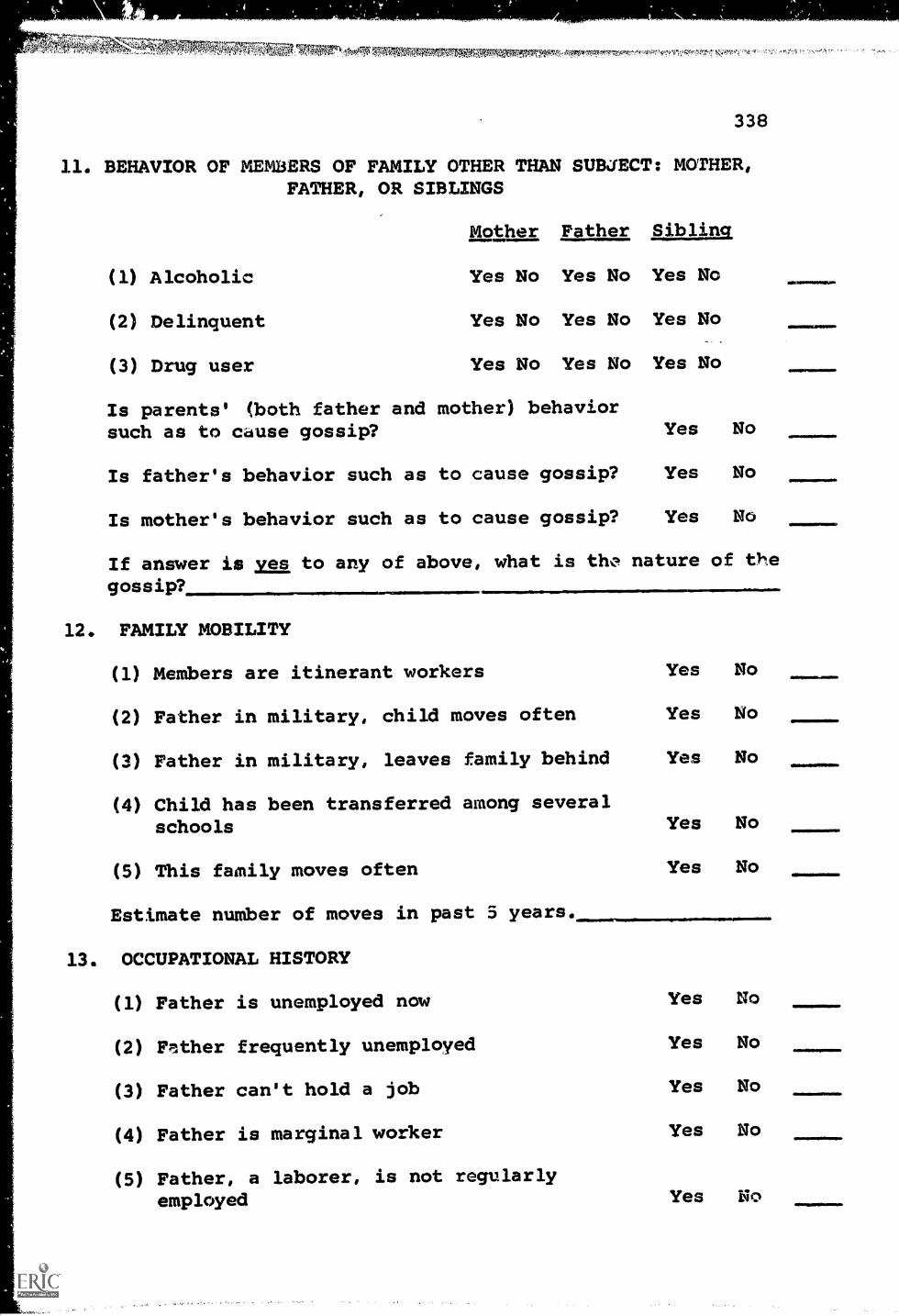
338

11. BEHAVIOR OF MEMBERS OF FAMILY OTHER THAN SUBJECT: MOTHER,FATHER, OR SIBLINGS

Mother Father Sibling

(1) Alcoholic Yes No Yes No Yes No

(2) Delinquent Yes No Yes No Yes No

(3) Drug user Yes No Yes No Yes No

Is parents' (bath father and mother) behaviorsuch as to cause gossip? Yes No

Is father's behavior such as to cause gossip? Yes No

Is mother's behavior such as to cause gossip? Yes No

If answer is yes to any of above, what is th:z nature of t),e

gossip?

12. FAMILY MOBILITY

(1) Members are itinerant workers Yes No

(2) Father in military, child moves often Yes No

(3) Father in military, leaves family behind Yes No

(4) Child has been transferred among severalschools Yes No

(5) This family moves often Yes No

Estimate number of moves in past 5 years.

13. OCCUPATIONAL HISTORY

(1) Father is unemployed now Yes no

(2) Father frequently unemployed Yes No

(3) Father can't hold a job Yes No

(4) Father is marginal worker Yes No

(5) Father, a laborer, is not regularlyemployed Yes No

if2Y ...!..16.40,4,41,&tiraYkoANWiito4AV44;11,gayiWit.-44,0 7IT.,5755

339

(6) Father is crippled and can no longer

work at his usual trade Yes No

(7) Father has a traveling job and is not

home much of the time Yes No

(8) Father is overseas (Military? ) Yes No

(9) Mother supports family Yes Ne

(10) Mother takes in laundry, babysits Yes No

14. PARENTS' EDUCATION

a. Parent

(1) Is illiterate Yes No Yes No

(2) Educational level

(a) Lower than 8th grade Yes No Yes No

(b) 8th to 11th grade Yes No Yes No

(c) High school graduate Yes No Yes No

(d) Some college Yes No Yes No

(e) Bachelor's degree Yes No Yes No

(f) Higher than bachelor degree Yes No Yes No

15. BILINGUAL HOME

a. Child is from bilingual home Yes No

b. Mother speaks English Yes No

c. Father speaks English Yes No

16. CHILD'S EDUCATIONAL STATUS

a. Has been retained: (1) One grade Yes No

Father Mother

(2) Two grades Yes No

(3) More than twogrades Yes No

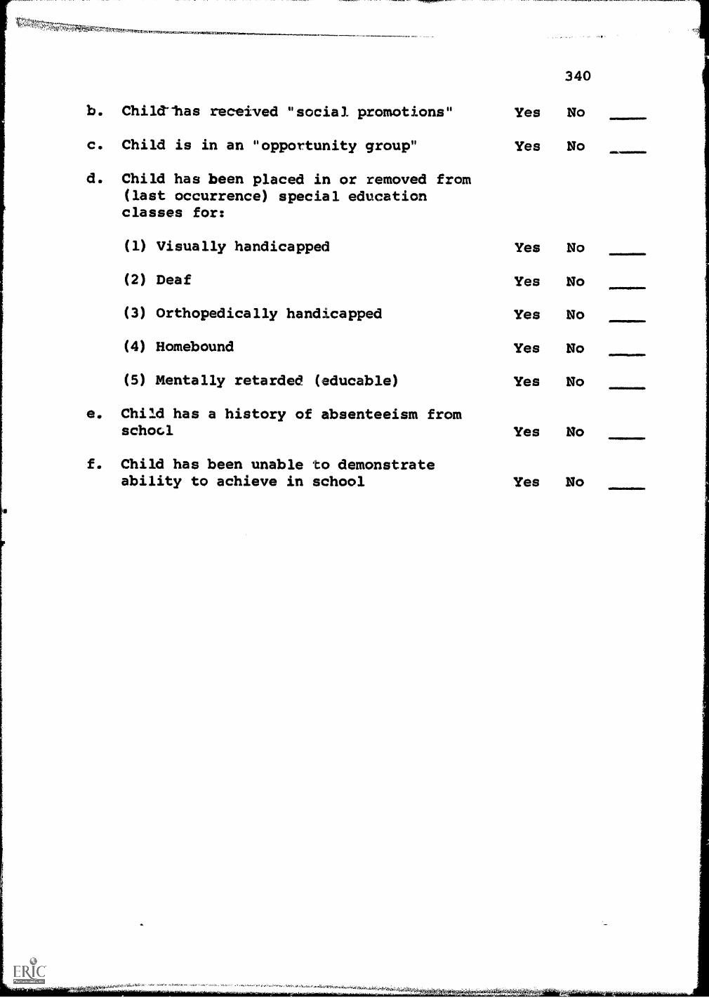
b. Childhas received "social promotions"

c. Child is in an "opportunity group"

d. Child has been placed in or removed from(last occurrence) special educationclasses for:

(1) Visually handicapped

(2) Deaf

(3) Orthopedically handicapped

(4) Homebound

(5) Mentally retarded (

e. Child has a history oschool

f. Child has been unaability to achiev

educable)

f absenteeism from

ble to demonstrate

340

Yes No

Yes No

Yes No

Yes No

Yes No

Yes No

Yes No

Yes No

e in school Yes No

1111M

011110111111111110M.

*TIrr7:".!erreltx7FTrirwors.i.411gli44,1zaiaL,,2

CHAPTER V

FOLLOWUP STUDIES. LATER CORRELATES

OF PEER ACCEPTANCE- REJECTION IN THE

ELEMENTARY GRADES

r '14141.?..

342

V. MUM!) STUDIES. LATER CORRELATES OF PEER

ACCFPTAME-REJECTION IN THE ELEMENTARY GRADES.

INTRODUCTION

The main thrust of this research program has been to

identify antecedent correlates of peer acceptance-rejection

and to illuminate the developmental processes involving peer

relations that have appeared to exert such major influences

on the child and young adult. The impetus for this research

arose from Roff's followup studies, referred to in earlier

chapters, in which peer rejection in elementary school was

a strong predictor of young-adult maladjustment. Although

the present investigation of the sources and effects of peer

acceptance-rejection and associated variables was focused on

a contemporary sample of elementary school children in grades

3 to 6, beginning in 1962, sufficient followup data concerning

early delinquency and early school dropout have become

available to test the basic hypothesis that peer rejection

in the early grade period is predictive of subsequent adjust-

ment problems. This chapter presents two studies, the first

on early delinquency, based on Minnesota data, and the second

on school dropout, using Texas data. The results of both

studies strongly confirm Roff's original results and lend

343

substantial support and generality to the general assumptions

underlying this entire undertaking.

PEER STATUS AND EARLY DELINQUENCY

Juvenile delinquency is one of the socially significant

later behavior categories to which the measures of peer

acceptance-rejection collected in this study could be

expected to be related. Other criteria of this kind include

dropping out of school prematurely and being dealt with in

a child guidance clinic. It is known from Roff's earlier

work (1961b; 1963b; 1964) that a record of delinquency is

not inevitably predictive of adult criminal behavior; in fact,

the substantial majority of all juvenile delinquents even-

tually get along without serious difficulty. The problem of

delinquency is still, however, an important one from both a

theoretical and a practical point of view.

Definition of Delinquency. Although the term

"delinquency" has a definite sound, its actual definition

and the practices followed in dealing with it vary from place

to place and from time to time. One dictionary definition

is "a transgression of law....or offense. Or: a tendency

to commit such offenses." In practice, there are various

degrees of juvenile delinquency, and these are defined not

only in terms of the offenses but also in terms of the

apprehension and subsequent treatment of the offender.

ru sca;

344

First is breaking the law without being observed; in terms

of frequency of occurrence, this would include practically

everyone. Another degree is being detected by a policeman

and verbally corrected, perhaps without even beirg known by

name to the officer involved. This may occur with juveniles,

as it may occur with adults for some minor traffic offenses.

It isimpossible to get accurate information on the frequency

with which this occurs. A degree above this is apprehension

and more formal admonition, either by an arresting officer

or at a juvenile department. A great many youngsters have

no history of delinquency after such an occurrence. A still

higher degree, following further trouble or a more serious

offense, consists in bringing the youngster into juvenile

court where he may be adjudicated delinquent and put under

supervision or on'probation.

Because it has a certain administrative definiteness,

the term "adjuicated delinquent" is probably the most

commonly used single criterion of delinquency, in studies in

this area. Like many other clear-cut administrative actions,

the frequency with which youngsters are "adjudicated" varies

from place to place, from judge to judge, and from probation

office to probation office, so that its definiteness as a

criterion is in practice more apparent than real. In any

case, many youngsters never proceed beyond this point. If

there is still further trouble, a decision may be reached to

ir44i4,kWA

mi

345

take the youngster out of an unsatisfactory home and neigh-

borhood situation. In both the cities dealt with here, a

boy could be sent to a county training school. It is easily

possible to get a count of these individuals, and in this

Minnesota group, other work by Roff (1964) indicates that

about one out of five boys from the county training school

were later sent to the state training school. Later, as

they outgrow the juvenile age, a certain proportion of those

sent t) the state training school appear as adult offenders.

Approach

This section describes the results of a partial followup

in terms of delinquency records for the two Minnesota cities.

A parallel study on the Texas sample has not yet been made.

Criterion information was collected in the probation offices

of these two cities during the summer of 1966.

For the first of these cities, followup was four years

after the initial choice-status scores were obtained. In

the second city, this interval was three years. Since all

those for whom data were initially obtained were in the

third through sixth grades, the oldest children in the first

city would have completed only the tenth grade, and in the

other city, the ninth grade. We thus refer to the results

presented here as relating to "early" delinquency.

The term "delinquency" as used here includes all cases

in each city who had contact with the juvenile authorities

formal enough to result in the preparation of a case file.

Most, but not all, of these were "adjudicated delinquents."

Almost all of their offenses occurrA before they reached

the age of 16. One consequence of this is that the diffe-

rence in total frequency between different socioeconomic

levels is not quite so sharp as it usually is, if juvenile

delinquents of all ages are counted. Even if subsequent

work on this project should change the picture presented

here, were juvenile delinquents of all ages to be included,

any validity that the present study of early delinquents may

have will not be affected by such a change. This might

simply lead to th,1 recognition of a difference between early

delinquency and later delinquency, which has received some,

but very little, attention (Neumeyer, 1961).

Subjects

For budgetary reasons, delinquency information was

obtained in the first city only for boys on whom teacher

interviews had been completed in the spring of 1962. These

structured teacher interviews were described earlier in

connection with the analysis of family background data.

In the first city, interviews were obtained regarding

800 boys. A search was made in this city for "interview"

boys in all four grades. In the second city, in view of

restricted time and funds, a search was made only for the

fifth and sixth grade boys. These seemed more likely to

WO' .,/04iltrar"t%1 4 4b64' 1,

AFF;WW:14,M1M1'0,*.47,7ft,

347

have acquired a delinquency record than the original third

and fourth graders. Since delinquency occurs so much more

frequently among boys, a search of these records for the

Of the 800 boys in City 1 for whom a search was made,

files were found for 87, or approximately 11 per cent. The

presence of a file meant that the boy had been apprehended,

and had gotten far enough beyond a preliminary stage of

consideration to have a file made for him, presenting the

circumstances of his misbehavior and indicating the steps

taken in an attempt to assist him. Allowing for the attri-

tion in the sample due to those lost as a result of moving

away from the city, the 87 found cases would be definitely

more than 11 per cent of those still present in the area.

comparable group of girls was postponed.

It should also be remembered that those who were in the

third grade at the time of initial testing are far from

being through the delinquency period.

As mentioned earlier, the schools in each Minnesota

city were divided into quartiles on the basis of a combi

nation of income and education of the adults in the school

district, based on the 1960 census figures, In the first

city all four of these socioeconomic quartiles were used.

Ir the second city, schools were obtained only from the

third and fourth quartiles in socioeconomic status. That is,

they were drawn only from the lower socioeconomic half of

348

the city. This provided enough pupils to meet the pre =set

sample size, and by concentrating on the lower half of the

city, it was thought that the data would involve the area

with the greatest incidence of later problem behavior.

Results

Figure 2 shows the incidence of early delinquency in

City 1, broken down by the four socioeconomic quartiles for

the entire city, and by high, middle, or low choice status

at each of the four SES levels. This includes all the cases

for whom interviews had been obtained. Since the interviewed

cases included two low pupils per class, and only one high

and one middle pupil, the number of low-choice pupils has

been divided by two throughout this figure to make the

number of low cases equal to that of the high and of the

middle cases. With this exception, the frequencies shown

represent individual cases rather than percentages. (A more

comprehensive figure showing percentages is presented below

for a different sample.) It may be noted in Figure 2 that

the number of delinquents in the low/2 group consistently

exceeds the number in the high and the middle groups in the

%per three SES quartiles. This is in line with our expec-

tations. In the fourth quartiles, however, the number of

delinquents among the high-choice pupils was almost as high

as the number in the low-choice group. This was contrary to

our expectations and, taken by itself, might seem a chance

effect.

t , OW? 4r5Wr I.Mr-V.WrolArPA'vPx.r"TVCYpff

Figure 2 349

,- - .....

'4.7'J.... On

HMI il :LIMIIK111W11=1millitrn/O011mulsonszo...........m.=il i nomau a

m

=11magma...........w...

..111Ern=savidrjzonam, . . ,

_r_,_ ....s........... ,._t_ _,_f_,.. ...........

._._,_i_ rum

EL=mow......411:13swumma.

0111111

/ ,

1

EFAM

1 -;

;-;_ ; '.1 I Ili LijIL. t

-i.111 iit11,,t-t,-; 1 - 1.;.;-1-111.1., 1 I it; -141 f t

_1- h -j E-141" -4-

176.2111+3 11:71.747 H 12. 1..tIt 1.1'41 )111:' 44-1:41-117141-,::14-

naggri

811111111

7ariit -venttifwenr..-4,-xo,*

350

Figure 3 shows the results for early delingLants in

City 2. Originally, each city was divided into SES quartiles,

on the assumption that this was a fine enough subdivision

socioeconomically for almost any purpose. We decided,

however, that it would be more interesting, in looking at

the results in City 2, for which we had schools only in the

lower two SES quartiles, if each of these quartiles were

divided into upper and lower parts. Using the same criteria

on which the original division into quartiles had been made,

the third and fourth quartiles were each split into upper

and lower, and the results plotted. This sample includes

fifth and sixth grade boys only. They also differed from

the boys in City I in that three instead of four years had

elapsed since the scores were obtained.

Inspection of Figure 3 indicated that there were no

early delinquents at all among the high-choice or middle-

choice boys in SES groups III (upper) and III (lower), and

only one in group IV (upper). In group IV (lower) there are

at least as many high-choice boys as low-choice boys with

delinquency records, thus replicating the results of

Figure 2 almost exactly.

Since there was an observable difference between the

upper and lower part, of the fourth SES quartile, we returned

to the data from City 1 and re-worked the third and fourth

quartiles by upper and lower parts. The results of this are

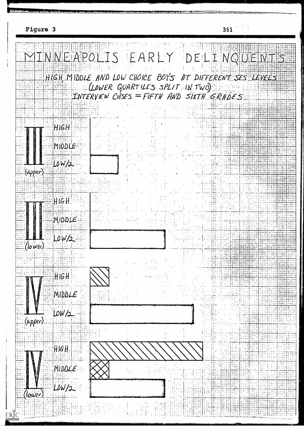
WR, "7:,,7Ers1,13c,43-,rowlrf., ,74117-,

Figure 3 351

1 ?It tr , 1 ,

T1 , Fr.1 ; 1 I-4-4-' II

;-; 1

I r,i4.4. 14/r-t,

, , .

. ,, ,,

, jr

!EA R L. Y.......... .;.,...,,,,.

_...,...,_..,_,,r.....

1-iz:3- iii.q....-,j.F. .2144-r t ,--

:-.'," 4.---,. 1:.: ,.,,

6:1-1:'11.1DDLE Alp.

t .-,21; 11;' -,t-41:--,----14:4----tii-i-,. . , . .

LOW CHOICE 801-15 PT DirreREA s-Es.4LEvEts-1--ft_rftt,-4,

1.:II --11.. if I-7 1 1-1 -I Tyr t-t-- --rt ,:r.

iilek. QuARTILY,5

t--.--T reRyetil (5-es = FFT-1/' .51x-rit''s.R.'Tr: I

* 1 -* * ' 1 ! 1 I t

..___...._...."'71'$

. . 1..tL 1 :II .7-....''I 11-I: .!!'-' 1:17;r11.1'-t-11."7t-1:!"""i

'I*.. 1:1 : $-I I

1f

$ r r

.

1.4.: : r -r, 4 .4,. rr :

, . ' 1 ; r1 iti ; t ' ; , ;

r r : -- i -- r r r r 1-1 'I

. . *-1 . , . '' " , 1 1 . I-$

, ....I....Li -, i 1 $

* $ . 1 I 1

! 1 . 1 I

14' 1

r --r r-t-r-r-r

.. ;

.

r -1 . , r , t.

1-116; 1-i

. I,

L 1

144 'IODLE-..

1 r

-1r

4541-ri-

_,

--,-1 i 1 . - . , 1 1-1 1 1 :1 I

4/ Ir-r --'---, ,

; i 1 , 1 i

71,

r 1

10 tA!_er :I --:...:. I

I - r- -;

I: : : ;-,

-

I !

1 ;-

. . :

t 1 I

iI rr1..... . , 4 I ., I . -

**** ''. -1 r 191.4._ - ....,7-1 1:-.1-

..

, r ,

j ..., . $ , , , ...--. i- -. ...I-, -,-... . 4 I... . 1-1.- ..-.1--1-j-

. .. ; ' --I- r--1.- ., r -.---..-,,- ,-- , , --,-.1-.1.-.1 , a-1-

$ .1- 1 i

1 1 .

LI 1-1.-t t 1 I"; 1-1 I-- /T :: 1 t .1-1 .- .4.-I-' ---r-1-' : 1 .t...t. 4_; , . 4 1 .... ,...4. .. 1. . . '1- 4-""----"-

: H.-- -1!!I-__,....-1_,'-t-.7.___., _...----:_____.......--

4-rt.,- -i -,- -- -i---, - ---7-7 .-,, --,-r, -

1c , r . -,- - ,-. -

,-

'. ,. 1±; 1. , 11 I.. 1. LI: 1+1- f _-_,.-.-I-4-r_r' -r-2,---"*" r 1,', "; 4." ------, -4. -,..-L-nr--i-1,- r r 1 - $ 1 -1 ,--rr-

I ---r1; -. 1 -t -- ' ,- -- - t-r---r ;" 1 ' ' 1-1" "r"' I "t1 t - , ...,....4-..- .-. ---.,---1---, -

. 1 1 1 1 . 1-rt: 1- "-I -, -4 1 i4T-r-71, .. ; T. I .,.. I ; . .- ,71...' ,..: .,.... .

1 "--1" r t r.1.17I 1 rr '---r--I-

t-t- : ---, , - 1 - 1,-- -..-----,- .----..--,-71-4------;. ---,

I $ 1

'r. r --I 1-, --,-*-1- I r

/ -I.-- , $

I '

tt ,

_.,--I . /--.1-. I I .

, ;

' , j ,- '. : :i.e.: , , : ,.., !.., .., r., . ,

.i 1 . : ;.- - . - fI ; --I ''- I 1

.

.. . : . r : . 1 r 1, r-- ? 1 1

. I : 1 1 i ; _ .: 1

ELT .

'at'

352

shown in Figure 4. For the III (upper?, III (lowsr), and

IV (upper) SES groups, the results were approximately

according to our original expectation. For the IV (lower)

SES group, the number of delinquents among the high-choice

boys who were delinquent, in accordance with what was

becoming our new, revised expectation.

To fill in the omissions which resulted from the use of

high, middle, and low boys, for whom we had interviews,

information was obtained in City 2 for all the 1,729 fifth

and sixth grade boys for whom first-year scores had been

obtained. The total number found in the delinquency files

was 187, or 11 per cent. Figure 5 shows the percentage

delinquent for five standard score class intervals of choice

status, for the four SAS divisions of the schools of the lower

half of the city. Again our expectations were approximated

closely except for the boys with standard scores of 6.5 and

above in the lowest SES group. Here the proportion delin-

quent was almost exactly the same as in the low-choice group

with standard scores of 3.4 and below. The other standard

score groups for the IV (lower) schools showed the same sort

of patterning as did the schools in the other groups, and

the high and middle groups of Figures 2, 3, and 4.

`1

Figure 4misms=r:.; . . I 1-,-1! I

I I 11

1

4111,, T-7

- ,- ; ; -f

! t ' 1 :1-111M I ODLE N LOW CHO, , . ,, 1 1

-1 ; t 1 1-1:47.-1:

;.,!. 1114:I r7"

rvi-.C4T

, , 7-I

. , .:, . . : .

(77-- ,-. 7 -71 . . , Lowc 09RTILE...5.!..LH°1-17-:17---77:7-1--- 71- --:

;Li I 1!;";;.. I 10-reVIcki 045E.5": itOiri Let ki.'SE5j...J/ii :--. - ;

1 I .t 1,:ty

. .1

;

; . 7

1 ....

t.474iVO4 '71X1'..titi-itAtQ477,..9-77,7=17f:P7M77.1'7774;147..nr..,.-,741-Pto-it

353

1

'-`-

7 t

1611-.; ;

I.* '

M I DOLL-

.1

I- -- i I t I

r I - I"

;

_ . 4., ; . -7-, 7177r 11111.11111.....111.11111.1110M11111111111011804116/11010

; 1' -I. _; , :; ....7, 4 71

T _77;71 71,7 7

-L77

L - Li:, :,

7-1

--t-,-1 -1 '

4

1-

1,1',.,,f1.1;_: 7.

1--,1-71'7

1 1.

1 1

10 we

tf

- - .

.. .

7

. : , 7 .

' : : 1 . . . . ' 1.:-;(I 7

I t 7 I.I. 1_ . I i .

-..-:-:71: I:I I . I.!

gro4vvopft...14*A

1-1 ' 1 7 1 1 I

-1 t r ;

MINIgr r s 7 ` 1 ;

I

4

. . I

. ,

7 - 7

PI%*Amystitimm

1 1 I

I ...:...,.....,-.7 ...

t!i!!!7

--,-4---------74-4----;

r-

0

r 7

I- '

i .

,-77.7- 1- rL-7 I

1-- L 7

2

rI 4

I-

i' r

1,;: -f 7-14-

7, ' .7

- 1

r r14 . 4;

! t ; , - ,- 14j :11::!... 1. 74 *; r*:T.

1.1 , t, T

.71-,f., 4 1!_!..! : ; .1.,.:-4,-4 7-r -71 -77r- 7 -77 --i

',7-; -7 - 7t--r ----i-li-rrt

rt.,- r7+,--It r:

'1,-1

1 1 1 1

.

i 1 _.'i. i,_4.

I ;

77 777.1 1--t 1-1 7 ;

1 -17 -.!

7 r " *. r t7 1

7 7

rr7I- --47-17-f

..;:: 7 7 :; Is r --t

* 1

r-T

1 r l "r I 7 '1 7

r-I 7 . L .I

, -

7

_7

41o."Ir

1

L7---I I

44-f-

..I t : *7-*

jr 1 -1 I/ 7 I, ,

7-

-1-17'» ' ' 1 t 7', I 1-7. 1 -- .-7--7

; 7-7*

-,7-,..

. I , :1-1 '

' -7 44,-

4- .1--......1.

-.7

7-14 -t -t-1'17

i71' !, 7- 1 -1.

1 7.1. 4 -; 1-

rr r- .

IXNSMX%M.,rirc %NI

r it t

[:

,

;

'4-,

---;

-r ±''7-I- -I 1 t

- , - 4 I-.

-t' rr 7-,.....r. , ,_ . I-;;;.;;;+-1- . ,.... I 1 1. -r, ,

-

4-44-

i 7-11- - --71--17 r *It:.:. ! 17'1

r -7

111' 11

7:1

L11 :_, _''1_i: '-.;111',1 1;7,12;1 ' -I- i 1 - . -1, -1 - f; 1- t - ,-;-i-1-

' ' 1 t ,r1- 4" . . Li ' . 1- ;"--. '-1 1 1 1 _I- t . T 7 . I

7 7.1 ! ;f:: 1 7 f' 74 i I 1

.: :-.;.L.....1...1. 7t .-7 1 f - tI

; 4

1 i- , i t 7 ; 7 t -7,-7 1 I

__7 1,,

t 1 , 'HI 7- li I : i ' i l ; 7 - , '4 t,

114', ::: '.--.I! : , _ .. _L.. __ ,. ...,

......lit,17 ..1.1 11 *7.-:* -; I '*. 1.- 7I * 1 1. I i 4 . . I . I 7' .

,_,. , , ......L I 7 1 '

' : 1.

i 71,

, . - - -,

354Figure 5

pJJ .F.Jfl:H iLi'_sCO1

:t1!1-

f ? LL 4 j t

j t t L! _ 'I irt I 4

!r :

Li4 h ,

::515: H. ji4ThT :;

'*1:::: E!: TE ': TETP . F:;:tT :Y ±t ft TTbe.1wf 4E4L: 4: 4:1 U

jt tTtEit H+- ---4 4- i) i:; ii ::t:" Ht.1 :4. ;.1FB !

.t r;-:T 4 TF4t f t1 .r:-: T::i T 1 r.5

-1 r p- --trt

4; ;:r4 --t -- t.

1-. r-- ;' r-t t.

t i_L 4, L:::3. I±O:::L tf: I ;:!J± r tiEk -Fz,.;4SS:4 lTö

I I;:T: JIi i.tt:: ii5

:I::. 1S:i14

-5-.-' .- .. -S$S_

S.S,

S.7 j 4 14

f ., 4_ 4'..- . - S.I:

S4 - j 4-. .5 -r- ----t- -+1t :t ti:tTt: + tr : S:-' 1:t_Lf.L_1tS S. : 37s 4z3i4 I

.:4f.:s: :Lt5 ::4:t: SJS -f; : t i5 tt '-:- ± '-i-tSt _1 i T

Pt r frN rr L -r 11jrI4:

:

r:-v:( r 1t+r +

L1_4:Ls:1 55T ift: pE.EI tS ; :1:

t--, l-.- r ' -,55 ±:Q 43:1

r' t1 -r: th f-L iO(14 -± 13r-91 1 *1

!fi L':F

I: .'4.: ' :L+.T,rt 9

Jii t 'it.5 .:.tf ::I4 : .:: :' r:: J ' ii Tt fli t ii + '

.5

4tr±r1r 4 4 (1.jr .4

L?:L r r

E ±t ut r t4 L 9EE-T r : Hr49 t 4 t r + . t

-.&4

_: I t.i': i1 1ft4r '1L

:j ' : s;;:

-H; : Uh.+j. 4h 4i

C..: .:,.5--; ,. ..

:4 ' X, E r- Lf f 'T 1r4 (4

. T -rL fl

, to ::r 1 r.!±i H .4t1 J : c) +

tt-'---S 4_ 44-i t-r+-+- .,, 4 , r S. . _

t1E ::.aT ..1

.. : 1:L) :r .1 .. St ti:t- _ --- .

5S

.k,,;

.

355

ILLUSTRATIVE CASES

In the first year of the project, descriptions of

selected high, middle, and low children in each class were

obtained by interviews with teachers in order to provide a

more concrete picture of the individual children than was

given by the choice-status score alone. These descriptions

have been found useful in many ways. In the present context,

they give information about the cthildas seen by school

personnel, including various factors in his life situation

which may have had some relationship to his subsequent

behavior. Selected cases are presented here to illustrate

the way high and low-choice children at different socio-

economic levels were described.

per SES Quartiles. As indicated in Figure 2, there

was only one high-choice delinquent in the two upper SES

quartiles in City 1. We can begin the illustration of the

described behavior characteristics of high and low-choice

ya.angsters with the single high-choice boy from the two

upper groups and the two low-choice boys of high SES status.

These are, respectively, Frank, who was high choice, and

Thomas and John who were low-choice boys.

FrankFrank (sixth grade) is a large, fat boy, extremely shy,

who always looks dirty and unkempt, his clothes messy andhis hair uncombed. Although he can do things all right, helooks awkward when doing them, particularly writing. Henever volunteers for anything. He has been absent a greatdeal, usually three or four days at a time, with stomachtrouble due to extreme nervousness. He is good at his work,

4Aa:1,14,;:4.

356

tries hard, and when absent always makes an effort to do themakeup work so that he can keep up with the class. He isself-effacing, seems quite embarrassed when called on andshows much ambivalence in volunteering for things. On theother hand, he is beginning to take part in the teenageactivity; they do giggle and laugh about the other sex, buthe is quite upset when the teacher has to reprimand him.The teacher feels that in some ways this activity is animprovement and she would rather put up with much of hisplay with the other kids as long as he is doing what seemsmore natural and normal for him. She has had him for two yearsand has seen a decided change in his behavior, particialarlyin his asserting himself more than he used to do.

On the whole, though, Frank is still a rather passiveindividual in class. On the playground, he is definitelyinterested, and he comes back all out of breath, having beenthoroughly active in the games. He speaks in an extremelytiny voice and seems afraid to make mistakes. He gives theimpression that he would die if he made another mistake.He does not demand much attention of the teacher, justaccepts her.

The other boys accept him well; he talks to them easily,they choose him on their sides when there is some sort ofcontest, and they give him much recognition when he doessomething well.

Little information on the family except that his motherwas divorced from his father and is now remarried. Frankreflects his stepfather's interest in him and talks aboutthe stepfather's experiences. The mother is cooperativetoward the school, and the teacher feels that Frankdefinitely reflects kindness from mother and stepfather.

Probation Information:Two years after testing, malicious destruction of

property. Referred to parents. About a year after this, themother became overtly psychotic. Soon after this, Frank wasarrested for auto theft and placed on probation.

ThomasAverage-size sixth grader, fairly good development..

He possesses average physical skills and generally can holdhis own on the playground. Teacher estimates that he hasabove average ability; however, achievement is not up towhat might be expected. Rather poor general adjustment.He is quite a problem. Has to be watched carefully. Majormisbehavior such as throwing stones at cars and lightingmatches on the school stairs. Untruthful and antagonistic,both toward teacher and classmates, so in general he is notwell liked by his peers. He has one other friend, a boy whois also known as a "troublemaker."

ox,r0o,11,,M117,..02.

357

Tom is restless, constantli on the move. He appearsto be quite happy, is outgoing. The teacher believes thathe has good possibilities. He is able to reason in a fairlymature fashion and seems quite sensible when called upon todiscuss life in general. Both parents are working, and theboys (3) are left alone a good deal of the time. Theteacher knows the parents are in disagreement as to how tohandle the disciplinary problem. His father has ratherstrict standards, but the mother is on the other hand verypermissive and perhaps unconcerned.

Probation Information:Age 16 1/2: Possession of liquor and drunk. No

record of either social agency contact or contact with thelaw for any other member of the family.

JohnJohn is a very large fifth-grade boy, the largest in

the class. He is also one year older than the others,having failed one year. Last year he broke his leg and hewas somewhat lame; it is getting better now although he stillis not too well-coordinated and is somewhat awkward at times.

He is a bully. He picks on younger children and doesnot play well with the kids in his classroom.

He is an apple polisher; he tries very hard to workhis way into the group of children who are the most popular.

On the playground, John picks on the small participantsand he is one of the last chosen. In the classroom he isvery good, quiet, cooperative, and causes no disturbance.You hardly know he is in the room. Academically, he isbelow average, has a very difficult time getting his school-work done, but he works at his assignments.

His attitude toward other children is one of domineeringthem. He takes it out on smaller classmates and singles themout one at a time for picking on. He teases them, holdsthem down, takes their hats away, etc. His aggressivenessis not confined to overt fighting, but rather to some formof passive aggressiveness holding a child down to say uncleand not letting him go, or teasing. His relationship to theteacher is very good. He does what he is told and causes notrouble in the classroom. He tries to please the teacherand he brings things from home to show the teacher and theclass. The trouble he is experiencing is all out-of-doors.

He has been doing better in school work, and there hasbeen some progress in his relationship with others. Thekids seem to accept him more now. He can now Ht the balland, being the biggest in the class, he's somewhat moreaccepted on the playground in athletics.

Most of the students let him alone. The smaller onesdislike him intensely and fight him off.

358

The mother is described as being very good. She willgo to bat for the children. Whela they are wrong, she willpunish them. John is the second youngest of five children,four of which are boys. At home there is a rather rough andtumble life, and John ta picked on, being somewhat dullerthan his siblings.

Probation Information:At 15, burglary. Lives with father and stepmother.

There is no history of contact with any social agency, nor ofany contact with the law by any other, member of his family.

Lower SES Quartiles. Space does not permit the presen-

tation of a case of this kind for all possible combinations

of SES and choice status. Typical low-choice boys from the

second and third quartiles are presented next (Paul and

Randy). For both of these SES groups, the number of high -

choice boys who became delinquent is very small.

PaulA very small, undernourished fourth grader who has a

cute face and is rather nice looking. He talks babytalk attimes. He has no marked strengths. He is often dishonestat games and he generally makes a poor adjustment withothers. Nevertheless, the teacher pointed out, there issome indescribable quality that makes this youngster likeableby adults.

On the playground, he is aggressive at times with otheryoungsters. He enters games and seems to enjoy them. Inthe classroom, he was described as sneaky. Sometimes ire, theclassroom he displays bad temper. He treats others in theclassroom in an aloof manner. He visits others occasionallybut seems not to become too personally involved in socialcontacts. The group in return for his aloofness also treatshim in an aloof, distant manner. A good relationship existsbetween the teacher and the pupil. She can correct and guidethis youngster when he is not behaving properly. He hasnever shown any strong feelings toward the teacher.

He is totally disliked. The girls dislike him and theboys dislike him. The girls dislike him because he beatsthem up, and the boys dislike him because he's sneaky andbecause he doesn't follow the group's standards of behavior.He disturbs them because he does not follow directions andhe is not fair.

359

The family is large and somewhat lower economicallythan their neighbors. The parents are not effective indirecting the youngster or his siblings. There are economicproblems that the family must face. The mother does notfollow through consistently on any plan concerning theyoungsters.

Probation Information:When in second grade, picked up on three separate

occasions within one week once for burglary, twice forpetty larceny. No charge was placed. The following summer,he was arrested for burglary and put on probation for twoyears, Soon after school started, again caught for pettylarceny. In the spring when in the third grade, he wasarrested for burglary and sent to county training school.On release, again charged with burglary and prowling cars.Two months after this testing, burglary and arson, andagain sent to Detention Home.

The father has a history of five arrests for assaultand battery, drunkenness, and wife beating. About a yearafter testing, father hopitalized as psychotic. Oldest .

brother had history of six arrests, next brother had on.arrest, oldest sister had six arrests, next brother hadthree arrests, and next sister had seven arrests. Motherdescribed as showing serious emotional disturbance.

Probation report while in second grade: quite percep-tive and capable of independent thinking and expressinghimself. Open negative feeling to father. Lives forpresent. Expect severe destructive aggression in future.Severe character disorder manifested by impulsive actingout, impaired ability to enter into meaningful relation withothers and considerable immature narcissism.

Mother and father divorced while Paul was in sixthgrade; they tried to give him some attention, but this wasdifficult with ten children. Both drank too much.

RandyA small, wiry sixth-grade boy with flashing eyes, a big

smile, and usually neat appearance. Devil-may-care attitude.He doesn't seem to care if school keeps or not. Highlyself-seeking, self-pushing, egocentric. Seems to need tomake sure that everyone knows he is intelligent. He is veryverbal, loves to recite orally, but hates written work.Tremendous memory for facts which he acquirea from reading,TV and radio. He is a complete individualist. He isn't atall like the other children except that he does seem to wanttheir approval. His answer to a list of offenses told himby the teacher was in the nature of debating style. "Now inthe first place, I did not...." and so forth. He counts

360

them off on his fingers. His strengths are his _.: mindand wits and his ability to thin. something through, althoughan IQ test suggests his ability is less than teacher hadsupposed. Almost analytical in his thinking. He has theability to bluff. His greatest weakness is his completelack of motivation. He seems willing to be far less thanthe best academically, partly because he is unwilling toreveal his shortcomings. He is almost criminal-like in histendency to shift blame. Two juvenile officers came toschool to talk to him about vandalism in a closed store, andwith an innocent look he sent them to the junior high schoolto talk with his older brother, who was really just an on-looker. The officers soon returned.

On the playground, he wants to be a big leader, astrategist. He would have been a good Nazi. He is not out-right cruel to others, but he lacks understanding of theirfeelings and fears. No one else matters. He is a goodcompetitor in class games, is not a poor loser, and is satis-factory in supervised.' play, but in unsupervised activityhe wants to be the ....preme dictator.

In the classroom his behavior is not exceptionally bad.He has a tendency to be polite when he is criticized, and heseems to take it well even though he gives excuses. He getshis name on the board for little things, and he is constantlyreported by guides and patrols.

He has fairly normal relations with his peers, in spiteof his acting so superior, for he doesn't act superior withall the boys, nor all the time. He irritates the girlcbecause or his acting so smart, and because of his frequentinterruptions. He wants to be very friendly with theteachers, but he has difficulty achieving this, for he feelsthat rules made for others don't apply to him. Rules arefor the ignorant ones. He doesn't outright defy the teacher,rather he seems to ignore. Sometimes he grins as though hehas to go along because it is necessary for the rest, but heseems to say that you know and I know that I really don'tneed these rules.

Most of the children pass Randy off. They have beenused to him a long time. H4s cuteness and sharpness can'thelp but impress some of these kids, even though he irritatesthem. His patronizing attitude of cutting in on others'recitations is one of the reasons why the children react tohim as they do. He is also too aggressive. He is really abully, even though he is small. He will try his bullying ona larger child even, but one who doesn't want to fight.

The parents are impressed by his factual knowledge, andthey and his older brother and sister think he is cute. Theyare not as sharp as Randy. He is so well accepted by hisfamily that he surely feels secure. A definite weakness isthat the parents are not realistic in their appraisal, and

N

361

they do not think the school appreciates their boy. They don'trealize that he does not do the writing work expected of him,even though they have been told many times.

Probation Information:During spring of sixth grade, he was arrested for

malicious destruction of property. There is no subsequentrecord.

Lower Half of Fourth SES Quartile. The SES level of

greatest interest here is the lower half of the fourth

quartile or approximately the lower eighth of the boys in

SES status. In this group, as indicated in all four charts,

2, 3, 4, and 5, there are as many high-choice delinquents as

there are low-choice delinquents. Our interviews indicate

that in general the high-choice boys were in tune not only

with the other boys, but also with the teacher and the school

in general. Insofar as both their peer status and the inter-

view materials are concerned, they do not seem to be "person-

a li problems." On the other hand, the low peer status

boys in this SES level are characteristically disliked by

the other boys and not so well in tune with the teacher and

the school. There has been a good deal of talk in the

literature about the "delinquent subculturc," As a general

explanation of all delinquency at this level, this represents

an unproved assumption. It is closer to the facts to describe

these delinquent boys as coming from a bottom economic level,

which produces more than its share of delinquents, whether

as members of a delinquent subculture or through the

.11

362

operation of other factors, such as family disorganization,

"improper" rearing, etc. Edward is typical of these.

EdwardEdward (fifth grade) sometimes looks very neat and

clean, and other times looks like he climbed out of a ragbag.Occasionally he doesn't even make it to school, apparentlybecause of insufficient clothing. Edward is slender andappears undernourished. He is an attractive boy with a lotof drive. He probably is a good deal more sophisticated inthe ways of the world than one would guess from his conver-sation. He's very nice and polite in school. Edward is agood student, but one handicap is that he rushes to get done.

Edward is a good ball player and a good sport and well-liked and one of the first to be chosen on any athletic team.In class the youngsters also like him very well and arequick to choose him. He's usually mannerly. He's no botherto anyone, would quickly reach out to help others. He'sdependable and is listed as the best-liked boy in class.Good average intelligence. The teacher said that he couldnot be nicer to her; he's cooperative and courteous, wantsto do well. He does not ask her for help. I think part ofthis comes from his being forced to be independent from hisdisadvantaged family.

He does things well, is quiet, does not make himselfa pest.

A very unfortunate home situation. MoLer apparentlydoes try to help work with the youngsters. Neither mothernor father make conferences.

The father and mother could perhaps be adequate parentsif they had one or two children, but with the extremelylarge family that they have, they are both overwhelmed. Asa result the youngsters do not get the proper care andemotional help that they should get. Father is frequentlyaway from home, separated from the mother; mother, in seekingcompanionship, is apt to reach out to other men and toentertain them and have them with her in her own home. Thisprobably has some adverse effects for the youngsters. I seeboth parents as being rather immature adults who are apt tosatisfy their own needs before satisfying the needs of theyoungsters. As a result, the youngsters are many times leftwithout the proper parental attention. Surprisingly enough,they seem to do quite well under these conditions. They areattractive, lovable, and likeable boys and girls. Whilethere has been some petty thievery, some truancy, and somelack of application on the part of these youngsters, by andlarge they are happy, fairly well organized boys and girls,who seemingly make the most of what little life has offered

2A. ....AMON,.

363

them. Currently, there has been talk by the welfare agenciesof the possibility of removal of the youngsters from thisfamily. At this point, because again of the kind of adjust-ment made under these adverse circumstances, they have beenreluctant to see the older youngsters go; it's the smallerones that would be most hurt if they should hEve to leave,yet it's the small ones that perhaps would have the bestchance to move on and more fully develop their capacitieswith the chance to live somewhere else.

Probation Information:Edward had been arrested for malicious destruction of

property and referred to his parents about a year beforetesting. About a year and a half after testing, he wasarrested for shoplifting and put on probation for a year.Six months after this probation, he was arrested for bur-glary; at that time he admitted nine other burglaries. Hewas sent to the county training school, where he stayed forsix months and remained on probation for another six monthsafter that. This brings him almost up to the time of thefollowup.

The family was well known to various social agencies.An older brother was in an adult reformatory, and a secondolder brother was on probation at the time of followup. Thefamily was described as being unstable without the father.The mother seemed unable to supervise and had had an ille-gitimate child about two years before followup. The psycho-logical interview report said that there was nothing grosslyabnormal or unusual about him. Stable mood, emotionalreactions generally appropriate, though well-guarded; slightlyunhappy, has some poor opinion about himself, is fairlyenergetic--likes people. A normal person is indicated.

It may be noted that although the description of this

family situation seems to be adverse, apparently the boys

and girls get along surprisingly well. Of course, there has

been some petty thievery, truancy, etc., but both at the

time of the initial teacher interview and at the time of the

probation interview after he had gotten into trouble, he was

judged to be a "normal person" who was exhibiting some

misbehavior.

364

A somewhat similar picture is given by Joe, also a

high-choice boy from the bottom SES group.

JoeJoe (fifth grade) is small, short and stocky, very

handsome, with a sparkling eye and a bright alert-lookingface. He's very well coordinated. Distinguishing him fromother children, is his quick smile, his sense of humor, andhis tolerance and acceptance of others. He's extremely fairin all his dealings, seems to expect fairness in return and,generally, has a good, healthy outlook on life. Has leader-ship ability, accepts responsibility well, has an inquisitivemind, and is rather adult-like in conversation.

Joe does very well in playground participation, respectsthe rights of others and is a very good group member. Hehas athletic ability and is looked up to for this. He's oftenchosen as captain of a team, but this seems to be morebecause of his fairness in dealing with the other youngstersin a heated discussion than because of his athletic ability.

In the classroom he is very responsive. He participateswillingly, volunteers regularly, has a great deal of back-ground information. His tests indicate that he is over-achieving. Youngsters are anxious to have him on committeesand often look to him for leadership in class as well as onthe playground and in the halls. He has been a good policeboy. He's very well liked by the children. He has an olderbrother who has been involved in a great deal of delinquentbehavior. The children have mentioned this to Joe, and helaughs and says, "Sometimes we are not all alike." Heresponds well to the teacher; he wants to please, but not inan anxious way. Joe accepts the teacher's role as a disci-plinarian and will respond to discipline. He comes from adisorganized family. His mother has been married three times.The whereabouts of his own father is unknown. He did notget along with his first stepfather but does relatively wellwith this one. He has one brother and several half-siblings.The mother and the current stepfather have been fairlycooperative with the school, coming for conferences. Themother feels that the youngsters are capable of caring forthemselves and has given them an undue amount of freedom.Joe has been able to use this very well, while other membersof the family have not. The mother has indicated there isa lack of discipline within the home, and this is evidencedvery clearly with other members but not with Joe. He isresponsive to adults, respects authority, and generally isa happy, well-dispositioned child.

365

Probation Information:About 18 months before the study, when he was nine

years old, he was arrested for petty larceny and referred tohis parents. Two and a half years after testing, he wasarrested for malicious destruction of property and referredto the school authorities. A year after that he was arrestedfor incorrigibility, truancy, and running away from homeand placed on probation.

His older brother was sentenced to the penitentiary forseveral years, a few months prior to the time when Joe wastested.

It may be noted that the personality characteristics

described for him are generally very favorable ones. Neither

originally nor later was he considered a personality problem.

On the other hand, if we take a look at a pair of low-

choice boys in this bottom SES group, we find not only

indications of delinquency but also indications of perso-

nality difficulties. Jackie is one illustration of this,

and James is another.

JackieJackie (fifth grade) is of average height, has fair

hair, is fairly neat and clean - -it varies. He is very loud,has a very mouthy, negative attitude. He can be caughtdoing something right in the middle of it, and he will denythat he had anything to do with it. He takes pins out ofthe bulletin boards, pulls the shades, throws the flowers onthe floor, pulls the bristles out of brooms, and he usuallythinks he is being very funny and he has six or sevenchildren egging him on. The teacher felt that he is entirelydifferent from everyone in her room. The assistant principalhas said that he is a "crazy nut." He never works in theclassroom. He does no spelling, no arithmetic, no reading.The teacher doesn't have too much trouble with him, but sheis very dissatisfied with him. He is usually sent out ofthe room.

In the gym he is very uncooperative, not much coordi-nation. He has to be protected to see that he gets his turn.He is not chopan very often; he doesn't play fair. If thereis something that goes wrong he never says that it is hisfault. He always blames somebody else.

'4W*91",tvi..4,

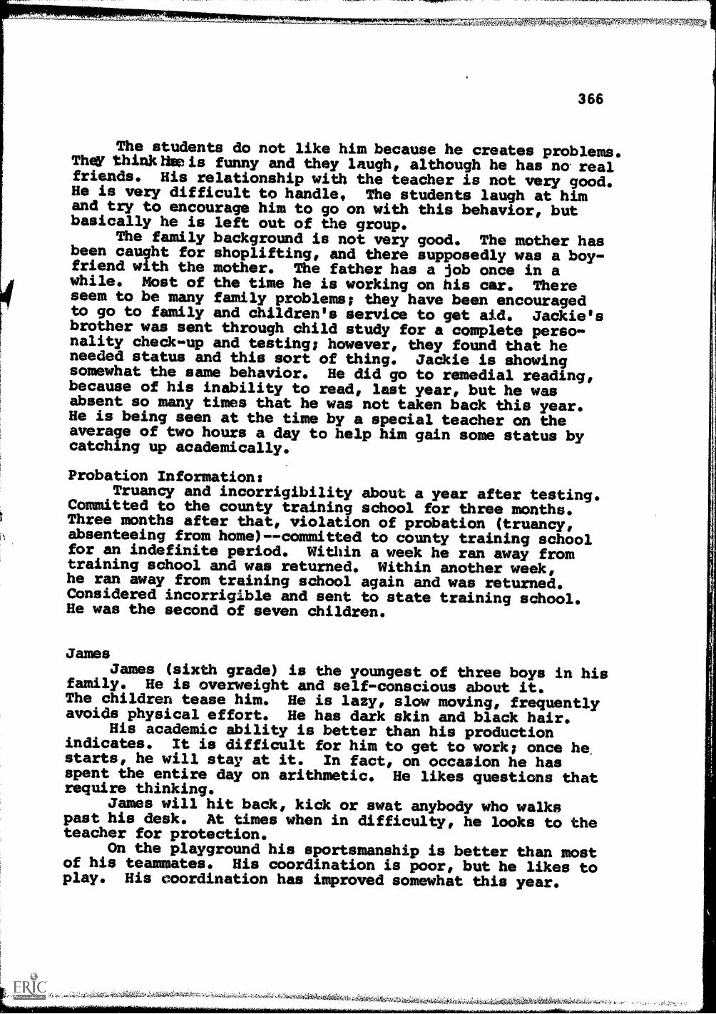
r mlmnsrAng

366

The students do not like him because he creates problems.They think Ike is funny and they laugh, although he has no realfriends. His relationship with the teacher is not very good.He is very difficult to handle, The students laugh at himand try to encourage him to go on with this behavior, butbasically he is left out of the group.

The family background is not very good. The mother hasbeen caught for shoplifting, and there supposedly was a boy-friend with the mother. The father has a job once in awhile. Most of the time he is working on his car. Thereseem to be many family problems; they have been encouragedto go to family and children's service to get aid. Jackie'sbrother was sent through child study for a complete perso-nality check-up and testing; however, they found that heneeded status and this sort of thing. Jackie is showingsomewhat the same behavior. He did go to remedial reading,because of his inability to read, last year, but he wasabsent so many times that he was not taken back this year.He is being seen at the time by a special teacher on theaverage of two hours a day to help him gain some status bycatching up academically.

Probation Information:Truancy and incorrigibility about a year after testing.

Committed to the county training school for three months.Three months after that, violation of probation (truancy,absenteeing from home)--committed to county training schoolfor an indefinite period. Within a week he ran away fromtraining school and was returned. Within another week,he ran away from training school again and was returned.Considered incorrigible and sent to state training school.He was the second of seven children.

JamesJames (sixth grade) is the youngest of three boys in his

family. He is overweight and self-conscious about it.The children tease him. He is lazy, slow moving, frequentlyavoids physical effort. He has dark skin and black hair.

His academic ability is better than his productionindicates. It is difficult for him to get to work; once he,starts, he will stay at it. In fact, on occasion he hasspent the entire day on arithmetic. He likes questions thatrequire thinking.

James will hit back, kick or swat anybody who walkspast his desk. At times when in difficulty, he looks to theteacher for protection.

On the playground his sportsmanship is better than mostof his teammates. His coordination is poor, but he likes toplay. His coordination has improved somewhat this year.

,S ,rsTIMMOT;.q.5 "

367

In his classroom behavior, he aggressively acts out against

the children and against the teacher. Teacher holds himbriefly in his more explosive moments. After he quiets down,

he will go to work. Limits have to be set and firmly held

for him,He tries to buy friends through giving candy, gum, and

so on. He has one friend in the room, a boy who is quiteemotionally disturbed. When he does not strike out against

the children, some are apt to bring him to it. The children

seem to have cast him in a role that will be very difficult

for him to change. At the beginning of the school year, hescreamed, lashed out at or walked out on the teacher. Now

he still gets angry and will lash out at him, but he recoversfrom it more quickly and settles down more easily. There

has been a slow but fairly consistent growth in self-control.Children reject him. He almost demands this, despite

his wanting to be liked and trying to buy friends. He

starts many fights with children over petty things. The

children fight back. He is gradually withdrawing from this

kind of fighting. If children really start a fight with him,

he will fight it through.The teacher has only talked with his mother by tele-

phone. She is interested in James, overprotects him, andwill take his side against any other information that might

be offered.

Probation Information:In seventh grade, insubordinate in school; sent to

county training school for six months.Family had eight social agency contacts. Father

attempted to murder mother and committed suicide when Jameswas four years old. Mother was unstable, but willing to

help. Psychological interview found: Impulsive, aggressive,

seeks attention--many somatic complaints--inner self-control

lacking. Marked dependency needs--poor peer relations- -

unresolved emotional conflicts (parents not desirous ofseeking help) --not sociable.

Whereas Joe, above, was mentioned for his fairness,

Jackie was described as "he doesn't play fair." And whereas

Edward, above, was described as "very nice and polite in

school," James was described as "hitting anybody who walks

past his desk." These pairs of boys seem at the extremes

of other continua besides that of peer status.

i",:fiNa446.*

368

Negro Delinquents. Since there is a tendency in some

areas for low economic status to be confounded with race, it

was a matter of interest to see to what extent, if at all,

the phenomenon that we are discussing here was attributable

to race. Inspection of the abstracts, of which two are

presented here, indicate that delinquent youngsters with

both good and poor peer adjustment occurred in the Negro

group. In these cities, less than four per cent of the

entire grade-school population is Negro, and these are not

all confined within the lowest SES group. The pattern found

here may not fit other cities such as New York or Chicago

where the proportion of Negro students is so much larger.

It should fit a large number of cities where the ethnic

composition does not differ too markedly from that of the

present cities.

Of the two Negro cases presented here, Willy is not

only liked by the other boys, but he is also diligent in his

schoolwork, although his ability level is not high.

WillyA sixth-grade Negro boy, well coordinated and in good

physical condition. He is the number two boy in the schoolin control. The bois respect him and a great many are afraidof him. He seems to be a leader. A consistent good sporton the playground. At times he protects the underdog, buton occasion he may kick him.

Willy is a very dependable police boy. In school heworks hard. He is of dull normal ability. Even though heis slow in Glasswork, he does not want his assignments cutdown for him. His effort is great enough to complete hiswork. He is not always right, but he certainly tries.

1WA

741M7ggier

369

Teacher, a man, gives Willy responsibility in theclassroom, and he carries it out consistently. He does notassume responsibility if it is not given to him. Boysrespect him and like him. There are several boys who wouldlike to take his crown as number two man away from him. He

is respectful, cooperative, and responsible. He is recog-nized by his peers for his leadership qualities. Strangelyenough, for the position he holds especially in the estimationof the boys, he is not an aggressive leader. He always holdshis own and gives an excellent account of himself whenchallenged. He rarely seems to challenge others.

There seems to be a gradual, consistent maturing inWilly this year. Children like his persistent trying, nomatter what the job assigned.

His mother is cooperative with the school. She is muchinterested in her son. She wants him to be a good studentand a good boy. Willy respects his mother and, on occasion,has told teacher of little things he has bought for hismother. They are a close family.

Probation Information :Two months after testing, charged with immoral conduct

and placed on informal probation. One month after that,auto theft and sent to county training school. In spring ofseventh grade, truancy and returned to county training school.The following summer, shoplifting. No further trouble untilninth grade when charged with driving without a license anddisorderly conduct; informal probation.

Has five older and two younger siblings; two olderbrothers have histories of delinquency. Father is deliveryman, mother is housewife. Probation interview notes "lacksstrong male influence - -quite close-knit family--good siblingrelationship."

On the other hand, Don is actively disliked and consis-

tently nonconforming in the classroom. He has twelve

siblings, some of whom also have records of delinquency.

He is not described as being a boy who is getting along well

within his own peer culture.

DonDon is a dirty, sloppy, well-built, apparently healthy

colored boy (fifth grade). He is a nonconformist with littleconsideration of others or of the situation. Athletics is

1.7r=torAl,

370

Don's only visible asset. His weaknesses are that hepresents no apparent reasoning ability, is greatly retardedacademically and is very inconsiderate of others.

On the playground Don tries to run the show, tends tobully, is quick with the fists. He has good athleticability and skills, but shows poor sportsmanship.

In the classroom he talks constantly. He is consis-tently nonconforming. Rules are made for everybody but him.With others he is inconsiderate of their feelings; he mayeven knock heads together. He delights in proving hisphysical strength, even in adverse ways. He himself is notinterested in others except by way of showing his strength.

With the teacher there is no communication either way.He may not answer at all; he often has an "I don't know"response, and there continues to be an impasse, no outrightconflict, but no real rapport possible. There has been nochange in Don's behavior during the year.

Others' reactions toward Don are that some fear himbecause of his size, some are disgusted with his behaviorand lack of cleanliness. Those who are fearful of himbecause of his size, he tends to intimidate. His tangleswith the law tend to appeal to some. Others may look to hisability in athletic skills. But even with the variety ofresponses, actual relationship with others is limited.

Don comes from a very large family. There are twelveor thirteen children. To observers there may appear to beparental apathy. However, there may be interests which areoverlooked because of the overwhelming responsibility heapedupon this family. There is a sweet compliance on the partof the parents but an inability to follow through withguidance and with real care. The father remains employed,which is a decided family strength, but his livelihood isnot really sufficient for that many children. Guidance isinconsistent. Actual physical surroundings are bare andsparse. There is sometimes not enough food and insufficientclothing. Many of Don's siblings are retarded, and severalare in a great deal of trouble with the law.

Probation Information:First delinquency recorded while in third grade,

breaking and entering and petty larceny. In two days duringfourth grade, charged with four offenses, primarily shop-lifting and petty larceny; placed on probation fors year.In fifth grade, insubordinate in school and probationextended. In May of fifth-grade year, bicycle theft,insubordinate in school; committed to county training schoolfor an indefinite period. In fall of sixth grade, assault;probation continued. In spring of sixth grade, insubor-dinate in school; committed to state training school. r

4r24 «SAtigaeiVaaaik44-4,.

MWRiMMAMMa704

371

Had twelve siblings, seven older than he. Two olderbrothers and an older sister had repeated records ofdelinquency.

SUMMARY OF RESULTS

The contrast is sharp between the high and low choice

boys in the bottom group. The interviews presented above

give a clear picture of some of the behavior of the low-choice

boys, who constitute one important group of delinquents;

they are obviously not well accepted by their peers. The

high-choice boys got along well, not only with their peers,

but also with the school. The interviewed teachers were not,

of course, totally unaware of the status of the boys that

they were describing. They had had an opportunity to see

some of the choices made, in the course of data collection,

a month or two before the interviews. More important than

this, they had opportunity to observe the younsters daily,

and interviews concerning both boys and girls are full of

comments such as "he (or she) is always the last to be

chosep,l'or, at the other end, "he is a leader and is usually

the first one chosen on the playground (or in the classroom)."

Choosing is a frequently occurring activity, and youngsters

who are not chosen can hardly fail to be aware that they are

not.

At all levels above the bottom one, delinquency is prog,

gressively less frequent as we go up the scale of choice

Mut,.;fattt'N'OpPlrpAvlr.Fo...rmpT,,,

372

scores. In the bottom group, this is also true except for

the highest status boys. From earlier work, we still expect

these high-choice boys of the bottom group to make better

adult adjustments than the lcw-choice boys.

DISCUSSION

This discussion has consistently referred to the delin-

quents followed up as "early". In the light of the emphasis

placed upon gang activity in some discussions of delinquency

(Cohen, 1955; Short and Strodtbeck, 1965), this group may at

the time of the followup check still be too young for this

to be as prominent as it may be later. With this reservation,

it is of interest to compare the present findings with

currently prominent points of view on delinquency. The

literature on delinquency is very large, and space does not

permit a comprehensive review of it here. To place our

findings somewhat in the context of one particular part of

the literature, reference is made to a conference report from

the Children's Bureau in 1960, "Sociological Theories and

Their Implications for Juvenile Delinquency" (Bordua, 1960).

In an overall view, two theoretical positions quoted below

are most prominent, particularly in accounting for group

delinquency.

Theories of Delinquency

One of these sees the delinquent subculture as "arising

out of the socially structured gap between the aspirations

Si9iia4;

373

of lower-class boys and the means realistically I:mai:Able

to them to realize these aspirations. According to this view,

lower class socialization does not equip boys to perform

according to the requirements of middle-class dominated

institutions such as the school, and consequently the boys

suffer 'status deprivation' and low self-esteem.... The

delinquent subculture values precisely what middle-class

institutions devalue; e.g., 'hanging around' instead of

industriousness, aggressiveness instead of self-control."

"'Status deprivation,' then, provides the motivational

core for the lower-class male delinquent subculture

Equally crucial is the fact that 'status punishment,' in an

institution such as the school, tends to be differentially

concentrated in lower-class groups who are residentially

concentrated in certain parts of any city."

This simply does not fit the picture given above of the

present sample of boys at around the fifth or sixth grade

level.

The second point of view sees the "beliefs and values

of the street-corner group as arising, not from any situation

of status deprivation, but as simply the adolescent version

of 'lower-class culture.' .This position directly opposes

the notion that the street gang or groups' culture derives

from a reaction to the demands of middle-class culture.

Instead, it emphasizes the view that 'lower-class culture,'

374

as a more or less systematized body of beliefs, values,

'focal concerns,' and even household forms, has existed in

its own right for generations and need not be considered as

a reaction to beliefs, values, and household patterns of

the middle class." One question that arose was "What is the

evidence that there is a loweir-class culture which the

adolescents are considered to be reflecting?"

Delinquency Theory in Relation to Present Results

Our present results clearly support the second point of

view and offer clear-cut indications of a difference in the

pattern of delinquency at our upper and bottom social .levels.

At our upper social levels, delinquency appears as primarily

a function of personality disturbance as reflected by low

peer-group status. Almost no high-choice status boys from

the upper levels were delinquent. At the bottom of our

eight social levels, there was still a marked trend for the

boys with low peer status to show delinquency more frequently

than the average boys. Here, however, the high peer status

boys exhibited delinquency almost exactly as frequently as

the low peer status boys. Qualitative information available

for these boys at the fifth and sixth grade levels indicates

quite clearly that they were not at that time in rebellion

against that so-called middle-class institution, the school.

They got along well with their associates and exhibited a

reasonable amount of ambition scholastically. In some cases

w,:o.vawa-Avok-A

1,72 '''=4=2:SirreZZrlit74Zr

375

the boy had already shown some delinquency at the time of our

study, and the teacher sometimes mentioned this as casually

as he or she would mention the color of his hair. Some of

these boys gave a clear picture at this age of being "in tuna"

with their associates, and with the school, and with the

teacher, although they sometimes came from highly pathological

family situations. Nowhere in the literature, have we found

anything which describes the total effect that is being

described here.

In the present study, social levels were divided in

terms of the education and income of the adults in the area.

It seems clear, and is replicated from one to another of the

two sample cities, that the lowest of the eight education-

income levels produces n substantial number of boys during

the pre-adolescent period who are not in any sense in

rebellion at that time, although they may exhibit some delin-

quency, then and later. On the other hand, there is also a

sizeable group, similar to that found more commonly at our

higher levels, where the delinquency is accompanied by

personality disturbance and a rebelliousness which seems to

be personally rather than class oriented.

Because of their natural preoccupation with cultures

and subcultures, discussions of delinquency by sociologists

have tended to center on the gang and on organized group

delinquency. Although adolescent gang activity is a

qFP

376

frequently occurring phenomenon (which is recognized by some

writers as occurring either in conjunction with, or inde-

pendent of, delinquency), it is unduly restrictive to limit

discussion of delinquency to gang activity. Psychological

or psychiatric discussions tend to focus more on the charac-

teristics of individuals which are associated with delin-

quency, whether the delinquency is on a group or individual

basis. Again, there is a large literature which cannot be

reviewed here in any detail. Mention must be made, hcwever,

of Jenkins' distinction between the socialized and unso-

cialized delinquent (1949).

The studies of delinquency employing the Minnesota

Multiphasic Personality Inventory, of Hathaway and Monachesi

(1953) and of Wirt and Briggs (1959), contribute important

information about differences in personality patterns between

delinquents and non-delinquents but do not break them down

in detail in relation to socioeconomic status. Kvaraceus

and Miller (1959), both of whom have worked intensively with

delinquents, have discussed some of the satisfactions which

delinquent behavior can bring to adolescent boys, particularly

in the lower class. Conger and Miller (1966), using a

sample of tenth-grade pupils in an entire city, studied

certain personality variables in relation to social class

and delinquency. With a social class criterion of per cent

of 'dilapidated bona in an area, they used a dichotomous

AV.4,1JV 1.

377

division for social class. This would not have permitted

the differences found in the present study to appear, even

if they had been there. None of the factual information

from any of these sources is incompatible with the results

presented here, but none of these have combined the charac-

teristics of individuals with a detailed break-down of socio-

economic status.

The criterion of delinquency used here was that the

boy's behavior was serious enough to lead to a preparation

of a file for him. This definition was adopted in earlier

work where we were concerned with studying the later outcome

of delinquents and wanted to be sure we had a broad enough

definition to start with. Occasionally, someone argues that

"delinquency" is so vague a term as to be of no particular

utility in the behavioral sciences. As defined for the

present study, it proved to be precise enough to give very

meaningful relationships with the peer group phenomena which

we are studying.

CONCLUSION

The present results need replication with boys and

girls in the Texas sample, and in other areas, to find the

range of populations to which they can be generalized. It

is expected that they will be replicable in samples not too

much different from the ones used here. It may be possible

4Mo.k::14:4!).a.k,i4,41&;,:j411Aik 1pi° viii iii

to find groups with different ethnic or racial proportions

in relation to socioeconomic level that will yield different

results. In the meantime, we have a more detailed picture

here than has been presented before of the relationship

between choice status, socioeconomic level, and delinquency.

PEER STATUS RND EMILY SCHOOL DROPOUT

Although Roff's longitudinal studies indicated a

relation between peer rejection in the elementary grades and

young adult maladjustment, the rationale of the present study

encouraged concern with more proximal criteria of maladjust-

ment subsequent to elementary school. Another such criterion

is school dropout.

In 1964, it appeared that a substantial number of

children who participated in the Study in the first year had

dropped out of school, and a formal inquiry was initiated.

First, all nineteen school superintendents were approached

and their cooperation was requested. On receipt of approval

and promises of cooperation from all nineteen, a questionnaire,

Report of School Dropout was prepared, and a quantity of

these sent to all school coordinators early in 1965. Follow -

up was restricted to eighteen districts; the district that

excluded LL ratings was dropped from this study. Because of

budgetary problems and personnel changes in the school

.,....i,34.411a,ovirswWTh7Z.i80171104-1,6;11,!jr

379

districts that discontinued participation after the first

year, it became necessary to send staff personnel to obtain

the information from some of the districts. The final

sample was assembled throughout 1965 and the spring of 1966.

It was made up about half of questionnaires received by mail

from part of the districts and the other half completed by

staff personnel from school records and interviews with

clerks, teachers, and other available persons at school

district offices. One of the eighteen districts had no

dropouts. A copy of the questionnaire is included.

Sample

Information was obtained on 191 dropouts for whom LM,

LL, and LD scores were available. TR data were not available

for 7 of these, 4 boys and 3 girls. Although the question-

naire requested information on occupation of parents, IQ of

the child, reason for dropping out of school, and scholastic

record, which were considered relevant to the relation

between school dropout and peer status; this information was

not completely available, and the missing data required some

ingenuity in the analysis. Occupation of parents was pro-

vided for 122, or 63 per cent of the dropouts, Zci for 132,

or 69 per cent; some reported "reason for dropout" for 147,

og 76 per cent, and academic standing (passing or failing)

pr 103, or 54 per cent. Despite persistent efforts to

obtain the missing information, the combination of passage

of time and incomplete school records was an effective barrier.

380

Racial and Age Composition. The sample of 191 early

dropouts included 100 boys, of whom 92 were White and 8

Negro, and 91 girls, of whom 80 were White and 11 Negro.

In relation to the total Year I sample for the 18 districts

followed up, these 191 dropouts represent 1 per cent of the

population, who dropped out of school within four years of

the first peer rating survey. Since the highest grade

included in Year I was grade 6, these early school dropouts

were not beyond grade 10 by the time they left school.

Althrigh the statutory minimum age for dropping out of

school is 16, 47 of the 191 dropouts in this study were under

16. However, since they were reported as dropouts by the

schools, they must have come under an exception to the law,

the relevant portions of which are included in the Appendix

to this Chapter. The incidence of early dropout was the

same, 1 per cent, for total boys and for total girls. It

was higher for Negroes than for Whites, as shown in Table

107, although still very low for both groups. It should be

noted that the incidence statistics reported in this table

refer only to early school dropout of a sample, observed

initially in grades 3 through 6, after four years.

SES and School Progress. Data on SES and scholastic

progress were considered essential for an understanding of

the problem. However, overall statistics on the dropout

sample could not be computed because of the large amount of

fik.iikait.64ili C.:. titik ,iF

743REP,:wt7MRY 457.4.;R:jaRWOTTRIMT.51:mr:r4t."el

381

Table 107. Incidence of early school dropout after 4years for a sample of 11859 school children observed

three 21111_

Boys Girls TotalWhite Negro whiI2L...maro White Negro

Number insample 8795 419 ,2;471 334 17066 773

Number ofdropouts 92 8 80 11 172 19

Per cent ofdropouts 1.05 1.91 .97 3.11 1.01 2.46

oAWS:41*.

.4'71 4:4

.,.7,2717.11...Viti4,07471764' kARIZTRIZIATIMFMSTATI±ST7.7574rirmfm''.

382

missing data. An estimate of SES was made on the basis of

census reports for the communities in which the schools

attended were located, and school progress waa evaluated by

comparing the ages of the dropouts with age expectancies,

assuming normal entry and progress through school.

SES was determined on the basis of 1960 census reports

citing median years of schooling completed by adults over

age 25, for the census units appropriate to the schools

involved. These are expressed in quartiles computed for the

87 Texas schools in the Year I survey. As expected, the

ma3ority (70 per cent) were from the two lower quartiles,

and only 10 per cent were from the top quartile. Fifteen of

the 19 Negro dropouts (6 boys and 9 girls) were from the

lowest quartile; they represent 79 per cent of the Negro

children, as compared with 20 per cent of Whites in the

lowest quartile. The distribution of Negro and White boy

and girl dropouts by SES quartile is shown in Table 108.

It is apparent that race and SES must be controlled in

examining the relation of school dropout to peer status.

School progress could not be evaluated by usual indices

because of incomplete information. A satisfactory analysis

was designed, however, which involved comparing age at time

of dropout with age expected, on.the assumption that each

child had entered school at age 6 and had progressed at the

rate of one grade per year up to the time of comparison.

383

Table 108. Distribution of dropout sample by SES level(median school grade completed by adults over 25 years ofa e

SES Level (Quartiles)

LowLow Middle

(9.1 toj5920years) 10.2) H:::0

Middle(10.3 to

High

(?.11.1 vearp) Totals

Boys 24 42 22 12 100

White 18 42 22 10 92

Negro 6 0 0 2 8

Girls 25 43 16 7 91

White 16 41 16 7 80

Negro 9 2 0 0 11

Total 49 85 38 19 191

White 34 83 38 17 172

Negro 15 2 0 2 19

384

The birthdates were available for 170 of the 191 dropouts.

Of the remaining 21, 14 birthdates had been omitted from

class rolls and 7 were added to class rolls after initial

preparation, and their birthdates were omitted. Since

actual dropout date was not available, the comparison date

used was June 1, 1966, which was well beyond the date of the

last dropout reported. For each of the 170 dropouts, actual

age on this date was computed, as well as the age expected

on this date based on assumed normal entry and progress to

June 1, 1966, for his or her grade in the Year I survey.

For example, a pupil in grade 3 in June, 1962, would have

been 9 years old in June, 1962, and would be expected to be

13 on June 1, 1966, assuming normal age of entry and normal

progress. Similarly, a pupil in grade 6 in June, 1962, would

have been 12, and four years later, he would be expected to

be 16. Table 109 presents a scatter plot of the actual and

expected ages of the 170 dropouts included thus computed.

The range of expected ages extends from 13 to 16, to reflect

normal age of entry and school progress of pupils who four

years earlier were in grades 3 through 6. The range of

actual ages extends from 13 to 19, with a mean of 16.1 and

standard deviation of 1.17. It is of much interest that

five of the dropouts were only 13 years old.

The main diagonal, reflecting matched actual with

expected age, is enclosed in squares. Frequencies along the

C 12

121:i rT"

385

Table 109. Scatter Plot comparing expected age, based on

normal age of entry and normal school progress to June 1,

1966, from initial grade in the first year (1962) survey

with actual a e on Ju e 1 1966 for 170 chool dro outs.

Expected

Age

13

14

15

16

Actual Age on June 1, 1966

13 14 15

r-Ti 1

2[ 9

9

2 9

Total 5 11 31

16 17 19 19 Total

4

7 5 32

14 3 2 31

[ 33 40 17 2 103

54 48 19 2 170

386

diagonal reflect normal school progress; those to the left

of the diagonal could be considered accelerated, while those

to the right could be considered retarded. Looking first at

the totals at the right which correspond to initial grades

3 to 6 in vertical order, it is apparent that this early

dropout sample includes the full range of the initial sample,

but that dropouts were more extensive in the higher grades.

It may be expected that, as these children move up, the

dropout statistics will increase. However, the most striking

information in this table is that which shows that although

dropout is associated with school retardat3em (100 of the

170, or 59 per cent) 13 (8 per cent) were younger than

expected, and the remaining 57 (28 per cent) were at their

expected age..., These results imply that while scholastic

aptitude must be accounted for, as well as SES, in evaluating

the relation of dropout to peer status, the hypothesis for

a residual relationship appears to have some merit.

A higher proportion of retarded among the early drop-

outs in this sample was obtained from the questicylnaire item

on scholastic performance at the time of dropout. Eighty-

nine or 86 per cent of 103 pupils for whom this information

was provided were recorded as failing in school work at the

time of leaving school. It is difficult here to evaluate

bias due to nonreponse as for other incomplete items.

However, the preponderance of school failures among the

dropouts is not surprisinc.

111111111w

Iry ". ta tUt;_vjd

387

Reasons Given for Dro in Out of School No reasons

for dropout were available for a fourth of the boys and a

fifth of the girls, but although those advanced for the

remainder are interesting, as shown in Table 110, they must

be viewed with caution. While these "reasons" may have some

value in identifying salient, precipitating factors when

known, it is believed that so complex an event as dropping

out of school must be the resultant of complex patterns of

antecedent factors, including, as already demonstrated, SES

and race, which are interdependent in the samples studied,

intellectual or scholastic aptitude, as well as other factors

such as peer status. The object of the present analysis

is to examine the unique relation of peer status to school

dropout. However, the items listed in Table 110 are

reported as representative of the apparent reasons as seen

by school personnel from whom this information was obtained.

It is worthy, of mention that failure to perform

scholastic work is not mentioned. For a majority of boys in

this sample, the reasons advanced emphasize failure of the

school to challenge them; delinquency is relatively

infrequent. A major portion of the girls combine disinterest

in school with marriage, which is a socially acceptable

avenue of withdrawal in the culture.

,r,VASIIMISSISIMMIZMPV271,57,:ri.

388

Table 110. Summary of reasons given for dropping out ofschool.

Reason, B9X2 Zak1. Quit, non-attendance, not interested 48 26

2. Quit to go to work 12 2

3. Needed at home 1 1

4. Marriage 2 26

5. Pregnancy 0 8

6. Suspended 7 1

7. Illness 0 3

8. Sent to reform school 5 5

9, No reason given 25 19

Totals 100 91

389

Procedure

Samples of early dropouts from the total available

group of 191 were compared with matched samples of non-

dropouts on LM, LL, LD, and TR. Three comparisons were made,

with dropouts and controls matched as follows:

1. Each sample consisted of 132 children matched on:grade, sex, and IQ.

2. Each sample consisted of 122 children matched on:grade, sex, and SES (based on Warner's Social ClassIndex of parent's occupational level).

3. Each sample consisted of 102 children matched on:grade, sex, IQ, SES (as in 2).

In addition, the distribution of the total dropout sample

was compared with the total Year I Texas sample on LM, LL,

LD, and TR. Although not controlled for significant sus-

pected sources of variance, this comparison is of interest

to understand the general trend of relationship. In the

matched groups, race was not employed as a matching variable

because of the small number of Negro dropouts. Further work

on this problem should unquestionably take this into account.

However, in the present study, race and SES overlapped greatly.

Results

Table 111 compares the percentage frequency dis:xibu-

tions of the total dropout sample with that of the Year I

total Texas sample on LM, LL, LD, and TR. It is apparent

that the dropout distribution is overreprqsented in the

"rejected" range on all of the peer status measures. At the

rw

390

Table 111. Comparison of percentage frequency distributions oftotal dropout sample (N gi 191) and total Texas sample, Year I,

z-scoreintervals

LM

Percentage Frequencies

TRLL LDDropout TexasSa e S

Dropout Texase Sam_e at.le

Dropout TexasS le S m le

Dropout Texasam le S m le

7.5-7.9 .5 .7 .1

7.0-7.4 1.1 2.9 .5 .9 .5 .1

6.5-6.9 2.7 6.4 .2 1,6 4.9 1.1 2.7

6.0-6.4 2.7 9.5 4.8 6.9 3.7 11.3 3.2 14.6

5.5-5.9 7.4 11.0 21.2 34.8 11.1 16.4 4.8 9.0

5.0-5.4 10.1 17.2 18.0 25.6 12.7 22.2 21.2 21.0

4.5-4.9 17.0 16.9 15.9 10.1 20.7 17.7 28.6 34.2

4.0-4.4 36.6 24.4 11.1 7.6 20,1 12.4 17.0 8.3

3.5-3.9 22.3 10.0 13.0 L.3 11.7 7.2 11.7 5.7

3.0-3.4 1.1 1.0 10.1 3.8 12.7 4.4 3.2 2.8

2.5-2.9 .1 5.8 3.1 5.3 2.0 3.7 1.1

2.0-2.4 4.2 1.7 1.1 .5 2.7 .4

1.5-1.9 2.1 .7 .1

1.0-1.4 .1

Not rated 3.7

Per cent <5 77.0 52.4 57.2 32.4 71.6 44.2 72.5* 52.6

*Adjusted for 3.7 per cent not rated.

S.7:::ZarZ;"Zt";.YtZrtrtcS6MN114ZV:;"'T;gr:AWt:SFMPttnMtfr,t.M,,DP,VV .07,1,2111

391

Bottom of this table is listed the per cents of the distri-

bution below a z-score of 5. These are over 70 for the

dropouts as compared with per cents in the 50's for the

total Texas sample for LM, LD, and TR. However, for LL,

while the group difference remains about the same, the per

cents below 5 are much lower. Table 111 shows a substantial

difference between dropouts and the general school population

in peer status but does not control for well-known sources of

variance that partially account for school dropout. The

following analyses were designed to take IQ and SES into

account.

Peer Score Comparisons of Grn...ms Matched on Grade Sex

and IQ. It was possible to matdr 132 pairs of dropouts and

non-dropouts, drawn as far as possible from the same schools,

on grade, sex, and IQ. The male and female members of these

pairs were then assigned to samples for comparison on peer

scores. The male samples consisted of 71 boys each, and the

female samples of 61 girls each. Critical ratios, comparing

matched sample means on LM, LL, LD, TR, end also on IQ, are

shown in Table 112. As shown in the bottom part of this

table, the matching was imperfect although the differences

between means were small and nonsignificant.

Inspection of Table 112 shows that the dropout boys are

significantly lower than the non-dropout boys on LM and LD.

On LL, the means for dropout boys are lower than those for

392

Table 112. Comparison of mean LM, LL, LD, TR scores and IQ's

of school dropouts with non-dropouts matched on grade, sex, and

Variable Sam le

Dropouts Non-DropoutsCriticalRatio (one-tail testN Mean S D. Mean S D.

LM Boys 71 4.54 .72 71 4.89 .91 2.50, p<.01

Girls 61 4.58 .89 61 4.76 .80 1.12 ns

Total 132 4:56 .80 132 4.83 .86 2.58, P.01

LL Boys 71 4.46 1.15 71 4.73 1.10 1.46 ns

Girls 61 4.59 1.23 61 4.75 1.10 .76 ns

Tote 132 4.52 1.19 132 4.74* 1.10 1.58 ns

ID Boys 71 4.43 .92 71 4.78 .99 2.21, p<.01

Girls 61 4.50 1.06 61 4.70* .92 1.08 ns

Total 132 4.46 .99 132 4.74* .96 2.34, p<.01

TR Boys 68 4.64 .83 71 4.87 .72 1.32 ns

Girls 61 4.53 .92 61 4.73 .81 1.24 ns

Total 129 4.59 .87 132 4.81* .77 2.08, p<.01

IQ Boys 71 84.4 14.4 71 86.5 13.4 0.9 ns

Girls 61 87.8 12.4 61 88.4 12.5 0.7 ns

Total 132 86.1 12.3 132 87.5 13.0 0.8 ns

*Tniicates means for Non-Dropout Group is significantly lower than

the population mean of 5.0 with S.D. of 1.0, one-tailed tests.

Cults

393

the non-dropouts, but not significantly so. The means of

girl dropouts are lower, as expected, than those of non-

dropouts on all peer variables, but none of the differences

is statistically significant at the .05 level. As a result

of the trend of the differences for boys and girls separately,

the differences do reach significance for th :ee of the

variables, LM, LD, and TR when the samples are combined.

None of the differences on LL was significant.

Taken literally, the results shown in Table 112 suggest

that with IQ controlled by matching, dropouts are distin-

guished from non-dropouts on peer status measures. The discri-

mination is consistent in direction of differences for girls

but not significant in the samples used. However, when the

smaller girl samples are combined with the boy samples, the

discrimination is significant on LM, LD, and TR. The same

variables discriminate dropout boys significantly from non-

dropout boys. The reason for the failure of LL to discri-

minate in this analysis is not clear.

Peer Score Comparisons of Groups Hatched on Grade Sex,

and Parents' Occupational Level. The same four peer status

variables were similarly compared using four other groups,

overlapping the previous ones in composition. The new groups

were matched on grade, sex, and SES based on Warner's Social

Class Index scores for parents' occupational level ( Warner

et al, 1949). Although IQ was not a matching variable in

394

this comparison, the matched groups were closer together on

mean IQ than in the preceding analysis, as shown in Table 113.

Matching on SES scores was very close, as reflected by means

and standard deviations. The matched samples contained 65

pairs of boys and 57 pairs of girls, and 122 combined-sex

pairs.

The results shown in Table 113 are similar to those in

Table 112 in that all differences are in the expected

direction, with dropout means lower than those for matched

non-dropouts. The same pattern emerged with respect to sex

differences and the LL scores. However, in this analysis

the girls' results are significant for LM and LD and a

significant difference was found for LL on the combined-sex

sample.

Peer Score Com arisons of Grou s Matched on Grade Sex

IQ, and SES. Table 114, based on matched samples of 57

pairs of boys and 45 pairs of girls (102 pairs combined),

presents similar comparisons for smaller groups matched more

closely than above on both IQ and SES. Apparently, the gain

realized through better matching is compensated by the loss

of numbers in significance testing. The results are essen-

tially the same as in Table 114.

Conclusion

These data provide strong evidence that peer rejection

is associated with dropping out of school, and that peer

=. on. o. em !ft t TA.L: It *A t eV! larrAVOMPreV

395

Table 113. Comparison of mean sociometric scores of schooldropouts with non-dropout controls matched on socioeconomicstatu

Dropouts,

Variable Sample N Mean

LM Boys 65 4.53

Girls 57 4.56

Total 122 4.55

LL Boys 65 4.45

Girls 57 4.59

Total 122 4.51

LD Boys 65 4.43

Girls 57 4.51

Total 122 4.46

TR Boys 63 4.58

Girls 56 4.58

Total 119 4.58

IQ Boys 57 85.4

Girls 45 87.4

Total 102 86.3

SES Boys 65 6.14

Girls 57 5.98

Total 122 6.07

S.D.

.80

.86

.83

.96

1.08

1.02

1.01

.62

.84

13.21

1.x.46

12.51

.97

.96

.97

Non-Dropouts

N Mean S.D.

CriticalRatio (one-tail test)

65 4.98 .97 2.85, p<.01

57 4.85 .80 1.80, X.05

122 4.92 .90 3.32, P<.01

65 4.76 1.17 1.54 ns

57 4.92 1.02 1.54 ns

122 4.84 1.10 2.17, p<.01

65 4.86 1.07 2.44, p<.01

57 4.87 .90 1.94, p<.05

122 4.86 1.00 3.11, p<.01

65 4.86 1.08 2.16, p<.01

57 4r,72 .75 1.03, ns

122 4.81 .99 2.35, p<.01

57 85.9 13.06

45 87.1 11.13

102 86.5 12.32

65 6.14 .97

57 5.98 .96

122 6.07 .97

396

Table 114. Comparison of mean sociometric scores of schooldropouts and non-dropout controls matched on IQ and socio-

asaamis.....atgaris

Variable Sam le

Dropouts Non-DropoutsCriticalRatio (one-tail testN Mean S.D. N Mean

LM Boys 57 4.54 .70 57 4.99 .99 2,828 p<.01

Girls 45 4.61 .92 45 4.86 .80 1.40 ns

Total 102 4.57 .81 102 4.93 .91 3.03, p<.01

LL Boys 57 4.45 1.14 57 4.72 1.17 1.24 ns

Girls 45 4.59 1.30 45 4.92 1.06 1.31 ns

Total 102 4.51 1.21 102 4.80 1.13 1.808,p<.05

Boys 57 4.42 .91 57 4.86 1.05 2.37, 13<4,01

Girls 45 4.52 1.13 45 .86 .91 1.58 ns

Total 102 4.46 1.01 102 4.86 .99 2.81, p<.01

TR Boys 55 4.57 1.01 57 4.97 .68 2.48, p<.01

Girls 44 4.65 .54 45 4.80 .74 1.04 ns

Total 99 4.61 .83 102 4.89 .71 2.75, p<.31

IQ Boys 57 85.4 13.21 57 85.9 13.06

Girls 45 87.4 11.47 45 87.1 11.13

Total 102 86.3 12.51 102 86.5 12.32

SES Boys 57 6.12 .99 57 6.12 .99

Girls 45 6.02 ..,91 45 6.02 .91

Total 102 6.0C .96 102 6.08 .96

114

397

rejection accounts for variance associated with dropping out

of school that is independent of intelligence and SES.

While the results were more substantial for boys than for

girls, the results for girls are in the same direction, and

all indications are that they would hold in larger samples.

The implications are that further, large-scale followup

studies of the relation of peer acceptance-rejection to

dropping out of school, involving longer elapsed time

between the initial peer survey data and time of dropout,

would yield even more fruitful results.

APPENDICES TO CHAPTER V

igt1.4:`rty7IN07.,A,77,

1. Name

2. ID

TEXAS CHRISTIAN UNIVERSITYINSTITUTE OF BEHAVIORAL RESEARCH


REPORT OF SCHOOL DROPOUT

399

Last First

3. Father's Occupation

4. Mother's Occupation

5. Most recent IQ score

Name of test given

6. Reason for leaving school if known

Form

7. Was this pupil failing in school at the time he dropped

out? Yes No

8. Comments

TEXAS SCHOOL LAW*

400

COMPULSORY EDUCATION

1.

Article 2892. "Attendance Requirements.--Every childin the State who is seven years and not more than sixteenyears of age shall be required to attend the public sch ,o1in the district of its residence, or in some other districtto which it may be transferred as provided by law, for aperiod of not less than one hundrld and twenty days. Theperiod of compulsory school attendance at each school shallbegin at the opening of the school term unless otherwiseauthorized by the district school trustees and notice givenby the trustees prior to the beginning of such school term;provded that no child shall be required to attend school fora longer period than the maximum term of the public schoolin the district where such child resides."

Article 2893. "Exemptions.--The following classes ofchildren are exempt from the requirements of this law;

1. Any child in attendance upon a private or parochialschool which shall include in 4.ts course a study of goodcitizenship, and shall make the English language the basisof instruction in all subjects.

2. Any child whose bodily or mental condition is suchas to render attendance inadvisable, and who holds definitecertificate of a reputable physician specifying this condi-tion and covering the period of absence.

3. Any child who is blind, deaf, dumb or feebleminded,for the instruction of whom no adequate provision has beenmade by the school district.

4. Any child living more than two and one'half milesby direct and traveled road from the nearest public schoolsupported for the children of the same race and color ofsuch child and with no free transportation provided.

5. Any child more than sixteen (16) years of age whohas satisfactorily completed the work of the ninth grade,and whose services are needed in support of a parent or

-75r. 7 7:rem7rAmmr,,L.4.7.1.0:7.mrzsTvmr-wwytn167,0,4 rI9P074g77an:*

7.1.11,111,

401

other person standing in parental relation to the child, may,

on presentation of proper evidence to the county superinten-dent, be exempted from further attendance at school."

Article 2894. "Excuses for absences.--Any child nct so

exempt may be excused for temporary absence due to personal

sickness, sickness or death in the family, quarantine, severestorm which has destroyed bridges and made the regular means

of travel dangerous, or for unusual cause acceptable to the

teacher, principal or superintendent of the school in which

said child is enrolled; provided that the excuses are in

writing ani signed by the parent or guardian of said child.

Any case so excused may be investigated by the authorities

discharging the duties of attendance officer for the school

from which said child is so excused."

Article 299. (P.C.) "Duti-1 of parent or guardian.--If

any parent or person standing in parental relation to a child

within the compulsory school attendance ages who is not pro-

perly excused from attendance upon school for some exemption

provided by law fails to require such child :o attend school

regularly for such period as is required by law, it shall be

the duty of the attendance officer who has jurisdiction jn

the territory where said parent or person standing in parental

relation resides, to warn such parents or person standing in

parental relation that this law must be immediately complied

with, and upon failure of said parent or person standing in

parental relation to immediately comply with this law after

such warning has been given, the official discharging the

duties of the attendance officer shall forthwith file com-

plaint against such parent or person standing in parental

relation to said child, which complaint shall be filed in

the county court or in the justice court in the precinct

where such parent or guardian resides. Any parent or other

person standing in parental relation upon conviction for

failure to comply with the provisions of this law shall be

fined for the first offense five dollars, and for the second

offense ten dollars, and for each subsequent offense twenty-

five dollars. Each day that said child remains out of said

school after said warning has been given or after said child

has been ordered in school by the juvenile court, may consti-

tute a separate offense."

*Hinsley, J. C., Handbook of Texas school law, Austin, Texas;

Steck Co., 1958.

402

Article 300. (P.C.) "Habitual truant.--If any parentor person standing in parental relation to any child withinthe compulsory school attendance ages shall present proofthat he or she is unable to compel said child to attendschool, said person shall be exempt from the penalties pro-vided in the preceding article as regards the non-attendanceof such child, and such child may be proceeded against as anhabitual truant and be subject to commitment to the StateJuvenile Training School or any other suitable school agreedupon between such parent or guardian and the judge of thejuvenile court."

CHAPTER VI.

DEVELOPMENTAL PROCESSES ASSOCIATED

WITH PEER ACCEPTANCE-REJECTION

Prr7f,1,-;v1,'!.,`n.7,;5iftX,r$,F.:,,i,ikrin

404

VI. DEVELOPMENTAL PROCESSES ASSOCIATED

WITH PEER ACCEPTANCE-REJECTION

This chapter is a condensed summary of a study (Cox, 1966)

entitled Family Background Effects on Personality Deve:' pment

and Social Acceptance which has appeared as a separate

report of the general study. It was undertaken as an

pendent investigation within the general framework of the

research program on peer relations and personality develop-

ment described in this volume.

As discussed in preceding sections, Roff's followup

studies of samples of boys in Minnesota (1956, 1957, 1960,

1961a, 1963a), focused attention on childhood peer status

as a significant predictor of young adult adjustment level.

These were followed by the present general study, which not

only added new evidence conoc-ming the relations of peer

acceptance-rejection to criteria of early delinquency and

school dropout, but also obtained converging new results

from several approaches that implicated family influence as

a significant source of variance in peer acceptance-

rejection. However, even in the face of these significant

results, it is apparent that the specific factors that

mediate peer acceptance-rejection are still only vaguely

understood.

405

The study reported here represents an attempt to bring cer-

tain of the more salient of these factors into sharper focus.

Although the range and number of relevant biological, cul-

tural, familial, and social factors are recognized to be

extensive, those selected for careful study in this inves-

tigation are of particular interest because of their relation

to significant past research and because they appear to

represent pivotal aspects of several related classes of

variables that together form a conceptually related network

of relationships.

Such a network was hypothesized among four sets of

variables, as follows: (1) TfaillylaslamillLA!IlLnaial

factors, which reflect socioeconomic and educational level

of parents and hence the level of ease, comfort, enlighten-

ment, and perhaps goals for the children of the family,

(2) parental chtld-rearing attitudes and practices, Which were

assumed to be diagnostic of the relations between parents

and children, and therefore to influence the personality

development of the children, (3) self-concept, intelligence,

and other personality and behavioral characteristics of the

child, which were believed to be focal in peer relations,

and (4) peer acceptance-rejection. In order to investigate

relationships among these broad sets of factors, a number of

strategic variables was selected to represent each major

source of variance. As a result, some of the main lines of

influence can be describQUI but, in view of the selectivity

imposed, it was expected that these would account for only

a modest percentage of the total variance of the develop-

mental processes under examination..

PREVIOUS RESEARCH

Several of the linkages in the hypothesized netwc . of

relationships have received extensive empirical attent.;.)n

while others appear to have been largely ignored at the

empirical attention while others appear to have beer largely

ignored at the empirical level, although mentioned in theo-

retical formulation. The relevant literature has been

reviewed at length by Cox (1966). Briefly, reports of empi-

rical research concerning these four categories of variables

indicated that:

(1) Social (socioeconomic and educational) level of the

family has been related to v!)y:.ables in each of the domains

set forth above. The research, emphasizing the generally

favorable effects of high SES and educational level, has been

extensive and the results appear to be remarkably consistent.

(2) Parental attitudes and child-rearing practices

(involving concepts such as loving vs rejecting, casual vs

demanding, and overt concern) have been found to be elated

to childrenls personalities, behavior patterns, and adjust-

ment. The research in this area has been less extensive,

407

and the results appear more difficult to generalize. In

general, loving and casual attitudes of parents have been

associated with what is commonly recognized as favorably

adjusted cbild personality patterns.

(3) Despi'' extensive investigation of relations between

childre,.'s personality, behavior patterns, and adjustment,

and a number of sociometric choice patterns, the empirical

results are equivocal and the relations of various measures

of personality and adjustment to peer acceptance-rejection

are by no means clear.

Fifty high and fifty low peer status children who had

participated in this general study in the Castleberry (Texas)

School District for three years and their families consti-

tuted the sample for this intensive study. Selection was

based on the DT score in the third year. The DT score was

used for this purpose in view of its year-to-year stability

as shown by correlations between yearly measures exceeding

.70. Following a convention established in other studies

presented earlier, the limits of + and - one standard devia-

tion from the mean were used as criteria for identifying high

and low pupils. The reference means and standard deviations

were those of the respective class-groups of the children

in the sample.

ArgnsK, .qMiMitroMmeggwravorarn

408

Seven hundred children in the Castleberry school dis-

trict had participated in the Peer Relations Study for three

years when this study was begun. Of 700, 1j4 (67 high and

67 low) were available for this research, and the sample of

50 high and 50 low was drawn from these. After extensive

negotiations with school officials and parent groups, the

parents of the 134 children were requested to participate in

this research, and exactly 100 families agreed to cooperate.

During an introductory interview, the nature of the

study was explained to the parents, and they were advised in

detail concerning the types of information and amounts of

time that would be required to complete various tests, forms,

and questionnaires. A statement of voluntary participation

and written authority to permit testing of their child was

obtained from the parents of each family. The announced plan,

which was followed quite closely, involved one home visit,

two testing sessions for both parents, and testing of the

children during free time at school by professionally quali-

fied personnel.

Despite heroic efforts by Dr. Cox and the staff, the

data gathered were not complete in accordance with the

schedules established. The incomplete data are accounted

for in three broad categorins: (1) some parents were not

available in the home because of divorce or separation;

(2) some families moved after completing part of the question-

409

naires; and (3) some fathers refused to complete the forms,

although their wives were cooperating.

DATA COLLECTION

The total data collection schedule produced items of

information concerning home, parents, and child, that were

represented by 175 discrete variables. These are not

enumerated here but can be found in the original report

(Co:, 1966). However, since the number of variables

included exceeded the size of the sample, and also because

many of these were highly interrelated, a strategy was

devised for data reduction prior to analysis. Several

methods were employed, depending on the nature of the data,

to develop pooled, composite or factor scores that repre-

sented the original battery without substantial loss of

meaning. The final, reduced battery consisted of 29 measures

which represent 12 significant concepts, as explained below.

In order to avoid contamination, the measures in each con-

ceptual set were developed before examining relationships

across any of the sets. The relations among the four basic

categories or sets of variables, the 12 conceptual variables

representing them, and the 29 measures developed by empirical

analysis, are explained in the following enumeration. To

facilitate comprehension of relations among sets, general

variables, and specific variables, a numbering system has

410

been adopted in which the sets are designated as hundred,

general variables as tens, and specific variables as units.

Set

1'10. Family Background

200. Parents' Child-Rearing Attitudes andPractices. Conceptsand measures adoptedfrom Roe and Siegelman(1963)

GeneralVariable

110. Social Level(sum of standardscores of 111,112, 113)

120. Family Tension

Specific Variables

111. Family EconomicLevel

112. Years of Educa-tion-Father

113. Years of Educa-tion-Mother

121. Tension Index,an unweighted com-posite of 17 itemsjudged to be sympto-matic of tensionsthat produce familystress

210. Loving-Rejecting Five measures based(L-R) on summed standard

scores for three Roe-Siegelman scales(Loving, Rejecting,Neglecting)

211. Father-L-R scorerating by child (C/F)

212. Mother -L-R scorerating by child (C/M)

213. Mother-L-R scoreself rating (WC)

214. Father-L-R scoreself rating (F/C)

215. Consensual L-Rscore, common factor

SetGeneral

Variable

220. Casual-Demanding(C-D)

230. Overt Concernfor the child (0)

411

Specific Variables

Five measures basedon summed standardscores for four Roe-Siegelman scales(Casual, Demanding,Symbolic-Love PI/I:Lab-ment, and Direct-Object Punishment)

221. Father-C-D scorerating by child (C/F)

222. Mother-C-D scoreraing by child (C/M)

223. Mother-C-D scoreself rating (M/C)

224. Father-C-D scoreself rating (F/C)

225. Consensual C-Dscore, common factor

Four measures basedon summed standardscores for three Roe-Siegelman scores(Protecting, Symbolic-Love Reward, Direct-Object Reward)

231. Father-0 score,rating by child (C/F)

232. Mother-0 score,rating by child (C/M)

233. Mother-0 score,self rating (M/C)

234. Father-0 score,self rating (F/C)

Set

300. Characteristicsof the Child

1.4

GeneralVariable

240. ParentalDisagreement

310. Intelligence

320. Ego Development

330. Health Problems

412

Specific Variables

Two measures based onthe diffrence b9-tween 211 and 212(Loving-Rejecting)and between 221 and222 (Casual-Demanding)

241. Parental Disa-greement (L-R)

242. Parental Disa-greement (C-D)

311. The mean totalscale IQ for two ad-ministrations of theCalifornia Test ofMental Maturity

321. SelfConcept;the total score ofthe How I Feel AboutM self (Piers andHarr s, 1963)

322. Child's Problemsthe number of bigproblems reported byeach child on the SRAJunior Inventory

331. HeAlth Index; anunweighted compositeof 27 items reportedby the mother on thechild's Medical His-tory, an adaptationof the form used inthe National Healthsurvey; and 6 itemsreported by schoolpersonnel.

SetGeneral

Variable

340. Trait PatternSocially effectivebehavior

«

413

Specific Variables

A 341. Positive TraitPattern A (TR), afactor score based onteacher ratings onfive bipolar traits,Cattail (1963); thepositive poles were:Non-Aggressive, kind,considerate; conscien-tious: trustworthy;adaptable, flexible;trusiul of others;cooperative, compliant

350. Trait Pattern BSuperego strength

342. Negative TraitPattern A (Peer Nom.)a factor score basedon Bower's (1960)Class Play., using nom-THRions by peers:someone 40 getsangry at little thingsand gets into manyfights; bully whopicks on smaller,weaker children;person with a verybad temper; someonewho is almost asstubborn as a mule

351. Positive TraitPattern B (TR) afactor score based onfour bipolar Cattelltraits with positivepoles defined by:careful with propertyof others; neat, tidy,orderly; persevering,determined; respon-sible

:

Set

400. Peer Acceptance-Rejection Status Relation

44' LE7,71Mf'S

GeneralVariables

414

Specific Variables

352. Negative TraitPattern B (Peer Nom.)a ClassaPigy favtorscore using nomina-tions of peers on:a hermit who doesn'tlike to be withpeople; a neighborwho is careless withothers property; thelaziest person in theworld; aecharacterwho is a sloppydresser or very care-less about how he orshe looks; and a sus-picious character whois not trusted by theothers

410. Acceptance- 411. LD-four year

ANALYTIC PROCEDURE

Average score

Inasmuch as complete data were available for only 75

families, and data for mother and child for 97 of the 100

families, analyses were made for these two samples. The

missing fathers were in most cases from the low-SES, poorly

adjusted part of the sample. As a result, the elimination

of the 25 families related to them had the effect of under-

estimating many of the relationships studie04.

Correlational analysis was used primarily. After com-

puting two basic zero-order correlation matrices for variables

selected to represent the four data-sets, variance reduction

methods following Duboifi (1957) were used to compute multiple

415

and multiple partial correlations to examine in detail the

relationships among strategic variables in the hypothetical

network. In order to assess the cumulative proportions of

common variance among the sequentially ordered sets of

variables, the variables in each of the four successive sets

were grouped, when used as predictors in the multiple corre-

lations. The multiple partial correlations were used to

analyze the unique variances associated with particular sets

of predictors. The results are presented in Tables 115

through 123, which are explained below.

Tables 115 and 116 present the zero-order correlations

for the 75-family and 97-family samples, respectively.

Table 115 includes 14 variables from the four basic sets for

the 75 families in which data for fathers were available.

These represent the most general summary variables of each

set and include measures of father child-rearing attitudes

in the composite variables of set 200, thus representing the

total parental influence. A more detailed analysis was

included in Cox's study. Table 116 includes 22 variables

from the four sets for the 97 families in which data for

mothers and children were available. To facilitate the

identification of variables in Set 200, some of the component

scores included in the summary variables in Table 115 are

included separately. Thase reflect different frames of

reference for the LR, CD, and 0 variables, as explained

,..nimemmiumnammigimpax71.1

Table 115.

Intercorrelations of 14 variables from the four basic sets for 75 families in which data for

fathers were

F

available.

Measure

110

120

215

225

233

234

241

242

311

321

331

341

351

100.

Family Background

110. Social Level

120. Family Tension

-.47**

200.

Child-Rearing Practices

215. Consensual (L-R)

.23*

-.31**

225. Consensual (C-D)

.21

-.11

.54**

233. Mother 0 score, self-rating

-.28*

.28*

-.25*

-.32**

234. Father 0 score, self-rating

-.04

.15

-.21

-.12

.43**

241. Parental Disagreement (L-R)

-.30**

.37**

-.34**

-.12

-.01

-.04

242. Parental Disagreement (C-D)

-.26*

.41**

-.36**

-.04

-.07

.01

.44**

300.

Child's Characteristics

311. IQ

.53**

-.38**

.35**

.29**

-.06

-.16

-.21

-.30**

321. Self-Concept

.33**-.35**

.52**

.36**-.14

-.13

-.28*

-.28*

.44**

331. Health Index

-.31**

.45**

-.53**

-.32**

.20

.06

.40**

.27*

-.28*

-.41**

341. Positive Trait Pattern A (TR)

.28*

-.33**

.33**

.26*

-.15

-.25*

-.12

-.23*

.41**

.39**

-.30**

351. Positive Trait Pattern B (TR)

.30**-.31**

.40**

.29**

-.15

-.10

-.23*

-.29**

.37**

.35**

-.42**

.72**

400.

Peer Acceptance-Rejection

411. LD

.26*

-.44**

.48**

.29**

-.12

-.07

-.26*

-.31**

.53**

.62**

-.50**

.57**

.48**

Decimals omitted; *p < .05; **p <

.01

Table 116.

Intercorrelations of 22 variables from the four basic sets for 97 families in which data for mothers and children were available.

Measure

110

120

211

212

213

221

222

223

231

232

233

241

242

311

321

322

331

341

351

342

352

100.

Family Background

110. Social Level

120. Family Tension

-.47**

200.

Child-Rearing Practices

211. Loving-Rejecting C/F

.24*

-.26**

212. Loving-Rejectirg C/M

.36**

-.23*

.73**

213. Loving-Rejecting M/C

.37**

-.27**

.26**

.24*

221. Casual-Demanding C/F

.13

-.15

.39**

.28**

.26**

222. Casual-Demanding C/M

.15

-.11

.41**

.40**

.10

.71**

223. Casual-Demanding M/C

.30**

-.16

.28**

.36**

.27**

.29**

.33**

231. Father 0 score C/F

-.06

-.05

.41**

.25*

-.11

-.13

-.06

.03

232. Mother 0 score C/M

.06

-.04

.29**

.32**-.10

-.18

-.10

.20*

.72**

233. Mother 0 score M/C

-.13

.19

-.12

-.17

-.13

-.14

-.07

-.44**

.00

.03

241. Parental Disagreement (L-R)

-.25*

.32**

-.37**

-.16

-.10

-.13

-.08

.06

-.37**

-.13

.02


-.21*

.32**

-.30**-.21*

.00

-.08

-.09

.04

-.21*

-.02

-.03

.40**

300.

Child's Characteristics

311. IQ

.48**

-.35**

.42**

.41**

.21*

.08

.08

.14

.12

.12

-.02

-.17

-.25*

321. Self-Concept

.31*

-.26**

.56**

.56**

.21*

.22*

.32**

.20*

.17

.07

-.09

-.24*

-.24*

.46**

322. Child's Problems

-.26**

.18

-.47**

-.46**

-.19

-.28**

-.25*

.14

-.17

-.11

.18

.26**

.28**-.42**

-.64**

331. Health Index

-.31**

.39**-.53**

-.40**

-.29**

-.25*

-.23*

-.18

-.12

-.05

.19

.33**

.27**-.35**

-.48**

.51**

341. Positive Trait Pattern A (TR)

.24*

-.31**

.32**

.33**

.36**

.23*

.19

.26**

.00

.06

-.21*

-.13

-.18

.35**

.43**

-.39**

-.36**

351. Positive Trait Pattern B (TR)

.26**

-.34**

.40**

.38**

.32**

.24*

.25*

.23*

.07

,08

-.20*

-.19

-.17

.38**

.40**

-.35**

-.43**

.73**

342. Negative Pattern A (Peer)

-.13

.25*

-.09

-.23*

.07

-.06

-.13

-.17

.11

-.01

.21*

.13

00

-.24*

-.31**

.38**

.18

-.33**

-.15

352. Negative Pattern B (Peer)

-.27**

.34**

-.33**

-.33**

-.28**

-.23*

-.25*

-.21*

-.07

.01

.20*

.18

.06

-.44**

-.52**

.47**

.52**

-.55**

-.67**

.21*

400.


411. LD

.27**

-.47**

.54**

.38**

,27**

.25*

.25*

.17

.22*

.13

-.06

-.26**

-.24*

.54**

.61**

-.49**

-.53**

.56**

.54**

-.23*

-.64**

Decimals omitted; *p < .05; **p < .01.

.rff

418

earlier. They are identified as follows: Father rated by

child (C/F); Mother rated by child (C/M); Father's self

rating (F/C); and Mother's self rating (M/C).

Table 117 presents the multiple correlations among

successive sets in the matrix, for the 75 family sample.

Seven combinations of variables from the first three sets

were used as predictors, with variables in Set 400 and the

other sets (when not used as predictors) as criteria. The

multiple correlation coefficients are identified in the

first column. To save space, the subscripts of the first and

last predictor variables listed in sequential order are

indicated in the parentheses.

Table 118 reports a proportional analysis of the pre-

dicted variance for each of six criteria (five variables

from Set 300, Characteristics of the Child, and variable 411,

LD. Multiple partial correlations were computed in order to

estimate the proportion of predicted criterion variance (in

Sets 500 and 400) with the effects of other predictors (in

Sets 100 and 200) removed.

Table 119 includes both a multiple and a multiple

partial correlation analysis of the variance predicted in LD,

and provides a comparison between the 75 family and 97

family samples for similar relationships. Only the 11

variables which were significantly correlated with LD in the

75 Family Sample (Table 115) were used for the 75 Family

419

Table 117. Multiple correlation analysis by successive levels of the matrix; 12 selectedvariables 75 family

Identificationof CorrelationCoefficient

215(110,120)R225(110,120)R241(110,120)R242(110,120)R311(110,120)R321(110,120)R331(110,120)R341(110,120)R351(110,120)

R411(110,120)

R110(215...251)R120(215...251)R311(215...251)R321(215...251)R331(215...251)R341(215...251)R351(215...251)R411(215...251)

R110(311...351)R120(311...351)R215(311...351)R225(311...351)R241(311...351)R251(311...351)R411(311...351)

R311(110...251)R321(110...251)R331(110...251)R341(110...251)R351(17.0...251)R411(110...251)

R215(110...352)R225(110...352)R241(110...352)R251(110...352)R411(110...352)

R110(215...351)R120(215...351)R411(215...351)

R411(110...351)

Successive Criteria

Sets ofPredictorVariables

MultipleCorrelation*

Per centof Variance

215. Loving-Rejecting 110. Social Level .32 10.4

225. Casual-Demanding 120. Family Tension .21* 4.6

241. Parental Disagreement (L-R) .24* 6.0242. Parental Disagreement (C-D) .42 17.3

311. IQ .55 30.0

321. Self-Concept .40 16.0

331. Health Index .47 21.6

341. Pattern A (TR) .36 12.9

351. Pattern B (TR) .35 12.5

411. LD .44 19.7

110. Social Level 215. Loving-Rejecting .33 14.3

120. Family Tension 225. Casual-Demanding .48 22.8311. IQ 241. Parental Disagreement (L-R) .41 16.8321. Self-Concept 251. Parental Disagreement (C-D) .55 29.9

331. Health Index .58 34.0341. Pattern A (TR) .37 13.7351. Pattern B (TR) .45 19.9

411. LD .51 25.8

110. Social Level 311. IQ .56 31.0120. Family Tension 321. Self-Concept .54 29.6215. Loving-Rejecting 331. Health Index .64 41.1225. Casual-Demanding 341. Pattern A (TR) .45 20.4241. Parental Disagreement (L-R) 351. Pattern B (TR) .43 18.9251. Parental Disagreement (C-D) .39 15.5

411. LD .77 59.7

311. IQ 110. Social Level .61 37.6321. Self-Concept 120. Family Tension .58 34.2331. Health Index 215. Loving-Rejecting .64 40.2341. Pattern A (TR) 225. Casual-Demanding .45 19.9351. Pattern B (TR) 241. Parental Disagreement (L-R) .48 23.4411. LD 251. Parental Disagreement (C-D) .57 33.1

215. Loving-Rejecting 110. Social Level .64 41.4;25. Casual-Demanding 120. Family Tension .46 21.5241. Parental Disagreement (L-R) 311. IQ .46 21.2251. Parental Disagreement (C-D) 321. Self-Concept .40 15.9411. LD 331. Health Index .79 62.2

341. Pattern A (TR)352. Pattern B (TR)

110. Social Level 215. Loving-Rejecting .60 36.2120. Family Tension 225. Casual-Demanding .60 36.2

411. LD 241. Parental Disagreement (L-R) .77 59.9251. Parental Disagreement (C-D)

311. IQ321. Self-Concept331. Health Index341. Pattern A (TR)351. Pattern B (TR)

411. LD 110. Social Level .79 62.4120. Family Tension215. Loving-Rejecting225. Casual-Demanding241. Parental Disagreement (L-R)


311. IQ321. Self-Concept331. Health Index341. Pattern A (TR)351. Pattern B (TR)

. *All R's except R 225(110,120) and R241(110,120) are significantly greater than zero, p<.05.

Table 118.

Analysis of proportions of variance in

five child characteristics and in peer

acceptance-re'ection, predicted by sets*2ffamilyandparEntagriables;

75 family sample.,

Criterion Variable

Criterion

Variance

Predicted

by Sets

100 and 200

_Variance Uniquely Predicted by

Set 100

Set 200

(Family

,Parent Child

Back round)

Relations)

Variance

Common to

Sets 100

and 200

311.

IQ

.3755

(100%)

.2495

(66%)

.1082

(29%)

.0176

(5%)

321.

Self-Concept

.3419

(100%)

.0610

(18%)

.2167

(63%)

.0642

(19%)

331.

Health Index

.4055

(100%)

.0998

(25%)

.2414

(59%)

.0643

(16%)

341.

Pattern A (TR)

.1994

(100%)

.0724

(36%)

.0811

(41%)

.0459In%)

351.

Pattern B (TR)

.2338

(100 %)

.0431

(18%)

.1244

(53%)

.0663

(28%)

411.

LD

.3305

(100%)

.0979

(30%)

.1669

(50%)

.0657

(20%)

*Predictor Sets

100. Family Background: 110. Social Level, 120. Family Tension

e.00. Parent Child-Rearing Practices:

215. Loving-Rejecting, 225. Casual-Demanding;

241. ?arental Disagreement (L-R); 422. Parental Disagreement (C-D)

421

Table 119.

Multiple and multiple partial correlation analysis

showing proportions of variance in LD predicted

by different combinations of predictors.

Predictora

Sets

Complete Family Sample (N

= 75)

Per cent

Per centb

Number of

Multiple

of Common

of Total

Independent

Correlation

Variance

Predictable

Variables

RR2

Variance

Mother-Child Sample (N = 97)

Multiple Correlation Analysis:

Per cent

Number of

Multiple

of Common

Independent

Correlation Variace

Variables

Per centb

of Total

Predictable

Variance

100

2.44

.20

32

2.48

.23

33

200

4.51

.26

41

11

.56

.32

46

300

5.77

.60

94

6.77

.60

88

100

200

6.57

.33

53

13

.65

.42

61

100 + 300

7.79

.62

99.7

8.80

.64

94

200 + 300

9.77

.60

96

17

.81

.65

96

100 + 200 + 300

11

.79

.62

100

19

.83

.68

100

Multiple Partial Correlation Analysis:

Multiple

Predictor

Partial

Sets

Drrelation

Partial

Variance

Per centb

of Total

Predictable

Variance

Multiple

Partial

Correlation

Partial

Variance

Per centb

of Total

Predictable

Variance

R(411.200)(100.200)

.31

.10

16

.38

.15

21

R(411.300)(100.300)

.25

.06

10

.33

.11

16

R(411.200,300)(100.200,300)

.25

.06

10

.30

.09

13

R(411.3C))(100.300,200.300)

.26

.07

11

.45

.21

30

R(411.200)(100.200,300.200)

.70

.49

79

.73

.53

78

R(411.100)(200.100)

.41

.17

27

.50

=25

36

R(411.300) (200.300)

.06

.01

07

.36

.13

19

R(411.100,300)(200.100,300)

.06

.01

06

.33

.11

16

R(411.100)(200.100,300.100)

.73

.53

85

.77

.59

86

R(411.100) (300.100)

.73

.53

85

.73

.54

80

R(411.200)(300.200)

.68

.46

74

.70

.49

72

R(411.100,200)(300.100,200)

.66

.44

70

.67

.45

67

aVariables included at each level are listed in text; number of variables include the criterion.

bIndicates per cent of criterion variance predicted by Sets 100, 200, and 300.

}A,

422

Sample in this analysis. The two excluded variables (233,

234) might have been used as suppressors in order to inflate

the multiple correlation, but were excluded in order to

reduce the number of predictors in this rather small sample.

Nineteen of the 21 predictors used for the 97 Family

Sample (Table 116) were included for this sample in the

multiple correlational analysis reported in Table 119. Two

variables (342, 352) were excluded in the original study for

reasons that follow and could not be included here. In the

Cox study, they were included in separate analyses of CIE:

Class Play, the items of which, based on peer nominations,

were highly related to the peer choice scores.

Table 120 evaluates the significance of increments to

multiple correlations in which variables from Sets 300 and

400 are dependent and variables from Sets 100 and 200 are

independent, when additional predictors are included.

Table 121 compares the correlations of measures of

Loving-Rejecting from different frames of reference with

each variable in the other three sets. Similar comparisons

are provided for Casual-Demanding, in Table 122, and for

Overt Concern for the child, in Table 123.

RESULTS

Correlation Matrices

Family Table 115 presents the inter-

correlations of 14 variables, representing the four conceptual

'A 4441444.714.

423

Table 120. Significance tests of increments to multiple correla-

tion coefficients when addition -1 r -re included

Initial Multiple Correlation

PredictorSet

Number ofIndependentpredictor

R vaeables

Number ofadditionalindependent

Predictor predictorSet eta fables

F' Testofdignifi-ca ce

200

200

300

100,200100,300200,300

100

200

300

100,200100,300200,300

Complete Family Sample (N Q 75)

.44 2

.51 4

.77 5

.57 6

,79 7

177 9

100,200100,300All

100,200200,300All

100,300200,300All

AllAllAll

,57 4

$79 5

.79 9

.57 2

.77 5

.79 7

.79 2

.77 4

.79 6

.79 5

.79 4

.79 2

Mother-Child Sample (N = 97)

.48 2 100,200 .65

100,300 .80

All .83

.56 11 100,200 .65

200,300 .81

Al]. .83

.77 6 100,300 80

.65 1480 881 17

11617

2

6

8

2

200,300 ,81 11

All .83 13

All .83 6

All .83 11

41X, .63 2

3,35*16.09**/482**

3468*11,05**8 62**

2.17. 03. 72

9.67**.92

2.07

2.42*25.94**6.39**

6.99**12.46**10,89**

5.31**1.051.51

4.40**.80

3.65*

*p<.05; **p<.01.

Table 121.

Correlations of measures of loving-rejecting, representing six different frames

of reference, with selected variables in other sets. (V = 75)

Independent Variables

Loving-Rejecting ;cores,

Six Frames of Reference

Con-

sensual

(2151.

Father

Rating by

Child

(211)

Mother

Rating by

Child

(212)

Father

Self-

Rating

(214)

Mother

Self-

Rating

(213)

Parental

Disagree-

ment(241)

100.

Family Background

110.

Social Level

.23*

.20

.27**

.19

.36**

-.30**

120.

Family Tension

-.31**

-.26**

-.17

-.30**

-.23*

.37**

300.

Characteristics of the Child

311.

IQ

.35**

.33**

.30**

.19

.29 **

-.21

321.

Self-Concept

.52 **

.53**

.53 **

.13

.22*

-.28**

331.

Health Index

-.53**

-.48**

-.33*

-.35**

-.35**

.40**

322.

Child's Problems

-.45**

-.44**

-.35**

-.17

-.25*

.42**

341.

Pattern A (TR)

.33**

.27**

.29 **

.27**

.39**

-.12

351.

Pattern B (TR)

.40**

.38**

.34**

.21

.30**

-.23*

342.

Pattern A (Peer)

-.07

-.07

-.14

-.15

.11

.07

352.

Pattern B (Peer)

-.41**

-.37**

-.32**

-.32**

-.30**

.32**

400.


411.

LD

.48**

.43**

.32**

.39**

.24*

-.26*

*p<.05;

"p<.01.

NTable 122.

Correlations of measures of casual-demanding, representing six different

frames

of reference with selected variables in other sets,

= 75)

Six Frames of Reference

Parental

Disagree -

ment

Independent Variables

_,,,,(N

Casual-Demanding,

Con-

sensual

225)

Father

Rating by

Child221

Mother

Rating by

Child

Father

Self-

Rating

Mother

Self-

Rating

100.

Family Background

110.

Social Level

.21

.14

.18

.20

.26*

-.26*

120.

Family Tension

-.11

-.09

-.05

-.22*

00

.41**

300.


311.

IQ

.29**

.22*

.26*

.27*

.11

-.30**

321.

Self-Concept

.36**

.27*

.39**

.25*

.19

-.28*

331.

Health Index

-.32**

-.30**

-.37**

-.32*

-.17

.27*

322.

Child's Problems

-.39**

-.30**

-.37**

-.32**

-.17

.26*

341.

Pattern A (TR)

.26*

.25*

.16

.25*

.07

-.23*

351.

Pattern B (TR)

.29**

.23*

.24*

.29**

.10

-.29**

342.

Pattern A (Peer)

-.11

-.07

-.17

-.01

-.07

-.02

352.

Pattern B (Peer)

-.32**

-.24*

-.29**

-.34**

-.08

.24*

400.


411.

LD

.29**

.22*

.26*

.27*

.11

-.31**

*p<.05;

**p<.01.

VIFT,WPATTI,PRI,

Re

426

Table 123. Correlation of measures of overt concern,

representing four different frames of reference, with

/elected variables *11 other

indeendent Variables

Overt Concern Scores,

Four FramAl...94.221.1ESES9Father Mother Fathom

Rating by Rating by Self-

Child Child Rating

231 232 234

MotherSelf-Rating

233

100. Family Background

110. Social Level -.05 -.01 -.04 -.28*

120. Family Tension -.05 .04 .15 .28*

300. Characteristics of the Child

311. IQ .06 .05 -.16 -.06

321. Self-Concept .11 -.03 -.13 -.14

331. Health Problems -.04 .08 .06 .20

332. Childs Problems -.15 -.03 .15 .29**

341. Pattern A (TR) -.05 -.03 -.25* -.15

351. Pattern B (TR) .04 .03 -.10 -.15

342. Pattern A (Peer) .20 .08 .09 .11

352. Pattern B (Peer) -.08 .05 .18 .27*

400. Peer Acceptance-Rejection

411. LD .15 .01 ,.17 -.12

410..05; **p(.01.

4.4

427

sets described above, for the 75 complete-data families. Of

the 91 correlation coefficients in this matrix, 66 werr

significantly greater than zero (p< .05) and in the direction

expected according to hypothesized relationships, as set

forth in detail by Cox (1966). Of the 25 non-significant

coefficients, 19 involved the two measures of Overt Concern

(Roe's factor 0) which apparently failed to perform as

expected; 4 involved Consensual Casual-Demanding, and 2 in-

volved Parental Disagreement (L-R). If the two measures of

Overt Concern had been emitted, the yield of significant

correlation coefficients in Table 115 would have been 60

out of 66.

The 97 Family Sample. Table 116 presents the inter-

correlations for 22 measures, arranged by sets, for the

mothers and children in the 97 family sample. Of the 231

correlation coefficients in the matrix/ 144 were signifi-

cantly greater than zero in the expected direction. Forty-

seven of the 87 non-significant correlations involved three

measures of Overt Concern. If these three measures had been

omitted, the yield of significant correlation coefficients

would have been 129 out of 171.

Multiple Correlational Analyses

Variance reduction methods (DuBois, 1957) were used to

compute multiple and multiple partial correlations to examine

in more detail the relationships among strategic variables

,

428

in the hypothetical network. Separate analyses were made for

the sample of 75 complete families and for the sample of 97

families.

In order to assess the cumulative proportions of common

variance among the sequentially ordered sets of variables,

the variables in each of the four successive sets were

grouped when used as predictors in the multiple correlations.

The cumulative multiple correlation analysis in Table

117, with two exceptions, shows that each set of variables in

column 3 is significantly related to the variables in each

other set and that the network of hypothesized relationships

is supported strongly by the level and sign of the corre-

lation coefficients obtained. When LD is the dependent

variable and the other variables together are indn: ,7dent1

R is .79, which denotes 62.4 per cent of common v- ace.

The data in Table 1D, based on the 75 family sarv. -thow

that the R's for Set8100., 200 and 300, separately, LD

are .44, .51, and .77 (accounting for 19.7, 25.8, acid 59.7

per cent of common variance), respectively. It appears that

Set 300, consisting of five child characteristics, is most

highly correlated with LD but that 100, Family Background,

and 200, Parental Attitudes, contribute significantly to the

Characteristics of the Child as well as making a direct

incremental contribution to LO. These relationships are also

supported by Tables 118 and 119.

i44: wat,14.

it4

429

Table 120 presents the results in another way, showing

significance tests of increments to multiple correlation

coefficients, with LD as dependent variable, when predictors

are added, beginning initially with each of the three inde-

pendent sets. This table includes data for both the 75 family

and 97 family samples. Here again, the greatest increment

results from the addition of Set 300, although the other two

sets do account for significant increments in most of the

sequences analyzed.

Tables 121 and 122 summarize correlations of scores

representing the six frames of reference for parental atti-

tudes with the variables of Sets 100, 300, and 400 for

Loving-Rejecting and Casual-Demanding, respectively, and

Table 123 is similar for Overt Concern, but 1,,cludes only

four of the six attitude scores. A measure of common

variance among the first four scores for Overt Concern could

not be extracted because of low intercorrelations. These

tables, as the others, merit more detailed comment than can

be included here. Of particular interest are the general

consistency of sign across frames of reference and the

generally high level of relationships of Loving-Rejecting

and Casual-Demanding.

Comparison of specific relationships is tempting, but

only a few can be mentioned. For Loving-Rejecting and

Casual-Demanding, Tables 121 and 122 respectively, Social

,-; A4.141-A0t,

430

Level is positively correlated with all attitude variables

except Parental Disagreement, with which it is negatively

related, while Family Tension is negatively related to all

except Parental Disagreement, with which it is positively

related. Seven measures of Characteristics of the Child,

Set 300, were significantly correlated with Loving-Rejecting

and Casual-Demanding scores in three frames of reference,

Consensual, Father rated by Child, and Mother rated by Child,

on all but one of the 42 coefficients involved in these

comparisons. Some differences between patterns of correla-

tions of Fathers' self-ratings and Mohters' self-ratings on

Loving-Rejecting and on Casual-Demanding with measures from

Set 300 were apparent. The Loving-Rejecting scores for

Mother's self-report was significantly correlated with six

of the eight child characteristics (Set 300), whil the

corresponding correlations for Father's self - repot: 'rare

significant in only three cases. A reversal of th4, pattern

was found with respect to Casual-Demanding, where seven of

the eight child variables were significantly associated with

Father's self-report, but none were significant for the

Mother's self-report. LD was significantly correlated with

the six measures of Loving-Rejecting and with five of the

six measures of Casual-Demanding, as shown in Tables 121 and

122.

As shown in Table 123, only 5 of 44 correlations of

431

Overt Concern, from four frames of reference, with 11

variables from Sets 100, 300, and 400 were significantly

greater than zero. The scores on Overt Concern for Father's

self-ratings and Mother's self-ratings were moderately

correlated (r = .43), while the scores based on the children's

ratings of fathers and of mothers were correlated Pubstan-

tially (r = .70). The correlations between the parents'

self-reports and the children's ratings of them were about

zero.

DISCUSSION

amikx_Eaganael

Social Level. This measure, based on family income and

parents' education, was expected to reflect the influence of

socioeconomic status and education on (1) parental knowledge,

skill, understanding, values, and acceptance of a responsible

role in parenthood; and (2) factors which contribute to

tension and conflict, such as deprivation, financial strain,

overcrowding, and the like. The correlation results indicate

that children of high social level families were at a marked

advantage over those from low families. High social level

was significantly correlated with: low family tension;

loving rather than rejecting parental attitudes; casual

rather than punishing or demanding mothers' attitudes,

according to self-ratings, but not otherwise; agreement

432

among parents in expressed child-rearing attitudes; and, in

the children, high IQ, positive self-concept, absence of

serious health problems, personality trait patterns (as

rated by teachers) reflecting outgoing, friendly and con-

siderate relations to others, and high superego strength,

and high peer acceptance.

Family Tension. The scale developed to measure Family

Tension included a number of objective items judged to be

situationally diagnostic of stress and tension in the family.

The results support this judgment and demonstrate it to be a

sensitive and conceptually valid measure of tension. With

only minor exceptions, the correlates of family tension were

significant and conformed to theoretical expectations. As

conceptualized, family tension was significantly related to

social level, yet was independently associated with parent-

child relations. This independent relation was tested by

the part correlation between consensual loving-rejP-ting and

family tension with social level removed (r215(120,110)

.22 p< .05). Examination of the correlates of family tension

(Table 115 and 116) showed that this variable was strikingly

related to measures of parental disagreement, and also to

the child's self-concept, health problems, personality trait

ratings, and peer status. In general, these data suggest

that conditions and events which disrupt harmony in the

family produce tension which manifests itself at every level

in the matrix of relationships.

Parent Child - Rearing llactices and Attitudes

Loving-Rejecting. A pattern similarity analysis,

reported by Cox (1966), strongly supported the definition of

an attitude demension of loving-rejecting, which is stable

across groups of differing age and sex. The correlation

results with the measure of Loving-Rejecting, shown in

Tables 115 and 116, indicated that it was the best single

measure of the domain of parental attitudes investigated in

this study.

Consensual loving-rejecting was significantly correlated

with 12 of the 13 other variables in Table 115. A further

comparison in Table 121, indicates that this is at least as

suitable a measure of loving-rejecting as any of the remaining

four, taken from the frame of reference of either the child

or the parent. The construct of loving-rejecting, regard-

less of the mode of measurement, was markedly related to

measures of personality and acceptance-rejection of the

child. The self-reports of parents on loving-rejecting

evidenced slightly lower correlations, probably as a result

of the bias of selecting socially desirable responses

(Cox, 1966).

Casual-Destadin. Intergroup comparisons of means on

five measures of this variable by Cox showed that mothers,

but not fathers, tended to prefer the more socially desirable

response on scales of demanding and punishing. The absence

433

!WI

434

.AmnTmrwmi,

of significant correlations of casual-demanding as measured

by the mother's report (Table 122) tends to confirm this

bias. With the exception of mothers' self-report on casual-

demanding, the several measures of this dimension conform to

the hypothesis that casual parental attitudes are associated

with high social level, absence of tension in the family,

healthy, self-satisfied, and outgoing child personalities,

and peer acceptance.

Overt Concern. Analysis of the measures used for this

factor indicated a marked absence of common variance between

measurement modes involving parents and children. Parental

responses were biased in the direction of social desirability

on the protecting and rewarding scales, and a pattern simi-

larity analysis indicated quite different structures for

parents and for children. The intercorrelations of the

scores confirmed a lack of relatedness between measures

taken from the frame of reference of the child with those

taken from the frame of reference of the parents.


A basic assumption of the theoretical formulations in

this study was that peer acceptance-rejection is strongly

dependent on the stimulus value of the child in peer society.

The variables included as measures of child characteristics

were assumed to represent major aspects of the individual to

which peers respon'. The theoretical expectation was that

k

435

a comparatively large proportion of the variance in peer

acceptance-rejection (LD) would be accounted for by these

variables. The results give strong support to that expecta-

tion. However, the child's personality and peer acceptance-

rejection status were also expected and found to be related

to parental attitudes and child-rearing practices, and both

were expected and found to be related to family background

factors.

Intelligence. Intelligence is generally conceptualized

as ability to solve complex problems, including problems of

social, occupational, economic, and marital adjustment in

real life situations. To a degree, social level reflects

this intellectual capacity, especially in the father. It is

not surprising, therefore, that the child's IQ is highly

correlated with social level.

The moderate but significant pattern of correlations

with parental child-rearing attitudes suggests that parents

who are better educated and.at higher social levels tend to

have more intelligent children and to express more enlightened

attitudes related to the rearing of their children than those

at lower levels.

The multivariate analyses indicated that 30 per cent of

the variance of IQ was predictable from the measures of

social level and family tension, while only 16.8 per cent

was predicted by four measures of parental child-rearing

btu

Ibtoltraie

436

practices. In combination, these six variables predicted

37.6 per cent of the variance in IQ. Of the variance in IQ

predictable from these two sets, 66 per cent was uniquely

related to family background; 29 per cent was uniquely

related to the four measures of child-rearing; and 5 per

cent was shared by the two sets. These data throw light on

the independent influences of family background and parental

child-rearing attitudes on the intellectual development of

the child,

Self-Concept. Theoretically, this concept has roots in

parental attitudes of loving-rejecting, and the child's

perception of parental behaviors should be expected to be

one of its more relevant correlates. It can also be argued

that, if the child's perception of a parent is one of

rejecting then the veridical behavior of that parent may be

of little consequence, if the perception is inaccurate or

different from that of the parent. Veridical information

was not available. However, the evidence supports the theo-

retical formulation to the extent that self-concept as

significantly associated with the child's perception of each

parent (r = .56, p<.01) as loving. Parental disagreement

with respect to child-rearing practices of loving-rejecting

was, as expected, significantly negatively associated with

self-concept (r = -.24, p< .05).

The multiple correlation analysis indicated that only

eM041.4.,;01,01.1,

xYal.V4 44Fib

437

16 per cent of the variance in self-concept was predicted

from family background variables, while 29.9 per cent was

predicted from parent child-rearing practices; while variables

from both sets combined predicted 34.2 per cent of the

variance. Of the total predicted variance, 18 per cent was

uniquely predicted by the two family background variables;

63 per cent was uniquely related to the four parent child-

rearing variables, and 19 per cent was common to both sets.

The fact that a major portion of the predicted variance of

self-concept (72 per cent) was associated with child-rearing

practices is viewed as strong evidence that parental attitudes

and child-rearing practices play a major role in ego

development.

Health Index. The association of health problems with

parental loveing-rejecting was highly significant, suggesting

that parental rejection contributes to the child's poor

health. In addition, this measure was correlated with family

background variables in such a manner as to indicate that

low economic level and low parental education were contribu-

ting factors to poor physical health of the child.

The multiple correlation analysis indicated that

21.6 per cent of the variance of the health index was pre-

dicted by the two family background variables and 36 per cent

by the four parental child-rearing attitude variables. The

six variables together predicted 40.2 per cent of the total

4

Am

43"

variance, 25 per cent was uniquely associated with family

background factors; 59 per cent was uniquely associated with

parent child-rearing practices; and 16 per cent was shared in

common by both sets of variables.

Teacher Ratin s of Personality Traits. The two person-

ality trait patterns obtained by teacher ratings had highly

significant correlations across measures of family background

and parent child-rearing attitudes.

In the multiple correlation analysis, approximately

equal portions of variance of Positive Trait Pattern A (TR)

(12.9 per cent) and Positive Trait Pattern B (TR) (12.5 per

cent) were predicted by the two measures of family background.

A slightly larger portion of the variance of Pattern B

(19.9 per cent), than of Pattern A (13.7 per cent), was

predicted by the measures of parent attitudes. Of the pre-

dicted variance of Pattern A (19.9 per cent) and Pattern B

(23.4 per cent) associated with the sets of predictor vari-

ables, 36 and 18 per cent, respectively, were uniquely

related to family background factors, while 41 and 53 per

cent, respectively, were uniquely predicted by parent child-

rearing practices. A larger proportion of the predicted

variance of these two characteristics, Patterns A and B,

than any of three other characteristics of the child examined

in this manner, was in common with the measures at both

levels, suggesting that such behaviors may have antecedents

at both levels, but that the major influence is through

parental attitudes and practices.

439

Class Play Traits, In general, the scores developed

from the Class Play were suitable measures of the postulated

behaviors. However, the four items selected as Negative

Trait Pattern A (Peer Nom.) were among the least predictive

of the 21 Class Play items available. On the other hand,

the items selected as measures of Negative Trait Pattern B

(Peer Nom.) were highly associated with the other variables.

Peer Acceptance - Rejection

Significant association with LD was found for the

variables in each of the other sets, and 68 per cent of the

variance in LD was predicted by the combination of all other

variables. The evidence that the Set representing child

characteristics (Set 300) predicted the major portion (60

per cent) of the LD variance supports the expectation that

peer choice is primarily responsive to traits of the indi-

vidual that represent his stimulus value in peer interaction.

From the multiple partial correlations in Table 119 it

was estimated that: (1) about 9 per cent of the total

variance in LD was uniquely predicted by the family back-

ground variables; (2) 11 per cent of the total variance was

predicted uniquely by parent child-rearing practices; (3) 45

per cent was uniquely predicted by characteristics of the

child; (4) 21 per cent of the total was associated with the

composite measures of family background and parent child-

rearing practices, directly, with the influence of the

1

't ?,1,1

440

characteristics of the child partialed out; (5) 53 per cent

of the total variance was associated directly with the com-

posite measures of family background and characteristics of

the child, when the influence of parental attitudes was

partialed out; (6) 59 per cent of the total variance was

directly related to the composite measures of parental

attitudes and characteristics of the child, when the influence

of family background was removed.

The decrease in the magnitude of variance predicted by

family background variables (Set 100) from 23 to 9 per cent

with the removal of the common variance associated with

parental attitudes (Set 200) and characteristics of the

child (Set 300) demonstrated relationships which suggest

strongly that family background influence is reflected, in

part at least, by variables in the parent attitude and child

characteristic sets.

Similarly, the variance in LD associated with parental

attitudes (Set 200) is reduced from 32 to 13 per cent when

the variance shared by Set 200 with Child Characteristics

(Set 300) in removed by partial correlation. These results

show the extent to which the stimulus characteristics of the

child depend on parental attitudes and child-rearing

practices.

GANWAAA4AAA*4A.A.,ZWA:10,60RiwacaW4._

441

CONCLUSIONS

The relations of family background and parental atti-

tudes in child rearing to the personality development end

peer acceptance-rejection of the child constituted the,

problem of this study. A network of relationships among these

four sets of variables was hypothesized and strategically

selected variables were employed to examine pivotal linkages.

Multivariate methods were used in order to achieve control

through statistical analysis. The results supported the

theoretical formulations as significant relationships were

found throughout the hypothetical network. The significant

linkages thus established are interpreted as illuminating

some of the major factors which influence personality deve-

lopment and peer acceptance and rejection. Although corre-

lational evidence alone is usually inadequate to support

causal inferences, the sequential relations of the sets of

variables examined and the developmental frame of reference

involved are believed to justify the following conclusions.

Family Background

Social Level. This family background factor is asso-

ciated with the degree of enlightenment displayed in child-

rearing attitudes and practices, with the extent to which the

child develops psychologically favorable attributes, and

with the child's capacity for effective socialization which

affects his acceptance or rejection by peers.

+,4

442

Family Tension. Factors contributing to the Family

Tension index are positively related to disruption and

dissent in the family, with psychologically harmful and

conflicting child-rearing attitudes and practices of parents,

with hostile and neg ative child p ersonalit y trait patterns,

and with peer rejection.

Parent Child-Rearing Practices and Attitudes

Loving-Rejecting. In addition to linkages with family

background factors, discussed above, the degree of love or

rejection projected by parents has a marked influence on the

cognitive, physical, ego, and social development of the

child.

Casual-Demanding. This dimension demonstrated signi-

ficant influence on personality development and peer

acceptance-rejection in a manner analogous to that of Loving-

Rejecting, except that fewer significant linkages with

factors in the family background were manifested.

Overt Concern. The scales for Overt Concern used in

this study which were adapted from the work of Roe and

Siegelman, as were the preceding two, appear to have

measured something somewhat different for different subjects.

There was no area of agreement between scores based on

parents' self-reports and scores based on the child's per-

ception of that parent; the number of significant correla-

tions with other variables in the network, although in the

Tiiil';e'Wg-R.LMINIAMTAMM,KVIMSTIT4,1W.w.sOrfom,Y.vmsAvvYminnt-1-4,,,r,

443

hypothesized direction were only slightly better than chance

expectancy.

Parental Consistency. These results confirm that

parental disagreement in child-rearing attitudes and

practices has a pervasive influence on the child's person-

ality development, particularly that of ego development.

The highly significant associations of parental disagreement

with measures of tension in the family and low social level

are noteworthy.


p_Ittiligerage. The major portion of the predicted

variance of IQ was associated with social level; only a

moderate association was found with parental child-rearing

attitudes and practices.

Ego Development. This factor, measured by two instru-

ments, was most significantly influenced by parental atti-

tudes of loving-rejecting. Low self-concept was associated

with parental rejection. An appreciable association was

found between the child's self-concept and teachers' ratings

based on observed behaviors and also with peer acceptance-

rejection.

Personality Traits. Personality trait patte.ms based

on teacher ratings were almost equally influenced by family

background measures and by measures of parental child-

rearing attitudes and practices. Trait Pattern A (TR),

444

socially effective behavior, and Pattern B (TR), superego

strength, were substantially correlated with the other

variables in the matrix, and Pattern A (TR) was one of the

best single predicators of peer acceptance-rejection, LD,

( r= .57).

Of the two scores developed from the Class Play, only

one, 352, Negative Trait Pattern B (Peer Nom.), correlated

significantly with most of the variables in the matrix. On

the other hand, as mentioned above, the four items selected

as Negative Trait Pattern A (Peer Nom.) were among the least

predictive of the 21 Class Play items available.

Peer Acceptance- Rejection. The stimulus value of the

child, reflected in personality traits, health, intelligence,

and self-concept, is the principal determiner of peer

acceptance-rejection. Accepted children tend to be out-

going, friendly, healthy, and bright, while those who are

rejected by peers tend to be hostile, antagonizing, poor in

health, and dull.

CHAPTER VII.

SUMMARY AND CONCLUSIONS

446

VII. SUMMARY AND CONCLUSIONS

This report has presented the principal results of a

five-year research program which analyzed many of the corre-

lates of peer acceptance-rejection in a series of studies

involving 37S$3 school children in 19 Texas and 2 Minnesota

cities, in the age-range of 9 to 12, and demonstrated the

pivotal importance of this variable in sociolization zad

personality development. Peer acceptance-rejection, previously

found to be associated with young adult adjustment in military

studies, was significantly related to criteria of early

delinquency and early school dropout in the present study

within the short span of time available for followup. In

addition to adding substantial weight to the pioneering work

of Roff whose earlier followup studies were the impetus for

the present research, these results, reported in Chapter V,

emphasize the importance of obtaining greater understanding

of the factors associated with acceptance and rejection by

peers.

The measurement of acceptance-rejection was accomplished

by means of peer choice nominations of liked-most and liked-

least classmates of the same sex and by teacher rating, which

xc

447

provided five measures, designated LM (LE:e Host) , LL (Like

Least), LD (LM-LL) , TR (Teacher Rating), and DT (2LD+TR) .

All scores were computed from summed raw data and converted

to z-scores by same-sex class-group (although TR's were com-

puted for entire classes), with a mean of 5 and a standard

deviation of 1. The sample, measurement procedures, and forms,

and organization of the report are described in Chapter II.

Chapter III presented a series of methodological studies.

These refer to reliability and stability, over four years in

some cases, of peer status scores; agreement between teachers

and children in relation to peer scores; characteristics of

teachers related to such agreement; intercorrelations among

the five peer status scores within and across years; and the

use of matrix methods in obtaining measures of peer status.

Peer acceptance-rejection was shown to be a complex measure

capable of representation as a W.-polar variable (LD, TR, DT

are bi-polar in design), but having substantial independence

in measures based on positive (LM) and negative (LL) nomina-

tions, which, though correlated about .50, nevertheless have

subtle differences in their correlates. The reliability and

stability of the peer scores was substantial and justified

their use in the many analyses reported. Their interactions

448

with age, sex, ethnic group and race accounted for variations

in reliability and stability measures that are of considerable

interest. The analysis of teacher characteristics in relation

to accuracy of rating in relation to peer choice was, on the

whole, fruitless. The major discriminating factors found

suggested that teachers who took recent professional courses

were more accurate.

A major methodological contribution was the study relating

the peer status of chooser and chosen in the peer choice pro-

cedure. Using large samples from both states, highly reliable

and accurately replicated results were obtained which indicated

that the choice status of chooser and chosen are eseentially

unrelated, the correlations for positive choices being near

zero and those for negative choices not exceeding .19. These

results are highly relevant to research in sociometry and inter-

personal perception. Despite the claims of numerous writers

that matrix methods are necessary in computing scores, in

order to represent the status of choosers in computing the

status of individuals chosen, little empirical work has ap-

peared in support of their arguments. The results of this

study, which are elegant in structure and agreement between

the two state samples, remove any doubts that such methods are

unfounded.

+14

;.!D "S74"SYyr

Y1?

449

Antecedent correlates of pear acceptance-rejection were

investigated in a series of studies in Chapter IV. Here, the

peer scores were shown to be significantly correlated with Ics,

OES, birth order, school grades, a number of indices of family

pathology, relating to poverty, ignorance, indigency, immo-

rality, and family disorganization. In addition, low peer

status results from ethnic prejudice, as shown in a study of

children with Spanish surnames. It was not feasible to repeat

this with Negro children. However, in a study of Negro children

in segregated schools, it was found that within an all-Negro

sample, peer relations tend to be ordered essentially as they

are in the mostly-White school population.

The influence of family background as a factor influencing

peer acceptance-rejection was clearly implicated by the studies

of siblings and twins, also reported in Chapter IV. Using

intraclass correlation to assess resemblance within family

groups and control groups of unrelated children, a continuum

of increasing resemblance was found, ranging from R of zero

for controls, to .38 for siblings, to .80 for identical twins.

Within sibling and fraternal twin groups, like-sex members

were more highly similar in peer scores than unlike-sex members.

The studies in Chapter IV demonstrate that peer status

is not primarily a reflection of the unique attractiveness of

, ViZXil7AWNifMn4W

450

an individual, wa individual. On the contrary, it is very

much a function of lawful investiture of the individual with

degrees of attractiveness and unattractiveness related to

family background, including education of parents and socio-

economic status, parental attitudes in child rearing, family

organization, bitth order, ethnic group membership, race, and

numerous other factors, and their effects on the personality

and behavior of the child. The deterministic impact of these

relationships is very striking, but the separate results were

obtained in different studies and were not evaluated in a

multivariate frame of reference in which the unique proportions

of variance accounted for by the various background factors

could be determined. Such an analysis was undertaken in the

dissertation study of Samuel H. Cox, reported in Chapter VI.

Chapter V was devoted to the two followup studies, of

early delinquency in Minnesota and of early school dropout in

Texas. The criterion measures obtained in both studies were

obtained within the five-year term of the project and truly

emphasize the word early. Nevertheless, peer status did

successfully and significantly discriminate early delinquents

from non-delinquents and early school dropouts from non-dropouts.

The delinquency study further provided a basis for the post, hoc

tAli Olt ORrzfrrrt.

iddeaut ..?.E:eakt::4-4i3kEtikiataakt4VAlth,

451

formulation of a two-factor conception of the role of peer

status in delinquency. In this formulation, low peer status

is highly associated with delinquency at high and middle SES

levels, where delinquent behavior is deviant, but high peer

status is associated with delinquency at the low SES levels,

at which behavior regarded by society as delinquent is normal.

The followup of school dropouts demonstrated that prediction

of dropout on the basis of low peer status is possible, even

when IQ is controlled. Both of these studies were highly

suggestive of major explanatory principles and are believed

to warrant further followup of the sample and more extensive

analysis.

The 100 family study by Cox was an effort to incorporate

a broad conception of the problem into a single multivariate

analysis, linking selected variables from four frames of

reference considered essential to the explanation of the

origins of peer acceptance-rejection, as depicted in Chapter

IV. This study included 29 final variables, derived from an

extensive battery. They were classified in four sets, as

follows: Set 100, measures of family background, consisting

of family income and parents educational levels, and a measure

of family tension; Set 200, measures of parental child-rearing

452

AIRVIOWm'Y

attitudes, Loving-Rejecting, Casual-Demanding, and Overt

Concern, represented six ways for self-rating of father and

of mother, ratings of father and of mother by the child, con-

sensus of the four, and parental disagreement; Set 300, measures

of child characteristics, including IQ, health, self-concept,

an outgoing personality trait pattern, and a hostile personality

trait pattern; and Set 400, peer acceptance-rejection, repre-

sented by LD. Analysis by multiple correlation and multiple

partial correlation made it possible to estimate the linkages

among the four sets of variables and to compute the portions

of variance in LD attributable to each of the others.

In two subsamples of the 100 families participating, 62

and 68 per cent, respectively, of the variance in LD was

accounted for by the three preceding sets. The greatest

proportion of this variance was accounted for by the variables

in Set 300, Child Characteristics. However, variables in

Sets 100 and 200 account for substantial variance in the

variables of Set 3CO3 different patterns of relationship

being observed for different child characteristics, as shown

in Tables 117 to 119. In general the network of relationships

found suggests that (1) high peer status lacceptance) is a

function of outgoing personality pattern, good health, high

41,

453

IQ, and self-esteem of the individual child, which are in

turn (2) related to loving and casual attitudes of both

parents, perceived equally by both parents and the child and

also (3) to high SES and absence of family tension. The

patterns associated with peer rejection are the polar oppo-

sites of these. Although correlation analysis per se is not

a sufficient basis for the inference of causal relations, the

agreement of the results reported with many studies in the

literature related to various segments of the total network

investigated here, and the temporal sequence and developmental

schema represented by the four sets of variables included,

add muchweightto the desirability of a causal interpretation,

which follows.

From the viewpoint of child development, it appears that

parents of higher SES, who raise their children in more a-

bundant and enlightened home environments, free from tension

due to deprivation, illness, or interpersonal conflict, are

more likely to acquire, value, and project loving and casual

attitudes toward their children. Such comfortable, enlightened,

and ego-satisfying background tends to produce healthy, bright,

and outgoing children, with high self-esteem, who accept and

in turn are accepted by peers. In relation to subsequent

N.se.sa1.:11

454

^,4

life experience, such children are more likely to approach

maturity without undue strain and to adjust well in school

and society. At the opposite pole, poverty, discontent,

ignorance and frsutration at the parental level tend to pro-

duce rejecting and demanding parents, who in turn beget and

raise children poor in health, intelligence, and self-esteem,

who project attitudes of hostility to others and in turn are

rejected. Such children are vulnerable to the same problems

that defeated their parents and grow up with strong tendencies

to develop into maladjusted youth and adults and perpetuate a

vicious cycle.

The major modes of intervention that appear indicated in

the light of these results are parent education and the general

eradication of poverty and its associated social ills. Peer

rejection, which has been shown to be a strong precursor of

later severe maladjustment, is not an isolated event randomly

distributed among the child population. The results reported

here tie it to social forces of considerable generality and

of major significance. It appears evident that child-oriented

programs of enriched educational offering and group activities,

which enjoy current popularity among agencies concerned with

underprivileged, disadvantaged, maladjusted, and delinquent

nv0Vt4011...

youth, are focused on symptoms rather than caus

approaches may have short term value as palli

but the indications of the present research

their principal value may be only to buy

mental measures, designed to attack th

problems, can be put into effective

Prescription of such measures

report and perhaps beyond the ca

there are many loose ends in t

mentioned throughout the re

These include further ana

results, more extensive

455

es. Such

ative measures,

suggest that

time until more fur-la-

e root sources of the

operation.

is beyond the scope of this

pability of its authors. Indeed,

he research data, which have been

ort, which require further study.

ysis of the intriguing birth order

investigation of the ethnic and racial

minorities in the samples, and extension of the followup

studies in relation

well as other sig

of the 100 fami

to delinquency and school dropout, as

nificant criteria. Replication and extension

ly study, perhaps including families with more

than one child in the sample is another high priority.

No res

in this r

that ha

marsh

qu

earch is ever complete. However, it is hoped that

eport there will be found a synthesis of principles

ve appeared segmentally in the literature and a

ailing of evidence concerning the antecedents and conse-

ences of peer acceptance-rejection that may stimulate both

research and administrative interest in this area of human

behavior.

L

.r

CHAPTER V/ II*

ZWERENCES

"71,...,-gr---Aow,,0T,IM'OltalrIMM59? irour

'4=k4ii4N7

VIII REFERENCES

Almack, J. C. The influence of intelligence on the selectionof associates. School and Society, 1922, 16, 529-530.

Ames, R. G., and Higgins, A. C. Note on a UNIVAC programfor contingency analysis in the large scale sociogram.Sociometry, 1963, 26, 128.

Anderson, W. P. Relation of Lorge-Thorndike IntelligenceTest scores of public school pupils to the socio-eco-nomic status of their parents. I22E01.2umnimaaEducation, 1962, 31, 73-76.

Ausubel, D. P. Reciprocity and assumed reciprocity of accept-ance among adolescents. Sociometry,, 1953, 16, 339-448.

Ausubel, D. P. Sociempathy as a function of sociometricstatus in an adolescent group. Human Relations, 1955,8, 75-84.

Ausubel, D. P., and Schiff, H. M. Some interpersonal andinterpersonal determinants of individual differencesin sociempathic ability among adolescents. Journal ofilasitLaxttslaus 1955, 41 , 39-56.

Baron, D. Personal-Social characteristics and classroomsocial status: a sociometric study of fifth and sixthgrade girls.. Sociometry,, 1951, 14, 32-42.

Bedoian, V. H. Mental health analsses of socially over-accepted, socially under-accepted, over-age and under-age pupils in the sixth grade. Journal of EducationalPsychology, 1953, 44, 366-371.

Bell, G. B., and Hall, H. E., Jr. The relationship between3eadership and empathy. Journal of Abnormal and Socialgli2hology, 1954, 49,

Bonney, M. E. A study of social status on the second gradelevel. Journal of Genetic Psychology_, 1942, 60, 271-305.

Bonney, M. E. The constancy of sociometric scores and theirrelationship to teacher juCgments of social success andto personality self- ratings. Sociomstry, 1943, 6, 109-424. (a)

q'#% ,41+?....?"- ;)

458

Bonney, M. E. The relative stability of social, intellec-tual, and academic status in grades II to ry, and theinterrelationships between these various forms of growth.

......2JoEBELAJElaatIVALEM1912SE,1943, 34, 88-102. (b)

Bonney, M. E. Relationship between social success, 47amily

size, socio-economic home background and intelligence.

SociometrZ, 1944, 7, 26-37.

Bonney, M. E. A sociometric study of the relationship ofsome factors to mutual friendships on the elementary,secondary, and college levels. Sociometry, 1946, 9,21-47.

Bonney, M. E. Sociometric study of agreement between teacherjudgments and student dhoices. Sociometry, 1947, 10,133-146.

Bonney, M. E. Social behavior differences between secondgrade children of high and low sociometric status.Journal of Educational Research, 1955, 48, 481-495.

Bordua, D. J. (Ed.) Sociological theories and their impli-cations for uvenile dT lin uenc : a re ort of a child-ren s ureau con erence epar men or ea ,

friarral7777WW117747 Social Security AdministrationChildren's Bureau, 1966.

Bower, E. M. Ear1!ilitntificetionoferria3LppA'handl.caied'..children Iiiidh5$51. gl5FEWEERTT-rnaliaiiiMiaii-U;-Vhomas, 1960,

Brown, H. Social stratification in a sixth grade class.Journal of Educational Research, 1955, 49, 539-543.

Cannon, K. L. The relationship of social acceptance to socio-economic status and rest once among high school students.Rural Sociology, 1957, 22, 142-148.

Cannon, K. L. Stability of s ciometric score of high schoolstudents. Journal of Ed cational Research, 1958, 52,

43-48.

Cattell, R. B. Teacher's personality descriptions of six-year-olds: a check on structure. British Journal ofEducational Psychology, 1963, 219-235.

459

Chowdhry, K., and Newcomb, T. M. The relative abilities ofleaders and non-leaders to estimate opinions of theirown groups. sm.....2JJournalofAbnoral!E22.2cillpsnh212gE,1952, 47, 51-

Cohen, A. K. Delinquent boys : the culture of theGlencoe, Ill no s: The free Press, 1955.

Cohn, T. S., Fisher, A., and Brown, V. Leadership and pre-dicting attitudes of others. Journal of Social Psychol-

ogy, 1961, 55, 199-206.

Coleman, S. The adolescent societ . New York: The FreePress, 1

Conger, J. J., Miller, W. C., Rainey, R. V., and Walsmith,C. R. Personalit social class and delin uencNew Yor : o i eY,

Cox, S. H. Family background effects on personality develop-ment and social acceptance. Unpublished doctoral dis-sertation, Texas Christian University, 1966.

Dahlke, H. 0. Determinants of sociometric relations amongchildren in thA elementary school. Sociometry,, 1953,16, 327-338.

Davis, J. A. Correlates of sociometric status among peers.Journal of Educational Research, 1957, 50, 561-569.

DuBois, P. H. Multivariate correlational analysis. NewYork: Harper, 1/57.

Elkins, Deborah. Some factors related to the choice statusof 90 eighth grade children in a school society. GeneticPsychology Monographs, 1958, 207-272.

Exline, R. V. Interrelations among two dimensions of soci-ometric status, group congeniality and accuracy of socialperception. SociometrZ, 1960, 23, 85-101.

Festinger, L. The analysis of sociograms using matrix alge-bra. Human Relations, 1949, 2, 153-158.

Forsyth, Elaine, and Katz, L. A matrix approach to the analy-31.0 of sociometric data. Sociometry, 1946, 9, 340...347.

Gage, N. L. Judging interests from expressive behavior.Psychological Monographs, 1952, 66, No. 18 (Whole No.

350).

k.;

460

Gallagher, J. J. Social status of children related to intel-ligence, propinquity and social perception. ElementarySchool Journal, 1956, 58, 225-231.

Gallagher, J. J., and Crowder, T. The adjustment of giftedchildren in the regular classroom. Exceptional Children,1956, 23, 306312, 317-319.

Glanzer, M., and Glaser, R. Techniques for the study of groupstructure and behavior: I. Analysis of structure. airchological Bulletin, 1959, 56, 317-332.

Gosling D. A. Accuracy of self-perception and social accept-ance. Sociometry, 1962, 25, 283-296.

Green, G. H. Insight and group adjustment. Journal of Abnor-mal and Social Pucholou, 1948, 43, 49-61.

Greer, F. L., Galanter, E. G., and Nordlie, P. G. Interper-sonal knowledge and individual and group effectiveness.

ligretaLaaancalln122a12121,191212m, 1954, 49,ale

Gronlund, N. E. The accuracy of teachers! judgments concern-ing the sociometric status of sixth grade pupils. Soci-pmetry, 1950, 13, 197 -225. (a)

Gronlund, N. E. Thc accuracy of teachers! judgment concern-ing the sociometric status of sixth grade pupils. Soci-ometry, 1950, 13, 329-357. (b)

Gronlund, N. E. The relative ability of home-room teachersand special-subject teachers to judge the social accept-ability of pre-adolescent pupils. Journal of EducationalResearch, 1954, 48, 381-391.

Gronlund, N. E. Generality of sociometric status over criteriain measurement of social acceptability. Elementary SchoolJournal, 1955, 56, 173-176. (a)

Gronlund, N. E. Sociometric status and sociometric perception.Sociometry, 1955, 18, 122-127. (b)

Gronlund, N. E. Generality of teachers! sociometric percep-tions: relative judgment accuracy on several sociometriccriteria. Journal of Educational Psychology, 1956, 47,25-31.

!Im:.717.rA7r17,7mv-70,,,,m4,

461

Gronlund, N. E. Sociometry in the classroom. New York: HarperBrothers, 19

Cronlund, N. E., and Anderson, L. Personality characteris-tics of socially accepted, socially neglected, andsocially rejected junior high school pupils. EducationalAdministration and Supervision, 1957, 43, 329-330.

Gronlund, N. E., and Holmlund, W. S. The value of elementaryschool sociometric status scores for predicting pupils'adjustment in high school. Educational AdministrationlaLlammilians 1958, 44, 255:926D

Grossmann, Beverly, and Wrighter, Joyce. The relationshipbetween selection-rejection and intelligence, socialstatus, and personality amongst sixth-grade children.Sociometry, 1948, 11, 346-355.

Hardy, Martha C. Social recognition at the elementary schoolage. Journal of Social Psychology, 1937, 8, 365-384.

Hathaway, S. R., and Monachesi, E. D. Anal zin and redict-in uvenile delin uenc with the 4) nneapo s:e in vers y o nneso a ress, 3.

Hillinger, F. Introversion und stellung in der geschwister-reihe. Zeitschrift Vier ex erimentelle und an ewandtePsychologie,

Hinsley, J. C. Handbook of Texas school law. Austin, Texas:Steck, 1958.

Hites, R. W., and Campbell, D. T. A test of the ability offraternity leaders to estimate group opinion. Journalof Social Psychology' 1950, 32, 95-100.

Jenkins, R. L. The psychopathic delinquent. In Social Workin the Current Scene: Selected Papers, 7ETE7rEE717477t-ing, National Conference of Social Work, June 12-17,1949. New York: Columbia University Press, 1950.

Hollander, E. P. Leaders Grou s and Influence. New York:Oxford Univers y ress,

Hollander, E. P., and Webb, W. B. Leadership, followershipand friendship: An analysis of peer nominations. Journalof...mAbmbrELIELIecyajsmlIaadE, 1955, 50, 163-1677'

714

462

VFIRP/Prnit,"nW,Now,,,,,,

Jamrioh, J. X. Application of matrices in the analysis of

sociometric data. Journal of Experimental Education,

1960, 28, 249-252.

Jennings, Helen H. Leadership and isolation. New York:

Longmans and Green, 1934.

Johnson, G. O. A study of the social position of mentally

handicapped children in the regular grades. American

Journal of Mental Deficiency, 1950, 55, 60-89.

Justman, J., and Wrightstone, J. A comparison of three methods

of measuring pupil status in the classroom. Educational

and Psychological Measurement, 1951, 11, 362-77=-----

Katz, L. On the matrix analysis of sociometric data.

pmetrx, 1947, 10, 233-241.

Katz, L. A new status index derived from sociometric

ye is.. Psxchometrika, 1953, 18, 39-43.

Koch, Helen L. Popularity in preschool children: some re-

lated factors and s technique for its measurement.

Child Development, 1933, 4, 164-175.

Koch, Helen L. Attitudes of young children toward their

peers as related to certain characteristics of their

siblings. Psydhological Monographs, 1956, 70, No. 19

(Whole No. 426).

Kogan, N., and Tagiuri, R. On the visibility of choice and

awareness of being chosen. Pszchological Reports,

1958, 4, 83-86.

1221'

anal-

Kuhlen, R. G., and Bretsch, H. S. Sociometric status and

personal problems of adolescents. Sociometrx 1947,

10, 122-132.

Kvaraceus, W. C., and Miller, W. B. Delinquent Behavior.

Washington, D.C.: National Education AssociatIoh7

1959, 32-41.

LaGrone, H. F. (Study Director). The Texas Studies on Teach-

in Teacher and Teacher Educat on. A D es o he

Sutd-erDevere)e3a"n3rtheS-t-Eit-inroardof Examiners for

sac er uca on. oxas r s an in vers

MIFUTFERYTTErarch Center: 127 pp. (paper).

Lewis, M. N., and Spilka, B. Sociometric choice status,

empathy, assimilative and disowning projection. bacho-jafilEaLlecoil, 1960, 10, 95-100.

Y,

til

463

Lindzey, G., and Borgatta, E. R. Sociometric measurement.Chapter 11, in Lindzey, G. (Ed.) Handbook of socials cholo Vol. 1. 1122aallmethod. Cambridge:

son-lesley, 1954.

Loomis, C. P., and Proctor, C. The relationship betweenchoice status and economic status in social systwAs.Sociometa, 1950, 13, 307-313.

Luce, R. D., and Perry, A. D. A method of matrix analysisof group structure. Psyehometrika, 1949, 14, 95-116.

McGahan, F. E. Factors associated with leadership abilityof the elementary school child. Unpublished master'sthesis, North Texas State Teachers College, 1940.

McNemar, Q. The revision of the Stanford-Binet Scale. NewYork: 11.---ErTranougorirri77r94-127------

Mailer, J. B. Cooperation and competition - an experimentalstudy in motivation. Teachers College Contributions toEducation, 1929, No. 31347--

Mitchell, J. V., Jr. The factor analysis of a 'guess who'questionnaire designed to identify significant behaviorpatterns in children. Journal of Personalitx, 1956, 24,376-386.

Moreno, J. Le Who shall survive? Washington, D.C.: Nervousand Mental Ifsease Pdblishing Comnany, 1934.

Moreno, J. L., Jennings, H. H., and Stockton, R. Sociometryin the classroom. Sociompla, 1943, 6, 425-428.

Mouton, Jane S., Blake, R. R., and Fruchter, B. The reli-ability of sociometric measure. Sociometrz, 1955, 18,7-48. (a)

Mouton, Jane S., Blake, R. R., and Fruchter, B. The validityof sociometric responses. Sociometry, 1955, 18, 181-206. (b)

Murphy, G., Murphy, Lois B., and Newcomb, T. M. Experimental22211121Eltiodz. (Rev. ed.) New York: Harper, 1931.

Myers, R. K. Teachers' judgments of social success and soci-ometric scores. American Journal of Mental Deficient1961, 65, 463-4667----

464

Neugarten, Bernice L. Social class and friendship amongschool children. American Journal of Sociology, 1946,51, 305-313.

Neumeyer, M. H. 4L.imiaL42411111pply4s102441/.(3rd ed.) Pr nce on, : an os ran ,Chapter 11.

Newcomb, T. M. The acquaintmn e rocess. Ve "forks Holt,Rinehart an Itt ns on,

O'Connor, W. F. The interrelationshi s of social erceti,sociometric s a us ersona an ,e a y to u e

flegen!.....-7414 4 0 . va. e. Res. Rep.,, Frog. o. 005 13-5001, Sub. 2, No. 9,

Phillips, B. N., and DeVault, M. V. Relation of positive andnegative sociometric valuations to social and personaladjustment of school children. Journal of Applied Psy-chology,, 1955, 6, 409-412.

Piers, Ellen V., and Harris, D. B. Age and other correlatesof self-concept in children. Journal of EducationalPsychology, 1963, 55, 91-95.

Porterfield, O. V., and Schlichting, H. F. Peer status andreading achievement. Journal of Educational Research,1961, 54, 291-297.

Proctor, C. H., and Loomis, C. P. An analysis of sociometricdata. In Marie Jahoda, M. Deutsch, and S. W. Cook (Eds.),Research methods in social relations: with s ecial ref-erence to prejudice, Part two. Mew York: try en,561-565.

Roe, Anne, and Siegelman, M. A parent-child relations ques-tionnaire. Child Development, 1963, 34, 355-369.

R'ff, M. Intra-family resemblances in personality character-istics. Journal of Psychology, 1950, 30, 199-227.

Roff M. "Preservice personalit roblems and subsequent ad-ustmeno acce

o mi ar sery ce: gross ou come n re a onance re ec on a n 1.1C on An

C 00 0 Av at .on Medic ne, iS Repor.ary aervice

Roff, M. Preservice personality problems and subsequentad3ustment to military services The prediction ofpsychoneurotic reactions. School of Aviation Medicine,USAF, Report No. 57-136, 1957.

^Mr.frrITTNR,

465

Roff, M. Relations between certain preservice factors andpsychoneurosis during military duty. Armed ForcesMedical Journal, 1960, 11, 152-160.

Roff, M. Childhood social interactions and young adult badconduct. Journal of Abnormal and Social Psychology,1961, 63, 33=3377'711'

Roff, M. The service-related experience of a sample ofjuvenile delinquents. Report No. 61-1, U.S. Armyedical ReseiTqh and Development Command,, January,1961. (b)

Roff, M. Childhood social interaction and young adult psy-chosis. .....21.ofcJourrlintall. 1963, 19, 152-

Roff, M. The service-related experience of a sample of ju-venile delin uente. If. A re lication on a lar;ercamp e ano er s a e. epor o. , ' rmyMedical Research and Development Command, December,1963. (b)

Roff, M. The service-related experience of a sample of ju-venile deli uents In The redictive si nificance of

co nemen epor o. arc

Roff, M., and Sells, S. B. The relations between the statusof chooser and chosen in a sociometric situation at thegrade school level. Psychology in the Schools, 1967,4, in press.

Rosen, B. C. Family structure and achievement motivation.American Sociolo ical Review, 1961, 26, 574-585.

Satterlee, R. L. Sociometric analysis and personality ad-justment. California Journal of Educational Research,1955, 6, 1817734.

Sells, S. B., and Ralf, M. Problems in the estimation ofpeer rejection in the early grades. Ps choloujalleSchools, 1964, 1, 256-262. (a)

Sells, S. B., andbirth order.

Short, J. F., anddelinquency,

Roff, M. Peer acceptance-rejection andPsycholoriy in School, 1964, 1, 156-162. (b)

Strodtbeck, F. L. Group process and gangChicago: University of Chicago Press,

37.Z.a.t...,,,--.1Ziwamosxol?..Zarig.,..,ZriUMALWAIMME13431111141WAW4RimrmeArrxxx....,rn

466

Taguiri, R., Kogan, N., and Long, L. M. K. Differentiationof sociometric choice and status relations in a group,ElygialaesOrts, 1958, 4, 523-526.

Terman, L. H.pedagogy1904, 9,

A preliminary study in the psychology andof leadership. isly. olninary,413-451.

Texas State Board of Examiners for Teacher Education. ARe ort on atiher...:kr......lueetion. Austin, Texas, DecemEers

pp. paper

Thompson, G. G., and Powell,rating scale approach toEducational and Ps cholo

M0 An investigation of thethe measurement of social status..ical Measurement, 1951, 11, 440-

Thorpe, J. G. An investigation into some correlates of soci-ometric status within school classes. Sociometry, 1955,

48, 257-267.

Trent, R. D. Anxiety and accuracy of perception of sociomet-ric status among institutionalized delinquent boys.Journal of Genetic puchology, 1959, 94, 85-91.

Vuyk, R. Das Kind in der Zweikinder familie. Bern and Stut-tgart: ria Huber, 1959.

Ullman, C. A, Teachers, peers and tests as predictors ofadjustment. Educational 1957,48, 257-267.

Warrior. W. L., Meeker, M., and Eells, K. Social class inAmerica. Chicago: Science Research Associates, 1949.

White, Marv, and Harris, W. The school psychologist. NewYork Harper and Row, 1961.

Williams, P. E. A study of adolescent friendships. Peda-z2Eicalamiala, 1923, 30, 342-345.

Winder, C. L., and Rau, Lucy. Parental attitudes associatedwith social deviance in preadolescent boys. Journal ofAbnormal and s2115221ankliz, 1962, 64, 418:424.

Winer, B. J. Statistical rinci les in ex erimental design.New York: cGraw-

Wirt, R. D.,factors

1.19222=2..

and Briggs, P. F. Personality and environmentalin the development of delinquency. pucho3..........ozi..cal.

hs, 1959, 73, No. 15 (Whole No. 485).

R EPOR T RESUMES - ERIC

Documents

Transcript of R EPOR T RESUMES - ERIC