Querying and Mining Trajectory Databases Using Places of Interest

Querying and Mining TrajectoryDatabases Using Places of Interest

Leticia Gomez and Bart Kuijpers and Alejandro Vaisman

Abstract The study of moving objects has been capturing the attentionof Geographic Information System (GIS) researchers. Moving objects, carry-ing location-aware devices, produce trajectory data in the form of a sampleof (Oid, t, x, y)-tuples, that contain object identifier and time-space informa-tion. Recently, the notion of stops and moves was introduced. Intuitively, ifa moving object spends a su!cient amount of time in a certain geographicplace (which we denote a place of interest of an application), this place isconsidered a stop of the object’s trajectory. In-between stops, a trajectoryhas moves. In this paper we study how moving object data analysis can ben-efit from replacing raw trajectory data by a sequence of stops and moves.We first propose a formal model and query language (denoted Lmo) to ex-press complex queries involving spatial data stored in a GIS, non-spatial data(stored in a data warehouse) and moving object data. This query languagealso supports di"erent forms of aggregation. We then study the compressionof trajectory data produced by moving objects, using the concepts of stopsand moves. We show that stops and moves are expressible in Lmo and thatthere exists a fragment of this language (that can be expressed by meansof regular expressions) allowing to talk about temporally ordered sequencesof stops and moves. We use this fragment to perform data mining over tra-jectory data. We present an implementation and a case study, and discussdi"erent applications of our approach.

Leticia GomezInstituto Tecnologico de Buenos Aires, Av. Madero 399, Buenos Aires, Argentina e-mail:[email protected]

Bart KuijpersHasselt University and Transnational University of Limburg, Gebouw D, B-3590, Diepen-beek, Belgium e-mail: [email protected]

Alejandro VaismanUniversidad de Buenos Aires, Ciudad Universitaria, Pabellon I, Buenos Aires, Argentina(1428) e-mail: [email protected]

1

2 Leticia Gomez and Bart Kuijpers and Alejandro Vaisman

1 Introduction

Geographic Information Systems (GIS) have been extensively used in variousapplication domains, ranging from economical, ecological and demographicanalysis, to city and route planning [23, 26]. In recent years, time is playingan increasingly important role in GIS and spatial data management [19].One particular line of research in this direction, concerns moving object data.Moving objects, carrying location-aware devices, produce trajectory data inthe form of a sample of (Oid, t, x, y)-tuples, that contain object identifierand time-space information. Recently, the notions of stops and moves wereintroduced [1, 3, 18]. These concepts serve to compress the trajectory datathat is produced by moving objects using application-dependent places ofinterest. A designer may want to select a set of places of interest that arerelevant to her application. For instance, in a tourist application, such placescan be hotels, museums and churches. In a tra!c control application, theymay be road segments, tra!c lights and junctions, stored in GIS layers. If amoving object spends a su!cient amount of time in a place of interest, thisplace is considered a stop of the object’s trajectory. In between stops, thetrajectory has moves. Thus, we can replace a raw trajectory by a sequence ofapplication-relevant stops and moves, which also add semantic informationto the model.

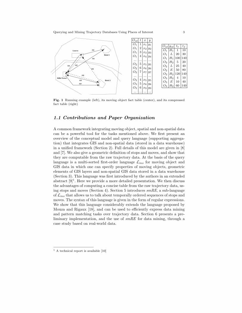
We motivate our work with the following example. Figure 1 (left) shows asimplified map of Paris, containing two hotels, denoted Hotel 1 and Hotel 2(H1 and H2 from here on), the Louvre and the Ei"el tower. We consider threemoving objects, O1, O2 and O3. Object O1 goes from H1 to the Louvre, theEi"el tower, spends just a few minutes there, and returns to the hotel. ObjectO2 goes from H2 to the Louvre, the Ei"el tower, (spending a couple of hoursvisiting each place), and returns to the hotel. Object O3 leaves H2 to theEi"el tower, visits the place, and returns to H2. Figure 1 (center) shows partof these trajectory samples. All points of the same trajectory are temporallyordered and stored together (i.e., the raw trajectories table is sorted by Oid

and t). In what follows, we will use the object identifier as the trajectoryidentifier, unless specified.

Many useful applications open in this scenario. For instance, a GIS usermay be interested in finding out trajectory information, like “number of per-sons going from H1 to the Louvre and then to the Ei"el tower (stopping tovisit both places) in the same day”. An analyst may want to discover hid-den information using data mining techniques. For example, she would liketo identify interesting patterns in the trajectory data using association rulemining. She may also want to verify a certain pattern, like “people do notvisit two museums in the same day”. Complex queries that aggregate non-spatial information, and also involve GIS and moving object data, must alsobe addressed. For instance, “total sales in museums located on the left bankof the Seine, such that people visit them before going to the Ei"el Tower inthe same day”.

Querying and Mining Trajectory Databases Using Places of Interest 3

O3

O3

O2

O2

O2

O1

O1

O1

Hotel 2

Hotel 1

Louvre

Eiffel Tower

Oid t x yO1 1 x1 y1

O1 2 x2 y2

O1 3 x3 y3

O1 4 x4 y4

... ... ... ...O2 5 x5 y5

O2 6 x6 y6

O2 7 x7 y7

... ... ... ...O3 4 x5 y5

O3 5 x8 y8

O3 6 x9 y9

... ... ... ...

Oid gid ts tfO1 H1 1 10O1 L 20 30O1 H1 100 140O2 H2 5 20O2 L 25 40O2 E 50 80O2 H2 120 140O3 H2 4 10O3 E 10 40O3 H2 60 140

Fig. 1 Running example (left), its moving object fact table (center), and its compressedfact table (right)

1.1 Contributions and Paper Organization

A common framework integrating moving object, spatial and non-spatial datacan be a powerful tool for the tasks mentioned above. We first present anoverview of the conceptual model and query language (supporting aggrega-tion) that integrates GIS and non-spatial data (stored in a data warehouse)in a unified framework (Section 2). Full details of this model are given in [8]and [7]. We also give a geometric definition of stops and moves, and show thatthey are computable from the raw trajectory data. At the basis of the querylanguage is a multi-sorted first-order language Lmo for moving object andGIS data in which one can specify properties of moving objects, geometricelements of GIS layers and non-spatial GIS data stored in a data warehouse(Section 3). This language was first introduced by the authors in an extendedabstract [9]1. Here we provide a more detailed presentation. We then discussthe advantages of computing a concise table from the raw trajectory data, us-ing stops and moves (Section 4). Section 5 introduces smRE, a sub-languageof Lmo that allows us to talk about temporally ordered sequences of stops andmoves. The syntax of this language is given in the form of regular expressions.We show that this language considerably extends the language proposed byMouza and Rigaux [18], and can be used to e!ciently express data miningand pattern matching tasks over trajectory data. Section 6 presents a pre-liminary implementation, and the use of smRE for data mining, through acase study based on real-world data.

1 A technical report is available [10]


1.2 Related Work

The field of moving objects databases has been extensively studied in thelast ten years, especially regarding data modeling an indexing. Guting andSchneider [12] provide a good reference to this large corpus of work. Wolfsonet al stated a set of capabilities that a moving object database must have, andintroduced the DOMINO system, that develops those features on top of exist-ing database management systems (DBMS) [25]. Hornsby and Egenhofer [13]introduced a framework for modeling moving objects, that supports viewingobjects at di"erent granularities, depending on the sampling time interval.For mining trajectories in road networks, Brakatsoulas et al. [2] proposed toenrich trajectories of moving objects with information about the relation-ships between trajectories (e.g., intersect, meets), and between a trajectoryand the GIS environment (stay within, bypass, leave). They also propose amining language denoted SML (for Spatial Mining Language). This languageis oriented to tra!c networks, and it is not clear how it could be extendedto other scenarios. Moreover, all information on moving objects must be pro-cessed (on the contrary, we use semantic information to reduce, if possible,the amount of data to be considered). Also in the framework of road tra!cmining, Gonzalez et al. [11] use a partitioning approach for obtaining interest-ing driving and speed patterns from large sets of tra!c data. They computefrequent path-segments at the area level with a support relative to the tra!cin the area (i.e., a kind of adaptative support), and propose an algorithm toautomatically partition a road network and build a hierarchy of areas. Thework of Lee et al. [16] is aimed at discovering common sub-trajectories, usinga partitioning strategy which divides a trajectory into a set of line segments,and then groups similar line segments together into a cluster.

Techniques that add semantic information to trajectory data have been re-cently proposed. Giannotti et al. [6] study trajectory pattern mining, basedon so-called Temporally Annotated Sequences (T AS), an extension of se-quential patterns, where there is a temporal annotation between two nodes.In this way, s1, 2, s2 defines a pattern that starts at s1 and after 2 secondsarrives at s2. In other words, a trajectory pattern is a set of trajectories thatvisit the same sequence of places with similar travel times between each ofthem. They also propose three di"erent mining methods. They also intro-duce the concept of Region of Interest (RoI). Although with similar goals,our work clearly di"ers from [6] in several ways. We work with stops andmoves instead of pre-defined regions of interest. This allows to identify whichof the RoIs are really relevant to a trajectory. We also use these stops andmoves to “encode” or compress a trajectory, which, in many practical sit-uations is enough to identify interesting sequences very e!ciently. A basicdi"erence is also that, in, [6], the authors focus on computing the RoIs dy-namically from the trajectories. On the contrary, in our approach, the userdefines the places of interest of an application in advance, and from themwe compute the stops and moves to perform trajectory mining. Finally, our


approach allows integration between trajectories and background geographicdata, an issue mentioned albeit not addressed in [6].

Mouza and Rigaux [18] presented a model where trajectories are repre-sented by a sequence of moves. They propose a query language based on reg-ular expressions, aimed at obtaining so-called mobility patterns. Note thatthis language, as well as the proposals commented above, does not relate tra-jectories with the GIS environment, which limits the types of queries that canbe addressed. With a similar idea, Damiani et al. [3] introduced the conceptof stops and moves, in order to enrich trajectories with semantically anno-tated data. Alvares et al. [1] presented a framework for trajectory analysisbased on stops and moves. In this paper we will show how these ideas can bee"ectively implemented and used.

The problem of trajectory similarity in moving object databases is a newtopic in the spatio-temporal database literature. Existing work focuses onthe spatial notion of similarity, sometimes borrowing from the time-seriesanalysis field. This is the approach followed by Pelekis et al. [22] introduceda framework consisting of a set of distance operators based on parameters oftrajectories like speed and direction, and propose distance operators basedon this. Frentzos et al. [5] proposed an approximation method for supportingthe k-most-similar-trajectory search using R-tree structures. We will presenta di"erent approach, based on association rule mining, in Section 6.

Data aggregation is still quite an open field, either in GIS or in a movingobjects scenario. Meratnia and de By [17] study trajectory aggregation byidentifying similar trajectories and merging them in a single one, and dividingthe area under study into homogeneous spatial units. Papadias et al [20]index historical aggregate information about moving objects. Our approachfor spatial aggregation is described in [8] and its implementation discussedin [4]2. Kuijpers and Vaisman [15] presented a taxonomy of aggregate querieson moving object data. The model and query language we present here coversthe di"erent types of aggregation queries in this taxonomy.

2 Preliminaries and Background

Spatial data in a GIS are organized in thematic layers, containing informa-tion on geometric objects. For instance, one layer may contain rivers, anotherone road networks, etc. Although these geometric objects could be annotatedwith numerical and/or textual data, given the size of the data involved, andthat aggregation will be relevant in our discussion, we will assume (althoughthis is not a limitation of our model) that non-spatial data is stored in a datawarehouse. Typically, in a data warehouse, numerical data are stored in facttables built along several dimensions. For instance, if we are interested in the

2 An implementation of the system (called Piet) can be found athttp://piet.exp.dc.uba.ar/piet


point point point

linenode

polyline

All All All

Geometric part

Algebraic part

Lr (rivers)

polygon

All

OLAP part

Lc (cities) Lp (provinces)

districts

provinces

All

river

OLAP part

all

x1,y1

x2,y2

x3,y3

x4,y4

l1l2

pl1

Layer Lr

α

Seine

(’Seine’)river - > polilyne

Lr,Rivers

point ->line

line ->polyline

r

rLr

Lr

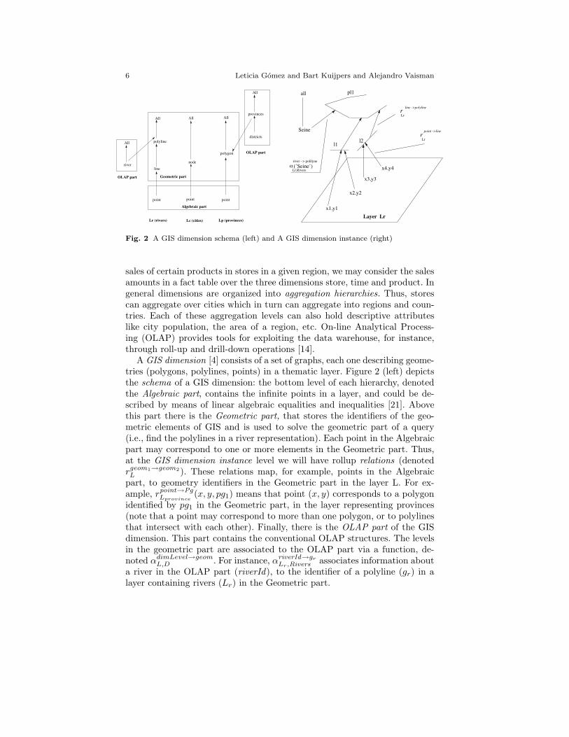
Fig. 2 A GIS dimension schema (left) and A GIS dimension instance (right)

sales of certain products in stores in a given region, we may consider the salesamounts in a fact table over the three dimensions store, time and product. Ingeneral dimensions are organized into aggregation hierarchies. Thus, storescan aggregate over cities which in turn can aggregate into regions and coun-tries. Each of these aggregation levels can also hold descriptive attributeslike city population, the area of a region, etc. On-line Analytical Process-ing (OLAP) provides tools for exploiting the data warehouse, for instance,through roll-up and drill-down operations [14].

A GIS dimension [4] consists of a set of graphs, each one describing geome-tries (polygons, polylines, points) in a thematic layer. Figure 2 (left) depictsthe schema of a GIS dimension: the bottom level of each hierarchy, denotedthe Algebraic part, contains the infinite points in a layer, and could be de-scribed by means of linear algebraic equalities and inequalities [21]. Abovethis part there is the Geometric part, that stores the identifiers of the geo-metric elements of GIS and is used to solve the geometric part of a query(i.e., find the polylines in a river representation). Each point in the Algebraicpart may correspond to one or more elements in the Geometric part. Thus,at the GIS dimension instance level we will have rollup relations (denotedrgeom1!geom2L ). These relations map, for example, points in the Algebraic

part, to geometry identifiers in the Geometric part in the layer L. For ex-ample, rpoint!Pg

Lprovince(x, y, pg1) means that point (x, y) corresponds to a polygon

identified by pg1 in the Geometric part, in the layer representing provinces(note that a point may correspond to more than one polygon, or to polylinesthat intersect with each other). Finally, there is the OLAP part of the GISdimension. This part contains the conventional OLAP structures. The levelsin the geometric part are associated to the OLAP part via a function, de-noted !dimLevel!geom

L,D . For instance, !riverId!gr

Lr,Rivers associates information abouta river in the OLAP part (riverId), to the identifier of a polyline (gr) in alayer containing rivers (Lr) in the Geometric part.


Example 1. Figure 2 (left) shows the schema of a GIS dimension, where wehave defined three layers, for rivers, cities, and provinces, respectively. Theschema is composed of three graphs; the graph for rivers contains edges sayingthat a point (x, y) in the algebraic part relates to a line identifier in thegeometric part, and that in the same portion of the dimension, this linecorresponds to a polyline identifier.

In the OLAP part we have information given by two dimensions, repre-senting districts and rivers, associated to the corresponding graphs, as thefigure shows. For example, a river identifier at the bottom level of the Riversdimension representing rivers in the OLAP part, is mapped to the polylinelevel in the geometric part in the graph of the rivers layer Lr.

Figure 2 (right) shows a portion of a GIS dimension instance of the riverslayer Lr in the dimension schema on the left. Here, an instance of a GIS di-mension in the OLAP part is associated to the polyline pl1, which correspondsto the Seine river. For simplicity we only show four di"erent points at thepoint level {(x1, y1), . . . , (x4, y4)}. There is a relation rpoint!line

Lrcontaining

the association of points to lines in the line level, and a relation rline!polylineLr

,between the line and polyline levels, in the same layer. !"

Elements in the geometric part can be associated with facts, each factbeing quantified by one or more measures, not necessarily a numeric value.The OLAP part may contain not only fact tables quantifying geometric di-mensions, but also classical OLAP fact tables defined in terms of the OLAPdimension schemas.

Moving objects are integrated in the framework above, using a distin-guished fact table denoted Moving Object Fact Table (MOFT).

Let us first say what a trajectory is. In practice, trajectories are availableby a finite sample of (ti, xi, yi) points, obtained by observation.

Definition 1 (Trajectory). A trajectory is a list of time-space points #(t0,x0, y0), (t1, x1, y1), ..., (tN , xN , yN )$,where ti, xi, yi % R for i = 0, ..., N and t0 < t1 < · · · < tN . We call theinterval [t0, tN ] the time domain of the trajectory. !"

For the sake of finite representability, we may assume that the time-spacepoints (ti, xi, yi), have rational coordinates.

A moving object fact table (MOFT for short, see the table in the righthand side of Figure 1), contains a finite number of identified trajectories.

Definition 2 (Moving Object Fact Table). Given a finite set T of trajec-tories, a Moving Object Fact Table (MOFT) for T is a relation with schema< Oid, T, X, Y >, where Oid is the identifier of the moving object, T rep-resents time instants, and X and Y represent the spatial coordinates of theobjects. An instance M of the above schema contains a finite number of tu-ples of the form (Oid, t, x, y), that represent the position (x, y) of the objectOid at instant t, for the trajectories in T . !"


RC1

RC2

RC3RC4

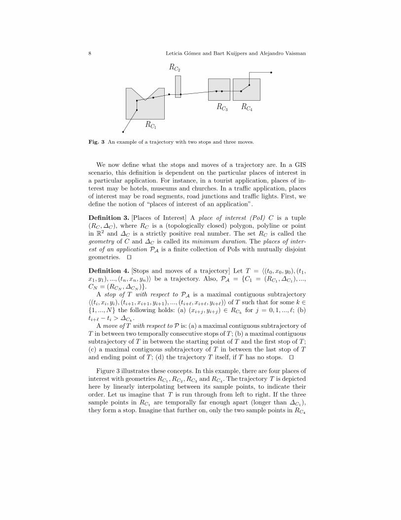
Fig. 3 An example of a trajectory with two stops and three moves.

We now define what the stops and moves of a trajectory are. In a GISscenario, this definition is dependent on the particular places of interest ina particular application. For instance, in a tourist application, places of in-terest may be hotels, museums and churches. In a tra!c application, placesof interest may be road segments, road junctions and tra!c lights. First, wedefine the notion of “places of interest of an application”.

Definition 3. [Places of Interest] A place of interest (PoI) C is a tuple(RC ,"C), where RC is a (topologically closed) polygon, polyline or pointin R2 and "C is a strictly positive real number. The set RC is called thegeometry of C and "C is called its minimum duration. The places of inter-est of an application PA is a finite collection of PoIs with mutually disjointgeometries. !"

Definition 4. [Stops and moves of a trajectory] Let T = #(t0, x0, y0), (t1,x1, y1), ..., (tn, xn, yn)$ be a trajectory. Also, PA = {C1 = (RC1 ,"C1), ...,CN = (RCN , "CN )}.

A stop of T with respect to PA is a maximal contiguous subtrajectory#(ti, xi, yi), (ti+1, xi+1, yi+1), ..., (ti+!, xi+!, yi+!)$ of T such that for some k %{1, ..., N} the following holds: (a) (xi+j , yi+j) % RCk for j = 0, 1, ..., #; (b)ti+! & ti > "Ck .

A move of T with respect to P is: (a) a maximal contiguous subtrajectory ofT in between two temporally consecutive stops of T ; (b) a maximal contiguoussubtrajectory of T in between the starting point of T and the first stop of T ;(c) a maximal contiguous subtrajectory of T in between the last stop of Tand ending point of T ; (d) the trajectory T itself, if T has no stops. !"

Figure 3 illustrates these concepts. In this example, there are four places ofinterest with geometries RC1 , RC2 , RC3 and RC4 . The trajectory T is depictedhere by linearly interpolating between its sample points, to indicate theirorder. Let us imagine that T is run through from left to right. If the threesample points in RC1 are temporally far enough apart (longer than "C1),they form a stop. Imagine that further on, only the two sample points in RC4


are temporally far enough apart to form a stop. Then we have two stops inthis example and three moves.

We remark that our definition of stops and moves of a trajectory is ar-bitrary and can be modified in many ways. For example, if we would workwith linear interpolation of trajectory samples, rather than with samples, wesee in Figure 3, that the trajectory briefly leaves RC1 (not in a sample point,but in the interpolation). We could incorporate a tolerance for this kind ofsmall exits from PoIs in the definition, if we define stops and moves in termsof continuous trajectories, rather than on terms of samples. Finally, in whatfollows we will assume that samples are taken at regular and relatively shortintervals. The following property is straightforward.

Proposition 1. There is an algorithm that returns, for any input (PA, T )with PA the places of interest of an application, and T a trajectory #(t0,x0, y0), (t1, x1, y1), ..., (tn, xn, yn)$, the stops of T with respect to PA. Thisalgorithm works in time O(n · p), where p is the complexity of answering thepoint-query [23]. !"

3 Querying Moving Object Data

The model introduced in Section 2 supports a language (in fact, a multi-sorted first-order logic), that we denote Lmo. We now define Lmo formally.

Definition 5. The first-order query language Lmo has four types of variables:real variables x, y, t, . . . ; name variables Oid, ...; geometric identifier variablesgid, ... and dimension level variables a, b, c, ..., (which are also used for dimen-sion level attributes). Besides (existential and universal) quantification overall these variables, and the usual logical connectives ',(,¬, ..., we considerthe following functions and relations to build atomic formulas in Lmo:

• for every rollup function in the OLAP part, we have a function symbolf

Ai!Aj

Dk, where Ai and Aj are levels in the dimension Dk in the OLAP

part;• analogously, for every rollup relation in the GIS part, we have a relation

symbol rGi!Gj

Lk, where Gi and Gj are geometries and Lk is a layer;

• for every ! relation associating the OLAP and GIS parts in some layer Li,we have a function symbol !

Ai!Gj

Lk,D!, where Ai is an OLAP dimension level

and Gj is a geometry, Lk is a layer and D! is a dimension;• for every dimension level A, and every attribute B of A, there is a function

$A!BDk

that maps elements of A to elements of B in dimension Dk;• we have functions, relations and constants that can be applied to the alpha-

numeric data in the OLAP part (e.g., we have the % relation to say thatan element belongs to a dimension level, we may have < on income valuesand the function concat on string values);


• for every MOFT, we have a 4-ary relation Mi;• we have arithmetic operations + and ), the constants 0 and 1, and the

relation < for real numbers.• finally, we assume the equality relation for all types of variables.

If needed, we may also assume other constants. !"

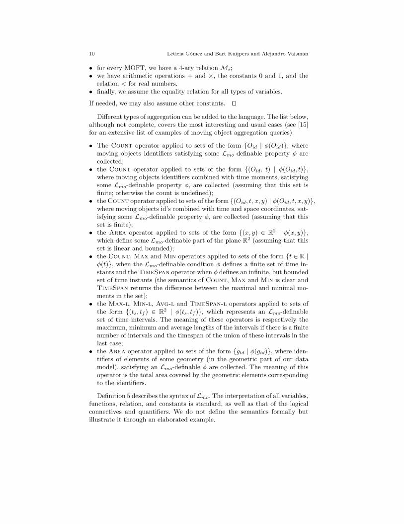
Di"erent types of aggregation can be added to the language. The list below,although not complete, covers the most interesting and usual cases (see [15]for an extensive list of examples of moving object aggregation queries).

• The Count operator applied to sets of the form {Oid | %(Oid)}, wheremoving objects identifiers satisfying some Lmo-definable property % arecollected;

• the Count operator applied to sets of the form {(Oid, t) | %(Oid, t)},where moving objects identifiers combined with time moments, satisfyingsome Lmo-definable property %, are collected (assuming that this set isfinite; otherwise the count is undefined);

• the Count operator applied to sets of the form {(Oid, t, x, y) | %(Oid, t, x, y)},where moving objects id’s combined with time and space coordinates, sat-isfying some Lmo-definable property %, are collected (assuming that thisset is finite);

• the Area operator applied to sets of the form {(x, y) % R2 | %(x, y)},which define some Lmo-definable part of the plane R2 (assuming that thisset is linear and bounded);

• the Count, Max and Min operators applied to sets of the form {t % R |%(t)}, when the Lmo-definable condition % defines a finite set of time in-stants and the TimeSpan operator when % defines an infinite, but boundedset of time instants (the semantics of Count, Max and Min is clear andTimeSpan returns the di"erence between the maximal and minimal mo-ments in the set);

• the Max-l, Min-l, Avg-l and TimeSpan-l operators applied to sets ofthe form {(ts, tf ) % R2 | %(ts, tf )}, which represents an Lmo-definableset of time intervals. The meaning of these operators is respectively themaximum, minimum and average lengths of the intervals if there is a finitenumber of intervals and the timespan of the union of these intervals in thelast case;

• the Area operator applied to sets of the form {gid | %(gid)}, where iden-tifiers of elements of some geometry (in the geometric part of our datamodel), satisfying an Lmo-definable % are collected. The meaning of thisoperator is the total area covered by the geometric elements correspondingto the identifiers.

Definition 5 describes the syntax of Lmo. The interpretation of all variables,functions, relation, and constants is standard, as well as that of the logicalconnectives and quantifiers. We do not define the semantics formally butillustrate it through an elaborated example.


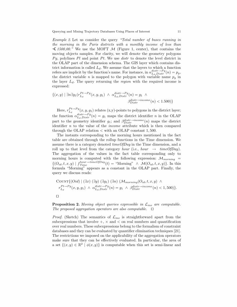
Example 2. Let us consider the query “Total number of buses running inthe morning in the Paris districts with a monthly income of less thanC 1500,00.” We use the MOFT M (Figure 1, center), that contains the

moving objects samples. For clarity, we will denote the geometry polygonsPg, polylines Pl and point Pt. We use distr to denote the level district inthe OLAP part of the dimension schema. The GIS layer which contains dis-trict information is called Ld. We assume that the layers to which a functionrefers are implicit by the function’s name. For instance, in !distr!Pg

Ld,Distr (n) = pg,the district variable n is mapped to the polygon with variable name pg inthe layer Ld. The query returning the region with the required income isexpressed:

{(x, y) | *n*g1(rPt!PgLd

(x, y, g1) ' !distr!PgLd,Distr (n) = g1 '

$distr!incomeDistr (n) < 1.500)}

Here, rPt!PgLd

(x, y, g1) relates (x,y)-points to polygons in the district layer;the function !distr!Pg

Ld,Distr (n) = g1 maps the district identifier n in the OLAPpart to the geometry identifier g1; and $distr!income

Distr (n) maps the districtidentifier n to the value of the income attribute which is then comparedthrough the OLAP relation < with an OLAP constant 1, 500.

The instants corresponding to the morning hours mentioned in the facttable are obtained through the rollup functions in the Time dimension. Weassume there is a category denoted timeOfDay in the Time dimension, and aroll up to that level from the category hour (i.e., hour + timeOfDay).The aggregation of the values in the fact table corresponding only tomorning hours is computed with the following expression: Mmorning ={(Oid, t, x, y) | fhour!timeOfDay

Time (t) = “Morning” ' M(Oid, t, x, y)}. In thisformula “Morning” appears as a constant in the OLAP part. Finally, thequery we discuss reads:

Count{(Oid) | (*x) (*y) (*g1) (*n) (Mmorning(Oid, t, x, y) 'rPt!PgLd

(x, y, g1) ' !distr!PgLd,Distr (n) = g1 ' $distr!income

Distr (n) < 1, 500)}.

!"

Proposition 2. Moving object queries expressible in Lmo are computable.The proposed aggregation operators are also computable. !"

Proof. (Sketch) The semantics of Lmo is straightforward apart from thesubexpressions that involve +, ) and < on real numbers and quantificationover real numbers. These subexpressions belong to the formalism of constraintdatabases and they can be evaluated by quantifier elimination techniques [21].The restrictions we imposed on the applicability of the aggregation operatorsmake sure that they can be e"ectively evaluated. In particular, the area ofa set {(x, y) % R2 | %(x, y)} is computable when this set is semi-linear and


bounded, and can be obtained by triangulating such linear sets and addingthe areas of the triangles. !"

4 The Stops and Moves Fact Table

Let the places of interest of an application be given. In this section, we de-scribe how we go from MOFTs to application-dependent compressed MOFTs,where (Oid, ti, xi, yi) tuples are replaced by (Oid, gid, ts, tf ) tuples. In the lat-ter, Oid is a moving object identifier, gid is the identifier of the geometry ofa place of interest and ts and tf are two time moments that encode the timeinterval [ts, tf ] of a stop. The idea is to replace the MOFT (containing theraw trajectories), by a stops MOFT that represents the same trajectory moreconcisely by listing its stops and the time intervals spent in them.

In practice, the MOFTs can contain huge amounts of data. For in-stance, suppose a GPS takes observations of daily movements of one thou-sand people, every ten seconds, during one month. This gives a MOFT of1000)360)24)30 = 259, 200, 000 records. In this scenario, querying trajec-tory data may become extremely expensive. Note that a MOFT only providesthe position of objects at a given instant. Sometimes we are not interestedin such level of detail, but we look for more aggregated information instead.For example, we may want to know how many people go from a hotel to amuseum on weekdays. Or, we can even want to perform data mining taskslike inferring trajectory patterns that are hidden in the MOFT. These tasksrequire semantic information, not present in the MOFT. In the best case, ob-taining this information from that table will be expensive, because it wouldimply a join between this table and the spatial data. As a solution, we pro-pose to use the notion of stops and moves in order to obtain a more conciseMOFT, that can represent the trajectory in terms of places of interest, char-acterized as stops. This table cannot replace the whole information providedby the MOFT, but allows to quickly obtain information of interest withoutaccessing the complete data set. In this sense, this concise MOFT, which wewill denote SM-MOFT behaves like a summarized materialized view of theMOFT. The SM-MOFT will contain the object identifier, the identifier of thegeometries representing the Stops, and the interval [ts, tf ] of the stop dura-tion. Notice that we do not need to store the information about the moves,which remains implicit, because we know that between two stops there couldonly be a move. Also, if a trajectory passes through a PoI, but remains therean insu!cient amount of time for considering the place a trajectory stop, thestop is not recorded in the SM-MOFT. The case study we will present inSection 6 will show the practical implications of these issues.

Definition 6 (SM-MOFT). Let PA = {C1 = (RC1 , "C1), ..., CN =(RCN ,"CN )} be the PoIs of an application, and let M be a MOFT. The SM-MOFT Msm of M with respect to PA consists of the tuples (Oid, gid, ts, tf )


such that (a) Oid is the identifier of a trajectory in M 3; (b) gid is the identi-fier of the geometry of a PoI Ck = (RCk , "Ck) of PA such that the trajectorywith identifier Oid in M has a stop in this PoI during the time interval [ts, tf ].This interval is called the stop interval of this stop. !"

The table in Figure 1 (right) shows the SM-MOFT for our running exam-ple. Proposition 3 below, states that SM-MOFTs can be defined in Lmo.

Proposition 3. There is an Lmo formula %sm(Oid, gid, ts, tf ) that definesthe SM-MOFT Msm of M with respect to PA. !"

We omit the proof of this property but remark that the use of the formula%sm(Oid, gid, ts, tf ) allows us to speak about stops and moves of trajectories inLmo. We can therefore add predicates to define stops and moves of trajectoriesas syntactic sugar to Lmo.

5 A Query Language for Stops and Moves

We will sketch a query language based on path regular expressions, along thelines proposed by Mouza and Rigaux [18]. However, our language (denotedsmRE ) goes far beyond, taking advantage of the integration between GIS,OLAP and moving objects provided by our model. Moreover, queries thatdo not require access to the MOFT can be evaluated very e!ciently, makinguse of the SM-MOFT. In this section we show through examples, that smREcan be used to query for trajectory patterns, and that smRE turns out to bea subset of Lmo.

We will assume that there is a di"erent dimension for each type of(application-dependant) place of interest in the OLAP part of the model.For instance, there will be a dimension for hotels, with bottom level hotelId,or a dimension for restaurants, with bottom level restaurantId. Aggregationlevels can be defined as required. There will also be a layer in the Geomet-ric part of the GIS dimension, that could be designed in di"erent ways. Forsimplicity, we consider that all places of interest with the same geometry willbe stored together, meaning that, for example, there will be a layer (i.e., ahierarchy graph) for polygons representing hotels, and/or one hierarchy forlines representing street segments. There are also the functions introduced inSection 2. For example, !hotelId!Pg

Lp,Hotel maps a hotel identifier to a polygon rep-resenting it, in a layer for polygonal PoIs (Lp). All identifiers of PoIs in Msm

are members of some dimension level in the OLAP part, and are mapped toa geometry through the function !. We will also need some operators on timeintervals. We say that an interval I1 = [t1, t2] strictly precedes I2 = [t3, t4],

3 We could also use a trajectory identifier other than the object’s id, if we want to analyzeseveral trajectories of an object in di!erent days. We use this approach in Section 6.


denoted I1 ! I2, if t1 < t2 < t3 < t4. Note that all stop intervals I1, I2 of thesame trajectory are such that either I1 ! I2 or I2 ! I1.

The idea is based on the construction (described in Definition 7), of agraph representing the stops and moves of a single trajectory.

Definition 7 (SM-Graph). Let us consider a trajectory sample T of mov-ing objects, the PoIs of an application PA = {C1 = (RC1 , "C1), ..., CN =(RCN ,"CN )}, a MOFT M, and its SM-MOFT Msm with respect to A.Also, for clarity but w.l.o.g., consider that all the tuples in Msm are orderedaccording to their stop interval attributes, that is, if t1 and t2 are two consec-utive tuples in Msm, t1.I ! t2.I, where I represents the time interval in thetuple (i.e., [ts, tf ]). An SM-Graph for Msm, denoted G(Msm), is a graphconstructed as follows:

1. For each gid %!

Gid(Msm) there is a node v in G, denoted v(gid), with a

node number n % N, di"erent for each node.2. There is an edge m in G between two nodes v1 and v2, for every pair t1, t2

of consecutive tuples in Msm with the same Oid.3. For each node v % G the extension of v, denoted ext(v) is given by the

identifier of the PoI that represents the node in the OLAP part of themodel.

4. For each node v % G the label of v, denoted label(v) is the name of thedimension of the PoI in the OLAP Part (i.e., the name of the dimensionD mentioned above).

5. For each node v % G the stop temporal elements of v, denoted STE (v) isa set of stop intervals {I1, ..., Ik} (technically, a temporal element), suchthat there is an interval Ii % STE(v) for each edge incoming to v in G. !"

Note that an object may be at a PoI (long enough for considering thisplace a stop in the trajectory) more than once within a trajectory.

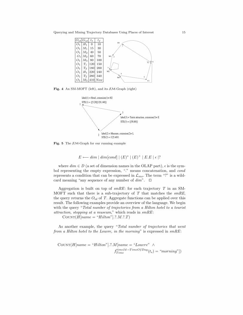
Example 3. Figure 4 (left) shows an SM-MOFT for one moving object’strajectory. The distinguished term “Now” indicates, as usual in temporaldatabases, the current time. We denote Hi, Mi, and Ti, hotels, museumsand tourist attractions, respectively. Figure 4 (right) shows the correspondingSM-Graph for object O1. As an example, the extension of node 3 is ext(3 ) =M2 , its label is label(3 ) = Museums, and STE (3 ) = {[80, 100], [410, Now]}.

Figure 5 shows the SM-Graph for the trajectory of object O2 in therunning example of Figure 1. !"

Now we are ready to define our query language based on Stops and Moves.The language combines the notions of regular expressions and first orderconstraints. The SM-Graph G can be seen as an automaton accepting regularexpressions over the places of interest.

Definition 8 (R.E. for Stops and Moves). A regular expression on stopsand moves, denoted smRE is an expression generated by the grammar


Oid Gid ts tfO1 H1 0 10O1 M1 15 30O1 M2 40 50O1 M2 60 70O1 M3 80 100O1 T1 120 150O1 T2 180 200O1 H1 220 240O1 T2 280 340O1 M3 410 Now

3

2

6

5

4

1

M2

M3

H1

T2

T1

M1

Fig. 4 An SM-MOFT (left), and its SM-Graph (right)

1

2

3

label(1) = Hotel, extension(1)= H2STE(1) = {[5,20][120,140]}

label(3) = Turist attraction, extension(3)= ESTE(3) = {[50,80]}

label(2) = Museum, extension(2)= LSTE(2) = {[25,40]}

Fig. 5 The SM-Graph for our running example

E ,& dim | dim[cond] | (E)" | (E)+ | E.E | & |?

where dim % D (a set of dimension names in the OLAP part), & is the sym-bol representing the empty expression, “.” means concatenation, and condrepresents a condition that can be expressed in Lmo. The term “?” is a wild-card meaning “any sequence of any number of dim”. !"

Aggregation is built on top of smRE : for each trajectory T in an SM-MOFT such that there is a sub-trajectory of T that matches the smRE,the query returns the Oid of T . Aggregate functions can be applied over thisresult. The following examples provide an overview of the language. We beginwith the query “Total number of trajectories from a Hilton hotel to a touristattraction, stopping at a museum,” which reads in smRE :

Count(H[name = “Hilton”].?.M.?.T )

As another example, the query “Total number of trajectories that wentfrom a Hilton hotel to the Louvre, in the morning” is expressed in smRE :

Count(H[name = “Hilton”].?.M [name = “Louvre” 'f timeId!TimeOfDay

Time (ts) = “morning”])


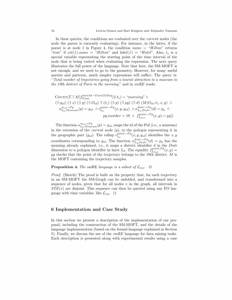
In these queries, the conditions are evaluated over the current nodes (thenode the parser is currently evaluating). For instance, in the latter, if theparser is at node 1 in Figure 4, the condition name = “Hilton” returns“true” if ext(1 ).name = “Hilton” and label(1 ) = “Hotel”. Also, ts is aspecial variable representing the starting point of the time interval of thenode that is being visited when evaluating the expression. The next queryillustrates the full power of the language. Note that here, the SM-MOFT isnot enough, and we need to go to the geometry. However, for many usefulqueries and patterns, much simpler expressions will su!ce. The query is:‘‘Total number of trajectories going from a tourist attraction to a museum inthe 19th district of Paris in the morning,” and in smRE reads:

Count(T.?.M [f timeId!TimeOfDayTime (I.ts) = “morning” '

(* gid) (* x) (* y) (* Oid) * (t1) (* p) (* pg) (* d) (M(Oid, t1, x, y) '!mid!Pg

Lp,Museum(p) = gid ' rpoint!PgLp

(x, y, gid) ' !distr!PgLd,Distr (d) = pg '

pg.number = 19 ' fpoint!PgLdist

(x, y) = pg])

The function !mid!PgLp,Museum(p) = gid, maps the id of the PoI (i.e., a museum)

in the extension of the current node (p), to the polygon representing it inthe geographic part (gid). The rollup rpoint!Pg

Lp(x, y, gid) identifies the x, y

coordinates corresponding to gid. The function !distr!PgLd,Distr (d) = pg has the

meaning already explained, i.e., it maps a district identifier d in the Distrdimension to a polygon identifier in layer Ld. The equality fpoint,Pg

Ldist(x, y) =

pg checks that the point of the trajectory belongs to the 19th district. M isthe MOFT containing the trajectory samples.

Proposition 4. The smRE language is a subset of Lmo. !"

Proof. (Sketch) The proof is built on the property that, for each trajectoryin an SM-MOFT the SM-Graph can be unfolded, and transformed into asequence of nodes, given that for all nodes v in the graph, all intervals inSTE (v) are disjoint. This sequence can then be queried using any FO lan-guage with time variables, like Lmo !"

6 Implementation and Case Study

In this section we present a description of the implementation of our pro-posal, including the construction of the SM-MOFT, and the details of thelanguage implementation (based on the formal language explained in Section5). Finally, we discuss the use of the smRE language for data mining tasks.Each description is presented along with experimental results using a case


Fig. 6 PoIs and two trajectories

study based on data obtained from the INFATI Project4. Our intention wasto experiment with real-world data, and at the same time, to work with alarge database. The original data set contained a total of 1.9 million recordsof the form (Oid, x, y, t), collected by GPS devices, at intervals of one second.Since we needed a larger database, we modified and expanded the originalone, until we obtained a MOFT with 30,808,296 tuples, corresponding totrajectories of 6.276 moving objects. Therefore, we worked with a MOFTcontaining a mixture of real-world and synthetic data.

Since the original data set did not include places of interest, we createdthem in order to complete the experimental evaluation. We worked with thefollowing kinds of PoIs: restaurants, co"ee shops, hotels and two tourist at-tractions: an aquarium and a zoo. For the minimum duration (see Definition3), we adopted the following criteria: 15 minutes for co"ee shops, 40 minutesfor restaurants and zoos, 45 minutes for hotels and 20 minutes for the aquar-ium. These PoIs are shown in Figure 6, using the GIS tool we developed5.We created a total of seventeen PoIs.

We ran our tests on a dedicated IBM 3400x server equipped with a dual-core Intel-Xeon processor, at a clock speed of 1.66 GHz. The total free RAMmemory was 4.0 Gb, and there was a 250Gb disk drive.

6.1 Computing the SM-MOFT

We first give details of the computation of the SM-MOFT from the MOFTcontaining the raw trajectories. We process the MOFT one trajectory at a

4 http://www.cs.aau.dk/ stardas/infati5 http://piet.exp.dc.uba.ar/piet/index.jsp


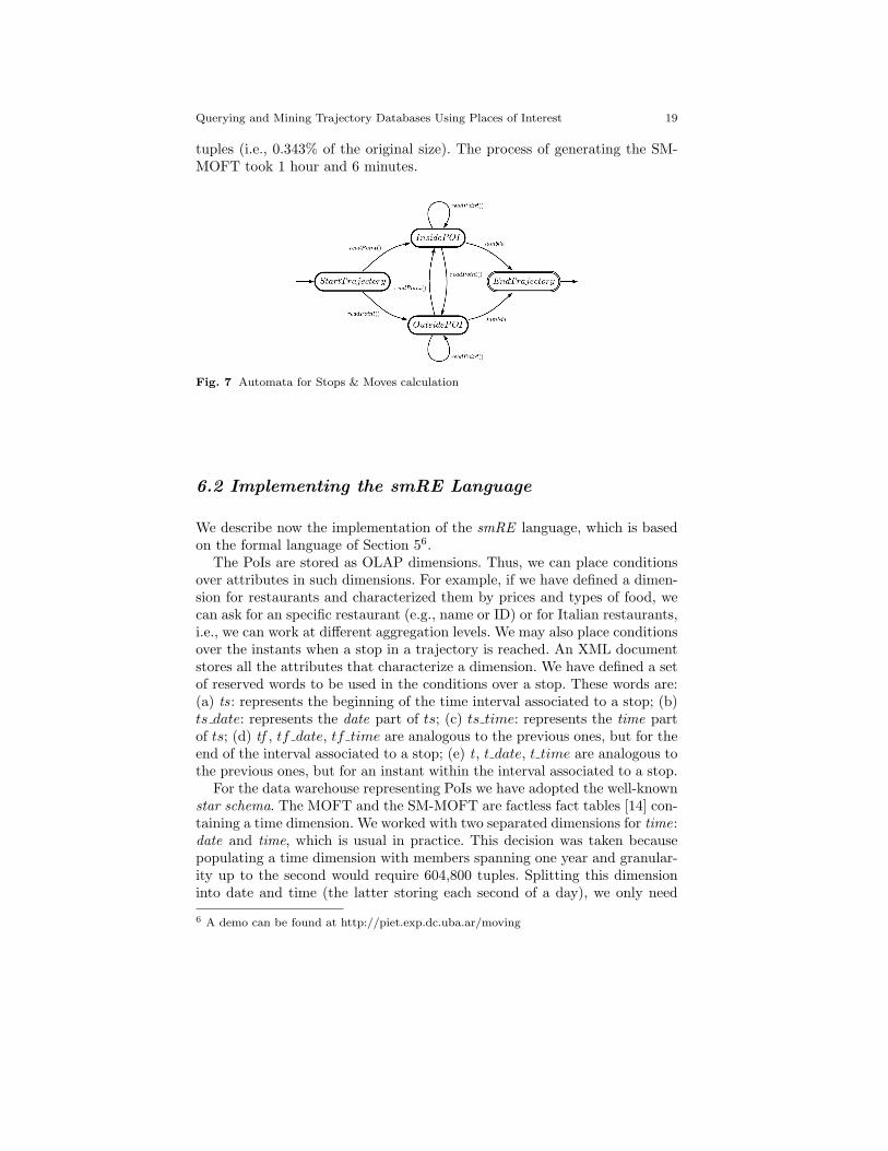
time. A cursor is placed at the first tuple of the trajectory, and only twopoints need to be in main memory at the same time. We used the automatonshown in Figure 7 to detect the sequence of PoIs that can become a stop inthe trajectory. The transitions in this automaton can be either a readPoint()action, or the empty string '. There are four states in the automaton: Start-Trajectory, EndTrajectory, InsidePOI, and OutsidePOI.

StartTrajectory : This is the initial state. If the first point in the trajectorybelongs to a PoI, the transition is to the InsidePOI state (we have recognizedthe beginning of a POI). If not, the transition is to the OutsidePOI state.InsidePOI: This state can be reached from any state, except EndTrajectory.Di"erent situations must be analyzed:

• The previous states were OutsidePOI or StartTrajectory. In the first case,the previous point must belong to a move. In the latter, we are at thestart of the trajectory. The current point corresponds to a POI, which isa candidate to become a stop (we call this a candidate stop). The timeinstant of the PoI becomes the initial time of the interval of this potentialstop.

• The previous state was InsidePOI : if two consecutive points (the previousand the current ones) are both inside the same POI, then the action willbe: read the next input (i.e., move to the next point). Otherwise, we havereached the boundary of the PoI, and we are entering another one; thus,before reading the next input, we need to compute the duration of theinterval in order to check if the sub-trajectory inside the PoI was actuallya stop. If we are using trajectory sampling, the timestamp of the previouspoint is the ending time of the stop interval. The timestamp of the currentpoint is used as the starting time of the interval of the new PoI the objectis entering. If we are using linear interpolation, we build a line betweenboth points and calculate the intersection between this line and the PoI(and, of course, the corresponding time instant).

OutsidePOI: this intermediate state can be reached from any state, exceptEndTrajectory. Again, di"erent situations must be analyzed:

• The previous states were OutsidePOI or StartTrajectory. In the first case,the previous point must belong to a move. In the latter we are at the startof the trajectory. The algorithm reads the next input point.

• The previous state was InsidePOI : the automaton has detected that theobject has left a candidate stop, and proceeds as explained above, com-puting the duration of the candidate stop to define if the object is stillwithin a move, or if it has found a stop.

EndTrajectory: The last state, when the cursor has consumed all the tuplesin the MOFT.

To give an idea of practical results, in our case study, starting from aMOFT containing 30,808,296 tuples, we obtained an SM-MOFT with 105,684


tuples (i.e., 0.343% of the original size). The process of generating the SM-MOFT took 1 hour and 6 minutes.

Fig. 7 Automata for Stops & Moves calculation

6.2 Implementing the smRE Language

We describe now the implementation of the smRE language, which is basedon the formal language of Section 56.

The PoIs are stored as OLAP dimensions. Thus, we can place conditionsover attributes in such dimensions. For example, if we have defined a dimen-sion for restaurants and characterized them by prices and types of food, wecan ask for an specific restaurant (e.g., name or ID) or for Italian restaurants,i.e., we can work at di"erent aggregation levels. We may also place conditionsover the instants when a stop in a trajectory is reached. An XML documentstores all the attributes that characterize a dimension. We have defined a setof reserved words to be used in the conditions over a stop. These words are:(a) ts: represents the beginning of the time interval associated to a stop; (b)ts date: represents the date part of ts; (c) ts time: represents the time partof ts; (d) tf , tf date, tf time are analogous to the previous ones, but for theend of the interval associated to a stop; (e) t , t date, t time are analogous tothe previous ones, but for an instant within the interval associated to a stop.

For the data warehouse representing PoIs we have adopted the well-knownstar schema. The MOFT and the SM-MOFT are factless fact tables [14] con-taining a time dimension. We worked with two separated dimensions for time:date and time, which is usual in practice. This decision was taken becausepopulating a time dimension with members spanning one year and granular-ity up to the second would require 604,800 tuples. Splitting this dimensioninto date and time (the latter storing each second of a day), we only need

6 A demo can be found at http://piet.exp.dc.uba.ar/moving


366 tuples for the date dimension and 86.400 for the time dimension. Thehierarchy of levels for the date dimension is: date + day + month + quarter+ year. For the time dimension we have: time+second + minute+ hour +range. The range level will have the members: “Midnight”, “Early Morning”,“Morning”, “Afternoon”, “Evening” and “Night”. Finally, the schemas of thetables are: M(Oid, t date, t time, x, y) and Msm(Oid, Gid, ts date, ts time,tf date, tf time). The language works, by default, with the SM-MOFT table(see below). For the function f (the rollup functions in the OLAP part ofthe model) we use the term rup(x ), where x is the member whose rollup rcomputes. We do not need to specify the dimension, which is implicit sinceall conditions are applied locally at the node being visited.

We will illustrate the implemented language through examples. We willuse a di"erent font to indicate that we are referring to the actual implemen-tation. We will work with the PoIs H (hotel), R (restaurant), C (co"ee shop),and Z(zoo). The corresponding dimensions have the attributes: ID (in all di-mensions); type of food and price for restaurants; and price for co"ee shops.

Q1: Trajectories that begin at the “Hilton” hotel, stop at an Italian restaurantand finish at a cheap co!ee shop.

H[name="Hilton"].R[food="Italian"].C[price="cheap"]

Q2: Trajectories that begin at the ”Sheraton”, stop at an Italian restaurant(during the first quarter of 2002), and finish at a cheap co!ee shop, leavingthe latter in the afternoon.

H[name="Sheraton"].R[food="Italian" and rup(ts_date)="2002.Q2"].C[price="cheap" and rup(tf_time)="Afternoon"]

Q3: Trajectories of the following form: (a) there is a stop at the ”Hilton”,and then at an Italian restaurant; this sequence occurs at least one time, andmay be repeated any number of consecutive times; (b) after this sequence, thetrajectories may include visits to other places, and finish at the Zoo.

(H[name="Hilton"].R[food="Italian"])+.?.Z[ ]

Q4:Trajectories that visited the ”Hilton” and stayed in it during the after-noon.

H[name="Hilton" and rup(t_time)="Afternoon"]

All queries, except Q4 use the Msm table. While Q1 uses only attributesassociated to dimensions, Q2 includes rollup functions for ts date and tf time(using the date and time dimensions, respectively). Q3 shows the use of arepetitive group. Q4 needs to access the original MOFT, instead the SM-MOFT, because it asks for an instant t between ts time and tf time. Noticethat the query could not be solved just using ts time and tf time, becauseboth of them may rollup to mornings of di"erent days, and time instants


in between may rollup to “Midnight”, “Early Morning”, or any other possi-ble range. Our implementation detects this need, and proceeds in the bestpossible way, accessing the original MOFT only when needed.

For solving path expressions we implemented the SM-Graph, explainedin Section 5. First, we build the automaton for the regular expression. Thealgorithm takes advantage of the order in the temporal elements associatedto the nodes, and unfolds the graph, reproducing the sequences of stops inthe trajectory. This unfolded graph is the input to be processed by the au-tomaton. A query is solved at most in two steps.

Step 1. If the query does not include a rollup function, we can solve it injust one step. We match the regular expression to the SM-Graph. Thus, foreach Oid we obtain the sub-trajectories that match the query. Consider thequery:

R[price="cheap"].?.Zoo[ts_date="20/09/200?"]

We obtain the following matches for Oid= 100:R[ID="Paris" and price="cheap" andts_date="18/09/2000" and ts_time="12:00:05" andtf_date="18/09/2000" and tf_time="14:04:20"].Zoo[ID="Central" and ts_date="20/09/2000" and ts_time="12:30:00" andtf_date="20/09/2000" and tf_time="13:45:04"]

R[ID="Paris" and price="cheap" andts_date="16/08/2001" and ts_time="23:15:05" andtf_date="17/08/2001" and tf_time="01:00:10"].C[ID="Best" and ts_date="17/08/2001" and ts_time="01:10:00" andtf_date="17/08/2001" and tf_time="02:00:03"].Zoo[ID="Central" and ts_date="20/09/2001" and ts_time="11:20:00" andtf_date="20/09/2001" and tf_time="13:00:00"]

The first sub-trajectory shows that there exists a direct path between acheap restaurant and the zoo:

Cheap Paris Restaurant[18/09/2000 12:00:05,18/09/2000 14:04:20]Central Zoo[20/09/2000 12:30:00,20/09/2000 13:45:04]

In the second sub-trajectory there is a path between a cheap restaurantand the zoo with a co"ee shop as intermediate stop.

Cheap Paris Restaurant [16/08/2001 23:15:05,17/08/2001 01:00:10]Best coffee [17/08/2001 01:10:00,17/08/2001 02:00:03]Central Zoo [20/09/2001 11:20:00,20/09/2001 13:00:00]

If the query includes the reserved word “t” (instead of “ts” or “tf”), the al-gorithm must perform an extra verification. For example, if in the query abovewe replace the term Zoo[ts date="20/09/200?"] by Zoo[t date="20/09/200?"],once the interval [ts date ts time, tf date tf time] was computed, the algo-rithm will check if this interval includes t date.

Step 2.Step 2.1. If the query includes a rollup function, once the sub-trajectories inStep 1 are obtained, an MDX7 query is performed to solve the rollup part.7 MDX is a standard language adopted by most OLAP tools


Our implementation uses Mondrian8 as the OLAP server. Let us consider thequery:

R[price="cheap"].?.Zoo[rup(ts_time)="Morning"]

Here, before the rollup function could be computed, step 2.1. must ob-tain the candidate values for ts date matching the regular expression (forthe dimension Zoo). Then, the algorithm executes the MDX query to findwhich of the following expressions are true: rup(“12:30:00”) = “Morning”,and rup(“11:20:00”) = “Morning” (note that in our example, only the latterverifies the rollup).

Step 2.2. If the query involves a rollup of the reserved word “t”, we havealready explained that the algorithm uses M (instead of Msm). Let us say,for example, that we replace Zoo[rup(ts time) = "Morning"] in the queryshown in Step 2.1, by Zoo[rup(t time)="Morning"]. We need to find outif there exists a sample point that rolls up to “Morning”, because it mayhappen that even though ts time rolls up to “Afternoon” and tf time rollsup to “Night”, these situations may occur in di"erent days, and in this case,there exists an instant in the interval rolling up to “Morning”.

Finally, we remark that our implementation also supports aggregation, asexplained in Section 5. For example:

Count(R[price="cheap"].?.Zoo[t date="20/09/2001"] )

6.3 Using smRE for Data Mining

There are many practical situations in which we are interested in findingwhich are the trajectories in the database that verify the same sequence ofstops. In these cases, we do not need to check if these trajectories are similar inthe usual time-series sense, but in a more semantically-oriented way. Further,we may be interested in di"erent kinds of similarity, with respect to certainpatterns. For example, two trajectories that would not be similar under anyusual metric, may contain the pattern H.R.?.C (see above). For certain kindsof analysis, this may su!ce for considering both trajectories similar.

We propose a two-step method for discovering trajectory patterns. Thefirst one consists in finding association rules using places of interest, witha certain support and confidence, in order to reduce the number of combi-nations of places of interest that must be checked. Then, we use smRE toanalyze the sequences followed by the moving objects and analyze trajectorypatterns. Then, we can either calculate the support of a certain pattern (us-ing the aggregate function Count, or check which are the trajectories thatfollow the pattern.

8 http://mondrian.sourceforge.net/


ID POI ts tf

101 3 26/10/2001 11:00:03 26/10/2001 12:00:03101 9 26/10/2001 14:10:00 26/10/2001 15:02:05101 3 26/10/2001 23:30:00 27/10/2001 02:00:01101 2 27/10/2001 09:22:00 ...

Fig. 8 The SM-MOFT table for the case study

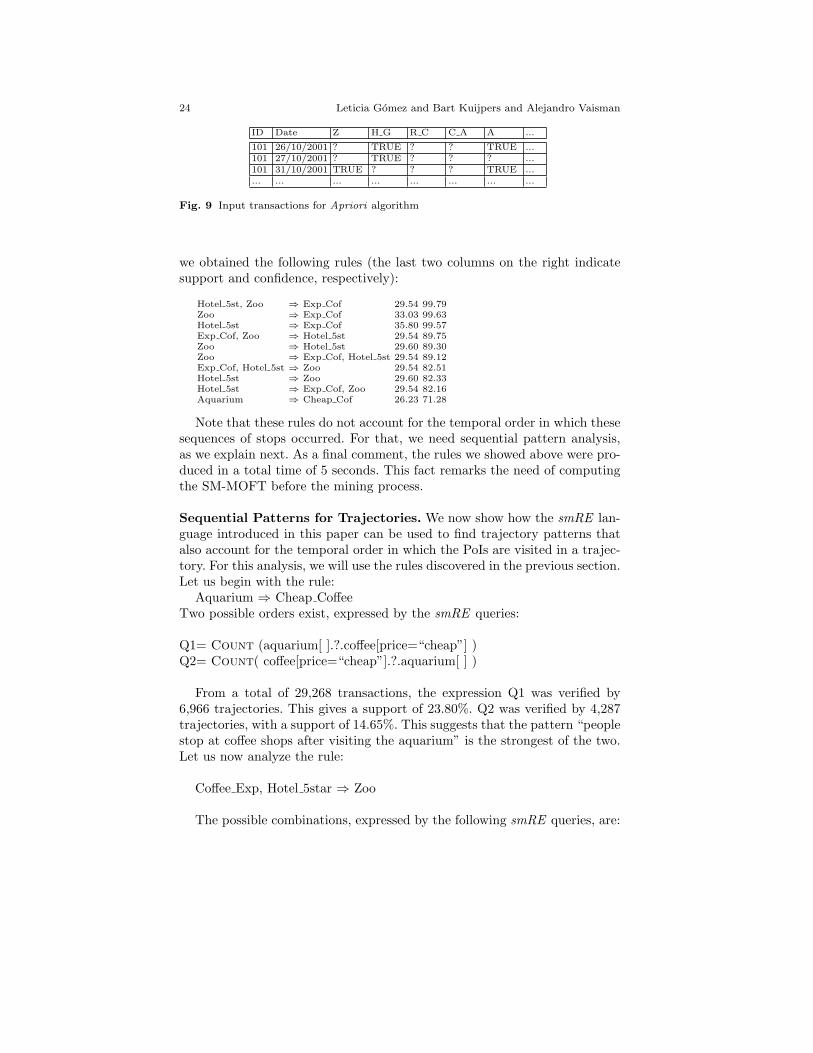
Association Rules for Stops and Moves. We use the Apriori algorithm[24] for finding association rules involving stops in trajectories, taking advan-tage of the information stored in the SM-MOFT. We first need to define whata transaction means in this scenario. In the case of a Market Basket Analysis,for instance, a transaction is clearly determined by the items bought togetherat the same moment by the consumer. On the contrary, moving objects havea semi-infinite trajectory and there is no clear notion of what a transactionis. In our case study we have considered that a transaction is a sequence oftrajectory stops occurred during the same day. Other criteria could be used,for example, a transaction could be defined as all stops occurred between 6:00AM on one day and 5:59 AM of the following day. Then, each trajectory ofa moving object could be thought as a sequence of sub-trajectories (trans-actions, in the association rule sense), each one corresponding to a di"erentday. Figure 8 shows a fragment of the SM-MOFT produced from the rawtrajectory database. We used an implementation of the Apriori algorithmincluded in the Weka framework9. The input to this algorithm is a recordcontaining the whole trajectory of an object in each observed day. Figure 9depicts the form of this table, specifically prepared for discovering associationrules at the finest granularity level. The names of the attributes reflect PoIidentifiers instead of dimension names. For example, “H G”, “R C”, “C A”,denote particular hotels, restaurants and co"ee shops, respectively, while “A”denotes the aquarium. Since we are also interested in multilevel associationrules, i.e., rules with itemsets of di"erent granularity, we also need a tablewhere the attributes (items) are the dimension levels instead of the identifiersof the PoIs. We used the following classification attributes: price for co"eeshops, number of stars for hotels, and type of food for restaurants. For theexperiments with the Apriori algorithm we generated the daily transactionsof the 6,276 moving objects. The execution time for this process was 10 sec-onds and 29,268 transactions were produced. We required a minimal supportand confidence of 25% and 70%, respectively. Finally, the only rule produced,working at the finest granularity level, was:

C L, H F - ZUsing higher levels of aggregation (i.e., rules where items are of coarser

granularity), new rules may be discovered. Applying the Apriori algorithm

9 http://www.cs.waikato.ac.nz/ml/weka/


ID Date Z H G R C C A A ...

101 26/10/2001 ? TRUE ? ? TRUE ...101 27/10/2001 ? TRUE ? ? ? ...101 31/10/2001 TRUE ? ? ? TRUE ...... ... ... ... ... ... ... ...

Fig. 9 Input transactions for Apriori algorithm

we obtained the following rules (the last two columns on the right indicatesupport and confidence, respectively):

Hotel 5st, Zoo # Exp Cof 29.54 99.79Zoo # Exp Cof 33.03 99.63Hotel 5st # Exp Cof 35.80 99.57Exp Cof, Zoo # Hotel 5st 29.54 89.75Zoo # Hotel 5st 29.60 89.30Zoo # Exp Cof, Hotel 5st 29.54 89.12Exp Cof, Hotel 5st # Zoo 29.54 82.51Hotel 5st # Zoo 29.60 82.33Hotel 5st # Exp Cof, Zoo 29.54 82.16Aquarium # Cheap Cof 26.23 71.28

Note that these rules do not account for the temporal order in which thesesequences of stops occurred. For that, we need sequential pattern analysis,as we explain next. As a final comment, the rules we showed above were pro-duced in a total time of 5 seconds. This fact remarks the need of computingthe SM-MOFT before the mining process.

Sequential Patterns for Trajectories. We now show how the smRE lan-guage introduced in this paper can be used to find trajectory patterns thatalso account for the temporal order in which the PoIs are visited in a trajec-tory. For this analysis, we will use the rules discovered in the previous section.Let us begin with the rule:

Aquarium - Cheap Co"eeTwo possible orders exist, expressed by the smRE queries:

Q1= Count (aquarium[ ].?.co"ee[price=“cheap”] )Q2= Count( co"ee[price=“cheap”].?.aquarium[ ] )

From a total of 29,268 transactions, the expression Q1 was verified by6,966 trajectories. This gives a support of 23.80%. Q2 was verified by 4,287trajectories, with a support of 14.65%. This suggests that the pattern “peoplestop at co"ee shops after visiting the aquarium” is the strongest of the two.Let us now analyze the rule:

Co"ee Exp, Hotel 5star - Zoo

The possible combinations, expressed by the following smRE queries, are:


Q1=Count(co"ee[price=“expensive”].?.hotel[star=“5”].?.zoo[])Q2=Count(co"ee[price=“expensive”].?.zoo[].?.hotel[star=“5”])Q3=Count(hotel[star=“5”].?.co"ee[price=“expensive”].?.zoo[])Q4=Count(hotel[star=“5”].?.zoo[].?.co"ee[price=“expensive”])Q5=Count(zoo[].?.co"ee[price=“expensive”].?.hotel[star=“5”])Q6=Count(zoo[].?.hotel[star=“5”].?.co"ee[price=“expensive”])

The following table summarizes the results, which shows that strongestpattern here the one expressed by query Q1.

Query # of trajectories support (%)Q1 8088 27.63Q2 5427 18.54Q3 6 0.02Q4 7662 26.18Q5 9 0.03Q6 5391 18.42

For query evaluation we used the SM-Graph explained in Section 5, witha slight variation: instead of producing a graph for each moving object, wegenerated a graph for each transaction. Thus, we generated 29,268 graphs,each one corresponding to a transaction (i.e., a daily trajectory of a movingobject). The six smRE queries were run 5 times. We report the minimum,average and maximum execution times for each query.

Query Min (sec) Max (sec) Avg (sec)Q1 151.76 154.91 153.48Q2 152.09 156.05 153.78Q3 152.87 154.19 153.48Q4 151.48 154.64 153.19Q5 151.97 154.39 153.47Q6 151.19 154.33 152.74

7 Future Work

The framework we presented in this paper supports a seamless integration ofspatial, non-spatial, and moving object data. We are currently in the processof including the implementation described in Section 6 into the Piet frame-work [4]. The smRE language is a promising tool for mining trajectory data,specifically in the context of sequential patterns mining with constraints, andwe will continue working in this direction.

We believe that many research directions open from the work presentedhere. For example, along the same research line presented in the paper, weare now working on extending well-known sequential patterns algorithms, inorder to compare these algorithms against the two-step process presentedin this paper. Further, e!cient automatic extraction of patterns using thesmRE language could be explored. This means that, instead of writing thequery expression, we would like to generate the ones with a given minimum


support. Relationships between objects (like the distance changes betweenthem during a certain period of time) can also be studied, as well as situationswhere the positions of the PoIs are not fixed. Updates to the MOFT and theSM-MOFTs must be studied, not only for the changes in trajectory data (i.e.,new objects or trajectories), but also under changes in the PoIs.

8 Acknowledgments

This work has been partially funded by the European Union under theFP6-IST-FET programme, Project n. FP6-14915, GeoPKDD: GeographicPrivacy-Aware Knowledge Discovery and Delivery, the Research FoundationFlanders (FWO-Vlaanderen), Project G.0344.05., and the Scientific Agencyof Argentina, Project PICT n. 21350.

References

1. Alvares, L.O., Bogorny, V., Kuijpers, B., de Macedo, J.A.F., Moelans, B., Vaisman,A.: A model for enriching trajectories with semantic geographical information. In:ACM-GIS (2007)

2. Brakatsoulas, S., Pfoser, D., Tryfona, N.: Modeling, storing and mining moving objectdatabases. In: Proceedings of IDEAS’04, pp. 68–77. Washington D.C, USA (2004)

3. Damiani, M.L., de Macedo, J.A.F., Parent, C., Porto, F., Spaccapietra, S.: A concep-tual view of trajectories. Technical Report, Ecole Polythecnique Federal de Lausanne,April 2007 (2007)

4. Escribano, A., Gomez, L., Kuijpers, B., Vaisman, A.A.: Piet: a gis-olap implementa-tion. In: DOLAP, pp. 73–80. Lisbon, Portugal (2007)

5. Frentzos, E., Gratsias, K., Theodoridis, Y.: Index-based most similar trajectory search.In: ICDE, pp. 816–825 (2007)

6. Giannotti, F., Nanni, M., Pinelli, F., Pedreschi, D.: Trajectory pattern mining. In:KDD, pp. 330–339. San Jose, California, USA (2007)

7. Gomez L., H.S., Kuijpers, B., Vaisman, A.: Spatial aggregation: Data model and im-plementation. In: Submitted for review (2008)

8. Gomez, L., Haesevoets, S., Kuijpers, B., Vaisman, A.A.: Spatial aggregation: Datamodel and implementation. CoRR abs/0707.4304 (2007)

9. Gomez, L., Kuijpers, B., Vaisman, A.A.: Aggregation languages for moving object andplaces of interest. In: To appear inProceedings of SAC 2008 - ASIIS track

10. Gomez, L., Kuijpers, B., Vaisman, A.A.: Aggregation languages for moving object andplaces of interest data. CoRR abs/0708.2717 (2007)

11. Gonzalez, H., Han, J., Li, X., Myslinska, M., Sondag, J.P.: Adaptive fastest pathcomputation on a road network: A tra"c mining approach. In: VLDB, pp. 794–805(2007)

12. Guting, R.H., Schneider, M.: Moving Objects Databases. Morgan Kaufman (2005)13. Hornsby, K., Egenhofer, M.: Modeling moving objects over multiple granularities. Spe-

cial issue on Spatial and Temporal Granularity, Annals of Mathematics and ArtificialIntelligence (2002)

14. Kimball, R., Ross, M.: The Data Warehouse Toolkit: The Complete Guide to Dimen-sional Modeling, 2nd. Ed. J.Wiley and Sons, Inc (2002)


15. Kuijpers, B., Vaisman, A.A.: A data model for moving objects supporting aggregation.In: ICDE Workshops, pp. 546–554. Istambul, Turkey (2007)

16. Lee, J.G., Han, J., Whang, K.Y.: Trajectory clustering: a partition-and-group frame-work. In: SIGMOD Conference, pp. 593–604 (2007)

17. Meratnia, N., de By, R.: Aggregation and comparison of trajectories. In: Proceedingsof the 26th VLDB Conference. Virginia, USA (2002)

18. Mouza, C., Rigaux, P.: Mobility patterns. Geoinformatica 9(23), 297–319 (2005)19. Ott, T., Swiaczny, F.: Time-integrative Geographic Information Systems–Management

and Analysis of Spatio-Temporal Data. Springer (2001)20. Papadias, D., Tao, Y., Zhang, J., Mamoulis, N., Shen, Q., Sun, J.: Indexing and re-

trieval of historical aggregate information about moving objects. IEEE Data Eng.Bull. 25(2), 10–17 (2002)

21. Paredaens, J., Kuper, G., Libkin, L. (eds.): Constraint databases. Springer-Verlag(2000)

22. Pelekis, N., Kopanakis, I., Marketos, G., Ntoutsi, I., Andrienko, G.L., Theodoridis, Y.:Similarity search in trajectory databases. In: TIME, pp. 129–140 (2007)

23. Rigaux, P., Scholl, M., Voisard, A.: Spatial Databases. Morgan Kaufmann (2002)24. Srikant, R., Agrawal, R.: Mining generalized association rules. In: VLDB, pp. 407–419

(1995)25. Wolfson, O., Sistla, P., Xu, B., Chamberlain, S.: Domino: Databases fOr MovINg

Objects tracking. In: Proceedings of SIGMOD’99, pp. 547 – 549 (1999)26. Worboys, M.F.: GIS: A Computing Perspective. Taylor&Francis (1995)

Querying and Mining Trajectory Databases Using Places of Interest

Documents

Transcript of Querying and Mining Trajectory Databases Using Places of Interest