Pulsation period variations in the RRc Lyrae star KIC 5520878

Michael Hippke

hippke@ifda.eu

Institute for Data Analysis, Luiter Str. 21b, 47506 Neukirchen-Vluyn, Germany

John G. Learned

jgl@phys.hawaii.edu

High Energy Physics Group, Department of Physics and Astronomy, University of Hawaii,

Manoa 327 Watanabe Hall, 2505 Correa Road Honolulu, Hawaii 96822 USA

A. Zee

zee@kitp.ucsb.edu

Kavli Institute for Theoretical Physics, University of California, Santa Barbara, California

93106 U.S.A.

William H. Edmondson

w.h.edmondson@bham.ac.uk

School of Computer Science, University of Birmingham, Birmingham B15 2TT, UK

Ian R. Stevens

irs@star.sr.bham.ac.uk

School of Physics and Astronomy, University of Birmingham, Birmingham B15 2TT, UK

John F. Lindner

jlindner@wooster.edu

Physics Department, The College of Wooster, Wooster, Ohio 44691, USA

arX

iv:1

409.

1265

v1 [

astr

o-ph

.SR

] 3

Sep

201

4

– 2 –

Department of Physics and Astronomy, University of Hawai‘i at Manoa, Honolulu, Hawai‘i

96822, USA

Behnam Kia

behnam@hawaii.edu

Department of Physics and Astronomy, University of Hawai‘i at Manoa, Honolulu, Hawai‘i

96822, USA

William L. Ditto

wditto@hawaii.edu

Department of Physics and Astronomy, University of Hawai‘i at Manoa, Honolulu, Hawai‘i

96822, USA

Received ; accepted

– 3 –

ABSTRACT

Learned et. al. proposed that a sufficiently advanced extra-terrestrial civi-

lization may tickle Cepheid and RR Lyrae variable stars with a neutrino beam

at the right time, thus causing them to trigger early and jogging the otherwise

very regular phase of their expansion and contraction. This would turn these

stars into beacons to transmit information throughout the galaxy and beyond.

The idea is to search for signs of phase modulation (in the regime of short pulse

duration) and patterns, which could be indicative of intentional, omnidirectional

signaling.

We have performed such a search among variable stars using photometric

data from the Kepler space telescope. In the RRc Lyrae star KIC 5520878, we

have found two such regimes of long and short pulse durations. The sequence of

period lengths, expressed as time series data, is strongly auto correlated, with

correlation coefficients of prime numbers being significantly higher (p = 99.8%).

Our analysis of this candidate star shows that the prime number oddity originates

from two simultaneous pulsation periods and is likely of natural origin.

Simple physical models elucidate the frequency content and asymmetries of

the KIC 5520878 light curve.

Despite this SETI null result, we encourage testing other archival and future

time-series photometry for signs of modulated stars. This can be done as a

by-product to the standard analysis, and even partly automated.

Subject headings: (stars: variables:) Cepheids — (stars: variables:) RR Lyrae variable

– 4 –

1. Introduction

We started this work with the simple notion to explore the phases of variable stars,

given the possibility of intentional modulation by some advanced intelligence (Learned et

al. 2008). The essence of the original idea was that variable stars are a natural target of

study for any civilization due to the fact of their correlation between period and total light

output. This correlation has allowed them to become the first rung in the astronomical

distance ladder, a fact noted in 1912 by Henrietta Leavitt (Pickering and Leavitt 1912).

Moreover, such oscillators are sure to have a period of instability at which time they are

sensitive to perturbations, and which can be triggered to flare earlier in their cycle than

otherwise. If some intelligence can do this in a regular manner, they have the basis of

a galactic semaphore for communicating not only within one galaxy, but in the instance

of brighter Cepheids with many galaxies. This would be a one-way communication, like

a radio station broadcasting indiscriminately. One may speculate endlessly about the

motivation for such communication; we only aver that there are many possibilities and

given our complete ignorance of any other intelligence in the universe, we can only hope we

will recognize signs of artificiality when we see them.

We must be careful to acknowledge that we are fully aware that this is a mission

seemingly highly unlikely to succeed, but the payoff could be so great it is exciting to try.

In what we report below, we have begun such an investigation, and found some behaviour

in a variable star that is, at first glance, very hard to understand as a natural phenomenon.

A deeper analysis of simultaneous pulsations then shows its most likely natural origin. This

opens the stage for a discussion of what kind of artificiality we should look for in future

searches.

By way of more detailed introduction, astronomers who study variable stars in the past

have had generally sparsely sampled data, and in earlier times even finding the periodicity

– 5 –

was an accomplishment worth publishing. Various analytical methods were used, such as

the venerable ’string method’, which involves folding the observed magnitudes to a common

one cycle graph, phase ordering and connecting the points by a virtual ’string’ (Petrie

1962; Dworetzki 1982). Editing of events which did not fit well was common. One moved

the trial period until the string length was minimized. In more recent times with better

computing ability, the use of Lomb-Scargle folding (Lomb 1976; Scargle 1982) and Fourier

transforms (Ransom et al. 2010) has become prominent. For our purposes however, such

transforms obliterate the cycle to cycle variations we seek, and so we have started afresh

looking at the individual peak-to-peak periods and their modulation.

The type of analysis we want to carry out could not have been done even a few years

ago, since it requires many frequent observations on a single star, with good control over the

photometry over time. This is very hard to do from earth – we seem to be, accidentally, on

the wrong planet for the study of one major type of variables, the RR Lyrae stars (Welch

2014). Typically, these stars pulsate with periods near 0.5 days (a few have shorter or longer

periods). This is unfortunately well-matched to the length of a night on earth. Even in case

of good weather, and when observing every night from the same location, still every second

cycle is lost due to it occurring while the observation site is in daylight. This changed with

the latest generation of space telescopes, such as Kepler and CoRoT. The Kepler satellite

was launched in 2009 with a primary mission of detecting the photometric signatures of

planets transiting stars. Kepler had a duty cycle of up to 99%, and was pointed at the same

sky location at all times. The high-quality, near uninterrupted data have also been used

for other purposes, such as studying variable stars. One such finding was a remarkable,

but previously completely undetected and unsuspected behavior: period-doubling. This is

a two-cycle modulation of the light curve of Blazhko-type RR Lyrae stars. And it is not a

small effect: In many cases, every other peak brightness is different from the previous one

by up to 10% (Blazhko 1907; Smith 2004; Kolenberg 2004; Szabo et al. 2010, 2011).

– 6 –

This has escaped earth-bound astronomers for reasons explained above 1.

2. Data set

Our idea was to search for period variations in variable stars. We employed the

database best suited for this today, nearly uninterrupted photometry from the Kepler

spacecraft, covering 4 years of observations with ultra-high precision (Caldwell at al. 2010).

In what follows, we describe this process using RRc Lyrae KIC 5520878 as an example.

For this star, we have found the most peculiar effects which are described in this paper.

For comparison, we have also applied the same analysis for other variable stars, as will be

described in the following sections.

KIC 5520878 is a RRc Lyrae star with a period of P1=0.26917082 days (the number of

digits giving a measure of the accuracy of the value (Nemec et al. 2013)). It lies in the field

of view of the Kepler spacecraft, together with 40 other RR Lyrae stars, out of which 4 are

of subtype RRc 2. Only one Cepheid is known in the area covered by Kepler(Szabo et al.

2011). The brightness of KIC5520878, measured as the Kepler magnitude, is M=14.214.

1It has also led to a campaign of observing RR Lyrae, the prototype star, from different

Earth locations, in order to increase the coverage (Le Borgne et al. 2014). This is especially

useful as Kepler finished its regular mission due to a technical failure.

2These are KIC 4064484, 5520878, 8832417, and 9453114, according to (Nemec et al.

2013).

– 7 –

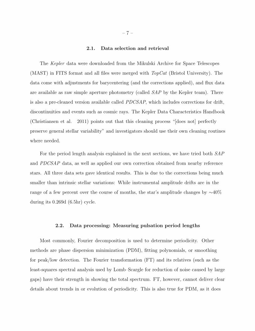
2.1. Data selection and retrieval

The Kepler data were downloaded from the Mikulski Archive for Space Telescopes

(MAST) in FITS format and all files were merged with TopCat (Bristol University). The

data come with adjustments for barycentering (and the corrections applied), and flux data

are available as raw simple aperture photometry (called SAP by the Kepler team). There

is also a pre-cleaned version available called PDCSAP, which includes corrections for drift,

discontinuities and events such as cosmic rays. The Kepler Data Characteristics Handbook

(Christiansen et al. 2011) points out that this cleaning process “[does not] perfectly

preserve general stellar variability” and investigators should use their own cleaning routines

where needed.

For the period length analysis explained in the next sections, we have tried both SAP

and PDCSAP data, as well as applied our own correction obtained from nearby reference

stars. All three data sets gave identical results. This is due to the corrections being much

smaller than intrinsic stellar variations: While instrumental amplitude drifts are in the

range of a few percent over the course of months, the star’s amplitude changes by ∼40%

during its 0.269d (6.5hr) cycle.

2.2. Data processing: Measuring pulsation period lengths

Most commonly, Fourier decomposition is used to determine periodicity. Other

methods are phase dispersion minimization (PDM), fitting polynomials, or smoothing

for peak/low detection. The Fourier transformation (FT) and its relatives (such as the

least-squares spectral analysis used by Lomb–Scargle for reduction of noise caused by large

gaps) have their strength in showing the total spectrum. FT, however, cannot deliver clear

details about trends in or evolution of periodicity. This is also true for PDM, as it does

– 8 –

not identify pure phase variations, since it uses the whole light curve to obtain the solution

(Stellingwerf et al. 2013).

The focus of our study was pulsation period length, and its trends. We have therefore

tried different methods to detect individual peaks (and lows for comparison).

In the short cadence data (1 minute integrations), we found that many methods work

equally well. As the average period length of KIC 5520878 is ∼0.269 days, we have ∼387

data points in one cycle. First of all, we tried eye-balling the time of the peaks and noted

approximate times. As there is some jitter on the top of most peaks, we then employed

a centered moving-average (trying different lengths) to smooth this out, and calculated

the maxima of this smoothed curve. Afterwards, we fitted n-th order polynomials, trying

different numbers of terms. While this is computationally more expensive, it virtually gave

the same results as eye-balling and smoothing. Deviations between the methods are on the

order of a few data points (minutes). We judge these approaches to be robust and equally

suitable. Finally, we opted to proceed with the peak times derived with the smoothing

approach as this is least susceptible for errors.

In the long cadence data (30 minutes), there are only ∼13 data points in one cycle

(Fig. 1). Simply using the bin with the highest luminosity thus introduces large timing

errors. We tried fitting templates to the curve, but found this very difficult due to

considerable change in the shape of the light curve from cycle to cycle. This stems from

two main effects: Amplitude variations of ∼3% cycle-to-cycle, and the seemingly random

occurrence of a bump during luminosity increase, when luminosity rises steeply and then

takes a short break before reaching its maximum. We found fitting polynomials to be

more efficient, and tested the results for varying number of terms and number of data

points involved. The benchmark we employed was the short cadence data, which gave us

1,810 cycles for comparison with the long cadence data. We found the best result to be a

– 9 –

5th-order-polynomial fitted to the 7 highest data points of each cycle, with new parameters

for each cycle. This gave an average deviation of only 4.2 minutes, when compared to the

short cadence data. Fig. 1 shows a typical fit for short and long cadence data.

– 10 –

Fig. 1.— Both peak finding methods applied: Square symbols show LC data points, with a

5th-order polynomial fitted to the 7 highest values. The right of the vertical lines indicates

the LC peak from this method. The small dots below are the SC data points, shifted by

1, 000e− downwards for better visibility. The peak of the SC data, derived with the smoothing

method, is shown by the left of the vertical lines. The two times indicated by the two lines

differ by 4 minutes. This is also the average deviation for SC versus LC data. Times are in

Barycentric Julian Date (MJD-2454833)

– 11 –

2.3. Data processing result

During the 4 years of Kepler data, 5,417 pulsation periods passed. We obtained the

lengths of 4,707 of these periods (87%), while 707 cycles (13%) were lost due to spacecraft

downtimes and data glitches. Out of the 4,707 periods we obtained, we had short cadence

data for 1,810 periods (38%). For the other 62% of pulsations, we used long cadence data.

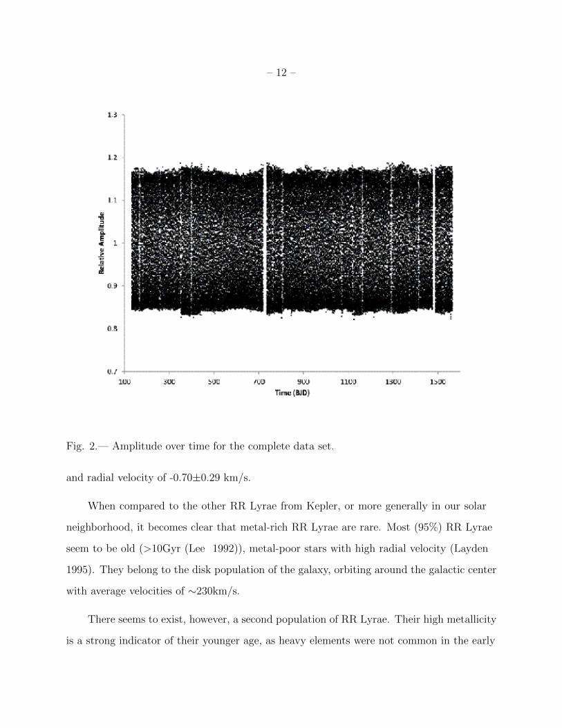
2.4. Data quality

The errors given by the Kepler team for short integrations (1 minute) for KIC 5520878

are ≤35e- for the flux (that is 0.1% of an average flux of 35,000e-). These errors are

smaller than the point size of Fig. 2, which shows the complete data set. We have applied

corrections for instrumental drift by matching to nearby stable stars. Some instrumental

residuals on the level of a few percent remain, which are very hard to clean out in such a

strongly variable star. As explained above, these variations are irrelevant for our period

length determination.

3. Basic facts on RRc Lyrae KIC 5520878

3.1. Metallicity and radial velocity

KIC 5520878 has been found to be metal-rich. When expressed as [Fe/H], which

gives the logarithm of the ratio of a star’s iron abundance compared to that of our Sun,

KIC 5520878 has a ratio of [Fe/H]=-0.36±0.06, that is about half of that of our sun.

This information comes from a spectroscopic study with the Keck-I 10m HIRES echelle

spectrograph for the 41 RR Lyrae in the Kepler field of view (Nemec et al. 2013). The

study also derived temperatures (KIC 5520878: 7,250 K, the second hottest in the sample)

– 12 –

Fig. 2.— Amplitude over time for the complete data set.

and radial velocity of -0.70±0.29 km/s.

When compared to the other RR Lyrae from Kepler, or more generally in our solar

neighborhood, it becomes clear that metal-rich RR Lyrae are rare. Most (95%) RR Lyrae

seem to be old (>10Gyr (Lee 1992)), metal-poor stars with high radial velocity (Layden

1995). They belong to the disk population of the galaxy, orbiting around the galactic center

with average velocities of ∼230km/s.

There seems to exist, however, a second population of RR Lyrae. Their high metallicity

is a strong indicator of their younger age, as heavy elements were not common in the early

– 13 –

universe. Small radial velocities point towards them co-moving with the galactic rotation

and, thus, them belonging to the younger population of the galactic disk, sometimes divided

into the very young thin disk and the somewhat older thick disk. Our candidate star, RRc

KIC 5520878, seems to be one of these rarer objects, as shown in Fig. 3.

Fig. 3.— Radial velocity versus metallicity for the 41 known Kepler RR Lyrae. Black dots

represent sub-type RRab, while gray squares represent sub-type RRc.

3.2. Cosmic distance

RR Lyrae stars are part of our cosmic distance ladder, due to the peculiar fact that

their absolute luminosity is simply related to their period, and hence if one measures the

– 14 –

period one gets the light output. By observing the apparent brightness, one can then derive

the distance. The empirical relation is 5log10D = m −M − 10 where m is the apparent

magnitude and M the absolute magnitude. If we take m = 14.214 for KIC5520878 and

M = 0.75 for RR Lyrae stars (Layden 1995), the distance calculates to D = 4.9kpc (or

∼16,000 LY), that is ∼16% of the diameter of our galaxy – the star is not quite in our

neighborhood.

3.3. Rotation period

Taking an empirical relation of pulsation period P and radius R of RR Lyrae stars

(Marconi et al. 2005) of log10R = 0.90(±0.03) + 0.65(±0.03)log10P , one can derive

R = 3.4RSUN for KIC 5520878. The inclination angle i is not derivable with the data

available. Thus, a corresponding minimum rotation period would be 33.8±1 days at i = 90,

or 47.8 days at i = 45. The minimum rotation period of 33.8 days is equivalent to ∼126

cycles (of 0.269 days length), so that the rotation period is much slower than the pulsation

period.

3.4. Fourier frequencies

KIC5520878 has been studied in detail (Moskalik 2014). In a Fourier analysis, a

secondary frequency fX = 5.879d−1(PX = 0.17 days) was found. The author calculates a

ratio PX/P1 = 0.632, a rare but known ratio among RR Lyrae stars (although its meaning

is unknown). In addition, significant subharmonics were found with the strongest being

fZ = 2.937d−1(PZ = 0.34 days), that is at 1/2fX . Their presence is described as “a

characteristic signature of a period doubling of the secondary mode, fX (. . .). Its origin

can be traced to a half-integer resonance between the pulsation modes (Moskalik, Buchler

– 15 –

1990).” The author also compares several RRc stars and finds “the richest harvest of low

amplitude modes (. . .) in KIC5520878, where 15 such oscillations are detected. Based on the

period ratios, one of these modes can be identified with the second radial overtone, but all

others must be nonradial. Interestingly, several modes have frequencies significantly lower

than the radial fundamental mode. This implies that these nonradial oscillations are not

p-modes, but must be of either gravity or mixed mode character.” These other frequencies

are usually said to be non-radial, but could also be explained by “pure radial pulsation

combinations of the frequencies of radial fundamental and overtone modes” (Benko et al.

2014).

3.5. An optical blend?

Unusual frequencies might be contributed by an unresolved companion with a different

variability. To check this, we have obtained observations down to magnitude 19.6 with a

privately owned telescope and a clear filter. Using a resolution of 0.9px/arcsec, it can be

easily seen that a faint (18.6mag) companion is present at a distance of ≈7 arcsec, as shown

in Fig. 4. The standard Kepler aperture mask fully contains this companion, however the

magnitude difference between this uncataloged companion and KIC5520878 is larger than

4.4 magnitudes, so that the light contribution into our Kepler photometry is very small. At

a distance of 4.9kpc, the projected distance of this companion is ≈0.15 parsec, resulting in

a potential circular orbit of ≈ 4 × 106 years. The most likely case is, however, that this

star is simply an unrelated, faint background (or foreground) star with negligible impact to

Kepler photometry.

A second argument can be made against blending: With Fourier transforms, linear

combinations of frequencies can be found. These are intrinsic behavior of one star’s interior,

and cannot be produced by two separate stars.

– 16 –

Fig. 4.— CCD photography centered on KIC5520878. The Kepler aperture mask of 4x4

Kepler pixels (1px ≈ 3.9 arcsec) is shown as a square. It fully contains the faint uncataloged

star, marked with a vertical line.

3.6. Phase fold of the light curve

We have used all short cadence data and created a folded light curve, as shown in

Fig. 5. It clearly displays the two periods present: The strong main pulsation P1, and the

weaker secondary pulsation PX .

3.7. Amplitude features: No period doubling or Blazhko-effect

With Kepler data, a previously unknown effect in RR Lyrae was discovered, named

“period doubling” (Kolenberg et al. 2013). This effect manifests itself in an amplitude

variation of up to 10% of every second cycle. It was found in several Blazhko-RRab stars,

but its occurrence rate is yet unclear. Our candidate star, KIC 5520878, does not show the

period doubling effect. Judging from figure 5, which shows a typical sample of amplitude

fluctuations, the variations are more complex. Regarding the Blazhko effect, a long-term

– 17 –

Fig. 5.— Left panel: Folded light curve for main pulsation period P1=0.269d with sine fit

(grey) centered on peak (upper curves). Below: Residuals of sine fit, displayed at 25,000.

Right panel: Phase fold to P2=0.17d. Note changed horizontal axis and sine fit (grey) with

much smaller variation, about 2% of P1.

variation best visible in an amplitude-over-time graph, we can see no clear evidence for it

being present in KIC 5520878. Fig. 6 shows the complete data set, which features some

amplitude variations over time, but not of the typical sinusoidal Blazhko style.

4. Period length and variations

4.1. Measured period lengths

The average period length is constant at P1=0.269d when averaged on a timescale of

more than a few days. On a shorter timescale, larger variations can be seen. Peak-to-peak,

the variation is in the range [0.24d to 0.30d], low-to-low in the range [0.26d to 0.28d].

For any given cycle, the qualitative result of measuring through the lows and through the

peaks is equivalent, meaning that a short (long) period is measured to be short (long), no

matter whether peaks or lows are used. As the peak-to-peak method gives larger nominal

– 18 –

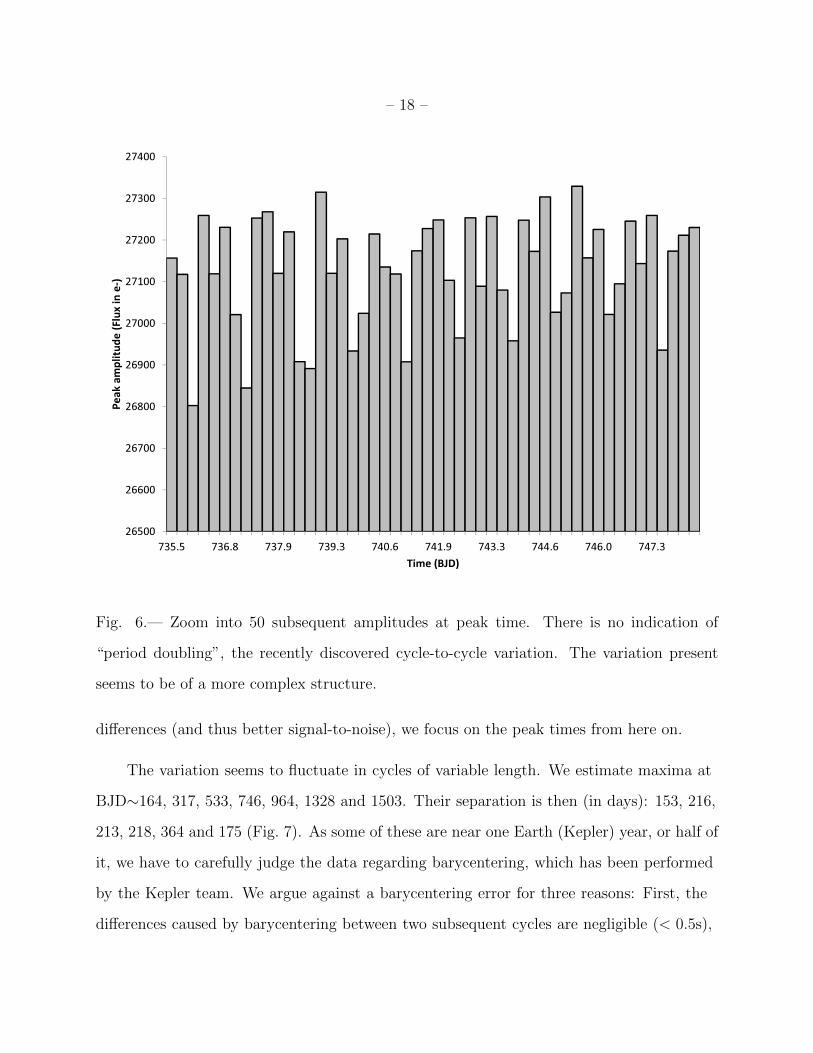
Fig. 6.— Zoom into 50 subsequent amplitudes at peak time. There is no indication of

“period doubling”, the recently discovered cycle-to-cycle variation. The variation present

seems to be of a more complex structure.

differences (and thus better signal-to-noise), we focus on the peak times from here on.

The variation seems to fluctuate in cycles of variable length. We estimate maxima at

BJD∼164, 317, 533, 746, 964, 1328 and 1503. Their separation is then (in days): 153, 216,

213, 218, 364 and 175 (Fig. 7). As some of these are near one Earth (Kepler) year, or half of

it, we have to carefully judge the data regarding barycentering, which has been performed

by the Kepler team. We argue against a barycentering error for three reasons: First, the

differences caused by barycentering between two subsequent cycles are negligible (< 0.5s),

– 19 –

while the cycle has an average length of ∼387 minutes. Second, the cycles are of varying

length, while a year is not. Third, the large Kepler community would most likely already

have found such a major error. We therefore judge the long-term variation of period lengths

to be a real phenomenon.

In section V, we will explain how the period length variations originate from the

presence of a second pulsation mode.

4.2. Comparing period length variations to other RR Lyrae stars

The period variation of RR Lyrae, the prototype star, has been measured at ∼0.53%

(Stellingwerf et al. 2013). This is low compared to ∼22% for KIC 5520878. The low value

of RR Lyrae is reproducible with our method of individual peak detection. The authors

estimate a scatter of ∼0.01 days caused by measurement errors. We have furthermore

looked at several other RR Lyrae stars in the Kepler field of view, and found others

(V445=KIC 6186029; KIC 8832417) that also show large period variations. For KIC

6186029 the variations are 0.49d to 0.53d, that is ∼8%. It has been analyzed in a paper

whose title summarizes the findings as “Two Blazhko modulations, a non-radial mode,

possible triple mode RR Lyrae pulsation and more” (Guggenberger 2013).

4.3. Period-Amplitude relation

KIC 5520878 shows a significant (p > 99.9%) relation of longer periods having

higher flux. In a recent paper, a counterclockwise looping evolution between amplitude

and period in the prototype RR Lyrae was detected. This looping, so far only found in

RRab-Blazhko-stars, cannot be reproduced in KIC 5520878 (Stellingwerf et al. 2013).

– 20 –

4.4. Distribution of period lengths

The period lengths of the 4,707 cycles that we measured are not just Gaussian

distributed, and the distribution changes over time considerably. Fig. 8 shows their change

over time. For every given time, we can see a regime of shorter and a regime of longer

period lengths. For the times of higher variance, these regimes are clearly split in two, with

no periods of average length (forbidden zone). During times of lower variance, no clear split

can be seen.

– 21 –

Fig. 7.— Pulsation period lengths over time using LC data (black) and SC data (gray).

Note the fluctuations of variance. The peaks are indicated with triangles at P1=0.24d.

In addition, there are “forbidden zones”, e.g. at BJD=1500: P1=0.265d. This diagram can

easily be understood as the typical O−C (observed minus calculated) diagram if the average

main pulsation period P1=0.269 is set to 0. Periods longer than P1 then have positive O−C

values and vice versa.

– 22 –

Fig. 8.— Histograms of pulsation period length for the complete data set (upper left panel),

for BJD=634, a time of low variation (upper middle panel) and for BJD=1514, when varia-

tion was high (upper right panel). Another histogram for BJD=1310 can be found in section

5, together with a comparison to simulated data. Times of histograms are indicated with

grey bars in the lower panel.

– 23 –

4.5. Discussion of period lengths

It has been proposed that a sufficiently advanced civilization may employ Cepheid

variable stars as beacons to transmit all-call information throughout the galaxy and beyond

(Learned et al. 2008). The idea is that Cepheids and RR Lyrae are unstable oscillators

and tickling them with a neutrino beam at the right time could cause them to trigger

early, and hence jog the otherwise very regular phase of their expansion and contraction.

The authors proposition was to search for signs of phase modulation (in the regime of

short pulse duration) and patterns, which could be indicative of intentional signaling. Such

phase modulation would be reflected in shorter and longer pulsation periods. We showed

that the histograms do indeed contain two humps of shorter and longer periods. In case

of an artificial cause for this, we would expect some sort of further indication. As a first

step, we have applied a statistical autocorrelation test to the sequence of period lengths.

This will be discussed in the following. Furthermore, we have assigned “one” to the short

interval and “zero” to the long interval, producing a binary sequence. This series has been

analyzed regarding its properties. It indeed shows some interesting features, including

non-randomness and the same autocorrelations. We have, however, found no indication of

anything “intelligent” in the bitstream, and encourage the reader to have a look himself

or herself, if interested. All data are available online (see appendix). A positive finding of

a potential message, which we did not find here, could be a well-known sequence such as

prime numbers, Fibonacci, or the like.

We have also compared several other RR Lyrae stars with Kepler data for their

pulsation period distribution, and created Kernel density estimate (Rosenblatt 1956;

Parzen 1962) plots (Fig. 9). We found no second case with two peaks, although some other

RRc stars come close.

– 24 –

! "# $ #%

""!&'

()

(

Fig. 9.— Kernel density of pulsation periods for some Kepler RR Lyrae. Only KIC5520878

(on the left) shows a clear double-peak feature.

5. Prime numbers have high absolute autocorrelation

We have performed a statistical autocorrelation analysis for the time series of period

lengths. In the statistics of time series analysis, autocorrelation is the degree of similarity

between the values of the time series, and a lagged version of itself. It is a statistical tool

to find repeating patterns or identifying periodic processes. When computed, the resulting

number for every lag n can be in the range [-1, +1]. An autocorrelation of +1 represents

perfect positive correlation, so that future values are perfectly repeated, while at -1 the

– 25 –

values would be opposite. In our tests, we found that pulsation variations are highly

autocorrelated with highest lags for n=5, 19, 24, and 42. When plotting integers versus

their autocorrelation coefficients (ACFs, Fig. 10), it can clearly be seen that prime numbers

tend to have high absolute ACFs. The average absolute ACF of primes in [1..100] is 0.51

(n=25), while for non-primes it is 0.37 (n=75). The average values for these two groups are

significantly different in a binominal test (this is the exact test of the statistical significance

of deviations from a theoretically expected distribution of observations into two categories),

p = 99.79% for the SC data, and p = 99.77% for the LC data. The effect is present over the

whole data set, and for integers up to ∼200. As there is no apparent physical explanation

for this, we were tempted to suspect some artificial cause. In the following section, however,

we will show its natural origin and why primes avoid the ACF range between -0.2 and 0.2.

– 26 –

Fig. 10.— Autocorrelation graph for period. All lags [1..100]. Prime numbers are shown

as squares, other numbers as dots. Prime numbers have higher autocorrelation (positive

or negative) as other numbers. The average of absolute AC values for the primes is 0.51

(n=25), compared to 0.37 (n=75) for all others. The difference is significant in a t-test with

p=99.8%.

– 27 –

5.1. Natural origin of prime numbers

As explained in section 3, through Fourier analysis two pulsation periods can be

detected, P1 = 0.269 days and PX = 0.17 days. While it is clear from figure 1 that the light

curve is not a sine curve, for simplicity we have taken it to be the sum of two sine curves in

the following model. We used two sine curves of periods P1 and PX , with relative strengths

of 100% and 20%, as shown in Fig. 11 (left panel). When added up (right panel), period

variations can easily be seen as indicated by the gray vertical lines.

Fig. 11.— Simultaneous sine curve model. Both curves are shown separately in the left

panel, and summed up in the right panel.

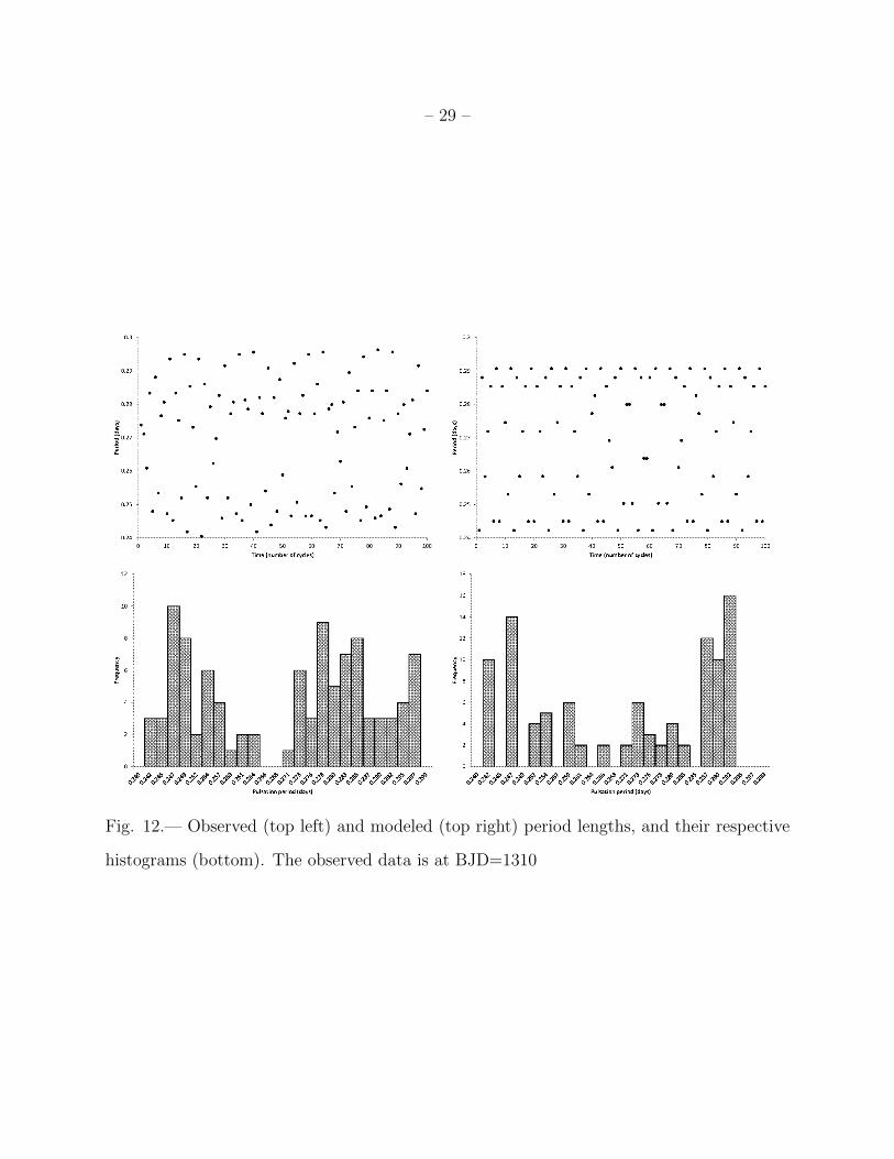
We then ran this simulated curve for 100 cycles, and compared the peak times with

the real data. The comparison is shown in Fig. 12 – this simple model resembles the

observational data to some extent. The histogram (figure 13, bottom right) also shows the

two humps. When certain ratios of P1 and PX are chosen, e.g. PX/P1 = 0.632±0.001, it can

also be shown that the two simultaneous sines create specific autocorrelation distributions.

Let us use a simple model equation of f(x) = int(xR)−xR, where int denotes the rounding

to the next integer, and R the period ratio. The function then gives values of close to

0 or close to 0.5 for odd numbers, while for even numbers it gives other values. When

– 28 –

re-normalized to the usual ACF range of [-1, +1], this gives high absolute autocorrelation

for odd numbers, and less so for even numbers.

We have compared our observational data to this model, and calculated all

ACFs(observed) minus ACFs(calculated). The result is an ACF distribution in which

primes are still prominent, but not significantly so (p = 91.35%). We judge this to be

the main explanation of the prime mystery, with some secondary, albeit insignificant,

fluctuation remaining.

One puzzle remains, however. To create the up to 20% phase variations, a relative

strength of ∼20% for PX is required. Fourier decomposition of the actual amplitudes in the

observed data shows that the underlying curve for PX is much weaker than 20%. Average

observed amplitude variations are 4, 015e− for P1 and 79e− for PX , which is a ratio of ∼2%.

Clearly, there is some additional mechanism present which alters the observed light curve.

6. Possible planetary companions

One might raise the question whether some of the observed perturbations are caused

by planetary influence, either through transits, or indirectly by gravitational influence of an

orbiting planet, or massive companion. With regard to the observed secondary frequency

PX = 0.17d, it seems rather on the short side compared to the almost 2,000 planets

discovered so far, but a few of these fall in the same period range (Rappaport et al. 2013).

This opens the possibility of pertubations visible as non-radial modes, perhaps caused by

gravitationally deforming the star elliptically. Another possible mechanism observed in

our own sun concerns the relation between the barycenter for the star and its convection

pattern(Fairbridge et al. 1987). We would therefore not eliminate the planet hypothesis

for RR Lyrae and Cepheids, even though it seems unlikely.

– 29 –

Fig. 12.— Observed (top left) and modeled (top right) period lengths, and their respective

histograms (bottom). The observed data is at BJD=1310

– 30 –

Unfortunately, detecting transits around a variable star is more difficult than for a quiet

star. Removing the pulsation variation(s) with templates or smoothing leaves residuals on

the level of several percent of amplitude, which is higher than the ∼1% fluctuation expected

for the most massive planets, thus obscuring any signature. In addition, the photometry

shows major jitter on the scale of ∼1% of amplitude, which originates from stellar activities.

Yet, a few planets have been found around variable stars. One such example is CoRoT-2b,

a Jupiter-sized planet around a star with low frequency and amplitude modulation (Alonso

et al. 2008).

As photometry is not ideally suited for this task, one might be tempted to opt for

the other major approach to detect planets, the radial velocity method. This is, however,

even less suited as the amplitude variations stem from large radial pulsations, reflected in

large radial velocity variations. Here the same problems with cycle-to-cycle variations and

jitter occur. One idea to overcome this might be to observe brightness and radial velocity

simultaneously, and correlate the findings.

We conclude that it is difficult to detect planets around RR Lyrae or Cepheid stars.

We would encourage the creation of models to study the gravitational impact such bodies

could cause. From these simulations, one could then conclude whether planets could explain

some of the observed effects.

We need also to note, in the context of ruling in or out ETI as any sort of influence or

factor, that the presence or absence of a planet orbiting in the “Goldilocks Zone” around

a variable star needs to be established beyond doubt. The observational difficulties will

be known to any ETI – this sort of star presents particular problems for the detection

of irrefutably artefactual elements in the light detected on earth. This can be taken as

pessimistic evidence regarding the possibility of ETI modulating the light from a variable

star.

– 31 –

7. Simple Pulsation Models

We provide two very simple dynamical models to elucidate the pulsations described

above, especially with regard to the frequency content and the asymmetry of the light

curve. We hope that these models capture some of the essence of the observed pulsation

variations.

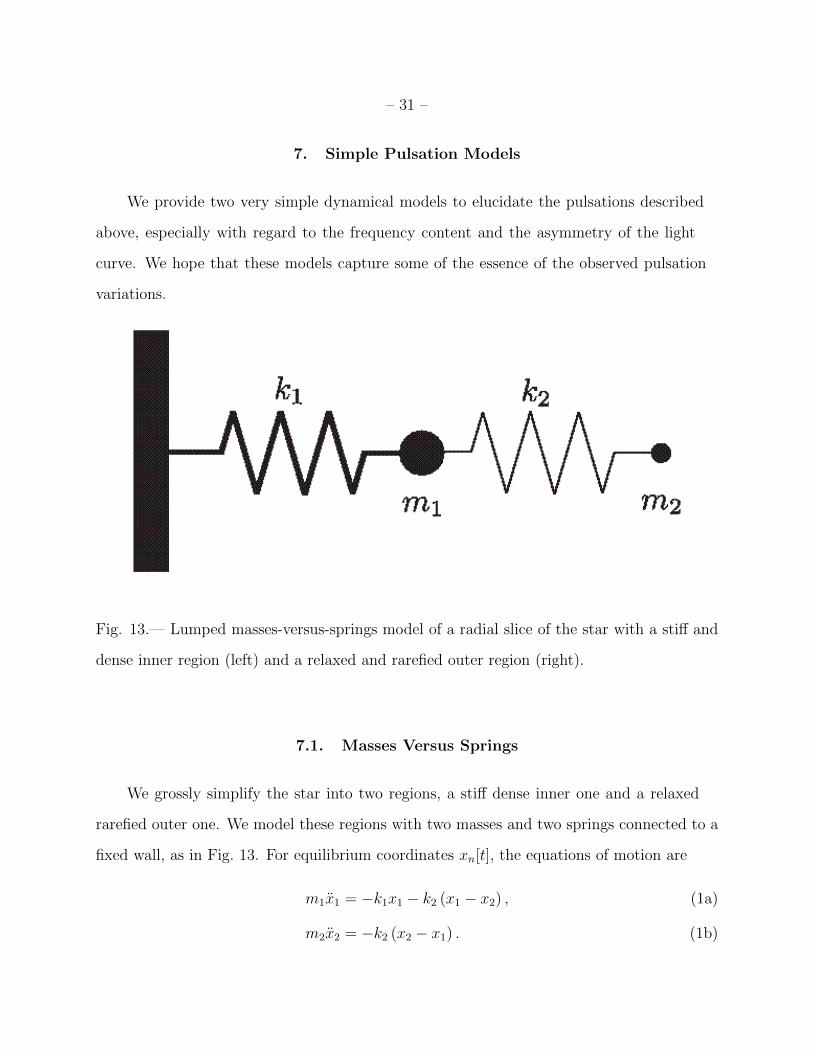
Fig. 13.— Lumped masses-versus-springs model of a radial slice of the star with a stiff and

dense inner region (left) and a relaxed and rarefied outer region (right).

7.1. Masses Versus Springs

We grossly simplify the star into two regions, a stiff dense inner one and a relaxed

rarefied outer one. We model these regions with two masses and two springs connected to a

fixed wall, as in Fig. 13. For equilibrium coordinates xn[t], the equations of motion are

m1x1 = −k1x1 − k2 (x1 − x2) , (1a)

m2x2 = −k2 (x2 − x1) . (1b)

– 32 –

We fix initial conditions x1[0] = 1, x2[0] = 2, x1[0] = 0, x2[0] = 0 and vary the stiffness and

inertia parameters. For k1 = 9, m1 = 8m, k2 = 1, and m2 = m, Eq. (1) has the solution

x1 = +1

3cos [ω+t] +

2

3cos [ω−t] , (2a)

x2 = −2

3cos [ω+t] +

8

3cos [ω−t] , (2b)

where the frequency quotient

ω+

ω−=

√3/2m√3/4m

=√

2 ≈ 1

0.707(3)

is Pythagoras’ constant, the first number to be proven irrational. For k1 = 4, m1 = 4m,

k2 = 4/5, and m2 = m, Eq. (1) has the solution

x1 =5−√

5

10cos [Ω+t] +

5 +√

5

10cos [Ω−t] , (4a)

x2 =5− 3

√5

5cos [Ω+t] +

5 + 3√

5

5cos [Ω−t] , (4b)

where the frequency quotient

Ω+

Ω−=

√(√5 + 1

)/√

5m√(√5− 1

)/√

5m=

1 +√

5

2≈ 1

0.618(5)

is the golden ratio, the most irrational number (having the slowest continued fraction

expansion convergence of any irrational number). In each case, the free mass parameter m

allows the individual frequencies to be tuned or scaled to any desired value.

We identify the star’s radius with the outer mass position, r = re + x2, where re is the

equilibrium radius. If the star’s electromagnetic flux is proportional to its surface area, then

F = k(re + x2)2. (6)

(Squaring generates double, sum and difference frequencies, including those in the original

ratios.) For appropriate initial conditions, Fig. 14 graphs the Eqs. (4-6) stellar flux as a

function of time and is in good agreement with the Kepler data.

– 33 –

Fig. 14.— Stellar flux versus time for the lumped masses-versus-springs model (black), based

on the Eq. (4) motion x2 of the outer mass with frequencies in the golden ratio, superimposed

on Kepler data (grey).

7.2. Pressure Versus Gravity

A star balances pressure outward versus gravity inward. Assuming spherical symmetry

for simplicity, the radial force balance on a shell of radius r and mass m surrounding a core

of mass M is

mr = fr = 4πr2P − GMm

r2, (7)

– 34 –

where the volume

V

V0=

(r

r0

)3

, (8)

and the pressure

P

P0

=

(V0V

)γ, (9)

Assuming adiabatic compression and expansion and including only translational degrees of

freedom, the index γ = 5/3, and the radial force

fr = f0

(rer

)2 (rer− 1), (10)

where re is the equilibrium radius, so that fr[re] = 0, and fr[0.68re] ≈ f0. The corresponding

potential energy

U = Ue

(rer

)(2− re

r

), (11)

where Ue = −f0re/2 is the equilibrium potential energy. The apparent brightness or flux of

a star of temperature T at a distance d is proportional to the star’s radius squared,

F =L

4πd2=

4πr2 (σT 4)

4πd2=(rd

)2 (σT 4

)= kr2, (12)

where k is nearly constant if the star’s luminosity L depends only weakly on its temperature

T . (In contrast, (Bryant 2014) relates a pulsating star’s luminosity to the velocity of its

surface.)

The resulting flux is periodic but non-sinusoidal. The curvature at the maxima is less

than the curvature at the minima due to the difference between the repulsive and attractive

contributions to the potential, but the contraction and expansion about the extrema are

symmetric. To distinguish contraction from expansion, we introduce a velocity-dependent

parameter step

f0 =

f1, r < 0,

f2, r ≥ 0.(13)

– 35 –

Fig. 15.— Stellar flux versus time for the pressure-versus-gravity models (black) super-

imposed on Kepler data (grey). The two-region piecewise constant model asymmetrizes

expansion and contraction (left), while the three-region piecewise constant model adds an

expansion bump (right).

For specific parameters, the left plot of Fig. 15 graphs the resulting light curve, which

asymmetrizes the solution with respect to the extrema. To add a bump to the expansion,

we introduce velocity- and position-dependent parameter steps

p =

p1, r < 0,

p2, r ≥ 0, r < rC ,

p3, r ≥ 0, r ≥ rC ,

(14)

where p is f0, re, or m. The right plot of Fig. 15 graphs the corresponding light curve. This

model captures most of the features of Fig. 5.

From a dynamical perspective, simple models with a minimum of relevant stellar

physics are sufficient to reproduce essential features of the KIC 5520878 light curve.

The masses-versus-spring example demonstrates that a lumped model can readily be

adjusted to exhibit a golden ratio frequency content similar to that of the light curve. The

pressure-versus-gravity example demonstrates that an adiabatic ideal gas model can readily

be modified to exhibit the asymmetry of the light curve. Nothing exotic is necessary.

– 36 –

8. Conclusion

We have tested the idea to search for two pulsation regimes in Cepheids or RR Lyrae,

and have found one such candidate (Learned et al. 2008). This fact, together with the large

period variations in the range of 20%, has previously been overlooked due to sparse data

sampling. We have shown, however, that the pulsation distribution and the associated high

absolute values of prime numbers in autocorrelation in this candidate are likely of natural

origin. Our simple modeling of the light curves naturally accounts for their key features.

Despite the SETI null result, we argue that testing other available or future time-series

photometry can be done as a by-product to the standard analysis. In case of sufficient

sampling, i.e. when individual cycle-length detection is possible, this can be done

automatically with the methods described above. Afterwards, the cycle lengths can be

tested for a two-peak distribution using a histogram or a kernel density estimate. In the

rare positive cases, manual analysis could search for patterns (primes, fibonacci, etc.) in

the binary time-series bitstream.

We like to thank Robert Szabo and Geza Kovacs for their feedback on an earlier draft,

and Manfred Konrad and Gisela Maintz for obtaining the photographs of KIC5520878.

AZ’s work is supported by the National Science Foundation under grant no. PHY07-57035

and partially by the Humboldt Foundation. JFL, BK, and WLD gratefully acknowledge

support from the Office of Naval Research under Grant No. N000141-21-0026.

– 37 –

REFERENCES

Alonso, R., Auvergne, M., Baglin, A. 2008, A&A, 482, L21-L24

Benko, J. M., Szab, R., Guzik, J. A. et al. 2014, IAU Symposium, 301, 383-384

Blazhko, S. 1907, Astronomische Nachrichten, 175, 327

Bryant, P. H. 2014, ApJ, 783, L15

Caldwell, D. A., Kolodziejczak, J. J., Van Cleve, J. E. et al. 2010, ApJ, 713, L92-L96

Christiansen J. L., Jenkins J. M. 2011, KSCI, 19040 - 004

Dworetsky, M. M. 1983, MNRAS, 203, 917-924

Fairbridge, R. W., Shirley, J. H. 1987, Solar Physics, 110, 191-210

Guggenberger, E., Kolenberg, K., Nemec, J. M. 2012, MNRAS, 424, 649-665

Kolenberg, K. 2004, Proceedings of the International Astronomical Union, 367-372

Kolenberg, K., Szab, R., Kurtz, D. W. et al. 2010, ApJ, 713, L198

Layden, A. C. 1995, AJ, 110, 2288

Le Borgne, J. F., Poretti, E., Klotz, A. et al. 2014, MNRAS, 441, 1435-1443

Learned, J. G., et al. 2008, arXiv:0809.0339

Lee, Y.-W. 1992, ed. Warner, B., RR Lyrae Variables and Galaxies Variable Stars and

Galaxies, 30, 103

Lomb, N. 1976, Kluwer Academic Publishers, 39, 447-462

Marconi, M., Nordgren, T., Bono, G. et al. 2005, ApJ, 623, L133-L13

– 38 –

Moskalik, P. 2014, Precision Asteroseismology, 301

Nemec, J. M., Cohen, J. G., Ripepi, V. et al. 2013, ApJ, 773, 181

Parzen, E. 1962, The Annals of Mathematical Statistics 33, 3

Petrie, R. M. 1962, Astronomical Techniques, University of Chicago Press

Leavitt, H. S., Pickering, E. C. 1912, Harvard College Observatory Circular, 173, 1-3

Ransom, S. M., Eikenberry, S. S., Middleditch, J. 2002, AJ, 124, 1788-1809

Rappaport, S., Sanchis-Ojeda, R., Rogers, L. A. 2013, ApJ, 773, L15

Rosenblatt, M. 1956, The Annals of Mathematical Statistics 27, 3

Scargle, J. D. 1982, ApJ, 263, 835-853

Smith, H. 2004, RR Lyrae Stars, Cambridge University Press

Stellingwerf, R. F., Nemec, J. M., Moskalik, P. 2013, arXiv:1310.0543

Szabo, R., Kollth, Z., Molnr, L. et al. 2010, MNRAS, 409, 1244-1252

Szabo, R., Szabados, L., Ngeow, C.-C. et al. 2011, MNRAS, 413, 2709-2720

Welch, D., Website, http://www.aavso.org/

now-less-mysterious-blazhko-effect-rr-lyrae-variables, accessed 21-

Aug-2014

*

This manuscript was prepared with the AAS LATEX macros v5.2.

– 39 –

A. Appendix: Model Parameters

Equation (4-6) model parameters and initial conditions for Fig. 14 are

m = 0.00263,

xe = 0.938,

k = 36 562.1,

x10 = −0.062,

x20 = 0.076,

v10 = 0.405,

v20 = −0.565.

Equations (7, 10, 12) model parameters and initial conditions for the left plot in Fig. 15

are

– 40 –

m = 0.00205,

re = 0.901,

f1 = 0.594,

f2 = 1.822,

k = 39 160,

r0 = 0.96,

v0 = −1.

– 41 –

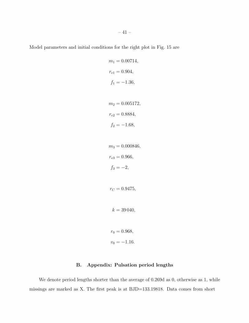
Model parameters and initial conditions for the right plot in Fig. 15 are

m1 = 0.00714,

re1 = 0.904,

f1 = −1.36,

m2 = 0.005172,

re2 = 0.8884,

f2 = −1.68,

m3 = 0.000846,

re3 = 0.966,

f3 = −2,

rC = 0.9475,

k = 39 040,

r0 = 0.968,

v0 = −1.16.

B. Appendix: Pulsation period lengths

We denote period lengths shorter than the average of 0.269d as 0, otherwise as 1, while

missings are marked as X. The first peak is at BJD=133.19818. Data comes from short

– 42 –

cadence where available, otherwise long cadence. Line breaks after 48 periods, showing

strong positive auto correlation.

101101010010100101001010101101011010100101011010

101101011010110101011010101101011010100101010010

10100101101010100101011XXXXXXXXXXXXXXXXXX1010110

101101010010XX1011010110101101010110XXXXXXXXX110

10110101010100101001011 XX00101010110101010010010

11000101010 XX01010010100XX10010111010XX010010100

10XX01100101011XX00001001001XX10100100101XX10110

XXX100XX1001XX10110XX0110XXXXX10XX10011011010010

110100101001011001011001010100101001XX1001XX1010

0XX1001010011101XX00100XXXX1001010XXXXXXXX101011

0101101010101101011 XX0110101101010XX110101101011

0101XX111010110XX110XXXX0101XX01101011010XX01011

010101XX1XXXXX01011XX01101010101XX10010100101010

1101010010XX01010010101XX1XX01001010010XX0101010

1XX1XX00101001010XX01010110XXXXXXXXXX101011XX010

10010XX0XX10010101010010XX01010010XX10010101XX1X

X00101001XX00101110101XX1XX101001010XXXXXXXXXXXX

1001010010100010 XX01001010010XX01000101001XX0010

1001010 XX01110100101XX101001XX100011101011010010

101101100101101011 XXXXX0100101000101001011010010

11011010010110101101XXXXXXXXXXXXXXXX101101011010

110010110101101001011010110010110111100101011011

11001110011010010101100101001101011010110110100X

X110110101XX10010010110101101001011010010011XXXX

– 43 –

XX1010110010110100101101001001011010010100101101

0110011010110101101001011XX101101011XX011XX0101X

X101011010100101011010XXXXXX11101011010101001010

010 XX11010100101010010100101001010101101XX001010

01010010101011010100XX10001101101XXXXX0101001110

1XX101010010100101001010110101011010100101001010

101101011010100 XX1011110101101011010100101010110

10110101101100101 XXXXXX0101101010000101001010010

10 XX011101011XX001010010100101110100101001010010

10100101001010100101011010XXXXX101101XX001011010

101011010111001101010101101011010110101001010110

101001010101101011 XX01001010110XX101101011010110

XXXXX0110XXXX010110101XX101010110101101011010110

011010110101101001001010111010110100101101011000

01101001011010110101 XXXX111011100110101100111011

100011000110100101001011100011000110101101101011

100011010110101101011010101011010110100XXX111010

101001010110101101010000101011010110101101010000

101011010110101001010100101011010110101001XX0101

101010 XXXXX01010XX010101101010010100101010010101

10101001010010101101010110101001XX0XXX1011010101

0010100101001010101XXXXXXXXXXXXXXXXXXXXXXXXXXXXX

XXXXXXXXXXXXXXXXXXXXXXXXXXX1XX101101010101001010

01010010100101010100101001010010101101010100100X

X010100XX101110010XX010100101XXXXXXXXXXX10100101

001010010101101010100101001010011001101010101101

– 44 –

00 XX10010101010101001011010100101011010101101011

010101101011010101101011010110101011000XXXXXXXXX

XXXXXXXXXXXXXX001011010100101001XX01101010110101

01101001010 XX010101101011010100101011010XX010101

101010010101101010110101101010010101101010110101

10101 XXXX101101010110101101011010101101010110101

101010110101 XX101011010XX01010110101001010110101

00101011010101101 XXXX101011010110101011010010101

0110101001010110101000010110101011010110101011XX

010010101101011010101001011010101101011XXXX11010

101101011010110101011010100101001010110101011010

100101001010010101011010110101001010010101011010

10010100100 XXX1101011010110101001010101101011010

110101101010101101011010110101100110101001011010

11010010011110010101101011010110100XXX1101011010

110111010110100101011010110011010010100101001010

110001010010100101001011101001010010100101001011

101000 XXXXX1010010100100010100101001010010101101

01XX001010XX0XXXX0101001010100101001010010101001

01011010101XX1001010101101011XXXX1010XX100101011

010 XX0101101010XX11010110101XX101011010100101011

010110 XX1011010101101XX1010100100111010101101011

XXXX001010100101011010110XXXXXXXXXXX110101101010

010101001010110101101010010100101010110101001010

01010100101011010110101001010XX110XXXXXX01101XX0

11010101101011010101001010010101101010010XX01010

– 45 –

101101XXXXXXXXX10101101XXXXX0101101010111XXX1010

101101010010101101010110101101010110101001XX0010

101001010110101011010110101011010110101011010110

1XXXXX01011010101101010XXXXXXXXXXXXXXXXXXXX10XXX

1010110100101010100011001010 XX01010010101XX10100

101001010 XXX010101101011010110101010010101101011

010110101010010101101011010100101010110101101011

010101001010110101101011010101011001 XX0101101011

010101001010110101101010110101001010110101101010

101101001010110101101010110101001011100101001010

111 XXX011010110101001010110101011010110101001010

1001010110101001010110101011010110100101011XXX10

10110101100 XXXX1010110101011010X0010100101010010

101101011010100101010011XXXXXXXXXXXXXXXXXXXXXXXX

XX11010110101001010101101011010111XXXX1101010110

101101011010101011010110101101011010101011010110

101101011010101011010110101101010101101011010110

101100 XXXX01101011010110101100010101101011010110

101100010100101001010110101010010100101011010110

1010100101001010110101011010100101001011XXXXXXXX

001010010100101011010101001010010101101010110101

101010010101101010110101001010010101001010110101

0010100101010110100 XXX01001010110101011010100101

11XXXXXXXXXXXXXXXXXXXXX1011010101101010010100101

01101010110101001010010101011010110100XXX1101101

010110101001010010101011010110101101010110101101

– 46 –

010110101101010110101011010110101011010101101011

010110101011010100101011011 XXXX01011010100101011

00XXXXXXXXXXXXXXXXXXXXXXXXXXXXXXXXXXXXXXXXXX1010

010101101011010100101010110101101011010101101010

110101101011010101101010110101101010110101101010

11010110101011010100101011010101100XXXX101001010

110101011010110101011010101101011010110101011010

101101011010110101010110101101011010010110010110

10110100101000 XXXX010111X00101001011010010010110

100101001011010010010110100101101001010010010010

100110XXXXXXXXXXXXXXXXXXX101011010010