Institute for Advanced Development Studies

Development Research Working Paper Series

No. 04/2010

Public Expenditure Policy in Bolivia: Growth and Welfare

by:

Carlos Gustavo Machicado Paul Estrada

Ximena Flores

May 2010 The views expressed in the Development Research Working Paper Series are those of the authors and do not necessarily reflect those of the Institute for Advanced Development Studies. Copyrights belong to the authors. Papers may be downloaded for personal use only.

-1-

Public Expenditure Policy in Bolivia: Growth and Welfare

Carlos Gustavo Machicado Paul Estrada Ximena Flores

La Paz, May 2010

Abstract

It has been widely documented that fiscal policy can promote economic growth, when it is based

on an efficient provision of pubic capital. But little work has been done, in Bolivia, in relation to the

macroeconomic and sectoral impacts of increasing public investment in infrastructure. This paper

develops a Dynamic Stochastic General Equilibrium (DSGE) model for a small open economy with

five sectors: Non-tradable or services, importable or manufacturing, hydrocarbons, mining and

agriculture. The model is parameterized and solved for the Bolivian economy and several

interesting scenarios are simulated by changing government expenditures, taxes, country risk,

Total Factor Productivity, effectiveness of public capital and terms of trade. This analysis is

relevant for the Bolivian economy, because the government is using fiscal policy as one of its main

tool to attack poverty and aims to put public investment as the foremost instruments to promote

growth and welfare.

Keywords: Fiscal Policy, Infrastructure, Multisector Growth Model

JEL Classification: E62, H54, O41

We would like to thank Tim Kehoe and Juan Pablo Nicolini for their useful comments and suggestions. We

are also indebted to Diego Vera for able research assistance. This work was carried out with financial and scientific support from the Poverty and Economic Policy (PEP) Research Network, which is financed by the

Australian Agency for International Development (AusAID) and by the Government of Canada through the

Canadian International Development Agency (CIDA), and the International Development Research Centre

(IDRC).

Institute for Advanced Development Studies (INESAD), e-mail: cmachicado@inesad.edu.bo

Institute for Advanced Development Studies (INESAD), e-mail: paulestrada2@gmail.com

Institute for Advanced Development Studies (INESAD), e-mail: xflores@inesad.edu.bo

-2-

1. INTRODUCTION Although infrastructure was incorporated into the theory of growth literature by Arrow & Kurzs

(1970) and Weitzman (1970), people only began to study the topic seriously after the seminal

work of Barro (1990). Barro's model is well known because he introduces government spending as

a variable in the production function. The existence of constant returns to capital and government

spending imply that the economy is capable of endogenous growth.

Coinciding with this rebirth of the growth literature, there is also the appearance of an empirical

literature related to infrastructure. Infrastructure becomes an important source of growth as

shown by Aschauer (1989a, 1989b). These works concentrated on the estimation of the

production elasticities of government expenditure, using aggregated data for countries, mainly the

U.S.1 There are also cross-country studies that emphasize the role of infrastructure for a country's

growth.2

Papers in this literature have typically used regression analysis on either "growth accounting" or

steady state equations. While these papers have been useful in pointing out the importance of

infrastructure, their methodology does not allow for the analysis of important general equilibrium

feedback effects among key macroeconomic variables and welfare.

In this sense, this paper examines the impact of fiscal policy on output, consumption, private

investment and foreign trade, using a Dynamic Stochastic General Equilibrium (DSGE) model for a

small open economy with five sectors and with the new feature that firms in each sector employ

public capital or infrastructure as a factor of production. These sectors which are the non-tradable

sector (services), the importable sector (manufacturing), hydrocarbons, mining and agriculture are

representative of the Bolivian economy. In particular the hydrocarbons sector, which is intensive

in capital, is conceived by the government as a strategic sector that will generate resources

necessary to attack poverty and underdevelopment.

Therefore, the main objectives of the paper are: First to analyze the macroeconomic impact of a

change in government expenditures, tax structure and public investment in infrastructure on

output, consumption, private investment, trade balance and welfare, i.e. the macroeconomic

impacts of fiscal policy. Second, we aim to analyze the macroeconomic impact of changes in

relative prices, productivity (TFP), effectiveness of public infrastructure, country risk and public

consumption valuation. In addition, in both cases we are interested in computing also the sectoral

impact of these simulations and the social impact measured through the transfers that the

government gives to the households.

1 Munnell (1990) and García-Milá, McGuire and Porter (1993) use Panel Data to estimate production

elasticities. 2 See Easterly and Rebelo (1993), Ford and Poret (1991), Hulten (1996) and Canning (1998) among others.

-3-

We aim to capture also important dynamics involving public expenditure as well as public

investment policies combined with expansions in TFP and in the effectiveness of public capital. The

transitional dynamics are also analyzed for situations in which the government intends to maintain

its transfer programs unaltered. In the last years, the Bolivian government has based its policy to

attack poverty on transfers to households through bonuses, therefore it is important to analyze

under which conditions this policy can be sustainable over time.

The DSGE model is based on Chumacero, Fuentes, & Schmidt-Hebbel (2004) but modified to

include public investment in infrastructure in a way similar to Rioja (2003) and sector division for

the exportable sector as in Estrada (2006). We calibrated the model for the Bolivian economy and

solved it using the second-order-approximation technique developed by Schmitt-Grohé and Uribe

(2004). The advantage in using this perturbation method is that it allows considering second-order

effects, which arise as important features in an economy with high levels of uncertainty.

An important aspect is that the model allows us to extract precise quantitative implications,

because we examine the effects of a range of different scenarios on real output and welfare, as

well as on other macroeconomic variables like consumption, investment and on output of the

different five sectors. Model simulation results are reported first, for steady-state effects and then

for the dynamic effects on the composition of these variables.

The paper is organized as follows. Section 2 briefly describes fiscal policy in Bolivia. Section 3

describes the dynamic general equilibrium model and its calibration for the Bolivian economy.

Then in section 4 we present the simulation results for steady-state effects as well for the dynamic

effects on selected macroeconomic and sectoral variables. Section 5 concludes.

2. FISCAL POLICY IN BOLIVIA Since 2006 the Bolivian economy has recorded a fiscal surplus, explained mainly by the

international economic boom, translated into high export prices of the products that the country

exports, more revenues from the Direct Tax on Hydrocarbons and royalties which increased public

sector revenues in an important manner. Between 2004 and 2008 the government income has

increased by almost 20 percentage points of GDP.3

The following figure shows how these events affected the path of the fiscal deficit as a percentage

of GDP and its close relationship with the rate of growth of the economy. Since 2002 the trend of

the fiscal deficit was decreasing until turning into a surplus in 2006. The fiscal surplus was 4.5

percent of GDP, the highest in recent years, and the fiscal balance remained positive until 2009

inclusive.

3 For comparison, the fiscal revenues of the U.S. federal government increased by 18.7 percent of GDP in the

last 40 years (U.S. Congressional Budget Office, 2009).

-4-

Figure 1: Fiscal Surplus and Economic Growth (in percentages)

Source: Central Bank of Bolivia

The growth rate of the economy has been steadily growing since 2002 and it is positively

correlated with the public sector fiscal results. In the period 2004 - 2008 the average growth rate

of the economy was 4.8 percent and in 2008 it was 6.1 percent, the highest rate of growth since

1975. In that sense, the economy experienced an unprecedented scenario mainly driven by the

hydrocarbons sector, mining and construction. On the other hand, government expenditures grew

significantly in the last years, but much less than incomes. Total incomes increased from 31.6

percent of GDP in 2005 to 48.4 percent of GDP in 2008, while total expenditures increased from

33.9 percent of GDP to 45.1 percent of GDP in the same period. Tax revenues increased also by 17

percent (average between 2004 and 2009). The principal taxes are the Value Added Tax (IVA) and

the Direct Tax on Hydrocarbons (IDH), which together represent 50 percent of total tax revenues

(see table 1). All of this allowed strengthening the country’s infrastructure and stimulating

economic development by increasing resources for the health and education sectors. The State

also increased its participation in productive activities.

In recent years public investment increased from 6.3 percent of GDP in 2005 to 10.5 percent of

GDP in 2009. Around 1.5 percentage points of this increase corresponds to investment in

infrastructure. It seems that infrastructure investment increased in line with the growth of the

economy, but social investment and in particular in health and education has remained almost

unchanged. The data show that capital spending in recent years has focused on road infrastructure

and water resources, however since 2005 investment to support productive activities has again

increased but not up to the levels reported in 2002. Certainly, investment in infrastructure plays a

crucial role in any development strategy for Bolivia, since transport costs are very high, about 20

times higher than in Brazil, according to Weisbrot et al. (2009).

-3.7

-6.8

-8.8-7.9

-5.5

-2.3

4.51.7 3.2 4.8

2.51.7

2.5 2.7

4.2 4.4 4.8 4.6

6.1

3.2

-10.0

-8.0

-6.0

-4.0

-2.0

0.0

2.0

4.0

6.0

8.0

2000 2001 2002 2003 2004 2005 2006 2007 2008 2009 I SemDeficit/Surplus Fiscal Economic Growth

-5-

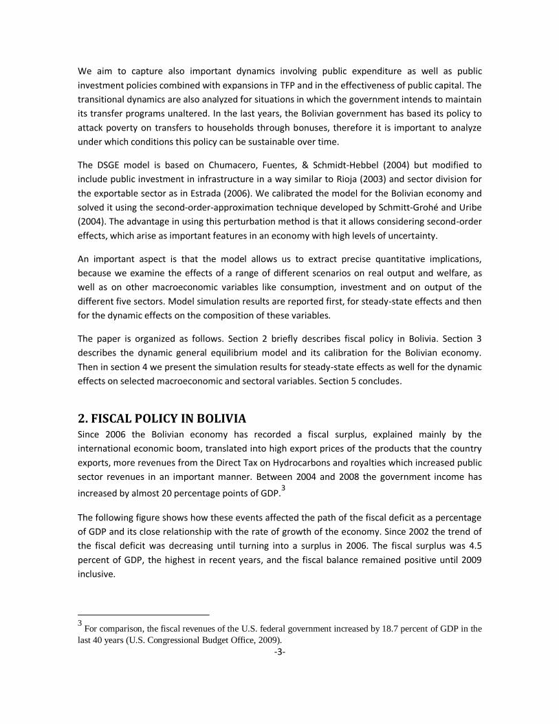
Table 1: Tax Revenues, 2004 – 2009 (In Millions of Bolivianos)

2004 2005 2006 2007 2008 2009

Value Added Tax (IVA) 4,411 5,261 6,405 7,756 9,558 8,859 Transactions Tax (IT) 1,567 1,704 1,812 2,081 2,560 2,166 Firm’s Profits Tax (IUE) 1,468 2,081 2,872 3,059 4,502 7,172 Specific Consumption Tax (ICE) 558 663 782 930 1,113 1,171 Complementary Regime Value Added Tax (RC-IVA)

193 213 216 217 258 288

Hydrocarbons Especial Tax (IEHD) 1,147 1,886 2,000 2,383 2,530 1,791 Financial Transactions Tax (ITF) 314 633 446 324 340 339 Others 914 317 345 525 695 1,140

Total Domestic Taxes 10,571 12,757 14,879 17,275 21,556 22,927

Direct Tax on Hydrocarbons (IDH) 0 2,328 5,497 5,954 6,644 6,465 Import Tariff (GA) 672 796 921 1,117 1,407 1,179

Total Domestic Taxes + IDH + GA 11,243 15,881 21,297 24,346 29,607 30,571 Source: Ministry of Economy and Public Financing

Figure 2: Public Investment (percentages of GDP)

Source: UDAPE

Figure 2, shows the evolution of public investment as percentage of GDP. Investment in social

issues has decreased from 3.3 percent in 2002 to 2.3 percent in 2006, but then it has increased

again up to 2.8 percent in 2009. Notice that investment in infrastructure has increased the most.

In 2009 it accounts for 4 percent of GDP. Weisbrot et al. (2009) indicate that the creation of the

0.00%

0.50%

1.00%

1.50%

2.00%

2.50%

3.00%

3.50%

4.00%

4.50%

% o

f GD

P

Infrastructure Social Health Education Production

-6-

Productive Development Bank (BDP for its initials in Spanish) in 2007 is in part reflected in public

investment.4

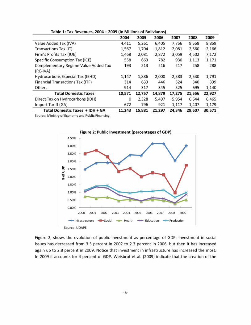
Figure 4 shows the composition of current income of the nonfinancial public sector. It can be seen

that tax revenues remain the main source of income, although oil revenues have increased due to

the boost in international prices. Also in 2007 public companies began to generate incomes due to

the process of nationalization of the so called strategic companies.5

Figure 3: Public Investment (percentage of GDP)

Source: Central Bank and Ministry of Economy and Public Financing

Much of these revenues are transferred to sub national governments (Prefectures, Municipal

Governments and public universities) which are the entities that execute the public investment,

but mostly in social issues than in road infrastructure. The largest infrastructure projects are

implemented by national bodies such as the Ministry of Public Works or the Bolivian road

company (Administradora Boliviana de Caminos, ABC).

4 Since October 2009 the BDP has lent USD 156 million to 15,903 individuals with an average of USD

10,000 per person. 5 Here we can mention the nationalization of YPFB –the oil company- in 2006, the nationalization of Entel-

the telecom company- in 2008, the creation of BOA –an aviation company- in 2008 and the reactivation of

Comibol –the mining company- in 2009.

2.9% 3.1%2.4%

3.5% 3.8%4.4%

3.6%

5.0%

1.0% 1.0%

0.7%

0.7%0.9%

1.5%

1.7%

2.3%3.5% 3.2%

2.2%

1.7%1.7%

2.1%2.3%

2.7%

0.5% 0.7%

0.5%0.5%

0.4%

0.5%0.4%

0.6%

0.0%

2.0%

4.0%

6.0%

8.0%

10.0%

12.0%

2002 2003 2004 2005 2006 2007 2008 2009

Multisectorial

Social

Productive Act.

Infrastructure

-7-

Figure 4: Composition of Government Current Income (percentage of total)

Source: UDAPE

As shown in Table 2 the main sources of financing public investment are the Direct Tax on

Hydrocarbons (IDH), royalties and co-participation with municipalities. Between 2004 and 2008

the government revenues from hydrocarbons raised from USD 53 per capita up to USD 401.1 (in

constant dollars of 2008). Remark that most of the resources that are currently financing public

investment are temporary, in particular those resources that come from the high prices of natural

gas and mining exports. In this framework it is necessary to optimize the executions of public

investment.

Table 2: Public Investment Composition by Source of Financing (as percentage of total)

Source 2000 2001 2002 2003 2004 2005 2006 2007 2008

Total Public Investment 100.0 100.0 100.0 100.0 100.0 100.0 100.0 100.0 100.0

Internal Resources 52.9 52.1 46.2 36.4 33.6 37.2 62.4 68.6 68.5

TGN y TGN-Titles 5.2 6.6 5.0 3.9 3.5 2.4 1.3 2.2 6.4 Found of Compensation 1.6 1.8 1.4 0.9 1.1 0.5 0.6 0.5 0.7 Counter Value Resources 3.8 3.0 5.3 2.7 3.0 1.7 1.8 1.6 1.4 Co participation IEHD 5.2 5.9 3.0 2.7 2.0 2.1 1.8 1.2 2.8 Direct Tax on

Hydrocarbons (IDH) -- -- -- -- -- 1.5 24.4 31.7 21.6

Co participation Municipalities

17.3 15.2 13.4 13.1 11.0 10.4 9.9 10.7 11.2

Royalties 3.2 4.3 5.6 6.6 7.3 12.2 19.6 17.0 15.2 Own Resources 13.3 13.1 10.9 5.5 5.2 5.6 2.6 3.2 8.6 Other 3.4 2.3 1.5 1.0 0.6 0.7 0.5 0.5 0.7

External Resources 47.1 47.9 53.8 63.6 66.4 62.8 37.6 31.4 31.5

Credits 34.8 30.3 33.9 43.4 50.3 49.5 26.1 22.2 22.1 Donations 12.4 17.6 19.9 20.2 16.1 13.3 11.5 9.2 9.3

Source: Ministry of Economy and Public Financing

Bolivia’s poverty reduction strategy is based solely in the conditional transfers that the

government gives to households. The type of transfers has expanded in the last years. There are

-8-

currently three types of transfers: Renta Dignidad (for persons over 60 years of age), bono

Juancito Pinto (for students in primary school) and bono Juana Azurduy (for mothers during and

after pregnancy)6. Figure 5 shows the current transfers, with and without pensions.

Figure 5: Transfers (in Millions of Bolivianos)

Source: Ministry of Economy and Public Financing

In 2008 the number of beneficiaries amounted to 1,681,135 and 687,962 for the Bono Juancito

Pinto and Renta Dignidad, respectively. The percentage of relevant population covered by these

conditional transfers programs is 95.9 percent for the first bonus and 101.8 percent for the second

bonus. This amount is larger than 100 percent because they covered more people than what was

expected. These transfers are social in nature and directly influence the consumption of

beneficiary households. By calibrating the general equilibrium model, in the next section, we aim

to identify the macroeconomic impact of these policies as well as the pressure on the fiscal

balance.

Finally, figure 6 shows the domestic and external debt acquired by the government during the last

seven years (period 2002 – 2009). Notice, that there has been a substitution between foreign and

domestic debt, with domestic debt becoming more important than foreign debt in 2006. The

domestic debt has been increasing steadily from USD 1710 millions in 2002 to USD 5256 millions in

2008, and only in 2009 do we observe a slight decline. The opposite happened with the external

debt, although we observe an increase in the last two years. Most of the domestic debt is with the

so called AFP’s (Pension Funds Administrators) and with the Central Bank. However, the

6 According to Ministry of Economy and Public Financing, the 28 percent of Bolivian population is

beneficiary of these three bonds..

0.0

500.0

1,000.0

1,500.0

2,000.0

2,500.0

3,000.0

3,500.0

4,000.0

2000 2001 2002 2003 2004 2005 2006 2007 2008 2009 (sept)

Without Pensions Pensions

-9-

government has been able to reduce its debt with the Central Bank, because it has enjoyed fiscal

surpluses.

Figure 6: Debt Domestic and External (In Millions of USD)

Source: Central Bank of Bolivia

3. MODELLING AND CALIBRATION

3.1 THE BASIC MODEL

The model is based on Chumacero, Fuentes, & Schmidt-Hebbel (2004) and modified in order to

address the issue of public investment in infrastructure as in Rioja (2003) and expanded for a

multisector economy as in Estrada (2006). The model is suitable to perform numerous and

interesting simulations related to fiscal policy (increase or decrease of taxes, current spending, and

public investment), increase in productivity, variation in relative prices of agriculture, mining and

energy-goods, variation in country-risk, among others, as will become clear from the following

description.

3.1.1 The Households

The economy is inhabited by infinitely-lived individuals who derive utility from consumption of

importable goods (cm,t), consumption of non-tradable goods (cn,t) and government consumption

(gt) which is basically a public good that does not suffer from congestion. Therefore, a

representative agent maximizes the expected value of lifetime utility as given by

0

,, ),,(t

ttntm

t

t gccuE (1)

4299.7

5039.7 4949.54767.5

3242.1

2188.9

2440.9 2585.6

1710.61951.5

2172.5

2675.5

3672.6

5256.3

4797.0

0

1,000

2,000

3,000

4,000

5,000

6,000

2002 2003 2004 2005 2006 2007 2008 2009

Debt External Debt Domestic

-10-

The other goods that are produced in the economy are exportable goods which we denote xh as

the hydrocarbon good (natural gas), xm as the mineral good (zinc, gold, silver or tin) and xa as the

agricultural good (soya, Brazilian nuts or quinoa).

Each household receives interest income rk, lump-sum transfers from the government , profits

from the importable, non-tradable, mineral and agricultural firms πm, πn, πxm and πxa respectively7

and can also contract foreign debt abroad, b. The household's budget constraint is

tttntmtxatxmttk

tttcmtntnctmcm

bkr

bricpc

1,,,,

,,,

))(1()1(

)~1()1)(1()1()1)(1(

(2)

where τm is an import tariff, τk is the tax on capital income, τc represents the tax rate on

consumption of importables and non-tradables, τ is the tax on sectoral profits, pn is the relative

price on the non-tradable good in terms of the importable good (used as numeraire) and r~ is the

(net) interest rate paid on foreign debt. Private investment, which we denote by i, follows the

standard law of motion for private capital:

ttt kik )1(1 (3)

where δ is the depreciation rate of private capital stock and kt is the capital stock.

Household make choices of cm,t, cn,t, bt+1 and kt+1, i.e the problem of the representative consumer

can be summarized by the following Bellman equation:

tt

tntmtxatxmttk

ttttcm

tntnctmcm

tttntmtttt

b

kr

brkk

cpc

gccubkvbkv

1

,,,,

1

,,,

,,1,1))(1()1(

)~1())1()(1)(1(

)1()1)(1(

),,()(),(

(4)

The first-order conditions are:

)1(,

,

, m

tcm

tcn

tnu

up

(5)

)~1(1 1

,

1,

t

tcm

tcm

t ru

uE (6)

7 Profits can be interpreted also as the retribution to the labor factor, since we are assuming that labor is sector

specific.

-11-

)1

)1)(1(

)1((1 1

,

1,

t

cm

k

tcm

tcm

t ru

uE (7)

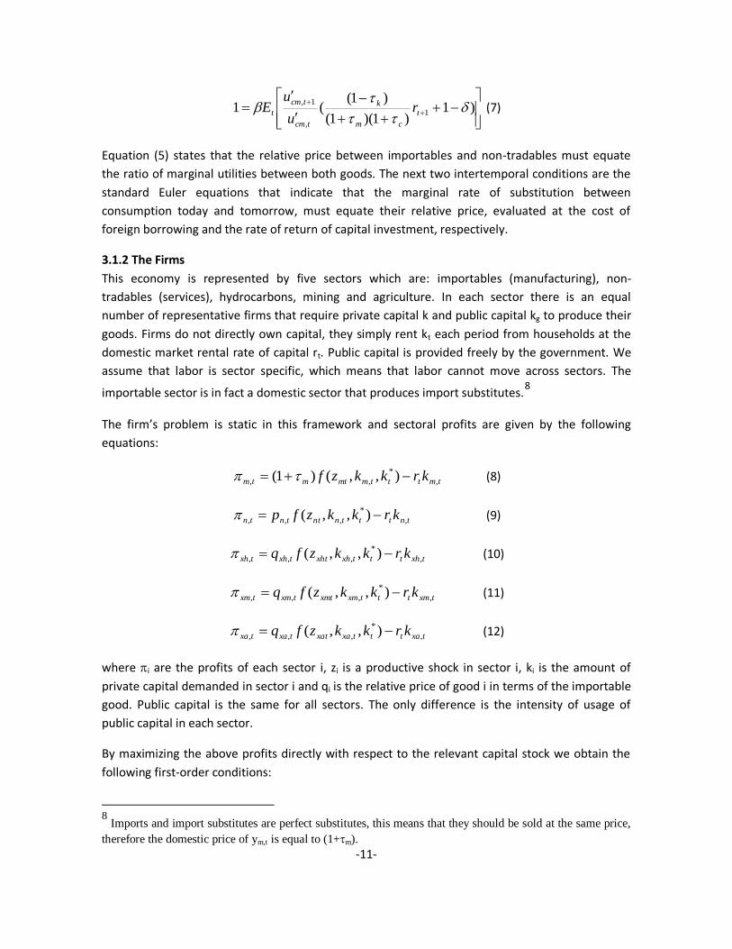
Equation (5) states that the relative price between importables and non-tradables must equate

the ratio of marginal utilities between both goods. The next two intertemporal conditions are the

standard Euler equations that indicate that the marginal rate of substitution between

consumption today and tomorrow, must equate their relative price, evaluated at the cost of

foreign borrowing and the rate of return of capital investment, respectively.

3.1.2 The Firms

This economy is represented by five sectors which are: importables (manufacturing), non-

tradables (services), hydrocarbons, mining and agriculture. In each sector there is an equal

number of representative firms that require private capital k and public capital kg to produce their

goods. Firms do not directly own capital, they simply rent kt each period from households at the

domestic market rental rate of capital rt. Public capital is provided freely by the government. We

assume that labor is sector specific, which means that labor cannot move across sectors. The

importable sector is in fact a domestic sector that produces import substitutes.8

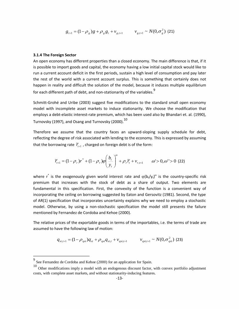
The firm’s problem is static in this framework and sectoral profits are given by the following

equations:

tmtttmmtmtm krkkzf ,

*

,, ),,()1( (8)

tntttnnttntn krkkzfp ,

*

,,, ),,( (9)

txhtttxhxhttxhtxh krkkzfq ,

*

,,, ),,( (10)

txmtttxmxmttxmtxm krkkzfq ,

*

,,, ),,( (11)

txatttxaxattxatxa krkkzfq ,

*

,,, ),,( (12)

where i are the profits of each sector i, zi is a productive shock in sector i, ki is the amount of

private capital demanded in sector i and qi is the relative price of good i in terms of the importable

good. Public capital is the same for all sectors. The only difference is the intensity of usage of

public capital in each sector.

By maximizing the above profits directly with respect to the relevant capital stock we obtain the

following first-order conditions:

8 Imports and import substitutes are perfect substitutes, this means that they should be sold at the same price,

therefore the domestic price of ym,t is equal to (1+m).

-12-

tttmtmkmm rkkzf ),,()1( *

,, (13)

tttntnkntn rkkzfp ),,( *

,,, (14)

tttxhtxhxhtxh rkkzfq ),,( *

,,, (15)

tttxmtxmxmtxm rkkzfq ),,( *

,,, (16)

tttxatxaxatxa rkkzfq ),,( *

,,, (17)

These equations describe the demand for capital services by firms of each production sector of the

economy.

3.1.3 The Government

The government invests in infrastructure I, has current expenditure consumption g and provides

lump-sum transfers to households . The Government has the following budget constraint:

txhttxhtxh

txatxmtntmttxatxatxmtxmtntntmm

ttktmmttmcmttntntmcttt

kryq

kkkkryqyqypy

kryicicpcIg

,,,

,,,,,,,,,,,

,,,,,

)())1((

))(1()(

(18)

Notice that in the right hand side of equation (18) we include all the taxes but also the profits from

the hydrocarbons sector. This is in concordance with the nationalization of the hydrocarbon's

sector that took place in year 2006. Since then, the hydrocarbon's sector is meant as the strategic

sector for the Bolivian economy and one of the main sources of incomes of the government.

Public capital evolves according to

tggttg kIk ,1, )1( (19)

where 0≤kg≤1 is a constant depreciation rate of public capital.

As in Rioja (2003) we assume that only the effective measure of the stock of public capital kg is

useful for private production. That is,

tgt kk ,

* (20)

where 0<θ<1 is an infrastructure effectiveness index. The closer θ is to 1, the more effective the

public capital stock, and the larger the benefit that firms get.

As usual, the government does not optimize any explicit objective function but instead its current

expenditure follows the rule:

-13-

1,1 )1( tgtggt vggg ),0(~ 2

1, gtg Nv (21)

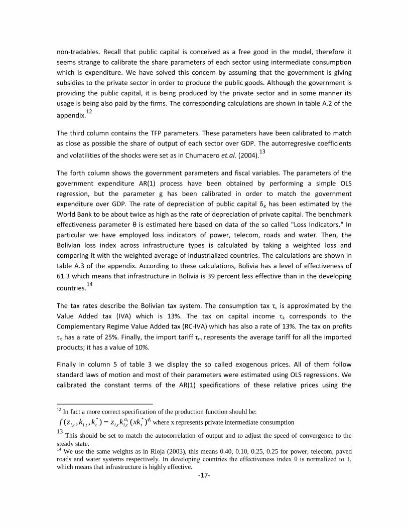
3.1.4 The Foreign Sector

An open economy has different properties than a closed economy. The main difference is that, if it

is possible to import goods and capital, the economy having a low initial capital stock would like to

run a current account deficit in the first periods, sustain a high level of consumption and pay later

the rest of the world with a current account surplus. This is something that certainly does not

happen in reality and difficult the solution of the model, because it induces multiple equilibrium

for each different path of debt, and non-stationarity of the variables.9

Schmitt-Grohé and Uribe (2003) suggest five modifications to the standard small open economy

model with incomplete asset markets to induce stationarity. We choose the modification that

employs a debt-elastic interest-rate premium, which has been used also by Bhandari et. al. (1990),

Turnovsky (1997), and Osang and Turnovsky (2000).10

Therefore we assume that the country faces an upward-sloping supply schedule for debt,

reflecting the degree of risk associated with lending to the economy. This is expressed by assuming

that the borrowing rate 1~tr , charged on foreign debt is of the form:

1,

*

1~)1()1(~

trtr

t

trrt vr

y

brr

0'',0' (22)

where r* is the exogenously given world interest rate and (bt/yt) is the country-specific risk

premium that increases with the stock of debt as a share of output. Two elements are

fundamental in this specification. First, the convexity of the function is a convenient way of

incorporating the ceiling on borrowing suggested by Eaton and Gersovitz (1981). Second, the type

of AR(1) specification that incorporates uncertainty explains why we need to employ a stochastic

model. Otherwise, by using a non-stochastic specification the model still presents the failure

mentioned by Fernandez de Cordoba and Kehoe (2000).

The relative prices of the exportable goods in terms of the importables, i.e. the terms of trade are

assumed to have the following law of motion:

1,,1, )1( tqxitxiqxixiqxitxi vqqq ),0(~ 2

1, qxitqxi Nv (23)

9 See Fernandez de Cordoba and Kehoe (2000) for an application for Spain.

10 Other modifications imply a model with an endogenous discount factor, with convex portfolio adjustment

costs, with complete asset markets, and without stationarity-inducing features.

-14-

where i=xh, xm and xa.

3.1.5 Market-Clearing Conditions

We define the production function of any of the sectors by:

),,( *

,,, ttititi kkzfy (24)

where i again represent each of the five sectors. Remark that the public capital k* is the same for

all the sectors, which means, for instance, that infrastructure will benefit all the sectors in the

same manner. Public capital is a non-rival good.

Equations (24) and (25) represent the market clearing conditions. The first equation describes the

equilibrium in the importable good market, which shows that the current account (CA) balance

must be compensated by the capital account balance. The second equation is the typical

equilibrium condition in the non-tradable good market.

ttttttmtmtxatxatxmtxmtxhtxhtt brIigcyyqyqyqbbCA ~)( ,,,,,,,,1 (24)

and

tntntntn cpyp ,,,, (25)

3.1.6 Competitive Equilibrium

A competitive equilibrium is a set of allocation rules cm=Cm(s), cn=Cn(s), k₊₁=K(s), b₊₁=B(s), k₊₁∗=K∗(s),

kxh+1=Kxh(s), kxm+1=Kxm(s), kxa,+1=Kxa(s), km,+1=Km(s), kn,+1=Kn(s); a set of pricing functions r=R(s), and

pn=Pn(s); and the laws of motion of the exogenous state variables s₊₁=S(s), such that:

Households solve the problem (4) taking as given s and the form of the functions R(s),

Pn(s), and S(s), with the equilibrium solution to this problem satisfying cm=Cm(s), cn=Cn(s),

k₊₁=K(s), and b₊₁=B(s).

Firms of the hydrocarbons, mining, agriculture, importable and non-tradable sectors

maximize profits (13)-(17) taking as given s and the form of the functions R(s), Pn(s), and

S(s), with the equilibrium solutions to these problems satisfying kxh,+1=Kxh(s), kxm,+1=Kxm(s),

kxa,+1=Kxa(s), km,+1=Km(s), kn,+1=Kn(s).

The economy-wide resource constraints (24) and (25) hold each period, and the factor

market clears:

Kxh(s)+ Kxm(s)+Kxa(s)+Km(s)+Kn(s)=K(s)

-15-

3.2 FUNCTIONAL FORMS AND CALIBRATION

The model which is clearly non-linear, is difficult to solve analytically. The alternative is to use

numerical methods. Therefore, we adopt functional forms for the utility and productions functions

and give values to the parameters of the model to match the Bolivian macroeconomic context in

year 2006.

3.2.1 Functional Forms

The generic model presented above suggests the following functional form for preferences:

)ln()ln(),,( ,,,, tnnttmmttntm cgcgccu

with θm, θn>0 and θm+θn=1. The parameter measures how a typical individual values public

consumption relatively to private consumption. The specification for the relationship between

private consumption of importables and public consumption follows Aschauer (1985), Barro

(1981) and Christiano and Eichenbaum (1992). We are assuming that consumption of public goods

can be perfectly substituted (depending on the value of ) with consumption of importable goods,

but not with consumption of non-tradable goods. In this way we want to incorporate into the

model, the fact that the government is increasing its involvement in production activities.11

For the production functions we employ the following specification:

ii

ttitittiti kkzkkzf

)(),,( *

,,

*

,,

where αi is the compensation for capital as a share of output of sector i=xh, xm, xa, m and n and φi

is the coefficient of public capital in the production function that reflects the importance of

infrastructure in each of the different five sectors of the economy.

The productivity shocks zi follow standard AR(1) processes of the form:

1,,1, )1( titiiiti vzzz ),0(~ 2

1, iti Nv

3.2.2 Calibration

Once the laws of motion are specified, we accurately calibrate the model so that it can display the

main characteristics of the Bolivian economy. We are considering 2006 as our base year and the

data used is quarterly. In table 3, we display the parameters of the model, which we assume, for

now, that are invariant to changes in economic policies.

11

In the last years many public firms have been created to provide manufacturing goods at subsidized prices.

They produce rice, flour, cardboard, among other products.

-16-

The first column of table 3 shows the deep parameters of preferences. The subjective discount

factor β was set to make it consistent with a 10.66 percent annual rate at which Bolivians can

borrow ( r~ in our model). The parameters θm and θn are calibrated so as to reproduce the share of

total consumption over GDP in steady state, where we define total consumption as consumption

in importables plus consumption in non-tradables times its relative price. We set =0.5 as a

benchmark, implying there is imperfect substitution between private and public consumption.

Table 3: Parameters

Preferences Prod. Functions Technology Shocks Fiscal Variables Exogenous Prices

β=0.975 =0.04 (yearly) xh=0.9 g=0.21 qxh=0.174

m=0.4585 αxh=0.66 xm=0.9 g=0.2401 qxm=0.14

n=0.5415 αxm=0.25 xa=0.9 g=0.0531 qxa=0.2

=0.5 αxa=0.19 m=0.9 g=2* qxh=0.9965

αm=0.58 n=0.9 =0.613 qxm=0.9884

αn=0.38 xh=0.01 m=0.1 qxa=0.93

xh=0.25 xm=0.01 c=0.13 qxh=0.0623

xm=0.14 xa=0.01 k=0.13 qxm=0.07

xa=0.12 m=0.01 =0.25 qxa=0.13

m=0.07 n=0.01 =0.248

n=0.25 zxh=0.43 r=0.6576

zxm=0.83 r=0.01146

zxa=0.64 r*=0.048

zm=0.165 =1.2

zn=0.7

Source: Author’s calculations

The second column describes the deep parameters of the production functions. The depreciation

rate of private capital δ has been set to 4 percent per year. The output-factor elasticities α in each

sector were obtained in the following manner: We have reduced the 35 sectors that represent the

Bolivian economy in the 2006 input-output matrix, to 6 sectors that represent agriculture,

hydrocarbons, mining, importables, non-tradables and infrastructure. In particular, we are

considering as infrastructure sectors: i) energy, gas and water, ii) transport and storage and iii)

communications. Then, we have used the value-added decomposition in factor payments for 1996

(the only year available) and imputed these shares for our sectoral value-added of 2006. The

corresponding calculations are shown in table A.1 of the appendix.

Key parameters are the infrastructure shares in each sector. We have used also our input-output

matrix disaggregation, but here we employed the intermediate consumption of infrastructure in

each of the five sectors of the model. In other words, we have calculated the ’s as the share of

intermediate consumption of infrastructure in agriculture, mining, hydrocarbons, importables and

-17-

non-tradables. Recall that public capital is conceived as a free good in the model, therefore it

seems strange to calibrate the share parameters of each sector using intermediate consumption

which is expenditure. We have solved this concern by assuming that the government is giving

subsidies to the private sector in order to produce the public goods. Although the government is

providing the public capital, it is being produced by the private sector and in some manner its

usage is being also paid by the firms. The corresponding calculations are shown in table A.2 of the

appendix.12

The third column contains the TFP parameters. These parameters have been calibrated to match

as close as possible the share of output of each sector over GDP. The autorregresive coefficients

and volatilities of the shocks were set as in Chumacero et.al. (2004).13

The forth column shows the government parameters and fiscal variables. The parameters of the

government expenditure AR(1) process have been obtained by performing a simple OLS

regression, but the parameter g has been calibrated in order to match the government

expenditure over GDP. The rate of depreciation of public capital δg has been estimated by the

World Bank to be about twice as high as the rate of depreciation of private capital. The benchmark

effectiveness parameter θ is estimated here based on data of the so called "Loss Indicators." In

particular we have employed loss indicators of power, telecom, roads and water. Then, the

Bolivian loss index across infrastructure types is calculated by taking a weighted loss and

comparing it with the weighted average of industrialized countries. The calculations are shown in

table A.3 of the appendix. According to these calculations, Bolivia has a level of effectiveness of

61.3 which means that infrastructure in Bolivia is 39 percent less effective than in the developing

countries.14

The tax rates describe the Bolivian tax system. The consumption tax τc is approximated by the

Value Added tax (IVA) which is 13%. The tax on capital income τk corresponds to the

Complementary Regime Value Added tax (RC-IVA) which has also a rate of 13%. The tax on profits

τ has a rate of 25%. Finally, the import tariff τm represents the average tariff for all the imported

products; it has a value of 10%.

Finally in column 5 of table 3 we display the so called exogenous prices. All of them follow

standard laws of motion and most of their parameters were estimated using OLS regressions. We

calibrated the constant terms of the AR(1) specifications of these relative prices using the

12 In fact a more correct specification of the production function should be:

ii

ttitittiti xkkzkkzf

)(),,( *

,,

*

,, where x represents private intermediate consumption 13

This should be set to match the autocorrelation of output and to adjust the speed of convergence to the

steady state. 14 We use the same weights as in Rioja (2003), this means 0.40, 0.10, 0.25, 0.25 for power, telecom, paved

roads and water systems respectively. In developing countries the effectiveness index θ is normalized to 1,

which means that infrastructure is highly effective.

-18-

respective index prices calculated by the Bolivian Central Bank. Finally, we calibrated equal to

0.248 to match a ratio of external debt over GDP equal to 0.3790, which is consistent with the

capital account balance in steady state. This value for combined with a value of equal to 1.2

(arbitrary) gives a country risk value equal to 0.05857.

4. RESULTS In this section we perform different simulations with key parameters of the model to quantify the

effects of fiscal policy on several macroeconomic variables like output, consumption, investment,

among others. We distinguish the long run effects from the short run dynamics. The long run

effects are obtained by comparing the steady states of the model under the baseline scenario and

under the simulations scenario. The short run dynamic effects require that we impose initial

conditions, solve the model (find the policy functions of the control variables and the laws of

motion of the endogenous state variables), and characterize the transition to the new steady

state.

According to our specification, the policy functions of the control variables cannot be obtained

analytically and we have to resort to numerical methods. We use a second-order approximation to

the policy function. This perturbation method has been proven superior to the traditional linear-

quadratic approximations.15

In addition, we have divided the analysis of the results in two groups. The first group is formed by

all the fiscal policy variables that we have in the model. The second group is composed by non-

fiscal policy variables, like TFP, Country Risk, commodity prices and individual valuation of public

consumption. In both cases we pay attention to the effects on output and welfare.

According to the structure of the model, we analyze the effects of fiscal policy variables by:

Reducing and increasing the import tariff. According to the Customs Office, the average

tariff in Bolivia in 2006 was more or less 10 percent. We simulate a hundred percent

increase and decrease. A 0 percent tariff can be interpreted as a fully opened economy,

while a 20 percent tariff can be translated into a less world linked economy.

Increasing the value added tax. Bolivia's value added tax is 13 percent. According to

Otalora (2009) Bolivia's value added tax is close to the average in Latin America which is

14.05 percent. The countries with the highest value added tax are Argentina and Mexico

with a tax of 21 percent, while the country with the lowest tax is Paraguay with 5 percent

only. We simulate the case where Bolivia changes its tax up to the Latin America average.

Decreasing and increasing the capital tax. We are proxying the capital tax by the RC_IVA.

We simulate a 10 percent increase and decrease of this tax.

15

We used the same Matlab codes developed by Schmitt-Grohé and Uribe (2004).

-19-

Increasing government expenditures. In our setting, public consumption includes

everything that is not investment; this means that health and education expenditure is

considered in this variable among other expenditures like wages and benefits for public

workers. In the last two years (2007 and 2008) public expenditure increased on average by

33 percent. This is the change that we simulate in the model.

Increasing public investment in infrastructure as a share of total government revenues.

We simulate an increase of this share equal to the average of years 2007and 2008.

Increasing the infrastructure effectiveness index. Rioja (2003) shows that raising

effectiveness has sizable positive effects on private investment, consumption and welfare.

Following this paper, we simulate an increase in the level of effectiveness of the existing

infrastructure network from 0.613 to 0.74. The value of θ=0.74 is the value of

effectiveness computed by Rioja (2003) for seven Latin American countries.

Table 4 resumes the change in parameter values for all the fiscal variables described above.

Table 4: Values of the Parameters (Fiscal Policy Variables)

Base Scenario Simulation Scenario

Import Tariff

m=0.1 m=0; m=0.2

Value Added Tax

c=0.13 cm=0.1405

Capital Tax

k=0.13 cn=0.117

k=0.13 cn=0.143

Profits Tax

=0.25 =

Government Expenditure

g =0.21 g =0.2793

Public Investment Share

I/Ig=0.2669 I/Ig=0.2756

Infrastructure Effectiveness Index

=0.613 =0.74

Source: Authors’ calculations

We simulate the effects of the non-fiscal policy variables by:

Increasing TFP in all sectors. According to the National Development Plan (PND for its

initials in Spanish) in the period 2006-2011, Bolivia should have reached an average annual

growth in output of 6.3 percent. To attain this overall rate of growth, the sectors should

have grown (annually) by 3.1 percent (agriculture), 6.8 percent (importables), 18.8 percent

-20-

(non-tradables), 13.2 percent (hydrocarbons) and 10.4 percent (mining). We have re-

calibrated the TFP parameters in each sector in order to attain these rates of growth in

each of the sectors. But, recall that we have calibrated the TFP parameters for quarterly

rates of growth16

Increasing country risk. Country risk is the risk of an economic investment due to specific

factors common to a certain country. The country risk is related to the possibility that a

sovereign state is unable or incapable of fulfilling its obligations to a foreign agent, for

reasons beyond the usual risks that arise from any credit relationship. We simulate a 2

percent increases in country risk due to political instability.

Change in relative prices (qxh, qxa and qxm). The Bolivian Central Bank has computed these

relative prices for the basic exportable products of Bolivia. According to these calculations,

we simulate a 26.5 percent decrease in the relative price of minerals, a 1.6 percent

increase in the relative price of agricultural goods and a 15.8 percent increase in the

relative price of hydrocarbons. These changes represent the change in prices between

2006 and the last two years.

Change in public consumption valuation. Public consumption is related to importable's

consumption by the parameter μ. We simulate an increase in μ to 1 which represents a

situation where consumers weight public and private consumption equally and a decrease

in μ to 0, where public consumption is pure waste.

Table 5: Values of the Parameters (Non-fiscal Policy Variables)

Base Scenario Simulation Scenario

Productivity Changes

zm=0.165 zm=0.16601

zn=0.7 zn=0.7308

zxh=0.43 zxh=0.43332

zxm=0.83 zxm=0.84486

zxa=0.64 zxa=0.6439

Country Risk Variation

r*=0.048 r*=0.0469

Relative Prices

174.0xhq 2017.0xhq

14.0xmq 1029.0xmq

2.0xaq 2032.0xaq

Valuation of Public Consumption

16

The PND expresses the economic and planning strategy that the government will follow in the next years

to consolidate the process of transformation of the economy.

-21-

=0.5 =0; =1

Source: Authors’ calculations

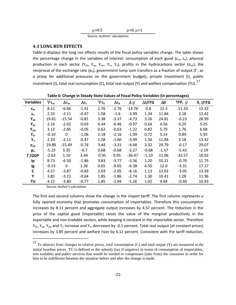
4.1 LONG RUN EFFECTS

Table 6 displays the long run effects results of the fiscal policy variables change. The table shows

the percentage change in the variables of interest: consumption of each good (cm, cn), physical

production in each sector (Yxh, Yxa, Yxm, Ym, Yn), profits in the hydrocarbons sector (πxh), the

reciprocal of the exchange rate (pn), government lump sum transfers as a fraction of output (, as

a proxy for additional pressures on the government budget), private investment (i), public

investment (I), total real consumption (C), total real output (Y) and welfare compensation (TU).17

Table 6: Change in Steady State Values of Fiscal Policy Variables (in percentages)

Variables m m c k k g I/ITG TFP, g , I/ITG

cm 8.11 -6.66 -1.41 2.76 -2.76 -14.76 0.8 12.3 -11.33 13.32 cn 2.33 -2.11 -0.47 1.58 -1.6 -3.99 1.34 11.84 2.18 13.42 Yxh 19.81 -15.54 -0.81 3.38 -3.37 -4.73 3.26 24.81 -0.23 28.99 Yxa 2.16 -2.02 -0.03 0.44 -0.46 -0.97 0.64 4.56 0.25 5.25 Yxm 3.12 -2.85 -0.05 0.62 -0.63 -1.22 0.82 5.79 1.76 6.68 Ym -0.10 0 -1.06 2.18 -2.16 -1.09 0.72 5.14 0.89 5.93 Yn 2.33 -2.11 -0.47 1.58 -1.60 -3.99 1.34 11.84 2.18 13.42

xh 19.88 -15.49 -0.74 3.44 -3.31 -4.68 3.32 24.79 -0.17 29.07

pn -5.23 5.35 -0.7 0.68 -0.68 -2.27 -0.68 -1.57 -5.43 -2.19

/GDP -2.63 1.10 3.44 -0.95 0.95 -36.47 -1.10 11.06 -32.57 10.02

Ip 8.73 -6.50 -1.86 3.83 -3.77 -3.36 1.20 10.21 -0.70 11.75 Ig -0.53 0 1.36 0.65 -0.65 -6.38 4.50 12.0 -3.31 17.17 C 4.57 -3.87 -0.83 2.03 -2.05 -8.16 1.13 12.02 -3.05 13.39 Y 3.85 -3.21 -0.64 1.85 -1.86 -2.74 1.30 10.41 1.28 11.96

TU 4.12 -3.80 -0.77 1.85 -1.94 -5.26 1.02 9.94 -0.40 10.93 Source: Author’s calculation.

The first and second columns show the change in the import tariff. The first column represents a

fully opened economy that promotes consumption of importables. Therefore this consumption

increases by 8.11 percent and aggregate output increases by 4.57 percent. The reduction in the

price of the capital good (importable) raises the value of the marginal productivity in the

exportable and non-tradable sectors, while keeping it constant in the importable sector. Therefore

Yxh, Yxa, Yxm and Yn increase and Ym decreases by -0.1 percent. Total real output (at constant prices)

increases by 3.85 percent and welfare rises by 4.12 percent. Consistent with the tariff reduction,

17

To abstract from changes in relative prices, total consumption (C) and total output (Y) are measured at the

initial baseline prices. TU is defined as the subsidy (tax if negative) in terms of consumption of importables,

non tradables and public services that would be needed to compensate (take from) the consumer in order for

him to be indifferent between the situation before and after the change is made.

-22-

the real exchange rate depreciates. The opposite effects occur when we increase the import tariff

(second column), real output decreases by -3.21 percent and real consumption decreases by -3.87

percent. Notice also that private investment experiences an important increase in a fully opened

economy, while it decreases by -6.5 percent in a closer economy. Public investment decreases by -

0.53 percent in a fully opened economy, while it remains constant when tariffs increase. Notice

that although profits in the hydrocarbons sector increase by almost 20 percent in a fully opened

economy, this increase does not compensate income reduction of the government ant so transfers

and also public investment shrink.

A change in the value added tax (third column), ceteris paribus, from 13 percent to 14.05 percent

reduces all the variables except government transfers which increase by 3.44 percent and public

investment which increases by 1.36 percent. Despite the endogenous increase in the lump sum

transfer, the net welfare effect is negative (-0.77 percent) as well as the output effect (-0.64

percent). Many policymakers think that an increase in the value added tax is the best option to

sustain the transfers and public investment policies, and looking at these variables only it can be

true. However, the general equilibrium effects show that the overall effect for the economy is

adverse.

The literature on optimal fiscal policy states that capital taxes should be zero in an optimal setting.

It can be seen that a reduction in capital tax promotes aggregate capital accumulation and this

increases the amount of capital used in each sector, and thus output in each sector. The sector

that most benefits from a reduction in capital tax is the hydrocarbon sector, its output increases

by 3.38 percent. Certainly, this happens because the hydrocarbon sector is intensive in capital (

larger than 0.5). The other sector that is intensive in capital which is manufacturing (importables)

grows by 2.18 percent. Notice that the effects of an increase or a decrease in capital tax are almost

linear. When capital tax increases by 10 percent, aggregate output decreases by -1.86 percent

while it increases by 1.85 percent when capital tax decreases by 10 percent.18

People always expect to find a positive effect on output from an increase in government

expenditures or public investment. Cross-country empirical studies have generally found that

public infrastructure has positive effects on a country's productive performance (e.g, Easterly and

Rebelo (1993), Canning and Fay (1993), Canning (1999)) and this is indeed the case of Bolivia. An

increase in public investment as a share of government revenues by 3.2 percent (average of the

last two years) increases output by 1.3 percent. However, the opposite happens when the

government increases its current expenditures. An increase by 33 percent of government

expenditures decreases output by -2.74 percent. Certainly, an increase in government

expenditures represents an important pressure for fiscal balance, since transfers as a share of GDP

have to be reduced by -36.74 percent. This huge reduction explains the negative effects on output,

consumption and welfare.

18

See Chamley (1986) and Chari, Christiano and Kehoe (1994) for references on optimal fiscal policy.

-23-

In the last two columns of table 6 we have performed two combined exercises to infer what other

conditions should go along with an expansive fiscal policy, so that the Bolivian economy can enjoy

an increase in output and welfare in the long run. First we combine an increase in government

expenditures with an increase in TFP in all sectors (both increases are in the same magnitude as

described in tables 4 and 5). The results show that now an expansive fiscal policy based in current

expenditure can increase output by 1.28 percent, but still welfare is deprived by -0.4 percent,

because transfers are still highly and negatively affected and this affects consumption negatively.

Notice that consumption of importables decreases by -11.33 percent. It is remarkable the trade-

off between government expenditures and transfers. In other words, there is an important trade-

off that has to be considered between increasing public expenditures in education, health and

other issues and sustaining a social policy based on transfers to households.

Important and sizable effects but in a smaller magnitude can be seen in the last column where we

combine an increase in public investment with an increase in the effectiveness parameter θ. Total

real output increases by 11.96 percent, welfare gains are in the order of 10.93 percent and total

real consumption rises by 13.39 percent. Lump sum transfers also increase by 10 percent, because

one of the sources of financing which are hydrocarbons’ profits increases by almost 30 percent.

This result shows the importance of public investment, but accompanied with effectiveness as

stressed by Rioja (2003). Looking at the column where we simulate an increase in alone, it is

noteworthy the increase in all variables and in particular in sectoral outputs.19

Table 7: Change in Steady State Values of Non-fiscal Policy Variables (in percentages)

Variables TFP CR qxm qxa qxh

cm 3.44 -0.24 -8.68 0.53 29.01 1.18 -1.41 cn 6.31 -0.11 -4.63 0.29 16.23 -8.83 8.18 Yxh 4.58 -0.11 -5.52 0.35 63.26 -6.21 5.94 Yxa 1.20 -0.03 -1.15 0.44 4.18 -1.29 1.16 Yxm 2.98 -0.02 -11.04 0.10 5.31 -1.61 1.48 Ym 1.98 -0.02 -1.27 0.08 4.73 -1.44 1.32 Yn 6.31 -0.11 -4.63 0.29 16.23 -8.83 8.18

xh 4.65 -0.05 -5.47 0.40 89.26 18.56 6.01

pn -3.27 -0.08 -2.59 0.16 6.51 -8.95 7.97

/GDP 2.89 -0.12 -7.47 0.44 28.28 -7.47 6.15

I 2.77 -0.06 -5.16 0.29 26.10 -7.37 7.19 I 3.12 -0.12 -7.39 0.47 31.97 -8.33 8.22 C 5.19 -0.16 -6.20 0.38 21.18 -4.96 4.47 Y 4.09 -0.07 -5.53 0.35 20.32 -5.07 4.71

TU 4.48 -0.15 -6.13 0.36 16.42 -14.5 10.76 Source: Authors’ calculations

19

We might be overestimating the increase in effectiveness of public capital. In fact we are considering a 20

percent increase in effectiveness.

-24-

Table 7 shows the change in steady state values for the changes in non-fiscal policy parameter

values. The largest positive effect in this exercise comes, as expected, from TFP. The favorable

productivity boost raises output in all sectors, with a positive effect on real income, real

consumption, lump sum transfers and welfare. The real exchange rate depreciates by -3.27

percent. The new literature on growth emphasizes that a sustainable growth can be reached only

through productivity boosts. Moreover, those Latin American countries that have experienced an

increase in TFP are the ones that have been able to reduce their growth gap with developing

countries like the US or UK. Our model demonstrates that this could be the Bolivian case also, if

the country begins to dismantle all the restrictions and distortions that impede a productivity

expansion. But, it is not only TFP that could promote the development of the country, because

certainly an output increase of 4 percent in the long run is still not sufficient to reduce poverty.

Therefore, we can state that there is room for government policies based on public investment in

infrastructure, but with effectiveness. This combination will certainly help in reducing poverty and

the economic sectors will grow in an important magnitude solving also other problems like

unemployment and reduced usage of installed capacity.20

In contrast to what we expected, an increase in the country risk premium due to political

instability, for example, would have negative but small effects on output and welfare, and in most

sectors the effect would be negligible. Certainly, private and public investment will suffer from a

higher country risk premium, private investment will decrease by -0.06 percent and public

investment will decrease by -0.12 percent.

The result of the exercises with commodity prices (relative prices) show that Bolivia is typically a

mining country and the mining sector is one of the sectors that most contribute to GDP. A

decrease in mineral prices, in international markets, by -26.5 percent impacts strongly the

economy. Real output declines by -5.53 percent and real consumption decreases by -6.2 percent.

The production in mining decreases by -11 percent and there is a contagion effect to all the other

sectors. In sum, all the variables in the third column have negative signs, showing the large

dependence that the Bolivian economy has on natural resources like minerals.

For agriculture we are simulating a low increase in its relative price (1.6 percent). Therefore the

effects on macroeconomic and sectoral output are low also, but positive. Aggregate output rises

by 0.35 percent and output in the agriculture sector rises by 0.44 percent. There is also an

appreciation of the real exchange rate equal to 0.16 percent.

After TFP, the relative price of hydrocarbons is the second variable of which a change in its value

can have a remarkable impact in the Bolivian economy. In part this is explained by the fact that the

hydrocarbons sector is the main exportable sector in the economy and as it is a nationalized

sector, its profits represent an important source of income for the government. For instance, this

20

See Restuccia (2008) for a nice explanation of the low GDP per worker in Latin America based on a low

and declining relative TFP.

-25-

can be seen by the fact that an increase in xhq allows the government to augment public

investment as a share of government income by 31.97 percent and also increment the lump sum

transfers to households by 28.28 percent. Notice also that profits in the hydrocarbons sector rises

by almost 90 percent. It is noteworthy also that private investment increases by 26.10 percent.

This occurs because the economy is being able to accumulate more capital in its sector which is

precisely intensive in capital.21

Finally, we modify the value of the parameter μ. Cavalcanti and Goncalvez (2006) perform a

sensitivity analysis and find that there is no problem to use values for μ between 0 and 1, although

Evans and Karras (1996) have estimated a value of μ equal to 1.14 using a GMM estimator. We

observe that when public consumption is pure waste (μ=0) people substitute it with consumption

of importables (cm increases by 1.18 percent), but when both consumptions are equally valued by

the people, people consume less importables (cm decreases by -1.41 percent). It is interesting to

observe also that when public consumption is equally valued to private consumption, the welfare

gains are sizable, and this happens because we are considering that public consumption is part of

the utility function. Recall again that in public consumption we are considering the government

expenditures in health and education. So another way to interpret this last results is that if human

capital were more prized in Bolivia (through health and education), the economy would benefit

from higher output (aggregate and sectoral) and welfare. Other key macroeconomic variables like

consumption and investment (private and public) will also improve.22

4.2 IMPACT AND DYNAMIC TRANSITION EFFECTS

In the long run, we model fiscal policy and non-fiscal policy variations as permanent changes in the

levels of tax rates levied on different sectors or as multiplicative shocks on their production

functions. Thus, to quantify the long run level effects of these policies we concentrated on

comparisons between two steady states.

Three issues are overlooked in the long run analysis: First, because of their nature fiscal policy

produces gradual and not instantaneous changes in the macroeconomic variables. Second,

potential costs and benefits of policy changes have to be evaluated considering the period in

which they go into effect (initial conditions are very different from steady-state conditions).

Finally, the structure of the economy determinates the speed of convergence to the new steady

state and the transitional dynamics.

Let s0 be the values of the state variables in the initial period (that we calibrated to replicate the

Bolivian economy in the year 2006). Let Gi (⋅) be the policy functions of the control variables and

Si(⋅) the implied laws of motion of the state variables for scenarios i=B,C1,C2,C3 and C4. B is the

21

This can explain also the extremely favorable conditions that the Bolivian economy has enjoyed in the last

years. The international economic crisis has not affected either the Bolivian economy. 22

Perhaps a better specification of the utility function would be to consider public consumption as a

substitute of non-tradable’s consumption rather than importable’s consumption.

-26-

base scenario. C1 is the combined scenario 1 that combines an increase in government

expenditures and an increase in TFP for all sectors. C2 is the combined scenario 2 than combines

an increase in public investment as a percentage of government incomes and an increase in θ.

Scenario C3 is the combined scenario 1 plus an increase in the relative price of hydrocarbons in a

magnitude exactly to offset the decrease in the lump sum transfers to households. Finally,

scenario C4 encompasses scenario 2 with a reduction in the relative price of hydrocarbons exactly

to maintain the transfers unaltered. These last exercises aim to analyze the needed increase or the

feasible decrease in the price of hydrocarbons, in order to apply an expansive fiscal policy, but

without having to reduce transfers to households, which is the actual social policy that the

government is using to attack poverty.23

Using the policy functions, laws of motion, and initial conditions in all scenarios, dynamic

simulations are carried out for all variables of interest. Then, we compare the dynamic trajectories

of each variable under any with those of scenario B.

4.2.1 Impact on Macroeconomic Variables

Table 8 reports the impact and dynamic-transition effects for Bolivia under the four fiscal policy

scenarios for the main macroeconomic variables. In the table we report the effects at quarter four

(equivalent to a one year effect, i.e. 2007), at quarter 20 (equivalent to a five year effect, i.e. 2011)

and at quarter 40 (equivalent to a ten year effect, i.e. 2016). As a result of the persistence of policy

changes, productivity shocks, changes in the effectiveness of infrastructure, combined with the

discrepancies between initial conditions and steady-state conditions, the economy converges

slowly to its steady-state equilibrium. In figure A.1 in the appendix we show the corresponding

graphs for each scenario where it is clearly seen the slow convergence to the new steady state

variation.24

Table 8: Transition in Macroeconomic Variables (% points, quarters after change)

Scenario C1 C2 C3 C4

Quarter 4 20 40 4 20 40 4 20 40 4 20 40

pn -3.2 -5.2 -5.5 -3.4 -3.2 -3.1 -3.3 -5.2 -5.3 -3.3 -3.2 -3.2 cm -10.5 -10.6 -10.6 1.2 2.6 4.1 -10.6 -10.6 -10.2 1.3 2.6 3.9 cn 0.5 2.6 2.9 4.5 5.5 6.6 0.5 2.6 3.1 4.5 5.5 6.6 Y 2.2 2.0 1.9 3.7 4.7 5.7 2.2 2.3 2.5 3.7 4.5 5.4 C -3.7 -2.5 -2.3 3.2 4.4 5.6 -3.8 -2.5 -2.1 3.3 4.4 5.5 I -2.7 -2.6 -2.7 6.8 7.9 9.2 -1.1 -0.6 0.0 6.2 7.2 8.1

Source: Author’s calculation based on PEP 1-1 model

23

Recall that in we are considering all the bonus that are being given to households. 24

The consistency of the results was checked by simulating the transition for up to 2000 periods and

comparing the results with their respective steady states.

-27-

The impact effects of scenario C1 reflect a decreasing expansion of output as a result of the

increased government expenditures. Consumption decreases by -3.7 percent in the first year and

it decreases by -2.3 percent in 10 years. However it reaches its steady-state level after 100

quarters. Notice that the reduction of consumption is mainly driven by a reduction in cm. In fact,

consumption of non-tradables increases by 2.9 percent in 10 years. The exchange rate depreciates

by 5.2 percent after 5 years and by 5.5 percent after 10 years (almost its steady-state value).

Public investment (last row of table 8) converges also slowly to its steady-state value. After 40

quarters it has decreased by -2.7 percent and after 300 quarters it reaches its steady state

decrease of -3.3 percent. All these effects can be better appreciated in figure A.1 of the appendix.

Under scenario C2, the effects are smoother than under scenario C1 and all variables reach their

steady-state variations simultaneously (around quarter 600. It is important to mention that all

variables displayed on the table are far from their steady-state after 10 years. This is not the case

under scenario C1. For instance, output increases by 5.7 percent after 40 quarters, while it

increases by 11.9 percent after 700 quarters. Public investment increases by 6.8 percent after one

year and it increases by 9.2 percent after 10 years, but again it is far from its steady-state variation

which is 17.1 percent.

Next, we combine the exercise performed in scenario 1 with an increase in the relative price of

hydrocarbons, exactly to offset the decrease in lump sum transfers to households. The results

show that if relative prices of hydrocarbons increase by 14.74 percent, transfers as a percentage of

output will remain constant in the long run. The transitional dynamics are also different in scenario

C3 than in scenario C1, in particular if we look at the effects on output, consumption and public

investment. Although, in the short and medium run, there is a decrease in consumption and public

investment, both variables end up increasing by 13.3 percent and 21.4 percent after 700 quarters

respectively (see figure in the appendix). In the table it is shown that investment does not change

after 40 years, but then it starts to increase. It is noteworthy to see also that real exchange rate

depreciates in the short run, but then this depreciation rate reverses and the economy converges

in the long-run to an appreciation of 0.5 percent. The same happens with consumption of

importables, it decreases by -10.2 percent after 40 quarters, but then it increases by 10.6 percent

after 700 quarters.

One explanation is that the effects of an increase in government expenditures are perceived

immediately and faster than the effects of an increase in the relative price of hydrocarbons. We

can infer this by observing that the percentage change of pn in scenario C3 after 40 quarters is the

same of scenario C1 after 40, 700 or even 1500 quarters. The economy delays in perceiving the

effect of the increase in the relative price of hydrocarbons. Transition is also slow because the

economy is seeking to recover consumption but also transfers at he same time, without reducing

investment.

We can infer also from table 8 and figure A.1 that the transition is longer under a fiscal policy that

is accompanied by a variation in the relative price of hydrocarbons. We do not have a clear

-28-

explanation for this result, but it seems that as transfers are not being affected, the economy

takes more time to accommodate to its new steady state. Certainly, behind these results it is likely

to be the fact that the reactions of the functions are calibrated for a change not so fast (low

sigmas)

Finally, we combine scenario 2 with a decrease in the relative price of hydrocarbons (qxh). The

analysis indicates that if the government wants to maintain its transfer policy unaltered, qxh could

decrease in 6 percent. In other words, there is a margin of 6 percent for the relative price of

hydrocarbons that could decrease and the government could maintain its social policy based in

bonuses. It is a low margin, though. Nevertheless, it is remarkable to see that during the initial

periods of the transition (before 40 quarters) the change in variables is small. Observe that the

percentage changes reported in table 8 are very similar under scenario C2 and under scenario C4.

It is only in figure A.1 in the appendix that we can perceive that in the long run, there are indeed

large differences between scenarios C2 and C4. Clearly, all variables are depressed under scenario

C4 than under scenario C2. For instance, the change in output falls from 11.9 percent (C2) to 5.9

percent (C4) after 700 quarters and consumption declines from 13.4 percent (C2) to 6.3 percent

(C4) after 1500 quarters.

4.2.2 Impact on Sectoral Output

To end this section we have included the transition dynamics for the output in each of the five

sectors under analysis. Table 9 resumes these results under the same four fiscal policy scenarios

described above. In general, it can be seen that, if the government wishes to promote output in all

of the sectors, a fiscal policy based in an expansion of public investment rather than in

government expenditures is preferred.

Table No. 9: Transition in Sectoral Output (percentage points, quarters after policy changes)

Scenario C1 C2 C3 C4

Quarter 4 20 40 4 20 40 4 20 40 4 20 40

Yxh 1.8 1.5 1.2 10.7 12.7 15.0 2.1 3.2 4.7 10.5 12.0 13.4 Yxa 0.7 0.6 0.5 2.4 2.7 3.1 0.7 0.6 0.6 2.4 2.7 3.1 Yxm 2.1 2.2 2.1 3.0 3.4 3.9 2.1 2.1 2.1 3.0 3.4 3.9 Ym 1.3 1.2 1.2 0.3 1.0 1.7 1.2 0.8 0.6 0.4 1.1 1.9 yn 3.4 3.1 2.9 4.5 5.5 6.6 3.3 3.1 3.1 4.5 5.5 6.6

Source: Authors’ calculations

In scenarios 1 and 3, we analyze a fiscal policy expansion based on an increase in government

expenditures. We know that under scenario C1, output in the hydrocarbons sector displays a

negative change in the long run. However, notice that output in this sector displays a positive

change in quarter 40. Under scenario C3, hydrocarbon’s output changes by 4.7 percent in quarter

40 and its change larger than 50 percent are noticeable only after quarter 500 more or less.

Table 9 also shows that output in the importables (manufacturing) sector displays a similar path

under scenario C1 and under scenario C3 and also comparing scenarios C2 and C4. But, if we look

-29-

at figure A.2 in the appendix we can see that this sector displays different rates of change in the

long run. The same occurs with the non-tradables. According to table 9, scenarios C2 and C4 are

exactly the same, but according to figure A.2 there are important differences in the long run. In

fact, non-tradables output changes by 13.4 percent in scenario C2 and it changes by 8.5 percent in

scenario C4, after 700 quarters.

Another interesting result is that in all sectors, output displays positive changes, although these

changes can be decreasing. For instance, in the agricultural sector, under scenario C1, output

change declines from 0.7 percent in one year to 0.5 percent in 10 years. This is true also in the long

run, except for the hydrocarbons sector that we already mentioned that displays negative output’s

change in the long-run, under scenario C1.

The transition to the new steady-state, in terms of percentage changes, is again smoother under

scenario C2 than under scenario C4. Under scenario C2, all variables reach their new steady-state

variation around quarter 400. Under scenario C4, all variables display a bumpy figure, they jump to

a highest percentage change and then they start to decrease until they reach their new steady-

state percentage change. In particular, it is striking the hump-shaped figure of the hydrocarbon’s

output, which indicates again that the reduction in the relative price of hydrocarbons is perceived

after several periods or turns into effect after several periods.

Finally, we can conclude form this section that dynamic transitions are slow under expansive fiscal

policies in the Bolivian economy, and they become slower when there are also accompanied by

changes in the relative price of hydrocarbons. In addition, the change in the relative price of

hydrocarbons generates an irregular transition, which can be seen clearly by the hump-shaped

figures that output displays in all sectors.

5. Concluding Remarks Bolivia has experienced in recent years an important commodity price boom, which has

significantly increased its external revenues. This export boom has allowed the country to reverse

chronic fiscal and external deficits, and accumulate foreign exchange reserves up to a level never

seen before (USD 7.7 billion in 2008 and USD 8.5 billion in 2009). In addition in the last four years,

the Bolivian economy has grown more than in the last three decades, with an average of 5.2

percent. Moreover, the growth forecasts for 2009 allocate the Bolivian economy with the highest

rate of growth in the western hemisphere.

Since 2004 the government revenues has increased almost 20 percentage points of GDP. A large

proportion of this increase is due to the increase of the revenues from hydrocarbons, and this

occurred because royalties’ payment increased, the government renationalized the industry and

the international market experienced highest international oil prices. This unprecedented scenario

allowed the government to impulse fiscal policy (expenditure and investment policy) and to put in

place several transfer programs for poor people.

-30-

This paper simulates the macroeconomic and sectoral impact of different fiscal policy scenarios by

setting up a five-sector dynamic general equilibrium model for a small open economy, inhabited

by representative infinitely-lived agents that face an upward sloping supply of foreign capital,

reflecting an endogenous country risk premium. Firms in each sector employ also public capital as

a factor of production, which allows us to analyze the impact on private production of public

investment in infrastructure. Public capital displays non-rivalry and only its effective measure is

useful for private production. The model has been calibrated to match the national account ratios

and sectoral output of the Bolivian economy for the base year 2006.

Simulation results for key sectors and aggregate variables are reported for steady state under two

groups of variables, fiscal variables (taxes, government expenditures and public investment) and

non fiscal variables (TFP, country risk and relative prices). The results indicate that having a fully

opened economy is very beneficial for the economy; all variables experience an important

increase, while increasing the consumption tax (IVA) is very detrimental although it allows

increasing transfers to households by 3.44 percent. A decrease in the capital tax promotes private

capital accumulation, private investment increases by 3.83 percent. Production in the hydrocarbon

sector rises by 3.38 percent because it is a capital intensive sector.

It is verified that the effectiveness index of public capital is a very sensible parameter in the

Bolivian economy. A 20 percent increase in the effectiveness of public capital can raise output by

10.41 percent and welfare by 9.94 percent. In general all macroeconomic and sectoral variables

are strongly improved by an efficient provision of infrastructure. It is observed also that

government expenditures expansive policies can have negative effects even if they are

accompanied by an increase in productivity. In the combined scenario of TFP changes according to

the National Development Plan goals with a 33 percent increase in government expenditures,

output rises by 1.28 percent, but consumption declines by -0.4 percent.

In another combined scenario we combine an increase of public investment as a share of

government incomes with an increase in the index of effectiveness of public capital. The results

are sizable, aggregate output boosts by 11.96 percent and welfare by 10.93 percent. Transfers as a

share of GDP increase by 10 percent and public investment increases by 17.17 percent. These

results indicate that a fiscal policy based on public investment is preferable to a fiscal policy based

on government expenditures, because the latter implies a marked trade-off between fiscal policy

and social policy in Bolivia.

Recall that Bolivia has renationalized the oil industry; this means that the government actually has

an additional source of financing which are precisely the profits of the hydrocarbon sector. We

have explored this issue by computing the percentage increase of the relative price of

hydrocarbons needed to off-set the negative effects on transfers of an expansive fiscal policy

based on current expenditures. The results indicate that prices (of natural gas) should increase by

14 percent. This is another advantage of a fiscal policy based on public investments in

infrastructure; there is a margin in which the relative prices of hydrocarbons can even decrease,

-31-

without altering the transfers to households. In our simulations this relative price can decrease by

6 percent.

Finally, we simulated the dynamic transition paths of the four combined scenarios to analyze the

speed of convergence when the economy moves from one steady state (base scenario) to a new

steady state. The macroeconomic and sectoral results show that the transitions are slow and take

several years to converge to the new steady state variations. These transitions are even longer and

display hump-shaped figures when they are accompanied by variations in the relative price of

hydrocarbons.

The paper has analyzed fiscal policy in Bolivia and has tried to guide the decisions that a

government will have to make if it wants to use fiscal policy as the main tool to promote

development and structural transformations of the Bolivian economy. The results should come as

no surprise. Productivity is very important to promote an increase in output and welfare, but there

is also room for fiscal policy, in particular to attain larger increases in output and welfare. The best

that the government can do is to employ public investment in infrastructure as the main tool to

promote output and welfare expansions in a magnitude necessary to attack poverty. But, that is

not the end of the story, public capital or infrastructure should be efficiently provided.

-32-

REFERENCES

Arrow, K.J. and M. Kurz (1970) "Public Investment, the Rate of Return and Optimal Fiscal Policy", Baltimore: The Johns Hopkins Press (For Resources for the Future).

Aschauer, D. (1985) “Fiscal Policy and Aggregate Demand,” American Economic Review, v.75, pp. 117-127.

Aschauer, D.A. (1989a) "Is Public Expenditure Productive?" Journal of Monetary Economics, Vol. 23, pp: 177-200.

Aschauer, D.A. (1989b) "Public Investment and Productivity Growth in the Group of Seven," Economic Perspectives, Federal Reserve Bank of Chicago, 13.

Barja, G, J. Monterrey and S. Villarroel (2005) "The Elasticity of Substitution in Demand for Non-Tradable Goods in Bolivia. IADB (mimeo).

Barro, R. (1981) “Output Effect of Government Purchases,” Journal of Political Economy, v.89, pp. 1086-1121.

Barro, R. (1990) "Government spending in a simple model of endogenous growth," Journal of Political Economy, 98, pp: S103-S125.

Bhandari, J., N. Haque, and S. Turnovsky (1990) “Growth, External debt, and Sovereign Risk in a Small Open Economy,” IMF Staff Papers 37, pp: 388-417.

Canning, D. (1998) "A Database of World Infrastructure Stocks, 1950-1995," Policy research working paper, No 1929, Washington, D.C., World Bank.

Canning, David (1999) "Infrastructure Contribution to Aggregate Output," World Bank Policy Research working paper 2246.

Canning, David and Marianne Fay (1993) "The Effect of Trasnportation Networks on Economic Growth," manuscript, Columbia University.

Cavalcanti, P. and L. Goncalves do Nascimento (2006) “Welfare and Growth Effects of Alternative Fiscal Rules for Infrastructure Investment in Brazil,” Fundacao Getulio Vargas (mimeo).

Chamley, C. (1986) “Optimal Taxation of Capital Income in General Equilibrium with Infinite Lives," Econometrica, Vol.54 (3), pp: 607-622.

Chari, V.V., Lawrence Christiano and Patrick Kehoe (1994) “Optimal Fiscal Policy in a Business Cycle Model,” Journal of Political Economy, Vol.102 (4), pp: 617-652.

Christiano, L. and M. Eichenbaum (1992) “Current Real Business Cycle Theories and Aggregate Labor Markets Fluctuations,” American Economic Review, v.82, pp: 430-450.

-33-

Chumacero, R., Rodrigo Fuentes and Klaus Schmidt-Hebbel (2004) "Chile's Free Trade Agreements: How Big is the Deal?," Working Paper No. 264, Central Bank of Chile.

Easterly, W. and S. Rebelo (1993) "Fiscal Policy and Economic Growth: An Empirical Investigation," Journal of Monetary Economics, 32, pp: 417-458.

Eaton, J. and M. Gersovitz (1981) “Debt with Potential Repudiation: Theoretical and Empirical Analysis,” Review of Economic Studies, 48, pp: 289–309.

Estrada, P. (2006) "Economía Pequeña, Abierta, Exportadora de Gas y Soya, con Shocks Internos y Externos: Cambios que Bolivia no esperaba", Universidad de Chile.

Evans, P. and G. Karras (1996) “Private and Government Consumption with Liquidity Constraints,” Journal of International Money and Finance, v.15, pp: 255-266.

Fernandez de Cordoba, G. and T. Kehoe (2000) “Capital Flows and Real Exchange Rate Fluctuations Following Spain’s Entry into the European Community,” Journal of International Economics, 51, pp: 49-78.

Ford, R. and P. Poret (1991) "Infrastructure and Private Sector Productivity," OECD Working Paper, 91.

García-Milá, T., T. McGuire y R.M. Porter (1993) "The Effect of Public Capital in State- Level Production Functions Reconsidered," The Review of Economics and Statistics, Vol.LXXVIII, pp: 162-180.

Hulten, C.R. (1996) "Infrastructure Capital and Economic Growth: How Well You Use It May Be More Important Than How Much You Have," NBER Working Paper 5847.

Ministry of Economy and Public Financing (2009) ”Fiscal Memory”. La Paz, Bolivia.

Munnell, A. (1990) "How Does Public Infrastructure Affect Regional Economic Performance?" New England Economic Review, (September/October), pp: 11- 32.

Osang, T. and S. Turnovsky (2000) “Differential Tariffs, Growth and Welfare in a Small Open Economy,” Journal of Development Economics, 62, pp. 315-342.

Otalora, Carlos (2009) Economía Fiscal, primera edicion, Plural Editores, La Paz, Bolivia.

Restuccia, Diego (2008) “The Latin American Development Problem,” Working Paper 318, University of Toronto, Department of Economics.

Rioja, F.K. (2003) "The Penalties of Inefficient Infrastructure," Review of Development Economics, 7(1), pp: 127-137.

-34-

Schmitt-Grohé S. and M. Uribe (2003) "Closing small open economy models,” Journal of International Economics, 61, pp: 163-185.

Schmitt-Grohé S. and M. Uribe (2004) "Solving dynamic general equilibrium models using a second-order approximation to the policy function," Journal of Economic Dynamics and Control, 28, pp: 755-775.

Turnovsky, S. (1997) “Equilibrium Growth in a SmallEconomy Facing an Imperfect World Capital Market,” Review of Development Economics, 1, pp: 1-22.

Weisbrot, M., R. Ray and J. Johnston (2009) “Bolivia: La economía bajo el gobierno de Morales,” Center of Economic and Policy Research, mimeo.

Weitzman, M.L. (1970) "Optimal Growth with Scale Economies in the Creation of Overhead Capital," Review of Economic Studies, October, pp: 555-570.

-35-

APPENDIX Calibrations

Table A.1: Calibration of

1 2 3 4 5 24 27 28

Agriculture

(1-5)

Hydrocarbons

(6 y 19)

Mining (7,

20, 21 y 22)

Importables

(8-18 y 23)

Non-tradables

(25, 26 y 29-35)

Electricity, gas and

water

Transport and

storage Communications TOTAL

VA (in thousands

of Bs. Of 1990)

f-lab 6,444,261 798,415 3,384,730 3,270,488 19,476,173 535,857 4,447,022 120,588 38,477,535

f-cap 1,873,349 4,834,479 1,295,147 4,440,511 11,971,380 1,579,682 3,220,626 1,324,170 30,539,342

f-land 1,459,264 0 0 0 0 0 0 0 1,459,264

f-natres 0 1,670,433 511,687 0 0 0 0 0 2,182,120

total 9,776,874 7,303,326 5,191,564 7,711,000 31,447,553 2,115,539 7,667,648 1,444,758 72,658,262

in%

f-lab 0.66 0.11 0.65 0.42 0.62 0.25 0.58 0.08 0.53

f-cap 0.19 0.66 0.25 0.58 0.38 0.75 0.42 0.92 0.42

f-land 0.15 0.00 0.00 0.00 0.00 0.00 0.00 0.00 0.02

f-natres 0.00 0.23 0.10 0.00 0.00 0.00 0.00 0.00 0.03

total 1.00 1.00 1.00 1.00 1.00 1.00 1.00 1.00 1.00

Source: Input-output matrix (2006)

Table A.2: Calibration of

1 2 3 4 5

Sectors Agriculture

(1-5) Hydrocarbons (6

y 19) Mining (7, 20,

21 y 22) Importables (8-18 y 23)

Non-tradables (25,

26 y 29-35) Intermediate Consumption (thousands of Bs. Of 1990)

Agriculture 673,280 1,903 16,516 3,633,472 196,011

Hydrocarbons 37,740 1,171,274 106,898 154,590 187,431

Mining 31,698 162,272 585,708 574,910 1,022,309

Importables 528,444 88,162 257,327 2,823,865 2,331,561

Non-tradables 128,294 369,308 57,827 260,887 1,008,874

Electricity, gas and wáter 322 52,109 50,813 89,587 169,092

Transport and storage 186,842 534,921 102,381 403,240 1,161,924

Communications 1,781 3,935 18,218 66,670 235,227

Total 1,588,400 2,383,885 1,195,688 8,007,221 6,312,428

Infrastructure 188,944 590,965 171,412 559,497 1,566,243

Phis 0.12 0.25 0.14 0.07 0.25

Source: Input-output matrix (2006)

-36-

Table A.3. Calibration of

Year Power (i) Telecom (ii) Paved Roads (iii) Water (iv)

1995 11.56 n.a. 94.50 n.a.

1996 11.49 n.a. 94.50 n.a.

1997 11.61 n.a. 94.30 n.a.

1998 11.99 n.a. 94.00 n.a.

1999 11.41 n.a. 93.60 n.a.

2000 10.18 n.a. 93.40 n.a.

2001 12.40 n.a. 93.30 n.a.

2002 13.07 n.a. 93.30 n.a.

2003 14.35 n.a. 93.00 n.a.

2004 13.61 n.a. 93.00 n.a.

2005 13.95 n.a. n.a. n.a.

2006 14.36 n.a. n.a. 37.03

2007 n.a. 17.76 n.a. 31.97

2008 n.a. n.a. n.a. 32.87

(i) Electric power transmission and distribution losses (% of output)

(ii) Faults (per 100 mainlines per year)

(iii) Roads, not paved (% of total roads)

(iv) Losses (% of total water provision)

Dynamic Transitions

Figure A.1: Scenarios C1, C2, C3 and C4 – Macroeconomic Impact

-1.0%

-0.5%

0.0%

0.5%

1.0%

1.5%

2.0%

2.5%

3.0%

3.5%

-12.0%

-10.0%

-8.0%

-6.0%

-4.0%

-2.0%

0.0%

1 101 201 301 401 501 601 701 801 901 1001 1101 1201 1301 1401 1501 1601 1701 1801 1901

Scenario 1 v.s. Baseline (percentage points - Y and cn right axis)

p cm C I cn Y

-4.0%

-3.5%

-3.0%

-2.5%

-2.0%

-1.5%

-1.0%

-0.5%

0.0%

0.0%

2.0%

4.0%

6.0%

8.0%

10.0%

12.0%

14.0%

16.0%

18.0%

1 101 201 301 401 501 601 701 801 901 1001 1101 1201 1301 1401 1501 1601 1701 1801 1901

Scenario 2 v.s. Baseline (percentage points - p right axis)

cm cn Y C I p

-37-

Source: Authors’ calculations

Figure A.2: Scenarios C1, C2, C3 and C4 – Sectoral Impact

Source: Authors’ calculations

-6.0%

-5.0%

-4.0%

-3.0%

-2.0%

-1.0%

0.0%

1.0%

-15.0%

-10.0%

-5.0%

0.0%

5.0%

10.0%

15.0%

20.0%

25.0%

1 101 201 301 401 501 601 701 801 901 1001 1101 1201 1301 1401 1501 1601 1701 1801 1901

Scenario 3 v.s. Baseline (percentage points - p right axis)

cm cn Y C p

-4.5%

-4.0%

-3.5%

-3.0%

-2.5%

-2.0%

-1.5%

-1.0%

-0.5%

0.0%

0.0%

2.0%

4.0%

6.0%

8.0%

10.0%

12.0%

1 101 201 301 401 501 601 701 801 901 1001 1101 1201 1301 1401 1501 1601 1701 1801 1901

Scenario 4 v.s. Baseline (percentage points- pright axis)

cm cn Y C I p

0.0%

0.5%

1.0%

1.5%

2.0%

2.5%

3.0%

3.5%

4.0%

-0.5%

0.0%

0.5%

1.0%

1.5%

2.0%

2.5%

1 101 201 301 401 501 601 701 801 901 1001 1101 1201 1301 1401 1501 1601 1701 1801 1901

Scenario 1 v.s. Baseline (percentage points - yn right axis)

yxh yxa yxm ym yn

0.0%

5.0%

10.0%

15.0%

20.0%

25.0%

30.0%

35.0%

0.0%

1.0%

2.0%

3.0%

4.0%

5.0%

6.0%

7.0%

8.0%

1 101 201 301 401 501 601 701 801 901 1001 1101 1201 1301 1401 1501 1601 1701 1801 1901

Scenario 2 v.s. Baseline (percentage points -yn and yxh right axis)

yxa yxm ym yxh yn

0.0%

10.0%

20.0%

30.0%

40.0%

50.0%

60.0%

70.0%

0.0%

1.0%

2.0%

3.0%

4.0%

5.0%

6.0%

7.0%

8.0%

1 101 201 301 401 501 601 701 801 901 1001 1101 1201 1301 1401 1501 1601 1701 1801 1901

Scenario 3 v.s. Baseline (percentage points -yxh and yn right axis)

yxa yxm ym yxh yn

0.0%

2.0%

4.0%

6.0%

8.0%

10.0%

12.0%

14.0%

16.0%

18.0%

0.0%

2.0%

4.0%

6.0%

8.0%

10.0%

12.0%

1 101 201 301 401 501 601 701 801 901 1001 1101 1201 1301 1401 1501 1601 1701 1801 1901

Scenario 4 v.s. Baseline (percentage points -yxh right axis)

yxa yxm ym yn yxh