PTV experiments of subcooled boiling flow through a vertical rectangular channel

International Journal of Multiphase Flow 36 (2010) 691–706

Contents lists available at ScienceDirect

International Journal of Multiphase Flow

journal homepage: www.elsevier .com/ locate / i jmulflow

PTV experiments of subcooled boiling flow through a vertical rectangular channel

C.E. Estrada-Perez a, Y.A. Hassan a,b,*

a Texas A&M University, Department of Mechanical Engineering, Zachry 129, MS 3133, College Station, TX 77843, USAb Texas A&M University, Department of Nuclear Engineering, Zachry 129, MS 3133, College Station, TX 77843, USA

a r t i c l e i n f o a b s t r a c t

Article history:Received 28 November 2009Received in revised form 28 April 2010Accepted 20 May 2010Available online 26 May 2010

Keywords:PTVConvective boilingLiquid turbulenceMultiphase flow

0301-9322/$ - see front matter � 2010 Elsevier Ltd. Adoi:10.1016/j.ijmultiphaseflow.2010.05.005

* Corresponding author at: Department of NucleUniversity, Zachry 129, MS 3133, College Station, Tex

E-mail address: [email protected] (Y.A. Hassan

Time resolved Particle Tracking Velocimetry (PTV) experiments were carried out to investigate turbulent,subcooled boiling flow of refrigerant HFE-301 through a vertical rectangular channel with one heatedwall. Measurements were performed with liquid Reynolds numbers (based on the hydraulic diameter)of Re = 3309, 9929 and 16,549 over a wall heat flux range of 0.0–64.0 kW/m2. Turbulence statistics areinferred from PTV full-field velocity measurements. Quantities such as: instantaneous 2D velocity fields,time-averaged axial and normal velocities, axial and normal turbulence intensities, and Reynolds stressesare obtained. The present results agree well with previous studies and provides new information due tothe full-field nature of the technique. This work is an attempt to provide turbulent subcooled boiling flowdata for validation and improvement of two-phase flow computational models.

� 2010 Elsevier Ltd. All rights reserved.

1. Introduction

Turbulent subcooled boiling flow has been used extensively inthe industry because it is one of the most efficient heat transfermodes. The continuous mixing and stirring of liquid produced dur-ing the life cycle of the subcooled boiling bubbles (nucleation,growth, detachment, coalescence and collapsing) are local enhanc-ing mechanisms of heat and momentum transfer. Therefore, liquidturbulence modification produced by these mechanisms, have tobe accurately measured and modeled in the numerical correla-tions/equations used to design energy transfer systems. Multipleexperimental efforts have been directed towards this goal, andthe literature contains many examples of such works, but for brev-ity, we will refer to only a few.

Isothermal air–water flow experiments were performed byLance and Bataille (1991) to understand the influence of the localvoid fraction, a, on the liquid phase turbulence. They used LaserDoppler Anemometry (LDA) and Hot Film Anemometry (HFA) mea-surements to study the turbulence of the liquid in a grid-generated,turbulent bubbly flow. They found that the turbulent kinetic en-ergy greatly increases with the void fraction. They described tworegimes: the first one corresponds to low values of a, where hydro-dynamic interactions between bubbles are negligible, and the sec-ond regime to higher a values, in which the bubbles transfer agreater amount of kinetic energy to the liquid. The Reynolds stresstensor shows that the quasi-isotropy was not altered. Furthermore,

ll rights reserved.

ar Engineering, Texas A&Mas 77843-3133, USA.).

their one-dimensional spectra analysis showed a large range ofhigh frequencies associated with the wakes of the bubbles andthe classical �1/5 power law is progressively replaced by a �8/3dependence.

Non-isothermal air–water flow experiments were conducted bySerizawa et al. (1975a,b,c) to study the turbulence structure ofupward air–water bubbly flow in a pipe. They used hot film ane-mometry to measure liquid velocities and liquid turbulence inten-sities, a double resistivity probe to measure void fraction, bubbleimpaction rate, and bubble velocities. New principles were pre-sented for measuring the turbulent dispersion coefficient of bub-bles and the eddy diffusivity of heat by means of tracertechniques. They found flat radial velocity profiles for both liquidand bubbles; however, the radial void fraction profiles showed amaximum in the near-wall region. For a constant liquid flow rate,the liquid turbulent intensity decreased with increments of gasflow rate. This behavior was seen up to a certain value of the gasflow rate, after which the turbulent liquid intensity started to in-crease. Furthermore, from their analysis of transport properties,they found that the turbulent transport process is dominatedmainly by the liquid phase turbulent velocity component, and thatthere is systematic increase of heat diffusivity with quality andwater velocity.

Non-isothermal single-phase flow experiments were performedto elucidate the effect of density changes on the fluid turbulencewithin circular and square channels. Barrow (1962) performed sin-gle-phase flow experiments in a rectangular channel with unequalheat fluxes in the channel walls. He analyzed the influence of un-even heating on friction and heat transfer coefficients. He measuredliquid velocity fields, only for the unheated case. Roy et al. (1986)

http://dx.doi.org/10.1016/j.ijmultiphaseflow.2010.05.005

mailto:[email protected]

http://dx.doi.org/10.1016/j.ijmultiphaseflow.2010.05.005

http://www.sciencedirect.com/science/journal/03019322

http://www.elsevier.com/locate/ijmulflow

692 C.E. Estrada-Perez, Y.A. Hassan / International Journal of Multiphase Flow 36 (2010) 691–706

performed extensive investigations on heated and unheated R-113refrigerant through annular channels. Using HFA they obtainedmean axial velocity profiles and turbulence intensities for variousReynolds numbers and heat fluxes. They concluded that accuratevelocity field measurements in turbulent liquid flow by constanttemperature anemometry are difficult since generally only low sen-sor overheats can be used. Hasan et al. (1992) obtained velocity andtemperature fields of heated and unheated refrigerant R-113. UsingHFA and a chromel–constantan micro-thermocouple. They pre-sented radial profiles of velocity, turbulence intensities and Rey-nolds stresses, together with single-point correlations betweenturbulent velocity and temperature fluctuations. Wardana et al.(1992) used Laser Doppler Velocimetry (LDV) and a resistance ther-mometer to study air velocity and temperature statistics in astrongly heated turbulent two-dimensional channel flow, with walltemperatures up to 700 �C and a fixed Reynolds number of 14,000.They found that for this conditions (Gr/Re2 = 5.25 � 10�5, where Grand Re are Grashof and Reynolds numbers) the normalized meanvelocity and mean temperature profiles were not significantly af-fected by the wall heating. However, they found a suppression ofthe axial turbulence intensity profile only for points laying on therange (y/H = 0.2–0.6). Velidandla et al. (1996) used a two-compo-nent LDV and a micro-thermocouple to measure velocities and tem-peratures of refrigerant R-113. They found buoyancy effects on thetime-mean velocity and turbulence fields, even at very low valuesof Gr/Re2. Zarate et al. (1998) developed velocity and temperaturewall laws in a vertical concentric annular channel from measure-ments in turbulent liquid flow of refrigerant R-113, noting thatwhen buoyancy forces influence becomes large, the velocity andtemperature data do not follow the respective wall laws. Kanget al. (2001) summarized experimental measurements from iso-thermal and heated turbulent up-flow of refrigerant R-113. Theypresented liquid turbulence statistics, radial turbulent heat flux dis-tributions and Prandtl number estimations.

One of the early attempts to measure local fields of subcooledboiling parameters of the liquid phase was performed by Royet al. (1993). They measured turbulent velocity and temperaturefields in the all-liquid region adjacent to a subcooled flow boilinglayer. Significant changes in the turbulent structure of the all-liquid region were observed due to boiling. Improving their mea-surement techniques, Roy et al. (1997) were able to measure liquidturbulence statistics of the liquid refrigerant R-113 even within theboiling layer region adjacent to the heated wall. They found thatthe near-wall liquid velocity field was significantly different fromthat in single-phase liquid flow at a similar Reynolds number.Lee et al. (2002) performed measurements of subcooled boilingflow of water in a vertical concentric annulus. Using a two-conduc-tivity probe they measured the local void fraction and vapor veloc-ity and with a Pitot tube they measured the liquid velocity. Situet al. (2004) measured the flow structure of subcooled boiling flowin an annulus. They used a double-sensor conductivity probemethod to measure local void fraction, interfacial area concentra-tion and interfacial velocities. Using LDA Ramstorfer et al. (2008)performed subcooled boiling flow experiments in a horizontalchannel with one heated wall, to gain insight into the bubble ladennear-wall velocity field. Contrary to the vertical channel experi-ments, they found that the streamwise velocity component wasconsiderably reduced compared to the single-phase case, whilethe near-wall turbulence was increased due to the presence ofthe bubbles.

Using the experimental information from the previous studies,different two-phase flow models were developed and used to cal-culate convective subcooled boiling flow (Roy et al., 2002; Yeohet al., 2002; Koncar et al., 2004; Ramstorfer et al., 2008) with somesuccess. These models share the characteristics of being based ontime-average analysis of information from point measurements

probes. However, due to the complex nature of the turbulencefound in subcooled boiling, this approach seems to be limited. Afull-field measurement approach is needed to provide spatial andtemporal information.

Visualization techniques such as Particle Image Velocimetry(PIV) and Particle Tacking Velocimetry (PTV) can be used to over-come some of the limitations associated with point measurementstechniques. PIV and PTV are non-intrusive and provide full-fieldquantitative and qualitative information of the flow with high spa-tial and temporal resolution. The common measuring principle be-hind these methods is that instantaneous fluid velocities can beevaluated by recording the position of images produced by smalltracers suspended in the fluid, at successive time instants. Theunderlying assumption is that these tracers closely follow the fluidmotion with minimal lag. This assumption holds true for a widevariety of flows of interest provided that the tracers are small en-ough and/or their density approaches that of the fluid. The differ-ence between PIV and PTV is that in PIV, the concentration oftracers is rather high and the measurement of the ‘‘local” fluidvelocity results from an average over many tracers contained in ameasurement volume. This is in contrast with PTV, where thevelocity is determined at random locations using the images pro-duced by a single tracer. Although both techniques can be appliedon the analysis of two-phase flows, PTV is preferred, due to its abil-ity to differentiate between the gas and liquid phases and subse-quently deliver simultaneous velocity fields associated with eachphase.

Using visualization techniques in conjunction with PTV, severaladiabatic two-phase flow experimental studies were performed(Hassan et al., 2005; Dominguez-Ontiveros et al., 2006; Ortiz-Vil-lafuerte and Hassan, 2006, among others) to investigate the influ-ence of void fraction on liquid turbulence parameters. Morerecently PTV with high spatial and temporal resolution has beenused by Koyasu et al. (2009) to study the liquid turbulencemodification by dispersed bubbles in an upward pipe flow. Theyobserved similar trends as those obtained with hot film anemom-etry (Serizawa et al., 1975b). They concluded that dissipativeeddies around small bubbles increased the dissipation rate of tur-bulence kinetic energy and eddies from large bubbles augmentedthe turbulence kinetic energy.

These studies elucidate the phenomenological events importantfor the modeling of two-phase flows. However, there appears to bea scarcity of subcooled boiling experimental studies that can cap-ture instantaneous whole-field measurements with a fast timeresponse. In this study, time-resolved PTV experiments are per-formed to obtain liquid flow measurements in turbulent subcooledboiling flow of refrigerant HFE-301 3M (2009) through a rectangu-lar channel. This investigation is an attempt to obtain a databaseon turbulent subcooled boiling flow for validation and improve-ment of two-phase flow computational models.

2. Experimental rig

The experimental facility was designed for the visualization ofsubcooled boiling flow of refrigerant HFE-301 at low system pres-sure. Fluid selection justification and experimental setup detailsare given in the following sections.

2.1. Fluid selection and scaling

The selection of the working fluid was based on a scaling anal-ysis of thermodynamic properties. Scaling can be achieved by usingcritical fluid properties such as critical density, temperature orpressure. It has been shown (Mayinger, 1981) that the critical pres-sure ratio p/pc is the most useful parameter for many applications,

Table 1Important operation conditions and corresponding values for HFE-301 refrigerant andwater.

Condition No. PHFE (bar) TsatHFE (�C) PH2O ðbarÞ TsatH2O ð�CÞ

1 1.00 36.00 8.95 175.132 7.80 107.00 70.00 285.833 16.08 141.00 140.00 336.67

C.E. Estrada-Perez, Y.A. Hassan / International Journal of Multiphase Flow 36 (2010) 691–706 693

including scaling between water and refrigerants. Scaling with thecritical pressure ratio provided good similarity only for some fluidproperties while for others a correction was needed. As an exam-ple, Fig. 1 shows the comparison of scaled thermodynamic proper-ties of water and HFE-301 at saturation conditions. Fig. 1a showsthe two-phase flow density ratio (qL/qv) scaled with the criticalpressure ratio. There is only a deviation of a few percent in thetwo-phase flow density ratio for water and HFE-301; however,when comparing the liquid viscosities lL in Fig. 1b, a larger dis-crepancy is found. A multiplication factor (k4) is used to correctfor this discrepancy. Fig. 1b shows that liquid viscosities for bothfluids are comparable after applying the correction factor (blackdotted line). This correction factor then must be considered inthe estimation of dimensionless numbers. Also shown in Fig. 1are three conditions on which HFE-301 may be used to simulatewater. Condition 1 was selected to perform the HFE-301 boilingexperiments, simulating the behavior of a geometrically similarwater system at a pressure of about 9 bars and saturation temper-atures of 175 �C. Conditions 2 and 3 are of importance for the nu-clear industry, they represent typical operational conditions ofBoiling and Pressurized Water Reactors (BWR, PWR), respectively.Table 1 shows saturation pressure and temperature values for bothwater and HFE-301 for each condition.

2.2. Hydraulic loop

The hydraulic loop consists of an external loop and a test sec-tion, both designed to withstand temperatures in excess of200 �C, and pressures up to 100 psi. The external loop provides

Fig. 1. Comparison of thermodynamic properties of water and HFE-301 as afunction of reduced pressure.

thermal and hydraulic steady state conditions. The temperatureof the fluid inlet is controlled with a Watlow circulation heater,managed by an internal PID temperature controller, capable of afast response to temperature changes. The system excess energyis removed with a small plate heat exchanger connected to a chill-ing system. The mass flow rate to the test section was measuredwith a variable area flow-meter and controlled by adjusting thetest section valves. The test section is a rectangular channel madeof transparent polycarbonate 530 mm long with a cross-sectionalarea of 8.7 � 7.6 mm2. The test section dimensions were selectedto approximate those typically found in coolant channels of boilingand pressurized water nuclear reactors (BWR, PWR) Energy forboiling was provided by a Kapton thin heater with a length andwidth of 175 mm and 7 mm, respectively, and a maximum work-ing temperature of 200 �C. The heater is attached to the lateralinterior face of the channel (see Fig. 2). The electric current to

Fig. 2. Test section schematics and dimensions.

Fig. 3. Visualization system schematics.


the heater is provided and adjusted by a DC power supply, fromwhich a maximum wall heat flux of 64 kW/m2 was measured. Toreduce heat losses to the ambient, the external face of the channelwas insulated with 10 mm of balsa wood. With this configurationan unheated length of 320 mm is achieved. To measure the heaterwall temperature, six J-type thermocouples were attached to theexternal face of the heater in a vertical arrangement along the hea-ter wall with a space of 25.4 mm in between them. Test sectionfluid inlet (Tin) and outlet (Tout) temperatures were also measuredby two J-type thermocouples. Fig. 2 shows the schematics anddimensions of the test section.

2.3. Visualization system

The visualization system consisted of a high-speed high-resolu-tion camera, a high-speed high-power laser, a continuous halogenlamp,1 mirrors, translational stages, lenses and particle flow tracers.The high-speed camera has a maximum frame rate of 4700 fps at aresolution of 800 � 600 pixels, with a maximum bit depth of 12 bits.The illumination was provided by a Pegasus dual lamp laser whichcan operate at a maximum power of 27 mJ/pulse. A maximum pulserate of 20,000 pulse/s can be also achieved. Two optical mirrors andtwo concave–convex lenses are used to convert the small circularbeam from the laser, into a 1 mm thick sheet of light. The laser lightsheet is positioned on the measurement region, parallel to the cam-era focal area. The camera, mirrors and lenses are mounted on trans-lational stages to have the capability of changing the measuringregion along the test section. The flow tracers are highly reflectivesilver coated particles with a density range of 1.39–1.41 g/cm3, withan average particle diameter of 40 lm. Fig. 3 shows the schematicsof the visualization system.

1 The halogen lamp provided illumination for shadowgraphy measurements fromwhich bubble dynamics can be determined. However, for the sake of brevity,shadowgraphy results are not shown.

3. Velocity measurement system and accuracy

3.1. PTV algorithm

In this study, the PTV algorithm used to analyze subcooled boil-ing flow is a home-developed routine that has been applied suc-cessfully in several previous two-phase flow investigations(Hassan et al., 2005; Dominguez-Ontiveros et al., 2006; Ortiz-Villafuerte and Hassan, 2006). The original algorithm was devel-oped by Canaan and Hassan (1991), and has been improved overthe years. A simplified version of the PTV algorithm performs: (1)particle detection, (2) particle centroid location estimation and(3) particle matching in between consecutive frames (particletracking). In this section, the components of the PTV algorithm thatare new or relevant for the present study are described. A more de-tailed description of the PTV algorithm can be obtained from Estra-da-Perez (2004).

3.1.1. Particle detectionThe particle detection procedure is particularly important in

multi-phase flow experiments where accurate identification anddiscrimination between phases is required. In this study a particlemask correlation method (Takehara, 1998) is implemented. Thistechnique is an image template matching routine, where the se-lected template is generated from a Gaussian representation ofan ideal particle given by the following equation:

Iðx; yÞ ¼ I0 exp � 12r2

0

x� x0ð Þ2

a2 þ ðx� x0Þðy� y0Þc2 þ ðy� y0Þ

2

b2

!" #

ð1Þ

where I(x,y) is the gray scale intensity at the (x,y) position, (xo,yo) isthe particle centroid location, Io is the maximum intensity, a, b, andc are shape modifier parameters, and ro is the particle radius. Theimage template selection depends on the object of interest, forexample, selecting a small value for ro (particle size) will in turn


provide an approach of discrimination between small and largeobjects.

3.1.2. Particle centroid estimationOnce a particle is identified, its centroid is estimated to sub-pix-

el accuracy. In this study three different centroid estimation tech-niques are available: three point Gaussian interpolation (3PGI)(Willert and Gharib, 1991), two-dimensional Gaussian regression(2DGR) (Noback and Honkanen, 2005), and center of mass tech-nique (CMT). 3PGI and 2DGR performance and accuracy are similaras both are well suited for small (radius <10 pixels) Gaussianshaped objects. The CMT is better suited for larger objects (radius>10 pixels) without shape restriction. In a two-phase flow PTVexperiment, CMT will be ideal for the location of bubbles centroid,while 3PGI and 2DGR are well suited to estimate the liquid tracerparticles centroids. Although 3PGI technique is the most com-monly used among researchers due to its simplicity, in this work,2DGR is preferred since it relies on more information (9 pixelsare used in the regression rather than 6) to estimate the centroids.

3.1.3. Particle trackingThe particle tracking algorithm is based on direct spatial corre-

lation. This algorithm computes a correlation coefficient betweentwo sub-images of single-exposed PTV pictures. The correlationcoefficient between the two sub-images IA and IB with a � b dimen-sions is computed using the following relation:

CIAIBðxo; yoÞ ¼Xa

i¼1

Xb

j¼1

½IAði; jÞ � IA�½IBði; jÞ � IB�

�Xa

i¼1

Xb

j¼1

½IAði; jÞ � IA� !�1=2

�Xa

i¼1

Xb

j¼1

½IBði; jÞ � IB� !�1=2

ð2Þ

where IA and IB are the average intensities of sub-images A and B,respectively. Assuming two experimental pictures A and B, acquiredat two different times t = to and t = to + Dt, respectively, the correla-tion coefficient will determine which particle in picture B is the bestmatch of a particle on picture A. Since particles location is estimatedto sub-pixel accuracy, and the interval between pictures is known,an accurate particle velocity estimation is achieved.

3.2. PTV algorithm accuracy

The accuracy of the PTV algorithm used in this work has beenextensively tested and benchmarked against synthetic and experi-mental data. A version of this program was used in the PIV Chal-lenge 2005 (Stanislas et al., 2008), where it was shown that forsuitable PTV images (low particle density images as in Case A1 ofthe PIV Challenge 2005), the algorithm bias and RMS errors (as de-fined in Section 3.2.2) for both velocity components accounts for0.0001 and 0.1056 pixel/Dt, respectively (with Dt = time betweenframes). To further test the accuracy of the PTV algorithm, and todiscern experimental conditions which exhibited a lesser error, asensitivity analysis was performed by Estrada-Perez (2004). Thesensitivity analysis was performed with home-made artificialimages. These images were created simulating ideal conditions totest specific algorithm performances. Particle positions, sizes anddisplacements were varied. Since particles positions and velocitieswere known, the experimental parameters that have high impacton the measurements accuracy were identified. Some of the rele-vant results are summarized below.

3.2.1. Particle detection and centroid estimation errorsFig. 4a shows the centroid estimation error as a function of par-

ticle size. For the boiling experiments, the average particle imageradius was about 2 pixels, where the minimum algorithm error(RMS � 0.002 pixel) is located. This optimal size was obtained witha trade-off between camera magnification, resolution and particledimensions. Since particle dimensions and camera resolution arefixed (30–40 lm and 800 � 600), the required magnification pro-vided a visualization area of 9.87 � 7.40 mm2 with 81.03 pixel/mm. Fig. 4b presents centroid estimation error as a function of par-ticle image density using a fixed particle radius of 2 pixels. As ex-pected, increasing particle image density increases the centroidestimation error. Having crowded pictures with particles imagesclose and overlapped, results in difficulty distinguishing individualparticles from their neighbors. In the boiling experiments, an aver-age of 3000 particles in a 800 � 600 image (equivalent to 1562 par-ticles in a 500 � 500 image) was obtained. This corresponds to aRMS error for the centroid location of about 0.02 pixels(�0.3 lm). Fig. 4c shows the effectiveness of the particle detectionalgorithm. Both 2DGR and 3PGI estimation techniques have accept-able performances even for high particle image densities. Thesetechniques accurately detect and estimate the centroid of over-lapped particle images. CGT technique lacks this capability, there-fore, overlapped particles will be considered as a single particle;consequently both efficiency and accuracy are degraded. For theboiling experiments, 2DGR technique was used. The experimentalparticle image density was 1562 particles per image. This providedan experimental particle image detection efficiency of about 98%.

3.2.2. Accuracy of velocity estimationTo analyze the PTV algorithm velocity measurement error, a

procedure similar to the one presented by Astarita and Cardone(2005) was employed. Home-made synthetic images were usedto estimate the influence of particle concentration and displace-ment on the velocity measurements accuracy. Gui and Wereley(2002) identified three types of errors: bias (b), random (r) and to-tal error (d). By using synthetic images, the exact displacementfield is known, thus these errors can be quantified as follows:

b ¼ u� �u ð3Þ

r ¼ffiffiffiffiffiffiffiffiffiffiffiffiffiffiffiffiffiffiffiffiffiffiffiffiffiffiffiffiffiffiffiffiffiffiffi1N

XN

i¼1ðui � �uÞ2

rð4Þ

d ¼ffiffiffiffiffiffiffiffiffiffiffiffiffiffiffiffiffiffiffiffiffiffiffiffiffiffiffiffiffiffiffiffiffiffiffi1N

XN

i¼1ðui � uÞ2

rð5Þ

where �u is the mean measured displacement value, u is the exactimposed displacement, ui the measured displacement, and N isthe number of samples. Knowing that the bias and random errorsare contained within the total error (d2 = b2 + r2), only the total er-ror is considered. Sets of 100 images with 512 � 512 resolutionwere generated, with a particle radius of 2 pixels (to obtain the min-imum error in the particle centroid location). Four cases were con-sidered, each with a particle image density of 2500, 5200, 8200 and10,000 particles per image. An interrogation window of 32 � 32pixels was selected for correlation computation. Therefore, for eachcase, the average number of particles within the interrogation win-dow (NI) was NI = 9.76, 20.31, 32.03, and 39.06. Correlation basedalgorithms are affected by a bias error with a periodic pattern ofone pixel wavelength causing a measurement bias toward integervalues (peak locking). It is known that the source of this kind of er-ror must be ascribed to the particle image pixelization and in theconsequent discrete nature of the correlation signal (Scarano andRiethmuller, 2000). This periodic behavior, typical of iterative meth-ods, is observed also for the present algorithm. In Fig. 5 the totalerror as a function of the imposed particle displacement for the dif-ferent image densities is shown. The periodic behavior of the total

Fig. 4. Centroid estimation error sensitivity analysis.


error is similar for the different imposed displacements, but withlarger amplitude for the higher particle image density cases. Fixedmaximum and minimum errors are found no matter the imposeddisplacement. Particle image density plays an important role inthe PTV accuracy, as seen in Fig. 5, the lowest particle image densitycase leads to lower values for d because no particle overlapping oc-curs and image pattern lost is reduced. It is clear that the maximumtotal error on the velocity is below 0.02 pixel/Dt (even for the highparticle density cases). This error is about the same as the oneencountered for the centroid location error. However it has to beconsidered that on the calculation of the velocity error, about 20%of the particles had bad centroid detection or bad particle matchingbetween frames, leading to spurious vectors that were eliminated

based on a statistical analysis. This analysis provided a confirmationthat in the boiling experiments, the particle image sizes, densityand displacements were within ranges that induce acceptable errorvalues; therefore, a conservative estimation for the boiling experi-mental error on the velocity measurement will account for 0.1 pix-el/Dt or 0.004 m/s (about 0.26% of the maximum axial velocity).

4. Influence of visualization devices on temperaturemeasurements

The fluid turbulence modification due to changes of wall heatflux can not be correctly assessed without an estimate of the

Fig. 5. Measured velocity total error for different particle velocities.

Table 2Maximum relative and absolute wall temperature differences with respect to thereference case.

Device Relative difference (%) Absolute difference (�C)

PTV particles 2.23 1.56Halogen lamp 4.11 1.09PTV laser 6.53 2.18

Fig. 7. Differences between channel outlet and inlet fluid temperatures measuredfor each different illumination case for different heater powers.


addition or loss of energy provided by the flow visualization de-vices. To this end, convective boiling experiments with Re = 9929and heater power values (QH) of 0.0, 4.98, 15.13, 45.42, and80.56 W were performed considering four different cases: (a) refer-ence (with no visualization devices), (b) flow with particle tracers,(c) flow when halogen light illumination is on, and (d) flow whenlaser light illumination is on. In these experiments three hourswere used as a steady state waiting time, after which, temperaturemeasurements were acquired for 10 s at a rate of 1000 Hz. The hea-ter wall temperature at different heights, the channel inlet andoutlet fluid temperatures and the ambient air temperature weremeasured for each case. Fig. 6 shows a comparison of the heateraverage wall temperatures for the different cases. The maximumrelative and absolute differences with respect to the reference caseare shown in Table 2. There are not noticeable differences on themeasured temperatures within the cases. The laser light inducedthe largest wall temperature increase with respect to the referencecase; the absolute difference accounted for 2.18 �C which is lowerthan the thermocouples tolerance. Fig. 7 shows the effects of theillumination devices on the difference between inlet and outlet li-quid temperatures (DTf = Tout � Tin) for different heater powers.The effect of the illumination devices on DTf is also negligible, hav-ing a maximum absolute difference value of 0.15 �C. Although theeffect of the illumination devices on the overall heat transfer of thesystem is negligible and within the values of the temperature mea-surement uncertainties, further investigations are needed to deter-mine the local effects induced by the illumination devices.

Fig. 6. Wall temperature comparison for case: (a) reference h, (b) PTV particles ,(c) halogen illumination , (d) laser illumination j.

5. Experimental uncertainties

A variable area flow-meter model F-450 from Blue-Whiteindustries, was used to measure the volumetric flow rate throughthe test section. The full-scale accuracy accounts for ±5%. Addi-tional corrections were needed since water was used for theflow-meter factory calibration. The correction formula for a work-ing fluid with density of 1400 kg/m3 is _Q C ¼ _Q M � 0:6842, where_QC and _QM are the corrected and the measured volumetric flowrates.

Temperature measurements were performed with J-type Ome-ga thermocouples with ±2.25 �C tolerance or 0.75% of the mea-sured temperature within the range �40 �C and 375 �C. In theboiling experiments, the outside heater wall temperature wasmeasured with six thermocouples attached along the heater wall(see Fig. 2). Direct measurements of inside wall temperature werenot performed to avoid flow disturbances in the near-wall region.To estimate inside wall temperature from the outside wall temper-ature measurements, a calibration curve was experimentally ob-tained. For the calibration experiments, two thermocouples wereused; one to measure the outside heater wall temperature (THo)and the other to measure the inside heater wall temperature(THi). Different flow rates and heat fluxes were considered to coverthe full range of experimental conditions. It was found that thewall temperature ratio was always close to THo/THi = 1.3. The heaterpower was calculated as the product of the current and the voltagedifference across the heater. The DC power supply (Mastech D.C.HY3020MR) voltage and current reading accuracy accounted for±1% and ±2%, respectively, from which a heater power measure-ment accuracy of ±2.23% was calculated with the error analysissuggested by Kline and McClintock (1953). The heat losses fromthe test section to the ambient were calculated with a heat balancefrom experimental data obtained under no-liquid, no-flow condi-tions, with power ranges from 5.01 to 13.72 W. Fig. 8 shows thepercentage of heat loss (QLOSS %) as a function of temperature dif-ference between wall heater temperature (TH) and ambient tem-perature (T1). The maximum temperature difference (TH � T1) in

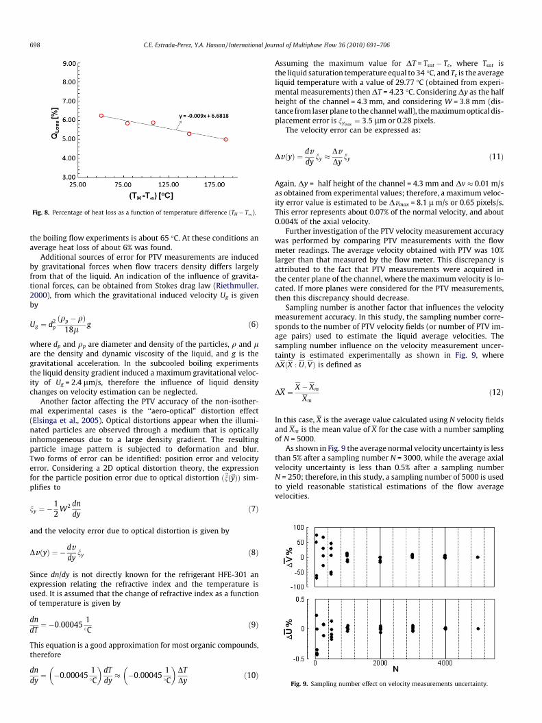
Fig. 8. Percentage of heat loss as a function of temperature difference (TH � T1).

Fig. 9. Sampling number effect on velocity measurements uncertainty.


the boiling flow experiments is about 65 �C. At these conditions anaverage heat loss of about 6% was found.

Additional sources of error for PTV measurements are inducedby gravitational forces when flow tracers density differs largelyfrom that of the liquid. An indication of the influence of gravita-tional forces, can be obtained from Stokes drag law (Riethmuller,2000), from which the gravitational induced velocity Ug is givenby

Ug ¼ d2p

ðqp � qÞ18l

g ð6Þ

where dp and qp are diameter and density of the particles, q and lare the density and dynamic viscosity of the liquid, and g is thegravitational acceleration. In the subcooled boiling experimentsthe liquid density gradient induced a maximum gravitational veloc-ity of Ug = 2.4 lm/s, therefore the influence of liquid densitychanges on velocity estimation can be neglected.

Another factor affecting the PTV accuracy of the non-isother-mal experimental cases is the ‘‘aero-optical” distortion effect(Elsinga et al., 2005). Optical distortions appear when the illumi-nated particles are observed through a medium that is opticallyinhomogeneous due to a large density gradient. The resultingparticle image pattern is subjected to deformation and blur.Two forms of error can be identified: position error and velocityerror. Considering a 2D optical distortion theory, the expressionfor the particle position error due to optical distortion ð~nð~yÞÞ sim-plifies to

ny ¼ �12

W2 dndy

ð7Þ

and the velocity error due to optical distortion is given by

DvðyÞ ¼ � dvdy

ny ð8Þ

Since dn/dy is not directly known for the refrigerant HFE-301 anexpression relating the refractive index and the temperature isused. It is assumed that the change of refractive index as a functionof temperature is given by

dndT¼ �0:00045

1�C

ð9Þ

This equation is a good approximation for most organic compounds,therefore

dndy¼ �0:00045

1�C

� �dTdy� �0:00045

1�C

� �DTDy

ð10Þ

Assuming the maximum value for DT = Tsat � Tc, where Tsat isthe liquid saturation temperature equal to 34 �C, and Tc is the averageliquid temperature with a value of 29.77 �C (obtained from experi-mental measurements) then DT = 4.23 �C. Considering Dy as the halfheight of the channel = 4.3 mm, and considering W = 3.8 mm (dis-tance from laser plane to the channel wall), the maximum optical dis-placement error is nymax

¼ 3:5 lm or 0.28 pixels.The velocity error can be expressed as:

DvðyÞ ¼ dvdy

ny �DvDy

ny ð11Þ

Again, Dy = half height of the channel = 4.3 mm and Dv � 0.01 m/sas obtained from experimental values; therefore, a maximum veloc-ity error value is estimated to be Dvmax = 8.1 l m/s or 0.65 pixels/s.This error represents about 0.07% of the normal velocity, and about0.004% of the axial velocity.

Further investigation of the PTV velocity measurement accuracywas performed by comparing PTV measurements with the flowmeter readings. The average velocity obtained with PTV was 10%larger than that measured by the flow meter. This discrepancy isattributed to the fact that PTV measurements were acquired inthe center plane of the channel, where the maximum velocity is lo-cated. If more planes were considered for the PTV measurements,then this discrepancy should decrease.

Sampling number is another factor that influences the velocitymeasurement accuracy. In this study, the sampling number corre-sponds to the number of PTV velocity fields (or number of PTV im-age pairs) used to estimate the liquid average velocities. Thesampling number influence on the velocity measurement uncer-tainty is estimated experimentally as shown in Fig. 9, whereDXðX : U;VÞ is defined as

DX ¼ X � Xm

Xmð12Þ

In this case, X is the average value calculated using N velocity fieldsand Xm is the mean value of X for the case with a number samplingof N = 5000.

As shown in Fig. 9 the average normal velocity uncertainty is lessthan 5% after a sampling number N = 3000, while the average axialvelocity uncertainty is less than 0.5% after a sampling numberN = 250; therefore, in this study, a sampling number of 5000 is usedto yield reasonable statistical estimations of the flow averagevelocities.


6. Experimental approach

6.1. Flow characteristics, single-phase

To characterize the flow, single-phase unheated liquid velocitymeasurements were performed using PTV at three different axialpositions along the channel length. The distances from the mea-surement region positions with respect to the channel inlet areshown in Table 3.

At each measurement region, 5000 images were acquired usingthe high speed camera. The camera was synchronized with thehigh energy laser. The camera frame rate was 2500 fps with anexposure time of 2 ls. Each image consisted of 504 � 800 pixelsresulting in a spatial resolution of 20.1 lm/pixel. A Reynolds num-ber (Re) of 9929 was considered in this experiment, and a constantinlet temperature of 25.5 �C was maintained at atmospheric pres-sure. Fig. 10 shows the mean axial velocity U and its turbulenceintensity u0 distribution, both normalized by the mean centerlineaxial velocity ðUcÞ. The distance from the wall is normalized bythe channel half-height (h). No significant differences were foundbetween the different measurement locations, only small discrep-ancies of the turbulence intensities in the near-wall region wereobserved. This analysis presents sufficient evidence of a fullydeveloped flow. Ideally, for two-dimensional fully developed flow,the mean normal velocity V should be zero; however, in this exper-iments nonzero values of this velocity were measured, but wereonly about 0.7% of the mean axial velocity component. Measure-ment region P56 at 455 mm from the channel inlet (see Table 3)

Table 3Test section measurement regions.

Distance from the inlet (mm) L/Dh Symbol

P56 455 56P23 365 45N10 275 34

Fig. 10. Axial mean velocity U and axial turbulence intensity u0 profiles at variousaxial locations from the inlet: 455 mm , 365 mm , and 275 mm , from thechannel inlet.

presented fully developed flow statistical characteristics. Conse-quently, it was selected as a suitable measurement area for theboiling experimental investigations.

6.2. PTV experiments

The measurement area selected was located at 455 mm (posi-tion P56) from the channel inlet. PTV measurements to obtain li-quid flow velocities were performed at this position, which isequivalent to L/DH = 56. A camera frame rate of 3500 fps, and anexposure time of 2 ls were selected. Each acquired image con-sisted of 600 � 800 pixels with a spatial resolution of 12.3 lm/pix-el. Three different Reynolds numbers were considered: 3309, 9926and 16,549. For each Reynolds number condition, about 13 differ-ent heat fluxes (q00) were imposed ranging from 0.0 to 64.0 kW/m2.With the help of the shadowgraphy images (see Section 2.3)important bubble dynamics can be determined. For example, theonset of nucleate boiling for the lowest Reynolds number(Re = 3309) was observed at a heat flux q00 ¼ q00ONB ¼ 3:9 kW/m2,and was located at 20 mm from the beginning of heating (at420 mm from the channel inlet), with an average departure bubblediameter of Ddep = 0.31 mm, and a bubble departure frequency of77 Hz. The average bubble diameter at the measurement position(position P56) was DB = 1.78 mm with an average velocity of0.2 m/s. More detailed information can be acquired from the shad-owgraphy images. However, for the sake of brevity, this informa-tion is not provided. For all cases a constant inlet temperature of25.5 �C was maintained. The heater wall average temperatureand fluid outlet temperature were also measured.

Fig. 11 shows the experimental images obtained from the PTVexperiment at a Re = 9929. Fig. 11a presents the unheated single-phase flow images, where the flow seedings are easily identifiedfrom the black background. The heated single-phase experimentalimages are similar and are not shown for brevity. Fig. 11b presents

Fig. 11. PTV experimental images: (a) unheated single-phase flow, (b) boiling flowwith q00 = 56.9 kW/m2.


an example of the boiling flow images with a heated condition ofq00 = 56.9 kW/m2. A bubble layer is shown on the left side of thechannel where boiling occurs. From these images, bubbles can beeasily discriminated from the flow seedings due to differences insize, gray scale value and shape.

Fig. 12 shows instantaneous velocity fields obtained fromexperimental images at Re = 9929. Fig. 12a presents the velocityfield from the unheated single-phase flow experiments. Fig. 12bpresents the velocity field obtained from the boiling flow experi-ment with q00 = 56.9 kW/m2. No velocity vectors were obtained atpositions fully occupied by bubbles, confirming that only the liquidvelocity is being tracked. It is also noted that the velocity magni-tude is larger in regions close to the heated wall (left part of thechannel).

7. Results

7.1. Heat flux influence on the liquid-phase behavior

Wall heating brought changes in the velocity distribution pro-files. Some of these changes are general trends observed also inother studies (Roy et al., 1993; Wardana et al., 1994; Lee et al.,2002) and are summarized here: First, the mean liquid axial veloc-ity in regions close to the heated wall increases accompanied witha decrease in the axial velocity for regions far from the heated wall.Second, there is a marked shift of the maximum liquid axial veloc-ity location toward the wall. These trends are also observed inFig. 13. Fig. 13a shows the profiles of mean liquid axial velocityU for Re = 3309 with wall heat fluxes ranging from 0 to 64 kW/m2. It is observed that for wall heat fluxes ranging from 3.9 to9.0 kW/m2 the increase of velocity close to the wall shifted themaximum towards a common position located at abouty = 2.5 mm. These heat fluxes shared a common maximum velocitymagnitude of approximately 0.2 m/s. Further increase in the heat

Fig. 12. Velocity fields obtained from experimental images for: (a) unheated single-phase flow, (b) boiling flow with q00 = 56.9 kW/m2.

Fig. 13. Mean axial liquid velocity profile for: (a) Re = 3309, (b) Re = 9926, (c)Re = 16,549 with q00 = 0.0 , 3.9 , 9.0 , 12.2 , 16.0 , 18.3 , 20.3 , 22.3 ,35.9 , 42.3 0,0,0.65 , 48.7 0.66,0.0,0.66 , 56.9 , 64.0 (kW/m2).

Fig. 14. Mean axial liquid velocity profile normalized with single-phase flowfriction velocity for: (a) Re = 3309, u* = 0.012 m/s, (b) Re = 9926, u* = 0.027 m/s, (c)Re = 16,549, u* = 0.040 m/s, with q00 = 0.0 , 3.9 , 9.0 , 12.2 , 16.0 , 18.3 ,20.3 , 22.3 , 35.9 , 42.3 0, 0,0.65 , 48.7 0.66,0.0,0.66 , 56.9 , 64.0(kW/m2).


flux forced the maximum velocity magnitude to increase and toshift closer to the wall (y � 0.5 mm). This behavior is observedup to a heat flux of 42.3 kW/m2. The velocity profiles for these heatfluxes intersected at a common position (y = 2.5 mm). The generaltrends previously mentioned changed for the highest heat fluxcases (from 48.7 to 64.0 kW/m2). For these cases new trends werefound: first, the maximum liquid axial velocity reaches a ‘‘termi-nal” maximum velocity of about 0.34 m/s, and second, the maxi-mum liquid axial velocity starts shifting away from the walltowards the center of the channel. Furthermore, the common inter-secting point found in the lower heat fluxes (y = 2.5 mm) is notpresent in the higher heat flux cases. Instead, a shifting of this pointtowards the center of the channel was observed. Similar trendswere also observed for the medium Reynolds number case(Re = 9929) shown in Fig. 13b. For this Reynolds number, the influ-ence of wall heat flux over the axial velocity follows the same gen-eral trends as observed for the lower Reynolds number case(Re = 3309); however, the increase of axial liquid velocity due tothe increase of wall heat flux is lower, and the velocity reductioneffect for regions far from the wall is present, but with less magni-tude. The unheated single-phase profile, together with those of lowheat flux (i.e., 0–16.0 kW/m2), showed no significant differences inthe velocity profiles. Only small discrepancies for points close tothe heater wall were noted. For medium heat fluxes (18.3–35.9 kW/m2), there was an increase of the axial velocity, extendingfrom y = 0 to a distance of about y = 3.5 mm. Further increase in theheat flux forced the maximum velocity magnitude to increase andto shift closer to the wall (y � 1 mm). This behavior was observedfor heat fluxes 42.3 and 48.7 kW/m2. A shift of the maximum veloc-ity location towards the center of the channel started to be ob-served when reaching a heat flux value of 48.7 kW/m2. Thesetrends are similar to those of higher heat fluxes cases of theRe = 3309 experiment, except that the ‘‘terminal” maximum veloc-ity is now about 0.54 m/s. Fig. 13c shows the profiles of mean li-quid axial velocity U for Re = 16,549 with wall heat fluxesranging from 0 to 64 kW/m2. It is clear that with this Reynoldsnumber, the influence due to heat flux is minimal. The increaseof velocity for regions close to the wall as a function of wall heatingis less and velocity reduction for regions far from the wall is notnoticeable; however, small changes start showing with a wall heatflux of 56.9 kW/m2, where a noticeable increase of velocity is ob-served for points in the region from y = 1.0 to about 2.5 mm.

7.2. Liquid turbulence statistics

Since most of the changes in the liquid behavior due to wallheating are observed within the boundary layer region, near-wallnon-dimensional parameters are utilized. In the wall coordinatesystem, a characteristic velocity is needed to obtain non-dimen-sional variables. This characteristic velocity was chosen to be thefriction velocity (u* = [sw/q]1/2). The friction velocity can be esti-mated by plotting the dimensional total stress profile and takinga best fit of the near-wall total stress to determine sw. Followingthe previous procedure, single-phase unheated friction velocitieswere obtained for Re = 3309, 9929, and 16,549. Their values were,respectively, u* = 0.012, 0.027, and 0.040 m/s. All results presentedin this section are normalized by the corresponding single-phaseunheated friction velocity for each Reynolds number. The measure-ment uncertainty of the liquid turbulence statistics are presentedin the Appendix.

Fig. 14 shows the axial non-dimensional velocity profile (u+ = u/u*) versus the non-dimensional distance from the wall (y+ = yu*/m)for various values of wall heat fluxes for cases of Re = 3309, 9929,and 16,549. Fig. 14a shows that the unheated single-phase flowcase (q00 = 0) has a fairly good approximation to the law of the wall.


Fig. 14b shows that the single-phase profile, together with those oflow heat flux (0–9 kW/m2), showed no significant differences fromthe law of the wall, and only small discrepancies for points close tothe wall heater were observed. For the high Reynolds cases(Fig. 14c), the behavior of the mean velocity was closer to the sin-gle-phase flow case, however, for points below y+ = 30 a significantdifference is noted. Fig. 15 shows the non-dimensional axial turbu-lence intensity profile (u0+ = u0/u*) for various values of wall heatingfor Re = 3309, 9929, and 16,549. For the low Reynolds number case(Fig. 15a) the heat flux influence is large, including the low heat fluxcases. Two trends are observed: first, from q00 = 3.95 to 9.02 kW/m2

there is a decrease in the axial turbulence intensities with respect tothe isothermal case, the second trend is observed for the higherheat fluxes where an increase of wall heat flux significantly increasethe turbulence intensity. The axial turbulence intensity profiles forthe medium Reynolds number (Re = 9929) are presented inFig. 15b. Two trends were observed here as well, but in this casethe first trend persisted for higher heat flux cases, ranging fromq00 = 3.9 to 22.3 kW/m2 where the profiles were seen to be belowor close to the isothermal case. The starting point for the secondtrend is shown for wall heat fluxes larger than 35.9 kW/m2, but asignificant increase of the turbulence intensity profile was observedafter reaching a wall heat flux of 48.7 kW/m2. Fig. 15c shows theturbulence intensity profiles for the high Reynolds case(Re = 16,549). Here the wall heat flux influence was dampenedand only a small increase of the turbulence intensity profile was ob-served. No decrease in the axial turbulent intensity was observedbelow the isothermal case as in the low Reynolds case studied here.Fig. 16 show the non-dimensional normal turbulence intensity pro-file (v0+ = v0/u*) at various values of wall heat flux for Re = 3309,9929, and 16,549. These figures showed similar trends as thosefound for the axial turbulence intensities (u0+). The two trends dis-cussed previously were observed in Fig. 16a. The first heat flux caseq00 = 3.95 kW/m2 showed a decrease on the profile compared to theisothermal case, while the rest of the heat flux cases presented alarge increase on turbulence intensity due to the wall heating. Sim-ilar behavior was found for the medium and high Reynolds number;however, wall heating influence was reduced while increasing theReynolds number value. The non-dimensional Reynolds stressesðu0v 0þ ¼ u0v 0=u�2Þ profiles are shown in Fig. 17 for Re = 3309, 9929,and 16,549. A profile decrease tendency was found as a result of awall heat flux increment, and a marked shift of the zero location to-ward the heated wall can be observed. For the low Reynolds num-ber (Fig. 17a) these changes were more pronounced. At thebeginning of heating from q00 = 3.95–12.23 kW/m2 a peak reductionand shift of the zero Reynolds stress locations towards the wall wasfound. Further increase of the heat flux resulted in more reductionin the profile and an inverted peak is observed. The location of thisinverted peak (minimum value) will shift towards the center of thechannel as a result of the increase of the wall heat flux. The sametrends are found for the medium Reynolds number (Fig. 17b),where the profile reduction is more pronounced for points up toy+ = 380. For positions larger than this value, less decrease occurs.The zero shifting and peak inversion is also present. For the highestReynolds number, the effect of the wall heat flux starts to be notice-able only at high q00 values. There are no significant differences inthe profiles up to a heat flux value of 48.7 kW/m2. For this valueof high Reynolds number, the zero value shifting and peak inversioninfluence were not noted.

Fig. 15. Mean axial turbulence intensity profile normalized with single-phase flowfriction velocity for: (a) Re = 3309, u* = 0.012 m/s, (b) Re = 9926, u* = 0.027 m/s, (c)Re = 16,549, u* = 0.040 m/s, with q00 = 0.0 , 3.9 , 9.0 , 12.2 , 16.0 , 18.3 ,20.3 , 22.3 , 35.9 , 42.3 0,0, 0.65 , 48.7 0.66,0.0,0.66 , 56.9 , 64.0(kW/m2).

8. Discussion

Some of the mechanisms that govern the fluid behavior are pre-sented and discussed. First, the heated single-phase behavior is ex-

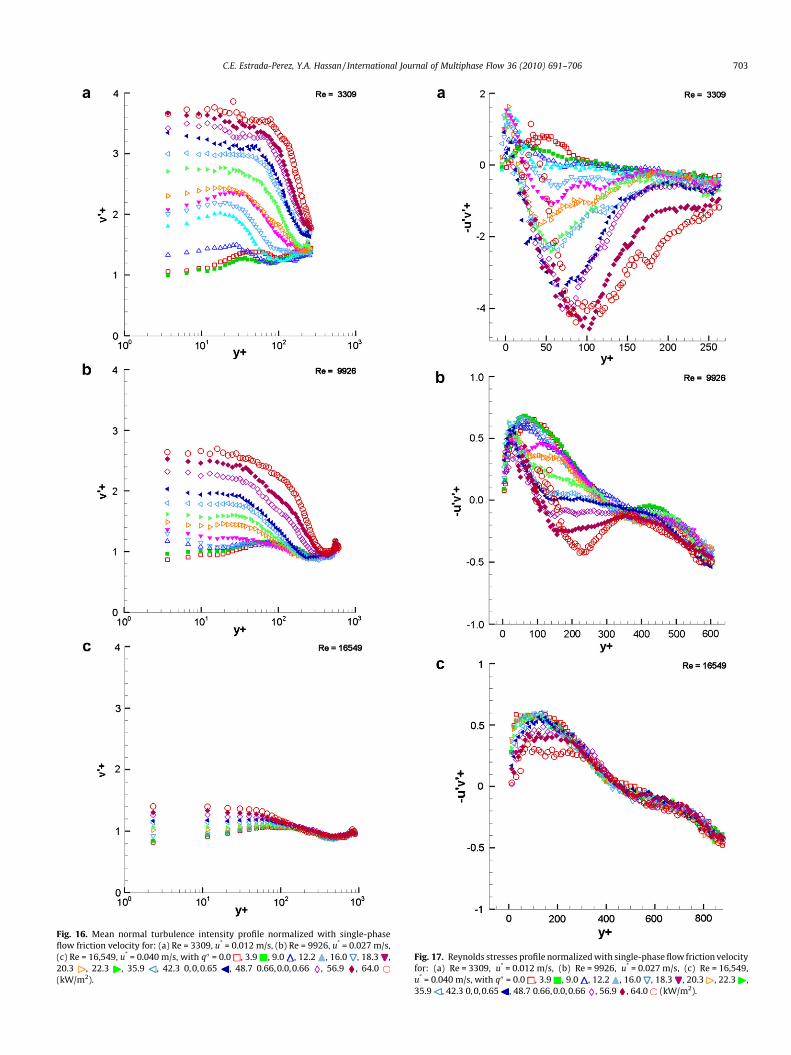
Fig. 16. Mean normal turbulence intensity profile normalized with single-phaseflow friction velocity for: (a) Re = 3309, u* = 0.012 m/s, (b) Re = 9926, u* = 0.027 m/s,(c) Re = 16,549, u* = 0.040 m/s, with q00 = 0.0 , 3.9 , 9.0 , 12.2 , 16.0 , 18.3 ,20.3 , 22.3 , 35.9 , 42.3 0,0,0.65 , 48.7 0.66,0.0,0.66 , 56.9 , 64.0(kW/m2).

Fig. 17. Reynolds stresses profile normalized with single-phase flow friction velocityfor: (a) Re = 3309, u* = 0.012 m/s, (b) Re = 9926, u* = 0.027 m/s, (c) Re = 16,549,u* = 0.040 m/s, with q00 = 0.0 , 3.9 , 9.0 , 12.2 , 16.0 , 18.3 , 20.3 , 22.3 ,35.9 , 42.3 0,0,0.65 , 48.7 0.66,0.0,0.66 , 56.9 , 64.0 (kW/m2).


Fig. 18. Number of vectors depending on position from the wall for Re = 3309 withq00 = 0.0 h, 22.3 M, 64.0 s kW/m2.


plored to serve as a basis to explain the more complex mechanismspresent when subcooled boiling occurs. Previous works have dis-cussed the effects of buoyancy forces on the single-phase heatedvelocity fields (no boiling involved).

According to Petukhov and Polyakov (1988), the transport ofmomentum and heat in a boundary layer of a two-dimensionalchannel flow under the action of gravity is associated with ther-mogravity effects being manifest via two mechanisms. First, abuoyant force acts over the whole flow as a consequence of theinhomogeneous distribution of mean density. This effect, is calledthe external effect. The second effect includes the direct influenceof buoyancy forces on the liquid turbulence due to the fluctuatingdensity in the gravity field. This effect was termed the structural ef-fect by Petukhov and Polyakov (1988). They stated that in turbulentmixed convection in a vertical channel, the influence of the struc-tural effect appears first in regions where the viscous forces aresurpassed by the buoyancy forces, i.e., outside of the viscous sub-layer. This influence can be observed for conditions of low heat fluxand high Reynolds number (small Gr/Re2) such as the low heat fluxcases in Fig. 13c; however, a closer look to the experimental datashows a significant influence within the viscous sublayer (seeFig. 14c). The external effect would not be significant during phasesof low Gr/Re2. By increasing the wall heat flux, the external effectsare expected to become more pronounced leading to the well-known free convection effect of a higher mean axial velocity profilenear the heated wall. For points far from the heated wall, the fluc-tuating buoyancy force contribution is expected to be negative; theproduction term, which is positive, decreases in magnitude com-pared to the isothermal flow. The suppression of turbulence istherefore expected. This effect is shown during the low wall heatflux cases in Fig. 15a) to Fig. 16c. The turbulence intensity suppres-sion was found in all cases except for the higher Reynolds numbercase (Re = 16,549). For this case a consistent increase with wallheat flux was found.

We now briefly discuss some of the physical implications ofthe subcooled boiling measurements. Lance and Bataille (1991)suggested that two-phase flow turbulence is the result of inter-actions between wall turbulence and bubble-induced pseudo-turbulence, the latter being perturbations due to random stirringof the liquid by the bubbles and deformation of their surface. Ithas been conjectured that these perturbations are proportionalto the local vapor fraction and the square of the vapor bubblevelocity relative to the liquid. In this study such interactionswere found as important modifications to the two-phase flowturbulence statistics profiles, noting new features that were notmeasured or explained in previous works; for instance, the con-comitant increase and shift towards the heated wall of the max-imum axial velocity magnitude reached a limit, after which anincrease of wall heat flux results in new observed tendencies.Now the maximum axial velocity shifts towards the center ofthe channel, and its magnitude no longer increases. This behav-ior is believed to be due to the formation of a fuller bubble layerthat will act as a solid wall moving with a speed proportional tothe terminal velocity of the near-wall bubbles. Increasing furtherthe heat flux will increase the bubble layer thickness, but not itsmoving velocity. The bubble layer will result in that both the li-quid and its maximum axial velocity position being shifted awayfrom the wall. This behavior was observed on high heat flux andlow Reynolds number cases (Fig. 13a).

Fig. 19. Mean axial velocity and its standard error for Re = 3309 with q00 = 0.0 h,22.3 M, 64.0 s kW/m2.

9. Conclusions

Using PTV, the effect of heat flux on the liquid statistical quan-tities of subcooled boiling flow was studied. The accuracy of themeasurement technique was estimated by various sensitivity stud-

ies, proving that PTV is a reliable tool to study subcooled boilingflow. Furthermore, a complete characterization of the flow patternwith various heat fluxes and flow Reynolds numbers was per-formed; consequently, velocity components, turbulence intensi-ties, and Reynolds stresses under various conditions wereobtained as a function of distance from the wall, Reynolds number,and heat flux values. The present results agree with previous worksand provides new information due to the full-field nature of thetechnique. This work is an attempt to provide data of turbulentsubcooled boiling flow for validation and improvement of two-phase flow computational models.

Acknowledgments

The authors would like to acknowledge the participation anddedication of Dr. Elvis Dominguez-Ontiveros and Dr. Hee SeokAhn to make this work possible.


Appendix A. Uncertainty of turbulence statistics

The error analysis presented on the PTV algorithm accuracy sec-tion assumed ideal conditions. The effects of large velocity gradi-ents, non-uniform distribution of particles, image noise, wallinduced reflections, or any other difficulty that can be encounterin a real PTV experiment, were not considered. To have a betterunderstanding of the uncertainty induced by these effects, threeheat flux cases were selected: q00 = 0.0, 22.3, and 64.0 kW/m2, allwith a fixed Reynolds number of Re = 3309. Repeated measure-ments at these conditions were performed, and uncertainties wereestimated from the variance about the sample mean. The measure-ment uncertainty depends largely on the sample number; in this

Fig. 20. Mean axial turbulence intensity and its standard error for Re = 3309 withq00 = 0.0 h, 22.3 M, 64.0 s kW/m2.

Fig. 21. Mean normal turbulence intensity and its standard error for Re = 3309 withq00 = 0.0 h, 22.3 M, 64.0 s kW/m2.

Fig. 22. Reynolds stresses and its standard errors for Re = 3309 with q00 = 0.0 h, 22.3M, 64.0 s kW/m2.

case, in the number of vectors found at each location. Fig. 18 showsthe effect of heat flux on the number of vectors found at differentpositions from the wall. The number of vectors distribution ismostly uniform for the single-phase flow case (q00 = 0), althoughin the near-wall region there is a significant decrease of the num-ber of vectors mostly due to wall effects such as wall reflections,high velocity gradients, and loss of correlation of the PTV algo-rithm. In the boiling flow cases (q00 = 0), the bubble induced reflec-tions and turbulence greatly reduce the number of vectors found.Fig. 19 shows the axial velocity and its accuracy (represented witherror bars) for the analyzed cases. The wall and bubble effectsshowed little influence in the axial velocity accuracy. An uncer-tainty of less than ±1% was found even for the near-wall regionof the high heat flux case. Figs. 20 and 21 show the axial and nor-mal turbulence intensities, respectively, and their uncertainties.Wall and bubble effects have a considerable impact on the uncer-tainties in the near-wall regions of the high heat flux cases. Themaximum uncertainty found was about ±3% for both axial and nor-mal turbulence intensities. Significantly larger uncertainties werefound for the Reynolds stresses as shown in Fig. 22. The near-wallregion accounted for uncertainties as large as ±20%, thereforepoints estimated with less than 1000 vectors were discarded.

References

Barrow, H., 1962. An analytical and experimental study of turbulent gas flowbetween two smooth parallel walls with unequal heat fluxes. Int. J. Heat MassTransfer 5, 469–487.

Canaan, R., Hassan, Y., 1991. Simultaneous velocity measurements of bothcomponents of a two-phase flow using particle image velocimetry. Trans. Am.Nucl. Soc. 63.

Dominguez-Ontiveros, E., Estrada-Perez, C., Ortiz-Villafuerte, J., Hassan, Y., 2006.Development of a wall shear stress integral measurement and analysis systemfor two-phase flow boundary layers. Rev. Sci. Inst. 77, 105103.

Elsinga, G.E., van Oudheusden, B.W., Scarano, F., 2005. Evaluation of aero-opticaldistortion effects in PIV. Exp. Fluids 39 (2), 246–256.

Estrada-Perez, C., 2004. Analysis, comparison and modification of various particleimage velocimetry (PIV) algorithms. Master thesis, Texas A&M University, TX,USA.

Gui, L., Wereley, S.T., 2002. A correlation-based continuous window shift techniqueto reduce the peak-locking effect in digital PIV image evaluation. Exp. Fluids 32,506–517.


Hasan, A., Roy, R., Kalra, S., 1992. Velocity and temperature fields in turbulent liquidflow through a vertical concentric annular channel. Int. J. Heat Mass Transfer 35(6), 1455–1467.

Hassan, Y., Gutierrez-Torres, C., Jimenez-Bernal, J., 2005. Temporal correlationmodification by microbubbles injection in a channel flow. Int. Commun. HeatMass Transfer 32 (8), 1009–1015.

HFE-301 3M, 2009. Product information, 3M Novec 7000, engineered fluid. <http://multimedia.mmm.com/mws/>.

Kang, S., Patil, B., Zarate, J., Roy, R., 2001. Isothermal and heated turbulent upflow ina vertical annular channel – part i. Experimental measurements. Int. J. HeatMass Transfer 44 (6), 1171–1184.

Kline, S., McClintock, F., 1953. Describing uncertainties in single-sampleexperiments. Mech. Eng. 75 (1), 3–8.

Koncar, B., Kljenak, I., Mavko, B., 2004. Modelling of local two-phase flowparameters in upward subcooled flow boiling at low pressure. Int. J. HeatMass Transfer 47 (6–7), 1499–1513.

Koyasu, M., Tanaka, T., Sato, Y., Hishida, K., 2009. Turbulence structure of bubblyupward flow (high spatial and temporal resolution measurements using highspeed time series PTV). Trans. Jpn. Soc. Mech. Eng., Part B 75 (755), 1446–1453(in Japanese).

Lance, M., Bataille, J., 1991. Turbulence in the liquid phase of a uniform bubbly air–water flow. J. Fluid Mech. 222, 95–118.

Lee, T., Park, G., Lee, D., 2002. Local flow characteristics of subcooled boiling flow ofwater in a vertical concentric annulus. Int. J. Heat Mass Transfer 28 (8), 1351–1368.

Mayinger, F., 1981. Scaling and modeling laws in two-phase flow and boiling heattransfer. Two-Phase Flow and Heat Transfer in the Power and ProcessIndustries, vol. 1. Hemisphere Publishing Corporation, Washington, DC. pp.424–454 (Chapter 14).

Noback, H., Honkanen, M., 2005. Two-dimensional Gaussian regression for sub-pixel displacement estimation in particle image velocimetry or particle positionestimation in particle tracking velocimetry. Exp. Fluids 38 (4), 511–515.

Ortiz-Villafuerte, J., Hassan, Y., 2006. Investigation of microbubble boundary layerusing particle tracking velocimetry. J. Fluid Mech. 128, 507.

Petukhov, B., Polyakov, A., 1988. Heat Transfer in Turbulent Mixed Convection.Hemisphere, Washington.

Ramstorfer, F., Steiner, H., Brenn, G., 2008. Modeling of the microconvectivecontribution to wall heat transfer in subcooled boiling flow. Int. J. Heat MassTransfer 51, 4069–4082.

Riethmuller, M., 2000. Particle Image Velocimetry and Associated Techniques. vonKarman Institute for Fluid Dynamics Rhode St. Genese, Belgium.

Roy, R., Hasan, A., Kalra, S., 1993. Temperature and velocity fields in turbulent liquidflow adjacent to a bubbly boiling layer. Int. J. Multiphase Flow 19 (5), 765–795.

Roy, R., Kang, S., Zarate, J., Laporta, A., 2002. Turbulent subcooled boiling flowexperiments and simulations. J. Heat Transfer 124, 73.

Roy, R., Krishnan, V., Raman, A., 1986. Measurements in turbulent liquid flowthrough a vertical concentric annular channel. J. Heat Transfer 108, 216–218.

Roy, R., Velidandla, V., Kalra, S., 1997. Velocity field in turbulent subcooled boilingflow. J. Heat Transfer 119, 754.

Scarano, F., Riethmuller, M., 2000. Advances in iterative multigrid PIV imageprocessing. Exp. Fluids 29, 51–60.

Serizawa, A., Kataoka, I., Michiyoshi, I., 1975a. Turbulence structure of air–waterbubbly flow – I. Measuring techniques. Int. J. Multiphase Flow 2 (3), 221–233.

Serizawa, A., Kataoka, I., Michiyoshi, I., 1975b. Turbulence structure of air–waterbubbly flow – II. Local properties. Int. J. Multiphase Flow 2 (3), 235–246.

Serizawa, A., Kataoka, I., Michiyoshi, I., 1975c. Turbulence structure of air–waterbubbly flow – III. Transport properties. Int. J. Multiphase Flow 2 (3), 247–259.

Situ, R., Hibiki, T., Sun, X., Mi, Y., Ishii, M., 2004. Flow structure of subcooled boilingflow in an internally heated annulus. Int. J. Heat Mass Transfer 47 (24), 5351–5364.

Stanislas, M., Okamoto, K., Kähler, C., Westerweel, J., Scarano, F., 2008. Main resultsof the third international PIV challenge. Exp. Fluids 45 (1), 27–71.

Takehara, K., 1998. A study on particle identification in PTV particle maskcorrelation method. J. Visual. 1 (3), 313–323.

Velidandla, V., Putta, S., Roy, R., 1996. Turbulent velocity field in isothermal andheated liquid flow through a vertical annular channel. Int. J. Heat Mass Transfer39, 3333–3346.

Wardana, I., Ueda, T., Mizomoto, M., 1992. Structure of turbulent two-dimensionalchannel flow with strongly heated wall. Exp. Fluids 13 (1), 17–25.

Wardana, I., Ueda, T., Mizomoto, M., 1994. Effect of strong wall heating onturbulence statistics of a channel flow. Exp. Fluids 18 (1), 87–94.

Willert, C., Gharib, M., 1991. Digital particle image velocimetry. Exp. Fluids 10 (4),181–193.

Yeoh, G., Tu, J., Lee, T., Park, G., 2002. Prediction and measurement of local two-phase flow parameters in a boiling flow channel. Numer. Heat Transfer, Part A42 (1), 173–192.

Zarate, J., Capizzani, M., Roy, R., 1998. Velocity and temperature wall laws in avertical concentric annular channel. Int. J. Heat Mass Transfer 41, 287–292.

http://multimedia.mmm.com/mws/

http://multimedia.mmm.com/mws/

PTV experiments of subcooled boiling flow through a vertical rectangular channel

Documents

Transcript of PTV experiments of subcooled boiling flow through a vertical rectangular channel