Program evaluation of agricultural input subsidies in Malawi using treatment effects: methods and...

Abstract

The study evaluates the impact of two agricultural input subsidies in Malawi during the 2003/04 and

2006/07 production periods on household income. The study employs quasi-experimental

econometric techniques that use propensity score matching to control for selection bias on

beneficiaries. A household model for each dataset is estimated together with Average Treatment

Effects on the Treated. The evidence suggest that the matching mechanism performs well in

evaluating the impact of the starter pack program which had a significant negative impact on

household income compared to the refined agricultural input subsidy program which showed

significant positive impacts on household income.

JEL Classification: D13, H23, H43, I38

Keywords: Fertilizer Subsidies; Propensity Score Matching; Average Treatment Effects on the Treated

a I would like to acknowledge two anonymous referees and colleagues in the Ministry of Agriculture and Food

Security in Malawi for their comments. The views expressed in this paper are those of the author not affiliated to any institution. This is a working paper series. For comments please forward to the following Email address: [email protected], or phone (265) 888-511-848, Fax (265) 1-774-302

Program evaluation of agricultural input subsidies in Malawi using treatment effects:

methods and practicability based on propensity scores

Themba Gilbert Chirwa*a

Revised June 2010

* Millennium Challenge Account – Malawi, P. O. Box 31513, Lilongwe, Malawi, Central Africa

mailto:[email protected]

1

1.0 INTRODUCTION

Almost 85% of Malawi’s population belongs to farm (peasant) households and agricultural

production and productivity are often dependent on their performance as farmers. Malawi

being a labor intensive country, the importance of these farmers is often undermined and

understanding the determinants of their welfare, functionality of markets in their communities

and the interventions that are more effective in improving their livelihoods are of vital

importance both to Government and policy makers. This approach helps policy makers in

developing strategies of poverty alleviation that seek to address problems faced by peasant

farmers.

However, once such strategies are developed they are faced with lack of sustainability partly

because there is failure to understand how agrarian institutions work and how to promote

such agrarian societies up the life cycle ladder. Some of these problems arise due to lack of

an understanding that peasant households are single institutions where decisions are made

holistically on production, consumption and reproduction over time (Sadoulet and de Janvry,

1995). These decisions require the functioning of markets within and outside their social

stratum.

In this case, one need to understand why households are always semi-commercialized in the

sense that, even when markets are working, they still keep part of their production for home

consumption or utilize part of their household labor for their own use. Secondly, on the

markets, one needs to understand why rural markets fail in forming backward and forward

linkages to the household entity. As we will see in later sections, the failure to comprehend

these two important questions necessitates the formulation of poor policies that do not

maximize the utility of the householder’s social welfare function.

2

The Agricultural Input Subsidy Program in Malawi and Intended Effects

The goal of the agricultural input subsidy programs in Malawi is to improve agricultural

production and productivity of smallholder farmers for both food and cash crops thereby

reducing the vulnerability of food insecurity and hunger. These input subsidy programs have

been in existence since Malawi attained its independence from Britain in 1964.

The Starter Pack (TIP) program is one such agricultural input program that was implemented

from 1998-2004. The program provided 10-15 kg of fertilizers and ample hybrid maize seed,

free of charge, worthy of planting 0.1 hectares of land. It targeted between 33-96% of rural

smallholder farmers which was scaled down from being a universal subsidy in 1998/99 to a

targeted input program in 2003/04 production periods (Harrigan, 2003; Levy, 2005).

There are variable conclusions concerning the success of the starter pack (TIP) program from

different researchers and data sources. Real GDP growth in Malawi since 1998 to 2005 has

been variable averaging 0.5% per annum (see figure 1). Since the backbone of the Malawi

economy heavily relies on agriculture, the variability in real GDP growth rate signifies the

failure of the starter pack program in improving agricultural production and productivity.

Figure 1: Real GDP Growth Rate in Malawi 1998-2004

Source: Malawi Annual Statistics Data 1998-2005

2.3% 1.3%

-8.4%

-4.1%

2.1% 3.9%

5.1%

2.1%

-10.0%

-5.0%

0.0%

5.0%

10.0%

15.0%

20.0%

25.0%

1998 2005

Re

al G

DP

gro

wth

Year

rdgp growth rate Poly. (rdgp growth rate)

3

Chirwa et al (2006, p. 3) argues that maize production since 1990 has been uneven and

increasingly disappointing depicting an agricultural growth rate of 2.2% per annum between

2000 and 2004. Maize prices have also been increasing amid falling and variable maize

production during the same period (see figure 2).

Figure 2: Maize Production and Prices (Nominal) in Malawi, 1980-2004

Source: Chirwa (2006)

Dorward et al (2008), on the other hand, argues that the impact of higher maize prices are a

dilemma as only about 10% of Malawi maize producers are net sellers of maize while 60%

are net buyers. Peters (2006) further argues that the success of the starter pack program was

affected by famine in various parts of the country during the 2001/02 and 2004/05 production

periods. We argue in this paper that the variability in both real GDP and maize production in

the late 1990s and early 2000s was partly a result of the small quantities of the starter pack

program that negatively impacted on maize production and hence affected real GDP growth.

The 2006/07 input subsidy program, on the other hand, was a continuation from the 2005/06

revised program that allocated 2 million of improved seed and 3 million fertilizer coupons to

all districts in Malawi. The distribution of fertilizers initially targeted 1 million marginalized

farmers that were unable to purchase agricultural inputs. The selection of households in

targeted areas was done by Village Development Committees (in consultation with the entire

4

members of the village) to select households that would benefit three coupons from the input

program: two to buy back 50 kg of basal fertilizer (23:21:0 or NPK) and 50 kg of top dressing

fertilizer (Urea) at MK950, each; and the third coupon to be used in exchange for a 10 kg bag

of improved maize seed worthy of planting one acre of land. For tobacco smallholder

farmers, the approach was similar only that they would buy back Compound D and CAN

fertilizers. These input subsidies for tobacco farmers were only implemented during the

2005/06 production period.

However, in this paper we concentrate on maize farmers to compare the differences in

impacts between the 2003/04 and 2006/07 production periods. As we will notice later on, not

all beneficiaries in this improved input subsidy program received both coupons for basal and

top dressing fertilizer. It is reported that there were some significant diversion of coupons in

some areas whereby households ended up receiving one fertilizer coupon in order to expand

the number of beneficiaries within a village (Dorward et al, 2008).

It should be noted at the outset that, amid all these problems faced by the householder, the

goal of input subsidies in Malawi are mainly meant to increase household income, reduce

food insecurity and hence poverty reduction. Therefore, assessing the direct impacts of such a

program on household income or expenditures on the targeted beneficiaries becomes a good

decision tool for policy makers. Evaluating the complexities beyond the farm gate requires an

understanding of the transformative and network effects and whether the householder is

geared towards competing with established businesses such as large scale commercial

farmers. In most studies, the rural smallholder farmer is always referred to as a subsistence

farmer (Levy, 2005; Dorward et al, 2008).

5

Study Objectives and Hypotheses to be Tested

The agricultural system in Malawi is seasonal and several months in a given year are left idle

and farmers have to seek alternative ways of generating income for their survival.

Government interventions in this case become very important tools to boost their income in

lean periods. Government either would initiate a public works program or provide safety nets

with emphasis on cash transfers to marginalized smallholder households.

Several evaluations have been conducted to assess the impact of agricultural input subsidy

programs in Malawi which have either been descriptive or qualitatively inferred (Gregory,

2006; Dorward et al, 2008; Minot and Benson, 2009) or the econometric methods employed

have not controlled for any measurement errors or unobserved heterogeneity on the

beneficiaries (Bohne, 2009; Ricker-Gilbert, 2009).

The argument in this paper is intended to inform policy makers on the impact of input

subsidy programs on household income by using quasi-experimental econometric techniques.

The process adopted estimates a conventional household model to determine the

effectiveness of two input subsidy programs by controlling for treatment effects. To our

knowledge, no study has been done that employs such a technique to assess program

intervention effects of the input subsidy program in Malawi.

The study objectives, therefore, are twofold. The first one seeks to evaluate government

interventions using treatment evaluation techniques that focus on evaluating periodic panel

datasets with the aim of assessing intervention effects on the goal of the agricultural input

subsidy program. Secondly, to provide quantitative evidence that complementing the input

subsidy program with programs that seek to address market failures directly impact on

household income, positively.

6

The second objective aims at assessing other determinants of household income such as

access to basic services (roads, markets) and how they impact on household income. This

approach will inform agricultural policy makers of the need to include additional program

objectives when implementing the next agricultural input subsidy program.

In line with the objectives of the Agricultural Input Subsidy Program in Malawi and the

outcomes envisaged given any treatment, the key hypotheses to be tested in this paper,

therefore, are as follows:

(a) The 2003/04 starter pack (TIP) program that provided 10-15 kg of fertilizer subsidy

had a significant positive impact on household incomes.

(b) The 2006/07 agricultural input subsidy that provided 100 kg worth of fertilizer had a

significant positive impact on household incomes.

(c) Access to key basic services such as improved roads and markets in rural areas has a

significant positive impact on household income.

The sections of the paper are as follows: section 2 looks at literature review. Section 3

outlines the methodology to be adopted in this paper. Section 4 looks at results and findings.

Lastly, section 5 concludes and provides recommendations for future policy interventions.

2.0 LITERATURE REVIEW

It has been noted that different researchers often ask the wrong questions and use wrong

methodologies when assessing agricultural empirical questions that target the poor or less

privileged in any given society. In any assessment or evaluation of a public intervention

seeking to improve a given social welfare function of the disadvantaged groups, it is

important to ask the question whether the targeted beneficiaries were better or worse off after

7

the intervention was implemented. It becomes irrelevant, in my view, to consider the cost

implications of such interventions especially when the intervention proved to be a success.

With regard to the second Pareto Optimality principle1, Government’s role is to redistribute

wealth and if such distribution is done in a transparent and accountable manner without

making other players worse off then it would be an added advantage. On the issue of

methodology, Lalonde (1986) argues that standard non-experimental techniques such as

regression, fixed effects, and latent-variable selection models are either inaccurate or

sensitive to model specification. Thus, employing such techniques to assess the impact of an

intervention may be subjected to measurement errors and selection bias.

Other researchers have attempted to compare smallholder farmers with commercial farmers

in which those who received subsidized fertilizers have been compared with yield responses

of farmers who pay commercial prices (Ricker-Gilbert et. al, 2009). This depicts a lack of

understanding of how smallholder households behave and a clear eulogy to measurement

error. According to Sadoulet and de Janvry (1995), on one hand, smallholder farmers are

usually semi-commercialized and usually production is at a subsistence level. They only sell

if they have excess production and this depends on their production and consumption needs.

Large commercial farmers, on the other hand, rely on markets and have different objectives

than a rural smallholder subsistence farmer.

For one to make such a comparative analysis it has to be done at a similar level playing field.

For instance, access to effective and efficient agricultural extension services, educational

programs, market and transport systems and credit markets are vital and necessary

components if we are to compare commercial and smallholder farmers. Commercial farmers 1 The second theorem of welfare economics states that if all consumers have convex preferences and all firms

have convex production possibility sets, any Pareto efficient allocation can be achieved as the equilibrium of a complete set of competitive markets after a suitable redistribution of initial endowments (Gravelle and Rees, 2004)

8

are usually strategically positioned and can easily access these basic services. They usually

have access to skilled personnel that are well conversant with latest technologies of

improving agricultural production unlike rural households that utilize traditional experience

to perpetuate their agrarian methodologies. As such, utility functions for smallholder and

commercial farmers are incomparable.

Therefore, arguments assuming that smallholder farmers who receive subsidized inputs at

discounted prices through the Government may obtain similar output responses as

commercial farmers may be an assumption that does not reflect reality. This hypothesis on its

own is an oversimplification and would lead to gross measurement errors, model

misspecification and selection bias. This approach would and has always led to the non-

acceptance on the application of input subsidies on marginalized households and thus has

confused policy makers and development partners of the need to subsidize inputs to the

underprivileged groups.

It also follows that a smallholder farmer will only have an incentive to use a productive asset

as efficiently as possible regardless of the purchasing price if and only if the farmer has

access to the same conditions faced by commercial farmers. In this case, access to

knowledge, information and years spent on education become important. Some studies, for

example, have found that fixed costs (distant to market) and variable costs (price per unit)

may affect market participation (Key et al, 2000; Bellemare et al, 2006). Others have also

shown that access to credit and insurance may be constraints being faced by farmers in order

for them to purchase inputs at reasonable prices (Kherallah et al, 2000; Croppenstedt et al,

2003; Jayne et al, 2003).

Another misconception that is frequently being abused is the combination of a social welfare

function with profit-maximizing behavior. Gregory (2006) argues that input subsidy vouchers

9

are an income transfer to the farmer from Government, donor or any other implementing

agency but also a transfer that can be realized through private sector participation (see also

Kelly et al, 2003). This assumption, however, has its own problems and in this paper we

identify two: firstly, the role of Government is to raise taxes from private entities and

distribute wealth to marginalized households or communities. Since private sector entities are

profit driven and liable to additional taxation, the process affects the ‘laissez-faire’

assumption of the free operation of market forces and becomes one that continuously add

transaction costs that become unsustainable, rendering the intervention too expensive to

public coffers. Government comes in to correct a market failure – a failure that was created

by the private sector in the first place that profiteers a social good. Secondly, since other

factors such as access to basic services may affect the distribution of agricultural inputs to

smallholder farmers, the involvement of private sector participants creates rent-seeking

behavior amongst private players as the business involved is risk-free guaranteed by

Government thereby adding more on the transaction costs.

As Shultz (1945) indicates, smallholder farmers in developing countries may be poor but are

efficient. It, therefore, depends on the quality and quantity of agricultural inputs being

supplied to the targeted beneficiaries and whether they would have access to the same

privileges that a normal commercial farmer would receive. Kelly and Murekezi (2000) and

Duflo et al (2008) also note that application of fertilizer in maize, for example, improves the

yield if the application is made in right quantities and using the correct methods. In other

words, the rate of return to fertilizer application is positive but varies by region.

Another error that researchers make is to employ panel data sets which may have been

developed using different set of conditions. Therefore, any assessment of the impact of

fertilizer subsidy before and after an intervention is made, for example, cannot be justified by

10

looking at different periods or time series but rather creating a counterfactual within the same

period and dataset. Such methodologies are severely affected by seasonality and unobserved

heterogeneity effects. By utilizing the same dataset to create a control group significantly

reduces the potential for selection bias (Dehejia and Wahba, 1999; Browyn and Maffioli,

2008).

As evidenced by Ricker-Gilbert et al (2009), one problem could be that the same respondents

have different farm size within and between agricultural seasons. Thus, in order to avoid such

plot-level unobserved heterogeneity, the study considers periodic analysis of each input

subsidy production period in order to contain for any measurement errors. Recent

econometric tools are available to assess the effectiveness of public interventions targeting

the poor.

3.0 METHODOLOGY

Model Specification

The main objective of the input subsidy programs before and after 2004/05 was to increase

agricultural productivity and food security. The overall goal of the program was to promote

economic growth and reduce vulnerability to food insecurity, hunger and poverty. The

2006/07 Agricultural Input Subsidy Program (AISP) was implemented through the

distribution of fertilizer vouchers of which the beneficiary had to contribute MK950 per

voucher of fertilizer and exchange a voucher of seed free of charge. In later years, the

contribution made by beneficiaries reduced to MK500 during the 2009/10 production period.

In comparison to the TIP program, targeted smallholder farmers were given all inputs free of

charge but in small quantities.

11

To assess the impact of such interventions in the given seasons or fiscal years, we will

employ an empirical model on household food security. The model adopts Sadoulet and De

Janvry (1995) household model with less efficient markets where the household problem is to

solve simultaneously allocation of resources between production, consumption and work

decisions given household characteristics. In its structural form, the household problem is to

maximize utility u with respect to consumption and work decisions subject to a given

production function g and household characteristics:

ha

hlma

ccclxq

lxqgts

ccculmaa

z

z

,,, ..

;,,max,,,,,

(1a)

In equation (1a), utility is maximized given consumption goods (agricultural goods ac and

manufactured goods mc ), home time lc and household characteristics hz subject to a

household production function aq and a set of fixed and variable inputs lx, . The empirical

model assumes a linear function and in a reduced form format the household function is:

LSWCEHPG ,,,,,,,ii yy (1b)

In equation (1b), iy is the outcome of interest – household real expenditure per household

which is a proxy for household income per capita; G is a vector of government interventions

(starter pack program or TIP of 2003/04, agriculture extension services, Agricultural Input

Subsidy Program of 2006/07); P is a vector of prices (tobacco auction price, maize grain

price, maize flour price, fertilizer, casual labor – supply and demand prices, charcoal,

transport, and price index of other consumables); H is a vector of household characteristics

(age, gender, education, health status, sources of lighting and cooking, farm size, livestock

assets, access to portable water, wellbeing); E is a vector of economic characteristics (market

12

access, distance to market, area of residence, access to road surface); C is a vector of

community characteristics (belonging to an association/cooperative, access to agricultural

credit, irrigation scheme, access to small and large markets): W is a vector of weather

conditions (availability of rain); S is a vector of seasonal effects (lean period, dry period,

harvest period, year of interview); and L is a vector of location effects (agricultural

division).

Data Description and Management

The study utilizes raw household data from the 2004/05 second Integrated Household Survey

(IHS2) and the 2006/07 Agricultural Input Subsidy Survey (AISS). The variables within each

vector of interest of the household model in equation (1a) and (1b) are calculated and

averaged over districts. The prices calculated are district level averages from both household

and community databases. A number of data analysis checks are conducted which include

controlling for outliers, management of duplicate records and conducting principal

component analysis to create a livestock index.

Our focus is mainly on rural households since they are more capable of benefiting from the

agricultural input subsidy program than households that live in urban areas. Using the IHS2

data out of a sample of 11280, about 9840 households reside in rural areas, which is our point

of reference. About 60% of households who reside in rural areas reported to have benefited

from the starter pact (TIP) program compared to 11.6% in urban areas (1440)2. The focus on

rural areas also hinges on the household model employed as we assume that households in

rural areas are semi-commercialized and thus would expect their behavior to be similar from

one area to the next.

2 IHS2 Survey data

13

A follow-up survey was conducted in May/June 2007 re-interviewing 3,298 households in

175 EAs. Out of this sample, 2,874 households were previously interviewed in the IHS2

survey. This dataset will be referred in this study as the AISS. The survey design process was

the same as the one adopted under IHS2. After controlling for duplicate records, the AISS

sample size was reduced to 2,937 households of which 1,205 households reported to have

benefited from the input subsidy. Based on this response, 57% reported receiving both 100 kg

of basal and top dressing fertilizers through the Government’s AISP. The analysis of the

impact of the AISP will, therefore, be based on respondents who received 100 kg of fertilizer

based on the goal of the AISP.

The 2006/07 AISS database has a lot of missing values which constrains the analysis to only

those variables that can be used to estimate the household model. In order to complement

some of the missing variables, the study uses 2004/05 IHS2 survey data on some key

variables such as annual household real expenditure and selected community based variables

such as access to safe water, electricity, distance to and availability of markets in the

community, among others.

These common variables are assumed to be constant in 2006/07 as they were during the

2004/05 IHS2 survey. Annual household real expenditures per capita will also be used to

proxy household income per capita and is projected based on real GDP growth rates

experienced since 2003/04 to 2006/07 fiscal years to match the current household income

levels in 2006/07 production season. The impact of the AISP will thus be assessed on

whether it was effective in positively contributing to increased household income in 2006/07

production year.

14

Treatment Effects Framework

The problems assessed in sections 1 and 2 above in evaluating the impact of interventions on

input subsidies in Malawi warrant different methodologies to be looked into. It is more

relevant to assess the impact of an intervention based on ‘with or without’ the intervention

scenario of the sample or population that benefited from the project. As Browyn and Maffioli

(2008) notes, this provides a rigorous strategy of identifying statistically robust control

groups on non-participants. Though the ideal evaluation of an intervention necessitates the

creation of a treatment or control group, this approach cannot be applied on human beings

prior to the beginning of the intervention.

Rosenbaum and Rubin (1983) propose ‘propensity score matching’ (PSM) as a method that

can be used to measure the impact of interventions on outcomes of interest. Propensity score

matching is a method used to reduce selection bias in the estimation of treatment or

intervention effects with observational data sets. The methodology developed is used to

assess a counterfactual in a given set of observational data just like in any scientific

experiment where the same sample can be used to assess the impact on the outcome if the

treatment was not administered. Unlike interventions made on human beings, it is not likely

that an intervention can be administered in one case and also assess the outcome on the same

individual if the intervention was not administered, hence the need for propensity score

matching.

The effect of treatment evaluation on policy formulation is direct because if an intervention is

successful it can be linked to desirable social programs or improvements in existing programs

through reviews. The aim of adopting such a process is to enable policy makers assess the

objectives or goals of the intervention. According to Cameron and Trivedi (2005), the

15

standard problem of treatment evaluation involves the ‘inference of a causal’ connection

between the treatment and the intended outcome.

The idea of measuring the effect of a treatment or intervention requires constructing a

measure that compares the average outcomes of the treated and non-treated groups.

Rosenbaum and Rubin (1983) show that if the exposure to treatment or an intervention is

random within cells defined by the vector ,ix it is also random within cells defined by the

values of the propensity score. Therefore, given a population or sample of units i the

propensity score or the conditional probability of receiving a treatment given ix is:

xxx DEDp 1Pr (2)

Once propensity scores are known, we then can calculate the Average effect of Treatment on

the Treated (ATT) as follows:

1,0,1

,1

1

01

01

01

iiiii

iii

iii

DpDyEpDyEE

pDyyEE

DyyEATT

xx

x (3)

In equation (3), iy1 assumes the individual receives a treatment or intervention and iy0 is a

counterfactual if the same (or similar) individual receives no treatment. In its simplest form

the average treatment effect is estimated simply by subtracting the average outcome for the

treated with the average outcome for the untreated.

This hypothesis requires two key assumptions namely: the conditional independence

assumption and the assumption of unconfoundedness. The first assumption states that

conditional on ,ix the outcomes are independent of treatment. In other words, participation

in the program intervention does not depend on the outcome. The unconfoundedness

16

assumption, which in some cases is referred to as the Balancing condition, is necessary if we

are to identify some population measures of impact (Rosenbaum and Rubin, 1983; Cameron

and Trivedi, 2005). Given the overlap or matching assumption in equation (2), the

independence assumption ensures that for each value of the vector ,ix there exist both

treated and non-treated cases. The propensity score measure can be computed given the data

iiD x, through either a probit or logit regression.

Propensity Score Matching

The key to the balancing property between the treated and un-treated is to identify

comparable or counterfactual groups by focusing on key household attributes or

characteristics. The agricultural input subsidy program mainly focuses on promoting food

security or household income. The matching methodology calculates propensity scores based

on the following logit model:

poorfhhhhagefTIP ,, (4)

The rationale for selecting these household attributes is based on the selection criteria that the

input subsidy program follows when distributing fertilizer coupons to intended beneficiaries.

The beneficiaries are considered marginalized and vulnerable and mostly the selection

criterion is based on whether the householder is headed by a female, regarded as poor or by

the age variable. Furthermore, the area of residence (rural or urban) is the key identifier of an

agricultural input subsidy and the focus of analysis will only consider householders that

reside in rural areas.

The advantage of the survey data used is that the observations were randomly drawn and thus

the treatment will not be subjected to a situation where we are unable to identify a control

group. In the 2006/07 AISS dataset, the creation of a control group takes advantage of the

17

distributional problems of the input subsidy program where not all beneficiaries received both

basal and top-dressing fertilizers. In doing so, we are able to create a control group for the

treated. However, this may create contamination as the control group still receives fertilizer

but only the basal type. The bias created may affect the significant difference between the

beneficiaries and non-beneficiaries. Nonetheless, we may not run into such a problem as the

yields that a farmer would get by just applying one type of fertilizer are significantly lower

than yields when both types of fertilizers (basal and top-dressing) are applied.

Balancing Properties

One critical area of PSM literature is to assess whether the matching mechanism adopted is

balanced in the allocated blocks/cells. Fifteen (15) and nine (9) blocks/cells have been created

for models 1 and 2, respectively. We present tests for equality of means for each of the three

regressors presented in equation (4) within each block. The results are presented in table 1

(annex I) and the logit regression in table 2. The results show that all variables are balanced

in each block and we cannot reject the null hypothesis that the differences in mean of the

treated and controls are different from zero. Thus, the balancing properties when estimating

propensity scores in both models are satisfied.

Using calculated propensity scores as defined in equation (2) and (4) is not enough to

estimate average treatment effects of an intervention (Dehejia and Wahba, 1999; Cameron

and Trivedi, 2005; Becker and Ichino, 2009). The reason is that the propensity score is

usually a continuous variable and the probability of observing two units with exactly the

same propensity score is in principle not possible. A number of methodologies have been

proposed in the literature with the aim of overcoming this problem (see Cameron and Trivedi,

2005). In this evaluation exercise, however, we will consider only four most common

18

methods widely used: nearest neighbor matching, radius matching, kernel matching and

stratification (or interval) matching3.

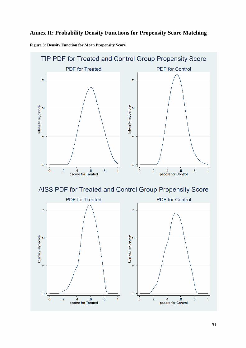
We plot density functions for the treated and control groups to see whether the matching of

scores is over a reasonable number of observations. The probability density functions for the

propensity scores are displayed in figures 3, 4 and 5 (annex II) for models 1 and 2,

respectively, obtained from and , , attkattrattnd STATA commands. The results show that

the mean propensity score between the treated and control group is well distributed in both

models. The distribution of treatment also performs well when one uses radius and kernel

matching techniques.

4.0 MODEL ESTIMATION AND RESULTS

Robustness Checks

Table 3 (annex III) present robustness checks on the data for the two models to be estimated.

We first check whether the models have no omitted variables. We use the Ramsey RESET

test using powers of the fitted values of the food expenditure dependent variable. The results

show that the two models are affected by omitted variables. Since the two datasets are limited

on the number of variables that can be generated from each database, we still estimate the

models given the present variables.

On functional form and heteroskedasticity, we use Cameron and Trivedi decomposition of

the IM test that tests for heteroskedasticity, skewness and kurtosis. The results for both

models suggest that there are problems of heteroskedasticity and skewness. We will

therefore, use weighted least squares and a log-linearised model to correct for skewness.

3 Details on how these matching estimators are calculated can be found in Cameron and Trivedi, 2005, p.871-

879

19

The Breusch-Pagan/Cook-Welsberg test is used to test for overall heteroskedasticity in the

two models and the results show that both models are affected by heteroskedasticity. This

further substantiates the need to report Huber/White heteroskedasticity consistent standard

errors.

We test for multicollinearity on the variables of interest using variance inflation factors

(VIF). In both models there is evidence of multicollinearity and the variables with a high

variance inflation factor (VIF) are dropped. One common variable in both equations is the

square of household age.

A new regression model is estimated using ordinary least squares (OLS) and corrected based

on problems identified by the above common misspecification tests. We also test for

endogeneity and the results show that the model suffers from an endogeneity problem and

one of the suspected parameters is the household age variable (hhage) which has a positive

sign as we would expect that as age of an individual increases, the propensity of being food

insecure is high.

We, therefore, should expect a negative sign for the household age variable. In this case we

expect that the household age variable is correlated with the error term or there is a

measurement error being influenced by a reverse causation of the dependent variable. In this

case, the two models may present biased and inconsistent parameter estimates.

Instrumental Variables

To correct our problem we identify an instrumental variable for the household age variable in

order to obtain consistent estimates. A good instrument is one that is correlated with the

endogenous household age variable, conditional on other covariates, but also at the same time

not correlated with the error term. We follow this process in identifying the instrumental

20

variable for hhage and test the correlation coefficients between hhage and three related

exogenous variables – elderly, madult and fadult. The correlation coefficients are presented in

table 4 (annex III) and show that the elderly variable is strongly correlated with hhage

(0.6382, model 1; 0.5405 model 2) and has a strong significant p-value.

We further test the validity of the selected instrumental variable (elderly) and the results are

presented in table 3. The results show that we cannot reject the null hypothesis that the

elderly variable is exogenous in both models (p-values 0.2812 and 0.9032) and hence not

correlated with the error term. In this case, the elderly variable is a good instrument for the

hhage variable. The model to be estimated will, therefore, follow two stage least squares

(2SLS) estimation to provide consistent parameter estimates.

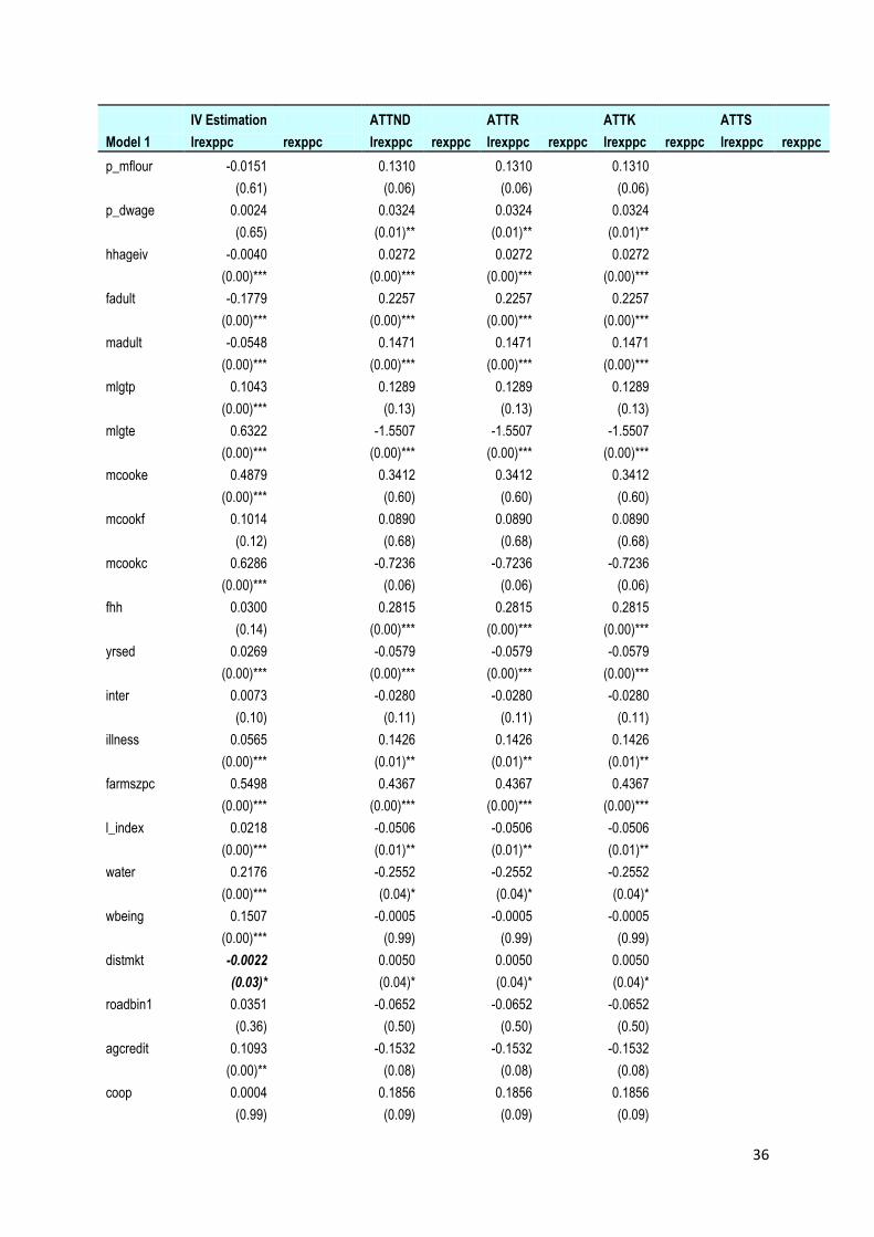
Regression Results

The results for the estimated instrumental variable or 2SLS models are presented in tables 5

and 6 (see annex IV) together with the estimated average treatment effects on the treated (or

ATT) for the input subsidy intervention based on Becker and Ichino (2009) algorithms. The

goodness of fit shows that in the first model using IHS2 data the explanatory variables

explain about 33% of the variation on the dependent variable and 27% in the second

household model.

Tables 7 and 8 (see annex V) present an average propensity score difference estimator

between the treated and the control group based on equation (3) and show the number of

treated and control groups for each matching mechanism adopted. The ATT estimators

presented in tables 7 and 8 are average treatment effects based on all blocks/cells created as

outlined in table 9 (annex VI). We now present the regression results based on the hypotheses

to be tested.

21

Hypothesis 1: Impact of the 2003/04 Starter Pack (TIP) Program on

Household Income

After controlling for complex survey design and 2SLS estimation, the results show that those

who benefited from the Starter Pack (TIP) program, holding other factors constant, had a

significant negative impact of approximately 0.0819 (8.2%) or reduced annual household

income per capita by MK1399.00 (1399 Malawi Kwacha).

Overall the results obtained after controlling for treatment effects (nearest neighbor, radius,

kernel matching and stratification) taken together, also give evidence of a significant negative

treatment effect in the ranges of MK1228-MK2521 associated with the TIP subsidy when

evaluated with control or comparison groups, ceteris paribus. Note that the ATT results are

close to the coefficient estimate for the TIP impact given in our household model of

MK13994.

The results are not surprising and concur with evaluations made by government and some

researchers on the impact of the TIP subsidy as not being effective in reducing poverty and

food insecurity (Dorward et al 2008; Ricker-Gilbert et al 2009). The size of the package

distributed to targeted households contributed significantly to the negative impact as well as

corrupt practices identified by Peters (2006). It is more likely that the application of fertilizers

were done to fit a householder’s farm size that was more than 0.1 hectares. In such

circumstances, yield would generally be low or equivalent to a situation where no fertilizers

are applied to a particular field. This could have been necessitated by poor extension services

that did not advise targeted farmers on how to apply the subsidized fertilizer.

4 Note that the coefficient estimates in log-terms for annual household real expenditure per capita are

transformed using the exponential function and obtain the difference between the treated and untreated.

22

Hypothesis 2: Impact of 2006/07 Agricultural Input Subsidy Program on

Household Income

The second household model results (table 6) show that those who benefited from the full

subsidy of the AISP, holding other things constant, had a significant positive contribution of

0.082 (8.2%) or MK1679 more towards household income than those who did not benefit

from the AISP. Overall, the results obtained after controlling for ATT also give significant

evidence (except the ATTR) on the effect of treatment on the beneficiaries. Those who

received a full subsidy from Government, ceteris paribus, experienced a positive impact in

the ranges of MK1567-MK1705 (ATT of 0.075-0.083) associated with the 2006/07 AISP

when evaluated without the intervention comparison group. Again the results support

observations by other researchers about the positive impact that the revised agricultural input

subsidy program had on household incomes and in reducing food security in Malawi

(Dorward et al, 2008).

Hypothesis 3: Impact of Basic Services on Household Income

The study also evaluated the impact of market access on annual household income per capita.

Three key variables were included in each household model that looked at the impact of

roads, market access and distance to the market on household income. The study results are

similar in both models and show that those who had access to large markets, holding other

things constant, had a significant negative impact of 0.1218 (or 12.2%) and 0.154 (or 15.4%),

in 2003/04 and 2006/07 production periods, respectively, than those who did not. This is

surprising as one would expect that farmers with better access to large markets would be

better off than those who do not. The reason is that these markets are secondary markets and

are far away from main markets in the three cities in the country. As such, farm gate prices

offered by intermediate buyers are affected by high transaction costs and tend to be below the

smallholder farmer’s long-run marginal cost curve in rural areas.

23

This also concurs with the fact that lack of or existence of poor basic services such as markets

in rural areas greatly affect household production and consumption decisions (see Dorward et

al, 2008 and Chirwa et al, 2006). This is supported by the negative impact that distances to

markets have on household income that registered -0.0022 (or -0.22% during 2003/04

production season) and -0.0019 (or -0.2% during the 2006/07 production season) significant

at 1% level, ceteris paribus.

As for roads, during the 2003/04 production season the variable of interest was dropped due

to multicollinearity. During the 2006/07 production season, however, the road variable

registered, ceteris paribus, a significant negative impact of 0.163 (or 16.3%) for communities

that had access to only a dirt road maintained on a regular basis. Unpaved roads usually raise

transportation costs and thus lower farm gate prices as intermediate buyers have to cover their

marginal costs. This also supports the argument of the need to complement the improvement

of basic services in rural areas in order to lower transaction costs and maximize the benefits

from any social program through proper marketing mechanisms.

5.0 CONCLUSIONS AND RECOMMENDATIONS

The paper has demonstrated on how we can use treatment effects to evaluate the impact of

public interventions based on independent datasets. The adopted approach is important as it

controls for selection bias that may result from measurement errors and model

misspecification.

There is clear evidence of a significant negative impact of the 2003/04 Starter Pack (TIP)

program and significant positive impact of the AISP on household income when we use

treatment effects. The differences are a result of Government improving on the quantities of

fertilizer used by smallholder farmers and improving on the distribution to marginalized

beneficiaries.

24

The benefits can further be maximized if such programs are complemented with projects

aimed at improving access to basic services in the targeted areas such as roads and markets.

Access to basic services in rural areas such as large markets and unpaved roads negatively

impact on the availability of household income. We conclude that interventions geared

towards complementing input subsidies should be supported with interventions aimed at

improving basic services such as the development of markets and roads in rural areas.

The main conclusions from this study can be summarized as follows: the impact of the input

subsidy programs in Malawi becomes stronger as policy makers improve on the quantities of

inputs subsidized. In addition, it can also be inferred that universal subsidies tend to be costly

and ineffective as the program compromises on quality and output. Focusing the agricultural

input subsidy program on a targeted – but very effective and efficient set of beneficiaries – is

essential for the program to reap its intended benefits periodically.

The study also faced some data problems when assessing the two household models

particularly for the follow-up survey conducted in 2007 that was different from the original

IHS2 survey. The panel survey contained data gaps for key variables required to perform a

similar analysis. It is recommended that follow-up surveys conducted by the National

Statistical Office should promote the continuance collection of original questionnaire

variables collected in the Integrated Household Survey or at least tracking of common

variables relevant to household characteristics in order to be able to evaluate the impact of a

specific intervention based on the household model.

25

6.0 BIBLIOGRAPHY

Becker, S. O., and A. Ichino. 2009. ‘Estimation of Average Treatment Effects Based on

Propensity Scores’, unpublished manuscript available at

www2.dse.unibo.it/ichino/psj7.pdf

Bellemare, M. and C. Barrett. 2006. ‘An Ordered Tobit Model of Market Participation:

Evidence from Kenya and Ethiopia’, American Journal of Agricultural Economics,

88(2): 324-337

Bohne, A. 2009. ‘Agriculture, Agricultural Income and Rural Poverty in Malawi: Spatial

analysis of determinants and differences’, unpublished manuscript available at

http://www.uni-koeln.de/phil-fak/afrikanistik/kant/data/Bohne-KANT2.pdf

Browyn, H., and A. Maffioli. 2008. ‘Evaluating the Impact of Technology Development

Funds in Emerging Economies: evidence from Latin America,’ a Technical Report

unpublished manuscript available at http://hd1.handle.net/10086/15999

Cameron, A. C. and P. K. Trivedi. 2005. Microeconometrics: Methods and Applications,

New York: Cambridge University Press

Chirwa, E. W., J. Kydd and A. Dorward. 2006. ‘Future Scenarios for Agriculture in Malawi:

Challenges and dilemmas’, draft version, March, unpublished manuscript available at

http://www.future-agricultures.org/pdf%20files/Ag_Malawi.pdf

Croppenstedt, A., M. Demke, M. Meschi. 2003. ‘Technology Adoption in the Presence of

Constraints: The Case of Fertilizer Demand in Ethiopia’, Review of Development

Economics, 7(1): 58-70

http://www.dse.unibo.it/ichino/psj7.pdf

http://www.uni-koeln.de/phil-fak/afrikanistik/kant/data/Bohne-KANT2.pdf

http://hd1.handle.net/10086/15999

http://www.future-agricultures.org/pdf%20files/Ag_Malawi.pdf

26

Dehejia, R. H., and S. Wahba. 1999. ‘Causal Effects in Non-Experimental Studies: re-

evaluating the evaluation of training programs’, Journal of the American Statistical

Association, 94, 1053-1062

Dorward, A., E. Chirwa, V. Kelly, T. S. Jayne, R. Slater, and D. Boughton. 2008. ‘Evaluation

of the 2006/07 Agricultural Input Subsidy Programme, Malawi’, Final Report,

Ministry of Agriculture and Food Security, Lilongwe: March

Duflo, E., M. Kremer, J. Robinson. 2008. ‘How High are Rates of Return to Fertilizer?

Evidence from Field Experiments in Kenya’, American Economics Association

Meetings, New Orleans, Los Angeles: January

Franses, S. 1995. Adjustment and Poverty: Options and Choices. New York: Routledge

Gravelle, H. and R. Rees. 2004. ‘Microeconomics’, Third Edition, Edinburgh Gate: Pearson

Education Limited

Gregory, I. 2006. ‘The Role of Input Vouchers in Pro-Poor Growth’, Background Paper

Prepared for the African Fertilizer Summit, Abuja, Nigeria: June 9-13

Harrigan, J. 2003. ‘U-Turns and Full Circles: Two decades of agricultural reform in Malawi

1981-2000’, World Development, Vol. 31(5), 847-863

Jayne, T. S., J. Govereh, M. Wanzala, M. Demke. 2003. ‘Fertilizer Market Development: a

comparative analysis of Ethiopia, Kenya and Zambia’, Food Policy: 28(4): 293-326

Kelly, V. and A. Mukerezi. 2000. ‘Fertilizer Response and Profitability in Rwanda’, Ministry

of Agriculture, Animal Resources and Forestry, Kigali, Rwanda: February

27

Key, N., E. Sadoulet, A. de Janvry. 2000. ‘Transaction Costs and Agricultural Household

Supply Response’, American Journal of Agricultural Economics, 82(5): 245-259

Kherallah, M., C. Delgado, E. Gabre-Madhin, N. Minot, M. Johnson. 2000. ‘Agricultural

Market Reform in Sub-Saharan Africa: a synthesis of research findings’, Washington

D. C.: International Food Policy Research Institute

Levy, S. 2005. Starter Packs: A strategy to fight hunger in developing countries?

Wallingford, UK: CABI publishing

Minot, N. and T. Benson. 2009. ‘Fertilizer Subsidies in Africa: Are vouchers the answer?’,

International Food Policy Research Institute, IFPRI Issue Brief 60: July

Peters, P. E. 2006. ‘Rural Income and Poverty in a Time of Radical Change in Malawi’,

Journal of Development Studies, Vol. 42(2), 322-345

Ricker-Gilbert J., T. S. Jayne and J. R. Black. 2009. ‘Does Subsidizing Fertilizer Increase

Yields? Evidence from Malawi’, Selected paper prepared for presentation at the

Agricultural and Applied Economics Association 2009 AAEA and ACCI Joint Annual

Meeting, Milwaukee, Wisconsin, July 26-29, 2009

Rosenbaum, P., and D. B. Rubin. 1983. ‘The Central Role of Propensity Score in

Observational Studies for Causal Effects,’ Biometrika, 70, 227-240

Rostow, W. W. 1963. The Economics of Take-Off into Sustained Growth: Proceedings of a

Conference held by the International Economic Association. W. W. Rostow (ed.),

London: Macmillan.

28

Sadoulet, E., and A. de Janvry. 1995. ‘Quantitative Development Policy Analysis’, Baltimore

and London: The John Hopkins University Press

Schultz, T. W. 1945. Food for the World. Chicago: University of Chicago Press

Tarp, F. 1993. Stabilization and Structural Adjustment: Macroeconomic frameworks for

analyzing the crisis in Sub-Saharan Africa. New York: Routledge

29

7.0 ANNEXES

Annex I: Two Sample t-tests for Mean Propensity Score and Logit

Regression Results

Table 1: Two Sample t-test with Equal Variances

H0:Mean Propensity Score not different for treated and controls Variable Name Block Difference estimate t-statistic p-value

Model 1 Model 2 Model 1 Model 2 Model 1 Model 2

Mean pscore 8 0.002

9 0.000 -0.002 -0.31 -1.40 0.76 0.18

10 0.000 -0.002 -0.86 -0.74 0.39 0.46

11 -0.001 0.002 -1.61 1.27 0.11 0.21

12 -0.001 -0.002 -1.84 -0.84 0.07 0.41

13 -0.001 -0.001 -1.73 -0.29 0.08 0.77

14 -0.001 0.001 -1.93 0.05

15 0.001 -0.001 1.15 -1.12 0.25 0.26

16 0.000 -0.020 0.35 -1.66 0.73 0.10

17 -0.001 -1.65 0.10

18 0.000 -0.14 0.89

19 -0.001 -0.95 0.34

20 0.000 0.47 0.64

21 0.000 -0.32 0.75

22 0.000 0.06 0.95

23 -0.003 -0.96 0.34

hhage 8 2.800

9 -0.140 -2.221 -0.72 -1.40 0.48 0.18

10 -0.115 -2.594 -1.00 -0.75 0.32 0.46

11 -0.157 1.843 -1.25 1.27 0.21 0.21

12 -0.184 -0.132 -1.57 -0.05 0.12 0.96

13 -0.192 -0.595 -1.47 -0.28 0.14 0.78

14 -0.101 0.600 -0.60 0.55

15 -0.006 -1.152 -0.03 -1.13 0.98 0.26

16 0.042 -2.208 0.21 -1.66 0.84 0.10

17 -0.346 -1.59 0.11

18 -0.203 -0.73 0.46

19 -0.119 -0.46 0.65

20 0.477 1.45 0.15

21 -0.399 -0.89 0.37

22 -0.065 -0.11 0.91

23 -1.072 -0.82 0.42

fhh 8 0.000

9 0.017 0.000 0.75 0.45

10 0.011 0.000 0.59 0.56

11 0.015 0.000 0.61 0.54

30

H0:Mean Propensity Score not different for treated and controls Variable Name Block Difference estimate t-statistic p-value

Model 1 Model 2 Model 1 Model 2 Model 1 Model 2

12 0.010 -0.038 0.59 -0.59 0.56 0.55

13 0.005 0.000 0.31 0.00 0.76 1.00

14 -0.011 0.000 -0.41 0.68

15 0.019 0.000 0.64 0.52

16 0.001 0.000 0.02 0.99

17 0.029 0.89 0.38

18 0.035 0.75 0.46

19 -0.011 -0.31 0.76

20 -0.076 -1.37 0.17

21 0.060 0.83 0.41

22 0.015 0.23 0.82

23 0.022 0.15 0.88

poor 8 0.000

10 0.000

11 0.000

12 0.038 0.59 0.55

13 0.000 0.00 1.00

14 0.000

15 0.000

16 0.000

Table 2: Logit Estimates for Mean Propensity Score if Householder Resides in Rural Area

Model 1 Model 2

TIP aissf

hhage 0.0271 hhage 0.0040

(0.00)*** (0.31)

fhh 0.1463 fhh -0.4596

(0.01)** (0.00)**

poor -0.6821

(0.00)***

_cons -0.7612 _cons 0.3336

(0.00)*** (0.08)

N 9573 N 1171

pR-sq 0.035 pR-sq 0.022

Note: Balancing property is satisfied

Marginal Effects; t-statistics in parenthesis

(d) for discrete change of dummy variable from 0 to 1

="* p<0.05 ** p<0.01 *** p<0.001"

31

Annex II: Probability Density Functions for Propensity Score Matching

Figure 3: Density Function for Mean Propensity Score

32

Figure 4: Model 1

33

Figure 5: Model 2

34

Annex III: Robustness Checks

Table 3: Robustness Checks on Survey Data if Householder Resides in Rural Area

Robustness Checks Null Hypothesis Statistic Model 1: Model 2: Conclusion

Ramsey RESET test using powers of the fitted values of dependent

variable

Model has no omitted variables

F-statistic 89.96 84.17 Reject null hypothesis. However dataset has limited observations

p-value 0.0000 0.0000

Functional Form and Heteroskedasticity using Cameron and Trivedi decomposition of IM-

test

Heteroskedasticity p-value 0.0000 0.0000 Reject but not for kurtosis. For skewness transform

dependent variable to log form

Skewness p-value 0.0000 0.0000

Kurtosis p-value 1.0000 1.0000

Breusch-Pagan/Cook-Welsberg test for heteroskedasticity

constant variance

chi2 9244.36 4086.77 Reject & report Huber/White het-consistent standard errors: weighted

least squares p-value 0.0000 0.0000

Test for Multicollinearity using Variance Inflation Factors

No Multicollinearity mean VIF 20.01 4.56 Drop some variables in both models and form principal components

Test for Endogeneity Variables are exogenous

Robust Score chi2 7.72236 14.3377 reject null hypothesis and variables are endogenous

p-value 0.0055 0.0002

Test of Linear Hypothesis Variables are

exogenous (elderly)

F-statistic 0.38 0.01 Instrumental variable is

exogenous p-value 0.5400 0.9032

Table 4: Correlation Coefficients to Determine Instrumental Variable for Household Age (Reside=Rural)

Model 1

Model 2

hhage elderly madult fadult

hhage elderly madult fadult

hhage 1.0000

hhage 1.0000

elderly 0.6395 1.0000

elderly 0.5405 1.0000

0.0000

0.0000

madult -0.0583 -0.2266 1.0000

madult -0.0382 -0.2371 1.0000

0.0000 0.0000

0.0388 0.0000

fadult 0.0037 -0.2014 0.2413 1.0000 fadult -0.0119 -0.2200 0.2288 1.0000

0.7169 0.0000 0.0000

0.5204 0.0000 0.0000

35

Annex IV: OLS Estimates of Household Model (Dependent Variable:

Annual Household real expenditure per Capita)

Table 5: Regression Results on Model 1 with ATT5 if Householder Resides in Rural Area

IV Estimation ATTND ATTR ATTK ATTS

Model 1 lrexppc rexppc lrexppc rexppc lrexppc rexppc lrexppc rexppc lrexppc rexppc

TIP -0.0819 -1399 -0.087 -1488 -0.071 -1228 -0.076 -1303 -0.143 -2521

(0.00)*** (0.00)*** (0.00)*** (0.00)*** (0.00)***

agext -0.1423 0.3016 0.3016 0.3016

(0.00)*** (0.00)*** (0.00)*** (0.00)***

agextcp -0.0705 0.2891 0.2891 0.2891

(0.26) (0.19) (0.19) (0.19)

agextsv 0.0152 0.1302 0.1302 0.1302

(0.76) (0.55) (0.55) (0.55)

agextfu 0.0619 0.2018 0.2018 0.2018

(0.36) (0.36) (0.36) (0.36)

agextirri -0.0274 0.3917 0.3917 0.3917

(0.46) (0.02)* (0.02)* (0.02)*

agextac 0.0349 -0.1042 -0.1042 -0.1042

(0.38) (0.55) (0.55) (0.55)

agextmkt -0.0250 -0.0768 -0.0768 -0.0768

(0.55) (0.66) (0.66) (0.66)

agextcre 0.0257 -0.0268 -0.0268 -0.0268

(0.53) (0.87) (0.87) (0.87)

p_tobauction 0.0003 0.0068 0.0068 0.0068

(0.93) (0.45) (0.45) (0.45)

p_maize 0.0119 0.0794 0.0794 0.0794

(0.16) (0.00)*** (0.00)*** (0.00)***

p_fert 0.0129 -0.0133 -0.0133 -0.0133

(0.00)** (0.17) (0.17) (0.17)

p_ganyu -0.0023 -0.0945 -0.0945 -0.0945

(0.84) (0.00)*** (0.00)*** (0.00)***

p_index 0.0010 -0.0352 -0.0352 -0.0352

(0.91) (0.10) (0.10) (0.10)

p_char 0.0041 -0.0033 -0.0033 -0.0033

(0.00)*** (0.19) (0.19) (0.19)

p_ker -0.0022 0.0679 0.0679 0.0679

(0.85) (0.03)* (0.03)* (0.03)*

p_tpt 0.0013 -0.0137 -0.0137 -0.0137

(0.41) (0.00)*** (0.00)*** (0.00)***

5 Second column presents results based on instrumental variable or 2SLS using complex survey design.

Columns 4-10 presents Average Treatment Effects on the Treated (ATT) using propensity scores – 4th

column: ATT ( Nearest Neighbor matching); 6

th Column: ATT (Radius matching); 8

th Column: ATT (Kernel matching); 10

th

Column: ATT (Stratification matching)

36



p_mflour -0.0151 0.1310 0.1310 0.1310

(0.61) (0.06) (0.06) (0.06)

p_dwage 0.0024 0.0324 0.0324 0.0324

(0.65) (0.01)** (0.01)** (0.01)**

hhageiv -0.0040

0.0272 0.0272 0.0272

(0.00)*** (0.00)*** (0.00)*** (0.00)***

fadult -0.1779 0.2257 0.2257 0.2257

(0.00)*** (0.00)*** (0.00)*** (0.00)***

madult -0.0548 0.1471 0.1471 0.1471

(0.00)*** (0.00)*** (0.00)*** (0.00)***

mlgtp 0.1043 0.1289 0.1289 0.1289

(0.00)*** (0.13) (0.13) (0.13)

mlgte 0.6322 -1.5507 -1.5507 -1.5507

(0.00)*** (0.00)*** (0.00)*** (0.00)***

mcooke 0.4879 0.3412 0.3412 0.3412

(0.00)*** (0.60) (0.60) (0.60)

mcookf 0.1014 0.0890 0.0890 0.0890

(0.12) (0.68) (0.68) (0.68)

mcookc 0.6286 -0.7236 -0.7236 -0.7236

(0.00)*** (0.06) (0.06) (0.06)

fhh 0.0300 0.2815 0.2815 0.2815

(0.14) (0.00)*** (0.00)*** (0.00)***

yrsed 0.0269 -0.0579 -0.0579 -0.0579

(0.00)*** (0.00)*** (0.00)*** (0.00)***

inter 0.0073 -0.0280 -0.0280 -0.0280

(0.10) (0.11) (0.11) (0.11)

illness 0.0565 0.1426 0.1426 0.1426

(0.00)*** (0.01)** (0.01)** (0.01)**

farmszpc 0.5498 0.4367 0.4367 0.4367

(0.00)*** (0.00)*** (0.00)*** (0.00)***

l_index 0.0218 -0.0506 -0.0506 -0.0506

(0.00)*** (0.01)** (0.01)** (0.01)**

water 0.2176 -0.2552 -0.2552 -0.2552

(0.00)*** (0.04)* (0.04)* (0.04)*

wbeing 0.1507 -0.0005 -0.0005 -0.0005

(0.00)*** (0.99) (0.99) (0.99)

distmkt -0.0022 0.0050 0.0050 0.0050

(0.03)* (0.04)* (0.04)* (0.04)*

roadbin1 0.0351 -0.0652 -0.0652 -0.0652

(0.36) (0.50) (0.50) (0.50)

agcredit 0.1093 -0.1532 -0.1532 -0.1532

(0.00)** (0.08) (0.08) (0.08)

coop 0.0004 0.1856 0.1856 0.1856

(0.99) (0.09) (0.09) (0.09)

37



irriscm -0.0525 -0.1567 -0.1567 -0.1567

(0.23) (0.22) (0.22) (0.22)

mktsmall -0.0203 -0.0583 -0.0583 -0.0583

(0.44) (0.43) (0.43) (0.43)

mktlarge -0.1218 0.3662 0.3662 0.3662

(0.00)** (0.00)*** (0.00)*** (0.00)***

rain_l -0.0546 0.2428 0.2428 0.2428

(0.09) (0.00)*** (0.00)*** (0.00)***

rain_m 0.0397 0.0330 0.0330 0.0330

(0.26) (0.64) (0.64) (0.64)

season1 -0.1726 -0.0494 -0.0494 -0.0494

(0.00)*** (0.58) (0.58) (0.58)

season2 -0.1123 0.0893 0.0893 0.0893

(0.00)*** (0.21) (0.21) (0.21)

season4 -0.1361 -0.1119 -0.1119 -0.1119

(0.00)*** (0.10) (0.10) (0.10)

year2004 0.1545 0.1185 0.1185 0.1185

(0.00)*** (0.12) (0.12) (0.12)

_cons 8.3034

3.2734 3.2734 3.2734

(0.00)*** (0.16) (0.16) (0.16)

N 7890 7890 7890 7890 9573

R-sq 0.325 0.072 0.072 0.072

Marginal Effects; t-statistics in parenthesis (d) for discrete change of dummy variable from 0 to 1

="* p<0.05 ** p<0.01 *** p<0.001"

38

Table 6: Regression Results on Model 2 with ATT6 if Householder Resides in Rural Area



aissf 0.0821 1679 0.078 1605 0.075 1567 0.083 1705 0.073 1587

(0.02)* (0.07) (0.30) (0.01)** (0.02)*

agextsv -0.1424 0.6203 0.6203 0.6203

(0.24) (0.21) (0.21) (0.21)

agextfu 0.2010 -0.6444 -0.6444 -0.6444

(0.11) (0.20) (0.20) (0.20)

p_lmaize -0.0055 0.0656 0.0656 0.0656

(0.65) (0.03)* (0.03)* (0.03)*

p_hmaize 0.0170 -0.1011 -0.1011 -0.1011

(0.46) (0.10) (0.10) (0.10)

p_tobacco 0.0041 -0.0157 -0.0157 -0.0157

(0.15) (0.02)* (0.02)* (0.02)*

p_wage 0.0012 0.0144 0.0144 0.0144

(0.52) (0.00)** (0.00)** (0.00)**

hhageiv -0.0033

0.0084 0.0084 0.0084

(0.08) (0.27) (0.27) (0.27)

madult -0.0626 0.1876 0.1876 0.1876

(0.00)** (0.02)* (0.02)* (0.02)*

fadult -0.1469 0.2184 0.2184 0.2184

(0.00)*** (0.03)* (0.03)* (0.03)*

mlgtp 0.1631 0.3053 0.3053 0.3053

(0.01)* (0.21) (0.21) (0.21)

mlgte 1.0610 0.8316 0.8316 0.8316

(0.00)*** (0.40) (0.40) (0.40)

mcooke -0.0803 -1.2166 -1.2166 -1.2166

(0.75) (0.37) (0.37) (0.37)

mcookf -0.0885 -0.2248 -0.2248 -0.2248

(0.59) (0.73) (0.73) (0.73)

mcookc 0.1420

(0.52)

fhh 0.0372 -0.3711 -0.3711 -0.3711

(0.28) (0.02)* (0.02)* (0.02)*

consyr -0.0139 -0.2343 -0.2343 -0.2343

(0.67) (0.09) (0.09) (0.09)

l_index 0.0316 0.1717 0.1717 0.1717

(0.09) (0.02)* (0.02)* (0.02)*

water 0.0673 0.1215 0.1215 0.1215

(0.60) (0.70) (0.70) (0.70)

distmkt -0.0019 -0.0023 -0.0023 -0.0023

(0.35) (0.71) (0.71) (0.71)

mktsmall 0.0694 0.0143 0.0143 0.0143

6 Note that those in parenthesis for ATT are t-statistics.

39



(0.23) (0.93) (0.93) (0.93)

mktlarge -0.1542 0.2436 0.2436 0.2436

(0.04)* (0.20) (0.20) (0.20)

roadbin1 0.1006 -0.3673 -0.3673 -0.3673

(0.38) (0.26) (0.26) (0.26)

roadbin3 -0.1629 -0.5443 -0.5443 -0.5443

(0.03)* (0.02)* (0.02)* (0.02)*

roadbin4 -0.1153 0.1951 0.1951 0.1951

(0.23) (0.49) (0.49) (0.49)

ADMARC -0.0602 -0.2030 -0.2030 -0.2030

(0.40) (0.34) (0.34) (0.34)

farmszpc 0.5796 0.1514 0.1514 0.1514

(0.00)*** (0.51) (0.51) (0.51)

wbeing -0.0640 -0.1661 -0.1661 -0.1661

(0.10) (0.32) (0.32) (0.32)

poor -0.0832 -0.5602 -0.5602 -0.5602

(0.03)* (0.00)*** (0.00)*** (0.00)***

coop -0.0100 0.5246 0.5246 0.5246

(0.88) (0.01)** (0.01)** (0.01)**

irriscm -0.1202 -0.3664 -0.3664 -0.3664

(0.13) (0.06) (0.06) (0.06)

ICT -0.0698 -0.8016 -0.8016 -0.8016

(0.64) (0.43) (0.43) (0.43)

_cons 9.3445

-0.1758 -0.1758 -0.1758

(0.00)*** (0.91) (0.91) (0.91)

N 1147 N 1143 1143 1143 1176

R-sq 0.270 pR-sq 0.066 0.066 0.066

Marginal Effects; t-statistics in parenthesis (d) for discrete change of dummy variable from 0 to 1

="* p<0.05 ** p<0.01 *** p<0.001"

40

Annex V: ATT and Bootstrapped Standard Errors

Table 7: ATT and Bootstrapped Standard Errors for Model 1 based on IHS2 Dataset

ATTND ATT estimation with Nearest Neighbor Matching method (random draw version)

Bootstrapped Standard Errors Mean Abs. Mean Observations Std. Error t-Statistic p-value

Matched Treated 9.705 16397 4748

Matched Controls 9.792 17885 1903

ATT (y1-y0) -0.087 -1488 6651 0.021 -4.244 0.000

Note: the numbers of treated and controls refer to actual nearest neigbor matches

ATTR ATT estimation with the Radius Matching method

Bootstrapped Standard Errors No. Treated Mean Abs. Mean Observations Std. Error t-Statistic p-value



ATT (y1-y0) -0.071 -1228 5242 0.024 -2.971 0.000

Note: the numbers of treated and controls refer to actual matches within radius

ATTK ATT estimation with the Kernel Matching method

Bootstrapped Standard Errors No. Treated ATT Abs. Mean Observations Std. Error t-Statistic p-value



ATT (y1-y0) -0.076 -1303 7887 0.013 -6.027 0.000

ATTS ATT estimation with the Stratification Matching method




ATT (y1-y0) -0.143 -2521 9568 0.014 -10.601 0.000

IV Estimation No. Treated ATT Abs. Mean Observations Std. Error t-Statistic p-value

Treated 9.705 16397 687

Untreated 9.787 17796 518

y1-y0 -0.082 -1399 1205 0.016 -5.030 0.000

41

Table 8: ATT and Bootstrapped Standard Errors for Model 2 using AISS Dataset

ATTND ATT estimation with Nearest Neighbor Matching method (random draw version)

Bootstrapped Standard Errors Mean Abs. Mean Observations Std. Error t-Statistic p-value



ATT (y1-y0) 0.078 1605 923 0.052 1.498 0.0672

Note: the numbers of treated and controls refer to actual nearest neigbor matches

ATTR ATT estimation with the Radius Matching method

Bootstrapped Standard Errors No. Treated Mean Abs. Mean Observations Std. Error t-Statistic p-value



ATT (y1-y0) 0.075 1567 208 0.151 0.499 0.3092

Note: the numbers of treated and controls refer to actual matches within radius

ATTK ATT estimation with the Kernel Matching method




ATT (y1-y0) 0.083 1705 1142 0.032 2.589 0.0049

ATTS ATT estimation with the Stratification Matching method




ATT (y1-y0) 0.077 1587 1166 0.036 2.159 0.0155

IV Estimation No. Treated ATT Abs. Mean Observations Std. Error t-Statistic p-value

Treated 9.966 21297 687

Untreated 9.884 19618 518

y1-y0 0.082 1679 1205 0.002 2.460 0.02

42

Annex VI: Blocks/Cells for Treated and Control Groups

Table 9: Inferior Bound, Number of Treated and Controls for Each Block (Reside==Rural)

Model 1

Model 2

Inferior of block of pscore

Householder received a Starter Pack (TIP) as

safety net from Government

Inferior of block of pscore

Householder received both basal and top dressing

subsidy fertilizers

No Yes Total

No Yes Total

0.4 58 33 91 0.325 5 1 6

0.45 167 108 275 0.3375 8 13 21

0.4625 256 205 461 0.35 32 16 48

0.475 535 504 1039 0.4 36 27 63

0.5 883 1040 1923 0.45 67 64 131

0.55 338 394 732 0.5 79 79 158

0.575 287 435 722 0.55 1 5 6

0.6 404 678 1082 0.6 248 436 684

0.65 231 435 666 0.65 18 31 49

0.675 154 399 553

0.7 238 699 937

0.75 114 286 400

0.775 60 243 303

0.8 79 259 338

0.85 10 36 46

Total 3,814 5,754 9,568 Total 494 672 1,166

Note: the common support option has been selected Note: the common support option has been selected

43

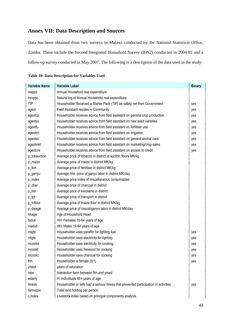
Annex VII: Data Description and Sources

Data has been obtained from two surveys in Malawi conducted by the National Statistical Office,

Zomba. These include the Second Integrated Household Survey (IHS2) conducted in 2004/05 and a

follow-up survey conducted in May 2007. The following is a description of the data used in the study:

Table 10: Data Description for Variables Used

Variable Name Variable Label Binary

rexppc Annual Household real expenditure

lrexppc Natural log of Annual Household real expenditure

TIP Householder Received a Starter Pack (TIP) as safety net from Government yes

agext Field Assistant resides in Community yes

agextcp Householder receives advice from field assistant on general crop production yes

agextsv Householder receives advice from field assistant on new seed varieties yes

agextfu Householder receives advice from field assistant on fertiliser use yes

agextirri Householder receives advice from field assistant on irrigation yes

agextac Householder receives advice from field assistant on general animal care yes

agextmkt Householder receives advice from field assistant on marketing/crop sales yes

agextcre Householder receives advice from field assistant on access to credit yes

p_tobauction Average price of tobacco in district at auction floors MK/kg

p_maize Average price of maize in district MK/kg

p_fert Average price of fertiliser in district MK/kg

p_ganyu Average hire price of ganyu labor in district MK/day

p_index Average price index of miscellaneous consumables

p_char Average price of charcoal in district

p_ker Average price of kerosene in district

p_tpt Average price of transport in district

p_mflour Average price of maize flour in district MK/kg

p_dwage Average price of casual/ganyu labor in district MK/day

hhage Age of Household Head

fadult HH: Females 15-64 years of age

madult HH: Males 15-64 years of age

mlgtp Householder uses paraffin for lighting fuel yes

mlgte Householder uses electricity for lighting yes

mcooke Householder uses electricity for cooking yes

mcookf Householder uses firewood for cooking yes

mcookc Householder uses charcoal for cooking yes

fhh Householder is female (0/1) yes

yrsed years of education

inter Interaction term between fhh and yrsed

elderly H: Individuals 65+ years of age

illness Householder or wife had a serious illness that prevented participation in activities yes

farmszpc Total land holding per person

l_index Livestock index based on principal components analysis

44

Variable Name Variable Label Binary

water Householder has access to personal water supply yes

wbeing Householder considers wellbeing in year improved 0/1 yes

distmkt distance (km) to nearest daily market

reside Urban/Rural dummy yes

roadbin1 road==Tar/Asphalt Graded yes

roadbin3 road==Dirt Road (maintained) yes

roadbin4 road==Dirt track yes

agcredit Existence of Farmers credit clubs in community yes

coop Existence of Farmers cooperatives in community yes

irriscm Irrigation scheme in community yes

mktsmall Access to a Daily Market in community yes

mktlarge Access to a Larger Market in community yes

rain_l For growing maize, the amount of rain was too little yes

rain_m For growing maize, the amount of rain was too much yes

season1 Interview took place in the months of Dec, Jan, Feb yes

season2 Interview took place in the months of March, April, May yes

season4 Interview took place in the months of Sept, Oct, Nov yes

year2004 Interview took place in 2004 yes

psu Enumeration Area/PSU (564 total)

hhwght IHS2 HH weight

hhsize HH Size (based on household members

strata Stratum: district & urban/rural (30 total)

aissf Householder received both basal and top dressing subsidy fertilizer in 2006/07 yes

p_lmaize Average price of local maize in district MK/kg in 2006/07

p_hmaize Average price of hybrid maize in district MK/kg in 2006/07

p_tobacco Average price of burley tobacco in district MK/kg in 2006/07

p_wage Average wage of casual/ganyu labour in district MK/day in 2006/07

consyr Householder considers food consumption inadequate in 2006/07 yes

Program evaluation of agricultural input subsidies in Malawi using treatment effects: methods and...

Documents

Transcript of Program evaluation of agricultural input subsidies in Malawi using treatment effects: methods and...