Product-market competition and executive compensation

Dis

kuss

ions

schr

iften

Product Market Competition and Executive Compensation: An Empirical Investigation

Patricia Funk Gabrielle Wanzenried

03-09

June 03

Universität Bern Volkswirtschaftliches Institut Gesellschaftstrasse 49 3012 Bern, Switzerland Tel: 41 (0)31 631 45 06 Web: www.vwi.unibe.ch

Product Market Competition and Executive

Compensation: An Empirical Investigation

Patricia Funk∗ and Gabrielle Wanzenried†

June 2003

Abstract

There is an ongoing theoretical debate about whether firm-owners would op-

timally use stronger or weaker incentive schemes for their managers as product

market competition increases. Schmidt (1997) shows that the outside options of

the managers play a crucial role: if the market for managers is soft, an increase in

competition is more likely to result in stronger incentive schemes than if the mar-

ket for managers is tough. In this paper, we for the first time analyze the effect

of product market competition on the level and structure of executive compensa-

tion. With panel-data for firms in the the U.S. manufacturing industries (NAICS

32-33), we investigate (a) how an increase in product market competition affects

the use of incentive contracts and (b) whether this relationship depends on the

outside options of the managers as predicted by theory.

JEL Classification: G3, J3, L2.

Key Words: CEO compensation, product market competition, incentive schemes.

∗Department of Economics, University of Basel, Petersgraben 51, CH-4003 Basel, Switzerland, tel.++41 61 260 12 64, fax ++41 61 260 12 66, [email protected].

†Department of Economics, University of Bern, Gesellschaftsstrasse 49, CH-3012 Bern, Switzerland,tel. ++41 31 631 39 23, fax ++41 631 39 92, [email protected] would like to thank Winand Emons, Peter Kugler and various participants of the 2003 congressof the Swiss Society of Economics and Statistics for helpful comments and suggestions.

Product Market Competition and Executive

Compensation: An Empirical Investigation

Abstract

There is an ongoing theoretical debate about whether firm-owners would op-

timally use stronger or weaker incentive schemes for their managers as product

market competition increases. Schmidt (1997) shows that the outside options of

the managers play a crucial role: if the market for managers is soft, an increase in

competition is more likely to result in stronger incentive schemes than if the mar-

ket for managers is tough. In this paper, we for the first time analyze the effect

of product market competition on the level and structure of executive compensa-

tion. With panel-data for firms in the the U.S. manufacturing industries (NAICS

32-33), we investigate (a) how an increase in product market competition affects

the use of incentive contracts and (b) whether this relationship depends on the

outside options of the managers as predicted by theory.

JEL Classification: G3, J3, L2.

Key Words: CEO compensation, product market competition, incentive schemes.

1

1 Introduction

There is a growing theoretical debate about the effects of product market competition

on managerial effort and firm owners’ use of incentive schemes. While the earlier liter-

ature speculates that insufficient competition leads to managerial slack,1 Hart (1983)

was one of the first to formalize the idea that competition reduces managerial slack.2

However, subsequent research showed that the relationship between competition and

managerial slack becomes ambiguous as soon as Hart’s assumption of infinitely risk

averse managers is abandoned (Scharfstein, 1998).3

While most of the papers focus on the information effects of competition (i.e. the

idea that competition helps a principal to make better inferences about his agent’s

actions), Schmidt (1997) investigates the interactions between product market compe-

tition and incentives of managers without relying on such information effects. In his

setup, increased competition reduces the firm’s profit, which induces the manager to

work harder for a cost reduction in order to avoid liquidation. However, the reduction

in profits also affects the profitability of a cost reduction, which may have an ambiguous

effect on manager’s work effort.

As for the effect of competition on managerial effort and executive compensation,

Schmidt (1997) is in line with other papers by showing that this relationship is am-

biguous and depends on different effects. However, in contrast to previous research,

Schmidt (1997) shows that the outside options of the managers play a crucial role in

determining the sign of the total effect. Specifically, if the market for managers is

1According to Leibenstein (1966), there may be a substantial amount of X-inefficiency if outputmarkets are imperfectly competitive. Also, he argues that that this type of inefficiency is much moreimportant in practice than more conventional sorts of inefficiencies due to prices not being equal tomarginal costs. Machlup (1967) notes that managerial slack as an inefficiency source does not existif a firm operates in a perfectly competitive environment. However, Jensen and Meckling (1976)claim that a monopolist has the same incentives to reduce agency costs than an owner of a perfectlycompetitive firm.

2He develops a model of the relationship between competition and slack in a situation whereinefficiency is explicitly the result of a conflict of interest between owners and managers. Since firmowners cannot monitor managerial actions and are also uncertain about their costs, they do not knowwhether a bad performance of the firm is due to mismanagement or high costs. Given the fact thatthe firms’ costs are positively correlated, lower costs lead to lower prices. It follows that managerswho must fulfill profit targets will have less opportunity to engage in managerial slack than if theircosts alone had fallen without a change in the output prices.

3Hermalin (1992) considers two other effects, competition might have on a firm’s agency problem,namely the risk-adjustment effect and the change-in-relative-value-of-action effect. Overall, Hermalin(1992) finds that each of these effects is of potentially ambiguous sign. He concludes that theory doesnot offer a definitive defense of the presumption that increased competition reduces managerial slack.

2

tough, an increase in competition is less likely to result in stronger incentive schemes

than if the market for managers is soft. This feature of the model allows us to em-

pirically discriminate these different cases, which makes it attractive for an empirical

test.

The aim of our paper is to empirically investigate the effect of competition on exec-

utive compensation. Besides looking at the level of compensation, we for the first time

consider various measures which characterize the structure of executive compensation

and which give a more complete picture of the incentives the executives are facing.4 In

addition, we explicitly take into account whether the bargaining power of the managers

affects the relationship between competition and executive compensation, as predicted

by Schmidt’s (1997) model.

The data set is a panel for firms in the US manufacturing industries over the years

1992 to 2000. While data on executive compensation and firm characteristics are taken

from the Compustat Executive database and Compustat Industrial Annual database,

we first have to build measures for the intensity of competition.

For each sub-industry in the industries 32 and 33 (NAICS 3 digit-level), we esti-

mate an intensity of competition measure as suggested by Boone and Weigand (2000).

The advantage of the Boone-Weigand Indicator, compared to traditional competition

measures (e.g. concentration ratio, industry profitability) is that it not only captures

competition going together with more firms in the market, but also competition re-

sulting from more aggressive behavior of the firms in the industry.5 However, we also

employ the price-cost margin as an alternative measure of competition.

Using these two measures of competition, we find the following relationship between

competition and executive compensation: The relationship between competition and

4There are a two related papers, which focus on the strategic effect of compensation schemes. Ag-garwal and Samwick (1999), for instance, test for the effects of competition on relative performanceevaluation in executive compensation contracts. As such, the focus is on the joint impact of competi-tion and (own- and rival-firm) performance on compensation; in contrast, the effect of competition onthe level and structure of compensation can hardly be tested, since there is no variation of the com-petition measure over time (Aggarwal and Samwick (1999) use the Herfindahl-Index in the differentindustries for the year 1992). Kedia (1998), on the other hand, investigates how firms use incentivecontracts in order to alter product market behavior. Therefore, the analysis focuses on the effectof compensation contracts on competition and not, as in our analysis, on the effects of a changingintensity of competition on the level and structure of compensation.

5The basic idea is to empirically estimate how changes in efficiency (relative costs) are reflectedin changed profits. For instance, if competition in an industry is low, an increase in costs may notreduce profits, whereas the opposite holds true under tough competition.

3

executive compensation differs between the industries. In industry 32, an increase in

the intensity of competition led to a decrease in compensation as well as to the use of

weaker incentive schemes. In contrast, the opposite was observed in industry 33. For

both industries, however, we find that with increasing outside options of the managers

(measured by the growth rate of the Dow Jones Index and a measure of the CEO’s

past performance), an increase in competition led to higher executive compensation

(especially in the variable part of the salary).

Therefore, our results are consistent with the literature which posits an ambigu-

ous relationship between competition and executive compensation, but predicts that

increasing outside options of the managers positively affect this relationship.

The main innovations of the paper can be summarized as follows. It is the first paper

which empirically investigates the relationship between executive compensation and

product market competition while explicitly taking into account the outside option of

managers. In addition, we use a new concept to measure the intensity of product market

competition which overcomes the ambiguity problems of the conventional competition

measures.

The rest of the paper is structured as follows: Section 2 contains Schmidt’s (1997)

theoretical model and our derivation of a testable hypothesis. Section 3 describes

the concepts to measure the intensity of competition on product markets and shows

the estimates for the different sub-industries. The econometric model, which relates

competition to executive compensation, is presented in section 4, and section 5 contains

the results. Section 6 concludes. Some supplementary materials can be found in the

appendix.

2 The model

Subsections 2.1. to 2.2. outline the theoretical model which goes back to Schmidt

(1997). As is described in section 2.3., we use Schmidt’s model in order to derive a

testable hypothesis for the empirical section of the paper. The reader familiar with

Schmidt’s model can skip the first two subsections and directly go to subsection 2.3,

where the effect of competition on the compensation contract is derived or subsection

2.4, where the results are summarized and the testable hypothesis is outlined.

4

2.1 The basic setup

Schmidt (1997) considers the following model: At date t = 0, the owner of the firm

hires a manager for the CEO position on a competitive market for identical managers.

The owner of the firm and the manager are risk neutral. The manager’s job is to

improve the efficiency of the firm by reducing the future production costs. The cost

function is characterized by a parameter c, with c ∈{

cL, cH}

and cH > cL. Initially,

the firm is characterized by a high cost parameter cH . At date t = 1, the manager

chooses his effort level. The probability that the manager’s activities lead to a cost

reduction is a function of his effort, i.e., by exerting effort, the manager increases the

probability p that a cost reduction takes place and that the technology switches to

the low cost parameter cL. The effort of the manager is unobservable. The manager

chooses p, with p ∈ [0, 1] , at personal costs G(p) which increase with p at an increasing

rate, i.e., G′(p) > 0, G′′(p) > 0 with G(0) = G′(0) and limp→1 G(p) = ∞.

At date t = 2, the realization of c becomes publicly observable. The owner of the

firm then decides whether to stay in the market and to compete with its rivals, or

to exit the market and liquidate the firm. In the latter case, the liquidation value of

the firm is normalized to zero. At date t = 3, in case the firm still is in the market,

production takes place and profits π are realized.

Figure 1 resumes the structure of the game.

Figure 1: Structure of the game

t 0 1 2 3 4

manager chooses p

c observable liquidation decision

production and/or price decisions

profits are realized, payoffs

cost reduction market

5

As for the third stage of the game, Schmidt (1997) does not explicitly model the

market game, but assumes that it has a unique equilibrium and that the reduced-form

gross profit function is given by

π = π(c, φ, ε) (1)

where φ measures the degree of product market competition in the market and ε

is an exogenous noise variable. The degree of product market competition φ, with

φ ∈ Φ ∈ R, is a continuous variable which can reflect the number of competitors

in the market, whether the firms compete in prices or in quantities, the degree of

product differentiation or any other indicator of the intensity of competition. The

exogenous noise variable ε, with ε ∈ R, is distributed according to the cumulative

distribution function F (ε) and may reflect how many firms in the market have been

successful in reducing their costs, or some exogenous technological or demand shocks.

Its realization is publicly observable at date t = 2, i.e. after the manager has chosen his

effort level and before the owner decides on liquidation of the firm. The reduced-form

profit function π(c, φ, ε) is continuously differentiable in φ and is assumed to have the

following properties.

π(cL, φ, ε) > π(cH , φ, ε) ∀φ ∈ Φ, ε ∈ R (2)

π(cL, φ, ε) ≥ 0 ∀φ ∈ Φ, ε ∈ R (3)

∂π(ci, φ, ε)

∂φ< 0 ∀j ∈ {L,H} , ε ∈ R (4)

Equation (2) says that if the manager is successful in reducing the costs, the firm’s

profit increases. Equation (3) states that profits are always non-negative in case the

manager was successful, independently of the degree of competition. Finally, equation

(4) defines the meaning of more competition, i.e., when competition increases, the

profits decrease.

Given this structure of the game and the profit function (1) with properties (2)-(4),

we now can describe the payoff functions for the owner and the manager and derive

the owner’s optimization problem.

6

The payoff of the firm owner U p is given by

Up = max {0, π(c, φ, ε) − w} (5)

where w is the wage payment to the manager. Given that the owner is risk neutral, he

can always close down the firm and realize a payoff of zero.

The manager’s payoff is given by

Um = {w − G(p) if the firm stays in the marketw − G(p) − Lm if the firm is liquidated

(6)

Lm represents the utility loss of the manager in case the firm is liquidated. It may

represent the search costs to look for a new job, the loss of human capital or a negative

reputation effect which lowers his future income.

Given that the manager’s effort is not observable, it cannot be contracted on. By the

revelation principle, we can restrict our attention to contracts of the form {wL, wH},

where wj is the wage payment to the manager if the cost realization of his firm is

cj, j ∈ {L,H}. With Πj denoting the expected gross profit of the firm,6 the principal’s

optimization problem at date t = 0 is as follows:

max{p,wL,wH}

p[ΠL − wL] + (1 − p)[ΠH − wH ] (7)

subject to

p ∈ arg maxp′∈[0,1]

p′wL + (1 − p′)wH − G(p′) − (1 − p′)lLm (8)

pwL + (1 − p)wH − G(p) − (1 − p)lLm ≥ Um (9)

wj ≥ 0, j ∈ {L,H} (10)

(8) represents the incentive compatibility constraint, with l(φ) denoting the probability

the manager assigns at date t = 1 to the event that his firm will be liquidated at t = 2

6The expected gross profit of the firm for a given level of intensity of competition φ and therealization of the cost parameter cj is given by:

Πj(φ) =∫

εmax{0, π(cj , φ, ε)}dF (ε), j ∈ {L,H}

7

(conditional on the cost parameter being cj). The incentive compatibility constraint

(8) guarantees that it is optimal for the manager to choose p′ = p. We assume that

the principal wants to implement a positive p; otherwise, he did not have to hire a

manager in the first place. Accordingly, the manager’s payoff is strictly concave in p

for any {wL, wH}. If the effort choice problem has an interior solution, constraint (8)

can be replaced by the first order condition (11), i.e.,

wL − wH + lLm − G′(p) = 0 (11)

The participation constraint (9) makes sure that the manager’s expected utility from

working for the company is at least as high as his outside option given by Um ≥ 0. The

wealth constraint (10) states that the payment to the manager has to be non-negative

in both states of the world. It rules out, for instance, that the firm can be sold to the

manager.

The following assumption, which is imposed by G′′′(p) ≥ 0, guarantees that the

principal’s optimization problem is globally concave and has a unique solution:

2G′′(p) + pG′′′(p) > 0, ∀p ∈ [0, 1] (12)

In addition, it is assumed that the manager cannot pay for the company ex post in

neither state of the world. Despite the wealth constraint, he could do so if ΠHwere

larger than the expected surplus generated by the first best level of effort pFB. In this

case it would be optimal to sell the company to the manager for a lump-sum payment

amounting to the expected social surplus generated by the first best solution pFB : (13)

guarantees that the manager’s cost to work for the firm and to choose pFB is smaller

than the expected increase in profits, i.e.,

Um + G(pFB) + (1 − pFB)lLm < pFB(ΠL − ΠH) (13)

2.2 The optimal contract

Schmidt (1997) shows in proposition 1 of his paper7 that the unique optimal contract

solving the second-best problem implements pSB = max{p∗, p}, where pSB is charac-

7We do not give any proof since it can be found in Schmidt (1997).

8

terized by

G′(p∗) + p∗G′′(p∗) = ΠL − ΠH + lLm (14)

pG′(p) − G(p) = lLm + Um (15)

(14) denotes the case when the participation constraint (9) is not binding (p∗ > p),

and (15) the case where it is binding (p∗ < p). The optimal compensation scheme is

then given by

wL = G′(pSB(φ)) − l(φ)Lm (16)

wH = 0 (17)

It can be shown that pSB = max{p∗, p} < pFB.

The wage in the high costs state has to be zero to guarantee that the wealth

constraint (10) is binding. If it were not binding, i.e., wH > 0, the solution to the

second best problem should be the same as for the relaxed problem without (10).

By (13), however, the solution to the relaxed problem is selling the company to the

manager, i.e., wH < 0, so (10) is violated, which is a contradiction. The expression for

wL then follows directly from the incentive compatibility constraint (11).

In what follows, we measure the strength of incentives by the difference between

the two wage levels (wL − wH).

2.3 The effects of competition on the strength of incentives

Based on Schmidt’s (1997) model, we now derive the effect of an increase in competition

on the manager’s strength of incentives. Specifically, we are interested in the sign of

(18):

∂(wL − wH)

∂φ= G′′(pSB(φ))

dpSB(φ)

dφ−

dl(φ)

dφLm (18)

First, we need to understand how competition affects the manager’s effort level,

i.e., dpSB(φ)dφ

. There are two effects which play a role, one which Schmidt (1997) calls

9

“threat of liquidation effect” (working through dl(φ)dφ

Lm), and another, which he calls

the “value-of-a-cost reduction effect” (working through [∂ΠL(φ)/∂φ − ∂ΠH(φ)/∂φ]).

Let us first describe the threat of liquidation effect. Given assumption (2), an

increase in the degree of competition reduces the profit in both states of the world.

Therefore, it increases the probability that the firm will be liquidated in the high cost

situation, i.e. dl(φ)dφ

≥ 0, which would cause the manager a utility loss of Lm. This

increased probability of a utility loss (turnover costs etc.) gives the manager a direct

incentive to work harder. Also, by threat of liquidation, the owner’s cost to implement

a higher level of effort may decrease as competition becomes more intense. The threat-

of-liquidation effect thus captures the common presumption that the manager works

harder if competition becomes more intense.

The second effect which has to be taken into account is the value-of-a-cost reduction

effect. From (14) we know that the optimal effort level p∗ trades off the marginal

increase of total surplus given by (ΠL −ΠH + lLm −G′(p)) against the higher marginal

rent the firm owner has to pay to his manager, which is equal to (pG′′(p)). The value-

of-a-cost reduction effect to the principal is given by (ΠL−ΠH). Given that an increase

in φ reduces both ΠL and ΠH , the sign of [∂ΠL(φ)/∂φ− ∂ΠH(φ)/∂φ] is ambiguous. In

case an increase in the intensity of competition erodes the value of a cost reduction to

the principal, i.e.,

∂ΠL

∂φ−

ΠH

∂φ< 0 (19)

then the principal is less likely to offer a high rent to the manager, and he may want

to switch to a low-powered incentive scheme. In this case, an increase in competition

induces the manager to work less.

As Schmidt shows in Proposition 3 of his paper, the effect of a marginal increase

in competition on the manager’s optimal effort level is given by

dp∗

dφ=

[∂ΠL(φ)/∂φ − ∂ΠH(φ)/∂φ] + (dl(φ)/dφ)Lm

2G′′(p∗) + p∗G′′′(p∗)(20)

if (9) is not binding, and by

10

dp

dφ=

(dl(φ)/dφ)Lm

pG′′(p)(21)

if (9) is binding.

After having understood how competition affects the manager’s effort level, we can

now go back to (18) and rewrite it as follows: In case (9) is not binding, the effect of

competition on the strength of incentives is given by (22).

∂(wL − wH)

∂φ=

G′′(p∗)[∂ΠL(φ)/∂φ − ∂ΠH(φ)/∂φ]

2G′′(p∗) + p∗G′′′(p∗)+

dl(φ)

dφLm

[

G′′(p∗)

2G′′(p∗) + p∗G′′′(p∗)− 1

]

(22)

The second part of (22), which now captures the threat of liquidation effect, is always

negative since dl(φ)/dφLm > 0 and the term in brackets is negative due to G′′(p∗) >

0, G′′′(p∗) > 0 and G′′(p∗) < [2G′′(p∗) + p∗G′′′(p∗)]. The sign of (22) now depends on

whether the value-of-a-cost reduction effect [∂ΠL(φ)/∂φ − ∂ΠH(φ)/∂φ] is positive or

negative and on its relative size to the threat of liquidation effect as given by the second

term in (22). In case [∂ΠL(φ)/∂φ − ∂ΠH(φ)/∂φ] > 0,we cannot determine the sign of

(22) since both terms go in opposite directions. If [∂ΠL(φ)/∂φ − ∂ΠH(φ)/∂φ] < 0,

however, (22) is negative, i.e., an increase in the intensity of competition always lowers

the strength of incentives.

In case (9) is binding, (18) can be replaced by (23), and the effect of competition

on the strength of incentives is just related to the threat of liquidation effect and as

follows:

∂(wL − wH)

∂φ=

dl(φ)

dφLm

[

1

p− 1

]

(23)

Equation (23) is greater or equal to zero since dl(φ)/dφLm > 0 and [1/p − 1] ≥ 0 due

to 0 ≤ p ≤ 1. In other words, more intense competition leads to stronger incentives for

managers.

Intuitively, these results can be explained as follows: stronger competition induces

the manager to work harder due to the higher threat of liquidation and the associ-

11

ated turnover costs (as follows from the incentive compatibility constraint (8)). If his

bargaining power is strong (good outside options, participation constraint binding), he

can afford to demand a higher compensation for his increased effort level. On the other

hand, if the manager’s bargaining power is weak (participation constraint not binding),

the owner can profit from the fact that the manager has an (intrinsic) incentive to work

harder and can therefore reduce the incentives. As such, an increase in competition

decreases incentives in this case - unless the value of an innovation increases strongly

with competition.8

2.4 Summary and testable hypothesis

We can resume the effects of an increase in the intensity of competition on the manager’s

effort level and on the strength of incentives by the following table:

Table 1: Summary of effects of an increase in the intensity of competition

effecton pSB

effecton(wL − wH)

totaleffect on(wL − wH)

threatof liq.effect

val.-of-cost red.effect

threatof liq.effect

val.-of-cost red.effect

(PC)not bindingand

[∂ΠL

∂φ− ∂ΠH

∂φ] > 0

↗ p ↗ p ↘ (wL − wH) ↗ (wL − wH) ?

(PC)not bindingand

[∂ΠL

∂φ− ∂ΠH

∂φ] < 0

↗ p ↘ p ↘ (wL − wH) ↘ (wL − wH) ↘ (wL − wH)

(PC)binding

↗ p - ↗ (wL − wH) - ↗ (wL − wH)

Since we cannot observe the effort level of the manager, we draw our attention to

the strength of incentives in order to derive a testable hypothesis from the model. In

case the participation constraint (9) is not binding, we do not know whether more

8Then, the owner has again an incentive to induce the manager to work harder by a higher com-pensation in the case of success.

12

competition leads to stronger or weaker incentives. It depends on the sign of the value-

of-a-cost reduction effect. In contrast, the model predicts an increase in the strength

of incentives (wL − wH) if (9) is binding (for an intuitive explanation of these effects,

see Section 2.3, last paragraph).

To empirically discriminate between these two situations, we can interpret the

meaning of the participation constraint as follows. If the participation constraint (9) is

binding, the manager is just indifferent between his job and his outside option utility.

Therefore, he is in a situation of strong bargaining power. In the case where the partic-

ipation constraint is not binding, however, the manager gets an expected rent in excess

of his reservation utility. It is likely that there is an excess supply of managers and that

the manager’s bargaining power is weak(er). Let us now formulate this hypothesis as

follows:

Hypothesis 1 If managers have good outside options (compared to when they have bad

outside options), an increase in the intensity of competition leads to stronger incentive

schemes for the manager and a higher compensation.9

Or, in mathematical terms: ∂(wL−wH)∂φ

(pc binding) ≥ ∂(wL−wH)∂φ

(pc not binding)10

3 Measuring the intensity of Competition

Since we would like to empirically explore the relationship between product market

competition and executive compensation, we need an indicator for the degree of com-

petition in an industry.

9Since wH = 0 in the optimal contract, an increase in wL − wH not only signifies an increase inthe relative, but also the absolute salary.

10As can be seen from Table 1 (or equations (22) and (23)), Hypothesis 1 always holds if[∂ΠL(φ)/∂φ − ∂ΠH(φ)/∂φ] ≤ 0, but does not necessarily hold if the value-of-cost reduction ef-fect is positive ([∂ΠL(φ)/∂φ − ∂ΠH(φ)/∂φ] > 0) and very large compared to the threat-of-liquidation effect. However, as Schmidt (1997: 201) mentions, there are good reasons to believethat [∂ΠL(φ)/∂φ−∂ΠH(φ)/∂φ] ≤ 0 holds, especially if competition is intense. In this case, the ownercan always liquidate the firm if expected profits are negative. This sets a lower bound for his profitsif costs are high which is not relevant in the low cost state. Furthermore, empirical studies suggest aninverted U-shaped relationship between competition and the incentive to innovate; while the incentiveto innovate increases, when the market changes from monopoly to an oligopoly, it decreases again assoon as more competitors enter the market and the market share declines (see Schmidt, 1997: 201).As such, Hypothesis 1 is very plausible for markets with a minimal (initial) level of competition.

13

3.1 The Boone-Weigand indicator

There exists a large empirical literature on measuring the intensity of competition

in an industry. Common measures of competition include the concentration ratio of

an industry, industry profits, price-cost margins or import penetration. As Boone

and Weigand (2000) outline, these concentration measures only capture the notion of

increased competition if competition is intensified through a reduction of entry costs.

However, if competition increases as a result of more aggressive interaction between

firms, more competition can be consistent with increases as well as decreases of these

traditional measures.11

Boone and Weigand (2000) propose a competition indicator which is based on rel-

ative profits12 and which overcomes the ambiguity problem of the traditional competi-

tion measures. The basic idea is to relate efficiency differences between firms to profit

differences. The more competitive an industry is, the more it raises the profits of an

efficient firm relative to the profit of a less efficient firm. As such, higher competition

(as implied by many models, see Boone and Weigand (2000)) goes together with higher

relative profits.13

The Boone-Weigand (BW) indicator always moves in the same direction as “com-

petition” itself. It captures the notion of a higher competition going together with

more firms in the market, but it also encompasses the case of increased competition

resulting from a more aggressive behavior of the firms in the industry. The relation

between the relative profits of firm i to its relative costs can be represented as follows,

i.e.,

πit

πt

= a + bcit

ct

(24)

11Consider an industry where firms start to interact more aggressively with each other, because aminimum price is abolished or because shop opening hours are liberalized for instance. It is likelythat the least efficient firms have to exit. As a result, we have a higher intensity of competition whichresults in a higher concentration. As to industry profits, an increase in competition always reducesthe profits of the least efficient firms in the market, but it does not necessarily reduce each firm’sprofit and it can even raise the profits of the most efficient firms. Therefore, more intense competitionlowers an industry’s average profits only under certain conditions.

12Relative profits are defined as the profit of the efficient firm relative to the profit of an inefficientfirm.

13An increase in competition can go together with higher or lower absolute profits of the efficientfirm. The important point to note is that when the profits of the efficient firm increases, the profitsof the inefficient firm increases relatively less or decreases; and when the profits of the efficient firmdecreases, the profits of the inefficient firm decreases even more.

14

i = 1, ..., n, t = 1, ..., T

where πit = (pit − cit)xit defines the profit of firm i, excluding possible fixed costs,

producing output level xit at marginal cost cit and selling at price pit in period t in a

certain market or industry. πt and ct,which are used to normalize firm i’s profits and

marginal costs, stand for the profits and the marginal costs of the most efficient firm.

The coefficient b measures the intensity of competition. It is typically negative

since firms with higher relative marginal costs have also relatively lower profits.14 As

competition increases, the slope b becomes larger in absolute value, i.e., in a more

competitive environment, a given efficiency gain is better rewarded in the sense that

relative profits increase more.

A detailed description of the empirical implementation of the Boone-Weigand com-

petition indicator can be found in the appendix. As can be seen therefrom, the goal

would be to empirically estimate the b in equation (24) for each (3-digit) sub-industry

in the industries 32 and 33. However, the best feasible solution is to estimate the

elasticity of relative profits (relative to the industry median) to changes in relative av-

erage costs. Again, the more sensitive relative profits react to relative costs, the more

competitive an industry is assumed to be.

3.2 Industry price-cost margin

For comparison purposes, we use another year-specific competition measure, which is

based on the firms’ price-cost margins as defined by (25) and is frequently used as a

proxy for the Lerner index.

pcmit =profititsalesit

(25)

We compute an industry-specific price-cost margin measure ind3 pcmjt, by taking

the median of the firm-specific price-cost margins pcmit in a given 3-digit sub-industry.

Figure 2 and 3 display the development of competition in industries 32 and 33.

As can be seen therefrom, competition measured by the Boone-Weigand-Indicator

14This hypothesis is supported by empirical evidence in Boone and Weigand (2000). It is alsoconsistent with the theoretical models which relate profits of a firm to its efficiency.

15

(Comp(BWI)) seems to move in the same direction as competition measured by the

Price-Cost-Margin (Comp(PCMarg)).15 Only for industry 326, we observe a remark-

able increase in the intensity of competition from 1992 to 1993 as measured by the

BWI, but not as measured by the Price-Cost-Margin. However, an increase in com-

petition from 1992 to 1993 is quite plausible, since the plastic and rubber products

manufacturing industry (NAICS 326, see Appendix) is highly dependent on sales to

the transport industries (road, air, rail and marine). Due to the first Irak war in 1991

and the subsequent increase in oil prices, more aggressive interactions between the

firms might have resulted, which is reflected in the BWI but not necessarily in the

Price-Cost-Margin. However, in the empirical part, we will check the robustness of the

results with respect to this potential outlier.

Although the Boone-Weigand-Indicator is theoretically superior to the Price-Cost-

Margin since it better captures the interaction between the firms, we have to bear in

mind that it has to be empirically estimated with imperfect data (proxies for marginal

costs etc.) We address this problem in the empirical part as follows: In a first set of

estimations, we employ the Boone-Weigand-Indicator as a measure of competition. In

a second set, we model competition as a latent variable, with two indicators (Boone-

Weigand-Indicator, PC-Margin) thereof. Since the first principal component explains

roughly 80 percent of the variation of the X-Matrix (BWI, PCMarg) for both indus-

tries (83 % in industry 32 and 79 % in industry 33), it seems to be a reasonable

approximation for the unobservable intensity of competition.

15Since a higher estimated Boone-Weigand-Indicator and a higher Price-Cost-Margin reflect lesscompetition, we took the negative amount of these measures in order to get competition-indicators,which increase in the intensity of competition.

16

Figure 2: Competition in Industry 32

Industry 322

-505

10152025

92 93 94 95 96 97 98 99 00 -0.1

-0.08

-0.06

-0.04

-0.02

0

Comp(BWI) Comp(PCMarg)

Industry 324

0

2

4

6

8

92 93 94 95 96 97 98 99 00-0.25-0.2-0.15-0.1-0.050


Industry 325

0

1

2

3

4

92 93 94 95 96 97 98 99 00-0.25-0.2-0.15-0.1-0.050


Industry 326

020406080

100

92 93 94 95 96 97 98 99 00-0.4-0.200.20.40.6


Industry 327

0

5

10

15

92 93 94 95 96 97 98 99 00-0.25-0.2-0.15-0.1-0.050


Notes: 1) The left vertical axis measures the intensity of competition as implied by the BWI and the right axis as implied by the PCMargin. Higher values reflect an increasing intensity of competition.2) From the 7 3-digit subindustries in Industry 32(321, 322, 323, 324, 325, 326, 327), there are 5 subindustries (322, 324, 325, 326, 327) with enough data for estimating the Boone-Weigand-Indicator (i.e.> 30 observations, see Appendix).

17

Figure 3: Competition in Industry 33

Industry�333

0

5

10

15

92 93 94 95 96 97 98 99 00-0.25-0.2-0.15

-0.1-0.050

Comp(BWI) Comp(PC-Marg)

Industry�334

012345

92 93 94 95 96 97 98 99 00-0.25-0.2-0.15-0.1-0.050


Industry�335

0

10

20

30

40

92 93 94 95 96 97 98 99 00-0.15

-0.1

-0.05

0


Industry�336

05

1015202530

92 93 94 95 96 97 98 99 00-0.1

-0.05

0

0.05

0.1


0123456

92 93 94 95 96 97 98 99 00-0.4

-0.3

-0.2

-0.1

0


Industry�339 Notes:�1)�The�left�vertical�axis�measures�the�intensity�of�competition�as�implied�by�the�BWI�and�the�right�axis�as�implied�by�the�PCMargin.�Higher�values�reflect�an�increasing�intensity�of�competition.2)�From�the�8�3-digit�subindustries�in�Industry�33(331,�332,�333,�334,�335,�336,�337,�338),�there�are�5�subindustries�(333,�334,�335,�336,�339)�with�enough�data�for�estimating�the�Boone-Weigand-Indicator�(i.e.>�30�observations,�see�Appendix).

18

4 The Econometric Models

In the following, we will estimate two different models. While model 1 focuses on

the relationship between competition and executive compensation, model 2 captures

the interaction between competition and the manager’s outside options in relation to

executive compensation.

4.1 Model 1: Relationship between Competition and Execu-

tive Compensation

The basic panel-data model to be estimated is the following:

Exeit = αj+γt+b·Compjt+c·Salesit+d·∆ShareholderV alueit+e·Uncertit+f ·DJgt+εit

(26)

where i denotes the firm, j the (3-digit-level) industry, firm i is in, and t stands for

the specific year (recall that we have panel data from 1992 to 2000).

Exe refers to firm i’s executive compensation measures. We build five measures to

describe the level and structure of executive compensation:

1. The fixed level of compensation: salaryit stands for the fixed salary, the CEO

receives.

2. The variable level of compensation: salaryvit denotes the variable part of the

total compensation, which includes bonus, the total value of restricted stock

granted, total value of stock options granted (using B-S formula), long-term in-

centive payouts, and all other total.

3. Relative compensation: In order to get an idea about the relationship between

fixed and variable compensation, we build a variable called relative compensa-

tion, which is defined as:

salaryrelit =salaryvit

salaryit

(27)

4. Stock options granted relative to total compensation (optpcit): An indicator,

which measures more directly the strength of CEO incentives is the value of stock

19

option grants per total compensation (salaryit+salayvit). If a CEO is exclusively

paid by options, then the measure takes a value of 1, whereas the absence of stock

option grants generates a value of 0.

Precisely,

optpcit =blk valueit

salaryit + salaryvit

(28)

where blk valueit is the value of stock option grants to the CEO.16

5. CEO ownership of firm (shrownpcit): Letting executives own part of the firm

is another way to align their interests with those of the owners. We measure CEO

firm ownership by the percentage of the company’s shares owned by the CEO,

i.e.

shrownpcit =shares owned by CEOit

total number of sharesit

∗ 100 (29)

By taking these different measures of compensation, we are not only able to derive

the effect of competition on total compensation, but also to investigate how a chang-

ing degree of competition affects the structure of compensation (fix versus variable

compensation, use of incentive schemes etc.)

As for a measure of the degree of competition (Comp), we shall employ two indi-

cators (see Section 3): the Boone-Weigand indicator and a latent variable indicator.17

In order to control for firm-specific characteristics, we further include sales (approx-

imating the size of the firm, see Baker and Hall (1998))18, the change in shareholder

16The value is calculated using the Black Scholes formula.17As described in Section 3.2, we employ the first principal component of the Matrix (BW-indicator,

Price-Cost-Margin). If a factor analysis is conducted instead of a principal component analysis (whichrequires an estimate for the communalities), the difference between the first principal component andthe score of the factors is mainly in the level; the correlation between the two is very high, or even 1if the communalities are estimated using the squared multiple correlations between the two variables(which is a standard routine in STATA).

18For instance, the size of the firm might influence ownership concentration shrownpc. When a firmgrows, managers are likely to have a lower share due to wealth constraints and efficient risk bearing,see Demsetz and Lehn (1985).

20

value19 and uncertainty of the economic environment20. Since executive compensation

might be driven by the development of the stock market, we include the growth rate

of the Dow-Jones-Index (DJg) as a further control. Next to the control variables,

we include industry-fixed effects as well as time-fixed effects. However, we will later

check the robustness of the results if firm-specific fixed effects are included instead of

industry-fixed-effects.

Of course, our main interest lies on the coefficient b, which describes the relationship

between the degree of competition in industry j and executive compensation of firms

i in industry j.

4.2 Model 2: Relationship between Competition, Outside Op-

tions Manager and Executive Compensation

Model 2 differs from Model 1 in that we include an interaction term Comp · OP

(Competition·Outside Options) instead of Comp. The idea is to test the hypothe-

sis (see Section 2) that with good outside options of the managers, an increase in

competition is more likely to lead to an increase in incentives/compensation than with

bad outside options. We employ two measures for the outside options of the manger.

First, we think that the growth rate of the Dow Jones (denoted by DJg) might reflect a

CEO’s outside options reasonably well. The better the economy is going and the better

the expectations are about future growth, the easier it is for managers to find another

(good) job and therefore, the higher the outside options generally are. Secondly, we

employ an indicator which is more tightly related to a CEO’s past performance (de-

noted by BP (=bargaining power)). The following dummy variable is used for that

purpose: a value of 1 (strong bargaining power) is assigned, if the CEO’s firm had an

average growth rate of shareholder return, which exceeded the industry’s median over

the past three years; otherwise a value of zero is assigned (weak bargaining power).

19As is standard in the literature on the relationship between pay and performance, we measurefirm performance by the the change in shareholder value, which is defined as the return on equitymultiplied by the market value of equity in the previous period (see e.g. Jensen and Murphy, 1990).

20The uncertainty of the economic environment is measured by the standard deviation of the stockprice over the latest 60 months. It is the volatility figure which is used in calculating the Black-Scholesvalues for options. The idea is that with higher uncertainty, it becomes more difficult to monitor themanagement, and incentive alignments may be more likely achieved through high CEO ownershipthan through cash compensation (see Demsetz and Lehn, 1985).

21

Model 2 is given by equation (30):

Exeit = αj+γt+b·Compjt · OPit+c·Salesit+d·∆ShareholderV alueit+e·Uncertit+f ·DJgt+εit

(30)

Except from the interaction term, Model 2 employs the same variables as Model

1. We expect b to take a positive sign since an increase in competition is more likely

to result in higher compensation/incentives if the manager’s outside options are good

rather than bad.21

5 Results

We estimate equations (26) and (30) using OLS. Although the intensity of competi-

tion might depend on on the way, executives are compensated, we do not think that

endogeneity poses a problem in our application. First of all, the four-firm concentra-

tion ratios in the considered industries are rather low (except for industry 336, see

www.census.gov). Therefore, strategic interaction between firms, where compensation

contracts are used to affect competition, is unlikely. Secondly, our regressions yield

very similar results when using the one-year lagged (and hence exogenous) competi-

tion indicator instead of the simultaneous one (see the Section with the robustness

tests).

5.1 Results for Model 1

Tables 1 and 2 depict the estimation results for industry 32. Whereas table 1 relies on

the BW-indicator as a measure of competition, table 2 uses the latent variable (LV)

approach. Since we look at five sub-industries, we include 5 industry-fixed effects next

to the time-fixed effects (the year 1992 is dropped in order to avoid perfect collinearity).

As can be seen from table 1, an increase in competition led to a decrease in executive

compensation, in absolute terms (salary) as well as in incentives (variable salary, option

share). Therefore, for industry 32, we find a negative relationship between competition

and the use of incentives.

21The competition indicator is constructed in a way which assigns higher values to more intensecompetition, see Section 3.

22

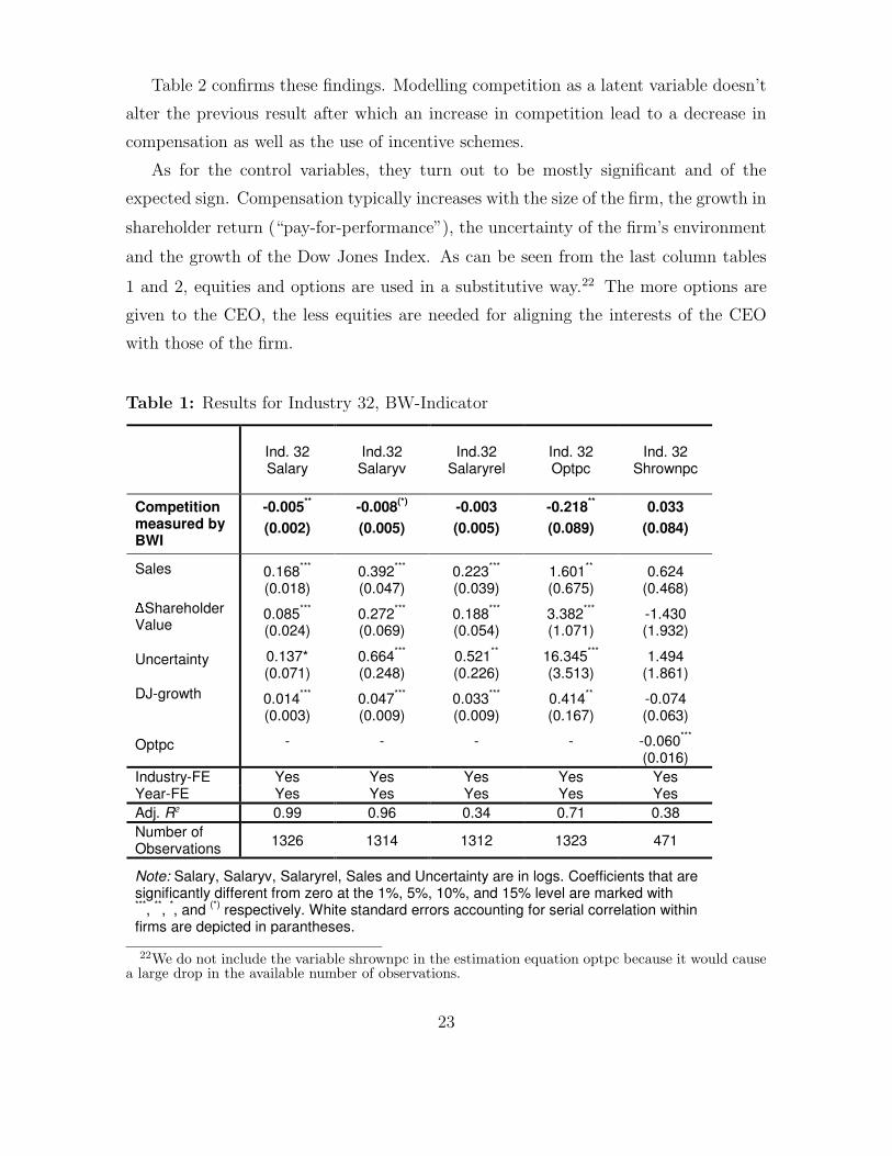
Table 2 confirms these findings. Modelling competition as a latent variable doesn’t

alter the previous result after which an increase in competition lead to a decrease in

compensation as well as the use of incentive schemes.

As for the control variables, they turn out to be mostly significant and of the

expected sign. Compensation typically increases with the size of the firm, the growth in

shareholder return (“pay-for-performance”), the uncertainty of the firm’s environment

and the growth of the Dow Jones Index. As can be seen from the last column tables

1 and 2, equities and options are used in a substitutive way.22 The more options are

given to the CEO, the less equities are needed for aligning the interests of the CEO

with those of the firm.

Table 1: Results for Industry 32, BW-Indicator

� �Ind.�32�Salary�

�

�Ind.32�Salaryv�

�Ind.32�

Salaryrel��

�Ind.�32�Optpc�

�Ind.�32�

Shrownpc�

Competition�measured�by�BWI�

-0.005**�

(0.002)�-0.008(*)�

(0.005)�-0.003�(0.005)�

-0.218**�(0.089)�

0.033�(0.084)�

Sales��

�Shareholder�

Value�

Uncertainty�

DJ-growth�

�

Optpc�

0.168***�(0.018)�

0.085***�(0.024)�

0.137*�(0.071)�

0.014***�(0.003)�

-�

0.392***�(0.047)�

0.272***�(0.069)�

0.664***�(0.248)�

0.047***�(0.009)�

-�

0.223***�(0.039)�

0.188***�(0.054)�

0.521**�(0.226)�

0.033***�(0.009)�

-�

1.601**�(0.675)�

3.382***�(1.071)�

16.345***�(3.513)�

0.414**�(0.167)�

-�

0.624�(0.468)�

-1.430�(1.932)�

1.494�(1.861)�

-0.074�(0.063)�

-0.060***�(0.016)�

Industry-FE� Yes� Yes� Yes� Yes� Yes�Year-FE� Yes� Yes� Yes� Yes� Yes�Adj.�R2 0.99� 0.96� 0.34� 0.71� 0.38�Number�of�Observations� 1326� 1314� 1312� 1323� 471�

Note:�Salary,�Salaryv,�Salaryrel,�Sales�and�Uncertainty�are�in�logs.�Coefficients�that�are�significantly�different�from�zero�at�the�1%,�5%,�10%,�and�15%�level�are�marked�with��***,�**,�*,�and�(*)�respectively.�White�standard�errors�accounting�for�serial�correlation�within�firms�are�depicted�in�parantheses.��

22We do not include the variable shrownpc in the estimation equation optpc because it would causea large drop in the available number of observations.

23

Table 2: Results for Industry 32, LV-Indicator


�


�Ind.32�

Salaryrel��


�Ind.�32�

Shrownpc�

Competition�as�a�latent�variable�

-0.050**�(0.020)�

-0.100*�(0.056)�

-0.051�(0.050)�

-2.313**�(0.962)�

0.021�(0.763)�

Sales��

�Shareholder�

Value�

Uncertainty�

DJ-growth�

0.169***�(0.018)�

0.086***�(0.024)�

0.140*�(0.071)�

0.013***�(0.003)�

0.393***�(0.047)�

0.274***�(0.069)�

0.672***�(0.249)�

0.046***�(0.010)�

0.224***�(0.039)�

0.189***�(0.054)�

0.527**�(0.227)�

0.033***�(0.009)�

1.619**�(0.675)�

3.405***�(1.074)�

16.490***�(3.518)�

0.398**�(0.168)�

0.633�(0.470)�

-1.461�(1.934)�

1.536�(1.866)�

-0.078�(0.064)�

Optpc� -��

-� -� -� -0.060***�(0.016)�

Industry-FE� Yes� Yes� Yes� Yes� Yes�Year-FE� Yes� Yes� Yes� Yes� Yes�Adj.�R2� 0.99� 0.96� 0.34� 0.71� 0.38�Number�of�Observations� 1326� 1314� 1312� 1323� 471�

Note:�Salary,�Salaryv,�Salaryrel,�Sales�and�Uncertainty�are�in�logs.�Coefficients�that�are�significantly�different�from�zero�at�the�1%,�5%,�10%,�and�15%�level�are�marked�with��***,�**,�*,�and�(*)�respectively.�White�standard�errors�accounting�for�serial�correlation�within�firms�are�depicted�in�parantheses.�

Tables 3 and 4 depict the relationship between competition and compensation for

industry 33. In contrast to industry 32, where more competition led to lower com-

pensation/incentive schemes, the opposite turns out to be true for industry 33. An

increase in competition led to an increase in variable compensation (salaryv), although

only significantly in the latent variable approach.

At any rate, it is striking that the sign of the competition measure is exactly the

opposite in industries 32 and 33 for four out of five compensation indicators. As such,

the theoretical models which predict ambiguous effects of competition on compensation

seem to be supported by the data.

24

Table 3: Results for Industry 33, BW-Indicator


�


�Ind.33�

Salaryrel��


�Ind.�33�

Shrownpc�

Competition�measured�by�BWI�

0.002�(0.003)�

0.008�(0.006)�

0.005�(0.007)�

0.146�(0.156)�

0.097�(0.073)�

Sales��

�Shareholder�

Value�

Uncertainty�

DJ-growth�

�

Optpc�

0.197***�(0.031)�

-0.080(*)�

(0.052)�

-0.117(*)�

(0.074)�

0.010***�(0.003)�

-�

0.505***�(0.036)�

0.117�(0.117)�

0.329**�(0.151)�

0.050***�(0.008)�

-�

0.290***�(0.038)�

0.223*�(0.119)�

0.421***�(0.146)�

0.040***�(0.008)�

-�

2.619***�(0.644)�

2.572�(2.368)�

18.133***�(2.859)�

0.714***�(0.158)�

-�

-0.871*�(0.477)�

4.739***�(0.638)�

1.796�(1.759)�

0.032�(0.070)�

-0.101***�(0.018)�



25

Table 4: Results for Industry 33, LV-Indicator


�


�Ind.33�

Salaryrel��


�Ind.�33�

Shrownpc�

Competition�as�a�latent�variable�

0.006�(0.035)�

0.088**�(0.040)�

0.069(*)�

(0.047)�1.093�

(0.895)�0.510�

(0.473)�

Sales��

�Shareholder�

Value��

Uncertainty�

�

DJ-growth�

0.197***�(0.031)�

-0.080(*)�(0.052)�

-0.118(*)�

(0.073)�

0.010***�(0.003)�

0.504***�(0.036)�

0.116�(0.117)�

0.323**�(0.151)�

0.054***�(0.008)�

0.290***�(0.038)�

0.222*�(0.118)�

0.416***�(0.146)�

0.043***�(0.008)�

2.613***�(0.644)�

2.564�(2.358)�

18.043***�(2.859)�

0.770***�(0.158)�

-0.872*�(0.479)�

4.726***�(0.647)�

1.734�(1.756)�

0.064�(0.074)�

Optpc� -��

-� -� -� -0.101***�(0.018)�



5.2 Robustness Tests for Model 1

Before drawing any definite conclusions, we would like to see how robust our results

are with respect to the chosen econometric specification as well as the timing between

changes in competition and executive compensation.

As for the first, we re-estimate model 1 using firm-fixed-effects instead of industry-

fixed effects. Although inclusion of firm-fixed effects makes sense from a conceptual

point of view, the estimation of 242 (industry 32) or 613 (industry 33) additional

parameters poses an econometric problem in terms of lost degrees of freedom as well

as small remaining variation in the competition indicator.23 Nevertheless, it seems

23In fact, inclusion of firm- and time-fixed effects captures a large part of the variance of the

26

important to check at least whether the signs remain the same as soon as firm-fixed

effects are included instead of industry-fixed effects.

Secondly, it might be the case that firm-owners do not immediately adapt executive

compensation to changes in competition, but rather with a lag. Therefore, we re-

estimate model 1 including the 1-year-lagged competition indicators instead of the

contemporaneous competition indicators.

As can be seen from tables 5 and 6, the results are fairly robust with respect to

these changes. Alternative specifications mostly affect the significance, but not the

sign of the estimated coefficients.

Table 5: Robustness Tests, Industry 32

� �Salary�

�

�Salaryv�

�Salaryrel�

�

�Optpc�

�Shrownpc�

Competition�measured�by�BWI�Ind.�32�Firm-FE:�yes�

-0.001�(0.001)�

-0.006�(0.005)�

-0.005�(0.005)�

-0.13*�(0.07)�

0.08�(0.07)�

Competition�measured�by�BWI�Ind.�32�Competition:�1�Lag�

-0.003*�(0.002)�

-0.008(*)�(0.005)�

-0.005�(0.005)�

-0.22*�(0.11)�

-0.04�(0.05)�

Competition�measured�by�LV�Ind.�32�Firm-FE:�yes�

-0.006�(0.017)�

-0.078�(0.054)�

-0.071�(0.05)�

-1.22(*)�(0.77)�

0.78�(0.65)�

Competition�measured�by�LV�Ind.�32�Competition:�1�Lag�

-0.044**�(0.02)�

-0.08(*)�(0.06)�

-0.04�(0.05)�

-2.17**�(1.02)�

-0.02�(0.56)�

Coefficients�that�are�significantly�different�from�zero�at�the�1%,�5%,�10%,�and�15%�level��are�marked�with�***,�**,�*,�and�(*)�respectively.�White�standard�errors�accounting�for�serial��correlation�within�firms�are�depicted�in�parantheses.�

competition indicator. A simple regression of the BW-Indicator on firm- and time-fixed effects showsthat 75 percent (industry 32) / 88 percent (industry 33) of the variance of the BW-Indicator can beexplained by these fixed effects.

27

Table 6: Robustness Tests, Industry 33

� �Salary�

�

�Salaryv�

�Salaryrel�

�

�Optpc�

�Shrownpc�

Competition�measured�by�BWI�Ind.�33�Firm-FE:�yes�

-0.001�(0.002)�

0.005�(0.006)�

0.005�(0.007)�

0.18�(0.15)�

0.01�(0.03)�

Competition�measured�by�BWI�Ind.�33�Competition:�1�Lag�

-0.0006�(0.004)�

-0.003�(0.006)�

-0.003�(0.007)�

-0.16�(0.14)�

-0.03�(0.05)�

Competition�measured�by�LV�Ind.�33�Firm-FE:�yes�

0.02�(0.02)�

0.07*�(0.04)�

0.07(*)�(0.04)�

1.22�(0.97)�

-0.08�(0.22)�

Competition�measured�by�LV�Ind.�33�Competition:�1�Lag�

-0.006�(0.02)�

0.07(*)�(0.04)�

0.07(*)�

(0.05)�0.5�

(0.9)�0.2�

(0.4)�

Coefficients�that�are�significantly�different�from�zero�at�the�1%,�5%,�10%,�and�15%�level��are�marked�with�***,�**,�*,�and�(*)�respectively.�White�standard�errors�accounting�for�serial��correlation�within�firms�are�depicted�in�parantheses.�

Not reported for the sake of brevity is a last robustness check, which we conducted

for industry 32. Since the sub-industry 326 showed a very high number of the BW-

Indicator in the year 1993, we dropped this year as a further sensitivity check. As it

turns out, the estimated coefficients do not change much if this particular data point

is dropped.

As such, our estimation results confirm the theoretical prediction, after which the

relationship between competition and incentives is ambiguous and depends on varying

countervailing effects. At least for the industries 32 and 33 of the manufacturing sector,

this relationship seems to be very different indeed.

5.3 Results for Model 2

Up so far, we focused on the relationship between competition and executive compen-

sation. Since the only testable hypothesis refers to the joint impact of competition and

outside options managers on executive compensation, we now turn to the estimation

28

of model 2.

Precisely, Schmidt’s (1997) model predicts that with increasing outside options

of the mangers, an increase in competition is more likely to lead to an increase in

incentives/compensation.

Table 7: Results for Industry 32, BW-Indicator*DJg


�


�Ind.32�

Salaryrel��


�Ind.�32�

Shrownpc�

Comp(BWI)*DJg� 0.0001�

(0.0001)�0.001**�

(0.003)�0.001(*)�

(0.0003)�0.003�

(0.008)�0.006(*)�

(0.004)�

Sales��

�Shareholder�

Value�

Uncertainty�

DJ-growth�

�

Optpc�

0.167***�(0.018)�

0.085***�(0.024)�

0.129*�(0.071)�

0.014***�(0.003)�

-�

0.389***�(0.047)�

0.271***�(0.069)�

0.649***�(0.247)�

0.044***�(0.009)�

-�

0.222***�(0.039)�

0.187***�(0.054)�

0.515**�(0.225)�

0.031***�(0.009)�

-�

1.553**�(0.674)�

3.349***�(1.070)�

16.003***�(3.497)�

0.424**�(0.170)�

-�

0.613�(0.467)�

-1.249�(1.998)�

1.482�(1.838)�

-0.103�(0.064)�

-0.061***�(0.016)�



�

Tables 7 and 8 depict the results for industry 32, using the BW-Indicator as a

competition measure. As can be seen therefrom, an increase in competition results in

higher compensation and stronger incentive payments, the better are the manager’s

outside options. The most significant results occur for the variable part of the salary.

The better the CEO’s bargaining power (in terms of general favorable economic en-

vironment (DJg) or successful past performance (BP)), the more a CEO wants to be

29

rewarded with a higher variable salary for the increase in competition.24

Table 8: Results for Industry 32, BW-Indicator*BP


�


�Ind.32�

Salaryrel��


�Ind.�32�

Shrownpc�

Comp(BWI)*BP� 0.001�

(0.002)�0.010*�

(0.006)�0.009*�

(0.005)�-0.102�(0.092)�

0.080�(0.251)�

Sales��

�Shareholder�

Value�

Uncertainty�

DJ-growth�

�

Optpc�

0.170***�(0.019)�

0.082***�(0.024)�

0.138*�(0.071)�

0.015***�(0.003)�

-�

0.398***�(0.047)�

0.262***�(0.068)�

0.683***�(0.236)�

0.051***�(0.010)�

-�

0.228***�(0.039)�

0.181***�(0.054)�

0.539**�(0.216)�

0.037***�(0.009)�

-�

1.614**�(0.686)�

3.355***�(1.067)�

16.341***�(3.387)�

0.491**�(0.170)�

-�

-0.153�(1.374)�

-11.094***�

(3.772)�

17.793***�

(1.861)�

0.362�(0.307)�

-0.894***�(0.256)�



�

Tables 9 and 10 replicate the estimations with the latent variable indicator instead

of the BW-Indicator. While there is again a positive impact on the variable salary, as

long as the growth rate of the Dow Jones Index is taken as a measure for the outside

options, the joint impact of competition and outside options becomes insignificant, if

the CEO’s bargaining power is measured by past performance.

Overall, however, the picture remains that in industry 32, an increase in the bar-

gaining power of the CEO’s positively affects the relationship between competition and

executive compensation.

24Note that the correlation between Comp(BWI)·DJg and DJg is quite low (below 30 percent) andtherefore unlikely causing the positive signs.

30

Table 9: Results for Industry 32, LV-Indicator*DJg


�


�Ind.32�

Salaryrel��


�Ind.�32�

Shrownpc�

Comp(LV)*DJg� 0.001�

(0.009)�0.004*�

(0.002)�0.03�

(0.002)�0.006�

(0.057)�0.036�

(0.028)�

Sales��

�Shareholder�

Value�

Uncertainty�

DJ-growth�

�

Optpc�

0.167***�(0.018)�

0.085***�(0.024)�

0.139*�(0.071)�

0.014***�(0.003)�

-�

0.389***�(0.047)�

0.271***�(0.069)�

0.648***�(0.247)�

0.048***�(0.009)�

-�

0.222***�(0.039)�

0.188***�(0.054)�

0.514**�(0.225)�

0.034***�(0.009)�

-�

1.554**�(0.674)�

3.351***�(1.070)�

16.007***�(3.500)�

0.439***�(0.168)�

-�

0.619�

(0.465)�

-1.242�(2.011)�

1.504�(1.834)�

-0.066�(0.065)�

-0.060***�(0.016)�



31

Table 10: Results for Industry 32, LV-Indicator*BP


�


�Ind.32�

Salaryrel��


�Ind.�32�

Shrownpc�

Comp(LV)*BP� -0.001�(0.017)�

-0.028�(0.045)�

-0.025�(0.041)�

-2.274***�(0.770)�

0.218�(0.450)�

Sales��

�Shareholder�

Value�

Uncertainty�

DJ-growth�

0.170***�(0.019)�

0.083***�(0.024)�

0.140*�(0.071)�

0.015***�(0.003)�

0.402***�(0.047)�

0.263***�(0.068)�

0.708***�(0.238)�

0.051***�(0.010)�

0.232***�(0.039)�

0.182***�(0.054)�

0.561**�(0.219)�

0.036***�(0.009)�

1.654**�(0.685)�

3.255***�(1.072)�

16.566***�(3.394)�

0.479***�(0.169)�

0.652�(0.478)�

-1.459�(1.885)�

1.660�(1.901)�

-0.107�(0.075)�

Optpc� -��

-� -� -� -0.057***�(0.016)�



A similar picture arises for industry 33 (see tables 11 to 14). An increase in compe-

tition leads to a higher increase (or smaller decrease) in the variable part of the salary,

if the manager’s outside options are high. Note further that the joint impact of com-

petition and outside options on the variable salary is significant or highly significant in

most of the specifications.

32

Table 11: Results for Industry 33, BW-Indicator*DJg


�


�Ind.33�

Salaryrel��


�Ind.�33�

Shrownpc�

Comp(BWI)*DJg�� 0.0001�

(0.0001)�0.0002�

(0.0003)�0.0001�

(0.0003)�-0.006�(0.005)�

0.004�(0.003)�

Sales��

�Shareholder�

Value�

Uncertainty�

DJ-growth�

�

Optpc�

0.2***�(0.03)�

-0.08(*)�(0.051)�

-0.117(*)�(0.074)�

0.009**�(0.003)�

-�

0.5***�(0.036)�

0.119�(0.117)�

0.328**�(0.15)�

0.049***�(0.008)�

-�

0.29***�(0.038)�

0.224**�(0.118)�

0.42***�(0.15)�

0.039***�(0.008)�

-�

2.61***�(0.64)�

2.62�(2.38)�

18.06***�(2.86)�

0.78***�(0.16)�

-�

-0.86*�(0.477)�

4.72***�(0.64)�

1.8�(1.76)�

0.13�(0.073)�

-0.1***�(0.018)�



33

Table 12: Results for Industry 33, BW-Indicator*BP


�


�Ind.33�

Salaryrel��


�Ind.�33�

Shrownpc�

Comp(BWI)*BP�� 0.002�

(0.003)�0.02***�

(0.004)�0.018***�(0.005)�

0.2**�(0.089)�

-0.045�(0.006)�

Sales��

Shareholder�

Value�

Uncertainty�

DJ-growth�

�

Optpc�

0.2***�(0.03)�

-0.078(*)�(0.05)�

-0.112(*)�(0.076)�

0.009***�(0.003)�

-�

0.5***�(0.036)�

0.111�(0.113)�

0.28*�(0.15)�

0.�0.05***�(0.008)�

-�

0.28***�(0.038)�

0.217*�(0.115)�

0.37**�(0.15)�

0.039***�(0.008)�

-�

2.68***�(0.66)�

2.4�(2.33)�

17.74***�(2.91)�

0.69***�(0.157)�

-�

-0.8*�(0.484)�

4.65***�(0.64)�

1.58�(1.78)�

0.029�(0.073)�

-0.1***�(0.018)�



34

Table 13: Results for Industry 33, LV-Indicator*DJg


�


�Ind.33�

Salaryrel��


�Ind.�33�

Shrownpc�

Comp(LV)*DJg�� 0.001�

(0.001)�0.002(*)�

(0.001)�0.0008�(0.002)�

-0.034�(0.03)�

0.016�(0.002)�

Log(Sales)��

Shareholder�

Value�

Uncertainty�

DJ-growth�

�

Optpc�

0.2***�(0.03)�

-0.08(*)�(0.051)�

-0.117(*)�(0.074)�

0.01***�(0.003)�

-�

0.5***�(0.036)�

0.119�(0.117)�

0.327**�(0.15)�

0.052***�(0.008)�

-�

0.29***�(0.038)�

0.224*�(0.118)�

0.42***�(0.15)�

0.041***�(0.008)�

-�

2.61***�(0.64)�

2.62�(2.38)�

18.09***�(2.85)�

0.71***�(0.15)�

-�

-0.86*�(0.477)�

4.72***�(0.64)�

1.8�(1.76)�

0.06�(0.073)�

-0.1***�(0.018)�



35

Table 14: Results for Industry 33, LV-Indicator*BP


�


�Ind.33�

Salaryrel��


�Ind.�33�

Shrownpc�

Comp(LV)*BP�� 0.008�

(0.015)�0.073**�

(0.037)�0.057(*)�(0.038)�

0.69�(0.72)�

0.14�(0.348)�

Log(Sales)��

�Shareholder�

Value�

Uncertainty�

DJ-growth�

�

Optpc�

0.19***�(0.032)�

-0.077(*)�(0.05)�

-0.111(*)�(0.076)�

0.009***�(0.003)�

-�

0.5***�(0.037)�

0.118�(0.116)�

0.29*�(0.15)�

0.05***�(0.008)�

-�

0.28***�(0.038)�

0.22*�(0.117)�

0.38**�(0.15)�

0.041***�(0.008)�

-�

2.7***�(0.66)�

2.4�(2.35)�

17.81***�(2.92)�

0.71***�(0.157)�

-�

-0.82*�(0.49)�

4.68***�(0.65)�

1.49�(1.79)�

0.031�(0.073)�

-0.1***�(0.018)�



As for the robustness of model 2 with respect to using the lagged (joint) competition-

indicator, the results look similar.25 Only in industry 32, we observe a stronger positive

impact on the fixed salary rather than the variable salary and a stronger positive impact

on the equity shares. Maybe, the variable part of the salary is easier changeable in the

short run, whereas re-negotiation of the fixed salary requires more time.

Including firm-fixed-effects instead of industry-fixed-effects sometimes strengthens

the joint impact of competition and bargaining power on the fixed salary and the equity

share, but lowers the effect on the variable salary. Again, with the exception of the

option-share in table 10,26 significant coefficients are always positive and mostly affect

the fix and variable part of the salary as well as the equity shares.

25The robustness tests are omitted for the sake of brevity, but are available on request.26The negative coefficient remains significant even with firm-fixed effects.

36

Therefore, for industry 32 as well as industry 33, we find results which are consistent

with Schmidt’s (1997) model. In fact, the bargaining power of the manager seems to be

a crucial determinant of how an increase in competition affects executive compensation.

Concerning the different components of executive compensation, it turns out that CEOs

with a strong bargaining power particularly aim at increasing the variable salary, as

soon as competition becomes more intense.

6 Conclusions

The discussion about whether competition fosters the use of incentive schemes for

executives or not has been mainly theoretical so far. If there is anything like a consensus

in the literature, then it is the cognition that the relationship between competition and

executive compensation is ambiguous and depends on varying, countervailing effects.

The goal of this paper was to add empirical evidence to the theoretical debate. Al-

though the desirability of empirical research was already mentioned in Schmidt (1997),

the relationship between changing competition and executive compensation has not

yet been explored with real data.

Focusing on firms in US manufacturing industries (NAICS 32-33) over the years

1992 to 2000, we discovered interesting effects of competition on executive compen-

sation. For instance, in industry 32, an increase in competition led to a lower level

of executive compensation (fix as well as variable) and to the use of weaker incen-

tive schemes (lower share of variable compensation, less option and equity shares). In

contrast, exactly the opposite was observed in industry 33.

The finding that competition affects executive compensation differently in differ-

ent industries may be explained with the theoretical claim that countervailing effects

persist. Also consistent with the literature (particularly Schmidt (1997)) is the result

that outside options of the manager matter for the relationship better competition and

executive compensation. During times where the economy was booming and managers

had good outside options, an increase in competition affected the level of compensa-

tion and the use of incentive schemes more positively than in a recession, where the

managers had no bargaining power.

Even though the results are quite robust with respect to different specifications and

37

different measures of competition, it is too early to draw definite conclusions. Since this

is the first empirical study, more research in this area is clearly warranted. Especially

applying the same type of analysis to other industries than the manufacturing industry

seems to be a promising approach.

7 References

Aggarwal, R.K. and Samwick, A.A. (1999). ’Executive Compensation, Strategic Com-

petition, and Relative Performance Evaluation: Theory and Evidence’, Journal of

Finance, vol. 54, pp. 1999-2043.

Baker G.P. and Hall, B.J. (1998). ’CEO Incentives and Firm Size’, NBER Working

Paper No. 6868.

Boone, J. and Weigand, J. (2000). ’Measuring competition: How are cost differ-

entials mapped into profit differentials?’, Working Paper CPB Netherlands Bureau for

Economic Policy, The Hague.

Demsetz, H. and Lehn, K. (1985). ’The structure of corporate ownership: causes

and consequences’, Journal of Political Economy, vol. 93, pp. 59-78.

Hall, R. (1988). ’The Relation between Price and Marginal Costs in US Industry’,

Journal of Political Economy, vol. 96, pp. 921-947.

Hart O. (1983). ’The Market Mechanism as an Incentive Scheme’, Bell Journal of

Economics, vol. 14, pp. 366-382.

Hermalin, B.E. (1992). ’The effects of competition on executive behavior’, Rand

Journal of Economics, vol. 23, pp. 350-365.

Jensen, M. and Meckling, W. (1976). ’Theory of the firm: Managerial behavior,

agency costs, and ownership structure’, Journal of Financial Economics, vol. 4, pp.

305-360.

Jensen M.C. and Murphy, K.J. (1990). ’Performance Pay and Top- Management

Incentives’, Journal of Political Economy, vol. 98, pp. 225-264.

Kedia, S. (1998). ’Product Market Competition and Top Management Compensa-

tion’, WP Harvard Business School.

Leibenstein, H. (1966). ’Allocative Efficiency vs. X-Efficiency’, American Economic

Review, vol. 56, pp. 392-415.

38

Machlup, F. (1967). ’Theories of the Firm: Marginalist, Behavioral Managerial’,

American Economic Review, vol. 57, pp. 1-33.

Scharfstein, D.S. (1988). ’Product-Market Competition and Managerial Slack’,

Rand Journal of Economics, vol. 19, pp. 147-155.

Schmidt K.M. (1997). ’Managerial Incentives and Product Market Competition’,

Review of Economic Studies, vol. 64, pp. 191-213.

8 Appendix

8.1 The empirical implementation of the Boone-Weigand in-

dicator

The Boone-Weigand indicator outlined in section 3 requires data on economic profits

and marginal costs, which are both not directly observable. Economic profits can

be approximated by accounting profits. The main difference between economic and

accounting profit is that the former are based on market values and take into account

the opportunity costs of all factors of production in a forward looking way, while

accounting profits are based on historical book values.

Marginal costs can be approximated by the average variable costs under the as-

sumption of constant returns to scale.27 This approximation may cause problems, for

instance, when the quality of a product is important and cannot be observed. As a

consequence, the relevant market should be defined at the lowest possible disaggrega-

tion level, i.e., the goods should be not too heterogenous. Another problem is when the

firms within an industry do not meet the same condition. This is the case, for instance,

when there is an import tax on products of a foreign firm, whereas the domestic firm’s

products are not taxed. If this tax cannot be observed, the domestic firms appears

relatively more efficient. To the extent that these measurement problems with respect

to marginal costs and uneven conditions stay constant over time within an industry,

changes in the relative profits indicator over time can be interpreted as changes in

competition in this industry.

27An alternative is to specify a total cost function and take the first derivative. See, e.g., Hall(1988).

39

Finally, note that the computation of this competition measure does not require

the observation of all the firms in the industry since we can replace the values of the

most efficient firms by the industry median of profits and marginal costs.

Once we accept these approximation measures, we need firm-specific data on turnover,

expenses for direct labor (payroll) and materials to compute the regression variables

as follows:28

profitit = turnoverit − payrollit − expenses for materialsit (31)

av var costit =(payrollit + expenses for materialsit)

salesit

(32)

We then compute the relative profits rel profitit and the relative costs, which we

denote by relative efficiency rel effit, by normalizing the firm specific profits and

average variable costs by the median of the industry j at the 3-digit level to which the

firm belongs, i.e.,

rel profitit =profitit

median profitjt(33)

rel effit =av var costit

median av var costjt(34)

For each 3-digit industry in our sample we estimate the following equation:

log rel profitit = ai + λt +T

∑

t′=t+1

bt′Dt

′T log rel effit

′ + c log salesit + uit (35)

λt is a time-specific intercept, with

λt = 1 for year t = 1992, ..., 2000 (36)

λt = 0 for year t′

= 1992, ..., 2000, t 6= t′

28In order to measure marginal costs more precisely, other costs such as expenses for debt service,taxes, depreciation, advertising, and administration may be included.

40

To obtain year-specific coefficients of the competition measure b, we interact the relative

efficiency variable with a time dummy Dt′T , which is defined like the time specific

intercept, i.e.,

Dt′T = 1 for year t = 1992, ..., 2000 (37)

Dt′T = 0 for year t

′

= 1992, ..., 2000, t 6= t′

We include sales as a control variable. The log specification controls for the skewness

of the distribution. Finally, uit is the remainder disturbance, with uit ∼ IID(0, σ2u)

independent of each other and among themselves.

We estimate (35) for each of the NAICS industries at the 3-digit level from the

NAICS industries 32 and 33 for which there are at least 30 observations.

The NAICS industry 32 has the following seven sub-industries (see Appendix 8.2):

321, 322, 323, 324, 325, 326, 327. For the five sub-industries 322, 324, 325, 326 and 327

we have enough data, i.e., more than 30 observations, for estimating the BW-Indicator.

For the NAICS industry 33, there are eight sub-industries at the three-digit level: 331,

332, 333, 334, 335, 336, 337, 339. Enough observations are available for estimating the

BW-Index for five sub-industries, namely the industries 333, 334, 335, 336 and 339.

41

8.2 NAICS industries

NAICS 2-digit NAICS 3-digit industry description32 321 Wood Product Manufacturing

322 Paper Manufacturing323 Printing and Related Support Activities324 Petroleum and Coal Products Manufacturing325 Chemical Manufacturing326 Plastics and Rubber Products Manufacturing327 Nonmetallic Mineral Product Manufacturing

33 331 Primary Metal Manufacturing332 Fabricated Metal Product Manufacturing333 Machinery Manufacturing334 Computer and Electronic Product Manufacturing335 Electrical Equipment, Appliance

and Component Manufacturing336 Transportation Equipment Manufacturing337 Furniture and Related Product Manufacturing339 Miscellaneous Manufacturing

42

Product-market competition and executive compensation

Documents

Transcript of Product-market competition and executive compensation