Product kernels adapted to curves in the space
31
arXiv:0905.3889v1 [math.FA] 24 May 2009 PRODUCT KERNELS ADAPTED TO CURVES IN THE SPACE VALENTINA CASARINO, PAOLO CIATTI, AND SILVIA SECCO Abstract. We establish L p -boundedness for a class of operators that are given by convolution with product kernels adapted to curves in the space. The L p bounds follow from the decomposition of the adapted kernel into a sum of two kernels with sigularities concentrated respectively on a coordinate plane and along the curve. The proof of the L p -estimates for the two corresponding operators involves Fourier analysis techniques and some algebraic tools, namely the Bernstein-Sato polynomials. 1. Introduction The purpose of this paper is to establish L p boundedness for a class of product-type convolution operators. In the last thirty years the theory of singular integrals on product domains has been largely developed. The first case which was considered is that of a convolution operator Tf = K ∗ f on R d 1 × R d 2 , with K (x,y )= K 1 (x)K 2 (y ), x ∈ R d 1 , y ∈ R d 2 , K 1 and K 2 being of Calder´on-Zygmund type. In this case a simple iteration argument yields the L p boundedness of T . A more involved situation is that of a convolution operator T , whose kernel K is defined on R d 1 × R d 2 and satisfies all the analogous bounds to those satisfied by K 1 K 2 on R d 1 ×R d 2 , but cannot be decomposed as product of two kernels K 1 (x) and K 2 (y ). A precise definition of such kernels, which are called ”product kernels”, was introduced in terms of certain differential inequalities and suitable cancellation conditions. Several conditions on K , guaranteeing the L p boundedness of the operator T , have been introduced [FS], and many applications of the product theory to the operators arising in certain boundary value problems have been studied [NRS], [NS06]. . Moreover, the euclidean spaces R d j , j =1, 2, have been replaced by appropriate nilpotent groups [MRS], [NRS], and by smooth manifolds with a geometry determined by a control distance [NS04]. Recently, one of the authors studied the L p boundedness for convolution operators with kernels obtained adapting product kernels to curves in the plane [Se]. Here we extend these results to higher dimensional spaces. In order not to burden the exposition with notational complexities, we are going to give the full details only for the space R 3 , with d 1 = 1 and d 2 = 2. In the last section we shall quickly describe how the arguments should be modified in the higher dimensional setting. We denote an element of R 3 = R × R 2 by the pair (x 1 ,x), where x =(x 2 ,x 3 ) ∈ R 2 . On R we consider the usual dilations by δ> 0, while on R 2 we consider the anisotropic Date : December 8, 2013. 1991 Mathematics Subject Classification. 42B20, 44A35. Key words and phrases. Product kernels, L p estimates, convolution, Bernstein-Sato polynomials. 1
-
Upload
independent -
Category
Documents
-
view
1 -
download
0
Transcript of Product kernels adapted to curves in the space

arX
iv:0
905.
3889
v1 [
mat
h.FA
] 2
4 M
ay 2
009
PRODUCT KERNELS ADAPTED TO CURVES IN THE SPACE
VALENTINA CASARINO, PAOLO CIATTI, AND SILVIA SECCO
Abstract. We establish Lp-boundedness for a class of operators that are given by
convolution with product kernels adapted to curves in the space. The Lp bounds followfrom the decomposition of the adapted kernel into a sum of two kernels with sigularitiesconcentrated respectively on a coordinate plane and along the curve.
The proof of the Lp-estimates for the two corresponding operators involves Fourieranalysis techniques and some algebraic tools, namely the Bernstein-Sato polynomials.
1. Introduction
The purpose of this paper is to establish Lp boundedness for a class of product-typeconvolution operators.
In the last thirty years the theory of singular integrals on product domains has beenlargely developed. The first case which was considered is that of a convolution operatorTf = K ∗ f on Rd1 × Rd2 , with K(x, y) = K1(x)K2(y), x ∈ Rd1 , y ∈ Rd2 , K1 and K2
being of Calderon-Zygmund type. In this case a simple iteration argument yields the Lp
boundedness of T . A more involved situation is that of a convolution operator T , whosekernel K is defined on Rd1×Rd2 and satisfies all the analogous bounds to those satisfied byK1K2 on Rd1×Rd2 , but cannot be decomposed as product of two kernels K1(x) and K2(y).A precise definition of such kernels, which are called ”product kernels”, was introducedin terms of certain differential inequalities and suitable cancellation conditions.
Several conditions on K, guaranteeing the Lp boundedness of the operator T , havebeen introduced [FS], and many applications of the product theory to the operatorsarising in certain boundary value problems have been studied [NRS], [NS06]. . Moreover,the euclidean spaces R
dj , j = 1, 2, have been replaced by appropriate nilpotent groups[MRS], [NRS], and by smooth manifolds with a geometry determined by a control distance[NS04].
Recently, one of the authors studied the Lp boundedness for convolution operators withkernels obtained adapting product kernels to curves in the plane [Se]. Here we extendthese results to higher dimensional spaces. In order not to burden the exposition withnotational complexities, we are going to give the full details only for the space R3, withd1 = 1 and d2 = 2. In the last section we shall quickly describe how the arguments shouldbe modified in the higher dimensional setting.
We denote an element of R3 = R × R2 by the pair (x1, x), where x = (x2, x3) ∈ R2.On R we consider the usual dilations by δ > 0, while on R2 we consider the anisotropic
Date: December 8, 2013.1991 Mathematics Subject Classification. 42B20, 44A35.Key words and phrases. Product kernels, Lp estimates, convolution, Bernstein-Sato polynomials.
1

2 VALENTINA CASARINO, PAOLO CIATTI, AND SILVIA SECCO
dilation given by
(1.1) δ ◦ x = (δ12nx2, δ
12mx3) , with δ > 0 , m, n ∈ N , m < n .
We denote by
(1.2) Q =1
2n+
1
2m
the homogeneous dimension of R2 with respect to the dilations (1.1) and by ρ(x) =x2n
2 + x2m3 a smooth homogeneous norm on R2.
In this context the proto-typical example of a product kernel in R3 (we refer to Section
3 for a precise definition) is given by the distribution
(1.3) H(x1, x) = Cµ p.v.1
x1
ρ(x)−Q+iµ , µ ∈ R \ {0} .
Throughout the paper we concentrate our attention on the convolution by product-typekernels in R3 whose singularities are supported on a coordinate plane and on a transversalcurve of finite type. A rather simple example of such a kernel is
K(x1, x) = Cµ p.v.
(1
x1
)ρ(x− γ(x1))−Q+iµ , µ ∈ R \ {0} ,
where γ : R → R2 is the curve γ(x1) = (xm
1 , xn1 ).
More generally, we introduce the following class of product-type kernels.
Definition 1.1. Assume that K0 is a product kernel on R3 and consider the curve x =γ(x1) with γ(x1) = (xm
1 , xn1 ), x1 ∈ R. We define a distribution K by
(1.4)
∫K(x1, x)f(x1, x) dx1dx :=
∫K0(x1, x)f(x1, x+ γ(x1)) dx1dx
for a Schwartz function f on R3. K will be called an adapted kernel.Here with an abuse of notation we write pairings between distributions and test functions
as integrals.
The kernel K given by the formula (1.4) is a well-defined tempered distribution whichis singular on the coordinate plane x1 = 0 and along the curve x = γ(x1), x1 ∈ R.
We shall prove the following theorem.
Theorem 1.2. Let K be the distribution defined by the formula (1.4). Then the convo-lution operator T : f 7→ f ∗K, initially defined on the Schwartz space S(R3), extends toa bounded operator on Lp(R3) for 1 < p <∞.
To prove Theorem 1.2 we decompose the adapted kernel K of T as the sum of a kernel K1
with singularities concentrated on the coordinate plane x1 = 0 and of a kernel K2 singularalong the curve x = γ(x1), x1 ∈ R. As in [Se] we show that the multiplier associatedwith K1 satisfies some Marcinkiewicz-type conditions, while K2 is treated by means ofanalytic interpolation (our proof is inspired by some arguments used in [SW] to provethe Lp boundedness of the Hilbert transform along curves in the plane). In particular, toapply the analytic interpolation method we need to introduce a non-isotropic version ofthe Riesz potentials
Iz(u1, u2) := (ρ(u1, u2))z−Q , z ∈ C .
PRODUCT KERNELS ADAPTED TO CURVES IN THE SPACE 3
and to determine their meromorphic continuation. To extend in a meromorphic wayIz, we study the location of its singularities using Bernstein-Sato polynomials. Since thereader is not assumed to be familiar with Bernstein-Sato functional identities, we illustratethe definition and the basic properties of this algebraic tool in Section 2.
In the last section we shall discuss how Lp bounds for convolution by product kernelsadapted to curves are related in a natural way to the study of Lp − Lq estimates foranalytic families of fractional operators [CCiSe].
Throughout the paper we will use the variable constant convention, and denote by C,possibly with sub- or superscripts, a constant that may vary from place to place.
2. Bernstein-Sato polynomials and a family of Riesz-type kernels
Consider the polynomial
(2.1) ρ(u1, u2) := u2n1 + u2m
2 ,
with m,n ∈ N , m ≥ 1 , n > m . Observe that ρ is homogeneous with respect to theone-parameter family of non isotropic dilations given by (1.1).
We shall often use, in the following, the relations between ρ and the euclidean norm | · |in R2
(2.2) Aρ(u)12n ≤ |u| ≤ Bρ(u)
12m if ρ(u) > 1
and
(2.3) A′ρ(u)1
2m ≤ |u| ≤ B′ρ(u)12n if ρ(u) ≤ 1
for some A,B,A′, B′ > 0.Define now the distribution
(2.4) Iz(u1, u2) := (ρ(u1, u2))z−Q ,
where z ∈ C, ℜez > 0.Observe that both ρ and Iz depend on m and n. Anyway, for the sake of semplicity,
we shall avoid to indicate the dependence on m and n.We collect in the next proposition some obvious properties of Iz.
Proposition 2.1. If ℜez > 0, theni) Iz is well defined as distribution and locally integrable.ii) Iz is a tempered distribution.iii) Iz is an analytic family of tempered distributions, that is, given f ∈ S(R2), thefunctions z 7→< Iz, f > are holomorphic.
We shall now prove that Iz admits a meromorphic extension, with poles in a at mostcountable set, consisting of rational negative points. Our method is based on the theoryof Bernstein-Sato polynomials.
It is well-known in algebra that, given a non-zero polynomial p(u1, u2) with complexcoefficients, there exist a non-zero polynomial bp(s) ∈ C[s] and a differential operator L(s)whose coefficients are polynomials in s , u1 , u2 , such that formally
(2.5) L(s) (p(u1, u2))s+1 = bp(s) (p(u1, u2))
s for all s ∈ C .

4 VALENTINA CASARINO, PAOLO CIATTI, AND SILVIA SECCO
The set of all polynomials bp(s) ∈ C[s] satisfying this formal identity (for some operatorL) is an ideal, and the unique monic generator of this ideal is called the Bernstein-Satopolynomial of p.
In our case, for ℜez > 0 we may write
(2.6) (ρ(u1, u2))z−Q =
L(z −Q) (ρ(u1, u2))z+1−Q
bρ(z −Q).
By repeatedly using the functional equation (2.6) we may extend Iz to the complex planein a meromorphic way, with poles whenever bρ(z − Q + k) vanishes for a non-negativeinteger k. Therefore we shall now seek for the zeros of the Bernstein-Sato polynomialbρ(z −Q).
According to a theorem of Kashiwara, the roots of the Bernstein-Sato polynomial arenegative rational numbers. Moreover, if ρ has the particularly simple form given in (2.1),it is easy to find the roots of bρ(s).
Lemma 2.2. If bρ(s) denotes the Bernstein-Sato polynomial associated to ρ(u1, u2) :=
u2n1 + u2m
2 , m < n, m,n ∈ N, then the roots of bρ(s)s+1
are given by
(2.7) −p1
2n−
p2
2m, 1 ≤ p1 ≤ 2n− 1 , 1 ≤ p2 ≤ 2m− 1 ,
with multiplicity one.
Proof. It is essentially due to Kashiwara [K]. See also [M] and [BMSa, remark 3.8]. �
In the following corollary we collect some observations, which will be useful in thefollowing.
Corollary 2.3. i) The largest root of bρ(s) is −Q = − 12m
− 12n
.ii) −1 is a root of bρ(s) with multiplicity two.iii) The set of the roots of bρ(s) is symmetric with respect to −1.
Proof. i) It follows obviously from (2.7) for p1 = 1 and p2 = 1.ii) Observe that − p1
2n− p2
2m= −1 for p1 = n and p2 = m. Then −1 is a root of multiplicity
one for bρ(s)s+1
, whence the thesis follows.
iii) Suppose that the −1 + δ := − p1
2n− p2
2mis a root of bρ(s) for some p1 , p2 ∈ N, 1 ≤ p1 ≤
2n− 1 , 1 ≤ p2 ≤ 2m− 1 and some δ > 0. Take p1 := 2n− p1 and p2 := 2m− p2. Since1 ≤ p1 ≤ 2n− 1 , 1 ≤ p2 ≤ 2m− 1 , then
−p1
2n−
p2
2m= −2 +
p1
2n+
p2
2m= −1 − δ
is a root of bρ(s). �
Example 2.4. By means of formula (2.7) it is possible to find the roots of the Bernstein-Sato polynomial associated to u6
1 + u42 and one finds
bρ(s) =(s+ 1)2 (s+2
3) (s+
4
3) (s+
3
4) (s+
5
4) (s+
5
6) (s+
7
6) (s+
5
12) (s+
19
12)
(s+7
12) (s+
17
12) (s+
11
12) (s+
13
12) .

PRODUCT KERNELS ADAPTED TO CURVES IN THE SPACE 5
Let us now consider the distribution Iz defined by (2.4). Let s1 , . . . , sh be the zeros ofbρ(s) in (−Q−1,−Q], each counted with its multiplicity and ordered in a decreasing way.Then the meromorphic continuation of Iz has poles whenever z = Q+ sj − k, k ≥ 0. Weremark, in particular, that 0 and −1 +Q are always poles for Iz. By gluing all together,we get the following result.
Proposition 2.5. Iz may be analytically continued to a meromorphic distribution-valuedfunction of z, also denoted by Iz, with poles in a set A, consisting of rational negativepoints. More precisely,
A = {ζj,k := Q+ sj − k : k ∈ N , j = 1, . . . , h} ,
sj, j = 1, . . . , h, denoting the zeros of the Bernstein-Sato polynomial bρ in (−Q− 1,−Q],each listed as many times as its multiplicity. Each pole has order one, with the exceptionof the points −1 +Q− k, k ∈ N, which have order two.
Set ζj := ζj,0. Observe that ζ1 = 0 is a pole of order 1 for Iz .Consider now the function G, given by
(2.8) G(z) := Γ (z + 1 −Q) ·∏
j=2,..,h
Γ(z − ζj) .
If S denotes the sphere
S := {(u1, u2) ∈ R2 : ρ(u1, u2) = 1}
with surface measure σ(S), set
(2.9) Iz(u1, u2) :=G(0) (u2n
1 + u2m2 )
z−Q
σ(S) Γ(z)G(z).
In the sequel we will denote by S(Rs), s = 2, 3, the Schwartz space on Rs endowed witha denumerable family of norms ‖ · ‖(N) given by
‖Φ‖(N) =∑
|α|≤N
supu∈Rs
(1 + |u|)N |∂αu Φ(u)|.
Here we use the conventional notation
∂αu =
∂α1
∂uα11
· · ·∂αs
∂uαss
,
with α = (α1, . . . , αs) s-tuple of natural numbers and |α| = α1 + · · · + αs.
Proposition 2.6. The distribution Iz satisfies
I0 = δ0 .

6 VALENTINA CASARINO, PAOLO CIATTI, AND SILVIA SECCO
Proof. Take z ∈ C, ℜez > 0, and ϕ ∈ S(R2). Set Cz := G(0)σ(S)Γ(z)G(z)
. Then
< Iz, ϕ > = Cz
∫
R2
ρ(u1, u2)z−Qϕ(u1, u2) du1 du2
= Cz
(∫
{ρ(u1,u2)≤1}
ρ(u1, u2)z−Q (ϕ(u1, u2) − ϕ(0, 0)) du1 du2
+
∫
{ρ(u1,u2)≤1}
ρ(u1, u2)z−Qϕ(0, 0) du1 du2 +
∫
{ρ(u1,u2)≥1}
ρ(u1, u2)z−Qϕ(u1, u2) du1 du2
)
= Cz (I1 + I2 + I3) .
By introducing polar coordinates (see [FoS]) we obtain
I2 =
∫
S
∫ 1
0
ϕ(0, 0)ρ(r ◦ (v1, v2))z−QrQ−1dr dσ(v1 v2) =
∫
S
∫ 1
0
ϕ(0, 0) (r · ρ(v1, v2))z−Q rQ−1dr dσ(v1 v2)
=ϕ(0, 0)
∫
S
∫ 1
0
rz−1dr dσ(v1 v2) = ϕ(0, 0)σ(S)
z,
so that
(2.10) CzI2 = ϕ(0, 0)G(0)
zΓ(z)G(z)= ϕ(0, 0)
G(0)
Γ(z + 1)G(z)
and this expression is well-defined for every z, with ℜez > −min{−ζ2, 1}.Now, it it is easy to show that both I1 and I3 are absolutely convergent for ℜez >
−min{ 12n,−ζ2}. Indeed,
|I1| ≤
∫
{ρ(u1,u2)≤1}
ρ(u1, u2)ℜez−Q |ϕ(u1, u2) − ϕ(0, 0)| du1 du2
≤C||∇ϕ||∞
∫
{ρ(u1,u2)≤1}
ρ(u1, u2)ℜez−Q |(u1, u2)| du1 du2
≤C||∇ϕ||∞
∫
{ρ(u1,u2)≤1}
ρ(u1, u2)ℜez−Q+ 1
2n du1 du2
=C||∇ϕ||∞
∫
S
∫ 1
0
ρ (r ◦ (v1, v2))ℜez−Q+ 12n rQ−1 dr dσ(v1, v2)
=C||∇ϕ||∞
∫
S
∫ 1
0
rℜez−Q+ 12n rQ−1 dr dσ(v1, v2)
=C||∇ϕ||∞σ(S)
12n
+ ℜez,
which is well-defined for ℜez > − 12n
. Here, in particular, we used (2.3).
PRODUCT KERNELS ADAPTED TO CURVES IN THE SPACE 7
Moreover,
|I3| ≤
∫
{ρ(u1,u2)>1}
ρ(u1, u2)ℜez−Q |ϕ(u1, u2)| du1 du2
≤C||ϕ||(N)
∫
{ρ(u1,u2)>1}
ρ(u1, u2)ℜez−Q− N
2n du1 du2 ,
since
|ϕ(u1, u2)| ≤||ϕ||(N)
(1 + |(u1, u2)|)N
≤||ϕ||(N)
|(u1, u2)|N≤ C
||ϕ||(N)
(ρ(u1, u2))N2n
when ρ(u1, u2) > 1, as a consequence of (2.2). Now by passing to polar coordinates weobtain
|I3| ≤C||ϕ||(N)
∫
S
∫ +∞
1
ρ (r ◦ (v1, v2))ℜez−Q− N
2n rQ−1 dr dσ(v1 v2)
=C||ϕ||(N)σ(S)
N2n
−ℜez< +∞ ,
if N is a positive integer greater than 2n · ℜez. Thus, as a consequence of the uniquenessof the analytic continuation, the expression
< Iz, ϕ >= Cz (I1 + I2 + I3)
defines the action of Iz on a Schwartz function ϕ in R2, for ℜez > −min{ 12n,−ζ2, 1} and
by using the bounds for I1 and I3 and (2.10) one gets the thesis.�
Proposition 2.7. Iz is a homogeneous tempered distribution of degree −Q + z.
We recall that this means that for all ϕ ∈ S(R2) the following equality is satisfied
< Iz, ϕδ >= δz−Q < Iz, ϕ > ,
whereϕδ(u1, u2) := δ−Qϕ
(δ−1 ◦ u
)= δ−Qϕ
(δ−
12nu1, δ
− 12mu2
).
Thus the Fourier transform of the (tempered and homogeneous) distribution Iz is a well-defined distribution, homogeneous of degree −Q− (z−Q) = −z. Moreover, the followingholds.
Proposition 2.8. Iz agrees with a function C∞(R2\{(0, 0)}) away from (0, 0). Moreover,
(2.11) |Iz(ξ)| ≤ Cρ(ξ)−ℜez ,
for all ξ ∈ R2 \ {(0, 0)}.
Proof. It suffices to prove the statement for 0 < ℜez < Q; indeed, the other cases can betreated by analytic continuation.
We first construct a partition of unity adapted to the dyadic spherical shells. Theprocedure is standard and we briefly recall it only for the sake of completeness.
Let ψ be a C∞c (R2) function, such that

8 VALENTINA CASARINO, PAOLO CIATTI, AND SILVIA SECCO
(i) 0 ≤ ψ(u1, u2) ≤ 1 for every (u1, u2) ∈ R2;(ii) ψ(u1, u2) ≡ 0 if (u1, u2) 6∈ C0 := {(u1, u2) ∈ R2 : 1
4≤ ρ(u1, u2) ≤ 8} ;
(iii) ψ(u1, u2) ≡ 1 if (u1, u2) ∈ C1 := {(u1, u2) : 12≤ ρ(u1, u2) ≤ 4}.
Define now for (u1, u2) ∈ R2 \ {(0, 0)}
(2.12) Ψ(u1, u2) :=∑
j∈Z
ψ(2j ◦ (u1, u2)) .
Since there is at most a finite number of nonzero terms in the sum (2.12), Ψ is well-definedand strictly positive on R2 \ {(0, 0)}. Thus we may introduce the functions
(2.13) η(u1, u2) :=ψ(u1, u2)
Ψ(u1, u2).
It is easy to check that
(2.14)∑
j∈Z
η(2j ◦ (u1, u2)
)= 1 for every (u1, u2) ∈ R
2 \ {(0, 0)}
Now using (2.14) we may write
Iz(u1, u2) = Czρ(u1, u2)z−Q
= Cz
∑
j∈Z
η(2j ◦ (u1, u2))ρ(2−j ◦ 2j ◦ (u1, u2))z−Q
= Cz
∑
j∈Z
η(2j ◦ (u1, u2))2−j(z−Q)ρ(2j ◦ (u1, u2))
z−Q
= Cz
∑
j∈Z
2−j(z−Q)f0(2j ◦ (u1, u2)) ,
where we set
f0(u1, u2) := η(u1, u2)ρ(u1, u2)z−Q .
Since(f0(2j ◦ (·, ·))
)(ξ1, ξ2) = 2−jQf0
(2−j ◦ (ξ1, ξ2)
),
we obtain formally
∑
j∈Z
2−j(z−Q)(f0(2j ◦ (·, ·))
)(ξ1, ξ2) =
∑
j∈Z
2−jzf0(2−j ◦ (ξ1, ξ2)) .

PRODUCT KERNELS ADAPTED TO CURVES IN THE SPACE 9
This series is absolutely convergent, since if (ξ1, ξ2) 6= (0, 0) one has∣∣∣∣∣∑
j∈Z
2−jzf0(2−j ◦ (ξ1, ξ2))
∣∣∣∣∣ ≤∑
j∈Z
2−jℜez∣∣∣f0(2
−j ◦ (ξ1, ξ2))∣∣∣
≤
∑
2−jρ(ξ1,ξ2)≤1
+∑
2−jρ(ξ1,ξ2)>1
2−jℜez
∣∣∣f0(2−j ◦ (ξ1, ξ2))
∣∣∣
≤ ||f0||(0)∑
2−jρ(ξ1,ξ2)≤1
2−jℜez +∑
ρ(2−j◦(ξ1,ξ2))>1
2−jℜez ||f0||(N)
(1 + |(2−j ◦ (ξ1, ξ2))|)N
≤ C ||f0||(0)ρ(ξ)−ℜez + C∑
2−jρ(ξ1,ξ2)>1
2−jℜez ||f0||(N)
(ρ(2−j ◦ (ξ1, ξ2)))N2n
≤ C ||f0||(0)ρ(ξ)−ℜez +C
(ρ(ξ1, ξ2))N2n
∑
2−jρ(ξ1,ξ2)>1
2−jℜez+j N2n
≤ C ||f0||(0)ρ(ξ)−ℜez +C
(ρ(ξ1, ξ2))N2n
ρ(ξ1, ξ2)−ℜez+ N
2n
≤ C ρ(ξ1, ξ2)−ℜez ,
where we used in particular the fact that
|(u1, u2)| ≥ C ρ(u1, u2)12n for |(u1, u2)| > 1 .
We set therefore
v(ξ1, ξ2) :=∑
j∈Z
2−jzf0(2−j ◦ (ξ1, ξ2)) ∈ L∞(R2) .
By the Dominated Convergence Theorem we obtain, given ϕ ∈ S(R2),∫
R2
vϕ =∑
j∈Z
2−jz
∫
R2
f0(2−j ◦ (·, ·))ϕ ,
that isv(·, ·) =
∑
j∈Z
2−jzf0(2−j ◦ (·, ·))
in the sense of distributions, whence
Iz(·, ·) =∑
j∈Z
2−jzf0(2−j ◦ (·, ·))
in the sense of distributions and, moreover,
(2.15)∣∣∣Iz(ξ1, ξ2)
∣∣∣ ≤ ρ(ξ1, ξ2)−ℜez for all (ξ1ξ2) ∈ R
2 \ {(0, 0)}
(observe that this inequality could also be retrieved from the homogeneity). Finally we
prove that Iz agrees with a function C∞(R2 \ {(0, 0)}) away from (0, 0). First of all, we
10 VALENTINA CASARINO, PAOLO CIATTI, AND SILVIA SECCO
observe that f0 is in the Schwartz space, hence f0(2−j◦(·, ·)) belongs to C∞(R2). Moreover,
the following estimates hold:∣∣∣∂k
ξ1
(2−jzf0(2−j ◦ (ξ1, ξ2))
)∣∣∣ ≤ Ck 2−j(ℜez+ k2n) for all (ξ1, ξ2) ∈ R
2
∣∣∣∂kξ1
(2−jzf0(2−j ◦ (ξ1, ξ2))
)∣∣∣ ≤ Ck,N 2−j(ℜez+ k2n) 1
(1 + |(2−j ◦ (ξ1, ξ2))|)N
≤Ck,N
ρ(ξ1, ξ2)N2n
2j(−ℜez− k2n
+ N2n) if ρ
(2−j ◦ (ξ1, ξ2)
)> 1 ,
for all k ∈ N. Since analogous bounds hold for ∂kξ2
(2−jzf0(2−j ◦ (ξ1, ξ2)), with 2n replaced
by 2m, the series of the partial derivatives of 2−jzf0(2−j ◦ (·, ·)) of any order k converge
on the compact subsets of R2 \ {(0, 0)}. It follows that Iz(·, ·) =
∑j∈Z
2−jzf0(2−j ◦ (·, ·))
is C∞(R2 \ {(0, 0)}) �
3. Some preliminary results
In the following, if f(x1, x) ∈ S(R3) we denote by F−1f the inverse Fourier transformof f and by F2f and F−1
2 f respectively the partial Fourier transform and the inverse ofthe partial Fourier transform of f with respect to the variable x.
Moreover we denote the dual variables as (ξ1, ξ) with ξ = (ξ2, ξ3).
Characterization of product kernels. As recalled in the Introduction, the precise defini-tion of product kernels involves certain differential inequalities and certain cancellationconditions which are analogous to those satisfied by the kernel H(x1, x) defined by (1.3).Our study will be based on the following equivalent definition (see [NRS]).
Definition 3.1. A product kernel K on R3 is a sum
(3.1) K(x1, x) =∑
J∈Z2
2−j1−jQψJ(2−j1x1, 2−j ◦ x), J = (j1, j)
convergent in the sense of distributions, of smooth functions ψJ supported on the set where1/2 ≤ |x1| ≤ 4 and 1/2 ≤ ρ(x) ≤ 4, satisfying the cancellation conditions
(3.2)
∫ψJ(x1, x) dx1 = 0
(3.3)
∫ψJ(x1, x) dx = 0
identically for every J , and with uniformly bounded Ck norms for every k ∈ N.
We shall need a characterization of product kernels as dyadic sums of Schwartz functionson R3 which are compactly supported only in the first variable and that satisfy somemoment conditions.

PRODUCT KERNELS ADAPTED TO CURVES IN THE SPACE 11
Lemma 3.2. A product kernel K on R3 can be written as a sum
K(x1, x) =∑
J∈Z2
2−j1−jQϕJ(2−j1x1, 2−j ◦ x), J = (j1, j),
convergent in the sense of distributions, of Schwartz functions ϕJ such that
(i) the ϕJ have compact x1-support where 1/2 ≤ |x1| ≤ 4;(ii) the ϕJ form a bounded set of S(R3), that is the Schwartz norms ‖ϕJ‖(N) are
uniformly bounded in J for each N ∈ N;(iii) the ϕJ satisfy the cancellation conditions
(3.4)
∫xℓ
1ϕJ(x1, x) dx1 = 0
for every positive integer ℓ ≤M1, for some fixed M1 ∈ N, and
(3.5)
∫xβϕJ(x1, x) dx = 0
for every multi-index β = (β1, β2) ∈ N2, identically for every J ∈ Z2. Here, as
usual, xβ = xβ1
2 xβ2
3 .
Proof. Let K be a product kernel on R3. By Definition 3.1 we can write K as a sum
K(x1, x) =∑
(j1,i)∈Z2
2−j1−iQψ(j1,i)(2−j1x1, 2
−i ◦ x),
convergent in the sense of distributions, of smooth functions ψ(j1,i) supported on the setwhere 1/2 ≤ |x1| ≤ 4 and 1/2 ≤ ρ(x) ≤ 4, satisfying the cancellation conditions (3.2) and(3.3) identically for every (j1, i) ∈ Z2, and with uniformly bounded Ck norms for everyk ∈ N.
LetK(ξ1, ξ) =
∑
(j1,i)∈Z2
ψ(j1,i)(2j1ξ1, 2
i ◦ ξ)
be the corresponding product multiplier.Consider a smooth function ζ on the real line, supported on the interval [1, 4] and such
that∑
k∈Zζ(2kt) = 1 for every t > 0. For J = (j1, j) ∈ Z2, define
µJ(ξ1, ξ) :=∑
i∈Z
ψ(j1,i)(ξ1, 2i−j ◦ ξ)ζ(ρ(ξ)).
It can be easily proved that the µJ form a bounded set of S(R3). In addition, a directcomputation shows that
K(ξ1, ξ) =∑
J∈Z2
µJ(2j1ξ1, 2j ◦ ξ)
in the sense of distributions. Setting
ϕJ(x1, x) := (F−1µJ)(x1, x)
= F−12
(∑
i∈Z
(F2ψ(j1,j))(x1, 2i−j ◦ ·)ζ(ρ(·))
)(x),
12 VALENTINA CASARINO, PAOLO CIATTI, AND SILVIA SECCO
it is possible to write the product kernel K as the sum
(3.6) K(x1, x) =∑
J∈Z2
2−j1−jQϕJ(2−j1x1, 2−j ◦ x),
convergent in the sense of distributions, of functions ϕJ that form a bounded set of S(R3)and have compact x1-support where 1/2 ≤ |x1| ≤ 4. Finally, the fact that µJ(0, ξ) = 0
and (∂βξ µJ)(ξ1, 0) = 0 for every multi-index β = (β1, β2) ∈ N2, identically for every J ∈ Z2,
yields (3.4) for m = 0 and (3.5).In fact, we can choose ϕJ so that a finite number of moments in the variable x1 vanish.
This follows from a slight modification of the arguments in Lemma 2.2.3 in [NRS]. Moreexplicitly, denote by ϕ each function ϕJ in the decomposition (3.6). Then each functionϕ may be written as a series
(3.7) ϕ(x1, x) =∑
k∈Z
2−kAk(2−kx1, x) ,
convergent in the sense of distributions, of functions Ak which form a bounded set ofS(R3) with norms that decay exponentially in k as k → ±∞, have compact x1-supporton the set {x1 ∈ R : 1/2 ≤ |x1| ≤ 4}, and satisfy (3.4) with ℓ = 1.
To prove this fact, consider a function η ∈ C∞0 (R), supported on the set [−4,−1]∪ [1, 4],
such that∑
k∈Zη(2kt) = 1 for every t 6= 0 and
∫t η(t) dt 6= 0 . Set
χk(x1) := η(2−kx1) ,
χk(x1) :=χk(x1)∫
x1χk(x1) dx1
,
ak(x) =
∫x1 χk(x1)ϕ(x1, x) dx1 ,
Sk(x) =∑
j≥k
aj(x) .
Then write ϕ as
ϕ(x1, x) =∑
k∈Z
(ϕ(x1, x)χk(x1) − ak(x)χk(x1)
)+∑
k∈Z
(Sk(x) − Sk+1(x))χk(x1
)
=∑
k∈Z
(ϕ(x1, x)χk(x1) − ak(x)χk(x1)
)+∑
k∈Z
Sk(x)(χk(x1) − χk−1(x1)
)
=∑
k∈Z
Ak(x1, x) ,
where the series converges in the sense of distributions, the functions Ak satisy the mo-ment conditions
∫x1 Ak(x1, x) dx1 = 0 for all k ∈ Z, and the Schwartz norms decay
exponentially in k as k → ±∞. Now by rescaling x1 we obtain (3.7). Iterating thisargument yields (3.4) for all ℓ ≤M1, for some fixed M1 ∈ N.
�
A result analogous to Lemma 3.2 can be stated by interchanging the role of x1 and x.

PRODUCT KERNELS ADAPTED TO CURVES IN THE SPACE 13
Estimates on oscillatory integrals. In the following, we prove some estimates on certainoscillatory integrals related to our problem. Let ||| · ||| denote any homogeneous normwith respect to the family of non-isotropic dilations
(3.8) δ • (ξ1, ξ) = (δξ1, δmξ2, δ
nξ3), δ > 0 ,
e.g. we may choose
(3.9) |||(ξ1, ξ)||| = max{|ξ1|, |ξ2|1m , |ξ3|
1n} .
We observe in passing that
(3.10) δ • (ξ1, ξ) = (δξ1, δ2mn ◦ ξ) .
Consider the integral
(3.11) I (ξ1, ξ, η) :=
∫f(x1, η)e−i(ξ1,ξ)·(x1,γ(x1)) dx1 ,
where γ(x1) = (xm1 , x
n1 ) and f is such that
(h1) f belongs to S(R3) and is x1-compactly supported on the interval 1/2 ≤ |x1| ≤ 4;(h2) f(x1, 0) = 0 for all x1 such that 1/2 ≤ |x1| ≤ 4.
The constant CN occurring in the following inequalities depend on the Schwartz normsof f .
Lemma 3.3. Under the hypotheses (h1) and (h2) the following estimate holds for theintegral I(ξ1, ξ, η) defined by (3.11)
(3.12) | I(ξ1, ξ, η)| ≤ CNρ(η)
12n
(1 + ρ(η))N
for every integer N ≥ 0.
Proof. Since f is a Schwartz function, by using (h2), (2.2) and (2.3) we deduce that forevery (x1, η) ∈ {x1 ∈ R : 1/2 ≤ |x1| ≤ 4} × R2
(3.13) |∂kx1f(x1, η)| ≤ CN
ρ(η)12n
(1 + ρ(η))N
for all N ∈ N and k ∈ N. For k = 0 this inequality yields then (3.12). �
Lemma 3.4. Let I be the oscillatory integral defined by (3.11). Assume that (h1) and(h2) are satisfied.
Then
(3.14) |I (ξ1, ξ, η)| ≤ CNρ(η)
12n
(1 + ρ(η))N |||(ξ1, ξ)|||1n
if |||(ξ1, ξ)||| > 1
for every integer N ≥ 0.
Under the additional assumption
(3.15)
∫f(x1, x) dx1 = 0 , x ∈ R
2 ,
14 VALENTINA CASARINO, PAOLO CIATTI, AND SILVIA SECCO
the following estimate holds
(3.16) |I (ξ1, ξ, η)| ≤ CNρ(η)
12n
(1 + ρ(η))N|||(ξ1, ξ)||| if |||(ξ1, ξ)||| ≤ 1
for every integer N ≥ 0.
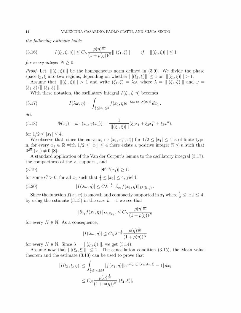
Proof. Let |||(ξ1, ξ)||| be the homogeneous norm defined in (3.9). We divide the phasespace ξ1, ξ into two regions, depending on whether |||(ξ1, ξ)||| ≤ 1 or |||(ξ1, ξ)||| > 1.
Assume that |||(ξ1, ξ)||| > 1 and write (ξ1, ξ) = λω, where λ = |||(ξ1, ξ)||| and ω =(ξ1, ξ)/|||(ξ1, ξ)|||.
With these notation, the oscillatory integral I (ξ1, ξ, η) becomes
(3.17) I (λω, η) =
∫
12≤|x1|≤4
f(x1, η)e−iλω·(x1,γ(x1)) dx1 .
Set
(3.18) Φ(x1) = ω · (x1, γ(x1)) =1
|||(ξ1, ξ)|||(ξ1x1 + ξ2x
m1 + ξ3x
n1 ),
for 1/2 ≤ |x1| ≤ 4.We observe that, since the curve x1 7→ (x1, x
m1 , x
n1 ) for 1/2 ≤ |x1| ≤ 4 is of finite type
n, for every x1 ∈ R with 1/2 ≤ |x1| ≤ 4 there exists a positive integer n ≤ n such thatΦ(n)(x1) 6= 0 [S].
A standard application of the Van der Corput’s lemma to the oscillatory integral (3.17),the compactness of the x1-support , and
(3.19) |Φ(n)(x1)| ≥ C
for some C > 0, for all x1 such that 14≤ |x1| ≤ 4, yield
(3.20) |I (λω, η)| ≤ Cλ−1n‖∂x1f(x1, η)‖L1(Rx1) .
Since the function f(x1, η) is smooth and compactly supported in x1 where 12≤ |x1| ≤ 4,
by using the estimate (3.13) in the case k = 1 we see that
‖∂x1f(x1, η)‖L1(Rx1 ) ≤ CNρ(η)
12n
(1 + ρ(η))N
for every N ∈ N. As a consequence,
|I (λω, η)| ≤ CNλ− 1
nρ(η)
12n
(1 + ρ(η))N
for every N ∈ N. Since λ = |||(ξ1, ξ)|||, we get (3.14).Assume now that |||(ξ1, ξ)||| ≤ 1. The cancellation condition (3.15), the Mean value
theorem and the estimate (3.13) can be used to prove that
|I (ξ1, ξ, η)| ≤
∫
12≤|x1|≤4
|f(x1, η)||e−i(ξ1,ξ)·(x1,γ(x1)) − 1| dx1
≤ CNρ(η)
12n
(1 + ρ(η))N|(ξ1, ξ)|,

PRODUCT KERNELS ADAPTED TO CURVES IN THE SPACE 15
for every N ∈ N. Since by hypothesis |||(ξ1, ξ)||| ≤ 1, we have that |(ξ1, ξ)| ≤ 3|||(ξ1, ξ)|||.This inequality, together with the previous estimate, yields (3.16).
�
The estimate (3.14) in Lemma 3.4 can be improved in the region of the space (ξ1, ξ)where the first derivative of the phase (3.18) never vanishes for 1/2 ≤ |x1| ≤ 4, as thefollowing lemma shows.
Lemma 3.5. Let I be the oscillatory integral defined by (3.11). Under the hypotheses
(h1) and (h2) there exists a costant C > 1 such that for every integer N ≥ 0
(3.21) |I (ξ1, ξ, η)| ≤ CNρ(η)
12n
(1 + ρ(η))N |||(ξ1, ξ)|||Nwhen |||(ξ1, ξ)||| > 1
and
|ξ1| > C(|ξ2| + |ξ3|) , or |ξ2| > C(|ξ1| + |ξ3|) , or |ξ3| > C(|ξ1| + |ξ2|) .
Proof. We use for the integral I the notation introduced in formula (3.17).In order to improve the estimate (3.14), we have to determine the subsets of the phase
space (ξ1, ξ) where
(3.22) Φ′(x1) = ξ1 +mξ2xm−11 + nξ3x
n−11 = 0
for some x1 ∈ R such that 12≤ |x1| ≤ 4. Some elementary estimates show that we can find
a constant C > 1 sufficiently large, such that for any fixed point (ξ1, ξ) ∈ R3, satisfying|||(ξ1, ξ)||| > 1 and
|ξ1| > C(|ξ2| + |ξ3|) or |ξ2| > C(|ξ1| + |ξ3|) or |ξ3| > C(|ξ1| + |ξ2|),
there exists a constant Cω > 0 such that
(3.23) |Φ′(x1)| ≥ Cω
for every x1 ∈ R with 1/2 ≤ |x1| ≤ 4.Let D denote the differential operator
Df(x1, η) = (−iλΦ′(x1))−1 ∂f
∂x1
(x1, η)
and let tD denote its transpose
tDf(x1, η) =∂
∂x1
(f
iλΦ′(x1)
).
Since DN(e−iλΦ(x1)) = e−iλΦ(x1) for every N ∈ N, integration by parts shows that
I (λω, η) =
∫
12≤|x1|≤4
f(x1, η)DN(e−iλΦ(x1)
)dx1
=
∫
12≤|x1|≤4
(tD)Nf(x1, η)e−iλΦ(x1) dx1.

16 VALENTINA CASARINO, PAOLO CIATTI, AND SILVIA SECCO
Since f(x1, η) is a smooth function with compact support in the x1 variable in the regionwhere 1/2 ≤ |x1| ≤ 4, f satisfies the estimate (3.13), and Φ(x1) is a smooth functionsatisfying the inequality (3.23), we can verify that
|(tD)Nf(x1, η)| ≤ CN,ωρ(η)
12n
(1 + ρ(η))Nλ−N
for every N ∈ N.Therefore we conclude that
|I (λω, η)| ≤ CN,ω λ−N ρ(η)
12n
(1 + ρ(η))N
for every N ∈ N. By a compactness argument we can show that the previous estimate isindependent of ω, so that
|I (λω, η)| ≤ CNλ−N ρ(η)
12n
(1 + ρ(η))N
for every N ∈ N. Since λ = |||(ξ1, ξ)|||, we obtain the inequality (3.21). �
Remark 3.6. In the sequel, we shall sistematically apply the estimates (3.12), (3.14),(3.16), and (3.21) to the oscillatory integral (3.11) with the integrand f(x1, η) of the formxα
1 (F2(xβϕJ))(x1, η), where the functions ϕJ are given by Lemma 3.2. In particular, the
Schwartz norms ‖ · ‖(N) of the functions ϕJ are uniformly bounded in J ∈ Z2 for everyN ∈ N.
We observe that the functions xα1 (F2(x
βϕJ))(x1, η) fullfil the hypotheses (h1) and (h2),as a consequence of the cancellation condition (3.5).
Moreover we have ∫xℓ
1(F2(xβϕJ))(x1, η)dx1 = 0
as a consequence of the cancellation property (3.4) for all ℓ ≤M1 for some fixed M1 ∈ N,so that (3.15) is satisfied.
4. L2-boundedness
Let K be the kernel defined by (1.4) and T the operator given by T : f 7→ f ∗K. Inthis section we prove that T is bounded on L2(R3).
Let J = (j1, j). We proved in Lemma 3.2 that the product kernel K0 can be written asa sum
K0(x1, x) =∑
J∈Z2
2−j1−jQϕJ(2−j1x1, 2−j ◦ x)
convergent in the sense of distributions, of Schwartz functions {ϕJ}J∈Z2 on R3, satisfying
the properties (i), (ii) and (iii) of Lemma 3.2.
Proposition 4.1. The series
(4.1) K(x1, x) =∑
J∈Z2
2−j1−jQϕJ
(2−j1x1, 2
−j ◦ (x− γ(x1))
PRODUCT KERNELS ADAPTED TO CURVES IN THE SPACE 17
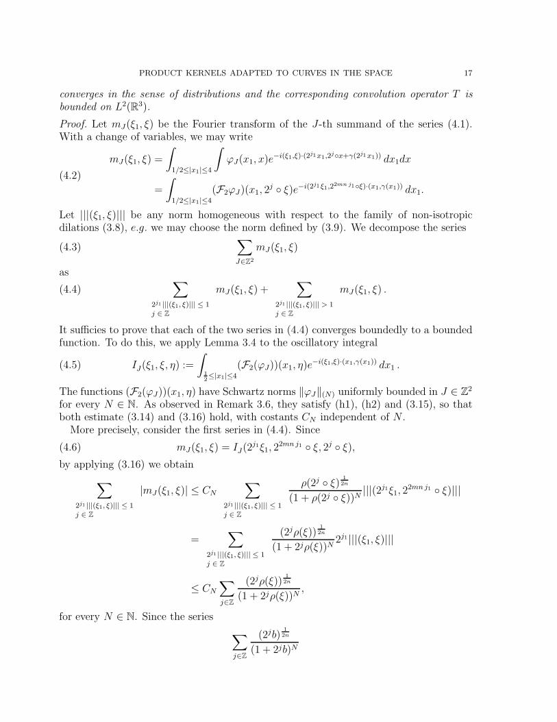
converges in the sense of distributions and the corresponding convolution operator T isbounded on L2(R3).
Proof. Let mJ(ξ1, ξ) be the Fourier transform of the J-th summand of the series (4.1).With a change of variables, we may write
(4.2)
mJ(ξ1, ξ) =
∫
1/2≤|x1|≤4
∫ϕJ(x1, x)e−i(ξ1,ξ)·(2j1x1,2j◦x+γ(2j1x1)) dx1dx
=
∫
1/2≤|x1|≤4
(F2ϕJ)(x1, 2j ◦ ξ)e−i(2j1ξ1,22mn j1◦ξ)·(x1,γ(x1)) dx1.
Let |||(ξ1, ξ)||| be any norm homogeneous with respect to the family of non-isotropicdilations (3.8), e.g. we may choose the norm defined by (3.9). We decompose the series
(4.3)∑
J∈Z2
mJ(ξ1, ξ)
as
(4.4)∑
2j1 |||(ξ1, ξ)||| ≤ 1j ∈ Z
mJ(ξ1, ξ) +∑
2j1 |||(ξ1, ξ)||| > 1j ∈ Z
mJ(ξ1, ξ) .
It sufficies to prove that each of the two series in (4.4) converges boundedly to a boundedfunction. To do this, we apply Lemma 3.4 to the oscillatory integral
(4.5) IJ(ξ1, ξ, η) :=
∫
12≤|x1|≤4
(F2(ϕJ))(x1, η)e−i(ξ1,ξ)·(x1,γ(x1)) dx1 .
The functions (F2(ϕJ))(x1, η) have Schwartz norms ‖ϕJ‖(N) uniformly bounded in J ∈ Z2
for every N ∈ N. As observed in Remark 3.6, they satisfy (h1), (h2) and (3.15), so thatboth estimate (3.14) and (3.16) hold, with costants CN independent of N .
More precisely, consider the first series in (4.4). Since
(4.6) mJ(ξ1, ξ) = IJ(2j1ξ1, 22mn j1 ◦ ξ, 2j ◦ ξ),
by applying (3.16) we obtain
∑
2j1 |||(ξ1, ξ)||| ≤ 1j ∈ Z
|mJ(ξ1, ξ)| ≤ CN
∑
2j1 |||(ξ1, ξ)||| ≤ 1j ∈ Z
ρ(2j ◦ ξ)12n
(1 + ρ(2j ◦ ξ))N|||(2j1ξ1, 2
2mn j1 ◦ ξ)|||
=∑
2j1 |||(ξ1, ξ)||| ≤ 1j ∈ Z
(2jρ(ξ))12n
(1 + 2jρ(ξ))N2j1|||(ξ1, ξ)|||
≤ CN
∑
j∈Z
(2jρ(ξ))12n
(1 + 2jρ(ξ))N,
for every N ∈ N. Since the series
∑
j∈Z
(2jb)12n
(1 + 2jb)N

18 VALENTINA CASARINO, PAOLO CIATTI, AND SILVIA SECCO
is uniformly bounded in b, it follows that the series in the previous formula convergesboundedly to a bounded function.
By using the identity (4.6) and the inequality (3.14) we prove that also the second sumon the righthand side of (4.4) converges boundedly to a bounded function.
This proves that the series in (4.3) converges boundedly (and hence in the sense ofdistributions) to a bounded function m(ξ1, ξ). As a consequence the series (4.1) convergesin the sense of distributions to the distribution K = F−1(m).
Finally, by Plancherel’s theorem, the boundedness of m implies that the correspondingoperator T is bounded on L2(R3). �
5. Lp-boundedness
In this section we prove the Lp-boundedness of the operator T . For this we split thesum (4.1) into two parts
(5.1)
K(x1, x) =∑
2mnj1≤j
2−j1−jQϕJ
(2−j1x1, 2
−j ◦ (x− γ(x1))
+∑
2mnj1>j
2−j1−jQϕJ
(2−j1x1, 2
−j ◦ (x− γ(x1))
=: K1(x1, x) +K2(x1, x).
Correspondingly we break the operator T into the sum
Tf = f ∗K1 + f ∗K2 =: T1f + T2f
and we prove that T1 and T2 are bounded on Lp(R3) for 1 < p <∞.
Proposition 5.1. The operator T1 is bounded on Lp(R3) for 1 < p <∞.
Proof. Let mJ(ξ1, ξ) be the multiplier given in (4.2). We show that the series
K1(ξ1, ξ) =∑
2mnj1≤j
mJ(ξ1, ξ)
defines a Marcinkiewicz multiplier on R × R2 adapted to the dilations (1.1) on R2. As aconsequence, we will obtain that T1 is bounded on Lp(R3). This is part of the folklore,for a formal proof see [R].
It suffices to show that K1(ξ1, ξ) is a bounded function on R3 such that for each s1 ∈{0, 1} and for each multi-index s = (s2, s3) ∈ N
2 with |s| ≤ 2 there is a positive constantCs1,s for which
(5.2) |∂s1ξ1∂s
ξK1(ξ1, ξ)| ≤ Cs1,s|ξ1|−s1ρ(ξ)−
s22n
−s32m
for every (ξ1, ξ) ∈ R × R2 with ξ1 6= 0 and ξ 6= 0.
We already proved in Proposition 4.1 that K1(ξ1, ξ) is a bounded function on R3.We give the proof of the differential inequalities (5.2) for s1 = 1 and s = (0, 0) and
for s1 = 0 and s = (1, 0), the other cases being essentially the same, with the extradisadvantages of more complicated notation and computations.

PRODUCT KERNELS ADAPTED TO CURVES IN THE SPACE 19
Set
(5.3) Iα,βJ (ξ1, ξ, η) :=
∫
12≤|x1|≤4
xα1 (F2(x
βϕJ))(x1, η)e−i(ξ1,ξ)·(x1,γ(x1)) dx1 ,
where α ∈ N, α ≤ 2 and β = (β1, β2) ∈ N2 with |β| ≤ 2.
We first consider the case s1 = 1 and s = (0, 0). Since
∂ξ1mJ (ξ1, ξ) = −i2j1I1,(0,0)J (2j1ξ1, 2
2mn j1 ◦ ξ, 2j ◦ ξ) ,
we write
∑
2mn j1≤j
|∂ξ1mJ(ξ1, ξ)| ≤ |ξ1|−1
( ∑
2j1 |||(ξ1, ξ)||| ≤ 1j ∈ Z
2j1|ξ1| |I1,(0,0)J (2j1ξ1, 2
2mn j1 ◦ ξ, 2j ◦ ξ)|
+∑
2j1 |||(ξ1, ξ)||| > 12mn j1 ≤ j
2j1 |ξ1| ≤ C(2mj1 |ξ2| + 2nj1 |ξ3|)
2j1 |ξ1| |I1,(0,0)J (2j1ξ1, 2
2mn j1 ◦ ξ, 2j ◦ ξ)|
+∑
2j1 |||(ξ1, ξ)||| > 12mn j1 ≤ j
2j1 |ξ1| > C(2mj1 |ξ2| + 2nj1 |ξ3|)
2j1 |ξ1| |I1,(0,0)J (2j1ξ1, 2
2mn j1 ◦ ξ, 2j ◦ ξ)|
)
=: Σ1 + Σ2 + Σ3 .
Since 2j1|ξ1| ≤ 2j1 |||(ξ1, ξ)|||, the convergence of Σ1 follows from the estimate (3.12) applied
to the integral I1,(0,0)J (2j1ξ1, 2
2mn j1 ◦ ξ, 2j ◦ ξ).
The inequalities 2j1|ξ1| ≤ C(2mj1 |ξ2| + 2nj1|ξ3|) and 2mnj1 ≤ j imply that 2j1|ξ1| ≤
C(2j
2n |ξ2| + 2j
2m |ξ3|) ≤ C((2jρ(ξ))12n + (2jρ(ξ))
12m ). This fact, together with the estimate
(3.14) for the integral I1,(0,0)J (2j1ξ1, 2
2mn j1 ◦ ξ, 2j ◦ ξ) shows that also Σ2 converge to abounded function. Finally, the sum Σ3 converges because of (3.21). Therefore (5.2) holdsfor s1 = 1 and s = (0, 0).
Now, assume that s1 = 0 and s = (1, 0), then we have that
∂ξ2mJ(ξ1, ξ) = −i2j/2nI0,(1,0)J (2j1ξ1, 2
2mn j1 ◦ ξ, 2j ◦ ξ)− i2mj1Im,(0,0)J (2j1ξ1, 2
2mn j1 ◦ ξ, 2j ◦ ξ).

20 VALENTINA CASARINO, PAOLO CIATTI, AND SILVIA SECCO
We write(5.4)∑
2mn j1≤j
|∂ξ2mJ(ξ1, ξ)| ≤ ρ(ξ)−12n
( ∑
2j1 |||(ξ1, ξ)||| ≤ 1j ∈ Z
(2jρ(ξ))12n |I
0,(1,0)J (2j1ξ1, 2
2mn j1 ◦ ξ, 2j ◦ ξ)|
+∑
2j1 |||(ξ1, ξ)||| > 1j ∈ Z
(2jρ(ξ))12n |I
0,(1,0)J (2j1ξ1, 2
2mn j1 ◦ ξ, 2j ◦ ξ)|
+∑
2j1 |||(ξ1, ξ)||| ≤ 1j ∈ Z
(2jρ(ξ))12n |I
m,(0,0)J (2j1ξ1, 2
2mn j1 ◦ ξ, 2j ◦ ξ)|
)
+∑
2j1 |||(ξ1, ξ)||| > 1j ∈ Z
(2jρ(ξ))12n |I
m,(0,0)J (2j1ξ1, 2
2mn j1 ◦ ξ, 2j ◦ ξ)|
).
By using the estimate (3.16) we can easily prove that the first and the third series on therighthand side of (5.4) converge to a bounded function. Also, the second and the fourthseries on the righthand side of (5.4) converge to a bounded function as we can see byapplying the estimate (3.14). Hence (5.2) holds for s1 = 0 and s = (1, 0). �
We now prove the Lp-boundedness of the operator T2 by means of the analytic inter-polation method. We start constructing an analytic family of linear operators T2,z.
For z ∈ C we consider the kernel and its analytic continuation, defined in (2.9),
Iz(u) =G(0)ρ(u)z−Q
σ(S)Γ(z)G(z)
on R2, where u = (u2, u3), σ(S) denotes the surface measure of the sphere
S := {u ∈ R2 : ρ(u) = 1} ,
and G(z) has been defined in (2.8).
Example 5.2. In the light of Example 2.4, when m = 2 and n = 3 we have
(5.5)
G(z) :=
(Γ
(z +
7
12
))2
· Γ
(z +
1
6
)Γ
(z +
1
4
)Γ
(z +
1
3
)
Γ
(z +
5
12
)Γ
(z +
1
2
)Γ
(z +
2
3
)Γ
(z +
3
4
)Γ
(z +
5
6
)Γ
(z +
11
12
).
We shall denote by Br, r > 0, the non-isotropic ball
(5.6) Br :={
(u1, u2) ∈ R2 : u2n
1 + u2m2 ≤ r
}.
Let θ be a smooth compactly supported function on R2 whose support is contained inthe ball B 1
4and which is identically one in a neighbourhood of the origin. Let Bz be the
distribution defined by
(5.7) 〈Bz, h〉 := 〈Iz, θh〉, h ∈ S(R2).

PRODUCT KERNELS ADAPTED TO CURVES IN THE SPACE 21
Observe that B0 = δ0, since I0 = δ0 and θ is identically one in a neighbourhood of theorigin.
By considering the convolution between 2−j1−jQϕJ(2−j1x1, 2−j◦(x−γ(x1)) and 2−(m+n)j1(δ0⊗
Bz)(x1, 2−2mn j1 ◦ x) we get the kernel
K2,z(x1, x)=∑
2mn j1>j
2−(m+n+1)j1−jQ
∫ϕJ(2−j1x1, 2
−j ◦ (u−γ(x1)))Bz(2−2mnj1 ◦ (x−u))du .
If we set
(5.8) λJ(x1, x) := 2(2mn j1−j)Q
∫ϕJ(x1, 2
2mn j1−j ◦ (x− u− γ(x1)))Bz(u) du ,
then the kernel K2,z may be written, by a change of variable, as
(5.9) K2,z(x1, x) :=∑
2mn j1>j
2−(m+n+1)j1λJ(2−j1x1, 2−2mn j1 ◦ x) .
We consider the analytic family of operators (of admissible growth)
(5.10) T2,zf := f ∗K2,z, f ∈ S(R3) ,
and we observe that T2,0f = f ∗K2,0 = T2f .In order to prove the Lp-boundedness of T2 we need some preliminary results. The first
result is an L1- Lipschitz condition for the distribution Bz defined by (5.7).
Lemma 5.3. For all 0 < ℜez < Q
(5.11)
∫ ∣∣∣Bz(u+ h) − Bz(u)∣∣∣ du ≤ Czρ(h)ℜez
for all h ∈ R.
Proof. First we split the integral in (5.11) in two parts∫ ∣∣∣Bz(u+ h) − Bz(u)
∣∣∣ du =
∫
ρ(h)≤ρ(u)
2
∣∣∣Bz(u+ h) −Bz(u)∣∣∣du
+
∫
ρ(h)>ρ(u)
2
∣∣∣Bz(u+ h) − Bz(u)∣∣∣du =: I + II .
Now
I ≤
∫
ρ(h)≤ ρ(u)2
∣∣∣Czθ(u+ h)(ρz−Q(u+ h) − ρz−Q(u)
)∣∣∣ du
+
∫
ρ(h)≤ ρ(u)2
∣∣∣Cz
(θ(u+ h) − θ(u)
)ρz−Q(u)
∣∣∣du =: Ia + Ib .
To estimate Ia, we use the Mean Value Theorem [FoS, p. 11], obtaining
Ia ≤ C
∫
ρ(h)≤ρ(u)
2
(ρ(u)
)ℜez−Q−1ρ(h)du = Cρ(h)
∫ +∞
2ρ(h)
rℜez−Q−1rQ−1dr
∫
S
ρ(v)ℜez−Q−1dσ(v)
≤ Cρ(h)ρ(h)ℜez−1 = Cρ(h)ℜez .

22 VALENTINA CASARINO, PAOLO CIATTI, AND SILVIA SECCO
To estimate Ib, we observe that
Ib ≤ C
∫
ρ(h)≤ ρ(u)2
∣∣θ(u+ h) − θ(u)∣∣(ρ(u)
)ℜez−Qdu
≤ Cρ(h)ℜez−Q
∫
ρ(h)≤ ρ(u)2
∣∣θ(u+ h) − θ(u)∣∣ du ≤ 2Cρ(h)ℜez−Q
∫ ∣∣θ(u)∣∣ du
≤ Cρ(h)ℜez−Q .
Finally, if k denotes a positive costant such that ρ(x + y) ≤ k(ρ(x) + ρ(y)
)we observe
that by [FoS, p. 14]
II =
∫
ρ(h)>ρ(u)
2
∣∣∣Bz(u+ h) − Bz(u)∣∣∣du
≤ 2C
∫
ρ(h)> ρ(u)3k
(ρ(u)
)ℜez−Qdu = 2C
∫ 3kρ(h)
0
rℜez−QrQ−1dr
∫
S
ρ(v)ℜez−Qdσ(v)
≤ Cρ(h)ℜez .
This inequality, combined with the bounds for I, yields (5.11).�
Then we need to recall the definition of non-isotropic Besov spaces [S].
Definition 5.4. In R3 we consider the family of one-parameter non-isotropic dilationsdefined in (3.8). Let ρ(x1, x) be any homogeneous norm with respect to these dilations.
We denote by Bα1,∞ the non-isotropic Besov space of functions f ∈ L1(R3) which satisfy
an L1-Lipschitz condition of order α, 0 < α < 1, i.e. there exists a positive constant Csuch that ∫
|f(x1 + h1, x+ h) − f(x1, x)| dx1dx ≤ Cρ(h1, h)α
for every (h1, h) ∈ R × R2, where h = (h2, h3).If f ∈ Bα
1,∞ we set
‖f‖Bα1,∞
:= ‖f‖1 + sup(h1,h)6=(0,0)
ρ(h1, h)−α
∫|f(x1 + h1, x+ h) − f(x1, x)| dx1dx.
Our proof hinges on the following result.
Theorem 5.5. Let {ψl}l∈Z be a family of functions such that for some positive constantsC, α, ε the following hypotheses hold uniformly in l:
(i) {ψl}l∈Z ⊂ L1(R3);
(ii)
∫|ψl(x1, x)|(1 + ρ(x1, x))ε dx1dx ≤ C;
(iii)
∫ψl(x1, x) dx1dx = 0;
(iv) ‖ψl‖Bα1,∞
≤ C.

PRODUCT KERNELS ADAPTED TO CURVES IN THE SPACE 23
Then the series∑
l∈Z2−(m+n+1)lψl(2
−l • ·) converges in the sense of distributions to aCalderon-Zygmund kernel.
Finally we can state and prove the Lp-bounds for T2.
Proposition 5.6. The operator T2 is bounded on Lp(R3) for 1 < p <∞.
Proof. The proof is by complex interpolation.We first prove that T2,z is bounded on L2(R3) for − 1
2mn2 < ℜez < 0.En easy computation shows that
(2−(m+n+1)j1λJ(2−j1·, (2−2mn j1 ◦ ·)
)(ξ1, ξ) = λJ
(2j1ξ1, 2
2mnj1 ◦ ξ)
= Bz(22mnj1 ◦ ξ
)mJ(ξ1, ξ) ,
where λJ id defined by (5.8), mJ is the Fourier transform of 2−j1−jQϕJ (2−j1x1, 2−j ◦ (x− γ(x1))
and it is given by (4.2), while Bz is the Fourier transform of 2−(m+n)j1
(δ0⊗B
z(ξ1, 2
−2mnj1◦
x))
.
It follows from Proposition 2.8 that
(5.12)∣∣∣Bz(ξ)
∣∣∣ ≤ C(1 + ρ(ξ))−ℜez .
Our aim is now to prove that the series∑
2mnj1>j
Bz(22mnj1 ◦ ξ
)mJ (ξ1, ξ) ,
corresponding to the Fourier transform of (5.9), converges boundedly to a bounded func-tion. The inequality (5.12) yields∣∣∣∑
2mnj1>j
Bz(22mnj1 ◦ ξ
)mJ(ξ1, ξ)
∣∣∣ ≤ Cz
∑
2j1 |||(ξ1, ξ)||| ≤ 12mn j1 > j
(1 + ρ(22mnj1 ◦ ξ)
)|ℜez| ∣∣mJ(ξ1, ξ)∣∣
+∑
2j1 |||(ξ1, ξ)||| > 12mn j1 > j
(1 + ρ(22mnj1 ◦ ξ)
)|ℜez| ∣∣mJ (ξ1, ξ)∣∣ =: J1 + J2 .
Since
22mnj1ρ(ξ) = 22mnj1(ξ2n2 + ξ2m
3 ) ≤ 2 ·(2j1|||(ξ1, ξ)|||
)2mn,
we have
(5.13) J1 ≤ C 3|ℜez|∑
2j1 |||(ξ1, ξ)||| ≤ 12mn j1 > j
∣∣mJ(ξ1, ξ)∣∣ ≤ Cz ,
In the light of what has been proved in Proposition 4.1, to estimate J2 observe that
J2 ≤ Cz
∑
2j1 |||(ξ1, ξ)||| > 12mn j1 > j
(2j1|||(ξ1, ξ)|||
)2mn|ℜez|∣∣mJ(ξ1, ξ)∣∣ .
24 VALENTINA CASARINO, PAOLO CIATTI, AND SILVIA SECCO
Now, by using (4.6) and estimate (3.14) for IJ , we obtain
J2 ≤ Cz
∑
2j1 |||(ξ1, ξ)||| > 12mn j1 > j
(2j1|||(ξ1, ξ)|||
)2mn|ℜez|
(2j1 |||(ξ1, ξ)|||
)1/n
ρ(2j ◦ ξ)1/2n
(1 + ρ(2j ◦ ξ)
)N,
so that the operator T2,z is bounded on L2(R3) if − 12mn2 < ℜez < 0.
We will now show that the operator T2,z is bounded on Lp(R3) for 1 < p < ∞ for0 < ℜez < Q.
By setting j − 2mnj1 = k and using (3.10), (5.9) may be written as
K2,z(x1, x) =∑
j1∈Z
2−(m+n+1)j1
0∑
k=−∞
λ(j1,k+2mn j1)(2−j1 • (x1, x))
where
(5.14) λ(j1,k+2mn j1)(x1, x) = 2−Qk
∫ϕ(j1,k+2mn j1)(x1, 2
−k ◦ (x− u− γ(x1)))Bz(u) du.
We shall now prove that the functions
ψj1(x1, x) :=0∑
k=−∞
λ(j1,k+2mn j1)(x1, x)
satisfy the hypotheses of Theorem 5.5 uniformly in j1.Since the estimates on the functions ψj1(x1, x) that we will prove later are independent
of j1, it suffices to prove that
ψ0(x1, x) =0∑
k=−∞
λ(0,k)(x1, x)
satisfies the hypotheses of Theorem 5.5.We begin proving that ψ0 belongs to L1(R3). As a consequence of (3.5) with β = 0 and
a change of variable we obtain
ψ0(x1, x) =
0∑
k=−∞
∫ϕ(0,k)(x1, v)
(Bz(x− 2k ◦ v − γ(x1)) − Bz(x− γ(x1))
)dv ,
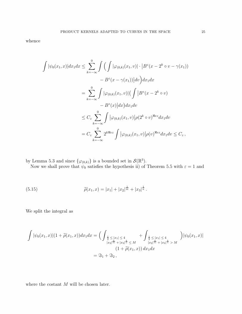
PRODUCT KERNELS ADAPTED TO CURVES IN THE SPACE 25
whence
∫|ψ0(x1, x)|dx1dx ≤
0∑
k=−∞
∫ ( ∫|ϕ(0,k)(x1, v)| ·
∣∣Bz(x− 2k ◦ v − γ(x1))
− Bz(x− γ(x1))∣∣dv)dx1dx
=0∑
k=−∞
∫|ϕ(0,k)(x1, v)|
( ∫ ∣∣Bz(x− 2k ◦ v)
− Bz(x)∣∣dx)dx1dv
≤ Cz
0∑
k=−∞
∫ ∣∣ϕ(0,k)(x1, v)∣∣ρ(2k ◦ v)ℜezdx1dv
= Cz
0∑
k=−∞
2kℜez
∫ ∣∣ϕ(0,k)(x1, v)∣∣ρ(v)ℜezdx1dv ≤ Cz ,
by Lemma 5.3 and since {ϕ(0,k)} is a bounded set in S(R3).Now we shall prove that ψ0 satisfies the hypothesis ii) of Theorem 5.5 with ε = 1 and
(5.15) ρ(x1, x) = |x1| + |x2|1m + |x3|
1n .
We split the integral as
∫|ψ0(x1, x)|(1 + ρ(x1, x))dx1dx =
(∫12≤ |x1| ≤ 4
|x2|1
m + |x3|1
n ≤ M
+
∫12≤ |x1| ≤ 4
|x2|1
m + |x3|1
n > M
)|ψ0(x1, x)|
(1 + ρ(x1, x)) dx1dx
= ℑ1 + ℑ2 ,
where the costant M will be chosen later.

26 VALENTINA CASARINO, PAOLO CIATTI, AND SILVIA SECCO
Now ℑ1 is bounded by some positive costant C, since ψ0(x1, x) belongs to L1(R3) andρ(x1, x) is bounded on the integration set. To study ℑ2, observe that
ℑ2 ≤
0∑
k=−∞
2−kQ
∫12≤ |x1| ≤ 4
|x2|1
m + |x3|1
n > M
∫
ρ(u)≤ 14
∣∣∣ϕ(0,k)(x1, 2−k ◦ (x− u− γ(x1))
∣∣∣ ·∣∣∣Bz(u)
∣∣∣du
(5 + |x2|1m + |x3|
1n ) dx1dx
≤ C0∑
k=−∞
2−kQ
∫12≤ |x1| ≤ 4
|x2|1
m + |x3|1
n > M
∫
ρ(u)≤ 14
||ϕ(0,k)||(N)
∣∣Bz(u)∣∣
(1 +
∣∣2−k ◦ (x− u− γ(x1))∣∣)N
du
(5 + |x2|1m + |x3|
1n ) dx1dx
≤ C0∑
k=−∞
2−kQ
∫12≤ |x1| ≤ 4
|x2|1
m + |x3|1
n > M
(5 + |x2|1m + |x3|
1n )
∫
ρ(u)≤ 14
||ϕ(0,k)||(N)
∣∣Bz(u)∣∣
(1 +
∣∣2−k ◦ x∣∣)N
du dx1dx ,
where the last inequality follows from the fact that for some costant C > 0 we have
1 +∣∣2−k ◦ (x− u− γ(x1))
∣∣ ≥ C(1 +
∣∣2−k ◦ x∣∣)
if |x2|1m + |x3|
1n > M , if M is sufficiently large, ρ(u) ≤ 1
4, 1
2≤ |x1| ≤ 4.
Next (2.2) yields
(5.16)∣∣2−k ◦ x
∣∣ ≥ A(ρ(2−k ◦ x)
) 12n
for some A > 0, if k ≤ 0 and |x2|1m + |x3|
1n > M .
Now (5.16) and the local integrability of Bz give
ℑ2 ≤ C
0∑
k=−∞
2−kQ
∫
|x2|1m +|x3|
1n >M
(5 + |x2|1m + |x3|
1n )
1(
1 + ρ(2−k ◦ x
)) N2n
dx
≤ C
0∑
k=−∞
2−kQ
∫
|x2|1m +|x3|
1n >M
(5 + |x2|1m + |x3|
1n )
1(
1 + 2−kρ(x)) N
2n
dx
≤ C
0∑
k=−∞
2−kQ2kN2n
∫
|x2|1m +|x3|
1n >M
(5 + |x2|1m + |x3|
1n )
1
ρ(x)N2n
dx ≤ C ,
yielding ii).Property iii) is an immediate consequence of (3.5).Finally we shall prove that ψ0 satisfies property iv) in Theorem 5.5.We start proving that
(5.17)
∫ ∣∣ψ0(x1, x+ h) − ψ0(x1, x)∣∣dx1 dx ≤ C ′
zρ(h)ℜez4mn , h ∈ R
2 .

PRODUCT KERNELS ADAPTED TO CURVES IN THE SPACE 27
Indeed we have∫ ∣∣ψ0(x1, x+ h) − ψ0(x1, x)
∣∣dx1 dx
≤0∑
k=−∞
∫ ( ∫ ∣∣∣ϕ(0,k)(x1, v)(Bz(x + h− 2k ◦ v − γ(x1)) − Bz(x+ h− γ(x1))
)
− ϕ(0,k)(x1, v)(Bz(x− 2k ◦ v − γ(x1)) − Bz(x− γ(x1))
)∣∣∣dxdx1
)dv
=:
0∑
k=−∞
∫Jk(v)dv .
Now observe that
Jk(v) ≤ 2
∫ ∣∣∣ϕ(0,k)(x1, v)(Bz(x− 2k ◦ v − γ(x1)) −Bz(x− γ(x1))
)∣∣∣dxdx1
= 2
∫ ∣∣ϕ(0,k)(x1, v)∣∣( ∫ ∣∣∣Bz(y − 2k ◦ v) − Bz(y)
∣∣∣dy)dx1
≤ Cz,Nρ(2k ◦ v)ℜez
(1 + |v|)N= Cz,N2kℜez ρ(v)ℜez
(1 + |v|)N, N ∈ N ,(5.18)
where we used both the Lemma 5.3 and the fact that the functions ϕ(0,k) are a boundedset in S(R3).
On the other hand, as a consequence of Lemma 5.3
Jk(v) ≤ 2
∫ ∣∣∣ϕ(0,k)(x1, v)Bz(y + h− γ(x1)) − ϕ(0,k)(x1, v)Bz(y − γ(x1))∣∣∣dydx1
≤ Cz,Nρ(h)ℜez
(1 + |v|)N, N ∈ N , h ∈ R
2 .(5.19)
By taking a suitable mean between estimates (5.18) and (5.19) we obtain(5.20)
Jk(v) = Jk(v)4mn−14mn · Jk(v)
14mn ≤ Cz,N2
4mn−14mn
kℜezρ(h)ℜez4mn
ρ(v)4mn−14mn
ℜez
(1 + |v|)N, N ∈ N , h ∈ R ,
so that∫ ∣∣ψ0(x1, x+ h) − ψ0(x1, x)
∣∣dx1 dx ≤
0∑
k=−∞
∫Jk(v)dv
≤ Cz,N
0∑
k=−∞
24mn−14mn
kℜezρ(h)ℜez4mn
∫ρ(v)
4mn−14mn
ℜez
(1 + |v|)Ndv ≤ Cz,Nρ(h)
ℜez4mn ,
proving (5.17).

28 VALENTINA CASARINO, PAOLO CIATTI, AND SILVIA SECCO
In an analogous way we can prove the inequality
(5.21)
∫ ∣∣ψ0(x1 + h1, x) − ψ0(x1, x)∣∣dx1 dx ≤ C ′
z|h1|ℜez2 .
Finally we have∫ ∣∣ψ0(x1 + h1, x+ h) − ψ0(x1, x)
∣∣dx1 dx
≤
∫ ∣∣ψ0(x1 + h1, x+ h) − ψ0(x1 + h1, x)∣∣dx1 dx+
∫ ∣∣ψ0(x1 + h1, x) − ψ0(x1, x)∣∣dx1 dx
≤ Cz
(∣∣h1
∣∣ℜez2 + ρ(h)
ℜez4mn
)
Since∣∣h1
∣∣ℜez2 + ρ(h)
ℜez4mn ≤ C
(∣∣h1
∣∣ + ρ(h)1
2mn
)ℜez2
and, by a standard inequality,(h2n
2 + h2m3
) 12mn ≤ |h2|
1m + |h3|
1n ,
we finally get∣∣h1
∣∣ℜez2 + ρ(h)
ℜez4mn ≤ Cρ(h1, h)
ℜez2 ,
proving (iv) with α = ℜez2
. As a consequence of Theorem 5.5 the operator T2,z is boundedon Lp(R3), 1 < p <∞, for 0 < ℜez < Q.
Finally choose p0 ∈ (1, 2) and fix q0 ∈ (1, p0) such that
1
p0=
b
2(b− a)−
a
q0(b− a).
Then the operator T2,0 = T2 is bounded on Lp0(R3). By the arbitrariness of p0 and byduality we conclude that T2,0 = T2 is bounded on Lp(R3) for all 1 < p <∞. �
6. Final remarks
Remark 1. We observe that our results also hold in the more general situation in whichthe curve γ(x1) = (xm
1 , xn1 ) is perturbed to γ(x1) = (xm
1 +λ2(x1), xn1 +λ3(x1)) with λ1 and
λ2 smooth and satisfying λ2(x1) = o(xm
1) and λ3(x1) = o(x n
1). In fact, given a product
kernel K0 on R3, we define the distribution K by
∫K(x1, x)f(x1, x) dx1dx :=
∫K0(x1, x)f(x1, x+ γ(x1)) dx1dx
for all Schwartz functions f on R3. Then we break the integral on the right-hand side as
∫K0(x1, x)f(x1, x+ γ(x1)) dx1dx =
∫
R
1∫
−1
+
∫
R
∫
|x1|>1
K0(x1, x)f(x1, x+ γ(x1)) dx1dx .
The first term, by means of a Taylor expansion, may be reduced to the polynomial case,while the latter one is of Calderon-Zygmund type.
PRODUCT KERNELS ADAPTED TO CURVES IN THE SPACE 29
Remark 2. Our results still hold for convolution operators on Rd = R×Rd−1 with kernelsadapted to curves of the form γ(x1) = (xm1
1 , xm21 , . . . , x
md−1
1 ), 1 < m1 < m2 < . . . < md−1,mj ∈ N, j = 1, . . . , d − 1, with values in Rd−1. Since notation in the higher dimensionalcase is more cumbersome, we gave full details of the proof only for the space R3.
On Rd−1 we introduce the dilations given by
(6.1) δ ◦ x = (δ1/2md−1x2, δ1/2md−2x3, . . . , δ
1/2m1) ,
where δ > 0 and x = (x2, . . . , xd−1). Moreover we equip Rd−1 with the smooth homoge-neous norm
ρ(x) = x2md−1
2 + x2md−2
3 + . . .+ x2m1d
on Rd−1. From this point on, the proof follows the same pattern as in R3. In particular,the strategy of using Bernstein-Sato polynomials to build the meromorphic continuation
of the non isotropic Riesz potentials ρ(x)z−Q (here Q = 12md−1
+ 12md−2
+ . . .+ 12m1
) works
in the multidimensional case as well, with some additional computational difficulties infinding the zeros of the Bernstein-Sato polynomials [BMSa].
Remark 3. As an example of the class of operators studied in this paper we exhibit thefollowing operator, arising in the study of the Lp − Lq boundedness of a double analyticfamily of fractional integrals along curves in the space (see [CSe] for the planar case).
Let ψ be a smooth function on R2, such that ψ(u1,−u2) = ψ(u1, u2) for every (u1, u2) ∈R2, ψ ≡ 1 on B 1
2and ψ ≡ 0 outside B1, with 0 ≤ ψ ≤ 1 on R2 (here Br, r > 0, denotes
the non-isotropic ball in R2 defined by (5.6)).Define an analytic family of distributions Kγ
z , for γ and z in C, ℜeγ ≥ 0, in the followingway
(6.2) < Kγz , f >:=
∫< Dz(u1, u2), f(t, u1t
m, u2tn) > |t|γ
dt
t,
where Dz, ℜe z > 0, denotes the family of analytic distributions given by
< Dz, h >:= < ψ(·, ·) Iz(·, ·) , h(· + 1, · + 1) >
=Cz
∫
R2
ρ(u1 − 1, u2 − 1)z−Qψ (u1 − 1, u2 − 1) h(u1, u2) du1, du2 ,
with Cz := G(0)2σ(S)Γ(z)G(z)
and h ∈ C∞c (R2). It is straightforward to check that Dz may be
extended to all z ∈ C.As a consequence of Proposition 2.6 we have
(6.3) < D0, h >= h(1, 1).
We remark that, if ℜeγ = 0, then
< Kγz , f >:= lim
ε→0
∫< Dz(u1, u2), f(t, u1t
m, u2tn) > |t|iρ+εdt
t,
where ℑmγ = ρ, for every f ∈ C∞c (R2). Observe moreover that Kγ
z depends analyticallyon both γ and z.

30 VALENTINA CASARINO, PAOLO CIATTI, AND SILVIA SECCO
At this point we may introduce the family of convolution operators with kernel Kγz
defined by (6.2), that is(6.4)
(Sγz f) (x1, x2, x3) := (Kγ
z ∗ f) (x1, x2, x3) =
∫< Dz(u1, u2), f(x1−t, x2−u1t
m, x3−u2tn) > |t|γ
dt
t.
We observe that, in the light of (6.3), we have
(Sγ0 f) (x1, x2, x3) := C0
∫
R3
f(x1 − t, x2 − tm, x3 − tn) > |t|γdt
t,
that is, at the height z = 0 we recover the fractional integration operator along the curvet 7→ (t, tm, tn) in the space.
In a forthcoming paper [CCiSe] we shall give a complete picture of the characteristicset of the operator Sγ
z . A key step in the proof of that result is the fact that at theheight ℜez = 0 and for ℜeγ = 0 the kernel Kγ
z is a product kernel adapted to the curvex1 7→ (xm
1 , xn2 ).
References
[BMSa] N. Budur, M. Mustata and M. Saito, Combinatorial description of the roots of the Bernstein-Sato polynomials for monomial ideals, Comm. Alg., 34 (2006), 4103-4117.
[CCiSe] V. Casarino, P. Ciatti and S. Secco, in preparation.[CSe] V. Casarino and S. Secco, Lp-Lq boundedness of analytic families of fractional integrals, Studia
Mathematica 184 (2008), 153-174.[FS] R. Fefferman and E. M. Stein, Singular integrals on product spaces , Adv. in Math. 45 (1982),
no. 2 117-143.[FoS] G. B. Folland and E. M. Stein, Hardy Spaces on Homogeneous Groups Mathematical Notes,
Princeton University Press, (1982).[J] J. L. Journe, Calderon-Zygmund operators on product spaces, Rev. Mat. Iberoamericana 1
(1985), 55-92.[K] M. Kashiwara, B-functions and holonomic systems, Invent. Math. 38 (1976/77), 33-53, MR
0430304.[M] B. Malgrange, Sur les polynomes de I. N. Bernstein , Seminaire Goulauic-Schwartz 1973-1974:
Equations aux derivees partielles et analyse fonctionnelle, Centre de Math., Ecole Polytech.,Paris (1974),no.20, MR 0409883.
[MRS] D. Muller, F. Ricci and E. M. Stein, Marcinkiewicz multipliers and multi-parameterstructure onHeisenberg (-type) groups, I. Invent. Math. 119 (1995), 119-233.
[NS04] A. Nagel and E. M. Stein, On the product theory of singular integrals, Rev. Mat. Iberoamericana20 (2004), 531-561.
[NS06] A. Nagel and E. M. Stein, The ∂b-complex on decoupled boundaries in Cn , Ann. of Math. (2)164 (2006), 649-713.
[NRS] A. Nagel, F. Ricci and E. M. Stein, Singular integrals with flag kernels and analysis on quadraticCR manifolds, J. Funct. Anal. 181 (2001), 29-118.
[R] F. Ricci Fourier and spectral multipliers in Rn and the Heisenberg group, manuscript, 2003.[Se] S. Secco Adapting product kernels to curves in the plane, Math. Z. 248 (2004), 459-476.[S] E.M. Stein, Harmonic Analysis, Real-Variable Methods, Orthogonality and Oscillatory Integrals,
Mathematical Notes, Princeton Univ. Press., Princeton, NJ, 1993.[SW] E. M. Stein and S. Wainger, Problems in harmonic analysis related to curvature, Bull. Amer.
Math. Soc. 84 (1978), 1239-1295.

PRODUCT KERNELS ADAPTED TO CURVES IN THE SPACE 31
Dipartimento di Matematica, Politecnico di Torino, Corso Duca degli Abruzzi 24,
10129 Torino
Dipartimento di Metodi e Modelli matematici per le scienze applicate, Via Trieste 63,
35121 Padova
E-mail address : [email protected], [email protected], [email protected]