Available online at www.sciencedirect.com

www.elsevier.com/locate/jprocont

Journal of Process Control 18 (2008) 244–257

Process optimization via constraints adaptation

B. Chachuat *, A. Marchetti, D. Bonvin

Laboratoire d’Automatique, Ecole Polytechnique Federale de Lausanne (EPFL), CH-1015 Lausanne, Switzerland

Received 19 December 2006; received in revised form 27 June 2007; accepted 11 July 2007

Abstract

In the framework of real-time optimization, measurement-based schemes have been developed to deal with plant-model mismatch andprocess variations. These schemes differ in how the feedback information from the plant is used to adapt the inputs. A recent idea thereinis to use the feedback information to adapt the constraints of the optimization problem instead of updating the model parameters. Thesemethods are based on the observation that, for many problems, most of the optimization potential arises from activating the correct setof constraints. In this paper, we provide a theoretical justification of these methods based on a variational analysis. Then, various aspectsof the constraint-adaptation algorithm are discussed, including the detection of active constraints and convergence issues. Finally, theapplicability and suitability of the constraint-adaptation algorithm is demonstrated with the case study of an isothermal stirred-tankreactor.� 2007 Elsevier Ltd. All rights reserved.

Keywords: Real-time optimization; Measurement-based optimization; Constraints adaptation; Variational analysis; CSTR

1. Introduction

Throughout the petroleum and chemicals industry, thecontrol and optimization of many large-scale systems isorganized in a hierarchical structure [1–3]. At the lowestlevel, sensor measurements are collected from the plant,and basic flow, pressure, and temperature control is imple-mented, possibly via advanced regulatory controllers thatinclude cascade controllers and (linear) multivariable pre-dictive controllers (MPC) [4]. The nominal execution per-iod of these low-level controllers is usually in the order ofseconds or minutes. At the next level, short-term decisionsare made on a time scale of hours to a few days by consid-ering economics explicitly in operations decisions. This steptypically relies on a real-time optimizer (RTO) that deter-mines the optimal operating point under changing condi-tions, e.g., feed or process changes. Finally, at the higherlevel, longer-term issues are addressed such as material

0959-1524/$ - see front matter � 2007 Elsevier Ltd. All rights reserved.

doi:10.1016/j.jprocont.2007.07.001

* Corresponding author. Tel.: +41 21 693 3844; fax: +41 21 693 2574.E-mail address: benoit.chachuat@epfl.ch (B. Chachuat).

inventories and production rate targets, based on plant-wide planning and scheduling optimization techniques. Inorder to combat uncertainty, all levels utilize process mea-surements as inputs to their feedback loops, and eachhigher level provides guidance to the subsequent lowerlevel.

This paper focuses on the real-time optimization level.The RTO is typically a nonlinear program (NLP) minimiz-ing cost or maximizing economic productivity subject toconstraints derived from steady-state mass and energy bal-ances, reaction kinetic relationships, thermodynamic equi-librium equations, physical property relationships, andphysical equipment constraints. Many successful industrialapplications have been reported [5,3]. In particular, it iscommon to find RTO applications with ten to a hundreddecision variables (e.g., the set-points to low-level processcontrollers or steady-state inputs), and thousands or eventens of thousand state variables and constraint equations.Since the underlying models are steady-state models, theseapplications operate at the time scale of the plant steady-state response time, with often several hours betweenimplemented solutions.

B. Chachuat et al. / Journal of Process Control 18 (2008) 244–257 245

Mathematical models with high accuracy are unavail-able for most industrial applications. In response to this,RTO classically proceeds by a two-step iterative approach[2], namely an identification step followed by an optimiza-tion step. The idea is to repeatedly estimate the uncertainmodel parameters, and then use the updated model toadapt the decision variables via model-based optimization.In order for this scheme to converge to the plant optimum,it is necessary that the values and gradients of the con-straints as well as the gradient of the cost predicted bythe model match those of the plant. This way, the necessaryconditions of optimality (NCO) are satisfied for theplant.

It is well known that such two-step approaches workwell provided that (i) model mismatch is low, and (ii) theoperating conditions yield sufficient excitation for all theuncertain model parameters to be estimated accurately.Yet, such conditions are rarely met in practice. Regardingthe latter condition, in particular, the situation is somewhatsimilar to that found in the area of system identificationand control, where the two tasks of identification and con-trol are typically conflicting (dual control problem [6]).Furthermore, this problem becomes even more acute whenthe number of uncertain model parameters grows large. Away of improving the synergy between the identificationand optimization steps is to reconcile the objective func-tions of these two problems. In the so-called integrated sys-

tem optimization and parameter estimation (ISOPE) method

[7,8], a gradient modification term is added to the costfunction of the optimization problem so that the iteratesconverge to a point at which the NCO are satisfied forthe plant. On the other hand, one can also modify theobjective function of the identification problem by includ-ing the cost and constraint functions of the optimizationproblem [9], following the paradigm of ‘‘modeling for

optimization’’.In response to the aforementioned difficulties of two-

step RTO techniques, methods that do not rely on a pro-cess model update have gained in popularity in recentyears. These methods can be further classified dependingon whether no process model is used during the operation(model-free methods), or an approximate model is usedwithout refinement (fixed-model methods).

• In model-free methods, also known as implicit optimiza-tion techniques [10], two subclasses can be further distin-guished. In the first one, successive steady-stateoperating periods are determined by ‘‘mimicking’’ vari-ous iterative numerical optimization algorithms. Forexample, evolutionary-like schemes have been proposedthat implement the Nelder–Mead simplex algorithm toapproach the optimum [11]. To achieve faster conver-gence, techniques based on gradient-based algorithmshave also been developed, yet these techniques requirethat the gradients of the cost and constraint functionsbe calculated from the available measurements. Finite-difference schemes provide a straightforward way of esti-

mating the gradients, but become experimentally intrac-table for more than a few decision variables. Alternativemethods have also been proposed such as dynamic per-turbations [12], and recursive Broyden-like updates[13].The second subclass of model-free methods consistsof recasting the NLP problem into a problem of choos-ing outputs whose optimal values are approximatelyinvariant to uncertainty. The idea is to use the availablemeasurements to bring these outputs back to theirinvariant values, thereby rejecting the uncertainty. Inother words, a feedback law is sought that implicitlysolves the optimization problem. Two such controlschemes are self-optimizing control [14] and NCO track-

ing [15,16] (see also [17]). A particularly nice feature ofNCO tracking lies in its ability to handle constrainedproblems, although this requires that the active setremain unchanged in the presence of uncertainty.

• In contrast to the previous class of methods, fixed-modelmethods utilize both the available measurements and a(possibly inaccurate) process model for guiding the iter-ative scheme towards an optimal operating point. Anal-ogous to classical two-step RTO methods, the availableprocess model is embedded within an NLP problem thatis solved repeatedly. In other words, the process model isused in the optimization procedure for estimating thegradients of the cost and constraint functions. Butinstead of refining the process model from one RTOiteration to the next, the measurements are used todirectly update the cost and constraint functions in themodel in such a way that they approximate the corre-sponding measured values at the current iterate. TheRTO system with bias update [18] is one such fixed-modelmethod wherein the constraint functions are simply off-set based on their measurements; see also the internal

model controller (IMC) optimization scheme [19]. Morerecently, additional correction terms have been pro-posed so that, not only the constraint values predictedby the model be equal to those of the actual process,but also their gradients as well as the gradient of the costfunction [20]. This way, a point at which the NCO of thereal process are satisfied is obtained upon convergence.Note that these correction terms are similar to thoseused in the ISOPE method, and that their calculationrequires that the cost and constraint gradients be esti-mated from the available measurements.

When comparing fixed-model RTO methods withmodel-free approaches, it should be stressed that the directsolution of an NLP problem allows handling constraintswithout having to make any assumption regarding the setof active constraints at the optimal point. In addition, sinceconstraints are known to play a major role in many optimi-zation problems, fixed-model RTO methods are particu-larly well suited for practical applications. Indeed, for thevast majority of problems wherein the solution lies on theconstraints, most of the potential of optimization arisesfrom the correct set of constraints being activated.

246 B. Chachuat et al. / Journal of Process Control 18 (2008) 244–257

The focus in this paper is on fixed-model RTO methods.More specifically, we put emphasis on the bias updatemethod [18], which we shall refer to as constraint-adapta-

tion scheme throughout. The paper undertakes a novelstudy of various aspects of constraint-adaptation schemes.It is organized as follows. The formulation of the RTOproblem as well as a number of preliminary results are pre-sented in Section 2. Section 3 motivates the use of con-straint-adaptation schemes via a sensitivity analysis of theoptimal cost with respect to uncertain parameters. Theconstraint-adaptation scheme is presented in Section 4,and various theoretical aspects are discussed. A case studyrelative to a continuous stirred-tank reactor is then detailedin Section 5, which illustrates the applicability of con-straint-adaptation schemes. Finally, Section 6 concludesthe paper.

2. Optimization problem

2.1. Problem formulation

The usual objective in RTO is the minimization or max-imization of some steady-state operating performance ofthe process (e.g., minimization of operating cost or maxi-mization of production rate), while satisfying a numberof constraints (e.g., bounds on process variables or productspecifications). In the context of RTO, since it is importantto distinguish the plant from its model, we will use thenotation �ð�Þ for the variables associated with the plantand (Æ) for those of the process model.

The optimization problem for the plant can be formu-lated as follows:

minimize : UðuÞ :¼ /ðu; �yÞsubject to : GðuÞ :¼ gðu; �yÞ 6 0;

uL6 u 6 uU;

ðPÞ

where u 2 Rnu denote the decision (or input) variables, and�y 2 Rny are the controlled (or output) variables for theplant; / : Rnu � Rny ! R is the scalar cost function to beminimized; gi : Rnu � Rny ! R, i = 1, . . . ,ng, is the set ofoperating constraints; and uL, uU are the bounds on thedecisions variables.1

On the other hand, the model-based optimization prob-lem is a general NLP of the form

minimize : /ðu; yÞsubject to : Fðu; y; hÞ ¼ 0;

gðu; yÞ 6 0;

uL6 u 6 uU;

where F is a set of process model equations, which includemass and energy balances and thermodynamic relation-ships, predicting the values of the controlled variables

1 These bounds are considered separately from the constraints g sincethey are not affected by uncertainty and, thus, do not require adaptation.

y 2 Rny for given values of the decision variables u. Observethat these predictions depend on a set of adjustable modelparameters h 2 Rnh . For simplicity, we shall assume thatthe model outputs y can be expressed explicitly as functionsof u and h, thereby leading to the equivalent NLPformulation

minimize : Uðu; hÞsubject to : Gðu; hÞ 6 0;

uL6 u 6 uU;

ðPhÞ

with U and G defined as U(u,h) :¼ /(u,y(u,h)) andG(u,h) :¼ g(u,y(u,h)).

Under the assumptions that U(Æ,h) is continuous on[uL,uU] and the feasible set Uh :¼ {u 2 [uL,uU]: G(u,h) 60} is nonempty and bounded for h given, the infimum forproblem Ph, labeled UH

h , is assumed somewhere on [uL,uU]and thus a minimum exists (Weierstrass’ theorem – see,e.g., [21], Theorem 2.3.1). Here, we shall denote by uH

h aminimizing solution for the problem Ph, i.e., UðuH

h ; hÞ ¼UH

h , and by Ah :¼ fi : GiðuH

h ; hÞ ¼ 0; i ¼ 1; . . . ; ngg the setof active constraints at uH

h .

2.2. Necessary conditions of optimality

Assume that the cost function U and the inequality con-straints G are differentiable at the solution point uH

h andfurthermore that the following constraint qualificationholds:

rank

oGou

diagðGÞInu diagðu� uUÞ�Inu diagðuL � uÞ

0B@1CA

h;uH

h

¼ ng þ 2nu;

i.e., this (ng + 2nu) · (ng + 3nu) matrix is of full row rank.Then, there exist unique Lagrange multiplier vectorsl 2 Rng , fU; fL 2 Rnu such that the following conditionshold at uH

h (see, e.g., [21], Theorem 4.2.13):

G 6 0; uL6 u 6 uU; ð1Þ

lTG ¼ 0; fUTðu� uUÞ ¼ 0; fLTðuL � uÞ ¼ 0; ð2Þl P 0; fU P 0; fL P 0; ð3ÞoL

ou¼ oU

ouþ lT oG

ouþ fUT � fLT ¼ 0; ð4Þ

with L :¼ Uþ lTGþ fUTðu� uUÞ þ fLTðuL � uÞ being theLagrangian function. The necessary conditions of optimal-ity (1) are referred to as primal feasibility conditions, (2) ascomplementarity slackness conditions, and (3), (4) as dualfeasibility conditions.

3. Variational analysis of NCO in the presence of

uncertainty

Satisfying the NCO is necessary for process operation tobe feasible and for achieving optimal performance. More

B. Chachuat et al. / Journal of Process Control 18 (2008) 244–257 247

precisely, failure to meet any of the primal feasibility con-ditions (1) leads to infeasible operation, whereas violatingthe complementarity and dual feasibility conditions (2)–(4) results in suboptimal operation. That is, a very desirableproperty for a RTO scheme is that the iterates converge toa point at which the NCO of the real process are satisfied.Regarding fixed-model RTO methods, the algorithmdescribed in [20], provided it converges, can be shown toattain such points. However, for RTO schemes to satisfycertain NCO, it is necessary that the gradients of the costand constraint functions be available, which in turnrequires that these gradients be estimated experimentallyfrom the available measurements.

In this section, we conduct a variational analysis of theNCO in the presence of uncertainty. The underlying idea isto quantify how deviations of the parameters h from theirnominal values h affect the NCO and, through them, theperformance of the process. Said differently, the objectiveis to determine which parts of the NCO influence theprocess performance the most, and which parts can bedropped without much impact in terms of performance.For simplicity, and without loss of generality, the boundconstraints uL

6 u 6 uU shall be considered as a subset of

the general inequality constraints G(u,h) 6 0 for thisanalysis.

We start the analysis by recalling the following theoremgiving conditions under which a solution to problem Ph

exists and is unique for values of the adjustable parametersh close to their nominal values h.

Theorem 1 (Basic Sensitivity Theorem). Let U and Gi,

i = 1, . . . , ng, in Ph be twice continuously differentiable

functions with respect to (u,h). Consider the problem Ph

for

the nominal parameter values h, and let uH

h2 ½uL; uU� be such

that:

(1) the second-order sufficient conditions for a local mini-

mum of Ph hold at uH

h, with associated Lagrange multi-

pliers lH

h(see, e.g., [21, Theorem 4.4.2]);

(2) uH

his a regular point for the active constraints,

rankoG

ou

� �h;uH

h

¼ cardðAhÞ;

(3) lH

h i> 0 for each i 2Ah.

Then, there is some g > 0 such that, for each h 2 BgðhÞ – a

ball of radius g centered at h, there exists a unique

continuously differentiable vector function nðhÞ ¼½ uHT

h lHTh �

T satisfying the second-order sufficient condi-

tions for a local minimum of Ph, with nðhÞ ¼ ½ uHTh

lHTh�T.

That is, uH

h is an isolated local minimizer of Ph with

associated unique Lagrange multipliers lH

h . Moreover, theset of active constraints Ah is the same as A

h, the Lagrange

multipliers are such that lH

h k > 0 for each k 2Ah, and the

active constraints are linearly independent at uH

h .

Proof. See, e.g., [22, Theorem 3.2.2] for a proof. h

Remark 1. The derivative of the vector function nðhÞ ¼½ uHT

h lHTh �

T at h can be obtained upon differentiation ofthe first-order necessary conditions

lH

h kGkðuH

h ; hÞ ¼ 0; k ¼ 1; . . . ; ng; ð5ÞoL

ouðuH

h ; lH

h ; hÞ ¼ 0 ð6Þ

that must be satisfied for each h 2 BgðhÞ. In particular, theassumptions of Theorem 1 imply that the Jacobian Mh ofthe system (5) and (6) with respect to (u,l) at h is nonsin-gular. That is, a first-order approximation of the variationsduH :¼ uH

h � uH

hand dlH :¼ lH

h � lH

hin the optimal inputs

and Lagrange multipliers, induced by the variationdh :¼ h� h in the model parameter, is

duH

dlH

� �¼ �ðMhÞ

�1Nhdhþ oðkdhkÞ; ð7Þ

where Nh stands for the Jacobian of (5) and (6) with respect

to h at h.

In the remainder of this section, we shall assume, with-out loss of generality, that all the constraints Gð�; hÞ are

active at uH

h, since an inactive constraint at uH

hcan always

be removed from the problem Ph. The number of activeconstraints at an optimal solution point being less thanthe number of inputs, there exist directions in the inputspace along which taking an infinitesimal step from anoptimal solution point does not modify the active con-straints. A characterization of these directions is given inthe next definition.

Definition 1 (Constraint- and sensitivity-seeking direc-

tions). If the assumptions of Theorem 1 are met, theJacobian matrix oG

ouis full rank at ðuH

h; hÞ. Singular value

decomposition of oGou

gives

oG

ouðuH

h; hÞ :¼ URVT;

where R is a (ng · nu) matrix of the form

R ¼

r1 0 � � � 0

. .. ..

. . .. ..

.

rng 0 � � � 0

0BB@1CCA :¼ Rc 0½ �:

U is an (ng · ng) orthogonal matrix; and V :¼ ½Vc Vs � isan (nu · nu) orthogonal matrix. The ng columns of Vc definethe constraint-seeking directions, while the (nu � ng) col-umns of Vs define the sensitivity-seeking directions.

Clearly, infinitesimal moves along a constraint-seekingdirection away from an optimal solution point modifythe active constraint values, whereas infinitesimal movesalong a sensitivity-seeking direction leave the active con-straints unchanged. The subsequent theorem quantifiesthe variation of the optimal inputs, in both the constraint-and sensitivity-seeking directions, which is induced by adeviation of the model parameters from their nominalvalues.

2 For sake of conciseness, the arguments uH

h; lH

h; h are dropped in the

remainder of the proof.

248 B. Chachuat et al. / Journal of Process Control 18 (2008) 244–257

Theorem 2 (Input variations in the constraint- and sensi-tivity-seeking directions). Let the assumptions in Theorem 1be met and g be chosen such that Theorem 1 applies. Let

duH :¼ uH

h � uH

hdenote the variation of the optimal inputs

induced by the variation dh :¼ h� h, with h 2 BgðhÞ, and

consider the variations duc and dus of the optimal inputs inthe constraint-seeking and sensitivity-seeking directions,

respectively,

duc

dus

� �:¼ Vc Vs½ �TduH:

Then, the first-order approximations of duc and dus are givenby:

duc ¼ � oG

ouVc

� ��1oG

ohdhþ oðkdhkÞ; ð8Þ

dus ¼ � VsT o2L

ou2Vs

� ��1

VsT

� o2L

ouoh� o

2L

ou2Vc oG

ouVc

� ��1oG

oh

" #dhþ oðkdhkÞ; ð9Þ

where o2Lou2 , o2L

ouoh, oG

ouand oG

ohare calculated at the nominal solu-

tion point h ¼ h.

Proof. By Theorem 1, there exist continuously differentia-ble vector functions uH

h and lH

h satisfying the second-ordersufficient conditions for a local minimum of Ph for eachh 2 BgðhÞ. The active constraints being linearly indepen-dent, and all the inequality constraints being assumedactive with strictly positive Lagrange multipliers, we have

GðuH

h ; hÞ ¼ 0; ð10ÞoL

ouðuH

h ; lH

h ; hÞ ¼oUouðuH

h ; hÞ þ lHTh

oG

ouðuH

h ; hÞ ¼ 0; ð11Þ

for each h 2 BgðhÞ.The primal feasibility condition (10) gives

0 ¼ GðuH

h ; hÞ �GðuH

h; hÞ

¼ oG

ohðuH

h; hÞdhþ oG

ouðuH

h; hÞduH þ oðkdhkÞ

¼ oG

ohðuH

h; hÞdhþ oG

ouðuH

h; hÞVcduc þ oG

ouðuH

h; hÞVsdus

þ oðkdhkÞ:

Then, (8) follows by noting that oGou

Vs ¼ 0 and oGou

Vc ¼ URc

is nonsingular at h ¼ h, provided that uH

his a regular point

for the active constraints.On the other hand, the dual feasibility condition (11),

taken along the sensitivity-seeking directions, gives

0 ¼ VsT oL

ouðuH

h ; lH

h ; hÞ �oL

ouðuH

h; lH

h; hÞ

� �¼ VsT o

2L

ouohðuH

h; lH

h; hÞdhþ o

2L

ou2ðuH

h; lH

h; hÞduH

�þ o2L

ouolðuH

h; lH

h; hÞdlH

�þ oðkdhkÞ;

where dlH :¼ lH

h � lH

h. Since VsT o2L

ouol¼ oG

ouVs

� �T ¼ 0 ath ¼ h, we obtain2

0 ¼ VsT o2L

ouohdhþ o2L

ou2Vcduc þ o2L

ou2Vsdus

� �þ oðkdhkÞ; ð12Þ

and from (8),

0 ¼ VsT o2L

ouoh� o2L

ou2Vc oG

ouVc

� ��1oG

oh

" #dh

þ VsT o2L

ou2Vs

� �dus þ oðkdhkÞ:

Finally, (9) follows by noting that VsT o2Lou2 Vs is nonsingular

at h ¼ h, provided that the second-order sufficient condi-tions for a local minimum of Ph hold at uH

h. h

In the presence of uncertainty, i.e., when the modelparameters h deviate from their nominal values h, failureto adapt the process inputs results in the cost valueUðuH

h; hÞ. To combat uncertainty, adaptation of the process

inputs can be made both in the constraint- and the sensitiv-ity-seeking directions. The cost value corresponding to per-fect input adaptation in the constraint-seeking directions isUðuH

hþ Vcduc; hÞ, whereas perfect input adaptation in the

sensitivity-seeking directions gives UðuH

hþ Vsdus; hÞ. The

cost variations dUc and dUs obtained upon adaptation ofthe process inputs in the constraint- and sensitivity-seekingdirections, respectively, are thus given by

dUch :¼ UðuH

hþ Vcduc; hÞ � UðuH

h; hÞ;

dUsh :¼ UðuH

hþ Vsdus; hÞ � UðuH

h; hÞ:

Approximations of these variations are derived in thefollowing theorem, based on the first-order approxima-tions of the directional input variations established inTheorem 2.

Theorem 3 (Cost variations in the constraint- and sensi-tivity-seeking directions). Let the assumptions in Theorem 1hold and g be chosen such that Theorem 1 applies. Then, the

first- and second-order approximations of the cost variations

dUch and dUs

h, for h 2 BgðhÞ, are given by

dUch ¼ �lHT

h

oG

ohdhþ oðkdhkÞ; ð13Þ

dUsh ¼ dhT 1

2

o2L

ohouVs VsT o2L

ou2Vs

� ��1"

� VsT o2Uou2

Vs

� �VsT o2L

ou2Vs

� ��1

� VsT o2L

ouoh� o2U

ohouVs

�dhþ oðkdhk2Þ; ð14Þ

B. Chachuat et al. / Journal of Process Control 18 (2008) 244–257 249

where oGoh

, o2Uou2 , o2L

ou2 , o2Uouoh

, and o2Louoh

are calculated at the nominal

solution point h ¼ h.

Proof. Consider the variation in cost function dUh :¼UðuH

h ; hÞ � UðuH

h; hÞ. Its approximation up to second-order

reads

dUh ¼oUouðuH

h; hÞduH þ 1

2duHT o

2Uou2ðuH

h; hÞduH þ oðkdhk2Þ

¼ oUouðuH

h; hÞduH þ dhT o2U

ohouðuH

h; hÞduH

þ 1

2duHT o

2Uou2ðuH

h; hÞduH þ oðkdhk2Þ;

where dh :¼ h� h and duH :¼ uH

h � uH

h.3 Splitting the input

variations duw into constraint- and sensitivity-seekingdirections, and noting that oU

ouVs ¼ 0 at h ¼ h, we obtain

dUh ¼oUou

Vcduc þ dhT o2Uohou

Vcduc þ dhT o2Uohou

Vsdus

þ 1

2ducTVcT o2U

ou2Vcduc þ 1

2dusTVsT o2U

ou2Vsdus

þ ducTVcT o2Uou2

Vsdus þ oðkdhk2Þ: ð15Þ

On the one hand, the cost variation dUch is obtained by let-

ting dus = 0 in (15), and dropping the second-order terms,

dUch ¼

oUou

Vcduc þ oðkdhkÞ:

From (8), we then get

dUch ¼

oUou

Vc

� �oG

ouVc

� ��1oG

ohdhþ oðkdhkÞ

and (13) follows by noting that lHTh¼ � oU

ouVc

� oGou

Vc� �1

(dual feasibility condition along constraint-seekingdirections).

On the other hand, the cost variation dUsh is obtained by

letting duc = 0 in (15),

dUsh ¼ dhT o2U

ohouVsdus þ 1

2dusTVsT o2U

ou2Vsdus þ oðkdhk2Þ

and (14) follows upon substitution of dus ¼� VsT o2L

ou2 Vs ��1

VsT o2Louoh

dhþ oðkdhkÞ, as obtained from

(12) with duc = 0. h

Overall, the variational analysis shows that failure toadapt the process inputs in the constraint-seeking directionsresults in cost variations in the order of the error dh; more-over, constraint violation can occur if the constraint-seek-ing directions are not adapted. On the other hand, failureto adapt the process inputs in the sensitivity-seeking direc-tions gives cost variations proportional to the squared errordh2 only. From a practical perspective, and provided that

3 For sake of conciseness, the arguments uH

h; h are dropped in the

remainder of the proof.

model mismatch remains moderate, more effort shouldtherefore be placed on satisfying the process constraintsrather than the sensitivity part of the NCO. Based on theseconsiderations, an algorithm implementing constraintsadaptation is presented in the following section.

4. Constraint-adaptation algorithm

Building upon the results obtained from the variationalanalysis of the NCO, a so-called constraint-adaptationalgorithm, which utilizes measurements for adapting theprocess constraints while relying on a fixed process modelfor satisfying the remaining part of the NCO, is consideredin this section. We start by giving a general description ofthis algorithm in Section 4.1 and then discuss a numberof theoretical aspects in Section 4.2.

4.1. Principles of constraints adaptation

In the presence of uncertainty, the constraint values pre-dicted by the model do not quite match those of the plant.The idea behind constraints adaptation is to use measure-ments for correcting the constraint predictions betweensuccessive RTO periods so as to track the actual constraintvalues. Such a correction can be made by simply offsettingthe constraint predictions as

Gðu; hÞ 6 e; ð16Þ

where e 2 Rng denotes the vector of constraint correctionfactors. Observe that, instead of using additive correctionfactors, the adaptation could also be made by using multi-plicative correction factors or, more generally, by any cor-rection strategy of the form eGðu; h; eÞ 6 0.

The decision variables are updated in each RTO periodby solving an NLP problem similar to Ph, which takes theconstraint corrections into account:

minimize : Uðu; hÞsubject to : Gðu; hÞ 6 e;

uL6 u 6 uU:

ðPhð e ÞÞ

Then, assuming that measurements are available for everyconstrained quantity during each RTO period, the correc-tion factors can be updated recursively as

ekþ1 ¼ ek � B½ek � ðGðuH

k ; hÞ �GðuH

k ÞÞ�; ð17Þ

where uH

k is an optimal solution point for the problemPh(ek), and B 2 Rng�ng is a gain matrix. On the other hand,the model parameters h are not subject to adaptation.

Note that (17) can also be written as

ekþ1 ¼ ðI� BÞek þ BðGðuH

k ; hÞ �GðuH

k ÞÞ; ð18Þ

which explicits the exponential filtering effect of B. In thespecial case where B is a diagonal matrix with entries bi,i = 1, . . . ,ng, the update law can be seen as the filtereddifference GiðuH

k ; hÞ � GiðuH

k Þ between the predicted andmeasured values of each constraint. No adaptation is

250 B. Chachuat et al. / Journal of Process Control 18 (2008) 244–257

performed for the ith constraint by setting bi = 0, whereasno filtering is used for this constraint when bi = 1, i.e. thefull correction GiðuH

k ; hÞ � �GiðuH

k Þ is applied. Observe alsothat making the adaptation directly on the constraint cor-rection factors rather than the process inputs constitutes animportant difference with the constraint-adaptation proce-dure presented in [19].

The proposed constraint-adaptation algorithm is illus-trated in Fig. 1. Unlike many other existing RTO schemes,the present approach relies on constraint measurementsonly, and it does not require that the gradients of the costand constraint functions be estimated. In return, of course,the constraint-adaptation algorithm may terminate at asuboptimal, yet feasible, point upon convergence. This lossof optimality depends on the quality of the process modelused in the numerical optimization step.

It may happen that some of the constraints are not mea-sured during process operation, especially in those applica-tions having very many constraints. In this case, observersthat estimate the values of the unmeasured constrainedquantities based on the available measurements (e.g., mea-sured outputs �y) can be used. However, to avoid potentialconflicts between the control and estimation tasks, greatcare must be taken to ensure that the rate of convergenceof these observers is actually much faster than the RTOexecution period itself. Moreover, if the unmeasured con-strained quantities cannot be estimated from plant mea-surements, one should opt for a more conservativeapproach, e.g., a robust optimization approach [23].

4.2. Theoretical study of constraints adaptation

We start the analysis with a number of definitions rela-tive to the parametric programming problem Ph(Æ) [24,25].The feasible solution map, Uh(Æ), is defined as

U hðeÞ :¼ fu 2 ½uL; uU� : Gðu; hÞ 6 eg;

such that, for each e 2 Rng , Uh(e) is a subset of Rnu . Astraightforward property of feasible solution sets is

U hðe1Þ � U hðe2Þ; if e1 6 e2:

Observe also that Uh(e) may be empty for some values of e,which motivates the definition of the domain of Uh(Æ) as

Fig. 1. Constraint-adaptation algorithm for real-time optimization.

domU h :¼ fe 2 Rng : U hðeÞ 6¼ ;g:Clearly, e2 2 domUh for every e2 P e1 provided thate1 2 domUh.

In turn, the optimal value function, UH

h ð�Þ, and the opti-

mal solution map, UH

h ð�Þ, are defined as

UH

h ðeÞ :¼inffUðu; hÞ : u 2 U hðeÞg; if e 2 dom U h

þ1; otherwise;

�UH

h ðeÞ :¼ fu 2 U hðeÞ : Uðu; hÞ ¼ UH

h ðeÞg:

The cost function U(Æ,h) being continuous and the feasibleregion Uh(e) being bounded for h given, it follows that theinfimum UH

h ðeÞ is assumed somewhere on [uL,uU] for eache 2 domUh, thus being a minimum (Weierstrass’ theorem– see, e.g., [21], Theorem 2.3.1). Besides the existence of aminimum point, we make the following uniquenessassumption throughout.

Assumption 1. Let h be given. For each e 2 domUh, theproblem Ph(e) has a unique (global) solution point.

This assumption implies that UH

h ðeÞ is a singleton, foreach e 2 dom Uh. That is, the map Ch : dom U h ! Rng rep-resenting the difference between the plant constraints andthe corrected values of the predicted constraints for a givencorrection e,

ChðeÞ :¼ e� Gðu; hÞ � �GðuÞ�

; u 2 UH

h ðeÞ; ð19Þ

is a point-to-point map.

Remark 2. In the more general case where Assumption 1does not hold, UH

h ðeÞ may not be a singleton fore 2 domUh. That is, (19) defines a point-to-set map [26],Ch : domU h ! 2Rng

.

Based on the foregoing definitions and Assumption 1,the (additive) constraint-adaptation algorithm Mh can bestated as

ekþ1 ¼MhðekÞ; ð20Þwhere from (17)

MhðeÞ :¼ e� BChðeÞ ð21Þfor any e 2 domUh.

4.2.1. Feasibility

An important property of the constraint-adaptationalgorithm Mh is that the iterates, upon convergence, areguaranteed to terminate at a feasible point. This is formal-ized in the following theorem.

Theorem 4 (Feasibility upon convergence). Let the gain

matrix B be nonsingular and the constraint-adaptation

algorithm Mh converge, with limk!1ek = e1. Then,u1 2 UH

h ðe1Þ is a feasible operating point.

Proof. Since B is nonsingular, every fixed point e� of thealgorithmic map Mhð�Þ must satisfy

Chðe�Þ ¼ e� � GðuH

� ; hÞ �GðuH

� Þ�

¼ 0;

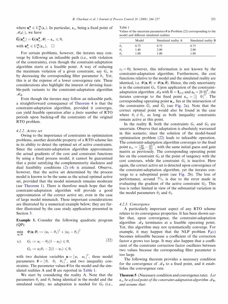
Table 1Values of the uncertain parameters h in Problem (22) corresponding to themodel and different simulated realities

Model Simulated reality A Simulated reality B

h1 0.75 0.75 0.75h2 1.40 2.00 2.00h3 1.00 1.00 1.80

B. Chachuat et al. / Journal of Process Control 18 (2008) 244–257 251

where uH

� 2 UH

h ðe�Þ. In particular, e1 being a fixed point ofMhð�Þ, we have

GðuH

1Þ ¼ GðuH

1; hÞ � e1 6 0;

with uH

1 2 UH

h ðe1Þ. h

For certain problems, however, the iterates may con-verge by following an infeasible path (i.e., with violationof the constraints), even though the constraint-adaptationalgorithm starts at a feasible point. A way of reducingthe maximum violation of a given constraint, say Gi, isby decreasing the corresponding filter parameter bi. Yet,this is at the expense of a lower convergence rate. Theseconsiderations also highlight the interest of devising feasi-ble-path variants to the constraint-adaptation algorithmMh.

Even though the iterates may follow an infeasible path,a straightforward consequence of Theorem 4 is that theconstraint-adaptation algorithm, provided it converges,can yield feasible operation after a finite number of RTOperiods upon backing-off the constraints of the originalRTO problem.

4.2.2. Active set

Owing to the importance of constraints in optimizationproblems, another desirable property of a RTO scheme liesin its ability to detect the optimal set of active constraints.Since the constraint-adaptation algorithm approximatesthe actual gradients of the cost and constraint functionsby using a fixed process model, it cannot be guaranteedthat a point satisfying the complementarity slackness anddual feasibility conditions (2)–(4) is attained. Observe,however, that the active set determined by the processmodel is known to be the same as the actual optimal activeset, provided that the model mismatch remains moderate(see Theorem 1). There is therefore much hope that theconstraint-adaptation algorithm will provide a goodapproximation of the correct active set, even in the caseof large model mismatch. These important considerationsare illustrated by a numerical example below; they are fur-ther illustrated by the case study application presented inSection 5.

Example 1. Consider the following quadratic program(QP):

minuP0

Uðu; hÞ :¼ ðu1 � h1Þ2 þ ðu2 � h1Þ2

s:t: G1 :¼ u1 � h2ð1� u2Þ 6 0;

G2 :¼ u2h3 � 2ð1� u1Þ 6 0;

ð22Þ

with two decision variables u ¼ ½ u1 u2 �T, three modelparameters h ¼ ½ h1 h2 h3 �T, and two inequality con-straints. The parameter values h for the model and the sim-ulated realities A and B are reported in Table 1.

We start by considering the reality A. Note that theparameters h1 and h3 being identical in the model and thesimulated reality, no adaptation is needed for G2 (i.e.,

e2 = 0); however, this information is not known by theconstraint-adaptation algorithm. Furthermore, the costfunctions relative to the model and the simulated reality areidentical, i.e. Uðu; hÞ � Uðu; hÞ. Hence, the only uncertaintyis in the constraint G1. Upon application of the constraint-adaptation algorithm Mh with B = I2·2 and e0 = [0 0]T, theiterates converge to the fixed point e1 ¼ ½ 15 0 �T. Thecorresponding operating point u1 lies at the intersection ofthe constraints G1 and G2 (see Fig. 2a). Note that thecorrect optimal point would also be found in the casewhere h1 6¼ h1, as long as both inequality constraintsremain active at this point.

In the reality B, both the constraints G1 and G2 areuncertain. Observe that adaptation is absolutely warrantedin this scenario, since the solution of the model-basedoptimization problem (22) leads to infeasible operation.The constraint-adaptation algorithm converges to the fixedpoint e1 ¼ 69

290� 1429

� �T, with the same initial guess and gain

matrix as previously. The corresponding operating pointlies on the constraint G2 at the point of tangency with thecost contours, while the constraint G1 is inactive. Hereagain, the correct active set is detected upon convergence ofthe constraint-adaptation algorithm, yet the iterates con-verge to a suboptimal point (see Fig. 2b). The loss ofperformance, around 7%, is due to the error made inevaluating the gradient of the active constraint G2. Thisloss is rather limited in view of the substantial variation inthe model parameters h2 and h3.

4.2.3. Convergence

A particularly important aspect of any RTO schemerelates to its convergence properties. It has been shown ear-lier that, upon convergence, the constraint-adaptationalgorithm Mh terminates at a feasible operating point.Yet, this algorithm may not systematically converge. Forexample, it may happen that the NLP problem Ph(e)becomes infeasible because a coefficient of the correctionfactor e grows too large. It may also happen that a coeffi-cient of the constraint correction factor oscillates betweentwo values because the corresponding filter parameter istoo large.

The following theorem provides a necessary conditionfor the convergence of Mh to a fixed point, and it estab-lishes the convergence rate.

Theorem 5 (Necessary condition and convergence rate). Lete1 be a fixed point of the constraint-adaptation algorithm Mh,

and assume that:

Simulated Reality A

Simulated Reality B

0.4

0.5

0.6

0.7

0.8

0.9

0.4 0.5 0.6 0.7 0.8 0.9 0.4

0.5

0.6

0.7

0.8

0.9

0.4 0.5 0.6 0.7 0.8 0.9

0.4

0.5

0.6

0.7

0.8

0.9

0.4 0.5 0.6 0.7 0.8 0.9 0.4

0.5

0.6

0.7

0.8

0.9

0.4 0.5 0.6 0.7 0.8 0.9

Fig. 2. Illustration of the constraint-adaptation algorithm for Problem (22). Left plots: no constraint adaptation; Right plots: converged constraintsadaptation; Thin solid lines: constraint bounds for the simulated reality; Colored area: feasible region; Thick dash-dotted lines: constraint bounds predictedby the model without adaptation; Thick solid lines: constraint bounds predicted by the model upon convergence of the constraint-adaptation algorithm;Dotted lines: contours of the cost function; Point R: optimum for the simulated reality; Point M: optimum for the model without adaptation; Point C:optimum for the model upon convergence of the constraint-adaptation algorithm; Arrows: direction of constraints adaptation.

252 B. Chachuat et al. / Journal of Process Control 18 (2008) 244–257

(1) the second-order sufficient conditions for a local mini-

mum of Ph(e1) hold at u1 2 UH

h ðe1Þ, with the associ-

ated Lagrange multipliers l1, fU1, and fL

1;

(2) u1 is a regular point for the active constraints;(3) l1,k > 0, fU

1;k > 0, and fL1;k > 0 for each active

constraint.

Then, a necessary condition for the local convergence of

Mh to the fixed point e1 is that the gain matrix B be chosen

such that

. I�B Iþ oG

ouðu1;hÞ�

o�G

ouðu1Þ

� �PuMhðe1Þ�1

Nhðe1Þ� ��

< 1;

ð23Þ

where the matrices Mh 2 Rðngþ3nuÞ�ðngþ3nuÞ, Nh 2 Rng�ðngþ3nuÞ,

and Pu 2 Rnu�ðngþ3nuÞ are defined as

MhðeÞ :¼

o2Uou2 þlT o2G

ou2oG1

ou� � � oGng

ouInu�nu �Inu�nu

l1oG1

ou

TG1� e1

..

. . ..

lng

oGng

ou

TGng � eng

diagðfUÞ diagðu�uUÞ�diagðfLÞ diagðuL�uÞ

0BBBBBBBBBBBB@

1CCCCCCCCCCCCANhðeÞ :¼ 0ng�nu �diagðlÞ 0ng�2nu

� T; Pu :¼ Inu�nu 0nu�ðngþ2nuÞ

� ;

and .{Æ} stands for the spectral radius. Moreover, if the con-

straint-adaptation converges, then the rate of convergence islinear.

Table 2Values of the uncertain parameters h in Problem (25) corresponding to themodel and the simulated reality.

Model Simulated reality

h1 0.5 0.5h2 1.1 0.2h3 1.0 �1.0

B. Chachuat et al. / Journal of Process Control 18 (2008) 244–257 253

Proof. It follows from the assumptions and Theorem 1that there is some g > 0 such that, for each e 2 Bgðe1Þ,there exists a unique continuously differentiable vectorfunction nhðeÞ ¼ uH

h ðeÞT

lHTh ðeÞ fUH

h ðeÞT

fLH

h ðeÞT

� �Tsatisfying the second-order sufficient conditions for a local

minimum of Ph(e), with nhðe1Þ ¼ uT1 lT

1 fU1

TfL1

Th iT

.

Moreover, we have (see Remark 1):

ouH

h

oeðe1Þ ¼ �PuMhðe1Þ�1

Nhðe1Þ:

The constraint functions Gi(Æ,h) and Gið�Þ, i = 1, . . . ,ng,being differentiable with respect to u, it follows that Ch(Æ)given by (19) is also differentiable with respect to e in aneighborhood of e1, and we have

oCh

oeðe1Þ ¼ I� oG

ouðu1; hÞ �

oG

ouðu1Þ

� �ouH

h

oeðe1Þ

¼ Iþ oG

ouðu1; hÞ �

oG

ouðu1Þ

� �PuMhðe1Þ�1

Nhðe1Þ:

That is, a first-order approximation of Ch in a neighbor-hood of e1 is

ChðeÞ ¼ Iþ oG

ouðu1;hÞ �

o�G

ouðu1Þ

� �PuMhðe1Þ�1

Nhðe1Þ� �

de

þ oðkdekÞ;

where de :¼ e � e1.Next, suppose that the algorithm (20), with e0 given,

converges to e1. Then,

9k0 > 0 such that ek 2 Bgðe1Þ 8k > k0

and we have

dekþ1 ¼ N1dek þ oðkdekkÞ ð24Þfor each k > k0, with

N1 :¼ I�B Iþ oG

ouðu1;hÞ�

oG

ouðu1Þ

� �PuMhðe1Þ�1

Nhðe1Þ� �

:

For Mh to converge to e1, the spectral radius of N1 musttherefore be less than 1.

Finally, it follows from (24) that, if Mh converges, thenit has a linear rate of convergence. h

Remark 3. It follows from the local analysis performed inthe proof of Theorem 5 that a necessary conditions for theiterates ek to converge to the fixed point e1 monotonically,i.e. without oscillations around e1, is that all of the eigen-values of the matrix N1 be nonnegative.

We illustrate these results in the following example.

Example 2. Consider the same QP problem (22) as inExample 1, with the parameters specified in Table 1. Forthe simulated reality A, the converged correction factors aswell as the corresponding inputs and multipliers are:

e1 ¼15

0

� �; uH

h ðe1Þ ¼2323

!; lH

h ðe1Þ ¼5

541

27

!:

In particular, it can be verified that the second-order suffi-cient conditions hold at uH

h ðe1Þ. The derivativesouH

h

oeand oCh

oe

at e1 are obtained as

ouH

h

oeðe1Þ ¼

1

9

59� 7

9

� 109

59

!;

oCh

oeðe1Þ ¼

53� 1

3

0 1

� �:

Upon choosing the diagonal gain matrix as B :¼ cI, thematrix N1 :¼ I� B oCh

oeðe1Þ reads

N1 ¼1� 5

3c � 1

3

0 1� c

� �:

Clearly, the necessary condition (23) is satisfied for every0 < c < 6

5. Note also that monotonic convergence is en-

sured as long as 0 < c 6 35

(see Remark 3).

The foregoing analysis provides conditions that are nec-essary for the constraint-adaptation algorithm to converge.Yet, these conditions are inherently local and, in general,they are not sufficient for convergence. This is the case,e.g., when the algorithm starts far away from a fixed point.Another source of divergence for the constraint-adaptationalgorithm is when the constraint map Ch(e) is always non-zero, i.e., the algorithm does not have a fixed point. Onesuch example is discussed subsequently.

Example 3. Consider the (convex) QP:

minuP0

Uðu; hÞ ¼ ðu1 � h1Þ2 þ ðu2 � h1Þ2

s:t: G :¼ h2 � u1 � u2h3 6 0;ð25Þ

with two decision variables u ¼ ½ u1 u2 �T, three uncertainparameters h ¼ ½ h1 h2 h3 �T whose values for both themodel and the simulated reality are given in Table 2, anda single constraint to be adapted using the constraint cor-rection factor e.

Upon application of the constraint-adaptation algo-rithm with B = cI, c > 0, the iterates are found to diverge,ek! +1 as k! +1. The situation is illustrated in the leftplot of Fig. 3. Here, divergence occurs because the optimalsolution set UH

h ðeÞ does not intersect with the plant feasibleregion, irrespective of the constraint correction factor e. Inother words, the constraint map Ch(e) shown in the rightplot of Fig. 3 is always nonzero, i.e., the algorithm does nothave a fixed point. Clearly, the necessary conditions givenin Theorem 5 do not hold for this problem.

Fig. 3. Divergence of the constraint-adaptation algorithm for Problem (25). Left plot: iterates in the u1 � u2 space; Thin solid lines: constraint bounds forthe simulated reality; Colored area: feasible region; Thick dash-dotted lines: constraint bounds predicted by the model without adaptation; Thin dash-dotted

lines: constraint bounds upon application of the constraint-adaptation algorithm; Dotted lines: contours of the cost function; Point R: optimum for thesimulated reality; Point M: optimum for the model without adaptation; Arrow: direction of constraint adaptation; Right plots: optimal solution point uH

h ðeÞand constraint map Ch(e) versus e.

254 B. Chachuat et al. / Journal of Process Control 18 (2008) 244–257

4.2.4. Effect of measurement errors

To analyze the effect of measurement errors on the con-vergence of the constraint-adaptation algorithm, supposethat the constrained quantities during the kth RTO periodare measured as GðuH

k Þ þ DGk instead of GðuH

k Þ. From (17),the measurement errors DGk give rise to the followingerrors in the correction factors:

Dekþ1 ¼ �BDGk:

In turn, provided that the correction factors ek+1 are in aneighborhood of the fixed point e1, a first-order approxi-mation of the input deviations is obtained as

DuH

kþ1 ¼ �ouH

h

oeðe1ÞBDGk þ 0ðkDGkkÞ

¼ PuMhðe1Þ�1Nhðe1ÞBDGk þ oðkDGkkÞ:

Accordingly, variations in both the correction factors andthe process inputs induced by measurement errors can bereduced by tuning the gain matrix B. In the case of a diag-onal gain matrix, this is done most easily by decreasing thegain coefficients b1; . . . ; bng . Yet, this is at the expense of aslower convergence, and a tradeoff must therefore be foundbetween the level of filtering and the speed of convergenceof the algorithm. In particular, observe that DuH

kþ1 may stillbe very large although Dek+1 is small, e.g., when some of

the sensitivity coefficientsouH

h

oeðe1Þ are large.

In the case where the measurements of the constrainedquantities are biased, with permanent offset equal toDG1, the fixed point e1 is shifted by De1 so that

e1 þ De1 � ðGðu1 þ Du1; hÞ �Gðu1 þ Du1Þ � DG1Þ ¼ 0;

where Du1 stands for the input shift.For small measurement biases, the following first-order

approximation of the error De1 is obtained:

De1 ¼ � Iþ oG

ouðuH

1;hÞ �oG

ouðuH

1Þ� �

PuMhðe1Þ�1Nhðe1Þ

� �þ�DG1 þ oðkDG1kÞ;

where A+ :¼ (ATA)�1AT stands for the Moore–Penrosepseudoinverse of A. Interestingly, the deviation De1 de-pends not only on the sensitivity

ouH

h

oeðe1Þ, but also on the

difference between the gradients of the predicted and mea-sured constraints at uH

1. This analysis confirms the ratherintuitive idea that biased measurements are likely to yieldlarger deviations of the correction factors when a poormodel is used, especially when the optimal inputs are highlysensitive to the correction factors.

5. Case study

The example presented in [27] is considered to illustratethe constraint-adaptation algorithm. It consists of anisothermal continuous stirred-tank reactor with tworeactions:

Aþ B! C; 2B! D: ð26ÞThe desired product is C, while D is undesired. The reactoris fed by two streams with the flow rates FA and FB and thecorresponding inlet concentrations cAin

and cBin.

5.1. Model equations and parameters

The steady-state model results from material balanceequations:

F AcAin� ðF A þ F BÞcA � r1V ¼ 0; ð27Þ

F BcBin� ðF A þ F BÞcB � r1V � 2r2V ¼ 0; ð28Þ

� ðF A þ F BÞcC þ r1V ¼ 0; ð29Þ

with

Table 4Plant optimum for various values of the parameter �k1

�k1 F H

A F H

Bqr

qr;max

F AþF BF max

UH

0.3 8.21 13.79 0.887 1.000 8.050.75 8.17 13.83 1.000 1.000 11.161.5 7.61 13.05 1.000 0.940 12.30

Table 3Nominal model parameters and parameter bounds

k1 1.5 lmol h k2 0.014 l

mol h

cAin2 mol

l cBin1.5 mol

l

DH1 �7 · 104 Jmol DH2 �105 J

mol

V 500 l qr,max 106 Jh

Fmax 22 lh

B. Chachuat et al. / Journal of Process Control 18 (2008) 244–257 255

r1 ¼ k1cAcB; r2 ¼ k2c2B: ð30Þ

The heat produced by the chemical reactions is:

qr ¼ ð�DH 1Þr1V þ ð�DH 2Þr2V : ð31ÞThe variables and parameters are: cX: concentration of spe-cies X, V: volume, ri: rate of reaction i, ki: kinetic coefficientof reaction i, DHi: enthalpy of reaction i.

The numerical values of the parameters are given inTable 3. In the sequel, k1 denotes the value of the kineticparameter used in the process model,4 whereas �k1 corre-sponds to the value used in the simulated reality.

5.2. Optimization problem

The objective function is chosen as the amount of prod-uct C, (FA + FB)cC, multiplied by the yield factorðF A þ F BÞcC=F AcAin

. Upper bounds exist for the amountof heat qr produced by the reactions and the total flowF :¼ FA + FB (see Table 3). The optimization can be for-mulated mathematically as:

maxF A;F B

U :¼ ðF A þ F BÞ2c2C

F AcAin

s:t: model equations ð27Þ–ð31Þ;G1 :¼ qr � qr;max 6 0;

G2 :¼ F A þ F B � F max 6 0:

ð32Þ

The optimal feed rates, the values of the constrained quan-tities, and the objective function for �k1 ¼ 0:3, 0.75 and1:5 l

mol hare given in Table 4. Notice that the set of active

constraints in the optimal solution changes with the valueof �k1.

5.3. Constraint-adaptation algorithm

Since the constraint G2 is not affected by the uncertaintyin k1, only the constraint G1 requires adaptation. That is,the filter parameter for G2 is set to b2 = 0 throughout.

5.3.1. Accuracy of the constraint-adaptation algorithm

In this paragraph, the accuracy of the constraint-adap-tation algorithm, upon convergence, is investigated in theabsence of measurement noise and process disturbances(ideal case).

4 Note that this value is different from the one used in [27].

The scaled constrained quantities qr/qr,max and(FA + FB)/Fmax are represented in Fig. 4 for values of �k1

(simulated reality) varying in the range 0.3 to 1:5 lmol h

.Note that the constrained quantities obtained with the con-straint-adaptation algorithm (thick lines) follow closelythose of the true optimal solution (thin lines). But,although the proposed algorithm guarantees feasible oper-ation upon convergence irrespective of the value of �k1, itfails to detect the correct active set in the vicinity of thoseoperating points where the active set changes (i.e.,�k1 0:65 and �k1 0:8). This deficiency results from theerror introduced by the process model in the evaluationof the sensitivities with respect to FA and FB of both thecost function and the process-dependent constraints.

Fig. 5 shows the performance loss

DU :¼ UH � UðuH

1ÞUH

where UH denotes the plant optimal cost value, and UðuH

1Þthe cost value upon convergence of the constraint-adapta-tion algorithm. Clearly, DU is equal to zero for �k1 ¼ 1:5,for there is no model mismatch in this case. Interestinglyenough, DU is also equal to zero when the two constraintsare active and the adaptation scheme provides the correctactive set; this situation occurs for �k1 in the range0:68 < �k1 < 0:79 (see Fig. 4). Overall, the performance lossremains lower than 0.6% for any value of �k1 in the range0:3–1:5 l

mol h, and is even lower (less than 0.2%) with k1 cho-

sen as 0.3 and 0:75 lmol h

in the process model. These resultsdemonstrate that the optimal loss remains limited, despite

Fig. 4. Optimal values of the constrained quantities qr/qr,max (solid lines)and (FA + FB)/Fmax (dashed lines) versus �k1, for k1 ¼ 1:5 l

mol h. Thick lines:

Constraint-adaptation solution; Thin lines: Plant optimum.

Fig. 5. Performance loss of the constraint-adaptation solution. Thick line:k1 ¼ 1:5 l

mol h; Thin dot-dashed line: k1 ¼ 0:75 l

mol h; Thin dashed line:

k1 ¼ 0:3 lmol h

.

256 B. Chachuat et al. / Journal of Process Control 18 (2008) 244–257

the error made in the detection of the active set for somescenarios.

Fig. 7. Evolution of the constrained quantities. Thick lines: Scenario 1ð�k1 ¼ 0:75 l

mol hÞ; Thin lines: Scenario 2 �k1 ¼ 0:3 l

mol h

� .

5.3.2. Convergence of the constraint-adaptation algorithm

In this paragraph, we take a closer look at the conver-gence properties of the constraint-adaptation algorithm.Two scenarios that correspond to different sets of activeconstraints at the optimum are considered. In either sce-nario, the process model with k1 ¼ 1:5 l

mol his chosen. Note

also that the adaptation is started with a highly conserva-tive initial constraint factor e0 ¼ �1:5� 105 J

h, and the fil-

ter parameter for G1 is taken as b1 = 1 (no filtering).To depart from the ideal case of the previous paragraph,

Gaussian noise with standard deviation of 1800 Jh

is addedto the measurements of qr. In response to this, a back-offis introduced so as to ensure that the heat production con-straint is satisfied, i.e., qr;max ¼ 9:9� 105 J

h. Two scenarios,

corresponding to a simulated reality with �k1 ¼ 0:75 lmol h

and 0:3 lmol h

, respectively, are considered.Scenario (1) Simulated reality with �k1 ¼ 0:75 l

mol h. The

evolution of the constraint factor e with the RTO periodis shown in Fig. 6 (thick line). A negative value of e indi-cates that the heat production is overestimated by themodel, which is consistent with the values of �k1 chosenfor the simulated reality. Note also that the convergence

Fig. 6. Evolution of the constraint factor e. Thick lines: Scenario 1�k1 ¼ 0:75 l

mol h

� ; Thin lines: Scenario 2 �k1 ¼ 0:3 l

mol h

� .

is very fast in this case, as the region where the adaptationis within the noise level is reached after two RTO periodsonly. The corresponding constrained quantities (FA + FB)and qr are represented in Fig. 7. Due to the chose back-off, the heat production remains lower than the maximumallowed value of 106 J

hdespite measurement noise.

Moreover, with this back-off, only the heat productionconstraint is active, while the feed rate remains lower thanthe maximum allowed feed rate (i.e., this scenario departsfrom the ideal case shown in Fig. 4 where both constraintsare active). Finally, the evolution of the cost function U isshown in Fig. 8 (thick line). The converged cost value isclose to 11, i.e., within a few percent of the ideal cost givenin Table 4. The performance loss results from the back-offfrom the heat production constraint.

Scenario (2) Simulated reality with �k1 ¼ 0:3 lmol h

. Theevolution of the constraint factor e, the constrained quan-tities (FA + FB) and qr, and the objective function U, withthe RTO iteration is shown as thin lines in Figs. 6–8,respectively. It is seen from Fig. 6 that the constraint factoris larger in this scenario than in the previous one, as theprocess model is even farther from the simulated reality.Moreover, Fig. 7 shows that only the feed rate constraintsgets active, while the heat production remains inactive.Hence, the optimal inputs are unaffected by the

Fig. 8. Evolution of the cost function. Thick lines: Scenario 1�k1 ¼ 0:75 l

mol h

� ; Thin lines: Scenario 2 �k1 ¼ 0:3 l

mol h

� .

B. Chachuat et al. / Journal of Process Control 18 (2008) 244–257 257

measurement noise. It takes a single RTO period for theconstraint-adaptation algorithm to detect the correct activeset in this case. Finally, it is seen from Fig. 8 that the con-verged cost value of about 8 is very close to the plant opti-mum reported in Table 4, in spite of the large modelmismatch.

6. Conclusions

In this paper, constraint-adaptation algorithms havebeen considered in the context of real-time optimization.The underlying idea is to use the measurements for adapt-ing the process constraints in each RTO period, while rely-ing on a fixed process model for satisfying the remainingpart of the NCO. Constraints-adaptation algorithms arebased on the observation that, for many problems, mostof the optimization potential arises from activating the cor-rect set of constraints. In the first part of the paper, we haveprovided a theoretical justification of these methods, in thecase of moderate uncertainty, based on a variational anal-ysis of the cost function. Then, various aspects of the con-straint-adaptation algorithm have been discussed andillustrated through numerical examples, including thedetection of active constraints and convergence issues.Finally, the case study of an isothermal stirred-tank reactorhas been presented, which illustrates the applicability andsuitability of this approach.

When the optimal solution lies on the constraints of theRTO problem, constraints adaptation provides fastimprovement within a small number of RTO periods.Moreover, this approach does not requires that the gradi-ent of the cost and constraint functions be estimated exper-imentally, which makes it less sensitive to measurementnoise than many other RTO methods. In return, the con-straint-adaptation algorithm may terminate at a subopti-mal, yet feasible, point upon convergence. Moreover, thisloss of optimality directly depends on the quality of the(fixed) process model.

It should also be noted that, unlike many model-freeRTO methods, the constraint-adaptation algorithm allowshandling constraints without having to make any assump-tion regarding the active constraints at the optimal point.Another major advantage with respect to many RTO meth-ods is that the nominal model employed does not requirerefinement, and thus the conflict between the identificationand optimization objectives is avoided. These features,together with constraint satisfaction and fast convergence,make the constraint-adaptation approach much appealingfor RTO applications.

References

[1] M.L. Darby, D.C. White, On-line optimization of complex processunits, Chem. Eng. Progress (1988) 51–59.

[2] T.E. Marlin, A.N. Hrymak, Real-time operations optimization ofcontinuous processes, in: AIChE Symposium Series – CPC-V, vol. 93,1997, pp. 156–164.

[3] R.E. Young, Petroleum refining process control and real-timeoptimization, IEEE Contr. Syst. Mag. 26 (6) (2006) 73–83.

[4] S.J. Qin, T.A. Badgwell, An overview of industrial model predictivetechnology, in: AIChE Symposium Series – CPC-V, vol. 93, 1997, pp.232–256.

[5] O. Rotava, A.C. Zanin, Multivariable control and real-time optimi-zation – an industrial practical view, Hydrocarbon Process 84 (6)(2005) 61–71.

[6] K.J. Astrom, B. Wittenmark, Adaptive Control, second ed., Addison-Wesley, Reading, Massachusetts, 1995.

[7] P.D. Roberts, T.W. Williams, On an algorithm for combined systemoptimisation and parameter estimation, Automatica 17 (1) (1981)199–209.

[8] P. Tatjewski, Iterative optimizing set-point control – the basicprinciple redesigned, in: 15th IFAC World Congress, Barcelona,Spain, 2002.

[9] B. Srinivasan, D. Bonvin, Interplay between identification andoptimization in run-to-run optimization schemes, in: AmericanControl Conference, Anchorage, AK, 2002, pp. 2174–2179.

[10] B. Srinivasan, D. Bonvin, Real-time optimization of batch processesby tracking the necessary conditions of optimality, Ind. Eng. Chem.Res. 46 (2) (2007) 492–504.

[11] G.E.P. Box, N.R. Draper, Evolutionary Operation, A statisticalmethod for process improvement, John Wiley, New York, 1969.

[12] M. Kristic, H.-H. Wang, Stability of extremum seeking feedback forgeneral nonlinear dynamic systems, Automatica 36 (2000) 595–601.

[13] P.D. Roberts, Broyden derivative approximation in ISOPE optimis-ing and optimal control algorithms, in: 11th IFAC Workshop onControl Applications of Optimisation, vol. 1, St. Petersburg, Russia,2000, pp. 283–288.

[14] S. Skogestad, Self-optimizing control: the missing link betweensteady-state optimization and control, Comput. Chem. Eng. 24(2000) 569–575.

[15] G. Francois, B. Srinivasan, D. Bonvin, Use of measurements forenforcing the necessary conditions of optimality in the presence ofconstraints and uncertainty, J. Process Contr. 15 (6) (2005) 701–712.

[16] S. Gros, B. Srinivasan, D. Bonvin, Static optimization based onoutput feedback, Comput. Chem. Eng., submitted for publication.

[17] P. Tatjewski, M.A. Brdys, J. Duda, Optimizing control of uncertainplants with constrained feedback controlled outputs, Int. J. Control74 (15) (2001) 1510–1526.

[18] J.F. Forbes, T.E. Marlin, Model accuracy for economic optimizingcontrollers: the bias update case, Ind. Eng. Chem. Res. 33 (1994)1919–1929.

[19] A. Desbiens, A.A. Shook, IMC-optimization of a direct reduced ironphenomenological simulator, in: 4th International Conference onControl and Automation, Montreal, Canada, 2003, pp. 446–450.

[20] W. Gao, S. Engell, Iterative set-point optimization of batch chroma-tography, Comput. Chem. Eng. 29 (2005) 1401–1409.

[21] M.S. Bazaraa, H.D. Sherali, C.M. Shetty, Nonlinear Programming:Theory and Algorithms, second ed., John Wiley and Sons, New York,1993.

[22] A.V. Fiacco, in: Introduction to Sensitivity and Stability Analysis inNonlinear Programming, Mathematics in Science and Engineering,vol. 165, Academic Press, New York, 1983.

[23] Y. Zhang, General robust-optimization formulation for nonlinearprogramming, J. Opt. Th. Appl. 132 (1) (2007) 111–124.

[24] B. Bank, J. Guddat, D. Klatte, B. Kummer, K. Tammer, Non-LinearParametric Optimization, Birkhauser Verlag, Basel, 1983.

[25] A.V. Fiacco, Y. Ishizuka, Sensitivity and stability analysis fornonlinear programming, Ann. Oper. Res. 27 (1990) 215–236.

[26] W.W. Hogan, Point-to-set maps in mathematical programming,SIAM Rev. 15 (1973) 591–603.

[27] B. Srinivasan, L.T. Biegler, D. Bonvin, Tracking the necessaryconditions of optimality with changing set of active constraints usinga barrier-penalty function, Comput. Chem. Eng., in press,doi:10.1016/j.compchemeng.2007.04.004.