proceedings_book_f.pdf - Transport and Telecommunication ...

The 14th International Conference

RELIABILITY and STATISTICS in TRANSPORTATION and COMMUNICATION

(RelStat’14)

15–18 October 2014. Riga, Latvia

Organised by

Transport and Telecommunication Institute (Latvia)The K.Kordonsky Charitable Foundation (USA)

in co-operation withLatvian Academy of Science (Latvia)

PROCEEDINGS

Edited by

Igor V. Kabashkin

Irina V. Yatskiv

RIGA - 2014

Proceedings of the 14th International Conference RELIABILITY and STATISTICS in TRANSPORTATION and COMMUNICATION (RelStat’14), 15–18 October 2014, Riga, Latvia.

THE PROGRAMME COMMITTEE

Prof. Adolfas Baublys, Vilnius Gediminas Technical University, LithuaniaProf. Maurizio Bielli, Institute of System Analysis and Informatics, ItalyDr. Brent D. Bowen, Purdue University, USADr. Vadim Donchenko, Scientific and Research Institute of Motor Transport, RussiaProf. Ernst Frankel, Massachusetts Institute of Technology, USAProf. Alexander Grakovski, Transport & Telecommunication Institute, LatviaProf. Igor Kabashkin, (Chairman) Transport & Telecommunication Institute, LatviaProf. Eugene Kopytov, Transport & Telecommunication Institute, LatviaProf. Zohar Laslo, Sami Shamoon College of Engineering, IsraelProf. Andrzej Niewczas, Lublin University of Technology, PolandProf. Lauri Ojala, Turku School of Economics, FinlandProf. Jurijs Tolujevs, Transport & Telecommunication Institute, LatviaProf. Irina Yatskiv, Transport & Telecommunication Institute, LatviaProf. Edmundas Zavadskas, Vilnius Gediminas Technical University, Lithuania

ORGANIZATION COMMITTEE

Prof. Igor Kabashkin, Latvia – Chairman Mrs. Inna Kordonsky-Frankel, USA – Co-ChairmanProf. Irina Yatskiv, Latvia – Co-ChairmanMrs. Anna Agafonova, Latvia – Secretary

All articles are reviewed by members of the Programme Commitee.

Transport and Telecommunication InstituteLomonosova iela 1, LV-1019, Riga, Latviahttp://RelStat.tsi.lv

ISBN 978-9984-818-70-2

Transport and Telecommunication Institute, 2014

iii

The 14th International Conference “RELIABILITY and STATISTICS in TRANSPORTATION and COMMUNICATION - 2014”

ContentsSession 1. Transport Systems

IDENTIFYING MODAL SHIFT BY UTILITY FUNCTIONS TO ENHANCE REGIONAL DEVELOPMENTTamas Andrejszki, Maria Csete, Adam Torok ................................................................................................2

THE EAST-WEST TRANSPORT CORRIDOR ACTIVITIES GOVERNANCEDarius Bazaras, Ramūnas Palšaitis ............................................................................................................. 9

HOW TO DELIVER THE NECESSARY DATA ABOUT SERIOUS INJURIES TO THE EU?Péter Holló, Diána Sarolta Kiss ................................................................................................................. 17

THE FUTURE OF AUTOMOTIVE - AUGMENTED REALITY VERSUS AUTONOMOUS VEHICLESTomasz Serafin and Jacek Mazurkiewicz .................................................................................................... 23

THE OPTIMIZATION VARIANTS OF POSTAL TRANSPORTATION NETWORKRadovan Madleňák, Lucia Madleňáková, Jozef Štefunko .......................................................................... 34

CONTROLLING CONCEPTS FOR GREEN TRANSPORT CORRIDORSGunnar Prause ............................................................................................................................................ 42

SAFETY INSPECTIONS OF RAILWAY CROSSINGS AND STRENGTHENING OF INDIVIDUAL RESPONSIBILITY FOR SUSTAINABLE TRAFFIC SAFETYLajos Szabó, Viktor Nagy ............................................................................................................................ 50

STAKEHOLDER TYPOLOGYAND DIMENSIONS OF GREEN TRANSPORT CORRIDORSMike Wahl, Gunnar Prause ......................................................................................................................... 59

THE IMPACT OF ACCESSIBILITY ON TRANSPORT INFRASTRUCTURE WITHIN COMMERCIAL SITENadezhda Zenina, Yuri Merkuryev .............................................................................................................. 69

Session 2. Transport Logistics

CLASSIFICATION OF LOGISTIC PRODUCTS IN TERMINAL NETWORK MULTIMODAL TRANSPORTATIONVladimir Glinskiy, Polina Butrina .............................................................................................................. 78

DEVELOPMENT OF THE ALGORITHM FOR DESIGN AND REENGINEERING OF LOGISTICS DISTRIBUTION NETWORKValentina Dybskaya ..................................................................................................................................... 84

MODEL OF DECISION SUPPORT FOR ALTERNATIVE CHOICE IN THE LARGE SCALE TRANSPORTATION TRANSIT SYSTEMIgor Kabashkin, Jelena Mikulko ................................................................................................................. 92

TRANSMODAL SHIPMENT: DEFINITION AND FORMULATION OF OPTIMISATION PROBLEMSAleksandr Kirichenkо, Elena Koroleva .................................................................................................... 102

LAYER MODEL OF THE POSTAL SYSTEM Lucia Madleňáková, Radovan Madleňák ................................................................................................. 106

INDUSTRY 4.0 AND ITS IMPACT ON SUPPLY CHAIN RISK MANAGEMENTMeike Schröder, Marius Indorf, Wolfgang Kersten ...................................................................................114

STATUS ANALYSIS OF LOGISTICS CONTROLLING AT RUSSIAN COMPANIESVictor Sergeyev .......................................................................................................................................... 126

iv


Session 3. Reliability and Maintenance

THE EVALUATION OF THE RELIABILITY OF SUPPLY CHAINS: FAILURE MODELSValery Lukinskiy, Vladislav Lukinskiy ....................................................................................................... 136

EXPERIMENTAL STUDY OF A ROLLER BEARING KINEMATICS THROUGH A HIGH-SPEED CAMERAAlexey Mironov, Pavel Doronkin, Sergey Yunusov ................................................................................... 142

Session 4. Intelligent Transport Systems

GPS/GLONASS TRACKING DATA SECURITY ALGORITHM WITH INCREASED CRYPTOGRAPHIC STABILITYSergey Kamenchenko ................................................................................................................................ 154

USING OF THE ADAPTIVE ALGORITHM FOR NARROWING OF THE PARAMETER SEARCHING INTERVALS IN INVERSE PROBLEM OF ROADWAY STRUCTURE MONITORINGAlexander Krainyukov, Valery Kutev ........................................................................................................ 165

EXAMINATION OF MULTIPATH STRUCTURE ON SOME ELECTROMAGNETIC TRANSIENTSYury A. Krasnitsky ..................................................................................................................................... 177

ARTIFICIAL NEURAL NETWORK ADJUSTMENT FOR INVERSE PROBLEM OF PLATE-LAYERED MEDIA SUBSURFACE RADAR PROBINGDaniil Opolchenov, Valery Kutev .............................................................................................................. 186

FIBRE-OPTIC SENSORS CALIBRATION METHOD BASED ON GENETIC ALGORITHM IN WEIGHT-IN-MOTION PROBLEM Alexey Pilipovecs, Alexander Grakovski ................................................................................................. 192

EFFICIENT MEASURING OF COMPLEX PROGRAMMABLE LOGIC DEVICE (CPLD) IMPLEMENTED ANALOG-TO-DIGITAL CONVERTERS STATIC PARAMETERSSergejs Šarkovskis, Sergejs Horošilovs ..................................................................................................... 200

PILOT TESTING EVALUATION OF PORTABLE SYSTEM OF DYNAMIC TRAFFIC FLOW MANAGEMENT AT TRAFFIC CLOSURESMarek Ščerba, Tomáš Apeltauer, Jiří Apeltauer ....................................................................................... 208

Session 5. Transport and Logistics System Modelling

THE APPLICATION OF A NEW ITERATIVE OD MATRIX ESTIMATION FOR URBAN PUBLIC TRANSPORTBalázs Horváth, Richárd Horváth ............................................................................................................ 218

MODELLING OF CONTAINER TRAINS IN THE STRUCTURE OF A DRY PORT WITH THE USE OF TECHNOLOGY “BLOCK-TRAIN”Mikhail Malykhin, Aleksandr Kirichenko ................................................................................................. 225

THE USE OF MATHEMATICAL MODELS FOR LOGISTICS SYSTEMS ANALYSISBaiba Zvirgzdiņa, Jurijs Tolujevs ............................................................................................................. 230

Session 6. Aviation

“FLYING TRUCKS” CONCEPT AS AN ALTERNATIVE FOR THE DEVELOPMENT OF THE REGIONAL AIRPORTS IN THE BALTIC SEA REGIONAnatoli Beifert ........................................................................................................................................... 242

v


USING THRUST-BASED SAFETY MARGIN OF GAS TURBINE ENGINE AS A CRITERION FOR ASSESSMENT ITS TECHNICAL STATEEugene Kopytov, Vladimir Labendik, Sergey Yunusov ............................................................................. 250

THE LITHIUM-ION BATTERIES OF BOEING 787 – ARE THEY ALREADY SAFE?Mária Mrázová, Paulína Jirků, Ján Pitor ................................................................................................ 258

GLOBAL AIRLINE ALLIANCES MODELSAlena Novák Sedláčková, Marek Turiak ................................................................................................... 268

FLIGHT SIMULATION TRAINING DEVICE TERRAIN MODEL CREATIONJán Pitor, Mária Mrázová, Paulína Jirků ................................................................................................. 274

Session 7. RFID Applications for Transport and Logistics

UHF RFID TAG FOR UNDERWATER APPLICATIONSLibor Hofmann .......................................................................................................................................... 284

MUTUAL COEXISTENCE OF ACTIVE AND PASSIVE RFID TECHNOLOGYPeter Kolarovszki, Zuzana Kolarovszká ................................................................................................... 294

THE USE OF RFID TECHNOLOGY TO IDENTIFY TRAFFIC SIGNSJuraj Vaculík, Jiří Tengler, Ondrej Maslák .............................................................................................. 303

THE CORRECTION OF RFID IDENTIFIERS SCANNING ERRORS ON DYNAMICALLY MOVING LOGISTIC UNITSDaniel Zeman, Jiří Tengler, Libor Švadlenka ........................................................................................... 313

Session 8. Applications of Mathematical Methods to Logistics and Business

USING OF THE ALGORITHM OF ARTIFICIAL IMMUNE SYSTEMS FOR ADAPTIVE MANAGEMENT AT CROSSROADSSergey Anfilets, Vasilij Shuts ..................................................................................................................... 324

MODELLING OF SPATIAL EFFECTS IN TRANSPORT EFFICIENCY: THE ‘SPFRONTIER’ MODULE OF ‘R’ SOFTWAREDmitry Pavlyuk ......................................................................................................................................... 329

DEDICATED HARDWARE IMPLEMENTATION OFKECCAK HASH ALGORITHM FOR IMPROVING SECURITY IN DATA PROCESSINGJarosław Sugier ......................................................................................................................................... 335

UTILISATION OF SELECTED MATHEMATICAL FUNCTIONS FOR SOME METAL OIL DATA EVALUATIONDavid Valis, Libor Žák .............................................................................................................................. 344

Session 9. IT Applications for Transport and Logistics

THE PERFORMANCE ANALYSIS OF WIFI DATA NETWORKS USED IN AUTOMATION SYSTEMSAleksandr Krivchenkov, Rodeon Saltanovs ............................................................................................... 356

DOMAIN-SPECIFIC SOFTWARE ARCHITECTURE OPTIMISATION FOR LOGISTICS AND TRANSPORT APPLICATIONS

Sergey Orlov, Andrei Vishnyakov ...............................................................................................................367

Transport Systems

Session 1

2

Session 1. Transport Systems

Proceedings of the 14th International Conference “Reliability and Statistics in Transportation and Communication”(RelStat’14), 15–18 October 2014, Riga, Latvia, p. 2–8. ISBN 978-9984-818-70-2Transport and Telecommunication Institute, Lomonosova 1, LV-1019, Riga, Latvia

IDENTIFYING MODAL SHIFT BY UTILITY FUNCTIONS TO REACH AN OPTIMAL POINT OF REGIONAL DEVELOPMENT

Tamas ANDREJSZKI1, Maria CSETE2, Adam TOROK3

1 Ph.D. student, Budapest University of Technology and Economics, Department of Transport Technology and Economics, Stoczek utca 2 Budapest H-1111, [email protected]

2 Associate professor, Budapest University of Technology and Economics, Department of Environmental Economics, Magyar tudósok körútja 2 Budapest H-1117, [email protected]

3 Assistant researcher, Budapest University of Technology and Economics, Department of Transport Technology and Economics, Stoczek utca 2 Budapest H-1111, [email protected]

The aim of this study was to analyze the modal shift of passengers by analyzing their preferences. If the preferences of passengers are known it is possible to simulate how the modal shift of the investigated area would change if there were some changes in the investigated parameters of transport services (e.g.: implementing a new transport service or introducing new development strategy).

To capture the preferences of passengers stated preference method was used in online questionnaire. Five key factors were identified (from the point of passengers): travel cost, travel time, comfort, safety and environmental efficiency. In these factors three levels was predefined as simplification which made the base of the choice model. At every replier got three alternatives and they were told to choose the best for themselves. From the results of the questionnaire the formulas and the parameters of the mode choice utility function was derived and identified. In the reviewed statistical sample an exponential utility function showed the best matching. For the validation process a probability model was set up to be compared to the proportions of the utilities.

With this utility function it is possible to handle possible future transport services by evaluating the services through the defined five factors. Based on the introduced statistical approach the described method can be used to identify the effect of transport modes on regional development.Keywords: Utility function; Modal shift; Stated preference

1. Introduction- the explanation of stated preference method

In the literatures stated preference method refers to two different concepts so it is important to define clearly the frames of the examination. The demand can be identified by the curves of indifference so the forecast of demands requires knowing the preferences of the consumers which is equal to the utility function of them. The direct way to interview consumers is a possible method (which is generally used) but it cannot be said a completely suitable tool to get the preferences. The individuals do not have real interest to reveal their preferences because there are no consequences of the answers so their wallet will not feel the gravity of the decision. Their decision is just a reaction to a hypothetic situation. An objective evaluation can be given only if the actual decisions are known so the preferences can be revealed only by the observation of the market behaviour. In 1947 P. A. Samuelson worked out the method of stated preference which makes it possible to simulate approximately the consumer preferences (plus the curves of indifference and the utility function) from factual data (e.g. prices, income, and demanded quantities). Based on Samuelson’s work it can be represented that the curves of indifference can be approximately identified from the information of the purchase if exact prerequisites are true (Karajz, 2008).

Nevertheless making interviews and questionnaires seems to be the best way to reveal transport demands of a future transport service (Kampf et. al., 2012). According to Kroes and Sheldon’s definition the term “stated preference method” refers to a family of techniques which use individual respondent’s statements about their preferences in a set of transport options to estimate utility function

3


(Kroes and Sheldon, 1988). Different stated preference methods are available under a wide variety of names; the best known methods are:

• Conjoint analysis;• Functional measurement;• Trade-off analysis;• The transfer price method.These methods were originally developed to marketing researches in the beginning of the 70’s

but a study from 1978 made them known (Green and Srinivasan, 1978). In this study the authors gave the following description to define the conjoint analysis (which seems to be the most suitable for transport purposes): every method that aims to estimate the structure of the consumer preferences and the consumers evaluate options where the levels of the different quantities have been defined before.

2. Design consideration

The first step of designing a stated preference method examination is to identify the relevant variables (factors) and the values belong to each factor (levels). A related task is here the specification of the mathematical formula of the utility function which refers to the authors’ hypothesis about how the integrated preference comes from the individual preferences. The linear, additive, compensational model is the mostly used form which has the following structure:U = α1x1 + α2x2 + ... + αnxn (1)

Here U refers to the complete utility; xn is the value of factor n and αn is the utility weight of factor n. It is practical if the sum of the utility weights is 1.

The factors can be defined as continuous variables or as a group of discrete variables also. The stated preference method can also be used to test alternative hypothesises (Kroes and Sheldon, 1988).

The next step in planning is the optimization of the mathematical option combinations. According to the experiences it is worth decreasing the number of options because the respondents can be spared by not answering questions that are trivial. If the number of questions is less the willingness of respondents to fill out completely the questionnaire might be higher because it will not need that much time from them. If the number of factors and the belonging levels is given the needed number of combinations can be calculated.

The factorial structure (Kroes and Sheldon, 1988) refers to a combinatorial expression. Because of that the full factorial structure means all the possible combinations of the options and the partial factorial structure means an exact part of the full factorial one. There are values belong to the factors; and an exact value of an exact factor is called “quality”. In an option of a question there are more qualities but none of them comes from the same factor (e.g. in a question the first option to choose is a travel that takes 10 minutes, worth 3 €-s and has a low comfort level). The full factorial structure generates too much options and combinations at higher number of factors and levels so the partial factorial structure might be better to go on with.

The examination of stated preference method can be done by two possible ways. The first opportunity is when the questioner creates cards from preference possibilities and options and at each question more cards are given to the respondent. The task of the respondent here is to make a sequence from them. The second opportunity is to make choice option cards which contain predefined questions with predefined options so the task of the respondent is to tick the best option of the card that he/she would choose in the given situation (Kroes and Sheldon, 1988).

3. Identification of transport utility function

At every question the respondent is asked to choose one (the best) from three options. Based on the international literature in this model five key factors were considered as playing important role in decision making (Simecki et. al., 2013): the travel time, travel cost, comfort, safety and environmental friendliness. Each factor has three values (one bad, one middle and one good) so there are 15 qualities which are the followings:

• Travel time (T) 30 minutes, 20 minutes and 10 minutes;• Travel cost (TC) 4 €, 2 € and 1 €;• Comfort (C) not comfortable, more or less comfortable and comfortable;

4


• Safety (S) not safety , more or less safety and safety;• Environmental friendliness (E) not environmental friendly, more or less environmental

friendly and environmental friendly.These exact qualities come from a transport situation that is given to the respondent so they

have their meanings. In the situation the respondent lives in a small town and want to get to the train station to go to work in a weekday morning. By car this journey can be done in 10 minutes if there are no traffic jams. Comfort refers to the quality level of the transport service that was used (e.g. a crowded dirty bus means a non-comfortable mode but a clean car or train can represents a comfortable level; but comfort is not linked to any transport mode) (Duleba et. al., 2013). Safety in this meaning refers to the number of accidents that happens on the used section of road per one year. On a not safety section there are 12 accidents per year, the middle value is 4 accidents per year and the most safety value is 0.5 accidents per year. At environmental friendliness the emission level of an internal combustion engine was the sample for the so called bad level. This means more or less 179 g from CO2 per kilometre (Kok, 2013). The good level has almost zero emission like walking and cycling.

If we used all the qualities of all the five factors to create the three options of one question, that would cause 360 questions to be asked (if every quality appears maximum once in one question). To reduce this number at the beginning of the questionnaire respondents are asked to choose the three most relevant factors from the enumerated five. After this decision the following questions will just deal with the chosen three factors and count the non-chosen factors with a zero parameter in the individual utility function. According to this operation there are ten versions of the questionnaire:

(2)In one question there are always three options. In all the options there are three qualities from

three different factors. According to combinatory this means three repeated variation: (3)

But these 216 questions contain same questions with different order of the options. To have the real number of possible question 216 should be divided by the number of possible ordering:

(4)These 36 questions are equal to the full factorial structure. For further reduction the trivial

questions should be selected. In this case the expression “trivial” refers to those questions that have an option which contains three good qualities or two good qualities and one middle quality. The model handle these questions like these were answered by the respondent in a logical way so they always choose this outstanding option. After the selection of these trivial questions 20 questions remain that can be asked from the respondents. This amount seems to be user friendly and gives the hope of high filling rate.

4. The implemented questionnaire

In the implemented online questionnaire the transport situation was written first. Then the respondent chose the three more relevant factors. From these factors the respondent got 20 questions to answer. The questions were like Figure 1. As it can be seen this kind of questions includes partly the appointment of WTP (Willingness to pay) (Drevs et. al., 2014).

Figure 1. One question of the questionnaire

The questionnaire was filled out correctly by 462 respondents. The ages of the respondents are shown in Figure 2. As it can be seen the questionnaire was not representative (at the ages) but because of the time and cost constraints of the examination this was not an expectation.

5


Figure 2. The ages of the respondents

4.1. The algorithm of evaluation

The basis of the evaluation was to give 1-1 point to the qualities of the chosen option and give 0 point to the qualities of the non-chosen options. In this case each quality can gain 20 points as maximum and zero points as minimum. At this moment the 16 questions are added to the real answers then the maximum becomes 36 points. If the given factor is not important for the respondent -so it does not have a high preference – the points of the qualities of this factor will be around the one third of all questions

Figure 3. The process of the questionnaire and the evaluation

which is 12. If the factor was relevant for the respondent the good quality might get a higher score or (because avoiding the bad quality of this factor is also a preference) the bad quality might get

6


a lower score. From these values the individual utility function should be calculated. The parameter of one factor of the individual utility function is rational number in the interval of [0; 1] where:

• 0 is the preference parameter if the factor is absolutely not relevant;• 1 is the preference parameter if the factor is absolutely relevant.The parameter of factor 1 should be calculated by the following method. After the points of

each quality are summarised the next step is to calculate the square of the distances between the good quality and the average value (which is 12 now) and then to add the square of the distances between the bad quality and the average value. It is enough to examine just the good and the bad quality because (as it was mentioned before) the possible strategies of the respondents do not appear in the middle quality. So getting the middle quality into the algorithm would distort the utility function. After each factor has this basic value this value of factor 1 should be divided by the sum of this basic value of each factor. This process causes that the sum of the parameters gives 1. So if factor 1 is absolutely relevant its’ parameter will be 1 and the other factors’ parameter will be 0. The whole procedure can be seen in Figure 3.

The utility weights of the complete utility function come from the averages of the individual parameters. The structure of utility function was also the object of the examination. Linear, exponential and logarithmical models were considered but the most effective was the following structure:

(5)In this formula the same notation is used like in equation (1). The values that are connected

to the different levels are 1 for bad qualities, 2 for middle qualities and 3 for good qualities. In this case the worst combination of bad qualities causes the zero utility.

4.2. Process of validation

The accuracy of the model can be validated by the examination of the decision situations. The question is that: what is the ratio between the quotient of the utilities of two options and the quotient that shows how many people preferred the first option against the second.

To prepare the probability matrix the first step is to integrate the 10 versions (Figure 4). This is not trivial because the versions were filled out by different amount of people and in one question the complete order is not known because the respondent only chose the best option (so the relation of the two not chosen options is not known). So firstly 10 preference matrixes were created in the sizes of 27*27. In the columns and rows there are all the mathematically possible options so one element means that how many times were the option of the row chosen against the option of the column. The second step is the creation of another 10 matrixes called answered matrixes. Here the elements mean that how many times the respondents chose from the two options.

The probability matrix has 35 = 243 rows and 243 columns because in the integration all the 15 qualities of the five factors should be counted with. Every element is the quotient of choosing the option of the row against the option of the column. These options have five dimensions. In this five-dimension option there are 10 three-dimension options that can be found in the 10 preference matrixes and answered matrixes. So to get one element of the probability matrix the appropriate cells of the 10 preference matrixes should be summarised and then this sum should be divided by the sum of the appropriate cells of the answered matrixes.

In the edge of the utility matrix there are the same 243 options as in the probability matrix. One element means the quotient of the utility of the row option and the utility of the column option. Then the next step is to create a matrix in the same size where the elements show the relation between the utility and the probability matrixes. In this validation matrix the value is 1 if the two quotients are similar and 0 if not. Similarity means the followings:

• The row option is better [0; 0.45]• The row option is similar to the column option ]0.45; 0.55]• The column option is better ]0.55; ∞[So if the quotients are in the same interval the validation matrix element gets 1 if not it gets

0. After having all the values the average of them will give the accuracy of the model. In this case the accuracy level of 73.12% was reached. This level was accepted for further examinations with the created transport utility function.

7


Figure 4. The process of validation

4.3. Evaluation of transport projects by the utility function - Conclusion

With the above demonstrated process the utility of passengers can be determined. The analysis of this hidden and personal utility can help the professional transport planners to identifying the key parameters that play an important role in transport development (Stenci, Lendel, 2012) or enhance modal shift (Cerny et. al., 2014). This could help to find the optimal path of regional development.

The aim of this study was to show an easy method to statistically analyse passenger preferences. If the preferences of passengers are known it is possible to stimulate modal shift. To capture the passengers’ stated preferences an online questionnaire was built. Five passenger focused key factors were identified: travel time, cost, comfort, safety and environmental friendliness. In these factors three levels was predefined as simplification which made the base of the choice model. Although the statistical sample was not representative, this method gives a clear guideline for cities, companies and planners to create their questionnaires and make their sample representative. From the results of the questionnaire the parameters of the mode choice utility function were statistically estimated. An exponential utility function was used as it had the best fit for the examined sample. For the validation process a probability model was set up to be compared to the proportions of the utilities.

With this utility function it is possible to handle possible future transport services by evaluating the services through the defined five factors. It is feasible to compare the possibilities of transport developments, and the opportunity is given to make the comparison by measurable statistical indicators. Based on the introduced statistical approach the described method can be used to identify the effects of transport modes on regional development.

Acknowledgements

The authors are grateful to the support of Bolyai János Research fellowship of HAS (Hungarian Academy of Science).

References

1. Černýa J, Černáa A, Lindab B (2014): Support of decision-making on economic and social sustainability of public transport, Transport, 29(1):59-68, doi: 10.3846/16484142.2014.897645

2. Dulebaa Sz., Shimazakib Y., Mishinab T. (2013): An analysis on the connections of factors in a public

8


transport system by AHP-ISM, Transport, 28(4):404-412, doi: 10.3846/16484142.2013.8672823. Green, P. E., Srinivasan, V. (1978) - Conjoint analysis in consumer research: Issues and outlook.

Journal of Consumer Research, 5, 103-123.4. Kampf R., Gašparík J., Kudláčková N. (2012): Application of different forms of transport

in relation to the process of transport user value creation, Periodica Polytechnica Transport Engineering, 40(2):71-75, doi: 10.3311/pp.tr.2012-2.05

5. Karajz, S. (2009) - Közgazdasági elméletek (Economical theories), tutorial notes6. Kok, R. (2013) New Car Preferences Move Away from Greater Size, Weight and Power: Impact

of Dutch Consumer Choices on Average CO2-emissions. Transportation Research Part D: Transport and Environment 21 (June): 53–61. doi:10.1016/j.trd.2013.02.006.

7. Kroes, E.P., Sheldon, R.J. (1988) - Stated preference methods: an introduction, Journal of Transport Economics and Policy

8. Kumar M., Sarkar P., Madhu E. (2013): Development of fuzzy logic based mode choice model considering various public transport policy options, International Journal for Traffic and Transport Engineering, 3(4):408-425, doi: 10.7708/ijtte.2013.3(4).05

9. Šimecki A., Steiner S., Čokorilo O. (2013): The accessibility assessment of regional transport network in the south east Europe, International Journal for Traffic and Transport Engineering, 3(4):351-364, doi: 10.7708/ijtte.2013.3(4).01

10. Štencl M., Lendel V. (2012): Application of selected artificial intelligence methods in terms of transport and intelligent transport systems, Periodica Polytechnica Transport Engineering, 40(1):11-16, doi: 10.3311/pp.tr.2012-1.02

11. Drevs F., Tscheulin D. K., Lindenmeier J., Renner S. (2014): Crowding-in or Crowding out: An Empirical Analysis on the Effect of Subsidies on Individual Willingness-to-Pay for Public Transportation, Transportation Research Part A: Policy and Practice 59 (January): 250–61. doi:10.1016/j.tra.2013.10.023.

9


Proceedings of the 14th International Conference “Reliability and Statistics in Transportation and Communication” (Relstat’14), 15-18 October 2014, Riga, Latvia, p. 9–16. ISBN 978-9984-818-70-2Transport and Telecommunication Institute, Lomonosova 1, LV-1019, Riga, Latvia

THE EAST-WEST TRANSPORT CORRIDOR ACTIVITIES GOVERNANCE

Darius Bazaras1, Ramūnas Palšaitis2

1,2Transport Engineering Faculty, Vilnius Gediminas Technical UniversityPlytinės 27, Vilnius LT-10105, Lithuania

Phones 1(+370 5) 2370635; 2(+370 5) 2744776. E-mails:[email protected]; [email protected]

The keynote of the development is effective integration of the EU countries and East countries transport sector into East–West transport corridor service system and transport services market complying with the common criteria for transport development in the corridor. One of the biggest present problems is insufficient transport infrastructure and long border crossing procedures limiting international accessibility for goods and passengers. The joint action plan must highlight the areas and components of the transport system which are important for the effective interconnectivity of the individual networks, and/or for absorbing the steadily increasing intraregional and transcontinental freight flows. The development and modernization of transport infrastructure is one of the essential measures that ensure economic progress in working out national economy development strategies and programmes of both the EU, CIS and other East countries.Keywords: transport corridors, management, governance, planning, infrastructure

1. Introduction

Exist large differences between EU countries (Lithuania, Sweden, Denmark, Germany) and other countries located in the East of EU (Belarus, Ukraine, Russia, Kazakhstan, China). The disparity in quality and availability of infrastructure in particular is seen in the East-West connections (backlog of transport infrastructure investments in the East).

The keynote of the development is effective integration of the EU countries and East countries transport sector into East–West transport corridor service system and transport services market complying with the common criteria for transport development in the corridor.

All countries which are crossing EW transport corridor governmental authorities must consolidate the results of complex joint international efforts directed towards specifying the long-term plans for further East–West transport corridor development perspectives. These decisions must give the priority status at the highest governmental level to the EW transport corridor international importance, crossing the territory of 8–10 countries. The focus in the decisions must be given to the better use of the existing infrastructure, “intelligent” management of traffic, networks and systems.

Due to the East–West transport corridor countries specific nature and needs and apart the EW corridor, the region is covered by its own transport network. One of the biggest present problems is insufficient transport infrastructure and long border crossing procedures limiting international accessibility for goods and passengers.

To define a mission of public authorities in the field of development of the transport system, it is essential to analyze two most important segments of this broad system: the in-frastructure and its users (carriers, operators) having different specific features of function-ing and activity development. Transport networks in EW corridor countries are a drive for competitiveness of a common market artery or even of markets. Therefore, the development and modernization of transport infrastructure is one of the essential measures that ensure economic progress in working out national economy development strategies and programmes of both the EU, CIS and other East countries.

10


2. Current transport system development situation in the East–West transport corridor countries

One important aspect would be to interconnect individual transport networks of the EU, CIS and other East countries, diminish infrastructural drawbacks and to harmonize various transport development priorities. This requires actions to overcome the impact of administrative borders on efficiency of transport flows within EU, CIS and other East countries and to reduce the remoteness of this area to main economic centers of Europe and other part of the world. This requires better connections from the EU countries to the Russia, the Black Sea and the Mediterranean regions and Fare East countries. The joint action plan must highlight the areas and components of the transport system which are important for the effective interconnectivity of the individual networks, and/or for absorbing the steadily increasing intraregional and transcontinental freight flows. A joint strategic transport planning process must support sustainable growth in the EU, CIS and other East countries and requires close cooperation between the European, national, regional authorities, concerned professional associations and involvement of the public and private market stakeholders.

Transport is an integral part of most economic activities. All stakeholders involved in transportation can expect to benefit from the upon common EU, CIS and other East countries transport system development. It will contribute to a sustainable growth of transport capacity in parallel with the smaller energy consumption and emission.

Common transport system development must be strongly supported by EU, CIS and other East countries policy makers especially because of its socio-economic benefits for society as a whole. EWTC transport system development will stimulate intermodal transport development which will be cheaper than the alternatives and the quality of service will be higher.

Activities related to planning and development of the transport networks should be aligned with the regional development perspective. For this intention the establishment of formalized coordinating bodies (e.g. EGTC or other structures) for the regional transport systems and nodes connecting to EWTC is essential. Those coordinating bodies should negotiate and identify most prominent bottlenecks and obstacles in transport connections to major European and transnational corridors and aim at identification of most important investment necessities for transport corridors which cross various EWTC countries.

This would allow bringing together a variety of stakeholders at all levels of administration, business and civil society along the corridor to address specific issues of green corridor development, attract funds for the corridor development and to ensure further EW corridor planning.

Furthermore, better integration as EU, CIS and other East countries transport into the socio-economic development processes of the region is required. Bridging EU, CIS and other East countries transport networks could increase the region’s accessibility.

3. International project “BSR TransGovernance”

The bigger number of the surveys which are described in this article were organized and fulfilled during international project “BSR TransGovernance” activities. This project was financed by the European Union’s Baltic Sea Region Programme 2007–2013. The project objective is to demonstrate how multi-level governance models, tools and approaches can contribute to a better alignment of transport policies in the BSR at various administrative levels and better incorporation of the business perspective. This is expected to increase commitment of public and private stakeholders to achieving greener and more efficient transport in the Baltic Sea Region, in line with Priority Area Transport of the EU Baltic Sea Strategy.

The project will place particular focus on developing and testing joint planning and implementation frameworks for transport policies at such reference scales, which have witnessed a long process of cooperation across the national borders with involvement of public/private stakeholders, and/or which have gathered a vast evidence for Multi-level governance (MLG) actions. These are: MACRO (overall BSR area), MESO (cross-border integration areas), CORRIDOR (transnational multimodal transport corridors) and MICRO (intermodal terminals).

In specific real conditions at those reference scales the project will run a few demonstration showcases. Through the so called stakeholder management process the project will engage relevant public and private actors to jointly develop:

11


• sustainable implementation and management frameworks for macroregional and cross-border strategies, programmes and action plans (WP3) - and test them on the case how to streamline the results of the BTO and TransBaltic, and use them in the national and regional transport planning processes (MACRO); and how to secure durability of joint strategic transport processes in the Öresund region, Helsinki-Tallinn area and Eastern Norway County network (MESO);

• MLG models for the planning and operation stages of intermodal terminals (WP4) – and test them on five differentiated cases in the BSR (MICRO);

• operational MLG model for better freight management in a transnational transport connecting EU with non-EU countries (WP5) – and test them on the case of the East West Transport Corridor (CORRIDOR);

• operational MLG model supporting the transformation of a multimodal transport corridor into a regional development axis (WP6) – and test them on the case of the Scandria Corridor (CORRIDOR).

The project has a strong triple-helix partnership from all BSR EU Member States and Norway representing all vertical governance levels. It is supported by PA Transport Coordinators, national transport ministries and several other actors, which will be engaged as reference partners.

4. Target group and methodology of the survey

The objective was to choose a heterogeneous target group, in order to guarantee for an analysis from as many perspectives as possible. In each country, five to ten interview partners were selected, representing different institution or company groups. Another aspect in selecting the companies or institutions was the possibility to contact potential interview partners on a higher management level. Through this it could be assured that the interview partners had the willingness to answer the questions and had a good overview of the development of the industry in the region.

The private sector is represented by transport and logistics service providers. The public sector is mainly represented by the administrators who are responsible for state and regional development. Support initiatives may either belong to the private or the public sector or are public-private-partnership. Both institutional groups have experience in initiating, financing and executing regional development activities. Last, representatives from research institutions complete the target group by an independent and research-oriented perspective.

Some of the main methodologies used within the “BSR Transgovernance” project are expert interviews and empirical web-based surveys based on a big number of respondents. While the surveys mainly focus on the current status and needs of the transport and logistics business community and allow for a quantitative analysis, the expert interviews mainly follow a qualitative approach. The aim is to investigate East West transport corridors strengths and weaknesses with respect to better align transport policies in the EWTC. Nevertheless, expectations and future visions of different kinds of institutions and companies are to be determined as well.

The willingness to answer questions in a greater depth and in an open discussion can only be achieved by personal and individual conversations with selected interview partners. Furthermore, it is not only the aim to analyse the current situation but also the background and causes which lead to this situation as well as to give recommendations and to determine future trends of EWTC development. Thus, the complexity and multifariousness of the research questions require personal interviews and a qualitative approach. With ten to fifteen interviews it is possible to cover the major views on EWTC development regarding transportation and logistics services development.

The expert interviews will play an important role in the stage of the project when it comes to the development of a comparative report on the Baltic Sea Region (BSR) and East- West transport corridor. Since expert meetings took place in all in the project participating countries, best practices and recommendations will be deduced for the regional decision makers.

The Baltic intermodal (co-modal) transport corridor stretches from Esbjerg, Denmark and Sassnitz, Germany in the west to Vilnius, Lithuania in the east has potential to become important East–West trade route. The Eastern part of the corridor is a gateway to and from the Baltic Sea Region connecting it with Russia, Kazakhstan and China to the east and Belarus, Ukraine and Turkey to the South-East (see fig. 1–2).

12


Figure 1.Baltic East–West transport corridor (regional perspective). Source: EWTC II, 2010

Figure 2.Baltic East–West transport corridor (global perspective) Source: MOTC Lithuania, 2009

For the identification directions of multi-level governance to better align transport policies in the East-West transport corridor it was organized two round surveys.

The first round survey was organized during the October of 2013. The distributed first questionnaire was intended to research how joint governance of East–West transport corridor must highlight the areas and components of the BSR transport system which are important for the effective interconnectivity of the individual networks, and/or for absorbing the steadily increasing intraregional and transcontinental freight flows.

The second round survey was organized during the March of 2014 and directed to the identification alternatives of East West transport corridor management structures.

Figure 3.Survey’s respondents distribution by countries

13


Figure 4.The target groups distinguished by public or private sector

5. Overview of the survey results’, related with problematical points

During the survey it was identified that transport infrastructure in the EWTC is extremely important for effective development of transport services quality, reliability and attractiveness. The bigger attention must be appointed to the corridor infrastructure in CIS countries (Table 1), but the EWTC transport infrastructure development in EU countries also must be in the centre of all activities.

Table 1.Infrastructure “bottlenecks” in the EU and CIS countriesBottlenecks EU CIS

Infrastructure 6,78 7,61

Equipment 6,22 7,33

Services provided using international intermodal transport 7,61 7,67

Conditions for the effectiveness of international intermodal transport services in the corridor 7,94 7,89

It is etremely important to create cooperation system along transport corridor between governmental and private companies (Table 2). It must be eliminated differences in the equipment, low regulation, information systems and transport and logistics business model using.

Table 2.Sensitive points in the management of the transport corridorsSensitive point Rate

Can be a single moderator for management process organization? 5,35

Differences in the equipment using. 6,06

Differences in the transport and logistics business model using. 6,56

Differences in the low regulation. 7,11

Differences in the information system using. 7,29

Cooperation along transport corridor from private companies’ point of view. 7,50

Cooperation along transport corridor from governmental (municipality) companies’ point of view. 7,78

For the successful the East–West transport corridor activities governance it is need to identify the corridor administrative structure, identify EWTC association place in the management structure, partnerships between the transport hubs in the EWTC mechanism, cooperation possibility between private and public sector.

As it was previously noticed – research methodology is broad and comprises diverse aspects related to transport corridor management possibilities. However, this article is intended to highlight the most problematic points – bottleneck effect and sensitive point in management. Other research results are still being processed and will be presented in other publications.

14


Research results indicated, that bottleneck effect is unambiguously evaluated as more problematic phenomenon in the CIS than in the EU states. Virtually all problematic scores in the evaluation were assigned to the CIS countries, which shows that the work of infrastructure, equipment and service providers is assessed as more complex and problematic in comparison with the EU states. The present evaluation indicates that the establishment of general methodology and possible management institutions requires inevitable confrontation with specific problematic points at the particular environment. Therefore, different economic-political circumstances existing the CIS and the EU area are substantially relevant and theoretically possible equalization of these areas is the basis for separate scientific discussion.

The other aspect of research – sensitive points in management. This term was coined and provided for the respondents as the prerequisite for the evaluation of possible challenges within unified management of transport corridor. The results were astonishing – the idea of single moderator were evaluated in the frames of the lowest relevance score by the respondents. The explanation of this evaluation may be twofold: 1) respondents did not pay enough attention to ascertain the establishment possibility of unified management institution; 2) Experts claim, that the establishment of this single moderator is hardly possible. However, the following evaluation criteria remain significant due to practical implementation issues – legal regulation; application of information technologies; co-operation between private and public sectors. All of the aforementioned criteria are directly linked with management processes and authors assume that they should be coordinated by the possible and unified management institution or newly established management technologies which would be admissible to all stakeholders.

Single EU and CIS administrative structure (directorate) has many advantages for transport policy in the development of EWTC. It can:

• Improve and develop regional and local transport infrastructure;• Promote multimodal transport and intermodality in the EWTC;• Provide high value added logistics services;• Ensure sustainability of transport system through energy efficiency and better mobility

demand management;• Improve traffic safety and security.In accordance with the conducted research and assessing the problematic transport corridor

management aspects it is therefore possible to formulate the following questions linked to the possibility of the establishment of unified management institution. If it is possible to create Single EU and CIS administrative structure (directorate) if it could be found the answers to these questions:

• Who can be constitutor?• How big could be authorization?• Whence will be financing?• What intersources will be with the transport administrators of particular countries? More realistic is to create the binary EU and CIS administrative structures (directorates) which

could be responsible for: • EU and CIS ( China ) transport activities coordination;• Improve and develop regional and local transport infrastructure;• Promote multimodal transport and intermodality in the EWTC;• Provide high value added logistics services;• Ensure sustainability of transport system through energy efficiency and better mobility

demand management;• Improve traffic safety and security.The binary EU and CIS administrative structure can be created if it could be found the answers

to these questions:• Who can be constitutor?• How big could be authorization?• Whence will be financing?• What intersources will be with the transport administrators of particular countries? The main motivation for the establishing a management structure for the development EWTC is

that while business mostly has a short term perspective – the EWTC Association could add more medium and long term perspective to the corridor, when it is needed to improve its functions and capacity.

15


This includes the necessary dialogue with regional, national or the EU important institutions – a dialogue that could not be successfully handled by individual companies. Also the EWTC Association’s partnership is built on the idea that al partners can be more successful through cooperation. It is some answer to the challenges of globalization. But such cooperation needs a clear and transparent management structure. The association is the product of INTERREG project EWTCII the main task of this project was to identify the main transport hubs and main transport links along East-West transport corridor in southern BSR and to prepare action plan for their harmonized development. Now Association has ambitious task – to facilitate of the implementation this action plan.

Summary

The joint action plan must highlight the areas and components of the transport system which are important for the effective interconnectivity of the individual networks, and/or for absorbing the steadily increasing intraregional and transcontinental freight flows. The following elements are considered critical implementation issues which would need to be addressed at the next stage of the East–West transport corridor development programme:

• output definition (organizational structure, potential financing schema, risk management overview, pre-planning budget, pre-planning time-line, etc.);

• organisational structure, governance arrangements and reporting structures;• financing options and resource planning;• implementation of programme risk management strategies; • integration strategies with existing rail systems throughout the EWTC system;• impact assessment of programme on regional transport market provision and competing

modes;• identification and consultation on programme phasing requirements noting commercial,

social and political imperatives.In general, it is possible to state, that transport corridor management mechanism still remains

problematic; first of all due to economic-political environment which influences business organization and regulatory models. The latest events and constantly changing environment shows that the impact of political solutions on business is prevalent in the CIS and the EU countries. Thus, the analysis of the following aspects remains significant: economic, political, managerial, legal, even morals affecting the interests of the stakeholders.

References

1. European Union Strategy for the Baltic Sea region and the role of macro-regions in the future Cohesion policy. Draft report by MEP WojciechOlejiczak. Committee of Region Development European Parliament. 4.2.2010.

2. Discussion paper “Promoting sustainable transport and removing bottlenecks in key network infrastructures” Thematic Programming Workshop. 24 April, 2013, Riga. 9 p.

3. Bazaras, D.; Bartulis, V.; Batarliene, N.; Palšaitis, R. (2013)Governance of East BSR countries common transport system development. // Reliability and statistics in transportation and communication (RelStat’13): proceedings of the 13th international conference, 16–19 October, 2013, Riga, Latvia. Riga: Transport and Telecommunication Institute, 2013. ISBN 9789984818580. p. 48–51.

4. Bazaras, D.; Palšaitis, R. (2011)The Impact of the Market Structure on Safety and security in the BSR: Lithuania Point of View. Proceedings of the 11th Reliability and Statistics in Transportation and Communication. (RelStat’11) 173–175 p. 2011 Riga, Latvia. ISBN 978-9984-818-46-7.

5. International project “BSR TransGovernance”. Information about project. http://www.transgovernance.eu/transgovernance/about-the-project.aspx.

6. Palšaitis, R.; Zvirblis, A. (2010) MulticriteriaAssesment of the International Environment to the Lithuania Transport System for Transit Transport. Transport Means 2010. 85–88 p. Proceedings of the 14th International conference. Kaunas. 2010. ISSN 1822-296 X.

7. Rail Baltica Final Report. EOCOM. (2011) 332 p.

16


8. Šakalys, A. (2011)The East-West Transport Corridor Association aims to develop an important logistical link. A platform for efficiency. Innovation Europe. Journal of UK. 2011, 83 p. ISBN 1-900521-84-9.

9. Sydorowski, W.; Talberg, O. (2013)Multi-level governance-European experience and key success factors for transport corridors and transborder integration areas. Final draft task 3.2. BSR TransGovernance project.

10. TransBaltic Policy Report 2011. 55 p. ISBN 978-91-980129-0-3. www.transbaltic.eu.

17



HOW TO DELIVER THE NECESSARY DATA ABOUT SERIOUS INJURIES TO THE EU

Prof. Dr. Péter Holló1, Diána Sarolta Kiss2

1Prof. Dr. Péter Holló: KTI Institute for Transport Sciences Non-profit LtdSzéchenyi István University, Department of Transport

Győr, Hungary, 9026 Egyetem tér 1.+36 (96) 503-400/335, [email protected]

2Diána Sarolta Kiss: Széchenyi István University, Department of TransportGyőr, Hungary, 9026 Egyetem tér 1.

+36 (96) 503-400/3265, [email protected]

In the EU in 2011 the number of the victims of serious road injuries was more than 250,000 and the death tolls were 28,000.

In the last period (between 2001 and 2011) the number of those who lost their lives as a result of road accident decreased ordinarily by 43 percent in the EU countries on average, whereas that of the seriously injured by 36 percent – in the light of these countries’ own definitions differing from one another.

The MAIS3+ is the adopted common EU definition, that is all 3-grade or above values according to the Maximum Abbreviated Injury Scale (MAIS).

Although the definition seems professionally justified, in our view further clarification is necessary.

For the years 2014 and 2015 the EU has already drawn up specific tasks for the member states. Since the Baltic States were particularly successful in the field of road safety in the last 10 years, it is certain that in the future they can do a lot in order to have the number of serious road accident victims significantly reduced and also internationally compared and assessed. Keywords: road safety, serious injuries, MAIS3+

1. Introduction

As a consequence of road accidents the number of the seriously injured victims was over 250,000 and that of people killed was 28,000 in the EU in 2011. (ETSC, 2013).

According to the data on average 44 injuries have fallen on each road accident fatality, out of which 10 are considered as serious ones.

In the EU the road accident is considered as number one mortality cause in the age group of 45 years and younger ones. Road accident is similarly the cause of most hospitalizations.

Beyond human sufferings injuries cause tremendous loss for the national economy, too. In the EU this is estimated to 2% of the GDP. In 2012 this amount was 250 billion Euro. In worldwide dimension, according to WHO data, this is approximately equal to 580 million dollars/year (WHO,2004).

On the priority list the most frequent serious injuries are the head and brain impairments then follow the traumas of the lower limbs and the vertebral column. Mainly vulnerable road users (pedestrians, cyclists, motorcyclists) or the most vulnerable age groups (elderly people, children) are the victims of such injuries.

Such kind of injuries can be experienced on every road types, however most of them occur in built-up areas and their victims are the vulnerable road users. Mainly because of higher speed, injuries are even more serious outside built-up areas.

In the last period (between 2001 and 2011) the number of those who lost their lives as a consequence of road accident decreased by 43 percent in the EU countries on average, whereas that of the seriously injured by 36 percent.

18


The Figure below illustrates the change in EU fatalities.

Figure 1: The number of EU road accident fatalities between 1990 and 2010

Figure 2: Change in the number of road accident fatalities in the EU member states between 2001 and 2010

Comparing the two data there are many who note that while in the period in question in the EU on average the number of fatalities decreased by 43%, that of the seriously injured by 36% “only”.

“Only”, in our opinion is unjustifiable because one must not forget that several passive safety devices (e.g. the safety belt, the airbag, etc) are the cause different kinds of injuries while saving the life of those involved in accidents.

To put it in another way: the “price” of survival mostly involves the endurance of the consequences of some injury.

To set a more moderate, numerical target in order to change the number of seriously injured seems to be more realistic.


The Figure below illustrates the change in EU fatalities.

Figure 1: The number of EU road accident fatalities between 1990 and 2010

-70

-60

-50

-40

-30

-20

-10

0

Latv

ia

Est

onia

Lith

uani

a

Spa

in

Luxe

mbo

urg

Sw

eden

Slo

vaki

a

Fra

nce

Slo

veni

a

Por

tuga

l

Ger

man

y

Irela

nd

The

Net

herla

nds

UK

Italy

Bel

gium

Aus

tria

Cze

ch R

epub

lic

Hun

gary

Cyp

rus

Den

mar

k

Fin

land

Gre

ece

Pol

and

Bul

garia

Mal

ta

Rom

ania

Changes 2010-2001

[%]

- 44 = EU average

Figure 2: Change in the number of road accident fatalities in the EU member states between 2001 and 2010

Comparing the two data there are many who note that while in the period in question in the EU on average the number of fatalities decreased by 43%, that of the seriously injured by 36% “only”.

“Only”, in our opinion is unjustifiable because one must not forget that several passive safety devices (e.g. the safety belt, the airbag, etc) are the cause different kinds of injuries while saving the life of those involved in accidents.

To put it in another way: the “price” of survival mostly involves the endurance of the consequences of some injury.

19


In most highly motorized countries a dramatic decrease in the number of accident fatalities can be observed, i.e. primarily it was not the probability of the occurrence of road accidents with personal injury that decreased but the probability of survival increased. In other words: it seems that the development of passive safety is more effective than that of the active safety. (So-called “risk compensation” is likely to have a role in this which means that the devices meant to enhance active safety – while generating a false sense of safety in the driver – unfavourably affect the driver’s behaviour and lead to higher levels of risk-taking.)

Such trends can be observed in Hungary, too. No doubt those active safety devices are important, too, which – even without the driver’s

knowledge – support accident prevention and, as a consequence, the serious injuries as well. Such an active safety device is for example the electronic stability programme (ESP) which by separate braking of different wheels is responsible for correcting the stability loss of the vehicle (under- or over-steering) in critical situations.

Figure 3: Number of road motor vehicles, of personal injury accidents and the victims killed as a consequence between 1976 and 2012 (The main road safety phases).

1.1. Definitions in Hungary

The EU has recognized the importance of serious injuries however, the absence of a uniform EU definition made impossible the setting of a common numerical target.

Before describing the development accomplished in this area a brief overview of the domestic situation is given below.

Until 2011 according to national accident statistics those injured were considered as serious cases whose recovery was beyond 8 days.

The experts of accident analysis have already previously found that this 3-degree scale (fatal, serious and slight injuries) is completely improper for the appropriate classification of traumatic injuries, because, for example a person already entirely healthy on the ninth day was considered as seriously injured as the one who was forced to end his life in a wheelchair.

The AIS scale (Abbreviated Injury Scale) (AAAM, 2008) which makes a more suitable and a more relevant comparison possible has been used long ago in the domain of public health nonetheless that its application requires high level medical knowledge.

20


Before dealing with this, one has to see how the tools of the accident statistics changed. As of 2011 the Hungarian Central Statistical Office (KSH) adopted the following definitions (KSH, 2013):

Serious injury: means an injury suffered in the course of an accident, and which• requires hospitalization for more than 48 hours within seven days as of the date of the injury, or • causes some fracture, with the exception of the fractures of fingers, toes and nose, or which• involves lacerations causing severe haemorrhage or nerve, muscle or tendon damages, or • causes damage to the internal organs, or• involves second or third degree burns or harms as a result of which more than 5% of the body

surface area burns. This definition – which has been introduced in the spirit of the harmonization of the different

transport modes – raises doubts on the one hand, in connection with the homogeneity of time series, and on the other hand, with respect to data’s verification.

Not to mention the fact that one cannot expect the police officer visiting the scene of the accident to judge the outcome in a professional way, since no such training has been obtained.

Despite the change in definition no significant change appears in the decreasing tendency, so in addition to various definitions of terms the number of injuries seems to be comparable without correction factors.

Causing a road traffic accident with serious injury is considered as a criminal offence, consequently it is the subject of a more severe judgement and the administrative proceedings related to the case differ also from the milder cases.

Figure 4: Number of serious injuries resulting from road accidents between 1990 and 2013 (KSH, 2013)

1.2. Definitions used in other countries

It is just the absence of a uniform definition that makes difficult the international comparison of the data related to serious injuries and the definition of the numerical EU target.

This is one reason why the international comparison of road safety is still limited to comparing the data of road accident fatalities, because the definition of the fatally injured (the so-called 30-day definition) is widely uniform. In case of some countries where this is not used, its lack can be solved by the application of the so-called correction factor.

Some examples to illustrate different definitions of the seriously injured:• The period of hospitalization: In most countries 24 hours In Poland: 7 days

21


• Type of injury: Sweden: a person who has suffered some fracture, contusion, rupture, severe cut, shock, or

internal injury. • Incapacity: Austria, Switzerland.• Time of recovery: Japan: more than 30 days.To compare the data of different countries is further complicated by the circumstance that there

is a significant discrepancy between the statistical data which are based on police investigation on the spot and the data recorded in the medical databases. This is the so-called UNDERREPORTING, which is due to the fact that in the event of serious or light injuries in some cases the participants do not call police. According to some studies only about 70% of the data relating to serious injuries are recorded in the databases of the police (Europeran Comission, 2013). From the point of view of data deficiency, too, the figures relating to fatal injuries can be considered as the most complete and reliable ones. Not to mention the fact that these are the most tragic consequences of road accidents.

The uniform definition could eliminate the differences manifested in data deficiency (Broughton, 2010).

The first step taken in this direction has been made by IRTAD (the accident and traffic database of the OECD countries) with the introduction of the definition of the “hospitalized person”. This referred to injured who spent minimum 24 hours in hospital. (Derriks-Mok, 2007). (Today you may already know that besides its benefits it wasn’t precise enough and did not really spread).

It seems increasingly that only a reliable, professional national public health database can provide a complete picture on the data relating to the injured of the road accidents.

Brief information concerning the AIS scale To encode the severity of injuries the following codes are used in the AIS 2005 (AAAM, 2008)

updated in 2008: AIS code: description:

1. Minor (slight, insignificant)2. Moderate (moderate)3. Serious (serious)4. Severe (very serious)5. Critical (dangerous, life-threatening)6. Maximal (fatal, life-incompatible)

(currently untreatable, irrecoverable)

The common EU-wide definition that until now has been adopted by all organizations (the EU High Level Group, IRTAD, ETSC, etc.) is the

MAIS3+,

I.e. all number 3 values or those beyond this according to the Maximum Abbreviated Injury Scale (MAIS).

In our view this definition is not precise enough.On the one hand, includes the AIS6 value, too, which practically means those who died on the

spot. Thus, there is a risk that the fatal victims are taken into account twice. On the other hand, as engineers in our opinion the definition which delimits the interval in question from the one side only and it leaves open on the other side, is not precise.

We consider that the precise definition of serious injuries can range from MAIS3 to MAIS5. Based on the above the EU has defined the following tasks:

• In 2014 the member states have to make arrangements for being prepared for the use of the new definition

22


• In 2015 the member states have to provide information concerning the first, serious injury data

Subsequently the EU sets a numerical target and determines a strategy for reducing the number of serious injuries between the years 2015 and 2020. The Forum of European Road Safety Research Institutes (FERSI) established a working group called the “Severely injured road users in crash statistics” when recognized the challenges of the tasks and the existing gaps of the research. Dr. Péter HOLLÓ is member of this group.

Currently the finalization of that “position paper” is going on which provides suggestions for the EU in order to solve the existing problems.

It’s definitely worth mentioning that an ongoing EU project is just aimed at creating a uniform European system in order to record the injured persons’ data in a professional and reliable way (Rogmans, 2012).

This is the JAMIE (Joint action on monitoring injuries in Europe) project, which will be completed by mid 2014. As we are informed not even the suggested whole data content (FDS) will include the data describing the injury’s severity. The National Health Development Institute will represent Hungary in the consortium.

The EU High Level Group deems that the following solutions are feasible to resolve the outlined tasks:

• Further collection of police data, application of correction factors to estimate the real number of the injured,

• Collection of the data at hospitals using the MAIS codes.• Linking the two data sources (police and hospitals). In our opinion the first solution may only be a temporary one and determining the correction

factors must be based on a representative sample. It goes without saying that data recorded by the police forming the bases of numerous activities are still very much needed. (Limitations: underreporting, not always precisely defined accident causes, etc.) This may be the reality in the near future.

The second solution requires the establishment of the collection system of the national health data and professional application of the AIS codes. To our knowledge this cannot be expected in the near future in Hungary. Without the collection of former police data this is not sufficient either.

The third option gives the optimal long-term solution providing the most complete picture about the seriously injured. In most countries linking of the two datasets cannot be done by using the name of the injured person (protection of personality rights) which complicates this process.

Close co-operation and common work of the police and hospitals (moreover, of the polyclinics and family physicians) are indispensable for preparing precise statistics.

No “medical” accomplishment can be expected from the police officer arriving at the scene of an accident to determine on the basis of what has been witnessed the severity of an injury. While having an almost permanent contact with the police, neither a doctor’s working time nor the intensive stress of work allow to harmonize the number and severity of the injuries. Co-operation between these two work-fields needs necessarily the development of such an information background that would allow the simple, fast but the more accurate recording.

Currently there are only a few EU member states that have the data meeting all the requirements (Sweden, the Netherlands, etc.)

In some countries helped by the appropriate algorithms the ICD codes are transformed into AIS, or MAIS codes, which is also a possible solution (Bos, 2013).

2. Conclusion

The EU expectations for 2014, such as the new uniform definition, too, seem somewhat premature. See some challenges which can be outlined already now:

• The definition should be clarified.• Development of a national public health database containing also the severity data needs

much time and expenditure. It requires the increased co-operation of the ministry of health and home affairs.

• It is not decided yet whether the overburdened health workers should be involved in

23


the encoding process, or is there any other idea to solve the problem. (The application requires a high level expertise.) Universities, research institutes could come into question.

• The numerical target for reducing the number of seriously injured can be developed only if it is known already the real number of the occurrence of serious injuries.

Overall it may be concluded that co-ordinated measures are needed which have to cover the division of responsibilities, collaboration, legislation, enforcement and even many other areas.

Rereferences

1. Association for the Advancement of Automotive Medicine (2008) AIS 2005, Abbreviated Injury Scale 2005

2. Broughton, J., Keigan, M., Yannis, G., Evgenikos, P., Chaziris, A., Papadimitriou, E., Bos, N.M., Hoeglinger, S., Pérez, K., Amoros, E., Holló, P., Tecl, J. (2010): Estimation of the real number of road casualties in Europe, Safety Science, 48, 365-371

3. Derriks, H.M., Mak, P.M. (2007): IRTAD special report: underreporting of road traffic casualties4. ETSC (2013): Response to the European Commission Staff Working Document, First Milestone

towards a Serious Injury Strategy. Brussel5. European Commission (2013): Towards a European road safety area: policy orientations on

road safety, viewed 5 June 2014.6. <http://europa.eu/rapid/press-release_MEMO-13-232_hu.htm>7. Hungarian Central Statistical Office (2013), Road accidents 2012., Budapest8. Niels Bos (2013): Injury coding systems and conversations between them: AIS, ICD., viewed

June 5 20149. http://www.oisevi-irtad.com.ar/presentaciones-en.php10. W.H.J.Rogmans (2012): Joint action on monitoring injuries in Europe (JAMIE), Rogmans

Archives of Public Health, 70:1911. World Health Day: Road safety is no accident! WHO viewed June 5. 2014. <http://www.who.

int/mediacentre/news/releases/2004/pr24/en/>

24



THE FUTURE OF AUTOMOTIVE - AUGMENTED REALITY VERSUS AUTONOMOUS VEHICLES

Tomasz Serafin and Jacek Mazurkiewicz

Wrocław University of TechnologyInstitute of Computer Engineering, Control and Robotics

ul. Janiszewskiego 11/17, 50-372 Wrocław, Polandtel.: +48 71 3202681, e-mail: [email protected], [email protected]

Autonomous Vehicles (AV) are the field of interest of many research groups. An Augmented Reality (AR) research in connection with a Driving Assistance (DA) research contributed to market launch several systems. Success in both research areas is a fact, although AV is not connected with any solution on the market. This article is going to show where is the border between those two fields of interest (using some examples from the past few years and new ideas) and how they are going to influence on the future of automotive. Besides authors show how Head-up Displays (HUD) and sound can be used in AR. Authors also present their own AR system - Intelligent Driving e-Assistant (IDEA) - based on soft-computing methods used for an object classification problem.Keywords: autonomous vehicles, augmented reality, intelligent driving assistant.

1. Introduction

Augmented Reality (AR) and Autonomous Vehicles (AV): two approaches, two different types of understanding of the future of automotive. AR solutions give driver a chance to change a way of driving (make it easier, safer and much more reliable), whereas AV eliminates driver at all. This paper presents main features of both approaches and gives a necessary background to show the IDEA (Serafin et al., 2011b) system developed by the authors at Wroclaw University of Technology. It is a driving assistance system created to recognize road events and inform a driver about (for example) road signs, pedestrians, unidentified dangerous objects only using some voice (specialized voice alerts). IDEA works as an autonomous solution without any interference with a driving process. IDEA elements are shown in Figure 5 and are described in a detailed way further in Section 3.

2. Augmented Reality for Vehicles

2.1. AR Basics

AR solutions have to be integrated with a natural user’s environment. This paradigm enhances interaction between user and system. The major advantage of AR approach is an intuitive perception of information - real objects coexists with the virtual ones in the same space. It allows user (driver) to recognize the content of information without any additional abstract interface which can delay each kind of perception process. AR is strictly connected with a personal recognition of shapes, colours, object’s locations or movements and sound which can be set as an AR element too (Lin et al., 2011a).

Figure 1. Perception in both realities

25


2.2. Head-Up Display (HUD) as a Basic Device for AR

Technology of HUD comes from the aircraft solutions. Nowadays it is also rarely used in cars to display basic information (on windscreen) such as: speedometer, tachometer, and navigation system - showed in Figure 2 The potential of this solution is unused. HUD is the best way to augment a reality during driving a car (Lin et al., 2011a).

Figure 2. Information on a head-up display in a BMW car (by BMW)

2.3. AR with Navigation and Driving Assistance

Nartzt and partners in (Narzt et al., 2005) constructed prototype of AR a navigation system which connects GPS data with video from a front camera. The picture from Figure 3 is an example of working application, besides it should be displayed on a windscreen HUD (Li et al., 2011).

Figure 3. Information on a head-up display in a BMW car (by BMW)

The proposal of a future solution is to connect assumptions from IDEA system (sound alerting) with the Nartzt prototype and set HUD as a main information source for a driver - Figure 4.

Figure 4. A supplementary solution

26


3. Intelligent Driving e-Assistant (IDEA)

3.1. Idea and Specification

IDEA system is an effort to use intelligent processing methods in vehicles to increase an active safety. The main goal of this system is overtaking driver’s reactions as an AR solution (Serafin et al., 2011b).

Figure 5. IDEA elements

To get results in creating IDEA, there is a necessity to use advanced computing methods connected with a pictures analysis and shapes recognition. IDEA is going to be an autonomous solution without any connection to any database or other remote resource. This system should be able to learn in its whole life cycle. Each “turning on” should start a learning procedure based on patterns collected previously.

General Assumptions:

• IDEA informs a driver about various types of road events e.g. recognises speed limits, traffic jams, obstacles;

• system is autonomous and needs only a power supply;• system works in a real time;• IDEA cannot have any direct influence to a driving process;• devices used for a prototype cannot be especially assembled; they must be widely available;• software developed for IDEA should use most known algorithms adapted for special tasks.

An application developed for IDEA system is modular. Each module is a part of the application responsible for a special task. Modules are grouped into functional blocks (Figure 6).

Functional blocks and modules communicate to each other using some specified data and parameters. Each module can be controlled outside the application by control parameters without which its processing is impossible. The control parameters are very important. Their values determine a correct IDEA processing. ADC is a device which converts a camera signal to digital frames in a specified format (readable for the application). Extraction block is a set of modules which processes frames. Contours selector is responsible for finding and selecting contours in a frame which is processed (Lindner et al., 2004).

On the other hand a number and type of contours is controlled by external parameters. Moreover a segments manipulation module starts working when the contours selector gives its output. The manipulation on the specified segment is understood as a scaling process (scaling is an equivalent of a normalization process). After this process, selected and normalized segments are an input for a classifier block and if a classification process matches some segments to some classes, it send them to a files output module (it is a part of a self-learning process) (Serafin et al., 2011b).

27


Figure 6. IDEA architecture

Figure 7. Classification Module

28


Classifier block is a set of modules which consists of two subsystems: a classifier and learning subsystem. The first one works in “a real time”.

The learning subsystem starts working after IDEA is turned on and is responsible for a system initial learning (from patterns collected in bitmaps stored on a hard disk: a file input module). A result interpretation module is connected with a voice module and file input module. After matching segment to a specified class, it sends information about the segment to store on the hard disk (in a specified class folder) – it will be used for a next learning procedure. Simultaneously it gives a specified class name to a voice module and then a sound with an alert is played (Figure 7).

3.2. IDEA Research

IDEA research process was divided into three parts:• architecture concept and application development;• laboratory tests;• real environment tests (equipment in a vehicle shown in Figure 8).

Figure 8. IDEA equipment during the real environment tests

From the AR point of view, the most important issue in the IDEA research process, was finding ROIs (Regions of Interest), which are named segments in IDEA system. After many experiments with steering parameters, authors got satisfactory results in a segmentation process calibrated to find road signs. Examples from the real environment tests are shown in Figure 9 and Figure 10 (segments are normalized, after thresholding and ready for being classified).

Figure 9. Segments coming from the frame showed in Figure 10

29


A satisfactory effect was gained using a simple algorithm:1. get a frame and do a threshold;2. find contours in a binary scene;3. eliminate contours bigger than par_max and smaller than par_min;4. set selected contours as segments and normalize them.

Figure 10. Input frame and ROIs

This algorithm is really simple. It just needs setting proper parameters par_min and par_max which needs to be found according to a frame resolution, camera point of view and type of objects needs to be found.

Figure 11 shows how such a simple segmentation algorithm can give satisfactory results. There is an interesting fact, that bigger frames are better for finding the most suitable ROIs, but a risk of not finding some ROIs is bigger. IDEA segmentation algorithm gives the most suitable input for the Classifier Block, where a cascade of neural networks classifies segments.

Figure 11. Segmentation algorithm results

4. Autonomous Vehicles

4.1. Volvo “Road Trains”

Trains have locomotives. So why cars cannot be like a railway wagons? The idea of setting one leading car (with the driver) and “catching on” it and getting autonomy in driving is shown by Coelingh and Solyom in (Coelingh et al., 2012).

Volvo engineers adapted their active cruise control system to give a car some autonomy. They used additionally different Volvo systems: pedestrian detection system and road signs detection system. This mixed solution was fully developed and successfully tested (2009-2010). Except leading car, the rest was fully autonomous (World, 2013a).

Technology (in prototype):• a short-range system of three laser beams, which measures distances of up to 8 meters ahead;• 76GHz radar in the active cruise control, which measures the ranges of objects up to 200

meters ahead;• side-to-side movement of the car up ahead - forward-looking camera used in Volvo

vehicles to detect pedestrians and recognize road signs;• two rear- and side-looking radars 76GHz;• wireless system, based on the 5.9GHz IEEE 802.11p Wi-Fi standard, to allow direct data

links among all the vehicles.

30


4.2. DARPA Urban Challenge

The DARPA Urban Challenge (DARPA, 2012) is an autonomous vehicle research and development program. There was a third edition of a challenge in 2007. The most interesting rules for the teams were:

Figure 12. Volvo road train part 1 (by Volvo)

Figure 13. Volvo road train part 2 (by Volvo)

31


• vehicle must be entirely autonomous, using only the information it detects with its sensors and public signals such as GPS;

• vehicles must operate in rain and fog, with GPS blocked;• vehicles must avoid collision with vehicles and other objects such as carts, bicycles,

traffic barrels, and objects in the environment such as utility poles;• vehicles must be able to operate in parking areas and perform U-turns as required by the

situation.The winner of the challenge was a group from Carnegie Mellon University (USA). From

the local (European) point of view, the most interesting team which took a part in a final was Team CarOLO from Braunschweig (Germany). Researchers from the University of Braunschweig (Berger et al., 2008) constructed vehicle based on Volkswagen Passat using similar devices as in a famous Google autonomous car.

Figure 14. Autonomous car Caroline (by Christian Berger, Bernhard Rumpe (Berger et al., 2008)

DARPA noticed official result for Caroline: “Pulled after two near collisions head on in traffic circles”. Is this “one collision” in one of a few separated solutions the reason (and the proof) why autonomous vehicles are not present in a real traffic?

5. AR in Opposition to AV

According to the complexity of road traffic, many fast changing conditions with a strong influence to any driving process, there is a chance to set AR in opposition to AV. The biggest problem for AV researchers is not a technology and algorithms. The main problem with any autonomous automotive system is a changing environment which needs extensions for each road, traffic scenario and weather conditions. Each extension needs a long and expensive process of development. As an example can be used a learning process for object recognition systems (computer vision based systems) which needs thousands of patterns for each atomic object, for each separated scenario (real life), to learn a classifier. Volvo (Coelingh et al., 2012) collected 3TB of data and needed to drive over 500000km to confirm, that in its Pedestrian Detecting System (the main function is autonomous breaking) a risk of inadvertent breaking is acceptably low (Geronimo et al., 2010). Nevertheless AV should not make any mistakes - there is no place for any acceptance level. For the automotive industry, there is no sense in production of semi-autonomous cars.

Coelingh and Solyom determined other AV issues (Coelingh et al., 2012). They tested their

32


solution wintertime. The biggest problem was not a gasoline consumption or wrong system behaviour. The problem was windscreen full of salty spray. It caused the problem with a camera view. For instance washing fluid consumption and necessity of cleaning was unacceptable.

Figure 15. Caroline’s perception (by Christian Berger, Bernhard Rumpe (Berger et al., 2008)

The last problem in AV research is a legal use of autopilot solutions for a road traffic. It is not allowed in Europe and North America. The situation comes from the lack of consensus who would be responsible for a potential accident.

The elimination of a driver is not possible nowadays, so AR solutions are much more useful and many of them are released (road signs recognition systems, line assistants, distance assistants, park assistants, adaptive cruise control).

6. Conclusion

The future of AR solutions for an automotive industry is strictly connected with head-up displays. They needs to be cheaper and easier to obtain.

Compilation of:• object recognition systems (pedestrian, road signs, buildings and institutions);• GPS based navigation;• set of sensors monitoring vehicle environment;• adaptive cruise control systems;• simple sensors such as park sensors;in connection with a head-up display and sound device can increase traffic safety, give the

chance to drive the easiest way and does not eliminate a driver.The future of AV is to collect as much data as possible to cover the biggest number of road

traffic scenarios. Next challenges such as DARPA Grand Challenge (DARPA, 2012) will show the trend of development. Nevertheless future changes in a law should give a motivation for an automotive industry to commercialize developed autonomous solutions.

But there is a one open question for AV developers: are people mentally prepared to share roads with robots?

33


References

1. Berger, C., Rumpe, B. (2008) Autonomes Fahren - Erkenntnisse aus der DARPA Urban Challenge. Information technology. Oldenbourg Wissenschaftsverlag 4/2008.

2. Coelingh, E., Solyom, S. (2012) All Aboard the Robotic Road Train. IEEE Spectrum, 26-31.3. DARPA Urban Challenge. (2013) http://archive.darpa.mil/grandchallenge/index.asp; retrieved

March 2014.4. Geronimo D., Lopez A.M., Sappa A.D., Graf T. (2010) Survey of Pedestrian Detection for

Advanced Driver Assistance Systems. IEEE Transactions On Pattern Analysis And Machine Intelligence. Vol. 32, No. 7.

5. Li H., Nashashibi F. (2011) Multi-vehicle Cooperative Perception and Augmented Reality for Driver Assistance: A Possibility to “See” Through Front Vehicle. 14th International IEEE Conference on Intelligent Transportation Systems, Washington DC, 78-89.

6. Lin J.H., Lin C.M., Dow C.R, Wang C.Q. (2011a) Design and Implement Augmented Reality for Supporting Driving Visual Guidance. Second International Conference on Innovations in Bio-inspired Computing and Applications. IEEE Computer Association, 105-123.

7. Lindner F., Kressel U., Kaelberer S. (2004) Robust Recognition of Traffic Signals. IEEE Intelligent Vehicles Symposium. University of Parma.

8. Narzt, W., Pomberger, G., Ferscha, A., Kold, D., Muller, R., Wieghardt, J., Hortner, H., Lindinger, C. (2005) Augmented reality navigation systems. Springer-Verlag.

9. Serafin, T.P., Mazurkiewicz, J. (2011b) IDEA - intelligent driving e-assistant system. Problems of dependability and modelling. Oficyna Wydawnicza Politechniki Wroclawskiej, Wroclaw, Chapter 18, 241-253

10. World first: automated driving in real urban traffic. (2013a) http://www.dlr.de/en/desktopdefault.aspx/tabid-6216/10226\_read-26991/; retrieved December 2013.

34



THE OPTIMIZATION VARIANTS OF POSTAL TRANSPORTATION NETWORK

Radovan Madleňák1, Lucia Madleňáková2, Jozef Štefunko3

1University of Zilina, Zilina, Slovakia, ++412/41/5133124, [email protected]

2 University of Zilina, Zilina, Slovakia, ++412/41/5133125, [email protected]

3University of Zilina, Zilina, Slovakia, ++412/41/5133144, [email protected]

Optimizing process of the postal transportation network can be based on several variables and on the different infrastructures. The most commonly used variables for optimization are time and distance. This article is focused on comparison of the results of optimization process based on the time and distance variables in the conditions of the Slovak national postal operator.

The different types of underlying infrastructures (roads or railways) could be used for optimization based on territory conditions. For the optimization is used the p-median method, that described the problem of locating P “facilities” relative to a set of “customers” such that the sum of the shortest demand weighted distance between “customers” and “facilities” is minimized.

In conclusion, the article authors will formulate the rule for selection of the best optimization variables for postal transportation network optimization.Keywords: optimization, postal transportation network, distance, time, infrastructure, p-median.

1. Introduction

Appropriate location decision is a key to optimally solve variety of public and private problems, since poor location can result in various negative scenarios. We can consider such decisions as critical, or strategic. In private sector it can lead to increasing costs, loss of competitive advantage and market share. Location theory provides many different approaches, procedures and solution to support decisions of locating facilities, either building new ones or relocating existing. The choice of solution depends exclusively on the nature of the problem, known inputs, decision variables and the outputs we want to achieve. In location models, demands and candidate locations are discretized to simplify the solution. These models also assume that there is an underlying network for the problem, consisting of certain infrastructure, such as transport or other logistic connections. The distance between demand nodes and facility locations is not necessarily the physical distance. It could be also the travel time, travel costs, etc. (Ahuja, Magnanti, and Orlin, 1993)

The design of a suitable system of postal technology is the most important issue for providing elementary functions of the postal enterprise. A correct technology decision depends on the chosen postal infrastructure model and specific technological methods and processes. The designed model takes into consideration demands of the outside postal environment and requirements of the high level automation equipment in the conditions of postal enterprises.

1.1. Analysis of the problem

On the basis of essential postal technology, terms it is important to analyse main areas, which influencing the whole technological process of the postal items processing. The analysis determines the critical part of the whole optimization process – the choice of suitable construction variant of the postal transportation network (Madleňák, 2002).

35


The most suitable construction variant of the postal transportation network is selected from experiences of the postal enterprises in two European countries, which are comparable to Slovakia in geomorphological character and demographical structure (Čorejová, 1995). The chosen countries are Swiss and Denmark. The construction variant of the transportation network that seemed to be the optimum for these countries conditions is hierarchical three-level model of postal transportation network (Fig 1).

Figure. 1 Hierarchical three-level model of postal transportation network (Madleňák, 2003)

After choosing the construction model of the transportation network, it is necessary to determine the number and placement of the each node at all levels of the postal network. For reasons to reach the real results, the postal optimization process is realized in conditions of the Slovak postal enterprise – Slovak Post.

The existence of transportation network of Slovak Post determined variant-oriented optimization process. Therefore a two-phase optimization method have to be created, which at first re-evaluates existence of middle level nodes and after suggest the number and placement of the highest level nodes of the postal transportation network (Madleňák and Madleňáková, 2006).

2. First phase of optimization

In the first optimization phase mathematic-statistics methods could be used to reduce the number of middle level nodes or to re-evaluate the position of the zone centres. As an optimal for this phase optimization could be used the methods of multicriterial analysis (Madleňák and Zeman, 2009):

• rating method;• method of scaling factors;• method of standardized variable;This methods works with the set of demographical and geographical attributes, which

represents the characteristics of the particular middle-level regions:• number of villages (or cities) in the middle-level region;• number of villages (or cities) with postal offices in the middle-level region;• number of citizens in the middle-level region;• total area of the middle-level region;• total distance between the middle-level region centre and each villages (or cities) in the

middle-level region; • total distance between the middle-level region centre and each villages (or cities) with

postal office in the middle-level region;The part-optimized model of the transportation network is depicted in the form of graph, which served

as the basis for the second phase of the optimization (Fig. 2). The graph G= (V, E) is intuitively defined as a pair consisting of a set of nodes and a set of edges. A

graph G is a set of vertex (nodes) V connected by edges (links) E. A node V is a terminal point or an intersection point of a graph. It is the abstraction of a location such

as a city, an administrative division, a road intersection or a transport terminal (stations, terminuses, harbours and airports).

36


An edge E is a link between two nodes. The link (i, j) is of initial extremity i and of terminal extremity j. A link is the abstraction of a transport infrastructure supporting movements between nodes (Drezner, 1995).

For modelling the postal transportation network nodes we used weighted graph where weight assigned to each node (a node is location of the postal item processing centre) represent the importance of node in the graph and weight assigned to the edge could be represent in two ways:

• metric distance (in km),• travel time (in minutes).

Figure. 2 Model of postal transportation network – graph after first phase optimization (Madleňák, 2003)

3. Second phase of optimization

In the second part of optimization is important to choose the suitable optimization method to find the optimum number and placement of the highest level nodes of the postal transportation network. One class of location problems deals with covering of demands by at least one facility. We can either find the minimum number of facilities needed to cover all demand nodes at least once (set covering model) or maximize the number of covered demands by locating fixed number of facilities (maximum covering model). Other class is center problems. Solution to these problems is to find location of certain number of facilities, so the maximum coverage distance is as small as possible (p-center problem). To consider benefits obtain within the coverage distance or beyond the coverage distance, there is a class of median problems. Since we consider p-median problem as the most appropriate for our work, we will describe it further (Madleňák, 2003).

3.1. P-median problem

The p-median model locates p facilities to minimize the demand-weighted average distance resulting in minimizing of total costs. The cost of serving demands at specific node is given by the demand at node and the distance between demand node and the nearest facility to that node. This problem may be formulated as follows (Hakimi, 1964):

Inputs

hj - demand at node i

dij - distance between demand node i and candidate site j

P - number of facilities to locate

37


Decision Variables

Xj = 1 if we locate at candidate site j Xj = 0 if not

Yij = 1 if demands at node i are served by a facility at node j Yij = 0 if not

Minimize

(1)

Subject to:

(2)

(3)

The objective function (1) minimizes the total demand-weighted distance between each demand node and the nearest facility. Constraint (2) requires each demand node i to be assigned to exactly one facility j. Constraint (3) states that exactly P facilities are to be located. (Daskin 1995)

While the P-median problem can be solved easily on a tree network, in complex real networks the solution is difficult and time-consuming to find. Thus, a number of heuristic algorithms have been proposed. These heuristics fall into two classes: construction algorithms and improvement algorithms. Basic construction algorithm is myopic algorithm (Figure 3). This algorithm tries to find initial solution based on consecutive selection from optimal locations for 1-median problem.

Locate:First facility at optimal 1-median location

using total enumeration

Have we located P facilities?

Locate:Next facility at optimal location (using total enumeration) holding the location of other

facilities fixed

Perform:Improvement algorithm (neighborhood

search or substitution)

stop

Yes

No

Figure. 3 Myopic algorithm with improvement heuristic shown after all facilities are located (Daskin 1995)

38


Solution is not always optimal for p-median problems (except 1-median), therefore this algorithm is used only as first step for other algorithms. The aim of improvement algorithms is to find optimal or sub-optimal solution for facility location. Substitution algorithm minimizes the average weighted distance by replacing the one of considered nodes by other node. The improvement of objective function is observed for each replacement. In case of improved solution, the nodes are replaced permanently and we continue until all nodes are considered for possible location. Other improvement algorithm is neighborhood search algorithm (Mesa, Boffey, 1995). This algorithm can also begin with any set of P facilities. For each facility, the algorithm identifies the set of demand nodes that constitute the neighborhood around the facility. Within each neighborhood, the optimal 1-median is found by myopic algorithm. If any sites have changed, the algorithm relocates demands to the nearest facility and creates new neighborhoods. If any of the neighborhoods change, the algorithm again finds the 1-median within each neighborhood, and so on. By integrating myopic algorithm into one of improvement algorithms, we can find optimal solution for minimizing the total demand-weighted distance between demand nodes and facilities.

Results

Variant - time represents the solution for optimizing the location of the main centers in postal transportation network when we will use the travel time between neighboring nodes as an edge weight. This attribute is specified as the time taken to travel the distance between nodes of postal transportation network in minutes. When we processed the optimization procedure to allocate the main nodes using p-median allocation model we came to the following result.

When we want to find only a single main center, the location of this center was placed in the node Žiar nad Hronom. The average time needed to serve all nodes from the main node was 139 minutes and a maximum time for covering the farthest node from main node was 296 minutes.

Figure. 4 Allocation of two centers in Variant – time model

If we are trying to find two main centres in the network graph, based on the optimization, these two nodes will be allocated to Trnava and Prešov (Figure 3). Compared with the previous solution we can see the reduction of the average time needed to serve all nodes from the main nodes from 139 minutes to 68 minutes and maximum time for covering the farthest node from main nodes to 181 minutes.

When we are searching three main nodes in the network graph, where the edges are weighted by the travel time, these main nodes will be allocated to nodes Trnava, Martin and Prešov. The average time needed to serve all nodes from the main nodes was reduced to 51 minutes and the farthest node is situated 157 minutes from the head nodes.

When trying to find the four main centres in the travel time criteria edge weighted network

39


graph, the main centres are allocated to nodes Bratislava, Nitra, Martin and Prešov. When the postal transportation network will be served from these designated main nodes, the average time needed to serve all nodes from the main nodes will be 44 minutes and the farthest node was the same as in previous variant (3 main centres) 157 minutes away from the main nodes.

In the Variant – distance we are trying to optimize the location of the main nodes in postal transportation network based on the assumption that the weighted assigned to the edges of network graph is specified as the shortest distance between neighbouring network nodes expressed in kilometres.

If we are looking for only one main centre in the network graph, then the result of applying p-median allocation model is the same as in variant - time. The main node will be located at node Žiar nad Hronom. The average distance between the main node and all nodes of the network was worth 151 km. A maximum distance between the main node and covered nodes network was 314 km.

In a variant when we are searching two main nodes in the network graph, the main centres are allocated to Nitra and Prešov. The average distance network nodes from the central nodes was 79 km and the maximum distance between the main node and covered nodes network was 171 km.

The biggest difference between the variants distance and time is just in a case when we are searching three main centres in the postal transportation network. In the variant - time were the main centres allocated to Bratislava, Prešov and Prievidza. The average distance between the central nodes and covered network nodes was 53 km and the maximum distance between the main node and covered nodes network was 148 km.

The results of four main nodes allocation in the network graph were the same in both variants distance and time. The main centres were allocated to Bratislava, Nitra, Martin and Prešov (Figure 5). Attribute average distance between the main nodes in the network and covered nodes was 43 km while the farthest node was 150 km away from the main nodes.

Figure. 5 Allocation of four centers in Variant – distance model

4. Conclusions

The results of application p-median allocation model on the underlying network graph (where edges was variantly weighted by travel time and metric distance) brings interesting findings.

In the case of allocating a single main centre in the postal transportation network is not important if we take into consideration the travel time or distance for weighting graph edges. In both cases we find at the location of the main centre to node Žiar nad Hronom.

40


When we want to allocate two main centres in the variantly constructed postal transportation network we will reach the different results. The location of the main centre to node Nitra (edges weighted by metric distance) is due to advantageous geographic location node Nitra in its attraction area and location of the main centre to node Trnava (edges weighted by travel time) is due to the most comfortable position of node Trnava regards transport infrastructure (mainly highway) in the attraction area. Location of the main centre to node Prešov is given by its position in the graph (Prešov is located in the geographical center of the region), but also by its good access to highway.

In the case of three main centres allocation we can see a clear impact of better infrastructure on the location of the main centres. In the time variant, the edges weighted by travel time between neighbouring nodes of graph resulting in enlarging the attraction area in places where exist a higher quality transport infrastructure (highways existence), and for the distance variant is visible centrist location of the main node Prievidza within its attraction area.

By searching four or more main centres in the network graph we reach the same result for both variants.

In conclusion we can stated that the postal transport network (represented by network graph) where edges are weighted by travel time or metric distance between neighbouring nodes brings different results if we want to allocated more than one and less than four main centres. The difference between the weighting of edges by distance or time in the network graph to allocate large amounts (more than three) of the main centres in the conditions of territory similar to Slovak Republic is losing.

Generalization of the knowledge gained from the research presented in this article can be concluded that the choice of the optimization criteria of postal transportation network is dependent on the size and character of the territory (where takes place optimization) and optimization parameters (mainly covering distance of the attraction area).

Acknowledgements

KEGA-053ŽU-4/2013 – Improvement and interconnection the key subjects of the study program Ecommerce and Management (Skvalitnenie a prepojenie kľúčových predmetov študijného programu Elektronický obchod a manažment).

This article was created in response to a project co-financed by EU’s “Quality of education and human resources development as the pillars of the knowledge society at the Faculty PEDAS University of Zilina, ITMS 26110230083” („Kvalita vzdelávania a rozvoj ľudských zdrojov ako piliere vedomostnej spoločnosti na Fakulte PEDAS Žilinskej univerzity v Žiline, ITMS 26110230083.“

Modern education for the knowledge society / Project co-financed from EU sources (Moderné vzdelávanie pre vedomostnú spoločnosť/Projekt je spolufinancovaný zo zdrojov EÚ)

References

1. Ahuja, R.K., Magnanti, T.L., Orlin, J.B. (1993) Network Flows: Theory, Algorithms, and Applications. Prentice Hall, New Jersey, 1993. ISBN 978-0-136-17549-0.

2. Daskin, M.S. (1995) Network and Discrete Location: Models, Algorithms and Applications. John Wiley and Sons, Inc., New York, 1995. ISBN 0-471-01897-X.

3. Drezner, Z. (1995) Facility Location: A Survey of Applications and Methods. Springer-Verlag, Berlin, 1995. ISBN 978-0-387-94545-3.

41


4. Madleňák, R., Zeman, D. (2009) Construction of postal transportation network in conditions of Slovak republic. In: Postpoint 2009: conference proceedings. - Žilina: Žilinská univerzita, 2009. - ISBN 978-80-554-0085-3.

5. Madleňák, R. (2002) To problem of postal transportation networks construction. In: proceedings Studies of Faculty of Operation and Economics of Transport and Communications, Žilinská univerzita v Žiline, Žilina, 2002, str. 105 – 110. ISBN 80-8070-021-4.

6. Madleňák, R. (2003) Proposal of postal transportation network model; In: Conference proceedings PERNER´S CONTACT 2003, Univerzita Pardubice, Pardubice, 2003, str. 6-11, ISBN 80-7194-524-2

7. Madleňák, R. (2003) Optimal model of postal item’s processing technology, disertation thesis, Katedra spojov, FPEDAS, ŽU v Žiline; 2003

8. Čorejová, T., Achimský, K., Fitzová, M., Kajánek, B. (1995) Postal networks design I. Publishing house of VŠDS, Žilina, 1995. ISBN 80-7100-238-0.

9. Mesa, J.A., Boffey, T.B. (1995) A Review of Extensive Facility Location in Networks. In: European Journal of Operational Research, 1995, str. 592 – 603.

10. Hakimi, S.L. (1964) Optimum Location of Switching Centers and the Absolute Centers and Medians of a Graph. In: Operations Research vol. 12, 1964, str. 450 – 459.

11. Madleňák, R., Madleňáková, L. (2006) Postal network optimization approaches. In: Conference proceedings “New opportunities for transport and communications”, Pardubice: University of Pardubice, Jan Perner Transport Faculty, 2006. ISBN 80-7194-880-2.

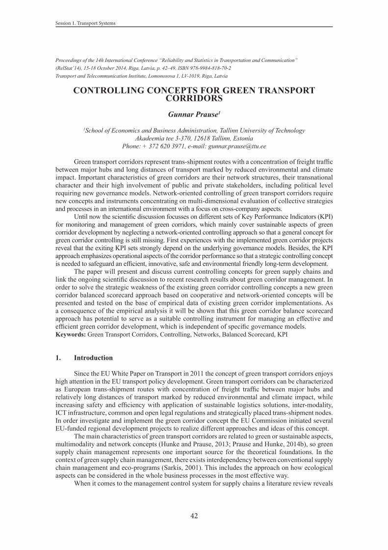
42


Proceedings of the 14h International Conference “Reliability and Statistics in Transportation and Communication”(RelStat’14), 15-18 October 2014, Riga, Latvia, p. 42–49. ISBN 978-9984-818-70-2Transport and Telecommunication Institute, Lomonosova 1, LV-1019, Riga, Latvia

CONTROLLING CONCEPTS FOR GREEN TRANSPORT CORRIDORS

Gunnar Prause1

1School of Economics and Business Administration, Tallinn University of TechnologyAkadeemia tee 3-370, 12618 Tallinn, Estonia

Phone: + 372 620 3971, e-mail: [email protected]

Green transport corridors represent trans-shipment routes with a concentration of freight traffic between major hubs and long distances of transport marked by reduced environmental and climate impact. Important characteristics of green corridors are their network structures, their transnational character and their high involvement of public and private stakeholders, including political level requiring new governance models. Network-oriented controlling of green transport corridors require new concepts and instruments concentrating on multi-dimensional evaluation of collective strategies and processes in an international environment with a focus on cross-company aspects.

Until now the scientific discussion focusses on different sets of Key Performance Indicators (KPI) for monitoring and management of green corridors, which mainly cover sustainable aspects of green corridor development by neglecting a network-oriented controlling approach so that a general concept for green corridor controlling is still missing. First experiences with the implemented green corridor projects reveal that the exiting KPI sets strongly depend on the underlying governance models. Besides, the KPI approach emphasizes operational aspects of the corridor performance so that a strategic controlling concept is needed to safeguard an efficient, innovative, safe and environmental friendly long-term development.

The paper will present and discuss current controlling concepts for green supply chains and link the ongoing scientific discussion to recent research results about green corridor management. In order to solve the strategic weakness of the existing green corridor controlling concepts a new green corridor balanced scorecard approach based on cooperative and network-oriented concepts will be presented and tested on the base of empirical data of existing green corridor implementations. As a consequence of the empirical analysis it will be shown that this green corridor balance scorecard approach has potential to serve as a suitable controlling instrument for managing an effective and efficient green corridor development, which is independent of specific governance models.Keywords: Green Transport Corridors, Controlling, Networks, Balanced Scorecard, KPI

1. Introduction

Since the EU White Paper on Transport in 2011 the concept of green transport corridors enjoys high attention in the EU transport policy development. Green transport corridors can be characterized as European trans-shipment routes with concentration of freight traffic between major hubs and relatively long distances of transport marked by reduced environmental and climate impact, while increasing safety and efficiency with application of sustainable logistics solutions, inter-modality, ICT infrastructure, common and open legal regulations and strategically placed trans-shipment nodes. In order investigate and implement the green corridor concept the EU Commission initiated several EU-funded regional development projects to realize different approaches and ideas of this concept.

The main characteristics of green transport corridors are related to green or sustainable aspects, multimodality and network concepts (Hunke and Prause, 2013; Prause and Hunke, 2014b), so green supply chain management represents one important source for the theoretical foundations. In the context of green supply chain management, there exists interdependency between conventional supply chain management and eco-programs (Sarkis, 2001). This includes the approach on how ecological aspects can be considered in the whole business processes in the most effective way.

When it comes to the management control system for supply chains a literature review reveals

43


that specific controlling topics in this context have been discussed by several scholars but no integral theory or conceptual framework papers about supply chain controlling exist in the leading English speaking supply chain journals except the article of Seuring (2006), who introduced in the German supply chain controlling concepts explaining the dominance of references of German scholars in this field. Consequently, a comparable situation can be stated for green supply chains and green corridors, which have gained attention in recent years but beside the discussion of certain controlling tools still no single concept or theory exists in this field (Seuring and Müller, 2008; Göpfert, 2013).

Since green corridors are imbedded into an international network, environment new concepts and instruments concentrating on multi-dimensional evaluation of collective strategies and processes are required taking into account international and cross-company aspects, but such a network-oriented controlling is still in the beginning (Sydow and Möllering, 2009). A widespread approach for a network- oriented controlling is based on the balanced scorecard concept of Kaplan and Norton (1996), which has been transferred and adapted to a cross-company interactions leading to “cooperative scorecards” of “network-balanced scorecards” (Hippe, 1997; Lange et al., 2001; Hess, 2002).

The current scientific discussion related to performance monitoring of green corridors focusses on different sets of Key Performance Indicators (KPI) for management of green corridors, which are mainly covering sustainable aspects of green corridor development by neglecting a network-oriented controlling approach so that a general concept for green corridor controlling is still missing. First experiences with implemented green corridor projects reveal that the exiting KPI sets strongly depend on the underlying governance models. Besides, the KPI approach emphasizes the operational aspects of the corridor performance so that a strategic controlling concept is needed to safeguard an efficient, innovative, safe and environmental friendly long-term development.

The paper will present and discuss current controlling concepts for green supply chains and link the ongoing scientific discussion to recent research results about green corridor management. In order to solve the strategic weakness of the existing green corridor controlling concepts a new green corridor balanced scorecard approach based on cooperative and network-oriented concepts will be presented and tested on the base of empirical data of existing green corridor implementations. As a consequence of the empirical analysis it will be shown that this green corridor balance scorecard approach has potential to serve as a suitable controlling instrument for managing an effective and efficient green corridor development, which is independent of specific governance models.

2. Supply Chain Controlling

One way to characterize a transport corridor is to understand the corridor as a conglomeration of different stakeholders, which act along a defined geographical area in order to achieve different goals but with the same objective to reduce costs, increase efficiency, minimize environmental impact and create safe and sustainable logistics solutions (Hunke and Prause, 2013; 2014a). This approach based on the interaction of acting organisations along their supply chains in the corridor stresses a network perspective from organisation’s point of view on the collaborative practices and integrative behaviours of the stakeholders in the supply chains (Lee, 2005). As the stakeholders act in a coherent sense and are located in a certain geographical area a green transport corridor can be described as a tubular service cluster.

An interesting example for a green transport corridor is the East-West Transport Corridor (EWTC), linking Southern Sweden, Lithuania, Belarus and Ukraine, where the tubular cluster has the following shape (Prause and Hunke, 2014b):

Figure 1. Green transport corridor as a tubular service cluster

Source: Prause and Hunke, 2014aFigure 1 highlights already that the network-oriented consideration of a green transport

corridor concerns questions like intercultural issues related to different business cultures and models as well as different legal systems, which are beyond ordinary network topics like collective processes

44


and strategies of the heterogeneous set of network stakeholders. Therefore, for the monitoring and controlling of those networks there are instruments required, which are able to evaluate these collective strategies and processes related to the demand of a holistic coverage, planning and development for such networks.

Ackermann (2003) proposed for the controlling of a supply chain a “supply chain balanced scorecard”, where the traditional perspectives related to finance, processes, clients and learning are still maintained but they are oriented on the integral supply chain instead on unique companies or stakeholders. Weber (2002) took one step further and created cross-company balanced scorecard for a supply chain, which keeps the two traditional perspectives finance and processes but he replaced the other two traditional perspectives by two new ones, which he called cooperation intensity and cooperation quality:

• financial perspective,• process perspective,• cooperation intensity, and• cooperation quality.

In his proposal Weber subsumed under the cooperation intensity perspective the “hard factors” of cooperation like data exchange, whereas he used the cooperation quality to focus on the “soft factors” like trust. Weber’s proposal for a supply chain balanced scorecard has the following structure:

Figure 2. Weber’s modified Supply Chain Balanced Scorecard Source: Sydow and Möllering, 2013

Together with his proposal Weber (2002) pointed out that a large number of proposed scorecards for the evaluation of supply chains are only slightly modified classical balanced scorecards without any significant network perspective. The challenge to find an appropriate approach for an effective network controlling lies in the fact that networks are rather dynamic structures, whereas most of the existing controlling concepts are rather targeting on stable structures, so that more flexible management control systems are needed (Sydow and Möllering, 2013).

3. Monitoring of Green Corridor Performance

Most of the green corridor initiatives represent EU-funded regional development projects due to the political background of the green corridor concept with its links to the EU White Paper on Transport 2011. Consequently, the implementations of green transport corridors are based of different understandings and realizations of the concept making it necessary to evaluate, compare and benchmark existing green corridor implementations.

45


Already for the monitoring of green transport corridors there are many different attempts starting from individual companies and industry representatives up to international government level. An important case was the EU-funded project “EWTC2” within the BSR Interreg IVB Programme, where for the first time a “Green Corridor Manual” based on the East-West-Transport-Corridor was developed trying to give a holistic and consistent monitoring concept for multi-modal sustainable transport (Hunke and Prause, 2013). An important element of the Green Corridor Manual was a proposal for a set of Key Performance Indicators (KPI), which measures different aspects of the performance of transport chains.

The set of KPI can be separated into two subsets of indicators measuring enabling and operational criteria. The enabling indicators describe the settings and characteristics of the transport chain in regard to the hard infrastructure. The operational indicators characterise the soft infrastructure including the information and communication systems, which support the transport logistics services, the aspects related to regional, national and international policies and the set of regulations, which apply to all stakeholders. In this sense, operational aspects describe the geographical settings as such, the transport and logistics solution by involving new and innovative business models. The implementation of transport techniques will have also a direct impact on the performance of a transport chain measured by given KPIs.

TABLE 1 PERFORMANCE INDICATORS

Source: EWTC2 Green Corridor Manual, 2012

Table 1 gives an overview about the KPIs, which were selected from the EWTC2 project and which have been tested during the project life-time. As can be seen from the table the performance areas of the EWTC2 KPI system are covering economic, environmental and social dimensions.

Additionally to the table of performance indicators, often in a more detailed way the enabling factors are described by a corridor dashboard aiming at connecting the short-term KPIs and enabling KPIs by visualizing capacity, accessibility and performance. Thus, the dashboard stimulates improvements of the corridor infrastructure and facilitates the cooperation of all stakeholders along the corridor in order to improve total performance (EWTC2 Green Corridor Manual, 2012).

4. Framework conditions of Green Transport Corridors

In order to characterise the framework conditions for green transport corridors it is important to get familiar with the main results of some of the most important logistics development project in the Baltic Sea Region. The starting point of all later green corridor initiatives was the BSR Interreg IIIB project “LogOn Baltic – Developing Regions through Spatial Planning and Logistics & ICT Competence”, which was implemented 2006-2007 and aimed at depiction of the logistics status in the BSR after the EU enlargement in 2004. The empirical activities of LogOn Baltic showed that the landscape of inter-company logistics was dominated by larger production companies and logistics service providers together with their closed and company oriented ICT-systems in order to safeguard the control of their individual supply chains and to realise dedicated platforms for sourcing of transport services mainly from regional SME (Kersten et al., 2007; Kron and Prause, 2008).

The second important initiative with a strong impact on the green corridor activities in the BSR was led by the Swedish Logistics Forum and resulted into the formulation of six requirements on green corridors (Green Corridor, 2010):

46


• Sustainable logistics solutions with documented reductions of environmental and climate impact, high safety, high quality and strong efficiency;

• Integrated logistics concepts with optimal utilization of all transport modes, so called co-modality;

• Harmonized regulations with openness for all actors;• A concentration of national and international freight traffic on relatively long

transport routes; • Efficient and strategically placed trans-shipment points, as well as an adapted,

supportive infrastructure; and A platform for development and demonstration of innovative logistics solutions, including

information systems, collaborative models and technology.The six framework conditions comprise a couple of important characteristics for the

organisation and structuring of green transport corridors. Since the stakeholders within a green corridor are composed of different institutions including public and private organisations of different size and intention, of special importance for the SME sector is the demand of “openness and harmonization for all actors” as well as “collaborative models and technology” stressing a more balanced and cooperative work of all kind of stakeholders in the green corridor.

The set of framework conditions of the Swedish Logistics Forum have to be completed by a set of quantitative indicators to allow the monitoring and controlling of the performance and development of the Green Transport Corridor. Here the two EU projects “SuperGreen” and “EWTC2” developed and delivered for the first time proposals for KPI (Hunke and Prause, 2013). Especially the “Green Corridor Manual” of the EWTC2 project fixed a set of recommendations and guidelines on how to implement the green corridor concept according to the EU freight agenda and as promoted by the EU Baltic Sea Strategy and trying to give a holistic and consistent monitoring concept for multi-modal sustainable transport (EWTC2 Green Corridor Manual, 2012). The EWTC approach was based on the results of the green corridor initiative of the Swedish Logistics Forum and the FP7 – project “SuperGreen”.

A more detailed picture about the framework conditions of green corridors can be drawn by analysing the requirements for logistics ICT systems and in particular about integrated green corridor ICT systems. Already the results of the comparison of regions within the LogOn Baltic project brought to light that the BSR regions with higher logistics competence enjoyed a higher degree of ICT usage in logistics together with a significant higher level of outsourced logistics ICT services, but the outsourcing of logistics ICT solutions was laid on closed and company oriented systems (Kron and Prause, 2008). Expert interviews revealed that the landscape of inter-company logistics ICT systems was dominated by larger production companies and logistics service providers to safeguard the control of their individual supply chains and to realise dedicated platforms for sourcing of transport services mainly from regional SMEs (Prause et al., 2010).

In a comparable analysis Prause and Hunke (2014) summed up the main results and properties of the ICT systems of green corridor initiatives from BSR in order to formulate system requirements for an integrated green corridor ICT system. The analysis was able to fix a set of functionalities, technical requirements and organizational frame conditions for such integrated green corridor ICT systems:

• open architecture,• oriented on standards,• focus on inter-operability and co-modality,• independent of technology,• endorsed and adopted by major freight ICT-systems providers and logistics operators,• support the European transport and logistics system to be more efficient and

environmental-friendly,and• creation of a fair and balanced transport spot market within the corridors enabling

market leaders and SMEs to interact at a low cost.Especially the realization of the last condition represents a task far beyond a technical question,

since the implementation is related to the political question of convincing the current big logistics players to open their closed ICT systems and to integrate these systems into the common logistics

47


platform of the green transport corridor, which is directly related to a loss of their influence and market power.

Another rather political challenge for the whole green corridor is related to the creation of an open data base within the green corridor ICT system comprising freight tariffs and contracting conditions in order to be able to build green corridor spot market for logistics services. This requirement is related to the implementation of openness, transparency and trust among the stakeholders, which is rather an organizational or political task belonging to the sphere of the “soft factors” of the green corridor.

5. Controlling of Green Transport Corridors

Weber (2002) integrated in his supply chain balanced scorecard approach the cross-company aspects by replacing two traditional perspectives by two new ones, which led to his four perspectives for the supply chain:

• financial perspective,• process perspective,• cooperation intensity, and• cooperation qualityThe cooperation intensity describes the “hard factors” of the cooperation in the supply

chain, whereas the cooperation quality expresses their related “soft factors”. Since the two cooperation perspectives apply to green transport corridors in the same way like for supply chains it is recommendable to keep these two network perspectives in a controlling concept for green corridors.

More complicated is to decide whether the financial and process perspectives are appropriate from the controlling point of view for green corridors. The KPI system of the EWTC “Green Corridor Manual” used the “sustainability” perspective covering economic, ecologic and social aspects, thus from the EWTC understanding the financial and process perspective is integrated into the sustainability perspective. Consequently, it makes sense to take the “sustainability perspective” with the full EWCT-KPI system as a third perspective for a tentative green corridor scorecard.

In the classical balanced scorecard approach of Kaplan and Norton (1996) a fourth perspective is introduced. By comparing classical balanced scorecard approach with the proposal of Weber (2002) it turns out that learning, client and growth perspectives are missing. Since a green corridor enjoys a network or a tubular cluster structure, development and growth represent an important element for such a construction due to inter-organizational knowledge transfer among the network partners, the generation of innovations and new service design solutions for the clients as well as the implementation of process and organizational innovations in the corridor. Therefore, it is recommendable to integrate a growth perspective as the fourth dimension for the green corridor.

By summing up the done reflections and results concerning a Green Corridor Balanced Scorecard the four perspectives together with a set of possible indicators lead to the following situation:

• Sustainability perspective• Economic efficiency• Environmental efficiency• Social efficiency

• Growth perspective• Innovation activities• New services• Green corridor stakeholder fluctuation • TO of new services

• Cooperation intensity• Data exchange• Coordination needs

• Cooperation quality• Openness • Trust level

48


• Transparency level• Conflict level

This balanced scorecard includes all important perspectives for green transport corridors and focusses on the underlying network properties of a corridor. Furthermore, it constitutes the KPI system of the EWTC2 project. The set of indicators is not complete and also the type of measurement and evaluation of the indicators is still open, but nevertheless the presented concept for a green corridor balanced scorecard is a further development and in line with a controlling concept for supply chains. In this sense the presented balanced scorecard represents an important stepping stone for a controlling concept for green corridors, but it is obvious that further research has to be done to mature a complete controlling concept for green transport corridors.

6. Conclusions

The concept of Green Transport Corridor plays an important role in the European transport policy but a powerful management control system for those corridors in still missing. Even for supply chains a literature review reveals that no integral theory or conceptual framework papers about supply chain controlling exist in the leading English speaking journals. The situation is slightly different among German speaking scholars, since a German supply chain controlling concepts exists in German literature.

By understanding green corridors as a regional network, which enjoys supply chain characteristics, methods of network-oriented controlling and supply chain controlling can be applied. In network-oriented controlling the balanced scorecard concept of Kaplan and Norton (1996) has been successfully adapted and further developed. An important step towards supply chain and network-oriented controlling was established by Weber (2002), who created a cross-company balanced scorecard for a supply chain, which consisted of four perspectives including the financial perspective, the process perspective, the two perspectives of cooperation intensity and cooperation quality. The two cooperation perspectives describe the “hard factors” and “soft factors” of the cooperation.

Based on these results the paper tries to integrate the results and experiences of important green corridor initiatives in the Baltic Sea Region in order to create green corridor balanced scorecard. First, the KPI system of the EWTC project is integrated into the scorecard in order to safeguard the “sustainability” perspective. Second, the growth perspective is integrated into the green corridor balanced scorecard in order to represent development and growth as important elements of such a corridor, since inter-organizational knowledge transfer, the generation of innovations and new service design solutions for the clients as well as the implementation of process and organizational innovations in the corridor are of vital importance. Finally, a fully developed balanced scorecard for green transport corridors needs not only the definition of appropriate perspectives, but it also requires a set of powerful indicators together with types of measurement and evaluation of the indicators. All these topics are still subject to research so that the presented balanced scorecard constitutes a first step towards a controlling concept for green corridors.

References

1. Ackermann, I. (2003). Using the balanced scorecard for supply chain management – Prerequisites, integration issues, and performance measures. In: Seuring, S.; Müller, M.; Goldbach, M.; Schneidewind, U. (Hrsg.): Strategy and organization in supply chains. Heidelberg and New York, 289-304.

2. EWTC II Green Corridor Manual. (2012). Green Corridor Manual – Task 3B of the EWTC II project.

3. Göpfert, I. (2013). Logistik, Verlag Franz Vahlen, 3rd edition, München4. Green Corridor (2010). Regeringskansliet – Government Offices of Sweden. Green Corridors.

15.06.20105. Hess, T. (2002). Netzwerkcontrolling: Instrumente und ihre Werkzeugunterstützung. Wiesbaden6. Hippe, A. (1997). Interdependenzen von Strategie und Controlling in Unternehmensnetzwerken,

Wiesbaden

49


7. Hunke, K.; Prause, G. (2014). Sustainable supply chain management in German automotive industry: experiences and success factors. Journal of Security and Sustainability Issues, 3(3), 15 - 22.

8. Hunke, K.; Prause, G. (2013). Management of Green Corridor Performance. Transport and Telecommunication, 14(4), 292 - 299.

9. Info Broker (2012). A key to efficient performance with as small ecological footprint as possible. EWTC II, Net.Port Karlshamn

10. Kaplan, R.; Norton, D. (1996). The Balanced Scorecard. Translating Strategy into Action, Boston.

11. Kersten, W., Boeger, M.; Schroeder, M.; Singer, C. (2007). Developing Regions through Spatial Planning and Logistics & ICT competence – final report. As part of the publication series of the EU project LogOn Baltic, Turku School of Economics, report no. 1:2007, Turku.

12. Kron, E.; Prause, G. (2008). LogOn Baltic aggregated ICT Survey Report, Turku School of Economics, Turku 2008

13. Lange, C.; Schaefer, S.; Daldrup, H. (2001). Integriertes Controlling in strategischen Unternehmensnetzwerken, Controlling 13(2), 75-83

14. Lee, P.D. (2005). Measuring Supply Chain Integration: A Social Network Approach. Supply Chain Forum: An International Journal 6(2), 58–67.

15. Prause, G.; Hunke, K. (2014a). Sustainable Entrepreneurship along green corridors. Journal of Entrepreneurship and Sustainability Issues, 1(3), 124 - 133.

16. Prause, G.; Hunke, K. (2014b). Secure and Sustainable Supply Chain Management: Integrated ICT-Systems for Green Transport Corridors. Journal of Security and Sustainability Issues, 3(4), X - X. [forthcoming]

17. Prause, G.; Kron, E.; Beifert, A. (2010). Final ICT Report of the project “Innovation Network – Logistics Cluster Wismar Seaport”, Wismar 2010

18. Sarkis, J. (2001). Introduction. Greener Management International 35(3), 21-2519. Seuring, S. (2006). Supply Chain Controlling: summarizing recent developments in German

literature, Supply Chain Management: An International Journal, Vol. 11(1), 10 - 1420. Seuring, S.; Müller, M. (2008). From literature review to a conceptual framework for sustainable

supply chain managmement, Journal of Cleaner Production, Vol. 16, 1699 - 1710 21. Sydow, J.; Möllering, G. (2009). Produktion in Netzwerken, Verlag Franz Vahlen, 2nd edition,

München

50



SAFETY INSPECTIONS OF RAILWAY CROSSINGS AND STRENGTHENING OF INDIVIDUAL RESPONSIBILITY FOR

SUSTAINABLE TRAFFIC SAFETY

Lajos Szabó1, Viktor Nagy2

1Széchenyi István University – Department of TransportGyőr, Hungary, Egyetemtér 1.

phone: +36 (96) 503-494, fax: +36 (96) 613-561, [email protected]échenyi István University – Department of Transport

Győr, Hungary, Egyetemtér 1.phone: +36 (96) 613-561, fax: +36 (96) 613-561, [email protected]

The study examines the possibility of application of models and presents a possible solution, which can be the basis for the creation of renovation catalogue of railway crossings. The study describes the process of the model creation. Show, that how the evaluation matrix is setting up and how can we define the level crossings’ hazard ranking with the help of the catalogue. With the help of them, feasibility studies and implementation plan documentations can be prepared. The paper mentions the importance of traffic awareness, its methodological basis, and the main questions in traffic education.Keywords: hazard ranking, review criteria, scoring system, enhanced security actions, traffic awareness, features of railway crossings

1. Introduction

The dangerous characteristics of railway crossings come from the fact that a crossing is a contact point of different traffic systems, where structurally different traffic paths cross each other. These different kinds of paths are used by vehicles with significantly different technical parameters. Therefore the railway crossings have prominent importance in terms of traffic safety. Because of the facts above, and in addition due to a ministerial instruction released in 2003, the most dangerous railway crossings must be determined. The basis of this determination is an establishment of a hazard ranking (Tigyi and Gábor, 2010). This hazard ranking can be created using a total score per crossings indicator generated by a data processing algorithm. Within the project called ‘Safety Inspection of Railway Crossings in the Area of Railway Track Sections Extended to the Border of Burgenland and West Hungary’ (Sicherheitsinspektionen von Eisenbahnkreuzungenentlang der grenzüberschreitendenBahnlinien in Burgenland und Westungarn - SIEBaBWe) by the examination of several possible modelling techniques (Pokorádi, 2008) we created a model which is suitable not only for the determination of the railway crossings’ hazard ranking in our project, but also it is applicable for every railway crossings. The point creation was the common element in the potentially attractive models; the method of this point creation meant the difference. Regarding to certain models a mentionable common feature was the demand of counting with the environmental characteristics of railway crossings, the accident and traffic data and the way of insurance. The railway crossing, where the implementation of enhanced security actions are the most reasoned, can be designated by model outputs which are checked and filled with proper data. Beyond the enhanced security actions included in the reconstruction catalogue the safety inspection is integrally complemented with the strengthening of road users’ responsibility in every society groups along regional and main lines. The main objective of raising awareness (Arató et al., 2014) is the increased safety of railway crossings and the reduced number of accidents.

51


2. Examination of useable modelversions

In this chapter we present two modelling procedure, which are found appropriate by the committee (established within the framework of the project), to determine the hazard rank of a railway crossing. From any kind of suitable modelling procedure are we talking about, it’s necessary to mention the content and the freshness of the available data. The source of data is the National Transport Authority, the MÁV Co. (Hungarian State Railways Private Company by Shares) Department of Infrastructure, the Hungarian Public Road Non-profit Private Limited Company, and railway companies’ records. The railway companies record all events that happen in the railway crossings, whether it’s personal traumatic or material harmful accident. The past years ranking practice met with incomplete, wrong, old or not even registered data. Experts agree, that such kind of central database would be necessary, what based on the railway crossings’ GPS coordinates and all of the digitally recorded data from the given railway crossing concerning to the coordinates. The regulation of refreshing the databases would lead to an additional improvement.

2.1. GySEV model (Tigyi and Gábor, 2010)

GySEV (Győr-Sopron-Ebenfurth Railway Corp.) provided the model, what sets up a hierarchy, which shows the road safety risk degree of the railway crossings compared to each other. The model defines the maximum score of each railway crossings what can be given. The maximum score is divided up between the factors, what characterize the crossing. These factors are the followings:

• the number and outcome of level crossing accidents• the volume of the crossing’s road and railway traffic• the safety equipment, installed in the railway crossing• other features (Figure 1.)The scoring system uses formulas in the case of all factors

Figure 1.The percentile distribution of the score which can be handed out maximally according to indicator groups, (Tigyi and Gábor, 2010)

52


Accident situationThe given score value based on the past 10 years railway crossing’s events. The events

(accidents), what happened earlier than 5 years, count only with 50% weight.

(1)

where: CEN: corrected event numbervalue: a) if there is not a built up pedestrian crossing: CEN = the number of car hits + 0.3*(the number of pedestrian + cyclist hits) b) if there is a built up pedestrian crossing: CEN = the number of car hits

Traffic situationThe records of the railway companies include the given line’s data from the number of running

trains and the distribution according to type and time for a 24 hours period. In the light of the number of railway trains in the examined railway crossing, we can project the daily traffic onto the crossing.

(2)

where: AADT: annual average daily traffic the value’smeasure is in„vehicle unit/day” maximum value is defined as the maximum value of the numerator td: average disturbing time Nt: number of trains B: bus traffic value: 1, if there is bus traffic 0, if there isn’t bus traffic

Traffic technicalfeatures and other dangerousness increasing factorsThe “railway speed limit” (3) takes four speed interval into account. The bases of the calculation

of “other dangerousness increasing factors” are the followings:• what kind of road is along the crossing (regional character)• the existence of public lighting, separate pavement, footpath• is there any intersection within 30 metres, where the vehicles (arriving from the railway

crossing) haven’t got priority and there is no rescue lane

(3)

where: IM: insurance method Vrail: speed limit of railway traffic Vroad: speed limit of road traffic Re: recognisability, negotiability, geometry, angle of the intersection Rm: road markings Ts: traffic signs Od: otherdangerousness increasing factors

2.2. Traffic model

If we examine the railway crossing, like a physical object, than we think about the system like a model, which can be described with physical variables. The content of the physical variables may be heterogeneous, for example the combination of physical, chemical or economical features. Some

53


of the variables are given. These are the inputs. It is typical to the other group of variables that we want to identify the behaviour of these. These are the outputs. There is also a third group of variables, which are responsible for describing the connection between the inputs and outputs. In this case, it is true, that we describe an object with a system. In other words, the system is the model of a given physical object.

We can separate the models onto two major types. The model type depends on, that what kind of process we want to mapping. The material models include geometric, physical and mathematical models. The so-called mental models work according to the logical connections, which set up by the men. Looking at their method, and their form there are subjective, looking at their content there’re objectives. The mental models include the so-called traffic models too (Pokorádi, 2008). The modelling process can be used, if we need to make different scenarios for a problem. In our case the scenarios are equivalent with the hazard ranking of railway crossings. This procedure may be especially suitable in the case of railway crossings, because some of the inputs cannot be expressed in money or it can be express, but only with difficulties. In the case of level crossings, the possible inputs cover a quite wide circle. It is necessary to limit the circles of the inputs and take only those inputs into account, which are fundamentallyaffect to the expected outputs. During the modelling procedure, the railway crossing can be created as the essential properties included replica of the examined system.

The process of creating the modelIn the first step of the model creation, we need to define those inputs, which are suitable to

describe the railway crossing as a system and limit the circle of the inputs if it’s necessary, as it mentioned in the previous chapter. The first steps include the precise definition of each input. The main groups of the inputs could be the next:

• the environment of railway crossing• the insurance method of railway crossing• the accident situation of railway crossing• the traffic data of railway crossing• the traffic control in the railway crossingWe may define the most favourable (Zmax) and the most adverse (Zmin) value of every single

input. With the use of the most favourable, the most adverse and the real input value we can produce the score of each input which can be given.

(4)

where: Zix: the real value of input (ith input inside of umpteen input group)For the hazard ranking generation, it is necessary to define the total score of every single

railway crossing and to aggregate the input indicators (5).

(5)

where: AIxg: the aggregated value of inputs Iix: the score of ith input Wgi: the ith input’s weight of preference,according to the given expert group’s (g)opinion

The inputs’ weight of preference is defined by an expert group in the traffic model. The aggregated value is the total score of the level crossing. The higher value means higher degree of dangerousness.

54


3. Hazard ranking generation with the help of Evaluation matrix

After the examination of the potential models, the so-called Evaluation matrix was set up. With taking the practical and theoretical viewpoints into account it is verifiable, that the Evaluation matrix is flexible and gives well used solution and base for the preparation of railway crossings’ renovation catalogues.

3.1. Architecture of the Evaluation matrix

The base of the Evaluation matrix is the simplest data direction procedure, the order of magnitude. The elements of the sample are equal to the level crossings involved in the examination. We summarize the scores of the level crossing features for every single crossing and we arrange the received sum values in ascending order. The received order is thehierarchy;the numbers imply the rank numbers.

The Evaluation matrix separates three big input groups (Figure 2.):• accidents• traffic situation• traffic technical features

Figure 2. Input system of Evaluation matrix

In capital features the input groups’ content is equal to the GySEV model.However, there are also essential differences. In the calculation of score values, the circumstance that deriving from the fault of the railway yield an extra point. The base of the calculation of score value is the last 5 years. In the traffic situation input group we’re taking the experienced seasonal traffic increase in the railway crossing also into account. The evaluation matrix counts with the average daily road and rail traffic. This element makes the practical adaptability of the matrix easier. The government decree 10/1984 about “the traffic control of roads and the placement of road marks” (what is in operative today) is mentioning the “authoritative hourly railway crossing traffic value”. We built the authoritative character of the traffic into the model with the existence or non-existence of seasonal traffic growth. The average daily railway traffic takes not only the trains what cross over according to the timetable into account, in contrast to the government decree. In the relation of the velocities, the base of the calculation is the highest allowed speed limit of regional railway lines (80 km/h). According to this, only two group of velocity was defined. The highest allowed road speed limit in the railway crossing was split into four class intervals. New elements have been added to the group of traffic technical features, for example:

55


• the contrast effect of the sunshine disturbs the road traffic for several hours due to the location of the railway crossing

• the “beginning of the level crossing” signboard is faded or injured (also if only one signboard is inappropriate)

3.2. The modellingprocess

In the first step of Evaluation matrix creation we appointed the circles of the inputs, defined the inputs and then we separated them into input groups. The processing algorithms of the evaluation matrix take the simple, fast and reliable practical application requirements into account. Score can be given in the case of existence or absence of an input element. Formula 6 describe the method, how is the railway crossing’s traffic situation score countable.

(6)

where: ADTroad: average daily road traffic ADTrailway: average daily railway traffic

If the value of ADT is under 800.000, than the score which can be given to the traffic situation is distributed proportionally, if ADT is higher than 800.000, the maximum score must be given. With the help of the processing algorithms, the outputs (the scores which can be given to the input element) can be manufactured. After the model has been made, we filled up the model with values, and then we verified the availability of outputs (Figure 3.).

Figure 3.The modelling process

4. The description of level crossing, which selected onto renovation

The reason of the development of the evaluation matrix is, that the traditional examination item based evaluation of level crossings’ classification does not give a real dangerousness picture of all aspects many times (e.g. according to certain studies and analyses the grievous accidents occur in railway crossings with smaller traffic (Konrád, 2013)).

A score or a score limit was determined for every single Evaluation matrix’ input (evaluation criteria). For the weighting of the given score system (from-to) were the relevant standards, the valid orders and the rules of law the basis (Gov. Reg. 20/1984 (XII.21); KPMSZ. Kk 108-73; ÚT2-1.201; ÚT2-1.225)

Some results (AP3, traffic count, etc.), which were born in the previous works (as connection

56


points) of the project, were used for determination of some input factor values. The matrix also include some other input factors (e.g. community surveys, opinion based reflections and demands as input factors) beyond the main criterion (mentioned above).

Every single railway crossing got a so-called total score of dangerousness according to the summation of the single input elements’ score. Based on this, among the examined level crossings the most dangerous is the one, which got the highest score, and the one, which got the lowest score, is the safest. However, it is important to emphasize, that every 28 (23+5) appointed level crossings are correspondent for provisions and regulations according to the classification of special authorities.

4.1. “Hazard ranking” of the examined railway crossings, the most dangerous railway crossing

The AS765 level crossing in railway line 8 got the highest score (1574) among the examined level crossings (on GySEV railway lines) according to the evaluation matrix, so this is the most dangerous railway crossing (The safest level crossing is the AS759 in line 15 with 306 point. The unfortunate fact, that two accidents happened in the last half year in the given level crossing, and one of them had fatal outcome, justifies the living of the experts group’s theoretical aspect system. At the same time, it is important to note, that the railway crossing is proper for all the magisterial requirements and regulations, as it mentioned before (date of the last perambulation: 2013.07.24.).

5. Traffic awareness

In the level crossings, 99% of the accidents ensue because of the lack of knowledge. The perpetrator’s deficiency of knowledge is retraceable to an extremely complicated factor system. One part of the factors is related with the human psyche, the other part of factors is related with the lack of rules’ knowledge. Therefore, it is very important in traffic awareness to affect to the mental factors, so the individual can make correct choices and thanks to that, make the right moves.

5.1. Methodological basics

One of the taglines of the traffic awareness lecture in the framework of project SiEBaBWe was the next: I am the responsible!” The title expresses the aim of traffic education and awareness aptly. Independently from the target group, the most efficient way of traffic safety developing is the reinforcement of individual responsibility.

Everybody belongs to the target group, started with the youngest age-group (who had some kind of traffic knowledge yet) to the eldest one (travelling pensioners)

The curriculum primarily built on the correct behavioural rules and the reinforcement of individual sense of responsibility. The following chapter imply this more detailed. In the awareness lectures, as a complement of the educational materials, posters and flyers have been dealt. At the end of a lecture, the presenter and the audience talk over the content of the presentation in an informal conversation.

5.2. Main questions in education(Arató et al., 2014)

The causes of the accidents at level crossings are usually clear from legal perspective. Despite this, several questions may arise relatedly with the accident. The question is that what kind of reasons are in the background. The most common causes are the irresponsibility, inattention and the lack of routine. An accident may occur due to sudden sickness or pain. The incorrect behaviour in level crossings has several other causes too (e.g. detection mistakes, undervaluation of dangers, decision mistakes), but the question of individual responsibility is always there.

The railway crossing is a dangerous place, because significantly different ground transport systems, structurally different traffic paths cross each other. These different kinds of paths are used by vehicles with significantly different technical parameters. The different features entail different kind of driving dynamic characteristics.

The level crossings are special places. Compared with other places of traffic, we found here special and active insurance equipment and passive cautionary marks too. The large number of signs generates high risk level (Figure 4.).

57


Figure 4. Road signs(Arató et al., 2014)

The level crossings are qualified as critical points of the traffic, because of that the reduction of emerging dangers and material harms has high significance. The desired aim can be reached with the insurance of level crossings. Apart from the fact that the railway crossings insurance methods and the applied equipment are different per railways, the following criterion must be met:

• the driver of the road vehicle can be able to stop the vehicle from the detection of the train to the starting of the level crossing

• the vehicle can be able to leave the danger area in safe, if couldn’t stop before the level crossing

• the insurance equipment of level crossing depends on several facts:• topological environment of level crossing• specialities of applied technical solutions• placement environment of insurance equipmentThe travelling people have several qualities. Among these, it is possible to specify which

are necessary in traffic. In the possession of necessary nature the forms of right behaviour can be developed.The accidents in level crossings follow from the fault of travellers in almost 100%. The traffic awareness is the widely dissemination of different forms of the right behaviour. The traffic awareness gives an opportunity to the travelling people to change their bad habits, to enhance danger and security awareness, and to improve the ruling ability.

During the traffic awareness course of project SiEBaBWe we visited 11 settlements, primarily those where theinhabitants and the commuters use the examined railway crosses. Among the settlements there were shire- and district town, and also small villages with a few thousand people. In the target group there were nearly one thousand elementary school, high school and college students, active workers and pensioners. The program of the lectures was the next:

• description of the project• 1. quiz: filling of the questions, common evaluation• inspection of theinstructional movie about an impact, common evaluation• analysis of railway crossing accidents, experienced deficiencies• dangerous and special nature of the level crossing• insurance of level crossings, function of safety equipment• domestic methods of safety handling• the right behaviour in the level crossing and its environment• 2. quiz: filling of the questions, common evaluation• informal conversation with the participantsBefore and after of the presentation the audience filled up the same question included, lecture

based test. Compared to each other the test results, the effect of the lecture was measurable. The instructional movie presented a simulated accident in a railway crossing, where two automobile ignored the level crossing’s semaphore sign and crashed to each other on the tracks. One of the automobile passed through the red sign earlier and broke the pole of the barrier. In spite of the sound signal of the approaching train the vehicles don’t leave the tracks and the train hits the cars. As a

58


result of the collision, the locomotive shoves out one of the cars apart from the tracks, keeps down the other and pushes it until the place of stop. As a result of the accident, one man died and several people were injured.

6. Conclusions

The correction of the safety situation of the level crossings is a complex task. It is necessary to establish the level crossings’ hazard ranking based on some kind of method. Independently of the method, the number and the type of the used inputs is quite high. The inputs can be separated into three large groups: accident and traffic situation of the level crossings, traffic technical features of the level crossings, other factors that cause dangerousness. Introduction of further safety enhancing measures is necessary in the most dangerous level crossings. That means token investments connected with infrastructure. It is important to note again, that all of the level crossings are proper for all the magisterial requirements and regulations, independently of safety enhancing measures. Beside the infrastructure investments, the traffic education and awareness is the most effective method to decrease the number of accidents in level crossings. In other words, the development of the individual sense of responsibility (beside other solutions) is the most effective method for traffic safety correction.

Acknowledgements

The work reported in the paper has been developing in the framework of the project “Sicherheitsinspektionen von Eisenbahnkreuzungenentlang der grenzüberschreitendenBahnlinien in Burgenland und Westungarn – SIEBaBWe”. This project is supported by the grant “Creating the future” program of the European Union ERDF.

References

1. Arató, K., Horváth, G., Somogyi, M., Szabó, L. (2014) Vasútiátjárókbiztonsága. Győr: SzéchenyiIstván University – Department of Transport.

2. Konrád, Gy. (2013) A GYSEV Zrt. vonalainüzemeltetettvasútiátjárókésbalesetek. Sopron3. Pokorádi, L. (2008) Rendszerekésfolyamatokmodellezése. Debrecen: Campus Kiadó4. Tigyi, Sz. and Gábor, M. (2010) A Magyarországivasútiátjárókbiztonságihelyzete,

veszélyességirangsoránakkidolgozása. In: Proceedings of the XI. RODOSZ Konferencia, Kolozsvár, November 2010.

5. Standard KPMSZ. Kk 108-736. Standard ÚT2-1.201, Designing of public roads7. Standard ÚT2-1.225, Construction of level crossings8. Government regulation 20/1984 (XII.21), „About road’s traffic shaping and placement of road

marks”

59



STAKEHOLDER TYPOLOGY AND DIMENSIONS OF GREEN TRANSPORT CORRIDORS

Mike Wahl1, Gunnar Prause2

1Tallinn School of Economics and Business Administration, Tallinn University of TechnologyAkadeemia tee 3-365, 12618 Tallinn, Estonia

Phone: + 372 620 3956, e-mail: [email protected] Tallinn School of Economics and Business Administration, Tallinn University of Technology

Akadeemia tee 3-370, 12618 Tallinn, EstoniaPhone: + 372 620 3971, e-mail: [email protected]

Abstract

Since the appearance of the White Paper on Transport in 2001 the concept of green transport corridors represent an important element in the future of EU Transport Policy. The green transport corridor approach stresses European trans-shipment routes with a concentration of freight traffic. There are different ways to understand the meaning of a transport corridor and to describe and understand such corridors. One important approach is a network-based view which allows seeing the corridor as a conglomeration of different stakeholders acting along a defined geographical area in order to create sustainable logistics solutions. The stakeholders in such a transport corridor can be characterized by typologies so that the local properties of a transport corridor can be derived by its regional stakeholder composition.

The paper will present recent research results about stakeholder typology and its application to a better understanding of the dimensions of green transport corridors. Since green transport corridors can be regarded as tubular service clusters which are built of regional parts with their own stakeholders the typology approach gives the opportunity to understand the values and strategies of stakeholders on meso-level and to find successful and sustainable governance models for green transport corridors. Keywords: Green Transport Corridors, Cluster Governance, Stakeholder Typology, Strategy.

1. Introduction

Since the appearance of the first Transport White Paper (COM, 2001) of the European Commission the necessity of shifting volumes of the dominant road traffic to other efficient transport modes is being expressed constantly. The goal was linked to the preparation of an environmental friendly transport sector, and at the same time to provide safer and efficient transportation by reducing accidents, congestions and negative impacts through emissions, i.e. noise and pollution. After the revision of the EU Transport White paper (COM, 2006), the concept of green corridors was introduced as an initiative of the European Commission, in the Freight Transport Logistics Action Plan (FTLAP). According to FTLAP, green corridors will reflect an integrated transport concept where short sea shipping, rail, inland waterways and road complement each other to enable the choice of environmentally friendly transport (COM, 2007). In recent years, on European and also on national level an increasing number of initiatives have been taken to speed up the shift towards greener and more efficient logistic solutions in Europe. Green corridor development requires five types of activities: performance monitoring, policy support, trade and transport facilitation, information facilitation and communication (EWTC II, 2012). Important steps on EU level in this development process have been the Green Paper on TEN-T from 2009, as well as the TEN-T Policy Review 2011 and the EC White Paper on “A Sustainable Future of Transport”. Since 2009, several projects on territorial cooperation were launched aiming at improving sustainable transportation in European Union: e.g. The East West Transport Corridor II (EWTC II), Scandria, TransBaltic, North-East-Cargo-Link (NECL), Rail Baltica Growth Corridor (RBGC).

60


The current situation shows that the main characteristics of a green transport corridor and conditions that make a transport corridor actually green are varying but it is already visible that there are also common topics, which are recognised by green corridor initiatives. Firstly, it is co-modality, which enables the choice of environmentally friendly transport along the transport route, since reduced emissions is one of the obvious objectives of a greener transportation. Secondly, in order to be able to provide efficient and environmentally friendly transport along European transhipment routes with a concentration of freight traffic between relatively long distanced major hubs along the corridors which are called nodes and which play a very significant role for the corridor performance and development (Hunke and Prause, 2012).

Network-based view allows seeing the green transport corridor as a conglomeration of different stakeholders, acting along a defined geographical area in order to create sustainable logistics solutions. All the involved stakeholders have their own goals and strategies (e.g. ownership strategy) which have to be bundled and subsumed under the green corridors vision and long term missions. In order to better understand the local and global properties of a transport corridor, the stakeholders in such a green transport corridor can be characterized by typologies and the regional stakeholder composition can be analysed and used to describe the local properties and regional strategic objectives of a corridor. Stakeholder theory concerns values and beliefs about the appropriate relationships between the individual, the enterprise, and the state (Tricker, 2009). Stakeholder theory begins with the assumption that values are necessarily and explicitly a part of doing business. Far too little attention has been paid to “soft logistics” issues in green transport corridors including intercultural aspects and stakeholder’ research, and any focus on behaviour rooted in basic human values has been missing. On-going green corridor initiatives like the EWTC II project reveal that intercultural issues, different business models and regulations as well as regional strategic goals have crucial impact on corridor development so that the problem of not understanding the green transport corridors stakeholder’ behaviour, either on individual, firm or society level, is of big importance for future developments. There are considerable similarities and differences between stakeholders that a green transport corridors stakeholder typology would explain.

Until now the available typologies for stakeholders are limited to owners (Wahl, 2011, 2012) so the starting point for the research is the application of the existing ownership typology to green transport corridor stakeholders and to extend the existing typology to all green corridor stakeholders including political institutions, NGO’s and entrepreneurs. So the paper presents recent research results about stakeholder typology and its application to a better understanding of the dimensions of green transport corridors. The main purpose of this research is to develop a research process for constructing of a green transport corridors stakeholder typology, and a better understanding of the dimensions of green transport corridors.

The present paper is organised as follows. Section 2, “Theoretical framework” begins by defining the key constructs that underscore the green transport corridors approach from a holistic perspective. First explaining why typologies are complex theories. Relevant theories and evidence relating to the constructs are reviewed, showing network perspective of green transport corridor stakeholders, and while owners are the most influential stakeholders, the ownership typology, which is planned to use as model were presented. Section 3, “Green transport corridors dimensions form the basis for a stakeholder typology” tells us about the philosophical considerations, research approaches, and research design. The proposed research process, and relevant analysing dimensions needed for construction of the green transport corridors stakeholder typology are explained. Section 4, “Conclusions and recommendations” concludes by describing the main insights and locating potential for the further research.

2. Theoretical framework

2.1. Typologies are complex theories

Typologies are a well-known form of theory building. Doty and Glick (1994) argue that when typologies are properly developed and fully specified, they are complex theories. Typologies meet several of the important criteria of theories, and are shown to contain multiple levels of theory. The construction of typologies is of central importance for qualitative social research; it is necessary to clarify the concept of types and the process of typology construction. If typologies are to be considered theories, they must meet some of the minimal definitions of a theory. Although there

61


are no concise, unanimously accepted definitions of a theory, theory-building experts seem to agree that there are at least three primary criteria that theories must meet. First, a theory’s constructs must be identified. Secondly, relationships between these constructs must be specified. And thirdly, these relationships must be falsifiable. To empirically falsify any theory, the verbal model presented by the initial theorist must be translated into a quantitative model. To accurately model typological theories, the quantitative models must capture the similarity of real organizations to one or more of the ideal types because similarity to the ideal types is hypothesized to predict the dependent variable. The similarity of real organizations to ideal types of organizations can be modelled as profile similarity. Techniques for assessing profile similarity assess deviation with the weighted Euclidean distance formula. The typological theory can then be tested by using the fit index to predict the dependent variable. (Doty and Glick, 1994)

2.2. Network perspective of green transport corridor stakeholders

In order to understand what a transport corridor means by theoretical backgrounds it can be helpful to see the corridor as a conglomeration of different stakeholders which act along a defined geographical area in order to achieve different goals but with the same objective to reduce costs, increase efficiency, minimize environmental impact and create sustainable logistics solutions (Wahl, Hunke, and Prause, 2013). Network perspective may better explain the emergence of collaborative practices and integrative behaviours in logistics in general and supply chain management from organisation’s point of view (Lee, 2005).

Rowley (1997) applied such a social network perspective to the stakeholder theory of the firm. Freeman’s (1984) definition states that stakeholders are any group or individual, who can affect or is affected by the achievement of organisation’s objectives. Clarkson (1995) defines stakeholders as persons or groups that have, or claim ownership, rights, or interests in a corporation and its activities, past, present, or future. He further differentiates between primary and secondary stakeholders. The first group includes stakeholders, like shareholders, employees, customers, suppliers, government and communities, without their participation the organization cannot exist. The secondary stakeholders are those who influence or affect, or are influenced or affected by, the organisation, but they are not engaged in transactions and are not essential for its existence. Examples of secondary stakeholders are the media and competing companies. Spurgin (2001) as in capitalistic markets the importance of the decisions taking by stakeholders is increasing. Decisions do not only have an impact on the organization itself but also to society and a wider group of stakeholders, mainly when it comes to environmental effects and public serving obligations like it can be assumed for the green transport corridors. (Wahl, Hunke, and Prause, 2013)

The type is defined as a combination of stakeholder attributes; one first needs properties and dimensions of green transport corridors which form the basis for the stakeholder typology. With the help of these stakeholder attributes, the similarities and differences between the stakeholders must be adequately grasped. And finally, the constructed groups and types have to be described with the help of these properties. Stakeholders of green transport corridors are all kind of task environment groups that directly affect a green transport corridor and are affected by the green transport corridor. They could be owners (shareholders, entrepreneurs), customers (logistics centres, ports), suppliers (transport service providers, shippers, and railway companies), employees (corridor managers), competitors, trade associations, communities (municipalities), creditors, special interest groups (authorities), and governments (infrastructure providers, institutions).

One crucial aspect of governance of a green transport corridor is still how the decision making process can be solved with such a big group of different stakeholders. Decision making should focus on the long-run future of the green transport corridor. Strategic decision making process should include following steps: Evaluate current performance results, review corporate governance, scan and assess the external environment, scan and assess the internal corporate environment, analyse strategic factors, generate and evaluate and select the best alternative strategy, implement selected strategies, and evaluate implemented strategies. Strategic audit provides a checklist of questions, by area or issue that enables a systematic analysis to be made of various corporate functions and activities. (Wheelen and Hunger, 2012) Hansmann (1996) already stated that the more groups of stakeholders there are, the more complicated it will be to reach a decision, especially as the stakeholders often have different goals.

62


When it comes to governance structure of an organization like a green transport corridor also the question of property rights arises. Property rights theory has mainly been developed by Coase (1960), Grossman and Hart (1986) and Hart (1995). The party that possesses the rights to an asset can decide the use of it and is entitled to receive the income from it. Unfortunately this is not obvious to distinguish in the case of transport corridor as the rights of the available assets, i.e. roads, terminals, railways, land, infrastructure, etc. belongs to different stakeholders. Mainly these assets belong to public institutions which by their nature have no interest in earning income form their assets but serving the society and ensuring economic freedom. Next to the question of the property rights there are also other opinions when it comes to assets of the organization. Kay (1996), Blair (1996), Blair and Stout (1999) and Donaldson and Preston (1995) argue that the assets of the firm do not only consist of physical assets but also the skills of its employees, the expectations of customers and suppliers, and its reputation in the community. This is not only applicable to the transport corridor concept in general but to very participating company on lower level as well. (Wahl, Hunke, and Prause, 2013)

Since the purpose of this paper is to develop a research process for constructing of a green transport corridors stakeholder typology, and a better understanding of the dimensions of green transport corridors, we are shortly presenting the ownership typology, which is planned to use as model. This is justified while owners are the most influential stakeholders.

2.3. Ownership typology

Ownership is the key building block in the development of the capitalist socio-economic system. It is not just a legal-economic construct; it has also personal, social, political, and economic value dimensions. The problem of not understanding the owners’ role or behaviour, either on individual, firm or societal levels is solved in form of the ownership typology. Based on the Wahl’s (2011, 2012) ownership research on capital company ultimate owners’ basic human values and will, the author constructed an ownership typology (Figure 1). This typology contains four ideal types of owners (explanatory hypotheses): 1. Humanist-Traditional ownership type (HUSTA); 2. Modern ownership type (MODERN); 3. Pragmatist-Materialist ownership type (PRAMA), and 4. Idealist ownership type IDEA.

Figure 1. Ideal types of owners in a three-dimensional A-space (Source: Author’s calculations based on empirical data; PAST ver. 2.00)

The ideal types are placed in a three-dimensional A-space. Axis x: idealism – pragmatism; y: humanism – materialism; z: modernism – traditionalism. The first dimension spans the field from idealism, where “one dramatizes one’s values” to pragmatism and instrumentality, where “one compromises one’s values” (Zetterberg, 1997). The second dimension separates a concern with human beings from a concern with material things, thus bridging the poles of humanism and materialism. The third dimension of the A-space runs from becoming to being. It corresponds to a scale from modernism, where one welcomes change: “becoming”; to traditionalism, where one upholds stability: “being” (Zetterberg, 1997).

63


2.3.1. Humanist-Traditional ownership type (HUSTA)

The Ownership Typology ideal type HUSTA carries the motivationally distinct basic value (value type) benevolence; the main characteristics for benevolence are preservation and enhancement of the welfare of people with whom one is in frequent personal contact. Owners’ basic human values − single value items: helpful, honest, forgiving, loyal, responsible, true friendship, a spiritual life, mature love, meaning in life. Here the Schwartz’s (1992) theory of basic human values was used as the theoretical basis.

What the owners of the company want to have from the company in the long run is seen as objectives and results of achieving the objectives (personal, social, political, and economic values). The ways the values are created and how the owners’ will is achieved is seen as instrumental tools for the achievement of the objectives (time, risk, and process).

The owner wants to have power by giving bonuses; it refers to positive reinforcement and the ability to award something of value. The owner’s contribution to the realisation of the business idea is strategic and financial. For him return is more important than power; specifically − economic goal, current benefit, dividends. The owner agrees to found a company with a participatory rate of 100% (majority), and take high risk for the achievement of objectives.

2.3.2. Modern ownership type (MODERN)

The Ownership Typology ideal type MODERN carries the motivationally distinct basic values (value type), such as: hedonism, stimulation, and self-direction. The main characteristics for hedonism are pleasure and sensuous gratification for oneself − single value items: pleasure, enjoying life, self-indulgent. The main characteristics for stimulation are excitement, novelty, and challenge in life − single value items: daring, a varied life, an exciting life. The main characteristics for self-direction are independent thought and action-choosing, creating, exploring − single value items: creativity, curiosity, freedom, choosing own goals, independent, private life.

The company owner wants to have return and power through owner’s legitimacy and punishments; punishment is predicated on the fear of losing status, position, bonuses or job. Equally important to owners’ economic goals are current benefit, dividends and increasing capital, increasing stock price. The company’s market value is very high. The risk spreading owner agrees to take medium high risk for the fast achievement of objectives (short range owners’ investment horizon). Owners are working in the company or used to work in the company they own (insiders). Consensus is important.

2.3.3. Pragmatist-Materialist ownership type (PRAMA)

The ideal type PRAMA of the Ownership Typology carries the motivationally distinct basic values (value type), such as: conformity, security, power, and achievement. The main characteristics for conformity are restraint of actions, inclinations, and impulses likely to upset or harm others and violate social expectations or norms − single value items: politeness, honouring parents and elders, obedient, self-discipline. The main characteristics for security are safety, harmony and stability of society, of relationships, and of oneself − single value items: clean, national security, social order, family security, reciprocation of favours, healthy, sense of belonging. The main characteristics of power are social status and prestige, control or dominance over people and resources − single value items: social power, authority, wealth, preserving my public image, social recognition. The main characteristics for achievement are personal success through demonstrating competence according to social standards − single value items: successful, capable, ambitious, influential, intelligent, self-respect.

The company owner wants to have power through personal authority, in a company that rewards stakeholders and has a role in society. For the achievement of objectives the owner agrees to take low risk. Owner’s participatory rate is 10 to 50% (minority). They are relatively professional ultimate owners, make compromises, and have an active role in governance and management. An active owner is interested in his property, and might have some emotional connection to it.

64


2.3.4. Idealist ownership type IDEA

The ideal type IDEA of the Ownership Typology carries the motivationally distinct basic values (value type) − universalism and tradition. The main characteristics for universalism are understanding, appreciation, tolerance and protection for the welfare of all people and for nature − single value items: protecting the environment, a world of beauty, unity with nature, broad-minded, social justice, wisdom, equality, a world at peace, inner harmony. The main characteristics for tradition are respect, commitment and acceptance of the customs and ideas that traditional culture or religion provides for the self − single value items: devout, accepting portion in life, humble, moderate, respect for tradition.

The company owner wants to have power through identification, which refers to the ability to influence others through charisma, personality, and charm. For him the owners are the key stakeholders. Capital is raised ethically, through quality and contributing in strategy. For the achievement of objectives owner agrees to take low risk. Owner’s participatory rate, in a high turnover company, is more than 50% (majority). The investment horizon is long range, which means an investment for more than one year. He enters into a coalition agreement, and is ready to work as a management board member (insider) in the company owned by him.

The ownership typology (Wahl, 2011) improves understanding about the owners’ role and behaviour at the individual, firm, and societal level. The typology and constructed ideal types (HUSTA, MODERN, PRAMA, and IDEA) shed light to the phenomenon of ownership, and help to explain behaviour of the most important actor in corporate governance. Perhaps most important, the ownership typology explains how basic human values and will are linked. Since owners’ are the most influential stakeholders the problem of not understanding the green transport corridors stakeholder’ behaviour, either on individual, firm or society level, is solvable in developing a similar research process for constructing of a green transport corridors stakeholder typology.

3. Green transport corridors dimensions form the basis for a stakeholder typology

3.1. Proposed research process, relevant analysing dimensions and case database

Prause and Hunke (2014) proposed the concept of tubular service cluster for describing the networked-based view on green corridors. For the example for the EWTC green corridor, linking in its kernel Sweden, Lithuania, Belarus and Ukraine, the tubular cluster has the following shape (Figure 2).

Figure 2. Green transport corridor as a tubular service cluster

Figure 2 highlight that the stakeholders of a corridor act in a coherent sense and are located in a certain geographical area so that intercultural issues due to different business cultures, different business models and different legal systems have to be analysed and harmonized. Furthermore the governance of green corridors has to recognise and bundle the heterogeneous sets of regional stakeholders together with their own interests, agendas and strategic goal and to subsume and unify them under the green corridor vision and development strategy. Since the national parts of the tubular system are built of regional parts including important hubs or strategic part of the transport network regional subdivision can done. As an example in the Lithuanian case important parts of the green corridor consist of Klaipeda region, Kaunas region and Vilnius region representing the meso-level of the corridor.

So a full stakeholder typology is needed to solve this task. Until now only an ownership typology exists which can be applied to green corridors. Since a green corridor consists also of stakeholders who are not represent a classical ownership relationship like political institutions, NGO’s and entrepreneurs the research have to be extended. Consequently the research process needs clear objectives derived from the research problem; to specify sources of data collection; to consider

65


constraints and ethical issues; and valid reasons for the choice of research design. Data collection proves to be problematical, relevant obligations imposed by the corridor management might be a solution. Research process turns the research problem and objectives into a project that considers strategies, choices and time horizons. Different rules and steps of Kelle and Kluge’s (2010) “model of empirically grounded type construction” are integrated into the research process developed by author (Figure 3).

Every typology is a result of a grouping process, which results from the combination of the selected attributes and their dimensions. Both the empirical regularities and correlations and the existing meaningful relationships must be analysed in order to achieve a suitable interpretation of typical social action and to develop understandable types of social action. It is only when empirical analyses are combined with theoretical knowledge that “empirically grounded types” can be constructed. Types are always constructions which are dependent on the attributes that should form the basis for the typology.

The chosen research strategy should be case study, using mixed methods, and it can be categorised as an explanatory, cross-sectional research project. Subcategories of purposive sampling methods, heterogeneity sampling together with snowball sampling will be used in the research. Heterogeneity sampling is used because the primary interest is getting a broad spectrum of cases. The interview manual is based on the research problem and the theoretical framework. Non-standardised, semi-structured forms of face-to-face interviews and standardised interviewer administered questionnaires will be used.

Categories will be added to the case database during the thematic coding of interview transcriptions, subcategories were dimensionalised. The type is defined as a combination of attributes; one first needs properties and dimensions which form the basis for the typology. With the help of these attributes, the similarities and differences between the researches elements (persons, groups, behaviour, norms, cities, organisations etc.) must be adequately grasped, e.g. the similarities and differences between the stakeholders. And finally, the constructed groups and types have to be described with the help of these properties. These properties and their dimensions are elaborated and dimensionalised during the process of analysis by means of collected data and theoretical knowledge.

Figure 3. Research Process (Author’s illustration)

All material and data has to be stored into a case database. All chosen cases will be thoroughly described, starting with personal data, followed by value issues; then categories and subcategories of

66


stakeholders’ will e.g. legal status, economic goal, role in governance and management, contribution to the realisation of a business idea, investment horizon, participatory rate, attitude toward risk, country of residence, and involvement will be described. Thematic case analysis and case contrasts will be done before grouping of the cases, and analysis of empirical regularities.

3.2. Grouping of the cases, analysis of empirical regularities and construction of the green trans-port corridors stakeholder typology

The cases are grouped by means of the defined properties and their dimensions. Based on the research problem, general and significant attributes are related to value and will. Attributes of stakeholders’ values are the value types. Attributes for what the stakeholders of the green transport corridor want to have from the company in the long run, are seen as objectives and results in the achieving of objectives (personal, social, political, and economic values). Valuation of the way how values are created and how the stakeholders’ will is achieved, are seen as instrumental tools for the achievement of objectives (time, risk, and process). Chosen cases should be analysed by general and significant attributes, starting with contextual, followed by value, then objectives and results, and finally instrumental tools.

Clustering is a common descriptive task where one seeks to identify a finite set of categories or clusters to describe the data. Objects in each cluster tend to be similar to each other and dissimilar to objects in the other clusters. Hierarchical clustering is characterised by the development of a hierarchy or tree-like structure. The second type of clustering procedures, the non-hierarchical clustering method, is frequently referred to as k-means clustering. For Ward’s method, a Euclidean distance measure is inherent in the algorithm; clusters are joined so that increase in in-group variance is minimised (Hammer, Harper, and Ryan, 2001). The two-way clustering option allows simultaneous clustering in R mode and Q mode (Figure 4). Cluster centroids of all instances, in the current case stakeholders, for all attributes should be calculated.

Multidimensional scaling is a set of related statistical techniques used in information visualization for exploring similarities or dissimilarities in data. It visualises a general view of all possible combinations and the concrete empirical distribution of the cases. As result of hierarchical, non-hierarchical cluster analysis and non-metric multidimensional scaling (nMDS), the authors will be able to group stakeholders into internally homogeneous and externally heterogenic groups. Groups and their memberships are found using the non-hierarchical clustering method k-means.

0821

15_1

0822

56_1

0823

12_2

0821

04_1

0821

04_2

0839

73_1

0822

65_2

0821

10_2

0823

11_2

0981

81_1

0823

05_2

0821

11_2

0821

11_1

0822

53_2

0823

16_1

0839

88_1

0821

23_2

0822

73_1

0821

08_1

0821

13_2

0823

13_1

0821

16_2

0823

05_3

0823

06_2

0821

05_2

0821

18_1

0725

39_2

0822

94_1

0839

76_2

0822

52_2

0823

01_2

0822

94_2

0822

79_2

0822

62_1

0821

15_2

0823

17_2

0822

50_2

0822

69_2

0822

79_1

0822

53_1

0821

10_1

0822

89_1

0823

11_1

0823

18_2

0839

89_2

0822

64_2

0822

68_2

0823

18_1

0822

65_1

0823

19_1

0822

63_1

0821

06_1

0821

14_1

0822

98_3

0822

66_2

0822

99_2

0823

01_1

0822

56_2

0823

05_1

0822

82_2

0822

82_1

0839

91_1

0821

18_2

0823

16_2

0822

64_1

0823

19_2

0845

28_1

0839

88_2

0822

57_2

0746

67_2

0823

03_2

0822

54_2

0821

27_1

0839

91_2

0822

92_1

0823

20_1

0746

67_1

0823

20_3

0822

68_1

0823

17_1

0823

21_1

0821

13_1

0822

73_2

0821

08_2

0823

20_2

0839

73_2

0822

50_1

0822

70_1

0821

23_1

0822

70_2

0821

27_2

0822

99_1

0822

89_2

0821

16_1

0822

92_2

0981

81_2

0822

96_2

0821

15_3

0823

70_2

0308

86_2

0821

06_2

0823

12_1

0839

89_1

0822

54_1

0901

48_2

0823

70_1

0839

76_1

0821

25_1

0822

83_1

0821

12_1

0821

14_2

0821

07_1

0821

17_2

0823

21_2

0822

55_2

0725

39_1

0748

65_2

0821

25_2

0822

55_1

0822

83_2

0839

74_1

0821

19_2

0823

06_1

0822

98_1

0823

03_1

0822

66_1

0822

81_1

0308

86_1

0822

69_1

0822

96_1

0725

39_3

0822

75_2

0821

05_1

0823

10_1

0822

90_1

0821

17_1

0822

98_2

0839

74_2

0821

20_2

0822

52_1

0822

63_2

0823

13_2

0845

28_2

0821

12_2

0822

75_1

0822

85_1

F_E_01VVT_2F_PANUS_SFIBV_POIBV_ACIBV_HEIBV_STIKAMIIBV_UNIBV_BEIBV_SDID_VANUSIBV_SEIBV_TRIBV_COMYYKFRISK_KF_SEOTUS_JFRISK_VF_EETIKAAEG_OFRISKNVVS_05IVIN_04VVS_02F_PANUS_SF_OSALUS_KF_OSALUS_EIF_TARV_VF_VAIKS_HGRUPP_OS_HGRUPP_RS_HGRUPP_AUS_HGRUPP_AVS_HGRUPPNFPYFROLLNAEGNS_HGRUPP_KS_HGRUPP_TF_ASUTAJAID_HUVIFRISKDIVF_TVF_E_03PROSUGUNF_OSALUS_EF_OSALUS_AF_OSALUS_VF_OSALUS_MF_OSALUS_SF_OSALUS_PF_SEOTUS_NF_SEOTUS_EIF_SEOTUS_MVVT_3VKO_03F_TARV_SF_SUURVVT_1VVT_4FRISK_SF_AKAIVEKVALF_E_04S_HGRUPP_MF_PANUS_EIF_PANUS_FVKO_02F_KOALVKO_01F_E_02F_TARV_KF_KESKF_VORMF_TARV_MF_MIKRVVS_01VVS_03VVS_04

1110,80,80,80,70,38890,6667110,31030,60,88890,41011011-1110111110100,28571110011-10,000600000000000000000000,0013980,33330000011000000-10,80,8

1110,60,70,30,30,72220,41670,57140,16670,13790,60,77780,710111100,400,60111111110,85711111101-1-100000000000000000000,0013980,3333000001100000010,80,2

1010,90,70,40,40,88890,66670,714310,44830,80,22220,800111010,410,20111111110,85711111100-10,0006400000000000010000000,0031520,3333000000100000010,80,6

11010,9110,55560,666710,83330,327610,66670,910100110,8111110011110,85711111101-12E-0500100000000000000010100000110000110,250,60,2

1100,90,80,910,33330,66670,857110,55170,80,44440,811100000,6110111111110,85711111110-10,000400100000000000000000,001943000010110000000,750,40,2

1100,70,80,70,80,88890,58330,571410,25860,80,33330,51000010110,81111100010,4286111111100,0007700,5000000001000000010,01512000001100000000,250,60,2

1100,90,80,50,60,88890,66670,71430,83330,12070,50,22220,600111110,210,81111111111111111100,0003500000000000000000000,00187200100100000-10010,60,4

0100,50,80,710,33330,750,857110,4310,50,44440,510111110,6111101100110,5714111111100,0319711000010000000000000,0001185000001100000000,750,40,2

0100,40,70,40,60,333300,571410,4310,60,55560,100111100,6111101111110,85711111111-10,0003201000100000000000000,004479000001101000000,750,40,2

1100,50,40,40,20,44440,58330,71430,33330,9310,90,66670,500111000,80-11011111110,85711111111-12,6E-0500000000100000000000,00118500000100000000-11-1

1100,30,30,30,30,27780,16670,71430,66670,34480,40,44440,310011000,8011101111110,85711111111-10,0011100,5000010010000000000,0047160,333300001000001000,250,60,2

1100,30,50,20,50,38890,58330,57140,66670,51720,50,66670,410111100,4011111111110,85711111110-1-100000000000000000000,0052610000010000010000,80,6

1100,60,80,70,30,27780,66670,57140,50,36210,80,33330,710011000,6111111111110,85711111100-1-101000000000100000000,007085000001000001000,250,80,2

1110,20,30,30,60,22220,83330,71430,83330,37930,60,77780,31110111100,80110011110,85711111111-1-100100000000000000000,01443000001100111000,5-1-1

1100,60,40,30,20,38890,41670,285710,48280,30,77781110001-10,400,61010011110,857111111110-100100000100100000000,010590000010001100010,20,8

1000,60,60,80,50,72220,1667000,39660,70,22220,401000110,8011111111110,85711111110-1-100000000000110000000,004526000001000000000,50,40,2

1100,50,50,70,50,83330,83330,85710,83330,34480,60,88890,501001110,8111010011110,85711111100-1-10010100000010000000-1000000010000110,250,60,2

1100,40,50,70,90,77780,33330,85710,83330,15520,50,44440,40001011110,61110011110,85711111100-10,000100000000000100000000,0035310000010000001100,80,4

1100,60,30,60,40,11110,41670,42860,66670,44830,50,44440,411101100,810,61111111110,8571111111100,003201000000000000000000,0075590000010000010010,40,2

1100,40,60,610,11110,66670,85710,50,44830,70,66670,61110111110,81111111100,714301111110-100,5000000000000000000,004953000000010000000,50,20,4

1100,50,20,80,90,16670,66670,71430,83330,37930,610,611000010,8011111101100,5714111111100,00200000000000100000000,00891000000010001000,250,60,2

0100,50,20,50,50,11110,58330,71430,33330,50,80,77780,800011110,600,81011111110,857100,511111-10,000610101000000100000000,004479000000-1100000010,40,2

0100,40,40,30,40,77780,83330,85710,50,32760,70,66670,301001110,8111111111110,8571111111100,0019210100000000100000000,000710900000011000000-10,6-1

1110,60,80,70,510,50,42860,50,068970,70,44440,700-11-1110,4110110011110,8571010110110,0002200,50000000-1-1-100000000,00035550,333300000110000110,750,60,2

1110,40,20,40,30,33330,250,571400,36210,40,33330,311101110,810,60100011110,857111111111000000001000000000000,0030570000001100001110,20,4

1110,50,80,310,50,750,57140,83330,5690,30,55560,511100110,610,80000011110,857111111111-100,5110100000000000000,0063750000001100001110,40,2

1100,70,710,90,72220,41670,71430,83330,13790,40,22220,201100110,6011110010010,5714111111110,0001900000000000000000000,0013980,333300000-110000110,750,20,4

1100,40,60,30,30,50,58330,85710,83330,53450,60,66670,700111010,6111010011110,857110,5111111-100,5110000000000000000,0014930,333300000010000110,250,80,2

1100,20,40,20,70,88890,750,71430,83330,55170,60,55560,611100100,6111010011010,714311111111-100110000000000000000,000118500000100000011-10,80,4

0110,40,50,70,40,72220,41670,857110,17240,20,44440,601001110,6110110010000,428611111111-100,5000000000100000000,004005000000111000110,250,80,2

0110,70,70,80,40,88890,58330,71430,66670,10340,60,55560,411001110,8110010011110,857110111111-100001000000100000000,0002133000000-111000110,50,40,2

0110,30,70,30,60,72220,50,57141-10,30,55560,701101110,6110010011110,85711111110-1-100,5110000000000000000,00447900000001100-1110,750,40,2

0010,40,70,40,70,94440,66670,71430,83330,20690,70,77780,210101100,810,60110001010,571411111111-100000000000000000110,00447900000001100011-11-1

0110,60,40,30,40,16670,66670,57140,83330,51720,30,44440,60011101110,60110010000,428611111111-110000000000000000000,0029860,3333000000101100000,80,4

0110,50,20,50,50,11110,91670,85710,50,46550,910,710111110,8110110011110,857111111110-110000000000000000000,0004265000000110000110,50,40,2

0110,20,40,50,60,44440,66670,71430,50,29310,80,77780,700111110,810,40110011010,7143111110110,0002600000000000000000000,00042650000000110001110,60,2

00000,10,60,800,83330,57140,83330,4310,30,33330,11110100-100,81101010000,4286111111100,03200000001000010000000,0303100000100101100-110,6

0010,80,80,60,800,510,83330,34480,90,55560,411101110,6010001100000,285711111111000001001000010000000,0045260,33330000110100000-10,8-1

1000,40,40,30,60,66670,50,57140,50,53450,30,44440,40110011100,81011110000,428600,5111000-100001000000010000000,0006872000000-11000000-10,6-1

0100,40,50,40,80,44440,66670,71430,66670,53450,50,55560,511100110,600,81000000000,285710,51110100,002900,5001010000000000000,03789000000-111110000,2510,2

01000,20,10,70,16670,66670,85710,33330,44830,70,55560,111101000,800,61010000110,5714101111110,0006400,5101000000000000000,001493000001-101000110,2510,2

1100,50,40,60,80,055560,50,857110,50,70,11110,900111000,400,80001111000,571411111111-100001001000000000000,0022510000100100000010,60,2

1100,70,80,60,80,83330,41670,71430,83330,36210,90,66670,8-10010110,610,80011100000,285710,5111111-101001000001000000000,00011850,333300010-1100000010,40,2

0100,50,510,90,11110,916710,83330,46550,810,911100000,410,81111110000,4286111110010,0001610000000000000000000,0004265000001000001000,510,2

1100,10,20,40,810,50,57140,83330,13790,60,33330,610110100,8111101110010,5714010110010,0002600,5000100000001000000,0006635000000000000000,50,40,2

0110,30,70,80,80,88890,9167110,34480,70,33330,31011011100,80111100000,2857111110110,00110000000000000000000,004716000000010000000,250,60,2

0110,40,80,90,50,88890,58330,714300,31030,70,55560,601100110,6110111100000,142911110111000000000000000000000,0044790,3333000000110000000,80,4

1010,60,50,50,40,50,41670,71430,50,37930,70,44440,611101110,8110011110000,4286111111000,0009600,5010000000000001000,00301000001000000000,250,60,2

0100,80,80,90,70,88890,50,57140,66670,10340,50,11110,711101110,410,61111110000,428610,5111110-100,5000000000000000000,00187200000001100-10010,20,8

0100,30,20,20,50,11110,83330,42860,50,46550,40,88890,600111100,8111001111110,8571111111110,0001300010100000000000000,004716000000011000000,250,60,2

1100,510,80,90,77780,50,714310,31030,90,44440,21011111110,81001100000,2857111111110,000200110100000000000000,0011610,666700000010000000,50,40,2

0110,90,80,810,94440110,086210,80,11110,311100010,610,80001110000,4286110110110,0003110,5010100000000000000,0044790000000100000010,20,4

0100,60,70,50,40,83330,66670,57140,66670,31030,90,66670,511101010,8111001011110,8571111110100,012810,5110100000000000000,0777000000-1100100000,40,6

1-100,30,80,70,70,83330,91670,571410,4310,90,33330,401101010,2111111100000,28571-11111116E-05010000000000-1100-1-100,001493000000100000000,50,80,4

0-110,50,500,10,77780,833310,83330,5690,90,77780,31011101110,80000011110,8571111110110,06400,50101000000-1001-1-100,43720000000111010000,60,4

1-100,60,60,70,90,44440,83330,57140,66670,41380,70,33330,210011010,410,81011111110,85711111101-10,000600,51100000001-1000-1-100,002820,3333000010000000010,60,2

0110,20,50,60,80,22220,66670,85710,16670,32760,50,44440,411001010,8110001111110,8571111110100,0017900,5100001100100000000,0054270000000110010000,60,4

0010,410,50,70,38890,50,857110,46550,20,55560,411001110,8110011111110,8571111110110,002600110000010010000000,0025830000011010010000,40,6

0010,30,50,50,50,16670,750,42860,50,48280,40,44440,511001100,8110011111110,8571111111100,00700,5010000010000000100,004716000000011001000,50,40,2

00000,60,40,90,611110,85710,83330,27590,40,22220,41110110110,81111111110,857111111110-100100000000010000000,0011610,3333000000110000000,60,4

0010,30,60,40,90,44440,9167110,27590,60,55560,51001111110,80111111110,85711111111-10,0006400,5100000000110000000,0004502000000111000000,250,60,2

0010,60,70,20,30,055560,83330,85710,66670,86210,50,22220,700111110,6110011111110,857111111110-100110000000010000000,004526000000011000000,250,80,2

0000,30,60,40,70,44440,33330,28570,83330,5690,30,44440,310111010,81-11111111110,8571111111110,00300,5000000000010000000,007559000001001000001-1-1

1110,50,710,90,27780,666710,66670,24140,40,55560,210110-110,8110001111010,7143111110110,00300,5010100000001000000,007559000000100000000,5-1-1

0110,50,60,40,60,22220,41670,42860,50,39660,60,66670,51110111110,80111111110,857111111111-110,5000000000000000000,004479000001100001000,50,40,2

0110,80,80,90,800,750,85710,66670,53450,60,33330,711101100,410,80101101110,7143111111110,003200000100000000000000,015120000010010010010,60,2

0110,40,50,80,40,16670,750,57140,66670,413810,77780,61011111-100,80011111110,8571111111110,00300,5010000000000000000,0014930000011010000010,6-1

-1010,30,40,20,60,055560,50,42860,50,46550,30,44440,401101110,6-110111111110,857110,5111111-1-10,5000000000010000000,0075590-1000100-1000000,750,60,6

1000,60,30,60,80,38890,583310,83330,46550,20,88890,61011111110,61-100011110,857110,511101-1-100,50-1-1010-100010000000,01277000000-1101100000,80,4

0000,50,30,40,80,055560,750,71430,666700,70,55560,411100110,4111010011110,8571111111110,000400,5010000000010000000,004479000000011111000,750,60,2

0000,80,80,60,60,22220,50,714310,39660,70,33330,711100110,600,81100011110,8571111111110,0319710,5000100000010000000,0061380000001101100010,40,2

0100,40,40,40,60,11110,58330,57140,33330,5690,80,66670,6111000-10,4110000011110,8571111111100,001600,5010100000000000000,01419000010011111000,50,80,2

0110,80,80,70,90,22220,58330,714310,50,40,33330,510111110,8110000011110,8571111111100,003200,5010010000000000000,004479000000111110000,50,40,2

0110,40,60,40,60,16670,66670,42860,33330,55170,50,44440,510111110,210,80010011110,857111111110-110,5010000000000000000,010590000000101110010,40,6

0110,30,40,40,40,055560,750,85710,83330,63790,90,77780,510101110,4110100011110,8571111111100,002600000001000000000010,0054270000000111110000,80,6

0110,40,30,20,80,055560,91670,85710,50,4310,30,222201000110110,80000011110,8571111111100,0639400,5010100010000000010,007559010000010111000,250,60,2

0100,30,40,20,70,16670,750,57140,66670,50,60,77780,31110111110,81000010000,4286111110100,012901000100100000110000,0047160,333300001101001000,50,40,2

0000,40,40,20,50,16670,41670,42860,33330,55170,10,44440,401100010,8111000011110,857111111111-110001001000000111000,068150000011000000000,60,4

1100,80,80,80,60,16670,50,571410,46550,70,33330,21110011110,81000011110,8571111110100,000600001100000000110000,007536000000110000000,50,40,2

1110,70,50,50,50,61110,33330,28570,16670,32760,500,211100110,400,80001111110,8571111111100,000100,5001100000000000000,00042650000011000000000,61

0100,910,50,40,22220,83330,71430,83330,41380,80,44440,810011110,6011111111110,857111111110-110,5000000010001000000,0068010,3333000000000010000,80,4

0100,50,60,50,40,55560,58330,85710,66670,44830,40,33330,710111010,400,21110011110,8571111110100,03201000000000001110000,03481000000101001000,7510,6

0000,40,80,50,60,11110,750,857110,31030,60,66670,61010111110,81100011110,8571111111110,038400000100000000111010,15140,3333000001110010000,60,4

0100,20,40,40,30,83330,66670,857100,44830,60,55560,61011101110,81111011110,8571111111100,012800000000000000000000,056610000001110110000,60,4

0000,50,80,40,10,11110,58330,857110,60340,90,88890,91011111110,81110011110,8571111111100,0200100000000000010000000,039530000000111110000,60,4

0000,70,70,40,80,22220,250,71430,66670,37930,30,77780,710111110,2111100011110,8571111110100,0025600,5000001000010000000,01512000001101110000,250,80,6

0000,40,30,10,30,22220,750,71430,33330,5690,80,66670,90011111110,81100010000,42861111111-1-100000001000000001000,0044790000011011100000,60,4

0000,40,20,20,30,111110,28570,83330,60340,90,77780,800111011011111100010,42860111111-1-100000000000000000100,00613800000011100000111

1100,50,80,40,70,055560,8333110,396600,22220,511100010,6111010011110,8571111111106E-060101000000000-100000-100000-11-100001100,80,4

0000,40,50,50,40,11110,66670,714310,5690,40,22220,411101110,8111010001000,428610,511110-10,000351001000000001-1000000,00353100000-10-10110000,250,60,2

1100,50,50,60,60,66670,250,57140,66670,53450,80,55560,510011110,2111000000000,28571011111-10,000100,500110000010-1000000,00021330,33330000-1-1-10000110,750,60,4

1100,50,40,810,055560,5833110,46550,30,77780,800111000,210,41000000000,142910,5110110-10000101000000-1000000,00149300000-10-100001110,80,8

1110,40,90,90,40,16670,58330,857110,36210,50,11110,10001111110,600-10011110,857110,51110000,0009600001-1-1-100100-1000000,0044790,33330000-1-1-10000110,250,80,2

1110,400,40,40,22221110,362111101101110,400,80000011110,857110,501101-100000100100000-1000000,000213300000-1-1-10000110,510,2

1110,50,80,40,50,61110,583310,50,50,20,55560,300111000,4110010011110,8571111111100,0003800,500100000000-100000-10,33330000-1-1-1000-1110,750,60,2

0010,700,50,70,66670,41670,285710,51720,60,44440,110110110,200,80010110110,7143-111111100,0287710,501000000000-1001000,0105900000-10-100001010,60,4

0110,20,30,810,6111110,50,27590,20,44440,200110010,8110011100110,571410,51111-110,00321001000000000-1000000,0028200000-1-1-100000000,60,4

0110,70,40,80,70,44440,58330,428610,482810,66670,91011111110,80011111010,714300,51110110,001400,500100000000-1000000,0051900000-1-1-11000000,250,60,2

0010,80,410,80,16670,66670,85710,66670,36210,60,88890,610111110,200,80001101110,7143111111110,0063910,500100100001-1000000,022700000-1-1-10000000,2510,6

1100,10,20,70,910,58330,85710,66670,051720,10,77780,310-101100,410,210-1-1011110,857110,50111101,6E-0500001-1-1-10-1-1-100-100010,0001185000001-100-100-1110,80,6

1110,30,40,50,80,11110,58330,428610,44830,70,55560,11110-101-10000-1-1011110,857110111111-101001-1-1-1000000-10000-1000000010-100-11-1-11

0000,60,40,40,80,16670,250,857110,41380,30,22220,50100111110,801-11100000,285710,5111001-100,5000-1-1-1000111000000,0014690,3333000100010000000,60,4

0110,70,60,60,90,77780,083330,571410,20690,10,44440,511001110,610,800-11100000,285711111001-110001-1-1-1000100000000,0007346000000-110000000,510,6

11-10,30,30,20,300,66670,57140,33330,51720,70,55560,610110110,811-11-10010000,4286011111100,012800000-1-1-1000000000000,0127000-1-10010111000,250,60,2

1100,70,70,40,60,77780,58330,71430,66670,31030,90,55560,7-11100110,61111-10010000,42861111110-1-100,5000-1-1-100000000000-1000000-110000110,750,40,2

0110,90,510,90,50,50,71430,66670,22410,60,44440,210111110,200,800-10000000,2857011110100,003210,5001-1-1-1000000000000,0006635000000-1100001110,60,4

1010,70,80,60,40,94440,58330,57140,83330,50,80,66670,600011100,21100-10001110,7143111111103E-0500,5101-1-1-100100000100-1000000-110000110,750,40,6

0110,30,400,80,055560,583300,833310,30,11110,310-11111110,20-110010000,1429110000015E-0500,50-1-1000-1-1-1-100110000,0355200000110100-1000,750,60,4

0100,60,90,80,80,94440,250,28570,66670,034480,40,22220,311001110,8110-100000000,285710,5111001110,50-1-1010-1010001100010,3333000100100010000,60,4

1010,90,9110,88890,833310,50,051720,20,33330,200-10010-11-10-110010000,428610,511111-1-1000-1-1000-1-1-1-110000010,0002133000000010000111-1-1

0100,70,50,90,40,83330,9167110,689710,77780,511-101110,8111110000000,14291111001-1-1000000000-1-1-100000000,0364700000100111100-10,6-1

1110,20,70,210,94440,833310,50,120710,44440,210-111110,6110000001000,2857101101100,00016000011000-1-1-100000000,0003555000001-1000001100,80,4

0000,20,40,300,44440,58330,71430,83330,37930,50,33330,411-10100110,81001100000,28570111101-10,003800,50100010-1-1-111000000,01372000000101001001-1-1

0010,50,50,30,70,11110,66670,71430,83330,44830,80,55560,50000-110110,80010000000,14291110111-10,0050000100000010-1000110,0070850,33330000-10-11110000,250,60,2

0010,40,20,50,70,16670,66670,57140,50,36210,60,88890,8-10-111000,8110110010000,42860011111-10,0019000000000-1-1-100000100,0068490,666700000011110000,50,40,2

1100,40,40,60,60,27780,750,57140,33330,51720,70,88890,700011110,8111010010000,4286111111100,001900110000010000000000,020830,666700001000111000,250,60,2

0110,50,70,90,80,11110,583310,83330,5690,50,44440,70001111100,20000010000,2857111011000,019200,5000001110000000000,07581000000011111000,50,80,4

0010,40,10,710,66670,83330,857110,39660,50,33330,200100110,8110110000000,1429111101-11-100100000000010000010,001635000000111110000,50,40,2

0100,20,50,60,50,16670,50,28570,50,50,70,44440,211100000,8111110010000,14290110011-10,00500,5000000000000000000,01419000000011111000,50,20,4

0000,50,50,50,60,27780,83330,57140,16670,44830,30,55560,21011-1010,8111110000000,2857111111100,003400100000000000000100,010640,333300000011111000,50,40,2

1110,60,60,70,90,88890,58330,57140,66670,12070,20,33330,311100110,6-110000011000,5714-1-111111-13E-0500,5010100000000000000,00042650000010000001100,80,4

1100,60,50,60,60,50,58330,85710,50,5690,80,88890,800100010,4011010000000,28571011111-13E-0600101000000000000010,0002133000001-100000110,750,60,2

1100,70,60,50,80,88890,58330,71430,33330,051720,50,55560,710100100,8011110001000,428610,511111-10,0001300000000000000000010,00071090,333300001000000110,250,60,2

1110,40,30,60,30,66670,33330,71430,16670,53450,80,44440,400010110,8110010000000,285710,51111100,000200110000000100000000,0004265000000110000110,250,60,2

1110,40,40,40,50,33330,50,85710,83330,41380,40,44440,41110011110,80010000000,2857101111100,0009600101000000000000000,004479000001100001110,250,60,2

0110,20,20,10,20,50,66670,57140,50,53450,80,55560,200111010,6110010001100,57140111110-1-100001000000000000000,0001185000000-111001110,250,80,2

0010,40,70,50,30,55560,83330,57140,66670,39660,90,77780,50010100110,60000001000,428611111000-100001001000010000019,479E-050,333300000-1110001100,80,4

0110,70,20,910,44440,50,85710,50,17240,40,77780,501101110110100011100,4286011000100,005110,5000001000000000002,37E-05000000010001110,7500

0100,50,60,30,40,66670,58330,42860,50,24140,70,55560,600111110,800,61110000000,14290111000-18E-0510000000000000000000,002820000001100011110,40,2

0100,70,60,80,30,33330,66670,85710,16670,44830,90,55560,500011100,8011110011000,4286011011-1-16E-0500,5100000001000000000,0001185000001001000110,250,60,2

1110,40,20,70,20,11110,50,42860,33330,5690,50,55560,500110110,610,80100010000,285700,51101000,001800,5000001000000000000,00068720000010000001110,40,2

1100,30,20,10,10,77780,50,14290,50,44830,20,66670,11011111110,61100010000,28571111010-1-100000001000000000000,004479000001000000110,250,80,2

0100,40,60,40,90,11110,58330,714310,70690,90,66670,81100000-10-10011111110,857100111011-100,5100000100101000000,0014930,33330010000100100-1-1-1

1100,70,70,60,70,33330,5110,74140,80,66670,61100-110-10-11000010000,4286001110100,001800,5000010110001000000,0093130,333300000100111001-1-1

0110,40,40,60,70,77780,66670,57140,66670,53450,30,66670,910010100,8110000011110,857110111010-100000001101000110000,988200000001100100-1-1-1

0010,20,30,10,110,750,57140,33330,46550,30,66670,50011101-11-10100011110,857111111010-110000001000000111000,0047160,66670000011000000-1-1-1

0000,30,40,70,60,055560,58330,85710,50,34480,40,66670,20011111-10-11000010000,428601111111-100000001100000000100,01680,33330000001111100-1-1-1

11-10,20,20,80,50,55560,66670,42860,50,32760,70,55560,4101110010-1-1010000000,14291111011-1-100001000000000000000,001493000-1-1100000011-1-1-1

1110,50,70,90,90,55560,83330,57140,83330,46550,90,88890,91110-11111-101111-1-1-1-10111-1-111-1-100,5100000000000000000,00028440,33330-100001000000-1-1-1

1110,20,20,60,50,11110,250,57140,16670,50,30,55560,4101111-1-1110001100000,285710,511111-10,00280000110000000-1000000,0115900000-1-1-1000100-1-1-1

0100,100,60,80,16670,833310,50,53450,80,88890,11110111-1111000000000,2857011111010,00041000101000000-1000000,000426500000-10-1000011-1-1-1

0110,40,40,80,70,44440,750,71430,83330,46550,20,66670,41001001-1010010000000,142911101111-100010000000100000000,00042650,33330000001100011-1-1-1

1110,50,50,80,80,83330,50,28570,66670,32760,40,44440,21100110-1110010000100,4286111111110,001900,5110000000100000000,00447900000001000011-1-1-1

1000,50,10,10,60,44440,50,28570,50,25860,20,33330,60001011-1111011100000,1429101101110,000500010000000100001000,001161000000010000000,75-1-1

0000,30,300,30,11110,91670,57140,66670,75860,30,66670,810111110,610,81010001000,428610,5111100-100001000000000001000,004479010000-110000111-1-1

0110,70,40,70,70,38890,50,57140,66670,46550,80,66670,51001111-11-10110000000,142910,511010-1-100,5-10000000010000000-100000001100-1111-1-1

Figure 4. Two-way dendrogram, Ward’s method, Euclidean similarity measure (Source: Author’s calculations based on empirical data; PAST ver. 2.00)

The identified groups are analysed with regard to empirical regularities. Cases which are assigned to a combination of attributes are compared to each other, in order to check the internal homogeneity of the constructed groups. Furthermore, the groups are compared to one another in order to check whether there is a sufficiently high external heterogeneity on the “level of the typology” and to check whether the resulting typology contains sufficient heterogeneity and variation in the data.

67


The examined social phenomena should be not only described but also “understood” and “explained”, therefore the meaningful relationships which form the basis of the empirically founded groups and combinations of attributes are analysed. Finally the constructed types are described extensively by means of their combinations of attributes as well as by the meaningful relationships. In addition, the criteria for the characterisation of the types are specified. The author chose the ideal types.

An ideal type is formed from characteristics and elements of the given phenomena, but it is not meant to correspond to all of the characteristics of any one particular case. It is not meant to refer to perfect things, moral ideals or to statistical averages but rather to stress certain elements common to most cases of the given phenomena. It is also important to pay attention to that in using the word “ideal” Max Weber (1864–1920) refers to the world of ideas (Gedankenbilder) and not to perfection; these “ideal types” are idea-constructs that help put the chaos of social reality in order. Finally the authors will be able to construct a stakeholder typology containing ideal types. The stakeholder types should be placed in a three-dimensional A-space.

4. Conclusions and recommendations

Green transport corridors enjoy a high attention on the European transport agenda but until now the implementation of such concepts is based on the experience of international initiatives and European projects. The Baltic Sea Region (BSR) is an important arena for sustainable transport projects since in several logistics projects on European and regional level aspects of green transportation have been studied in order to design more efficient and safe processes for multi-modal transport. An important green transport projects in BSR was the East-West Transport Corridor project (EWTC II) implementing an inter-modal green transport corridor between the South Baltic Sea and the Black Sea Region and which delivered for the first time a Green Corridor Manual.

Beside other important aspects the BSR green corridor initiatives revealed that too little attention has been paid to “soft logistics” issues including intercultural aspects and stakeholder’ research, and any focus on behaviour rooted in basic human values has been missing. Therefore the problem of not understanding the green transport corridors stakeholder’ behaviour, either on individual, firm or society level, arises is of big importance for future developments. Here a green transport corridors stakeholder typology could contribute to a better understanding of corridor behaviour.

Until now the available typologies for stakeholders are limited to owners so that the research is the paper extended the existing ownership typologies to all green transport corridor stakeholders including political institutions, NGO’s and entrepreneurs. In this sense the paper presents recent research results about stakeholder typology and its application to a better understanding of the strategic and “soft” dimension of green transport corridors.

With the developed new results the governance of green corridors can be better recognise and bundle the heterogeneous sets of regional stakeholder types together with their own interests, agendas and strategic goals and try them to integrate and subsume under the green corridor vision and development strategy. By following the network-based view on green corridors thus approach also to build consistent and coherent corridor strategy from the meso-level of the corridor.

References

1. Blair, M. (1996). Ownership and control. Washington: Brookings Institution.2. Blair, M. and Stout, L. (1999). A team production theory of corporate law. Virginia Law Review,

pp.247--328.3. Clarkson, M. (1995). A stakeholder framework for analyzing and evaluating corporate social

performance. Academy of management review, 20(1), pp.92--117.4. Coase, R. H. (1960). The Problem of social cost. Journal of Law and Economics, 3, pp.1--44.5. COM. (2001). White Paper: European transport policy for 2010: Time to decide. Brussels:

Commission of the European Communities.6. COM. (2006). Keep Europe moving - Sustainable mobility for our continent, Mid-term review

of the European Commission’s 2001 Transport White Paper. Brussels: Commission of the European Communities.

68


7. COM. (2007). Communication from the Commission: Freight Transport Logistics Action Plan. Brussels: Commission of the European Communities.

8. Donaldson, T. and Preston, L. (1995). The stakeholder theory of the corporation: Concepts, evidence, and implications. Academy of management Review, 20(1), pp.65--91.

9. Doty, D. and Glick, W. (1994). Typologies as a unique form of theory building: Toward improved understanding and modeling. Academy of Management Review, 19(2), pp.230--251.

10. EWTC II. (2012). Green Corridor Manual – Task 3B of the EWTC II project. Region Blekinge.11. Freeman, R. E. (1984). Strategic management: A stakeholder approach. Boston: Pitman.12. Grossman, S. and Hart, O. (1986). The costs and benefits of ownership: A theory of vertical and

lateral integration. The Journal of Political Economy, 94(4), pp.691--719.13. Hammer, Ų., Harper, D. and Ryan, P. (2001). PAST: Paleontological statistics software package

for education and data analysis. Palaeontologia Electronica, [online] 4(1). Available at: http://palaeo-electronica.org/2001_1/past/issue1_01.htm [Accessed 9 Jun. 2014].

14. Hansmann, H. (1996). The ownership of enterprise. 1st ed. Cambridge, Mass.: The Belknap Press of Harvard University Press.

15. Hart, O. (1995). Firms, contracts, and financial structure. 1st ed. Oxford: Clarendon Press.16. Hunke, K. and Prause, G. (2012). Hub development along green transport corridors in Baltic

Sea region. In: T. Blecker, W. Kersten and C. Ringle, eds., Pioneering supply chain design - A comprehensive insight into emerging trends, technologies and applications, 1st ed. Lohmar: Josef Eul Verlag GmbH, pp.265--282.

17. Kay, J. (1996). The business of economics. 1st ed. Oxford: Oxford University Press.18. Kelle, U. and Kluge, S. (2010). Vom Einzelfall zum Typus. 1st ed. Wiesbaden: VS Verlag für

Sozialwissenschaften / GWV Fachverlage, Wiesbaden.19. Lee, P. (2005). Measuring supply chain integration: a social network approach. Supply Chain

Forum: An International Journal, 6(2), pp.58--67.20. Prause, G.; Hunke, K. (2014). Secure and sustainable supply chain management: Integrated

ICT-systems for green transport corridors. Journal of Security and Sustainability Issues, 3(4), [forthcoming].

21. Rowley, T. (1997). Moving beyond dyadic ties: A network theory of stakeholder influences. Academy of management Review, 22(4), pp.887--910.

22. Schwartz, S. (1992). Universals in the content and structure of values: Theoretical advances and empirical tests in 20 countries. In: M. Zanna, ed., Advances in experimental social psychology. 1st ed., New York: Academic Press, pp.1--65.

23. Spurgin, E. (2001). Do shareholders have obligations to stakeholders? Journal of Business Ethics, 33(4), pp.287--297.

24. Tricker, R. (2009). Corporate governance. 1st ed. Oxford: Oxford University Press.25. Wahl, M. (2011). Kapitaliühingute lõppomanike alusväärtuste ja tahte uurimine ning

omanikkonna tüpoloogia konstrueerimine [Basic human values & will of capital companies’ ultimate owners and construction of an ownership typology]. Ph.D. Tallinn University of Technology, Chair of Organization and Management. Tallinn: TUT Press.

26. Wahl, M. (2012). Ownership typology: Four basic human values and will based ideal types. Research in Economics and Business: Central and Eastern Europe, 4(2), pp.61--83.

27. Wahl, M., Hunke, K. and Prause, G. (2013). Stakeholder typologies in green transport corridor governance. In: W. Kersten, T. Blecker and C. Ringle, eds., Sustainability and collaboration in supply chain management: A comprehensive insight into current management approaches, 1st ed. Lohmar: Josef Eul Verlag GmbH, pp.143--161.

28. Wheelen, T. and Hunger, J. (2012). Strategic management and business policy: Toward global sustainability. 13th ed. New Jersey: Pearson Education.

29. Zetterberg, H. (1997). The study of values. In: R. Swedberg and E. Uddhammar, eds., Sociological Endeavor. Selected Writings, 1st ed. Stockholm: City University Press, pp.191--219.

69


Proceedings of the 14th International Conference “Reliability and Statistics in Transportation and Communication”(RelStat’14), 15-18 October 2014, Riga, Latvia, p. 69–76. ISBN 978-9984-818-70-2Transport and Telecommunication Institute, Lomonosova 1, LV-1019, Riga, Latvia

THE IMPACT OF ACCESSIBILITY ON TRANSPORT INFRASTRUCTURE WITHIN COMMERCIAL SITE

Nadezhda Zenina 1, Yuri Merkuryev 2

1Riga Technical university Riga, Latvia, 1 Kalku Street

[email protected] Technical university

Riga, Latvia, 1 Kalku [email protected]

In the traffic impact studies (micro level) accessibility is affected by different activities within a commercial, office or residential land. Activities include pedestrian and bicycle conditions, transport infrastructure changes, network capacity, level of service within a site. The aim of this paper is to provide better understanding of how transportation infrastructure changes within the commercial site influence on car-based trip generation rates at micro level. Transportation changes include development of new connections to the site: signalized and unsignalized intersections with different allowed traffic movements. Three parameters: demand, supply and readiness were considered and analyzed.

Readiness (the number of traffic flows at the connections after changes in geometrical parameters) was determined by Synchro / Simtraffic 6.0 simulation tool with assumption that the level of service of the site connection should be better than D / E. Verification and validation of simulation model were performed. Demand for commercial site was calculated based on ITE trip generation rates (ITE, 2010) taking into account “smart growth” criteria for local conditions (Zenina and Borisovs, 2013). Supply including existing incoming and outcoming traffic flows for the commercial site was observed by the survey (Solvers, 2013).Keywords: Accessibility, simulation, trip generation, traffic impact studies.

1. Introduction

Accessibility by Litman (2011) is defined as the ability to reach destination or activity and can include different transportation modes such as motorized and non-motorized.

Land use patterns have significant impacts on transportation and accessibility at the macroscopic, mesoscopic and microscopic scales. Development of big commercial centres around cities, tend to increase the travel time, distance and congestion in the area.

There are many ways how to improve accessibility connected to destination land use pattern (Abley, 2012), but mostly all of them are connected to possibility to reduce distance, travel time or costs between two points. Some of the ways include improvements in transportation, for example, changing traffic organization, reducing congestions, developing new roads and connections, in mobility, for example, improving public transport service, pedestrian and cycling routes or reducing distance between destinations.

Another way in evaluating accessibility lies in understanding of individuals’ perceptions proximity to urban businesses and associated measurement issues (Krizek, Horning, El-Geneidy, 2012). The results of research have showed that in areas where landscape is very complex with a lot of elements and without smooth way to destination, individuals will perceive distances as longer.

In the study by Geurs and Wee (2004) four ways of how to identify accessibility measures were considered: infrastructure-based, location-based, person-based and utility-based measures. All these measures are interrelated and are focused on how to reduce travel time or distance travelled by motorized and non-motorized modes and improve walking, cycling and public transport facilities.

70


In this study accessibility is considered with the aim to get better understanding of how transportation infrastructure changes within the commercial site influence on car-based trip generation rates at micro level. Two main things were evaluated: 1) how to measure accessibility for motorized modes on condition that existing access to the commercial site will be redeveloped. Four variants of access organization to the commercial site were analysed: unsignalized access, signalized access with and without allowed left turns and development of new access. 2) how to change the incoming traffic flows to the commercial site after improvements in existing accesses?.

2. Accessibility evaluation

Reducing travel time or distance to the destination improves accessibility. From this point of view does it mean that, for example, if travel time or distance to commercial site will reduce, the number of incoming traffic flow will increase? And how to change incoming flows if new transport accesses will be developed? To check this hypothesis the accessibility was considered as a function of three parameters (1): demand, supply and readiness.

R)S,f(D, ity Accessibil = (1)

where accessibility – relative measure, that describes an increasing or reducing number of incoming traffic flows to commercial centre based on transport demand, supply and readiness.

D (demand) – the number of incoming traffic flow calculated by rate method based on ITE trip generation model and additionally evaluated with “smart growth” tools to increase the accuracy of generated trip calculations with mixed-land use and transport infrastructure availability (public transport, pedestrians).

S (supply) – the number of incoming traffic flow observed by survey.R (readiness) – the number of incoming traffic flows that come to the commercial site based on

traffic organization scheme, road capacity, signal timing, pedestrian and bicycling flow at intersection and level of service.

The next chapters describe in details how each of parameters were calculated and evaluated.

2.1. Incoming traffic flow demand and supply to the commercial site

Number of incoming traffic flow demand depends on purpose of trip destination, land use pattern, social – demographic factors and personal behaviour.

Incoming traffic flow demand for commercial site was calculated based on ITE trip generation rates (ITE, 2010) taking into account “smart growth” criteria for local conditions (Zenina and Borisovs, 2013).

ITE trip generation rates method based on linear regression equations (2) and is one of the most frequently used for traffic impact studies (at micro scale). The number of generated trips (incoming and outcoming traffic flows) is expressed as the number of trips per unit X, where X – describes the activity of land use, the gross leasable area is used for commercial site.

xb +…+ xb + xb +a = Y nn2211 (2)

where Y – the dependent variable (trips/household).x1, x2 .. – independent variables (population, number of apartments, gross leasable area). b1, b2..bn – regression coefficients that show to what extent Y changes, if хn variable increases.All ITE rates are based on historical data that are provided for isolated areas and does not

take into account public transport services and pedestrian routes availability. To correct number of incoming traffic flows to commercial site, additional corrections by Urbemis (urban emissions) program (2005) were evaluated for local conditions. Corrections took into account information about public transport, pedestrian activity and available number of parking places around and within the commercial site.

The ITE linear regression equation used in this study for evening Saturday peak hour is showed

71


in (3) for the commercial site.

e = Y 3.78+LN(10.76X)*0.65 (3)

where Y – number of incoming and outcoming traffic flow.X – gross leasable area of the commercial site.

Incoming traffic flow supply including existing incoming and outcoming traffic flows for the commercial site was observed by the survey (Solvers, 2012). Survey was conducted on regular Saturday basis (in this day there were not any events or city holydays) in the time period from 15:00 till 20:00. Respondents were drivers coming to the commercial site parking and the main questions included the time spent in car to get to the site, number of person in the car, name of origin and destination point and name of road direction from/where respondents are coming. All received data firstly were pre-processed, noisy and unrealistic data were cleaned. Secondly data were processed with the aim to distribute the number of incoming traffic flow to the commercial site by city’s directions and to understand how many vehicles come to the site by the each street road.

2.2. Incoming traffic flow readiness to the commercial site

The readiness was used as third parameter of accessibility evaluation. These parameters were introduced to evaluate the number of incoming traffic flows to the commercial site that depend on traffic scheme organization. It means that for signalized intersection with only one incoming lane to the site, 80 seconds cycle of signal timing at access, volume to capacity more than one at this access and demand of 2 000 vehicles per hour, the maximum supply will be in the range of 700 – 900 vehicles per hour based on road type. And readiness will be at level of 400 – 600 vehicles per hour taking into account signal timing, congestion and level of service within a site. To improve the readiness or to increase the number of incoming traffic flow to the commercial site it will be necessary to improve conditions of transport organization around the site and site access.

Readiness or the number of traffic flows at the accesses before and after changes in traffic organization scheme was determined by the following steps:

• Five variants of traffic scheme organization for the transport access to the commercial site were considered. Variants were developed based on business requires.

Variants included unsignalized access, signalized access with allowed left turns and two outcoming lanes, signalized access with allowed left turns and four outcoming lanes, signalized access with allowed left turns and two outcoming lanes plus development of new access, and unsignalized access and development of new access. Variants with signalized access with allowed left turns and two or four outcoming lanes are showed in Figure 1.

a) signalized access with allowed left turns and 4-out lanes b) signalized access with allowed left turns and 2-out lanes

Figure 1. Examples of traffic scheme organization for the transport access to the commercial site

72


• Simulation model for each variant was developed based on collected data from survey. Percent of public transport and truck volumes was 9% from total traffic flows at network based on survey data. Synchro/Simtraffic 6.0 simulation tool was used for this purpose.

Simtraffic simulation tool was designed as modelling and optimisation software for traffic flow and signal timing. It is a microscopic simulation tool that uses the outputs of the Synchro (macroscopic level) to model street networks (modelling travel through signalised and unsignalised intersections and arterial networks, as well as freeway sections, with cars, trucks, pedestrians and buses). Most of the inputs are entered through the Synchro program, but some parameters, such as driver and vehicle characteristics are modified through SimTraffic specifically (Zenina, Merkuryev, 2009).

Verification and validation of simulation model were done. • The level of service of the site access was calculated based on HCM 2010 methodology.

It was assumed that level of service at site access should be better than D / E (traffic volumes are near the capacity of roads, drivers have little freedom to manoeuvres and in some cases for short time periods, traffic flow is unstable).

For the existing situation (without traffic scheme changes in transport accesses) it was assumed that readiness is equal to incoming traffic flow supply.

Verification and validation of simulation model and method for level of service calculation are described later in this section.

Verification and validation of simulation model

Verification and validation of simulation model were carried out by calculating number of multiple runs of the simulation model, calculation the root mean square and compares the incoming traffic flow to the commercial centre from simulation model with observed volumes from transport data survey. The verification process of simulation model is shown in Figure 2.

Figure 2. Verification process of simulation model

Number of simulation model runs is one of the steps to receive acceptable simulation results. Run is the performance of singleness simulation model program, in which model time monotonically increases. Because of variation of simulation model results multiple run can provide more accurate calculations of performance indices. Accuracy depends on multiple runs number of model. To reach the β accuracy at the reliability level α, it is necessary to perform n runs of the simulation model and calculate confidence interval, average values and variance (3).

73


nnStnX n

)()(2

2/1,1

__

α−−± (3)

where )(__

nX - average value of n observation.

2/1,1 α−−nt - the critical value of t-distribution. (for n=10, α =0.05, t=1.833).

)(2 nS – the deviation between simulation results and initial values of the parameter.

In the next step root mean error (4) was calculated to measure distance between observes incoming traffic lows and evaluated from simulation models.

2

1

)(1ij

n

jiji vw

nRMS −= ∑

=

(4)

The plot of the incoming traffic flow to the commercial site for estimated and real traffic flows is shown in Figure 3. Comparison of estimated incoming traffic flows and surveys has shown acceptable results, the root mean square was 14% for existing traffic organization variant with unsignalized transport access. The number of multiple runs was chosen 10 that match up 95% confidence interval.

Figure 3. Results of simulation model verification

Level of service calculation and evaluation

Evaluation and comparison of different traffic organization variants were performed based on average control delay calculation according to Highway capacity manual 2010 for analyzed time period. Average control delay is expressed in seconds and includes time spent on acceleration and deceleration at signalized intersection.

d + d + pd = d 321 f⋅ (5)

where d – control delay per vehicle expressed in seconds (seconds/veh).d1 – uniform delay (seconds/veh).d2 – incremental delay (seconds/veh).d3 – initial queue delay (seconds/veh).pf – progression adjustment factor, that affects uniform delay (d1) and shows the correlation

between vehicles arriving during green time and effective green-time ratio.

74


Uniform delay estimates the time that driver has spent to come to the intersection taking into account presence or lack of vehicle queue.

( )

−

−

=

CgX

CgC

d,1min1

15.02

1

(6)

where C – the length of the cycle (seconds).g – effective green time for lane group (seconds).X – volume to capacity (v/c) ratio for the lane group.

Incremental delay (7) evaluates the incremental delay due to nonuniform traffic arrivals to the intersection.

( ) ( )

+−+−=

cTklXXXTd 811900 2

2

(7)

where T – duration of analysis period expressed in hours.k – incremental delay adjustment for the actuated control (к=0.5 according to HCM 2010);c – capacity of lane group (veh/h).

Average control delay was calculated for all five traffic organization variants providing that Level of service at intersections was D – E. It means that for variants with signalized access control delay should be in range of 35 – 80 seconds per vehicle and for variant with unsignalized intersection control delay time should be 25 – 50 seconds per vehicle. The level of service and control delay is shown in Table 2.

Table 2. Average control delay and level of service

Level of serviceDelay (sec./vehicle)

Signalized intersection Unsignalized intersection

A Minimal delay <= 10 <= 10

B > 10 – 20 > 10 – 15

C > 20 – 35 > 15 – 25

D Acceptable delay > 35 – 55 > 25 – 35

E > 55 – 80 > 35 – 50

F Demand exceeds capacity > 80 > 50

3. Evaluation of accessibility indices

The incoming traffic flow demand, supply and readiness were calculated and evaluated according to the methods that were described above. The demand was calculated according to the ITE trip generation equations with correction to local conditions. Supply was observed from survey data. And readiness of the incoming traffic flow to the commercial site was evaluated from simulation model with assumption that level of service of considered traffic organization variants will be D – E.

The result of interrelation between transport infrastructure development and the incoming traffic flow to the commercial site is presented in Figure 4.

75


Figure 4. The incoming traffic flow and analysed transport organization variants

The demand of the incoming traffic flow to the commercial site is as an upper boundary, means that regardless of transport infrastructure around commercial site, different management measures, location of the site and its attraction, the number of incoming traffic flow could not exceed this level.

The transport supply for the existing situation with unsignalized access was observed from survey, for others transport organization variants that are not developed in the present, supply was evaluated according to “ideal” origin – destination pairs pattern (Solvers, 2013). Two patterns were used, one for pass-by trips and other for primary trips (Table 3).

Table 3. Origin destination pairs “ideal” patternDay of the week OD pair for pass-by trips OD pair for primary trips

Friday 7.8% 5.3%

Saturday 4.8% 10%

OD pair for pass-by trips– ratio of pass-by trips (without primary trips) to the background flow. OD pair for primary trips – ratio of primary trips (without pass-by trips) to the background flow.The results of supply calculation have shown that improving the traffic organization at

the access, the number of incoming traffic flow will grow, but completely to reach demand is possible only with developing new access to the commercial site. It is important to mention that supply is the number of traffic flow that will come to the site in condition that around the site any congestion will not occur and road capacity will be acceptable in the distance of 800 – 1000m from the site.

And the readiness is the indices that show how much traffic will come to the commercial site according to the traffic organization variants at the access and taking into account the transportation situation around the site in the distance of 800 – 1000m.

From the Figure 4 it can been seen that in variant with signalized access and two outcoming lanes to the commercial site, the readiness is bigger then supply, which means that drivers would be ready to go to commercial site, but transport infrastructure is unacceptable for them. The situation can be improved with extension of two out coming lanes to four, but still it is impossible to reach the demand at this level. To reach the demand it is necessary to develop new access to the commercial site.

76


4. Conclusions

The accessibility expressed as the interrelation between transport infrastructure development and the incoming traffic flow to the commercial site was considered and transportation infrastructure changes within the commercial site influence on car-based trip generation rates at micro level was evaluated.

Three accessibility indices were analysed: demand, supply and readiness. Results of this analysis can be used in traffic impact analysis, when it is necessary to determine

if there is any possibility in the enlargement of square meters for the commercial sites and if it is possible to reach demand with existing traffic organization or maybe it is necessary to improve traffic organization at accesses before expanding commercial site.

The limitation of the research is due to the fact that pedestrian, bicycles and public transport flows were considered at intersections for level of service calculation. Future analysis and research should include the analysis of “ideal” origin and destination pattern.

Acknowledgements

This study was partially supported by Solvers Sia by providing transportation survey data for analysis.

References

1. Ort´uzar, J. D. and Willumsen, L. G. (2011) Modelling Transport, Fourth Edition. New York: John Wiley & Sons Inc. 606 p.

2. Geurs, K.T. and Wee, B. (2004) Accessibility evaluation of land-use and transport strategies: review and research directions. Transport Geography, 12, 127–140. doi:10.1016/j.jtrangeo.2003.10.005

3. Zenina, N. and Borisovs, A. (2013) Regression Analysis for Transport Trip Generation Evaluation. Information Technology and Management Science. Vol.16, 89-94. DOI:10.2478/itms-2013-0014.

4. Zenina, N. and Merkuryev, J. (2009) Analysis of Simulation input and output to compare simulation tools. Mechanics Transport Communication. Issue 3. pp V-4-V-10. ISSN 1312-3823

5. Victoria Transport Policy Institute. (2011) Measuring Transportation Traffic, Mobility and Accessibility. Todd Alexander Litman.

6. The Institute of Transportation Engineers. (2004) Trip Generation Handbook, 2nd ed. An ITE Recommended Practice, 2004.

7. Nelson\Nygaard Consulting Associates (2005) Adjusting Site-Level Vehicle Trip Generation Using URBEMIS. San Francisco. USA. (Tech. Rep. CA 94103).

8. Zenina, N. and Lopatenoks, V. (2013) Site access planning and on-site circulation. Riga: Solvers SIA (NO. TIA-KIPETRIVKA01).

Transport Logistics

Session 2

78



CLASSIFICATION OF LOGISTIC PRODUCTS IN MULTIMODAL TERMINAL NETWORK

Glinskiy V.A.1, Butrina P.V.2

1Saint-Petersburg State University of Civil Aviation Saint-Petersburg, Russia, Pilotov street 38

1E-mail: [email protected] number: +7 921 565 5612

2E-mail: [email protected] number: +7 905 286 2719

Abstract. The article introduces the concept of International Multimodal Transportation (IMT), development problems and options to improve the efficiency of IMT. We considered principles of delivery, formulated the principles classification of terminal products In this article we discussed innovative techniques and methods of delivery. Keywords: multimodal transportation, terminal network, warehouse terms, freight forwarder product

1. Introduction

Multimodal transportation is a system of international transportation of goods by two or more modes of transport. Optimization of speed and costs are critical to multimodal transportation and warehousing operations, but it requires planning and preparation. Poor preparation is the most costly cause of warehouse efficiency. Planning for all the contingencies like particularly warehouse contract terms is vital.

This goods movement on the transport routes is impossible without the development of unified transport terms and conditions, which form the transport product. Since a central place in the organization of interaction of all participants trade transport operation belongs to the freight forwarder, the focus of this paper will be on freight forwarder product.

Our specific research questions are:• What are essential elements of a freight forwarder product?• How to classify terminal products?

2. Effectiveness of international multimodal transportation

From the analysis of the technology of international multimodal transport, it is determined that the services that are provided to the client are optimal route and calculated through rate. Table 1 presents advantages of the methods for implementing international multimodal transport reviewed. According to Table 1, it can be stated that we can achieve efficiency by the usage of international transport corridors, discount systems, coordination of transport nodes of the interaction, cargo consolidation to reduce logistics costs and more.

Table 1. Effectiveness of international multimodal transportation

The method for implementing IMT

Advantages

79


Terminal system Provide wide range of servicesA single freight distribution centerReliable delivery datesIncrease the speed of deliveryReduce costs of transportationGreater flexibility of the systemReduce cargo damageFast processing of ordersReduce inventory build upImproving the quality of transport and logistics services

Сargo consolidation Minimal costs for shipping a small consignment anywhere in the worldSimplify the accompanied documentation of transportationProvide necessary conditions for storage and handlingDifferent types of goods can be transported in a single vehicleGoods of different senders can be placed in the same vehicleEnsure delivery within a specified time frame

International transport corridors

Rationalization of the interaction between different modes of transport in the intermodal transport chainUnimpeded movement across national borders for passengers and cargoProvide international transitInternational standards are unifiedMinimizing the cost of transit

Cross-docking Reduce the logistics cost of warehouse services by eliminating storage and thus a number of handling operationsIncrease speed of deliveryImproving health outcomes and efficiency of, as goods pass by warehouseIncrease efficiency of operations and overall outcomeRational usage of motor vehiclesReduce document circulation

Advanced transport and technology delivery system

Combining different transport modes for shipping to improve their effective interactionUse of new principles of movement in order to increase the speed of delivery of cargoIncreased intensity of cargo operations and reduce material and labor costsHigh degree of organization, mechanization and automation of technological processesIncreasing the capacity of vehiclesReduce the number of transport documentsImprove the safety of cargoIncreased transportation capacity of company

Information Systems Quick exchange of information flow between participantsTransparency of the entire transportation operations and servicesProvide timely and reliable information - enabling improved decision-making processAn integrated financial services systemOrganization of a unified information space with data of transportation participants, infrastructure of roads, freight services.

Unification of transport documents

Improve export opportunitiesImprove the competitiveness of the choice of forwarderImprove national control of the transport system and the movement of freight flowsReduce the volume of documentation and document flow by simplifyingCustoms formalitiesIncreased monitoring of common transport, forwarding costs and facilitate their calculationsSave currency costs and improve the balance of payments, reduce dependence on changes in rates and tariffs for cargo handling, port chargesSimplification of suing and reduce costs associated with the presentation of claims, insurance premiums, interest on paymentsAcceleration of transport and delivery of goods and providing reliable transaction

Different types of logistics providers

Growth of logistics servicesAbility to focus on core competenciesProvide technological flexibilityCustomize approach to each clientHigh level of security of supply

80


Transportation outsourcing Focus on core business (core competence)Reduce non-core costs in many areasMore effective implementation of transport functions under the control of experienced professionalsGuarantee the quality and reliability of serviceFlexible management of transport servicesCompany can shift their focus on core developmentOptimization of transport costs

Forms of payment in foreign trade activities

Secure transactionsMutual control participants for the correctness of the calculations and their financial responsibility for keeping order calculationsMutual control over correctness of the calculationsLegal regulation of cashless payment order to ensure its consistency

Associations, alliances, conferences, organizations of carriers

Protecting the interests of carriersDeveloped unified rules and documents

Forwarding services and classificator of terminal and network products

Some advantages for which a customer would choose international multimodal transport operator are - having one person responsible for the cargo and its transportation; ensuring the safety of cargo; price characteristics; option of customs clearance; option of issuing a multimodal transport document received by domestic and foreign banks; financial transparency between customers.

Terminals are needed to optimize customer logistics costs. To create a high quality network we need adjustment of terminal product policy that caused by the need for specialization on key services. Terminal product is services provided by the terminal. Formulation of basic services will impact the plan of development of higher quality terminal network at all stages, will highlight key customer groups and will increase the competition. Terminal network is formed by the key logistics distribution centers in the region.

List of forwarding services in the terminal network is really wide. Figure 1 presents the forwarding services. Forwarder organizes movement part of the process (including the monitoring of transportation), handling operations, warehousing; interaction modes at transhipment points, storage, issuance, acceptance, paperwork, settlements, legal support, contract work, consulting, customs clearance, choice of optimal carriers and other participants freight turnover, selection of the optimal route, minimization of transport costs in the price of goods, payment through rate and insurance, etc.

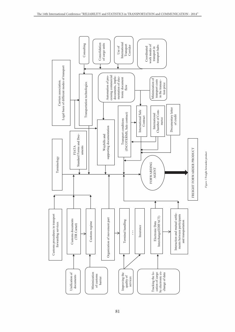
81


Tran

spor

t and

Tel

ecom

mun

icat

ion

…

Uni

ficat

ion

of

docu

men

ts

Term

inol

ogy

FOR

WA

RD

ING

A

GEN

T

FREI

GH

T FO

RW

AR

DER

PR

OD

UC

T

Car

riers

ass

ocia

tion.

Le

gal b

asis

of d

iffer

ent m

odes

of t

rans

port

Tran

spor

tatio

n te

chno

logi

es

Con

sulti

ng

Con

solid

atio

n of

car

go u

nits

Use

of

Inte

rnat

iona

l Tr

ansp

ort

Cor

ridor

Coo

rdin

ated

w

ork

mod

es o

f tra

nspo

rt in

tra

nspo

rt hu

bs

Way

bills

and

su

ppor

ting

docu

men

tatio

n

Tran

spor

t con

ditio

ns

(IN

CO

TER

MS,

Sal

e co

ntra

ct)

Inte

rnat

iona

l Sal

e C

ontra

ct

FIA

TA

Stan

dard

For

ms a

nd D

oc-

umen

ts

Inte

rnat

iona

l C

ham

ber o

f Com

-m

erce

Aut

omat

ion

of p

ro-

cess

ing

com

mer

cial

do

cum

ents

, im

ple-

men

tatio

n of

ele

c-tro

nic

docu

men

t flo

w

Min

imiz

atio

n of

tra

nspo

rt co

sts

in th

e tra

nsac

-tio

n pr

ice

Cus

tom

s pro

cedu

res i

n tra

nspo

rt fo

rwar

ding

serv

ices

Cus

tom

s doc

umen

ts

(TIR

Car

net)

Cus

tom

s reg

ime

Org

aniz

atio

n of

mov

emen

t par

t

Term

inal

han

dlin

g

Insu

ranc

e

Impr

ovin

g th

e qu

ality

of

serv

ices

Elec

troni

c D

ata

Inte

rcha

nge(

EDIF

AC

T)

Trac

king

the

lo-

catio

n of

car

go

by e

lect

roni

c ex

-ch

ange

of d

ata

Inte

ract

ion

and

mut

ual s

ettle

-m

ents

bet

wee

n pa

rtici

pant

s an

d tra

nspo

rtatio

n

Doc

umen

tary

lette

r of

cre

dit

Min

imiz

atio

n of

cus

tom

s ba

rrie

r

Figu

re 1

Fre

ight

forw

arde

r pro

duct

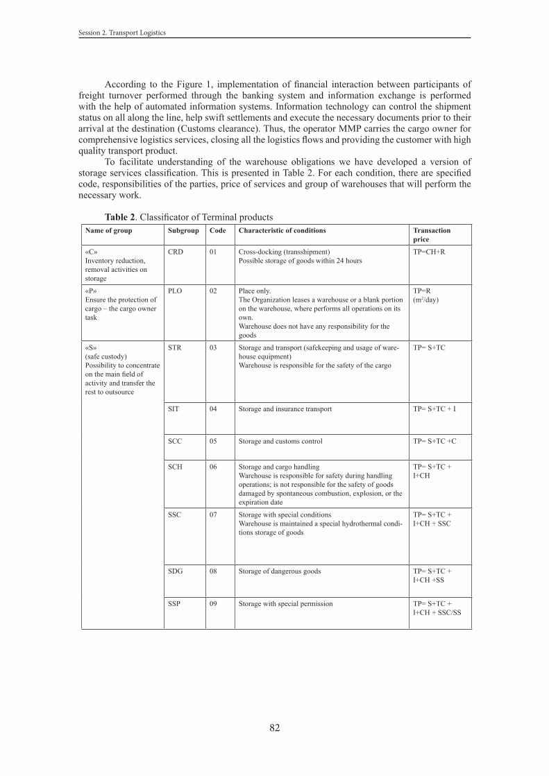
82


According to the Figure 1, implementation of financial interaction between participants of freight turnover performed through the banking system and information exchange is performed with the help of automated information systems. Information technology can control the shipment status on all along the line, help swift settlements and execute the necessary documents prior to their arrival at the destination (Customs clearance). Thus, the operator MMP carries the cargo owner for comprehensive logistics services, closing all the logistics flows and providing the customer with high quality transport product.

To facilitate understanding of the warehouse obligations we have developed a version of storage services classification. This is presented in Table 2. For each condition, there are specified code, responsibilities of the parties, price of services and group of warehouses that will perform the necessary work.

Table 2. Classificator of Terminal products Name of group Subgroup Code Characteristic of conditions Transaction

price

«C»Inventory reduction, removal activities on storage

СRD 01 Cross-docking (transshipment)Possible storage of goods within 24 hours

TP=CH+R

«P»Ensure the protection of cargo – the cargo owner task

PLO 02 Place only.The Organization leases a warehouse or a blank portion on the warehouse, where performs all operations on its own.Warehouse does not have any responsibility for the goods

TP=R (m2/day)

«S»(safe custody)Possibility to concentrate on the main field of activity and transfer the rest to outsource

STR 03 Storage and transport (safekeeping and usage of ware-house equipment)Warehouse is responsible for the safety of the cargo

TP= S+TC

SIT 04 Storage and insurance transport TP= S+TC + I

SCC 05 Storage and customs control TP= S+TC +C

SCH 06 Storage and cargo handlingWarehouse is responsible for safety during handling operations; is not responsible for the safety of goods damaged by spontaneous combustion, explosion, or the expiration date

TP= S+TC + I+CH

SSC 07 Storage with special conditionsWarehouse is maintained a special hydrothermal condi-tions storage of goods

TP= S+TC + I+CH + SSC

SDG 08 Storage of dangerous goods TP= S+TC + I+CH +SS

SSP 09 Storage with special permission TP= S+TC + I+CH + SSC/SS

83


«A» (assortment process) Warehouse is the best place for sorting, packing and consolidation of goods

ACB 10 Assortment consolidation break bulk TP= S+TC + I+CH +C/D

APP 11 Assortment preselling preparation:- marking - design - repacking - production of packaging - Preparation of gift sets - providing advertising and information materials

TP= S+TC + I+CH +C/D+CU

«Q»(quality)Quality management of the warehouse

QMA 12 Quality management:- complete quality control before shipment;- party and batch records;Product rotation on terms date and batch number (FIFO, LIFO).

TP= S+TC + I+CH +C/D + QC

QCW 13 Quality complaint work:- work with returns,- replacement;- repair.

TP= S+TC + I+CH +C/D + QC+CA

«V»Vendor managed re-sources

VMR 14 Warehouse controls inventory and sends the goods to the store when this needed.

TP= S+TC + I+CH +C/D + QC + IM

«D» (delivery)delivery management

DWT 15 Delivery by warehouse transport TP= S+TC + I+CH+D

DTC 16 Delivery by a transport company TP= S+TC + I+CH + CTC

DSC 17 Delivery special conditions TP= S+TC + I+CH+D+SSC

TP- transportation price, CH- cargo handling, R- price of the rent, S-storage, TC-transportation costs, I-insurance, C-customs, SSC- special storage conditions, SS- security system, C/D- consolidation/deconsolidation, CU-customization, QC- quality control, CA-claims activities, IM- inventory management, D-delivery, CTC- contract with a transport company

3. Conclusion

The detailed analysis of the International Multimodal transportation showed us that one of the important parts of the transportation is freight forwarder product. It consists of a plurality of options as handling, warehousing, consulting etc. One of the main components of the transportation costs is terminal handling charges. Thus, it is very important to optimize these costs.

The aim of the classificator of terminal products is to provide a set of terminal uniform tariffs of the most commonly used trade terms terminal handling. Knowledge of the uniform tariffs allows to a customer and to a forwarder itself have advantages as opportunity to plan terminal costs, legal protection of customer’s responsibility and tariffs transparency.

This classification has a potential to be used in the small storage companies, and regional and international levels.

References

1. Peter Jones. (2008) FIATA Legal Handbook on Forwarding. Republic Communications, Incorporated

2. Palagin Y.I.(2009) Logistics: planning and delivering. SPb.: Politehnika

84



DEVELOPMENT OF THE ALGORITHM FOR DESIGN AND REINGENEERING OF LOGISTICS DISTRIBUTION NETWORK

Valentina Dybskaya

Author’s information: National Research University Higher School of Economics, Moscow, Russian Federation, office 506, building 3, Kochnovskiy proezd,

phone: +7 (499) 152-17-01, e-mail: [email protected]

The current situation in the fast moving consumer goods market in Russia is changing drastically: the growing influence of retail chains on the manufacturer and the dynamic growth of logistics intermediaries make wholesalers seek all possible ways to ensure the reinforcement of its market positions. Practice shows that the main tool of competitiveness improvement and even more survival of merchants is an effective alignment of logistics. Distribution network design, ensuring maximum market cover with optimum costs of promoting trade flows based on the customer requirements is becoming the most important task of any company.

In this paper an algorithm for design and reengineering of logistics distribution network is proposed which is based on the models of supply chain network structure optimization, system analysis and benchmarking.Keywords: wholesalers, development trends, logistics, logistics infrastructure, distribution network, design algorithm

1. Introduction

Priorities of most participants in the supply chains regarding the distribution of many product groups are seriously altering in current markets. Even yesterday the main principal agents were wholesalers: they helped to ensure a wide assortment of goods for retail chains, transforming the industrial goods into the trade items through the operations in the wholesalers’ warehouses. But today, the development of retail chains and strengthening of market positions of logistics providers are drastically modifying the supply chains. The main trends of wholesale trade market development in Russia are the following (Dybskaya, 2013):

• The turnover of wholesalers in Russia is growing, but the direction of goods distribution is changing.

• Logistics infrastructure of merchant is in progress.• New models of relationship between finished-goods wholesalers and manufacturers are

appearing.• Maintenance of different market segments are being restructured and prioritized.• Market players are consolidating in the regulated markets.The growing influence of retail chains on the manufacturer and the dynamic growth of logistics

intermediaries make wholesalers seek all possible ways to ensure the reinforcement of its market positions.Retail chains are also changing rapidly. The key market trends (Sverchkov, 2013), which are typical

for the current stage of retail development are the following:• Slowdown of turnover rate in retail trade;• Changes in the product mix;• Rapid growth of such formats as retail chains;• Consolidation of main players;• Spread of shopping malls;• Increase of turnover in e-commerce;• Development of own retail trade by major producers and wholesalers;• Implementation of “green technologies” and development of premium sales.Effective management of logistics is the main tool of competitiveness for both wholesalers and retail

chains in the context specified above.

85


One of the most important strategic objectives for the trading companies in Russia remains maximum coverage of market. The implementation of such strategy is always concerned with the design of optimal logistics distribution system. It should be noted that the retailer is accounted as the end user of logistics system. Therefore, the complexity of solving problems of reengineering of logistics distribution network is explained in most cases by the differentiation of retailers’ formats (from hypermarkets to shops at home), the growing requirements to the logistics services and the geographical dispersion of sales points. So, for example, the number of stores has reached 6,884 units in the retail chain “Magnit”, the amount of sales points in “X5 Retail Group”, another widespread retail chain in Russia, is 3702 stores located practically across the whole country.

According to the logistics of any company, it is important to find out the optimum between the level of service and total logistics costs within the whole distribution network. Maintenance of required level of service is complicated by the fact that the company, designing a distribution network, may have stores not only with different format, but also with different price categories of stores, and hence with different needs for customer service. For instance, “X5 Retail Group” includes such shops as ”Pyaterochka”, “Karusel”, “Perekrestock” (shops from economy to the premium levels).

Logisticians design distribution networks within the function of distribution management. Design of logistics distribution network means the development of rational logistics infrastructure for the concentration and distribution of inventory in accordance with both customer requirements and the best logistics costs.

2. Factors affecting design and reengineering of logistics distribution network

Implementation of the distribution management function, as almost any logistic function, requires the participation of various related departments of the company. It supposes primarily the cooperation of logistics and commercial offices (marketing and sales departments) as well as procurement and finance ones. For a long period of time in the past just sales department was responsible for the distribution of trade flows in manufacturing or trading companies, due to the fact that the allocation of items in the markets were associated with the sales and distribution process. With the introduction of the logistics department in the organizational structure of management and rearrangement of functions between departments, it was brought up an issue of powers separation during the design of distribution network and promotion of trade flows to the final consumers.

Chosen sales and distribution system prescribed by commercial office lays a solid foundation for the future distribution network. Within sales and distribution process, marketing department defines strategy of sales and distribution system, segments sales markets, performs segmentation of customer base, determines the type of potential clients and pricing policy of sales department, implements sales promotion, creates sales and distribution system, develops customer service policy and product return policy, etc. In turn, sales department makes a contract, monitors the fulfillment of contract terms and the execution of orders.

Such functions as supply of customers and design of distribution network are delegated to logistics department. It is obvious that in order to ensure the promotion of the flow of goods to final consumers, logistics has to create a system of supply chains with a well-functioning logistics infrastructure. Logistics distribution network should be developed with the optimization of all available resources.

Logistics distribution network is a structure of objects which concentrate stocks formed by supplier of goods for further supply in order to meet customers’ requirements for delivery and optimal level of logistics costs in the whole network.

Distribution network can be developed by any entity of commodity-money relations, conducting sales and marketing activities. Spread of distribution network depends on the number of consumers and their geographic location. Logistics infrastructure especially supplier warehouse network of goods is the basis of distribution network design.

It is reasonable to design the distribution network if company promotes trade flows by its own or uses mixed variant of sales and distribution system. In most cases the design process is the logistics response on the proposed new marketing strategy, involving growth of sales, changes in the territorial coverage of consumers or service policy. Initiative of design can come from the logistics itself when the distribution strategy is modifying or analysis of the existing network reveals its ineffectiveness. Last two cases are usually transferred to reengineering of the existing distribution network.

86


Reorganization of distribution network may be the result of (Dybskaya and et al., 2008):• Changes in market demand;• Competitive environment strengthen which assumes need of search for more effective solutions;• Emergence of new customers;• Customer requirements for improvement of service levels;• Adjustment of product specialization;• Necessity of cost reduction within distribution network;• Sales market increase by expansion into new markets;• Modification of sales policy;• Revision of pricing policy;• Outsourcing strategy;• Company profile transformation;• Mergers of several companies;• Financial amendments in company;• Increase of service radius from one depot;• Low efficiency of resource used.

3. Guidelines for distribution management

Distribution management requires constant efficiency monitoring of logistics processes organization in the distribution network. Improving the efficiency of the distribution network lay a claim to a careful and thorough assessment of the current and future state of company’s distribution system. To assess the effectiveness of distribution system (DS), a comprehensive study of logistics processes structure within the system, physical distribution management system status and behavior and logistics costs of activities implementation within distribution should be conducted. It is necessary to carry out the identification of deficiencies in the planning, organizing, implementing and monitoring of DS logistics activity as well as quality of logistics services provision. Identified shortcomings helps to find out ways of their elimination. Analysis of DS allows logicians to develop structure of logistics of distribution and improve directions of its growth in order to enhance further effectiveness of the whole company.

To assess the efficiency of logistics of distribution it should be analyzed:• Existing logistics network and organizational structure of product distribution management;• Effectiveness of the main logistics functions performed by departments (offices) and business

units of company within distribution process;• Internal and external customers’ satisfaction with quality of DS logistics services;• Rationality of financial, material and human resources use performing distribution functions;• Total cost of logistics distribution and component of logistics costs by types of activities;• Occurrence of conflicts between departments of company regarding logistics parameters and

existence of cross- functions in leading of DS logistics processes;• Workflow efficiency relating to the logistics distribution in departments (offices, business units);• Conditions and requirements of inventory management;• State of warehousing, transport and other logistics infrastructure in distribution.Analysis results give to draw conclusions about the efficiency of the distribution network. In the

case of detected deviations from established performance criteria which reduce the effectiveness of the existing network, it is required to decide whether to reengineer distribution network or may be to design a new one.

Primary sources of information for further analysis and evaluation of DS effectiveness should be obtained from:

• Plans, accounting and reporting record;• Results of company’s employees survey (via questionnaire);• Documents forms used in the planning, implementation and monitoring of logistics functions

and operations in distribution;• Regulations of departments (offices, business units) and employees job descriptions in these

structural units;• Other regulatory and reference materials;• Results of quantitative data collection regarding logistics processes and costs in distribution.

87


4. Algorithm of logistics distribution network design and reengineering

The standard approach to distribution network design (Bowersox and Closs, 2005) includes three main stages: identification of the reasons that lead to changes in the system efficiency, collection and analysis of primary data for development options of design concepts and choice of optimal project among the number of decisions developed and suggested for implementation.

Based on this framework, the author of the paper offers detailed tree-phase algorithm of design and reengineering of logistics distribution network.

The approach provided consists of three-following phases:• Analysis of current logistics distribution network performance;• Identification of the main directions of logistics distribution network reengineering;• Design of a new logistics distribution network or reengineering of the current one.

• Each of the phases includes some steps in turn, which should be properly clarified. In order to assess how well present logistics distribution network operates, firstly, goals of the logistics distribution network should be defined in accordance with the logistics strategy of the company. Secondly, general features of business environment in which existing logistics distribution network functioning should be determined. And only then detailed analysis of the activities within the current distribution system should be run with evaluation of opportunities to achieve previously defined goals.

• External business environment, existing structure of consumer demand as well as customer service requirements and current logistics infrastructure of the company should be learnt on the second step of the first phase.

• The third most complicated step of the first phase proposes realization of two groups of estimation among which (1) analysis of the current structure of the logistics system and organizational structure of distribution management in the company and (2) assessment of the possibility to achieve goals within the logistics distribution network without any changes, otherwise to reveal the necessity to reorganize it.

• For the purpose of objective appraisal of logistics system structure as well as ways of distribution management, the following aspects of company activities should be analyzed:

• Present structure of logistics system and organizational structure of distribution in the company;• Effectiveness of key logistics functions performed by departments (offices, business units) of the

company in the distribution system;• Rate of internal and external customers’ satisfaction by quality of logistics services in the

distribution system;• Financial, material and human resources adequacy in the process of distribution functions

performance; • Total cost of logistics of distribution and logistics costs by types of activities;• Existence of conflicts between departments (offices, business units) of the company regarding

logistics parameters and cross-functions in managing logistics processes in distribution system;• Efficiency of workflow between departments (offices, business units) of the company relating

to the logistics of distribution;• Planning and inventory management systems;• Warehousing, transport and other logistics infrastructure employed within distribution process.

• Then on the base of performance indicators deviation, it is possible to investigate external and internal causes affecting distribution system performance reduction.

• Firstly, it requires performing situational analysis in order to reveal strength and weaknesses of current system at the present time and compliance with objectives to be achieved.

• Analysis is needed to determine the potential of the system, taking into account the characteristics of logistics distribution system and markets, competitive environment and modern technologies to be applied. Description of the system is necessary to clearly define the features of existing processes in the logistics system and the effectiveness of the system. The analysis should cover all major types of resources: human resources, utilized equipment and facilities of logistics infrastructure, existing relationships and information flow. As a result, it is necessary to identify bottlenecks of the processes used and determine the required volume of resources for their optimization.

88


• So, being more specific, data for SWOT-analysis should be collected, limitations of system operation should be identified, indicators to assess performance of the system should be deployed and, eventually, internal and external factors affecting logistics system should be evaluated.

• Secondly, the scheme of research must be developed (Brodetskiy, 2012). For this, actual opportunities of system activities examination should be analyzed, company’s resources should be assessed, performers should be chosen and methods of evaluation should be developed.

• Thirdly, it is necessary to evaluate the costs and effectiveness of existing distribution logistics network as well as of reengineered options, for which the following actions should be realized:

• Determination of structure of main costs in logistics distribution network;• Definition of acceptable level of logistics costs from the perspective of competitive prices on

goods and services for the evaluation of the analyzed indicators;• Development of key performance indicators and its criteria for existing distribution network;• Analysis and assessment of key performance indicators of the distribution network.

• Finally, it becomes possible to identify the necessity of logistics distribution system reengineering, providing technical and economic confirmation.

• In order to develop detailed (technical) project report of reengineering logistics distribution network, this is the second phase of the suggested approach, approved logistics strategy of the company, systematic goals and objectives of distribution network should be defined. Set goals should be result-oriented and have a quantitative or qualitative assessment to determine to which extent they are achieved. Defining restrictions imposed on the activities of the distribution system, key performance indicators and criteria for their evaluation, possibilities of available resources to achieve the established criteria of the system should be specified. The opportunities occur by improving organization of the processes within the present logistics distribution system, enhancing productivity and using other potentials that do not cover the fundamental changes of the current distribution network. To ensure effectiveness of distribution network reengineered, main possible directions of its reorganization should be exposed among which better customer service provision, costs saving (only one-time action) or elimination of unnecessary costs at all (cut of variable costs), order cycle time reduction and performance of logistics infrastructure improvement by implementation of advanced technological solutions and information systems. Process of reengineering may cover quite different levels of managerial decisions: from designing a new distribution network with the inclusion of some existing elements (e.g., one or more existing warehouses) to changes in technology of product distribution in specific supply chain. It should be noted that detailed project report of reengineering of logistics distribution network should cover those option that will help to achieve objectives of logistics distribution network. The most complete project will design optimal type of logistics distribution network.

The third phase of the proposed approach means direct design or reengineering of logistics distribution network which includes ten comprehensive steps. First of all, it is required (I) to forecast demand in the different markets choosing demand forecasting procedure, and then to plan volume of sales by sales regions. Using the information received in the previous phase, (II) utilization of existing distribution network as well as specific supply chains should be analyzed and evaluated taking into consideration the selected direction of reengineering and the intention to extant market coverage.

Based on the comprehensive analysis, (III) sales and distribution system by sales markets should be chosen. This means that relies on the established criteria and identified constraints the participants for further trading should be chosen. There are three possible sales and distribution systems: (1) independent sales and distribution system where goods sold to the independent distributors, (2) sales and distribution system of focal company where the physical distribution of good should be realized by the company itself utilizing its logistics distribution network, and (3) dependent sales and distribution system where goods promoted through dealers’ logistics distribution network. Taking decision about type of sales and distribution system, the following factors should be taken into account: competitive business environment, logistics infrastructure available in each region of the projected sales, types of customers, requirements for customer service level and costs associated with the activities of each of sales and distribution system option.

If independent sales and distribution system is preferred logistics have to deal with the decision of traditional logistics tasks, excluding distribution management issues, as in general cases the right of ownership on the goods passes to independent distributor when items are shipping from the warehouse.

89


When company decides to choose design of its own or dependent sales and distribution system it continues implement further steps of the procedure, which includes (IV) market segmentation by regions of service, (V) development of distribution network organizational structure, (VI) choice of optimal logistics distribution network, (VII) determination of costs associated with the implementation of optimum distribution network version, (VIII) elaboration of recommendations for implementing the proposed version of distribution network, (IX) deployment of the proposed option by working out the thorough implementation plan, coordinating schedules of work, determining acceptable indicator values, and (X) organization of activities monitoring and controlling systems in suggested logistics distribution network.

When it is necessary (IV) to segment markets by regions of own distribution network operation based on the established customer service policy, several sales markets can be supplied from one warehouse. Marketing department defines potential sales regions which later are combined by logistics department in segments of supply used to create warehouse network for customer maintenance. The decision to choose only one depot for goods promotion in sales market or several one should be previously confirmed by the separation of supply regions and by definition of inventory level and frequency of delivery of end customers (retailer networks and service companies). It should be taken into consideration the tendency of customers to work on the working inventory what determines the level of inventories in days and frequency of deliveries to maintain specified level.

Having the information regarding volume of stock and delivery frequency, it is possible (V) to segregate logistics supply chains for detailed description of each of them, including the choice of partners which will participate in promotion of trade flows in the system of goods distribution. First of all, the general system of goods distribution should be established for each of the selected sales segments. Then the inventory should be apportioned in it: level of stock should be specified for each deport from which end users will be supplied. Now it is possible to consider logistics infrastructure creation, resolving in-sourcing – outsourcing issue. In those cases when company attracts logistics service providers, logistics department of the company stops the design process. However if the outsourcing decision is taken to the concrete part of logistics system, the company organizes control over logistics service provider’s activities within this part of the system, continuing implementation of proposed approach further on.

Design of logistics infrastructure concerns the question of (a) optimal warehouse network development, (b) choice of physical distribution technology (or technology of delivery goods) and (c) provision of consolidated informational area in the distribution network.

In order to organize warehouse network (a) it is required to determine the number of deports in the sales region, their functions and links between each other, places of their allocation and strategy of inventory warehousing (the form of ownership by deport). The last point provides the possibility to combine different strategies of inventory warehousing, among which utilization of company’s warehouses, use of logistics services provider’s warehouses or renting storage capacity.

Selection of optimal physical distribution technology (b) supposes the decision on cargo container type for each supplier – customer link, means of transportation and delivery routes. Location of the customer, applied form of sales at the end user, delivery lot with specification of range of items and their quantity, frequency of delivery, sizes of consumer and transport packaging, condition of goods storage (necessity to maintain temperature regime) will specify the type of cargo container. When vehicle for different segments of the supply chain is chosen, it is necessary to be aware of the selected cargo container, sizes of delivery batches, route length, geography of consumers, existence of loading-unloading ramps and other technical features of clients’ infrastructure required for logistics process execution, conditions goods storage during transportation. The choice of vehicle should ensure maximum use of its standard cargo capacity.

Establishment of unified information system as well as smoothing workflow for all logistics chains are the keys to provision of consolidated informational area in the distribution network (c).

When all necessary information is collected, (VI) optimal logistics distribution network should be chosen. For this, it is firstly required to develop competitive options of logistics distribution network as a set of supply chains, then to identify measurable restrictions imposed on the activities of distribution network, later on to define indicators and criteria for evaluation of distribution network, and, finally, to evaluate developed options of logistics distribution network and select the optimal version.

The following basic parameters should be used for integrated distribution network performance evaluation: order cycle time, total costs in the network, customer service, use of logistics assets. Thus it is necessary to consider not only the magnitude of the total complex index, but all of its components.

90


The next four steps of the third phase will complete the execution of proposed algorithm which is presented on the Figure 1.

1st phase Analysis of the current logistics distribution network

performance

2nd phase Identification of the main directions of logistics

distribution network reengineering

3rd phaseDesign of new logistics distribution network or reengineering of the current network

1. Definition of the logistics distribution network goals in accordance with the logistic strategy of the company2. Determination of the general conditions of the existing distribution network functioning 3. Analysis of activities of current distribution system and evaluation of opportunities to achieve goals within the existing distribution network:1) Analysis of existing structure of logistics system and organizational structure of distribution2) Assessment the possibility to achieve goals within existing distribution network or revelation the necessity to reengineer logistics distribution network:2.1) Evaluation logistics distribution system performance in accordance with criteria of efficiency. Registration of deviations .2.2) Determination causes of effective logistics distribution system altering2.3) Analysis of external and internal causes of changes impacting on reduction of system performance:

a. Situational analysisb. Scheme of research development

2.4) Necessity to reengineer logistics distribution system confirmed by technical and economic report

1. Definition of approved logistics strategy, system of goals and problems of distribution network2. Determination of restrictions imposed on the activities of distribution system3. Choice of key performance indicators and criteria of distribution system efficiency evaluation4. Analysis of possibilities available resources to achieve the established criteria of the system 5. Designation of the main possible directions of distribution network reengineering6. Development of reengineering project

1. Forecasting demand and planning sales volume by sales regions.2. Analysis and evaluation of existing distribution network and specific supply chain to be reengineered3. Selecting sales and distribution system for each market: (1) Independent sales and distribution system, (2) Own sales and distribution system or (3) Dependent sales and distribution system4. Markets segmentation by region of service by own distribution network based on established customer service policy:4.1) Definition of supply regions4.2) Determination inventory levels of end customers and frequency of delivery to them5. Establishment of distribution network organizational structure 5.1) Choice of partners to be involved in promotion of trade flows5.2) Apportion of inventory in distribution system5.3) Logistics infrastructure creation: decision on “in-sourcing – outsourcing” of it5.4) Logistics infrastructure creation: optimal warehouse network development by determining (I) optimal number of warehouses in the regions of service, (II) functional purpose of warehouses in regions and their connections, (III) locations of warehouses, (IV) forms of warehouses ownership: use (1) own warehouses, (2) warehouses of logistics services providers or (3) leased storage capacity, and (V) centralized or decentralized ways of warehousing network supply5.5) Logistics infrastructure creation: selection of optimal physical distribution technology by selecting (1) cargo container type for each supplier – customer link, (2) means of transportation and (3) delivery routes5.6) Logistics infrastructure creation: to provision of consolidated informational area in the distribution network by establishing unified information system and smoothing workflow6. Choice of optimal logistics distribution network6.1) Offering of competitive options of logistics distribution network as a set of supply chains6.2) Identification of measurable restrictions imposed on the activities of distribution network6.3) Definition of indicators and criteria for evaluation of distribution network6.4) Evaluation of developed logistics distribution network options and optimum version selection7. Determination of costs associated with the implementation of optimum distribution network version8. Elaboration of recommendations for implementing the proposed version of distribution network9. Deployment of the proposed version of distribution network10. Organization of monitoring and controlling systems in suggested logistics distribution network

Figure 1 Algorithm of logistics distribution network design and reengineering

91


5. Conclusion

The main trends of Russian markets development force the managers consider the effectiveness and efficiency of current logistics distribution networks structure. Taking into account prerequisites which have an influence on the issue posted, the procedure of design and reengineering of logistics distribution network is not perceived as trivial one. The author of this article suggested the carefully specified algorithm which can be of significant not only for theoretical discuss, but also for practical implementation as it contains step-by-step recommendation for rational design and reengineering of logistics distribution network.

References

1. Bowersox, D.J. and Closs D.J. (2005) Logistics: the integrated supply chain. Moscow: ZAO “OLYMP-BUSINESS”

2. Brodetskiy, G.L. (2012) Economical and mathematical methods and models in logistics: optimization procedures. Moscow: Publishing centre “Academia”

3. Dybskaya, V.V. (2012) Basic approach to design and reorganization of the distribution network. Logistics and Supply Chain Management, 51 (4), 9-15.

4. Dybskaya, V.V. (2013) About the terminology concerning logistics centers. Logistics and Supply Chain Management, 56 (3), 7—10.

5. Dybskaya, V.V. (2013) Current trends in the development of logistics in the wholesalers. Logistics today, 5, 310-320.

6. Dybskaya, V.V. and Ivanova, A.V. (2012) Creation of logistics service system and service quality management in distribution network. Logistics and Supply Chain Management, 51 (4), 23-31.

7. Dybskaya, V.V. and at al. (2008) Logistics: integration and optimization of logistics business processes in supply chains. Moscow: EKSMO

8. Dybskaya, V.V. and Sergeev, V.I. (2012) Models of operative activities of logistics centers. Logistics and Supply Chain Management, 48 (1), 6-18.

9. Stock, J.R. and Lambert, D.M. (2005) Strategic logistics management. Moscow: INFRA-M10. Sverchkov, P.A. (2013) Influence of the wholesaler’s development strategy onto its logistics

infrastructure. Logistics today, 5, 258-267.11. Ministry of Industry and Trade of the Russian Federation. (2010) The strategy of trade

development in the Russian Federation during 2011-2015 and up to 2020. Moscow: Ministry of Industry and Trade of the Russian Federation. URL: http://www.gosbook.ru/node/20605 (Accessed date 14.04.2014).

92


Proceedings of the 14h International Conference “Reliability and Statistics in Transportation and Communication”(RelStat’14), 15–18 October 2014, Riga, Latvia, p. 92–101. ISBN 978-9984-818-70-2Transport and Telecommunication Institute, Lomonosova 1, LV-1019, Riga, Latvia

MODEL OF DECISION SUPPORT FOR ALTERNATIVE CHOICE IN THE LARGE SCALE TRANSPORTATION TRANSIT SYSTEM

Igor Kabashkin1, Jelena Mikulko2

Transport and Telecommunication InstituteLomonosova 1, Riga, LV-1019, Latvia

1Phone: +37 129215392. E-mail: [email protected] 2Phone: +371 29584606. E-mail: [email protected]

In the situation of strong competition between ports in the Baltic Sea Region (BSR) and clear-

cut ascendancy of alternative routes, the BSR is facing a need for major economic restructuring, and efforts to achieve more integrated and sustainable transport links within the BSR are needed. One of these efforts is the development of ports and logistics centres and their networking, which will continue to have an impact on improving communication links, spatial planning practices and approaches, logistics chain development and the promotion of sustainable transport modes. These factors will reflect on logistics processes both in major gateway cities and in remote BSR areas. The objective of paper is to suggest the multiple-criteria approach for evaluation and choice the alternatives of cargo transportation in the large scale transportation transit system with special attention to Baltic Sea Region. The multimodal transportation system with finite number of known alternatives defined by the routes and modes of transportation are considered. Each alternative is represented by its performance in multiple criteria.

The large scale transportation transit system is presented by directed finite graph which is an ordered pair D = (V, A) where V is set of finite vertices (railway stations, ports, border points and logistic centers) and A is set of finite arcs (transport lines between ports and/or logistics centers). The vertices are grouped in clusters. In each cluster only one vertex can be used as alternative for transit routes. Each vertex vi (V=vi, i=1,…n) is characterized by an individual set of key performance indicators Kvi and each arc aj (A=aj, j=1,…m) is characterized by an individual set of parameters Paj.It can be find several alternatives for cargo delivery determined by different routes and modes which form the vector space of a family of alternative transit vector routes. In the paper a model for decision of route choice is described, the finite graph of the large scale transportation transit system with special emphasis on BSR is presented, the criteria of optimization is formulated, the set of key performance indicators Kvi and set of parameters Paj are described.Keywords: Transport model, transit, decision support, Baltic Sea Region

1. Global Logistics Trends and Freight Transport Development

International business has been undergoing a period of rapid transformation. Researchers at the McKinsey Global Institute (McKinsey Global Institute, 2012) calculated the economic centre of gravity of the world by using Gross National Product (GDP) as a measure of the mass or weight of a country and using the world map as a physical object (Figure 1).

Based on the calculations, the centre of gravity in 1950 was in the Atlantic Ocean. Today the centre of gravity is over southern Russia and moving eastward, as shown in the map at figure 1. As a result of shift of economic mass, supply chain configurations are becoming increasingly volatile and the shift in the global economic centre of gravity to emerging regions may see reduced growth on traditional trade routes. Such restructuring is contributing to economic growth, better allocation of resources and more freedom of choice for consumers, as well as increased competition. In order to be internationally competitive, businesses are organising strategic worldwide networks that can deliver an efficient and high-quality response to demand from any segment of the world market. The efficient

93


and integrated organisation of such activities is often referred to as global logistics and it has become the core of global competitive power. Business will need extensive market intelligence for using of the opportunities that arise from this change of economic centre of gravity.

Global logistics networks serve as a circulatory system for the corresponding global value-adding chain where various components in the logistics network serve different functions in an organisationally unified manner. Therefore, in order to establish a region as a key component in global logistics networks, it is necessary to create a vision of how to position the region strategically within the context of the overall global logistics networks.

Figure 1. Evaluation of the earth’s economic centre of gravity

Development pattern of the particular sectors within the EU transport system is quite unbalanced which is preconditioned by the following factors: first of all, the extent of the particular countries involvement into the work of the transport industry varies from country to country; secondly, it is influenced substantially by the pattern of the EU financial packages allocation. Nowadays one of the top priorities of the EU transport policy is the expansion of the Trans-European networks (the possibility is envisaged even to stretch them outside the EU borders), as well as building up the global transport corridors in cooperation with other countries.

Any strategy adopted for the purposes of the transport system development is worth of mark since it contains two split-level components. One of these components is of a global character: today the appropriate infrastructure including transport must be ensured to guarantee a successful development of a given region. This assumption quite logically leads us to the next level – the EU specifically formulated practical proposals and problem-solving strategies. The same two-level approach can be used to describe the EU transport policy. However, when stipulating the EU transport policy, one has to take into account a major impact it confronts due to the influence of political and economic factors.

The Baltic region is remarkable for its economically advantageous geographical position within the Eurasian transport system, connecting Russia with the biggest world markets of the Central and Eastern Europe as well as with the Baltic States and the CIS States and China. In the situation where a large increase in trade and freight transport volumes in the Baltic Sea Region (BSR) is expected and in which the BSR is facing a major economic restructuring, efforts to additional study of more integrated and sustainable transport and communication links within the BSR are needed.

The volatility and uncertainties of today’s economic environment and expanding global supply chains require coordinated efforts to optimise network configurations and inventories to synchronise global supply and demand. At the same time, new business models are emerging with shift to customer-driven supply chains. Reconfiguring supply chains around customers has led to the necessity for more

94


flexible and adaptive formation system of transport and logistics links. In this situation decision support system (DSS) is one of the instruments for choice the most effective decision for customer in constant fluctuated business environment.

There are seven typical steps in the process of multicriteria decision making (Sinha, 2007): • Identify transportation alternatives;• Establish performance criteria;• Establish relative importance of performance criteria;• Establish commensurate scale for measuring levels of each criteria;• Using the established scale, quantify level (impact) of each criterion for each alternative

action;• Establish the combined impact of the different criteria for each alternative;• Determine the most satisfying alternative.

The first two tasks of above mentioned are the subject of current investigation.

2. Identification of transportation alternative. Case study for the route “China – Russia”

Containerization greatly reduced the expense of international trade and increased its speed, especially of consumer goods and commodities. Today approximately 90% of non-bulk cargo worldwide is moved by containers stacked on transport ships (Mikulko, 2013).

The increasing use of containers in transport has increased the share of intermodal transport chains, which contain several modes of transport. Cost-efficient railway or sea transport is used on the main routes of intermodal transport, while flexible road transport is used in collection and distribution activities.

Therefore the main transport corridors connecting China and Russia for containerised cargoes are:1. Southeast China -all-water route via Suez Canal to Baltic Sea;2. Southeast China -all-water route via Suez Canal to Black Sea; 3. International Transport Corridor “Trans-Siberian” (or “East-West”, the backbone of

which is Trans-Siberian Railway) with different connections to rail/sea/road and delivery network at both ends;

4. West Europe-West China (through Kazakhstan territory) – rail and road connections.

The main competition is taking place between the two all-water routes and “Trans-Siberian” transport corridor. The ocean route through the Suez Canal is the most important trade route between the Far East, South-eastern Asia and Europe and Russia. Large and global companies have developed an efficient logistics system which consists of a collection and delivery network at ends, terminals and large vessels for which some type of vessels can transport till 18000 TEU at a time.

Containerized cargoes are transported via shipping lines, operated on a regular basis. There are three main shipping companies in the container industry who provide services worldwide and named leaders in the industry because they have together about 39.65% market share. These are APM-Maersk, Mediterranean Shipping Company and CMA-CGM Group. These three shipping lines are the main service providers for cargoes transhipped through the Baltic ports (Midoro, 2005). Short sea connections are based on these three main service providers:

1. Loading place in China-Main China port-Hamburg-Riga-Custom clearance place-Unloading place

2. Loading place in China-Main China port-Hamburg-Klaipeda-Custom clearance place-Unloading place

3. Loading place in China-Main China port-Hamburg-Tallinn-Custom clearance place-Unloading place

4. Loading place in China-Main China port-Hamburg-HaminaKotka-Custom clearance place-Unloading place

5. Loading place in China-Main China port-Bremerhaven-St. Petersburg-Unloading place6. Loading place in China-Main China port-Gdansk-Riga-Custom clearance place-

Unloading place

95


7. Loading place in China-Main China port-Gdansk-Klaipeda-Custom clearance place-Unloading place

8. Loading place in China-Main China port-Gdansk-Tallinn-Custom clearance place-Unloading place

9. Loading place in China-Main China port-Gdansk-HaminaKotka-Custom clearance place-Unloading place

10. Loading place in China-Main China port-Gdansk-Ust Luga-Unloading place11. Loading place in China-Main China port-Zeebrugge-Ust Luga- Unloading place12. Loading place in China-Main China port-Rotterdam- St. Petersburg-Unloading place13. Loading place in China-Main China port-Antwerp-Riga Custom clearance place-

Unloading place14. Loading place in China-Main China port-Antwerp-Klaipeda Custom clearance place-

Unloading place15. Loading place in China-Main China port-Antwerp-Tallinn Custom clearance place-

Unloading place16. Loading place in China-Main China port-Antwerp-HaminaKotka-Custom clearance

place-Unloading place17. Loading place in China-Main China port-Antwerp-St. Petersburg-Unloading place18. Loading place in China-Main China port-Novorossiysk-Railway station in Russia-

Unloading place19. Loading place in China-Main China port-Novorossiysk-Unloading place20. Loading place in China-Main China port-Odessa-Custom clearance place-Unloading

place21. Loading place in China-Main China port-Odessa-Railway station in Russia-Unloading

place22. Loading place in China-Main China port- Vladivostok/Nahodka/Vostochny-Railway

station in Russia-Unloading place23. Loading place in China-Main China port-Railway station for train departure in China-

Suhe-Bator (MN) - Naushki (RU) border-Railway station in Russia-Unloading place24. Loading place in China-Main China port-Railway station for train departure in China-

Manzhouli (CN) - Zabaikalsk (RU) border-Railway station in Russia-Unloading place25. Loading place in China-Main China port-Railway station for train departure in China-

Alashankou (CN) - Dostyk (KZ) border-Railway station in Russia-Unloading place26. All mentioned possibilities could be started by rail or road transportation of cargo to the

China main port (50 above mentioned transportation chains).27. Loading place in China- Railway station for train departure in China- Suhe-Bator (MN)

- Naushki (RU) border-Railway station in Russia-Unloading place28. Loading place in China-Railway station for train departure in China- Manzhouli (CN) -

Zabaikalsk (RU) border-Railway station in Russia-Unloading place29. Loading place in China-Railway station for train departure in China- Alashankou (CN) -

Dostyk (KZ) border-Railway station in Russia-Unloading placeThree mentioned possibilities could be started by rail or road transportation of cargo to the

Railway station for train departure in China (6 above mentioned transportation chains).30. Loading place in China – Horgos (CN) - Korgas (KZ) border-Custom clearance place in

Russia-Unloading place (by road)In total there are 57 alternatives of cargo transportation in the large scale transportation transit

system which can be presented by graph shown at figure 2.

96


Ha

mb

urg

Bre

me

rha

ven

Gd

an

sk

Zee

bru

gge

Ro

tterd

am

An

twe

rp

An

y “Ma

in” C

hin

a P

ort

Loa

din

g p

lace

in C

hin

a

Riga

Kla

ipe

da

Tallin

n

Ha

min

aK

otka

St.P

ete

rsbu

rg

Ust Lu

ga

Ra

ilway sta

tion

in R

ussia

Cu

stom

clea

ran

ce p

lace

Un

loa

din

g p

lace

No

voro

ssiysk

Od

essa

Vla

divo

stok/N

ah

od

ka/V

osto

chn

y

Ea

stern

Ba

ltic Sea

Ma

in C

on

tain

er P

orts

De

ep

Se

a M

od

e

Sho

rt Sea

Mo

de

Ra

ilwa

y statio

n fo

r train

de

pa

rture

in C

hin

a

1

2

3

Su

he

-Ba

tor (M

N) - N

au

shki (R

U) b

ord

er

1

Ma

nzh

ou

li (CN

) - Zab

aika

lsk (RU

) bo

rde

r23

Ala

sha

nko

u (C

N) - D

ostyk (K

Z) b

ord

er

Ro

ad

De

ep

sea

Sho

rt sea

Ra

il

4H

orgo

s (CN

) - Ko

rga

s (KZ

) bo

rde

r

4

Fig

ure

2. T

he altern

atives o

f cargo

transp

ortatio

n in

the larg

e scale transp

ortatio

n tran

sit system

5

97


The large scale transportation transit system is presented by directed finite graph which is an ordered pair D = (V, A) where V is set of finite vertices (railway stations, ports, border points and logistics centers) and A is set of finite arcs (transport lines between ports and/or logistics centers). The vertices are grouped in clusters. In each cluster only one vertex can be used as alternative for transit routes. Each vertex vi (V=vi, i=1,…n) is characterized by an individual set of key performance indicators Kvi and each arc aj (A=aj, j=1,…m) is characterized by an individual set of parameters Paj. The set of key performance indicators Kvi and set of parameters Paj are described further.

If all characteristics of the graph were known the research would come down to the standard task solving. The standard System of KPI (Key Performance Indicators) of ports and other Logistics

objects currently used in Baltic States came down to the very simple provide an incomplete picture of competitiveness. These KPIs are primarily describing the gross level of logistic object activity (e.g. total TEU or total tonnage). But traffic volumes often present a distorted picture: they are not always accurate (e.g., transshipment ports double count containers, once when unloaded and then when reloaded), container volumes give equal weight to empty and loaded boxes, cargo tonnages often include container tare weight, they do not distinguish between low-value/high-volume bulk cargoes and high-value unitized cargoes, and they are affected by a number of exogenous factors which makes it difficult to establish solid correlations with a logistic object’s competitiveness (The World Bank, 2013). It is often sought to make transportation decision on the basis of wider range of performance criteria that reflect the concerns of all key stakeholders, i.e. agency goals, perspectives of facility users, concerns of society as a whole, environmental impact from transportation and others (Maciulis, 2009; Kopytov, 2010). But in reality such criterias are not decisive for the cargo owners.

That’s why the set of key performance indicators Kvi and set of parameters Paj should be determined to suggest further the multiple-criteria approach for evaluation and choice the alternatives of cargo transportation in the large scale transportation transit system with special attention to Baltic Sea Region.

3. Performance criteria for transportation decision making

There are a lot of major issues in business decision making in the international container transportation industry and cargo owners determine the mode by which they will have their freight transported, considering mainly their corporate, personal priorities. One of the general approaches for taxonomy of cargo owner’s preferences was proposed in (Kabashkin, 2003). The framework D for decision making sets out the factors influencing the transit sector from users’ point of view in the order of their priority:

, = , i= , where – factor of influence with parameters:

– geographical plane, – economical plane, – institutional/political plane, – infrastructure plane,

– technology plane.

The choice of parameters at higher levels , k= become feasible when lower level is achieved.

=

In this case the analyse could be minimized by making decision support system taking into account the infrastructural, technologic, economical, geographical factors and excepting the political. Taxonomy of KPI Kvi for this model can be described by set of parameters shown at the figure 3.

98


KP

Is of lo

gistic o

bje

cts

Fig

ure

3. T

he T

axon

om

y o

f the set o

f key p

erform

ance in

dicato

rs Kvi

8

99


Taxonomy of the set of KPI’s parameters Paj includes two groups of metrics: quantitative and qualitative.

The set of quantitative metrics could include the next parameters:1. Direct costs for freight for light cargo – costs for transportation from A to B without

custom clearance costs for cargo till 20 t. brutto weight (kg).2. Direct costs for freight for heavy cargo – costs for transportation from A to B without

custom clearance costs for cargo over 20 t. brutto weight (kg).3. Fluctuation of costs during the year (times) – how much costs for transportation could

be changed during the year (increase or decrease), based on statistics from 2008 year. 4. Time of transportation – (days) how much days in average is necessary to reach unloading

point.5. Frequency with which shipments don’t reach the consignee within the scheduled or

expected time – (%) in which cases shipments don’t reach the consignee within the scheduled or expected time using this transport corridor.

6. Costs for custom clearance – (US dollars) costs for custom clearance at bonded warehouse in destination. On which route the most logical custom clearance point is differ.

7. Quantity of border point on the route – (quantity) how many border points exists (only customs points) on the route from A to B.

8. Probability of risk factor (theft) – (%) risk of theft on the route (expert evaluation).9. Probability of risk factor (damages) - (%) risk of damages on the route (expert evaluation).10. LPI of transhipments countries – (LPI index). 11. Warehouse services price level – (index) expect evaluation comparing warehouse

services price level on existing routes in logical transhipment points.12. Distance from A to B – (km) distance from loading place till unloading place.13. Presence of regular Shipping Lines – (quantity) quantity of regular Shipping Lines which

connect ports of loading and unloading.14. Cargo flow corridors – (quantity) how much major cargo flows existing nowadays in this

transport corridor.15. Transportation distance to the port (km) distance from the loading point till the nearest

logical port of loading.16. Transportation distance from the port (km) distance from the unloading port till the

unloading place.17. Availability of equipment – (%) cases in which necessary equipment (containers) are

available. Expert evaluation.18. Availability of transport – (%) cases in which necessary truck and/or railway platforms

are available. Expert evaluation.19. Container terminal drafts (value).20. Capacity of ports and border points (value in tn. or TEU).21. Quality of transport related infrastructure (index) (expert evaluation).

The set of qualitative metrics could include the next parameters:1. Additional “adding value” services on the route – (yes/no) presence (expert evaluation). 2. Congestions in the transhipment ports and border point – (yes/no) presence (expert

evaluation). 3. Reliability of transport modes – (index) presence (expert evaluation).4. Availability of railway services on the route (yes/no). 5. Availability of bonded warehouses on the route (yes/no). 6. Electronic invoices and customs (yes/no) presence.7. Terminal operations efficiency (index) (expert evaluation).8. People competences and quality of logistics services in transhipment countries (index)

(expert evaluation).9. Ability to track and trace on the route (index) (expert evaluation).10. Quantity of used languages in the country/city of transhipment (quantity).11. “Longstanding trading spirit” of ports (index) (expert evaluation).

100


After the initial steps of the decision making process (defining the alternative transportation actions and establishing the appropriate performance criteria) are realized the relative weight to each performance criterion to reflect its importance compared to other criteria may be defined. The known methods can be used to establish such weights: equal weighting, direct weighting, regression-based observer-derived weighting, the Delphi approach, the gamble method, pairwise comparison by the analytical hierarchy process and value swinging (Sinha, 2007). The further elaboration of the core model of DSS is outside the scope of this paper.

Resume

Recent years have seen a shift of economic mass to emerging economies. As a result, supply chain configurations are becoming increasingly volatile and the shift in the global economic centre of gravity to emerging regions may see reduced growth on traditional trade routes. According to the (McKinsey Global Institute, 2012) the economic center of gravity has been shifting east for the past decade at a rate of 140 km. Reconfiguring supply chains around customers has led to the necessity for more flexible and adaptive formation system of transport and logistics links. In this situation decision support system (DSS) is one of the instruments for choice the most effective decision for customer in constant fluctuated business environment.

Global container cargo flows strongly depend on large commercial markets like Asia and Europe. Meanwhile China currently is one of key exporters of containerized cargoes in the world. The flows of containerized cargoes in the Easter Baltic ports region are determined by the neighborhood of consumer markets with Russia being the key destination point of such cargoes.

The multicriteria decision making process of route choice for containerized cargo flows coming from China with destination points in Russia via Baltic Sea Region is case study of DSS development for the large scale transportation transit system.

There are a lot of major issues in business decision making in the international container transportation industry and cargo owners determine the mode by which they will have their freight transported, considering mainly their corporate, personal priorities. Firstly - the lack of systemized information with respect to the criteria for decision making.

From another side the standard System of KPI of ports and other Logistics objects currently used in Baltic States came down to the very simple provide an incomplete picture of competitiveness.

That’s why the set of key performance indicators Kvi and set of parameters Paj of should be determined to suggest further the multiple-criteria approach for evaluation and choice the alternatives of cargo transportation in the large scale transportation transit system with special attention to Baltic Sea Region.

Therefore the multiple-criteria approach for evaluation and choice the alternatives of cargo transportation in the large scale transportation transit system with special attention to Baltic Sea Region was suggested. The multimodal transportation system with finite number of known alternatives defined by the routes and modes of transportation were considered. Each alternative was represented by its performance in multiple criteria.

The large scale transportation transit system was presented by directed finite graph which is an ordered pair D = (V, A) where V is set of finite vertices (railway stations, ports, border points and logistics centers) and A is set of finite arcs (transport lines between ports and/or logistics centers).

Each vertex vi (V=vi, i=1,…n) was characterized by an individual set of key performance indicators Kvi and each arc aj (A=aj, j=1,…m) was characterized by an individual set of parameters Paj.

It could be find several alternatives for cargo delivery determined by different routes and modes which form the vector space of a family of alternative transit vector routes.

In further researches the full model for decision of route choice will be described, with special emphasis on BSR, the criteria of optimization will be formulated.

References

1. Kopytov, E., Abramov, D. (2010). Modelling of multimodal freight transportation system using process approach. In Proceedings of the 13th International Conference on Harbour Maritime Multimodal Logistics Modelling and Simulation, September 12-14, 2011 (pp. 46-51). Rome, Italy: I3M2011.

101


2. Midoro, R., Musso, E. and Parola, F. (2005) Maritime liner shipping and the stevedoring industry: market structure and competition strategies, Maritime Policy and Management, 32(2), pp. 95-106.

3. Mikulko J. (2013) Containerised Cargo Shipments: “China-Baltic States” Trade Line, in “Economics and Management” ISSN: 1822-6515

4. The World Bank (2013), Review of the ports sector of Latvia: Competitiveness and governance, October issue

5. Alminas Maciulis, Aidas Vasilis Vasiliauskas, Grazvydas Jakubauskas (2009). The Impact of the Competitivenes of National Economy, Transport 24(2), pp. 93-99.

6. Igor Kabashkin (2003). The Problems of Transport and Logistics in European Research Area, Proccedings of the International Conference “logistics and Transport in International Trade” 3-4 December 2003, pp. 18-32.

7. McKinsey Global Institute (2012). Urban world: Cities and the rise of the consuming class. Report. June 2012, 92 pp.

8. Kumares C.Sinha, Samuel Labi (2007). Transportation Decision Making. Principles of Project Evaluation and Programming. – John Wile & Sons, Inc. - 544 p.

102



TRANSMODAL SHIPMENT: DEFINITION AND FORMULATION OF OPTIMIZATION PROBLEMS

Aleksandr Kirichenkо1, Elena Koroleva2

1. Doctor of Technical Sciences, Professor, Admiral Makarov State University of Maritime and Inland Shipping, Saint Petersburg, Russian Federation, [email protected]

2. Doctor of Economical science, Professor, Admiral Makarov State University of Maritime and Inland Shipping, Saint Petersburg, Russian Federation, [email protected]

Keywords: various transport, plan of the transport system, transmodal shipment

Produced analysis of modern transport market participants (including both transport operators and the public to accept the status of former intraindustrial carriers, such as JSC “Transport Company ”LUKOIL-Trans”, JSC “Severstaltrans”, etc.) shows that operated transportation characterized by the familiar complicated structures formed logistics systems.

At the international level unification terms produced for three intergovernmental organizations – the European Union, the European Conference of Ministers of Transport and the Economic Commission for Europe, to prepare, as compiled glossary “Terminology of Combined Transport” (Terminology of Combined Transport, 2001). However glossary seems not exhaustive.

At the same consignment, with the ultimate goal of increasing the efficiency of transportation, distributed by type of transport and vehicles. Accordingly, the structure takes the form of transport links operated by combining a number of series and parallel multimodal transport – so called “transmodal” transportation (Kirichenko, Denyak, 2007). The structure of such transport is shown in Fig. Arrows indicate parallel traffic flows, based on different carriers. Rectangles denote transshipment points, fitted temporary storage. Transportation planned in the interests of the cargo (not carrier).

Fig. Structure of transmodal shipment

Thus, it is useful in the interests of the study and optimization of these systems to put into circulation the term “transmodal shipment”, under which a swarm of means: a fixed amount of cargo transportation of one or more interacting senders with serial and parallel use of several types of transport and transport enterprises, performed on a single plan of the transport operator.

It should be noted that the approach indicated the presence of a single cargo waybill as mandatory characteristics of trans-carriage is not mandatory. You must have a single contract between the cargo and the transport operator.

Managerial decision-making in these conditions requires, on the one hand, the decision block optimization problems dynamic programming (constellation and key) and, on the other hand, a balanced management system formed chains (unlike flows, chains rely on specific subjects). Of course, said chain with goods produced complexes logistics operations (up scaling and downscaling packages, temporary storage, etc.).

103


The optimization problem of transmodal shipments seem mutually exclusive requirements is in alignment problems mentioned classes, because this combination leads to unjustified from the standpoint of common sense, globalization mathematical model of functioning.

So, we know that by now formulated two concepts of constructing an optimal plan transport system by means of economic and mathematical methods. One of them comes from the description of the object of planning as a single “global” economic-mathematical model. This concept is based on the writings of transport means V.N. Obraztsov, V.V. Zvonkov, V.G. Bakaev and others who have studied the transport sector of the economy as representing a single set of all modes of transport (Kirichenko, Kuznetsov, Izotov, 2013).

However, at the moment, due to the dismemberment of the transport industry, the acquisition of economic independence is no real coordinating body control and transport network, this approach is associated with many difficulties, both theoretical and practical nature.

The second concept involves the construction of an optimal plan for the functioning of the transport network by describing the object through the planning system of interrelated economic and mathematical models of the functioning of individual links on the modes of transport. On the basis of such a system can be arranged multiple-step planning process, when each step is processed only part of the information and solve local problems functioning of the transport system. By the early 1990s, scientists transporters was established the theoretical basis for this approach (Kirichenko, Kuznetsov, Izotov, 2013).

Scheduling optimization problems are solved with iterative methods: each model in the course of solving conditionally alienated from ties with the entire system, and these connections are fixed at a certain level. Then, after a meaningful analysis of a number of models, identifies and assesses the achieved values of parameters of interest and plans, after the necessary proof, newly translated. Incremental calculations are repeated until a plan of operation such large and extra large transport systems for which any changes would have been impractical, not increase its utility for all subsystems hoc logistics system.

In modern conditions it seems obvious advantage of the second approach. Since the main content of the logistic organization of material flow is the integration of individual units cargo chain into a single system capable of adequately responding to the external environment, the most difficult step of forming a workable and manageable system of trans-shipments is to analyze the various available options in the transport market, choice and association in a rational combination transport subsystems, elements which belong to different owners.

Obviously, this explains the direction of further research on the topic.Consider the example of optimizing shipments of successive points on the ladder

transport chain (so-called “many-trunk logistics system”) (Kirichenko A. V., Koroleva E. A. and others, 2004).

We investigate the transport logistics system, including the sequence of the two groups of distribution centers (DC).

Upon completion of the formation of consignments (materiel different (non-super imposable) nomenclatures) in DC1 (port or ports of various specializations, train station, transit base), they come in DC2 (port, unloading station (overload)), where reshape consumed in party materiel, and then ramp delivered to consumers. Thus, we consider pulling “double trunk” logistics system, which is at a low level of complexity regarding “many-trunk” systems.

Loads delivered lots of volume in batches fixed and the same for both DC. Processing operations are organized on several production lines for each different DC. For each cargo nomenclature is known for their processing rate in the logistics channel (due to capacity production lines and carrying capacity of the DC specialized vehicles).

We introduce the notation:- signs: q = 1, ..., m – nomenclature of goods; i = 1, ..., n – DC1 production lines; j

= 1, ..., k – DC2 production lines;- indicators: b – the size of the consignment, t; d – the amount consumed by the party

supplies by certain nomenclature, t; M – norm handling the logistics channel, day / t.Assume that the nominal capacity of logistics channels emanating from each DC, known

as defined on the basis of the balance of cash available to fund the DC time money (handling,

104


warehouse equipment, vehicles, items of railways, that is – technological resources) and norms of handling different nomenclatures in logistics channels (determined through negotiation qualitative transportation):

Obviously, loads, lots of which is less than or equal to the volume consumed by the party supplies by this nomenclature for the planning period are included in the production program of the logistics system. Thrust measures are necessary in cases where the size of shipments exceed current needs.

We introduce the variables y1qt and y2

qt, given a value of one if the consignment q-th range of processed functional (planned) period t, respectively, in the first and second DC, and takes the value zero – otherwise.

We define the first restriction – bandwidth logistics channels. It means that in every planning period t the total need for material handling shall not exceed the rated capacity of existing technological resources, that is:

To ensure continuity of traffic in each DC (in the “trunk”) must be certain stocks. Suppose that at the beginning of the planning period t there is some margin for each nomenclature q materiel: r1

qt – in DC1, r2qt – in DC2.

Based on these data, we can determine the value of the stock at the beginning of the next plan period:

Past technological processing loads completely passed on logistics channels to the end of the plan period. Therefore, to ensure continuity of the logistics system the value of stock in any planning period must not fall below requirements:

Moreover, for any production process is characterized by a so-called safety stock. It provides continuity of operations in the probability of deviations from the accepted plan. Manage insurance stocks performed operational control system, using the provisions of the theory of reliability of the systems and in this paper is not considered.

A mathematical model of the proposed process for the case bq > dq takes the form:

The 14 International Conference “RELIABILITY and STATISTICS in TRANSPORTATION and COMMUNICATION – 2014”


q

qqii dMP ;

q

qqjj dMP .

q

iqt1

qqi PybM ;

q

jqt2

qqj PybM .


qt – in DC1, r2

qt – in DC2. Based on these data, we can determine the value of the stock at the beginning of the next plan

period: 1qtq

2qtq

1qt

11t,q ybybrr – for DC1;

2qtqqt

2qt

21t,q ybdrr – for DC2.


2qtq

1qt ybr ;

qt2qt dr .


otherwise,0

;DK1in t periodin processedth -q renomenclatu goods theif,1y1

qt

otherwise,0

;2DKin t periodin processedth -q renomenclatu goods theif,1y2

qt

q

qi1qtqqi PybM ;

q

qj2qtqqj PybM ;

1qtq

2qtq

1qt

11t,q ybybrr ;

2qtqqt

2qt

21t,q ybdrr ;

2qtq

1qt ybr ;

qt2qt dr .

Solution of the system are the vectors: Y1

qt = y11t, y1

2t,…, y1mt, Y2

qt = y21t, y2

2t,…, y2mt.

Vector Y1t sets production program for the DC1 in the planning period t, and the vector Y2

t – DC2 respectively.

Solving the system of equations in each planning period t get the total production program functioning logistics system. Obviously, the possibility of solving the system in the next period depends significantly on the decision in the previous period.



q

qqii dMP ;

q

qqjj dMP .

q

iqt1

qqi PybM ;

q

jqt2

qqj PybM .


qt – in DC1, r2


period: 1qtq

2qtq

1qt


2qtqqt

2qt



2qtq

1qt ybr ;

qt2qt dr .


otherwise,0


qt

otherwise,0


qt

q

qi1qtqqi PybM ;

q

qj2qtqqj PybM ;

1qtq

2qtq

1qt

11t,q ybybrr ;

2qtqqt

2qt

21t,q ybdrr ;

2qtq

1qt ybr ;

qt2qt dr .


qt = y11t, y1

2t,…, y1mt, Y2

qt = y21t, y2

2t,…, y2mt.






q

qqii dMP ;

q

qqjj dMP .

q

iqt1

qqi PybM ;

q

jqt2

qqj PybM .


qt – in DC1, r2


period: 1qtq

2qtq

1qt


2qtqqt

2qt



2qtq

1qt ybr ;

qt2qt dr .


otherwise,0


qt

otherwise,0


qt

q

qi1qtqqi PybM ;

q

qj2qtqqj PybM ;

1qtq

2qtq

1qt

11t,q ybybrr ;

2qtqqt

2qt

21t,q ybdrr ;

2qtq

1qt ybr ;

qt2qt dr .


qt = y11t, y1

2t,…, y1mt, Y2

qt = y21t, y2

2t,…, y2mt.






q

qqii dMP ;

q

qqjj dMP .

q

iqt1

qqi PybM ;

q

jqt2

qqj PybM .


qt – in DC1, r2


period: 1qtq

2qtq

1qt


2qtqqt

2qt



2qtq

1qt ybr ;

qt2qt dr .


otherwise,0


qt

otherwise,0


qt

q

qi1qtqqi PybM ;

q

qj2qtqqj PybM ;

1qtq

2qtq

1qt

11t,q ybybrr ;

2qtqqt

2qt

21t,q ybdrr ;

2qtq

1qt ybr ;

qt2qt dr .


qt = y11t, y1

2t,…, y1mt, Y2

qt = y21t, y2

2t,…, y2mt.






q

qqii dMP ;

q

qqjj dMP .

q

iqt1

qqi PybM ;

q

jqt2

qqj PybM .


qt – in DC1, r2


period: 1qtq

2qtq

1qt


2qtqqt

2qt



2qtq

1qt ybr ;

qt2qt dr .


otherwise,0


qt

otherwise,0


qt

q

qi1qtqqi PybM ;

q

qj2qtqqj PybM ;

1qtq

2qtq

1qt

11t,q ybybrr ;

2qtqqt

2qt

21t,q ybdrr ;

2qtq

1qt ybr ;

qt2qt dr .


qt = y11t, y1

2t,…, y1mt, Y2

qt = y21t, y2

2t,…, y2mt.




105


Solution of the system are the vectors:Y1

qt = y11t, y

12t,…, y1

mt, Y2qt = y2

1t, y22t,…, y2

mt.Vector Y1

t sets production program for the DC1 in the planning period t, and the vector Y2t –

DC2 respectively.Solving the system of equations in each planning period t get the total production program

functioning logistics system. Obviously, the possibility of solving the system in the next period depends significantly on the decision in the previous period.

References

1. Terminology of Combined Transport. (2001). UN, New York and Geneva2. Kirichenko A. V., Denyak O. A. (2007). Logistics development in modern conditions.

Эксплуатация морского транспорта. 3(49).3. Kirichenko A. V., Kuznetsov A. L., Izotov O. A. (2013) Methodology decisions in transport

logistics. Final Report on the scientific work. Admiral Makarov State University of Maritime and Inland Shipping, Saint Petersburg. reg. 01201172251.

4. Kirichenko A. V., Koroleva E. A. and others (2004). Transportation of import and export cargoes. Organization of logistics systems. Saint Petersburg. “Piter” Publ.



q

qqii dMP ;

q

qqjj dMP .

q

iqt1

qqi PybM ;

q

jqt2

qqj PybM .


qt – in DC1, r2


period: 1qtq

2qtq

1qt


2qtqqt

2qt



2qtq

1qt ybr ;

qt2qt dr .


otherwise,0


qt

otherwise,0


qt

q

qi1qtqqi PybM ;

q

qj2qtqqj PybM ;

1qtq

2qtq

1qt

11t,q ybybrr ;

2qtqqt

2qt

21t,q ybdrr ;

2qtq

1qt ybr ;

qt2qt dr .


qt = y11t, y1

2t,…, y1mt, Y2

qt = y21t, y2

2t,…, y2mt.




106



LAYER MODEL OF THE POSTAL SYSTEM

Lucia Madleňáková1, Radovan Madleňák2

1Univerzity of Žilina Žilina, Slovakia, Univerzitná 1

++421 41 5133125, [email protected] of Žilina Žilina,

Žilina, Slovakia, Univerzitná 1++421 41 5133124, [email protected]

The paper is devoted to problematic of the postal system. It can by analyse by postal processes along the value chain. Whereas the postal sector belongs to the network industry, but also in the communications industry, at the analysis it is possible to look similarity with other systems such as transport and telecommunications. On this basis, the paper shows that by use of sufficient disaggregation, the postal market/system can be analysed by network layers or both along processes (including clearance, transportation, sorting and delivery of items) as well as along layers. This new “network layers approach” will be represented by designed postal model based on three layers. The first consists of applications/services provided by postal infrastructure, the second layer consisting of the active part network layer (technology of transportation) and the third layer is passive infrastructure (vehicles, transport routes…) of postal network. The paper will be include important aspects of layer model such as makes the possibility to define rules for regulating, technical and technological requirements and interfaces to communicate with other postal systems. This will allow interoperability systems.Keywords: Postal Transport Network. Model of Postal System. Process. Layer. Interconnection.

1. Introduction

The assurance of the basic functions for the postal systems of which networks and their technical and technological equipment must enable interoperability with other postal systems belongs to the complicated problems that are difficult to solve. Interoperability is not important only in terms of providing international postal service, but also in a fully liberalized postal market at a national level to deal with issues of economic competition support and user protection. It is also necessary to consider the access safety to elements of postal infrastructure or services provided within the frame of the universal services. The question that arises is the determination of access points in the network of an universal service provider and the establishment of conditions for access and connection to other postal operators. This requires the confrontation of processes for collection and distribution of packages with the construction of postal transmission network and it also requires a search of common intersections in the postal systems. This fact leads to the idea to examine the postal system not only from a procedural point of view, but also to look at it as an open communication system, what is typical for other departments of communication sector (transport, electronic communication).

The aim of this article is to present the formation of layer model for postal system, with the determination of the basic rules and tasks for mutual communication of individual layers for the purpose of interoperability assurance and regulation. The model for communication of open systems OSI (Open System Interconnection) seems to be an appropriate formula for this type of model, which was defined in 1978 by International Organization for Standardization (ISO) to avoid problems associated with the use of large amount of incompatible standards.

107


2. The current state of the problem solving and its resource

The postal services and their properties are defined in normative and regulative way. They are defined by the European postal standards of which content is reflected into national legislation, but they are defined also by the Acts of the Universal Postal Union, which determine the conditions associated with the ensurance of territorial coverage with normative attributes of accessibility (local, time and price), regularity and reliability including the determination of another qualitative indicators for the universal postal services.

Normative and regulatory aspect in defining and assessing of the postal services is often completed by an analysis of the entire postal chain consisting of four basic activities / processes that form the postal service (collection, sorting, transport, delivery).

This kind of postal services is apparent also in the evaluation European Commission reports or in the professional reports and discussions of many authors (Heitzler, 2009) (Maegli, M., Jaag, Ch., Koller, M., Trinkner, U. 2010). It is a view of the postal service to the analysis of processes and sub-processes taking place in the networks, which is particularly relevant in recent times in terms of addressing interoperability and control access to the public network. The network character of postal services is not different from other network systems. The overlapping of common features is apparent mainly in transport and communicational systems, whether we speak about construction and organization of networks or in the character and requirements for coverage of territory, mainly in the connection with regulated services of general public interest.(Švadlenka, L., Chlaň, A.,2009) Although we are accustomed to portrayal of postal services through the processes and sub-processes, it is possible to see the postal system at a certain level of abstraction also in layers as in the case of telecommunication services and transport systems. Agreement is significant especially in terms of the service provided through the model of layers, in which the basis consists of the physical layer, network layer, and layer of services. The physical layer represents a means of transport or vehicle of transport and it is responsible for the physical realisation of transmission in the case of telecommunication. The network layer expresses mainly the creation of interconnection for transport requirements or for the transfer of message in telecommunication.

Figure 1: Approaches for network analysis: Telecommunications Infrastructure vs. Postal Infrastructure

3. Layer model of postal system

We will describe the selection of package and its distribution between postal systems and the way of its connection on the basis of the model principles OSI. We will describe not only the immediate shipment of package between the systems, but also the abilities of the system to collaborate and to solve tasks of relocation with other systems, through which the package is going during its transfer until the delivery to the addressee. It is possible to characterize the interconnected postal systems on

108


the basis of grouping that consists of one or more access points, related hardware, terminals / hubs / depots, human features and vehicles used for the carriage of postal substrate, etc.

Communicating devices in the postal system will be represented by the means of the layer architecture. This layer architecture is characterized by the hierarchical organisation of the functions (entities) that are needful for linking system. The highest layer allows the contact with the user interface (e.g. with network subscribers) and the lowest layer allows the contact with the physical transmission medium.

Different functions are allocated to the individual layers of model that enable the realisation of “the system interconnection”. The architecture of the open system is made up from number of subsystems - layers that are stored on each other. Every layer contains interface between the nearest higher and the nearest lower layer. The highest layer has the interface towards the user environment and the lowest layer towards the transmission medium (Madleňáková, 2013).

3.1. Basic elements of layer model

A layer can be understood as a part of the network´s function. When we monitor the activities that take place in the postal network, it is clear that those functions depend on each other- one function provides its services to another while using the services of other layers. Those categories can be called the layers of network. It is important to note, that only the same layers (equal) of the postal system will communicate between the sender and the addresee during the relocation process and transport of the package. Layer (N) does not understand higher layer and does not care about lower layer (N-1), it just assumes that this layer is ready to accept its demands. It means that the sender and the addressee do not care about the way of the package shipment, or the type of the network. This task is left to a lower layer. The function of the network is to arrange that the package reaches the addressee.

Function / functionality will constitute a certain functioning, security operation or determination of specific activities in the transfer process. It can also determine the relationship between two layers. It limits the layer competence, role and its importance in ensuring of goal achievement- the transfer of the package from the sender to the recipient.

The fundamental assumption for secure communication between the sender and the addressee is the reciprocal interconnection of access points, through which the submission and delivery of the package into common network or interconnected networks will be ensured. On the other side, their interconnection does not have to guarantee their ability to communicate with each other. To ensure this condition, it is necessary to know and use the same communication protocol in both sides. This condition should ensure desired speed of transfer in the network, its accessibility and network security. Identification of the sender, recipient, transmitted postal substrate and endpoints in network are related to the use of a suitable protocol. Protocol can be understood in two ways. It may be characterised as a register, report, record of the process or a result of the activity or operation, for example a book of records about the acceptance and dispatch of packages. On the other hand, it may be a sum of the procedures and rules determining the operation of the installation or method of communication between endpoints in the postal system.

Protocols specify the attributes such as:• assurance of the basic physical connection (road, rail, air) or the existence of other

endpoints or nodes in the network• shipping conditions • procedures for problems solving and irregularities arising in technological processes

(what to do with the damaged packages or with the wrong selected packages, wrongly paid packages, etc.).

Each layer (N) has specific functions that form a part of the management communication and defined way of communication with a neighbouring lower (N-1) and higher layer (N +1). This is the way, how the interface is formed. Higher layer is always an applicant of some service, lower layer is a service provider for a higher layer. The interface is defined as a border between two layers. It can be a set of elements that are necessary for the connection of one device to another, for the purpose of ensuring communication or shipment relocation. The interface in layer postal model is formed by a physical point (mailbox, post office box), but it is formed also as a set of norms, regulations and protocols defining characteristics of a connection that may be virtual/ electronic.

109


The determination of the security and qualitative characteristics is a very important part of architecture for the layer model.

Security can be understood as a minimalisation of the “vulnerability” whether of the postal substrate that enters the technological system or instruments and procedures that ensure the distribution of the postal substrate. Security features provided in the architecture of open systems will be effective only if they are used together with the safety instruments that belong also beyond the specified architecture.

This means that, if the substrate is secured for example by the cover, barrier or by another element of protection against loss or damage, but on the other side the access to the postal system does not include any physical security restrictions, the protection may be pointless. (Madleňáková, 2013).

Solutions to questions of safety follow from: 1. the legislative adaptation dealing with the data protection, for example in the Slovak republic

• The Constitution (Article 22) - the guaranteed right of citizens for information protection in written communication between citizens, which is provided by the protection of criminal law - breakdown or disclosure of letter is considered to be a criminal act

• Act. 324/2011 about postal services• general requirements of the UPU Acts and EC Directives to ensure the postal secrecy

as protection, not only in the content of the mail posting, but also in the case of information about postal items and services,

• Act. 122/2013 about the protection of personal data and about alternation of certain acts2. the need to ensure the connectivity of open systems for distribution of packages, in which

the security components are one of the basic requirements of the customer. It is important to carry out identification of risks and threats for the determination of safety, as well as to set the necessary countermeasures to eliminate them. The attributes for threats assessment are:

• identification of vulnerable place in the system• analysis of threat probability oriented on the usage of identified vulnerable places• assessment of the impact for each threat• estimation of the costs associated with every attempt for violation• calculation of the costs for countermeasures• selection of identified security mechanismsThe safety measures do not have to be set just at the technical and technological level, they

can also be measures in the form of insurance, because it is not possible to achieve perfect technical and physical security. The goal of safety measures should be to reduce the risk of violation on acceptable level.

The quality of the postal service is defined as a degree of achievement of the customer´s expectation with the provided service and as a disproportion between expectations and perceptions. The quality is determined by the normative requirements and its level is dependent not only on the perception of impact- the output process, but mainly on the quality of the whole process. The postal services contain the key evaluation criteria that are:

• availability of access and contact points of the postal network• time availability of services• time for shipment • safety of shipment • reliability• tangibility and substantivity of services (presence of physical dispatch for providing

of service)• competence and courtesy of staff (skills, abilities and knowledge, sophistication,

respect, friendliness).The qualitative indicators are currently established normatively only for service category

within the scope of universal service. They result from the recommendations of European Commission instructions and they are obligatory for the universal service providers being specified by the law of postal services and quality requirements of the universal service. The determination of the basic qualitative requirements is necessary from a view of ensuring the interconnection and interoperability of postal systems. (Čorejová, T., Rostášová, M., Chrenková, A., Madudová, E.,2013)

110


3.2. Basic characteristics of the layers formation in the postal system

The layer number 1: The physical layer (the lowest layer of architecture) is identified as a physical communication (shipment) in available infrastructure (road, rail, air, water), that is provided through physical media (a means of transport). This layer specifies the characteristics of individual vehicles (postal rates), such as capacity, loading surface and it also defines the way of shipment. Another devices that belong into this layer are different types of nodes for example (depots, hubs ...).

The layer number 2: The line (data link) layer provides a connection between two neighbouring systems, respectively nodes. It identifies and organizes packages from the physical layer into logical units and it provides the connection of neighbouring nodes and enables the setting of transmission data between two nodes. Its function is also to ensure the formation of transport units on the basis of codes such as: (ZIP code, label of direction ...), and it announces the errors of sorting and loading. Its task is to ensure the functions in transport of postal substrate between the network units and the detection of errors that occur in physical layer.

The layer number 3: The network layer takes care about the direction of packages within the network and network addressing. It provides the connection between the systems that are not neighbouring ones. It means, that some systems have a function of an end source (post) and a goal of dispatched package (the delivery post office, PO Box...) and vice versa. Some open systems have functions of internode link (processing centres) that ensures the handover of distributed postal substrate to another systems. The basic function of this layer is a collection of network-oriented protocols for the goal of correct shipment (sorting feature, e.g Zip code) and crossing of different technological characteristics that are applied in individual networks. This layer provides a connecting path between endpoints (the sender and the addressee), including the use of internodes. It is responsible for the selection of the best path between the terminal equipments and transport between them, as well as the delivery.

The layer number 4: The transport layer manages the transport of postal item from end node source (open system), into targeted end node (open system) that is not realised in internodes. This layer reminds us an illusion as if each node in the network had direct connections with any other node. It ensures the creation of transport units from expedition of packages and their deconsolidation in delivery. Its purpose is to provide such quality distribution that is required by higher layers. This required quality is maintained throughout whole time of the transport connection. Higher layer is informed in the case of quality failure (service T & T). This includes for example the application of protocols related to the requirements for distribution with guarantee (recorded packages as registered mail, insurance ...) and the requirements for distribution without guarantee (non-registered mail). The guarantee can be applied also to loss and damage of the package.

The layer number 5: The relational (session) layer organizes and synchronizes dialog between co-relational layers of both systems and it controls the exchange of data between them. It creates a connection between the sender and the addressee through the application of defined protocols- the selection of suitable cover for package and the presentation of personalized features, followed by submission of package- the enter into the postal system. The mailbox or partition are considered to be the interface. In the case of system´s failure to deliver the package, it may be returned to the sender on the basis of referred synchronized data- address (sender, recipient).

The layer number 6: The presentation layer transforms the package into the shape that is used by application. It determines the conditions for the requested service and it sets rules for the choice and distribution of packages. The protocols are based on legislative measurement. It deals with the formal aspect of package (cover, address information) and with the preservation of information content during the transport. Its task is to ensure the secrecy of correspondence.

The layer number 7: The application layer includes the postal service of which disclosure is required by the sender through the entry of the postal system.

3.3. Design of basic conception for postal system model

We can divide layers on the basis of their characteristics and functional content into two basic groups: either in terms of their functions within the network, or from the perspective of user access.

• Division of layers in terms of their functions within the network:

111


1. End-oriented layers- they are implemented only into the terminals-(application, presentation, session, transport layer).

2. Network-oriented layers- they are dependent on the network technology that is used and they have to be at least partially implemented into the network (network, line/data link, physical layer).

• Division of layers in terms of their users:1. User-oriented layers (application, presentation, session layer) - they play important roles in

interpretation of the data to user.2. Transport-oriented layers (transport, network, line/data link, physical layer) - they are

related to the distribution of the package.The transport layer can be described also as so called interlayer that forms an interface between

user-oriented layers and network-oriented layers. During application of the layer model into environment of the postal system, it is possible to think

about the integration of chosen layers. This is possible just in the case of insufficiency of functional filler, or in the functional intersection of the individual layers, in which the interface identification between layers or setting of communicating protocols will be not possible. (Zeman, D., Madleňák, R.,2010)

1. Variant solution- two-layer modelIn terms of functional load of the individual layers we can see several options to create a n-layer

model. If we consider the division of layers from the user and network perspective, we will create a basic 2-layer model. (Madleňáková, 2013)

This division is based on the separation principle of user oriented layers and network-oriented layers. User-oriented layers declare the customer´s request for service on the basis of available offer, including the determination of conditions for that demand, so that the service can be provided. On contrary, network-oriented layers are directly related to the relocation of package, so they will perform the functions related to the processing, transport and organization of transport. User-oriented part of layer model involves the establishment of basic attributes (characteristics of postal service and postal conditions), that clearly define to provider, but also to user of the service, their rules for offered service, price, delivery date, possibilities of claim, guarantee, the way of package identity and so on. It is actually a contract issue, which includes a declaration of obligation to respect and fulfil the conditions by the user and the provider. Postal contract may include also arrangements in relation to other activities that are provided to the user of the postal services for example activities related to the collection of mailing and postal item creation.

Figure 2. Two-layer model of postal system

2. Variant solution-three-layer model The second option is the creation of a model that works in three layers, established on the basis

of their functionality, in which the theory of network systems works with them on the basis of ISO/OSI recommendations. User-oriented part of the layer model is the same as in the previous case, it is more oriented on the field of determining the commercial-marketing parameters and defining of the relationship: user-provider. Modelling of other parts is based on the assumption that an important part of the model, that contains clear rules regarding the determination of technological processing of the package (the type of the service is important), is a transport layer. This is the reason why, its function is irreplaceable in the model, and it is not appropriate to combine it with lower network-oriented layers that are equally important. (Madleňáková, 2013)

112


Figure 3. Three-layer model of postal system

4. Conclusions

The idea and the purpose of this paper consist in problematic solving of postal system model through the decomposition into independent subsystems by the form of layer network model depiction. Postal service that is generally understood as a sequence of processes for collection and distribution of package can be presented through the security functions in identified layers of postal systems.

Another reason why to think about the postal system in the forms of layers is its wider range of services and their penetration into the field of electronic communication, that are becoming necessary part of delivery services, mainly in the form of supplementary services that increase the positive perception of the customer. Interesting part is the creation of hybrid products involving ICT into the process of selection and distribution, when the part of the chain is realized through the electronic means. This creates space for discussion, especially in the field of service regulation. Into which regime of regulation can we include these services? Which regulating organ should solve this regulation? Which regulating orders or means will be redundant and which will be absent?

Acknowledgements

VEGA 1/0421/12 Modeling of diffusion knowledge in corporate value chains (Modelovanie difúzie znalostí v podnikových hodnotových reťazcoch).

KEGA-053ŽU-4/2013 Improvement and interconnection the key subjects of the study program Ecommerce and Management (Skvalitnenie a prepojenie kľúčových predmetov študijného programu Elektronický obchod a manažment).

This article was created in response to a project co-financed by EU’s “Quality of education and human resources development as the pillars of the knowledge society at the Faculty PEDAS University of Zilina, ITMS 26110230083” („Kvalita vzdelávania a rozvoj ľudských zdrojov ako piliere vedomostnej spoločnosti na Fakulte PEDAS Žilinskej univerzity v Žiline, ITMS 26110230083.“

Modern education for the knowledge society / Project co-financed from EU sources (Moderné vzdelávanie pre vedomostnú spoločnosť/Projekt je spolufinancovaný zo zdrojov EÚ)

113


References

1. Ahuja, R.K., Magnanti, T.L., Orlin, J.B.: Network Flows: Theory, Algorithms, and Applications. Prentice Hall, New Jersey, 1993. ISBN 978-0-136-17549-0.

2. Čorejová, T. and collective (2010) Economics of networks. Second Edition. Žilina: University of Žilina - EDIS, - 322 p., ISBN 978-80-554-0155-3

3. Čorejová, T., Rostášová, M., Chrenková, A., Madudová, E. (2013) Regional dimensions of knowledge processes in the sector of transport and logistics and ICT in the Žilina region In: Communications : scientific letters of the University of Žilina. Volume 15, No. 2, p. 25-33. - ISSN 1335-4205

4. Heitzler, S. (2009) “Traditional Regulatory Approaches and the Postal Service Market”, Competition and Regulation in Network Industries. In: Econ Papers. Volume 10, Issue 1, pages 77-106.

5. Knieps, G, Zenhäusern, P., and Jaag, C. (2009) Wettbewerb und Universaldienst in europäischen Postmärkten, In: Fallstudien zur Netzökonomie, Wiesbaden: Gabler, 87-110

6. Madleňák, R., Madleňáková, L., Dydňanský, P. (2013). Global postal network - a trade facilitator for the small and medium enterprises for entering the global market.In: International Journal of Arts and Commerce. Vol. 2, No. 5, p.109-114. ISSN 1929-7106.

7. Madleňáková, L. (2013). Layer model of the postal system. Habilitation Thesis - University of Žilina -. Faculty of Operation and Economics of Transport and Communications. Žilina: 112 pages.

8. Maegli, M., Jaag, Ch., Koller, M., Trinkner, U. (2010) Postal Markets and Electronic Substitution: What is the Impact of Convergence on Regulatory Practices and Institutions? In: ECPR conference: ‘Regulation in the Age of Crisis’, Dublin

9. Pastor, O., Tuzar, A. (2007) Theory of transport systems, ASPI Praha, ISBN 978-80-7357-285-310. Švadlenka, L., Madleňák, R. (2009) Akceptace internetové reklamy uživateli v České republice.

E + M Ekonomie a management, Volume 7, Issue 1. p. 98-107. ISSN 1212-3609.11. Švadlenka, L., Chlaň, A. (2009) Principles of the Proposed Czech Postal Sector Price Control

Model. PROMET Traffic & Transportation. Scientific Journal on Traffic and Transportation Research. Sveučilište u Zagrebu, Fakultet prometnih znanosti, Zagreb, Croatia. No. 1, Vol. 21, p. 33-40. ISSN 0353/5320

12. Zeman, D., Madleňák, R. (2010) Application of the OSI reference model in terms of the design creation of postal transportation networks. In: Perner´s Contacts. ISSN 1801-674X. Volume 5, č. 3, s. 422-429.

13. ITA Consulting & WIK-Consult (2009): The Evolution of the European Postal Market since 1997

14. http://www.pocitacovyexpert.eu/sietove-modely-rm-osi-a-tcpip

114


Proceedings of the 14th International Conference “Reliability and Statistics in Transportation and Communication”(RelStat’14), 15–18 October 2014, Riga, Latvia, p. 114-125. ISBN 978-9984-818-70-2Transport and Telecommunication Institute, Lomonosova 1, LV-1019, Riga, Latvia

INDUSTRY 4.0 AND ITS IMPACT ON SUPPLY CHAIN RISK MANAGEMENT

Meike Schröder1, Marius Indorf2, Wolfgang Kersten3

1 Hamburg University of TechnologyHamburg, Germany, Schwarzenbergstrasse 95 D, 21073 Hamburg

+49-(0)40-42878-4384, [email protected] Hamburg University of Technology

Hamburg, Germany, Schwarzenbergstrasse 95 D, 21073 Hamburg+49-(0)40-42878-4383, [email protected]

3 Hamburg University of Technology Hamburg, Germany, Schwarzenbergstrasse 95 D, 21073 Hamburg

+49-(0)40-42878-3525, [email protected]

Industry 4.0, also mentioned as the fourth industrial revolution is characterized by a new method of controlling the production processes. Through the employment of new technical approaches, like e.g. cloud computing or cyber physical systems, the supply chain becomes more flexible and more transparent. However, supply chain management will be increasingly faced with new challenges. Resulting from modified framework conditions in Industry 4.0 also new types of risks may occur. Therefore, the paper aims at identifying the impact of Industry 4.0 on supply chain risk management. Possible risks that might occur will be identified and classified. Changes in the content and running of the supply chain risk management process will be analysed and first risk mitigation measures for professional practice will be given. Keywords: Industry 4.0, supply chain risk management, risk classification, mitigation measures

1. Introduction

The ongoing development of information and communication technologies and their application in industrial companies’ production environment has led to a paradigm shift which is summarized in Germany under the term “Industry 4.0”. The vision that is pursued with the implementation of new technologies is to achieve an unprecedented level of flexibility in terms of smart production. This enables companies to produce highly customized products in an economic way, meaning without jeopardising a mass producers’ profitability (Kagermann, 2014).

Due to changes in business environment caused by Industry 4.0 supply chains will be increasingly faced with new challenges. Moreover,new kind of risks will occur that need to be managed (Kersten et al. 2014). Therefore, the aim of this paperis to identify the impact of Industry 4.0 on supply chain risk management. At first, a brief introduction about the vision of Industry 4.0 and its characteristics is given. Besides, a theoretical background is provided for supply chain management. Afterwards, the effects of Industry 4.0 on the supply chain are analyzed. For this purpose the innovativeness of existing structures and processes will be examined as well as the future challenges the management of supply chains must overcome. Subsequently, the development of Industry 4.0 will be discussed against the background of supply chain risk management. In addition, its associated effects on the established processes will be determined. Finally, the paper finishes with a conclusion.

2. Conceptual demarcation

The following chapter deals with the vision and the conceptual demarcation associated with Industry 4.0. In addition, the concept of supply chain management will be described.

115


2.1. Industry 4.0

Industry 4.0, also mentioned as the fourth industrial revolution, depends on so-called cyber physical systems (CPS) as key technology.Main characteristic of Industry 4.0 is a new method of controlling the production processes. Today production orders are predominantly centrally controlled and managed. In contrast to this, in the future it will be possible that an order which is released by the end customer moves independently through a dynamic value chain.While it is proceeding it reserves the required materials as well as capacities and heads for the required workstations automatically. After every step the correct execution is examined, possible delays are revealed and countermeasures, e.g. in the form of additional capacities, are organized. However, delays that cannot be prevented are directly reported to the respective customer (Spath, 2013). As a consequence the decisions regarding control of orders are no longer taken centrally. Instead autonomous and selforganizing production units are replacing the conventional passive production units. Key elements in this procedure are the value-adding processes which are adjusted and optimized according to the actual demands by employing real-time information. Hereby, independent production units form an ad-hoc network in the production and lead to highly flexible value-adding processes on higher level(Kagermann, 2014).

These elements and properties have been summarized by the PlattformIndustrie 4.0, a collaborative project of different German industrial federations, in a comprehensive and frequently quoted definition: “The term Industry 4.0 represents the fourth industrial revolution which is a new level of organization and control of the entire value chain throughout the lifecycle of products. […] By connecting humans, objects and systems dynamic, real-time optimized and self-organizing, cross-company value creation networks are formed that can be optimized according to different criteria, e.g. costs, operational availability and consumption of resources” (PlattformIndustrie 4.0, 2013; translated by the authors).

As mentioned before, interconnected CPS are to be considered as a technical precondition for Industry 4.0(Spath, 2013). They are equipped with sensors for gathering environmental data and actuators to affect the environment selectively. Further, CPS are interconnected via digital networks and are capable of accessing data and services which are available worldwide. CPS own multimodal human-machine-interfaces to communicate with external entities (Geisberger and Broy, 2012). This enables the interaction with the current operator or inspector.

Overall, Industry 4.0 can be understood as a poolingof new principles for controlling production/transport systems and as various further developments regarding hardware, software and communication. This combination of different areas and disciplines is most likely also responsible for the far-reaching consequences and the so often emphasized revolutionary dimension of Industry 4.0 (see e.g. Feld et al., 2012). When introducing Industry 4.0 substantial changes for the individual company emerge. The application of technologies associated with Industry 4.0 naturally does not terminate at the boundary of one company, but extends throughout the entire supply chain.

2.2. Supply Chain Management

For several years the supply chain concept isintensively discussedin theory andpractice. In German literature it is often referred to as delivery chain, logistics chain, supplying chain or value chain (Erdmann, 2013; Vahrenkamp et al., 2012). Despite those comprehensive discussions a definition of the term supply chain that is commonly accepted and which unifies all distinct perspectives of the subject to equal extent does not exist. However, for certain properties there is agreement: on the one hand supply chain describes a group of independent companies, on the other hand these companies are interconnected through flows of goods, information and currency in either up- or downstream processes (Mentzer et al., 2001).

This paper follows the definition of Christopher (2011, p. 13) who describes supply chain as ”the network of organizations that are involved, through upstream and downstream linkages, in the different processes and activities that produce value in the form of products and services in the hands of the ultimate consumer”. Companies that collaborate in a supply chain on a midterm perspective aim to increase the end customer’s benefit. At the same time they strive for a win-win situation that ensues from advantages of mutual exposure to the market dynamics.

116


To achieve an enduring superiority over competitors in terms of customer preference a better management of the supply chain is required. Supply chain management (SCM) can provide a major source of competitive advantage(Christopher, 2011).A wide range of definitions for the term supply chain management exists, resulting from taking into account the four perspectives, which cover all possible ways of the two fields, logistics and supply chain management (Larson et al., 2007). In this paper the understanding of SCM follows Stock and Lambert (2001, p. 54)who define SCM as “the integration of key business processes from end user through original suppliers that provides products, services and information that add value for customers and other stakeholders”.

3. The effectsof Industry 4.0

The following chapter initially examines the consequences on the supply chain caused by an implementation of Industry 4.0. Subsequently, the effects of those changes on the management of supply chains will be analyzed.

3.1. New Structures and Processes in the Supply Chain

The introduction of Industry 4.0 will influence the entire supply chain on a midterm perspective (Bauer et al., 2014; Feld et al., 2012). Especially the production process is undergoing change, in addition to the varying structures. The implementation of Industry 4.0 with its concepts and technical approaches is accompanied bymodifications in the applied hardware, software and communication technology. As a result consequences for the value-adding process in the supply chain occur.

Regarding the implementation of concepts and approaches associated with Industry 4.0 the paper of Ulich (1997) needs to be considered. Ulichdeclaresthat the implementation of computer-aidedproduction systems in companies may only be successful if the process is embedded in a comprehensive concept aiming at optimize the use of technology, the organizational structure and the development of employee qualification simultaneously.

This determination is based on the so-called MTO concept as a socio-technical approach. This concept states that the three sub-elements human (Mensch), technology (Technik) and organization (Organisation) are characterized by mutual dependence.The causality of their optimal interaction needs to be fully determined (Ulich, 1997).This means, within a company the three sub-elements may not be considered in an isolated way. They are interacting with each other during the working processin particular. From this, it can be deduced that the implementation of Industry 4.0 which is frequently only associated with technical innovations should simultaneously also takehuman and organizational factorsinto account.

In the current discussion about Industry 4.0 the practical implementation is often related to numerous key technologies or technology fields. Different lists and descriptions of these terms can be extracted from scientific literature (e.g.Kagermann, 2014; Blanchet et al., 2014; Bauer et al., 2014) which only show to some extend identical terminology. Therefore, at the current state it is not possible to comprehensively differentiate between the technologies used and affected by Industry 4.0(Bauer et al., 2014). For this reason in the following often-quoted key technologies and their impact on the supply chain will be described.

As explained in chapter 2.1 CPS are substantial for Industry 4.0. Apart from this, also terms like Big Data, Cloud Computing, intelligent products and machines are pointed out. In principle, these technical innovations create self-organizing, cross-company value-added networks by enabling an interconnection between humans, objects and systems (PlattformIndustrie 4.0, 2013). How these networks are designed in detail strongly depends on the one hand on companies involved and on the other hand on the industry (Bauer et al., 2014).

As a basic technology CPS do notfundamentally change the tasks of machines and equipment used in production.However, the way in which they are operated and controlled reflects asignificant development; from a hierarchically organized system to a decentralized and semi-autonomous collective. Further, the interaction between machine and operator is transforming. As a result, new ways of communication in form of mobile devices, such as smart phones and tables will be integrated into the manufacturing area. Via innovative applications a larger volume of information is available for the employees in real-time. This significant high volume of data which is in addition

117


increasing by intelligent objects and by ubiquitous sensors and other producers of data requires a suitable infrastructure for aggregation and analysis. Only in this way companies are able to assemble produced raw data to a real-time image of the production and to use it for their decision process. Thus,today companies need to face the question to what extend they have already invested in the required infrastructure and in the required know-how and which further steps in development still need to be taken.

In the processes of data storage a trend towards cloud computing can be observed (KPMG, 2014). This means that data is not stored on local desktops or serversanymore, but instead on virtual platforms across different locations. These virtual platforms can be owned and run by the companies themselves or by specialized service providers. Also, applications do not require an installation onto local computers in the future, but will be instead ran from the cloud on all devices (Bauer et al., 2014). However, these possibilities imply a modification of the conventional infrastructure and the organizational configuration as well. In particular, companies from industrieswhich are characterized by highly fluctuating demands gain a profit from cloud services as they are comparatively reasonable and available at any time. Yet, this increase in flexibility requires again a qualification of staff and an alignment of the organization.

Through the employment of the technical approaches of Industry 4.0 the supply chain becomes more flexible and more transparent. In addition, possibilities for customers to make use of (personalized) functionalities are increasing allowed by customized mass-production that operates in an economically profitable way(Baum, 2013).This requires an exchange of information between the supply chain partners that is far beyond today’s level. Besides the described data collection, data storage and processing, a reliable and safe data transmission via related networks is a key factors for success. An increased flexibility can only be achieved if the requirements in form of detailed demand data are known.

The increased data volume and its availability requiresat the same time to reconsiderthe information handling in order to exploit the potentials of Industry 4.0. Assuming a company has committed itself to a restrictive information policy towards its suppliers and customers in the future this company might face requirements to loosen those restrictions. Only then a far reaching integration of all supply chain partners on informational level will be brought along by Industry 4.0 and allows as a consequence new forms of collaboration.

Human Technology

Organization

Industry 4.0

Human Technology

Organization

Industry 4.0

Information and material flow

Human Technology

Organization

Industry 4.0

CPS

Big data

Cloud computing

Real-time information

Intelligent products

Decentra-lization

…

Globalization Urbanization Demographic change

Climate change Shortage of resources…

Figure1.Integration of Industry 4.0 in the supply chain

Figure 1 summarizesthe integration of Industry 4.0 in the supply chain graphically. On the one hand it illustrates the supply chain which is challenged to secure the flows of information and goods influenced by different megatrends, like globalization, demographic change or shortage of resources. Here the flow of information is extremely important, since it is even more far reaching than before due to the use of new technologies. On the other hand it shows the strong impact that key technologies of Industry 4.0, e.g. cloud computing and CPS have on the structures and processes

118


within a company and the entire supply chain. In particular,the impact on the interacting sub-elements human, technology and organization must be emphasized.

3.2. NewChallenges for Supply Chain Management

The implementation of Industry 4.0 does not only bear challenges for the supply chain but also for its management. Hence, the paradigm shift from centralized to decentralized control leads to severe changes for SCM as well. For example, established industry sectors might vanish, caused by the new arrangement of value-adding processes. As a result, new and extensive fields of action arise and collaborations that have been unknown so far become possible or even essential (ten Hompel et al., 2014b). Furthermore, future production structures will differ in terms of responsibility assignment and legal competencies (VereinDeutscherIngenieure, 2014). This is a consequence of the progressive integration of supply chain partners and the arising action fields and collaborations for which the framework conditions need to be determined.

Due to further expanding global production networks the management approaches concerned must bedeveloped further (ten Hompel et al., 2014a). Today’s common practice of focusing on one manufacturing location becomes insufficient. Instead, it should consider the entire production network in a high level of detail. Sub-systems that had been independent before will be connected,synchronized and interactingwith each other. Subsequently, flows of material can be redirect at short notice and therefore it can be reacted quickly to unforeseen changes in demand. Meaning, the entire production network can be managed like anindividual location today (Bauer et al., 2014). Those decisions regarding the material flow are influenced from the logistics cloud as virtual point of central control. Thus, the usage of cloud-based information technologies becomes integral part for the SCM and its work content (ten Hompel et al., 2014b).

Further, SCM is influenced by the separation of the normative and operational level which is conditioned by the new way of control and operation. By giving great autonomy to the production units on operational level it will be only necessary to interfere in the material flow to a minor degree. Therefore, SCM predominantly takes strategic decisions.Less orno detailed layouts or the like may be needed on the normative level which makes a significant difference to the current practice (ten Hompel et al., 2014a). This leads to the conclusion that SCM as business function acts in Industry 4.0 as a controlling entity on operational level and predominantly takes active decisions on normative level.

Additionally, changes are made concerning the prognosis of systems’ target achievement. As a result of the independent production units only a statistical statement regarding its fulfilment will be possible in the future. That is because a central control and the associated predetermination will not be given (ten Hompel et al., 2014a) . This must be taken into account, however it should not have large impact on the management of the supply chain.

On the contrary,a significant impact can be observedwhen considering inventory management.Inventories are an important tool, although they are hard to foresee,due to sudden changes in order volume. Unfortunately, they require a certain investment. But by using reliable real-time information and an increased flexibilitythe costs for inventory can be reduced by 30 to 40 percent in Industry 4.0 (Bauernhansl, 2014).

4. Supply Chain Risk Management within the Fourth Industrial Revolution

Resulting from modified framework conditions in Industry 4.0 also new types of risks may occur. Those risks associated with the supply chain will be of focus in the following chapter. Subsequently, changes of the supply chain risk management process in Industry 4.0 will be analyzed. The chapter concludes with giving first recommendation for professional practice.

4.1. Categorization of Arising Risks in the Supply Chain

The association of companies forming a supply chain is on the one hand connected with an increasing dependency between those partners and on the other hand the number of potential supply chain risks grows as well. Possible consequences from those risks depend on the intensity of

119


relationships between the companies. In order to handle supply chain risks and their negative effects in a professional way a risk management is of great importance. Generally,risks in decision theory are referred toas variation in the distribution of possible outcomes, their likelihood, and their subjective values(Jüttner et al., 2003). Therefore, risk is associated with a positive as well as a negative outcome.Since, risk is a result of the uncertainty of future outcomes, this approach is also considered as cause-related perspective(Gabler-Wirtschaftslexikon, 2004). In a broader sense, uncertainty covers the term risk as well as uncertainty in a narrower sense. Further, Knight (1921, p. 20) distinguishes between “measureable” and “unmeasurable” uncertainties. In contrast to the cause-related perspective the effect-related perspective puts the main emphasis on risk consequences. Here the risk is understood as the “possibility of targetshortfall” (Braun, 1984, p. 23). From that in business administration it is assumed to be a potential damage or loss that could lead to a targetshortfall in the company. In this paper risk is defined as a product of the likelihood of a negative event and the extent of damage that can be expected (Holzbaur, 2001).

It is a key factor for the company’s success to identify and mitigate risks in the supply chain. Therefore, it is necessary to fully identify emerging risks in Industry 4.0 and to approach them with suitable measures. Only then companies will be successful on a long-term basis. For a systematic identification and consideration it is useful to classify risks by different categories. This work follows the classification of Christopher and Peck (2004) dealing with supply chain risks, since it is frequently applied in literature commonly accepted. In here, the classification of categories is carried out according to five possible risk sources: supply, process, demand, controland environment (Christopher and Peck, 2004).

In view of supply chain risks caused by Industry 4.0 comprehensive descriptions or discussions cannot be found, until now. Merely a few risks in the general context of Industry 4.0 and its implementation are being explained in scientific literature. For that reason, the general risks mentioned were analyzed by the five categories from Christopher and Peck (2004) and classified respectively to the greatest possibleextent. Additionally, further risks were added to the categories that originated from discussions with experts (see figure 2).

Control

Process

Supply

Demand

Environ-ment

Lack of decision logicInvalid control data

Stability of the net-based communicationHigher vulnerability to operational accidents Dependence on technology providersLoss of competence to improveInfrastructure shortcomings / network congestionsIT-interface problemsSabotage from outsideIncreased system maintenance / incompatibilitiesAcceptance of innovations among the employees Risks of qualification at staff levelSabotage by employees

Loss of suppliers (barriers to technologies)Different safety standards along the SC

Requirements of early adoptersHigh requirements in flexibility in deeper SC levels

Low data security / industrial espionageTechnological development

Lack of standardsAcceptance by society

Supp

ly C

hain

Ris

ks w

ithin

Indu

stry

4.0

Increased dependence on processes

Restrictions by employees’ representatives SC = Supply Chain

Figure2. Supply Chain Risks within Industry 4.0

The here mentioned list does not claim to be complete, but provides a few practical approaches. In the following risks highlighted in figure 2 are explained exemplarily.

120


The stability of the net-based communication marks a significantrisk for the production process. Rapidly increasing volume of data and its necessity for the decision process leads to the assumption that broadband communication form the backbone of Industry 4.0. In order to realize a reliable supply chain the highest availability of the communication systems as well as the maximum in network security avoiding any sort of cyber attacksmust be achieved (Bauer et al., 2014).

Further, safety of the employed staff is a critical issue for a functioning supply chain. As a result of autonomous transport systems for example this safety could be jeopardized by a higher vulnerability to operational accidents(Liggesmeyer and Trapp, 2014). This creates a possible process risk.

Furthermore, when implementing Industry 4.0 the employees’ right to participate maynot be ignored. It is tobe considered as basis for acceptance of innovations among the employees(Bauer et al., 2014). The deriving process risk results from absolutely necessary support of the employees to achieve an efficient and stable supply chain. Correspondingly, also restrictions by employees’ representatives operating on a cross-company level must be prevented by involving all parties in an early dialog. Otherwise the environmental risk in form of paralyzing restrictions could occur. Reason for those restrictions could be for example the fear of staff reduction or forced flexible working hours(Kurz, 2013).

Due to limited space further risks cannot not be discussed in detail. However, from a general perspective it appears to be true that the risk examination should be conducted for every company individually. Reason for that are differing supply chain designs, industrial branches and situational aspects. Further, a temporary aspect of those risks must be considered. Depending on the level of implementation supply chain risks have different probabilities of occurrence and cause more or less damage. For example it is to be expected that the risk of qualification will arise in the beginning of Industry 4.0 more extreme than at a later point in time. Same applies to the risk of missing standards which will be reduced by the establishment of commonly accepted solutions as time passes.

4.2. Effects on the Supply Chain Risk Management Process

For the systematic management of identified risks in the supply chain a risk management process has to be established. As shown in figure 3 the process contains four steps, namely risk identification, risk analysis, risk handling and risk control(see e.g. Kersten et al., 2011).

SCRM-Prozess

Identification

Handling

Analysis Control

Assessment of newly identified risks Adaptation of assessment

criteria (probability of occurrence and damage)

Choice of supply chain strategies Measures for newly

identified risks

Better identification and forecasting Identification of new risks Reduction of well-known

risks Faster identification

Increased data volume -evaluation (information overload)More comprehensive

evaluation features Control of newly identified

risks Higher level of automation

General effects:More rapid iteration of

processes Employment of external

know-how Stronger focus on global

production network and supply chain partners because of increasing networking

Figure 3.Risk Management along the Supply Chain in Industry 4.0

During the step of risk identification all supply chain risks are being located. Here, different approaches for classifying risks can be used. Due to altered framework conditions in Industry 4.0 multiple changes occur compared to the conventional supply chain: by using innovative key

121


technologies a significantly higher amount of information is available in real-time that needs to be processed. With this comprehensive database on the one hand,risks can be identified in a simpler and faster way.On the other hand risks and their effects can be predetermined more accurately. Caused by the innovative infrastructure new risks at the multimodal human-machine interface may occur that have been previouslyunknown. The self-controlling logistics processes could lead to an increase of the vulnerability to operational accidents. Yet, well-known risks such as delays in the production process could be reduced by detailed forecasts.

In the second process step, risk analysis the previously identified supply chain risks will be assessed by determining the probability of occurrence and the potential damage. In addition to the conventional supply chain risks also newly developed risks need to be assessed. Due to the large volume of data that derives from the entire supply chain potential damages and their probability of occurrence can be predicted more precise. However, new assessment procedures might be needed in order to manage the complexity of these scenarios. Also an adaptation of assessment criteria (probability of occurrence and damage) seems conceivable.

The third process step that deals with risk handling ensures the determination of supply chain strategies and measures for managing the afore identified risks.Also in the context of Industry 4.0 it must be differentiated between avoidance and mitigation of risks (cause-related) or between risk limitation, risk sharing and bearing their own risks (effect-related) (Pfohl, 2008). Nonetheless, it is necessary to modify further measures to be taken according to the new framework conditions. A detailed explanation follows in chapter 4.3.

In the fourth process step which containsthe risk control a verification of the measures taken is being conducted regarding their effectiveness and their efficiency. In here the increased data volume that results from the application of the key technologies can be used for the evaluation. Although the possibilities to assess the risk situation are increased by the enlarged volume of data. Butnot all data is of great relevance and could lead to a so-called “information overload”. This would result in an increasingcomplexity in the control process. The transmission of relevant data however is connected to a higher level of automation which makes the exchange between the individual partners more easy.

Generally, the SCRM process should be iterated on a regular basis, because change in the risk landscape could evolve at any point in time. Due to the altered framework conditions caused by Industry 4.0 a more rapid iteration of the process becomes necessary, because relevant data is constantly exchanged and modifications can be predicted far in advance.

Further, the employment of external know-how in the individual process steps of the SCRM will be required, since the applied instruments and techniques demand a high level of specialized capabilities in the work force that needs to be brought into operation within shortest time.

4.3. Approaches for Professional Practice

As a result of different new risks that might occur in the supply chain in the context of Industry 4.0 a revision of all conventional measures taken so far is required and an introduction of further actions must be considered. As an example table 1 summarizes some measures that are related to the risks identified in chapter 4.1. Those measures result from a workshop of the authors, corroborated byresults of discussions with experts. This compilation was also combined with measures named in scientific literature.

Table 1.Measures for Managing Supply Chain Risks in Industry 4.0Supply

Loss of suppliers (barriers to technologies)

•Early information processing to suppliers about technological and structural changes

•Demand for proof of implementation

Different safety standards along the SC •Establish uniform standards in cooperation with the principal players/ industry associations of the SC

Loss of bargaining power over suppliers •Taking technological requirements into account while designing the SC

•Contractual arrangements

122


Process

Stability of the net-based communication

•Regular checking of communication networks (stress test, vulnerabilities, etc.)

•Redundantequipment

Higher vulnerability to operational accidents

•Regular staff training in occupational and operational safety

•Establish security standards in corporate culture

Dependence on technology providers •Respectively employment and training of own employees with expertise

Loss of competence to improve •Regular staff training to increase methodological competence

Infrastructure shortcomings / network congestions

•Development of alternatives

•Future-proof dimensioning of infrastructure

IT-interface problems •Establishing of standards

Sabotage from outside •Increasing and regular checking oftechnical standards

Increasedsystem maintenance / incompatibilities

•Regular system maintenance and development of alternatives

•Develop concepts for trouble-free maintenance

Acceptance of innovations among the employees

•Enhance motivation by setting incentives, e.g. promotion possibilities resulting from training

•Involvement of employees in arrangement

Risks of qualification at staff-level •In time and regular training of staff

Sabotage by employees •Setting incentives, motivation of employees

•Monitoring mechanisms to prevent abuse

Increased dependence on processes •Decoupling of processes and creating of buffers

Control

Lack of decision logic •Thematic management training (e.g. risk and complexity management, IT)

•Full test in pilot implementation

Invalid control data •Development of compatible test algorithms

•Provide emergency strategies

Higher complexity •Modularization of corresponding processes

Demand

Requirements of early adopters •Timely involvement of early adopters into the process ofchange

•Regular exchange of experience

High requirements in flexibility in deeper SC levels

•Timelydeterminationof needs for flexibility

•Updated knowledge of market developmentand communication tothe supplier as well as to the customer

Environment

Acceptance by society •Communication of advantages corresponding to Industry 4.0 at events

•Delegate dialogue with stakeholders to interest groups

Lack of standards •Development of uniform standards within the industry by working groups

•Discussion in industry associations

Lowdata security / industrial espionage •Increase of safety regulations (virus program, password, etc.)

•Consultation of extern service providers

•Exchange only necessary data

Technological development •Establish technology partnerships

•Diversification regarding technologicalsystems

Restrictions by employees’ representatives •Involvement of groups of interest into process of change

123


The measures listed in table 1 reveal that an adaptation to Industry 4.0 also requires far reaching activities of technical nature. Only then a secured communication can be established that guarantees data being correct, complete and available in time.

New methodical and technical approaches are necessary that allow an evaluation and control of the information and communication systems and that further help to quantify any associated risks. The development of new security standards which meet the challenges of the connected and embedded systems and which are resist against cyber attacks at the same time seems to be indispensable (Fallenbeck and Eckert, 2014).When choosing the measures and developing new approaches the MTO concept that was described in chapter 3.1 should be considered sufficiently. Apart from the technical and organizational aspects especially the employees should be involved when implementing Industry 4.0.

Furthermore, it is also noted that while choosing any measures also the level of implementation should be considered. Risks occurring in the introduction phase differ strongly from those in a steady-state condition.

5. Conclusion

The aim of the paper was to identify the impact of Industry 4.0 on supply chain risk management and to compile measures to support entrepreneurs in managing these new risks. The implementation of Industry 4.0 has shown that the connection of humans, objects and systems formed to dynamic, real-time optimized and self-organizing, cross-company value creation networks, can have an impact on the entire supply chain.Through the employment of the technical approaches of Industry 4.0, e.g. cloud computing or cyber physical systems (CPS) as key technology, the supply chain becomes more flexible and more transparent. At the same time, the fact of increased data volume and availability in real-time requires new infrastructures and an adapted handling of information. Supply chain management will be increasingly faced with new challenges, because new handling fields will arise, great autonomy is given to the production and decision-making competences will be transferred. Relevant controlling instruments must be developed further for the intended purpose, considering the high level of detail.

The analysis of supply chain risk management against the background of Industry 4.0 has shown that numerous new risks may occur due to the changing conditions. Along with supply, control, demand and environment risks it was determined that process risks occur more frequently in Industry 4.0. Also, the content and the running of the supply chain risk management process will change, which is not least due to the availability of real-time data. Each step of the supply chain risk management process can be run faster. Therefore, existing instruments and measures must be adapted. Finally, a miscellaneous number of measures has been compiled which can be used by companies in order to manage the identified new risks. Additional mitigation measures must be developed even further in the future. Though, the own employees should be involved in designing to gain acceptance of the processes at an early stage and to ensure company’s success in the long term.

References(German titles translated by the authors)

1. Bauer, W.,Schlund, S. andMarrenbach, D. (2014) Industry 4.0: Economic Potential for Germany. Available at http://www.bitkom.org/files/documents/Studie_Industrie_4.0.pdf, (14/07/23).

2. Bauernhansl, T. (2014) Introduction of Industry 4.0 in Production Systems: Managing Complexity. mavmaschinen anlagen verfahren, (4), 64.

3. Baum, G. (2013) Innovation as Basis for the next industrial Revolution. In: Sendler, U. (ed.)Industry 4.0: Mastering industrial Complexity with SysLM. Berlin. Heidelberg: Springer, 37-53.

4. Blanchet, M.,Rinn, T., von Thaden, G. and de Thieulloy, G. (2014) Industry 4.0: The new industrial revolution - How Europe will succeed.Available at http://www.rolandberger.com/media/pdf/ Roland_Berger_TAB_Industry_4_0_20140403.pdf, (14/07/22).

5. Braun, H. (1984) Risk Management: A specific Controlling Assignment. Darmstadt: Toeche-Mittler.

6. Christopher, M. (2011) Logistics & Supply Chain Management. Harlow: Financial Times Prentice Hall.

124


7. Christopher, M. and Peck, H. (2004) Building the Resilient Supply Chain. The International Journal of Logistics Management, 15 (2), 1-13. DOI: 10.1108/09574090410700275.

8. Erdmann, M.-K. (2013) Supply Chain Performance Measurement: Operational and strategic Management and Controlling Approaches. Lohmar, Cologne: Josef Eul.

9. Fallenbeck, N. and Eckert, C. (2014) IT Security and Cloud Computing. In: ten Hompel, M., Vogel-Heuser, B. andBauernhansl, T. (ed.): Industry 4.0 in Production, Automation and Logistics: Application – Technologies – Migration. Wiesbaden: Springer,397431.

10. Feld, T., Hoffmann, M. and Schmidt, R. (2012) Industry 4.0: From an intelligent Product to an intelligent Production. Information Management & Consulting (3), 38-42.

11. Gabler-Wirtschaftslexikon. (2004) Business Administration, Economics, Law, Taxes. Wiesbaden: Gabler.

12. Geisberger, E. andBroy, M. (2012) agendaCPS: Integrated Research Agenda Cyber-Physical Systems. Berlin, Heidelberg: Springer.

13. Holzbaur, U. (2001) Management. Ludwigshafen (Rhein): Kiehl.14. Jüttner U, Peck, H. and Christopher, M. (2003) Supply Chain Risk Management: Outlining an

Agenda for Future Research. International Journal of Logistics: Research and Applications, 6 (4), 197-210. DOI: 10.1080/13675560310001627016.

15. Kagermann, H. (2014) Cyber Security and Industry 4.0. Potsdam Conference for national Cyber Security. Hasso-Plattner-Institut: Potsdam. Available at http://www.teletask.de/archive/video/flash/

16. 23855/, (14/07/21).17. KPMG. (2014) Cloud Monitor 2014: Cloud Computing in Germany – Status quo and Perspectives.

Study. Available at http://www.bitkom.org/files/documents/ Cloud_Monitor_2014_KPMG_Bitkom_Research.pdf, (14/07/15).

18. Kersten, W.,Hohrath, P.,Boeger, M. and Singer, C. (2011) A supply chain risk management process. International Journal of Logistics Systems and Management, 8 (2), 152-166. DOI: 10.1504/IJLSM.2011.0386

19. Kersten, W., Schröder, M. and Indorf, M. (2014) Industry 4.0 – Impact on Supply Chain Risk Management. In: Annual Convention HAB – Academic Society for Work and Industrial Organization, 12-13 September 2014, Hamburg, forthcoming.

20. Knight, F. H. (1921) Risk, uncertainty and profit. Boston, New York: Houghton Mifflin.21. Larson, P. D.,Poist, R. F. andHalldórsson, Á. (2007) Perspectives on Logistics vs. SCM: a

Survey of SCM Professionals. Journal of Business Logistics, 28 (1), 1-24. DOI: 10.1002/j.2158-1592.2007.tb00230.x.

22. Liggesmeyer, P. and Trapp, M. (2014) Safety: Challenges and Approaches to Solution. In: ten Hompel, M., Vogel-Heuser, B. andBauernhansl, T. (ed.): Industry 4.0 in Production, Automation and Logistics. Application – Technologies – Migration. Wiesbaden: Springer, 433-450.

23. Mentzer, J. T., DeWitt, W., Keebler, J. S.,Soonhoong M., Nix, N. W., Smith, C. D. andZacharia, Z. G. (2001) Defining Supply Chain Management. Journal of Business Logistics, 22 (2), 1-25. DOI: 10.1002/j.2158-1592.2001.tb00001.x.

24. Pfohl, H.-C. (2008) Security and Risk Management in the Supply Chain: Configuration Approaches and practical Realization. Hamburg: DVV Media Group.

25. PlattformIndustrie 4.0 (2013)What Industry 4.0 (for us) is. Available athttp://www.plattform-i40.de/blog/was-industrie-40-f%C3%BCr-uns-ist, (14/07/25).

26. Spath, D. (2013) Production Workof the Future: Industry 4.0. Study. Fraunhofer IAO. Stuttgart: Fraunhofer.

27. Stock, J. R. and Lambert, D. M. (2001) Strategic logistics management. Boston: McGraw-Hill/Irwin.

28. ten Hompel, M. and Henke, M. (2014a) Logistic 4.0. In: ten Hompel, M.; Vogel-Heuser, B. andBauernhansl, T. (ed.): Industry 4.0 in Production, Automation and Logistics. Application – Technologies – Migration. Wiesbaden: Springer, 615-624.

29. ten Hompel, M., Kirsch, C.and Kirks, T. (2014b) Future Pathways for Logistics: Technologies, Processes and Visions of the fourth industrial Revolution. In: Schuh, G. and Stich, V. (ed.): Enterprise-Integration: On the Way to collaborative Companies. Berlin, Heidelberg: Springer, 203-213.

125


30. Ulich, E. (1997) Human-Technology-Organization: a European Production Concept. In: Strohm, O. andUlich, E. (ed.): Evaluating Companies from an occupational psychological Perspective: A multi-level Approach with particular Reference to Human, Technology and Organization. Zürich: vdfHochschulverlag an der ETH Zürich, 5-17.

31. Vahrenkamp, R.,Kotzab, H. andSiepermann, C. (2012) Logistics: Management and Strategies. Munich: Oldenbourg.

32. VereinDeutscherIngenieure (2014) Industry 4.0: Value Chains. Status Report.. Available at http://www.vdi.de/fileadmin/vdi_de/redakteur_dateien/gma_dateien/VDI_Industrie_4.0_Wertschoepfungsketten_2014.pdf, (14/07/25).

126



STATUS ANALYSIS OF LOGISTICS CONTROLLING AT RUSSIAN COMPANIES

Victor Sergeyev

National Research University Higher School of EconomicsMoscow, Russia, Kochnovsky pr. 3

Phone +7 (499) 152-06-31, e-mail: [email protected]

Abstract

The article presents the results of the research on logistics controlling at Russian enterprises. As a result of the research the author carried out a system analysis of logistics controlling condition and development trends at Russian enterprises in production, trade and services sector. In the framework of the research the top managers of Russian enterprises logistics were interviewed about logistics controlling. The survey took place in a form of written and online questionnaires. The results are documented and processed by special instruments.

The study of logistics controlling was initiated in International Logistics Training Center (ILTC) under the supervision of NRU-HSE in 2012 by on-line surveying of logistics top-managers of Russian companies. 145 companies were selected for the analysis. The objective of the investigation was to study organizational methodical aspects of logistics controlling in Russian enterprises as well as an analysis of logistics KPI influence on companies’ business effectiveness. The study aimed to assist improvement of logistics controlling planning and assessment of logistic indicators.

Keywords: Logistics, company, controlling, questionnaire, system analysis, research technique

1. Introduction

Logistics practice shows that the best results in business are obtained by those companies that use the concept of integration in logistics, which allows efforts joining of company’s key personal and logistic inter-mediators in end-to-end control of commodity and information flows in an integrated business structure: “projecting – acquisitions – production – distribution – sales – service”.

In order to assess functioning effectiveness of companies’ logistics departments, a presence of a controlling procedure is necessary. Measuring outcomes of logistic business processes management in the controlling process is a necessary condition of goals achieving of a logistic strategy as it ensures feedback needed for an effective management. In this regard, the logistics controlling has two aspects: firstly, establishment of a certain measures system (of quantitative and qualitative indicators, namely KPI, criteria, attitude and preference scales); secondly, directly measuring outcome of logistic decisions making.

Nowadays only few Russian companies pay enough attention to issues of logistics monitoring, deviation detection and prevention of potential logistics problems in the future. In this connection it is considered vital to carry out a comprehensive research on logistics controlling in Russian enterprises.

The present study is urgent due to the necessity to be informed about the condition of logistics in Russian companies and also to prove general connection of logistical activities elements with business effectiveness. Such necessity is caused by the fact that top managers of Russian companies want to be aware of main logistics trends and developments. In particular, they are interested in logistics controlling for competitive benefits.

To evaluate logistical efficiency and logisticians’ activities in an enterprise it is necessary to have a procedure of measuring employees’ decisions of the Logistics Department. Estimation of logistics business process results is an essential requirement of reaching the goals of a logistics system,

127


as this provides feedback needed for effective management. Dybskaya, Zaitsev, Sergeev, Sterligova (2008) showed in their works that measurement of logistics work outcomes has two aspects: firstly, setting a certain system of measures (KPI, criteria, ratio scales and preferences); secondly, direct measurement of logistics decisions results.

Russian literature devoted to logistics controlling in Russian enterprises is scarce, for example, in particular Sergeyev’s works (2004, 2005, 2007).

When analyzing a vast English literature, we have to point out prevalence of logistical costs evaluation issues and their influence on return on assets. According to Ballou (1999), logistical costs in manufacturing can exceed 25% out of all business costs. Because of this improved logistics management and logistical costs controlling can result in savings which will increase a company’s profitability. However, current facts show that many companies do not possess required accurate data on costs (Ballou, 2003). Depending on the industry logistical costs can be more or less a key element of benefiting from cooperation with a specific consumer or benefiting from launching a specific product. Moreover, an accurate measurement of logistical costs and their control will allow fostering cash flows potential and increasing return on assets (Coyle, J.J., Bardi, J.E., Langley, J.J., 2002).

According to the studies, reports on profitability in segments used by managers of most US corporations have big drawbacks (Martin Christopher, 2011). Such reports are based on distribution of average costs but not on real expenses at the time of an operation. Costs on the report period (for example, regular all-plant overhead costs or general costs (administrative expenses) are distributed randomly for customers and products and they are based on such charges as the number of working hours of regular workers, sales revenue and cost of goods sold. At the same time mature markets require to directly find ways for increasing productivity of logistical activities. In such markets it is difficult to achieve sales growth and corporate profitability, because they are always under threat due to rising costs and fierce competition (Simchi-Levi, D., Chen, X., Bramel, J., 1998).

Unfortunately, most of logisticians in Russian companies are aimed at operational activities and they do not know the real cost of goods and services manufactured and provided by their companies. Moreover, they do not know how to reduce expenses more effectively or how to distribute resources to the most profitable business segments.

Costs control and motivation of regular workers are equally important in any business and logistics is not an exception. However, controlling concepts which are successfully implemented in other functional spheres of business are poorly adapted for logistical activities. Some experts maintain that logistics is different from other fields and therefore cannot be measured by traditional methods (Sergeyev, 2013). Moreover, the situation is even worse, as in most cases no steps are taken to introduce such control in reality. A typical example of such an approach is the concept of flexible budgeting.

The result of successful logistics is a high level of services provided to customers. Although many companies measure timely delivery of goods or average order execution of a specific customer for logistical activity controlling, there is no deep understanding of controlling processes (Sergeyev, 2005).

To summarize this short review of the research’s topicality in Russian enterprises it is necessary to emphasize that logistics value should be estimated and demonstrated both inside and outside a company. With the help of an effective controlling system it is necessary to constantly show logistics values to customers. The same should be demonstrated to top-managers and owners of companies as otherwise they may ignore logistics achievements and underestimate significance of logistics which often happens when a company is successful. For the same reason top-managers of logistics departments should estimate logistics value inside and outside a company throughout the whole supply chain and learn how to “sell” this value.

The author started to research logistics controlling in 2012 in the International Logistics Training Centre (ILTC) of the National Research University Higher School of Economics by online surveying of logistics top managers of Russian companies. 145 companies were analyzed. The object of the research was to study organization and methodology of logistics controlling in Russian enterprises and also to analyze logistics KPI influence on business effectiveness. The study aims to create instruments to improve logistics controlling and to build an effective system of key performance indicators evaluation.

Enterprises were surveyed by written and online questionnaires. Logistics top-managers (directors, logistics departments and divisions’ chiefs, logistics

128


coordinators, integral logistics managers and others) who took part in the research individually assessed the following components of logistics controlling:

1. Organizational structure of logistics service,2. Logistical costs accounting,3. Logistics budgeting,4. Reporting,5. Special instruments of logistics controlling,6. Logistics performance estimation,7. Effectiveness controlling of supply chains. The study was designed to solve the following problems:• To analyze the main concepts and tools of logistics controlling and on their basis to

analyze the collected data;• To present the results of the conducted analysis in the form of processed statistics of

logistics controlling among Russian enterprises;• To suggest recommendations for Russian companies about specific elements of

logistics controlling in these enterprises.

2. Methodology of the Research

The objectives of the study were as follows:• The determination of current state of logistics controlling of Russian companies• Identify bottlenecks and backlogs in logistics controlling from leading companies,

both in Russia and abroad.• Development of recommendations for the development of logistics controlling at

Russian enterprises and overcome bottlenecks.Functional scope of the study included:

• organizational structure of logistics services• institutionalized logistics controlling in logistics management structure• current goals, functions and tasks of the logistics controlling at Russian enterprises• keeping logistics costs• budgeting logistics• reporting logistics; • use of special tools of logistics controlling; • measuring logistics performance and composition of KPI• features logistics controlling in the supply chain; • current barriers and catalysts development of logistics controlling.

The study is a qualitative logistics controlling exploratory study with purposive sampling. From a relatively small number of respondents (145 representatives of Russian logistics services companies) on the basis of a detailed questionnaire was received significant amount of information, which allowed determining the degree of development of certain aspects of logistics and controlling the main problem areas.

Sample is intentional, since its elements are determined and were selected manually according to the research objectives. In this case, the respondents were senior managers of logistics companies, which can give a full answer on the specifics of logistics controlling. Deliberate sampling acceptable in exploratory studies aimed at practicing certain ideas or concepts based on expert opinion. In the case of this study, the choice of forms of purposive sampling was also due to the ease of access to the target respondents and motivates them to provide detailed and objective answers. Thus, in our opinion, selected elements give full understanding of the general population studied.

The basic questionnaire consisted of 39 questions grouped under the following seven sections. Some of the basic questionnaires, broken on these topics are as follows:

1) Perception of logistics enterprise2) Logistics controlling at the enterprise3) Target Position of logistics controlling4) Tools of logistics controlling5) Performance Measurement 6) Controlling the supply chain7) The development of logistics controllingTable 1 shows the relationship of companies by industry and noted the number of companies

with an annual turnover of more than 100 and more than 1,000 million Euros.

129


Table 1. Distribution of companies by industries and number of companies with annual turnover of over 100 and 1000 mln. Euros

Brunch The number of par-ticipating companies

Of them with a turnover of 100 mil-

lion euro to 1,000

Of which have a turnover of more than 1,000 mil-

lion euro

Automotive 4 (3) 2 1

Wood and paper 3 (1) 0 0

Distribution and retail 49 (43) 13 2

Publishing and bookselling 3 (3) 0 0

Light industry 5 (3) 2 0

Logistics services 21 (17) 2 0

Oil and gas and mining 17 (15) 3 8

Food 12 (11) 5 0

Construction and Maintenance 4 (4) 1 1

Pharmaceutics 5 (5) 2 3

Chemical 7 (7) 1 2

Electrical engineering 15 (15) 7 2

Methodically sectional study is based on the proof or refutation of the set of hypotheses. In other words, first detected a possible association between the research questions inherent rational behaviour of logistics, and then on the basis of the responses received is set, it is in reality.

Then, after the analysis of statistical data obtained from the completed questionnaires, and detects abnormalities in the company of a rational component of logistics; the analysis shows the factors that could potentially affect the company logistics activities that is factor analysis was conducted. It should be noted that to enhance the visibility, the results of research and processing of statistical data were graphically interpreted means of MS Excel.

3. The Results of the Study Data

We begin with a general description of the logistics situation in light of the division companies by industry. For this we consider six questions: 1 - logistics as core competence; 2 - the importance of quality to meet customers; 3 – the availability of logistics sourcing; 4 - the availability of logistics goals, 5 – devotion time to logistics and SCM, 6 - measured logistics performance indicators and availability of information for their measurement.

1.”Logistics is a key competence in your company?” Figure 1 shows the responses of managers and specialists of participating companies. The figures for each sector reflect the percentage of participants who answered ‘yes’ to this question. As expected, the greatest seriousness to impose logistics companies operating in the field of logistics services. In the range of 40-50% of the companies answered “yes” the company is located in the automotive industry, light industry, as well as the scope of the distribution and retailing.

130


Figure 1. Percentages of companies for which Logistics is a key competence

In the first two cases, the output of logistics in the category of key competence, likely due to high volume turnover of raw materials, work in process, finished goods within companies, as well as due to the inability of external logistics providers to provide the required level of logistics service, so they have to be oriented towards logistics operations on their own. As for companies in distribution, 45% of positive responses – it is a very low figure, since the main objective in this sector is the distribution of products in the supply chain, and this is an integral part of the logistics.

2.“What is the quality of the logistics to meet your clients?” Figure 2 shows the responses to this question. It is important to note that virtually in every industry; most companies objectively note the high impact of logistics on customer satisfaction. For a small percentage of companies in the areas of distribution, retail, logistics and light industry, moreover, plays a crucial role.

Figure 2. Value logistics companies to meet customers

Automotive (1), Wood and paper (2), Distribution and retail (3), Publishing and bookselling (4), Light industry (5), Logistics services (6), Oil and gas and mining (7), Food (8), Construction and Maintenance (9), Pharmaceutics (10), Chemical (11), Electrical engineering (12)

131


For companies engaged in distribution and retail, the importance of logistics is the need for timely delivery, supply flexibility (ability to respond to changing conditions on the part of customers and external changes) to maintain the required quality of delivery. In light industry, some companies faced with changes in customer preferences (trend in fashion), thus requiring manufacturers to create something new, and timely provision of outlets this product to meet customer expectations. As in the previous question, leadership remains for companies providing logistics services. On the other hand, a surprise is the fact that more than half of such companies’ logistics is not a decisive factor in customer satisfaction.

3. “There you have a written form and the communicated logistics strategy?” Figure 3 shows the responses to this question. On average, 40% of companies in the field of electrical engineering, pharmaceuticals, and oil, gas and mining industries have clearly expressed logistics strategy. Although most of these companies 40% in each sector do not produce logistics as core competence, as their activity is still primarily focused on the production and extraction, they understand the importance of logistics and, most likely, logistics operations are implemented independently, without focusing on logistics providers. One of the main reasons for insourcing of logistics for these industries can serve significant numbers of companies that require extensive and strict control of material flows and associated with the logistic point of view. Today, however, this requirement cannot be met in outsourcing of logistics, due to the insufficient level of quality of logistics service providers. In the oil and gas and mining industry large amounts of raw materials transported through pipelines, which requires a certain

Figure 3. The presence of logistics strategy in the company

infrastructure and transportation under similar conditions using rail transport is unprofitable. In the pharmaceutical companies often faced with the need to work with a wide range of medicines, tablets, etc. and with plenty of places in retail sales, and this involves a complex organization, marketing logistics and control execution of logistics operations. In electrical engineering a possible factor in the refusal of logistics outsourcing is part of new items, updating the product range, customer preferences change, requiring a rapid response on the part of all these changes in order to maintain the company’s performance and to obtain a high return on core activities. In the oil and gas and mining industries and fields of electrical engineering, in addition to 40% of companies with a strong logistics strategy has added, on average, 25% of companies in each industry, noted the presence in the enterprise strategy, though not explicitly.

Much worse is the case in the areas of logistics services and distribution and retail. Among the companies providing logistics services, only 30% have a specific sourcing explicitly and 30% - in an implicit form. In distribution and retail these figures 22% and 40%, respectively. In companies whose activities are focused on logistics, lack of sourcing leads employees and managers themselves sometimes to misunderstanding of what is necessary to strive in the short and long term. Moreover, within the organization cannot be a unified logistics system with interconnected units, clearly understands landmark Development Company as a whole and aware of what is worth emphasis.

132


4. “Are there output from sourcing mandatory and measurable goals logistics?” On this issue, treatment response is shown on Figure 4. If we compare the responses by the presence of strategies and responses by the presence of goals, there is an approximate equality in the results. There is the availability of

Figure 4. The presence of logistics strategy in the company

logistics goals of more companies in the sectors of electrical engineering, construction and repair, food industry and logistics services. In the latter case, however, only a third of all companies have explicit goals and logistics another third goal has implicitly.

Thus, a third of companies offering their services in the logistics market do not have logistics purposes, allow a clear understanding of the task to implement them in the company. In the area of distribution and retail situation worse, since the goal explicitly has an even smaller number of companies: 18% vs. 22% in the issue regarding strategy.

5. “How often senior management devotes time to logistics and SCM?” The results obtained are displayed on Figure 5. Despite the very large proportion of the companies did not respond, most responding companies dedicate time on logistics at least several times a month. The least attention paid to logistics in the construction, repair, and chemical industries.

Figure 5. Frequency of initiation time the company management on logistics and supply chain management

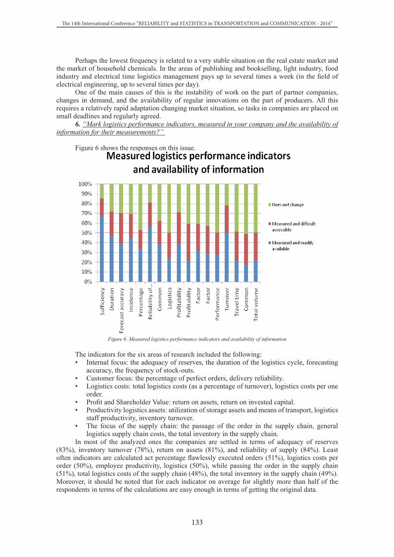
133


Perhaps the lowest frequency is related to a very stable situation on the real estate market and the market of household chemicals. In the areas of publishing and bookselling, light industry, food industry and electrical time logistics management pays up to several times a week (in the field of electrical engineering, up to several times per day).

One of the main causes of this is the instability of work on the part of partner companies, changes in demand, and the availability of regular innovations on the part of producers. All this requires a relatively rapid adaptation changing market situation, so tasks in companies are placed on small deadlines and regularly agreed.

6. “Mark logistics performance indicators, measured in your company and the availability of information for their measurements?”

Figure 6 shows the responses on this issue.

Figure 6. Measured logistics performance indicators and availability of information

The indicators for the six areas of research included the following:• Internal focus: the adequacy of reserves, the duration of the logistics cycle, forecasting

accuracy, the frequency of stock-outs. • Customer focus: the percentage of perfect orders, delivery reliability. • Logistics costs: total logistics costs (as a percentage of turnover), logistics costs per one

order. • Profit and Shareholder Value: return on assets, return on invested capital.• Productivity logistics assets: utilization of storage assets and means of transport, logistics

staff productivity, inventory turnover.• The focus of the supply chain: the passage of the order in the supply chain, general

logistics supply chain costs, the total inventory in the supply chain.In most of the analyzed ones the companies are settled in terms of adequacy of reserves

(83%), inventory turnover (78%), return on assets (81%), and reliability of supply (84%). Least often indicators are calculated act percentage flawlessly executed orders (51%), logistics costs per order (50%), employee productivity, logistics (50%), while passing the order in the supply chain (51%), total logistics costs of the supply chain (48%), the total inventory in the supply chain (49%). Moreover, it should be noted that for each indicator on average for slightly more than half of the respondents in terms of the calculations are easy enough in terms of getting the original data.

134


4. Conclusions

Summarizing the above first part of the study the logistics of controlling (the ratio of companies in the logistics and logistics situation at the enterprises), it can be noted:

1. Many companies specializing in industrial activity, such as a company in the automotive industry, the company in the field of light industry and electrical engineering, logistics equate to the rank of key competencies, understanding its importance and impact on the efficiency of the company.

2. Aside from the obvious impact on logistics performance of works, most managers and researchers from surveyed companies also produce high impact logistics products, customer satisfaction, confirming that the correct organization of the logistics processes within the company and in cooperation with partners helps to improve service and customer confidence and increase their side.

3. Preponderance of the companies surveyed does not have clearly-defined and coordinated logistics strategy within the enterprise, as well as clearly defined logistics purposes. Their absence, especially for companies that provide logistics services, and companies in the distribution and retail, does not clearly visible landmarks in the development of the company, with this in the harmonization of certain key issues between departments of conflict may arise and misunderstandings due to lack of relevant logistics information.

4. Regarding the frequency of initiation time logistics company management problems (although a third of respondents did not answer), almost all respondents noted that attention is paid to issues of logistics at least several times a month. Of course, this frequency is low, but interest from the leadership of logistics still regularly attends, and in the future, most likely will only grow.

5. Results of the analysis of logistics KPI and their impact on business performance, it was concluded that CEOs primarily directed at optimizing the logistics activities of inventory management, on-time delivery and monitor return on investment. The least attention from them is paid to the logistics supply chain that is leaders do not understand yet the importance of optimizing logistics business processes in the supply chain as a whole.

References

1. Ballou, R.H. (2003) Business Logistics/Supply Chain Management. Prentice Hall. 676 p.2. Ballou, R. (1999) Business logistics management: Planning, organizing, and controlling the

supply chain, 4. Aufl. Upper Saddle River (NJ): Prentice-Hall. 744 р.3. Coyle; J.J., Bardi, J.E., Langley, J.J. (2002) Management of Business Logistics: A Supply Chain

Perspective, 7th edition. South-Western College Pub. 672 p.4. Dybskaya, V., Zaytsev, E., Sergeyev, V., Sterligova, A. (2008). Logistics: integration and

optimization of logistic business-processes in supply chains, Professor V.I.Sergeyev (Ed.). M.: Exmo. 944р. (MBA complete course).

5. Martin Christopher. (2011) Logistics and Supply Chain Management, 4th edition. Financial Times Series, January 6.

6. Sergeyev, V. (2013) Corporative logistics in questions and replies, 2nd edition, revised and enlarged,

7. Professor V. Sergeyev (Ed.). M.: INFRA-M. 634 р. 8. Sergeyev, V. (2004) Logistics influence on company’s business effectiveness. Logistics Today,

4, рр. 21-29. 9. Sergeyev, V. (2005) Controlling in logistic systems. Logistics and Supply Chains Management,

3-4, рр. 19-31.10. Sergeyev, V. (2007) New vision of controlling system of logistic business-processes in supply

chain. Logistics and Supply Chains Management, 5, рр. 9-23.11. Sergeyev, V. (2004) System development of logistics balanced indicators of an industrial company.

Logistics and Supply Chains Management, 4-5, рр. 46-62.12. Simchi-Levi, D., Chen, X., Bramel, J. (1998) The Logic of Logistics: theory, algorithms, and

applications for logistics and supply chain management. Springer Science+Business Media Inc. 562 р.

Reliability and Maintenance

Session 3

136



THE EVALUATION OF THE RELIABILITY OF SUPPLY CHAINS: FAILURE MODELS

Lukinskiy Valery(1), Lukinskiy Vladislav (2)

(1) National Research University Higher School of Economics St. Petersburg, Russia, 16 Soyuza Pechatnikov ulitsa

ph.:007(812)7466623, e-mail: [email protected] (2) National Research University Higher School of Economics

St. Petersburg, Russia, 16 Soyuza Pechatnikov ulitsa ph.:007(812)7466623, e-mail: [email protected];

Apart from the criterion of total logistics costs that is used to evaluate the efficiency of supply chains, another criterion - the total satisfaction of consumer needs - is increasingly used for the same purpose. It can be explained by the transition to such new logistics concept as the sustainability of supply chains, which is characterized not only by flexibility, rate of response, strength, adaptability, but mostly by reliability of functioning of logistics system’s elements.

The paper presents the critical analysis of existing approaches to the formation of failure models in supply chains, the methodical approach and classification of failures for key logistics functions (purchasing, order processing, transportation, storage, warehousing and materials handling) as well as developed and improved failure models for a number of logistic functions and operations.Keywords: supply chains, reliability, failures, calculation models.

1. Introduction

Modern period of logistics development is characterized by a heightened interest in the reliability of supply chains. The aim of researches in this direction is the creation of complex of models and methods by which it would be possible to optimize the supply chains taking into account reliability indices.

But the peculiarity of the situation is that this stage of development of the theory of logistics and supply chain management is associated with the emergence of new concepts such as «sustainability», «durability», «robustness», «flexibility», «adaptability», «response time» and, of course, «reliability». So in the paper (Sergeev, 2013) on the basis of shift of logistical paradigms authors conclude that «durability has become one of the most important parameters of the supply chain operation along with the level of service and costs», «and namely durability serves as the criterion of efficiency of the whole supply chain». However, in our opinion, in the cited paper there is uncertainty in the interpretation of the concepts of «durability» and «reliability». For example, in the section, which is concerned with the «durability and reliability of technical systems», both concepts are based on the same principles and the difference between them is the following:

• reliability is a property of system to maintain its characteristics of key performance indicators (KPI) within the established values;

• durability is a property of system to restore itself that means that «system is able to return the values of KPI in the specified tolerances».

Given that objects of the theory of reliability are restorable objects, for which recovery of serviceable state is stipulated in the relevant documentation, it appears that the distinction between the two terms is virtually erased. However, during the formation of the table of distinctive characteristics «sustainability» and «durability» were attributed by authors to higher levels, respectively, to the zero and first level, whereas «reliability» was attributed to the lower third level.

For almost all above-mentioned concepts there are no indicators (except KPI system in the SCOR-model) and methods for their evaluation. Therefore, we believe that reliability theory of

137


technical systems as well as its accumulated analytical and application developments, taking into account the specific character of functioning of the supply chain, can be chosen as the real platform for their formation.

Performed analysis of a number of sources showed that, despite the existence of separate decisions, the bulk of the problems of assessing the reliability of supply chains are far from a final decision for the following reasons:

1. Supply chains are considered as systems that are operating to first failure, while the probability of no-failure operation is accepted as the main indicator of the reliability of supply chains (Blanchard, 2004; Zaitzev and Uvarov, 2012).

2. Calculations on the proposed models and methods are being made on the base of the original data, while collection, analysis and systematization are reduced to simple statistical dependencies (Sergeev, 2013); for example, the «perfect order» is defined as the ratio «the number of precisely executed orders» to «the total number of orders».

3. Number of variations of simple failure models is limited and reduced to three types:• the model of the «perfect» or «ideal» order (Ballou, 1999; Christopher, 2004);• the model of «supply and demand» (Wolfgang and Thorsten, 2006), which is formed

by analogy with technical systems «load-strength» (Gertsbakh and Kordonsky, 1966);• the «just-in-time» model (Lukinskiy et.al., 2012).

1. Description of complicated failure models involving multiple logistic operations was not possible to find in the sources available to reviewers.

2. The main tool for improving the reliability of supply chains is considered external (or excess) redundancy, while internal sources, in particular, insurance reserves, are not given the necessary attention (Lukinskiy et.al., 2014).

2. Development of a methodological approach to the classification of failure models in supply chains

For development of a methodological approach to the classification of failure models it is useful to clarify the basic concepts and definitions that form the conceptual framework of reliability of supply chains.

Analysis of a number of sources showed that the concept of «failure» has a fairly wide range. Therefore, in this paper we choose a synthesized version of «failure» as «a loss of the ability of the whole supply chain as well as links in the chain to perform its functions in accordance with the agreements between the members of the chain».

It should be emphasized that in works on reliability except the notion «failure» one can find such terms as «defect», «damage», «problem» and «malfunction» that sometimes are used interchangeably and it is, in our opinion, incorrect. The most important of these terms is «malfunction», which can be characterized as a transient failure leading to short-term partial loss of functioning that can be corrected by the operator without significant time and cost.

For specification of the general approach we will consider the kinds of failures related to main and related logistics flows.

Material flow includes components related to the physical parameters of the order (for example, the number, nomenclature, weight and others). Examples of failures related to material flow are damage of packages, deficiency in quantity, re-sorting, insufficient amount dispatched, etc.

Information flow includes document flow and information sharing occurring within the supply chain during its operation. Failures may be associated with execution or handling of documents in the supply chain or in the process of information exchange between supply chain members.

Financial flow is characterized by monetary costs for the organization of delivery orders in the supply chain. Occurring failures are associated with additional costs for the organization of cargo delivery. These costs may occur in the process of recovery after a failure or as a consequence of any failure (for example, penalties for exceeding the allowable cargo weight or penalties for lateness).

Intellectual flow reflects the influence of the human factor. Despite the controversial nature of this concept, we believe that consideration of the impact of staff is relevant, but so far researchers have not paid enough attention to this factor, despite the fact that it is involved in the performance of all types of logistics operations and functions in the supply chain.

138


In addition to the mentioned failures, in all flows various kinds of extreme emergency situations, which are advisable to segregate to a separate category, can occur. It refers to situations caused by natural disasters, force majeure and other reasons which cannot be influenced by the supply chain participants.

Thus, the supply chain is a complex system which has independent functionality and consists of many interacting components (subsystems), thereby acquiring new properties that cannot be reduced to the properties of subsystem level.

The supply chain is a system of «man-machine-environment», where the environment means the totality of social and economic environments. Obviously, in the supply chain one should allocate units (members of the supply chain) and elements (executable operations). Such decomposition, which separates companies and the operations they perform within a specific supply chain, allows evaluating any supply chains.

We should also note the property of self-organization (and self-training) of supply chain, that is goal-directed behavior in complex environments through adequate changes both internal and external conditions for recovery of operation.

Table 1. Classification of criteria of failure models in supply chainsCriterion Classification

Type of logistics flow Material, information, financial, service, intellectual (human factor), etc.

Consideration of failure occurrence Without considering time (statistical)Taking into account time (dynamical)

Character of variables (arguments) Stochastic events, stochastic variablesStochastic processes (flows)

Relationship between the variables Independent Dependent (functional, stochastical)

The relationship between operationsSimple (one-parameter)Complicated (multiparameter)Combined

Generalization of different sources, dedicated to researches of reliability of logistics systems, allows us to classify the main criteria of failure models in the supply chain (see table 1). Obviously, the criteria listed in the table do not represent all the possible options, but at the same time they make it possible to characterize a large number of them, which is particularly important for the complicated and combined models involving different types of processes, the types of relationship between the variables, their character and others.

3. Correction and refinement of failure models in supply chains

Table 2 shows the basic failure model for a number of logistic functions and operations. Presented models are based on the general theory of reliability of complex systems (Gertsbakh and Kordonsky, 1966; Lukinskiy et.al., 2012) and disciplines that are included in operations research (probability theory, the theory of stochastic processes, queuing theory, the theory of recovery, etc.), in particular, on the theorem on numerical characteristics, repeated experiments, the compositions of distributions, the transformation of random variables, etc. (Wentzel, 1969).

Table 2. Failure models in supply chainsLogistical function Logistical operation Model for calculation of reliability indices (similar

model)

1. Procurement, orders management

Forecasting of supply and demand volumes

The task of «demand – offer» (similar to task of «load – strength»)

Determination of order quantity Statistical problem - one-time purchase (analogous to «economic risk»)

The choice of the intermediary (suppliers, carriers, etc.)

Reliability of redundant systems (similar to «hot», «cold» and «easier» redundancy and etc.)

2. Warehousing, materials handling

Formation of the perfect (ideal) order Simple probabilistic models for separate indicators. Сombined models

Order picking A probabilistic model that is based on the composition of stochastic variables (analogous to «just in time» model)

139


Logistical function Logistical operation Model for calculation of reliability indices (similar model)

3. Transportation Transportation (multimodal, unimodal and etc.), delivery The «just-in-time» model. Reliability of redundant systems

4. Inventory management

Determination of inventory parameters Probabilistic estimates of values of safety stock and deficit

Selection of inventory management strategy

Models based on the achievement the limiting values of implementations of inventory consumption (similar to «calculations for wear»)

Let us consider failure models (see table 2), focusing attention on their clarification and correction.

The model of «supply and demand». In describing the logistics processes of procurement and the management of orders with stochastic values of demand S (consumer) and supply R (supplier), the probability of customer satisfaction (the lack of deficit) Z = R-S is defined by the dependence

where fR(R) – function of distribution density of vendor supply;FS(S) – distribution function of consumer demand.

If fR(R) and FS(S) follow the law of normal distribution with parameters mR, mS (mean values) and σR, σS (root-mean-square deviations), then the probability of lack of deficit can be determined by formula

where Ф( ) – probability integral.Model of «selection of intermediary». The model is based on classic dependencies of so-

called circuit reliability when redundant elements are included in system «in parallel» to those elements, whose reliability is insufficient. For example, to assess the reliability of the supply chain link, which includes one main and «n» redundant suppliers, the probability of no-failure operation is calculated by the formula

where Po, Pi –the probabilities of no-failure operation of one main and «n» redundant suppliers, respectively.As a rule, this kind of models is complemented by the condition, associated with limiting of costs for the system operation.

Model of «perfect (ideal) order». This model is most common in the works related to the reliability of supply chains. Usually calculated dependence includes three criteria of failure: fulfillment of an order out-of-time (P1), number of orders that are fulfilled not to the fullest extent (P2) and the number of improperly executed documents (P3).

The calculation formula is the probability of failure of formation of a perfect order has the form

The number of elements in the calculation formula varies within wide limits, for example, in (Ballou, 2004) n=5. There also when forming the multiproduct order it is recommended to use the formula for WAFR (weighted average fill rate)

where wi – frequency (weighting coefficient) for ith nomenclature;Pi – the probability of failure-free formation of the ith nomenclature of an order.

Session 2. Transport and Business Logistic


dSSFRfP SRz

)()( , (1)

where fR(R) – function of distribution density of vendor supply; FS(S) – distribution function of consumer demand.


221

SR

SR mmФP

, (2)

where Ф( ) – probability integral. Model of «selection of intermediary». The model is based on classic dependencies of so-called

circuit reliability when redundant elements are included in system «in parallel» to those elements, whose reliability is insufficient. For example, to assess the reliability of the supply chain link, which includes one main and «n» redundant suppliers, the probability of no-failure operation is calculated by the formula

))1(1)(1(110

Ri iPPP , (3)

where Po, Pi –the probabilities of no-failure operation of one main and «n» redundant suppliers, respectively.

As a rule, this kind of models is complemented by the condition, associated with limiting of costs for the system operation.



n

i i PPPPP1 3210 . (4)


iiPP 0 , (5)

where wi – frequency (weighting coefficient) for ith nomenclature; Pi – the probability of failure-free formation of the ith nomenclature of an order.

However, the validity of using (5) requires the further proof, perhaps, by using a general theorem on repeated experiments.

The «just-in-time» (JIT) model. This is one of the concepts of logistics, which is according to SCOR - model corresponds to the indicator «duration cycle of order fulfillment». In paper (Lukinskiy et al, 2012) JIT model is formed on the basis of the composition of distribution laws of stochastic variables Тi, which are the time of execution of ith operation. The probability P of just-in-time logistic cycle execution can be calculated with the formula

T

co TTФP

, (6)

where Т0 – «just-in-time» delivery time with probability Р0; Тс, σТ – the mean and the root-mean-square deviation of the delivery time accordingly.

In the case of constraints instead of dependence (6) one should use the simulation modeling.



dSSFRfP SRz

)()( , (1)



221

SR

SR mmФP

, (2)



))1(1)(1(110

Ri iPPP , (3)





n

i i PPPPP1 3210 . (4)


iiPP 0 , (5)




T

co TTФP

, (6)





dSSFRfP SRz

)()( , (1)



221

SR

SR mmФP

, (2)



))1(1)(1(110

Ri iPPP , (3)





n

i i PPPPP1 3210 . (4)


iiPP 0 , (5)




T

co TTФP

, (6)





dSSFRfP SRz

)()( , (1)



221

SR

SR mmФP

, (2)



))1(1)(1(110

Ri iPPP , (3)





n

i i PPPPP1 3210 . (4)


iiPP 0 , (5)




T

co TTФP

, (6)





dSSFRfP SRz

)()( , (1)



221

SR

SR mmФP

, (2)



))1(1)(1(110

Ri iPPP , (3)





n

i i PPPPP1 3210 . (4)


iiPP 0 , (5)




T

co TTФP

, (6)



140




where Т0 – «just-in-time» delivery time with probability Р0;Тс, σТ – the mean and the root-mean-square deviation of the delivery time accordingly.

In the case of constraints instead of dependence (6) one should use the simulation modeling.Models of inventory management. The main difference of this group of models from the rest

is that the calculated dependencies are based on stochastic stock consumption processes and their reaching of one (or two) limits states.

In table 3 there are a systemized calculation failure models (models of probability of deficit) for main inventory management strategies and different options of description of stock consumption processes.

Table 3. Failure models for different inventory management strategiesStrategy Options Options of description of stock consumption

processes

With a fixed level (with reorder point ROP)

1.Order quantity S3=const2.Order quantity S3≠const (minimax)

1. Deterministic:- linear, nonlinear;- initial state («focus» or «stochastic variable »).2. Stochastic processes:- stable, unstable;- with vigorous or gentle stirring; - initial state (see item 1).3. Flows of «rare events»4. The above-mentioned processes with «pulse» or «extreme» emissions.

Periodic (T, S)

1. Periodic delivery: values of T0 and S3 are constant.2. T0=constS3= var (up to Smax)

Combined

1. Order is placed when inventory level is less than ROP or at Т0 moment of time2. Order is placed at Т0 moment of time if inventory level is less than ROP

Calculation dependencies to estimate the probability of occurrence of deficit are given in the papers (Ballou, 1999; Gertsbakh and Kordonsky, 1966; Lukinskiy et.al., 2012).

Presented failure models allow evaluating the probability of failure-free performance when executing a number of logistics operations and functions. At the same time, a number of problems require further development associated with diversification of supplies, the relationship between events and running processes, their sequence and others.

4. Approbation

Approbation of the developed methodical approach was carried out using published in various sources data and collected information on indicators of reliability of logistics enterprises (transport companies, warehouses, etc.).

The most developed of all failure models to assess the reliability are models related to inventory management in warehouses in multilevel supply chains. On the one hand, this is due to the importance of the solution of the problem connected with deficit and excess inventories for enterprises; on the other hand, it can be explained by a deep theoretical study of inventory management tasks and cumulated experience of their practical solving. In addition, by its nature the inventory management models are identical to the classical failure models in technical systems.

With regard to models of perfect order, the practice of calculations of key performance indicators (KPI), which gained widespread because of the implementation of the balanced scorecard system in some enterprises, played a positive role in their development. In general, we can say



dSSFRfP SRz

)()( , (1)



221

SR

SR mmФP

, (2)



))1(1)(1(110

Ri iPPP , (3)





n

i i PPPPP1 3210 . (4)


iiPP 0 , (5)




T

co TTФP

, (6)



141


that these models are efficient, and their further development requires changes and updates to data collection and analysis of primary data.

The model of selection of intermediaries and the JIT model also can be referred to quite successfully developed models. But the wide distribution they did not receive due to the lack of relevant sections in the textbooks on logistics and supply chain management. For this reason, the probabilistic model of «supply and demand» is almost never used in the process of procurement and management of orders.

5. Conclusion

Complex of failure models to assess the reliability covers the major functional areas of logistics and includes key logistics functions and operations: procurement, orders management, transportation, inventory management, warehousing and materials handling. Revised and improved models allow calculating the necessary reliability indices for the elements of supply chains, in other words they allow actually assessing the level of customer satisfaction.

At the same time, some questions remain open. For example, regarding the model of «supply and demand» we should emphasize that a number of papers contain formulas similar to (2), for significantly positive values (exponential law, Poisson, and others); in addition, they can be used when delivering specific batches of products in inventory management problems.

Despite the obvious simplicity and ease of calculation by formula (4), in our view, the further research in the following areas is required. First of all, the formula does not reflect the possibility of combining several criteria in a single delivery. Secondly, the evaluation procedure of quantitative and qualitative criteria, combined by probability Р2, is not considered.

Further development of the developed complex is connected with the identification of causes that are giving rise to failures during the execution of logistics operations that are related to the change in the parameters of material, information, financial, and particularly intellectual (human factor) flows. In this case, the opportunity to assess the reliability of supply chains not only during re-engineering, but also during the design of logistic systems becomes real.

References

1. Ballou, R.N. (1999) Business logistics Management. New Jersey: Prentice-Hill International.2. Blanchard, Benjamin S. (2004) Logistics Engineering and Management. USA: Pearson.

Prentice Hall.3. Christopher, M. (2004) Logictics and supply chain management. Harlow, UK: FT Prentice Hall.4. Gertsbakh, B. and Kordonsky, K. (1966) Models of failures. Soviet radio.5. Lukinskiy, V.S., Lukinskiy, V.V., Churilov, R. (2014) Problems of the supply chain reliability

evaluation. Transport and telecommunication, 15(2), 214-222. DOI: 10.2478/ttj-2013-1018.6. Lukinskiy, V.S., Lukinskiy, V.V., Malevich, J.V., Plastuniak, I.A., Pletneva, N.G. (2012) Models

and methods of the logistics theory. St.Petersburg: SPbSUEE.7. Sergeev, V.I. (2013) Supply Chain Management. Moscow: Uwrite.8. Wentzel, Elena. (1969) Model for calculation of reliability indices (similar model). Moscow:

Nauka. 9. Wolfgang, K. and Thorsten, B. (2006) Managing Risks in Supply Chains. How to Build Reliable

Collaboration in Logistics. Berlin: Erich Schmidt Verlag.10. Zaitzev, E.I. and Uvarov, S.A. (2012) Using indicators of Perfect order Fulfillment in the

distribution logistics, Logistics and Supply Chain Management, 4(51), 16-22.

142



EXPERIMENTAL STUDY OF A ROLLER BEARING KINEMATICS THROUGH A HIGH-SPEED CAMERA

Alexey Mironov1, Pavel Doronkin1, Sergey Yunusov2

1D un D centrs Ltd. 7, Margrietas Str, Riga, Latvia, LV-1046

Phone: +(371) 67 468850, Fax +(371) 67 468856e-mail: [email protected], [email protected]

2Transport and Telecommunication Institute1 Lomonosov Str., Riga, Latvia, LV-1019

Phone: +(371)-26435655, e-mail: [email protected]

The paper presents the results of a roller bearing motion characteristics investigation, which was carried out on a custom-made rig using a high-speed video camera. The obtained results attest to the fact that the rotation rate of balls under the actual operating conditions differs from the calculated theoretical values, which are used in process of a roller bearing diagnostics. The difference of actual velocity parameters of a ball bearing from the respective theoretical parameters is the reason why some methods of vibration-based diagnostics of roller bearings yield inadequate results. The goal of investigation is to study a variation of rotation speed of rolling elements caused by operating conditions and kind of roller bearing defects. Another goal is scale estimations of above mentioned variation changes.Key words: diagnostics, roller bearing, vibration signal, experimental studies.

1. Introduction

The standard methods for vibration-based diagnostics of roller bearings are based on monitoring of the spectral components levels of vibration envelope whose position on frequency axis is determined by geometrical dimensions and the number of rollers in the bearing (Patent US, ). The comparative test results have shown the low efficiency of those methods – in particular, many false responses and defect skipping. It turned out that the main reason for low efficiency was the fact that the informative components of vibration of faulty bearings are often not detected within preset frequency ranges, while the normal bearings, on the contrary, frequently demonstrate an increase in values of those components without visible reasons.

In this regard, the goal of this research is to investigate the kinematics of a rolling bearing at a detailed level in order to determine the impact of bearing faults on the speed of rotation of bearing elements (cage and balls) and to find out how they differ from the respective theoretical values. Moreover, this became necessary due to the comparative test results obtained by D un D centrs. In process of studies aimed at the identification of technical state of roller bearings applied within industrial plants, one of the typical methods for bearing diagnostics – the SKF method – was applied alongside with a new adaptive technology which takes into account the rotor speed and uses data processing not in frequency but in time domain. One can find the test results in the paper (Mironov, Doronkin, Priklonskiy, Yunusov, 2014).

Moreover, the relevance of this study is due to the fact that the specialized scientific literature concerning bearings is normally dedicated to the development and studying of mathematical models; however, those models are lacking of actual test data on the characteristics of rollers movement subject to operating conditions and the bearing state. In particular, there is lack of data on rollers and cage rotation speed variation caused, for example, by a change in lubricant properties and occurrence of defects on work surfaces.

143


2. The research procedure

Test rig for investigating the motion modes of roller bearing in operation A custom-made test rig was used to investigate the roller bearing kinematics. The test rig made

it possible both to change the bearing functioning conditions and record the behavior of the bearing’s rotating components. The rig layout is shown on Fig. 1. The bearing under test is mounted into an adjustable support; at the same time, the illuminated borescope lens is placed close to the rolling balls. The support design is carried out so as to make the rolling bearing components visible through the lens of the borescope; in other words, the rotating rollers, the inner race and the cage get into the area visible through the borescope, which enables to trace their motion and take measurements.

The borescope is connected to a high-speed video camera providing the shooting speed up to 150000 frames per second.

Figure 1. Test rig to investigate the motion characteristics of roller bearing rotating components

The adjustable-speed motor rotates the inner race of the bearing with the rotor speed through a clutch and shaft; at the same time, the bearing is mounted into a special support.

The support is designed so as to remove and install the bearing conveniently – both for the maintenance and modification of its state (changing lubrication conditions, introduction of faults etc.).

As the bearing under test, a cylindrical roller bearing NU308 was used. To measure the rotation rate of the bearing components, some matchmarks were indented on their susrface circumferentially at a pitch of 5 degrees (Fig.2).

Figure 2. The marking of roller bearing items and a sample of video shooting frame obtained in process of investigation: a) set of rollers; b) bearing cage; c) bearing assembly; d) a sample of a frame with the roller bearing, with the statement of sector of observation

144


Tests and measurementsThe measurement of motion parameters was made using the frames of high-speed video shooting,

within the non-movable sector as shown on Fig. 2d, for all the rollers sequentially. The measurement purpose was to determine the rotation speed ranges of the rollers and the bearing cage depending on various factors including lubrication quality, presence of faults of the bearing items, and their phase in relation to the rotor. After the registration of video images of the bearing moving items, the rotational speed of the inner race, the bearing cage, and the balls was measured by recording phase match marks of each rotating item.

The measurements were repeated for each roller of the bearing cage. After each test measurement of speeds of all the balls within five revolutions of the bearing cage relative to the rotor were done.

Parameters calculation Based on the measurement results, some parameters of rotational speeds of the bearing cage

and the balls, with reference to the inner race speed, were calculated, - including:• The maximum and the minimum value of relative rotational speed for each ball and the

bearing cage throughout the test;• The weighted average (geometric mean) of relative speeds of balls and the bearing cage; • Root mean square scatter of relative speed of the bearing cage and the balls with reference

to the mean value; • The amplitude-dependent standard normal cumulative distribution.Moreover, the percentage of relative speeds as against their nominal values determined based

on the dimensions of bearing items, was calculated to evaluate the sliding of rollers and the bearing cage. The nominal values were calculated according to the formulas as follows:

[ ]2 2

/ 0.5 (1 / )cos ;

/ 0.5 / 1 ( / ) cos ,c c r rol c

a ak k r c rol rol c

d d

d d d d

ω ω ω α

ω ω ω α

= = ⋅ −

= = ⋅ ⋅ − 2.1 – 2.2where cω – angular rotation speed of bearing cage;

rω – angular rotor speed;

akω – angular rotation speed of ball;

,rol cd d – diameters of ball and bearing cage, respectively;

α – angle of contact of rollers.

According to the test results, dependence diagrams were plotted, reflecting the dependence of relative speeds of bearing items upon rotor rotation phase and the graphics of standard normal cumulative distribution of relative speeds. The analysis of the obtained results is presented in the following section.

3. The analysis of test results

The test data in the form of the bearing speed variables, normalized to nominal (calculated) values, are presented in Tables 1 and 2. The presented data relate to a grease-lubricated bearing in various states.

Table 1. Kinematic characteristics of balls according to test results Defects of rotating elements

Rollers rotation speed parameters initial outer inner 1 roller 3 rollers combined

combined dispersed

max mean, % 98.3 82.4 978 99.8 97.8 99.6 68.7

min mean, % 84.6 71.2 79.9 80.0 83.0 84.9 59.5

effective mean, % 92.2 77.3 90.6 92.4 92.4 94.7 65.1

scatter, % 3.4 2.6 4.0 3.2 3.0 2.3 1.6

145


Table 2. Kinematic characteristics of bearing cage according to test results Defects of rotating elements

Cage rotation speed parameters initial outer inner 1 roller 3 rollers combined

combined dispersed

max mean, % 101.4 88.3 99.2 101.8 103.0 101.4 70.2

min mean, % 93.4 80.0 91.3 90.8 95.1 93.8 63.9

effective mean, % 97.9 82.7 96.7 97.0 97.1 97.5 68.1

scatter, % 1.2 1.6 1.3 1.6 1.2 1.5 1.0

Non-defective grease-lubricated bearingWith respect to a good-state, grease-lubricated bearing, relative speed values of rollers were

varying within the range from 84.6% to 98.3% (Table1) of the nominal value (Table1), which is marked on the diagram (Fig.3a) by the red dot line.

a) b)Figure 3. Relative rotation speed of good state & consistent lubricant evaluation to rotor phase: a) rollers; b) cage

Since the scatter of the measured rotation speed values of the rollers was essentially higher than the measurement error, this fact detects their speed variation. The weighted average value of the rollers’ speed values constituted 92.2%; therefore, even under the nominal operating condition, the rollers are rolling over with a sliding motion whose value is 7.8%. The analysis of the speed values dependence on the rotor phase showed that the minimum values were observed in the range of 270о–360о. Thus, there is the reason to assume that the sliding rollers may have a dependence of the rotor phase.

According to the accepted model of a roller bearing operation, one of the reasons for the dependence of rollers’ rotation speed of the rotor phase is a certain imbalance. The rotor imbalance is transferred through the bearing inner race simultaneously not more than through two rollers. Inertial loads from the rotor ensure the greatest contact with the bearing tracks of the two races for those rollers, while the rest of the rollers nestle to the surface of the outer race’s bearing track only due to centrifugal forces of their own. Decreasing of contact of rollers not nestled to the outer race enhances their sliding motion. The probability density function for the relative speeds (Fig. 4) illustrates the concentration of speed values of the velocities near the mathematical expectation.

Unlike the rollers, the calculated values of bearing cage rotation speed have a considerably less variation in reference to the rated value (Fig. 3b). Based on the diagram, one may also come to the conclusion that, unlike the rollers, there is no visible connection between the bearing cage speed fluctuation and the rotor phase. The weighted average value of the bearing cage relative speed shows the presence of sliding motion which constitutes 2.1%, while its value (97.9%) turns out to be close to the maximum values of the relative speed of rollers rotation (98.3%). This fact is consistent with one of the concepts of the bearing model described above, according to which, the bearing cage rotation speed is determined by the speed of rotation of rollers contacting with the two races simultaneously. The fact that the maximum measured value exceeds the relative speed of bearing cage by attaining

146


101.4% of the rated value is explained by a large reduced error of measurement.

a) b)Figure 4. Probability density function for: a) rollers, b) cage

The diagram on Fig. 4b shows that the maximum measured value lying beyond the physical sense has a negligent density.

Therefore, rollers and the bearing cage “slide” even with a technically sound bearing, i.e., their actual values are less than the calculated ones.

A fault of bearing inner race The local defect of the inner and outer race was a transverse “groove” with a width of 2mm

and the depth of about 0.3mm, which crossed the entire width of the bearing race (Fig. 5a). In process of the bearing assembly, the bearing inner ring was mounted on the rotor so that the defect was on the direction of the imbalanced rotor load vector. According to the scale indented on the end surface of the bearing inner race, the defect was identified in the area of the phase equal to zero (or 360о).

a) b) c) d)

Figure 5. Local defects on the bearing items: a) on the inner race, b) on the outer race; c) on the roller; d) distributed damage of the outer race

As compared to the initial state, the weighted average of speed values decreased a little (see Table 1.2): by 1.6% with the rollers and by 0.8% with the bearing cage. At the same time, the speed dispersion almost hasn’t changed. Just like as it was with the technically sound bearing, the sliding of the bearing cage with a defect of inner race corresponded to a minimal sliding (maximal speed value) of the rollers. Therefore, the inner race defect leads to a slight decrease of rotation speed of the rollers and the bearing cage.

However, the analysis of the dependence of relative speed of rollers on the rotor rotation phase reveals certain regularity (dash trendline).

147


a) b)Figure 6. Relative rotation speed evaluation to rotor phase of inner ring faulty bearing: a) rollers, b) cage

It is clearly seen on Fig. 6 that the minimal roller speed values are related to the phase range of about 360о which is linked with the position of the rotor unbalanced load vector and the fault introduction place on the inner race. At the same time, the bearing cage speed distribution does not depend on the rotor phase. Such a character of speed distribution is determined by the fact that, when the defect on the bearing inner race gets “under” the roller, the contact between the race and the roller can be lost, since the rotor is at the moment supported by two adjacent rollers (through the inner race). Loss of contact between the inner race and the roller, caused by the defect, leads to a decrease in friction force couple driving it, since the roller is impacted only by a centrifugal force of its own which is far less than the rotor load. This leads to an increase in sliding and a decrease in the rotation speed of the balls that get into the defect area. Thus, a defect of the inner ring may cause a local decrease in roller speeds, while having little impact on the average value of their speeds.

The outer race defect The defect of the outer race had the shape and dimensions similar to the defect of the inner race

(5b). Fault introduction into the outer race has dramatically reduced average speed values (Table 1.2): the sliding of rollers achieved 22.7% (100% minus effective mean), and that of the separator – 17.1%. At the same time, speed dispersion has decreased as well. Thus, if a fault of about similar scale is introduced into bearing races, it follows that the defect of the outer race has a far greater impact on the speeds of rollers and bearing cage as compared to a defect of the outer race.

Physically, the process is caused by the bearing cage deceleration by the roller which rolled up into a cavity on the outer race. At the same time, the contact with the outer race disappears and the inner rotating ring ceases to press the roller against the outer fixed ring. With lack of energy input to the roller, the kinetic energy of bearing cage is spent to the roller “runoff” from the fault which leads to reduction of its rotational speed. In turn, this effect impacts the rotational speeds of other rollers, “regulating” and retarding their speed at the same time. Thus, a local defect of the outer race can change the kinematics of operating roller bearing substantially.

a) b) Figure7. Relative rotation speed evaluation to rotor phase of outer ring faulty bearing: a) –rollers; b) –cage.

148


The dependence of rollers’ rotational speeds (Fig.7a) on rotor phase shows the nature similar to that of a roller bearing in a good state: there is an insignificant tendency towards speed reduction and dispersion of speed values in the last quarter of the rotor rotation period. The distribution of bearing cage speed values (Fig. 7b) has not revealed any dependence on rotor phase – just as it was in the previous cases.

Fault of a single bearing rollerThe bearing roller fault was formed by a chord shear of the material, with the material removal

depth 0.3 mm (Fig. 5c). The data shown in Tables 1.2 prove that, in case of a roller’s fault, the speed weighted average values vary insignificantly as against the initial state. However, when analyzing the roller speeds dependence on rotor phase (Fig. 8a), a noticeable speed drop within the rotor imbalance coverage area is observed. An insignificant reduction of bearing cage speed is also noticeable within the vector imbalance coverage area (Fig. 8b) – i.e., within the area of about 360 degrees.

a) b)Figure 8. Relative rotation speed evaluation to rotor phase of faulty roller bearing: a) rollers; b) cage

Faults of three bearing rollers

With similar faults introduced into three rollers at a time, the average weighted speed values almost haven’t changed (Table 1, 2). An increase in the number of faulty rollers has not actually influenced the average weighted speed values of rollers and bearing cage. However, Fig. 9a clearly shows that the decrease in speed values within the rotor imbalance coverage area has remained. It should also be noted that the spread itself has decreased both with the rollers and the cage (Fig. 11b).

a) b)Figure9. Relative rotation speed evaluation to rotor phase of 3 faulty rollers bearing: a) rollers; b) cage

Thus, rollers faults have very limited impact on the weighted average speed values, but they appear in the form of non-uniform distribution from rotor phase against the background of reduced scatter.

149


Impact from a combined fault In process of the test with a combined fault, the two damaged races with local faults were

used as well as one faulty roller described above. Oddly enough, the statistical characteristics of the movement of the bearing elements with a combined fault were close to those obtained in good condition. In this connection, only when analyzing the rollers’ speed dependence on rotor phase (10a) one had managed to identify a local speed reduction in the rotor imbalance vector application area. Although the bearing cage rotation speed dependence showed a slight variation, still it did not extend beyond the error.

a) b)Figure10. Relative rotation speed evaluation to rotor phase of bearing with combined fault: a) rollers; b) cage

Impact from the fault natureChanging the nature of the fault which was introduced onto the track of outer race had a

substantial impact on the motion characteristics of rollers and the bearing cage. A fault in the form of notch 0.05 mm deep, indented as a mesh on 1/5 of the circumference, has shown quite different results in combination with local defect of the inner race and one roller. The speed values both of the rollers and the bearing cage were much lower than the rated values and constituted 65.1% and 68.1% accordingly. Spread of values was also very small (Fig. 11).

a) b) Figure11. Relative rotation speed evaluation to rotor phase of bearing with combined dispersed fault: a) rollers; b) cage

Other factors’ influenceBesides the faults in bearing elements, an essential impact upon rollers and bearing cage

speed values is exercised by operational mode and conditions of the bearing, including the quality of lubrication, radial clearance, etc. As an illustration, Figures 12 and 13 show dependence diagrams for the speed values of rollers and bearing cage which were lubricated by too runny lubricant (Fig. 12) and completely without a lubricant (Figure 13).

150


a) b) Figure12. Relative rotation speed evaluation to rotor phase of liquid lubricating bearing: a) rollers; b) cage.

Under the conditions of a too runny lubricant, the weighted average of rollers and bearing cage speed values decreases dramatically: to 43% with the rollers and up to 49% of nominal value with the bearing cage, which is apparently due to insufficient coupling of rollers with bearing races under the available loads. At the same time, the roller speed scatter decreased considerably and is revealed mainly in the rotor imbalance coverage area.

With the total lack of lubrication, rotational speeds of the rollers and the bearing cage dropped to 18% for the rollers and to 35% of the nominal values for the cage and acquired a totally random character with a disperse range comparable to average values . As the roller behavior analysis has shown, such a mode was triggered by increased friction between the rollers and the cage, which lead to deceleration of both.

a) b)

Figure13. Relative rotation speed evaluation to rotor phase of ”dry” bearing: a) rollers; b) cage

4. Conclusion

According to the survey results, we may conclude that the rotational speeds of balls and bearing cage operating under conditions close to nominal, respond to all kinds of faults. Changes may have different nature, which reveal in the reduction of weighted average values as against the nominal value, and / or in speed variation depending on rotor phase. At the same time, speed value and nature depend on the kind of fault and scale ratio of various components, so it does not seem possible to establish any generalized dependences. When changing the bearing operation mode – for example, when lubrication conditions deteriorate, the behavior of rotating components of a bearing becomes difficult to predict, deviating far from the design parameters.

151


The results obtained noticeably undermine confidence to the methods for bearings diagnostics based on monitoring of vibration components whose position on the frequency axis is determined based on the geometric dimensions of the bearing. Changing the operating mode, lubrication and technical condition affecting the rotational speed of balls and bearing cage leads to a “smearing” of the above-mentioned deterministic components and reduces the efficiency of such methods. To ensure their efficiency, permanent “adjustment” of methods requiring additional test running and attracting highly-skilled professionals is needed.

In conclusion it could be noticed that the results of this research study showed obviously the motion complexity of rolling bearing’s elements. This is one of the most probable reasons of existing diagnostic methods low efficiency. To improve the situation the new advanced approach is required, but it is not the subject of this article.

References

1. Method and instrument for determining the condition of an operating bearing. Patent:US 4528852 A, Inventors: Eivind O. Sohoel

2. Butler D.E. (1973) The Shock-pulse method for the detection of damaged rolling bearings. Non-Destructive Testing, 6(2), 92–95.

3. Mironov A., Doronkin P., Priklonskiy A., Yunusov S. (2014) Adaptive technology application for vibration-based diagnostics of roller bearings on industrial plants. Transport and Telecommunication, 15(3), 97–110. DOI 10.2478/ttj-2014-0009.

Intelligent Transport Systems

Session 4

154



GPS/GLONASS TRACKING DATA SECURITY ALGORITHM WITH INCREASED CRYPTOGRAPHIC STABILITY

Sergey Kamenchenko

Transport and Telecommunication InstituteLomonosova str.1, Riga, LV-1019, Latvia

Phone: (+371)22335050. E-mail: [email protected]

Satellite monitoring and tracking systems, thanks to the global Internet network, have been applied not only in transport and logistics areas, but also in everyday life. IT development has opened the door to the use of satellite applications, as an integral part of any intellectual system constantly expanding and providing new opportunities.

Nowadays, the volume of transmitted information in global networks is constantly increasing as rapidly as the number of unauthorized persons wishing to obtain this information is increasing. With the development of computer technology, the level of data protection is reduced, and, as a result, it appears to be a relevant task to create new algorithms with high cryptographic strength and high speed in government, military, transport (railways, airports, etc.) and other areas. One possible data protection way based on the one-time pad principle, symmetric cryptographic system with an absolute cryptographic resistance for cracking is presented in the article. Encryption/decryption system based on using involutory matrices in modified Hill encryption algorithm.Keywords: GPS/GLONASS, matrix encryption, involutory matrix, AES, Triple DES, Internet network

1. Introduction

Satellite tracking and monitoring systems have found their main applications in the transport and logistics sector. It is difficult to imagine a modern logistics and transport world without satellite technologies, which greatly strengthened position as its integral part. The use of these systems allows tracking the location and status of the interested object in real-time. Satellite navigation system GPS / GLONASS used to determine the speed, direction and location of the object. All subsequent information of the object obtained from various kinds of sensors, including satellite data, transmitted via telecommunications and computer networks to the data center.

Figure 1. Data transmission in satellite monitoring and tracking systems

155


To transfer data from the object system needs access to the global Internet network, which is provided by a mobile GSM network. If GSM network is not available, then the system stores data in the local drive until GSM access network appears, after which the stored data is transmitted to the network. To transmit data to the Internet mobile GSM providers are using interconnections with internet service providers (ISP). Data transferred from the object passes through a large number of network equipment before they get to the destination (server), which is the main gap in data protection.

2. Modern encryption algorithms analysis used in mobile and computer networks

Nowadays, the problem of using cryptographic methods in information and intelligent transport systems has become particularly relevant, because of the routine introduction and extensive use of global computer networks, which carry large amounts of information that does not allow access to them by unauthorized persons. The rapid development of computing and neural technologies constantly reduces the time for ciphers cracking, which until now had the high cryptographic strength (Kang et al., 2013), (Kodera et al., 2013).

2.1. Encryption algorithms used in GSM networks

There are used A5 and GEA family encryption algorithms in second and third generations of mobile network. A5/3 and GEA3 are most resistant for cracking algorithms, which are based on the use of KASUMI block encryption algorithm. Data encryption in 4G mobile network is based on an AES algorithm.

The first practical attack on the KASUMI cipher, allowing to break the cipher was presented in 2010 year (Dunkelman et al., 2010). However, cryptanalysts did not stop to continue developing new methods for breaking KASUMI cryptographic algorithm (Wentan and Shaozhen, 2014).

Figure 2. Data transmission in GSM network

А5/3 and GEA3 algorithms encrypt data only in wireless segment, from the transmitter mounted on the object to GSM base stations. GSM base station equipment must support these encryption algorithms, and they must be activated. In the mobile provider network data is transmitted in clear format, which can be intercepted, corrupted or tampered by the third persons.

2.2. Encryption algorithms used in data transmission networks

Internet network is interconnection between an internet service provider networks which connect large set of servers, hosts, computers, systems, data centers and so on. Data transmission on the Internet network are based on routing so all objects need to know the real IP address of the destination (server). When transmitting data from one router to another router, the data are not encrypted, as it is done in the GSM wireless network segment, but transmitted in the form in which they were originally formed (figure 3). However, some systems support data encryption before their transmission to the destination, using advanced encryption algorithms like AES or Triple DES.

156


Figure 3. Encrypted data transmission

Data Encryption Standard (DES) - a symmetric block encryption algorithm based on the Feistel network structure, which encrypts the plaintext blocks of 64 bits with 56 bit key. Due to lack calculating power of computer, DES algorithm for a long time had been invincible and the only way to attack is the exhaustive search of key combinations (255 combinations). With the rapid development of computer technology exhaustive search of the keys becomes a reality at the same time repeatedly minimizing spent time. So in 1993, Michael Wiener was developed specialized computer able to carry out search all keys for 3.5 hours (Weiner, 1996).

The main drawback of the DES algorithm is a short key, that DES has pushed developers to create new versions of an algorithm. The most successful modification of the algorithm was Triple DES. In the Triple DES algorithm block plaintext being three times coding with DES algorithm, in each case using a separate key, that increase key lengths up to 168 bits and increase resistance of cipher. However, high resistance of Triple DES algorithm pays a low rate, which is 3 times less than the speed of DES encryption. Triple DES algorithm gradually replaced by AES, which is six times faster.

In 1997, the National Institute of Standards and Technology announced public competition of symmetric block encryption algorithms, which should replace the DES algorithm as a new standard. AES (Advanced Encryption Standard) competition won Rijndael algorithm. Rijndael algorithm using variable block size and variable key length, which is not dependent on each other and can take the values of 128, 192 and 256 bits. In encryption is used 4 internal functions (these functions are used repeatedly - at least 10 times), each of which is reversible, therefore, for cipher decryption is used inverse functions in reverse order.

The algorithm was developed for high speed at the expense of decreasing its cryptographic strength, thus won the AES competition. However, after the adoption of Rijndael algorithm as the standard AES, cryptanalysts found many examples to break the algorithm (Kang et al., 2013), (Das and Bhaumik, 2014). To improve cryptographic strength of the algorithm its developers recommend to use 18 - 24 rounds, that lowers the algorithm speed.

The actual task of constructing a completely resistant and high-speed encryption algorithm, one of the variant for implementing such kind of algorithm is presented in this article.

3. Basic moments used to develop new high-speed and cryptographically strong algorithm

To implement the new algorithm is used a heavily modified basic idea of Hill cipher (Eisenberg, 1998), and also used a great progress in matrix arithmetic, which is the main part of a cryptosystem.

3.1. Hill cipher

In 1929, Lester Hill created an encryption algorithm, which is based on algorithm which replaces the sequence of plain text with encrypted sequence of the same length (Eisenberg, 1998).

Hill Cipher is using orthogonal matrix for data encryption/decryption, for example: let’s encrypt the word «cipher». Length of the English alphabet is 26 letters, then assign a serial number for each letter of the plaintext, hence, c=2, i=8, p=15, h=7, e=4 and r=17. Let’s take for encryption a square matrix (key)

157


−

−−

−

=== −

121

452

431

;111432853

1ABA , (1)

where A - encryption matrix (key), and B - decryption matrix (key). Cipher text:

= kkzavqb (2)

Decryption:

= cipher (3)

Hill cipher didn’t find practical applications in cryptography, because of a number of significant drawbacks:

• Weak resistance for cracking, due to the use of small matrices;• Lack algorithm description for direct and inverse matrices generation of a large size.

3.2. Involutory matrix

In matrix theory (Franklin, 1993), (Zhang, 1999) sometimes mentioned about the existence of an involutory matrices, for which the initial and its inverse matrix are the same, then

EAAAAAAAA ==== −−−− 1111 **** (4) The use of such matrices for encryption/decryption contributes increasing of a high speed

system, as there is no need to calculate inverse matrix, and the initial matrix is a key for encryption and for decryption. Unfortunately algorithms for generating and descriptions of any involutory matrices properties didn’t mentioned in the scientific literature.

However to find such matrices of the small sizes rather easily, for example:

ECCCCCC

EBBBBBB

=⇒==−−−

=−−−

=

=⇒==−−−

=−−−

=

−−

−−

211

211

;;1)det(;021111122

;021111122

;;1)det(;122212223

;122212223

(5)

Obviously, the design of optimal high-speed cryptosystem requires the use of involutory matrices with numbers ±2n, where n – smallest possible integer. Involutory matrices of size 2x2 and 3x3 with numbers ±2n (expression (5)), where n – integer, do not exist, but matrices of size 4x4 with numbers ±2n are possible to construct. For example:

1;1)det(;

1211211122212212

−==

−−

−−−−−−

=

AAAA (6)

[ ]2162125101021621

,251010

)26(mod1747

,1582

* ⇒==

AC

===

1747

,1582

)26mod(21621

,251010

*)27(mod* BCBD

158


Operation of encryption/decryption using involutory matrix as a key, will looks like:

There is used the same matrix for encryption and decryption in expression (7), therefore, the processor at the receiving end doesn’t need to spend time for inverse (decryption) matrix calculation, thus repeatedly increasing the speed of a cryptosystem. At the same time processor for data encryption/decryption will used only shift and addition operations by using a matrix with numbers ±2n, where n – minimum integer, that also increase the speed of the cryptosystem.

3.3. Algorithms for forming an expanded set of involutory matrices

It is obvious that the number of involutory matrices is strictly limited, so we’ll try to find their quantity based on the found properties of these matrices:

• Formation of the involutory matrices using permutation of its rows and columns• If in any involutory matrix we substituted with places any two rows and appropriate two

columns, then we obtain a new involutory matrix.• Formation of a involutory matrix rotated it for 180 degrees• If any involutory matrix rotated for 180 degrees, then we obtain a new involutory matrix.• Formation of a new involutory matrix using transpose• If any involutory matrix transpose, then we obtain a new involutory matrix.• Formation of a involutory matrix using transpose and then rotated it for 180 degrees• If any involutory matrix transpose, and then rotated it for 180 degrees, then we obtain a

new involutory matrix. We can use these two operations in another order and we still get a new involutory matrix.

• Formation of a new involutory matrix by changing sign of elements in initial involutory matrix rows and columns

If in any involutory matrix we replaced the elements sign in any row and in the appropriate column, then we obtain a new involutory matrix.

From one involutory matrix we can obtain a large set of involutory matrices, using the above described properties. If for received new matrices we again used the properties described in this section, then we obtain a large number of involutory matrices, many of which will be repeated, so in the last steps we’ll need to sort the results.

From any involutory matrix 4x4, that contains numbers ±2n, where n – minimum possible number, we can obtain a full set of involutory matrices, total number of which is 4,5*28 = 1152.

3.4. Formation algorithms for expanded set of mutually inverse pairs of matrices

When we create a generation algorithm for mutually inverse pairs of matrices, we should use a fast and simple operation, not requiring complex calculations. As basic matrices we use the involutory matrices, and then the generation algorithms for mutually inverse pairs of matrices are the following:

• Formation a mutually inverse pairs of matrices by permutation of rows and columns in


121

452

431

;111432853

1ABA , (1)

2162125101021621

,251010

)26(mod1747

,1582

*

AC = kkzavqb (2)

1747

,1582

)26mod(21621

,251010

*)27(mod* BCBD = cipher (3)

ECCCCCC

EBBBBBB

211

211

;;1)det(;021111122

;021111122

;;1)det(;122212223

;122212223

(5)

1;1)det(;

1211211122212212

AAAA (6)

ABBA

ABBA

textOpen

XWCD

DCWX

textCipher

TextABBAText

0110

)26mod(

322223

*

1211211122212212

322223

)26mod(

1221

*

1211211122212212

];0110[;

(7)

159


the initial involutory matrix If in the initial involutory matrix expression (8), in the first step permute any two rows,

and in the second step permute appropriate two columns, then we obtain a mutually inverse pairs of matrices. This condition is true for all eight combinations of permutations, hence, this algorithm from one involutory matrix can form eight different mutually inverse pairs of matrices.

• Formation a mutually inverse pairs of matrices by rotating initial involutory matrix respectively for 90 and -90 degrees

• If in any initial involutory matrix in the first step we rotate it for 90 degrees, in the second step, rotate it for - 90 degrees, then we obtain a mutually inverse pairs of matrices.

• Formation a mutually inverse pairs of matrices by changing signs of elements in initial involutory matrix rows and columns

• If in any involutory matrix in the first step we change the sign of elements in any row, and in the second step, change the sign of elements in the appropriate column, then we obtain a mutually inverse pairs of matrices.

Any involutory matrix forms a unified basis for the formation of a large number of mutually inverse pairs of matrices.

3.5. Recursive creation of involutory and mutually inverse pairs of matrices for a large size

To generate involutory and mutually inverse pairs of matrices we’ll use the tensor product.

Let’s calculate an involutory matrix for the first case of expression (9):


EAAAA

AAAAA

column

row

11121

11

2111

*;

1211211122122221

;

1211211122122221

;

1211211122212212

(8)

;;;;;;

);,();,(

);,();,(

);,();,(

);,();,(

;

1112221221222111

;;

1211211122212212

434232413121

144

11144

133

11133

122

11122

111

11111

22

HHHHHHHHHHHHHHBBkronHBBkronH

HHAAkronHAAkronH

HHABkronHABkronH

HHBAkronHBAkronH

EBBEAA

(9)

1111 ;

1112222411121112221244242212221221224244212221222111422221112111222411121112111244242212221222124244212221222122422221112111211122242224222411124424442444242212424442444244212242224222422221112224222411122224442444242212442442444244212242444222422221114222

),(

HHBAkronH (10)


EAAAA

AAAAA

column

row

11121

11

2111

*;

1211211122122221

;

1211211122122221

;

1211211122212212

(8)

;;;;;;

);,();,(

);,();,(

);,();,(

);,();,(

;

1112221221222111

;;

1211211122212212

434232413121

144

11144

133

11133

122

11122

111

11111

22

HHHHHHHHHHHHHHBBkronHBBkronH

HHAAkronHAAkronH

HHABkronHABkronH

HHBAkronHBAkronH

EBBEAA

(9)

1111 ;

1112222411121112221244242212221221224244212221222111422221112111222411121112111244242212221222124244212221222122422221112111211122242224222411124424442444242212424442444244212242224222422221112224222411122224442444242212442442444244212242444222422221114222

),(

HHBAkronH (10)

160


(10)

Using the involutory matrix 4x4 we can obtain 1327104 combinations of involutory matrix 16x16. All the above described properties of involutory matrices are valid for any involutory matrix of any size. Combining volutory matrices of different sizes we can obtain a large set of matrices. But for obtaining a full set of matrices 2nx2n, where n = 2, 3, …, ∞, it’s necessary to obtain a involutory matrix 8x8. The author of this article developed a completely new algorithm for generating involutory matrices of size 8x8. For example:

1;

2222212212212221122122122222122222212222122222222212112221221122

−=

−−−−−−−−−−−−−−−−−−−−

−−−−−−−−−−−−−−−−−−−−

=

AAA

(11)

Mutually inverse pairs of matrices are generated in the same way, using different combinations. Tensor product allows us to generate a large set of matrices, but due to its structure, the resulting matrices will always contain elements ±2n+1. For generation matrices 16x16 we use matrices 4x4 with numbers ±1 and ±2, so resulting matrix will always contain numbers in one order higher, namely ±1, ±2 and ±4. The author of this article developed a completely new algorithm, that allows to generate a involutory matrix with elements ± 1 and ± 2 of any size 2nx2n, where n = 2, 3, …, ∞. For example involutory matrix 16x16:

1111 ;

1112222411121112221244242212221221224244212221222111422221112111222411121112111244242212221222124244212221222122422221112111211122242224222411124424442444242212424442444244212242224222422221112224222411122224442444242212442442444244212242444222422221114222

),( −=

−−−−−−−−−−−−−−−−

−−−−−−−−−−−−−−−−−−−−−−−−

−−−−−−−−−−−−−−−−−−−−−−−−

−−−−−−−−−−−−−−−−

−−−−−−−−−−−−−−−−−−−−−−−−

−−−−−−−−−−−−−−−−

−−−−−−−−

==

HHBAkronH

161


1;

2212212222121221221221222211121122212221222221222222222222222221221221222211222122212221122222222212212221111221222222222212222222222122221222211221121112222122222222212222222222211221122221221221222112222122221222222212222111211221122221222221222222222222

−=

−−−−−−−−−−−−−−−−

−−−−−−−−−−−−−−−−−−−−−−−−−−−−−−−−−−−−−−−−−−−−−−−−−

−−−−−−−−−−−−−−−−−−−−−−−−−−−

−−−−−−−−−−−−−−−

−−−−−−−−−−−−−−−−

−−−−−−−−−−−

= AAA (12)

4. Development of high-speed and cryptographically strong encryption system based on matrix transformations

Below are some examples of cryptosystems that can be used in different situations, depending on required cryptographic strength.

4.1. Cryptosystem with constant key length

To encrypt data we proposed to use the key with a constant length, in each encryption block the key is changed to a new one. To improve system’s resistance, we offer to use the multiplication of several matrices (keys). The general scheme of system encryption/decryption is shown in figure 4, where m - a length of plaintext block, and n – selected number of matrices.

Figure 4. Cryptosystem structure with constant key length

4.2. Cryptosystem with variable key length

162


The structure of this algorithm is the same as in section 4.1, the main difference lies in the fact that the length of plaintext is changed randomly, and therefore encryption/decryption matrix are changed in the same way (Figure 5). Length of the plaintext block is equal 2n, where n – random integer, which varies in the range from 2 to a number, which is set by the user.

Figure 5. Cryptosystem structure with variable key length

This system uses a transition from one matrix size to another depending on the length of plaintext block. Resistance of the algorithm is increased many times, as there is no information what length of plaintext is used in first, second stages and so on.

4.3. Cryptosystem with a double transformation

First block of plaintext is encrypted using the small size of matrices, and then obtained result is encrypted using the larger size of matrices (Figure 6).

Figure 6. Cryptosystem with a double transformation

163


Due to the large number of transformations, this algorithm will lose speed compared with previously described algorithms, but it resistance will exceed. This algorithm can be implemented with a variable key, which was described in section 4.2.

5. Conclusion

Satellite tracking and monitoring systems like mobile technology have become massively popular and available at any point of the globe thanks to the global Internet network, but their safety is doubtful. Time for popular strong encryption algorithm crack is constantly decreasing due to the rapid development of neural and nano technologies that challenge cryptography to create new stronger encryption algorithms. One embodiment of such system based on modified Hill encryption algorithm is proposed in the article. Modified Hill system is based on a new algorithm for generating initial (encryption) and inverse (decryption) matrices of a large size, in which all of the numbers are ±2n, where n - the minimum possible number. As all matrices contain the numbers of computer arithmetic’s ±2n, then encryption/decryption operations will be performed without any multiplication that significantly increases the speed of the algorithm.

The paper also suggests an algorithm for constructing involutory matrices with elements ±2n, for which the initial and its inverse matrix are the same. Using these matrices enables to realize high-speed system, because the key for encryption and decryption is the same. Shown, that any involutory matrix offers with significant advantages, allowing to obtain from any involutory matrix a complete set of involutory and mutually inverse pairs of matrices. In article is shown a recursive method to forming from any involutory matrix a large set of involutory and mutually inverse pairs of matrices gradually increasing size. Because of the almost inexhaustible set of matrices obtained in this article, the proposed cryptosystems allow for encryption/decryption using more than one pair of keys, but a few that greatly increases system resistance. Each block of plaintext is processed by a separate key (matrices), which is equivalent to the principle of “one-time pad” in a completely resistant system for cryptanalysis.

To break Triple DES (Kelsey et al., 2000) we’ll need to use exhaustive search for 272 combinations, but to break 10 round AES 128 (Bogdanov et al., 2011) we’ll need to use exhaustive search for 2126.1 combinations, then ceteris paribus to break a new algorithm, which consists of 10 rounds (using 10 matrix 16x16) we’ll need to use exhaustive search for 2264 combinations.

These algorithms can be used not only in the basic cryptosystem, but also as additional algorithms for increasing the resistance for the existing block system, for example, to improve resistance for SAFER+ algorithm.

All considered models of cryptosystems have following properties:• Diffusion - influence spread of one plaintext character into a large number of cipher text

characters that hides statistical properties of the plaintext. Development of this principle is influence spread of one key character into a large number of cipher text characters that prevents key recovery in parts;

• Mixing - use of encryption transformations that complicate the restoration relationship for statistical properties of plaintext and cipher text;

• Random keys; • Equality of key length and the length of the plaintext;• Using the key only once, without its repeating.

References

1. J. Kang, K. Jeong, J. Sung, S. Hong and K. Lee. (2013) Collision Attacks on AES-192/256, Crypton – 192/256, mCrypton-96/128, and Anubis. Journal of Applied Mathematics, Vol.2013, 1-10, DOI:10.1155/2013/713673

2. H. Kodera, M. Yanagisawa and N. Togawa. (2013) Scan-based attack against DES and Triple DES cryptosystems using scan signatures.Journal of Information Processing, Vol.21, No 3, 572 – 579, DOI: 10.2197/ipsjjip.21.572

3. O. Dunkelman, N. Keller and A. Shamir. (2010) IACR Eprint archive. Berlin: Springer-Verlag.4. Y. Wentan and C. Shaozhen. (2014) Multidimensional Zero-Correlation Linear Cryptanalysis of the

164


Block Cipher Kasumi. Computing research repository, Vol. abs/1404.61005. J. Wiener. (1996) Efficient DES Key Search and Update. RSA Laboratories Cryptobytes, Vol.3, No 2,

6 – 8.6. S. Das and J. Bhaumik. (2014) A Fault Based Attack on MDS-AES. International Journal of Network

Security, Vol.16, No 3, 193 – 198.7. M. Eisenberg. (1998) Hill Ciphers and Modular Linear Algebra. Mimeographed notes, University of

Massachusetts.8. N. Franklyn. (1993) Matrix theory. Canada: Dover Publications.9. F. Zhang. (1999) Matrix theory. USA: Springer.10. J. Kelsey, B. Schneier, D. Wagner, and C. Hall. (2000) Side Channel Cryptanalysis of Product

Ciphers. Journal of Computer Security, Vol. 8, No. 2-3, 141-158.11. A. Bogdanov, D. Khovratovich and C. Rechberger. (2011) Asiacrypt 2011, 344-371.

165



USING OF THE ADAPTIVE ALGORITHM FOR NARROWING OF THE PARAMETER SEARCHING INTERVALS IN INVERSE

PROBLEM OF ROADWAY STRUCTURE MONITORING

Alexander Krainyukov, Valery Kutev

Transport and Telecommunications InstituteLomonosova iela 1, Riga, LV-1019, LatviaTel.:+371 7100634. Fax: +371 7100660 ,

E-mail: [email protected], [email protected]

Problems of the data processing improving for roadway structure evaluation with help of subsurface radar probing are discussed. Iterative procedure to solve the inverse problem in frequency domain is used on the base of the genetic algorithm. For improving of data processing effectiveness it is proposed to use a modified genetic algorithm with adaptation of search range of roadway parameters. The results of reconstruction of electro-physical characteristics for tree models of roadway structure are presented.Keywords: subsurface radar probing, inverse problem, pavement parameter search range, genetic algorithm, adaptation of search range, narrowing of the parameter searching intervals

1. Introduction

The state of the roadway structure is defined by its structural peculiarities and it changes under the impact of traffic load and under the influence of natural environment and climatic factors. The hidden processes in lower layers of the roadway structure or in the ground layers, such as occurring voids, altering humidity of ground, changes in filtration of water in ground, and so on, start before the moment when the apparent damages become visible; then these problems result in deformation and destruction of the roadway surface. There is monitoring of the motorway roads state with employment of various technical methods oriented on timely receiving the information about the state of the motor roadways.

The specialized modern ground – penetrating radars (GPR) are widely used for monitoring of roadway pavement. Radar monitoring of roadway is an operational method to obtain information about hidden processes and tendencies that precede the visible destruction of the road. The results of radar monitoring can determine the best action and the necessary volume of repair and reconstruction of the roadway (Loizos & Plati, 2010; Saarenketo, 2005, 2006; Tosti & Benedetto, 2012). Radiolocation profiles generated by GPR present the qualitative image of the roadway construction, not more; and only the experienced expert can give the correct interpretation (quite often only approximately) of radiolocation profiles and reconstruct the structure of the inspected roadway structure. Therefore it is necessary to perform reconstruction of electro-physical parameters of roadway structures with detection and identification of inner zones and objects.

Reconstruction of electro-physical characteristics of the roadway structure is in essence identification of electro-physical parameters of the layers, which can be achieved by solving the inverse problem of roadway structure monitoring. Earlier (Krainyukov & .etc, 2010; Krainyukov & Kutev, 2011) we investigated the inverse problem of roadway structure radar probing in the frequency domain basing on the selection method, when the informative parameter is represented with the spectral density of the signal, received by the GPR.

To solve the inverse problem of radar probing in the frequency domain by the selection method the aim function Φ is used, which has the following form:

166


, (1)

The aim function Φ is minimized by applying global optimization methods: the genetic algorithm and the bee swarm algorithms (see, Krainyukov & et.al, 2010; Krainyukov & Kutev, 2011; Krainyukov & et.al., 2013). Analysis of the results of solving the inverse structural problem of subsurface probing of the roadway structure with employment of the genetic algorithm and the bee swarm algorithms allows concluding on as follows: narrowing the searching intervals of parameters is necessary for decreasing the relative errors of the reconstruction of electro-physical parameters, since this fact provides narrowing the set of the quasi-solutions of the inverse problem. It requires as follows:1. Narrowing the searching intervals of the parameters is implemented adaptively in the process

of operation of the algorithms of global optimisation;2. Algorithm of narrowing the searching intervals takes into consideration the peculiarities of

dependence of aim function on every electro-physical parameters of layers of the roadway structure;

3. Reconstruction of the electro-physical parameters is the result of one-time solution of the inverse problem with employment of one of the iterative algorithms of global optimisation.

In this work we research the inverse problem of reconstruction the electrical parameters of the roadway is solved in the frequency domain using adaptive narrowing of the searching intervals of the parameters on the basis of the genetic algorithm. To create the adaptive algorithm for narrowing of the parameter searching intervals we research also the peculiarities of aim function (1), which correspond to the tree electro-physical models of the road structures.

2. Impact of electro-physical parameters of the road structures on aim function

Analysis of the types of flexible pavement structure shows that their structural elements having the same functionality, either performed from the same material or of materials having similar values

( ) ( )∑=

=Φmax

0

2

max

,-,1 n

iMitie PSPS

nr&r& ωω


where nmax is a number of the spectral component with frequency fmax; PS ie

, is the

complex spectral density from the reflected signal and is function of parameter vector P

for angular frequency i; Mit PS

, is the complex spectral density, which is derived from the

solving of forward problem of GPR probing. Mit PS

, is function of parameter vector MP

for

angular frequency i. The vector npppP ,...,, 21

, in which components ip are electro-physical parameters of layers for n-layered probed roadway pavement. Electro-physical parameters of each layer are: thickness h, conductivity and the relative dielectric permittivity of the layer’s materials.

The solution of the inverse problem is the vector of parameters MP

, which corresponds to the global minimum of the aim function . To calculate Mit PS

, it is necessary to limit the

vector of parameters MP

by the set of allowed values of parameters POSP

. An iterative procedure is used to select of electro - physical characteristics values and to find of the aim function global minimum. If the value of the aim function is not more than the value of a threshold , then solving the inverse structure problem is finished. The value of a threshold α is set as follows:

KPav , (2)

where avP – is the averaged mean power of those spectral components PS ie

, , which are used

for calculating of aim function , and К – dimensionless coefficient, set by the user. The solution (pseudo-solution) is the vector of parameters MP

.

The aim function is minimized by applying global optimization methods: the genetic algorithm and the bee swarm algorithms (see, Krainyukov & et.al, 2010; Krainyukov & Kutev, 2011; Krainyukov & et.al., 2013). Analysis of the results of solving the inverse structural problem of subsurface probing of the roadway structure with employment of the genetic algorithm and the bee swarm algorithms allows concluding on as follows: narrowing the searching intervals of parameters is necessary for decreasing the relative errors of the reconstruction of electro-physical parameters, since this fact provides narrowing the set of the quasi-solutions of the inverse problem. It requires as follows:

1. Narrowing the searching intervals of the parameters is implemented adaptively in the process of operation of the algorithms of global optimisation;

2. Algorithm of narrowing the searching intervals takes into consideration the peculiarities of dependence of aim function on every electro-physical parameters of layers of the roadway structure;

3. Reconstruction of the electro-physical parameters is the result of one-time solution of the inverse problem with employment of one of the iterative algorithms of global optimisation.

In this work we research the inverse problem of reconstruction the electrical parameters of the roadway is solved in the frequency domain using adaptive narrowing of the searching intervals of the parameters on the basis of the genetic algorithm. To create the adaptive algorithm for narrowing of the parameter searching intervals we research also the peculiarities of aim function (1), which correspond to the tree electro-physical models of the road structures. 2. Impact of electro-physical parameters of the road structures on aim function

Analysis of the types of flexible pavement structure shows that their structural elements having the same functionality, either performed from the same material or of materials having similar values of the electro-physical characteristics. The main differences are in the number and thickness of the structural layers of road constructions (see, AS "Latvijas Valsts ceļi", 2013). Therefore three models were determined for road of SV / I / II / III classes loads of Latvia. These models were used in investigations.

The electro-physical parameters of the modelled of the roadway constructions are presented in Tables 1-3. The electro-physical parameters of the roadway constructions has been modelled taking into

167


of the electro-physical characteristics. The main differences are in the number and thickness of the structural layers of road constructions (see, AS “Latvijas Valsts ceļi”, 2013). Therefore three models were determined for road of SV / I / II / III classes loads of Latvia. These models were used in investigations.

The electro-physical parameters of the modelled of the roadway constructions are presented in Tables 1-3. The electro-physical parameters of the roadway constructions has been modelled taking into account that the roadway layers are composed of such materials as asphalt, concrete, crushed stone, crushed slag, sand and others. The number of the layers can vary but the electro-physical characteristics of some layers can be very similar or even equal. Electro-physical parameters of the model partial layers as well as the parameters of two semi-infinite spaces: upper space – air, and low space – subgrade.

Forward problem of the flexible pavement structure GPR probing was solving numerically with the using of the frequency model of signal forming channel for subsurface GPR probing of flexible pavement described in [12]. Calculations were carried out under the following conditions: distance between the antennas – 1 m; antennas high over upper boundary – 0.05 m; half length of linear antennas – 0,25 m; diameter of antennas – 0,0025 m; load resistor of the receiving antenna – 425 Om.

The probing signal was generated by the shock excitation of the transmitting antenna by triangular video, pulse duration of which was equal to 2 ns, and it was equal to 100 V. Complex transfer function is calculated according to (Krainyukov & Kutev, 2011) for vector , components of which are corresponded data presented in Table 1-Table 3.

Table 1. Electro-physical parameters of the road structure layers (model 1)

Numberof

layerLayer material

Electro-physical parameters of layer material

ε ′& σ, s/m h, m

1 Air 1 0 ∝

2 Dense grated HMA 2,9 0 0,06

3 Coarse-grained asphalt 2 marks 3,6 0 0,08

4 Coarse asphalt 2 marks 5,0 0-6 0,12

5 Crushed stone 7,0 5*10-4 0,33

6 Sand 9,0 5*10-3 0,65

7 Loam 15,0 5*10-2 ∝


Numberof

layerLayer material


ε ′&σ, s/m h, m

1 Air 1 0 ∝

2 Asphalt-concrete 4,5 0 0,15

3 Crushed stone 7 0,0005 0,33

4 Sand 9 0,005 0,65

5 Loam 15 0,05 ∝


Numberof

layerLayer material


ε ′& σ, s/m h, m


account that the roadway layers are composed of such materials as asphalt, concrete, crushed stone, crushed slag, sand and others. The number of the layers can vary but the electro-physical characteristics of some layers can be very similar or even equal. Electro-physical parameters of the model partial layers as well as the parameters of two semi-infinite spaces: upper space – air, and low space – subgrade.


The probing signal was generated by the shock excitation of the transmitting antenna by triangular video, pulse duration of which was equal to 2 ns, and it was equal to 100 V. Complex transfer function

),( PKRAD

is calculated according to (Krainyukov & Kutev, 2011) for vector P

, components of which

are corresponded data presented in Table 1-Table 3.


Number of

layer Layer material


, s/m h, m

1 Air 1 0




5 Crushed stone 7,0 5*10-4 0,33

6 Sand 9,0 5*10-3 0,65

7 Loam 15,0 5*10-2


Number of



, s/m h, m

1 Air 1 0



4 Sand 9 0,005 0,65

5 Loam 15 0,05


Number of



, s/m h, m

1 Air 1 0 2 Asphalt-concrete 4,5 0 0,15


4 Loam 15 0,05 The spectrum of receiving signal is computed in the following form:


account that the roadway layers are composed of such materials as asphalt, concrete, crushed stone, crushed slag, sand and others. The number of the layers can vary but the electro-physical characteristics of some layers can be very similar or even equal. Electro-physical parameters of the model partial layers as well as the parameters of two semi-infinite spaces: upper space – air, and low space – subgrade.


The probing signal was generated by the shock excitation of the transmitting antenna by triangular video, pulse duration of which was equal to 2 ns, and it was equal to 100 V. Complex transfer function

),( PKRAD

is calculated according to (Krainyukov & Kutev, 2011) for vector P

, components of which

are corresponded data presented in Table 1-Table 3.


Number of



, s/m h, m

1 Air 1 0




5 Crushed stone 7,0 5*10-4 0,33

6 Sand 9,0 5*10-3 0,65

7 Loam 15,0 5*10-2


Number of



, s/m h, m

1 Air 1 0



4 Sand 9 0,005 0,65

5 Loam 15 0,05


Number of



, s/m h, m

1 Air 1 0 2 Asphalt-concrete 4,5 0 0,15


4 Loam 15 0,05 The spectrum of receiving signal is computed in the following form:

168


1 Air 1 0 ∝



4 Loam 15 0,05 ∝

The spectrum of receiving signal is computed in the following form:

а b c

Figure 1. Model-based cross - sections of the aim function along relative dielectric permittivity of pavement layers: a – model 1; b – model 2; c –model 3 (digit near the line is the number of layer)

а b cFig. 2. Model-based cross - sections of the aim function along the thickness of pavement layers:

a – model 1; b – model 2; c –model 3 (digit near the line is the number of layer)


)()()( exRADT SKS , where dtetuS tjexex

)()( (3)

is spectrum of excitation signal )(tuex . )(TS was used in expression (1) to calculate the aim function . Figures 1, 2 and 3 show the cross section of the aim function along all electro-physical

characteristics (directions). The cross - sections of the aim function along the relative dielectric permittivity of the all layers of models are asymmetrical (Figure 1). Degree of asymmetry of the cross - sections is different. The cross - section along the relative dielectric permittivity of the second and third layers have the greatest asymmetry. The aim function increases more slowly, if the value of the relative dielectric permittivity of each layer increases with respect to the model value.

а b c

Figure 1. Model-based cross - sections of the aim function along relative dielectric permittivity of pavement layers: a – model 1; b – model 2; c –model 3 (digit near the line is the number of layer)

а b c

Fig. 2. Model-based cross - sections of the aim function along the thickness of pavement layers: a – model 1; b – model 2; c –model 3 (digit near the line is the number of layer)

169


а b c

Figure 3. Model-based cross - sections of the AF along the specific electrical conductivity of pavement layers: a – model 1; b – model 2; c –model 3 (digit near the line is the number of layer)

The cross - sections of the aim function along the thickness of the all layers are symmetrical (Figure 2). The local maximums and local minimums are presented at the cross sections of the aim function along the thickness of the bottom layers of every model of roadway construction (5th line in Fig. 2.a, 3rd line Fig. 2.b and 2nd line in Fig. 2.c). This can be explained by large thicknesses of these layers. The cross - sections of the aim function along the specific electrical conductivity of the all layers of models are perfectly symmetrical for all layers as it is shown on Figure 3.

Figures 4, 5 and 6 show the change in sensitivity of the aim function along all electro-physical characteristics (directions). The maximum value and change sensitivity of the aim function for each section are defined by maximum value of the aim function along of each parameter.

а b c

Figure 4. Sensitivity of the aim function along relative dielectric permittivity of pavement layers: a – model 1; b – model 2; c – model 3

170


а b c

Figure 5. Sensitivity of the aim function along relative dielectric permittivity of pavement layers: a – model 1; b – model 2; c – model 3

а b c

Figure 6. Sensitivity of the aim function along specific electrical conductivity of pavement layers: a – model 1; b – model 2; c – model 3

The aim function is most sensitive to changes in the relative dielectric permittivity of the first layers (1st lines in Fig. 1.a, 1.b and 1.c ; blue lines in Fig. 3.a, 3.b and 3.c) of all three models. The aim function has high sensitive to changes in the relative dielectric permittivity of the second layers and the thickness of the second layers (2st lines in Fig. 2.a, 2.b and 2.c; green lines in Fig. 5.a and 5.b) of all three models, also to changes in the thickness of the lower layers (5st line in Fig. 2.a, 3th line in Fig. 2.b) of first and second models. These lines correspond to the sensitivity lines of aim function along the thickness of the lower layers in the Figures 5.a and 5.b. The aim function is lowest sensitive to the changing in specific electrical conductivity of all layers of tree models (Fig. 3 and Fig. 6) in comparison to the sensitivity to the changing in relative dielectric permittivity and thickness of layers.

Unequal sensitivity and symmetry of aim function along different electro-physical characteristics (directions) impact on relative mean displacement and the relative root mean square (RMS) for each reconstructed electro-physical characteristics of roadway structure model after the first step of the algorithm. Mean relative bias and the normalized standard deviation of reduced electrical parameters were determined after multiple solutions of the inverse problem (100 inverse problem solutions were made for this). The relative root mean square was normalized using half the width of the search.

According to the analysis of the dependences shown in Figures 1 - 6 and test solutions of the inverse problem displacements of electro-physical characteristics estimates ∆ and coefficients Kint for calculating of new search interval boundaries were determined for all electro-physical characteristics of the three model 1 roadway structures. Displacements of electro-physical characteristic estimates ∆

171


and coefficients Kint values are given in Tables 4 - 6.

Table 4. Displacements of parameter estimates ∆ and coefficients Kint for calculating of new search interval (model 1)

Electro-physical characteristics of model 1roadway structure

h1 h2 h3 h4 h51ε ′ 2ε ′ 3ε ′ 4ε ′ 5ε ′ 6ε ′

∆ RMS - RMS 0 0 0 0 -1,5* RMS - RMS -1,5 RMS 0 RMS

Kint1 1 2 1 1 2 1 1 1 2 1



h1 h2 h31ε ′ 2ε ′ 3ε ′ 4ε ′

∆ RMS 0 0 0 -1,5* RMS 0 RMS

Kint1 1 1 2 1 2 1



h1 h21ε ′ 2ε ′ 3ε ′

∆ RMS 0 0 -1,5* RMS RMS

Kint1 1 2 1 1

Obviously, that displacement of parameter estimates ∆ and coefficients Kint values depend on electro-physical characteristic of layer and on the location of the layer in the roadway structure. According to the results of the analysis of aim functions of three models for solving of the inverse problem with adaptive narrowing of the search interval necessary:

• to perform analysis of the distribution of values in the search intervals after the formation of the specified number of the best individuals;

• to define new search interval for those parameters only that have irregular distribution of values in the search interval;

• to define new search interval taking into account displacement and RMS of reconstructed parameter;

• to define threshold α as the mean value of the aim functions of the best individuals after each refinement of search intervals;

• after refinement search interval to determine the best individuals, and then the electro-physical characteristic`s values, which have been found the best individuals, to use for calculate the average and RMS values of the electro-physical characteristics, and calculated values are considered reconstruction;

• to set the number of the best individuals of at least 100 to ensure that the conditions of the statistical processing of the results;

• a value of K is necessary to chosen between 20 and 40.

3. The algorithm with adaptive narrowing of the searching intervals of the electro-physical characteristics on the basis of the genetic algorithm

The algorithm with adaptive narrowing of the searching intervals of the parameters on the basis of the genetic algorithm was developed in accordance with the above requirements. The first stage of algorithm involves following actions:

172



1. The values of the search interval minP

and maxP

are determined a priori information about the probed roadway structure.

2. The value of K is necessary to chosen to close to 20, and the population size 200popN . The threshold is calculated (2).

3. The other genetic algorithm parameters are set base values (Krainyukov & etc., 2010; Krainyukov & Kutev, 2011).

4. For the given parameters of genetic algorithm initial population is generated. Then, for each сhromosome aim function is calculated in accordance with aim function Ф (1). If the initial search intervals are used, the best сhromosomes are sought, such whose aim function is less than α (2).

5. If the number of best сhromosomes in the population is less than half of the population size, the new generation is created and a new iteration of the inverse problem solution is performed.

6. If the condition is "the number of the best individuals of more than half the size of the

population" (2pop

bestN

N ) is satisfied, the average, RMS, coefficient of excess, coefficient

of variation and the normalized RMS are determined using electro-physical characteristics values, found the best individuals. RMS normalized relative half-width of the search interval.

7. If the normalized RMS of electro-physical characteristic is less than 0.2 (the values, found the best chromosomes, not distributed in a uniform law), a new search interval was calculated for this parameter.

8. The middle iC , the minimum miniC and maximum maxiC values of the new interval are calculated using the average, standard deviation and coefficient of excess, where i is the serial number of electro-physical characteristics in the model of road structure. If the new interval for the ith parameter is redefined the first time, a new interval calculation is performed using the displacement and coefficients Kint, as shown in Tables 4 - 6:

iii mC , iii RMSKCC intmin and iii RMSKCC intmin , where the mi ( average) and RMSi, are determined using i-th electro-physical characteristics values, found the best individuals. If the clarification of a new interval for the ith parameter is executed is not the first time, a

new interval calculation is performed using the following expressions:

ii mC , iii RMSCC min and iii RMSCC min . 9. After finding a new search interval for at least one electro-physical characteristics, the new

threshold value α is calculated equal to the average value of the fitness function of the best individuals bestN . The new value α used in the next iteration to determine the best individuals.

10. If the search interval for a parameter is performed with a coefficient of variation of less than 0.03, the calculation of the new search intervals for this parameter is terminated. This condition reduces the probability that a new search interval does not contain the true value of electro-physical characteristic.

11. The calculation of the new search intervals is complete when calculating new search intervals for the relative dielectric permittivity and thickness of the all layers, or performing a specified number of iterations of the algorithm.

12. After determining the new search interval a new generation of individuals is formed, the best individuals are identified and the electro-physical characteristic`s values found best individuals are averaged. The averaged values of the electro-physical characteristic are the solution of the inverse problem, the reconstructed electro-physical characteristics of roadway structure.

173


values found best individuals are averaged. The averaged values of the electro-physical characteristics are the solution of the inverse problem, the reconstructed electro-physical characteristics of roadway structure.

4. Reconstruction results of the electro-physical characteristics of roadway structures with employment of adaptive algorithm

The developed algorithm has been investigated when the width of relative parameters searching interval equals 50% and 100% for all electro-physical characteristics of tree models roadway structure. In order to evaluate the algorithm, the narrowing coefficients were determined that characterize the narrow of search intervals. Figure 7 - 8 show the values of these coefficients for the relative dielectric permittivity and thickness of the layers of roadway structures.

a b

c d

Figure. 7. Coefficients of the narrowing of search intervals: a, c - coefficients of the narrowing for layer’s relative dielectric permittivity; b, d - coefficients of the narrowing for layer’s thickness

(model 1; a, b - initial searching interval equals 50%; c, d - initial searching interval equals 100%;)

The diagrams in figures 7 and 8 show that the proposed algorithm allows narrowing of the initial searching intervals of parameters by several times. It is very important to reconstruct of the relative dielectric permittivity and the thickness of the roadway structure lower layers when searching intervals are set wide.

An important feature of the proposed algorithm is the probability of finding the model values of electro-physical characteristics in the new narrowed search intervals (probability of localization value). Figures 9 show the probabilities localization of layer’s relative dielectric permittivity and thickness of roadway structure (model 1, Table 1) in the new narrowed search interval.

174


a b

c dFigure. 8. Coefficients of the narrowing of search intervals: a, c - coefficients of the narrowing for layer’s relative dielectric

permittivity; b, d - coefficients of the narrowing for layer’s thickness (a, b – model 2, initial searching interval equals 100%; c, d - model 3, initial searching interval equals 100%)

a b

c dFigure 9. Probability of localization electro-physical characteristics in the new narrowed search interval: a, c -probability of layer’s

for relative dielectric permittivity localization; b, d - probability of layer’s thickness localization (model 1; a, b - initial searching interval equals 50%; c, d - initial searching interval equals 100%)

175


It is seen that the probabilities of layer’s thickness localization close to 1, high values are typical for the probability of layer’s relative dielectric permittivity localization. However, narrowing of the initial search intervals not produced by the algorithm to the specific electrical conductivity of the lower layers of the model 1 road structure. This is explained the fact that the RMS values found for the specific electrical conductivity were always greater than 0.2, that is not the condition of paragraph 7 of the algorithm refinements. The found specific electrical conductivity values are distributed uniformly on the appropriate initial search intervals when the first stage of the algorithm is executed. The reason is that the aim function Φ depends on relatively weak specific electrical conductivity of the lower layers of roadway structure (Figure 3 and Figure 6) compared to its dependence on the thickness (Figure 2 and Figure 5) and on the relative dielectric permittivity of roadway structures layers (Figure 1 and Figure 4).

The high probabilities of layer’s thickness localization and relative dielectric permittivity localization provide decrease errors of these parameters reconstruction. Figure 10 shows the relative errors of model 1 roadway structure electro-physical characteristics reconstruction after narrowing the initial search intervals.

a b

c d

Figure 10. Relative errors of model 1 roadway structure electro-physical characteristics a-results reconstruction of layer’s relative dielectric permittivity; b - results reconstruction of layer’s thickness

(a, b - initial searching interval equals 50%; c, d - initial searching interval equals 100%)

The narrowing of the initial search intervals produced in about 10 iterations of the algorithm. The search interval of first layer relative dielectric permittivity is specified at the first iteration always. This increases the sensitivity of the aim function to change of other parameters and allows to narrowing the search intervals for relative dielectric permittivity and thickness of other layers. The model 1 roadway structure electro-physical characteristics reconstruction was carried after the formation of a new population generation the use of new search intervals. This means that to reconstruct the

176


roadway structure electro-physical characteristics it is necessary to implement 10 iterations of the proposed algorithm. To reconstruct the roadway structure electro-physical characteristics for model 2 or model 3 it is necessary to implement 3-5 iterations of the algorithm with adaptive narrowing of the searching intervals of the parameters.

5. Conclusions

The main results are following:• relative errors of reconstructing of the electro-physical characteristics of the road layers

have been obtained for tree models of roadway structures;• there has been investigated sensitivity of the aim function to the changing each of electro-

physical characteristics of roadway structure.• duration of the electro-physical parameter estimation were performed with and without

of the adaptive algorithm for narrowing of the parameter searching intervals.• as result of investigation it was be shown that using of the adaptive algorithm for

narrowing of the parameter searching intervals in inverse problem of roadway structure monitoring is essential for improving of data processing effectiveness.

References

1. AS “Latvijas Valsts ceļi”. (2013) Ceļu specifikācijas 2012. from http://lvceli.lv/lat/sadarbibas_partneriem/normativie_dokumenti/autocelu_specifikacijas

2. Krainyukov, A., Kutev, V., Opolchenov, D. (2010) Reconstruction of the Roadway Inner Structure Electro-physical Characteristics. In Proceedings of the 10th International Conference “Reliability and Statistics in Transportation and Communication” (RelStat’10), 20–23 October 2010. Riga, Latvia: Transport and Telecommunication Institute, pp. 382 – 393.

3. Krainyukov,A., Kutev,V. (2011) Problem of Road Coverage Quality Estimation by GPR Probing Method. Transport and Telecommunication, 12(4), pp. 4–12.

4. Krainyukov, A., Kutev, V., Andreeva, E. (2013). Solving of Radar Pavement Monitoring Inverse Problem by Using of Bees Algorithms. In Proceedings of the 13th International Conference “Reliability and Statistics in Transportation and Communication” (RelStat’13), 16–19 October 2013 (p. 277). Riga, Latvia: Transport and Telecommunication Institute.

5. A. Loizos and C. Plati. (2010) Accuracy of pavement thicknesses estimation using different ground penetrating radar analysis approaches. NDT&E International, 40(1), pp. 147-157.

6. Saarenketo, Timo. (2005) Load Restriction Policies, Monitoring and rehabilitation. from http://www.roadex.org/uploads/publications/docs-RII-EN/2_3%20Spring_Thaw_Weakening_l.pdf

7. Saarenketo, Timo. (2006) Monitoring Low Volume Roads. Executive Summary. from http://www.roadex.org/uploads/publications/docs-RII-S-EN/Monitoring_English.pdf

8. F. Tosti and A. Benedetto. (2012) Pavement pumping prediction using ground penetrating radar. Social and Behavioral Sciences, 53, pp. 1045-1054.

177



EXAMINATION OF MULTIPATH STRUCTUREON SOME ELECTROMAGNETIC TRANSIENTS

Yury A. Krasnitsky

Transport and Telecommunication Institute, Riga, Lomonosov str., 1, LV-1019, LatviaPh.: (+371)-67100656. E-mail: krasn@ tsi. lv

The aim of this study is to work out an approach to filter the individual waveforms in electromagnetic transient pulses of different physical nature by uniform digital signal processing methods. The method of empirical mode decomposition (EMD) is considered in detail. In many cases observed signal would be well to interpret as a result of interference of several waves arrived to the observation point by different paths. It is interesting to find out as far as the EMD approaches being applied to some antenna pulse responses are compatible with their physical nature and the results are mutually complementary with one another. The other task is to discover the mutual delays for all the multipath waves. The real transients from a bow tee dipole antenna were proceeded based on the specially worked out Matlab codes set.Key words: system pulse response, empirical mode decomposition, analytical signal, amplitude-frequency demodulation, singular value decomposition.

1. Introduction

Decisions of many problems in radar and sonar technologies, geophysics, medicine diagnostics, etc., have start from input information contained in some signal waveforms. As contaminated by highly complicated reasons these forms are frequently described in common features only. Therefore, a linear model

is postulated most often. This equation reflects the result of action of the operator L on the current pulse

0|),,,(),0( ==== zyxtzyxiti (2)which excites the source of certain geometrical form creating the observed signal e(t). These

values x = y = z = 0 designate the starting point of the Cartesian coordinates system. As that source is spatially extent (say a current filament) then x, y, z should be belong to the present source points.

Thus, the operator L in (1) contains all the information about structural features of the source and the propagation trace. Source radiation field modelling, or direct problem, as well as finding of trace (and/or signal source) characteristics from the received waveform, or inverse problem, demand some knowledge of L from a theoretical or experimental data.

In many application the inverse problem objective is to recover the form of operator L from observed data e(t) disposed of a minimum a priori information about source and trace. As a rule, the exact form of the L is uncertain. But, as some better options are absent, the L in (1) should be consider as a convolutional operator, based on the linear time-invariant system (LTIS) theory [Hayes, 1996; Sylvia & Robinson, 1979]. It is supposed a signal waveform e(t) has formed as convolution of an origin impact with a response function, or pulse characteristics, of some system (e.g., a four-terminal network). The last describes a propagation channel of the signal waveform. And at the same time neither the origin impact mode nor the channel features are unknown in detail, as a rule. In shorthand notation, the convolutional equation is


)],0([)( tiLte (1)

)()(),0()(),0()( trsimp ththtithtite , (3)

(t)h(t)hth arrels )( ,

(t)h(t)h(t)hh(t) tracearrel (4)

)1(1)()( 321

el1

el rk

kri

riHth FF (5)

)(1)( n

N

1ntr

tath

n

(6)

)(1*)(1)(*)()( n

N

1nnm

M

1mmtrsimp tatbththth (8)

178


where h(t) is a pulse response of the system, hs(t) is a source pulse function (SPF) and htr(t) is a trace pulse function (TPF). The asterisks are symbols of convolution. Mathematically, )()( trs thth ∗ is the pulse response generating by the LTIS provided )(),0( tti δ= where δ (t) is Dirac’s delta function.

In reality, it would be well to keep in mind that the source pulse function hs(t) should be depend on the radiator features, in particular, from the geometry of it and electrophysical properties of structural materials. Considering a radiator as a set, or some array, of elementary electric dipoles, we obtain

and

where

is the pulse response described by the inverse Fourier transform F-1 from the frequency transfer function for one of these dipoles. That function is written in figured brackets where k = w /c and r is the distance to the observation point. A function harr(t) describes the response of an antenna array formed by the set of dipoles replaced by punctual nondirectional radiators For some sources these dipoles may be identified as undoubted structural inhomogeneities combined into a certain discrete array [Balanis, 1997].

In many cases observed signal would be well to interpret as a result of interference of several waves arrived to the observation point by different paths. It is supposed commonly that multipath signal nature appears due to certain reflections in the propagation channel although true physical causes may be quite another matters. In order to carry out “reduction of a signal towards system input” it is necessary to evaluate the multipath influence and eliminate of it from signal structure. These inverse problems are enough complicated. Additional difficulties appear when the signal represents as unique non-repeated realization excluded in that way all the statistical approaches of attack.

Conformably to LTIS the inverse problem solution supposes the recovering all the members in equation (3), or deconvolution. The most complications are displayed if the only observed output e(t) in (3) is known. Under such the conditions some blind deconvolution variants has to take place. The problem becomes complicate once more if output, i.e., the left part in (3), is an individual, nonrepeated signal. For instance, it is an electromagnetic pulse generated by lightning discharge [Krasnitsky, 1994, 2000].

The methods of solution would be based, in particular, on empirical mode decomposition (EMD), singular value decomposition (SVD) or empirical orthogonal function (EOF) decomposition. This study is restricted to the utility of EMD methods as appplied to transient electromagnetic pulses (EMP) generated by some antennas. The aim is to work out an approach to filter the individual EMP waveforms by uniform digital signal approach. Pulse characteristics (i.e., responses on Dirac’s delta impulses) of so-called bow-tee antenna [Balanis, 1997] were selected from [Lestari et al., 2001] as the experimental data. The main task is to find out as far as the EMD approaches being applied to that signals are compatible with their physical nature and the results are mutually complementary with one another.. The other aim is to discover the mutual delays for all the multipath waves. It may be use as the first step to separate waves interacted in the observation point.

Results of processing had been found based on the set of Matlab programs worked out to illustrate the algorithms considered later.

2. Time-domain multipath signal structure

In an actual environment the trace in (3) becomes a multipath channel resulted by reflection, diffraction, scattering, etc. Neglecting of possible distortions, one can write


)],0([)( tiLte (1)




)1(1)()( 321

el1

el rk

kri

riHth FF (5)

)(1)( n

N

1ntr

tath

n

(6)

)(1*)(1)(*)()( n

N

1nnm

M



)],0([)( tiLte (1)




)1(1)()( 321

el1

el rk

kri

riHth FF (5)

)(1)( n

N

1ntr

tath

n

(6)

)(1*)(1)(*)()( n

N

1nnm

M



)],0([)( tiLte (1)




)1(1)()( 321

el1

el rk

kri

riHth FF (5)

)(1)( n

N

1ntr

tath

n

(6)

)(1*)(1)(*)()( n

N

1nnm

M


179


where τn are time delays and an, | an | < 1, are weighting coefficients for the n-th individual path. Separate estimation of SPF and TPF in (3) is greatly impeded if geometrical and electrophysical

structures of the source include discrete or extent inhomogeneities [Krasnitsky, 2000]. Then it is possible to write in simplified form

)(1)( m

M

1mms τδ −+= ∑

=tbth , (7)

where, as in (6), τm and bm are time delays and exciting coefficients of the inhomogeneities. Therefore when every δ-impulse in (7) forces over TPF (6), it has be create a train of impulses

as result of convolution. Then anyone can see instead of (3)

)(*),0()(1*)(1*),0()( impn

N

1nnm

M

1mm thtitatbtite =

−+

−+= ∑∑

==τδτδ (9)

where impulse function himp(t) maps interactions of signals passed to observing point by different paths. As noted above, the asterisk in (8), (9) is symbol of convolution. Every m-th impulse from M in SPF (7) gives raise to (N +1) - pulses train conformed with TPF (6). Hence, in frames of LTI models, overall number of impulses in time series (6) may consist of (M+1)w(N+1), even if it takes no account a possibility for scattering inside of the multipath propagation channel.

In common case, partial or total superposition of separate pulses from different trains would be present in time series (8) or (9). As a rule, determination of sequential order and parentage of individual pulses offers sufficiently difficult task.

3. Empirical mode decomposition in temporal domain

Empirical mode decomposition (EMD) introduced by N. E. Huang in 1998 [see, e.g., Huang & Shen, 2005] deals with any signals both linear and nonlinear or non-stationary. It is a method to adaptively decompose a certain signal into a finite set of oscillatory items, called intrinsic mode functions (IMFs). The IMFs are derived directly and adaptively from the signal itself iteratively forming a set of natural basis functions. The EMD process called the ‘sifting’ performs the mapping of a signal u(t). In analogous form the result is

where the cm(t), m = 1,…M denote the set of IMFs and r(t) is the residual or the final member in this set

also referred as a trend. The IMFs must obey two general assumptions: a) have the same number of extrema and zero crossings or differ at most by one from the signal; b) be symmetric with respect to the local zero mean. Sifting algorithm has been described quite enough in literature [see, e.g., Huang & Shen, 2005;

Tanaka & Mandic, 2007; Krasnitsky, 2009]. Extensive studies in different fields had been carry out based on it. However, it seems that correlation features of the IMFs are not yet adequately explored.

We would be replace a certain signal u(t) by a model of it based on EMD results. Fig. 1 is sketched out some “physically permissible” manner of formation of this signal as a sum of IMFs using the convolutional approach. The Eq.( 10) demonstrates that we would be interpreting the


)],0([)( tiLte (1)




)1(1)()( 321

el1

el rk

kri

riHth FF (5)

)(1)( n

N

1ntr

tath

n

(6)

)(1*)(1)(*)()( n

N

1nnm

M



)],0([)( tiLte (1)




)1(1)()( 321

el1

el rk

kri

riHth FF (5)

)(1)( n

N

1ntr

tath

n

(6)

)(1*)(1)(*)()( n

N

1nnm

M


)10()()()(

1m trtсtu

M

m

+= ∑=

180


processed signal u(t) as the result of interactions of M different IMFs with each other. In that way we should suppose that the every IMF propagates from a common source to

observation point by an own path. Therefore, the model (10) permits to consider the signal u(t) as some conditional multipath one. Indeed, everyone can write in place of (10)

An input signal u0(t) is the same for each of IMFs, but each IMF cm(t) taken separately is the result of convolution of u0(t) with a certain function hm(t). It is analogous with TPF himp (t) in Eq. (8).

We can obtain due to linearity of the model (11)

Figure 1 demonstrates the structure of this model. Thus, the model permits to consider the IMFs as the some interacting waves propagated to the observation point by different paths. It would be create certain additional possibilities for analysis of signal structure with multipath waves interferring in just as in Eq. (9).

Fig. 1. The model of a signal based on EMD.in temporal domain.

As an example, we would consider the pulse response of the so-called bow-tie antenna shematically plotted in Figure 2 a. This antenna is a plain variant of a biconical vibrator [Balanis, 1997]. Due to broadband properties the bow-tie antennas are extensively used in different fields for radiating and receiving of extremely short EM pulses. In simplified form the imaginary pulse response of it is illustrated in Figure 2 b.

Fig. 2. Shematic image of a bow-tie dipole (a), fictious (b) and real pulse response (c) of this antenna.

)11(.)()()]()([)()( imp0m

10 thtutrthtutu

M

m

∗=+∗= ∑=

)12(.)()()(

1mimp ththth r

M

m

+= ∑=

181


It is supposed the antenna is produced from strongly conductive material and radiated structural irregularities are concentrated only in input terminal gap and butt-ends of the bow-tie. Only at just strips of the antenna the velocity of the excitatory current alters its direction and/or value. In such a way the antenna may be imagined as an array consisted of three elements. Their EM radiation arrives at the observation point P with proper delays relative to the time moment τ0 = r0/c. One can find approximately

where l is the length of antenna shoulder, c is the light velocity. All the remaining symbols are clear from the sketch. Experimental data for 2l = 0.5 m [Lestari et al., 2001] is represented in Figure 2, c.

It is seen that the pulse trains (b) and (c) in Fig. 2 have the same temporal structure. There are a similarity in some other outlines. Every idealized δ-pulse from Fig. 2, b turns into Gauss-like pulse in Fig. 2 c. Since elements of the array are excited repeatedly owing to reflections of the current from the antenna ends. Therefore, process of radiation is periodical. One can consider the antenna as a filter with infinite impulse response. Positions of extrema in the train (c) in Fig. 2 permit to evaluate the successive delays The value of period is nearly equal to delay t3.

The form of the pulse stimulated the train (c), or, in other words, the signal u0(t) in (11) and in Fig. 1, is unknown. The problem discovered below is in attempt to take some information about it from the pulse in Fig. 2, c and evaluate values of delays in (13) starting from the model discussed earlier.

Results of EMD for the pulse from Fig. 2, c is displayed in Fig. 3, b where all the IMFs are shown in the order determined by sifting procedure. The amplitudes and frequencies of oscillations exhibit a tendency to increase from top to down. It is seen the very upper IMFs (1, 2) are contaminated by noises. Due to smallest amplitudes these IMFs should not into account hereinafter. The same situation acts toward the bottom member,or the residue of EMD which is complied with slowest component, or trend, in the pulse. The slowest oscillatory items (3-8) behave as main members in this decomposition. Just they determine the basic energetics in the signal.

Fig. 3. The processed signal (a), the EMD of it (b); the correlation handling (c, d).

)13(/)2(;/)(;/)( 03022011 crlτcrrlτcrrlτ −=−+=−+=

182


In many cases we dispose in the model displayed in Fig. 1 only of the output pulse u(t) as the single accessible result of a certain measurement. This situation is occurred everywhere as any natural events are observed, or in medical investigation. Some information about the manner of forming of this signals, i.e., the kinds of u0(t) and himp(t) in Eq. (11) is situated on rate of supposition. As applied to the signal from Figures 2 and 3 it is supposed the pulse u0(t) should be similar to δ-pulse. Hence, the every IMF in the Fig. 2 has to represent the pulse function of the proper trace. The equivalent transfer function of paralleled traces is the sum of transfer function for every traces.

In order to restore at least the correlation features for the input pulse u0(t) differed from δ(t) it make sense to study a sum of correlation functions of the IMFs. The results for the significant IMFs designed by numbers from 3 to 8 are shown in Figure 3, c and 3, d. The upper triangle matrix from reciprocal correlation coefficients of different IMFs are combined in the Table 1 below.

Table 1. Cross correlation coefficients of IMFs from Fig. 3.

It is seen these coefficients are not great most likely. Indeed, mean value of all the correlation coefficients known as orthogonality index is 0.2739. In other words, individual EMFs are rather independent one another. The orthogonality in the strict sense is default.

4. Empirical mode decomposition in spectral domain

The parallel model of EMD (Eqs (11, 12)) from Fig. 1 allows to represent a signal u(t) in temporal domain as a sum of IMFs. But it should be not adequate, in particular, if only supposed structure of a linear system is sequential, or cascaded. That is

The hn(t) is a pulse function of a n-th cascade. In this case, being adjusted to the signal as it would be a sum of IMFs in time, the parallel EMD is not physically comply with the convolutional nature (14) of the signal. To find the convolutional components as the certain structural items it is necessary to perform the homomorphic transformation on the signal u(t) to transfer it from temporal domain to logarithmic spectral domain. The complex logarithmic spectrum is

where F and Log are symbols of Fourier and complex logarithmic transformations accordingly, φn(ω) is a phase of complex spectrum Sn(iω). On this domain convolutional components of the signal are projected additively, hence EMD is adequate at once as decomposition of a certain sum. In general case the EMD procedures for the complex function (15) have to take into account the inherent relations of real and imaginary parts (or module and phase) of it. One can make attempt to use some algorithms [e.g., Huang & Shen, 2005; Tanaka & Mandic, 2007; Rilling et al., 2007] to find the EMD.

However, the problem should be more simplifier as some necessary conditions are maintained

( )14.)()()()( 10 ththtutu N∗∗∗= K

[ ][ ] )15()]()([log])(Log[)(FLog)(

11∑∏

==

ωϕ+ω=ω==ωN

nnn

N

nnL iiSiStuiS &&&

183


in order to everyone would be able consider a miniphase equivalent instead of the signal. In fact, the module and phase in logarithmic spectrum of that equivalent are joined by the Hilbert transform [Hann, 1996]:

where p denotes integration in the Cauchy principal value sense. In that way, if u(t) is minimum-phased function the items in (15) generate the canonical pair in terms of the analytic signal.

In some cases we dispose of power spectrum, or a squared module of the signal amplitude spectrum, only. The EMD of it would be useful in evaluating delays in the signal u(t). Let consider the problem more detail. Starting power spectrum may be received at least by one of third means: 1) Fourier transform of the u(t); 2) the same transform of the output ACF from Fig. 3, d); 3) as the marginal Hilbert spectrum based on idea that the IMFs, i.e. cm(t) in (10), are analytical signals [see, e.g., Huang & Shen, 2005]. It would be well to remember that power spectrum not contains any information about phase of the u(t).

The expansion of the logarithmic power spectrum would be consider as additive attribute of convolutional model described the original signal in time. Figure 4 shows this spectrum extracted by FFT. Before calculating IMFS it is desirable to eliminate trend presented in the spectrum. In Fig. 4 the latter was approximated by parabola. The abcissa in Fig. 4 have to be graduated in frequencies (not times!) units.

Fig. 4. Power logarithmic spectrum (1 - starting spectrum; 2 - quadratic approximation of a trend ; 3- the trend is eliminated);

Proper IMFs in frequency domain obtained from the detrended spectrum 3 are presented in Fig. 5, a. It is seen that these IMFs retain the same features just as in temporal area. All the IMFs may be considered as a double modulating signals: there are as amplitude, as well frequency changes. The structural delays in a signal prove as certain amplitude modulations in spectral domain (Fig. 5 a). The result of EMD consists in division of the spectrum into some bands, every with inherent modulation periods. If the main aim of study is to estimate delays the problem reduces to evaluating of some predominant periods in proper IMF.

)16()(1|)(|ln;|)(|ln1)( Ω

ω−Ωωϕ

π=ΩΩ

ω−ΩΩ

π−=ωϕ ∫∫

∞

∞−

∞

∞−

dpiSdiSp

184


Fig. 5. EMD in spectral domain (a, c) and, accordingly, imverse FFT to temporal domain (b, d).

Every IMF from Fig. 5, a designed as ci(w) may be used as the starting material for inverse homomorphic transformation to return to the originated temporal domain. Owing to losses of information about phase relations in the power spectrum the partial convolutional members in the processed signal u(t) cannot be recovered. Nevertheless, one can realize a certain sequence of operations

Ui(t) = FT-1[ci(w)] (17)

where FT-1 is symbol of the inverse Fourier transformation. Applying the Eq. (17) to IMFs from Fig. 5, a we achieve results illustrated in the Fig. 5, b.

These pulse components are the items of an empirical convolutional model of the signal considered. The term “empirical” in this context implies that detail structure of a system which had generated the learned signal is unknown a priori.

One can consider these convolutional items (17) as some responses produced by successive elements pertained to a unknown structure. Apparently, such empirical model, as a rule, should be more complicated than it is supposed, in a wave propagation problems, for example. To set up a conformity with appointed system items and to inspire reasonable physical meanings to the recovered partial members from (17) careful analysis of these results has to require as a some original research. It unfortunately is out from frames of the presented paper.

On the other hand, every pulse Ui(t) in (17) may be considered as an elementary power pseudocepstrum for proper IMF. In principle, required delays are determined by positions of individual pulses. However, one can seen from Fig. 5, b that forms of these pulses are out from ideal d-pulses. One of plausible reasons is in noticeable difference from sinusoidal form that is demonstrated by any IMF.

Some improvement would be achieved by normalization of IMFs based on Hilbert transformation [Hann, 1996]. Having applied to any IMF ci(w) it creates an analytical signal

cai (w) = ci(w)+ibi(w) (18)

where bi(w) = Hb[ci(w)]. The Hb is symbol of Hilbert transformation. In complex representation

Then, any IMF would be represent by Euler’s rule as

ci(w) = ai(w) cos ji(w) (20)

)19(;)](exp[)()( ii ωϕω = ω iiaca

]))atan[)(;)))( ii2i

2ii ω(ω(=ωϕω(+ω(=ω сbbсa i

185


It is seen amplitude modulation is joined with envelop ai(w), and information about anglular, or phase modulation contains in ji(w). Normalized form of IMF supposes removing the multiplier ai(w) from (20):

cmi(w) = cos ji(w) = ci(w) /ai(w). (21)Plots of IMFs (21) and proper impulses (17) are represented in Fig. 5, c and 5, d accordingly.

Modified impulses make more compressed. Hence, positions of theirs and, in consequence, values of delays would be found more exactly.

As it is well known [Sylvia & Robinson, 1979], a complex cepstrum, in fact, is a real function of time (or delays). just as the so-called real cepstrum. But in contrast to the latter the complex cepstrum holds the data about phase ratios in the signal analysed. Owing to that property inverse homomorphic transformation can be used to recover this signal starting from the complex cepstrum of it. One may suppose that the same correlations would be holded for partial complex pseudocepstrum (12) and the real pseudocepstrum introduced in [Krasnitsky, 2009].

Additional augmentation in resolvability of delays would be achieved by spectrum extension into high frequency domain. It can be carry out, for example, by means of harmonic expansion of separate IMFs. One of modern tools to realize it is matrix pencil method allowed to represent a certain signal as a sum of complex exponentials. This method is based on singular value decomposition (SVD) [Lee, 2008].

5. Conclusions

In this paper, EMD of a transient signals is considered in temporal and frequency domains. It is displayed that the EMD in temporal domain is not adequated with convolutional model of the signal. The correlation features of separate EMD are demonstrated by the example starting from the pulse response of bow-tie antenna. The method for the analysis of inherent structure of transients had proposed based on EMD in logarithmic spectrum domain. The result of it may be presented as certain expansion of the signal in some empirical convolutional basis. The appropriate computing procedures have been realized in Matlab. Not completely transparent physical meanings of EMD demand to continuate studies in that domain including some questions connected with blind deconvolution problem.

References

1. M. H. Hayes (1996). Statistical digital signal processing and modeling. – N.Y., Wiley & Sons.2. M. T. Sylvia, E.W. Robinson (1979). Deconvolution of geophysical time series in the exploration

for oil and natural gas. – N.Y., Elsevier.3. C. A. Balanis (1997). Antenna theory: analysis and design. – N.Y., Wiley & Sons. 4. Yu. A. Krasnitsky (1994). Evaluation of lightning current pulse parameters from spherics

waveforms.- Journ. of Geophys. Res., 99, No. D5, 10723-10725.5. Yu. A. Krasnitsky (2000). Lightning spherics: analysis of the thin structure. – Computer

modelling and new technologies, 4, No.2, 79 – 83.6. A.A. Lestari, A.G. Yarovoy, L.P. Ligthart (2001). Numerical analysis of transient antennas. –

Proc. Int. Conf. on Electromagnetics in Advanced Applications. Turin, Sept. 10-14, 435-438 .7. N. E. Huang and S. S. P. Shen, Eds. (2005) Hilbert-Huang transform and its applications. –

Singapore, World Scientific.8. T. Tanaka, D. P. Mandic (2007). Complex empirical mode decomposition. – IEEE Sign. Proc.

Lett., V. 14, No 2, 101-104.9. Yu. A. Krasnitsky (2009). Pseudocepstral analysis of transient pulses based on empirical mode

decompo sition. – Transport and Telecommunication, V. 10, No 3, 4-9.10. G. Rilling, P. Flandrin, P. Goncalves, J. M. Lilly (2007). Bivariate empirical mode decomposition.

– IEEE Sign. Proc. Lett., V. 14, No 12, 936-939.11. S. L. Hahn (1996). Hilbert transform in signal processing. – Norwood, Artech House, Inc.12. J. H. Lee (2008). Natural frequency extraction using generalized pencil-of function method and

transient response reconstruction. –. Progress in Electromagnetics Research C, V. 4, 65-84.

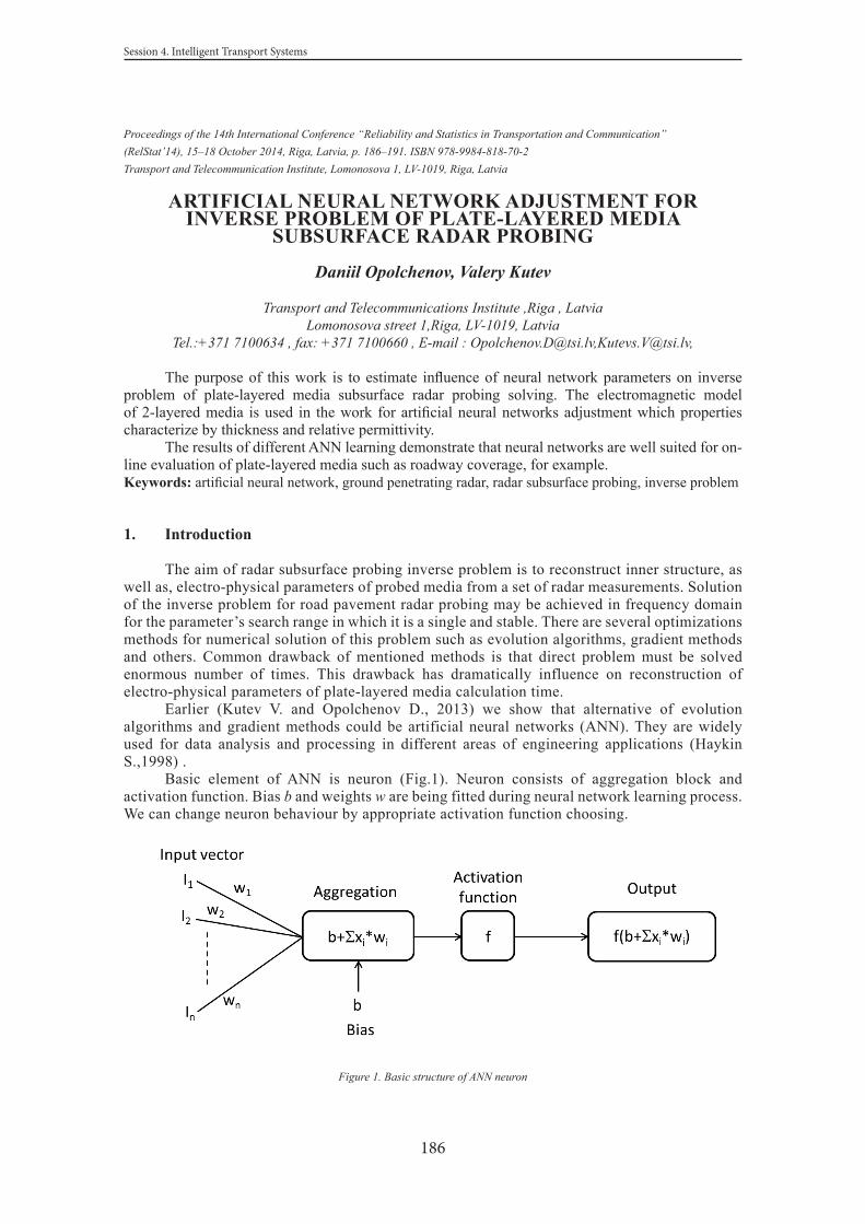
186



ARTIFICIAL NEURAL NETWORK ADJUSTMENT FOR INVERSE PROBLEM OF PLATE-LAYERED MEDIA

SUBSURFACE RADAR PROBING

Daniil Opolchenov, Valery Kutev

Transport and Telecommunications Institute ,Riga , LatviaLomonosova street 1,Riga, LV-1019, Latvia

Tel.:+371 7100634 , fax: +371 7100660 , E-mail : [email protected],[email protected],

The purpose of this work is to estimate influence of neural network parameters on inverse problem of plate-layered media subsurface radar probing solving. The electromagnetic model of 2-layered media is used in the work for artificial neural networks adjustment which properties characterize by thickness and relative permittivity.

The results of different ANN learning demonstrate that neural networks are well suited for on-line evaluation of plate-layered media such as roadway coverage, for example.Keywords: artificial neural network, ground penetrating radar, radar subsurface probing, inverse problem

1. Introduction

The aim of radar subsurface probing inverse problem is to reconstruct inner structure, as well as, electro-physical parameters of probed media from a set of radar measurements. Solution of the inverse problem for road pavement radar probing may be achieved in frequency domain for the parameter’s search range in which it is a single and stable. There are several optimizations methods for numerical solution of this problem such as evolution algorithms, gradient methods and others. Common drawback of mentioned methods is that direct problem must be solved enormous number of times. This drawback has dramatically influence on reconstruction of electro-physical parameters of plate-layered media calculation time.

Earlier (Kutev V. and Opolchenov D., 2013) we show that alternative of evolution algorithms and gradient methods could be artificial neural networks (ANN). They are widely used for data analysis and processing in different areas of engineering applications (Haykin S.,1998) .

Basic element of ANN is neuron (Fig.1). Neuron consists of aggregation block and activation function. Bias b and weights w are being fitted during neural network learning process. We can change neuron behaviour by appropriate activation function choosing.

Figure 1. Basic structure of ANN neuron

187


There are several common activation functions: Step Function, Linear combination, Log-Sigmoid Function, Tan-Sigmoid Function and others. In our work we used hyperbolic tangent sigmoid transfer function (Fig.2) for all neurons in network. This kind of activation function gives us opportunity to teach ANN to find nonlinear dependences between input and output data.

-5 -4 -3 -2 -1 0 1 2 3 4 5-1

-0.8

-0.6

-0.4

-0.2

0

0.2

0.4

0.6

0.8

1

n

tans

ig(n

)

Figure 2. Tangent- sigmoid activation function of ANN neuron

Tangent- sigmoid activation function is defined as:

[ ] .1)2exp(1

2)(tan −−+

=n

nsig (1)

Artificial network architecture could be rather complex structures. In our work we use one of simplest feed-forward architecture (fig.3). Feed-forward ANN usually consists of input layer, several hidden layers and output layer. Each layer consists of many unrelated neurons which inputs are connected to previous layer and output to next layer. Usually only input data without neurons take into account as full-grown input layer, but we don’t consider this layer as separate and count number of layers without input layer.

Figure 3. ANN architecture used in the work

188


We performed model-based investigation of the using ANN for reconstruction of electro-physical parameters of plate-layered media. Electro-physical parameters for each model layer were thickness h and relative dielectric permittivityε ′ of the layer’s materials, which values were the same as ones for typical road pavement. Investigation was performed with Neural Network Toolbox™ software. As parameters of ANN were used number of inputs I, number of neurons in first and second hidden layers H1 and H2 and number of outputs O. In most cases number of neurons in first hidden layers equals to number of inputs.

Neural network must be trained to solve inverse problem. Learning process could be either supervised either unsupervised. In our work we have used supervised learning that mean we must have an input-target training pairs.

2. Model-based experiment conditions

The electromagnetic model of roadway coverage may be conceived as homogeneous horizontal layers 2 and 3 of h2 and h3 thickness between medium 1 (air) and medium 4 with thickness

∞→hh 41, , as shown in Fig.4.

1 1,ε σ1

2

4

3

h2

h3

2 2,ε σ

3 3,ε σ

4 4,ε σ

Probe signal

Reflected signals

Figure 4. Electromagnetic model of roadway coverage

Electrical properties of each model medium will be described by relative dielectric constants ε i and conductivity σ i (for upper medium ε1 =1 and σ 1 =0). We allow that 2,3,4 media to be conductive, in which case the complex relative dielectric permittivity of medium i (for i =2,3,4), having conductivity σ i .

Fixed values of model electro-physical parameters are presented in Table 1 below,

Table 1. Electro-physical parameters of model mediaNumber

of layerMedia ε i σ i , S/m hi, m

1 Air 1,00 0 ∞

2 Coarse-grained asphalt 3.65 5e-8 0.20

3 Macadam 7,00 5e-4 0.33

4 Priming 15,00 0.05 ∞It is proposed that subsurface radar probing is performing with help of parallel line antennas in the following conditions:

• distance between the antennas …………………....……..1 m;• antennas high over upper boundary............................... 0.05 m;• half length of linear antennas...................................... 0,25 m;• diameter of antennas................................................ 0,0025 m;

189


For calculations of spectral density for received signals is used known(Krainyukov A., Kutev V, 2011) model of signal forming channel for subsurface GPR probing in frequency domain in which complex transfer function is presented in form:

3. Results of investigation

In case of ANN using inverse problem of plate-layered media subsurface radar probing may be considerate as template recognition problem. Therefore several ANN with different adjustments (as it shown in Table 2) have been simulated. Training of these ANN had been performed with using of 25% searching range around pavement model parameters presented in Table 1.

100,000 pairs of spectra of the received signal and electrical parameters of the selected model of the medium had been used to train ANN. The sets of physical parameters were not generated randomly, but by generating all possible combinations of parameters at 10 distributed evenly values of each parameter in the selected finding range.

Table 2. Artificial networks under researchName Number of layers Number of neurons per layer

2-layers ANN 2 79-5

3-layers ANN 1 3 79-79-5

3-layers ANN 2 3 79-158-5

5-layers ANN 5 79-158-158-79-5

All networks are feed-forward networks without feedback. All neurons of ANN use tangent sigmoid transfer function. Scaled conjugate gradient method has been used as train method.

We estimate performance of ANN using mathematical expectation and root-mean-square deviation of ANN working error for 10000 arbitrary generated couples of received signal specters and electro-physical parameters of modeled pavement. For all ANN we have mathematical expectation near zero. Therefore we use root-mean-square deviation as main comparing criteria.

As can be seen from Fig.5 relative dielectric permeability of second and third layers of pavement are found very precisely with small range of error by all ANN. Reconstruction accuracy of reminder model parameters depends on ANN configuration heavily.

Session 4.Intelligent Transport Systems

)()()()()()()()( 2 nRWLWFWANTexLRAD RKKKKSSK (2)

where:

)(LS is the spectrum of the signal across the load resistance of the receiving antenna; )(exS is the signal spectrum, which is used for impact excitation of the transmitting

antenna; )(ANTK is complex transfer function of the antenna system;

)(FWK is a complex transfer function of direct signal;

)(LWK is a complex transfer function of lateral signal;

)(RWK is a complex transfer function of the signal reflected from the subsurface ideal reflector, located at a depth equal to the thickness of the first layer of roadway coverage;

)(2 nR is a reflection coefficient of 2-n layers of the roadway coverage

3. Results of investigation

In case of ANN using inverse problem of plate-layered media subsurface radar probing may be considerate as template recognition problem. Therefore several ANN with different adjustments (as it shown in Table 2) have been simulated. Training of these ANN had been performed with using of 25% searching range around pavement model parameters presented in Table 1.

100,000 pairs of spectra of the received signal and electrical parameters of the selected model of the medium had been used to train ANN. The sets of physical parameters were not generated randomly, but by generating all possible combinations of parameters at 10 distributed evenly values of each parameter in the selected finding range.

Table 2. Artificial networks under research

Name Number of layers Number of neurons per layer 2-layers ANN 2 79-5 3-layers ANN 1 3 79-79-5 3-layers ANN 2 3 79-158-5 5-layers ANN 5 79-158-158-79-5

All networks are feed-forward networks without feedback. All neurons of ANN use tangent sigmoid transfer function. Scaled conjugate gradient method has been used as train method.

We estimate performance of ANN using mathematical expectation and root-mean-square deviation of ANN working error for 10000 arbitrary generated couples of received signal specters and electro-physical parameters of modeled pavement. For all ANN we have mathematical expectation near zero. Therefore we use root-mean-square deviation as main comparing criteria.

As can be seen from Fig.5 relative dielectric permeability of second and third layers of pavement are found very precisely with small range of error by all ANN. Reconstruction accuracy of reminder model parameters depends on ANN configuration heavily.

190


Figure 5. ANN structure influence on electrophysical parameters of soil media reconstruction accuracy

Obtained results show that ANN 3-layer 1 gives as good reconstruction accuracy of our pavement model parameters. At the same time could be seen that accuracy of parameters which weakly influence on GRP received signal spectra, such as 4th layer relative electric permeability, increases with number of ANN layers and summary number of neurons.

To define finding range of parameters within ANN could be trained, finding range influence on parameters reconstruction accuracy was researched. ANN 3-layer 1 was trained using different finding range. Time of training was limited by 1000 epochs. Training results are presented on Fig.6

Figure 6. Finding range influence on electrophysical parameters of soil media reconstruction accuracy

As can see on the Figure 6 at the finding range more than 25% root-mean square error of media parameters reconstruction dramatically increased. It could be assumed that accuracy decreases according to increasing of absolute step value that can take pavement model parameters in training set. To estimate absolute step value influence on reconstruction accuracy dependency graph of root-mean error of soil media parameters reconstruction on number of values at finding range that can be taken by parameters in training set was drawn up. ANN training conducted at 25 % finding range.

Influence of number of parameters levels on electro-physical characteristics of soil media reconstruction accuracy is presented on Fig.7.

191


Figure 7. Influence of parameters levels on electro-physical parameters of soil media reconstruction accuracy

It can be seen that accuracy of soil media parameters reconstruction heavily depends on absolute step size. Absolute step value decreasing increases the accuracy of electrophysical properties of soil media reconstruction. After a certain point decrease of step value does not make sense, since no significant increase of the accuracy of parameters reconstructions, but leads to a significant increase in training time due to a significant increase of the training set.

On the basis of the two previous graphs, we can assume that for each electro-physical parameter there is an optimal value of the absolute step that allows you train the neural network with the required accuracy in a desired period of time.

4. Conclusion

The main results of our model-based investigation are following:• It is enough 3-layer artificial neural network structure 79-79-5 to solve the inverse

problem of subsurface sounding for two-layer model of asphalt with 5 parameters• The accuracy of determining the electro-physical parameters of the medium with the

help of ANN depends on the ratio of the search range and number of points in it that can take parameters in the training set.

References

1. Haykin S.(1998). Neural Networks: A Comprehensive Foundation. Prentice Hall PTR Upper Saddle River, NJ, USA. 842 pp.

2. Kutev V. and Opolchenov D. (2013) “Electro-Physical Parameters of Plate-Layered Media Reconstruction Using Artificial Neural Network Algorithm”. Abstracts of the 13th International Conference RELIABILITY and STATISTICS in TRANSPORTATION and COMMUNICATION (RelStat’13). pp. 95

3. Krainyukov A., Kutev V. Using of radar monitoring for road coverage quality estimation. Proceedings of the 11th International Conference “Reliability and Statistics in Transportation and Communication” (RelStat’11), 19–22 October 2011, Riga, Latvia, p. 275-283

4. Neural Network Toolbox™ User’s Guide. M.H.Beale (2014.) – 435 pp.

192



FIBRE-OPTIC SENSORS CALIBRATION METHOD BASED ON GENETIC ALGORITHM IN WEIGHT-IN-MOTION

PROBLEM

Alexey Pilipovecs1, Alexander Grakovski2

1 Transport and Telecommunication Institute, Riga, Latvia, Lomonosova 1, Riga, LV 1019, Latvia,Phone: (+371) 67100654, Fax: (+371) 67100535, E-mail: [email protected]

2 Transport and Telecommunication Institute, Riga, Latvia, Lomonosova 1, Riga, LV 1019, Latvia, Phone: (+371) 67100654, Fax: (+371) 67100535, E-mail: [email protected]

The problem of measuring vehicle’s weight-in-motion (WIM) is one of the most important research topics in the field of transport telematics. It is important not only for development of intelligent systems used for planning and cargo fleet managing, but also for control of the legal use of transport infrastructure, for road surface protection from early destruction and for safety support on roads. The fibre-optic sensors (FOS) became popular nowadays for WIM applications. Considered WIM system consists of: six fiber optic pressure sensors, temperature sensor, induction loop for distinguishing vehicles, and data processing unit for weight and other parameters estimation.

It is necessary to calibrate the system every time after reconnecting the fiber-optic sensor, since the optical coupling is sensitive to weather conditions. The calibration process consists in choosing the normalizing coefficients, which will compare the data obtained from the experiment with the reference data, known in advance. The system and method of calibration of WIM system is the subject of this study. Recorded signals from a group of FOS of a passing truck with various speeds and known weight are used as an input data. To solve the problem of sensor calibration is proposed to transform it into a problem of optimization and use evolutionary (genetic) algorithms. The results of a truck FOS weighting system calibration based on optimization algorithm, are being discussed, in order to use this information for axle weight-in-motion estimation.Keywords: telematics, WIM problem, fibre-optic pressure sensors, calibration, evolutionary algorithms

1. Introduction

The worldwide problems and costs associated with the road vehicles overloaded axles are being tackled with the introduction of the new weigh-in-motion (WIM) technologies. WIM offers a fast and accurate measurement of the actual weights of the trucks when entering and leaving the road infrastructure facilities. Unlike the static weighbridges, WIM systems are capable of measuring vehicles travelling at a reduced or normal traffic speeds and do not require the vehicle to come to a stop. This makes the weighing process more efficient, and in the case of the commercial vehicle allows the trucks under the weight limit to bypass the enforcement.

The fibre optic weight sensor is the cable consisting of a photoconductive polymer fibres coated with a thin light-reflective layer (SensorLine GmbH, 2010). A light conductor is created in such a way that the light cannot escape. If one directs a beam of light to one end of the cable, it will come out from the other end and in this case the cable can be twisted in any manner. To measure the force acting on the cable, the amplitude technology is more appropriated for the measurements based on measuring of the optical path intensity, which changes while pushing on the light conductor along its points.

193


Fibre optic load-measuring cables are placed in the gap across the road, filled with resilient rubber (Fig. 1). The gap width is 30 mm. Since the sensor width is smaller than the tyre footprint on the surface, the sensor takes only part of the axle weight. The Area method (Teral, 1998) is used in the existing system to calculate the total weight of the axle. The following formula is used to calculate the total weight of the axis using the basic method:

(1)

where Wha – weight on half-axle, At(t) – dynamic area of the tyre footprint, Pt(t) ~ V(t) – air pressure inside the tyre and, according to Newton’s 3rd law, it is proportional to the axle weight (Grakovski et al., 2013).

Figure 1. Fibre optic sensors position against the wheel and tyre footprint and the algorithm of the weight-in-motion measurement station.

194


At these points the deflection of a light conductor and reflective coating occurs, that is why the conditions of light reflection inside are changed, and some of it escapes. The greater the load the less light comes from the second end of the light conductor. Therefore the sensor has the unusual characteristic for those, familiar with the strain gauges: the greater the load the lower the output is.

As we can see the exact values of the formula (1) factors are unknown. The area of the tyre footprint is calculated roughly by the length of the output voltage impulse, which, in its turn, depends on the vehicle speed. The Area Method uses the assumption that the area under the recorded impulse curve line, in other words – the integral, characterizes the load on the axle. To calculate the integral, the curve line is approximated by the trapezoid. In this case the smaller the integral – the greater the load. This method does not require knowing the tyre pressure, but it requires the time-consuming on-site calibration.

2. Tyre Footprint and Weight Estimation

There was the set of measurement experiments with the roadside FOS sensors on April, 2012 in Riga, Latvia (Grakovski et al., 2013, Grakovski et al., 2014, and Krasnitsky, 2012). Loaded truck was preliminary weighed on the weighbridge with the accuracy < 1%. The output signals from FOS sensors for truck speeds 70 km/h and 90 km/h are demonstrated on Figure 2.

It is evident that the signals for the different speeds have been changing by amplitude and the proportion of amplitudes does not fit the axle weights (Fig.2).

Figure 2. Examples of FOS signals from A and B sensors (Fig.1) for vehicle’s speeds 70 km/h and 90km/h respectively

The reason of this behaviour may be explained by FOS properties such as weight (pressure) distribution along the sensor length as well as sensor non-linearity and temperature dependence (Grakovski et al., 2014).

195


3. Vehicle speed and tire contact width evaluation

Using FOS A (FOS B) and FOS 1 (FOS 2) symmetric signals, which are shown in Figure 3, it is possible to calculate the speed of each axle, also the truck speed by calculating the average of the values found before. In order to do this, it is necessary to normalize the signals, filter out the noise and obtain symmetrical signal components. Then impulse peak time value of these components will be used in the axle speed calculation. Distance between FOS A and FOS 1 (or FOS B and FOS 2) should be known in advance; in our case it is equal to 3 m (see Figure 1).

Figure 3. FOS vertical weight component (symmetric) of s1_A, B, 3, 4_70km_27_09_2013 signal

Calculated axle and vehicle speeds, based on the FOS signal peak time of symmetric components, are shown in Table 1.

Figure 4. (a) FOS A and FOS 1d filtered s1_A, B, 1d, 2d_90km_27_09_2013 signal; (b) Tyre footprint interaction with FOS

196


Table 1. Calculated speed values of s1_A, B, 3, 4_70km_27_09_2013 signal

Speed/axle 1st axle 2nd axle 3rd axle 4th axle 5th axle Vehicle

Calculated speed [km/h] 72.34 72.00 71.63 71.56 71.93 71.89

Using FOS 1d and FOS A (or FOS 1), which are shown in Figure 4(a), as well as the symmetric FOS pair signals, it is possible to evaluate left and right tyre footprint widths. In order to do this, it is necessary to normalize the signals, filter out the noise and make linearization of the signals according to the pre-calculated axial velocity and temperature of the FOS.

Then pulse widths of perpendicular and diagonal FOS (see Figure 4(b)) are measured on experimentally chosen level of 0.4, multiplying this width subtraction by corresponding axle speed will be the evaluation of tyre footprint.

Table 2. Evaluated tyre footprint width of s1_A, B, 1d, 2d_90km_27_09_2013 signal

Parameter / axle 1st axle 2nd axle* 3rd axle 4th axle 5th axle

Footprint width [mm] 315 680 385 385 385

Evaluated footprint width [mm] 310.317 890.633 399.993 375.202 387.925

Error [%] -1.487% 30.975% 3.894% -2.545% 0.499%

* - dual wheels (the distance between two neighbour dual wheels approximately is 40-50 mm and it cannot be measured exactly)

4. Fibre-optic sensors calibration based on genetic algorithm

The application of FOS for WIM problem solution can provide us the level of accuracy 5-10% for each axle of truck (Grakovski et al., 2013, Grakovski et al., 2014), but we can meet with the unexpected high errors in especial situations.

Figure 5. Example of FOS signals with experimental truck in a sunny day 20.04.2012 (vehicle speed 70 km/h).

197


Figure 6. Example of FOS signals with experimental truck in a rainy day 23.09.2013 (vehicle speed 70 km/h).

After several live experiments with FOS group it was discovered, that measurement results differs on weather conditions, especially when the sensor’s fibres are applied to a recorded. This happens due to sensitivity of physical connection and weather conditions, for example, changes in air humidity results in a signal fading at recorder’s site. Notice, that magnitude in figure 5 is much greater than in figure 6. Small particles of water scatters light beam, what leads to a wrong data readings, as a result vehicle’s weight cannot be measured correctly. Rainy experimental data was gathered on 23.09.2013.

When these signals were run through WIM algorithm (Grakovski et al., 2014), it was found, that error in rainy data on each wheel was grater than 40%, see Table 3.

Table 3. The results weight estimation before calibration.Signal

(conditions) 1st axle 2nd axle 3rd axle 4th axle 5th axle Total weight of the truck

Sunny -3.3205% -9.5662% -10.7336% -6.8906% -9.8579% -8.1430%

Rainy -44.3129 -51.5012 -55.2587 -48.9375 -49.2731 -50.1531%

The idea of sensors calibration according to its own properties and peculiarities of situating into the pavement, as well as weather conditions at this moment, consists on the selection of these calibration coefficients for each pair of two sensors (left and right), let to obtain the minimum of axle’s weight errors for all set of measurements. If the task is to optimize some quantitative factors, the genetic algorithm (Zhao et al., 2013) can be used here.

FOS calibration based on genetic algorithm:

• Coding and initialization. Two calibration coefficients are considered as chromosome, which are coded using real numbers. Population size is 30.

• Fitness Function. As optimization criteria maximal error rate of all 5 axles is used additionally with sum of minimal difference between right and left wheels. After each new population, all results are sorted in order to obtain best calibration results.

• Selection operation. 30 best chromosomes are selected from generation, for following breeding.

198


• Crossover operation. The roulette method is used for selection of better chromosome within population for crossover operation with probability of 0.8. In which two chromosomes are used to produce 7 new successors in a linear combination.

• Mutation operation. In order to obtain global optimization, any chromosome can completely mutate with probability of 0.05.

Figure 7. Convergence of FOS calibration algorithm.

Figure 7 shows, that approximately 10-15 generations is enough to reach the convergence of algorithm.

Therefore it was decided to use calibration algorithm for a FOS group. As an option genetic algorithm was used for a calibration purpose. The idea of calibration is to find a scaling coefficient, which will take into account optical losses for each sensor. Initial signal will be multiplied with a calibration factor, which will be found in genetic optimization process. Vehicles error rate after applying calibration coefficients can be found in Table 4.

Table 4. The results of weight estimation after calibration.Signal

(conditions) 1st axle 2nd axle 3rd axle 4th axle 5th axle Total weight of the truck

Sunny 4.0547% -2.0695% -4.0596% 0.7838% -2.3053% -0.7571%

Rainy 10.7654 -3.0131% -10.7620% 1.3957% 0.9509% -0.6750%

From Table 4 it can be seen, that FOS calibration strongly affects weight estimation. It means that it is possible to decrease the level of the errors by optimizing calibration coefficients for each pair of two sensors.

199


5. Conclusions

Consider the WIM problem through the FOS sensor’s accuracy point of view we can conclude that the installation of it into the pavement produce some probabilistic influence to the measurement results. It depends not only on sensor’s geometric position and properties of components, but also on weather conditions at the time of installation. So, calibration is required.

The experimental results show that the range of the vehicles velocity from 50 to 90 km/h seems more appropriate for WIM based on fibre-optic sensors let to allow B+(7) class according to COST 323 for the high speeds and D2 according to OIML R134 for the low speeds (O’Brien and Jacob, 1998).

Additionally, from the analysis of the results we can assume, that most exact result can be obtained for total weight of the truck, not for each axle of it, because of longitudinal oscillations exists here (especially between 1st and 3rd axles). From other hand, it can be caused by incorrect cargo distribution along the length of the truck and trailer, but it is separate task on future.

Acknowledgements

This research was granted by ERDF funding, project “Fiber Optic Sensor Applications for Automatic Measurement of the Weight of Vehicles in Motion: Research and Development (2010-2013)”, No. 2010/0280/2DP/2.1.1.1.0/10/APIA/VIAA/094, 19.12.2010.

References

1. Grakovski, A., Pilipovecs, A., Kabashkin, I. and Petersons, E. (2014). Weight-in-motion estimation based on reconstruction of tyre footprint’s geometry by group of fibre optic sensors. Transport and Telecommunication, 15(2), 97–110.

2. Grakovski, A., Krasnitski, Y., Kabashkin, I., Sikerzhicki, Y. and Truhachov, V. (2013). Some approaches to the rolling wheels’ dynamics modelling in the weight-in-motion problem. Transport and Telecommunications, 14(1), 57–78.

3. Zhao, L., Jiang, J., Song, C., Bao, L. and Gao, J. (2013). Parameter Optimization for Bezier Curve Fitting Based on Genetic Algorithm. // Advances in Swarm Intelligence. Lecture Notes in Computer Science, Springer-Verlag, Berlin, vol. 7928, pp 451-458.

4. Krasnitsky, Y. (2012). Transient Response of a Small-Buried Seismic Sensor. Computer Modelling and New Technologies, 16 (4), 33–39.

5. SENSORLINE GmbH. (© Sensor Line). (2010). SPT Short Feeder Spliceless Fiber Optic Traffic Sensor: product description. Retrieved January 7, 2011 (from http://sensorline.de/home/pages/downloads.php)

6. Teral, S. (1998). Fiber optic weigh-in-motion: looking back and ahead. Optical Engineering, 3326, 129-137.

7. O’Brien, E., Jacob, B. (1998). European Specification on Vehicle Weigh-in-Motion of Road Vehicles. In Proceedings of the 2nd European Conference on Weigh-in-Motion of Road Vehicles (pp. 171–183). Luxembourg: Office for Official Publications of the European Communities.

200



EFFICIENT MEASURING OF COMPLEX PROGRAMMABLE LOGIC DEVICE (CPLD) IMPLEMENTED ANALOG-TO-

DIGITAL CONVERTERS STATIC PARAMETERS

Sergejs Šarkovskis1, Sergejs Horošilovs2

1 The Faculty of Computer Science and Telecommunication, Transport and Telecommunication Institute

Lomonosova street 1/4, LV-1019, Riga, Latvia, e-mail: [email protected] RPAP AS

Ropazu street 140, LV-1006, Riga, Latvia, e-mail: [email protected]

The precision of analog-to-digital signal conversion plays an important role in digital communication systems. At the present moment, the histogram method is the method mainly used for measuring analog-to-digital converter (ADC) static parameters, such as differential nonlinearity (DNL) and integral nonlinearity (INL). In such case the ADC input signal is being changed linearly and output data is used to construct a histogram, thus calculating the number of specific codes occurrences. The main problem of such method implementation is necessity to store a large volume of data – ADC output code words during the collection of information. It is usual to use memory modules for such purpose. This article focuses on implementation of histogram method of ADC static parameters measuring based on inexpensive complex programmable logic device (CPLD) arrays. The article proposes histogram real-time calculation algorithm and it’s realization on CPLD, which allows reducing volume of required memory or stopping using it entirely.Keywords: analog-to-digital converter, differential nonlinearity, integral nonlinearity, histogram method.

1. Introduction

At the present moment, analog-to-digital converters (ADC) are widely used in the fields of electronics and communications. Digital signal processing is base tool in measuring devices; digital telephony and digital television systems; data collecting and such processing is impossible without high-quality ADC.

In ideal case ADC converts continuous analog signal into digital, usually binary coded. The minimal change of input signal available for conversion is quant, which is related to ADC bitness. This quant is least significant bit (LSB) and it determines resolution of ideal ADC. The LSB value can be estimated according to (Kester, 2005)

,2

FSNLSB ∆

= (1)

where ΔFS – is range of input signal, N – ADC bitness. ΔFS defines unipolar or bipolar ADC operation mode. In the first case input signal is in range between 0 and FS, the FS denotes full scale, which is often related to reference voltage of ADC. In case of bipolar operation mode, ΔFS is in range between – FS and FS.

Depending on the ADC bitness N the output code varies in range between 0 and 2N – 1. Thus, for 3 bit ADC there are 8 possible levels, beginning with code 0 (0002) and ending with code 7 (1112). Transfer function (TF) of such ideal ADC in unipolar mode is shown in Figure 1a. The analog input is given as fraction of FS. Note, that all ones code corresponds to analog value FS – 1LSB.

In Figure 1a dots denote code transitions, which are separated by 1LSB beginning with 0.5LSB for ideal ADC. For real ADC it is impossible to define unambiguous level of input signal for each digital code. For the same digital code there is certain range of input signal, which doesn’t exceed 1LSB in ideal case (Figure 1b). Such phenomenon is named a quantization uncertainty and it leads to difficulties in definition of code transitions (Kester, 2005).

201


Analog input

Digi

tal o

utpu

t

1 LSB

000

001

010

011

100

101

110

111

1/8 1/4 3/8 1/2 5/8 3/4 FS7/8

Code transitions INL line

(a)Analog input

Digi

tal o

utpu

t

Code transitions INL line

1 LSB

000

001

010

011

100

101

110

111

1/8 1/4 3/8 1/2 5/8 3/4 FS7/8

(b)

Figure 1. Ideal transfer function of 3 bit ADC

At the present moment converters in market vary in pricing, resolution, performance and quality. The last is defined by set of parameters, which can be divided into static and dynamic.

2. Histogram method

There are different methods for evaluation of ADC static parameters which are based on finding points of code transitions. The main problem related to defining these points is the noise of code transitions, especially in the presence of negative differential non-linearity (DNL). The possibility of such methods applicability is limited by a few tenths of an LSB peak-to-peak noise. Histogram method (code density method) can be used for evaluation of any ADC static parameters for any level of noise. In such case for input signal of specified form it is necessary to accumulate ADC output data and calculate occurrences of each code word. Input signal should slightly overload (recommended value if 10%) ADC. It is possible to use ramp signal for this purpose (Kester, 2005), the sequence of triangular pulses (Alegria, Arpaia etc, 2002) or harmonic function (Blair, 1994). For code words k from 1 to 2N – 2 there are M samples and each code word occurrence is being calculated. Note, that “overload” codes, such as all zero and all ones are not included in calculations. Theoretical number of occurrences for each code word k can be evaluated according to (Kester, 2005)

theoretical( ) .2 2N

Mn k =−

(2)

If n(k)actual – is real number of occurrences for code word with number k it is simple to calculate DNLk for this code word (Kester, 2005)

actual

theoretical

( )DNL 1.( )kn k

n k= − −

(3)

DNL for full ADC can be calculated according to (Kester, 2005)

( )DNL max DNL .k= (4)

Figure 2 shows typical histogram with wide, narrow and missing code words.For given DNLk it is possible to calculate integral non-linearity (INL) by usual addition (Kester,

2005)

1INL DNL .

m

m kk =

= ∑ (5)

202


Missingcode

Wide code

Narrow code

k

n(k)actual

Code bin

All zeroscode

All onescode

n(k)theoretical

Figure 2. Typical histogram for ramp input signal

Histogram method removes the effect of ADC noise by calculating average value over entire code intervals and is ideally suited for testing of any ADC. At the present moment histogram method is standard method for static parameters measuring.

2.1. Implementation of histogram method

Figure 3 shows typical histogram method setup.

ADCN

Outputdata

Nadr

Data bus

Address bus

MemoryMCU N

PC

Samplingclock

Rampsignal

-FS

FS

Figure 3. Histogram method setup

The ADC for testing purpose is driven by linear positive slope signal generator. A microcontroller provides clock for ADC, collects output data and copies them into memory. When testing is complete, the data is being sent to PC for further processing and required parameters calculation.

This article proposes to use complex programmable logic device (CPLD) arrays for histogram calculation and control process. The use of CPLD arrays provides different benefits, such as parallel and independent process control, high data processing rate and so on. The proposed histogram calculation algorithm applied to CPLD arrays reduces the volume of required memory or makes it possible to stop using it entirely.

The simplest way to calculate histogram by means of programmable logics uses the output code word as an address for corresponding counter. Every time the code word is being read the value of respective counter is increased by one unit, thus it is possible to form required histogram. When using such approach the functional scheme consists of one N-to-2N decoder and 2N counters, where N is the bitness. The problems of such approach are obvious – 10 bit ADC requires 10-to-1024 decoder and 1024 counters, at the same time 12 bit ADC requires 4096 counters and 12-to-4096 decoder. Such

203


increase of scheme components requires CPLD arrays of higher capacity or conversion to FPGA arrays with high cost. It would be beneficial to implement universal scheme, which can be used for most ADC available on the market.

3. Windowed Histogram Method - WHM

The improved histogram calculation scheme proposed in this article is based in the first place on knowledge of the analog signal form. If the signal increases linearly it’s logical to assume that ADC output code words will also monotonically advance from 0 to 2N – 1. At the beginning of measurements output codes will be localized at zero level and probability of high values is low. In such case it’s possible to define the window with certain width and calculate histogram within its bounds while shifting the window if necessary in a direction of the code words increments. The resulting set of the histograms at the output should be summed as is shown in Figure 4.

0

7

1 2 3 4 5 6 7 8 9 ...

4 3

6

2 2 1 0 0 0

0 1 2 3 4 5 6 7 8 9 ...

13 4 5

31 1 0 0

100

0 1 2 3 4 5 6 7 8 9 ...

75

76

10

5

20 0

100

0

1

...5

7

2

54

002N-1

00... 2N-3 k

k

k

k

Window

Window

Window

Figure 4. Windowed histogram method

Such approach, which is called the windowed histogram method, leads to two main questions:1. what width of the window should be chosen;2. when the window should be shifted.

The answer on the first question is directly connected with ADC code transition noise. For stronger noise the wider window is necessary. It is proposed to shift histogram in case, when during certain time interval there were no code words in the beginning of window.

When implementing WHM via CPLD array it was decided to choose the width of window equal to 8, i.e. the one, which corresponds to 3 bits. In fact, this means that ADC noise may not be stronger than 4-5 LSB. The choice of specific window width equal to 8 dictates the necessity to use 3-to-8 decoder and 8 counters, regardless of the ADC bitness. Decoder is driven by three low-order bits – those are numbers from 0 to 7, so that the value of the first counter increases by 1 when the input is 0, the number of second counter increases by 1 when the input is 1, and so on.

It has been decided to shift histogram at the moment, when there have been no code words from the first two bins during 10-15 clocks of the histogram window. The smaller is number of clocks impacting the shift the more often it should be shifted, and hence the more often output data should be saved. The higher number of clocks can force code words to leave the right border of the window, which is unacceptable.

When shifting window, it is necessary to edit input data, since only three low-order bits are being used. When the window shifts to the right, the bin of code word 0 departs and the bin of code word 8 arrives. Now three zeroes in ADC output low-order bits denote the code word 8 and further the value of the last counter is increased, instead of the value of the first counter. Such correction can be implemented by subtraction of the number of shifts from the input code and further addition on the modulo 8. The block diagram of such WHM algorithm is shown in Figure 5.

204


START

Read Data

k = mod(Data-sum, 8)

k == 0

k == 1

k == 2

k == 3 k == 4

k == 5

k == 6

no

cnt1 = cnt1 + 1cnt = 0

cnt2 = cnt2 + 1cnt = 0

cnt3 = cnt3 + 1cnt = cnt + 1





cnt8 = cnt8 + 1cnt = cnt + 1yes

cnt == 15 sum = sum + 1All cnt’s = 0

no

yesyes

yes

yes

no

no no

no

yes

yes

no

yes

no

All cnt’s = 0sum = 0

Figure 5. The block diagram of WHM algorithm

Here Data – is ADC data, cnt1..8 – 8 counters for window bins, cnt – clock counter for the 1-st and the 2-nd bins when there are no code words present, sum – addition of the shifts.

3.1. WHM implementation via ALTERA company CPLD family MAX3000A

It is expected to implement designed scheme in existing project with purpose of testing ADC parameters. This project includes signal generator based on 16 bit digital-to-analog converter (DAC), CPLD EPM3256ATC144-10 and coupling board for PC with 16 digital inputs/outputs. The scheme with WHM implementation was designed in Quartus II and its schematic is shown in Figure 6.

This scheme consists of one 3-to-8 decoder implemented in block lpm_decode0 and 8 counters implemented in blocks lpm_counter0. Counters length is set to 5 bits. This means these counters can be used to count up to 31 before reset occurs. The choice of such counters length isn’t accidental and it’s related to theoretical number of code word occurrence. The input of decoder is driven by three low-order bits of ADC – ADC[2..0]. The indication scheme for histogram shifting is implemented with counter lpm_counter3 and comparator lpm_compare0. If the upper two counters (representing two left bins of the window) have data, then OR2 element resets counter lpm_counter3, otherwise this counter is incremented by 1 after a new code word. When this value will reach the value of comparator, counter data from lpm_counter0 is sent to output register lpm_shiftreg0 with length of 40 bits (8 counters with 5 bit length) and the specified counters are then reset. In such case there is an output signal ‘Shift’. Further to this, it is necessary to prevent the loss of data for overflow of these counters. This can be achieved by ‘cout’ outputs, which signal counters overflow and OR8 element. The signal of this element launches the similar to window shifting mechanism excepting the signal ‘Shift’.

The code correction scheme for shifting is implemented by another counter lpm_counter2 and subtracter lpm_add_sub0. The counter lpm_counter2 is cyclic one, so modulo 8 adding is achieved automatically. Also, note that when overflow of counters lpm_counter0 occurs the window isn’t shifted, so lpm_counter2 counter value doesn’t increment.

205


Figure 6. Functional schematic of WHM implementation in Quartus II

206


The data transferring to PC is realized with multiplexer lpm_mux2 and ‘DataReady’ signal, which indicates the status of collected data. With external clocking the data of output register is serially transferred to outputs ‘Data2PC’. If the new shift of the window is necessary before the data has been transferred to PC, the scheme includes ‘Pause’ signal, which suspends execution of the algorithm. Such approach makes it possible to completely avoid the use of memory and send data directly to PC.

The scheme also includes block ‘GenDac’, which has been written in Verilog HDL language to form control signals for external DAC and clocks ADC in testing. In scheme also defines internal signal generation logics.

The full project volume is 205 macrocells of 256 available (80%) and used 26 ports of 116 available (22%).

4. Simulation

In order to test functionality of designed scheme it was necessary to create Test Bench using Verilog HDL language and execute simulation using ModelSim Altera Starter Edition software. In order to bring simulation to reality as close, as it is possible there is MATLAB program for input data simulation. The project uses analog signal generator based on 16 bit DAC and output voltage in range ±12.5V. Thus, the program simulated analog signal and relative ADC with noise was driven by this signal. Three low-order bits of ADC output code word were recorded to the text file, which was used in ModelSim simulation.

During the simulation output data (the window of histogram) was also recorded into text file, which has been used in MATLAB program to plot resulting histogram. Finally, this histogram is being compared with standard template histogram which has also been built in MATLAB for source data. Then it is possible to conclude, whether WHM algorithm works correctly.

ADC noise has been generated by random numbers generator with uniform distribution an expectation of E = 0. Probability density function (PDF) width can be chosen arbitrarily.

Below there are results of simulation for the following parameters:• the relative 10 bits ADC in testing has reference voltage 10.24V, thus

1LSB = 1mV;• the input signal varies in range from -1.024V to 11.264V (with 10% overload);• the width of ADC noise PDF is 5LSB;• artificially created missing codes – the 15-th and the 40-th. The generated voltage and respective ADC code is shown in Figure 7.

Figure 7. The input analog voltage and output ADC code

207


ModelSim output text file is formatted as following:

1 0 4 10 4 2 3 1 01 0 4 6 8 5 3 1 01 0 0 4 5 1 5 0 0

The first column indicates shifting signal, the rest of 8 columns are bins of the histogram. After simulation was complete, this data has been processed and used to plot resulting histogram. The example of such histogram for the first 50 bins is shown in Figure 8.

Figure 8. The part of resulting histogram

The histogram clearly shows the missing codes in the 15-th and the 40-th bins of histogram. The comparison of resulting histogram with standard template histogram shows no errors.

5. Conclusion

The article proposes new software implementation method for testing of ADC static parameters. This method is based on knowledge of input analog signal – it is ramp function. It is proposed to create histogram only for certain window with specified width, which is being shifted from low-order code words to high-order code words, rather than generate entire histogram at once. This method is named Windowed Histogram Method (WHM) and it has been implemented via ALTERA company CPLD array of the family MAX3000A with 256 macrocells. The designed scheme volume takes up 80% of the full CPLD array capacity. In order to test functionality of the WHM the simulation has been executed in ModelSim software, and the data for this simulation has been simulated in MATLAB. The input data has been intentionally noised with uniformly distributed noise with PDF width of 5LSB. As a result of this simulation there are histograms before shifting, which have been used to construct resulting ADC histogram in MATLAB. The WHM designed scheme has been implemented via cheap CPLD array (the cost at mouser.com is approx. 17.7€ when the article has been written) and it allows to avoid use of additional memory, which significantly decrease costs of the project.

References

1. Alegria F., Arpaia P., da Cruz Serra A.M, Daponte P. (2002) Performance Analysis of an ADC Histogram Test Using Small Triangular Waves. IEEE Transaction on Instrimentation and Measurement, 51(4), 723-729.

2. Blair J. (1994) Histogram Measurement of ADC Nonlinearities Using Sine Waves. IEEE Transaction on Instrimentation and Measurement, 43(3), 373-383.

3. Kester W.A. (2005) The Data Conversion Handbook. Oxford: Elsevier. 976 p.

208



PILOT TESTING EVALUATION OF PORTABLE SYSTEM OF DYNAMIC

TRAFFIC FLOW MANAGEMENT AT TRAFFIC CLOSURES UPPERCASE

Marek Ščerba1, Tomáš Apeltauer2, Jiří Apeltauer3

1Centrum dopravního výzkumu, Brno, Czech Republic,

Lišeňská 33a the present address+420 606689956, [email protected]

2Brno University of Technology, Faculty of Civil Engineering Brno, Czech Republic, Veveří 331/95

+420 737 383 389, [email protected] University of Technology, Faculty of Civil Engineering

Brno, Czech Republic, Veveří 331/95+420 541 147 356, [email protected]

Problematic localities which occur on transport infrastructure for a limited time periods during traffic closures, reconstructions, large accidents are an important aspect affecting road safety and traffic flow. The research identified several main factors which cause significant losses in travel times and which cause frequent road accidents. Lower road capacity is responsible for an occurrence of so-called bottlenecks which leads to instability of traffic flow. Consequently, drivers may make errors and choose wrong solutions of traffic situations. An important role for the above mentioned factors is played by incorrect late merge, speeding, tailgating, lower tolerance and consideration to other road users, and nervousness and ignorance of drivers. In 2011 to 2013,project ViaZONE was in progress, which was to design an intelligent system with the aim to eliminate the mentioned risks and reduce economic losses generated by traffic congestions. Reliability of all used components of the system was verified during pilot testing. Regarding traffic management, the system showed some problems due to indisciplined drivers and the system proved that speeding in these hazardous road segments is a common practice which caused accidents and congestions.Keywords: Workzones, Traffic management, accident, congestion, detectors, portable variable message signs

1. Introduction

In 2011 to 2013, project ViaZONE was in progress “Traffic Flow Harmonisation and Increase of Road Capacity at Road Works with the Use of Co-operating ITS Systems – Portable Traffic management”, which was to design an intelligent system with the aim to eliminate the mentioned risks and reduce economic losses generated by traffic congestions.

The research team consisted of Centrum dopravního výzkumu, v.v.i. as the coordinator and cooperating organizations HIT HOFMAN, s.r.o. and Brno University of Technology, Faculty of Civil Engineering. The project was funded by Technological Agency of the Czech Republic within Alfa programme. The project aimed to develop, produce, test and verify a pilot operation of “Portable System of Traffic Management”, particularly on sites in front of and in traffic closures. The aim of the project was reached in December 2013, when the pilot operation of the system was finished on a motorway D1 segment between Brno and Vyškov.

This paper presents the result of the impact assessment of the pilot testing VIAZONE system.

209


1.1. The system VIAZONE

The system in question consists of interoperable components, which are tailor-made to the requirements for portable systems [6]. The main feature of these components is their modularity, portability, minimum requirements for installation, calibration and maintenance, economic operation, and independence of mains. The complex system is a set of HW and SW tools which allow for an effect on drivers through portable, mobile, variable road signs. Unique algorithms for the displayed pictograms and messages on variable road signs are displayed in real time on the basis of evaluated input data from various traffic detectors which are installed in several predefined profiles of an area in question. Reliability of all used components of the system was verified during testing. Evaluating and control software allowed for remote controlling and automated operation of the system without any problems. Subsequently, the data from the measuring and system operation were evaluated and methodology “Methods to Improve Road Safety and Traffic Flow at Traffic Closures Using ITS” was produced.

Figure 1. Illustrative photo made during system pilot testing

2. Theoretical expectations for system effectiveness

In-depth analysis of traffic flow behaviour at road closures was performed in the first stages of the project. Traffic detectors were installed at several reference traffic closures for the period of 6 weeks. The obtained data were used for creation of micro-simulation models. Input values of the model were obtained from measurements performed on highway closures and also using the values for estimating the capacity of highway closures in [1] and [2]. Traffic flow model was calibrated and validated in comparison with the source data from floating vehicles. Control scenarios, which were verified on the models, were created in the other stage. After performing more than 300 simulation tests, the most suitable scenario was selected (Graph 1 shows Scenario 2), which was a combination of adaptable speed reduction and warning system with the function of informing of queues, possibly other hazards. The system design and algorithms used in model has been suggested in relationship between capacity and driver behaviour [3].

The performed analyses show that the use of dynamic controlling according to Scenario 2 is able improve the capacity of a bottleneck by approximately 10 - 15%.

Regarding the late merge, the critical value for the Czech Republic is approximately 1400 v/h. Higher traffic volume is beyond the capacity of late merge and queues are likely to occur. Model cases show that the use of the dynamic system may lead to the harmonization of traffic flow and the rule of late merge could be respected more (with the current vehicles classes). Regarding traffic closures which uses two narrowed traffic lanes, there is not such frequent occurrence of queues, but queues and significant time losses are likely in crisis situations and peak hours.

The conclusion of analytical studies show that dynamic controlling in work zones may lead to significant road safety improvement and improvement of travel times by 10%-15% and reduction of the number of vehicles standing in the queue by 15% - 20%.

210


Graph 1. Number of vehicles in queue of 1400 veh/h

3. System pilot testing

3.1. Information on road closure

Reconstruction of motorway D1 near Brno started in the middle of 2013. This concrete road pavement reconstruction was the largest reconstruction of D1 with the exception of the modernized segments between Brno and Prague which are under the progress. The traffic was guided in both directions in two auxiliary traffic lanes using the hard shoulder.

In the time period from 20 September 2013 to 3 December 2013, a system of Portable traffic management, which is the main outcome of the project of Portable Traffic Management, was installed on motorway segment Olomouc – Brno on kilometres 213 to 229.

3.2. System architecture within pilot testing

Figure 2. Complete architecture within pilot testing on D1 motorway segment between kilometers of 207.5 – 229.5

During the pilot testing has been installed these system components with respect of requirements in [4]:• Portable VMS installed in the middle of the road (2x)• Information trailer LED (3x)• Nonintrusive traffic detector Wavetronix (4x) • The queue radar detectors (3x) • Travel time detectors (4x bluetooth detectors)• Camera • Industrial PC with minimum power consumtion, compatible with all detection and

display components with GPS, GPRS (9x)• Evaluation software• Alternative source of energy

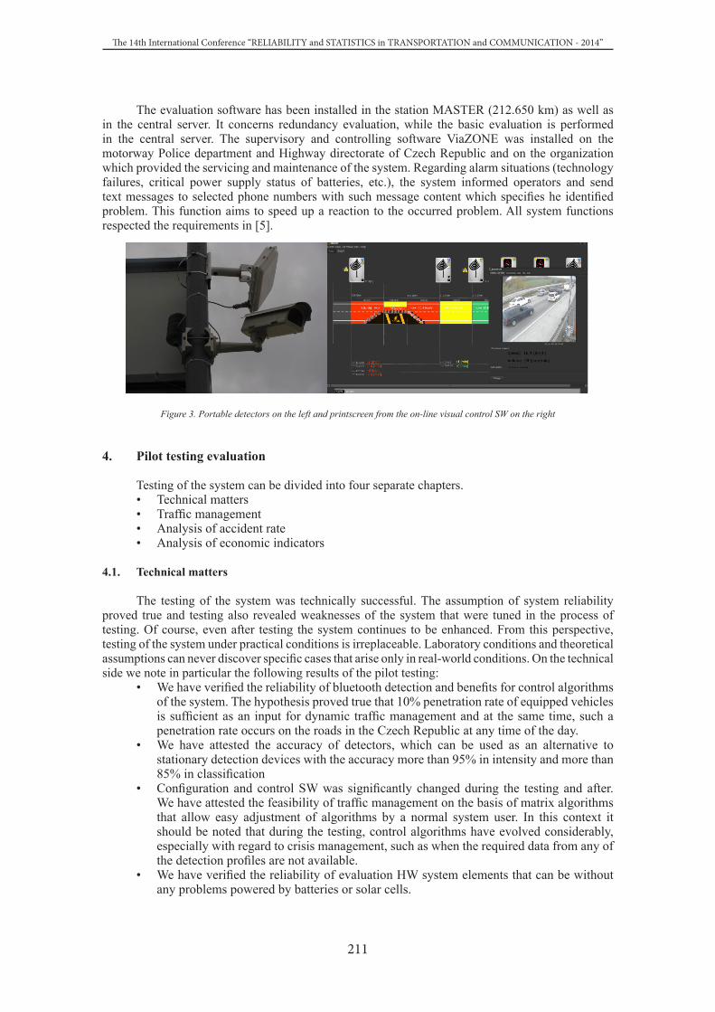
211


The evaluation software has been installed in the station MASTER (212.650 km) as well as in the central server. It concerns redundancy evaluation, while the basic evaluation is performed in the central server. The supervisory and controlling software ViaZONE was installed on the motorway Police department and Highway directorate of Czech Republic and on the organization which provided the servicing and maintenance of the system. Regarding alarm situations (technology failures, critical power supply status of batteries, etc.), the system informed operators and send text messages to selected phone numbers with such message content which specifies he identified problem. This function aims to speed up a reaction to the occurred problem. All system functions respected the requirements in [5].

Figure 3. Portable detectors on the left and printscreen from the on-line visual control SW on the right

4. Pilot testing evaluation

Testing of the system can be divided into four separate chapters. • Technical matters • Traffic management • Analysis of accident rate• Analysis of economic indicators

4.1. Technical matters

The testing of the system was technically successful. The assumption of system reliability proved true and testing also revealed weaknesses of the system that were tuned in the process of testing. Of course, even after testing the system continues to be enhanced. From this perspective, testing of the system under practical conditions is irreplaceable. Laboratory conditions and theoretical assumptions can never discover specific cases that arise only in real-world conditions. On the technical side we note in particular the following results of the pilot testing:

• We have verified the reliability of bluetooth detection and benefits for control algorithms of the system. The hypothesis proved true that 10% penetration rate of equipped vehicles is sufficient as an input for dynamic traffic management and at the same time, such a penetration rate occurs on the roads in the Czech Republic at any time of the day.

• We have attested the accuracy of detectors, which can be used as an alternative to stationary detection devices with the accuracy more than 95% in intensity and more than 85% in classification

• Configuration and control SW was significantly changed during the testing and after. We have attested the feasibility of traffic management on the basis of matrix algorithms that allow easy adjustment of algorithms by a normal system user. In this context it should be noted that during the testing, control algorithms have evolved considerably, especially with regard to crisis management, such as when the required data from any of the detection profiles are not available.

• We have verified the reliability of evaluation HW system elements that can be without any problems powered by batteries or solar cells.

212


• It was verified (5) that the system cannot operate on only one communication technology. GPRS technology is not sufficiently permeable to allow (at least in 99% of cases) sending the data every minute to the evaluation server. This interval was defined as the minimum necessary for traffic management.

• Control SW Viazone, or more precisely the control algorithms of the system allowed commanding the Information trailer LED from different supplier, which demonstrated the possibility of independence of the system on LED technology vendors.

• The possibility of trouble-free maintenance of interim ITS systems was demonstrated what is suggested in (4). Regular replacement of batteries in the central reserve may be routine and very fast operation that does not disturb traffic flow.

4.2. Traffic management

If we wanted to fulfil the theoretical assumptions drawn from the prepared calibrated models and shorten travel times and the length of queues in the place of work zones with the use of dynamic management (theoretical models indicate the potential for improved traffic-carrying capacity by more than 10%) based on the speed limit, it would be necessary to propose additional measures. The degree of acceptance of variable road signs by drivers is insufficient and disobedience and arrogance of most drivers occurs. The data showed that traffic flow is faster on average by about 20 km/h than is the permitted speed limit, even at places of work zones where workers are moving and the width of lanes is significantly reduced.

An average traffic volume was 27 vehicles/ min (minimum of 10 vehicles/min, maximum 45 vehicles/min). The speed was evaluated for 5 minutes. From the performed tests we can conclude that by displaying the road sign 80, slowing the speed of traffic flow by about 25% down to the speed of around 100 km/h (at best) is achieved. Better results is obtained by displaying a warning sign “Queue“ (results are better than with maximum 80). The average speed was reduced to the speed around 95 km/h. Before displaying the symbol, the speed of traffic flow was 112 km/h (max. 115 km/h and min. 108 km/h). In the first minute, traffic flow moved without limitation, in minute 2-3 there was also no significant decrease in the speed (average 107 km/h) but in the 4th minute the average was 92.4 km/h and in the 5th minute 98.2 km/h.

From the above it can be deduced that drivers react more to warning road signs that symbolize certain approaching danger than to speed limit signs.

These results, however, are insufficient for traffic management, as they do not match the model assumptions by far and therefore it is not possible to make a reliable statement on the effectiveness of the tested pilot system to improve traffic flow and increase throughput at bottlenecks. It is also not possible to make a credible statement with regard to the length of pilot installation, since the effectiveness and efficiency of the system should be evaluated at least after 1-2 years of its routine operation.

Diagram 1: Comparison of speeds and traffic volumes during the long-term measurement. There is no apparent relationship between speed limit compliance and traffic volume. Upper diagram show the slowing traffic flow, if the max 80 km/h has been displayed.

213


4.3. Analysis of accident rates

During the period of traffic closures in 2013 (71 days), 48% (25 accidents) of all accidents in that year were reported on the monitored segment. We are talking about incidents where the Police of the CR had to intervene. In 2012, traffic closures on the same segment lasted only 53 days, however, during that period there occurred 17 accidents, which is 33% of all accidents in that particular road segment in 2012.

For example during the 71 days immediately prior to installation of traffic closures only one traffic accident occurred on this segment of the motorway. In the period from January to June 2013 there were 26 accidents in the monitored segment. So in the test segment, during the two years of monitoring there was 3.84 times higher probability of an accident in the segment with transport limitations compared to the period with no traffic limitations on the monitored segment. From these data it is evident that road closures are significant risky places, which should be provided with a system to harmonize traffic, in combination with repressive systems that will enhance respect for road signing and marking.

4.4. Analysis of economic losses due to the work zone on D1 and congestions at the site of pilot installation

After completion of the testing it was attempted to determine the total economic losses incurred due to delays in the work zone near Vyškov and show the importance of measures that lead to elimination of delays and traffic accidents. For these calculations, we used data from the system RODOS (from the system of floating car data), where we compared the five-minute aggregated outputs from ASIM detectors located at road mileage 207 and 226 (traffic volume, classification) with the values of delay in individual segments of the affected site. As input values for idle time of cars, trucks and buses we used the HDM-4 methodology [7]. All 71 days of the existence of this work zone were covered and all delays in the segments exceeding 3 minutes were included.

Table 1. Total time losses due to the traffic closure, quantified in Czech crownsTotal losses Cars Trucks Total lossesDirection Vyškov -

BrnoCZK 53,378,380 CZK 26,687,742 CZK 80,066,132

Direction Brno -

VyškovCZK 9,147,871 CZK 4,768,595

CZK 13,916,466

5. Economic indicators of the system

In order to estimate the benefits of active management of work zones it is not possible to make a simple statement that traffic flow improved and travel times shortened. The initial investments in the system and its subsequent operation generate substantial costs that need to be taken into account. When calculating the economic indicators of the system a model case was established, which was simulated based on real data. The simulation was carried out on a calibrated traffic model that was created in earlier stages of the project and related to one traffic closure in each direction. Consideration was given to the data that emerged from real testing the system, so the already calibrated models were set according to specific values coming from drivers’ reaction to the system (these results are presented later in this document). Therefore, the input values are more realistic compared to initial simulations. Therefore, the creation of an economic model counted with savings in travel times between 7-9%. In the model, the system was used in configuration of an adaptable speed decreasing system of 3 VMS profiles (on both right and left side) and one information trailer. On the other side of the working zone a warning and information system was used in configuration with 2 VMS profiles (both on the right and left side) and an information trailer.

These inputs to the economic model were used: • Values of time spent in congestions specified by HDM-4 (National methodology) [7]

214


• The value of time spent in congestions related to classification of vehicles on the motorway D1 according to data from a fixedly mounted profile detector

• The value of travel time savings during a simulation experiment • The investment costs of the system. • Maintenance and operation of the system, including depreciation • Comparison of benefits and costs of the system The findings of this economic model show that for the given test configuration and time, the

system efficiency index calculated as the ratio of benefits and costs of its operation was CIES = 6.6 Thus, the system during the monitored time within the simulation period proved to theoretically generate savings of more than six times the operating costs. Index like this is quite crucial for evaluating the economic efficiency of the system.

However, it is important to emphasize that it is not possible to search for a fixed number for the system, but always a combination of the system, installation location and operating time.

The resulting system efficiency index is determined inter alia, by the following factors: • Traffic volume in the site of installation influences the efficiency index the most. As it

turned out, shortening of travel times is in the case of active traffic management more pronounced for low traffic flow, i.e. more vehicles in a queue.

• On the contrary, the management may be counterproductive in case of a lower number of vehicles.

• Operating time of the system includes phases during the day with higher and lower volumes, which reflects in its effectiveness. If the system is in operation 24 hours a day, its effectiveness will be lower than in the case where it is active only during the weekdays and only during the daytime.

• Seasons influence drivers’ behaviour in work zones. In the winter months, drivers tend to drive more slowly and the dynamics of traffic flow is therefore different from the summer months.

Generally it can be stated that although the system under study was tested on data especially during the time of the day that involves afternoon rush hours, its index is so high that it would fall to the zone of unprofitability only in case of very unfavourable combination of several of these factors acting simultaneously

6. Conclusions

All the above facts have one clear and easily verifiable result. In areas of road closures, the probability of traffic accidents is approximately 4 times higher than on the segments of motorways and expressways with no limitations. It is the result of exceeding speed limits, not maintaining safe distances and not adjusting the driving to road surface conditions. However, drivers themselves do not perceive this fact.

From the perspective of research, we can therefore consider the results of this testing as very valuable. In order to achieve the theoretical assumptions of the possibility to reduce economic losses from increased travel times and accidents through telematics tools, it is necessary to seek other appropriate measures. It could be effective to use restrictive measures in the form of heavy fines and point penalties for violations of traffic rules in work zones. It is necessary to take into account the safety of workers in work zones, which is considerably endangered by fast driving. The above mentioned large number of traffic accidents is a sad evidence of the critical situation in complying with traffic rules in work zones.

According to discussions with members of the police force is not easy to penalize drivers in road closures. There is a problem with a place to stop vehicles. For this reason, possibilities should be considered of dedicating a place in road closures to measure the speed of vehicles with the possibility of their stopping. In the long run, it is necessary to increase respect of drivers from these places similarly as in tunnels where exceeding the speed limits is much less frequent.

Another result of the performed tests and analyses shows that the design and management of traffic closures has a significant impact on the overall losses in travel times of drivers and related economic losses. For this reason, it is necessary to provide sufficient space for the planning process of system deployment. At least the following sequence should always be observed:

215


• Familiarity with the plan of a closure, traffic routing, the number of lanes and their width, familiarity with traffic volumes at the time of planned closure

• Preparation of a model of traffic closure• Determining a predicted delay with and without management• Calculation of CIES• Decisions about the form of the system, its functions (managing, warning, surveillance,

etc.) and the number of components depending on information gained in previous steps

References

1. Barrel W., Pesti G., Sun D., Ding L., Capacity and road user cost analysis of selected freeway work zones in Texas, Texas: Texas Transportation Institute 2009, 68 p.

2. Calvert, S., A-Priori Travel Time Predictor for Long Term Roadworks on Motorways, Delft: Delft University of Technology 2009, 153s.

3. Akcelik, R. (2008) The Relationship between Capacity and Driver Behaviour. In: TRB National Roundabout Conference, Victoria, May 2008. Kansas City, 14 p.

4. Highway directoriate of Czech Republic. (2013), Zobrazování zpráv na informačních vozících na dálnicích a rychlostních silnicích ve správě Ředitelství silnic a dálnic ČR – Příručka VMS: Ředitelství silnic a dálnic.

5. Highway directoriate of Czech Republic. (2013), Projekt dopravní telematiky při modernizaci dálnice D1: Ředitelství silnic a dálnic

6. Přibyl P., Dopravní telematika při modernizaci D1 – conceptual project, Praha: České vysoké učení technické v Praze, fakulta dopravní 2012, 85 p.

7. Prováděcí pokyny pro hodnocení ekonomické efektivnosti projektů silničních a dálničních staveb. Technické předpisy, Ředitelství silnic a dálnic, Příloha C, [cit. 2013-7-9]. Dostupný WWW:http://www.rsd.cz/rsd/rsd.nsf/a3eda25d005dc6bec125737e0045602e/f6965540595261bdc1257b2500335a23/$FILE/Priloha%20C%20-%202012.pdf

Transport and Logistics System Modelling

Session 5

218



THE APPLICATION OF A NEW ITERATIVE OD MATRIX ESTIMATION FOR URBAN PUBLIC TRANSPORT

Balázs Horváth1, Richárd Horváth2

1,2Széchenyi István University – Department of TransportGyőr, Hungary, Egyetem tér 1.

p+36-96-503-494, [email protected], [email protected]

Keywords: public transport, OD matrix, matrix estimation, PTV-VISUM

1. Introduction

The estimation of OD matrix is an “evergreen” topic especially in the field of public transport, due to the phenomena that this is the key of the planning of public transport systems. Other hand it is one of the most important mosaic to the accurate prediction of the traffic load, or the correct execution of the planning stage assignment. This requires not only a well-functioning assignment method, but also reliable passenger data. Reliable passenger data means time-dependent origin-destination matrix. There is a lack of well working origin-destination matrix estimator method in the field of urban public transport.

The research team at the Széchenyi István University (Hungary) dealing with this topic for years (Winkler, 2011). There were several predecessor methods, e.g. one shown four years ago at TRA2010 (Horváth, 2010). Through the use of that method in the every day practice, it has been clear that the method can be used only if the network is simple without lot of transfers. Therefore in 2012 the group started a research in a new direction, based on an old model (Prileszky, 1995). The first test results of this research were shown at TRA 2014 (Horváth, 2014).

This paper shows the first real network results of the method used in Hungarian cities.The newly developed method working with two kinds of input data: full scope cross-section

data and a sample origin-destination matrix. These data will be used in one hand to produce multiplier to correct the sample origin-destination matrix, but on the other to help the calibration of the matrix. The method is an iterative method which needs 20-50 steps to produce a reliable origin-destination matrix.

The paper describes the theory of the process and shows real network experiences.Theory of the method is that origin traffic (boarding passengers) and destination traffic

(alighting passengers) together with the link load of the public transport lines on each and every section (link) bear some information about the real origin-destination matrix. In the method we collect these information for every origin-destination pair separately and multiply the elements of the sample network with a multiplier calculated from the above mentioned information through a mathematical function.

The paper shows the effect of different mathematical functions using by the calculation of the multipliers on a test network. It is very interesting to see that in some cases even the simplest function can give good result.

Finally a real public transport network will be shown to prove the effectiveness of the method. After this example the paper shows that the newly developed method is good enough to use in the real life work without any limitation like experienced with the old estimation method.

2. Theoretical background of the matrix estimation method

The background of the newly developed matrix estimation method was already described in (Horváth 2014), although we show it here again to give a clear picture, how we the later shown

219


result reached. The origin of the matrix estimation procedure shown in this paper was developed by Prileszky [4]. After the above written lack of easily usable OD matrix estimation in public transport, we revised and improved the original method which previously sunk into oblivion. This section describes the operation of this method.

2.1. Theory of the matrix estimation method

As mentioned before, the basis of the transport planning is the knowledge of transport demands. Considering the fact, that the budget and elaboration time of short-term and medium-term planning is restricted, there is no possibility of detailed data collection in every case. In case of most projects, however, there is a full-scale cross-section passenger counting and OD survey sample during the preparation of the planning.

The essence of this method is, that the data gathered in the course of the passenger counting let us be allowed to correct the elements of the sample matrix gained from the survey.

It is possible to make use of the data of the passenger counting in two ways. On the one hand these give information about the number of boarding and alighting passengers at each stop; on the other hand these give information about the travellers’ number between stops.

These data can be produced with the use of a suitable flow assignment procedure. If we compare the obtained data from the two sources (counting, assignment) we have an opportunity to correct the model matrix. In order to do this correction, we have to use the boarding and alighting numbers and the numbers of passengers between stops.

2.2. Details of the method

The sums of rows and columns of the OD matrix that is the number of departing and arriving passengers of each zone equals to the sum of the boarding and alighting passengers of the stops in the given zone. Because all of this, the sums of rows and columns of the OD matrix (to be determined) are known on full scale cross-section passenger counting. These are utilizable as target values through the following calculations. Boarding and alighting numbers compared to the sums of rows and columns of the model matrix expose the difference between the model (seed) and target matrices, which difference can be corrected by row and column factors. It is especially important to notice that the pi and aj values refer to departing and arriving passengers in the model matrix, however, the Pi and Aj values are the boarding and alighting numbers of the passenger counting, that is the latter contains transfers. Taking account this problem the planned sums of rows and columns have to be corrected before the above mentioned factor calculation. This means that the sums of rows and columns of those relations where the transfer occurs have to be corrected.

The basis of the transfer correction is the following connection:


2.1. Theory of the matrix estimation method

As mentioned before, the basis of the transport planning is the knowledge of transport demands. Considering the fact, that the budget and elaboration time of short-term and medium-term planning is restricted, there is no possibility of detailed data collection in every case. In case of most projects, however, there is a full-scale cross-section passenger counting and OD survey sample during the preparation of the planning.

The essence of this method is, that the data gathered in the course of the passenger counting let us be allowed to correct the elements of the sample matrix gained from the survey.

It is possible to make use of the data of the passenger counting in two ways. On the one hand these give information about the number of boarding and alighting passengers at each stop; on the other hand these give information about the travellers’ number between stops.

These data can be produced with the use of a suitable flow assignment procedure. If we compare the obtained data from the two sources (counting, assignment) we have an opportunity to correct the model matrix. In order to do this correction, we have to use the boarding and alighting numbers and the numbers of passengers between stops.

2.2. Details of the method

The sums of rows and columns of the OD matrix that is the number of departing and arriving passengers of each zone equals to the sum of the boarding and alighting passengers of the stops in the given zone. Because all of this, the sums of rows and columns of the OD matrix (to be determined) are known on full scale cross-section passenger counting. These are utilizable as target values through the following calculations. Boarding and alighting numbers compared to the sums of rows and columns of the model matrix expose the difference between the model (seed) and target matrices, which difference can be corrected by row and column factors. It is especially important to notice that the pi and aj values refer to departing and arriving passengers in the model matrix, however, the Pi and Aj values are the boarding and alighting numbers of the passenger counting, that is the latter contains transfers. Taking account this problem the planned sums of rows and columns have to be corrected before the above mentioned factor calculation. This means that the sums of rows and columns of those relations where the transfer occurs have to be corrected.

The basis of the transfer correction is the following connection:

i

ikorr

ii

i

PP

ntpp ,

(1)

where nti numbers of transfers in i. stop By this correspondence it is possible to calculate the corrected target row and column sums.

ii

iiikorr átp

pPP

,

(2)

ii

iiikorr átp

pPP

,

(3)

k

mmjj

k

nnii LAFP

1,

1, ;

(4)

where k number of stops in the whole area Fi,n boarding in n. stop of i. zone Lj,m alighting in m. stop of j. zone Executing this correction step the row and column factors can be calculated as the following:

220


∑∑==

==k

mmjj

k

nnii LAFP

1,

1, ;

(4)

where k number of stops in the whole area Fi,n boarding in n. stop of i. zone Lj,m alighting in m. stop of j. zone Executing this correction step the row and column factors can be calculated as the following:

i

ikorri p

Ps ,=

(5)

j

jkorrj a

Ao ,=

(6)

where si i. row’s factor oj j. column’s factor

However, as we mentioned, this matrix estimation method doesn’t use only stop point data. We take into consideration the data of passenger numbers between stops to achieve adequate precision. These are called link data, factors deriving from them are link factors. Preparation of these link factors is more complex task than of the row and column factors taking into consideration that the model link data are unknown. To determine model link data we have to assign the model matrix onto the transport network. The generated link loads give the model link data, which can be compared to the counted number of passengers between stops.

ji

jiji assignmentfromloadlinkcomputed

loadlinkreallink

,

,, =

(7)

After calculating the factors of every row, column and link, they have to be linked to each travel relation. Or vice versa, we have to collect the row, column and link factors of given relations for every single element of the OD matrix. While the determination of the first two is quite simple as departing and arriving zones are known in every relation, association of link factors needs another single study.

To associate the link factors, we have to know the shortest path or k shortest paths in the given relation and we have to associate all the links covered by these paths to the given relation.

After execution of the abovementioned steps, factors needed for following calculations are known regarding all relations. But these factors can be used in different ways:

• only the shortest path• k. shortest paths

• link factors associated to paths and weighted by assignment• link factors associated to paths• every factor weighted equally

We show the differences further on the model network.

3. Matrix estimation method in the practice

The key for the functional correctness of the matrix estimation method is the accuracy of the applied flow assignment method. To aid the future improvement of the method, we fitted the procedure to the VISUM transport planning software of the PTV AG.

Applying this software was obvious, as the VISUM is one of the market leading products in this field and we use it for ten years. Another asset of the program is the cooperation with numerous

221


program languages through Windows COM protocol. This possibility helped the development of the method. The third reason was that the VISUM can be used as [transport] data bank for containing different network data.

In the first phase of the development we used the Python script based language. It was too slow and therefore was able to let us do test runs on small test networks. Later we changed the whole script from internally runnable Python script to externally runnable Lasarus (Pascal) code.

The matrix estimation procedure is the following:The matrix estimation method reads out the model data built up previously in VISUM through

the COM interface then process it. The readout contains the results of the base assignment, executed previously.

After the former computing method the script modifies the OD matrix and writes it back into the transport model. After changing the code from Python to Pascal we could reach big improvement in speed. The code now is able to perform one iteration step of the matrix estimation for an urban public transport network of a city with 50.000 inhabitants in 50 seconds.

Our very first real network test showed that results after 10 iterations are already acceptable and results after 30 steps are good enough for further work. The test runs shown in this paper overwritten these statements while it gave us good results after only 10 steps.

4. Latest test runs on real network

After the usage of a test network (Horváth 2014), due to the reengineering of the script code we were able to let run the estimation on real networks. For the very first real network test we used the public transport network of the Hungarian city Eger (publication is under review). After this one we changed to another city where the network structure in more complex. This one is also a Hungarian city: Dunaújváros.

This city is a good field for testing while in 2008 we performed there a full scale cross-section counting on all public transport vehicles moving on the local network. That time it had more or less 40.000 inhabitants and a public transport network with 89 stops and 43 lines.

Figure 1. Public transport network of the Hungarian city Dunaújváros

As mentioned above the method works with factors and as listed before there are four possibilities to use these factors. The first possibility is to use only the shortest path between two zones as define in the original method (Prileszky 1995). We rejected this one due to the reason we

222


find it unrealistic to use only we and only path between two zones. Therefore we dealt during our tests only with the three remaining methods.

We controlled the goodness of the different variants with the function assignment analysis of the VISUM software. This analysis allows us to compare an observed value (in this case the counted number of passengers on network links) with a model (or calculated) value (in this case assigned number of passengers on network links). If the model would describe reality with 100% precision, observed and calculated values would compose a straight line with a starting point of 0 (Y=0) and a slope with 1.

4.1. Link factors associated to paths and weighted by assignment

The theory of this scenario is to separate each possible path’s factors and weighted them by the ratio of its load. It means a path between two zones with higher load (higher importance) has higher influence on the final factor of the element of the origin-destination matrix. The formula of this factor calculation seems as follow in the case of an example where there are n paths between two zones (i,j), where path nr 1. has k pieces of links and nr n. has l pieces of links:

2

......

... ,,

2,,

1,,

,1,

2,1,

1,1,

1

, +

+++⋅++

+++⋅++

=n

llinklinklink

wk

linklinklinkwos

factor

lnji

nji

nji

n

kjijiji

ji

ji (8)

where wi is the weight of the i. path

This method is the most complex and it takes into consideration the most factors. The pre-tests with the small test network showed that this one is the worst among the methods. It has not been changed. It is the worst as shown in the assignment analysis diagram.

Figure 2. Assignment analysis results with weighted factors

The results shown above are after 10 iterations. May there is an uncertainty to have better results after 20 or 50 steps. Parallel to this calculation we also checked the total number in the OD matrix. While this sum started to reach its limit we decided to stop the process (the changes of this sum will be shown later). Other hand these results are too poor to deal with it further. The correlation coefficient R2 is only 0.50, which is far from the ideal 1, the same is true for the slope, which is instead of 1 only 0.65.

4.2. Link factors associated to paths

This variant has similar principles as the previous one but in this case there is no weighting all possible paths has the same weight, namely 1. In an example where there are n paths between two zones (i,j), where paths nr 1. has k pieces of links and nr n. has l pieces of links the formula seems as follows:

223


2

......

... ,,

2,,

1,,

,1,

2,1,

1,1,

, +

+++++

+++++

=n

llinklinklink

klinklinklink

osfactor

lnji

nji

nji

kjijiji

ji

ji (9)

The pre-test showed for this variant better result. During the real network test we experienced the same. This method has clear better performance.

Figure 3. Assignment analysis results with unweighted factors

The assignment analysis give a very good result. The correlation coefficient is 0.98 which is almost the perfect result. It is even better than at the other real network test we recognised (0.95). It means this kind of factor usage for this kind of network seems to be ideal.

4.3. Equal weight for every factor

In this variant we are using the simple average of all the related factors. During pretest it was the best and was also suggested by the original method (Prileszky 1995). Although the very first real network test gave worse result for this method than the previous one. Therefore we was curious on the results of this method. Will it better or worse than the unweighted method.

Figure 4. Assignment analysis results with equal weight for every factor

Unexpected the results of the equal weight method is the best at this network. As the assignment analysis chart shows the correlation coefficient R2 0.98, which is the same as in the previous case, but the slope is growth from 0.96 to 0.98 which is closer to the ideal 1. Although the starting point of the linear regression line is changed from 28.56 to 29.06 instead of 0. After all we had to state the two latter methods give similar results. It needs further investigation in which case which method is better.

224


4.4. Speed of the iteration

All the results were shown are results of only 10 iteration steps. We decided to stop at this point while it seems to be the „final result”. As figure 5 shows the changes of the total number of OD matrices in the three cases more or less stop to change after few steps.

Figure 5. Speed of iteration

The experience with the speed of the iteration seems very important due the fact that one step needs around 1 minute. Whit the decrease of number of steps we can save 15-20 minutes at a calculation, it means at a trial with all three methods we can save more or less one hour.

5. Conclusions

With two real network trials behind we can stated, the matrix estimation method working fine. The „only” question to answer is why unweighted and equal weight method’s goodness alternate with each other. To clear this and test the performance of the model at bigger networks, we are planning to do a trial with a network in the city Győr. In this city there are 130.000 inhabitants and a public transport network with more than 400 stops.

Acknowledgements

The research resulted these achievements is supported by the „TÁMOP-4.2.2.C-11/1/KONV-2012-0012: “Smarter Transport” - IT for co-operative transport system” project - The Project is supported by the Hungarian Government and co-financed by the European Social Fund

References

1. Horváth, B. (2010) Forecasting of travel demand in urban public transport. In: Proceedings of the Transport Research Arena Europe 2010, Brussels, June 2010.

2. Horváth, B. and Horváth, R. and Gaál, B. (2014) A new iterative method to estimate origin-destination matrix in urban public transport. In: Proceedings of the Transport Research Arena Europe 2014, Paris, April 2014. Paris: IFSTTAR

3. Prileszky, I. (1995) Közlekedéstervezés. Győr: Széchenyi István College 76p.4. Winkler Á. (2011) Experiments to Discover Passenger Preferences in Public Transport. In:

Proceedings of the Mobilita’11: Sustainable Mobility, Bratislava, May 2011. Bratislava: Slovenská Techniká Universita, pp. 136-141.

225



MODELING OF CONTAINER TRAINS IN THE STRUCTURE OF A DRY PORT WITH THE USE OF TECHNOLOGY

“BLOCK TRAIN”

Mikhail Malykhin1, Aleksandr Kirichenko2

1Admiral Makarov State University of Maritime and Inland Shipping, Saint Petersburg, Russian Federation, [email protected]

2Doctor of Technical Sciences, Professor, Admiral Makarov State University of Maritime and Inland Shipping, Saint Petersburg, Russian Federation, [email protected]

Keywords: simulation modeling, dry port, “Block Train” technology

Summary

The purpose of this research is to develop a simulation model of transport communication between the sea and inland container terminals for determination the mode of this unit and the necessary volume of railway rolling stock.

Introduction

At this moment, the most of Russian seaports that possess container terminals, have nearly completely exhausted their capacities.

The main restriction is the city location of terminals, which creates a natural bound for the expansion of the port infrastructure.

As the obvious disadvantage of city location, is the negative impact at the environment due to the fact that the input and output of cargo to the port are, usually carried by trucks.

In addition to geographical factors, the capacity of terminals is reduced by long-term storage of import and export cargoes at sea terminals due to customs’ clearance.

Moreover, the experience shows that the possibilities’ lack to expand the areas of sea terminal, stevedores, to maintain existing capacities, are forced to reject customers’ requests for such services as the unstuffing of LCL containers, or, vice versa, the consolidation of parties.

The development of substitution port facilities at the cities’ outside is the expensive and difficult project not only by technology reasons, but also by social ones, since the location of new terminals outside the cities should be accompanied with their stable supply with workforce.

Dry port as a way to solve the problems of Russian sea port

One of the ways to solve the mentioned problems is the commissioning of inland terminals or, as they are called, “dry ports” which are located around of the city limits. First, these decisions have been applied in Western Europe in the middle of the last century to diversion the cargo flows from the destroyed by Second World War port facilities. At this moment, the effectiveness of dry ports has already been proved both in the worldwide practice, and in Russia (Kirichenko, Kuznetsov, 2014; Kirichenko, Kuznetsov, Izotov, 2013; Kuznetsov, Eglit, Kirichenko, 2013; Scherbakova-Slusarenko, 2014). As the example the terminal in Shushary, that is used as the dry port for First Container Terminal.

The implementation of the “dry port” technology allows marine terminals to perform only transit or transshipment functions. The storage of cargo during the customs’ clearance as well as the consolidation operations is provided by the inland terminal. Thus, it can function as a distribution center.

226


Problems of dry ports and existing research to address them

The technological problems include docking modes of transport in a dry port and uninterrupted implementation of transport between the sea and inland terminals. Appearance the additional link at the cargo supply chain, and the emergence of extra cargo operations, creates added cost of transporting goods, which is reflected in the cost of services and end-user operator (Scherbakova-Slusarenko, 2014).

Two possible ways of reducing the value added are cutting costs of terminal’s operator to optimize the using of expensive coastal areas (no need long-term storage site containers at the Marine Terminal) and the costs of transport communication between the sea and inland terminals. There is a need to develop scientific methods specified optimization.

Currently in Russia there was carried out a number of applied research related to the operation of “dry ports”. The simulation modeling is a more often applicable method in these studies.

The first group of studies related to problems of seaport’s design.So, papers by of A. L. Kuznetsov, M. N. Goryntsev and others, a seaport regarded as

macroobject, it capacity is based on the superposition of states of its elements (Goryntcev, 2014; Kirichenko, Kuznetsov, 2014; Kuznetsov, 2009). Hence, the derived models do not allow to take operational decisions in the chain “sea terminal – inland terminal”.

Local models developed by simulation modeling apply to newly constructed port of Taman (in particular, the work simulated the approach channel), where the problem of “dry port” is not relevant.

The second group of studies is related to railway and directly concerns the problem of “dry ports”, as in the work of J. N. Panova (Panova, 2012). In this paper a probabilistic description of technological areas of container terminals by discrete-event simulation software environment “AnyLogic” was developed. However, the main attention was paid to cooperation with the automobile transport (as the limiting level of the container terminal was selected checkpoint).

The application of the “dry port” concept poses several requirements to the cargo terminal:• A single operator possessing the sea terminal;• The mandatory presence of the railway communication between two terminals;• The simplification of customs procedures for moving containers between the sea and

inland complex;• The harmonized system of cargo flow management for both the sea and the inland

terminal.However, this solution has a major drawback: the usage of inland terminal forms additional

transport link for delivering of cargo from the sea to inland terminals. Consequently, there arise additional costs that are reimbursed by the operator of logistic complex.

Optimization of dry port’s operation by using of simulation modeling

The study considered the possibility of optimizing the number of railway rolling stock, which includes shunting locomotives at sea and inland terminals and flatcars to carry containers. Rolling stocks mentioned above are owned by the operator of infrastructure. In addition, one should determine the required amount of mainline locomotives, which carry out transportation of platforms between gateways to which front and rear terminals are assigned. Locomotives, in accordance with the legislation of the Russian Federation, are the property of JSC “Russian Railways” and are the subject of the commercial work on the railways.

There is a need to determine the optimum amount of rolling stock to provide additional transport link and the subsequent optimization of costs for the purchase or lease of rolling stock` and its subsequent operation.

At this research the solution of this task are proposed by using of simulation modeling. The research model was developed on the base of the “AnyLogic” software.This product allows the user to create models with the help of the set of active elements that

simulate real-world objects and experiments that define the configuration settings of the model.This software is based on the JAVA computer language and supports three well-known methods

of simulation modeling:• System dynamics;

227


• Discrete event simulation;• Agent based modeling.The operational activity of any transport system may be represented as a chronological

sequence of events. Modeling such kind of system relates to discrete modeling.

Description of the source data, formation of the model, the experiment

For modeling purposes, following factors were defined:• determination the transport unit operations mode;• determination the rolling stock required number;• improving the “Block train” transportation technologies.As a background information for the simulation modeling the available statistic data on import

cargo flows between the “First Container Terminal” and a terminal in Shushary was selected, as well as the data on traffic conditions in the area “Avtovo railway station – Shushary railway station” of the October Railway.

As a random variables were specified next parameters: probability of railroad trucks’ occupied, probability of availability of free transport units, probability of transport units fault, probability of cargo’s lack. For definition of these parameters first of all were studied a statistics information concerning these events at railway stations of the October Railway, serving the “First Container Terminal” and a terminal in Shushary. Then, applying statistical law sought quantities were obtained.

The model considers the application of the “Block-Train” rail transportation technology, which implies the presence of dedicated timetable of train moving and reducing the time of inspection at the intermediate railway stations.

Current algorithm of the model is shaped by standardized units available and configured settings or by means of the JAVA language.

Input data for this model is taken from the of statistical information, but may be modified manually before the start of the experiment. Each container in that model is named “entity” and loaded to it by the “Source” object.

Events are considered as models of discrete events, which occurring at a present time. Agent based modeling is not suitable at that case, since entities are not independent objects.. General view of the block diagram model is presented in Figure 1.

Figure 1. General view of the block diagram model

Application of Technology “Block Train”, which follows a dedicated timetable is regarded as the highest priority on several parameters:

228


• removes the dependency on the availability of the involved rolling stock;• reduces the inspection at the junction;• provides simplified coordination of train schedule.The first object <Source> – simulates the receipt of entity in the system that is input stream of

containers. In this model, they are operating according to the exponential distribution.Next comes the launch of an experiment to determine the necessary number of rolling stocks.

The experiment, 30 days for a given container cargo traffic 274 cont./day. Figure 3 shows the simulation results in graphical form. The simulation period is limited to one minute. The accelerated mode of the model allows to realize for a few minutes the experiment for the period, corresponding to one calendar month.

Figure 2. Simulation results

By running the model in an accelerated mode, one can simulate the movement of trains on the route during the calendar month. The model visualization is occurring in 2D and 3D modes, and allows the user to demonstrate the operation of this transport link. The simulation results are presented in numerical and graphical form.

As Figure 2 shows, subject to specified parameters, such as the length composition, its speed, while commercial inspection, delays in loading and unloading, as well as probabilistic parameters, the bandwidth of this stretch of track is 134 40-foot containers per day. Number of trains per day is 2. Given the number of containers in circulation at the site path must be 289 rail flatcars. Thus, this model allows us to determine the capacity of the path, as well as the required amount of rolling stock to ensure it.

The adequacy of this model should be discussed. The adequacy of a model is its correspondence to an object, which is being studies. It is well known, that a model can replace the physical object only if they are quite similar. If the model is not adequate to the object, the results obtained during the simulation cannot be taken as a truth.

The adequacy of this model was checked by the following method:• model behavior is enough concurrency to object’s behavior;• purpose of the model corresponds to target of the study;• the results, obtained during simulation modeling, are checked on the accuracy.

Conclusion

This example shows that with the help of the abstraction model, the method allows one to determine accurately the number of rolling stock, taking into account the inherent potential delays in the model, with different causes and factors.

229


References

1. Goryntcev M. N. (2014) Simulation modeling Taman port. 2nd Interuniversity scientific and practical conference “System analysis and logistics of transport”: Abstracts Admiral Makarov State University of Maritime and Inland Shipping, Saint Petersburg.

2. Kirichenko A. V., Kuznetsov A. L. (2014) Interrelations between cities and ports: evolution and perspectives. Транспорт РФ. 1 (50). С. 12–15.

3. Kirichenko A. V., Kuznetsov A. L., Izotov O. A. (2013) Methodology decisions in transport logistics. Final Report on the scientific work. Admiral Makarov State University of Maritime and Inland Shipping, Saint Petersburg. reg. 01201172251.

4. Kuznetsov A. L., Eglit Ya. Ya., Kirichenko A. V. (2013) On the issue of organising the operation of a transport hub. Транспорт РФ. 1 (44). С. 30–33.

5. Kuznetsov A. L. (2009) The Methodology of modern container terminal’s technological design. Academy of Transport of the Russian Federation, Saint Petersburg.

6. Panova J. N. (2012) Justification development phasing rear container terminals. Dissertation for the degree of candidate of technical sciences. Saint Petersburg Sate Transport University.

7. Scherbakova-Slusarenko V. N. (2014) The concept of dry ports in the world and in the Russian Federation. 2nd Interuniversity scientific and practical conference “System analysis and logistics of transport”: Abstracts. Admiral Makarov State University of Maritime and Inland Shipping, Saint Petersburg.

8. Sterman John (2000) Business Dynamics: Systems thinking and modeling for a complex world. McGraw Hill.

9. Grigoriev Ilya (2012) AnyLogic 6 in Three days: A quick course in Simulation Modeling

230



THE USE OF MATHEMATICAL MODELS FOR LOGISTICS SYSTEMS ANALYSIS

Baiba Zvirgzdiņa, Jurijs Tolujevs

Transport and Telecommunication InstituteLomonosova str. 1, LV-1019, Riga, Latvia

E-mail: [email protected]

A mathematical model is a description of a system using mathematical concepts and language. The process of developing mathematical model is termed mathematical modelling. Mathematical models are used in logistics systems analysis. A model help to explain a system, study the effects of different components, and make predictions about behaviour. Mathematical models can take forms such as dynamical systems, statistical methodologies, differential equations, queuing theory, mathematical programming and others. Mathematical models can be divided into two types: analytical and simulation models.This paper will review the contributions of mathematics to logistics and illustrate how the use of new mathematical insights and procedures will ensure the potential for continued successes in logistics.Keywords: mathematical models, logistics systems analysis

1. Introduction

Mathematical modelling gets more and more important for logistics systems analysis as systems gets complex and there is a need for tool that helps to understand the systems and to give the desired answers to questions in time as short as possible. There are literature sources that describe how mathematical models are applied for logistics systems analysis. This paper will review the contributions of mathematics to logistics and illustrate how the use of new mathematical insights and procedures will ensure the potential for continued successes in logistics. In the second section is viewed development of logistics over the years.The third section envisaged disciplines of mathematics that are used for modellingand analysing logistics systems.The forth section is devoted for logistic systems management.

2. Development of Logistics

The last forty years has undergone profound and far-reaching changes in the function of logistics from its heavy concentration on a company’s physical processes to a holistic process and customer oriented management. That led to continual researches and contributions of the mathematical applications in logistics. An overview of the development of logistics over time and the related areas of optimization is visible on Figure 1 (Baumgarten and Walter,2000).

Classical logistics in the 1970s was mainly concerned with the flow of materials and goods. The aim was to guarantee the availability of materials and goods in the production process. The 1980s were characterized by the development of logistics management. Logistics had a cross-section function with the aim of optimizing functional comprehensive sequences. Logistics management optimize logistics services by integral consideration of previously separately planned and headed functions. Functional integration and company comprehensive integration are the two development recorded in the 1990s, when transformation from a functional perspective towards a flow-oriented perspective occurred. Construction and optimization of process chains as functional integration and of value chains as company comprehensive integration were the focus of interest. Today, logistics goes beyond a single company’s borders and that is the worldwide integration of value chains. The horizon of logistics increased from efficient flow management of materials and goods up to comprehensive,

231


customer-oriented optimization of total supply chains. Logistics is a strategic instrument for business management and a decisive factor in competition (Neubauer, 2011).

Globalization of logistics, innovative network structures and co-operations, rising demand for superior logistics services, growing demand for customized logistics solutions, logistics as the key for cost reduction, trend „outsourcing” persists, accumulated and intensified safety regulations, rising importance of intelligent information and communication technologies, increasing requirements for the logistics staff improved flexibility of labour, change of the economic structure from the logistical point of view, sustainable management of logistics systems, integration of logistics in the business strategies, competitive and locational advantages of logistics are the factors for impact on logistics and the contribution to a sustainable development (Flotzingeret al.,2008).Global logistics entails trade-offs in facility location, distribution networks, the routing and scheduling of deliveries by different modes of travel (e.g., air, water, truck, rail), procurement, and the overall management of international supply chains (Bookbinder, 2012).

Figure 1. Development of Logistics

To understand the contributions of mathematics to logistics, it is helpful to look at definitions of logistics that have been offered though out its continual development. Modern logistics comprises operative logistics, analytical logistics and management of performance networks (Gudehus, 2009). The task of operative logistics or the four rights of logistics states that logistics has to provide the right quantities of goods most efficiently at the right place in the right order within the right time (see Figure 2).

Figure 2.Functions and Tasks of Operative Logistics

232


Tasks of analytical logistics are to design optimal supply networks and logistics systems, to develop strategies for planning, scheduling and operation and to organize efficient order and performance processes. Daganzo (1999) mentioned that tasks of analytical logistics are to develop and organize optimal processes, structures, systems and networks for the operative logistics. Logistic management has to plan, implement and operate performance networks and to schedule the orders, resources and inventories.

3. Disciplines of Mathematics used to Model and Analyse Logistics Systems

Mathematics very often supports the transfer of knowledge between different scientific disciplines and industrial applications that are otherwise unrelated. Mathematical models (see Figure 3) are used to describe observations of the real world, physical or social processes in the language of mathematics.

Figure 3.Ways to Study a System

Once we have built a mathematical model, it must then be examined to see how it can be used to answer the questions of interest about the system it is supposed to represent. If the model is simple enough, it may be possible to work with its relationships and quantities to get an exact, analytical solution.Some analytical solutions can become extraordinarily complex, requiring vast computing resources. If an analytical solution to a mathematical model is available and is computationally efficient, it is usually desirable to study the model in this way rather than via a simulation. However, many systems are highly complex, so that valid mathematical models of them are themselves complex, precluding any possibility of an analytical solution. In this case, the model must be studied by means of simulation, i.e., numerically exercising the model for the inputs in question to see how they affect the output measures of performance (Law and Kelton, 1999).

The last forty years have been very important in logistics developments field, from its concentration on a company’s physical processes to a holistic process and customer oriented management instrument. That also meant a continual change of the mathematical challenges in logistics (Möhring and Schenk, 2010).The importance of mathematical methods for logistics systems analysis confirms separate sections of international conferences or even ongoing individual conferences of this theme.

Application areas of mathematics for logistics problems are numerous. Figure 4 shows a list of particular kinds of logistics problems for which mathematics has been found to be a useful and powerful tool.

Peruvemba (2005) have given a brief overview of mathematical problems in logistics. The Queuing theory is an important tool used to model many supply chain problems. It is used to

study situations in which customers or orders placed by customers form a line and wait to be served by a service or manufacturing facility. Long lines result in high response times and dissatisfied customers.

The Queuing theory may be used to:• determine capacity required by manufacturing and service facilities within a supply

chain;• determine work-in-process inventory in a manufacturing facility;• determine the average number of customers waiting to be served in a service facility;• obtain information about service levels and shortages in manufacturing and service

facilities;• determine lead times between stages i.e. the time taken by one stage in a supply chain to

satisfy an order placed by the next stage.

233


Areas and Activities of Logistics Logistical Problems Areas of Mathematics

Figure 4.Mathematics in Logistical Problems

Statistical methodologies are used to make predictions about the level of consumer demand and the extent of unpredictability of consumer demand. They form the basis of Statistical Process Control techniques used for the monitoring of quality levels. Data mining techniques based partly on statistical tools are used to look for patterns and relationships in a body of data. One important application of data mining is in the analysis of marketing data to determine consumer behaviour patterns.

Statistical methodologies can be applied for:• monitoring quality levels and identifying quality problems;• setting up programs for improvement in quality;• analysing marketing data to determine consumer behaviour patterns;• forecasting future sales:

• obtain information about average demand for a product or service over a period of time;

• obtain information about the relationships between demand levels for various products and services;

234


• obtain information about short-term and long-term demand trends;• obtain information about demand seasonality;• identify the underlying factors that drive consumer demand and the relative magnitude

and importance of each factor;• obtain information about the level of unpredictability in demand for a product or service to

set safety stock levels.Moore and Ray (1999) have presented several statistical techniques that can be used to investigate

sensitivity and performance analysis of simulation models. Formal statistical methods such as analysis of variance-based methods and regression tree analysis are used to determine variables having substantive influence on the experimental results and to investigate the structure of the underlying relationship between inputs and outputs.

Simulation is used to study situations characterized by uncertainty. Simulation involves the creation of a model of a system based on specific assumptions about system behaviour and information about probability distributions associated with various variables. By running simulations, it may be possible to determine the best values of various system parameters, subject to the underlying assumptions. The main advantage of simulation is that it can be used to study extremely complex systems that cannot be easily modelled by using other mathematical tools. It must be emphasized that the recommended solutions are a function of the quality of the model and the underlying assumptions.

Simulation of logistics systems can be used to:• determine the location and capacity of manufacturing and service facilities within a supply

chain;• compare expected system performance and total costs for various configurations of a supply

chain;• determine lead times within a supply chain.The increasing use of computer simulation methods for modelling complex manufacturing processes

had led to the need for statistical methods that can be used to understand such systems. Simulation model of a manufacturing supply chain may contain many different process activities, such as receiving, processing, transporting, inspecting. Each of these activities may have many different variables whose values can affect the resulting process performance, including the inventory replenishment strategy, manufacturing orientation or capacity planning strategy. Outputs of interest may include, among others, measures of manufacturing cycle time, supplier lead time, number of lost customers and profits.

Mathematical programming includes linear programming, nonlinear programming, and integer programming. A mathematical programming problem consists generally of an objective (often the maximization of profits or the minimization of costs) and a set of constraints (for instance, a limited budget or capacity) faced by the decision-maker. Usually there are sets of variables that are under the control of the decision-maker. There are also parameters that are fixed, values that are not under the control of the decision-maker. Mathematical programming techniques make it possible for a decision-maker to determine the values of variables that result in the optimal solution.These mathematical tools are used to obtain solutions to specific problems in supply chains.

Linear programming tool is used for situations when a manager must allocate limited resources to maximize the profits, market share, or sales revenue or minimize the costs, defects and the objective (e.g. sales revenue) is proportional to the values of certain variables (e.g. the number of units sold). Such situations include the allocation of the following:

• limited amount of manufacturing capacity to a set of products;• limited amount of raw material, components or subassemblies to the production of various

products;• limited amount of shelf space at a retail facility to various products;• capital budget to various kinds of capacity acquisition and investment alternatives.Nonlinear programmingtool is used in situations when the objective does not vary linearly with

the values of certain variables. This includessituations in which there exist economies or diseconomies of scale, such as:

• capacity acquisition in the presence of significant economies of scale;• determine the appropriate level of overtime in situations in which quality and employee morale

exhibit diseconomies of scale i.e. they are adversely affected at high levels of overtime, and wages exhibit nonlinearities because overtime pay exceeds regular-time pay;

235


• determine the appropriate level of machine utilization in situations in which available machine time decreases and costs increase at high levels of utilization due to increased wear-and-tear and machine breakdowns;

• assign tasks to a set of workers in situations in which a significant learning curve effect exists for certain tasks.

Integer programming tool is used for situations in which a yesorno decision must be made, and situations in which fractions of an object serve no purpose.This includes:

• choosing an appropriate location for a manufacturing facility, warehouse or service facility;

• deciding whether to shut down a manufacturing facility, warehouse or service facility;• developing production schedules and determining the sequence of production of

various products at a manufacturing facility;• developing workforce schedules and timetables at a manufacturing or service

facility;• making a choice between infrequent full truckload shipments and frequent less-

than-truckload shipments;• determining the optimal set of routes for a fleet of trucks and a given set of drop-

off points;• determining appropriate purchase quantities and an appropriate purchase schedule in

situations in which suppliers offer price discounts for bulk purchases;• determining the optimal number of machines in a manufacturing facility;• determining the size and composition of a fleet of trucks consisting of trucks of various

dimensions and capacities;• decisions relating to the introduction of a new product or the phasing out of an old

product;• making a choice between performing an activity or business process in-house versus

outsourcing the activity or business process.To obtain a more strategic perspective researchers have often used the tools of game theory.

Game theory may be used to model negotiation processes in supply chains and to develop insights into the balance of power in supply chains including:

• determining the optimal strategy to be adopted during negotiation of supply chain contracts;

• determining the appropriate relationship with a supplier or customer deciding whether vertical integration (taking over a supplier or a customer) is appropriate;

• making a choice between using a single source or multiple sources for a component or raw material;

• determining the appropriate level of competition within a firm;• determining the impact of incentive systems and performance measurement systems on

the level of coordination between different functional areas (e.g. between manufacturing and marketing) in a firm.

4. Logistic Systems Management

Management science has been known by a variety of other names, for example, operations research. Some people tend to identify the scientific approach to managerial problem solving under such other names as system analysis, cost-benefit analysis, and cost-effectiveness analysis.Operations research is focused on solving practical problems that can be described by mathematical model. Taha (2007) in his book presents the main aspects of the operations research theory: mathematical programming (linear and nonlinear, deterministic and stochastic), decision making theory and game theory, inventory management theory, queuing theory, simulation modelling.Domschke (2007) in his books looks at operations research problems in transport, traveling and tourism, as well as locations.

Logistics decisions may be divided or grouped in several dimensions based on various criteria. Langevin and Riopel (2005) presented a three-part decision hierarchy consisting of a Strategic Planning level, a Network level and an Operations level (see Figure 5).

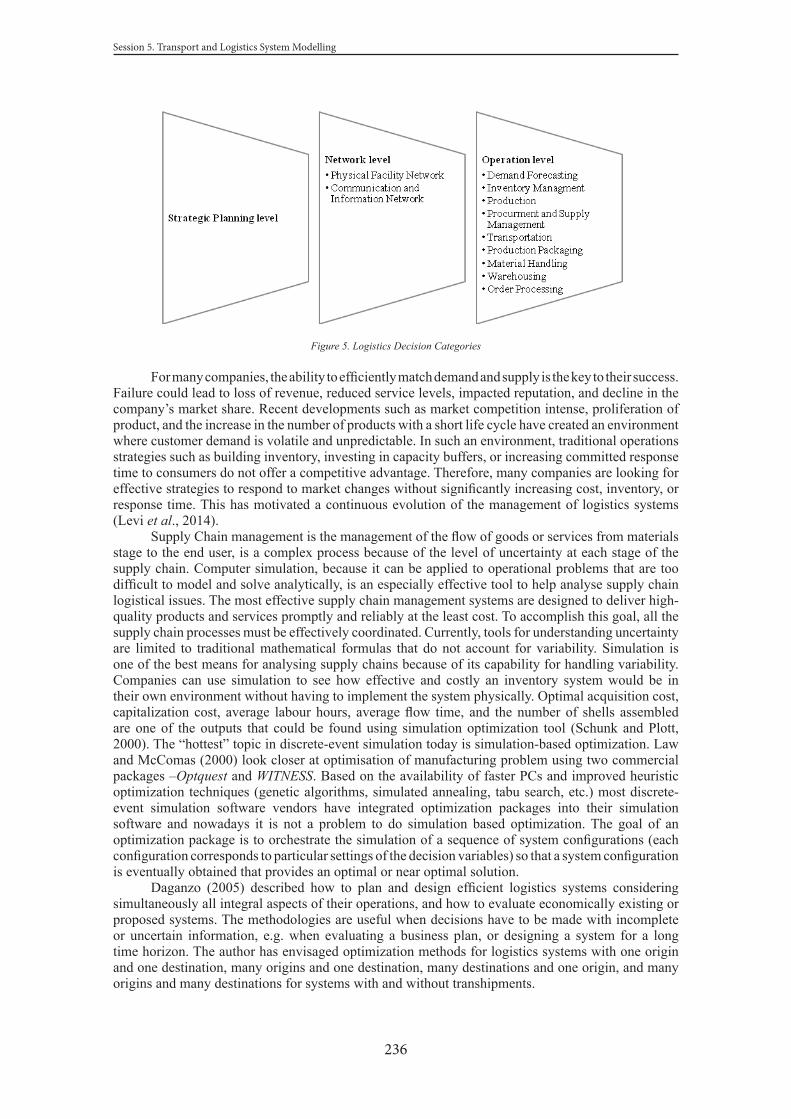
236


Figure 5. Logistics Decision Categories

For many companies, the ability to efficiently match demand and supply is the key to their success. Failure could lead to loss of revenue, reduced service levels, impacted reputation, and decline in the company’s market share. Recent developments such as market competition intense, proliferation of product, and the increase in the number of products with a short life cycle have created an environment where customer demand is volatile and unpredictable. In such an environment, traditional operations strategies such as building inventory, investing in capacity buffers, or increasing committed response time to consumers do not offer a competitive advantage. Therefore, many companies are looking for effective strategies to respond to market changes without significantly increasing cost, inventory, or response time. This has motivated a continuous evolution of the management of logistics systems (Levi et al., 2014).

Supply Chain management is the management of the flow of goods or services from materials stage to the end user, is a complex process because of the level of uncertainty at each stage of the supply chain. Computer simulation, because it can be applied to operational problems that are too difficult to model and solve analytically, is an especially effective tool to help analyse supply chain logistical issues. The most effective supply chain management systems are designed to deliver high-quality products and services promptly and reliably at the least cost. To accomplish this goal, all the supply chain processes must be effectively coordinated. Currently, tools for understanding uncertainty are limited to traditional mathematical formulas that do not account for variability. Simulation is one of the best means for analysing supply chains because of its capability for handling variability. Companies can use simulation to see how effective and costly an inventory system would be in their own environment without having to implement the system physically. Optimal acquisition cost, capitalization cost, average labour hours, average flow time, and the number of shells assembled are one of the outputs that could be found using simulation optimization tool (Schunk and Plott, 2000). The “hottest” topic in discrete-event simulation today is simulation-based optimization. Law and McComas (2000) look closer at optimisation of manufacturing problem using two commercial packages –Optquest and WITNESS. Based on the availability of faster PCs and improved heuristic optimization techniques (genetic algorithms, simulated annealing, tabu search, etc.) most discrete-event simulation software vendors have integrated optimization packages into their simulation software and nowadays it is not a problem to do simulation based optimization. The goal of an optimization package is to orchestrate the simulation of a sequence of system configurations (each configuration corresponds to particular settings of the decision variables) so that a system configuration is eventually obtained that provides an optimal or near optimal solution.

Daganzo (2005) described how to plan and design efficient logistics systems considering simultaneously all integral aspects of their operations, and how to evaluate economically existing or proposed systems. The methodologies are useful when decisions have to be made with incomplete or uncertain information, e.g. when evaluating a business plan, or designing a system for a long time horizon. The author has envisaged optimization methods for logistics systems with one origin and one destination, many origins and one destination, many destinations and one origin, and many origins and many destinations for systems with and without transhipments.

237


The logistics management issues that span a large spectrum of decisions are network configuration, production planning, inventory control and pricing optimization, procurement strategies and supply contracts, process flexibility, integration of production, inventory and transportation decisions, vehicle fleet management, truck routing and packing problems (Simchi-Levi et al., 2014). Due to the fact that as the models become more complex and integrate more and more issues that arise in practice, their analysis becomes more difficult. Some problems require the use of methods from game theory in order to understand how different supply chain partners respond to various challenges. Other problems have at their core difficult combinatorial problems in the class called NP-hard problems. This implies that it is very unlikely that one can construct an algorithm that will always find the optimal solution, or the best possible decision, in computational time that is polynomial in the size of the problem. Therefore, in many cases, an algorithm that consistently provides the optimal solution is not considered a reachable goal and hence heuristic or approximation methods are employed. For assessing and quantifying a heuristic’s effectiveness the following methods may be employed: empirical comparisons, worst case analysis, average case analysis.

Supply chain is a complex system, as well as a system of systems, because it embeds other systems representing product, process, and organizational structures of an enterprise. Three system facets applied to the supply chain are depicted in Figure 6 (Chandra and Grabis, 2007).

Figure 6.General SystemFacetsApplied to a SupplyChain

From the system management perspective, a supply chain is viewed as an organizational system, because a supply chain has managerial issues that can be classified into three levels – strategic, tactical, and operational.

Table 1.Decision-Making Levels in Supply ChainsDecision-Making Level Timeline Type of Decision Made

Strategic 3 to 10 yearsInvestment on plants and capacities.Introduction of new products.Creation of a logistics network.

Tactical 3 months to 2 yearsInventory policies to use.Procurement policies to be implemented.Transportation strategies to be adopted.

Operational Day to DayScheduling of resources.Routing of raw materials and finished products.Solicitation of bids and quotations.

Logistics management is that part of the business that plans, implements, and controls the efficient forward and reverses flow and storage of goods, services and related information between the point of origin and the point of consumption in order to meet customers’ requirements. Supply networks consist of delivery sites and receiving sites that are connected to one another through supply chains and depending on the process in question are called supply chains, acquisition chains, transport chains, cargo chains, shipping chains or disposal chains, or logistical chains in general (Gudehus, 2009).In logistics systems items are produced at one or more factories, shipped to warehouses and distribution centres for intermediate storage, and then shipped to retailers or customers.Consequently, to reduce cost and improve service levels, logistics strategies must take into account the interactions of these various levels in this logistics network, also referred to the supply chain. This network consists of suppliers, manufacturing centers, warehouses, distribution centers, and retailer outlets, as well as raw materials, work-in-process inventory, and finished products that flow between the facilities, see Figure 7(Levi et al., 2014).

238


Figure 7. The Logistics Network

Firstly, logistics management takes into consideration every facility that has an impact on cost and plays a role in making the product conform to customer requirement. Secondly, the objective of logistics management is to be efficient and cost-effective across the entire system; from transportation and distribution to inventories of raw material, work-in-process, and finished goods, is to be minimized. So the emphasis is not on simply minimizing transportation cost or reduction inventories but, rather, on taking a systems approach to logistics management.

5. Conclusions

The importance of mathematical methods for logistics systems analysis nowadays confirms separate sections of international conferences or even ongoing individual conferences of this theme. The International Symposium on Mathematics of Logistics took place at Tokyo University of Marine Science and Technology (2011), where scientists and practitioners had opportunities to attend lectures on theory and practices of mathematical methods of logistics. Also the Winter Simulation Conference attracts many researchers in this field every year.

There are institutions that providing services for logistics performance improvements, for example, in Australia there is the Centre for Industrial Modelling and Optimisation (CIMO), which specialises in industry-focused research and training, it offers consulting services in applying optimisation, operations research and statistics to industries such as transport. There are many challenging optimisation problems in the design and operation of transport and logistics networks. The activities of the research are applied to vehicle routing and scheduling for long and short haul operations; optimal fleet sizing, composition, maintenance and replacement; optimal warehouse operations; supply chain management; and a wide range of other logistics issues.

References

1. Baumgarten, H. and Walter, S. (2000) Trends und Strategien in der Logistik 2000+: EineUntersuchung der Logistik in Industrie, Handel, Logistik-Dienstleistung und anderen Dienstleistungsunternehmen. Berlin: Techn. Univ.

2. Bookbinder, J. H. (2012) Handbook of Global Logistics: Transportation in International Supply Chains.Springer.

3. Chandra, Ch. and Grabis, J. (2007) Supply Chain Configuration. Concepts, Solutions, and Applications. Springer.

4. Daganzo, C. F. (2005) Logistics Systems Analysis. 4th edition. Springer.

239


5. Domschke, W. (2007) Logistik: Transport. Grundlagen, Lineare Transport- und Umladeprobleme. 5. Auflage. Oldenbourg.

6. Domschke, W. and Drexl, A. (1995) Logistik: Standorte. 4. Auflage. Oldenbourg.7. Domschke, W. and Scholl, A. (2010) Logistik: Rundreisen undTouren. 5. Auflage.Oldenbourg.8. Flotzinger, C. W., Hofmann-Prokopczyk, H., Starkl. F.(2008)Future Scenarios 2030 – The

Impact on Logistics and the Contribution to a Sustainable Development.Austria: Competence Centre for Logistics and Enterprise networks.

9. Gudehus, T. and Kotzab, H. (2009) Comprehensive Logistics. Berlin: Springer.10. Möhring, R. H. and Schenk, M. (2010) Towards More Intelligence in Logistics with Mathematics.

In: Production Factor Mathematics.Germany: Springer. pp. 123 – 137.11. Moore, L. M. and Ray, B. K. (1999) Statistical Methods for Sensitivity and Performance

Analysis in Computer Experiments.In: Proceedings of the 1999 Winter Simulation Conference, IEEE, Inc., New York, NY, USA,pp. 486 – 491.

12. Neubauer, R. M. (2011)Business Models in the Area of Logistics. 1st edition. GablerVerlag.13. Langevin, A. and Riopel, D. (2005)Logistics Systems. Design and Optimisation. Springer.14. Law, A. M. and McComas, M. G. (2000) Simulation Based Optimization.In: Proceedings of the

2000 Winter Simulation Conference,IEEE, Inc., Orlando, FL, USA,pp. 46. – 49.15. Law, A. M. and Kelton, W. D. (1999) Simulation Modeling and Analysis. 3rd edition. Springer.16. Peruvemba, S. R. (2005) Understanding the Mathematics of Supply Chain Management.

Logistics Quarterly Magazine, Vol. 11, Issue 5, December 2005.17. Simchi-Levi, D., Chen, X., Bramel, J. (2014) TheLogic of Logistics. Theory, Algorithms, and

Applications for Logistics Management Series. 3rd edition. Springer.18. Schunk, D., Plott, B. (2000) Using Simulation to Analyze Supply Chains. In: Proceedings of the

2000 Winter Simulation Conference,IEEE, Inc., Orlando, FL, USA, pp. 1095 – 1100.19. Taha, H. A. (2007) Operations Research: An Introduction. 8th edition, Pearson Education.20. International Symposium on Mathematics of Logistics: Theory and Practices. (2011) Tokyo

University of Marine Science and Technology, Tokyo, Japan.http://www.youtube.com/watch?v=hc1U7P3CcSA

Aviation

Session 6

242

Session 6. Aviation


“FLYING TRUCKS” CONCEPT AS AN ALTERNATIVE FOR THE DEVELOPMENT OF THE REGIONAL AIRPORTS IN THE

BALTIC SEA REGION

Anatoli Beifert

Wismar University of Applied SciencesPhilipp-Müller Str 14, 23966 Wismar, Germany

[email protected]

Abstract

Especially in the times of economic slowdown, the pace of change in the transport sector is increasing. In the total market of logistic services air cargo transport has very low volume, but a high revenue yield part. The growth of the airfreight is mostly driven by business internationalization as well as decreasing air transport costs due to improving efficiency and strong competition among air carriers. Most regional airports in the Baltic Sea region that act totally isolated, do not have a clear picture of the current situation on the international air cargo market, its future perspectives and sustainable development plans. Trying to meet the market demand, the regional airports are making huge and unjustified investments, e.g. improving airport infrastructure. It is not clear till now which elements of the Pan-Baltic cargo market could be managed as an alternative revenue yielding services for consolidated operation by air or what infrastructure is needed to provide the opportunity for an optimal economic mix of road-rail-air-sea transport? Nowadays, to a large degree air cargo traffic relies on scheduled, frequent passenger services in hub-and-spoke as well as in point-to-point traffic. Regional airports are presently suffering from a lack of scheduled uplift capacity. The volume currently transported by air is almost entirely based on the occasional charter flights. However, the growth of the air cargo business is likely to be based not only on cargo charters, but to a larger extend on truck-based services for transit shipments. Onward transportation by truck may occur on road feeder service, so called “flying trucks”, where a real truck substitutes a flight. “Flying trucks” are having flight numbers etc., therefore they must be prioritized in many ways in the BSR transport policy.

The paper will investigate the possible role of Road Feeder Services, named here as “Flying Truck” concept as an opportunity for the development of the regional airports to be more actively involved in the global air cargo network.Keywords: Air cargo, Road Feeder Services (RFS), regional airports, multimodality, air-road concept

1. Introduction and problem definition

With regard to the specific air cargo market in the Baltic Sea Region (BSR) the current results presented in this paper to a large extend are based on the reports and official outputs produced in the framework of the EU funded research project1 “Baltic.AirCargo.Net” (http://www.balticaircargo.net/).

In order to define the region in the following study, the dimensions of the BSR has been set by the coordinates of the airports Cologne (CGN) for the western and Hahn (HHN) for the Southern boundary in Germany; Mehamn airport (MEH) in Norway sets the Northern and airport Ivanovo (IWA) I Russia defines the Eastern boundary of the BSR (Table 1). 1 Baltic Sea Region Programme 2007 - 2013, ERDF Funds

243


City Airport Name IATA Code

ICAO Code Longitude Latitude Country

Mehamn Mehamn MEH ENMR 71.03333 27.833332 NorwayHahn Frankfurt - Hahn HHN EDFH 49.948334 7.264167 Germany

Cologne Cologne Bonn CGN EDDK 50.878365 7.122224 GermanyIvanovo Ivanovo IWA 56.942955 40.944546 Russia

Table 1: Defining BSR airports (FlightStats 2013)2

According to these set frames, there are 290 civil airports in the BSR (i.e. having a 3-letter IATA code) of which 176 airports (61%) have regular scheduled traffic (Table 2).3

Countries Number of Airports in the Region1 Number of Airports with scheduled Traffic2

Belarus 7 1Denmark 18 9Estonia 6 4Finland 31 22Germany 66 23Latvia 3 1Lithuania 6 4Norway 46 41Poland 18 12Russia 33 18Sweden 56 41Sum 290 176

Table 2: BSR Airports (OAG, Flightstats)

(1) Airports with IATA Code located within the region defined above (cf. Table 1)(2) Recorded Traffic in 2013

The Baltic states, i.e. Estonia, Latvia, Lithuania and Belarus have 22 airports in total of which ten (four, one, four and one respectively) have regular scheduled traffic. Despite strong competition from Germany, Sweden and Norway the main hub of Denmark - Copenhagen airport (CPH) has a large share of cargo traffic and ranks seventh in terms of number of cargo flights, behind German airports Frankfurt international (FRA; 1.), Frankfurt-Hahn (HHN; 3.), Halle/Leipzig (LEJ; 4.) and Köln/Bonn (CGN; 6.) and the Russian airports SVO (2.) and DME (5.).

It may be also sated that the airports in the BSR are located close to each other with the overlapping catchment areas and close distances to the bigger hubs. Thus the regional airports need to seek a comparative advantage over other airports and countries.

Figure 1 demonstrates the distribution of the air cargo flights in the BSR of the observations in the 2013. About half of all cargo flights (47%) go through Frankfurt am Main International airport (FRA), ca. 22% of the flights pass Moscow-Sheremetyevo (SVO) airport. The main air cargo market players in the BSR are Germany with a total market share of 59% (Frankfurt [FRA], Frankfurt-Hahn [HHN], Halle/Leipzig [LEJ] and Köln/Bonn [CGN]), Russia with 26,4% share (Moscow-Sheremetyevo [SVO], Moscow-Domodedovo [DME], Saint Petersburg-Pulkovo [LED] and Vnukovo [VKO] airports), Denmark with a 3,4% share (Copenhagen [CPH] airport), Finland with 3,3% market share (Helsinki [HEL] airport), Norway with 1,6% market share (Oslo [OSL] airport) and Sweden with 1,5% share (Stockholm-Arlanda [ARN] and Gothenburg-Landvetter [GOT] airport).

2 Cf. Bubalo, Branko, Economic Outlook for an Air Cargo market in the Baltic Sea region, Baltic.AirCargo.Net Project, 20133 Regular scheduled traffic here - minimum one flight observation per week in 2013, FlightStats.

244

Session 6. Aviation

47.0%

21.9%

8.1%

4.1% 3.9% 3.7% 3.4% 3.3%1.6% 1.2% 0.6% 0.4% 0.3% 0.3% 0.3%

0%

5%

10%

15%

20%

25%

30%

35%

40%

45%

50%

Fran

kfur

t Int

erna

tiona

l

Sher

emet

yevo

Fran

kfur

t - H

ahn

Leip

zig/H

alle

Dom

oded

ovo

Koel

n/Bo

nn

Cope

nhag

en

Helsi

nki-V

anta

a

Oslo

Arla

nda

Siau

liai

Min

sk In

tern

atio

nal 2

Pulk

ovo

Vnuk

ovo

Land

vett

er

FRA SVO HHN LEJ DME CGN CPH HEL OSL ARN SQQ MSQ LED VKO GOT

Figure 1: Distribution of Cargo-flights in the BSR4

According to breakdown to the average daily movement numbers there might be observed 127 average daily cargo flights at the defined sample of the BSR airports. This could be in indicator for a small and limited market, but with a very strong growth potential. If an average growth rate of 5% per annum can be maintained in the long-term in the BSR, then we may expect a doubling of the daily movements after 15 years and an increase by 164 daily movements (129%) to a level of 291 daily movements by 2030.5 However, it might be stated that only big airports are taking advantages of the current air cargo business opportunities.

According to the “Baltic.AirCargo.Net” project data, the most regional airports in the Baltic Sea Region unfortunately act isolated and do not have a clear understanding of the current situation on the international air cargo market, they lack future perspectives and in some cases sustainable development plans. Trying to meet the market demand, the regional airports sometimes make huge and very often unjustified and unnecessary investments, e.g. improving airport infrastructure. However, the air cargo transport takes place not isolated but within a global net of value-added supply chains. Furthermore, it is not clear till now which elements of the Pan-Baltic cargo market could be managed as an alternative revenue yielding services for consolidated operation by air or what infrastructure is needed to provide the opportunity for an optimal economic mix of road-rail-air-sea transport?

Furthermore, to a large degree, air cargo traffic relies heavily on scheduled, frequent passenger services in hub-and-spoke system as well as in point-to-point traffic. Regional airports are presently suffering from a lack of scheduled uplift capacity. The volume currently transported by air in the Baltic Sea Region is almost entirely based on the occasional charter flights. However, the growth of the air cargo business is likely to be based not only on cargo charters, but to a larger extend on truck-based services for transit shipments.

Onward transportation by truck may occur on road feeder service, so called “flying trucks”, where a real truck substitutes a flight. “Flying trucks” are having flight numbers etc., therefore they must be prioritized in many ways in the BSR transport policy.

4 Source: Economic Outlook for an Air Cargo market in the Baltic Sea Region, Baltic.AirCargo.Net Project, 20135 cf. Economic Outlook for an Air Cargo market in the Baltic Sea Region, Baltic.AirCargo.Net Project, 2013

245


2. Interconnection between accessibility of the Baltic Sea region and the air cargo

The accessibility of the Baltic Sea Region depends heavily on so called hub and spoke transport system. Most of the remote areas of the BSR could not reach the same accessibility (e.g. number of transport routes, destinations or frequencies; transport cost level, etc.) without hub and spoke model:

• Maritime: Container hubs like Hamburg offer oversea (intercontinental) connections and feeder traffic (e.g. Short Sea Shipping) is the spoke between the hub and the hinterland;

Aviation: Aviation hubs like Copenhagen) offer intercontinental flight connections and feeder traffic (e.g. flying truck, Road Feeder Service) is the spoke between the hub and the hinterland.

Therefore, it can be stated that the Road Feeder Services along with the strong impact on the air cargo market also does heavily support the intercontinental passenger flights and the major aviation hubs of the Baltic Sea Region. Consequently it is very important to consider the fact that major aviation hubs of the BSR influence the accessibility of the BSR significantly and the economic viability of several intercontinental passenger flights strongly depends on the air cargo business, its efficiency and profitability.

The Finnair data might be a good example here: the Majority of Finnair’s revenues generated by Europe – Asia traffic; whereas to be noted that the revenues coming from air cargo business represent ca. 20% of Asian revenues. As intercontinental passenger and cargo flights are strongly linked together, the so called “widebody” aircrafts performing the intercontinental flights carry significant part of the air cargo.

Figure 2: Distribution of revenues in scheduled traffic in Helsinki Airport (source: Finnair 2013)

According to Finnair data, the air cargo transported on scheduled flights (belly cargo) constitutes a significant proportion of the revenue from long-haul traffic; in 2013, belly cargo accounted for approximately 17% of total long-haul revenue. The overall load factor in Finnair’s cargo traffic improved to 66%, while the available tonne kilometres rose by 1,3%. The new operating model strengthens air cargo demand in Finnair’s Asian passenger flight network, as it also allows Finnair Cargo to offer faster cargo connections between Central Europe and Asia.6

Thus, it can be stated that the air cargo generates a significant part of revenues for the airlines that operate intercontinental flights. Therefore the economic viability of several intercontinental passenger flights is strongly dependent and directly relates to the air cargo business. The price level for the passengers directly depend on the utilization grade of the air cargo capacities of the “widebody” carriers. The results from the Baltic.AirCrago.Net project also confirm the statement that the major aviation hubs in the Baltic Sea Region generate significant part of their income from the air cargo business.6 cf. Finnair Annual Report 2013, http://www.finnairgroup.com/linked/en/konserni/23162-Finnair_2013_EN_withlinks_v2.pdf

246

Session 6. Aviation

3. “Flying Trucks” concept for regional airports

A “flying truck” (RFS, Road Feeder Service) can be defined as a truck operating between two airports on so called Air Waybill (AWB) or air consignment note, which refers to a receipt that is issued by an international airline. It is very important to note that one truck might have several route numbers or flight numbers if it is carrying goods from more than one airline.

Figure 3: Scheduled truck-flight cargo service routes as of May 2007 (source: Boeing 2008)

The flying trucks are treated and handled exactly in the same way like real aircrafts, i.e. the “flying trucks” possess herewith exactly the same insurance as if the goods were transported by aircraft and on route number, they are fulfilling all custom and security regulations set by the relevant authorities as if the goods were really flying by air.7

The network of the operational Road Feeder Services in Europe has been considerably extended within last years and the road feeder concept has become to an essential part not only of the airfreight, but the whole logistics structural network. Although the concept is well known to air cargo professionals, it might be a bit unknown to representatives of other transport modes, regional actors and EU policy makers. Moreover the role of Road Feeder Services or “flying truck” concept and relationship to other transport modes as well as to other air cargo concepts is still underestimated and lacks behind its possibilities.

One flying truck can have several route numbers if it is carrying goods from more than one airline. The route numbers are set by local airline cargo manager, so there is no database to see the flying truck routes; and they are changing all the times. The Road Feeder Services also can happen while using the truck along with entire transport chain. The distances might vary from 100 up to 1000 kilometers and even more. Thus, while talking about air cargo transport serves within Europe normally professional mean delivery via RFS.8

7 Grandjot, Roessler, Roland, Air Cargo Guideline, 2007, 86-888 Grandjot, Roessler, Roland, Air Cargo Guideline, 2007, 86-88

247


Figure 4: Scheduled truck-flight cargo service routes as of May 2010 (source: Boeing 2011)

The figures 3 and 4 demonstrate the rapid development of the RFS network in the air cargo business. However, according to the results of the Baltic.AirCargo.Net project the current EU transport strategies clearly underestimate its big role. Thus, it is of a vital importance to make flying trucks concept and its role in the international logistics network more known and understandable to broader community, for it shall be more efficiently adapted to the EU and BSR transport policies and regional development.

Especially for small and regional airports that do not have international regular air flights and pure freight carriers, the recognition and implementation of the flying trucks concept might be of a special importance. Nowadays very few regional airports in the Baltic Sea Region utilize the Road Feeder Service. In many cases the flying trucks are operated only in the capital cities like Helsinki, Copenhagen, Stockholm (Arlanda) or major hub-airports like Hamburg. The project Baltic.Aircargo.Net is studying possibilities to utilize the concept also by the small and regional airports and thus support the economic viability of the regional airports in the BSR.

The Baltic.AirCargo.Net project has been focusing on remote airports and not on capital / major airports. The project has been trying to promote air cargo operations of remote airports through alternative concepts like “flying trucks”, since might be almost impossible to utilize belly cargo concepts in the remote / regional airports. Also pure freighter concept is rather difficult even, if there is few success stories, for example Billund in Denmark and current plans of Parchim Airport to implement regular pure freighter line with China. Thus, the flying truck concept might be a very interesting and also realistic concept for remote airports when they are trying to access to the air cargo market. Preliminary interview results that have been carried out in the participating regions of the Baltic.AirCargo.Net project showed the regional airports have normally a sub-hub system to forwarders and integrators. Some airports are used as an interim-terminal where goods are collected for further transport to bigger hubs by road feeder services. The local SMEs are completely not involved in the air cargo mostly due to lack of knowledge and insight view of air cargo opportunities.

In the framework of the Baltic.AirCargo.Net Project three regional airports have been chosen as pilot sites for testing and demonstration, aiming also at promoting and implementation of the flying truck concept in their regions., i.e.:

248

Session 6. Aviation

• Tampere Airport in Finland;• Linköping Airport in Sweden;• Parchim Airport in Germany.It has been recommended that the pilot sites interested in flying trucks concept implementation

shall define their own detailed demonstration actions related to flying truck concept in the following frame:

• The sites shall familiarize themselves with the air cargo concepts, air cargo markets and roles of air cargo stakeholders. The planning of the demonstrations should be based on these facts of the air cargo.

• The roles of current air cargo concepts, cooperation and connections to other transport modes shall be identified. Each of these concepts has their advantages/disadvantages and thus the concepts are strong in different markets. What is the role of flying trucks, why, when and how it should be used?

• Identification of regional air cargo stakeholders – for example airport, airline (freighters, long-haul wide bodies, others) forwarders, ground handling, integrators, consignor, consignee – and their role in the logistics chain.

Although the concept of flying trucks is not so widely implemented and utilized by regional and small airports, e.g. in Finland only Helsinki is utilizing flying trucks concept and no one of regional airports is taking advantages of this. On the other hand, in Sweden quite many remote and regional airports have been already successfully implementing the flying truck concept:

• NYO, Skavsta• NRK, Norrköping Kungsangen• JKG, Jonköping• AGH, Ängelholm-Helsingborg Airport• MMX, Malmö Sturup

4. Summary and outlooks

Air cargo of the Baltic Sea Region is heavily concentrated on the airports, which have intercontinental passenger flights: significant part of the Baltic Sea Region air cargo is utilizing belly cargo concept and intercontinental passenger flights operated by wide body aircrafts. These airports are typically capital airports like Copenhagen (CPH), Stockholm (ARN) and Helsinki (HEL). Also the major part of the Baltic Sea Region freighter flights is operating to the same capital airports, which have the belly cargo flows.

The current results of Baltic.AirCargo.Net Project are pointing out that the Baltic Sea region transport policy should recognize and accept the importance of the Road Feeder Service or “Flying Truck” concept much stronger than it does today.

Aviation, i.e. both airports and airlines, are facing strong competition and the Baltic Sea Region should utilize possibilities that are being offered by Road Feeder Service in order to strengthen the economic viability of the aviation industry.

It can be generally noticed that within the Europe or the BSR the passengers are flying but the goods are being transported by flying trucks. It might be a disputable or provocative notice that the general and basic approach of the Short Sea Shipping corresponds with the concept of the Flying Trucks. The concept of the “Short Sea Shipping” has been introduced, discussed and promoted by relevant regional, national and international stakeholders. Should it be now recommendable to mention, promote, develop and implement efficient structures of the concept of Road Feeder Service?

Generally belly cargo concept might be impossible to implement by regional and remote airports since it is based on the intercontinental passenger flights. Furthermore, the freighter concept would be basically possible; however its implementation requires strong and consistent air cargo volume (e.g. 200 tons/week in and out) between the remote airport and some other region.

Thus, the Flying trucks concept might be at this time the only one realistic concept for remote and / or regional airports when they are trying to access to the air cargo market. In case of the acceptance of this hypothesis, the next questions for the regional airports that shall be analyzed might be:

249


1. Role of the airport in the region;2. What are the possible air cargo volumes, destinations in the catchment area of a given

airport?3. What are the possible “flying truck routes” for a given airport?4. What are the goods-flows (annual volumes, frequencies) that might be potentially

transported as air cargo within BSR? (described per segment: carried by freighters, carried by courier/express planes,” carried by flying trucks”)

5. What are the typical goods carried per route and direction, what is the balance of the flows?

Having fulfilled this analysis the regional airports might have a rough evaluation whether they can be an interesting feeder for some other major air cargo hub of the BSR region like Copenhagen, Helsinki or Stockholm (Arlanda) Airports. Furthermore, in the reference to the passenger traffic (network carriers, low cost, charter) and air cargo (RFS / flying trucks, freighters, mail / express) the following analysis shall be fulfilled:

1. transport forecast, objectives concerning volumes;2. current capacities that are available in airport and its facilities;3. future needs and possibilities of airport and its facilities, expansion plans.Only after fulfilling above-mentioned evaluation it might be possible for regional airports to

conduct a development strategy and a sustainable action plan involving among other things air cargo business opportunities.

References

1. Hans-Helmut Grandjot, Ingo Roessler, Ailine Roland, Air Cargo Guideline, Munich 2007, pp. 86-88, p. 271.

2. Bubalo, Branko, Economic Outlook for an Air Cargo Market in the Baltic Sea Region, Baltic.AirCargo.Net Project 2013.

3. Baltic Transport Outlook 2030. 2011. “Baltic Transport Outlook 2030 Executive Report - Annex II.” http://www.baltictransportoutlook.eu/files/Executive_report_Annex2_TEN-T_Reviewmaps.pdf.

4. Doganis, R. S., and G. F. Thompson. 1975. “Airport Profitablity And Managerial Effectiveness.” The Manchester School 43 (4): 331–352. doi:10.1111/j.1467-9957.1975.tb01236.x.

5. Kim Irmov, and Hans Christian Stigaard, “To Identify the Current Air Cargo Set up and Flows in the Baltic Region, and to Identify the Possibilities to Improve These.”, Baltic.AirCargo.Net project 2013.

6. Manheim, L. M., Fundamentals of transport Systems Analysis, Volume 1: Basic concepts, 1979, p. 116.

Web sources:

7. Baltic.AirCargo.Net project: www.balticaircargo.net8. Baltic Sea Region Programme 2007 - 2013, http://eu.baltic.net9. http://ec.europa.eu/economy_finance/economic_governance/sgp/index_en.htm10.http://epp.eurostat.ec.europa.eu/statistics_explained/index.php/Freight_transport_

statistics#Air_freight11. Finnair Annual Report 2013, http://www.finnairgroup.com/linked/en/konserni/23162-

Finnair_2013_EN_withlinks_v2.pdf12. http://epp.eurostat.ec.europa.eu/cache/ITY_OFFPUB/KS-RA-10-028/EN/KS-RA-10-028-EN.

PDF 13. KS-RA-10-028-EN14. http://ec.europa.eu/economy_finance/eu/forecasts/2013_winter_forecast_en.htm15. EC 261/2004 regulation establishing common rules on compensation and assistance to

passengers in the event of denied boarding and of cancellation or long delay of flights

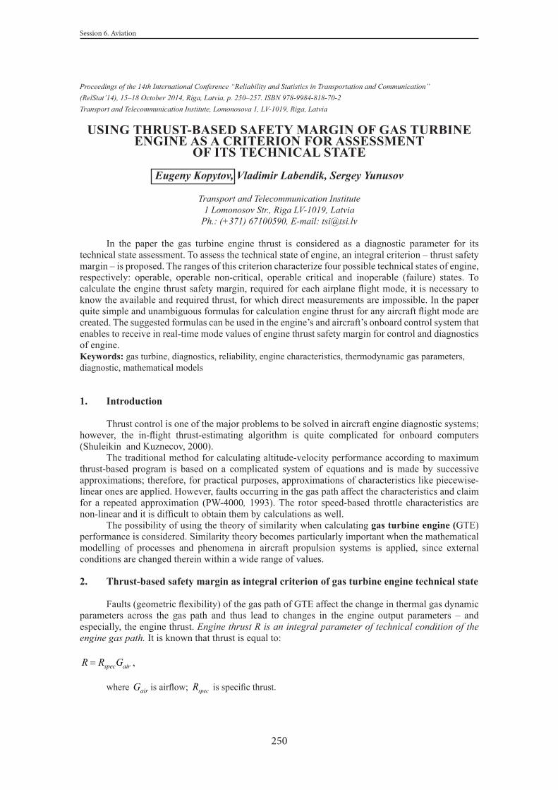
250

Session 6. Aviation


USING THRUST-BASED SAFETY MARGIN OF GAS TURBINE ENGINE AS A CRITERION FOR ASSESSMENT

OF ITS TECHNICAL STATE

Eugeny Kopytov, Vladimir Labendik, Sergey Yunusov

Transport and Telecommunication Institute1 Lomonosov Str., Riga LV-1019, Latvia

Ph.: (+371) 67100590, E-mail: [email protected]

In the paper the gas turbine engine thrust is considered as a diagnostic parameter for its technical state assessment. To assess the technical state of engine, an integral criterion – thrust safety margin – is proposed. The ranges of this criterion characterize four possible technical states of engine, respectively: operable, operable non-critical, operable critical and inoperable (failure) states. To calculate the engine thrust safety margin, required for each airplane flight mode, it is necessary to know the available and required thrust, for which direct measurements are impossible. In the paper quite simple and unambiguous formulas for calculation engine thrust for any aircraft flight mode are created. The suggested formulas can be used in the engine’s and aircraft’s onboard control system that enables to receive in real-time mode values of engine thrust safety margin for control and diagnostics of engine.Keywords: gas turbine, diagnostics, reliability, engine characteristics, thermodynamic gas parameters, diagnostic, mathematical models

1. Introduction

Thrust control is one of the major problems to be solved in aircraft engine diagnostic systems; however, the in-flight thrust-estimating algorithm is quite complicated for onboard computers (Shuleikin and Kuznecov, 2000).

The traditional method for calculating altitude-velocity performance according to maximum thrust-based program is based on a complicated system of equations and is made by successive approximations; therefore, for practical purposes, approximations of characteristics like piecewise-linear ones are applied. However, faults occurring in the gas path affect the characteristics and claim for a repeated approximation (PW-4000, 1993). The rotor speed-based throttle characteristics are non-linear and it is difficult to obtain them by calculations as well.

The possibility of using the theory of similarity when calculating gas turbine engine (GTE) performance is considered. Similarity theory becomes particularly important when the mathematical modelling of processes and phenomena in aircraft propulsion systems is applied, since external conditions are changed therein within a wide range of values.

2. Thrust-based safety margin as integral criterion of gas turbine engine technical state

Faults (geometric flexibility) of the gas path of GTE affect the change in thermal gas dynamic parameters across the gas path and thus lead to changes in the engine output parameters – and especially, the engine thrust. Engine thrust R is an integral parameter of technical condition of the engine gas path. It is known that thrust is equal to:

spec airR R G= ,

where airG is airflow; specR is specific thrust.

251


Specific thrust depends on the cycle operation (parameters *GT andπΣ ), flight velocity fV and

altitude (external conditions), and on the bypass ratio m, power distribution between the ducts x and losses in the units characterized by loss of efficiency at compression ñompη , expansion expη and hydraulic losses IIη. Table 1 containing the typical faults of gas path of GTE is shown below. This table shows the dependence between GTE fault and the instrumental state parameters within the mathematical model (MM) of engine.

Table 1. Typical faults of gas path of an engine

Type of fault Fault-dependent state variable

Variable reflecting a fault in MM GTE

Input device surface erosion r inεinσ

Blade contamination r bε *cη

Erosion (corrosion) of blades , / , ,r b ci cib tε β α *,c cilη

Increased radial clearances in the impeller. δ *,c cilη

Deterioration of guide vanes /b t *,c cilη

Spontaneous change of air bleed in Air Conditioning System after the k-th stage of compressor

b

g ,air ciG l

Burnout and cracks in can-type combustion chamber of KS – , ,gas t fG Pη

Corrosion (erosion) of turbine bladesr t

ε * * *, , ,t gas g tG T Pη

Coked turbine blades ,r t CAFε * * *, , ,t gas g tG T Pη

Change in turbine-blade tip clearances pk iδ * * *, , , ,t gas g t tG T P lη

As a criterion for technical state of engine, the thrust-based safety margin of a jet RK∆ is proposed:

.at dtR

dt

R RKR−

∆ =

For example, Airbus and Boeing have adopted flexible take-off practice, i.e. available thrust of engine atR is reduced to the level of demanded thrust power dtR . There exist two thrust reduction methods: a stepwise transfer to a lower stage (derate) and outdoor temperature simulation (assumed temperature). According to the standards, thrust cannot be reduced by more than 25%. For example, there are 4 thrust levels for CFM-56-3 engine: 18.5, 20, 22 and 23 pounds accordingly. Then, the maximum value of thrust-based safety margin at take-off will constitute:

23 18.5 0.2418.5RK −

∆ = = .

It is suggested to describe possible technical states of engine by ranges of change in its thrust-based

safety margin as follows: _1RK∆ is normal state; _ 2RK∆

is operable non-critical state; _ 3RK∆ is critical

operable state, and _ 4RK∆ is inoperable state (see Fig.1).

252

Session 6. Aviation

Figure 1. Ranges of engine thrust-based safety margins for take-off mode

The assessment of critical operable state is the most important in terms of the flight safety provision, since a pilot should know whether he will be able to complete the flight successfully in the event of engine fault occurrence.

However, it is impossible to perform direct measurement of in-flight thrust onboard the aircraft. Therefore, to define the thrust produced by engine installed on aircraft, a certain performance parameter proportional to thrust should be measured.

3. Obtaining of the in-flight turbofan engine thrust equation

Turbofan engine thrust value at any flight altitude and velocity can be determined based on a generalized dependence:

0 S drSR R R R= ⋅ ⋅ . (1)

At a present flight mode, the efficient thrust of engine should be equal to the demanded thrust power,

based on aircraft drag , based on which, throttle ratio of an ideal (unspecified)

engine in relation to full thrust power at engine modules similarity can be specified:

(2)

The actual safety margin can also be specified based on throttle ratio in relation to maximum

thrust value maxÍRor its relative change according to altitude-velocity performance maxHR

at the program 0

*GÒ const= :

max max max max

H

ef arîÍ Ídr

Í î Í H H

RR R R R XRR R R R R

−= = ⋅ = =

. (2а)

However, according to traditional methods, the maximum thrust is defined through the method of successive approximations based on altitude-velocity performance (AVP) mathematical model consisting of a cumbersome system of equations, so it cannot be used in on-board computer.

At 0

* 1.65Vπ ≥, critical discharge mode is established in a convergent-divergent nozzle of a subsonic

engine already on take-off (MH > 0,45):

( )3.5* 2( ) 1.65 1 0.2 0.45 1.89S cr V dπ π π= ⋅ = + ⋅ =

.

Then, engine thrust must be calculated according to the formula used at incomplete expansion:( ) .G S Gs S H SR G C G V p p F= − + − (3)

In turbofan engines with a split discharge from ducts (Fig. 2), the mode of optimal energy distribution over the ducts corresponds to the duct-discharged flows velocity ratio in the form of the dependence as follows (Klyachkin, 1969):

The 14th International Conference “RELIABILITY and STATISTICS in TRANSPORTATION and COMMUNICATION – 2014”





0 S drSR R R R . (1)

At a present flight mode, the efficient thrust of engine should be equal to the demanded thrust

power, based on aircraft drag arоdref XRRRR / , based on which, throttle ratio of an ideal (unspecified) engine in relation to full thrust power at engine modules similarity can be specified:

ef arоID IDdrS

S о S S S


(2)

The actual safety margin can also be specified based on throttle ratio in relation to maximum thrust value

maxНR or its relative change according to altitude-velocity performance maxHR at the program

0

*GТ const :

max max max max

H

ef arоН Нdr

Н о Н H H


. (2а)


At 0

* 1.65V , critical discharge mode is established in a convergent-divergent nozzle of a subsonic engine already on take-off (MH > 0,45):

3.5* 2( ) 1.65 1 0.2 0.45 1.89S cr V d .

Then, engine thrust must be calculated according to the formula used at incomplete expansion:

.G S Gs S H SR G C G V p p F (3)


(II) ( ) ( )N N I IIC C ,

where (II) ( ),N N IC C are velocities of exhaust nozzle discharge from the nozzles of the first and the second

duct, accordingly; ( )II is the efficiency of energy transfer to the second duct. The similarity mode of the propulsion module can be achieved if the exhaust velocity of gases

effluent from the core nozzle has reached the sound velocity level ( )S IC a , while at the same time, according to the above-stated formula, the exhaust velocity of gases effluent from the secondary nozzle will be less than sound velocity ( )S IIC a .






0 S drSR R R R . (1)

At a present flight mode, the efficient thrust of engine should be equal to the demanded thrust

power, based on aircraft drag arоdref XRRRR / , based on which, throttle ratio of an ideal (unspecified) engine in relation to full thrust power at engine modules similarity can be specified:

ef arоID IDdrS

S о S S S


(2)

The actual safety margin can also be specified based on throttle ratio in relation to maximum thrust value

maxНR or its relative change according to altitude-velocity performance maxHR at the program

0

*GТ const :

max max max max

H

ef arоН Нdr

Н о Н H H


. (2а)


At 0

* 1.65V , critical discharge mode is established in a convergent-divergent nozzle of a subsonic engine already on take-off (MH > 0,45):

3.5* 2( ) 1.65 1 0.2 0.45 1.89S cr V d .

Then, engine thrust must be calculated according to the formula used at incomplete expansion:

.G S Gs S H SR G C G V p p F (3)


(II) ( ) ( )N N I IIC C ,

where (II) ( ),N N IC C are velocities of exhaust nozzle discharge from the nozzles of the first and the second

duct, accordingly; ( )II is the efficiency of energy transfer to the second duct. The similarity mode of the propulsion module can be achieved if the exhaust velocity of gases

effluent from the core nozzle has reached the sound velocity level ( )S IC a , while at the same time, according to the above-stated formula, the exhaust velocity of gases effluent from the secondary nozzle will be less than sound velocity ( )S IIC a .

253


(II) ( ) ( )N N I IIC C η= ,

where (II) ( ),N N IC C are velocities of exhaust nozzle discharge from the nozzles of the first and the

second duct, accordingly; ( )IIηis the efficiency of energy transfer to the second duct.

The similarity mode of the propulsion module can be achieved if the exhaust velocity of gases effluent from the core nozzle has reached the sound velocity level ( )S IC a=

, while at the same time, according to the above-stated formula, the exhaust velocity of gases effluent from the secondary nozzle will be less than sound velocity ( )S IIC a<

.

Figure. 2. Diagram of a turbofan with separate nozzles

In that case, full extension of gas ( )N II Hp p=will take place at the bypass duct outlet, where:

( )N IIp is nozzle static pressure; Hp is air pressure at the corresponding flight altitude (H).

On achieving sound velocity of gases effluent from the bypass duct nozzle ( )N IIC a=, the exit

velocity of convergent-divergent nozzle of the first duct will remain sound velocity ( )N IC a=, but static

pressure will be higher than air pressure due to under-expansion ( )N I Hp p≥; then, these velocities can be

defined from the expressions derived for critical exhaust velocities:

*( ) ( ) ( )2

1N cr NkC C RT

kΙΙ ΙΙ ΙΙ= =+ ; (4)

*( ) ( ) ( )2

1g

N cr g Ng

kC C R T

kΙ Ι Ι= =+

, (5)

where * *

( ) ( ), N NT TΙ ΙΙ are outlet temperatures of stagnated air flows – respectively, at the outlets of the first and the second ducts of turbofan engine;

, gk k are adiabatic indices of air and gas, respectively;

R R are constants of air and gas, respectively.

At the values 1.4, 1.33gk k= =

and 287, 288gR R= =

, expressions (4) and (5) assume the form as follows:

*( ) ( ) ( )334.8N cr NC C TΙΙ ΙΙ ΙΙ= = ⋅ ; (4а)

*( ) ( ) ( )328.8N cr NC C TΙ Ι Ι= = ⋅ . (5а)

The velocity ratio at 328.8 334.8 0,99 1= ≈ can be presented as

0

*( ) ( ) *

*( ) ( )

N NN N

N N

C TC

C TτΙ Ι

ΙΙ ΙΙ

= = =

. (6)The maximum on-ground thrust of a turbofan engine (H=0) under the critical mode of nozzle

operation is determined according to the expression:

254

Session 6. Aviation

0 00( ) ( ) ( )cr N NR G C G CΙΙ ΙΙ Ι Ι= + , (7)

where 0 0, G GΙ ΙΙ are gas and air flow effluent, accordingly, through the first and the second ducts of

engine on the deck.

Taking into account the expression (7) and the fact that 0 0 0G G mΙΙ Ι=, where 0m is the on-ground

value of bypass ratio, the thrust equation will assume the form as follows:

00( ) ( )0

1 Ncr N

CR G CmΙΙ ΙΙ

= +

. (7а)

Here, 0

0( ) ( )

( )N cr N

N

pG C FRT ΙΙΙΙ ΙΙ

ΙΙ

= is the airflow through the bypass duct;

0p is on-ground air pressure;

( )N IIF is nozzle-throat area of the bypass duct.Taking that into account, the expression for maximum thrust (7a) will assume the form as follows:

0

*20

0( ) ( ) ( )( ) 0

1 Ncr N cr N

A N

pR C FR T m

τΙΙ ΙΙ

ΙΙ

= + ⋅ . (7в)

Further, taking into account that, at the critical flow,2

( ) ( )N cr A A NC k R TΙΙ ΙΙ= ⋅ ⋅

, we will present the maximum thrust value as according to expression (7в) in the form as follows:

0

*

0( ) 0 ( )0

1,4 1 Ncr NR p F

m

τΙΙ

= + . (7с)

The maximum in-flight thrust under the critical (similar) operation mode of engine can be

defined from the equation:

where FN(I) and FN(II) are nozzle-throat areas of the first and the second (bypass) ducts;ΙΙΙ )()( , crNcrN pp

are static pressures in nozzle-throat areas of the first and the second (bypass) ducts.Unifying the first and the second terms of equation (8) by taking ( )N crG C

ΙΙΙΙ from them, and unifying the second and the fourth terms by taking pH ∙ ( )N IIF

and designating the nozzle areas ratio )()( ΙΙΙ= NNN FFF

, we simplify equation (8) to the form as follows:

Taking into account that static nozzle-exit pressures

( )

11.85

12

g

g

H N H d RN cr k

kg

p ppk

π π πΙ

−

= =+

;

( )1

1.8912

H NII H d VN cr k

k

p ppk

π π πΙΙ

−

= =+

,


00( ) ( )0

1 Ncr N

CR G Cm

. (7а)

Here, 0

0( ) ( )

( )N cr N

N

pG C FRT

is the airflow through the bypass duct;


( )N IIF is nozzle-throat area of the bypass duct. Taking that into account, the expression for maximum thrust (7a) will assume the form as follows:

0

*20

0( ) ( ) ( )( ) 0

1 Ncr N cr N

A N

pR C FR T m

. (7в)

Further, taking into account that, at the critical flow, 2( ) ( )N cr A A NC k R T


0

*

0( ) 0 ( )0

1,4 1 Ncr NR p F

m

. (7с)

The maximum in-flight thrust under the critical (similar) operation mode of engine can be defined from the equation:

( ) (c ) ( ) ( ) ( ) ( ) ( ) ,S ск N r N cr H N N cr N cr H NR G C V p p F G C V p p F (8)

where FN(I) and FN(II) are nozzle-throat areas of the first and the second (bypass) ducts;

)()( , crNcrN pp are static pressures in nozzle-throat areas of the first and the second (bypass) ducts.

Unifying the first and the second terms of equation (8) by taking ( )N crG C from them, and

unifying the second and the fourth terms by taking pH ∙ ( )N IIF and designating the nozzle areas ratio

)()( NNN FFF , we simplify equation (8) to the form as follows:

( ) ( )( ) ( ) ( )

( )

11 1 1 1 .N cr N crNS сr N сr H N N

N cr H H

p pC VR G C p F Fm C m p p

(8а)


( )

11.85

12

g

g

H N H d RN cr k

kg

p ppk

; ( )1

1.8912

H NII H d VN cr k

k

p ppk

,

and at critical nozzle flow

2( ) ( ) ( ) ( )

( )

H dN cr N cr N H d N

A N

pG C C F kp FR T

,

where 3.521 0.2d M is the dynamic compression; * *

R N Hp p is differential pressure in turbo compressor;

V is fan pressure ratio, and taking into account the expression


00( ) ( )0

1 Ncr N

CR G Cm

. (7а)

Here, 0

0( ) ( )

( )N cr N

N

pG C FRT

is the airflow through the bypass duct;


( )N IIF is nozzle-throat area of the bypass duct. Taking that into account, the expression for maximum thrust (7a) will assume the form as follows:

0

*20

0( ) ( ) ( )( ) 0

1 Ncr N cr N

A N

pR C FR T m

. (7в)

Further, taking into account that, at the critical flow, 2( ) ( )N cr A A NC k R T


0

*

0( ) 0 ( )0

1,4 1 Ncr NR p F

m

. (7с)

The maximum in-flight thrust under the critical (similar) operation mode of engine can be defined from the equation:

( ) (c ) ( ) ( ) ( ) ( ) ( ) ,S ск N r N cr H N N cr N cr H NR G C V p p F G C V p p F (8)

where FN(I) and FN(II) are nozzle-throat areas of the first and the second (bypass) ducts;

)()( , crNcrN pp are static pressures in nozzle-throat areas of the first and the second (bypass) ducts.

Unifying the first and the second terms of equation (8) by taking ( )N crG C from them, and

unifying the second and the fourth terms by taking pH ∙ ( )N IIF and designating the nozzle areas ratio

)()( NNN FFF , we simplify equation (8) to the form as follows:

( ) ( )( ) ( ) ( )

( )

11 1 1 1 .N cr N crNS сr N сr H N N

N cr H H

p pC VR G C p F Fm C m p p

(8а)


( )

11.85

12

g

g

H N H d RN cr k

kg

p ppk

; ( )1

1.8912

H NII H d VN cr k

k

p ppk

,


2( ) ( ) ( ) ( )

( )


A N

pG C C F kp FR T

,

where 3.521 0.2d M is the dynamic compression; * *

R N Hp p is differential pressure in turbo compressor;

V is fan pressure ratio, and taking into account the expression

255



2( ) ( ) ( ) ( )

( )


A N

pG C C F kp FR T

ππ

ΙΙ ΙΙΙΙ ΙΙ ΙΙΙΙ

= =,

where ( )3.521 0.2d Mπ = + ⋅ is the dynamic compression;* *

R N Hp pπ = is differential pressure in turbo compressor;

Vπ is fan pressure ratio,

and taking into account the expression

**( )

12

21

H H

N cr VV

M kRT TV kMC Tk RT

kΙΙ

+= = ⋅

+ ,

the equation (8a) will assume the form as follows:

(cr) ( ) *1 1 11,4 1 1,2 1

1.89 1.85N vH R

S H d N Nd dV

C TR p F M Fm mT

π ππ

π πΙΙ

= + − ⋅ + + − + − . (8в)

If we denote * * *V V HT Tτ = , where *

VT is fan discharge temperature of stagnated flow, and taking

into account that * 2112H H

kT T M− = + ⋅

, and at critical nozzle flow *( 1.89Vπ ≈ and 1CM = ) the

value 0

0

** *

( )0

1 1.22

VV V cr

T kT

τ τ += = = = is retained under a similar operation mode, then we can present

the velocity ratio in the final form as follows:

*2 2( )

1,2

1 0.2 1 0.2N cr V

V M MC M Mτ

ΙΙ

= ⋅ =+ + .

The convergent-divergent nozzles area ratio can be presented in the form:

( )( )

0

0

*( ) ( ) *

( )( )

NN g NN N

NN

G C R TF

mRT mG C

τρτ

ρΙ Ι Ι Ι

ΙΙΙΙ ΙΙ ΙΙ

= = ≈

.

Taking into account the above-stated expressions, the thrust equation under similarity mode will assume the form as follows:

( )0 0 00

* * *

(cr) ( ) 2

1 1 11.4 1 1 1 .1.851 0.2

N N NRS H d N

d

M mR p F

m m mM

τ τ τππ

πΙΙ

+ = ⋅ + − + ⋅ + − + + (8с)

The in-flight thrust equation in its relative form (in relation to maximum thrust under critical ground mode), provided the turbo compressor operation similarity is retained, will assume the final form as follows:

256

Session 6. Aviation

( )00

00

*

2( )

( ) *

1 11

1.85 1 0.2111.4

1.4 1

SR

S crS cr H d

cr d S

M mm MR

R pR

m

τπ

ππ τ

+ + − + = = − + + , (9)

where ( )5.2550 1 0.02257H Hp p p H= = − is relative air pressure at the altitude H, km;

( )3.521 0.2d Mπ = + is the dynamic compression ratio. As is evident from the expression (9), the faults in the engine gas path directly affect the thrust

due to a change in loss values in the engine components through turbo compressor pressure difference

0Rπ and the value of the ducts flow velocity ratio:

0

( )**

( )

1 1 .S krS

S kr V TV

CC

τη η η

Ι

ΙΙ

∗ΙΙ

= = =

To analyze the influence of bypass ratio upon thrust, let us assume that typical values of fan

discharge duct losses are * 0.87Vη = and fan turbine losses are * 0.915TVη = . Then,

* *1 1 1.256

0.87 0.915V TVη η= =

⋅ .

In that case, the equation (9) will assume the form:

( )( )

(cr) 2

1 11 11 11.4 1.4 1 1.256 1 0.2

S H dd

M mR p

m Mπ

π

− = + − − ⋅ + ⋅ + . (10)

The changes of relative thrust under similarity mode at different velocities and altitudes, with typical values of bypass ratio 5m = and 10 are shown on Fig. 3

0,0

0,2

0,4

0,6

0,8

1,0

1,2

1,4

1,6

0 0,2 0,4 0,6 0,8 1

m=5

m=10

H=0

H=4

H=8

H=11

Figure 3.The influence of bypass ratio of a split-discharge bypass turbofan engine upon altitude-speed performances under turbo compressor similarity mode

The form of equation for a relative throttle degree of in-flight thrust of turbofan engine according to expression (1) is presented in the paper (Yunusov et. al., 2006).

257


4. Conclusion

Application of the laws of the theory of similarity can significantly reduce the amount of calculations of altitude and velocity performances of engine based on characteristics of its elements. It was suggested to present velocity-altitude characteristics of aircraft engines in the form of a set of basic characteristics under similarity modes at the maximum corrected mode and a set of relative changes of parameters according to the corrected throttle characteristic, using the change of fan pressure ratio as a throttling criterion. Therefore, the obtained general formula of a bypass turbofan thrust has a unique and simple algebraic form of a product of maximum thrust change according to flight velocity and speed under similarity mode and the throttling in relation to that maximum thrust of engine.

A worn engine produces less thrust at a preset rotor speed supported by engine ACS. At the same time, the compressor and the fan pressure ratios will be lower as well. However, to maintain the basis flight reference, a neutral trust is required onboard the plane; so the engine will have to be operated under a boosted mode (implying higher AE and fan speed values).

Diagnosing the reason for a thrust change requires fault isolation across the gas path of engine, but it is an independent problem of diagnosing technical state of individual engine components.

References

1. Klyachkin A. (1969). Theory of air-breathing engines. Moscow: Machine-building industry. 512 p. (In Russian)

2. PW-4000. Customer training (1993). United Technologies, Pratt & Whitney, July 1993.3. Shuleikin V.T., Kuznecov A.I. (2000). About complex indicators of turbofan workflow for

its technical condition evaluation. / Scientific Bulletin of MSTUCA, Series “Operation of air transport and repair of aviation technique», 29. - Moscow: MSTUCA, pp. 105-111. (In Russian)

4. Yunusov S. (2014) Promotion work “Improvement of Models and Methods for Diagnostics of Gas Path of Gas Turbine Engine within the Aircraft Power Plant Monitoring System”. Riga: Transport and Telecommunication Institute, 2014.

5. Yunusov S., Labendik V., Kopytov E. (2006) Statistical representation of turbofan operational characteristics by thrust parameter. In: Scientific & Research Journal “TRANSPORT and TELECOMMUNICATION”, Vol. 7, No 2. Riga: TTI, 2006. pp. 304-308.

258

Session 6. Aviation


THE LITHIUM-ION BATTERIES OF BOEING 787 – ARE THEY ALREADY SAFE?

Mária Mrázová1, Paulína Jirků 2, Ján Pitor3

1University of Žilina Air Transport Department

Žilina, Slovakia, Univerzitná 8215/ 1, 010 26+421 914195 369, [email protected]

2University of ŽilinaAir Transport Department

Žilina, Slovakia, Univerzitná 8215/1, 010 26+421 944 021 692, [email protected]

3University of ŽilinaAir Transport Department

Žilina, Slovakia, Univerzitná 8215/1, 010 26+421 908 760 911 , [email protected]

This paper deals with Boeing 787 Dreamliner lithium-ion batteries problems. Several aircraft suffered from electrical system problems caused mainly by battery overheat and fire. These occurrences lead to full grounding of the entire Boeing 787 fleet, the first such grounding since that of DC-10s in 1979. At the beginning, the paper describes the 787´s batteries location and their utilization. The next part summarizes significant battery occurrences from the start of operations until present days. Occurrences of such magnitude place stress on aircraft manufacturer, which should flexibly fix design problems in the timeliest manner. Any delay in this process may lead to loss of customer interest and subsequent order cancellations or decreased number of future orders. The last part of this paper deals with the perceived impact on Boeing 787 orders in the months following the Boeing 787 grounding due to outcomes of Japan Airlines B787 incident investigation. This is also supported by statistical analysis of orders. It is a big challenge for Boeing to improve its image due to mentioned problems and keep all customers satisfied. However, on 14th January 2014, 9 months after the B787 returned to service, a problem was discovered again during Japan Airlines Dreamliner maintenance.Keywords: Boeing 787, lithium-ion batteries, overheating, aircraft orders, electrical system, APU.

1. Introduction

Electricity has been used in powered flight since the pioneering days of aviation. Orville and Wilbur Wright used an electrical spark to ignite the fuel mixture in the engine that powered the Wright Flyer off the ground and into the history books. Today’s jet airplanes have much more demanding requirements and consequently more advance electrical systems, of which batteries are an integral component. Boeing 787 Dreamliner with its lithium-ion batteries is airplane with almost all electrical system that was never used before. This battery saves weight on one side, but on another one, we can see many problems due to them. This paper deals with description of these batteries in Dreamliner structure and also highlights that something is wrong with them due to many problems which airlines had to face. Moreover, we stress NTSB’s recommendations that could help to solve this problem and of course, if they are successful, we will see during next months.

1.1. Dreamliner’s electrical system architecture

The Boeing 787 introduces a completely new approach to on-board systems. All systems that has been powered by Bleed-Air from the engines in the past, nowadays they have been transitioned to an electric architecture. All affected systems are shown in Figure 1 below.

259


Figure 1. The transition from Bleed-Air power to an electric architecture [proposed by author]

As can be seen in Figure 1, the only remaining bleed system on the 787 is the anti-ice system for the engine inlets. It is clear that Dreamliner aircraft reduces mechanical systems complexity by more than 50 % compared to Boeing 767. Also, the major contributor of this electrical architecture is based on the elimination of pneumatic systems. From the electric brakes point of view it is necessary to say that they have many advantages. For instance, they are lighter than its competitor, also simplified brake actuation and maintenance also they are the most eco-friendly electric brake.

Comparison of electrical system between traditional aircraft and B787

The electrical system produces controls and distributes power to all the other systems that need it, such as flight deck displays, flight controls or in-flight entertainment, etc. On the hand, it is necessary to admit that airplanes generate their own electricity in flight.

On a traditional airplane, power is extracted from the engines in 2 ways to power other airplane systems:

1. Engine-driven generators, which power the electrical system2. Diverting hot, high-energy air from the engines into the pneumatic system (the pneumatic

system, also known as a bleed-air system, bleeds air off the engines to power other systems).

Figure 2. Differences in electrical system between traditional aircraft and B787 [7]

260

Session 6. Aviation

As can be seen in Figure 2 above, traditional airplane has one generator on each of the two main engines and one generator on the APU. Also, power feeders run from generators to the front electrical equipment bay. In comparison with B787 we can see 2 generators on each engine and 2 generators on the APU, unlike power feeders run from generators to the aft electrical equipment bay. In this case, this electrical system offers many advantages, such as better fuel efficiency or lower maintenance costs.

Additionally, other power sources include:1. The main battery – which is used primarily for brief ground operations and

braking2. The APU battery – which helps start the APU,3. Ground power – which can connect through 2 power receptacles. The main battery, APU battery and ram air turbine also are available as backup power

in flight in the unlikely event of a power failure. The Boeing 787 uses an electrical system that is a hybrid voltage system consisting

of:1. 235 volts alternating current (VAC) – large, rear galley2. 115 volts alternating current (VAC) – smaller galleys, in-flight entertainment3. 28 volts direct current (VDC) – power control units, flight deck displays4. +-270 volts, direct current (VDC) – motors for large hydraulic pumps.This airplane has more generators than other jetliners because its system needs to use

more electricity. There are six generators – 2 on each engine and 2 at the rear of the airplane for the APU. Each engine has 2 variable frequency starter generators (VFSG) which connect directly to the engine gearbox (variable frequency – because they generate frequency in proportion to the speed of the engine). VFSGs are the primary source of electrical power when the engines are running. On the ground, they also can be used to start the engines without using any ground power equipment. Furthermore, the APU battery starts the APU generators, which start the APU to power the engine generators, which then start the engines. In flight, the primary sources of electrical power are four engine generators, secondary ones are APU generators. [1] [2]

1.2. Dreamliner’s lithium-ion batteries overview

GS Yuasa’s lithium-ion cells were chosen for the Electrical Power Conversion System in Boeing’s next generation commercial airliner, the 787 Dreamliner. This kind of contract is a historic first one as it also marks the first commercial aviation application of Li-ion technology anywhere in the world. This battery plays a key role in on-board power, providing both APU start and emergency power back-up capabilities. In addition, the battery can charge from 0 % to 90% in only 75 minutes and comes with battery management electronics which guarantees multiple levels of safety features. [3]

The 787 Dreamliner has 2 primary rechargeable batteries – the main battery and auxiliary power unit battery. Note: the location of the batteries is shown in Figure 3 bellow. The main battery is located in the forward electronics equipment bay, which is under the main cabin floor at the front of the airplane. It powers up airplane systems, bringing the airplane to life before the engines have been started. Once the engines are started, the electrical energy to run the systems comes from generators. It also is used to support ground operations such as refuelling and powering the braking system where the airplane is towed. Moreover, it provides backup power for critical systems during flight in the extremely unlikely event of a power failure. The reason why Boeing decided to use this type of battery was that it has the right functionality and chemistry to deliver a large amount of power in a short period of time to do a high-energy task like start a jet engine. It then has the ability to recharge in a relatively short period of time so that it is available for the critical backup role that it plays during flight. For instance, earlier commercial airplane models (The 777, 747 and MD-11) used nickel cadmium batteries, which are heavier, larger and less powerful. [4]

261


Figure 3. The location and characteristics of the B787 [7]

In flight, the airplane is powered by electricity produced by the engine generators. The batteries are part of the multiple layers of redundancy that would ensure power in the extremely unlikely event of a power failure. Note: Battery description is shown in Figure 4 below.

Certainly, all planes have batteries, but the Dreamliner needs especially powerful ones because its control systems are driven entirely by electrical signals in place of the hydraulic controls seen on earlier generations of jets. But, we have to realize that lithium-ion units were already known to have a number of potentially serious safety drawbacks. Unless, carefully managed, these batteries can be prone to what is referred to as “thermal runway” due to the nature of its chemistry. Once the battery reaches a certain temperature, it can start self-heating with potentially disastrous result.

However, we have to realize that the lithium-ion batteries used in Boeing’s 787 Dreamliner are central to the design of a plane which is billed as being lighter and 20% more fuel efficient than earlier generation of jets. Also, this type of battery has an unusually high energy density, which means the units can be smaller and thus lighter for a given amount of power than traditional batteries.

262

Session 6. Aviation

Figure 4. Structure of lithium-ion batteries used in B787 [3]

1.3. Past and current electrical system occurrences

Boeing is a legendary manufacturer of some of the highest profile and most consequential aircraft in history, from the B-17 of WW2, to the immensely successful 747 Jumbo Jet, to the most popular airliner ever, the 737.

However, it is strange that in its first year of service (went into service in late 2011, after years of production delays); many aircraft suffered from electrical system problems stemming from its lithium-ion batteries. Although teething problems are common within the first year of a new aircraft design’s life, after a number of incidents including an electrical fire aboard an All Nippon Airways 787, and a similar fire found by maintenance workers on a landed Japan Airlines 787 at Boston’s Logan International Airport, the US FAA ordered a review into the design and manufacture of the Dreamliner, following 5 incidents in 5 days involving the aircraft, mostly involved with problems with the batteries and electrical systems. Besides, this was followed with a full grounding of the entire Boeing 787 fleet, the first such grounding since that of DC-10s in 1979.

Overview of Dreamliner’s problems that airlines faced is shown in Table 1 below. As it is mentioned in Table 1, in April 2013, Boeing Vice President and 787 Chief Project

Manager Mr. Mike Sinnet made some statements about certification of 787 Battery due to many problems that company had to face before. New battery has got 3 layers of protection and more than 100,000 hours were devoted to testing. In addition, this extensive testing validates effectiveness of battery solutions.

Examples of cases with Dreamliner’s batteries problems

263


All Nippon Airways Case

It is necessary to say that in five of the 10 replacements in case of All Nippon Airways, the main battery had showed an unexpectedly low charge. An unexpected drop in a 787’s main battery also occurred on the All Nippon flight that had to make an emergency landing in Japan on January 16.

Additionally, the airline also revealed that in 3 instances, the main battery had failed to start normally and had had to be replaced, along with the charger. In other cases, one battery showed an error reading and another, used to start the auxiliary power unit, failed.

Japan Airlines Case of battery problems at Boston’s International Airport

The fire aboard a Japan Airlines 787 in Boston that precipitated the 3 month grounding of the 787 fleet occurred under similar circumstances while the plane was unattended after a long flight. The cause of that fire was thermal runway; a catastrophic overheating of the battery’s cells caused by multiple short-circuits in a single cell of the plane’s battery. [4]

Ethiopian Airline Case

The fire comes just under 3 months after the FAA approved fixes implemented by Boeing to the lithium-ion batteries used aboard the 787 and lifted the grounding order on the aircraft. Ironically, the plane caught fire at Heathrow; it was the same plane that made the first commercial 787 flight after the fixes were implemented.

Additionally, we have to say, that another electrical problems was dealing with a different type of battery than the problematic ones caused earlier incidents. (Note - the attention was focused on the lithium batteries that power the plane´s emergency location transmitters). [5]

Japan Airlines – January 2014

Dreamliner 787 was held at Tokyo’s Narita International Airport after smoke which was seen outside the plane. The aircraft was empty and its scheduled passengers flew to Bangkok aboard a different B787. This accident happened almost exactly 1 year after the decision made by global regulators to ground the entire fleet of B787s on January 16, 2013.

Table 1. Overview of Dreamliner’s problems [proposed by author]

Summary of Dreamliner’s batteries problems

Date Airlines Description of problem

January 7, 2013 JAL (at Boston’s Logan International Airport)

A fire breaks out on a an empty Dreamliner in Boston

January 9, 2013 ANA (Flight NH-692 / from Ube to Tokyo Haneda)

BP warning followed by a burning smell while climbing from Ube about 35 NM west of Takamatsu, Japan. Inspection revealed a battery fire.

April 5, 2013 Final tests on new batteries completed

July 12, 2013 Ethiopian Airlines (Heathrow Airport)

Aircraft caught fire while was parked on a remote parking stand – problem was caused by lithium-manganese dioxide batteries

July 26, 2013 2 ANA’s operated Dreamliners

Faulty battery wiring, the same problem that caused the fire at Heathrow

January 14, 2014 Full JAL Dreamliner’s fleet grounded after more battery problems (3 months)

264

Session 6. Aviation

Figure 5 Diagram of lab testing with usage of new battery [9]

In Figure 5 we can see laboratory testing that one of the important factor – heat – were due to testing lower and dissipates quickly.

Also, improved design features of the batteries, enhanced production, and all testing processes ensure the highest level of quality and performance of the battery and its components. New enclosure system what was introduces will keep any level of battery overheating from affecting the airplane of being noticed by passenger.

New Lithium-ion Battery from Mid-Continent Instrument’s True Blue Power

Fascinating thing is that Mid-Continent Instrument’s True Blue Power division introduced two new lithium-ion main-ship batteries in October 2013 that is designed for jets, turboprops, piston airplanes and helicopters. We are talking about 2 sizes: the TB44 -44 ampere hours and TB17 – 17 ampere hours.

These batteries should have benefits in power, safety, life and energy. These benefits are available in a package that in the case of the TB44, weighs 53 pounds, 40 % less than a comparable lead-acid or nickel-cadmium battery (typically 80 to 90 pounds).

The question why are these batteries so powerful is not just for their lithium-ion characteristics but also a function of the nan-phosphate chemistry. They also deliver 2 to 3 times the service life compared to traditional aircraft batteries, all while producing more power without the drawbacks of lead-acid (limited life, sulfation at low charge levels) and nickel-cadmium (deep-cycling required to prevent memory effect, thermal runaway).

Even if this effort will be the right step ahead in aviation industry the question is: is it really necessary to accept any new kind of lithium-type battery technology? Despite the Boeing’s battery problems, the future seems to show itself in the short period of time. The outcomes of the orders analysis prove that despite the initial problems the new batteries may be a step in the right direction in economic terms, as the problems did not reflect in orders decrease.

1.4. Batteries problems – how long do we have to face them?

We faced batteries problems so often, that it is a question – is it really never ending story? Since March 2013, when Boeing was confident that everything is all right, we can see that something is still playing a key role in this case. We accepted investigation reports that will reveal those problems and

265


we will know how to avoid them, or what was the main source of this unforgettable gaffe.Many open questions we could ask and what is clear that Boeing has not solved the problems

that plagued batteries earlier. For instance, in the case of JAL, they operate the second-largest number of Dreamliner aircraft, was one of the first airlines to report burnt batteries on one of its 787 planes, a recurring issue that prompted the FAA to suspend Dreamliner flights worldwide for 4 months starting on January 16. Boeing redesigned the battery system to prevent heat from spreading and causing electrical fires, before resuming flights in the second quarter of 2013. Also, in October JAL also diverted two of its Dreamliner flights bound to Tokyo from San Diego and Moscow following electrical glitches that led to the failure of a system to prevent ice from accumulating around the engine on one flight and rendered six toilets unusable in the order. Other carriers around the world (All Nippon Airways, LOT, and Air India) have reported a variety of issues with Boeing’s pioneering Dreamliner aircraft since the FAA lifted the ban.

Another remarkable fact is that JAL snubbed Boeing, long time its exclusive supplier, in a deal to buy 31 A350 jets, although the airline maintained that the decision to switch vendors had nothing to do with the Dreamliner’s troubles. [8]

In brief, the NTSB is calling on the FAA to take another look at the safety of the batteries used in its Dreamliners. The NTSB recommends that the FAA review the methods of compliance used to certify permanently installed, rechargeable lithium-ion batteries on in-service aircraft and require additional testing, if needed, to ensure that the battery design and installation adequately protects all adverse effects of a cell thermal runaway.

2. Conclusions

INVESTIGATIONS

The cases of incidents that led to the B787 grounding last year, first of all was a fire in the rear electrical bay of a JAL where its Dreamliner parked at Boston’s Logan Airport and secondly, subsequent emergency landing of an All Nippon B787 in Japan, after the same type of battery failed. This case has not yet been determined.

On 12 July 2013, a Boeing 787-8 being operated by Ethiopian Airlines had been parked out of service for several hours at London Heathrow. The problem was based on smoke that was coming from the aircraft and it activated the crash alarm. The ongoing investigation has found that the cause of the fire was a thermal runaway of all 5 cells in the lithium-metal battery pack which powers the ELT (Emergency Locator Transmitter) fitted at that position. One of the significant facts was that FAA-approved certification process for the use of this kind of batteries is fundamentally flawed in respect of the mitigation of the fire risk and that’s why corrective action is required.

One of possible solutions - Nickel-cadmium batteries

There is the possibility to go back to Ni-Cd and the competitor from Airbus – A350 XWB does that. Of course, it will require a different charging system and a modified BMS. Also, the lower specific energy of Ni-Cd will double the battery numbers and weight, but the Airbus stays less dependent on electric power than the Dreamliner. Li-ion batteries hold nearly three times much energy with the same amount of weight. On the other hand, outfitting the plane with Ni-Cd batteries would have made each aircraft about 200 pounds heavier. In addition, Airbus A380 uses lithium-ion batteries to power its emergency lighting system, and it was interfaced with extra certification requirement. Still, we have to admit, that the scale and operational requirements for this batteries in the 787 is vastly different, and, frankly unprecedented for a commercial airliners. Many problems with batteries since January 2013 are the results of that.

CERTIFICATION CASE / NTSB RECOMMENDATIONS

On May 2014, the safety board says the problems go back to September 2004, when company for the first time told aviation regulators of its plans to use lithium-ion batteries on the 787.

266

Session 6. Aviation

Also, it meant that the FAA was forced to create for the first time, this kind of requirements for usage of lithium-ion batteries on commercial aircraft. The FAA consists on one important fact that refers to this design of batteries and they must preclude the occurrences of self-sustaining, uncontrolled increases in temperature or pressure.

Moreover, the NTSB’s recommendations for the testing and certification process of B787’s batteries consist of this:

• Development of aircraft – level thermal runaway test – to demonstrate safety performance in the presence of an internal short circuit failure,

• Recommendation of the test mentioned above, to use as a part of certification process for future aircraft designs,

• Creation of guidance manual for thermal runaway test methods.Boeing made one arrangement that assured the FAA that if the same thing happened again

the airplane would not be endangered. They had sealed the batteries in an armoured box which, they said, ensured the absence of oxygen to fuel a fire and, at the same time, they installed a pipe designed to vent gases from the box and out of the plane. As Mr. Conner said, this arrangement would keep any level of battery overheating from affecting the airplane or being notice by passengers.

From the company point of view, it is necessary to do all recommendations in cooperation with requirements to stay competitive on aviation market. Also, they should try to avoid a worst-case scenario that could be based on the case that airlines will start backing away from their orders. As we know, the grounding cost Boeing hundreds of millions of dollars, much of it in undisclosed compensation to airlines as well as the cost, estimated at $465.000 per airplane, of the new battery installations.

In brief, everyone concerned should concentrate them to one thing – accept all recommendations and after that to ensure that flights will be safe.

Acknowledgements

Paper is published as one of the scientific outputs of the project: Implementation of scientific

research knowledge to the Air Transport ITMS 26220220010We support research an activity in Slovakia/Project is co-financed by EU.

References

1. Wagner, M. Norris, G. (2009) Boeing 787 Dreamliner. United States: MBI Publishing Company, pp. 26-30.

2. Bugaj, M. (2012) Failure analysis – basic steps of applying reliability centered maintenance in general aviation. Transport Problems, 7 (1), 77-86. ISBN 1896-0596

3. Drew, Ch. (2013) Boeing 787Battery Was a Concern Before Failure. January 2013. Available at http://www.nytimes.com/2013/01/30/business/boeing-aware-of-battery-ills-before-the-fires.html?_r=1&.

4. Gregory, M. (2013) Boeing 787: Dreamliner’s lithium ion batteries probed. January 2013. Available at: http://www.bbc.co.uk/news/business-21059605

5. Duane Ireland, R., Hoskisson, R. (2008) Understanding Business Strategy, Second Edition. Canada: Cengage Learning, 37 p.

267


6. Kopytov, E., Labendik, V., Yunusov, S., Tarasov, A. (2007) Managing and Control of Aircraft Power Plant Using Artificial Neural Networks. In: Proceedings of the 7th International Conference ‘Reliability and Statistics in Transportation and Communication. October 2007. Riga. 215 p.

7. Meigs, B. (2013) Can Boeing’s Battery Fix Save the Dreamliner? Available at: http://www.popularmechanics.com/technology/aviation/safety/can-boeings-battery-fix-save-the-dreamliner-15220754

8. Irving, C., (2014) NTSB Doesn’t Think the Boeing 787 Dreamliner Is Safe Enough to Fly. Available at: http://www.thedailybeast.com/articles/2014/05/28/ntsb-doesn-t-think-the-boeing-787-dreamliner-is-safe-enough-to-fly.html

268

Session 6. Aviation

Proceedings of the 14th International Conference “Reliability and Statistics in Transportation and Communication”(RelStat’14), 15–18October 2014, Riga, Latvia, p. 268–273. ISBN 978-9984-818-70-2Transport and Telecommunication Institute, Lomonosova 1, LV-1019, Riga, Latvia

GLOBAL AIRLINE ALLIANCES MODELS

Alena Novák Sedláčková1, Marek Turiak1

1University of Žilina Univerzitná 1, 010 26 Žilina,Slovakia

[email protected], [email protected]

This paper deals with the issue of global airline alliances. According to Oum, Park and Zhang (2000) the basic division of alliances distinguishes between Complementary and Parallel alliances, however in practice all alliances are a mix of the two. Advantages of both and airlines’ benefits resulting from membership in such an association are further discussed in the paper.

According to research it was only after cooperation in form of alliances or code-share were introduced that enabled provision of higher level services for travellers by for example flight schedule coordination that save the passenger their valuable time when changing or transferring flights. More importantly it enabled the alliance airlines to offer higher frequencies on their routes. This can be supported by an example where initially each of the partners offered one service on route from point A to B. After joining the alliance and signing a code-share agreement each of the partners continued to operate its route and at the same time it code-shared the additional connection of the partner. This effect is however influenced by multiple conditions resulting from the behaviour of travellers and airlines whose consequence is adjustment or modification of route structure after alliance entry. Hypothetically we can distinguish among four different patterns travellers adopt on route between individual points. Frequency of the route combined together with aforementioned four types of passenger behaviour means that there are four models that the alliance can adopt. Paper further analyses these traits and gives a well-organized outline of possible results in each individual case.

Conducted research also stresses the network element of the routes as a main benefit for the new member airlines. For many airlines the intention to enlarge its route network into more global scale is the foremost incentive to join an alliance.Keywords: Global Airline Alliance, Route Network, Air Services Agreements, Network Effect

1. Introduction

Since the nineties the individual airlines has started to integrate themselves into a network of several global airline alliances.And with respect to the nature of air transport the close cooperation on either bilateral or multilateral level is a necessity. After the liberalization of the air transport market the fight for every passenger and every ton of cargo is hard not to apprehend. In some instances it even borders with the economic efficiency and a basic definition of entrepreneurship that always says that it is a conscious activity that is performed in order to make profit. With regard to a never-ending effort to decrease prices in the competitive fight with the low-cost companies taking risks with artificially created low prices is a way to perdition. And in such competition one way of increasing the efficiency of the undertaking is the cooperation between the airlines that can have multiple forms. Cooperation on the multilateral level is provided mainly by signing of international agreements that deal with the issues of air transport as well as by the membership in the international organizations of civil aviation that lay down worldwide accepted standards and practices such as ICAO, IATA or on the European level AEA. During the development of global strategic alliances various controversial be it political or populist thoughts have been expressed regarding the influence these groups may have on the markets’ competitive environment. On one hand the entrance of the alliance, competitor can be perceived as a way to increase the competition in the market, on the other hand a creation of alliance between two former competitors on particular route will be the most certainly perceived as being unfavourable regarding the rate of competition on this particular route.

269


2. Global Airline Alliances Models

Known forms of airline cooperation include Interline, Pooling agreement, Royalties, Joint ventures, Franchising, Special prorate agreement, code-share agreements and the creation of global strategic alliances of airlines. This paper creates the background for next research about an impact of different models of global airline alliances on the economy of individual airlines and on system of evaluation process of code-share agreements and code-share cooperation in these alliances.In 1999 Fernandez de la Torre created a typology review of global airline alliances and their models stating their positive and negative impact on airlines. He also focused on analysis of the impact the alliances have on the rate of networking. Later in the year 2002 Morris and Hamilton created a review of most important studies that dealt with global airline alliances in the period from 1986 until 2000. They pointed out at fact that the alliances help the airlines increase the load factor and productivity index. And at the same time they pointed out that the alliances have a positive influence on profitability of its members. On the other hand he showed that the competitive position cannot be claimed. Despite this members are trying to increase the frequency of connections and decrease the prices of airfare but in consequence it can bring a zero effect. In 2000 Oum has presented in his publication that alliances have the greatest influence on increasing of the frequencies and at the same time the lowest influence concerning the airfare prices and costs reduction. He also states that the productivity and profitability has increased by 1.5% while the airfare prices were lower. Based on the above mentioned information he determined basic models of global airline alliances that enable the creation of theoretical background used for interpretation of airline alliances influence on competition rate on the market with air transport services. Basic division according to Oum, Pak and Zhang (2000) is as follows:

• Complementary alliances,• Parallel alliancesComplementary alliances are those where two airlines connect their existing route networks in

order to extend their common network.Parallel alliances denote a relationship where two airlines who were a direct competitors on

particular routes form an alliance.In most cases alliances choose a combination of these two basic models. In case of alliance models

formation various characteristics are classified for both complementary and parallel alliances. Model points out at fact that complementary alliances are likely to increase the economic prosperity whereas parallel have a rather negative influence in this regard. Figure 1 depicts a basic model of airline alliance that creates alliance network. A, B and H are partner airlines that operate routes between network points (destinations) A1, B1 and H1. Airways network consists of two route segments A1H1 and H1B1 that are operated by three airlines. Airline H is eligible to operate on both route segments from its hub in point H. Airlines A and B operate routes A1H1 and B1H1 respectively. This network also contains two local Origin-Destination (O/D)routes from A1 to H1 and from H1 to B1 and connecting transfer flight from A1 to B1. This network also captures travellers returning on above mentioned routes in both segments. On local connections A1H1 or H1B1 travellers or cargo can be transported by company A or H and H or B respectively. For transfer flights A1B1 it is necessary to change connection in H1 (hub/transfer point). These flights can be operated by company H or segment A1H1 by company A, in point H1 change connection and segment H1B1 can be operated by company B.

Figure 1. Simple airline alliance model (Source: authors/OUM 2000)

Session X.

positive and negative impact on airlines. He also focused on analysis of the impact the alliances have on the rate of networking. Later in the year 2002 Morris and Hamilton created a review of most important studies that dealt with global airline alliances in the period from 1986 until 2000. They pointed out at fact that the alliances help the airlines increase the load factor and productivity index. And at the same time they pointed out that the alliances have a positive influence on profitability of its members. On the other hand he showed that the competitive position cannot be claimed. Despite this members are trying to increase the frequency of connections and decrease the prices of airfare but in consequence it can bring a zero effect. In 2000 Oum has presented in his publication that alliances have the greatest influence on increasing of the frequencies and at the same time the lowest influence concerning the airfare prices and costs reduction. He also states that the productivity and profitability has increased by 1.5% while the airfare prices were lower. Based on the above mentioned information he determined basic models of global airline alliances that enable the creation of theoretical background used for interpretation of airline alliances influence on competition rate on the market with air transport services. Basic division according to Oum, Pak and Zhang (2000) is as follows:

Complementary alliances, Parallel alliances

Complementary alliances are those where two airlines connect their existing route networks in order to extend their common network.

Parallel alliances denote a relationship where two airlines who were a direct competitors on particular routes form an alliance.

In most cases alliances choose a combination of these two basic models. In case of alliance models formation various characteristics are classified for both complementary and parallel alliances. Model points out at fact that complementary alliances are likely to increase the economic prosperity whereas parallel have a rather negative influence in this regard. Figure 1 depicts a basic model of airline alliance that creates alliance network. A, B and H are partner airlines that operate routes between network points (destinations) A1, B1 and H1. Airways network consists of two route segments A1H1 and H1B1 that are operated by three airlines. Airline H is eligible to operate on both route segments from its hub in point H. Airlines A and B operate routes A1H1 and B1H1 respectively. This network also contains two local Origin-Destination (O/D)routes from A1 to H1 and from H1 to B1 and connecting transfer flight from A1 to B1. This network also captures travellers returning on above mentioned routes in both segments. On local connections A1H1 or H1B1 travellers or cargo can be transported by company A or H and H or B respectively. For transfer flights A1B1 it is necessary to change connection in H1 (hub/transfer point). These flights can be operated by company H or segment A1H1 by company A, in point H1 change connection and segment H1B1 can be operated by company B.

Figure 1. Simple airline alliance model (Source: authors/OUM 2000)

Bruecker (1997) and Park (1997) were undertaking theoretical research which examined the influence of alliances on level of transport and prosperity using linear functions of supply and marginal costs. Mainly Brueckner pointed out that alliances can decrease the level of competition on entrance markets that were initially operated by alliance members. However the cooperation in pricing within the

Airline A Airline B

A1 H1 B1

Airline H

270

Session 6. Aviation

Bruecker (1997) and Park (1997) were undertaking theoretical research which examined the influence of alliances on level of transport and prosperity using linear functions of supply and marginal costs. Mainly Brueckner pointed out that alliances can decrease the level of competition on entrance markets that were initially operated by alliance members. However the cooperation in pricing within the alliance can increase the traffic on subsequent (continuing) routes when these complement one another from the connection point.

It is necessary to acknowledge that the airline alliances have an impact on the quality level of provided services. Strategic goal of majority of commercial companies is not just reaching the lowest price in the market but also a drive to be competitive in qualitative level of provided services through a product warranty, aftermarket services or maintenance services. Airlines and alliances are no exceptions. Many of the corresponding quality indicators include level of safety, company goodwill and level of services provided during flight. It was only after cooperation in form of alliances or code-share were introduced that enabled provision oh higher level services for travellers by for example flight schedule coordination that save the passenger their valuable time when changing or transferring flights. Even more important is the option of member airlines to offer more frequent flights on particular route thanks to a code-share cooperation. This can be supported by an example where initially each of the partners offered one service on route from point A to B. After joining the alliance and signing a code-share agreement each of the partners continued to operate its route and at the same time it code-shared the additional connection of the partner where it was fulfilling a role of marketing carrier. Result of this cooperation is possibility of each partner to offer twice as many routes. This simple example can be defined through a mathematical relation:

(1)

Pn - Number of partners operating on particular routeFn - Number of frequenciesFt - Total frequencies offered by alliance on particular route.This simple relation is however influenced by multiple conditions resulting from the behaviour

of travellers and airlines whose consequence is adjustment or modification of route structure after alliance entry. Hypothetically we can distinguish among the following patterns travellers adopt on route between individual points:

1. Local passengers who are not loyal to one particular airline (LPNL),2. Local passengers who are loyal to one particular airline (LPL),3. Transfer passengers who are not loyal to one particular airline (TPNL),4. Transfer passengers who are loyal to one particular airline (TPL).Loyalty can be assigned to an intense effort to tighten the relationship with passengers

trough loyalty programmes – frequent flyers programes. These programmes were created in order to strengthen the loyalty towards a brand or a name of the company so that it would bring higher market share and revenue.

Influence of the alliances on daily route frequencies can be explained using the following figures. Figure 2 for complementary alliances uses an effect of mutual completion of companies. Individual airlines are complementing each other in the aggregate network.

Figure 2. Complementary Alliance Model (Source: Authors/OUM 2000)

Airline A

The XXInternational Conference “RELIABILITY and STATISTICS in TRANSPORTATION and COMMUNICATION – 20XX”

alliance can increase the traffic on subsequent (continuing) routes when these complement one another from the connection point.


(1)

Pn - Number of partners operating on particular route

Fn - Number of frequencies

Ft - Total frequencies offered by alliance on particular route.

This simple relation is however influenced by multiple conditions resulting from the behaviour of travellers and airlines whose consequence is adjustment or modification of route structure after alliance entry. Hypothetically we can distinguish among the following patterns travellers adopt on route between individual points:

1. Local passengers who are not loyal to one particular airline (LPNL), 2. Local passengers who are loyal to one particular airline (LPL), 3. Transfer passengers who are not loyal to one particular airline (TPNL), 4. Transfer passengers who are loyal to one particular airline (TPL). Loyalty can be assigned to an intense effort to tighten the relationship with passengers trough

loyalty programmes – frequent flyers programes. These programmes were created in order to strengthen the loyalty towards a brand or a name of the company so that it would bring higher market share and revenue.


Prior to allianceentry Aftertheallianceentry


B CB

A B

A B C

Airline A

AirlineB

Airline A

AirlineB

271


Bruecker (1997) and Park (1997) were undertaking theoretical research which examined the influence of alliances on level of transport and prosperity using linear functions of supply and marginal costs. Mainly Brueckner pointed out that alliances can decrease the level of competition on entrance markets that were initially operated by alliance members. However the cooperation in pricing within the alliance can increase the traffic on subsequent (continuing) routes when these complement one another from the connection point.


(1)

Pn - Number of partners operating on particular routeFn - Number of frequenciesFt - Total frequencies offered by alliance on particular route.This simple relation is however influenced by multiple conditions resulting from the behaviour

of travellers and airlines whose consequence is adjustment or modification of route structure after alliance entry. Hypothetically we can distinguish among the following patterns travellers adopt on route between individual points:

1. Local passengers who are not loyal to one particular airline (LPNL),2. Local passengers who are loyal to one particular airline (LPL),3. Transfer passengers who are not loyal to one particular airline (TPNL),4. Transfer passengers who are loyal to one particular airline (TPL).Loyalty can be assigned to an intense effort to tighten the relationship with passengers

trough loyalty programmes – frequent flyers programes. These programmes were created in order to strengthen the loyalty towards a brand or a name of the company so that it would bring higher market share and revenue.



Airline A

In case of parallel alliances we distinguish two possible types of partnership. First one being No Shut-Down Parallel Alliance Type (Figure 3) in which each of the partners continues to operate the route individually. The second one being Shut-Down Parallel Alliance Type (Figure 4) where the route is operated by only one of the partners.

Figure 3. No Shut-Down Parallel Alliance model(Source: Authors/OUM 2000)

Figure 4. Shut-Down Parallel Alliance model (Source: Authors/OUM 2000)

Last model type is depicted on figure 5 and it is a combination of both Complementary and Parallel alliance.

Figure 5. Combined model of Complementary and Parallel alliances (Source: Authors/OUM 2000)

Session X.








A BCB

A B

A B

Airline A

AirlineB

Airline A

A BCB

A B

A B

Airline A

AirlineB

Airline A

AirlineB

Session X.








A BCB

A B

A B

Airline A

AirlineB

Airline A

A BCB

A B

A B

Airline A

AirlineB

Airline A

AirlineB

The XXInternational Conference “RELIABILITY and STATISTICS in TRANSPORTATION and COMMUNICATION – 20XX”

Figure 5. Combined model of Complementary and Parallel alliances (Source: Authors/OUM 2000)

The overall influence of airline on route frequency for passengers or cargo can be summarized by a demonstrative table that takes into account all above mentioned basic divisions of airline alliances based on their characteristics:

1. Complementary Alliances (CA), 2. Parallel Alliances (PA),

a) No Shut-Down Parallel Alliance (NSPA) b) Shut-Down Parallel Alliance (SPA)

3. Combination of CA and PA Equally it takes into account the nature of passengers according to their behaviour and their

division in a way it is mentioned at the beginning of this paper into: LPNL, LPL, TPNL, TPL, as well as the route frequency before the alliance entry which is defined for one airline as x-number of connections per day.

Table 1.Matrix of overall effect of alliance on route frequency (Source: Authors/OUM 2000)

CA NSPA SPA

CA and PA

Combination

PERIOD before after before after before after before After

PASSENGER BEHAVIOUR

LPNL x x 2x 2x 2x X 2x 2x

LPL x x x 2x x X X 2x

TPNL x 2x 2x 2x 2x X 2x 3x

TPL x 2x x 2x x X X 3x Based on the simple mathematical relation where route frequency is listed in the table 1 as x-

number of routes (flights) a day in accordance with variant application of individual conditions means that the biggest impact on frequency of routes is posed by combined complementary and parallel alliance where the passengers behave on basis of TPNL or TPL.

In case of Global airline alliances the network effect on partner routes is often emphasized. For many airlines the intention to enlarge its route network into more global scale is the foremost incentive to join an alliance. They assume that the passengers will prioritize an airline that offers many destinations throughout the world and has established a wide global route network before the one that operates routes to a smaller number of destinations. For one airline it is unthinkable to build a truly world-wide network

A B C

Airline A

AirlineB

D AB

BC

AirlineB

Airline A

D A B C

AirlineB AirlineB

Airline A Airline A

Session X.








A BCB

A B

A B

Airline A

AirlineB

Airline A

A BCB

A B

A B

Airline A

AirlineB

Airline A

AirlineB

272

Session 6. Aviation

The overall influence of airline on route frequency for passengers or cargo can be summarized by a demonstrative table that takes into account all above mentioned basic divisions of airline alliances based on their characteristics:1. Complementary Alliances (CA),2. Parallel Alliances (PA),

a) No Shut-Down Parallel Alliance (NSPA)b) Shut-Down Parallel Alliance (SPA)

3. Combination of CA and PAEqually it takes into account the nature of passengers according to their behaviour and their



CA NSPA SPA

CA and PA

Combination


PASSENGER BEHAVIOUR




TPL x 2x x 2x x X X 3x

Based on the simple mathematical relation where route frequency is listed in the table 1 as x-number of routes (flights) a day in accordance with variant application of individual conditions means that the biggest impact on frequency of routes is posed by combined complementary and parallel alliance where the passengers behave on basis of TPNL or TPL.

In case of Global airline alliances the network effect on partner routes is often emphasized. For many airlines the intention to enlarge its route network into more global scale is the foremost incentive to join an alliance. They assume that the passengers will prioritize an airline that offers many destinations throughout the world and has established a wide global route network before the one that operates routes to a smaller number of destinations. For one airline it is unthinkable to build a truly world-wide network only using bilateral air services agreements. This option is still opposed by many strict regulatory measures relative to the area of airline ownership rights.

Figure 6. Route network model with networking effect (Source: Authors/OUM 2000) Airline C

Session X.

only using bilateral air services agreements. This option is still opposed by many strict regulatory measures relative to the area of airline ownership rights.

Figure 6. Route network model with networking effect (Source: Authors/OUM 2000)

Figure 6 depicts airlines A and B that both operate route between points (destinations) H1 and H2. These are characterized as entry points or network hubs. Airline C operates subsequent connections beyond the H2 point. Airlines A and C create complementary alliance where they benefit from increasing number of transported passengers and cargo through the point H2. Based on the above mentioned information airline A can offer subsequent services through a combination of its own connections between H1 and H2 as well as code-share cooperation with airline C for flights between H2D1, H2D2, H2Dn. Points D1, D2, Dn are in the code-share agreement defined as significant points of network.

3. Conclusion

The significance of global airline alliances resides on theoretical contributions of these associations for its members that are based on various alternatives of alliance network models. At the same time there is a very narrow boundary between the members of alliance who benefit from the alliance cooperation which gives them competitive advantage and possible monopolistic position of alliance partners on one hand and the alliance as an entity on the market with air services that the international authorities consider to be breaking the rules of economic competition and antitrust policy. In year 2011 airlines that belong to one of the aforementioned global alliances carried out more than two thirds of international transport, but has this fact an effect on the economy of the individual airlines or is it a real advantage for passenger?

Acknowledgements This paper is written as a part of research project VEGA 1/0838/13- THE basic research of

CHARGES POLICY AT THE SPECIFIC MARKET OF AIRPORT SERVICES.

References 1. BRUECKNER, J.K.: The Economics of Traffic Density in the Deregulated Airline Industry, Journal

of Law and Economics n.37, p. 379-415, 1997 2. DE LA TORRE,F.: Airline Alliances: The Airline Perspective.. Master Thesis at Massachusetts

Institute of Technology, 1999 3. MORRISH,S., HAMILTON,R.: Airline alliances-who benefits?Journal of Air Transport

Management n.8, p. 401-407 4. OUM, T.H., PARK, J.H., ZHANG, A.: Globalization and Strategic Alliances. The Case of the

Airline Industry.Elsevier Science, Ltd., Oxford, 2000, GB UK, ISBN 0080435963

Airline A

Airline B

H1 H2 D2

Airline C

D1

Dn

273


The overall influence of airline on route frequency for passengers or cargo can be summarized by a demonstrative table that takes into account all above mentioned basic divisions of airline alliances based on their characteristics:1. Complementary Alliances (CA),2. Parallel Alliances (PA),

a) No Shut-Down Parallel Alliance (NSPA)b) Shut-Down Parallel Alliance (SPA)

3. Combination of CA and PAEqually it takes into account the nature of passengers according to their behaviour and their



CA NSPA SPA

CA and PA

Combination


PASSENGER BEHAVIOUR




TPL x 2x x 2x x X X 3x

Based on the simple mathematical relation where route frequency is listed in the table 1 as x-number of routes (flights) a day in accordance with variant application of individual conditions means that the biggest impact on frequency of routes is posed by combined complementary and parallel alliance where the passengers behave on basis of TPNL or TPL.

In case of Global airline alliances the network effect on partner routes is often emphasized. For many airlines the intention to enlarge its route network into more global scale is the foremost incentive to join an alliance. They assume that the passengers will prioritize an airline that offers many destinations throughout the world and has established a wide global route network before the one that operates routes to a smaller number of destinations. For one airline it is unthinkable to build a truly world-wide network only using bilateral air services agreements. This option is still opposed by many strict regulatory measures relative to the area of airline ownership rights.

Figure 6. Route network model with networking effect (Source: Authors/OUM 2000) Airline C

Figure 6 depicts airlines A and B that both operate route between points (destinations) H1 and H2. These are characterized as entry points or network hubs. Airline C operates subsequent connections beyond the H2 point. Airlines A and C create complementary alliance where they benefit from increasing number of transported passengers and cargo through the point H2. Based on the above mentioned information airline A can offer subsequent services through a combination of its own connections between H1 and H2 as well as code-share cooperation with airline C for flights between H2D1, H2D2, H2Dn. Points D1, D2, Dn are in the code-share agreement defined as significant points of network.

3. Conclusion

The significance of global airline alliances resides on theoretical contributions of these associations for its members that are based on various alternatives of alliance network models. At the same time there is a very narrow boundary between the members of alliance who benefit from the alliance cooperation which gives them competitive advantage and possible monopolistic position of alliance partners on one hand and the alliance as an entity on the market with air services that the international authorities consider to be breaking the rules of economic competition and antitrust policy. In year 2011 airlines that belong to one of the aforementioned global alliances carried out more than two thirds of international transport, but has this fact an effect on the economy of the individual airlines or is it a real advantage for passenger?

Acknowledgements

This paper is written as a part of research project VEGA 1/0838/13- THE basic research of CHARGES POLICY AT THE SPECIFIC MARKET OF AIRPORT SERVICES.

References

1. BRUECKNER, J.K.: The Economics of Traffic Density in the Deregulated Airline Industry, Journal of Law and Economics n.37, p. 379-415, 1997

2. DE LA TORRE,F.: Airline Alliances: The Airline Perspective.. Master Thesis at Massachusetts Institute of Technology, 1999

3. MORRISH,S., HAMILTON,R.: Airline alliances-who benefits?Journal of Air Transport Management n.8, p. 401-407

4. OUM, T.H., PARK, J.H., ZHANG, A.: Globalization and Strategic Alliances. The Case of the Airline Industry.Elsevier Science, Ltd., Oxford, 2000, GB UK, ISBN 0080435963

5. PARK, J.H.: The Effects of Airline Alliances on the Markets and Economic Welfare. Transportation Research E. N. 33, p. 181-195, 1997

6. TUGORES-GARCÍA, A.: Analysis of Global Airline Alliances as a Strategy for International Network Development. Massachusetts Institute of Technology, 2012, p. 20

274

Session 6. Aviation


FLIGHT SIMULATION TRAINING DEVICE TERRAIN MODEL CREATION

Ján Pitor1, Mária Mrázová2, Paulína Jirků3

1University of ŽilinaŽilina, Slovakia, Univerzitná 1, 01026

+421944021692, [email protected] of Žilina

Žilina, Slovakia, Univerzitná 1, 01026+421914195369, [email protected]

3University of ŽilinaŽilina, Slovakia, Univerzitná 1, 01026

+421908760911, [email protected]

The goal of high resolution 3d model of terrain (Digital Terrain Model – DTM) is to provide the pilot all the required visual cues in order to perform the flight efficiently and to mimic the information provided by terrain, signs and lights, but also to make the pilot forget about the flight taking place in a simulator and make him react as in a real situation.

Two technologies usable for the goal are aerial photogrammetry and aerial laser scanning. This paper will mostly deal with laser scanning technologies.

The hilly terrain of the Slovak republic brings challenges for terrain model creation, especially when using 3d laser scanning. Laser scanning tasks are flown relatively low above terrain in comparison to photogrammetric flights. The low flight altitude subsequently brings problems with coverage. The overlaps of LIDAR strips must be set very high, as the real coverage significantly decreases with increasing terrain undulation.

This paper will provide information on technical possibilities to create detailed 3D models of terrain for flight simulation training devices, utilizing aerial photography and laser scanning of the surface. It will also provide overview of the equipment used by the University of Žilina and our initial experience with its operations.

Further it will show the methods we used to deal with the aforementioned problem of lateral overlap between LIDAR strips in hilly terrain and the terminal effect on cost effectivity of laser scanning in comparison to flat terrain.Keywords: laser, scanning, terrain, model, flight, simulation

1. Introduction

The development of flight simulation training devices proceeds every year with newer and newer technological advancements, improving not only the possibilities of airplane behaviour and technical details fidelity, but also the immersion provided by the visual and audio systems. The goal is not only to provide the pilot all the required visual cues in order to perform the flight efficiently and to mimic the information provided by terrain, signs and lights, but also to make the pilot forget about the flight taking place in a simulator and make him react as in a real situation.

This can be achieved by creation of high resolution 3d model of terrain (Digital Terrain Model – DTM). This can be achieved by several ways, but most commonly by aerial sensing, meaning aerial photogrammetry and aerial laser scanning. The University of Žilina has obtained equipment for both ways of DTM creation, but this paper will mostly deal with laser scanning technologies, as laser scanning is a newer and not so wide spread technology and brings some new challenges especially in flight planning.

The hilly terrain of the Slovak republic brings challenges especially when using 3d laser

275


scanning. Laser scanning tasks are flown relatively low above terrain in comparison to photogrammetric flights. This is due to low energy of laser-scanning equipment and correspondingly low range. The low flight altitude subsequently brings problems with coverage. The overlaps of LIDAR strips must be set very high, as the real coverage significantly decreases with increasing terrain undulation. As an example, overlap setting of 55% will provide coverage of only 15% when terrain elevation is 400 meters above the reference elevation. This problem is more exaggerated with increasing LIDAR resolution. The higher the resolution, the lower the flight altitude because of laser scanning equipment capabilities. All this is of course equipment dependent. Although there exist laser scanners with sufficient performance to scan from relatively high altitude, but these scanners are considerably more expensive.

This paper will provide information on technical possibilities to create detailed 3D models of terrain for flight simulation training devices, utilizing aerial photography and laser scanning of the surface. It will also provide overview of the equipment used by the University of Žilina and our initial experience with its operations.

Further it will show the methods we used to deal with the aforementioned problem of lateral overlap between LIDAR strips in hilly terrain and the terminal effect on cost effectivity of laser scanning in comparison to flat terrain.

2. DTM and DSM

Digital terrain model (DTM) is one of the most important concepts in representing the terrain surface. DTM is simply a statistical representation of the continuous surface of the ground by a large number of selected points with known X, Y, Z coordinates in an arbitrary coordinate field. (Figure 1)

A digital terrain model is a mathematical (or digital) model of the terrain surface. It employs one or more mathematical functions to represent the surface according to some specific methods based on the set of measured data points. These mathematical functions are usually referred to as interpolation functions. The process by which the representation of the terrain surface is achieved is referred to as surface reconstruction or surface modelling and the actual reconstructed surface is often referred to as the DTM surface. Therefore, terrain surface reconstruction can also be considered as DTM surface construction or DTM surface generation. After this reconstruction, height information for any point on model can be extracted from the DTM surface.[1]

Figure 1. Example of digital terrain model[9]

2.1. Differences between DTM and DSM

There is a fundamental difference between Digital terrain model (DTM) and digital surface model (DSM). From most of the methods of primary data collection you will get DSM as the first outcome. DSM is the upper surface of all the features of the ground coverage, including buildings,

276

Session 6. Aviation

vegetation and all other human-made constructions. On the other hand, DTM is often needed for simplification purposes. DTM can be created by removal of elements protruding above ground level such as buildings.

The advantage of laser scanning known also as LIDAR (Light Detection And Ranging)is, that every transmitted beam of light can be reflected multiple times, for example in a forest the laser will illuminate the leaves (often several layers) and the ground beneath. This simplifies the process of DTM creation, leaving only ground under larger structures uncovered.

The main difference between DTM and DSM is illustrated on figure 2, where red line is the DSM and black line corresponds to the DTM.

Figure 2. Differences between DTM and DSM [4]

2.2. Relationship with flight simulation image generators

For flight simulation terrain model creation purposes, we usually use DTM. I say usually, because there is a possibility to use, at least party, the DSM. An example would be usage of buildings contained in DSM. However, this approach is not practical due to quality of the outcome.

In order to create a terrain model usable for flight simulation purposes, the DTM is not enough. There must be a texture overlaid over the DTM itself, as we know the position of particular points in the space, but we do not know their colour. This texture can be photorealistic, which means taken from photogrammetry or satellite photography. The next possibility is creation of textures for various types of ground coverage, e.g. forest, grass, field, city, town, roads, railway etc. Onto the surface created by texture overlaid DTM we can place other 3D objects such as buildings, but most importantly airport lighting and air navigation aids, airport signs etc.

An example of simple hilly terrain with relatively high polygon resolution can be seen on figure 3:

Figure 3. Example of digital terrain model covered with texture[8]

277


3. Photogrammetric equipment used by the University of Žilina

The Uiversity of Žilina purchased photogrammetric equipment to be used for applied research for aviation stakeholders and organisations from other fields of industry on the basis of research needs. An example can be assessment of forest damage after strong wind calamity, landslide periodic checks, but also research in the field of image generators for flight simulation training devices.

3.1. Camera

The system purchased is Trimble Harrier 68i, which is a combined system consisting of a digital camera and LIDAR.

The digital camera is Trimble AC P65+ with operating altitude up to 10000 ft AGL (above ground level), 50 mm lenses, 60 megapixel resolution, three channels (RGB) max exposure rate 2.8 s and down to 0.03 m pixel resolution.

The main disadvantage of this camera is the absence of near infrared channel, which is part of some other alternative solutions. This somewhat decreases the usage of this camera for forest research and mapping solutions in conjunction with forest health, as the temperature is one of the main diagnostic features of large forest areas.

One of the limiting factors in our system is the max exposure rate of 2.8 seconds. As this is the minimal time between consecutive frames, this factor limits the maximum forward overlap when flying in lower altitudes.

3.2. LIDAR

Laser scanning equipment forms the second part of the system. The beam is deflected by rotating polygon in adjustable pulse repetition rate of 80 kHz to 400 kHz. This means the laser can acquire 80 000 to 400 000 pints per second. This number can however be even higher, as in some areas one transmitted beam can be reflected several times (for example from several leaves, grass and droud).

The field of view is adjustable between 45 and 60 degrees. As the camera has 56 degrees field of view, this setting determines which equipment will be limiting for lateral overlap calculation. If the LIDAR is set at 60 degrees, the camera is limiting as it has narrower strip.

The operating altitude is from 30 m up to 1600 m AGL. If we compare this with the range of the camera, we will see that the LIDAR is usable to about one half of the camera maximum altitude. This is the most limiting factor when scanning hilly areas, as the lower the flight altitude, the bigger are the problem with actual side overlap. This problem will be more deeply examined in the next chapter.

The whole system is depicted on figure4:

Figure 4. Trimble Harrier 68i system [7]

278

Session 6. Aviation

The system consists of a computer rack where all the hard disks for camera data, position data and laser data are stored. This computer also manages the whole system’s operation. The second part of the system is actual camera and LIDAR, which are both situated in one compact box. This box can be mounted inside the aircraft with a hole in the bottom of fuselage, or outside of aircraft, which is often done in case of helicopters. The last two parts of the system are pilot’s and operator’s displays.

3.3. The aircraft

The carrier aircraft of our system is a Piper Seneca 3 which is modified via a hole in the fuselage underside and required mounting plates for the system and computer rack. The biggest disadvantage of this aircraft in conjunction with LIDAR point density is the speed, as the comfortable flight speed of this aircraft is over 110 kt, usually around 120 kt. When flying so fast, the LIDAR must be set for 400 kHz repetition rate in order to have 5 points per square meter point density when flying at maximum flight altitude. However, maximum flight altitude for this rate is only 680 meters compared to 1600 meters when set to 80 kHz.

4. High terrain issues

As was already stated, the lower the flight altitude is, the smaller is the side overlap in hilly terrain.

However, lets talk at first about laser modes. The LIDAR has MTA (multi-time-around) capability, which basically means, that there can be more pulses ravelling through the air at the same time. For example MTA 2 means that the laser transmits two pulses before receives echoes from the first pulse. This provides possibility to increase number of points with the same rotation speed of the polygon if the plane is high enough. On figure 5 you can see the distribution of MTA zones with different pulse repetition rates and corresponding maximal flight altitudes. It is possible to measure in more MTA zones on one line, but it is necessary for the line to start and end in the planned MTA zone. However, loss of data will occur in the white band between MTA zones, as there the transmitted and received pulses will coincide.

Figure 5. Multi-time-around zones [Trimble documentation]

279


To illustrate the effect of high ground on side overlap table 1 provides values of planned and actual overlap parameters with various terrain heights. All the plans are made with almost maximal flight altitude for 400 kHz pulse repetition rate and 50% planned overlap, which would theoretically provide average point density of 10 points per square meter, as a strip itself provides 5 points per square meter. However, you can see that with high terrain undulation this can be decreased down to 8% at marginally high ground for flight in one MTA zone (MTA 2). 8% is not usable due to possible pilot errors, as the aircraft is not equipped with a stabilizer for the laser and camera. Even with stabilizer installed, this overlap is not enough for orthophoto processing.

In the first column there is an example of mitigation. We are forced to increase the planned overlap in order to significantly increase the actual overlap at high terrain. This poses no great problem when the required overlap for post processing is relatively low, but could pose problems if true-ortho photos are being made.

The next aspect of this issue is the financial aspect. As we increased the overlap by 10%, we actually increased also our costs by at least 10%.

But, lets look what happens if the terrain is even higher than one MTA zone, for example 800 meters. The actual overlap would reach negative values, forcing us to increase the planned overlap even more, possibly over 95%, which is highly inefficient if used for the whole project. Another problem is the actual maximal flight altitude of the laser, which could be lower than actual height of the scanned terrain.

Table 1. High terrain flight planning parameters comparison

Parameters High terrain + increased overlap

High terrain

Medi-um terrain

Low terrain

Max flight altitude [m]

660 660 660 660

Max terrain undula-tion [m]

300 300 150 50

Overlap 60% 50% 50% 50%

Strip width [m] 546.8 546.8 546.8 546.8

Strip distance [m] 218.7 273.4 273.4 273.4

Min strip width [m] 298.2 298.2 422.5 505.3

Min overlap [m] 79.5 24.9 149.1 232

Min overlap [%] 27% 8% 35% 46%

Figure 6 illustrates a problematic area around hill Zobor in Slovak republic. The lowest ground in the polygon of interest (black line) is approximately 150 meters above mean sea level. The highest ground (peak marked with green triangle) is over 800 meters above mean sea level. The difference is over 650 meters, which is more than maximal flight altitude using 400 kHz pulse repetition rate (needed for the high point count requested).

High overlap was utilized, as the elevation difference in every line was close to the limit in one MTA zone. However, this was not sufficient, because of total elevation difference, as stated above. The solution to this problem was to divide the area of interest into more areas. In this case two areas were enough, with lower ground being covered in NE – SW direction and higher ground being covered in NW – SE direction. Both portions had different flight altitudes, 660 m above the lowest elevation in the flight line footprint.

280

Session 6. Aviation

Figure 6. Example of high ground planning solution

The flight lines directions differ, because a cross strip is always needed for relative levelling of the strips. One cross strip could not encompass all the flight lines. However, the crossing sections of strips from both parts of the area serve as cross strips providing levelling of adjacent strips, and these are later levelled with all other strips via one cross strip.

5. Conclusions

The paper shall provide basic overview of the issues of photogrammetry and its usage for flight simulation training device 3D terrain model creation. Moreover, it provides experience of the University of Žilina with photogrammetric works in hilly terrain.

The high terrain issues are rather specific to the scanner used, which is more suited for corridor mapping than large area mapping. However, every type of such device may have these problems, albeit in higher ground elevation differences. These problems also diminish with lower required point density, as lower pulse repetition rates can be used. These lower pulse repetition rates have higher minimum flight altitude.

The conclusions of this paper may be profitable for organizations seeking aerial laser scanning operations in mountainous countries. It is imperative to check suitability of the purchased equipment for the task at hand.

Acknowledgement

This paper is supported by the following project: University Science Park of the University of Zilina (ITMS: 26220220184) supported by the Research&Development Operational Program funded by the European Regional Development Fund.

281


This paper is published as one of the scientific outputs of the project: „ The research on virtual reality elements application: the significant improvement of simulator performance characteristics“, CODE: 26220220167.

We support research activities in Slovakia. Project is co-financed by EU.

References

1. 3D Surface Mapping from Remote Sensing, Available at: http://www.surveygraphics.com.au/dtm-dem (2014).

2. Digital Terrain Modelling, Available at: http://www.pointtopointsurvey.com/digital-terrain-modeling/ (2014).

3. http://forum.unity3d.com/threads/real-world-terrain-test.157815/4. http://gis.stackexchange.com/questions/5701/what-is-the-difference-between-dem-dsm-and-

dtm5. http://www.trimble.com/imaging/Harrier-68.aspx?dtID=product-information6. http://www.wassenberg.dreamhosters.com/projects.html7. https://www.trimble.com/3d-laser-scanning/ (2014).8. Kuznetsov B., Serebryakov M., Proshkin V., Bormotov A. (2011), Upgrading The Efficiency Of

Airspace Flight Simulators For Emergency-Response Training Of Space Crewmembers, Riga: Transport and Telecommunication Institute, (ISSN 1407-6179)

9. Li z., Zhu Ch., Gold Ch. (2005) Digital Terrain Modeling: Principles and Methodology. Boca Raton, Florida: CRC Press,

10. Unit 38 - Digital Elevation Models, Available at: http://www.geog.ubc.ca/courses/klink/gis.notes/ncgia/u38.html (2014).

11. Ziemann, H. and Grohmann, D. (2009) Photogrammetric Procedures for Digital Terrain Model Determination. Available at: http://www.kolleg.loel.hs-anhalt.de/studiengaenge/mla/mla_fl/conf/pdf/conf2003/12zieman.pdf, Heidelberg: WichmannVerlag, (ISBN 3879074682).

RFID Applications for Transport and Logistics

Session 7

284



UHF RFID TAG FOR UNDERWATER APPLICATIONS

Libor Hofmann

VUT Brno, TheFacultyofElectricalEngineering and CommunicationBrno, The Czech Republic, Antoninska 548/1

+420 605 298 578, [email protected], www.rfidtag.cz

Keywords: UHF RFID tag, underwater identification, rfid technology

1. Introduction

For many years, RFID technology has been the center of comercial and industrial interest, with new technology and applications still being researched in these sectors. Underwater identification is one application which involves the use of RFID tags.

For underwater applications, the typical radio wave frequency is very low (3-30KHz) penetrating up to 20m in sea water, or ultra-low (3-300Hz), travelling up to hundreds of meters in sea water(GuilianoBeneli and Alessandro Pozabon, 2013).RFID technology can be used in various underwater environments, for example, to monitor underwater pipelines and identify fish in aquariums (J.Edwards, 2012). The US Navy is also currently testing the use of RFID technology with underwater vehicles (John Keller, 2011). These applications are based on on low frequency (LF) 125KHz or high frequency (HF) 13,56MHz.

One question to address is whether it is possible to use 865-928MHz frequency UHF RFID tags for underwater applications? If so, what conclusions can we draw from the result?

2. Theory of propagation electromagnetic wave in water

From the theory of electromagnetic energy propagation in free space, it is generally known that the speed of propagated electromagnetic waves in free space is 300 000 m/s. The air is the environment through which an electromagnetic wave is propagated, but what are the conditions for propagation of electromagnetic waves (EM) through water? There is a sufficient quantity of publications about the propagation of EM waves in the sea. This theory is mainly examined and described from the perspective of the use of communication for the submarines. For example, American communication systems for submarines use the frequency of 76Hz, whileRussian systems use the frequency of 82Hz.

The use of low frequency in the current digital era, when tens of GHz are considered, suggests that the propagation of EM waves in water is different from the spread of EM waves in the air. The reason is that the water has a significantly greater permittivity and electrical conductivity. The issue of the EM propagation in an environment with high conductivity – the sea - is for example described in articles (GuilianoBeneli and Alessandro Pozabon, 2013; John Keller, 2011).

The parameters of the water • Sea water µ = 80 and σ = 4S/m• Spring water µ = 80 and σ = 0, 01S/m

285


Solution to the task of identification UHF RFID tag under the water surface, see Figure 1 can be divided into four basic parts of replicating the way of EM waves:

1. Propagation of EM waves in the free space from the UHF RFID reader until the boundary of air/water

2. Propagation of EM waves in the water environment from the air/water boundary to UHF RFID tag

3. Propagation of EM waves in the water environment from UHF RFID tag (reply) to the boundary water/air

4. Propagation of EM waves in the free space from the boundary water/air to UHF RFID reader

A basic limitation of EM waves propagation in water is determined by the conductivity of the water, which causes attenuation of EM waves. For example in the article (John Keller, 2011), it is stated that bad propagation of RF signal in the sea is due to the high conductivity of salt water, which has a typical conductivity σ = 4S/m, in comparison with spring water in which the typical conductivity ranges around σ = 0.01 S/m. Subsequently, the scope of the article will be limited only to the EM propagation in the spring water.

For the purpose of modeling electrical properties of water-the environment in which the EM wave is propagated, the Debye model can be used. According to the conclusions of the article (J.Edwards, 2012), the loss of EM in the water environment changes significantly in the frequency range 23Hz-10MHz, see Figure 3 from the frequency of 10MHz, it is almost constant.

Session X.

UHF RFID forward link tag to reader






A basic limitation of EM waves propagation in water is determined by the conductivity of the

water, which causes attenuation of EM waves. For example in the article (John Keller, 2011), it is stated that bad propagation of RF signal in the sea is due to the high conductivity of salt water, which has a typical conductivity σ = 4S/m, in comparison with spring water in which the typical conductivity ranges around σ = 0.01 S/m. Subsequently, the scope of the article will be limited only to the EM propagation in the spring water.


Air Air/Water Index 1.33

Water

Air UHF RFID tag

Water Air/Water Index 1

Air

Air/Water Index 1

Water / Air

Index 1.33

UHF RFID reader Transmiter

Receiver

Air Water

UHF RFID reader

Output 32dBm Input -75dBm

UHF RFID tag Max sensitivity

-27dBm

1,0m Border Air/Water

-21dBm

-17dBm

0,3m (-15dBm)

+32dBm +0,8dBm

-67dBm -36dBm

Figure 1. UHF RFID link reader – tag - reader

Figure 2. UHF RFID link budgerreader – tag –reader (simple model)

Session X.

UHF RFID forward link tag to reader






A basic limitation of EM waves propagation in water is determined by the conductivity of the

water, which causes attenuation of EM waves. For example in the article (John Keller, 2011), it is stated that bad propagation of RF signal in the sea is due to the high conductivity of salt water, which has a typical conductivity σ = 4S/m, in comparison with spring water in which the typical conductivity ranges around σ = 0.01 S/m. Subsequently, the scope of the article will be limited only to the EM propagation in the spring water.


Air Air/Water Index 1.33

Water

Air UHF RFID tag

Water Air/Water Index 1

Air

Air/Water Index 1

Water / Air

Index 1.33

UHF RFID reader Transmiter

Receiver

Air Water

UHF RFID reader



-27dBm

1,0m Border Air/Water

-21dBm

-17dBm

0,3m (-15dBm)

+32dBm +0,8dBm

-67dBm -36dBm

Figure 1. UHF RFID link reader – tag - reader

Figure 2. UHF RFID link budgerreader – tag –reader (simple model)

286


Figure 3.Transmission loss in water (John Keller, 2011)

The loss inserted in transmission route caused by the water permeability in dependence on the depth is on the pic. 4. The total loss, see pic. 5, in the depth of 0.5 m is on the level of 18dB.

According to the theoretical premise, see pic. 2, there must be a solution for UHF RFID tag from the perspective of energy balance.

Figure4. Propagation loss in water (John Keller, 2011)

From the theoretical findings, it is assumed that the level of the signal in the depth of 0.5 m will be -18dBm.

The total inserted loss on the signal route in the water environment will be -36dBm. If the signal level at the input of the antenna of UHF RFID tag is assumed to be -18dBm, see pic. 2, it is inappropriate to use UHF RFID passive chips that have a maximum sensitivity of -18dBm. Battery-assisted chips EM4324 (EM Microelectronics, 2012) with sensitivity of -27dBm and Monza X 8K (Impinj, 2013)with sensitivity of -2$4Bm have been selected for the implementation, in order to make it possible to achieve maximum technologically available boundary values of the solution.

287


To calculate the design of the antenna, it is necessary to calculate the wavelength of the EM in the air and waterenvironment.

wavelength in airc = speed of light 299.79 E6 m/sf = frequency in MHzThe wavelength of the EM wave in the water

Where is the speed of light in water which is 230 609 583m/s.

The wavelength of the EM wave in water is 26 cm, λ/2 = 13 cm was used as a basic parameter for the calculation of the antenna.

3. SOLUTION

The program WIPL-D(WIPL-D d.o.o., 2013)was used for designing the antenna and simulation. The most appropriate solution has been provided by the “slim antenna” (Rudy Severns, 2006) based on the simulation.

While designing a solution for the UHF RFID antenna, it is necessary to create a model of the antenna which will be able to receive and broadcast signal in the environment with the permittivity of 7 as well as in the environment with the permittivity ten times higher - 70 (water).

The generic optimization method and optimization tools that are part of the program WIPL-D (WIPL-D d.o.o., 2013) were used for creating the model.

Impinj Monza X 8K chip impedance values X (Impinj, 2013) 20-j180 and the chip EM4324 19-j188 ((EM Microelectronics, 2012)having capacitive characteristics consequently of the input impedance of the antenna must have inductive character values in the range of 20 + j180. A suitable antenna for underwater applications will be the one that will cover the band of 865-1154MHz (λ = 0, 34 m Air condition - λ = 0, 26 m aquatic environment) or that will have two resonances. The antenna must be able to work in open space as well as in the aquatic environment. From a wide range of antennas simulation, which were realized in the permittivity environment interval 7 <Eps< 70, the Logaritmic-Spiral Antenna was selected as the most appropriate. It is equipped with a radiation perpendicular to the Helix axis and the two maxims similarly as the dipolantenna.By the Smith chart, it was defined the permissible range of solutions for UHF RFID antenna.

The input data are as follows:• Frequency 865-868MHz and 902-928MHz (1160MHz)• Permittivity 3<Eps< 70• The Impedance of the antenna 5 j100 < 20 + j180 <25 – j600For the UHF RFID chips, it is typical output impedance as a complex impedance,

consequently we have to calculate the complex impedance of the antenna as well.S11 parameter for a one-port network is calculated as

Γ = Reflection coefficientZL = impedance at reflectionZC = impedance of chipThree values of environment were chosen for calculating the parameterLogaritmic-spiral

antenna Free Air and Water cylinders with thickness 30mm and 150mm.

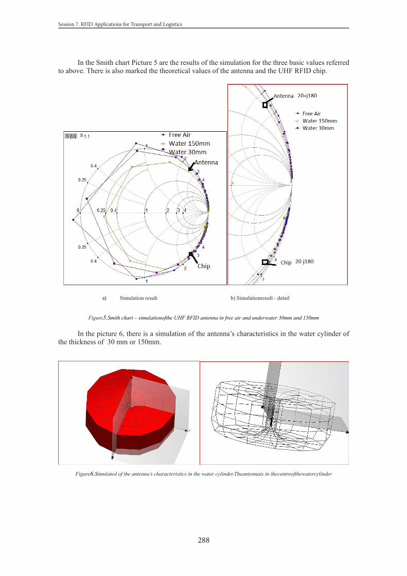
288


In the Smith chart Picture 5 are the results of the simulation for the three basic values referred to above. There is also marked the theoretical values of the antenna and the UHF RFID chip.

a) Simulation result b) Simulationresult - detail

Figure5.Smith chart – simulationofthe UHF RFID antenna in free air and underwater 30mm and 150mm

In the picture 6, there is a simulation of the antenna’s characteristics in the water cylinder of the thickness of 30 mm or 150mm.

Figure6.Simulated of the antenna’s characteristics in the water cylinder.Theantennais in thecentreofthewatercylinder

289


Figure7.Simulated Z parametersoftheUHD RFID antenna in free air

Figure8.Simulated Z parametersofthe UHD RFID antenna in underwater 30mm and 150mm

From the results, we can conclude that the proposed antenna has linear characteristics of real part of impedance in the frequency range 865-960MHz .

In order to obtain the S11 for complex impedance instead of 50 Ohms port, firstly was obtained S11 parameters for 50-ohm-port and then the file was post-processed in Excel - Table 1, Table 2 and Table 3.

290


Table 1. RecalculatedS11 parametersforcomplex impedance ofthechipZ=20-j180, the UHF RFID tagis in free air

Freq Zreal Zimag Z Z-Zc Z+Zc S11 VSWR

862 16,21 -630,39 16,20-630,38i -3,79-810,38i 36,20-450,38i 0,554-0,029i 3,45

865 15,90 -619,55 15,89-619,55i -4,10-799,55i 35,89-439,55i 0,548-0,029i 3,41

868 15,59 -608,12 15,59-608,12i -4,40-788,12i 35,59-428,12i 0,541-0,030i 3,35

902 11,59 -464,26 11,58-464,25i -8,41-644,25i 31,58-284,25i 0,439-0,034i 2,56

905 11,14 -447,70 11,14-447,70i -8,85-627,70i 31,14-267,70i 0,424-0,035i 2,45

908 10,68 -431,09 10,67-431,09i -9,32-611,09i 30,67-251,09i 0,409-0,035i 2,34

911 10,20 -414,02 10,19-414,02i -9,80-594,02i 30,19-234,02i 0,392-0,036i 2,27

914 9,69 -395,98 9,68-395,97i -10,31-575,97i 29,68-215,97i 0,373-0,037i 2,17

917 9,14 -376,77 9,14-376,77i -10,85-556,77i 29,14-196,77i 0,351-0,037i 2,07

920 8,58 -357,19 8,57-357,18i -11,42-537,18i 28,57-177,18i 0,327-0,038i 1,94

923 7,97 -336,14 7,97-336,13i -12,02-516,13i 27,97-156,13i 0,300-0,039i 1,82

927 7,34 -314,59 7,34-314,59i -12,65-494,59i 27,34-134,59i 0,269-0,040i 1,72

930 6,67 -291,25 6,66-291,25i -13,33-471,25i 26,66-111,25i 0,233-0,041i 1,59

Table 3. RecalculatedS11 parametersforcomplex impedance ofthechipZ=20-j180, the UHF RFID tagis in 150mm underwater

Freq Zreal Zimag Z Z-Zc Z+Zc S11 VSWR

862 20,72 -534,21 20,72-534,21i 0,721-714,21i 40,72-354,21i 0,494-0,027i 2,92

865 21,16 -520,20 21,15-520,19i 1,15-700,19i 41,15-340,19i 0,484-0,026i 2,85

868 22,11 -505,43 22,11-505,42i 2,11-685,42i 42,11-325,42i 0,473-0,025i 2,77

902 19,74 -374,45 19,74-374,45i -0,256-554,45i 39,74-194,45i 0,348-0,025i 2,07

905 18,01 -354,06 18,00-354,06i -1,99-534,06i 38,00-174,06i 0,324-0,026i 1,94

908 16,83 -333,55 16,82-333,55i -3,17-513,55i 36,82-153,55i 0,297-0,027i 1,82

911 15,83 -313,05 15,83-313,04i -4,16-493,04i 35,83-133,04i 0,267-0,027i 1,71

914 15,07 -291,09 15,06-291,08i -4,93-471,08i 35,06-111,08i 0,233-0,027i 1,59

917 14,53 -268,54 14,52-268,53i -5,47-448,53i 34,52-88,53i 0,195-0,027i 1,47

920 14,14 -245,11 14,14-245,11i -5,85-425,11i 34,14-65,11i 0,151-0,025i 1,35

923 13,79 -220,63 13,79-220,63i -6,28-400,63i 33,79-40,63i 0,099-0,023i 1,20

926 13,49 -195,88 13,49-200,88i -6,51-380,88i 33,49-20,88i 0,040-0,020i 1,07

929 12,94 -169,39 12,94-169,39i -7,05-349,39i 32,94+10,60i -0,031-0,017i 1,07

291


Figure9.Radiationpaternoverlap Figuge 10.Radiationpatern 920MHz, UHF RFID tag 150mm underwater

Figure11.Comparasionof WSWR port 20-j180 ,UHD RFID antenna in free air and underwater 30mm and 150mm

In the Figure 11, there are the results of the complex impedance simulation of the final optimized model of the antenna in the environment of water column of permittivity 70.

The article is not provided with a full description of the antenna, as each stage of antenna’s optimization far outweigh the scope of this contribution, therefore, only the final values are listed.

During testing in laboratory conditions, the following results were achieved.The maximum distance for UHF RFID tag reading was 2.0 m, which was achieved under the

condition that the tag was 30 cm under the surface (clean water). Thanks to the results of measurement, it can be perceived that the signal intensity was approximately -5.2dBm on theboundary of air/water and ˗20.2dBm on the input of the UHF RFID tag’s antenna.According to the theoretical calculation the worst VSWR is 3,57 = Reflection Power 30% = -6dBm

292


Figure12.Measurement of UHF RFID tag for underwater applications 52mm x dia16mm

4. CONCLUSION

Three prototypes were made and identical parameters were achieved by the measurement. This study proves that it is possible to use the UHF RFID technology and applications in the water environment. It is obvious how misleading may commercial information be about using the RFID technology in such applications. It is certainly necessary to design the correct antenna for similar types of applications. The classic inlays cannot be used due to the fact that the antenna is debugged when immersed in an environment with permittivity of 80 because of its construction.

The solution opens up more options of the UHF RFID tag applications for monitoring waste water the construction of a water supply system, monitoring corrosion, etc.

Figure13.The UHD RFID tagforunderwaterapplication 52mmx dia 16mm

References

1. GuilianoBeneli and Alessandro Pozabon, RFID Under Water: Technical Issues and Appliations http://dx.doi.org/10.5772/53934

2. J.Edwards, Undersea with RFID, RFID Journal, www.rfidjournal.com,(2012)3. John Keller, AUVAC, Navy seeks to apply RFID technology to undersea navigation and obstacle

avoidancefor UUVs, (2011)http://auvac.org/community-information/community-news/view/866#sthash.M3iviQ4L.dpuf

4. Rudy Severns, Skin Depth and Wavelength In Soil , www.antennasbyn6lf.com

The XXInternational Conference “RELIABILITY and STATISTICS in TRANSPORTATION and COMMUNICATION – 2014”

Figure12.Measurement of UHF RFID tag for underwater applications 52mm x dia16mm

4. CONCLUSION

Three prototypes were made and identical parameters were achieved by the measurement. This study proves that it is possible to use the UHF RFID technology and applications in the water environment. It is obvious how misleading may commercial information be about using the RFID technology in such applications. It is certainly necessary to design the correct antenna for similar types of applications. The classic inlays cannot be used due to the fact that the antenna is debugged when immersed in an environment with permittivity of 80 because of its construction.

The solution opens up more options of the UHF RFID tag applications for monitoring waste water the construction of a water supply system, monitoring corrosion, etc.

Figure13.The UHD RFID tagforunderwaterapplication 52mmx dia 16mm

UHF RFID reader


ImpinjSpeedway R420 [10]


EM4324-27dBm[7] Monza X 8K -24dBm[9]

Max mismatchloss 1,57dB = 78% ThroughtPower

2.0m

Border Air/Water

-27dBm

-20.2dBm

0.3m (-15dBm)

+32dBm -5.2dBm

-79dBm -42dBm

293


5. Shan Jiang, Stavros Georgakopoulos Electromagnetic Wave Propagation into Fresh Water Journal of Electromagnetic Analysis and Applications, 2011, 3, 261-266

6. Al-Shamma’a, A. Shaw and S. Saman, “Propagation of Electromagnetic Waves at MHz Frequencies through Seawater,” IEEE Transactions on Antennas and Propa- tion, Vol. 52, No.11, November 2004, pp. 2843-2849.

7. Datasheet EM4324 http://www.emmicroelectronic.com/products.asp?IdProduct=2848. G. Benelli, A. Pozzebon and G. Ragseo, “An RFID Based System for the Underwater Tracking

of Pebbles on Artifi-cial Coarse Beaches,” IEEE 2009 Third International Conference on Sensor Technologies and Applications, Athens, 18-23 June 2009, pp.294-200.

9. Data sheet Impinj Monza X 8K https://support.impinj.com/hc/en-us/articles/202756868-Monza-X-8K-Dura-Datasheet

10. ImpinjCompany. (2010). Impinj Speedway Revolution: brochure. USA: Impinj, Inc.11. WIPL-D d.o.o., EM software, https://www.wipl-d.com

294


Proceedings of the 14th International Conference “Reliability and Statistics in Transportation and Communication”(RelStat’14), 15–18October 2014, Riga, Latvia, p. 294–302. ISBN 978-9984-818-70-2Transport and Telecommunication Institute, Lomonosova 1, LV-1019, Riga, Latvia

MUTUAL COEXISTENCE OF ACTIVE AND PASSIVE RFID TECHNOLOGY

Peter Kolarovszki, Zuzana Kolarovszká

University of Žilina, Faculty of operation and economics of transport and communications, Department of communications, Univerzitná 1, 010 26, Slovakia, Ph. (+421)- 908227492, E-mail:

[email protected]

Abstract:

This article deals with research of mutual coexistence of active and passive RFID technology, which is a part of automatic identification and data capture. In this article we would like to describe an identification of transport unit based on passive technology and also by active technology. We would like to specify, how this technologies can work together and in which application focuses on postal and logistics. All results are verified by measurement in our AIDC laboratory, which is located at the University of Žilina. Our research contains different types of measurements in order to point out the possible influence of these two technologies. The results of our research bring the new point of view and indicate the ways using of UHF RFID technology in postal and logistics applications. At the end of this article is characterized the utilization of the RFID technology in postal logistics chain by using both passive and active technologies.Keywords: RFID technology, active tag, passive tag, transport unit, identification

Introduction

Radio frequency identification is becoming a modern and useful in many sectors. It provides a contactless identification, tracking and tracing of goods, property and people in real time. Increase efficiency, performance and competitiveness. One area of application of RFID technology is also postal and logistic processes. In this context there are several question of feasibility of the use of identification of letters, parcels etc. In addition to the costs associated with the introduction of technology is necessary to examine the feasibility of using RFID technology in the field of postal and logistic processes.

Today, postal operations have implemented RFID in various closed-loop systems to measure, monitor, and improve operations. For example, RFID is being used to monitor international mail service between major hubs. By randomly “seeding” tagged letters into trays, elapsed delivery time can be measured. This allows service issues to be identified and addressed in a reliable and cost-effective manner. Other postal and also logistics companies have piloted tracking mail containers to measure trailer utilization and to track container locations. Manual container tracking systems tend to break down when volumes are high and there’s a deadline to meet departure times. By allowing information to be captured automatically, RFID makes sure it is done, even under stressful conditions.

This article deals with research of mutual coexistence of active and passive RFID technology in the field of postal and logistics network optimization and transport processes. We performed research of readability of RFID identifiers attached to transport items.

1. Objective and methodology

Object of the research are the transport items (letter trays) and active, passive RFID identifiers placed into this transport units. RFID tags were read by active and passive RFID readers in several

295


position and conditions. In order to achieve the relevant results of the research, more than 100 measurements were performed by various types of testing.

2. RFID in postal and logistics processes

The AMQM1™ Platform provides postal operators with a complete overview and effective traceability of mail volumes, parcels, mail bags, mail items, trucks, roll-containers and letter trays across the entire logistics chain. One key feature is automatic consignment system that associates the mail items to the containers carrying these items and to the trucks transporting these.

This solution can be based on various technologies such as: RFID, disposable RFID labels and bar codes, as well as combinations thereof. It also enable objective documentation of times of arrival and departure of vehicles, which postal containers are loaded/unloaded, vehicle load space management, real-time information on types of mail, quantities, times of arrival, delays or changes in transport times etc. With regard to postal operational systems, the following conditions must be taken into account:

• Rough industrial environments. • Large volumes of goods and mail. • Short time available for processing. • High labor costs in connection with the daily operations. • Large potentials in automation and streamlining of manual processes. [4]

2.1. RFID-based Vehicle Management

Tracking vehicles and trailers throughout the entire transport logistics chain provides considerable benefits to all parties involved, e.g. management, users and customers. The Vehicle and Trailer Tracking System is an advanced and effective IT system for monitoring and managing precise arrivals and departures of vehicles at specific points in the logistics chain. The system is built on the experience and know-how acquired from supplying the world’s largest and most widespread RFID network stretching across about 60 countries.

Implementing this system offers unique values. Examples of benefits:• Fully automatic registration of vehicles - i.e. no manual work involved. • Improved yard and vehicle management. • Precise and objective record of exchange of goods between parties. • Early warning on delays in transport to all parties. • Precise feedback to transport planning systems. • Improved vehicle maintenance routines. • Cost savings in centers with real-time information available.[6]

2.2. Roll Cage Tracking and managing

One of the main issues being addressed by the roll container tracking and managing project is need to take control of and better manage transportation assets. Another primary project requirement is to ensure that the required containers will be always available at the customers’ premises and within postal operator facilities. This should overcome the tendency for planned or unplanned hoarding of roll containers that causes shortages elsewhere, especially at peak times. Additionally, the lack of visibility of roll container whereabouts led to unnecessary loss since it was not possible to identify where the roll containers disappeared and hence forced expensive purchase of new roll containers to meet the customer service level agreements. System of the monitoring and managing roll cages includes tag (active or passive, it depends of application), that is placed on a side or on the bottom of the container (Figure 1), it also includes a handheld terminal solution for consignment of roll container, product and destination enabling load control on all roll containers (Figure 2).

1 AMQM – Automatic Mail Quality Measurement

296


Figure 1. RFID tag placed on the container Figure 2. Handheld terminal

The result is avoiding miss-sending and has real-time t volume forecasting into all facilities in the network providing efficient and on time production and distribution. Also a handheld terminal solution designed for track and trace of all individual parcels is a part of the solution providing key customers with shipment visibility throughout the whole logistic network. Miss-shipments are prevented by load-control.

When a roll container is ready for dispatch, the roll container is scanned for destination and product type. If the roll container is lead through a gate not matching the destination, an alert will immediately help correct the mistake. Solution must include Asset Management software platform enabling full, real-time transparency of the location of each roll container and can be also used to track specific mail and parcel transports. Implementing this system offers unique values. Examples of benefits:

• Improves availability and load balance throughout the logistics chain. • Prevents hoarding of roll-containers. • Minimizes losses. • Helps to improve supply chain efficiency. • Provides the ability to monitor the transported delivery time of goods. • Helps to improve service and maintenance.[5]

2.3. Letter Tray Tracking

Tracking and tracing letter trays throughout the entire postal logistics chain provides benefits to postal customers, employees and management. The trays are automatically registered in the postal logistics by means of RFID technology. Each letter tray has a tag that communicates and transmits information to the reader in Real-time load control (Figure 3). Now it is possible for the postal operators to reuse the same RFID network to track & trace postal letter trays. This new opportunity is a fast pay-back investment with many unique advantages to postal operators worldwide.

Figure 3. RFID tags on letter trays and Real-time load control

Key Benefits:• Better utilization of postal letter trays. • Possibility to analyze through-put times of mail and letter trays at distribution centre. • Knowing the location of trays improves their availability throughout the entire logistics chain. • Knowing the location and contents of trays improves the possibility of managing the tray

sorting process right on time. • On automatic handling systems, such as tray sorters, the reading rate can be improved

dramatically compared to that of bar codes - reducing manual intervention. • Being able to identify trays helps to improve service and maintenance.

297


3. RFID components used in measurements

The RFID system architecture consists of a reader and a tag (also known as a label or chip). The reader queries the tag, obtains information, and then takes action based on that information. That action may display a number on a hand held device, or it may pass information on to a POS system, an inventory database or relay it to a backend payment system thousands of miles away. Let’s looks at some of the basic components we have used in our research.

3.1. RFID tags used in measurements

An RFID tag is a small device that can be attached to an item, case, container, or pallet, so it can be identified and tracked. It is also called a transponder. The tag is composed of microchip and antenna. These elements are attached to a material called a substrate in order to create an inlay.

Tags are categorized into three types based on the power source for communication and other functionality.

• Active.• Passive.• Semi-passive.We have used special active RFID tags used in postal and logistics environment, which can

works at different modules:• Broadcast ID at predefined intervals (heart beat and long range approximate tag location

information)• Broadcast ID along with exciter ID when activated by an LS exciter (short range defined

tag location information)• Broadcast ID when the tag is in motion (vibration sensor activates the tag and indicates

the asset is on the move).[2]

Figure 4. Active RFID tag

3.2. RFID Portal

Our RFID portal combines two technologies (active and passive). It consists of passive Impinj RFID reader, which we used in measurements due to passive RFID tags and also active reader used in conjunction with active tags.

Figure 5. Combine RFID active and passive portal

298


3.3. RFID Middleware

Middleware is software that controls the reader and the data coming from the tags and moves them to other database systems. It carries out basic functions, such as filtering, integration and control of the reader. RFID systems work, if the reader antenna transmits radio signals. These signals are captured tag, which corresponds to the corresponding radio signal. This is a very special software device enabling mutual communication between two and more applications. This device is marked also as a mediator between various application components.

We have used two middleware platforms, one from company Aton AMP, that consist of several processors programmed in Java and second one from Lyngsoe systems named as EDECS (see figure 6).[3]

Figure6. EDECS middleware

4. Description of measurements and AMP model configuration

In order to achieve relevant outcomes, it was inevitable at first to design functional system enabling realization of single measurements under laboratory conditions. In order to comprehend single measurements, we have to define the principle they operate under and what is being detected by them. .

4.1. AMP model configuration

Configuration of the model for readability measurement of passive tags was designed in environment of AMP middleware. Configuration in AMP ensures communication between hardware and software part of our model. At the same time, it enables to set up the configuration itself, so by its use we define practically what, how and when should the particular hardware and software components operate. Our configuration (figure 7) consists of several processors:

• LLRPProcessor• EarlyDecoupler• TimeFormatter2• WhitelistFilter• InsertProcessor• MessageTransformer• LoggerNeW• db – connection to database

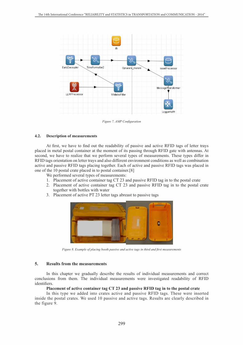
299


Figure 7. AMP Configuration

4.2. Description of measurements

At first, we have to find out the readability of passive and active RFID tags of letter trays placed in metal postal container at the moment of its passing through RFID gate with antennas. At second, we have to realize that we perform several types of measurements. These types differ in RFID tags orientation on letter trays and also different environment conditions as well as combination active and passive RFID tags placing together. Each of active and passive RFID tags was placed in one of the 10 postal crate placed in to postal container.[8]

We performed several types of measurements: 1. Placement of active container tag CT 23 and passive RFID tag in to the postal crate2. Placement of active container tag CT 23 and passive RFID tag in to the postal crate

together with bottles with water3. Placement of active PT 23 letter tags abreast to passive tags

Figure 8. Example of placing booth passive and active tags in third and first measurements

5. Results from the measurements

In this chapter we gradually describe the results of individual measurements and correct conclusions from them. The individual measurements were investigated readability of RFID identifiers.

Placement of active container tag CT 23 and passive RFID tag in to the postal crateIn this type we added into crates active and passive RFID tags. These were inserted

inside the postal crates. We used 10 passive and active tags. Results are clearly described in the figure 9.

300


Figure 9. Result of readability of passive tags

As we can see only one passive RFID identifier was not read correctly. All others were read with any problems. In conjunction with active tags we can say that all of them were read.

Placement of active container tag CT 23 and passive RFID tag in to the postal crate together with bottles with water

In this type we added into crates active and passive RFID tags, but we added also two bottles (1,5 L) to each postal crate (see figure 10). We used again 10 passive and active tags. Results are clearly described in the figure 11.

Figure 10. Placement of passive and active tags in second measurement


As we can see, the presence of bottles of water significantly affected the readability of passive RFID identifiers. The average of readability was just 77 %. In terms of active identifiers, all ten were read similarly as in the previous case.

301


Placement of active PT 23 letter tags abreast to passive tagsIn this type we added to passive tags also active RFID tags used in AMQM measurements.

These were inserted inside the postal crates. We used 10 passive and active tags. We placed passive and active tags as follow:

< passive tag + active tag + passive tag + active tag + …..... >, until we reached 10 active tags.Between each tags was no space, so it was very similar as in real conditions. On figure 12 we

can see results of this type of measurements.


On this figure are graphically shown just passive tags, because active tags obtained 100% of readability. As we can see 4 passive RFID tags obtained less than 70 % of readability. This result was due to the interference of active RFID identifiers that were placed close to the passive tags.

When compare all our measurement than we can see following result of readability RFID tags in several conditions:

Table 1. Comparative result of measurements

Type of measurement Placement of active container tag CT 23

and passive RFID tag in to the postal crate

Placement of active container tag CT 23

and passive RFID tag in to the postal crate together with bottles

with water

Placement of active PT 23 letter tags

abreast to passive tags

Average Result (%) 97 77 75,45

Conclusion

We can state, that utilization of active radio frequency identification of postal crates or letters (testing letters) in postal operation is technically feasible as a very high level of readability was achieved by scanning of particular crates and letters under laboratory conditions. The results of placing passive RFID tags together with active tags are very dependent indeed on specific placement of passive RFID tags. As we can saw at the results the presence of active RFID identifiers led to interference of passive identifiers. Obviously polarization orientation and tags is also important, but in our case we have considered a horizontal orientation with respect to the deployment tag antenna of the reader. Due to usability measurement in practice we set a statistical significant value measurement for the readability of 99%.

Due to this research result we can say that we can use passive technology for identification of postal crates, parcel an also post containers but identification letters is very complicated. In conjunction with placing of active RFID test letters together with passive identifiers leading to possible interference on the part of active tags.

302


References

1. Hunt, V., Puglia, A. and Puglia M. (2007). RFID: A Guide to Radio Frequency Identification. New Jersey (USA): John Wiley & Sons, Inc. 201 p.

2. Thornton, F. and Lanthem, Ch. (2006). RFID Security. Rockland (MA, USA): Syngres Publishing, Inc. 229 p.

3. Michálek I. and Vaculík, J. (2008). RFID planning levels for postal and courier services. In: Future Role of Postal Services in the Face of New Market Conditions and Communication Technologies, Pardubice, Czech republic, December, 2008 (pp. 144-151). Pardubice: University of Pardubice.

4. L. Vojtěch, M. Neruda : Application of Shielding Textiles for Increasing Safety Airborne Systems - Limitation of GSM Interference.In The Ninth International Conference on Networks (ICN 2010). Los Alamitos: IEEE Computer Society, 2010,p.157-161.ISBN 978-0-7695-3979-9.

5. Beneš, F., Kubáč, L., Staša, P., Kebo, V.: RFID and Augmented Reality; Proceedings of the 14th International Carpathian Control Conference (ICCC): Rytro, Hotel Perła Południa, Poland, May 26-29, 2013. Vienna: IEEE, 2013, s. 186-191. ISBN: 978-1-4673-4489-0

6. Vaculík, J.,Tengler, J. (2012). Potential of new technologies in logistics services. In CLC 2012 - Carpathian logistics congress: November 7th-9th 2012, Jesenik, Czech Republic, EU: congress proceedings. Ostrava: TANGER.

7. Kendra, M., Lalinská, J., Čamaj, J. (2012). Optimalization of transport and logistics processes by simulation. In ISTEC; Proceedings of the 3rd International Science, Technology and Engineering Conference, Dubai, United Arab Emirates (UAE), December 13-15, 2012 (pp. 886-892). [Online] ISSN 2116-7383

8. Klapita, V., Mašek, J. (2012) Processes solution in the warehouse by the queuing theory application. In Horizons of Railway Transport: scientific papers (pp. 64-6). Vol. 3, no. 1. ISSN 1338-287X

9. Madleňák R., Švadlenka L. (2009). User Acceptance of Internet advertising in Czech Republic (Akceptace internetové reklamy uživateli v České republice) / In: Ekonomie a management = Economics and management :. - ISSN 1212-3609. - Vol. 12, n. 1, p. 98-107.

About the authors

Ing. Peter Kolarovszki, PhD. works at the University of Žilina, Faculty of Operation and Economics of Transport and Communications, Department of Communications. He is a solutionist and co-solutionist of projects relating to a field of ICT (Information and Communication Technology). He focuses mainly on the area of radio frequency identification and on the automatic identification and data collection. (AIDC). As researcher coordinates on KEGA projects, VEGA projects, project EUREKA and development projects of the Ministry of Education, Science, Research and Sport of the Slovak Republic.

Ing. Zuzana Kolarovszká, PhD. works at the Department of Communications, University of Žilina, Slovakia as a lecturer at the department of electronic communications and services. As university lecturer provides teaching of courses focused on creating web presentations and the design and development of database applications. As researcher coordinates on KEGA projects, VEGA projects, project EUREKA and development projects of the Ministry of Education, Science, Research and Sport of the Slovak Republic. She is an active member of the Oracle Academy, graduated from the program Introduction to Computer Science.

This article was created to support project named as:

E!7592 AUTOEPCIS - RFID Technology in Logistic Networks of Automotive Industry

Centre of Excellence for Systems and Services of Intelligent Transport II ITMS 26220120050 supported by the Research & Development Operational Programme funded by the ERDF.

303



THE USE OF RFID TECHNOLOGY TO IDENTIFY TRAFFIC SIGNS

Juraj Vaculík1, Jiří Tengler2, Maslák Ondrej3

1prof. Ing. Juraj Vaculík, PhD, University of., Žilina, Slovak republic, Univerzitná 1; 010 26 Žilina, Head of AIDC Lab,

tel: +421-41-513-3132,. email: [email protected],2Ing. Jiří Tengler, PhD., University of., Žilina, Slovak republic, Univerzitná 1; 010 26 Žilina,

tel: +421-41-513-3132,. email: [email protected],3Ing. Ondrej Maslák, University of., Žilina,

Slovak republic, Univerzitná 1; 010 26 Žilina, tel: +421-41-513-3145,. email: [email protected],

This article deals with the possibility to identify traffic signs by means of RFID technology, the nature of the use (target utilization) is a diverse that can be used for diverse purposes. The introductory part of this post is about the way type and location of RFID identifier to any traffic sign, i.e. how effectively put RFID identifier to ensure the best possible level of readability of RFID identifier detainee at the road sign. An integral part of this chapter was the creation of appropriate measurement methodology to ensure high quality and comparable results. The following chapter consists of a description of measuring the readability of RFID identifier that you have placed on signs in laboratory conditions. The penultimate chapter depicts the results already obtained in the above measurements. Finally, the paper summarized the general lessons learned during the measurements and there are other possibilities of examining the readability of RFID identifier that you have placed on road signs by measuring very close to the real traffic.Keywords: RFID technology, road traffic, traffic signs, identification.

1. Introduction

RFID technology for the past 15 years, recorded a relatively large explosive development. This development was reflected in many industries especially in the areas of logistics, ie the identification of diverse industrial goods, mail and many others. However, RFID technology has long been aimed only at those areas, but getting to raising even more specific areas such as the identification of transport services, especially in identifying road signs which is also the subject of this article. In the introduction, it would be useful therefore to define what traffic signs are, what they represent and what their purpose. Traffic signs are signs that are placed on columns or other structures firmly embedded in the ground or variables that are displayed on panels and eventually portable traffic signs placed on racks or cars. Simplicity is the pictograms designed to control and regulate traffic on roads. Also, it is a device to alert road users to dangerous sites, store them prohibitions, orders or restrictions, provide them with information or more accurate, complete or restrict the meaning of different road signs. So, when we think about the meaning of traffic signs, there a question arises, what we need to equip traffic signs RFID technology. The answer to this question can be classified from several levels:

1. Increased first warning to road users 2. Getting a second operational information for the operator maintainer of traffic signs in a

particular regionAd 1) the actual traffic sign is as mentioned above a particular purpose for road users, but

only in the case when traffic sign in time to see. Currently, many modern cars already equipped with a camera system which, when scanned, and recognition of traffic signs allows road users in time. However, like the human eye, and the camera system is not immune to the adverse effects of the

304


weather, such as fog, snow, etc. In this case, it would be preferable if it were still available as well as other complementary technologies allow remote identification of road signs without the need for line of sight. Now in this case, the RFID technology could play a relatively important role, since it does not need to communicate RFID tag and reader direct visibility (Hunt, Puglia2007). Thus, RFID technology could serve as an adequate means of compensation of the optical capture traffic signs.

AD 2) another plane, which could be used RFID technology is the acquisition of operating data for recording, monitoring and maintenance of traffic signs. Together with GPS technology, could be allowed monitoring of specific brands over time and space. Thus it would be possible to monitor what specific traffic sign is placed in the different transport segments in which km, condition, etc. The technology would allow the administration to provide relatively automated collection of data on the quantity, type, respectively age of traffic signs in real time and space (Hofmann 2012, Vsetin).

These two ways of using RFID technology in transport services, however, reflects only a fraction of the possibilities that RFID technology can offer this area, but within the scope of this article, we will pay only the above.

1.1. Placing RFID identifier for traffic signs

From a technical point of view and the nature of RFID technology to apply to the traffic sign, we need to characterize several basic and important parameters which when considering the application of RFID identifier on traffic signs must count (Hofmann 2012, Riga).

The first and most important factor is that the road signs are in a metallic material. Thus one of the materials, wherein the RFID reader can have a reduced ability to read RFID identifiers witch is detainee in the abovementioned metallic materials.

Another parameter is where you place traffic signs to place RFID identifier. Whether to use the information area traffic signs, or used in posts to which they are attached tags, etc.

In the case of placing RFID identifier for the above posts, however, there may be risks that the identifier someone steals or damaged. The same risk as well as the location of the RFID identifier transport information on area traffic signs. How can we ensure quality and yet safe placement RFID identifier? One of the ways to ensure the security of RFID identifier is that it must not be visibly noticeable, respectively inseparable. Most of the new information surfaces traffic sign is made of metallic material respectively sheet metal substrate. This substrate is modified and applied it to a specialized cover sheets with information specific brand. Thus, the above options would be the application of RFID identifier before the application of specialized foil. However, there may be problems related to the readability of the specialized nature of the foil. To improve the reflecting properties may be to add the color these foils of metal or glass-like elements (Hofmann 2012, Riga).

1.2. Placing RFID identifier for traffic signs

To investigate the feasibility of using RFID technology placed on road signs and to find a solution that would enable seamless readability of RFID identifier traffic signs in connection with the previous chapter we performed a series of measurements in the laboratory of automatic identification AIDC Lab, University of Žilina (Figure. 1)

Figure 1. Spaces of AIDC Lab for testing

305


To measure was used for the following equipment:• Motorola RFID reader • RFID identifiers (for metal) • RFID middleware Onid/AMP from Aton • Application by the middleware AMP for this measurement (fig. 2)• Traffic signs • Specialist covers foil used on road signs

Figure 2. Graphic environment of middleware

Figure 3. Examine traffic signs

306


Figure 4. Foil used for testing

To test was designed applications in the Onid /AMP in two steps. In the first part of the set needed a predefined value, such as distance measurement, the intensity of antennas and other relevant values and the second part was defined management logic and its own measurements (Vaculík at all 2013).

Figure 5. Setting of environment Onid/AMP for measurement

Figure 6. Custom logic control measurement

307


2. Metodology

The aim of the screening was to determine the nature of the readability of RFID identifier located on the road sign, the key outcome for us was the degree of legibility i.e. the number of load RFID identifier for the period of time at predetermined distances between traffic sign identifier provided with RFID antennas and RFID readers. A second inherent value for us RSSI i.e. the quality of the reflected resp. signal returned from the RFID identifier toward RFID reader antennas.

Examining RFID identifier carried out in several consecutive steps, namely:a) reading RFID identifier detainee on varying surfaces and varying hitting the road sign b) reading RFID identifier overlapping specialized protective foil without traffic signs c) reading the RFID identifier superimposed specialized protective foil directly on the road sign

3. Description of measurement

First was measurement status read / unread was the first reference measurement to determine the optimal orientation and unsatisfactory cases RFID tag and antenna. Measurement status read / unread was detected first reference measurement to determine the optimal orientation and unsatisfactory cases RFID tag and antenna. To simulate road signs, for ease of manipulation, was used small box on which they were placed tags at figure below.

Accepted cases where distance communication between RFID tag and RFID reader is at least 3000 mm at the reference consignment have been cases 1, 2, 5 and 6 (indicated in Figure 7, third above green).

Figure 7. (Left) Measurement of reference content, (Right) Measurement of metal content

In accepted cases, we measured the RSSI returned label reading device. Value in the table (below 1) means the sum of the amount of RSSI of each label for each load, so we get an average value of the RSSI = ΣRSSI/N, where N is the number of loading plate in this case is N = 500 in each case at the chosen working distance of 3000 mm and similarly for the other measurements, but a variable distance.

Table 1. RSSI change the metal contentRSSI [dBm]/dis-tance Case1 Case2 Case5 Case6

3000 mm 33,864 25,842 28,568 35,298

2000 mm - no metal 34,068 37,384

2000 mm - metal 28,208 31,826

308


Comparing the readability of RFID tags placed on the reference and consignments inappropriate content filled with metal showed that the distance of 2000 mm at the most favorable of the two cases (Figure 7 and 8) gain is always above 28 dBm (Tab.1). Communication distance and RSSI signal is back to functioning application sufficient even when the metal content of the consignment it follows that the RFID can also be implemented on a road sign, which is made of metal at a suitable location of the tag.

Each measurement was carried out by a constant period of time i.e. 30 seconds. This value we chose for the previous finding that the collection of data that is loaded latency RFID identifier RFID reader is a period of relatively linear. Every single type of measurement (e.g., when examining specific cover sheet) was carried out at predefined distances between RFID identifier and RFID reader, which was valid for all types of measurement. At the same time specific measurements complemented with a maximum distance of load (i.e. the distance at which still managed to read data from RFID identifier).

4. Result of measurement

Measured was performed under laboratory conditions without the interference of the external environment. We varied the distance from 25 cm to 250 cm, and we investigated the dependence of the signal quality at all distances and whether the RFID tag on metal with plate loaded (response rate label reader). The proper functioning of the system is obviously sufficient to load one-one response label reader. Reader we set at 100 percent power, and we allowed the maximum possible loading responses from the label. This means that we have received as many answers many of the RFID tag has been technically possible.

In addressing the current state is not known how many would be in range RFID tag reading taken in real applications, but we expect that less than 30 seconds. Even with minimal time spent in the reading field label reads at least once. This has been verified by measurement in which we diminish the time interval in which the RFID tag can be read. This dependence of the loading time showed a linear characteristic, i.e. at 10 times shorter time interval of the same load your plate 10 times less (at 30 seconds, we had 500 reference load at 3 and 48 seconds).

The measurement results with underlay and underlay at different distances can be seen below in table tab. 2 and figure 8.

Table 2. Dependence on the distance

Distance: 250 500 750 1000 1500 2000 2500Reading [count] 491 638 612 599 603 580 528

Average RSSI [dBm] 33,7 36 36,3 31,7 27,1 27 24,9

Figure 8. (Left) Number of reading tags, (Right) Average RSSI value

309


On the graph above (fig. 8) we can see the declining quality of the incoming signal from the RFID tag back to the reader with increasing distance. The best result we achieved at a distance of 750 mm, but at a distance of 2500 mm we loaded test RFID tag 528 times in 30 seconds. The required functionality of the system is sufficient if the RFID reader detects at least one answer from the reader.

The following graph (fig. 9) shows the number of reading of tag depending on the time when it is in the reading zone. As can be seen, the number of loading the tag has an increasing linear characteristic (from 21 at 1 sec. to 303 at 15 sec., while the intensity of the returned signal is constant (e.g. 62 dBm.).

Figure 9. Number of reading tags

As we mentioned above, one of the factors that reduce the readability of the kind of foil that is used for traffic signs. The following graphs show the results of measurements, for different types of film (yellow (fig. 10), orange (fig. 11) and black color (fig. 12)), after the elimination of iron-containing foil, which cannot be used.

Figure 10. Number of reading tags and RSSI yellow foil

310




Than the previous graphs show the use of foil, not substantially reduces the readability of the tag, although in some cases the fluctuations, but a bad impact on readability has application to metal (no sign - direct measurement of the film, he signed - application to metal traffic sign). Although the RSSI level is relatively constant, although smaller (bar graph), there is a visible decrease in number of reading - line chart. For sure it is appropriate to reiterate that it is sufficient retrieving tag at least once.

Interesting is also the location of the tag on the side of traffic sign (fig. 13), which is the readability constant in both parameters, although lower. It’s understandable given the location of the tag and the expected position of the reader.

311


Figure 13. Tag placed on side of sign and around of sign (green)

Points based on the location of the tag on the metal structure (handle) traffic sign (fig. 14), which reached a maximum reading distance: 515 cm. But here is a bit losing its original meaning - identification of transport sign.

Figure 14. Metal tag placed on the rack

312


5. Conclusion

The results show that it is possible to use RFID technology for the application of road marking. However, the measurements showed that the fact that the right and perfect legibility, which would be required for these applications is contingent upon many factors (metal base, cover color foil, a small reading distances, etc..) where synergies could be resolved.

But the benefits that these applications have, for example, the service safety features, simplifying navigation solution for temporary signage and more, worth the effort, and further work in this area.

Acknowledgements

This article was created to support project named as:• Centre of Excellence for systems and intelligent transport II (048/2009/2.1/OPVaV,

Activity 1.4) – ITMS 26220120050• E!7592 AUTOEPCIS - RFID Technology in Logistic Networks of Automotive Industry• The quality of education and human resources development as pillars of the knowledge

society at the Faculty PEDAS at the University of Zilina, ITMS 26110230083” - Modern education for the knowledge society / project is co-financed by the EU

• Inštitucionálný výskum - Výskum faktoru ovlivňujícich obsah prepravovaných balíkových zásilek prostřednictvím senzoru pohybu, teploty, otřesu a dalších - 4/KS/2014

References

1. Hofmann, L. Monitoring of heating industry process by UHF RFID tags. In Proceedings 2nd computer science on-line conference in 2012. Vsetín : Silhavy sro, 2012. ISBN 978-80-904741-1-6.

2. Hofmann, L. UHF RFID industry heat resistant tag. In: Reliability and statistics in transport and communications (RelStat ´12): proceedings. Riga : Transport and Communications Institute, 2012. ISBN 978- 9984-818-49-8, s. 326-331.

3. Hunt, V., Puglia, A. Puglia M. (2007). RFID: A Guide to Radio Frequency Identification. New Jersey (USA): John Wiley & Sons, Inc. 201 p.

4. Vaculík, J., Kolarovszki, P., Tengler, J., Radiofrequency identification from system to applications, chapter 19, Possibilities of RFID in Conditions of Postal Operators, InTech: Rijeka, 2013. - ISBN 978-953-51-1143-6. - S. 397-450.

5. Zeman, D., Juránkova, P., Švadlenka, L., The application of automatic identification technologies by the Czech Post. Transport and Communications,2013, roč. I/2013, č. 1, s. 33-39. ISSN 1336-7676.

313


Proceedings of the 14th International Conference “Reliability and Statistics in Transportation and Communication” (RelStat’14), 15-18 October 2014, Riga, Latvia, p. 313–322. ISBN 978-9984-818-70-2 Transport and Telecommunication Institute, Lomonosova 1, LV-1019, Riga, Latvia

THE CORRECTION OF RFID IDENTIFIERS SCANNING ERRORS ON DYNAMICALLY MOVING LOGISTIC UNITS

Daniel Zeman1, Jiří Tengler2, Libor Švadlenka3

1University of Pardubice, Jan Perner Transport FacultyDepartment of Transport Management, Marketing and Logistics

Studentská 95, 532 10 Pardubice, Czech RepublicPh.: (+420)-466 036 568, E-mail: [email protected]

2University of Žilina, Faculty of Operation of Economics of Transport and CommunicationsDepartment of Communications

Univerzitná 8215/1, 010 26 Žilina, SlovakiaPh.: (+421)-41-513 5558, E-mail: [email protected]

3University of Pardubice, Jan Perner Transport FacultyDepartment of Transport Management, Marketing and Logistics

Studentská 95, 532 10 Pardubice, Czech RepublicPh.: (+420)-466 036 375, E-mail: [email protected]

The aim of the research presented in this paper is to find possible ways of corrections of errors and scanning of static RFID identifiers, which are located on dynamically moving logistic transport units. The main reason for examination of these issues and for its testing is looking for solutions, which will be able to improve current systems of automation and processing of consignments, goods and material, increase in accuracy and reliability. Laboratory measurement includes simulated operation parameters of the real RFID gate, as well as machine equipment of the logistic chain, such as conveyor belt, pallet truck, and forklift truck. Combination of these devices and RFID gate, together with the need for performing scanning and identification of particular goods and material create specific conditions for the formation of the bottleneck, which subsequently needs to be eliminated; or set the rules for its 100% use. The core of the paper contains an analysis of measurement progress, gained results and particular values and its comparison with hypothetical theses. Primarily, mutual dependence between RSSI values and the speed of tag movement is examined.Keywords: dynamic movement, conveyor belt, logistic unit, radio frequency identification, tag

1. Introduction

Current logistics, as well as its individual processes, either in manufacture or in processing and distribution of material and goods, are characterized by continual increase in demands as well as by change of demanded and realized volumes of performance. This change means not only gradual increase in transport of goods and materials and in the amount of manipulations with logistic transport units, but also the change of dynamic and qualitative parameters of processing and distribution processes, such as speed, time, accuracy and reliability. Within the structure of individual processes of logistic chain, the improvement of above mentioned parameters depends mainly on implementation of new technologies, methods and procedures, which will be able to appropriately eliminate critical parts or bottlenecks in the chain. Bottlenecks in logistic chain are represented by particular machine, device or other factor, which in some way restrict manufacture processes and further processing.

In recent years, RFID technology came to the fore and in many cases replaced older identification technologies (e.g. barcode). Reduced technical and economic requirements enabled its better availability, as well as development of new hardware and software solutions and more opportunities in further research and use. The main objective of RFID technology is an exact identification and keeping records of objects, goods, material, incomplete products etc. (Zeman, Juránková and Švadlenka, 2013). It is used mainly in production, logistics, warehouse management,

314


postal and express services, sale, safety systems etc. In most of the above stated areas, reliability, accuracy and the speed of operation processes is very important; the combination of these parameters can be determinative factor for improving its position on the market. It is the RFID technology, which together with continual development and research of its improvement possibilities and reducing imperfections / errors leads to absolute satisfying and ensuring of these requirements. The potential and possibilities of RFID technology always depend on current technical progress and development; therefore it would be useful to look for solutions, which could improve already implemented technology and its operation conditions without need of procuring a new one.

2. Specification of parameters and conditions of scanning

From the viewpoint of practical application, as well as with respect to the dynamic nature of tag scanning, the greatest emphasis in the processes of improving of the existing situation is given on parameters such as e.g. received signal strength indication (RSSI) value, error rate, the speed of scanning tag / object with tag; number, position and the angle between scanning antennas. Individual parameters, to a greater or lesser extent, influence the scanning process; the main objective of presented research, however, is aimed at elimination scanning errors resulting from the relationship between the object with the tag and the value of the reflected signal, that is, change and quantity of reading (or not reading) of RSSI value is recorded. In general, within dynamic parameters of measurement the speed of tag / object with tag movement is changing, while static parameters, such as number of antennas, performance and the angle between the antennas stay constant during one series of measurement. When defining the relationship between the speed and RSSI value in relation to time, we primarily focus on verification of the following research assumptions – propositions:

• increased speed causes change (reduction) in quantity of reading tag• constant speed on a specified path does not cause any change (reduction or increment)

of RSSI valueThe tag placed on the object usually keeps its static position; however, it may change its

orientation on selected area, therefore we discuss only its orientation to the antenna. From this point of view, we are mainly interested in influence of particular number of antennas of RFID system and their positioning in the space on the quantity and values of RSSI signal reflected / received from the tag.

2.1. Received signal strength indication

The intensity (strength) of reflected RF signal can be also indicated by other than RSSI units, e.g. dBm (decibel-milliwatts), mW (milliwats), or as a percentage. Middleware solution by Aton OnID Company, which was used during the measurement, provides output values of signal reflected from the tag in form of RSSI, therefore, in the following sections we will use this indicator. RSSI is quantitative dimensionless quantity expressing the strength of received signal. Based on this quantity also the RSSI error rate is determined, which indicates the quality of received / reflected signal, while it is true that the lower error rate, the better is reflected signal. (Vaculík, Kolarovszki and Tengler, 2013) Also, the lower final (negative) RSSI value, the better is the intensity of reflected signal, for example, reflected signal with the value –44 is better than the signal with the value –59. In general, RSSI value consists of quantities stated in the following formula:

where TP is transmission power of the source, AG1 and AG2 are gains of antennas 1 and 2, and PL is path loss in free space (Qian Dong and Dargie, 2012).

As already stated, RSSI does not use an exactly defined unit (dimension); hardware producers (producing antennas, readers, sensors), however, often give conversion formulas for changing RSSI values to values of signal intensity. In addition, it is possible to define RSSI values in dBm (decibel-milliwatts) as follows:


technical progress and development; therefore it would be useful to look for solutions, which could improve already implemented technology and its operation conditions without need of procuring a new one.



increased speed causes change (reduction) in quantity of reading tag constant speed on a specified path does not cause any change (reduction or increment) of RSSI

value The tag placed on the object usually keeps its static position; however, it may change its




PLAGAGTPRSSI 21 (1)

dBmAdndBmRSSI 10log10 (2)

AzLrLtLoGrGtPtdBmRSSI Re22 (3)

ddBLo 4log20

(4)

fc

(5)

where d is distance between the antennas (in metres), λ is wavelength (in metres), f is frequency of waves (Hz) and c is speed of propagation of electromagnetic waves in vacuum (m/s) (Nagy and Karásek, 2010).

2.2. Ideal radio frequency identification system vs. laboratory measurement










PLAGAGTPRSSI 21 (1)



ddBLo 4log20

(4)

fc

(5)



315


This formula for calculation of RSSI value is created by Texas Instruments, where n is signal propagation constant or path loss exponent (in dBm) and may vary from 2 – 4 (free space has n = 2 for reference). Unit A represents received signal strength in dBm at 1 metre distance without any obstacle and d is relative distance (in metres) between the communicating nodes (from the sender to receiver).

In case of using omnidirectional antenna, RSSI value (in dBm) is expressed also by means of the formula (3), which in greater degree accepts losses caused by signal propagation, whether in free area or within antenna downspout of the transmitter or receiver.

Unit Pt represents output power of the transmitter (in dBm), Gt (dBm) is gain of the transmitting antenna and Gr is gain of the receiving antenna. Units Lo, Lt and Lr (all in dBm) represent losses of signal, where Lo is loss due to the propagation in free space, Lt is loss of the antenna downspout at the transmitting end and Lr is loss of the antenna downspout at the receiving side. Abbreviation Rez means reserve and A indicates the value of the antenna attenuation; both values are in dB (decibels).

The value of loss due to the propagation in free space (Lo) is calculated as (see formulas 4 and 5),

fc

=λ (5)



One of the conditions for achieving objective results by performing measurement was the definition of conditions, under which testing of RFID system would best correspond to the conditions and characteristics of ideal RFID system. Authors like Bolić, Simplot-Ryl and Stojmenović (2010) define the ideal RFID system as system which provides basic functionality and is characterized by following features:

• There exists a well-defined, controllable read zone for each reader. For every tag within its read zone, each reader has a 100% read rate or read accuracy and for tags outside its read zone, each reader has a 0% read rate (Bolić, Simplot-Ryl and Stojmenović, 2010). It means whether the tag can or cannot be scanned in / outside the electromagnetic field of reader.

• Performance is insensitive to the physical orientation of tags.• Performance is insensitive to the nature of the object on which the tag is placed.• Performance is insensitive to the environment in which the system is deployed.• Multiple tags communicate with the reader in a collision-free manner and the time for reading

a fixed number of tags is a deterministic function of the number of tags while utilizing the maximum allowable bandwidth.

• Performance is unaffected by the presence of multiple readers with overlapping read zones or of multiple tags within a read zone.

• Performance is unaffected by relative motion between the readers and tags as long as the tags remain within the reading zone of the reader (Bolić, Simplot-Ryl and Stojmenović, 2010).

When talking about the measurement conditions, created RFID system met only the 1st, 3rd, 5th, 6th and partially the 4th feature of ideal RFID system. Within defined time always only one tag was scanned by only one reader, thus there was no overlapping of read zones, as well as no collisions when reading the tag. The system was also partially influenced by the laboratory setting (point 4), when it was not possible to eliminate all objects, which could have negative impact on signal propagation and reflection, while at the same time the effect of these influences was maximally reduced (that is, constant conditions with sufficient area without unnecessary objects were created).










PLAGAGTPRSSI 21 (1)



ddBLo 4log20

(4)

fc

(5)












PLAGAGTPRSSI 21 (1)



ddBLo 4log20

(4)

fc

(5)



316


Points 2 and 7 of ideal RFID system characterization could not be fulfilled, because when studying how RSSI value depends on the tag movement speed, there comes about a change of its position on object and thus to a change of orientation towards the antennas of the reader. After reaching stated speed, the speed of the object containing tag was in certain part of measurement constant, while the relative distance between the tag and antennas was changing.

All sets of measurement were performed in the AIDC Lab laboratory at the University of Žilina. The used system included the Motorola FX7400 (4 ports) reader, various number of Motorola AN480 antennas (the combination of different positions of 1 – 3 antennas), and used UHF frequency bandwidth in the range specified for Europe (865.6 – 867.6 MHz). For speeding up and simulation of consignment unit (object containing tag) movement, linear line was used, which was approximately 6 metres long. For the measurement were selected following three different types of tags:

• TTF M-Prince Tag – plastic UHF tag with dimensions (length x width x height): 90 x 34 x 6 mm; and ID: 1234 0000 0000 0000 0000 0000

• RFID sticky tag used by Hella Company – UHF label with dimensions (length x width x height): 60 x 40 x 1 mm; and ID: 4830 3130 3431 3731 3730 3037

• Alien ALN-9540-02 Squiggle RFID World Tag – UHF label with dimensions (length x width x height): 97 x 11 x 1 mm; and ID: E200 3411 B802 0114 1224 4113

2.3. Specification of speed of the handling equipment

Inability to meet points 2 and 7 in characteristics of ideal RFID system does not represent any great restriction with regard to the course of the measurement, because in real operation it is not always possible to create conditions for functioning of RFID system like this one. In such case, negative aspects of the setting, which influence the electromagnetic field and thus the signal emission within it (presence of metal objects, reinforced concrete beams and walls, etc.), are taken into consideration as well.

As we have mentioned earlier, the presented research is aimed, first of all, on simulation of dynamically changing value of the speed. From practical point of view, given parameter represents the speed of movement of various handling devices, such as forklift truck, pallet truck, or belt conveyor, by means of which we perform transport and handling units manipulations in RFID gate area. In this case, the transport unit is represented by the plastic crate with the tag placed on its front side. The analysis of speed values of crate containing tag moving on linear line and their comparison with the speeds of handling units movement is based on the Figure 1, which defines the relationship of pre-defined speeds of laboratory measurement and approximate speeds of selected handling units movement.

Figure 1. Definition of the speed of the handling equipment

Maximum speed of object movement that can be reached on linear line is 2.0 m/s; we have tested ten possible variants of speed with the intervals of 0.2 m/s in order to evaluate the change of RSSI value with regards to the speed. Thus, minimum speed of scanned tag movement was 0.2 m/s and maximum speed was 2.0 m/s. For particular handling units speed simulation we give the range of its maximum, or, in case of belt conveyor, standard operation speed. Maximum speed of forklift truck movement (it is not in the defined range on Figure 1) is, depending on the type, in the range of 3.6 m/s – 8.6 m/s (13 – 31 km/h); when talking about pallet truck, this speed is limited by maximum walking speed of the operator, that is approximately 1.4 – 1.7 m/s (5 – 6 km/h). Standard operational speed of conveyor belt, depending on frequention of frequency changer, ranges from 0.05 m/s to 0.9 m/s (3 – 54 m/min). Exact specification of individual handling units enables us taking appropriate measures, which could eliminate possible errors and imperfections in processes, during which goods, products, etc. are handled.

317


3. Simulation of the practical operation using RFID gate

During the measurement five test variants with different number and orientation of antennas were realized. Within each variant ten transits were simulated (ten speed levels of linear line as shown on Figure 1) for two positions (horizontal and vertical position at the object) of each of the three tags; RSSI values as well as change of speed in time were recorded (start → acceleration → constant speed → slowing down → stop). Tag was located on front side of the plastic crate and the scanning took place only when moving from the beginning to the end of the linear line.

All antennas of RFID gate had circular polarization and remained static during the measurement; their distance to the object with the tag was changing only as a result of the movement of this object on linear line. RFID gate was located in the middle of total length of linear line (6 metres), in order to ensure sufficient space for moving off and finishing of the object with the tag being scanned, and to prevent scanning immediately after starting corresponding processor of control application (Aton OnID), or after stopping. Early tag reading (without movement of the crate containing the tag) was ensured also by regulating the power of individual antennas, which was by means of the software reduced to 25% of overall emitting power. The number and placement of antennas, as well as the distance between these antennas and the linear line / tag, the angle between them and horizontal surface / crate with the tag can be seen on the following figures, which represent the schemes and the size of the tested RFID gate.

Figure 2. Measurement scheme – deployment of the antennas in variant D

Figure 3. Distances and deployment of the antennas in variants D (A, B, C) and E

318


As we can see in Figure 3, the following variants of antennas’ deployment were tested (distinguished by different colours of antennas):

• Variant A (green colour) – has one antenna (Antenna 1) at the distance of 1 metre from the linear line (tag).

• Variant B (blue colour) – consists of two against each other built antennas, each at the distance of 1 metre from the linear line.

• Variant C (red colour) – has two antennas, where Antenna 1 (AN1) is at the distance of 1 metre from the linear line. The second antenna (AN2) is above the linear line at the distance of 1.2 metre from the tag.

• Variant D (grey colour) – consists of three antennas; the antennas AN1 and AN3 are placed opposite each other at the distance of 1 metre from the linear line. Location of Antenna 2 (AN2) is similar to variant C, above the linear line (1.2 metre distance).

• Variant E (black colour) – consists of two against each other rotated antennas (AN1 and AN2), which are inclined at the angle of 45 degrees with respect to the vertical plane.

4. Analysis and evaluation of dynamically moving RFID identifiers

As we have mentioned, the values obtained by laboratory measurements (RSSI, quantity of reading) were analysed and evaluated with regards to predetermined research assumptions (see part 2 of this article). The following part deals with the presentation of results. Due to the large amount of data gained by every type of tag; each of them was evaluated separately and then compared with the data gained from other tags.

4.1. The impact of the change of speed to the quantity of reading tag

According to recent studies by Hunt, Puglia A. and Puglia M. (2008), Kaur, Sandhu M., Mohan and Sandhu P. S. (2011) and also based on physical properties of electromagnetic waves, there were assumptions that first research proposition is true; without the need to perform the measurement. By means of measurement we found out that within speed range from 0.2 m/s to 2.0 m/s, the quantity of tag 1 reading has exponentially leaping course, which was even more noticeable at lower speeds. The quantity of reading is decreasing, while with increasing speed this course becomes even and constant.

Figure 4. The quantity of reading tag 1 – horizontal and vertical position (A, B, C, D, E)

319


As we can see in Figure 4, the change of speed has the greatest influence on the quantity of reading when comparing the reading by speed 0.2 m/s (v1) and 0.4 m/s (v2), where the loss of read values is nearly 50%, e.g. variant A (vp – vertical position): v1 / 108 values → v2 / 56 values (48% change), variant B (hp – horizontal position): v1 / 83 values → v2 / 44 values (47% change) or variant C (hp): v1 / 60 values → v2 / 31 values (48% change).

Despite the fact that according to parameters, tag 1 should have better readability in horizontal plane, best values (greatest quantity of reading) were achieved in vertical position on the crate. In this regard, it is also appropriate to assess the change of the number of reading values that occurred as a result of change in the position and orientation of second antenna between variants B and C (28% decrease of the quantity of values at speed 0.2 m/s). Tag 1 responded to changes relatively less flexibly when distant from the RFID gate (slow change of RSSI with values around –65 to –72) and in case of variant E (vp) (45° orientation of the antennas to the tag, vertical position of tag on the crate) the tag was not scanned at all.

Figure 5. The quantity of reading tag 2 – horizontal and vertical position (A, B, C, D, E)

Figure 5 shows the quantity of reading for tag 2 with different variants of antenna location. The quantity of reading has again exponentially leaping course depending on the speed, while it decreases continually with increasing speed. This tag from Hella Company responded more dynamically in the electromagnetic field of RFID gate, as well as with change in distance from the antennas, when the quantity of reading at speed v1 both in horizontal and vertical position is greater on average 72% when compared to the first tag (e.g. variant B (vp): v1 (t1) / 91 values → v1(t2) / 305 values (70% increase), variant D (hp): v1 (t1) / 54 values → v1(t2) / 158 values (66% increase) or variant E (hp): v1(t1) / 73 values → v1(t2) / 269 values (73% increase)). Changing the position of second antenna from vertical to horizontal (variant B → variant C) caused about 50% increase in the quantity of reading in horizontal position of the tag and also about 50% decrease in the quantity of reading in vertical position of the tag. This decrease or increase decreases with increasing speed.

According to the estimated orientation of the tag antenna, the readability should be better in the horizontal position of the tag on the crate, but this hasn´t been confirmed by measurement. RSSI values ranged from –53 to –77, when tag already has not responded to antenna signal. In variant E there were no problems with reading of the tag.

320


The following Figure 6 shows the quantity of reading of tag 3. As in case of previous tags, the quantity of reading this tag has again exponential course, which decreases with increasing speed. Tag 3 has characteristics similar to those of the second tag and it has flexibly responded to the change of distance from the antennas, when maximum values of the quantity of reading are around the value 350. The difference occurs at the RSSI value that is within the range from –43 to –64; when it is exceeded then no more tag is scanned.

Figure 6. The quantity of reading tag 3 – horizontal and vertical position (A, B, C, D)

The increment, based on the change in position of second antenna from horizontal to vertical (variant B → variant C), is about 37% for the horizontal position of the tag. In the vertical position of the tag in compared variants B and C, the quantity of tag reading decreases in the range of 38% to 54% at all speeds. Figure 6 does not show the deployment of antennas according to the variant E, because this measurement was not realized (45° orientation of the antennas 1 and 2 towards the tag).

Based on these results, the truth of first research assumption, which states that increased speed causes change (reduction) in quantity of tag reading, has been verified. This change in quantity of reading has an exponential course, which in response to the increase of speed is almost constant (at the maximum possible speed of linear path from 1.6 to 2.0 m/s).

4.2. The relation between RSSI value and the constant speed of tag movement.

Figure 7 shows the course of RSSI values depending on time. All values are for horizontal tag 1, but with different variants of antenna position (A, B, C, D and E) and in the time interval of 3 seconds.

62

64

66

68

70

72

74

1 2 3variant A variant B variant C variant D variant E

Figure 7. The course of RSSI values depending on time – for horizontal tag 1 (variants A, B, C, D, E)

321


Y-axis represents the negative value of RSSI; X-axis is the measurement interval of three seconds, when the tag was read. The speed of movement of the object with tag is 1.0 m/s (v5). In the picture we can see that there occurs change in the value of RSSI at the constant speed, therefore second research assumption was not truthful.

4.3. The evaluation and correction of errors

Correction or complete elimination of RFID identifiers scanning errors always depends on possibilities and conditions of the particular RFID system. Based on performed measurements and gained results, we have defined the following scanning errors:

• wrong position of the tag on the postal crate / wrong orientation of the tag to the antennas – in some cases it caused approximately 43 – 60 percentage increase in the quantity of reading tags (from hp to vp), or 32 – 34 percentage decrease (from vp to hp) depending on the antenna position and orientation (calculated at the speed 0.2 m/s).

• wrong change of the position or orientation of RFID antennas – it relates to variants B, C and E, which have two antennas and where the quantity of reading tag has decreased by 28% (tag 1 in horizontal position, variants B → C) or it has increased by 51% / 55% (tag 2, hp, variant B compared to variant C and E). Quantity of reading tag 3 changes (variant B vs. variant C) are +37% in horizontal position and –49% in vertical position. In some cases the tag was not scanned at all (tag 1, vertical position, variant E).

• inadequate speed of the movement of the object with tag (too high) – changing the speed of the tag about the value of 0.2 m/s can cause 50% decrease in the quantity of reading tag, e.g. for tag 2 in horizontal position (v1 → v2): variant A → 58% decrease, variant B → 48% decrease, variant C → 50% decrease, variant D → 45% decrease and variant E → 49% decrease. All used RFID tags have exponential course of quantity of reading, which decreases with increasing speed.

• wrong tag for required speed of the movement – this error is related to the previous error, because laboratory measurements were carried out using the free available tags that are not specialized for reading at high speeds. Tag 1 has worse quantity of reading and responded relatively less flexibly to the changes of distance from antenna (compared to tags 2 and 3). In next research it would be useful to test RFID tag that is specially adapted to higher speeds.

• inadequate or too large antenna performance – by controlling of antenna performance continuous capture of data can be achieved; define the exact area where the scanning would take place, as well as prevent scanning of unwanted tags (too large performance of the antenna).

5. Conclusions

Correct operation of each RFID system in logistics is influenced by many parameters, which are connected with the requirements for its reliability, accuracy, robustness, as well as easy operability. In practice, it is not always possible to ensure all parameters of the ideal system, as there are negative influences of the setting, as well as technical restrictions leading to various limitations and errors, which have to be taken into consideration. The elimination of these errors or restrictions represents the way of increasing the potential of using modern technologies and contributes to sustaining high standard of products and services, which are dependent on the application of these technologies.

In the article we focused on the simulation of dynamic scanning parameters, which change in dependence on time: the speed of moving object with tag, received signal strength indication (RSSI) value, quantity of reading, etc. The results are comprised of verification of two research assumptions, specification of main scanning errors together with the possible ways of their correction; and partial specification of basic elements and parameters of the RFID system.

322


Acknowledgements

This article was supported by projects:• EE2.3.30.0058 – Rozvoj kvalitních vědeckovýzkumných týmů na Univerzitě Pardubice

[The development of high-quality scientific research team at the University of Pardubice]/ ROUTER, reg. no.: CZ.1.07/2.3.00/30.0058.

• Podpora stáží a odborných aktivit při inovaci oblasti terciárního vzdělávání na DFJP a FEI Univerzity Pardubice [Support for internships and professional activities in innovation in tertiary education DFJP and FEI University of Pardubice], reg. no.: CZ.1.07/2.4.00/17.0107 in the Team of Technology and Management of Postal Services Sector and Electronic Communications.

• Interní rozvojová soutěž Univerzity Pardubice IRS2014/24 – Využití technologie automatické identifikace jako nástroje inovace předmětu Mechanizace a automatizace v poštovních službách [The use of automatic identification technology as a tool for innovation of the subject Mechanization and automation of postal services]

• 4/KS/2014 – Výzkum faktorů ovlivňujících obsah přepravovaných balíkových zásilek prostřednictvím senzorů pohybu, teploty, otřesu a dalších [Research on the factors affecting the content of transported parcels through sensors of motion, temperature, vibration, and more].

References

1. Bolić M., Simplot-Ryl D., and Stojmenović I. (2010) RFID Systems: Research Trends and Challenges. Chichester (United Kingdom): John Wiley & Sons Ltd. 552 p.

2. Hunt D. V., Puglia A., and Puglia M. (2007) RFID: A Guide to Radio Frequency Identification. New Jersey (United States): John Wiley & Sons, Inc. 241 p.

3. Jones E. C., and Chung C. A. (2008) RFID in Logistics: A Practical Introduction. Boca Raton, Florida (United States): CRC Press – Taylor & Francis Group. 491 p.

4. Kaur M., Sandhu M., Mohan N., and Sandhu P. S. (2011) RFID Technology Principles, Advantages, Limitations & Its Applications. International Journal of Computer and Electrical Engineering, 3(1), 151-157. DOI: 10.7763/IJCEE (ISSN 1793-8163).

5. Nagy Ľ., Karásek J., and Holešinský P. (2010) Localization based on RSSI method. Elektrorevue, 12(4), 55-1-55-6. (ISSN 1213-1539).

6. Qian Dong, and Dargie W. (2012) Evaluation of the reliability of RSSI for indoor localization Wireless Communications in Unusual and Confined Areas (ICWCUCA), 2012 International Conference on, 1-6. DOI: 10.1109/ICWCUCA.2012.6402492 (ISBN 978-1-4673-1290-5).

7. Švadlenka L. (2007) Supply chain management in services industry: RFID in postal and courier services. Hyderabad (India): Icfai University Press. pp. 68-74.

8. Vaculík J., Kolarovszki P., and Tengler J. (2012) Results of automatic identification of transport units in postal environment. Transport and Telecommunication, 13(1), 75-87. DOI: 10.2478/v10244-012-0007-7 (ISSN 1407-6160).

9. Vaculík J., Kolarovszki P., and Tengler J. (2013) Radio Frequency identification from system to applications: Possibility of RFID in conditions of postal operators. Rijeka (Croatia): InTech. pp. 397-450.

10. Zeman D., Juránková P., and Švadlenka L. (2013) The Application of Automatic Identification Technologies by the Czech Post. Transport and Communications, 9(1), 33-39. (ISSN 1336-7676).

Applications of Mathematical Methods to Logistics and Business

Session 8

324



USING OF THE ALGORITHM OF ARTIFICIAL IMMUNE SYSTEMS FOR ADAPTIVE MANAGEMENT AT CROSSROADS

Sergey Anfilets1, Vasili Shut2

1Brest State Technical Universityst. Moskovskaja, 267, Brest, Belarus

Ph.: +375295272199. E-mail: [email protected] State Technical University

st. Moskovskaja, 267, Brest, BelarusPh.: +375295264295. E-mail: [email protected]

Article is devoted to the development of an adaptive algorithm that successfully will replace the existing rigid program control. Algorithm use the data on changes in the intensities during the day, which provided by the prediction module. Adaptive algorithm based on the search for the minimum delay at the crossroads of transport, and based on artificial immune systems. Keywords: traffic light, adaptive control, artificial immune systems.

1. Introduction

Artificial immune system (AIS) is a class of intelligent automated systems using the principles of the immune system [3]. For solving these algorithms use the properties of the immune system for learning and memory.

Artificial immune system - an adaptive computing system, using models, principles, mechanisms and functions described in theoretical immunology, which are used to solve applied problems. The immune system is of great interest to experts in computer science as it is an example of powerful and flexible decentralized information processing [2].

Despite the fact that the natural immune system is not fully understood, today there are at least three theories to explain the functioning of the immune system and describe the interaction of its components, namely the theory of adverse selection theory clonal selection theory and the immune network.

The immune system has all the main features of artificial intelligence: memory, ability to learn, the ability to recognize and make a decision as to how to deal with unknown code, entered the body [1]. Like artificial neural networks, AIS can accumulate new information and using a preliminary study of information, perform pattern recognition in a decentralized manner. Along with other systems of organism it supports sustainable state of vital functions, called homeostasis.

By considering computational aspects of the immune systems paradigm, the following elements of immune algorithms:

• set of ways to represent system components • set of mechanisms to evaluate the interaction of individuals with environment and with

each other • adaptation procedures that controls dynamics of the system Ways of presenting allow creating abstract models of immune systems. Evaluation mechanisms,

which are also called functions affinity allow assess quantitatively interaction of these “artificial immune systems”, and adaptation procedures manage the dynamics of AIS as a set of algorithms to achieve goals.

2. Optimization based on AIS

AIS perform a targeted search of the local extremum, combined with the ability to search the

325


global extremum. A method for finding the optimal solution based on the use of operators clonal selection, mutation and negative selection. Each of the estimated measures of fitness of antibodies according to how “good” the corresponding solution of the problem. Most appropriate antibodies are able to “reproduce” with the help of hypermutation. This leads to the appearance of new antibodies that during hypermutation improve its compliance with the fitness function. Antibodies with the worst affinity are replaced by randomly generated elements, uniformly distributed over whole domain of definition the target function that allows to not close on local extremes, and to explore the entire space of the domain of definition target function. Thus, there is an iterative process of reproduction of new populations of the best representatives of the previous generations. Each new generation has a higher ratio of characteristics that best members of previous generations.

The main steps of the algorithm reduced to the following sequence.1. Generate initial population of antibodies – Pt, t = 0.2. For each r ( r =1, N ) antibody define direction of mutation and calculate affinity – Ф(q).3. Sort antibodies in population Pt by value of Ф(q) in ascending order. 4. Select for cloning k of antibodies with the best affinity.5. Create a population of modified clones using the mechanism of mutation. For each parameter xi , estimated two values Δqji for xi = xi + hi and xi = xi – hi for each j = 1,n. Of two values xi select the one for which Ф(q) better. As a result of this procedure, will be selected direction of hi mutations and calculated value of the affinity Ф(q) on t iteration. Relevant characteristics pi set in – pi = 1. Sign of stimulate antibody becomes equal Aff = Σpi.6. Replace the original population new antibody clone. Generate a second clone by changing parameters xi, which is obtained improving the affinity by rule: xi = xi + hi/2. Calculate affinity of clones. Add this clone in the population of clones Pc. Repeat steps 5,6 for all k antibodies. 7. Unite the original and modified clones generated population: Pt = PtUPc. Execute 3 step of algorithm. 8. Check conditions of end the algorithm: Ф(q) < e or t + 1 = T. Otherwise proceeds on to 9 step.9. Perform the operation of negative selection. Remove from populations not stimulating antibodies, where value Aff = 0. Deleted elements replace with new generated antibodies. Execute step 2 for the newly generated antibodies.10. t = t + 1, go to step 3 of the algorithm.

3. Results of testing

Program of management should calculate traffic light signals, depending on intensity of the input stream. The intensity of flows on roads changes not only during the day, but are random in general, for that optimization algorithm should performed each discrete time interval. Adaptive control based on the use of artificial immune systems for calculate time of green signals in cycle to minimize waiting time in queues. Modeling based on queuing theory. Crossroads can be represented as a system with four servicing devices and four streams of requests. Time delay in servicing devices depends on the time of green and red of traffic lights phases, as well as the transient time.

Input intensity at the crossroads in the test period in Table 1.

Table 1. Input intensity at the crossroad

Intensity of the i-th phase, 15 min

1 2 3 41 153 89 167 1312 147 149 169 1083 138 162 172 1154 158 148 154 1275 162 158 147 1396 148 145 143 1257 135 124 146 1128 169 164 151 127

326


Based on the specified intensities by the algorithm we obtain the duration of the green phase of traffic light cycle. The data obtained for the artificial immune systems are summarized in Table 2.

Table 2. Calculated duration of phases Duration i-th phase of cycle

1 2 3 4 1+3 2+4

1 18 0 27 30 33 14

2 39 0 0 17 14 14

3 19 21 27 0 16 14

4 38 18 19 0 0 15

5 0 0 0 29 31 14

6 18 0 36 0 15 25

7 0 0 22 0 26 14

8 0 0 0 0 19 19Input data for the algorithm are intensity, where intensity of phase 5 is the sum of the first

and third, and for phase 6 - the second and fourth. The main results of modeling crossroads with the adaptive algorithm of artificial immune systems are summarized in table 3 and rigid management in Table 4.

Table 3. The simulation results of the algorithm of artificial immune systems

Direction number

Max. Queue length

Avg. Queue length

Avg. Queue time

1 8 2,666 20,711 2 16 7,537 63,434

3 14 4,705 27,1554 14 4,117 26,827

21 4 0,848 5,7112 8 3,792 29,4633 16 7,848 37,7444 5 1,668 17,7381 10 3,999 36,716

3 2 8 2,491 16,7753 9 3,631 17,4624 8 3,011 32,0751 12 5,13 29,61

4 2 10 4,631 32,2563 14 3,014 20,9954 10 6,976 40,2591 9 3,479 23,423

5 2 14 7,457 45,6443 8 2,574 19,9994 7 1,767 11,5131 9 3,721 29,478

6 2 15 5,725 33,6933 8 2,409 17,7234 11 4,31 29,5931 9 3,12 21,734

7 2 9 3,031 25,5093 3 0,469 3,1574 8 3,488 24,2951 6 2,289 11,033

8 2 5 1,463 11,3683 5 1,443 10,0534 4 1,277 9,211

327


Table 4. The simulation results rigid management algorithm

Direction number Max. Queue length

Avg. Queue length

Avg. Queue time

1 22 7,726 45,298 1 2 10 1,598 34,097

3 23 8,088 44,732 4 19 5,8 40,85

2 1 22 6,359 45,231 2 34 10,615 50,968 3 25 10,111 50,359

4 17 4,317 41,401 1 27 7,707 47,182

3 2 22 7,513 44,779 3 22 6,679 42,63 4 15 3,894 39,444

1 30 7,784 45,421 4 2 28 10,065 48,913 3 22 7,408 46,783 4 18 5,712 41,867

1 26 10,121 50,477

5 2 24 7,717 46,535 3 32 12,841 53,969 4 23 7,152 44,469

1 19 4,917 40,299 6 2 24 6,621 44,88 3 41 18,096 62,205 4 19 5,435 40,83

1 28 9,693 49,298 7 2 22 5,852 40,894 3 36 15,079 57,908 4 19 5,12 42,736

1 30 9,429 48,644

8 2 19 6,18 43,779 3 38 16,808 59,831 4 16 3,642 35,395

In the model, with the algorithm of artificial immune systems, can be seen that queue decreased and the average time spent in queues too. Are diagrams average value of 8 tests a total of all queues average value of queues (Figure 1), average queuing time (Figure 2).

Figure 1. Average queuing time

328


Figure 2. Average queue length

4. Conclusion

From the graphs can be concluded that the artificial immune algorithm significantly improved capacity of traffic light with rigid control mode.

Average queuing time at the crossroads decreased by 62% during the test. Average queue length reduced by 47%. Adaptive control algorithm shows better results, because has information about the changing intensity. Due to the flexibility of adaptation algorithm based on artificial immune systems in criterion function may be implemented restrictions if necessary for a specific task. This may be a restriction on duration of cycle, or the maximum duration of signal or to use a fixed cycle time. Further development of this use of the adaptive algorithm may be in a searching for calculating the durations of signals for crossroads group. This problem significantly increases requirements for computing capacity and therefore involves the use of a server in the control center of traffic lights.

References

1. Dasgupta, D. (2006) Artificial immune systems and its application. Moscow: Fizmatlit.2. De Castro L.N. (2002) Artificial Immune Systems: A New Computational Intelligence Approach.

New York: Press.3. Fogel D. B. (2000) Evolutionary Computation: Toward a New Philosophy of Machine

Intelligence. New York: Press.

329



MODELLING OF SPATIAL EFFECTS IN TRANSPORT EFFICIENCY: THE ‘SPFRONTIER’ MODULE

OF ‘R’ SOFTWARE

Dmitry Pavlyuk

Candidate of Economic Science, Transport and Telecommunication Institute Lomonosova 1, Riga, LV-1019, Latvia

Phone: (+371)29958338. Email: [email protected]

This research is devoted to analysis of spatial effects in modelling of transport efficiency. Four different types of spatial effects, essential for efficiency modelling, are discussed and a spatial modification of the stochastic frontier model, which includes effects of the specified types, is formulated. We also discuss a problem of maximum likelihood estimation of the SSF model and its implementation in the ‘spfrontier’ package. We suggest utilising of the SSF model and the ‘spfrontier’ package for different areas of transport modelling and compile a list of topical transport problems, where a presence of spatial effects is widely acknowledged.Keywords: spatial effects, stochastic frontier, transport, efficiency estimation

1. Introduction

The importance of spatial effects is widely acknowledged in different areas of transport science. Spatial interactions take a place in national, regional, and less aggregated levels. For example, regional science strongly states spatial spillovers of transport infrastructure on industry, agriculture, and overall regional economic and social development (Tong et al. 2013; Cohen 2010); spatial design of public transport routes and movements are an essential part of urban spatial planning; spatial competition for traffic among transport enterprises is a feature of modern liberalised transportation market.

Spatial econometrics (Anselin 1988) provides an extensive set of tools for modelling different types of spatial effects. Spatial effects include relationships between neighbour units (e.g. spatial competition) and spatial heterogeneity (influence of area-specific factors like climate, economics and others).

Economic efficiency of units like transport enterprises and transport systems is a key indicator, frequently used in decision making processes on different levels. Stochastic frontier model (Kumbhakar & Lovell 2003)is one of the most popular tools for statistical estimation of units’ efficiency. Recently significant research efforts have been made to introduce spatial effects in stochastic frontier (Druska & Horrace 2004; Affuso 2010; Barrios & Lavado 2010).

Estimation of spatial effects is quite complicated both from theoretical and computational points of view. This complexity is a serious obstacle for inclusion of spatial effects into everyday work of economists and urban managers. A stable and convenient software tool can bridge this gap. The “spfrontier” tool is one of the first steps in this direction. The tool is implemented as a module for CRAN R, a free software environment for statistical computing and graphics. ‘spfrontier’ is developed by the author, so the main goal of this research is to introduce this tool to scientific community and investigate its facilities for modelling of efficiency in transport science and adjacent research areas.

2. Spatial stochastic frontier model

A classical linear stochastic frontier model is formulated as:

,~~1

ii

K

kkkii uvâXY −+= ∑

=

330


where

i is a unit index, i = 1,…, n,

Yi is an output of a unit i,

Xki are inputs of a unit i, k = 1,…,K,

βk are coefficients, representing direct effects of inputs, k = 1,…,K,

iv~ are independent identically distributed (IID) random disturbances,

iu~ are IID inefficiency levels.

In the context of the stochastic frontier model, we specify a hypothesis about existence of the following four types of spatial effects:

• Endogenous spatial effects• Exogenous spatial effects• Spatially correlated random disturbances• Spatially related efficiencyEndogenous spatial effects represent a relationship between an output (or, more generally,

decisions) of a particular unit and outputs of its neighbours. Exogenous spatial effects represent a relationship between an output of a particular unit and

inputs (explanatory factors) of its neighbours. These effects can be explained by indirect flow of resources into neighbourhood, where a production process and output registration can be separated in space.

The third type of spatial effects, spatially correlated random disturbances, is not based on a theory, but usually is consistent with modelling features. Suppose a model, where observations are affected by an unobserved factor with a spatial nature. Some of these factors can be technically unobservable; some of them are just not available in a research sample. Spatial heterogeneity of these factors leads to spatially correlated random disturbances in a model.

The fourth type of spatial effects, spatially related efficiency, reflects a relationship between efficiency of neighbour units. This type of effects is under-researched and rarely used in applications. Researches, where spatially related efficiency is included into the model, are limited with (Druska & Horrace 2004), (Barrios & Lavado 2010), (Areal et al. 2010), (Tonini & Pede 2011), (Fusco & Vidoli 2013), among few others. A reasoning of spatially related efficiency is very similar to endogenous spatial effects and includes possible spatial impact of units.

Note that first three types of spatial effects are well known (Elhorst 2009), but spatial effects in efficiency are a relative novelty.

A complete stochastic frontier linear model with all types of spatial effects (SSF, spatial stochastic frontier) takes the form:

,~

,~

,

1,

1,

1 1,

)(

11,

i

n

jjijuui

i

n

jjijvvi

ii

K

k

n

jkjijX

sk

K

kkki

n

jjijYYi

uuwñu

vvwñv

uvXwâXYwñY

+=

+=

−+

++=

∑

∑

∑ ∑∑∑

=

=

= ===

β

where

wY,ij are spatial weights for spatial endogenous effects between units i and j, j = 1,…, n,

wX,ij are spatial weights for spatial exogenous effects between units i and j,

wv,ij are spatial weights for spatially correlated random disturbances of units i and j,

331


wu,ij are spatial weights for spatially related efficiency of units i and j,

β(s)k are coefficients, representing spatial exogenous effects of inputs, k = 1,…,K,

ρY is a coefficient, representing spatial endogenous effects,

ρv is a coefficient, representing spatially correlated random disturbances,

ρu is a coefficient, representing spatially related efficiency.

Folding the model by i, j, and k, we formulate the model in the matrix form:

.~,~

,)(

uuWñuvvWñv

uvXWXâYWñY

uu

vv

sXYY

+=+=

−+++= β

A set of methods, used to estimation of a classical stochastic frontier model, includes method of moments, maximum likelihood estimator (MLE), generalised maximum entropy estimator, and Bayesian estimator. Objectives of the estimators are estimation of the production frontier parameters β and values of the technical inefficiency ui for each unit in the sample. The SSF model also requires estimation of coefficients ρY, β(s), ρv, and ρu for spatial effects of four types.

MLE is one of the most frequently utilised techniques in stochastic frontier analysis. Likelihood functions for different specifications of the classical stochastic frontier model are well known(Kumbhakar & Lovell 2003) and implemented in specialised software packages (R, Stata, LIMDEP). Such likelihood functions utilise an assumption of error term independency and represented as a product of univariate distribution densities. The independency assumption is obviously not satisfied for spatially correlated components of the SSF model’s composed error term, so a multivariate closed skew normal (CSN) distribution is used as a base for MLE(Domınguez-Molina et al. 2003). Estimation of CSN distribution parameters itself is a complicated task, which is weakly covered in literature and requires additional research. Given the probability density function for ε, the log-likelihood function can be stated as:

( )( ) ( ) ( ) ( ) ( )

( )( ) ( )( )( ) ( ) .,

,

,

where

,,,ln,,ln,,0ln

,,,,,,,ln

112~

112~

)(

1111

2~

2~

)(

−−

−−

−−−−

−−=Σ

−−=Σ

−−−=

Σ+Σ−+

Σ+Σ−+Σ+ΣΣ−Φ+Σ−Φ−=

=

uunT

uunuu

vvnT

vvnvv

sXYY

uvnuvuvunun

uvYuvs

WñIWñI

WñIWñI

XâWXâYWñYe

ee

ñññâL

σ

σ

µϕµµµ

µσσβ

3. Review of the spfrontier package

Implementation of the stated maximum likelihood estimator of the SSF model parameters requires a set of functions, which are well-known in theory, but computationally hard. These functions include:

• Multivariate normal probability density and distribution functions calculation is required for the likelihood function. Note that number of dimensions matches the sample size n and can be very significant. Computation of multivariate normal functions is recently intensively researched(Genz 2004) and implemented in many software packages.

• Multivariate truncated normal probability density and distribution functions calculation is straightforward on the base of multivariate normal functions.

• Moments for multivariate truncated normal random variables are required for calculation of individual technical efficiency levels.

• The likelihood function also requires extensive matrix algebra. In practice, the matrixes

332


contain a large percent of zero values (sparse), so implementation of sparse matrix algebra algorithms is helpful.

• Maximisation of the likelihood function requires implementation of optimisation algorithms (quasi-Newton BFGS, Nelder-Mead, SANN, and others).\

R (CRAN 2014) is one of popular software tools, where all of the required core algorithms are implemented. The Comprehensive R Archive Network (CRAN) contains a large number of packages, implementing particular statistical tools and algorithms.

Relying on the required functions, we chose the R environment as a base for implementation of the MLE functions. The developed software package is called ‘spfrontier’ and available in the official CRAN archive(Pavlyuk 2014). The main estimator of the SSF model is implemented as a function of the same name ‘spfrontier’ and encapsulates all algorithms, required for the MLE of SSF model parameters and individual inefficiency values. The function allows estimating all four types of spatial effects, specified in the SSF model. Results of the ‘spfrontier’ function include:

• vectors of parameter estimates and their standard errors,• a Hessian matrix of the parameter estimates,• a vector of individual efficiency estimates,• a vector of fitted values of the dependent variables, and• a vector of residuals.Spatial effects, estimated with the ‘spfrontier’ package, can be qualified as an essential feature

of econometric benchmarking models in different areas of transport science.

4. Potential applications of the SSF model in transport science

Transport science includes a large number of models and methods, related with benchmarking. Measuring of efficiency of transport units, nodes, routes or decisions is widely utilised in transport planning and decision making. In this paragraph we list several application areas, where spatial effects can play an important role in efficiency measurement.

4.1. Spatial interactions between transport nodes

Efficiency of transport nodes (airports, coach terminals, ports), located near to each other, can be affected by different types of spatial effects. Spatially correlated random disturbances are the most expected type of spatial effects in transport units’ benchmarking. Spatial settings, which have a significant effect on transport node productivity and efficiency, are distributed over space unevenly. Some of these effects (population density, income) can be included into a model explicitly, but a lot of them are hardly measured and rarely included into consideration (for example, population habits, weather specifics, location features). This fact leads to spatially correlated error terms of models and, as a result, to heteroscedasticity of residuals and biased estimates of efficiency.

Endogenous spatial effects also can be a feature of these models and can be explained by interaction between neighbourhood nodes. Interactions can be both positively or negatively directed. Positive endogenous spatial effects appear when traffic from one transport node continues its flow using neighbour nodes. For example, within a popular hub and spokes organisation of airport networks, traffic, attracted by a hub airport, flows to secondary airports, increasing their productivity. Negative endogenous spatial effects are also possible and can be explained by spatial competition for traffic (passengers, cargo) in a particular geographical area between transport nodes.

4.2. Spatial effects of transport infrastructure

Another application area, intensively modelled by practitioners and academic researchers, is transport infrastructure and its effects on territory enhancements. These effects can appear on the regional level, when transport infrastructure helps regional development (in terms of population, income, manufacturing, tourism, etc.), and also on less aggregated levels. For example, there are many researches, devoted to analysis of a role of public transport infrastructure in district grow and housing pricing. Estimation of decision efficiency is very important for urban planners and regional government and spatial effects should be taken into account. Endogenous and exogenous spatial

333


effects of transport infrastructure are obviously very significant, but rarely included into efficiency modelling explicitly.

4.3. Modelling transport emission

Modelling of environmental impact of transport is another application area, where presence of spatial effects is undisputable. Different types of transport emission and noise pollution spread over space, which leads to positive endogenous spatial effects. Frequently spatial effects play a role, which is more significant than activities, executed in a particular point or region. Thus this is necessary to include spatial effects when modelling efficiency of different emission-preventing decisions and actions.

4.4. Traffic accident prediction

Traffic accident prediction models are also a popular tool of transport planners, which likely affected by spatial effects. Accidents have endogenous spatial effects, when an occurring accident leads to changes in road environment and related accidents in neighbourhood. An accident affects behaviour of drivers, who change their usual routes, depart from the rules to avoid traffic jams, and as a result frequently leads to new accidents near to the first one. Also accidents are frequently explained by area-specific reasons like weather, road conditions, speed limits, etc., which can be included into a model in form of spatially correlated random disturbances.

There are many other areas of transport modelling, where spatial effects play an important role. It includes analysis of roads and crossroads congestion, trip generation and origin-destination flows prediction, modelling of transport demand. The ‘spfrontier’ package, encapsulating different types of spatial effects in the stochastic frontier model, can be a useful tool for decision makers in these and other areas of transport researches.

5. Conclusions

This paper is devoted to analysis of spatial effects in modelling of transport efficiency. There are four different types of spatial effects, peculiar to efficiency estimation: endogenous spatial effects (dependence between neighbour units’ outputs), exogenous spatial effects (dependence between an output of a unit and inputs of its neighbours), spatially correlated random disturbances and spatially related efficiency. A spatial modification of the stochastic frontier model (SSF model), which includes all four specified spatial effects, is formulated. We also discuss a problem of maximum likelihood estimation of the SSF model and provide a derived likelihood function. Maximum likelihood estimator is implemented within the ‘spfrontier’ package.

We suggest utilising of the SSF model and the ‘spfrontier’ package for different areas of transport modelling. A number of application areas of the transport science, related with efficiency modelling, are presented and a presence of spatial effects in these areas is substantiated. The list of discussed areas includes benchmarking of transport enterprises, modelling of transport emission, predicting effects of transport infrastructure, analysis of roads congestion, trip generation prediction, modelling of transport demand, and others.

References

1. Affuso, E., 2010. Spatial autoregressive stochastic frontier analysis: An application to an impact evaluation study, USA: Auburn University.

2. Anselin, L., 1988. Spatial econometrics: methods and models, Dordrecht: Kluwer Academic Publishing.

3. Areal, F.J., Balcombe, K. & Tiffin, R., 2010. Integrating spatial dependence into stochastic frontier analysis, Munich, Germany: University Library of Munich.

4. Barrios, E.B. & Lavado, R.F., 2010. Spatial stochastic frontier models, The Philippines: Philippine Institute for Development Studies.

334


5. Cohen, J.P., 2010. The broader effects of transportation infrastructure: Spatial econometrics and productivity approaches. Transportation Research Part E: Logistics and Transportation Review, 46(3), pp.317–326.

6. CRAN, 2014. R software, CRAN. Available at: http://cran.r-project.org/.7. Domınguez-Molina, J.A., González-Farıas, G. & Ramos-Quiroga, R., 2003. Skew-normality

in stochastic frontier analysis. Skew-elliptical distributions and their applications: A journey beyond normality, pp.223–241.

8. Druska, V. & Horrace, W.C., 2004. Generalized moments estimation for spatial panel data: Indonesian rice farming. American Journal of Agricultural Economics, 86(1), pp.185–198.

9. Elhorst, J.P., 2009. Spatial panel models. In Handbook of Applied Spatial Analysis. New York: Springer: Berlin Heidelberg, pp. 377–407. Available at: http://www.york.ac.uk/media/economics/documents/seminars/2011-12/Elhorst_November2011.pdf.

10. Fusco, E. & Vidoli, F., 2013. Spatial stochastic frontier models: controlling spatial global and local heterogeneity. International Review of Applied Economics, 27(5), pp.679–694.

11. Genz, A., 2004. Numerical computation of rectangular bivariate and trivariate normal and t probabilities. Statistics and Computing, 14(3), pp.251–260.

12. Kumbhakar, S.C. & Lovell, C.A.K., 2003. Stochastic frontier analysis, Cambridge: Cambridge Univ. Press.

13. Pavlyuk, D., 2014. CRAN R package “spfrontier,” Available at: http://cran.at.r-project.org/web/packages/spfrontier/index.html.

14. Tong, T. et al., 2013. Evaluating the spatial spillover effects of transportation infrastructure on agricultural output across the United States. Journal of Transport Geography, 30, pp.47–55.

15. Tonini, A. & Pede, V., 2011. A Generalized Maximum Entropy Stochastic Frontier Measuring Productivity Accounting for Spatial Dependency. Entropy, 13(11), pp.1916–1927.

335



DEDICATED HARDWARE IMPLEMENTATION OF NEW HASH ALGORITHMS FOR IMPROVING SECURITY

IN DATA PROCESSING

Jarosław Sugier

Wrocław University of TechnologyInstitute of Computer Engineering, Control and Robotics

ul. Janiszewskiego 11/17, 50-372 Wrocław, Polandtel.: +48 71 3203996, e-mail: [email protected]

Security issues are one of the most important problems that define reliability of operation in contemporary Complex Information Systems and, practically, in all other technical systems which are backed-up with computer-based information infrastructure. In this paper we discuss one class of the methods aimed at improving security of data processing – the one which is based on so called hash functions and which is used, among others, in digital signatures, fingerprinting or authentication mechanisms. The recent SHA-3 competition announced by the National Institute of Standards and Technology, USA, resulted in development of new hash methods from which, after intensive public evaluation of the candidates, the Keccak algorithm has been selected as the winner. The focus of this work is on various hardware implementations of the Keccak-f[400] permutation function – the core component of the mid-range sized version of the Keccak algorithm – which can be created from the basic iterative architecture by round replication (loop unrolling) and pipelining. Different variants of the proposed architectures are implemented in popular Spartan-3 and Spartan-6 devices form Xilinx and based on the results we identify important problems which arise if the function is implemented on these FPGA platforms.Keywords: Keccak hash function, SHA algorithm, configurable hardware, hardware implementation.

1. Introduction

Contemporary Complex Information Systems (CIS), being involved and multifaceted amalgamates of technical, information, organization, software and human resources (users, administrators, technical support, etc.), are one of the most complicated yet most reliable systems engineered by man. Ensuring required security and confidentiality of information processing (at data acquisition, transmission, storage and retrieval levels) constitute one of the main and one of the most important challenges in their design, implementation, maintenance and management, and this calls for application of appropriate cryptographic methods. In our paper we discuss one class of such methods which is based on so called hash functions.

A cryptographic hash function (Menezes et al., 2001), generally, is a computationally efficient function which maps binary strings of arbitrary length to binary strings of some fixed length, called hash-values. To be cryptographically efficient, for a given hash function h it should be computationally infeasible to find two distinct inputs which evaluate to the same hash value (i.e., two colliding inputs x1 and x2 such that h(x1) = h(x2)), and having a specific hash-value y, it should be computationally infeasible to find an input (pre-image) x such that h(x) = y.

Hash functions boast a long history of cryptographic development. Common applications of information systems which use in practice digital signatures, fingerprinting or authentication mechanisms has led to development of numerous robust and computationally efficiently methods. Recently, the SHA-3 competition announced by the U.S. National Institute of Standard and Technology in November 2007 (NIST, 2007) ignited a lot of additional research on them. From the 5 selected finalists of the competition, the Keccak algorithm proposed by Guido Bertoni, Joan Daemen, Michaël Peeters and Gilles Van Assche was eventually selected as the winner and at the time of this writing it

336


is about to be announced as the official new SHA-3 standard. From the Keccak family (which consists of 7 different size variants) the largest member with 1600 bits of state was proposed by the authors and was finally chosen by the NIST.

In this work we will discuss hardware implementations of the essential component of the algorithm used for hash calculation – the Keccak-f[400] permutation function – in high speed organizations built around the concepts of loop unrolling and pipelining. The smaller 400b version of the hash was chosen in order to be able to test a wider range of implemented architectures, up to and including the variant in which all cipher rounds are implemented in hardware i.e. the loop is unrolled completely. Such approach was not possible with the targeted FPGA devices in case of both the full-size 1600b version as well as the reduced 800b variant. All the proposed architectures will be implemented in two chips from popular families from Xilinx: the well-established Spartan-3 and the newer Spartan-6 – thus we will create a consistent base not only for evaluation of the concepts of different hardware organizations with diverse loop unrolling and pipelining options but also for comparison how the Keccak’s specifics are handled by the automatic implementation tools when the older (Spartan-3) versus the newer, more advanced (Spartan-6) FPGA arrays are used.

Organization of the text is as follows. In the next chapter we will relate to extensive research on Keccak hardware implementations done during the SHA-3 competition and present motivation for this work on this background. Then, in chapter 3, we will present Keccak operation and introduce loop unrolled and pipelined architectures being under evaluation. Finally, in chapter 4 we will discuss the results obtained after their implementation in the two FPGA chips and identify specific problems which were observed.

2. Related work

2.1. Implementing Keccak in hardware

Implementation efficiency in both software as well as in hardware was, next to cryptographic strength, the key aspect taken into account by the Keccak’s authors during development of the method (Bertoni et al., 2011a). Regularity of the round-based processing and simplicity of the elementary transformations (which purposely do not include any substitution boxes neither multi-bit additions, unlike most of the state-of-the-art block ciphers of the AES genre) were adopted intentionally in order to facilitate implementations in hardware. This was also in line with requirements put forward by NIST already in the initial SHA-3 competition call (NIST, 2007) which, among requirements for candidate submissions, listed “a statement of the algorithm’s estimated computational efficiency and memory requirements in hardware”.

The official author’s statement about hardware implementations of the Keccak (Bertoni et al., 2012b) includes two reference VHDL designs with different speed vs. area trade-offs: the “high speed” stand-alone core and the “mid-range” coprocessor. The high speed core was built upon implementation of one complete round of the hash in hardware where the block of state bits was iterated in a series of clock cycles equal to the number of rounds. The low-area coprocessor made use of external (system) memory for storage of the state bits and was suitable for embedded environments like smart cards or wireless sensor networks where area and power savings are particularly important. Bertoni et al. (2012b) presented implementation of both designs as ASIC (mask programmable) devices using STMicroelectronics 130 nm technology while results of their FPGA (user programmable) implementations were given by Strömbergson (2008).

2.2. Different architectural options

The most comprehensive database of various FPGA implementations of Keccak (and other cryptographic algorithms, including all other SHA-3 candidates) has been built around ATHENa project at George Mason University and is publicly available through the World-Wide Web (ATHENa, 2014). An “Automated Tool for Hardware EvaluatioN” was developed to create an open-source environment for fair, comprehensive, automated, and collaborative hardware benchmarking of algorithms belonging to the same class (Gaj et al., 2010). It was

337


the platform used by a group of researchers from GMU in their comprehensive evaluation of all SHA-3 contenders with regard to their FPGA effectiveness. The conclusions of their studies were published by Gaj et al. (2012) and were thoroughly discussed during the phase of public evaluation during the SHA-3 contest.

In taxonomy of that discussion, taking as the starting point the plain iterative organization (one round implemented in hardware and transformation of the state data consisted in a loop of nr iterations, nr = number of rounds) the two opposing techniques can be used to create various derivate architectures with different area vs. speed trade-offs: loop unrolling or round folding. In loop unrolling more than one round is instantiated in hardware so the number of loop iterations is reduced and thus the speed of data processing is increased, while in round folding either only part of the round in instantiated in the hardware block (so called horizontal folding) or only part of the state is processed in the block (so called vertical folding). In both variants the computation of one round takes multiple clock cycles (slower processing as a cost of reduced area) while in loop unrolling the extra hardware returns in increased throughput. Additionally, each of these techniques can be enhanced with pipelining if there is a cascade of combinational modules and multiple data blocks can be processed in parallel. Whether the latter condition is met depends on operational environment of the hash unit and essentially is equivalent to ability of independent hashing multiple messages from the input stream.

Apart from these generic variations of the basic iterative architecture another intrinsic optimizations of the Keccak core processing steps can be applied which would bring additional benefits especially in cases of low-throughput area-sensitive designs. For example, Junkg and Apfelbeck (2011) proposed an original re-arrangement of round operation with the intention to implement vertical round folding by a factor of 8: the entire 24-round processing was re-partitioned into new 25 rounds so that the order of elementary transformations within each one could be specifically adjusted. Then, with the 1600b of state stored in 25 8x8 distributed RAM modules and 1/8 of the state processed in each clock cycle, all the rounds could be computed in 200 clock cycles – but with substantial savings in design size.

2.3. Aim of this work

In this paper we will evaluate effectiveness of automatic implementation of the high-speed Keccak-f[400] cores built around the concepts of loop unrolling and pipelining, realized in configurable arrays of popular Spartan-3 (Xilinx, 2009) and Spartan-6 (Xilinx, 2011) FPGA devices from Xilinx. The initial intention of this work was to investigate efficiency of automatic implementation of the wide range of architectural options – from the basic iterative one (x1) through multiple different unrolled options (x2 – x10) up to the fully unrolled architecture tested also in the pipelined variant. As it soon turned out, the full 1600b version of the algorithm as well as its reduced 800b option could not be fitted in the intended Spartan families in all the planned architectural variations hence the choice of the smaller Keccak-f[400]. It should be noted, though, that even in the case of this compact version the size of the data path which needs to be realized in hardware is comparable to that of, for example, Salsa20 – another contemporary hash algorithm to which Keccak can be measured up.

The terms “popular” or “low-cost” that we refer to in the title and in this text is understood not only as using inexpensive devices as the target hardware, but also as trying to minimize the cost of the design and its automatic implementation. In contemporary applications the cryptographic unit often becomes just one of the elements of the entire system on the chip and it is not desirable, or even not possible, to make its optimization to be the dominant aspect of the whole project. The module must share both resources and optimization effort appropriately with the rest of the system. In such a situation not only the performance of the unit (typically understood as maximum data throughput per occupied area) but its flexibility and fast, fully automatic implementation become highly valued features that facilitates installation of the cipher in the whole design and, consequently, reduces time-to-market in device development. On such a background, it is the contribution of this work to evaluate effectiveness of the software tools in automatic implementation of the Keccak algorithm in the above mentioned architectures, and with the two selected hardware platforms.

338


3. High-speed implementations of the Keccakf function

3.1. Specification of the algorithm

Keccak-f[b] is a family of seven permutation functions: for parameter l = 0, 1, … 6 each function operates on a state of b = 25 × 2l bits (b = 25, 50, 100, 200, 400 800, and 1600) where a single word w of 2l bits length is called a lane. Every function computes its result processing the state in a series of nr rounds, nr = 12 + 2l (nr = 12, 14, 16, 18, 20, 22, and 24). The rounds are internally identical but they apply different w-bit constants in their final transformation. For the SHA-3 contest the strongest (and the largest) version of Keccak[1600] was proposed where 1600 bits of state consisted in 25 64b lanes are transformed in 24 rounds. In this work we concentrate on Keccak[400] – with 20 rounds, 16b lanes and 400b state.

With the use of the selected Keccak-f permutation, the complete Keccak[c, r] hash function (c + r = b) is built on the fundamental concept of a sponge construction (Bertoni et al., 2011a) which, with specific padding, can generate a hash digest of a variable (within a specific range) size for an input stream of arbitrary length. Parameters c (capacity) and r (bitrate) can be adjusted to find the desired balance between speed vs. cryptographic strength of the hash.

The reference specification by Bertoni et al. (2011b) describes one round R of Keccak-f[b] as a sequence of operations on state A which is represented as a 3-dimensional array A[5][5][w]. The sequence consists of 5 transformations:

R = ι χ π ρ θand each one is defined as a set of operations on individual bits of a lane. Computing the

permutation is equivalent just to applying the round function nr times to the input vector, each time using a unique w-bit constant RC[ i ] in the last transformation ι.

In the reference VHDL specification by Bertoni et al. (2012a) transformations of the Keccak round are expressed as manipulations of the individual bits of the state. While such a description on the lowest level of abstraction does not enforce any constraints on interpretations made by the implementation tools and may help in efficient synthesis, the code itself is quite long and cumbersome in maintenance.

For the needs of this work an original code was prepared and it was based on lane-oriented operations where most of the transformations work on w bit vectors. Such a specification was then ported to VHDL language using strict RTL style: there was no instances of any Xilinx library primitives, no sequential (procedural) descriptions were inserted and no references to any hardware attributes were made so that the code was ready to be synthesized for a different device from any manufacturer. Since the elementary operations include vector rotations in θ and ρ steps, it was decided to use VHDL rol operator from the standard NUMERIC_STD library and because of this all the internal vector signals were defined as unsigned type. The only other elementary operations are and, xor and not and these are built-in operators of the language.

Simplified and more concise description did not cause any noticeable changes in efficiency of the resultant hardware. As a test, the round module coded with the two styles was used in the basic iterative architecture (x1) of the full Keccak[1600] algorithm implemented in the two families of FPGA devices – Spartan-3 and Spartan-6. The results turned out to be almost identical: the only difference reaching the level of 1% was in implementation size expressed in number of occupied slices in the case of Spartan-3 device, but in the same design there was no difference in number of used LUTs so just packing of the LUTs in the slices was a little less effective for that specific implementation effort. The throughputs of both implementations were also very close: the maximum operating frequency of the proposed coding was by 0.23% higher in Spartan-6 and by 0.55% lower in Spartan-3, when compared to results obtained with the code from the reference.

3.2. The scope of selected architectural variants

In this paper we will investigate implementation of the Keccak permutation function in six organizations: the basic iterative (x1), four loop unrolled (x2, x4, and x10), the combinational, i.e. with the loop completely unrolled (x20) and loop unrolled pipelined (x20-PPL20).

Regular structure of Keccak-f[400] processing with a series of 20 identical rounds made

339


implementation of the basic iterative architecture x1 straightforward. Apart from the state register, the hardware needed to include one instance of the round module, simple multiplexing logic at the input (loading either the input data or feeding back the round output) and a counter providing the iteration number with rudimentary control logic. Although in the case of this organization it was possible to use an LFSR register for on-the-fly generation of 16b round constants as it is specified in the definition by Bertoni et al. (2011b), the constants were stored in a ROM module which was addressed with the round counter similarly to the solution chosen for the reference implementation presented in (Bertoni et al., 2012a) . All these elements can be expressed in VHDL with a few lines of code. Latency of the complete computation (i.e. the time from loading the input data to reading the output) is 20 clock cycles.

In the case of loop unrolling the only aspect that makes this simple scheme more complex is simultaneous application of multiple round constants RC. For a xk unrolling the latency of computation is 20/k and there is a cascade of k round blocks in hardware: in the consecutive clock cycles the first block uses constants RC[0], RC[k], RC[2k]…, the second uses RC[1], RC[k + 1], RC[2k + 1]…, etc.. As a result, each round block operates with its own ROM module and uses its own counter for addressing.

Because there are 20 rounds in Keccak-f[400], the loop can be unrolled by the factors of k = 2, 4, 5 and 10. Of all these options the only one which was not included in the test series was x5 organization because it was very close in the result to the x4 option. Additionally, the x20 architecture with the iteration loop unrolled completely represented an extreme case when the whole function was computed in just one clock cycle by a (quite large) combinational circuit located between the input and output registers.

Finally, the last architecture added to the test range – x20-PPL20 – was created by pipelining the fully unrolled x20 organization in such a way that each unrolled round created a separate pipeline stage (since it is the only pipelined architecture it will be denoted just as PPL20 in the rest of this text). This returned the latency to the value of nr (i.e. 20) clock cycles and, in the sense of synchronous data propagation, returned the synchronization flow to the basic x1 architecture with data being transformed in every clock cycle by just one round. This analogously reduced the longest combinational path in the circuit.

From the implementation point of view, pipelining adds more complications to the unrolled architecture: special considerations was needed not because of the presence of the pipeline registers (adding such registers was trivial) but because of the new rules which had to be applied to addressing the RC constants in each of the 20 round blocks. Still, the result was created around the configuration where each hardware round operates with its own ROM module and with its own addressing counter – although in this case the counter cycle needed careful redefinition.

4. The results

All six architectures: the basic iterative x1 plus 5 other variants were automatically synthesized and implemented in Xilinx ISE ver. 14.6 software with XST synthesis tool, and targeted for two devices – Spartan-3 (XC3S2000-5, package FGG676) and Spartan-6 (XC6SLX150-3, same package). In all cases the hardware module computing the function was equipped with basic serial input/output shift registers for transferring the 400b vectors lane-by-lane, i.e. in 16b chunks. The input source files describing the design were identical for both target platforms.

The results are listed in Table 1. Size of each design is given in a number of occupied slices (elementary logic blocks in the Xilinx FPGA array, each consisting of two logic cells) as well as in a number of used Look-Up Tables (LUTs), generators found in each logic cell for computation of a combinational transformation. Ratio of used slices vs. LUTs tells about efficiency of packing of the design in the configurable blocks of the array, while additionally listed average fan-out of non-clock nets allow to compare complexity of the combinational networks coming out of the LUTs.

Performance figures are computed from the minimum clock period (Tmin) which was reported by the implementation software as a result of static timing analysis of the final, fully routed design. Its value allows to calculate the latency parameter and, taking into account possible multiplicity of parallel data threads in the pipelined architecture, the maximum theoretical throughput, i.e. amount of data processed in unit time.

340


Finally, the table also describes the path which generated the longest combinational delay (and thus determined the value of Tmin): its propagation time is split into the shares generated by logic and routing resources.

The devices XC3S2000 and XC6S150 were selected to be sufficiently large to accommodate the most sized x20 or PPL architecture variants: in terms of the occupied LUTs they took 49 or 12% of the total available resources in, respectively, Spartan-3 and Spartan-6 chip while, on the other hand, the most compact x1 design used only 4 or 1% of the device.

Figure 1. Parameters of the Spartan-3 (left) and Spartan-6 (right) implementations related to the values predicted from the reference x1 architectures

4.1. The Spartan-3 platform

By analysing the figures included in Table 1 for all the architectures we can evaluate how the concepts of loop unrolling and pipelining are practically realized in the resources of this particular FPGA array.

Taking the values obtained for the basic x1 organization as the reference implementation, one can expect that for the xk unrolled case the size of the design will increase k times (k round modules are implemented in the hardware one by another) and the longest propagation delay will also increase ×k enlarging Tmin likewise:

Sizexk ≈ k ⋅ Sizex1 (1)Tminxk ≈ k ⋅ Tminx1 (2)

In the PPL architecture (PPL20), on the other hand, the increase in size ×20 should be accompanied by keeping approximately the same propagation delay (the data passes through one round in every clock cycle, like in the basic iterative organization) hence comparable value of Tmin should be observed:

SizePPL20 ≈ 20 ⋅ Sizex1 (3)

TminPPL20 ≈ Tminx1 (4)

Table 1. The six architectures implemented in Spartan-3 and Spartan-6 devicesPPL20 x1 x2 x4 x10 x20

Spar

tan-

3

Slices 10665 1116 1656 2684 5899 10846LUTs generators 19265 1777 2808 4771 10954 20177% of total 47 4 7 12 27 49Registers 8800 1206 1210 1209 1215 1600Avg. non-clk net fanout 3.19 3.45 3.47 3.43 3.46 3.34Tmin [ns] 8.00 8.92 15.9 30.8 71.8 140Latency [clk] / [ns] 20 / 160 20 / 178 10 / 159 5 / 154 2 / 144 1 / 140Throughput [Gbps] 50 2.2 2.5 2.6 2.8 2.9Longest path: logic [ns] 2.66 3.24 4.10 8.76 17.8 37.0 route [ns] 5.34 5.47 11.6 21.7 53.8 103

Spar

tan-

6

Slices 3161 405 617 824 1685 2933LUTs generators 11009 1339 2166 2935 6176 11192% of total 12 1 2 3 7 12Registers 8800 1207 1206 1206 1202 1600Avg. non-clk net fanout 5.52 4.18 4.67 4.99 5.44 5.52Tmin [ns] 6.75 4.89 10.7 25.8 76.6 139Latency [clk] / [ns] 20 / 135 20 / 97.7 10 / 107 5 / 129 2 / 153 1 / 139Throughput [Gbps] 59 4.1 3.7 3.1 2.6 2.9Longest path: logic [ns] 1.21 1.40 1.67 3.11 6.90 12.8 route [ns] 5.67 3.45 9.05 22.7 69.6 126

341


Ratios of actual parameters to the above estimations values are given in Table 2 and are visualized in the left part of Figure 1. Tracing their trends is helpful in evaluation of actual effectiveness of the implementation process more than examination of the absolute values which depend on numerous particularities.

Table 2. Parameters of the tested architectures in the Spartan-3 device as ratios of the expected values PPL20 x2 x4 x10 x20

Size (LUTs) 0.54 0.79 0.67 0.62 0.57

Speed (Tmin) 0.90 0.89 0.86 0.81 0.78

Longest path logic 0.82 0.63 0.68 0.55 0.57

route 0.97 1.06 0.99 0.98 0.94

In general, actual parameters of the unrolled architectures in most cases are better than the above simplified prediction expects. The size in number of LUTs, for example, increases slower than simple “×k” formula suggested; the larger the design the larger is the difference and for x20 case the size is only at 57% of the predicted level. Comparably, an analogous trend is also visible in the performance parameters: the minimum clock period does not increase with k as fast as estimation predicts, although the benefits (89 down to 78%) are not as high as in the raw LUT figures. Moreover, it is worth noting that this improvement is almost exclusively in the “logic” part of the propagation delay because scaling of the “routing” component is almost exactly as predicted in eq. (2) (106 to 94%). This fact is the first sign of a trend in which the routing resources are becoming the limiting factor in implementation of the large combinational nets.

The same effects can also be seen in parameters of the PPL architecture. Additional pipeline registers are usually well absorbed by the FPGA array and the PPL case provides a good example. Comparing this design with the equivalent in size but purely combinational x20 organization (see Table 1) we can see that although the number of flip-flops is accordingly higher, there is no increase at all in neither the number of used slices nor LUTs. Actually, introducing additional registers, that is uniform splitting of long combinational networks found in the x20 architecture, resulted in improved placement which in turn produced a slight decrease in the size parameters, leading to even lower ratios in Table 2.

Also performance-wise the PPL implementation behaves according to expectations. Although dealing with not so long combinational paths with relatively low numbers of LUTs the optimization procedures cannot offer as much of an improvement as it was possible in the x20 case, the Tmin parameter is by 10% lower as compared to the value expected from eq. (4) (for x20 design the reduction was by 22%) and, once again, this saving in much more in logic delay than in routing propagation.

Overall, the implementations of all the tested architectures in the Spartan-3 device gave predictable and stable results, without indication of any significant problems. Summarizing their processing speed it can be noted that, because increase of Tmin is slower than ×k, loop unrolling did produce some advantages in the throughput (from 2.2 Gbps in x1 to 2.9 Gbps in x20). Still, when looking at this parameter alone, the pipelining is obviously the unquestionable leader: thanks to simultaneous processing of 20 data streams the PPL architecture reaches level of 50 Gbps. Pipelined organizations, though, can only be applied in applications where consecutive data blocks can be hashed independently, as it was noted in chapter 2.

4.2. The Spartan-6 platform

An equivalent analysis will be done now for the results obtained with the newer Spartan-6 device. Again, Table 3 and the right part of the Figure 1 presents basic size and performance parameters of the implementations as fractions of the expected values predicted from the reference x1 architecture, applying the same set of equations (1) – (4).

Like it was in the case of Spartan-3 implementations, in the numbers of used LUT elements we can see effects of the optimization procedures which are especially effective in case of the larger designs. On the Spartan-6 platform these effects (reductions to 81 – 42%) are even stronger than they were in Spartan-3 device (79 – 57%). For the unrolled pipelined architecture once more the savings are close to that of the combinational sibling – the x20 case.

342


Optimizations effects are also confirmed by the average fan-out of non-clock nets given in Table 1: in the unrolled cases this parameter increases constantly with k, so the more rounds are instantiated in hardware, the more complex nets are produced (with intention to use less LUTs). It is worth noting that increase in this parameter was not present in Spartan-3 device.

Table 3. Parameters of the tested architectures in the Spartan-6 device as ratios of the expected values PPL20 x2 x4 x10 x20

Size (LUTs) 0.41 0.81 0.55 0.46 0.42

Speed (Tmin) 1.38 1.10 1.32 1.57 1.43

Longest path logic 0.87 0.60 0.56 0.49 0.46

route 1.64 1.31 1.64 2.02 1.83

This stronger effects of optimization in the new Spartan-6 family can be attributed to a better, more powerful yet more flexible configuration of the LUT resources. In case of Spartan-3 devices, the LUTs were 4-input tables holding 16b each thus they could generate any function of maximum 4 variables. A function of fever variables still had to occupy one LUT while any wider function would use more of them (5-input function = 32b or 2 LUTs, 6-input function = 64b or 4 LUTs, etc.). In Spartan-6 architecture, in turn, every LUT table has the total capacity of 64b being sufficient for generation of one 6-input Boolean function but, alternatively, it can be configured for generation of two independent 5-input functions of the same variables. This difference makes Spartan-6 LUTs much more powerful (Table 1 shows that in the largest unrolled architectures numbers of LUTs in Spartan-6 decreased to nearly one half compared to that in Spartan-3) whereas the option to generate two independent 5-input functions provides extra flexibility which the implementation software may need if the design is built from simpler functions.

While the size parameters scale even better than in the Spartan-3 case, the situation is much worse with regard to the performance figures. Looking at the trend in the Tmin figures with increasing unroll factor k, we do not see a stable slow decrease; instead, there is an increase up to the level of 1.57 (versus the expected prediction) which is totally opposite to the tendency seen in the older device.

Comparison of absolute numbers against the Spartan-3 implementations is even more disadvantageous: if the x1 design is almost twice faster in Spartan-6 than in Spartan-3 (which is as anticipated for the newer generation of chips manufactured with more sophisticated technology and being natively able to operate with higher clock frequencies), this advantage diminishes with k up to the point when there is virtually no difference in speed between the two platforms implementing the x20 organization.

5. Conclusion

As a discussion of security and reliability issues in contemporary information systems, this paper provided comparison of different high speed architectures of the Keccak-f[400] permutation function implemented in low-cost Spartan-3 and Spartan-6 FPGA devices. The architectures were built around the standard concept of loop unrolling with an additional example of the completely unrolled and pipelined case. Having the total of 6 different organizations it was possible to compare their implementation on both FPGA platforms.

The results illustrate difficulties which the new SHA-3 algorithm may create if it is implemented automatically on the platform of Spartan-6 devices. The trend in development of the FPGA arrays is towards more complex logic blocks – nodes of the array – which are capable of implementation of more and more involved combinational functions, but the progress in the routing resources is not as considerable. Very dense combinational networks of Keccak’s elementary transformations, irregular down to the individual bit level, are very difficult in automatic routing even though they are built from simple bitwise operations. When mapped to the newer Spartan-6 resources they very quickly lead to routing congestion and low performance parameters if the number of implemented rounds increases. It is a noteworthy observation that with respect to this aspect the older Spartan-3 devices are much less prone to suffer from this deficiency.

343


References

1. ATHENa Database of FPGA Results (2014) http://cryptography.gmu.edu/athenadb/fpga_hash; accessed April 2014.

2. Bertoni, G., Daemen, J., Peeters, M. and Van Assche, G. (2011a) Cryptographic sponge functions. http://keccak .noekeon.org/; retrieved April 2014.

3. Bertoni, G., Daemen, J., Peeters, M. and Van Assche G. (2011b) The Keccak reference. http://keccak.noekeon.org/; retrieved April 2014.

4. Bertoni, G., Daemen, J., Peeters, M. and Van Assche G. (2012a) Hardware implementation of Keccak in VHDL. http://keccak.noekeon.org/; retrieved April 2014.

5. Bertoni, G., Daemen, J., Peeters, M., Van Assche G. and Van Keer, R. (2012b) Keccak implementation overview. http://keccak.noekeon.org/; retrieved April 2014.

6. Gaj, K., Homsirikamol, E., Rogawski, M., Shahid, R. and Sharif, M. U. (2012) Comprehensive evaluation of high-speed and medium-speed implementations of five SHA-3 finalists using Xilinx and Altera FPGAs. In: Proceedings of the 3rd SHA-3 Candidate Conference, Washington, DC, USA.

7. Gaj, K., Kaps J.P., Amirineni, V., Rogawski, M., Homsirikamol, E. and Brewster B.Y. (2010) ATHENa – Automated Tool for Hardware EvaluatioN: Toward Fair and Comprehensive Benchmarking of Cryptographic Hardware Using FPGAs. In: Proceedings of the 20th International Conference on Field Programmable Logic and Applications, Milano, Italy.

8. Junkg B. and Apfelbeck J. (2011) Area-efficient FPGA implementations of the SHA-3 finalists. In: Proceedings of the 2011 International Conference on Reconfigurable Computing and FPGAs (ReConFig), IEEE, 235-241.

9. Menezes, A.J., van Oorschot, P.C. and Vanstone, S.A.(2001) Handbook of Applied Cryptography. CRC Press. 780 p.

10. National Institute of Standards and Technology (2007) Announcing Request for Candidate Algorithm Nominations for a New Cryptographic Hash Algorithm (SHA–3) Family. U.S. Federal Register, 72, 62212-62220.

11. Strömbergson, J. (2008) Implementation of the Keccak hash function in FPGA devices. http://www.strombergson .com/files/Keccak_in_FPGAs.pdf; retrieved April 2014.

12. Sugier J. (2010) Low-cost hardware implementation of Serpent cipher in programmable devices. Monographs of System Dependability: Technical Approach to Dependability, Publishing House of Wrocław University of Technology, Wrocław, 3, 159-172.

13. Sugier J. (2012) Implementing AES and Serpent ciphers in new generation of low-cost FPGA devices. Advances in Intelligent and Soft Computing: Complex Systems and Dependability. Berlin-Heidelberg : Springer Verlag, 170, 273-288.

14. Sugier J. (2013) Implementing Salsa20 vs. AES and Serpent in Popular-Grade FPGA Devices. Advances in Intelligent and Soft computing: New Results in Dependability and Complex Systems. Proceedings of the 8th Int. Conf. Dependability and Complex Systems DepCoS-RELCOMEX, Berlin-Heidelberg: Springer Verlag, 224, 431-438.

15. Xilinx, Inc. (2009) Spartan-3 Family Data Sheet. www.xilinx.com (ds099.pdf); retrieved April 2014.

16. Xilinx, Inc. (2011) Spartan-6 Family Overview. www.xilinx.com (ds160.pdf); retrieved April 2014.

344



UTILISATION OF SELECTED MATHEMATICAL FUNCTIONS FOR SOME METAL OIL DATA EVALUATION

David Valis1, Libor Žák2

1University of DefenceBrno, Czech Republic, Kounicova 65, 662 10 Brno

+420 604 530 230, [email protected]

2Brno University of TechnologyBrno, Czech Republic, Technicka 1853, 612 00 Brno

[email protected]

The paper deals with application of selected mathematical – statistical methods for analysing field data from heavy off-road military vehicles. We apply selected regression functions for description of the oil particles generation. The reason is to find suitable and predictable behaviour of the particles. This helps for creating the picture of the system – vehicle in our case – operational behaviour.

It is the vehicle engine and its metal – copper Cu – oil data which are explored here for further utilisation. The pieces of information from the engine oil are interpreted in form of deteriorated oil characteristics (like changed viscosity, decreasing additives like Mn, Si, Zn, etc.) and polluting particles in oil (e.g. particles from wear process like Fe, Pb, Cu, etc.).

The novelty is to providing inputs for helping to change e.g. the cost optimisation, system maintenance policy, system operation and mission planning. Further development of our outcomes will be provided using other mathematical methods like fuzzy logic and diffusion processes.Keywords: Field data assessment, off-line diagnostics, first hitting time, residual life, maintenance optimization

1. Introduction

The growing dependability and operation safety requirements for modern equipment together with the increasing complexity and continuous attempts to reduce operation and maintenance costs might be satisfied among others by the consistent use of modern diagnostic systems. The main task of object technical state diagnostics is not only to find out incurred failures, but also to prevent from the failure occurrence with the help of sensible detection and changes localization in the object structure and in its behaviour changes. Many various approaches have been published on system diagnostics and CBM (Condition Based Maintenance).

A tribotechnical system (TTS), friction in it, wear and lubrication, and especially the outcomes of it are the subjects of our major concern. We would like to analyse the outcomes from technical diagnostics of TTS. There exists wide range of data from the TTS which are not analysed further. We find this is a pity. Our main objective is to extract maximum in-formation from the diagnostic of TTS in order to gain tools for optimising: maintenance, cost-benefit processes, operation and mission planning. The authors will apply selected mathematical tools to get some inputs into previously mentioned areas. Regarding the tribotechnical system, the basic infor-mation about tribological process, operating and loss variables are provided (GesellschaftfürTribologie, 2002; Czichos&Habig, 2003).

Owing to the TTS we have got a lot of diagnostic oil data. In view of tribo-diagnostics this data is considered to be the final outcome. This data can tell us a lot about lubricants/life fluids quality itself as well as about system condition. Such data are very valuable. System operation, taking the oil samples and the outcomes themselves, are very fuzzy therefore we further plan using approaches from the fuzzy logic theory in our future research. The procedure and results presented below are based on

345


standard mathematical principles – a regression function and a regression analysis which later will be supported with fuzzy logic. From both presumptions we can expect reasonable costs savings (see e.g. Stodola & Mazal, 2012; Stodola et al 2013). As from the military point of view we would like to determine remaining residual life to be able to perform a mission. Following the regression analysis it is possible among others to assess the operating history of an observed vehicle.

The main goal of the paper is to study and to understand the courses of oil particles generations at the beginning part of the system technical life.

2. Objects of diagnostics and methods

The assumed objects of diagnostics in our case the medium lorry engines have not been ready yet in terms of design to use the ON-LINE system, though in practice similar possibilities for other applications have already existed. It results from the in-formation stated above that we are still supposed to use OFF-LINE engine diagnostics system when sampling lubrication fluid at certain intervals, and using known and optimised special tribodiagnostic methods (Lippay, 1991). In our case we use the results and information from atomic emission spectrometry. Following this analysis we can obtain the information about the presence of the elements of a specific kind and the amount of elements. If the vagueness in classes distribution is not given by a stochastic character of measured characteristics but by the fact that the exact line among states classes does not exists, it will be later on good to use fuzzy set theory and adequate multi-criteria fuzzy logic. However, we cannot identify their real origin – e.g. as a result of fatigue, cutting or sliding.

Therefore in our further research we try to identify where the elements might come from. We base our assumptions on idea to increase the potential for maintenance optimisation inputs and cost benefit analysis inputs. Usable diagnostic approaches might be found e.g. in Klimaszewski&Woch, 2012 and Woch, 2013.

3. Oil field data assessment and mathematical model

There is enough statistically important set of field data obtained from the diagnosed objects. It fulfils the basic assumption that we might be capable to solve this problem successfully. Since the data sets are very extensive, we are not going to introduce them here except for a part/example of Cooper (Cu) particles representing the sample – it is presented in modified form in Table 1. While Mh is number of motor-hours (Mh) and ppm is number of particles per milion.

Table 1.Input data of Cu particlesSample/Mh Cu particles Sample/Mh Cu particles

1/0 4.34 11/84 4.62

2/8 5.11 12/95 4.62

3/11 5.62 13/106 5.46

4/22 4.92 14/109 4.33

5/26 4.58 15/119 5.05

6/35 5.14 16/136 5.70

7/46 4.52 17/146 5.84

8/57 5.28 18/153 5.10

9/64 5.23 19/164 5.42

10/72 5.72 20/175 5.67

We deal with dozens of samples taken and analysed at different types of observed engines. In certain aspects we consider the engine from an infantry fighting vehicle to be a reference object, because the event of a failure type has occurred in it. All tribodiagnostic processes related to the failure occurrence have been recorded. We assume that we have potential for obtaining inputs for system maintenance optimisation and system residual life estimation.

346


3.1. Utilisation of Regression Model – Theory

Introduction –When analysing diagnostic data, the question arises whether the data is described by only one regression function across all measurement interval, or there are areas of a different regression function in the data record. If the data is divided into more areas for which relevant regression functions will be calculated, in most cases the regression functions will have a different functional value at the point where the data is divided. When looking for a suitable regression function, a continuity requirement is often set. We would like to modify the form of our data regression functions so that they could have the same value at the point where the data is divided into single areas.At the beginning let us presume that the system is in two states. The diagnostic data will be therefore divided into two parts/areas (part “a)”) and in each of them we will look for the regression functions whose functional value at a dividing point will be the same (part “b)”).

An independent variable is with a view of its random character represented by a random variable X (motohours – Mh), while a dependent variable is represented by a random variable Y (the number ofCuparticles). The breakpoint for two parts will be defined by the value x0. In the first area we are searching for the following regression function:

))(),(1 xXYExy === 1âϕ

for the data for which it applies: 0xx < .In the second area we are looking for the regression function as follows:

))(),(2 xXYExy === 2âϕ

for the data for which it applies: 0xx > .and at the same time – for the part “b)” we require that the following equation applies:

),(),( 2121 ââ 00 xx ϕϕ =

We are looking for both regression functions for the whole area of data concurrently. As for our data, the regression functions will be searched for in a linear form and we will use a linear regression model:

)(1

xfym

jjj∑

=

= β ,

where )(xf j are known functions not containing ,,1 ..., mββ .This model is based on the assumptions listed below:

1 Values x are non-random so the functions )(xf j acquire non-random values )( ijji xff = for j = 1,...,mand i= 1,...,n.

2 Matrix

=

mnm

n

ff

ffF

LMOM

L

1

111

of the type (m, n) with the elements jif is of the rank m<n.

3 Random variables iY , where ∑=

=m

jjiji fYE

1)( β and 0)( 2 >= σiYD for i= 1,...,n.

4 Random variables iY are non-correlated and have a regular probability distribution fori= 1,...,n.

In the single areas we have selected the following regression functions: for the first area: m=2, f1(x)=1, f2(x)=x, the regression function is: xy 1

211 ββ +=

for the second area: m=2, f1(x)=1, f2(x)=x, the regression function is: xy 22

21 ββ +=

347


For the required dependency we select the model which will fit the data and at the same time will be as simple as possible. We are going to do it like this:

1 We chose a fixed the value x0 and a relevant regression function in the following manner: we are looking for the values 2

22

112

11 ,,, bbbb (the point estimation of the parameters: 2

22

112

11 ,,, ββββ ) so

that the function:

222

21

212

11 ))(())((

00

xyxySxxxx

ββββ ∑∑><

+−++−=

could acquire minimum value. The minimum is marked as *min

0 Sx

2 Out of the regression models for different x0 we select the one for which the value *min

0 Sx is

as low as possible. This value will be denoted as*minS .

The parameters of required points might be obtained by solving the following equation:

+−++− ∑∑><

222

21

212

11,,,

))(())((minmin00

22

21

12

110

xyxyxxxxx

ββββββββ

Limitation: To keep the model simple, in both areas we have chosen linear dependability which is line-shaped. Owing to a large data spread for low values at motohours, we have selected the value x0 from the value 20.

3.2. Utilisation of Regression Model – part “a)” – Results for two areas

The lowest value *minS we have obtained for x0 =150,17 (motohours).

*minS = 1012,54.

The dependency *min

0 Sx on the value x0 is shown in the graph in figure 1 below.

Figure 1.The dependency of *min

0 Sx on the value x0 for Cu

For the value x0 =150,17we acquired the following regression coefficients values: First area: Point estimation of the parameter

11β :

11b = 8,24,

12β :

12b = 0,01

Interval estimations: 95% dependability interval for 11β : ⟨7,84; 8,65⟩; 1

2β : ⟨0,003; 0,019⟩.Second area: Point estimation of the parameter 2

1β : 21b = 13,25, 2

2β : 22b = 0,003

348


Interval estimations: 95% dependability interval for 21β : ⟨10,002; 16,5⟩, 2

2β : ⟨−0,008; 0,016⟩.As for the values of regression lines, it is important to estimate the coefficient 2β . We are

testing the hypothesis H: 02 =β . It results from p-values that in the first area the hypothesis H: 012 =β

is rejected at the confidence level of 0,05 (p-value 0,005). As to the second area the hypothesis H: 02

2 =β is not rejected at the confidence level 0,05 (p-value 0,535). The data in the second area then might be approximated with an invariable without diminishing the mathematical value of determination.

Original intention was to create two regression courses for the two sets of clusters in data. This is presented in figure 2 – for individual vehicle and in figure 3 for mean value.

Figure 2.Course of the broken function with 95% confidence interval for individual value for Cu

Figure 3.Course of the broken function with 95% confidence interval for mean value for Cu

349


While using two lines we try to approximate the data by the regression function with more parameters. The value

*minS then is lower than if all the area is approximated by the regression function

of the same type. For two areas divided in x0 =150,17and regression lines we obtained *minS = 1012,54.

If the data is approximated by one line, then *minS = 1154,21. When approximating by a second degree

polynomial, there is *minS = 1151,83, while approximating by a third degree polynomial, there is

*minS

= 1068,19, and with a fourth degree polynomial there is *minS = 1045,53. Approximating by a broken

function is then more appropriate than using even a fourth degree polynomial.

This expression however does not provide continuous course of the curve which is important for further calculations.In further work we will focus on the continuous regression function.

3.3. Utilisation of Regression Model – part “b)” – Results for broken function

The lowest value *minS we have obtained for x0 =26 (motohours).

*minS = 1110,59.The

dependency *min

0 Sx on the value x0 is shown in the graph in figure 1 below.

Figure 1.The dependency of *min

0 Sx on the value x0 for Cu

For the value x0 =26we acquired the following regression coefficients values:

First area: Point estimation of the parameter 11β : 1

1b = 8,96, 12β : 1

2b = −0,039

Interval estimations: 95% dependability interval for 11β : ⟨8,24; 9,69⟩; 1

2β : ⟨−0,08; 0,001⟩.

Second area: Point estimation of the parameter 21β : 2

1b = 7,31, 22β : 2

2b = 0,025

Interval estimations: 95% dependability interval for 21β : ⟨6,71; 7,91⟩, 2

2β : ⟨0,021; 0,028⟩.

As for the values of regression lines, it is important to estimate the coefficient 2β . We are test-ing the hypothesis H: 02 =β . It results from p-values that in the first area the hypothesis H: 01

2 =β is not rejected at the confidence level of 0,05 (p-value 0,057). As to the second area the hypothesis H:

022 =β is rejected at the confidence level 0,05 (p-value 2,77E-28).Original intention was to create

two regression courses for the two sets of clusters in data. This expression however does not provide continuous course of the curve which is important for further calculations.The “continuous broken function” for the data was constructed. The confidence intervals are drawn for both an individual value y (see figure 2) and a mean value y (see figure 3).

350




The maximum value *min

0 Sx is for x0 =134,73, when we get one line. The confidence intervals might be also drawn for both an individual value y (see figure 4) and

a mean value y (see figure 5).

351




While using the broken function we try to approximate the data by the regression function with more parameters. The value *

minS then is lower than if all the area is approximated by the regression function of the same type. For two areas divided in x0 =26 and regression lines we obtained *

minS = 1110,53. If the data is approximated by one line, then *

minS = 1154,21. When approximating by a second degree polynomial, there is *

minS = 1151,83, while approximating by a third degree polynomial, there is *

minS = 1068,19, and with a fourth degree polynomial there is *minS = 1045,53. Approximating by a

broken function is then more appropriate than using even a fourth degree polynomial.

352


4. Summary

It is remarkable that the Cu particles generation based on oil field data might have the broken form of the course. This co-relation outcome is based on the analysis performed above and will be in later re-search supported with the fuzzy approach. The fuzzy approach has the chance to capture the course more precisely and may suit better with the coefficient of determination R2.

The authors hope for having broadened the possibilities of extracting and utilisation of pieces of in-formation from TTS diagnostics – and respective interesting elements indicators. Although the regression analysis and expected utilisation of FIS are common mathematical tools they have never been properly applied for analysis of TTS oil data. Whereas the potential of the TTS oil data is actually big valuable. The authors describe just small portion of the capabilities. Application of FIS will support our idea of describing some data generation course by selected regression forms.

The authors present capabilities of the analysis re-sults which play significant role as inputs e.g. for the system residual life estimation (RLE), maintenance optimisation, mission planning, etc. Some inspira-tional proposals for further development especially in terms of diagnostics and maintenance optimisation are mentioned e.g. in (Babiarz 2006; Babiarz 2014a,b; Bartlett et al. 2009; Edleston& Bartlett 2012; Jodejko-Pietruczuk et al 2010; Kierzkowski et al 2012a,b; Kierzkowski 2010; Klimaszewski&Woch 2012, Kowalski et al 2011, Nowakowski &Werbińska-Wojciechowska 2009, Quigley & Walls 2007; Rak& Pietrucha 2008; Revie et al. 2011; Stodola & Stodola 2010; Stodola & Stodola 2009a,b; Stodola et al. 2012; Studzinski& Pie-trucha-Urbanik 2012; Wierbińska-Wojciechowska 2013; Wierbińska 2007; Woch 2013; Woch 2014; Zajac et al 2012). Using the TTS oil data from reference engine it is found that RLE might be de-termined for the other similar units. This approach will be further extended and developed into more precise RLE approaches.

5. Conclusion

In this paper we were looking for dependencies among measured values using statistical methods. While have applied two non-typical approaches therefore the comparison of acquired results is reasonable. At the beginning we did not know the exact theoretical background of the possible dependence of Cu particles occurrence on operating time.

We were looking for this dependence using suitable approximate methods. The regression analysis serves as starting methods. We further expect utilisation of Fuzzy Inference System. When dealing with the regression analysis, it is necessary to choose a regression analysis form in advance. If the regression analysis form cannot be deduced theoretically, it is necessary to select relevant regression functions and then compare them with the measured data. In the case of further utilization of fuzzy methods we will not have to select the form of an expected function, but need to determine the form and the amount of language values. It follows from the other results of other sets of field data obtained from different vehicle types that when combining properly both methods, we can find out that the dependence of measured data correspond with a real process. When dealing with the assessed data, it is advisable to use the FIS first, and then, following the form of a found dependence, select a relevant regression function. Despite taking a different analytical approach when applying single methods, the results are very similar to each other (see e.g. figures 3 and 5). It can be then assumed that the processed dependencies can be used for describing expected development under real operating conditions.

The obtained results will be used for further research, e.g. exact determination of end of the “run-in” period, the optimising of maintenance procedures, mission planning, or the estimation of residual operating units, etc.

Acknowledgements

This paper has been prepared with the support of the Ministry of Defence of the Czech republic, Partial Project for Institutional Development, K-202, Department of Combat and Special Vehicles, University of Defence, Brno, the project of Ministry of Defence of the Czech Republic – BOPROS nr. OFVTUV2013002.and the research project no. 3, „Management Support of Small and Middle-Sized Firms Using Mathematical Methods” of Academy Sting, Business College in Brno.

353


References

1. Babiarz, B. (2006)An introduction to the assessment of reliability of the heat supply systems. International Journal of Pressure Vessels and Piping 83(4): 230-235.

2. Babiarz B. (2014in prep.) Heat supply system reliability management. Article accepted for European Safety and Reliability Conference ESREL, 2014 Conference, 14-18 September , Wroclaw Poland.

3. Babiarz B. (2014in prep.) Risk assessment in heat supply sys-tem. Article accepted for European Safety and Reliability Conference ESREL, 2014 Conference, 14-18 September , Wroclaw Poland.

4. Bartlett, L.M., Hurdle E.E. and Kelly, E.M. (2009). Intergrated System Fault Diagnostics Utilising Diagraph and Fault Tree-based Approaches. Reliability Engineering and System Safety, 94(9): 1371-1380.

5. Czichos, H. and Habig, K-H. (2003). Tribologie-Handbuch; Reibung und Verschleiß, 2nd edition. Weisbaden: Vieweg.

6. Edleston, O.S.S.T. and Bartlett, L.M. (2012). A Tabu search algorithm applied to the staffing roster problem of Leicester-shire police force. Journal of the Operational Research Society. 63(4): 489-496.

7. Gesellschaft für Tribologie e.V. GfT. (2002). Arbeitsblatt 7: Tribologie - Verschleiß, Reibung, Definitionen, Begriffe, Prüfung (GfT, Moers).

8. Jodejko-Pietruczuk, A., Mlynczak, M. and Zajac, M. (2010). Assessment of economical lifetime of heavy-duty machines, Case study. Reliability, Risk and Safety: Theory and Applications. Taylor & Francis Group, London. 1-3, pp. 531-534.

9. Kierzkowski, A., Kowalski, M., Magott, J. and Nowakowski, T. (2012). Maintenance process optimization for low-cost airlines. In 11th International Probabilistic Safety Assessment and Management Conference and the Annual European Safety and Reliability Conference 2012, PSAM11 ESREL 2012 . 8: pp. 6645-6653.

10. Kierzkowski, A. and Zajac, M. (2012). Analysis of the reliability discrepancy in container transshipment. In 11th International Probabilistic Safety Assessment and Management Confe-renceand the Annual European Safety and Reliability Conference 2012, PSAM11 ESREL 2012, 1: pp. 826-831.

11. Kierzkowski, A. (2010). Reliability models of transportation sys-tem of low cost airlines. Reliability, Risk and Safety: Back to the Future, pp. 1325-1329.

12. Klimaszewski, S andWoch, M. (2012). Modified Hagg& Sankey method to estimate the ballistic behaviour of lightweight metal/composite/ceramic armour and a fuselage skin of an aircraft.Journal of KONES, 19(2), 245-252.

13. Kowalski, M., Magott, J., Nowakowski, T. and Werbinska-Wojciechowska, S. (2011). Analysis of transportation system with the use of Petri nets. Eksploatacja i Niezawodnosc – Maintenance and Reliability, 13(1), 48-62.

14. Lippay, J. (1991). Tribological diagnostics of heavy of road lorriesTatra 815 engines which operate with OA-M6 ADS II oil. Inauguration Thesis, Brno: Military Academy.

15. Nowakowski T. and Werbińska-Wojciechowska S. (2009). On problems of multicomponent system maintenance modelling. International Journal of Automation and Computing, 6(4), 364-378.

16. Quigley, J. and Walls, L. (2007). Trading reliability targets within a supply chain using Shapley´s values. Reliability Engineering and System Safety, 92(10), 1448-1457.

17. Rak, J.R. and Pietrucha, K. (2008). Risk in drinking water quality control. PrzemyslChemiczny, 87(5), 554-556.

18. Revie, M., Bedford, T. and Walls, L. (2011). Supporting Reliability Decisions During Defence Procurement Using a Bayes Linear Methodology. IEEE Transactions on Engineering Management, 58(4), 662-673.

19. Stodola, P. and Mazal, J. (2012). The Trapezoid and S-curve for Re-al-time Servomotors Control. In Proceedings of the 15th International Conference on Mechatronics – Mechatronika 2012. Prague: Czech Technical University in Prague, pp. 165-168.

20. Stodola, P., Mazal, J., Mokrá, I. andPodhorec, M. (2013). The Real-Time Control Algorithm

354


and Control Curves for Servomotors. International Journal of Circuits, Systems and Signal Processing, 7(2), 118-125.

21. Stodola, J. and Stodola, P. (2010). Mechanical System Wear and Degradation Process Modelling. Transactions of Famena, 34(4), 19-32.

22. Stodola, J. and Stodola, P. (2009a). Operation Reliability and Di-agnostics of Mechanical Systems. Transactions of Famena, 33(1), 47-56.

23. Stodola, J. and Stodola, P. (2009b). Tribology´s Contribution to Efficient Maintenance of Military Engines. In: ICMT´09. Oprox, Brno.

24. Stodola, P., Jamrichova, Z. and Stodola, J. (2012). Modelling of Erosion Effects on Coating of Military Vehicles Compo-nents. Transactions of Famena, 36(3), 33-44.

25. Studzinski, A. and Pietrucha-Urbanik, K. (2012). Risk Indicators of Water Network Operation. Chemical Engineering Transactions, 26, 189-194. DOI: 10.3303/CET1226032.

26. Werbinska-Wojciechowska, S. (2013). Time resource problem in logistics systems dependability modelling. Eksploatacja i Niezawodnosc – Maintenance and Reliability, 15(4), 427-433.

27. Werbinska, S. (2007). Interactions between logistic and opera-tional system – an availability model. Risk, reliability and societal safety. Eds. TerjeAven, Jan Erik Vinnem. Leiden: Taylor and Francis, pp. 2045-2052.

28. Woch, M. (2013). Analysis of operating loads on an aircraft’s vertical stabilizer on the basis of recorded data, Chemical Engineering Transactions, 33, 643-648.

29. Woch, M. 2014(in prep.) Risk analysis of the point on aging aircraft structure. Article accepted for European Safety and Reliability Conference ESREL, 2014 Conference, 14-18 September , Wroclaw Poland.

30. Zajac, M. & Kierzkowski, A. (2012). Uncertainty assessment in semi Markov methods for Weibull functions distributions. Advances in Safety, Reliability and Risk Management - Proceedings of the European Safety and Reliability Conference, ESREL 2011,p. 1161-1166.

IT Applications for Transport and Logistics

Session 9

356


Proceedings of the 14h International Conference “Reliability and Statistics in Transportation and Communication”(RelStat’14), 15–18 October 2014, Riga, Latvia, p. 356–366. ISBN 978-9984-818-70-2Transport and Telecommunication Institute, Lomonosova 1, LV-1019, Riga, Latvia

THE PERFORMANCE ANALYSIS OF WIFI DATA NETWORKS USED IN AUTOMATION SYSTEMS

Aleksandr Krivchenkov1, Rodeon Saltanovs2

1Transportation and Telecommunication InstituteLomonosova str. 1, Riga LV-1019, Latvia

Ph.: +371 29210689, E-mail: [email protected] and Telecommunication Institute

Lomonosova str. 1, Riga LV-1019, LatviaPh.: +371 27178331, E-mail:[email protected]

The networks with wireless links for transmission automation control applications traffic when packets have small size and applicationpayload is predictable are under consideration. Analytical model for packets delay estimations in the case of WiFi wireless networks is proposed. The specifications for physical layer 802.11 a/b/g/n are under consideration.The data from analytical model are compared with simulation and field experiments.Keywords: WiFi, 802.11, 802.11 a/b/g/n, packet delay

1. Introduction

Wireless Local Area Networks based on 802.11technology (often called as WiFi) have become quite popular and widespread. The nature of links based on the radio channel and the access to the shared resource of this channel cause variable available bandwidth, variable packet delay and loss rate. This may prevent to the correct operation of the networked time-sensitive applications, such as multimedia or control applications.

In the automation area, there is a clear trend promoting the use of wireless control channels in the factory floor. Closing control loops over wireless networks is raising interest also in the automation systems of moving objects.

As an example of such system is a wireless electric recharge of driving vehicles (A.V. Gordyushins , R. Saltanovs , et, 2013 ) . For successful operation it is necessary to organize multiple streams of data between modules that transmit and receive energy and no wired links for data transfer are possible between such modules. For datastream providing system operating frequency synchronization demands are formulatedfor the data channel delay time. In this example of automation control the size of application packets is estimated as 72 bits, the latency of transmission of such packet need to be no more than 18 milliseconds, and the payload for such application traffic (for both data streams, one from energy receiving module and second from energy transmitting module) is estimated as 7,2 Kbps. The payload on the wireless channel obviously when it is common shared resource is proportional to the number of wireless links. So for considered simple system design of two modules and channel implementation on WiFi infrastructure architecture (all wireless links only between communicating nodes and Access Point) the requirements will be: for wireless link latency no more than 9 ms (two hops are needed to deliver a packet) and guaranteed network bandwidth for application traffic no less than 14,4 Kbps. Moreover, in the wireless links of the system high levels of electromagnetic interference is expected andcommunication media must provide multiple access opportunities for communication with multiple vehicles.

This example illustrates how automation control applications bring forward the demands to wireless links structure. It is obviously that the delay introduced by the network may degrade control performance or just make such control quite impossible. Therefore, a good estimation of the network latency together with network bandwidth will facilitate robust system designs.

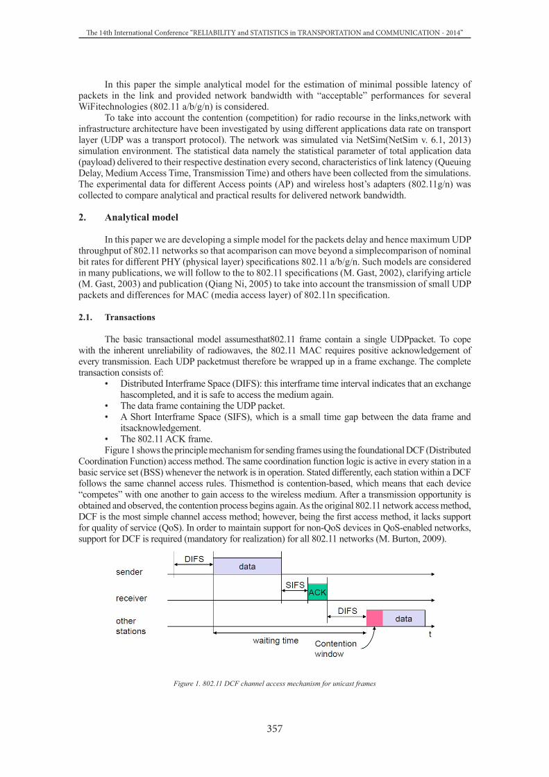
357


In this paper the simple analytical model for the estimation of minimal possible latency of packets in the link and provided network bandwidth with “acceptable” performances for several WiFitechnologies (802.11 a/b/g/n) is considered.

To take into account the contention (competition) for radio recourse in the links,network with infrastructure architecture have been investigated by using different applications data rate on transport layer (UDP was a transport protocol). The network was simulated via NetSim(NetSim v. 6.1, 2013) simulation environment. The statistical data namely the statistical parameter of total application data (payload) delivered to their respective destination every second, characteristics of link latency (Queuing Delay, Medium Access Time, Transmission Time) and others have been collected from the simulations. The experimental data for different Access points (AP) and wireless host’s adapters (802.11g/n) was collected to compare analytical and practical results for delivered network bandwidth.

2. Analytical model

In this paper we are developing a simple model for the packets delay and hence maximum UDP throughput of 802.11 networks so that acomparison can move beyond a simplecomparison of nominal bit rates for different PHY (physical layer) specifications 802.11 a/b/g/n. Such models are considered in many publications, we will follow to the to 802.11 specifications (M. Gast, 2002), clarifying article (M. Gast, 2003) and publication (Qiang Ni, 2005) to take into account the transmission of small UDP packets and differences for MAC (media access layer) of 802.11n specification.

2.1. Transactions

The basic transactional model assumesthat802.11 frame contain a single UDPpacket. To cope with the inherent unreliability of radiowaves, the 802.11 MAC requires positive acknowledgement of every transmission. Each UDP packetmust therefore be wrapped up in a frame exchange. The complete transaction consists of:

• Distributed Interframe Space (DIFS): this interframe time interval indicates that an exchange hascompleted, and it is safe to access the medium again.

• The data frame containing the UDP packet.• A Short Interframe Space (SIFS), which is a small time gap between the data frame and

itsacknowledgement.• The 802.11 ACK frame.Figure 1 shows the principle mechanism for sending frames using the foundational DCF (Distributed

Coordination Function) access method. The same coordination function logic is active in every station in a basic service set (BSS) whenever the network is in operation. Stated differently, each station within a DCF follows the same channel access rules. Thismethod is contention-based, which means that each device “competes” with one another to gain access to the wireless medium. After a transmission opportunity is obtained and observed, the contention process begins again. As the original 802.11 network access method, DCF is the most simple channel access method; however, being the first access method, it lacks support for quality of service (QoS). In order to maintain support for non-QoS devices in QoS-enabled networks, support for DCF is required (mandatory for realization) for all 802.11 networks (M. Burton, 2009).

Figure 1. 802.11 DCF channel access mechanism for unicast frames

358


2.2. Encapsulation

In addition to the payload data, there are 36 additional bytes of dataadded in the encapsulation process. The 802.11 MAC header adds28 bytes of data for various control and management functions,error detection, and addressing. A further eight bytes are added bythe SNAP encapsulation header to identify the network layer protocol (M. Gast, 2002). The total size of the l application bytes encapsulated in UDP packet and in 802.11 MAC frame is:

l + 8 (for UDP header)+ 20 (for IP header) + 36 (for MAC frame) = (l + 64) bytes = (8l + 512) bits.

2.3. Throughput

In our study we are interesting in throughput of the network at the UDP payload layer. So, if RFramethe frames rate on MAC layer, TFrame is the time to deliver the frame in the link and each transaction delivers one data frame, the rate for the application data on UDP layer RApp according with encapsulation will be:

FrameFrameAppPApp T

llRlRR 888 =⋅=⋅= (1)

bits per seconds, where l – the size of application packet in bytes.By adding up the total time required for each component ofthe transaction, a frame transaction rate can be derived.

2.4. Frame delivery time estimations

The transactional model is simplified, it neglects important effect. First of all, it assumesa steady stream of well-ordered frames with no contention for the medium. 802.11 implementscollision avoidance and exponential back off (in contention window, see Figure 1), so in reality, the time between frame exchanges will belonger than one DIFS. Exponential back off in the presence of contention will further decreasethroughput. (M. Gast, 2003) estimates that contention for the medium would reducethe maximum throughput figures above by 25% to 50%, depending on the exact assumptions made. So, if we do not take into account the contention period, we will estimate the minimal time for frame delivery. Other wordsless frame delivery time may not be and, if it satisfies not control application requirements, the WiFi technology is not applicable in this case.

Estimations for 802.11bThe baseline speed comes from 802.11b. It is not as fast as the newer specifications, but we

do the calculation for 802.11b first to compare with other. See table 1in what the parameters and calculations for different specifications are presented.First off, the basic timing numbers for 802.11b:

SIFS = 10 μsSlot time = 20 μsDIFS = 2 x Slot time + SIFS = 50 μs.802.11b requires that a preamble be prepended to every frame before it is transmitted to the air.

Thatpreamble may be either the traditional “long” preamble, which requires 192 μs for transmission, or itmay be an optional “short” preamble that requires only 96 μs. Support of the long preamble ismandatory, and is the default setting on most devices, so we will use in calculations only the long preamble.

802.11b running at the max speed (11 Mbps) divides data up into 8-bit symbols. There are (l+64) 8-bit blocks inthe UDPpacket. The 802.11 ACK does not haveSNAP headers, and is only 14 bytes long.Encoding the MAC frames is easy. 802.11b divides up the MAC frame into a series of 8-bit”symbols,” and then transmits 1.375 million symbols per second. So add up the individual componentsof the transaction to get the total duration:

For 802.11 data frame: 192 μs + ((l+64)/1.375) μs;For 802.11 ACK: 192 μs + (14/1.375) μs = 192 μs + 10μs= 202μs.As it is also can be seen in table 1 transaction for 802.11b when l=10 bytes requires 508μs

(TFrame). At that duration, 1968 exchanges can complete per second. With a UDP payload of 10 bytes per exchange, the throughput from relationship (1) is 0.157 Mbps.

359


Estimations for 802.11a802.11a is faster than 802.11b for two reasons: timing relationships between frames in the

exchanges, and the encoding used by 802.11a does not require such long preambles forsynchronization. The basic timing numbers for 802.11a in table 1.

Like 802.11b, 802.11a divides data up into a series of symbols for transmission. However, theencoding used by 802.11a uses much larger symbols. At 54 Mbps, each symbol encodes 216 bits. Fora full listing of encoding block sizes, see Table 11-3 in (M. Gast, 2002). The OFDMencoding used by 802.11a adds six bits for encoding purposes to the end of the frame.The 802.11 ACK also requires just one symbol.Each frame is prepared for transmission in the air with a 20 μspreamble to synchronize the receiver.Following the 20 μs header is a series of symbols, each requiring 4 μs(216 bits divided on 54 Mbps) for transmission.

At 105μs per transaction, it is possible to complete 9524 exchanges per second. That corresponds to a throughput of 0,762 Mbps.

Estimations for 802.11g802.11g operates in the same frequencyband as 802.11b, and is required to remain backwards-

compatible. The encoding used by 802.11g willnot be recognized by 802.11b stations, so “protection” mechanisms are defined to limit the cross-talkin mixed b/g environments. Essentially, the protection mechanisms require that 802.11g stationsoperating at high rates pre-reserve the radio medium by using slower, 802.11b-compatible reservationmechanisms.

802.11g SIFS = 10 μs802.11g short slot time = 9 μs (802.11g-only mode with no legacy stations)802.11g long slot time = 20 μs (mixed mode requires slow slot time)802.11g uses many of the same timing parameters as 802.11a. It inherits the short 10 μs SIFS

time from 802.11b, but the high-ratecoding in 802.11g needs additional time. Therefore, 802.11g adds a 6 μs “signal extension” time at theend of every frame.

When no 802.11b stations are present, no protection is required. The 802.11g ERP-OFDM PHY is nearly identical to the 802.11a PHY, except that it operates in adifferent frequency band and uses a shorter SIFS time. Physical layer headers are identical, as is thecoding. Therefore, the calculation for the time required to transmit a frame is nearly identical, withonly minor changes to the interframe space times (see table 1).

The transaction length of only 802.11g is identical to 802.11a. So, At105μs per transaction, it is possible to complete 9524 exchanges per second. That corresponds to a throughput of 0,762 Mbps.

Once the first 802.11b station associates with an 802.11g access point, however, protection is required. Figure 2 shows the principle mechanism for sending frames using the foundational DCFaccess method with RTS/CTS frames for protection.

Figure 2. 802.11 DCF channel access mechanism for unicast frames with RTS/CTS frames exchange

The minimal protection contemplated by the standard is that 802.11g stations will protect the fast802.11g frame exchange with a slow Clear To Send (CTS) frame that locks out other stations access tothe medium. Protection dramatically reduces the maximum theoretical throughput because

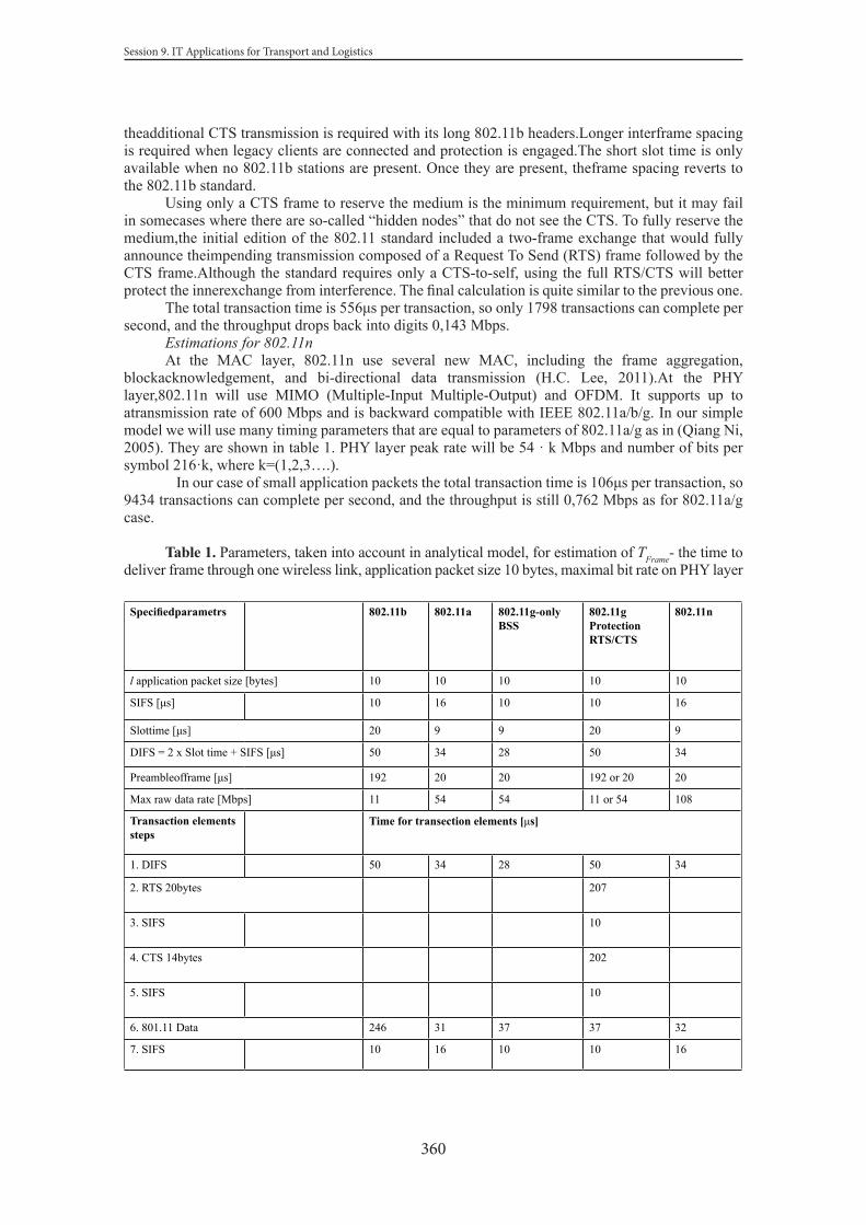
360


theadditional CTS transmission is required with its long 802.11b headers.Longer interframe spacing is required when legacy clients are connected and protection is engaged.The short slot time is only available when no 802.11b stations are present. Once they are present, theframe spacing reverts to the 802.11b standard.

Using only a CTS frame to reserve the medium is the minimum requirement, but it may fail in somecases where there are so-called “hidden nodes” that do not see the CTS. To fully reserve the medium,the initial edition of the 802.11 standard included a two-frame exchange that would fully announce theimpending transmission composed of a Request To Send (RTS) frame followed by the CTS frame.Although the standard requires only a CTS-to-self, using the full RTS/CTS will better protect the innerexchange from interference. The final calculation is quite similar to the previous one.

The total transaction time is 556μs per transaction, so only 1798 transactions can complete per second, and the throughput drops back into digits 0,143 Mbps.

Estimations for 802.11nAt the MAC layer, 802.11n use several new MAC, including the frame aggregation,

blockacknowledgement, and bi-directional data transmission (H.C. Lee, 2011).At the PHY layer,802.11n will use MIMO (Multiple-Input Multiple-Output) and OFDM. It supports up to atransmission rate of 600 Mbps and is backward compatible with IEEE 802.11a/b/g. In our simple model we will use many timing parameters that are equal to parameters of 802.11a/g as in (Qiang Ni, 2005). They are shown in table 1. PHY layer peak rate will be 54 · k Mbps and number of bits per symbol 216·k, where k=(1,2,3….).

In our case of small application packets the total transaction time is 106μs per transaction, so 9434 transactions can complete per second, and the throughput is still 0,762 Mbps as for 802.11a/g case.

Table 1. Parameters, taken into account in analytical model, for estimation of TFrame- the time to deliver frame through one wireless link, application packet size 10 bytes, maximal bit rate on PHY layer

Specifiedparametrs 802.11b 802.11a 802.11g-only BSS

802.11g Protection RTS/CTS

802.11n

l application packet size [bytes] 10 10 10 10 10

SIFS [μs] 10 16 10 10 16

Slottime [μs] 20 9 9 20 9

DIFS = 2 x Slot time + SIFS [μs] 50 34 28 50 34

Preambleofframe [μs] 192 20 20 192 or 20 20

Max raw data rate [Mbps] 11 54 54 11 or 54 108

Transaction elements steps

Time for transection elements [μs]

1. DIFS 50 34 28 50 34

2. RTS 20bytes 207

3. SIFS 10

4. CTS 14bytes 202

5. SIFS 10

6. 801.11 Data 246 31 37 37 32

7. SIFS 10 16 10 10 16

361


8. 802.11 ACK 14bytes 202 24 30 30 24

TFrame [μs] 508 105 105 556 106

In table 2 the calculations for different WiFi technologies are generalized and expressed through specified in specifications figures, application packets size and “physical” bit rate in the wireless link.

Table 2.Relationships for TFrame estimations for different specifications. UDP packets, application packet size l [bytes], Rraw-bit rate on PHY layer [Mbps]

Packets delays

In principal there is a latency of application packets on the path from initial to end node due to the time to deliver frame in one link TFrame, calculated on the previous steps, and queuing in the nodes at the time when radio channel is busy for transmitting another frames. It is true, if radio channel is common recourse as for an example in BSS, when all nodes are communicating through access point AP.

Figure 3. Queuing model of the channel with two links

According to the Queueing Theory, when requests with intensity λ are coming on sequence of serving nodes on what service is made with intensity μ and when time intervals between requests and time of request’s service are exponentially distributed (so called M/M/1model) the average service time will be:

ρρ

µµ −⋅+=1

11t , where ρ=λ/μ and 10 <≤ ρ (2.1)

Simplification of real world processes in this model for packets delay is obvious, but it accepted in many cases for the estimations in computer networks design. This model can be “easy improved”. For an example we may use M/G/1 instead M/M/1 approximation, when service tame has an arbitrary distribution and the average service time instead (2.1) will be:

D(t)- the variance of service time (for exponential distribution of service time c=1).Using (2.1) or (2.2), we can estimate the application packets delay DAppthrough the path of

several links. For (2.1) we have:

)RT

T(Dn

n,iAppPFrame

FrameAppn,in,i

n,ii ∑ ∑⋅−⋅=1

1, where (3)

Session 9. Information Technologies for Transport and Logistics

Table 2.Relationships for TFrame estimations for different specifications. UDP packets, application packet size l [bytes], Rraw-bit rate on PHY layer [Mbps]

802.11b 802.11a 802.11g-only BSS 802.11g Protection RTS/CTS

802.11n

TFrame [μs]

rawR)l( 788444

rawR

)l( 664894

rawR)l( 664894

rawR

)l( 62348520

rawR)l( 6648100

2.5. Packets delays

In principal there is a latency of application packets on the path from initial to end node due to the time to deliver frame in one link TFrame, calculated on the previous steps, and queuing in the nodes at the time when radio channel is busy for transmitting another frames. It is true, if radio channel is common recourse as for an example in BSS, when all nodes are communicating through access point AP.

Figure 3. Queuing model of the channel with two links

According to the Queueing Theory, when requests with intensity λ are coming on sequence of serving nodes on what service is made with intensity μ and when time intervals between requests and time of request’s service are exponentially distributed (so called M/M/1model) the average service time will be:

1

11t , where ρ=λ/μ and 10 (2.1)

Simplification of real world processes in this model for packets delay is obvious, but it accepted in many cases for the estimations in computer networks design. This model can be “easy improved”. For an example we may use M/G/1 instead M/M/1 approximation, when service tame has an arbitrary distribution and the average service time instead (2.1) will be:

)()c(t

12111 2

, wheret

)t(Dc (2.2)

D(t)- the variance of service time (for exponential distribution of service time c=1). Using (2.1) or (2.2), we can estimate the application packets delay DAppthrough the path of several

links. For (2.1) we have:

)RT

T(Dn

n,iAppPFrame

FrameAppn,in,i

n,ii 1

1, where (3)

nenumerateslinks on the paths of packets, and ienumerates the applications.For the clarification of relationship (3) several examples.

Example1

Node1, connected through WiFi channel to AP, transmits to Node2. Node2 is connected to AP with wired network. If we neglect with the delay in wired network, (3) gives:

362


nenumerateslinks on the paths of packets, and ienumerates the applications.For the clarification of relationship (3) several examples.

Example1Node1, connected through WiFi channel to AP, transmits to Node2. Node2 is connected to AP

with wired network. If we neglect with the delay in wired network, (3) gives:

FrameAppPFrameApp TR

TD⋅−

⋅=1

1 (3.1)

Example 2Node1 and Node2 are in the same BSS and Node 1 transmits to Node2. So, we have 2 wireless

links and (3)gives:


TD⋅⋅−

⋅⋅=21

12 (3.2.1)

On the basis of M/G/1 model for this example 2 we receive:

FrameAppP


TR)c(TD

⋅⋅−⋅⋅−+

⋅⋅=21

112

2

(3.2.2)Example 3Node1 and Node2 are in the same BSS. Node 1 transmits to Node2 and Node2 transmits to

Node1. If characteristics of application traffic for Node1 and Node2 are the same, the delay of packets in both directions from (3) will be:


TD⋅⋅−

⋅⋅=41

12 (3.3.1)

On the basis of M/G/1 model for this example 3 we receive:

FrameAppP


TR)c(TD

⋅⋅−⋅⋅−⋅+

⋅⋅=41

1212

2

(3.3.2)

Example 4Node1 and Node2 are in different BSSs generated by AP1 and AP2. APs are connected through

wired network. Characteristics of application’s traffic are different: from Node1 to Node2 data rate is RApp1 and from Node2 to Node1data rate is RApp2. Moreover the times of frames delivery are different for applications and links (for an example in BSS1 802.11g-only is but in BSS2 802.11g with RTS/CTS protection is on). For transmission from Node1 to Node2 in BSS1 link the frame time is TFrame11 and in BSS2 link TFrame12. Respectively for packet stream from Node2 to Node1 the times are TFrame22 and TFrame21. In this case from (3):

For the delay of packets from Node1

122112

1121111 1

11

1

FrameAppPAppPFrame

FrameAppPAppPFrameApp T)RR(

TT)RR(

TD⋅+−

⋅+⋅+−

⋅= ,

and for the delay of packets from Node2

212121

2221222 1

11

1

FrameAppPAppPFrame

FrameAppPAppPFrameApp T)RR(

TT)RR(

TD⋅+−

⋅+⋅+−

⋅=

2.5. Network bandwidth for applications

For automation control applications we suppose that network bandwidth will be acceptable if traffic of packets can be delivered and the delay of packets remains in acceptable range. We will not write general relations for the bandwidth they are pretty obvious for our model of delays in the packagedelivery but we will consider maximal possible and “acceptable” bandwidth for the example 2 from topic 2.5 Packets delays.

363


For this case (Node1 and Node2 are in the same BSS and Node 1 transmits to Node2, we have 2 wireless links) from (3.2.1) (or from (3.2.2)) the maximal application possible throughput or maximal bandwidth can be achieved when expression in the denominator is equal to zero, hence:

Frame

MaxAppP

MaxApp

MaxApp T

llRBR2

88 =⋅⋅=≡ in bits per second, (4)

as above, l– the size of application packets in bytes.But, when application data rate achieves its maximum, the number of packets in queues and

packets delay tends to infinity. In many practical cases it is reasonable to limit the packet delay to some value. If we accept that the average delay not greater than two its possible minimal values (physical sense – only one packet waits in a queue, see (2.1)), then for our example 2:

FrameApp T

lB4

8=

(5)

This bandwidth should be considered as “acceptable” in the sense that if application data rate

RApp not exceeds bandwidth BApp the package delay will be in the range MinAppApp

MinApp DDD 2≤≤ .

Completely analogous for the example 3 (Node1 and Node2 are in the same BSS. Node 1 transmits to Node2 and Node2 transmits to Node1) the acceptable network bandwidth will be:

FrameApp T

lB8

8= (6)

2.6. Analytical model summarization

Thus,developed on previous steps model, gives the basis for the estimations of delays in

application packets delivery through the network with wireless links. The delay on every packet

path in our model is a function of network structure Sr

, structure of payload on application level AppR

rand parameters of wireless technologies P

r used in the wireless links. Calculations for delays

)T,R,S(D FrameAppApp

rrrfunction are presented in topic (2.5. Packets delays) and MAC frames

transmission time through wireless links for different WiFi specifications )l,P(TFrame

rcalculations

are presented in table 2. Application payload (the size of packets l) is carried by UDP transport layer

protocol.

3. Simulation

For the validation of analytical estimations we have performed several numeric simulations. The simulation and analytical results for two network and application payloadstructures what we have considered in the topic 2.5. Packets delays are presented on figure 4 and figure 5. The structures were from Example 2 and Example 3. The payload in all cases is provided by “small” UDP packets, the application part size is 10 bytes. On figure 4 the results for 802.11b wireless links and on figure 5 for 802.11g-only. As the simulation environment NetSim(NetSim v. 6.1, 2013) were used.

On figure 4 we can see, that for simulation of Example 2 (Node1 and Node2 are in the same BSS and Node 1 transmits to Node2, communications through links under 802.11b specification take place) packets delay time per link is about 2 milliseconds when application payload is near 39 kilobits per second (refer to points on the graph marked as rhomb as shown on legend panel). We refer to delay per link because in all our cases the parameters of all links were the same. For Example 2 only one path exists (from Node 1 to Node 2) and the delay on the path will be multiplied by two (4 ms in case above).

364


The analytical model calculated as (3.2.1) (curve “Ex2,M/M/1” on the graph) gives us in this case near 1 ms but calculated as (3.2.2) (curve “Ex2,M/G/1,c=1,6”), if we suppose c=1.6, gives estimation near 1.9 ms.

On the graph also the “acceptable” bandwidth is shown (line “Ex2 bandwidth” for Example 2, when RApp=39.4 Kbps and line “Ex3 bandwidth” for Example 3, when RApp=19.7 Kbps), calculated as (5) and (6) respectively.

On figure 5 (when WiFi technology 802.11g-only for the links is used) one can see other numerical values but similar dependences.

Figure 4.Simulation and analytical results for structures of Example 2 and Example 3. 802.11b links in BSS

Figure 5.Simulation and analytical results for structures of Example 2 and Example 3. 802.11g-only links in BSS

365


Comparing simulation and analytical model results, one can go to conclusion that they are in a good correspondence in appropriate range of payloads. The range is lager for M/G/1 than M/M/1 analytical model approximation. The range of such “validity” (for M/G/1) is from zero to about “acceptable” bandwidth calculated for M/M/1 model ((5) and (6) for Example 2 and Example 3). Using M/G/1 approximation, one needs to know variation coefficient c (see (3.2.2) and (3.3.2)) for the distributions of time in frame delivery through wireless link. For our simulation models it was found in the range 1.5 – 1.6. For many processes in computer systems this coefficient not greater than 3. In our cases we can recommend for estimations to take c from the range 1 – 3 (1 when exponential distribution is supposed, 1.5 for “optimistic” and till 3 for “pessimistic” estimations).

4. Experiments

For the validation of some analytical estimation several experiments have been made on real WiFi networks with different types of computer wireless adapters and Access Points. In this paper we present the results for measuring maximal possible throughput on application level from what frame transfer time under experimental circumstances can be received. In this experiments the network structure was as in Example 1 (Node1, connected through WiFi channel to AP, transmits to Node2. Node2 is connected to AP with wired network). The UDP packets with application data size of 10 bytes perform the payload on one Node1-wireless link-AP-wired link-Node2 in this case. Jperf version 2.0.2 utility as network performance measurement tool was used. The measurement results are presented in table 3.

Table 3.The measurement results for maximal throughputType of AP used TP-Link 150M Wireless Lite N Router Wireless-N Gigabit Router WRT350N

AP mode 802.11g only 54 Mbps

Measured parameters Maximal throughput [Kbps]

Jitter [ms] Maximal throughput [Kbps]

Jitter [ms]

Mean value for 10 time intervals, one interval 1s 451 0.173 433

Standard deviation 7.87 0.242 25.06

10 byte packet delivery time [ms] 0.177 0.185

Using results from experiments we can check significance of some our analytical estimations. So, 10 byte packet delivery time indicated as 0,177 ms we can compare with TFrame estimation in table 1 for 802.11g-only column (0,105 ms) as our experiment structure corresponds to Example 1for what the maximal throughput due to (3.1) will be achieved at the bitrate 1/TFrame. Estimations in table 1 give the minimal possible TFrame (the concurrent process for the wireless media is not taken into account, also we neglect of the delays in hardware/software structures of Nodes and wired network). So, the correspondence of analytical and experimental figures is sufficient. Also from the experiment we can estimate the variance coefficient c from measuring of jitter, and it is of the order of 1.4 what is consistent with our recommendations in the topic (3.Simulation).

5. Conclusions

In the matter of fact we have proposed an approach for the estimations of application packets delay time on propagation paths through the network in what wireless links are present. It is done on the basis of analytical model summarized in this article topic (2.7. Analytical modelsummarization). Packets delays have often restricted due to automation control applications and need to be in appropriate range of values for the working diapason of application’s payload. Our analytical model gives the relationships between delays and bit rate on application level.

The delays in wireless links frames transfer are considered for 802.11 MAC layer specifications (often called as WiFi). Only DCF (Distributed Coordination Function) access method was under consideration and PHY layer specifications 802.11 a/b/g/n were analyzed. On transport layer of the network UDP protocol was used which carry application packets of small size (no packetization is

366


performed as for Voice over IP case) and this is often a demand of automation control applications.In wireless channel no pass loss, fading and interference was supposed but those effects

may be taken into account in analytical model by reducing maximal possible raw bit rate given by specifications of PHY layer to some lover bit rate (also according with specifications).

If we proceed with the example of wireless electric recharge of driving vehicles system what demands for data transmission were formulated in introduction of this article. When network design suppose communication between system modules through one Access Point, using the analytical model one can receive the next estimations:

Table 4. Values for comparing application demands and possibilities of WiFi technologies Demand of the system

WiFi technology 802.11 b WiFi technology 802.11 g-only

For raw speed 1Mbps

For raw speed 11Mps

For raw speed 6Mbps

For raw speed 54Mbps

Application packet size 72 bit 72 bit 72 bit 72 bit 72 bit

Data rate for one application stream 7.2 Kbps 7.2 Kbps 7.2 Kbps 7.2 Kbps 7.2 Kbps

Packets delay on the path of two links 18 ms 5.4 ms 1.44 ms 0.43 ms 0.23 ms

Comparing the value in table 4 (18 ms with 5.4, 1.44, 0.43, 0.23 ms) one can make a conclusion that both technologies 802.11b and 802.11g are applicable for wireless system design of considered structure and payload even in the case when sufficient disturbances can be expected in wireless channel.

Performed simulations and field experiments are not in contradictions with proposed analytical model.

References

1. A.V Gordyushins, R. Saltanovs, I. Galkins, T.V Lohman, A. Baums. “Investigation of the system to recharge the public vehicles”, Electric power industry through the eyes of Youth 2013, Proceedings of the IV International scientific conference 14-18 October 2013 Novocherkassk, Volume 2, pp 251-254.

2. NetSim simulation environment http://www.tetcos.com/netsim_academic.3. Matthew Gast. “802.11 Wireless Networks: The Definitive Guide”, O’Reilly, 2002, 464 pp.4. Matthew Gast. “When Is 54 Not Equal to 54? A Look at 802.11a, b, and g Throughput”,

published on Wireless DevCenter (http://www.oreillynet.com/wireless/), 2003.5. Qiang Ni. “Design and Analysis of MAC Protocol for IEEE 802.11n”, published of Hamilton

Institute (www.hamilton.ie/ncnrc/) , 2005, 23 pp.6. Marcus Burton. “802.11 Arbitration”, White paper of CWNP Inc.(www.cwnp.com/), 2009, 24

pp.7. Ha Cheol Lee. “DCF Throughput Analysis of IEEE 802.11a/g/n-based Mobile LAN over

Correlated Fading Channel”, International Journal on Electrical Engineering and Informatics ‐ Volume 3, Number 4, 2011, pp 415-430.

367



DOMAIN-SPECIFIC SOFTWARE ARCHITECTURE OPTIMISATION FOR LOGISTICS AND TRANSPORT

APPLICATIONS

Sergey Orlov, Andrei Vishnyakov

Transport and Telecommunication InstituteLomonosova str.1, Riga, LV-1019, Latvia

E-mail: [email protected], [email protected]

The domains of logistics and transport systems are complex, so it’s necessary to use modern design approaches that could cope with that complexity. Domain-Driven Design is one of approaches that can solve such problems. Unfortunately, all the existing well-established software architecture design and quality evaluation techniques are not directly applicable for this approach.

In this paper the metric suite that allows evaluating the quality of the created domain model for logistics and transport systems is proposed. On the base of this, the technique that allows selecting the optimal suite of patterns for software architecture creation using Domain-Driven Design. The software architecture construction is reduced to the classical problem of integer programming where the optimal solution should be found. The results allow us making conclusions about usefulness of the proposed technique during architecture design phase for transport and logistics software.Keywords: Domain-Driven Design, Domain-Specific Software Architecture, architecture efficiency metrics, logistics and transport software.

1. Introduction

Architectural and detailed design of modern logistics and transport software has a huge impact on a quality and cost of the development process, hence it’s required to pay reasonable attention while making architectural and design decisions. The formation of architecture is the first and fundamental step in the designing process that provides the framework of a software system, which can perform the full range of detailed requirements (Orlov and Tsilker, 2012; Bass et al., 2013).

At the moment, there are no well-established techniques used for software architecture design and quality evaluation. In papers (Orlov and Vishnyakov, 2012, 2013) is proposed a technique that allows evaluating and creating a software architecture that is based on reusing number of enterprise architecture patterns.

Usually, the domains of logistics and transport systems is not trivial, so approaches like Domain-Driven Design (Evans, 2003) and Domain-Specific Software Engineering (Taylor et al., 2009) might be used for such software development. Although Domain-Driven Design and Domain-Specific Software Engineering methodologies are not well formalized. Also they lack of metric suites for evaluation of architecture’s quality. Unfortunately the technique proposed in works (Orlov and Vishnyakov, 2012, 2013) could not be applied for Domain-Driven Design, as this approach is quite different compared to “classical” software design processes.

This paper propose metric suite that allows evaluating the quality of the created domain model for logistics and transport systems. On the base of this, the technique that allows selecting the optimal pattern suite for software architecture built using Domain-Driven Design (Evans, 2003).

2. Selection of an Optimal Pattern Suite

2.1. Overview

The proposed technique allows obtaining an optimal pattern suite for a software architecture that is built using Domain-Driven Design (Evans, 2003; Vernon, 2013). If we would like to be able to apply this technique, first, we have to get the domain model of the system. Next, the domain model

368


should be separated into Bounded Contexts, and relationships between them should be defined. After that, according to the requirements, Bounded Context and Context Map patterns should be chosen. Implementation of these components can be accomplished by using various combinations of patterns, where the domain patterns may be implemented using enterprise (Fowler, 2002) and integration patterns (Hohpe and Woolf, 2003). In other words, based on the defined domain model and number of domain and enterprise patterns, we want to create an architecture that uses an optimal pattern suite.

Figure 1 shows a graphical representation of this technique.

Figure 1. Graphical representation of the technique

2.2. Domain-specific software architecture efficiency metric

Once the domain model is created, we can split it down into Subdomains and Bounded Contexts. Subdomains could be classified as Core Domain, Generic Subdomains and number of Supporting Subdomains. Usually, Subdomains are logical partitioning of the domain model; on the contrary, Bounded Contexts is domain model decomposition into individual components of the architecture. Technically, they could overlap and include several elements. In this paper we focus mostly on Bounded Context and Context Map.

As long as each separate Bounded Context is isolated from other Bounded Context using Context Map, each Bounded Context can be considered separately (Figure 2). Thus, architecture efficiency metric of the entire system can be represented as a sum of architecture efficiency metric for each Bounded Context plus architecture efficiency metric for every Context Map.

Figure 2. Bounded Contexts

To determine architecture efficiency metric let’s introduce the following notation. Suppose that there is a set of Bounded Contexts in a Domain Model — 1,..., .iBC i g=

369


Also there is a set of Context Map — 1,..., .iCM i k=Since each pair of Bounded Contexts may have one Context Map between them, the maximum

number of possible Context Maps is the number of edges of a complete graph:( 1)2

g gn × −= ,

where g – the number of vertices in the graph.From the above it follows that the architecture efficiency metric for software architecture in

general can be represented as follows:

1 1i i

g n

A BC CMi i

K K Kα β= =

= × + ×∑ ∑whereKBCi – the value of architecture efficiency for i-th Bounded Contexts;

KCMi – the value of architecture efficiency for i-th Context Map;

α, β – weight coefficients where 1α β+ = .

2.3. Domain model function points analysis

Before going to the components of the architecture efficiency metric, let’s consider the metric that can evaluate part of domain model that is implemented in particular Bounded Context.

In other words, we want to estimate a complexity of the domain model, where for basis we take Functional Points metric. In this metric we replace Unadjusted Function Point count to Domain model Unadjusted Function Point count.

Thus, the metric is defined as follows:14

1

0.65 0.01 ,ii

DFP DUFP F=

= × + ×

∑

whereDUFP – Domain model Unadjusted Function Point count;Fi – general system characteristics that corresponds to Fi from original FP metric. For Unadjusted Function Point count calculation in the original Functional Points metric, the

system is divided into smaller components, such as Internal Logical Files, External Logical Files, External Inputs, External Outputs and External Inquiry (Orlov and Tsilker, 2012).

For domain model we are interested in components that could be implemented in Bounded Context, including: Entities, Value Objects, Aggregates, Domain Services, and Domain Events.

For each listed component in the domain model we need to specify number of ranks and ratings, which are listed in table 1. Values in the table is based on experience and may require additional calibration, as we validated it only on small number of samples.

Table 1. Input data for obtaining Domain model Unadjusted Function Point countComponent type Component complexity Total

Low Average High

Entities __ x 4 = E1 __ x 5 = E2 __ x 7 = E3 E1+E2+E3=Eall

Value Objects __ x 2 = V1 __ x 3 = V2 __ x 4 = V3 V1+V2+D3=Vall

Aggregates __ x 7 = A1 __ x 10 = A2 __ x 15 = A3 A1+A2+A3=Aall

Domain Services __ x 5 = DS1 __ x 7 = DS2 __ x 10 = DS3 DS1+DS2+DS3=DSall

Domain Events __ x 4 = DE1 __ x 5 = DE2 __ x 7 = DE3 DE1+DE2+DE3=DEall

Total DUFP: Eall+Vall+Aall+DSall+DEall

370


Having the value of Domain model Unadjusted Function Point count, as well as the values of all general system characteristics, we can obtain the value of Domain model Functional Points metric.

2.4. Coupling and cohesion of domain model

In the Object Oriented world there are various metrics that evaluate coupling and cohesion. The most commonly used are Coupling between Object Classes (CBO) and Lack of Cohesion of Methods (LCOM) metrics from Chidamber & Kemerer’s metric suite (Orlov and Tsilker, 2012).

In accordance with them we introduce the following metrics:• Coupling Between domain model Components (CBC); • Lack of Cohesion of domain model Component Methods (LCCM).CBC and LCCM metrics are calculated for specific components, but we need to evaluate the

entire system. So it’s necessary to make these metrics applicable for a group of components. We define Coupling Between domain model Components Factor (CBCF) and Lack of Cohesion of domain model Component Methods Factor (LCCMF) metrics that could be used in our criterion of efficiency.

CBCF metric is defined as the arithmetic mean of the normalized values of CBC in the system (the value of this factor varies from 0 to 1):

1

,,

,

Ni i CBC

i CBC

CBC

CBC if CBC TT else

CBCFT N

=

< =

×

∑

whereCBC — the value of Coupling Between domain model Components metric;TCBC — threshold that cut down very large values of CBC. Such limitation is necessary as the

theoretical value of CBC may vary indefinitely;N — number of components in the domain model.The definition of LCCMF metric is similar, i.e. LCCMF defined as the arithmetic mean of the

normalized values of LCCM in the system:

1

,,

,

Ni i LCCM

i LCCM

LCCM

LCCM if LCCM TT else

LCOMFT N

=

< =

×

∑

whereLCCM — the value of Lack of Cohesion of domain model Component Methods metric;TLCCM — threshold that cut down very large values of LCCM. Such limitation is necessary as

the theoretical value of LCCM may vary indefinitely;N — number of components in the domain model.

2.5. Domain Model efficiency metric

In order to evaluate the domain model we introduce the domain model efficiency metric K, which is defined as:

1

2 3

,(1 ) (1 )

DFPKCBCF LCCMF

αα α

×=

− × × − ×

whereα1, α2, α3 – weight coefficients of efficiency indicators;DFP — the value of Domain model Functional Points;CBCF – the value of Coupling Between domain model Components Factor;LCCMF – the values of Lack of Cohesion of domain model Component Methods Factor.

371


2.6. Bounded Context architecture efficiency metric

The value of architecture efficiency for i-th Bounded Contexts can be defined as:,

iBC iK K=

whereKi – the value of K for i-th Bounded Context.For the separation of different functional responsibilities of separate Bounded Context we can

use Layered Architecture. Besides Layered Architecture, there are other architectures that support the separation of the program, such as Hexagonal Architecture, Onion Architecture, etc. Figure 3 shows the case where Layered Architecture is applied for several Bounded Contexts.

Figure 3. Layered Architecture

Layered Architecture might contain the following layers: Persistence Layer, Domain Layer, Application Layer, Presentation/UI Layer, Infrastructure Layer, etc.

There are various patterns which could be applied for each layer of this model. For different systems the most suitable patterns depends on size of a system and also on requirements.

Martin Fowler in his book (Fowler, 2002) presents the following patterns suitable for some layer:

• Domain Layer: Domain Model, Transaction Script, Table Module.• Persistence Layer: Table Data Gateway, Row Data Gateway, Active Record, Data

Mapper.• Presentation Layer: Model View Controller, Page Controller, Front Controller, Template

View, Transform View, Two-Step View, Application Controller.He indicates (Fowler, 2002) the steps how to select a pattern from multiple groups taking

into account the requirements for the software. Also he indicates the relationship between groups of patterns, for example, it’s allowed to choice only one pattern from multiple groups, etc. The other groups of patterns might be also considered for the architecture development.

In order to determine which pattern is better suited according to requirements of a system, let’s define a partial pattern-architecture efficiency metric K’ which is defined as:

1

2 3

'' ,(1 ' ) (1 ' )

PiPi

Pi Pi

DFPKCBCF LCCMF

αα α

×=

− × × − ×

whereDFP’Pi — the value of DFP if pattern Pi is used for software development;CBCF’Pi – the value of CBCF if pattern Pi is used for software development;LCCMF’Pi – the value of LCCMF if pattern Pi is used for software development.DFP’ is a modification of the original DFP and it is calculated as follows:

372


14

1

' 0.65 0.01 ,ii

DFP DUFP CF=

= × + ×

∑

whereDUFP – Domain model Unadjusted Function Point count;and CFi – defined as follows:

5, 5;( ), ,

i ii

i i

if c FCF

round c F otherwise× >

= ×

whereСFi — adjusted degree of influence coefficient, which corresponds to Fi used in original DFP;ci — pattern influence on i-th system’s characteristic.For getting ci values, first, we need to evaluate a characteristic using the following scale:• 1 — use of a pattern reduces the significance of a system characteristic;• 2 — use of a pattern slightly reduces the significance of a system characteristic;• 3 — no influence;• 4 — use of a pattern slightly actualises a system characteristic;• 5 — use of a pattern actualises a system characteristic (i.e. we must pay more attention

to this characteristic when applying this pattern).Next, these values are converted into ci using scale conversion rule presented in Table 2.

Table 2. Characteristic’s evaluation scale correspondence to ci valueScore As ci

1 ½

2 ⅔

3 1

4 1½

5 2

CBCF’ metric is modification of CBCF and it is defined as:

( )' 3PiCBCF CBCF CBCF cα= + × × − ,

whereCBCF – the original value of Coupling Between domain model Components Factor;α – weight coefficient;cPi – pattern influence on CBCF which is evaluated using scale similar to ci and varies from 1

to 5.LCOMF’ metric is defined as:

( )' 3PiLCCMF LCCMF LCCMF cα= + × × − ,

whereLCCMF – the original value of Lack of Cohesion of domain model Component Methods

Factor;α – weight coefficient;cPi – pattern influence on LCCMF which is evaluated using scale similar to ci and varies from

1 to 5.

2.7. Context Map architecture efficiency metric

When implementing Context Map we can use a number of different domain patterns. In the book (Vernon, 2013) are offered the following patterns that could be used for context mapping: Anti-Corruption Layer, Shared Kernel, Open Host Service, Publish-Subscribe, Published Language, Customer-Supplier, Conformist, Partnership, Separate Ways.

373


When considering the implementation of Context Map it’s necessary to consider the relation of connected Bounded Contexts. This relation consists of upstream and downstream sides. Upstream model have influence on downstream model. For each side of relation different integration patterns should be used. It is also obvious that this dependence should be taken into account in architecture efficiency metric.

Figure 4 shows relationship of three Bounded Contexts, where Context Map is implemented using the following patterns: Open Host Service, Published Language and Anti-Corruption Layer.

Figure 4. Context Maps with integration points

We can determine a number of alternatives of Context Map implementation; for example, the figure shows an implementation that uses Anti-Corruption Layer for the downstream side; Open Host Service and Published Language for the upstream side.

Thus, for every specific case we can choose different alternatives. In turn, such alternative that contains number of Bounded Context’s patterns can be implement using number of integration patterns. More precisely, existing integration patterns can be joined into groups, where from each group we can select one or more patterns for part of Bounded Context implementation.

It’s rationally to consider integration patterns together with Context Map. There are several different Integration Styles available for handling integration, including: File Transfer, Shared Database, Remote Procedure Invocation and Messaging. In modern distributed systems most commonly the Messaging style is used, as other integration styles have a serious flaws.

Messaging includes a number of components: Message, Message Channel, Message Router, Message Translator, Message Endpoint, etc. Each of these components could be implemented using number of different patterns.

In (Hohpe and Woolf, 2003) are listed the following integration patterns:Messaging Channels: Point-To-Point Channel, Publish-Subscribe Channel, Datatype

Channel, Guaranteed Delivery, Message Bridge, Message Bus.Message Routing: Content-Based Router, Message Filter, Dynamic Router, Recipients List,

Splitter, Aggregator, Resequencer, Composed Message Processor, Scatter-Gather, Routing Slip, Process Manager, Message Broker.

Messaging Endpoints: Messaging Gateway, Messaging Mapper, Transactional Client, Polling Consumer, Event-Driven Consumer, Competing Consumer, Message Dispatcher, Selective Consumer, Durable Subscriber, Idempotent Receiver, Service Activator.

According to the mentioned above, we need to consider upstream and downstream sides in our metric. It’s obviously that upstream and downstream sides have different impact on the system; so to account it we introduce weight coefficients.

374


Thus, the value of architecture efficiency for i-th Context Map can be determined as follows:

i i iCM UP DOWNK K Kα β= × + ×,

whereKUPi – the value of K of upstream side for i-th Context Map;KDOWNi – the value of K of downstream side for i-th Context Map;α, β – weight coefficients where 1α β+ = .In a similar way define partial pattern-architecture efficiency for Bounded Context:

' ' 'i i iCM UP DOWNK K Kα β= × + × ,

whereK’UPi – the value of KUPi if pattern Pi is used for software development;K’DOWNi – the value of KDOWNi if pattern Pi is used for software development;α, β – weight coefficients where 1α β+ = .

2.8. Model definition for selection of an optimal pattern suite

To find the optimal pattern suite it’s necessary to build a model, and then solve the problem of integer programming. As we consider Bounded Context and Context Map separately, both these parts must be taken into account in our model.

The model for a domain model in general is defined as:

1 1

min 1,..., min 1,...,ij ij

g n

BC CBi i

W W j n W j mα β= =

= × = + × =∑ ∑ ,

whereWBCij – the optimal solution of i-th Bounded Context using j-th base architecture;WCBij – the optimal solution of i-th Context Map using j-th implementation alternative of

Context Map;α, β – weight coefficients where 1α β+ = .The unknown components here are the objective functions for Bounded Context and Context

Map, which we define in the following sections.

2.9. Steps of selection of the optimal pattern suite for Bounded Context

To determine optimal pattern suite for specific Bounded Context let’s introduce the following notation.

Suppose that there is a set of base architectures that could be used for implementation of Bounded Context – 1,..., iBA i n= . Examples of such base architecture could be Layered Architecture, Hexagonal Architecture, Onion Architecture, etc.

Each such base architecture may contain a number of components: 1,..., ; 1,..., ij iC i n j l= = .

For example, for Layered Architecture the considered components are layers of the architecture, i.e. Persistence Layer, Domain Layer, Application Layer, Presentation Layer, etc.

Each component can be implemented using a specific pattern. A set of such patterns applicable to a particular component are organized in groups:

1,..., ; 1,..., ; 1,..., ,ijk i jP i n j l k m= = =

wherePijk — k-th pattern from group j (for implementation of component j) for base architecture type i;li — number of components (groups) for base architecture i, which is a variable number;mj — number of pattern in group j, which is a variable number.As an example, assume that Domain Layer can be implemented using one of the following

patterns: Domain Model, Transaction Script, Table Module. In other words, these patterns must be combined in to the single pattern group, which are used for single architecture layer implementation.

375


Let’s assume that from some groups we aren’t obligated to select a pattern (this is due to the fact that the selection of some patterns can exclude a whole group of patterns). On the other hand, we can select several patterns from some of the groups.

Thus the input data for our model makes a complete set of patterns for each group, and such set can be represented as a multiset.

We can consider all the different implementation of Bounded Context separately. Also for simplicity, we reduce the multiset to a uniform set of patterns 1 ,..., mP P where we use special restrictions for partitioning to the groups.

At the output, the model with the specified constrains should select the optimal combination of patterns which should be used for software development.

The produced restrictions should exclude those combinations of patterns that are logically inconsistent or interchangeable. In addition, some restriction should allow selection of multiple patterns from specified group of patterns.

The objective function for finding the optimal suite of pattern for i-th base architecture type defined as follows:

( )1 1 2 2( ) ( )i m mW f P x f P x f P x min= × + × +…+ × → ,

wheref(Pj) — function which reflects a numerical changes of the system characteristics depending

on used pattern Pj;xj — variable which indicates the usage of the j-th pattern.It’s obviously that the integrally constrain should be applied for a given variable xj:

0, 1 1,2,..., ,jx i m= =

where m — number of patterns in the one dimensional set which were transformed from the original

multiset of patterns.To indicate the fact that we can select only one pattern from the group, let’s introduce the

following restriction:

1,i end

ii start

x=

=

=∑wherestart, end — the start and end indices of patterns in a group.To take in to account that, the selection of the j-th pattern excludes patterns from a different

group, we use the following restrictions:

1.i end

j ii start

x x=

=

+ =∑If we can select any number of patterns from the group we specify the following constrains:

( 1).i end

ii start

x end start=

=

≤ − +∑On the base of the mentioned definitions and assumptions, we obtain the classical integer

programming problem where we need to find the optimal solution.Next, we need to obtain the best solutions for all alternatives of base architectures and choose

the best one:

min 1,..., BC iW W i n= = .

Our function which reflects numerical changes of the system characteristics depending on used pattern Pi defined as follows:

376


'( ) iP

i

Kf P

K=

,whereK — the metric of architecture efficiency for Bounded Context;K’Pi — metric of partial pattern-architecture efficiency for Bounded Context (if pattern Pi is

used for software development).

2.10. Steps of selection of the optimal patter suite for Context Map

To determine optimal pattern suite for specific Context Mat let’s introduce the following notation.Suppose that there is a set of alternative implementations of Context Map – 1,..., iCM i n=

. For example, we can use Anti-Corruption Layer from downstream side; and Open Host Service and Published Language from upstream side.

Each such alternative implementation of Context Map may contain a number of components:

1,..., ; 1,..., .ij iCMP i n j l= =

Some of these patterns for context mapping may be implemented using one or several integration patterns. Sets of such integration patterns applicable to a particular context mapping pattern should be joined in to pattern groups:

1,..., ; 1,..., ; 1,..., ,ijk i jP i n j l k m= = =wherePijk — k-th pattern from group j (for implementation of context mapping pattern j) for Context

Map’s alternative i-th implementation;li — number of Context Map implementations (groups) i, which is a variable number;mj — number of pattern in group j, which is a variable number.Let’s assume that from some groups we aren’t obligated to select a pattern and from some

groups we can select several patterns.We can consider all the different implementation of Context Map separately. Also for simplicity,

we reduce the multiset to a uniform set of patterns 1 ,..., mP P where we use special restrictions for partitioning to the groups.

At the output, the model with the specified constrains should select the optimal combination of patterns, which should be used for Context Map’s alternative implementation.

The objective function for finding the optimal suite of pattern for i-th Context Map architecture defined as follows:

( )1 1 2 2( ) ( )i m mW f P x f P x f P x min= × + × +…+ × → , (1)

wheref(Pj) — function which reflects a numerical changes of the system characteristics depending

on used pattern Pj;xj — variable which indicates the usage of the j-th pattern.Similar restrictions as for Bounded Context model could be applied for this model as well.Next, we need to obtain the best solutions from all alternatives of Context Map implementation:

min 1,..., CM iW W i n= = .

Our function which reflects numerical changes of the system characteristics depending on used pattern Pi defined as follows:

'( ) iCM

iCM

Kf P

K=

, (2)whereKCM — the metric of architecture efficiency for Context Map;K’CMi — metric of partial pattern-architecture efficiency for Context Map (if pattern Pi is used

for software development).

377


3. Case study

3.1. Domain Model

For a case study let’s find an optimal pattern suite for one Bounded Context from the Subdomain of airline business’ Domain Model. Part of this domain model is shown on figure 5; it consists of two Bounded Contexts: Customer Bounded Context and Ticket Bounded Context.

Figure 5. Sub-domain of airline business Domain Model

3.2. Mathematical model building

After we have the domain model, let’s construct a model for Customer Bounded Context. Before that, it’s necessary to obtain the values of several indicators, coefficients and metrics.

Applying the obtained results we can get the objective function which should be based on equation (1), where every coefficient should be calculated using equation (2). So the resulting objective function is defined as follows:

1 2 3 4 5 6 7

8 9 10 11 12

1.03 0.968 1.028 0.969 0.986 1.031

0.972 1.014 0.987 1.027 1.013

x x x x x x x

x x x x x min

+ + + + + +

+ + + + + →

+

with the following restrictions which came from the patterns usage limitations:a) We can choose only one pattern from the groups:

1 2 3 4 1,x x x x+ + + =

5 6 7 8 1,x x x x+ + + =

9 10 11 12 1.x x x x+ + + =

378


b) If Transaction Script is selected from the first group we can choose Table Data Gateway or Row Data Gateway from the second group:

1 7 8 1.x x x+ + ≤

c) If Table Module is selected from the first group we are allowed to choose only Table Data Gateway from the second one:

3 6 7 8 1.x x x x+ + + ≤

d) If Domain Model is selected from the first group we can choose Active Record or Data Mapper from the second group:

2 5 6 1.x x x+ + ≤

3.3. The solution of integer programming problems

Once the objective function is defined as well as all restrictions, we can find the optimal solution for this integer programming problem. The optimal solution for the considered problem is formed by the following values of the variables: x2 = x8 = x10 = 1. Thus, the optimal pattern suite for this Bounded Context consists of the following patterns: Domain Model, Data Mapper, Page Controller.

4. Conclusions

In this paper the metric suite that allows evaluating the quality of the created domain model for logistics and transport systems is proposed. On the base of this, the technique that allows selecting the optimal suite of patterns for software architecture that created using Domain-Driven Design. By optimal solution, we understand the optimal solution for a limited number of considered input parameters. This selection technique is reduced to the classical problem of integer programming where the optimal solution should be found.

The paper proposes a number of metrics for evaluating the quality of the individual components of software architecture that created using Doman-Driven Design. Architecture efficiency metric of the entire system can be represented as the sum of architecture efficiency metric for each Bounded Context plus architecture efficiency metric for every Context Map.

Proposed Domain model Function Points metric, which estimates the complexity of the Domain Model. Also, introduced coupling and cohesion metrics. Based on these metrics, proposed Domain Model efficiency metric that evaluates the efficiency of the entire domain model.

The paper proposes the model for selection of an optimal patterns suite, which also contains steps of selection of the optimal pattern suite for Bounded Context and Context Map.

In addition, the quantitative study is given to determine optimal pattern suite for given domain model.

According to that, the results indicate that the proposed technique is applicable for solving problems of optimal architectural patterns’ suite selection when we construct architecture for the logistics and transportation systems using Domain-Driven Design.

References

1. Bass, L., Clements, P. and Kazman, R. (2013) Software Architecture in Practice, 3rd ed. New Jersey: Addison Wesley. 608 p.

2. Evans, E. (2003) Domain-Driven Design: Tackling Complexity in the Heart of Software. Boston: Addison Wesley. 320 p.

3. Fowler, M. (2002) Patterns of Enterprise Application Architecture. Boston: Addison Wesley. 560 p.

4. Hohpe, G., Woolf, B. (2003) Enterprise Integration Patterns: Designing, Building, and Deploying Messaging Solutions. Boston: Addison Wesley. 736 p.

379


5. Orlov, S. and Tsilker, B. (2012) Software Engineering: A Textbook for Universities, 4th ed. St. Petersburg: Piter. 608 p. (In Russian)

6. Orlov, S. and Vishnyakov, A. (2012) Architectural pattern suite optimization for logistics and transport systems. Computer Modelling and New Technologies, 16(3), 68–75. ISSN 1407-5814.

7. Orlov, S. and Vishnyakov, A. (2013) Multi-tier architecture optimisation for logistics and transport software. In: Proceedings of the 13th International Conference “Reliability and Statistics in Transportation and Communication” (RelStat’13), 16–19 October 2013, Riga, Latvia. Riga: TTI. pp. 340–351.

8. Taylor, R. N., Medvidovic, N. and Dashofy, M. (2009) Software Architecture: Foundations, Theory, and Practice. New York: John Wiley and Sons. 736 p.

9. Vernon, V. (2013) Implementing Domain-Driven Design. New Jersey: Addison Wesley. 656 p.

proceedings_book_f.pdf - Transport and Telecommunication ...

Documents

Transcript of proceedings_book_f.pdf - Transport and Telecommunication ...