
PROCEEDINGS OF THE GHRSST XVII SCIENCE TEAM ...
168
PROCEEDINGS OF THE GHRSST XVII SCIENCE TEAM MEETING Washington DC, USA 6 – 10 June 2016 ISSN 2049–2529 Issue 3.0 Edited by: The GHRSST Project Office Meeting hosted by: in association with NOAA
-
Upload
khangminh22 -
Category
Documents
-
view
1 -
download
0
Transcript of PROCEEDINGS OF THE GHRSST XVII SCIENCE TEAM ...

PROCEEDINGS OF
THE GHRSST XVII SCIENCE TEAM MEETING
Washington DC, USA 6 – 10 June 2016
ISSN 2049–2529 Issue 3.0
Edited by: The GHRSST Project Office
Meeting hosted by:
in association with NOAA

GHRSST XVII Proceedings Issue: 3
6-10 June 2016, Washington, DC, USA Date: 28th March 2017
Page 2 of 168
Copyright 2016© GHRSST
This copyright notice applies only to the overall collection of papers: authors retain their individual rights and should be contacted directly for permission to use their material separately. Editorial correspondence and requests for permission to publish, reproduce or translate this publication in part or in whole should be addressed to the GHRSST Project Office. The papers included comprise the proceedings of the meeting and reflect the authors’ opinions and are published as presented. Their inclusion in this publication does not necessarily constitute endorsement by GHRSST or the co–organisers.
GHRSST International Project Office Gary Corlett, Project Coordinator [email protected]
Silvia Bragaglia-Pike, Project Administrator [email protected]
www.ghrsst.org

GHRSST XVII Proceedings Issue: 3
6-10 June 2016, Washington, DC, USA Date: 28th March 2017
Page 3 of 168
TableofContents
SECTION1:AGENDA..............................................................................................5MONDAY,6THJUNE2016...............................................................................................................................6TUESDAY,7THJUNE2016...............................................................................................................................9WEDNESDAY,8THJUNE2016.......................................................................................................................10THURSDAY,9THJUNE2016...........................................................................................................................11FRIDAY,10THJUNE2016..............................................................................................................................13
SECTION2:PLENARYSESSIONSSUMMARYREPORTS...........................................14PLENARYSESSIONII:REVIEWOFACTIVITIESSINCEG-XVI(PART1).........................................15
SESSIONREPORT...........................................................................................................................................15CEOSSST-VCREPORT....................................................................................................................................20GLOBALDATAASSEMBLYCENTER(GDAC)REPORTTOTHEGHRSSTSCIENCETEAM..................................22GHRSSTSYSTEMCOMPONENTS:LTSRF........................................................................................................25REPORTFROMTHEAUSTRALIANRDACTOGHRSST-XVII..............................................................................28CANADIANMETEOROLOGICALCENTRE:REPORTTOGHRSST......................................................................34EUMETSATREPORTTOGHRSST....................................................................................................................38RDACUPDATE:EUMETSATOSISAF...............................................................................................................41REPORTTOGHRSSTXVIIFROMJAXA............................................................................................................44REPORTTOGHRSSTXVIIFROMJMA.............................................................................................................49
PLENARYSESSIONII:REVIEWOFACTIVITIESSINCEG-XVI(PART2).........................................53SESSIONREPORT...........................................................................................................................................53METOFFICERDAC–PROGRESSSINCETHELASTSCIENCETEAMMEETING.................................................57NAVOCEANORDACSTATUSBRIEF................................................................................................................60RDACREPORT-NOAA/NESDIS/STAR2..........................................................................................................61RDACUPDATE:NOAA/NESDIS/NCEI..............................................................................................................65RDACUPDATE:RSS........................................................................................................................................69
GHRSSTPARALLELBREAKOUTSFORTAGS/WGS.....................................................................70CLIMATEDATARECORDSTAGBREAKOUTSESSION......................................................................................70
PLENARYSESSIONIII:BIASESINSSTRETRIEVALS....................................................................72SESSIONREPORT...........................................................................................................................................72IMPORTANCEOFUNCERTAINTYESTIMATESATLEVEL1SATELLITEDATAFORSSTCDR..............................74
PLENARYSESSIONIV:FRONTS&GRADIENTS.........................................................................79SESSIONREPORT...........................................................................................................................................79SUB-DIURNALVARIATIONOFSSTGRADIENTSININFRAREDSATELLITEDATA.............................................81ENHANCEDRESOLUTIONOFSSTFIELDFROMSSTGRADIENTTRANSFORMATION......................................85OSISAFMSG/SEVIRIACTIVITIES....................................................................................................................91VALIDATIONOFNEAR-REAL-TIMEDIURNALWARMINGESTIMATESWITHGEOSTATIONARYSATELLITEDATA..............................................................................................................................................................94OBSERVATIONSANDMODELSOFOCEANICDIURNALWARMING................................................................98NOAACORALREEFWATCH:MONITORINGCORALBLEACHINGRISKUSINGNOAA’SOPERATIONALDAILY

GHRSST XVII Proceedings Issue: 3
6-10 June 2016, Washington, DC, USA Date: 28th March 2017
Page 4 of 168
GLOBAL5KMGEO-POLARBLENDEDSSTANALYSIS....................................................................................103PLENARYSESSIONVI:ANALYSIS...........................................................................................110
SESSIONREPORT.........................................................................................................................................110ASSIMILATIONOFACSPOVIIRSANDREMSSAMSR2INTOOSTIA...............................................................114THERMALUNIFORMITYANALYSISOFSSTDATAFIELDS.............................................................................122NEWMATHEMATICALTECHNIQUEFORSATELLITEDATAINTERPOLATIONANDAPPLICATIONTOL4GENERATION...............................................................................................................................................128SEASURFACETEMPERATUREINTHEMARGINALICEZONESOFTHEARCTICOCEAN................................133ERRORSANALYSISOFSST/AVHRRESTIMATIONINUPWELLINGANDATMOSPHERICSUBSIDENCECONDITIONS................................................................................................................................................135
PLENARYSESSIONVIII:IMPACTSTUDIES..............................................................................136SESSIONREPORT.........................................................................................................................................136IMPACTOFSATELLITEOBSERVATIONSONSEASURFACETEMPERATUREFORECASTSVIAVARIATIONALDATAASSIMILATIONANDHEATFLUXCALIBRATION..................................................................................138USINGSSTFORIMPROVEDMESOSCALEMODELLINGOFTHECOASTALZONE..........................................142SIDEMEETING:NEXTGENERATIONGEOSTATIONARYSENSORS................................................................148REPORTONDAS-TAGBREAKOUTSESSION,GHRSSTXVII...........................................................................151CLIMATEDATARECORDSTAGBREAKOUTSESSION....................................................................................156
SECTION3:POSTERS...........................................................................................158POSTERSLIST........................................................................................................................159
SECTION4:APPENDICES.....................................................................................162APPENDIX1–LISTOFPARTICIPANTS...................................................................................163APPENDIX2–PARTICIPANTSPHOTO....................................................................................166APPENDIX3–SCIENCETEAM2015/16.................................................................................167

GHRSST XVII Proceedings Issue: 3
6-10 June 2016, Washington, DC, USA Date: 28th March 2017
Page 5 of 168
SECTION 1: AGENDA

GHRSST XVII Proceedings Issue: 3
6-10 June 2016, Washington, DC, USA Date: 28th March 2017
Page 6 of 168
MONDAY, 6TH JUNE 2016
Plenary Session I: Introduction
Chair: Peter Minnett - Rapporteur: Gary Corlett
09:00-10:30 Welcome and introductory talks
09:00-09:05 Welcome to GHRSST XVII Peter Minnett
09:05-09:20
Sea Surface Temperature: A Common Thread Through NOAA's Oceanographic Portfolio Margarita Gregg
09:20-09:35 Sea Surface Temperatures at STAR: The O in NOAA Paul DiGiacomo
09:35-09:50
NOAA NCEI's Sea Surface Temperature Portfolio: Foundational Data Sets for Environmental Applications Krisa Arzayus
09:50-10:05
Uses of Sea Surface Temperatures at the National Weather Service Hendrik Tolman
10:05-10:20 Sea Surface Temperature in support of NOAA Fisheries Michael Ford
10:20-10:30 Logistics Gary Corlett
Tea/Coffee Break
Plenary Session II: Review of activities since G-XV (Part 1)
Chair: Sandra Castro - Rapporteur: Keith Willis
10:55-11:05 GHRSST Connection with CEOS: SST-VC Anne O’Carroll
11:05-11:15 GHRSST system Components: GDAC Ed Armstrong
11:15-11:25 GHRSST system Components: EU GDAC Jean-François Piollé
11:25-11:35 GHRSST system Components: LTSRF Ken Casey
11:35-11:45 GHRSST system Components: SQUAM and iQUAM Alexander Ignatov
11:45-11:55 GHRSST system Components: Felyx Jean-François Piollé
11:55-12:05 RDAC Update: ABoM Helen Beggs
12:05-12:15 RDAC Update: CMEMS Françoise Orain

GHRSST XVII Proceedings Issue: 3
6-10 June 2016, Washington, DC, USA Date: 28th March 2017
Page 7 of 168
MONDAY, 6TH JUNE 2016
12:15-12:25 RDAC Update: CMC Dorina Surcel Colan
12:25-12:35 RDAC Update: EUMETSAT Anne O’Carroll
12:35-12:45 RDAC Update: EUMETSAT OSI SAF Stéphane Saux Picart
12:45-12:55 RDAC Update: JAXA Misako Kachi
12:55-13:05 RDAC Update: JMA Toshiyuki Sakurai
Lunch
Plenary Session II: Review of activities since G-XV (Part 2)
Chair: Lei Guan - Rapporteur: Ioanna Karagali
13:55-14:05 RDAC Update: Met Office Simon Good
14:05-14:15 RDAC Update: NASA Jorge Vazquez
14: 15-14:25 RDAC Update: NAVO Keith Willis
14: 25-14:35 RDAC Update: NOAA/NESDIS/STAR 1 Alexander Ignatov
14: 35-14: 45 RDAC Update: NOAA/NESDIS/STAR 2 Eileen Maturi
14: 45-14: 55 RDAC Update: NOAA/NCEI Sheekela Baker-Yeboah
14: 55-15:05 RDAC Update: REMO Gutemberg França
15:05-15:15 RDAC Update: RSS Chelle Gentemann
15:15-15:25 ESA Contribution to GHRSST Craig Donlon
15:25-15:35 R/GTS Update Gary Corlett
Tea/Coffee Break
Posters Session (See Posters List)

GHRSST XVII Proceedings Issue: 3
6-10 June 2016, Washington, DC, USA Date: 28th March 2017
Page 8 of 168
MONDAY, 6TH JUNE 2016
18:00-21:00 Side Meeting on Next Generation Geostationary Sensors
Chair: Misako Kachi (JAXA) Rapporteur: Helen Beggs (ABoM)
18:00-18:05
Purposes and goals of the meeting M. Kachi (JAXA)
18:05-18:30
Report on Himawari-8 from JMA T. Sakurai, M. Kimura, A. Shoji, D. Uesawa, R. Yoshida, A. Okuyama,
M. Takahashi (JMA, Japan)
18:30-18:55 Himawari-8 SST by JAXA
Y. Kurihara, M. Kachi, H. Murakami (JAXA, Japan)
18:55-19:20 NOAA ACSPO Himawari-8 SST product
A. Ignatov, M. Kramar, B. Petrenko, Y. Kihai, P. Dash, I. Gladkova, X. Liang (NOAA, US)
19:20-19:45 GHRSST HW8 SST at ABOM
C. Griffin, L. Majewski (ABoM, Australia)
19:45-20:15 Discussion and Issues

GHRSST XVII Proceedings Issue: 3
6-10 June 2016, Washington, DC, USA Date: 28th March 2017
Page 9 of 168
TUESDAY, 7TH JUNE 2016
GHRSST Parallel Breakouts for TAGs/WGs
08:30-10:30
EarWiG, ST-VAL and ICTAG
DAS-TAG
Joint session on uncertainties (1)
Detailed agenda to follow
Evolution of R/GTS framework (1)
Detailed agenda to follow
Tea/Coffee Break
11:00-12:30
EarWiG, ST-VAL and ICTAG
DAS-TAG
Joint session on uncertainties (2)
Detailed agenda to follow
Evolution of R/GTS framework (2)
Detailed agenda to follow
12:00-13:00
GHRSST
Group discussion on future structure of GHRSST TAGs and WGs (1)
Lunch
14:00-14:30
GHRSST
Group discussion on future structure of GHRSST TAGs and WGs (2)
14:30-16:00
DVWG
Tea/Coffee Break
16:30-18:00
CDR-TAG

GHRSST XVII Proceedings Issue: 3
6-10 June 2016, Washington, DC, USA Date: 28th March 2017
Page 10 of 168
TUESDAY, 7TH JUNE 2016
WEDNESDAY, 8TH JUNE 2016
Plenary Session III: Biases in SST retrievals
Chair: Andy Harris - Rapporteur: Jon Mittaz
08:30-08:50
Importance of uncertainty estimates at Level 1 satellite data for SST CDR Marine Desmons
08:50-09:10
One year comparison of two methods of calculating inter sensor bias correction: operational and “DINEOF“ method applied on SEVIRI data over European seas over in the
context of the Copernicus program
Françoise Orain
09:10-09:30 SST error of drifting buoys: possible eddy effect? Alexey Kaplan
09:30-10:00 Open discussion led by session chair
Tea/Coffee Break
Plenary Session IV: Fronts & gradients
Chair: Peter Cornillon - Rapporteur: Gary Wick
10:30-10:50
Towards high resolution ocean thermal fronts product from JPSS VIIRS Irina Gladkova
10:50-11:10 Sub-diurnal variation of SST gradients in infrared satellite data Peter Cornillon
11:10-11:30
Enhanced resolution of SST field from SST gradient transformation Emmanuelle Autret
11:30-12:00 Open discussion led by session chair
12:00-17:00 Afternoon Team Building (Box Lunch Provided)
17:00-18:00 CIRA Reception (Mount Vernon Inn)
18:00-21:00 GHRSST Dinner (Mount Vernon Inn)

GHRSST XVII Proceedings Issue: 3
6-10 June 2016, Washington, DC, USA Date: 28th March 2017
Page 11 of 168
THURSDAY, 9TH JUNE 2016
Plenary Session V: The Importance and Applications of Geostationary Sea Surface Temperatures
Chair: Chelle Gentemann - Rapporteur: Prasanjit Dash
09:30-09:45 The history and development of Geostationary Satellites Eileen Maturi
09:45-10:00 Calibration of the geostationary satellites Jon Mittaz
10:00-10:15
Algorithms that generate sea surface temperatures: Differences and Challenges Andy Harris
10:15-10:30 OSI SAF Geostationary SEVIRI SST product Stéphane Saux Picart
10:30-11:00 Open discussion led by session chair
Tea/Coffee Break
11:30-11:45
Validation of near-real time Diurnal Warming Estimates using Geostationary Data Gary Wick
11:45-12:00 Observations and models of oceanic diurnal warming Chelle Gentemann
12:00-12:15
Inclusion of Geostationary SST’s into the NOAA Real Time Ocean Forecast System Bob Grumbine
12:15-12:30
Coral Reef Watch: Monitoring Coral Reef Bleaching Potential Using NOAA 5 km Geo-Polar SST Gang Liu
12:30-13:00 Open discussion led by session chair
Lunch
Plenary Session VI: Analysis
Chair: Mike Chin - Rapporteur: Dorina Surcel Colan
14:00-14:20 Assimilation of ACSPO VIIRS and REMSS AMSR2 into OSTIA Simon Good
14:20-14:40 Thermal uniformity analysis of SST data fields Jean-François Cayula
14:40-15:00
New mathematical technique for satellite data interpolation and application to L4 generation Sandra Castro
15:00-15:30 Open discussion led by session chair
Tea/Coffee Break

GHRSST XVII Proceedings Issue: 3
6-10 June 2016, Washington, DC, USA Date: 28th March 2017
Page 12 of 168
THURSDAY, 9TH JUNE 2016
Plenary Session VII: Regional Aspects of SST
Chair: Alexander Ignatov - Rapporteur: Werenfrid Wimmer
16:00-16:20
Sea surface temperature in the marginal ice zones of the Arctic Ocean Mike Steele
16:20-16:40 Harmonized quality assessments using GHRSST SSES Chris Griffin
16:40-17:00
Errors analysis of SST/AVHRR estimation in upwelling and atmospheric subsidence conditions Gutemberg França
17:00-17:30 Open discussion led by session chair

GHRSST XVII Proceedings Issue: 3
6-10 June 2016, Washington, DC, USA Date: 28th March 2017
Page 13 of 168
FRIDAY, 10TH JUNE 2016
Plenary Session VIII: Impact Studies
Chair: Craig Donlon - Rapporteur: Simon Good
08:30-08:50
Impact of satellite observations on SST forecasts via variational data assimilation and heat flux calibration Charlie Barron
08:50-09:10
Assessing the impact of assimilating OSTIA SST and along-track Aviso SLA on the performance of a regional eddy-
resolving model of the Agulhas system Christo Whittle
09:10-09:30
Using SST for improved mesoscale modelling of the coastal zone Ioanna Karagali
09:30-10:00 Open discussion led by session chair
Closing Session
Chair: Peter Minnett - Rapporteur: Gary Corlett
10:00-10:15 Report from Advisory Council Craig Donlon
10:15-10:30 Report from GEO Side Meeting Misako Kachi
Tea/Coffee Break
11:00-11:45 Summary of breakout groups
11:00-11:10 EarWiG, ST-VAL and ICTAG Andy Harris
11:10-11:20 DAS-TAG Jean François Piollé
11:20-11:45 Future structure of GHRSST TAGs and WGs
11:45-12:15 Review of action items
12:15-12:45 New ST Chair
12:45-13:00 Wrap-up/closing remarks
Tea/Coffee Break
Close of GHRSST XVII

GHRSST XVII Proceedings Issue: 3
6-10 June 2016, Washington, DC, USA Date: 28th March 2017
Page 14 of 168
SECTION 2: PLENARY SESSIONS SUMMARY REPORTS

GHRSST XVII Proceedings Issue: 3
6-10 June 2016, Washington, DC, USA Date: 28th March 2017
Page 15 of 168
PLENARY SESSION II: REVIEW OF ACTIVITIES SINCE G-XVI (PART 1) SESSION REPORT
Sandra Castro(1), Keith Willis(2), Charlie Barron(3)
CCAR, University of Colorado, Boulder, CO, USA, Email: [email protected] NAVOCEANO, Stennis Space Center, MS. USA, Email: [email protected]
Naval Research Laboratory, Stennis Space Center, MS. USA, Email: [email protected]
ABSTRACT Review of GHRSST-related activities since GHRSST XVI.
1. Introduction Each topic area provided a 10-minute review of its GHRSST-relevant activities since GHRSST XVI. A recurring question after several talks and in the lunch discussion afterward involved how users would be informed when the operational centers modified or discontinued their products. Users who rely on the operational products for their own operational purposes would prefer clear advance notification of planned changes and interruptions. If a product is to be discontinued, it would be helpful to identify suggested alternative or replacement products to use in place of the discontinued or interrupted data streams. Such advance notice and mitigation suggestions will simplify the effort by SST product users to adapt their processes to planned changes in the available data, thereby maintaining SST as a reliable basis for a range of operational applications.
2. GHRSST Connection with CEOS: SST-VC - Anne O’Carroll Report prepared by co-chairs Anne O’Carroll and Kenneth S. Casey. Committee on Earth Observing Satellites (CEOS0 SST Virtual Constellation (VC). Concentrating on two main aspects: VC-1 List of relevant datasets from VCs and VC-19 Documented plan for the SST virtual constellation. Conducted several teleconferences, workshop in Melbourne (host Helen Beggs; see presentations online), technical workshop in Darmstadt. Preparations for SST-VC in Japan 2016.
81 GHRSST products in archive; search for GHRSST collections or full product table. GDS V2 fully operational. Documented plan for SST virtual constellation (white paper). Will be under review soon, to be discussed at session Friday.
Questions: none
3. GHRSST System Components: GDAC - Ed Armstrong US Global Data Assembly Center (GDAC; Ed Armstrong). Statistics, user metrics, new tools from last year. A number of contributors acknowledged. Nearly all data sets in GDS 2.0; some monthly distributions over 30 TB. Supporting operational data streams and data from 15 RDACS. User community engagement by responding to user requests and applications users (report Mon afternoon). Populating forum with data recipes and tutorials.
Growth in number of users this year compared with prior years. Data volume is significantly increased from prior years, largest is over 40TB per month. Access through OPeNDAP and THREDDS in addition to FTP (still largest by far). FTP will be going away at NASA in favor of NASA User Registration Service (URS). A user account is required to access data through HTTP or OPENDAP. Tool summary included SOTO2D visualization, PO.DAAC web services, HiTIDE database sub-setter, and others. Data extraction python scripts should be able to wrap in password access and still allow automated data access. Emerging technology includes (see poster) virtual quality screening service (VQSS), Ocean Xtremes, Distributed Oceanographic Matchup Service, and others to improve search relevancy.

GHRSST XVII Proceedings Issue: 3
6-10 June 2016, Washington, DC, USA Date: 28th March 2017
Page 16 of 168
New GDS2 datasets include MODIS L2P, VIIRS ACPSO and VIIRS NAVO L2P, L3 AVHRR Metop-B, L4 GOS Mediterranean and Black sea, others. Only things not in GDS2 are primarily L1 data. GHRSST GDS2 catalog is near complete, subsetting tools are provided.
Peter Cornillion: will WGET still work with new access? Answer: yes.
Eileen Maturi: If getting rid of FTP, how will PODAC pull data: Answer: still pull with SFTP and regular protocols.
4. GHRSST System Components: EU GDAC - Jean-François Piollé Activities at Ifremer. Acknowledge additional contributors. Ifremer is primary RDAC/GDAC in France since 2005. Does push top US-GDAC, which serves as a mirror. Includes additional regional ESA products under ODYSSEA and Mersea/MyOcean/MyOcean2 multisensor global products. Data flow combines long and short term storage of EU and mirror of products from US-GDAC and LTDAC. A list of available products was presented identifying some as to be discarded soon. Data access is via FTP and OpenDAP with complete archive on Nephelae cloud. System serves ~5.5 TB per month, 163 registered users, ~1,700,00 files per month. In April 2016 this activity constituted 5% of total Ifremer data transfers. User interaction with diverse groups is largely managed through multi-partner project using CERSAT and EU-GDAC infrastructure. Issues: interfaces of new R/GTS redistribution policies, duplication of datasets, GDAC relevancy, redistribution issues from data providers. Distributed data access: would a GHRSST cloud be of interest? Share investment in remote processing, validation tools, etc.
Chelle Gentemann: Who are users for cloud dataset? A: yes we have some users identified.
Craig Donlon: Action for science team to look at issues of redistribution policy in a world interconnected by metadata.
5. GHRSST System Components: LTSRF - Ken Casey Long term stewardship and reanalysis facility (acknowledgement of team). Survived merger and moving forward. Show where NOAA relates to GHRSST. Continues to archive all GHRSST data via GDAC, directly receive NOAA ACSPO SST. New products (lots that don’t show up on screen due to color table) in GDS2 format. Dynamic data table is summary of data volumes, file start/stop dates, updated for accuracy. Digital Object Identifiers are implemented for data sets but not required. Real time archive of ACSPO from RDACS are archived without 30-day lag to meet NOAA requirements from JPSS. CEOS CWIC integration: update granular level inventory, nearly 100% discoverable. Records indexed in discovery system. Moving into elastic search capability to handle 109 number of granules. Work with other groups to understand needs of users and how they want to access data. Upward trends in data access over 10+ years of service providing GHRSST data. Users steady in 35-40 users per day range. Issues on the horizon: URLs will change to new NCEI name.
No questions
6. GHRSST System Components: SQUAM and IQUAM - Alexander Ignatov Sasha Ignatov acknowledges team. Squam In situ SST Quality Monitor (iQuam) and SST Quality Monitor (SQUAM). IQuam is emphasis on in situ data, providing data matchups for satellite SST monitoring with SQUAM. Collect in situ data since 1981, perform uniform and accurate QC, serve QCed data to number of US and international users. iQuam updated to version 2 last year, upgrades including data to beginning of satellite era (1981). Four new in situ data types including ships, drifters, tropical moorings, and coastal moorings. Data is updated twice daily. Completing transition to iQuam2 format and iQuam1 will no longer be supported. Answers for users assisted by online set of FAQ and answers.
Major SQUAM additions since last meeting include Himawari SST and AVHRR reprocessing. Various sources provided the reanalyses for each. Showed an example using iQuam2 and SQUAM looking at NOAA and JAXA Himawari processing for Himawari 7 and 8; bias in initial JAXA product. Ongoing work to remove products that have received little interest from users.

GHRSST XVII Proceedings Issue: 3
6-10 June 2016, Washington, DC, USA Date: 28th March 2017
Page 17 of 168
Peter Cornillon: Does the Pathfinder data represent a new version? Answer: Consider replacing Pathfinder with ACPSO, now there are multiple global products with various combinations of sensors. Ken Casey: providers are looking at improvements on both ACPSO and Pathfinder; make decisions on which or both products in a role once these improvements have been fully implemented and evaluated.
Peter Cornillion: what about navigation of earlier AVHRR data? A: Have not processed earlier data.
7. GHRSST System Components: Felyx - Jean-François Piollé Felyx extracts data subsets (miniprod) over static and dynamic data sets, produce statistics over these subsets. It is a capability to generate matchup data sets with a web interface. Can use in remote scripts (i.e., Python) using available API. It has been tested in different contexts, with new capabilities being added for the various applications. Show some example usage: Database of hurricane/storm observations to identify data under storm tracks, Example: matchup database for SLSTR refining/evaluating SLSTR retrievals. Example: preparing a climate data assessment framework to assess whether a dataset is appropriate for climate trend detection. Documentation at felyx.readthedocs.org with a virtual machine available for testing (http://felyx.org).
Craig Donlon: Question for science team consideration: Who on science team is interested in collaborating on Felyx applications to leverage international cooperation?
8. RDAC Update: ABoM - Helen Beggs Thanks collaborators, introduces Chris Griffin (first GHRSST meeting), Review: still providing real time GHRSST products, regional 1/12 degree and global ¼ degree in GDS 1.6; update to GDS 2.0 soon. Reprocessed 24 years of data at 1 km resolution, provided in GDS 2.0 format in skin and foundation SST. Provided information to access data, all available publically except L2P data, which is looking for a home to be archived and accessed (24-year record). Now producing a real-time Himawari-8 L2P SST using regression with VIIRS data rather than regression with comparatively sparse surface drifter data. More info in Himawari-8 session tonight. New data from 0.1-degree global model has much smaller SST errors, likely due to assimilation of data closer to the forecast time. Report about 3-day satellite oceanography users workshop 9 – 11 Nov 2016; meeting was well received and there are plans for IMOS to host a similar meeting every 2 years. IMOS Ship SST depth looking to have high quality observations of SST as a function of depth, to be provided via iQuam for broader distribution. 11 ships reported over last year, reported once per minute. A lot of data in Indonesia region that is otherwise largely unobserved by buoys and Argo floats.
9. RDAC Update: CMEMS - Françoise Orain CMEMS Copernicus Marine Environment Monitoring Service (started 01/05/15). Objective is regular reference information on environments. CMEMS satellite SST has global and regional near real time reprocessed multisensory L3 and L4 SST products. Main activities since GHRSST XVI is near real time assimilation of AMSR2, VIIRS ACSPO in OSTIA foundation SST, replace METOP_A with METOP_B, reprocessing 1982-12015 data over Mediterranean and Black Sea. OSI SAF SST products data distribution presented. Issues: SLSTR L2P Sentinel to be used; need reliable observation error variance estimates associated with the input SST.
Ken Casey: Motivation providing data in NetCDF 3: A: Have users that still want NetCDF 3.
10. RDAC Update: CMC - Dorina Surcel Colan Canadian Meteorological Center. Describe different data sets provided: Global 0.2-degree version 1, version 2 1991-present, version 3 global 0.1-degree run daily with data since Sep. 2015 but has not yet been assigned operational status. Input data from NAVOCEANO via PO.DAAC (NOAA and Metop), RSS AMSR2, NOAA/NESDIS/ACSPO VIIRS, in situ from GTS. Show improved performance from v1 to v2 to v3. CMC analyses are used by NWP systems in Canada for weather forecasts; also used by Canadian Global Ice Ocean Prediction System (GIOPS, operational since 2014). The Global Coupled Prediction System is being implemented in experimental mode. Presently the GIOPS is performing about as well as the operational 0.2

GHRSST XVII Proceedings Issue: 3
6-10 June 2016, Washington, DC, USA Date: 28th March 2017
Page 18 of 168
degree CMC but not as well as the global 0.1 degree version 3 analysis. Next year is planned to migrate operational predictions to new computer platforms. Unlikely to implement new operational products during this migration. Experimental products likely to be interrupted.
Ed Armstrong: Question about availability of version 3 during transition. A: Probably interrupted, plan to maintain single operational product and interrupt non-operational/experimental products that have previously been provided.
Martin Lange: Question about how operational users will be informed about planned discontinuation of products. A: not clear.
Prasanjit Dash: Reiterate question about when CMC 0.2-degree SST will be discontinued in the Summer. Will the users be notified in advance as there are quite a number of users? A: Plan to transition to and maintain availability of v3 product (global 0.1 degree product. Some effort will be made to inform users of changes. Prasanjit says that his preliminary investigation shows the 0.1-degree product should be a good replacement.
Unknown: For version 3 will you reprocess data? A: maybe next year. Unknown: When will the migration occur? A: July or August. Comment: The new product is wanted for GMPE.
11. RDAC Update: EUMETSAT - Anne O’Carroll Overview and acknowledgement of collaborators. EUMETSAT has a range of satellite products in addition to SST. It is an operational provider of level 2 data. Most recent launches Copernicus Sentinel-3A, MSG-4, Metop-B. Planned Sentinel-3B, Metop-C, MTG-I1, Metop-SG, MTG-S1. Plan Meteosat—8 Indian Ocean from January 2017 onwards. Sentinel-3 SLSTR launched Feb 2016, in orbit review to occur July 2016, validation team will get early access to data. Several posters related to Sentinel-3; ask questions there, IASI SST with upgrade of processor in June. SST retrieval update to identify a larger number of clear observations. GHRSST-2 drifting buoys will incrementally improve the capability of drifting buoys for satellite SST validation. SLSTR is working on cloud screening over sea ice, working to provide sea-ice surface temperature. Development and validation of retrievals should have initial capability in late 2016, implementation in 2018/19.
List planned data delivery status for various satellite products. List 3rd party data re-distribution of products from various sources. EUMETview to provide data visualization.
Q: sea ice versus land ice: A: Focus will be on sea ice, but will have land ice temperature as well.
Hold other questions until after lunch.
12. RDAC Update: EUMETSAT OSI SAF - Stéphane Saux Picart Ocean and Sea-Ice Application Facility of EUMETSAT. Describe ongoing real time SST production: Metop-A,B, METEOSAT 10/SEVIRI, GOES-13 L3 and L2 Products regional and global. Main activities since GHRSST XVI updating processing chain for low earth orbiters and MSG/SEVIRI reprocessing (final data set to cover 2004-2012 on 0.05 regular grid (primarily Atlantic). Update on high latitude SST: New L2 SST product poleward of 50N/S; also working on L3 SST to include ice surface temperature. Data can be accessed through Ifremer FTP, PO.DAAC, EUMETCast, EUMETSAT data center. Will stop distribution of data in GRIB format by end of 2016.
No questions.
13. RDAC Update: JAXA - Misako Kachi Mission Status on Aqua/AMSR-E (completed Dec 4 2015; data from prior three years available); GCOM-@ no major problems, anticipated life to May 2017; GPM Core observatory (NASA-JAXA) no major problems, mission life Apr. 2017; GCOM-C preparation for launch in Japanese FY2016 (early 2017). JAXA datasets from JAXA GHRSST server. GMI SST updated in Mar. 2016; planned Windsat SST update June 2016. Main activities since GHRSST XVI include organization of Marine Environment Monitoring research team; AMSR-E algorithm updates; AMSR2 algorithm updates. Planned TRMM updates, new GPM versions, Mimawari-9

GHRSST XVII Proceedings Issue: 3
6-10 June 2016, Washington, DC, USA Date: 28th March 2017
Page 19 of 168
agreements and update in summer 2016. Side meeting on Himawari-8 tonight. Describe JAXA L1, L2 Himawari products. GCOM-C/SGLI preparation for launch; will apply SGLI SST algorithm to Himawari-8 and Aqua/Terra MODIS data for consistency among datasets. Data available via automatic registration process at JAXA sites. No restriction to data for non-commercial applications. Issues: ingest JAXA products into GDAC; also Global Space-Based Inter-Calibration system with GISST evaluation.
No questions.
14. RDAC Update: JMA - Toshiyuki Sakurai First GHRSST meeting. JMA responsible for produce daily global SST (0.25-degree resolution); to be included in GMPE system. JMA operates Himawari-8 and MTSAT-2 (at present a stand-by satellite). Timeline for Himawari-8/-9; Himawari-9 scheduled for launch in 2016. Main activities since GHRSST XVI: Himawari-8 L3 SST; development of regional SST analysis using Himawari-8 data. Ongoing development to improve MGDSST includes work with shorter time-scale component of AMSR2 and incorporation of VIIRS ACSPO L3 SST. Data availability covers MGDSST, HIMSST, and Himawari-8 L4 and L3 products. Himawari-8 L3 SST is hourly with 0.02-degree horizontal resolution, compared with 0.04-degree resolution available from MTSAT-2. Himawari-8 has better overall agreement with matchup buoy SSTs than did MTSAT-2. Regional SST analysis (HIMSST) at 1/10-degree resolution for western North Pacific had test operations start in March 2016. HIMSST reduces unnaturally sharp gradients near international date line. HIMSST shows better cooling response after typhoon passage than did MTSAT-2.
No questions.

GHRSST XVII Proceedings Issue: 3
6-10 June 2016, Washington, DC, USA Date: 28th March 2017
Page 20 of 168
CEOS SST-VC REPORT Anne O’Carroll(1), Ken Casey2) and SST-VC members
(1) EUMETSAT, Darmstadt, Germany, Email: [email protected] (2) NOAA NCEI, USA, Email: [email protected]
ABSTRACT The Committee on Earth Observing Satellites (CEOS) SST Virtual Constellation (SST-VC) serves as the bridge between the international SST community, GHRSST, and the coalition of national space agencies, CEOS.
1. Main activities in 2015 / 2016 The SST-VC spent the last year focusing on a narrower number of activities specifically identified in the CEOS Work Plan.
VC-1 List of Relevant Datasets from VCs
VC-19 Documented Plan for the SST Virtual Constellation The SST-VC participated in inter-sessional teleconference with the CEOS Strategic Implementation Team (SIT) chair. Other activities included:
• Presentation and participation to 2015 SIT Technical Workshop in Darmstadt. • Satellite Oceanography User Workshop, Melbourne, 9-11th Nov 2015
https://www.ghrsst.org/ghrsst/Meetings-and-workshops/satellite-oceanography-user-workshop/ (Helen Beggs).
• Welcomed Dr Pradeep K Thapliyal (ISRO) October 2015 as new member. • Presentation and participation to SIT-31 including PMW constellation for SST. • SST-VC presentation to IOVWST in Sapporo, May 2016 (Misako Kachi). • SST-VC presentation to CGMS-44 (remotely on 7th June) on PMW constellation for SST.
2. Progress on data Eighty one GHRSST products are now in the archive. Other aspects include:
• Collection-level and granule-level discovery and access fully web-service enabled (CSW, OpenSearch, OAI-PMH plus DAP, WMS, WCS) are maintained and upgraded with new capabilities and performance
• Updates to CWIC are fully operational. • GHRSST Data Specification (GDS) Version 2 fully operational. • Products span September 1981 – June 2016. • 5.6 million netCDF data files, 109 Terabytes in collection and growing. • Served over 250,000,000 files, amounting to over 1 Petabyte of information, to over 175,000 users. • GHRSST Regional/Global task sharing framework looking toward future.
Examples of system improvements include:
• Added cart function; allows users to select a list results and pull out the FTP links or HTTP download links.
• Advanced JSON response with the total number of results on the top. • Capacity of handling millions of records (higher indexing speed). • Better performance in discovery.

GHRSST XVII Proceedings Issue: 3
6-10 June 2016, Washington, DC, USA Date: 28th March 2017
Page 21 of 168
• The advance REST APIs; e.g. CSW has DC and ISO responses; the ISO responses have brief and summary options.
• There are other system related new features https://github.com/Esri/geoportal-server/wiki/Geoportal-Server-1.2.6---What%27s-New
3. Progress on white paper
VC-19 Documented Plan for the SST Virtual Constellation The SST-VC is developing a whitepaper on the next generation SST Virtual Constellation, including necessary on-orbit assets, measurement method (microwave and infrared, geostationary and polar), Fiducial Reference Measurements, and data management system. A draft of the white paper is in preparation with publication targeted for later in 2016.

GHRSST XVII Proceedings Issue: 3
6-10 June 2016, Washington, DC, USA Date: 28th March 2017
Page 22 of 168
GLOBAL DATA ASSEMBLY CENTER (GDAC) REPORT TO THE GHRSST SCIENCE TEAM
Edward Armstrong(1), Jorge Vazquez(1), Rob Toaz(1), Yibo Jiang(1), Thomas Huang(1), Cynthia Chen(1), Chris Finch(1), Vardis Tsontos1)
(1) Jet Propulsion Laboratory, California Institute of Technology, Pasadena, CA, USA Email: [email protected]
ABSTRACT In 2015-2016 the Global Data Assembly Center (GDAC) at NASA’s Physical Oceanography Distributed Active Archive Center (PO.DAAC) continued its role as the primary clearinghouse and access node for operational GHRSST data streams, as well as its collaborative role with the NOAA Long Term Stewardship and Reanalysis Facility (LTSRF) for archiving.
1. Introduction The summary accomplishments and milestones performed by the GDAC are noted below:
• Management of GHRSST data o Nearly all GHRSST datasets are now GDS2
* Consistent monthly distribution near 30TBs
* Supported operational datastreams for L2P/L3/L4 data from 15 RDACs
* Maintained linkages to data providers and LTSRF archive
* Coordinated with NASA ESDIS components on Sentinal-3A data
• Continual development and improvement of tools and services for data usage Web services, Subsetting, Visualization, Data Aggregation, Metadata services
• User community engagement * Responded to GHRSST user queries
* Worked with applications users
* Populated PO.DAAC forum with data recipes and tutorials
• Coordination activity on new Regional Global Task Sharing (R/G TS) architecture proposals * Goal: Decentralize the ingest and distribution locations
* Focus on specific datasets and RDACs
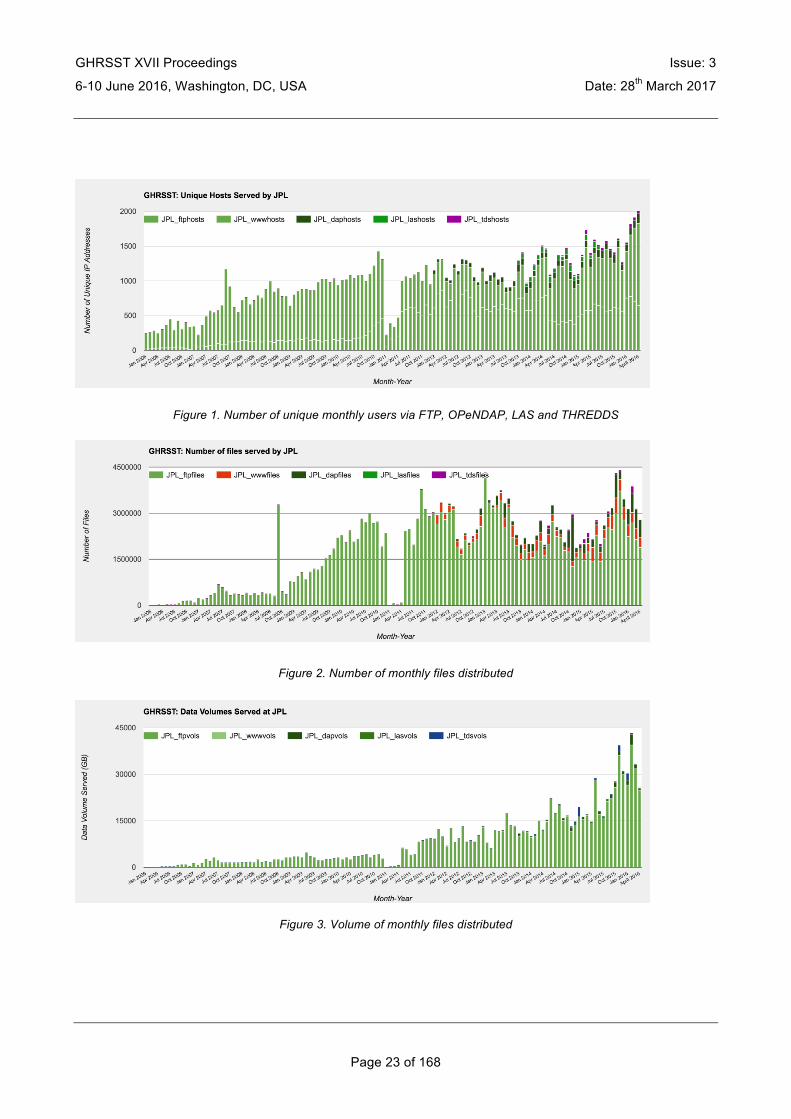
2. Distribution metrics The following figures show distribution metrics from the GDAC since 2005. Users, data volumes and number of files are all steady or have slightly increased. Users are leveraging interfaces and services such as OPeNDAP, THREDDS and LAS more so than in the past.
GHRSST XVII Proceedings Issue: 3
6-10 June 2016, Washington, DC, USA Date: 28th March 2017
Page 23 of 168
Figure 1. Number of unique monthly users via FTP, OPeNDAP, LAS and THREDDS
Figure 2. Number of monthly files distributed
Figure 3. Volume of monthly files distributed

GHRSST XVII Proceedings Issue: 3
6-10 June 2016, Washington, DC, USA Date: 28th March 2017
Page 24 of 168
3. New and Emerging Technologies • New version of HiTide L2 subsetter to be released Summer 2016 • PO.DAAC “Drive” will replace FTP access • Virtual Quality Screening Service (VQSS)
o Seamlessly applying GDS2 quality information (quality_level, l2p_flags, etc.) to granule data extraction and subsetting requests
• OceanXtremes o Climatology generation, SST anomaly detection and mining using cloud based databases
• Distributed Oceanographic Matchup Service (DOMS) o Satellite to in situ (ICOADS,SPURS, ARGO, SAMOS) matchup service
• Mining and Utilizing Dataset Relevancy from Oceanographic Dataset (MUDROD) Metadata, Usage Metrics, and User Feedback to Improve Data Discovery and Access o Improving data search relevancy (finding the right datasets)
o Text and relevance mining of science literature
o Coordinating with NASA Earth Science Data Systems Working Group (ESDSWG) on Search Relevance
§ Chairs: Ed Armstrong and Lewis Mcgibbney
4. Summary • GHRSST GDS2 “catalog” near complete
o datasets online, discoverable, available via tools and services
• PO.DAAC continues to improve tools and services implemented for subsetting, discovery, dataset and granule web services. o New interface “PO.DAAC Drive” for data download
o L2 subsetting service (L2SS) and revised HiTide coming
o Further JPL technology development has implications for GHRSST data and users (Armstrong et al. poster)
• Issues for consideration: o Regional/Global Task Sharing re architecture proposal (in DAS-TAG)
o Improving access to quality information
o Improving search relevance
5. Acknowledgements This work was carried out at the NASA Jet Propulsion Laboratory, California Institute of Technology. Government sponsorship acknowledged. Copyright 2016 California Institute of Technology. Government sponsorship acknowledged.

GHRSST XVII Proceedings Issue: 3
6-10 June 2016, Washington, DC, USA Date: 28th March 2017
Page 25 of 168
GHRSST SYSTEM COMPONENTS: LTSRF Kenneth S. Casey, Korak Saha, Ajay Krishnan, Yuanjie Li, John Relph,
Dexin Zhang, Yongsheng Zhang, Sheekela Baker-Yeboah(1) (1) NOAA National Centers for Environmental Information, Email: [email protected]
ABSTRACT The GHRSST Long Term Stewardship and Reanalysis Facility (LTSRF) at the NOAA National Centers for Environmental Information (NCEI) had another successful year maintaining GHRSST archive and access operations. New products were included in the archive, the Dynamic Data Table was updated and improved, Digital Object Identifiers (DOIs) were minted, the near real-time archive of OSPO ACSPO VIIRS was achieved, and CEOS CWIC Integration was maintained. Archive and access Statistics are also presented showing continued growth in user uptake of GHRSST data.
1. Introduction The GHRSST Long Term Stewardship and Reanalysis Facility (LTSRF) at the NOAA National Centers for Environmental Information (NCEI) had another successful year maintaining GHRSST archive and access operations. New products were included in the archive, the Dynamic Data Table was updated and improved, Digital Object Identifiers (DOIs) were minted, the near real-time archive of OSPO ACSPO VIIRS was achieved, and CEOS CWIC Integration was maintained. Archive and access Statistics are also presented showing continued growth in user uptake of GHRSST data. The remaining sections of this document provide details in these areas.
2. New Products New products this past year brought into the LTSRF are shown below:
• GHRSST-SEVIRI_SST-OSISAF-L3C-v1.0 • GHRSST-Geo_Polar_Blended-OSPO-L4-GLOB-v1.0 • GHRSST-Geo_Polar_Blended_Night-OSPO-L4-GLOB-v1.0 • GHRSST-REMSS-L4HRfnd-GLOB-MWIROI • GHRSST-VIIRS_NPP-OSPO-L3U-v2.4 • GHRSST-AVHRR_SST_METOP_B_NAR-OSISAF-L3C-v1.0
In addition, GHRSST-AVHRR_OI-NCEI-L4-GLOB in GDS2 format was archived.
3. Dynamic Data Table Improvements were made to the dynamic data table at: http://ghrsst.nodc.noaa.gov/accessdata.html. The table:
• Is built automatically and dynamically from metadata and archive metrics
• Includes key summary information for each product
• Includes data access and metadata links
• Displays Summary stats for all products at bottom
• Includes important improvements made in the last year to enhance consistency

GHRSST XVII Proceedings Issue: 3
6-10 June 2016, Washington, DC, USA Date: 28th March 2017
Page 26 of 168
4. Digital Object Identifiers (DOIs) DOIs continue to be minted for requested datasets. Key notes about GHRSST DOIs at the LTSRF include:
• DOIs can be minted for your GDS datasets
• LTSRF staff sent out request for authorship lists
• DOIs are not required
• The LTSRF minted six new OSPO DOIs this year
5. CEOS CWIC Integration Update Connections to the CEOS WGISS Integrated Catalog (CWIC) were maintained at the LTSRF this year on behalf of the GHRSST community. Updates since the last GHRSST meeting include:
• Granule inventories for discovery are being maintained and are at nearly 100%
• New granule Geoportal deployed with:
o Shopping cart
o Improved REST APIs
6. Real-time Archive of OSPO ACSPO VIIRS L3U and L2P SST ver 2.4 Using a mechanism established last year, the LTSRF put into operations this year the direct ingest of GHRSST data produced by the OSPO RDAC using the ACSPO system, for L2P and L3U version 2.4 data. These data are now archived without the usual 30-day lag, to meet NOAA requirements from JPSS Program.
7. Archive and Access Statistics Figures 1 through 3 highlight the various access statistics at the LTSRF over time.
Figure 1: Daily Average access statistics since 2006 at the LTSRF.

GHRSST XVII Proceedings Issue: 3
6-10 June 2016, Washington, DC, USA Date: 28th March 2017
Page 27 of 168
Figure 2: Number of GHRSST products, archival information packages (accessions), files, and data volumes for
GHRSST data at the LTSRF.
Figure 3: Combined access statistics between the LTSRF and PO.DAAC GDAC going back to 2006.
8. Conclusion The last year marked another successful year of operations at the GHRSST LTSRF.

GHRSST XVII Proceedings Issue: 3
6-10 June 2016, Washington, DC, USA Date: 28th March 2017
Page 28 of 168
REPORT FROM THE AUSTRALIAN RDAC TO GHRSST-XVII Helen Beggs(1), Christopher Griffin(2) , Leon Majewski(3), Pallavi Govekar(4) and Janice Sisson(5)
(1) Bureau of Meteorology, Melbourne, Australia, Email: [email protected] (2) Bureau of Meteorology, Melbourne, Australia, Email: [email protected]
(3) Bureau of Meteorology, Melbourne, Australia, Email: [email protected] (4) Bureau of Meteorology, Melbourne, Australia, Email: [email protected] (5) Bureau of Meteorology, Melbourne, Australia, Email: [email protected]
ABSTRACT This is a report of progress during the past 12 months in the Australian Regional Data Assembly Centre at the Australian Bureau of Meteorology, relating to the provision and validation of GHRSST products, and related SST research.
1. Overview The Australian Bureau of Meteorology (ABoM) produces a number of GHRSST format products, both in real-time and delayed mode (reprocessed). They are:
1.1. Real-time GDS1.6 • Operational Daily Regional 1/12º SSTfnd L4 ("RAMSSA") over 60ºE to 190ºE, 70ºS to 20ºN • Operational Daily Global 0.25º SSTfnd L4 ("GAMSSA")
1.2. Real-time GDS2.0 • IMOS fv01 HRPT AVHRR SSTskin (NOAA-18, NOAA-19)
o L2P and 0.02º L3U, day/night L3C, day/night L3S over 70ºE to 190ºE, 70ºS to 20ºN and Southern Ocean (2.5°E to 202.5°E, 77.5°S to 27.5°S)
• IMOS fv01 HRPT AVHRR SSTfnd (NOAA-18, NOAA-19) o 0.02º day+night L3S over 70ºE to 190ºE, 70ºS to 20ºN and Southern Ocean (2.5°E to 202.5°E,
77.5°S to 27.5°S)
• ABoM operational AHI Himawari-8 SSTskin L2P
1.3. Reprocessed GDS2.0 • IMOS HRPT AVHRR L2P/L3U/L3C/L3S fv02 products from 1992 to 2015 (NOAA-11 to NOAA-19
satellites) • IMOS MTSAT-1R Hourly 0.05º L3U (2006 to 2010)
2. Data availability
2.1. Real-time GDS1.6 • Operational daily L4 (RAMSSA/GAMSSA) are available within 6 hours of final observation back to
2008 from the GDAC (http://podaac.jpl.nasa.gov/dataset/ABOM-L4HRfnd-AUS-RAMSSA_09km and http://podaac.jpl.nasa.gov/dataset/ABOM-L4LRfnd-GLOB-GAMSSA_28km), LTSRF and Bureau OPeNDAP server

GHRSST XVII Proceedings Issue: 3
6-10 June 2016, Washington, DC, USA Date: 28th March 2017
Page 29 of 168
• Work is nearly complete to convert to GDS2.0 (see Section 3.4).
2.2. Real-time GDS2.0 • IMOS fv01 HRPT AVHRR (available 1 January 2015 to present)
o L2P: Bureau OPeNDAP server (contact [email protected]) o L3U/L3C/L3S: IMOS Thredds server at http://rs-data1-mel.csiro.au/thredds/catalog/imos-
srs/sst/ghrsst/catalog.html • ABoM AHI Himawari-8 (available 24 March 2016 to present)
o L2P: NCI’s OPeNDAP server (contact [email protected])
2.3. Reprocessed GDS2.0 • IMOS fv02 HRPT AVHRR (available 1992 to 31 Dec 2014)
o L2P: NCI server - Contact [email protected]
o L3U/L3C/L3S: IMOS Thredds server at
http://rs-data1-mel.csiro.au/thredds/catalog/imos-srs/archive/sst/ghrsst-fv02/catalog.html
• IMOS MTSAT-1R L3U (available Jun 2006 to Jun 2010): IMOS Thredds server at • http://rs-data1-mel.csiro.au/thredds/catalog/imos-srs/sst/ghrsst/L3U/mtsat1r/catalog.html
Figure 1: Example of IMOS fv01 AVHRR SST product - 1-month Night-time L3S SSTskin for June 2016.
3. Progress since GHRSST-XVI
3.1. IMOS Ship SST
3.1.1. Overview Since 2008, the Integrated Marine Observing Project (IMOS: www.imos.org.au) has enabled accurate, quality controlled, SST data to be supplied in near real-time (within 24 hours) to the Global Telecommunications System (GTS) from Ships of Opportunity and research vessels in the Australian region. In total, since 2008 21 ships have contributed data to the IMOS Project, most also collecting wind data. QC’d IMOS ship SST data are available in L2i netCDF format from the iQUAM v2 portal (http://www.star.nesdis.noaa.gov/sod/sst/iquam/v2/data.html) and in IMOS netCDF format from the IMOS OPeNDAP server (http://thredds.aodn.org.au/thredds/catalog/IMOS/SOOP/SOOP-SST/catalog.html and

GHRSST XVII Proceedings Issue: 3
6-10 June 2016, Washington, DC, USA Date: 28th March 2017
Page 30 of 168
http://thredds.aodn.org.au/thredds/catalog/IMOS/SOOP/SOOP-ASF/catalog.html). See http://imos.org.au/sstsensors.html for more information.
Applications: Global ocean data sets (HadSST, ICOADS, GOSUD, Coriolis), ingestion into SST analyses, and validation of real-time and reprocessed IMOS AVHRR L2P SST data over the Australian region (see http://opendap.bom.gov.au:8080/thredds/fileServer/abom_imos_ghrsst_archive/v02.0fv02/Validation/web/index.html ).
3.1.2. Progress Over the past year 11 IMOS ships reported QC'd, real-time, SSTdepth observations to the GTS, IMOS Ocean Portal (https://portal.aodn.org.au/) and NOAA/NESDIS iQUAM v2 (http://www.star.nesdis.noaa.gov/sod/sst/iquam/v2/). Figure 2 shows transects of the ships reporting SST to IMOS over the past year.
Figure 2: Tracks of the ships of opportunity that contributed SST data to the IMOS Project during
1 June 2015 to 1 June 2016.
In collaboration with CSIRO and ABoM, the IMOS Project has also contributed real-time skin SST data from the ISAR radiometer installed on RV Investigator from 24 March 2016. This data still requires reprocessing and QA back to March 2015.
3.2. IMOS HRPT AVHRR GHRSST Products
3.2.1. Overview As part of the Integrated Marine Observing System (IMOS: www.imos.org), ABoM in collaboration with CSIRO, produces a range of HRPT AVHRR GDS2.0 L2P, L3U, L3C and L3S products from the series of NOAA Polar Orbiting Environmental Satellites (NOAA-11 to NOAA-19). The 0.02º resolution level 3 products are available in a range of averaging periods from single orbit to 1 month to suit different applications. All products are available in real-time (within 3 to 24 hours of final observation) and have also been reprocessed to cover the period from 1992 to 2015. For more information see http://imos.org.au/sstproducts.html or see Helen Beggs’ presentation during the CDR_TAG Session, Tuesday 7th June 2016 - https://www.ghrsst.org/documents/q/category/ghrsst-science-team-meetings/ghrsst-xvii-washington-d-c/ghrsst-xvii-presentations/tuesday-7th-june-2016/cdrtag/).
Applications: ABoM operational coral bleaching nowcasting service, ReefTemp NextGen (http://www.bom.gov.au/environment/activities/reeftemp/reeftemp.shtml), ABoM operational SST analyses (RAMSSA, GAMSSA), fisheries (e.g. www.fishtrack.com), regional maps of ocean currents and SST (http://oceancurrent.imos.org.au/), SST climatologies (e.g. http://oceancurrent.imos.org.au/monthlymeans.php#), SST diurnal variation research and marine biology research.

GHRSST XVII Proceedings Issue: 3
6-10 June 2016, Washington, DC, USA Date: 28th March 2017
Page 31 of 168
3.2.2. Progress During the past year, ABoM implemented daily real-time (Figure 3) and delayed mode (Figure 4) validation of the Australian region HRPT AVHRR L2P SST, using matchups with SST observations from drifting buoys, moored buoys, Argo floats and IMOS ships (http://imos.org.au/sstdata_validation.html). It is clear that subtracting sses_bias improves the bias of the IMOS L2P SSTskin values compared with drifting buoy SST observations at all quality levels (Figure 3).
Figure 3: Example of plots of median of night-time IMOS fv02 HRPT AVHRR L2P SSTskin (from NOAA-18) minus drifting buoy SST. The L2P SSTs have been filtered on various quality levels (“q”) and are shown before and after bias correction by subtracting sses_bias. The drifting buoy SSTdepth values have been adjusted to SSTskin by subtracting
0.17 K. Figure accessed from http://opendap.bom.gov.au:8080/thredds/fileServer/abom_imos_ghrsst_archive/v02.0fv01/Validation/web/index.html
on 13 July 2016.
Figure 4: Example of plots of standard deviation of night-time IMOS fv02 HRPT AVHRR L2P SSTskin (from NOAA-11 to -19) minus drifting buoy SST. The L2P SSTs have been filtered on quality_level 5 and bias-corrected by subtracting
sses_bias. The drifting buoy SSTdepth values have been adjusted to SSTskin by subtracting 0.17 K. Figure accessed from http://opendap.bom.gov.au:8080/thredds/fileServer/abom_imos_ghrsst_archive/v02.0fv02/Validation/web/index.html
on 13 July 2016.
Research is under way to investigate methods to merge L2P/L3U files from different sensors into multiple-sensor L3S products, using existing SSES and quality level values. For more information see Chris Griffin’s
GHRSST XVII Proceedings Issue: 3
6-10 June 2016, Washington, DC, USA Date: 28th March 2017
Page 32 of 168
presentation at https://www.ghrsst.org/documents/q/category/ghrsst-science-team-meetings/ghrsst-xvii-washington-d-c/ghrsst-xvii-presentations/thursday-9th-june-2016/.
3.3. Operational Himawari-8 SST ABoM, in collaboration with JMA and NOAA/NESDIS/STAR, have since 24 March 2016 produced operational real-time Himawari-8 L2P skin SSTs on the GEOS grid, by regressing against ACSPO VIIRS L3U SSTdepth (see Chris Griffin’s presentation from the Next Gen GEO SST Side Meeting at : https://www.ghrsst.org/documents/q/category/ghrsst-science-team-meetings/ghrsst-xvii-washington-d-c/ghrsst-xvii-presentations/geo-side-meeting/ ).
Applications: The ABoM Himawari-8 L2P files are currently being tested for assimilation into the ABoM new 4 km resolution ocean model over the Great Barrier Reef.
ABoMplanstoreprocesstheHimawari-8SSTdatatoL2PfromJuly2015laterin2016.Atthistime,4isthehighestqualitylevelpresentinthefiles,duetodeficienciesintheclouddetectionmethod.
3.4. Operational SST Analyses
3.4.1. Overview ABoM produces regional 1/12º (“RAMSSA”) and global 1/4º (“GAMSSA”) operational daily foundation L4 SST analyses in near real-time based on an optimal interpolation method. For more information on RAMSSA see Beggs et al (2011) and for GAMSSA see Zhong and Beggs (2009) and Beggs et al (2011).
SST inputs: • 1 km IMOS fv01 HRPT AVHRR (NOAA-18,-19) L2P SSTskin (Paltoglou et al., 2010) • 9 km NAVOCEANO GAC AVHRR GHRSST-L2P SST1m (NOAA-18, NOAA-19, METOP-A, METOP-
B) • ~50 km AMSR-2 (GCOM-W) L2P SSTsubskin (since 1 December 2014) • ~50 km WindSat L2P_gridded SSTsubskin (since 11 December 2012) • Buoy and ship in situ SSTdepth
Applications: Boundary condition for NWP models, initialising Seasonal Prediction Model, validating ocean forecasts. In addition, GAMSSA contributes to the GHRSST Multi-Product Ensemble.
3.4.2. Progress Since April 2016 a test RAMSSA system has run in parallel ingesting the IMOS fv01 HRPT AVHRR L2P SSTs, corrected for biases using sses_bias. Comparisons against independent buoy SSTs from the day following analysis for the period 10 April to 30 June 2016 show that subtracting sses_bias reduces the mean bias by 0.08 K (0.03 K cf 0.11 K) and reduces the standard deviation by 0.05 K (0.46 K cf 0.51 K).
During July 2016, ABoM staff completed the process of converting RAMSSA and GAMSSA GDS1.6 L4 files to GDS2.0 format back to 2007. Once these files have been assessed by the U.S. GDAC and LTSRF then they will be supplied in near real-time in parallel to the GDS1.6 format files.
3.5. Tropical Warm Pool SST Diurnal Variability Project (TWP+) Since 2009, ABoM in collaboration with GHRSST has been collating high resolution SST observations and model forecasts of ocean/atmospheric parameters in a common grid and format over the Tropical Warm Pool region (25°S to 15°N, 90°E to 170°E). The data sets now cover the period 1 January 2009 to 31 December 2014 and have been used both to quantify the amount of SST diurnal variation over the region and for input into and validation of diurnal variation models. For more information see https://www.ghrsst.org/ghrsst/tags-and-wgs/dv-wg/twp/ or email Helen Beggs ([email protected]).

GHRSST XVII Proceedings Issue: 3
6-10 June 2016, Washington, DC, USA Date: 28th March 2017
Page 33 of 168
PhD student, Haifeng Zhang (UNSW, Canberra) has in collaboration with Helen Beggs (ABoM) been investigating the seasonal patterns of SST diurnal variation over the Tropical Warm Pool during 2010 to 2014 using 0.02º IMOS AVHRR fv02 L3C SSTs (see Haifeng Zhang's poster at https://www.ghrsst.org/documents/q/category/ghrsst-science-team-meetings/ghrsst-xvii-washington-d-c/ghrsst-xvii-presentations/posters-g-xvii/?page=3&). Haifeng’s paper on his study of SST DV over the Tropical Warm Pool using MTSAT-1R SST (Zhang et al., 2016) has recently been published in Remote Sensing Environment (see http://www.sciencedirect.com/science/article/pii/S003442571630195X).
3.6. User Engagement/Training The inaugural Satellite Oceanography Users Workshop was held 9-11 November 2016 in Melbourne, Australia, hosted by ABoM in collaboration with GHRSST, CEOS SST-VC and IMOS. The user workshop covered several satellite-derived ocean variables: SST, altimetry, winds and ocean colour. Approximately 65 people attended from Australia, New Zealand, China, Japan, Germany, U.S. and U.K. The IMOS Project Office, CSIRO and GA have expressed a desire to repeat similar user workshops on a biannual basis. Agenda, presentations and workshop report are available from https://www.ghrsst.org/documents/q/category/ghrsst-workshops/satellite-oceanography-users-melbourne-australia-2015/Workshop%20Presentations/. Videos of the plenary presentations are available at http://ceos.org/home-2/satellite-oceanography-user-workshop-videos-available/.
4. Plans for 2016/2017 During the coming 12 months, the Bureau of Meteorology plans to:
• Provide Himawari-8 10-min L2P (GEO projection, full disk) and hourly, 0.02° L3C files (IMOS rectangular grid, 70°E to 170°W, 70°S to 20°N) from July 2015 to present in GDS2.0 format
• Test ingesting ACSPO VIIRS 0.02º L3U products into BoM operational SST analyses, ocean models and IMOS L3C and L3S products
• Reprocess ISAR SSTskin data from RV Investigator from Mar 2015 onwards • Investigate replacing RAMSSA/GAMSSA L4 with OceanMAPS 0.1° global ocean model nowcast SST
5. References Beggs H., A. Zhong, G. Warren, O. Alves, G. Brassington and T. Pugh, RAMSSA – An Operational, High-Resolution, Multi-Sensor Sea Surface Temperature Analysis over the Australian Region, Australian Meteorological and Oceanographic Journal, 61, 1-22, 2011 http://www.bom.gov.au/jshess/papers.php?year=2011
Paltoglou, G, H. Beggs and L. Majewski, New Australian High Resolution AVHRR SST Products from the Integrated Marine Observing System, In: Extended Abstracts of the 15th Australian Remote Sensing and Photogrammetry Conference, Alice Springs, 13-17 September, 2010, 2010. http://imos.org.au/srsdoc.html
Zhang H., H. Beggs, L. Majewski, X.H. Wang, A. E. Kiss, Investigating Sea Surface Temperature Diurnal Variation over the Tropical Warm Pool Using MTSAT-1R Data. Remote Sensing Environment, 183, 1-12, 2016. http://www.sciencedirect.com/science/article/pii/S003442571630195X .
Zhong, Aihong and Helen Beggs, Analysis and Prediction Operations Bulletin No. 77 - Operational Implementation of Global Australian Multi-Sensor Sea Surface Temperature Analysis, Bureau of Meteorology Web Document, 2008. http://www.bom.gov.au/australia/charts/bulletins/apob77.pdf

GHRSST XVII Proceedings Issue: 3
6-10 June 2016, Washington, DC, USA Date: 28th March 2017
Page 34 of 168
CANADIAN METEOROLOGICAL CENTRE: REPORT TO GHRSST Dorina Surcel Colan
Numerical Environmental Prediction Section, National Prediction Development Division, Meteorological Service of Canada, Environment Canada,
Email:[email protected]
ABSTRACT The Canadian Meteorological Centre (CMC) produces every day three SST analyses. Verification against independent data confirms that these analyses performed well in 2015, with the higher resolution analysis presenting the best results.
1. Introduction Among the three SST analyses produced daily at CMC, two products generated in GDS2.0 format are available to the GHRSST community.
The first analysis has a resolution of 0.2° and the dataset starts in September 1991. The second analysis with a resolution of 0.1° has been implemented in experimental mode at CMC in September 2015 and in January 2016, it became available on the PO.DAAC website. The performance of these analyses for 2015 is assessed by comparing them with independent data and with the operational CMC SST analysis. The operational analysis with a resolution of 0.2° is used every day as observations in the assimilation module of the operational Global Ice-Ocean Prediction System (GIOPS). Details about all three analyses are presented in the next section, followed by the evaluation against Argo floats. Conclusions and future plans are presented in the last section.
2. CMC SST analyses All CMC SST analyses are based on the statistical interpolation method as described in Brasnett (2008). The statistical interpolation method is used for the analysis, the quality control of observations and the bias correction of satellite retrievals. The analysis variable is the anomaly from climatology and the background is based on simple persistence.
The 0.2° SST analysis produced in the operational cycle (CMC SST v1) assimilates data from 4 AVHRR instruments together with in situ data from moored and drifting buoys and ships and ice information.
The 0.2° SST analysis available for GHRSST community via PO.DAAC (CMC SST v2) is similar with the first analysis but assimilates data from 3 AVHRR instruments and from VIIRS and AMSR2 instruments.
The last analysis, CMC SST v3 has a resolution of 0.1° and assimilates data from 4 AVHRR instruments together with VIIRS and AMSR2 data. Along with increasing the resolution of the analysis grid, additional modifications have been made to fully benefit from the improved resolution. More details about this product are included in Brasnett and Surcel (2016).
Table 1 contains details about each data set used in these analyses.
CMC SST v1 analysis is used every day as observations in GIOPS (Smith et al, 2015). GIOPS includes a full multivariate ocean data assimilation system that combines satellite observations of sea level anomaly and sea surface temperature together with in situ observations of temperature and salinity.
The CMC SST analysis is interpolated onto the GIOPS grid and it was assimilated with a constant error of 0.3°C. This error corresponds to the estimated error from the CMC SST analysis (Brasnett, 2008) and also provides a tightly constrained SST which helps reduce initialization shocks when using GIOPS analyses in coupled medium-range forecasts with the GDPS (Smith et al., 2013). The latter version of GIOPS, implemented in June 2016 uses a constant error of 0.2°C.

GHRSST XVII Proceedings Issue: 3
6-10 June 2016, Washington, DC, USA Date: 28th March 2017
Page 35 of 168
Data set Data type Producer / Source NOAA18 AVHRR L2P NAVOCEANO / PO.DAAC NOAA19 AVHRR L2P NAVOCEANO / PO.DAAC MetOp-A AVHRR L2P NAVOCEANO / PO.DAAC MetOp-B AVHRR L2P NAVOCEANO / PO.DAAC GCOM-W2 AMSR2 L3 REMSS SUOMI-NPP VIIRS L2P NOAA/NESDIS/OSPO / PO.DAAC In situ TAC / BUFR GTS Sea-ice concentration L4 CMC ice analysis
Table 1: Use of data sets in CMC SST analyses
3. Evaluation of SST analyses against independent data All CMC SST analyses are evaluated by estimating analysis error using the Argo float temperatures. These temperature reports, which are not used in the analysis, are used for verification only if they are between 3 m and 5 m in depth and within four standard deviations of the climatology interpolated temporally and spatially to the date and location of the Argo float observation.
In fig. 1a, a 12-month time series of analysis standard deviations and biases are shown for CMC SST v1, CMC SST v2 and CMC SST v3. The analyses which assimilate AMSR2 and VIIRS data are more accurate than the analysis assimilating only AVHRR data. The higher resolution CMC SST v3 presents a small but persistent improvement over CMC SST v2 for the whole period, except during the summer when both analyses have similar biases and standard deviations. Looking at the annual mean over different regions for the same products, as presented in figure 1b, the results clearly show that the reduction in analysis standard deviation results from the addition of AMSR2 and VIIRS data sets in CMC SST v2 and CMC SST v3.
Figure1: a) Monthly verification statistics for 2015 using independent data from Argo floats as truth. Standard deviation (°C, solid lines) and bias (dot-dashed lines) for the operational analysis (v1) are in blue, the experimental analysis (v3) is in red and the 0.2° analysis including AMSR2 and VIIRS data (v2) is in green. b) Analysis bias (°C, dot-dashed lines) and
standard deviation (solid lines) for several regions for 2015 for the same products as in 1a).
The next evaluation was done by comparing the two CMC products available to GHRSST together with the GHRSST multi-product ensemble (GMPE). The GMPE product, described in Martin et al. (2012), is the median of several (typically ten or eleven) real-time analyses and was found to be more accurate than any of the
Jan Feb Mar Apr May Jun Jul Aug Sep Oct Nov Dec Month of
2015
-0.2
-0.1
0.0
0.1
0.2
0.3
0.4
0.5
0.6
0.0
Anal
ysis
bia
s an
d st
anda
rd d
evia
tion
(o C)

GHRSST XVII Proceedings Issue: 3
6-10 June 2016, Washington, DC, USA Date: 28th March 2017
Page 36 of 168
contributing analyses. The GMPE product contains data from CMC SST v2, but CMC SST v3 is not included in the ensemble. The 0.1° analysis is more accurate than the GMPE product for the period between January to June of 2015 and also that of December 2015. From July to November 2015, the GMPE product and CMC SST v3 analysis show similar standard deviation errors (fig 2a).
The annual mean for 2015 over different regions is almost similar for all products except over the North Atlantic region where 0.1° resolution CMC SST v3 has the smallest standard deviation error compared to GMPE and CMC SST v2. This could be explained by the higher resolution of ice information and smaller background length-scale error correlations in higher latitudes (Brasnett and Surcel, 2016).
Figure 2 a) Monthly verification statistics for 2015 using independent data from Argo floats as truth. Standard deviation (°C, solid lines) and bias (dot-dashed lines) for the GMPE product are in blue, the experimental analysis (v3) is in red and the 0.2° analysis including AMSR2 and VIIRS data (v2) is in green. b) Analysis bias (°C, dot-dashed lines) and standard
deviation (solid lines) for several regions for 2015 for the same products as in 2a).
Recently, the daily GIOPS analysis was used to initialise coupled medium-range forecasts over a three-month period during the summer of 2014. GIOPS analysis assimilates CMC SST v1 as observations with a constant error of 0.2°C. However, the dynamical model used in GIOPS analysis is able to produce small-scale features which are not included in the CMC SSTv1 analysis. An evaluation of GIOPS analysis compared to CMC SST v1 analysis and CMC SST v3 analysis was performed for summer 2014. Figure 3 shows time-series of 10-day average statistics for the bias and standard deviation errors against Argo floats. As expected, GIOPS and CMC SST present similar results but the higher resolution CMC SST v3 analysis has the best performance. This test shows the importance of using better quality SST in GIOPS initialisation process in the future, at this moment the use of CMC SST v1 being preferred only for synchronisation with the atmospheric analysis.
Jan Feb Mar Apr May Jun Jul Aug Sep Oct Nov Dec Month of
2015
-0.2
-0.1
0.0
0.1
0.2
0.3
0.4
0.5
0.6
0.0
Anal
ysis
bia
s an
d st
anda
rd d
evia
tion
(o C)

GHRSST XVII Proceedings Issue: 3
6-10 June 2016, Washington, DC, USA Date: 28th March 2017
Page 37 of 168
Figure 3: 10-day averages of verification statistics for summer 2014 using independent data from Argo floats. Standard deviation (°C, solid lines) and bias (dot-dashed lines) for the CMC SST v1 are in blue, the GIOPS analysis is in red and
the CMC SST v3 is in green.
4. Conclusions and future plans All three CMC SST analyses continue to show good performance over 2015. As CMC SST v3 is an improved version of CMC SST v2, assimilating the same satellite data type, the production of the second analysis will no longer be supported and it is planned to stop at the end of summer 2016. The users are encouraged to use CMC SST v3. As it was demonstrated (fig2 a, b), this analysis shows more skill than CMC SST v2 and the GMPE product, which is perhaps not surprising because not many ensemble members are using VIIRS and AMSR2 data sets which have been proved to add value to CMC SST analysis. Nevertheless, since the GMPE product is recognized as the most accurate global SST product available in real-time, it remains an important benchmark for assessing analysis accuracy.
5. References Brasnett B., The impact of satellite retrievals in a global sea-surface-temperature analysis, Quart. J. Roy. Met. Soc., 134, 1745-1760, 2008.
Brasnett B. and D. Surcel Colan, Assimilating Retrievals of Sea Surface Temperature from VIIRS and AMSR2, J. Atmos. Oceanic Technol. 33, 361–375, 2016, doi: 10.1175/JTECH-D-15-0093.1.
Martin, M., and Coauthors, Group for High Resolution Sea Surface Temperature (GHRSST) analysis fields inter-comparisons. Part 1: A GHRSST multi-product ensemble (GMPE), Deep-Sea Res. II., 77-80, 21-30, 2012.
Smith GC, Roy F, Belanger J-M, Dupont F, Lemieux J-F, Beaudoin C, Pellerin P, Lu Y, Davidson F, Ritchie H., Small-scale ice-ocean-wave processes and their impact on coupled environmental polar prediction, Proceedings of the ECMWFWWRP/THORPEX Polar Prediction Workshop , 24-27 June 2013, ECMWF Reading, UK.
Smith, G.C., and Coauthors, Sea ice Forecast Verification in the Canadian Global Ice Ocean Prediction System. Quart. J. Roy. Met. Soc., 2015, DOI:10.1002/qj.2555.
06/22 07/02 07/12 07/22 07/31 08/10 08/20 08/30Month and Day of 2014
-0.4
-0.2
0.0
0.2
0.4
0.6
0.8
1.0
0.0
Anal
ysis
bia
s an
d st
anda
rd d
evia
tion
(o C)

GHRSST XVII Proceedings Issue: 3
6-10 June 2016, Washington, DC, USA Date: 28th March 2017
Page 38 of 168
EUMETSAT REPORT TO GHRSST Anne O’Carroll(1), Igor Tomazic(1) ), Prasanjit Dash(1)
(1) EUMETSAT, Eumetsat Allee 1, 64295 Darmstadt, Germany, Email: [email protected]
1. Introduction EUMETSAT is an operational data provider covering weather, climate, ocean and atmospheric composition. These involve mandatory, optional and third party programmes. The Level-2 products from the mandatory programmes are produced by the EUMETSAT Ocean and Sea-ice Satellite Application Facility (OSI SAF). Oceanography activities at EUMETSAT are organized within the Marine Applications group, part of the Remote Sensing and Products Division. These activities are organized within four teams: Surface Temperature Radiometry, Ocean Colour, Altimetry and Scatterometry.
2. Sea Surface Temperature missions and activities The most recent launches containing Sea Surface Temperature (SST) related missions are Copernicus Sentinel-3A Sea and Land Surface Temperature Radiometer (SLSTR) (16th February 2016), MSG-4 (15th July 2015) and Metop-B (17th September 2012). Upcoming launches include Copernicus Sentinel-3B (~Autumn 2017), Metop-C AVHRR and IASI (~October 2018); MTG-I1 FCI (~Q3 2020); Metop-SG A METimage and IAS (~June 2021) and MTG-S1 IRS (~2022). Considerations for Meteosat-8 Indian Ocean Data Coverage (IODC) are planned to be available from January 2017 onwards following a period of parallel operations with Meteosat-7 from October 2016 to mid January 2017.
Commissioning activities (led by the European Space Agency) continue for Sentinel-3 SLSTR and are due to end in July 2016. A ramp up to full operations will continue with EUMETSAT operating the satellite and distributing the marine level 2 products (including GHRSST SLSTR L2P). Participation to the Sentinel-3 Validation Team continues to be open to new members with full details available from https://earth.esa.int/aos/S3VT.
Figure 1: Example of first SLSTR Sea Surface Temperature data from April 22nd 2016 (not a complete day).
SST products from Metop-IASI continue to be operational and available from the OSI SAF. The IASI Level 2 processor at EUMETSAT will be upgraded to v6.3 in early January 2017. Plans are to include a new SST retrieval scheme using a greater number of clear observations especially at high latitudes, inclusion of improved aerosol correction and flagging, and the consideration of inclusion of uncertainties as experimental fields in addition to Sensor Specific Error Statistics (SSES).

GHRSST XVII Proceedings Issue: 3
6-10 June 2016, Washington, DC, USA Date: 28th March 2017
Page 39 of 168
Figure 2: Example of possible IASI SST coverage under consideration for IASI L2 v6.3.
3. Projects and activities A project on improved drifting buoy sea surface temperature for Copernicus satellite validation is due to begin in late summer 2016. This will provide measurements from a significant number of drifting buoys equipped with digital SST probes in order to achieve a better calibrated capability. The aim is to assess and establish the benefit of improved incremental capability of drifting buoys for satellite SST validation. Assessment will be performed through planned Sentinel-3 SST Validation activities. Coordination with the Data Buoy Cooperation Panel (DBCP) will continue and data availability will be possible through the Global Telecommunications System (GTS). Coordination is also ongoing with the ESA project on FRM4STS (http://www.frm4sts.org/) where there is a study of the SI traceability of historical and current drifter SST measurements.
A number of activities are ongoing relating to sea-ice surface temperature. A current project is ongoing to provide a recommended algorithm and related auxiliary data files for cloud screening over sea-ice for SLSTR. The outcomes from this study will then be used for a project on SLSTR sea-ice surface temperature retrieval and validation in 2017, with consideration of implementation of sea-ice surface temperature and marginal ice zone surface temperature projects planned for 2018 and 2019.
A project will begin in summer 2016 on ice surface temperature from Metop IASI. This will include an assessment of in situ datasets and validation of current L2 retrievals available. This work will provide research and development towards future possible ice surface temperature products from Metop IASI for land, sea-ice and marginal ice zones.
4. Data delivery and discovery Level-1 data continues to be available from the EUMETSAT data centre (www.eumetsat.int). Level-2 products from the EUMETSAT OSI SAF are available from www.osi-saf.org and EUMETCast. Operational availability of Metop-A IASI SST full L2P began on 28th May 2015 with the switch to Metop-B from 23rd February 2016. These products are available from both the OSI SAF and EUMETCast. Metop-A and Metop-B L2Pcore IASI SST remain available from the EUMETSAT data centre.
Copernicus Sentinel-3 marine data will be available from the EUMETSAT data centre and the SLSTR SST product will additionally be available from EUMETCast. Sentinel-3 data availability is expected from summer 2016 with a gradual ramp up from L1 to L2 full operations.
Third party SST data is also available from EUMETSAT, including data re-distribution from NOAA, JAXA, ISRO, NSOAS and SOA. There has been an S-NPP VIIRS ACSPO operational service through EUMETCast since 2014. This was updated from an L2P to L3U service. A GCOM W2 AMSR-2 GHRSST L2P operational

GHRSST XVII Proceedings Issue: 3
6-10 June 2016, Washington, DC, USA Date: 28th March 2017
Page 40 of 168
NRT L2P service has been operating to EUMETSAT member states since 19th May 2015. An INSAT-3D service (L1C image data and L2B SST in hdf) with dissemination of data via EUMETCast began on 22 September 2015 and the service has been running nominally since then. EUMETSAT are receiving a continuous data stream of HY-2a non-SST data. The availability of SST data from NSOAS is under discussion.
Development into the CEOS WGISS Integrated Catalogue (CWIC) is underway at EUMETSAT. This is for earth observation data providers to make collections searchable through common standards. There are development activities ongoing at EUMETSAT towards CWIC to test the system, with the way forward to be discussed by the EUMETSAT Council in summer 2016. However, in the meantime the following datasets are being included: OSI SAF hourly GOES SST, OSI SAF hourly MSG SST, OSI SAF multi-mission NAR SST, OSI SAF global Metop AVHRR SST, OSI SAF multi-mission Atlantic SST, OSI SAF IASI SST, Sentinel-3 SLSTR SST.
The EUMETview mapviewer is now available for use with Meteosat and Metop imagery from http://www.eumetview.eumetsat.int/mapviewer. Sentinel-3 SLSTR radiances, brightness temperatures and SSTs are due to be included later this year.

GHRSST XVII Proceedings Issue: 3
6-10 June 2016, Washington, DC, USA Date: 28th March 2017
Page 41 of 168
RDAC UPDATE: EUMETSAT OSI SAF Saux Picart S.*, Eastwood S.1
*Centre de Météorologie Spatiale, Météo-France, Lannion, France 1Norwegian Meteorological Institute, Oslo, Norway
ABSTRACT OSI SAF objective is to provide users with operational data related to the ocean surface derived from meteorological satellite. As far as Sea Surface Temperature is concerned, the OSI SAF is currently delivering a suite of products in near real time mode (see table below).
These products are disseminated through various means:
1. Update of the Low Earth Orbiter Processing chain: On the 23rd February 2016 OSI SAF released Metop-B/AVHRR products issued by the updated processing chain of Low Earth Orbiter data. The new chain is based on classical split window algorithms (day and night). The methodology of Le Borgne et al. (2011) is used to correct for regional and seasonal biases. It relies on simulations of brightness temperature by a radiative transfer model (RTTOV) which uses water vapour and temperature profiles from NWP model as inputs. Details of the methodology can be found in the ATBD (EUMETSAT, 2015) and validation of the products is presented in the validation report (EUMETSAT, 2016). The chain delivers L2 products over the globe and global as well as North Atlantic Regional L3 products.

GHRSST XVII Proceedings Issue: 3
6-10 June 2016, Washington, DC, USA Date: 28th March 2017
Page 42 of 168
Figure 4: Metop-B/AVHRR SST products: left, L2 granule (product OSI-204-b); right, L3 12hourly global field (product OSI-201-b).
2. High latitude update: In summer 2016, OSI SAF is releasing a new combined SST and IST (Ice Surface Temperature) L2 product. It will be delivered as satellite swath poleward of 50°N and 50°S. Ongoing work is focusing on including IST into the current high latitude SST L3 product (an example is given Figure 2). OSI SAF is also working on including SNPP/VIIRS data into its L2 and L3 high latitude products.
Figure 5: SST and IST field (product OSI-203-b)
3. Reprocessing of the MSG/SEVIRI archive: OSI SAF is currently working on a reprocessing of MSG/SEVIRI archive (2004-2012). For more details about this activity, please see the extended abstract: Saux Picart et al., OSI SAF MSG/SEVIRI activities, in this proceeding.

GHRSST XVII Proceedings Issue: 3
6-10 June 2016, Washington, DC, USA Date: 28th March 2017
Page 43 of 168
4. References: P. Le Borgne, H. Roquet, C.J. Merchant (2011) Estimation of Sea Surface Temperature from the Spinning Enhanced Visible and Infrared Imager, improved using numerical weather prediction.Remote Sensing of Environment, 115-1, 55-65.
EUMETSAT, 2015, Algorithms Theoretical Basis Document for the Low Earth Orbiter Sea Surface
Temperature Processing Chain (OSI-201b / OSI-202b / OSI-204b), SAF/OSI/CDOP2/M-F/SCI/MA/216
EUMETSAT, 2016, Validation report for OSI SAF Metop/AVHRR SST (OSI-201b / OSI-202b / OSI-204b), SAF/OSI/CDOP2/M-F/SCI/TEC/233

GHRSST XVII Proceedings Issue: 3
6-10 June 2016, Washington, DC, USA Date: 28th March 2017
Page 44 of 168
REPORT TO GHRSST XVII FROM JAXA Misako Kachi(1)
(1) Japan Aerospace Exploration Agency (JAXA), Tsukuba (Japan), Email : kachi.misako@ jaxa.jp
ABSTRACT Recent activities of the Japan Aerospace Exploration Agency (JAXA) related to sea surface temperature (SST) and GHRSST are summarized and reported.
1. Introduction JAXA has operated the GHRSST server (Japanese RDAC) to distribute JAXA-produced Sea Surface Temperature (SST) products in GDS format. Those products include SST from non-JAXA satellites as well as JAXA satellites.
JAXA has developed several instruments that measures SST. Especially, a series of conical scanning passive microwave imagers that have C-band channels provide invaluable information of SST under clouds, which cannot be obtained by infrared (IR) imagers.
The latest and currently operational passive microwave imager is the Advanced Microwave Scanning Radiometer 2 (AMSR2) on board the Global Change Observation Mission (GCOM) – Water (GCOM-W, also known as “SHIZUKU”), which was launched in May 2012. AMSR2 has succeeded the observation by AMSR for EOS (AMSR-E) on board the NASA’s EOS Aqua satellite in the A-train orbit. Its big antenna size of 2-m diameter and C-band (6.9-/7.3-GHz) channels with all-weather capability enable frequent measurements of SST and other water-related parameters for various applications.
JAXA is also developing the optical and infrared radiometer, the Second-generation Global Imager (SGLI), which will be carried by the GCOM - Climate (GCOM-C) scheduled to be launched in Japanese Fiscal Year (JFY) 2016.
The Global Precipitation Measurement (GPM) Core Observatory, which is a JAXA-NASA joint mission launched in February 2014, also carries conical scanning passive microwave imager provided by NASA. The GPM Microwave Imager (GMI) has 10-GHz channels that can measure SST higher than around 10 °C.
In March 2015, JAXA exchanged agreement between Japan Meteorological Agency (JMA) to distribute Level 1 data of the geostationary satellite Himawari-8, which was launched in October 2014, from the JAXA server to non-profit purposes in near-real-time basis. JAXA Himawari Monitor web site opens to public in August 2015 (http://www.eorc.jaxa.jp/ptree/), and JAXA-produced Level 2 products, including SST are also available from the server.
2. Current status of JAXA missions
2.1. AMSR-E AMSR-E on board the Aqua satellite was launched on May 4, 2002, and halted its observation on October 4, 2011. AMSR-E has restarted observation in slow rotation mode at 2-rpm (2 rotations per minute) since December 4, 2012 to implement cross-calibration with AMSR2. It completed its operation on December 4, 2015, archiving 3-year overlapping observation data with AMSR2.
AMSR-E L1B data in 2-rpm mode is distributed to public through the GCOM-W Research Product web page (http://suzaku.eorc.jaxa.jp/GCOM_W/research/terms.html).
JAXA is preparing new AMSR-E products, which are processed with the latest AMSR2 L2 algorithms and output in AMSR2 file formats, to produce continuous and coherent dataset between AMSR-E and AMSR2.

GHRSST XVII Proceedings Issue: 3
6-10 June 2016, Washington, DC, USA Date: 28th March 2017
Page 45 of 168
2.2. AMSR2 on GCOM-W AMSR2 is multi-frequency, total-power microwave radiometer system with dual polarization channels for all frequency bands. The instrument is a successor of AMSR and AMSR-E. The frequency bands include 6.925, 7.3, 10.65, 18.7, 23.8, 36.5, and 89.0-GHz.
AMSR2 onboard the GCOM-W satellite was launched on May 18, 2012 (JST), and started observation on July 3, 2012. The GCOM-W satellite was installed in front of the Aqua satellite to keep continuity of AMSR-E observations and provide synergy with the other A-Train instruments for new Earth science researches. Currently, both satellite and instrument are working well. AMSR2 is expected to achieve designed mission life of 5 years in May 2017.
AMSR2 standard products are distributed through the GCOM-W1 Data Distribution Service system (http://gcom-w1.jaxa.jp) as well as AMSR-E and AMSR standard products. The latest version is version 2 updated on March 26, 2015.
AMSR2 SST Version 2 was validated by comparing with the quality controlled buoy SST observations of the iQUAM version 1 provided by NOAA/NESDIS, and root mean square error (RMSE) between AMSR2 and buoy SSTs from August 1, 2012 to July 31, 2014 is 0.58 °C, which is including both ascending (day) and descending (night).
In addition to eight standard products, eight research products were defined for AMSR2 in Mar. 2015, including 10-GHz SST and all-weather sea surface wind speed (ASW). 10-GHz SST (research product) has been included in standard SST product from Ver.2, and ASW product has been released in October 2015 via the GCOM-W Research Product web page (http://suzaku.eorc.jaxa.jp/GCOM_W/research/terms.html).
2.3. GMI on GPM Core Observatory The GPM Core Observatory, a joint mission between JAXA and NASA, was launched on February 28, 2014 (JST). GMI was developed by NASA as a successor of the Tropical Rainfall Measurement Mission (TRMM) Microwave Imager (GMI) on board the TRMM satellite. There is no major problem in satellite and instruments, and it is expected to achieve designed mission life of 3 years and 2 months in April 2017.
The latest product version (V04) was released during March and April 2016 for DPR, GMI, DPR/GMI compbined, and the first GPM latent heating products. Standard products are availale from JAXA G-Portal (http://www.gportal.jaxa.jp/) and also from NASA PPS.
JAXA has developed the GMI 10GHz SST, GMI sea ice concentration (SIC), and DPR SIC products as JAXA’s GPM research products. GMI 10GHz SST is available at the JAXA GHRSST server in GDS 2.0 format since April 2015, and was updated in March 2015 in corresponding to GMI Level 1 algorithm updates.
2.4. SGLI on GCOM-C SGLI is a versatile, general purpose optical and infrared radiometer system covering the wavelength region from near ultraviolet to infrared. SGLI system consists of two components; SGLI-VNR (Visible & Near infrared push-broom Radiometer); and SGLI-IRS (shortwave & thermal InfraRed Scanner) to optimize optics for each wavelength range. Two major new features are added to SGLI, they are 250 m spatial resolution for 11 channels and polarization/multidirectional observation capabilities. The GCOM-C satellite is currently scheduled to be launched in Japanese Fiscal Year of 2016.
The 250m resolution data of SGLI-VNR will enable to detect more fine structure in the coastal area such as river outflows, regional blooms, and small currents SST and ocean color products derived from SGLI will provide additional information to AMSR2 SST.
2.5. AHI on Himawari-8 JMA’s new geostationary satellite Himawari-8 (means sunflower) was launched in October 2014, and has replaced observation by MTSAT-2 since July 7, 2015. Himawari-8 carries the Advanced Himawari Imager

GHRSST XVII Proceedings Issue: 3
6-10 June 2016, Washington, DC, USA Date: 28th March 2017
Page 46 of 168
(AHI). The functions and specifications are notably improved from those of the imagers on board MTSATs (see more details at JMA’s web site: http://www.jma-net.go.jp/msc/en/support/index.html).
JAXA exchanged agreement with JMA to receive the AHI Level 1 products in near-real-time basis in order to distribute them to user communities for non-profit purposes. In addition, JAXA produces AHI geophysical parameters seeking synergy with JAXA’s future Earth Observation missions, such as GCOM-C, EarthCARE, and GOSAT-2.
JAXA has started operation of the web site “JAXA Himawari Monitor” (http://www.eorc.jaxa.jp/ptree) since August 31, 2015 (Figure 1). The web site provides browse images of Himawari-8 RGB and geophysical parameters in 10-minutes intervals and/or 1-hour composites. Users can download both the Level 1 and JAXA-produced geophysical parameter products via FTP after simple registration.
Table 1 is a list of current (and planning) products that are (will be) available at the JAXA Himawari Monitor. L2 Algorithms are based on those developed for GCOM-C/SGLI. References are available at the web site. Level 1 products are in Himawari Standard Data (HSD) format, and consist of Full-disk data in 10-minute intervals, Japan area (region 1 & 2) in 2.5-minute intervals, and Target area (region 3) in 2.5-minute intervals. Currently, we are planning to distribute Level 1 data in NetCDF format. JAXA’s Level 2 products are all in NetCDF format, and currently aerosol properties including optical thickness and angstrom exposition, SST including normal (day & night) SST and nighttime SST, ocean color (chlorophyll-a), photosynthetically active radiation (PAR), and shortwave radiation are provided. SST algorithm is same as that is developed for SGLI, and monthly RMSE shows 0.54-0.57 °C from June to September 2015 (Kurihara et al., 2016). Figure 1 is example of hourly average images of Hiawari-8 normal SST and chlorophyll-a. Himawari-8’s frequent observations reveal that detailed structures of ocean surface are changing rapidly.
Level Product name Grid size Interval Format
L1 Reflectance (6 bands) Brightness temperature (10 bands)
500 m/ 1 km/ 2 km
10-min (full-disk) /2.5-min (Japan, target area)
HSD NetCDF4*
L2
Atmosphere Aerosol properties 5 km 10-min / 1-hour*
NetCDF
Cloud properties* TBD TBD
Ocean
Sea surface temperature (normal (day & night), nighttime only) 2 km 10-min / 1-hour
Ocean color (Chlorophyll-a) 5 km(full-disk) / 1 km (Japan area) 1-hour
Land Vegetation index*
TBD TBD Snow cover* Wild fire*
Flux Photosynthetically active radiation (PAR) and Shortwave radiation
5 km(full-disk) / 1 km (Japan area) 1-hour
Table 1. List of current and planning products available from the JAXA Himawari Monitor web site and ftp. Products indicated with “*” are under investigation and not released yet.

GHRSST XVII Proceedings Issue: 3
6-10 June 2016, Washington, DC, USA Date: 28th March 2017
Page 47 of 168
Figure 1. Example of Himawari-8’s hourly SST (left) and chlorophyll-a (right) at 00Z on July 24, 2015. Rapid changing structures of SST and chlorophyll-a distributions are well-captured in details from Himawari-8’s frequent observations.
3. Current status of JAXA GHRSST Server The JAXA GHRSST server (http://suzaku.eorc.jaxa.jp/GHRSST/) has been operating since 20XX. The web site shows information of available SST products produced by JAXA, registration form to download data, and near-real-time monitor of products.
Simple registration is needed to access to password protected ftp site to download data. Several passive microwave imagers, such as AMSR2, AMSR-E, GMI, NOAA’s WindSat onboard the Colioris, and the Visible Infrared Scanner (VIRS) onboard the Tropical Rainfall Measuring Mission (TRMM) satellite are available. L2P and L3C SST products of those instruments will be available in GDS 2.0 format. AMSR2, GMI and Windsat SSTs are provided both in near-real-time and standard (late) modes.
Himawari-8 SSTs are provided to users not from the JAXA GHRSST server but from the JAXA’s P-Tree system (http://www.eorc.jaxa.jp/ptree) along with the other Himawari-8 products, mainly due to its file size. However, the Himawari-8 SST products are in GDS2.0 format and in 2km resolution in Full Disk area. Day/night SST has both L2P (10-minute intervals) and L3C (1-hour average) products. Nighttime SST has only L3C (1-hour average) product. Utilization of Himawari-8 products including SSTs are limited to non-profit purposes only due to the JMA’s data policy.
Currently, we are working with PO.DAAC how to ingest JAXA SST products to GDAC.
4. Conclusion Activities and future plans of JAXA are described. Both of GCOM-W satellite and AMSR2 instruments are in good condition after the launch in May 2012, and their performances are excellent. All AMSR2 standard products were updated to Version 2 in March 2015 and distributed through the GCOM-W Data Providing Service System (DPSS) (https://gcom-w1.jaxa.jp). AMSR2 10-GHz SST is accepted as one of eight research products in March 2015, and included in the AMSR2 standard SST product as complementary information.
The GPM Core Observatory and its instruments are also in good condition after the launch in February 2014. All GPM standard products are released to public in September 2014 through the JAXA G-Portal (http://www.gportal.jaxa.jp/) and also from NASA PPS. JAXA has developed GMI SST algorithm applying AMSR2 10-GHz SST algorithm, and distributed data through the JAXA GHRSST server since April 2015.
JAXA is planning to integrate the DPSS into the G-Portal system in 2017, and the GCOM-C data will be also added to the G-Portal system.

GHRSST XVII Proceedings Issue: 3
6-10 June 2016, Washington, DC, USA Date: 28th March 2017
Page 48 of 168
Himawari-8 SST products are produced by JAXA, and have been distributed from the JAXA P-Tree system (http://www.eorc.jaxa.jp/ptree) since August 2015, as well as JMA’s Himawari-8 L1 products and other JAXA-produced L2 products. Himawari-8 SST products are distributed in GDS2.0 format with 2km resolution and 10-minute or hourly intervals. We also produce 1-hour average nighttime SST in GDS2.0 format.
JAXA GHRSST server (http://suzaku.eorc.jaxa.jp/GHRSST/) currently distributes SST data from AMSR2, Windsat, VIRS and GMI in GDS 2.0 format. Currently, we are working with PO.DAAC how to ingest JAXA SST products to GDAC.

GHRSST XVII Proceedings Issue: 3
6-10 June 2016, Washington, DC, USA Date: 28th March 2017
Page 49 of 168
REPORT TO GHRSST XVII FROM JMA Toshiyuki Sakurai(1), Mika Kimura(1), Akiko Shoji(1), Masakazu Higaki(1), Hiromu Kobayashi(1) and
Yoshiaki Kanno(1) (1) Office of Marine Prediction, Japan Meteorological Agency, Tokyo (Japan),
Email: [email protected]
ABSTRACT This report describes the recent activities of Japan Meteorological Agency (JMA) related to GHRSST. The highlights include: (1) JMA’s Meteorological Satellite Center (MSC) started routine production of Himawari-8 L3 SST in Oct 2015. (2) JMA started the test operation of a new regional SST analysis (High-resolution MGDSST: HIMSST) by utilizing Himawari-8 L3 SST in March 2016 and plans the product release via the NEAR-GOOS Regional Real Time Database (RRTDB) for JFY2016. (3) The GDS 2.0 implementation of MGDSST is planned for 2016.
1. Introduction JMA has operated an SST analysis system to generate global daily SST data (Merged satellite and in-situ data Global Daily Sea Surface Temperature: MGDSST) on a routine basis since 2005. The system adopts an optimal interpolation (OI) method which considers not only spatial correlation but also temporal correlation. It produces 0.25° resolution, daily global SST analysis, using both satellite and in-situ SST observation. The satellite data currently ingested to MGDSST are: AVHRR SST (NOAA-18, NOAA-19 and MetOp-A), WindSat SST and AMSR2 SST. Prompt analysis of MGDSST is running within JMA’S NWP System in operational basis, and delayed analysis is conducted five-months later in principle. Since long term, consistent time series of the SST analysis is needed for climate research, JMA also conducted the reanalysis of MGDSST for the 1982 – 2006 period using AVHRR Pathfinder Version 5.0/5.1 SST and AQUA/AMSR-E SST. MGDSST analysis contributes to the GHRSST Multi-Product Ensemble (GMPE) system (Martin et al, 2012) as one of input data.
JMA has operated a series of geostationary meteorological satellites that observe the East Asia and Western Pacific Region, contributing to the space-based global observation system. Himawari-8 is the latest satellite of the series and the world’s first next-generation geostationary meteorological satellite. It was launched on 7 October 2014, and started operation at 02 UTC on 7 July 2015, replacing its predecessor, MTSAT-2. MTSAT-2 observation parallel to Himawari-8 operation terminated at 00 UTC on 24 March 2016. To ensure the robustness of the satellite observation system, Himawari-9 is scheduled for launch in 2016. These two satellites, Himawari-8 and -9 will observe the East Asia and Western Pacific regions for a period of 15 years (Figure 1).
Figure 1: Schedule of JMA’s geostationary meteorological satellites: MTSAT-2 and Himawari-8/9.

GHRSST XVII Proceedings Issue: 3
6-10 June 2016, Washington, DC, USA Date: 28th March 2017
Page 50 of 168
2. Himawari-8 L3 SST JMA’s Meteorological Satellite Center (MSC) started routine production of Himawari-8 L3 SST in October 2015. JMA adopts the same SST retrieval algorithm as used by JAXA based on a quasi-physical algorithm (Kurihara et al. 2016). One of the main differences between JMA’s and JAXA’s product is the method of cloud masking. For cloud screening on Himawari-8 L3 SST, JMA uses the Fundamental Cloud Product for Himawari-8 (Imai and Yoshida, 2016) and JAXA adopts the Bayesian inference method (Kurihara et al. 2016). The L3 SST is produced hourly with 0.02-degree horizontal grid resolution and the coverage of 60S – 60N, 80E – 160W. The new Advanced Himawari Imager (AHI), which doubles the spatial resolution of its predecessor satellite (i.e. MTSAT-2), enables the horizontal grid resolution of L3 SST from 0.04-degree to 0.02-degree.
JMA’s MSC has routinely validated Himawari-8 on monthly basis, comparing to buoy and Argo float data, which are collected via GTS at JMA. Match-up criteria are that satellite and buoy observations need to be within 1.25 hours and less than 10km each other. The RMSE (BIAS) of Himawari-8 and MTSAT-2 for March 2016 are 0.78℃ (-0.41℃) and 1.27℃ (-0.45℃), respectively. This results shows that Himawari-8 SST are superior to those of MTSAT-2 SST.
More details of Himawari-8 SST are described in the JMA’s report at ‘Side Meeting on Next Generation Geostationary Sensors’.
3. Regional SST analysis (HIMSST) SST analyses with a higher resolution are expected to provide better information to applications such as the boundary condition for ocean data assimilation system and NWP models. Therefore, JMA has been developing a regional daily high resolution (0.1°) SST analysis system for the western North Pacific region. I t’s analysis framework is based on that of MGDSST. In addition to the satellite data used in MGDSST, the components of smaller spatial-temporal scale derived from Himawari-8 L3 SST product are ingested to the regional analysis. This new regional product was named HIMSST (High-resolution MGDSST). HIMSST with Himawri-8 SST started its test operation in March 2016 and the product is available for the period after October 2015. JMA plans to release HIMSST via the NEAR-GOOS Regional Real Time Database (RRTDB) for JFY2016 in text format.
Figure 2 is the daily HIMSST (left) and MGDSST (right) on 17 March 2016 in the seas east of Japan. HIMSST shows sharper SST gradients than those of MGDSST because of its higher grid resolution and the use of short wavelength components from Himawari-8.
HIMSST using MTSAT-2 had been produced as a pilot product for the period from June 2013 to March 2016. Figure 3 shows SST gradients calculated from HIMSST with Himawari-8 (left) and HIMSST with MTSAT-2 (right) in the same manner as in Martin et al. (2012). Both products show sharp SST gradients in the Kuroshio Extension region and other SST frontal zone, however, HIMSST with Himawari-8 (left) reduced unnatural high gradients around the dateline and at the high latitudes (except north of 55°N) seen in HIMSST with MTSAT-2.
In the case of rapid SST decrease due to passing of typhoon CHAMPI in 2015, HIMSST exhibits clearer cooling response than MGDSST after passing the typhoon in the seas south of Japan around 23 October 2016 (not shown in figure).

GHRSST XVII Proceedings Issue: 3
6-10 June 2016, Washington, DC, USA Date: 28th March 2017
Page 51 of 168
Figure 2: Comparison of HIMSST (left) and MGDSST (right) in the seas east of Japan on 17 Mar. 2016.
Figure 3: Comparison of SST gradients on 1st December 2015 (left: HIMSST with Himawari-8, right: HIMSST with
MTSAT-2).
4. Current Status of MGDSST Although there has not been significant change in the MGDSST analysis since GHRSST XVI meeting, the latest version of MGDSST re-analysis data (1982-2006) was made available via NEAR-GOOS RRTDB in December 2015.
To improve MGDSST, several developments are ongoing in JMA. We are considering the use of the shorter timescale (10- to 27-day) components from AMSR2 observation for better temporal response in MGDSST. Parameters for optimal interpolation (OI), such as spatial/temporal decorrelation scales and signal-to-noise ratio, have been determined by statistical calculation using 1 year AMSR2 data. Another development plan is introducing ACSPO VIIRS L3 SST into MGDSST analysis. We started the routine data acquisition from NOAA server, and are accumulating the data in order to calculate the OI parameters.
We are preparing the GDS 2.0 implementation of MGDSST, to facilitate the use of JMA’s SST products in GHRSST activities. Distribution of them via JAXA’s RDAC Server is planned for 2016.

GHRSST XVII Proceedings Issue: 3
6-10 June 2016, Washington, DC, USA Date: 28th March 2017
Page 52 of 168
5. Conclusion The recent activities of JMA related to GHRSST are summarized. Himawari-8 L3 SST has been produced since October 2015. JMA has developed a new regional SST analysis (HIMSST) by taking advantage of Himawari-8 L3 SST. The GDS 2.0 implementation of MGDSST is planned for 2016.
6. References Imai T and Yoshida R., Algorithm theoretical basis for Himawari-8 Cloud Mask Product, Meteorological Satellite Center Technical Note, 61,1-7, 2016.
Kurihara Y, Murakami H and Kachi M., Sea surface temperature from the new Japanese geostationary meteorological Himawari-8 satellite, Geophysical Research Letters, 43(3), 1234-40, 2016.
Martin, M., P. Dash, A. Ignatov, V. Banzon, H. Beggs, B. Brasnett, JF Cayula, J. Cummings, C. Donlon, C. Gentemann, R. Grumbine, S. Ishizaki, E. Maturi, R. Reynolds and J. Roberts-Jones, Group for High Resolution Sea Surface temperature (GHRSST) analysis fields inter-comparisons. Part 1: A GHRSST multi-product ensemble (GMPE), Deep Sea Research Part II: Topical Studies in Oceanography, 77–80, 21–30, doi:10.1016/j.dsr2.2012.04.013. 2012.

GHRSST XVII Proceedings Issue: 3
6-10 June 2016, Washington, DC, USA Date: 28th March 2017
Page 53 of 168
PLENARY SESSION II: REVIEW OF ACTIVITIES SINCE G-XVI (PART 2) SESSION REPORT
Lei Guan(1), Ioanna Karagali(2)
(1) Ocean University of China, China Email: [email protected] (2) Technical University of Denmark, Denmark Email: [email protected]
ABSTRACT The afternoon plenary session II of the 17th GHRSST Science Team Meeting continued morning plenary session II, covering review of the activities since G-XVI. This report provides a brief overview of the 10 presentations mainly on the RDAC updates, ESA contribution to GHRSST and R/GTS update given by the various agencies and organizations.
Summary of the Presentations
1. RDAC Update: Met Office: Simon Good • Introduction of products (OSTIA, GMPE no update this year, Diurnal skin SST, reprocessed OSTIA,
climate datasets) • Summary of data access (need to change ftp access to PODAAC – will be stopped) • Main activities
o Looking to increase data types fed in OSTIA
o Update in March 2016 added VIIRS and AMSRE2-RSS
o Switch to MetOpB AVHRR caused unexpected feedback (bias and RMSE)
o VIIRS as reference data
o Efforts to use NEMOVAR maybe spring 2017
o Diurnal skin SST (update files to add warm layer and cool skin, change calculation of diurnal change – around September/October)
o CCI (user requirements)
• Issues to be raised (update GMPE: format, region, timeliness, accessibility, etc.)
2. RDAC Update: NASA: Ed Armstrong • JPL RDAC (MODIS L2P)
o GDS2 since May 2016
o Historical processing to start soon (prioritizing Aqua)
• JPL-OUROCEAN o Outage JAN 2016 (many users affected)
o Wide variety of applications
o Transition to GDS2 unknown
o 2DVAR methodology to be optimized
• MUR L4 o V4.1 processed to 2002

GHRSST XVII Proceedings Issue: 3
6-10 June 2016, Washington, DC, USA Date: 28th March 2017
Page 54 of 168
o New inputs (AMSR2 L2P SST, sea ice)
o New pixel flag
o Reviewing VIIRS L2P input
o Validation of high resolution features
o Over 76 TB of data downloaded
• VIIRS L2 o Experiments to test OI approach with MODIS
• NASA PO program support o Soil Moisture Active/Passive (SMAP)
o SPURS
o Sponsored workshop SST/salinity
o CEOS Coverage Project
3. RDAC Update: NAVO: Keith Willis Overview of products
• List of L2P products – no changes • List of L2P Input Data • List of Usage Statistics • 10 km L4 product (replacing WindSat with AMSRE2) • 2km L4 product (same methodology as 10km) – only inhouse
o Uses only highly res SST
o Recently updated bug, better performance
• Change to nighttime cloud screening for VIIRS o Variable threshold based in the difference of SST – field
• Added ice mask to 10K L4 to eliminate “false” SST data, more accurate definition of ice edge • VIIRS SST v3.0 (new methods to improve daytime SST coverage on frontal boundaries)
Future plans (move VIIRS 3.0 to production, similar for nighttime, cloud mask improvements, switch to daily Pathfinder SST climatology, obtain Sentinel-3, K2 L4 could be available)
Discussion: K2 L4 could go to GMPE (which at the moment is too coarse).
Regions that are persistently cloudy (Argentina) showed up with issues in the cloud mask.
4. RDAC Update: NOAA/NESDIS/STAR 1: Alexander Ignatov ACSPO Product: STAR (Research Branch – Reprocessed and Experimental) and OSPO (Operational branch)
• Work to consolidate algorithms o Polar (VIIRS, AVHRR)
o Geostationary (GOES, Himawari)
• ACSPO VIIRS SST meets specs and expectations day/night o Biases gradually improve
o Reprocessing underway

GHRSST XVII Proceedings Issue: 3
6-10 June 2016, Washington, DC, USA Date: 28th March 2017
Page 55 of 168
o More stable
o StD smaller for nighttime (~0.35 K) vs day (0.45 K)
o Progress: fully archived (L2P May 2014-ongoing, L3U May 2015-ongoing)
o Reprocessed from March 2012 à going to the archive
o New version 2.41 under testing
• NOAA processed EXP ACSPO H8 SST in Jul 2015. Will do the same for GOES-R • Future:
o Support GOES-R Cal/Val
• Topics to discuss: Archiving, Feedback from Users
5. RDAC Update: NOAA/NESDIS/STAR 2: Eileen Maturi • Operational Geostationary SST (L2, L4 SST)
o Using Physical Retrieval Algorithm
o GHRSST L2P
o GHRSST L4
o Reprocessing 2002-2015
o Improvement on GOES reprocessed
o Effect of diurnal adjustment on bias corrections (most effects in places where no ARGO data are available)
o Validation vs ARGO
• Users (Coral Reef Watch, Ocean Forecasting Model) • Issues (How to produce L3C products) • Look at posters 27, 55, 19
6. RDAC Update: NOAA/NCEI: Sheekela Baker-Yeboah • AVHRR Pathfinder SST
o Provide longest, most accurate, high resolution CDR
o Version 5.3 GDS2
o Coral Reef thermal anomaly product (CoRTAD) available and will be updated
o Provide more pixels
o Also L2P, L3C, L3U
• Daily OISST ¼ o 30 year climatology available
o Now available in GDS2.0
o Future: evaluate new Pathfinder and ACSPO for reprocessing
• ERSST V4 • Operational ERSST v3b and v4 (uncertainty included)
Discussion: why does not everybody produce L4 back since the “beginning”?

GHRSST XVII Proceedings Issue: 3
6-10 June 2016, Washington, DC, USA Date: 28th March 2017
Page 56 of 168
7. RDAC Update: REMO: Gutemberg França • REMO (Oceanographic Modeling and Observation Network) • SST Time series
o Daily SST analysis (NOAA, MSG, GOES, .05 degrees, validation every 6 months)
o Bias with buoy off Brazil in upwelling region
8. RDAC Update: RSS: Chelle Gentemann • Passive Microwave Data in GDS2 (AMSR2 L3U needs to be reprocessed, L2P single sensor error
stats uncertain, southern hemisphere issue) • Calculation of SSES uncertain since 1/2016 • Gridded WindSat and AMSR2 (waiting for JLP to approve WindSat) • AMSR2 10.7 V GHz channel issue, correction applied but not perfect • MWIR OISS / PMW OISST
9. ESA Contribution to GHRSST: Craig Donlon • Overview of Missions • Copernicus (EU, EUMETSAT, ESA) Deployment Schedule • Climate Change Initiative (progress but with significant delays, new DMI activity for robust Passive
Microwave capability) • Fiducial reference measurements for validation of Surface Temperature from Satellites (FRM4STS) • Ocean Virtual Laboratory • Sentinel3 Update • Earth Explorer 9 Call for New Missions
10. R/GTS Update: Gary Corlett • Proposal for the Modernization of Regional-Global Task Sharing Framework • Reminder of today’s R-GTS framework • Proposed framework (concept of services at any level)

GHRSST XVII Proceedings Issue: 3
6-10 June 2016, Washington, DC, USA Date: 28th March 2017
Page 57 of 168
MET OFFICE RDAC – PROGRESS SINCE THE LAST SCIENCE TEAM MEETING Simon Good
Met Office, FitzRoy Road, Exeter, Devon, EX1 3PB, UK, Email: [email protected]
1. Introduction The Met Office produces a range of products that are relevant to GHRSST both in near real time and in delayed mode. In near real time it produces the Operational Sea Surface Temperature and Sea Ice Analysis (OSTIA), a diurnal SST product and a multi-product ensemble. OSTIA is a gap-free global gridded foundation SST product on a 0.05° grid and is produced daily (Donlon et al., 2012). Associated products include estimates of biases relative to reference instruments and monthly and seasonal averages. Also produced daily are hourly average skin SSTs produced by combining the OSTIA foundation SST with a ‘warm layer’ model (which assimilates satellite SSTs) and a cool skin model (While et al., 2016, submitted). The GHRSST Multi-Product Ensemble (Martin et al., 2012) takes various level 4 analyses as its input, places them on a common grid and produces files containing, amongst other things, the median and standard deviation of the ensemble. All these products are available through the Copernicus Marine Environment Monitoring Service (CMEMS; http://marine.copernicus.eu/). The OSTIA foundation analyses are also available via the GHRSST GDAC.
Reprocessed/climate dataset are also produced at the Met Office. There is a reprocessed version of OSTIA covering 1985-2007 (Roberts-Jones et al., 2012) available from CMEMS. More recently, analyses produced as part of the ESA SST Climate Change Initiative project (Merchant et al., 2014) have been made available via the UK’s NERC (Natural Environment Research Council (NERC) Earth Observation Data Centre (NEODC) (http://neodc.nerc.ac.uk). Long (>100 year) climate datasets are produced by the Met Office Hadley Centre: HadISST (the Hadley Centre Sea Ice and SST reconstructions; Rayner et al., 2003), HadSST (non-interpolated gridded data which uses an ensemble to represent uncertainty; Kennedy et al. 2011 a and b) and HadIOD (the Hadley Centre Integrated Ocean Database which includes both surface and subsurface observations; Atkinson et al. 2014). Data are available from www.metoffice.gov.uk/hadobs except HadIOD (which can be made available on request). Note also that a more recent version of HadISST is also available on request.
2. Updates since the last science team meeting The main development to OSTIA since the last GHRSST science team meeting has been to add VIIRS and AMSR2 (as produced by Remote Sensing Systems) into the selection of data from which the analyses are made. This was the subject of a separate talk written by Emma Fiedler, but in summary adding each data type individually improved the quality of the analysis (as measured using differences to Argo measurements between 3-5 m, which are not used in the analysis), while adding both gave further improvement. The main improvement was in the RMS of the differences; without either data type the RMS was 0.50 K while adding either on its own improved the RMS to 0.44 K and with both in use it was 0.42 K.
An issue that arose during the last year was that a feedback occurred when an update to the MetOp AVHRR data was implemented by OSI-SAF. These data are currently used by OSTIA as a reference against which the other satellite data types are bias corrected but in the new version, OSTIA was being used in the MetOp processing algorithm. This caused both the MetOp AVHRR data and OSTIA to drift over the period of about a month before the issue was identified. At that point OSI-SAF made the original version of the data available (and kindly continue to do so) and the problem was corrected.
The impact of changes to OSTIA are illustrated in plots comparing the products in the GMPE to Argo data, as shown in Figure 1. The MetOp data issue can be seen in the second-to-last data point and the inclusion of the new data types in the final point. These plots are updated regularly and can be accessed at http://ghrsst-pp.metoffice.com/pages/latest_analysis/sst_monitor/argo/index.html.

GHRSST XVII Proceedings Issue: 3
6-10 June 2016, Washington, DC, USA Date: 28th March 2017
Page 58 of 168
Figure 1: Comparisons of the products available in the GMPE product to Argo data showing mean difference (dashed lines) and RMS (solid).See http://ghrsst-pp.metoffice.com/pages/latest_analysis/sst_monitor/argo/index.html.
There are ongoing efforts to update the data assimilation scheme that is used to produce the OSTIA analyses to the NEMOVAR variational scheme. It is anticipated that this work will be completed over the next 6 months and the new system will go live next year.
A development made during the last year to the diurnal SST analyses is to change the way that the observations are used to estimate the diurnal temperature change. Results indicate that this will help to reduce bias in the analyses. The netCDF output files are also being expanded to include the warm layer and cool skin components of the analyses so that users can make use of these data if they wish. These updates will go live later this year. A paper on the analyses has been submitted (While et al., 2016).
3. References Atkinson, C. P., N. A. Rayner, J. J. Kennedy, and S. A. Good (2014), An integrated database of ocean temperature and salinity observations, J. Geophys. Res. Oceans, 119, 7139–7163, doi:10.1002/2014JC010053.
Donlon, C. J., M. Martin, J. Stark, J. Roberts-Jones, E. Fiedler and W. Wimmer, (2012), The Operational Sea Surface Temperature and Sea Ice Analysis (OSTIA) system, Remote Sensing of Environment 116, 140-158
Kennedy J.J., Rayner, N.A., Smith, R.O., Saunby, M. and Parker, D.E. (2011a). Reassessing biases and other uncertainties in sea-surface temperature observations since 1850 part 1: measurement and sampling errors. J. Geophys. Res., 116, D14103, doi:10.1029/2010JD015218 (PDF 1Mb)
Kennedy J.J., Rayner, N.A., Smith, R.O., Saunby, M. and Parker, D.E. (2011b). Reassessing biases and other uncertainties in sea-surface temperature observations since 1850 part 2: biases and homogenisation. J. Geophys. Res., 116, D14104, doi:10.1029/2010JD015220 (PDF 1Mb)Martin, M. et al., (2012), Group for High Resolution Sea Surface temperature (GHRSST) analysis fields inter-comparisons. Part 1: A GHRSST multi-product ensemble (GMPE), Deep Sea Research II, 77-80, 21-30
Merchant, C. J., O. Embury, J. Roberts-Jones, E. Fiedler., C. E. Bulgin, G. K. Corlett, S. Good, A. McLaren, N. Rayner, S. Morak-Bozzo, and C. Donlon, (2014), Sea surface temperature datasets for climate applications from Phase 1 of the European Space Agency Climate Change Initiative (SST CCI). Geoscience Data Journal, 1: 179–191. doi: 10.1002/gdj3.20
Rayner, N. A.; Parker, D. E.; Horton, E. B.; Folland, C. K.; Alexander, L. V.; Rowell, D. P.; Kent, E. C.; Kaplan, A. (2003) Global analyses of sea surface temperature, sea ice, and night marine air temperature since the late nineteenth century J. Geophys. Res.Vol. 108, No. D14, 4407 10.1029/2002JD002670
Roberts-Jones, J., E. K. Fiedler, M. J. Martin, (2012), Daily, global, high-resolution SST and sea ice reanalysis for 1985-2007 using the OSTIA system, Journal of Climate, 25, 6215-6232.

GHRSST XVII Proceedings Issue: 3
6-10 June 2016, Washington, DC, USA Date: 28th March 2017
Page 59 of 168
While, J., C. Mao, M. Martin, J. Roberts-Jones, A. McLaren, P. Sykes, S. Good (2016) An operational analysis system for the global diurnal cycle of sea surface temperature: implementation and validation. Submitted to Quarterly Journal of the Royal Meteorological Society.

GHRSST XVII Proceedings Issue: 3
6-10 June 2016, Washington, DC, USA Date: 28th March 2017
Page 60 of 168
NAVOCEANO RDAC STATUS BRIEF Keith D. Willis
Naval Oceanographic Office, Stennis Space Center, MS. USA, Email: [email protected] The NAVOCEANO RDAC status brief was presented by Keith Willis to GHRSST science team meeting participants. The purpose of this brief was to provide information on the status of GHRSST products produced by NAVOCEANO and discuss changes over the past year.
Topics briefed included:
• NAVOCEANO L2P products • NAVOCEANO K10 and K2 L4 products • NAVOCEANO product usage on GDAC • MCSST product statistics • MCSST product improvements • Future plans for the NAVOCEANO RDAC
There was particular interest in NAVOCEANO’s new 2km L4 SST data set (K2). The K2 data provide a significant improvement over the legacy K10 product in terms of resolution and detail in ocean surface features. This product is not currently provided to GHRSST data users, but I plan to pursue making it available due to the positive feedback received for it in the GHRSST community.
One of the product improvements discussed relative to VIIRS SST processing was for updates to nighttime cloud detection. Legacy uniformity threshold tests were replaced with a “progressive” threshold based on the relationship of the computed SST to a field SST.
A pending product improvement for VIIRS SST relates to work being performed by Jean-Francois Cayula for enhancing SST coverage in high gradient frontal regions.
Improvements to the NAVOCEANO K10 L4 included the addition of ice data to this product. Before and after graphics demonstrated how the data produced by the Naval Ice Center has been used to better identify ice zones in NAVOCEANO L4 SST products.
Future plans for NAVOCEANO GHRSST products include the following:
• Move VIIRS SST 3.0 to production (this includes updates for Cayula’s research) • Investigate improved frontal zone coverage for nighttime SST • Continue improvements to NAVOCEANO cloud mask • Switch to Pathfinder daily SST climatology • Obtain Sentinel-3 L2P SST data from GHRSST partner • Make the NAVOCEANO K2 L4 available to GHRSST partners

GHRSST XVII Proceedings Issue: 3
6-10 June 2016, Washington, DC, USA Date: 28th March 2017
Page 61 of 168
RDAC REPORT - NOAA/NESDIS/STAR2 Eileen Maturi(1), Andy Harris(2), Jonathan Mittaz(3), Prabhat Koner(2), Gary Wick(4), Bonnie Zhu(5),
John Sapper(6), Robert Potash(7), Riley Conroy(8) (1) NOAA/NESDIS/STAR College Park, MD, U.S.A. [email protected]
(2) University of Maryland, CICS, College Park, MD, U.S.A., [email protected], [email protected]
(3) University of Reading, Reading, UK, [email protected] (4) NOAA/OAR/ESRL, Boulder, Co., U.S.A., [email protected]
(5) Contractor, Global Science and Technology, College Park, MD, U.S.A. [email protected] (6) NOAA/NESDIS/OSPO College Park, MD, U.S.A. [email protected]
(7) Contractor, MAXIMUS, College Park, MD, U.S.A, [email protected], [email protected] (8) Contractor, Stinger Ghaffarian Technologie, College Park, MD, U.S.A, [email protected]
ABSTRACT The National Oceanic and Atmospheric Administration’s (NOAA) office of the National Satellite Data and Services (NESDIS) generates operational geostationary Level-2P (L2P) sea surface temperature (SST) products in GHRSST GDS2.0 format from GOES-E/W, MSG-3, Himiwari-8 and blended Level 4 SST analyses to satisfy the requirements of the GHRSST users.
1. Introduction NOAA’s National Environmental Satellite, Data, and Information Service (NESDIS) generate Sea Surface Temperature (SST) products from Geostationary (GOES) East (E) and West (W) satellites on an operational basis in GHRSST format. This capability was extended to permit the generation of operational SST retrievals from the Japanese Multi-function Transport Satellite (MTSAT) and the European Meteosat Second Generation (MSG) satellite, thereby extending spatial coverage. The MTSAT satellite was replaced 1 December 2015 by Himawari-8(H-8) in which Sea Surface Temperatures were seamlessly generated. The four geostationary satellites (longitudes 75°W, 135°W, 140°E, and 0°, respectively) provide high temporal SST retrievals for most of the tropics and mid-latitudes, with the exception of a region between ~60°E and ~80°E. The goal is to continue the development of steady improvements in the SST product accuracy. The implementation of the physical retrieval algorithm based on a Modified Total Least Squares algorithm (Koner et al. 2015) is used to generate GOES-E/W and MSG-3. The H-8 Advanced Himawari Imager (AHI) is similar to the GOES-R Advanced Baseline Imager (ABI) therefore the GOES-R SST algorithm is used to generate the H-8. These operational geostationary SST products are then blended with the polar operational SSTs to produce daily global, high resolution SST analyses in GHRSST L4 format.
2. Geostationary Sea Surface Temperature Products
GHRSST L2P SST NOAA provides full L2P SST products for GOES E/W as part of its operational processing. The L2P products are derived from ½-hourly GOES-East & West North & South sectors in native satellite projection, and include the full L2P ancillary fields. NOAA provides full L2P SST products for Himiwari-8 and MSG-3 as part of routine operations. For Himawari-8, the L2P product is produced every hour in native satellite projection whereas for MSG-3 the L2P product is produced every 15 minutes. Both the Himawari-8 and MSG-3 L2P products contain the full L2P ancillary field as required by the GSD2.0 format. The NOAA generated L2P SST products for GOES-E/W, and MSG-3 includes diurnal warming estimates as part of their ancillary field but not Himawari-8. Table 1 lists the NOAA GHRSST operational geostationary SST L2P products with their area of coverage and frequency.
Figure 1 shows an Image of the Himawari-8 SST product.

GHRSST XVII Proceedings Issue: 3
6-10 June 2016, Washington, DC, USA Date: 28th March 2017
Page 62 of 168
SATELLITE AGENCY AREA FREQUENCY
GOES-EAST NOAA N-HEM Sector S-HEM Sector
Every 30 min
Every 30 min
GOES-WEST NOAA N-HEM Sector S-HEM Sector
Every 30 min
Every 30 min
Himawari-8 JAPAN(JAXA) Full Disk Every hour
MSG-3 EUROPE (EIUMETSAT)
Full Disk Every 15 Minutes
Table 1: NOAA GHRSST Operational Geostationary SST L2P data sets for GOES-E/W, Himawari-8, and MSG,
Figure 1. This is an example of the NOAA Himawari-8 SST Product.
3. Blended SST Analyses Operational SST retrievals from both NOAA and non-NOAA geostationary and polar- orbiting satellites are used to produce an operational daily global, high resolution 5km blended SST analyses and a global, high resolution 5km SST Nighttime Only Analysis (Maturi, et al). These analyses are both generated in GHRSST L4 in GSD2.0 format. Figures 2 shows the global 5km Geo-polar GHRSST L4 analysis product for day and night. Nighttime only is available and will show no difference in coverage.

GHRSST XVII Proceedings Issue: 3
6-10 June 2016, Washington, DC, USA Date: 28th March 2017
Page 63 of 168
Figure 5. This shows the daily 5-km global Geo-polar SST analysis for day and night.
These global 5km Geo-polar SST analyses are produced daily from 24 hours of geostationary and polar-orbiting sea surface temperature satellite retrievals ( Metop-B, GOES-E/W, Himawari-8 and Meteosat-10) and it does not use buoy data only satellite data.
Reprocessed GHRSST L4 products
Geostationary SST and polar-orbiting SST data have been reprocessed for 2002-2015.
The global 5km day/night Geo-polar SST analyses (using the reprocessed geostationary and polar-orbiting data) were reprocessed in GHRSST L4 format for the years 2002-2015. The Coral Reef Watch STAR team is evaluating the data and will start to use the reprocessed data to generate a new climatology for their STAR Coral Reef Watch operational products.
4. Main Activities The main activities for the STAR2 SST Team are the operational implementation of the following products: 1) GHRSST L2P AMSR-2 SSTs; 2) the Global 5km Geo-polar diurnally corrected SST analysis; 3) ~1km regional Geo-polar SST analysis; 4) Lake SSTs in GHRSST L2P format; 5) Geostationary Frontal SST product in GHRSST format; 6) GHRSST L3 products; 7) INDSAT-3 SST or Meteosat-8 SST over the Indian Ocean ( between ~60°E and ~80°). (; 8) MSG-4 SST in GHRSST format to replace MSG-3 SST; and 9) include all operational GHRSST L2P SSTs into the Geo-polar SST analysis.
5. Data Availability All the GHRSST L2P and L4 SST products are currently produced operationally at NOAA/NESDIS and are pulled by NASA's Jet Propulsion Laboratory (JPL) Physical Oceanography (PO): Distributed Active Archive Center (DAAC) in real time. After thirty days, the National Centers for Environmental

GHRSST XVII Proceedings Issue: 3
6-10 June 2016, Washington, DC, USA Date: 28th March 2017
Page 64 of 168
Information(NCEI) in Silver Spring, Maryland pulls the data from NASA JPL PO:DAAC into their stewardship archive where it is archived and set up for user data access.
6. Conclusion The GHRSST geostationary SST and blended SST Analyses products provide to the GHRSST user community a uniquely powerful data set for studying SST and makes it possible to study such effects as diurnal warming of the ocean surface and the evolution of mesoscale features such as fronts and eddies. The temporal and increased data coverage of the geostationary satellites and the gap free SST analyses provides reliable, accurate data coverage in important oceanographic, meteorological, and climatic regions.
7. References Koner, P., A. Harris, and E. Maturi, “A physical deterministic inverse method for operational satellite remote sensing: an application for SST retrievals, IEEE Transactions on Geoscience and Remote Sensing, Volume: 53 Issue: 11, page(s): 1-17, NOVEMBER, 2015.
E. Maturi, A. Harris, J. Mittaz, J. Sapper, P. Dash, X. Zhu, G. Wick, P. Koner, "A New High Resolution Sea Surface Temperature Blended Analysis“- BAMS (in Press).

GHRSST XVII Proceedings Issue: 3
6-10 June 2016, Washington, DC, USA Date: 28th March 2017
Page 65 of 168
RDAC UPDATE: NOAA/NESDIS/NCEI Sheekela Baker-Yeboah (1,2), Kenneth S. Casey(2), Viva Banzon(3)
(1) University of Maryland CICS, College Park, MD 20740-3823, Email: [email protected] or [email protected]
(2) Kenneth S. Casey, NOAA/NESDIS/NCEI. 1315 East West Highway, Silver Spring, MD 20910. Email: [email protected]
(3) Viva Banzon, NOAA/NESDIS/NCEI. 151 Patton Avenue, Asheville, NC 28801-5001. Email: [email protected]
ABSTRACT The NOAA National Centers for Environmental Information (NCEI) develops and maintains two long-term, climate data records (CDR) of global satellite sea surface temperature (SST): (1) a high resolution ~4 km level 3 Pathfinder SST from Advanced Very High Resolution Radiometer (AVHRR) instruments aboard NOAA polar-orbiting satellites going back to 1981 and (2) a 25 km resolution level 4 product based on PFSST and in situ data, the Daily Optimally Interpolated SST (dOISST). In addition, NCEI produces an in situ SST product extending back to 1854, the Extended Reconstructed Sea Surface Temperature (ERSST) dataset of global monthly sea surface temperature. An overview and updates of these SST products are presented.
1. Introduction The high resolution, long-term, climate data record (CDR) of global satellite sea surface temperature (SST) called Pathfinder SST was generated at approximately 4 km resolution using Advanced Very High Resolution Radiometer (AVHRR) instruments aboard NOAA polar-orbiting satellites going back to 1981. The Pathfinder SST algorithm is applied consistently over the full time period (August 1981 - December 2014) and is based on the Non-Linear SST algorithm using the NASA SeaWiFS Data Analysis System (SeaDAS). Coefficients for this SST product were generated using regression analyses with co-located in situ and satellite measurements based on Kilpatrick, Podesta and Evan (2001) and are maintained both wet and dry coefficients to improve accuracy of retrievals. Notably, the data were processed using an AWS cloud and will be made available through all of the modern web visualization and subset services at the Long Term Stewardship and Reanalysis Facility (LTSRF) at NCEI through the THREDDS Data Server, the Live Access Server, and the OPeNDAP Hyrax Server. This PFSST product was designed to provide the longest (>32 years), most accurate, and highest resolution consistently-reprocessed SST climate data record (CDR) from the AVHRR sensor series and to serve as a fundamental input to GHRSST Reanalysis CDRs. Building on the long historical aspect of Pathfinder SST (Casey et. al., 2011), quarterly updates will be maintained to continue this long (>33 years), consistently processed, global high-resolution SST climate data record.
NOAA 1/4° daily Optimum Interpolation Sea Surface Temperature (daily OISST) is produced from a combination of satellite, buoy, and ship data using an optimum interpolation scheme to fill in gaps https://www.ncdc.noaa.gov/oisst. The satellite data has dominant spatial and temporal coverage, but in situ data is important for bias correction of the satellite data. PFSSTs are the source of historic AVHRR data but since it is not available in near real time, Navy SSts are used to extend the record forward. In the marginal ice zone, proxy SSTs are estimated using sea-ice concentrations. Both PFSST and daily OISST met the requirements of the NOAA Climate Data Records Program.
In addition, NCEI produces an in situ SST analysis extending back to 1880, the Extended Reconstructed Sea Surface Temperature (ERSST) dataset of global monthly sea surface temperature. The ERSST product is derived from the International Comprehensive Ocean–Atmosphere Dataset (ICOADS), provided on 2ox2o spatial grids and updated monthly with buoy and ship data.
http://gis.ncdc.noaa.gov/geoportal/catalog/search/resource/details.page?id=gov.noaa.ncdc:C00833. The current status of these three SST products is presented below.
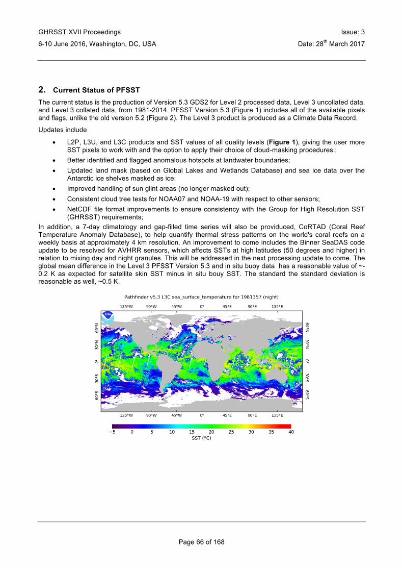
GHRSST XVII Proceedings Issue: 3
6-10 June 2016, Washington, DC, USA Date: 28th March 2017
Page 66 of 168
2. Current Status of PFSST The current status is the production of Version 5.3 GDS2 for Level 2 processed data, Level 3 uncollated data, and Level 3 collated data, from 1981-2014. PFSST Version 5.3 (Figure 1) includes all of the available pixels and flags, unlike the old version 5.2 (Figure 2). The Level 3 product is produced as a Climate Data Record.
Updates include
• L2P, L3U, and L3C products and SST values of all quality levels (Figure 1), giving the user more SST pixels to work with and the option to apply their choice of cloud-masking procedures.;
• Better identified and flagged anomalous hotspots at landwater boundaries; • Updated land mask (based on Global Lakes and Wetlands Database) and sea ice data over the
Antarctic ice shelves masked as ice; • Improved handling of sun glint areas (no longer masked out); • Consistent cloud tree tests for NOAA07 and NOAA-19 with respect to other sensors; • NetCDF file format improvements to ensure consistency with the Group for High Resolution SST
(GHRSST) requirements; In addition, a 7-day climatology and gap-filled time series will also be providuced, CoRTAD (Coral Reef Temperature Anomaly Database), to help quantify thermal stress patterns on the world's coral reefs on a weekly basis at approximately 4 km resolution. An improvement to come includes the Binner SeaDAS code update to be resolved for AVHRR sensors, which affects SSTs at high latitudes (50 degrees and higher) in relation to mixing day and night granules. This will be addressed in the next processing update to come. The global mean difference in the Level 3 PFSST Version 5.3 and in situ buoy data has a reasonable value of ~-0.2 K as expected for satellite skin SST minus in situ bouy SST. The standard the standard deviation is reasonable as well, ~0.5 K.

GHRSST XVII Proceedings Issue: 3
6-10 June 2016, Washington, DC, USA Date: 28th March 2017
Page 67 of 168
Figure 1: An example of the current Level 3 Pathfinder SST version 5.3 (upper panel) and
the old Pathfinder SST version 5.2 (lower panel).
3. Current Status of Daily OISST The dOISST version 2 (v2) dataset currently in production (also referred to as the AVHRR_ONLY) is based primarily on AVHRR SST observations (the PFSST level 3 product). AVHRR_ONLY extends from late 1981 to the present. For most of this time span, reprocessed datasets were used as inputs because of their higher quality over operational datasets. However, reprocessed datasets are by nature delayed in availability so operational datasets are utilized to extend the time series forward. These daily updates are often referred to as the operational production. To increase accessibility, transportability and transparency, the Climate Data Records program funded an effort to modernize the dOISST production code, called refactoring, which is spearheaded by the Software Engineering Branch at NCEI. While most of the refactoring per se has been completed, the testing phase is ongoing. An additional requirement to transfer from a 32-bit to a 64-bit environment, and switch to newer software versions uncovered a bug in older 32-bit Fortran compiler. Hence, a reprocessing of the entire time series will be needed when the refactored code is adopted in the 64-bit environment for operational production. As the refactoring testing continues, research work will be focused on evaluating input datasets for the next version.
To meet shorter term GHRSST requirements, the operational scripts (and the refactored code) were modified to produce GDS2.0 compliant-files. The first part of the dOISST dataset was also converted to GDS2.0. At present, both GDS1.0 and 2.0 files are sent to JPL. The long period of record permitted a 30-year dOISST climatology (1982-2011) to be published (Banzon et al., 2014). Also, since the description of version2 is in a web pdf, a dataset description was published recently (Banzon et al., 2016).
A related dOISST product (called AVHRR+AMSR) included microwave SST data from AMSR-E. However, when AMSR-E lost its daily global observation capability in 2011, production was stopped because the only other instrument WindSat has not been evaluated. Now WindSat has been evaluated and AMSR-2 is flying, but resources are not available to restart production and all resources have been placed in refactoring.
4. Current Status of ERSST The current status of ERSST includes maintaining operational ERSST v3b and v4; maintaining operational SST uncertainty for ERSSTv4; providing SST to NOAAGlobalTemp v4 merged with GHCN v3.3.0; and

GHRSST XVII Proceedings Issue: 3
6-10 June 2016, Washington, DC, USA Date: 28th March 2017
Page 68 of 168
ERSST development including updated sea-ice concentration, ICOADS Release 3, and Argo temperature observations above 5m.
5. Summary The Pathfinder SST Version 5.3 AVHRR products will include Level 2 processed data, Level 3 uncollated data, and Level 3 collated data, from 1981-2014. The Level 3 CDR product will include all of the available pixels and flags and will be release this year of 2016 in July/August. The Pathfinder SST products are improved with scientific quality assessments through rich inventory analysis and in situ data matchups.The global mean difference in the Level 3 PFSST Version 5.3 and in situ buoy data is at a reasonable value of ~-0.2 K and the standard deviation as well, ~0.5 K. Daily OISST processing v2 continues until refactoring of code is complete. Adoption of refatored code will require a reprocessing. This includes evaluation of new or updated inputs (latest Pathfinder version ACSPO). The long-term goal is to have a more integrated approach between ICOADS, PF and dOISST. New version of ERSST to be released in 2017
6. References Banzon, V., Smith, T. M., Chin, T. M., Liu, C., and W. Hankins, 2016.: A long-term record of blended satellite and in situ sea-surface temperature for climate monitoring, modeling and environmental studies, Earth Syst. Sci. Data, 8, 165-176, doi:10.5194/essd-8-165-2016.
Banzon, V. F., R. W. Reynolds, D. Stokes, and Y. Xue, 2014: A 1/4° spatial resolution daily sea surface temperature climatology based on a blended satellite and in situ analysis. Journal of Climate, 27, 8221–8228, doi:10.1175/JCLI-D-14-00293.1
Casey, K.S., T.B. Brandon, P. Cornillon, and R. Evans (2010). "The Past, Present and Future of the AVHRR Pathfinder SST Program", in Oceanography from Space: Revisited, eds. V. Barale, J.F.R. Gower, and L. Alberotanza, Springer. DOI: 10.1007/978-90-481-8681-5_16.
Casey, K.S., R. H. Evans, W. Baringer, K.A. Kilpatrick, G.P. Podesta, S. Walsh, E. Williams, T. B. Brandon, D. A. Byrne, G. Forti, Y. Li, S.A. Phillips, D. hang, and Y. Zhang (2011). AVHRR Pathfinder Version 5.2 Leel 3 Collated (L3C) Global 4km Sea Surface Temperature. National Oceanographic Data Center, NOAA. Dataset. Doi:10.7289/V5WD3XHB.
Kilpatrick, K. A., G. P. Podesta, and R.H. Evans. 2001. "Overview of the NOAA/NASA Pathfinder algorithm for Sea Surface Temperature and associated Matchup Database." J. Geophys Res., 106: 9179-9198. 13497- 13510.

GHRSST XVII Proceedings Issue: 3
6-10 June 2016, Washington, DC, USA Date: 28th March 2017
Page 69 of 168
RDAC UPDATE: RSS Chelle L. Gentemann(1)
(1) Earth and Space Research, Seattle, WA, USA, Email: [email protected]
REPORTS This report describes the status of GHRSST data at Remote Sensing Systems (RSS).
1. Satellite SST Data RSS produces L2P and L3U data for GHRSST through the JPL GDAC. The data RSS produces is all based on the RSS passive microwave SST data and includes TMI, Aqua AMSR-E, WindSAT, and AMSR2. There are plans to begin producing data for GPM GMI within the next few months (Table 1). At this time, the quality of all SSES unknown since 1/2016 when NRT buoy collocation was not updated. RSS is currently transitioning GDS2.0 processing, including SSES calculation, to a new environment. A test file for WindSAT has been provided to PO.DAAC for evaluation.
Sensor Dates Coverage L2P L3U
TRMM TMI 1998-3/2015 40S-40N Yes Yes
Aqua AMSRE 6/2002 – 10/ Global Yes Yes*
WindSAT 2/2003 – present* Global NO Yes**
AMSR2 7/2012-present* Global Yes**^ Yes**
GPM GMI 65S-65N Soon Soon
Table 1: L2P data sets developed within the framework of the MISST project. *Needs to be reprocessed, problem with flagging. **SSES unknown quality since 1/2016. ^AMSR2 S.Hem 10V problems, correction applied.
2. L4 SST Data RSS currently produces both a global 25 km daily passive microwave (PMW) only L4 analysis and a global 9 km daily microwave and infrared (MWIR) analysis. The MWIR analysis is scheduled to be retired soon and users are recommended to switch to other operational GHRSST L4 data.

GHRSST XVII Proceedings Issue: 3
6-10 June 2016, Washington, DC, USA Date: 28th March 2017
Page 70 of 168
GHRSST PARALLEL BREAKOUTS FOR TAGS/WGS CLIMATE DATA RECORDS TAG BREAKOUT SESSION
Jonathan Mittaz(1), Viva Banzon(2)
(1) University of Reading, Reading, Berkshire, UK, Email: [email protected] (2) NCEI Asheville, Asheville, NC , USA, Email: [email protected]
ABSTRACT A very limited number of dataset producers have tried to apply the metrics described in the Climate Data Assessment Framework (CDAF) document. Therefore the Climate Data Records (CDR) Technical Advisory Group (TAG) breakout session identified the need for tools that would facilitate the work. The breakout session consisted of three presentations of validation efforts, followed by the demonstration of Felyx , a matchup database tool and then complementary add-on modules based on the SQUAM system which are still in the conceptual phase. The presentations and discussions underlined the importance of the reference dataset and its adjustment to the appropriate SST depth of the product being evaluated. The use of a model to validate in areas or times without data was also discussed.
1. Introduction In the past, the initial part of the Climate Data Records (CDR) Technical Advisory Group (TAG) session would be a report from the different data producers. However, in this session, this portion was significantly reduced to allow more time to focus on other matters. The different contributors were asked ahead to submit their update slides for the individual products and then fill in their information in a summary table. These will be available at the GHRSST website, for anyone interested.
The CDR_TAG session focused on developing tools that will allow for assessments of datasets for climate applications, and not necessarily the identification of a CDR, per se. The Climate Data Assessment Framework (CDAF) document contains guidelines for product assessment. In past meetings, dataset producers were encouraged to apply the CDAF criteria to their products and submit assessments. However few (one) made the effort, and one of the clear problems is the lack of standardized methodology and tool.
The first three presentations in this session involved recent work on validation, in line with the CDAF requirements: 1) AVHRR HRPT SST product around Australia by Helen Beggs, 2) the ESA CCI validation by Gary Corlett, and 3) a new reprocessed L2 dataset called AVHRR RAN1 by Sasha Ignatov.
The second half the session was dedicated to the CDAF tools. The Felyx tool, although still in development, has progressed sufficiently so that a short demo could be made by Jean Francois Piolle. Development of additional modules (statistics, visualization) that could be applied to the output of Felyx were discussed by Prasanjit Dash based on SQUAM and the new EUMETSAT validation tool developed for the Sentinel-3 mission.
2. Validation talks The evaluation of a regional product and the custom statistics (night buoy data adjusted to skin) to assess real time and delayed mode algorithms was presented by Helen Beggs. The AVHRR HRPT SST L2 product around Australia represents a ~25 year record, merging data from different AVHRR satellites. Algorithm coefficients are referenced to drifting buoys. Foundation SSTs are also generated by rejecting low wind data and a bias correction. Product stability was assessed by mapping the coefficients over time. Adaptive error statistics are used. Drifting buoy data were adjusted to skin SSTs before comparing to satellite skin SSTs. Validation with the IMOS ship data required a depth adjustment, and produced noisier results, but this could be due to the fact that the ship measurements tend to be more coastal, while the buoys are offshore. Plots can be viewed on web with and without the satellite bias correction. It was suggested that the website be modified to allow for interactive plots.

GHRSST XVII Proceedings Issue: 3
6-10 June 2016, Washington, DC, USA Date: 28th March 2017
Page 71 of 168
The CCI approach, which represents a next generation validation effort, was presented Gary Corlett. The reference value is adjusted for geophysical offset, satellite instrument error, and reference error and an uncertainty model is constructed. The CCI products are then provided with uncertainty at the pixel level, and validation is performed with an independent dataset (e.g., Argo) so in the case of the CCI the uncertainty/error is not derived from in-situ matches but is only validated by them. Some in situ data may be used in algorithm training, but not in production. Three types of validation were performed: point, grid and functional. The functional approach uses an uncertainty model to transfer to areas and times whether there are no reference measurements. Satellite uncertainty was broken down into five components: instrument (from calibration), reference (known for buoys, etc.), geophysical spatial footprint, geophysical depth (including diurnal model for low windspeed). This approach seems to be leading the way forward.
RAN1,a first version reanalysis of SSTs from the AVHRR3 series (2002-2015) using the Advanced Clear Sky processor for Oceans (ACSPO) algorithm was assessed by Sasha Ignatov using drifters and tropical buoys as reference. A comparison was made with two other datasets: CCI and Pathfinder. The ACSPO bias was about 0. The Pathfinder offset was 0.17, as expected and CCI offset was 0.1. The morning platforms compare better than the afternoon ones. There was a question whether the CCI comparisons used the skin or depth SSTs, which are both in the same file. In any case, the recommendation was that the reference dataset be adjusted by depth to match the SST dataset being evaluated.
3. CDAF Tools Felyx is a dataset matchup tool being developed under the CCI. It has the advantage that it can be downloaded as a package by the dataset producer and run on locally. It can also be deployed remotely as a service but the dataset to be assessed needs to be pushed to the Felyx server. Jean Francois Piolle gave a brief demonstration and status report. It is run from a command line and features include 1) a space-time window can be specified, 2) metrics product generation using operators (wind threshold, satellite zenith angle, night/day, etc.). The tool is expected to be ready before the end of the year. For now the tool uses one reference dataset (from Gary Corlett) also developed under the CCI. But other reference datasets could be used, such as the radiometer measurements, which are not yet publicly available, but are expected to become organized and centralized in the coming year.
Prasanjit Dash described a SQUAM-like tool to support CDAF metrics and beyond. It that can be applied to Felyx output will provide more sophisticated analysis and visualization modules. He is in the initial phase of developing a tool for Sentinel 3 that will be similar to SQUAM but with regional capability. Computationally this can also be applied locally, like Felyx. Plotting capabilities include maps, histograms, robust min-max, time-series of parameters. Again, the question regarding the choice of reference dataset was raised. He suggested Coriolis, but of course the potentially others like radiometer data could be added. Other diagnostics could be added to examine trends, seasonality, noise.
Discussion pointed out that these tools can be used for other applications other than CDAF validation. Also, regarding the skin-depth difference, should everyone be using 0.17 K at wind speeds less than 6 m/s? Peter Minnet is planning to assess the skin effect correction as a function of wind, time, etc. Other opinion was that this depended on wind stress, related to turbulence and hence mixing. This discussion really dovetails into the choice of reference datasets and their proper adjustment. The CDR TAG should look further into this question.
4. Conclusion Few dataset producers have made an effort to assess their product following the CDAF document. To improve the situation, the CDR-TAG is focusing on tools that producers can deploy in their local computers. Within the year, Felyx, a matchup extraction tool, will be ready, and it will be complemented by a SQUAM-like tool, still under development. The validation efforts presented underlined the need to adjust reference datasets to the depth of the SST being compared to. Also, where there is no reference dataset, then an uncertainty model could be employed. The CDR-TAG also supported continuing efforts to continue work on a tool to help the CDAF assessment process so work will continue on this in the coming year.

GHRSST XVII Proceedings Issue: 3
6-10 June 2016, Washington, DC, USA Date: 28th March 2017
Page 72 of 168
PLENARY SESSION III: BIASES IN SST RETRIEVALS SESSION REPORT
Andrew Harris(1), Jonathan Mittaz(2)
(1) ESSIC/CICS, University of Maryland, College Park, MD, USA Email: [email protected] (2) University of Reading, Reading, Berkshire, UK Email: [email protected]
1. Introduction The session was aimed at discussing possible sources of bias in the SST retrieval schemes, including biases caused by issues in both the Level 1 radiances as well as those introduced into Level 2 products. In total, three talks were presented ranging from Level 1 data issues in the AVHRR, bias correction methods applied to SEVIRI data and the issue of errors and biases in the in situ network (primarily drifting buoys). Most of the discussion in this session followed after each presentation, rather than having a dedicated discussion time at the end.
2. Talk: Importance of uncertainty estimates at Level 1 satellite data for SST CDR (Marine Desmons, University of Reading)
This talk discussed the impact of variable instrument noise on SST retrievals. The example given was from the AVHRR satellite record where there can be significant changes in the instrument noise, particularly for the earlier (pre-AVHRR/3, i.e. up to NOAA-14) sensors. The channel most impacted by the changes in the noise is the 3.7μm channel where variations of more than a factor of 10 can be seen. It was also pointed out that the ‘standard’ NeΔT used for the AVHRR of 0.12 K is actually the design noise specification and the true random noise component is smaller that this (of order of 0.08 K for the 11/12μm channels). The impact of the noise on a regression-based retrieval (the OSI-SAF nighttime retrieval) showed that, for well-constrained sensors (the newer ones), the instrument noise component of the uncertainty budget was small compared to the statistics obtained by comparing with drifting buoys. On the other hand, for the early sensors ,if the 3.7μm channel was used this would not be the case as an uncertainty > 2K could be introduced due to the increase in instrument noise that typically manifested itself in the record within a year or so after launch.
Discussion
Craig Donlon pointed out that the analysis of instrument behavior, including the noise characteristics, should be a crucial step for all sensors and that continuous monitoring of instrumental parameters is needed and the thus work of the type presented in this talk is important. Jon Mittaz said that such instrumental monitoring is going on at NOAA and EUMETSAT but was only in place for the recent past (last 6 or 7 years) and needed to be extended back in time for climate purposes. He also pointed out that the FIDUCEO project (www.fiduceo.eu) will be providing noise statistics for all AVHRR sensors as part of its data stream. Helen Beggs asked about what improvements could be expected from the sort of detailed analysis being undertaken by FIDUCEO and Jon Mittaz replied that one should expect to see a reduction in radiance bias together with a more consistent sensor-to-sensor harmonization.
3. Talk: One year comparison of two methods of calculating inter sensor bias correction: operational and “DINEOF“ method applied on SEVIRI data over European seas over in the context of the Copernicus program (Françoise Orain, Meteo France)
The problem that this talk addressed is how to merge SSTs from two different sensors using one as a reference. Operationally OI is used but the need for improvements has been noted so a comparison with the DINEOF method (which is a method using EOFs to fill gaps) has been undertaken. First, using the AATSR sensor as a reference for SEVIRI showed that the DINEOF method seemed to work best. Also the same comparison has been made where MetOp-A was used as a reference for SEVIRI (required due to the lack of

GHRSST XVII Proceedings Issue: 3
6-10 June 2016, Washington, DC, USA Date: 28th March 2017
Page 73 of 168
an AATSR sensor currently). Again, the DINEOF method was shown to be better for most regions studied. An operational test will be implemented at CMS.
Discussion
Sasha asked if the EOFs were in the form of timeseries or fields and was told that the EOFs are in the form of fields. Sasha then asked about the time window used and was told that it is currently set at 20 days. Irina Gladkova asked if the 20 day window was the reason for gaps in the temporal coverage and was told that yes, the gaps were due to the 20 day window. Igor Tominski pointed out that tests had been run and 20 days was found to be optimal for the technique. Sasha then asked by OSTIA wasn’t used as a reference and was told it was because started with AATSR and needed a similar reference. Also, OSTIA uses MetOp-A in the absence of an ATSR-type sensor.
4. Talk: SST error of drifting buoys: possible eddy effect? (Alexey Kaplan, Columbia University)
This presentation was about the impact of eddies on the drifting buoy record. Platform-related biases are needed at the 0.3 K level to model realistically relatively slow error reduction in regional and temporal averages over time, which is anticipated due to the increasing number of platforms. Studies of drifting buoys, however, seen to show much smaller reductions. It is hypothesized that a significant number of drifting buoys are captured by ocean eddies for some fraction of their trajectory. Since there are systematic differences between eddy cores and the surrounding water this difference could give rise to the somewhat smaller improvement in the accuracy of regional and global SST estimates.
Discussion
Craig Donlon raised the importance of how buoy drogues (which tend to detach after some months from the SVP-type buoys that dominate the recent in situ record) relate to what each buoy was measuring and how eddies could impact their motion. Alexey responded that trajectories between buoys and eddies are far from consistent (this could, of course be due to the aforementioned drogue/no-drogue situations). Craig then said that if you have buoys trapped in dynamic systems when you related SST with a large window (6-12 hours) have to account for different in displacement error only need to be 1-km off to get different SST and thinks there more to the bias issue than the AK approach to this issue. Andy Harris was bothered by the large value of the error which seemed too large to him, though Gary Corlett said that it was assumed that the 0.2 K value mentioned assumed no bias. Helen Beggs then came back to the fact that buoys measure a point and that the location of the buoys reported can be at a much coarser resolution (for older buoys only to 0.1 degree lat/lon) than was ideal. This raises the issue of geolocation errors just due to the reporting format. David Meldrum then made some comments regarding the drifting buoy network. He pointed out that the network was never intended for detailed SST work but was intended for the modelling and ocean dynamics community. The GRHSST requirements are now being incorporated. ESA also has a project to study the impact of higher resolution buoy data. Initial results seem to show a negative impact. Reason may be due to the drifter population – young drifters and older drifters. Older drifters are good surface property trackers whereas those with a drogue will tend to profile the water column and give cooler bias due to pull down of drogue. This may help explain Alexey’s biases (see comments above). Also waves will go over the top of a drogued buoy. The distribution is non-uniform though it might be that drogued drifters will congregate in convergent areas. Craig then said that this would impact averages. Andy Harris then said that we should also remember that satellite data tends to screen out cold water and will give rise to a warm bias. Alexey said that there was a database of eddies from Dudley Chelton which may help. Anne O’Carroll the said that EUMETSAT is setting up a study to understand when the drifter loses the drogue put surface and water sensors to get understanding of drifter depth. Finally Craig said that drifters remain a really important source of information for currents and that the equator will be important for un-drogued drifters.
5. Open discussion There was no time for open discussion after the end of talk specific discussions.

GHRSST XVII Proceedings Issue: 3
6-10 June 2016, Washington, DC, USA Date: 28th March 2017
Page 74 of 168
IMPORTANCE OF UNCERTAINTY ESTIMATES AT LEVEL 1 SATELLITE DATA FOR SST CDR
Marine Desmons (1), Jonathan Mittaz(1), Christopher Merchant(1) and Owen Embury(1)
(1) Department of Meteorology, University of Reading, Reading, united Kingdom, Emails: [email protected],
[email protected], [email protected], [email protected]
1. Introduction FIDUCEO (Fidelity and uncertainty in climate data records from Earth Observations - http://www.fiduceo.eu) aims to provide FCDRs and CDRs with rigorous and traceable uncertainty estimates. These estimates are developed through the use of metrological standards and practices and are responding to the need of better climate data to support rigorous science, decision making and climate services. The approach aims to provide improved CDRs that have traceable uncertainties where a complete understanding of both FCDR (radiance) and CDR algorithms and sources of uncertainty have been studied. However, FCDR uncertainties can be quite complex and it is still often the case that these Level 1 uncertainties are not explicitly taken into account for many SST datasets. In this work we are limiting ourselves to the uncertainties caused by instrumental noise for the case of the complete AVHRR record. At small spatial and temporal scales (pixel, instantaneous) such radiometric noise is one of the dominant sources of uncertainty for satellite data. It turns out, however, that such noise is strongly variable and presents rapid changes that need to be understood and taken into account to produce accurate CDRs uncertainties. Here we present a detailed study of the noise for AVHRR Level-1 data, with insights into the noise differences between space view and internal calibration view observations across different versions of the instrument. We also describe the impact of our noise estimates on SST retrievals using a simple SST retrieval algorithm.
2. The noise in the AVHRR Level-1 data There are different sources of error in radiance data (Level 1), such as radiometric noise (resulting from badly characterized calibration system, thermal noise of the detector, shot noise...), the retrieval algorithm, the forward model, etc. Often, Level 1 data users have estimated the uncertainty on the radiances with the value given in the associated documentation, which, in the case of the AVHRR was simply the design specification of the instrument (0.12K in the IR). However, as we can see on Figure 6, the AVHRR noise is far more complex than a unique value. Moreover, the value given in the instrument specification tends to overestimate the uncertainty, and to not represent properly its variability. A better way to determine the instrument noise is to use on-board measurements. In this work, we have used the ten measurements of the warm internal calibration target (ICT) and of the cold target (deep space) that are provided every full scan by the in-flight calibration system of the AVHRR thermal channels, to estimate the random component of the instrument noise. While this is not done here, another method to estimate the uncertainty for the Earth scenes explicitly is to look at uniform scenes [1].
As we can see on Figure 6, the noise varies according to the channel and to the temperature of the target the sensor is looking at. The noise is also inconsistent with the 0.12K value which has been used in the past. More over, the noise presents a temporal variability, either at a very short scale (for instance over an orbit for TIROS-N) or over the lifetime of the instrument. On the long timescales this variability can be due to the degradation of the instrument over the time or it can be linked to events that impacted the instrument itself. This is shown on the panel (a) of Figure 6 where the large jumps in noise correspond to outgassing times of NOAA-7 where all the electronics are turned off. Given the potential very high variability of the noise for AVHRR Level 1 data and the difference in noise from the often used quoted noise estimate it is necessary to investigate the impact of the true noise on geophysical retrievals, in this case on SST.

GHRSST XVII Proceedings Issue: 3
6-10 June 2016, Washington, DC, USA Date: 28th March 2017
Page 75 of 168
(a) channel at 3.7 µm
(b) channel at 11 µm
(c) channel at 12 µm
Figure 6: Orbital average of the NeDT of the warm and cold targets over all the lifetime of NOAA-07.

GHRSST XVII Proceedings Issue: 3
6-10 June 2016, Washington, DC, USA Date: 28th March 2017
Page 76 of 168
3. Radiometric uncertainty on SST In this part, we estimate the effect of the noise in Level 1 data on the sea surfaces temperatures by propagating the level 1 data uncertainty into a typical SST retrieval algorithm. There are different formalisms usable to derive SST from the AVHRR IR brightness temperatures. Here, we use the nighttime algorithm used in OSI SAF [2]:
𝑆𝑆𝑇 = (𝑎 + 𝑏𝑆))𝑇+, + (𝑐 + 𝑑𝑆))(𝑇// − 𝑇/1) + 𝑒 + 𝑓𝑆) + 𝑐𝑜𝑟𝑟 Equation 1
Where 𝑇+,, 𝑇//, 𝑇/1 are the brightness temperatures at 3.7, 11 and 12 microns, respectively; corr is the correction term resulting from preliminary adjustment on the matchup database; 𝑆) = sec(𝜃) − 1, where 𝜃 is the satellite zenith angle. The coefficients of the algorithm have been derived on a simulated brightness temperatures database [3]. Considering in a first approximation that the uncertainties on the brightness temperatures measured in the different channels are independent, the uncertainty on the SST due to the radiometric noise is:
𝛥𝑆𝑆𝑇 =𝜕𝑆𝑆𝑇𝜕𝑇+,
1
𝛥𝑇+, 1 +𝜕𝑆𝑆𝑇𝜕𝑇//
1
𝛥𝑇// 1 +𝜕𝑆𝑆𝑇𝜕𝑇/1
1
𝛥𝑇/1 1
Equation 2
Equation 2 describes the addition of uncertainty terms in quadrature, with the differential describing the sensitivity of the uncertainty to the observation.
Brightness Temp.
BT
Radiance
N
DT=(DT1+DT2)/2 NeDN
DT1,2=BT1,2-BT BT1,2 N1,2=N± NeDN
Figure 7: Algorithm to estimate DT due to the radiometric noise
Figure 8: Histogram of the median per orbit of 𝛥𝑆𝑆𝑇 for AVHRR18_G, June 2010
Given that the fundamental unit for the instrument uncertainty is radiance, the estimate of the uncertainties ΔT is obtained in the following way: First, we transform the brightness temperature BT into a radiance N thanks to Planck's law. The radiance uncertainty NeΔN, which is calculated orbit-by-orbit through the warm and cold target measurements, is then added and subtracted from the scene radiance to provide an upper and a lower brightness temperatures BT1 and BT2. We then compute two differences of temperatures ΔT1,2=BT1,2-BT from which we can deduce the uncertainty on BT. The algorithm is summarized on Figure 7.
Then, we can estimate the uncertainty of the sea surface temperatures due to the instrumental noise by replacing the obtained values DT in Equation 2. For AVHRR18_G, we see on Figure 8 and on the panel (a) of Figure 9 that the uncertainties on SST due to the radiometric noise are close to 0.1. This value is much lower than the uncertainty of 0.49 on the SST decribed by Merchant and Le Borgne [4] for this algorithm, which

GHRSST XVII Proceedings Issue: 3
6-10 June 2016, Washington, DC, USA Date: 28th March 2017
Page 77 of 168
implies that the dominant source of uncertainty in SST is due to the retrieval process and not to the noise on the measurements. On the other hand, panel (b) of Figure 4 shows that for the AVHRR07_G, the uncertainties range from 0 to 2 over the lifetime of the instrument, following the trend of the radiometric noise already shown on panel (a) of Figure 1. This behaviour emphasizes the necessity to take the variability of the radiometric noise while estimating the uncertainty on the SST.
(a) AVHRR18_G (b) AVHRR07_G
Figure 9: Monthly median of ΔT over the archive
4. Conclusion The detailed study of the noise of the AVHRR radiances in the infrared domain underlines the important variability of the noise at Level 1. Indeed, the amplitude of the radiometric noise varies according to the temperature of the target the sensor is looking at. Then the noise undergoes an important and unpredictable temporal evolution, which can be smooth when following the degradation of the sensor or more sudden when linked to events that touched the instrument.
The analysis of the instrument noise impact on SST retrievals has then shown that for ‘well behaved’ AVHRRs (mostly NOAA-16 and alter) the noise makes up only a small part of the SST uncertainty. On the other hand, for the older (AVHRR/2) instruments where the noise variations are large, the instrument noise can be a dominant part of SST uncertainty, particularly if the 3.7μm channel is used. All this means that it is important to know the true underlying noise characteristics of any instrument used to retrieve SST.
5. References [1] Madhavan, Sriharsha, Xiaoxiong Xiong, Aisheng Wu, Brian N. Wenny, Kwofu Chiang, Na Chen, Zhipeng Wang, and Yonghong Li. ‘Noise Characterization and Performance of MODIS Thermal Emissive Bands.’ IEEE Transactions on Geoscience and Remote Sensing 54, no. 6 (June 2016): 3221–34. doi:10.1109/TGRS.2015.2514061. [2] O&SI SAF Project Team. ‘Low Earth Orbiter Sea Surface Temperature.’ Product User Manual. Météo France, November 2014. http://www.osi-saf.org/biblio/docs/ss1_pum_leo_sst_2_7.pdf.
[3] François, Christophe, A Brisson, P Le Borgne, and A Marsouin. ‘Definition of a Radiosounding Database for Sea Surface Brightness Temperature Simulations.’ Remote Sensing of Environment 81, no. 2–3 (August 2002): 309–26. doi:10.1016/S0034-4257(02)00008-1.

GHRSST XVII Proceedings Issue: 3
6-10 June 2016, Washington, DC, USA Date: 28th March 2017
Page 78 of 168
[4] Merchant, Christopher J., and Pierre Le Borgne, ‘Retrieval of Sea Surface Temperature from Space, Based on Modeling of Infrared Radiative Transfer: Capabilities and Limitations’, Journal of Atmospheric and Oceanic Technology 21, no. 11 (November 2004): 1734–46, doi:10.1175/JTECH1667.1.

GHRSST XVII Proceedings Issue: 3
6-10 June 2016, Washington, DC, USA Date: 28th March 2017
Page 79 of 168
PLENARY SESSION IV: FRONTS & GRADIENTS SESSION REPORT
Chair: Peter Cornillon(1), Rapporteur: Gary Wick(2)
(1)University of Rhode Island, Email: [email protected] (2) NOAA/ESRL, Email: [email protected]
ABSTRACTS / REPORTS Plenary session IV on “Fronts and gradients” was held on the morning of June 8th 2016 beginning at 10:30 am. The session consisted of three presentations by Irina Gladkova, Peter Cornillon, and Emmanuelle Autret, followed by an open discussion session used primarily for additional questions for the presenters. This report highlights the presentations and subsequent questions and discussions.
1. Towards high resolution ocean thermal fronts product from JPSS VIIRS – Irina Gladkova
Irina began her presentation addressing why fronts are important and more work is required in the area. Approaches to identifying fronts are not new, but all rely on a reliable cloud mask which may not be available on regional scales. She proposed that it might not be desirable to entirely separate cloud screening from front detection. The main goal of this project is to improve cloud masking and in so doing to develop a thermal front product consisting of a mask of where fronts exist. The approach identifies frontal regions in brightness temperature fields (not SST) and then makes decisions on cloud contamination based on regional statistics. The basis of the approach is a 1st and 2nd order Taylor expansion, and then employs the eigenvalue of the Hessian to identify peaks in the gradient which are then thinned to individual points. The presentation also questioned the reliability of existing ice masks and said that the methods could also be employed to correct sea ice boundaries as well. Comparisons were also presented between frontal detection in L4 and L2 products. The MUR product was found to capture general patterns but could not fully replicate what was possible from the highest resolution L2 products. In summarizing, Irina stated that the next steps were to test and implement the approach in the VIIRS ACSPO 2.60 product and integrate it with other corrections.
Ken Casey questioned if the frontal information would be added to an L2 product. Sasha Ignatov replied that they were trying to collect information on what users desired but did plan to do something. Jorge Vasquez commented that he saw many applications of the work and asked what were the main lessons learned. Was it that one mask does not fit all? Irina replied that yes, that was a fair assessment. She added that ice was a specific concern and she specifically wanted to address conditions surrounding thin ice. During the later open discussion, Craig Donlon asked how the results might be applied more generally to the cloud clearing problem. Irina replied that the results will be in the ACSPO mask and she didn’t really know how else to answer. Eventually they may employ the results to both MODIS and potentially AVHRR products. Craig asked further how the results might be employed for ocean color and the SLSTR. Irina replied that while chlorophyll fronts were a question for someone else, frontal detection works fine in clear conditions, and it may be possible to use cloud masks from other imagers. Sasha added that a prerequisite for the technique is a good quality imager and that a sensor like SLSTR will have different problems. It will be important to address any unique image problems first. Irina has looked at Himawari-8 and feels the technique can be applied but they are not there yet.
2. Sub-diurnal variation of SST gradients in infrared satellite data – Peter Cornillon Peter cited motivation for this work as coming from a former Master’s thesis which found a 10% increase in front probability over 30 years. This was traced to drift in the overpass time of satellite orbits and leads to the question of whether there is a diurnal signal in front probability. A large signal exists for more fronts in the afternoon than in the morning and the work examines this in more detail in the eastern Mediterranean. The approach looks at gradients (rather than fronts) using the Sobel kernel and SEVIRI data. Gradients were found

GHRSST XVII Proceedings Issue: 3
6-10 June 2016, Washington, DC, USA Date: 28th March 2017
Page 80 of 168
to exhibit a strong diurnal signal as well as fronts and he examined what was contributing to the increase – all gradients or just weak or strong ones. During spring/summer an increase in weak gradients is observed in the afternoon hours, partially balanced by a decrease in strong gradients. The results were seasonally dependent, however, as during the winter there was no creation of weak gradients but still the decrease in strong gradients. Application to another region (off north Africa) suggested that there was also significant regional variability in the results. Peter stated that he found the results intriguing but he doesn’t yet fully understand them. To conclude, he emphasized that there was a strong diurnal signal with gradients increasing strongly in the spring and summer but with substantial regional variability. Peter also presented a brief overview of Fan Wu’s poster (EVALUATION OF THE PRECISION OF SATELLITE-DERIVED SEA SURFACE TEMPERATURE FIELDS) that examined the fidelity of small scale structures in single sensor satellite products. The best results were obtained for VIIRS with relatively poor results for AVHRR.
Gary Corlett questioned what was the resolution of the AVHRR data used. Peter replied that it was HRPT data. He also questioned if there was any potential influence of the cloud flagging. Prashanjit Dash then requested some clarification on the color meaning in some of the graphics utilized in the main presentation. In the later open discussion, Charlie Barron asked, with respect to the different weak front results off north Africa, if thinning potentially got rid of the weak fronts. Peter replied that it was not the result of thinning. Salvatore Marullo noted that the temporal variability of gradients has a significant impact on heat fluxes and Peter agreed completely. Peter added that the results could be further stratified by the amount of warming.
3. Enhanced resolution of SST field from SST gradient transformation – Emmanuelle Autret
This presentation was motivated by the existence of many small scale features in the SST which can make significant contributions to horizontal and vertical transports as well as the boundary layer. Information is split between low resolution fields, discontinuous high resolution data, and gap-free L4 data. The objective of the work was to characterize high resolution SST fields (e.g. infrared) with respect to low resolution data (microwave) and to investigate obtaining enhanced resolution fields from using both. The work used simultaneous AMSR and MODIS data and employed spectral analysis on the full and spatially smoothed fields. The results demonstrated that the strongest gradients were still visible at low resolution while weaker ones disappeared and examined models for the distributions. Ultimately the work showed that it is possible to link high resolution anomalies and low resolution gradients and a high resolution SST field was reconstructed by enhancing major fronts in lower resolution data. It was possible to reconstruct sharp fronts and the spectrum of the reconstructed SST field was indistinguishable from the high resolution field at scales larger than 60 km.
Craig Donlon asked if this approach could be pushed further – was it possible to construct a full L4 product? Emmanuelle replied that yes, this should be possible. During the later open discussion Viva Banzon asked how would one know if this approach created artifacts. Emmanuelle acknowledged that this is challenging and the method could potentially create artifacts. Craig Donlon added that it should be possible to use the information together with other “brute force” optimal interpolation methods to help address this and potentially construct a new analysis.
4. Open Discussion The majority of questions posed during the discussion were directly to the individual speakers as noted above in the description of each presentation. Gary Corlett, however, did pose a more general question as to whether the group is now at a position to define a resolution metric. Peter Cornillon answered that he felt we were not there yet. Gary followed by asking if a group should be formed to explore this – should this be set as a target? No firm answer was given and the topic was left more generally for Friday and the discussion of future GHRSST groups and activities.

GHRSST XVII Proceedings Issue: 3
6-10 June 2016, Washington, DC, USA Date: 28th March 2017
Page 81 of 168
SUB-DIURNAL VARIATION OF SST GRADIENTS IN INFRARED SATELLITE DATA Peter Cornillon(1), Carol Anne Clayson(2), Pierre Le Borgne(3)
(1) U. Rhode Island, Narragansett, RI, USA, Email: [email protected] (2) Woods Hole Oceanographic Institution, Woods Hole, MA, USA, Email: [email protected]
(3) Retired, Email: [email protected]
ABSTRACT Ocean fronts are known to influence many physical, biological, and chemical processes including ocean mixing, air-sea interaction, cloud and wind patterns, and marine productivity. Satellite-derived Sea Surface Temperature (SST) measurements are an invaluable tool in studying ocean fronts because of the large spatial and temporal coverage of satellite data, extending back as far as the early 1980s. One of the limitations to satellite-derived ocean fronts is that they provide no information about the underlying vertical structure; furthermore, the dynamics on sub-diurnal time scales for ocean fronts are poorly understood. In this poster we examine the daily signal of SST gradient magnitudes for the eastern Mediterranean sea as the first step in quantifying a subset of ocean fronts globally and how they vary on sub-diurnal time scales. We find that mean gradient magnitude in summer months increases and peaks around 2-4 PM Local Sun Time (LST). We find that the peak in summer months results from an increase in the magnitude of weaker gradients while the magnitude of the strongest gradients decrease; however, the weaker gradients contribute more strongly to the mean signal, resulting in the increase. The mid-afternoon peak in SST gradient magnitude disappears in winter with only a suggestion of a peak earlier in the day although the paucity of cloud free data in winter precludes making a statistically significant statement in this regard.
1. Introduction Previous work, undertaken by Kelsey Obenour as part of her Master’s Thesis at the University of Rhode Island, suggested a significant increase in the global sea surface temperature (SST) front probability based on the Pathfinder 4km SST dataset (Figure 1). However, several issues with regard to the Pathfinder dataset raise concerns with regard to these results. Relevant to the work presented here is the observation, also presented in Obenour’s thesis, that front probability appears to have a diurnal cycle and that the orbits of the NOAA satellites on which the AVHRRs contributing to the Pathfinder dataset drift in time. The combination of these two factors could result in an apparent change in front probability. The objective of this work is to quantify the diurnal cycle in front probability and, eventually, to determine its source. To this end, we examine in detail the diurnal cycle in SST gradient magnitude in the eastern Mediterranean and, to a lesser degree, the same in the upwelling region off the northwest coast of Africa.

GHRSST XVII Proceedings Issue: 3
6-10 June 2016, Washington, DC, USA Date: 28th March 2017
Page 82 of 168
Figure 1: Global front probability versus time.
2. Data We used hourly SEVIRI SST fields based on radiances from the MSG satellites for the period January 2004 – December 2011. These data were produced by the Centre de Météorologie Spatiale of Météo-France. The fields were in satellite coordinates adjusted slightly such that all fields were in the same projection. These fields were then passed through a Sobel gradient operator along each of the two coordinate axes of the field and the resulting gradients were corrected for the geographic distortion of the grid to obtain northward and eastward SST gradients in K/km. Finally, a gradient magnitude was obtained for each pixel location. The resulting 24 gradient magnitude fields per day were then reorganized into local sun time (LST) fields – each of the original fields corresponded to a specific GMT hour. Then for every hour after 4 LST, 2D histograms of the gradient magnitude at each pixel location at 4 LST and the change in gradient magnitude between 4 LST and the subsequent hour of interest at that location were generated. These histograms were summed by region and by climatological season in order to determine how pixels of a given gradient at 4 LST contributed to any change in the gradient magnitude at subsequent times in the day.
3. Results Figure 2 and 3 show the diurnal variation of SST gradient magnitude averaged over the eastern Mediterranean and the eastern North Atlantic off of northwest Africa, respectively, for each of the four seasons. The scales on the axes are the same for the two plots. The diurnal variation in the fall and winter is similar for the two regions – relatively little variability if any at all. In contrast the spring and summer show significant variability in the eastern Mediterranean compared with a relatively weak signal off of Africa. The reason for this difference has yet to be determined. Of particular interest is the relatively low front probability at night in the Mediterranean – especially in spring – compared to the region off of northwest Africa.
Figure 2: Diurnal variation in SST gradient magnitude for the eastern Mediterranean – the Mediterranean east of 35°E.

GHRSST XVII Proceedings Issue: 3
6-10 June 2016, Washington, DC, USA Date: 28th March 2017
Page 83 of 168
Figure 3: Diurnal variation in SST gradient magnitude for the North Atlantic off of northwest Africa – east of 25°W, north
of 20°N and south of 35°N.
Although Figures 2 and 3 (especially Figure 2) point to diurnal variation in the gradient field, they do not address the question of whether the changes result from changes in weak gradients or strong gradients or changes over the entire range. Figure 4, addresses this in the context of 2D histograms showing the change in gradient magnitude of pixels between 4 LST and the indicated hour. The figure suggests that the increase in gradient magnitude between 4 LST and 1400 LST results from weak gradients getting stronger – on average, the gradients of pixels with strong gradients at 4 LST tend to get weaker.
Strong
Weak

GHRSST XVII Proceedings Issue: 3
6-10 June 2016, Washington, DC, USA Date: 28th March 2017
Page 84 of 168
Figure 4: Two-dimensional histograms of change in gradient magnitude between 4 LST and the indicated hour versus the gradient magnitude at 4 LST. Weak gradients correspond to 0.0095 to 0.0105 K/km, while strong gradients are for
0.037 to 0.038 K/km.
This is seen more clearly in Figure 5, which shows the fraction of pixels in the two bins indicated in Figure 4, one for weak and one for strong gradients. (Be careful, this plot is a little tricky; the curves are not cyclic over the 24 hour period. One might readily come to the conclusion that the number of pixels with strong gradients is increasing, but this is not what the plot says. Consider for instance the gradients labeled as strong in Figure 4. At 4 LST the gradient for the pixels in this bin are around 0.0375 K/km. As the day goes on, many of these gradients are weakened. By 4 LST, 24 hours later, the gradients of a significant fraction of these pixels have decreased to values near 0 K/km – the orange peak in each panel near 0.0375 K/km, -0.03 K/km. In the next 24 hour period, these pixels would actually start as weak gradients, gradients in the 0.01 K/km range and they would get stronger as the day progresses.)
Figure 5: Fraction of pixels in the ‘weak’ and ‘strong’ bins indicated in Figure 4 as a function of LST.
4. Conclusion This preliminary study shows significant regional and seasonal structure in the diurnal signal in SST gradient magnitude. There is a suggestion that diurnal forcing gives rise to or enhances gradients in locations with weak early-morning gradients and reduces the magnitude of strong early-morning gradients. However, as noted above, these results are quite preliminary. First, we need to determine whether or not the apparent changes in gradients result from actual changes or simply from a shift in the location of the local gradient field. To address this, we will reprocess the data, but this time rather than examining the change in gradient magnitude at fixed locations, we will examine the change assuming a spatial shift in the local SST field determined from the maximum cross-correlation of the later field with the 4 LST field. Second, we will examine the seasonal variation as a function of 15°x15° square in the SEVIRI field of view. Finally, we will determine the forcing that results in the changes, be it diurnal insolation or a diurnal signal in the wind field.

GHRSST XVII Proceedings Issue: 3
6-10 June 2016, Washington, DC, USA Date: 28th March 2017
Page 85 of 168
ENHANCED RESOLUTION OF SST FIELD FROM SST GRADIENT TRANSFORMATION
Emmanuelle Autret(1), Bertrand Chapron(1), Marouan Bouali(2)
(1) Ifremer, Univ. Brest, CNRS, IRD, Laboratoire d'Océanographie Physique et Spatiale (LOPS), IUEM, F-29280, Plouzané, France, Email: [email protected]
(2) Universidade de Sao Paulo (USP), Instituto Oceanografico 5IO), Brazil Email: [email protected]
Abstract Today, one important challenge is to better resolve and characterize the upper ocean dynamics at small scales. Small scale features (1-10km) are ubiquitous on high resolution remote sensing observations of the ocean surface such as optical, infrared and radar images and the contribution of the processes that are associated with these structures to the vertical fluxes in the upper ocean and between the ocean and the atmosphere is important. This study focuses on the characterization and the reconstruction of high resolution sea surface temperature (SST) fields from satellite-derived observations. High resolution (HR) observations from infrared instruments suffer from large missing data rates due to cloud contamination whereas microwave data are available with a global and quasi daily coverage but with a lower spatial resolution (LR, ~ 60 km). In this work, we highlight the non-Gaussian character of the HR fields and we investigate the enhanced resolution of LR SST fields from an Eulerian technique relying on a transformation of SST gradient fields. The results indicate that our method allows to reconstruct the larger SST fronts which leads to an enhanced spatial resolution of up to 15 km.
1. Introduction High resolution satellite images (~1-10 km) of sea surface temperature (SST) or chlorophyll reveal numerous small scale features such as eddies, filaments and fronts characterized by thin and elongated structures. Theoretical works indicate that these small scales make a significant contribution to the horizontal and vertical transport in the upper oceanic layers (Lapeyre and Klein (2006); Capet et al. (2008); Klein et al. (2008)). With regard, more specifically, to SST fronts, there have been a number of observational or numerical studies investigating interactions of sharp SST gradients and the marine atmospheric boundary layer and deeper atmosphere (e.g., Wallace et al. (1989), O'Neill et al. (2010)). Furthermore, SST fields make a major contribution in methods based on the surface quasi geostrophic therory aiming to retrieve horizontal and vertical velocities in the upper ocean from surface data (Isern-Fontanet et al. (2006)). Satellite derived SST from infrared (IR) radiometers can resolve fronts at submesoscale by providing high resolution images (~1-5 km). However SST can be retrieved only when there is no cloud. Microwave radiometers are capable of measuring SST independently of cloud cover but with lower spatial resolution. Gap-free global or regional SST products, merging various SST data sources, are also available. However commonly used interpolation methods, such as optimal interpolation, are based on Gaussian field assumptions that are not suitable to restitute thin and elongated sharp structures.
The objective of this study is to characterize HR SST fields (~IR products), i.e their spatial distribution, with respect to low resolution fields (~ MW products) and investigate the enhanced resolution of LR SST fields from an Eulerian technique relying on a priori-defined relationships between LR and HR images.
2. Data Our study relies on satellite derived SST data from AQUA. This dataset is particularly relevant for studying possible relations between the two spatial scales since the AQUA satellite carries both the Advanced Microwave Resolution Scanning Radiometer-Earth Observing System (AMSR-E) and the Moderate Resolution Imaging Spectroradiometer (MODIS), thus providing independent contemporaneous MW and IR measurements. For this study we have chosen two cases with a low cloud coverage. Figure 1 shows the SST

GHRSST XVII Proceedings Issue: 3
6-10 June 2016, Washington, DC, USA Date: 28th March 2017
Page 86 of 168
fields simultaneously observed by the MW and the IR instruments. The first case is on 6 may 2010 over the Gulf Stream and the second one is on 29 March 2010 off South California. In this study, we use version-7 AMSR-E L3 data from Remote Sensing Systems (REMSS). The MODIS SST data have been produced by The Advanced Clear-Sky Processor for Ocean (ACSPO) and the stripe noise has been here reduced by the algorithm described in Bouali and Ignatov (2014). In this study the cloud masking has been done by hand and the MODIS observations of 1 km at nadir has been remapped onto a regular 0.02° grid.
The 0.25° resolution AMSR-E SST L3 product can be seen as the result of a spatial integration acting as a high resolution field smoothing. It can be shown that this filter can be approximated either by a Gaussian filter with a standard deviation of 22 km or a 60 km averaging filter (not detailed here). In the following, the smoothed MODIS SST versions are obtained by the Gaussian filtering.
3. High resolution characterization tools
4. Spectral characterization The two-dimensional spectra estimated from the low and the high resolution SST fields are plotted in Figure 2a and 2b. These graphics show that the variance distributions are impacted by the spatial filtering for scales smaller than 200-250 km. Fitting a power-law 𝒌𝒏, with k the wavenumber and n the slope, in the 70-250 km band for the two cases shows that the spatial filtering between the high resolution SST and the MW SST product is thus close to 𝒌A𝟐in the Fourier domain.
5. SST gradient and anomaly distributions MODIS images show narrow and sharp gradient structures, with high values compared to those of AMSR-E gradients (~ 10-12 times higher). However the strongest gradients are still visible (in a smoothed version) in the LR fields. SST images show large regions of small gradient and small regions of high gradient. This inhomogeneity results, especialy for high resolution fields, in gradient distribution far from Gaussian. The non-Gaussian character can be seen in the distribution of MODIS SST zonal gradient shown in Figure 2c. These heavy-tailed distributions can be fitted by the Hyper-Laplacian distribution. The anomaly fields, that are the differences between MODIS SST and the smoothed MODIS SST, distributions are also far from Gaussian distributions (not shown here) and the Figure 2d highlights the relationship between HR anomaly variances and low LR SST gradients.
6. Reconstruction from gradient transformation The spectral analysis presented in section 3.1 clearly shows the energy that have been lost for scales smaller than 250 km due to the smoothing filtering but does not provide information concerning the spatial distribution of the small scales variability. The section 3.2 shows that large HR anomaly variances are associated with large gradient features visible in the LR fields. In this study, we propose to use the phase information provided by the LR field and estimate the contribution of the major fronts. The reconstruction relies on four steps: 1) gradient profile model definition, 2) transfert function between HR and HR profiles (at edge points) estimation, 3) HR gradient field construction, 4) HR SST field reconstruction. In this study, the gradient profile models, for HR and LR, are defined by a Gaussian function. Since the smoothing filter is known, the estimation of the LR profile sharpness allows for reconstructing HR profiles at edge points. From this new HR gradient field and the LR SST field, the reconstruction of the HR SST field can be achieved by the minimization of an objective function enforcing the constraints in both image domain and gradient domain.

GHRSST XVII Proceedings Issue: 3
6-10 June 2016, Washington, DC, USA Date: 28th March 2017
Page 87 of 168
Figure Error! No sequence specified.: AMSR-E (left) and MODIS (right) SSTs on 6 May 2010 (top) and on 29 March 2010 (bottom).
The resulting HR fields for the two regions are presented Figure 3a and 3b The Figure 3c shows an example of SST profile from the different SST fields. Due to possible small offsets in the position of the structures, a quantitative pixel-to-pixel comparison can lead to large errors. The effectiveness of these reconstructions is therefore evaluated with the help of the statistical properties presented section 3. First, the likelihood between the LR and the smoothed HR fields is guaranteed by the first term used in the energy function to be minimized. Second, the spectra presented in Figure 3d show the energy gain. For the Gulf Stream case, the spectrum of the reconstructed SST is indistinguishable from that of the HR field at scales larger than 60 km and the energy levels are comparable up to 15 km. For the California case (not shown here), the spectra are indistinguishable for scales larger the 65 km and the energy gain is also significant for smaller scales up to 15 km. The comparison in terms of gradient distributions is shown in Figure 3e representing the zonal gradient distribution for the reconstructed fields and the hyper-Laplacian fit (for the Gulf Stream region) of the HR gradients. As confirmed by these heavy tail distributions, the method allows to reconstruct the stronger gradients. The

GHRSST XVII Proceedings Issue: 3
6-10 June 2016, Washington, DC, USA Date: 28th March 2017
Page 88 of 168
relation between anomalies and LR gradients are shown in Figure 3f (for the Gulf Stream region). A qualitative comparison of the anomaly fields shows a good agreement in terms of spatial distribution, and the higher the LR gradient, the higher the HR detail is.
(a) SST spectra for the Gulf stream image. 2D spectra from MODIS SST (solid black), AMSR-E SST (solid grey),
smoothed MODIS SST (dash-dot black).
(b) SST spectra for the California image. 2D spectra from MODIS SST (solid black), AMSR-E SST (solid grey),
smoothed MODIS SST (dash-dot black).
(c) Normalized histogram of zonal SST gradient for the
Gulf Stream image (black line) compared to the Gaussian distribution (dotted grey line). The red line is the hyper-
laplacian fit.
(d) Squared SST anomalies versus LR SST gradient for
the Guf Stream image.
Figure 2

GHRSST XVII Proceedings Issue: 3
6-10 June 2016, Washington, DC, USA Date: 28th March 2017
Page 89 of 168
(a) Reconstructed SST
(b) Reconstructed SST
(c) Exemple of SST profile from MODIS (blue), AMSR-E (dot grey), smoothed MODIS (grey) and reconstructed
(blue)
(d) SST spectra for the Gulf Stream image from MODIS (solid black), smoothed MODIS (grey) and reconstructed
SST (blue).

GHRSST XVII Proceedings Issue: 3
6-10 June 2016, Washington, DC, USA Date: 28th March 2017
Page 90 of 168
(e) Normalized histogram of zonal SST gradient for the
Gulf Stream image for the reconstructed field. The red line is the hyper-Laplacian fit of the MODIS SST zonal gradient
distribution.
(f) Squared SST anomalies versus the LR gradient for the
Gulf Stream reconstructed SST image.
Figure 3
7. Conclusion This study highlights the non-Gaussian character of HR SST fields and propose a method able to reconstruct sharp fronts from LR observations. The distributions, in terms of SST gradient and HR SST anomaly, are strongly non-Gaussian with regions of very low values that contribute to the peaks of zeros, and very strong gradients contributing to heavy-tails. Moreover, this paper shows the significant role of the phase information and the relationship between HR anomaly variances and LR gradients. The reconstruction method we proposed in this study allows for reconstructing sharp fronts for the major fronts that are visible on the LR fields.
8. References Bouali , M., Ignatov, A., 2014. Adaptive reduction of striping for improved sea surface temperature imagery from suomi national polar-orbiting partnership (s-npp) visible infrared imaging radiometer suite (viirs). Journal of Atmospheric & Oceanic Technology 31.
Capet, X., Klein, P., Hua, B.L., Lapeyre, G., McWilliams, J.C., 2008. Surface kinetic energy transfer in surface quasi geostrophy flows. Journal of Fluid Mechanics 604, 165-174.
Isern-Fontanet, J. and Chapron, B. and Lapeyre, G. and Klein, P., 2006. Potential use of microwave sea surface temperatures for the estimation of ocean currents. Geophys. Res. Lett 33, L24608.
Klein, P. and Hua, B.L. and Lapeyre, G. and Capet, X. and Le Gentil, S. and Sasaki, H., 2008. Upper ocean turbulence from high-resolution 3D simulations. Journal of Physical Oceanography 38, 1748-1743.
Lapeyre, G. and Klein, P., 2006. Dynamics of the upper oceanic layers in terms of surface quasigeostrophy theory. Journal of Physical Oceanography 36, 165-176.
O'Neill, Larry W and Chelton, Dudley B and Esbensen, Steven K, 2010. The effects of SST-induced surface wind speed and direction gradients on midlatitude surface vorticity and divergence. Journal of Climate 23, 255-281.
Wallace, John M and Mitchell, TP and Deser, C., 1989. The influence of sea-surface temperature on surface wind in the eastern equatorial Pacific: Seasonal and interannual variability. Journal of Climate 2, 1492-1499.

GHRSST XVII Proceedings Issue: 3
6-10 June 2016, Washington, DC, USA Date: 28th March 2017
Page 91 of 168
OSI SAF MSG/SEVIRI ACTIVITIES Saux Picart S.*, Legendre G.*, Marsouin A.*, Roquet H.*, Péré S.*
*Centre de Météorologie Spatiale, Météo-France, France
Introduction The Meteosat Second Generation (MSG) satellites are spin stabilized geostationary satellites operated by the European Organization for the Exploitation of Meteorological Satellites (EUMETSAT) to provide accurate weather monitoring data through its primary instrument SEVIRI, which has the capacity to observe the Earth in 12 spectral channels including the 10.8 and 12.0 micron channels enabling SST retrieval.
Activities regarding SST from MSG/SEVIRI conducted by OSI SAF are two-fold: An operational near real time processing and a reprocessing activity.
1. Operational near real time SST processing The OSI-SAF SST processing chain for geostationary satellite ingests the SEVIRI radiometric data in full time (every 15 minutes) and space resolution. Data are cloud masked using the product delivered by the Satellite Application Facility on support to Nowcasting (SAF NWC).
SST computation is primarily performed with a classical split-window algorithm using brightness temperature at 10.8 and 12.0μm and a climatology of SST as first guess. This type of algorithm produces seasonal and regional biases primarily due to the variability of atmospheric water vapour. In order to correct for these biases the methodology of Le Borgne et al. (2011) is used. It relies on a radiative transfer model (RTTOV), a guess SST (OSTIA analysis) and simulations of atmospheric water vapor and temperature profiles by a Numerical Weather Prediction model to simulate brightness temperatures at the wavelength of the SEVIRI instrument. A “simulated” SST can be derived from these simulation by applying the split-window algorithm. Under some assumption and careful adjustment of the simulated Bts (for details see Le Borgne et al., 2011), the difference between the guess SST and the “simulated” SST is an estimate of the algorithm biases. The algorithm biases are then subtracted to the split-window algorithm. An example of the bias correction impact on comparison of satellite SST to drifting buoys. Figure 1 illustrate the impact of algorithm correction.
Before correction
After correction
Figure 10: METEOSAT nighttime SST differences with respect to drifting buoys averaged over 3 years (2011–2013) for the first quarter (January to March) without (left) and with (right) algorithm correction (Extracted from Marsouin et al.,
2015).

GHRSST XVII Proceedings Issue: 3
6-10 June 2016, Washington, DC, USA Date: 28th March 2017
Page 92 of 168
The operational products are then produced by remapping over a 0.05° regular grid (60S-60N and 60W-60E) SST fields obtained by aggregating all 15 minute SST data available in one hour, the priority being given to the value the closest in time to the product nominal hour. The same processing chain also ingest GOES13-East data (60S-60N and 135W-15E). Figure 2 gives an example of L3 SST products for GOES13-East and Meteosat10.
Control and validation are routinely performed using drifting buoys data available on the Global Telecommunication System.
Figure 11:Sample of L3 SST products from GOES13-E and Meteosat10 for the 1st June 2016 at 12:00 UTC.
2. Reprocessing OSI SAF is doing the reprocessing of MSG/SEVIRI archive from 2004 to 2012. It is based on Level 1.5 data reprocessed by EUMETSAT central facility and the cloud mask at full space and time resolution, reprocessed by the Climate Monitoring SAF. Other input data include SST climatology from OSTIA daily re-analysis, OSTIA daily SST re-analysis and analysis and 3-hourly atmospheric temperature and humidity profiles.
Improvements with respect to operational processing are expected for various aspects such as:
• Saharan dust index estimation during daytime • Control of the cloud mask • Brightness temperature adjustment
Two methods of SST retrieval have been tested in a preliminary study: the algorithm correction method used in operational processing of MSG/SEVIRI data; and the optimal estimation method as described in Merchant et al. (2013). When applied to historical matchup dataset for MSG1 and 2, the two methodologies show very little differences in term of comparison with drifting buoys. It was therefore decided to produce two reprocessing dataset respectively using optimal estimation and algorithm correction.
The reprocessing is done at full space and time resolution. Although the final official OSI SAF dataset will be delivered on a regular lat/lon grid with a 0.05° resolution every hour (same as the operational processing chain), the full resolution datasets will remain available on demand.
The delivery of the reprocessed dataset is expected early 2017 after thorough validation using the ERAclim dataset (Atkinson et al., 2013; Atkinson et al., 2014).

GHRSST XVII Proceedings Issue: 3
6-10 June 2016, Washington, DC, USA Date: 28th March 2017
Page 93 of 168
3. References Atkinson, C.P., N.A. Rayner, J.J. Kennedy, S.A. Good, (2014) An Integrated Database of Ocean Temperature and Salinity Observations. JGR-Oceans, 119, 7139-7163, doi:10.1002/2014JC010053.
Atkinson, C. P., N. A. Rayner, J. Roberts-Jones, and R. O. Smith (2013), Assessing the quality of sea surface temperature observations from drifting buoys and ships on a platform-by-platform basis, J. Geophys. Res. Oceans, 118, doi:10.1002/jgrc.20257.
Le Borgne, P.; Roquet, H. & Merchant, C. (2011), Estimation of Sea Surface Temperature from the Spinning Enhanced Visible and Infrared Imager, improved using numerical weather prediction Remote Sensing of Environment, 115, 55–65
Marsouin, A.; Le Borgne, P.; Legendre, G.; Péré, S. & Roquet, H. (2015) Six years of OSI-SAF METOP-A AVHRR sea surface temperature Remote Sensing of Environment, 159, 288–306
Merchant, C. J.; Le Borgne, P.; Roquet, H. & Legendre, G. (2013), Extended optimal estimation techniques for sea surface temperature from the Spinning Enhanced Visible and Infra-Red Imager (SEVIRI) Remote Sensing of Environment, 131, 287–297

GHRSST XVII Proceedings Issue: 3
6-10 June 2016, Washington, DC, USA Date: 28th March 2017
Page 94 of 168
VALIDATION OF NEAR-REAL-TIME DIURNAL WARMING ESTIMATES WITH GEOSTATIONARY SATELLITE DATA
Gary A. Wick(1), Sandra L. Castro(2), Andy Harris(3), Eileen Maturi(4), and Jon Mittaz(5)
(1) NOAA/OAR/ESRL, Boulder, CO, USA, Email: [email protected] (2) University of Colorado, Boulder, CO, USA, Email: [email protected]
(3) U. Maryland and NOAA/NESDIS, College Park, MD, USA, Email: [email protected] (4) NOAA/NESDIS/STAR, College Park, MD, USA, Email: [email protected]
(5) University of Reading, Reading, UK, Email: [email protected]
ABSTRACT During the past year, hourly estimates of diurnal warming amplitudes at multiple depths have been computed in near-real-time using physical models forced with numerical weather prediction inputs. The diurnal warming models include the Kantha-Clayson model with wave effects, COARE warm layer model, and the Generalized Ocean Turbulence Model (GOTM). Forcing conditions have been drawn from the Global Forecast System (GFS) and Wave Watch III models. Evaluation of the accuracy of the warming estimates at multiple times and on large spatial scales is challenging and is facilitated by available sea surface temperature (SST) retrievals from geostationary satellites.
Hourly SST retrievals from the SEVIRI sensor have been employed to assess the accuracy of the derived diurnal warming estimates over the full SEVIRI disk for the past year. Foundation SST estimates are first derived using a combination of nighttime scenes over a couple of days surrounding the desired day. This minimizes potential residual cloud contamination and increases data coverage. Hourly diurnal warming estimates are then computed from SEVIRI as the difference between the hourly SST retrievals and the corresponding foundation estimate. These warming estimates are compared directly with the model-derived values. Results of the comparisons are presented through statistics, spatial difference maps, and frequency distributions of the measured and modeled warming. The results suggest useful skill in the modeled real-time diurnal warming estimates.
1. Introduction A longstanding goal of the GHRSST Diurnal Variability Working Group (DVWG) has been to provide diurnally resolved SST information at multiple depths to complement existing daily Level 4 SST analyses. Information on the diurnal warming present in a satellite observation at a given time is also of value in combining observations from different times in the analyses. In response to these objectives, a facility has been established at the NOAA Earth System Research Laboratory (ESRL) to provide global, hourly estimates of the diurnal warming at multiple depths based on different physical diurnal warming models forced with inputs from numerical weather prediction (NWP) inputs. This facility (accessible at: http://www.esrl.noaa.gov/psd/psd2/coastal/satres/data/html/diurnal_sst_analysis.php) was described in a presentation at the GHRSST XVI Science Team Meeting. The facility has been active since that meeting and over a year of diurnal warming estimates are now available.
Validation of these modeled diurnal warming estimates, however, is extremely challenging. In situ observations are only available at limited points and often miss the most extreme warming events which are the most uncertain and difficult to model. Other observations, such as from polar orbiting satellites, might not provide sampling throughout the entire diurnal cycle. Geostationary satellite SST observations provide a unique possibility to provide independent validation of the modeled diurnal warming estimates over extended geographic regions and the full diurnal cycle. The remaining challenge is to ensure that the diurnal warming values derived from the geostationary satellites are themselves of sufficient accuracy.
In this work, hourly SST retrievals from the SEVIRI sensor have been used to derive diurnal warming estimates and these were used to validate the modeled diurnal warming amplitudes.

GHRSST XVII Proceedings Issue: 3
6-10 June 2016, Washington, DC, USA Date: 28th March 2017
Page 95 of 168
2. Product Inputs and Methods
2.1. Modeled diurnal warming estimates While multiple physical diurnal warming models are being considered, the initial model evaluated is the one-dimensional Kantha-Clayson turbulence closure model with wave effects (e.g., Kantha and Clayson, 2004). Forcing of the model is obtained from the NOAA Global Forecast System (GFS) NWP model and the Wave Watch III wave model. Inputs are obtained every 6 hours at 00, 06, 12, and 18Z and are mapped to 0.5° resolution grids on which the model is run. The input fields are temporally interpolated to the time step of the model which is currently 60 s. Simple linear interpolation is used for all fields except insolation. For insolation, the interpolation is done in the domain of cloud fraction. The model is run for a period of 2 days with the output taken from the second day of the simulation. This allows for proper initialization of the diurnal cycle at all longitudes and reduction of any spin-up effects. The domain is global between 60 N and 60 S. Warming is modeled at multiple depths, but for comparison with satellite data the amount of warming is taken as the difference between the top layer of the model (assumed to correspond to the subskin temperature) and the temperature at 5-m depth.
Previous results have shown that the model performs very reliably in replicating diurnal warming during the daytime hours when forced with continuous, high quality direct observations from ships and buoys. The model has exhibited a tendency to retain the warming too far into the evening hours, but this is less of a concern for applications focused on peak daytime warming amplitudes. The biggest question to be addressed is how well the model is able to perform when forced with data that is much more temporally sparse and is of more questionable quality. Is use of such a physically sophisticated model warranted under these circumstances?
2.2. SEVIRI-derived diurnal warming
The SEVIRI-derived diurnal warming estimates are based on hourly 0.05° data made available by IFREMER. Hourly diurnal warming amplitudes are computed as the difference between the instantaneous SST retrieval and a derived foundation temperature estimate. Only the highest confidence level data is used in all of the computations. The foundation product is produced at 0.5° resolution to match the resolution of the modeled warming and to enable increased data density. A first estimate of the foundation temperature is based on observations collected between 00 and 06 LST the night before. For each hourly satellite scene containing observations in this period, the median value is computed over a 10x10 array of the full resolution data. The mean of these values is then computed over all available satellite scenes from that night. A final foundation temperature estimate is then computed as the median value of a running 5-night window centered on the desired night. The use of multiple nights in deriving the foundation estimate, while adding the potential for mixing in seasonal warming or cooling, was found to be necessary to obtain smoother, more realistic, day-to-day variations in the foundation temperature and resulting diurnal warming amplitudes.
3. Model Validation Evaluation of the modeled diurnal warming estimates was conducted in multiple ways including qualitative visual comparisons, comparisons of distributions of the diurnal warming amplitudes, and some direct comparison of coincident observed and modeled values. An example graphical comparison of modeled and SEVIRI-derived warming is shown in Figure 1. The results highlight that the simulated areas of enhanced warming agree quite well in location, extent and magnitude of the warming with the SEVIRI results, lending confidence to all the methods employed.
The model validation was, however, primarily based on the comparison of distributions to minimize the impact of possible small errors in the modeled location of wind speed minima and to evaluate the model’s ability to accurately reproduce the full range of diurnal amplitudes and extreme events. Distributions were compiled hourly using data compiled over both monthly and seasonal periods. Included points were limited to locations where coincident modeled and observed amplitudes were available.

GHRSST XVII Proceedings Issue: 3
6-10 June 2016, Washington, DC, USA Date: 28th March 2017
Page 96 of 168
Figure 1: Comparison of observed (left) and modeled (right) warming at 1400 UTC on 5 August 2015.
A comparison of the distributions of diurnal warming amplitudes for multiple image times during the month of March 2016 is shown in Figure 2. The results are extremely positive, demonstrating that through the daytime hours from 1200 through 1800 UTC, the model does very well in reproducing the range and relative frequencies of diurnal warming amplitudes during this period. After the sun sets, however, as observed previously, the model does tend to persist the diurnal warming for too long into the evening relative to the satellite observations.
Figure 2: Comparison of distributions of observed and modeled diurnal warming at multiple times for data compiled over
March 2016.
An extension of the comparisons to additional months shows, unfortunately, that the daytime amplitudes are not as accurately reproduced during other periods. Comparisons for August and December 2015 are shown in Figure 3, corresponding to the Northern Hemisphere summer and winter, respectively. The results are shown at 1400 UTC to capture close to the peak diurnal amplitudes, but the results are representative of other times as well. The model tends to over predict the largest amplitude diurnal warming events during the Northern Hemisphere summer and under predict the largest amplitudes during the Southern Hemisphere summer.
Various potential reasons for this discrepancy were considered. A major factor is suspected to be the quality of data available in the Mediterranean Sea. For the August 2015 period, separate distributions were constructed for inclusion and exclusion of the Mediterranean Sea as shown in Figure 4. When the

GHRSST XVII Proceedings Issue: 3
6-10 June 2016, Washington, DC, USA Date: 28th March 2017
Page 97 of 168
Mediterranean is excluded, the model is seen to under predict the diurnal warming as in the Southern Hemisphere summer. Diurnal warming is apparently over predicted in the Mediterranean and under predicted elsewhere. Within the operational global data feed available through NOAA, Wave Watch III data are not available within the Mediterranean and were not used in the simulations. This suggests that the information provided by the wave data is very important to the accuracy of the modeled warming. The wave data are available through other distribution channels and will be explored. The under prediction in other regions is likely the result of the tuning of a gustiness factor that was employed to fit the distribution of warming during another period. This gustiness correction will be revisited and will address the simulation of the warming distribution outside the Mediterranean. The quality of the modeled wind speeds within the Mediterranean may also be another contributing factor.
Figure 3: Comparison of observed and modeled distributions of diurnal warming at 1400 UTC for data compiled from
August (left) and December (right) 2015.
Figure 4: Comparison of observed and modeled distributions of diurnal warming at 1400 UTC for data including (left) and
excluding (right) the Mediterranean Sea in August 2015.
4. Conclusion Retrievals of SST from geostationary satellites provide a highly valuable resource for validation of modeled estimates of diurnal warming amplitudes through there sampling of the full diurnal cycle over large geographic regions. The SEVIRI sensor demonstrates sufficient accuracy for this application, though some smoothing of foundation temperature estimates over multiple days is required. Modeled estimates of diurnal warming based on NWP forcing and wave inputs show significant promise, though some refinements are required to accurately reproduce the observed distribution of warming in all regions and seasons. The refinements include adjustment to a wind gustiness correction and ensuring the input of wave data in all regions. The wave data, in particular, appears to be having a very important impact on the diurnal warming simulations.
5. References Kantha, L. H., and C. A. Clayson, On the effect of surface gravity waves on mixing in the oceanic mixed layer, Ocean Modell., 6, 101-124, 2004.

GHRSST XVII Proceedings Issue: 3
6-10 June 2016, Washington, DC, USA Date: 28th March 2017
Page 98 of 168
OBSERVATIONS AND MODELS OF OCEANIC DIURNAL WARMING Chelle L. Gentemann(1), Santa Akella(2), Hérve Roquet(3), Stéphan Saux-Picart(3),
Anastasiia Tarasenko(4)
(1) Earth and Space Research, Seattle, WA, USA, Email: [email protected] (2)NASA GSFC GMAO, Email: [email protected] (3) Meteo-France CMS, Email: [email protected]
(4) Université de Bretagne Occidentale and Russian State Hydrometeorological University, Email: [email protected]
ABSTRACTS The overall goal of the proposed work is a next-generation Integrated Earth System Analysis (IESA), with consistent analyses of the ocean and atmosphere. To achieve this goal, we propose to develop and test a major advance in the GEOS-5 coupled model interface, focused initially on improved representations of SST and the ocean and atmospheric surface boundary layers, and ultimately on an on-line analysis of interface quantities such as SST and air-sea fluxes.
1. Introduction We are working to evaluate the GEOS-5 diurnal warming against a number of satellite datasets and models. We have acquired 2D, hourly, ocean surface data from Santha Akella for April 2012. Data are all formatted 576x181 (1.25ºx1º grid). is the diurnal warming at the sea surface as calculated using Zeng and Beljaars, 2005 (hereafter ZB05), and found using data in the files by:
w foundationT T SSTDD = -
Where foundationSST is the OSTIA SST from the UK Met Office, and called ‘TS_FOUND’. It is a 4 km global
daily analysis that is designed to calculate a daily foundation SST. TD is given in the files as ‘TDEL’ and is defined as the foundation SST plus the ZB05 estimated diurnal warming.
Akella provided Gentemann with the diurnal code that he implemented in the model. Using the model, we are able to run it using the inputs given in the GMAO data and calculate the diurnal warming. This allows we to adjust and tune the model as necessary to improve its model of warming.
To evaluate the model, ESR is using SEVIRI hourly SSTs from IFREMER. The hourly SEVIRI were spatially averaged onto the GMAO grid and saved in daily arrays of 24 hourly maps. Next, they were put onto local-mean-time (LMT) daily maps, which were used to calculate a daily foundation SST by averaging 5 days of data from 8 PM to 6AM LMT. These nighttime data should represent a best-estimate of the foundation SST. Figure 1 shows an example on 2012 March 5 at 13:30 GMT. The SEVIRI diurnal warming (upper left) shows many of the features seen in the model (upper right). There is a strong feature in both images in the mid-North Atlantic Ocean that is associated with a low wind stress (lower left) and appears to be stronger in the SEVIRI data than in the model. Another long filament of warming is present in the southeastern Atlantic and appears to be stronger in the model than in the data.
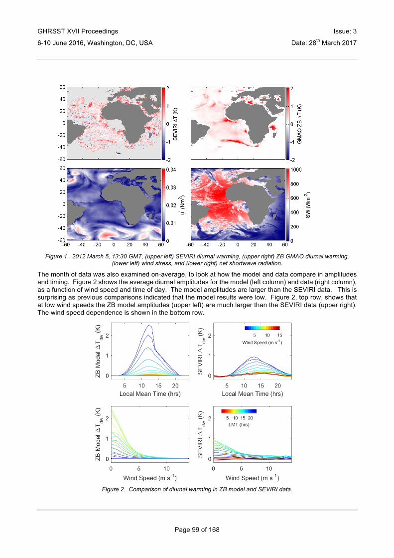
GHRSST XVII Proceedings Issue: 3
6-10 June 2016, Washington, DC, USA Date: 28th March 2017
Page 99 of 168
Figure 1. 2012 March 5, 13:30 GMT, (upper left) SEVIRI diurnal warming, (upper right) ZB GMAO diurnal warming,
(lower left) wind stress, and (lower right) net shortwave radiation.
The month of data was also examined on-average, to look at how the model and data compare in amplitudes and timing. Figure 2 shows the average diurnal amplitudes for the model (left column) and data (right column), as a function of wind speed and time of day. The model amplitudes are larger than the SEVIRI data. This is surprising as previous comparisons indicated that the model results were low. Figure 2, top row, shows that at low wind speeds the ZB model amplitudes (upper left) are much larger than the SEVIRI data (upper right). The wind speed dependence is shown in the bottom row.
Figure 2. Comparison of diurnal warming in ZB model and SEVIRI data.

GHRSST XVII Proceedings Issue: 3
6-10 June 2016, Washington, DC, USA Date: 28th March 2017
Page 100 of 168
To better examine how the model compares to the data, we have plotted them on the same panel, at different wind speeds, shown in Figure 3 where the diurnal warming for each are plotted as a function of wind speed. Below 4 m/s, the amplitudes are very different, but above 4 m/s they are similar. The PDF of global wind speeds is shown in Figure 4, just to illustrate how this may impact results. Diurnal warming amplitudes generally are measureable below 6 m/s, which accounts for 34% of the global winds. Where the model and data are diverging, below 4 m/s, these winds account for 15% of the global winds. At 2.5 m/s, where the model and data show significant differences, these winds speeds account for 5.5% of the global winds. While it would be better to improve the model’s amplitudes at very low wind speeds, the larger amplitudes only account for about 5% of the global data, but since they preferentially occur in the Tropics, there may be some biasing in the Tropical band because of this.
Figure 3. Diurnal warming amplitudes as a function of wind speed at different times of the day.
Figure 4. SSMI wind speeds version 7 global PDF.
To examine how warming evolves through the day the model and data are also plotted as a function of local time for different wind speeds (Figure 5). This figure clearly shows the issue of timing. As we should expect, the lower wind speeds have larger differences in amplitude of the peak warming. But at 4 m/s and above, the amplitudes are close in magnitude. At all wind speeds, the ZB model is peaking too early and losing heat too quickly in the afternoon. If you compare the model and data, averaging through the day, the differences mostly cancel each other out at 4 m/s and below and have a small positive bias (in the data) at higher wind

GHRSST XVII Proceedings Issue: 3
6-10 June 2016, Washington, DC, USA Date: 28th March 2017
Page 101 of 168
speeds. From approximately 16 – 24 hr LMT, there are differences. This may impact model results more than the wind speed dependence since it is impacting 30% of the data. This afternoon effect is a known issue with ZB and has been related to the parameterization of the
Figure 5. Diurnal amplitudes for model and data as a function of LMT for different wind speeds.
The diurnal depth was sent to 2.0 m rather than 3.0 m to increase the amplitudes. While the amplitudes are larger, the decrease with increased wind speed is realistic. Figure 3 shows the model and data compared again, this time as a function of local time. This figures shows how the model decreases far too rapidly in the afternoon. This is a known problem for ZB and we are looking at how we can adjust the model to correct for this.
Now, mixing is assumed throughout the layer, but in the afternoon as heat is leaving the diurnal layer, it will leave from the surface and this cooling will then be mixed downward. We are looking at whether implanting a mixing depth will help with this afternoon cooling issue. Initial results show the change in amplitude of ZB modelled diurnal warming when the depth is changed (Figure 5). Changing the depth does not improve the late afternoon decrease in warming that is too large.
Figure 6. Change in depth of diurnal warm layer.

GHRSST XVII Proceedings Issue: 3
6-10 June 2016, Washington, DC, USA Date: 28th March 2017
Page 102 of 168
Figure 5 shows a comparison between ZB05 (red line) and T2010 (blue line). What is most noticeable in this figure is that the addition of the Takaya 2010 parameterization results in smaller amplitudes of diurnal warming, it shifts the peak to earlier in the day, and there is faster heat loss in the late afternoon.
Figure 7. Figure from "Testing of the Zeng and Beljaars scheme in the TWP" by Brunke and Zeng, presented at
GHRSST 2012. ZB05 is shown in the red line. ZB+T2010 is shown in the blue line.
2. Conclusions The ZB+T model is overestimating at low winds and underestimating warming in the afternoon, when compared to SEVIRI SSTs. More work should be done to improve the representation of warming for models.

GHRSST XVII Proceedings Issue: 3
6-10 June 2016, Washington, DC, USA Date: 28th March 2017
Page 103 of 168
NOAA CORAL REEF WATCH: MONITORING CORAL BLEACHING RISK USING NOAA’S OPERATIONAL DAILY GLOBAL 5 KM GEO-POLAR BLENDED SST
ANALYSIS Gang Liu1,2,3, Scott F. Heron1,2,3, C. Mark Eakin1,3, Jacqueline L. De La Cour1,2,3, Erick F. Geiger1,2,3, William J. Skirving1,2,3, Timothy F. R. Burgess1, Alan E. Strong1,2,3, Andy Harris3,4, Eileen Maturi3,
Alexander Ignatov3, John Sapper5
(1) Coral Reef Watch, National Oceanic and Atmospheric Administration, College Park, MD 20740, USA (2) Global Science and Technology, Inc., Greenbelt, MD 20770, USA
(3) NESDIS/STAR, National Oceanic and Atmospheric Administration, College Park, MD 20740, USA (4) Earth System Science Interdisciplinary Center, University of Maryland, College Park, MD 20740, USA
(5) NESDIS/OSPO, National Oceanic and Atmospheric Administration, College Park, MD 20740, USA
Contact emails: [email protected], [email protected], and [email protected]
ABSTRACT The U.S. National Oceanic and Atmospheric Administration’s (NOAA) Coral Reef Watch (CRW) program has developed a suite of next-generation daily global 5 km satellite products to monitor thermal stress that can cause coral bleaching. These fulfill requests from coral reef managers and researchers for higher resolution products by taking advantage of new satellites, sensors, and algorithms. The products increase near-shore coverage and allow monitoring at reef or near-reef scales. The 5 km product suite has been a critical tool for monitoring and predicting in near-real-time the ongoing global coral bleaching event that started in mid-2014 – the longest and most widespread global event ever recorded. These products significantly advance the capability of resource managers and researchers to respond to environmental stresses on their local coral reefs.
1. Introduction Mass coral bleaching events due to anomalously warm ocean water have increased in frequency and severity [1] and become the most significant global contributor to the deterioration of coral reef ecosystems [2]. Coral bleaching occurs when the symbiotic relationship between corals and the microscopic algae (zooxanthellae) living in their tissues breaks down due to environmental stress [3,4]. After a significant number of zooxanthellae are expelled, the underlying white calcium carbonate coral skeleton becomes visible through the transparent coral tissue; this phenomenon is known as bleaching (Figure 1). Thermal stress that persists for several weeks with ambient water temperatures as little as 1 to 2 °C above a coral’s tolerance level has been shown to cause bleaching [5,6]. Corals can die if thermal stress is severe or long lasting; death can also result if thermal stress leads to subsequent disease in the affected colony [1,7,8]. Extensive bleaching events have dramatic long-term ecological and social impacts [9,10]. Even under favorable conditions, it can take decades or longer for severely bleached reefs to recover [2].
Reliable monitoring and prediction of environmental conditions leading to bleaching is critical to guide targeted observations, management responses, and communication about bleaching events [11,12,13]. Satellite remote sensing facilitates such monitoring with synoptic views of the global oceans in near-real-time and monitors stress to all reefs, whether they are easily accessed or remote. In 1997, the U.S. National Oceanic and Atmospheric Administration’s (NOAA) National Environmental Satellite, Data and Information Service (NESDIS) began operating a near-real-time, web-accessible, satellite sea surface temperature (SST)-based global Coral Bleaching HotSpot product for monitoring thermal conditions where corals were at risk of mass bleaching [14]. Subsequently, CRW developed a suite of products (augmenting the HotSpot with SST Anomaly, Degree Heating Week (DHW), and Bleaching Alert Area) that formed the first near-real-time decision support system to inform management of tropical coral reef ecosystems [14]. Widely used by the global coral reef community, these original CRW satellite products (implemented at 50-km spatial resolution and updated twice weekly) proved highly successful in nowcasting of mass coral bleaching episodes globally

GHRSST XVII Proceedings Issue: 3
6-10 June 2016, Washington, DC, USA Date: 28th March 2017
Page 104 of 168
[e.g.,1,14,15,16,17,18,19]. More recently, this system has been expanded to use seasonal climate models to forecast potential bleaching thermal stress out to four months [20,21].
Figure 1. An extensively bleached reef surveyed by a marine biologist in American Samoa, February 2015 [22]. Photo
courtesy of XL Catlin Seaview Survey (http://catlinseaviewsurvey.com/).
Advances in coral reef management have driven the need for higher resolution monitoring at reef or near-reef scales (up to several kilometers). In May 2014, CRW released its daily global 5 km product suite, right before the third global bleaching event began in the Commonwealth of the Northern Mariana Islands and Guam in July 2014 [23]. The event has since affected all tropical ocean basins and is ongoing. Providing a higher-resolution view of bleaching risk, the 5 km products were embraced immediately by CRW’s user communities. The 5 km and 50 km satellite monitoring products and climate model-based global Four-Month Coral Bleaching Thermal Stress Outlook have been the only global monitoring and outlook products available to the U.S. and global coral reef communities, and accessible at http://coralreefwatch.noaa.gov.
In this article, the core 5 km products are briefly introduced and the application of the products during the third global bleaching event is demonstrated. Plans for future improvements are discussed at the end.
2. CRW’s Core Global 5 km Products CRW’s next-generation 5 km satellite coral bleaching product suite is based on the NOAA/NESDIS operational daily global 5 km Geo-Polar Blended Night-Only SST Analysis. The 5 km Blended SST Analysis (Figure 2a) uses higher resolution data than previously available with increased data density acquired by multiple new satellites and sensors and employs new SST retrieval and analysis algorithms [24,25]. CRW’s 5 km products significantly advance its monitoring capacity over its pioneer 50 km products and are briefly described below (a detailed description can be found in [26]).
CRW’s satellite monitoring products are anomaly-based, comparing daily values with long-term climatologies. The required climatologies were derived from night-only values of the 4 km Advanced Very High Resolution Radiometer (AVHRR) Pathfinder SST Version 5.2 (PFv5.2) for the period 1985–2012 [27]. Note that PFv5.2 SST was not used in the generation of the Blended SST Analysis. For each pixel, monthly mean and daily SST climatologies were derived for calculating the SST anomaly. The SST Anomaly (Figure 2b) monitors the departure of SST from the daily climatology for each specific location. Warm anomalies prior to a bleaching season can lead to early onset of bleaching thermal stress. The maximum of the monthly mean (MMM) climatologies was determined for calculating the coral-specific HotSpot product and its derivatives. The Coral Bleaching HotSpot (Figure 2c), a positive-only anomaly from the MMM climatology, measures the magnitude of daily thermal stress that can lead to coral bleaching. The DHW (Figure 2d), expressed in the unit °C-weeks,

GHRSST XVII Proceedings Issue: 3
6-10 June 2016, Washington, DC, USA Date: 28th March 2017
Page 105 of 168
accumulates daily HotSpots over the most-recent 12 weeks and has been shown to effectively predict mass bleaching events [1,5,15,26]. Based, in part, on the finding that temperatures exceeding 1 °C above the usual summertime maximum are sufficient to cause thermal stress [5], only HotSpots ≥ 1 °C are accumulated in the DHW. The Bleaching Alert Area (Figure 3) identifies locations where bleaching thermal stress satisfies specific criteria based on HotSpot and DHW values (Table 1). Due to the high temporal variability in the daily 5 km SST and, thus, HotSpot, the Bleaching Alert Area shows the maximum alert level of the preceding seven days. The Bleaching Alert Area is extremely useful in management applications as it provides a single, convenient tool for describing thermal conditions, incorporating information from both the HotSpot and DHW products.
Figure 2. NOAA CRW’s daily global 5 km (a) Sea Surface Temperature (SST); (b) SST Anomaly; (c) Coral Bleaching
HotSpot; and (d) Degree Heating Week (DHW) images for June 1, 2016.
Figure 3. NOAA CRW’s daily global 5 km 7-Day Maximum Bleaching Alert Area image for June 1, 2016.
Stress Level Definition Ecosystem Impact
No Stress HotSpot ≤ 0 --
Bleaching Watch 0 < HotSpot < 1 --
Bleaching Warning 1 ≤ HotSpot and 0 < DHW < 4 Possible Bleaching
Bleaching Alert Level 1 1 ≤ HotSpot and 4 ≤ DHW < 8 Bleaching Likely
Bleaching Alert Level 2 1 ≤ HotSpot and 8 ≤ DHW Mortality Likely
Table 1. CRW’s coral bleaching thermal stress levels based on Coral Bleaching HotSpot and DHW values.

GHRSST XVII Proceedings Issue: 3
6-10 June 2016, Washington, DC, USA Date: 28th March 2017
Page 106 of 168
3. The Third Global Bleaching Event The third confirmed global coral bleaching event started in the Commonwealth of the Northern Mariana Islands and Guam in July 2014, and was declared global by NOAA in October 2015 after widespread bleaching had occurred across the Pacific, Atlantic, and Indian Ocean basins [23] (Figure 1). The extremely strong 2015-2016 El Niño further spread and worsened the global bleaching [28]. As of February 2016, it was the longest global event ever recorded [29]. At the time of this writing, this bleaching event has affected more reefs in the U.S. and worldwide than any previously documented global bleaching event (1998 and 2010) and has been the worst ever experienced in some locales (e.g., the northern Great Barrier Reef, Kiritimati (Christmas) Island, and Jarvis Island). In addition, some reefs bleached extensively for the first time on record (e.g., the northern Great Barrier Reef), and some major reefs have been affected in consecutive years (e.g., the Main Hawaiian Islands and Florida Keys) [29]. CRW’s 5 km satellite-based products, along with its model-based Bleaching Outlook, have been predicting, monitoring, and tracking this global bleaching event from its onset, providing critical information and guidance for management responses (e.g., closing dive sites over coral bleaching crisis [30]) and ecological impact surveys [e.g.,26,29,31]. Figure 4 shows the maximum thermal stress levels reached during the first two-and-a-half years (January 2014-May 2016) of the ongoing global event. Reef regions where extensive bleaching has been reported are outlined by ellipses in the figure, based on preliminary collation of bleaching observations that CRW has collected. CRW is still actively coordinating the collection and collation of bleaching observations. Analysis of this global bleaching event and validation of CRW’s product performance during the event will be conducted and published after the conclusion of the event and associated field data collection and quality control.
Figure 4. NOAA CRW’s maximum composite of the daily global 5 km Bleaching Alert Area for January 1, 2014 – May 31,
2016. Major bleaching has been reported in at least the reef regions outlined by ellipses, based on bleaching reports collated by CRW.
4. Discussions In addition to providing the only near-real-time coral bleaching thermal stress monitoring and outlook available to the global coral reef community, CRW continues to improve and enhance its products and services. A climatology derived directly from NESDIS’ Geo-Polar Blended Night-Only SST is preferred for CRW applications. Work is underway at NOAA to produce long-term records of polar Advanced Clear-Sky Processor (ACSPO) [32] and geostationary SSTs and reprocess the Blended SST for a period sufficient to construct a new climatology more consistent with the SST product and to enable the validation of the 5 km products during earlier bleaching events. Incorporating microwave SST data is desired to further reduce data gaps and improve SST quality in regions with persistent cloud cover (e.g., southeast Asia during its monsoon season), although the substantially lower resolution and effect of land contamination near the coast due to antenna sidelobes are likely to reduce the benefit for coastal reefs. Additional work is underway to develop products that incorporate additional environmental stressors into CRW’s bleaching ecoforecasting systems.
To provide monitoring at spatial resolutions closer to reef scales of hundreds of meters, a regional higher spatial resolution SST analysis (< 5 km) is desired to account for the high horizontal heterogeneity often

GHRSST XVII Proceedings Issue: 3
6-10 June 2016, Washington, DC, USA Date: 28th March 2017
Page 107 of 168
encountered in the physical environment. Furthermore, global SST products are usually not calibrated using coastal in situ SST measurements. With the availability of 750 m spatial resolution data provided by the Visible Infrared Imaging Radiometer Suite (VIIRS) onboard the Suomi National Polar-orbiting Partnership (NPP) spacecraft and ~2 km spatial resolution provided by the imagers onboard Himawari-8 and the upcoming GOES-R satellite, SST analysis at resolutions of 1 to 2 km for select reef locations becomes feasible. A finer and more accurate land mask for reef areas also will be critical for monitoring the physical environment at reef scales.
CRW provides end-to-end service to the coral reef community. CRW communicates with reef managers and scientists directly to understand their needs on the ground and works with them throughout product development, validation, and improvement. CRW conducts substantial outreach and training for reef managers and scientists about its decision support system for coral bleaching management and its appropriate application. In addition, CRW is collating in situ water temperature data and bleaching observations for product development, improvement, and validation. CRW strives to provide the best possible information to reef managers and other stakeholders to inform the effective management of coral reefs.
5. Acknowledgements: Coral Reef Watch work is supported primarily by the NOAA Coral Reef Conservation Program and the NOAA National Environmental Satellite, Data, and Information Service’s Center for Satellite Applications and Research. The contents in this article are solely the opinions of the authors and do not constitute a statement of policy, decision, or position on behalf of NOAA or the U.S. Government.
6. References 1. Eakin, C.M.; Morgan, J.A.; Heron, S.F.; Smith, T.B.; Liu, G.; Alvarez-Filip, L.; Baca, B.; Bartels, E.;
Bastidas, C.; Bouchon, C.; et al. Caribbean corals in crisis: Record thermal stress, bleaching, and mortality in 2005. PLoS One 2010, 5, e13969.
2. Wilkinson, C.R. Status of Coral Reefs of the World: 2008; Global Coral Reef Monitoring Network and Reef and Rainforest Research Centre: Townsville, Australia, 2008.
3. Jokiel, P.L.; Coles, S.L. Response of Hawaiian and other Indo-Pacific reef corals to elevated temperature. Coral Reefs 1990, 8, 155–162.
4. Jaap, W.C. Observations on zooxanthellae expulsion at Middle Sambo Reef, Florida Keys. Bull. Mar. Sci. 1979, 29, 414–422.
5. Glynn, P.W.; D’Croz, L. Experimental evidence for high temperature stress as the cause of El Niño-coincident coral mortality. Coral Reefs 1990, 8, 181–191.
6. Berkelmans, R.; Willis, B.L. Seasonal and local spatial patterns in the upper thermal limits of corals on the inshore Central Great Barrier Reef. Coral Reefs 1999, 18, 219–228.
7. Miller, J.; Muller, E.; Rogers, C.; Waara, R.; Atkinson, A.; Whelan, K.R.T.; Patterson, M.; Wither, B. Coral disease following massive bleaching in 2005 cause 60% decline in coral cover on reefs in the US Virgin Islands. Coral Reefs 2009, 28, 925–937.
8. Rogers, C.S.; Muller, E.; Spitzack, T.; Miller, J. Extensive coral mortality in the US Virgin Islands in 2005/2006: A review of the evidence for synergy among thermal stress, coral bleaching and disease. Caribb. J. Sci. 2009, 45, 204–214.
9. Munday, P.L.; Jones, G.P.; Pratchett, M.S.; Williams, A.J. Climate change and the future for coral reef fishes. Fish Fish. 2008, 9, 261–285.
10. Doshi, A.; Pascoe, S.; Thébaud, O.; Thomas, C.R.; Setiasih, N.; Tan Chun Hong, J.; True, J.; Schuttenberg, H.Z.; Heron, S.F. Loss of economic value from coral bleaching in S.E. Asia. In Proceedings of 12th International Coral Reef Symposium, Cairns, Australia, 9–13 July 2012.
11. Marshall, P.; Schuttenberg, H. A Reef Manager’s Guide to Coral Bleaching; Great Barrier Reef Marine Park Authority: Townsville, Queensland, Australia, 2006.

GHRSST XVII Proceedings Issue: 3
6-10 June 2016, Washington, DC, USA Date: 28th March 2017
Page 108 of 168
12. Maynard, J.A.; Johnson, J.E.; Marshall, P.A.; Eakin, C.M.; Goby, G.; Schuttenberg, H.; Spillman, C.M. A strategic framework for responding to coral bleaching events in a changing climate. Environ. Manag. 2009, 44, 1–11.
13. Anthony, K.R.N.; Marshall, P.A.; Abdulla, A.; Beeden, R.; Bergh, C.; Black, R.; Eakin, C.M.; Game, E.T.; Gooch, M.; Graham, N.A.J.; Green, A.; Heron, S.F.; van Hooidonk R.; Knowland, C.; Mangubhai, S.; Marshall, N.; Maynard, J.A.; McGinnity, P., McLeod, E.; Mumby, P.J.; Nystrõm, M.; Obura, D.; Oliver, J,; Possingham, H.P.; Pressey, R.L.; Rowlands G.P.; Tamelander, J.; Wachenfeld, D.; Wear, S.. Operationalising resilience for adaptive coral reef management under global environmental change. Glob. Change Biol. 2014, 21(1), 48-61, doi: 10.1111/gcb.12700.
14. Liu, G.; Rauenzahn, J.L.; Heron, S.F.; Eakin, C.M.; Skirving, W.J.; Christensen, T.R.L.; Strong, A.E.; Li, J. NOAA Coral Reef Watch 50 km Satellite Sea Surface Temperature-Based Decision Support System for Coral Bleaching Management; NOAA Technical Report NESDIS 143. NOAA/NESDIS: College Park, MD, USA, 2013; p. 33.
15. Liu, G.; Strong, A.E.; Skirving, W. Remote sensing of sea surface temperature during 2002 Barrier Reef coral bleaching. EOS Trans. AGU 2003, 84, 137–144.
16. Liu, G.; Strong, A.E.; Skirving, W.; Arzayus, L.F. Overview of NOAA coral reef watch program’s near-real time satellite global coral bleaching monitoring activities. In Proceedings of the 10th International Coral Reef Symposium, Okinawa, Japan, 28 June–2 July 2004; Volume 1, pp. 1783–1793.
17. Strong, A.E.; Arzayus, F.; Skirving, W.; Heron, S.F. Identifying coral bleaching remotely via Coral Reef Watch—Improved integration and implications for climate change. In Coral Reefs and Climate Change: Science and Management; Phinney, J.T., Hoegh-Guldberg, O., Kleypas, J., Skirving, W., Strong, A.E., Eds.; American Geophysical Union: Washington, DC, USA, 2006; Volume 61, p. 244.
18. Skirving, W.J.; Strong, A.E.; Liu, G.; Liu, C.; Arzayus, F.; Sapper, J.; Bayler, E. Extreme events and perturbations of coastal ecosystems: Sea surface temperature change and coral bleaching. In Remote Sensing of Aquatic Coastal Ecosystem Processes: Science and Management Applications; Richardson, L.L., LeDrew, E.F., Eds.; Springer: New York, NY, USA, 2006; p. 348.
19. Liu, G.; Eakin, C.M.; Rauenzahn, J.L.; Christensen, T.R.L.; Heron, S.F.; Li, J.; Skirving, W.; Strong, A.E.; Burgess, T. NOAA Coral Reef Watch’s Decision Support System for coral reef management. In Proceedings of the 12th International Coral Reef Symposium, Cairns, Queensland, Australia, 9–13 July 2012.
20. Liu, G.; Matrosova L.E.; Penland, C.; Gledhill, D.K.; Eakin C.M.; Webb, R.S.; Christensen, T.R.L.; Heron, S.F.; Morgan, J.A.; Skirving, W.J.; Strong, A.E. NOAA Coral Reef Watch Coral Bleaching Outlook System. In Proceedings of the 11th International Coral Reef Symposium, Ft. Lauderdale, Florida, USA, 7-11 July 2008; pp. 951-955.
21. Eakin, C.M.; Liu, G.; Chen, M.; Kumar, A. Ghost of bleaching future: Seasonal outlooks from NOAA’s operational Climate Forecast System. In Proceedings of 12th International Coral Reef Symposium, Cairns, Queensland, Australia, 9–13 July 2012.
22. http://catlinseaviewsurvey.com/gallery/i1323_marine-biologist-surveys-bleaching-in-american-samoa-during-february-2015 (accessed on 15 June 2016).
23. http://www.noaanews.noaa.gov/stories2015/100815-noaa-declares-third-ever-global-coral-bleaching-event.html (accessed on 15 June 2016).
24. NOAA/NESDIS Operational Geo-Polar Blended SST Products Website: http://www.star.nesdis.noaa.gov/sod/mecb/blended_validation/background.php (accessed on 15 June 2016).
25. Maturi, E.; Harris, A.; Mittaz, J.; Sapper, J.; Dash, P.; Zhu, X.; Wick, G.; Koner, P. A New High Resolution Sea Surface Temperature Blended Analysis, Bull. Amer. Meteor. Soc. 2016, in press.
26. Liu, G.; Heron, S.F.; Eakin, C.M.; Muller-Karger, F.E.; Vega-Rodriguez, M,; Guild, L.S.; De La Cour, J.L.; Geiger, E.F.; Skirving, W.J.; Burgess, T.F.R.; Strong, A.E.; Harris, A.; Maturi, E.; Ignatov, A.; Sapper, J.; Li, J.; Lynds, S. Reef-scale Thermal Stress Monitoring of Coral Ecosystems: New 5-km Global Products from NOAA Coral Reef Watch. Remote Sensing 2014, 6(11): 11579-11606, doi:10.3390/rs61111579.

GHRSST XVII Proceedings Issue: 3
6-10 June 2016, Washington, DC, USA Date: 28th March 2017
Page 109 of 168
27. Heron, S.F.; Liu, G.; Eakin, C.M.; Skirving, W.J.; Muller-Karger, F.E.; Vega-Rodriguez, M.; De La Cour, J.L.; Burgess, T.F.R.; Strong, A.E.; Geiger, E.F.; Guild, L.S.; Lynds, S. Climatology Development for NOAA Coral Reef Watch's 5-km Product Suite. NOAA Technical Report NESDIS 145. 2015, NOAA/NESDIS. College Park, MD. 21pp.
28. http://www.noaa.gov/el-niño-prolongs-longest-global-coral-bleaching-event (accessed on 15 June 2016). 29. Eakin, C.M.; Liu, G.; Gomez, A.M.; De La Cour, J.L.; Heron, S.F.; Skirving, W.J.; Geiger, E.F.; Tirak, K.V.;
Strong, A.E. Global Coral Bleaching 2014-2017: Status and an Appeal for Observations. Reef Encounter 43 (2016), 31(1): 20-26.
30. https://www.theguardian.com/environment/2016/may/26/thailand-closes-dive-sites-over-coral-bleaching-crisis (accessed on 15 June 2016).
31. Heron, S.F.; Johnston, L.; Liu, G.; Geiger, E.F.; Maynard, J.A.; De La Cour, J.L.; Johnson, S.; Okano, R.; Benavente, D.; Burgess, T.F.R.; Iguel, J.; Perez, D.; Skirving, W.J.; Strong, A.E.; Tirak, K.; Eakin, C.M. Validation of Reef-scale Thermal Stress Satellite Products for Coral Bleaching Monitoring. Remote Sensing 2016, 8(1): 59, doi: 10.3390/rs8010059.
32. Ignatov, A.; Zhou, X.; Petrenko, B.; Liang, X.; Kihai, Y.; Dash, P.; Stroup, J.; Sapper, J.; DiGiacomo, P. AVHRR GAC SST Reanalysis Version 1 (RAN1). Remote Sensing 2016, 8(4), 315, doi:10.3390/rs8040315.

GHRSST XVII Proceedings Issue: 3
6-10 June 2016, Washington, DC, USA Date: 28th March 2017
Page 110 of 168
PLENARY SESSION VI: ANALYSIS SESSION REPORT
Chair: Mike Chin(1) - Rapporteur: Dorina Surcel Colan(2)
Jet Propulsion Laboratory, California Institute of Technology, Pasadena, CA, USA, Email: [email protected]
Numerical Environmental Prediction Section, National Prediction Development Division, Meteorological Service of Canada, Dorval, QC, Canada, Email: [email protected]
ABSTRACT The session featured three speakers representing three organizations, and an open floor discussion.
Summary of Speakers Assimilation of ACSPO VIIRS and REMSS AMSR2 into OSTIA (20min) – Simon Good
Thermal uniformity analysis of SST data fields (20min) – Jean-François Cayula
New mathematical technique for satellite data interpolation and application to L4 generation (20min) – Sandra Castro
Open floor discussion (30min)
1. Assimilation of ACSPO VIIRS and REMSS AMSR2 into OSTIA --- Simon Good This presentation summarizes the work of Emma Fiedler and the Met Office team to assimilate two new data sets in OSTIA analysis.
OSTIA is a foundation L4 SST analysis assimilating data from three AVHRR instruments (NOAA 18, NOAA 19 and MetOp-A), geostationary retrievals (SEVIRI and GOES-E) and in situ data. It uses SSES estimates for satellite retrievals before OSTIA bias correction is applied.
Two new retrieval data from AMSR2 provided by REMSS (L2P) and VIIRS provided by NOAA/OSPO (L3U) have been introduced in the operational cycle starting in March 2016. The results presented here were from tests performed for January 2016. Validation against Argo floats was presented for the operational analysis (before March 2016), the analysis assimilating either AMSR2 or VIIRS and the analysis assimilating both datasets.
The conclusions were:
• Improvement of 0.08 K in RMS difference to Argo for the analysis with both data sets compared to the operational analysis
• Quasi-consistent agreement between all regions • Warm bias in the Arctic for both datasets, more observations from AMSR2 in high latitudes • Mean bias was too cold in the Arctic for AMSR2 and VIIRS when compared with OSTIA reference
(in situ and a subset of AVHRR data) • Analyses using VIIRS and AMSR2 have good accuracy compared to other SST analyses • Other data sets have been tested: GOES-W did not improve the analyses, Himawari-8 has large
errors outside the central disk, JAXA AMSR2 not as good as REMSS, EUMETSAT MetOp IASI promising but the number of observations too small, looking forward to use VIIRS as reference instead of MetOp-A (MetOp-B feedback issues when used as reference in February 2016)

GHRSST XVII Proceedings Issue: 3
6-10 June 2016, Washington, DC, USA Date: 28th March 2017
Page 111 of 168
Questions: Mike Chin: How the bias is in the Arctic, positive or negative?
Response by the speaker (R): Negative
Sasha Ignatov: All the statistics you showed have MetOp-A as reference?
R: Yes.
Sasha Ignatov: If you use VIIRS as the reference does RMS go down?
R: Possible.
Sasha Ignatov: Has Himawari-8 from ACSPO been tested?
R: Not yet.
Prasanjit Dash: Just a remark, the number of IASI will increase soon, EUMETSAT will make some changes
Misako Kachi: How has JAXA AMSR2 performed?
R: The bias and RMS were larger than for REMSS AMSR2
Chelle Gentemann remark: JAXA and REMSS use different channels for SST, it would have been interesting to see the differences between the two data sets
Andy Harris: Do you have maps for day or night only for AMSR2?
R: No
Hellen Beggs’ remark: AMSR2 data really improve the analysis, I’m curious if they could improve RAMSSA.
Craig Donlon points out the importance of using microwave data specially in regions with clouds.
Bob Grumbine remarks that there are still regions were AMSR2 has no data, especially the Gulf Stream
2. Thermal uniformity analysis of SST data fields --- Jean- François Cayula The uniformity test is a quality determination procedure for SST field based on the differences between the maximum and minimum SST values within a small neighborhood. The test tends to smooth-out existing fronts. A revised test based on coherence of thermal gradient vector field is presented and is applied to several SST products. Highlights:
a) SST uniformity field for NAVO daytime VIIRS and ACSPO daytime VIIRS • - Thermal uniformity test included in NAVOCEANO SST processing: defined as difference between
Max and Min in neighborhoods • - Test presented for Jan 16 2016: ACSPO looks better, NAVO still has striping • - Global SST shows aggregation pattern of VIIRS

GHRSST XVII Proceedings Issue: 3
6-10 June 2016, Washington, DC, USA Date: 28th March 2017
Page 112 of 168
b) NAVOCEANO thermal uniformity test: coherence of thermal gradient and correlation temperature/reflectance
• - Changes from fixed threshold in front detection to a variable threshold show good improvements • - For the correlation of thermal and reflective fields, the comparison between working with SST or
brightness temperature resulted in change to brightness temperature
c) Modification of SST equations • - Shows results when compare with old products or this ACSPO for the coast of Japan and the Coast
of Argentina • - The global results for the number of observations and STD are smaller than for ACSPO
d) Evaluation, orbital overlap/buoy match-ups • - Evaluation over buoys match-ups is preliminary
Conclusion: • Improvement in detection of frontal regions while maintaining strong cloud detection • Uniformity preforms better with the Brightness Temperature (BT) data instead of the SST data
derived from BT.
Questions: Irina Gladkova: How you do compute the gradients?
R: No gradients were computed for front detection, only the minimum and maximum.
Chelle Gentemann: What are these lines?
R: These are striping in VIIRS. ACSPO uses a de-striping method.
Craig Donlon: Replacing SST with BT, we changed this long time ago because the signal was not strong
R: The11 µm channel has less noise.
Sasha Ignatov: Go back to the slide with the overlaps statistics. Can you consider a possible explanation to this? If one product keeps more diurnal warming and the other not, how do you explain this?
R: Often more data keep residual clouds
Helen Beggs: When will the product be operational?
R: It is not operational.
3. New mathematical technique for satellite data interpolation and application to L4 generation --- Sandra Castro
The new methodology is developed with the Numericus Group. This method is intended for gap filling of L4 products and is based on Fourier analysis. No equations are presented (proprietary technology of the Numericus Group).
The interpolation functions are built from L3 SEVIRI and L2 MODIS SST, and L4 products are generated by evaluating the interpolation functions.

GHRSST XVII Proceedings Issue: 3
6-10 June 2016, Washington, DC, USA Date: 28th March 2017
Page 113 of 168
In the first stage L4 products are generated from a single sensor, in the second stage multi-sensor L4 products will be generated. The results shown here are from the first stage.
First example uses SEVIRI SST L3 input data from OSI-SAF, 3-hour product, 0.1deg resolution. Results from February 8, 2009 show that the interpolation looks really good except for regions where there are no data. Comparing with the original L3 SEVIRI, some spurious structures appear, which are under investigation. Similar results were obtained when comparing with FNMOC.
Second example uses AQUA/MODIS L2 SST input at 1 km resolution. When comparing the L4 product with the original, the results are good. Removal of residual clouds improves the results for the interpolator, but the gain of new information from ultra-high resolution is limited.
It is preferable to have coarser resolution with smaller gap than higher resolution with larger gaps. Comparisons with OSTIA and MUR analysis were also presented.
The last point was related to the diurnal warming as represented by interpolation from SEVIRI. The peak warming is similar with those in AMSRE.
In conclusion the method is robust and efficient. The interpolator can detect noise and outliers and it can be used for quality control or cloud detection.
Questions: Christopher Griffin: Did you try just to remove the clouds?
R: Not yet, these are just the first tests
4. Open floor discussion Peter Cornillon referring to J.F. Cayula presentation makes comments about NAVO products.
Craig Donlon: There are several tools looking at front detection but nothing for comparison. It will be nice to have a method for evaluation. Is there a plan to compare frontal detection methods? Can we have standard formats for various methods?
Peter Cornillon: This depends on what different users are looking for, generally all methods show different aspects of front detection.
Peter Cornillon: Comments about SST vs. BT.
Irina Gladkova: If you want the intensity of the front you should use SST. If you want only position you should use BT.
J.F. Cayula: My choice for BT was because I observed that using SST the fronts have disappeared.
Irina Gladkova: I use BT for cloud detection, discussion about the method used by NOAA ACSPO to detect fronts.
Mike Chin: How many fronts do you get at the end?
Irina Gladkova: I don’t know, it is difficult to count, you have to decide on what you want to count.
Question for Craig Donlon: Do you suggest to introduce fronts as a part of GDS2?
Response: No, but it will be good to have some coordination inside GHRSST.
Sasha Ignatov: NOAA ACPSO is going to introduce the fronts and they are asking feedback.
Peter Cornillon presents another available front product.

GHRSST XVII Proceedings Issue: 3
6-10 June 2016, Washington, DC, USA Date: 28th March 2017
Page 114 of 168
ASSIMILATION OF ACSPO VIIRS AND REMSS AMSR2 INTO OSTIA Emma Fiedler(1), Simon Good(1)
(1) Met Office, Exeter, UK, Email: [email protected]
1. Introduction OSTIA is the Met Office’s Operational SST and Ice Analysis system, which produces L4 (globally complete, gridded) SST analyses on a daily basis. The effect of assimilating ACSPO VIIRS L3U and REMSS AMSR2 L2P SST observations into the OSTIA analysis was tested. Both new datasets were accessed via PODAAC, which also provides documentation on them.
2. Methods Four OSTIA runs were conducted for January 2016:
• Operational configuration (control) • Operational configuration with AMSR2 (+AMSR2) • Operational configuration with VIIRS (+VIIRS) • Operational configuration with both AMSR2 and VIIRS (+AMSR2, VIIRS)
Each run was given a two week spin-up period.
The operational configuration at the time of the runs used data types NOAA-18,19 AVHRR, MetOp-A AVHRR, SEVIRI, GOES-E and in situ (ships, moored buoys, drifting buoys). Similar to the other satellite data types used in OSTIA, the observation error variances for the new data types were taken from the SSES standard deviation estimates provided in the GHRSST files. The SSES bias estimate was removed from the observations before any bias correction using the OSTIA reference dataset was applied. The data were subsampled to the OSTIA grid size of ~6 km.
3. Results Table 1 shows validation of the OSTIA runs against Argo observations, which are independent from the analysis. These are sourced from the Met Office Hadley Centre EN4 database, which also performs quality control. For the matchups with the OSTIA analysis the shallowest Argo observation between 3-5 m depth was used, as this has previously been shown to be a good representation of foundation temperature (Fiedler and McLaren, 2014).
Results show that assimilation of the VIIRS and AMSR2 datasets together leads to a significant improvement in the global RMS of the OSTIA analysis compared to Argo of 0.08 K, for January 2016 (Table 1). Test runs assimilating VIIRS and AMSR2 observations separately indicate that the total improvement in the RMS is due to the action of both datasets together rather than one or the other. The updated RMS of 0.42 K is well within the OSTIA target uncertainty of 0.50 K RMS (Donlon et al. 2012).
This improvement is consistent across all regions (Table 2), with the largest magnitude decrease in RMS of 0.11 K in the South Atlantic. The smallest magnitude decrease in RMS of 0.03 K was seen in the Tropical Atlantic. Minor changes in the mean difference to Argo of no greater than 0.02 K were seen in almost all regions, both positive and negative.
Figure 1 shows the monthly mean of the AMSR2 and VIIRS observations minus the OSTIA analysis. The observations have already been assimilated, so the plots demonstrate how well the analysis agrees with the individual data types. For both datasets the mean of the differences to the analysis is generally small, with the exception of the Arctic, where both sets of observations are warmer than the analysis. The differences to the analysis in the central Pacific correspond to a region of low numbers of observations in both datasets, which

GHRSST XVII Proceedings Issue: 3
6-10 June 2016, Washington, DC, USA Date: 28th March 2017
Page 115 of 168
requires further investigation. AMSR2 provides more observations than other datasets at very high latitudes, which is important for the analysis as observations are generally sparse here.
For VIIRS, the RMS of the differences to the analysis is generally small outside regions of high SST variability, as would be expected, with the exception of the Arctic (and the region of reduced data volume in the central Pacific). There is more spatial noise in the RMS of the AMSR2 differences to the analysis compared to the RMS for VIIRS, particularly in the North Atlantic and North Pacific.
4. Bias corrections OSTIA performs a bias-correction of the satellite data to a reference dataset comprising of all in situ observations and a high-quality subset of MetOp-A AVHRR. For the reference MetOp-A AVHRR, nighttime data only is used, with quality flags 4 and 5, and a maximum satellite zenith angle of 48 degrees. Figure 3 shows the monthly means of the AMSR2 and VIIRS differences to the OSTIA reference dataset, which are then removed from the data prior to assimilation. Figure 3 demonstrates a lack of agreement between both the VIIRS and AMSR2 observations and the reference dataset in the Arctic. (NOAA AVHRR also shows a weaker warm bias in the Arctic, not shown.) The agreement of these independent datasets (VIIRS infrared, AMSR2 microwave) suggests the MetOp-A AVHRR reference data is too cold in the Arctic. This demonstrates the usefulness of examining these bias fields, as there are no independent in situ observations for SST validation in the Arctic.
Note also the large positive bias compared to the reference data off the coast of Africa for AMSR2 (figure 3). This is likely to be linked to the presence of Saharan aerosols. The microwave AMSR2 instrument is not sensitive to aerosols, unlike the reference AVHRR. The microwave dataset is therefore providing additional information here but this is being “corrected” out by comparison to the reference infra-red dataset. This is an area which requires future improvement.
5. Conclusions The effect of adding VIIRS and AMSR2 into OSTIA improves its accuracy compared to other global SST analyses, using Argo as a reference, see table 3. As above, the Argo data were taken from the EN4 dataset, and are independent from all analyses shown.
The positive test results mean that ACSPO VIIRS L3U and REMSS AMSR2 L2P products have been included operationally in OSTIA from 15 March 2016.
6. Further work As mentioned above (section 4), the issue of how to make use of additional information provided by microwave datasets compared to infra-red, e.g. in regions with high levels of aerosols or persistent cloud cover, is an area for future research.
The low data volumes in the centre of the Pacific seen in both AMSR2 and VIIRS datasets requires
Other data types were tested at the same time but not included in OSTIA operationally:
• NOAA/NESDIS GOES-W did not improve the analysis according to our usual measures, but may still provide extra information for e.g. feature resolution so we plan to look at this again
• JAXA Himawari-8 needs more work on filtering observations (large errors outside centre of disk) • JAXA AMSR2 did not perform as well as REMSS AMSR2 • EUMETSAT MetOp IASI results are promising but the number of observations is very small
compared to other data types so has little effect on the analysis. We will look again at any new releases

GHRSST XVII Proceedings Issue: 3
6-10 June 2016, Washington, DC, USA Date: 28th March 2017
Page 116 of 168
Results from our testing phase (January 2016) have been shown here rather than from the operational system as results were complicated by a feedback issue between MetOp-B AVHRR and OSTIA when MetOp-A AVHRR was replaced on 23 February 2016.
OSTIA uses a high quality subset of MetOp AVHRR as a reference dataset for bias correction of other satellite data. As part of their new processing chain, OSI SAF have begun to use OSTIA for bias correction of the MetOp-B AVHRR product. When MetOp-A AVHRR was switched to MetOp-B AVHRR for the OSTIA bias correction, it led to a feedback between the two products and both started to drift. OSI SAF agreed to make MetOp-A available once again and this was switched back in OSTIA on 23 March 2016. Figure 4 illustrates the drift in the OSTIA analysis compared to NOAA AVHRR and in situ observations whilst bias correcting to MetOp-B AVHRR.
The bias correction to MetOp-A AVHRR performs satisfactorily, as OSTIA compares well to Argo alongside other analyses. However, there is room for improvement in the OSTIA reference dataset, particularly in the high latitudes. We also need to move away from using MetOp-A AVHRR for bias correction due to data availability. We are therefore currently investigating using VIIRS as a reference dataset for OSTIA, at least until SLSTR becomes available.
7. References Donlon, C.J., M. Martin, J. D. Stark, J. Roberts-Jones, E. Fiedler and W. Wimmer, The Operational Sea Surface Temperature and Sea Ice Analysis (OSTIA), Rem. Sens. Env. 116, 140-158, 2012.
Fiedler, E. and A. McLaren, SST: Results and Recommendations, Euro-Argo Improvements for the GMES Marine Service, D4.3.3, 23pp, 2014.
TABLES
Table 1: Near-surface Argo minus OSTIA SST analysis for January 2016, global statistics
Experiment Mean diff to Argo (K)
Standard deviation of diff
to Argo (K)
RMS diff to Argo (K)
Control 0.12 0.49 0.50
+ AMSR2 0.12 0.43 0.44
+ VIIRS 0.10 0.43 0.44
+ AMSR2, VIIRS 0.11 0.41 0.42

GHRSST XVII Proceedings Issue: 3
6-10 June 2016, Washington, DC, USA Date: 28th March 2017
Page 117 of 168
Table 2: Near-surface Argo minus OSTIA SST analysis for the operational system (control), and a run with VIIRS and AMSR2 (January 2016; regional statistics).
Table 3: Standard deviation of near-surface Argo minus SST analyses for January 2016, using the GMPE (GHRSST
Multi-Product Ensemble) system
Region (CMEMSdefinitions)
Mean diff to Argo (K)
RMS diff to Argo (K)
control +VIIRS, AMSR2 control +VIIRS,
AMSR2Global 0.12 0.11 0.50 0.42North Atlantic 0.23 0.21 0.59 0.49Tropical Atlantic 0.14 0.13 0.30 0.27South Atlantic 0.02 0.03 0.56 0.45North Pacific 0.20 0.18 0.50 0.44Tropical Pacific 0.08 0.06 0.33 0.28South Pacific 0.03 0.03 0.39 0.35Indian Ocean 0.04 0.05 0.34 0.30Southern Ocean 0.07 0.06 0.52 0.44
Analysis Name Global standard deviation of diff to Argo (K)
CMC 0.36Updated OSTIA 0.42FNMOC 0.44K10_SST 0.46OSTIA 0.49GAMSSA 0.52RSS mw 0.52MGDSST 0.54Reynolds 0.55RTG 0.63RSS mw_ir 0.87

GHRSST XVII Proceedings Issue: 3
6-10 June 2016, Washington, DC, USA Date: 28th March 2017
Page 118 of 168
FIGURES
Figure 1: Monthly means of AMSR2 minus OSTIA mean difference (top) and VIIRS minus OSTIA mean difference (bottom), both for January 2016, in K.

GHRSST XVII Proceedings Issue: 3
6-10 June 2016, Washington, DC, USA Date: 28th March 2017
Page 119 of 168
Figure 2: Monthly means of AMSR2 minus OSTIA RMS (top) and VIIRS minus OSTIA RMS (bottom), both for January 2016, in K.

GHRSST XVII Proceedings Issue: 3
6-10 June 2016, Washington, DC, USA Date: 28th March 2017
Page 120 of 168
Figure 3: Monthly means of AMSR2 bias to OSTIA reference (top), and VIIRS bias to OSTIA reference (bottom), both
for January 2016, in K.

GHRSST XVII Proceedings Issue: 3
6-10 June 2016, Washington, DC, USA Date: 28th March 2017
Page 121 of 168
Figure 4: Daily global mean observation minus OSTIA analysis for NOAA AVHRR (top) and in situ (bottom), from
end February 2016 to start of April 2016.

GHRSST XVII Proceedings Issue: 3
6-10 June 2016, Washington, DC, USA Date: 28th March 2017
Page 122 of 168
THERMAL UNIFORMITY ANALYSIS OF SST DATA FIELDS Jean-François Cayula(1), Doug May(2), and Keith Willis(2)
(1) Vencore, Inc., Stennis Space Center, USA, [email protected] (2) Naval Oceanographic Office, Stennis Space Center, USA, [email protected], [email protected]
ABSTRACT Statistically comparing the performance of Sea Surface Temperature (SST) products typically ignores the problem that products containing fewer oceanic features often show better apparent accuracy than those retaining more features. Through the SST uniformity field, defined here as the field of the differences between the maximum and minimum SST values within a small neighborhood, this study highlights strengths and weaknesses of the NAVOCEANO and Advanced Clear-Sky Processor for Oceans (ACSPO) Visible Infrared Imaging Radiometer Suite (VIIRS) SST products. NAVOCEANO SST processing includes strict uniformity cloud detection tests and thus largely avoids cloud contamination and noise related to the Multi-Channel SST (MCSST) equations at the cost of discarding ocean fronts. ACSPO SST is much noisier but retains ocean frontal regions. We identified improvements to NAVOCEANO SST processing, which increase the retention of ocean fronts while also tightening the thermal uniformity test to remove contamination. For this purpose, the SST uniformity test is made contingent on the coherence of the gradient vector field and the correlation between the temperature field and the reflectance field. For the uniformity, coherence, and correlation tests, it is shown that operating on the brightness temperature field rather than the SST field reduces the uncertainty associated with those tests. Finally, noting that the intrinsic SST noise is mostly introduced through the correction term of the MCSST equations, the NAVOCEANO SST calculations replaces the correction term with its local average. In addition to visual inspection, results are evaluated with the orbital overlap method and match-up to buoys.
1. Introduction One of the steps commonly included to detect contamination in SST fields is a check of the uniformity of the thermal data. This step is included in the NAVOCEANO (May et al, 1998) and ACSPO (Petrenko et al, 2010) SST processing. This study uses the uniformity field as derived from the NAVOCEANO uniformity test to examine and highlight characteristics of daytime VIIRS SST fields. In particular, section 2 discusses examples of SST uniformity fields corresponding to the NAVOCEANO and NOAA ACSPO VIIRS SST products. This leads to modifications to NAVOCEANO SST processing of daytime VIIRS data which add conditions to the uniformity test to identify actual ocean features. Section 3 presents three of the most significant updates. The first one is a test on the coherence of the gradient vector field (Cayula, 1992) which includes a discussion the effect of noise on the determination of the threshold value. The second update is a test on the correlation between the temperature field and the reflectance field which is similar to the test found in ACSPO (Petrenko et al, 2010) except that a less noisy brightness temperature field rather than SST is chosen here. The last update discussed here addresses the noisy nature of SST fields as observed in section 2 and investigated in Padula (2015). The SST uniformity fields show that replacing the correction term of the MCSST equation with its local average significantly improves the signal to noise ratio of the final SST products. The last section presents results for both the original and updated NAVOCEANO SST as well as for ACSPO SST.
2. SST uniformity field In this study, the uniformity field for an array A is defined as:
U(A) = fmax(A) - fmin(A) (1)
where fmax and fmin denote respectively the sliding window maximum and sliding window minimum filters. This corresponds to the uniformity test in the original NAVOCEANO SST processing which is based on the difference between the maximum and minimum values within a window. However, a 3x3 pixel window is used here while the original NAVOCEANO SST processing relies on a 2x2 pixel window. Applying Eq. (1) to SST

GHRSST XVII Proceedings Issue: 3
6-10 June 2016, Washington, DC, USA Date: 28th March 2017
Page 123 of 168
data produces the SST uniformity fields Those uniformity fields can reveal flaws not seen in the SST fields because of the dynamic range of the SST data in most scenes but the most extreme close-ups.
Figure 1 shows the NAVOCEANO daytime SST and corresponding uniformity field for a region of the Gulf of Mexico on January 16, 2016. The SST uniformity field shows low level of SST intrinsic noise and striping. Because of a strict uniformity test, without allowance for ocean features, fronts are weaker than they should be, but cloud contamination is kept to a minimum.
Figure 1: a) NAVOCEANO daytime SST Gulf of Mexico on January 16, 2016. b) SST uniformity field indicates little cloud contamination but also weak fronts.
In Figure 2, NAVOCEANO SST data are replaced with NOAA ACSPO SST. Although the SST field is comparable to that of Figure 1, the uniformity field shows stronger fronts but also cloud contamination, especially around 92°W 24°N. The uniformity field also shows that the de-striping filter (Bouali and Ignatov, 2014) that was incorporated in ACSPO v.2 is successful at removing the striping and the intrinsic SST noise.
Figure 2: a) Same as Figure 1 with ACSPO SST. b) SST uniformity field shows strong fronts but also the presence of cloud contamination. ACSPO de-striping filter removes striping and reduces intrinsic SST noise.
Global VIIRS SST uniformity fields were found to exhibit a vertical banding pattern, as shown in Figure 3. The Close-up in Section 3 shows that the pattern is related to the VIIRS aggregation scheme. Examination of brightness temperature uniformity fields would point to the SST equations amplifying the noise.

GHRSST XVII Proceedings Issue: 3
6-10 June 2016, Washington, DC, USA Date: 28th March 2017
Page 124 of 168
Figure 3: SST uniformity field corresponding to ACSPO daytime VIIRS SST on July 14, 2014. The SST uniformity field shows a clear vertical banding pattern of lower and higher SST variability.
3. Updated NAVOCEANO SST processing
4. Revised Uniformity Test To improve the performance of NAVOCEANO VIIRS SST processing in frontal regions the thermal uniformity test is modified to operate on 3x3 sliding windows and is made conditional on two additional tests: the coherence of thermal gradient vector field (Cayula and Cornillon, 1992) and correlation between temperature and reflectance field (Petrenko et al, 2010). Using Eq. (1) and T as the temperature field gives:
U(T) > 0.4°K ⇒ coherence and cohesion tests (2)
5. Coherence of thermal gradient vector field The test helps differentiate between random variability of non-front regions and the more orderly vector field associated with fronts. Taking (x,y) in a n x n window, W , centered at (xc,yc), the coherence can be expressed as:
coherence(xc,yc) = ǁ meanw(grad(x,y)) ǁ / ǁ meanw( | grad(x,y) | ) ǁ (3)
In a noise free environment, (xc,yc) can just be classified as cloudy when coherence(xc,yc) is lower than a constant threshold, f. However when noise is present choosing a constant f results in a higher probability of classifying clear regions with weak ocean features as cloudy and cloud contaminated regions with strong fronts as clear. Synthetic fields made of repeating step functions (idealized fronts) to which Gaussian noise is added (Figure 4) are used here to derive f as a function of fronts strength. Results for varying step sizes from 0.3°K to 4°K, standard deviation of noise set to 0.05°K (VIIRS M15) and probability of correct front detection set at 0.95 are shown in Figure 5.
Figure 4: synthetic field Figure 5: f as a function of step size
The implementation of the coherence test uses the function of Figure 5 but replaces the step size with the uniformity value.

GHRSST XVII Proceedings Issue: 3
6-10 June 2016, Washington, DC, USA Date: 28th March 2017
Page 125 of 168
6. Correlation of the thermal and reflective fields This correlation test is based on the observation that negative correlation indicates cloud contamination. The present implementation substitutes SST by the brightness temperature at 10.763μm, T11, because, as the example of Figure 6 shows, the lower noise level of T11 produces better results. The reflectance is that at 0.865μm.
Figure 6: a) Correlation of reflectance with a) T11 and b) SST. a) is cleaner than b). The standard deviation as estimated by the orbital overlap SST evaluation (Cayula et al, 2015) is 0.34°K for a) and 0.37°K for b).
7. Revised SST calculations The daytime MCSST equations can be approximately written as “SST= a * T11 + b * ( T11 - T12 )” where, a ~ 1 and b ~ 2.5 are semi constant variables, and, T12 is the brightness temperatures at 12μm. As shown in Figure 7, the SST uniformity field highlights the noise in the SST data which includes random noise and striping and also corresponds to the horizontal VIIRS aggregation scheme.
Figure 7: Daytime SST Uniformity field on July 14, 2014, updated NAVOCEANO processing with standard SST
Noting that the correction term of the SST equations, “b * ( T11 - T12 )”, is the source for the increased level of noise, the revised SST calculation uses an nxn average of clear pixels for the correction term. This scheme keeps the strength of SST fronts to at least that of T11 level and reduces the effects of random noise and striping. The value of n is set at 7 for the present implementation (Figure 8).

GHRSST XVII Proceedings Issue: 3
6-10 June 2016, Washington, DC, USA Date: 28th March 2017
Page 126 of 168
Figure 8: Same as Figure 7, but with the revised SST.
8. Results Figure 9 shows that the updated SST processing is successful at preserving fronts and reducing SST noise. It should be compared to Figures 1 and 2.
Figure 9: a) updated NAVOCEANO daytime SST Gulf of Mexico on January 16, 2016. b) SST uniformity field indicates little cloud contamination strong fronts and low level of noise.
SST fields from January 16, 2016 from 120°E to 30°W and 55°S to 55°N were analyzed with the orbital overlap method (Cayula et al, 2015). The results are listed in Table 1.
Method Number of Retrievals Standard deviation
Updated NAVOCEANO 61 million 0.43°K
Original NAVOCEANO 68 million 0.40°K
NOAA ACSPO 75 million 0.50°K
Table 1: Results of the SST orbital overlap evaluation for January 16, 2016.
As seen in Table 1, NAVOCEANO updated processing retains a low standard deviation while also recovering high gradient frontal regions. It produces about 80 % of the number of ACSPO retrievals. NAVOCEANO original processing results in the lowest standard deviation because of its conservative cloud detection which often discards frontal regions. It produces about 90% of ACSPO retrievals. ACSPO processing is not as strict with cloud contamination but produces the largest number of retrievals and good coverage of frontal regions at the cost of a higher standard deviation.

GHRSST XVII Proceedings Issue: 3
6-10 June 2016, Washington, DC, USA Date: 28th March 2017
Page 127 of 168
Evaluation through buoy match-ups is preliminary. Early results indicate a standard deviation of 0.45°K for the updated and original NAVOCEANO SST (all categories), and 0.47°K for ACSPO SST (quality level 5 only).
9. Conclusion The updated NAVOCEANO SST processing successfully improves the coverage of frontal regions while maintaining strong cloud detection. However more importantly it was noted that the uniformity and associated tests perform better with brightness temperature than SST. This may have implications for SST edge detection. Finally, replacing the standard correction term in the daytime SST equations by an nxn pixel average can significantly reduce the effect of random noise and striping while keeping the strength of the fronts in the resulting SST field to at least that of the level of the fronts in the brightness temperature field.
10. References Bouali, M. and A. Ignatov, Adaptive reduction of striping for improved sea surface temperature imagery from Suomi National Polar Orbiting Partnership (S-NPP) Visible Infrared Imaging Radiometer Suite (VIIRS). J. Atm. Ocean. Tech. 31, 150–163, 2014.
Cayula, J.-F. and P. Cornillon, Edge detection algorithm for SST images, J. Atm. Ocean. Tech., 12, 821-829, 1992.
Cayula, J.-F., May, D., Arnone, R. and R. Vandermeulen, Evaluation of VIIRS SST fields through the analysis of overlap regions between consecutive orbits, Proceedings of SPIE Vol. 9459, 94590S, 2015.
Petrenko, B., Ignatov, A., Kihai, Y. and A. Heidinger, Clear-sky mask for the Advanced Clear-Sky Processor for Oceans (ACSPO). J. Atm. Ocean. Tech., 27, 1609—1623, 2010.
May, D. A., Parmeter, M. M., Olszewski, D. S. and B.D. McKenzie (1998).Operational processing of satellite sea surface temperature retrievals at the Naval Oceanographic Office. Bull. Am. Meteorol. Soc., 79(3), 397407, 1998.
11. Acknowledgments This work was partially supported by NOAA JPSS Program Office through a grant to NGLI and USM. This study made extensive use of data from NOAA's Comprehensive Large Array-data Stewardship System (CLASS) and GHRSST Global Data Assembly Center (GDAC) at the NASA JPL PO.DAAC.

GHRSST XVII Proceedings Issue: 3
6-10 June 2016, Washington, DC, USA Date: 28th March 2017
Page 128 of 168
NEW MATHEMATICAL TECHNIQUE FOR SATELLITE DATA INTERPOLATION AND APPLICATION TO L4 GENERATION
Sandra Castro(1), Lucas Monzon(2) , Ryan Lewis(2) , Greg Beylkin(2), Gary Wick(3)
(1) University of Colorado, CCAR 431 UCB, Boulder, CO, USA, 80309, Email: [email protected] (2) The Numericus Group, LLC, Boulder, CO, USA, 80303, Email: [email protected]
(3) NOAA/ESRL/PSD, Boulder, CO, USA, 80305, Email: [email protected]
ABSTRACT Using novel multi-stage algorithms and Fourier Analysis techniques developed by The Numericus Group, LLC, in Boulder, Colorado for the interpolation of satellite SST images, we present preliminary results showcasing how the interpolation algorithms can generate a gridded, no-gap SST product, based exclusively on the sensor's L2P data (i.e., a single-sensor L4 SST). Since these algorithms build an interpolation function, this function can be evaluated at any point in the input domain or even be scaled at multiple resolutions. A byproduct of the methodology is its own uncertainty estimate, which can be derived from the fitting error of the interpolated data with respect to the input L2P values. Preliminary results for a L3 SEVIRI and a L2P MODIS SSTs are validated using in situ buoy data. We also compare our single-sensor L4 SST with other GHRSST L4 products, regardless of their resolution. We discuss issues of validation and quality of the interpolation.
1. Introduction We show the results of using a new interpolation methodology that does not rely on any standard interpolation technique or on statistical analysis, but rather poses the interpolation problem from within the framework of Fourier analysis. This methodology uses recent and novel mathematical techniques that have proven successful with other types of remote sensing data. Since satellite-retrieved SST data have a limited frequency content, a natural approach to generating an L4 (no-gap) product is to find a function (an interpolating function or interpolator for short) that fits the given L2 data by constraining its frequency content. To avoid both, over-fitting and under-fitting, the interpolation is performed using a global, multi-stage frequency analysis. As a consequence, we remove high frequencies present in the input data that are due to noise or are the result of nonphysical frequencies introduced as part of the retrieval process used to generate the L2 SST input. Once the interpolator is built, it can be efficiently evaluated anywhere within the input domain, including buoy locations, the input grid, or any other regular/irregular grid. In particular, the L4 product is the result of evaluating the interpolator at a regular grid with a resolution matching the input grid.
A brief description of the concept behind the new methodology is described in Section 2. Initial tests (Section 3) aim to clarify algorithmic issues regarding the construction of an interpolator using just data from a single low level (L2 or L3) SST product. Follow-up tests are designed to mitigate the impact of missing information by developing similar algorithms that merge multiple scenes/passes from the same sensor (i.e., a single-sensor, multi-stage interpolation algorithm). In Section 4 we demonstrate how the interpolator of a lower resolution input can be used to remove outliers from a higher resolution input. Since an interpolator can be evaluated at any grid within the original input domain, we can use the interpolator from an independent, high-quality product, and evaluate it at a finer grid to help identify regions with oversized differences relative to the quality-controlled product. There are other refinements of this approach that we are planning to pursue. First, we plan to incorporate additional information (quality flags, wind magnitude, etc.) to weight the relative importance of the input data. Second, we plan to extend the method to merge multiple inputs from multiple sensors, obtained on different resolution grids. In this way, we can better deal with large gaps and improve the overall quality of the interpolated product.
2. Methodology As an example of the application of the methodology to L4 SST generation, consider a L2 input data corresponding to an infrared (IR) sensor. This input consists of a set of vectors {(𝑥E, 𝑦E, 𝑡E)}I∈K, where 𝑡E is

GHRSST XVII Proceedings Issue: 3
6-10 June 2016, Washington, DC, USA Date: 28th March 2017
Page 129 of 168
the satellite-retrieved SST value corresponding to the location given by the longitude 𝑥E and latitude 𝑦E. We assume that the set 𝑆 has been selected so that there is a reasonable confidence on the quality of the 𝑡E values, but we will explain later how our methodology can also be used to quality control the input data and to remove outliers or other corrupted/non-physical data. The set of locations {(𝑥E, 𝑦E)}I∈Kform a non-uniform grid which have many gaps of irregular sizes (mostly due to clouds in the IR) across the domain. Also, the data density of the input grid is determined by the (native) resolution of the sensor. Our goal is to find a function 𝐼 = 𝐼(𝑥, 𝑦), named the interpolator, such that:
|𝐼(𝑥E, 𝑦E) − 𝑡E| < 𝜖,(1)
and the Fourier transform of 𝐼, 𝐼, is zero outside a disk of radius 𝑐, i.e.,
𝐼 𝑢, 𝑣 = 0, 𝑖𝑓 𝑢1 + 𝑣1 > 𝑐.(2)
Here, 𝜖 is the tolerance in the interpolation error and can be thought as a target absolute accuracy (if convenient, relative errors can be used instead). The value of 𝜖 in the spatial fit (1) and of 𝑐 in the frequency constrain (2) are data-dependent and are found iteratively: we increase the value of 𝑐 if there is a significant improvement in the fit (i.e., if 𝜖 decreases in a significant way). We settle on a value for 𝑐 when the improvement on 𝜖 is insignificant. We interpret this algorithmic step as to increase the frequency content of the interpolator up to the point where it tries to fit noise or use highly oscillatory components that have no physical meaning. Both of these components are easily identifiable because they tend to drastically increase the value of 𝑐 with almost no improvement on the value of 𝜖. Once the frequency content of the target interpolating function is constrained, we determine the interpolator which provides the smallest error in the fit (1) under the frequency constrain (2). In summary, this is a global, multi-stage method that avoids under-fitting by using a large enough set of frequencies and, at the same time, prevents over-fitting by tracking the improvement on the fit as we increase the range of allowable frequencies. The resulting interpolating functions are smooth (infinitely differentiable) and can be efficiently evaluated at any uniform or non-uniform grid. To deal with the issue of disparate data density in the input, an adaptive method is used to weight the impact of an input vector relative to its distance from dense regions.
Since the input is fit within a tolerance 𝜖 and a limited domain of frequencies, we argue that the non-physical frequencies, introduced by the retrieval process, are absent from the interpolator, and thus, in the process of replacing 𝑡E by 𝐼(𝑥E, 𝑦E), we effectively “de-noised” and quality-controlled the input data. The accuracy of the fit is, therefore, algorithmically adjusted to match the properties of the input data, and provides an estimate of the uncertainty in the measurements, which can be used to estimate the uncertainty in our new L4 products. To validate the interpolated product, we can measure the error between in situ data (or any other reference data) and the corresponding values obtained from evaluating the interpolator at the exact locations of the in situ measurements. In this way we avoid the need of matching up the satellite to the in situ data by conventional means like using spatiotemporal windows and their associated errors.
3. L4 Generation from a single-sensor, lower-level SST product For this demonstration we use a single scene from the OSI-SAF, level 3 (L3), three-hourly, 0.1-degree resolution, SEVIRI SST product. This product was created as part of the Medspiration project, and was later replaced by the 1-hour, 0.05-degree operational product. It is available through the NOAA/NCFEI LTSRF. The scene, shown in Fig. 1a, is for February 8, 2009, 16:00 UTC and covers the region from 4N-40S, 34W-8E. This scene was chosen because of its unusually good coverage, and for the extreme diurnal warming event it captured. The corresponding L4 SST, shown in Fig. 1.b, was obtained by evaluating the SEVIRI interpolator at the L3 input grid, using all proximity confidence (PC) values.Gaps were successfully filled using the frequency content of the L3 alone. The bottom-left corner was problematic, however, since there was no data at the boundary to constrain the interpolation with. The lack of data at this corner was ameliorated by using additional information from collating all the available SEVIRI scenes for that day in a maximum value composite, using only the best quality data (PC = 5). This approach provided enough information as to generate an improved interpolation consistent with other data sets with smaller gaps in the problematic corner (see power point presentation).

GHRSST XVII Proceedings Issue: 3
6-10 June 2016, Washington, DC, USA Date: 28th March 2017
Page 130 of 168
SEVIRI Single-Scene L4 SST
Buoys with Satellite Matchups Buoys with No Satellite Matchups No. Buoys Matchup Interpolator No. Buoys Interpolator
RMSE 81 0.46 0.43 24 0.60 Bias 81 -0.04 -0.05 24 -0.17
Table 1: SEVIRI validation statistics using buoys.
Figure 1: (a) SEVIRI L3 input data, and (b) Corresponding L4 SST, obtained from the interpolator evaluated at a 0.1-degree regular grid.
Shown in Fig. 2 is the difference between the input and the interpolator evaluated at the input grid (i.e., the misfit). The RMSE of the difference is 0.018K and the maximum absolute error is 0.23K. Additionally, 91% of the data is within 0.01% of the fitted value. These results attest to the good quality of the SEVIRI input since it can be said that for the majority of the data, the interpolating function was very precise. Fig. 2, however, reveals small-scale artifacts (< 0.1K) present in the SEVIRI L3 input, most likely due to a loss of precision from the 3-hourly averaging. These features are present in the difference because they do not follow the assumed frequency model of the interpolation.
Table 1 shows the statistics of validating the interpolated SSTs with respect to buoys. Buoy data was obtained from the NOAA/STAR iQuam system. The validation is done in two ways: by matching the buoy measurements to the closest satellite pixel within a 20 km radius and 1-h acquisition window; and by evaluating the interpolator at precise buoy locations. The latter was split into two groups: for buoys with and without a matchup. In the case where there is a matchup, the RMSE for the interpolator minus buoy differences is better than the RMSE for the matchups. This is not surprising since the interpolator adjusts the input for noise. Note that by using the interpolator, we reduce the error introduced by way of the matchup by 0. 461 − 0.431 = 0.16K. The RMSE for buoy differences with respect to filled gaps (24 buoys with no matchups) is higher (0.60 K vs. 0.43 K), but still acceptable.
Figure 2: Misfit in the SEVIRI L3 input

GHRSST XVII Proceedings Issue: 3
6-10 June 2016, Washington, DC, USA Date: 28th March 2017
Page 131 of 168
4. Interpolation of MODIS L2P SSTs For the next demonstration we use MODIS granules from the swaths, within the same spatial domain, closest in time to the previous example, i.e., between 13:40 and 15:45 UTC. The L2P were generated by the Ocean Biology group at NASA Godard and have 1 km resolution. For the interpolation we selected data with the top two quality flags (PC = 0 and PC = 1). The pixels with PC = 1 are at the edge of the scan and were considered to minimize the gap between swaths. Unfortunately, there is significant residual cloud contamination in the MODIS L2P best quality data, which introduced very high frequencies that resulted in artifacts in the interpolation.
Since we can think of a coarse IR pixel as an integration of the radiation from a finer sub-grid, we evaluated the SEVIRI interpolator on the MODIS L2 grid and computed the difference between both values (Fig. 3.a). This difference clearly revealed the MODIS cloud-contaminated pixels (Fig. 3.b), which were removed before building a new interpolator. The quality control MODIS L2P and corresponding L4 product are shown at the bottom of Fig. 3. The latter image suggests that the orbital gaps in MODIS are too large for an interpolator build from a single L2P scene to work properly. In order to improve use this method in the interpolation of high-resolution, IR L2 products, extra information from other sensors must be considered. Preliminary results towards the development of a multi-sensor interpolator where shown in the presentation, but further work needs to be done.
Figure 3: (a) Difference between the MODIS input and the SEVIRI interpolator evaluated at the MODIS input, (b) residual cloud contaminated pixels identified with the aid of (a), (c) Quality-control MODIS L2P using the SEVIRI
interpolator, and (d) Single-sensor L4 MODIS obtained from the new interpolator evaluated at a 0.1-degree regular grid.

GHRSST XVII Proceedings Issue: 3
6-10 June 2016, Washington, DC, USA Date: 28th March 2017
Page 132 of 168
5. Conclusion Some of the issues to consider when choosing an appropriate interpolation algorithm are: How accurate is the method? How computationally expensive is it? How many data points are needed? In the new method, the accuracy of the fit is data-driven and can be adjusted to match properties of the input. In other words, the interpolation can be as accurate as the user chooses it to be. It also generates a smooth interpolator that can be expressed as a trigonometric polynomial for computational efficiency. Finally, we have shown that the method produces robust L4 products that do not require multi-sensor blending, although interpolation of L2 SSTs from polar orbiters could benefit from additional data. In summary, the new interpolation not only offers potentially new uses like cloud screening, but it overcomes most of the problems of linear interpolation.

GHRSST XVII Proceedings Issue: 3
6-10 June 2016, Washington, DC, USA Date: 28th March 2017
Page 133 of 168
SEA SURFACE TEMPERATURE IN THE MARGINAL ICE ZONES OF THE ARCTIC OCEAN
Michael Steele (1), Suzanne Dickinson(1), Wendy Ermold(1), Sarah Dewey(1), and Peter Minnett(2) (1) Polar Science Center, Applied Physics Lab, University of Washington, Seattle, WA, 98105, USA,
Email: [email protected] (2) RSMAS/MPO, University of Miami, 4600 Rickenbacker Causeway, Miami, FL 33149
1. Introduction Gridded, interpolated Level 4 (L4) SST data sets generally provide values both under the perennial sea ice pack and in the Marginal Ice Zone (MIZ, where ice concentration transitions between 0% and 100%). Satellite SST data under the ice pack is in fact unavailable, while in situ observations have been rare until recently. Thus most L4 SST data sets provide some kind of “proxy” SST under ice that is either a seawater freezing point value (most commonly, -1.8 degC), a freshwater freezing point (i.e., 0 degC), or regionally and/or temporally varying climatological values. The question here is, how good is this method, compared to historical and more recently acquired in situ observations?
2. In situ observations The year-long drift of the SHEBA (Surface Heat and Energy Balance of the Arctic) ice camp in 1997-1998 provided an opportunity to examine the evolution of upper ocean temperatures within the ice pack. Observations showed a warming during calm winds of up to about 3 degC above the freezing point in a lead, i.e., down to the ice bottom depth. This persisted for a few weeks in July 1998, but was then completely erased when winds accelerated to 5-8 m/s. The question then is, what is the frequency of “calm” vs. “windy” conditions that lead to high stratification vs. well-mixed conditions? Recent research indicates that climatological mean summer surface winds are ~4-5 m/s, i.e., very close to the transition value that determines the amount of surface-enhanced warming. Thus more work on this subject is warranted.
However, SHEBA also provides us with a year-long record of daily ocean temperature in the mixed layer, not just in a lead. This time series indicates that in fact, the elevation above freezing in the mixed layer is ten times smaller than in the July 1998 lead, i.e., it reached a maximum of only about 0.3 degC. Still, this does indicate that in the summer, SSTs are often warmer the freezing point, if only by a small amount.
More recent observations over the past 10 years (and even more in the past 3 years) are available from icebreaker cruise CTD data, air-dropped expendable CTDs (AxCTDs), drifting buoys, and gliders. These diverse data sets generally agree on a summer mixed layer elevation above the freezing point on the order of 0.2-0.5 degC at 50% ice concentration. On the other hand, during fall freeze-up, our early analysis indicates that SSTs remain at the freezing point in the MIZ. While this might seem obvious, some gridded L4 data sets assume above-freezing temperatures within the MIZ in seasons besides summer. In fact, this might reasonable in mid-winter, when the ice edge has advanced southward to meet the warm ocean fronts in the North Pacific and North Atlantic Oceans that prevent it from expanding indefinitely. However, in fall this might not be a realistic parameterization. All of this analysis is quite preliminary, and more extensive analysis is planned.
3. L4 SSTs across the MIZ Preliminary work indicates that some L4 data sets are providing MIZ SSTs that generally match the observations, while others are too warm and/or have a SST vs. ice concentration curve that does not match in situ observations. However, only a few such data sets were examined here, and more will be included in future analyses.

GHRSST XVII Proceedings Issue: 3
6-10 June 2016, Washington, DC, USA Date: 28th March 2017
Page 134 of 168
4. Conclusion It seems from preliminary work that Arctic Ocean SSTs do rise above the freezing point in the MIZ. However, the magnitude, depth structure, and response to wind and solar forcing is still poorly understood and requires further work. After a more extensive quantification of SSTs in the Arctic ice pack and a comparison with gridded products, the next step will be to determine an optimal strategy for producing realistic L4 gridded SSTs in this environment.

GHRSST XVII Proceedings Issue: 3
6-10 June 2016, Washington, DC, USA Date: 28th March 2017
Page 135 of 168
ERRORS ANALYSIS OF SST/AVHRR ESTIMATION IN UPWELLING AND ATMOSPHERIC SUBSIDENCE CONDITIONS
Gutemberg Borges França, Rosa Cristhyna de Oliveira Vieira Paes, Rodrigo Carvalho de Sousa Federal University of Rio de Janeiro, Department of Meteorology, Laboratory of Applied Meteorology,
University City Campus, CEP: 21.941-916 Rio de Janeiro, RJ - Brazil., Email: [email protected],[email protected],[email protected]
ABSTRACT In July 2013 a buoy (called IEAPM buoy) was settled around 6 km in coastal influence area of Cabo Frio’s upwelling, Rio de Janeiro State – Brazil. During 2014 southeast Brazil summer drought - where the mentioned upwelling area is located –, a curious positive bias values were observed on SST/AVHRR of until 4 K. Thus, what are the possible reasons for this feature of BTs during the here studied upwelling event that is uncommon and somewhat counter intuitive? The latter addresses to three key comments as follows. Firstly, Le Borgne et al. (2011) and Hoyer et al. (2013) have similarly identified this BT behaviour in METOP/AVHRR-3 leading to SST retrieval errors (positive bias) in the Artic, and their conclusions show that this rare aspect and the resultant SST errors are associated to an specific atmospheric condition, i.e. high concentration of humidity in low troposphere (below 800 hPa) associated to temperature inversion. Secondly, considering the upwelling event period studied in this work, Caio et al. (2015) and Otto et al. (2015) have particularly an existence of a semi-permanent high-pressure system leading to a strong subsidence over Southeast Brazil, which corroborate to the expressive negative precipitation anomalies observed and consequently a cloud-free area during entire studied period. Thirdly, BTs in channels 4 and 5 results from surface, and upwelling and downwelling atmospheric emissions. Accordingly, the atmosphere acts as an emission source to the total signal reaching the sensor, but at the same time, the atmospheric transmission along the path decreases surface emission. In general, the decreasing atmospheric effect wins out, and BT is lower than SST. In the described specific atmospheric condition, the atmospheric contribution overcomes the surface emission reduction, and BT is greater than SST. Obviously, under such condition, regular split-window methods will provide useless SST retrievals and those algorithms using climatological first-guess may provide even worst results. As pointed out by Le Borgne et al. (2011), MCSST and NLSST algorithms may even deal with such unexpected conditions; however their coefficients, determined for a global processing, are not adapted to this situation. Possible strategies to correct episodic positive biases on SST retrieval algorithms are suggested.

GHRSST XVII Proceedings Issue: 3
6-10 June 2016, Washington, DC, USA Date: 28th March 2017
Page 136 of 168
PLENARY SESSION VIII: IMPACT STUDIES SESSION REPORT
Chair: Craig Donlon(1) - Rapporteur: Simon Good(2)
(1) ESA/ESTEC, Noordwijk, The Netherlands, Email: [email protected] (2) Met Office, Exeter, UK Email: [email protected]
1. Impact of satellite observations on SST forecasts via variational data assimilation and heat flux calibration – Charlie Barron • There is a paper by Jackie May that talks about this (Applied Meteorology and Climate). • NFLUX: this refers to use of errors in hindcast to predict what happens in the forecast with respect
to errors in fluxes, SST etc. • Uses 2D VAR to estimate surface air temp and wind to get estimate of heat flux. Assimilates L2 data
(VIIRS, AVHRR). Can look at time mean to find a persistent bias correction. • Get better results in general from NFLUX daily heat flux; NFLUX is prepared daily for short-medium
forecasts. • Error standard deviation in heat fluxes can be locally large. • The 4D VAR scheme adjusts both the initial state and the fluxes over the analysis window. It
interprets the observations in the context of a dynamical model. It is thought that the combination of flux correction with the 4D VAR will do better than a single scheme.
• COAMPS is the regional model, NAVGEM is the global model. • Results in Southern Californa Current region compared to ISCCP shows that there is not enough
cloud. • Some problems in NFLUX calculations have been noticed. Open ocean results may not imply what
is happening along the coast. E.g. inlet with low values. Background temperatures in longwave calculation are wrong due to mismatch in land-sea mask between ocean and atmosphere.
• In coupled systems will need to decide what to do if ocean says one thing and the atmosphere says another. Need a 'mediator' to correctly balance the coupling.
2. Assessing the impact of assimilating OSTIA SST and along-track Aviso SLA on the performance of a regional-eddy-resolving model of the Agulhas system – Christo Whittle • Very complex region south of Africa. • Favourable region for pelagics. Want to understand the reason for the shift in these. • Looking at month of year of peak production in MODIS Aqua Chl-a. October – December is the
normal peak. • Wanted to look at the SST to understand the physics of the situation. MODIS Aqua had problem with
cloud flagging. Also very low number of retrievals per month. Want more data but still high quality. Blended Aqua/Terra MODIS – better estimates than L4.
• Also use a model to understand regime in the area; assimilates OSTIA (no thinning of observations) and Aviso. Improvements due to assimilation are mainly in high variability regions.
• Model was compared to blended MODIS. Model is warmer and Agulhas current broader. When add SLA the comparison is worse. When adding OSTIA the results look better.
• Problem on East Coast when model does not match MODIS well. This area has a lot of cloud; low number of observations.

GHRSST XVII Proceedings Issue: 3
6-10 June 2016, Washington, DC, USA Date: 28th March 2017
Page 137 of 168
• Could look at other metrics e.g. distribution of mammals consuming the food, zooplankton, where fishing is being done, level of effort required etc.
3. Using SST for improved mesoscale modelling of the coastal zone – Ioanna Karagali • Interested in knowing about winds for wind farms. • Want to see if can enhance model using observations. • LIDAR instruments onshore scan offshore. Also a wave and a LIDAR buoy. • In some cases had good measurements 5km off coast. • WRF model used in the study. Tried different configurations e.g. land use classification. • Land use differences include either defining a lake as 'lake' or 'water', which will change the way it is
represented in the model. • Find that mean wind speed profile from observations diverges from the model setups. • Model captures the gradients in wind speed. Pretty good agreement between wind speed going from
offshore to onshore. Jump in wind speed from LIDAR as get to coast is an artefact. • WRF does not currently include impact of currents caused by winds (Peter Cornillon did this in a pre-
WRF version); interested in looking at coupled models. • Resolution of SST dataset is important. Investigated two SST datasets (DMI (2km) and OI (0.25 deg);
DMI not available everywhere though). Not clear of the impact because there are other factors involved. Higher resolution seems better, though.
• Paper is in preparation.
4. Discussion • Update on GOES-R from Ken Casey – level 1b being archived not level 0. Will be a 2 year rolling
level 0 store (University of Wisconsin and STAR have plans for archiving these). Will be a user consultation to ask about needs for archiving L0.
• Need to be able to demonstrate the impact of GHRSST. Can all send in images/list of publications to demonstrate impacts?
• People visiting GHRSST website needs to be able to see a list of impacts easily. • Impacts tend to be shown at GODAE rather than at GHRSST. Maybe we could have action to show
these at next science team meeting. • SST is an established parameter with broad range of applications. After all these years need to be
able to show the impacts of improvements. Challenge that SST is taken for granted and is thought of as done. Hurricane Katrina is a good example of why SST is important as it was affected by passing over a loop current. SST/heat flux is very important when thinking about OHC/altimetry – may get overlooked. Another example is what is the best dataset for cal/val. Would be good to have short (~300) words to illustrate these kind of applications – science team members could provide these.
• Each incremental improvement to SST is smaller than for altimetry because it is so well developed – this is a challenge because effort will tend to be pushed towards altimetry.
• Next generation of analyses will need to be dynamically accurate.

GHRSST XVII Proceedings Issue: 3
6-10 June 2016, Washington, DC, USA Date: 28th March 2017
Page 138 of 168
IMPACT OF SATELLITE OBSERVATIONS ON SEA SURFACE TEMPERATURE FORECASTS VIA VARIATIONAL DATA ASSIMILATION AND HEAT FLUX
CALIBRATION Charlie N. Barron(1), Clark Rowley(1), Scott R. Smith(1), Jackie May(1), Jan M. Dastugue(1), Peter L.
Spence(2), and Silvia Gremes-Cordero(3)
(1) Naval Research Laboratory, Code 7321, Stennis Space Center, MS, 39529, (USA), Email: [email protected]
(2) Vencore, Stennis Space Center, MS, 39529, (USA) (3) University of New Orleans, Stennis Space Center, MS, 39529, (USA)
ABSTRACT
Satellite observations are used to guide forecasts of sea surface temperature (SST) through variational data assimilation and heat flux calibration. In the experiments considered, assimilation is conducted using the Navy Coupled Ocean Data Assimilation (NCODA) in either a standard 3D variational (3DVAR) or an alternative 4DVAR formulation. Heat flux for the forecasts follows the original operational highest-quality time series or modifies the flux-determining fields using the Naval Research Laboratory ocean flux (NFLUX) capability. These alternatives are evaluated relative to independent, unassimilated in situ sea surface temperature (SST) observations in two sets of year-long experiments, sets based on atmospheric fields from either the global or the regional operational atmospheric model. Each set begins with a control run with standard forcing and standard 3DVAR assimilation, and the experimental variants employ the various combinations of 4DVAR assimilation and NFLUX-modified forcing. Results in the California Current region demonstrate that the combination of 4DVAR assimilation with NFLUX-modified forcing tends to produce forecasts in best overall agreement with independent in situ observations.
1. Introduction
Satellite observations support a variety of avenues to improve sea surface temperature (SST) forecasts. The upwelling visible, infrared and microwave radiation intensities integrated across various wavelength bands or channels are sensitive to various physical properties of the atmosphere and ocean. In this way satellite instruments can offer information not only on SST itself but also on other ocean and atmospheric properties that influence heat flux and therefore the evolution of SST over the forecast. Among these properties are atmospheric temperature, relative humidity, temperature and humidity from the upper atmosphere to the ocean surface, and cloud cover. Use of these satellite observations is categorized either within systems to modify heat fluxes or as assimilation to refine the ocean and possibly boundary layer states.
Brief overviews of the Naval Research Laboratory Ocean Surface Flux (NFLUX) and 3D and 4D variational (3DVAR/4DVAR) data assimilation in the Navy Coupled Ocean Data Assimilation (NCODA; Cummings, 2005) are in Section 2, with greater detail available in the references and in the GHRSST XVI proceedings (Barron et al., 2016). Section 3 reports on experiments in the California Current and northern Arabian Sea regions. Section 4 summarizes our conclusions to date and projects future developments relating to NFLUX and the COFFEE project.
2. Methods The experiments examining the effectiveness of heat flux correction and variational ocean data assimilation for reducing forecast errors of SST rely on two capabilities recently developed and introduced for use in U.S. Navy ocean forecast systems: NFLUX (May et al., 2016, 2014; Van de Voorde et al., 2015) and NCODA 4DVAR (Smith et al., 2015). NFLUX combines satellite observations or retrievals related to wind speed, air and sea surface temperature, atmospheric temperature and moisture profiles, and cloud conditions with other operational products or databases of aerosols, trace gases, and other properties to provide more accurate estimates of the ocean and atmospheric properties related to various components of heat flux. Heat flux is

GHRSST XVII Proceedings Issue: 3
6-10 June 2016, Washington, DC, USA Date: 28th March 2017
Page 139 of 168
partitioned into its constituent components of shortwave (or solar), longwave, sensible, and latent heat flux. Flux estimates are expressed in terms of COARE 3.0 bulk flux algorithm (Fairall et al., 2003; Wallcraft et al., 2008) for coupling with ocean models. Radiant heat flux components are estimated using the Rapid Radiative Transfer Model for Global circulation models (RRTM-G; Iacono et al., 2000). NFLUX can produce estimates of flux fields using swath-level observations from satellites; these are interpolated to produce full-field estimates using 2DVAR assimilation with background fields from regional Navy Coupled Ocean Atmosphere Prediction System (COAMPS) or global Navy Global Environmental Model (NAVGEM) forecasts.
The second capability evaluated in these experiments is data assimilation of satellite altimeter or SST observations and subsurface observations of temperature and salinity using NCODA 3DVAR (Smith et al., 2012) or 4DVAR capabilities. NCODA 3DVAR has been the standard assimilation in Navy ocean prediction systems, and 4DVAR is a recently-introduced capability that is anticipated to provide greater forecast skill in priority regions. A primary difference between these capabilities is that 3DVAR only modifies the initial model state at nowcast time, while 4DVAR modifies the model trajectory over a recent hindcast period, typically 3
days, to adjust not only the nowcast state but also the trajectory and dynamic balance of the model in the window leading up to the nowcast. It is anticipated that the increased computational cost of 4DVAR assimilation will reduce forecast error by not only correcting the nowcast but also the dynamic balance leading into and during the forecast.
3. Experiments Experiments are conducted using the Navy Coupled Ocean Model (NCOM; Barron et al., 2006; Rowley and Mask, 2015) from May 2013-April 2014 in two domains (Fig. 1): a California Current region and a northern Arabian Sea region. In each region, a set of four experimental cases is run for each of the atmospheric forcing cases, the regional COAMPS and global NAVGEM. In each set of experiments, the control run uses the original atmospheric forcing and standard 3DVAR assimilation, while the experimental variants use standard or NFLUX-modified heat fluxes combined with 3DVAR or 4DVAR assimilation. The forecasts cycle daily with assimilation of satellite SST (GOES, AVHRR, VIIRS),
altimeter (Jason, Altika), and in situ temperature and salinity profile observations. Surface-only in situ data are not assimilated; these are a means of independent validation. Other observations are independent when used to evaluate the forecast period, as the daily assimilation includes no data measured after the 00:00 UTC analysis. Each experimental case starts in April 2013 as initialized from the operational global run, allowing a one-month spin-up before the 12-month evaluation.
Table 1 shows evaluation of forecasts out to 96-hours from the California Current experiments using NAVGEM or COAMPS forcing as the background. Matchups are interpolated horizontally and in time from the 3-hourly forecast fields on the ~3.5 km model grids. Temporal interpolation treats the forecast fields as a
Figure 1: July 1 2017 00:00 UTC forecasts from the 3DVAR NFLUX COAMPS California Current (left) and 3DVAR NFLUX NAVGEM
northern Arabian Sea (right) experiment cases.

GHRSST XVII Proceedings Issue: 3
6-10 June 2016, Washington, DC, USA Date: 28th March 2017
Page 140 of 168
continuous time series sampled at every three hours; for example, the matchups labeled 24 h are sampled from the time series beginning with the 29 April 2016 24 UTC forecast to the 03-24 hour forecasts from 30 April 2016, 03-24 hour forecasts from 1 May 2013, and continuing in that manner to the 24 UTC forecast field from 29 April 2014. In that way the 24 h forecast time series has three-hourly forecast fields valid at the times from 00 UTC 1 May 2013 through 24 UTC 30 April 2014. In general, the cases using NFLUX modification of the heat fluxes outperform those with the standard unmodified fluxes, and the cases with 4DVAR assimilation have smaller errors than those using 3DVAR assimilation.
Similar statistics are shown in Table 2 for the 3DVAR assimilation cases in the northern Arabian Sea forecasts over the same time period. While the 57M
matchups indicate that the NFLUX cases have accuracy in general similar or superior to the accuracy of cases with standard fluxes, spurious forecasts with matchups errors as large as 12°C cold have been identified very nearshore along the northern coast of Qatar. Such large negative biases appear to be due to errors in the longwave terms where the NFLUX estimates are contaminated surface temperature values appropriate for land regions rather than water cells. This may be a consequence of imprecision in aligning coarser land/sea masks appropriate for atmospheric products with higher-resolution land/sea masks corresponding to the ocean
model. Work continues to resolve these discrepancies and complete a corrected set of northern Arabian Sea cases. Additional development is underway to extend NFLUX corrections into the forecast period and extend the 4DVAR assimilation into the atmospheric boundary layer. Examples of using NFLUX in other applications are reported in Rowley et al., 2015.
4. Conclusion
COFFEE uses satellite-based heat flux corrections and 3D/4D variational assimilation capabilities to enable more accurate SST forecasts. Year-long results (May 2013-April 2014) in the California Current indicate that forecast skill is generally improved through the use of NFLUX corrections combined with 4DVAR assimilation. Preliminary results in the northern Arabian Sea similarly support the use of NFLUX corrections; issues in longwave flux corrections will be resolved before completing the Arabian Sea cases. Work is proceeding on extending corrections in a forecast mode in short term forecasts, providing a capability that is responsive to environmental and forecast system changes. Demonstration of these capabilities in these regional cases is a first step in establishing their applicability in other regions and globally. Such a capability is envisioned to play a role in mediating imbalances between components of regional and global coupled modeling systems.
Table 2: Evaluation of forecast bias and rms error (°C) relative to VIIRS SST for NAVGEM and COAMPS cases in the northern Arabian Sea, May 2013-April 2014. Cases with smallest errors are highlighted in
green, most often cases using NFLUX. The 4DVAR experiments have been interrupted to resolve issues with spurious COAMPS NFLUX
corrections perhaps contaminated by longwave values valid for land.

GHRSST XVII Proceedings Issue: 3
6-10 June 2016, Washington, DC, USA Date: 28th March 2017
Page 141 of 168
5. Acknowledgements
Work under the Calibration of Ocean Forcing with satellite Flux Estimates (COFFEE) project was supported by the Naval Research Laboratory and the Office of Naval Research, which further supported participation in GHRSST XVI and preparation of these through the Multisensor Improved Sea Surface Temperature for Integrated Ocean Observing System (MISST-IOOS) project.
6. References
Barron, C.N., J.M. Dastugue, J. May, C. Rowley, S.R. Smith, P.L. Spence, and S. Gremes-Cordero, 2016: Forecast of SST: calibration of ocean forcing with satellite flux estimates (COFFEE). Proceedings of GHRSST XVI, 20-24 July 2015, ESTEC, Netherlands, 196-201.
Barron, C.N., A.B. Kara, P.J. Martin, R.C. Rhodes, and L.F. Smedstad, 2006: Formulation, implementation and examination of vertical coordinate choices in the global Navy Coastal Ocean Model (NCOM). Ocean Modelling 11(3-4), 347-375, doi:10.1016/j.ocemod.2005.01.004.
Cummings, J.A., 2005: Operational multivariate ocean data assimilation. Quart. J. Roy. Met. Soc. 131, 3583-3604.
Fairall, C.W., E.F. Bradley, J.E. Hare, A.A. Grachev, and J.B. Edson, 2003: Bulk parameterization of air sea fluxes: updates and verification for the COARE algorithm. J. Climate, 16, 571-591.
Iacono, M.J., E.J. Mlawer, S.A. Clough, and J.J. Morcette, 2000: Impact of an improved longwave radiation model, RRTM, on the energy budget and thermodynamic properties of the NCAR community climate model, CCM3. J. Phys. Oceanography, 105(D11), 14,873-14,890.
May, J.C., C. Rowley, and N. Van de Voorde, 2016: The Naval Research Laboratory ocean surface flux (NFLUX) system: Satellite-based turbulent heat flux products. Journal of Applied Meteorology and Climatology, 55, 1221-1237, DOI 10.1175/JAMC-D-15-0187.1.
May, J., N. Van de Voorde, and C. Rowley, 2014: Validation test report for the NRL ocean flux (NFLUX) quality control and 3d variational analysis system. NRL Memorandum Report, NRL/MR/7320--14-9524.
Rowley, C., C. Barron, G. Jacobs, and J. May, 2015: Ocean surface structure assimilation at NRL. Joint Center for Satellite Data Assimilation Quarterly, 51, 1-4.
Rowley, C., and A. Mask, 2014: Regional and coastal prediction with the relocatable ocean nowcast/forecast system. Oceanography, 27(3), 44-55, DOI 10.5670/oceanog.2014.67.
Smith, S.R., M.J. Carrier, H.E. Ngodock, J. Shriver, and P. Muscarella, 2015: Validation Testing Report for the Navy Coastal Ocean Model Four-Dimensional Variational Assimilation (NCOM 4DVAR) System, Version 1.0. NRL Memorandum Report NRL/MR/7320-15-9574.
Smith, S.R., J.A. Cummings, P. Spence, S.N. Carroll, C. Rowley, O.M. Smedstad, P. Chu, B. Lunde, J. Shriver and R. Helber, 2012. Validation Test Report for the Navy Coupled Ocean Data Assimilation 3D Variational Analysis (NCODA-VAR) System, Version 3.43. NRL Memorandum Report, NRL/MR/7320-12-9363.
Van de Voorde, N.E., J. May, and C. Rowley, 2015: NFLUX PRE: Validation of new specific humidity, surface air temperature, and wind speed algorithms for ascending/descending directions and clear or cloudy conditions. NRL Memorandum Report, NRL/MR/7320-15-9611.
Wallcraft, A.J., A.B. Kara, H.E. Hurlburt, E.P. Chassignet, and G.H. Halliwell, 2008: Value of bulk heat flux parameterizations for ocean SST prediction. J. Mar. Sys., 74, doi:10.1016/j.marsys.2008.01.009.

GHRSST XVII Proceedings Issue: 3
6-10 June 2016, Washington, DC, USA Date: 28th March 2017
Page 142 of 168
USING SST FOR IMPROVED MESOSCALE MODELLING OF THE COASTAL ZONE Ioanna Karagali(1), Rogier Floors(2), Andrea N. Hahmann(3), Alfredo Peña(4)
(1) DTU Wind Energy, Risø Campus, Frederiksborgvej 399, Roskilde, Denmark, Email: [email protected] (2) DTU Wind Energy, Risø Campus, Frederiksborgvej 399, Roskilde, Denmark, Email: [email protected]
(3) DTU Wind Energy, Risø Campus, Frederiksborgvej 399, Roskilde, Denmark, Email: [email protected] (4) DTU Wind Energy, Risø Campus, Frederiksborgvej 399, Roskilde, Denmark, Email: [email protected]
1. Introduction Many offshore wind farms are located and planned in the near-coastal areas, where the winds are higher and connection to the grid is easier. Existing wind measurements in near-shore and offshore areas are sparse and scarce, therefore simulations from state-of-the-art meso-scale models are used for wind resource predictions. In coastal and near-shore areas, models are inaccurate and uncertain, mainly because of numerical approximations, which do not resolve the large changes in local topographic features and atmospheric stability well (Floors 2013). In coastal and near-shore areas, such models are rather inaccurate and uncertain, primarily due to their numerical approximations, which do not resolve the large changes in local topographic features and atmospheric stability well. The accuracy of modelled wind resource predictions can be improved by using local wind measurements to calibrate the models.
The RUNE project aimed at Reducing Uncertainty of Near-shore wind resource Estimates and investigated cost-effective measurement solutions for improving the wind resource modelling of coastal areas. During the RUNE project, the wind over a coastal area was measured by land-based lidar systems, an offshore lidar buoy and satellite radar remote sensing (SAR and scatterometers) while simulations from the Weather Research & Forecasting (WRF) mesoscale model were performed. The purpose of the analysis is to evaluate the uncertainty of the modelled wind in the coastal zone and further improve it. The high-resolution daily SST analysis product from the Danish Meteorological Institute (DMI) (Høyer and Karagali, 2016), specifically developed for the North Sea and Baltic Sea region was introduced as a boundary condition to WRF. In addition, to improve the physical description of the domain, the elevation, topography and land use, the CORINE land cover with a spatial resolution of 100~m to 250~m and the SRTM elevation database were used as boundary conditions.
This study provides an overview of the measurement campaign and the lidar systems in Section 2 and the description of the model set-up in section 3. Some preliminary results regarding the sensitivity of the model to different options for the SST, land use, resolution and PBL scheme are presented in Section 4.1 while comparisons with the lidar measurements are presented in Section 4.2. Finally, the conclusions are available in Section 5.
2. Measurement Campaign Measurements during the RUNE campaign were obtained in the west coast of Denmark (Figure 1) during the period November 2015 to February 2016.

GHRSST XVII Proceedings Issue: 3
6-10 June 2016, Washington, DC, USA Date: 28th March 2017
Page 143 of 168
Figure 1: Location of the measurement campaign with markers for the onshore lidars and yellow dots for the lidar and wave buoy (16 m depth).
Three scanning lidars were installed on the coast, the north and south instruments were programmed to operate in dual scanning mode (DD), with a separation distance of 50 meters and a 1 sec scanning time. The middle lidar was operating in sector scanning mode, obtaining wind speed every 200 m and each plane was scanned for 45 sec at 60 degrees. Four vertical profilers were installed on land scanning with a resolution of 20 meters. The scanning pattern for all the instruments is depicted in Figure 2.
Figure 2: 3D overview of the scanning pattern for the lidar instruments on land (right side, vertical lines), the DD system (two black lines), the sector scans (light blue) and the lidar buoy (red vertical line, left side).
3. Meso-scale del The Weather Research and Forecasting (WRF) model is used to simulate the wind speed evolution near the coast. Sensitivity tests related to the model set-up were conducted to evaluate the appropriate configuration in order to predict accurately the wind speed at a certain location. The inputs of land cover and sea surface temperature descriptions were investigated. In addition, different horizontal resolution and planetary boundary layer (PBL) schemes were tested, because these parameters were shown to have great influence on the description of wind speed with height (Floors 2013). The set of experiments aimed at exploring the sensitivity to land and sea-surface data was run between the 1st of October and the 9th of December 2014.
Two different SST products were tested, the daily OI SST (Reynolds et al., 2007) with a horizontal resolution of 0.25 degrees and the DMI North Sea-Baltic Sea daily analysis (Høyer and Karagali, 2016), with a resolution of 0.02 degrees. Two different land use products were implemented in WRF for the land characterization. The standard USGS product and the CORINE land use product, with a higher spatial resolution (250 m). All experiments used the ERA Interim data as boundary conditions and are summarized in table Table 1.

GHRSST XVII Proceedings Issue: 3
6-10 June 2016, Washington, DC, USA Date: 28th March 2017
Page 144 of 168
Abbreviation PBL SST Land Cover Resolution (m)
YSU18DMICOR YSU DMI Corine 2000
YSU12DMICOR YSU DMI Corine 1333
YSU13.5DMICOR YSU DMI Corine 1000
YSU9DMICOR YSU DMI Corine 500
MYJ18DMICOR MYJ DMI Corine 2000
MYJ12DMICOR MYJ DMI Corine 1333
MYJ13.5DMICOR MYJ DMI Corine 1000
MYJ9DMICOR MYJ DMI Corine 500
YSU12IOSCOR YSU OI (Reynolds et al., 2007) Corine 500
YSU12DMIUSG YSU DMI USGS 500
Table 1: Explanation of the different experimental set-ups.
An example of the WRF domain and the grid configuration, for a certain spatial resolution, is shown in Figure 3.
Figure 3: WRF domain configuration.
4. Results
4.1. WRF Sensitivity tests The sensitivity of the coastal wind gradient, depending on the WRF set-up was evaluated and is presented for different heights in Figure 4. It is evident that the gradients are larger for the lower heights. The color lines

GHRSST XVII Proceedings Issue: 3
6-10 June 2016, Washington, DC, USA Date: 28th March 2017
Page 145 of 168
represent the different set-ups, which show some minor deviation in wind speed for the offshore areas; the MYJ PBL scheme (warmer colours) produces wind gradients that are lower offshore compared to the YSU scheme. An average 0.3 m/s offshore wind speed difference is attributed to the resolution of the model grid. A noticeable kink on the wind gradient at the point of the coastline, especially for the higher levels, could be attributed to a speed up effect due to the change of roughness from water to land.
Figure 4: Wind speed (y axis) gradients for different heights, from 60 to 160 meters, from offshore (left side of each panel) to onshore (right side). The coastline is depicted with the blue line.
Figure 5 shows the mean wind speed profiles (left panel) from the WRF model using different set-ups (color lines) and a vertical profiler installed on land (orange dots). There is a large agreement for most model set-ups with the measurements, up to 40 meters above the ground. A deviation of the model from the measurements occurs from 50 m and higher, with the model showing a more pronounced increase of the wind speed with height. The right panel of Figure 5 shows the evolution with height of the root mean square error (RMSE) between the measurements and the model with the lines representing the different set-ups.
Figure 5: Wind speed profiles with height (left) and root mean square error profiles (right), for the different WRF set-ups compared to cup anemometer measurements (orange dots).

GHRSST XVII Proceedings Issue: 3
6-10 June 2016, Washington, DC, USA Date: 28th March 2017
Page 146 of 168
The lowest RMSE is found for the MYJ PBL scheme using the DMI SST and the CORINE land use. The highest RMSE and the only one showing a reduction with height, is found for the set-up using the USGS land cover.
5. Modelled vs Measured wind gradients Some comparisons between the modeled and measured wind gradients from offshore to onshore are shown in Figure 6. Each panel represents a different height, from 50 m (left) to 100 m (middle) and 150 m (right). The profile of the coastal terrain is depicted by the black line and it is not in scale. The color lines represent the different WRF set-ups while the red dots, the Dual Doppler measurements. The purple triangle depicts the reconstructed wind from the sector scan and the blue dot, the wind speed at each height from a vertical profiler.
Figure 6: Mean wind speed using 3368 10-min measurements with 100% availability of the Dual Doppler system up to a distance of 2 km offshore and onshore (total 5 km).
The reduction of wind speed over land is represented in the model and measured by the instruments, especially noticeable at the lower height of 50 m. The kink in the measured wind speed occurring exactly at the coastline is speculated to be artificial and due to the limitation of the Dual Doppler scanning pattern, which does not allow for a proper wind reconstruction when the lidar beams oppose each other.
Figure 7 shows a case where the lidar systems had a larger range of up to 5 km offshore and thus more points were available. The MYJ WRF runs consistently matched the DD wind measurements (red dots) for the 50 and 100 m heights, were the differences between model set ups were more pronounced offshore. The sector scans were closer to the YSU WRF runs offshore and for the same heights. At 150 meters, all measurements match with the YSU WRF runs, both offshore and onshore. The kink of the DD system at the coastline appears in this case, while the wind speed gradient flattens for increasing heights from the surface.

GHRSST XVII Proceedings Issue: 3
6-10 June 2016, Washington, DC, USA Date: 28th March 2017
Page 147 of 168
Figure 7: Mean wind speed using 1904 10-min measurements with 100% availability of the Dual Doppler system up to a distance of 5 km offshore and onshore (total 7 km and not filtered for the wind direction).
6. Conclusion This study has summarised the efforts undertaken during the RUNE project to obtain an accurate measured and modelled description of the wind evolution in the coastal zone. Utilising higher resolution SST and land cover data from Earth Observation missions can enhance modelling of the coastal wind gradients. From sensitivity tests it was found that the representation of the coastline, the elevation, topography and land use was improved when implementing the CORINE land cover and the SRTM elevation databases in the WRF model. Moreover, WRF was evaluated using the high-resolution SST reanalysis from the Danish Meteorological Institute (DMI), specifically developed for the North Sea and Baltic Sea region. Sensitivity tests utilising profiling lidars, showed that the modelled wind speed was improved compared to the one produced using the NOAA OI daily SST v2. More example results from comparisons of WRF with the LIDAR scans are available from Hahmann et al. (2016).
7. References Floors R., Vincent C.L., Gryning S.E., Peña A. and E. Batchvarova, The Wind Profile in the Coastal Boundary Layer: Wind Lidar Measurements and Numerical Modelling. Boundary-Layer Meteorol. 147 (3), 469-491, 2013.
Hahmann A.N., Floors R., Karagali I., Vasiljevic N., Lea G., Simon L., Courtney M., Badger M., Peña A. and C. Hasager, Simulating and validating coastal gradients in wind energy resources, Presentation at EGU2016-14694, 2016.
Høyer J.L. and I. Karagali, Sea surface temperature climate data record for the North Sea and Baltic Sea, J. Climate , 2016.
Reynolds R.W., Smith T.M., Liu C., Chelton D.B., Casey K.S. and M.G. Schlax, Daily High-Resolution-Blended Analyses for Sea Surface Temperature, J. Climate 20, 5473-5496, 2007.

GHRSST XVII Proceedings Issue: 3
6-10 June 2016, Washington, DC, USA Date: 28th March 2017
Page 148 of 168
SIDE MEETING: NEXT GENERATION GEOSTATIONARY SENSORS Chair: Misako Kachi (1), Rapporteur: Helen Beggs2)
(1) Japan Aerospace Exploration Agency (JAXA), Tsukuba, Japan, Email: [email protected] (2) Bureau of Meteorology, Melbourne, Australia Email: [email protected]
ATTENDEES About 40 people, including four speakers.
Purposes and goals of the meeting Misako Kachi (JAXA) introduced the purpose and goals of the meeting, and showed some suggested items to be discussed during the meeting. Purpose of the meeting is 1) to exchange information among data providers and users about Himawari-8 and future next generation Geostationary satellites; and 2) to get feedback from users about sensitivity analyses in their applications. Discussions may include issues in algorithms, calibration, validation and applications.
Alexander Ignatov (NOAA) explained willingness from L2 producers to get feedback from L4 producers about evaluation of Himawari-8 SSTs, e.g., assimilation of H8 SST vs non-assimilation, assimilation of different H8 SSTs, and utilization of SSES bias corrected SST vs. not SSES bias corrected SST.
Report on Himawari-8 from JMA Toshiyuki Sakurai (JMA) introduced overall information of Himawari-8 satellite, calibration and validation results of IR bands, recent updates in image navigation and registration, and L3 cloud masks used in JMA’s SST products. Himawari-8 was launched on 7 October 2014, and started operation at 02 UTC on 7 July 2015, replacing MTSAT-2 (also known as Himawari-7). Advanced Himawari Imager (AHI) on board Himawari-8 has more spectral bands (16 bands), double the spatial resolution (2 km for IR), and more frequent observation (10 minutes for full-disk) compared to those of MTSAT-2. JMA has developed an infrared calibration method under the GSICS (Global Space-based Inter-Calibration System) framework. Calibration and validation for IR bands shows that brightness temperature biases are very stable and less than 0.2K for standard scenes with no significant diurnal variation. Himawari-8 ground processing system was updated on 9 March 2016. Those are; 1) improvement of the band-to-band co-registration process for IR bands; 2) improvement of the resampling process, 3) implementation of a coherent noise reduction process; and 4) bug fix for Himawari Standard Data (HSD) header information. These updates significantly improved Himawari-8 image quality. Meteorological Satellite Center (MSC) of JMA produces Himawari-8 L3 SST data in 0.02 degree grid and hourly basis. Retrieval algorithm used in JMA is almost same to that used by JAXA, based on a quasi-physical algorithm (Kurihara et al., 2016), but uses different cloud mask method, Fundamental Cloud Product (FCP) that was also used in retrievals of other Himawari-8 products within MSC. Validation of JMA Himawari-8 SST compared with buoys shows results of bias -0.3 ~ -0.4 degree C, and RMSE about 0.7 ~ 0.8 degree C.
Christopher Griffin (ABoM) questioned why the navigation update in Mar. 2016 is not applied to bands 14 & 16, and Sakurai answered that these bands have better navigation errors compared to others so decided to leave them until later. Ignatov asked the length of validation period and types of in situ data. Sakurai said period is one month including both day and night using drifting and moored buoy SST data from GTS.
Himawari-8 SST by JAXA Yukio Kurihara (JAXA) presented the algorithm and performance of the JAXA Himawari-8 SST products. Under an agreement between JAXA and JMA, JAXA has operated the Himawari Monitor since Aug. 31, 2015, and the Himawari-8 SST product has been released through the web site. Normal mode Himawari-8 SST products in GDS2.0 are provided in 0.02 degree grid and 10 minutes intervals and hourly composite. A quasi-physical algorithm and a Bayesian-based cloud algorithm are used for the Himawari-8 SST product. Comparison of Himawari-8 SST with buoy data (iQuam2) shows good agreement between buoy data and Himawari-8 SST,

GHRSST XVII Proceedings Issue: 3
6-10 June 2016, Washington, DC, USA Date: 28th March 2017
Page 149 of 168
but some seasonal biases are found in the north Pacific regions. Current Ver1.1 product has an issue in cloud mask over detection, but it will be improved soon in the next version. The update of the L1 processing in JMA has likely made a positive impact on the SST product. Kurihara also showed some slides introducing positive impacts of Himawari-8 SST when it is assimilated into JAMSTEC’s 3-km resolution dynamic regional ocean model. Detailed results are also presented in Poster No.15 by Tsutomu Hihara (JAMSTEC) during the GHRSST-XVII.
Ignatov pointed out that cold tail found in histogram of Himawari-8 minus buoy SSTs might be caused by combined use of day and night data. Additional analysis with separating day and night data may help to see from where they are originated.
NOAA ACSPO Himawari-8 SST product Alexander Ignatov (NOAA) presented their activity to produce Himawari-8 SST in the ACSPO Enterprise System and performance of the product. Currently, NOAA is consolidating SST processing under the ACSPO (Advanced Clear-Sky Processor for Ocean) Enterprise System. NOAA produces Himawari-7 (MTSAT2) SST by the NOAA heritage geo system, and at the same time, the ACSPO Team worked on GOES-R SST Algorithm, which will be launched in Oct 2016. Since the AHI sensor is a sister sensor to GOES-R ABI, it will contribute to GOES-R risk reduction. The ACSPO AHI SST algorithm uses three bands in the longwave IR and 8.6 micron band, but does not use the 3.9 micron band since it is too cold and too absorbent. An experimental ACSPO L2P SST with 10 minutes interval and swath projection has been produced since July 1, 2015. It successfully replaced the H7 SST as input into the geo-polar blended SST analysis and contributed to the risk reduction exercise for GOES-R. Current performance of the product is good and meets formal NOAA requirements for accuracy of ±0.2 K and precision of 0.6 K. It realistically resolves SST diurnal cycle. It also improves upon NOAA heritage H7 SST (improved sensor, algorithms). Data from 1 Apr 2015 is monitored in the SQUAM system along with NOAA H7 and JAXA H8 SSTs. Ignatov also showed some planned work, including to derive L2C/L3C of reduced size and to archive them, and to revisit the SST algorithm ensuring sensitivity.
Ignatov also mentioned the importance of sensitivity, even if it degrades the overall accuracy of the data compared with buoys.
GHRSST HW8 SST at ABoM Christopher Griffin (ABoM) presented Himawari-8 SST production at the Australian Bureau of Meteorology (ABoM). ABoM provides full disk L2P skin SST with 2km resolution in 10 minute intervals in GDS 2.0 along with other parameters, quality_level, sses_bias and sses_standard_deviation. ABoM is interested in using polar-orbiting satellites to calibrate the geostationary satellites, and uses Suomi-NPP VIIRS SST L2P (ACSPO) product, which is applied using a cool skin correction of -0.17 K, as a “standard” for Himawari-8 brightness temperatures. The ABoM Himawari-8 SST production system uses a regression method with a single equation for day and night and Griffin has also trialed using a dual day/night algorithm. The system uses the SEVIRI GEOCAT cloud mask, but this needs to be improved. Results show that the skin SST bias is slightly colder than -0.17 K compared to drifting buoys, and standard deviation is around 0.5 K compared to drifting buoys. ABoM also proposes some new products. One is an hourly median skin SST L3C product with diurnal components and indications of cloud cover. The other is a daily foundation SST L3C product using data 15 to 5 degrees before local sunrise. Interpolated or gap-filled L3S products are also proposed to preserve measurements. They may use a similar method to the ABoM interpolated rain products.
Ignatov mentioned that he had only considered adjusting coefficients against in situ data and did not think of regressing against VIIRS SST. He is happy to hear this has been tried. Griffin explained that this is preliminary work but they have already obtained 0.6 K standard deviation, even though ABoM have only used one day of VIIRS L2P SST data to train the ABoM Himawari-8 L2P SST data. There is a technical issue about data dissemination of ABoM H8 L2P SST, and it is currently only available on the NCI computer to Australian researchers with NCI accounts. NCI are working on OPeNDAP server access of ABoM Himawari-8 data. Helen Beggs (ABoM) mentioned that it may help if NOAA, JMA and JAXA request public access to the ABoM Himawari-8 SST data, as this may speed up implementation of public access.

GHRSST XVII Proceedings Issue: 3
6-10 June 2016, Washington, DC, USA Date: 28th March 2017
Page 150 of 168
Discussions and issues Ignatov said L2 developers need feedbacks from users, such as L4 producers, particularly demonstrating improvements when L2P SSTs are assimilated into L4 analyses with and without sses_bias correction. Beggs responded that L2 and L4 developers need to work together on H8 SST products (e.g. L4 SSTfnd and L4 SSTskin), so that they don’t replicate effort. Prasanjit Dash (EUMETSAT) pointed out that replication of H8 SST products is a way to compare methods and algorithms, so the different L3 and L4 products can be compared in SQUAM. Kachi commented that sharing results from each group during GHRSST meeting will be effective. Mike Chin (JPL) would like to have actual pixel latitude and longitude information for SST input into L4, since using the gridded L3U/L3C products causes issues for geolocation in an L4 product. Andrew Harris (U of Maryland) requested to L2 producers to provide latitude and longitude offsets of data that go into the H8 L3 cell. Simon Good (UK Met Office) commented that JAXA Himawari-8 SST quality is very poor at satellite zenith angles larger than 70 degrees.
Bruce McKenzie (NAVO) noted that the near-shore SST is becoming more important to validation. Beggs explained that IMOS ship SST (covering Antarctic and coastal Australian regions) is available from iQuam v2 for validation, and they use calibrated SST sensors and data is quality controlled.
Kachi introduced on behalf of the GSICS Executive Panel on their proposal to GHRSST to evaluate their brightness temperature corrections applying them to H8 or other GEO SSTs, and showed JMA’s GSICS web site, which provided AHI corrections, and JAXA’s preliminary work to apply JMA’s AHI corrections to JAXA Himawari-8 SST product. She commented that Gary Corlett (GPO) will be contact point to GSICS but anyone interested is welcome to participate.
Jonathan Mittaz (U of Reading) asked if JAXA applies GSICS corrections to its operational SST processing, and Kachi explained they are only experimental results. Mittaz commented that there are other problems that are not solved by GSICS, such as the midnight effect. Ignatov showed his presentation slide that shows standard deviation and biases of OSTIA and ACSPO versus CMC SST during January 2016, and pointed out that ACSPO still have a residual midnight effect of around 0.1 K in their Himawari-8 SST. Peter Minnett (U of Miami) commented that they may like to look at SST in March or April, so they may know whether there is a change in the midnight effect due to a change in the solar angle.
Beggs asked Minnett if he has plans to validate Himawari-8 SST using ship SSTskin and inquired about his ISAR data availability. Minnett said there is no plan at present due to funding constraints, but commented that various agencies aim to provide ship SSTskin data for use by others, and there will be a joint data portal for shipborne radiometer SST based at the British Atmospheric Data Centre (BADC). Beggs commented that ABoM plans to validate H8 SST using ship SSTskin, possibly in 2017. The Australian research vessel, RV Investigator, has had an ISAR operating on board since March 2015, and as part of the Integrated Marine Observing System (IMOS) Beggs will reprocess these data to accurate skin SST measurements. These data will be publicly available on the IMOS Ocean Portal and the BADC In Situ SST Radiometer Network data portal.

GHRSST XVII Proceedings Issue: 3
6-10 June 2016, Washington, DC, USA Date: 28th March 2017
Page 151 of 168
REPORT ON DAS-TAG BREAKOUT SESSION, GHRSST XVII Jean-François Piollé(1), Ed Armstrong(2)
(1) IFREMER, France, Email: [email protected] (2) Jet Propulsion Laboratory, California Institute of Technology, Pasadena, CA, USA Email:
The DAS-TAG provides the informatics and data management expertise in emerging information technologies for the GHRSST community. It provides expertise in data and metadata formats and standards, fosters improvements for GHRSST data curation, experiments with new data processing paradigms, and evaluates services and tools for data usage. It provides a forum for producer and distributor data management issues and coordination.
1. Introduction The main topics addressed during the DAS-TAG session of GHRSST-16 were focused on the future evolutions of GHRSST producer/GDAC/RDAC system (R/GTS), and reviewing the policy document for GHRSST dataset DOIs.
The new R/GTS organization was drafted by Ken Casey, Ed Armstrong, Jean-François Piollé and Gary Corlett.
2. Presentation of the new R/GTS organization The proposed R/GTS organization is illustrated on the following figure:

GHRSST XVII Proceedings Issue: 3
6-10 June 2016, Washington, DC, USA Date: 28th March 2017
Page 152 of 168
The R/GTS defines :
• GHRSST data producers (GDP) : produce datasets but don’t distribute them directly within GHRSST system. They may have a GHRSST independant dissemination channel (EumetCast, etc.).
• GHRSST data assembly centers (GDAC) : distribute datasets from one or more GDP. A GDAC organization may be itself a GDP. A GDAC has to implement a set of required and recommended services to be part of GHRSST system.
The former concept of GDAC/RDAC/LTSRF is therefore somewhat revised :
• there is no formal GDAC or LTSRF anymore though these will still operate their current function on a selection of RDAC datasets. The retirement transition procedure for unsupported datasets will be managed in a case by case with each each current RDAC.
• GDAC/LTSRF functions (archiving, metrics, dissemination, data search) are pushed back to the new GHRSST DACs. The storage/archiving load is now shared among more system nodes.
The current GHRSST system, once reshaped to the proposed new R/GTS organization will look as illustrated on the following figure:
The services to be implemented by each DACs are illustrated below and described in the next subsections:

GHRSST XVII Proceedings Issue: 3
6-10 June 2016, Washington, DC, USA Date: 28th March 2017
Page 153 of 168
3. Dissemination services The dissemination services that will be required from each DAC :
• Thredds for gridded products (L3, L4), including the shipped in WMS and WCS services • DAP : DAP2 or DAP4 are allowed. • Http/https
The recommended dissememination services include :
• ftp/ftps/sftp : a bit of research is required from the DAS TAG to recommend the most suitable ftp configuration (secured or not, active/passive mode, etc...)
Note: some organizations are not allowed to pull data from ftp (NAVO). NASA will retire ftp dissemination of its data. As a consequence, ftp be optional and http access is mandatory.
4. Discovery and search services A central catalog will hold product pages, discovery interface, etc.. at GHRSST PO. It will relies on search and discovery services available at each GDAC.
Each GDAC will have to implement the CEOS/CWIC CSW and Opensearch protocols. CWIC extends OpenSearch specifications with conventsions for EO data granules. A central search portal at GPO will redirect queries to each GDAC CWIC server and harvest the results.
Software exist to support this, such as GeoPortal which is open source.
Examples of service implementation :
• http://nodc.noaa.gov/archivesearch • https://api.echo.nasa.gov/cwicsmart

GHRSST XVII Proceedings Issue: 3
6-10 June 2016, Washington, DC, USA Date: 28th March 2017
Page 154 of 168
At NODC, the granule metadata feeding OpenSearch are generated with custom scripts. It is possible to generate them from thredds.
Granules may be available at different places. The distributed search will collect all existing locations for a granule. This also improve the system reliability (multiple paths to the same file possible).
5. Metrics services In current GHRSST system, metrics were a manual thing. This needs to be improved and made more operational. Some metrics had been defined by GHRSST in Perros-Guirec (Gary) : they are now considered as too ambitious and difficult to implement realistically.
GDACs will have to implement and make available to GPO some metrics :
• structure metrics : measure the availability and reliability of the services. For consistency and independency, they should be measured from an external service (see for instance https://statuschecker.fgdc.gov).
• User metrics : each GDAC must provides monthly stats about data usage. Submission mechanism is still to be defined (could be a simple Googlesheet). Metrics will be measures per dissemination service (ftp, DAP, etc...) of :
• number of files o number of unique visitors
o volumes of data transfered
For user support, questions will have to be sent to the GDAC acting as the distributor for a given dataset. (Gary) It would be good if the questions/answers could be collected periodically and centralized at GPO.
6. Archive services Each GDAC will be asked to state what they are doing in terms of data long-term preservation and how they meet the OAIS reference model.
A template to fill in will be provided to each GDAC.
7. Timeline The DAS-TAG will set up a GHRSST system document, describing the new architecture. This shall be provided to Science Team by next GHRSST meeting. A first outline is aimed by this summer, to be prepared by Ed, Ken and JF. Writing tasks will be assigned by then.
The first implementation shall also be available by next meeting (NOAA and NASA have already almost all required services in place).
Full transition of the other current RDACs and GDACs is expected within two years.
8. Other issues Open issues related to former GDAC concept removal have been raised and will have to be addressed :
• (Jorge) PODAAC was also providing ECMWF data from some RDAC datasets. Will this service still be supported ?
• Many users were used to go to GDAC to discover products and get data. They will have to be redirected to the new central discovery system
• former GDAC ensured compliance checks of submitted products. This will be now the responsibility of each GDAC to enforce this compliance.
Other comments :

GHRSST XVII Proceedings Issue: 3
6-10 June 2016, Washington, DC, USA Date: 28th March 2017
Page 155 of 168
• new upcoming missions like SWOT are a challenge in terms of data access and storage. GHRSST can probably learn from this.
9. DOI A DOI guideline document was drafted by Jean-François Piollé, following the discussions and recommendations issued at GHRSST XVI. It was reviewed during the DAS TAG session without any major issue raised. A few recommendations need some rephrasing (Action on Ken Casey) and the document will then be submitted to DAS TAG members and GHRSST project office (action on JF Piollé).

GHRSST XVII Proceedings Issue: 3
6-10 June 2016, Washington, DC, USA Date: 28th March 2017
Page 156 of 168
CLIMATE DATA RECORDS TAG BREAKOUT SESSION Jonathan Mittaz(1), Viva Banzon(2)
(1) University of Reading, Reading, Berkshire, UK, Email: [email protected] (2) NCEI Asheville, Asheville, NC , USA, Email: [email protected]
ABSTRACT A very limited number of dataset producers have tried to apply the metrics described in the Climate Data Assessment Framework (CDAF) document. Therefore the Climate Data Records (CDR) Technical Advisory Group (TAG) breakout session identified the need for tools that would facilitate the work. The breakout session consisted of three presentations of validation efforts, followed by the demonstration of Felyx , a matchup database tool and then complementary add-on modules based on the SQUAM system which are still in the conceptual phase. The presentations and discussions underlined the importance of the reference dataset and its adjustment to the appropriate SST depth of the product being evaluated. The use of a model to validate in areas or times without data was also discussed.
1. Introduction In the past, the initial part of the Climate Data Records (CDR) Technical Advisory Group (TAG) session would be a report from the different data producers. However, in this session, this portion was significantly reduced to allow more time to focus on other matters. The different contributors were asked ahead to submit their update slides for the individual products and then fill in their information in a summary table. These will be available at the GHRSST website, for anyone interested.
The CDR_TAG session focused on developing tools that will allow for assessments of datasets for climate applications, and not necessarily the identification of a CDR, per se. The Climate Data Assessment Framework (CDAF) document contains guidelines for product assessment. In past meetings, dataset producers were encouraged to apply the CDAF criteria to their products and submit assessments. However few (one) made the effort, and one of the clear problems is the lack of standardized methodology and tool.
The first three presentations in this session involved recent work on validation, in line with the CDAF requirements: 1) AVHRR HRPT SST product around Australia by Helen Beggs, 2) the ESA CCI validation by Gary Corlett, and 3) a new reprocessed L2 dataset called AVHRR RAN1 by Sasha Ignatov.
The second half the session was dedicated to the CDAF tools. The Felyx tool, although still in development, has progressed sufficiently so that a short demo could be made by Jean Francois Piolle. Development of additional modules (statistics, visualization) that could be applied to the output of Felyx were discussed by Prasanjit Dash based on SQUAM and the new EUMETSAT validation tool developed for the Sentinel-3 mission.
2. Validation talks The evaluation of a regional product and the custom statistics (night buoy data adjusted to skin) to assess real time and delayed mode algorithms was presented by Helen Beggs. The AVHRR HRPT SST L2 product around Australia represents a ~25 year record, merging data from different AVHRR satellites. Algorithm coefficients are referenced to drifting buoys. Foundation SSTs are also generated by rejecting low wind data and a bias correction. Product stability was assessed by mapping the coefficients over time. Adaptive error statistics are used. Drifting buoy data were adjusted to skin SSTs before comparing to satellite skin SSTs. Validation with the IMOS ship data required a depth adjustment, and produced noisier results, but this could be due to the fact that the ship measurements tend to be more coastal, while the buoys are offshore. Plots can be viewed on web with and without the satellite bias correction. It was suggested that the website be modified to allow for interactive plots.

GHRSST XVII Proceedings Issue: 3
6-10 June 2016, Washington, DC, USA Date: 28th March 2017
Page 157 of 168
The CCI approach, which represents a next generation validation effort, was presented Gary Corlett. The reference value is adjusted for geophysical offset, satellite instrument error, and reference error and an uncertainty model is constructed. The CCI products are then provided with uncertainty at the pixel level, and validation is performed with an independent dataset (e.g., Argo) so in the case of the CCI the uncertainty/error is not derived from in-situ matches but is only validated by them. Some in situ data may be used in algorithm training, but not in production. Three types of validation were performed: point, grid and functional. The functional approach uses an uncertainty model to transfer to areas and times whether there are no reference measurements. Satellite uncertainty was broken down into five components: instrument (from calibration), reference (known for buoys, etc.), geophysical spatial footprint, geophysical depth (including diurnal model for low windspeed). This approach seems to be leading the way forward.
RAN1,a first version reanalysis of SSTs from the AVHRR3 series (2002-2015) using the Advanced Clear Sky processor for Oceans (ACSPO) algorithm was assessed by Sasha Ignatov using drifters and tropical buoys as reference. A comparison was made with two other datasets: CCI and Pathfinder. The ACSPO bias was about 0. The Pathfinder offset was 0.17, as expected and CCI offset was 0.1. The morning platforms compare better than the afternoon ones. There was a question whether the CCI comparisons used the skin or depth SSTs, which are both in the same file. In any case, the recommendation was that the reference dataset be adjusted by depth to match the SST dataset being evaluated.
3. CDAF Tools Felyx is a dataset matchup tool being developed under the CCI. It has the advantage that it can be downloaded as a package by the dataset producer and run on locally. It can also be deployed remotely as a service but the dataset to be assessed needs to be pushed to the Felyx server. Jean Francois Piolle gave a brief demonstration and status report. It is run from a command line and features include 1) a space-time window can be specified, 2) metrics product generation using operators (wind threshold, satellite zenith angle, night/day, etc.). The tool is expected to be ready before the end of the year. For now the tool uses one reference dataset (from Gary Corlett) also developed under the CCI. But other reference datasets could be used, such as the radiometer measurements, which are not yet publicly available, but are expected to become organized and centralized in the coming year.
Prasanjit Dash described a SQUAM-like tool to support CDAF metrics and beyond. It that can be applied to Felyx output will provide more sophisticated analysis and visualization modules. He is in the initial phase of developing a tool for Sentinel 3 that will be similar to SQUAM but with regional capability. Computationally this can also be applied locally, like Felyx. Plotting capabilities include maps, histograms, robust min-max, time-series of parameters. Again, the question regarding the choice of reference dataset was raised. He suggested Coriolis, but of course the potentially others like radiometer data could be added. Other diagnostics could be added to examine trends, seasonality, noise.
Discussion pointed out that these tools can be used for other applications other than CDAF validation. Also, regarding the skin-depth difference, should everyone be using 0.17 K at wind speeds less than 6 m/s? Peter Minnet is planning to assess the skin effect correction as a function of wind, time, etc. Other opinion was that this depended on wind stress, related to turbulence and hence mixing. This discussion really dovetails into the choice of reference datasets and their proper adjustment. The CDR TAG should look further into this question.
4. Conclusion Few dataset producers have made an effort to assess their product following the CDAF document. To improve the situation, the CDR-TAG is focusing on tools that producers can deploy in their local computers. Within the year, Felyx, a matchup extraction tool, will be ready, and it will be complemented by a SQUAM-like tool, still under development. The validation efforts presented underlined the need to adjust reference datasets to the depth of the SST being compared to. Also, where there is no reference dataset, then an uncertainty model could be employed. The CDR-TAG also supported continuing efforts to continue work on a tool to help the CDAF assessment process so work will continue on this in the coming year.

GHRSST XVII Proceedings Issue: 3
6-10 June 2016, Washington, DC, USA Date: 28th March 2017
Page 158 of 168
SECTION 3: POSTERS

GHRSST XVII Proceedings Issue: 3
6-10 June 2016, Washington, DC, USA Date: 28th March 2017
Page 159 of 168
POSTERS LIST Number Name Title
1 Armstrong,Ed EMERGINGINFORMATIONTECHNOLOGIESFOROCEANOGRAPHICDATA
2 Banzon,Viva INVESTIGATIONOFLONG-TERMCHANGEINGLOBALCORALBLEACHINGTHERMALSTRESSANDIDENTIFICATIONOFGLOBALBLEACHINGEVENTSUSINGNOAA1/4°DAILYOISST
3 Bouali,Marouan
TRENDSINSSTSUBMESOSCALEGRADIENTSINTHESOUTHATLANTICOCEANUSINGTERRAANDAQUAMODISDATAI:\GPO\GHRSSTXVII\G-XVIIPosters\P03-2016_GHRSST_Poster_Marouan_Bouali.pdf
4 Chen,Chuqun THEBUOYANTEQUIPMENTFORSKINTEMPERATURE(BEST),ANEWINSTRUMENTFORIN-SITUVALIDATIONOFSATELLITERETRIEVEDSEASURFACETEMPERATURE
5 Crosman,Erik SATELLITE-DERIVEDLAKESURFACETEMPERATURE:CURRENTSTATEANDFUTURENEEDS
6 Dash,Prasanjit SENTINEL-3SLSTRSSTMONITORINGATEUMETSAT–THEPLAN
7 Ding,Yanni ACSPOVIIRSL3UVERSION2SSTPRODUCT
8 Ding,Yanni REGIONALVALIDATIONANDPOTENTIALENHANCEMENTSTONOAAPOLARACSPOSSTPRODU
9 Donlon,Craig THECOPERNICUSSENTINEL-3MISSION:CURRENTSTATUSE
10 Fox,Nigel ANESAINITIATIVETOESTABLISHANINSITUREFERENCEFRAMEWORKFORSATELLITESSTVALIDATION:FRM4STS
12 Gentemann,Chelle 2014-2016PACIFICSSTANOMALY
13 Guan,Lei EVALUATIONOFSEASURFACETEMPERATUREFROMFY-3CVIRRDATAINTHEARCTIC
14 He,Kai NOAASENSORSTABILITYFORSST(3S)FORIMPROVEDCHARACTERIZATIONOFAVHRRTHERMALBANDS
15 Hihara,Tsutomu DYNAMICINTERPOLATIONOFHIMAWARI-8SST
16 Karagali,Ioanna IMPLICATIONSOFDIURNALWARMINGEVENTSONATMOSPHERICMODELLING
17 Kilpatrick,Katherine CLASSIFICATIONOFSSTQUALITYUSINGACOMBINEDFORESTOFWEAKANDSTRONGCLASSIFIERS
18 Lange,Martin IMPACTOFGMPEBASEDSST-PERTUBATIONSONTHELETKFENSEMBLEDATAASSIMILATIONSYSTEMATDWD
19 Maturi,Eileen NOAA'SOPERATIONALGEOSTATIONARYFRONTALPRODUCT

GHRSST XVII Proceedings Issue: 3
6-10 June 2016, Washington, DC, USA Date: 28th March 2017
Page 160 of 168
Number Name Title
20 Liu,Liyan IMPROVEMENTANDVERIFICATIONOFSSTANALYSIS
21 Liu,Mingkun EVALUATIONOFSEASURFACETEMPERATUREFROMHY-2SCANNINGMICROWAVERADIOMETER
22 Liu,W.Timothy WHYDOSCATTEROMETEROBSERVATIONSHAVEAUBIQUITOUSCOHERENCEWITHSEASURFACETEMPERATURE?
23 Liu,Yang THEPARAMETERIZATIONOFSAMPLINGERRORSININFRAREDSEASURFACETEMPERATURES
24 Luo,Bingkun COMPARISONSOFSHIPBOARDINFRAREDSKINSEASURFACETEMPERATUREDATAWITHSATELLITEANDMODELDATA
25 Mao,Chongyan VALIDATIONOFMETOFFICEOSTIADIURNALANALYSISUSINGARGOFLOATS
26 Marullo,Salvatore THEEFFECTOFDIURNALSEASURFACETEMPERATUREWARMINGONTHEMEDITERRANEANSEAHEATANDWATERBUDGET
27 Maturi,Eileen NOAA/NESDISGEOSTATIONARYANDBLENDEDOPERATIONALGHRSSTSEASURFACETEMPERATUREPRODUCTS
28 Mauzole,Yackar AUTOMATEDMETHODTOTRACKPERSISTENTSSTFRONTS
29 Meldrum,David DRIFTINGBUOYSWITHINTHEESAINITIATIVETOESTABLISHANINSITUREFERENCEFRAMEWORKFORSATELLITESSTVALIDATION:FRM4STS
30 Minnett,Peter INFRAREDRADIOMETERSONSHIPSFORTHEVALIDATIONOFSATELLITE-DERIVEDSEA-SURFACETEMPERATUREVALIDATION
31 Minnett,Peter SKINSSTSFROMMODISANDVIIRS
32 O'Carroll,Anne SENTINEL-3MARINECENTREANDOPERATIONSOFSLSTRSST
33 O'Carroll,Anne SEASURFACETEMPERATUREFROMIASI:OSISAFL2PANDRECENTRESULTS
34 Park,Kyung-Ae APPLICATIONOFHYBRIDSSTALGORITHMTOTHESEASAROUNDKOREAUSINGCOMSMIDATA
35 Peré,Sonia PROGRESSESONTHEOSI-SAFSEVIRI/MSGSSTREPROCESSING
36 Petrenko,Boris POSSIBLEDEFINITIONSOFSSTQUALITYLEVELSBASEDONTHESTATISTICALSTRUCTUREOFREGRESSORSINTHEMATCHUPDATASET
37 Piollé,Jean-François FELYXINACTIONFORSENTINEL-3CAL/VALANDCLIMATEDATARECORDASSESSMENT
39 Pisano,Andrea LONG-TERMCHANGESINTHEMEDITERRANEANANDBLACKSEASSTFROM1982TO2015

GHRSST XVII Proceedings Issue: 3
6-10 June 2016, Washington, DC, USA Date: 28th March 2017
Page 161 of 168
Number Name Title
40 Rayner,Nick REQUIREMENTSFORSEASURFACETEMPERATUREDATASETSFORCLIMATERESEARCHANDSERVICES
41 Reid,Rebecca MAKINGUSEOFINFORMATIONABOUTCORRELATIONSINOBSERVATIONERRORSINTHEOPERATIONALSEASURFACETEMPERATUREANDSEAICEANALYSISSYSTEM(OSTIA)
42 Saha,Korak VALIDATIONOFTHEPATHFINDERVERSION5.3L3CSEASURFACETEMPERATUREWITHGLOBALDRIFTERDATA
43 SauxPicart,Stéphane NEWOSISAFMETOP-B/AVHRRSSTOPERATIONALPRODUCTS
44 SheekelaBaker-Yeboah PATHFINDERAVHRRSEASURFACETEMPERATURE4KMCLIMATEDATARECORD
45 SheekelaBaker-Yeboah SCIENTIFICSTEWARDSHIPOFGHRSSTPRODUCTS
46 Szczodrak,Goshka RETRIEVALOFMODISSSTWITHOPTIMALESTIMATION
47 Thorpe,Livia IMPLEMENTATIONOFASKINSSTSCHEMEINTOTHEMETUM-GC2
48 Tomažić,Igor SENTINEL-3SLSTRL1ANDMARINEL2PRODUCTS
49 Tomažić,Igor SENTINEL-3SLSTRCAL/VALACTIVITIESATEUMETSAT
50 Wong,Elizabeth THERESPONSEOFTHEOCEANTHERMALSKINLAYERTOAIR-SEAINTERFACIALHEATFLUXES
51 Wu,Fan EVALUATIONOFTHEPRECISIONOFSATELLITE-DERIVEDSEASURFACETEMPERATUREFIELDS
52 Xu,Feng TOWARDSERRORCHARACTERIZATIONINIQUAMINSITUSST’SUSINGTHREE-WAYANALYSISWITHAVHRRANDAATSRCCISST’S
53 Zhang,Haifeng SEASONALPATTERNSOFSEASURFACETEMPERATUREDIURNALVARIATIONOVERTHETROPICALWARMPOOLREGION
54 Zhou,Xinjia AVHRRGACSSTReanalysisversion1(RAN1)
55 Zhu,Xiaofang REPROCESSINGA14-YEARGLOBAL5KMGEO-POLARBLENDEDL4SSTUSINGNOAA/NESDISOPERATIONALALGORITHMS

GHRSST XVII Proceedings Issue: 3
6-10 June 2016, Washington, DC, USA Date: 28th March 2017
Page 162 of 168
SECTION 4: APPENDICES

GHRSST XVII Proceedings Issue: 3
6-10 June 2016, Washington, DC, USA Date: 28th March 2017
Page 163 of 168
APPENDIX 1 – LIST OF PARTICIPANTS
Surname Name Affiliation emailArmstrong Ed NASAJetPropulsionLab [email protected] Emmanuelle IFREMER [email protected] Sheekela UniversityofMaryland [email protected] Viva NOAA [email protected] CharlieN. NavalResearchLaboratory [email protected] Helen BureauofMeteorology [email protected] Marouan OceanographicInstituteofthe
UniversityofSã[email protected]
Bragaglia-Pike Silvia GHRSSTProjectOffice [email protected] Ken NOAANCEI [email protected] Sandra UniversityofColorado [email protected] Jean-François Vencore [email protected] Chuqun SouthChinaSeaInstituteof
Chin T.Mike NASAJPL/CalTech [email protected] Gary GHRSSTProjectOffice [email protected] Peter UniversityofRhodeIsland [email protected] Erik UniversityofUtah [email protected] Prasanjit EUMETSAT(assc./affiliate
CIRA/NOAA)[email protected]
Desmons Marine UniversityofReading(C.Merchantteam)
Ding Yanni NOAA/CSU [email protected] Craig ESA [email protected]ça Gutemberg
BorgesUFRJ [email protected]
Gangwar Rishi ISRO Gentemann Chelle Earth&SpaceResearch [email protected] Irina NOAA/STAR&CCNY [email protected] Simon UKMetOffice [email protected] Christopher AustralianBureauof
Grumbine Robert NOAA/NWS [email protected] Lei OceanUniversityofChina [email protected] Andrew UniversityofMaryland [email protected] Kai NOAA/GST [email protected] Tsutomu JapanAgencyforMarine-Earth
Ignatov Alexander NOAASTAR [email protected] Misako JAXA/EORC [email protected] Alexey LDEOofColumbiaUniversity [email protected]

GHRSST XVII Proceedings Issue: 3
6-10 June 2016, Washington, DC, USA Date: 28th March 2017
Page 164 of 168
Surname Name Affiliation emailKaragali Ioanna DTU [email protected] Hee-Ae SeoulNationalUniversity [email protected] Holli CIRA [email protected] Prabhat ESSIC,UMD [email protected] Maxim NOAA/STAR&GST [email protected] Yukio JAXA [email protected] Martin DWD [email protected] Arrow RALSpace [email protected] Gang NOAACoralReefWatch/
GlobalScienceandTechnology,Inc.
Liu Liyan NOAA/NWS/NCEP [email protected] Mingkun OceanUniversityofChina [email protected] W.Timothy JetPropulsionLaboratory [email protected] Yang UniversityofMiami [email protected] Bingkun UniversityofMiami [email protected] Salvatore ENEA [email protected] EileenMaria NOAA/NESDIS [email protected] Yackar UniversityofRhodeIsland [email protected] Bruce NavalOceanographicOffice [email protected] David ScottishMarineInstitute [email protected] Peter UniversityofMiami [email protected] Jonathan UniversityofReading/NPLUK [email protected]'Carroll Anne EUMETSAT [email protected] Françoise MétéoFrance/CMS [email protected] Kyung-Ae SeoulNationalUniversity [email protected]éré Sonia MétéoFrance [email protected] Boris NOAA/STAR/GST,Inc. [email protected]é Jean-François IFREMER [email protected] Andrea CNR-ISAC [email protected] Rebecca UKMetOffice [email protected] Korak NOAANCEI/ESSIC [email protected] Toshiyuki JapanMeteorologicalAgency [email protected] Jennifer NOAAClimateObservation
Santoleri Rosalia ConsiglioNazionaledelleRicerche-CNR
SauxPicart Stéphane Météo-France [email protected] Michael UniversityofWashington [email protected] Dorina CMC,EnvironmentCanada [email protected] Pradeep IndianSpaceResearch
Organisation(ISRO)[email protected]
Thorpe Livia UKMetOffice [email protected]

GHRSST XVII Proceedings Issue: 3
6-10 June 2016, Washington, DC, USA Date: 28th March 2017
Page 165 of 168
Surname Name Affiliation emailTomazic Igor EUMETSAT [email protected] Cristina CNR-ISAC [email protected] Jorge JPL/Caltech [email protected] ChristoPeter CSIR [email protected] Gary NOAA/ESRL [email protected] Elizabeth UniversityofMiami [email protected] Keith NAVOCEANO [email protected] Werenfrid UniversityofSouthampton [email protected] Hye-Jin SeoulNationalUniversity [email protected] Fan OceanUniversityofChina [email protected] Xiaosu JetPropulsionLaboratory [email protected] Feng FudanUniversity [email protected] Xinjia NOAA/NESDIS/STAR [email protected] Xiaofang NOAA/NESDIS,GlobalScience
Zlotnicki Victor Caltech/JPL [email protected]

GHRSST XVII Proceedings Issue: 3
6-10 June 2016, Washington, DC, USA Date: 28th March 2017
Page 166 of 168
APPENDIX 2 –PARTICIPANTS PHOTO

GHRSST XVII Proceedings Issue: 3
6-10 June 2016, Washington, DC, USA Date: 28th March 2017
Page 167 of 168
APPENDIX 3 – SCIENCE TEAM 2015/16
Peter Minnett (Chair) RSMAS, University of Miami, USA
Ed Armstrong NASA JPL, USA Viva Banzon NOAA/NESDIS, USA Helen Beggs Bureau of Meteorology, Melbourne, Australia Kenneth S Casey NOAA/NODC, USA Sandra Castro University of Colorado, Boulder, USA Mike Chin NASA JPL, USA Carol Anne Clayson WHOI, USA Peter Cornillon University of Rhode Island, USA Prasanjit Dash NOAA, USA Craig J Donlon European Space Agency, The Netherlands Steinar Eastwood Met.no, Norway Owen Embury University of Reading, UK Emma Fiedler MetOffice, UK Gutemberg França Federal University of Rio de Janeiro - UFRJ, Brazil Chelle Gentemann Remote Sensing Systems Inc., USA Simon Good MetOffice, UK Robert Grumbine NOAA/NWS/NCEP, USA Lei Guan Ocean University of China, China Andrew Harris NOAA/NESDIS, USA Simon Hook NASA JPL, USA Jacob Høyer Danish Meteorological Institute, Denmark Alexander Ignatov NOAA/NESDIS/STAR, USA Misako Kachi Japan Aerospace Exploration Agency (JAXA), Japan Alexey Kaplan Lamont–Doherty Earth Observatory of Columbia University, USA Ioanna Karagali Technical University of Denmark, Denmark W Timothy Liu NASA JPL, USA Eileen Maturi NOAA/NESDIS, USA Doug May Naval Oceanographic Office, USA Christopher Merchant University of Reading, UK Jonathan Mittaz University of Reading, UK Tim Nightingale Rutherford Appleton Laboratory, UK Anne O'Carroll EUMETSAT, Darmstadt, Germany Jean–François Piollé IFREMER, France David Poulter Pelamis Scientific Software Ltd, UK Nick Rayner MetOffice Hadley Centre, UK Hervé Roquet Météo-France, France Jorge Vazquez NASA JPL,USA Christo Whittle CISR, South Africa Gary Wick NOAA ETL, USA Keith Willis Naval Oceanographic Office, USA Werenfrid Wimmer University of Southampton, UK

GHRSST XVII Proceedings Issue: 3
6-10 June 2016, Washington, DC, USA Date: 28th March 2017
Page 168 of 168