Proceedings of the 1st International Conference on Algebras ...

HAL Id: hal-02918958https://hal.archives-ouvertes.fr/hal-02918958

Submitted on 21 Aug 2020

HAL is a multi-disciplinary open accessarchive for the deposit and dissemination of sci-entific research documents, whether they are pub-lished or not. The documents may come fromteaching and research institutions in France orabroad, or from public or private research centers.

L’archive ouverte pluridisciplinaire HAL, estdestinée au dépôt et à la diffusion de documentsscientifiques de niveau recherche, publiés ou non,émanant des établissements d’enseignement et derecherche français ou étrangers, des laboratoirespublics ou privés.

Proceedings of the 1st International Conference onAlgebras, Graphs and Ordered Sets (ALGOS 2020)

Miguel Couceiro, Pierre Monnin, Amedeo Napoli

To cite this version:Miguel Couceiro, Pierre Monnin, Amedeo Napoli. Proceedings of the 1st International Conference onAlgebras, Graphs and Ordered Sets (ALGOS 2020). Miguel Couceiro; Pierre Monnin; Amedeo Napoli.1st International Conference on Algebras, Graphs and Ordered Sets (ALGOS 2020), Aug 2020, Nancy,France. 2020, Proceedings of the 1st International Conference on Algebras, Graphs and Ordered Sets(ALGOS 2020). hal-02918958

https://hal.archives-ouvertes.fr/hal-02918958

https://hal.archives-ouvertes.fr

Proceedings

A

LG

O

S

2020

First International Conference

“Algebras, graphs and ordered sets”

ALGOS 2020

August 26–28, 2020

Nancy, France

Editors

Miguel Couceiro (Loria)

Pierre Monnin (Loria)

Amedeo Napoli (Loria)

https://algos2020.loria.fr/

Preface

Originating in arithmetics and logic, the theory of ordered sets is now a field of combina-torics that is intimately linked to graph theory, universal algebra and multiple-valued logic,and that has a wide range of classical applications such as formal calculus, classification,decision aid and social choice.

This international conference “Algebras, graphs and ordered set” (ALGOS) brings to-gether specialists in the theory of graphs, relational structures and ordered sets, topics thatare omnipresent in artificial intelligence and in knowledge discovery, and with concrete appli-cations in biomedical sciences, security, social networks and e-learning systems. One of thegoals of this event is to provide a common ground for mathematicians and computer scientiststo meet, to present their latest results, and to discuss original applications in related scien-tific fields. On this basis, we hope for fruitful exchanges that can motivate multidisciplinaryprojects.

The first edition of ALgebras, Graphs and Ordered Sets (ALGOS 2020) has a particularmotivation, namely, an opportunity to honour Maurice Pouzet on his 75th birthday! Forthis reason, we have particularly welcomed submissions in areas related to Maurice’s manyscientific interests:

• Lattices and ordered sets

• Combinatorics and graph theory

• Set theory and theory of relations

• Universal algebra and multiple valued logic

• Applications: formal calculus, knowledge discovery, biomedical sciences, decision aidand social choice, security, social networks, web semantics...

The many submissions were subject to a strict reviewing process that resulted in theselection of 27 contributions. ALGOS 2020 includes regular sessions (extended abstracts,short and long papers) and special sessions (dedicated and open problems). Furthermore, italso features 12 plenary contributions.

ALGOS 2020 was originally planned to take place on August 26 (Wednesday), 27 (Thurs-day), 28 (Friday) of 2020, at the Lorraine Research Laboratory in Computer Science and itsApplications (LORIA, UMR 7503). However, due to the covid-19 pandemic, we were forcedto move it fully online...We are truly thankful to IRISA (“Institut de Recherche en Informa-tique et Systèmes Aléatoires”) for providing the access to an instance of plateform Big BlueButton for hosting our online event.

On behalf of the organising committee we also wish to express our deepest gratitude toall members of the scientific committee and to all colleagues and friends of Maurice Pouzet,that contributed to the reviewing process, to the scientific content to honour Maurice, andthat agreed to participate in this non physical form.

Miguel CouceiroPierre MonninAmedeo Napoli

3

Organizing Committee

Nathalie Bussy (Loria)

Miguel Couceiro (General chair, Loria)

Lucien Haddad (RMC, CA)

Jean-Yves Marion (Loria)

Pierre Monnin (Loria)

Amedeo Napoli (Loria)

Lauréline Nevin (Loria)

Justine Reynaud (Loria)

Michael Rusinowich (Loria)

Hamza Si Kaddour (U. Lyon)

Scientific Committee

Kira Adaricheva (Hofstra U., USA)

Ron Aharoni (Technion, Haifa, IL)

Jorge Almeida (U. Porto, PT)

Karell Bertet (U. Rochelle, FR)

Guillaume Bonfante (U. Lorraine, Loria, FR)

Robert Bonnet (U. Savoie, FR)

Moncef Bouaziz (King Saud U., SA)

Imed Boudabbous (U. Sfax, TN)

Youssef Boudabbous (King Saud U., SA)

Pierre Charbit (U. Paris 7, IRIF, FR)

Christian Delhommé (U. Réunion, FR)

Jimmy Devillet (U. Luxembourg, LU)

Dwight Duffus (Emory U., USA)

Mirna Dzamonja (U. East Anglia, UK)

Stephan Foldes (U. Miskolc, HU)

Michel Grabisch (U. Paris I, FR)

4

Jens Gustedt (Inria, FR)

Frederic Havet (I3S, CNRS/UNSA-INRIA)

Mustapha Kabil (U. Hassan II de Casablanca, MA)

Benoit Larose (Lacim UQAM, CA)

Erkko Lehtonen (U. Nova Lisboa, PT)

Jean-Luc Marichal (U. Luxembourg, LU)

Gerasimos Meletiou (U. Ioannina, GR)

Djamila Oudrar (U.S.T.H.B., DZ)

Maurice Pouzet (U. Lyon & U. Calgary, FR & CA)

Fatiha Saïs (U. Paris Sud, FR)

Luigi Santocanale (U. Aix-Marseille, FR)

Jean-Sébastien Sereni (CNRS, FR)

Nicolas Thiery (U. Paris Sud, FR)

Nicolas Trotignon (ENS Lyon, FR)

Tamás Waldhauser (U. Szeged, HU)

Fred Wehrung (CNRS, FR)

Robert Woodrow (U. Calgary, CA)

Imed Zaguia (RMC, CA)

Nejib Zaguia (U. Ottawa, CA)

5

Table of Contents

Preface 3

Extended abstracts 11

Some remarks on Skula spacesRobert Bonnet . . . . . . . . . . . . . . . . . . . . . . . . . . . . . . . . . . . 13

Permanent and determinant of Toeplitz-Hessenberg matrices with generalized Fi-bonacci and Lucas entriesIhab Eddine Djellas, Hacène Belbachir, and Amine Belkhir . . . . . . . . . . . 15

Integer sequences and ellipse chains inside a hyperbolaSoumeya M. Tebtoub, Hacène Belbachir, and László Németh . . . . . . . . . . 17

Bisnomial coefficients and s–Lah numbersImène Touaibia, Hacène Belbachir, and Miloud Mihoubi . . . . . . . . . . . . 19

On generalization of bi-periodic r-numbersN. Rosa Ait-Amrane . . . . . . . . . . . . . . . . . . . . . . . . . . . . . . . . 21

From ternary abstract cosets to groups and from medians to semilattices via base-points: comments on analogiesStephan Foldes and Gerasimos Meletiou . . . . . . . . . . . . . . . . . . . . . 23

On the enumeration of p-oligomorphic groupsJustine Falque . . . . . . . . . . . . . . . . . . . . . . . . . . . . . . . . . . . . 25

Log-concavity and unimodality in arithmetical trianglesAssia F. Tebtoub . . . . . . . . . . . . . . . . . . . . . . . . . . . . . . . . . . 27

Short papers 29

Decomposition schemes for symmetric n-ary bandsJimmy Devillet and Pierre Mathonet . . . . . . . . . . . . . . . . . . . . . . . 31

Linearly definable classes of Boolean functionsMiguel Couceiro and Erkko Lehtonen . . . . . . . . . . . . . . . . . . . . . . . 39

Combinatorial interpretation of bisnomial coefficients and generalized Catalan num-bersHacène Belbachir and Oussama Igueroufa . . . . . . . . . . . . . . . . . . . . 47

Graphs containing finite induced paths of unbounded lengthMaurice Pouzet and Imed Zaguia . . . . . . . . . . . . . . . . . . . . . . . . . 55

Monotonic computation rules for nonassociative calculusMiguel Couceiro and Michel Grabisch . . . . . . . . . . . . . . . . . . . . . . 59

Structures with no finite monomorphic decomposition: application to the profile ofhereditary classesDjamila Oudrar and Maurice Pouzet . . . . . . . . . . . . . . . . . . . . . . . 67

A note on the Boolean dimension of a graph and other related parametersMaurice Pouzet, Hamza Si Kaddour, and Bhalchandra D. Thatte . . . . . . . 73

7

Long papers 79

Bijective proofs for Eulerian numbers in types B and DLuigi Santocanale . . . . . . . . . . . . . . . . . . . . . . . . . . . . . . . . . . 81

Polymorphism-homogeneity and universal algebraic geometryEndre Tóth and Tamás Waldhauser . . . . . . . . . . . . . . . . . . . . . . . . 95

Termination of graph rewriting systems through language theoryGuillaume Bonfante and Miguel Couceiro . . . . . . . . . . . . . . . . . . . . 105

Inversion number of an oriented graph and related parametersJørgen Bang-Jensen, Jonas Costa Ferreira da Silva, and Frédéric Havet . . . . 119

Tackling scalability issues in mining path patterns from knowledge graphs: a pre-liminary studyPierre Monnin, Emmanuel Bresso, Miguel Couceiro, Malika Smaïl-Tabbone,Amedeo Napoli, and Adrien Coulet . . . . . . . . . . . . . . . . . . . . . . . . 141

(−k)-critical trees and k-minimal treesWalid Marweni . . . . . . . . . . . . . . . . . . . . . . . . . . . . . . . . . . . 157

Unstable graphs and packing into fifth powerMohamed Y. Sayar, Tarak Louleb, and Mohammad Alzohairi . . . . . . . . . 167

Special sessions 179

Reconstruction of digraphs up to complementationAymen Ben Amira, Jamel Dammak, and Hamza Si Kaddour . . . . . . . . . . 181

Big Ramsey degrees of the universal homogeneous partial order are finiteJan Hubička . . . . . . . . . . . . . . . . . . . . . . . . . . . . . . . . . . . . . 183

Well quasi ordering and embeddability of relational structuresMaurice Pouzet . . . . . . . . . . . . . . . . . . . . . . . . . . . . . . . . . . . 185

On relational structures with polynomial profileNicolas M. Thiéry . . . . . . . . . . . . . . . . . . . . . . . . . . . . . . . . . 189

Recursive construction of the minimal prime digraphsMohammad Alzohairi, Moncef Bouaziz, and Youssef Boudabbous . . . . . . . 191

Abstract of the invited talks 193

The colorful world of rainbow setsRon Aharoni . . . . . . . . . . . . . . . . . . . . . . . . . . . . . . . . . . . . 195

F3-reconstructionYoussef Boudabbous and Christian Delhommé . . . . . . . . . . . . . . . . . . 197

Extremal problems for boolean lattices and their quotientsDwight Duffus . . . . . . . . . . . . . . . . . . . . . . . . . . . . . . . . . . . 199

On logics that make a bridge from the discrete to the continuousMirna Džamonja . . . . . . . . . . . . . . . . . . . . . . . . . . . . . . . . . . 201

Graph searches and maximal cliques structure for cocomparability graphsMichel Habib . . . . . . . . . . . . . . . . . . . . . . . . . . . . . . . . . . . . 203

8

Ordering infinitiesJoris van der Hoeven . . . . . . . . . . . . . . . . . . . . . . . . . . . . . . . . 207

Maurice’s siblingsClaude Laflamme . . . . . . . . . . . . . . . . . . . . . . . . . . . . . . . . . . 211

Applications of order trees in infinite graphsMax Pitz . . . . . . . . . . . . . . . . . . . . . . . . . . . . . . . . . . . . . . 213

Synchronous programming of real-time systems or turning mathematics into trustablecodeMarc Pouzet . . . . . . . . . . . . . . . . . . . . . . . . . . . . . . . . . . . . . 215

Partitioning subgroups of the symmetric group S(U)Norbert Sauer . . . . . . . . . . . . . . . . . . . . . . . . . . . . . . . . . . . . 217

Twin-widthStéphan Thomassé . . . . . . . . . . . . . . . . . . . . . . . . . . . . . . . . . 219

(TBA)Jaroslav Nešetřil . . . . . . . . . . . . . . . . . . . . . . . . . . . . . . . . . . 221

9

Extended abstracts

SOME REMARKS ON SKULA SPACES

Robert BonnetLaboratoire de Mathématiques (U.M.R. 5127, C.N.R.S.)

Université de Savoie-Mont BlancBâtiment Le Chablais, Campus Scientifique,

F - 73376, Le Bourget du Lac CEDEX, Francehttps://www.lama.univ-smb.fr/pagesmembres/bonnet/

[email protected]

This lecture is a survey of a joint work with Taras Banack and Wiesław Kubis entitledVIETORIS HYPERSPACES OF SCATTERED PRIESTLEY SPACES [2]: http://arxiv.org/abs/2007.12890

This paper is the continuous of the work well-generated Boolean algebras, in a topological way, started in [3].

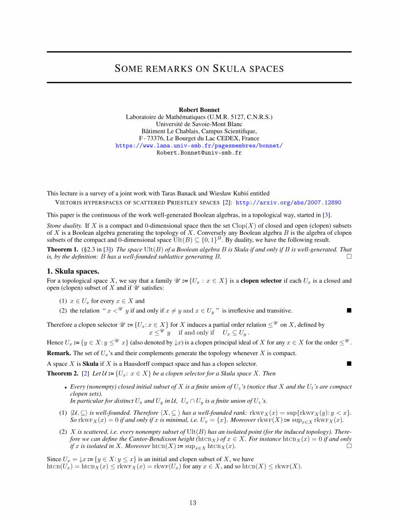
Stone duality. If X is a compact and 0-dimensional space then the set Clop(X) of closed and open (clopen) subsetsof X is a Boolean algebra generating the topology of X . Conversely any Boolean algebra B is the algebra of clopensubsets of the compact and 0-dimensional space Ult(B) ⊆ 0, 1B . By duality, we have the following result.Theorem 1. (§2.3 in [3]) The space Ult(B) of a Boolean algebra B is Skula if and only if B is well-generated. Thatis, by the definition: B has a well-founded sublattice generating B.

1. Skula spaces.For a topological space X , we say that a family U := Ux : x ∈ X is a clopen selector if each Ux is a closed andopen (clopen) subset of X and if U satisfies:

(1) x ∈ Ux for every x ∈ X and(2) the relation “ x <U y if and only if x 6= y and x ∈ Uy ” is irreflexive and transitive.

Therefore a clopen selector U := Ux:x ∈ X for X induces a partial order relation ≤U on X , defined byx ≤U y if and only if Ux ⊆ Uy .

Hence Ux := y ∈ X: y ≤U x (also denoted by ↓x) is a clopen principal ideal of X for any x ∈ X for the order≤U .

Remark. The set of Ux’s and their complements generate the topology whenever X is compact.

A space X is Skula if X is a Hausdorff compact space and has a clopen selector. Theorem 2. [2] Let U := Ux: x ∈ X be a clopen selector for a Skula space X . Then

• Every (nonempty) closed initial subset of X is a finite union of Uz’s (notice that X and the Ut’s are compactclopen sets).In particular for distinct Ux and Uy in U , Ux ∩ Uy is a finite union of Uz’s.

(1) 〈U ,⊆〉 is well-founded. Therefore 〈X,⊆ 〉 has a well-founded rank: rkWFX(x) = suprkWFX(y): y < x.So rkWFX(x) = 0 if and only if x is minimal, i.e. Ux = x. Moreover rkWF(X) := supx∈X rkWFX(x).

(2) X is scattered, i.e. every nonempty subset of Ult(B) has an isolated point (for the induced topology). There-fore we can define the Cantor-Bendixson height (htCBX ) of x ∈ X . For instance htCBX(x) = 0 if and onlyif x is isolated in X . Moreover htCB(X) := supx∈X htCBX(x).

Since Ux = ↓x := y ∈ X: y ≤ x is an initial and clopen subset of X , we havehtCB(Ux) = htCBX(x) ≤ rkWFX(x) = rkWF(Ux) for any x ∈ X , and so htCB(X) ≤ rkWF(X).

13

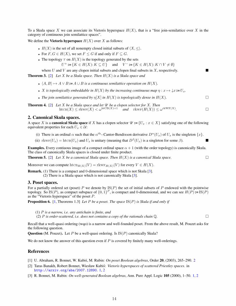
To a Skula space X we can associate its Vietoris hyperspace H(X), that is a “free join-semilattice over X in thecategory of continuous join semilattice spaces”.

We define the Vietoris hyperspace H(X) over X as follows:

• H(X) is the set of all nonempty closed initial subsets of 〈X,≤〉.• For F,G ∈ H(X), we set F ≤ G if and only if F ⊆ G.• The topology T on H(X) is the topology generated by the sets

U+ := K ∈ H(X):K ⊆ U and V − := K ∈ H(X):K ∩ V 6= ∅where U and V are any clopen initial subsets and clopen final subsets in X , respectively.

Theorem 3. [2] Let X be a Skula space. Then H(X) is a Skula space and

• 〈A,B〉 7→ A ∨B :=A ∪B is a continuous semilattice operation on H(X).

• X is topologically embeddable in H(X) by the increasing continuous map η : x 7→ ↓x :=Ux.

• The join semilattice generated by η[X] in H(X) is topologically dense in H(X).

Theorem 4. [2] Let X be a Skula space and let U be a clopen selector for X . ThenhtCB(X) ≤ rkWF(X) < ωhtCB(X)+1 and rkWF(H(X)) ≤ ωrkWF(X).

2. Canonical Skula spaces.A space X is a canonical Skula space if X has a clopen selector U := Ux : x ∈ X satisfying one of the followingequivalent properties for each Ux ∈ U :

(i) There is an ordinal α such that the αth– Cantor-Bendixson derivative Dα(Ux) of Ux is the singleton x.(ii) rkWF(Ux) = htCB(Ux) and Ux is unitary (meaning that Dβ(Ux) is a singleton for some β).

Examples. Every contiuous image of a compact ordinal space α+ 1 (with the order topology) is canonically Skula.The class of canonically Skula spaces is closed under finite product.Theorem 5. [2] Let X be a canonical Skula space. Then H(X) is a canonical Skula space.

Moreover we can compute htCBH(X)(V ) = rkWFH(X)(V ) for every V ∈ H(X).

Remark. (1) There is a compact and 0-dimensional space which is not Skula [3].(2) There is a Skula space which is not canonically Skula [3].

3. Poset spaces.For a partially ordered set (poset) P we denote by IS(P ) the set of initial subsets of P endowed with the pointwisetopology. So IS(P ), as compact subspace of 0, 1P , is compact and 0-dimensional, and we can see H(P ) := IS(P )as the “Vietoris hyperspace” of the poset P .Proposition 6. [1, Theorems 1.3] Let P be a poset. The space IS(P ) is Skula if and only if

(1) P is a narrow, i.e. any antichain is finite, and(2) P is order-scattered, i.e. does not contains a copy of the rationals chain Q.

Recall that a well-quasi ordering (wqo) is a narrow and well-founded poset. From the above result, M. Pouzet asks forthe following question.Question (M. Pouzet). Let P be a well-quasi ordering. Is IS(P ) canonically Skula?

We do not know the answer of this question even if P is covered by finitely many well-orderings.

References

[1] U. Abraham, R. Bonnet, W. Kubis, M. Rubin: On poset Boolean algebras, Order 20, (2003), 265–290. 2[2] Taras Banakh, Robert Bonnet, Wiesław Kubis: Vietoris hyperspaces of scattered Priestley spaces. in

http://arxiv.org/abs/2007.12890. 1, 2[3] R. Bonnet, M. Rubin: On well-generated Boolean algebras, Ann. Pure Appl. Logic 105 (2000), 1–50. 1, 2

14

PERMANENT AND DETERMINANT OF TOEPLITZ-HESSENBERGMATRICES WITH GENERALIZED FIBONACCI AND LUCAS

ENTRIES

Ihab Eddine DjellasUSTHB, Faculty of Mathematics,

RECITS Laboratory,P. Box 32, El Alia, 16111, Bab Ezzouar, Algiers, Algeria

[email protected]

Hacène BelbachirUSTHB, Faculty of Mathematics,


[email protected]

Amine BelkhirUSTHB, Faculty of Mathematics,


[email protected]

ABSTRACT

In this work we give formulas for the permanent and determinant of some families ofToeplitz–Hessenberg matrices having generalized Fibonacci numbers and generalized Lucas numbersas entries and so we generalize some previous results. Then, using the structure of the matrix wederive new identities involving sums of products of generalized Fibonacci numbers and generalizedLucas numbers with multinomial coefficients. Finally we give an application of the determinant ofsuch matrices.

Keywords Generalized Fibonacci numbers · generalized Lucas numbers · Toeplitz-Hessenberg permanent ·Toeplitz-Hessenberg determinant.

1 Introduction

Let p, q ∈ Z. The generalized Fibonacci sequence, "denoted Un", is defined by U0 = 0, U1 = 1, and the followingrecurrence relation

Un = pUn−1 + qUn−2, (1)The generalized Lucas sequence, "denoted (Vn)", is defined by V0 = 2, V1 = p, and the recurrence relation

Vn = pVn−1 + qVn−2. (2)

Let A = (aij) be an n× n matrix. The permanent of A, written Per(A) was introduced in the 1800s, and is defined by

Per(A) =∑

σ

n∏

i=1

aiσ(i),

15

where the summation extends over all elements σ of the symmetric group Sn.

A lower Toeplitz–Hessenberg matrix is a square matrix of the form

Mn(a0, a1, . . . , an) =

a1 a0 0 · · · 0 0a2 a1 a0 · · · 0 0

· · · · · · · · ·. . . · · · · · ·

an−1 an−2 an−3 · · · a1 a0

an an−1 an−2 · · · a2 a1

, (3)

where a0 6= 0 and ak 6= 0 for at least one k > 0.

2 Main results

In this work we generalize the results of [2]. We give formulas for the permanent and determinant of matrices definedas (3) with generalized Fibonacci numbers and generalized Lucas numbers as entries. First we give the formulas of thepermanent:

PerMn(1, Uas+b, Ua(s+1)+b, . . . , Ua(s+n−1)+b),

and,PerMn(1, Vas+b, Va(s+1)+b, . . . , Va(s+n−1)+b).

And also the formulas of the determinant,

DetMn(1, Uas+b, Ua(s+1)+b, . . . , Ua(s+n−1)+b),

and,DetMn(1, Vas+b, Va(s+1)+b, . . . , Va(s+n−1)+b).

For any n, s, a ≥ 1 and 0 ≤ b < a.

Next, we provide new identities for generalized Fibonacci and Lucas numbers using a combination of Trudi’s formula,see [4]; and the results already found for the permanent and determinant.

We conclude our work by using the determinant of the Toeplitz-Hessenberg matrices with generalized Fibonacci entriesto give the nth term of the recurrence sequence (wm)m>−n defined as follow,

w−j = 0 for 1 ≤ j ≤ n− 1,w0 = 1,wm = −Uas+bwm−1 − Ua(s+1)+bwm−2 − · · · − Ua(s+n−1)+bwm−n

Also similar results for generalized Lucas, usual Fibonacci and usual Lucas were established.

References

[1] H. Belbachir and F. Bencherif. Sums of products of generalized Fibonacci and Lucas numbers. arXiv preprintarXiv:0708.2347. 2007.

[2] T. Goy and M. Shattuck. Fibonacci and Lucas Identities from Toeplitz–Hessenberg Matrices. Applications andApplied Mathematics , 14(2) 2019.

[3] H. Minc. Permanents. Cambridge University Press. (Vol. 6) 1984.[4] T. Muir. The Theory of Determinants in the Historical Order of Development: Volume One: General and Special

Determinants Up to 1841. Volume Two: The Period 1841 to 1860. Dover Publications. 1960.

16

INTEGER SEQUENCES AND ELLIPSE CHAINS INSIDE AHYPERBOLA

Soumeya M. TebtoubDepartment of Mathematics

RECITS LaboratoryUSTHB, Algiers, Algeria

[email protected] or [email protected]

Hacene. BelbachirDepartment of Mathematics

RECITS LaboratoryUSTHB, Algiers, Algeria

[email protected] or [email protected]

Laszlo. NemethInstitute of Mathematics

University of SopronSopron, Hungary

and associate member of RECITS Laboratory, [email protected]

ABSTRACT

We propose an extension to the work of Lucca [Giovanni Lucca, Integer sequences and circle chainsinside a hyperbola, Forum Geometricorum, Volume 19. 2019, 11–16.]. Our goal is to examinechains of ellipses inside (outside) the branch of hyperbola, and we derive recurrence relations ofcenters and minor (major) axes of the ellipse chains. As well as to determine conditions for theserecurrence sequences that consist of integer numbers.

Keywords Ellipse chains · Circle chains · Hyperbola · Integer sequences.

1 Introduction

Let us consider the hyperbolaH with the canonical equation

x2

a2− y2

b2= 1, (1)

and foci (±c, 0), where a and b are positive real numbers and c2 = a2 + b2. Lucca [1] examined a tangential chain ofcircles inside the branch x > 0 of the hyperbola so that the i-th circle with center (xi, 0) and radius ri is tangent to thehyperbola and to the preceding and succeeding circles labelled by indexes i − 1 and i + 1, respectively. He showedthat in case of certain ratios b

a the sequences xi

x0∞i=0 and rir0

∞i=0 are integers.

The objective of this paper is to extend Lucca’s work, therefore, we are able to provide more integer sequences.We define and examine a special chains of ellipses inside the branch x > 0 of the hyperbola, when the ratio of theminor and major axis is fixed. It is a natural extension of Lucca’s circle chains. We describe the recurrence relationsof center’s sequences, major and minor axes, which determine another type of proof to give integer sequences.We also examine special chains of circles and ellipses between the branches of hyperbola H (or outside of H), which

17

elements are tangent to the hyperbolaH and mutually tangent to each other.We also define a special tangential chain of ellipses between the branches of H, where the centers of the ellipsescoincide with the centers of the circles. We give recurrence formulas for the parameters of ellipses.We generate our result for 3-dimensional space when we consider the one sheeted hyperboloid of revolutionRH withequation

x2

a2+y2

a2− z2

b2= 1, (2)

which can be generated by rotating the hyperbola x2

a2 − z2

b2 = 1 around the minor axis z. Then we define and examinea tangential chain of spheres, later chain of ellipsoids inside the hyperboloid with fix ratio of axes.Our other main purpose is to give integer sequences, which describe the parameters of our chains, we should noticethat our results contain Lucca’s results.We found more then fifty such integer sequences which appear in the On-Line Encyclopedia of Integer Sequences(OEIS [5]), and thus our investigation give them geometrical interpretations.We mention that there are some sequences, ie. A098706, which have only definition and have not any combinatorialor geometry example. Our paper could provide a geometric interpretation for them.In number theory there are hundreds of articles dealing with balancing numbers and the sequence of balancing numbers(A001109), ex., see [4]. In our work this sequence also appears.

2 Associated integer sequences of chains

In this section we give some examples of integer sequences

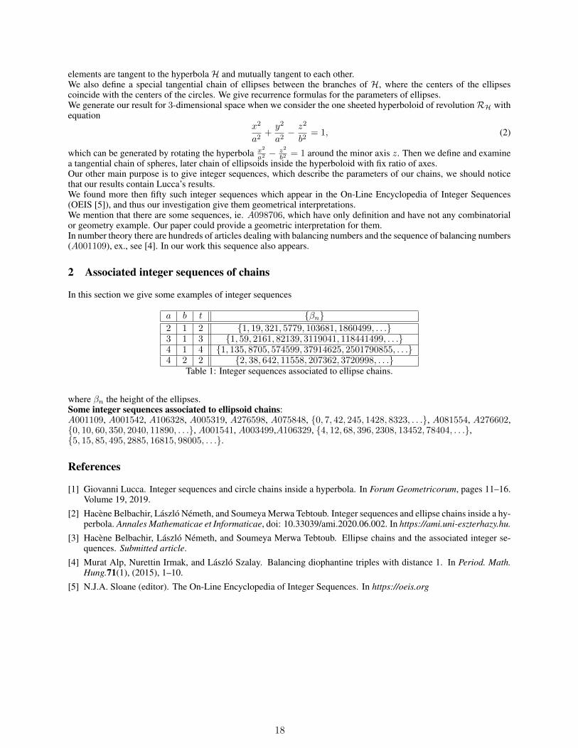
a b t βn2 1 2 1, 19, 321, 5779, 103681, 1860499, . . .3 1 3 1, 59, 2161, 82139, 3119041, 118441499, . . .4 1 4 1, 135, 8705, 574599, 37914625, 2501790855, . . .4 2 2 2, 38, 642, 11558, 207362, 3720998, . . .

Table 1: Integer sequences associated to ellipse chains.

where βn the height of the ellipses.Some integer sequences associated to ellipsoid chains:A001109, A001542, A106328, A005319, A276598, A075848, 0, 7, 42, 245, 1428, 8323, . . ., A081554, A276602,0, 10, 60, 350, 2040, 11890, . . ., A001541, A003499,A106329, 4, 12, 68, 396, 2308, 13452, 78404, . . .,5, 15, 85, 495, 2885, 16815, 98005, . . ..

References

[1] Giovanni Lucca. Integer sequences and circle chains inside a hyperbola. In Forum Geometricorum, pages 11–16.Volume 19, 2019.

[2] Hacene Belbachir, Laszlo Nemeth, and Soumeya Merwa Tebtoub. Integer sequences and ellipse chains inside a hy-perbola. Annales Mathematicae et Informaticae, doi: 10.33039/ami.2020.06.002. In https://ami.uni-eszterhazy.hu.

[3] Hacene Belbachir, Laszlo Nemeth, and Soumeya Merwa Tebtoub. Ellipse chains and the associated integer se-quences. Submitted article.

[4] Murat Alp, Nurettin Irmak, and Laszlo Szalay. Balancing diophantine triples with distance 1. In Period. Math.Hung.71(1), (2015), 1–10.

[5] N.J.A. Sloane (editor). The On-Line Encyclopedia of Integer Sequences. In https://oeis.org

18

BIsNOMIAL COEFFICIENTS AND s−LAH NUMBERS.

Imène TouaibiaUSTHB, Faculty of Mathematics,


[email protected]

Hacène BelbachirUSTHB, Faculty of Mathematics,


[email protected]

Miloud MIHOUBIUSTHB, Faculty of Mathematics,


[email protected]

ABSTRACT

We construct in this work two formulas of the exponential generating function of the bisnomialcoefficients. Using these generating functions, we give some formulas and properties of the bisnomialcoefficients and the s−Lah numbers.

Keywords Binomial coefficients · ordinary generating function · exponential generating function · Lah numbers.

1 Introduction

For s ≥ 1, the bisnomial coefficients [1] denoted by(nk

)s, where

(nk

)s= 0 for k /∈ 0, 1, 2, . . . , sn, are the positive

integers that occur as coefficients of the xk term in the multinomial expansionns∑

k=0

(n

k

)

s

xk = (1 + x+ x2 + · · ·+ xs)n. (1)

For s = 1, we get the classical binomial coefficients.Therefore, the bisnomial coefficients can be seen as an extention of the binomial coefficients, and they generalize themost important properties (see [2] and [3] for instance) of the

(nk

)coefficients:

They verify the following reccurence relations(n

k

)

s

=s∑

i=1

(n− 1

k − i

)

s

, (2)

(n

k

)

s

=n∑

i=0

(n

i

)(i

k − i

)

s−1. (3)

19

They verify the symmetry relation (n

k

)

s

=

(n

sn− k

)

s

. (4)

Using the binomial coefficients, these coefficients can be expressed as follows(n

k

)

s

=∑

i1+i2+···+is=k

(n

i1

)(i1i2

)· · ·(is−1is

). (5)

The s−Lah numbers [6] is a restricted class of the Lah numbers (see for instance [4] and [5]) denoted by⌊kj

⌋≤s, and

which counts the number of partitions of a k-set into j ordered blocks such that the cardinality of any block is at most s,and they have the following properties:

- they have the following exponential generating function

∑

k≥0

⌊k

j

⌋≤stk

k!=

1

j!

(s∑

m=1

tm

)j

=1

j!

(t(1− ts)

1− t

)j

. (6)

- they have the following exact expression⌊k

j

⌋≤s

=∑

j1+2j2+···+sjs=kj1+j2+···+js=j

k!

j1!j2! . . . js!. (7)

- and using the bisnomial coefficients [3], they have the following expression⌊k

j

⌋≤s

=k!

j!

(j

k − j

)

s−1

. (8)

2 Main results

Our main result is the construction of two formulas of the exponential generating function of the the bisnomialcoefficients, one of which is obtained by using the s−Lah numbers. Using these two formulas, we give some recurrencerelations for the bisnomial coefficients, the ordinary generating function of the s−Lah numbers and we conclude byshowing the log concavity and the unimodality of this class of numbers.

References

[1] H. Belbachir, A. Benmezai. A q-analogue for bisnomial coefficients and generalized Fibonacci sequences. ComptesRendus Mathematique. 352(3): 167–171, 2014.

[2] A. Bazeniar, M. Ahmia, H. Belbachir. Connection between bisnomial coefficients and their analogs and symmetricfunctions. Turkish Journal of Mathematics 42(3): 807–818, 2018.

[3] H. Belbachir, S. Bouroubi, A. Khelladi. Connection between ordinary multinomials, Fibonacci numbers, Bellpolynomials and discrete uniform distribution. Annales Math. et Informaticae, 35, 21-30, 2008.

[4] H. Belbachir, I. E. Bousbaa. Combinatorial identities for the r-Lah numbers. Ars Comb. 115:453-458, 2014.[5] H. Belbachir, A. Belkhir. Cross recurrence relations for r-Lah numbers. Ars Comb. 110:199-203, 2013.[6] M. Mihoubi, M. Rahmani. The partial r-Bell polynomials. Afrika Matematika 28(7-8):1167-1183, 2017.

20

ON GENERALIZATION OF BI-PERIODIC r-NUMBERS

N. Rosa AIT-AMRANE∗Department of Mathematics and Computer Science, Yahia Fares University

Medea, AlgeriaUSTHB, Faculty of Mathematics, RECITS Laboratory, 16111 Bab-Ezzouar

Algiers, [email protected]

ABSTRACT

We define a new class of the bi-periodic r-Fibonacci sequence. Then, we introduce a new family of thecompanion sequences of the bi-periodic r-Fibonacci sequence, named bi-periodic r-Lucas sequenceof type s, which extend the classical Fibonacci and Lucas sequences. Afterwards, we establish thelink between the bi-periodic r-Fibonacci sequence and its companion sequence. Furthermore, we givetheir basic properties linear recurrence relations, generating functions, Binet formulas and explicitformulas.

Keywords Bi-periodic Fibonacci sequence, bi-periodic Lucas sequence, generating function, Binet formula, explicitformula.

1 Introduction

Yazlik et al. [3] introduced generalization of the bi-periodic Fibonacci r-numbers (fn), for r a positive integer and a, ba positive real numbers by, for n ≥ r + 1

fn =

afn−1 + fn−r−1, for n ≡ 0 (mod 2),bfn−1 + fn−r−1, for n ≡ 1 (mod 2),

(1)

and the bi-periodic Lucas r-numbers (ln) by, for n ≥ r + 1

ln =

bln−1 + ln−r−1, for n ≡ 0 (mod 2),aln−1 + ln−r−1, for n ≡ 1 (mod 2),

(2)

with the initial conditions f0 = 0, f1 = 1, f2 = a, ..., fr = abr/2cbb(r−1)/2c and l0 = r + 1, l1 = a, l2 = ab, ..., lr =ab(r+1)/2cbbr/2c, respectively.We define a new class of the bi-periodic r-Fibonacci sequence (U

(r)n )n and we give its linear recurrence relation. We

introduce a new family of companion sequences associated to the bi-periodic r-Fibonacci sequence indexed by theparameter s; with 1 ≤ s ≤ r; named the bi-periodic r-Lucas sequence of type s, (V (r,s)

n )n. After that, we expressV

(r,s)n in terms of U (r)

n and s. Then we give some algebraic properties.

2 The bi-periodic r-Fibonacci sequence

First, we define the bi-periodic r-Fibonacci sequence (U(r)n )n and give its linear recurrence relation. For a, b, c, d

nonzero real numbers and r ∈ N, the bi-periodic r-Fibonacci sequence (U(r)n )n is defined by, for n ≥ r + 1

U (r)n =

aU

(r)n−1 + cU

(r)n−r−1, for n ≡ 0 (mod 2),

bU(r)n−1 + dU

(r)n−r−1, for n ≡ 1 (mod 2),

(3)

∗[email protected]

21

with the initial conditions U (r)0 = 0, U

(r)1 = 1, U

(r)2 = a, . . . , U

(r)r = abr/2cbb(r−1)/2c. The bi-periodic r-Fibonacci

sequence can be expressed by linear recurrence relation. For a, b, c, d nonzero real numbers and r ∈ N, the bi-periodicr-Fibonacci sequence satisfies the following linear recurrence, for n ≥ 2r + 2

U (r)n = abU

(r)n−2 + (aξ(r+1)d+ bξ(r+1)c)U

(r)n−r−1−ξ(r+1) − (−1)r+1cdU

(r)n−2r−2. (4)

3 The bi-periodic r-Lucas sequence of type s

Secondly, we introduce a new family of companion sequences related to the bi-periodic r-Fibonacci sequence, calledthe bi-periodic r-Lucas sequence of type s, (V (r,s)

n )n. For any nonzero real numbers a, b, c, d and integers s, r suchthat 1 ≤ s ≤ r, we define for n ≥ r + 1

V (r,s)n =

bV

(r,s)n−1 + dV

(r,s)n−r−1, for n ≡ 0 (mod 2),

aV(r,s)n−1 + cV

(r,s)n−r−1, for n ≡ 1 (mod 2),

(5)

with the initial conditions V (r,s)0 = s + 1, V (r,s)

1 = a, V(r,s)2 = ab, . . . , V

(r,s)r = ab(r+1)/2cbbr/2c. The bi-periodic

r-Fibonacci sequence (U (r)n )n and the bi-periodic r-Lucas sequence of type s, (V (r,s)

n )n can be seen as a generalizationof the Fibonacci and Lucas sequences, we will list some particular cases. The bi-periodic r-Lucas sequence of types, 1 ≤ s ≤ r satisfy the following linear recurrence relation. For a nonzero real numbers a, b, c, d and s, r such that1 ≤ s ≤ r, the family of the bi-periodic r-Lucas sequence of type s satisfy, for n ≥ 2r + 2

V (r,s)n = abV

(r,s)n−2 + (aξ(r+1)d+ bξ(r+1)c)V

(r,s)n−r−1−ξ(r+1) − (−1)r+1cdV

(r,s)n−2r−2. (6)

After that, we express the bi-periodic r-Lucas sequence of type s, V (r,s)n in terms of U (r)

n . Let r and s be nonnegativeintegers such that 1 ≤ s ≤ r, the bi-periodic r-Fibonacci sequence and the bi-periodic r-Lucas sequence of type ssatisfy the following relationship

V (r,s)n =

U(r)n+1 + sdU

(r)n−r, n ≥ r, for r odd,

U(r)n+1 + scbU

(r)n−r−1 + scdU

(r)n−2r−1, n ≥ 2r + 1, for r even.

(7)

4 Main results

We also give the generating functions of the bi-periodic r-Fibonacci sequence and the bi-periodic r-Lucas sequence oftype s. Then, we express an explicit formulas of (U (r)

n )n and (V(r,s)n )n. Finally, we give the Binet Formulas of them.

References

[1] S. Abbad, H. Belbachir, B. Benzaghou, Companion sequences associated to the r-Fibonacci sequence: algebraicand combinatorial properties, Turkish Journal of Mathematics, 43 (3) (2019), 1095-1114.

[2] H. Belbachir, F. Bencherif, Linear recurrent sequences and powers of a square matrix, Integers 6 (2006), A12,17pp.

[3] Y. Yazlik, C. Köme, V. Madhusudanan, A new generalization of Fibonacci and Lucas p-numbers. Journal ofcomputational analysis and applications 25 (4), (2018), 657–669.

22

FROM TERNARY ABSTRACT COSETS TO GROUPS AND FROMMEDIANS TO SEMILATTICES VIA BASEPOINTS: COMMENTS ON

ANALOGIES

Stephan FoldesUniversity of Miskolc

3515 Miskolc, [email protected]

Gerasimos MeletiouUniversity of Ioannina

Arta, GR-47150, [email protected]

ABSTRACT

Some analogies between the ternary median operation in a distributive lattice and the ternary operationa · b−1 · c in a group [8] were noted in the 40’s papers of Grau [4] and of Birhoff and Kiss [5], andsubstantially expanded in Knobel’s recent article [9]. For these ternary operations commutativity ofthe groups is not an essential requirement, and beyond distributive lattices a larger class of semilatticesis considered, called median semilattices. In this further comments are made in the line of an earlierpaper of one of the present authors [2].In that sense median algebras ([3], [6], [7]) and abstract cosets ([8], [9],[10]) can be studied in paralleland compared due to their analogous properties. Both of them are ternary algebraic structures. Byfixing the central operand (the second one) a collection of binary operations is derived. For a medianalgebra we get a family of mutually distributive semilattice operations; for an abstract coset we get afamily of mutually paraassociative group structures. In both cases the original ternary operation canbe reconstructed from any of the derived binary operations.In any group, where the group operation is denoted o the passage from the operation o to anothergroup operation ω with neutral element b−1 is specified by defining aωc = aoboc. This is equivalentto Certaine’s scheme [8] which takes for every b the product a · b−1 · c. This way the new operationaωc = aoboc can be defined not only in groups, but is any semigroup, even if b has no inverse.In any median semilattice, where meet is denoted by ∧ and join – when it exists – is denoted by∨, the passage to the meet operation b of another median semilattice with minimum element b isspecified by defining abc = (a ∧ b) ∨ (b ∧ c) ∨ (a ∧ c). Even if the original semilattice is actually alattice, the semilattice defined by the new meet operation will generally not by a lattice. In fact inthe integer lattices discussed above, it will not be a lattice for any choice of the basepoint elementb. However, in the case of a finite, n-dimensional Boolean lattice, the new semilattice will defineanother n-dimensional Boolean lattice for any choice of the basepoint element b. We note that for atree semilattice - trivially - the new semilattice will also be a tree, and never a lattice if the originaltree semilattice is not one.The paradigmatic example we propose is that of the integer lattice (grid) in n-dimensional space. Inany visual representation it appears as a 2n-regular infinite graph. As a discrete model for physicalspace (say for n = 3) it exhibits the obvious relativity of the notion of origin, and of the arbitrarynessof the choosing X , Y and Z axes in a coordinatization.The classical algebraic structure of the integer lattice is the commutative group structure (or Z-module), which can be defined once an origin is chosen. In fact this group structure is completelydetermined by the choice of the origin, with no need for coordinatization by n-tuples of numbers.The various groups obtained this way are all isomorphic.The classical order structure on the integer grid, on the other hand, is the distributive lattice structurethat is usually decribed as a vectorial order (or Laurent monomial order) based on a chosen coordina-tization by integer n-tuples (which can in fact also be achieved without coordinatization, in terms

23

of the graph structure of the grid alone). The distributive lattice structures obtained this way are allisomorphic. There is, however, a meet semilattice structure obtained for each choice of the origin, bydefining a vertex x to be smaller or equal to y if it lies on a shortest graph-theoretical path betweenthe origin and y. The meet semilattices so obtained are not lattices, but they are all isomorphic toeach other: they are called base-point semilattices.

References

[1] G. Birkhoff, Some applications of universal algebra. In Colloq. Math. Soc. Janos Bolyai 29 (Universal algebra,Esztergom, 1977), pages 107–128.

[2] G.C. Meletiou, Median algebras acting on sets. In Algebra Universalis 29, pages 477–484, 1992.[3] H. J. Bandelt and J. Hedlikova, Median algebras. Discrete mathematics, vol. 45, pages 1–30, 1983.[4] A.A. Grau, Ternary boolean algebra. Bull. Amer. Math. Soc. 53, pages 567–572, 1947.[5] G. Birkhoff and S.A. Kiss, A ternary operation in distributive lattices. Bull. Amer. Math. Soc. 53, pages 749-–752,

1947.[6] M. Sholander, “Medians, lattices, and trees”. Proc. American Mathematical Society, 5(5), pages 808—812, 1954.[7] M. Sholander, Trees, lattices, order, and betweenness. Proc. Am. Math. Soc. 3(3), pages 369—381 , 1952.[8] J. Certaine, The ternary operation (abc) = ab−1c of a group. Bull. Amer. Math. Soc. 49, pages 869 – 877, 1943.[9] A. Knoebel, Flocks, groups and heaps, joined with semilattices. Quasigroups and Related Systems 24, pages 43 –

66, 2016.[10] C. Hollings and M. Lawson, Wagner’s Theory of Generalised Heaps. Springer International Publishing AG, 2017.

24

ON THE ENUMERATION OF P -OLIGOMORPHIC GROUPS

Justine Falque∗

ABSTRACT

We describe an algorithm to enumerate (closed) P -oligomorphic permutation groups per profilegrowth, up to kernel, and we announce its implementation as an ongoing work. This work is based onthe recent classification of P -oligomorphic groups from [1].

Keywords Infinite permutation groups · profile · P -oligomorphic groups · blocks · computer algebra · enumeration

1 Introduction

Given a permutation group G of a set E, the profile of G is the sequence that counts, for every nonnegative integer n,the G-orbits of degree n: that is, the orbits of the induced action of G on the subsets of size n of E. In the seventies,Cameron initiated the study of infinite permutation groups of countably infinite sets whose profile took only finitevalues, calling them oligomorphic groups[2].

When, in addition, the profile is bounded by a polynomial, the group may be called P -oligomorphic. In that case,as once conjectured by Cameron, the profile has been recently shown by the author and Thiéry to be asymptoticallyequivalent to a polynomial [3], and the profile growth refers to the degree of this polynomial.

Along with the resolution of the conjecture, these groups have been classified [1]: basically, a P -oligomorphic group isuniquely and entirely described by a finite permutation group endowed with a block system, each block of which isdecorated by a pair of groups — one finite, the other infinite — satisfying some explicit conditions.

This extended abstract presents an algorithm, based on this classification, that allows to enumerate all closed P -oligomorphic groups per profile growth, up to kernel (for else there would be infinitely many groups for each growth),the closure notion refering to the simple convergence topology. It is being implemented using the software SageMath [4]and features from GAP-system [5]. The obtained counting sequence will hopefully be presented at the ALGOS2020conference.

This paper is dedicated to Maurice Pouzet on the occasion of his 75th birthday. Oligomorphic groups are a particularcase of relational structures, which are one of his domains of predilection, and he is at the origin of my work onoligomorphic groups.

2 Enumeration of (closed) P -oligomorphic groups

2.1 Generation of finite permutation groups

As it is the first brick in the classification, the first step is to generate all finite permutation groups F , up to permutationgroup isomorphism. They are counted, per degree, by the following sequence (A000638):

1, 1, 2, 4, 11, 19, 56, 96, 296, 554, 1593, 3094, 10723, . . .

We implemented this using the GAP Data Library “Transitive Groups”, thanks to the property that any intransitivegroup is a subdirect product of transitive groups.

∗Webpage of the author, mail: [email protected]

25

The method used is essentially that described in [6]. Roughly speaking, for each domain size N , one needs to enumerateall partitions of N , which represent the possible sets of orbits; then, for each one of them, choose a transitive groupFi on each orbit, and finally compute the subdirect products of these groups in order to generate all permutationgroups with these orbits. Some care can be taken at different stages of the generation in order to limit the productionof isomorphic groups, yet the author could not spare a final conjugacy test. As the references consulted about thisdid not include any code, we created a repository to share our implementation with SageMath. The enumeration ofP -oligomorphic groups should be available there as well by the time of the conference.

2.2 Enumeration of P -oligomorphic groups using their classification

2.2.1 Block systems of intransitive groups

Once the finite permutation groups have been generated, there remains to enumerate their block systems: generalizingthe usual definition to intransitive groups, a block system is a set partition of the domain that is globally stable under theaction of the group.

As for the previous one, this step needs some implementation work. Indeed, the implementation of block systems inGAP (and thereby SageMath) requires the group to be transitive, and therefore requires to be extended. This involvesconsidering the automorphism group of the finite permutation group F that is being processed, more precisely its actionon the orbit restrictions Fi.

There are some technical issues to handle along the way: for instance, the fact that trivial block systems are not includedin the output of AllBlocks, or that fixed points are removed when GAP computes an action. In addition, one mustmanually consider the systems involving blocks that are union of orbits — all that up to isomorphism.

2.2.2 The decorations and profile growth

The final layer, in the enumeration as in the classification, is the choice of decorations for each one of the orbits ofblocks of the finite permutation group F : on the one hand, a normal subgroup Hi of the induced action of F on one ofthe blocks of this orbit; on the other hand, a (closed) highly homogeneous group. There are five of this latter kind ofgroups, but only one (the infinite symmetric group) is possible if the blocks are not singletons.

This steps corresponds to choosing the behaviour of the final P -oligomorphic group inside each one of its superblocks.It must again be carried out up to isomorphism.

When a P -oligomorphic group is finally obtained this way, one determines its profile growth using the profiles of theHi’s (the profile has been previously implanted by the author as a method for finite permutation groups). Indeed, itcorresponds to the total number of orbits of subsets of the Hi’s, minus one. This ensures that it is (tightly) boundedabove by the degree of F minus one, so when asking for the number of P -oligomorphic groups up to growth r, oneneeds to consider finite groups F up to degree r + 1.

Note that the whole enumeration is much easier when counting only transitive P -oligomorphic groups. An implementa-tion can be found in the same repository, and hands the sequence:

1, 5, 6, 14, 33, 32, 114, 47, 323, 260, 338, 50, 2108, 58, 430, 940, 12470, 60, 7361, 64, 12136, . . .

which is unknown by OEIS.

References

[1] Justine Falque and Nicolas M. Thiéry. Classification of P-oligomorphic groups, conjectures of Cameron andMacpherson. Submitted, 39 pages, arXiv:2005.05296 [math.CO], May 2020.

[2] P. J. Cameron. Oligomorphic permutation groups, volume 152 of London Mathematical Society Lecture NoteSeries. Cambridge University Press, Cambridge, 1990.

[3] Justine Falque and Nicolas M. Thiéry. The orbit algebra of a permutation group with polynomial profile isCohen-Macaulay. In 30th International Conference on Formal Power Series and Algebraic Combinatorics (FPSAC2018, Hanover), February 2018.

[4] The Sage Developers. SageMath, the Sage Mathematics Software System (Version 9.0), 2020.https://www.sagemath.org.

[5] The GAP Group, Aachen, St Andrews. GAP – Groups, Algorithms, and Programming, Version 4.10, 1999.[6] Derek F. Holt. Enumerating subgroups of the symmetric group. 2010. oeis.org/A000638.

26

LOG-CONCAVITY AND UNIMODALITY IN ARITHMETICALTRIANGLES

Assia F. TEBTOUBUSTHB, Faculty of Mathematics, RECITS Lab.

PB 32, El Alia, 16111, Bab Ezzouar, [email protected]

ABSTRACT

In this work, we establish log-cancavity and unimodality in some well-known arithmetical triangles.

Keywords Arithmetical triangles · Log-concavity · Unimodality

A real sequence (ak)nk=0 is unimodal if it rises to a maximum ak0

and then decreases, the entire ak0is called the

mode of the sequence (ak). And it is logarithmically concave (log-concave) if ai−1ai+1 ≤ a2i , for i = 1, · · · , n− 1. Itis known that a log-concave sequence is unimodal. Many combinatorial sequences are unimodal and the well knownexample is the sequence of binomial coefficients. The simplicity of its explicit formula makes easy the proof of itsunimodality. The concept of unimodality is simple and obviously assimilated, but its elaboration is not always easy,since many sequences are not as explicit as the Newton’s sequence. The question of unimodality has been the objectof diverse articles under different aspects: proof of unimodality [8, 10], detection of modes [5], or the enumeration ofthe methods to prove unimodality [1, 6, 9].

We are interested in our work on the study of sequences linked to different arithmetical triangles. Principally, we areinspired by the works that have been already done on the most known triangle, which is: the Pascal triangle. The firstresult of unimodality in Pascal’s triangle other than the binomial coefficient is due to Tanny and Zuker [10]. Manyother works treat the question of unimodality of sequences linked to different directions of this triangle. And thencomes the work of Belbachir and Szalay [2], where they showed that any sequence lying over any finite direction inPascal’s triangle is unimodal. By analogy to these works, we propose to study the unimodality of sequences linked toarithmetical triangles other than Pascal’s triangle, and this using different methods.

We deal in this work with many arithmetical triangles such as: Stirling triangle of second kind [3, 4], Lah triangle[11], associated Stirling triangle and the Eulerian triangle.

References

[1] M. Balazard. Quelques exemples de suites unimodales en théorie des nombres. In Journal de théorie des nombresde Bordeaux, pages 13–30, 1990.

[2] H. Belbachir, L. Szalay. Unimodal rays in the regular and generalized Pascal triangles. In J. of Integer Seq., 11,Article. 08.2.4., 2008.

[3] H. Belbachir, A. F. Tebtoub. Les nombres de Stirling associés avec succession d’ordre 2, nombres de Fibonacci-Stirling et unimodalité. C. R. Acad. Sci. Paris, Ser. I, 2015.

[4] H. Belbachir, A. F. Tebtoub. The t-successive associated Stirling numbers, t-Fibonacci Stirling numbers andUnimodality. Turkish Journal of Mathematics, pages 1279–1291, 2017.

[5] M. Benoumhani. Sur une propriétés des polynômes à racines négatives. Journal de mathématiques pures etappliqués, 75(2), pages 85–105, 1996.

27

[6] F. Brenti. Unimodal, log-convave and Polyà frequency sequences in combinatorics. American Mathematical Soc.,V413, 1989.

[7] E. R. Canfield. Location of the maximum Stirling number(s) of second kind. Studies in App Math, 59, pages83–93, 1978.

[8] L. H. Harper. Stirling behaviour is asymptotically normal. Ann. Math. Stat., 38, pages 410–414, 1967.[9] R. P. Stanley. Log-concave and unimodal sequences in Algebra, Combinatorics and Geometry. Annals of the New

York academy of sciences , 576(1), pages 500–535, 1989.[10] S. Tanny, M. Zuker. On unimodality sequence of binomial coefficients. Discrete Math., 9, pages 79–89, 1974.[11] A. F. Tebtoub. Log-concavity of principal diagonal rays in the regular Lah triangles. Ars Combinatorias, V114,

pages 75–83, 2018.

28

Short papers

DECOMPOSITION SCHEMES FOR SYMMETRIC n-ARY BANDS

Jimmy DevilletDepartment of MathematicsUniversity of Luxembourg

[email protected]

Pierre MathonetDepartment of Mathematics

University of LiegeLiege, Belgium

[email protected]

ABSTRACT

We extend the classical (strong) semilattice decomposition scheme of certain classes of semigroupsto the class of idempotent symmetric n-ary semigroups (i.e. symmetric n-ary bands) where n ≥ 2 isan integer. More precisely, we show that these semigroups are exactly the strong n-ary semilatticesof n-ary extensions of Abelian groups whose exponents divide n − 1. We then use this main result toobtain necessary and sufficient conditions for a symmetric n-ary band to be reducible to a semigroup.

Keywords Semigroup ⋅ idempotency ⋅ semilattice decomposition ⋅ reducibility

1 Introduction

Semigroups are ubiquitous and have numerous applications both in theoretical and applied mathematics. An extensivestudy of these structures began in the second half of the 20th century (see the pioneering works [2] and [19], or thetextbooks [3, 10, 12, 20, 21] and references therein). In the algebraic analysis of semigroups, it soon became clear that itwas useful to obtain a decomposition scheme of the semigroup under consideration into subsemigroups that are easier todescribe or have additional properties (e.g. being groups), but also to be able to build a semigroup by combining givensubsemigroups in a suitable way, that is, to use a composition scheme for semigroups.

Several classes of semigroups have the remarkable property to admit such composition/decomposition schemes; see,e.g., Krohn-Rhodes theorem for finite semigroups and finite automata [14]. A noteworthy example of such a schemeis given by strong semilattice decompositions of certain classes of bands 1. In this paper we generalize these strongsemilattice decompositions to structures with higher arities, defined as follows.

An n-ary operation F ∶Xn →X (where n ≥ 2 is an integer and X is a non-empty set) is associative ifF (x1, . . . , xi−1, F (xi, . . . , xi+n−1), xi+n, . . . , x2n−1) = F (x1, . . . , xi, F (xi+1, . . . , xi+n), xi+n+1, . . . , x2n−1), (1)

for all x1, . . . , x2n−1 ∈ X and all 1 ≤ i ≤ n − 1. If F is an n-ary associative operation on X , then (X,F ) is an n-arysemigroup. These n-ary structures, first studied in [9] and [22], have applications in different fields such as automatatheory (see, e.g., [11]), coding theory, and cryptology (see, e.g., [16, 17]).

The classical definitions of symmetry and idempotency can also be extended to n-ary operations as follows: F isidempotent if F (x, . . . , x) = x for every x ∈X and F is symmetric (or commutative) if F is invariant under the actionof permutations.

Many examples of n-ary semigroups are obtained by extending binary semigroups: if G∶X2 → X is an associativeoperation, then we can define a sequence of operations inductively by setting G1 = G, and

Gm(x1, . . . , xm+1) = Gm−1(x1, . . . , xm−1,G(xm, xm+1)), m ≥ 2.

Setting F = Gn−1, it is straightforward to see that the pair (X,F ) is indeed an n-ary semigroup. It is said to be then-ary extension of (X,G) and we say that (X,F ) is reducible to (X,G)2. However, not every n-ary semigroup

1A band is a semigroup (X,G) where X is a nonempty set and the binary associative operation G∶X2 →X satisfies G(x,x) = xfor every x ∈X; see, e.g., [12] for more details.

2We also say that F is the n-ary extension of G or that F is reducible to G or even that G is a binary reduction of F .

31

is the n-ary extension of a binary semigroup. For instance, the ternary associative operation F defined on R3 byF (x1, x2, x3) = x1 − x2 + x3 is not reducible to any binary associative operation. The problem of reducibility wasconsidered recently in [13, 18] for n-ary semigroups endowed with additional structures and in [1, 4, 6] for the classof quasitrivial n-ary semigroups3. These are n-ary semigroups (X,F ) that preserve all unary relations, i.e., suchthat F (x1, . . . , xn) ∈ x1, . . . , xn for all x1, . . . , xn ∈X . It was shown [4] that all quasitrivial n-ary semigroups arereducible. Then in [5], the authors relaxed the quasitriviality condition by considering operations whose restrictions oncertain subsets of the domain are quasitrivial. It turns out that these operations are also reducible.

In this work we study the class of symmetric (or commutative) n-ary bands, that is, symmetric idempotent n-arysemigroups. Typical examples of symmetric n-ary bands are given by n-ary extensions of semilattices and n-aryextensions of Abelian groups whose exponents divide n − 1. Both classes of examples will play a central role in ourconstructions. However, as shown in the following examples, not every symmetric n-ary band is obtained in this way.

Example 1.1. (a) We consider the set X = 1,2,3,4 and we define the symmetric ternary operationF1∶X3 →X by its level sets given (up to permutations) by F −1

1 (1) = (1,1,1), F −11 (2) = (2,2,2),

F −11 (3) = (1,1,2), (1,1,3), (1,2,4), (1,3,4), (2,2,3), (2,3,3), (2,4,4), (3,3,3), (3,4,4). ThenF −11 (4) is made up of all the remaining elements of X3. This operation defines a symmetric ternary

band and is not reducible to any binary operation.

(b) We consider the set X = 1,2,3 and we define the symmetric ternary operation F2∶X3 →X again by its level sets given (up to permutations) by F −1

2 (1) = (1,1,1), F −12 (2) =(1,1,2), (1,2,2), (1,3,3), (2,2,2), (2,3,3), and F −1

2 (3) = (1,1,3), (1,2,3), (2,2,3), (3,3,3).This operation defines a symmetric ternary band. It turns out that it is reducible to a binary operationon X .

In the next section we define the n-ary counterpart of the classical strong semilattice (de)composition for semigroups(namely the strong n-ary semilattice decomposition). We show that it enables us to compose n-ary semigroups: everystrong n-ary semilattice of n-ary semigroups is an n-ary semigroup (see Proposition 2.2). Then in Section 3, we providea constructive description of the class of symmetric n-ary bands, that is, we show that the symmetric n-ary bandsare exactly the strong n-ary semilattices of n-ary extensions of Abelian groups whose exponents divide n − 1 (seeTheorem 3.12). In the final section, we give a reducibility criterion for symmetric n-ary bands based on their strongn-ary semilattice decomposition (see Proposition 4.3). Also, Example 1.1 shows how these constructions enable us tobuild and analyze examples of symmetric n-ary bands. Almost all the definitions and results in this work stem from [7],where the reader may find their proofs and alternative developments as well.

2 Strong n-ary semilattices of n-ary semigroups

Throughout this work, we consider a nonempty set X and an integer n ≥ 2. Recall that (X,F ) is said to be an n-arygroupoid whenever F ∶Xn → X is an n-ary operation. Moreover, if F is associative (i.e., satisfies (1)), then (X,F )is said to be an n-ary semigroup. The concepts of homomorphims and isomorphisms of n-ary groupoids and n-arysemigroups are defined as usual.

Recall that e ∈X is said to be a neutral element for F ∶Xn →X if

F ((k − 1) ⋅ e, x, (n − k) ⋅ e) = x, x ∈X, k ∈ 1, . . . , n,where, for any k ∈ 0, . . . , n and any x ∈X , the notation k ⋅ x stands for the k-tuple x, . . . , x (for instance F (3 ⋅ x,0 ⋅y,2 ⋅ z) = F (x,x, x, z, z)).

In [8, Lemma 1], it was proved that any associative operation F ∶Xn →X having a neutral element e is reducible to anassociative binary operation Ge∶X2 →X defined by

Ge(x, y) = F (x, (n − 2) ⋅ e, y), x, y ∈X. (2)

Finally, recall that an equivalence relation ∼ on X is said to be a congruence for F ∶Xn → X (or on (X,F )) if it iscompatible with F , that is, if F (x1, . . . , xn) ∼ F (y1, . . . , yn) for any x1, . . . , xn, y1, . . . , yn ∈X such that xi ∼ yi forall i ∈ 1, . . . , n. We denote by [x]∼ (or [x] when there is no risk of confusion) the equivalence class of x for ∼ and byF the map induced by F on X/∼ defined by

F ([x1]∼, . . . , [xn]∼) = [F (x1, . . . , xn)]∼, ∀x1, . . . , xn ∈X.3For n = 2, the quasitrivial semigroups were described by Länger [15].

32

We say that a congruence ∼ on an n-ary groupoid (X,F ) is an n-ary semilattice congruence if (X/∼, F ) is an n-arysemilattice4.

Now, let us extend the well-known concept of semilattice of semigroups to n-ary semigroups. Let (Y,⋏) be a semilatticeand let (Xα, Fα)∶α ∈ Y be a set of n-ary semigroups such that Xα ∩Xβ = ∅ for any α ≠ β. We say that an n-arygroupoid (X,F ) is an n-ary semilattice (Y,⋏n−1) of n-ary semigroups (Xα, Fα) if X = ⋃

α∈YXα, F ∣Xnα = Fα for every

α ∈ Y , andF (Xα1 ×⋯ ×Xαn) ⊆Xα1⋏⋯⋏αn , α1, . . . , αn ∈ Y. (3)

In this case we write (X,F ) = ((Y,⋏n−1); (Xα, Fα)) and we simply say that (X,F ) is an n-ary semilattice of n-arysemigroups.

Actually, any decomposition of an n-ary semigroup (X,F ) as an n-ary semilattice of n-ary semigroups is associatedwith an n-ary semilattice congruence on (X,F ); see, e.g., [12] for the binary counterpart of this result.

The fact that an n-ary groupoid is an n-ary semilattice of n-ary semigroups is not sufficient to ensure that it is an n-arysemigroup. We need to introduce a generalization of the strong semilattice decomposition. This is done in the followingdefinition.Definition 2.1. Let (X,F ) = ((Y,⋏n−1); (Xα, Fα)) be an n-ary semilattice of n-ary semigroups. Suppose that forany α,β ∈ Y such that α ⪰ β there is a homomorphism ϕα,β ∶Xα →Xβ such that the following conditions hold.

(a) The map ϕα,α is the identity on Xα.

(b) For any α,β, γ ∈ Y such that α ⪰ β ⪰ γ we have ϕβ,γ ϕα,β = ϕα,γ .

(c) For any (x1, . . . , xn) ∈Xα1 ×⋯ ×Xαn we have

F (x1, . . . , xn) = Fα1⋏⋯⋏αn(ϕα1,α1⋏⋯⋏αn(x1), . . . , ϕαn,α1⋏⋯⋏αn(xn)).Then (X,F ) is said to be a strong n-ary semilattice (Y,⋏n−1) of n-ary semigroups (Xα, Fα). In this case we write(X,F ) = ((Y,⋏n−1); (Xα, Fα);ϕα,β) and we also say that (X,F ) is a strong n-ary semilattice of n-ary semigroups.

This definition enables us to obtain the main result concerning the composition of n-ary semigroups, which is importanton its own, but also in the next sections.Proposition 2.2. If (X,F ) is a strong n-ary semilattice of n-ary semigroups, then it is an n-ary semigroup.

3 The structure theorem

Throughout this section, we consider a symmetric n-ary band (X,F ). We associate with it a family of unary operationsand study their most important properties.Definition 3.1. For every x ∈X , we define the operation `Fx ∶X →X by

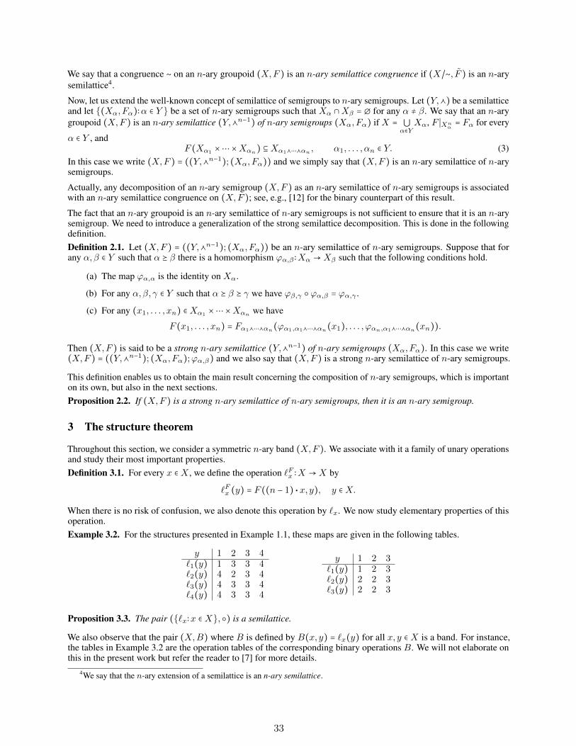
`Fx (y) = F ((n − 1) ⋅ x, y), y ∈X.When there is no risk of confusion, we also denote this operation by `x. We now study elementary properties of thisoperation.Example 3.2. For the structures presented in Example 1.1, these maps are given in the following tables.

y 1 2 3 4`1(y) 1 3 3 4`2(y) 4 2 3 4`3(y) 4 3 3 4`4(y) 4 3 3 4

y 1 2 3`1(y) 1 2 3`2(y) 2 2 3`3(y) 2 2 3

Proposition 3.3. The pair (`x∶x ∈X, ) is a semilattice.

We also observe that the pair (X,B) where B is defined by B(x, y) = `x(y) for all x, y ∈ X is a band. For instance,the tables in Example 3.2 are the operation tables of the corresponding binary operations B. We will not elaborate onthis in the present work but refer the reader to [7] for more details.

4We say that the n-ary extension of a semilattice is an n-ary semilattice.

33

The semilattice defined in Proposition 3.3 can be extended to define a symmetric n-ary band. The following resultestablishes a tight relation between (X,F ) and this n-ary band.

Proposition 3.4. For every x1, . . . , xn ∈X we have

`F (x1,...,xn) = `x1 ⋯ `xn ,that is, the map `∶ (X,F )→ (`x∶x ∈X, n−1) defined by `(x) = `x is a homomorphism.

The map ` defined in the previous proposition enables us to characterize the reducibility of a symmetric n-ary band to asymmetric (binary) band, i.e., a semilattice.

Proposition 3.5. Let (X,F ) be a symmetric n-ary band. The following assertions are equivalent.

(i) The map ` is injective.

(ii) The n-ary band (X,F ) is isomorphic to (`x∶x ∈X, n−1).

(iii) The n-ary band (X,F ) is an n-ary semilattice.

Also, the map ` enables us to characterize those symmetric n-ary bands that are reducible to Abelian groups. Recallthat a group (X,∗) with neutral element e has bounded exponent if there exists an integer m ≥ 1 such that the m-foldproduct x ∗ ⋯ ∗ x is equal to e for any x ∈ X . In that case, the exponent of the group is the smallest integer m ≥ 1having this property. Using the characterization of Abelian groups having bounded exponent given by Prüfer and Baer(see [23]), it is straighforward to see that the exponent of an Abelian group divides n − 1 if and only if the group is adirect sum of cyclic groups whose orders divide n − 1.

Proposition 3.6. Let (X,F ) be a symmetric n-ary band. The following conditions are equivalent.

(i) The map ` is constant (i.e., `x is the identity map on X for any x ∈X).

(ii) The n-ary band (X,F ) is the n-ary extension of a group (X,∗) (and in particular (X,∗) is Abelian and itsexponent divides n − 1).

Now, when the map ` associated with F is not injective, it is natural to consider a quotient, and identify the elements ofX that have the same image by `. In this context, we have the following result.

Proposition 3.7. The binary relation ∼ on X defined by

x ∼ y ⇔ `x = `y, x, y ∈X,is an n-ary semilattice congruence on (X,F ).

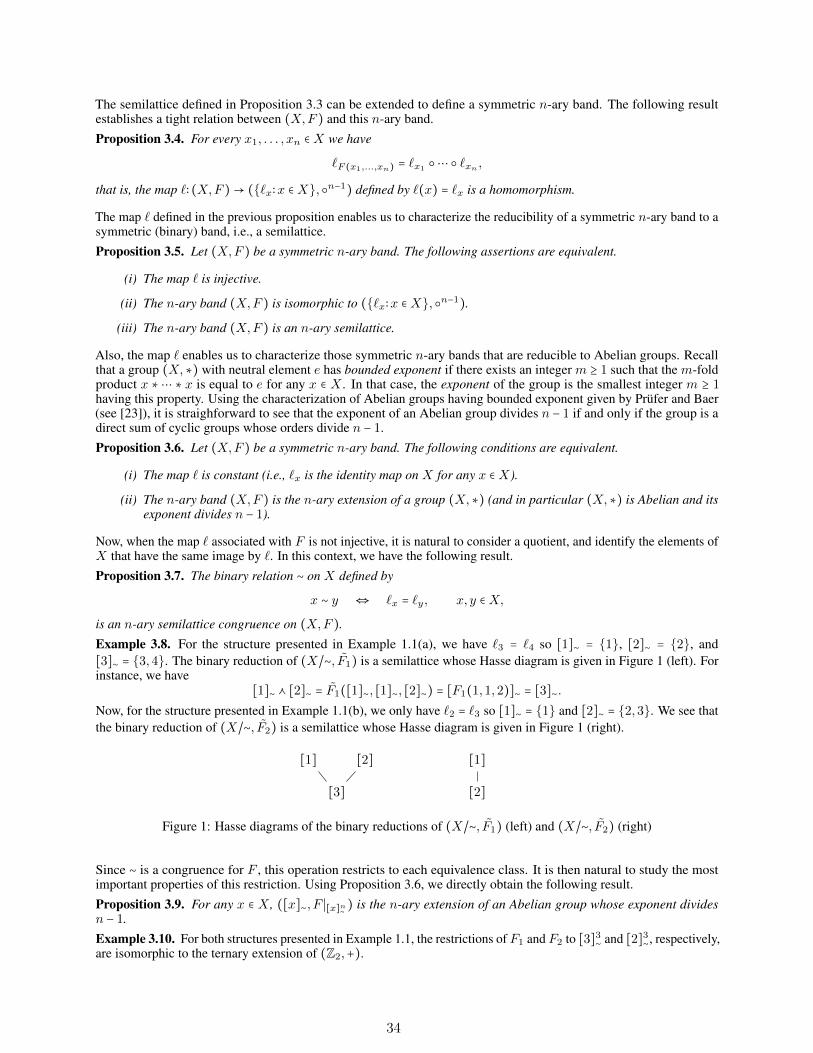
Example 3.8. For the structure presented in Example 1.1(a), we have `3 = `4 so [1]∼ = 1, [2]∼ = 2, and[3]∼ = 3,4. The binary reduction of (X/∼, F1) is a semilattice whose Hasse diagram is given in Figure 1 (left). Forinstance, we have [1]∼ ⋏ [2]∼ = F1([1]∼, [1]∼, [2]∼) = [F1(1,1,2)]∼ = [3]∼.Now, for the structure presented in Example 1.1(b), we only have `2 = `3 so [1]∼ = 1 and [2]∼ = 2,3. We see thatthe binary reduction of (X/∼, F2) is a semilattice whose Hasse diagram is given in Figure 1 (right).

[3][1] [2] [1]

[2]Figure 1: Hasse diagrams of the binary reductions of (X/∼, F1) (left) and (X/∼, F2) (right)

Since ∼ is a congruence for F , this operation restricts to each equivalence class. It is then natural to study the mostimportant properties of this restriction. Using Proposition 3.6, we directly obtain the following result.

Proposition 3.9. For any x ∈ X , ([x]∼, F ∣[x]n∼ ) is the n-ary extension of an Abelian group whose exponent dividesn − 1.

Example 3.10. For both structures presented in Example 1.1, the restrictions of F1 and F2 to [3]3∼ and [2]3∼, respectively,are isomorphic to the ternary extension of (Z2,+).

34

The congruence ∼ enabled us to decompose X as a n-ary semilattice of n-ary semigroups. In order to obtain a strongn-ary semilattice decomposition, we still need to define a suitable family of homomorphisms.Proposition 3.11. For every x, y ∈ X such that [x]∼ ⪰ [y]∼, the map ϕ[x]∼,[y]∼ = `y ∣[x]∼ is a homomorphism from([x]∼, F ∣[x]n∼ ) to ([y]∼, F ∣[y]n∼ ).

We can now state our main structure theorem for symmetric n-ary bands.Theorem 3.12. An n-ary groupoid (X,F ) is a symmetric n-ary band if and only if it is a strong n-ary semilattice ofn-ary extensions of Abelian groups whose exponents divide n − 1.

As a direct application of this theorem, we obtain that a symmetric n-ary band is an n-ary group5 if and only if it is then-ary extension of an Abelian group whose exponent divides n − 1.

In view of the main result, in order to build symmetric n-ary bands, we have to consider Abelian groups whoseexponents divide n−1, and build homomorphisms between the n-ary extensions of such groups. These homomorphismsare described in the next result.Proposition 3.13. Let (X1,∗1) and (X2,∗2) be two Abelian groups whose exponents divide n − 1 and denote by F1

and F2 the n-ary extensions of ∗1 and ∗2, respectively. For every group homomorphism ψ∶X1 →X2 and every g2 ∈X2,the map h∶X1 →X2 defined by

h(x) = g2 ∗2 ψ(x), x ∈X1,

is a homomorphism of n-ary semigroups.

Conversely, every homomorphism from (X1, F1) to (X2, F2) is obtained in this way.

4 Reducibility of symmetric n-ary bands

In this section, we use Theorem 3.12 in order to analyze the reducibility problem for symmetric n-ary bands. We thusconsider a symmetric n-ary band (X,F ).Proposition 4.1. If F is reducible to an associative operation G∶X2 →X , then the following assertions hold.

(i) G is surjective and symmetric;

(ii) The n-ary semilattice congruence ∼ associated with F is a binary semilattice congruence for G.

It follows from Proposition 4.1 that if F is reducible to G, then G induces an operation G∣[x]2∼ on every equivalenceclass [x]∼ of X/∼. This operation is a binary reduction of F ∣[x]n∼ . Therefore, it is natural to study the properties of thereductions of such operations. This is performed in the following result.Proposition 4.2. If (X,F ) is the n-ary extension of an Abelian group (X,G1) whose exponent divides n − 1, thenevery reduction (X,G2) of F is a group that is isomorphic to (X,G1). Moreover, all the reductions of (X,F ) areobtained by using (2) with any element e of X .

We are now able to analyze the reducibility of symmetric n-ary bands.Proposition 4.3. A symmetric n-ary band (X,F ) = ((Y,⋏n−1); (Xα, Fα);ϕα,β) is reducible to a semigroup if andonly if there exists a map e∶Y →X such that

(i) For every α ∈ Y , e(α) = eα belongs to Xα;

(ii) For every α,β ∈ Y such that α ⪰ β, we have ϕα,β(eα) = eβ .

Moreover, when (X,F ) is reducible to a semigroup, a reduction is given by the semigroup decomposed as((Y,⋏n−1); (Xα,Gα);ϕα,β), where Gα is the reduction of Fα with respect to eα.Example 4.4. For the structures of Example 1.1(a) and (b), respectively, the only non obvious homomorphisms aregiven by ϕ[1]∼,[3]∼ = `3∣[1]∼ , ϕ[2]∼,[3]∼ = `3∣[2]∼ , and ϕ[1]∼,[2]∼ = `2∣[1]∼ , respectively.

• For (X,F1), we have ϕ[1]∼,[3]∼(1) = `3(1) = 4 and ϕ[2]∼,[3]∼(2) = `3(2) = 3.

• For (X,F2), we have ϕ[1]∼,[2]∼(1) = `2(1) = 2.

5Recall that an n-ary group is an n-ary semigroup (X,F ) such that for any i ∈ 1, . . . , n and any x1, . . . , xi−1, xi+1, . . . , xn, y ∈X there exists a unique z ∈X such that F (x1, . . . , xi−1, z, xi+1, . . . , xn) = y.

35

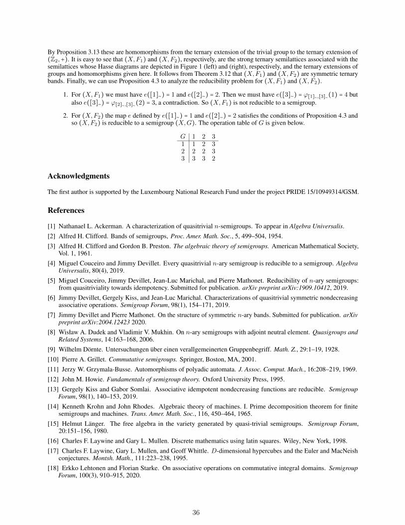
By Proposition 3.13 these are homomorphisms from the ternary extension of the trivial group to the ternary extension of(Z2,+). It is easy to see that (X,F1) and (X,F2), respectively, are the strong ternary semilattices associated with thesemilattices whose Hasse diagrams are depicted in Figure 1 (left) and (right), respectively, and the ternary extensions ofgroups and homomorphisms given here. It follows from Theorem 3.12 that (X,F1) and (X,F2) are symmetric ternarybands. Finally, we can use Proposition 4.3 to analyze the reducibility problem for (X,F1) and (X,F2).

1. For (X,F1) we must have e([1]∼) = 1 and e([2]∼) = 2. Then we must have e([3]∼) = ϕ[1]∼,[3]∼(1) = 4 butalso e([3]∼) = ϕ[2]∼,[3]∼(2) = 3, a contradiction. So (X,F1) is not reducible to a semigroup.

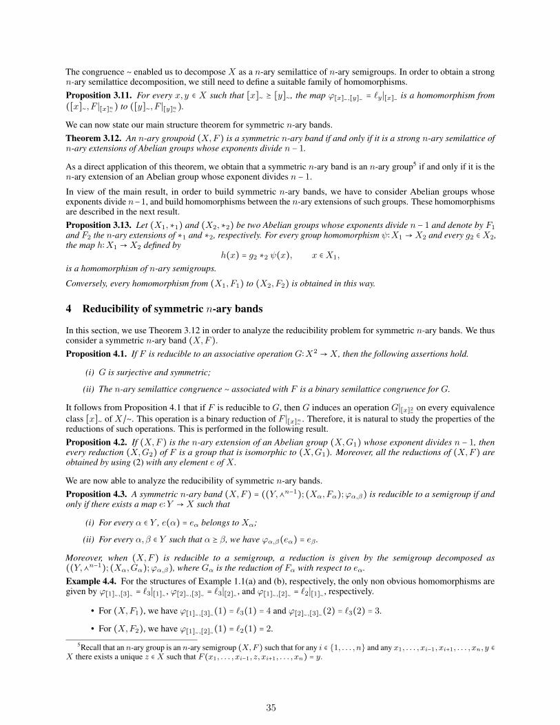
2. For (X,F2) the map e defined by e([1]∼) = 1 and e([2]∼) = 2 satisfies the conditions of Proposition 4.3 andso (X,F2) is reducible to a semigroup (X,G). The operation table of G is given below.

G 1 2 31 1 2 32 2 2 33 3 3 2

Acknowledgments

The first author is supported by the Luxembourg National Research Fund under the project PRIDE 15/10949314/GSM.

References

[1] Nathanael L. Ackerman. A characterization of quasitrivial n-semigroups. To appear in Algebra Universalis.

[2] Alfred H. Clifford. Bands of semigroups, Proc. Amer. Math. Soc., 5, 499–504, 1954.

[3] Alfred H. Clifford and Gordon B. Preston. The algebraic theory of semigroups. American Mathematical Society,Vol. 1, 1961.

[4] Miguel Couceiro and Jimmy Devillet. Every quasitrivial n-ary semigroup is reducible to a semigroup. AlgebraUniversalis, 80(4), 2019.

[5] Miguel Couceiro, Jimmy Devillet, Jean-Luc Marichal, and Pierre Mathonet. Reducibility of n-ary semigroups:from quasitriviality towards idempotency. Submitted for publication. arXiv preprint arXiv:1909.10412, 2019.

[6] Jimmy Devillet, Gergely Kiss, and Jean-Luc Marichal. Characterizations of quasitrivial symmetric nondecreasingassociative operations. Semigroup Forum, 98(1), 154–171, 2019.

[7] Jimmy Devillet and Pierre Mathonet. On the structure of symmetric n-ary bands. Submitted for publication. arXivpreprint arXiv:2004.12423 2020.

[8] Wisław A. Dudek and Vladimir V. Mukhin. On n-ary semigroups with adjoint neutral element. Quasigroups andRelated Systems, 14:163–168, 2006.

[9] Wilhelm Dörnte. Untersuchungen über einen verallgemeinerten Gruppenbegriff. Math. Z., 29:1–19, 1928.

[10] Pierre A. Grillet. Commutative semigroups. Springer, Boston, MA, 2001.

[11] Jerzy W. Grzymala-Busse. Automorphisms of polyadic automata. J. Assoc. Comput. Mach., 16:208–219, 1969.

[12] John M. Howie. Fundamentals of semigroup theory. Oxford University Press, 1995.

[13] Gergely Kiss and Gabor Somlai. Associative idempotent nondecreasing functions are reducible. SemigroupForum, 98(1), 140–153, 2019.

[14] Kenneth Krohn and John Rhodes. Algebraic theory of machines. I. Prime decomposition theorem for finitesemigroups and machines. Trans. Amer. Math. Soc., 116, 450–464, 1965.

[15] Helmut Länger. The free algebra in the variety generated by quasi-trivial semigroups. Semigroup Forum,20:151–156, 1980.

[16] Charles F. Laywine and Gary L. Mullen. Discrete mathematics using latin squares. Wiley, New York, 1998.

[17] Charles F. Laywine, Gary L. Mullen, and Geoff Whittle. D-dimensional hypercubes and the Euler and MacNeishconjectures. Montsh. Math., 111:223–238, 1995.

[18] Erkko Lehtonen and Florian Starke. On associative operations on commutative integral domains. SemigroupForum, 100(3), 910–915, 2020.

36

[19] David McLean. Idempotent semigroups. Amer. Math. Monthly, 61:110–113, 1954.[20] Mario Petrich. Introduction to semigroups. Charles E. Merrill, 1973.[21] Mario Petrich. Lectures in semigroups. John Wiley, London, 1977.[22] Emil L. Post. Polyadic groups. Trans. Amer. Math. Soc., 48:208–350, 1940.[23] Joseph J. Rotman, An Introduction to the Theory of Groups. 4th Ed. Springer-Verlag, New York, USA, 1995.

37

LINEARLY DEFINABLE CLASSES OF BOOLEAN FUNCTIONS∗

Miguel CouceiroUniversité de Lorraine, CNRS, Inria, LORIA

F-54000 Nancy, [email protected]

Erkko LehtonenCentro de Matemática e AplicaçõesFaculdade de Ciências e Tecnologia

Universidade Nova de Lisboa, [email protected]

Dedicated to Maurice Pouzet on the occasion of his 75th birthday

ABSTRACT

In this paper we address the question “How many properties of Boolean functions can be defined bymeans of linear equations?” It follows from a result by Sparks that there are countably many suchlinearly definable classes of Boolean functions. In this paper, we refine this result by completelydescribing these classes. This work is tightly related with the theory of function minors and stableclasses, a topic that has been widely investigated in recent years by several authors including MauricePouzet.

Keywords Functional equation · linear definability · clone · clonoid · Boolean function

1 Introduction and motivation

Functional equations are universally quantified first-order sentences in a certain algebraic syntax, with a single functionsymbol and no other predicate symbol than equality. More precisely, a functional equation for a function of severalarguments from A to B is a formal expression

h1(f(g1(v1, . . . ,vp)), . . . , f(gm(v1, . . . ,vp))) = h2(f(g′1(v1, . . . ,vp)), . . . , f(g

′t(v1, . . . ,vp))), (1)

where m, t, p ≥ 1, h1 : Bm → C, h2 : Bt → C, each gi and g′j is a map Ap → A, the v1, . . . ,vp are p distinctsymbols called vector variables, and f is a distinct symbol called function symbol. An n-ary function f : An → B issaid to satisfy the equation (1) if, for all a1, . . . ,ap ∈ An, we have

h1(f(g1(a1, . . . ,ap)), . . . , f(gm(a1, . . . ,ap))) = h2(f(g′1(a1, . . . ,ap)), . . . , f(g

′t(a1, . . . ,ap))),

where the gi and g′i are applied componentwise. Well-known examples of functional properties definable by suchfunctional equations include the linearity property of functions over fields, the monotonicity and convexity propertiesthat are typically expressed by functional inequalities.

Such functional equations regained interest in 2000, due to the work of Ekin, Foldes, Hammer, and Hellerstein [8] whoshowed that the equational classes of Boolean functions are exactly those classes that are closed under introductionof fictitious variables, and identification and permutation of variables. These operations on functions give rise to apreorder on functions, the so-called simple minor relation, and equational classes are exactly the “initial segments”for this preorder [3, 7]. Alternatively, these classes appear naturally in a Galois theory proposed by Pippenger [18]that is based on the preservation relation between functions and relation pairs (also called “relational constraints”).Using this framework it was shown that, even in the case of Boolean functions, there are uncountably many classes offunctions definable by functional equations. For instance, all Post’s classes (clones of Boolean functions), traditionallycharacterized by relations, are definable by functional equations.

∗This work is funded by National Funds through the FCT – Fundação para a Ciência e a Tecnologia, I.P., under the scope of theproject UIDB/00297/2020 (Center for Mathematics and Applications).

39

This motivated several studies that considered syntactic restrictions on functional equations and relational constraints.Foldes and Pogosyan [10] considered a variant, the so-called functional terms, to define all Boolean clones and to give acriterion to determine whether a clone is finitely definable. In [4] the authors focused on linear equations and showedthat the classes of Boolean functions definable by linear equations are exactly those that are stable under left and rightcompositions with the clone of constant-preserving linear functions or, equivalently, definable by affine constraints.This was later extended to arbitrary functions over fields [5], and to stability under compositions with arbitrary clones[6]: an equational class is definable by relation pairs in which the two relations are invariant for clones C1 and C2,respectively, if and only if the class is stable under left composition with C1 and under right composition with C2 (inshort, (C1, C2)-stable). Instances of the idea of (C1, C2)-stability are present in various studies. The initial segmentsof so-called C-minor quasiorders, systematically studied in [12, 13, 14, 15, 16, 17], are exactly such (C1, C2)-stableclasses where the first clone C1 is the clone of projections. On the other hand, when C2 is the clone of projections,we get clonoids, as studied by Aichinger, Mayr, and others [1, 2, 21]. The case when both C1 and C2 are clones ofprojections corresponds to minor-closed classes. As an example of recent work on (C1, C2)-stable classes that isclosely related with the current paper, we would like to mention studies of function classes stable under left and rightcompositions with clones of linear functions by Fioravanti and Kreinecker [9, 11].

Getting back to linearly definable classes of Boolean functions, in [5] it was observed that, for each integer k ≥ 0, theclass of Boolean functions whose degree is upper bounded by k is definable by the following linear equation:

∑

I⊆1,...,k+1f(∑

i∈Ivi) = 0.

This shows that even in the case of Boolean functions, there are infinitely many linearly definable classes. Otherexamples were also provided, but it remained until recently an open problem to determine whether there are uncountablymany linearly definable classes as is the case with classes definable by unrestricted functional equations. The answerfollows from a result of Sparks [21, Theorem 1.3], namely, there are a countably infinite number of linearly definableclasses.

In this paper we refine this result by explicitly describing the linearly definable classes of Boolean functions. Afterrecalling some basic notions and results on function minors and stability under composition with clones in Section 2, wethen completely describe the lattice of linearly definable classes (Section 3). Using this result and Post’s classificationof Boolean clones, we can easily determine the classes which are stable under right and left compositions with clonesC1 and C2 containing the clone of constant-preserving linear functions (Section 4).

2 Basic notions and preliminary results

Throughout this paper, let N and N+ denote the set of all nonnegative integers and the set of all positive integers,respectively. For any n ∈ N, the symbol [n] denotes the set i ∈ N | 1 ≤ i ≤ n .Let A and B be sets. A mapping of the form f : An → B for some n ∈ N+ is called a function of several argumentsfrom A to B (or simply a function). The number n is called the arity of f and denoted by ar(f). If A = B, then such afunction is called an operation on A. We denote by FAB and OA the set of all functions of several arguments from A

to B and the set of all operations on A, respectively. For any n ∈ N+, we denote by F (n)AB the set of all n-ary functions

in FAB , and for any C ⊆ FAB , we let C(n) := C ∩ F (n)AB and call it the n-ary part of C.

Example 2.1. For b ∈ B and n ∈ N, the n-ary constant function c(n)b : An → B is given by the rule (a1, . . . , an) 7→ b

for all a1, . . . , an ∈ A.

Example 2.2. In the case when A = B, for n ∈ N and i ∈ [n], the i-th n-ary projection pr(n)i : An → A is given by

the rule (a1, . . . , an) 7→ ai for all a1, . . . , an ∈ A.

Let f : An → B and i ∈ [n]. The i-th argument is essential in f if there exist a1, . . . , an, a′i ∈ A such that

f(a1, . . . , an) 6= f(a1, . . . , ai−1, a′i, ai+1, . . . , an).

An argument that is not essential is fictitious.

2.1 Minors and functional composition

Let f : Bn → C and g1, . . . , gn : Am → B. The composition of f with g1, . . . , gn is the function

f(g1, . . . , gn) : Am → C given by the rule

f(g1, . . . , gn)(a) := f(g1(a), . . . , gn(a)), for all a ∈ Am.

40

Let σ : [n]→ [m]. Define the function fσ : Am → B by the rule

fσ(a1, . . . , am) = f(aσ(1), . . . , aσ(n)),

for all a1, . . . , am ∈ A. Such a function fσ is called a minor of f . Intuitively, minors of f are all those functionsthat can be obtained from f by manipulation of its arguments: permutation of arguments, introduction of fictitiousarguments, identification of arguments. It is clear from the definition that the minor fσ can be obtained as a compositionof f with m-ary projections on A:

fσ = f(pr(m)σ(1), . . . ,pr

(m)σ(n)).

We write f ≤ g if f is a minor of g. The minor relation ≤ is a quasiorder (a reflexive and transitive relation) on FAB ,and it induces an equivalence relation ≡ on FAB and a partial order on the quotient FAB/≡ in the usual way: f ≡ g iff ≤ g and g ≤ f , and f/≡ ≤ g/≡ if f ≤ g.

Functional composition can be extended to classes of functions. Let C ⊆ FBC and K ⊆ FAB . The composition of Cwith K is defined as

CK := f(g1, . . . , gn) | f ∈ C(n), g1, . . . , gn ∈ K(m), n,m ∈ N+ .It follows immediately from definition that function class composition is monotone, i.e., if C,C ′ ⊆ FBC andK,K ′ ⊆ FAB satisfy C ⊆ C ′ and K ⊆ K ′, then CK ⊆ C ′K ′.

2.2 Clones, minor closure and stability under compositions with clones

A class C ⊆ OA is called a clone on A if CC ⊆ C and C contains all projections. The set of all clones on A is aclosure system in which the greatest and least elements are the clone OA of all operations on A and the clone of allprojections on A, respectively.

Definition 2.3. Let K ⊆ FAB , C1 ⊆ OB , and C2 ⊆ OA. We say that K is stable under left composition with C1 ifC1K ⊆ K, and that K is stable under right composition with C2 is KC2 ⊆ K. If both C1K ⊆ K and KC2 ⊆ Khold, we say that K is (C1, C2)-stable. If K,C ⊆ OA and K is (C,C)-stable, we say that K is C-stable. The set ofall (C1, C2)-stable subsets of FAB is a closure system.

Remark 2.4. A set K ⊆ FAB is minor-closed if and only if it is stable under right composition with the set of allprojections on A. Every clone is minor-closed. A clone C is (C,C)-stable.

Lemma 2.5. Let C1 and C ′1 be clones on B and C2 and C ′2 clones on A such that C1 ⊆ C ′1 and C2 ⊆ C ′2. Then forevery K ⊆ FAB , it holds that if K is (C ′1, C

′2)-stable then K is (C1, C2)-stable.

Proof. Assume that K is (C ′1, C′2)-stable. It follows from the monotonicity of function class composition that

C1K ⊆ C ′1K ⊆ K and KC2 ⊆ KC ′2 ⊆ K.In other words, K is (C1, C2)-stable.

3 The lattice of linearly definable classes of Boolean functions

Recall that operations on 0, 1 are called Boolean functions. In this section we completely describe the lattice oflinearly definable classes of Boolean functions. The starting point is the following characterization of these classes firstobtained for Boolean functions in [4], and later extended to classes of functions defined on 0, 1 and valued in rings[6].

Theorem 3.1. A class of Boolean functions is linearly definable if and only if it is stable under left and right compositionswith the clone of constant-preserving linear Boolean functions.

Hence to completely describe the linearly definable classes it suffices to determine those that are stable under left andright compositions with the clone of constant-preserving linear Boolean functions. This will be presented in Subsection3.2.

3.1 Some special classes of Boolean functions

The class of all Boolean functions is denoted by Ω. It is well known that every f ∈ Ω(n) is represented by a uniquemultilinear polynomial over the two-element field, i.e., a polynomial with coefficients in 0, 1 in which no variable

41

appears with an exponent greater than 1. This polynomial is known as the Zhegalkin polynomial of f , and it can bewritten as

f =∑

S∈Mf

xS ,

where xS is a shorthand for∏i∈S xi and where Mf ⊆ P([n]) is the family of index sets corresponding to the

monomials of f . Note that x∅ = 1 and∑S∈∅ xS = 0. The terms xS with S 6= ∅ are called monomials. If ∅ ∈ Mf ,

then we say that f has constant term 1; otherwise f has constant term 0. Without any risk of confusion, we will oftendenote functions by their Zhegalkin polynomials, and we refer to the set Mf as the set of monomials of f .

The degree of a Boolean function f , denoted deg(f), is the size of the largest monomial of f , i.e.,

deg(f) := maxS∈Mf

|S|

for f 6= 0, and we agree that deg(0) := 0. For k ∈ N, we denote by Dk the class of all Boolean functions of degree atmost k. Clearly Dk ( Dk+1 for all k ∈ N. A Boolean function f is linear if deg(f) ≤ 1.2 We denote by L the class ofall linear functions. Thus L = D1.

For a ∈ 0, 1, let Ca := f ∈ Ω | f(0, . . . , 0) = a and Ea := f ∈ Ω | f(1, . . . , 1) = a . Clearly C0 ∩ C1 = ∅and C0 ∪C1 = Ω; similarly, E0 ∩E1 = ∅ and E0 ∪E1 = Ω. It is easy to see that Ca is the class of all Boolean functionswith constant term a.

For a ∈ 0, 1, a Boolean function f is a-preserving if f(a, . . . , a) = a. A function is constant-preserving if it isboth 0- and 1-preserving. We denote the classes of all 0-preserving, of all 1-preserving, and of all constant-preservingfunctions by T0, T1, and Tc, respectively. Note that Tc = T0 ∩ T1. It follows from the definitions that T0 = C0,T1 = E1, and Tc = C0 ∩ E1.Remark 3.2. The reason why we have introduced multiple notation for the classes T0 = C0 and T1 = E1 is to facilitatewriting certain statements in a parameterized form and to make reference, as the case may be, to either the classes Ca(a ∈ 0, 1), Ea (a ∈ 0, 1), or Ta (a ∈ 0, 1).

The parity of a Boolean function f , denoted par(f), is a number, either 0 or 1, which is given by

par(f) := |Mf \ ∅| mod 2.

We call a function even or odd if its parity is 0 or 1, respectively. We denote by P0 and P1 the classes of all even and ofall odd functions, respectively. Clearly P0 ∩ P1 = ∅ and P0 ∪ P1 = Ω.

For a ∈ 0, 1, let a denote the negation of a, that is, a := 1− a. A function f is self-dual if

f(a1, . . . , an) = f(a1, . . . , an), for all a1, . . . , an ∈ 0, 1.A function f is reflexive (or self-anti-dual) if f(a1, . . . , an) = f(a1, . . . , an) for all a1, . . . , an ∈ 0, 1. We denoteby S the class of all self-dual functions. Let Sc := S ∩ Tc, the class of constant-preserving self-dual functions.

We also let L0 := L ∩ T0, L1 := L ∩ T1, LS := L ∩ S, and Lc := L ∩ Tc. It is easy to verify that L0 = L ∩ C0,L1 = (L ∩ P0 ∩ C1) ∪ (L ∩ P1 ∩ C0), Lc = L ∩ P1 ∩ C0, and LS = L ∩ P1.

It was shown by Post [19] that there are a countably infinite number of clones of Boolean functions. In this paper, wewill only need a handful of them, namely the clones Ω, T0, T1, Tc, S, Sc, L, L0, L1, LS, and Lc that were defined above.

Let f be an n-ary Boolean function. The characteristic of a set S ⊆ [n] in f is given by

ch(S, f) := |A ∈Mf | S ( A | mod 2.

The characteristic rank of f , denoted by χ(f), is the smallest integer m such that ch(S, f) = 0 for all subsets S ⊆ [n]with |S| ≥ m. Clearly, χ(f) ≤ n because ch([n], f) = 0. For k ∈ N, denote by Xk the class of all Boolean functionsof characteristic rank at most k. For any k ∈ N, we have Xk ( Xk+1. The inclusion is proper, as witnessed by thefunction x1 . . . xk+1 ∈ Xk+1 \ Xk. Moreover, for any k ∈ N, we have Dk ⊆ Xk.

Reflexive and self-dual functions have a beautiful characterization in terms of the characteristic rank.Lemma 3.3 (Selezneva, Bukhman [20, Lemmata 3.1, 3.5]).

1. A Boolean function f is reflexive if and only if χ(f) = 0.

2Strictly speaking, functions of degree at most 1 are affine in the sense of linear algebra. We go along with the term linear that iscommon in the context of clone theory and especially in the theory of Boolean functions.

42

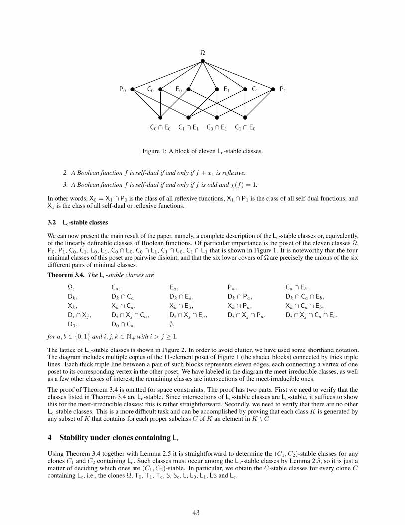
Ω

P0 C0 E0 E1 C1 P1

C0 ∩ E0 C1 ∩ E1 C0 ∩ E1 C1 ∩ E0

Figure 1: A block of eleven Lc-stable classes.

2. A Boolean function f is self-dual if and only if f + x1 is reflexive.

3. A Boolean function f is self-dual if and only if f is odd and χ(f) = 1.

In other words, X0 = X1 ∩ P0 is the class of all reflexive functions, X1 ∩ P1 is the class of all self-dual functions, andX1 is the class of all self-dual or reflexive functions.

3.2 Lc-stable classes

We can now present the main result of the paper, namely, a complete description of the Lc-stable classes or, equivalently,of the linearly definable classes of Boolean functions. Of particular importance is the poset of the eleven classes Ω,P0, P1, C0, C1, E0, E1, C0 ∩ E0, C0 ∩ E1, C1 ∩ C0, C1 ∩ E1 that is shown in Figure 1. It is noteworthy that the fourminimal classes of this poset are pairwise disjoint, and that the six lower covers of Ω are precisely the unions of the sixdifferent pairs of minimal classes.

Theorem 3.4. The Lc-stable classes are

Ω, Ca, Ea, Pa, Ca ∩ Eb,

Dk, Dk ∩ Ca, Dk ∩ Ea, Dk ∩ Pa, Dk ∩ Ca ∩ Eb,

Xk, Xk ∩ Ca, Xk ∩ Ea, Xk ∩ Pa, Xk ∩ Ca ∩ Eb,

Di ∩ Xj , Di ∩ Xj ∩ Ca, Di ∩ Xj ∩ Ea, Di ∩ Xj ∩ Pa, Di ∩ Xj ∩ Ca ∩ Eb,

D0, D0 ∩ Ca, ∅,for a, b ∈ 0, 1 and i, j, k ∈ N+ with i > j ≥ 1.

The lattice of Lc-stable classes is shown in Figure 2. In order to avoid clutter, we have used some shorthand notation.The diagram includes multiple copies of the 11-element poset of Figure 1 (the shaded blocks) connected by thick triplelines. Each thick triple line between a pair of such blocks represents eleven edges, each connecting a vertex of oneposet to its corresponding vertex in the other poset. We have labeled in the diagram the meet-irreducible classes, as wellas a few other classes of interest; the remaining classes are intersections of the meet-irreducible ones.

The proof of Theorem 3.4 is omitted for space constraints. The proof has two parts. First we need to verify that theclasses listed in Theorem 3.4 are Lc-stable. Since intersections of Lc-stable classes are Lc-stable, it suffices to showthis for the meet-irreducible classes; this is rather straightforward. Secondly, we need to verify that there are no otherLc-stable classes. This is a more difficult task and can be accomplished by proving that each class K is generated byany subset of K that contains for each proper subclass C of K an element in K \ C.

4 Stability under clones containing Lc

Using Theorem 3.4 together with Lemma 2.5 it is straightforward to determine the (C1, C2)-stable classes for anyclones C1 and C2 containing Lc. Such classes must occur among the Lc-stable classes by Lemma 2.5, so it is just amatter of deciding which ones are (C1, C2)-stable. In particular, we obtain the C-stable classes for every clone Ccontaining Lc, i.e., the clones Ω, T0, T1, Tc, S, Sc, L, L0, L1, LS and Lc.

43

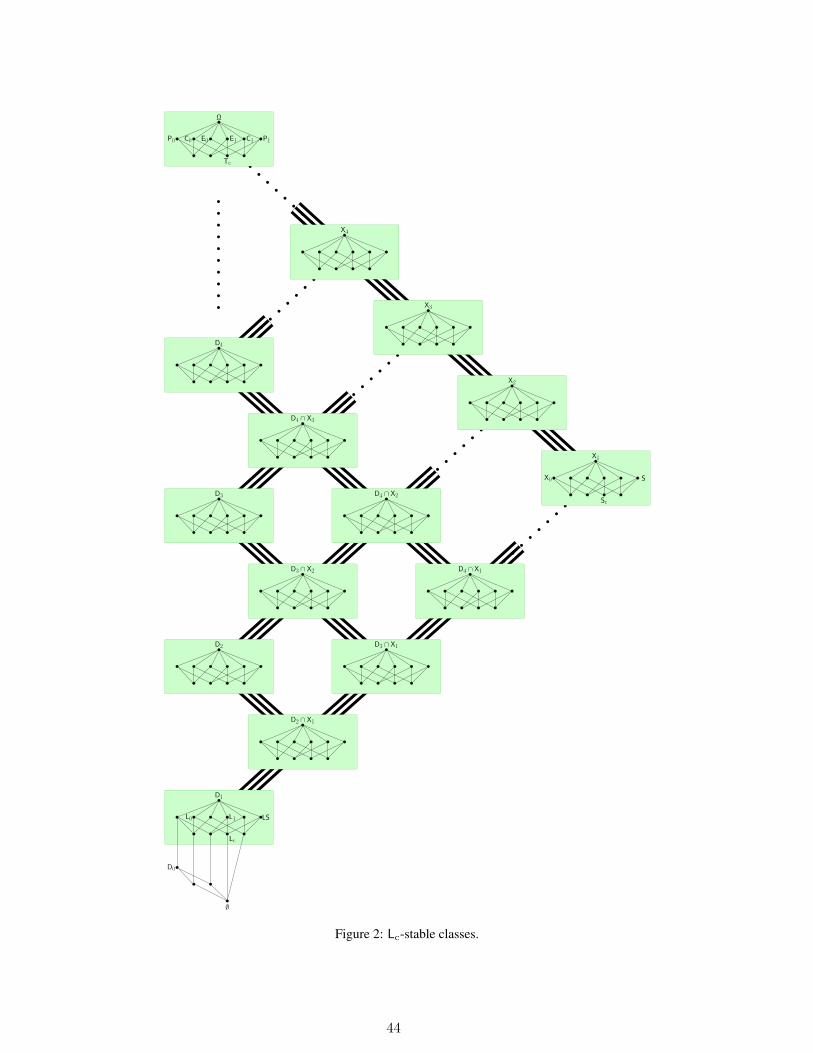
D1

D2 ∩ X1

D2 D3 ∩ X1

D3 ∩ X2

D3

D4 ∩ X1

D4 ∩ X2

D4 ∩ X3

D4

X1

X2

X3

X4

Ω

P0 C0 E0 E1 C1 P1

Tc

X0 S

Sc

L0 L1 LS

Lc

D0

∅

Figure 2: Lc-stable classes.

44

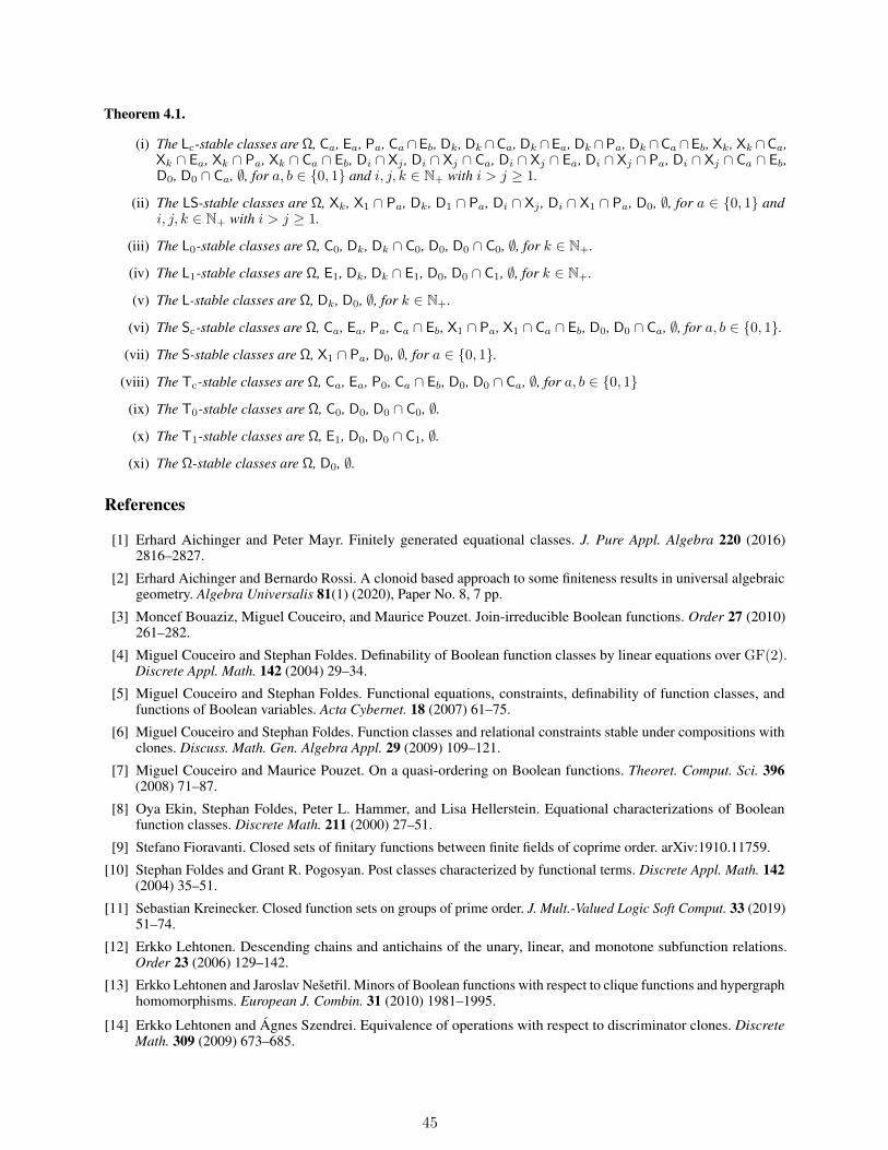
Theorem 4.1.

(i) The Lc-stable classes are Ω, Ca, Ea, Pa, Ca ∩Eb, Dk, Dk ∩Ca, Dk ∩Ea, Dk ∩Pa, Dk ∩Ca ∩Eb, Xk, Xk ∩Ca,Xk ∩ Ea, Xk ∩ Pa, Xk ∩ Ca ∩ Eb, Di ∩ Xj , Di ∩ Xj ∩ Ca, Di ∩ Xj ∩ Ea, Di ∩ Xj ∩ Pa, Di ∩ Xj ∩ Ca ∩ Eb,D0, D0 ∩ Ca, ∅, for a, b ∈ 0, 1 and i, j, k ∈ N+ with i > j ≥ 1.

(ii) The LS-stable classes are Ω, Xk, X1 ∩ Pa, Dk, D1 ∩ Pa, Di ∩ Xj , Di ∩ X1 ∩ Pa, D0, ∅, for a ∈ 0, 1 andi, j, k ∈ N+ with i > j ≥ 1.

(iii) The L0-stable classes are Ω, C0, Dk, Dk ∩ C0, D0, D0 ∩ C0, ∅, for k ∈ N+.

(iv) The L1-stable classes are Ω, E1, Dk, Dk ∩ E1, D0, D0 ∩ C1, ∅, for k ∈ N+.

(v) The L-stable classes are Ω, Dk, D0, ∅, for k ∈ N+.

(vi) The Sc-stable classes are Ω, Ca, Ea, Pa, Ca ∩ Eb, X1 ∩ Pa, X1 ∩ Ca ∩ Eb, D0, D0 ∩ Ca, ∅, for a, b ∈ 0, 1.(vii) The S-stable classes are Ω, X1 ∩ Pa, D0, ∅, for a ∈ 0, 1.

(viii) The Tc-stable classes are Ω, Ca, Ea, P0, Ca ∩ Eb, D0, D0 ∩ Ca, ∅, for a, b ∈ 0, 1(ix) The T0-stable classes are Ω, C0, D0, D0 ∩ C0, ∅.(x) The T1-stable classes are Ω, E1, D0, D0 ∩ C1, ∅.

(xi) The Ω-stable classes are Ω, D0, ∅.

References

[1] Erhard Aichinger and Peter Mayr. Finitely generated equational classes. J. Pure Appl. Algebra 220 (2016)2816–2827.

[2] Erhard Aichinger and Bernardo Rossi. A clonoid based approach to some finiteness results in universal algebraicgeometry. Algebra Universalis 81(1) (2020), Paper No. 8, 7 pp.

[3] Moncef Bouaziz, Miguel Couceiro, and Maurice Pouzet. Join-irreducible Boolean functions. Order 27 (2010)261–282.

[4] Miguel Couceiro and Stephan Foldes. Definability of Boolean function classes by linear equations over GF(2).Discrete Appl. Math. 142 (2004) 29–34.

[5] Miguel Couceiro and Stephan Foldes. Functional equations, constraints, definability of function classes, andfunctions of Boolean variables. Acta Cybernet. 18 (2007) 61–75.

[6] Miguel Couceiro and Stephan Foldes. Function classes and relational constraints stable under compositions withclones. Discuss. Math. Gen. Algebra Appl. 29 (2009) 109–121.

[7] Miguel Couceiro and Maurice Pouzet. On a quasi-ordering on Boolean functions. Theoret. Comput. Sci. 396(2008) 71–87.

[8] Oya Ekin, Stephan Foldes, Peter L. Hammer, and Lisa Hellerstein. Equational characterizations of Booleanfunction classes. Discrete Math. 211 (2000) 27–51.

[9] Stefano Fioravanti. Closed sets of finitary functions between finite fields of coprime order. arXiv:1910.11759.

[10] Stephan Foldes and Grant R. Pogosyan. Post classes characterized by functional terms. Discrete Appl. Math. 142(2004) 35–51.

[11] Sebastian Kreinecker. Closed function sets on groups of prime order. J. Mult.-Valued Logic Soft Comput. 33 (2019)51–74.

[12] Erkko Lehtonen. Descending chains and antichains of the unary, linear, and monotone subfunction relations.Order 23 (2006) 129–142.

[13] Erkko Lehtonen and Jaroslav Nešetril. Minors of Boolean functions with respect to clique functions and hypergraphhomomorphisms. European J. Combin. 31 (2010) 1981–1995.

[14] Erkko Lehtonen and Ágnes Szendrei. Equivalence of operations with respect to discriminator clones. DiscreteMath. 309 (2009) 673–685.

45

[15] Erkko Lehtonen and Ágnes Szendrei. The submaximal clones on the three-element set with finitely many relativeR-classes. Discuss. Math. Gen. Algebra Appl. 30 (2010) 7–33.

[16] Erkko Lehtonen and Ágnes Szendrei. Clones with finitely many relativeR-classes. Algebra Universalis 65 (2011)109–159.

[17] Erkko Lehtonen and Ágnes Szendrei. Partial orders induced by quasilinear clones. In Contributions to GeneralAlgebra 20, Proceedings of the Salzburg Conference 2011 (AAA81), pages 51–84. Verlag Johannes Heyn,Klagenfurt, 2012.

[18] Nicholas Pippenger. Galois theory for minors of finite functions. Discrete Math. 254 (2002) 405–419.[19] Emil L. Post. The Two-Valued Iterative Systems of Mathematical Logic. Annals of Mathematics Studies, no. 5.

Princeton University Press, Princeton, 1941.[20] Svetlana N. Selezneva and Anton V. Bukhman. Polynomial-time algorithms for checking some properties of

Boolean functions given by polynomials. Theory Comput. Syst. 58 (2016) 383–391.[21] Athena Sparks. On the number of clonoids. Algebra Universalis 80(4) (2019), Paper No. 53, 10 pp.

46

COMBINATORIAL INTERPRETATION OF BIsNOMIALCOEFFICIENTS AND GENERALIZED CATALAN NUMBERS

Hacène BelbachirFaculty of Mathematics

USTHB, RECITS Laboratory, CATI TeamB.P. 32, El Alia, 16111, Bab Ezzouar, Algeria.

[email protected]

Oussama IgueroufaFaculty of Mathematics

USTHB, RECITS Laboratory, CATI TeamB.P. 32, El Alia, 16111, Bab Ezzouar, Algeria.

[email protected]

ABSTRACT

We provide a combinatorial interpretation of bisnomial coefficients, by using paths that lie on hyper-grids. We also give a generalization of Catalan numbers, called as s-Catalan, through using s-Pascaltriangle. Two identities of s-Catalan numbers are derived.

Keywords Bisnomial coefficients · s-Pascal triangle · Generalized Pascal Formula · Hypergrids · s-Catalan numbers.

1 Introduction

Bisnomial coefficients were introduced for the first time in 1730, by Abraham de Moivre [7], in his study to answer tothe following question: "Considering L dices with (s+ 1) numbered faces. If they are thrown randomly, what wouldbe the chance of the sum of exhibited numbers to be equal to k ?", see also Hall and Knight [16]. Some years later,Euler [8, 9], studied these coefficients and derived a number of properties, as formulae (4), (6) below. In 1876, André[1] used combinations on words to establish several other properties.

Recently, the authors [3], published a paper that focused on a historical introduction of bisnomial coefficient, as wellas a presentation of some new arithmetical properties of these numbers. First, we need to introduce some definitionsand concepts concerning bisnomial coefficients, s-Pascal triangle and Catalan numbers.

1.1 Bisnomial Coefficients

Definition 1.1 Let s ≥ 1, n ≥ 0 be integers and let k ∈ 0, 1, . . . , sn. The bisnomial coefficient denoted by(nk

)s, is

the coefficient of xk in the following development

(1 + x+ x2 + · · ·+ xs)n =∑

k≥0

(n

k

)

s

xk. (1)

For k < 0 or k > sn, we have,(nk

)s= 0. For s = 1, we get the classical binomial coefficient

(nk

)1=(nk

). In the

literature of bisnomial coefficients, we often meet the following well known properties

• Expression of bisnomial coefficients in terms of binomial coefficients,(n

k

)

s

=∑

j1+j2+···+js=k

(n

j1

)(j1j2

)· · ·(js−1js

). (2)

• de Moivre alternate summation,(n

k

)

s

=

bk/(s+1)c∑

j=0

(−1)j(n

j

)(k − j(s+ 1) + n− 1

n− 1

). (3)

47

• Symmetry relation, (n

k

)

s

=

(n

sn− k

)

s

. (4)

• Generalized Pascal Formula, (n

k

)

s

=s∑

m=0

(n− 1

k −m

)

s

. (5)

• Diagonal recurrence relation, (n

k

)

s

=

n∑

m=0

(n

m

)(m

k −m

)

s−1. (6)

By definition, Pascal triangle is the triangular array of binomial coefficients, where each of their elements is calculatedby using Pascal Formula,

(nk

)=(n−1k

)+(n−1k−1). We consider a generalization of Pascal triangle denoted by s-Pascal

triangle, as the array of bisnomial coefficients that are generated by using Relation (5). For example, Table 1, gives the3-Pascal triangle in the left justified form. We find the first values of bisnomial coefficients in SLOANE [22], throughusing the codes A027907, A008287 and A053343, for, s = 2, s = 3 and s = 4, respectively.

Table 1: Triangle of bi3nomial coefficients(nk

)3.

n\k 0 1 2 3 4 5 6 7 8 9 10 11 120 11 1 1 1 12 1 2 3 4 3 2 1 03 1 3 6 10 12 12 10 6 3 14 1 4 10 20 31 40 44 40 31 20 10 4 1

1.2 Catalan Numbers

For a well introduction to Catalan numbers, their properties and combinatorial interpretations, the reader can refer toStanley [23], Kochy [19]. Catalan numbers, named after the Belgian mathematician Eugène Charles Catalan (1814-1894), are defined as follows,

Cn =1

n+ 1

(2n

n

), n ∈ Z+. (7)

The generating function of these numbers is,

C(x) =∑

n

Cnxn =

1−√1− 4x

2x. (8)

Catalan numbers are given in Sloane [22], by using the code A000108, the first elements are,

1, 1, 2, 5, 14, 42, 132, 429, 1430, 4862, 16796, 58786, 208012, . . . .

These numbers could be generated by subtracting the mentioned columns of Pascal triangle, as given in Table 2. Thispermit us to get the three Formulae, (9), (10), (11).

Cn =

(2n

n

)−(

2n

n+ 1

), n ≥ 0. (9)

Cn =

(2n− 1

n

)−(2n− 1

n+ 1

), n ≥ 1. (10)

Cn+1 =

(2n

n

)−(

2n

n+ 2

), n ≥ 0. (11)

In the following section, we give combinatorial interpretations of both bisnomial coefficients and generalized PascalFormula, through using oriented paths that moving on Hypergrids.

48

Table 2: Right part of Pascal triangle.

11

2 13 1

6 4 110 5 1

20 15 6 135 21 7 1

70 56 28 8 1...

......

......(

2nn

) (2n−1

n

) (2nn+1

) (2n−1n+1

) (2nn+2

)

2 Combinatorial interpretation of bisnomial coefficients

Freund [10], gave a combinatorial interpretation of bisnomial coefficients(nk

)s, as the number of different ways of

distributing k objects among n cells, where each cell contains at most s objects, see also, Bondarenko [4]. Recently,A. Bazeniar et al., [2], provided an interpretation of these numbers, as the number of lattice paths that connect the twopoints of a grid, (0, 0) and (k, n− 1), for 0 ≤ k ≤ sn, by taking at most s vertices in the eastern direction. We beginby giving some definitions and terminologies that we need in the rest of this paper.

2.1 Definitions and Notations

We denote by Hn,s, an hypergrid of dimension n, (we consider n ordered directions), such that each axis containss vertices without counting the vertex of origin O. As particular cases, for s = 1 and n ≥ 4, hypergrids are calledhypercubes, whereas, for n = 2 and s ≥ 2, we talk about grids.

Definition 2.1 Let n, s, p ∈ Z+, i ∈ 1, 2, . . . , n. An up-oriented path lying on the hypergrid Hn,s, is a path of afinite length, such that

1. it starts from the vertex O,

2. when the path reaches the vertex U by taking the ith direction, it should reach a vertex V by taking the (i+p)thdirection.

We denote by pi1,i2,...,in , an up-oriented path lying on the hypergrid Hn,s, that reached,

• i1 vertices by taking the 1st direction,• i2 vertices by taking the 2nd direction,

•...

• in vertices by taking the nth direction,

with 0 ≤ im ≤ s, for m ∈ 1, 2, . . . , n.We represent the up-oriented path pi1,i2,...,in by the linear form,

11 · · · 1︸︷︷︸i1 times

22 · · · 2︸︷︷︸i2 times

· · ·nn · · ·n︸︷︷︸in times

,

or by the power form, 1i12i2 · · ·nin . We denote by the number k, the length of pi1,i2,...,in , such that k = i1 + i2 +· · ·+ in, as well as Pn,k,s the set of all pi1,i2,...,in of length k that lie on the hypergrid Hn,s.

Example 2.1 In Figure 1, we differentiate an up-oriented path from ordinary paths that lie on the grid H2,3, asfollows,

• The first path on the left is an up-oriented path because the directions are taken in an increasing order, then,we have, p3,1 = 1112 = 1321.

49

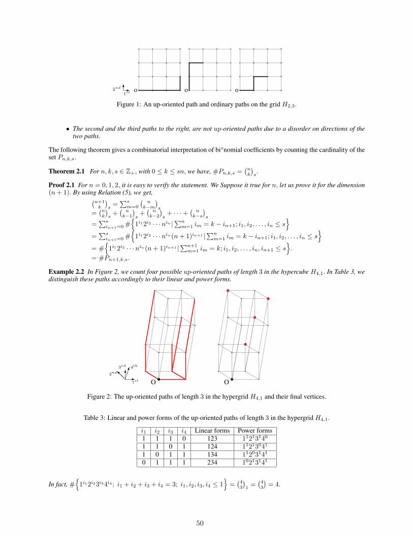
-61st

2nd o o o

Figure 1: An up-oriented path and ordinary paths on the grid H2,3.

• The second and the third paths to the right, are not up-oriented paths due to a disorder on directions of thetwo paths.

The following theorem gives a combinatorial interpretation of bisnomial coefficients by counting the cardinality of theset Pn,k,s.

Theorem 2.1 For n, k, s ∈ Z+, with 0 ≤ k ≤ sn, we have, #Pn,k,s =(nk

)s.

Proof 2.1 For n = 0, 1, 2, it is easy to verify the statement. We Suppose it true for n, let us prove it for the dimension(n+ 1). By using Relation (5), we get,

(n+1k

)s=∑s

m=0

(n

k−m)s

=(nk

)s+(

nk−1)s+(

nk−2)s+ · · ·+

(n

k−s)s

=∑s

in+1=0 #1i12i2 · · ·nin |∑n

m=1 im = k − in+1; i1, i2, . . . , in ≤ s

=∑s

in+1=0 #1i12i2 · · ·nin(n+ 1)in+1 |∑n

m=1 im = k − in+1; i1, i2, . . . , in ≤ s

= #1i12i2 · · ·nin(n+ 1)in+1 |∑n+1

m=1 im = k; i1, i2, . . . , in, in+1 ≤ s.

= #Pn+1,k,s.

Example 2.2 In Figure 2, we count four possible up-oriented paths of length 3 in the hypercube H4,1. In Table 3, wedistinguish these paths accordingly to their linear and power forms.

-@@I6

1st

2nd

3rd 4th

Os

O

s

s

ss

sFigure 2: The up-oriented paths of length 3 in the hypergrid H4,1 and their final vertices.

Table 3: Linear and power forms of the up-oriented paths of length 3 in the hypergrid H4,1.

i1 i2 i3 i4 Linear forms Power forms1 1 1 0 123 11213140

1 1 0 1 124 11213041

1 0 1 1 134 11203141

0 1 1 1 234 10213141

In fact, #1i12i23i34i4 ; i1 + i2 + i3 + i4 = 3; i1, i2, i3, i4 ≤ 1

=(43

)1=(43

)= 4.

50

In the following subsection, by using Theorem 2.1, we derive a combinatorial interpretation of generalized PascalFormula over hypergrids.

2.2 Combinatorial interpretation of generalized Pascal Formula

Definition 2.2 We denote by Jn−1, the projection map on the hypergrid Hn−1,s, defined as,

Jn−1 : Pn,k,s → ⋃sm=0 Pn−1,k−m,s

pi1,i2,...,in 7→ pi1,i2,...,in−1

Theorem 2.2 The generalized Pascal Formula,(nk

)s=∑s

m=0

(n−1k−m

)s, can be interpreted over hypergrids by the

following bijection, Pn,k,sJn−1∼

⋃sm=0 Pn−1,k−m,s.

Proof 2.2 Obviously, the map Jn−1 is surjective by definition, so, Jn−1(Pn,k,s) =⋃s

m=0 Pn−1,k−m,s. On one hand,by Theorem 2.1, we have, #Pn,k,s =

(nk

)s.On the other hand, for allm1,m2 ∈ 0, 1, . . . , s, such thatm1 6= m2, it is

clear that, Pn−1,k−m1,s

⋂Pn−1,k−m2,s = ∅, so, #Jn−1(Pn,k,s) = #

⋃sm=0 Pn−1,k−m,s =

∑sm=0 #Pn−1,k−m,s =∑s

m=0

(n−1k−m

)s=(nk

)s. Consequently, we have proved that the two sets Pn,k,s and

⋃sm=0 Pn−1,k−m,s, have the same

cardinality, then, they are in bijection.

Example 2.3 For n = 4, k = 6, s = 3, the generalized Pascal Formula,(46

)3=∑3

m=0

(3

6−m)3= 10+12+12+10,

is interpreted over hypergrids by the following bijection, P4,6,3J3∼ P3,6,3 ∪ P3,5,3 ∪ P3,4,3 ∪ P3,3,3, see Table 4,

Table 4: The bijection P4,6,3J3∼⋃3

m=0 P3,6−m,3.

P4,6,3 P3,6,3 P4,6,3 P3,5,3 P4,6,3 P3,4,3 P4,6,3 P3,3,3

111222 111222 111234 11123 111244 1112 111444 111111223 111223 222334 22233 123344 1233 222444 222112223 112223 111334 11133 112344 1123 333444 333111233 111233 112234 11223 223344 2233 233444 233111333 111333 112334 11233 122344 1223 133444 133222333 222333 122234 12223 112244 1122 123444 123122233 122233 113334 11333 113344 1133 223444 223122333 122333 112224 11222 233344 2333 122444 122112333 112333 123334 12333 122244 1222 112444 112112233 112233 223334 22333 133344 1333 113444 113

122334 12233 222344 2223111224 11122 111344 1113

3 Generalized Catalan numbers

In this section, our aim is to generalize Catalan numbers by using s-Pascal triangle, as well as to extend their identitiescorresponding to this generalization. First, we recall some generalizations of Catalan numbers.

Stanley, [23], Koshy, [19] and Grimaldi, [15], collect many combinatorial interpretations of Catalan numbers throughusing: paths, parenthesis, words or binary numbers, binary trees, . . . . In 1791, before Eugène Charles Catalan studiedthese numbers, Fuss, [11], introduced Fuss-numbers, given under many expressions, as, F (k, n) = 1

(k−1)n+1

(knn

), see

[14], or, F (k, n) = 1kn+1

(kn+1

n

), see [19], also as follows, F (k, n) = 1

n

(knn−1), see, [15, 17]. We mention that, for

k = 2, F (2, n) gives the Catalan numbers. A combinatorial interpretation of these numbers is given as the number ofpaths from (0, 0) to (n, (k− 1)n), which take steps of the set (0, 1), (1, 0), that lie below the line y = (k− 1)x, see[20].

Raney numbers, [21], are defined as R(k, r, n) = rkn+r

(kn+r

n

), this is a generalization of Fuss-numbers, as we have,

R(k, 1, n) = F (k, n). R(k, r, n) counts the forests composed by r ordered rooted trees, with k components and nvertices, see [23].

51

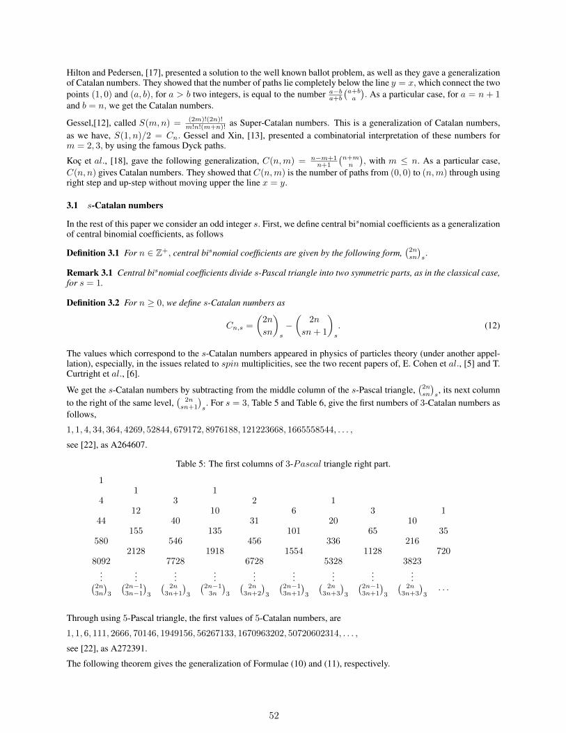
Hilton and Pedersen, [17], presented a solution to the well known ballot problem, as well as they gave a generalizationof Catalan numbers. They showed that the number of paths lie completely below the line y = x,which connect the twopoints (1, 0) and (a, b), for a > b two integers, is equal to the number a−b

a+b

(a+ba

). As a particular case, for a = n + 1

and b = n, we get the Catalan numbers.

Gessel,[12], called S(m,n) = (2m)!(2n)!m!n!(m+n)! as Super-Catalan numbers. This is a generalization of Catalan numbers,

as we have, S(1, n)/2 = Cn. Gessel and Xin, [13], presented a combinatorial interpretation of these numbers form = 2, 3, by using the famous Dyck paths.

Koç et al., [18], gave the following generalization, C(n,m) = n−m+1n+1

(n+mn

), with m ≤ n. As a particular case,

C(n, n) gives Catalan numbers. They showed that C(n,m) is the number of paths from (0, 0) to (n,m) through usingright step and up-step without moving upper the line x = y.

3.1 s-Catalan numbers

In the rest of this paper we consider an odd integer s. First, we define central bisnomial coefficients as a generalizationof central binomial coefficients, as follows

Definition 3.1 For n ∈ Z+, central bisnomial coefficients are given by the following form,(2nsn

)s.

Remark 3.1 Central bisnomial coefficients divide s-Pascal triangle into two symmetric parts, as in the classical case,for s = 1.

Definition 3.2 For n ≥ 0, we define s-Catalan numbers as

Cn,s =

(2n

sn

)

s

−(

2n

sn+ 1

)

s

. (12)

The values which correspond to the s-Catalan numbers appeared in physics of particles theory (under another appel-lation), especially, in the issues related to spin multiplicities, see the two recent papers of, E. Cohen et al., [5] and T.Curtright et al., [6].

We get the s-Catalan numbers by subtracting from the middle column of the s-Pascal triangle,(2nsn

)s, its next column

to the right of the same level,(

2nsn+1

)s. For s = 3, Table 5 and Table 6, give the first numbers of 3-Catalan numbers as

follows,

1, 1, 4, 34, 364, 4269, 52844, 679172, 8976188, 121223668, 1665558544, . . . ,

see [22], as A264607.

Table 5: The first columns of 3-Pascal triangle right part.

11 1

4 3 2 112 10 6 3 1

44 40 31 20 10155 135 101 65 35

580 546 456 336 2162128 1918 1554 1128 720

8092 7728 6728 5328 3823...

......

......

......

......(

2n3n

)3

(2n−13n−1

)3

(2n

3n+1

)3

(2n−13n

)3

(2n

3n+2

)3

(2n−13n+1

)3

(2n

3n+3

)3

(2n−13n+1

)3

(2n

3n+3

)3· · ·

Through using 5-Pascal triangle, the first values of 5-Catalan numbers, are

1, 1, 6, 111, 2666, 70146, 1949156, 56267133, 1670963202, 50720602314, . . . ,

see [22], as A272391.

The following theorem gives the generalization of Formulae (10) and (11), respectively.

52

Table 6: Generating of 3-Catalan numbers by definition.

n(2n3n

)3

(2n

3n+1

)3

Cn,3 =(2n3n

)3−(

2n3n+1

)3

0 1 0 11 4 3 12 44 40 43 580 546 344 8092 7728 3645 116304 112035 42696 1703636 1650792 528447 25288120 24608948 6791728 379061020 370084832 89761889 5724954544 5603730876 12122366810 86981744944 85316186400 1665558544

Theorem 3.1 We have,

Cn,s =

(2n− 1

sn

)

s

−(2n− 1

sn+ 1

)

s

, n ≥ 1. (13)

Cn+1,s =

(2n

sn

)

s

−(

2n

sn+ (s+ 1)

)

s

, n ≥ 0. (14)

Proof 3.1 By using Formula (5), we get, Cn,s =(2nsn

)s−(

2nsn+1

)s=∑s

m=0

(2n−1sn−m

)s− ∑s

m=0

(2n−1

sn+1−m)s=(

2n−1sn−s

)s−(2n−1sn+1

)s. Formula (4) gives,

(2n−1sn−s

)s=(2n−1sn

)s, then we find, Cn,s =

(2n−1sn

)s−(2n−1sn+1

)s.

To get Formula (14), first we calculate Cn+1,s, by using Formula (12), then we follow the same proof of Formula (13),by applying Formula (5) twice.

As a future work, we want to find a combinatorial interpretation of s-Catalan numbers, especially, by using up-orientedpaths on hypergrids.

References

[1] D. André. Mémoire sur les combinaisons régulière et leurs applications, Annales scientifique de l’ENS. 2eme série,tome 5, pages 155–198, 1876.

[2] A. Bazeniar, M. Ahmia, H. Belbachir. Connection between bisnomial coefficients and their analogs and symmetricfunctions. Turkish Journal of Mathematics, 42, pages 807–818, doi: 10.3906/ mat-1705-27, 2018.

[3] H. Belbachir, O. Igueroufa. Congruence properties for bisnomial coefficients and like extended Ramand Kummer theorems under suitable hypothesis. Mediterranean Journal of Mathematics, 17:36,https://doi.org/10.1007/s00009-019-1457-0, 2020.

[4] B. Bondarenko. Generalized Pascal triangle and Pyramids, their fractals graphs and applications. The FibonacciAssociation, Santa Clara, 1993.

[5] E. Cohen, T. Hansen, N. Itzhanki. From entanglement witness to generalized Catalan numbers. Scientific Reports,6:30232, doi:10.1038/srep30232, 2016.

[6] T. Curtright, T. V. Kortryk, C. Zachos. Spin Multiplicities. Physics letter A. Elsevier, 381, pages 422–427, 2017.[7] A. de Moivre. The Doctrine of Chances, 3rd ed. London: Millar, 1756, rpt. New York: Chelsea, 1967.[8] L. Euler. De evolutione potestatis polynomialis cuiuscunque (1+x+x2+· · · )n. Nova Acta Academiae Scientarum

Imperialis Petropolitinae 12, 1801, 47-57; Opera Omnia: Series 1, Volume 16, 28–40. Original copy is availableonline in Euler’s archive.

[9] L. Euler. Observationes analyticae, Novi Commentarii Academiae Scientarum Petropolitanae. 11, 1767, 124–143,Opera Omnia, Series 1 Vol. 15, 50–69. Original copy is available online in Euler’s archive.

[10] J. E. Freund. Restricted Occupancy Theory A Generalization of Pascal’s Triangle. The American MathematicalMonthly, 63, No. 1, pages 20–27, 1956.

53

[11] N. Fuss. Solutio quaestionis, quot modis polygonum n laterum in polygona m laterum, per diagonales resolviquaeat. Nova acta academiae scientiarum imperialis Petropolitanae, 9, p. 243–251, 1791.

[12] I. M. Gessel. Super ballot numbers. Journal of Symbolic Computation. Elsevier, 14, pages 179–194, 1992.[13] I. M. Gessel, G. Xin. A combinatorial interpretation of the numbers 6(2n)!n!(n + 2)!. Journal of Integer Se-

quences, 8, article 05.2.3, 2005.[14] R. L. Graham, D. E. Knuth, O. Patashnik. Concrete Mathematics. Addison-Wesley, Boston, 1994.[15] R. P. Grimaldi. Fibonacci and Catalan numbers An introduction. Wiley, 2012.[16] H. S. Hall, S. R. Knight. Higher Algebra: a Sequel to Elementary Algebra for Schools. London : Macmillan and

Co, 1894.[17] P. Hilton, J. Pedersen. Catalan numbers, their generalization, and their uses. The Mathematical Intelligencer, 13,

pages 64–75, 1991.[18] C. Koç, I. Güloglu, S. Esin. Generalized Catalan number, sequences and polynomials. Turkish Journal of Math-

ematics, 34, pages 441–449, 2010.[19] T. Koshy. Catalan Numbers with Applications. Oxford University Press, 2009.[20] C.H. Lin. Some Combinatorial Interpretations and Applications of Fuss-Catalan Numbers. International Schol-

arly Research Network ISRN Discrete Mathematics, article ID 534628, doi:10.5402/2011/534628, 2011.[21] G. N. Raney. Functional composition patterns and power series reversion. American Mathematical Society, 94,

No 3, pages 441–451, 1960.[22] Sloane. The On-Line Encyclopedia of Integer Sequences. Available on line at https://oeis.org/.[23] R. P. Stanley. Catalan numbers. Cambridge University Press, 2015.

54

GRAPHS CONTAINING FINITE INDUCED PATHS OF UNBOUNDEDLENGTH

Maurice PouzetUniv. Lyon, Université Claude-Bernard Lyon1

CNRS UMR 5208, Institut Camille Jordan43, Bd. du 11 Novembre 1918, 69622

Villeurbanne, Franceet

Department of Mathematics and StatisticsUniversity of Calgary, Calgary, Alberta, Canada

[email protected]

Imed Zaguia*∗Department of Mathematics & Computer Science

Royal Military College of CanadaP.O.Box 17000, Station Forces

Kingston, Ontario, Canada K7K 7B4 [email protected]

ABSTRACT

The age A(G) of a graph G (undirected and without loops) is the collection of finite inducedsubgraphs of G, considered up to isomorphy and ordered by embeddability. It is well-quasi-ordered(wqo) for this order if it contains no infinite antichain. A graph is path-minimal if it contains finiteinduced paths of unbounded length and every induced subgraph G′ with the same property admits anembedding of G. We construct 2ℵ0 path-minimal graphs whose ages are pairwise incomparable withset inclusion and which are wqo. Our construction is based on uniformly recurrent sequences andlexicographical sums of labeled graphs.

Keywords (partially) ordered set · incomparability graph · graphical distance · isometric subgraph · paths · well quasiorder · symbolic dynamic · sturmian words · uniformly recurrent sequences

1 Introduction and presentation of the results

We consider graphs that are undirected, simple and have no loops. Let H = (X,F ) be a graph and let (Gx =(Vx, Ex))x∈X be a family of graphs whose vertex sets are pairwise disjoint. The lexicographical sum of (Gx)x∈X(over the graph H) is the graph H[Gx, x ∈ X] whose vertex set is ∪x∈XVx and two vertices ux and vx′ are adjacent ifx = x′ and ux, vx ∈ Ex or x 6= x′ and x, x′ ∈ F . If H is empty i.e. F = ∅, the lexicographical sum is called adirect sum. Else if H is a complete graph, then the lexicographical sum is called the complete sum.

Among those graphs with finite induced paths of unbounded length, we ask which one are unavoidable. If a graph is aninfinite path, it can be avoided: it contains a direct sum of finite paths of unbounded length. This latter one, on the otherhand, cannot be avoided. Indeed, two direct sums of finite paths of unbounded length embed in each other. Similarly,two complete sums of finite paths of unbounded length embed in each other. Hence, the direct sum, respectively thecomplete sum of finite paths of unbounded length are, in our sense, unavoidable. Are there other examples? Thisquestion is the motivation behind this article.

We recall that the age of a graph G is the collection Age(G) of finite induced subgraphs of G, considered up toisomorphy and ordered by embeddability (cf. [7]). It is well-quasi-ordered (wqo) for this order if it contains no infiniteantichain. A path is a graph P such that there exists a one-to-one map f from the set V (P ) of its vertices into aninterval I of the chain Z of integers in such a way that u, v belongs to E(P ), the set of edges of P , if and only if|f(u)− f(v)| = 1 for every u, v ∈ V (P ). If I = 1, . . . , n, then we denote that path by Pn; its length is n− 1, so,if n = 2, P2 is made of a single edge, whereas if n = 1, P1 is a single vertex. We denote by P∞ the path on N. Thedetour of a graph G [4] is the supremum of the length of induced paths included in G. Our aim is to give a structural

∗Corresponding author. Supported by Canadian Defence Academy Research Program (CDARP) and NSERC DDG-2018-00011.

55

result on graphs with infinite detour (for the existence of infinite paths we refer to [14, 19, 27]. We say that a graph G ispath-minimal if its detour is infinite end every induced subgraph G′ with infinite detour embeds admits an embeddingof G. Let ⊕nPn respectively

∑n Pn be the direct sum, respectively the complete sum of paths Pn. These graphs are

path-minimal graphs. There are others. Our main result is this.

Theorem 1 There are 2ℵ0 path-minimal graphs whose ages are pairwise incomparable and wqo.

Our construction uses uniformly recurrent sequences, and in fact Sturmian sequences (or billiard sequences) [17, 6],and lexicographical sums of labelled graphs. The existence of 2ℵ0 wqo ages is a non trivial fact. It was obtained forbinary relations in [21] and for undirected graphs in [24] and in [25]. The proofs were based on uniformly recurrentsequences. These sequences were also used in [15].

We leave open the following:

Problems 1 [(i)]

If a graph admits an embedding of finite induced path of unbounded length, does it embed a path-minimalgraph?

1.2. If a graph is path-minimal, is its age wqo?

3. If a graph G is path-minimal, can G be equipped with an equivalence relation ≡ whose blocks are paths insuch a way that (G,≡) is path-minimal?

In some situations there are only two path-minimal graphs (up to equimorphy).

Theorem 2 If the incomparability graph of a poset admits an embedding of finite induced paths of unbounded length,then it admits an embedding of the direct sum or the complete sum of finite induced paths of unbounded length.

If G := (V,E) is a graph, and x, y are two vertices of G, we denote by dG(x, y) the length of the shortest pathjoining x and y if any, and dG(x, y) := +∞ otherwise. This defines a distance on V with values in the completionN+

:= N+ ∪ +∞ of non-negative integers. This distance is the graphic distance. If A is a subset of V , the graph G′induced by G on A is an isometric subgraph of G if dG′(x, y) = dG(x, y) for all x, y ∈ A.

If instead of induced path we consider isometric paths, then

Theorem 3 If a graph admits an embedding of isometric finite paths of unbounded length, then it admits an embeddingof a direct sum of such paths.

We examine the primality of the graphs we obtain. Prime (or indecomposable) graphs are the building blocks of theconstruction of graphs ([2, 8, 9, 11, 12, 23, 26]). Direct and complete sums of finite paths of unbounded length are notprime and not equimorphic to prime graphs. We construct 2ℵ0 examples, none of them being equimorphic to a primeone. We construct also 2ℵ0 which are prime. These examples are minimal in the sense of [22], but not in the sense of[23] nor in the sense of [18] p. 92.

We conclude this introduction with:

1.0.1 An outline of the proof of Theorem 1.

It uses two main ingredients. One is the so called uniformly recurrent sequences (or words).

A uniformly recurrent word with domain N is a sequence u := (u(n))n∈N of letters such that for any given integer nthere is some integer m(u, n) such that every factor v of u of length at most n appears as a factor of every factor of u oflength at least m(u, n). [1, 3, 16, 6]. To a uniformly recurrent word u on the alphabet 0, 1 we associate Pu, the pathon N with a loop at every vertex n for which u(n) = 1 and no loop at vertices for which u(n) = 0. Next comes thesecond ingredient.

Fix a binary operation ? on 0, 1. Define the lexicographical sum of copies of Pu over the chain ω, denoted by Pu ·? ω,and made of pairs (i, v) ∈ ω × Pu, with an edge between two vertices (i, n) and (j,m) of Puα ·? ω, such that i < j, ifu(n) ? u(m) = 1. Since u is uniformly recurrent, the set Fac(u) of finite factors of u is wqo w.r.t the factor ordering,hence by a theorem of Higman [10] (see also [20]), the ages of Pu and of G(u,?) := Pu ·? ω are wqo. Deleting theloops, we get a graph that we denote G(u,?) and whose age is also wqo. Let Q(u,?) be the restriction of G(u,?) to theset (m,n) : n < m+ 4 of V := N× N. This restriction has the same age as G(u,?) and it is path-minimal. If the

56

operation ? is constant and equal to 0, respectively equal to 1, Q(u,?) is a direct sum, respectively a complete sum ofpaths. To conclude the proof of the theorem, we need to prove that there is some operation ? and 2ℵ0 words u such thatthe ages of G(u,?) are incomparable. This is the substantial part of the proof. For that, we prove that if ? is the Booleansum or a projection and u is uniformly recurrent then every long enough path in G(u,?) is contained in some projection(subset of the form i × N). This is a rather technical fact. We think that it holds for any operation. We deduce that ifFac(u) and Fac(u′) are not equal up to reversal or to addition (mod 2) of the constant word 1 the ages of G(u,?) andG(u′,?) are incomparable w.r.t. set inclusion. To complete the proof of Theorem 1, we then use the fact that there are2ℵ0 uniformly recurrent words uα on the two-letter alphabet 0, 1 such that for α 6= β the collections Fac(uα) andFac(uβ) of their finite factors are distinct, and in fact incomparable with respect to set inclusion (this is a well-knownfact of symbolic dynamic, e.g. Sturmian words with different slopes will do [6], Chapter 6 page 143).

The proofs will appear in the full version of the paper.

References

[1] J-P. Allouche and J. Shallit, Automatic Sequences: Theory, Applications, Generalizations. Cambridge UniversityPress, 2003; ISBN: 0-521-82332-3

[2] R. Assous, M. Pouzet, Jónsson posets, Algebra Universalis, 79 (2018) no. 3, Art. 74, 26 pp.[3] V. Berthé and M. Rigo eds. Combinatorics, automata, and number theory. Encyclopedia of Mathematics and its

Applications. 135. 2010, Cambridge: Cambridge University Press. ISBN 978-0-521-51597-9.[4] F. Buckley and F. Harary, On longest induced paths in graphs. Chinese Quart. J. Math., 3 (3), (1968) 61–65.[5] A. Ehrenfeucht, T. Harju, G. Rozenberg, The theory of 2-structures. A framework for decomposition and

transformation of graphs. World Scientific Publishing Co., Inc., River Edge, NJ, 1999.[6] N. Pytheas Fogg, Substitutions in dynamics, arithmetics and combinatorics, Valérie Berthé, Sébastien Ferenczi,

Christian Mauduit and Anne Siegel, eds., Lecture Notes in Mathematics. 1794. Berlin: Springer-Verlag, 2002.[7] R. Fraïssé, Theory of relations. Revised edition. With an appendix by Norbert Sauer. Studies in Logic and the

Foundations of Mathematics, 145. North-Holland Publishing Co., Amsterdam, 2000. ii+451.[8] R. Fraïssé, L’intervalle en théorie des relations, ses généralisations, filtre intervallaires et clôture d’une relation,

In "Orders, description and roles", M. Pouzet and D. Richard(éd), Annals of Discrete Math., 23 (1984), 343–358.[9] T. Gallai, Transitiv orientierbare Graphen, Acta Math. Acad. Sci. Hungar., 18 (1967), 25–66 (English translation

by F. Maffray and M. Preissmann in J.J. Ramirez-Alfonsin and B. Reed (Eds), Perfect graphs, Wiley 2001, pp.25–66).

[10] G. Higman, Ordering by divisibility in abstract algebras. Proc. London Math. Soc. 3 (1952), 326–336.[11] P. Ille, A characterization of the indecomposable and infinite graphs, Glob. J. Pure Appl. Math., 3, (2005) 272–285.[12] D. Kelly, Comparability graphs, NATO Adv. Sci. Inst. Ser. C Math. Phys. Sci., 147 (1985), 3–40.[13] K. Kearnes, G. Oman, Jónsson posets and unary Jónsson algebras, Algebra Universalis 69 (2013), no. 2, 101–112.[14] D. Konig, Über eine Schlussweise aus dem Endlichen ins Unendliche, Acta Sci. Math. (Szeged) (in German)

(3(2-3)): (1927), 121–130.[15] C. Laflamme, M. Pouzet, N. Sauer, I. Zaguia, Orthogonal countable ordinals, Discrete Math. 335(2014) 35-44.[16] M. Lothaire, Finite and Infinite Words. In Algebraic Combinatorics on Words (Encyclopedia of Mathematics and

its Applications, pp. 1-44). Cambridge: Cambridge University Press, 2002. doi:10.1017/CBO9781107326019.002[17] M. Morse and G. A. Hedlund, Symbolic Dynamics II. Sturmian Trajectories. American Journal of Mathematics.

62 (1940): 1–42.[18] D. Oudrar, Sur l’énumération de structures discrètes: une approche par la théorie des relations. Thèse de doctorat,

Université d’Alger USTHB à Bab Ezzouar, 28 sept. 2015, ArXiv:1604.05839.[19] N. Polat, Graphs Without Isometric Rays and Invariant Subgraph Properties, I, Journal of Graph Theory, Volume

27, Issue 2, (1998), 99–109.[20] M. Pouzet, Un belordre d’abritement et ses rapports avec les bornes d’une multirelation. Comptes rendus Acad.

Sci. Paris 274(A) (1972), pp. 1677–1680.

[21] M. Pouzet, Sur la théorie des relations, Thèse de doctorat d’État, Université Claude-Bernard, Lyon, 23 Janvier1978.

57

[22] M. Pouzet, Relation minimale pour son âge, Zeitsch. f. math. Logik und Grundlag d. Math. Bd. 25, S. 315-344(1979).

[23] M. Pouzet and I. Zaguia, On Minimal Prime Graphs and Posets, Order 16 (2009), 357–375.[24] M. Sobrani, Structure d’ordre de la collection des âges de relations, Thèse de doctorat, Université Claude-Bernard,

Lyon, 18 déc. 1992.[25] M. Sobrani, Sur les âges de relations et quelques aspects homologiques des constructions D+M, Thèse de doctorat

d’état, Université S.M.Ben Abdallah-Fez, Fez, January 2002.[26] D.P. Sumner, Graphs indecomposable with respect to the X-join, Discrete Math., 6 (1973), 281–298.[27] M.E. Watkins, Infinite paths that contain only shortest paths, Journal of Combinatorial Theory, Series B Volume

41, Issue 3, December 1986, 341–355.

58

MONOTONIC COMPUTATION RULES FOR NONASSOCIATIVECALCULUS

Miguel CouceiroUniversite de Lorraine, CNRS, Inria N.G.E., LORIA


Michel GrabischParis School of Economics, University of Paris I106-112, Bd de l’Hopital, 75013 Paris, France

[email protected]


ABSTRACT

In this paper we revisit the so-called computation rules for calculus using a single nonassociativebinary operation over possibly infinite sequences of integers. In this paper we focus on the symmetricmaximum 6 that is an extension of the usual maximum ∨ so that 0 is the neutral element, and −x isthe symmetric (or inverse) of x, i.e., x6(−x) = 0. However, such an extension does not preservethe associativity of ∨. This fact asks for systematic ways of bracketing terms of a sequence using 6,and which we refer to as computation rules.These computation rules essentially reduce to deleting terms of sequences based on the conditionx6(−x) = 0, and they can be quasi-ordered as follows: say that rule 1 is below rule 2 if for allsequences of numbers, rule 1 deletes more terms in the sequence than rule 2. As it turns out, thisquasi-ordered set is extremely complex, e.g., it has infinitely many maximal elements and atoms, andit embeds the powerset of natural numbers by inclusion.Local properties of computation rules have also been presented by the authors, in particular, con-cerning their canonical representations. In this paper we address the problem of determining thosecomputation rules that preserve the monotonicity of ∨, and present an explicit description of mono-tonic computation rules in terms of their factorized irredundant form.

Keywords Nonassociative calculus · symmetric maximum · computation rules · monotonic rules

1 Motivation

This short contribution is the continuation of the work initiated in [1, 2], and we refer the reader to these referencesfor further motivation. Let L be a totally ordered set with bottom element 0, and let −L := −a : a ∈ L be its“symmetric” copy endowed with the reversed order. Consider the symmetric ordered structure L := L∪ (−L)\−0, abipolar scale analogous to the real line where the zero acts as a neutral element and such that a+ (−a) = 0 (symmetry).In particular, −(−a) = a.

The symmetric maximum 6 is intended to extend the maximum on L with 0 as neutral element, while fulfillingsymmetry. However, this symmetry requirement immediately entails that any extension 6 of the maximum operator∨ cannot be associative. To illustrate this point, let L = N and observe that (26 3)6(−3) = 36(−3) = 0 whereas26(36(−3)) = 26 0 = 2.

Nonetheless, Grabisch [3] showed that the “best” definition of 6 (see Theorem 1 below) is:

a6 b =

−(|a| ∨ |b|) if b 6= −a and |a| ∨ |b| = −a or = −b0 if b = −a|a| ∨ |b| otherwise.

(1)

In other words, if b 6= −a, then a6 b returns the element that is the larger in absolute value among the two elements aand b. Moreover, it is not difficult to see that 6 satisfies the following properties:

59

(C1) 6 coincides with the maximum on L2;

(C2) a6(−a) = 0 for every a ∈ L;

(C3) −(a6 b) = (−a)6(−b) for every a, b ∈ L.

Hence, 6 almost behaves like + on the real line, except for associativity a6(b6 c) = (a6 b)6 c, for every a, b, c ∈ L.For instance, we have:(−36 3)6 1 = 06 1 = 1 but −36(36 1) = −36 3 = 0. However, it was shown in [3] that ifone requires that (C1), (C2) and (C3) hold, then (1) is the best possible definition for 6.Theorem 1. [3, Prop. 5] No binary operation satisfying (C1), (C2), (C3) is associative on a larger domain than 6.

Further properties of 6 were presented in [3, 1, Prop. 5]. In particular, it was shown that 6 is associative on anexpression involving a1, . . . , an ∈ L, with |i : ai 6= 0| > 2, if and only if

∨ni=1 ai 6= −

∧ni=1 ai. Sequences

fulfilling this condition were referred to as associative in [1].

To remove the ambiguity when evaluating 6 on nonassociative sequences, Grabisch [3] suggested ways of making 6associative. The solution proposed was to define a rule of computation, that is, a systematic way of putting parenthesesso that the result is no longer ambiguous. Let us present here informally three of these rules1 that are rather natural:

(i) aggregate separately positive and negative terms, then compute their symmetric maximum. Taking the sequence3, 2,−3, 1,−3,−2, 1, we obtain

6(3, 2,−3, 1,−3,−2, 1) = (36 26 16 1)6((−3)6(−3)6(−2))= 36(−3) = 0.

(ii) aggregate first extremal opposite terms to cancel them, till there is no more extremal opposite terms. Thisgives:

6(3, 2,−3, 1,−3,−2, 1) = (36(−3))6(26 16(−3)6(−2)6 1)

= 06(−3) = −3.(iii) the same as above, but first aggregate these extremal opposite terms. This gives:

6(3, 2,−3, 1,−3,−2, 1) = (36((−3)6(−3)))6(26(−2))6(16 1)

= (36(−3))6 06 1 = 06 1 = 1.

One sees that all results differ, and that many other rules can be created. In fact, it is more convenient to define a rule asa systematic way of deleting terms in a sequence of numbers, so as to make it associative, provided the way of deletingterms corresponds to some arrangement of parentheses. Indeed, the first rule consists in deleting all terms wheneverthe sequence does not fulfill the condition of associativity. The second rule consists in deleting recursively all pairsof extremal opposite elements, and the third rule deletes recursively all occurrences of extremal opposite elements.However, one has to be careful that any systematic way of deleting elements making any sequence associative does notnecessarily correspond to an arrangement of parentheses. For example, deleting the maximal element 3 in the abovesequence makes it associative, however no arrangement of parentheses can produce this.

This framework based on rules of computation was formalized in [1], and we will recall it in the next section. Wewill also recall equivalent, yet semantically rather different, quasi-orderings of rules, and briefly survey the maincharacteristics of the resulting partially ordered set of (equivalent classes) of computation rules.

Denoting a computation rule by R, 6R is an unambiguously defined operator acting on any sequence of L, by firstmaking the sequence associative by means of R, and then computing the result by 6. Then, to any given computationrule R corresponds an aggregation operator 6R, aggregating all ”numbers” of a sequence into a single number in L.In the sequel, we only deal with countable sets L, so that L can be thought to be Z. It follows that such a study isrelated to the aggregation of integers, in particular to the so-called integer means or Z-means, see [4]. In the latterwork, it is shown that the decomposability property introduced by Kolmogoroff [5] imposes a very limitative form ofinteger means, namely that the output depends only on the smallest and greatest entries. In [2], we have weakened thedecomposability property and shown that a whole family of operators 6R can serve as integer means.

The main objective of this paper is to study monotonic computation rules R, that is, leading to an aggregation operator6R which is monotonically nondecreasing w.r.t. all terms of the sequence. This property is a basic requirement inmost fields of application, and this is why aggregation operators, defined on either real numbers or integers, are alwaysrequired to be nondecreasing (see, e.g., any kind of means, median, order statistics, etc.). As it will be shown, not allcomputation rules are monotonic. The main result of this paper, shown in Section 3, is to give a characterization of theset of monotonic computation rules.

1These will be revisited in Section 2 and formally defined in the proposed language formalism of [1].

60

2 Rules of Computation

We now recall the formalism of [1]. As we will only consider countable sequences of elements of L, without lossof generality, we may assume that L = Z. In this way, elements of L∗ are (finite) sequences of integers, denoted byσ = (λi)i∈I for some finite index set I , including the empty sequence ε, i.e.,

L∗ =( ⋃

n∈N(L)n

)∪ ε.

This convention will simplify our exposition and establish connections to the theory of integer means.

Also, as 6 is commutative, the order of symbols in the word does not matter, and we can consider the decreasing orderof the absolute values of the elements in the sequence (e.g., 5, 5,−5,−3, 2,−2, 1, 0). Since sequences are ordered, wecan consider the following convenient formalism for representing sequences. For an arbitrary sequence

σ = (n1, . . . , n1︸︷︷︸p1 times

,−n1, . . . ,−n1︸︷︷︸m1 times

, . . . , nq, . . . , nq︸︷︷︸pq times

,−nq, . . . ,−nq︸︷︷︸mq times

)

with n1 ≥ · · · ≥ nq , let θ(σ) = (n1, . . . , nq) be the sequence of absolute values (magnitudes) of integers in σ, and letψ(σ) = ((p1,m1), . . . , (pq,mq)) be the sequence of pairs of numbers of occurrence of these integers. For instance, ifσ = (3, 3,−3, 2,−2,−2, 1, 1, 1, 1), then

θ(σ) = (3, 2, 1); ψ(σ) = ((2, 1), (1, 2)(4, 0)).

Let S denote the set of all integer sequences in this formalism, including the empty sequence, and let S0 be the subsetof all nonassociative sequences.

To facilitate the precise definition of rules of computation, we proposed [1] a language formalism over a 5-elementalphabet made of 5 elementary rules ρi : S→ S that act on σ in the following way:

(i) Elementary rule ρ1: if p1 > 1 and m1 > 0, then p1 is changed to p1 = 1;(ii) Elementary rule ρ2: same as in (i) with p1,m1 exchanged;

(iii) Elementary rule ρ3: if p1 > 0, m1 > 0, the pair (p1,m1) is changed into (p1−c,m1−c), where c = p1∧m1;(iv) Elementary rule ρ4: if p1 > 0, m1 > 0, and if p2 > 0, then p2 is changed into p2 = 0;(v) Elementary rule ρ5: same as in (iv) with m2 replacing p2.

Hence, elementary rules delete terms only in nonassociative sequences, and leave the associative ones invariant.

A (well-formed) computation rule R is a word built with the alphabet ρ1, . . . , ρ5, i.e., R ∈ L(ρ1, . . . , ρ5), such thatR(σ) ∈ S \S0 for all σ ∈ S. The set of (well-formed) computation rules is denoted by R. Examples of rules are(words are read from left to right)

(i) 〈·〉+− = (ρ4ρ5)∗ρ1ρ2ρ3, that corresponds to first putting parentheses around all positive terms and all negative

terms, and then computing the symmetric maximum of the two results.(ii) 〈·〉0 = ρ∗3, that corresponds to putting parentheses around each pair of maximal symmetric terms.

(iii) 〈·〉= = (ρ1ρ2ρ3)∗, that corresponds to putting parentheses around terms with the same absolute value and

sign, and then to putting parentheses around each each pair of maximal symmetric resulting terms.

It is shown in [1] that each computation rule R ∈ R corresponds to an arrangement of parentheses together with apermutation on the terms of sequences. Thus each R ∈ R turns the symmetric maximum into an associative operation6R : L∗ → L defined by 6R = 6 R, since R(σ) ∈ S \S0 for all σ ∈ S 2. Moreover, each computation rule hasthe form R = T1T2 · · · , where each Ti has the form ωρα1 ρ

β2ρ3, with ω ∈ L(ρ4, ρ5) and α, β ∈ 0, 1 (factorization

scheme)3

Now, to compute 6R(σ) one needs to delete symbols in the sequence θ(σ) exactly as they are deleted in ψ(σ). Thisentails an ordering of R that is discussed below.

Let R,R′ ∈ R and, for each sequence σ = (ai)i∈I , let Jσ ⊆ I and J ′σ ⊆ I , be the sets of indices of the terms in σdeleted by R and R′, respectively. Then, we write R 6 R′ if for all sequences σ ∈ S we have Jσ ⊇ J ′σ. Clearly, it is

2For convenience, we assume that 6R(ε) = 0 and 6R(a) = a, for every a ∈ L3Here, ρ0 = ε and ρ1 = ρ.

61

reflexive and transitive, and thus it is a preorder. This induces an equivalence relation ∼ defined as follows: R ∼ R′ ifR 6 R′ and R′ 6 R. The following proposition reassembles several results in [1], and provides equivalent definitionsof ∼.

Proposition 1. Let R,R′ ∈ R. Then the following assertions are equivalent.

(i) R ∼ R′.(ii) 6R = 6R′ .

(iii) Ker(6R) = Ker(6R′), where Ker(6R) denotes the kernel of 6R that is defined by

Ker(6R) = σ ∈ S | 6R(σ) = 0.

Furthermore, any two equivalent rules have exactly the same “ factorized irredundant form”. Recall that a rule R ∈ Ris considered in factorized irredundant form (FIF) if the two following conditions are verified:

(i) Factorization: R can be factorized into a composition

R = T1T2 · · ·Ti · · · (2)

where each term has the form Ti = ωiρai1 ρ

bi2 ρ3, with ωi ∈ L(ρ4, ρ5) (possibly empty), and ai, bi ∈ 0, 1.

(ii) Simplification: Suppose that in (2) there exists j ∈ N such that ωj = ωρ∗4 or ωρ∗5 for some ω ∈ L(ρ4, ρ5),or that ρ4 and ρ5 alternate infinitely many times in ωj . Let

k1 = minj : ωj = ωρ∗4 or ωρ∗5, andk2 = minj : ρ4 and ρ5 alternate infinitely many times in ωj.

• If k1 < k2, then R ∼ T1 · · ·Tk1 .

• Otherwise, k2 6 k1, and R ∼ T1 · · ·T ′k2 , where T ′k2 = (ρ4ρ5)∗ρak21 ρ

bk22 ρ3.

Observe that every non-terminal term Tj (i.e., of the form ωρa1ρb2ρ3) in a rule in FIF has a “certificate”.

Certificates can be defined recursively as follows. A certificate γ of non-terminal term T = ωρa1ρb2ρ3 is an element

of Ker(T ) such that no letter of T is left unused (unread or without deleting an element of γ) when γ is deleted.For instance, consider T = ρ4ρ

25ρ4ρ3. Then σ = (1, 1)(2, 1)(0, 1) is a kernel element but not a certificate, while

γ = (1, 1)(2, 1)(1, 1) is a certificate.4 The definition is then recursively extended to rules in R/∼ using factorization.

The structure of the poset R/∼ of equivalence classes endowed with the partial order induced by 6 was investigatedin [1] and shown to be highly complex. To give an idea, the subposet R123/∼ of equivalence classes of rulesR ∈ L(ρ1, ρ2, ρ3) has infinitely many maximal elements, and (R123/∼,6) (and thus (R/∼,6)) embeds the powerset(2N,⊆) of natural numbers, and hence it is of continuum cardinality. For further results on R/∼, see [1].

The complex structure of (R/∼,6) gives little hope to obtain a complete description of this poset. In addition toconsidering restrictions on the syntax of computation rules, another approach to provide local descriptions is to considercomputation rules with certain desirable properties. One of such properties is monotonicity which is particularlyrelevant in applied mathematics, especially, in decision making and aggregation theory. In the next section we providethe explicit description of monotonic computation rules in terms of their factorized irredundant form (FIF).

3 Monotonic computation rules

In this section we aim to describe those computation rules that are monotonic. Recall that a rule R ∈ R is monotonicif 6R(a1, . . . , an) 6 6R(a

′1, . . . , a

′n), whenever ai 6 a′i for every n ∈ N and i = 1, . . . , n. For instance, it is not

difficult to see that both 〈·〉0 and 〈·〉+− are monotonic, however, 〈·〉= is not:

6〈·〉=(5,−5,−5, 4, 3) = 4 whereas 6〈·〉=(5,−5,−4, 4, 3) = 3.

In order to study monotonicity, first observe the following facts.

(i) 6R is monotonic for every rule R on S \S0. Hence, we can consider only sequences in S0.

4Note that a certificate exists if and only if ω neither contains ρ∗4, ρ∗5 nor (ρ4ρ5)∗.

62

(ii) It is sufficient to study the effect of increasing one element of the sequence σ. If we increase nk to n > n1,then the sequence becomes associative, and the value of 6R is n. Hence, it is sufficient to consider an increaseto any value at most n1.

Lemma 1. Let σ ∈ S0. Then 6R is monotonic w.r.t. any element n1 or −n1 of the sequence, for any ruleR = T 1T 2 · · · with T 1 = ωρ3.

Proof. Suppose that an element n1 is changed to n′1 > n1. Then the new sequence σ′ becomes associative and6R(σ

′) = n′1 > 6R(σ). Suppose now that an element −n1 is changed to −n1 + ε ≤ −n2. Then (p1,m1) is changedto (p1,m1 − 1), which can only increase the result of 6R, as ρ1, ρ2 are not present in T 1.

Let us start with computation rules with a single term.Lemma 2. If R has the form (ρ4ρ5)

∗ρa1ρb2ρ3 then 6R is monotonic.

Proof. Let σ ∈ S0. After the application of (ρ4ρ5)∗ only the first term (p1,m1) remains, so that it is enough to studythe effect of increasing±n1. If n1 is increased to n′1, then 6R(σ

′) = n′1, and if−n1 is increased, this can only increasethe result of 6R.

Lemma 3. Let R ∈ R be in FIF.

(i) Suppose that R has the form ωρa1ρb2ρ3 for ω = ω′ρ∗4 with ω′ ∈ L(ρ4, ρ5). Then R is monotonic if and only if

(a, b) = (a, 0), for a ∈ 0, 1, and ω′ = ε.

(ii) Suppose that R has the form ωρa1ρb2ρ3 for ω = ω′ρ∗5 with ω′ ∈ L(ρ4, ρ5) . Then R is monotonic if and only if

(a, b) = (0, b), for b ∈ 0, 1, and ω′ = ε.

Proof. We show that (i) holds; the proof of (ii) is analogous. To see that the condition is necessary, suppose that(a, b) = (a, 1), where a ∈ 0, 1. Consider the sequence

σ1 = (1, 2)σω′σ′,

where σω′ is a certificate of ω′ and σ′ a sequence such that the difference between the smallest absolute value of σω′and the greatest absolute value of σ′ is at least 2. Then 6R(σ1) = −n for some −n in σ′ if it exists, or 6R(σ1) = 0.Consider now the sequence

σ2 = (1, 1)σω′(0, 1)σ′,

obtained from σ by increasing −n1 to −n′ greater than all −n in σω′ and smaller than all −n in σ′. Clearly, σ1 < σ2but 6R(σ2) = −n′ < 6R(σ1).

To see that we must have ω′ = ε, suppose to the contrary that ω′ 6= ε. Hence, ω′ has the form ω′ = ω′′ρ5, otherwise wewould have ω′ρ∗4 = ρ∗4. Consider the sequences

σ = (1, 1)σω′′(0, 1)(1, 0) < (1, 1)σω′′(1, 0)(0, 1) = σ′

where σ′ has been obtained from σ by increasing the last but one element −n to −n′ s.t. n′ < n′′, with n′′ the lastelement in σ. Then 6R(σ) = 0 > 6R(σ

′) = −n′, which contradicts the fact that R is monotonic. Hence, ω′ = ε.

To prove sufficiency, consider the case (a, b) = (0, 0) (the case (a, b) = (1, 0) is similar). Any sequence σ has theform σ = (p1,m1)(p2, 0) · · · (pt, 0)σ′ with t ≥ 0. Note that (a) if p1 > m1, then 6R(σ) = n1, (b) if p1 < m1, then6R(σ) = −n1 (smallest value), and (c) if p1 = m1, 6R(σ) = −n if it exists in σ′, or 6R(σ) = 0. It is not difficult tocheck that, in each case, any increase in σ can only result in an increase of 6R(σ).

We now extend our study to rules made of several terms, and we will make use of the two following auxiliary results tosimplify our search for nonmonotonic rules.Lemma 4. Suppose that 6R is not monotonic, and let T ∈ L(ρ1, . . . , ρ5) such that TR ∈ R be in FIF. Then 6TR alsois not monotonic.

Proof. Since TR ∈ R is in FIF, T = T1T2 · · ·Ti · · · is finite and each term Tj has a certificate σj . Hence, thecomposition σ = σ1σ2 · · ·σi · · · is a certificate of T .

Suppose that 6R is not monotonic, and let σ′ and σ′′ be sequences such that σ′ < σ′′ and 6R(σ′) > 6R(σ

′′). Considerthe two composite sequences σσ′ and σσ′′. Clearly, σσ′ < σσ′′ but

6TR(σσ′) = 6R(σ

′) > 6R(σ′′) = 6TR(σσ

′′).

In other words, 6TR is not monotone.

63

Lemma 5. Let R ∈ R be in FIF, and let T = ρk3R with k ≥ 1. Then, 6R is monotonic if and only if 6T is monotonic.

Proof. From Lemma 4 it follows that the condition is sufficient. Conversely, suppose that 6R is monotonic. It sufficesto prove that 6ρ3R is monotonic and apply k times the result. Consider any sequence σ = (p1,m1)σ1 ∈ S0. ByLemma 1, 6ρ3R is monotonic w.r.t. ±n1. Now, consider σ′ obtained by increasing any element in σ1. Then

σ′ =

(p1,m1)σ

′1 with σ′1 > σ1

(p1 + 1,m1)σ′1

In the first case, 6ρ3R(σ′) = 6ρ3R(σ) when p1 6= m1, otherwise 6ρ3R(σ

′) = 6R(σ′1) ≥ 6R(σ1) since R is

monotonic.

In the second case, we have 6ρ3R(σ′) > 6ρ3R(σ) if p1 = m1 or p1 = m1 − 1, otherwise 6ρ3R(σ

′) = 6ρ3R(σ).

Lemma 6. Let R = T 1T 2 · · · be in FIF where T i = ωiρai1 ρ

bi2 ρ3. If there exists k such that

• (ak, bk) = (1, 0) and ωk 6= ρ∗4, (ρ4ρ5)∗,

• (ak, bk) = (0, 1) and ωk 6= ρ∗5, (ρ4ρ5)∗, or

• (ak, bk) = (1, 1) and ωk 6= ρ∗4, ρ∗5, (ρ4ρ5)

∗,

then 6R is not monotonic.

Proof. Assuming that R is in FIF, by Lemma 4, we may assume that k = 1.

• Suppose that (a1, b1) = (1, 0) and ω1 6= ρ∗4, (ρ4ρ5)∗. Consider the sequences

σ1 = (1, 1)(1, 0)|ω1|ρ4 (1, 0) and σ2 = (2, 1)(1, 0)|ω1|ρ4

obtained from σ1 by augmenting n|ω1|ρ4+2 to n1, where |ω1|ρ4 indicates the number of occurrences of ρ4 inω1. Although σ1 < σ2 we have

6R(σ1) = n|ω1|ρ4+2 > 0 = 6R(σ2),

and thus 6R is not monotonic.

• Suppose that (a1, b1) = (0, 1) and ω1 6= ρ∗5, (ρ4ρ5)∗. Consider the sequences

σ1 = (1, 2)(0, 1)|ω1|ρ5 and σ2 = (1, 1)(0, 1)|ω1|ρ5 (0, 1),

obtained from σ1 by increasing the value −n1 to −n|ω1|ρ5+2. Clearly, σ1 < σ2 but 6R(σ1) = 0 >

−n|ω1|ρ5+2 = 6R(σ2), and thus 6R is not monotonic.

• The remaining case (a1, b1) = (1, 1) and ω1 6= ρ∗4, ρ∗5, (ρ4ρ5)

∗ is dealt with similarly.

We now consider the case where (ai, bi) = (0, 0) in each term T i = ωiρai1 ρ

bi2 ρ3.

Lemma 7. Suppose R = T 1T 2 · · · is in FIF, and that no term contains ρ1 nor ρ2. If there is k ≥ 1 such that ωk in T k

is of the AFT type or equal to ρα4 or ρβ5 , then 6R is not monotonic.

Proof. By Lemma 4, it suffices to consider the case k = 1. Suppose first that R = ωρ3R′ with ω of the AFT type, say

ω = ρα14 ρβ1

5 · · · ραt4 ρβt5 . Consider the sequence

σ = (1, 1)(1, 0)χ1(0, 1)ξ1 · · · (1, 0)χt(0, 1)ξt(1, 0)(1, 0).5Clearly, 6R(σ) = nt+2. Now let us increase the term with value nt+2 to nj , where j is the first index such that χj = 1,so that we obtain the sequence σ′. Clearly, we have σ < σ′ but 6R(σ) = nt+2 > nt+3 = 6R(σ

′).

Now, w.l.o.g. suppose that ω = ρα4 with ω 6= ρ∗4; the other case ω = ρβ5 with ω 6= ρ∗5 is dealt with similarly. Considerσ = (1, 1)(1, 0)α(1, 0)(1, 0) and σ′ obtained from σ by increasing the value of nα+2 to n2, i.e.,

σ = (1, 1)(2, 0)(1, 0)α−1(1, 0).

In this case, we get 6R(σ) = nα+2 > nα+3 = 6R(σ′).

In both cases, we get that 6R is not monotonic.5Here χi = 1 if αi > 0, otherwise χi = 0. Similarly, ξi = 1 if βi > 0, otherwise ξi = 0.

64

We can now provide a complete description of monotonic rules.Theorem 2. Let R ∈ R be in FIF. Then 6R is monotonic if and only if either

(i) R = ρ∗3, or

(ii) R = ρk3T , where T = ωρa1ρb2ρ3 satisfies the following conditions

• if (a, b) = (1, 0), then ω = ρ∗4 or (ρ4ρ5)∗,• if (a, b) = (0, 1), then ω = ρ∗5 or (ρ4ρ5)∗,• if (a, b) = (1, 1), then ω = (ρ4ρ5)

∗,• if (a, b) = (0, 0), then ω = ρ∗4, ρ

∗5, (ρ4, ρ5)

∗.

Proof. Let us prove that all rules in (i) and (ii) are monotonic. It was already established that 6ρ∗3 = 〈·〉0 is monotonic.As for (ii), by using Lemma 5, it suffices to prove monotonicity for R = T , which is obtained by Lemmas 2 and 3.

It remains to prove that no other rule is monotonic. As rules are in FIF, no term can exist after T . Moreover, byLemmas 6 and 7, no term of the form T ′ = ω′ρa

′1 ρ

b′2 ρ3 with ω′ ∈ L(ρ4, ρ5) finite can occur before T or before ρk3 .

Furthermore, by Lemma 3, it is not possible to add a finite ω′ ∈ L(ρ4, ρ5) before T . Thus, every monotonic rule mustbe of one of the stated forms, and the proof of Theorem 2 is now complete.

References

[1] Miguel Couceiro and Michel Grabisch. On the poset of computation rules for nonassociative calculus. Order,30(1):269–288, 2013.

[2] Miguel Couceiro and Michel Grabisch. On integer-valued means and the symmetric maximum. AequationesMathematicae, 91(2):353–371, 2017.

[3] Michel Grabisch. The Mobius transform on symmetric ordered structures and its application to capacities on finitesets. Discrete Mathematics, 287(1-3):17–34, 2004.

[4] C. D. Bennett, W. C. Holland, and G. J. Szekely. Integer valued means. Aequationes Mathematicae, 88:137–149,2014.

[5] A. Kolmogoroff. Sur la notion de moyenne. Atti delle Reale Accademia Nazionale dei Lincei Mem. Cl. Sci. Fis.Mat. Natur. Sez., 12:323–343, 1930.

65

STRUCTURES WITH NO FINITE MONOMORPHIC DECOMPOSITION:APPLICATION TO THE PROFILE OF HEREDITARY CLASSES∗

Djamila OudrarFaculty of Mathematics, USTHB, Algiers, Algeria

[email protected]

Maurice PouzetUniv. Lyon, Université Claude-Bernard Lyon1,

CNRS UMR 5208, Institut Camille Jordan, France,University of Calgary, Maths and Stats,

Calgary, Alberta, [email protected]

Dedicated to the memory of Roland Fraïssé and Claude Frasnay

ABSTRACT

We present a structural approach of some results about jumps in the behavior of the profile (aliasgenerating function) of hereditary classes of finite structures. We consider the following notion dueto N.Thiéry and the second author. A monomorphic decomposition of a relational structure R is apartition of its domain V (R) into a family of sets (Vx)x∈X such that the restrictions of R to twofinite subsets A and A′ of V (R) are isomorphic provided that the traces A∩Vx and A′ ∩Vx have thesame size for each x ∈ X . Let Sµ be the class of relational structures of signature µ which do nothave a finite monomorphic decomposition. We show that if a hereditary subclass D of Sµ is made ofordered relational structures then it contains a finite subset A such that every member of D embedssome member of A. Furthermore, for each R ∈ A the profile of the age A(R) of R (made of finitesubstructures of R) is at least exponential. We deduce that if the profile of a hereditary class of finiteordered structures is not bounded by a polynomial then it is at least exponential. This result is a partof classification obtained by Balogh, Bollobás and Morris (2006) for ordered graphs.

Keywords ordered set, well quasi-ordering, relational structures, profile, asymptotic enumeration, indecomposability,graphs, tournaments, permutations.

1 Introduction and presentation of the results

The profile of a class C of finite relational structures is the integer function ϕC which counts for each non negativeinteger n the number of members of C on n elements, isomorphic structures being identified. The behavior of thisfunction has been discussed in many papers, particularly when C is hereditary (that is contains every substructureof any member of C ) and is made of graphs (directed or not), tournaments, ordered sets, ordered graphs or orderedhypergraphs. Futhermore, thanks to a result of Cameron [7], it turns out that the line of study about permutations (see[1]) originating in the Stanley-Wilf conjecture, solved by Marcus and Tardös (2004) [20], falls under the frame of theprofile of hereditary classes of ordered relational structures (see [23, 25]). The results show that the profile cannot bearbitrary: there are jumps in its possible growth rate. Typically, its growth is polynomial or faster than every polynomial([29] for ages, see [34] for a survey) and for several classes of structures, it is either at least exponential (e.g. fortournaments [4, 6], ordered graphs and hypergraphs [2, 3, 16] and permutations [14]) or at least with the growth of thepartition function (e.g. for graphs [5]). For more, see the survey of Klazar [17].

In this paper, we consider hereditary classes of ordered relational structures. We describe those with polynomiallybounded profile, we identify those with unbounded polynomial profile which are minimal w.r.t. inclusion and provethat their profile is exponential. The case of ordered binary relational structures and particularly the case of ordered∗The first author was supported by CMEP-Tassili grant.

67

irreflexive directed graphs are treated in Chapter 8 of [22] and are presented in [26]. On the surface, the cases of orderedbinary relational structures and the case of ordered relational structures are similar. But the case of ternary relations ismore involved.

Let us present our main results. Each structure we consider is of the form R ∶= (V,≤, (ρj)j∈J), where ≤ is a linearorder on V and each ρj is a nj-ary relational structure on V , that is a subset of V nj for some non-negative integernj , the arity of ρj . We will say that the sequence µ ∶= (nj)j∈J is the restricted signature of R. The age of R is theset A(R) consisting of the structures induced by R on the finite subsets of V , these structures being considered upto isomorphy. A relational structure of the form (V,≤) where ≤ is a linear order on V is a chain; if it is of the formB ∶= (V,≤,≤′) where ≤ and ≤′ are two linear orders on V this is a bichain, and if it is of the form G ∶= (V,≤, ρ) whereρ is a binary relation this is an ordered directed graph. Chains, bichains and ordered directed graphs are the basicexamples of ordered structures.

An interval decomposition of R is a partition P of V into intervals I of the chain C ∶= (V,≤) such that for every integern and every pair A, A′ of n-element subsets of V , the induced structures on A and A′ are isomorphic whenever thetraces A∩I and A′∩I have the same number of elements for each interval I . For example, if R is the bichain (V,≤,≤′),P is an interval decomposition of V iff each block I is an interval for each of the two orders and they coincide or areopposite on I (see [21]). If a relational structure R has an interval decomposition decomposition into finitely manyblocks, say k + 1, then trivially, the profile of A(R) is bounded by some polynomial whose degree is, at most, k.According to a result of [35] this must be a quasi-polynomial, that is a sum ak(n)nk +⋯ + a0(n) whose coefficientsak(n), . . . , a0(n) are periodic functions. Here, we show that this is in fact a polynomial.

We prove that essentially the converse holds.Theorem 1.1. Let C be a hereditary class of finite ordered relational structures with a finite restricted signature µ.Then, either there is some integer k such that every member of C has an interval decomposition into at most k + 1blocks, in which case C is a finite union of ages of ordered relational structures, each having an interval decompositioninto at most k + 1 blocks, and the profile C is a polynomial, or the profile of C is at least exponential.

The jump of the growth of profile from polynomial to exponential was obtained for bichains by Kaiser and Klazar [14]and extended to ordered graphs by Balogh, Bollobás and Morris (2006) (Theorem 1.1 of [3]). Their results go muchbeyond exponential profile.

The first step of the proof of Theorem 1.1 is a reduction to the case where C is of the form A(R). For that, we provethe following lemma:Lemma 1.2. If a hereditary class C of finite ordered relational structures with a finite signature µ contains for everyinteger k some finite structure which has no interval decomposition into at most k + 1 blocks, then it contains ahereditary class A with the same property which is minimal w.r.t. inclusion.

Clearly, A cannot be the union of two proper hereditary classes, hence it must be up-directed w.r.t. embeddability.Thus, according to an old and well know result of Fraïssé [8] p.279, this is the age of some relational structure R.Clearly, R is ordered and does not have a finite interval decomposition. Hence our reduction is done.

For the second step, we introduce the class Dµ of ordered relational structures of signature µ, µ finite, which do nothave a finite interval decomposition. We define an equivalence relation ≡R on the domain of a relational structure Rwhose classes form a monomorphic decomposition, a notion previously introduced in [35]. This equivalence is anintersection of equivalences ≡k,R. When R is ordered, there is some integer k such that ≡R and ≡k,R coincide. UsingRamsey’s theorem, we prove thatTheorem 1.3. There is a finite subset A made of incomparable structures of Dµ such that every member of Dµ embedssome member of A.

Note that if D is the subclass of Dµ made of bichains then A ∩D has twenty elements [21]. If D is made of orderedreflexive (or irreflexive) directed graphs, A ∩D contains 1246 elements (cf Theorem 8.23 of [26]).

The members of A have a special form. There are almost multichainable (a notion introduced by the second author inhis thèse d’État [29] which appeared in [32] and [30]).

Next, we prove that the profile of members of A grows at least exponentially.

Theorem 1.4. : If R ∈ D(k)µ then the profile ϕR is at least exponential. Indeed, for n large enough it satisfies

ϕR(n) ≥ d.cn where c is the largest solution of Xk+1 −Xk − 1 = 0 and d is a positive constant depending upon k.

In the case of ordered undirected graphs, it was proved in [3] that it grows as fast as the Fibonacci sequence.

68

From Lemma 1.2 and Theorem 1.1, we can deduce the following.Corollary 1.5. If the profile of a hereditary class C of finite ordered relational structures (with a finite restrictedsignature µ) is not bounded by a polynomial then it contains a hereditary class A with this property which is minimalw.r.t. inclusion.

Proof. If the profile of C is not bounded by a polynomial then for every integer k it contains some finite structurewhich has no interval decomposition into at most k + 1 blocks. According to Lemma 1.2 it contains a hereditary classA with this property which is minimal w.r.t. inclusion. As already observed, there is some R such that A = A(R).According to Theorem 1.1, the profile of A is exponential. Since the profile of every proper subclass of A is boundedby a polynomial, A is minimal.

This result holds for arbitrary hereditary classes of relational structures (provided that their arity is finite). It appears ina somewhat equivalent form as Theorem 0.1 of [35]. It is not trivial, the main argument relies on a result going back tothe thesis of the second author [29], namely Lemma 4.1 p. 23 of [35]. No complete proof has been yet published. Theproof of Corollary 1.5 is complete.

The proof of Lemma 1.2 relies on properties of well-quasi-ordering and of ordered structures. The proof of Theorem 1.3relies on Ramsey’s theorem. These results are part of the study of monomorphic decompositions of a relational structure,a notion introduced in [35] in the sequel of R. Fraïssé who invented the notion of monomorphy and C. Frasnay whoproved the central result about this notion [9]. Indeed, an ordered relational structure has a finite interval decompositioniff it has a finite monomorphic decomposition. The profile of a class of finite relational structures, not necessarilyordered, each admitting a finite monomorphic decomposition in at most k + 1 blocks, is the union of finitely many agesof relational structures admitting a finite monomorphic decomposition in at most k + 1 blocks and is a quasi-polynomial(this is the main result of [35]). Lemma 1.2 extends. But, we do not know if Theorem 1.3 extends in general. We statethat as a conjecture.

Let Sµ be the class of all relational structures of signature µ, µ finite, without any finite monomorphic decomposition.Conjecture 1.6. There is a finite subset A made of incomparable structures of Sµ such that every member of Sµ

embeds some member of A.

The difficulty is with ternary structures. We may note that if one restricts Sµ to tournaments, there is a set A withtwelve elements [6]. The first author has shown that the conjecture holds if Sµ consists of binary structures. She provedthat for ordered reflexive graphs, A contains 1242 elements. We show that if we consider the class of undirected graphs,A has ten elements. The proof is easy, we give it in order to illustrate in a simple setting the technique used in the proofof Theorem 1.3. We may note that a graph has a finite monomorphic decomposition iff it decomposes into a finitelexicographic sum of cliques and independent sets. Hence our latter result can be stated as follows:Proposition 1.7. There are ten infinite graphs such that a graph does not decompose into a finite lexicographic sum ofcliques and independent sets iff it contains a copy of one of these ten graphs.

We may note that some of these graphs have polynomial profile, hence our machinery is not sufficient to illustrate thejump in profile beyond polynomials.

Results of this paper are included in Chapter 7 of the thesis of the first author [26]. They have been presented in part atICGT 2014 (June 30-July 4 2014, Grenoble) [24]. Proofs are included in the full version of the paper.

Acknowledgement

We thank an anonymous referee who pointed out an analogy between the jumps in profile of finite structures and theMain Gap Theorem of Shelah for infinite structures, showing that exponential growth is obtained for unstable theories,and referred to [36] and [12].

References

[1] M.H. Albert and M.D. Atkinson, Simple permutations and pattern restricted permutations. Discrete Mathematics,300 (2005) 1–15.

[2] J. Balogh, B. Bollobás and R. Morris, Hereditary properties of partitions, ordered graphs and ordered hypergraphs.European Journal of Combinatorics, 8, (2006) 1263–1281.

[3] J. Balogh, B. Bollobás and R. Morris, Hereditary properties of ordered graphs, in Topics in discrete mathematics,179–213, Algorithms Combin., 26, Springer, Berlin, 2006.

69

[4] J. Balogh, B. Bollobás and R. Morris, Hereditary properties of tournaments. Electron. J. Combin. 14 (2007), no. 1,Research Paper 60, 25 pp.

[5] J. Balogh, B. Bollobás, M. Saks and V. T. Sós, The unlabelled speed of a hereditary graph property. J. CombinatorialTheory, series B 99 (2009) 9–19.

[6] Y. Boudabous and M. Pouzet, The morphology of infinite tournaments; application to the growth of their profile.European Journal of Combinatorics. 31 (2010) 461-481.

[7] P. J Cameron, Homogeneous permutations. Permutation patterns (Otago, 2003). Electron. J. Combin. 9 (2002/03),no. 2, Research paper 2, 9 pp.

[8] R. Fraïssé, Theory of relations. Second edition, North-Holland Publishing Co., Amsterdam, 2000.

[9] C. Frasnay, Quelques problèmes combinatoires concernant les ordres totaux et les relations monomorphes. Thèse.Paris. Annales Institut Fourier Grenoble 15 (1965), pp. 415–524.

[10] C. Frasnay, Détermination du degré optimal dm de monomorphie pour les structures relationnelles au plus m-aires.Math. Rep. Acad. Sci. Canada vol.12 (4) p.141–146.

[11] D.H. Gottlieb, A class of incidence matrices, Proc. Amer. Math. Soc. 17 (1966), 1233-1237.

[12] B. Hart, E.Hrushovski, M.C. Laskowski, The uncountable spectra of countable theories. Ann. of Math. (2) 152(2000), no. 1, 207?257.

[13] G. Higman, Ordering by divisibility in abstract algebras. Proc. London Math. Soc., (3) 2 (1952) 326–336.

[14] T. Kaiser, M. Klazar, On growth rates of closed permutation classes. Permutation patterns (Otago, 2003). Electron.J. Combin. 9 (2002/03), no. 2, Research paper 10, 20 pp.

[15] W. Kantor, On incidence matrices of finite projection and affine spaces, Math.Zeitschrift 124 (1972), 315-318.

[16] M. Klazar, On growth rates of permutations, set partitions, ordered graphs and other objects. Electron. J. Combin.15 (2008), no. 1, Research Paper 75, 22 pp.

[17] M. Klazar, Overview of general results in combinatorial enumeration, in Permutation patterns, London Math. Soc.Lecture Note Ser., Vol. 376, (2010), 3–40, Cambridge Univ. Press, Cambridge.

[18] G. Lopez, Sur la détermination d’une relation par les types d’isomorphie de ses restrictions. C. R. Acad. Sci. ParisSér. A-B 275 (1972) A951–A953.

[19] G. Lopez, L’indéformabilité des relations et multirelations binaires. Z. Math. Logik Grundlag. Math. 24 (1978),no. 4, 303–317.

[20] A. Marcus, G. Tardös, Excluded permutation matrices and the Stanley-Wilf conjecture, J. Combin. Theory, Ser. A107 (2004), 153–160.

[21] T. Monteil and M. Pouzet, From the complexity of infinite permutations to the profile of bichains. In ROGICS’08:International Conference on Relations, Orders and Graphs: Interaction with Computer Science, pages 1–6, 2008.

[22] D. Oudrar, Sur l’énumération de structures discrète. Une approche par la théorie des relations. Thèse de Doctorat.Université des sciences et de la technologie Houari Boumediene, U.S.T.H.B., Alger (28 Septembre 2015) 248 pages.Available at arXiv:1604.05839[math.CO].

[23] D. Oudrar, M. Pouzet, Profile and hereditary classes of relational structures, Proceedings ISOR’11, InternationalSymposium on Operational Research, Algiers , Algeria , May 30-June 2, 2011, H.Ait Haddadene, I.Bouchemakh,M.Boudar, S.Bouroubi (Eds)LAID3.

[24] D. Oudrar, M. Pouzet, Décomposition monomorphe des structures relationelles et profil de classes héréditaires. 7pp, 2014, arXiv:1409.1432[math.CO].

[25] D.Oudrar, M.Pouzet, Profile and hereditary classes of relational structures, J. of MVLSC Volume 27, Number 5-6(2016), pp. 475-500.

[26] D.Oudrar, Hereditary classes of ordered binary structures, preprint, 28pp. dec.2018.

[27] M. Pouzet, Un belordre d’abritement et ses rapports avec les bornes d’une multirelation. Comptes rendus Acad.Sci. Paris, Sér A 274 (1972), pp. 1677–1680.

[28] M. Pouzet, Application d’une propriété combinatoire des parties d’un ensemble aux groupes et aux relations,Math. Zeitschr. 150 (1976), no. 2, 117–134.

[29] M. Pouzet, Sur la théorie des relations, Thèse d’État, Université Claude-Bernard, Lyon 1, 1978.

[30] M. Pouzet, Relation minimale pour son âge. Z. Math. Logik Grundlag. Math. 25 (1979), 315–344.

70

[31] M. Pouzet, The asymptotic behavior of a class of counting functions. Combinatorics 79 Part 2. M.Deza andI.G.Rosenberg, Eds., Annals of Discrete Math. 9 (1980), 223–224.

[32] M. Pouzet, Relation impartible. Dissertationnes 103 (1981), 1–48.[33] M. Pouzet, Application de la notion de relation presque-enchaînable au dénombrement des restrictions finies

d’une relation, Z. Math. Logik Grundlag. Math., 27 (1981), 289–332.[34] M. Pouzet, The profile of relations, Glob. J.Pure Applied Math. 2 (2006) 237–272 (Proceedings of the 14th

symposium of the Tunisian Mathematical Society, held in Hammamet, March 20-23, 2006).[35] M. Pouzet and N. M. Thiéry. Some relational structures with polynomial growth and their associated algebras I:

Quasi-polynomiality of the profile. Electron. J. Combin., 20(2):Paper 1, 35, 2013.[36] S. Shelah, Classification theory and the number of nonisomorphic models, Volume 92, 2nd Edition, North Holland,

1990.

71

A NOTE ON THE BOOLEAN DIMENSION OF A GRAPH AND OTHERRELATED PARAMETERS

Maurice PouzetUniv. Lyon, Université Claude-Bernard Lyon1

CNRS UMR 5208, Institut Camille Jordan43, Bd. du 11 Novembre 1918, 69622 Villeurbanne, France

Department of Mathematics and StatisticsUniversity of Calgary, Calgary, Alberta, Canada

[email protected]

Hamza Si KaddourUniv. Lyon, Université Claude-Bernard Lyon1

CNRS UMR 5208, Institut Camille Jordan43, Bd. du 11 Novembre 1918, 69622 Villeurbanne, France

[email protected]

Bhalchandra D. Thatte ∗Departamento de Matemática

Universidade Federal de Minas Gerais (UFMG)Av. Antonio Carlos, 6627

Caixa Postal 702, Região PampulhaBelo Horizonte - MG, CEP: 31270-901, Brasil

[email protected]

ABSTRACT

We consider Boolean, binary and symplectic dimensions of a graph. We obtain an exact formulafor the Boolean dimension of a tree in terms of a certain star decomposition. We relate the binarydimension to the mrank2 of a graph.

Keywords Graphs ⋅ Tournaments

1 Preliminaries

Let F2 be the 2-element field, identified with the set 0,1. Let U be a vector space over F2, and B be a bilinear formover U . This form is symmetric if B(x, y) = B(y, x) for all x, y ∈ U . A vector x ∈ U ∖ 0 is isotropic if B(x,x) = 0;two vectors x, y are orthogonal if B(x, y) = 0. The form B is said to be alternating if each x ∈ U is isotropic, inwhich case (U,B) is called a symplectic space. The form is a scalar product if U has an orthonormal base (madeof non-isotropic and pairwise othogonal vectors). If U has finite dimension, say k, we identify it with Fk2 , the set ofall k-tuples over 0,1; we suppose that the scalar product of two vectors x ∶= (x1, . . . , xk) and y ∶= (y1, . . . , yk) is⟨x ∣ y⟩ ∶= x1y1 + ⋅ ⋅ ⋅ + xkyk.

∗Supported by CAPES Brazil (Processo: 88887.364676/2019-00); the stay of this author was supported by LABEX MILYON(ANR-10-LABX-0070) of Université de Lyon within the program "Investissements d’Avenir (ANR-11-IDEX-0007)" operated by theFrench National Research Agency (ANR).

73

The graphs we consider are undirected and have no loop. That is a graph is a pair (V,E) where E is a subset of [V ]2,the set of 2-element subsets of V . Elements of V are the vertices and elements of E are its edges. The graph G be given,we denote by V (G) its vertex set and by E(G) its edge set. For u, v ∈ V (G), we write u ∼ v if there is an edge joiningu and v. For a vertex v ∈ V (G), we denote by N(v) the set of vertices in G adjacent with v. We are going to definethree notions of dimension of a graph. The graph does not need to be finite, but our main results are for finite graphs.Definition 1.1. Let B∶U × U → F2 be a symmetric bilinear form. Let G be a graph. We say that φ∶V (G) → U isa representation of G in (U,B) if for all u, v ∈ V (G), u ≠ v, we have u ∼ v if and only if B(φ(u), φ(v)) = 1. Thebinary dimension of G is the least cardinal κ for which there exists a symmetric bilinear form B on a vector space U ofdimension κ and exists a representation of G in (U,B). The symplectic dimension of G is the least cardinal κ for whichthere exists a symplectic space (U,B) in which G has a representation. When the bilinear form is a scalar product, arepresentation is called a Boolean representation. The Boolean dimension of G is the least cardinal κ for which G has aBoolean representation in a space of dimension κ equipped with a scalar product.

For the Boolean representation and the Boolean dimension, we have the following equivalent definition (Proposition 3.1of [2]).Definition 1.2. Let G be a graph. A Boolean representation is a family V ∶= (Vi)i<κ of subsets of V such that u ∼ v ifand only u and v belong to an odd number of Vi’s. The Boolean dimension is the minimum cardinality of the family Vfor which such a representation exists. The Boolean dimension of G is denoted by b(G).

This notion of Boolean dimension has been considered by Belkhechine et al. [2, 3] (see also [1, 7]) The symplecticdimension has also been considered by other authors, for example, [5, 6].

2 Boolean dimension of trees

In this section, we show that there is a nice combinatorial interpretation for the Boolean dimension of trees.

We mention the following result [Belkhechine et al. [3]]Lemma 2.1. Let G ∶= (V,E) be a graph, with V ≠ ∅. Let f ∶V → Fm2 be a boolean representation of G. Let S ⊆ Vsuch that S ≠ ∅. Suppose that for all A ⊆ S,A ≠ ∅, there exists v ∈ V ∖ A such that ∣N(v) ∩ A∣ is odd. Thenf(x) ∣ x ∈ A is linearly independent.

This suggests the following definition.Definition 2.2 (Belkhechine et al. [3]). Let G ∶= (V,E) be a graph. A set U ⊂ V is called independent (mod 2) iffor all B ⊆ U,B ≠ ∅, there exists u ∈ V ∖B such that ∣NG(u) ∩B∣ is odd, where NG(u) denotes the neighbourhoodof u in G; otherwise U is said to be dependent (mod 2). Let a(G) denote the maximum size of an independentset (mod 2) in G. From now, we omit (mod 2) unless it is necessary to talk about independence in the graphtheoretic sense.Definition 2.3. Let T ∶= (V,E) be a tree. A star decomposition Σ of T is a family S1, . . . , Sk of subtrees of T suchthat each Si is isomorphic to K1,m (a star) for some m ≥ 1, the stars are mutually edge-disjoint, and their union isT . For a star decomposition Σ, let t(Σ) be the number of trivial stars in Σ (stars that are isomorphic to K1,1), andlet s(Σ) be the number of nontrivial stars in Σ (stars that are isomorphic to K1,m for some m > 1). We define theparameter m(T ) ∶= minΣt(Σ) + 2s(Σ) over all star decompositions Σ of T . A star decomposition Σ of T for whicht(Σ) + 2s(Σ) =m(T ) is called an optimal star decomposition of T .Theorem 2.4. For all trees T , we have a(T ) = b(T ) =m(T ).

We know that a(G) ≤ b(G) for all graphs G, and b(T ) ≤m(T ) for all trees T . See Belkhechine et al. [3] for details.

The proof of Theorem 2.4 will depend on the following propositions.Definition 2.5. A cherry in a tree T is a maximal subtree S isomorphic to K1,m for some m > 1 that contains m endvertices of T . We refer to a cherry with m edges as an m-cherry.Proposition 2.6. Let T ∶= (V,E) be a tree that contains a cherry. If all proper subtrees T ′ of T satisfy a(T ′) =m(T ′),then a(T ) =m(T ).

Proof. Let x ∈ V be the center of a k-cherry in T , with NT (x) = u1, . . . , uk,w1, . . . ,w`, where d(ui) = 1 for all i,and d(wi) > 1 for all i. Here d(x) denotes the degree of vertex x. For each i = 1 to `, let Ti be the maximal subtree thatcontains wi but does not contain x.

First, we show that any optimal star decomposition of T in which x is not the center of a star can be transformed into anoptimal star decomposition in which x is the center of a star. Consider an optimal star decomposition Σ in which x is

74

not the center of a star. Therefore, edges xui are trivial stars of Σ. Now if k > 2 or if there is a trivial star xwi in Σ,then we could have improved t(Σ) + 2s(Σ) by replacing all trivial stars containing x by their union, which is a starcentered at x. Hence, assume that k = 2 and each wi is the center of a nontrivial star Si, which contains the edge xwi.Now replace each Si by S′i ∶= Si − xwi, and add a new star centered at x with edge set xw1, . . . , xw`, xu1, xu2. Thenew decomposition is also optimal.

Now consider an optimal star decomposition Σ in which x is the center of a star. The induced decompositions on Tiare all optimal since Σ is optimal. Let for each i ∈ 1, . . . , `, let Ai be a maximum size independent set in Ti. Hence∣Ai∣ = a(Ti) = m(Ti) for all i, and m(T ) = 2 +∑im(Ti) = 2 +∑i a(Ti). We show that A ∶= x,u1 ∪ (∪iAi) is amaximum size independent set in T .

Consider a non-empty set B ⊆ A. We show that there exists v ∈ V such that ∣NT (v) ∩B∣ is odd. If x ∈ B, then we takev = u2. If B = u1, then we take v = x. In all other cases, Bi ∶= B ∩ Vi is non-empty for some i, and x /∈ B. We findv ∈ Vi ∖Bi such that ∣NTi ∩Bi∣ is odd. Now ∣NT (v) ∩B∣ is odd since x /∈ B and v is not adjacent to u1. Moreover,∣A∣ =m(T ).

Proposition 2.7. Let T ∶= (V,E) be a tree that contains a vertex y of degree 2 adjacent to a vertex z of degree 1. Ifa(T − z) =m(T − z), then a(T ) =m(T ).

Proof. First, we show that m(T ) =m(T − z) + 1. If there is an optimal star decomposition of T − z − y in which x isthe center of a star, then m(t − z) =m(T − z − y) and m(T ) =m(T − z) + 1, else m(T − z) =m(T − z − y) + 1 andm(T ) =m(T − z − y) + 2.

Now we consider a maximum size independent set A′ in T − z. We have ∣A′∣ = a(T − z) = m(T − z). We defineA ∶= A′ ∪ y if y /∈ A′; and A ∶= A′ ∪ z if y ∈ A′. We show that A is independent in T .

Case 1: y /∈ A′, hence y ∈ A and z /∈ A. Let B ⊆ A,B ≠ ∅.

If y ∈ B, then ∣NT (z) ∩B∣ is odd.

If y /∈ B, then B ⊆ A′, hence there exists v ∈ V (T − z) such that ∣NT−z(v) ∩B∣ is odd, and ∣NT (v) ∩B∣ is odd.

Case 2: y ∈ A′, hence z ∈ A. Let B ⊆ A,B ≠ ∅.

If z /∈ B, then B ⊆ A′. Find v ∈ V (T − z) ∖B such that ∣NT−z(v) ∩B∣ is odd. Hence ∣NT (v) ∩B∣ is odd.

Now suppose that z ∈ B. If B = z, then NT (y) ∩B is odd. Otherwise, consider (B ∖ z), which is a subset of A′.Find v ∈ V (T − z) ∖ (B ∖ z) such that ∣NT−z(v) ∩ (B ∖ z)∣ is odd. If v ≠ y, then ∣NT (v) ∩B∣ is odd. and x ∈ B.In this case, let B′ ∶= (B ∖ z) ∪ y. This is a subset of A′. Find u ∈ V (T − z) ∖B′ such that ∣NT−z(u) ∩B′∣ is odd.Since B′ contains x and y, we conclude that u is not adjacent to any of y and z, hence ∣NT (u) ∩B∣ is odd.

Thus we have shown that A is independent. We have a(T ) ≥ ∣A∣ = ∣A′∣+ 1 =m(T − z)+ 1 =m(T ). Since a(T ) cannotbe more than m(T ), we have a(T ) =m(T ).

Proof of Theorem 2.4. If a tree T has 2 vertices, then a(T ) =m(T ) = 1. Each tree with at least 3 vertices contains acherry or a vertex of degree 2 adjacent to a vertex of degree 1. (This is seen by considering the second-to-last vertex of alongest path in a tree.) Now induction on the number of vertices, using Propositions 2.6 and 2.7 implies the result.

Remark 2.8. Fallat and Hogben [4] consider the problem of minimum rank of graphs, and obtain a combinatorialdescription for the minimum rank of trees. The connection between minimum rank and the binary dimension is madeclear in the next section for arbitrary graphs. Here we only state that in case of trees, the Boolean dimension, binarydimension and the minimum rank coincide, thus the formula given above for the Boolean dimension gives yet anothercombinatorial description for the minimum rank of a tree.

3 Binary and symplectic dimensions

A graph G is called reduced if it has no isolated vertices and no two vertices have the same neighbourhood. Ourdefinition is that from Godsil and Royle [6], where it is noted that there are slightly different definitions of ’reduced’ inthe literature.

75

Let A(G) denote the adjacency matrix of G. We denote the rank of a matrix M over F2 by rank2(M), and definerank2(G) ∶= rank2(A(G)). Let Dn be the set of n×n matrices with non-diagonal entries 0 and diagonal entries 0 or 1.Suppose that ∣V (G)∣ = n. We define mrank2(G) ∶= minrank2(D +A(G)) ∣D ∈ Dn. In the following propositions,we relate the binary and symplectic dimensions of a graph G to its rank and mrank, respectively.Proposition 3.1. Let G be a reduced graph on n vertices with adjacency matrix A(G). The symplectic dimension of Gis equal to rank2(G).

Proof. The argument is essentially based on [6], where it is shown that there exists a symplectic representation in avector space over F2 of dimension r ∶= rank2(G).

As shown in [6], it is possible to write

A(G) = (M HT

H N) ,

where the matrix M is the adjacency matrix of a reduced r-vertex graph of rank r, and H = RM , and N = RHT =RMRT , which expresses the rows of the (n − r) × n matrix (H N) as a linear combination of the rows of the r × nmatrix (M HT ). Rewriting, we have

A(G) = ( M MRT

RM RMRT) = (I

R)M (I RT ) ,

where the matrix I is the r × r identity matrix. Thus M determines a non-degenerate symplectic form on Fr2 given byB(x, y) ∶= xTMy. Taking the columns of the r × n matrix (I RT ) as the vertices of G, we obtain a representation ofG in (Fr2,B). Hence the symplectic dimension of G is at most r.

Now suppose that there is a symplectic representation φ of G in (Fk2 ,B) for some symplectic form B on Fk2 . We showthat k ≥ r.

Writing φ(V (G)) ∶= x1, . . . , xn, where x1, . . . , xn are column vectors representing the vertices of G with respect tothe standard basis, we can write A(G) =XTMX , where M is the symmetric k × k matrix of the form B with respectto the standard basis e1, . . . , ek (i.e., Mij = B(ei, ej)), and X ∶= (x1⋯xn).

Now let X ∶= (P Q), where P is a k × k matrix (the first k columns of X) and Q is a k × (n− k) matrix (the last n− kcolumns of X). Therefore,

A(G) = (PTQT

)M (P Q) = (PTQT

)(MP MQ) .Thus we have expressed the rows of A(G) as linear combinations of the rows of the k × n matrix (MP MQ), whichimplies that k ≥ r.

Proposition 3.2. Let G be a reduced graph on n vertices with adjacency matrix A(G). The binary dimension of G isequal to mrank2(G).

Proof. The proof of this proposition is similar to that of Proposition 3.1.

Let D ∈ Dn. Suppose that the rank of D +A(G) = r. As in Proposition 3.1, we write

D +A(G) = (M HT

H N) ,

where the matrix M is a symmetric matrix of rank r (it is the adjacency matrix of a graph which possibly has loopsbut no multiple edges), and H = RM , and N = RHT = RMRT , which expresses the rows of (H N) as a linearcombination of the rows of (M HT ). Rewriting, we have

D +A(G) = ( M MRT

RM RMRT) = (I

R)M (I RT ) ,

where the matrix I is the r × r identity matrix. Thus M determines a non-degenerate bilinear form on Fr2 given byB(x, y) ∶= xTMy. Taking the columns of (I RT ) as the vertices of G, we obtain a representation of G in (Fr2,B).Hence the binary dimension of G is at most r, which further implies that the binary dimension of G is at mostmrank2(G) (by taking D that minimises rank2(D +A(G))).

Next we show that the binary dimension is at least mrank2(G).

76

Let B be a bilinear form on Fk2 , and suppose that there exists a representation φ of G in (Fk2 ,B). We write φ(V (G)) ∶=x1, . . . , xn, where xi are column vectors with respect to the standard basis of Fk2 . Hence, for some D, we haveD +A(G) =XTMX , where M is the symmetric matrix of the bilinear form B. As in Proposition 3.1, we write

D +A(G) = (PTQT

)M (P Q) = (PTQT

)(MP MQ) ,where P and Q are obtained from X as before.

Thus we have expressed the rows of D +A(G) as linear combinations of the rows of the k × n matrix (MP MQ),which implies that k ≥ rank2(D+A(G)) ≥ mrank2(G). Hence the binary dimension of G is at least mrank2(G).

Acknowledgements

The third author would like to thank Institut Camille Jordan, Université Claude Bernard Lyon 1 for hospitality andsupport. Support from CAPES Brazil (Processo: : 88887.364676/2019-00) and Labex MILYON: ANR-10-LABX-0070are gratefully acknowledged.

References

[1] Houmen Belkhechine. Indécomposabilité des graphes et des tournois. Thèse de doctorat, Université de Sfax etUniversité Claude-Bernard. 15 Juillet 2009.

[2] Houmen Belkhechine, Moncef Bouaziz, Imed Boudabbous and Maurice Pouzet. Inversion dans les tournois. C.R.Acad. Sci. Paris, Ser. I 348 (2010) 703–707.

[3] Houmen Belkhechine, Moncef Bouaziz, Imed Boudabbous and Maurice Pouzet. Inversions in tournaments.Unpublished manuscript, 2012.

[4] Shaun M Fallat and Leslie Hogben. The minimum rank of symmetric matrices described by a graph: a survey.Linear Algebra and its Applications 426 (2007), no. 2-3, 558–582.

[5] Max H. Garzon. Symplectic embeddings of graphs. Journal of Combinatorial Mathematics and CombinatorialComputing 2 (1987), 193–207.

[6] Chris D Godsil and Gordon F Royle. Chromatic number and the 2-rank of a graph. Journal of CombinatorialTheory, Series B 81 (2001), no. 1, 142–149.

[7] Maurice Pouzet. Boolean dimension of a graph and inversions in tournaments, 2017, Slides of a talk to "40 Yearsof Graphs and Algorithms". Workshop in honor of Michel Habib. October 10-12, 2018, Irit, Paris.

77

Long papers

BIJECTIVE PROOFS FOR EULERIAN NUMBERS IN TYPES B AND D

Luigi Santocanale

LIS, CNRS UMR 7020, Aix-Marseille Universite, [email protected]

ABSTRACT

Let⟨nk

⟩,⟨Bn

k

⟩, and

⟨Dn

k

⟩be the Eulerian numbers in the types A, B, and D, respectively—that is,

number of permutations of n elements with k descents, the number of signed permutations (of n el-ements) with k type B descents, the number of even signed permutations (of n elements) with k typeD descents. Let Sn(t) =

∑n−1k=0

⟨nk

⟩tk and Bn(t) =

∑nk=0

⟨Bn

k

⟩tk, and Dn(t) =

∑nk=0

⟨Dn

k

⟩tk.

We give bijective proofs of the identity

Bn(t2) = (1 + t)n+1Sn(t)− 2ntSn(t2) .

and of Stembridge’s identity

Dn(t) = Bn(t)− n2n−1tSn−1(t) .

These bijective proofs rely on a representation of signed permutations as paths. Using the samerepresentation we establish a bijective correspondence between even signed permutations and pairs(w,E) with ([n], E) a threshold graph and w a degree ordering of ([n], E).

1 Introduction

For n ≥ 0, we use [n] for the set 1, . . . , n and Sn for the set of permutations of n-elements—that is, bijections of[n]. We write a permutation w ∈ Sn as a word w1w2 . . . wn with wi ∈ [n] and wi 6= wj for i 6= j. A descent of

w ∈ Sn is an index (or position) i ∈ [n − 1] such that wi > wi+1. The Eulerian number⟨nk

⟩counts the number of

permutations w ∈ Sn that have k descent positions. This is, of course, one among the many interpretations that we cangive to these numbers, see e.g. [14]. The given interpretation is closely related to order theory. Let us recall that the setSn can be endowed with a lattice structure, see e.g. [11, 6]. The lattice Sn is known under the name of Permutohedronor weak (Bruhat) order. Exploiting the bijection between descent positions and lower covers of w ∈ Sn, the Euleriannumber

⟨nk

⟩counts the number of permutations w ∈ Sn with k lower covers. In particular,

⟨n1

⟩= 2n − n − 1 is

the number of join-irreducible elements in Sn. A subtler order-theoretic interpretation is given in [2]: since the Sn are(join-)semidistributive as lattices, every element can be written canonically as the join of join-irreducible elements [9];the numbers

⟨nk

⟩counts then the permutations w ∈ Sn that can be written canonically as the join of k join-irreducible

elements.

The symmetric groups Sn are particular instances of Coxeter groups, see [4]. Under the usual classification of finiteCoxeter groups, the symmetric group Sn yields a concrete model for the Coxeter group An−1 in the family A. Similarlyto the symmetric groups, notions of length, descent, and inversion, and a weak order as well, can be defined forelements of an arbitrary Coxeter group [3]. We move our focus to the families B and D of Coxeter groups. Moreprecisely, this paper concerns the Eulerian numbers in the types B and D. The Eulerian number

⟨Bn

k

⟩(resp.,

⟨Dn

k

⟩)

counts the number of elements in the group Bn (resp., Dn) with k descent positions. Order-theoretic interpretationsof these numbers, analogous to the ones mentioned for the standard Eulerian numbers, are still valid. As the abstract

81

group An−1 has a concrete realization as the symmetric group Sn, the group Bn (resp., Dn) has a realization as thehyperoctahedral group of signed permutations (resp., the group of even signed permutations). Starting from theseconcrete representations of Coxeter groups in the types B and D, we pinpoint some new representations of signedpermutations relying on which we provide bijective proofs of known formulas for Eulerian numbers in the types Band D. These formulas allow to compute the Eulerian numbers in the types B and D. from the better known Euleriannumbers in type A.

Let Sn(t) and Bn(t) be the Eulerian polynomials in the types A and B:

Sn(t) :=n−1∑

k=0

⟨nk

⟩tk , Bn(t) :=

n∑

k=0

⟨Bn

k

⟩tk . (1)

In [14, §13, p. 215] the following polynomial identity is stated:

2Bn(t2) = (1 + t)n+1Sn(t) + (1− t)n+1Sn(−t) . (2)

Considering that, for f(t) =∑

k≥0 aktk,

f(t) + f(−t) = 2∑

k≥0a2kt

2k ,

the polynomial identity (2) amounts to the following identity among coefficients:⟨Bn

k

⟩=

2k∑

i=0

⟨ni

⟩(n+ 1

2k − i

). (3)

We present a bijective proof of (3) and also establish the identity

2n⟨nk

⟩=

2k+1∑

i=0

⟨ni

⟩(n+ 1

2k + 1− i

). (4)

Considering that, for f(t) =∑

k≥0 aktk,

f(t)− f(−t) = 2∑

k≥0a2k+1t

2k+1 ,

the identity (4) yields the polynomial identity:

2n+1tSn(t2) = (1 + t)n+1Sn(t)− (1− t)n+1Sn(−t) .More importantly, (3) and (4) jointly yield the polynomial identity

(1 + t)n+1Sn(t) = Bn(t2) + 2ntSn(t2) . (5)

Let now Dn(t) be the Eulerian polynomial in type D:

Dn(t) :=

n∑

k=0

⟨Dn

k

⟩tk .

Investigating further the terms 2nSn(t), we also ended up finding a simple bijective proof, that we present here, ofStembridge’s identity [22, Lemma 9.1]

Dn(t) = Bn(t)− n2n−1tSn−1(t) , (6)

which, in terms of the Eulerian numbers in type D, amounts to⟨Dn

k

⟩=

⟨Bn

k

⟩− n2n−1

⟨n− 1k − 1

⟩.

Let us remark that the proofs presented here follow different paths from known proofs of the identities (2) and (6). Assuggested in [14], the first identity may be derived by computing the f -vector of the type B Coxeter complex and thenby applying the transform yielding h-vector from the f -vector. A similar method is used in [22] to prove the identity(6). On the other hand, our proofs directly rely on the combinatorial properties of signed/even signed permutations andon the representation of these objects that we call the path representation of a signed permutation and simply barredpermutations.

82

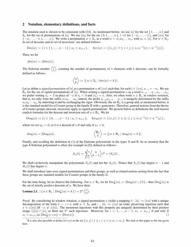
2 Notation, elementary definitions, and facts

The notation used is chosen to be consistent with [14]. As mentioned before, we use [n] for the set 1, . . . , n andSn for the set of permutations of [n]. We use [n]0 for the set 0, 1, . . . , n , [−n] for −n, . . . ,−1 , and [±n] for−n, . . . ,−1, 1, . . . , n . We write a permutation w ∈ Sn as a word w = w1w2 . . . wn, with wi ∈ [n]. For w ∈ Sn,its set of descents and its set of inversions1 are defined follows:

Des(w) := i ∈ 1, . . . , n− 1 | wi > wi+1 , Inv(w) := (i, j) | 1 ≤ i < j ≤ n,w−1(i) > w−1(j) .

Then, we let

des(w) := |Des(w)| .

The Eulerian number⟨nk

⟩, counting the number of permutations of n elements with k descents, can be formally

defined as follows:⟨nk

⟩:= |w ∈ Sn | des(w) = k | .

Let us define a signed permutation of [n] as a permutation u of [±n] such that, for each i ∈ [±n], u−i = −ui. We useBn for the set of signed permutations of [n]. When writing a signed permutation u as a word u−n . . . u−1u1 . . . un,we prefer writing ui = x in place of −x if ui < 0 and |ui| = x. Also, we often write u ∈ Bn in window notation,that is, we only write the suffix u1u2 . . . un; indeed, the prefix u−nun−1 . . . u−1 is uniquely determined by the suffixu1u2 . . . un, by mirroring it and by exchanging the signs. Obviously, the set Bn is a group and, as mentioned before, itis the standard model for a Coxeter group in the family B with n generators. Therefore, general notions from the theoryof Coxeter groups (descent, inversion) apply to signed permutations. We present below as definitions the well-knownexplicit formulas for the descent and inversion sets of u ∈ Bn. We let

DesB(u) := i ∈ 0, . . . , n− 1 | ui > ui+1 , InvB(u) := (i, j) | 1 ≤ |i| ≤ j ≤ n, u−1(i) > u−1(j) ,

where we set u0 := 0, so 0 is a descent of u if and only if u1 < 0,

desB(u) = |DesB(u)| ,⟨Bn

k

⟩:= |u ∈ Bn | desB(u) = k | .

Finally, and recalling the definition in (1) of the Eulerian polynomials in the types A and B, let us mention that thetype A Eulerian polynomial is often (for example in [5]) defined as follows:

An(t) :=n∑

k=1

⟨n

k − 1

⟩tk = tSn(t) .

We shall exclusively manipulate the polynomials Sn(t) and not the An(t). Notice that Sn(t) has degree n − 1 andBn(t) has degree n.

We shall introduce later even signed permutations and their groups, as well as related notions arising from the fact thatthese groups are standard models for Coxeter groups in the family D.

For the time being, let us observe the following. For u ∈ Bn we let Des+B (u) := DesB(u) \ 0 —thus Des+B (u) isthe set of strictly positive descents of u. We have then:

Lemma 2.1. | u ∈ Bn | Des+B (u) = k | = 2n⟨nk

⟩.

Proof. By considering its window notation, a signed permutation u yields a mapping u : [n] −→ [±n] with a uniquedecomposition of the form u = ι w with w ∈ Sn and ι : [n] −→ [±n] an order preserving injection such thatx ∈ ι([n]) iff −x 6∈ ι([n]). The monotone injections with this property are uniquely determined by their positiveimage ι([n]) ∩ [n], so there are 2n such injections. Moreover, for i = 1, . . . , n − 1, wi > wi+1 if and only ifui > ui+1, so |Des+B (ι w)| = |Des(w)|.

1It is also also possible to define Inv(w) as the set (i, j) | 1 ≤ i < j ≤ n,wi > wj . We stick in this paper to the one givenhere.

83

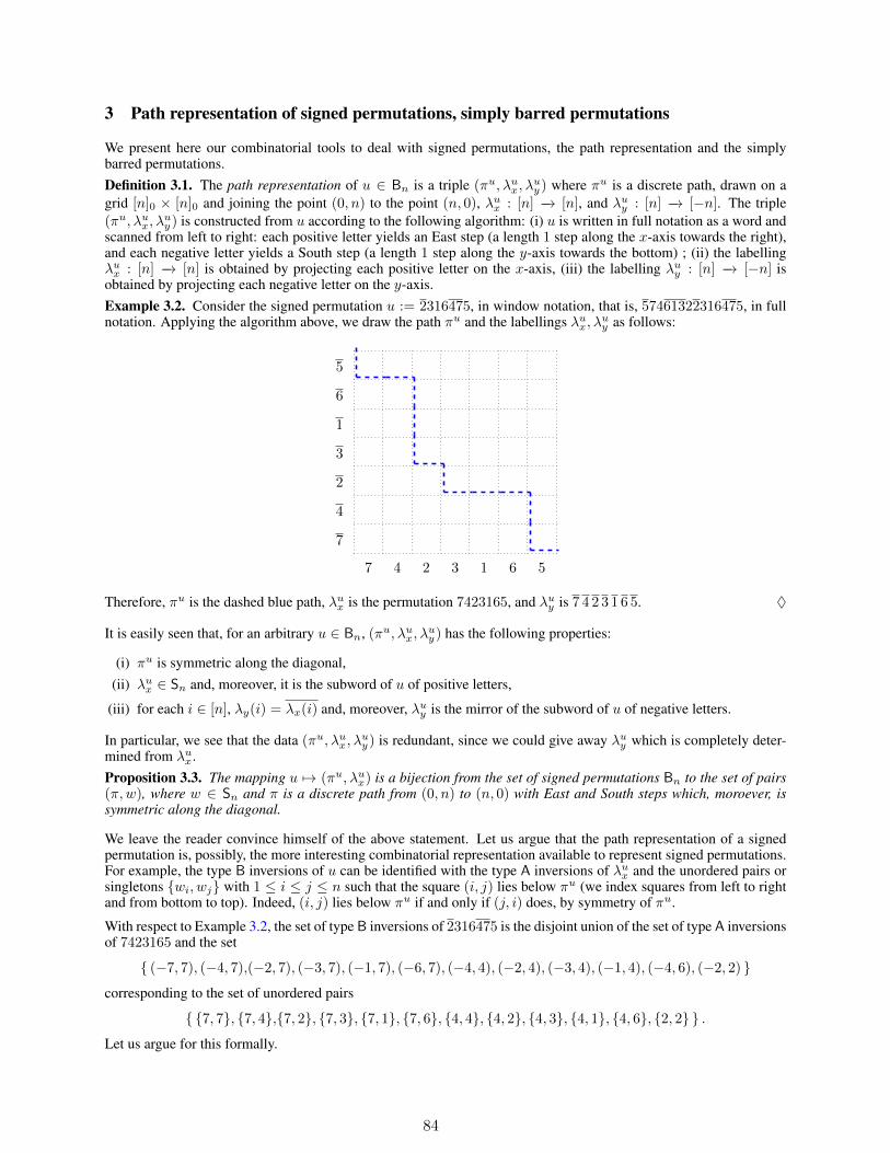
3 Path representation of signed permutations, simply barred permutations

We present here our combinatorial tools to deal with signed permutations, the path representation and the simplybarred permutations.Definition 3.1. The path representation of u ∈ Bn is a triple (πu, λux, λ

uy ) where πu is a discrete path, drawn on a

grid [n]0 × [n]0 and joining the point (0, n) to the point (n, 0), λux : [n] −→ [n], and λuy : [n] −→ [−n]. The triple(πu, λux, λ

uy ) is constructed from u according to the following algorithm: (i) u is written in full notation as a word and

scanned from left to right: each positive letter yields an East step (a length 1 step along the x-axis towards the right),and each negative letter yields a South step (a length 1 step along the y-axis towards the bottom) ; (ii) the labellingλux : [n] −→ [n] is obtained by projecting each positive letter on the x-axis, (iii) the labelling λuy : [n] −→ [−n] isobtained by projecting each negative letter on the y-axis.Example 3.2. Consider the signed permutation u := 2316475, in window notation, that is, 57461322316475, in fullnotation. Applying the algorithm above, we draw the path πu and the labellings λux, λ

uy as follows:

7

7

4

4

2

2

3

3

1

1

6

6

5

5

Therefore, πu is the dashed blue path, λux is the permutation 7423165, and λuy is 7 4 2 3 1 6 5. ♦

It is easily seen that, for an arbitrary u ∈ Bn, (πu, λux, λuy ) has the following properties:

(i) πu is symmetric along the diagonal,(ii) λux ∈ Sn and, moreover, it is the subword of u of positive letters,

(iii) for each i ∈ [n], λy(i) = λx(i) and, moreover, λuy is the mirror of the subword of u of negative letters.

In particular, we see that the data (πu, λux, λuy ) is redundant, since we could give away λuy which is completely deter-

mined from λux.Proposition 3.3. The mapping u 7→ (πu, λux) is a bijection from the set of signed permutations Bn to the set of pairs(π,w), where w ∈ Sn and π is a discrete path from (0, n) to (n, 0) with East and South steps which, moroever, issymmetric along the diagonal.

We leave the reader convince himself of the above statement. Let us argue that the path representation of a signedpermutation is, possibly, the more interesting combinatorial representation available to represent signed permutations.For example, the type B inversions of u can be identified with the type A inversions of λux and the unordered pairs orsingletons wi, wj with 1 ≤ i ≤ j ≤ n such that the square (i, j) lies below πu (we index squares from left to rightand from bottom to top). Indeed, (i, j) lies below πu if and only if (j, i) does, by symmetry of πu.

With respect to Example 3.2, the set of type B inversions of 2316475 is the disjoint union of the set of type A inversionsof 7423165 and the set

(−7, 7), (−4, 7),(−2, 7), (−3, 7), (−1, 7), (−6, 7), (−4, 4), (−2, 4), (−3, 4), (−1, 4), (−4, 6), (−2, 2) corresponding to the set of unordered pairs

7, 7, 7, 4,7, 2, 7, 3, 7, 1, 7, 6, 4, 4, 4, 2, 4, 3, 4, 1, 4, 6, 2, 2 .Let us argue for this formally.

84

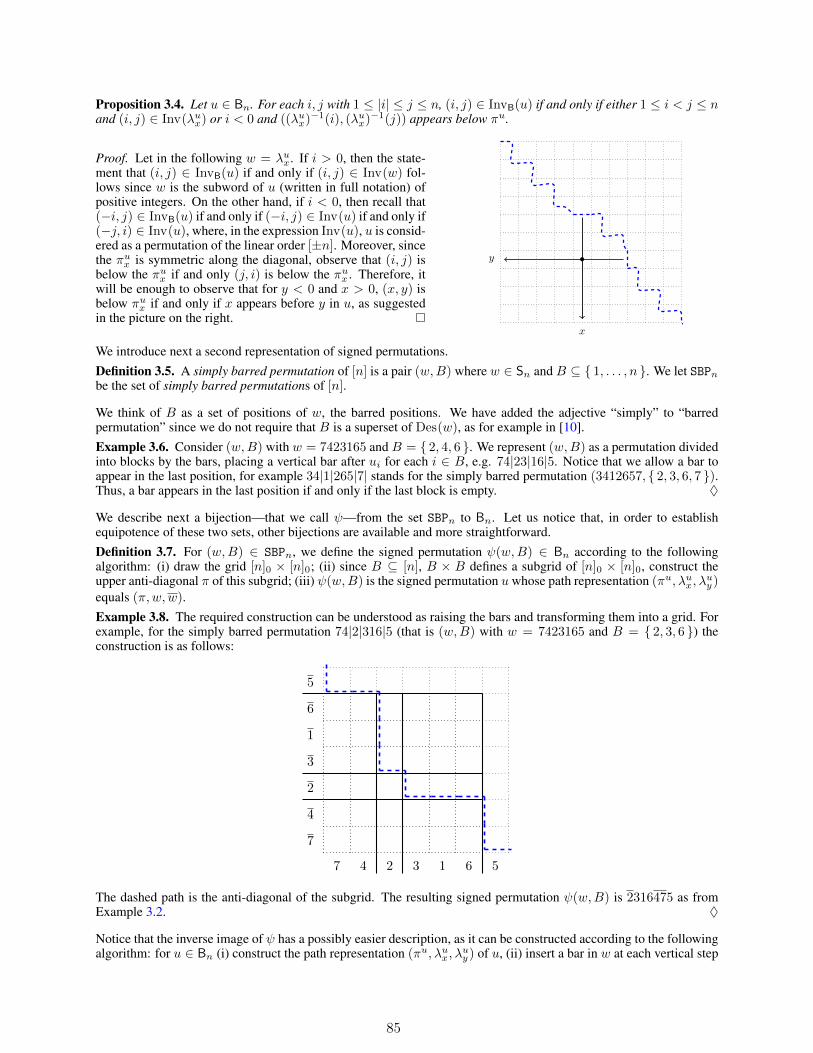
Proposition 3.4. Let u ∈ Bn. For each i, j with 1 ≤ |i| ≤ j ≤ n, (i, j) ∈ InvB(u) if and only if either 1 ≤ i < j ≤ nand (i, j) ∈ Inv(λux) or i < 0 and ((λux)−1(i), (λux)−1(j)) appears below πu.

Proof. Let in the following w = λux. If i > 0, then the state-ment that (i, j) ∈ InvB(u) if and only if (i, j) ∈ Inv(w) fol-lows since w is the subword of u (written in full notation) ofpositive integers. On the other hand, if i < 0, then recall that(−i, j) ∈ InvB(u) if and only if (−i, j) ∈ Inv(u) if and only if(−j, i) ∈ Inv(u), where, in the expression Inv(u), u is consid-ered as a permutation of the linear order [±n]. Moreover, sincethe πu

x is symmetric along the diagonal, observe that (i, j) isbelow the πu

x if and only (j, i) is below the πux . Therefore, it

will be enough to observe that for y < 0 and x > 0, (x, y) isbelow πu

x if and only if x appears before y in u, as suggestedin the picture on the right.

y

x

•

We introduce next a second representation of signed permutations.Definition 3.5. A simply barred permutation of [n] is a pair (w,B) where w ∈ Sn and B ⊆ 1, . . . , n . We let SBPnbe the set of simply barred permutations of [n].

We think of B as a set of positions of w, the barred positions. We have added the adjective “simply” to “barredpermutation” since we do not require that B is a superset of Des(w), as for example in [10].Example 3.6. Consider (w,B) with w = 7423165 and B = 2, 4, 6 . We represent (w,B) as a permutation dividedinto blocks by the bars, placing a vertical bar after ui for each i ∈ B, e.g. 74|23|16|5. Notice that we allow a bar toappear in the last position, for example 34|1|265|7| stands for the simply barred permutation (3412657, 2, 3, 6, 7 ).Thus, a bar appears in the last position if and only if the last block is empty. ♦

We describe next a bijection—that we call ψ—from the set SBPn to Bn. Let us notice that, in order to establishequipotence of these two sets, other bijections are available and more straightforward.Definition 3.7. For (w,B) ∈ SBPn, we define the signed permutation ψ(w,B) ∈ Bn according to the followingalgorithm: (i) draw the grid [n]0 × [n]0; (ii) since B ⊆ [n], B × B defines a subgrid of [n]0 × [n]0, construct theupper anti-diagonal π of this subgrid; (iii) ψ(w,B) is the signed permutation uwhose path representation (πu, λux, λ

uy )

equals (π,w,w).Example 3.8. The required construction can be understood as raising the bars and transforming them into a grid. Forexample, for the simply barred permutation 74|2|316|5 (that is (w,B) with w = 7423165 and B = 2, 3, 6 ) theconstruction is as follows:

7

7

4

4

2

2

3

3

1

1

6

6

5

5

The dashed path is the anti-diagonal of the subgrid. The resulting signed permutation ψ(w,B) is 2316475 as fromExample 3.2. ♦

Notice that the inverse image of ψ has a possibly easier description, as it can be constructed according to the followingalgorithm: for u ∈ Bn (i) construct the path representation (πu, λux, λ

uy ) of u, (ii) insert a bar in w at each vertical step

85

of πu (and remove consecutive bars), (iii) remove a bar at position 0 if it exists. Said otherwise, (w,B) = ψ−1(u) isobtained from u by transforming each negative letter into a bar, by removing consecutive bars, and then by removinga bar at position 0 if needed.

In the following chapter we shall deal mostly with simply barred permutations. Even if we understand simply barredpermutations just as shorthands for path representations of even signed permutations, some remarks are due:Lemma 3.9. If u = ψ(w,B), then there is a bijection between the set B of bars and the set of xy-turns of πu.

4 Descents from simply barred permutations

We start investigating how the type B descent set can be recovered from a simply barred permutation.Proposition 4.1. For a simply barred permutation (w,B), we have

desB(ψ(w,B)) = |Des(w) \B|+⌈ |B|

2

⌉. (7)

Proof. Write u = ψ(w,B) in window notation and divide it in maximal blocks of consecutive letters having the samesign. If the first block has negative sign, add a zero positive block which is empty. Each change of sign +− amongconsecutive blocks yields a descent. These changes of sign bijectively correspond to xy-turns of πu that lie on orbelow the diagonal. By Lemma 3.9, each bar determines an xy-turn and, by symmetry of πu along the diagonal, thenumber of xy-turns that are on or below the diagonal is

⌈|B|2

⌉. Therefore this quantity counts the number of descents

determined by a change of sign.

The other descents of ψ(w,B) are either of the form wiwi+1 with wi > wi+1 and wi, wi+1 belonging to the samepositive block, or of the form wi+1wi with wi > wi+1 and wi, wi+1 belonging to the same negative block. Thesedescents are in bijection with the descent positions of w that do not belong to the set B.

The following lemma might be immediately proved by considering that 0 ∈ DesB(u) if and only if, in the pathrepresentation of ψ(w,B), the first step of πu is along the y-axis. In this case (and only in this case), πu makes anxy-turn on the diagonal. This happens exactly when πu has an odd number of xy-turns.Lemma 4.2. We have 0 ∈ DesB(ψ(w,B)) if and only if |B| is odd.

For each k ∈ 0, 1, . . . , n , in the following we let SBPn,k be the set simply barred permutations (w,B) ∈ SBPn such

that |D(w) \B|+⌈|B|2

⌉= k.

Corollary 4.3. The set SBPn,k is in bijection with the set of signed permutations of n with k descents.Definition 4.4. A loosely barred permutation of [n] is a pair (w,B) where w is a permutation of [n] and B ⊆ 0, . . . , n is a set of positions (the bars). We let LBPn be the set of loosely barred permutations of [n].

Loosely barred permutations are being introduced only as a tool to index simply barred permutations independentlyof the even/odd cardinalities of their set of bars. Namely, for a loosely barred permutation (w,B), let us define itssimplification ς(w,B) by

ς(w,B) := (w,B \ 0 ) .Then ς(w,B) is a simply barred permutation whose set of bars has even (resp., odd) cardinality if either 0 ∈ B and|B| is odd (resp., even), or 0 6∈ B and |B| is even (resp., odd). For a loosely barred permutations (w,B), we shalloften need to evaluate the expression

⌈|B\ 0 |

2

⌉. We record this value once for all in the lemma below.

Lemma 4.5. For a loosely barred permutation (w,B) we have

⌈ |B \ 0 |2

⌉=

|B|2 , if |B| is even,|B|−1

2 , if |B| is odd and 0 ∈ B ,|B|+1

2 , if |B| is odd and 0 6∈ B .

(8)

Next, we define an involution—that we name θ—from the set of loosely barred permutations to itself. For a looselybarred permutation (w,B), θ(w,B) is defined by:

θ(w,B) := (w,Des(w)∆B) , (9)

86

where ∆ stands for symmetric difference. Let us insist that this involution is defined for all loosely barred permuta-tions, not just for the simply barred permutations.2

Lemma 4.6. If (u,C) = θ(w,B), then|D(w)|+ |B| = 2|D(u) \ C|+ |C| . (10)

Proof. Recall that C = D(w)∆B and so D(u) \ C = D(w) ∩ B. Equation (10) follows since |D(w)| + |B| =|D(w)∆B|+ 2|D(w) ∩B|.

More formally, we define a variant Θn of the correspondences θ defined in (9) as follows:Θn(w,B) := ς(θ(w,B)) = (w,Des(w)∆B \ 0 ) .

Notice that, this time, Θn : LBPn −→ SBPn.Definition 4.7. For each n ≥ 0 and k ∈ [2n]0, we let LBPn,k be the set of loosely barred permutations (w,B) suchthat |Des(w)|+ |B| = k.Proposition 4.8. For each n ≥ 0 and k ∈ [n]0, the restriction of Θn to LBPn,2k yields a bijection Θn,k from LBPn,2kto SBPn,k.

Proof. Let (w,B) ∈ LBPn,2k, so |Des(w)| + |B| = 2k. Let also (u,C) = θ(w,B), so Θn(w,B) = (w,C \ 0 ).Then, by (10),

2k = 2|D(u) \ C|+ |C|and so |C| is even. Therefore

|D(w) \ (C \ 0 )|+⌈ |C \ 0 |

2

⌉= |D(u) \ C|+

⌈ |C \ 0 |2

⌉= |D(u) \ C|+ |C|

2= k ,

where in the last step we have used equation (8).

The transformation Θn,k is injective. If Θn(w,B) = Θn(w′, B′), then w = w′ and Des(w) = Des(w′). Moreover,from Des(w)∆B \ 0 = Des(w)∆B′ \ 0 we deduce B \ 0 = B′ \ 0 . If moreover (w,B), (w′, B′) ∈LBPn,2k, then |B| = 2k − |Des(w)| = |B′| and B \ 0 = B′ \ 0 imply that 0 ∈ Des(w)∆B if and only if0 ∈ Des(w)∆B′. It follows that B = B′.

In order to show that the transformation Θn,k is surjective, let us fix (u,C) ∈ SBPn,k, so |Des(u) \ C|+⌈|C|2

⌉= k.

If |C| is even, then (w,B) := θ(u,C) is such that Θn(w,B) = θ(w,B) = (u,C) and, using equations (8) and (10),(w,B) ∈ LBPn,2k:

|Des(w)|+ |B| = 2|Des(u) \ C|+ |C| = 2( |Des(u) \ C|+⌈ |C|

2

⌉) = 2k.

If |C| is odd, then (w,B) := θ(u,C ∪ 0 ) is such that Θ(w,B) = (u,C) and (w,B) ∈ LBPn,2k:

|Des(w)|+ |B| = 2|Des(u) \ (C ∪ 0 )|+ |C ∪ 0 | = 2|Des(u) \ C|+ 2|C|+ 1

2

= 2( |Des(u) \ C|+⌈ |C|

2

⌉) = 2k .

Definition 4.9. For each k ∈ [n− 1]0, we let SBPkn be the set of simply barred permutations (w,B) ∈ SBPn such that|Des+B (ψ(w,B))| = k.

Notice that

|Des+B (ψ(w,B))| = k iff

0 6∈ DesB(ψ(w,B)) and desB(ψ(w,B)) = k, or

0 ∈ DesB(ψ(w,B)) and desB(ψ(w,B)) = k + 1 .

Using Lemma 4.2 and equation (7), for (w,B) ∈ SBPn we have

(w,B) ∈ SBPkn iff

|B| is even and |D(w) \B|+⌈|B|2

⌉= k, or

|B| is odd and |D(w) \B|+⌈|B|2

⌉= k + 1 .

2At the moment of writing we cannot pinpoint any other usage of this involution apart, of course, from yielding our bijectionsand counting results.

87

Proposition 4.10. For each k ∈ [n− 1]0, the restriction of Θn to LBPn,2k+1 yields a bijection Θkn from LBPn,2k+1 to

SBPkn.

Proof. Let (w,B) ∈ LBPn,2k+1 and (u,C) = θ(w,B), so Θn(w,B) = (w,C \ 0 ). Thus |Des(w)|+ |B| = 2k+1and, by (10),

2k = 2|D(u) \ C|+ |C| − 1 ,

so in particular |C| is odd. Using equation (8), we obtain

|D(u) \ C|+⌈ |C \ 0 |

2

⌉=

|D(u) \ C|+ |C|−1

2 = k , 0 ∈ C,

|D(u) \ C|+ |C|+12 = k + 1 , 0 6∈ C .

Considering that |C| is odd, we have

|D(u) \ (C \ 0 )|+⌈ |C \ 0 |

2

⌉=

k , |C \ 0 | is even,k + 1 , |C \ 0 | is odd,

that is, (u,C \ 0 ) = Θn(w,B) ∈ SBPkn.

The transformation Θkn is injective, the reason being similar to the one for Θn,k. If Θn(w,B) = Θn(w′, B′) then

w = w′ and Des(w) = Des(w′). Moreover, from Des(w)∆B \ 0 = Des(w)∆B′ \ 0 we deduce B \ 0 =B′\ 0 . Considering now that |B| = 2k+1−|Des(w)| = |B′| andB\ 0 = B′\ 0 , we derive 0 ∈ Des(w)∆Bif and only if 0 ∈ Des(w)∆B′, whence B = B′.

In order to show that the transformation Θkn is surjective, let us fix (u,C) ∈ SBPkn, so either (i) |C| is even and

|D(u) \ C|+⌈|C|2

⌉= k or (ii) |C| is odd and |D(u) \ C|+

⌈|C|2

⌉= k + 1.

Let us suppose (i). Then (w,B) := θ(u,C ∪ 0 ) is such that Θn(w,B) = (u,C) and, using equations (8) and (10),(w,B) ∈ LBPn,2k+1:

|Des(w)|+ |B| = 2|Des(u) \ C|+ |C ∪ 0 | = 2|Des(u) \ C|+ 2|C|+ 1

2

= 2( |Des(u) \ C|+⌈ |C|

2

⌉+

1

2) = 2k + 1.

Let us suppose (ii). Then (w,B) := θ(u,C) is such that Θn(w,B) = θ(w,B) = (u,C) and, using equations (8) and(10), (w,B) ∈ LBPn,2k+1:

|Des(w)|+ |B| = 2|Des(u) \ C|+ |C| = 2|Des(u) \ C|+ 2|C|2

= 2( |Des(u) \ C|+⌈ |C|

2

⌉− 1

2) = 2(k + 1)− 1 = 2k + 1.

To end this section, we collect the consequences of the bijections established so far.Theorem 4.11. The following relations hold:

⟨Bn

k

⟩=

2k∑

i=0

⟨ni

⟩(n+ 1

2k − i

), (3)

2n⟨nk

⟩=

2k+1∑

i=0

⟨ni

⟩(n+ 1

2k + 1− i

). (4)

Proof. We have seen that signed permutations u ∈ Bn such that desB(u) = k are in bijection (via the mapping ψ ofDefinition 3.7) with simply barred permutations in SBPn,k. Next, this set is in bijection (see Proposition (4.8)) with theset LBPn,2k of loosely barred permutations (w,B) ∈ LBPn such that des(w) + |B| = 2k. The cardinality of LBPn,2kis the right-hand side of equality (3).

The left-hand side of equality (4) is the cardinality of the set of signed permutations u such that |Des+B (u)| = k, seeLemma 2.1. This set is in bijection with the set SBPkn (via ψ defined in 3.7 and by the definition of SBPkn) which, inturn, is in bijection (see Proposition (4.10)) with the set LBPn,2k+1 of loosely barred permutations (w,B) ∈ LBPnsuch that des(w) + |B| = 2k + 1. The cardinality of this set is the right-hand side of equality (4).

88

Theorem 4.12. The following relation holds:

Bn(t2) = (1 + t)n+1Sn(t)− 2ntSn(t2) . (11)

Proof. By (3),⟨Bn

k

⟩, which is the coefficient of t2k in the polynomial Bn(t2), is also the coefficient of t2k in (1 +

t)n+1Sn(t). By (4), 2n⟨nk

⟩is the coefficient of t2k+1 in the polynomials 2ntSn(t2) and (1 + t)n+1Sn(t). Therefore

Bn(t2) + 2ntSn(t2) = (1 + t)n+1Sn(t) , (5)

whence equation (11).

5 Stembridge’s identity for Eulerian numbers in type D

Let us recall that a signed permutation u ∈ Bn is even signed if the number of negative letters in its window notationis even. The even signed permutations of Bn form a subgroup Dn of Bn and in fact the groups Dn are the standardmodels for abstract Coxeter groups of type D.

Definitions analogous to those given in Section 2 for the types A and B can be given for type D. Namely, for u ∈ Dn,we set

DesD(u) := i ∈ 0, 1, . . . , n− 1 | ui > ui+1 , (12)

where we have set u0 = −u2,

desD(u) := |DesD(u)| ,⟨Dn

k

⟩:= |u ∈ Dn | desD(u) = k | , Dn(t) :=

n∑

k=0

⟨Dn

k

⟩tk .

The formula in (12) is the standard one, see e.g. [4, §8.2] or [1]. The reader will have no difficulties verifying that, upto renaming 0 by −1, the type D descent set of u can also be defined using the following, see [14, §13]:

DesD(u) := i ∈ −1, 1, . . . , n− 1 | ui > u|i|+1 . (13)

It is convenient to consider a more flexible representation of elements of Dn. If u ∈ Bn, then its mate is the signedpermutation u ∈ Bn that differs from u only for the sign of the first letter. Notice that u = u. We define a forkedsigned permutation (see [14, §13]) as an unordered pair of the form u, u for some u ∈ Bn. Clearly, just one of themates is even signed and therefore forked signed permutations are combinatorial models of Dn.

The path representation of a forked signed permutation is insensitive of how the diagonal is crossed, either from theWest, or from the North. The following are possible ways to draw a forked signed permutation on a grid:

1

1

2

2

3

3

4

4

5

5

1

1

2

2

3

3

4

4

5

5

1

1

2

2

3

3

4

4

5

5

Even if the formulas in (12) and (13) have been defined for even signed permutations, they still can be computed forall signed permutations. The formula in (13) is not invariant under taking mates, however the following lemma showsthat this formula suffices to compute the number of type D descents of a forked signed permutation and therefore theEulerian numbers

⟨Dn

k

⟩.

Lemma 5.1. For each u ∈ Bn, 1 ∈ DesD(u) if and only if −1 ∈ DesD(u). Therefore desD(u) = desD(u).

Proof. Suppose 1 ∈ DesD(u), that is u1 > u2. Then u−1 = −(−u1) = u1 > u2, and so −1 ∈ DesD(u). Theopposite implication is proved similarly.

For the last statement, observe that DesD(u) = ∆u ∪ i ∈ 2, . . . , n− 1 | ui > ui+1 with ∆u := i ∈ 1,−1 |ui > u|i|+1 and, by what we have just remarked, we have |∆u| = |∆u|. It follows that |DesD(u)| = |DesD(u)|.

89

Our next aim is to derive Stembridge’s identity

Dn(t) = Bn(t)− n2n−1tSn−1(t) , (14)

see [22, Lemma 9.1], which, in term of the coefficients of these polynomials, amounts to⟨Dn

k

⟩=

⟨Bn

k

⟩− n2n−1

⟨n− 1k − 1

⟩. (15)

Definition 5.2. A signed permutation u is smooth if u1, u2 have equal sign and, otherwise, it is non-smooth.

The reason for naming a signed permutation smooth arises again from the path representation of a signed permutation:the smooth signed permutation is, between the two mates, the one that minimizes the turns nearby the diagonal, assuggested below with two pairs of mates as examples:

1

1

2

2

3

3

4

4

5

5

1

1

2

2

3

3

4

4

5

5

1

1

2

2

3

3

4

4

5

5

1

1

2

2

3

3

4

4

5

5

Lemma 5.3. If u ∈ Bn is smooth, then −1 ∈ DesD(u) if and only if 0 ∈ DesB(u) and therefore desD(u) = desB(u).

Proof. Suppose 0 ∈ DesB(u), so u1 < 0 and u2 < 0 as well, since u is smooth. Then u−1 = −u1 > 0 > u2, so−1 ∈ DesD(u). Conversely, suppose −1 ∈ DesD(u), that is, u−1 > u2. If u1 > 0, then 0 > −u1 = u−1 > u2, sou1, u2 have different sign, a contradiction. Therefore u1 < 0 and 0 ∈ DesB(u).

Next, we consider the correspondence—let us call it χ—sending a non-smooth signed permutation u ∈ Bn to the pair(|u1|, u′), where u′ is obtained from u2 . . . un by normalising this sequence, so that it takes absolute values in the set[n− 1]. For example χ(6123475) = (6, 123465) and χ(2316475) = (2, 215364), as suggested below:

6123475 (6, 123475) (6, 123465) , 2316475 (2, 316475) (2, 215364) .

The process of normalizing the sequence u2 . . . un can be understood as applying to each letter of this sequence theunique order preserving bijection Nn,x : [±n] \ x, x −→ [±n − 1] where, in general, x ∈ [n] and, in this case,x = |u1|.Lemma 5.4. Let n ≥ 2. For each pair (x, v) with x ∈ [n] and v ∈ Bn−1, there exists a unique non-smooth u ∈ Bn

such that χ(u) = (x, v).

Proof. We construct u firstly by renaming v to v′ so that none of x, x appears in v′ (that is, we apply to each letter ofv the inverse of Nn,x) and then by adding in front of v′ either x or x, according to the sign of the first letter of v′.

Lemma 5.5. The correspondence χ restricts to a bijection from the set of non-smooth signed permutations u ∈ Bn

such that desB(u) = k to the set of pairs (x, v) where x ∈ [n] and v ∈ Bn−1 is such that |Des+B (v)| = k − 1.

Proof. We have already argued that χ is a bijection from the set of non-smooth signed permutations u of [n] to theset of pairs (x, v) with x ∈ [n] and v ∈ Bn−1. Therefore, we are left to argue that, for non-smooth u and v, ifdesB(u) = k, then |Des+B (v)| = k − 1. Since u1, u2 have different sign, then |DesB(u) ∩ 0, 1 | = 1. Clearly, ifχ(u) = (x, v), then Des+B (v) = i − 1 | i ∈ DesB(u) ∩ 2, . . . , n − 1 , from which the statement of the lemmafollows.

Theorem 5.6. The following relations hold:⟨Bn

k

⟩=

⟨Dn

k

⟩+ n2n−1

⟨n− 1k − 1

⟩, Bn(t) = Dn(t) + n2n−1tSn−1(t) .

Proof. Every signed permutation is either smooth or non-smooth. By Lemma 5.3, the smooth signed permutationswith k type B descents are in bijection with the even signed permutations with k type D descents. By Lemma 5.5, thenon-smooth signed permutations u ∈ Bn with k type B descents are in bijection with the pairs (x, v) ∈ [n] × Bn−1such |Des+B (v)| = k − 1. Using Lemma 2.1, the number of these pairs is n2n−1

⟨n− 1k − 1

⟩.

90

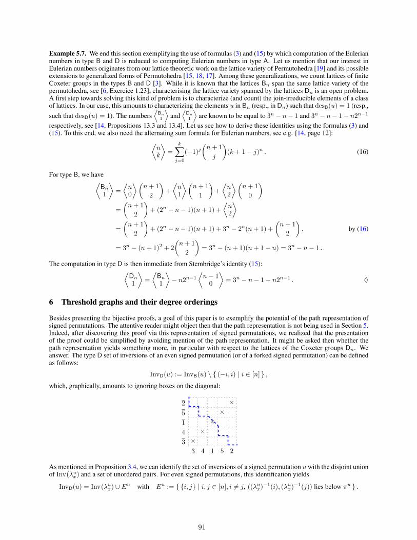
Example 5.7. We end this section exemplifying the use of formulas (3) and (15) by which computation of the Euleriannumbers in type B and D is reduced to computing Eulerian numbers in type A. Let us mention that our interest inEulerian numbers originates from our lattice theoretic work on the lattice variety of Permutohedra [19] and its possibleextensions to generalized forms of Permutohedra [15, 18, 17]. Among these generalizations, we count lattices of finiteCoxeter groups in the types B and D [3]. While it is known that the lattices Bn span the same lattice variety of thepermutohedra, see [6, Exercice 1.23], characterising the lattice variety spanned by the lattices Dn is an open problem.A first step towards solving this kind of problem is to characterize (and count) the join-irreducible elements of a classof lattices. In our case, this amounts to characterizing the elements u in Bn (resp., in Dn) such that desB(u) = 1 (resp.,such that desD(u) = 1). The numbers

⟨Bn

1

⟩and

⟨Dn

1

⟩are known to be equal to 3n − n− 1 and 3n − n− 1− n2n−1

respectively, see [14, Propositions 13.3 and 13.4]. Let us see how to derive these identities using the formulas (3) and(15). To this end, we also need the alternating sum formula for Eulerian numbers, see e.g. [14, page 12]:

⟨nk

⟩=

k∑

j=0

(−1)j(n+ 1

j

)(k + 1− j)n . (16)

For type B, we have⟨Bn

1

⟩=

⟨n0

⟩(n+ 1

2

)+

⟨n1

⟩(n+ 1

1

)+

⟨n2

⟩(n+ 1

0

)

=

(n+ 1

2

)+ (2n − n− 1)(n+ 1) +

⟨n2

⟩

=

(n+ 1

2

)+ (2n − n− 1)(n+ 1) + 3n − 2n(n+ 1) +

(n+ 1

2

), by (16)

= 3n − (n+ 1)2 + 2

(n+ 1

2

)= 3n − (n+ 1)(n+ 1− n) = 3n − n− 1 .

The computation in type D is then immediate from Stembridge’s identity (15):⟨Dn

1

⟩=

⟨Bn

1

⟩− n2n−1

⟨n− 1

0

⟩= 3n − n− 1− n2n−1 . ♦

6 Threshold graphs and their degree orderings

Besides presenting the bijective proofs, a goal of this paper is to exemplify the potential of the path representation ofsigned permutations. The attentive reader might object then that the path representation is not being used in Section 5.Indeed, after discovering this proof via this representation of signed permutations, we realized that the presentationof the proof could be simplified by avoiding mention of the path representation. It might be asked then whether thepath representation yields something more, in particular with respect to the lattices of the Coxeter groups Dn. Weanswer. The type D set of inversions of an even signed permutation (or of a forked signed permutation) can be definedas follows:

InvD(u) := InvB(u) \ (−i, i) | i ∈ [n] ,which, graphically, amounts to ignoring boxes on the diagonal:

3

3

4

4

1

1

5

5

2

2

×××××

As mentioned in Proposition 3.4, we can identify the set of inversions of a signed permutation uwith the disjoint unionof Inv(λux) and a set of unordered pairs. For even signed permutations, this identification yields

InvD(u) = Inv(λux) ∪ Eu with Eu := i, j | i, j ∈ [n], i 6= j, ((λux)−1(i), (λux)−1(j)) lies below πu .

91

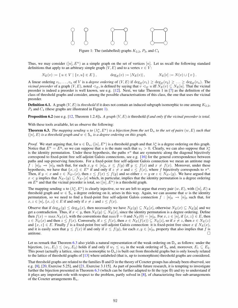
Figure 1: The (unlabelled) graphs K2,2, P3, and C4

Thus, we may consider ([n], Eu) as a simple graph on the set of vertices [n]. Let us recall the following standarddefinitions that apply to an arbitrary simple graph (V,E) and to a vertex v ∈ V :

NE(v) := u ∈ V | v, u ∈ E , degE(v) := |NE(v)| , NE [v] := N(v) ∪ v .A linear ordering v1, . . . , vn of V is a degree ordering of (V,E) if degE(v1) ≥ degE(v2) ≥ . . . ≥ degE(vn). Thevicinal preorder of a graph (V,E), noted CE , is defined by saying that v CE u iff NE(v) ⊆ NE [u]. That the vicinalpreorder is indeed a preorder is well known, see e.g. [12]. Next, we take Theorem 1 in [7] as the definition of theclass of threshold graphs and consider, among the possible characterisations of this class, the one that uses the vicinalpreorder.

Definition 6.1. A graph (V,E) is threshold if it does not contain an induced subgraph isomorphic to one among K2,2,P3 and C4 (these graphs are illustrated in Figure 1).

Proposition 6.2 (see e.g. [12, Theorem 1.2.4]). A graph (V,E) is threshold if and only if the vicinal preorder is total.

With these tools available, let us observe the following:

Theorem 6.3. The mapping sending u to (λux, Eu) is a bijection from the set Dn to the set of pairs (w,E) such that

([n], E) is a threshold graph and w ∈ Sn is a degree ordering on this graph.

Proof. We start arguing that, for u ∈ Dn, ([n], Eu) is a threshold graph and that λux is a degree ordering on this graph.Notice that Eu = Eu, so we can suppose that u is the mate such that u1 > 0. Clearly, we can also suppose that λuxis the identity permutation. Under these hypothesis, the paths πu that are symmetric along the diagonal bijectivelycorrespond to fixed-point free self-adjoint Galois connections, see e.g. [16] for the general correspondence betweenpaths and sup-preserving functions. For a fixed-point free self-adjoint Galois connection we mean an antitone mapf : [n]0 −→ [n]0 such that, for each x, y ∈ [n]0, x ≤ f(y) iff y ≤ f(x) and x 6= f(x). Moreover, under thesehypothesis, we have that x, z ∈ Eu if and only if z 6= x and z ≤ f(x), where f bijectively corresponds to πu.Then, if y < x and z ∈ NEu(x), then z ≤ f(x) ≤ f(y) and so either z = y or z ∈ NEu(y). We have argued thatx < y implies that NEu(y) ⊆ NEu [x] which, in particular, implies that the identity permutation is a degree orderingon Eu and that the vicinal preorder is total, so ([n], Eu) is a threshold graph.

The mapping sending u to (λux, Eu) is clearly injective, so we are left to argue that every pair (w,E), with ([n], E) a

threshold graph and w ∈ Sn a degree ordering on it, arises in this way. Again, we can assume that w is the identitypermutation, so we need to find a fixed-point free self-adjoint Galois connection f : [n]0 −→ [n]0 such that, forx, z ∈ [n], x, z ∈ E if and only if x 6= z and z ≤ f(x).

Observe that if degE(y) ≤ degE(x), then necessarily we have NE(y) ⊆ NE [x], otherwise NE(x) ⊆ NE [y] and weget a contradiction. Thus, if x < y, then NE(y) ⊆ NE [x], since the identity permutation is a degree ordering. Definethen f(x) = maxNE(x), with the conventions that max ∅ = 0 and NE(0) = [n]0. For x, z ∈ [n], if x, z ∈ E, thenz ∈ NE(x) and then z ≤ f(x). Conversely, if z ≤ f(x), then x ∈ NE(f(x)) ⊆ NE [z], so if x 6= z, then x ∈ NE(z)and x, z ∈ E. Finally f is a fixed-point free self-adjoint Galois connection: it is fixed-point free since x 6∈ NE(x),and it is easily seen that y ≤ f(x) if and only if x ≤ f(y), for each x, y ∈ [n]0, property that also implies that f isantitone.

Let us remark that Theorem 6.3 also yields a natural representation of the weak ordering on Dn as follows: under thebijection, (w1, E1) ≤ (w2, E2) holds if and only if w1 ≤ w2 in the weak ordering of Sn and, moreover, E1 ⊆ E2.This poset (actually a lattice, since it is isomorphic to Dn) is built out from threshold graphs but is only loosely relatedto the lattice of threshold graphs of [13] where unlabeled (that is, up to isomorphism) threshold graphs are considered.

That threshold graphs are related to the families B and D in the theory of Coxeter groups has already been observed, seee.g. [8], [20, Exercise 5.25], and [21, Exercise 3.115]. As part of possible future research, it is tempting to investigatefurther the bijection presented in Theorem 6.3 (which can be further adapted to fit the type B) and try to understand ifit plays any important role with respect to the problem, partly solved in [8], of characterizing free sub-arrangementsof the Coxeter arrangements Bn.

92

References

[1] E. Bagno, R. Biagioli, and D. Garber. Stirling and eulerian numbers of types B and D. In L. Ferrari and M. Vam-vakari, editors, Proceedings of the 11th International Conference on Random and Exhaustive Generation ofCombinatorial Structures, GASCom 2018, Athens, Greece, June 18-20, 2018, volume 2113 of CEUR WorkshopProceedings, pages 53–59. CEUR-WS.org, 2018.

[2] E. Barnard. The canonical join complex. Preprint, retrievable from https://arxiv.org/abs/1610.05137,2016.

[3] A. Bjorner. Orderings of Coxeter groups. In Combinatorics and Algebra (Boulder, Colo., 1983), volume 34 ofContemp. Math., pages 175–195. Amer. Math. Soc., Providence, RI, 1984.

[4] A. Bjorner and F. Brenti. Combinatorics of Coxeter groups, volume 231 of Graduate Texts in Mathematics.Springer, New York, 2005.

[5] M. Bona. Combinatorics of permutations. Discrete Mathematics and its Applications (Boca Raton). CRC Press,Boca Raton, FL, second edition, 2012. With a foreword by Richard Stanley.

[6] N. Caspard, L. Santocanale, and F. Wehrung. Permutohedra and associahedra. In Lattice theory: special topicsand applications. Vol. 2, pages 215–286. Birkhauser/Springer, Cham, 2016.

[7] V. Chvatal and P. L. Hammer. Aggregation of inequalities in integer programming. In Studies in integer pro-gramming (Proc. Workshop, Bonn, 1975), pages 145–162. Ann. of Discrete Math., Vol. 1, 1977.

[8] P. H. Edelman and V. Reiner. Free hyperplane arrangements between An−1 and Bn. Math. Z., 215(3):347–365,1994.

[9] R. Freese, J. Jezek, and J. Nation. Free Lattices, volume 42 of Mathematical Surveys and Monographs. AmericanMathematical Society, Providence, RI, 1995.

[10] I. Gessel and R. P. Stanley. Stirling polynomials. J. Combinatorial Theory Ser. A, 24(1):24–33, 1978.[11] G. Guilbaud and P. Rosenstiehl. Analyse algebrique d’un scrutin. Math. Sci. Hum., 4:9–33, 1963.[12] N. V. R. Mahadev and U. N. Peled. Threshold graphs and related topics, volume 56 of Annals of Discrete

Mathematics. North-Holland Publishing Co., Amsterdam, 1995.[13] R. Merris and T. Roby. The lattice of threshold graphs. JIPAM. J. Inequal. Pure Appl. Math., 6(1):Article 2, 21,

2005.[14] T. K. Petersen. Eulerian numbers. Birkhauser Advanced Texts: Basler Lehrbucher. [Birkhauser Advanced Texts:

Basel Textbooks]. Birkhauser/Springer, New York, 2015. With a foreword by Richard Stanley.[15] M. Pouzet, K. Reuter, I. Rival, and N. Zaguia. A generalized permutahedron. Algebra Universalis, 34(4):496–

509, 1995.[16] L. Santocanale. On discrete idempotent paths. In R. Mercas and D. Reidenbach, editors, WORDS 2019, volume

11682 of Lecture Notes in Comput. Sci., pages 312–325. Springer, Cham, 2019.[17] L. Santocanale and M. J. Gouveia. The continuous weak order. Journal of Pure and Applied Algebra, 2020. In

press.[18] L. Santocanale and F. Wehrung. Generalizations of the permutohedron. In Lattice Theory: Special Topics and

Applications. Vol. 2, pages 287–397. Birkhauser, 2016.[19] L. Santocanale and F. Wehrung. The equational theory of the weak Bruhat order on finite symmetric groups.

Journal of the European Mathematical Society, 20(8):1959–2003, 2018.[20] R. P. Stanley. An introduction to hyperplane arrangements. In Geometric combinatorics, volume 13 of IAS/Park

City Math. Ser., pages 389–496. Amer. Math. Soc., Providence, RI, 2007.[21] R. P. Stanley. Enumerative combinatorics. Volume 1, volume 49 of Cambridge Studies in Advanced Mathematics.

Cambridge University Press, Cambridge, second edition, 2012.[22] J. R. Stembridge. Some permutation representations of Weyl groups associated with the cohomology of toric

varieties. Adv. Math., 106(2):244–301, 1994.

93

POLYMORPHISM-HOMOGENEITY ANDUNIVERSAL ALGEBRAIC GEOMETRY

Endre TóthBolyai Institute

University of SzegedAradi vértanúk tere 1

H–6720 Szeged, [email protected]

Tamás WaldhauserBolyai Institute

University of SzegedAradi vértanúk tere 1

H–6720 Szeged, [email protected]

Dedicated to Maurice Pouzet on the occasion of his 75th birthday.

ABSTRACT

We assign a relational structure to any finite algebra in a canonical way, using solution sets ofequations, and we prove that this relational structure is polymorphism-homogeneous if and only ifthe algebra itself is polymorphism-homogeneous. We show that polymorphism-homogeneity is alsoequivalent to the property that algebraic sets (i.e., solution sets of systems of equations) are exactlythose sets of tuples that are closed under the centralizer clone of the algebra. Furthermore, we provethat the aforementioned properties hold if and only if the algebra is injective in the category of itsfinite subpowers. We also consider two additional conditions: a stronger variant for polymorphism-homogeneity and for injectivity, and we describe explicitly the finite semilattices, lattices, Abeliangroups and monounary algebras satisfying any one of these three conditions.

Keywords Polymorphism-homogeneity · Algebraic set · Universal algebraic geometry · Solution set of a system ofequations · Injective algebra

1 Introduction

Various notions of homogeneity appear in several areas of mathematics, such as model theory, group theory, combi-natorics, etc. Roughly speaking, a structure A is said to be homogeneous if certain kinds of local morphisms (i.e.,morphisms defined on “small” substructures of A) extend to endomorphisms of A. Specifying the kind of morphismsthat are expected to be extendible, one can define many different versions of homogeneity. We consider a variant calledpolymorphism-homogeneity introduced by C. Pech and M. Pech [1] that involves “multivariable” homomorphisms:we require extendibility of homomorphisms defined on finitely generated substructures of direct powers of A (seeSection 2.4 for the precise definition).

We study polymorphism-homogeneity of finite algebraic structures and of certain relational structures constructed fromalgebras. Since homomorphisms depend on the term operations, not on the particular choice of basic operations, wework mainly with the clone C = Clo(A) of term operations of the algebraic structure A = (A,F ) (i.e., C is the clonegenerated by F ; see Section 2.1). An n-ary operation f : An → A can be regarded as an (n+ 1)-ary relation, calledthe graph of f , denoted by f• (see Section 2.3). Probably the most natural way to convert A into a relational structureis to consider the graphs of the operations of A, thus we define C• = f• : f ∈ C to be the set of graphs of termoperations of A. We will prove that if the relational structure (A,C•) is polymorphism-homogeneous, then the algebraA is also polymorphism-homogeneous, but the converse is not true in general.

To construct a relational structure that is equivalent to A in terms of polymorphism-homogeneity, observe that therelation f• is nothing else than the solution set of the equation f(x1, . . . , xn) = xn+1. We might consider more

95

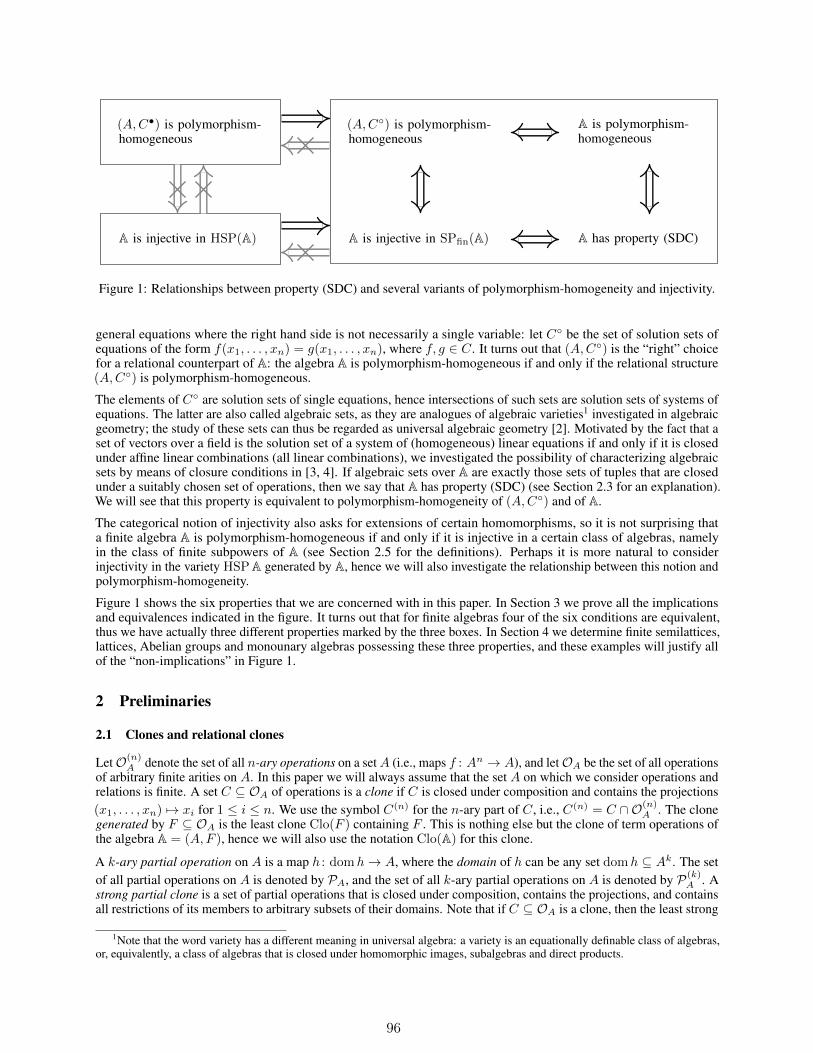
(A,C•) is polymorphism-homogeneous

(A,C) is polymorphism-homogeneous

A is polymorphism-homogeneous

A is injective in HSP(A) A is injective in SPfin(A) A has property (SDC)

Figure 1: Relationships between property (SDC) and several variants of polymorphism-homogeneity and injectivity.

general equations where the right hand side is not necessarily a single variable: let C be the set of solution sets ofequations of the form f(x1, . . . , xn) = g(x1, . . . , xn), where f, g ∈ C. It turns out that (A,C) is the “right” choicefor a relational counterpart of A: the algebra A is polymorphism-homogeneous if and only if the relational structure(A,C) is polymorphism-homogeneous.

The elements of C are solution sets of single equations, hence intersections of such sets are solution sets of systems ofequations. The latter are also called algebraic sets, as they are analogues of algebraic varieties1 investigated in algebraicgeometry; the study of these sets can thus be regarded as universal algebraic geometry [2]. Motivated by the fact that aset of vectors over a field is the solution set of a system of (homogeneous) linear equations if and only if it is closedunder affine linear combinations (all linear combinations), we investigated the possibility of characterizing algebraicsets by means of closure conditions in [3, 4]. If algebraic sets over A are exactly those sets of tuples that are closedunder a suitably chosen set of operations, then we say that A has property (SDC) (see Section 2.3 for an explanation).We will see that this property is equivalent to polymorphism-homogeneity of (A,C) and of A.

The categorical notion of injectivity also asks for extensions of certain homomorphisms, so it is not surprising thata finite algebra A is polymorphism-homogeneous if and only if it is injective in a certain class of algebras, namelyin the class of finite subpowers of A (see Section 2.5 for the definitions). Perhaps it is more natural to considerinjectivity in the variety HSPA generated by A, hence we will also investigate the relationship between this notion andpolymorphism-homogeneity.

Figure 1 shows the six properties that we are concerned with in this paper. In Section 3 we prove all the implicationsand equivalences indicated in the figure. It turns out that for finite algebras four of the six conditions are equivalent,thus we have actually three different properties marked by the three boxes. In Section 4 we determine finite semilattices,lattices, Abelian groups and monounary algebras possessing these three properties, and these examples will justify allof the “non-implications” in Figure 1.

2 Preliminaries

2.1 Clones and relational clones

LetO(n)A denote the set of all n-ary operations on a setA (i.e., maps f : An → A), and letOA be the set of all operations

of arbitrary finite arities on A. In this paper we will always assume that the set A on which we consider operations andrelations is finite. A set C ⊆ OA of operations is a clone if C is closed under composition and contains the projections(x1, . . . , xn) 7→ xi for 1 ≤ i ≤ n. We use the symbol C(n) for the n-ary part of C, i.e., C(n) = C ∩ O(n)

A . The clonegenerated by F ⊆ OA is the least clone Clo(F ) containing F . This is nothing else but the clone of term operations ofthe algebra A = (A,F ), hence we will also use the notation Clo(A) for this clone.

A k-ary partial operation on A is a map h : domh→ A, where the domain of h can be any set domh ⊆ Ak. The setof all partial operations on A is denoted by PA, and the set of all k-ary partial operations on A is denoted by P(k)

A . Astrong partial clone is a set of partial operations that is closed under composition, contains the projections, and containsall restrictions of its members to arbitrary subsets of their domains. Note that if C ⊆ OA is a clone, then the least strong

1Note that the word variety has a different meaning in universal algebra: a variety is an equationally definable class of algebras,or, equivalently, a class of algebras that is closed under homomorphic images, subalgebras and direct products.

96

partial clone Str(C) containing C consists of all restrictions of elements of C, i.e., h ∈ PA belongs to Str(C) if andonly if h can be extended to a total operation h ∈ C.

An n-ary relation on A is a subset of An; the set of all relations (of arbitrary arities) on A is denoted byRA. Given aset of relations R ⊆ RA, a primitive positive formula Φ(x1, . . . , xn) over R is an existentially quantified conjunction:

Φ(x1, . . . , xn) = ∃y1 · · · ∃ymt

i=1

ρi(z

(i)1 , . . . , z(i)

ri

), (2.1)

where ρi ∈ R is a relation of arity ri, and each z(i)j is a variable from the set x1, . . . , xn, y1, . . . , ym for i =

1, . . . , t, j = 1, . . . , ri. The relation ρ = (a1, . . . , an) : Φ(a1, . . . , an) is true ⊆ An is then said to be defined by theprimitive positive formula Φ. The set of all primitive positive definable relations over R is denoted by 〈R〉∃, and suchsets of relations are called relational clones. If we allow only quantifier-free primitive positive formulas, then we obtainthe weak relational clone 〈R〉@.

2.2 Galois connections between operations and relations

We say that a k-ary (partial) operation h preserves the relation ρ ⊆ An, denoted as h B ρ, if for every matrixM ∈ An×k

such that each column of M belongs to ρ (and each row of M is in the domain of h), applying h to each row of M ,we obtain a column that also belongs to ρ. If R is a set of relations, then we write h B R to indicate that h preservesall elements of R. In other words, h B R holds if and only if h is a (partial) polymorphism of the relational structureA = (A,R), i.e., h is a homomorphism from (the substructure domh of) Ak to A. The set of all (partial) operationspreserving each relation of R is denoted by PolR (pPolR), and the set of all relations preserved by each member of aset F of (partial) operations is denoted by InvF :

PolR =h ∈ OA : h B ρ for every ρ ∈ R

;

pPolR =h ∈ PA : h B ρ for every ρ ∈ R

;

InvF =ρ ∈ RA : h B ρ for every h ∈ F

.

Note that PolR = pPolR ∩ OA.

The closed sets under the Galois connection Pol− Inv (pPol− Inv) between (partial) operations and relations areexactly the (strong partial) clones and the (weak) relational clones; this makes these Galois connections fundamentaltools in clone theory.Theorem 2.1 ([5, 6, 7]). For any set of operations F ⊆ OA and any set of relations R ⊆ RA, we have Clo(F ) =Pol InvF and 〈R〉∃ = Inv PolR. For any set of partial operations F ⊆ PA and any set of relations R ⊆ RA, wehave Str(F ) = pPol InvF and 〈R〉@ = Inv pPolR.

2.3 Universal algebraic geometry and centralizers

Let A be a finite algebra and let C = Clo(A). If f and g are n-ary term operations of A, then f(x1, . . . , xn) =g(x1, . . . , xn) is an equation in n variables over A, which we may simply write as a pair (f, g). The solution setof (f, g) is then the set Sol(f, g) = (a1, . . . , an) ∈ An : f(a1, . . . , an) = g(a1, . . . , an). Of special interestare the equations of the form f(x1, . . . , xn) = xn+1; the solution set of this equation is the (n + 1)-ary relationf• = (a1, . . . , an, an+1) ∈ An+1 : f(a1, . . . , an) = an+1), which is called the graph of f . We use the symbols C•and C for the set of graphs and for the set of all solution sets of equations over C:

C• =f• : f ∈ C

;

C =

Sol(f, g) : f, g ∈ C(n), n ∈ N.

Note that C• ⊆ C, and it is easy to verify that 〈C•〉∃ = 〈C〉∃ (see Lemma 3.2 of [3]), but in general 〈C•〉@ and〈C〉@ may be different weak relational clones.

The members of 〈C〉@ are intersections of solution sets of finitely many equations, i.e., 〈C〉@ consists of solution setsof finite systems of equations over A. Allowing infinite systems of equations, we obtain the so-called algebraic sets,which are the main objects of study in universal algebraic geometry [2]. Since we deal only with finite algebras, everysystem of equations is equivalent to a finite system of equations, thus the elements of 〈C〉@ are exactly the algebraicsets.

As mentioned in Section 1, basic results of linear algebra hint at the possibility that algebraic sets can sometimes bedescribed by closure conditions. It turns out that if there is a clone D such that algebraic sets are exactly those sets of

97

tuples that are closed under D, then D must be the clone C∗ = PolC• (see Corollary 3.7 in [3]). This clone is calledthe centralizer of C, since it consists of those operations that commute with every member of C; in other words, a k-aryoperation h belongs to C∗ if and only if h is a homomorphism from Ak to A. (Observe that since 〈C•〉∃ = 〈C〉∃, thecentralizer can equivalently be defined as C∗ = PolC, by Theorem 2.1.)

If the algebraic sets (i.e., solution sets of systems of equations) of A coincide with the C∗-closed sets of tuples, then wesay that the algebra A has property (SDC); this abbreviation stands for “Solution sets are Definable by closure underthe Centralizer”. We proved in [4] that every two-element algebra has this property, and in [3] finite semilattices andlattices with property (SDC) were characterized (see Sections 4.1 and 4.2). In general, property (SDC) is easily seen tobe equivalent to the condition 〈C〉∃ = 〈C〉@, i.e., the algebra A has property (SDC) if and only if quantifiers can beeliminated from primitive positive formulas over C (see Theorem 3.6 of [3]).

2.4 Polymorphism-homogeneity

A first-order structure A (i.e., a set A equipped with relations and/or operations) is said to be k-polymorphism-homogeneous, if every homomorphism h : B → A defined on a finitely generated substructure B ≤ Ak extends to ahomomorphism h : Ak → A. (As usual, a substructure B is said to be finitely generated if there is a finite set S ⊆ Asuch that B is the smallest substructure ofA that contains S. Considering only finite structures, the assumption that B isfinitely generated can be omitted from the definition.) The case k = 1 gives the notion of homomorphism-homogeneityintroduced by P. J. Cameron and J. Nešetril [8]. If A is k-polymorphism-homogeneous for every natural number k,then we say that A is polymorphism-homogeneous [1]. These two notions are linked by the following result, whichwas proved for relational structures by C. Pech and M. Pech [1] and for algebraic structures by Z. Farkasová andD. Jakubíková-Studenovská [9], but the same proof works for arbitrary first-order structures.Proposition 2.2 ([1, 9]). A first-order structure A is polymorphism-homogeneous if and only if Ak is homomorphism-homogeneous for all natural numbers k.

In the next proposition we recall a useful result from [1] that relates polymorphism-homogeneity and quantifierelimination for finite relational structures; we give a short proof utilizing the Galois connections between (partial)operations and relations.Proposition 2.3 ([1]). A finite relational structure has quantifier elimination for primitive positive formulas if and onlyif it is polymorphism-homogeneous.

Proof. A finite relational structure A = (A,R) has quantifier elimination for primitive positive formulas if and onlyif 〈R〉@ = 〈R〉∃. Using the Galois connections Pol− Inv (clones and relational clones) and pPol− Inv (strongpartial clones and weak relational clones), we can reformulate this condition in several steps to reach polymorphism-homogeneity:

〈R〉@ = 〈R〉∃ ⇐⇒ Inv pPolR = Inv PolR

⇐⇒ pPol Inv pPolR = pPol Inv PolR

⇐⇒ pPolR = Str(PolR)

⇐⇒ h ∈ PA : h B R = h ∈ PA : h extends to h ∈ OA such that h B R⇐⇒ A is polymorphism-homogeneous.

2.5 Injectivity

Let K be a class of algebras and A ∈ K. We say that A is injective in K if every homomorphism h : B→ A extends toa homomorphism h : C→ A whenever B,C ∈ K and B ≤ C. Clearly, if A is injective in K, then A is also injective inevery subclass of K that contains A. Injectivity is most often considered in the largest relevant class K; for example,if A is a group or a lattice, then K is usually chosen to be the class of all groups or lattices. In this paper we shallconsider smaller classes, namely the variety HSPA generated by A and the set of finite subpowers SPfin A of A (thelatter consists of all subalgebras of finite direct powers of A). Let us mention that in [10] a group A is called relativelyinjective if it is injective in the variety HSPA.

98

3 Polymorphism-homogeneity, algebraic sets and injectivity

First let us prove the equivalences shown on the right hand side of Figure 1. The equivalence of property (SDC) andpolymorphism-homogeneity of (A,C) follows immediately from Proposition 2.3.Proposition 3.1. If A is a finite algebra and C = Clo(A), then A has property (SDC) if and only if (A,C) ispolymorphism-homogeneous.

Proof. By Theorem 3.6 of [3], property (SDC) of A is equivalent to quantifier elimination for primitive positiveformulas for the relational structure (A,C), and the latter is equivalent to polymorphism-homogeneity of (A,C) byProposition 2.3.

Our main result is the following theorem that establishes the connection between “algebraic” and “relational”polymorphism-homogeneity (for the proof, see the extended version of the present paper at arXiv:2007.04405).Theorem 3.2. If A is a finite algebra and C = Clo(A), then A is polymorphism-homogeneous if and only if (A,C) ispolymorphism-homogeneous.

To complete the proof of the equivalences in the box on the right hand side of Figure 1, we relate injectivity andpolymorphism-homogeneity.Proposition 3.3. If A is a finite algebra, then A is polymorphism-homogeneous if and only if A is injective in SPfin(A).

Proof. Assume that A is polymorphism-homogeneous, and let B,C ∈ SPfin(A) such that B ≤ C. Then we haveB ≤ C ≤ Ak for some k ∈ N; in particular, B is a subalgebra of Ak. Therefore, if h : B→ A is a homomorphism, thenh extends to a homomorphism h : Ak → A by the polymorphism-homogeneity of A. A restriction of h then gives ahomomorphism form C to A that extends h, thereby proving the injectivity of A.

Conversely, if A is injective in SPfin(A) and h ∈ P(k)A is a homomorphism from a subalgebra domh ≤ Ak to A, then the

injectivity of A immediately yields an extension h : Ak → A of h, thus A is indeed polymorphism-homogeneous.

Corollary 3.4. If A is a finite algebra and C = Clo(A), then the following conditions are equivalent:

(i) A has property (SDC);

(ii) A is polymorphism-homogeneous;

(iii) (A,C) is polymorphism-homogeneous;

(iv) A is injective in SPfin(A).

Proof. Combine propositions 3.1 and 3.3 and Theorem 3.2.

It remains to verify the “one-way” implications in Figure 1. Since HSP(A) ⊇ SPfin(A), it is trivial that if A is injectivein HSP(A), then it is also injective in SPfin(A). We end this section by proving the remaining implication; in fact, weformulate it in a bit more explicit form, which will be useful in the next section.Proposition 3.5. If A is a finite algebra and C = Clo(A), then (A,C•) is polymorphism-homogeneous if and only if(A,C) is polymorphism-homogeneous and 〈C•〉@ = 〈C〉@.

Proof. According to Proposition 2.3, we need to prove the following equivalence:

〈C•〉@ = 〈C•〉∃ ⇐⇒ 〈C〉@ = 〈C〉∃ and 〈C•〉@ = 〈C〉@.This follows immediately from the following chain of containments (the last containment is Lemma 3.2 of [3], theothers are trivial):

〈C•〉@ ⊆ 〈C〉@ ⊆ 〈C〉∃ = 〈C•〉∃.

99

4 Examples

We describe explicitly the finite algebras satisfying the properties considered in the previous section in certain wellknown varieties: semilattices, lattices, Abelian groups and monounary algebras. These characterizations will providecounterexamples showing that the only valid implications among these properties are the ones shown in Figure 1.

4.1 Semilattices

If we consider finite semilattices, then it turns out that five of the six conditions of Figure 1 are equivalent, and thesesemilattices have already been determined in the literature.

Theorem 4.1. If A is a finite semilattice and C = Clo(A), then the following conditions are equivalent:




(iv) A is injective in SPfin(A);

(v) A is injective in HSP(A);

(vi) A is the semilattice reduct of a finite distributive lattice.

Proof. We know that conditions (i)–(iv) are equivalent (see Corollary 3.4), and it was proved in Theorem 5.5 of [3] that(i) is equivalent to (vi). G. Bruns and H. Lakser [11] and, independently, A. Horn and N. Kimura [12] showed that theinjective objects in the category of semilattices are the semilattice reducts of completely distributive lattices. Therefore,if A is the semilattice reduct of a finite distributive lattice, then A is injective in the variety of all semilattices, thus A isalso injective in HSP(A). This proves that (vi) implies (v), and taking into account that (v) obviously implies (iv), theproof is complete.

The top left condition of Figure 1 is not equivalent to the others; in fact, there is no nontrivial finite semilattice forwhich (A,C•) is polymorphism-homogeneous.

Lemma 4.2. Let A be a two-element semilattice and let C = Clo(A). Then the relational structure (A,C•) is notpolymorphism-homogeneous.

Proof. We can assume without loss of generality that A = (0, 1,∧) with the usual ordering 0 < 1. Let us considerthe equation x ∧ y ∧ z = x ∧ y. Obviously, the solution set S = 0, 13 \ (1, 1, 0) of this equation is definedby a quantifier-free primitive positive formula over C. The nontrivial 3-variable equalities that can appear in aquantifier-free primitive positive formula over C• are the following:

x = y, x = x ∧ y, x = x ∧ z, x = y ∧ z, x = x ∧ y ∧ z,y = z, y = x ∧ y, y = x ∧ z, y = y ∧ z, y = x ∧ y ∧ z,z = x, z = x ∧ y, z = x ∧ z, z = y ∧ z, z = x ∧ y ∧ z.

It is easy to check that S does not satisfy any of the equalities above; therefore, S cannot be defined by a quantifier-freeprimitive positive formula over C•. Thus S belongs to 〈C〉@ but not to 〈C•〉@, hence (A,C•) is not polymorphism-homogeneous by Proposition 3.5.

Theorem 4.3. If A is a nontrivial finite semilattice and C = Clo(A), then the relational structure (A,C•) is notpolymorphism-homogeneous.

Proof. Let a, b ∈ A such that a < b, and let us consider the same equation as in the proof of Lemma 4.2. Now for thesolution set S of this equation we have that S ∩ a, b3 = a, b3 \ (b, b, a). The same argument as in the proof ofLemma 4.2 shows that S cannot be defined by a quantifier-free primitive positive formula over C•.

100

4.2 Lattices

For finite lattices the situation is very similar to the case of semilattices: five of the six conditions of Figure 1 areequivalent, and the sixth one is satisfied only by trivial lattices.

Theorem 4.4. If A is a finite lattice and C = Clo(A), then the following conditions are equivalent:





(v) A is injective in HSP(A);

(vi) A is a finite Boolean lattice (i.e., a direct power of the two-element chain).

Proof. Just as in the proof of Theorem 4.1, the equivalence of (i)–(iv) follows from Corollary 3.4, (v) trivially implies(iv), and the equivalence of (i) and (vi) is Theorem 4.8 of [3]. (Let us mention that I. Dolinka and D. Mašulovic [13]proved that a finite lattice is homomorphism-homogeneous if and only if it is a chain or a Boolean lattice. This togetherwith Proposition 2.2 can also be used to prove that (ii) and (vi) are equivalent.) To complete the proof, it sufficesto prove that (vi) implies (v). This follows immediately from a result of R. Balbes [14]: the injective objects in thecategory of distributive lattices are the complete Boolean lattices (observe that if A is a nontrivial Boolean lattice, thenHSP(A) is the variety of distributive lattices).

Lemma 4.5. Let A be a two-element lattice and let C = Clo(A). Then the relational structure (A,C•) is notpolymorphism-homogeneous.

Proof. We can assume without loss of generality that A = (0, 1,∨,∧) with the usual ordering 0 < 1. Let us considerthe equation (x1 ∨x2)∧ (x3 ∧x4) = x3 ∧x4; the solution set S = 0, 14 \ (0, 0, 1, 1) of this equation is defined bya quantifier-free primitive positive formula over C. If S can be defined by a quantifier-free primitive positive formulaΦ over C•, then we can assume without loss of generality that Φ consists of a single equality, as S misses only oneelement of 0, 14 (in other words, S is meet-irreducible in the lattice of subsets of 0, 14). Thus S is the solution setof an equation of the form f(x1, x2, x3, x4) = u, where u ∈ x1, x2, x3, x4. Note that since f is generated by thelattice operations ∨ and ∧, it is a monotone function. We consider four cases corresponding to the variable u.

1. If u = x1, then f(x1, x2, x3, x4) = x1 holds for all (x1, x2, x3, x4) ∈ S and f(0, 0, 1, 1) = 1. In particular,we have f(0, 1, 1, 1) = 0 < 1 = f(0, 0, 1, 1), contradicting the monotonicity of f .


3. If u = x3, then f(x1, x2, x3, x4) = x3 holds for all (x1, x2, x3, x4) ∈ S and f(0, 0, 1, 1) = 0. In particular,we have f(0, 0, 1, 0) = 1 > 0 = f(0, 0, 1, 1), contradicting the monotonicity of f .


We see that S cannot be defined by a quantifier-free primitive positive formula Φ over C•, hence 〈C〉@ 6= 〈C•〉@, andthus (A,C•) is not polymorphism-homogeneous by Proposition 3.5.

Theorem 4.6. If A is a nontrivial finite lattice and C = Clo(A), then the relational structure (A,C•) is notpolymorphism-homogeneous.

Proof. Let a, b ∈ A such that a < b, and let us consider the same equation as in the proof of Lemma 4.5. Now for thesolution set S of this equation we have that S∩a, b4 = a, b4 \(a, a, b, b). If S can be defined by a quantifier-freeprimitive positive formula Φ over C•, then at least one of the equalities in Φ defines the set a, b4 \ (a, a, b, b)when restricted to the sublattice a, b, and this leads to a contradiction using the same argument as in the proof ofLemma 4.5.

101

4.3 Abelian groups

For Abelian groups all six conditions of Figure 1 are equivalent, and these groups have already been determined, so weonly need to combine some results from the literature to prove the following theorem.Theorem 4.7. If A is a finite Abelian group and C = Clo(A), then the following conditions are equivalent:


(ii) A is homomorphism-homogeneous;

(iii) A is polymorphism-homogeneous;

(iv) (A,C) is polymorphism-homogeneous;

(v) (A,C•) is polymorphism-homogeneous;

(vi) A is injective in SPfin(A);

(vii) A is injective in HSP(A);

(viii) each Sylow-subgroup of A is homocyclic, i.e., A ∼= Zm1q1 × · · ·×Zmk

qk, where q1, . . . , qk are powers of different

primes and m1, . . . ,mk ∈ N.

Proof. Conditions (i), (iii), (iv) and (vi) are equivalent by Corollary 3.4. It is clear that (iv) is equivalent to (v), since wehave C• = C for groups: every equality can be written in an equivalent form where there is only a single variable onthe right hand side. The equivalence of (ii) and (viii) follows from the description of quasi-injective Abelian groupspresented as an exercise in [15] (for finite groups quasi-injectivity is equivalent to homomorphism-homogeneity).The class of groups given in (viii) is closed under taking finite direct powers, so we can conclude with the help ofProposition 2.2 that (iii) and (viii) are equivalent. It seems to be a folklore fact that the injective members of the varietyof Abelian groups defined by the identity nx = 0 with n = q1 · . . . · qk are exactly the groups given by (viii) (see, e.g.,[16]). Therefore, (viii) implies (vii), and this completes the proof, as (vii) trivially implies (vi).

4.4 Monounary algebras

A monounary algebra is an algebra A = (A, f) with a single unary operation f ∈ O(1)A . An element a ∈ A is cyclic if

there is a natural number k such that fk(a) = a. (Here fk(a) stands for f(· · · f(a) · · · ) with a k-fold repetition of f ,and we also use the convention f0(a) = a.) If A is finite, then for every element a ∈ A there is a least nonnegativeinteger ht(a), called the height of a, such that fht(a)(a) is cyclic. If a ∈ A \ f(A), i.e., a has no preimage, then we saythat a is a source. (Note that ht(a) = 0 if and only if a is cyclic; in particular, ht(a) ≥ 1 for any source a.)

Polymorphism-homogeneous monounary algebras were characterized by Z. Farkasová and D. Jakubíková-Studenovskáin [9] using Proposition 2.2 and the description of homomorphism-homogeneous monounary algebras obtained byÉ. Jungábel and D. Mašulovic [17].Theorem 4.8 ([9]). If A = (A, f) is a finite monounary algebra and C = Clo(A), then the following conditions areequivalent:





(v) Either A has no sources, or all sources of A have the same height: ∀a, b ∈ A \ f(A) : ht(a) = ht(b).

Proof. Conditions (i)–(iv) are equivalent by Corollary 3.4, and the equivalence of (ii) and (v) follows from Theorem 5of [17] and Theorem 4.3 of [9], specialized to finite monounary algebras.

Next we determine finite monounary algebras corresponding to the top left box of Figure 1.Theorem 4.9. Let A = (A, f) be a finite monounary algebra, and let C = Clo(A). Then the relational structure(A,C•) is polymorphism-homogeneous if and only if f is either bijective or constant.

102

Proof. If f is constant, then it is clear that (A,C•) is polymorphism-homogeneous. Assume now that f is bijective.Then the condition of Theorem 4.8 is satisfied (there are no sources at all), so A is polymorphism-homogeneous, andthus by Theorem 3.2 (A,C) is polymorphism-homogeneous as well. Therefore, by Proposition 3.5, it suffices to showthat 〈C〉@ = 〈C•〉@. This is clear, as any equality of the form fk(x) = f `(x) with k < ` is equivalent to x = f `−k(x),since f is bijective.

For the other direction, let us suppose that (A,C•) is polymorphism-homogeneous. By Proposition 3.5, (A,C) isalso polymorphism-homogeneous, and then Theorem 4.8 (together with Theorem 3.2) implies that either there are nosources, or there is an integer n ≥ 1 such that every source in A has height n. If there are no sources in A, then everyelement is cyclic, and therefore f is bijective. From now on let us suppose that A has sources with a common height n.Proposition 3.5 shows that there exists a quantifier-free primitive positive formula Φ(x, y) over C• such that Φ(x, y) isequivalent to f(x) = f(y). We can write Φ(x, y) in the following form:

Φ(x, y) =t

i=1

(fri(ui) = vi

),

where t, ri are nonnegative integers, and ui, vi ∈ x, y for i = 1, . . . , t. Obviously, Φ(a, a) holds for every elementa ∈ A. Let us choose a to be of height n, i.e., let a be a source. Then fri(ui) = vi holds for ui = vi = a if and only ifri = 0, thus Φ(x, y) is equivalent either to x = y or to x = x. Taking into account that Φ(x, y) is also equivalent tof(x) = f(y), we can conclude that f(x) = f(y) ⇐⇒ x = y or f(x) = f(y) ⇐⇒ x = x. In the first case f is abijection, and in the second case f is constant.

Injective objects in the category of all monounary algebras were determined by D. Jakubíková-Studenovská [18]; in thefinite case these are exactly the monounary algebras A = (A, f) where f is bijective and has a fixed point. However, inorder to complete the picture of Figure 1 for monounary algebras, we need to describe those monounary algebras A thatare injective in the variety HSPA. This has been done by D. Jakubíková-Studenovská and G. Czédli, but this resultappeared only in Hungarian in the masters thesis [19] of T. Jeges, a student of G. Czédli.Theorem 4.10 ([19]). A finite monounary algebra A = (A, f) is injective in the variety HSP(A) if and only if all of itssources have the same height and it has a one-element subalgebra (i.e., f has a fixed point).

Let us note that comparing theorems 4.8, 4.9 and 4.10, one can construct examples illustrating each one of the“non-implications” of Figure 1.

Acknowledgements

The authors are grateful to Dragan Mašulovic and Christian Pech for helpful discussions.

This research was partially supported by the National Research, Development and Innovation Office of Hungary undergrants K115518 and K128042.

References

[1] Christian Pech and Maja Pech. On polymorphism-homogeneous relational structures and their clones. AlgebraUniversalis, 73(1):53–85, 2015.

[2] Boris Plotkin. Some results and problems related to universal algebraic geometry. Internat. J. Algebra Comput.,17(5-6):1133–1164, 2007.

[3] Endre Tóth and Tamás Waldhauser. Solution sets of systems of equations over finite lattices and semilattices.Algebra Universalis, 81(2):13, 2020.

[4] Endre Tóth and Tamás Waldhauser. On the shape of solution sets of systems of (functional) equations. AequationesMath., 91(5):837–857, 2017.

[5] V. G. Bodnarcuk, L. A. Kalužnin, V. N. Kotov, and B. A. Romov. Galois theory for Post algebras. I, II. Kibernetika(Kiev), (3):1–10; ibid. 1969, no. 5, 1–9, 1969.

[6] David Geiger. Closed systems of functions and predicates. Pacific J. Math., 27:95–100, 1968.[7] B. A. Romov. The algebras of partial functions and their invariants. Kibernetika (Kiev), (2):i, 1–11, 149, 1981.[8] Peter J. Cameron and Jaroslav Nešetril. Homomorphism-homogeneous relational structures. Combin. Probab.

Comput., 15(1-2):91–103, 2006.

103

[9] Zuzana Farkasová and Danica Jakubíková-Studenovská. Polymorphism-homogeneous monounary algebras. Math.Slovaca, 65(2):359–370, 2015.

[10] L. G. Kovács and M. F. Newman. Injectives in varieties of groups. Algebra Universalis, 14(3):398–400, 1982.[11] G. Bruns and H. Lakser. Injective hulls of semilattices. Canad. Math. Bull., 13:115–118, 1970.[12] Alfred Horn and Naoki Kimura. The category of semilattices. Algebra Universalis, 1(1):26–38, 1971.[13] Igor Dolinka and Dragan Mašulovic. Remarks on homomorphism-homogeneous lattices and semilattices. Monatsh.

Math., 164(1):23–37, 2011.[14] Raymond Balbes. Projective and injective distributive lattices. Pacific J. Math., 21:405–420, 1967.[15] László Fuchs. Infinite abelian groups. Vol. I. Pure and Applied Mathematics, Vol. 36. Academic Press, New

York-London, 1970.[16] O. C. García and F. Larrión. Injectivity in varieties of groups. Algebra Universalis, 14(3):280–286, 1982.

[17] Éva Jungábel and Dragan Mašulovic. Homomorphism-homogeneous monounary algebras. Math. Slovaca,63(5):993–1000, 2013.

[18] Danica Jakubíková-Studenovská. Retract injective and retract projective monounary algebras. In Contributions togeneral algebra, 10 (Klagenfurt, 1997), pages 207–214. Heyn, Klagenfurt, 1998.

[19] Tünde Jeges. Injektív algebrák. University of Szeged, Hungary, 2000. Thesis (MA in Mathematics Education)–University of Szeged (Hungary).

104

TERMINATION OF GRAPH REWRITING SYSTEMSTHROUGH LANGUAGE THEORY

Guillaume BonfanteUniversité de Lorraine, CNRS, LORIA





ABSTRACT

The termination issue that we tackle is rooted in Natural Language Processing where computationsare performed by graph rewriting systems (GRS) that may contain a large number of rules, often inthe order of thousands. This asks for algorithmic procedures to verify the termination of such systems.The notion of graph rewriting that we consider does not make any assumption on the structure ofgraphs (they are not “term graphs”, “port graphs” nor “drags”). This lack of algebraic structure led usto proposing two orders on graphs inspired from language theory: the matrix multiset-path order andthe rational embedding order. We show that both are stable by context, which we then use to obtainthe main contribution of the paper: under a suitable notion of “interpretation”, a GRS is terminatingif and only if it is compatible with an interpretation.

Keywords Graph Rewriting · Termination · Order · Natural Language Processing

1 Introduction

Computer linguists rediscovered a few years ago that graph rewriting is a good model of computation for rule-basedsystems. They used traditionally terms, see for instance Chomsky’s Syntagmatic Structures [1]. But usual phenomenasuch as anaphora do not fit really well within such theories. In such situations, graphs behave much better. For examplesof graph rewriting in natural language processing, we refer the reader to the parsing procedure by Guillaume andPerrier [2] or the word ordering modeling by Kahane and Lareau [3]. The first named author with Guillaume and Perrierdesigned a graph rewriting model called GREW [4] that is adapted to natural language processing.

The rewriting systems developed by the linguists often contain a huge number of rules, e.g., those synthesized fromlexicons (e.g. some rules only apply to transitive verbs). For instance, in [2], several systems are presented, some withmore than a thousand of rules. Verifying properties such as termination by hand thus becomes intractable. This factmotivates our framework for tackling the problem of GRS termination.

Following the tracks of term rewriting, for which the definition is essentially fixed by the algebraic structure of terms,many approaches to graph rewriting emerged in past years. Some definitions (here meaning semantics) are based on acategorical framework, e.g., the double pushout (DPO) and the single pushout (SPO) models, see [5]. To make use ofalgebraic potential, some authors make some, possibly weak, hypotheses on graph structures, see for instance the maincontribution by Courcelle and Engelfriet [6] where graph decompositions, graph operations and transformations aredescribed in terms of monadic second-order logics (with the underlying decidability/complexity results). In this spirit,Ogawa describes a graph algebra under a limited tree-width condition [7].

Another line of research follows from the seminal work by Lafont [8] on interaction nets. The latter are graphswhere nodes have some extra structure: nodes have a label related to some arity and co-arity. Moreover, nodes havesome "principal gates" (ports) and rules are actionned via them. One of the main results by Lafont is that rewritingin this setting is (strongly) confluent. This approach has been enriched by Fernandez, Kirchner and Pinaud [9],

105

who implemented a fully operational system called PORGY with strategies and related semantics. Also, it is worthmentioning the graph rewriting as described by Dershowitz and Jouannaud [10]. Here, graphs are seen as a generalizationof terms: symbols have a (fixed) arity, graphs are connected via some sprouts/variables as terms do. With such a setting,a good deal of term rewriting theory also applies to graphs.

Let us come back to the initial problem: termination of graph rewriting systems in the context of natural languageprocessing. We already mentioned that rule sets are large, which makes manual inspection impossible. Moreover,empirical studies fail to observe some of the underlying hypotheses of the previous frameworks. For instance, there isno clear bound on tree-width: even if input data such as dependency graphs are almost like trees, the property is notpreserved along computations. Also, constraints on node degrees are also problematic: graphs are usually sparse, butsome nodes may be highly connected. To illustrate, consider the sentence “The woman, the man, the child and thedog eat together”. The verb “eat” is related to four subjects and there is no a priori limit on this phenomenon. Typedversions (those with fixed arity) are also problematic: a verb may be transitive or not. Moreover, rewriting systemsmay be intrinsically nondeterministic. For instance, if one computes the semantics of a sentence out of its grammaticalanalysis, it is quite common there are multiple solutions. To further illustrate nondeterminism consider the well knownphrasal construction “He saw a man with a telescope” with two clear readings.

Some hypotheses are rather unusual for standard computations, e.g., fixed number of nodes. Indeed, nodes are usuallyrelated to words or concepts (which are themselves closely related to words). A paraphrase may be a little bit longerthan its original version, but its length can be easily bounded by the length of the original sentence up to some linearfactor. In GREW, node creations are restricted. To take into account the rare cases for which one needs extra nodes, a“reserve” is allocated at the beginning of the computation. All additional nodes are taken from the reserve. Doing so hassome efficiency advantages, but that goes beyond the scope of the paper. Also, node and edge labels, despite beinglarge, remain finite sets: they are usually related to some lexicons. These facts together have an important impact on thetermination problem: since there are only finitely many graphs of a given size, rewriting only leads to finitely manyoutcomes. Thus, deciding termination for a particular input graph is decidable. However, our problem is to addresstermination in the class of all graphs. The latter problem is often referred to as uniform termination, whereas the formeris refereed to as non-uniform. For word rewriting, uniform termination of non increasing systems constituted a wellknown problem, and was shown to be undecidable by Sénizergues in [11].

This paper proposes a novel approach for termination of graph rewriting. In a former paper [12], we proposed a solutionbased on label weights. Here, the focus is on the description (and the ordering) of paths within graphs. In fact, paths ina graph can be seen as good old regular languages. The question of path ordering thus translates into a question ofregular language orderings. Accordingly, we define the graph multi-set path ordering that is related to that in [13].Dershowitz and Jouannaud, in the context of drag rewriting, consider a similar notion of path ordering called GPO(see [14]). Our definitions diverge from theirs in that our graph rewriting model is quite different: here, we do notbenefit (as they do) from a good algebraic structure. Our graphs have no heads, tails nor hierarchical decomposition. Infact, our ordering is not even well founded! Relating the two notions is nevertheless interesting and left for further work.Plump [15] also defines path orderings for term graphs, but those behave like sets of terms.

One of our graph orderings will involve matrices, and orderings on matrices. Nonetheless, as far as we see, there is norelationship with matrix interpretations as defined by Endrullis, Waldmann and Zantema [16].

The paper is organized as follows. In Section 2 we recall the basic background on graphs and graph rewriting systems(GRS) that we will need throughout the paper, and introduce an example that motivated our work. In Section 3 weconsider a language theory approach to the termination of GRSs. In particular, we present the language matrix, and thematrix multiset path order (Subsection 3.4) and the rational embedding order (Subsection 3.5). We also propose thenotion of stability by context (Subsection 3.6) and show that both orderings are stable under this condition (Subsection3.7). In Section 4 we propose notion of graph interpretability and show one of our main results, namely, that a GRS isterminating if and only if it is compatible with interpretations.

Main contributions: The two main contributions of the paper are the following.

1. We propose two orders on graphs inspired from language theory, and we show that both are monotonic andstable by context.

2. We propose a notion of graph interpretation, and show that GRSs that are terminating are exactly those that arecompatible with such interpretations.

106

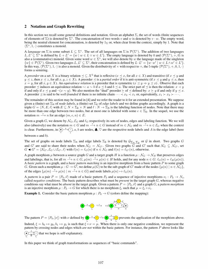
2 Notation and Graph Rewriting

In this section we recall some general definitions and notation. Given an alphabet Σ, the set of words (finite sequencesof elements of Σ) is denoted by Σ∗. The concatenation of two words v and w is denoted by v · w. The empty word,being the neutral element for concatenation, is denoted by 1Σ or, when clear from the context, simply by 1. Note that〈Σ∗, 1, ·〉 constitutes a monoid.

A language on Σ is some subset L ⊆ Σ∗. The set of all languages on Σ is P(Σ∗). The addition of two languagesL,L′ ⊆ Σ∗ is defined by L+ L′ = w | w ∈ L ∨ w ∈ L′. The empty language is denoted by 0 and 〈P(Σ∗),+, 0〉 isalso a (commutative) monoid. Given some word w ∈ Σ∗, we will also denote by w the language made of the singletonw ∈ P(Σ∗). Given two languages L,L′ ⊆ Σ∗, their concatenation is defined by L ·L′ = w ·w′ | w ∈ L∧w′ ∈ L′.In this way, 〈P(Σ∗), 1, ·〉 is also a monoid. Given the distributivity of×with respect to +, the 5-tuple 〈P(Σ∗),+, 0, 1, ·〉forms a semiring.

A preorder on a set X is a binary relation ⊆ X2 that is reflexive (x x, for all x ∈ X) and transitive (if x y andy z, then x z, for all x, y, z ∈ X). A preorder is a partial order if it is anti-symmetric (if x y and y x, thenx = y, for all x, y ∈ X). An equivalence relation is a preorder that is symmetric (x y ⇒ y x) . Observe that eachpreorder induces an equivalence relation ∼: a ∼ b if a b and b a. The strict part of is then the relation: x ≺ yif and only if x y and ¬(x ∼ y). We also mention the “dual” preorder of defined by: x y if and only if y x.A preorder is said to be well-founded if there is no infinite chain · · · ≺ x2 ≺ x1 or, equivalently, x1 x2 · · · .The remainder of this section may be found in [4] and we refer the reader to it for an extended presentation. We supposegiven a (finite) set ΣN of node labels, a (finite) set ΣE of edge labels and we define graphs accordingly. A graph is atriple G = 〈N,E, `〉 with E ⊆ N × ΣE ×N and ` : N → ΣN is the labeling function of nodes. Note that there maybe more than one edge between two nodes, but at most one is labeled with some e ∈ ΣE. In the sequel, we use thenotation m e−→ n for an edge (m, e, n) ∈ E.

Given a graph G, we denote by NG, EG and `G respectively its sets of nodes, edges and labeling function. We we willalso (abusively) use the notation m ∈ G and m e−→ n ∈ G instead of m ∈ NG and m e−→ n ∈ EG when the contextis clear. Furthermore, in ♣

a

♥b

A , a, b are nodes, ♣,♥ are the respective node labels and A is the edge label (here

between a and b).

The set of graphs on node labels ΣN and edge labels ΣE is denoted by GΣN,ΣEor G in short. Two graphs G

and G′ are said to share their nodes when NG = NG′ . Given two graphs G and G′ such that NG ⊆ NG′ , setG J G′ = 〈NG′ , EG ∪ EG′ , `〉 with `(n) = `G(n) if n ∈ NG and `(n) = `G′(n), otherwise.

A graph morphism µ between a source graph G and a target graph H is a function µ : NG → NH that preserves edgesand labelings, that is, for all m e−→ n ∈ G, µ(m)

e−→ µ(n) ∈ H holds, and for any node n ∈ G: `G(n) = `H(µ(n)).A basic pattern is a graph, and a basic pattern matching is an injective morphism from a basic pattern P to some graphG. Given such a morphism µ : G→ G′, we define µ(G) to be the sub-graph ofG′ made of the nodes µ(n) | n ∈ NG,of the edges µ(m)

e−→ µ(n) | m e−→ n ∈ G and node labels µ(n) 7→ `G(n).

A pattern is a pair P = 〈P0, ~ν〉 made of a basic pattern P0 and a sequence of injective morphisms νi : P0 → Ni,called negative conditions. The basic pattern describes what must be present in the target graph G, whereas negativeconditions say what must be absent in the target graph. Given a pattern P = 〈P0, ~ν〉 and a graph G, a pattern morphismis an injective morphism µ : P0 → G for which there is no morphism ξi such that µ = ξi νi.Example 1. Consider the basic pattern morphism µ : P0 → G (colors define the mapping):

♣b0

♥b1

A µ♣g0

♥g1

♣g2

A

B

D

C

AE

The pattern P = 〈P0, [ν]〉 with ν defined by ♣b0

♥b1

A ν ♣b0

♥b1

A

Bprevents the application of the morphism above.

Indeed, ξ = b0 7→ g0, b1 7→ g1 is such that ξ ν = µ. When there is only one negative condition, we represent thepattern by crossing nodes and edges which are not within the basic pattern. For instance, the pattern P above looks like

♣b0

♥b1

A

B× that we hope is self-explanatory.

In this paper we think of graph transformations as sequences of “basic commands”.

107

Definition 1 (The command language). There are three basic commands: label(p, α) for node renaming,del_edge(p, e, q) for edge deletion and add_edge(p, e, q) for edge creation. In these basic commands, p and qare nodes, α is some node label and e is some edge label. A pattern 〈P0, ~ν〉 is compatible with a command whenever allnodes that it involves belong to P0.

Definition 2 (Operational semantics). Given a pattern P = 〈P0, ~ν〉 compatible with some command c, and somepattern matching µ : P → G where G is the graph on which the transformation is applied, we have the followingpossible cases: c = label(p, α) turns the label of µ(p) into α, c = del_edge(p, e, q) removes µ(p)

e−→ µ(q) if itexists, otherwise does nothing, and c = add_edge(p, e, q) adds the edge µ(p)

e−→ µ(q) if it does not exist, otherwisedoes nothing. The graph obtained after such an application is denoted by G ·µ c. Given a sequence of commands~c = (c1, . . . , cn), let G ·µ ~c be the resulting graph, i.e., G ·µ ~c = (· · · ((G ·µ c1) ·µ c2) ·µ · · · cn).

Remark 1. We took a slightly simplified version of patterns. Actually, in [4], we have negative conditions withinpatterns to avoid some rule applications. But these simplifications should be transparent with respect to termination.Nevertheless, informally, we will omit the right node in a pattern like ♣

b0

· · ·B× to say that there is no edge labeled B

from node b0.

Definition 3. A rule is a pair R = 〈P,~c〉 made of a pattern and a (compatible) sequence of commands. Such a ruleR applies to a graph G via a pattern morphism µ : P → G. Let G′ = G ·µ ~c, then we write G→R,µ G

′. We defineG→ G′ whenever there is a rule R and a pattern morphism µ such that G→R,µ G

′.

2.1 The main example

Let ΣN = A and ΣE = α, β, T. For the discussion, we suppose that T is a working label, that is not presentin the initial graphs. We want to add a new edge β between node n and node 1 each time we find a maximal chain:A

1

A

2

A

3

· · · A

n

α α α α within a graph G. Consider the basic pattern Pinit = A

p

A

q

α together with its two

negative conditions ν1 = A A

p

A

q

αα× and ν2 = A A

p

A

q

αβ× . We consider three rules:

Init: 〈〈Pinit, [ν1, ν2]〉, (add_edge(p, T, q))〉 which fires the transitive closure.

Follow: 〈 A

p

A

q

A

r

T α , (add_edge(p, T, r), del_edge(p, T, q))〉 which follows the chain.

End: 〈 A

p

A

q

AT α× , (del_edge(p, T, q), add_edge(q, β, p))〉 which stops the procedure.

To prevent all pathological cases (e.g., when the edge β is misplaced, when two chains are crossing, and so on), wecould introduce more sophisticated patterns. But, since that does not change issues around termination, we avoidobscuring rules with such technicalities.

Example 2. Consider the graph G = A

1

A

2

A

3

α α . By applying succesively ’Init’, ’Follow’ and ’End’, G rewrites

as: A

1

A

2

A

3

α α → A

1

A

2

A

3

αα

T

→ A

1

A2

A

3

αα

T

→ A

1

A2

A

3

αα

β

2.2 Three technical facts about Graph Rewriting

It is well known that the main issue with graph rewriting definitions is the way the context is related to the pattern imageand its rewritten part. We shall tackle this issue with Proposition 1.

Self-application Let R = 〈P,~c〉 be the rule made of a pattern P = 〈P0, ~ν〉 and a sequence of commands ~c. There isthe identity morphism 1P0 : P0 → P0, and thus we can apply rule R on P0 itself, that is, P0 →R,1P0

P ′0 = P0 ·1P0~c.

We call this latter graph the self-application of R.

Rule node renaming To avoid heavy notation, we will use the following trick. Suppose that we are given a ruleR = 〈P,~c〉, a graph G and a pattern morphism µ : P → G. Let P = 〈P0, ~ν〉. We define Rµ to be the rule obtainedby renaming nodes p in P0 to µ(p) (and their references within ~c). For instance, the rule ’Follow’ can be rewritten asFollowµ = 〈 A

1

A

2

A

3

T α , (add_edge(1, T, 3), del_edge(1, T, 2))〉 where µ denotes the pattern morphism used

to apply ’Follow’ in the derivation. Observe that: (i) the basic pattern of Rµ is actually µ(P0), which is a subgraph of

108

G, (ii) ι : µ(P0)→ G mapping n 7→ n is a pattern matching, and (iii) applying rule Rµ with ι is equivalent to applyingrule R with µ. In other words, G→R,µ G

′ if (and only if) G→Rµ,ι G′. To sum up, we can always rewrite a rule so

that its basic pattern is actually a subgraph of G.

Uniform rules Let us consider rule ’Init’ above. It applies on: A

p

A

q

α

T , and the result is the graph itself: A

p

A

q

α

T .

Indeed, we cannot add an already present edge (relative to a label) within a graph. Thus, depending on the graph, therule will or will not append an edge. Such an unpredictable behavior can be easily avoided by modifying the pattern of

’Init’ to: A

p

A

q

α

T× . The same issue may come from edge deletions. A uniform rule is one for which commands apply

(that is, modify the graph) for each rule application. Since this is not the scope of the paper, we refer the reader to [4]for a precise definition of uniformity. We will only observe two facts.

First, any rule can be replaced by a finite set of uniform rules (using negative conditions as above) that operate identically.Thus, we can always suppose that rules are uniform.

Second, the following property holds for uniform rules (see [4]§7 for a proof).

Proposition 1. Suppose that G→R,ι G′ with R = 〈P,~c〉 and P = 〈P0, ~ν〉 (the basic pattern P0 being a subgraph of

G). Let C be the graph obtained from G by deleting the edges in P0. Then G = P0 J C and G′ = P ′0 J C with P ′0being the self-application of the rule. Moreover, EC ∩ EP0

= ∅ and EC ∩ EP ′0 = ∅.

Throughout the remainder of the paper we assume that all rules are uniform.

3 Termination of Graph Rewriting Systems

By a graph rewriting system (GRS) we simply mean a set of graph rewriting rules (see Section 2). A GRS R is saidto be terminating if there is no infinite sequence G1 → G2 → · · · . Such sequences, whether finite or not, are calledderivations.

Since there is no node creation (neither node deletion) in our notion of rewriting, any derivation starting from a graphG will lead to graphs whose size is the size of G. Since there are only finitely many such graphs, we can decide thetermination for this particular graph G. However, the question we address here is the uniform termination problem (seeSection 1).Remark 2. Suppose that we are given a strict partial order , not necessarily well founded. If G→ G′ implies G G′for all graphs G and G′, then the system is terminating. Indeed, suppose it is not the case, let G1 → G2 → · · · be aninfinite reduction sequence. Since there are only finitely many graphs of size of G1, it means that there are two indices iand j such that Gi → · · · → Gj with Gi = Gj . But then, since Gi Gi+1 · · · Gj , we have that Gi Gj = Giwhich is a contradiction.

A similar argument was exhibited by Dershowitz in [17] in the context of term rewriting. For instance, it is possible toembed rewriting within real numbers rather than natural numbers to prove termination.

Let us try to prove the termination of our main example (see Subsection 2.1). Rules such as ’Init’ and ’End’ are“simple”: we put a weight on edge labels ω : ΣE → R and we say that the weight of a graph is the sum of the weights ofits edges labels. Set ω(α) = 0, ω(β) = −2 and ω(T ) = −1. Then, rules ’Init’ and ’End’ decrease the weight by 1 and,since rule ’Follow’ keeps the weight constant, it means the two former rules can be applied only finitely many times.Observe that negative weights are no problem with respect to Remark 2.

But how do we handle rule ’Follow’? No weights as above can work.

3.1 A language point of view

Let G→ G′ be a rule application. The set of nodes stays constant. Let us think of graphs as automata, and let us forgetabout node labeling for the time being. Let ΣE be the set of edge labels. Consider a pair of states (nodes), choose one tobe the initial state and one to be the final state. Thus the automaton (graph) defines some regular language on ΣE. Infact, the automaton describes n2 languages (one for each pair of states).

Now, let us consider the effect of graph rewriting in terms of languages. Consider an application of the ’Follow’ rule:G→ G′. Any word to state r that goes through the transitions p T→ q

α→ r can be mapped to a shorter one in G′ viathe transition p T→ r. The languages corresponding to state r contain shorter words. The remainder of this section is

109

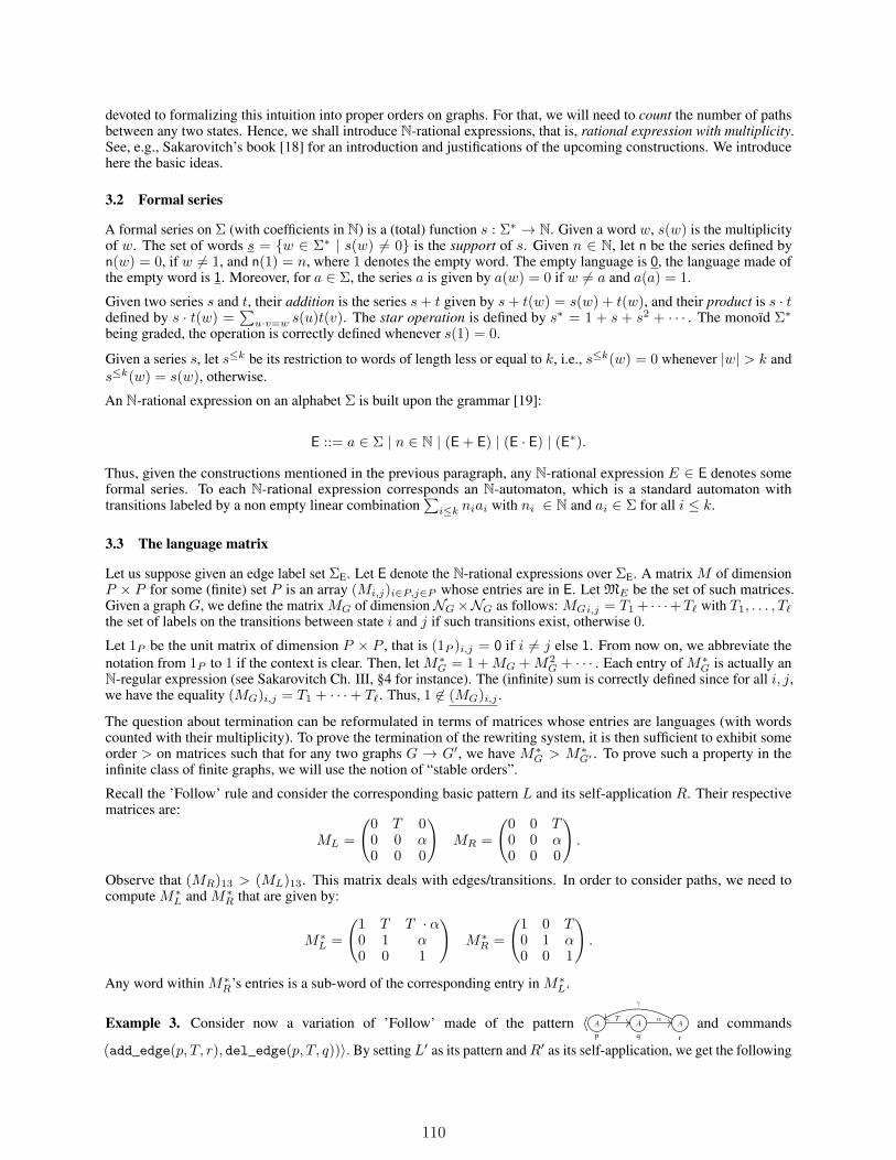
devoted to formalizing this intuition into proper orders on graphs. For that, we will need to count the number of pathsbetween any two states. Hence, we shall introduce N-rational expressions, that is, rational expression with multiplicity.See, e.g., Sakarovitch’s book [18] for an introduction and justifications of the upcoming constructions. We introducehere the basic ideas.

3.2 Formal series

A formal series on Σ (with coefficients in N) is a (total) function s : Σ∗ → N. Given a word w, s(w) is the multiplicityof w. The set of words s = w ∈ Σ∗ | s(w) 6= 0 is the support of s. Given n ∈ N, let n be the series defined byn(w) = 0, if w 6= 1, and n(1) = n, where 1 denotes the empty word. The empty language is 0, the language made ofthe empty word is 1. Moreover, for a ∈ Σ, the series a is given by a(w) = 0 if w 6= a and a(a) = 1.

Given two series s and t, their addition is the series s+ t given by s+ t(w) = s(w) + t(w), and their product is s · tdefined by s · t(w) =

∑u·v=w s(u)t(v). The star operation is defined by s∗ = 1 + s + s2 + · · · . The monoïd Σ∗

being graded, the operation is correctly defined whenever s(1) = 0.

Given a series s, let s≤k be its restriction to words of length less or equal to k, i.e., s≤k(w) = 0 whenever |w| > k ands≤k(w) = s(w), otherwise.

An N-rational expression on an alphabet Σ is built upon the grammar [19]:

E ::= a ∈ Σ | n ∈ N | (E + E) | (E · E) | (E∗).

Thus, given the constructions mentioned in the previous paragraph, any N-rational expression E ∈ E denotes someformal series. To each N-rational expression corresponds an N-automaton, which is a standard automaton withtransitions labeled by a non empty linear combination

∑i≤k niai with ni ∈ N and ai ∈ Σ for all i ≤ k.

3.3 The language matrix

Let us suppose given an edge label set ΣE. Let E denote the N-rational expressions over ΣE. A matrix M of dimensionP × P for some (finite) set P is an array (Mi,j)i∈P,j∈P whose entries are in E. Let ME be the set of such matrices.Given a graph G, we define the matrix MG of dimensionNG×NG as follows: MGi,j = T1 + · · ·+T` with T1, . . . , T`the set of labels on the transitions between state i and j if such transitions exist, otherwise 0.

Let 1P be the unit matrix of dimension P × P , that is (1P )i,j = 0 if i 6= j else 1. From now on, we abbreviate thenotation from 1P to 1 if the context is clear. Then, let M∗G = 1 +MG +M2

G + · · · . Each entry of M∗G is actually anN-regular expression (see Sakarovitch Ch. III, §4 for instance). The (infinite) sum is correctly defined since for all i, j,we have the equality (MG)i,j = T1 + · · ·+ T`. Thus, 1 6∈ (MG)i,j .

The question about termination can be reformulated in terms of matrices whose entries are languages (with wordscounted with their multiplicity). To prove the termination of the rewriting system, it is then sufficient to exhibit someorder > on matrices such that for any two graphs G → G′, we have M∗G > M∗G′ . To prove such a property in theinfinite class of finite graphs, we will use the notion of “stable orders”.

Recall the ’Follow’ rule and consider the corresponding basic pattern L and its self-application R. Their respectivematrices are:

ML =

(0 T 00 0 α0 0 0

)MR =

(0 0 T0 0 α0 0 0

).

Observe that (MR)13 > (ML)13. This matrix deals with edges/transitions. In order to consider paths, we need tocompute M∗L and M∗R that are given by:

M∗L =

(1 T T · α0 1 α0 0 1

)M∗R =

(1 0 T0 1 α0 0 1

).

Any word within M∗R’s entries is a sub-word of the corresponding entry in M∗L.

Example 3. Consider now a variation of ’Follow’ made of the pattern 〈 A

p

A

q

A

r

T α

γ

and commands

(add_edge(p, T, r), del_edge(p, T, q))〉. By setting L′ as its pattern andR′ as its self-application, we get the following

110

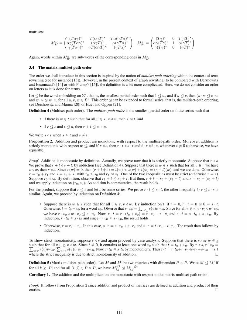
matrices:

M∗L′ =

((Tαγ)∗ T (αγT )∗ Tα(γTα)∗

αγ(Tαγ)∗ (αγT )∗ α(γTα)∗

γ(Tαγ)∗ γT (αγT )∗ (γTα)∗

)M∗R′ =

((Tγ)∗ 0 T (γT )∗

αγ(Tγ)∗ 1 α(γT )∗

γ(Tγ)∗ 0 (γT )∗

).

Again, words within M∗R′ are sub-words of the corresponding ones in M∗L′ .

3.4 The matrix multiset path order

The order we shall introduce in this section is inspired by the notion of multiset path ordering within the context of termrewriting (see for instance [13]). However, in the present context of graph rewriting (to be compared with Dershowitzand Jouannaud’s [14] or with Plump’s [15]), the definition is a bit more complicated. Here, we do not consider an orderon letters as it is done for terms.

LetE be the word embedding on Σ∗, that is, the smallest partial order such that 1 E w, and if u E v, then (u ·w E v ·wand w ·u E w · v, for all u, v, w ∈ Σ∗. This orderE can be extended to formal series, that is, the multiset-path ordering,see Dershowitz and Manna [20] or Huet and Oppen [21].

Definition 4 (Multiset path order). The multiset path order is the smallest partial order on finite series such that

• if there is w ∈ t such that for all v ∈ s, v / w, then s E t, and

• if r E s and t E u, then r + t E s+ u.

We write s / t when s E t and s 6= t.

Proposition 2. Addition and product are monotonic with respect to the multiset-path order. Moreover, addition isstrictly monotonic with respect to E, and if r / s, then r · t / s · t and t · r / t · s, whenever t 6= 0 (otherwise, we haveequality).

Proof. Addition is monotonic by definition. Actually, we prove now that it is strictly monotonic. Suppose that r / s.We prove that r + t / s+ t, by induction (see Definition 4). Suppose that there is w ∈ s such that for all v ∈ r we havev / w, then r / s. Since r(w) = 0, then (r + t)(w) = t(w) < s(w) + t(w) = (s+ t)(w), and we are done. Otherwise,r = r0 + r1 and s = s0 + s1 with r0 E s0 and r1 E s1. One of the two inequalities must be strict (otherwise r = s).Suppose r0 / s0. By definition, observe that r1 + t E s1 + t. But then, r + t = r0 + (r1 + t) and s = s0 + (s1 + t)and we apply induction on (r0, s0). As addition is commutative, the result holds.

For the product, suppose that r E s and let t be some series. We prove r · t E s · t; the other inequality t · r E t · s issimilar. Again, we proceed by induction on Definition 4:

• Suppose there is w ∈ s such that for all v ∈ r, v / w. By induction on t, if t = 0, r · t = 0 E 0 = s · t.Otherwise, t = t0 + v0 for a word v0. Observe that r · v0 =

∑v∈r r(v)v · v0. Since for all v ∈ r, v · v0 /w · v0,

we have r · v0 / w · v0 E s · v0. Now, r · t = r · (t0 + v0) = r · t0 + r · v0 and s · t = s · t0 + s · v0. Byinduction, r · t0 E s · t0 and since r · v0 E s · v0, the result holds.

• Otherwise, r = r0 + r1. In this case, s · r = s · r0 + s · r1 and t · r = t · r0 + t · r1. The result then follows byinduction.

To show strict monotonicity, suppose r / s and again proceed by case analysis. Suppose that there is some w ∈ ssuch that for all v ∈ r, v / w. Since t 6= 0, it contains at least one word v0 such that t = t0 + v0. By r / s, r · v0 =∑v∈r r(v)v·v0/

∑v∈s s(v)v·v0 = s·v0. Now, r·t0 E s·t0 by monotonicity. Thus r·t = r·t0+r·v0/s·t0+s·v0 = s·t

where the strict inequality is due to strict monotonicity of addition.

Definition 5 (Matrix multiset-path order). Let M and M ′ be two matrices with dimension P × P . Write M EM ′ iffor all k ≥ |P | and for all (i, j) ∈ P × P , we have M≤ki,j EM ′i,j

≤k.

Corollary 1. The addition and the multiplication are monotonic with respect to the matrix multiset-path order.

Proof. It follows from Proposition 2 since addition and product of matrices are defined as addition and product of theirentries.

111

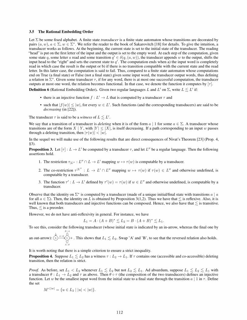
3.5 The Rational Embedding Order

Let Σ be some fixed alphabet. A finite state transducer is a finite state automaton whose transitions are decorated bypairs (a,w), a ∈ Σ, w ∈ Σ∗. We refer the reader to the book of Sakarovitch [18] for details. To give the intuition, atransducer works as follows. At the beginning, the current state is set to the initial state of the transducer. The reading“head” is put on the first letter of the input and the output is set to the empty word. At each step of the computation, givensome state q, some letter a read and some transition q′ ∈ δ(q, (a,w)), the transducer appends w to the output, shifts theinput head to the "right" and sets the current state to q′. The computation ends when a) the input word is completelyread in which case the result is the output or b) if there is no transition compatible with the current state and the readletter. In this latter case, the computation is said to fail. Thus, compared to a finite state automaton whose computationsend on True (a final state) or False (not a final state) given some input word, the transducer output words, thus defininga relation in Σ∗. Given some transducer τ , if for any word, there is at most one successful computation, the transduceroutputs at most one word, the relation becomes functional. In that case, we denote the function it computes by [τ ].Definition 6 (Rational Embedding Order). Given two regular languages L and L′ on Σ, write L . L′ if:

• there is an injective function f : L′ → L that is computed by a transducer τ and

• such that |f(w)| ≤ |w|, for every w ∈ L′. Such functions (and the corresponding transducers) are said to bedecreasing (in [22]).

The transducer τ is said to be a witness of L . L′.We say that a transition of a transducer is deleting when it is of the form a | 1 for some a ∈ Σ. A transducer whosetransitions are of the form X | Y , with |Y | ≤ |X|, is itself decreasing. If a path corresponding to an input w passesthrough a deleting transition, then |τ(w)| < |w|.In the sequel we will make use of the following results that are direct consequences of Nivat’s Theorem [23] (Prop. 4,§3).Proposition 3. Let [τ ] : L→ L′ be computed by a transducer τ , and let L′′ be a regular language. Then the followingassertions hold.

1. The restriction τ|L′′ : L′′ ∩ L→ L′ mapping w 7→ τ(w) is computable by a transducer.

2. The co-restriction τ |L′′

: L → L′ ∩ L′′ mapping w 7→ τ(w) if τ(w) ∈ L′′ and otherwise undefined, iscomputable by a transducer.

3. The function τ ′ : L→ L′ defined by τ ′(w) = τ(w) if w ∈ L′′ and otherwise undefined, is computable by atransducer.

Observe that the identity on Σ∗ is computed by a transducer (made of a unique initial/final state with transitions a | afor all a ∈ Σ). Then, the identity on L is obtained by Proposition 3(1,2). Thus we have that . is reflexive. Also, it iswell known that both transducers and injective functions can be composed. Hence, we also have that . is transitive.Thus, . is a preorder.

However, we do not have anti-reflexivity in general. For instance, we have

L1 = A · (A+B)∗ . L2 = B · (A+B)∗ . L1.

To see this, consider the following transducer (whose initial state is indicated by an in-arrow, whereas the final one by

an out-arrow): q0 q1A | B

B | A

A | B

. This shows that L1 . L2. Swap ’A’ and ’B’, to see that the reversed relation also holds.

It is worth noting that there is a simple criterion to ensure a strict inequality.Proposition 4. Suppose L1 . L2 has a witness τ : L2 → L1. If τ contains one (accessible and co-accessible) deletingtransition, then the relation is strict.

Proof. As before, set L1 < L2 whenever L1 . L2 but not L2 . L1. Ad absurdum, suppose L1 . L2 . L1 witha transducer θ : L1 → L2 and τ as above. Then θ τ (the composition of the two transducers) defines an injectivefunction. Let w be the smallest input word from the initial state to a final state through the transition a | 1 in τ . Definethe set

M<|w| = u ∈ L2 | |u| < |w|.

112

For any word u, we have |θ τ(u)| ≤ |u|. Thus θ τ(M<w) ⊆M<w. Since M<w is a finite set and θ τ is injective,it is actually bijective when restricted to M<w. However, |θ τ(w)| ≤ |τ(w)| < w implies θ τ(w) ∈M<w. By thePigeon-hole Principle, there is one word in M<w that has two pre-images via θ τ . Thus, θ τ cannot be injective,which yields a contradiction.

Remark 3. From Proposition 3 it follows that if two regular languages L and L′ are such that L ⊆ L′, then L . L′.Definition 7. The rational embedding order extends to matrices by pointwise ordering: Let M and N with dimensionP × P , and write M . N if for every i, j ∈ P × P , we have Mi,j . Ni,j .

Recall the modified version of ’Follow’ (Example 3). The following transducers show that all entries strictly decrease.

q0 q1 q2T | T α | 1

γ | γ

q−1 q0 q1 q2T | 1 T | 1 α | 1

γ | 1

q−1q−2 q0 q1 q2T | T α | 1 T | T α | 1

γ | γ

q−1q−2 q0 q1 q2α | α γ | γ T | T α | 1

γ | γ

q−1

q−2 q−3

q0 q1 q2

T | 1

α | 1

γ | 1 T | T α | 1

γ | γ

q−1 q0 q1 q2α | α γ | γ T | T

α | 1

q−1 q0 q1 q2γ | γ T | T α | 1

γ | γ

q−1q−2 q0 q1 q2γ | 1 T | 1 α | 1 γ | 1

T | 1

q0 q1 q2γ | γ T | T

α | 1

In the following, to compare two graphs by means of the rational embedding order, we transform graphs into matricesas follows. Given a graph G, let M ′G be the matrix of dimensionNG ×NG such that (M ′G)i,j = T i,j1 +T i,j2 + · · ·T i,j`with T1, . . . , T` the labels of the edges from i to j. In other words, we “decorate” the labels with the source and targetnodes. Then, G . G′ whenever M ′G .M ′G′ .

3.6 Stable orders on matrices

A matrix on E is said to be finite whenever all its entries are finite. Two matrices M and M ′ (of same dimension) on Eare said to be disjoint if for every i, j, Mi,j ·M ′i,j = 0.Definition 8. Let M be a matrix of dimension P × P and P ⊆ G. The extension of M to dimension G ×G is thematrix M↑G defined by:

(M↑G)i,j =

Mi,j if i, j ∈ P0 otherwise

The notation M↑G is shortened to M↑ when G is clear from the context.Fact 1. Let M be a matrix of dimension P × P , with P ⊆ G. Then (M↑G)∗ = (M∗)↑G.

Definition 9. We say that a partial order on E is stable by context if for every P ⊆ G, all matrices L and R ofdimension P × P , and every C of dimension G×G, the following assertions hold.

1. If L,R,C are finite, L being disjoint from C, R being disjoint from C and R∗ ≺ L∗, then (R + C)∗ ≺(L+ C)∗;

2. If R ≺ L, then R↑G ≺ L↑G.Lemma 1. Let be a partial order stable by context and consider finite matrices L,R of dimension P × P and let Cbe a finite matrix of dimension G×G with P ⊆ G. Then, R∗ ≺ L∗ implies (R↑ + C)∗ ≺ (L↑ + C)∗.

Proof. If R∗ ≺ L∗, then we have (R∗)↑ ≺ (L∗)↑ by Definition 9.2. By Lemma 1, it follows that (R↑)∗ ≺ (L↑)∗.Clearly, R↑ and L↑ are finite, and from Definition 9.1, we have (R↑ + C)∗ ≺ (L↑ + C)∗

Theorem 1. Let be a partial order stable by context. Suppose that for every rule R = 〈P,~c〉 with P = 〈P0, ~ν〉 andP ′0 the self-application of R, we have (P ′0)∗ ≺ (P0)∗. Then the corresponding GRS is terminating.

Proof. Let be a partial order on graphs and consider the corresponding order on matrices: G ≺ G′ if and only ifM∗G ≺M∗G′ . We show that for every rule, we have G→ G′ implies G′ ≺ G. So let R be a graph rewriting rule and letµ be a morphism such that G→R,µ G

′. By the discussion in the beginning of Section 3, without loss of generality, we

113

can suppose that µ is actually the inclusion of pattern P0 in G. Now, let P0 and P ′0 be respectively the basic pattern andthe self-application of R. Define C to be the graph made of the nodes of G without edges in P0. By Proposition 1,MG = M↑P0

+MC and MG′ = M↑P ′0+MC . Moreover, MP0

,MP ′0 and MC are finite, MP0is disjoint from MC , and

MP ′0 is disjoint from MC . From Lemma 1 it thus follows that M∗G′ = (M↑P ′0+MC)∗ ≺ (M↑P0

+MC)∗ = M∗G.

3.7 Stability of the orderings

We can now prove the two announced stability results.Proposition 5. The multiset path ordering is stable by context.

Proof. We first verify that condition 2 of Definition 9 holds. Suppose that R / L with R,L of dimension P × P .Then, for all (i, j) 6∈ P × P , R↑Gi,j = 0 E 0 = L↑Gi,j . Now, for all k ≥ |G| ≥ |P | and for all (i, j) ∈ P × P , we have(R↑G)≤ki,j = R≤ki,j E L

≤ki,j = (L↑G)≤ki,j . To verify that condition 1 also holds, let G×G be the dimension of L,R and C.

Take k ≥ |G|. On the one side we have

(R+ C)∗≤k =∑

(A1,...,A`)∈R,C∗, `≤k

∏

i≤`Ai

and on the other side

(L+ C)∗≤k =∑

(A1,...,A`)∈R,C∗|`≤k

∏

i≤`AiR← L,

where AiR ← L = L if Ai = R, and C otherwise. As the product and the addition are (strictly) monotonic, theresult follows.

Proposition 6. The rational embedding order is stable by context.

Proof. Since we use a component-wise ordering, it is easy to verify that condition 2 of Definition 9 holds. To verifythat condition 1 also holds, let P × P be the shared dimension of L,R and C of dimension G×G with P ⊆ G. SinceR < L, there are decreasing transducers τi,j : Li,j → Ri,j with at least one of them deleting. We build the family oftransducers (θp,q)p,q∈G×G as follows. The family of transducers will share the major part of the construction. Theyonly differ by their initial and terminal states. First, we make a copy of all transducers (τi,j)i,j . Then, we add as states

all the elements of G outside P . Given a non null entry T = Ci,j , we set a transition iT i,j |T i,j−→ j. That is the transducer

"copies" the paths within C. For a an entry T = Ci,j with i 6∈ P, j ∈ P , we set the transitions: iT i,j |T i,j−→ qn for all qn

initial state of the transducer τj,n, n ∈ P . Similarly, for any entry T = Ci,j with i ∈ P, j 6∈ P , we set the transitions:

rnT i,j |T i,j−→ j for each terminal state rn of the transducer τn,i, n ∈ P . This construction can be represented as follows:

ij ij

T i,j | T i,j

U j,i | U j,ip

q

r

s

V i,k | V i,k

W i,` |W i,`

τk,m

τ`,n

· · ·

· · ·

· · ·Xm,i | Xm,i

Y n,i | Y n,i

where U, T,W,X, Y range over the edge labels. Take k, ` 6∈ P . Any path from state k to state ` describes a path inC + L on the input side and a path in C +R on the output side. Indeed, transitions within C are simply copied and thetransducers τi,j transform paths in L into paths in R.

It remains to specify initial and final states of θp,q with (p, q) ∈ G×G. Given some entry p, q ∈ G, if p 6∈ P , we set

the initial state to be p. Otherwise, we introduce a new state ι which is set to be initial, and we add a transition ι1|1−→ i

for any state i initial in τp,r for some r. If q 6∈ P , then, q is the final state. Otherwise, any state j within some τr,q,r ∈ P , is final.

114

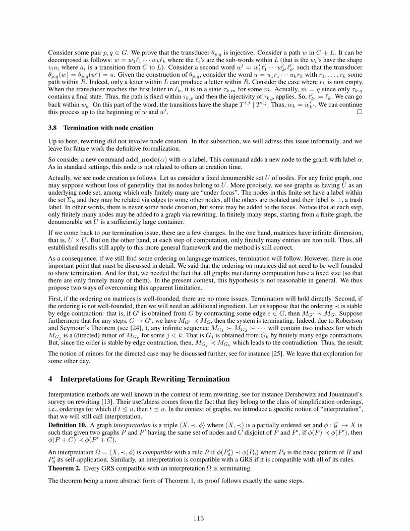
Consider some pair p, q ∈ G. We prove that the transducer θp,q is injective. Consider a path w in C + L. It can bedecomposed as follows: w = w1`1 · · ·wk`k where the `i’s are the sub-words within L (that is the wi’s have the shapeviai where ai is a transition from C to L). Consider a second word w′ = w′1`

′1 · · ·w′k′`′k′ such that the transducer

θp,q(w) = θp,q(w′) = u. Given the construction of θp,q, consider the word u = u1r1 · · ·ukrk with r1, . . . , rk some

path within R. Indeed, only a letter within L can produce a letter within R. Consider the case where rk is non empty.When the transducer reaches the first letter in `k, it is in a state τk,m for some m. Actually, m = q since only τk,qcontains a final state. Thus, the path is fixed within τk,p and then the injectivity of τk,p applies. So, `′k′ = `k. We can goback within wk. On this part of the word, the transitions have the shape T i,j | T i,j . Thus, wk = w′k′ . We can continuethis process up to the beginning of w and w′.

3.8 Termination with node creation

Up to here, rewriting did not involve node creation. In this subsection, we will adress this issue informally, and weleave for future work the definitive formalization.

So consider a new command add_node(α) with α a label. This command adds a new node to the graph with label α.As in standard settings, this node is not related to others at creation time.

Actually, we see node creation as follows. Let us consider a fixed denumerable set U of nodes. For any finite graph, onemay suppose without loss of generality that its nodes belong to U . More precisely, we see graphs as having U as anunderlying node set, among which only finitely many are “under focus”. The nodes in this finite set have a label withinthe set ΣN and they may be related via edges to some other nodes, all the others are isolated and their label is ⊥, a trashlabel. In other words, there is never some node creation, but some may be added to the focus. Notice that at each step,only finitely many nodes may be added to a graph via rewriting. In finitely many steps, starting from a finite graph, thedenumerable set U is a sufficiently large container.

If we come back to our termination issue, there are a few changes. In the one hand, matrices have infinite dimension,that is, U × U . But on the other hand, at each step of computation, only finitely many entries are non null. Thus, allestablished results still apply to this more general framework and the method is still correct.

As a consequence, if we still find some ordering on language matrices, termination will follow. However, there is oneimportant point that must be discussed in detail. We said that the ordering on matrices did not need to be well foundedto show termination. And for that, we needed the fact that all graphs met during computation have a fixed size (so thatthere are only finitely many of them). In the present context, this hypothesis is not reasonable in general. We thuspropose two ways of overcoming this apparent limitation.

First, if the ordering on matrices is well-founded, there are no more issues. Termination will hold directly. Second, ifthe ordering is not well-founded, then we will need an additional ingredient. Let us suppose that the ordering ≺ is stableby edge contraction: that is, if G′ is obtained from G by contracting some edge e ∈ G, then MG′ ≺ MG. Supposefurthermore that for any steps, G→ G′, we have MG′ ≺MG, then the system is terminating. Indeed, due to Robertsonand Seymour’s Theorem (see [24], ), any infinite sequence MG1

MG2 · · · will contain two indices for which

MGj is a (directed) minor of MGk for some j < k. That is Gj is obtained from Gk by finitely many edge contractions.But, since the order is stable by edge contraction, then, MGj ≺MGk which leads to the contradiction. Thus, the result.

The notion of minors for the directed case may be discussed further, see for instance [25]. We leave that exploration forsome other day.

4 Interpretations for Graph Rewriting Termination

Interpretation methods are well known in the context of term rewriting, see for instance Dershowitz and Jouannaud’ssurvey on rewriting [13]. Their usefulness comes from the fact that they belong to the class of simplification orderings,i.e., orderings for which if t E u, then t u. In the context of graphs, we introduce a specific notion of “interpretation”,that we will still call interpretation.Definition 10. A graph interpretation is a triple 〈X,≺, φ〉 where 〈X,≺〉 is a partially ordered set and φ : G → X issuch that given two graphs P and P ′ having the same set of nodes and C disjoint of P and P ′, if φ(P ) ≺ φ(P ′), thenφ(P + C) ≺ φ(P ′ + C).

An interpretation Ω = 〈X,≺, φ〉 is compatible with a rule R if φ(P ′0) ≺ φ(P0) where P0 is the basic pattern of R andP ′0 its self-application. Similarly, an interpretation is compatible with a GRS if it is compatible with all of its rules.Theorem 2. Every GRS compatible with an interpretation Ω is terminating.

The theorem being a more abstract form of Theorem 1, its proof follows exactly the same steps.

115

Proof. Suppose that G ≺ G′ if and only if φ(G) ≺ φ(G′). We prove that for each rule R of the GRS, G→ G′ impliesG′ ≺ G. Indeed, suppose that G →R,µ G

′. Let P0 and P ′0 be respectively the basic pattern and the self-applicationof R. Then, there is a graph C such that G = P0 + C, G′ = P ′0 + C, such that P0 and P ′0 are disjoint from C. Sinceφ(P ′0) ≺ φ(P ), we then have φ(G′) ≺ φ(G).

Example 4. The triple 〈M,E, (M(−))∗〉 is an interpretation for ’Follow’.

Example 5. Let us come back to the weight analysis. Define ω(G) =∑pe−→q∈G ω(e) with ω(α) = 0, ω(T ) =

−1, ω(β) = −1. Then, 〈R, <, ω(−)〉 is an interpretation for ’Init’ and ’End’.Example 6. Let 〈X1,≺1, φ1〉 be an interpretation for a set of rulesR1, and let 〈X2,≺2, φ2〉 be an interpretation for aset of rulesR2. Suppose that for every rule R inR2, G→R,µ G

′ implies G′ 1 G (that is without strict inequality).Then the lexicographic ordering on X1 ×X2 defined by (x1, x2) ≺1,2 (y1, y2) if and only if x1 ≺1 y1, or x1 1 y1

and x2 ≺2 y2, constitutes an interpretation 〈X1 ×X2,≺1,2, φ1 × φ2〉 forR1 ∪R2.

Thus, combining Example 4 and Example 5, we have a proof of the termination of the Main Example (Subsection 2.1).Corollary 2. The GRS given in Subsection 2.1 is terminating.Example 7. LetR be a terminating GRS. Then there is an interpretation that “justifies” this fact. Indeed, take 〈G,≺, 1G〉with ≺ defined to be the transitive closure of the rewriting relation→. The termination property ensures that the closureleads to an irreflexive relation. The compatibility of ≺ with respect to 1G is immediate.

We thus have the following corollary.Corollary 3. A GRS is terminating if and only if it is compatible with some interpretation.

5 Conclusion

We proposed a new approach based on the theory of regular languages to decide the termination of graph rewritingsystems, which does not account for node additions but settles the uniform termination problem for these GRS. Wethink that there is room to reconsider some old results of this theory under the new light. In particular, we think ofprofinite topology [26], is a powerful tool that could give us some insight on the underlying structure of the orders. Inthe two cases, we can extend the orders to take into account orders on the edge labels.

As the next natural step, we intend to explore more systematically graph rewriting with node creations and that take intoaccount node labels. Moreover, in the experiments mentioned in the introduction about natural language processing, inprinciple, these two orders should still be sufficient to ensure termination. However, we need to implement these newresults for an extensive and complete evaluation.

Acknowledgment. The authors are thankful to the anonymous reviewers for their careful reading of our manuscriptand for the constructive remarks and useful suggestions, that were of great help when revising this manuscript.

References

[1] Noam Chomsky. Syntactic Structures. The Hague: Mouton, 1957.[2] Bruno Guillaume and Guy Perrier. Dependency parsing with graph rewriting. In Proceedings of the 14th

International Conference on Parsing Technologies, IWPT 2015, Bilbao, Spain, July 5-7, 2015, pages 30–39, 2015.[3] Sylvain Kahane and François Lareau. Word ordering as a graph rewriting process. In Formal Grammar - 20th and

21st International Conferences, FG 2015, Barcelona, Spain, August 2015, Revised Selected Papers. FG 2016,Bozen, Italy, August 2016, Proceedings, volume 9804, pages 216–239. Springer, 2016.

[4] Guillaume Bonfante, Bruno Guillaume, and Guy Perrier. Application of Graph Rewriting to Natural LanguageProcessing. Logic, Linguistic and Computer Science. Wiley, 2018.

[5] Grzegorz Rozenberg, editor. Handbook of Graph Grammars and Computing by Graph Transformation: Volume I.Foundations. World Scientific Publishing Co., Inc., River Edge, NJ, USA, 1997.

[6] Bruno Courcelle and Joost Engelfriet. Graph Structure and Monadic Second-Order Logic. Cambridge UniversityPress, 2012.

[7] Mizuhito Ogawa. A note on algebraic structure of tree decomposition of graphs. In The First Asian Workshop onProgramming Languages and Systems, APLAS 2000, National University of Singapore, Singapore, December18-20, 2000, Proceedings, pages 223–229, 2000.

116

[8] Yves Lafont. Interaction nets. In Conference Record of the Seventeenth Annual ACM Symposium on Principles ofProgramming Languages, San Francisco, California, USA, January 1990, pages 95–108, 1990.

[9] Maribel Fernández, Hélène Kirchner, and Bruno Pinaud. Strategic port graph rewriting: an interactive modellingframework. Mathematical Structures in Computer Science, 29(5):615–662, 2019.

[10] Nachum Dershowitz and Jean-Pierre Jouannaud. Drags: A compositional algebraic framework for graph rewriting.Theor. Comput. Sci., 777:204–231, 2019.

[11] Géraud Sénizergues. Some undecidable termination problems for semi-Thue systems. Theoretical ComputerScience, 142:257–276, 1995.

[12] Guillaume Bonfante and Bruno Guillaume. Non-simplifying graph rewriting termination. In Proceedings 7thInternational Workshop on Computing with Terms and Graphs, TERMGRAPH 2013, Rome, Italy, 23th March2013, pages 4–16, 2013.

[13] Nachum Dershowitz and Jean-Pierre Jouannaud. Rewrite systems. In Handbook of Theoretical Computer Science,Volume B: Formal Models and Semantics, pages 243–320. 1990.

[14] Nachum Dershowitz and Jean-Pierre Jouannaud. Graph path orderings. In LPAR-22. 22nd International Conferenceon Logic for Programming, Artificial Intelligence and Reasoning, Awassa, Ethiopia, 16-21 November 2018, pages307–325, 2018.

[15] Detlef Plump. Simplification orders for term graph rewriting. In Igor Prívara and Peter Ružicka, editors,Mathematical Foundations of Computer Science 1997, pages 458–467, Berlin, Heidelberg, 1997. Springer BerlinHeidelberg.

[16] Jörg Endrullis, Johannes Waldmann, and Hans Zantema. Matrix interpretations for proving termination of termrewriting. Journal of Automated Reasoning, 40(2):195–220, Mar 2008.

[17] Nachum Dershowitz. A note on simplification orderings. Information Processing Letters, pages 212–215, 1979.[18] Jacques Sakarovitch. Elements of Automata Theory. Cambridge University Press, 2009.[19] Jan Rutten. Behavioural differential equations: a coinductive calculus of streams, automata, and power series.

Theoretical Computer Science, 308(1):1 – 53, 2003.[20] Nachum Dershowitz and Zohar Manna. Proving termination with multiset orderings. Commun. ACM, 22(8), 1979.[21] Gerard Huet and Derek C. Oppen. Equations and rewrite rules: a survey. In In formal language Theory: perspective

and open problems. Academic Press, 1980.[22] Jeannine Leguy. Transductions rationnelles décroissantes. RAIRO. Informatique théorique, 15(2):141–148, 1981.[23] Maurice Nivat. Transducteurs des langages de Chomsky. Ann. Inst. Fourier, Grenoble, 18:339–455, 1968.[24] Neil Robertson and Paul D. Seymour. Graph minors. XX. Wagner’s conjecture. J. Comb. Theory, Ser. B,

92(2):325–357, 2004.[25] Shiva Kintali and Qiuyi Zhang. Forbidden directed minors and Kelly-width. Theoretical Computer Science,

662:40 – 47, 2017.[26] Jean-Eric Pin. Profinite methods in automata theory. In 26th International Symposium on Theoretical Aspects of

Computer Science, STACS 2009, February 26-28, 2009, Freiburg, Germany, Proceedings, volume 3 of LIPIcs,pages 31–50. Schloss Dagstuhl - Leibniz-Zentrum fuer Informatik, Germany, 2009.

117

INVERSION NUMBER OF AN ORIENTED GRAPH AND RELATEDPARAMETERS

Jørgen Bang-JensenDepartment of Mathematics and Computer Science,

University of Southern DenmarkOdense, Denmark

[email protected]

Jonas Costa Ferreira da SilvaDepartment of Computer Science

Universidade Federal do CearáFortaleza, Brazil

[email protected]

Frédéric HavetUniversité Côte d’Azur, CNRS, Inria, I3S,

Sophia Antipolis, [email protected]

ABSTRACT

Let D be an oriented graph. The inversion of a set X of vertices in D consists in reversing thedirection of all arcs with both ends in X . The inversion number of D, denoted by inv(D), is theminimum number of inversions needed to make D acyclic. Denoting by τ(D), τ ′(D), and ν(D)the cycle transversal number, the cycle arc-transversal number and the cycle packing number ofD respectively, one shows that inv(D) ≤ τ ′(D), inv(D) ≤ 2τ(D) and there exists a function gsuch that inv(D) ≤ g(ν(D)). We conjecture that for any two oriented graphs L and R, inv(L →R) = inv(L) + inv(R) where L → R is the dijoin of L and R. This would imply that the firsttwo inequalities are tight. We prove this conjecture when inv(L) ≤ 1 and inv(R) ≤ 2 and wheninv(L) = inv(R) = 2 and L and R are strongly connected. We also show that the function g of thethird inequality satisfies g(1) ≤ 4.We then consider the complexity of deciding whether inv(D) ≤ k for a given oriented graph D. Weshow that it is NP-complete for k = 1, which together with the above conjecture would imply that itis NP-complete for every k. This contrasts with a result of Belkhechine et al. [6] which states thatdeciding whether inv(T ) ≤ k for a given tournament T is polynomial-time solvable.

Keywords Feedback vertex set · Feedback arc set · Inversion · Tournament · Oriented graph · Intercyclic digraph.

1 Introduction

Notation not given below is consistent with [2]. Making a digraph acyclic by either removing a mininum cardinality setof arcs or vertices are important and heavily studied problems, known under the names CYCLE ARC TRANSVERSALor FEEDBACK ARC SET and CYCLE TRANSVERSAL or FEEDBACK VERTEX SET. A cycle transversal or feedbackvertex set (resp. cycle arc-transversal or feedback arc set) in a digraph is a set of vertices (resp. arcs) whose deletionresults in an acyclic digraph. The cycle transversal number (resp. cycle arc-transversal number) is the minimumsize of a cycle transversal (resp. cycle arc-transversal) of D and is denoted by τ(D) (resp. τ ′(D)). Note that if F isa minimum cycle arc-transversal in a digraph D = (V,A), then we will obtain an acyclic digraph from D by eitherremoving the arcs of F or reversing each of these, that is replacing each arc uv ∈ F by the arc vu. It is well-known andeasy to show that τ(D) ≤ τ ′(D) (just take one end-vertex of each arc in a minimum cycle arc-transversal).

Computing τ(D) and τ ′(D) are two of the first problems shown to be NP-hard listed by Karp in [9]. They also remainsNP-complete in tournaments as shown by Bang-Jensen and Thomassen [4] and Speckenmeyer [14] for τ , and byAlon [1] and Charbit, Thomassé, and Yeo [7].

119

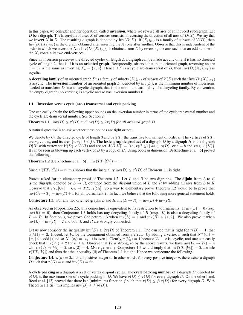
In this paper, we consider another operation, called inversion, where we reverse all arcs of an induced subdigraph. LetD be a digraph. The inversion of a set X of vertices consists in reversing the direction of all arcs of D〈X〉. We say thatwe invert X in D. The resulting digraph is denoted by Inv(D;X). If (Xi)i∈I is a family of subsets of V (D), thenInv(D; (Xi)i∈I) is the digraph obtained after inverting the Xi one after another. Observe that this is independent of theorder in which we invert the Xi : Inv(D; (Xi)i∈I) is obtained from D by reversing the arcs such that an odd number ofthe Xi contain its two end-vertices.

Since an inversion preserves the directed cycles of length 2, a digraph can be made acyclic only if it has no directedcycle of length 2, that is if it is an oriented graph. Reciprocally, observe that in an oriented graph, reversing an arca = uv is the same as inverting Xa = u, v. Hence if F is a cycle arc-transversal of D, then Inv(D; (Xa)a∈F ) isacyclic.

A decycling family of an oriented graphD is a family of subsets (Xi)i∈I of subsets of V (D) such that Inv(D; (Xi)i∈I)is acyclic. The inversion number of an oriented graph D, denoted by inv(D), is the minimum number of inversionsneeded to transform D into an acyclic digraph, that is, the minimum cardinality of a decycling family. By convention,the empty digraph (no vertices) is acyclic and so has inversion number 0.

1.1 Inversion versus cycle (arc-) transversal and cycle packing

One can easily obtain the following upper bounds on the inversion number in terms of the cycle transversal number andthe cycle arc-transversal number. See Section 2.Theorem 1.1. inv(D) ≤ τ ′(D) and inv(D) ≤ 2τ(D) for all oriented graph D.

A natural question is to ask whether these bounds are tight or not.

We denote by ~C3 the directed cycle of length 3 and by TTn the transitive tournament of order n. The vertices of TTnare v1, . . . , vn and its arcs vivj | i < j. The lexicographic product of a digraph D by a digraph H is the digraphD[H] with vertex set V (D)× V (H) and arc set A(D[H]) = (a, x)(b, y) | ab ∈ A(D), or a = b and xy ∈ A(H).It can be seen as blowing up each vertex of D by a copy of H . Using boolean dimension, Belkhechine et al. [5] provedthe following.

Theorem 1.2 (Belkhechine et al. [5]). inv(TTn[ ~C3]) = n.

Since τ ′(TTn[ ~C3]) = n, this shows that the inequality inv(D) ≤ τ ′(D) of Theorem 1.1 is tight.

Pouzet asked for an elementary proof of Theorem 1.2. Let L and R be two digraphs. The dijoin from L to Ris the digraph, denoted by L → R, obtained from the disjoint union of L and R by adding all arcs from L to R.Observe that TTn[~C3] = ~C3 → TTn−1[~C3]. So a way to elementary prove Theorem 1.2 would be to prove thatinv(~C3 → T ) = inv(T ) + 1 for all tournament T . In fact, we believe that the following more general statement holds.

Conjecture 1.3. For any two oriented graphs L and R, inv(L→ R) = inv(L) + inv(R).

As observed in Proposition 2.5, this conjecture is equivalent to its restriction to tournaments. If inv(L) = 0 (resp.inv(R) = 0), then Conjecture 1.3 holds has any decycling family of R (resp. L) is also a decycling family ofL → R. In Section 3, we prove Conjecture 1.3 when inv(L) = 1 and inv(R) ∈ 1, 2. We also prove it wheninv(L) = inv(R) = 2 and both L and R are strongly connected.

Let us now consider the inequality inv(D) ≤ 2τ(D) of Theorem 1.1. One can see that is tight for τ(D) = 1, thatis h(1) = 2. Indeed, let Vn be the tournament obtained from a TTn−1 by adding a vertex x such that N+(vi) =vi | i is odd (and so N−(vi) = vi | i is even. Clearly, τ(Vn) = 1 because Vn − x is acyclic, and one can easilycheck that inv(Vn) ≥ 2 for n ≥ 5. Observe that V5 is strong, so by the above results, we have inv(V5 → V5) = 4while τ(V5 → V5) = 2, so h(2) = 4. More generally, Conjecture 1.3 would imply that inv(TTn[V5]) = 2n, whileτ(TTn[V5]) and thus that the inequality (ii) of Theorem 1.1 is tight. Hence we conjecture the following.Conjecture 1.4. h(n) = 2n for all positive integer n. In other words, for every positive integer n, there exists a digraphD such that τ(D) = n and inv(D) = 2n.

A cycle packing in a digraph is a set of vertex disjoint cycles. The cycle packing number of a digraph D, denoted byν(D), is the maximum size of a cycle packing in D. We have ν(D) ≤ τ(D) for every digraph D. On the other hand,Reed et al. [12] proved that there is a (minimum) function f such that τ(D) ≤ f(ν(D)) for every digraph D. WithTheorem 1.1 (ii), this implies inv(D) ≤ f(ν(D)).

120

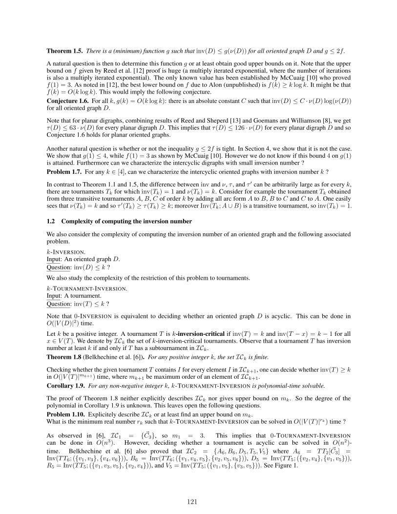
Theorem 1.5. There is a (minimum) function g such that inv(D) ≤ g(ν(D)) for all oriented graph D and g ≤ 2f .

A natural question is then to determine this function g or at least obtain good upper bounds on it. Note that the upperbound on f given by Reed et al. [12] proof is huge (a multiply iterated exponential, where the number of iterationsis also a multiply iterated exponential). The only known value has been established by McCuaig [10] who provedf(1) = 3. As noted in [12], the best lower bound on f due to Alon (unpublished) is f(k) ≥ k log k. It might be thatf(k) = O(k log k). This would imply the following conjecture.Conjecture 1.6. For all k, g(k) = O(k log k): there is an absolute constant C such that inv(D) ≤ C · ν(D) log(ν(D))for all oriented graph D.

Note that for planar digraphs, combining results of Reed and Sheperd [13] and Goemans and Williamson [8], we getτ(D) ≤ 63 · ν(D) for every planar digraph D. This implies that τ(D) ≤ 126 · ν(D) for every planar digraph D and soConjecture 1.6 holds for planar oriented graphs.

Another natural question is whether or not the inequality g ≤ 2f is tight. In Section 4, we show that it is not the case.We show that g(1) ≤ 4, while f(1) = 3 as shown by McCuaig [10]. However we do not know if this bound 4 on g(1)is attained. Furthermore can we characterize the intercyclic digraphs with small inversion number ?Problem 1.7. For any k ∈ [4], can we characterize the intercyclic oriented graphs with inversion number k ?

In contrast to Theorem 1.1 and 1.5, the difference between inv and ν, τ , and τ ′ can be arbitrarily large as for every k,there are tournaments Tk for which inv(Tk) = 1 and ν(Tk) = k. Consider for example the tournament Tk obtainedfrom three transitive tournaments A, B, C of order k by adding all arc form A to B, B to C and C to A. One easilysees that ν(Tk) = k and so τ ′(Tk) ≥ τ(Tk) ≥ k; moreover Inv(Tk;A ∪B) is a transitive tournament, so inv(Tk) = 1.

1.2 Complexity of computing the inversion number

We also consider the complexity of computing the inversion number of an oriented graph and the following associatedproblem.

k-INVERSION.Input: An oriented graph D.Question: inv(D) ≤ k ?

We also study the complexity of the restriction of this problem to tournaments.

k-TOURNAMENT-INVERSION.Input: A tournament.Question: inv(T ) ≤ k ?

Note that 0-INVERSION is equivalent to deciding whether an oriented graph D is acyclic. This can be done inO(|V (D)|2) time.

Let k be a positive integer. A tournament T is k-inversion-critical if inv(T ) = k and inv(T − x) = k − 1 for allx ∈ V (T ). We denote by ICk the set of k-inversion-critical tournaments. Observe that a tournament T has inversionnumber at least k if and only if T has a subtournament in ICk.Theorem 1.8 (Belkhechine et al. [6]). For any positive integer k, the set ICk is finite.

Checking whether the given tournament T contains I for every element I in ICk+1, one can decide whether inv(T ) ≥ kin O(|V (T )|mk+1) time, where mk+1 be maximum order of an element of ICk+1.Corollary 1.9. For any non-negative integer k, k-TOURNAMENT-INVERSION is polynomial-time solvable.

The proof of Theorem 1.8 neither explicitly describes ICk nor gives upper bound on mk. So the degree of thepolynomial in Corollary 1.9 is unknown. This leaves open the following questions.Problem 1.10. Explicitely describe ICk or at least find an upper bound on mk.What is the minimum real number rk such that k-TOURNAMENT-INVERSION can be solved in O(|V (T )|rk) time ?

As observed in [6], IC1 = ~C3, so m1 = 3. This implies that 0-TOURNAMENT-INVERSIONcan be done in O(n3). However, deciding whether a tournament is acyclic can be solved in O(n2)-time. Belkhechine et al. [6] also proved that IC2 = A6, B6, D5, T5, V5 where A6 = TT2[~C3] =Inv(TT6; (v1, v3, v4, v6)), B6 = Inv(TT6; (v1, v4, v5, v2, v5, v6)), D5 = Inv(TT5; (v2, v4, v1, v5)),R5 = Inv(TT5; (v1, v3, v5, v2, v4)), and V5 = Inv(TT5; (v1, v5, v3, v5)). See Figure 1.

121

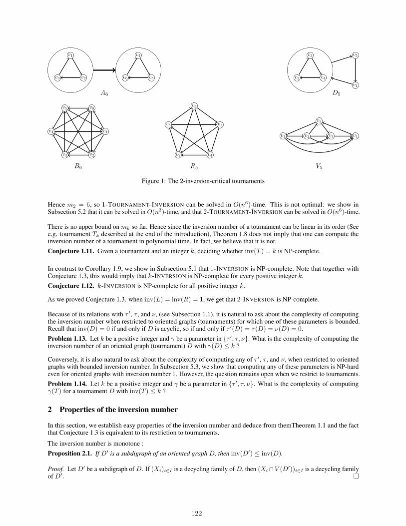
v1

v2v3

v4

v5v6

A6

v3

v4v2

v5

v1

D5

v1

v2v3

v4

v5 v6

B6

v1

v4v2

v5

v3

R5

v1 v2 v3 v4

v5

V5

Figure 1: The 2-inversion-critical tournaments

Hence m2 = 6, so 1-TOURNAMENT-INVERSION can be solved in O(n6)-time. This is not optimal: we show inSubsection 5.2 that it can be solved in O(n3)-time, and that 2-TOURNAMENT-INVERSION can be solved in O(n6)-time.

There is no upper bound on mk so far. Hence since the inversion number of a tournament can be linear in its order (Seee.g. tournament Tk described at the end of the introduction), Theorem 1.8 does not imply that one can compute theinversion number of a tournament in polynomial time. In fact, we believe that it is not.Conjecture 1.11. Given a tournament and an integer k, deciding whether inv(T ) = k is NP-complete.

In contrast to Corollary 1.9, we show in Subsection 5.1 that 1-INVERSION is NP-complete. Note that together withConjecture 1.3, this would imply that k-INVERSION is NP-complete for every positive integer k.Conjecture 1.12. k-INVERSION is NP-complete for all positive integer k.

As we proved Conjecture 1.3. when inv(L) = inv(R) = 1, we get that 2-INVERSION is NP-complete.

Because of its relations with τ ′, τ , and ν, (see Subsection 1.1), it is natural to ask about the complexity of computingthe inversion number when restricted to oriented graphs (tournaments) for which one of these parameters is bounded.Recall that inv(D) = 0 if and only if D is acyclic, so if and only if τ ′(D) = τ(D) = ν(D) = 0.Problem 1.13. Let k be a positive integer and γ be a parameter in τ ′, τ, ν. What is the complexity of computing theinversion number of an oriented graph (tournament) D with γ(D) ≤ k ?

Conversely, it is also natural to ask about the complexity of computing any of τ ′, τ , and ν, when restricted to orientedgraphs with bounded inversion number. In Subsection 5.3, we show that computing any of these parameters is NP-hardeven for oriented graphs with inversion number 1. However, the question remains open when we restrict to tournaments.Problem 1.14. Let k be a positive integer and γ be a parameter in τ ′, τ, ν. What is the complexity of computingγ(T ) for a tournament D with inv(T ) ≤ k ?

2 Properties of the inversion number

In this section, we establish easy properties of the inversion number and deduce from themTheorem 1.1 and the factthat Conjecture 1.3 is equivalent to its restriction to tournaments.

The inversion number is monotone :Proposition 2.1. If D′ is a subdigraph of an oriented graph D, then inv(D′) ≤ inv(D).

Proof. Let D′ be a subdigraph of D. If (Xi)i∈I is a decycling family of D, then (Xi ∩V (D′))i∈I is a decycling familyof D′.

122

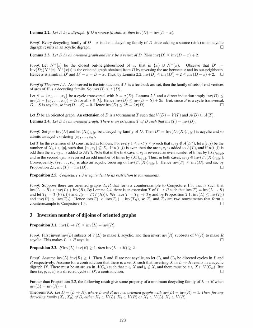
Lemma 2.2. Let D be a digraph. If D a source (a sink) x, then inv(D) = inv(D − x).

Proof. Every decycling family of D − x is also a decycling family of D since adding a source (sink) to an acyclicdigraph results in an acyclic digraph.

Lemma 2.3. Let D be an oriented graph and let x be a vertex of D. Then inv(D) ≤ inv(D − x) + 2.

Proof. Let N+[x] be the closed out-neighbourhood of x, that is x ∪ N+(x). Observe that D′ =Inv(D; (N+[x], N+(x))) is the oriented graph obtained from D by reversing the arc between x and its out-neighbours.Hence x is a sink in D′ and D′ − x = D − x. Thus, by Lemma 2.2, inv(D) ≤ inv(D′) + 2 ≤ inv(D − x) + 2.

Proof of Theorem 1.1. As observed in the introduction, if F is a feedback arc-set, then the family of sets of end-verticesof arcs of F is a decycling family. So inv(D) ≤ τ ′(D).

Let S = x1, . . . , xk be a cycle transversal with k = τ(D). Lemma 2.3 and a direct induction imply inv(D) ≤inv(D − x1, . . . , xi) + 2i for all i ∈ [k]. Hence inv(D) ≤ inv(D − S) + 2k. But, since S is a cycle transversal,D − S is acyclic, so inv(D − S) = 0. Hence inv(D) ≤ 2k = 2τ(D).

Let D be an oriented graph. An extension of D is a tournament T such that V (D) = V (T ) and A(D) ⊆ A(T ).

Lemma 2.4. Let D be an oriented graph. There is an extension T of D such that inv(T ) = inv(D).

Proof. Set p = inv(D) and let (Xi)i∈[p] be a decycling family of D. Then D∗ = Inv(D; (Xi)i∈[p]) is acyclic and soadmits an acyclic ordering (v1, . . . , vn).

Let T be the extension of D constructed as follows: For every 1 ≤ i < j ≤ p such that vivj /∈ A(D∗), let n(i, j) be thenumber of Xi, i ∈ [p], such that vi, vj ⊆ Xi. If n(i, j) is even then the arc vivj is added to A(T ), and if n(i, j) isodd then the arc vjvi is added to A(T ). Note that in the first case, vivj is reversed an even number of times by (Xi)i∈[p],and in the second vjvi is reversed an odd number of times by (Xi)i∈[p]. Thus, in both cases, vivj ∈ Inv(T ; (Xi)i∈[p]).Consequently, (v1, . . . , vn) is also an acyclic ordering of Inv(T ; (Xi)i∈[p]). Hence inv(T ) ≤ inv(D), and so, byProposition 2.1, inv(T ) = inv(D).

Proposition 2.5. Conjecture 1.3 is equivalent to its restriction to tournaments.

Proof. Suppose there are oriented graphs L,R that form a counterexample to Conjecture 1.3, that is such thatinv(L→ R) < inv(L) + inv(R). By Lemma 2.4, there is an extension T of L→ R such that inv(T ) = inv(L→ R)and let TL = T 〈V (L))〉 and TR = T 〈V (R))〉. We have T = TL → TR and by Proposition 2.1, inv(L) ≤ inv(TL)and inv(R) ≤ inv(TR). Hence inv(T ) < inv(TL) + inv(TR), so TL and TR are two tournaments that form acounterexample to Conjecture 1.3.

3 Inversion number of dijoins of oriented graphs

Proposition 3.1. inv(L→ R) ≤ inv(L) + inv(R).

Proof. First invert inv(L) subsets of V (L) to make L acyclic, and then invert inv(R) subbsets of V (R) to make Racyclic. This makes L→ R acyclic.

Proposition 3.2. If inv(L), inv(R) ≥ 1, then inv(L→ R) ≥ 2.

Proof. Assume inv(L), inv(R) ≥ 1. Then L and R are not acyclic, so let CL and CR be directed cycles in L andR respectively. Assume for a contradiction that there is a set X such that inverting X in L→ R results in a acyclicdigraph D′. There must be an arc xy in A(CL) such that x ∈ X and y /∈ X , and there must be z ∈ X ∩ V (CR). Butthen (x, y, z, x) is a directed cycle in D′, a contradiction.

Further than Proposition 3.2, the following result give some property of a minimum decycling family of L→ R wheninv(L) = inv(R) = 1.

Theorem 3.3. Let D = (L→ R), where L and R are two oriented graphs with inv(L) = inv(R) = 1. Then, for anydecycling family (X1, X2) of D, either X1 ⊂ V (L), X2 ⊂ V (R) or X1 ⊂ V (L), X2 ⊂ V (R).

123

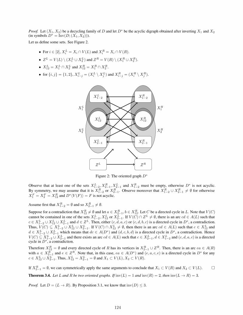
Proof. Let (X1, X2) be a decycling family of D and let D∗ be the acyclic digraph obtained after inverting X1 and X2

(in symbols D∗ = Inv(D; (X1, X2))).

Let us define some sets. See Figure 2.

• For i ∈ [2], XLi = Xi ∩ V (L) and XR

i = Xi ∩ V (R).

• ZL = V (L) \ (XL1 ∪XL

2 ) and ZR = V (R) \ (XR1 ∪XR

2 ).

• XL12 = XL

1 ∩XL2 and XR

12 = XR1 ∩XR

2 .

• for i, j = 1, 2, XLi−j = (XL

i \XLj ) and XR

i−j = (XRi \XR

j ).

XL1

XL2

XR1

XR2

XL1−2

XL12

XL2−1

XR1−2

XR12

XR2−1

ZL ZR

Figure 2: The oriented graph D∗

Observe that at least one of the sets XL1−2, X

R2−1, X

L2−1 and XR

1−2 must be empty, otherwise D∗ is not acyclic.By symmetry, we may assume that it is XR

1−2 or XR2−1. Observe moreover that XR

1−2 ∪ XR2−1 6= ∅ for otherwise

XF1 = XF

2 = XR12 and D∗〈V (F )〉 = F is not acyclic.

Assume first that XR1−2 = ∅ and so XR

2−1 6= ∅.Suppose for a contradiction that XR

12 6= ∅ and let a ∈ XR2−1, b ∈ XR

12. Let C be a directed cycle in L. Note that V (C)

cannot be contained in one of the sets XL1−2, X

L12 or XL

2−1. If V (C) ∩ ZL 6= ∅, there is an arc cd ∈ A(L) such thatc ∈ XL

1−2 ∪XL12 ∪XL

2−1 and d ∈ ZL. Then, either (c, d, a, c) or (c, d, b, c) is a directed cycle in D∗, a contradiction.Thus, V (C) ⊆ XL

1−2 ∪ XL12 ∪ XL

2−1. If V (C) ∩ XL12 6= ∅, then there is an arc cd ∈ A(L) such that c ∈ XL

12 andd ∈ XL

1−2 ∪ XL2−1 which means that dc ∈ A(D∗) and (d, c, b, d) is a directed cycle in D∗, a contradiction. Hence

V (C) ⊆ XL1−2 ∪XL

2−1 and there exists an arc cd ∈ A(L) such that c ∈ XL2−1, d ∈ XL

1−2 and (c, d, a, c) is a directedcycle in D∗, a contradiction.

Therefore XR12 = ∅ and every directed cycle of R has its vertices in XR

2−1 ∪ ZR. Then, there is an arc ea ∈ A(R)

with a ∈ XR2−1 and e ∈ ZR. Note that, in this case, ea ∈ A(D∗) and (e, a, c, e) is a directed cycle in D∗ for any

c ∈ XL12 ∪XL

2−1. Thus, XL12 = XL

2−1 = ∅ and X1 ⊂ V (L), X2 ⊂ V (R).

If XR2−1 = ∅, we can symmetrically apply the same arguments to conclude that X1 ⊂ V (R) and X2 ⊂ V (L).

Theorem 3.4. Let L and R be two oriented graphs. If inv(L) = 1 and inv(R) = 2, then inv(L→ R) = 3.

Proof. Let D = (L→ R). By Proposition 3.1, we know that inv(D) ≤ 3.

124

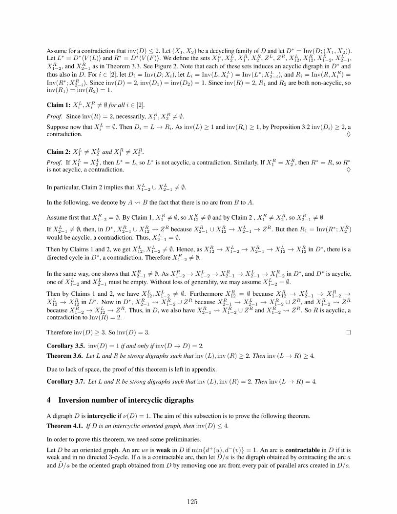
Assume for a contradiction that inv(D) ≤ 2. Let (X1, X2) be a decycling family of D and let D∗ = Inv(D; (X1, X2)).Let L∗ = D∗〈V (L)〉 and R∗ = D∗〈V (F )〉. We define the sets XL

1 , XL2 , XR

1 , XR2 , ZL, ZR, XL

12, XR12, XL

1−2, XL2−1,

XR1−2, and XR

2−1 as in Theorem 3.3. See Figure 2. Note that each of these sets induces an acyclic digraph in D∗ andthus also in D. For i ∈ [2], let Di = Inv(D;Xi), let Li = Inv(L,XL

i ) = Inv(L∗;XL2−i), and Ri = Inv(R,XR

i ) =

Inv(R∗;XR2−i). Since inv(D) = 2, inv(D1) = inv(D2) = 1. Since inv(R) = 2, R1 and R2 are both non-acyclic, so

inv(R1) = inv(R2) = 1.

Claim 1: XLi , X

Ri 6= ∅ for all i ∈ [2].

Proof. Since inv(R) = 2, necessarily, XR1 , X

R2 6= ∅.

Suppose now that XLi = ∅. Then Di = L→ Ri. As inv(L) ≥ 1 and inv(Ri) ≥ 1, by Proposition 3.2 inv(Di) ≥ 2, a

contradiction. ♦

Claim 2: XL1 6= XL

2 and XR1 6= XR

2 .

Proof. If XL1 = XL

2 , then L∗ = L, so L∗ is not acyclic, a contradiction. Similarly, If XR1 = XR

2 , then R∗ = R, so R∗is not acyclic, a contradiction. ♦

In particular, Claim 2 implies that XL1−2 ∪XL

2−1 6= ∅.

In the following, we denote by A B the fact that there is no arc from B to A.

Assume first that XR1−2 = ∅. By Claim 1, XR

1 6= ∅, so XR12 6= ∅ and by Claim 2 , XR

1 6= XR2 , so XR

2−1 6= ∅.If XL

2−1 6= ∅, then, in D∗, XR2−1 ∪XR

12 ZR because XR2−1 ∪XR

12 → XL2−1 → ZR. But then R1 = Inv(R∗;XR

2 )

would be acyclic, a contradiction. Thus, XL2−1 = ∅.

Then by Claims 1 and 2, we get XL12, X

L1−2 6= ∅. Hence, as XR

12 → XL1−2 → XR

2−1 → XL12 → XR

12 in D∗, there is adirected cycle in D∗, a contradiction. Therefore XR

1−2 6= ∅.

In the same way, one shows that XR2−1 6= ∅. As XR

1−2 → XL1−2 → XR

2−1 → XL2−1 → XR

1−2 in D∗, and D∗ is acyclic,one of XL

1−2 and XL2−1 must be empty. Without loss of generality, we may assume XL

1−2 = ∅.Then by Claims 1 and 2, we have XL

12, XL1−2 6= ∅. Furthermore XR

12 = ∅ because XR12 → XL

2−1 → XR1−2 →

XL12 → XR

12 in D∗. Now in D∗, XR2−1 XR

1−2 ∪ ZR because XR2−1 → XL

2−1 → XR1−2 ∪ ZR, and XR

1−2 ZR

because XR1−2 → XL

12 → ZR. Thus, in D, we also have XR2−1 XR

1−2 ∪ ZR and XR1−2 ZR. So R is acyclic, a

contradiction to Inv(R) = 2.

Therefore inv(D) ≥ 3. So inv(D) = 3.

Corollary 3.5. inv(D) = 1 if and only if inv(D → D) = 2.

Theorem 3.6. Let L and R be strong digraphs such that inv (L), inv (R) ≥ 2. Then inv (L→ R) ≥ 4.

Due to lack of space, the proof of this theorem is left in appendix.

Corollary 3.7. Let L and R be strong digraphs such that inv (L), inv (R) = 2. Then inv (L→ R) = 4.

4 Inversion number of intercyclic digraphs

A digraph D is intercyclic if ν(D) = 1. The aim of this subsection is to prove the following theorem.

Theorem 4.1. If D is an intercyclic oriented graph, then inv(D) ≤ 4.

In order to prove this theorem, we need some preliminaries.

Let D be an oriented graph. An arc uv is weak in D if mind+(u), d−(v) = 1. An arc is contractable in D if it isweak and in no directed 3-cycle. If a is a contractable arc, then let D/a is the digraph obtained by contracting the arc aand D/a be the oriented graph obtained from D by removing one arc from every pair of parallel arcs created in D/a.

125

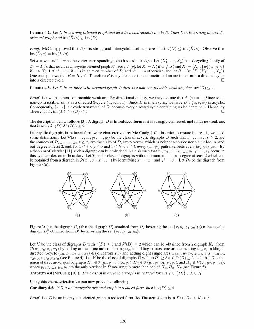
Lemma 4.2. Let D be a strong oriented graph and let a be a contractable arc in D. Then D/a is a strong intercyclicoriented graph and inv(D/a) ≥ inv(D).

Proof. McCuaig proved that D/a is strong and intercyclic. Let us prove that inv(D) ≤ inv(D/a). Observe thatinv(D/a) = inv(D/a).

Set a = uv, and let w be the vertex corresponding to both u and v in D/a. Let (X ′1, . . . , X′p) be a decycling family of

D′ = D/a that result in an acyclic oriented graphR′. For i ∈ [p], letXi = X ′i ifw /∈ X ′i andXi = (X ′i \w)∪u, vif w ∈ X ′i. Let a∗ = uv if w is in an even number of X ′i and a∗ = vu otherwise, and let R = Inv(D; (X1, . . . , Xp)).One easily shows that R = R′/a∗. Therefore R is acyclic since the contraction of an arc transforms a directed cycleinto a directed cycle.

Lemma 4.3. Let D be an intercyclic oriented graph. If there is a non-contractable weak arc, then inv(D) ≤ 4.

Proof. Let uv be a non-contractable weak arc. By directional duality, we may assume that d−(v) = 1. Since uv isnon-contractable, uv is in a directed 3-cycle (u, v, w, u). Since D is intercyclic, we have D \ u, v, w is acyclic.Consequently, w, u is a cycle transversal of D, because every directed cycle containing v also contains u. Hence, byTheorem 1.1, inv(D) ≤ τ(D) ≤ 4.

The description below follows [3]. A digraph D is in reduced form if it is strongly connected, and it has no weak arc,that is minδ−(D), δ+(D) ≥ 2.

Intercyclic digraphs in reduced form were characterized by Mc Cuaig [10]. In order to restate his result, we needsome definitions. Let P(x1, . . . , xs; y1, . . . , yt) be the class of acyclic digraphs D such that x1, . . . , xs, s ≥ 2, arethe sources of D, y1, . . . , yt, t ≥ 2, are the sinks of D, every vertex which is neither a source nor a sink has in- andout-degree at least 2, and, for 1 ≤ i < j ≤ s and 1 ≤ k < ` ≤ t, every (xi, y`)-path intersects every (xj , yk)-path. Bya theorem of Metzlar [11], such a digraph can be embedded in a disk such that x1, x2, . . . , xs, yt, yt−1, . . . , y1 occur, inthis cyclic order, on its boundary. Let T be the class of digraphs with minimum in- and out-degree at least 2 which canbe obtained from a digraph in P(x+, y+;x−, y−) by identifying x+ = x− and y+ = y−. Let D7 be the digraph fromFigure 3(a).

y1

y2 y3

y4

y5y6

y

(a)

y1

y2 y3

y4

y5y6

y

(b)

y1

y2 y3

y4

y5y6

y

(c)

Figure 3: (a): the digraph D7; (b): the digraph D′7 obtained from D7 inverting the set y, y2, y4, y6; (c): the acyclicdigraph D′′7 obtained from D′7 by inverting the set y2, y3, y5, y6.

Let K be the class of digraphs D with τ(D) ≥ 3 and δ0(D) ≥ 2 which can be obtained from a digraph KH fromP(w0, z0; z1, w1) by adding at most one arc connecting w0, z0, adding at most one arc connecting w1, z1, adding adirected 4-cycle (x0, x1, x2, x3, x0) disjoint from KH and adding eight single arcs w1x0, w1x2, z1x1, z1x3, x0w0,x2w0, x1z0 ,x3z0 (see Figure 4). LetH be the class of digraphs D with τ(D) ≥ 3 and δ0(D) ≥ 2 such that D is theunion of three arc-disjoint digraphsHα ∈ P(y4, y3, y1; y5, y2),Hβ ∈ P(y4, y5; y3, y1, y2), andHγ ∈ P(y1, y2; y3, y4),where y1, y2, y3, y4, y5 are the only vertices in D occuring in more than one of Hα, Hβ , Hγ (see Figure 5).

Theorem 4.4 (McCuaig [10]). The class of intercyclic digraphs in reduced form is T ∪ D7 ∪ K ∪H.

Using this characterization we can now prove the following.

Corollary 4.5. If D is an intercyclic oriented graph in reduced form, then inv(D) ≤ 4.

Proof. Let D be an intercyclic oriented graph in reduced form. By Theorem 4.4, it is in T ∪ D7 ∪ K ∪H.

126

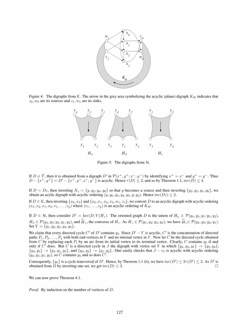
1

1

wz

x

x

x

x

z0

2

3

0

0

w1

KH

Figure 4: The digraphs from K. The arrow in the grey area symbolizing the acyclic (plane) digraph KH indicates thatz0, w0 are its sources and z1, w1 are its sinks.

1y

1y

1y

y2

y2

y2

y3

y3

y3

y4

y4

y4

y5

y5

Hα Hβ Hγ

Figure 5: The digraphs fromH.

If D ∈ T , then it is obtained from a digraph D′ in P(x+, y+;x−, y−) by identifying x+ = x− and y+ = y−. ThusD − x+, y+ = D′ − x+, y+, x−, y− is acyclic. Hence τ(D) ≤ 2, and so by Theorem 1.1, inv(D) ≤ 4.

If D = D7, then inverting X1 = y, y2, y4, y6 so that y becomes a source and then inverting y2, y3, y5, y6, weobtain an acylic digraph with acyclic ordering (y, y6, y3, y4, y5, y, y2). Hence inv(D7) ≤ 2.

IfD ∈ K, then inverting x0, x3 and x0, x1, x2, x3, w1, z1, we convertD to an acyclic digraph with acyclic ordering(x3, x2, x1, x0, v1, . . . , vp) where (v1, . . . , vp) is an acyclic ordering of KH .

If D ∈ H, then consider D′ = Inv(D,V (Hγ). The oriented graph D is the union of Hα ∈ P(y4, y3, y1; y5, y2),

Hβ ∈ P(y4, y5; y3, y1, y2), and←Hγ , the converse of Hγ . As Hγ ∈ P(y1, y2; y3, y4), we have

←Hγ∈ P(y4, y3; y2, y1).

Set Y = y1, y2, y3, y4, y5.We claim that every directed cycle C ′ of D′ contains y5. Since D′ − Y is acyclic, C ′ is the concatenation of directedpaths P1, P2, . . . , Pq with both end-vertices in Y and no internal vertex in Y . Now let C be the directed cycle obtainedfrom C by replacing each Pi by an arc from its initial vertex to its terminal vertex. Clearly, C contains y5 if andonly if C ′ does. But C is a directed cycle in J the digraph with vertex set Y in which y4, y3, y1 → y5, y2,y4, y5 → y3, y1, y2, and y4, y3 → y1, y2. One easily checks that J − v5 is acyclic with acyclic ordering(y4, y3, y1, y2), so C contains y5 and so does C ′.

Consequently, y5 is a cycle transversal of D′. Hence, by Theorem 1.1 (ii), we have inv(D′) ≤ 2τ(D′) ≤ 2. As D′ isobtained from D by inverting one set, we get inv(D) ≤ 3.

We can now prove Theorem 4.1.

Proof. By induction on the number of vertices of D.

127

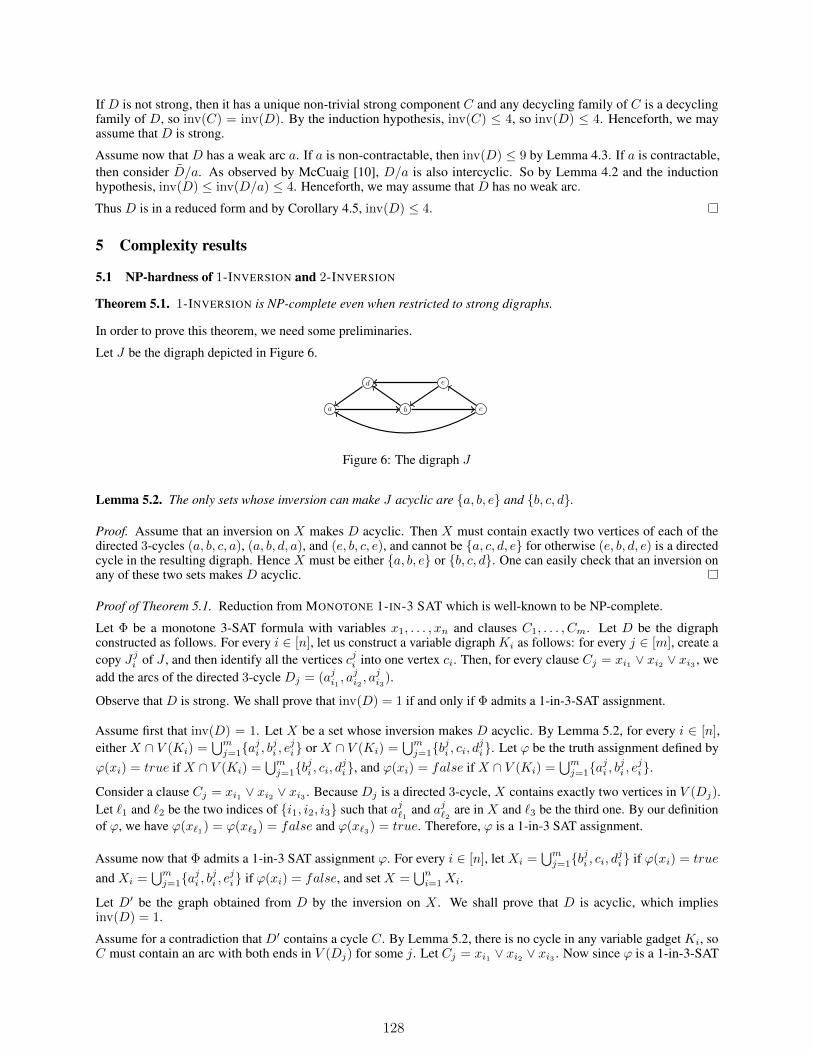
If D is not strong, then it has a unique non-trivial strong component C and any decycling family of C is a decyclingfamily of D, so inv(C) = inv(D). By the induction hypothesis, inv(C) ≤ 4, so inv(D) ≤ 4. Henceforth, we mayassume that D is strong.

Assume now that D has a weak arc a. If a is non-contractable, then inv(D) ≤ 9 by Lemma 4.3. If a is contractable,then consider D/a. As observed by McCuaig [10], D/a is also intercyclic. So by Lemma 4.2 and the inductionhypothesis, inv(D) ≤ inv(D/a) ≤ 4. Henceforth, we may assume that D has no weak arc.

Thus D is in a reduced form and by Corollary 4.5, inv(D) ≤ 4.

5 Complexity results

5.1 NP-hardness of 1-INVERSION and 2-INVERSION

Theorem 5.1. 1-INVERSION is NP-complete even when restricted to strong digraphs.

In order to prove this theorem, we need some preliminaries.

Let J be the digraph depicted in Figure 6.

a b c

d e

Figure 6: The digraph J

Lemma 5.2. The only sets whose inversion can make J acyclic are a, b, e and b, c, d.

Proof. Assume that an inversion on X makes D acyclic. Then X must contain exactly two vertices of each of thedirected 3-cycles (a, b, c, a), (a, b, d, a), and (e, b, c, e), and cannot be a, c, d, e for otherwise (e, b, d, e) is a directedcycle in the resulting digraph. Hence X must be either a, b, e or b, c, d. One can easily check that an inversion onany of these two sets makes D acyclic.

Proof of Theorem 5.1. Reduction from MONOTONE 1-IN-3 SAT which is well-known to be NP-complete.

Let Φ be a monotone 3-SAT formula with variables x1, . . . , xn and clauses C1, . . . , Cm. Let D be the digraphconstructed as follows. For every i ∈ [n], let us construct a variable digraph Ki as follows: for every j ∈ [m], create acopy Jji of J , and then identify all the vertices cji into one vertex ci. Then, for every clause Cj = xi1 ∨ xi2 ∨ xi3 , weadd the arcs of the directed 3-cycle Dj = (aji1 , a

ji2, aji3).

Observe that D is strong. We shall prove that inv(D) = 1 if and only if Φ admits a 1-in-3-SAT assignment.

Assume first that inv(D) = 1. Let X be a set whose inversion makes D acyclic. By Lemma 5.2, for every i ∈ [n],either X ∩ V (Ki) =

⋃mj=1a

ji , b

ji , e

ji or X ∩ V (Ki) =

⋃mj=1b

ji , ci, d

ji. Let ϕ be the truth assignment defined by

ϕ(xi) = true if X ∩ V (Ki) =⋃mj=1b

ji , ci, d

ji, and ϕ(xi) = false if X ∩ V (Ki) =

⋃mj=1a

ji , b

ji , e

ji.

Consider a clause Cj = xi1 ∨ xi2 ∨ xi3 . Because Dj is a directed 3-cycle, X contains exactly two vertices in V (Dj).Let `1 and `2 be the two indices of i1, i2, i3 such that aj`1 and aj`2 are in X and `3 be the third one. By our definitionof ϕ, we have ϕ(x`1) = ϕ(x`2) = false and ϕ(x`3) = true. Therefore, ϕ is a 1-in-3 SAT assignment.

Assume now that Φ admits a 1-in-3 SAT assignment ϕ. For every i ∈ [n], let Xi =⋃mj=1b

ji , ci, d

ji if ϕ(xi) = true

and Xi =⋃mj=1a

ji , b

ji , e

ji if ϕ(xi) = false, and set X =

⋃ni=1Xi.

Let D′ be the graph obtained from D by the inversion on X . We shall prove that D is acyclic, which impliesinv(D) = 1.

Assume for a contradiction that D′ contains a cycle C. By Lemma 5.2, there is no cycle in any variable gadget Ki, soC must contain an arc with both ends in V (Dj) for some j. Let Cj = xi1 ∨ xi2 ∨ xi3 . Now since ϕ is a 1-in-3-SAT

128

assignment, w.l.o.g., we may assume that ϕ(xi1) = ϕ(xi2) = false and ϕ(xi3) = true. Hence in D′, aji2 → aji1 ,aji2 → aji3 and aji3 → aji1 . Moreover, in D′〈V (Jji1)〉, aji1 is a sink, so aji1 is a sink in D′. Therefore C does not goesthrough aji1 , and thus C contains the arc aji2a

ji3

, and then enter Jji3 . But in D′〈V (Jji3)〉, aji3 has a unique out-neighbour,namely bji3 , which is a sink. This is a contradiction.

Corollary 5.3. 2-INVERSION is NP-complete.

Proof. By Corollary 3.5, we have inv(D → D) = 2 if and only inv(D) = 1, so the statement follows from Theorem5.1.

5.2 Solving k-TOURNAMENT-INVERSION for k ∈ 1, 2

Theorem 5.4. 1-TOURNAMENT-INVERSION can be solved in O(n3) time.

Proof. Let T be a tournament. For every vertex v one can check whether there is an inversion that transforms T into atransitive tournament with source v. Indeed the unique possibility inversion is the one on the closed in-neighbourhoodof v, N−[v] = N−(v) ∪ v. So one can make inversion on N−[v] and check whether the resulting tournament istransitive. This can obviously be done in O(n2) time

Doing this for every vertex v yields an algorithm which solves 1-TOURNAMENT-INVERSION in O(n3) time.

Theorem 5.5. 2-TOURNAMENT-INVERSION can be solved in in O(n6) time.

The main idea to prove this theorem is to consider every pair (s, t) of vertices and to check whether there are two setsX1, X2 such that the inversion of X1 and X2 results in a transitive tournament with source s and sink t. We need somedefinitions and lemmas.

The symmetric difference of two sets A ad B is A4B = (A \B) ∪ (B \A).

Let T be a tournament and let s and t be two vertices of T . We define the following four sets

A(s, t) = N+(s) ∩N−(t)

B(s, t) = N−(s) ∩N+(t)

C(s, t) = N+(s) ∩N+(t)

D(s, t) = N−(s) ∩N−(t)

Lemma 5.6. Let T be a tournament and let s and t be two vertices of T . Assume there are two sets X1, X2 such thatthe inversion of X1 and X2 results in a transitive tournament with source s and sink t.

(1) If s, t ⊆ X1 \X2, then ts ∈ A(T ), C(s, t) = D(s, t) = ∅ and X1 = s, t ∪B(s, t).

(2) If s ∈ X1 \X2, t ∈ X2 \X1, and the inversion of X1 and X2 makes T acyclic, then st ∈ A(T ), A(s, t) ∩(X1 ∪X2) = ∅, X1 = s ∪B(s, t) ∪D(s, t), and X2 = t ∪B(s, t) ∪ C(s, t).

(3) If s ∈ X1∩X2 and t ∈ X1 \X2, then ts ∈ A(T ), X1 = s, t∪B(s, t)∪C(s, t), and X2 = s∪C(s, t)∪D(s, t).

(4) If s, t ⊆ X1 ∩ X2, then st ∈ A(T ), C(s, t) = ∅, D(s, t) = ∅, X1 ∩ X2 ⊆ A(s, t) ∪ s, t, andB(s, t) = X14X2.

Proof. (1) The arc between s and t is reversed once, so ts ∈ A(T ).

Assume for a contradiction, that there is a vertex c ∈ C(S, t). The arc tc must be reversed, so c ∈ X1, but then the arcsc is reversed contradicting the fact that s becomes a source. Hence C(s, t) = ∅. Similarly D(s, t) = ∅.The arcs from t to B(s, t) and from B(s, t) to s are reversed so B(s, t) ⊆ X1. The arcs from s to A(s, t) and fromA(s, t) to t are not reversed so A(s, t) ∩X1 = ∅. Therefore X1 = s, t ∪B(s, t).

(2) The arc between s and t is not reversed, so st ∈ A(T ). The arcs from s to A(s, t) and from A(s, t) to t are notreversed so A(s, t) ∩ X1 = ∅ and A(s, t) ∩ X2 = ∅. The arcs from t to B(s, t) and from B(s, t) to s are reversedso B(s, t) ⊆ X1 and B(s, t) ⊆ X2. The arcs from s to C(s, t) are not reversed so C(s, t) ∩ X1 = ∅ and the arcs

129

from t to C(s, t) are reversed so C(s, t) ⊆ X2. The arcs from D(s, t) to s are reversed so D(s, t) ⊆ X1 and thearcs from D(s, t) to d are not reversed so D(s, t) ∩ X2 = ∅. Consequently, X1 = s ∪ B(s, t) ∪ D(s, t), andX2 = t ∪B(s, t) ∪ C(s, t).

(3) The arc between s and t is reversed, so ts ∈ A(T ). The arcs from A(s, t) to t are not reversed so A(s, t) ∩X1 = ∅.The arcs from s toA(s, t) are not reversed soA(s, t)∩X2 = ∅. The arcs from t toB(s, t) are reversed soB(s, t) ⊆ X1.The arcs from B(s, t) to s are reversed (only once) so B(s, t) ∩ X2 = ∅. The arcs from t to C(s, t) are reversedso C(s, t) ⊆ X1. The arcs from s to C(s, t) must the be reversed twice so C(s, t) ⊆ X2. The arcs from D(s, t) tot are not reversed so D(s, t) ∩ X1 = ∅. The arcs from D(s, t) to s are reversed so D(s, t) ⊆ X2. Consequently,X1 = s, t ∪B(s, t) ∪ C(s, t), and X2 = s, t ∪ C(s) ∪D(s, t).

(4) The arc between s and t is reversed twice, so st ∈ A(T ).

Assume for a contradiction, that there is a vertex c ∈ C(s, t). The arc tc must be reversed, so c is in exactly one of X1

ad X2. But then the arc sc is reversed contradicting the fact that s becomes a source. Hence C(s, t) = ∅. SimilarlyD(s, t) = ∅. The arcs from s to A(s, t) and from A(s, t) to t are not reversed so every vertex of A(s, t) is either inX1 ∩X2 or in V (T ) \ (X1 ∪X2). The arcs from t to B(s, t) and from B(s, t) to s are reversed so every vertex ofB(s, t) is either in X1 \X2 or in X2 \X1. Consequently, X1 ∩X2 ⊆ A(s, t) ∪ s, t, and B(s, t) = X14X2.

Lemma 5.7. Let T be a tournament of order n and let s and t be two vertices of T .

(1) One can decide in O(n3) time whether there are two sets X1, X2 such that the inversion of X1 and X2 resultsin a transitive tournament with source s and sink t and s, t ⊆ X1 \X2.

(2) One can decide in O(n2) time whether there are two sets X1, X2 such that the inversion of X1 and X2 resultsin a transitive tournament with source s and sink t and s ∈ X1 \X2 and t ∈ X2 \X1.

(3) One can decide in O(n2) time whether there are two sets X1, X2 such that the inversion of X1 and X2 resultsin a transitive tournament with source s and sink t and s ∈ X1 ∩X2 and t ∈ X1 \X2.

(4) One can decide in O(n4) time whether there are two sets X1, X2 such that the inversion of X1 and X2 resultsin a transitive tournament with source s and sink t and s, t ⊆ X1 ∩X2.

Proof. For all cases, we first compute A(s, t), B(s, t), C(s, t), and D(s, t), which can obviously be done in O(n2).

(1) By Lemma 5.6, we must have ts ∈ A(T ) and C(s, t) = D(s, t) = ∅. So we first check if this holds. Furthermore,by Lemma 5.6, we must have X1 = s, t ∪B(s, t). Therefore we invert s, t ∪B(s, t) which results in a tournamentT ′. Observe that s is a source of T ′ and t is a sink of T ′. Hence, we return ‘Yes’ if and only if inv(T ′ − s, t) = 1which can be tested in O(n3) by Theorem 5.4.

(2) By Lemma 5.6, we must have st ∈ A(T ). So we first check if this holds. Furthermore, by Lemma 5.6, the onlypossibility is that X1 = s ∪ B(s, t) ∪D(s, t), and X2 = t ∪ B(s, t) ∪ C(s, t). So we invert those two sets andcheck whether the resulting tournament is a transitive tournament with source s and sink t. This can done in O(n2).

(3) By Lemma 5.6, we must have ts ∈ A(T ). So we first check if this holds. Furthermore, by Lemma 5.6, the onlypossibility is that X1 = s, t ∪B(s, t) ∪ C(s, t), and X2 = s ∪ C(s, t) ∪D(s, t). So we invert those two sets andcheck whether the resulting tournament is a transitive tournament with source s and sink t. This can done in O(n2).

(4) By Lemma 5.6, we must have st ∈ A(T ), C(s, t) = ∅, D(s, t) = ∅. So we first check if this holds. Furthermore, byLemma 5.6, the desired sets X1 and X2 must satisfy X1 ∩X2 ⊆ A(s, t) ∪ s, t, and B(s, t) = X14X2.

In particular, every arc of TA = T 〈A(s, t)〉 is either not reversed or reversed twice (which is the same). Hence TA mustbe a transitive tournament. So we check whether TA is a transitive tournament and if yes, we find a directed hamiltonianpath PA = (a1, . . . , ap) of it. This can be done in O(n2).

Now we check that B(s, t) admits a partition (X ′1, X′2) with X ′i = Xi ∩ B and the inversion of both X ′1 and X ′2

transforms T 〈B(s, t)〉 into a transitive tournament TB with source s′ and sink t′. The idea is to investigate allpossibilities for s′, t′ and the sets X ′1 and X ′2. Since (X ′1, X

′2) is a partition of B(s, t) and (X ′1, X

′2) is a decycling

family if and only if (X ′2, X′1) is a decycling family, we may assume that

(a) s′, t′ ⊆ X ′1 \X ′2, or

130

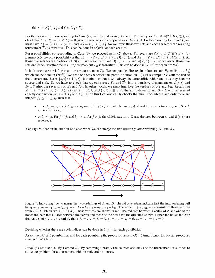
(b) s′ ∈ X ′1 \X ′2 and t′ ∈ X ′2 \X ′1.

For the possibilties corresponding to Case (a), we proceed as in (1) above. For every arc t′s′ ∈ A(T 〈B(s, t)〉), wecheck that C(s′, t′) = D(s′, t′) = ∅ (where those sets are computed in T 〈B(s, t)〉). Furthermore, by Lemma 5.6, wemust have X ′1 = s, t ∪B(s′, t′) and X ′2 = B(s, t) \X ′1. So we invert those two sets and check whether the resultingtournament TB is transitive. This can be done in O(n2) (or each arc t′s′.

For a possibilities corresponding to Case (b), we proceed as in (2) above. For every arc t′s′ ∈ A(T 〈B(s, t)〉), byLemma 5.6, the only possibility is that X ′1 = s′ ∪ B(s′, t′) ∪D(s′, t′), and X2 = t′ ∪ B(s′, t′) ∪ C(s′, t′). Asthose two sets form a partition of B(s, t), we also must have B(s′, t′) = ∅ and A(s′, t′) = ∅. So we invert those twosets and check whether the resulting tournament TB is transitive. This can be done in O(n2) for each arc t′s′.

In both cases, we are left with a transitive tournament TB . We compute its directed hamiltonian path PB = (b1, . . . , bq)which can be done in O(n2). We need to check whether this partial solution on B(s, t) is compatible with the rest ofthe tournament, that is s, t ∪ A(s, t). It is obvious that it will always be compatible with s and t as they becomesource and sink. So we have to check that we can merge TA and TB into a transitive tournament on A(s, t) andB(s, t) after the reversals of X1 and X2. In other words, we must interlace the vertices of PA and PB . Recall thatZ = X1 ∩X2 \ s, t ⊆ A(s, t) and Xi = X ′i ∪Z ∪ s, t, i ∈ [2] so the arcs between Z and B(s, t) will be reversedexactly once when we invert X1 and X2. Using this fact, one easily checks that this is possible if and only there areintegers j1 ≤ · · · ≤ jp such that

• either bj → ai for j ≤ ji and bj ← ai for j > ji (in which case ai /∈ Z and the arcs between ai and B(s, t)are not reversed),

• or bj ← ai for j ≤ ji and bj → ai for j > ji (in which case ai ∈ Z and the arcs between ai and B(s, t) arereversed).

See Figure 7 for an illustration of a case when we can merge the two orderings after reversing X1 and X2.

a1 a2 a3 a4 a5 a6 a7 a8 a9 a10 a11

b1 b2 b3 b4 b5 b6 b7 b8 b9 b10 b11 b12

Figure 7: Indicating how to merge the two orderings of A and B. The fat blue edges indicate that the final ordering willbe b1 − b3, a1 − a4, b4 − b6, a5 − a8, b7 − b9, a9 − a11, b10 − b12. The set Z = a2, a6, a10 consists of those verticesfrom A(s, t) which are in X1 ∩X2. These vertices are shown in red. The red arcs between a vertex of Z and one of theboxes indicate that all arcs between the vertex and those of the box have the direction shown. Hence the boxes indicatethat values of j1, . . . , j11 satisfy that : j1 = . . . = j4 = 3, j5 = . . . = j8 = 6, j9 = . . . = j11 = 9.

Deciding whether there are such indices can be done in O(n2) for each possibility.

As we have O(n2) possibilities, and for each possibility the procedure runs in O(n2) time. Hence the overall procedureruns in O(n4) time.

Proof of Theorem 5.5. By Lemma 2.2, by removing iterately the sources and sinks of the tournament, it suffices tosolve the problem for a tournament with no sink and no source.

131

Now for each pair (s, t) of distinct vertices, one shall check whether there are two sets X1, X2 such that the inversionof X1 and X2 results in a transitive tournament with source s and sink t. Observe that since s and t are neither sourcesnor sinks in T , each of them must belong to at least one of X1, X2. Therefore, without loss of generality, we are in oneof the following possibilities:

• s, t ⊆ X1 \X2. Such a possibility can be check in O(n3) by Lemma 5.7 (1).

• s ∈ X1 \X2 and t ∈ X2 \X1. Such a possibility can be check in O(n2) by Lemma 5.7 (2).

• s ∈ X1 ∩X2 and t ∈ X1 \X2. Such a possibility can be check in O(n2) by Lemma 5.7 (3).

• t ∈ X1 ∩X2 and s ∈ X1 \X2. Such a possibility is the directional dual of the preceding one. It can be testedin O(n2) by reversing all arcs and applying Lemma 5.7 (3).

• s, t ⊆ X1 ∩X2. Such a possibility can be check in O(n4) by Lemma 5.7 (4).

Since there are O(n2) pairs (s, t) and for each pair the procedure runs in O(n4), the algorithm runs in O(n6) time.

5.3 Computing related parameters when the inversion number is bounded

The aim of this subsection is to prove the following theorem.

Theorem 5.8. Let γ be a parameter in τ, τ ′, ν. Given an oriented graph D with inversion number 1 and an integer k,it is NP-complete to decide whether γ(D) ≤ k.

Let D be a digraph. The second subdivision of D is the oriented graph S2(D) obtained from D by replacing every arca = uv by a directed path Pa = (u, xa, ya, u) where xa, ya are two new vertices.

Proposition 5.9. Let D be a digraph.

(i) inv(S2(D) ≤ 1.

(ii) τ ′(S2(D)) = τ ′(D), τ(S2(D)) = τ(D), and ν(S2(D)) = ν(D).

Proof. (i) Inverting the set⋃a∈A(D)xa, ya makes S2(D) acyclic. Indeed the xa become sinks, the ya become source

and the other vertices form a stable set. Thus inv(S2(D)) = 1.

(ii) There is a one-to-one correspondence between directed cycles in D and directed cycles in S2(D) (their secondsubdivision). Hence ν(S2(D)) = ν(D).

Moreover every cycle transversal S of D is also a cycle transversal of S2(D). So τ(S2(D)) ≤ τ(D). Now consider acycle transversal T . If xa or ya is in S for some a ∈ A(D), then we can replace it by any end-vertex of a. Therefore,we may assume that T ⊆ V (D), and so T is a cycle transversal of D. Hence τ(S2(D)) = τ(D).

Similarly, consider a cycle arc-transversal F of D. Then F ′ = a | xaya ∈ F is a cycle arc-transversal of S2(D).Conversely, consider a cycle arc-transversal F ′ of S2(D). Replacing each arc incident to xa, ya by xaya for eacha ∈ A(D), we obtain another cycle arc-transversal. So we may assume that F ′ ⊆ xaya | a ∈ A(D). ThenF = a | xaya ∈ F ′ is a cycle arc-transversal of D. Thus τ ′(S2(D)) = τ ′(D).

Proof of Theorem 5.8. Since computing each of τ , τ ′, ν is NP-hard, Proposition 5.9 (ii) implies that computing eachof τ , τ ′, ν is also NP-hard for second subdivisions of digraphs. As those oriented graphs have inversion number 1(Proposition 5.9 (i)), computing each of τ , τ ′, ν is NP-hard for oriented graphs with inversion number 1.

Acknowledgement

The authors would like to thank Maurice Pouzet for suggesting the problem. There are very pleased to honour him onhis 75th birthday.

This research was supported by the Independent Research Fund Denmark under grant number DFF 7014-00037B,and by the french Agence Nationale de la Recherche under contract Digraphs ANR-19-CE48-0013-01. This workwas done while the Joergen Bang-Jensen was visiting team Coati, I3S and INRIA Sophia Antipolis. Hospitality andfinancial support is gratefully acknowledged. Ce travail a bénéficié d’une aide du gouvernement français, gérée par

132

l’Agence Nationale de la Recherche au titre du projet Investissements d’Avenir UCAJEDI portant la référence noANR-15-IDEX-01. This work was done while the Jonas Costa Ferreira da Silva was spending his second year of PhDas “sandwich” in team Coati, I3S and INRIA Sophia Antipolis.

References

[1] N. Alon. Ranking tournaments. SIAM J. Discrete Math., 20:137–142, 2006.[2] J. Bang-Jensen and G. Gutin. Digraphs: Theory, Algorithms and Applications. Springer-Verlag, London, 2nd

edition, 2009.[3] J. Bang-Jensen and M. Kriesell. On the problem of finding disjoint cycles and dicycles in a digraph. Combinatorica,

31:639–668, 2011.[4] J. Bang-Jensen and C. Thomassen. A polynomial algorithm for the 2-path problem for semicomplete digraphs.

SIAM J. Discrete Math., 5:366–376, 1992.[5] H. Belkhechine, M. Bouaziz, I. Boudabbous, and M. Pouzet. Inversions in tournaments. Unpublished.[6] H. Belkhechine, M. Bouaziz, I. Boudabbous, and M. Pouzet. Inversion dans les tournois. Comptes Rendus

Mathematique, 348(13):703 – 707, 2010.[7] P. Charbit, S. Thomassé, and A. Yeo. The minimum feedback arc set problem is NP-hard for tournaments. Combin.

Probab. Comput., 16:1–4, 2007.[8] M. X. Goemans and D. P. Williamson. Primal-dual approximation algorithms for feedback problems in planar

graphs. In W. H. Cunningham, S. T. McCormick, and M. Queyranne, editors, Integer Programming andCombinatorial Optimization, pages 147–161, Berlin, Heidelberg, 1996. Springer Berlin Heidelberg.

[9] R. Karp. Reducibility among combinatorial problems. In Complexity of computer computations (Proc. Symp.,IBM Thomas J. Watson Res. Center, Yorktown Heights, N.Y., 1972), pages 85–103. Plenum, 1972.

[10] W. McCuaig. Intercyclic digraphs. In N. Robertson and P. D. Seymour, editors, Graph Structure Theory,Proceedings of a AMS-IMS-SIAM Joint Summer Research Conference on Graph Minors held June 22 to July 5,1991, at the University of Washington, Seattle, USA, volume 147 of Contemporary Mathematics, pages 203–245.American Mathematical Society, 1991.

[11] A. Metzlar. ‘Minimum transversal of cycles in intercyclic digraphs. PhD thesis, University of Waterloo, Ontario,Canada, 1989.

[12] B. A. Reed, N. Robertson, P. D. Seymour, and R. Thomas. Packing directed circuits. Combinatorica, 16(4):535–554, 1996.

[13] B. A. Reed and F. B. Shepherd. The gallai-younger conjecture for planar graphs. Combinatorica, 16(4):555–566,1996.

[14] E. Speckenmeyer. On feedback problems in digraphs. In WG 1989, volume 411 of Lect. Notes Comput. Sci.,pages 218–231. Springer, 1989.

133

Appendix: Dijoin of oriented graphs with inversion number 2

In this appendix, we give the proof of the following Theorem 3.6

Theorem 3.6. Let L and R be strong digraphs such that inv (L), inv (R) ≥ 2. Then inv (L→ R) ≥ 4.

Proof. Assume for a contradiction that there are two digraphs L and R such that inv (L), inv (R) ≥ 2 and inv (L→R) = 3. By Lemma 2.4 and Proposition 2.1, we can assume that L and R are tournaments.

By Theoren b3.4, inv (L → R) ≥ 3. Assume for a contradiction that inv (L → R) = 3. Let (X1, X2, X3)be a decycling sequence of D = L → R and denote the resulting acylic (transitive) tournament by T . We willuse the following notation. Below and in the whole proof, whenever we use subscripts i, j, k together we havei, j, k = 1, 2, 3.

• XLi = Xi ∩ V (L), XR

i = Xi ∩ V (R) for all i ∈ [3].

• ZL = V (L) \ (XL1 ∪XL

2 ∪XL3 ) and ZR = V (R) \ (XR

1 ∪XR2 ∪XR

3 )

• XL123 = XL

1 ∩XL2 ∩XL

3 , XR123 = XR

1 ∩XR2 ∩XR

3 .

• XLij−k = (XL

i ∩XLj ) \XL

k and XRij−k = (XR

i ∩XRj ) \XR

k .

• XLi−jk = XL

i \ (XLj ∪XL

k ) and XRi−jk = XR

i \ (XRj ∪XR

k ).

For any two (possibly empty) sets Q,W , we write Q→ W to indicate that every q ∈ Q has an arc to every w ∈ W .Unless otherwise specified, we are always referring to the arcs of T below. When we refer to arcs of the originaldigraph we will use the notation u⇒ v, whereas we use u→ v for arcs in T .

Claim A: XLi , X

Ri 6= ∅ for all i ∈ [3].

Proof. Suppose w.l.o.g. that XR1 = ∅ and let D′ = Inv(D;X1). Then D′ contains C3 → R as an induced subdigraph

since reversing XL1 does not make L acyclic so there is still a directed 3-cycle (by Moon’s theorem). ♦

Claim B: In T the following holds, implying that at least one of the involved sets is empty (as T is acyclic).

(a) XR123 → XL

123 → XRij−k → XL

ik−j → XR123.

(b) XLij−k → XR

ij−k → XLik−j → XR

ik−j → XLij−k.

Proof. This follows from the fact that and arc of D is inverted if and only if it belongs to an odd number of the setsX1, X2, X3. ♦

Claim C: For all i 6= j, we have XLi 6= XL

j and XRi 6= XR

j .

Proof. Suppose this is not true, then without loss of generality XL3 = XL

2 but this contradicts that (XL1 , X

L2 , X

L3 ) is a

decycling sequence of L as inverting XL2 and XL

3 leaves every arc unchanged and we have inv(L) = 2. ♦

Now we are ready to obtain a contradiction to the assumption that (X1, X2, X3) is a decycling sequence forD = L→ R. We divide the proof into five cases. In order to increase readability, we will emphasize partial conclusionsin blue, assumptions in orange, and indicate consequences of assumptions in red.

Case 1: XLi−jk = ∅ = XR

i−jk for all i, j, k.

By Claim C, at least two of the sets XL12−3, X

L13−2, X

L23−1 are non-empty and at least two of the sets

XR12−3, X

R13−2, X

R23−1 are non-empty. Without loss of generality, XL

12−3, XL13−2 6= ∅. Now, by Claim B (b),

implies that one of XR12−3, X

R13−2 must be empty. By interchanging the names of X2, X3 if necessary, we may

assume that XR13−2 = ∅ and hence, by Claim C, XR

12−3, XR23−1 6= ∅. By Claim B (a), this implies XL

23−1 = ∅. Now

134

XR23−1 → XL

12−3 → XR12−3, so XR

23−1 → XR13−2. As XL

12−3 → XR12−3 → XL

13−2, we must have XL12−3 → XL

13−2.By Claim B (a), XL

123 → XR12−3 → XL

13−2 → XR123 → XL

123, so one of XL123 and XR

123 is empty. W.l.o.g. we mayassume XR

123 = ∅. As R is strong and XR23−1 dominates XR

12−3 in R (these arcs are reversed by X2), we must haveZR 6= ∅. Moreover the arcs incident to ZR are not reversed, so the set ZR has an out-neighbour in XR

12−3 ∪XR23−1.

But XR12−3 ∪XR

23−1 → XL13−2 → ZR so T has a directed 3-cycle, contradiction. This completes the proof of Case 1.

Case 2: Exactly one of XL1−23, X

L2−13, X

L3−12, X

R1−23, X

R2−13, X

R3−12 is non-empty.

By reversing all arcs and switching the names of L and R if necessary, we may assume w.l.o.g that XL1−23 6= ∅. As

XR2 6= XR

3 we have XR12−3 ∪XR

13−2 6= ∅. By symmetry, we can assume that XR12−3 6= ∅.

Suppose for a contradiction that XR23−1 = ∅. Then Claims A and C imply XR

13−2 6= ∅. Now, by Claim B (b), one ofXL

12−3, XL13−2 is empty. By symmetry, we can assume XL

13−2 = ∅. Now, by Claim C, XL2 6= XL

3 , so XL12−3 6= ∅.

Note that XL12−3 → XR

12−3 → XL1−23, thus XL

12−3 → XL1−23 because T is acyclic. We also have XL

123 → XL12−3

as XL123 → XR

13−2 → XL12−3, and XL

12−3 → XL23−1 as XL

12−3 → XR12−3 → XL

23−1. This implies that in L all arcsbetween XL

12−3 and XL23−1 ∪ XL

123 ∪ XL1−23 are entering XL

12−3 (the arcs between XL123 and XL

12−3 were reversedtwice and those between XL

1−23 ∪XL23−1 and XL

12−3 were reversed once). Hence, as L is strong, we must have an arcuz from XL

12−3 to ZL. But ZL → XR13−2 → XL

12−3 so together with uz we have a directed 3-cycle in T , contradiction.Hence XR

23−1 6= ∅.

Observe that XR12−3 ∪XR

13−2 → XR23−1 as XR

12−3 ∪XR13−2 → XL

1−23 → XR23−1.

If XL12−3 6= ∅, then XR

23−1 → XL12−3 → XR

12−3 → XR23−1, a contradiction. So XL

12−3 = ∅. But XL2 6= XL

3 by ClaimC. Thus XL

13−2 6= ∅. As XR23−1 → XL

13−2 → XR123, we have XR

23−1 → XR123. This implies that in R all the arcs

between XR23−1 and XR

13−2 ∪XR123 ∪XR

12−3 are leaving XR23−1. So as R is strong there must be an arc in R from ZR

to XR23−1. This arc is not reversed (in fact reversed twice), so it is also an arc in T . But since XR

23−1 → XL13−2 → ZR,

this arc is in a directed 3-cycle, a contradiction. This completes Case 2.

Case 3: Exactly one of XL1−23, X

L2−13, X

L3−12 is non-empty and exactly one of XR

1−23, XR2−13, X

R3−12 is non-empty.

By symmetry we can assume XL1−23 6= ∅.

Subcase 3.1: XR1−23 6= ∅.

By Claim C, XL2 6= XL

3 , so one of XL12−3 and XL

13−2 is non-empty. By symmetry we may assume XL12−3 6= ∅.

Suppose XR12−3 6= ∅. Then XR

23−1 = ∅ as XL1−23 → XR

23−1 → XL12−3 → XR

12−3 → XL1−23, and XL

23−1 = ∅ asXR

1−23 → XL12−3 → XR

12−3 → XL23−1 → XR

1−23.

By Claim B (b), one of XL13−2, X

R13−2 is empty. By symmetry, we may assume XR

13−2 = ∅.Observe that V (R) \ ZR = XR

123 ∪XR12−3 ∪XR

1−23, so V (R) \ ZR → XL1−23 → ZR, so V (R) \ ZR → ZR. But all

the arcs incident to ZR are not inversed, so in R, there is no arc from ZR to V (R) \ ZR. Since R is strong, ZR = ∅.NowXR

1−23 → XR12−3 ∪ XR

123 because XR1−23 → XL

12−3 → XR12−3 ∪ XR

123. But all the arcs between XR1−23 and

XR12−3 ∪XR

123 = V (R) \XR1−23 are inversed from R to T . Hence in R, no arcs leaves XR

1−23 in R, a contradiction toR being strong.

Hence XR12−3 = ∅. As XR

2 6= XR3 this implies XR

13−2 6= ∅.

135

Suppose that XR23−1 = ∅, then XR

123 6= ∅ because XR2 6= ∅ by Claim A. Furthermore XR

13−2 → XR123 as XR

13−2 →XL

12−3 → XR123, and XL

12−3 → XL1−23 as XL

12−3 → XR123 → XL

1−23. This implies that XL123 = ∅ as XL

123 →XR

13−2 → XR123 → XL

123.

Since L is strong, there must be an arc uv leaving XL12−3 in L. But v cannot be in XL

1−23 since all vertices of this setdominate XL

12−3 in L. Moreover v cannot be in ZL for otherwise (u, v, w, u) would be a directed 3-cycle in T for anyw ∈ XR

1−23 since ZL → XR1−23 → XL

12−3. Hence v ∈ XL13−2 ∪XL

23−1, so XL13−2 ∪XL

23−1 6= ∅.As XL

13−2 → XR13−2 → XL

23−1 → XR1−23 → XL

13−2, precisely one of XL13−2, X

L23−1 is non-empty.

If XL13−2 6= ∅ and XL

23−1 = ∅, then XL13−2 → XR

13−2 → XL1−23 ∪XL

12−3 implies that XL13−2 → XL

1−23 ∪XL12−3. As

d+L(XL13−2) > 0 there exists z ∈ ZL such that there is an arc uz from XL

13−2 to ZL, but then z → XR1−23 → u→ z is

a contradiction. Hence XL13−2 = ∅ and XL

23−1 6= ∅. Then XL23−1 → XL

1 as XL23−1 → XR

1−23 → XL1 .

Note that ZL = ∅ as every vertex in V (L) \ ZL has an in-neighbour in V (R) in T , implying that there can be no arcfrom V (L) \ ZL to ZL in L. Thus V (L) = XL

1−23 ∪ XL12−3 ∪ XL

23−1 where each of these sets induces an acyclicsubdigraph of L and we have XL

1−23 ⇒ XL12−3 ⇒ XL

23−1 ⇒ X1−23 in L. But now inverting the set XL1−23 ∪XL

23−1makes L acyclic, a contradiction to inv(L) = 2. Thus XR

23−1 6= ∅.

Suppose XL23−1 = ∅. As above ZL = ∅, so V (L) = XL

1 . As XL1−23 → XR

23−1 → XL12−3 ∪ XL

13−2 we haveXL

1−23 → XL12−3 ∪ XL

13−2. Thus, using d+L(XL1−23) > 0, we get XL

123 6= ∅. As XR123 → XL

123 → XR23−1 →

XL12−3 → XR

123, we have XR123 = ∅. Moreover XR

1 → XR23−1 because XR

1 → XL1−23 → XR

23−1. We also haveXR

1−23 → XR13−2 as XR

1−23 → XL123 → XR

13−2. Now V (R) \ ZR = XR1−23 ∪ XR

13−2 ∪ XR23−1 → XL

12−3 → ZR.Thus ZR = ∅ and V (R) = XR

1−23 ∪XR13−2 ∪XR

23−1 where each of these sets induces an acyclic digraph in R andXR

1−23 ⇒ XR23−1 ⇒ XR

13−2 ⇒ XR1−23 in D. But then inverting XR

1−23 ∪XR23−1 we make R acyclic, a contradiction to

inv(R) = 2. Thus XL23−1 6= ∅.

Therefore XL13−2 = ∅ as XL

13−2 → XR13−2 → XL

23−1 → XR23−1 → XL

13−2. As XL1−23 → XR

23−1 → XL12−3

we have XL1−23 → XL

12−3; As XL23−1 → XR

1−23 → XL1−23 ∪ XL

12−3 we have XL23−1 → XL

1−23 ∪ XL12−3; As

XR1−23 → XL

1−23 → XR23−1 we have XR

1−23 → XR23−1; as XR

13−2 → XL23−1 → XR

1−23 ∪XR23−1 we have XR

13−2 →XR

1−23 ∪XR23−1.

As every vertex in V (R) \ ZR has an out-neighbour in V (L), we derive as above ZR = ∅. Similarly, as every vertex inV (L) \ ZL has in-neighbour in V (R), we get ZL = ∅. Next observe that at least one of the sets XR

123, XL123 must be

empty as XR123 → XL

123 → XR23−1 → XL

12−3 → XR123. If XR

123 = ∅ then V (R) = XR1−23 ∪XR

13−2 ∪XR23−1 where

each of these sets induces an acyclic subtournament of R and XR1−23 ⇒ XR

23−1 ⇒ XR13−2 and XR

1−23 ⇒ XR13−2. Thus

R is acyclic, contradicting inv(R) = 2. So XR123 6= ∅ and XL

123 = ∅. As above we obtain a contradiction by observingthat L is acyclic, contradicting inv(L) = 2. This completes the proof of Subcase 3.1.

Subcase 3.2 XR1−23 = ∅.

By symmetry, we can assume XR2−13 = ∅ and XR

3−12 6= ∅. Hence XL1−23 → XL

3 because XL1−23 → XR

3−12 → XL3 ,

and XR1 → XR

3−12 because XR1 → XL

1−23 → XR3−12. Note that one of XL

13−2, XR13−2 is empty since

XL13−2 → XR

13−2 → XL1−23 → XR

3−12 → XL13−2. By symmetry we can assume that XL

13−2 = ∅. By Claim C,XL

2 6= XL3 , so XL

12−3 6= ∅.

Suppose first that XR123 6= ∅. Then XL

23−1 = ∅ since XL23−1 → XR

123 → XL1−23 → XL

23−1. Now, byClaim A, XL

3 6= ∅ so XL123 6= ∅. Now XL

123 → XR13−2 → XL

1−23 → XL123, so XR

13−2 = ∅. Furthermore,XR

23−1 → XL12−3 → XR

123 → XL1−23 → XR

23−1 so XR23−1 = ∅. Therefore XR

1 = XR2 , a contradiction to Claim C.

Thus XR123 = ∅.

Next suppose XL123 6= ∅. Then XR

12−3 = ∅ because XR12−3 → XR

3−12 → XL123 → XR

12−3. By Claim A, XR1 , X

R2 6= ∅,

so XR13−2 6= ∅ and XR

23−1 6= ∅. As XR13−2 → XL

1−23 → XR3−12 ∪ XR

23−1 we have XR13−2 → XR

3−12 ∪ XR23−1.

136

Since d+R(XR13−2) > 0 we have ZR 6= ∅. However, there can be no arcs from ZR to XR

3 = V (R) \ ZR, becauseXR

3 → XL123 → ZR. This contradicts the fact that R is strong. Thus XL

123 = ∅.

By Claim A, XL3 6= ∅, so XL

23−1 6= ∅. Thus XR23−1 = ∅ because XR

23−1 → XL12−3 → XR

3−12 → XL23−1 → XR

23−1. ByClaim A, XR

2 6= ∅ so XR12−3 6= ∅. By Claim C, XR

1 6= XR2 , so XR

13−2 6= ∅. As XL12−3 → XR

12−3 → XL1−23 ∪XL

23−1,we have XL

12−3 → XL1−23 ∪XL

23−1. Thus the fact that d+L(XL12−3) > 0 implies that there is an arc vz from XL

12−3 toZL. But then for any u ∈ XR

13−2, (u, v, z, u) is directed 3-cycle, a contradiction.

This completes Subcase 3.2.

Case 4: All three of XL1−23, X

L2−13, X

L3−12 or all three of XR

1−23, XR2−13, X

R3−12 are non-empty.

By symmetry, we can assume that XL1−23, X

L2−13, X

L3−12 6= ∅. There do not exist i, j ∈ [3] such that

XRi \ XR

j , XRj \ XR

i 6= ∅, for otherwise XLi−jk → (XR

j \ XRi ) → XL

j−ik → (XRi \ XR

j ) → XLi−jk, a

contradiction. Hence we may assume by symmetry that XR2 \ XR

1 , XR3 \ XR

1 , XR2 \ XR

3 = ∅. This implies thatXR

2 = XR123, XR

3 = XR123 ∪ XR

13−2 and XR1 = XR

123 ∪ XR13−2 ∪ XR

1−23. Moreover, XR1−23, X

R123, X

R13−2 6= ∅ by

Claim C. As XR3 → XL

3−12 → XR1−23 we have XR

3 → XR1−23, so since d−R(XR

1−23) > 0 we must have an arc fromZR to XR

1−23 and now XR1−23 → XL

1−23 → ZR gives a contradiction. This completes Case 4.

Case 5: Exactly two of XL1−23, X

L2−13, X

L3−12 or two of XR

1−23, XR2−13, X

R3−12 are non-empty.

By symmetry we can assume that XL1−23, X

L2−13 6= ∅ and XL

3−12 = ∅.

Subcase 5.1: XR1−23, X

R2−13, X

R3−12 = ∅.

As XL1−23 → XR

23−1 → XL2−13 → XR

13−2 → XL1−23, one of XR

13−2, XR23−1 is empty. By symmetry we may assume

that XR23−1 = ∅. By Claim C, XR

1 6= XR2 and XR

1 6= XR3 , so XR

13−2 6= ∅ and XR12−3 6= ∅. Now V (R) \ ZR = XR

1 →XL

1−23 → ZR, thus there is no arc leaving ZR. As R is strong, we get ZR = ∅.As XR

12−3 → XL2−13 → XR

13−2, we have XR12−3 → XR

13−2. Hence as R is strong, necessarily XR123 6= ∅. If XL

123 6= ∅,then XR

123 → XR12−3 ∪XR

13−2 as XR123 → XL

123 → XR12−3 ∪XR

13−2. This contradicts the fact that R is strong sinced+R(XR

123) = 0. Hence XL123 = ∅. By Claim A, XL

3 6= ∅, so XL13−2 ∪XL

23−1 6= ∅.Since XR

123 → XL2−13 → XR

13−2, we have XR123 → XR

13−2. We also have XR12−3 → XR

123 because XR12−3 →

XL13−2 ∪ XL

23−1 → XR123. Hence V (R) = XR

12−3 ∪ XR13−2 ∪ XR

123 where each of these sets induces an acyclicsubtournament of R and XR

13−2 ⇒ XR12−3 ⇒ XR

123 ⇒ XR13−2. Thus inverting XR

12−3 ∪ XR13−2 makes R acyclic,

contradicting inv(R) = 2.

This completes Subcase 5.1

Subcase 5.2: XR1−23 6= ∅ and XR

2−13 ∪XR3−12 = ∅.

We first observe that since XL2−13 ∪XL

23−1 → XR1−23 → XL

1 we can conclude that XL2−13 → XL

1 and XL23−1 → XL

1 .As XR

23−1 → XL2−13 → XL

1−23 → XR23−1, we have XR

23−1 = ∅. Now V (R) \ ZR = XR1 and XR

1 → XL1−23 →

ZR. So V (R) \ ZR → ZR. Since R is strong, ZR = ∅. Now Claims A and C imply that at least two of thesets XR

13−2, XR123, X

R12−3 are non-empty. This implies that every vertex of V (L) has an in-neighbour in V (R) (as

XR1−23 → XL

1 , XR13−2 ∪XR

12−3 → XL23−1 and XR

2 → XL2−13) so we must have ZL = ∅.

Suppose first that XR12−3 = ∅. By Claim A, XR

2 6= ∅, so XR123 6= ∅. Moreover, by Claim C, XR

2 6= XR3 , so XR

13−2 6= ∅.Since XL

12−3 ∪ XL13−2 → XR

123 → XL2−13 → XL

12−3 ∪ XL13−2 we have XL

12−3 ∪ XL13−2 = ∅. If XL

23−1 6= ∅, thenXL

123 = ∅ as XL23−1 → XL

123 → XR13−2 → XL

23−1 and we have XL2−13 → XL

23−1 as XL2−13 → XR

13−2 → XL23−1.

Now we see that d−L (XL23−1) = 0, a contradiction. Hence XL

23−1 = ∅ and XL123 6= ∅ because XL

3 6= ∅ by Claim A.Moreover XL

123 → XL1−23 because XL

123 → XR13−2 → XL

1−23. Now V (L) = XL1−23 ∪ XL

2−13 ∪ XL123 where each

of these sets induces an acyclic subdigraph in L and XL1−23 ⇒ XL

123 ⇒ XL2−13 ⇒ XL

1−23. Then inverting the set

137

XL1−23 ∪XL

2−13 makes L acyclic, a contradiction to inv(L) = 2. Thus XR12−3 6= ∅.

Note that XR12−3 → XR

1−23 ∪ XR13−2 as XR

12−3 → XL2−13 → XR

1−23 ∪ XR13−2. Thus XL

123 = ∅ becauseXL

123 → XR12−3 → XR

1−23 → XL123. Furthermore the fact that d+R(XR

12−3) > 0 implies that XR123 6= ∅ and

that there is at least one arc from XR12−3 to XR

123 in T (and in R). We saw before that XR12−3 → XR

1−23 andby the same reasoning XR

123 → XR1−23, hence, as ZR = ∅ and d−R(XR

1−23) > 0, there is at least one arc fromXR

1−23 to XR13−2. Hence XR

13−2 6= ∅ and XL23−1 = ∅ as XR

13−2 → XL23−1 → XR

1−23. We have XL12−3 = ∅ since

XL12−3 → XR

123 → XL2−13 → XR

1−23 → XL12−3. Finally, as XL

2−13 → XR1−23 → XL

1 we have XL2−13 → XL

1 . Butnow d+L(XL

1 ) = 0 (recall that ZL = ∅), a contradiction. This completes Subcase 5.2

Subcase 5.3: XR3−12 6= ∅ and XR

1−23 ∪XR2−13 = ∅.

As XR23−1 → XL

2−13 → XR13−2 → XL

1−23 → XR23−1 one of the sets XR

13−2, XR23−1 must be empty. By symmetry we

may assume that XR23−1 = ∅.

Suppose first that XR12−3 = ∅. Then, by Claim A, XR

2 6= ∅, so XR123 6= ∅, and by Claim C, XR

1 6= XR2 , so XR

13−2 6= ∅.Now XL

123 = ∅ because XL123 → XR

13−2 → XL1−23 → XR

3−12 → XL123. As XR

123 → XL2−13 → XR

13−2 ∪XR3−12, we

have XR123 → XR

13−2 ∪XR3−12. Next we observe that XL

13−2 = ∅ since XL13−2 → XR

123 → XR3−12 → XL

13−2. Now, asXL

3 6= ∅ by Claim C, we have XL23−1 6= ∅ but that contradicts that XL

23−1 → XR123 → XR

3−12 → XL23−1. So we must

have XR12−3 6= ∅.

First observe that XL123 = ∅ as XL

123 → XR12−3 → XL

1−23 → XR3−12 → XL

123. As XR1 6= XR

2 by Claim C,we have XR

13−2 6= ∅. Now XL13−2 = ∅ as XL

13−2 → XR13−2 → XL

1−23 → XR3−12 → XL

13−2. As XL3 6= ∅ by

Claim A, we have XL23−1 6= ∅. Since XL

12−3 → XR12−3 → XL

2−13 → XR13−2 → XL

12−3 we have XL12−3 = ∅. As

XL1−23 → XR

3−12 → XL23−1, we have XL

1−23 → XL23−1. Moreover XL

2−13 → XR13−2 → XL

23−1 ∪ XL1−23 implies

XL2−13 → XL

23−1 ∪XL1−23. We also have ZL = ∅ since every vertex in XL

1−23 ∪XL23−1 ∪XL

2−13 has an in-neighbourin R, implying that there can be no arc entering ZL. Now V (L) = XL

1−23 ∪ XL23−1 ∪ XL

2−13 where each of thesesets induces a transitive subtournament in L and XL

1−23 ⇒ XL23−1 ⇒ XL

2−13 ⇒ XL1−23. However this implies that

inverting XL1−23 ∪XL

2−13 makes L acyclic, a contradiction to inv(L) = 2. This completes the proof of Subcase 5.3.


R2−13 6= ∅ and XR

3−12 = ∅.

This case is trivial as XL1−23 → XR

2−13 → XL2−13 → XR

1−23 → XL1−23 contradicts that T is acyclic.

By symmetry the only remaining case to consider is the following.


R3−12 6= ∅ and XR

2−13 = ∅.

As XL23−1 → XR

1−23 → XL1−23 → XR

3−12 → XL23−1 we have XL

23−1 = ∅ and as XR23−1 → XL

2−13 →XR

1−23 → XL1−23 → XR

23−1 we have XR23−1 = ∅. Note that every vertex in V (L) has an in-neighbour in

V (R) (as XR1−23 → XL

1 and XR2 → XL

2−13) and every vertex in V (R) has an out-neighbour in V (L) (asXR

1 → XL1−23 and XR

3−12 → XL3 ). This implies that ZL = ∅ and ZR = ∅. At least one of XL

13−2, XR13−2

is empty as XL13−2 → XR

13−2 → XL1−23 → XR

3−12 → XL13−2 and at least one of XL

12−3, XR12−3 is empty as

XL12−3 → XR

12−3 → XL2−13 → XR

1−23 → XL12−3.

Suppose first that XR12−3 = ∅ = XR

13−2. Then XR2 6= ∅ by Claim A, so XR

123 6= ∅.Moreover XR

123 → XR1−23 ∪XR

3−12 because XR123 → XL

2−13 → XR1−23 ∪XR

3−12. This implies that d+R(XR123) = 0, a

contradiction.

138

Suppose next that XL12−3 = ∅ = XL

13−2. Then XL3 6= ∅ by Claim A, so XL

123 6= ∅. Moreover XL1−23 ∪XL

2−13 → XL123

as XL1−23 ∪XL

2−13 → XR3−12 → XL

123. This implies that d−L (XL123) = 0, a contradiction.

Now assume that XR12−3 = ∅ = XL

13−2 and XR13−2 6= ∅ 6= XL

12−3. Then XL123 6= ∅ as XL

3 6= ∅ by Claim A and nowwe get the contradiction XL

123 → XR13−2 → XL

1−23 → XR3−12 → XL

123.

The final case isXR12−3 6= ∅ 6= XL

13−2 andXR13−2 = ∅ = XL

12−3. We first observe thatXR123 = ∅ asXR

123 → XL1−23 →

XR3−12 → XL

13−2 → XR123. As XR

12−3 → XL2−13 → XR


1−23 and as XR1−23 → XL

1−23 →XR


3−12. This implies that d−R(XR1−23) = 0, a contradiction. This completes Subcase 5.5 and

the proof of the theorem.

139

TACKLING SCALABILITY ISSUES IN MINING PATH PATTERNSFROM KNOWLEDGE GRAPHS: A PRELIMINARY STUDY∗

Pierre MonninUniversité de Lorraine, CNRS, Inria, LORIA


Emmanuel BressoUniversité de Lorraine, CNRS, Inria, LORIA




Malika Smaïl-TabboneUniversité de Lorraine, CNRS, Inria, LORIA


Amedeo NapoliUniversité de Lorraine, CNRS, Inria, LORIA


Adrien CouletUniversité de Lorraine, CNRS, Inria, LORIA


ABSTRACT

Features mined from knowledge graphs are widely used within multiple knowledge discovery taskssuch as classification or fact-checking. Here, we consider a given set of vertices, called seed vertices,and focus on mining their associated neighboring vertices, paths, and, more generally, path patternsthat involve classes of ontologies linked with knowledge graphs. Due to the combinatorial nature andthe increasing size of real-world knowledge graphs, the task of mining these patterns immediatelyentails scalability issues. In this paper, we address these issues by proposing a pattern miningapproach that relies on a set of constraints (e.g., support or degree thresholds) and the monotonicityproperty. As our motivation comes from the mining of real-world knowledge graphs, we illustrateour approach with PGxLOD, a biomedical knowledge graph.

Keywords Path · Path Pattern · Ontology · Knowledge Graph · Scalability

1 Introduction

Knowledge graphs [1] have a central role in knowledge discovery tasks. For example, Linked Open Data [2] havebeen used in all steps of the knowledge discovery process [3]. In particular, features mined from knowledge graphshave been used in multiple applications such as knowledge base completion [4], explanations [5], or fact-checking [6].Here, we focus on knowledge graphs expressed using Semantic Web standards [7]. In this context, vertices are eitherindividuals that represent entities of a world (e.g., places, drugs, etc.), literals (e.g., integers, dates, etc.), or classesof individuals (e.g., Person, Drug, etc.). Arcs are defined by triples 〈subject, predicate, object〉 in the ResourceDescription Format language. Such a triple states that the subject is linked to the object by a relationship qualifiedby the predicate (e.g., has-side-effect, has-name, etc.). Classes and predicates are defined in ontologies, i.e.,formal representations of a domain [8], and organized into two hierarchies ordered by the subsumption relation. InSemantic Web standards, individuals, classes, and predicates are identified by a Uniform Resource Identifier (URI). Weview such a knowledge graph as a directed labeled multigraph K = (ΣV ,ΣA, V, A, s, t, `V , `A), where∗Supported by the PractiKPharma project, founded by the French National Research Agency (ANR) under Grant ANR15-CE23-

0028, and by the Snowball Inria Associate Team.

141

• V is the set of vertices.• A is the set of arcs connecting vertices through predicates2.• ΣV is the set of vertex labels, here, their URI3.• ΣA is the set of arc labels, here, URIs of predicates of K.• s : A→ V (respectively t : A→ V ) associates an arc to its source (respectively target) vertex.• `V : V → ΣV (respectively `A : A→ ΣA) maps a vertex (respectively an arc) to its label.

Hence, a triple 〈s, p, o〉 is represented by two vertices vs, vo ∈ V and an arc a〈s,p,o〉 ∈ A. The source and target verticesof a〈s,p,o〉 are respectively vs and vo, i.e., s(a〈s,p,o〉) = vs and t(a〈s,p,o〉) = vo. The labels of vs, vo, and a〈s,p,o〉 arerespectively s, o, and p, i.e., `V (vs) = s, `V (vo) = o, and `A(a〈s,p,o〉) = p.

In this work, we consider the task of mining features from K that are associated with a set of vertices of interest, whichwe call seed vertices. The set of seed vertices can be defined in intension (i.e., all vertices that instantiate a specifiedontology class) or in extension (i.e., by specifying the list of their URIs). For example, in the biomedical domain, anexpert may be interested in mining features associated with vertices that represent drugs causing a specific side effect.We propose to mine from K the three following kinds of features: neighboring vertices, paths, and path patterns.

Neighboring vertices are vertices that can be reached in K from at least one seed vertex. A neighbor is associated withall seed vertices from which it is reachable. Its support counts such seed vertices. For example, in the knowledge graphdepicted in Figure 1, the neighbor v6 is reachable from the seed vertices nC1 and nC2 , and thus its support is 2.

Paths are sequences of pairsp−→ e that represent an arc labeled by the predicate p incident to an individual e. A path is

associated with all seed vertices that root it in K. The support of a path counts such seed vertices. For example, thesupport of

p1−→ v2p2−→ v3 is 1 since only nC1 root it, i.e., nC1

p1−→ v2p2−→ v3 exists in K.

More generally, paths may share several characteristics. For instance, intermediate vertices in paths may instantiate thesame ontology classes. We propose to capture these characteristics by considering path patterns in addition to paths.Path patterns are sequences of pairs

p−→ E, where p is a predicate and E is either an individual or a class. Such a pairindicates that an arc labeled by p is incident to (i) E if E is an individual or (ii) an individual that instantiates E if Eis a class. A path pattern is associated with all seed vertices that root a path captured by the path pattern. Its supportcounts such seed vertices. In the example graph depicted in Figure 1, v2 instantiates T1, and v3 instantiates T2. Thus,p1−→ v2

p2−→ v3 is captured byp1−→ T1

p2−→ v3,p1−→ v2

p2−→ T2, andp1−→ T1

p2−→ T2. Since T2 is a subclass of T3, it is alsocaptured by the pattern

p1−→ T1p2−→ T3. Note that

p1−→ T1p2−→ T3 also captures

p1−→ v4p2−→ v5, which is rooted by nC2 .

Consequently, the support ofp1−→ T1

p2−→ T3 is 2. This illustrates the fact that path patterns may capture additionalcommon characteristics of seed vertices, and thus interestingly complete paths. Mining these patterns constitutes achallenging task due to the combinatorial nature and the size of real-world knowledge graphs, which naturally entailscalability issues. For example,

p1−→ v2p2−→ v3 can be generalized by up to 11 path patterns.

This mining task and its inherent scalability issues constitute the main concerns of the present work. To the best ofour knowledge, works available in the literature do not address such issues in knowledge graphs with the adoptedgranular modeling of path patterns. However, inspired by existing graph mining works [9], we propose an Apriori-basedapproach that alleviates these scalability issues by relying on (i) a set of constraints (e.g., support or degree thresholds),(ii) the hierarchy of ontology classes, (iii) an incremental expansion of paths and patterns, and (iv) the monotoniccharacter of the support of paths and patterns. We provide a reusable implementation on GitHub4.

The remainder of this paper is organized as follows. In Section 2, we outline related works that motivated our proposedapproach. In Section 3, we present in details our approach to mine paths and path patterns, and discuss how it tacklesscalability issues. We illustrate our framework in Section 4 on PGxLOD, a real-world biomedical knowledge graph [10].We comment on our results as well as indicate directions of future work in Sections 5 and 6.

2 Related work

Path patterns have been widely studied in different settings, for example graph rewriting [11] and query answering [12].Here, we recall some works that tackle the problem of mining path patterns from knowledge graphs in differentapplication contexts.

2Here, we discard literals from V and arcs that are incident to literals from A.3Hence, |ΣV | = |V |.4https://github.com/pmonnin/kgpm

142

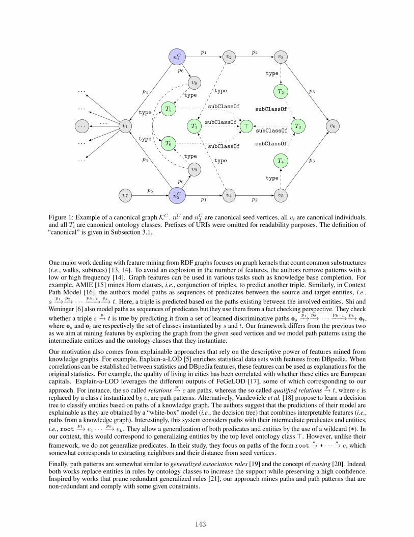
nC1

nC2

v1. . .

. . .

. . .

. . .

. . .

. . .

v2 v3

v4 v5

v6

v7

v8

v9

T1

T2

T3

T4

T5

T6

>

p4

p4

p6

p6

p5

p1 p2

p3

p1 p2

p3

type

type

type

type

type

type

subClassOf

subClassOf

type

type

subClassOf

subClassOf

subClassOf

subClassOf

Figure 1: Example of a canonical graph KC . nC1 and nC2 are canonical seed vertices, all vi are canonical individuals,and all Ti are canonical ontology classes. Prefixes of URIs were omitted for readability purposes. The definition of“canonical” is given in Subsection 3.1.

One major work dealing with feature mining from RDF graphs focuses on graph kernels that count common substructures(i.e., walks, subtrees) [13, 14]. To avoid an explosion in the number of features, the authors remove patterns with alow or high frequency [14]. Graph features can be used in various tasks such as knowledge base completion. Forexample, AMIE [15] mines Horn clauses, i.e., conjunction of triples, to predict another triple. Similarly, in ContextPath Model [16], the authors model paths as sequences of predicates between the source and target entities, i.e.,s

p1−→ p2−→ · · · pk−1−−−→ pk−→ t. Here, a triple is predicted based on the paths existing between the involved entities. Shi andWeninger [6] also model paths as sequences of predicates but they use them from a fact checking perspective. They checkwhether a triple s

p−→ t is true by predicting it from a set of learned discriminative paths osp1−→ p2−→ · · · pk−1−−−→ pk−→ ot,

where os and ot are respectively the set of classes instantiated by s and t. Our framework differs from the previous twoas we aim at mining features by exploring the graph from the given seed vertices and we model path patterns using theintermediate entities and the ontology classes that they instantiate.

Our motivation also comes from explainable approaches that rely on the descriptive power of features mined fromknowledge graphs. For example, Explain-a-LOD [5] enriches statistical data sets with features from DBpedia. Whencorrelations can be established between statistics and DBpedia features, these features can be used as explanations for theoriginal statistics. For example, the quality of living in cities has been correlated with whether these cities are Europeancapitals. Explain-a-LOD leverages the different outputs of FeGeLOD [17], some of which corresponding to ourapproach. For instance, the so called relations

p−→ e are paths, whereas the so called qualified relationsp−→ t, where e is

replaced by a class t instantiated by e, are path patterns. Alternatively, Vandewiele et al. [18] propose to learn a decisiontree to classify entities based on paths of a knowledge graph. The authors suggest that the predictions of their model areexplainable as they are obtained by a “white-box” model (i.e., the decision tree) that combines interpretable features (i.e.,paths from a knowledge graph). Interestingly, this system considers paths with their intermediate predicates and entities,i.e., root

p1−→ e1 · · · pk−→ ek. They allow a generalization of both predicates and entities by the use of a wildcard (*). Inour context, this would correspond to generalizing entities by the top level ontology class >. However, unlike theirframework, we do not generalize predicates. In their study, they focus on paths of the form root *−→ * · · · *−→ e, whichsomewhat corresponds to extracting neighbors and their distance from seed vertices.

Finally, path patterns are somewhat similar to generalized association rules [19] and the concept of raising [20]. Indeed,both works replace entities in rules by ontology classes to increase the support while preserving a high confidence.Inspired by works that prune redundant generalized rules [21], our approach mines paths and path patterns that arenon-redundant and comply with some given constraints.

143

Set of seed vertices N

Knowledge graph K

1. Canonicalizing K

2. Mining interestingneighbors and types

3. Mining interestingpaths and path patterns

4. Optional anddomain-dependent filtering

Binary matrixM∈ B|N|×|F|

Figure 2: Main steps to mine a set F of features (i.e., neighbors, paths, and path patterns) associated with a set N ofseed vertices from a knowledge graph K. Step 4 is optional and depends on the application domain.

Table 1: Parameters that configure the mining of interesting neighbors, paths, and path patterns in a knowledge graph K.Each parameter is associated with a domain and is used in specific steps (see Figure 2 for step numbers). Parameter mis specific to the considered application. Here, we illustrate the role of m with the biomedical domain.

Parameter Domain Steps Description

k N+ 2, 3 Maximum length of paths and path patternst N 3 Maximum level for generalization in class hierarchiesd N 2, 3 Maximum degree (u = true) or out degree (u = false) to allow expansionlmin N 2, 3 Minimum support for featureslmax N 2, 3 Maximum support for featuresu B 2, 3 Whether only out arcs (u = false) or all arcs (u = true) are traversedbpredicates List of URIs 2, 3 Blacklist of predicates not to traversebexp-types List of URIs 2, 3 Blacklist of classes whose instances are not to reachbgen-types List of URIs 2, 3 Blacklist of classes not to use in generalizationm none, p, g,

m, pg, pgm4 Optional and domain-dependent filtering strategy

Illustrated here with the biomedical domain

3 Towards a scalable approach to mine interesting paths and path patterns

In this paper, we consider a knowledge graph K and a set of seed vertices N = n1, n2, . . . , np ⊆ V . The task is tomine neighbors, paths, and path patterns from K that are associated with these seed vertices. For example, given a setof drugs that cause or not a side effect, we aim to mine features that can later be used to classify these drugs.

In the following subsections, we propose algorithms to build a binary matrixM of size |N | × |F| from the knowledgegraph K and the set of seed vertices N . The set F consists of interesting neighbors, paths, and path patterns mined fromK, i.e., neighbors, paths, and path patterns that satisfy the constraints defined in terms of the parameters summarized inTable 1. These parameters will be detailed in the following subsections. M associates a seed vertex n ∈ N with itsfeatures f ∈ F , i.e., ifMn,f = true, then n has feature f . We outline our approach in Figure 2 where steps 1, 2, and3 are mandatory, while step 4 is optional and depends on the application domain.

3.1 Canonicalizing K

The first step of our approach consists in canonicalizing the knowledge graph K, i.e., unifying vertices that representthe same real-world entity. We use the canonicalization word by analogy with the canonicalization of knowledgebases, which consists in unifying equivalent individuals into one [4]. Indeed, in knowledge bases under the OpenInformation Extraction paradigm, facts and entities can be represented by synonymous terms, which leads to co-existingand equivalent individuals. For example, in such knowledge bases, two individuals Obama and Barack Obama canco-exist. Similarly, in K, vertices can be connected through arcs labeled by the owl:sameAs predicate, indicating thatthese vertices are actually representing the same real-world entity.

Such a situation typically arises when K comprises several data sets. For example, a drug can be represented by twovertices linked by an owl:sameAs arc, resulting from the information extraction of two independent drug-relateddatabases. Therefore, their merging allows an easy access to the full extent of the knowledge in K about the drug they

144

represent. Such a canonicalization process corresponds to edge contraction in graph theory (i.e., taking graph quotient).In our framework, it reduces to contracting arcs whose label is the owl:sameAs predicate.

To perform this canonicalization, we must respect the semantics associated with the owl:sameAs predicate, and thustake into account its symmetry and transitivity. Indeed, an owl:sameAs arc between two vertices either is explicitlystated in K or follows from existing arcs and these two properties. Let us consider a vertex v in K. The canonicalizationstep merges v with all its identical vertices based on owl:sameAs arcs. To compute this set of vertices, it sufficesto compute the connected component of v in the undirected spanning subgraph formed by the owl:sameAs arcs ofK. Indeed, undirected edges comply with the symmetry of owl:sameAs and connected components comply with thetransitivity of owl:sameAs.

As a result, this step takes K as input and outputs its canonical graph KC =(ΣC

V ,ΣCA, V

C , AC , sC , tC , `CV , `CA

).

Similarly to K, KC is a directed labeled multigraph where

• V C is the set of canonical vertices.

• AC is the set of canonical arcs connecting canonical vertices through predicates.

• ΣCV is the set of canonical vertex labels.

• ΣCA is the set of canonical arc labels.

• sC : AC → V C (respectively tC : AC → V C ) associates a canonical arc to its canonical source (respectivelytarget) vertex.

• `CV : V C → ΣCV (respectively `CA : AC → ΣC

A) maps a canonical vertex (respectively a canonical arc) to itslabel.

Each canonical vertex in KC represents a vertex from K and all its identical vertices. It is possible for a canonical vertexin KC to only represent one vertex v from K if v has no identical vertices. This corresponds to creating a surjectivemapping λ : V → V C associating a vertex from K to its equivalent canonical vertex in KC . Canonical arcs in KC areconstructed by using λ to map the source and target vertices of arcs in K to canonical vertices. Similarly, the set of seedvertices N is mapped to the set of canonical seed vertices, denoted by NC .Remark 1. Note that storing URIs has a high memory footprint. Thus, inKC , we use indices in N instead of URIs to labelvertices and arcs, i.e., ΣC

V ⊆ N and ΣCA ⊆ N. This leads to a reduced memory consumption in subsequent algorithms.

Each canonical vertex has one unique label, differing from labels of other canonical vertices, i.e., |ΣCV | = |V C |. This

“relabeling” is inspired by the work of de Vries and de Rooij [13] that use a structure named pathMap to represent apath by an integer. We developed our own structure for this relabeling, which we named CacheManager.

3.2 Mining interesting neighbors and types

3.2.1 Mining interesting neighbors

Here, we select all vertices that are neighbors of at least one seed vertex in NC by performing a breadth-first searchconstrained by parameters k, d, u, bpredicates, and bexp-types. Neighbors are selected by traversing at most k arcs from theseed vertices in NC . If u = false, then only outgoing arcs are traversed; otherwise, all arcs are traversed regardless oftheir orientation.

However, not all neighboring vertices are of interest. For example, we want to avoid provenance metadata vertices.Indeed, they may not constitute discriminative features as they are specific to the vertex they describe. As we aim touse ontology classes to generate path patterns, we also need to keep the graph exploration over the individuals of Kand avoid traversing rdf:type arcs. To this aim, we do not traverse arcs that are labeled by a predicate whose URI orprefix of URI is blacklisted in bpredicates. For example, we blacklist in bpredicates the prefix of the provenance ontologyPROV-O5 and the URI of the rdf:type predicate6.

Additionally, we provide a blacklist bexp-types of URIs or prefixes of classes whose instances must not be reached.Hence, we do not reach individuals that instantiate directly or indirectly a blacklisted class, by following rdf:typeand rdfs:subClassOf arcs. For example, in a use case of classifying drugs that cause or not a side effect, one maywant to avoid neighbors that represent the side effect. That is why, the ontology class representing the side effect isblacklisted in bexp-types.

5http://www.w3.org/ns/prov#6http://www.w3.org/1999/02/22-rdf-syntax-ns#type

145

When mining neighboring vertices, we may encounter vertices with a high degree, hereafter named hubs. If thegraph exploration considered their numerous neighbors, then the size of the selected neighborhood would increaseexponentially, thus causing a scalability issue. Additionally, hub neighbors may not constitute specific and discriminativefeatures. Indeed, if a hub can be reached from some seed vertices, i.e., appears in their neighborhood, the neighborsof the hub will be reached by the same seed vertices. That is why, in our approach, we propose to stop the graphexploration at vertices whose degree is strictly greater than parameter d7.Remark 2. If u = false, then the degree of a vertex only counts outgoing arcs, otherwise all arcs are counted. Thedegree does not count arcs whose predicate is blacklisted in bpredicates. The degree counts arcs incident to a vertex thatinstantiates a blacklisted class in bexp-types.

As a result, with k, d, u, bpredicates, and bexp-types fixed, we obtain a set of neighboring vertices, denoted byN (NC) ⊆ V C .Each neighboring vertex v ∈ N (NC) may only appear in the neighborhood of some seed vertices from NC w.r.t. theparameters. Thus, v is associated with these seed vertices, which we indicate by defining the support set of v.

Definition 1 (Support set of a neighbor). For a given choice of these parameters, the support set of a neighboringvertex v ∈ N (NC) is denoted by SUPPORTSET(v) ⊆ NC and defined as the set of seed vertices from NC having v asneighbor. The support of a neighbor is defined as the cardinal of its support set.

Note that some vertices in N (NC) are not very discriminative: when they are associated with very few vertices fromNC or nearly all of them. This motivates the use of parameters lmin and lmax that define the minimum and maximumsupport for a neighbor to appear in the set F of features. Hence, a neighbor v ∈ N (NC) constitutes a feature in theoutput matrixM if and only if lmin ≤ |SUPPORTSET(v)| ≤ lmax. We denote the set of interesting neighbors to appearin F by

Nl(NC) =

v | v ∈ N (NC) and lmin ≤ |SUPPORTSET(v)| ≤ lmax

.

InM, for nC ∈ NC and v ∈ Nl(NC), we haveMnC ,v = true if and only if nC ∈ SUPPORTSET(v).

Example 1. From KC in Figure 1 and with k = 3, d = 4, lmin = 2, lmax = 3, u = false, bpredicates =type, subClassOf, and bexp-types = ∅, we obtain:

N (NC) = v1, v2, v3, v4, v5, v6, v8, v9 ;

SUPPORTSET(v1) = SUPPORTSET(v6) =nC1 , n

C2

;

SUPPORTSET(v2) = SUPPORTSET(v3) = SUPPORTSET(v8) =nC1

;

SUPPORTSET(v4) = SUPPORTSET(v5) = SUPPORTSET(v9) =nC2

;

Nl(NC) = v1, v6 .

The graph exploration stops at v1. Indeed, it is considered a hub as its degree is greater than d. Thus, vertices on the leftof Figure 1 are not explored. Because u = false, the graph exploration cannot reach v7. If bexp-types = T3, then v3and v5 cannot be traversed, resulting in N (NC) = v1, v2, v4, v8, v9.

3.2.2 Mining interesting types

Observe that we can use N (NC) to compute interesting types over the considered neighborhood. These interestingtypes will alleviate a scalability issue arising when building path patterns in Subsection 3.3. Interesting types must becomputed over N (NC) and not Nl(N

C) as vertices whose support is below lmin can instantiate interesting types. Asan intuitive example, in Figure 1, T3 is associated with both nC1 (because of v3) and nC2 (because of v5). For lmin = 2,v3 and v5 will not be selected as features, however T3 can be used in path patterns.

Parameters t and bgen-types constrain the ontology classes considered in the construction of path patterns, and thus theyare integrated in the computation of interesting types. Parameter t specifies the maximum level of considered classesin ontology hierarchies. This level is computed by starting at vertices to generalize and following rdf:type andrdfs:subClassOf arcs. t = 0 only allows to generalize vertices with >, which is considered to be instantiated byall vertices. For example, v3 can be generalized by T2 and > if t = 1, and by T2, T3, and > if t = 2. Additionally,types used for generalization must not be blacklisted in bgen-types. This blacklist consists of URIs or prefixes of ontologyclasses not to be used during the construction of path patterns. For example, we refrain from considering general classessuch as pgxo:Drug8.

7From a similar assessment, de Vries and de Rooij [14] tackle the hub issue by removing edges based on frequency of pairs(source, predicate) and (predicate, target).

8http://pgxo.loria.fr/Drug

146

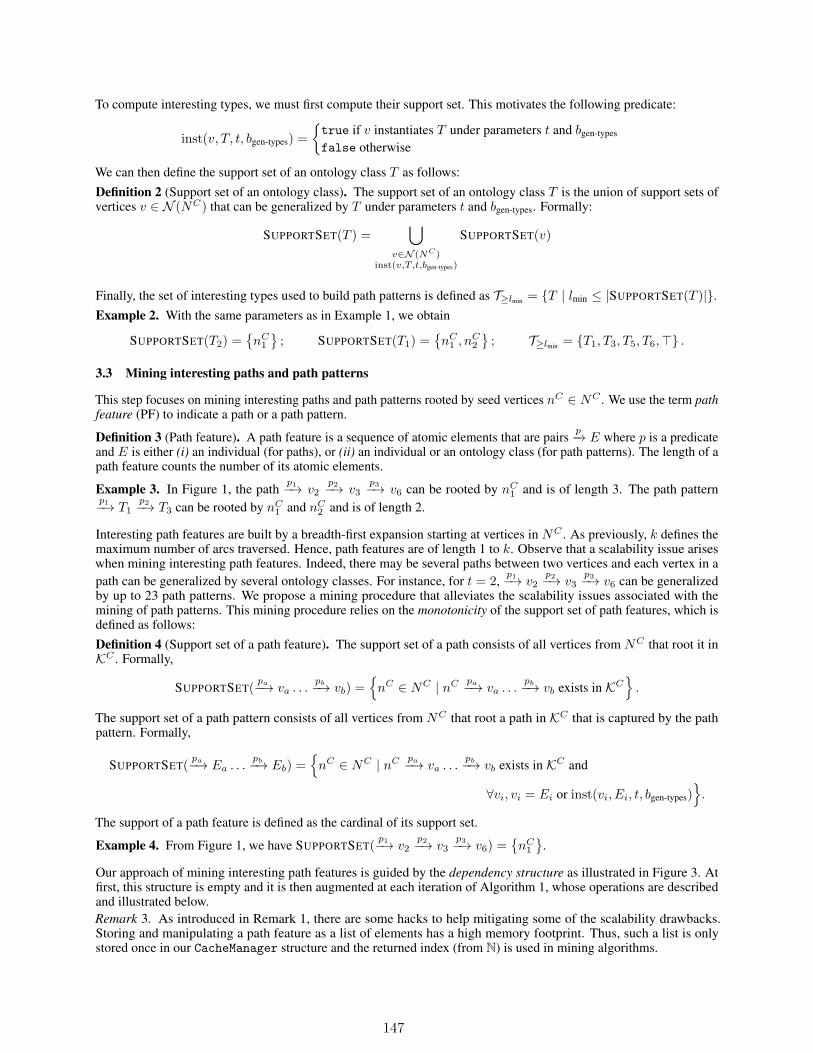
To compute interesting types, we must first compute their support set. This motivates the following predicate:

inst(v, T, t, bgen-types) =

true if v instantiates T under parameters t and bgen-types

false otherwise

We can then define the support set of an ontology class T as follows:Definition 2 (Support set of an ontology class). The support set of an ontology class T is the union of support sets ofvertices v ∈ N (NC) that can be generalized by T under parameters t and bgen-types. Formally:

SUPPORTSET(T ) =⋃

v∈N (NC)inst(v,T,t,bgen-types)

SUPPORTSET(v)

Finally, the set of interesting types used to build path patterns is defined as T≥lmin = T | lmin ≤ |SUPPORTSET(T )|.Example 2. With the same parameters as in Example 1, we obtain

SUPPORTSET(T2) =nC1

; SUPPORTSET(T1) =nC1 , n

C2

; T≥lmin = T1, T3, T5, T6,> .

3.3 Mining interesting paths and path patterns

This step focuses on mining interesting paths and path patterns rooted by seed vertices nC ∈ NC . We use the term pathfeature (PF) to indicate a path or a path pattern.

Definition 3 (Path feature). A path feature is a sequence of atomic elements that are pairsp−→ E where p is a predicate

and E is either (i) an individual (for paths), or (ii) an individual or an ontology class (for path patterns). The length of apath feature counts the number of its atomic elements.

Example 3. In Figure 1, the pathp1−→ v2

p2−→ v3p3−→ v6 can be rooted by nC1 and is of length 3. The path pattern

p1−→ T1p2−→ T3 can be rooted by nC1 and nC2 and is of length 2.

Interesting path features are built by a breadth-first expansion starting at vertices in NC . As previously, k defines themaximum number of arcs traversed. Hence, path features are of length 1 to k. Observe that a scalability issue ariseswhen mining interesting path features. Indeed, there may be several paths between two vertices and each vertex in apath can be generalized by several ontology classes. For instance, for t = 2,

p1−→ v2p2−→ v3

p3−→ v6 can be generalizedby up to 23 path patterns. We propose a mining procedure that alleviates the scalability issues associated with themining of path patterns. This mining procedure relies on the monotonicity of the support set of path features, which isdefined as follows:Definition 4 (Support set of a path feature). The support set of a path consists of all vertices from NC that root it inKC . Formally,

SUPPORTSET(pa−→ va . . .

pb−→ vb) =nC ∈ NC | nC pa−→ va . . .

pb−→ vb exists in KC.

The support set of a path pattern consists of all vertices from NC that root a path in KC that is captured by the pathpattern. Formally,

SUPPORTSET(pa−→ Ea . . .

pb−→ Eb) =nC ∈ NC | nC pa−→ va . . .

pb−→ vb exists in KC and

∀vi, vi = Ei or inst(vi, Ei, t, bgen-types).

The support of a path feature is defined as the cardinal of its support set.

Example 4. From Figure 1, we have SUPPORTSET(p1−→ v2

p2−→ v3p3−→ v6) =

nC1

.

Our approach of mining interesting path features is guided by the dependency structure as illustrated in Figure 3. Atfirst, this structure is empty and it is then augmented at each iteration of Algorithm 1, whose operations are describedand illustrated below.Remark 3. As introduced in Remark 1, there are some hacks to help mitigating some of the scalability drawbacks.Storing and manipulating a path feature as a list of elements has a high memory footprint. Thus, such a list is onlystored once in our CacheManager structure and the returned index (from N) is used in mining algorithms.

147

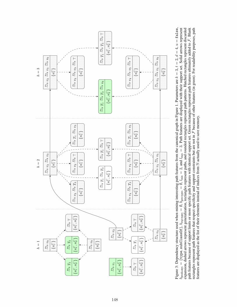
h=

1

p4 −→

v 1 n

C 1,n

C 2

p4 −→>

nC 1,n

C 2

p1 −→

v 2 n

C 1

p1 −→

T1

nC 1,n

C 2

p1 −→>

nC 1,n

C 2

p1 −→

v 4 n

C 2

p6 −→

v 8 n

C 1

p6 −→

T5

nC 1,n

C 2

p6 −→

T6

nC 1,n

C 2

p6 −→>

nC 1,n

C 2

p6 −→

v 9 n

C 2

h=

2

p1 −→

v 2p2 −→

v 3 n

C 1

p1 −→

v 4p2 −→

v 5 n

C 2

p1 −→

T1

p2 −→

T3

nC 1,n

C 2

p1 −→

T1

p2 −→>

nC 1,n

C 2

p1 −→

v 2p2 −→

T3

nC 1

p1 −→

v 2p2 −→>

nC 1

p1 −→

T1

p2 −→

v 3 n

C 1

p1 −→

v 4p2 −→

T3

nC 2

p1 −→

v 4p2 −→>

nC 2

p1 −→

T1

p2 −→

v 5 n

C 2

h=

3

p1 −→

v 2p2 −→

v 3p3 −→

v 6 n

C 1

p1 −→

v 4p2 −→

v 5p3 −→

v 6 n

C 2

p1 −→

v 2p2 −→

v 3p3 −→>

nC 1

p1 −→

v 4p2 −→

v 5p3 −→>

nC 2

p1 −→

T1

p2 −→

T3

p3 −→

v 6 n

C 1,n

C 2

p1 −→

T1

p2 −→

T3

p3 −→>

nC 1,n

C 2

Figu

re3:

Dep

ende

ncy

stru

ctur

eus

edw

hen

min

ing

inte

rest

ing

path

feat

ures

from

the

cano

nica

lgra

phin

Figu

re1.

Para

met

ers

arek

=3,t

=2,d

=4,u

=fa

lse,

b pre

dica

tes

=typ

e,su

bCla

ssOf,b e

xp-t

ypes

=∅,b g

en-t

ypes

=∅,l m

in=

2,a

ndl m

ax=

3.

Path

feat

ures

are

disp

laye

dw

ithth

eir

supp

orts

et.

Solid

arro

ws

repr

esen

tex

pans

ion,

dash

edar

row

sre

pres

entg

ener

aliz

atio

n,re

ctan

gles

repr

esen

tpat

hs,a

ndro

unde

dre

ctan

gles

repr

esen

tpat

hpa

ttern

s.H

atch

edre

ctan

gles

repr

esen

tdis

card

edpa

thfe

atur

esbe

caus

eof

supp

ortl

imits

orm

ore

spec

ific

path

feat

ures

with

iden

tical

supp

orts

et.G

reen

rect

angl

esre

pres

entp

ath

feat

ures

ultim

atel

yad

ded

toF

.Bla

nkre

ctan

gles

repr

esen

tpat

hfe

atur

esth

atre

spec

tspe

cific

ityan

dsu

ppor

tcon

stra

ints

buta

reno

tinF

beca

use

ofot

herf

eatu

res

(in

gree

n).F

orre

adab

ility

purp

oses

,pat

hfe

atur

esar

edi

spla

yed

asth

elis

toft

heir

elem

ents

inst

ead

ofin

dice

sfr

omN

actu

ally

used

tosa

vem

emor

y.

148

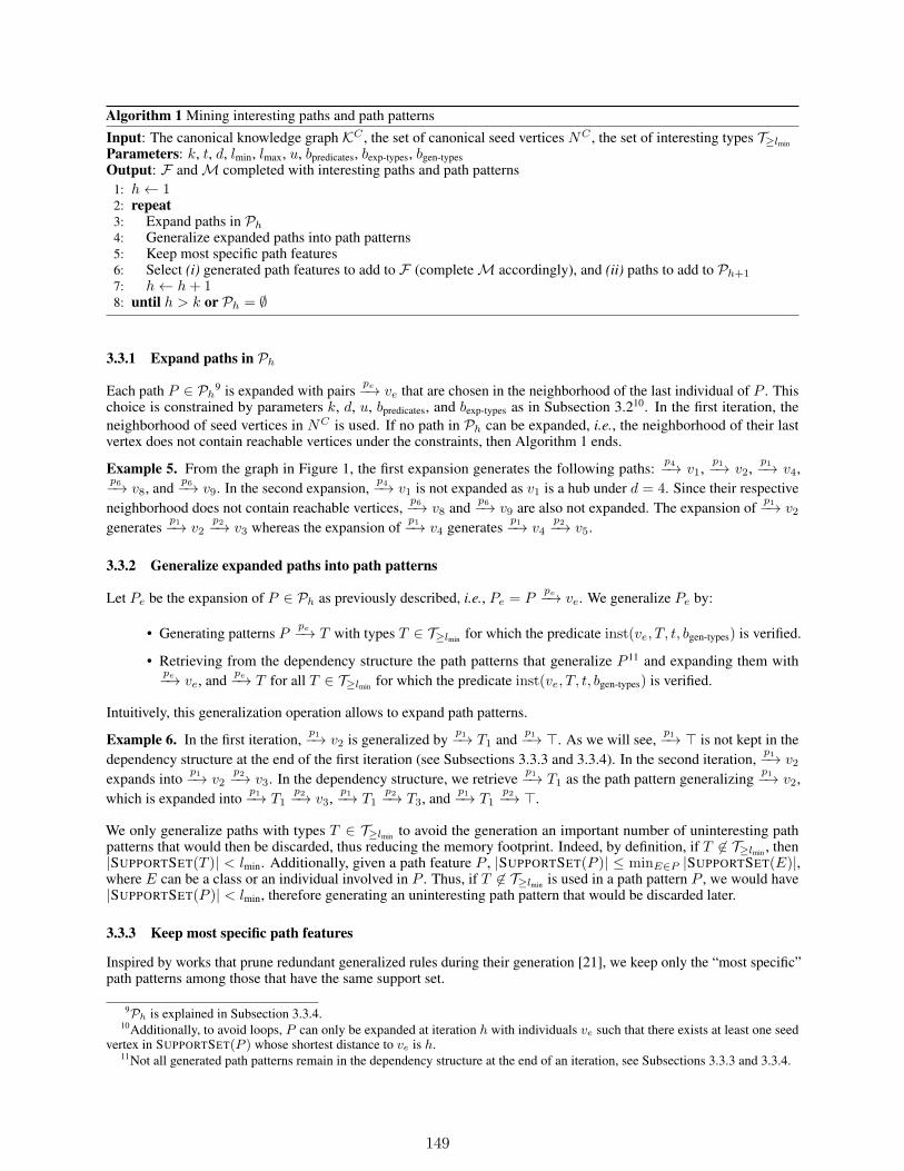
Algorithm 1 Mining interesting paths and path patternsInput: The canonical knowledge graph KC , the set of canonical seed vertices NC , the set of interesting types T≥lmin

Parameters: k, t, d, lmin, lmax, u, bpredicates, bexp-types, bgen-typesOutput: F andM completed with interesting paths and path patterns

1: h← 12: repeat3: Expand paths in Ph

4: Generalize expanded paths into path patterns5: Keep most specific path features6: Select (i) generated path features to add to F (completeM accordingly), and (ii) paths to add to Ph+1

7: h← h+ 18: until h > k or Ph = ∅

3.3.1 Expand paths in Ph

Each path P ∈ Ph9 is expanded with pairs

pe−→ ve that are chosen in the neighborhood of the last individual of P . Thischoice is constrained by parameters k, d, u, bpredicates, and bexp-types as in Subsection 3.210. In the first iteration, theneighborhood of seed vertices in NC is used. If no path in Ph can be expanded, i.e., the neighborhood of their lastvertex does not contain reachable vertices under the constraints, then Algorithm 1 ends.

Example 5. From the graph in Figure 1, the first expansion generates the following paths:p4−→ v1,

p1−→ v2,p1−→ v4,

p6−→ v8, andp6−→ v9. In the second expansion,

p4−→ v1 is not expanded as v1 is a hub under d = 4. Since their respectiveneighborhood does not contain reachable vertices,

p6−→ v8 andp6−→ v9 are also not expanded. The expansion of

p1−→ v2generates

p1−→ v2p2−→ v3 whereas the expansion of

p1−→ v4 generatesp1−→ v4

p2−→ v5.

3.3.2 Generalize expanded paths into path patterns

Let Pe be the expansion of P ∈ Ph as previously described, i.e., Pe = Ppe−→ ve. We generalize Pe by:

• Generating patterns Ppe−→ T with types T ∈ T≥lmin for which the predicate inst(ve, T, t, bgen-types) is verified.

• Retrieving from the dependency structure the path patterns that generalize P 11 and expanding them withpe−→ ve, and

pe−→ T for all T ∈ T≥lmin for which the predicate inst(ve, T, t, bgen-types) is verified.

Intuitively, this generalization operation allows to expand path patterns.

Example 6. In the first iteration,p1−→ v2 is generalized by

p1−→ T1 andp1−→ >. As we will see,

p1−→ > is not kept in thedependency structure at the end of the first iteration (see Subsections 3.3.3 and 3.3.4). In the second iteration,

p1−→ v2expands into

p1−→ v2p2−→ v3. In the dependency structure, we retrieve

p1−→ T1 as the path pattern generalizingp1−→ v2,

which is expanded intop1−→ T1

p2−→ v3,p1−→ T1

p2−→ T3, andp1−→ T1

p2−→ >.

We only generalize paths with types T ∈ T≥lmin to avoid the generation an important number of uninteresting pathpatterns that would then be discarded, thus reducing the memory footprint. Indeed, by definition, if T 6∈ T≥lmin , then|SUPPORTSET(T )| < lmin. Additionally, given a path feature P , |SUPPORTSET(P )| ≤ minE∈P |SUPPORTSET(E)|,where E can be a class or an individual involved in P . Thus, if T 6∈ T≥lmin is used in a path pattern P , we would have|SUPPORTSET(P )| < lmin, therefore generating an uninteresting path pattern that would be discarded later.

3.3.3 Keep most specific path features

Inspired by works that prune redundant generalized rules during their generation [21], we keep only the “most specific”path patterns among those that have the same support set.

9Ph is explained in Subsection 3.3.4.10Additionally, to avoid loops, P can only be expanded at iteration h with individuals ve such that there exists at least one seed

vertex in SUPPORTSET(P ) whose shortest distance to ve is h.11Not all generated path patterns remain in the dependency structure at the end of an iteration, see Subsections 3.3.3 and 3.3.4.

149

Definition 5 (More specific path pattern). A path pattern P1 is more specific than another path pattern P2 if everyatomic element of P1 is more specific than the atomic element of P2 at the same position. An atomic element

p1−→ E1 ismore specific than another atomic element

p2−→ E2 if and only if:

(i) p1 = p2, i.e., both atomic elements involve the same predicate12, and

(ii) E1 is more specific than E213.

When path patterns have the same support set, keeping the most specific ones remove redundant generalizations, thusreducing their number and the computational burden. Additionally, we ensure a high descriptive power because themost specific paths are the most descriptive. Intuitively, a path pattern involving a class T is less descriptive thananother pattern involving a subclass or an instance of the class. However, keeping the most specific path patterns iscomputationally expensive, which led us to propose the following computational procedure.

We notice that the support set of a path pattern is the union of the support sets of the paths it generalizes. Therefore,we discard path patterns that generalize only one path. Indeed, such path patterns have the same support set as theiroriginal path and are more general, by definition.

Example 7. For h = 3, we discard the following path patterns:p1−→ v2

p2−→ v3p3−→ > and

p1−→ v4p2−→ v5

p3−→ >.

However, there may exist path patterns that generalize several more specific path features while having the same supportset. Such path patterns should also be discarded.

Example 8. For h = 1,p1−→ > shares the same support set as the more specific path pattern

p1−→ T1 and thus should bediscarded.

To efficiently discard path patterns, we avoid computing their whole hierarchy. Instead, we focus on retaining only themost specific ones in the prefix tree depicted in Figure 4. This prefix tree is incrementally augmented and stores the mostspecific path patterns for a specific iteration and support set. In this tree, individuals/classes and predicates involved inpath patterns are indexed separately. Thus, its depth is twice the length of path patterns of the current iteration.

The prefix tree enables an efficient storage and selection of the most specific path patterns. Indeed, let P be a pathpattern to be compared with those already stored. A breadth-first traversal is performed to detect more specific patternsthan P : we only traverse identical or more specific elements according to Definition 5. At any depth, if such elementscannot be found, then P is one of the most specific patterns and the traversal stops. On the contrary, if the traversalreaches a leaf containing more specific elements, then there is a pattern more specific than P with the same support set.Consequently, P is discarded and removed from the dependency structure.

If P is to be stored, another breadth-first traversal is performed by considering identical or more general elements thanthe ones in P . When the traversal reaches a leaf, it means that more general patterns than P are currently stored andhave the same support set. These are removed from the prefix tree before storing P . They are also removed from thedependency structure.Remark 4. As the prefix tree relies on associative arrays and sets, the computational cost of traversal, insertion, andremoval is reduced. Additionally, resetting the tree at each expansion and each support set reduces the number ofpatterns to traverse and thus the global computational cost.

3.3.4 Select generated path features to add to F , and paths to add to Ph+1

In this subsection, we determine (i) which paths and path patterns should be added as features in F , and consequently,(ii) which paths to add to Ph+1, i.e., to expand during the next iteration.

A path feature P can be added in F if:

(C1) lmin ≤ SUPPORTSET(P ) ≤ lmax,

(C2) Prefixes of P with the same support set do not already exist in F ,

(C3) If P is a path pattern, it does not generalize a path with the same support set.

When P is in F , the output binary matrixM verifiesMnC ,P = true for all nC ∈ SUPPORTSET(P ).

12It is noteworthy that we do not consider the hierarchy of predicates in this work.13A class is more specific than all its super-classes and an individual is more specific than all classes it instantiates.

150

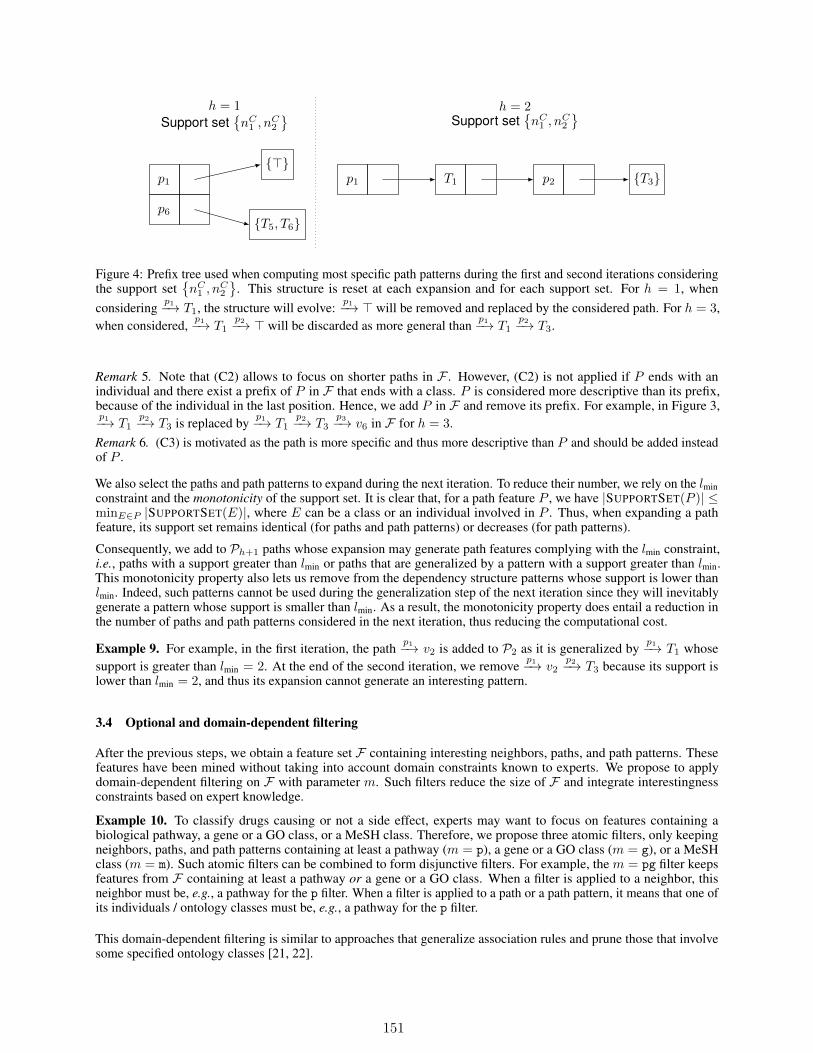
h = 1

Support setnC1 , n

C2

p1

p6

>

T5, T6

h = 2Support set

nC1 , n

C2

p1 T1 p2 T3

Figure 4: Prefix tree used when computing most specific path patterns during the first and second iterations consideringthe support set

nC1 , n

C2

. This structure is reset at each expansion and for each support set. For h = 1, when

consideringp1−→ T1, the structure will evolve:

p1−→ > will be removed and replaced by the considered path. For h = 3,when considered,

p1−→ T1p2−→ > will be discarded as more general than

p1−→ T1p2−→ T3.

Remark 5. Note that (C2) allows to focus on shorter paths in F . However, (C2) is not applied if P ends with anindividual and there exist a prefix of P in F that ends with a class. P is considered more descriptive than its prefix,because of the individual in the last position. Hence, we add P in F and remove its prefix. For example, in Figure 3,p1−→ T1

p2−→ T3 is replaced byp1−→ T1

p2−→ T3p3−→ v6 in F for h = 3.

Remark 6. (C3) is motivated as the path is more specific and thus more descriptive than P and should be added insteadof P .

We also select the paths and path patterns to expand during the next iteration. To reduce their number, we rely on the lminconstraint and the monotonicity of the support set. It is clear that, for a path feature P , we have |SUPPORTSET(P )| ≤minE∈P |SUPPORTSET(E)|, where E can be a class or an individual involved in P . Thus, when expanding a pathfeature, its support set remains identical (for paths and path patterns) or decreases (for path patterns).

Consequently, we add to Ph+1 paths whose expansion may generate path features complying with the lmin constraint,i.e., paths with a support greater than lmin or paths that are generalized by a pattern with a support greater than lmin.This monotonicity property also lets us remove from the dependency structure patterns whose support is lower thanlmin. Indeed, such patterns cannot be used during the generalization step of the next iteration since they will inevitablygenerate a pattern whose support is smaller than lmin. As a result, the monotonicity property does entail a reduction inthe number of paths and path patterns considered in the next iteration, thus reducing the computational cost.

Example 9. For example, in the first iteration, the pathp1−→ v2 is added to P2 as it is generalized by

p1−→ T1 whosesupport is greater than lmin = 2. At the end of the second iteration, we remove

p1−→ v2p2−→ T3 because its support is

lower than lmin = 2, and thus its expansion cannot generate an interesting pattern.

3.4 Optional and domain-dependent filtering

After the previous steps, we obtain a feature set F containing interesting neighbors, paths, and path patterns. Thesefeatures have been mined without taking into account domain constraints known to experts. We propose to applydomain-dependent filtering on F with parameter m. Such filters reduce the size of F and integrate interestingnessconstraints based on expert knowledge.

Example 10. To classify drugs causing or not a side effect, experts may want to focus on features containing abiological pathway, a gene or a GO class, or a MeSH class. Therefore, we propose three atomic filters, only keepingneighbors, paths, and path patterns containing at least a pathway (m = p), a gene or a GO class (m = g), or a MeSHclass (m = m). Such atomic filters can be combined to form disjunctive filters. For example, the m = pg filter keepsfeatures from F containing at least a pathway or a gene or a GO class. When a filter is applied to a neighbor, thisneighbor must be, e.g., a pathway for the p filter. When a filter is applied to a path or a path pattern, it means that one ofits individuals / ontology classes must be, e.g., a pathway for the p filter.

This domain-dependent filtering is similar to approaches that generalize association rules and prune those that involvesome specified ontology classes [21, 22].

151

4 Experimental setup

To illustrate our approach, we will address the following task: from a knowledge graph, mine a set of features to classifydrugs depending on whether they cause a specific side effect.

We explore PGxLOD14 [10], a knowledge graph that aggregates several sets of Linked Open Data (LOD) describingdrugs, phenotypes, and genetic factors: PharmGKB, ClinVar, DrugBank, SIDER, DisGeNET, and CTD. This aggre-gation may lead to features combining units from several LOD sets. Indeed, LOD sets may contain different andincomplete knowledge. Their combined use then enables leveraging a greater amount of knowledge, where some LODsets complete information provided by others. This asks for a canonical knowledge graph as described in Subsection 3.1.For instance, it is possible to complete the knowledge related to a drug described in PharmGKB if it is linked with anowl:sameAs arc to the same drug described in DrugBank. This constitutes the key interest in combining LOD sets inknowledge discovery and data mining tasks, as discussed by Ristoski and Paulheim [23].

We will use the following data sets that comprise positive (⊕) and negative () drug examples:Data set 1 (Drug Induced Liver Injury (DILI) [24]). It is formed by 1,036 drugs in 4 classes: “most DILI concern”(192 drugs), “ambiguous DILI concern” (254 drugs), “less DILI concern” (278 drugs), and “no DILI concern” (312drugs). We mapped these drugs from their PubChem identifiers to identifiers from PharmGKB, otherwise DrugBank,otherwise KEGG, resulting in the set of seed vertices NDILI = NDILI

⊕ ∪NDILI such that:

• |NDILI⊕ | = 146 drugs (118 from PharmGKB, 17 from DrugBank, and 11 from KEGG). The positive drug

examples are from the “most DILI concern” class.

• |NDILI | = 224 drugs (206 from PharmGKB, 9 from DrugBank, and 9 from KEGG). The negative drug

examples are from the “no DILI concern” class.Data set 2 (Severe Cutaneous Adverse Reactions (SCAR)15). It is formed by 874 drugs in 5 classes: “very probable”(18 drugs), “probable” (19 drugs), “possible” (94 drugs), “unlikely” (697 drugs), and “very unlikely” (46 drugs). Wemapped these drugs from their PubChem identifiers to identifiers from PharmGKB, otherwise DrugBank, otherwiseKEGG, resulting in the set of seed vertices NSCAR = NSCAR

⊕ ∪NSCAR such that:

• |NSCAR⊕ | = 102 drugs (100 from PharmGKB and 2 from DrugBank). The positive drug examples are from the

“very probable”, “probable”, and “possible” classes.

• |NSCAR | = 290 drugs (286 from PharmGKB and 4 from DrugBank). The negative drug examples are from

the “unlikely” and “very unlikely” classes.

We implemented our approach in Python16. We used a server with 700 GB of RAM and the following parameter valuesk ∈ 1, 2, 3, 4, t ∈ 1, 2, 3, d = 500, u = false, lmin = 5, lmax = +∞, and m ∈ p, g, m, pg, pgm. It should benoted that k = 4 was only tested with t = 1 because of memory issues caused by the high number of generated features.

Statistics about the features are detailed for k = 3, t = 3 and k = 4, t = 1 in Table 2 and discussed in the next section.We obtained the features associated with the DILI data set under k = 3, t = 3 in approximately 1 hour. However,computing the features with k = 4, t = 1 on the same data set required 4 days and 380 GB of RAM.

5 Results and discussion

The first two lines of Table 2 show the number of neighbors and types reachable before applying support limits.Enforcing these limits constitutes a first reduction of these numbers, thus reducing the memory and computationalfootprints. Here, numbers are approximately divided by 2. The mining of path features always relies on lmin, andthus it is not possible to count the number of all possible paths and path patterns. However, we show the number ofpath features generated during the mining, which already illustrates the combinatorial explosion. Enforcing supportconstraints and removing redundant generalizations allow to reduce their number in F (here, approximately by 20).Finally, the domain-dependent filtering defined by m also radically scales down the number of features ultimatelyoutput. However, this filtering only happens as post-processing and does not alleviate the scalability issues arisingduring the mining of patterns.

We observe a drastic increase in the number of neighbors and path features alongside k, which highlights the scalabilityissues of mining large knowledge graphs. Considering additional levels in ontology hierarchies by increasing t also

14https://pgxlod.loria.fr15http://www.regiscar.org/16https://github.com/pmonnin/kgpm

152

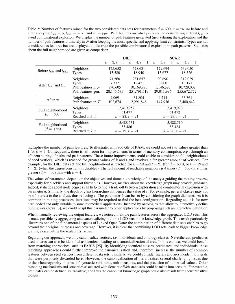
Table 2: Number of features mined for the two considered data sets for parameters d = 500, u = false before andafter applying lmin = 5, lmax = +∞, and m = pgm. Path features are always computed considering at least lmin toavoid combinatorial explosion. We display the number of path features generated (gen.) during the exploration and thenumber of path features ultimately in F after keeping the most specific and applying limit constraints. Types are notconsidered as features but are displayed to illustrate the possible combinatorial explosion in path patterns. Statisticsabout the full neighborhood are given as comparison.

DILI SCARk = 3, t = 3 k = 4, t = 1 k = 3, t = 3 k = 4, t = 1

Before lmin and lmaxNeighbors 175,652 628,681 179,694 639,050Types 13,580 18,940 13,677 18,526

After lmin and lmax

Neighbors 71,560 281,657 90,690 312,029Types 7,372 12,421 8,800 13,177Path features in F 790,605 10,169,975 1,146,585 10,729,002Path features gen. 20,145,635 251,791,519 29,011,996 255,672,772

After m Neighbors 4,069 31,804 4,214 33,361Path features in F 102,674 2,291,846 147,936 2,400,642

Full neighborhood(d = 500)

Neighbors 2,419,957 2,419,920Types 51,477 51,472Reached at k, t k = 23, t = 21 k = 23, t = 21

Full neighborhood(d = +∞)

Neighbors 5,488,531 5,488,510Types 53,486 53,484Reached at k, t k = 19, t = 21 k = 20, t = 21

multiplies the number of path features. To illustrate, with 700 GB of RAM, we could not set t to values greater than1 for k = 4. Consequently, there is still room for improvements in terms of memory consumption, e.g., through anefficient storing of paths and path patterns. These future improvements could enable to consider the full neighborhoodof seed vertices, which is reached for greater values of k and t and involves a far greater amount of vertices. Forexample, for the DILI data set, the full neighborhood is reached for k = 23 and t = 21 (for d = 500), or k = 19 andt = 21 (when the degree constraint is disabled). The full amount of reachable neighbors is 4 times (d = 500) or 9 timesgreater (d = +∞) than with k = 4.

The values of parameters depend on the objectives and domain knowledge of the analyst guiding the mining process,especially for blacklists and support thresholds. However, metrics about the knowledge graph may provide guidance.Indeed, statistics about node degrees can help to find a trade-off between exploration and combinatorial explosion withparameter d. Similarly, the depth of class hierarchies influences the value of t. For example, general classes may notbe of interest to the analyst, thus reducing t. The parameter k can be set by considering the graph diameter. As it iscommon in mining processes, iterations may be required to find the best configuration. Regarding m, it is for nowhard-coded and only suitable to some biomedical applications. Inspired by ontologies that allow to interactively definemining workflows [3], we could adapt this parameter to other applications by proposing such an interactive definition.

When manually reviewing the output features, we noticed multiple path features across the aggregated LOD sets. Thisis made possible by aggregating and canonicalizing multiple LOD sets in the knowledge graph. This result particularlyillustrates one of the fundamental aspects of Linked Open Data: the combination of different data sets enables to gobeyond their original purposes and coverage. However, it is clear that combining LOD sets leads to bigger knowledgegraphs, exacerbating the scalability issues.

Regarding our approach, we only canonicalize vertices, i.e., individuals and ontology classes. Nevertheless, predicatesused on arcs can also be identified as identical, leading to a canonicalization of arcs. In this context, we could benefitfrom matching approaches, such as PARIS [25]. By identifying identical classes, predicates, and individuals, thesematching approaches could further improve the canonicalization and, therefore, increase the number of commonfeatures between seed vertices from different data sets. Similarly, we could consider literals and arcs incident to literalsthat were purposely discarded here. However, the canonicalization of literals raises several challenging issues dueto their heterogeneity in terms of syntactic variations, unit measures, and the precision of numerical values. Otherreasoning mechanisms and semantics associated with Semantic Web standards could be taken into account. For example,predicates can be defined as transitive, and thus the canonical knowledge graph could also result from their transitiveclosure.

153

Regarding the modeling of path patterns, we could generalize paths with both the hierarchy of classes and the hierarchyof predicates. In addition to keeping the most specific patterns, we could use other metrics to further reduce theirredundancy (e.g., approaches relying on hierarchies [26, 27] and extents of ontological classes [27]). This could alsoreduce the number of generated patterns, therefore improving the scalability of the mining approach. Neighbors couldbe enriched with the distance between them and seed vertices, which would correspond to the generalized paths ofKGPTree [18]. We could also use other approaches than binary features (e.g., counting [13, 14], relative counting [28]).More importantly, it remains to test our mined features within a complete classification task to measure the influence ofk, t, and the three kinds of features (neighbors, paths, and path patterns).

6 Conclusion

In this preliminary study, we addressed the scalability issues associated with the task of mining neighbors, paths, andpath patterns from a knowledge graph and a set of seed vertices. We proposed a method for tackling these issues,which we illustrated by mining a real-world knowledge graph. Our results highlight the importance of considering thescalability of approaches when mining features from ever-growing knowledge graphs. Our work alleviates part of thecomputational cost (time and memory) of mining paths and path patterns but also reveals the need for a further reduction.Such future research works could enable the modeling of more complex path patterns, for example, considering thehierarchy of predicates.

References

[1] Aidan Hogan, Eva Blomqvist, Michael Cochez, Claudia d’Amato, Gerard de Melo, Claudio Gutierrez, JoséEmilio Labra Gayo, Sabrina Kirrane, Sebastian Neumaier, Axel Polleres, Roberto Navigli, Axel-Cyrille NgongaNgomo, Sabbir M. Rashid, Anisa Rula, Lukas Schmelzeisen, Juan F. Sequeda, Steffen Staab, and AntoineZimmermann. Knowledge graphs. CoRR, abs/2003.02320, 2020.

[2] Christian Bizer, Tom Heath, and Tim Berners-Lee. Linked data - the story so far. Int. J. Semantic Web Inf. Syst.,5(3):1–22, 2009.

[3] Petar Ristoski and Heiko Paulheim. Semantic web in data mining and knowledge discovery: A comprehensivesurvey. J. Web Semant., 36:1–22, 2016.

[4] Luis Galárraga, Geremy Heitz, Kevin Murphy, and Fabian M. Suchanek. Canonicalizing open knowledge bases.In Jianzhong Li, Xiaoyang Sean Wang, Minos N. Garofalakis, Ian Soboroff, Torsten Suel, and Min Wang,editors, Proceedings of the 23rd ACM International Conference on Conference on Information and KnowledgeManagement, CIKM 2014, Shanghai, China, November 3-7, 2014, pages 1679–1688. ACM, 2014.

[5] Heiko Paulheim. Generating possible interpretations for statistics from linked open data. In Elena Simperl,Philipp Cimiano, Axel Polleres, Óscar Corcho, and Valentina Presutti, editors, The Semantic Web: Research andApplications - 9th Extended Semantic Web Conference, ESWC 2012, Heraklion, Crete, Greece, May 27-31, 2012.Proceedings, volume 7295 of Lecture Notes in Computer Science, pages 560–574. Springer, 2012.

[6] Baoxu Shi and Tim Weninger. Discriminative predicate path mining for fact checking in knowledge graphs.Knowl.-Based Syst., 104:123–133, 2016.

[7] Tim Berners-Lee, James Hendler, Ora Lassila, et al. The Semantic Web. Scientific American, 284(5):28–37, 2001.

[8] Thomas R Gruber. A translation approach to portable ontology specifications. Knowledge Acquisition, 5(2):199–220, 1993.

[9] Charu C. Aggarwal and Haixun Wang, editors. Managing and Mining Graph Data, volume 40 of Advances inDatabase Systems. Springer, 2010.

[10] Pierre Monnin, Joël Legrand, Graziella Husson, Patrice Ringot, Andon Tchechmedjiev, Clément Jonquet, AmedeoNapoli, and Adrien Coulet. PGxO and PGxLOD: a reconciliation of pharmacogenomic knowledge of variousprovenances, enabling further comparison. BMC Bioinformatics, 20-S(4):139:1–139:16, 2019.

[11] Guillaume Bonfante, Bruno Guillaume, and Guy Perrier. Application of Graph Rewriting to Natural LanguageProcessing. Wiley Online Library, 2018.

[12] Pablo Barceló, Leonid Libkin, and Juan L. Reutter. Querying graph patterns. In Maurizio Lenzerini and ThomasSchwentick, editors, Proceedings of the 30th ACM SIGMOD-SIGACT-SIGART Symposium on Principles ofDatabase Systems, PODS 2011, June 12-16, 2011, Athens, Greece, pages 199–210. ACM, 2011.

154

[13] Gerben Klaas Dirk de Vries and Steven de Rooij. A fast and simple graph kernel for RDF. In Claudia d’Amato,Petr Berka, Vojtech Svátek, and Krzysztof Wecel, editors, Proceedings of the International Workshop on DataMining on Linked Data, with Linked Data Mining Challenge collocated with the European Conference on MachineLearning and Principles and Practice of Knowledge Discovery in Databases (ECMLPKDD 2013), Prague, CzechRepublic, September 23, 2013., volume 1082 of CEUR Workshop Proceedings. CEUR-WS.org, 2013.

[14] Gerben Klaas Dirk de Vries and Steven de Rooij. Substructure counting graph kernels for machine learning fromRDF data. J. Web Semant., 35:71–84, 2015.

[15] Luis Antonio Galárraga, Christina Teflioudi, Katja Hose, and Fabian M. Suchanek. AMIE: association rule miningunder incomplete evidence in ontological knowledge bases. In Daniel Schwabe, Virgílio A. F. Almeida, HartmutGlaser, Ricardo A. Baeza-Yates, and Sue B. Moon, editors, 22nd International World Wide Web Conference,WWW ’13, Rio de Janeiro, Brazil, May 13-17, 2013, pages 413–422. International World Wide Web ConferencesSteering Committee / ACM, 2013.

[16] Josua Stadelmaier and Sebastian Padó. Modeling paths for explainable knowledge base completion. In Proceedingsof the 2019 ACL Workshop BlackboxNLP: Analyzing and Interpreting Neural Networks for NLP, pages 147–157,2019.

[17] Heiko Paulheim and Johannes Fürnkranz. Unsupervised generation of data mining features from linked opendata. In Dumitru Dan Burdescu, Rajendra Akerkar, and Costin Badica, editors, 2nd International Conference onWeb Intelligence, Mining and Semantics, WIMS ’12, Craiova, Romania, June 6-8, 2012, pages 31:1–31:12. ACM,2012.

[18] Gilles Vandewiele, Bram Steenwinckel, Femke Ongenae, and Filip De Turck. Inducing a decision tree withdiscriminative paths to classify entities in a knowledge graph. In Zhe He, Jiang Bian, Cui Tao, and Rui Zhang,editors, Proceedings of the 4th International Workshop on Semantics-Powered Data Mining and Analytics co-located with the 18th International Semantic Web Conference (ISWC 2019), Aukland, New Zealand, October 27,2019., volume 2427 of CEUR Workshop Proceedings. CEUR-WS.org, 2019.

[19] Ramakrishnan Srikant and Rakesh Agrawal. Mining generalized association rules. In Umeshwar Dayal, PeterM. D. Gray, and Shojiro Nishio, editors, VLDB’95, Proceedings of 21th International Conference on Very LargeData Bases, September 11-15, 1995, Zurich, Switzerland., pages 407–419. Morgan Kaufmann, 1995.

[20] Xuan Zhou and James Geller. Raising, to enhance rule mining in web marketing with the use of an ontology. InData Mining with Ontologies: Implementations, Findings, and Frameworks, pages 18–36. IGI Global, 2008.

[21] Marcos Aurélio Domingues and Solange Oliveira Rezende. Using taxonomies to facilitate the analysis of theassociation rules. CoRR, abs/1112.1734, 2011.

[22] Claudia Marinica and Fabrice Guillet. Knowledge-based interactive postmining of association rules usingontologies. IEEE Trans. Knowl. Data Eng., 22(6):784–797, 2010.

[23] Petar Ristoski and Heiko Paulheim. Rdf2vec: RDF graph embeddings for data mining. In Paul T. Groth, ElenaSimperl, Alasdair J. G. Gray, Marta Sabou, Markus Krötzsch, Freddy Lécué, Fabian Flöck, and Yolanda Gil,editors, The Semantic Web - ISWC 2016 - 15th International Semantic Web Conference, Kobe, Japan, October17-21, 2016, Proceedings, Part I, volume 9981 of Lecture Notes in Computer Science, pages 498–514, 2016.

[24] Minjun Chen, Ayako Suzuki, Shraddha Thakkar, Ke Yu, Chuchu Hu, and Weida Tong. DILIrank: the largestreference drug list ranked by the risk for developing drug-induced liver injury in humans. Drug Discov Today,21(4):648–653, 2016.

[25] Fabian M. Suchanek, Serge Abiteboul, and Pierre Senellart. PARIS: probabilistic alignment of relations, instances,and schema. PVLDB, 5(3):157–168, 2011.

[26] Petar Ristoski and Heiko Paulheim. Feature selection in hierarchical feature spaces. In Saso Dzeroski, PancePanov, Dragi Kocev, and Ljupco Todorovski, editors, Discovery Science - 17th International Conference, DS 2014,Bled, Slovenia, October 8-10, 2014. Proceedings, volume 8777 of Lecture Notes in Computer Science, pages288–300. Springer, 2014.

[27] Claudia d’Amato, Steffen Staab, and Nicola Fanizzi. On the influence of description logics ontologies on concep-tual similarity. In Aldo Gangemi and Jérôme Euzenat, editors, Knowledge Engineering: Practice and Patterns,16th International Conference, EKAW 2008, Acitrezza, Italy, September 29 - October 2, 2008. Proceedings,volume 5268 of Lecture Notes in Computer Science, pages 48–63. Springer, 2008.

[28] Petar Ristoski and Heiko Paulheim. A comparison of propositionalization strategies for creating features fromlinked open data. In Ilaria Tiddi, Mathieu d’Aquin, and Nicolas Jay, editors, Proceedings of the 1st Workshop onLinked Data for Knowledge Discovery co-located with European Conference on Machine Learning and Principlesand Practice of Knowledge Discovery in Databases (ECML PKDD 2014), Nancy, France, September 19th, 2014.,volume 1232 of CEUR Workshop Proceedings. CEUR-WS.org, 2014.

155

(−k)-CRITICAL TREES AND k-MINIMAL TREES

Walid MarweniFaculty of Sciences

Sfax University, [email protected]

ABSTRACT

In a graph G = (V,E), a module is a vertex subset M of V such that every vertex outside M isadjacent to all or none of M . For example, ∅, x (x ∈ V ) and V are modules of G, called trivialmodules. A graph, all the modules of which are trivial, is prime; otherwise, it is decomposable. Avertex x of a prime graph G is critical if G− x is decomposable. Moreover, a prime graph with knon-critical vertices is called (−k)-critical graph. A prime graph G is k-minimal if there is somek-vertex setX of vertices such that there is no proper induced subgraph ofG containingX is prime. I.Boudabbous proposes to find the (−k)-critical graphs and k-minimal graphs for some integer k eventhough in a particular case of graphs. This paper answers I. Boudabbous’s question. First, it describesthe (−k)-critical tree. As a corollary, we determine the number of nonisomorphic (−k)-critical treewith n vertices where k ∈ 1, 2, bn2 c. Second, it gives a complete characterization of the k-minimaltree. As a corollary, we determine the number of nonisomorphic k-minimal tree with n vertices wherek ≤ 3.

Keywords Graphs, tree · module, prime · critical vertex, minimal.

1 Introduction

1.1 Presentation of the results

Our work lies on the framework of graph theory with a special focus on decomposition problems. A graph G =(V (G), E(G)) (or G = (V,E)) consists of a finite set V of vertices together with a set E of pairs of distinct vertices,called edges. On the one side, let G = (V,E) be a graph. The neighborhood of x in G, denoted by NG(x) or simplyN(x), is the set NG(x) = y ∈ V \ x : x, y ∈ E. The degree of x in G, denoted by dG(x) ( or d(x)), is thecardinal of NG(x). A vertex x with degree one is called a leaf, its adjacent vertex is called a support vertex and it isdenoted by x+. If x is a support vertex in G admits a unique leaf neighbor, this leaf is denoted by x−. The set of leavesand support vertices in a graph G is denoted by L(G) and S(G) respectively. An internal vertex is a vertex with adegree greater than or equal to 2. The distance between two vertices u and v in G is the length (number of edge) ofthe shortest path connecting them and is denoted by distG(u, v) or simply dist(u, v). The notation x ∼ Y for eachY ⊆ V \x means x is adjacent to all or none vertex of Y . The negation is denoted by x 6∼ Y .

On the other side, given a graph G = (V,E), with each subset X of V , the graph G[X] = (X,E ∩ (X2 )) is aninduced subgraph of G. For X ⊆ V (resp. x ∈ V ), the induced subgraph G[V \X] (resp. G[V \ x]) is denotedby G−X (resp. G− x). The notions of isomorphism and embedding are defined in the following way. Two graphsG = (V,E) and G′ = (V ′, E′) are isomorphic, which is denoted by G ' G′, if there is an isomorphism from Gonto G′, i.e., a bijection from V onto V ′ such that for all x, y ∈ V , x, y ∈ E if and only if f(x), f(y) ∈ E′.We say that a graph G′ embeds into a graph G if G′ is isomorphic to an induced subgraph of G. Otherwise, we saythat G omits G′. Given a graph G and a one-to-one function f defined on a set containing V (G), we denote by f(G)the graph (f(V (G)); f(E(G))) = (f(V (G)); f(x), f(y) : x, y ∈ E(G)). A nonempty subset C of V is aconnected component of G if for x ∈ C and y ∈ V \ C, x, y /∈ E and if for x 6= y ∈ C, there is a sequencex = x0, . . . , xn = y of C elements such that for each 0 ≤ i ≤ n− 1, xi, xi+1 ∈ E. A vertex x of G is isolated if

157

x constitutes a connected component of G. The set of the connected components of G is a partition of V , denotedC(G). The graph G is connected if it has at most one connected component of G. Otherwise, it is called non-connected.For example, a tree is a connected graph in which any two vertices are connected by exactly one path.

Add to this, given a graph G = (V,E). A subset M of V is a module of G if every vertex outside M is adjacentto all or none of M . This concept was introduced in [25] and independently under the name interval in [14, 18, 24]and an autonomous set in [16]. The empty set, the singleton sets, and the full set of vertices are trivial modules.A graph is indecomposable (or primitive) if all its modules are trivial; otherwise, it is decomposable. Therefore,indecomposable graphs with at least four vertices are prime graphs. This concept was developed in several papers e.g([16, 18, 19, 21, 24, 26]), and is now presented in a book by Ehrenfeucht, Harju and Rozenberg [15]. Properties of theprime substructures of a given prime structures were developed by Schmerl and Trotter [24] in their fundamental paper.Indeed, several papers within the same framework have then appeared ([4, 6, 7, 8, 12, 15, 20, 17, 22, 23]). For instance,the path defined on Nn = 1, ..., n, denoted by Pn, is prime for n ≥ 4. A path with extremities x and y is referred toas (x, y)-path. For example, it easy to verify that each prime graph is connected.

The study of the hereditary aspect of the primality in the graphs revolve around the following general question. Given aprime graph G, is there always a proper prime subgraph in G ? This problem leads to the publication of many papers. Afirst result in this direction dates back to D. P. Sumner [26]: For every prime graph G, there exists X ⊆ V (G) suchthat |X| = 4 and G[X] is prime. In 1990, A. Ehrenfeucht and G. Rozenberg [16] has also affirmed that the primegraphs have the following ascendant hereditary property. Let X be a subset of a prime graph G such that G[X] is prime.If |V (G)\X| ≥ 2, then there exist x 6= y ∈ V (G)\X such that G[X ∪ x, y] is prime. The latter result has beenimproved in 1993 by J. H. Schmerl and W. T. Trotter [24] as follows. For each prime graph of order n (n ≥ 7) embedsa prime graph of order n− 2. It is then natural to ask the next question. Given a prime graph G of order n, is therealways a prime subgraph of G of order n − 1? The answer to this question is negative and the prime graph G suchthat G− x is decomposable for each x ∈ V (G), is referred to as critical graph, is the counterexample. In 1993, J.H.Schmerl and W.T. Trotter [24] has characterized the critical graphs.

Consider now a prime graph G = (V,E). A vertex x of G is said to be critical if G−x is decomposable, otherwise x isa non-critical vertex. The set of the non-critical vertices of G is denoted by σ(G). Moreover, if G admits k non-criticalvertices is then called a (−k)-critical graph. Recently, Y.Boudabbous and Ille [11] asked about the description of the(−1)-critical graphs. Their question was solved by H. Belkhechine, I. Boudabbous and M. Baka Elayech [5] in the caseof graph. More recently, I. Boudabbous, J. Dammak and M. Yaich gave a new approach in order to characterize the(−1)-critical graphs [9]. In 2020, I. Boudabbous and W. Marweni described the triangle-free prime graphs having atmost two non critical vertices [10].

Another important tool in this work is the notion of minimal graphs defined a follows. A prime graph G is minimal for avertex subset X , or X-minimal, if no proper induced subgraph of G containing X is prime. A graph G is k-minimal ifit is minimal for some k-element set of k elements. A. Cournier and P. Ille [14] in 1998 characterized the 1-minimaland 2-minimal graphs. Recently, M. Alzohairi and Y. Boudabbous characterized the 3-minimal triangle-free graphs [2].In 2015, M. Alzohairi characterized the triangle-free graphs which are minimal for some nonstable 4-vertex subset [1].Motivated by this two fundamental notions, I. Boudabbous proposes to find the (−k)-critical graphs and k-minimalgraphs for some integer k even though in a particular case of graphs. This work resolves what was requested by I.Boudabbous. However, we describe the prime tree having exactly k non-critical vertices. Recall that bxc denotes thegreatest integer ≤ x. We obtain:

Theorem 1.1 Let T = (V,E) be a tree with at least 5 vertices and x1, ..., xk be a vertex subset of G where k is aninteger.T is (−k)-critical and σ(T ) = x1, ..., xk (see Figure 1 (a)) if and only if T satisfies the four assertions.

1. For each x 6= y ∈ L(T ), dist(x, y) ≥ 3,

2. x1, ..., xk ⊆ L(T ) and 1 ≤ k ≤ bn2 c,

3. For each x ∈ L(T )\x1, ..., xk, there is a unique i ∈ 1, ..., k such that dist(x, xi) = 3 and d(x+) = 2,

4. If d(x+i ) = 2 where i ∈ 1, ..., k, then for all x ∈ L(T )\xi, dist(xi, x) ≥ 4.

Second, we describe the k-minimal trees. We obtain:

Theorem 1.2 Let T = (V,E) be a tree with at least 5 vertices and let x1, ..., xk be a vertex subset of G where k is astrictly positive integer.T is minimal for x1, ..., xk (see Figure 1 (b)) if and only if T satisfies the three assertions.

158

1. For each x 6= y ∈ L(T ), dist(x, y) ≥ 3.

2. For each x ∈ L(T ), x, x+ ∩ x1, ..., xk 6= ∅.

3. If xi ∈ S(T ) and x−i /∈ x1, ..., xk where i ∈ 1, ..., k, then d(xi) = 2 and there is j 6= i ∈ 1, ..., k suchthat xj ∈ L(T ) and d(xi, xj) = 2.

Figure 1: (a) T is (−6)-critical and σ(T ) = x1, ..., x6. (b) T ′ is minimal for x1, ..., x9.

2 Proof of Theorem 1.1:

We recall the characterization of the prime tree due to M. Alzohairi and Y. Boudabbous.

Lemma 2.1 ([2])

1. If M is a nontrivial module in a decomposable tree T , then M is a stable set of T . Moreover, the elements ofM are leaves of T .

2. A tree with at least four vertices is prime if and only if any two distinct leaves have not the same neighbor.

As an immediate consequence of Lemma 2.1, we have the following result.

Corollary 2.2 Let T = (V,E) be a tree. T is prime if and only if d(x, y) ≥ 3, for each x 6= y ∈ L(T ).

The following observation follows immediately from Lemma 2.1.

Observation 2.3 Let T = (V,E) be a prime tree with n vertices. Then |S(T )| = |L(T )| ≤ bn2 c.

Now, we establish the next lemma that will be needed in the sequel.

Lemma 2.4 Let T = (V,E) be a prime tree and x ∈ L(T ). If T − x is decomposable, then there is y ∈ L(T )\xsuch that y, x+ is the unique module of T − x.

Proof: Consider a prime tree T = (V,E) and x ∈ L(T ). Assume that T − x is a decomposable tree, by Lemma 2.1,there exist two distinct leaves of T − x, said y and z, have the same neighbor. Then y, z is a module of T − x. SinceT is a prime tree, x 6∼ y, z. Thus x+ ∈ y, z. Without loss of generality, we may assume that x+ = z and we havey ∈ L(T ). Since T is prime and y ∈ L(T ), then dist(y, u) ≥ 3 for each u 6= y ∈ L(T ). Therefore, y, x+ is theunique module of T − x. Proof of Theorem 1.1. Consider a tree T = (V,E) with n vertices where n ≥ 5 and x1, ..., xk is a subset of Vwhere k is a strictly positive integer.Assume that T is (−k)-critical and σ(T ) = x1, ..., xk. Since T is prime, by Corollary 2.2, we have for each

159

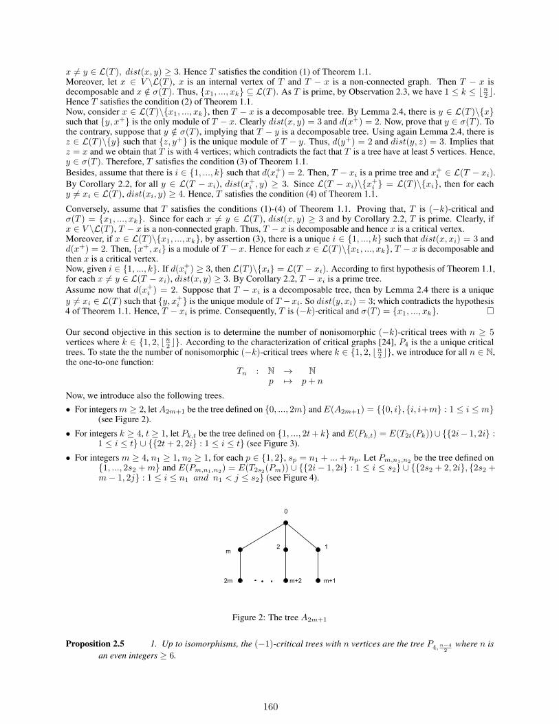
x 6= y ∈ L(T ), dist(x, y) ≥ 3. Hence T satisfies the condition (1) of Theorem 1.1.Moreover, let x ∈ V \L(T ), x is an internal vertex of T and T − x is a non-connected graph. Then T − x isdecomposable and x /∈ σ(T ). Thus, x1, ..., xk ⊆ L(T ). As T is prime, by Observation 2.3, we have 1 ≤ k ≤ bn2 c.Hence T satisfies the condition (2) of Theorem 1.1.Now, consider x ∈ L(T )\x1, ..., xk, then T − x is a decomposable tree. By Lemma 2.4, there is y ∈ L(T )\xsuch that y, x+ is the only module of T − x. Clearly dist(x, y) = 3 and d(x+) = 2. Now, prove that y ∈ σ(T ). Tothe contrary, suppose that y /∈ σ(T ), implying that T − y is a decomposable tree. Using again Lemma 2.4, there isz ∈ L(T )\y such that z, y+ is the unique module of T − y. Thus, d(y+) = 2 and dist(y, z) = 3. Implies thatz = x and we obtain that T is with 4 vertices; which contradicts the fact that T is a tree have at least 5 vertices. Hence,y ∈ σ(T ). Therefore, T satisfies the condition (3) of Theorem 1.1.Besides, assume that there is i ∈ 1, ..., k such that d(x+i ) = 2. Then, T − xi is a prime tree and x+i ∈ L(T − xi).By Corollary 2.2, for all y ∈ L(T − xi), dist(x+i , y) ≥ 3. Since L(T − xi)\x+i = L(T )\xi, then for eachy 6= xi ∈ L(T ), dist(xi, y) ≥ 4. Hence, T satisfies the condition (4) of Theorem 1.1.

Conversely, assume that T satisfies the conditions (1)-(4) of Theorem 1.1. Proving that, T is (−k)-critical andσ(T ) = x1, ..., xk. Since for each x 6= y ∈ L(T ), dist(x, y) ≥ 3 and by Corollary 2.2, T is prime. Clearly, ifx ∈ V \L(T ), T − x is a non-connected graph. Thus, T − x is decomposable and hence x is a critical vertex.Moreover, if x ∈ L(T )\x1, ..., xk, by assertion (3), there is a unique i ∈ 1, ..., k such that dist(x, xi) = 3 andd(x+) = 2. Then, x+, xi is a module of T − x. Hence for each x ∈ L(T )\x1, ..., xk, T − x is decomposable andthen x is a critical vertex.Now, given i ∈ 1, ..., k. If d(x+i ) ≥ 3, then L(T )\xi = L(T − xi). According to first hypothesis of Theorem 1.1,for each x 6= y ∈ L(T − xi), dist(x, y) ≥ 3. By Corollary 2.2, T − xi is a prime tree.Assume now that d(x+i ) = 2. Suppose that T − xi is a decomposable tree, then by Lemma 2.4 there is a uniquey 6= xi ∈ L(T ) such that y, x+i is the unique module of T −xi. So dist(y, xi) = 3; which contradicts the hypothesis4 of Theorem 1.1. Hence, T − xi is prime. Consequently, T is (−k)-critical and σ(T ) = x1, ..., xk.

Our second objective in this section is to determine the number of nonisomorphic (−k)-critical trees with n ≥ 5vertices where k ∈ 1, 2, bn2 c. According to the characterization of critical graphs [24], P4 is the a unique criticaltrees. To state the the number of nonisomorphic (−k)-critical trees where k ∈ 1, 2, bn2 c, we introduce for all n ∈ N,the one-to-one function:

Tn : N → Np 7→ p+ n

Now, we introduce also the following trees.

• For integersm ≥ 2, letA2m+1 be the tree defined on 0, ..., 2m andE(A2m+1) = 0, i, i, i+m : 1 ≤ i ≤ m(see Figure 2).

• For integers k ≥ 4, t ≥ 1, let Pk,t be the tree defined on 1, ..., 2t+ k and E(Pk,t) = E(T2t(Pk))∪2i− 1, 2i :1 ≤ i ≤ t ∪ 2t+ 2, 2i : 1 ≤ i ≤ t (see Figure 3).

• For integers m ≥ 4, n1 ≥ 1, n2 ≥ 1, for each p ∈ 1, 2, sp = n1 + ...+ np. Let Pm,n1,n2be the tree defined on

1, ..., 2s2 +m and E(Pm,n1,n2) = E(T2s2(Pm)) ∪ 2i− 1, 2i : 1 ≤ i ≤ s2 ∪ 2s2 + 2, 2i, 2s2 +

m− 1, 2j : 1 ≤ i ≤ n1 and n1 < j ≤ s2 (see Figure 4).

Figure 2: The tree A2m+1

Proposition 2.5 1. Up to isomorphisms, the (−1)-critical trees with n vertices are the tree P4,n−42

where n isan even integers ≥ 6.

160

2. Up to isomorphisms, the (−bn2c)-critical trees with n vertices are the tree An where n is odd integers ≥ 5.

Figure 3: The tree Pk,t

Figure 4: The tree Pm,n1,n2

Proof:

1. Clearly, by Theorem 1.1, P4,n−42

is a (−1)-critical tree where n ≥ 6 and σ(P4,n−42

) = n − 3. Now, weconsider a (−1)-critical tree T with n ≥ 5 vertices such that σ(T ) = x1. By Theorem 1.1, x1 ∈ L(T ).If x 6= x1 ∈ L(T ), then by assertion (3) of Theorem 1.1 dist(x, x1) = 3 and d(x+) = 2. To the contrary,suppose that |L(T )| = 2. Since T is prime, then T is isomorphic to P4; which a contradicts the fact thatT have at least 5 vertices. Hence, |L(T )| ≥ 3. By assertion (3), for each y ∈ L(T ), dist(y, x1) = 3 andd(y+) = 2. Thus, T is isomorphic to P4,n−4

2where n ≥ 6 is an even integers.

2. By Theorem 1.1, A2m+1 is (−b2m+ 1

2c)-critical and σ(A2m+1) = L(A2m+1) where m ≥ 2. Now, we

consider a (−bn2c)-critical tree T with n ≥ 5 vertices. Using Theorem 1.1, σ(T ) ⊆ L(T ) implying that

|σ(T )| = bn2c ≤ |L(T )|. By Observation 2.3, |L(T )| = |S(T )| ≤ bn

2c and so |L(T )| = |S(T )| = bn

2c.

Now, we will prove that n is odd. To the contrary, suppose that n is even, then |L(T )| = |S(T )| = n

2. Hence,

V (T ) = L(T ) ∪ S(T ). Since T [S(T )] is a tree, there exists a vertex y ∈ S(T ) with dT [S(T )](y) = 1. HencedT (y) = 2. We may assume that N(y) = y−, x where x ∈ S(T ). Thus y, x− is a module of T − y−;

which contradicts the fact that y− is a not critical vertex. Accordingly, n is odd, |L(T )| = |S(T )| = n− 1

2,

161

and V (T ) = L(T )∪S(T )∪z. We can assume that L(T ) = x1, ..., x(n−12 ) and S(T ) = x+1 , ..., x+(n−1

2 ).

Since T [S(T ) ∪ z] is a tree, there exists a vertex x+i ∈ S(T ) where 1 ≤ i ≤ n− 1

2with dT [S(T )](x

+i ) = 1

and so dT (x+i ) = 2. By Theorem 1.1, dist(xi, xj) ≥ 4 for each j 6= i ∈ 1, ..., n− 1

2. Hence, T is

isomorphic to An where n ≥ 5.

As a consequence of Theorem 1.1, we have the following result.

Proposition 2.6 Up to isomorphisms, the (−2)-critical trees with n ≥ 5 vertices are the trees Pn, Pk,t where k ≥ 4,t ≥ 1 and n = k + 2t, and Pm,n1,n2

where m ≥ 4, n1, n2 ≥ 1 and n = m+ 2(n1 + n2).

Proof: By Theorem 1.1, Pn, Pk,t where k ≥ 4, t ≥ 1, and Pm,n1,n2where m ≥ 4, n1, n2 ≥ 1 are (−2)-critical trees

and σ(Pn) = 1, n, σ(Pk,t) = 2t+ 1, 2t+ k, and σ(Pm,n1,n2) = 2s2 + 1, 2s2 +m. Now, assume that T is a

(−2)-critical tree with n ≥ 5 vertices such that σ(T ) = x1, x2. By Theorem 1.1, x1, x2 ∈ L(T ). As T is a primetree, then the (x1, x2)-path is isomorphic to Pk where k ≥ 4. If |L(T )| = 2, then T is isomorphic to Pn and n = k.Assume that |L(T )| ≥ 3, then by Theorem 1.1 for each x ∈ L(T )\x1, x2, there is a unique i ∈ 1, 2 such thatdist(x, xi) = 3 and d(x+) = 2. Hence, T is isomorphic to Pk,t where k ≥ 4, t ≥ 1 and n = k+2t or T is isomorphicto Pk,n1,n2 where k ≥ 4, n1, n2 ≥ 1 and n = k + 2(n1 + n2).

Theorem 2.7 The number of nonisomorphic (−2)-critical trees with n vertices equals:

•⌊n4

⌋2− 1 if n ≡ 0 (mod 4).

•⌊n4

⌋2if n ≡ 1 (mod 4).

•⌊n4

⌋(⌊n4

⌋+ 1)− 1 if n ≡ 2 (mod 4).

•⌊n4

⌋(⌊n4

⌋+ 1)

otherwise.

Proof: At the beginning, it is not difficult to verify that there are no two isomorphic different trees in the unionPm : m ≥ 5 ∪ Pk,t : k ≥ 5, t ≥ 1 ∪ Pm,n1,n2

: m ≥ 4, n1 ≥ 1 and n2 ≥ 1.By Proposition 2.6, P5 is the unique (−2)-critical tree with five vertex and P6 is the unique (−2)-critical tree with sixvertices, then the result holds.Now, assume that n ≥ 7. By Proposition 2, the nonisomorphic (−2)-critical trees with n vertices are Pn, thefamily of Pk,t where t ≥ 1, k ≥ 5, and n = 2t + k, or the family of Pm,n1,n2 where 1 ≤ n1 ≤ n2, m ≥ 4, andn = 2(n1 + n2) +m. Therefore, it suffices to determine the number of the family of Pk,t and the number of the familyof Pm,n1,n2 .Let Sm = (n1, n2) ∈ N× N : 1 ≤ n1 ≤ n2, n1 + n2 = n−m

2 where 4 ≤ m ≤ n− 4 and let Ct = k ∈ N : 5 ≤k and k = n − 2t where 1 ≤ t ≤ n−5

2 . Since n −m = 2(n1 + n2), it clear that n and m are of the some parity.Hence, we distinguish two cases.Case 1: If n = 2p where 4 ≤ p and m = 2q where 2 ≤ q ≤ p− 2.

Consider S =

p−2⋃

q=2

S2q and C =

p−3⋃

t=1

Ct. First, clearly that the number of the family of Pk,t is the cardinality of the set

C. Moreover, it is clear that |Ct| = 1 where 1 ≤ t ≤ p− 3. Hence, |C| =p−3∑

t=1

|Ct| = p− 3. Second, obviously the

number of the family of Pm,n1,n2 is the cardinality of the set S. Furthermore, we have |S| =p−2∑

q=2

|S2q|. It is easy to see

that for each 2 ≤ q ≤ p− 2, |S2q| = P2(n−2q

2 ), where Pi(j) is the number of partitions of j to i parts. Recall that for

162

an integer k ≥ 3, P2(k) = bk2 c where bxc is the greatest integer ≤ x [3]. We have then

|S| =p−2∑

q=2

P2

(n− 2q

2

)

=

p−2∑

q=2

⌊n− 2q

4

⌋

=

p−2∑

q=2

⌊ n2 − q2

⌋

=

p−2∑

i=0

⌊i

2

⌋.

=

(k − 1)2 if p = 2k,

(k − 1)k if p = 2k + 1.

Case 2: If n = 2p + 1 where 4 ≤ p and m = 2q + 1 where 2 ≤ q ≤ p − 2. Let S =

p−2⋃

q=2

S2q+1 and C =

p−2⋃

t=1

Ct.

Clearly, the number of the family of Pk,t is the cardinality of the set C. Hence, |C| =p−2∑

t=1

|Ct| = p− 2. In addition,

the number of the family of Pm,n1,n2 is the cardinality of the set S. We have |S| =p−2∑

q=2

|S2q+1|.

Since for each 2 ≤ q ≤ p− 2, |S2q+1| = P2

((n−1)−2q

2

). In the same manner of case 1, if p = 2k where k ≥ 2, then

|S| = (k − 1)2. Otherwise, |S| = (k − 1)k.Consequently, the number of nonisomorphic (−2)-critical trees with n vertices equals:

⌊n4

⌋2− 1 if n ≡ 0 (mod 4),

⌊n4

⌋2if n ≡ 1 (mod 4),

⌊n4

⌋(⌊n4

⌋+ 1)− 1 if n ≡ 2 (mod 4),

⌊n4

⌋(⌊n4

⌋+ 1)

if n ≡ 3 (mod 4).

3 Proof of Theorem 1.2:

We have two major objectives all along this section. First, to characterize the k-minimal trees. Second, to determine thenumber of nonisomorphic k-minimal trees with n vertices where k ∈ 1, 2, 3.Proof of Theorem 1.2. Let T = (V,E) be a tree with n ≥ 5 vertices and let x1, ..., xk be a vertex subset of G wherek is a strictly positive integer. Assume that T is minimal for x1, ..., xk. Since T is prime, it satisfies the first conditionof Theorem 1.2. Suppose to the contrary that there is y ∈ L(T ) such that y, y+ ∩ x1, ..., xk = ∅. Since T − y is adecomposable tree, by Lemma 2.4, there is x ∈ L(T ) such that x, y+ is a module of T − y. Thus d(y+) = 2 andd(x, y) = 3. If x /∈ x1, ..., xk, then T − x is a decomposable tree. By using again Lemma 2.4, d(x+) = 2 and so Tis isomorphic to P4; which contradicts the fact n ≥ 5.Moreover, assume that x ∈ x1, ..., xk and d(x+) ≥ 3, then L(T )\y = L(T − y, y+). By Lemma 2.1,T − y, y+ is a prime tree containing x1, ..., xk; which contradicts the fact T is minimal for x1, ..., xk. Hence,for each x ∈ L(T ), x, x+ ∩ x1, ..., xk 6= ∅ and T satisfies the second condition of Theorem 1.2.

163

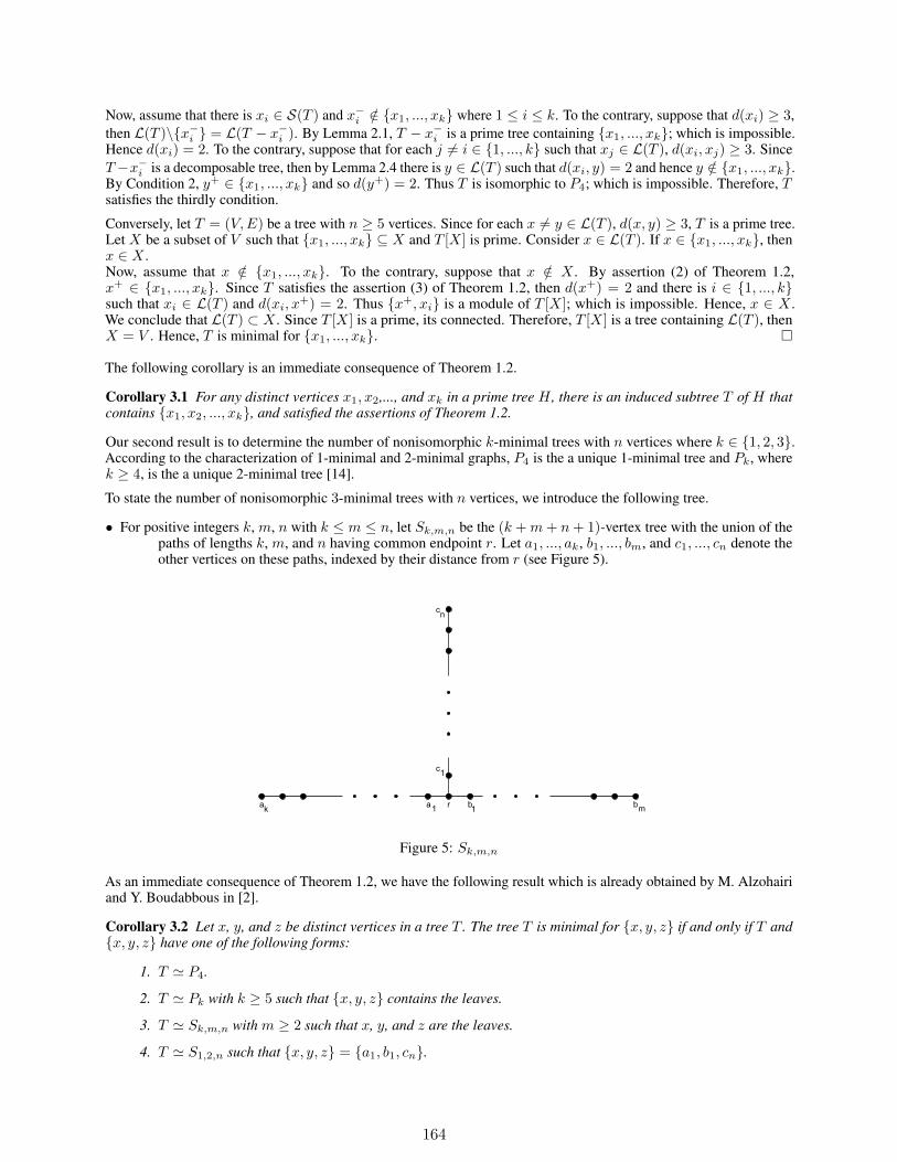
Now, assume that there is xi ∈ S(T ) and x−i /∈ x1, ..., xk where 1 ≤ i ≤ k. To the contrary, suppose that d(xi) ≥ 3,then L(T )\x−i = L(T − x−i ). By Lemma 2.1, T − x−i is a prime tree containing x1, ..., xk; which is impossible.Hence d(xi) = 2. To the contrary, suppose that for each j 6= i ∈ 1, ..., k such that xj ∈ L(T ), d(xi, xj) ≥ 3. SinceT−x−i is a decomposable tree, then by Lemma 2.4 there is y ∈ L(T ) such that d(xi, y) = 2 and hence y /∈ x1, ..., xk.By Condition 2, y+ ∈ x1, ..., xk and so d(y+) = 2. Thus T is isomorphic to P4; which is impossible. Therefore, Tsatisfies the thirdly condition.

Conversely, let T = (V,E) be a tree with n ≥ 5 vertices. Since for each x 6= y ∈ L(T ), d(x, y) ≥ 3, T is a prime tree.Let X be a subset of V such that x1, ..., xk ⊆ X and T [X] is prime. Consider x ∈ L(T ). If x ∈ x1, ..., xk, thenx ∈ X .Now, assume that x /∈ x1, ..., xk. To the contrary, suppose that x /∈ X . By assertion (2) of Theorem 1.2,x+ ∈ x1, ..., xk. Since T satisfies the assertion (3) of Theorem 1.2, then d(x+) = 2 and there is i ∈ 1, ..., ksuch that xi ∈ L(T ) and d(xi, x+) = 2. Thus x+, xi is a module of T [X]; which is impossible. Hence, x ∈ X .We conclude that L(T ) ⊂ X . Since T [X] is a prime, its connected. Therefore, T [X] is a tree containing L(T ), thenX = V . Hence, T is minimal for x1, ..., xk.

The following corollary is an immediate consequence of Theorem 1.2.

Corollary 3.1 For any distinct vertices x1, x2,..., and xk in a prime tree H , there is an induced subtree T of H thatcontains x1, x2, ..., xk, and satisfied the assertions of Theorem 1.2.

Our second result is to determine the number of nonisomorphic k-minimal trees with n vertices where k ∈ 1, 2, 3.According to the characterization of 1-minimal and 2-minimal graphs, P4 is the a unique 1-minimal tree and Pk, wherek ≥ 4, is the a unique 2-minimal tree [14].

To state the number of nonisomorphic 3-minimal trees with n vertices, we introduce the following tree.

• For positive integers k, m, n with k ≤ m ≤ n, let Sk,m,n be the (k +m+ n+ 1)-vertex tree with the union of thepaths of lengths k, m, and n having common endpoint r. Let a1, ..., ak, b1, ..., bm, and c1, ..., cn denote theother vertices on these paths, indexed by their distance from r (see Figure 5).

Figure 5: Sk,m,n

As an immediate consequence of Theorem 1.2, we have the following result which is already obtained by M. Alzohairiand Y. Boudabbous in [2].

Corollary 3.2 Let x, y, and z be distinct vertices in a tree T . The tree T is minimal for x, y, z if and only if T andx, y, z have one of the following forms:

1. T ' P4.

2. T ' Pk with k ≥ 5 such that x, y, z contains the leaves.

3. T ' Sk,m,n with m ≥ 2 such that x, y, and z are the leaves.

4. T ' S1,2,n such that x, y, z = a1, b1, cn.

164

5. T ' S1,2,2 such that x, y, z = a1, b1, c1.

Proposition 3.3 the number of nonisomorphic 3-minimal trees with n vertices equals:• 1 if n ∈ 4, 5.• 2 if n = 6.•[(n−1)2

12

]−⌊n−42

⌋+⌊n−22

⌋− 1 if n ≥ 7, where [x] is the nearest integer to x.

Proof: At the beginning, it is not difficult to verify that there are no two isomorphic different graphs in the unionPk : k ≥ 4 ∪ Sk,m,n : m = 2.By Corollary 3.2, P4 is the unique 3-minimal tree with four vertices and P5 is the unique 3-minimal tree with fivevertices. In addition, the only 3-minimal tree with six vertices are P6 and S1,2,2. Therefore, the result holds forn ∈ 4, 5, 6.Now, assume that n ≥ 7. By Corollary 3.2, the non isomorphic 3-minimal n-vertex tree are Pn and the family ofSk,m,t, where k ≤ m ≤ t, m ≥ 2, and k +m+ t+ 1 = n. Therefore, it suffices to prove that the cardinality of the setS = (k,m, t) ∈ N× N× N : 1 ≤ k ≤ m ≤ t,m ≥ 2, k +m+ t = n− 1 equals

[(n− 1)2

12

]−⌊n− 4

2

⌋+

⌊n− 2

2

⌋− 2.

Let S2 = (k,m, t) ∈ S : k ≥ 2. It is easy to see that |S − S2| = P2(n − 2) − 1. Notice that |S2| = |(p, q, r) ∈N× N× N : 1 ≤ p ≤ q ≤ r, p+ q + r = n− 4| = P3(n− 4). Moreover, by [3], the number of partitions of k towith most 3 parts is equal to

[(k+3)2

12

]. It follows that: P3(k) =

[(k+3)2

12

]−⌊k2

⌋− 1 [3]. Hence,

|S2| =[(n− 1)2

12

]−⌊n− 4

2

⌋− 1

and

|S − S2| =⌊n− 2

2

⌋− 1.

Therefore,

|S| =[(n− 1)2

12

]−⌊n− 4

2

⌋+

⌊n− 2

2

⌋− 2.

4 Conclusion

The problems of finding the (−k)-critical graphs and the k-minimal graphs seem to be challenging where k is aninteger (k ≥ 2). At least, we solve these problems in the particular case of trees. Also, we determine the number ofnonisomorphic (−k)-critical trees with n ≥ 5 vertices where k ∈ 1, 2, bn2 c. In addition, we count the number ofnonisomorphic 3-minimal trees with n (n ≥ 4) vertices.

References

[1] M. Alzohairi. Triangle-free graphs which are minimal for some nonstable 4-vertex subset. In Arab Journal ofMathematical Sciences, pages 159–169. IEEE, 2015.

[2] M. Alzohairi and Y. Boudabbous. 3-minimal triangle-free graphs. In Discrete Mathematics, pages 3–8. IEEE, 2014.

[3] G. Andrews, K. Eriksson, Integer Partitions, Cambridge University Press, Cambridge, 2004.

[4] H. Belkhechine and I. Boudabbous. Indecomposable tournaments and their indecomposable subtournaments on 5and 7 vertices. In Ars Combinatoria, pages 493-–504. IEEE, 2013.

[5] H. Belkhechine, I. Boudabbous and J. Dammak. Les tournois (-1)-critiques. In Communications in MathematicalAnalysis, pages 83–97. IEEE, 2007.

[6] H. Belkhechine, I. Boudabbous and M.B. Elayech. les graphes (-1)-critiques. In Ars combinatoria, pages 293–319.IEEE, 2015.

165

[7] H. Bouchaala, Y. Boudabbous and M. B. Elayech. Finite tournaments with a nonempty diamond’s support. InGraphs and Combinatorics, pages 1653-1673. IEEE, 2013.

[8] I. Boudabbous. Tournaments whose indecomposability graph admits a vertex cover of size 2. In Ars Combinatoria,pages 63–82. IEEE, 2016.

[9] I. Boudabbous, J. Dammak and M. Yaich. Prime critically and prime covering. In to apparent in journalMathematical reports.

[10] I. Boudabbous and W. Marweni. Description of the Triangle-free Prime Graphs Having at Most Two Non-CriticalVertices. In Journal of Multi-Valued Logic and Soft Computing, pages 77–103. IEEE, 2020.

[11] Y. Boudabbous and P. Ille. Indecomposability graph and critical vertices of an indecomposable graph. In DiscreteMath, pages 2839–2846. IEEE, 2009.

[12] A. Boussaïri and A. Chaïchaâ. The 2-reconstructible indecomposable graphs. In Comptes Rendus Mathematique,pages 1–4. IEEE, 2007.

[13] A. Breiner, J. Deogun and P. Ille. Partially critical indecomposable graphs. In Contributions to DiscreteMathematics, pages 40–59. IEEE, 2008.

[14] A. Cournier and P. Ille. Minimal indecomposable graphs. In Discrete Math, pages 61–80. IEEE, 1998.[15] A. Ehrenfeucht, T. Harju and G. Rozenberg. The Theory of 2-Structures. In A Framework for Decomposition and

Transformation of Graphs, World Scientific, Singapore (1999).[16] A. Ehrenfeucht and G. Rozenberg. Primitivity is hereditary for 2-structures. In Theoret. Comput. Sci., pages

343–358. IEEE, 1990.[17] M. B. Elayech, A. Salhi and H. Si Kaddour. The (−1)-critically duo-free tournaments. In Ars Combinatoria,

pages 391–402. IEEE, 2005.[18] R. Fraïssé. L’intervalle en théorie des relations, ses généralisations, filtre intervallaire et clô ture d’une relation. In

M. Pouzet and D. Richard eds, Order, Description and Roles, North-Holland, Amsterdam.(1984) 313-342.[19] M. Habib. Substitution des structures combinatoires. In Théorie et Algorithmes, Thèse d’état, Université Pierre et

Marie Curie (1981).[20] P. Ille. Indecomposable graphs. In Discrete Math, pages 71–78. IEEE, 1997.[21] D. Kelly. Comparability graphs. In I. Rival(Ed.), Graphs and Orders, Reidel, Dordrecht, pages 3-–40. IEEE, 1985.[22] M. Pouzet and I. Zaguia. On minimal prime graphs and posets. In Order, pages 357–375. IEEE, 2009.[23] M. Y. Sayar. Partially critical indecomposable tournaments and partially critical supports. In Contributions to

Discrete Mathematics, pages 52–76. IEEE, 2011.[24] J.H. Schmerl and W.T. Trotter. Critically indecomposable partially ordered sets, graphs, tournaments and other

binary relational structures. In Discrete Math, pages 191–205. IEEE, 1993.[25] J. Spinrad. P4-trees and substitution decomposition. In Discrete Appl. Math., pages 263–291. IEEE, 1992.[26] D. P. Sumner. Graphs indecomposable with respect to the X-join. In Discrete Math., pages 281—298. IEEE,

1973.

166

Unstable graphs and packing into fifth power

Mohamed Y. SayarDepartment of MathematicsFaculty of Science of Sfax

Soukra Road km 4, PO Box 802, 3018 Sfax, [email protected]

Tarak LoulebDepartment of MathematicsFaculty of Science of Sfax

Soukra Road km 4, PO Box 802, 3018 Sfax, [email protected]

Mohammad AlzohairiDepartment of Mathematics

King Saud UniversityP. O. Box 2455 Riyadh 11451, Arabie saoudite

[email protected]

ABSTRACT

In a graph G := (V (G), E(G)), a subset M of the vertex set V (G) is a module (or interval, clan)of G if every vertex outside M is adjacent to all or none of M . The empty set, the singleton sets,and the full set of vertices are trivial modules. The graph G is indecomposable (or prime) if allits modules are trivial. If G is indecomposable, we say that an edge e of G is a removable edge ifG− e is indecomposable (here G− e := (V (G), E(G)− e)). The graph G is said to be unstableif it has no removable edges. For a positive integer k, the k − th power Gk of a graph G is thegraph obtained from G by adding an edge between all pairs of vertices of G with distance at mostk. A graph G of order n (i.e |V (G)| = n) is said to be p − placeable into Gk, if Gk contains pedge-disjoint copies of G. In this paper, we answer a question, suggested by Y. Boudabbous in apersonal communication, concerning unstable graphs and packing into their fifth power as follows:First, we give a characterisation of the unstable graphs which is deduced from the results givenby A. Ehrenfeucht, T. Harju and G. Rozenberg (The theory of 2 − structures: a framework fordecomposition and transformation of graphs). Second, we prove that every unstable graph G is2− placeable into G5.

Keywords Indecomposable · Unstable · Packing · Graph power ·

1 Introduction

1.1 Graph theoretical definitions

All graphs considered in this paper are finite, undirected, without loops or multiple edges. For a graph G, wewill use V ,(V (G)), and E ,(E(G)), to denote its vertex and edge sets respectively. For a positive integers n,m.We say that a graph G is of order n and size m, if |V (G)| = n and |E(G)| = m. In this case, the graph G iscalled an (n,m)-graph. Given a graph G and X ⊂ V , the subgraph of G induced by X is denoted by G[X]. Agraph G is called a discrete graph if E(G) = ∅. A graph G is called a path, denoted by Pn, if it is of the form:V (Pn) = v1, v2, . . . , vn, E(Pn) = v1v2, v2v3, . . . , vn−1vn. A graph G is called a cycle, denoted by Cn, if it isof the form: V (Cn) = v1, v2, . . . , vn, E(Cn) = v1v2, v2v3, . . . , vn−1vn, vnv1. A subset X of vertices of V issaid to be k − subset if |X| = k. For an edge e ∈ E, we denote by G − e the graph (V (G), E(G) − e). Let x bea vertex of V . Then NG(x) = y ∈ V, xy ∈ E. The graph G is connected if there exists a path between any two

167

distinct vertices of G. Otherwise, the graph G is disconnected. The distance between two vertices u, v ∈ G, denoted bydist(u, v), is the minimum number of edges in a path connecting them. The diameter of G is the maximum distancebetween any two vertices of G. For a positive integer k, the k − th power Gk of a graph G is the graph obtained fromG by adding an edge between all pairs of vertices of G with distance at most k.

1.2 Unstable graphs

In a graph G, a subset M of the vertex set V is a module (or interval, clan) of G if every vertex outside M is adjacentto all or none of M . The empty set, the singleton sets, and the full set of vertices are trivial modules. A graph isindecomposable (or prime) if all its modules are trivial. In the opposite case, we will say that G is decomposable.

Let G be an indecomposable graph. We say that e ∈ E is removable edge if G− e is indecomposable. The graph Gis said to be unstable if it has no removable edges. Hence G is unstable if the removal of any edge e ∈ E creates anontrivial module in G− e.Unstable graphs were introduced by Sumner (1973).

1.3 Graph packing problem

Let G be a graph of order n. Consider a permutation σ: V (G) → V (Kn), the map σ∗: E(G) → E(Kn) such thatσ∗(xy) = σ(x)σ(y) is the map induced by σ. Let G1, . . . , Gk be k graphs of order n. We say that there is a packingof G1, . . . , Gk (into the complete graph Kn) if there exist permutations σi: V (Gi) → V (Kn), where i = 1, . . . , k,such that σ∗i (E(Gi)) ∩ σ∗j (E(Gj)) = ∅ for i 6= j, and here the map σ∗i : E(Gi) → E(Kn) is the one induced by σi.A packing of k copies of the same graph G will be called a k-packing (or a k − placement) of G. In particular, a2-packing of a graph G is a permutation σ on V (G) such that if an edge vu belong to E(G), then σ(v)σ(u) does notbelong to E(G).

Graph packing is well known field of graph theory that has been considerably investigated in the literature. The readercan find a good survey on packing of graphs in [1] and [2]. In particular, the question of the existence of 2-packing of agiven graph has received a great attention. In [3], a full characterization of all the 2-packable (n, n− 1)-graphs is given.Note that stars are the only connected (n, n − 1)-graphs that are not 2-packable. A similar result about 2-packable(n, n)-graphs can be found in [4]. Other papers about packing of different trees into Kn can be found in [5] and [6].

An example of such a result is the following theorem contained as a lemma in [7].

Theorem 1.1 Let T be a non-star tree of order n with n > 3. Then there exists a 2− placement σ of T such that forevery x ∈ V (T ), distT (x, σ(x)) ≤ 3.

This theorem immediately implies the following:

Corollary 1.2 Let T be a non-star tree of order n with n > 3. Then there exists an embedding σ of T such thatσ(T ) ⊂ T 7.

In [6], Kheddouci et al. considered the problem of the 2-placement of a tree T into T p such that p is as small as possible.They proved the following result.

Theorem 1.3 Let T be a non-star tree of order n, with n > 3. Then there exists a 2-placement σ of T such thatσ(T ) ⊂ T 4.

And in [8], Kaneko et al. proved that:

Theorem 1.4 Let T be a non-star tree of order n, with n > 3. Then there exists a 2-placement σ of T such thatσ(T ) ⊂ T 3.

The main result of this paper is:

Theorem 1.5 Let G be an unstable graph. Then there exists a 2-placement σ of G such that σ(G) ⊂ G5.

Our paper is organised as follows: First, we give a characterisation of the unstable graph which is deduced from theresults given by A. Ehrenfeucht, T. Harju and G. Rozenberg in [9]. Second, we prove Theorem 1.5.

168

2 Characterisation of the unstable graphs

We shall need some additional definitions and notations in order to formulate the results of this section.

Given a connected graph G. A vertex x of degree one, dG(x) = 1, is called a leaf of G. The set of leaves of G isdenoted by

Leaf(G) = x ∈ V, x is a leaf.

If x is a leaf, then the unique edge e incident with x is called pendant edge. An edge e is a bridge ifG−e is disconnectedgraph, otherwise, e is a non-bridge. A bridge is said to be proper if is not a pendant edge. A vertex x is an island if it isincident with bridges only.

We denote by:

Nob(G) = e ∈ E, e is not a bridgeIsl(G) = x ∈ V, x is an island

For X ⊆ V , NG(X) =⋃

x∈XNG(x) \X

Let G be an indecomposable graph. We say that x ∈ V (G) is an inside vertex, if there exists a non-bridge e =xy ∈ Nob(G) such that x ∈ X for a nontrivial module X of G − e. On the other hand, if there exists a non-bridgee = xy ∈ Nob(G) such that x /∈ X for a nontrivial module X of G, then x is called an outside vertex. We denote by

Out(G) = x ∈ V ;x is an outside vertex and Ins(G) = x ∈ V ;x is an inside vertex

the set of outside and inside vertices of G.

The following results are given in [9]

Lemma 2.1 Let G be an indecomposable graph. Then no inside vertex is incident with a bridge.

A graph G is triangle-free if for each 3-subset X = x1, x2, x3 of V (G) there exists an edge xixj /∈ E(G).

Lemma 2.2 Let G be a connected and triangle-free graph, and let X be a nontrivial module of G. If a vertex x ∈ X isincident with a bridge e = xy, then x is a leaf, and X ⊆ Leaf(G).

Theorem 2.3 An unstable graph is triangle-free.

Corollary 2.4 Let G be an unstable graph. Then inside and outside vertices, and the islands forms a partition ofV (G):

V = Out(G) ∪ Ins(G) ∪ Isl(G);

Out(G) ∩ Ins(G) = Out(G) ∩ Isl(G) = Ins(G) ∩ Isl(G) = ∅.

Lemma 2.5 Let G be an unstable graph, and e ∈ Nob(G). Then G− e has a unique module of two vertices and thismodule is discrete.

Theorem 2.6 Let G be an unstable graph. Then every inside vertex of G is adjacent to outside vertices only.

Theorem 2.7 Let G be an unstable graph and e ∈ Nob(G). Let Me be a non trivial module of G − e. ThenMe ⊆ Ins(G) ∪ Leaf(G).

Corollary 2.8 Let G be an unstable graph. Each outside vertex is adjacent to a leaf.

Let us call a subgraph H a pendant component of a graph G if H is a connected component of a graph G′, which isobtained by removing from G all its proper bridges. If G is its pendant component, then it is called a pendant graph. Inthis case, G has no proper bridges.

Lemma 2.9 For a pendant component H of a connected graph G,

169

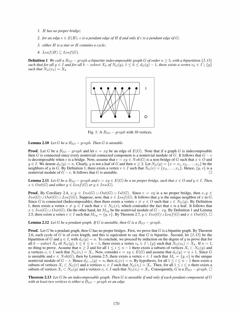
1. H has no proper bridge;

2. for an edge e ∈ E(H), e is a pendant edge of H if and only if e is a pendant edge of G;

3. either H is a star or H contains a cycle;

4. Leaf(H) ⊆ Leaf(G).

Definition 1 We call a BIO − graph a bipartite indecomposable graph G of order n ≥ 5, with a bipartition I,Osuch that for all y ∈ I and for all k − subset Xk of NG(y), 1 ≤ k ≤ dG(y) − 1, there exists a vertex vk ∈ I \ ysuch that NG(vk) = Xk

Fig. 1: A BIO − graph with 10 vertices.

Lemma 2.10 Let G be a BIO − graph. Then G is unstable.

Proof. Let G be a BIO − graph and let e = xy be an edge of E(G). Note that if a graph G is indecomposablethen G is connected since every nontrivial connected component is a nontrivial module of G. It follows that G − eis decomposable when e is a bridge. Now, assume that e = xy ∈ Nob(G) is a non-bridge of G such that x ∈ O andy ∈ I . We denote dG(y) = n. Clearly, y is not a leaf of G and then n ≥ 2. Let NG(y) = x = x1, x2, . . . , xn be theneighbors of y in G. By Definition 1, there exists a vertex v ∈ I such that NG(v) = x2, . . . , xn. Hence, y, v is anontrivial module of G− e. It follows that G is unstable.

Lemma 2.11 Let G be a BIO − graph and e = xy ∈ E(G) be a no proper bridge, such that x ∈ O and y ∈ I . Then,x ∈ Out(G) and either y ∈ Leaf(G) or y ∈ Ins(G).

Proof. By Corollary 2.4, x, y ∈ Ins(G) ∪ Out(G) ∪ Isl(G). Since e = xy is a no proper bridge, then x, y ∈Ins(G) ∪Out(G) ∪ Leaf(G). Suppose, now, that x ∈ Leaf(G). It follows that y is the unique neighbor of x in G.Since G is connected (Indecomposable), then there exists a vertex z 6= x ∈ O such that z ∈ NG(y). By Definition1, there exists a vertex v 6= y ∈ I such that v ∈ NG(x), which contradict the fact that x is a leaf. It follows thatx ∈ Ins(G) ∪Out(G). On the other hand, let Mxy be the nontrivial module of G− xy. By Definition 1 and Lemma2.5, there exists a vertex v ∈ I such that Mxy = y, v. By Theorem 2.7, y ∈ Ins(G)∪Leaf(G) and x ∈ Out(G).

Lemma 2.12 Let G be a pendant graph. If G is unstable, then G is a BIO − graph.

Proof. Let G be a pendant graph, then G has no proper bridges. First, we prove that G is a bipartite graph. By Theorem2.6, each cycle of G is of even length, and this is equivalent to say that G is bipartite. Second, let I,O be thebipartition of G and y ∈ I , with dG(y) = n. To conclude, we proceed by induction on the degree of y to prove that forall k − subset Xk of NG(y), 1 ≤ k ≤ n − 1, there exists a vertex vk ∈ I \ y such that NG(vk) = Xk. If n = 1,no thing to prove. Assume that n ≥ 2 and for all 1 ≤ i ≤ n − 1 there exists a subsets of vertices Xi ⊂ NG(y) anda vertices vi ∈ I such that NG(vi) = Xi. Now, consider e = xy ∈ E(G) and assume that dG(y) = n+ 1. Since Gis unstable and e ∈ Nob(G), then by Lemma 2.5, there exists a vertex v ∈ I such that Me = y, v is the uniquenontrivial module of G− e. Hence dG−e(y) = n, then dG(v) = n. By hypothesis, for all 1 ≤ i ≤ n− 1 there exists asubsets of vertices Xi ⊂ NG(v) and a vertices vi ∈ I such that NG(vi) = Xi. Then, for all 1 ≤ i ≤ n there exists asubsets of vertices Xi ⊂ NG(y) and a vertices vi ∈ I such that NG(vi) = Xi. Consequently, G is a BIO − graph.

Theorem 2.13 Let G be an indecomposable graph. Then G is unstable if and only if each pendant component of Gwith at least two vertices is either a BIO − graph or an edge.

170

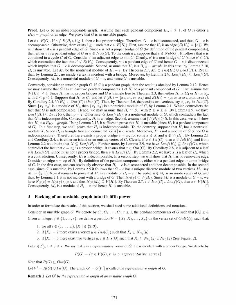
Proof. Let G be an indecomposable graph. Assume that each pendant component Hi, i ≥ 1, of G is either aBIO − graph or an edge. We prove that G is an unstable graph.

Let e ∈ E(G). If e /∈ E(Hi), i ≥ 1, then e is a proper bridge. Therefore, G− e is disconnected, and thus, G− e isdecomposable. Otherwise, there exists i ≥ 1 such that e ∈ E(Hi). First, assume that Hi is an edge (E(Hi) = e). Wewill show that e is a pendant edge of G. Since e is not a proper bridge of G (by definition of the pendant components),then either e is a pendant edge of G or e ∈ Nob(G). To the contrary, suppose that e ∈ Nob(G). It follows that e iscontained in a cycle C of G. Consider e′ an adjacent edge to e in C. Clearly, e′ is a non-bridge of G (since e′ ∈ C):which contradicts the fact that e′ /∈ E(Hi). Consequently, e is a pendant edge of G and hence G− e is disconnectedwhich implies that G− e is decomposable. Second, assume that Hi is a BIO − graph. In this case, by Lemma 2.10,Hi is unstable. Let Me be the nontrivial module of Hi − e. By Theorem 2.7, Me ⊂ Ins(Hi) ∪ Leaf(Hi). Recallthat, by Lemma 2.1, no inside vertex is incident with a bridge. Moreover, by Lemma 2.9, Leaf(Hi) ⊆ Leaf(G).Consequently, Me is a nontrivial module of G− e, and hence G is unstable.

Conversely, consider an unstable graph G. If G is a pendant graph, then the result is obtained by Lemma 2.12. Hencewe may assume that G has at least two pendant components. Let Hi be a pendant component of G. First, assume that|V (Hi)| ≤ 4. Since Hi has no proper bridges and G is triangle free by Theorem 2.3, then either Hi ' C4 or Hi ' Sp,with 2 ≤ p ≤ 4. Suppose that Hi ' C4 and let V (Hi) = x1, x2, x3, x4 and E(Hi) = x1x2, x2x3, x3x4, x4x1.By Corollary 2.4, V (Hi) ⊂ Out(G)∪ Ins(G). Then, by Theorem 2.6, there exists two vertices, say x1, x3, in Ins(G).Since x1, x3 is a module of Hi, then x1, x3 is a nontrivial module of G, by Lemma 2.1. Which contradicts thefact that G is indecomposable. Hence, we may assume that Hi ' Sp, with 2 ≤ p ≤ 4. By Lemma 2.9, we haveLeaf(Hi) ⊆ Leaf(G), then p = 2. Otherwise, G[Leaf(Hi)] is a nontrivial module of G, which contradicts the factthat G is indecomposable. Consequently, Hi is an edge. Second, assume that |V (Hi)| ≥ 5. In this case, we will showthat Hi is a BIO − graph. Using Lemma 2.12, it suffices to prove that Hi is unstable (since Hi is a pendant componentof G). In a first step, we shall prove that Hi is indecomposable. To the contrary, suppose that Hi has a nontrivialmodule X . Since Hi is triangle free and connected, G[X] is discrete. Moreover, X is not a module of G (since G isindecomposable). Therefore, there exists a proper bridge e = xy for some x ∈ X and y /∈ V (Hi). By Lemma 2.1and Corollary 2.4, x is either an island or an outside vertex of G. Clearly, if x ∈ Isl(G), then x ∈ Isl(Hi), and fromLemma 2.2 we obtain that X ⊆ Leaf(Hi). Further more, by Lemma 2.9, we have Leaf(Hi) ⊆ Leaf(G), whichcontradict the fact that e = xy is a proper bridge. It ensues that x ∈ Out(G). By Corollary 2.8, x is adjacent to a leafv ∈ Leaf(G). Since xv is not a proper bridge, then v ∈ Leaf(Hi). By Lemma 2.2, we have x is a leaf of Hi, whichis a contradiction. Consequently, Hi is indecomposable. In a second step, we will show that Hi has no removable edge.Consider an edge e = xy of Hi. By definition of the pendant components, either e is a pendant edge or a non-bridgeof G. In the first case, one can obviously observe that Hi − e is disconnected and then decomposable. In the secondcase, since G is unstable, by Lemma 2.5 it follows that G− e has a unique discrete module of two vertices Me, sayMe = y, z. Now it remains to prove that Me is a module of Hi − e. The vertex y ∈Me is an inside vertex of G, andthus, by Lemma 2.1, it is not incident with a bridge of G. Then NG(y) ⊆ V (Hi). Since Me is a module of G− e, wehave NG(z) = NG(y)\x, and thus NG(Me) ⊆ V (Hi). By Theorem 2.7, z ∈ Ins(G)∪Leaf(G), then z ∈ V (Hi).Consequently, Me is a module of Hi − e and hence Hi is unstable.

3 Packing of an unstable graph into it’s fifth power

In order to formulate the results of this section, we shall need some additional definitions and notations.

Consider an unstable graph G. We denote by C1, C2, . . . , Cr, r ≥ 1, the pendant components of G such that |Ci| ≥ 5.

Given an integer j ∈ 1, . . . , r, we define a partition P = X1, X2, . . . , Xp on the vertex set of Out(Cj), such that:

1. for all i ∈ 1, . . . , p, |Xi| ∈ 2, 3,2. if |Xi| = 2 there exists a vertex y ∈ Ins(Cj) such that Xi ⊆ NCj

(y),

3. if |Xi| = 3 there exist two vertices y, z ∈ Ins(G) such that Xi ⊆ NCj(y) ∪NCj

(z) (See Figure. 2).

Let x ∈ Cj , 1 ≤ j ≤ r. We say that x is a representative vertex of G if x is incident with a proper bridge. We denote by

R(G) = x ∈ V (G), x is a representative vertex

Note that R(G) ⊆ Out(G).Let V ′ = R(G) ∪ Isl(G). The graph G′ = G[V ′] is called the representative graph of G.

Remark 1 Let G′ be the representative graph of an unstable graph G.

171

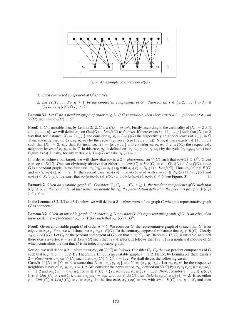
Fig. 2: An example of a partition P(O).

1. Each connected component of G′ is a tree.

2. Let T1, T2, . . . , T q, q ≥ 1, be the connected components of G′. Then for all i ∈ 1, 2, . . . , r and j ∈1, 2, . . . , q, |Ci ∩ Tj | ≤ 1.

Lemma 3.1 Let G be a pendant graph of order n ≥ 5. If G is unstable, then there exists a 2 − placement σC onV (G) such that σC(G) ⊆ G5.

Proof. IfG is unstable then, by Lemma 2.12, G is aBIO−graph. Firstly, according to the cardinality of |Xi| = 2 or 3,i ∈ 1, . . . , p, we will define σC on Out(G) ∪ Leaf(G) as follows. If there exists i ∈ 1, . . . , p such that |Xi| = 2.Say that, for instance, Xi = xi, yi and consider ui, vi ∈ Leaf(G) the respectively neighbors leaves of xi, yi in G.Then, σC is defined on xi, ui, yi, vi by the cycle (xiuiyivi) (see Figure 3 (a)). Now, if there exists i ∈ 1, . . . , psuch that |Xi| = 3. say that, for instance, Xi = xi, yi, zi and consider ui, vi, wi ∈ Leaf(G) the respectivelyneighbors leaves of xi, yi, zi in G. In this case, σC is defined on xi, ui, yi, vi, zi, wi by the cycle (xiuiyiviziwi) (seeFigure 3 (b)). Finally, for any vertex x ∈ Ins(G) we take σC(x) = x.

In order to achieve our target, we will show that σC is a 2 − placement on V (G) such that σC(G) ⊆ G5. Givene = xy ∈ E(G). One can obviously observe that either e ∈ Out(G) × Ins(G) or e ∈ Out(G) × Leaf(G), sinceG is a pendant graph. In the first case, σC(xy) = σC(x)y with σC(x) ∈ NG(x) ∩ Leaf(G). Thus, σC(x)y /∈ E(G)and distG(σC(x), y) = 2. In the second case, σC(xy) = σC(x)σC(y) with σC(x) ∈ NG(x) ∩ Leaf(G) andσC(y) ∈ Xi \ x. It ensues that σC(x)σC(y) /∈ E(G) and distG(σC(x), σC(y)) ≤ 5 (see Figure. 3).

Remark 2 Given an unstable graph G. Consider C1, C2, . . . , Cr, r ≥ 1, the pendant components of G such that|Ci| ≥ 5. In the remainder of this paper, we denote by σCi the permutation defined in the previous proof on V (Ci),1 ≤ i ≤ r.

In the Lemmas (3.2, 3.3 and 3.4) below, we will define a 2− placement of the graph G when it’s representative graphG′ is connected.

Lemma 3.2 Given an unstable graph G of order n ≥ 5, consider G′ it’s representative graph. If G′ is an edge, thenthere exists a 2− placement σS2

on V (G) such that σS2(G) ⊆ G5.

Proof. Given an unstable graph G of order n ≥ 5. We consider G′ the representative graph of G such that G′ is anedge e = x1x2. First, we will show that x1, x2 ∈ R(G). To the contrary, suppose for instance that x2 /∈ R(G). Clearly,x2 ∈ Leaf(G). Let C1 be the pendant component of G such that x1 ∈ C1. By Theorem 2.13, C1 is unstable, and thenthere exists a vertex v 6= x2 ∈ Leaf(G) such that x1v ∈ E(G). It follows that x2, v is a nontrivial module of G,which contradicts the fact that G is an indecomposable graph.

Second, we will define a 2− placement σS2on V (G) as follows. Consider C1, C2 the two pendant components of G

such that |Ci| ≥ 5, i = 1, 2. By Theorem 2.13, Ci is an unstable graph, i = 1, 2. Hence, by Lemma 3.1 there exists a2− placement σCi on V (Ci) such that σCi(Ci) ⊆ C5

i , i = 1, 2. We shall discus the following cases.Case.1: If |X| = |Y | = 3, assume that X = x1, y1, z1 and Y = x2, y2, z2. Let ui, vi, wi be the respectiveneighbors leaves of xi, yi, zi, i = 1, 2. We consider the permutation σS2 defined on V (G) by (x1u1x2u2)(yiviziwi),i = 1, 2 and σS2(w) = σCi(w), for w ∈ V (Ci) \ xi, yi, zi, ui, vi, wi, i = 1, 2. Now, consider e = xy ∈ E(Ci).If e ∈ Out(Ci) × Ins(Ci), then σS2

(xy) = vy, with xv ∈ E(G) then distG(σS2(x), σS2

(y)) = 2. Else, eithere ∈ Out(Ci) × Leaf(Ci) or e = x1x2. In the first case, σS2

(xy) = vu, with xv ∈ E(G) and u ∈ Xi and then

172

(a)

(b)

Fig. 3: Illustration of the proof of Lemma 3.1. The dots edges are in the second copy of G.

distG(σS2(x), σS2(y)) ≤ 5. In the second one, σS2(e) = u1u2 and distG(u1, u2) = 3. Hence, σS2 is a permutationon V (G) such that σS2(G) ⊆ G5.Case.2: If |X| = |Y | = 2 or |X| 6= |Y |. In this case we consider the permutation σS2 defined on V (G) byσS2(x) = σCi(x) for x ∈ V (G). It easily verified that σS2(G) ⊆ G5 (see Figure 4).

Lemma 3.3 Given an unstable graph G of order n ≥ 5, consider G′ it’s representative graph. If G′ is a star Sp, p ≥ 3,then there exists a 2− placement σS2

on V (G) such that σS2(G) ⊆ G5.

Proof. Let V (G′) = x1, x2, . . . , xp such that dG′(xp) = p − 1 (see Figure. 5). To begin, since G is an indecom-posable graph, one can obviously observe that |x1, x2, . . . , xp−1 \R(G)| ≤ 1. Let C1, C2, . . . , Cr be the pendantcomponents of G such that xi ∈ Ci, 1 ≤ i ≤ r. Let Xi ∈ P(Out(Ci)) such that xi ∈ Xi, 1 ≤ i ≤ r. We denote by uithe neighbor leaf of xi on Ci. Let T = G[V (G′)

⋃u1]. We consider the permutation σT defined on V (T ) by thecycle (x1u1xpx2 . . . xixi+1 . . . xp−1), 2 ≤ i ≤ p− 2. It easily verified that σT (T ) ⊆ T 3.

Now, according to the cardinality of Xi, we define a permutation σSp on V (G) as follows:Case.1: If |Xi| = 3, say for instance that Xi = xi, yi, zi. We denote by ui, vi, wi the respective neighbors leaves ofxi, yi, zi. Our permutation σSp

is defined on V (G) by σSp(yi) = vi, σSp

(zi) = wi, σSp(vi) = zi, σSp

(wi) = yi, andfor all other vertex x ∈ V (G)

σSp(x) =

σT (x), ifx ∈ V (T )σCi(x), ifx ∈ V (Ci).

Case.2: If |Xi| = 2, say for example that Xi = xi, yi. We denote by ui, vi the respective neighbors leaves of xi, yi.Our permutation σSp

is defined on V (Ci) \ xi by σSp(y1) = xp, σSp

(u1) = y1, σSp(yi) = ui and σSp

(ui) = yi for

173

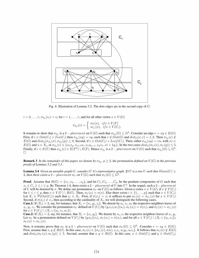
Fig. 4: Illustration of Lemma 3.2. The dots edges are in the second copy of G.

i = 2, . . . , r, σSp(vi) = vi for i = 1, . . . , r, and for all other vertex x ∈ V (G)

σSp(x) =

σT (x), ifx ∈ V (T )σCi

(x), ifx ∈ V (Ci).

It remains to show that σSpis a 2− placement on V (G) such that σSp

(G) ⊆ G5. Consider an edge e = xy ∈ E(G).First, if e ∈ Out(Ci)× Ins(Ci) then σSp(xy) = vy, such that v /∈ Out(G) and distG(x, v) = 1, 2. Then σSp(e) /∈E(G) and distG(σSp

(x), σSp(y)) ≤ 3. Second, if e ∈ Out(Ci)× Leaf(Ci). Then, either σS2

(xy) = vu, with xv ∈E(G) and u ∈ Xi, or σSp(e) ∈ u1xp, xi+1ui, x1up−1, xpv1, xi+ 1yi. In the two cases distG(σC(x), σC(y)) ≤ 5.Finally, if e ∈ E(T ) then σSp(e) ∈ E(T 3) \ E(T ). Hence σSp is a 2− placement on V (G) such that σSp(G) ⊆ G5.

Remark 3 In the remainder of this paper, we denote by σSp, p ≥ 2, the permutation defined on V (G) in the previous

proofs of Lemmas 3.2 and 3.3 .

Lemma 3.4 Given an unstable graph G. consider G′ it’s representative graph. If G′ is a tree U such that Diam(U) ≥3, then there exists a 2− placement σU on V (G) such that σU (G) ⊆ G5.

Proof. Assume that R(G) = x1, x2, . . . , xp, and let C1, C2, . . . , Cp, be the pendant components of G such thatxi ∈ Ci, 1 ≤ i ≤ p. By Theorem 1.4, there exists a 2− placement of U into U3. In the sequel, such a 2− placementof U will be denoted by σ. We define our permutation σU on V (G) as follows: Given a vertex x ∈ V (G), if x /∈ V (Ci)for 1 ≤ i ≤ p, thus x ∈ V (U) \ R(G). Then, σU (x) = σ(x). Else there exists i ∈ 1, . . . , p such that x ∈ V (Ci).Let Xi ∈ P(Out(Ci)) such that xi ∈ Xi. First, if σ(xi) = xi it suffices to put σU (x) = σCi(x) for x ∈ V (Ci).Second, if σ(xi) 6= xi, then according to the cardinality of Xi, we will distinguish the following cases.Case.1: If |Xi| = 3, say, for instance, that Xi = xi, yi, zi. We denote by ui, vi, wi the respective neighbors leaves ofxi, yi, zi. We consider the permutation σU defined on V (Ci) by (yiviziwi)(ui), σU (xi) = σ(xi), and σU (x) = σCi

(x)for x ∈ V (Ci) \ (Xi ∪ ui, vi, wi).Case.2: If |Xi| = 2, say, for instance, that Xi = xi, yi. We denote by ui, vi the respective neighbors leaves of xi, yi.Let σU be a permutation defined on V (Ci) by (yiui)(vi), σU (xi) = σ(xi), and for all x ∈ V (Ci) \ (Xi ∪ ui, vi),σU (x) = σCi

(x).

Now, it remains prove that σU is a 2 − placement on V (G) such that σU (G) ⊆ G5. Consider e = xy ∈ E(G).First, assume that x, y /∈ R(G). In this case, σU (e) ∈ σCi

(e), σ(e), vizi, wiyi, uivi. It follows that σU (e) /∈ E(G)and distG(σU (x), σU (y)) ≤ 5. Second, assume that x, y ∈ R(G). In this case, x ∈ Out(Ci) and y ∈ Out(Cj),

174

Fig. 5: An example when G′ is a star.

with i 6= j. Thus, σU (e) ∈ σ(xy), σ(x)σCj(y), σCi

(x)σ(y), σCi(x)σCj

(y). Hence, σU (e) /∈ E(G). Moreover,since distG(x, σ(x)) ≤ 3 and distG(x, σCi

(x)) = 1, one can obviously observe that distG(σU (x), σU (y)) ≤ 5.Finally, and without loss of generalities, we can assume that x ∈ R(G) and y /∈ R(G). In this case, σU (e) ∈σCi(e), σ(e), σ(x)y, σCi(x)σ(y), σ(x)ui. It ensues that σU (e) /∈ E(G). Furthermore, since distG(x, σ(x)) ≤ 3and distG(x, σCi(x)) = 1, it follows that distG(σU (x), σU (y)) ≤ 5. Consequently, σU is a 2− placement on V (G)such that σU (G) ⊆ G5.

Proof of Theorem 1.5.

Given an unstable graph G of order n ≥ 4, consider C1, C2, . . . , Cr, r ≥ 1, the family of it’s pendant components suchthat |Ci| ≥ 5, 1 ≤ i ≤ r.

Claim 1 If each pendant component of G is either a singleton or an edge, then there exists a 2− placement σ suchthat σ(G) ⊆ G3.

Indeed: In this case, the graph G is without cycles. Consequently, G is a tree. Moreover, since G is an indecomposablegraph, then G is a non-star tree. By Theorem 1.4, there exists a 2− placement σ such that σ(G) ⊆ G3.

Claim 2 If G is a pendant graph, then there exists a 2− placement σ such that σ(G) ⊆ G5.

Indeed: By Lemma 3.1, there exists a 2− placement σ such that σ(G) ⊆ G5.

From now on, we shall assume that we can apply neither Claim 1 nor Claim 2 to the graph G. Under this assumption,we will define a 2− placement σ on V (G) such that σ(G) ⊆ G5. Let Ci, 1 ≤ i ≤ r, be a pendant component of Gand Xi ∈ P(Out(Ci)). We shall discuss the followings two cases.

Case.1: If |Xi| = 2, say for instance that Xi = xi, yi and we denote by ui, vi the respective neighbors leavesof xi, yi. First, we assume that |Xi ∩ R(G)| = 0. In this case the permutation σ is defined on xi, yi, ui, vi byσ(x) = σCi

(x). Second, assume that |Xi ∩R(G)| = 1. Without loss of generality, we can suppose that xi ∈ R(G).Let T be a connected component of G′ such that xi ∈ V (T ). In this case it suffices to consider the permutation σdefined on xi, yi, ui, vi by σ(x) = σsp(x), p ≥ 2, if T ' Sp (i.e T is isomorphic to Sp) with σSp

is that given byLemma 3.2 and Lemma 3.3 and σ(x) = σU (x), if Diam(T ) ≥ 3 with σU is that given by Lemma 3.4. Finally, assumethat |Xi ∩R(G)| = 2. Let T, T ′ be the connected components of G′ such that xi ∈ V (T ) and yi ∈ V (T ′).

Subcase.1.1: If T ' Sp and T ′ ' Sp′ with p, p′ ≥ 2. We define a permutation σ on xi, yi, ui, vi by σ(x) = σSp(x)if x ∈ xi, ui and σ(x) = σSp′ (x) if x ∈ yi, vi, with σSp

and σSp′ are those given by Lemma 3.2 and Lemma 3.3.

175

Subcase.1.2: If T ' Sp, p ≥ 2, and Diam(T ′) ≥ 3. By Theorem 1.4, there exists a permutation σT ′ defined onV (T ′) such that σT ′(T ′) ⊆ T ′3. We define a permutation σ on xi, yi, ui, vi as follows. First, if σT ′(yi) 6= yi, thenσ(x) = σSp

(x) if x ∈ xi, ui, σ(yi) = σT ′(yi) and σ(vi) = vi, with σSpis the permutation given by Lemma 3.2

and Lemma 3.3. Second, if σT ′(yi) = yi, then σ(x) = σSp(x), with σSp

is the permutation given by Lemma 3.2 andLemma 3.3.

Subcase.1.3: If Diam(T ) ≥ 3 and Diam(T ′) ≥ 3. By Theorem 1.4, there exist permutations σT , σT ′ defined respec-tively on V (T ) and V (T ′) such that σT (T ) ⊆ T 3 and σT ′(T ′) ⊆ T ′3. We define a permutation σ on xi, yi, ui, vi asfollows. First, if σT (xi) = xi and σT ′(yi) = yi, then σ(x) = σCi

(x). Second if σT (xi) = xi and σT ′(yi) 6= yi (orσT (xi) 6= xi and σT ′(yi) = yi), then σ(x) = σU (x) with σU is that given by Lemma 3.4. Finally, if σT (xi) 6= xi andσT ′(yi) 6= yi, then σ(xi) = σT (xi), σ(ui) = ui, σ(yi) = σT ′(yi) and σ(vi) = vi.

Case.2: If |Xi| = 3, assume that Xi = xi, yi, zi and denote by ui, vi, wi the respective neighbors leaves of xi, yi, zi.First, assume that |Xi ∩R(G)| = 0. In this case, the permutation σ is defined on Xi ∪ ui, vi, wi by σ(x) = σCi

(x).Second, suppose that |Xi ∩R(G)| = 1. Then, either σ(x) = σSp

(x) with σSpis that given by Lemma 3.2 and Lemma

3.3, or σ(x) = σU (x) with σU is that given by Lemma 3.4. Third, if |Xi ∩R(G)| = 2. Without loss of generalities,one can assume that xi, yi ∈ R(G). Let T, T ′ be the connected components of the representative graph G′ such thatxi ∈ V (T ) and yi ∈ V (T ′). In this case, if one of the trees T or T ′, say T , is isomorphic to Sp, p ≥ 2, then it sufficesto put σ(x) = σSp

(x) for x ∈ xi, ui and identify σ with the permutations σSp, σU defined by Lemmas 3.2, 3.3,

3.4 (When|Xi| = 2), for x ∈ yi, zi, vi, wi. Otherwise, assume that Diam(T ) ≥ 3 and Diam(T ′) ≥ 3. In thiscase, if σT (xi) = xi and σT ′(yi) = yi, then σ(x) = σCi

(x) for x ∈ Xi ∪ ui, vi, wi. Else, assume for instance thatσT (xi) 6= xi. Then, it suffices to take σ(xi) = σT (xi), σ(ui) = ui and identify σ with the permutation σU defined byLemma 3.4 (Case.|Xi| = 2), for x ∈ yi, zi, vi, wi. Finally, assume that |Xi ∩R(G)| = 3. Let T, T ′ and T ′′ be theconnected components of the representative graph G′ such that xi ∈ V (T ), yi ∈ V (T ′) and zi ∈ V (T ′′). In this case,if one of the trees T, T ′ or T ′′, say for instance T , is isomorphic to Sp, p ≥ 2, then it suffices to put σ(x) = σSp(x) forx ∈ xi, ui, and for x ∈ yi, zi, vi, wi the permutation σ(x) is that given by the previous case (|Xi ∩ R(G)| = 2applied to T ′ and T ′′). Otherwise, Diam(T ) ≥ 3, Diam(T ′) ≥ 3 and Diam(T ′′) ≥ 3. Let σT , σT ′ and σT ′′ be thepermutation defined by Theorem 1.4 respectively on V (T ), V (T ′) and V (T ′′).

Subcase.2.1: Assume that σT (xi) = xi, σT ′(yi) = yi and σT ′′(zi) = zi. Then σ(x) = σCi(x) for x ∈ Xi ∪ui, vi, wi.Subcase.2.2: Assume that σT (xi) 6= xi, σT ′(yi) 6= yi and σT ′′(zi) 6= zi. Then, we define a permutation σ onXi ∪ ui, vi, wi by σ(xi) = σT (xi), σ(yi) = σT ′(yi), σ(zi) = σT ′′(zi) and σ(x) = x for x ∈ ui, vi, wi.Subcase.2.3: Assume that σT (xi) 6= xi, σT ′(yi) = yi. In this case, it suffices to put σ(xi) = σT (xi), σ(ui) = ui andfor x ∈ yi, zi, vi, wi, σ(x) is the permutation given by Lemma 3.4.

Now, for all other vertices x ∈ V (G), either x ∈ Ins(Ci), 1 ≤ i ≤ r, or x ∈ V \⋃ri=1 Ci. Then, it suffices to put

σ(x) = x if x ∈ Ins(Ci), 1 ≤ i ≤ r; otherwise, if x ∈ V \⋃ri=1 Ci then x ∈ T , with T is connected component of

the representative graph G′. Hence, σ(x) = σSp(x) if x ∈ Sp, p ≥ 3, and σ(x) = σT (x) if Diam(T ) ≥ 3, with σT isthe permutation given by Theorem 1.4.

To conclude, it remains to verify that our permutation σ is a 2−placement ofG intoG5. Given an edge e = xy ∈ E(G),then either e ∈ Nob(G) or not.Case.1: If e = xy ∈ Nob(G). Clearly, e ∈ Out(G)× Ins(G) (i.e x ∈ Out(G) and y ∈ Ins(G)) and

σ(e) =

σSp

(e), ifx ∈ Sp

σT (e), ifx ∈ T and σT (x) 6= x(with Diam(T ) ≥ 3).σCi

(e), ifx /∈ R(G) or x ∈ T and σT (x) = x(with Diam(T ) ≥ 3).

In all these cases, we have already checked that our permutation is a 2− placement of G into G5.Case.2: If e = xy /∈ Nob(G). Clearly, e is either a pendant edge or e is a proper bridge of G.Subcase.2.1: If e = xy is a pendant edge of G. Say, for instance, that y ∈ Leaf(G). In this case,

σ(e) =

σSp(e), ifx ∈ Sp

σT (e), ifx ∈ T \R(G) (with Diam(T ) ≥ 3).σT (x)y, ifx ∈ T ∩R(G) and σT (x) 6= x(with Diam(T ) ≥ 3).σCi

(e), ifx /∈ R(G) or x ∈ T ∩R(G) and σT (x) = x(with Diam(T ) ≥ 3).

Here, it remains just to verify that σT (x)y is an edge of E(G5) \ E(G). Clearly, σT (x) 6= y since y /∈ T . Moreover,distG(x, σT (x)) ≤ 3 and distG(x, y) = 1. Therefore, distG(σT (x), y) ≤ 4 and σT (x)y /∈ E(G). Which permits usto conclude.

176

Subcase.2.2: If e = xy is a proper bridge of G. Clearly, at least one of the two vertices x, y is not a representativevertex of G, say for instance y /∈ R(G). In this case,

σ(e) =

σT (e), ifx /∈ R(G) or x ∈ R(G) and σT (x) 6= x(with Diam(T ) ≥ 3)σCi

(x)σT (y), ifx ∈ R(G) and σT (x) = x(with Diam(T ) ≥ 3).

Here, it remains just to verify that σCi(x)σT (y) is an edge of E(G5) \ E(G). Clearly, distG(x, σCi(x)) = 1 sinceσCi

(x) is the neighbor leaf of x. Moreover, σCi(x) 6= y since xy is a proper bridge of G (i.e y is not a leaf of G).

Furthermore, distG(y, σT (y)) ≤ 3. Consequently, σCi(x)σT (y) /∈ E(G) and distG(σCi

(x), σT (y)) ≤ 5.

References

[1] Mariusz Wozniak. Packing of graphs and permutations—a survey. Discrete Mathematics, 276(1):379–391, 2004.[2] HP Yap. Packing of graphs—a survey. Discrete Mathematics, 72(1):395–404, 1988.[3] David Burns and Seymour Schuster. Embedding (p, p- 1) graphs in their complements. Israel Journal of

Mathematics, 30(4):313–320, 1978.[4] Ralph J Faudree, Cecil C Rousseau, Richard H Schelp, and Seymour Schuster. Embedding graphs in their

complements. Czechoslovak Mathematical Journal, 31(1):53–62, 1981.[5] SM Hedetniemi, ST Hedetniemi, and PJ Slater. A note on packing two trees into kn. Ars Combin, 11:149–153,

1981.[6] Hamamache Kheddouci, Jean-François Saclé, and Mariusz Wozniak. Packing two copies of a tree into its fourth

power. Discrete Mathematics, 213(1-3):169–178, 2000.[7] Agnieszka Görlich, Monika Pilsniak, Mariusz Wozniak, and Irmina A Zioło. A note on embedding graphs without

short cycles. Discrete mathematics, 286(1):75–77, 2004.[8] Atsushi Kaneko and Kazuhiro Suzuki. Packing two copies of a tree into its third power. Discrete Mathematics,

306(21):2779 – 2785, 2006.[9] Andrzej Ehrenfeucht, Tero Harju, and Grzegorz Rozenberg. The theory of 2-structures: a framework for decompo-

sition and transformation of graphs. World Scientific Publishing Company, 1999.

177

Special sessions

RECONSTRUCTION OF DIGRAPHS UP TO COMPLEMENTATION

Aymen Ben AmiraDepartment of Mathematics, College of Sciences

King Saud UniversityP. O. Box 2455, Riyadh 11451, Saudi Arabia

[email protected]

Jamel DammakDepartment of MathematicsFaculty of Sciences of Sfax

B.P. 1171, 3000 Sfax, [email protected]

Hamza Si KaddourICJ, Department of Mathematics

University of Lyon, University Claude-Bernard Lyon 143 Bd du 11 Novembre 1918, 69622 Villeurbanne Cedex, France

[email protected]

Dedicated with warmth and admiration to Maurice Pouzet at the occasion of his 75th birthday

ABSTRACT

We prove that if G and G′ are two digraphs, (≤ 8)-hypomorphic up to complementation, then G andG′ are isomorphic up to complementation; we prove also that the value 8 is optimal.

Keywords Digraph · Isomorphism · k-hypomorphy up to complementation · Boolean sum · Symmetric graph

1 Introduction

A directed graph or simply digraph G consists of a finite and nonempty set V of vertices together with a prescribedcollection E of ordered pairs of distinct vertices, called the set of the edges of G. Such a digraph is denoted by(V (G), E(G)) or simply (V,E). Given a digraph G = (V,E), to each nonempty subset X of V associate thesubdigraph (X,E ∩ (X ×X)) of G induced by X denoted by GX . With each digraph G = (V,E) associate its dualG∗ = (V,E∗) and its complement G =

(V,E

)defined as follows: Given x 6= y ∈ V, (x, y) ∈ E∗ if (y, x) ∈ E,

and (x, y) ∈ E if (x, y) 6∈ E. Two interesting types of digraphs are symmetric digraphs and tournaments. A digraphG = (V,E) is a symmetric digraph or graph (resp. tournament) whenever for x 6= y ∈ V , (x, y) ∈ E if and only if(y, x) ∈ E (resp. (x, y) ∈ E and (y, x) /∈ E or conversely). Given two digraphs G = (V,E) and G′ = (V ′, E′), abijection f from V onto V ′ is an isomorphism from G onto G′ provided that for any x, y ∈ V , (x, y) ∈ E if and only if(f(x), f(y)) ∈ E′. The digraphs G and G′ are isomorphic, if there exists an isomorphism from one onto the other.

Given two digraphs G and G′ on the same vertex set V . Let k be an integer with 0 < k < |V |, the digraphs G andG′ are k-hypomorphic if for every k-element subset X of V , the induced subdigraphs GX and G′X are isomorphic.The digraphs G and G′ are (≤ k)-hypomorphic if they are t-hypomorphic for each integer t ≤ k. A digraph G isk-reconstructible if any digraph k-hypomorphic to G is isomorphic to G.

In 1970, R.Fraïssé asked what is the least integer k such that the digraphs are (≤ k)-reconstructible. G.Lopez [8, 9]answered to this question by showing that k = 6.

Given two digraphs G and G′ on the same vertex set V . They are hereditarily isomorphic [10] if for each nonemptysubset X of V , the digraphs GX and G′X are isomorphic. They are isomorphic up to complementation (resp.hemimorphic) ifG′ is isomorphic toG orG (resp. toG orG∗). They are hereditarily isomorphic up to complementation[2] if they are hereditarily isomorphic, or G′ and G are hereditarily isomorphic. Let k be a positive integer, the digraphsG and G′ are k-hypomorphic up to complementation (resp. k-hemimorphic) if for every k-element subset X of V ,the induced subdigraphs GX and G′X are isomorphic up to complementation (resp. hemimorphic). The digraphs Gand G′ are (≤ k)-hypomorphic up to complementation (resp. (≤ k)-hemimorphic) if they are t-hypomorphic up tocomplementation (resp. t-hemimorphic) for each integer t ≤ k. A digraphG is k-reconstructible up to complementation

181

2

(resp. k-half-reconstructible) if any digraph k-hypomorphic up to complementation (resp. k-hemimorphic) to Gis isomorphic up to complementation (resp. hemimorphic) to G. A digraph G is (≤ k)-reconstructible up tocomplementation (resp. (≤ k)-half-reconstructible) if any digraph (≤ k)-hypomorphic up to complementation (resp.(≤ k)-hemimorphic) to G is isomorphic up to complementation (resp. hemimorphic) to G.

In 1993, J.G.Hagendorf raised the (≤ k)-half-reconstruction problem for digraphs and solved it with G.Lopez [6, 7],they showed that the finite digraphs are (≤ 12)-half-reconstructible. In 1995, Y.Boudabbous and G.Lopez [3] showedthat the finite tournaments are (≤ 7)-half-reconstructible.

In 1999, P.Ille asked what is the least integer k such that the digraphs are (≤ k)-reconstructible up to complementation.The case of symmetric graphs was solved by J.Dammak, G.Lopez, M.Pouzet and H.Si Kaddour [4, 5], they proved that,the symmetric graphs on v vertices are t-reconstructible up to complementation for every 4 ≤ t ≤ v − 3. In fact, thecase t = v − 3 was solved in [5].For digraphs, we first obtained with B. Chaari [1] a partially answer which is Theorem 1.1 below.Let G = (V,E) and G′ = (V,E′) be two digraphs, 2-hypomorphic up to complementation. The boolean sum G+G′

of G and G′ is the symmetric digraph U = (V,E(U)) defined by x, y ∈ E(U) if and only if (x, y) ∈ E and(x, y) /∈ E′, or (x, y) /∈ E and (x, y) ∈ E′.Theorem 1.1. (Theorem 1.3 of [1]) Let G and G′ be two digraphs on the same set V of n ≥ 4 vertices such that G andG′ are (≤ 5)-hypomorphic up to complementation. Let U := G+G′. If U and U are connected, then G and G′ arehereditarily isomorphic up to complementation.

2 Main result

Our main result, Theorem 2.1, extends Theorem 1.1. It says that 8 is the least integer k such that the digraphs are(≤ k)-reconstructible up to complementation.Theorem 2.1. Let G and G′ be two digraphs on the same set V of vertices such that G and G′ are (≤ 8)-hypomorphicup to complementation. Then G and G′ are isomorphic up to complementation. Moreover the value 8 is optimal.

The optimality of the value 8 of Theorem 2.1 follows from the following result.Proposition 2.2. For all integer n ≥ 8, there are two digraphs on the same set of n vertices, nonisomorphic up tocomplementation, which are (≤ 7)-hypomorphic up to complementation and not 8-hypomorphic up to complementation.

References

[1] A. Ben Amira, B. Chaari, J. Dammak and H. Si Kaddour, The (≤ 5)-hypomorphy of digraphs up to complementa-tion, Arab Journal of Mathematical Sciences 25 (2019), no. 1, 1–16.

[2] M. Bouaziz, Y. Boudabbous and N. El Amri, Hereditary hemimorphy of −k-hemimorphic tournaments fork ≥ 5. J. Korean Math. Soc. 48 (2011), no. 3, 599–626.

[3] Y. Boudabbous and G. Lopez, La relation différence et l’anti-isomorphie, Math. Logic Quart. 41 (1995), no. 2,268–280.

[4] J. Dammak, G. Lopez, M. Pouzet and H. Si Kaddour, Hypomorphy of graphs up to complementation. JCTB,Series B 99 (2009), no. 1, 84–96.

[5] J. Dammak, G. Lopez, M. Pouzet and H. Si Kaddour, Boolean sum of graphs and reconstruction up to comple-mentation. Advances in Pure and Applied Mathematics 4 (2013), 315–349.

[6] J. G. Hagendorf and G. Lopez, La demi-reconstructibilité des relations binaires d’au moins 13 éléments, C. R.Acad. Sci. Paris, t.317, Série I (1993), 7–12.

[7] J. G. Hagendorf and G. Lopez, Un théorème de demi-reconstruction des relations binaires de cardinal > 12(2017), hal-01501643v1.

[8] G. Lopez, Deux résultats concernant la détermination d’une relation par les types d’isomorphie de ses restrictions,C. R. Acad. Sci. Paris, t.274, Série A, (1972), 1525–1528.

[9] G. Lopez, Sur la détermination d’une relation par les types d’isomorphie de ses restrictions, C. R. Acad. Sci.Paris, t.275, Série A (1972), 951–953.

[10] K. B. Reid and C. Thomassen, Strongly self-complementary and hereditarily isomorphictournaments. Monatsh.Math. 81 (1976), no. 4, 291–304.

182

BIG RAMSEY DEGREES OF THE UNIVERSAL HOMOGENEOUSPARTIAL ORDER ARE FINITE

Jan HubickaDepartment of Applied Mathematics (KAM)

Charles UniversityPraha 1, 110 00

[email protected]

ABSTRACT

We show that the universal homogeneous partial order has finite big Ramsey degrees. Our proof usesthe Carlson–Simpson theorem rather than (a strengthening of) the Halpern–Läuchli and Millikentree theorem which is the main tool used to give bounds on big Ramsey degrees. We discuss twocorollaries.

Keywords big Ramsey degree · Carlson–Simpson Theorem · structural Ramsey theory · homogeneous structures

1 Introduction

We consider graphs, partial orders and metric spaces as special cases of model-theoretic relational structures. Givenstructures A and B, we denote by

(BA

)the set of all embeddings from A to B. We write C −→ (B)Ak,l to denote the

following statement: For every colouring χ of(CA

)with k colours, there exists an embedding f : B→ C such that χ

does not take more than l values on(f(B)A

).

For a countably infinite structure B and its finite substructure A, the big Ramsey degree of A in B is the least numberL ∈ ω ∪ ω such that B −→ (B)Ak,L for every k ∈ ω. We say that a countably infinite structure B has finite bigRamsey degrees if the big Ramsey degree is finite for every finite substructure of B.

A countable structure A is called (ultra)homogeneous if every isomorphism between finite substructures extends to anautomorphism of A. It is well known that there is a (up to isomorphism) unique homogeneous partial order P with theproperty that every countable partial order has embedding to P. We call P the universal homogeneous partial order.We prove the following.

Theorem 1.1. The universal homogeneous partial order has finite big Ramsey degrees.

The main novelty in our approach is the use of spaces described by parameter words in the context of big Ramseydegrees. We use an infinitary variant of the Graham-Rothschild Theorem [1] which is a direct consequence of theCarlson–Simpson Theorem [2]. This leads to a finer control over the sub-trees compared to constructions based onapplications of the Milliken tree theorem [3] which was the main tool used by Laver and Devlin to show that the orderof rationals has finite big Ramsey degrees [4], by Sauer to show that the random graph has big Ramsey degrees [5] andseveral followup results.

2 Applications

Big Ramsey degrees are studied mainly in the context of free amalgamation structures. Since the universal homogeneouspartial order is not a free amalgamation structure, it represents an important new example which has additionalconsequences. Let us discuss two corollaries.

183

1. Let S be a set of non-negative reals such that 0 ∈ S. A metric space M = (M,d) is S-metric space if for everyu, v ∈M it holds that d(u, v) ∈ S. A countable S-metric space M is a S-Urysohn metric space if it is homogeneous(that is, every isometry of its finite subspaces extends to an isometry from M to M) and every countable S-metricspace embeds into it. Finite set of non-negative reals S = 0 = s0 < s1 < · · · < sn is tight if if si+j ≤ si + sj forall 0 ≤ i ≤ j ≤ i+ j ≤ n (see [6]). It follows from a classification by Sauer [7] that for every such S there exists anS-Urysohn space. Mašulovic [6, Theorem 4.4] shows a way to represent all S-metric cases with finitely many distances(for every tight set S) as a partial order. We thus obtain:Corollary 2.1. Let S be a finite tight set of non-negative reals. Then the S-Urysohn space has finite big Ramseydegrees.

This can be seen as a continuation of the research on (in)divisibility of metric spaces started by Delhommé, Laflamme,Pouzet and Sauer [8, 9] and by Nguyen Van Thé [10, 11].

2. Recall that there is a up to isomorphism unique homogeneous triangle-free graph H (called the universal ho-mogeneous triangle-free graph) such that every countable triangle-free graph embeds to H. We also obtain the firstcombinatorial proof of the following recent result by Dobrinen:Theorem 2.2 (Dobrinen 2020 [12]). The universal homogeneous triangle-free graph has finite big Ramsey degrees.

We shall remark that Theorem 2.2 was generalized to the universal homogeneous Kk-free graphs (for every k > 2) [13]and to free amalgamation classes in binary relational languages [14]. Generalizing our construction to structures innon-binary relational languages and to structures that can not be described by means of forbidden substructures with atmost 3 vertices is presently work in progress based on results announced in [15].

Acknowledgement: Author is supported by project 18-13685Y of the Czech Science Foundation (GACR), Centerfor Foundations of Modern Computer Science (Charles University project UNCE/SCI/004), by the PRIMUS/17/SCI/3project of Charles University and by ERC Synergy grant DYNASNET 810115.

References

[1] Ronald L. Graham and Bruce L. Rothschild. Ramsey’s theorem for n-parameter sets. Transactions of the AmericanMathematical Society, 159:257–292, 1971.

[2] Timothy J. Carlson and Stephen G. Simpson. A dual form of Ramsey’s theorem. Advances in Mathematics,53(3):265–290, 1984.

[3] Keith R. Milliken. A Ramsey theorem for trees. Journal of Combinatorial Theory, Series A, 26(3):215–237, 1979.[4] Denis Devlin. Some partition theorems and ultrafilters on ω. PhD thesis, Dartmouth College, 1979.[5] Norbert W. Sauer. Coloring subgraphs of the Rado graph. Combinatorica, 26(2):231–253, 2006.[6] Dragan Mašulovic. Pre-adjunctions and the Ramsey property. European Journal of Combinatorics, 70:268–283,

2018.[7] Norbert W. Sauer. Distance sets of Urysohn metric spaces. Canadian Journal of Mathematics, 65(1):222–240,

2013.[8] Christian Delhommé, Claude Laflamme, Maurice Pouzet, and Norbert W. Sauer. Divisibility of countable metric

spaces. European Journal of Combinatorics, 28(6):1746–1769, 2007.[9] Christian Delhommé, Claude Laflamme, Maurice Pouzet, and Norbert W. Sauer. Indivisible ultrametric spaces.

Topology and its Applications, 155(14):1462–1478, 2008.[10] Lionel Nguyen Van Thé. Ramsey degrees of finite ultrametric spaces, ultrametric Urysohn spaces and dynamics

of their isometry groups. European Journal of Combinatorics, 30(4):934–945, 2009.[11] Lionel Nguyen Van Thé. Structural Ramsey Theory of Metric Spaces and Topological Dynamics of Isometry

Groups. Memoirs of the American Mathematical Society. American Mathematical Society, 2010.[12] Natasha Dobrinen. The Ramsey theory of the universal homogeneous triangle-free graph. Journal of Mathematical

Logic, page 2050012, 2020.[13] Natasha Dobrinen. The Ramsey theory of Henson graphs. arXiv:1901.06660, submitted, 2019.[14] Andy Zucker. A note on big Ramsey degrees. arXiv preprint arXiv:2004.13162, 2020.[15] Martin Balko, David Chodounský, Jan Hubicka, Matej Konecný, and Lluis Vena. Big Ramsey degrees of

3-uniform hypergraphs. Acta Mathematica Universitatis Comenianae, 88(3):415–422, 2019.

184

WELL QUASI ORDERING AND EMBEDDABILITY OF RELATIONALSTRUCTURES

Maurice PouzetUniv. Lyon, Université Claude-Bernard Lyon1, CNRS UMR 5203, Institut Camille Jordan

43 bd. 11 Novembre 1918, 69622 Villeurbanne Cedex, FranceMathematics & Statistics Department, University of Calgary, Calgary, Alberta, Canada T2N 1N4

[email protected]

ABSTRACT

A relational structure R is embeddable in a relational structure R′ if R is isomorphic to an inducedsubstructure of R′. In the late forties, Fraïssé, following the work of Cantor, Hausdorff and Sierpinski,pointed out the importance of the quasi-ordering of embeddability in the theory of relations. Forexample, he conjectured that the class of countable chains is well quasi ordered (w.q.o.) underembeddability, a conjecture positively solved by Laver in the early seventiees with the use of thetheory of better quasi ordering (b.q.o.), a far reaching strengthening of the notion of w.q.o., inventedby Nash-Williams. Fraïssé also noted that basic notions about ordered sets (posets) like initialsegments, ideals, chains and antichains have a direct counterpart in terms of relational structures. Forexample, a class C of structures is hereditary if it contains every structure which can be embeddedinto some member of C. Clearly, hereditary classes are initial segments of the class of relationalstructures quasi-ordered by embeddability. If R is a relational structure, the age of R is the setAge(R) of finite restrictions of R considered up to isomorphism. This is an ideal of the poset made offinite structures considered up to isomorphism and ordered via embeddability. As shown by Fraïssé,every countable ideal has this form. Several results along these lines about hereditary classes ofrelational structures have been obtained. Recent years have seen a renewed interest for the studyof those made of finite structures and notably for their profile. The profile of a hereditary class Cof finite structures considered up to isomorphism is the function ϕC which counts for every integern the number of members of C on n elements. General counting results as well as precise resultsfor graphs, tournaments, ordered graphs and permutations have been obtained, with a particularemphasis on jumps in the growth of the profile. I will present some general results about hereditaryclasses, particularly on those which are w.q.o. (or even b.q.o.), notably on their height, ordinal length,Cantor-Bendixson and Vietoris rank. I will discus extensions of Laver’s theorem to hereditary classesof binary structures. I will illustrate the role of w.q.o. in the classification of hereditary classes ofsmall growth. I will conclude with several problems, some going back to the seventies, on w.q.o. andhereditary classes of relational structures.

References

[1] M.H. Albert and M.D. Atkinson, Simple permutations and pattern restricted permutations. Discrete Mathematics,300 (2005) 1–15.

[2] A. Atminas, V. Lozin, Labelled induced subgraphs and well-quasi-ordering, Order 32 (2015), no. 3, 313–328.[3] P.J. Cameron, Orbits of permutation groups on unordered sets. II. J. London Math. Soc. 23(2) (1981), pp. 249–264.[4] P.J. Cameron, Oligomorphic permutation groups. Cambridge University Press, Cambridge, 1990.[5] P.J. Cameron, The algebra of an age. In Model theory of groups and automorphism groups (Blaubeuren, 1995),

pages 126–133. Cambridge Univ. Press, Cambridge, 1997.[6] P.J. Cameron, On an algebra related to orbit-counting. J. Group Theory 1(2) (1998), 173–179.

185

[7] E. Corominas. On better quasi-ordering countable trees. Discrete Math., 53 (1985) 35–53.

[8] D.H.J. de Jongh and R. Parikh, Well-partial orderings and hierarchies. Nederl. Akad. Wetensch. Proc. Ser. A80=Indag. Math. 39(3) (1977) 195–207.

[9] C. Delhommé, M. Pouzet, N. Sauer, G. Sági, Representation of ideals of relational structures, Discrete Math. 309(2009), no. 6, 1374–1384.

[10] G. Ding, Subgraphs and well-quasi-ordering, Journal of Graph Theory, 16, no 5 (1992), 489-502.

[11] A. Ehrenfeucht, T. Harju, G. Rozenberg, The theory of 2-structures. A framework for decomposition andtransformation of graphs. World Scientific Publishing Co., Inc., River Edge, NJ, 1999.

[12] R. Fraïssé, Sur la comparaison des types de relations. C. R. Acad. Sci. Paris 226, (1948). 987-988.

[13] R. Fraïssé, Sur la comparaison des types d’ordres. C. R. Acad. Sci. Paris 226, (1948). 1330-1331.

[14] R. Fraïssé, Sur quelques classifications des systèmes de relations, Thèse, Paris (1953), Alger-Math. 1 (1954),35–182.

[15] R. Fraïssé, Sur l’extension aux relations de quelques propriétes des ordres, Ann. Sci. Ecole Norm. Sup. 71 (1954),361–388.

[16] R. Fraïssé, Theory of relations. Revised edition. With an appendix by Norbert Sauer. Studies in Logic and theFoundations of Mathematics, 145. North-Holland Publishing Co., Amsterdam, 2000. ii+451.

[17] C. Frasnay, Quelques problèmes combinatoires concernant les ordres totaux et les relations monomorphes. Thèse.Paris. Annales Institut Fourier Grenoble 15 (1965), 415–524.

[18] D.H. Gottlieb, A class of incidence matrices, Proc. Amer. Math. Soc. 17 (1966), 1233–1237.

[19] T. Gallai. Transitiv orientbare graphen. Acta Math. Acad. Sci. Hungar. 18 (1967), 25–66 (English translation by F.Maffray and M. Preissmann in J.J. Ramirez-Alfonsin and B. Reed (Eds), Perfect graphs, Wiley 2001, 25–66.

[20] G. Higman, Ordering by divisibility in abstract algebras. Proc. London Math. Soc. (3) (1952), 326–336.

[21] P. Jullien, Contribution à l’étude des types d’ordres dispersés, Thèse Doctorat d’État, Université de Marseille, 27juin 1968.

[22] W.M. Kantor, On incidence matrices of finite projective and affine spaces, Math. Z. 124 (1972), 315–318.

[23] M. Klazar, Overview of general results in combinatorial enumeration, in Permutation patterns, London Math. Soc.Lecture Note Ser., Vol. 376, (2010), 3–40, Cambridge Univ. Press, Cambridge.

[24] I. Kríž, J. Sgall, Well-quasiordering depends on the labels. Acta Sci. Math. (Szeged) 55 (1991), no. 1-2, 59–65.

[25] J.B. Kruskal, The theory of well-quasi-ordering: a frequently discovered concept. J. Com. Th. 13 (1972), 297–305.

[26] C.Laflamme, M.Pouzet, R.Woodrow, Equimorphy- the case of chains, Archive for Mathematical Logic, 56 (2017),no. 7-8, 811–829.

[27] R. Laver, On Fraïssé’s order type conjecture, Ann. of Math. (2) 93 (1971) 89-111.

[28] R. Laver, An order type decomposition theorem. Ann. of Math. (2) 98 (1973), 96–119.

[29] H.D. Macpherson, Growth rates in infinite graphs and permutation groups. J. London Math. Soc. 35(1987) no2,276–286.

[30] H.D. Macpherson, M. Pouzet, and R.E. Woodrow, Countable structures of a given age. The Journal of SymbolicLogic 57 (1992), 992–1010.

[31] A.I. Mal’cev, The metamathematics of algebraic systems. Collected papers: 1936-1967. Translated, edited, andprovided with supplementary notes by Benjamin Franklin Wells, III. Studies in Logic and the Foundations ofMathematics, Vol. 66. North-Holland Publishing Co., Amsterdam-London, 1971. xviii+494 pp.

[32] A. Marcone, Foundations of bqo theory, Transactions of the A.M.S. 345 no 2 (1994) 641-660.

[33] A. Marcus, G. Tardös, Excluded permutation matrices and the Stanley-Wilf conjecture, J. Combin. Theory, Ser. A107 (2004), 153–160.

[34] E.C. Milner, Basic wqo- and bqo-theory. In Graphs and order, I.Rival Ed. (Banff, Alta., 1984), pages 487–502.Reidel, Dordrecht, 1985.

[35] C.St.J.A. Nash-Williams, On well-quasi-ordering infinite trees, Proc., Phil., Soc., 61, (1965), 697-720.

[36] D. Oudrar, Sur l’énumération de structures discrètes: une approche par la théorie des relations. Thèse de doctorat,Université d’Alger USTHB à Bab Ezzouar, 28 sept. 2015, 249 pp. arXiv:1604.05839.

186

[37] D. Oudrar, M. Pouzet, Profile and hereditary classes of relational structures, J. of MVLSC 27, no 5-6 (2016),475-500.

[38] M. Pouzet, Un belordre d’abritement et ses rapports avec les bornes d’une multirelation. Comptes rendus Acad.Sci. Paris 274(A) (1972), 1677–1680.

[39] M. Pouzet, Application d’une propriété combinatoire des parties d’un ensemble aux groupes et aux relations.Math. Z. 150 (1976) no2, 117–134.

[40] M. Pouzet, Sur la théorie des relations. Thèse d’état, Université Claude-Bernard, Lyon 1, 1978.[41] M. Pouzet, The asymptotic behavior of a class of counting functions. Combinatorics 79 Part 2. M.DEZA and

I.G.ROSENBERG Eds., Annals of Discrete Math. 9 (1980), 223–224.[42] M. Pouzet, Applications of well quasi-ordering and better quasi-ordering. In Graphs and order (Banff, Alta., 1984),

pp. 503–519. Reidel, Dordrecht, 1985.[43] M. Pouzet and I.G. Rosenberg, Sperner properties for groups and relations, Europ. J. Combinatorics 7 (1986),

349–370.[44] M. Pouzet and M. Sobrani, Sandwiches of ages. Ann. Pure Appl. Logic 108 (2001) no3, 295–326.[45][46] M.Pouzet, N.Thiéry, Some relational structures with polynomial growth and their associated algebras I. Quasi-

polynomiality of the profile, The Electronic J. of Combinatorics, 20(2) (2013), 35pp.[47] M. Pouzet, When is the orbit algebra of a group an integral domain? Proof of a conjecture of P. J. Cameron. Theor.

Inform. Appl. 42 (2008), no. 1, 83–103.[48] F.P. Ramsey, On a problem of formal logic, Proc. London Math. Soc. 30 (1930), 264–286.[49] N. Robertson, Neil, P.D. Seymour, Graph minors. A survey. Surveys in combinatorics 1985 (Glasgow, 1985),

153–171, London Math. Soc. Lecture Note Ser., 103, Cambridge Univ. Press, Cambridge, 1985.[50] A. Robinson, On the metamathematics of algebra. Studies in Logic and the Foundations of Mathematics. North-

Holland Publishing Co., Amsterdam, 1951. ix+195 pp.[51] J.G. Rosenstein, Linear orderings. Pure and Applied Mathematics, 98. Academic Press, Inc. [Harcourt Brace

Jovanovich, Publishers], New York-London, 1982. xvii+487 pp.[52] D. Schmidt. Well-partial orderings and their maximal order types. Habilitation, University of Heidelberg,

Heidelberg, 1978.[53] W. Sierpinski, Sur les types d’ordre des ensembles linéaires. Fund. Math. 37, (1950), 253-264.[54] M. Sobrani, Sur les âges de relations et quelques aspects homologiques des constructions D+M. Thèse de Doctorat

d’état, Université S.M. Ben Abdallah-Fez, Fez, 2002.[55] S. Thomassé, On better quasi ordering countable series-parallel orders, Trans. Amer. Math Soc. 352 (no 6) (1999),

2491–2505.[56] N. Zaguia, Chaînes d’idéaux et de sections initiales d’un ensemble ordonné, Publ. Dép. Math. (Lyon) (N.S.),

(7/D) 97, 1983.

187

ON RELATIONAL STRUCTURES WITH POLYNOMIAL PROFILE

Nicolas M. ThiéryLaboratoire de Recherche en Informatique

Université Paris-Saclay, CNRS, 91405, Orsay, [email protected]

ABSTRACT

During this presentation, we will review the state of the following favorite conjecture of MauricePouzet: the profile of a relational structure with bounded signature or finite kernel is eventually aquasi-polynomial whenever the profile is bounded by some polynomial.

The profile of a relational structure R is the function ϕR which counts for every integer n the number, possibly infinite,ϕR(n) of substructures of R induced on the n-element subsets, isomorphic substructures being identified.

The study of profiles started in the seventies; see [1] for a survey. More recently, the line of work became parallel tonumerous researches about the behavior of counting functions for hereditary classes made of finite structures, likeundirected graphs, posets, tournaments, ordered graphs, or permutations, which also enter into this frame; see [2]and [3] for a survey, and [4, 5, 6, 7, 8, 9, 10, 11, 12, 13]. These classes are hereditary in the sense that they containall induced structures of each of their members; in several instances, members of these classes are counted up toisomorphism and with respect to their size.

Several interesting examples of profiles come from permutation groups. For example, if G is a permutation group on aset E, the function θG which counts for every integer n the number of orbits of the action of G on the n-element subsetsof E, is a profile, the orbital profile of G. Groups whose orbital profiles take only finite values are called oligomorphic;their study, introduced by Cameron, is a whole research subject by itself [14, 15].

Results point out jumps in the behavior of these counting functions. Such jumps were for example announced forextensive hereditary classes in [16], with a proof for the jump from constant to linear published in [17]. The growthis typically polynomial or faster than any polynomial, though not necessarily exponential (as indicates the partitionfunction). For example, the growth of an hereditary class of graphs is either polynomial or faster than the partitionfunction [5]. In several instances, these counting functions are eventually quasi-polynomials, e.g. [5] for graphs and [10]for permutations.

In the case of orbital profiles, Cameron conjectured in the late seventies that, whenever the profile ϕG is bounded bya polynomial, it is asymptotically equivalent to a polynomial. In 1985, Macpherson further asked whether the orbitalgebra of G – a graded commutative algebra invented by Cameron and whose Hilbert function is ϕG – is finitelygenerated; in which case the profile would be a quasi-polynomial.

All these elements led Pouzet to the followingConjecture 1. [18] The profile of a relational structure with bounded signature or finite kernel is eventually aquasi-polynomial whenever the profile is bounded by some polynomial.

This conjecture holds if R is an undirected graph [5]. In [18] Pouzet and the author proved that it holds for any relationalstructure R admitting a finite monomorphic decomposition. This result was applied in [19] to show that the aboveconjecture holds for tournaments.

Recently, the conjecture was proven in the case of orbital profiles by Justine Falque [20] under the direction of the author.It results from a complete classification of oligomorphic permutation groups with profile bounded by a polynomial interms of finite permutation groups with decorated block systems. It follows from the classification that the orbit algebrasare essentially invariant rings of finite permutation groups; the latter are known to be finitely generated which resolvespositively Macpherson’s question. A key ingredient in this classification is the notion of blocks. This suggests to search

189

for an appropriate generalization of blocks to relational structures, of which the notion of monomorphic decompositionwould be just a first approximation.

The time seems ripe as well to extend the exploration to subexponential profiles. Indeed, Braunfeld recently gavea near complete description of the spectrum of sub exponential growth rates for orbital profiles, which confirmssome longstanding conjectures of Macpherson. Also, Falque’s classification seems amenable to generalization tosubexponential orbital profiles.

References

[1] Maurice Pouzet. The profile of relations. Glob. J. Pure Appl. Math., 2(3):237–272, 2006.[2] M. Klazar. Overview of some general results in combinatorial enumeration. Arxiv preprint arXiv:0803.4292,

2008.[3] Béla Bollobás. Hereditary properties of graphs: asymptotic enumeration, global structure, and colouring. In

Proceedings of the International Congress of Mathematicians, Vol. III (Berlin, 1998), number Extra Vol. III, pages333–342 (electronic), 1998.

[4] József Balogh, Béla Bollobás, and Robert Morris. Hereditary properties of combinatorial structures: posets andoriented graphs. J. Graph Theory, 56(4):311–332, 2007.

[5] József Balogh, Béla Bollobás, Michael Saks, and Vera T. Sós. The unlabelled speed of a hereditary graph property.J. Combin. Theory Ser. B, 99(1):9–19, 2009.

[6] Adam Marcus and Gábor Tardos. Excluded permutation matrices and the Stanley-Wilf conjecture. J. Combin.Theory Ser. A, 107(1):153–160, 2004.

[7] M. H. Albert and M. D. Atkinson. Simple permutations and pattern restricted permutations. Discrete Math.,300(1-3):1–15, 2005.

[8] M. H. Albert, M. D. Atkinson, and Robert Brignall. Permutation classes of polynomial growth. Ann. Comb.,11(3-4):249–264, 2007.

[9] V. Vatter. Small permutation classes. Proceedings of the London Mathematical Society, 103(5):879–921, 2011.arXiv:0712.4006.

[10] Tomáš Kaiser and Martin Klazar. On growth rates of closed permutation classes. Electron. J. Combin., 9(2):Re-search paper 10, 20 pp. (electronic), 2002/03. Permutation patterns (Otago, 2003).

[11] Martin Klazar. On growth rates of permutations, set partitions, ordered graphs and other objects. Electron. J.Combin., 15(1):Research Paper 75, 22, 2008.

[12] Robert Brignall, Sophie Huczynska, and Vincent Vatter. Decomposing simple permutations, with enumerativeconsequences. Combinatorica, 28(4):385–400, 2008.

[13] Djamila Oudrar and Maurice Pouzet. Profile and hereditary classes of relational structures. In H.Ait Haddadene,I.Bouchemakh, M.Boudar, and S.Bouroubi (LAID3), editors, Proceedings ISOR’11, International Symposium onOperational Research, Algiers, Algeria, May 30-June 2, 2011.

[14] Peter J. Cameron. Oligomorphic permutation groups, volume 152 of London Mathematical Society Lecture NoteSeries. Cambridge University Press, Cambridge, 1990.

[15] Peter Cameron. Oligomorphic permutation groups. In Mohan Delampady N. S. Narasimha Sastry, T. S. S. R.K. Rao and B. Rajeev, editors, Perspectives in Mathematical Sciences II: Pure Mathematics, pages 37–61. WorldScientific, Singapore, 2009.

[16] Maurice Pouzet. The asymptotic behavior of a class of counting functions. In M. Deza and I. G. Rosenberg,editors, Combinatorics 79. Part II, Proceedings of the Colloquium held at the University of Montréal, Montreal,Que., June 11–16, 1979, volume 9, pages 223–224. Elsevier, 1980.

[17] Maurice Pouzet. Application de la notion de relation presque-enchaînable au dénombrement des restrictions finiesd’une relation. Z. Math. Logik Grundlag. Math., 27(4):289–332, 1981.

[18] Maurice Pouzet and Nicolas M. Thiéry. Some relational structures with polynomial growth and their associatedalgebras I: Quasi-polynomiality of the profile. Electron. J. Combin., 20(2):Paper 1, 35, 2013.

[19] Youssef Boudabbous and Maurice Pouzet. The morphology of infinite tournaments; application to the growth oftheir profile. European J. Combin., 31(2):461–481, 2010.

[20] Justine Falque and Nicolas M. Thiéry. Classification of P-oligomorphic groups, conjectures of Cameron andMacpherson. Submitted, 39 pages, arXiv:2005.05296 [math.CO], May 2020.

190

RECURSIVE CONSTRUCTION OF THE MINIMAL PRIME DIGRAPHS

Mohammad AlzohairiKing Saud University. Saudi Arabia.

[email protected]

Moncef BouazizKing Saud University. Saudi Arabia.

[email protected]

Youssef BoudabbousUniversité de la Réunion. France.

[email protected]

ABSTRACT

In a digraph D, a module is a vertex subset M such that every vertex outside M does not distinguishthe vertices in M . A digraph D with more than two vertices is prime if the empty set, the singletonsets, and the full set of vertices are the only modules in D. A prime digraph D is k- minimal if thereis some k-element vertex subset U such that no proper induced subdigraph of D containing U isprime. In this paper, we give a recursive procedure to construct the minimal prime digraphs.

Keywords Module · Prime · Isomorphism ·Minimal prime digraph

1 Introduction

All digraphs mentioned here are finite, and have no loops and no multiple edges. Thus a digraph (or directed graph)D consists of a nonempty and finite set V (D) of vertices with a collection E(D) of ordered pairs of distinct vertices,called the set of edges of D. Such a digraph is denoted by (V (D), E(D)). For elementary definitions and notations ingraph theory we follow [9]. In particular we recall that the subdigraph of a digraph D induced by a nonempty vertexsubset X is denoted by D[X], and if | V (D) |≥ 2, then for each vertex x, the subdigraph D[V (D) \ x] is alsodenoted by D − x. Given a digraph D, the underlying graph of D is denoted by D, and the complement of D, definedby V (D) = V (D) and E(D) = (V (D)2 \ (x, x) : x ∈ V (D)) \ E(D), is denoted by D.

Let D be a digraph. A vertex subset M is a module (or a clan or an interval or an autonomous set) of D if every vertexoutside M does not distinguish the vertices in M . The empty set, the singleton sets, and the full set of vertices are trivialmodules. A digraph is indecomposable if all its modules are trivial; otherwise it is decomposable. Indecomposabledigraphs with at least three vertices are prime digraphs. A partition P of the vertex set V (D) of D is a modularpartition of D if all its elements are modules of D. It follows that the elements of P may be considered as the verticesof a new digraph, the quotient of D by P , denoted by D/P , and defined on P as follows: for any distinct elements Xand Y of P , XY ∈ E(D/P) if xy ∈ E(D) for any x and y with x ∈ X and y ∈ Y . A vertex subset X is a strongmodule of D provided that X is a module of D, and for every module Y of D, if X ∩ Y 6= ∅, then either X ⊆ Y orY ⊆ X . If | V (D) |≥ 2, then P(D) denotes the set of maximal, strong modules of D, under the inclusion, among thestrong modules of D distinct from V (D).

The following theorem gives Gallai’s decomposition result.

Theorem 1.1 [7, 8] Let D be a digraph with more than one vertex. The set P(D) is a modular partition of D, and thequotient D/P(D) is prime, or an acyclic tournament, or a complete digraph, or an empty digraph.

Given a digraph D with more than one vertex, the quotient D/P(D) is the frame of D.

A prime digraph D is minimal for a nonempty vertex subset A if each proper induced subdigraph of D containingA is decomposable. In this case, we say that the digraph D is A-minimal. Given a positive integer k, a digraph

191

D is k-minimal if it is minimal for some k-set of vertices. This concept was introduced by Cournier and Ille [4].They characterized the 1-minimal and 2-minimal digraphs. Alzohairi and Boudabbous [2] described the 3-minimaltriangle-free graphs. Finally, Alzohairi [1] described the triangle-free graphs which are minimal for some nonstable4-vertex subset. In this paper, given an integer k, with k ≥ 3, we give a method for constructing the k-minimal primedigraphs from the (k − 1)-minimal prime digraphs.

2 Results

First we establish the following separation principle which plays a crucial role in the proof of our main result.

Proposition 2.1 (Separation principle) Let D be a prime digraph which is A-minimal, where A is a vertex subset with| A |≥ 2, and X be a vertex subset including A such that the frame of the subdigraph D[X] is prime and P(D[X]) hasa unique non-singleton element M . Assume that there are two distinct vertices x and y in A such that M = x, y orM = x, y ∪ s1, . . . , sp, where p ≥ 1, s1, . . . , sp are distinct vertices outside X , and x, y ∪ sj : j < i is amodule of D − si. for each element i of [[1, p]].

Then there is a vertex u outside X such that M is a module of D − u. Moreover, either V (D) = X ∪ u or the frameof D[X ∪ u] is prime with M ∪ u ∈ P(D[X ∪ u]).

The key of the proof of Proposition 2.1 is the study of the prime subdigraphs (resp. the subdigraphs with prime frames)in a prime digraph, obtained by A. Ehrenfeucht and G. Rozenberg [6] (resp. Y. Boudabbous and P. Ille [3]).

Second we obtain our main result.

Theorem 2.2 Let D be a prime digraph, and A be a k-element vertex subset with k ≥ 3.If the digraph D is A-minimal, then one of the following assertions holds.

1. There is a vertex x in A such that D or D − x is (A \ x)-minimal.

2. There are distinct vertices x and y in A such that D is obtained from some (A \ x)-minimal digraph H ,with x 6∈ V (H), by adding x and a sequence s1, ..., sm of distinct vertices outside V (H) ∪ x with m ≥ 1such that the vertex subset x, y ∪ sj , j < i is a module of D − si, for each element i of [[1,m]]. Moreover,if m ≥ 2, then either V (H) is a module of D[V (H) ∪ sm], or there is a vertex u in A \ x, y such thatu, sm is a module of D[V (H) ∪ sm], or D[V (H) ∪ sm] is ((A \ x) ∪ sm)-minimal.

3. The subset A is a stable set of an element W of D,D, the elements of A are pendant vertices of theunderlying graph W of W , the corresponding edges of which form a matching in W , there are a vertex x inA and an (A \ x)-minimal digraph H with x /∈ V (H), and there is a vertex u outside V (H) ∪ x suchthat W [V \ V (H)] is a path P with ends x and u and W is obtained from the union of H and P by adding anonempty set of edges between u and V (H) \A.

References

[1] M. ALZOHAIRI, Triangle-free graphs which are minimal for some nonstable 4-vertex subset, Arab J. Math. Sc.Volume 21, Issue 2, 159-169 (2015).

[2] M. ALZOHAIRI AND Y. BOUDABBOUS, 3-minimal triangle-free graphs, Discrete Math. 331, 3-8 (2014).[3] Y. BOUDABBOUS AND P. ILLE, Cut-primitive directed graphs versus clan-primitive directed graphs, Adv. Pure

Appl. Math. 1, 223-231 (2010).[4] A. COURNIER AND P. ILLE, Minimal indecomposable graphs, Discrete Math. 183, 61-80 (1998).[5] A. EHRENFEUCHT, T. HARJU AND G. ROZENBERG, The Theory of 2-Structures. A Framework for Decomposi-

tion and Transformation of Graphs, World Scientific, Singapore (1999).[6] A. EHRENFEUCHT AND G. ROZENBERG, Primitivity is hereditary for 2-structures, fundamental study, Theoret.

Comput. Sci. 3 (70), 343-358 (1990).[7] T. GALLAI, Transitiv orientierbare Graphen, Acta Math. Acad. Sci. Hungar. 18, 25-66 (1967).[8] F. MAFFRAY AND M. PREISSMANN, A translation of Tibor Gallai’s paper: Transitiv orientierbare Graphen, In:

Perfect graphs, J.L. Ramirez-Alfonsin and B.A. Reed Eds., J. Wiley, 25-66 (2001).[9] D. WEST, Introduction to Graph Theory, second ed., Prentice Hall, (2001).

192

Abstract of the invited talks

THE COLORFUL WORLD OF RAINBOW SETS

Ron AharoniDepartment of Mathematics

Technion, Haifa, [email protected]

Given a family of sets, a partial choice function chooses elements from some of the sets. The image of such a functionis called a rainbow set, the name originating in viewing the sets as “colors” of the elements. In this context the goal istypically obtaining a partial choice function f such that either:

(I) Dom(f) is “large”, while Im(f) is “small”, or(II) Dom(f) is “small”, while Im(f) is “large”.

“Small” means here belonging to a given simplicial complex (the name topologists use for “a closed down family ofsets”), particular to the given setting. As to “large”, it means different things in (I) and in (II): in (I) it means “full”, ormore generally, spanning in a given matroid on the family of sets, while in (II) it means NOT belonging to some givensimplicial complex.

A classical result of type (I) is Hall’s theorem, in which the domain is required to be all sets, and the “small-ness” of theimage is injectivity. A famous result of type (II) is the Bárány-Lovász colorful version of Caratheodory’s theorem.

Theorem 1. [Bárány[1]] If S1, . . . , Sd+1 are sets of vectors in Rd satisfying ~v ∈ conv(Si) for all i ≤ d + 1, thenthere exists a rainbow set S such that ~v ∈ conv(S).

I will explain why the two types of theorems are one and the same, when viewed from a topological angle, and tellabout topological tools used to prove theorems of both types.

References

[1] Imre Bárány and Roman N. Karasev. Notes about the carathéodory number. Discret. Comput. Geom., 48(3):783–792,2012.

195

F3-RECONSTRUCTION

Youssef Boudabbous and Christian DelhomméLaboratoire d’Informatique et de Mathématiques (LIM), Université de la Réunion.

[email protected] and [email protected]

ABSTRACT

Two binary relational structures of a same signature are (≤ k)-hypomorphic if they have the samevertex set and their restrictions to each set of at most k vertices are isomorphic. A binary relationalstructure is (≤ k)-reconstructible if it is isomorphic with each structure it is (≤ k)-hypomorphicwith. We establish an inductive characterisation of pairs of (≤ 3)-hypomorphic binary relationalstructures. We infer a characterisation of (≤ 3)-reconstructibility for bi-founded binary relationalstructures. A binary relational structure is bi-founded if it has no infinite set of pairwise comparablestrong modules. On the one hand, we describe operations generating exactly the class of (≤ 3)-reconstructible bi-founded binary relational structures from singleton ones. On the other hand, thiscaracterisation can be formulated in terms of restrictions on the structuration of the tree of robustmodules of the structure. This allows in particular the extension of [BL05] : a bi-founded tournamentis (≤ 3)-reconstructible if and only if all its modules are selfdual. Furthermore we show that therestrictions on structuration above do not characterise (≤ 3)-reconstructibility on the natural nextclasses generalising bi-founded structures, namely the class of founded structures (structures ofwhich the collection of strong modules is well-founded for inclusion), and the class of co-foundedstructures (structures of which the collection of strong modules is well-founded for the reverse ofinclusion, equivalently of which every strong module is robust, corresponding to [HR94] class ofcompletely decomposable structures). Indeed we provide examples of founded, resp. co-founded,non (≤ 3)-reconstructible tournaments of which every module is selfdual.

We consider a set Λ, of labels, endowed with an involution λ 7→ λ∗. A (reversible) Λ-2-structure, of vertex set V , isa mapping A : V 2

∗ −→ Λ defined on the set of ordered pairs of distinct vertices, satisfying A(y, x) = (A(x, y))∗. Wedenote by

−→Λ the set of non-selfdual labels, i.e. of these λ ∈ Λ such that λ∗ 6= λ. An arc of a Λ-2-structure A is an

ordered pair (x, y) of distinct vertices such that A(x, y) ∈ −→Λ , (or A(y, x) 6= A(x, y)). Given a non-selfdual labelλ ∈ −→Λ , a λ-tournament is a 2-structure of range included in λ, λ∗ ; a λ-linear structure is one of which the vertex setis linearily strictly ordered by A(x, y) = λ. A modular partition of a 2-structure is a partition of its vertex-set such thatthe label of an ordered pair (x, y) transverse to this partition depends only on the ordered pair of classes of x and y,yielding a quotient structure, of which the vertices are the classes of the partition. A module is a set of vertices empty oroccurring as a class of a modular partition. A 3-vertex 2-structure is a peak, resp. a flag, if this is a non-tournamentadmitting a 2-vertex tournament quotient, resp. if its three unordered pairs of vertices are pairwise non-isomorphic. A2-structure is arc-connected if the simple graph defined on its vertex set by A(x, y) ∈ −→Λ is connected.

A 2-structure is prime if it is indecomposable (its only modular partitions are the coarse and the discrete ones) and hasmore than two vertices. A nonempty 2-structure is basic if it is prime or linear or constant. Each nonempty 2-structureA admits a finest basic quotient. The structure is robust if the corresponding modular partition is not coarse or thevertex set is a singleton, in which case the classes of this partition are the components of A and the quotient is the frameof A. A structure with a prime quotient admits this frame as unique prime quotient.

The dual of a 2-structure A is the structure A∗ with the same vertex set given by A∗(x, y) = A(y, x). Then A is selfdualif it is isomorphic to A∗. The neutral uniformisation of a 2-structure A is the structure A obtained from A by identifyingall selfdual labels. If this neutral uniformisation A has a prime quotient then the structure obtained from it by reversingall arcs transverse to its components is the pseudodual of A.

197

Definition 1 (F3-special structure) A Λ-2-structure A is λ-special, for a label λ ∈ −→Λ , if it satisfies the two pointsbelow. Say that A is special if it is λ-special for some λ.

1. A is arc-connected, peak-free and admits a prime quotient.

In this case, its neutral uniformisation A too has these three properties.

2. Each component of A is a λ-tournament and no arc of any flag is transverse to such components.

Definition 2 (F3-specific substitution) Say that a substitution B[Av : v ∈ V ] of nonempty structures along anonempty non-singleton structure is specific if it satisfies oneof the following three properties :

1. B is constant ;

2. B is prime non-special ;

3. there is a non-selfdual label λ ∈ −→Λ for which one of the two properties below is satisfied, in which case thesubstitution is said to be λ-specific :

(a) B is λ-linear and one of the two properties below is satisfied :i. B is finite and the summands Av are pairwise isomorphic λ-tournaments ;

ii. A. between any two λ-tournament summands there lies a non λ-tournament summand,B. each non λ-tournament summand fails to have any non-coarse λ-linear quotient ;

(b) B is prime and λ-special and the following two properties are satisfied :i. the summands are λ-tournaments,

ii. there exists an isomorphism ϕ : B→ B∗P , from B onto its pseudodual, such that for each vertexv ∈ V of B, Aϕ(v) is isomorphic to Av (in particular B is self-pseudodual, i.e., isomorphic to itspseudodual).

Definition 3 The class of nonempty short reversible Λ-2-structures is the closure of the class of singleton Λ-2-structuresunder substitutions along basic structures.

Theorem 1 The class of nonempty short F3-reconstructible reversible Λ-2-structures is the closure of the class ofsingleton Λ-2-structures under specific substitutions.

Remark 1 For a λ-special structure A to be F3-reconstructible it suffices that its components be F3-reconstructibleand that A be isomorphic to a particular F3-binom, viz. to its pseudodual A∗P , which is its unique binom, besides itself,if A is prime. Note that the components are λ-tournaments ; if the structure A is short then they are F3-reconstructibleif and only if their modules are all selfdual.

References

[BD14] Y. Boudabbous, C. Delhommé. (≤ k)-reconstructible binary relations. Eur. J. Comb. 37 (2014), 43–67.[BL05] Y. Boudabbous, G. Lopez. The minimal non (≤ k)-reconstructible relations. Discr. Math. 291 (2005) 19-40.[CD08] B. Courcelle, C. Delhommé. The modular decomposition of countable graphs. Definition and construction in

monadic second-order logic. Theor. Comp. Sc. 394, n. 1-2, pp. 1-38 (2008).[F70] R. Fraïssé. Abritement entre relations et spécialement entre chaînes. Symposi. Math., Instituto Nazionale di Alta

Mathematica 5 (1970), 203-251.[G67] T. Gallai. Transitiv orientierbare Graphen. Acta math. Acad. Sci. Hungar., 18, (1967), p. 25-66.[HLR13] J.-G. Hagendorf, G. Lopez and C. Rauzy. Caractérisation des classes de (≤ 3)-hypomorphie à l’aide

d’interdits. Proyecciones Journal of Mathematics Vol. 32, No 2, pp. 91-105, 2013.[HR94] T. Harju, G. Rozenberg. Decomposition of infinite labeled 2-structures. Lec. N. Cmp. Sc. 812 (1994) 145-158.[L78] G. Lopez. L’indéformabilité des relations et multirelations binaires. Z. Math. Logik Grundlag. Math., 24, (1978),

303-317.[LR92] G. Lopez, C. Rauzy. Reconstruction of binary relations from their restrictions of cardinality 2, 3, 4 and n− 1.

I, Z. Math. Log. Grundl. Math., 38 (1992), 27-37.

198

EXTREMAL PROBLEMS FOR BOOLEAN LATTICES AND THEIRQUOTIENTS

Dwight DuffusMathematics Department

Emory UniversityAtlanta, GA 30322 USA

[email protected]

Dedicated to Professor Maurice Pouzet on the occasion of his 75th birthday

Many beautiful results and conjectures in the 1970’s and 1980’s concern extremal and symmetry properties of finiteset systems and, in particular, the finite Boolean lattice B(n). This presentation concerns two types of questions, thesecond of which Maurice Pouzet and his collaborators studied extensively.

First, in the 1970’s, Peter Frankl raised a number of questions about families of subsets of a finite set. Here is oneposed by Daykin and Frankl [3] concerning the minimum width w(C) of a convex subset of B(n).

Conjecture 1. For any nonempty convex subset C of B(n),w(C)|C| ≥

(nbn/2c

)

2n.

(Recall that C is convex in B(n) if wheneverX,Y ∈ C withX ⊆ Z ⊆ Y then also Z ∈ C.) We made little progress onthe general conjecture beyond small cases but D. Howard, I. Leader and D. Duffus were able to show that Conjecture 1holds for binary downsets in B(n) [4]. (For A,B ⊆ [n], the binary order is given by A <b B if max(A∆B) ∈ B.A downset of B(n) whose elements constitute an initial segment of B(n) with the binary order is a binary downset.).Also, it is not difficult to show that among all d-element downsets in B(n), the binary ones maximize the number ofcomparabilities and, so, minimize the incomparabilities. Since we are inclined to support Conjecture 1, it is natural toconjecture the following [4] (also proposed by J. Goldwasser [7]).

Conjecture 2. Among all d-element downsets in B(n), the binary d-element downset has minimum width.

We considered properties of convex families in B(n) that might help us to understand the relationship between widthand size, in particular, partitions of convex families by width-many chains. Given elements x < y in a partiallyordered set X , write x ≺ y (and say y covers x) if y is an immediate successor of x. A chain C in X is skipless ifx ≺ y in C implies x ≺ y in X . A partition of X into a family of chains is a Dilworth partition if there are w(X)chains in the family. For brevity, call a Dilworth partition of X into skipless chains an SD-partition of X .

Theorem 1. [4] Every convex subset of B(n) has an SD-partition.

Still thinking about convex sets, B. Sands and D. Duffus became interested in covers of convex subsets of B(n) bysmall families of intervals: givenX ⊆ Y ⊆ [n], [X,Y ] = Z|X ⊆ Z ⊆ Y is the interval determined byX and Y . Itis obvious that if a convex family C in B(n) has r minimals and smaximals, it can be covered by r ·s intervals. One canconstruct a convex family in a Boolean lattice that requires that many, as Frankl observed. What happens if we focusattention on convex subsets of B(n) defined by levels? For 1 ≤ k ≤ l ≤ n, let B(n; k, l) = S ⊆ [n] | k ≤ |S| ≤ l.We rediscovered a result of Voigt and Wegener [16]: B(n; k, l) can be covered by the minimum possible number,max(

(nk

),(nl

)), of intervals. We investigated finite distributive lattices D and found that an analogous result holds for

convex subsets determined by the atoms and coatoms of D and have a conjecture for the smallest covering families ofintervals determined by any two levels of D [5].

————-

Keywords: Boolean lattice, convex family, Sperner property, quotient; AMS Subj [2020]: 06A07

199

The second type of problem concerns preservation of the Sperner property, the strong Sperner property, rank uni-modality, rank symmetry and the existence of symmetric chain decompositions (SCDs) in quotients of B(n). (See [1]for definitions.) Stanley [13, 14, 15] is concerned with quotients of a partially ordered set P defined by subgroupsof the automorphism group of P . Pouzet [10] and Pouzet and Rosenberg [11] study more general quotients on Pdefined by hereditary equivalences with ordering induced from that on P . The new ordered set is called the age of theequivalence on P . The main tools in Pouzet’s work are linear algebraic as is the case with Stanley’s papers though healso employs methods from algebraic geometry.

These papers settled many of the questions about preserving symmetry properties with a couple of notable exceptions.First, the existence of SCDs does not follow from their general theorems – both Stanley and Pouzet have raised severalspecific questions and it is possible that all quotients B(n)/G by subgroupsG of Sn have SCDs [2]. Progress has beenslow (see, for instance, [17] and [6]). (Stanley gives an interesting explanation why linear algebra does not provide uswith SCDs – see Section 7 in [13]).

Another question that has survived is whether the collection of all downsets of B(n), again ordered by containment,has the Sperner property. This partially ordered set is a distributive lattice, in fact, is the free distributive lattice FD(n)on n generators and is a sublattice of B(2n). It does not appear that FD(n) can be obtained from B(2n) as a quotientdefined by a subgroup of S2n or as the age of a hereditary equivalence. However, one can show that FD(n) can beobtained by a series of n “compressions” applied to the subsets of B(n), where B(n) is labelled by [2n] using thebinary order. We want to see if the linear algebraic approach used by Pouzet and Rosenberg [11] can be applied inconjunction with these compressions to find families of disjoint chains in FD(n), which would imply that FD(n) hasthe Sperner property.

It is interesting to note that the maximum size of an antichain in FD(n) determines the chromatic number of aniterated arc graph (see Theorem 3 in [12]). Were FD(n) known to be Sperner and rank unimodal, its width would bethe number of downsets in B(n) of size 2n−1. This has been verified for n ≤ 6 and has been conjectured for all n [9].It would be (more than) enough to show that FD(n) has a symmetric chain decomposition.

References

[1] I. Anderson, Combinatorics of finite sets, Clarendon Press, Oxford (1987)[2] E. R. Canfield and S. Mason, When is a quotient of the Boolean lattice a symmetric chain order? Preprint (2006)[3] D. E. Daykin and P. Frankl, Inequalities for subsets of a set and KLYM posets, SIAM J. Alg. Disc. Meth. 4 (1983)

67 - 69[4] D. Duffus D. Howard, I. Leader, The width of downsets, Europ. J. Combinatorics 79 (2019) 46 - 59[5] D. Duffus and B. Sands, Covers of convex subsets of distributive lattices by intervals, in preparation.[6] D. Duffus and K. Thayer, Symmetric chain decompositions of quotients by wreath products, Electronic J. Com-

bin. 22(2) (2015) #P2.35[7] J. Goldwasser, personal communication (2015)[8] C. Greene and D. J. Kleitman, Strong versions of Sperner’s theorem, J. Combin. Theory Ser. A 20 (1976) 80 - 88[9] R. W. McHard, Sperner properties of the ideals of a Boolean lattice , Ph.D.Thesis, UC Riverside (2009)

[10] M. Pouzet, Application d’une propriete combinatoire des parties d’un ensemble aux groupes and aux relations,Math Z. 150 (1976) 117 - 134

[11] M. Pouzet and I. G. Rosenberg, Sperner properties for groups and relations, Europ. J. Combinatorics 7 (1986)349 - 370

[12] D. Rorabaugh, C. Tardif, D, Wehlau, I. Zaguia, Iterated arc graphs, Comment. Math. Univ. Carolin. 59 (2018)277 - 283

[13] R. P. Stanley, Weyl groups, the hard Lefschetz theorem, and the Sperner property, SIAM J. Alg. Disc. Meth. 1(1980) 168 - 184

[14] R. P. Stanley, Some aspects of groups acting on finite posets, J. Combinatorial Theory A 32 (1982) 132 - 161[15] R. P. Stanley, Quotients of Peck posets, Order 1 (1984) 29 - 34[16] B. Voigt and I. Wegener, A remark on minimal polynomials of Boolean functions, Report No. 88539-OR,

Forschungsintitut fur Diskrete Mathematik, Bonn.[17] D. West, A symmetric chain decomposition of L(n, 4), European J. Combin. 1 (1980) 379 - 383

200

ON LOGICS THAT MAKE A BRIDGE FROM THE DISCRETE TO THECONTINUOUS

Mirna DžamonjaMembre Associée,

IHPST, CNRS-Université Panthéon-SorbonneParis, France

[email protected]://www.logiqueconsult.eu

ABSTRACT

We study logics which model the passage between an infinite sequence of finite models to anuncountable limiting object, such as is the case in the context of graphons. Of particular interest isthe connection between the countable and the uncountable object that one obtains as the union versusthe combinatorial limit of the same sequence.

Keywords logics for structural convergence · graphon · Chu order

1 Introduction

First order logic (FOL) is an epitome of mathematical elegance, with semantics and syntax perfectly matched throughthe Completeness Theorem, as well as strong properties such as Compactness (a consequence of Completeness) and theLöwenhiem-Skolem theorems. It is very useful for discrete mathematics of infinite models, such as algebra or infinitegraph theory. The situation changes when one needs to step out either in the direction of the continuity, such as inmathematical analysis, or in the direction of finite models, such as frequently studied in computer sciences. For theformer, the first order logic is not expressive enough, as even the simple idea of convergence is not expressible in FOL,and for the latter, FOL is too expressive and far from being decidable. In either case, one needs to change the approachif wanting to use logic in these applications. Something has to give either from the syntax or from the semantics side,since there are theorems which basically characterise FOL as the only logic with the properties given above.

One way of increasing the expressibility of FOL is to go through the realm of so called “strong" logics, while away to bound its expressibility is to go through “weak" logics. Strength is often obtained by increasing the syntacticability through a more permissive use of quantifiers or connectives, while weakening FOL may go through guardingor fragmenting. The notions of weakness and strength can be made formal using the idea of Chu transform (see [1]).Another way of changing FOL is to consider finite models.

Even though the Chu order between logics is far from being linear, we do obtain an image of discrete mathematics andfinite structures being on the one side of FOL and the continuous mathematics being on the other. So, the finite and thecontinuous are firmly distinguished in the world of logic, just as they have been classically distinguished in the world ofmathematics. However, in the world of mathematics, this distinction, at least in the context of certain mathematicalstructures, such as graphs, has been bridged by recent developments of various kind of combinatorial limits, includinggraphons [2]. The main new idea here is that rather than considering a single finite graph, one considers an infinitesequence of graphs of increasing sizes. Through a conveniently chosen notion of convergence for such a sequence, onearrives to a continuous representation of the limit in the form of a measurable function, a graphon.

The discovery of graphons has revolutionised the way that discrete and continuous mathematics communicate and hashad many applications, from theoretical computer sciences to statistical physics. Yet, this development has not yet beenunderstood from the point of view of logic, which is a strong motivation to what we propose to do.

201

2 Abstract logics that deal with countable sequence of finite models.

For simplicity we shall only deal with models of relational vocabularies τ and, for this abstract, the reader mayconcentrate on graphs. We let Lω,ω(τ) be the set of all FOL formulas obtained from τ .

Definition 2.1 A logic is a triple of the form L = (L, |=L, S) where |=L⊆ S × L and S comes with a notion ofisomorphism, usually understood from the context. We think of L as the set or class of sentences of L, S as a set orclass of models of L and of |=L as the satisfaction relation.

We shall deal with several versions of the following idea, going back to the work of Karol Carp [3] on chain logic :

Definition 2.2 A sequence model consists of a model A of τ and an increasing sequence 〈An : n < ω〉 of finite modelsof τ whose union is the universe A of A.

Our logics (L, |=L, S) will usually have L which is a subset of the set of sentences of Lω,ω(τ), but they will mainlydiffer by what we consider to be S and how the notion of |= is defined. We give several examples.

Definition 2.3 • This is an instance of Karp’s chain logic. Here S is formed of all sequence models but thenotion of |= is changed to |=c, where for a sentence ϕ of L, the notion A |=c is defined by induction ofcomplexity of ϕ. Everything is the same as in the Tarski’s definition of |=, except in the case of the existentialquantifier, where we have

A |=c (∃x)ψ iff for some n,An |= (∃x)ψ.

• This is an example coming from the theory of graphons. It is given approximately since a proper developmentrequires space. Here we consider for S only those models A obtained from sequences G of graphs thatconverge in the cut metric, and hence (by the theory developed in [2]) each of them uniquely defines a graphonΓ(G). For L we take those FOL sentences that are transferrable to graphons (a typical example would be asentence bounding the homomorphism density t(F,An) for a fixed graph F ). Then we define

A |=g ϕ iff Γ(G) |= ϕ.

• This is an example coming from the work of Nešetril and Mendez (see [4] for the history and a didacticdevelopment), where the notion of first-order convergence of a sequence of finite first order structures isdefined which to appropriate sequences of first order finite models A associates a measure µA. We can defineL = Lω,ω(τ), S to be the family of all models A obtained from sequences A of structures that converge infirst-order convergence and then define the satisfaction relation by

A |=f ϕ iff∫

S

1K(ϕ)dµ,

where the notions S and K(ϕ) need to be properly defined.

The idea in all the examples is that there is a non first-order element required to determine the truth in a countablemodel: the knowledge of an infinite sequence, a measurable function or a measure. The talk will give a variety ofresults about these and other similar logics, for example with respect to the Chu order. It will investigate the implicationbetween the position in the Chu order and the information carried through to the countable model A and will explorethe connection between this countable model and the uncountable structural limit in the cases that the latter is defined.

References

[1] Jouko Väänänen and Mirna Džamonja. Chain logic and shelah’s infinitary logic. preprint arXiv:1908.01177,submitted., 2019.

[2] László Lovász. Large networks and graph limits, volume 60 of American Mathematical Society ColloquiumPublications. American Mathematical Society, Providence, RI, 2012.

[3] Carol R. Karp. Languages with expressions of infinite length. PhD thesis, University of Southern California, 1959.[4] Jaroslav Nešetril and Patrice Ossona de Mendez. First-order limits, an analytical perspective. European J. Combin.,

52:368–388, 2016.

202

GRAPH SEARCHES AND MAXIMAL CLIQUES STRUCTURE FORCOCOMPARABILITY GRAPHS

Derek CorneilDepartment of Computer Science

University of TorontoToronto, Canada

[email protected]

Jérémie DusartIRIF, CNRS & Paris University

Paris, [email protected]

Michel HabibIRIF, CNRS & Paris University

& Gang INRIA projectParis, France

[email protected]

This talk is in honour of Maurice Pouzet’s 75 birthday, who from our very first meeting in Lyon (in the 80’s)was able to pass on me his passion for ordered sets theory.

ABSTRACT

A cocomparability graph is a graph whose complement admits a transitive orientation. An intervalgraph is the intersection graph of a family of intervals on the real line. In this work we investigatethe relationships between interval and cocomparability graphs. This study is motivated by recentresults [1, 2] that show that for some problems, the algorithm used on interval graphs can also beused with small modifications on cocomparability graphs. Many of these algorithms are based ongraph searches that preserve cocomparability orderings.First we propose a characterization of cocomparability graphs via a lattice structure on the set of theirmaximal cliques. Using this characterization we can prove that every maximal interval subgraph of acocomparability graph G is also a maximal chordal subgraph of G. Although the size of this lattice ofmaximal cliques can be exponential in the size of the graph, it can be used as a framework to designand prove algorithms on cocomparability graphs. In particular we show that a new graph search,namely Local Maximal Neighborhood Search (LocalMNS) leads to an algorithm to find in lineartime a maximal interval subgraph of a cocomparability graph which improves on the current state ofknowledge. Although computing all simplicial vertices is known to be equivalent to the recognitionof triangle-free graphs or boolean multiplication, see [3, 4], we will show that our structural insightsin cocomparability graphs together with the definition of a new graph search, allow us to achievelinear time on this class of graphs.

Keywords: (co)-comparability graphs, interval graphs, posets, maximal antichain lattices, maximal clique lattices,graph searches.

This work [5] is devoted to the study of cocomparability graphs, which are the complements of comparability graphs. Acomparability graph is simply an undirected graph that admits a transitive acyclic orientation of its edges. Comparabilitygraphs are well-studied and arise naturally in the process of modeling real-life problems, especially those involvingpartial orders. For a survey see [6, 7]. We also consider interval graphs which are the intersection graphs of a family ofintervals on the real line. Comparability graphs and cocomparability graphs are well-known subclasses of perfect graphs[6]; and interval graphs are a well-known subclass of cocomparability graphs [8]. Clearly a given cocomparabilitygraph G together with an acyclic transitive orientation of the edges of G (the corresponding comparability graph) canbe equivalently represented by a poset PG; thus new results in any of these three areas immediately translate to theother two areas. In this paper, we will often omit the translations but it is important to keep in mind that they exist.

A triple a, b, c of vertices forms an asteroidal triple if the vertices are pairwise independent, and every pair remainsconnected when the third vertex and its neighborhood are removed from the graph. An asteroidal triple free graph (AT-

203

free for short) is a graph with no asteroidal triples. It is well-known that AT-free graphs strictly contain cocomparabilitygraphs, see [6].

A classical way to characterize a cocomparability graph is by means of an umbrella-free total ordering of its vertices.

In an ordering σ of V (G), an umbrella is a triple of vertices x, y, z such that x <σ y <σ z, xy, yz /∈ E(G), andxz ∈ E(G).

It has been observed in [9] that a graph is a cocomparability graph if and only if it admits an umbrella-free ordering.We will also call an umbrella-free ordering a cocomp ordering. In a similar way, interval graphs are characterized byinterval orderings, where an interval ordering σ is an ordering of the graph’s vertices that does not admit a triple ofvertices x, y, z such that x <σ y <σ z, xy /∈ E(G), and xz ∈ E(G). (Notice that an interval ordering is a cocompordering).

This work studies the relationships shared by interval and cocomparability graphs and is motivated by some recentsresults:

• For the Minimum Path Cover (MPC) Problem (a minimum set of paths such that each vertex of G belongs toexactly one path in the set), Corneil, Dalton and Habib showed that the greedy MPC algorithm for intervalgraphs, when applied to a Lexicographic Depth First Search (LDFS) cocomp ordering provides a certifyingsolution for cocomparability graphs (see [1]).

• A linear-time algorithm to compute a maximal matching for cocomparability graphs by Mertzios et al [10],based on a similar idea : preprocessing via a LDFS cocomp ordering. Other results within this framework canbe found in [11].

• For the problem of producing a cocomp ordering (assuming the graph is cocomparability) Dusart and Habibshowed that the multisweep Lexicographic Breadth First Search (LBFS)+ algorithm to find an interval orderingalso finds a cocomp ordering ([2]). Note that O(|V (G)|) LBFSs could be used in the worst case to guaranteethese results.

For all these results the algorithm for cocomparability graphs is an easy extension of some algorithm already proposedfor intervals graphs. Easy algorithmic extensions but a new proof is always needed and sometimes is quite involved.From this remark, natural questions arise:

• Do cocomparability graphs have some kind of hidden interval structure that allows the “lifting” of someinterval graph algorithms to cocomparability graphs?

• What is the role played by graph searches LBFS and LDFS and are there other searches/problems wheresimilar results hold?

• What is the meaning of the greediness of all these algorithms?

As mentioned previously, interval graphs form a strict subclass of cocomparability graphs. It is also known that everyminimal triangulation of a cocomparability graph is an interval graph [12, 13]. We show that we can equip the set ofmaximal cliques of a cocomparability graph with a lattice structure where every chain of the lattice forms an intervalgraph. Note that an old Theorem by Gilmore and Hoffman states that a graph G is an interval graph if and only if themaximal cliques of G can be linearly ordered so that for every vertex x, the cliques containing x appear consecutively.Thus, through the lattice, a cocomparability graph can be seen as a special composition of interval graphs.

In particular, given a cocomparability graph G with P a transitive orientation of G, the latticeMA(P ) is formed onthe set of maximal antichains of P (i.e., the maximal cliques of G). A graph H = (V (G), E(H)) with E(H) ⊆ E(G)is a maximal chordal (respectively interval) subgraph if and only if H is a chordal graph and ∀S ⊆ E(G)− E(H),S 6= ∅, H ′ = (V (G), E(H) ∪ S) is not a chordal (respectively interval) graph. We finally prove that every maximalinterval subgraph of a cocomparability graph is also a maximal chordal subgraph.

Going back to graph searches, we can use the theory previously developed on the latticeMA(P ). We present analgorithm Chainclique which on input a graph G and a total ordering σ of V (G) returns an ordered set of cliques thatcollectively form an interval subgraph of G. We then introduce a new graph search (LocalMNS) that is very close to theclassical Maximal Neighborhood Search (MNS) see [14] for a reference, which is a generalization of MCS, LDFS andLBFS. We show that Chainclique with σ being a LocalMNS cocomparability ordering of G returns a maximal intervalsubgraph of the cocomparability graph G; this algorithm also gives us a way to compute a minimal interval extension ofa partial order. We also uses Chainclique to compute in linear time the set of all simplicial vertices in a cocomparabilitygraph.

2

204

References

[1] Derek G. Corneil, Barnaby Dalton, and Michel Habib. LDFS-based certifying algorithm for the minimum pathcover problem on cocomparability graphs. SIAM J. Comput., 42(3):792–807, 2013.

[2] Jérémie Dusart and Michel Habib. A new LBFS-based algorithm for cocomparability graph recognition. to appearin Discrete Applied Mathematics, 2016.

[3] Dieter Kratsch and Jeremy P. Spinrad. Between O(nm) and O(nalpha). SIAM J. Comput., 36(2):310–325, 2006.[4] David Coudert and Guillaume Ducoffe. Revisiting decomposition by clique separators. SIAM J. Discrete Math.,

32(1):682–694, 2018.[5] Jérémie Dusart, Michel Habib, and Derek G. Corneil. Maximal cliques structure for cocomparability graphs and

applications. CoRR, abs/1611.02002, 2016.[6] Martin Charles Golumbic. Algorithmic Graph Theory and Perfect Graphs (Annals of Discrete Mathematics, Vol

57). North-Holland Publishing Co., Amsterdam, The Netherlands, The Netherlands, 2004.[7] Rolf H. Möhring. Algorithmic aspects of comparability graphs and interval graphs. In Ivan Rival, editor, Graphs

and Order, volume 147 of NATO ASI Series, pages 41–101. Springer Netherlands, 1985.[8] Andreas Brandstädt, Van B. Le, and Jeremy P. Spinrad. Graph Classes, a survey. SIAM Monographs on Discrete

Mathematics and Applications, 1999.[9] Dieter Kratsch and Lorna Stewart. Domination on cocomparability graphs. SIAM J. Discrete Math., 6(3):400–417,

1993.[10] George B. Mertzios, André Nichterlein, and Rolf Niedermeier. A linear-time algorithm for maximum-cardinality

matching on cocomparability graphs. SIAM J. Discret. Math., 32(4):2820–2835, 2018.[11] Derek G. Corneil, Jérémie Dusart, Michel Habib, and E. Köhler. On the power of graph searching for cocompara-

bility graphs. SIAM J. Discrete Math., 30(1):569–591, 2016.[12] Rolf H. Möhring. Triangulating graphs without asteroidal triples. Discrete Appl. Math., 64(3):281–287, February

1996.[13] Daniel Meister. Recognition and computation of minimal triangulations for AT-free claw-free and co-comparability

graphs. Discrete Applied Mathematics, 146(3):193–218, 2005.[14] Derek G. Corneil and Richard Krueger. A unified view of graph searching. SIAM J. Discrete Math., 22(4):1259–

1276, 2008.

3

205

ORDERING INFINITIES

Joris van der HoevenCNRS, École polytechnique, Institut Polytechnique de Paris

Laboratoire d’informatique de l’École polytechnique (LIX, UMR 7161)1, rue Honoré d’Estienne d’OrvesBâtiment Alan Turing, CS35003

91120 Palaiseau, FranceEmail: [email protected]

ABSTRACT

We survey three types of ordered differential fields with infinitely large and small elements: Hardyfields, transseries, and surreal numbers.

1 Introduction

Are there infinities that are “larger” than others? If so, how to carry out computations with infinite quantities, like∞ +∞, 3∞−∞, ∞2, ∞∞? The mathematical study of this kind of questions started during the end of the 19th

century.

On the one hand, Cantor introduced ordinal and cardinal arithmetic [6, 12], which allowed him to quantify the “size”of an infinite set. Slightly anterior to Cantor’s work, but less well known, du Bois-Reymond [?, 9, 10] developed a“calculus of infinities” to deal with growth rates of real functions in one variable, representing their “potential infinity”by an “actual infinite” quantity.

At first sight, Cantor’s discrete infinities (generalizing natural numbers) and du Bois Reymond’s growth orders(generalizing real numbers) are of a very different nature. We will survey the subsequent developments of these theoriesand recent progress towards their ultimate unification [2].

2 From ordinals to surreal numbers

Ordinal numbers can be regarded as a generalization of natural numbers, where we are “allowed to count beyond allnumbers that we already constructed”:

0, 1, 2, 3, . . . , ω, ω + 1, . . . , ω · 2, ω · 2 + 1, . . . , ω2, ω2 + 1, . . . , ω3, . . . , ωω, . . .

In Conway’s theory of surreal numbers [7, 19], we may also construct numbers between already known numbers: giventwo sets L < R of surreal numbers, there exists a simplest surreal number L|R with L < L|R < R. This theorynaturally extends Cantor’s theory of ordinal numbers:

0 = |, 1 = 0|, 2 = 0, 1|, . . . , ω = 0, 1, . . . |, ω + 1 = 0, 1, . . . , ω|, . . .More interestingly, arithmetic operations on surreal numbers can be defined in a surprisingly elegant way, after whichthe class No of all surreal numbers turns out to be a totally ordered real closed field that contains R. For instance:

−1 = |0, ω − 1 = 0, 1, . . . |ω, 1

2= 0|1, 1

ω=

0| . . . , 1

4,1

2, 1

, . . .

An interesting question is which other real calculus operations “naturally” extend to the surreal numbers. For instance,Gonshor defined an exponential on No with the same first order properties as the usual exponential [13]. More recently,Berarducci and Mantova showed how to define a derivation with respect to ω on No [4].

207

3 Growth orders

Du Bois-Reymond’s ideas were put on a firm bases by Hausdorff [16] and Hardy [14, 15]. Hardy introduced the set of“logarithmic-exponential functions” such as

ex+(log x)2+√x + (log x)log(x−

√x+3) + 2log x/ log log x.

He proved the remarkable fact that the set of germs of such functions at infinity form a real closed differential field.This was later generalized by Bourbaki [5], who defined a Hardy field to be any field of germs at infinity that is stableunder differentiation.

Another formal direction of generalization is to consider so-called “transseries”, which are infinite logarithmic-exponential expressions such as

eex+2 ex

x +6 ex

x2 +··· +ee

x+2 ex

x +6 ex

x2 +···

x+

eex+2 ex

x +6 ex

x2 +···

x2+ · · ·+ ex log log x +

1

x+

1

x2+

1

x3+ · · · .

Transseries were introduced independently by Dahn–Göring [8] and Écalle [11], and their theory was further developedin [17, 18, 1]. Again, it turns out that the class of all transseries forms a totally ordered differential field.

4 H-fields

We have now seen three types of real closed differential fields with infinitely large quantities: the surreal numbers,Hardy fields, and the field of transseries. In each of the three cases, it turns out that the derivation and the orderingsatisfy additional compatibility properties like y > R =⇒ y′ > 0. The notion of an “H-field” captures the most obviouscommon first order properties of this kind.

The field of transseries T also satisfies several less obvious first order properties such as the intermediate valuetheorem [18]: given a differential polynomial P ∈ T[Y, Y ′, . . . , Y (r)] and u < v in T with P (u)P (v) < 0, there existsa y ∈ (u, v) with P (y) = 0. An H-field is said to be “H-closed” if it satisfies this and a few other closure properties.The main result of [1] is that the elementary theory of T is completely axiomatized by the axioms of H-closed H-fields.Moreover, we proved a quantifier elimination theorem for a natural expansion of this theory.

The language of H-fields allows us to make the relations between surreal numbers, Hardy fields, and transseries moreprecise. For instance, the ordered differential field of surreal numbers No is elementary equivalent to T [3]. Weconjecture that the same holds for all maximal Hardy fields. We also conjecture that there exists a natural isomorphismbetween No and a suitable field Hy of “hyperseries”—a generalization of transseries with functions such as thesolution of Eω(x+ 1) = expEω(x). We refer to [2] for detailed statements and partial results.

References

[1] M. Aschenbrenner, L. van den Dries, and J. van der Hoeven. Asymptotic Differential Algebra and Model Theoryof Transseries. Number 195 in Annals of Mathematics studies. Princeton University Press, 2017.

[2] M. Aschenbrenner, L. van den Dries, and J. van der Hoeven. On numbers, germs, and transseries. In Proc. Int.Cong. of Math. 2018, volume 1, pages 1–24. Rio de Janeiro, 2018.

[3] M. Aschenbrenner, L. van den Dries, and J. van der Hoeven. The surreal numbers as a universal H-field. J. Eur.Math. Soc., 21(4):1179–1199, 2019.

[4] A. Berarducci and V. Mantova. Surreal numbers, derivations and transseries. JEMS, 20(2):339–390, 2018.[5] N. Bourbaki. Fonctions d’une variable réelle. Éléments de Mathématiques (Chap. 5). Hermann, 2-nd edition,

1961.[6] G. Cantor. Sur les fondements de la théorie des ensembles transfinis. Jacques Gabay, 1899. Reprint from les

Mémoires de la Société des Sciences physiques et naturelles de Bordeaux.[7] J. H. Conway. On numbers and games. Academic Press, 1976.[8] B. I. Dahn and P. Göring. Notes on exponential-logarithmic terms. Fundamenta Mathematicae, 127:45–50, 1986.[9] P. du Bois-Reymond. Über asymptotische Werte, infinitäre Approximationen und infinitäre Auflösung von

Gleichungen. Math. Ann., 8:363–414, 1875.[10] P. du Bois-Reymond. Über die Paradoxen des Infinitärscalcüls. Math. Ann., 11:149–167, 1877.

208

[11] J. Écalle. Introduction aux fonctions analysables et preuve constructive de la conjecture de Dulac. Hermann,collection: Actualités mathématiques, 1992.

[12] Ph. Ehrlich. The rise of non-Archimedean mathematics and the roots of a misconception i: the emergence ofnon-Archimedean systems of magnitudes. Arch. Hist. Exact Sci., 60:1–121, 2006.

[13] H. Gonshor. An Introduction to the Theory of Surreal Numbers. Cambridge Univ. Press, 1986.[14] G. H. Hardy. Orders of infinity. Cambridge Univ. Press, 1910.[15] G. H. Hardy. Properties of logarithmico-exponential functions. Proceedings of the London Mathematical Society,

10(2):54–90, 1911.[16] F. Hausdorff. Grundzüge einer Theorie der geordneten Mengen. Math. Ann., 65:435–505, 1908.

[17] J. van der Hoeven. Automatic asymptotics. PhD thesis, École polytechnique, Palaiseau, France, 1997.[18] J. van der Hoeven. Transseries and real differential algebra, volume 1888 of Lecture Notes in Mathematics.

Springer-Verlag, 2006.[19] D.E. Knuth. Surreal Numbers: How Two Ex-students Turned on to Pure Mathematics and Found Total Happiness

: a Mathematical Novelette. Addison-Wesley Publishing Company, 1974.

209

MAURICE’S SIBLINGS

Claude LaflammeDepartment of Mathematics & Statistics

University of CalgaryCalgary, Alberta

[email protected]

ABSTRACT

Two structures are called siblings, or equimorphic, if each embeds in the other. If they are infinite,these structures need not to be isomorphic. Yet finite substructures often play a large role indetermining what these equimorphic structures are.

The main objective is to understand these equimorphic structures. In this direction a first step is oftensimply the ability to count them, and there two main conjectures relating the notions of equimorphyand isomorphy for infinite structures which are the motivation for this talk.

I will review some results obtained by Maurice and the Calgary group of Norbert Sauer, RobertWoodrow and myself during the last several years.

Keywords Graphs, trees, relational structures, equimorphy, isomorphy.

Summary

A sibling of a given (relational) structure R is any structure S which can be embedded into R, and vice versa. IfR is finite, there is just one sibling. The famous Cantor-Bernstein-Schroeder Theorem states that this is the caseeven for infinite sets, structures in a language with pure equality: if there is an injection from one set to another andvice-versa, then there is a bijection between these two sets. The same situation occurs in other (categorical) structuressuch as vectors spaces, where embeddings are linear injective maps. But, as expected, it is not in general the case thatequimorphic structures are isomorphic.

Thus, let sib(R) be the number of siblings of R (in its category), these siblings being counted up to isomorphism. Thereare a few main conjectures at the center of this investigation.

The first one is the Bonato - Tardif conjecture, often referred to as the Tree Alternative Conjecture.

Conjecture [Bonato - Tardif 06]Any tree T has either infinitely many twins, or none.That is sib(T ) = 1 or sib(T ) ≥ ℵ0.

Here, trees are connected (undirected) graphs without any cycle. Bonato and Tardif proved that the conjecture holds forrayless trees, that is trees not containing an infinite path (also called a ray).

In 2009, Tyomkyn proved that the tree alternative property for rooted trees. At the same time he conjectured a simplecharacterization for locally finite trees having infinitely many siblings.

Conjecture [Tyomkin - 09]sib(T ) ≥ ℵ0 for every locally finite tree T having a non-surjective embedding, except only for the infinite path.

In [5], we verified the Bonato -Tardif conjecture in the case of scattered trees (that is trees not containing a subdivisionof the binary tree), and the Tyomkin conjecture in the case of locally finite scattered trees.

211

A related conjecture was proposed by Thomassé around 2000 regarding countable relational structures made of at mostcountably many relations.

Conjecture [Thomassé - circa 2000]If A is a countable relational structure, then sib(A) = 1, ℵ0, or 2ℵ0 .A ‘special’ case is that sib(A) = 1 or sib(A) ≥ ℵ0 for any relational structure A (countable or not).

The above conjectures are connected through the following subtle observation. Every sibling of a connected graph isconnected, just in case G⊕ 1, the graph obtained by adding to G an isolated vertex is not a sibling; in particular everysibling of a tree T (as a binary relational structure) is a tree if and and only if T ⊕ 1 is not a sibling of T . Hence, fora tree T not equimorphic to T ⊕ 1, the Bonato-Tardif conjecture and the special case of Thomassé’s conjecture areequivalent. On the other hand, if a tree T is equimorphic to T ⊕ 1, the number of siblings of T is infinite and hence thespecial case of the Thomassé conjecture holds for those trees, and yet we do not know if the Bonato-Tardif conjectureholds.

The special case for graphs was considered by Bonato et al in [1], who proved it for rayless graphs. However both fullcases of these conjectures remain unsolved for graphs, even in the case of loopless undirected graphs, and even for trees.

We verified the full conjecture for countable chains in [7], and the special case for any chain.

Further investigations of this conjecture naturally lead into the the structure of the automorphism group of the relationalstructure. One important case is when that group is oligomorphic, that is the number of orbits of n-element subsets ofthe base set is finite for every integer n.

In [6], we showed that the number of siblings of a countable relational structure with an oligomorphic automorphismgroup is either one or infinite. Moreover it is one exactly when the structure is finitely partitionable, that is there is apartition of the domain of the structure into finitely many blocks such that every permutation preserving each block isan automorphism of the structure. This generalizes a result of Hodkinson & Macpherson in [4] .

We will discuss these results, give some indication of the tools involved in their proofs, together with some recentdirections and open problems.

References

[1] A. Bonato, H. Bruhn, R. Diestel, P. Sprüssel Twins of rayless graphs. In J. Combin. Theory Ser. B 101 (2011), no.1, 60–65.

[2] A. Bonato, C. Tardif Mutually embeddable graphs and the tree alternative conjecture. In J. Combin. Theory Ser., B96 (2006) no. 6, 874–880.

[3] R. Halin Fixed configurations in graphs with small number of disjoint rays. In R.Bodendiek (Ed) ContemporaryMethods in Graph Theory, Bibliographisches Inst., Mannheim, 1990, pp. 639-649.

[4] I.M. Hodkinson, H.D. Macpherson Relational structures determined by their finite induced substructures. In J.Symbolic Logic 53 (1988), no. 1, 222–230.

[5] C. Laflamme, M. Pouzet, N. Sauer Invariant subsets of scattered trees and the tree alternative property of Bonatoand Tardif. In Abh. Math. Semin. Univ. Hambg. 87 (2017), no. 2, 369–408.

[6] C. Laflamme, M. Pouzet, N. Sauer, R. Woodrow Siblings of an ℵ0-categorical relational structure. In Proceedingsof the BIRS conference on Homegenous Structures, Banff 2015.

[7] C. Laflamme, M. Pouzet, R. Woodrow Equimorphy: the case of chains. In Arch. Math. Logic 56 (2017), no. 7-8,811–829.

[8] S. Thomassé Conjectures on Countable Relations Circulating manuscript, 17p. 2000.[9] M. Tyomkyn A proof of the rooted tree alternative conjecture. In Discrete Math., 309 (2009) 5963-5967.

212

APPLICATIONS OF ORDER TREES IN INFINITE GRAPHS

Max PitzDepartment of Mathematics

University of Hamburg20146 Hamburg, Germany

[email protected]

ABSTRACT

Traditionally, the trees studied in infinite graphs are trees of height at most ω, with each node adjacentto its parent and its children (and every tree branch inducing a path or a ray). However, there is also amethod, systematically introduced by Brochet and Diestel, of turning arbitrary well-founded ordertrees T into graphs, such that every T -branch induces a generalised path in the sense of Rado. Inthis talk I will give a gentle introduction to this method and then describe three recent applicationsof order trees to infinite graphs, with relevance for well-quasi orderings, normal spanning trees andend-structure, the last two solving long-standing open problems by Halin.

Keywords Normal tree orders · normal spanning trees · well-quasi orderings · minor antichains

1 Overview

Given an order tree (T,≤), we say that a graph G = (V,E) is a T -graph if V = T , the ends of any edge e = tt′ arecomparable in T , and the neighbours of any t ∈ T are cofinal in dte := t′ ∈ T : t′ < t. A T -graph G is sparseif the down-neighbourhood N↓(t) := N(t) ∩ dte of any node t is of order type cf

(dte). These concepts have been

introduced by Brochet and Diestel in [1]. The purpose of this contribution is to describe three recent applications ofthese T -graphs.

If a graph G is (isomorphic to) a T -graph for some order tree (T,≤), we say that (T,≤) is a normal tree order for G.Not all graphs admit a normal tree order (consider an uncountable clique where every edge has been subdivided once)and it is an open problem to characterise the graphs which do.

Much more is known about which graphs admit a normal tree order (T,≤) where (T,≤) is a graph-theoretic tree (i.e.an order tree of height at most ω). In this case, T is called a normal spanning tree of G. This concept is due to Jung [2],who also offered a first characterization of graphs admitting a normal spanning tree. Another characterization has beenconjectured by Halin [3]: Recall that a graph G has countable colouring number if there is a well-order on V (G) suchthat every vertex has only finitely many neighbours that precede it in this well-order.Conjecture 1 (Halin). A connected graph G has a normal spanning tree if and only if every minor of G has countablecolouring number.

As the first result, I will describe a recent proof of this conjecture [4]. Even though the statement is about normalspanning trees, the proof uses the theory of normal tree orders in its full generality.

From Halin’s conjecture, one obtains a forbidden minor characterization of the graphs admitting a normal spanning tree.Diestel and Leader have asked to classify the minor-minimal forbidden graphs in this list [5].Problem 2 (Diestel and Leader). Classify the minor-minimal forbidden graphs for the property of having a normalspanning tree up to minor-equivalence.

Generalising the constructions of Thomas and Komjath that uncountable graphs are not well-quasi-ordered under theminor relation, as the second application I will describe a construction showing that any such list of forbidden minors

213

consistently contains arbitrarily large graphs, and in fact contains arbitrarily large antichains [6, 7]. These antichainsconsist of T -graphs for certain families of trees of height ω + 1, using a topological idea of Stone about Baire spaces ofuncountable weight from [8].

Finally, as the third application, a completely different topic: An end of a graph G is an equivalence class of rays, wheretwo rays R and S of G are equivalent if and only if there are infinitely many vertex disjoint paths between R and S inG. The degree deg(ε) of an end ε is the maximum cardinality of a collection of pairwise disjoint rays in ε, which iswell-defined by Halin [9].

Given a familyR = (Ri : i ∈ I) of disjoint equivalent rays Ri in a graph G, we call a graph H on I a ray graph ofRin G if there exists a family P of independentR-paths1 such that for each edge ij ∈ H there are infinitely many disjointRi–Rj paths in P . In [3], Halin proposed the following conjecture, with the aim of achieving a better understanding thecombinatorics behind ends of large degree.Conjecture 3 (Halin). For every end ε of a graph G there is a degree witnessing collectionR of disjoint rays in ε witha connected ray graph.

Halin’s conjecture is trivially true for ends of finite degree, and has been proven by Halin himself for ends of countabledegree (the so-called Halin’s grid theorem). Despite numerous attempts, no further progress in Halin’s conjecture hasbeen made up to now. Let HC(κ) be the statement that Halin’s conjecture holds for all ends of degree κ.

Recently, we have clarified the truth of HC(κ) for the first cardinals as follows [10]: HC(ℵ1) fails, HC(ℵn) holds forall 2 ≤ n ≤ ω, HC(ℵω+1) fails again, and HC(ℵω+n) for n ∈ N with n ≥ 2 is undecidable in ZFC. I will give animpression of our counterexamples which are built on certain T -graphs – in the case of HC(ℵ1) on a certain Aronszajntree T , and in the case of HC(ℵω+n) on T -graphs arising from scales as in Shelah’s pcf -theory.

References

[1] Jean-Michel Brochet and Reinhard Diestel. Normal tree orders for infinite graphs. Transactions of the AmericanMathematical Society, 345(2):871–895, 1994.

[2] Heinz A. Jung. Wurzelbäume und unendliche Wege in Graphen. Mathematische Nachrichten, 41(1-3):1–22,1969.

[3] R. Halin. Miscellaneous problems on infinite graphs. Journal of Graph Theory, 35(2):128–151, 2000.[4] Max Pitz. Proof of Halin’s normal spanning tree conjecture. https://arxiv.org/abs/2005.02833, 2020.[5] R. Diestel and I. Leader. Normal spanning trees, Aronszajn trees and excluded minors. Journal of the London

Mathematical Society, 63:16–32, 2001.[6] Max Pitz. A new obstruction for normal spanning trees. https://arxiv.org/abs/2005.04150, 2020.[7] Max Pitz. A note on minor antichains of uncountable graphs. https://arxiv.org/abs/2005.05816, 2020.[8] Arthur H Stone. On σ-discreteness and borel isomorphism. American Journal of Mathematics, 85(4):655–666,

1963.[9] R. Halin. Über die Maximalzahl fremder unendlicher Wege in Graphen. Mathematische Nachrichten, 30(1-2):63–

85, 1965.[10] Stefan Geschke, Jan Kurkofka, Ruben Melcher, and Max Pitz. Halin’s ray graph conjecture. In preparation, 2020.

1Paths that have precisely their end vertices on⋃R.

214

SYNCHRONOUS PROGRAMMING OF REAL-TIME SYSTEMS orTURNING MATHEMATICS INTO TRUSTABLE CODE

Marc PouzetDIENS,

Ecole normale supérieure45 rue d’Ulm, 75230 [email protected]

ABSTRACT

Large size and complex software now critically control and command airplanes, trains, cars andnuclear plants. This software interacts in real-time with a physical environment and is submitted tothe highest certification standards because a bug can make the whole system crash.Synchronous programming was introduced in the eighties to develop these software in a rigourousmanner. It was the foundation of several languages and tools, in particular the language Lustreinvented by Caspi and Halbwachs. Lustre introduced the idea that a dedicated programming language,manipulating infinite streams and stream functions would allow to express directly the mathematicalmodels of control theory, to simulate and verify them, and to translate them into executable code. Thisidea, radical for the time, was imposed in the development of most critical software. For example,Scade, a direct descendent of Lustre, is now used routinely to develop the most critical controlsoftware in airplanes, for example.Synchronous programming is a perfect example of the fruitful collaboration between engineeringpractice of control systems, pure and applied mathematics, informatics and the science of software.In this talk, we will come back to the origin of Lustre, the link with the data-flow language Lucid andwhy synchrony was key for real-time programming. We will show some of the dedicated type systemsthat are incorporated in compilers like Scade to ensure important safety properties like determinacyand the ability to generate code that execute in bounded time and space. We will present some recentresults, in particular the development of a formally verified Lustre compiler and the extension to dealwith systems that mix discrete time and continuous time.

References

[1] Timothy Bourke and Marc Pouzet. Zélus, a Synchronous Language with ODEs. In International Conference onHybrid Systems: Computation and Control (HSCC 2013), Philadelphia, USA, April 8–11 2013. ACM.

[2] Albert Benveniste, Timothy Bourke, Benoit Caillaud, Bruno Pagano, and Marc Pouzet. A Type-based Analysis ofCausality Loops in Hybrid Systems Modelers. In International Conference on Hybrid Systems: Computation andControl (HSCC), Berlin, Germany, April 15–17 2014. ACM.

[3] Timothy Bourke, Lélio Brun, Pierre-Évariste Dagand, Xavier Leroy, Marc Pouzet, and Lionel Rieg. A FormallyVerified Compiler for Lustre. In International Conference on Programming Language, Design and Implementation(PLDI), Barcelona, Spain, June 19-21 2017. ACM.

[4] Timothy Bourke, Lélio Brun, and Marc Pouzet. Mechanized Semantics and Verified Compilation for a DataflowSynchronous Language with Reset. In International Conference on Principles of Programming Languages (POPL),New Orleans, Louisiana, United States, January 19-25 2020. ACM.

215

PARTITIONING SUBGROUPS OF THE SYMMETRIC GROUP S(U)

Norbert SauerDepartment of Mathematics and Statistics

University of CalgaryAlberta, Canada T2N [email protected]

ABSTRACT

A relational structure U with U as set of vertices is homogeneous if every isomorphism of a finiteinduced substructure of U to a finite induced substructure of U extends to an autormphism of U.See [1]. The relational structure U is indivisible if for every colouring function γ : U → 2 thereexists an embedding f of U into U for which γ is constant on the image of f . It turns out that theproperty of being indivisible for a homogeneous relational structure U is a property of the actionof the automorphism group of U. Giving rise to a theory of indivisible subgroups of the symmetricgroup of a countable infinite set U . In my talk for the ALGOS 2020 meeting and for the occasion ofMaurice Pouzet is 75, I will discuss this situation as well as provide some results and their relation tothe existing literature.

Keywords Groups acting on a countable infinite set · homogeneous structures · partition theory.

1 Embeddings, partitions, groups and homogeneous structures

Let U be a countable infinite set and let G be a subgroup of the symmetric group S(U) of U . A function f of U intoU is in the closure of G relative to the pointwise-convergence topology if for every finite subset F of U there existsa function g ∈ G which agrees with the function f on the set F . Note that such a function f has to be an injectionand will be called an embedding of G. A copy of the group G is the image of an embedding f of G. Then g ∈ G tof g f−1 is a group action isomorphism. The group G is closed if every bijection of U which is in the closure of G isan element of G. The closure of G is the group G consisting of all embeddings of G which are bijections of U . Thegroup G is indivisible if for every colouring function γ : U → 2 there exists an embedding f of G into G for which γ isconstant on the image of f . For details on the following facts see [2],[3] and [4]. The group G is closed if and only ifthere exists a homogeneous relational structure U on U whose automorphism group is G. The group G is indivisible ifand only if its closure is indivisible. A function f is an embedding of G if and only if it is an embedding of the closureof G. If U is a homogeneous relational structure on U then f is an embedding of U if and only if it is an embedding ofthe automorphism group of U. The homogeneous structure U is indivisible if and only if the automorphism group of Uis indivisible.

Investigating the indivisibility property of a subgroup G of S(U) and related properties such as weak indivisibility, ageindivisibility, Ramsey degrees, the structure of its copies as well as the cardinality of the twins of the homogeneousstructures with automorphism group G goes well beyond classical group theory. See [3], [4], [5] and [6] for additionaldetails. So far, those investigations do not seem to involve any classical group theory beyond elementary definitions.In this context the small index conjecture as well as the notions of EPPA and amalgamation should be mentioned.That is: Every subgroup of the automorphism group of the Rado graph of index less than continuum is open in thepointwise-convergence topology. See Hrushovsky [7] and for connections of those notions with Ramsey theory see [5].For applications to topological dynamics see for example [8], [9] and [10].

In the talk, the notions for stating some results in the case of the automorphism groups of homogeneous structures ofHenson type, see [11], will be introduced. In particular a necessary and sufficient condition for Henson type homoge-neous structures to be indivisible will be discussed. See [4]. Special cases of Henson type homogeneous structures are

217

for example the Rado graph, the random triangle free homogeneous graph, the Kn-free random homogeneous graphand the random homogeneous partial order. It is not completely trivial, but does not require an extensive proof, to verifythat the Rado graph is indivisible. Similarly the order structure η of the rationals is homogeneous. It is an interestingexercise to show that it is indivisible. The first deep result due to P. Komjáth and V. Rödl, see [12], stated that therandom triangle free homogeneous graph is indivisible.

The action of the group G on the n-tuples of U produces again a subgroup of the symmetric group S(Un) of Un. Thatis of a countable infinite set. Even if the subgroup G of S(U) is of Henson type the action of G on U2 is usually not ofHenson type. Hence all of the notions of indivisibility etc. are much more difficult to analyse. For a result of this typein the case of the Rado graph see [13]. Using set theoretic methods Dobrinen obtained then a deep general result for theKn-free random graphs, see [14]. See also [15].

References

[1] Roland Fraïssé Theory of Relations, Revised Edition. In Studies in Logic and the Foundations of Mathematics,145, North Holland 2000.

[2] Peter J. Cameron Oligomorphic Permutation Groups. In London Math. Soc. Lecture Notes 152, Cambridge Univ.Press, 1990.

[3] Claude Laflamme, Maurice Pouzet, Norbert Sauer and Robert Woodrow. The poset of copies for automorphismgroups of countable relational structures. Submitted to the Rosenberg Special Issue. It is available on arXiv:arXiv:2002.04771v1 [math.CO].

[4] Norbert Sauer Colouring homogeneous structures. In arXiv: arXiv:2008.02375 [math.CO].

[5] Jan Hubicka, Jaroslav Nešetril All those Ramsey classes. In arXiv: arXiv: 1606.07979v4 [math.CO] 25 Jun 2016.

[6] Claude Laflamme, Maurice Pouzet, Norbert Sauer and Robert Woodrow Siblings of an ℵ0-categorical rela-tional structure. Submitted to Banff proceedings, editor: Lionel Nguyen Van Thé. It is available on arXiv:arXiv:1811.04185v2 [math.LO].

[7] Ehud Hrushovski Extending partial isomorphisms of graphs. In Combinatorica, 12(4):411-416, 1992.

[8] Andy Zucker Big Ramsey degrees and topological dynamics. In Groups, Geometry and Dynamics (2018), 235-276.

[9] Alexander S. Kechris, Vladimir G. Pestov, and Stevo Todorcevic. Fraïssé limits, Ramsey theory, and topologicaldynamics of automorphism groups. In Geometric and Functional Analysis, 15(1):106=189, 2005

[10] Lionel Nguyen Van Thé and Norbert Sauer The Urysohn Sphere is oscillation stable. In Goemetric and FunctionalAnalysis, Volume 19, Issue 2 (2009), Page 536-557.

[11] Ward Henson Countable homogeneous relational structures and ℵ0-categorical theories. In Journal of SymbolicLogic, (37), Issue 3 (1972), 494-500

[12] Peter Komjáth, Vojtech Rödl Coloring of universal graphs. In Graphs and Combinatorics 2, Issue 1 (1986) 55-60.

[13] Norbert Sauer Coloring subgraphs of the Rado graph. In Combinatorica, 26 (2), (2006), 231-253.

[14] Natasha Dobrinen The Ramsey theory of Henson graphs. In arXiv: 1901.06660v2 [math.CO] 27 Apr 2019.

[15] Denis Devlin Some partition theorems and ultrafilters on ω. In PhD thesis, Dartmouth College, 1979.

218

TWIN-WIDTH

Edouard BonnetENS de Lyon

Colin GenietENS de Cachan

EunJung KimUniversité Paris-Dauphine - PSL

Stéphan ThomasséENS de Lyon

Rémi WatrigantENS de Lyon

ABSTRACT

We generalize to binary structures a decomposition proposed by Sylvain Guillemot and DanielMarx for permutations. We hence propose a measure of complexity, the twin-width of a graph.Twin-width interplays very nicely with topics popularized by Maurice Pouzet: decompositions basedon homogeneous subsets, complexity of partial orders, free interpretation of relations, linear orders onvertices of relations, profile of ages, etc. We believe that many future connections can be establishedand hope that this talk will be the start of new developments.

1 Introduction

In 2014, Sylvain Guillemot and Daniel Marx proved that detecting a fixed permutation pattern S in a permutation P canbe done in linear time f(S).|P |. When S is 12345, this amounts to detect a 5-terms increasing subsequence in P , but Scan be much more tricky and many researchers believed before their proof that no f(S)nc algorithm could solve it forsome fixed c. They invented for this a completely new (decomposition method / dynamic programming) technique,based on the classical treewidth trick: if P does not contain S, then it admits a decomposition on which we can indeedefficiently prove that P does not contain S. The engine of their method is the Marcus-Tardos theorem: if an n × n01-matrix has c.n entries then there is an f(c) partition of its columns C1, ..., Cf(c) and rows R1, ..., Rf(c), each Ci

and Rj being consecutive subsets, such that every submatrix Ci ×Rj contains a 1 entry (of course f goes to infinity).

Since their approach was reminiscent of tree-width (also, Marcus-Tardos is strikingly close to "large linear degreeimplies large clique minor"), they asked for an extension of their method to other structures. We exactly follow theirtracks and propose the notion of twin-width of a graph (and more generally of a matrix). Here are some remarks:

1) Twin-width is easy to define, it corresponds to the maximum degree of errors one can make, starting from a graphG and iteratively contracting pairs of twins or near-twins (the sequence is called a twin-decomposition). For instancecographs are the graphs with twin width 0. More generally, bounded rank-width implies bounded twin-width.

2) A graph G has bounded twin-width k if and only if one can enumerate its vertices in such a way that its adjacencymatrixAG does not have a large partition of its columnsC1, ..., Cg(k) and rowsR1, ..., Rg(k) (all parts being consecutive)such that every submatrix Ci ×Rj is neither vertical (same column vector repeated) nor horizontal (same row vectorrepeated).

3) Using 2), one can prove for instance that strict minor closed classes of graphs, posets with bounded size antichains,strict classes of dimension two posets, strict classes of permutation graphs, all have bounded twin-width. Here "class"means closed under induced subgraphs.

4) Bounded twin-width is very resilient to operations, like of course taking complement, but also taking squares. Forinstance the square of a planar graph (add edges when distance is at most 2) has bounded twin-width. Much moregenerally, any first-order interpretation of a bounded twin-width graph has bounded twin width. It follows that forinstance map graphs, or interval graphs with bounded number of lengths have bounded twin-width.

219

5) First Order model checking is linear when we have the twin-decomposition. For instance deciding if G has diameterat most k, or domination number at most k, or an induced path of length k can be done in f(d, k)n time where d is thetwin width of G (again if we have a decomposition).

6) The class of graphs with twin-width at most d is small, i.e. there are cn.n! such labeled graphs on the vertex set1, ..., n. We conjecture that twin-width is exactly the right invariant to describe small classes, that is: a class is small iffits twin-width is bounded.

7) In view of 6), one can immediately derives that cubic graphs have unbounded twin-width. However, there are some(Bilu-Linial) cubic expanders with twin width at most 6, hence even for cubic graphs, the separation bounded/unboundedtwin-width is unclear. In particular twin-width is an independent notion of nowhere dense.

220

Proceedings of the 1st International Conference on Algebras ...

Documents

Transcript of Proceedings of the 1st International Conference on Algebras ...