Procedural motion control techniques for interactive animation ...
126
PROCEDURAL MOTION CONTROL TECHNIQUES FOR INTERACTIVE ANIMATION OF HUMAN FIGURES Armin Bruderlin Diplom (FH) Allgemeine Informatik, Furtwangen, Germany, 1984 M.Sc., School of Computing Science, Simon Fraser University, 1988 A THESIS SUBMITTED IN PARTIAL FULFILLMENT OF THE REQUIREMENTS FOR THE DEGREE OF DOCTOR OF PHILOSOPHY in the School of Computing Science @ Armin Bruderlin 1995 SIMON FRASER UNIVERSITY March 1995 All rights reserved. This work may not be reproduced in whole or in part, by photocopy or other means, without the permission of the author.
-
Upload
khangminh22 -
Category
Documents
-
view
1 -
download
0
Transcript of Procedural motion control techniques for interactive animation ...

PROCEDURAL MOTION CONTROL TECHNIQUES FOR INTERACTIVE ANIMATION O F HUMAN FIGURES
Armin Bruderlin
Diplom (FH) Allgemeine Informatik, Furtwangen, Germany, 1984
M.Sc., School of Computing Science, Simon Fraser University, 1988
A THESIS SUBMITTED IN PARTIAL FULFILLMENT
O F T H E REQUIREMENTS FOR T H E DEGREE O F
DOCTOR OF PHILOSOPHY
in the School
of
Computing Science
@ Armin Bruderlin 1995
SIMON FRASER UNIVERSITY
March 1995
All rights reserved. This work may not be
reproduced in whole or in part, by photocopy
or other means, without the permission of the author.
APPROVAL
Name: Armin Bruderlin
Degree: PhD
Title of thesis: Procedural Motion Control Techniques for Interactive h i -
mation of Human Figures
Examining Committee: Dr. Brian Funt
Chair
Date Approved:
"
Dr. Thomas W. Calvert
Senior SuperAsor
Dr. Arthur E. Chapman
Supervisor
- - . - @' J o h a C . Dill
Superf isorJ
Dr. Tom S h e w
SFU Examiner
. - . . - -
Dr. ~ i c h g e l F. Cohen
External Examiner

SIMON FRASER UNIVERSITY
PARTIAL COPYRIGHT LICENSE
I hereby grant to Simon Fraser University the right to lend my thesis, project or extended essay (the title of which is shown below) to users of the Simon Fraser University Library, and to make partial or single copies only for such users or in response to a request from the library of any other university, or other educational institution, on its own behalf or for one of its users. I further agree that permission for multiple copying of this work for scholarly purposes may be granted by me or the Dean of Graduate Studies. It is understood that copying or publication of this work for financial gain shall not be allowed without my written permission.
Title of Thesis/Project/Extended Essay Procedural Motion Control Techniques for Interactive Animation of Human Figures.
Author: Y ; . -
Armin Bruderlin
(name)
April 18, 1995
(date)

Abstract
The animation of articulated models such as human figures poses a major challenge because
of the many degrees of freedom involved and the range of possible human movement. Tra-
ditional techniques such as keyframing only provide support a t a low level - the animator
tediously specifies and controls motion in terms of joint angles or coordinates for each degree
of freedom. We propose the use of higher level techniques called procedural control, where
knowledge about particular motions or motion processing aspects are directly incorporated
into the control algorithm. Compared to existing higher level techniques which often pro-
duce bland, expressionless motion and suffer from lack of interactivity, our procedural tools
generate convincing animations and allow the animator to interactively fine-tune the motion
through high-level parameters. In this way, the creative control over the motion stays with
the animator.
Two types of procedural control are introduced: motion generation and motion modifi-
cation tools. To demonstrate the power of procedural motion generation, we have developed
a system based on knowledge of human walking and running to animate a variety of human
locomotion styles in real-time while the animator interactively controls the motion via high
level parameters such as step length, velocity and stride width. This immediate feedback
lends itself well to customizing locomotions of particular style and personality as well as to
interactively navigating human-like figures in virtual applications and games.
In order to show the usefulness of procedural motion modification, several techniques
from the image and signal processing domain have been "proceduralized" and applied to
motion parameters. We have successfully implemented motion multiresolution filtering,
multitarget motion interpolation with dynamic timewarping, waveshaping and motion dis-
placement mapping. By applying motion signal processing to many or all degrees of freedom

of an articulated figure a t the same time, a higher level of control is achieved in which exist-
ing motion can be modified in ways that would be difficult t o accomplish with conventional
methods. Motion signal processing is therefore complementary t o keyframing and motion
capture.

dedicated to Maria and Gerhard.
"If you want truly to understand something, try to change it."
Kurt Lewin.
Acknowlegment s
I like to truly thank everybody who has encouraged and believed in my research and the
completion of this thesis. A few people deserve my special gratitude. I very much appreciate
the conversations with my friend Sanjeev Mahajan about numerical issues related to the
locomotion algorithms. Thanks also to Kenji Amaya for his technical advice and helpfulness.
I am grateful t o Lance Williams for his inexhaustible urge of new ideas and his input on
the motion signal processing techniques presented in chapter 5. Frank Campbell has been
a great help numerous times when editing video material. I am thankful to my supervisor,
Tom Calvert, for his steady support and guidance. Finally, my special thanks to Heidi
Dangelmaier for believing in my abilities and pushing me when I needed it most.
Contents
Abstract iii
Acknowlegments vi
1 Introduction 1
2 The Problem 4
2.1 A Need for Procedural Motion . . . . . . . . . . . . . . . . . . . . . . . . . . 5
2.2 A Need for Procedural Motion Processing . . . . . . . . . . . . . . . . . . . . 6
. . . . . . . . . . . . . . . . . . . . . . . . . . 2.3 A Need for Hierarchical Control 7
2.4 A Need for an Integrated Approach . . . . . . . . . . . . . . . . . . . . . . . . 10
. . . . . . . . . . . . . . . . . . . . . . . . . . . . . . . . 2.5 Tools for Animators 12
. . . . . . . . . . . . . . . . . . . . . . . . . . . . . . . . . . . . . . 2.6 Objectives 13
Related Work 14
. . . . . . . . . . . . . . . . . . . . . . . . . . . . . . . . . 3.1 Human Animation 15
. . . . . . . . . . . . . . . . . . . . . 3.1.1 Low-Level vs . High-Level Control 15
3.1.2 Interactive vs . Scripted . . . . . . . . . . . . . . . . . . . . . . . . . . 18
3.1.3 Kinematic vs . Dynamic Control . . . . . . . . . . . . . . . . . . . . . 21
3.1.4 Motion Capture Systems . . . . . . . . . . . . . . . . . . . . . . . . . 26
3.2 Human Locomotion . . . . . . . . . . . . . . . . . . . . . . . . . . . . . . . . 28
. . . . . . . . . . . . . . . . . . . . . . . . . . . . . . . . . . 3.3 Signal Processing 33
. . . . . . . . . . . . . . . . . . . . . . . . . . 3.3.1 Multiresolution Filtering 35
. . . . . . . . . . . . . . . . . . . . . . . . . . . 3.3.2 Dynamic Timewarping 37
3.3.3 Waveshaping and Displacement Mapping . . . . . . . . . . . . . . . . 39
4 Procedural Gait Control 40
. . . . . . . . . . . . . . . . . . . . . . . . . . . . . . . . . . . . . . . 4.1 Walking 42
. . . . . . . . . . . . . . . . . . . . . . . . . . . . . 4.1.1 Walking Algorithm 43
. . . . . . . . . . . . . . . . . . . . . . . . 4.1.2 Parameters and Attributes 44
. . . . . . . . . . . . . . . . . . . . . . . . . . . . . . 4.1.3 Step Constraints 46
4.1.4 Joint Angles . . . . . . . . . . . . . . . . . . . . . . . . . . . . . . . . 49
. . . . . . . . . . . . . . . . . . . . . . . . . . . . . . . . . . 4.1.5 Discussion 50
4.2 Running . . . . . . . . . . . . . . . . . . . . . . . . . . . . . . . . . . . . . . . 57
. . . . . . . . . . . . . . . . . . . . . . . . . . . . . 4.2.1 Running Concepts 57
. . . . . . . . . . . . . . . . . . . . . . . . . . . . . 4.2.2 Running Algorithm 61
. . . . . . . . . . . . . . . . . . . . . . . . 4.2.3 Parameters and Attributes 62
. . . . . . . . . . . . . . . . . . . . . . . . . . . . . . 4.2.4 State Constraints 65
. . . . . . . . . . . . . . . . . . . . . . . . . . . . . 4.2.5 Phase Constraints 69
. . . . . . . . . . . . . . . . . . . . . . . . . . . . . . . . . . 4.2.6 Discussion 72
. . . . . . . . . . . . . . . . . . . . . . . . . . . . . . . . . . . . . 4.3 Conclusions 79
. . . . . . . . . . . . . . . . . . . . . . . . . . . . . . . . . . . . 4.4 Future Work 80
5 Motion Signal Processing 8 2
. . . . . . . . . . . . . . . . . . . . . . . . . 5.1 Motion Multiresolution Filtering 83
. . . . . . . . . . . . . . . . . . . . . . . . . . . . . . . . . . 5.1.1 Algorithm 84
. . . . . . . . . . . . . . . . . . . . . . . . . . . . . . . . . . 5.1.2 Examples 85
. . . . . . . . . . . . . . . . . . . . . . . . . . . . . 5.2 Multitarget Interpolation 88
. . . . . . . . . . . . . . . . . . . . . 5.2.1 Multitarget Motion Interpolation 88
. . . . . . . . . . . . . . . . . . . . . . . . . . . . . . . . 5.2.2 Timewarping 91
5.3 Motion Waveshaping . . . . . . . . . . . . . . . . . . . . . . . . . . . . . . . . 95
. . . . . . . . . . . . . . . . . . . . . . . . . . 5.4 Motion Displacement Mapping 97
5.5 Conclusions . . . . . . . . . . . . . . . . . . . . . . . . . . . . . . . . . . . . . 99
. . . . . . . . . . . . . . . . . . . . . . . . . . . . . . . . . . . . 5.6 Future Work 101
6 Summary and Conclusions 102
Bibliography 115
viii

List of Figures
2.1 Different models of the body . . . . . . . . . . . . . . . . . . . . . . . . . . . . 8
2.2 Levels of motion control . . . . . . . . . . . . . . . . . . . . . . . . . . . . . . . 9
3.1 Gaussian and Laplacian pyramids . . . . . . . . . . . . . . . . . . . . . . . . . 36
3.2 Vertex correspondence problem . . . . . . . . . . . . . . . . . . . . . . . . . . . 38
. . . . . . . . . . . . . . . . . . . . 4.1 Locomotion cycles for walking and running 41
4.2 Walking algorithm . . . . . . . . . . . . . . . . . . . . . . . . . . . . . . . . . . 44
4.3 Walking parameter panel . . . . . . . . . . . . . . . . . . . . . . . . . . . . . . 45
4.4 Walking attribute panel . . . . . . . . . . . . . . . . . . . . . . . . . . . . . . . 46
. . . . . . . . . . . . . . . . 4.5 Trajectory of the stance hip during a walking step 48
. . . . . . . . . . . . 4.6 Pelvis rotation and lateral displacement in a walking step 49
4.7 Pelvis list in a walking step . . . . . . . . . . . . . . . . . . . . . . . . . . . . . 50
4.8 GAITOR interface . . . . . . . . . . . . . . . . . . . . . . . . . . . . . . . . . . 51
4.9 Various sample walk snapshots . . . . . . . . . . . . . . . . . . . . . . . . . . . 52
. . . . . . 4.10 Motion-captured (top), dynamic (middle), kinematic (bottom) walk 53
. . . . . . . . . . . . . . . . . . . . 4.11 Sagittal hip-knee angle diagram of right leg 54
. . . . . . . . . . . . . . . . . . 4.12 Comparison between walks at different speeds 55
. . . . . . . . . . . . . . . . . . 4.13 Step length as a function of velocity in running 59
4.14 Duration of flight as a function of step frequency . . . . . . . . . . . . . . . . . 61
4.15 Running algorithm . . . . . . . . . . . . . . . . . . . . . . . . . . . . . . . . . . 62
4.16 Running parameter panel . . . . . . . . . . . . . . . . . . . . . . . . . . . . . . 63
4.17 Running attribute panel . . . . . . . . . . . . . . . . . . . . . . . . . . . . . . . 64
4.18 State constraints for a running step . . . . . . . . . . . . . . . . . . . . . . . . 66
4.19 Motion of pelvis for a running step . . . . . . . . . . . . . . . . . . . . . . . . . 67
4.20 Phase constraints for a running step . . . . . . . . . . . . . . . . . . . . . . . . 69
4.21 RUNNER interface . . . . . . . . . . . . . . . . . . . . . . . . . . . . . . . . . 72
4.22 Various sample run snapshots at heel-strike of the right leg . . . . . . . . . . . 73
4.23 Real treadmill run compared to generated run . . . . . . . . . . . . . . . . . . 74
4.24 Comparison between a walk and a run a t the same speed . . . . . . . . . . . . 75
4.25 Comparison between runs a t different speeds . . . . . . . . . . . . . . . . . . . 76
4.26 Comparison between a "normal", "bouncy" and "reduced overstride" run . . . 77
4.27 Comparison between vlsl relationship in walking and running . . . . . . . . . 78
4.28 Comparison between s flsl relationship in walking and running . . . . . . . . . 79
5.1 Gaussian and Laplacian signals . . . . . . . . . . . . . . . . . . . . . . . . . . . 83
5.2 Adjusting gains of bands for joint angles . . . . . . . . . . . . . . . . . . . . . 86
5.3 Adjusting gains of bands for joint positions . . . . . . . . . . . . . . . . . . . . 87
5.4 Example of multitarget motion interpolation . . . . . . . . . . . . . . . . . . . 88
5.5 Multitarget interpolation between frequency bands . . . . . . . . . . . . . . . . 89
5.6 Blending two walks without and with timewarping . . . . . . . . . . . . . . . . 90
5.7 Blending two waving sequences without and with timewarping . . . . . . . . . 91
5.8 Warping one motion signal into another . . . . . . . . . . . . . . . . . . . . . . 92
5.9 Vertex correspondence problem and cost functions for optimization . . . . . . 94
. . . . . . . . . . . . . . . . . . . . . 5.10 Application of timewarp (warp B into A) 95
5.11 Capping of joint angles via a shape function . . . . . . . . . . . . . . . . . . . 96
5.12 Adding undulations to motion via waveshaping . . . . . . . . . . . . . . . . . . 96
5.13 Steps in displacement mapping . . . . . . . . . . . . . . . . . . . . . . . . . . . 97
5.14 Examples of applying displacement curves . . . . . . . . . . . . . . . . . . . . 98

Chapter 1
Introduction
In recent years, three-dimensional computer animation has played an increasing role as a
tool for entertainment, communication, experimentation, education and scientific analysis
of models to capture reality. Beyond its use as a commercial vehicle to create flying logos for
advertising, animation has also become a major instrument in producing special effects for
movies. Several aspects are involved in making a complete animation - a typical system
provides tools for object modeling, motion specification and control, scene composition
and rendering. Usually, the final rendered animation is recorded on tape and enhanced
during postproduction by video and sound techniques. Among all these components, motion
control1 can be considered the central part of animation, for without it the process would
be reduced to generating static images.
It is the task of a motion control system to aid the animator in implementing movement
ideas. A flexible system should make it easy to specify and modify motion in an interactive
setting. Ideally, such a system should minimize the effort of the animator without taking
control and creativity away from him. However, there is usually a trade-off between how
much the system 'assumes' about motion and how much the animator is allowed to specify
and control. For instance, traditional keyframing is an 'assisting' tool which assumes very
little about a motion; it simply takes care of interpolation and administration of the input,
while it is really the animator who does motion control. On the other hand, animating a
'In this thesis, we frequently use the term animation synonymously with motion control.
1
CHAPTER 1. INTRODUCTION 2
bouncing ball in a physically-based system leaves the animator with very little control for
fine tuning after the equations of motion have been set up and initialized.
Whereas it is fairly straightforward to animate simple rigid objects, the process of ani-
mating human figures with a computer is a challenging task. Traditionally, an animator has
to tediously specify many keyframes for many degrees of freedom to obtain a desired move-
ment. At the same time, temporal and spatial components of a movement, coordination
of the limbs, interaction between figures as well as interaction with the environment need
to be resolved. Keyframing methods which provide tools for manipulating joint angles and
coordinates (i.e. low level motion parameters) support the animation process only at the
lowest level, and the animator has to explicitly account for higher level interactions based
on his experience and skills.
We propose the use of higher level motion control techniques called procedural control
which incorporate knowledge about particular motions or motion processing aspects directly
into the control algorithm. In contrast to current procedural techniques which 'replace' the
animator by completely automating motion generation, our approach 'relieves' the animator
from specifying tedious detail without stripping him of his creative expression. In order to
keep the creative control with the animator, higher level motion parameters are provided
to generate variations of a movement; it is shown that combinations of parameter settings
can produce animations of human figures with different style and quality of the movement.
These parameters can be changed interactively with real-time feedback in their effect on the
motion, analogous to 'tweaking' low-level parameters such as control points of joint angle
trajectories in a keyframing system. This way, several disadvantages usually attached to
higher level systems such as non-interactivity, lack of fine control and lack of expression are
eliminated. Furthermore, we think that our procedural techniques serve as a basis for high
level schemes which define personalities, moods and emotions for individual characters. In
this sense, the techniques introduced here would be most useful if integrated into a multi-
level motion control system. In addition to the "procedural level" of control, such a system
would provide an animator with very low-level control to fine-tune a motion, as well as even
higher levels of control to resolve interactions between several figures.
Two kinds of procedural control are examined: first, a system based on knowledge of
human walking and running will be developed. The system performs in real-time generating

CHAPTER 1. INTRODUCTION
a wide variety of human locomotion styles based on interactively changeable parameters,
such as step length, step frequency and bounciness of a gait. The second form of procedural
control demonstrates how techniques from image and signal processing can be successfully
applied to the animation of articulated figures with many degrees of freedom. Within the
scope of this thesis, we implemented multiresolution filtering, multitarget interpolation with
dynamic timewarping, waveshaping and displacement mapping. Here, an algorithm is used
not to generate new movements, but to provide useful ways to edit, modify, blend and align
motion parameters (signals) of articulated figures at a higher level of abstraction than con-
ventional systems support. For the purpose of animating articulated figures we are mainly
concerned with signals defining joint angles or positions of joints, but the signal processing
techniques also apply to higher level parameters like the trajectory of an end-effector or the
varying speed of a walking sequence. An effective application of these techniques lies in the
adaptation of motion captured data to produce variations in motion for different characters.
In the next chapter, the problem of animating human figures is presented from different
viewpoints motivating the use for procedural control. The chapter concludes with sugges-
tions for a multi-level motion control system and how procedural control fits in. Chapter 3
discusses existing techniques to motion control of articulated figures. Also presented in this
chapter are results from research on legged locomotion as well as a review of image and
signal processing techniques related to this work. Our approach to real-time procedural gait
control is presented in chapter 4. Chapter 5 introduces motion signal processing as a col-
lection of techniques suitable for efficiently modifying existing motion. Finally, a summary
of our research and a discussion of directions for future work are given in chapter 6.

Chapter 2
The Problem
As is the case in creating any computer program, developing motion control techniques for
computer animation requires the designer first to comprehend the problem and then to find
representations for solutions to the problem taking into consideration the requirements of
the users of the program.
With this in mind, we believe that the first step in developing useful tools for an animator
to produce human animation is to obtain a sound understanding of human movement itself.
The design of motion control techniques also involves the issue of storing or representing
movement in some form. For instance, in keyframing, movement is explicitly stored as
keyframes and a general interpolation scheme, whereas procedural control stores movement
as motion-specific algorithms and control parameters. Finally, motion control tools are used
by animators and therefore need to be practical and suitable to them. This means that the
designer must work with animators and understand their needs. The usefulness of such tools
often depends on how transparent they appear - how easily the motion can be specified or
modified, and through what kind of an interface?
In the remainder of this chapter, we advocate the use of procedural techniques as a good
solution to the problem of human figure animation as defined above.

CHAPTER 2. THE PROBLEM
2.1 A Need for Procedural Motion
The motion of animals and humans was studied long before the advent of computer anima-
tion (see [70], for example). As traditional hand-cel animation became more popular in the
30's, animators began t o put more effort into understanding the movements of animals and
humans. Even though the focus was on animating cartoon characters which would follow
different 'physical' laws than humans moving about in the real world, being able to come
to grips with the essence of motion and convincingly draw movements made the difference
between the audience identifying with the artificial characters or simply denouncing the
new technology. Historic examples of appealing animations are Winsor McCay's Gertie the
Dinosaur (1914) and Walt Disney's Steamboat Willie (1928), both done in black and white.
In fact, much of the early success of animation can be accredited to Walt Disney, who
taught his students how to bring characters to 'life'. Out of Disney's classes developed
what are now known as the principles of animation [97, 581; rules like 'squash and stretch',
'anticipation' of motion, 'staging' and 'follow through', 'overlapping' of actions and 'exag-
geration' of movements are now widely applied by animators to aid in creating the illusion
of motion. Although these principles have been established with cartoon-style animation in
mind, it is only by understanding 'real' motion that they become effective and convincing.
For instance, if we apply a 'squash and stretch' to a figure throwing a ball, then the motion
will only look good if the ball-throw is 'realistic'. Of course, the 'squash and stretch' is really
intertwined with the ball-throwing action and perhaps other principles like 'overlapping' the
throw with what follows next, but a thorough knowledge of a real ball throw is necessary.
In a sense, the information lies between the frames in animation, manifested in the
changes over a series of successive static images. An experienced animator can build up
a movement like 'throwing a ball' frame after frame by anticipating the proper changes
between frames to produce believable motion. Current commercially available computer
animation systems aid this process through keyframing and spline interpolation techniques.
However, when animating something as complex as human movement this approach can
become tedious very quickly. Even a skillful animator is challenged by, say, animating
a walking sequence convincingly. Moreover, once a walk is meticulously constructed this
way, altering its style - for instance, reducing the step length - t o use for a different
character would be equally challenging and timeconsuming. This is because the system

C H A P T E R 2. T H E PROBLEM 6
has no understanding of the notion of a 'walk'; at this frame level, there is no obvious
relationship between a particular step length and the motion parameters such as joint angles
of a keyframing system.
Incorporating knowledge about movements into the control system can lead to more
convenient, easier motion specification. To demonstrate this principle, we utilize knowledge
about locomotion, one of the most basic, yet complex human activities. In contrast to
keyframing, a desired walking or running motion can now be specified interactively via
higher level locomotion parameters such as step frequency and step length. In this way, a
walk at a smaller step length is conveniently obtained by reducing the step length parameter,
rather than having to change many low level joint angle parameters explicitly.
2.2 A Need for Procedural Motion Processing
One aspect of motion control is to create new movements. However, one advantage in
using a computer is that animations1 can be saved and reused for a different occasion.
Frequently, a whole library of motions is built over time, and new movements are more
readily created by modifying existing ones. Therefore, providing flexible and efficient tools
to modify and adapt motion data becomes an important part of a motion control system.
Current animation systems support motion modification through spline editing tools at a
low level, one painful degree of freedom at a time.
Another reason for the need of efficient motion modification tools stems from the fact
that the use of live motion capture techniques is becoming increasingly widespread (see
section 3.1.4 for a discussion). Although these techniques yield fairly realistic human ani-
mation, motion is represented by densely-spaced2 data, for which spline editing tools are not
very suitable. Because of this, a motion often needs to be recaptured if a slight modification
is desired.
We believe that certain techniques from the image and signal processing domain can be
employed in animation to greatly assist the modification of existing motion. For instance,
'In general, this holds for movements, models, colors, lights, camera paths, etc. 2The motion is frequently sampled at more than 30 frameslsec, which results in (at least) every frame
being a 'keyframe'.

C H A P T E R 2. T H E PROBLEM
modification of densely-spaced data, blending of different motions, aligning movements in
time, and even expressing some of the principles of animation mentioned above such as
squash and stretch through special filtering operations seem possible. Another advantage is
that these techniques can be applied to all or several degrees of freedom of a human figure at
the same time, suggesting a higher level of control than conventional spline editing methods.
What is meant by 'higher level' control? We now introduce human movement as a
hierarchical problem and show, how the levels of motion control go hand in hand with this
hierarchy and how procedural control fits in.
2.3 A Need for Hierarchical Control
While animating simple, rigid objects like flying logos has become common practice, ex-
pressing human movement with a computer is still in its infancy. One of the problems is
that the human body possesses over 200 degrees of freedom and is capable of very complex
movements. Another challenge in animating human movement is the fact that humans are
very sensitive observers of each others motion, in the sense that we can easily detect er-
roneous movement ("it simply doesn't look right"), although we often find it much more
difficult to isolate the factor which causes the movement to look incorrect.
Typically, a human body is modeled as a hierarchical structure of rotational joints where
each joint has up to three degrees of freedom. Even for very simplified models of a human
figure with as few as 22 body segments [18], on the order of 70 parameters (joint angles
and a reference point for the body) have to be specified in each frame of an animation; for
a 1 minute animation at 30 frames/sec, this means that 126,000 numbers are involved to
determine the motion of the model. This is often referred to as the degree of freedom (DOF)
problem [ I l l ] . The animation of realistic human models with "flesh" requires many more
parameters; problems such as facial expressions [38, 601, clothing [26], simulation of muscles
[30] and the adjustment of tissue around the joints [18] need to be resolved. Although
modeling the human body and animating can be seen as separate problem areas, they are
not completely independent: as the body moves (for example when bending a leg), its
surface is deformed [40], and clothes have to follow the motion of the body. However, these
issues are not addressed within the scope of this thesis, and the reader is referred to the
literature [18, 26, 38, 40, 601.

CHAPTER 2. THE PROBLEM
Figure 2.1: Different models of the body: stick, outline, contour and "fleshed out" figures.
A further challenge in both modeling and motion control is that the observer of an
animation has higher expectations about the quality of motion as models for the human
body become more realistic (see Figure 2.1), and is less likely to 'excuse' imperfections in
movement as compared to viewing the motion of a simple stick figure.
Because of the DOF problem mentioned above, much of the research in motion control
for articulated bodies has been devoted to ways of reducing the amount of specification
necessary to achieve a desired movement, that is to develop higher level controls which
relieve the animator from having to specify tedious detail explicitly (see section 3.1). As
shown in Figure 2.2, the levels of coordination of human movement suggest a hierarchical
structure for human figure animation.
The traditional keyframing technique [94] provides motion control at the lowest level
where joint angles are specified over time. As we move higher up in the hierarchy, the
system relies increasingly on internal knowledge about particular movements in order to
automate movement generation. More precisely, a motion control algorithm incorporates
information about movements appropriate to the level it supports: keyframing acts on
the joint level through supplying spline editing tools to create and manipulate keyframes.
Immediately above the joint level, an algorithm contains information about how limbs move.
For example, an inverse kinematic technique lets the user drag an end position of a limb and
automatically calculates the joint angles based on some optimization criteria; or, a dynamic

C H A P T E R 2. T H E PROBLEM
Animation ... ... within the world (Path Planning)
7 ... between figures I
... "tween limbs I ... within a limb
... in a joint
X
Figure 2.2: Levels of motion control.
simulation of a double pendulum can model the motion of an arm when the proper forces
and torques are specified.
The next higher level in the hierarchy labeled 'between the limbs' is what we define as
procedural control. Here an algorithm works on all the degrees of freedom of an articulated
figure by either 'knowing7 about certain movements like walking and running (case l ) , or
by processing the degrees of freedom in some automated way - for the scope of this thesis,
by certain signal processing techniques (case 2) - to achieve a desired effect; such an effect
could be to transform a 'neutral7 walking sequence into a walk with a nervous twitch. A
specific movement is generated based on some "high-level7' specification of the animator
(e.g. "walk at speed x7' for case 1, or "increase high frequency of all joint angles by a factor
of 2 " for case 2).
The second highest level shown in Figure 2.2 focuses on interactions between figures. A
motion control algorithm might contain behavioral rules such as maintaining personal space
or rules about constraints on possible body contacts between figures. At the top level of
the motion control hierarchy, the movement of figures within the world is addressed. At
this layer, individual articulated motions are secondary as tasks like path planning, stage
planning and scene composition become important. Ideally, motion at this highest level
would be specified in terms of a script like "Frank walks to the door while Sally is watching
him ..." from which the system would derive all the motion.

CHAPTER 2. THE PROBLEM 10
The reality today is that we are quite far from such a general, high-level system, and
most commercially available animation systems still rely on low-level keyframing, which
provides the most detailed control, but can be tedious to use (see section 3.1 on a discussion
of current motion control schemes). We think that an integrated, multi-layered approach to
motion control is desirable in which the animator can specify and modify at any level in the
motion hierarchy. For this purpose, the tools at each level should provide motion parameters
to influence aspects of motion appropriate to that level. We expect some movements that are
well-defined and of periodic nature to lend themselves to be proceduralized more effectively
at a higher level than others which have to be animated at a lower level with more input
from the animator.
The procedural techniques proposed in this thesis provide intuitive, interactive specifi-
cation and customization of locomotion sequences, and the procedural motion processing
tools allow for some novel, efficient modification of movement. Procedural control supports
animation at a higher level without taking the creativity away from the user. Since these
tools are designed for an animator, more general questions need to be addressed: what kinds
of tools are useful to the user in designing, specifying, controlling, modifying, conceptual-
izing or displaying a movement idea? What kinds of motion control parameters should be
provided for these tools? What is the essence of motion, both for motion perception and
for motion construction [51]?
2.4 A Need for an Integrated Approach
When looking at motion control from a hierarchical perspective as introduced in the previous
section (see Figure 2.2), the procedural techniques are situated at the "between limbs" level.
Ideally, we would like a system which incorporates the timing and spatial components of
movements at all levels of the motion hierarchy so that an animator has tools for the
manipulation of joint angles or coordinates, the specification and modification of movement
within a limb, between limbs, between figures as well as within the environment.
The motion hierarchy illustrates an important concept in the animation process: it allows
for the convenient creation and modification at different levels of abstractions or granularities
of animation, enabling the viewing of a "tree" without knowing about "forests", and the
CHAPTER 2. T H E PROBLEM 11
examination of a "forest" without distraction of the details of the "trees". We consider
animation to be a complex synthesis task similar to the composition of a musical piece or
the design of a new product. Such creative processes are inherently hierarchical, iterative,
and make use of alternate views of the problem to find a solution [88]. Koestler notes that
the act of discovery or creation often occurs when distinct representations are recognized as
depicting the same object, idea, or entity [55] . Thus, the intricacy of the way articulated
structures such as humans move is reflected in the complex process of animating movement,
which in turn relates to the complexity of the creative mental process which an animator
accomplishes when transforming initial movement concepts into concrete realizations. This
suggests a hierarchical approach both to control movement as well as to model and support
the creative process of animation itself. Modeling the creative thought process involves the
issue of what to visualize, what are the levels of visualization in this hierarchy from the
initial concept to the 'outcome' of animation [14]?
The levels of motion control are also intimately related to the amount and type of
knowledge required at each level. Several types of knowledge can be distinguished: explicit
knowledge means that the system "knows" little about a movement; the movement is cre-
ated either based on the experience and expertise of the animator, or by using a predefined
library sequence or motion captured data. Algorithmic knowledge refers to motion control
information directly encoded into an algorithm. This type of knowledge could be imple-
mented as an inverse kinematic algorithm at a lower level, or the procedural techniques we
propose in this thesis for human locomotion. Declarative knowledge is applied for anima-
tions which rely on complex interactions between rules and constraints. Here knowledge is
organized systematically as a knowledge base, and an inference engine or a set of intelli-
gent agents resolve conflicts and produce feasible animations. For more information on the
use of knowledge for human figure animation including a knowledge-based "blackboard"
architecture, the reader is referred to a discussion by Calvert [24]).
Another aspect in the consideration of movement as a hierarchical problem is the close
link to the notion of motion constraints, because any motion, but particularly articulated
movement, is subject to constraints. In fact, it is often the constraints that define or guide
the movement. External constraints can be geometric - such as preventing the foot from
penetrating the ground, or making the hand follow a trajectory. There might also be dy-
namic external constraints caused by the influence of gravity or external forces. Internal

CHAPTER 2. THE PROBLEM
constraints can occur due to joint limits, optimization of energy expenditure, and balance
rules. Constraints are present at each level in the motion control hierarchy (recall Fig-
ure 2.2). For example, a joint limit constraint applies at the "within a joint" level, keeping
the feet on the ground can be a constraint at the "between limbs" level, and avoiding colli-
sions between figures constrains the motion at the "between figures" level. Thus, constraints
have a hierarchical nature as well, and providing tools to specify constraints might simplify
the motion control process in some cases.
Hierarchical motion control also goes hand in hand with the levels of motion specification
and levels of interactions, that is what type of control parameters are provided and what
kind of feedback is desirable at each level. For example, at the "within a limb7' level an
inverse kinematic algorithm might require the user to specify the position or motion of the
end effector (e.g. a hand) by dragging the mouse while providing feedback by displaying the
updated kinematic chain (e.g. an arm). Alternatively, the user could define a curve for the
position and orientation of the end effector from which the joint angles are then calculated.
A framework for multi-level motion control should therefore integrate the levels of control
with the different levels of knowledge, levels of constraints, levels of interaction, levels of
visualization, and the levels of abstractions of the creative thought process of animation
itself. Such a framework should also take into account other important elements of motion
control like live motion capture and electronic storyboarding. A comprehensive design of
a motion control system can help to minimize system-based problems and assist with task-
based problems. Such a design should also support different user strategies such as depth
first (refine one motion before starting another) and breadth first (roughly define all motions
and then refine each one in turn) 1131.
2.5 Tools for Animators
Procedural control promises to facilitate motion specification while still giving an animator
control over the look or style of motion. In particular, these tools should make it easy to
specify new movement and to modify or adapt existing movement. They should also maintain
real-time feedback and interactive control to allow the animator to quickly visualize the
changes to the motion as a result of altering control parameters.

C H A P T E R 2. THE PROBLEM
Developing motion control techniques means developing tools for the animator. Since
animating human movements is a complex process - primarily because human movement
itself is intricate - an animator appreciates having a variety of tools at hand from which
he can choose the one best suited for a particular task. Procedural techniques provide a
higher level of control than traditional keyframing. They are in part motivated by a trend in
computer animation towards even higher level, autonomous control schemes which, perhaps
one day, will result in virtual actors. However, despite this tendency for ever higher levels
of control, it is important to keep in mind that the animator should maintain the creative
and aesthetic input and control over an animation. Thus, no matter what is animated
and at which level - whether defining motion curves, behavioral parameters, a motion
script, or a simulation of throwing a ball - a system must provide a means for the artist to
not only determine the outcome, but direct the process throughout. Although higher level
animation tools could lead to inexperienced users creating expert-like motions (which do
not necessarily lead to better 'animations'), the main intent of such tools is to aid animators
to achieve results with less effort, so that they can spend more time on the creative issues
of animation.
2.6 Objectives
After discussing human animation and motivating the use of higher-level motion control in
this chapter, we are now ready to specify the main objectives for developing the procedural
animation techniques described in this dissertation:
generation of believable motion,
ease of motion specification,
ease of customizing and personalizing motion,
interactive performance and real-time feedback.
Current motion control approaches which support the process of animating human fig-
ures are now presented in the context of these objectives.

Chapter 3
Related Work
The animation of human movement is an interdisciplinary problem. The development of
kinematic and dynamic models of human movement draws on some parallel efforts in biome-
chanics, human motor control, robotics and neurophysiology.
However, as stated in the last section, we are creating motion control tools for animators
with different criteria and objectives from the other disciplines. Although the end product
- a movement sequence - might be quite similar, the process as well as the reasons for
generating motion frequently differ between the disciplines. For instance, an animator inter-
actively shapes the movement of a figure throwing a ball perhaps in several iterations for the
purpose of entertainment, whereas a researcher in biomechanics simulates a ball throw by
solving dynamic equations of motion, applying computer graphics to visualize the results.
Van Baerle [5] points out an interesting criterion of animation to distinguish it from simu-
lation and visualization: the animator must be able to direct and make aesthetic decisions
which affect the motion during the production process. For the following discussion, the
term 'simulation' is used to mean animation utilizing a physically-based or dynamic control
model.
Approaches relevant to motion control of human figures are reviewed and classified in
the next section. In section 3.2, we discuss current research on human locomotion, which
will become relevant when proposing our control scheme for animating human locomotion in
chapter 4. Finally, section 3.3 will introduce some techniques from imagelsignal processing,
which we think can be applied to animating human figures as discussed in chapter 5.

CHAPTER 3. RELATED WORK
3.1 Human Animation
An extensive bibliography on motion control systems is given in a paper by Magnenat-
Thalmann [64]. Attempts have also been made to classify the different approaches to motion
control [106, 1111. Here, we propose the following three scales to categorize existing motion
control techniques of human or articulated figures taking into consideration some more
recent advances:
low-level high-level (section 3.1.1)
interactive (j scripted (section 3.1.2)
kinematic e dynamic (section3.1.3)
Much of the research in motion control of articulated figures has been directed towards
reducing the amount of motion specification to simplify the task of the animator. The idea is
to build some knowledge about motion and the articulated structure into the system so that
it can execute certain aspects of movement autonomously. This has lead us to introduce the
motion control hierarchy in the last chapter (see Figure 2.2). In a sense, except for the most
basic keyframing technique, any approach offers some amount of higher level automated
control and could be worked into the low-level/high-level category. However, for the sake of
this categorization we put techniques which embed knowledge in the equations of motion
into the dynamics category, and approaches for which knowledge is accessible through an
a-priori specification like a script or behavioral rules into the scripted category. Also, some
systems like LifeForms [20] or Jack [78] integrate more than one motion control technique,
and are therefore mentioned under several categories.
3.1.1 Low-Level vs. High-Level Control
Depending on the amount of specification needed to define motions or, conversely, the
amount of knowledge the system has about generic types of movements, motion control
systems can be placed on a scale from low-level to high-level control. Keyframing is placed
at the low end of the scale (joint level), since every joint angle has to be tediously specified.
Systems like BBOP [93], LifeForms [20] or Jack [78] allow the user to specify key-positions
for a motion sequence (usually about 5 frames apart depending on the complexity of the

CHAPTER 3. RELATED WORK
movements) and the computer then interpolates the in-between frames using, for example,
linear, quadratic or cubic splines. This interpolation is often performed in quaternion space
[87] rather than on Euler angles to avoid problems such as 'gimble lock' [104]. Virya [I061
is another such low-level system where control functions specify the motion for each DOF
(when operated in pure kinematics mode). A major problem with keyframing of articulated
figures is that there are many rotational DOF's to specify, and - unlike translational DOF's
- they do not combine in an intuitive way within a joint and within limbs of the hierarchical
model of the body. Also, even if certain constraints are satisfied a t the keyframes, such as
both feet are on the ground, they might be violated during the interpolation process, which
then involves defining more keyframes to adjust the motion.
Inverse kinematics can ease the positioning task by providing within-limb level coordi-
nation: an end effector like a hand can be dragged while the system automatically "fills in"
the joint angles for the shoulder, elbow and wrist based on some optimization criteria or
heuristics. Systems like LifeForms [I041 and Jack [78] incorporate this technique, allowing
additional constraints to be specified. For instance, the feet of a human figure can be locked
to the ground while dragging the pelvis with the mouse; in addition, joint limits and balance
rules restrict the range of possible movements. Jack has another higher-level feature termed
"strength guided motion" [59] based on a mix of inverse kinematics, simple dynamics and
biomechanical constraints. The path of an end effector such as a hand carrying various
types of loads is incrementally calculated according to a strength model subject to comfort
and exertion levels specified by the user. LifeForms also offers some support for animation
at higher, conceptual, between figures levels by providing editing tools for time and space
composition of movement for multiple human figures [25].
The Twixt 1431 animation system provides somewhat higher, "track-level" control through
event-driven animation: control values (of possibly different types) for position, rotation,
scaling, color, transparency etc., together with the time when they are used, define events.
These values are the input to associated display functions, which output new values con-
tributing to the picture. A track is a time-sorted list of events describing the activity of a
particular display function F. Events are stored only if an input value for F changes, then
interpolation is applied between different values. Tracks are treated as abstract objects
which can be linked together and transformed. For example, one could transform the track
for the position of object A into object B's position track (this is possible since both are

CHAPTER 3. RELATED W O R K
of the same type) and multiply it by -1. The resulting animation would show B exactly
mirroring A. Much of this approach is incorporated into commercially available systems,
such as those of Vertigo and Wavefront.
Inkwell [61] is a 2 112-D animation system which goes beyond basic keyframing. Al-
though only a layered 2-D system, Inkwell supports the animation of drawings or textured
Coons-patches for seamless deformations. Besides basic spline editing features, digital fil-
tering can be applied to motion parameters to achieve effects like oscillation or decay of
movement.
Motion specifications at the between-limbs or in-the-world level are expressed in more
general terms much like natural language (e.g. "walk to the door" [35]. Often denoted
as task-level animation [ I l l ] to emphasize that the animator only states general tasks like
"walking" or "grasping" - the system is told what to do and not how to do it. In SA
(Skeleton Animation System) [lll], an internal hierarchical procedure is implemented to
obtain the movement from the task specification in 3 layers: at the top-level, a task manager
isolates the motion verbs , like "walk", from the task and assigns it to a corresponding skill
s, which is internally represented as an intelligent data structure (a frame in A1 terms).
Attached to it are slots that point to other skills which, under certain conditions, might
have to be executed first before s can be satisfied. As an example, the skill for walking
might have a slot for "stand up" which is potentiated each time a walk is requested. If the
figure is already standing, it starts to walk; if it is sitting on the ground, then the stand-up
skill becomes active first, and in turn might activate, or a t least trigger other skills. At the
middle level, the skills now get executed by corresponding motor programs, which invoke a
set of local motor programs (LMP's) on the lowest level. For walking, the LMP's could be
left swing, right swing, left stance, right stance. All motor programs are implemented as
finite state machines (FSM) with the input alphabet consisting of feedback signals (events)
from the movement process. For example, the FSM for the left swing phase in walking would
go into its final state if the event "heel-strike" is signaled. The control is then returned to
the FSM of the walk-controller. The movement data for the LMP's is obtained from real
human walking.
More recently, other approaches to task-level animation have been proposed where the

CHAPTER 3. RELATED WORK
system has knowledge of an entire scene, and a planner autonomously generates the anima-
tion [24, 561, including gestures and conversations between characters [27].
Task-level animation relieves the animator since the system computes all of the details
of a motion; the animator does not have to worry about intricate relationships between
body segments for different types of movements. However, this approach takes away the
total control over the specification of movements that the animator has in low-level systems;
variations, the subtleties of movements or personalized motions are difficult t o obtain.
Like Zeltzer, KO [53] utilized rotoscoped data for animating human walking. However,
KO's approach is more general in that variations of a recorded walk can be generated. Two
types of generalizations are introduced: anthropometric and step length generalization,
which can be combined to generate steps of varying length for figures of different height
(within a certain range).
The KLAW (Keyframe-Less Animation of Walking) system [lo] was designed to generate
realistic human walking animations a t a high level while still allowing for variations in the
movement. A user can conveniently create a variety of walks by specifying parameters like
step length or velocity. Similar to Zeltzer [Ill], a high level task like "walk a t speed x"
is decomposed step by step. However, here a dynamic spring-and-damper model produces
the motion of the legs, for which the forces and torques are computed internally based on
the current parameters. In order to ensure stable solution for numerically integrating the
equations of motion, the input parameters can only vary within a certain range. Also due
to the numerical integration, the system does not quite perform in real-time, resulting in
the parameters being changed "off-line" rather than interactively. This approach will serve
as a basis for an improved system proposed in chapter 4.
3.1.2 Interactive vs. Scripted
Interactive (visually-driven) motion control means that the description of a movement causes
immediate real-time feedback on the screen. Thus the animator is able to quickly visualize
the appearance of a motion, possibly modify it and proceed with the specification process.
Keyframing is an example of such an interactive method and is still used by most of today's
commercially available systems.
CHAPTER 3. RELATED WORK
In scripted (language-driven) animation, the motion is described as a formal script by
the user and interpreted by the computer in a batch-type manner t o produce the animation.
Systems like ASAS [82] and MIRA [63] offer high-level programming languages to express
motion. These allow coordination and interaction of objects. ASAS is based on LISP and
includes graphical objects and operators. MIRA, which is an extension of PASCAL, supports
3-D vector arithmetic, graphic statements, standard functions and procedures as well as
viewing and image transformations. MIRA further permits the definition of parameterized,
3-D graphical abstract data types for static objects (figures) or animated figures (animated
basic type, actor type). Graphical variables of animated data types can be animated by
specifying start and end values, a lifetime and a function that defines how values vary
with time. The idea of data types which incorporate animation is fundamental also to
ASAS, where a graphical entity represents an actor with a given role to play. The ideal
characteristics of a language to specify human movement have been discussed by Calvert
[18]. Although this "programming" approach to motion is appealing, complex human-like
movements are very difficult if not impossible to express in this way.
Another form of scripted animation (notation-driven) is to specify movement patterns
in dance notation such as Labanotation, Benesh notation and Eshkol-Wachmann notation,
whose prime goal is the recording of movements. The first interpreter for Labanotation
was developed by Wolofsky [I101 in 1974. This has been extended by Calvert and others
[22, 61 and is currently available as a Pascal program. Badler proposed a computerized
version of Labanotation and designed an architecture [4] consisting of one processor for
each joint of the body. These joint-processors execute parallel programs which contain
descriptions of motion expressed in Labanotation-primitives (directions, rotations, facing,
shape and contact). Sutherland et al. [95] developed a system called Labanwriter mainly
to record and edit dance movements. Designed for the Macintosh, this system does not
allow for the visualization or animation of movement at this point. Ryman and others
[84] developed a computerized editor for Benesh notation. Another promising approach
is presented in [23], where the animation of a simple stick figure is automatically derived
from a Labanotation score. Although notation systems provide a means for conceptualizing,
recording and editing movement scores, they do not lend themselves to practical animation
tools because specification of desired movement as well as modification of motion is awkward
requiring many complex symbols.

CHAPTER 3. RELATED WORK 20
The use of a command language (command-driven) system can be considered another
form of scripted animation. Most commercially available animation systems incorporate
the specification of low level motion commands or macros, even though these commands
do not extend easily to controlling the motion of articulated figures. Jack has an extensive
language built in for the specification of various human figure manipulation commands. We
have experimented with this approach in LifeForms [14] by providing a simple yet effective
set of movement commands for walking, turning and jumping which can be specified and
refined in an iterative manner at several layers of abstraction.
Behavioral animation can be looked on as another type of scripted animation (rule-
driven). Although techniques in this category have only successfully been applied to basic
objects or very simple articulated figures with very few degrees of freedom, they can be
adapted to the control of human figures a t the within the world level to determine the paths
in a multiple figure scenario. The motion of each object is described by a set of behavioral
rules and a possible goal position. Even though the behaviors of these autonomous actors are
simple when viewed in isolation, they quickly result in complex interactions which would
be hard to animate by hand when several objects are "let loose" in a scene. Behavioral
animation makes use of declarative knowledge as discussed in section 2.4. Reynolds defined
artificial bird-like entities, called boids [83], where each individual boid follows three rules:
avoid collisions with neighboring flockmates, match velocity with nearby flockmates and
attempt to stay close to nearby flockmates. An interactive behavioral approach building
on Reynold's work was introduced by Wilhelms [107], in which objects are given sensors
(to sense stimuli from the environment) and eflectors (internal motors to move object).
Different mappings between sensors and effectors (how to move when something is sensed)
can be defined by the user in an interactive setting to create a variety of behaviors. The
concept of situated action [I021 goes beyond basic behavioral systems; autonomous agents
do not just "act" according to preconceived plans, but their actions are improvised from
moment to moment in relation to the situation in which they are embedded.

CHAPTER 3. RELATED WORK
3.1.3 Kinematic vs. Dynamic Control
Motion control techniques can also be partitioned according to whether they are purely
kinemat ic or use dynamic analysis (sometimes termed physically-based modeling). The ap-
proaches to motion control in the previous section are built on a kinematic model of the
objects and the world: motion is generated solely by the determination of positions over
time, neglecting the forces and torques that actually cause the motion. Thus, movements
often have a somewhat unrealistic appearance; in particular when the whole body is in
motion, figures may look as if they are pulled by strings. A dynamic model describes a
system with the underlying physical laws of motion. Dynamics has appeal as an alternative
method for motion control, since the behavior (movement) of an object is totally defined by
its equations of motion. The main advantage over kinematic systems is that the motion for
small systems can look quite natural since bodies move under the influence of forces and
torques (such as muscle torques) or gravity in a way that depends on the actual physical
characteristics such as mass, friction, etc. An object responds naturally to collisions like
heel-strike in walking. Also, a motion which is caused in one part of an articulated body
will automatically affect other body parts.
Wilhelms [I051 and Armstrong [3] used this approach for the simulation of the human
body. The former developed a system called Deva, where the equations of motion are
formulated (using the Gibbs formula) for a 15 segment human model. Armstrong derives
the equations of motion by Newtonian formulation, and specifies 6 equations (actually three
pairs) for torques and forces at each link and for the relation between accelerations at the
parent and child nodes.
A major problem with dynamics of this complexity is that there are no analytical so-
lutions and as a result of the many DOF7s, the system of nonlinear differential equations
becomes rather large. Although some effective recursive numerical methods [3] exist, ap-
proaches often suffer from lack of interactivity and numerical instabilities. Probably the
biggest disadvantage of forward dynamics is that the forces and torques must be specified
as input to initiate and guide a motion. Whereas with kinematics, movements are defined by
positions in space and the animator can make direct adjustments until the motion between
these positions looks right, with dynamics, motions look perfectly real, but the animator
has to experiment with indirect adjustments until he gets the one he desires.
CHAPTER 3. RELATED WORK
This somewhat limits the usability and practicality of pure forward dynamics for the
purpose of animation. Attempts have been made to get around the force-torque specification
problem, or in general, to simplify a full-blown dynamic simulation in one way or another,
by applying some mixture of dynamics and kinematics concurrently.
In Virya [106], as already mentioned above, control functions define the movements of
either translational or rotational joints over time, when operated in kinematic mode. Virya
also supports a dynamic mode where these control functions represent forces for sliding
DOF's or torques for revolute DOF's. In this mode, one is faced with exactly the difficulty
referred to above of having to non-intuitively and indirectly specify motion in terms of
forces and torques. Virya therefore offers a hybrid k-d mode, in which the control functions
describe translations or rotations of a joint as in kinematic mode. These descriptions are then
taken to estimate the forces or torques for the corresponding DOF's that will reproduce the
specified motion when input t o the underlying equations of motion for that joint. However,
the application of the hybrid k-d mode is rather restricted: since the calculated forces and
torques are only an approximation obtained by a stripped-down inverse dynamics procedure,
the dynamically generated motion will not be exactly the same as its kinematic description
in the control functions. In addition, the motion for a joint has t o be defined at each time
step first (as a control function), which is basically all that is needed in computer animation,
so the subsequent dynamic simulation is of little immediate contribution. Nevertheless, it
is fair to say that acquiring knowledge about forces and torques is helpful in shaping the
control functions in dynamic mode.
Another "hybrid" technique has been developed by Girard and Maciejewski [42]. They
designed PODA, a system t o animate legged figures, which is implemented using kinematic
techniques extended by a few very basic dynamic ideas. The dynamics became necessary to
ameliorate the typical visual kinematic side-effects which result when animating locomotion
( e.g. bodies look as if they were suspended from strings dragging their feet behind them).
The dynamics in PODA define the motion of a body as a whole. The vertical and horizontal
controls are treated separately. In the vertical case, the animator has to supply the system
with an upward force for each leg, which will cause an acceleration depending on which
phase the leg is in. The trajectory followed by the body is just the sum of all the individual
leg accelerations. The horizontal path of the figure is specified by the animator as a cubic
spline. The summation of all the horizontal leg forces that are input t o the system will

CHAPTER 3. RELATED W O R K
yield an acceleration, which determines the position of the body on the spline. The legs
are moved kinematically. The animator is able to design different gaits for figures with
variable number of legs by assigning values to parameters like duty factor1, relative phase2,
the duration that the leg is on the ground and in the air during each cycle, etc. A step is
specified by the trajectory of the feet through key positions. The coordination of the legs is
done by the system. To make sure that a foot stays on the ground during a support phase,
the inverse kinematics problem has to be solved, which is done by generating the Jacobian
and calculating its pseudoinverse. With this simple approach, a variety of basic animal gaits
can be produced. However, for animating human locomotion we need to incorporate more
specific knowledge about the movements of the legs to make the motion look convincing.
This is because humans are quite sensitive observers of each others motion and therefore
detect flaws in human movement more readily than in animal motion. Nonetheless, as shown
in chapter 4, we utilize a spline curve for the motion of the center of the body as well.
Applying dynamics can be useful if the motion of certain joints is known and the remain-
ing DOF7s obey the laws of physics. This is exploited in DYNAMO [50], where kinematic
constraints can be specified to automatically reduce the number of DOF7s of the underlying
dynamic model if the motion of portions of the figure is known. Furthermore, the definition
of behavior functions allows a figure to react to its environment by relating the state of the
dynamic model to the desired forces and accelerations within the figure. For example, the
behavior function for a reaching hand outputs the torques for the arm upon specification of
of the current joint positions and velocities, and the goal position.
In order to make dynamics more usable for computer animation, several researchers have
focused on finding control algorithms which guide the numerical solution finding process and
give the user more intuitive control over the motion. Cohen extended the initial spacetime
constraint paradigm [log] to include interactive spacetime windows for controlling simple
articulated figures [32]. Here, motion control is formulated as a constraint optimization
problem. A user can define windows as subsets of a figure's total degrees of freedom and
fractions of the total animation time for more local control. In addition, a user can specify
'The fraction of the duration of the stride for which the foot is on the ground. - 2Heel strike of one foot with respect to heel strike of an arbitrary chosen reference foot, expressed as
a fraction of the duration of the stride; the reference foot is assigned relative phase of 0, the others range between 0 and 1.

CHAPTER 3. RELATED WORK
constraints and keyframes to guide the simulation in obtaining a desired motion. An iter-
ative optimization process is then run to minimize an objective while maintaining all the
constraints for each spacetime window, and a global solution is constructed by continuity
conditions across windows. This basic approach has been extended to hierarchical spacetime
control [62] where the trajectories through time are now represented by hierarchical wavelet
basis functions which speed up the optimization procedure. In this way, movements like
throwing a ball into a basket are obtained with little user intervention.
Hodgins [46] describes another higher-level dynamic approach. A dynamic model gov-
erned by an internal control scheme defines systems like pumping a swing or riding a seesaw.
The control is imposed by a finite state machine, expressing the different states a system
can be in with respect to certain state variables. A change of state causes a change in the
degrees of freedom through proportional-derivative (PD), or springldamper, servos. The
control laws of each state specify the desired angles and gains for each servo. For instance,
for pumping the swing model the state variables are the angle and velocity of the swing.
Changes in their values triggers a change of state which results in a change of the joint
angles towards their desired values through the springldamper actuators.
This approach builds on work done by Raibert et a1 [80] on animation of legged lo-
comotion. The internal control algorithm to animate running is decomposed into three
independently treated functions: a vertical component to regulate hopping height, and a
horizontal component regulating body attitude (balance) and forward velocity. Hopping
height is controlled via an actuator force along the telescopic leg axis, balance is maintained
through a PD servo at the hip during stance, and forward velocity is controlled by foot
placement during flight; if the foot is placed ahead of the "neutral" position, the body slows
down, if it is placed behind the neutral position, the body speeds up during ground contact.
The different phases in running such as stance and flight phase are imposed by a finite state
machine as above. The finite state machine only actively controls one leg, the other (idle)
leg is treated as a virtual leg, and control is switched during the flight phase. This allows
for a simplified control which can be extended to quadrupal gaits as well. Using this control
scheme, Raibert built a number of legged robots 1791 which can hop, run, trot bound and
gallop at a range of speeds.
Hodgins [45] introduced a related approach to dynamically animate planar (2D) human

CHAPTER 3. RELATED WORK 25
running. The control algorithm relies on a cyclic state machine which determines the proper
control actions to calculate the forces and torques such that the desired forward speed is
satisfied. Stewart [92] presents another active control dynamically based system which
allows the user to write an algorithm (in LISP) for a particular motion. The equations
of motion are constructed from the algorithm, which then controls the motion by setting
values of variables and keeping track of the state of the simulation. The algorithm acts like
a set of finite state machines, by initiating new states and terminating old ones. Although
the authors produced quite convincing walking sequences of a simple biped, this approach
requires the user to know a lot about the motion to be animated by writing an appropriate
algorithm.
Although dynamic systems like the ones mentioned above are rather ingenious the user
has only limited control over the resulting motions. Animators are not satisfied with "just"
being able to control velocity of a run as in Raibert's case - they want variations of walks
and runs even for the same velocity with different step length and step frequency combi-
nations, or a diversity in pelvic movement patterns. Moreover, although the movements
produced this way look quite realistic in a sense of gross body movements, they do not
produce subtleties or represent personalities since they are based on simplified models of
the real world.
Another class of techniques based on physically-based modeling employ some kind of
behavioral mechanism to automate the production of movement of simple articulated figures.
In a sensor-actuated network [99], sensors are connected to actuators through a (neural) net
of weighted connections. As above, the actuators are PD controllers for each joint of the
figure. Sensors are binary values to signal certain events, such as contact with the ground or
an angle exceeding a range. Depending on the weights of the net the creatures will display
different behaviors. For most values of the weights, resulting behaviors are meaningless.
Exhaustive trial and error - random generation of weights and evaluation with successive
fine tuning - is applied to find usable motion. Van de Panne and Fiume [loo] expanded
this idea to automatically producing periodic locomotion cycles of simple creatures, by
applying the same generate-and-test and modify-and-test algorithms to find pose-control-
graphs (basically cyclic keyframes). This approach generates interesting motions, but is
limited to interactive, goal-directed motion control of simple articulated creatures. In a
similar system, Ngo [72] utilizes genetic algorithms to find optimal behaviors of simple

CHAPTER 3. RELATED W O R K
dynamical systems. These behaviors are represented by a subset of values for stimulus-
response parameters3 (analogous to the sensor-actuators above). Sims [89] presents a related
technique to "evolve" virtual creatures which consist of sensors, neurons and effectors. In
this case, the creatures themselves as well as their behaviors are automatically generated
from a genetic directed graph language with nodes and connections. The directed graphs are
combined and possibly mutated to determine which creatures are selected for reproduction.
Although these approaches to physically-based virtual creatures are promising and pro-
duce interesting behaviors, at the current time there are no examples of animating complex
human figures with many degrees of freedom in this way. It remains to be seen whether
control algorithms and parameters of these techniques can be designed to make it easy for
an animator to obtain a desired motion at interactive speeds.
3.1.4 Motion Capture Systems
An alternative technique that can be used to obtain movements of articulated figures is
performance animation where the motion is captured from live subjects. Sometimes also
termed live motion capture, rotoscoping or position tracking, this alternative avoids the issue
of motion control altogether by use of explicit knowledge: motion is captured and used as
is (although some filtering and smoothing is usually applied to the raw data). A variety
of technologies have been developed to fairly reliably measure life data (see [67] for a good
overview). They can be separated into four basic categories: mechanical (instrumentation),
optical, magnetic and acoustic position trackers. Parameters like resolution4, accuracy5,
sampling and data rates6, robustness and range of operation measure the performance of
such systems.
Goniometers are an example of instrumentation where the range of motion is mea-
sured directly in a joint. Examples of commercially available optically-based systems are
3A genetic algorithm creates new behaviors by randomization, selection, crossover and mutation opera- tions of stimulus-response pairs; a fitness value for each behavior determines whether the behavior is selected or abandoned.
4The smallest change the system can detect. 5The range within which a reported position is correct. 'Sampling rate is the rate a t which sensors are checked for data , da ta rate is the rate a t which data is
recorded.

C H A P T E R 3. RELATED WORK
SELSPOT( utilizing active LED markers) and OptoTrack (based on active IRED'S, infrared-
emitting diodes). Another optical technique involves the use passive markers, capturing the
motion with film or video and subsequent digitization of the marker positions [21]. Mag-
netic systems include those from Polhemus and Ascension Technologies (Flock of Birds).
Acoustic technology a t ultrasonic frequencies is used in the Matte1 PowerGlove and other
systems. All motion tracking techniques share the disadvantage of being quite expensive
and requiring extra equipment t o be hooked up to the computer. They are also inflexible in
the sense that if a recorded movement is not quite "right" the whole data capture process
needs to be repeated.
Another, more and more popular animation technique is the use of interactive input
devices to control characters in real-time. Devices such as waldos, DataGloves, joysticks,
Polhemus 3-D position and orientation sensors are connected t o various degrees of freedom
of a computer-modeled, articulated figure and operated by one or even a team of skillful
puppeteers who animate the figure in real-time on the screen, possibly 'interacting' with
real people in the video. Companies like Medialab (Paris, France), Pacific Data Images,
Colossal Pictures and others have successfully employed this technique for entertainment.

CHAPTER 3. RELATED W O R K
3.2 Human Locomotion
In this section we discuss the literature relevant to the development of our procedural,
between-limb level motion control algorithm for animating human locomotion. The main
motivation here is to identify procedural knowledge such as parameters, phases and rules
about locomotion which can be incorporated into a control algorithm to produce a wide
variety of locomotion styles.
A major challenge when designing a control algorithm for animation of human loco-
motion is that we have to base it on research results from many studies in many different
disciplines. The following areas of science have contributed to a better understanding of
legged systems: neural control aspects of human gait have been studied in neurology [77].
In zoology, the gaits of animals are examined and classified [I]. Robotics investigates the
dynamics of gaits of animals and humans with the goal of developing (simplified) control
models which serve as a basis to build actual legged machines [69, 791. In sports, analysis
of motion is done with the objective of improving the performance of athletes [29]. B' iome-
chanics deals with the the measurement, description, analysis and assessment of locomotion
[log]. Most of the kinematic aspects of locomotion presented below originate from research
in biomechanics and sports. One difficulty is that almost all research is of an analytical
nature investigating specific aspects of locomotion like the swing phase or the thigh-shank
relationship during a stride, but little has been done to actually assemble or synthesize
complete locomotion sequences. Another problem is that there is hardly any data available
on how kinematic movement patterns change as a result of changing velocity or step fre-
quency. Although walking or running at different velocities has been studied, it is not clear
how these results can be applied to the motion when accelerating or decelerating from one
velocity to another.
The scientific analysis of legged locomotion began in 1872 with Eadweard Muybridge.
By electronically triggering a series of cameras along a horsetrack in California, he was
able to prove that there are phases during the trotting of a horse where all 4 feet are off
the ground. Subsequently, Muybridge extended his studies of gaits and postures to other
mammals including humans. His extensive photographic documents are published in several
volumes [70].

CHAPTER 3. RELATED W O R K 29
In general, the total number of possible non-singular7 gaits for a k-legged animal is
(2k - I)! [6618. For bipedal locomotion, this means that a total of 6 gaits are possible.
However, walking and running are the most important and most frequently used gaits for
humans. A lot of investigation has been done on human walkingg, and at least conceptually
and kinematically it is well understood. On the other hand, there is not as much consensus
in research on running. This can be explained by the fact that there are a larger number
of running styles compared to walking. For instance, humans can run leisurely at a modest
pace, they can jog or sprint at maximum speed, which results in a much greater variability
in the kinematics than, say, between a slow and a fast walk. Variations between running
subjects are also more pronounced than in different people walking because of the flight
or airborne state which does not occur during a walking stride. Lastly, we believe that
anatomical differences between humans such as unequal leg lengths and muscle strengths
produce a wider range of kinematic patterns in running than in walking.
In the following, we are mainly interested in discovering differences and similarities
between running and walking as well as kinematic relationships in running. Rules on walking
have been established in [lo, 111. A running gait is chosen over walking as the speed of
locomotion increases. Usually, a transition from walking to running for a healthy adult
occurs spontaneously at about 2 mlsec (7.2 kmlh) [73]. Whereas in walking the maximum
step length is entirely dependent on the length of the leg, in running the power of the leg
drive is mostly responsible for the maximum step length because it determines how far the
body "flies" while both feet are off the ground [47]. The maximum speed a man can run is
about 35 kmlh [8], while the highest walking speed is about 12 kmlh. The cost of energy in
walking is greater than in running at speeds exceeding 8-9kmlh [47]; this is explained by the
fact that at this speed, the step frequency (stepslmin) in walking is higher than in running
(due to the limited step length) and higher step frequency means more energy expenditure.
Weber [I031 notes that for an average running stride, the steps are twice as long as in
walking, and one takes 3 steps in running for 2 walking steps. Thus, one travels a distance
about 3 times longer in running than walking. Whereas in walking, one naturally chooses
7 ~ a i t with strictly periodic sequence of leg states. 8This number includes non-regular gaits where not all legs spend the same fraction of a cycle in the
support phase. 'Inman [49] gives a good overview on kinematic and dynamic relationships in human walking. We have
incorporated some of his results into a dynamically-based walking algorithm [9, 10, 111 which serves as a basis for our interactive motion control scheme introduced in section 4.1.
CHAPTER 3. RELATED W O R K 30
one step length for every step duration, the same one-to-one relationship does not hold for
running; many steps lengths are possible for every step duration depending on the style of
run. For instance, a jogging stride might have the same step duration - and therefore a
similar flight duration - as a faster run, but in the latter case the distance traveled during
flight is greater due to a bigger velocity. This results in a larger (still "natural" looking)
step length than for jogging even though the step durations are equal.
Some factors have an obvious effect on the kinematics (and, of course, also on the
dynamics, which is ignored here for our purposes) of running. For example, the choice
between one of the two basic running techniques - either the toe or the heel impacting
with the ground first at the end of a running step - certainly affects the motion of the foot
and leg during stance. The level of expertise in running also affects the kinematics; Dillman
[34] as well as Kurakin [57] note that better runners have greater stride length at a given
velocity than less skilled or poor runners. Another factor influencing the kinematics of a
locomotion stride is leg length. For walking, Inman derived a normalization formula [49]
(see section 4.1), where step length is proportional to body height (which is a function of leg
length). Correlations between leg lengths and running step lengths are reported in [34]. The
problem with a linear regression between leg length and step length is that for animation
purposes it is not good enough to have just one step length for each leg length, since we
want to generate a variety of runs at different step lengths for the same figure (leg length).
Another approach has been suggested by Alexander. He observed that geometrically similar
animals of different sizes run in ways which are dynamically similar1' whenever their speeds
made their Froude number equal [2, 11. The Froude number is defined as the ratio between
the kinetic and potential energies, ~ ~ / ( 2 ~ l ) , where 1 is the leg length. This implies that
when the Froude numbers of different animals (or humans with different leg lengths) are
equal, they take strides in the same proportion to their leg length.
In section 4.2, we propose to incorporate terms which account for different leg lengths
(based on the Froude number) and level of expertise (based on experimental data [34, 571)
into the equations expressing the relationships between running the parameters. For both
walking and running, we have identified three basic locomotion parameters: step length, step
frequency and velocity of locomotion. Their interrelationships for walking have been studied
''Two motions are dynamically similar if one can be transformed to the other by uniform changes in the scales of length, time and force.
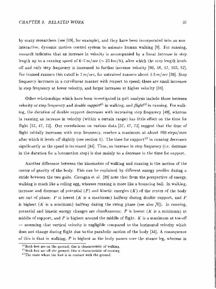
CHAPTER 3. RELATED WORK 3 1
by many researchers (see [49], for example), and they have been incorporated into an non-
interactive, dynamic motion control system to animate human walking [9]. For running,
research indicates that an increase in velocity is accompanied by a linear increase in step
length up to a running speed of 6-7 mlsec ( N 23 Lmlh), after which the step length levels
off and only step frequency is increased to further increase velocity [go, 48, 47, 103, 571.
For trained runners this cutoff is 7 mlsec, for untrained runners about 5.5 mlsec [36]. Step
frequency increases in a curvilinear manner with respect t o speed; there are small increases
in step frequency a t lower velocity, and larger increases a t higher velocity [34].
Other relationships which have been investigated in gait analysis include those between
velocity or step frequency and double support11 in walking, and fEight12 in running. For walk-
ing, the duration of double support decreases with increasing step frequency [49], whereas
in running an increase in velocity (within a certain range) has little effect on the time for
flight [57, 47, 731. Our correlations on various data [57, 47, 731 suggest that the time of
flight initially increases with step frequency, reaches a maximum at about 190 stepslmin
after which it levels off slightly (see section 4). The time for support13 in running decreases
significantly as the speed is increased [34]. Thus, an increase in step frequency (i.e. decrease
in the duration for a locomotion step) is due mainly t o a decrease in the time for support.
Another difference between the kinematics of walking and running is the motion of the
center of gravity of the body. This can be explained by different energy profiles during a
stride between the two gaits. Cavagna et al. [28] note that from the perspective of energy,
walking is much like a rolling egg, whereas running is more like a bouncing ball. In walking,
increase and decrease of potential ( P ) and kinetic energies (K) of the center of the body
are out of phase: P is lowest (K is a maximum) halfway during double support, and P
is highest (K is a minimum) halfway during the swing phase (see also [9]). In running,
potential and kinetic energy changes are simultaneous: P is lowest (K is a minimum) at
middle of support, and P is highest around the middle of flight. K is a maximum at toe-off
- assuming that vertical velocity is negligible compared t o the horizontal velocity which
does not change during flight due to the parabolic motion of the body [34]. A consequence
of this is that in walking, P is highest as the body passes over the stance leg, whereas in
l1 Both feet are on the ground; this is characteristic of walking. I2Both feet are off the ground; this is characteristic of running. I3The s tate where the foot is in contact with the ground.

CHAPTER 3. RELATED WORK
running, P is lowest as the body passes over the stance leg. Also, energy changes in running
are smallest during support and largest during flight phase [85].
As the speed of running increases the vertical displacement of the center of gravity
becomes smaller, and a t sprinting speeds it can be less than for walking (as little as 3cm)[103,
651. In accordance with this, a smaller vertical displacement - achieved by greater knee
flexion during support and more rapid and full extension of knee and hip a t toe-off - reduces
the potential energy expenditure (variations in vertical velocity). Also, the rise of the center
of gravity for a poor runner is greater than for a good runner (up to 4 cm)[34]. At lower
speeds, the body is projected slightly upwards a t toe-off, which results in a parabolic path.
At sprinting speeds, the initial rise during flight is almost eliminated and the body falls
during entire flight phase.
In chapter 4, we will integrate some of the above results into our motion control algorithm
for human locomotion. The approach will be an empirical one, where real data of human
locomotion is taken as a basis to establish rules and formulas whose legitimacy will mainly
be judged by the outcome, that is by the look of the resulting animation and the usefulness
of the tools.

CHAPTER 3. RELATED W O R K
3.3 Signal Processing
Signals describe a wide variety of physical phenomena such as the annual distribution of
precipitation in a specific geographic area, the weekly Dow Jones stock market index over a
period of ten years, or the acoustic pressure fluctuations of human speech. Signal processing
is concerned with the representation and transformation of signals. Mathematically, signals
are represented as functions of one or more independent variables. In this section, we
introduce some signal processing techniques which can be applied to the animation of human
figures. Our main interest lies in digital signal processing [75] rather than in continuous-time
analog technology. Digital signals and images are those for which both amplitude and time
are discrete. A digital signal is defined by a sequence of numbers, whereas a digital image
is represented by a two-dimensional array of numbers. For our purpose, a signal contains
the values of a motion parameter (e.g. a joint angle or the trajectory of an end-effector) for
an articulated figure over time (e.g. at each 30th of a second).
A great number of techniques have been developed to process digital signals and images
(see [71], for example). Computer vision heavily relies on many of these techniques for
image restoration and enhancement, as well as to retrieve various types of information
from images to help in the reconstruction of a scene14. In applying these techniques to
motion of articulated figures, we need to consider several criteria, in particular we would
like to produce controlled and desired effects in many or all degrees of freedom at the same
time. Thus, useful techniques should lend themselves towards higher level, "expressive" or
"qualitative" motion control. A candidate technique should also have a rapid interactive
loop for the creative and guided adaptation of existing motion. For instance, a general
filtering technique can be applied to smooth data, but it provides only limited control for
achieving a desired effect. We could also resort to a random (high frequency) noise function
to produce perhaps jerky movements, but what would the parameters look like, and how
would the technique be used?
Another requirement to make signal processing feasible for interactive manipulation of
animation data is that a system15 should be simple and solvable by analytic techniques.
14Computer vision - one or more images are given and the task is t o reconstruct a scene - can be considered as the inverse discipline to computer graphics, where a scene is specified and one or more images of that scene are generated.
15Here we define a system t o be any process which produces an output signal by applying a transformation

CHAPTER 3. RELATED W O R K 34
In the following, we give a brief discussion on some properties of such systems16. These
properties which characterize the complexity of the system have been thoroughly studied in
the field of signal processing (see [75], for example). A system is said to be
memoryless if the output ~ [ t ] at every value of t depends only on the input x[t] at
the same value of t. For example, the system y[t] = x[t] + 1 is memoryless, whereas
y[t] = x[t - 11 requires memory.
linear if the response to x1 [t] + x2[t] is yl [t] + y2[t], and the response to axl [t] is ayl [t],
where a is a complex constant. The first property is referred to as additivity and the
second as scaling property. For example, y[t] = x[t - 11 is a linear system, whereas the
system y[t] = sin(x[t]) is non-linear.
time-invariant if a time-shift in the input signal causes a time-shift in the output
signal. Formally, if a system transforms the input x[t] t o the output signal y[t], it is
time-invariant if for all to, the input x[t-to] produces the output y[t-to]. For example,
y[t] = x[t - 11 is a time-invariant system, and y[t] = x[5t] is not time-invariant because
it compresses (discards) four out of every five input samples.
Systems that are both linear and time-invariant form an important class with signifi-
cant signal processing applications. Many systems in nature can be successfuIly modeled in
this way and many system analysis tools have been developed for this class [75]. On the
other hand, highly non-linear systems requiring memory are hard to solve (difficult if not
impossible to handle analytically) in general. As we will show, efficient solutions exist for
the selection of techniques proposed below. They represent a pragmatic approach to signal
processing by providing analytic solutions at interactive speeds. The techniques have also
been chosen because they allow useful and meaningful operations on motion parameters
which would be difficult to obtain in conventional spline-based systems. Multiresolution
filtering can be categorized as a linear system with memory, which facilitates editing of
motion in terms of frequency bands. Dynamic timewarping is a non-linear, time-variant
system requiring memory which can be used for automatic time-registration when blending
to an input signal. I6Although the properties hold for both continuous and discrete systems, we only consider the discrete
case here for our purpose.

C H A P T E R 3. RELATED WORK
motions; a solution to this complex problem is found by dynamic programming. Waveshap-
ing, which falls into the category of non-linear systems without memory, alters a signal by
a user-defined shaping function. Finally, displacement mapping is a general tool to edit a
signal locally while maintaining its continuity. This is very convenient for efficient modifi-
cation of motion-captured data. In the following sections, these techniques are introduced
in general terms, and in chapter 5 we show how they can be adapted to procedural motion
control of articulated figures.
3.3.1 Multiresolution Filtering
The method of multiresolution filtering was initially proposed by Burt et al. [17, 741 as an
image representation method advantageous for certain kinds of operations such as seamless
merging of image mosaics and image interpolation (noise removal). It has also been applied
to temporal dissolves between images [91]. Images may be stored as Gaussian17 (low-pass)
or Laplacian (band-pass) pyramids of spatial filter bands, where each level represents a
different octave band of spatial frequency. Operations like merging two images are then
performed band by band before reconstructing the image by adding up the resulting bands.
In this way, the fine detail of an image corresponding to the higher frequencies is treated
separately from the coarse image features encoded by the low frequencies.
The first step in applying Burt's multiresolution analysis is to obtain the Gaussian
pyramid by successively convolving the image with a Gaussian filter kernel (e.g. 5 x 5),
while the image is subsampled by a factor of 2 at each iteration (as shown at the left
of Figure 3.1, where Go is the original image). This process is repeated until the image
size is reduced to one pixel, which is the average intensity, or "DC" value. The Laplacian
pyramid is then calculated by repeatedly subtracting 2 successive Gaussian images, with
the subtrahend image being expanded first in each case (right of Figure 3.1, where Lo is the
highest frequency band). The image can be reconstructed without manipulation by adding
up all the Laplacian bands plus the DC. The same procedure can be performed on two or
more images at the same time, whereby operations like merging are executed band by band
in the Laplacian spectrum before reconstructing the final result.
17Gaussian convolution and Laplacian filtering are formally defined in section 5.1; for the discussion here it is sufficient to know that we use the term Gaussian to denote a spatial low-pass filter which smoothes (blurs in the image domain) a signal, and the Laplacian is the second derivative of a signal with a high-pass effect by enhancing changes in the signal.

CHAPTER 3. RELATED WORK
Figure 3.1: Left: Gaussian pyramid; right: Laplacian pyramid.
In section 5.1, the multiresolution principle is applied to the motion parameters of hu-
man figures. For this purpose, a one-dimensional version of this technique is proposed which
can be applied to all degrees of freedom of an articulated figure at the same time. It is noted
here that Burt's multiresolution filtering is related to wavelet analysis [31]; the Gaussian
pyramid here is the counterpart to a wavelet decomposition based on cubic B-spline scaling
functions (commonly termed H ) , while the Laplacian bands correspond to the high fre-
quency wavelet components (commonly termed G). We believe that Burt's decomposition
is more computationally efficient since convolution is applied only to obtain the low-pass
Gaussian decomposition and the high frequency Laplacians are simple differences between
successive Gaussian levels. There is no need for two sets of filter coefficients. Burt's mul-
tiresolution approach is also more efficient for signals of more than one dimension [lol l . On
the other hand, wavelet analysis is more space efficient since only the differences are stored
at each level with the highest frequency level already reduced by a factor of 2 compared
to the original signal. Liu et al. [62] applied wavelet decomposition to speed up spacetime
interpolation of physically-based keyframe animation. They did not use the frequency de-
composition to provide direct manipulation of motion, and we believe that Burt's method
is more appropriate and efficient in this case.

CHAPTER 3. RELATED W O R K
In another related approach, Unuma et al. [98] apply Fourier transformations to data
on human walking for animation purposes. Based on frequency analysis of the joint angles,
a basic 'walking' factor and a 'qualitative' factor like "brisk" or "fast" are extracted. These
factors are then used to generate new movements by interpolation and extrapolation in the
frequency domain, such that now a walk can be changed continuously from normal to brisk
walking. Litwinowicz uses recursive filters to produce "lag, drag, and wiggle" effects to
keyframed two-dimensional animated motion in a system called Inkwell [61].
3.3.2 Dynamic Timewarping
The field of speech recognition has long relied on a nonlinear signal matching procedure
called "dynamic timewarping" to compare templates (for phonemes, syllables or words)
with input utterances [33]. Apart from being subject to the usual random error, each
acoustic input signal also shows variations in speed from one portion to another with respect
to the template signal. The timewarp procedure identifies a combination of expansion
and compression which can best "warp" the two signals together. The problem can be
decomposed and solved in two steps: find the optimal vertex correspondences between the
two signals, and then apply the warp.
The vertex correspondence problem is defined as finding the globally optimal corre-
spondence between the vertices (samples) of the two signals: to each vertex of one signal,
assign (at least) a vertex in the other signal such that a global cost function measuring
the "difference" of the two signals is minimized. In this sense, the problem is related to
contour triangulation [41] and shape blending [86], and is solved by dynamic programming
optimization techniques. The solution space can be represented as a two-dimensional grid,
where each node corresponds to one possible vertex assignment (see Figure 3.2). The opti-
mal vertex correspondence solution is illustrated in the grid by a path from (0,O) to (9,9).
In general, there are O(nn/n!) such possible paths18. A brute force dynamic programming
algorithm generates all possible paths using some local distance measure (cost function)
between the signals at each node, and once the node (n, n) is reached, the globally optimal
solution is recovered by backtracking through the graph. Sederberg [86] presents a method
''This holds for the vertex correspondence problem, where we favor a diagonal move in the graph over a south-followed-by-east-move or an east-followed-by-a-south-move. For contour triangulation, where diagonal moves are denied, the complexity is 0((2n) ! / (n!n! ) ) .

CHAPTER 3. RELATED WORK
Figure 3.2: Vertex correspondence problem (adapted from 1861).
which gives a globally opti~nal solution by visiting every node in the graph once (O(n2) with
constant amount of work per node).
The second part of the problem is t o interpret the optimal vertex correspondences, that
is to actually apply the warp. Three cases are distinguished: substitution, deletion and in-
sertion [33], indicated in Figure 3.2 by a diagonal, horizontal and vertical line, respectively,
between two nodes in the optimal path. Substitution is defined as a one-to-one correspon-
dence between successive samples in the two signals (e.g. between vertices 0 and 1 of the
two contours in Figure 3.2). Deletion means that multiple samples of one signal (top con-
tour in Figure 3.2) map to one sample of the other signal (bottom contour); for example,
vertices 3 and 4 of the top contour map to vertex 4 of the bottom contour. Insertion is
illustrated in Figure 3.2 such that one sample of the top contour maps to multiple samples
of the bottom contour (e.g. vertex 2 of the top contour ma,ps to vertices 2 and 3 of the
bottom contour). A complete warp for two signals A and B either warps A into B or B
into A. Section 5.2 shows how timewarping can be successfully applied to make multitarget
motion interpolation (blending of movement sequences) a more useful tool for animating
human figures.

CHAPTER 3. RELATED WORK
3.3.3 Waveshaping and Displacement Mapping
Both displacement mapping and waveshaping (in its basic form) are simple yet effective
techniques that change the amplitude of a signal in a non-uniform manner. In displacement
mappinglg, the shape of a signal can be changed locally (through a displacement map) while
preserving the global shape of the signal as much as possible.
LeBrun [15] introduced waveshaping for the generation of musical sounds by synthesizing
steady-state or time-varying harmonic sound spectra. The basic idea involves a non-linear
shaping function f of an arbitrary shape which operates as a special filter on a signal x (f
is assumed to be normalized, i.e. it accepts and outputs numbers in the range [-1,+1]).
For example, if we define f as the identity function f (x) = x, the signal will pass through
unchanged. If f is slightly changed, say, to having a subtle bump near 0, then the signal
x will be altered in that it will have slightly positive values where, and around where, it
was zero before, thus x has now some bumps as well. If f is defined as a partial cycle of a
cosine function from minimum to maximum in the [-I, +1] range, the values of x will be
exaggerated in the middle and attenuated at the extremes. If f is a step function, x will
be either one of two values. LeBrun dynamically varied the 'deformation' by multiplying x
with a time-varying factor a before passing through f , so x' = f (xu).
In sections 5.3 and 5.4, we present details and possible uses of these techniques in
animating articulated figures.
19 This idea was suggested to me through conversations with Lance Williams.

Chapter 4
Procedural Gait Control
In this chapter, we introduce the design of procedural motion control systems implemented
for the purpose of animating human locomotion. It will be shown that by incorporating
procedural knowledge of human walking and running into the algorithms, a wide variety of
human locomotion styles can be generated based on the specification of high-level parame-
ters like step length, step frequency or bounciness of a gait. We also demonstrate that the
goals as outlined in section 2.6 to characterize a good motion control algorithm are met by
our approach: a convenient, high-level1 of specification is accomplished producing believ-
able motion while providing the animator with tools to fine-tune and customize expression
and style of the movements. The parameters can be changed interactively and the system
supports real-time feedback by displaying a walking or running figure on the screen.
Human locomotion describes an intricate activity where body translation results from
rotational movements in the lower limbs. However, locomotion is made up of cyclic, recurring
movement patterns with a basic unit of one stride. Each stride consists of two symmetric
steps (left and right) as shown in Figure 4.1, so we can restrict our analysis to one locomotion
step, for instance from heel-strike of the left leg to heel-strike of the right leg.
For walking, a step consists of a double support state, where both feet are on the ground,
and a single support state, where one foot is off the ground. In contrast, a running step is
made up of a single support state plus a flight state where both feet are off the ground. With
'The level of control is denoted by "between-limbs "in Figure 2.2.
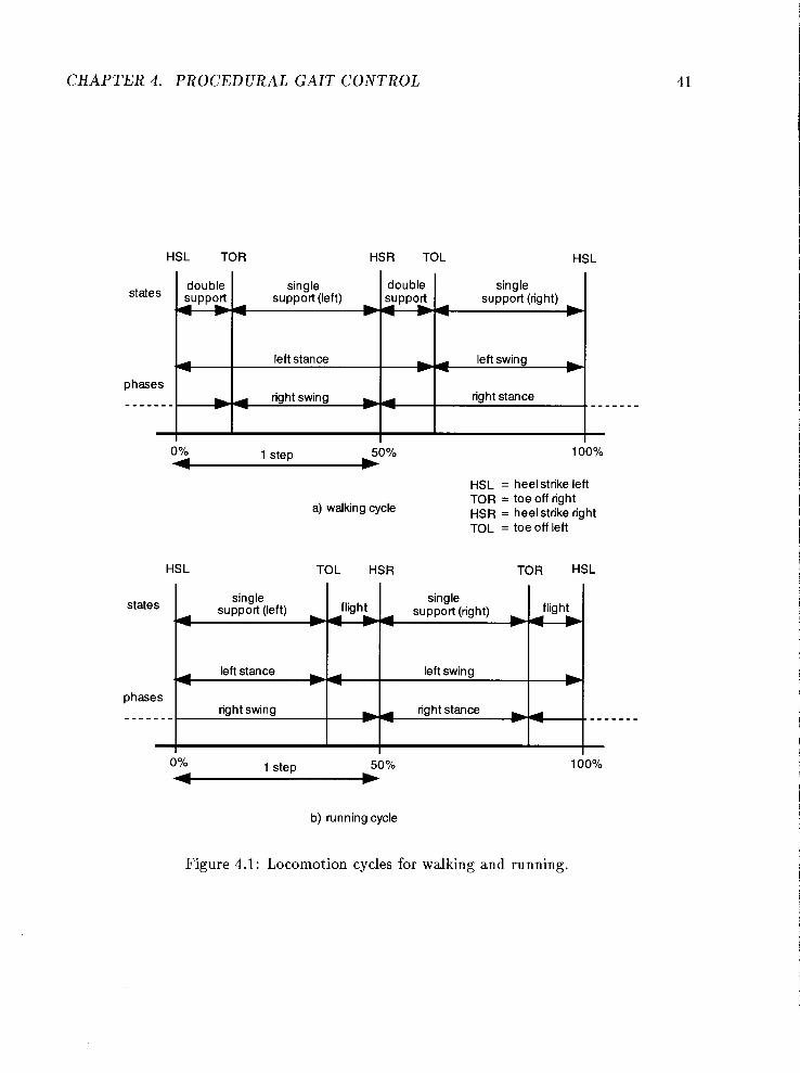
CHAPTER 4. PROCEDURAL GAIT CONTROL
HSL TOR HSR TOL HSL
states
phases
- - - - - -
states
phases
- - - - - -
single support (left)
left stance
r; Yo w
I 1 step
b
double single
b* left swing b
HSL = heel strike left TOR = toe off right
a) walking cycle HSR = heel strike right TOL = toe off left
HSL TOL HSR TOR HSL
single single support (left) flight support (right) flight
I
I I
0% 1 step 50% 4 b
I left stance
b1
right swing
b) running cycle
Figure 4.1: Locomotion cycles for walking and running.
b I
left swing
right stance bI
b
- - - - - - -

CHAPTER 4. PROCEDURAL GAIT CONTROL
respect to one stride, each leg cycles through a stance and a swing phase, shifted in time.
This holds for walking as well as for running. In fact, it is just the amount of "overlap" of
these phases that determines whether a walking or running gait is present. In walking, the
stance phases of the two legs overlap (double support); in other words, the duty factor2 for
each leg is greater than 0.5. As the step frequency increases, the duration of this overlap
becomes smaller. When the duration of double support vanishes completely, then a running
gait results in which the swing phases start to overlap (flight), that is the duty factor of
each leg is less than 0.5. In this sense a person walks and runs at the same time when the
duration for double support and flight are zero (duty factor for both legs is equal to 0.5).
The underlying idea of our locomotion algorithms is twofold: they are hierarchical and
step-oriented. 'Hierarchical' implies that each locomotion step is determined by certain
high-level parameters which enforce constraints on the states and phases of a step which in
turn provide the basis for interpolating the joint angles satisfying the specified parameters.
The algorithms are also 'step-oriented' which means that the appearance of a walk or run
- determined by the locomotion parameters and attributes (see below) - can be changed
with the granularity of one locomotion step. For example, the step length, pelvic rotation
or amount of knee bend can be changed from one step to the next. This way, acceleration
and deceleration are possible, as well as starting and stopping which are just special cases of
a "normal7' step. Section 4.1 discusses the approach taken to animate human walking, and
section 4.2 describes a prototype system for human running. Different algorithms for the
two gaits are necessary because the two motions are fundamentally different; for example,
there is a flight phase in running which does not occur in walking. Running also requires
a different set of control parameters. For instance, parameters to vary flight height or to
switch between the two basic running styles (toe-strike versus heel-strike) are desirable.
4.1 Walking
The algorithm proposed here is based on a goal-directed, dynamic system called KLAW
to animate human walking [9, 10, 111. The main objective behind the development of
KLAW was to generate realistic human walking sequences. Due to the underlying dynamic
'Fraction of a stride in which the foot is on the ground.

CHAPTER 4. PROCEDURAL GAIT CONTROL
model, the system did not perform in real-time, and the range of possible walking styles was
limited. By "substituting" kinematic interpolation for the dynamic model, our new approach
eliminates the drawbacks of the original system. Because this kinematic interpolation relies
on empirical knowledge about how real humans walk, the quality of the "kinematic" motion
comes very close t o the dynamically generated walks (see section 4.1.5). In this section the
differences between the two systems are outlined3.
A walking stride can be characterized by the following three high-level parameters: ve-
locity (v), step length (sl) and step frequency (sf) , where
v = sl x sf . (4.1)
Walking is possible a t a wide variety of combinations of s l and sf parameters. However,
when asked to walk a t a particular velocity or step length, humans naturally "choose" the
other parameters t o maintain a comfortable walking stride. For a high-level motion con-
trol scheme it is therefore crucial that the inter-relationships between these parameters are
determined. From studies on human walking, it is known that there is a linear relation-
ship between step frequency and step length. This is expressed in the following expression,
termed a normalization formula [49], where sf is in stepslmin, s l and bodyheight in m:
s 1 sf =
0.004 bodyheight
4.1.1 Walking Algorithm
The basic algorithm is illustrated in Figure 4.2. According to its step-oriented nature, the
main loop is executed for each walking step. At the end of each step, the current front
leg and hind leg are switched t o initialize the next step. Empirical knowledge is applied to
define the kind of control parameters and how they are interrelated. Physical knowledge
determines how the center of the body moves during a walking step. Limb-coordination
knowledge is used t o set up step-constraints which "guide" the joint-angle interpolation of
the stance and swing phases. We now describe each component of the algorithm in turn.
3This is also partially presented by Bruderlin and Calvert [12].
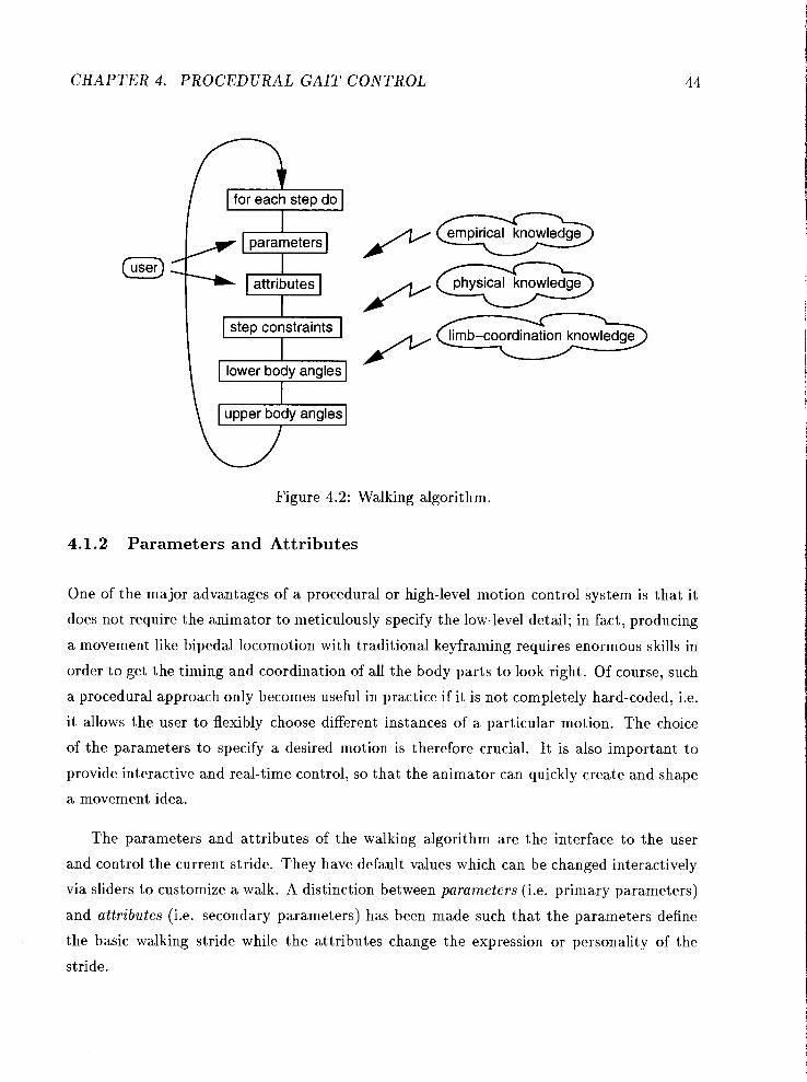
CHAPTER 4. PROCEDURAL GAIT CONTROL
parameters Pq attributes Q
step constraints I I lower body angles I
empirical knowledge s/- physical knowledge
A P a
upper body angles \- Figure 4.2: Walking algorithm.
4.1.2 Parameters and Attributes
One of the major advantages of a procedural or high-level motion control system is that it
does not require the animator to meticulously specify the low-level detail; in fact, producing
a movement like bipedal locomotion with traditional keyframing requires enormous skills in
order to get the timing and coordination of all the body parts to look right. Of course, such
a procedural approach only becomes useful in practice if it is not completely hard-coded, i.e.
it allows the user to flexibly choose different instances of a particular motion. The choice
of the parameters to specify a desired motion is therefore crucial. It is also important to
provide interactive and real-time control, so that the animator can quickly create and shape
a movement idea.
The parameters and attributes of the walking algorithm are the interface to the user
and control the current stride. They have default values which can be changed interactively
via sliders to customize a walk. A distinction between parameters (i.e. primary parameters)
and attributes (i.e. secondary parameters) has been made such that the parameters define
the basic walking stride while the attributes change the expression or personality of the
stride.

CHAPTER 4. PROCEDURAL GAIT CONTROL
Figure 4.3: Walking parameter panel.
As mentioned above, there are three locomotion parameters: step length, step frequency
and velocity. The interaction panel is shown in Figure 4.3. In normal mode, if one of the
parameters is changed via a slider, the other two are automatically adjusted to maintain a
'natural' gait according to equations 4.2 and 4.1. In locked mode, where one of the three
parameters is locked at the current setting, the other two can be adjusted via sliders. For
instance, to generate a slow walk at a large step length, the step length would be locked at
a large value and then the velocity slider would be set to a slow speed; this is indicated in
Figure 4.3, where step length was locked at 0.75 m and the velocity was then reduced to
3.0 k m l h .
In addition to the locomotion parameters, 15 locomotion attributes are also provided to
individualize walks, that is to produce walks at the same step length, step frequency and
velocity, but with different characteristics such as upper body tilt or leg bounciness. The
interaction panel for these attributes is illustrated in Figure 4.4; there are five attributes
for varying the movements of the arms: shoulder rotation, arm swing, arm out, minimum
elbow flexion and maximum elbow flexion. There are two attributes for the torso: forward
tilt and sway; two for the pelvis: rotation and list. Finally, there are six attributes for
the movement of the legs: bounciness, minimum knee flexion during stance, knee flexion at
impact, minimum toe clearance during swing, foot angle and stride width.

CHAPTER 4. PROCEDURAL GAIT CONTROL
Figure 4.4: Walking attribute panel.
4.1.3 Step Constraints
From the current parameter and attribute values, three step constraints are calculated.
These constraints define internal 'keyframes7 between which the intermediate joint angle
values for the lower body are then interpolated from the previous step to the current step:
duration for the leg phases,
leg angles at the end of each step,
planar motion of the stance leg hip during a step.
The duration for the leg phases can be computed from the step frequency parameter
value. Based on research on human locomotion [49], the following relationship holds between

CHAPTER 4. PROCEDURAL GAIT CONTROL
sf and the duration for double support td, (tds is in sec, sf in stepslmin):
As illustrated in Figure 4.1, the durations of the stance (tStance) and swing phases (tswin,)
can now be calculated, given that tstep = 11s f :
The leg angles at the end of each step are calculated based on the current step length
and the length of the legs by trigonometric relationships as explained in detail in [lo].
The motion of the stance leg hip for the current step is defined by an interpolating
cubic hermite spline segment [54]. This is performed in two dimensions (sagittal plane) and
extended into 3-D in the next section by adding a pelvis to the model. Thus, the computation
of the control points is done in two parts, a vertical (y) and a horizontal (x) component.
In each case, four control points per step are determined, as indicated in Figure 4.5 (HSL,
mid-double support, mid-step, HSR); the first and last point in x and y are easily derived
given the current step length and the leg angles at the beginninglend of each step (at HSL
and HSR in Figure 4.5). The second and third control points are computed as follows:
based on research on human locomotion [49] it is known that the vertical displacement of
the body4 is lowest around the middle of double support and highest around the middle
of the swing phase (mid-step), whereas the horizontal displacement reaches a maximum
(ahead of average position) around the middle of double support and a minimum (behind
average position) around the middle of the swing phase. These observations are in direct
correlation with energy expenditure during a walking stride as mentioned in section 3.2; the
potential energy of the motion of the body is proportional with the vertical displacement,
whereas kinetic energy changes primarily with horizontal velocity since the vertical velocity
during walking is comparatively small. Knowing the durations of the current step (tstep),
4We assume that the motion of the whole body is identical t o the motion of the stance hip, which carries the weight of the body.
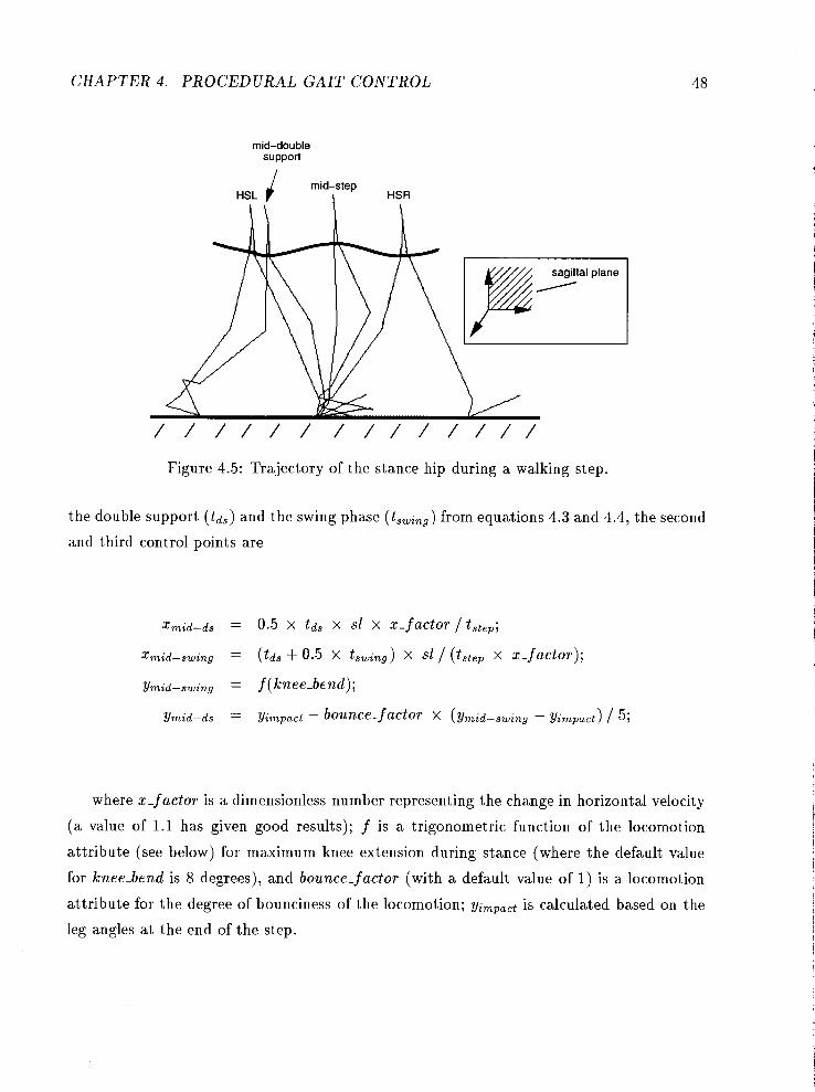
CHAPTER 4. PROCEDURAL GAIT CONTROL
mid-double support
HSL 4 mid-step \ HSR
sagittal plane
B/
Figure 4.5: Trajectory of the stance hip during a walking step.
the double support (tds) and the swing phase (tSwing) from equations 4.3 and 4.4, the second
and third control points are
where x-f actor is a dimensionless number representing the change in horizontal velocity
(a value of 1.1 has given good results); f is a trigonometric function of the locomotion
attribute (see below) for maximum knee extension during stance (where the default value
for knee-bend is 8 degrees), and bounce-factor (with a default value of 1) is a locomotion
attribute for the degree of bounciness of the locomotion; y;mp,ct is calculated based on the
leg angles at the end of the step.

CHAPTER 4. PROCEDURAL GAIT CONTROL
left hip HSL mid-step HSR /
I I I I I
U I 1 w -- r transverse plane
1 * / - I I
right hip
Figure 4.6: Plan view of pelvic rotation and lateral displacement.
4.1.4 Joint Angles
Compared to our dynamically-based KLAW system, the spline-interpolated stance hip
position replaces the simulated hip from the planar inverted pendulum model [9]. Given
this trajectory of the hip as calculated above and the position of the toe which is stationary
during stance, the angles for the stance leg during the current step are determined based
on knowledge of how the human foot moves during stance5.
Once the motion of the stance leg is known, a pelvis is introduced to the model to
produce three determinants of gait: pelvic rotation (transverse plane), lateral displacement
and pelvic list (coronal plane) of the body. As shown in Figure 4.6, pelvic rotation is a
maximum at heel-strike (HSL and HSR) and a minimum at mid-step (both hips are aligned
horizontally). Lateral displacement of the body is caused by the fact that the body always
shifts slightly over the weight-bearing leg (arrows in Figure 4.6). The displacement is a
minimum at heel-strike and a maximum halfway through the step. Figure 4.7 illustrates
pelvic list, which is a minimum at heel-strike (HSL and HSR; both hips are aligned vertically)
and a maximum at the end of double support (the hip of the swing leg drops below the
stance leg hip). From the extreme values of these determinants, the motion of the hip for the
swing leg is calculated by linear interpolation. Both the default values for rotation and list of
the pelvis can be changed interactively as locomotion attributes. Lateral displacement is a
function of stride width and velocity (greater stride width means more and faster locomotion
means less displacement).
5 A detailed explanation to this underconstrained inverse kinematics problem has been previously pub- lished [ll].

CHAPTER 4. PROCEDURAL GAIT CONTROL
HSL end of double
support HSR
Figure 4.7: Pelvic list.
Similar to KLAW, the motion of the swing leg is divided into 3 subphases [9]. However,
the dynamic simulation of the double pendulum leg model is replaced by linear interpolation
of the sagittal hip and knee angles. The upper body motion is expressed as functions of the
lower body. For example, the arm swings forward with the opposite leg, and the shoulder
rotation is a function of the pelvic rotation. Both arm swing and shoulder rotation are
defined as attributes and can be adjusted as desired.
4.1.5 Discussion
A prototype system called GAITOR has been implemented according to the concepts intro-
duced in this section. The program is written in C using the Forms interface package [76]
for Silicon Graphics workstations. GAITOR uses a producer-consumer, double-buffer setup
synchronized with semaphores. One process calculates all the joint angles for one locomo-
tion step based on the current parameters and attributes and writes into one buffer, while
the other process handles the display and interactions reading from the other buffer. As
long as the "producer" process can compute a step faster than the "consumer" process is
able display the previous step, the user can adjust parameters and attributes as the figure
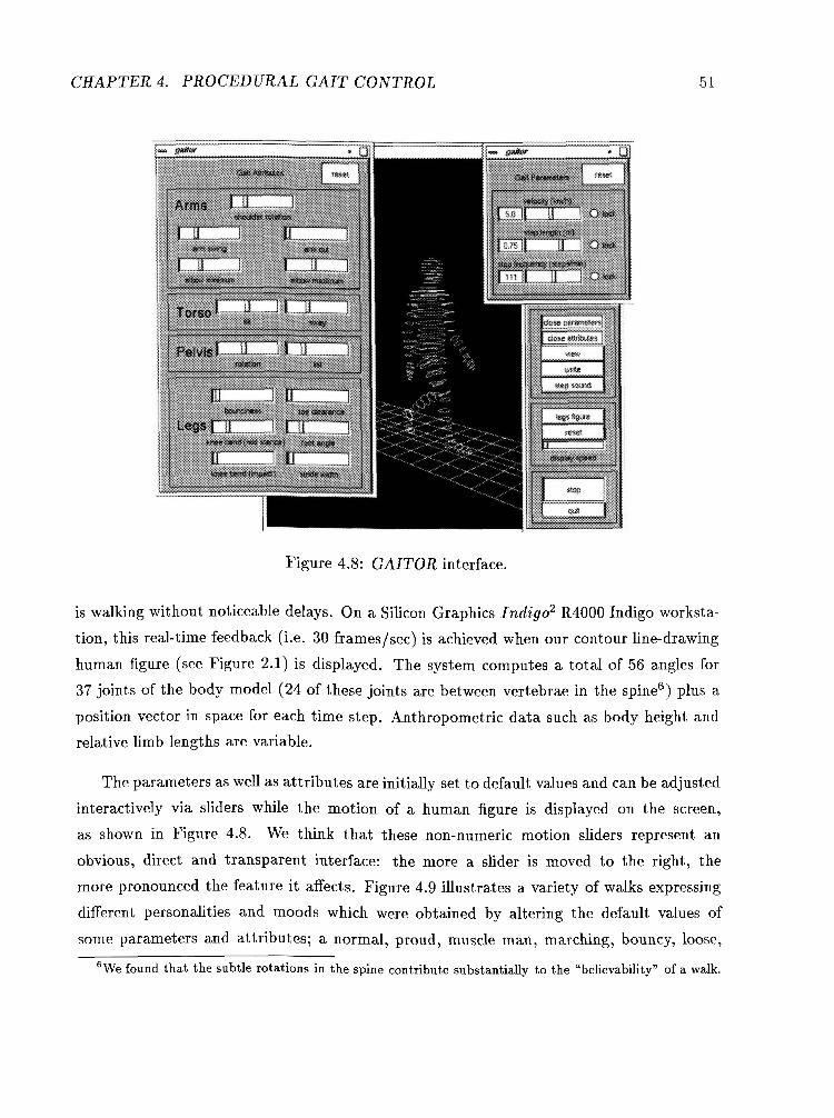
CHAPTER 4. PROCEDURAL GAIT CONTROL
Figure 4.8: GAITOR interface.
is walking without noticeable delays. On a Silicon Graphics Indigo2 R4000 Indigo worksta-
tion, this real-time feedback (i.e. 30 frames/sec) is achieved when our contour line-drawing
human figure (see Figure 2.1) is displayed. The system computes a total of 56 angles for
37 joints of the body model (24 of these joints are between vertebrae in the spine6) plus a
position vector in space for each time step. Anthropometric data such as body height and
relative limb lengths are variable.
The parameters as well as attributes are initially set to default values and can be adjusted
interactively via sliders while the motion of a human figure is displayed on the screen,
as shown in Figure 4.8. We think that these non-numeric motion sliders represent an
obvious, direct and transparent interface: the more a slider is moved to the right, the
more pronounced the feature it affects. Figure 4.9 illustrates a variety of walks expressing
different personalities and moods which were obtained by altering the default values of
some parameters and attributes; a normal, proud, muscle man, marching, bouncy, loose,
6We found that the subtle rotations in the spine contribute substantially to the "believability" of a walk.

CHAPTER 4. PROCEDURAL GAIT CONTROL
Figure 4.9: Various sample walk snapshots.
happy, and tired walk are displayed (left-to-right, top-to-bottom). The "normal" walk was
generated from the default values for all parameters and attributes. For the "proud" walk,
the velocity was set to 4 kmlh, then it was locked and the step length was increased from
its default value of 0.65 m to 0.75 m; the values for foot angle, arm swing, arm out and
shoulder rotation were then increased to almost their maximum values. As another example,
the "tired" walk was produced by reducing the velocity to 3 kmlh and the arm swing to
almost a minimum, while increasing the values for torso tilt, sway and bounciness slightly.
Compared with our older non-interactive, dynamic KLAW system [9], initial feedback7
suggests that the interactive feature is very helpful for users to feel and identify with the
motion generation process, and it is well suited to rapid prototyping of personalized human
locomotion. Also, this approach has more attributes than the dynamic system, and they
can be tweaked more as well; for example, KLAW could not produce a very "bouncy" walk
(which can be quite readily generated with GAITOR) due to numerical instabilities caused
by a loose spring (resulting from low values of the spring constant) in the leg model. In a
sense, GAITOR trades off absolute realism with real-time feedback. However, the difference
'GAITOR has been used by some animators, choreographers and novice users interested in animation.

CHAPTER 4. PROCEDURAL GAIT CONTROL
Figure 4.10: Motion-captured (top), dynamic (middle), kinematic (bottom) walk.
in the quality of motion is surprisingly small as illustrated in Figure 4.10 which compares
an instance of a walking sequence at 5 km/h computed by the dynamic (middle) and by the
new system (bottom). Shown in the top of Figure 4.10 for comparison is a motion-captured
walk8 at approximately 5 kmlh as well.
The same three walks are compared in Figure 4.11 for one stride of the right leg. Here the
sagittal hip angle is plotted against the knee angle. Following the curves counterclockwise,
the right leg is on the ground from HSR until TOR, and in its swing phase from TOR
until HSR. All three curves show a typical loop around heel-strike of the right leg (HSR)
'The data were collected by Winter [108]; only planar joint angles for the hip, knee and ankle were derived.

CHAPTER 4. PROCEDURAL GAIT CONTROL
. hip angle extension flexion
Figure 4.11: Sagittal hip-knee angle diagram of right leg.
where the hip as well as knee angle briefly flex due to the impact before extending for
the first half of the stance phase. Then, well before heel-strike of the other (left) leg (at
HSL), both the hip and knee angle flex again until shortly after toe-off of the right leg,
when the knee angle starts to extend rapidly while the hip still continues to flex until it
reaches its desired value for heel-strike about halfway during swing. Note that the key
events during a stride (HSR, HSL, TOR and TOL) match closely between the motion-
captured and our kinematically generated walkg. It is obvious that the motion-captured
curve is smoothest; this is mainly explained by the fact that lowpass filtering was applied
to the raw data to remove noise [108]. On the other hand, the kinematic walk produced by
GAITOR appears rather discontinuous due to linear interpolation of the leg angles. This
could be improved by using cubic spline interpolation for the angles or by subsequent filtering
similar to the motion-captured walk. Of course, excessive filtering might introduce artifacts
'The events are not marked for the dynamically simulated walk for clarity.

CHAPTER 4. PROCEDURAL GAIT CONTROL
. hip angle . extension flexion
Figure 4.12: Comparison between walks at different speeds (generated in GAITOR).
such as a sliding foot during stance or the foot going through the ground. However, the
linear interpolation used here is fast and therefore promotes interactive animation without
introducing obvious "visual" discontinuities.
The dynamic and the kinematic walks display a slight spike during double support - the
hip of the hind leg briefly extends during its flexion period just before toe-off. It is not clear
whether this actually happens in real walking as well, or whether it is solely a flaw in the
virtual leg algorithm [I 11. In Figure 4.12, the spikes were almost eliminated in the curves for
the 4 km/h and 7 km/h walks by decreasing the bounciness and knee flexion during stance
attributes as well as increasing pelvic rotation. This also demonstrates that the planar
and smoothed motion-captured data might actually be less accurate than our kinematically
generated sagittal hip and knee angles which are dependent on, reflect and compensate for
other lower body motions such as pelvic rotation and list, lateral displacement and stride
width.
CHAPTER 4. PROCEDURAL GAIT CONTROL
Figure 4.12 illustrates how the hip-knee angle relationships differ at various walking
velocities. Shown are walks at 4 kmlh, 5 kmlh and 7 kmlh, generated in GAITOR. Two
trends are visible: during swing (TOR to HSR), an increase in velocity goes hand in hand
with an increase in hip flexion caused by an increased step length. Secondly, the knee is
more flexed at higher velocities. This can be explained again by the the fact that step length
increases with velocity, which results in the body being lower towards the ground which in
turn requires the knee to be flexed more during stance and during swing to avoid the foot
stubbing the ground.

CHAPTER 4. PROCEDURAL GAIT CONTROL
4.2 Running
In order to procedurally animate human running in a manner analogous to the approach
taken for human walking, we need to construct relationships between locomotion parameters
at one end, and derive detailed rules about the movement of the legs during a running
stride on the other end. As mentioned in section 3.2, there is not as much consensus among
researchers on how people run as there is on how they walk. Nonetheless, analysis done on
running and available running data [48, 47, 103, 571 has lead to the approach set out below.
4.2.1 Running Concepts
As in walking, a bipedal running stride consists of 2 steps (recall Figure 4.1). A step is made
up of a single support state where one foot is off the ground, and a flight state where both
feet are off the ground. Compared to walking where the stance phases of the legs overlap,
in running the swing phases overlap. As shown in figure 4.1, this means that TOL now
occurs before HSR, and TOR before HSL. Due to the flight state characteristic of a running
step, the approach taken for walking which is based on the fact that at least one foot is on
the ground at all times during a step can no longer be applied here. Because of this, the
technique of using a simple planar walking model which is then extended to 3-D is replaced
here with a true 3-D algorithm. Also, running requires a different set of control parameters
as well as new interrelationships between these parameters.
A running stride can be characterized by the following four high-level parameters: ve-
locity (v ) , step length (sl), step frequency ( s f ) and flight height (H); the basic relationship
between v, sl and sf still holds (equation 4.1). As for walking, humans when told to run at
a particular velocity or step length naturally "choose" the other parameters to maintain a
comfortable stride. Research on human running indicates that an increase in velocity is ac-
companied by a linear increase in step length up to a speed of about 400mlmin ( N 24km/h),
then the step length increase levels off and only step frequency is increased to further increase
velocity [47, 48, 571. On the other hand, step frequency increases in a curvilinear manner
with respect to velocity; there are small increases in step frequency at lower velocity, and
larger increases at higher velocity [34]. We now establish this linear relationship between
u and sl more formally based on actual human running data from [47, 48, 57, 1031. The

CHAPTER 4. PROCEDURAL GAIT CONTROL
formula below was derived by linear regression using the statistical module of Maple [37]
applied to the data with v < 400 mlsec. A multiple r 2 coefficient of 0.94442 was obtained
(for n = 80 data pairs) indicating very good correlation ( sl is in m and v in mlmin):
To this equation, a term level is now added which models the level of expertise in running
based on the observation [34, 571 that better runners have a greater stride length at a given
velocity than less skilled or poor runners, where -0.001 (poor) 5 level 5 0.001 (skilled):
sl = 0.13944 + (0.00465 + level) v.
Another factor influencing this relationship between v and sl is leg length. For walking,
Inman derived a normalization formula [49] relating step length to body height (which is
a function of leg length). For running, we adopt an approach suggested by Alexander
[I]. He observed that geometrically similar animals of different sizes have runs which are
dynamically similar whenever their speeds made their Froude number equal. The Froude
number is defined as the ratio between kinetic and potential energies, v2/(2gl), where 1 is
the leg length. Since leg length is proportional to body height, the Froude equality can be
expressed as v2/bodyheight = ~12.~/1.8, where 1.8 m is the default body height. Putting
this information into our equation relating velocity to step length, we now have
/body;;ight sl = 0.13944 + (0.00465 + level) v
Figure 4.13 illustrates equation 4.5 as well as the real data pairs (dots). The three lines
close together indicate relationships with level = 0 and body height equal to 1.7 m (lower),
1.8 m (middle) and 1.9 m (upper). For the two lines with the smallest and largest slope,
body height is 1.8 m with level set to minimum for the former and maximum for the latter,
respectively.
Equation 4.5 represents the normalization formula for running. In correspondence
with research on running, we apply this formula up to v,,,,, where v,,,, = 400 mlmin

CHAPTER 4. PROCEDURAL GAIT CONTROL
Figure 4.13: Step length as a function of velocity in running.
( N 24 kmlh) for a human with a body height of 1.8 m. If v increases further, sl is kept
constant (sl,,,,) and only sf is increased (v = sl,,,, x s f ) ; v,,,, is calculated as follows:
dbodyih;ight v,,,, = 400 (0.00465 + level) / 0.00465.
Equations 4.1 and 4.5 establish a relationships between v, sl and s f . The fourth running
parameter, flight height H , is a function of flight time t f l i g h t and the vertical positions of
the pelvis at toe-off (yl) and heel-strike (y2); g denotes the gravitational acceleration:
tf l i g h t
Thus, in order to calculate H the duration of flight needs to be known. Research
on human running suggests that an increase in velocity has little effect on the time for
flight [47, 57, 731. However, the time for support in running decreases significantly as
CHAPTER 4. PROCEDURAL GAIT CONTROL
the speed is increased [34]. Therefore, an increase in step frequency is due mainly to a
decrease in the time for support. Correlations on the running data from a number of sources
[47, 57, 731 suggest that the time of flight initially increases with step frequency, reaches a
maximum at about 190stepslmin after which it levels off slightly. A best fit (residual mean
square = 0.00087 for n = 20 data pairs) was obtained by a 3rd order polynomial. As noted
in the literature [57], expert runners tend to have a longer flight period than poor runners
at comparable step frequencies. Incorporating a level attribute into the equation similar to
above (here, -0.0001 (poor) 5 level 5 0.0001 (skilled)), we have
The running data available ranged about between 160 steplmin and 230 stepslmin
(tflight is in sec). To get a more general expression for the relationship between sf and
t extrapolation becomes necessary. From experience, we think that the following
quadratic equation provides a good relationship below 180 steplmin:
tflisht -0.674698 - (0.14952 + level) sf + 0.541846 s f 2 . (4.8)
These results lead to the following method of calculating iflight from sf :
from 0 - 180 stepslmin, equation 4.8 is used;
from 180 - 230 stepslmin, equation 4.7 is applied;
above 230 stepslmin, tfl;,ht is kept constant.
This is shown in Figure 4.14, with level values set to a minimum for the bottom curves,
to zero for the middle curves, and to a maximum for the top curves, respectively. The real
data pairs are displayed as dots.

CHAPTER 4. PROCEDURAL GAIT CONTROL
Figure 4.14: Duration of flight as a function of step frequency.
Now we are ready to calculate the durations for the leg phases in running. From Fig-
ure 4.1 it follows that
where tste, is l/s f. These durations manifest timing constraints which guarantee natural
looking interpolations of the joint angles of a desired running stride. This is explained as
part of the running algorithm in the next section.
4.2.2 Running Algorithm
Figure 4.15 outlines the running algorithm. Similar to the approach used to animate human
walking, the main loop is executed for each running step, which means that changes the

CHAPTER 4. PROCEDURAL GAIT CONTROL
parameters cC7' I I I state constraints]
I
phase constraints I Figure 4.15: Running algorithm.
user makes to any of the parameters or attributes become active on the next running step.
Knowledge about human running has been incorporated at various levels. Empirical knowl-
edge is applied to determine the kind of control parameters and how they are interrelated:
the four main running parameters introduced in the previous section define a basic running
stride while nineteen attributes can be set to individualize a run. Physical knowledge de-
termines how the center of the body moves during a running stride: during the support
state its motion is defined by a cubic spline, whereas during flight it follows a parabolic tra-
jectory. Limb-coordination knowledge is used to set up both state-constraints for support
and flight, and phase-constraints to "guide" the joint-angle interpolation of the stance and
swing phases. In the following, a closer look is taken at each part of the algorithm.
4.2.3 Parameters and Attributes
As in the walking algorithm, the running parameters and attributes are the interface to the
user and control the current running stride. Again, a distinction between parameters and
attributes has been made such that the parameters define the basic running stride while the
attributes change the style of the stride. However, here a change in one of the parameters

CHAPTER 4. PROCEDURAL GAIT CONTROL
Figure 4.16: Running parameter panel.
not only causes a change in the other parameters to maintain a natural stride but also causes
changes in some attributes (see explanation of attributes below), whereas a change in any
of the attributes is independent of the parameters.
The parameter panel is illustrated in Figure 4.16. There are four main parameters:
velocity, step length, step frequency and flight height, plus an additional slider for the level of
expertise in running as discussed in section 4.2.1 above. If one of the parameters is changed,
the other ones are updated using equations 4.1, 4.5, 4.6, and 4.7 or 4.8, respectively. The
actual calculations of flight height and time of flight are a bit more complex and are explained
in section 4.2.4, since we do not yet know the vertical position of the pelvis (kinematic center
of the body) at toe-off and impact (yl and ya in equation 4.6). Initial experiments where the
vertical positions were kept the same (yl = ya, simplifying equation 4.6 to tfl;,ht =
did not produce animations convincingly close to real human running.
Parameters can be locked to produce somewhat unnatural strides. This is shown in
Figure 4.16, where the velocity was locked at 12kmlh and then step frequency was increased
from the default 187 stepslsec to 210, which decreased the normally chosen step length of
1.07 m to 0.95 and the flight height from 0.004 m to 0.001.
The attributes allow the user to individualize a running stride. As shown in Figure 4.17,

CHAPTER 4. PROCEDURAL GAIT CONTROL
Figure 4.17: Running attribute panel.
nineteen attributes have been implemented at this time. Five of these control the movement
of the arms and shoulders, two attributes control torso tilt and sway, three attributes are
provided to alter the motion of the pelvis and nine attributes change the motion of the legs
in one way or other. Among the attributes for the legs are a heel-toe-strike button (heel
or toe touches ground first at impact), a bounciness slider (amount of knee bend during
support), an overstride slider (amount by which the foot impacts the ground ahead of the
body), and a stride-width slider (lateral distance between the feet).
As with the parameters, default values for the attributes are chosen to produce a natu-
ral running stride. This involves the values of some attributes being automatically adjusted
when a parameter value changes. The adjustment is necessary since there is a large range in

CHAPTER 4. PROCEDURAL GAIT CONTROL
the kinematics of running from a slow run to a fast run. For example, the overstride value
decreases with increasing velocity, pelvic rotation increases with step length, bounciness
increases with flight height, whereas the knee angle at toe-off decreases with step length.
These relationships are implemented as linear functions of the current parameters, the at-
tribute values and their extreme values. Some attributes are also coupled. For instance,
lateral displacement increases as stride-width increases and both decrease with step fre-
quency. Lastly, there are some "hidden" attributes which can not be set directly by the user
but are automatically calculated; for example, the ankle and metatarsal angles at toe-off
which are functions of step length, or the ankle angle at impact which is a function of the
overstride and the heel-toe-strike attributes.
Based on the parameter and attribute settings for the current running step, the state
constraints including the motion of the pelvis are now determined, followed by the phase-
constraints which guide the interpolation of the joint angles (section 4.2.5).
4.2.4 State Constraints
The state constraint principle is illustrated in Figure 4.18 for a step beginning with heel-
strike (subsequently used to mean heel-or-toe-strike) of the right leg and ending at heel-strike
of the left leg. For the opposite step from heel-strike left leg t o heel-strike right leg, all the
calculations below are mirrored. The constraints establish the leg angles for the stance leg
at the beginning of a step (HSR) and at toe-off (TOR), as well as the leg angles of the
swing leg at the end of the step (HSL). These internal "keyframes" serve as the basis for
interpolating the leg angles in section 4.2.5.
We now explain how these constraints are calculated given the current parameters and
attributes, assuming that the leg angles at the beginning of the step (HSR) are known from
the end of the previous step or the resting position on the initial step. All the computations
are done in 3-D. For the explanations below it is noted that according to research on human
running, the actual values for lateral displacement of the body at toe-off and heel-strike are
80 % (to either side of neutral) of the maximum value given by the attribute. Similarly,
pelvic rotation (in the transverse plane) is a maximum at toe-off and about 20 % at heel-
strike, whereas pelvic list (in the coronal plane) is a minimum (zero) at toe-off and about

CHAPTER 4. PROCEDURAL GAIT CONTROL
Figure 4.18: State constraints for a running step.
80 % at heel-strike. This is shown in Figure 4.19. It is also illustrated that at mid-support,
lateral displacement as well as pelvic list are a maximum and rotation is a minimum (zero).
The first stage in calculating the state constraints for the current step is to add the
current step length to the heel position at HSR to obtain the heel position at the end of the
step (HSL). Then the position of the center of the pelvis at HSL, (x2, y2, z2), is determined
"bottom-up" using the current attributes for stride width, overstride, knee bend at heel-
strike, as well as the percentages of lateral displacement of the body, pelvic rotation and list
at heel-strike. Given the position of the pelvis at heel-strike, we now calculate "backwards"
using information on the flight state to obtain the position and orientation of the toe-off leg
(TOR). For this purpose, the length of the toe-off leg (rad in equation 4.11 below) from toe
to the center of the pelvis is computed first using the current attribute values. Note that
we can not directly calculate the pelvis position at toe-off since the orientation of the leg in
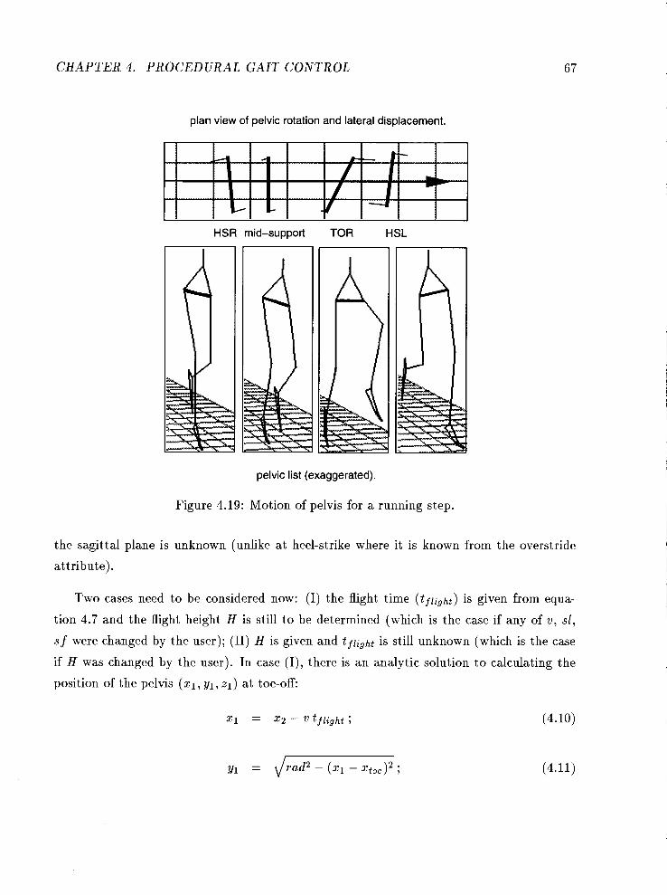
CHAPTER 4. PROCEDURAL GAIT CONTROL
plan view of pelvic rotation and lateral displacement.
HSR mid-support TOR HSL
pelvic list (exaggerated).
Figure 4.19: Motion of pelvis for a running step.
the sagittal plane is unknown (unlike at heel-strike where it is known from the overstride
attribute).
Two cases need to be considered now: (I) the flight time (tflight) is given from equa-
tion 4.7 and the flight height H is still to be determined (which is the case if any of v, sl,
sf were changed by the user); (11) H is given and tjlight is still unknown (which is the case
if H was changed by the user). In case (I), there is an analytic solution to calculating the
position of the pelvis (xl, yl, zl) at toe-off:

CHAPTER 4. PROCEDURAL GAIT CONTROL
where xt,, is known from the previous step and zl is the percentage of lateral displace-
ment at toe-off as explained above. Given y l and y2, H is obtained from equation 4.6.
For case (11) the position of the pelvis at toe-off is solved numerically by a two-dimensional
Newton-Raphson method [39] using equations 4.6 and 4.11, whereby x2 v x L is substituted
for t f l igh t in the former. Once X I is known, we determine t f [ i g h t by equation 4.10.
With these "keyframes" at HSR, TOR and HSL in place, the motion of the pelvis can
now be determined. During flight, the motion of the pelvis is calculated as a parabolic
trajectory, with 0 5 t 5 t f l igh t and z being interpolated between zl and zz:
During support, the position of the pelvis is defined by a 3-D cubic spline curve segment,
whose four control points are at HSR, mid-support, TOR and mid-flight. Whereas the
coordinates at HSR, TOR and mid-flight are known from above, the control points for mid-
support are chosen as follows: from research on human running [28,85], it is known that the
kinetic and potential energy changes within a stride are simultaneous and are both lowest
about the middle of support. Assuming that the motion of the whole body is represented
by the pelvis, the vertical position of the pelvis at mid-support is a minimum, defined as a
function of the vertical pelvis position at HSR and TOR, as well as bounciness and flight
height, such that the bigger H the lower y; the x-position of the pelvis at mid-support is
also a minimum (behind average forward position p) where a value of 0.8 x p has given good
results. Finally, the z control point of the pelvis at mid-support is set to the maximum lateral
displacement as mentioned above. The motion of the pelvis is illustrated in Figure 4.18,
with changes in velocity indicated by differently spaced circles along the path; also shown
is lateral displacement of the body.
The calculation of the orientation of the pelvis - rotation and list - during the current
step completes the state constraints. This is done by linear interpolation between the four
keyframes shown in Figure 4.19. The positions of the hip for the stance and swing leg are
now known and used next to interpolate the leg angles.

CHAPTER 4. PROCEDURAL GAIT CONTROL
HSR TOR H S L
I mid-support 1 I
Figure 4.20: Phase constraints for a running step.
4.2.5 Phase Constraints
Given the constraints on the support and flight states of the current running step introduced
in the last section, the phase-constraints further subdivide the constraints with respect to
the stance and swing phases of the legs in order to naturally interpolate the joint angles.
The subdivisions are based on observations of how real humans run. This is illustrated in
Figure 4.20 and explained below.
Single Support
During single support from HSR to TOR, the stance leg angles (right, solid leg in Fig-
ure 4.20) are calculated given the hip and the heelltoe position, as well as the leg angles
at HSR and TOR. We assume the motion of the foot to be planar (vertical). At the begin-
ning of stance, the foot rotates around the heel (heel-strike) or metatarsal joint (toe-strike)
until it is flat on the ground at mid-support. In this phase, the position of the ankle and
therefore the ankle-hip distance are known and from this the other leg angles are derived
trigonometrically. Subsequently, the foot stays flat on the ground until the beginning of the
next sub-phase during stance which lasts until TOR and is triggered by either the body
passing through the vertical or the ankle-hip distance becoming bigger than the length of
the extended leg. In both cases, the heel comes off the ground. This is implemented by

CHAPTER 4. PROCEDURAL GAIT CONTROL
interpolating both the metatarsal and knee angles from the current time and values until
TOR. Then the circle around the toe with the radius toe-ankle (with current metatarsal
angle) is intersected with the sphere around the hip and radius thigh-shank (with current
knee angle) to compute the remaining leg angles.
Automatic recovery procedures during stance are built in; if the hip is too high so the
above intersection fails (which can happen, for instance, if bounciness and flight height
are significantly reduced), the control point for the pelvis at mid-support is lowered. On
the other hand, if the hip is too low (due to an increased bounciness and flight height),
the intersection might push the foot through the ground. In this case, the knee angle is
automatically temporarily increased.
The swing leg angles during single support (left, dashed leg in Figure 4.20) are inter-
polated in the first subphase between the values at the end of the previous step (HSR)
to mid-support, where the thigh is vertical (sagittal hip angle is zero)'' and the knee is
maximally flexed. The next subphase for the swing leg goes until the end of support (TOR)
where the hip is maximally extended and the toe is vertically under the knee. Both the
maximum knee flexion and hip extension are functions of the current velocity, but can be
adjusted via attribute sliders by the user. If part of the foot stubs the ground during swing
(which might occur if bounciness is increased or maximum knee flexion during swing is
decreased), an automatic recovery procedure inserts a new control point with temporarily
increased knee flexion to lift the foot above the ground. Finally, we note that on the initial
step when starting a run from a standing position, the first subphase during swing is omitted
and its duration is added to the second phase.
Flight
During flight (TOR to HSL in Figure 4.20), both legs are in their swing phases. The
interpolation of the leg angles for the former stance leg (hind leg) are done such that at
''This is according to research on human running. In the actual implementation, we found that the vertical thigh condition does not always hold: a t small step lengths and for large values of the attribute for knee-bend a t toe-off, the thigh a t toe-off for the stance leg of the previous step (TOL) might be close to or has already extended past the vertical. To make sure that the thigh always extends a t least a minimal amount during this subphase, the hip angle a t mid-support is chosen as the maximum of either the thigh being vertical or half the difference of its value a t the end of the next subphase and a t TOL.
CHAPTER 4. PROCEDURAL GAIT CONTROL
HSL, the angles are a percentage (p) of the values a t mid-support of the next step. The
percentage automatically varies depending on whether the figure is currently accelerating,
running at a constant speed, or decelerating; values for p ranging between 0.6 and 0.9 have
given good results. On the last step before stopping, this subphase is omitted while the
previous stance phases for this leg are extended until HSL. The leg angles for other leg
during flight (dashed leg in Figure 4.20) are interpolated between their values a t TOR and
their values heel-strike known from the state-constraints.
Upper Body
Several degrees of freedom of the upper body are animated. Torso tilt and sway in the
sagittal plane have default values which can be changed via sliders. Tilt automatically
increases with velocity, while sway is interpolated between maximum forward lean reached
at mid-support and the maximum backward value at toe-off. In order for the head to
always point straight ahead, compensation for pelvis rotation and list are performed in the
spine. List compensation is distributed over the five lumbar vertebrae, and rotation over the
lumbar and the twelve thoracic vertebrae such that below the seventh thoracic vertebra the
rotations are towards the pelvis, whereas above it the rotations are counter to the pelvis.
The amount of this counter rotation is adjustable by an attribute.
Arm swing is implemented such that on the forward swing it is equal to the sagittal hip
rotation of the opposite (swing) leg multiplied by a default factor adjustable via a slider. On
the backward swing, instead of the hip angle which increases and decreases during support,
the angle between the vertical and the hip-ankle vector of the opposite leg is used which
decreases continuously. The amount of elbow flexion during a running step can also be
adjusted by the user through a minimum and maximum flexion attribute. Minimum flexion
occurs during the backward swing of the arm at toe-off, maximum flexion during forward
swing at toe-off.
This concludes the explanation of the running algorithm. Most of the implementation
is based on research and observations on human running, and an important contribution
of this approach is that it pulls together different knowledge and techniques to provide
an interactive environment in which a user can experiment and animate a wide variety of

CHAPTER 4. PROCEDURAL GAIT CONTROL
Figure 4.21: RUNNER interface.
runs in real-time without having to know about the intricacies of limb-coordination during
locomotion.
4.2.6 Discussion
A system called RUNNER has been implemented in C++ according to the above principles.
An illustration of the interface is given in Figure 4.21. Similar to GAITOR, the program
performs in real-time on a Silicon graphics Indigo2 R4000 workstation. For calculations
done at 30 frameslsec, this means that an animator can interactively change any of the
parameters and attribute sliders while viewing a real-time running stick-figure1' on the
screen.
Snapshots of a few sample runs are shown in Figure 4.22. For example, the top left run
was obtained by just reducing the velocity slider to about 5 kmlh; the second top run from
' ' R U N N E R uses the same default human figure with 37 joints and 56 degrees of freedom as GAITOR.

CHAPTER 4. PROCEDURAL GAIT CONTROL
Figure 4.22: Various sample run snapshots a t heel-strike of the right leg.
left was generated by increasing the velocity to about 15 kmlh and increasing elbow flexion
for both minimum and maximum. The third top run from the left was produced from the
settings of the previous run by increasing arm-swing and knee-bend during swing as well as
switching from heel-strike to toe-strike. In general, a large number of running styles can be
animated. For example, ranges in the parameters from a very slow run a t 2 kmlh t o a fast
run at 25 Lmlh with a step length well over 2 m are possible. Also, moving the attribute
sliders to their extreme values results in runs which can look very "stiff7' or very "loose".
Figure 4.23 demonstrates a comparison between a human running on a treadmill12 and
a run generated by our algorithm to match the real run. By setting the body height of our
figure to the height of the subject and the velocity to the speed of the treadmill, step length,
step frequency and flight height were successfully matched with the real run. In addition,
the default overstride attribute value was reduced slightly and elbow flexion was increased
to closely match the leg and arm movements of the treadmill run.
12Note that the kinematics and dynamics of treadmill running are significantly different from overground running a t larger velocities [36].

CHAPTER 4. PROCEDURAL GAIT CONTROL
Figure 4.23: Real treadmill run compared to generated run.
In the following, some results from research on human running are related to our algo-
rithm:
0 Nilsson [73] notes that compared to walking, running has a shorter duration of stance
at all comparable velocities. This follows directly from equation 4.4 and 4.9; for
walking tstance = tstep + tds, whereas for running, tstance = tstep - tflight.
0 The sagittal hip angle (at heel-strike) is somewhat larger in walking than in running
at the same speed [73], which makes sense since the flight phase distance is added in
running. This can directly be observed in the hip-knee diagram of Figure 4.2413 at
HSR'~.
During the support phase in running (HSR until TOR in Figure 4.24), 40% of the
time is utilized for recovery (leg flexion), and 60% for propulsion (leg extension) [34].
I3Due to cubic spline interpolation of the leg angles in running, the curve is much smoother than the linearly interpolated walking curve.
I4Note that the "event" sequence in running is HSR-TOR-HSL-TOL, while for walking it is HSR-TOL- HSL-TOR.
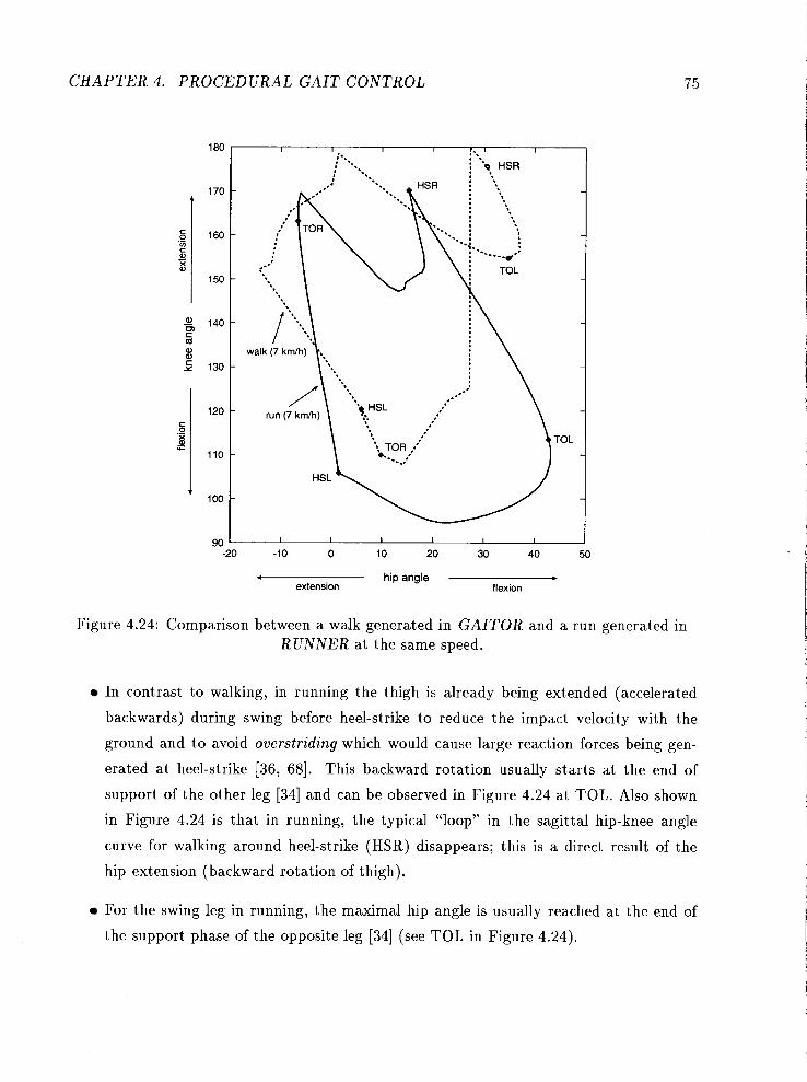
CHAPTER 4. PROCEDURAL GAIT CONTROL
. . . . : 'q HSR . .
walk (7 kdh )
. hip angle . extension flexion
Figure 4.24: Comparison between a walk generated in GAITOR and a run generated in RUNNER at the same speed.
In contrast to walking, in running the thigh is already being extended (accelerated
backwards) during swing before heel-strike to reduce the impact velocity with the
ground and to avoid overstriding which would cause large reaction forces being gen-
erated at heel-strike [36, 681. This backward rotation usually starts at the end of
support of the other leg [34] and can be observed in Figure 4.24 at TOL. Also shown
in Figure 4.24 is that in running, the typical "loop" in the sagittal hip-knee angle
curve for walking around heel-strike (HSR) disappears; this is a direct result of the
hip extension (backward rotation of thigh).
For the swing leg in running, the maximal hip angle is usually reached at the end of
the support phase of the opposite leg [34] (see TOL in Figure 4.24).

CHAPTER 4. PROCEDURAL GAIT CONTROL
. hip angle extension flexion
Figure 4.25: Comparison between runs at different speeds (generated in RUNNER).
a During the initial swing phase in running, the knee flexes rapidly (after TOR in
Figure 4.24). Knee extension begins about midway through the support phase of the
opposite leg [34] (about halfway between HSL and TOL in Figure 4.24).
Figure 4.25 illustrates how the sagittal hip-knee angle relationships differ at various
running velocities. The runs were generated in RUNNER by setting the velocity slider to
10, 16 and 22 kmlh, respectively. An increase in running speed results in
greater hip extension at take-off (TOR) [68].
0 greater knee extension at take-off (TOR) [68].
0 greater knee flexion during swing phase (between HSL and TOL) [34, 68, 731. This is
to the reduce moment of inertia during swing. Dillman [34] notes that better runners

CHAPTER 4. PROCEDURAL GAIT CONTROL
. hip angle . extension flexion
180
170
Figure 4.26: Comparison between a "normal7', "bouncy" and "reduced overstride" run (generated in RUNNER).
c .- U)
tl
flex the knee more than poor runners; our algorithm does not automatically take this
into account at the moment, but the user can experiment with the knee-flexion slider.
A
160
150
140
a increase of maximum hip flexion in swing (TOL) [34].
a increased knee flexion at heel-strike (HSR) and greater knee flexion during support
(HSR to TOR) [90]15.
w - 130 s w 0) r 120 Y
Figure 4.26 shows the effect of increasing the bounciness attribute, and reducing over-
c .- :: w - -
stride from a "normal" run at 2Okmlh. Increasing bounciness produced greater knee flexion
110
loo
90
v
during support and during swing (from HSL to TOL, which is the support phase of the other
80
70
15Further fine-tuning of the bounciness and knee-bend-at-impact attributes might be necessary to auto- matically set the right amount of knee flexion.

CHAPTER 4. PROCEDURAL GAIT CONTROL
Figure 4.27: Comparison between vlsl relationship in walking and running.
leg), the latter to avoid ground contact. Reducing the overstride slider resulted in a notably
increased knee flexion at heel-strike (HSR). This is because the foot is now closer under the
body and therefore the leg is shortened.
In Figure 4.27, the relationship between the velocity (v) and step length (sl) parameter
in running (equation 4.5) is compared to walking (equation 4.1 and 4.2). The three lines
close together express the equations for body heights of 1.7 m (lower), 1.8 m (middle) and
1.9 m (upper) in each case. Note that for running the equations are only applied up to
a velocity of 400 mlmin, and for walking up to a maximum speed of about 200 mlmin.
The diagram shows a linear relationship between v and sl for running and a curvilinear
relationship for walking.
Furthermore, it can be seen that at lower velocities a change from walking to running
results in a decrease in step length. The reason for this is that switching from walking
to running is accompanied by an increase in step frequency below a certain speed. This
has also been observed in studies on human locomotion; Nilsson [73] notes that a change

CHAPTER 4. PROCEDURAL GAIT CONTROL
Figure 4.28: Comparison between sf /sl relationship in walking and running.
from walking to running when v 5 180 mlmin results in a decrease in tStep, that is an
increase in sf and decrease in sl; at faster velocities, tStep is increased (sf is decreased and
sl is increased). Figure 4.28 shows this effect again by plotting the step frequency (sf)
against step length (sl). The relationship between these parameters is linear in walking
(equation 4.2) and curvilinear in running (equations 4.5 and 4.1).
4.3 Conclusions
In this chapter we introduced high-level, procedural motion control techniques to animate
human locomotion. Compared to keyframing, a higher, between limb level of control is
provided by specifying movements through high-level parameters rather than joint-angles.
By adopting a hierarchical approach in which knowledge about locomotion is incorporated
directly into the algorithm, an animator's productivity in creating convincing animations of
a wide variety of personalized human locomotion styles is significantly enhanced.

CHAPTER 4. PROCEDURAL GAIT CONTROL 8 0
Our main objectives set out for this research have been accomplished: a user can conve-
niently create customized human locomotion styles interactively while the system provides
real-time feedback. Unlike other high-level techniques [53, 1111, the creative control over
the motion remains with the animator, who can change the appearance of each locomotion
step (step-oriented principle). The approach is useful for customizing both "real" looking
walks and runs, or "funny" locomotion sequences for human-like figures of different sizes and
shapes. The results are better than motion-captured data in the sense that true 3-D motion
is generated which is easily modifiable on the fly. This approach is well suited for scripted
or even task-oriented animation, where synthetic actors perform autonomously based on a
script.
Finally, we point out that a consistent interface has been achieved to interactively con-
trol walking and running even though the underlying algorithms are quite different16. The
complex problem of animating human locomotion is presented to the user as a set of sliders
which are intuitive and easy to control. Human running is distinct from walking due to its
flight phase. Whereas in walking at least one leg is on the ground at all times, the "domi-
nating" factor in a running stride is the time when both legs are off the ground. In terms of
the interface, this requires another locomotion parameter for running: flight height. Also,
the flight phase and the bigger range of possible running velocities leads to a larger number
of running styles compared to walking. This has been accounted for by interrelating the
parameters with the attributes in running, as well as by introducing additional locomotion
attributes, such as the one for overstride, heel-toe-strike, lateral displacement and knee-bend
at toe-off.
4.4 Future Work
Extensions to the approach presented here are possible in several ways. An obvious, straight-
forward and useful feature would be to facilitate locomotion along inclines and arbitrary
paths. In this way, the control could be hooked up to devices like joysticks to navigate
figures in applications like interactive games or virtual environments. In addition, isolating
l6 Just as Microsoft Word has a similar feel to Microsoft Excel.

CHAPTER 4. PROCEDURAL GAIT CONTROL
the calculations from the graphics, the real-time performance of the algorithms could be ex-
ploited with the development of interactive locomotion drivers for new generations of video
games.
Although the algorithms are different for walking and running, we believe they can be
integrated into one system to enable transitions between the two gaits. Also, the motion or
keyframes extracted from the step, state and phase constraints at beginning-of-step, mid-
support, toe-off, mid-flight and end-of-step could be exported to general-purpose animation
systems for rendering or further manipulation. A useful alternative is to develop a a script-
ing language interface for human locomotion which could serve as a basis for higher-level,
autonomous, agent-based motion control schemes.
Chapter 5
Motion Signal Processing
The second form of interactive procedural control developed in this thesis is motion signal
processing. Here techniques from the image and signal processing domain are applied to
the animation of human figures. The techniques are well-suited for reuse and adaptation of
existing motion data such as joint angles, joint coordinates or higher level motion parameters
of articulated figures with many degrees of freedom. Existing motions can be modified and
combined in such a way and at a level that would be hard or impossible to accomplish using
conventional spline based systems. These techniques can be classified as motion modification
tools acting above the "in a joint" level (recall figure 2.2) by affecting several or all degrees of
freedom of an articulated figure at the same time. Because of the complexity of articulated
movements, the availability of motion libraries [20] and the increased use of motion-capture
technology we believe that it is desirable to provide tools that make it easy to reuse and
adapt existing motion data. For example, in the absence of effective editing tools a recorded
movement which is not quite "right" requires the whole data capture process to be repeated.
For the discussion below, we treat a motion parameter as a sampled signal. Rather than
a set of numbers which define a series of keyframes or control points of a parametric curve,
a signal contains the value at each frame for a particular degree of freedom. These values
could come from evaluating a spline curve in a keyframing system, or be derived from the
tracked markers in a motion capture system. In animating articulated figures we are often
concerned with signals defining joint angles or positions of joints, but the signal-processing

CHAPTER 5. MOTION SIGNAL PROCESSING
Figure 5.1: Left: Gaussian Go (grey) and Gg (black; computed with kernel of width 5); right: Laplacian Lo (grey) and L2 (black) of the sagittal knee angle for two walking cycles.
techniques we have implemented also apply to higher level parameters like the trajectory
of an end-effector or the varying speed of a walking sequence. In the following, we explain
how the techniques introduced in section 3.3 can be adapted for use on motion control
parameters. These techniques have been implemented in a prototype system where the user
can interactively set certain parameters and then view their effect on the motion sequence.
5.1 Motion Multiresolut ion Filtering
The principles of image multiresolution filtering are now applied to motion parameters of
an articulated figure, motivated by the following intuition: low frequencies contain general,
gross motion patterns, whereas high frequencies contain detail, subtleties, and (typically)
most of the noise. Each motion parameter is treated as a one-dimensional signal from which
the Gaussian (G) and Laplacian (L) levels are calculated. An example is illustrated in
Figure 5.1 based on the signal of the sagittal knee angle of two walking cycles generated
with GAITOR.

CHAPTER 5. MOTION SIGNAL PROCESSING
5.1.1 Algorithm
The length m (number of frames) of each signal determines how many frequency bands (fb)
are being computed:
let 2n < m < 2n+1, then f b = n.
Instead of constructing a pyramid of Gaussian and Laplacian sequences where each
successive sequence is reduced by a factor of 2 as described in section 3.3, alternatively the
sequences are kept the same length and the filter kernel (w) is expanded at each level by
inserting zeros between the values of the filter kernel (a, b, c below) [16]. For example, with
a kernel of width 5,
wl = [ c b a b c ] ,
w:! = [cObOaObOc],
w3 = [ c O O O ~ O O O ~ O O O ~ O O O ~ ] , ~ ~ ~ . ,
where a = 318, b = 114 and c = 1/16. Since we are dealing with signals rather than
images, the storage penalty compared to a true pyramid is not as significant ( f b x i versus
413 x i, where i = number of data points in original signal), while reconstruction is easier
and faster since the signal does not have to be expanded at each level. We now state the
motion multiresolution algorithm in detail. Steps 1 to 5 are done simultaneously for each
motion parameter signal.
1. calculate Gaussian sequence of all f b low pass signals (0 5 k < f b ) by successively
convolving the signal with the expanded kernels, where Go is the original motion signal
and G f b is the DC:
This can be calculated efficiently by keeping the kernel constant and skipping signal
data points (i ranges over all data points of a signa1)l:
We implemented several strategies of how to treat the edges of the signal, that is what to d o when i+2km
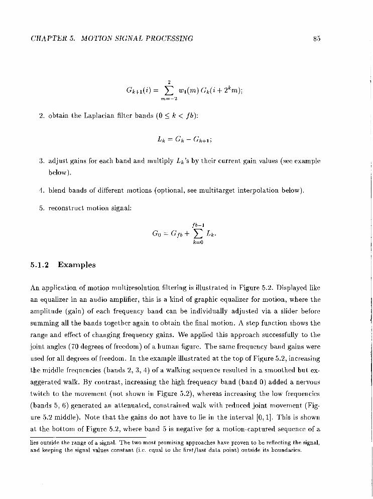
C H A P T E R 5. MOTION SIGNAL PROCESSING
2. obtain the Laplacian filter bands (0 5 k < fb):
3. adjust gains for each band and multiply Lk7s by their current gain values (see example
below).
4. blend bands of different motions (optional, see multitarget interpolation below).
5. reconstruct motion signal:
5.1.2 Examples
An application of motion multiresolution filtering is illustrated in Figure 5.2. Displayed like
an equalizer in an audio amplifier, this is a kind of graphic equalizer for motion, where the
amplitude (gain) of each frequency band can be individually adjusted via a slider before
summing all the bands together again to obtain the final motion. A step function shows the
range and effect of changing frequency gains. We applied this approach successfully to the
joint angles (70 degrees of freedom) of a human figure. The same frequency band gains were
used for all degrees of freedom. In the example illustrated at the top of Figure 5.2, increasing
the middle frequencies (bands 2, 3, 4) of a walking sequence resulted in a smoothed but ex-
aggerated walk. By contrast, increasing the high frequency band (band 0) added a nervous
twitch to the movement (not shown in Figure 5.2), whereas increasing the low frequencies
(bands 5, 6) generated an attenuated, constrained walk with reduced joint movement (Fig-
ure 5.2 middle). Note that the gains do not have to lie in the interval [ O , l ] . This is shown
at the bottom of Figure 5.2, where band 5 is negative for a motion-captured sequence of a
lies outside the range of a signal. The two most promising approaches have proven to be reflecting the signal, and keeping the signal values constant (i.e. equal to the firstflast da ta point) outside its boundaries.

C H A P T E R 5. MOTION SIGNAL PROCESSING
Figure 5.2: Adjusting gains of bands for joint angles; top: increasing middle frequencies; middle: increasing low frequencies; bottom: using negative gain value.

CHAPTER 5. MOTION SIGNAL PROCESSING
Figure 5.3: Adjusting gains of bands for joint positions.
figure knocking at the door, resulting in exaggerated anticipation and follow-through for the
knock. We also applied the same filtering to the joint positions (147 degrees of freedom) of
a human figure. Increasing the gains for the middle frequency bands of a walking sequence
produced a slight scaling effect of the end effectors, and resulted in a squash-and-stretch
cartoon walk (Figure 5.3).
From the examples, it becomes apparent that some constraints such as joint limits
or non-intersection with the floor can be violated in the filtering process. Our motion-
editing philosophy is to employ constraints or optimization after the general character of the
motion has been defined (see displacement mapping in section 5.4 below; or a more general
optimization method [52]). Whereas being trapped in local minima is the bane of global
optimization for most problems, animated motion is a good example of an underconstrained
problem where the closest solution to the animator's original specification is likely the best.
Of course, many animators disdain consistent physics, which is another good reason to
decouple motion editing from constraint satisfaction.

CHAPTER 5. MOTION SIGNAL PROCESSING
Figure 5.4: Example of multitarget motion interpolation.
5.2 Multitarget Interpolation
Multitarget interpolation refers to a process widely used in computer animation to blend
between different models. The technique was originally applied in facial animation [7, 381.
We might have a detailed model of a happy face, which corresponds parametrically to similar
models of a sad face, quizzical face, angry face, etc. The control parameters to the model
might be high level (like "raise left eyebrow by 0.7"), very high level (like "be happy"), or
they might simply be the coordinates of the points on a surface mesh defining the shape
of part of the face. By blending the corresponding parameters of the different models to
varying degrees, we can control the expression of the face.
5.2.1 Multitarget Motion Interpolation
We can apply the same technique to motion. Now we might have a happy walk, a sad walk,
angry walk, etc., that can be blended freely to provide a new result. Figure 5.4 shows an
example of blending two different motions of a human figure, a drumming sequence and
a "swaying arm sideways" sequence. In this case, the blend is linear, i.e. add 0.4 of the

CHAPTER 5. MOTION SIGNAL PROCESSING
blend + I -
Figure 5.5: Multitarget interpolation between frequency bands.
drum and 0.6 of the arm-sway. In general, the blend can be animated by "following" any
trajectory in time. Guo et al. [44] give a good discussion of this approach which they
term parametric frame space interpolation. Our approach generalizes on theirs in that the
motion parameters such as joint angles to be blended are completely decoupled from one
another, and have no implicit range limits. Each component of an arbitrary ensemble of
input parameters can have an independent blending coefficient assigned to it.
As indicated in step (4) of the multiresolution algorithm above, we can mix multitarget
interpolation and multiresolution filtering to blend the frequency bands of two or more
movements separately. This is illustrated in Figure 5.5 for the same two motions (a drum
and an arm-sway) as in Figure 5.4. Adjusting the gains of each band for each motion and
then blending the bands provides finer control while generating visually much more pleasing
and convincing motion.
However, there is a potential problem when applying multitarget interpolation to motion
which relates to the notion of parametric correspondence as stated above: for all our face
models to "correspond parametrically" implies that the parameters of each of the models

C H A P T E R 5. MOTION SIGNAL PROCESSING
Figure 5.6: Blending two walks without (top) and with (bottom) correspondence in time.
has a similar effect, so that if a parameter raises the left eyebrow of face number one, a
corresponding parameter raises the left eyebrow in face number two. If our parameters are
simply surface coordinates, it means that the points on each surface correspond, so if the
point at U, V coordinates U1, V1 is at the tip of the left eyebrow, the point a t the same
coordinates in any other face will also be at the tip of the left eyebrow.
In motion, parametric correspondence means much the same thing, except that now
a correspondence with respect to time is required. If we are blending walk cycles, the
steps must coincide so that the feet strike the ground at the same time for corresponding
parameter values. If the sad walk is at a slower pace than the happy walk, and we simply
blend them together without first establishing a correspondence between the steps, the
blend will be a curious dance of uncoordinated motions, and the feet will no longer strike
the ground at regular intervals; indeed, they are no longer guaranteed to strike the ground at
all (see Figure 5.6). Thus, multitarget motion interpolation must include both a distortion
(remapping a function in time) and a blend (interpolating among different mapped values).
In the visual domain a transformation like this is termed a "morph."

CHAPTER 5. MOTION SIGNAL PROCESSING
Figure 5.7: Blending two waves without (top) and with (bottom) correspondence in time.
Another example is illustrated in Figure 5.7; here the motion sequences of two human
figures waving at different rates and intensities (a "neutral" and a "pronounced" wave) were
first blended without timewarping. This resulted in a new wave with undesirable secondary
waving movements superimposed. After timewarping the neutral to the pronounced wave,
the blend produced the neutral wave at the pronounced rate. In the following section we
describe an automatic method for establishing correspondence between signals to make
multitarget motion interpolation meaningful and useful.
5.2.2 Timewarping
As mentioned in section 3.3, the field of speech recognition has applied "dynamic time-
warping" to compare stored templates with input utterances [33]. The timewarp procedure
identifies a combination of expansion and compression which best warps the input signal
to most closely match the template. In our case, timewarping is applied in the discrete
time domain to register the corresponding motion parameter signals such as joint angles. In

CHAPTER 5. MOTION SIGNAL PROCESSING
U~ 50 100 150
# of frames
Figure 5.8: Top: knee angles of two walking cycles; middle: red = blue curve warped to match green; bottom: red = green curve warped to match blue.

CHAPTER 5. MOTION SIGNAL PROCESSING
Figures 5.6 and 5.7, the timewarping was done simultaneously for all 70 rotational degrees
of freedom of the human figure for the duration of the movement sequences. If we have
a military march and a drunken stagger, two new gaits can immediately be defined from
the timewarp alone: the military march at the drunken pace, and the drunken stagger at
the military pace. Figure 5.8 shows an example for one degree of freedom (knee angle) for
the two walks warped in Figure 5.6. However, we are not limited to these two extreme
warps, but may freely interpolate between the mappings of the two walks, and between the
amplitudes of the signals through these mappings independently.
Algorithm
The problem can be solved in two steps:
1. find the optimal sample correspondences between the two signals;
2. apply the warp.
In section 3.3, the vertex correspondence problem was introduced and related to shape
blending [86]. Dynamic programming is applied to solve this problem. Recall that the
solution space can be represented as a two dimensional grid, and each node in the grid
corresponds to one possible vertex assignment as shown in Figure 5.9. The solution is the
globally optimal correspondence between the vertices of the two motion signals, which is
illustrated in the grid by a path from (0,O) to (9,9). We adopted Sederberg's shape blending
algorithm [86] which guarantees a globally optimal solution by visiting every node in the
grid once (O(n2) with constant amount of work per node). Upon reaching node (n, n), the
optimal solution is recovered by backtracking through the graph. Sederberg's "physically-
based" approach measures the difference in "shape" of the two signals by calculating how
much work it takes to deform one signal into the other. The cost function consists of the
sum of local stretching and bending work terms, the former involving two, the latter three
adjacent vertices of each signal. Intuitively, the larger the difference in distance between
two adjacent vertices of one signal and the two vertices of the other (given by two adjacent
nodes in the graph), the bigger the cost. Similarly, the larger the difference in angles
between three adjacent vertices of one signal and the three vertices of the other (given by
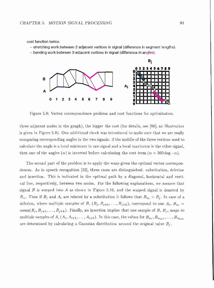
CHAPTER 5. MOTION SIGNAL PROCESSING
cost function tens: - stretching work between 2 adjacent vertices in signal (difference in segment lengths). - bending work between 3 adjacent vertices in signal (difference in ar-Inn).
Figure 5.9: Vertex correspondence problem and cost functions for optimization.
three adjacent nodes in the graph), the bigger the cost (for details, see [86]; an illustration
is given in Figure 5.9). One additional check was introduced to make sure that we are really
comparing corresponding angles in the two signals: if the middle of the three vertices used to
calculate the angle is a local minimum in one signal and a local maximum in the other signal,
then one of the angles ( a ) is inverted before calculating the cost term ( a = 360 deg -a).
The second part of the problem is to apply the warp given the optimal vertex correspon-
dences. As in speech recognition [33], three cases are distinguished: substitution, deletion
and insertion. This is indicated in the optimal path by a diagonal, horizontal and verti-
cal line, respectively, between two nodes. For the following explanations, we assume that
signal B is warped into A as shown in Figure 5.10, and the warped signal is denoted by
B,. Then if Bj and Ai are related by a substitution it follows that Bwi = Bj. In case of a
deletion, where multiple samples of B, (Bj, Bj+l,. . . , Bj+k), correspond to one A;, B,, =
mean(Bj , B j + ~ , . . . , Bj+k). Finally, an insertion implies that one sample of B, Bj , maps to
multiple samples of A, (Ab, Ai+l,. . . , Ai+k). In this case, the values for B,, , Bw,+l, . . . , Bwi+k
are determined by calculating a Gaussian distribution around the original value B j .

CHAPTER 5. MOTION SIGNAL PROCESSING
substitution: 1 :I correspondence of successive samples. deletion: multiple samples of B map to a sample of A. insertion: a sample of B maps to multiple samples of A.
warped B 1 Figure 5.10: Application of timewarp (warp B into A).
5.3 Motion Waveshaping
As introduced in section 3.3, waveshaping involves a shaping function which operates as a
special filter on a signal x. An example of how this idea can be adopted for animation is
illustrated in Figure 5.11. Here the default identity shaping function has been modified to
limit the joint angles for a motion sequence of an articulated figure waving. In the figure,
"hard" limits are imposed: values of x greater than a limit value simply map to that value.
An alternative is a "soft7' limit: as values exceed the limit, they are mapped to values that
gradually approach it. The implementation of our shaping function is based on interpolating
cubic splines [54]; a user can add, delete and drag control points to define the function and
then apply it to all or some degrees of freedom of an articulated figure.
Another application of waveshaping is to map the shape of input motions to a "charac-
xeristic" function. The shaping function in Figure 5.12 applied to the motion-captured data
of a human figure sitting and drinking introduced extra undulations to the original mono-
tonic reaching motion. This way, it is possible to build up a library of shaping functions
which will permit rapid experimentation with different styles of movement.
For animation, waveshaping - as well as displacement mapping, explained below - is
useful to efficiently edit densely-spaced motion signals such as live motion capture data
where each frame is a "key."
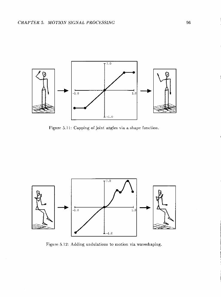
CHAPTER 5. MOTION SIGNAL PROCESSING
Figure 5.11: Capping of joint angles via a shape function.
Figure 5.12: Adding undulations to motion via waveshaping.

C H A P T E R 5. MOTION SIGNAL PROCESSING
Figure 5.13: Steps in displacement mapping.
5.4 Motion Displacement Mapping
Displacement mapping provides a means to change the shape of a signal locally through
a displacement map while maintaining continuity and preserving the global shape of the
signal. To alter a movement, the animator just changes the pose of an articulated figure at
a few keyframes. A spline curve is then fitted through these displacements for each degree
of freedom involved, and added to the original movement to obtain new, smoothly modified
motion. The basic approach is illustrated in Figure 5.13. Step 1 is to define the desired
displacements (indicated by the three vertical arrows) with respect to the motion signal;
in step 2, the system then fits an interpolating cubic spline [54] through the values of the
displacements (note that the first and last data points are always displacement points).
The user can then adjust the spline parameters in step 3 before the system calculates the
displaced motion satisfying the displacement points (step 4).

C H A P T E R 5. MOTION SIGNAL PROCESSING
Figure 5.14: Examples of applying displacement curves.
The displacement process can be applied iteratively until a desired result is achieved.
Since the operation is cheap, a fast feedback loop is guaranteed. In the top part of Fig-
ure 5.14, we took the output of a multiresolution filtering operation on joint angles of a
human walking figure, where some of the joint limits were violated and the feet did not
make consistent contact with the ground, and read it into LifeForms [19], a system to an-
imate articulated figures. There we adjusted some of the joints and translated the figure
at a few keyframes for which displacement curves were quickly generated and applied to
the motion of the figure as described above. To refine the resulting motion, a second loop
was executed; a frame of the final result is shown on the top right of Figure 5.14. The
same technique was used in modifying the rotoscoped motion of a human figure sitting and
drinking (Figure 5.14, bottom). Here, three out of the 600 motion-captured frames were
modified to include some additional gestures of the arms and legs.
C H A P T E R 5. MOTION SIGNAL PROCESSING
5.5 Conclusions
In this chapter we have assembled a simple library of signal processing techniques applica-
ble to animated motion. A prototype system has been implemented in the programming
language C using the Khoros Application Development Environment [81]. The immediate
goals of our motion-editing experiments have been fulfilled: the motion signal processing
techniques provide a rapid interactive loop, and facilitate reuse and adaptation of motion
data. By automating some aspects of motion editing such as time-registration of signals or
increasing the middle frequencies for several degrees of freedom at the same time, these tech-
niques lend themselves to higher level motion control and can serve as building blocks for
high-level motion processing. For example, we are involved in a promising research project
outside the scope of this thesis which relies on timewarping and multiresolution analysis
to capture "emotional" information from motion-captured data with the intent to produce
emotional motion by applying this information to other motions.
Of all the techniques introduced here, perhaps motion displacement mapping will prove
to be the most useful; it provides a means by which a basic movement such as grasping
an object from one place on a table can be easily modified to grasping an object anywhere
else on the table. This allows simple and straightforward modification of motion-capture
data through a standard keyframing interface. Timewarping as a non-linear method to
speed up or slow down motion is useful in blending different movements. It could also
play an important role in synchronizing various movements in an animation as well as in
synchronizing animation with sound. Multiresolution filtering has been demonstrated as an
easy tool to change the quality of a motion. Waveshaping represents a simple but efficient
way to introduce subtle effects to all or some degrees of freedom.
The interactive performance of these techniques is an important feature which support
the process of incremental and iterative modification of animations of articulated figures
with many degrees of freedom. We believe that a wide range of animation tasks can be
completed in this way with less effort than using conventional spline tweaking tools:
blending of motions is straightforward by using multitarget interpolation with auto-
matic time registration of movements. This is a convenient way to build up more
complex motions from elementary ones. For more fine-control, the frequency bands

C H A P T E R 5. MOTION SIGNAL PROCESSING
can first be computed for each motion before blending band-by-band while adjusting
the frequency gains.
0 concatenating motions is another practical application of multitarget interpolation.
The user has control over the blending interval t (transition zone) and the blending
coefficient a (where 0 5 a 5 1). For example, a simple linear blend for a particular
degree of freedom O1 then yields
where 01, (t) is the degree of freedom of the first motion for the transition zone, and
O1,(t) for the motion to be appended.
0 capping of joint angles is a task easily accomplished by waveshaping. This tool is
also well suited to apply user-defined undulations to all or some degrees of freedom to
make a "bland" motion more expressive.
0 some animation tasks which can be achieved with multiresolution analysis include
"toning down" a motion by increasing the low frequency gains, "exaggerating" a move-
ment by increasing the middle frequencies, producing a "nervous twitch" by increasing
the higher frequencies, and generating "anticipation and follow-through" by assigning
negative gain values. Because of immediate feedback, the user can quickly experiment
with different combinations of gain values for specific movement qualities.
0 editing of motion-captured data is very desirable yet very tedious in current systems.
As mentioned above, displacement mapping provides an interface through which the
animator can conveniently change such data at a few selected "keyframes" while pre-
serving the motion-captured "signature" of the motion.
We believe that our approach to apply techniques from the image and signal processing
domain to animation has been successful and provides a basis for motion editing complimen-
tary to keyframing and spline curve editing. It also opens the door for similar algorithms
to follow. As the use of motion capture is becoming increasingly popular and libraries of
motions are increasingly available, providing alternate methods for modifying and tweaking
movement for reuse can be of great value to animators.

CHAPTER 5. MOTION SIGNAL PROCESSING
5.6 Future Work
Natural extensions to these basic motion signal processing capabilities promise further pow-
erful operations. One useful feature for timewarping is to independently animate warping
and blending over time. In this way, "intermediate" motions could be obtained beyond
the two "extremes" of warping motion A into motion B, or B into A. Also, by comput-
ing vector similarity measures for multiple filter-bank components of a pair of signals at
once, we effect simultaneous time/spectrum registration of the signals. Similarly, facilities
for grouping motion parameters to compute and apply time registration collectively can be
provided. Finally, as suggested by research in speech recognition, we can apply time-warping
to recognize individual motions such as gestures.
A relatively simple editing task is to speed up or slow down an animated movement
within a small range by simply varying the sampling rate. However, changing the tim-
ing excessively in this way does not produce satisfactory results. For example, drastically
speeding up an animation does not give the impression of normal people simply moving
faster than usual. In this case, "time-scale modification" as applied to speech signals can
be adopted2; in "speeding up" the signal, pauses (silences) can be selectively shortened or
eliminated, and repeated cycles collapsed and averaged. These operations are enabled by
the filter banks and signal-matching algorithms we have implemented.
2This approach was suggested by Lance Williams through personal communication.

Chapter 6
Summary and Conclusions
Within the scope of this thesis, we designed and implemented interactive, procedural motion
control techniques to animate human figures. In chapter 4, the procedural control of human
walking and running was introduced as a useful tool for animating a wide variety of human
locomotion styles interactively and at a high level. The animator does not get bogged
down in complex limb coordination for locomotion, but maintains creative control by fine-
tuning intuitive parameters like bounciness, step length or torso tilt while receiving real-
time feedback on how these parameters affect the motion. Compared to other high-level
systems, this form of procedural animation thus combines the best of both worlds, higher
level specification and lower level customization of motion. All of our initial objectives set
out in section 2.6 have been satisfied: the algorithms facilitate ease of motion specification,
ease of customizing motion, interactive performance and real-time feedback, and generation
of believable motion. A few ideas on extending this work are given in section 4.4.
The work is original and manifests an important step in animating articulated figures.
Although the walking algorithm is based on an earlier non-interactive, dynamic system1 [9],
conceptual and structural changes were necessary in designing the new, interactive approach.
To animate human running, new techniques had to be developed since running is a sub-
stantially different motion from walking. The algorithms are the most flexible methods to
'The dynamic system, KLAW, was developed by the author as his master's thesis.
102

CHAPTER 6. SUMMARY AND CONCLUSIONS
animate human locomotion to date. Compared to other research [80,45] which is physically-
based, non-interactive and offers only limited control such as desired forward velocity, our
approach makes real-time animation possible while still producing realistic motion; in fact, it
demonstrates that convincing motion can be generated kinematically while providing much
better control than physically-based techniques.
The parameters and attributes currently implemented by the algorithms allow the user
to create locomotion with different expressions and variations in style. An open question
is how many and which parameters are "optimal" in a sense that they give the animator
adequate control without being too overwhelming, ambiguous or hard to use. Putting the
systems into the hands of experienced animators as well as novice users can shed some light
into this problem. One solution is to animate using overlays, that is to create motion in
several passes. With this method, motions like 'greeting while walking' can be obtained
quite readily. Taking the idea of generating variations in expression a step further leads to
the challenge of automating the animation of personalities, moods and emotions, such as the
walk of a grouchy old man or a jog of a happy young woman. This would enable complete
autonomous animation from a script where the animator plays the role of a film director.
We believe that the procedural locomotion techniques combined with the procedural motion
signal processing tools in chapter 5 provide valuable ingredients of such a high level system.
It is clear that we incorporated a lot of specific knowledge into our algorithms to "pro-
ceduralize" locomotion. An extension of this method to animate other motions is therefore
not considered as straightforward. Teo [96] has taken a similar approach to procedural-
ize human grasping by incorporating knowledge on modeling the human hand, objects to
be picked up and the grasping motion itself. In this way, various grasping styles such as
a power-grasp and a precision-grasp applied to different objects are animated at a high
level. Again, this approach works well for a specific class of motions with no claim to gen-
eralization. However, from experience gained during the development of these procedural
techniques, we can give some recommendations for the design of similar algorithms for other
motions: first, the movement needs to be analyzed carefully; how can a complex motion
be broken down into subcomponents? For example, in locomotion, there is a stance and a
swing phase; the swing phase can be further divided into subphases such as the period from
toe-off until the tip of the toe is vertically aligned with the knee. Similarly, for grasping,
there is an initial phase where the arm moves towards the object, and a preparation phase
C H A P T E R 6. SUMMARY A N D CONCLUSIONS
as the hand approaches the object and the fingers "get ready" for the grasp [96]. A second
guideline for developing procedural control algorithms is that the motion should be studied
with respect to how it could be parameterized; which parameters capture a specific motion
and give the animator control over different styles of this motion. For locomotion, obvious
parameters are those for step lengths and velocity, but also more subtle parameters like
heel-or-toe-strike or bounciness are desirable. In the case of grasping, parameters to switch
between the different types of a grasp (e.g. power-grasp or precision-grasp), or a parameter
to change the weight of the object which automatically alters the kinematics of the grasp
are good choices.
Besides developing the interactive generation tools for human locomotion, this thesis has
also investigated a variety of tools adopted from image and signal processing for interactive,
procedural motion manipulation. Chapter 5 discussed prototype implementations of these
tools. Our objectives to create new and efficient ways to ease the reuse and adaptation of
motion data for human figure animation have been satisfied; the techniques are useful for
certain kinds of global and local effects applied to one or many degrees of freedom at the
same time. Movements from different sources - including motion captured data - can
be blended, registered in time, exaggerated and locally edited. The techniques are also
unique in that they have not been applied to the animation of human movement before. We
believe that because of the complexity of human figure animation, motion signal processing
represents an important alternative to the conventional spline techniques for an animator
to tweak motion. The tools can also serve as building blocks for higher level operations in
animation. It is quite conceivable that the multiresolution and timewarping functions can be
utilized to transform "neutral" movements from keyframed, motion captured or physically-
based systems into motion with discernible personalities or emotions. Non-linear differences
in timings between, say, an angry and a tired person knocking at a door, as well as distinct
patterns in the frequency domain between these qualitatively dissimilar motions can be
captured this way. A more straightforward use of frequency analysis is to apply it to higher-
level parameters, for example to the parameters and attributes of our procedural locomotion
algorithm, or to the end effector positions of a human figure. We think that creating a
dual representation between motion multiresolution filtering and traditional spline-based
trajectories would give an animator a much more powerful movement editing tool. This
could lead to filter-based (step function) keyframe interpolation as a promising alternative

CHAPTER 6. SUMMARY AND CONCLUSIONS
to conventional keyframing systems. Section 5.6 suggests some ideas on how these tools can
be generalized and extended.
The procedural techniques presented in this thesis are interactive motion control tools,
not just interactive positioning control tools. Compared to interactive motion control by
input devices such as waldos, these tools support animation at a higher level (between limb
level; recall Figure 2.2) by having internal knowledge about motions or motion processing.
They are simple but effective, and besides animation they might equally be applicable to
new generations of video game applications as for studies of human movement or movement
control. Ideally, the tools should not to be used in isolation but within a system providing
low level spline editing as well as higher level path planning and expert knowledge as dis-
cussed in section 2.4. Low-level editing tools are invaluable to an animator for fine-tuning
movement and tailoring motion to a particular animated character. The procedural tech-
niques in this thesis lend themselves well for integration in a hierarchical motion control
system by providing some fine-control as well as higher level control at the "between limbs"
level. Analogous to how current systems allow for storing and reuse of libraries of movement
sequences, a high-level control scheme is conceivably which administers libraries of proce-
dural motion algorithms. A framework for such a system called blackboard architecture has
been proposed by Calvert et a1 [24].

Bibliography
[l] R. McNeil Alexander. The gaits of bipedal and quadrupedal animals. The Interna-
tional Journal of Robotics Research, 3(2):49-59, 1984.
[2] R. McNeil Alexander. How dinosaurs ran. Scientific American, 264(4): 130-136, 1991.
[3] W.W. Armstrong and Mark Greene. The dynamics of articulated rigid bodies for
purposes of animation. In Graphics Interface '85, Proceedings, pages 407-415, 1985.
[4] Norman Badler, J. O'Rourke, and B. Kaufman. Special problems in human movement
simulation. In Computer Graphics (SIGGRAPH '80 Proceedings), volume 14, pages
189-197, 1980.
[5] Susan Van Baerle. An expanded definition for animation. unpublished report, Texas
A/&M University, 1994.
[6] J. Barenholtz, Z. Wolofsky, I. Ganapathy, and T.W. Calvert. Computer interpretation
of dance notation. In IEEE Systems Man and Cybernetics Conference, September
1975.
[7] P. Bergeron and P. Lachapelle. Controlling facial expressions and body movements
in the computer-generated animated short: Tony de peltrie. In Computer Graphics
(SIGGRAPH '85)' Course Notes: Techniques for Animating Characters, July 1985.
[8] B.A. Blanksby. The biomechanics of running. Austrailian Journal of Sports Medicine,
4(8):34-40, 1972.
[9] Armin Bruderlin. Goal-directed, dynamic animation of human locomotion. Master's
thesis, Simon Fraser University, School of Computing Science, November 1988.
BIBLIOGRAPHY 107
[lo] Armin Bruderlin and Tom Calvert. Goal-directed, dynamic animation of human walk-
ing. In Computer Graphics (SIGGRAPH '89 Proceedings), volume 23, pages 233-242,
July 1989.
[ll] Armin Bruderlin and Tom Calvert. Adaptability of Human Gait, Advances in Psy-
chology Series, chapter Animation of Human Gait, pages 305-330. Elsevier Science
Publishers B.V., North Holland, 1991.
[12] Armin Bruderlin and Tom Calvert. Interactive animation of personalized human
locomotion. In Graphics Interface '93, Proceedings, pages 17-23, May 1993.
[13] Armin Bruderlin, John Dickinson, John Dill, and Lyn Bartram. Protocol analysis of
the use of a CAD system in a home design task. In ACM SIGCH1791, New Orleans,
short talk/poster, 1991.
[14] Armin Bruderlin, Thecla Schiphorst, and Tom Calvert. The animation of human
movement: How visual can we get? In Computer Graphics (SIGGRAPH 'go), in
Course Notes #8, Human Figure Animation: Approaches and Applications, pages
245-260, August 1990.
[15] Marc Le Brun. Digital waveshaping synthesis. Journal of the Audio Engineering
Society, 27(4):250-266, 1979.
[16] P.J. Burt. Multiresolution method for image merging. In Computer Graphics (SIG-
GRAPH '86), Course Notes: Advanced Image Processing, August 1986.
[17] P.J. Burt and E.H. Adelson. A multiresolution spline with application to image merg-
ing. ACM Transactions on Graphics, 2(4):217-236, October 1983.
[18] Tom Calvert. The challenge of human figure animation. In Graphics Interface '88,
Proceedings, pages 203-210, 1988.
[19] Tom Calvert, Armin Bruderlin, John Dill, Thecla Schiphorst, and Chris Welman.
Desktop animation of multiple human figures. IEEE Computer Graphics & Applica-
tions, 13(3):18-26, 1993.
[20] Tom Calvert, Armin Bruderlin, Sang Mah, Thecla Schiphorst, and Chris Welman.
The evolution of an interface for choreographers. In InterCHI'93, Proceedings, pages
117-122, 1993.

BIBLIOGRAPHY
[21] Tom Calvert and Arthur Chapman. Handbook of Pattern Recognition and Image Pro-
cessing: Computer Vision, chapter 12: Analysis and Synthesis of Human Movement,
pages 431-474. Academic Press, 1994.
[22] Tom Calvert, John Chapman, and Judy Landis. New Directions in Dance, chapter
Notation of Dance with Computer Assistance, pages 169-178. Pergamon Press, 1979.
[23] Tom Calvert, John Chapman, and Aftab Patla. Aspects of the kinematic simulation of
human movement. IEEE Computer Graphics and Applications, 2(9):41-50, November
1982.
[24] Tom Calvert, Russell Ovans, and Sang Mah. Towards the autonomous animation of
multiple human figures. In Computer Animation '94, Proceedings, pages 69-75, 1994.
[25] Tom Calvert, Chris Welman, Severin Gaudet, and Catherine Lee. Composition of
multiple figure sequences for dance and animation. In CG International'89, New
Advances in Computer Graphics, Proceedings, pages 245-255, June 1989.
[26] Michel Carignan, Ying Yang, Nadia Magnenat-Thalmann, and Daniel Thalmann.
Dressing animated synthetic actors with complex deformable clothes. In Computer
Graphics (SIGGRAPH '92 Proceedings), volume 26, pages 99-104, July 1992.
[27] Justine Cassell, Catherine Pelachaud, Norman Badler, Mark Steedman, Brett Achorn,
Tripp Becket, Brett Douville, Scott Prevost, and Matthew Stone. Animated conver-
sation: Rule-based generation of facial expression, gesture & spoken intonation for
multiple conversational agents. In Computer Graphics (SIGGRAPH '94 Proceedings),
pages 413-420, July 1994.
[28] G.A. Cavagna, F.P. Saibene, and R. Margaria. Mechanical work in running. journal
of Applied Physiology, 19:249-256, 1964.
[29] Arthur Chapman and G.E. Caldwell. Kinetic limitations of maximal sprinting speed.
Journal of Biomechanics, 16(1):79-83, 1983.
[30] David Chen and David Zeltzer. Pump it up: Computer animation of a biomechani-
cally based model of muscle using the finite element method. In Computer Graphics
(SIGGRAPH '92 Proceedings), volume 26, pages 89-98, July 1992.

BIBLIOGRAPHY 109
[31] Charles K. Chui. An Introduction to Wavelets, Series: Wavelet Analysis and its
Applications. Academic Press, Inc., 1992.
[32] Michael Cohen. Interactive spacetime control for animation. In Computer Graphics
(SIGGRAPH '92 Proceedings), volume 26, pages 293-302, July 1992.
[33] R. DeMori and D. Probst. Handbook of Pattern Recognition and Image Processing,
chapter Computer Recognition of Speech. Academic Press, 1986.
[34] Charles Dillman. Kinematic analysis of running. Exercise and Sport Sciences Reviews,
3:193-218, 1975.
[35] Karin Drewery. Goal-directed animation using english motion commands. In Graphics
Interface '86, Proceedings, pages 13 1-135, 1986.
[36] B.C. Elliott and B.A. Blanksby. A cinematographics analysis of overground and tread-
mill running by males and females. Medicine and Science in Sports and Exercise,
8(2):84-87, 1978.
[37] Bruce Char et al. MAPLE Reference Manual, 5th Edition. WATCOM Publications
Limited, Waterloo, Ontatio, Canada, 1988.
[38] Fred Parke et al. State of the art in facial animation. In Computer Graphics (SIG-
GRAPH 'go), Course Notes, August 1990.
[39] R. Fletcher. Practical Methods of Optimization. John Wiley & Sons, New York, 1987.
[40] Dave Forsey. A surface model for skeleton-based character animation. In Proceedings
of the the Second Eurographics Workshop on Animation and Simulation, September
1991.
[41] H. Fuchs, Z.M. Kedem, and S.P. Uselton. Optimal surface reconstruction from planar
contours. Communications of the ACM, 10(10):693-702, 1977.
[42] Michael Girard and A.A. Maciejweski. Computational modeling for the computer
animation of legged figures. In Computer Graphics (SIGGRAPH '85 Proceedings),
volume 19, pages 263-270, 1985.
[43] Julian Gomez. Twixt: A 3-d animation system. Computer 63 Graphics, 9(3):291-298,
1985.

BIBLIOGRAPHY
[44] S. Guo, J . Roberge, and T. Grace. Controlling movement using parametric frame space
interpolation. In Computer Animation '93, Proceedings, volume ??, pages 216-227,
1993.
[45] Jessica Hodgins. Simulation of human running. In IEEE International Conference on
Robotics and Automation, Proceedings, pages 1320-1325, 1994.
[46] Jessica Hodgins, Paula Sweeney, and David Lawrence. Generating natural-looking
motion for computer animation. In Graphics Interface '92, Proceedings, pages 265-
272, 1992.
[47] Paul Hogberg. Length of stride, stride frequency, "flight" period and maximum
distance between the feet during running with different speeds. Arbeitsphysiologie,
14:431-436, 1952.
[48] T. Hoshikawa, H. Matsui, and M. Miyashita. Analysis of running pattern in relation
to speed. Medicine and Sport: Biomechanics 111, 8:342-348, 1973.
[49] V.T. Inman, H.J. Ralston, and F. Todd. Human Walking. Williams & Wilkins,
Baltimore, 1981.
[50] Paul Isaacs and Michael Cohen. Controlling dynamic simulation with kinematic
constraints, behavior functions and inverse dynamics. In Computer Graphics (SIG-
GRAPH '87 Proceedings), volume 21, pages 215-224, 1987.
[51] G. Johansson. Perception and psychology. l4:2Ol-2ll, 1973.
[52] Michael Kass. Condor: Constraint-based dataflow. In Computer Graphics (SIG-
GRAPH '92 Proceedings), volume 26, pages 32 1-330, 1992.
[53] Hyeongseok KO and Norman Badler. Straight line walking animation based on kine-
matic generalization that preserves the original characteristics. In Graphics Interface
'93, Proceedings, pages 9-16, May 1993.
[54] Doris Kochanek and Richard Bartels. Interpolating splines with local tension, continu-
ity and bias control. In Computer Graphics (SIGGRAPH '84 Proceedings), volume 18,
pages 33-41, 1984.
[55] G. Koestler. The Act of Creation. 1964.

BIBLIOGRAPHY 11 1
[56] Yoshihito Koga, Koichi Kondo, James Kuffner, and Jean-Claude Latombe. Planning
motions with intentions. In Computer Graphics (SIGGRAPH '94 Proceedings), pages
395-408, July 1994.
[57] M. Kurakin. Relationships among running parameters. Yessis Review, 8(1):1-4,1973.
[58] John Lasseter. Principles of traditional animation applied t o 3d computer animation.
In Computer Graphics (SIGGRAPH '87' Proceedings), volume 21, pages 35-44, July
1987.
[59] Philip Lee, Susanna Wei, Jianmin Zhao, and Norman Badler. Strength guided motion.
In Computer Graphics (SIGGRAPH '90 Proceedings), volume 24, pages 253-262,1990.
[60] Yuencheng Lee, Demetri Terzopoulus, and Keith Waters. Constructing physics-based
facial models of individuals. In Graphics Interface '93, Proceedings, pages 1-8, May
1993.
[61] Peter Litwinowicz. Inkwell: A 2 112-d animation system. In Computer Graphics
(SIGGRAPH '91 Proceedings), volume 25, pages 113-122, 1991.
[62] Zicheng Liu, Steven Gortler, and Michael Cohen. Hierarchical spacetime control. In
Computer Graphics (SIGGRA P H '94 Proceedings), pages 35-42, July 1994.
[63] Nadia Magnenat-Thalmann and Daniel Thalmann. The use of high-level 3-d graphical
types in the mira animation system. IEEE Computer Graphics and Applications,
3(9):9-16, December 1983.
[64] Nadia Magnenat-Thalmann and Daniel Thalmann. An indexed bibliography on com-
puter animation. IEEE Computer Graphics and Applications, 5(7):76-85, July 1985.
[65] Roger Mann. Biomechanics of walking, running, and sprinting. American Journal of
Sports Medicine, 8(5):345-350, 1980.
[66] R.B. McGhee and A.K. Jain. Some properties of regularly realizable gait matrices.
Mathematical Biosciences, 13:179-193, 1972.
[67] Kenneth Meyer, Hugh Applewhite, and Frank Biocca. A survey of posistion trackers.
Presence: Teleoperators and Virtual Environments, 1(2):173-200, Spring 1992.

BIBLIOGRAPHY
[68] Doris Miller. Biomechanics of running-what should the future hold. Canadian Jour-
nal of Applied Sports Sciences, 3:229-236, 1978.
[69] H. Miura and I. Shimoyama. Dynamic walk of a biped. The International Journal of
Robotics Research, 3(2):60-74, 1984.
[70] Eadweard Muybridge. Human 13 Animal Locomotion. Dover Publications, New York,
1970.
[71] Harley Myler and Arthur Weeks. The Pocket Handbook of Image Processing Algo-
rithms in C. Prentice Hall, New Jersey, 1993.
[72] Thomas Ngo and Joe Marks. Spacetime constraints revisited. In Computer Graphics
(SIGGRAPH '93 Proceedings), volume 27, pages 343-350, 1993.
[73] Johnny Nilsson, Alf Thorstensson, and Junt Halbertsma. Changes in leg movements
and muscle activity with speed of locomotion and mode of progression in humans.
Acta Physiologica Scandinavica, 123(4):457-475,1985.
[74] J.M. Odgen, E.H. Adelson, J.R. Bergeb, and P.J. Burt. Pyramid-based computer
graphics. RCA Engineer, 30(5):4-15, 1985.
[75] Alan Oppenheim and Ronald Schafer. Discrete Time Signal Processing. Prentice Hall,
New Jersey, 1989.
[76] Mark Overmars. Forms library: A graphical user interface toolkit for silicon graph-
ics workstations (version2.2). Technical report, Utrecht University, Department of
Computer Science, 3508 T B Utrecht , The Netherlands, June 1993.
[77] K. Pearson. The control of walking. Scientific American, 235(6):72-86, 1976.
[78] Cary Phillips and Norman Badler. Interactive behaviors for bipedal articulated figures.
In Computer Graphics (SIGGRAPH '91 Proceedings), volume 25, pages 359-362,1991.
[79] Marc Raibert. Legged Robots that Balance. MIT Press, Cambridge, Massachusetts,
1986.
[80] Marc Raibert and Jessica Hodgins. Animation of dynamic legged locomotion. In
Computer Graphics (SIGGRAPH '91 Proceedings), volume 25, pages 349-358, 1991.

BIBLIOGRAPHY 113
[81] John Rasure and Steven Kubica. The khoros application development environment.
Technical report, Khoral Research, Inc., 4212 Courtney NE, Albuquerque, NM, 87108,
USA, 1993.
[82] Craig Reynolds. Computer animation with scripts and actors. In Computer Graphics
(SIGGRAPH '82 Proceedings), volume 16, pages 289-296, 1982.
[83] Craig Reynolds. Flocks, herds, and schools: A distributed behavioral model. In
Computer Graphics (SIGGRAPH '87 Proceedings), volume 21, pages 25-34, 1987.
[84] R. Ryman, J.C. Beatty, K.S. Booth, and A. Singh. A computerized editor for benesh
movement notation. CORD Dance Research Journal, 1983.
[85] Shinji Sakurai and Mitsurnasa Miyashita. Mechanical energy changes during treadmill
running. Medicine and Science in Sports and Exercise, 17(1):148-152, 1985.
[86] T.W. Sederberg and E. Greenwood. A physically-based approach to 2-d shape blend-
ing. In Computer Graphics (SIGGRAPH '92 Proceedings), volume 26, pages 26-34,
1992.
[87] Ken Shoemake. Animating rotation with quaternion curves. In Computer Graphics
(SIGGRA P H '85 Proceedings), volume 19, pages 245-254, July 1985.
[88] H.A. Simon. The Sciences of the Artificial. MIT Press, Cambridge, MA, 1969.
[89] Karl Sims. Evolving virtual creatures. In Computer Graphics (SIGGRAPH '94 Pro-
ceedings), pages 15-22, July 1994.
[90] Wayne Sinning and Harry Forsyth. Lower-limb actions while running a t different
velocities. Medicine and Science in Sports and Exercise, 2(1):28-34, 1970.
[91] C.S. Stein and H.E. Hitchner. The multiresolution dissolve. S M P T E Journal, pages
977-984, December 1988.
[92] James Stewart and James Cremer. Beyond keyframing: An algorithmic approach t o
animation. In Graphics Interface '92, Proceedings, pages 273-281, May 1992.
[93] David Sturman. A discussion on the development of motion control systems. In
Graphics Interface '86, Tutorial on Computer Animation, 1986.

BIBLIOGRAPHY 114
[94] David Sturman. Interactive keyframe animation of 3-d articulated models. In Graphics
Interface '86, Tutorial on Computer Animation, 1986.
[95] Scott Sutherland and Lucy Venable. Labanwriter 2.2 workshop. In Dance and Tech-
nology, Proceedings), pages 289-296, University of Wisconsin, March 1992. National
Dance Association.
[96] Chor Guan Teo. A hybrid procedural/knowledge-based approach t o the animation of
human hand grasping. Master's thesis, Simon Fraser University, School of Computing
Science, March 1994.
[97] Frank Thomas and Ollie Johnston. Disney Animation-The Illusion of Life. Abbeville
Press, New York, 1981.
[98] Munetoshi Unuma and Ryozo Takeuchi. Generation of human motion with emotion.
In Computer Animation '93, Proceedings, pages 77-88, 1993.
[99] Michiel van de Panne and Eugene Fiume. Sensor-actuated networks. In Computer
Graphics (SIGGRAPH '93 Proceedings), volume 27, pages 335-342, 1993.
[loo] Michiel van de Panne and Eugene Fiume. Virtual wind-up toys for animation. In
Graphics Interface '94, Proceedings, pages 208-215, 1994.
[ lo l l L. Velho. Piecewise Descriptions of Implicit Surfaces and Solids. PhD thesis, Univer-
sity of Toronto, Computer Science, 1994.
[lo21 Peter Wavish and Michael Graham. Applying situated action top video game char-
acters. In Bates & Kitano, editor, Proceedings of the AAAI-94 workshop on Artificial
Intelligence, Artificial Life and Entertainment, Seattle, July 1994.
[I031 Wilhelm Weber and Eduard Weber. Mechanics of the Human Walking Apparatus.
Springer-Verlag, Berlin, 1992.
[I041 Chris Welman. Inverse kinematics and geometric constraints for articulated figure
manipulation. Master's thesis, Simon Fraser University, School of Computing Science,
April 1993.
[I051 Jane Wilhelms. Using dynamic analysis to animate articulated bodies such as humans
and robots. In Graphics Interface '85, Proceedings, pages 97-104, 1985.

BIBLIOGRAPHY 115
[I061 Jane Wilhelms. Virya-a motion control editor for kinematic and dynamic aniamtion.
In Graphics Interface '86, Proceedings, pages 141-146, 1986.
[I071 Jane Wilhelms. An interactive approach to behavioral control. In Graphics Interface
'89, Proceedings, pages 1-8, 1989.
[I081 David Winter. Biomechanics of Human Movement. John Wiley & Sons, 1979.
[log] Andrew Witkin and Michael Kass. Spacetime constraints. In Computer Graphics
(SIGGRA P H '88 Proceedings), volume 22, pages 159-168, 1988.
[I101 Zella Wolofsky. Computer interpretation of selected labanotation commands. Master's
thesis, Simon Fraser University, School of Kinesiology, 1974.
[ I l l ] David Zeltzer. Towards an integrated view of 3-d computer character animation. In
Graphics Interface '85, Proceedings, pages 105-115, 1985.