To boost the flavor of electromagnetics, we accompanied many problems with short Matlab code acting as a calculator and result illustrator. We completely ignored the description of algorithms behind the codes because they are often quite complicated and required ample, very sophisticated as well as abstract mathematical specifics poorly helping to understand the physical picture. Such approach lets us shift the focus from the often emasculated and practically fruitless problems primarily based on math transformations to more complicated but close to practical tasks. We hope that it helps to visualize typically invisible EM fields and stimulate in-depth analysis and the following discussion of the fundamental principles. Projecting images onto a big screen, the lectures may organize whole class conversation making the audience to be significantly engaged. We cheer our readers to look through Matlab scripts to discover and sophisticate the algorithm embedded in them. We encourage to use the student edition of MATLAB and CST STUDIO SUITE® to get enhanced problem understanding. Sorry for compact transcription of scripts that is dictated by the blog environment. A better readable version of scripts will be sent to you upon request left on the Contact page. Attention. Regrettably, copy and paste into Matlab Command Window saves appropriate Matlab format just in Chrome Web Browser. You have to restart https://emfieldbook.com/ in https://www.google.com/ if your browser is different. Section 2.1 and 2.2. Torque Exerted by Electric and Magnetic Field

2.1 Rotation of Ball-and-Stick Model of Electric Dipole in Uniform E-field. Suppose a monopole duo similar to a field sensor #2 (see Section 1.4.1 in Chapter 1) is placed in a uniform E-field at the moment t = 0, and it is motionless at this moment, i.e. (𝑑𝑑𝑑𝑑 𝑑𝑑𝑑𝑑⁄ )𝑡𝑡=0 =0. The dipole initial angular displacement is 𝑑𝑑(0) = 𝑑𝑑0. Figure on the left depicts the E-force lines around this

dipole at t = 0. Figure on the right demonstrates the Lorentz’s forces 𝑭𝑭± (check expression (1.11)) are exerted by the applied E-field. Eventually, the dipole is forced spinning as a solid assembly around its center. The source of the external E-field is not shown except the polarity of far-away charges (large red sign + and blue -) that generate this field. The following Matlab script is built around the exact solution1 of the equation of motion. For simplification, it was assumed that the monopole duo consists of ∆𝑞𝑞𝑒𝑒 = ±𝑒𝑒 with mass 𝑚𝑚 = 𝑚𝑚𝑒𝑒 (see Table 1.5) and separation d = 6*10-11m. The reader may edit the 5th line of a script if desired. Copy, paste, and run the script below into Matlab Command Window starting from the relative small angular displacements 𝑑𝑑0 ≤ 60° and the dissipation factor equal to 0. Figure 1 plots the exact y-axis displacement 𝑦𝑦 =sin(𝑑𝑑(𝑑𝑑)), bold blue line, and the same displacement assuming the dipole pure harmonic angular oscillation (red asterisk line) with frequency 𝑓𝑓0 = �2∆𝑞𝑞𝑒𝑒𝐸𝐸/(𝑚𝑚𝑑𝑑) (recollect the motion of a simple gravity pendulum triggered by the net Lorentz’s force 2∆𝑞𝑞𝑒𝑒𝐸𝐸). Figure 2 is the animation illustrating the dipole angular

1 A. Beléndez1, C. Pascual, D.I. Méndez, T. Beléndez, C. Neipp, Exact solution for the nonlinear pendulum, Sociedade Brasileira de Física, 2007, http://www.scielo.br/scielo.php?script=sci_arttext&pid=S1806-11172007000400024

X

Y

movement where the black vector depict the value (not in scale) and direction of the torque vector 𝑻𝑻𝒆𝒆(𝑑𝑑) (read Section 2.1 and expression (2.7) in Chapter 2). The magenta vector shows the direction of dipole moment 𝒑𝒑𝑒𝑒. clc; close all; clear; E=input('Enter the intensity of uniform E-field [V/m] = '); dis=input('Enter the relative dissipation factor between 0 (no loss) and 1 (high loss) = '); theta0=input('Enter the initial angular displacement > 0 or < _180[degrees] = '); m=9.10938356e-31; e=1.60217662e-19; d=6e-11; omega0=sqrt(2*e*E/(m*d)); NN=2.4e2; theta0=pi*theta0/180; t=linspace(0,8*pi/omega0,NN); ss=sin(theta0/2); k=ss^2; K=ellipke(k); u=K-omega0*t; SN=jacobiSN(u,k); Arg=SN*ss; omega=pi*omega0/(2*K); Theta=2*asin(Arg).*exp(-omega*t*dis); Th=1; f1=figure('units','normalized','outerposition',[.2 .2 .6 .6]); axis square movegui(f1,'west'); plot(t,sin(Theta),'LineWidth',2); grid minor; hold on; plot(t,0*Theta,'-'); plot(t,cos(omega*t).*sin(theta0),'*r'); axis tight; xlabel('\bf Time [s]'); ylabel('\bfTorque (Kinetic Energy of Rotation) T(t) [J/radian]'); title(['\bf','Initial Angular Displacment = ',num2str(theta0*180/pi),' deg']) text(t(end/4),sin(theta0)-0.1,['\bfOscillation Frequency f_0 = ',num2str(omega0/(2*pi)/1e9),' [GHz]']) f2=figure; movegui(f2,'east'); grid minor; xlabel('\bfX-axis'); ylabel('\bfY-axis'); steps=length(t); axis([-1 1 -1 1 -Th/2 Th/2]*2); hold on; hp=patch([1 -1 -1 1]*2, [1 1 -1 -1]*2, [0 0 0 0]); alpha(hp,0.2) hPlot = plot(NaN,NaN,'--b','LineWidth',2); h3Plot = plot(NaN,NaN,'--b','LineWidth',2); plot(0,0,'or'); r12=1; hq1=quiver3(-2,0,0,4,0,0,'g'); set(hq1,'LineWidth',3,'AutoScale','off','MaxHeadSize',0.8) text(2.2,0,'\bfE','Color','g','FontSize',20); text(2.2,.4,'\bf-','Color','b','FontSize',40) text(-2.2,.4,'\bf+','Color','r','FontSize',40); x = [0.55 0.52]; y = [0.75 0.54]; annotation('textarrow',x,y,'String','\bfT = p_{e} x E','FontSize',14); x12 = zeros(steps,2); x13 = zeros(steps,2); y12 = zeros(steps,2); y13 = zeros(steps,2); theta1 = zeros(steps,1); MM(steps) = struct('cdata',[],'colormap',[]); for k = 1:steps theta1(k) = 2*pi*(k-1)/steps; x12(k,1) = 0; x13(k,1) = 0; y12(k,1) = 0; y13(k,1) = 0; x12(k,2) = r12*cos(Theta(k)); x13(k,2) = -r12*cos(Theta(k)); y12(k,2) = r12*sin(Theta(k)); y13(k,2) = -r12*sin(Theta(k)); set(hPlot,'XData',x12(k,:),'YData',y12(k,:)); set(h3Plot,'XData',x13(k,:),'YData',y13(k,:)); hr=plot(x12(k,2),y12(k,2),'o','MarkerSize',15,'MarkerEdgeColor','k','MarkerFaceColor','r'); hb=plot(-x12(k,2),-y12(k,2),'o','MarkerSize',15,'MarkerEdgeColor','k','MarkerFaceColor','b'); un=x12(k,2)/sqrt((x12(k,2)+0.25)^2+y12(k,2)^2); wn=y12(k,2)/sqrt((x12(k,2)+0.25)^2+y12(k,2)^2); hq2=quiver3(0,0,0,un,wn,0,'m'); set(hq2,'LineWidth',3,'MaxHeadSize',0.8) hq3=quiver3(x12(k,2),y12(k,2),0,0.9,0,0,'r'); set(hq3,'LineWidth',3,'MaxHeadSize',0.8) hq4=quiver3(-x12(k,2),-y12(k,2),0,-0.9,0,0,'b'); set(hq4,'LineWidth',3,'MaxHeadSize',0.8) hq=quiver3(0,0,0,0,0,-Th*sin(Theta(k)),'k'); set(hq,'LineWidth',3,'MaxHeadSize',0.8) MM(k) = getframe; if k~=steps; set(hq,'visible','off'); set(hr,'visible','off'); set(hb,'visible','off'); set(hq2,'visible','off'); set(hq3,'visible','off'); set(hq4,'visible','off'); end; view(-73,34); end 1. Suppose the dipole moment is aligned with the E-field vector. Is this equilibrium stable or not? What does it mean that some object at equilibrium? For what angles 𝑑𝑑 is the dipole in equilibrium? Briefly explain your answers. 2. Explain why the Lorentz’s forces applied to the top and bottom charges are directed in the opposite direction? 3. When does the torque reach the maximum and drop to zero? Will the shown above dipole rotate clockwise or counterclockwise when released at t = 0? When external E-field is on, will the torque on the dipole due to this field tend to align or misalign the electric moment with the field? 4. Explain the fact that the dipole released from rest at t = 0 with its moment not aligned with E-field, will oscillate back and forth about E-field direction. Check the animation images and the graph in Figure 1. 5. Can you predict where the dipole will momentarily stop by looking at the Figure 1 graph and animation? What are the dipole potential and kinetic energy at these moments? 6. What are the total net force on the dipole and the direction of torque vector T at t = 0? Hint. Apply the right-hand-rule. 7. What is the unit dimension of torque in SI? Explain spin-electric field energy exchange supporting dipole oscillation.

8. Justify the fact that the torque vector T is directed along the axis of the dipole spinning and the cross product of the moment 𝒑𝒑𝑒𝑒 and vector E. Hint. Use the analogy with the twisting force applied to the wrench and the direction of nut movement along the bolt (see Figure 2.1.1a in Chapter 2). 9. Demonstrate that the torque force rotates the dipole in the equilibrium position of minimal potential energy checking the time moment when T = 0 in Figure 2. 10. Run the case 𝑑𝑑0 = 91° and dissipation factor = 0. What happened to the dipole oscillation? Why is it not harmonic anymore? Check the case 𝑑𝑑0 = 170° to be sure and look carefully at how the dipole rotates and the torque vector varies. 11. Pay attention to the oscillation frequency printed on the top of Figure 1. Why is it so high? Does this frequency increase or decrease as the strength of E-field grows? Explain your answer. 12. Eventually, the dipole and E-fields around it rotates jointly being inseparable. Does it mean that the total E-fields is not static any longer and become time dependable? Check Table 1.7 in Chapter 1 and explain the consequences of this effect2. Hint. Come back to Section 1.6.15 in Chapter 1 and expression (1.62). Should we expect that part of the oscillation energy is lost through the EM radiation? 13. Run the Matlab script assuming the dissipation factor = 0.2 and explain the results. Does the aligned dipole produce its own E-field that reduces or increase the external E-field? What happens with multiple dipoles in dielectrics as soon as the external static E-field is applied (Check Figure 2.2.4 in Chapter 2)? 14. Following Section 2.2.2 in Chapter 2 and Matlab, simulation data explain the phenomenon of polarization. What is the nature of the damping effect? 15. Calculate the polarization vector magnitude of the material having 300 dipoles per unit volume in the volume of 10 units. What is unite dimension of this vector? 16. Explain how the displacement vector D holds unchanged and independent of material dielectric constant. When an object becomes polarized, does it acquire a charge and becomes a charged object? 17. Explain the differences between isotropic and anisotropic dielectric materials.

2.2 Rotation the Loop Carrying Steady Current in Uniform B-field.

Suppose a loop carrying a steady current I (see the problem 1.5M for Chapter 1) is placed in an external uniform steady B-field at the moment t = 0, and it is motionless at this moment, i.e. (𝑑𝑑𝑑𝑑 𝑑𝑑𝑑𝑑⁄ )𝑡𝑡=0 = 0. The initial angular displacement of loop magnetic moment |m| = IA is 𝑑𝑑(0) = 𝑑𝑑0 where A is the loop area. Figure on the left depicts the B-force red lines initiated by the loop at t = 0. The Lorentz’s torque force 𝑻𝑻𝒎𝒎 = 𝒎𝒎 × 𝑩𝑩 (the expression (2.4) in Chapter 1) is exerted by the applied B-field. Eventually, the loop is forced spinning by this torque force. The source of the external B-field is not shown. The following Matlab script is built around the exact solution of the same equation of motion that governs an electric dipole rotation. Copy, paste, and run the script into Matlab Command Window starting from the relative small angular displacements

≤ 60° and the dissipation factor equal to 0. Figure 1 plots the exact y-axis displacement 𝑦𝑦 = sin(𝑑𝑑(𝑑𝑑)), bold blue line, and the same displacement assuming the dipole pure harmonic angular oscillation (red asterisk line) with frequency 𝑓𝑓0 = �𝐼𝐼𝐼𝐼/(2𝜋𝜋𝑚𝑚) (recollect the motion of a simple gravity pendulum triggered by the net Lorentz’s force 𝐼𝐼𝐼𝐼). Figure 2 is the animation illustrating the loop angular movement where the black vector depict the value (not in scale) and the direction of the torque vector 𝑻𝑻𝒆𝒆(𝑑𝑑) (read Section 2.1 and expression

2 David J. Griffiths, , Introduction to Electrodynamics, 3rd Edition, Pearson Education , 2007, Chapter 11, Post 4 and http://physicspages.com/pdf/Griffiths%20EM/Griffiths%20Problems%2011.04.pdf

(2.4) in Chapter 2). The magenta vector is the direction of the dipole moment 𝒎𝒎𝑚𝑚 normal to the loop area. The phenomenon of dielectric and magnetic material polarization has so much in common (see, for example, the tables in https://www.tf.uni-kiel.de/matwis/amat/elmat_en/kap_4/basics/b4_1_1.html) that the reader may answer the questions from problem 2.1 just replacing some words like a dipole with loop, electric moment with magnetic moment, E-field with B-field, and so on. The critical additional question is what the difference between these phenomena is and how to explain them.

Enjoy the animation at https://www.youtube.com/watch?v=aMH7pdn-qr4.

clc; close all; clear; D=input('Enter the current loop diameter D < 4 [m]: '); B=input('Enter the intensity of uniform B-field [T] = '); theta0=input('Enter the initial angular displacement > 0 or < 180[degrees] = '); dis=input('Enter the relative dissipation factor between 0 (no loss) and 1 (high loss) = '); m=input('Enter the loop mass [kg] = '); I=input('Enter the current carried by loop [A] = '); omega0=sqrt(2*pi*I*B/m); NN=5e2; theta0=pi*theta0/180; R=D/2; t=linspace(0,4*pi/omega0,NN); ss=sin(theta0/2); k=ss^2; K=ellipke(k); u=K-omega0*t; SN=jacobiSN(u,k); Arg=SN*ss; omega=pi*omega0/(2*K); Theta=2*asin(Arg).*exp(-omega*t*dis); f1=figure(1); movegui(f1,'east'); plot(t,sin(Theta),'LineWidth',2); grid minor; hold on; plot(t,0*Theta,'-'); plot(t,cos(omega*t).*sin(theta0),'*r'); axis tight; xlabel('\bf Time [s]'); ylabel('\bfTorque (Kinetic Energy of Rotation) T(t) [J/radian]'); title(['\bf','Initial Angular Displacment = ',num2str(theta0*180/pi),' deg']) text(t(end/4),sin(theta0)-0.1,['\bfOscillation Frequency f_0 = ',num2str(omega0/(2*pi)),' [Hz]']) ro=linspace(0,2*D,NN); z1=linspace(-2*D,2*D,NN); [Ro,Z1]=meshgrid(ro,z1); a=Z1.^2+Ro.^2+R^2; b=2*R*Ro; k=2*b./(a+b); c=sqrt(Z1.^2+(R+Ro).^2); d1=R^2+Ro.^2+Z1.^2; d2=R^2-Ro.^2-Z1.^2; d3=(R-Ro).^2+Z1.^2; [K,E]=ellipke(k); Hr=-2*I*Z1.*(K-E.*d1./d3)./(c.*Ro)/(4*pi); Hz=2*I*(K+E.*d2./d3)./c/(4*pi); f2=figure('units','normalized','outerposition',[0 0.1 0.7 0.7]); grid minor; hold on; xlim([-2,2]*D); ylim([-2,2]*D); view(-153,24); zlim([-1,1]*D); r=0.1*R; [XX,YY,ZZ] = cylinder(r/10,1e2); ZZ(2,:)=D; mesh(XX,YY,ZZ); mesh(XX,YY,-ZZ); theta2=linspace(-pi,pi,64); phi=linspace(0,2*pi,64); [tt,p]=meshgrid(phi,theta2); x=(R+r*cos(p)).*cos(tt); z=(R+r*cos(p)).*sin(tt); y=r*sin(p); hSurface=mesh(x,y,z); rotate(hSurface,[0,0,1],theta0*180/pi); st=[0 -2*D]; en=[0 2*D]; head=0.4; v1 = head*(st-en)/2.5; theta=22.5*pi/180; theta1=-1*22.5*pi/180; rotM1 = [cos(theta) -sin(theta);sin(theta) cos(theta)]; rotM2 = [cos(theta1) -sin(theta1);sin(theta1) cos(theta1)]; v2=v1*rotM1; v3=v1*rotM2; x1=en; x2=x1+v2; x3=x1+v3; fill([x1(1) x2(1) x3(1)],[x1(2) x2(2) x3(2)],'g'); plot([st(1) en(1)],[st(2) en(2)],'linewidth',8,'color','g'); st=[0 0]; en=[0 D]; head=0.5; v1 = head*(st-en)/2.5; theta=22.5*pi/180; theta1=-1*22.5*pi/180; rotM1 = [cos(theta) -sin(theta);sin(theta) cos(theta)]; rotM2 = [cos(theta1) -sin(theta1);sin(theta1) cos(theta1)]; v2=v1*rotM1; v3=v1*rotM2; x1=en; x2=x1+v2; x3=x1+v3; hf=fill([x1(1) x2(1) x3(1)],[x1(2) x2(2) x3(2)],'m'); hp=plot([st(1) en(1)],[st(2) en(2)],'linewidth',4,'color','m'); rotate(hf,[0,0,1],theta0*180/pi); rotate(hp,[0,0,1],theta0*180/pi); hLines1=streamslice(Ro,Z1,Hr,Hz,1); set(hLines1,'Color','r'); hLines2=streamslice(-Ro,Z1,-Hr,Hz,1); set(hLines2,'Color','r'); rotate(hLines1,[0,0,1],theta0*180/pi); rotate(hLines2,[0,0,1],theta0*180/pi); for jj=2:length(Theta); dT=(Theta(jj)-Theta(jj-1))*180/pi; st=[0 0]; en=[0 D]*sin(Theta(jj)); head=0.5; v1 = head*(st-en)/1.5; theta=22.5*pi/180; theta1=-1*22.5*pi/180; rotM1 = [cos(theta) -sin(theta);sin(theta) cos(theta)]; rotM2 = [cos(theta1) -sin(theta1);sin(theta1) cos(theta1)]; v2=v1*rotM1; v3=v1*rotM2; x1=en; x2=x1+v2; x3=x1+v3; hf1=fill([x1(1) x2(1) x3(1)],[x1(2) x2(2) x3(2)],[0 0 0]); hp1=plot([st(1) en(1)],[st(2) en(2)],'linewidth',6,'color','k'); rotate(hf1,[1,0,0],90); rotate(hp1,[1,0,0],90); rotate(hLines1,[0,0,1],dT); rotate(hLines2,[0,0,1],dT) rotate(hf,[0,0,1],dT); rotate(hp,[0,0,1],dT); rotate(hSurface,[0,0,1],dT); drawnow set(hp1,'visible','off'); set(hf1,'visible','off'); end 2.3 Polarized Conductive Sphere in Uniform Electric Field. Assume an uncharged conductive sphere of

radius a is situated in a vacuum and thoroughly insulated. The uniform external E-field oriented in parallel to z-axis is produced by far-far away charges not shown in the picture on the left. Nonetheless, their polarity is marked. Sketch out the equipotential lines of electric potential and E-force lines nearby the sphere if, for example, a = 1, E = 1. Then copy, paste, and run the script below into Matlab Command Window and compare the obtained plots with your sketch. Pay special attention to the E-force lines’ configuration nearby the sphere surface. Explain differences if you found them. The plot in Figure 1 demonstrates the filled contour lines of the electric potential and E-force lines (red). You can examine all these data

looking at sequential elevation cross-section images. The red and blue cup indicates the polarity of charges

on the spherical surface. By the end of animation, the drawings in Figure 2 and 3 appear and depict, respectively, the additional electric potential and E-force lines emitted by the conductive sphere and the surface charge density 𝜌𝜌𝑒𝑒𝑒𝑒(𝑎𝑎,𝑑𝑑) on the spherical surface. All of them are induced by external E-fields.

clc; close all; clear; a=input('Enter the sphere radius a <= 2 [m] = '); E0=input('Enter the intensity of external uniform E-field [V/m]: '); Eps0=8.854187817e-12; Phi=linspace(0,pi,18); N=2e2; D=6; dd=linspace(-D/2,D/2,N); [X,Y,Z]=meshgrid(dd); [az,el,r] = cart2sph(X,Y,Z); U=-E0*(1-a^3./r.^3).*r.*sin(el); Ud=E0*a^3./r.^3.*r.*sin(el); [Ex,Ey,Ez]=gradient(-U,D/N); E=sqrt(Ex.^2+Ey.^2+Ez.^2); FF=20*log10(abs(U)); [Exd,Eyd,Ezd]=gradient(-Ud,D/N); Ed=sqrt(Exd.^2+Ey.^2+Ez.^2); FFd=Ud; f1=figure('units','normalized','outerposition',[0 0 1 1]); hold on; grid on; view(-138,9); axis square; A=[-1 1 -1 1 -1 1]*D/2; axis(A); [xs,ys,zs] = sphere(50); xs=xs*a; ys=ys*a; zs=zs*a; hC=surf(xs,ys,zs,'FaceColor','w'); r0 = a; b = 1 ; h = a/10; X1 = xs ; Y1 = ys ; Z1 = zs ; X1(zs<r0/2) = NaN ; Y1(zs<r0/2) = NaN ; Z1(zs<r0/2) = NaN ; surf(X1,Y1,Z1,'FaceColor','r'); X2 = xs ; Y2 = ys ; Z2 = zs ; X2(zs>-r0/2) = NaN ; Y2(zs>-r0/2) = NaN ; Z2(zs>-r0/2) = NaN ; surf(X2,Y2,Z2,'FaceColor','b'); h1=slice(X,Y,Z,FF,[],0,[]); set(h1,'FaceColor','interp','EdgeColor','none'); hs1=streamslice(X,Y,Z,Ex,Ey,Ez,[],0,[],2); set(hs1,'Color','r'); c=hsv; c=c(1:2:end,:); colormap(c); hc=colorbar; ylabel(hc,'\bf 20*log10(Electric Potential Intensity) [dB]','FontSize',20) zlabel('\bfZ-axis'); ylabel('\bfY-axis'); xlabel('\bfX-axis'); zArrow = [0-D/2 1 1 1.2 1 1 0-D/2]*(D/2)*0.8; yArrow = [-0.1 -0.1 -0.2 0 0.2 0.1 0.1]*D/2; xArrow = 0*yArrow; hArrow = fill3(-D/1e3+xArrow,yArrow+3*D/8,zArrow,[1 0 0]); hArrow = fill3(-D/1e3+xArrow,yArrow-3*D/8,zArrow,[1 0 0]); hArrow = fill3(xArrow+3*D/8,yArrow+3*D/8,zArrow,[1 0 0]); hArrow = fill3(xArrow+3*D/8,yArrow-3*D/8,zArrow,[1 0 0]); for jj=2:length(Phi); dT=(jj-1)*(Phi(jj)-Phi(jj-1))*180/pi; h1=slice(X,Y,Z,FF,0,[],[]); set(h1,'FaceColor','interp','EdgeColor','none'); hs1=streamslice(X,Y,Z,Ex,Ey,Ez,0,[],[],2); set(hs1,'Color','r'); rotate(h1,[0,0,1],dT); rotate(hs1,[0,0,1],dT); drawnow; set(h1,'visible','off'); set(hs1,'visible','off'); end phi=0:pi/100:pi; phi1=phi/4; [U1,V1]=pol2cart(phi,1+sin(phi)); [U2,V2]=pol2cart(-phi,1+sin(phi)); [U3,V3]=pol2cart(phi,1+0*phi); [U4,V4]=pol2cart(-phi,1+0*phi); [U5,V5]=pol2cart(phi1,0.5+0*phi1); f2=figure; grid minor; axis equal;movegui(f2,'west'); hold on; grid on; view(-138,9); axis square; A=[-1 1 -1 1 -1 1]*D/2; axis(A); [xs,ys,zs] = sphere(50); xs=xs*a; ys=ys*a; zs=zs*a; hC=surf(xs,ys,zs,'FaceColor','w'); r0 = a; b = 1 ; h = a/10; X1 = xs ; Y1 = ys ; Z1 = zs ; X1(zs<r0/2) = NaN ; Y1(zs<r0/2) = NaN ; Z1(zs<r0/2) = NaN ; surf(X1,Y1,Z1,'FaceColor','r'); X2 = xs ; Y2 = ys ; Z2 = zs ; X2(zs>-r0/2) = NaN ; Y2(zs>-r0/2) = NaN ; Z2(zs>-r0/2) = NaN ; surf(X2,Y2,Z2,'FaceColor','b'); h1=slice(X,Y,Z,FFd,[],0,[]); set(h1,'FaceColor','interp','EdgeColor','none'); hs1=streamslice(X,Y,Z,Exd,Eyd,Ezd,[],0,[],2); set(hs1,'Color','r'); c=hsv; c=c(1:2:end,:); colormap(c); hc=colorbar; ylabel(hc,'\bf Electric Potential Intensity [V]','FontSize',20) zlabel('\bfZ-axis'); ylabel('\bfY-axis'); xlabel('\bfX-axis'); title('\bfSelf Potential and E-force Lines of Sphere'); movegui(f2,'west'); f3=figure; grid minor; axis equal; movegui(f3,'east'); [xs,ys,zs] = sphere(50); xs=xs*a; ys=ys*a; zs=zs*a; hC=surf(xs,ys,zs);[azimuth,elevation,r1] = cart2sph(xs,ys,zs); Sigma=sin(elevation); set(hC,'CData',Sigma); colormap('jet'); shading interp; title('\bfNormilized Surface Charge on Sphere'); colorbar 1. Watching the sequential structure of electric potential and E-force lines explain why they are identical in all azimuthal cross-sections. 2. The red and blue cup on a spherical surface in Figure 1 indicates the existence of positive (red) and negative (blue) surface charges. What force supports their separation on a conductive surface (Hint. Read Section 2.2.7 in Chapter 2)? Explain the absence of free charges and E-fields inside the sphere. 3. How much is the electric potential of the spherical surface? Provide a detailed and clear answer. 4. Determine the direction of the electric moment 𝒑𝒑𝑒𝑒of sphere establishing its field resemblance to electric dipole shown in Figure 1.4.1 of Chapter 1. Prove that 𝒑𝒑𝑒𝑒 = 4𝜋𝜋𝜀𝜀0𝑎𝑎3𝑬𝑬𝟎𝟎. 5. What happens if the external E-field switches to opposite or vanishes? 6. Why are all E-force lines normal to the surface of a conductive sphere (Hint. Apply the proof by contradiction)? 7. Explain why the surface charge density is nonuniform and drops to zero (see Figure 3) along the sphere equator. 8. Is it possible that the top and bottom charges come to be not equal or equal but the same polarity? 9. Examine plots in Figure 2 to shed light on the idea of the artificial dielectric medium that includes the hollow metal spheres of small diameter (check Section 2.2.7 in Chapter 2). Compare E-force lines of the sphere in Figure 2 and electric dipole. Explain their similarity.

2.4 Polarized Dielectric Sphere in Uniform Electric Field3. Assume a dielectric sphere of radius a with absolute dielectric constant 𝜀𝜀 = 𝜀𝜀0𝜀𝜀𝑟𝑟 is placed in a uniform external E-field created some charges (not shown) whose are at the infinite distances from the sphere. Nonetheless, their polarity is marked. Sketch out the equipotential lines of E-field and E-force lines nearby the sphere if, for example, a = 1, E = 1, 𝜀𝜀𝑟𝑟 = 20. Then copy, paste, and run the script below into Matlab Command Window and compare the obtained plots with your sketch. Pay special attention to the E-force lines’ configuration nearby and inside the sphere. Explain differences if you found them. The plot in Figure 1 demonstrates the filled contour lines of E-fields and E-

force lines (red). You can examine all these data looking at sequential elevation cross-section images. The red and blue cup indicates the polarity of charges on the spherical surface. By the end of animation, the drawings in Figure 2 and 3 appear and depict the surface charge density 𝜌𝜌𝑒𝑒𝑒𝑒(𝑎𝑎,𝑑𝑑) induced by external E-fields on the spherical surface. A grey area in Figure 2 corresponds to the sphere interior while 𝑑𝑑 is the elevation angle measured from the positive Z-axis.

clc; close all; clear; a=input('Enter the sphere radius a <= 2 [m] = '); E0=input('Enter the intensity of external uniform E-field [V/m]: '); Eps=input('Enter the relative dielectric constan of sphere: '); Eps0=8.854187817e-12; PhiR=linspace(0,pi,18);D=10; N=1.5e2; [X,Y,Z]=meshgrid(linspace(-D/2,D/2,N),linspace(-D/2,D/2,N),linspace(-D/2,D/2,N)); S1=[]; S2=[]; r=sqrt(X.^2+Y.^2+Z.^2); for i1=1:length(X); for j1=1:length(Y); for k1=1:length(Z); if r(i1,j1,k1)<=a; S1(i1,j1,k1)=1; S2(i1,j1,k1)=0; else; S1(i1,j1,k1)=0; S2(i1,j1,k1)=1; end; end; end; end Uin=-(3/(Eps+2))*E0*Z; Uout=-E0*Z+E0*((Eps-1)/(Eps+2))*a^3*Z./r.^(3/2); Udout=E0*((Eps-1)/(Eps+2))*a^3*Z./r.^(3/2); U=S1.*Uin+S2.*Uout; Ud=S1.*Uin+S2.*Udout; [Ex,Ey,Ez]=gradient(-U,D/N); E=sqrt(Ex.^2+Ey.^2+Ez.^2); [Exd,Eyd,Ezd]=gradient(-Ud,D/N); Ed=sqrt(Exd.^2+Eyd.^2+Ezd.^2); Dx=Eps0*(Eps*S1+S2).*Ex; Dy=Eps0*(Eps*S1+S2).*Ey; Dz=Eps0*(Eps*S1+S2).*Ez; DD=sqrt(Dx.^2+Dy.^2+Dz.^2); FF=U; FFd=Ud; f1=figure('units','normalized','outerposition',[0 0 1 1]); hold on; grid on; view(-138,9); axis square; A=[-1 1 -1 1 -1 1]*D/2; axis(A); [xs,ys,zs] = sphere(50); xs=xs*a; ys=ys*a; zs=zs*a; r0 = a; b = 1 ; h = a/10; X1 = xs ; Y1 = ys ; Z1 = zs ; X1(zs<r0/2) = NaN ; Y1(zs<r0/2) = NaN ; Z1(zs<r0/2) = NaN ; hC1=surf(X1,Y1,Z1,'FaceColor','r'); alpha(hC1,0.6); X2 = xs ; Y2 = ys ; Z2 = zs ; X2(zs>-r0/2) = NaN ; Y2(zs>-r0/2) = NaN ; Z2(zs>-r0/2) = NaN ; hC2=surf(X2,Y2,Z2,'FaceColor','b'); alpha(hC2,0.6); h1=slice(X,Y,Z,FF,0,[],[]); set(h1,'FaceColor','interp','EdgeColor','none'); hs1=streamslice(X,Y,Z,Ex,Ey,Ez,0,[],[],3); set(hs1,'Color','r'); c=hsv; c=c(1:2:end,:); colormap(c); hc=colorbar; ylabel(hc,'\bf Electric Potential Intensity [V]','FontSize',20) zlabel('\bfZ-axis'); ylabel('\bfY-axis'); xlabel('\bfX-axis'); zArrow = [0-D/2 1 1 1.2 1 1 0-D/2]*(D/2)*0.8; yArrow = [-0.1 -0.1 -0.2 0 0.2 0.1 0.1]*D/2; xArrow = 0*yArrow; hArrow = fill3(-D/1e3+xArrow,yArrow+3*D/8,zArrow,[1 0 0]); hArrow = fill3(-D/1e3+xArrow,yArrow-3*D/8,zArrow,[1 0 0]); hArrow = fill3(xArrow+3*D/8,yArrow+3*D/8,zArrow,[1 0 0]); hArrow = fill3(xArrow+3*D/8,yArrow-3*D/8,zArrow,[1 0 0]); for jj=2:length(PhiR); dT=(jj-1)*(PhiR(jj)-PhiR(jj-1))*180/pi; h1=slice(X,Y,Z,FF,0,[],[]); set(h1,'FaceColor','interp','EdgeColor','none'); hs1=streamslice(X,Y,Z,Ex,Ey,Ez,0,[],[],1); set(hs1,'Color','r'); rotate(h1,[0,0,1],dT); rotate(hs1,[0,0,1],dT); drawnow; set(h1,'visible','off'); set(hs1,'visible','off'); end phi=0:pi/100:pi; phi1=phi/4; [U1,V1]=pol2cart(phi,1+sin(phi)); [U2,V2]=pol2cart(-phi,1+sin(phi)); [U3,V3]=pol2cart(phi,1+0*phi); [U4,V4]=pol2cart(-phi,1+0*phi); [U5,V5]=pol2cart(phi1,0.5+0*phi1); f2=figure('units','normalized','outerposition',[0.01 0.01 0.7 0.7]); grid minor; hold on; view(-138,9); axis square; A=[-1 1 -1 1 -1 1]*D/2; axis(A); [xs1,ys1,zs1] = sphere(a); h2=slice(X,Y,Z,FFd,[],0,[]); set(h2,'FaceColor','interp','EdgeColor','none'); hs2=streamslice(X,Y,Z,Exd,Eyd,Ezd,[],0,[],3); set(hs2,'Color','r'); c=jet; c=c(1:2:end,:); colormap(c); hc1=colorbar; ylabel(hc1,'\bf Electric Potential Intensity [V]','FontSize',20) zlabel('\bfZ-axis'); ylabel('\bfY-axis'); xlabel('\bfX-axis'); title('\bfSelf Potential and E-force Lines of Sphere'); f3=figure; grid minor; axis equal;movegui(f3,'east'); [xs,ys,zs] = sphere(50); xs=xs*a; ys=ys*a; zs=zs*a; hC=surf(xs,ys,zs);[az,el,r] = cart2sph(xs,ys,zs); Sigma=3*Eps0*(Eps-1)*sin(el)/(Eps+2); set(hC,'CData',Sigma); colormap('jet'); shading interp; title('\bfSurface Charge Distribution on Sphere'); colorbar

3 If you are looking for the equations behind this script go to https://unlcms.unl.edu/cas/physics/tsymbal/teaching/EM-913/section4-Electrostatics.pdf

1. Compare all plots obtained here and in the problem 2.3 (conductive sphere). Explain the surprising similarities and mild differences. 2. Why E-field inside the sphere drops so low (Hint. Section 2.3.4 in Chapter 2 might turn out to be useful) and increases outside? 3. Answer the appropriate question from problem 2.3.

2.5 Electric Potential and Field due to Charge Placed above Plane Dielectric Boundary (Dielectric-Dielectric Interface with no free charge). Two dielectrics of absolute permittivity 𝜀𝜀0 (vacuum) and 𝜀𝜀 = 𝜀𝜀0𝜀𝜀𝑟𝑟 (𝜀𝜀𝑟𝑟 > 1) define a XY-plane boundary at z = 0. A point charge 𝑄𝑄𝑒𝑒 is placed at (x,y,z) = (0,0,d) as shown in figure on the left for d > 0. Evidently, d < 0 corresponds the charge located in the bottom medium. Later you will be asked to simulate an exotic case of d < 0, 𝜀𝜀𝑟𝑟 < 0. Although to date the existence of metamaterials with negative permittivity at zero frequency is questionable and probably cannot occur, nevertheless the simulation results are very curious. Each of uniform dielectric the mediums

occupies the half space z > 0 and z < 0, respectively. The dotted cube depict the area of field simulation. Sketch out the equipotential lines of electric potential, lines of E- and D-force inside the box for some combination, for example, D = 10, d = 1 and 𝜀𝜀𝑟𝑟 = 3. Then copy, paste, and run the script below into Matlab Command Window and compare the obtained plots with your sketch. Pay special attention to the E-force lines’ configuration nearby the boundary. Explain differences if you found them. The center plot in Figure 1 demonstrates the filled contour lines of the electric potential that is continuous along x (and y)-coordinate (Think how to explain it looking at the expression (1.21) in Chapter 1 and boundary conditions in Table 2.1 of Chapter 2). The E-force lines are shown in red (piecewise with an angular point on the boundary). You can examine all these data getting multiple cross-section images by sequentially pressing any key on a computer keyboard. Finally, the drawings in Figure 2 and 3 appear and depict, respectively, the electrical potential with E-force lines and the same potential with D-force lines. Both are at the cross-section x = 0. Look at Figure 1 and Figure 2.3.4 (Chapter 2) and explain why electric potential in the medium with a higher dielectric constant is lesser.

1. Explain the meaning of boundary conditions and why they are so noteworthy (Read Section 2.3.1 in Chapter 2). Formulate the situations when the boundary conditions are required. 2. Are the boundary conditions derived from Maxwell’s equations in integral of differential form? 3. Do the boundary conditions supplement Maxwell’s equations in integral of differential form? 4. What are the differences between the tangential and normal components of the field? How many components should be comprised to get the whole set of boundary components? 5. The boundary interface indicates the existence of two mediums with unequal permeability, equal permittivity, and no free charges on the interface. What can be said about the behavior of tangential and normal components of E- and D-field along the boundary? 6. What is the induced/bound surface charge density on the boundary? How does it depend on the permittivity of dielectric mediums? (Hint. Check Sections 2.3.2 and 2.3.4 in Chapter 2). 7. Run the option 𝐷𝐷 = 10, 𝑑𝑑 = 1, 𝜀𝜀 𝑟𝑟 = 4 and look at Figure 2. Explain the reasons that E-force lines rotate counterclockwise as they cross the boundary. Why there is no indication of rotation at y = 0? 8. Compare E- and D-force lines’ structure in Figure 2 and 3 and spell out the differences. It seems that D-fields do not notice the boundary. Why? 9. Run first the option 𝜀𝜀𝑟𝑟 = 4, 𝑑𝑑 = −1m and look at Figure 2. Explain the reasons that E-force lines rotate clockwise as they cross the boundary. Why there is no indication of rotation at y = 0?

10. Compare E- and D-force lines’ structure in Figure 2 and 3 and spell out the differences. It seems that D-fields do not notice the boundary. Why? 11. Run the option 𝐷𝐷 = 10, 𝑑𝑑 = 1, 𝜀𝜀 𝑟𝑟 = 10 and explain the occurrence that the electric potential drops down nearby the boundary and almost ceases below the interface. 12. Run the option 𝐷𝐷 = 10, 𝑑𝑑 = 1, 𝜀𝜀 𝑟𝑟 = 1000 and explain the occurrence that all E-force lines are practically normal to the boundary, i.e. the tangential component of E-fields almost vanishes. Might a perfect conductor be always replaced by a dielectric medium with 𝜀𝜀𝑟𝑟 → ∞ (See the next problem and check Table 2.1 in Chapter 2)? 13. Run the option 𝐷𝐷 = 10, 𝑑𝑑 = −1, 𝜀𝜀 𝑟𝑟 = −1.1 and stare at the surprising images in Figure 1 and 2. It looks like we have two charges, one is real and located in the medium with negative permittivity and the second one is a virtual/mirrored copy of the real one and the same polarity. This effect was named superlensing and demonstrated at frequencies above static. clc; close all; clear; D=input('Enter the cube edge D <= 10 [m] = '); d=input('Enter the distance d < D/2 between charge and dielectric boundary [m]: '); Q=input('Enter the charge value Qe [C] = '); Eps=input('Enter the relative permittivity of bottom dielectric medium = '); N=1e2; Eps0=8.854187817e-12; k=1/(4*pi*Eps0); [X,Y,Z]=meshgrid(linspace(-D/2,D/2,N)); r1=1./sqrt(X.^2+Y.^2+(Z-d).^2); r2=1./sqrt(X.^2+Y.^2+(Z+d).^2); Q1=Q*(Eps-1)/(Eps+1); Q2=Q+Q1; U1=k*(Q./r1-Q1./r2); U2=(k/Eps)*Q2./r1; for jj=1:size(Z,3); if Z(:,:,jj)>=0; U(:,:,jj)=U1(:,:,jj); else; U(:,:,jj)=U2(:,:,jj); end; end; [Ex,Ey,Ez]=gradient(U,D/N); E=sqrt(Ex.^2+Ey.^2+Ez.^2); FF=U; Dx=Eps0*Ex; Dy=Eps0*Ey; for jj=1:size(Z,3); if Z(:,:,jj)>=0; Dz(:,:,jj)=Eps0*Ez(:,:,jj); else; Dz(:,:,jj)=Eps0*Eps*Ez(:,:,jj); end; end; f1=figure('units','normalized','outerposition',[0 0 1 1]); hold on; grid on; view(-60,29); axis square; A=[-1 1 -1 1 -1 1]*D/2; axis(A); patch([1 -1 -1 1]*D/2,[1 1 -1 -1]*D/2,[0 0 0 0],'b'); alpha(0.05) plot3([0,0,0],[-D/2,D/2,0],[0,0,0],'LineWidth',2,'Color','k'); plot3([0,0,0],[0,0,0],[0,0,d],'LineWidth',2,'Color','m','LineStyle','-.'); plot3([-D/2,D/2,0],[0,0,0],[0,0,0],'LineWidth',2,'Color','k'); plot3([0,0,0],[-D/2,D/2,0],[0,0,0],'LineWidth',2,'Color','k'); [xs,ys,zs] = sphere; mesh(xs*2*d/D,ys*2*d/D,zs*2*d/D+d) text(0,-0.2,d,['\bf','\leftarrow \itCharge'],'Color','r','FontSize',20) vals = linspace(0,D/2,10); h1 = slice(X,Y,Z,FF,0,[],[]); set(h1,'FaceColor','interp','EdgeColor','none'); hs1=streamslice(X,Y,Z,Ex,Ey,Ez,0,[],[],2); set(hs1,'Color','b'); c = jet(128); c = c(end:-4:32,:); colormap(c); zlabel('\bfZ-axis'); ylabel('\bfY-axis'); xlabel('\bfX-axis'); for id = vals; delete(h1); delete(hs1); if id~=vals(1); delete(hp); end; hp=plot3([id,id,id],[-D/2,D/2,0],[0,0,0],'LineWidth',2,'Color','k'); hs1=streamslice(X,Y,Z,Ex,Ey,Ez,id,[],[],2); set(hs1,'Color','b','LineWidth',1.5); h1 = slice(X,Y,Z,FF,id,[],[]); set(h1,'FaceColor','interp','EdgeColor','none') disp('Press Any Key'); w = waitforbuttonpress; end; f2=figure; movegui(f2,'west'); hold on; grid minor; view(-90,0); hs1=streamslice(X,Y,Z,Ex,Ey,Ez,0,[],[],2); set(hs1,'Color','r','LineWidth',1.5); h1= contourslice(X,Y,Z,FF,0,[],[],40); set(h1,'LineWidth',1.5); plot3([0,0,0],[-D/2,D/2,0],[0,0,0],'LineWidth',2,'Color','k'); title('\bfElrctric Potential and E-force Lines at Cross-section X = 0'); zlabel('\bfZ-axis'); ylabel('\bfY-axis'); axis tight f3=figure; movegui(f3,'east'); hold on; grid minor; view(-90,0); hs2=streamslice(X,Y,Z,Dx,Dy,Dz,0,[],[],2); set(hs2,'Color','r','LineWidth',1.5); h2= contourslice(X,Y,Z,FF,0,[],[],40); set(h2,'LineWidth',1.5,'LineStyle','-'); plot3([0,0,0],[-D/2,D/2,0],[0,0,0],'LineWidth',2,'Color','k'); title('\bfElrctric Potential and D-force Lines at Cross-section X = 0') zlabel('\bfZ-axis'); ylabel('\bfY-axis'); axis tight The Matlab script above is built around the exact solution based on the method of images4 and published on http://physics.usask.ca/~xiaoc/phys463/notes/note2.pdf.

4 David J. Griffiths, , Introduction to Electrodynamics, 3rd Edition, Pearson Education , 2007

2.6 Electric Potential and Field due to Charge Placed above Perfect Conductive Plane (Dielectric-PEC Interface). The half-space dielectric of absolute permittivity 𝜀𝜀0 (vacuum for simplification) and perfect electric conductor (PEC, 𝜎𝜎 = ∞) define a XY-plane boundary at z = 0. A point charge 𝑄𝑄𝑒𝑒 is placed at (x,y,z) = (0,0,d) as shown in figure on the left. Sketch out the equipotential lines of E-field intensity and lines of E-force inside the box for some parameters combination, for example, D = 10, d = 1, and 𝑄𝑄𝑒𝑒 = 1. Then copy, paste, and run the script below into Matlab Command Window and compare the obtained plots with your sketch. Pay special attention to the E-force lines’ orientation nearby the boundary. Explain differences if you found them.

The center plot in Figure 1 demonstrates the filled contour lines of the E-fields and E-force lines shown in blue above the conductive plane versus {y, z}-coordinates. You can examine all these data getting multiple cross-section images by sequentially pressing any key on a computer keyboard. Finally, the drawings in Figure 2 appear and depict the induced surface charge distributions 𝜌𝜌𝑒𝑒𝑒𝑒(𝑦𝑦) in some cross-section sequences demonstrated in Figure 1.

clc; close all; clear; D=input('Enter the cube edge D <= 10 [m] = '); d=input('Enter the distance d < D between charge PEC interface [m]: '); Q=input('Enter the charge value Qe [C] = '); N=1e2; Eps0=8.854187817e-12; k=1/(4*pi*Eps0); [X,Y,Z]=meshgrid(linspace(-D/2,D/2,N),linspace(-D/2,D/2,N),linspace(0,D,N) ); r1=1./sqrt(X.^2+Y.^2+(Z-d).^2); r2=1./sqrt(X.^2+Y.^2+(Z+d).^2); U=k*Q.*(r1-r2); Den1=r1.^(3/2); Den2=r2.^(3/2); Ex=k*Q*X.*(Den1-Den2); Ey=k*Q*Y.*(Den1-Den2); Ez=k*Q*((Z-d).*Den1-(Z+d).*Den2); E=sqrt(Ex.^2+Ey.^2+Ez.^2); FF=log(E); f1=figure('units','normalized','outerposition',[0 0 1 1]); hold on; grid on; view(-60,29); A=[-1 1 -1 1 0 2]*D/2; axis(A); plot3([0,0,0],[-D/2,D/2,0],[0,0,0],'LineWidth',2,'Color','k'); plot3([0,0,0],[0,0,0],[0,0,d],'LineWidth',2,'Color','m','LineStyle','-.'); plot3([-D/2,D/2,0],[0,0,0],[0,0,0],'LineWidth',2,'Color','k'); [xs,ys,zs] = sphere; mesh(xs*0.2,ys*0.2,zs*0.2+d) text(0,-0.2,d,['\bf','\leftarrow \itCharge'],'Color','r','FontSize',20); vals=linspace(0,D/2,10); h1=slice(X,Y,Z,abs(FF),0,[],[]); set(h1,'FaceColor','interp','EdgeColor','r'); hs1=streamslice(X,Y,Z,Ex,Ey,Ez,0,[],[],1); c=jet(64); c=c(1:4:end,:); colormap(c); hc=colorbar; ylabel(hc,'\bf log(E)-field Intensity [V/m]','FontSize',20); zlabel('\bfZ-axis'); ylabel('\bfY-axis'); xlabel('\bfX-axis'); for id = vals delete(h1); delete(hs1); if id~=vals(1); delete(hp); end; hp=plot3([id,id,id],[-D/2,D/2,0],[0,0,0],'LineWidth',2,'Color','k'); hs1=streamslice(X,Y,Z,Ex,Ey,Ez,id,[],[],2); set(hs1,'Color','r','LineWidth',1.5); h1=slice(X,Y,Z,abs(FF),id,[],[]); set(h1,'FaceColor','interp','EdgeColor','k','MeshStyle', 'row'); disp('Press Any Key'); w = waitforbuttonpress; end f2=figure; movegui(f2,'west'); hold on; grid minor; hold on; for ii=N/2:4:N; X1=(X(ii,:,1)); D1z=Eps0*Ez(ii,:,1); plot(X1,D1z,'LineWidth',1); end ar = annotation('arrow',[0.5 0.5],[0.2 0.8]); ar.Color='r'; ar.LineWidth=2; t = text('Units','normalized','Position',[0.5,0.8],'String','\bfX Grows from 0 to D/2'); t.FontSize=12; axis tight; ar.HeadStyle='cback3'; title('\bfSurface Elrctric Charge \rho_{eA }(y) as 0 <= X <= D/2 while Z = 0'); xlabel('\bfY-axis [m]'); ylabel('\bfSurface Elrctric Charge \rho_{eA } [C/m^2]'); 1. Examine and explain the E-force line orientations on the dielectric-PEC interface (z = 0) and match them with data in Table 2.2 in Chapter 2 and drawing in Figure 2.3.5. 2. What is the intensity of the tangential components of E- and D-fields on the PEC surface and how to explain their value? 3. What is the source of the surface free charges on PEC interface? (Hint. Check Section 2.2.7 in Chapter 2)? 4. If the intensity of E-fields is known at z = 0 how to estimate the surface free charges on PEC interface? (Look at Table 2.2 in Chapter 2) 5. What is the polarity of the surface free charges on PEC interface (see Figure 2)? Is it defined by the polarity of a point charge 𝑄𝑄𝑒𝑒 or always stays negative? 6. Explain the role of the surface free charges in the absence of E-fields inside PEC (shielding effect). 7. Right down and explain the boundary condition on the Dielectric-PEC Interface.

2.7 Magnetic Potential and Field due to Line Current Placed above Plane Permeable Half-Space5. Two

materials of absolute permeability 𝜇𝜇0 (vacuum) and 𝜇𝜇 = 𝜇𝜇0𝜇𝜇𝑟𝑟 define an YZ-plane boundary at x = 0. A line current 𝐼𝐼 [A/m] is placed at (x,y,z) = (d,0,0) as shown in figure on the left. Each of uniform mediums occupies the half space x > 0 and x < 0, respectively. There are no free charges or electric currents on the interface. The cube depicts the area of field simulation. Sketch out the equipotential lines of magnetic vector potential (see definition in Chapter 4, equations 4.19, 4.24, and (4.33)), lines of H- and B-force inside the box for some parameters combination, for example, D = 10, d = 1 and 𝜇𝜇𝑟𝑟 = 3. Then copy, paste, and run the script below into Matlab Command Window and compare the obtained plots with your sketch. Pay special attention to the H- and

B-force lines’ configuration nearby the boundary. Explain differences if you found them. clc; close all; clear; D=input('Enter the cube edge D <= 10 [m] = '); d=input('Enter the distance d < D above interface [m]: '); I=input('Enter the line curreny I magnitude [A/m] = '); N=3e2; Mu=input('Enter relative magnetic permeability of bottom half-space = '); Mu0=4*pi*1e-7; b=(Mu-1)/(Mu+1); I1=I*b; I2=I+I1; x=linspace(-D/2,D/2,N); y=linspace(-D/2,D/2,N); [X,Y]=meshgrid(x,y); S1=[]; S2=[]; for i1=1:length(x); for j1=1:length(y); if X(i1,j1)>=0 S1(i1,j1)=1; S2(i1,j1)=0; else; S1(i1,j1)=0; S2(i1,j1)=1; end; end; end A=(-I*log((X-d).^2+Y.^2)-I1*log((X+d).^2+Y.^2)).*S1 + (-I2*log((X-d).^2+Y.^2)).*S2; [By,Bx]=gradient(A,D/N); By=-By; Hy=By/Mu0; Hx=(Bx.*S1+Bx.*S2/Mu)/Mu0; B=sqrt(Bx.^2+By.^2); H=sqrt(Hx.^2+Hy.^2); f1=figure(1); hold on; axis square; movegui(f1,'west'); grid minor; c=jet(128); c=c(1:2:end,:); colormap(c); hc=colorbar; ylabel(hc,'\bf Magnetic Vector Potential Az Intensity [J/(A/m^2)]','FontSize',10) C=gradient(A); hm=surf(X,Y,A); alpha 0.5; shading interp; [xs,ys,zs]=cylinder(0.02,10);zs(2,:)=max(max(abs(A)))+D/2; hC=surf(xs+d,ys,zs-D/2); title('\bfMagnetic Vector Potential Az intensity [J/(A/m^2)]') xlim([-3 3]); ylim([-3 3]); xlabel('\bfX-axis [m]'); ylabel('\bfY-axis [m]'); zlabel('\bf Az intensity [J/(A/m^2)]'); view(-61,32); f2=figure(2); hold on; axis square; grid minor; c=jet(128); c=c(1:2:end,:); colormap(c); hc=colorbar; ylabel(hc,'\bf log(B)-field Intensity [T]','FontSize',20) pcolor(X,Y,log(B)); shading interp; plot(0*x,y,'k','LineWidth',2); sc=1/8; quiver(imresize(X,sc),imresize(Y,sc),imresize(Bx,sc),imresize(By,sc),'r') title('\bfLogarithm of B-field intensity and B-force lines [T]') xlim([-3 3]); ylim([-3 3]); xlabel('\bfX-axis [m]'); ylabel('\bfY-axis [m]'); f3=figure(3); hold on; axis square; movegui(f3,'east'); grid minor; c=jet(128); c=c(1:2:end,:); colormap(c); hc=colorbar; ylabel(hc,'\bf log(H)-field Intensity [A/m]','FontSize',20) pcolor(X,Y,log(H)); shading interp; plot(0*x,y,'k','LineWidth',2) sc=1/8; quiver(imresize(X,sc),imresize(Y,sc),imresize(Hx,sc),imresize(Hy,sc),'r') title('\bfLogarithm of H-field intensity and H-force lines [A/m]') xlim([-3 3]); ylim([-3 3]); xlabel('\bfX-axis [m]'); ylabel('\bfY-axis [m]'); The left plot in Figure 1 demonstrates the distribution of the magnitude of the magnetic vector potential 𝐴𝐴𝑧𝑧(𝑥𝑥,𝑦𝑦) in the XY-plane. The black rod pictures the location and orientation of the filament line current. Figure 2 in the center portraits the B-field intensity (blue background of filled contour lines) and orientation of B-vector shown in red. Figure 3 on the right depicts the same as Figure 2 but the H-field intensity (blue background) and orientation of H-vector shown in red. The black vertical line marks the interface location.

The phenomenon of dielectric and magnetic material polarization has so much in common (see, for example, the tables in https://www.tf.uni-kiel.de/matwis/amat/elmat_en/kap_4/basics/b4_1_1.html) that the reader may answer the questions from problem 2.4 just replacing some words like E-field with H- or B-field, electric potential with magnetic vector potential, and so on. The additional question is what the difference between these phenomena is and how to explain them. Run the option 𝐷𝐷 = 10, 𝑑𝑑 = −1, 𝜇𝜇 𝑟𝑟 = −1.1 and stare at the surprising images. It looks like we have two line currents, one is real and located in the medium with negative 5 If you are looking for the equations behind this script visit https://physics.princeton.edu/~mcdonald/examples/image.pdf

permeability and the second one is a virtual/mirrored copy of the real one and the same orientation. This effect was named superlensing and demonstrated at frequencies above static. The only step left is to discover such mediums. 2.8 Line Charge outside Dielectric Cylinder6. Suppose an infinitely long filament line charge (the black

line along the z-axis in the figure on the left) with charge density q [C/m] is placed parallel to an infinitely long dielectric cylinder (light green) of radius a [m] and relative dielectric constant 𝜀𝜀𝑟𝑟. The separation between the line charge and the cylinder origin is b [m]. The surrounding medium is assumed to be a vacuum, for the sake of simplicity. Sketch out the equipotential lines of electric potential and E-, D-force lines inside and outside the cylinder for some parameters combination, for example, a = 1, b = 3, 𝑞𝑞 = 1, 𝜀𝜀𝑟𝑟 = 4. Then copy, paste, and run the script below into Matlab Command Window and compare the obtained plots with your sketch7. Pay special attention to the potential and force lines’ behavior nearby the cylindrical boundary. Explain differences if you found them. The drawing in Figure 1 comprises several objects; line charge (red line) and cylinder image (transparent green), contour and force lines of electric potential and field. The bottom XY-plane demonstrates contour lines of total electric potential 𝑈𝑈𝑒𝑒 and E-force lines (blue arrowed lines), the middle XY-plane depicts contour lines of total E-field and E-force lines (blue arrowed lines), while the top XY-plane reflects contour lines of total electric potential 𝑈𝑈𝑒𝑒 and D-force lines (blue arrowed lines).

clc; close all; clear; a=input('Enter the cylinder radius a <= 2.5 [m] = '); b=input('Enter the distance b < 5, b > a from the cylinder center [m]: '); q=input('Enter the line charge q [C/m] = '); N=3e2; D=10; Eps=input('Enter relative dielectric permittivity of cylinder = '); Eps0= 8.854187e-12; k=1/(4*pi*Eps0); Lam1=k*q*(1-Eps)/(1+Eps); Lam2=2*k*q/(1+Eps); x=linspace(-D/2,D/2,N); y=linspace(-D/2,D/2,N); [X,Y,Z]=meshgrid(linspace(-D/2,D/2,N)); r=sqrt(X.^2+Y.^2); S1=[]; S2=[]; r2a=(X-a^2/b).^2+Y.^2; Theta=atan2(Y,X); r2b=(X-b).^2+Y.^2; for i1=1:length(x); for j1=1:length(y); if r(i1,j1)<=a; S1(i1,j1,:)=1; S2(i1,j1,:)=0; else; S1(i1,j1,:)=0; S2(i1,j1,:)=1; end; end; end Uin=-Lam2*log(r2b)+2*Lam1*log(b); Uout=-k*q*log(r2b)-Lam1*log(r2a)+2*Lam1*log(b); U=S1.*Uin+S2.*Uout; [Exi,Eyi,Ezi]=gradient(Uin,D/N); [Exo,Eyo,Ezo]=gradient(Uout,D/N); Ex=S1.*Exi+S2.*Exo; Ey=S1.*Eyi+S2.*Eyo; Ey=-Ey; Ex=-Ex; E=sqrt(Ex.^2+Ey.^2); Eps2=Eps0*(S1+Eps*S2); Dx=Eps2.*Ex; Dy=Eps2.*Ey; Dz=0*Dx; D=sqrt(Dx.^2+Dy.^2); f1=figure('units','normalized','outerposition',[0 0 1 1]); hold on; axis square; grid minor; [xs,ys,zs] = cylinder(a,50); hc=surf(xs,ys,zs); alpha(hc,0.4); shading interp; [xs,ys,zs] = cylinder(a/10); surf(xs+b,ys,zs,'FaceColor','r'); h1=slice(X,Y,Z,U,[],[],0); set(h1,'FaceColor','interp','EdgeColor','none'); hs1=streamslice(X,Y,Z,Ex,Ey,Ex*0,[],[],0.5,20); set(hs1,'Color','b'); h2=slice(X,Y,Z,E,[],[],.5); set(h2,'FaceColor','interp','EdgeColor','none'); hs2=streamslice(X,Y,Z,Ex,Ey,Ex*0,[],[],0,20); set(hs2,'Color','b'); h3=slice(X,Y,Z,U,[],[],1); set(h3,'FaceColor','interp','EdgeColor','none'); hs3=streamslice(X,Y,Z,Dx,Dy,Dz,[],[],1,20); set(hs3,'Color','b'); c=hsv; c=c(1:2:end,:); colormap(c); hc=colorbar; ylabel(hc,'\bf Electric Potential and Field Intensity','FontSize',20) view(30,23); xlim([-b b]); ylim([-b b]); xlabel('\bfX-axis [m]'); ylabel('\bfY-axis [m]'); movegui(f1,'west'); text(-3*b/4,-3*b/4,.05,'\bfU_e and E-force','FontSize',20); text(-3*b/4,-3*b/4,.55,'\bf|E| and E-force','FontSize',20); text(-3*b/4,-3*b/4,1.05,'\bfU_e and D-force','FontSize',20); 1. Look first at the bottom plot. Check the electric potential continuity on the cylindrical surface and explain the existence of angle points.

6 If you are looking for the equations behind this script visit http://physics.usask.ca/~hirose/p812/notes/Ch2.pdf 7 Wait patiently for the plot appearance. A relatively complicated graphics takes some time.

Cylin

der

exte

nds t

o

XY

Z

Charged Line extends to -

Char

ged

Line

exte

nds t

o

a

b

Cylinder extends to -

2. Explain the E-force line structure on the cylindrical surface. What could you tell about the surface charge polarity and distribution on this surface? What is the source of such induced charges? How to define the dipole electric moment of the cylinder? 3. Using the classical model of dielectric dipoles (see Figure 2.3.4 in Chapter2) sketch their orientation inside the cylinder. Can we expect that E-field intensity inside the cylinder exceeds or diminishes relative to the external E-field? To be sure run the Matlab script varying 𝜀𝜀𝑟𝑟. 4. Compare the middle and bottom drawings. How it happened and why the E-field intensity nearby the line charge much surpasses the electric potential strength? Hint. Refresh your memory: E-field intensity is proportional to the force while the potential is proportional to the work of this force. 5. Now compare the top drawing and the bottom one. Explain why both (!) E- and D-force lines behave as piecewise functions on the interface of the cylinder. Are there some problems with the boundary conditions (see Table 2.2 in Chapter 2)? 6. Run the case a = 1, b = 3, 𝑞𝑞 = 1, 𝜀𝜀𝑟𝑟 = 4000 (piezoelectric cylinder) and explain the results looking at E-, D-force lines’ structure and orientation. Look at the problem 2.3. 7. Right down and explain the boundary condition on the cylindrical surface. 2.9 Passive Magnetic Shielding. Cylindrical Shell with Permeable Core in Uniform External Magnetic

Field8. Assume a circular cylindrical shell with a permeable core on the left is placed in transverse, parallel to the x-axis and uniform B-field of B0 intensity. The sources (permanent magnets or steady currents on the infinity) of this field are expected but not shown. The infinitely long shell has inner and outer radius a, b and relative permeability 𝜇𝜇𝑟𝑟 > 1. Running the following Matlab script you can proof the practically useful phenomenon of magnetic shielding meaning that B- and H-fields in the region in the interior of the shell R < a could be significantly diminished as soon as 𝜇𝜇𝑟𝑟 ≫ 1 assuming that the permeability does not depend on B-flux intensity (Read Section 2,6.3 in Chapter 2 about ferromagnetics). Note that the transverse shielding is old science started probably from 1589 (!) publication9. Copy, paste, and run the script below into Matlab Command Window with the parameters’ combination a = 1, b = 1.2, 𝐼𝐼0 = 1, 𝜇𝜇𝑟𝑟 = 1 to be sure that the external B-field is close to uniform within the limit of numerical accuracy. Figure 1 illustrate B-field intensity in 3 cross-sections along the z-axis. All of them are identical (Why?). The colorbar on the right let you check the normalized to B0 Figure 2 pictures B-force lines in the area of simulation (Comment this result). Then repeat the simulation for a = 1, b = 1.2, 𝐼𝐼0 = 1, and the different value of 1 < 𝜇𝜇𝑟𝑟 <4000 (or take data from Table 2.4 in Chapter 2). Enjoy the colorful

images and pay attention not only B-flux distribution and intensity, but the normalized B-flux intensity within the shell (white area) that tell us the level of shielding ratio in dB and its dependence on the material permeability. You can also experiment with the shell wall thickness t = b – a. Since the simulation 3D grid in the script is restricted and chosen 106, do not go below t = 0.05. 1. Right down and explain the boundary condition on the cylindrical surfaces inside and outside the shell.

8 http://physics.usask.ca/~hirose/p812/notes/Ch2.pdf 9 Della Porta, Magiae Naturalis, Sive de Miraculous Rerum Naturalium, Libri, VII, 1589 (in Latin), https://plato.stanford.edu/entries/della-porta/, https://arxiv.org/pdf/1310.8242.pdf,

b

Z

Shell extends to -

Shel

l ext

ends

to

X

Ya

2. Explain in details the B-force lines’ structure and shielding phenomenon based on Figure 2 images. Why B-force lines change their direction inside the shell wall diverting more fields through the shell wall? Run the case of t >= 0.5 to see more details. You can verify that for high permeability, 𝜇𝜇𝑟𝑟 ≫ 1, and 𝑑𝑑 ≪ 2𝑏𝑏 the shielding factor ≅ −20 log10( 1 + 𝜇𝜇𝑟𝑟𝑑𝑑/2𝑏𝑏). 3. Draw the magnetic moments inside the shell wall with the proper orientation. What could you tell about B-field intensity inside the shell wall relative to fields outside? Note that the image in Figure 2 reflects B-force lines geometry and direction only independent of their strength. 4. How to explain that B-force lines within the shell are parallel to the external ones? 5. Do you have any idea how to strengthen the shielding efficiency without a simple increase in wall thickness? Check your approach reading the paper of E. Paperno and I. Sasada, Magnetic Circuit Approach to Magnetic Shielding, Journal of the Magnetics Society of Japan, vol. 24, 2000 or go to https://wwwee.ee.bgu.ac.il/~paperno/2000%20Magnetic%20circuit%20approach%20to%20magnetic%20shielding.pdf 6. How to explain that the Faraday cage doesn’t block the static magnetic fields? 7. Could the spherical shell with a permeable core provide similar passive magnetic shielding? clc; close all; clear; a=input('Enter the inner shell radius a <= 1 [m] = '); b=input('Enter the outer shell radius 2 > b > a [m]: '); B0=input('Enter the external uniform magnetic flux B0 [T] = '); Mu=input('Enter the relative permeability of shell = '); Mu0= 4*pi*10-7; H0=1/Mu0; N=1e2; D=6; x=linspace(-D/2,D/2,N); y=linspace(-D/2,D/2,N); z=linspace(0,D,N); [X,Y,Z]=meshgrid(x,y,z); rho=sqrt(X.^2+Y.^2); Phi=atan2(Y,X); S1=[]; S2=[]; S3=[]; for i1=1:length(x); for j1=1:length(y); for p1=1:length(z); if rho(i1,j1)<=a; S1(i1,j1,p1)=1; else; S1(i1,j1,p1)=0; end; if rho(i1,j1)>=a & rho(i1,j1)<=b; S2(i1,j1,p1)=1; else; S2(i1,j1,p1)=0; end; if rho(i1,j1)<=b; S3(i1,j1,p1)=0; else; S3(i1,j1,p1)=1; end; end; end; end; Mat=[a -a -1/a 0; 0 b 1/b -1/b; 1 -Mu Mu/a^2 0; 0 Mu -Mu/b^2 1/b^2]; Field=[0; -H0*b; 0; -H0]; C=Mat\Field; F1=C(1)*rho.*cos(Phi); [H1x,H1y,H1z]=gradient(F1,D/N); F2=(C(2)*rho+C(3)./rho).*cos(Phi); [H2x,H2y,H2z]=gradient(F2,D/N); F3=C(4)*cos(Phi)./rho-H0*rho.*cos(Phi); [H3x,H3y,H3z]=gradient(F3,D/N); F=S1.*F1+S2.*F2+S3.*F3; Hx=-(S1.*H1x+S2.*H2x+S3.*H3x); Hy=-(S1.*H1y+S2.*H2y+S3.*H3y); Hz=-(S1.*H1z+S2.*H2z+S3.*H3z); H=sqrt(Hx.^2+Hy.^2+Hz.^2); MU=Mu0*(S1+Mu*S2+S3); Bx=MU.*Hx; By=MU.*Hy; Bz=MU.*Hz; B=sqrt(Bx.^2+By.^2+Bz.^2); f1=figure('units','normalized','outerposition',[0 0 1 1]); hold on; axis square; grid minor; [xs,ys,zs] = cylinder(a,50); ha=surf(xs,ys,zs); alpha(ha,0.3); shading interp [xs,ys,zs] = cylinder(b,50); hb=surf(xs,ys,zs); alpha(hb,0.3); shading interp h1=slice(X,Y,Z,20*log10(B/(Mu0*H0)),[],[],[0 .5 1]); set(h1,'FaceColor','interp','EdgeColor','none','LineWidth',1.5); if Mu~=1; c=colorcube; c=c(end:-2:1,:); colormap(c); hc=colorbar; else; c=hot; c=c(end:-1:1,:); colormap(c); hc=colorbar; end; ylabel(hc,'\bf B-Flux Intensity Normalized to B_0 [dB]','FontSize',20); xlim([-1 1]*D/2); ylim([-1 1]*D/2); xlabel('\bfX-axis [m]'); ylabel('\bfY-axis [m]'); text(-3*b/2,-3*b/2,.05,'\bf|B|','FontSize',20,'Color','r'); text(-3*b/2,-3*b/2,.55,'\bf|B|','FontSize',20,'Color','r'); text(-3*b/2,-3*b/2,1.05,'\bf|B|','FontSize',20,'Color','r'); view(30,23); f2=figure(2); axis square; grid minor; hold on; hs1=streamslice(X,Y,Z,Bx,By,Bz,[],[],0,2); set(hs1,'Color','r'); xlim([-1 1]*D/2); ylim([-1 1]*D/2); xlabel('\bfX-axis [m]'); ylabel('\bfY-axis [m]'); movegui(f2,'west');view(0,90); title('B-force lines'); [xs,ys,zs] = cylinder(a,50); ha=surf(xs,ys,zs*0); [xs,ys,zs] = cylinder(b,50); hb=surf(xs,ys,zs*0); NET.addAssembly('System.Speech'); obj = System.Speech.Synthesis.SpeechSynthesizer; obj.Volume = 100; Speak(obj, 'Thank you! Now it is time to answer the questions'); x=[-2:.001:2];y=(sqrt(cos(x)).*cos(200*x)+sqrt(abs(x))-0.7).*(4-x.*x).^0.01;plot(x,y);

2.10 Superconducting Disk in External Uniform Magnetic Field10. Assume a superconducting ideally thin disk of radius a = 1m is placed in a uniform external magnetic field of intensity H0 [A/m] below the critical threshold (see Section 2.3.6 in Chapter 2). The disk axis is parallel to the magnetic field. The sources (for example, permanent magnets on the infinity) of this field are expected but not shown. Sketch out the equipotential lines of H- and B-force lines outside the disk keeping in mind the boundary condition (2.62). Then copy, paste, and run the script below into Matlab Command Window and compare the obtained plots in Figure 2 (on your right) with your sketch11. Pay particular attention to the potential and H-force lines’ behavior nearby the disk surface. Explain differences if you found them. The colorbar in Figure 1 and 2 depict the H-field intensity in dB. If so, the number -20 (deep blue) means 𝐻𝐻 = 10−20/20 = 0.1, while 0 (light green) corresponds to 𝐻𝐻 = 100 = 1, and so on. Explain the clear axial symmetry of the H-

field distribution. Figure 3 illustrates the surface conduction current 𝒋𝒋𝑒𝑒𝑒𝑒 induced on the disk by the tangential component of H-field (see the boundary conditions in Table 2.2). clc; close all; clear; a=input('Enter the disk radius a <= 2 [m] = '); H0=input('Enter the external uniform magnetic flux strength H0 [A/m] = '); fprintf(2,'Please wait '); fprintf('\n'); D=6; N=300; x=linspace(-D/2,D/2,N); y=linspace(-D/2,D/2,N); z=linspace(-D/2,D/2,N); [X,Y,Z]=meshgrid(x,y,z); rho=sqrt(X.^2+Y.^2); eta=real(acosh(rho+1i*Z)); theta=imag(acosh(rho+1i*Z)); phi=atan2(Y,X); F=a*H0*(-sinh(eta)+(2/pi)*(sinh(eta).*acot(sinh(eta))-1)).*sin(theta); [Hx,Hy,Hz]=gradient(-F,D/N); Htau=sqrt(Hx.^2+Hy.^2); H=10*log10(Hx.^2+Hy.^2+Hz.^2); Fd=a*H0*((2/pi)*(sinh(eta).*acot(sinh(eta))-1)).*sin(theta); [Hxd,Hyd,Hzd]=gradient(-Fd,D/N); Htaud=sqrt(Hxd.^2+Hyd.^2); Hd=10*log10(Hxd.^2+Hyd.^2+Hzd.^2); theta2=linspace(-pi,pi,64); phi2=linspace(0,2*pi,64); [tt,p]=meshgrid(phi2,theta2); xt=a*cos(tt).*cos(p); yt=a*cos(tt).*sin(p); zt=0*cos(tt); direction=[0 0 1]; del=0.02; f1=figure('units','normalized','outerposition',[0 0 1 1]); hold on; axis square; grid minor; xlim([-1,1]*D/2); ylim([-1,1]*D/2); zlim([-1,1]*D/2); hS1=mesh(xt,yt,zt+del,'edgecolor', 'r'); hS2=mesh(xt,yt,zt-del,'edgecolor', 'r'); view(30,23); xlabel('\bfX-axis'); zlabel('\bfZ-axis'); ylabel('\bfY-axis'); h1=slice(X,Y,Z,H,[],0,[]); set(h1,'FaceColor','interp','EdgeColor','none','LineWidth',1.5); hs1=streamslice(X,Y,Z,Hx,Hy,Hz,[],0,[],2); set(hs1,'Color','r'); c=jet; c=c(1:4:end,:); colormap(c); hc=colorbar; ylabel(hc,'\bf 20*log10(H-Field Intensity [A/m]','FontSize',20); text(0,0,D/2+0.5,'\bfH_0','FontSize',40,'Color','k') st=[0 -D/2]; en=[0 D/2]; head=0.4; v1 = head*(st-en)/2.5; theta2=22.5*pi/180; theta1=-22.5*pi/180; rotM1 = [cos(theta2) -sin(theta2); sin(theta2) cos(theta2)]; rotM2 = [cos(theta1) -sin(theta1); sin(theta1) cos(theta1)]; v2=v1*rotM1; v3=v1*rotM2; x1=en; x2=x1+v2; x3=x1+v3; hB(1)=fill([x1(1) x2(1) x3(1)],[x1(2) x2(2) x3(2)],'k'); hB(2)=plot([st(1) en(1)],[st(2) en(2)-.1],'linewidth',8,'color','k'); rotate(hB,[1,0,0],90); dt=20.5; for jj=1:dt:180; disp('Press Any Key'); k=waitforbuttonpress; rotate(hB,[0,0,1],dt); rotate(h1,[0,0,1],dt); rotate(hs1,[0,0,1],dt); end; fprintf(2,'Please wait '); fprintf('\n'); f2=figure; hold on; grid minor; axis tight h1=slice(X,Y,Z,Hd,[],0,[]); set(h1,'FaceColor','interp','EdgeColor','none','LineWidth',1.5); hs1=streamslice(X,Y,Z,Hxd,Hyd,Hzd,[],0,[],3); set(hs1,'Color','r'); xlabel('\bfX-axis'); zlabel('\bfZ-axis'); c=jet; c=c(1:4:end,:); colormap(c); hc=colorbar; ver=[a a -del;-a a -del;-a a del;a a del;-a 0 del;a 0 del;a 0 -del;-a 0 -del]; fac = [1 2 3 4;4 3 5 6;6 7 8 5;1 2 8 7;6 7 1 4;2 3 5 8]; cube = [ver(:,1),ver(:,2),ver(:,3)]; pp=patch('Faces',fac,'Vertices',cube); pp.FaceColor='r'; view(0,0); movegui(f2,'east'); ylabel(hc,'\bf 20*log10(H-Field Intensity) [dB]','FontSize',10) title('\bf H-Field Intensity and H-force Lines Iduces by Disk Current') f3=figure; hold on; grid minor; h4=slice(X,Y,Z,Htau,[],[],0); plot(x,0*x,'--k'); plot(0*x,y,'--k'); set(h4,'FaceColor','interp','EdgeColor','none','LineWidth',1.5); ylabel('\bfY-axis'); xlabel('\bfX-axis'); hq=quiver(0,0,.5,0.5,'MaxHeadSize',3); set(hq,'LineWidth',2,'Color','k'); text(0.5,0.5,'\bfr','FontSize',20); c=hot; c=c(end:-2:1,:); colormap(c); hc=colorbar; ylabel(hc,'\bf Inensity of Current {\itj_e_A} [A/m]','FontSize',10) xlim([-1,1]*a); ylim([-1,1]*a); movegui(f3,'west'); title('\bfSurface Conduction Current {\itj_e_A} [A/m]'); 1. Explain how this conductance current flow cancels the H-field inside the disk. Draw the magnetic moment of the disk. Prove that the disk magnetic moment 𝒎𝒎𝑚𝑚 = −8𝑎𝑎3𝑯𝑯0/3 and the fact that its orientation is opposite to the applied external H-field.

10 Look for details at http://physics.usask.ca/~hirose/p812/notes/Ch3.pdf 11 Wait patiently for the plot appearance. A relatively complicated graphics takes some time.

Superconductive Disk

2. Following H-force line orientation in Figure 2 draw the 𝒋𝒋𝑒𝑒𝑒𝑒-force lines on the surface and estimate the disk magnetic moment alignment. What is in common between the disk and loop carrying steady current? 3. Explain the spike of H-field intensity (yellow area in Figure 2) and current magnitude (deep red in Figure 3) at the disk edge (check Section 3.3.2 in Chapter 3). How much are the 𝛼𝛼-parameter and H-field singularity (edge effect) in the equation (3.77) (check Table 3.1)? 4. What happens with current if the external H-field drops to 0 as the disk superconductivity persists? 5. What happens with the surface conductance current if the external H-field is time-varying? 6. Is it possible to use superconducting material around some object as a shield expelling static magnetic field? 7. Explain magnetic levitation phenomenon (read http://web.mit.edu/6.763/www/FT03/Lectures/Lecture8.pdf ). 2.11 Superconducting Sphere in External Uniform Magnetic Field. Assume a superconducting sphere of

radius a is placed in a uniform external B-field of intensity B0 [T] below the critical threshold (see Section 2.3.6 in Chapter 2). The sources (for example, permanent magnets on the infinity) of this field are expected but not shown. Sketch out the equipotential lines of B-force lines outside the sphere keeping in mind the boundary condition (2.62). Then copy, paste, and run the script below into Matlab Command Window and compare the obtained plots in Figure 3 (on your right) with your sketch. Pay particular attention to the potential and B-force lines’ behavior nearby the sphere surface. Explain differences if you found them. The colorbar in Figure 1 depicts the azimuthal component of the magnetic vector potential intensity in dB, and B-force red lines structure around the sphere. Figure 2 on the left illustrates the surface

conduction current 𝒋𝒋𝑒𝑒𝑒𝑒 induced on the sphere surface by the tangential component of H-field (see the boundary conditions in Table 2.2). Figure 3 on the right demonstrates the B-force lines brought by this current. clc; close all; clear; a=input('Enter the sphere radius a <= 2 [m] = '); N=1.5e2; B0=input('Enter the intensity of external uniform B-field [T]: '); D=6; Mu0=4*pi*1e-7; Phi=linspace(0,pi,18); dd=linspace(-D/2,D/2,N); [X,Y,Z]=meshgrid(dd); [az,el,r] = cart2sph(X,Y,Z); Aaz=(B0/2)*(r-a^3./r.^2).*cos(el); Br=B0*(1-a^3./r.^3).*sin(el); Bel=-B0*(1+a^3./(2*r.^3)).*cos(el); Baz=0*Br; Bx=(Br.*cos(el)+Bel.*sin(el)).*cos(az); By=(Br.*cos(el)+Bel.*sin(el)).*sin(az); Bz=Br.*sin(el)-Bel.*cos(el); Aazd=-(B0/2)*(a^3./r.^2).*cos(el); Brd=-B0*(a^3./r.^3).*sin(el); Beld=-B0*(a^3./(2*r.^3)).*cos(el); Bxd=(Brd.*cos(el)+Beld.*sin(el)).*cos(az); Byd=(Brd.*cos(el)+Beld.*sin(el)).*sin(az); Bzd=Brd.*sin(el)-Beld.*cos(el); FF=20*log10(abs(Aaz)); FFd=20*log10(abs(Aazd)); f1=figure('units','normalized','outerposition',[0 0 1 1]); hold on; grid on; view(-138,9); axis square; A=[-1 1 -1 1 -1 1]*D/2; axis(A); [xs,ys,zs] = sphere(50); xs=xs*a; ys=ys*a; zs=zs*a; hC=surf(xs,ys,zs,'FaceColor','b'); r0 = a; b = 1 ; h = a/10; X1 = xs ; Y1 = ys ; Z1 = zs ; X1(zs>r0/1.2) = NaN ; Y1(zs>r0/1.2) = NaN ; Z1(zs>r0/1.2) = NaN ; surf(X1,Y1,Z1,'FaceColor','r'); X2 = xs ; Y2 = ys ; Z2 = zs ; text(-a/2,2*a,0,'\bfSurface Current','FontSize',20) X2(zs>-r0/1.2) = NaN ; Y2(zs>-r0/1.2) = NaN ; Z2(zs>-r0/1.2) = NaN ; surf(X2,Y2,Z2,'FaceColor','b'); h1=slice(X,Y,Z,FF,[],0,[]); set(h1,'FaceColor','interp','EdgeColor','none'); hs1=streamslice(X,Y,Z,Bx,By,Bz,[],0,[],3); set(hs1,'Color','r'); c=hsv; c=c(1:3:end,:); colormap(c); hc=colorbar; ylabel(hc,'\bf 20*log10(Magnetic Vector Potential Intensity) [dB]','FontSize',20) zlabel('\bfZ-axis'); ylabel('\bfY-axis'); xlabel('\bfX-axis'); zArrow = [0-D/2 1 1 1.2 1 1 0-D/2]*(D/2)*0.8; yArrow = [-0.1 -0.1 -0.2 0 0.2 0.1 0.1]*D/2; xArrow = 0*yArrow; hArrow = fill3(-D/1e3+xArrow,yArrow+3*D/8,zArrow,[1 0 0]); hArrow = fill3(-D/1e3+xArrow,yArrow-3*D/8,zArrow,[1 0 0]); hArrow = fill3(xArrow+3*D/8,yArrow+3*D/8,zArrow,[1 0 0]); hArrow = fill3(xArrow+3*D/8,yArrow-3*D/8,zArrow,[1 0 0]); for jj=2:length(Phi); dT=(jj-1)*(Phi(jj)-Phi(jj-1))*180/pi; h1=slice(X,Y,Z,FF,0,[],[]); set(h1,'FaceColor','interp','EdgeColor','none'); hs1=streamslice(X,Y,Z,Bx,By,Bz,0,[],[],2); set(hs1,'Color','r'); rotate(h1,[0,0,1],dT); rotate(hs1,[0,0,1],dT); drawnow; set(h1,'visible','off'); set(hs1,'visible','off'); end f2=figure; grid minor; axis equal; movegui(f2,'west'); [xs,ys,zs] = sphere(50); xs=xs*a; ys=ys*a; zs=zs*a; hC=surf(xs,ys,zs);[azimuth,elevation,r1] = cart2sph(xs,ys,zs); Sigma=(3*B0/(2*Mu0))*cos(elevation); set(hC,'CData',Sigma); colormap('jet'); shading interp; title('\bfNormilized Surface Current on Sphere'); colorbar; view(-74,11); f3=figure; movegui(f3,'east'); hold on; grid on; view(-138,9); axis square; A=[-1 1 -1 1 -1 1]*D/2; axis(A); [xs,ys,zs] = sphere(50); xs=xs*a; ys=ys*a; zs=zs*a; hC1=surf(xs,ys,zs,'FaceColor','w'); [azimuth,elevation,r1] = cart2sph(xs,ys,zs); view(-74,11); hs1=streamslice(X,Y,Z,Bxd,Byd,Bzd,0,[],[],1); set(hs1,'Color','r'); title('\bfB-force Lines Induced by Current on Sphere Surface');

Superconductive Sphere

Bo

a

Z

X Y

1. Watching the sequential structure of magnetic vector potential and B-force lines explain why they are identical in all elevation cross-sections. 2. Explain how this conductance current flow expels the B-field inside the sphere and reduce it outside. What does the Meissner effect12? Draw the magnetic moment of the disk. Prove that the disk magnetic moment 𝒎𝒎𝑚𝑚 = −2𝜋𝜋𝑎𝑎3𝑯𝑯0 and the fact that its orientation is opposite to the applied external H-field (𝑯𝑯0 = 𝑩𝑩0 𝜇𝜇0⁄ ). 3. Following H-force line orientation in Figure 1 draw the 𝒋𝒋𝑒𝑒𝑒𝑒-force lines on the surface and estimate the disk magnetic moment alignment. 4. Assume that a superconducting sphere is located in permanent B-field and orthogonal E-field. 5. Answer the appropriate question from problem 2.3.

2.12 Electrically Anisotropic Crystal13. Anisotropic material Ga2O3 with dielectric tensor shown on the right was chosen as an example. Schematic representation of the unit cell of Ga2O3 is depicted on the left where Ga atoms in different positions are shown in blue and green. The oxygen atoms are marked in red. The following Matlab script14 illustrating the polarization phenomenon in the anisotropic

material is built around the tensor values 𝜀𝜀𝑥𝑥𝑥𝑥 = 3.48, 𝜀𝜀𝑦𝑦𝑦𝑦 = 3.63, 𝜀𝜀𝑧𝑧𝑧𝑧 =3.57, 𝜀𝜀𝑧𝑧𝑧𝑧 is a 𝑣𝑣𝑎𝑎𝑣𝑣𝑣𝑣𝑎𝑎𝑏𝑏𝑣𝑣𝑒𝑒 between 0 and 2. clc; close all; clear; NN=input('Enter the number N of variable step <=10 = '); Exx=3.47; Eyy=3.63; Ezz=3.57; Exz=linspace(0,2,NN+1); I=eye(3); E0=[-.4;-.8;1]; Z=linspace(-.1,E0(3),50); Y=linspace(-E0(3),E0(3),50); ra=5e-3; rh=2e-2; warning('off'); f1=figure('units','normalized','outerposition',[0 0 1 1]); hold on; grid minor; view(-33,30); axis tight; zlim([-.1 E0(3)]); xlabel('\bfX-axis'); ylabel('\bfY-axis'); zlabel('\bfZ-axis'); text(E0(1),E0(2),E0(3),'\bfE_0','FontSize',20,'Color','g'); hp=patch([1 -1 -1 1], [1 1 -1 -1], [0 0 0 0], [1 1 -1 -1]); alpha(hp,0.2) hp=patch([1 -1 -1 1], [0 0 0 0], [1 1 -1 -1], [1 1 -1 -1]); alpha(hp,0.2); hp=patch([0 0 0 0], [1 -1 -1 1], [1 1 -1 -1], [1 1 -1 -1]); alpha(hp,0.2); line(0*Z,0*Z,Z,'Color','black','LineStyle','--'); line(0*Y,Y,0*Y,'Color','black','LineStyle','--'); line(Y,0*Y,0*Y,'Color','black','LineStyle','--'); for jj=1:NN; Eps=[[Exx 0 Exz(jj)]; [0 Eyy 0]; [Exz(jj) 0 Ezz]]; Ein=Eps\E0; hi=Eps-I; P=hi*Ein; D=Ein+P; text(P(1),P(2),P(3),['\bf\epsilon_{xz} = ',num2str(Exz(jj))],'FontSize',20,'Color','b') text(Ein(1),Ein(2),Ein(3),['\bf\epsilon_{xz} = ',num2str(Exz(jj))],'FontSize',20,'Color','r') for ii=1:12; head_frac=0.8; radii=ra; radii2=rh; if ii==1; x=[0 E0(1)]; y=[0 E0(2)]; z=[0 E0(3)]; radii=ra*2; colr='g'; end if ii==2; x=[0 E0(1)]; y=[0 0]; z=[0 0]; colr='g'; end; if ii==3; x=[E0(1) E0(1)]; y=[0 E0(2)]; z=[0 0]; colr='g'; end if ii==4; x=[E0(1) E0(1)]; y=[E0(2) E0(2)]; z=[0 E0(3)]; colr='g'; end; if ii==5; x=[0 Ein(1)]; y=[0 Ein(2)]; z=[0 Ein(3)]; radii=ra*2; colr='r'; end if ii==6; x=[0 Ein(1)]; y=[0 0]; z=[0 0]; colr='r'; end; if ii==7; x=[Ein(1) Ein(1)]; y=[0 Ein(2)]; z=[0 0]; colr='r'; end if ii==8; x=[Ein(1) Ein(1)]; y=[Ein(2) Ein(2)]; z=[0 Ein(3)]; colr='r'; end; if ii==9; x=[0 P(1)]; y=[0 P(2)]; z=[0 P(3)]; radii=ra*2; colr='b'; end if ii==10; x=[0 P(1)]; y=[0 0]; z=[0 0]; colr='b'; end; if ii==11; x=[P(1) P(1)]; y=[0 P(2)]; z=[0 0]; colr='b'; end if ii==12; x=[P(1) P(1)]; y=[P(2) P(2)]; z=[0 P(3)]; colr='b'; end x(3)=x(2); x(2)=x(1)+head_frac*(x(3)-x(1)); y(3)=y(2); y(2)=y(1)+head_frac*(y(3)-y(1)); z(3)=z(2); z(2)=z(1)+head_frac*(z(3)-z(1)); r=[x(1:2)',y(1:2)',z(1:2)']; N=50; dr=diff(r); dr(end+1,:)=dr(end,:); origin_shift=(ones(size(r))*(1+max(abs(r(:))))+[dr(:,1) 2*dr(:,2) -dr(:,3)]); r=r+origin_shift; normdr=(sqrt((dr(:,1).^2)+(dr(:,2).^2)+(dr(:,3).^2))); normdr=[normdr,normdr,normdr]; dr=dr./normdr; Pc=r; n1=cross(dr,Pc); normn1=(sqrt((n1(:,1).^2)+(n1(:,2).^2)+(n1(:,3).^2))); normn1=[normn1,normn1,normn1]; n1=n1./normn1; P1=n1+Pc; j=1; for theta=(0:N)*2*pi/N; R1=Pc+radii*cos(theta).*(P1-Pc) + radii*sin(theta).*cross(dr,(P1-Pc)) -origin_shift; X1(2:3,j)=R1(:,1); Y1(2:3,j)=R1(:,2); Z1(2:3,j)=R1(:,3); j=j+1; end; r=[x(2:3)',y(2:3)',z(2:3)']; dr=diff(r); dr(end+1,:)=dr(end,:); origin_shift=(ones(size(r))*(1+max(abs(r(:))))+[dr(:,1) 2*dr(:,2) -dr(:,3)]); r=r+origin_shift; normdr=(sqrt((dr(:,1).^2)+(dr(:,2).^2)+(dr(:,3).^2))); normdr=[normdr,normdr,normdr]; dr=dr./normdr; Pc=r; n1=cross(dr,Pc); normn1=(sqrt((n1(:,1).^2)+(n1(:,2).^2)+(n1(:,3).^2))); normn1=[normn1,normn1,normn1]; n1=n1./normn1; P1=n1+Pc; j=1; for theta=(0:N)*2*pi./N; R1=Pc+radii2*cos(theta).*(P1-Pc) + radii2*sin(theta).*cross(dr,(P1-Pc)) -origin_shift; X1(4:5,j)=R1(:,1); Y1(4:5,j)=R1(:,2); Z1(4:5,j)=R1(:,3); j=j+1; end; X1(1,:)=X1(1,:)*0+x(1); Y1(1,:)=Y1(1,:)*0+y(1); Z1(1,:)=Z1(1,:)*0+z(1); X1(5,:)=X1(5,:)*0+x(3); Y1(5,:)=Y1(5,:)*0+y(3); Z1(5,:)=Z1(5,:)*0+z(3); h=surf(X1,Y1,Z1,'facecolor',colr,'edgecolor','none'); camlight; lighting phong; end; end; rotate3d(f1,'on')

12 Look for details through https://hal.archives-ouvertes.fr/jpa-00243373/document 13 https://arxiv.org/pdf/1507.05401.pdf 14 Part of this script is slightly modified “3D arrow plot” function written by Moshe Lindner , Bar-Ilan University, Israel, https://www.mathworks.com/matlabcentral/fileexchange/28324-3d-arrow-plot

Note that this variation range is greatly exaggerated to make the plots more impressive. In reality 𝜀𝜀𝑥𝑥𝑧𝑧 = 0.016. Since the final plot could be quite crowded, you may rotate it for a better view. Drag the cursor to the plot, click (left-click) and hold the mouse button. Then shift the mouse in any direction to initiate the rotation. Read Sections 2.2.2 - 2.2.4 in Chapter 2, copy and paste Matlab script for N = 1 meaning that 𝜀𝜀𝑧𝑧𝑧𝑧 = 0. The green vector and its coordinate components correspond to the external E-field that equals to 𝑬𝑬0 =[𝐸𝐸𝟎𝟎𝟎𝟎 𝐸𝐸𝟎𝟎𝟎𝟎 𝐸𝐸𝟎𝟎𝟎𝟎] where 𝐸𝐸𝟎𝟎𝟎𝟎 = −0.4,𝐸𝐸𝟎𝟎𝟎𝟎 = −0.8,𝐸𝐸𝟎𝟎𝟎𝟎 = 1. There is no science behind such a choice. The issue is just to get a readable plot. You are free to change E0 vector editing the line 2 of the script. The blue vector and it’s coordinate components correspond to the polarization vector 𝑷𝑷 𝜀𝜀0⁄ while the red ones belong to the internal E-field, i.e. the vector E. 1. Indicate the orientation and length of the vector 𝑫𝑫 𝜀𝜀0⁄ on the plot and explain your thinking (Hint. Check the expression (2.13)). 2. Using the expressions (2.11) and (2.19) write down the components of the vector P to make sure that P and 𝑬𝑬𝟎𝟎 are practically parallel. 3. What can be said about the dipoles’ orientation in the material? How do they align vs. the external 𝑬𝑬0-vector? According to the plots the external E-fields (green vector) much exceed the internal ones (red vector). Is it correct and why? 4. Comment the fact that |P| < |𝑬𝑬0| using the equations (2.11) and (2.12). 5. Define the unit dimension for 𝑷𝑷-vector. 6. What forces move the dipoles in dielectric and what is the source of energy to do so? Now run the script for N = 2 and rotate the plot for better reading. The number next to the blue and red vectors indicates the value of 𝜀𝜀𝑥𝑥𝑧𝑧. 7. Explain the internal E-field and P-field variations in intensity and orientation as 𝜀𝜀𝑥𝑥𝑧𝑧 increases. Draw the picture illustrating the dipoles’ orientation. Do they align with internal E-vector or don’t? 8. Continue the experiment and explain the results. 2.13 Hysteresis (B-H) Loop15. The necessary information about ferromagnetic magnetization can be found

in Section 2.6.3 of Chapter 2. The following script demonstrates the numerical solution of the fundamental equation of Jiles-Atherton model16 of magnetic hysteresis calculating B-H loop using physical parameters of isotropic magnetic materials like interdomain coupling, domain walls density, saturation magnetization, and some additional factors. For the sake of simplicity, it was accepted that the saturation magnetization 𝑀𝑀𝑠𝑠0 = 1.6𝑒𝑒5 (𝐻𝐻𝑐𝑐 ≤ 100) for soft material with the relative narrow area inside the loop and quite steep slope, while 𝑀𝑀𝑠𝑠0 = 1.6𝑒𝑒6 as soon as 𝐻𝐻𝑐𝑐 > 100. If you mean some

specific material, use data from Table 15.1, page 320 and subsequent equation (15.29), page 332 from Rolf E. Hummel’s monograph.

15 Rolf E. Hummel, Electronic Properties of Materials, 3rd Edition, Springer, 2001, ftp://doc.nit.ac.ir/cee/m.gholipour/Nanoelectronics/Reading/Electronic%20Properties%20Of%20Materials%203rd%20Ed~tqw~_darksiderg.pdf and check http://www.ndhu.edu.tw/ezfiles/29/1029/img/2481/Chapter20-MagneticProperties.pdf 16 Great appreciation to prof. Krzysztof Chwastek who provided the core of this Matlab script and critical explanations. For more information check: Krzysztof Chwastek and Jan Szczygłowski, An alternative method to estimate the parameters of Jiles–Atherton model, Journal of Magnetism and Magnetic Materials 314(1), 2017, and Krzysztof Chwastek, Modelling of dynamic hysteresis loops using the Jiles–Atherton approach, Journal of Mathematical and Computer Modelling of Dynamical Systems, vol. 15, 2009, https://www.tandfonline.com/doi/abs/10.1080/13873950802432016

clc; close all; clear; Hc=input('Enter the Coercive Magnetic Field 10<=Hc<=2e5 [A/m] = '); Sw=input('Enter 1 if you want to correct Ms0 and 0 otherwise = '); if Sw==1; Ms0=input('Enter specific value of saturation magnetization Ms0 [A/m] ='); else; if Hc<=100; Ms0=1.6e5; else; Ms0=1.6e6; end; end; global Mu0 HM OMEGA H B Mu0 = 4*pi*1e-7; HM = 6*Hc; OMEGA = 2*pi*.1; x = [1e-4 Hc Hc Ms0]; [t,y] = ode45(@prosty, [0 2.54*pi/OMEGA], [eps eps], [], x); H = HM*sin(OMEGA*t); M = y(:,1); Heff = HM*sin(OMEGA*t) + x(1)*M; B = y(:,2); Man = x(4).*(coth(Heff./x(2))-x(2)./Heff); H=H/1e3; M=M/1e6; Heff=Heff/1e3; tq=linspace(0,2.57*pi/OMEGA,1.2e3); H=interp1(t,H,tq,'pchip'); B=interp1(t,B,tq,'pchip'); M=interp1(t,M,tq,'pchip'); f1=figure('units','normalized','outerposition',[0 0 1 1]); k=1; Col=['r';'g';'b';'g']; T1(1)=1; hold on; for i=1:size(tq,2); if i>1 && B(i)==max(B); k=k+1; T1(k)=i; end; if i>k && H(i-1)>=0 && H(i)<0 && B(i)>=0 ; k=k+1; T1(k)=i; end; if i>k && B(i-1)>=0 && B(i)<0 && H(i)<=0 ; k=k+1; T1(k)=i; end; if i>k && H(i)==min(H); k=k+1; T1(k)=i; end; if i>k && B(i-1)<=0 && B(i)>0 && H(i)>=0 ; k=k+1; T1(k)=i; end; if i>k && H(i-1)<=0 && H(i)>0 && B(i)<=0 ; k=k+1; T1(k)=i; end; plot(H(i),M(i),'or','MarkerSize',2,'MarkerFaceColor','r'); axis([-max(H) max(H) min(B) max(B)]); pause(0.001); end; xlabel('\bfApplied Magnetic Field H/1e3 [A/m]'); ylabel('\bfMagnetization M/1e6 [A/m]'); grid minor; axis tight; text(min(H),max(M),'\bfM_{s0}/1e6','FontSize',20,'Color','r'); f2=figure('units','normalized','outerposition',[0 0 .9 .9]); xlabel('\bfApplied Magnetic Field H/1e3 [A/m]'); ylabel('\bfInductance B-Field [T]'); for jj=1:4; if jj<=3; plot_dir(H(T1(jj):T1(jj+1))',B(T1(jj):T1(jj+1))',Col(jj)); end; if jj==4; plot_dir(H(T1(jj):end)',B(T1(4):end)',Col(jj)); end; end text(H(T1(2)),B(T1(2)),'$\raisebox{.5pt}{\textcircled{\raisebox{-.9pt} {\bf a}}}$', 'Interpreter', 'latex','FontSize',20) text(H(T1(2))-0.2*max(H),B(T1(2))+0.03*max(B),'\bfSaturation','FontSize',20); text(0,B(T1(3)),'$\raisebox{.5pt}{\textcircled{\raisebox{-.9pt} {\bf b}}}$', 'Interpreter', 'latex','FontSize',20) text(-0.2*max(H),B(T1(3))+0.02*max(B),'\bfRetentivity','FontSize',20); text(H(T1(4)),B(T1(4)),'$\raisebox{.5pt}{\textcircled{\raisebox{-.9pt} {\bf c}}}$', 'Interpreter', 'latex','FontSize',20) text(H(T1(4)),B(T1(4))-0.08*max(B),'\bf-H_c','FontSize',20); text(H(T1(4))-0.2*max(H),B(T1(4))+0.08*max(B),'\bfCoercivity','FontSize',20); text(-max(H),min(B),'$\raisebox{.5pt}{\textcircled{\raisebox{-.9pt} {\bf d}}}$', 'Interpreter', 'latex','FontSize',20) text(0,B(T1(6)),'$\raisebox{.5pt}{\textcircled{\raisebox{-.9pt} {\bf e}}}$', 'Interpreter', 'latex','FontSize',20) text(-H(T1(4)),B(T1(4)),'$\raisebox{.5pt}{\textcircled{\raisebox{-.9pt} {\bf f}}}$', 'Interpreter', 'latex','FontSize',20) text(-H(T1(4)),B(T1(4))-0.08*max(B),'\bfH_c','FontSize',20); text(H(T1(1)),B(T1(1))+0.05*max(B),'\bf1','FontSize',20,'Color','r'); TM2=floor((T1(2)+T1(3))/2); text(H(TM2),B(TM2)-0.02*max(B),'\bf2','FontSize',20,'Color','g'); TM3=floor((T1(3)+T1(4))/2); text(H(TM3),B(TM3)-0.02*max(B),'\bf2','FontSize',20,'Color','b'); xlabel('\bfApplied Magnetic Field H/1e3 [A/m]'); ylabel('\bfInductance B-Field [T]'); grid minor; axis tight f3=figure; movegui(f3,'east'); plot(H(1:T1(2)),(1e3)*B(1:T1(2))./H(1:T1(2))); xlabel('\bfApplied Magnetic Field H/1e3 [A/m]'); ylabel('\bfPermeability \mu_r'); grid minor; title('\bfPermeability \mu_r over Applied H-Field Intensity'); function [h1, h2] = plot_dir (vX, vY, C); global H B; rMag = .05; lenTime = length(vX); vSelect0 = 1:(lenTime-1); vSelect1 = vSelect0 + 1; vXQ0 = vX(vSelect0, 1); vYQ0 = vY(vSelect0, 1); vXQ1 = vX(vSelect1, 1); vYQ1 = vY(vSelect1, 1); vPx = (vXQ1 - vXQ0) * rMag; vPy = (vYQ1 - vYQ0) * rMag; h1 = plot (vX, vY, '.-','color',C); hold on; plot(H,0*H,'k'); plot(0*H,max(B)*H/max(H),'k') h2 = quiver (vXQ0,vYQ0,vPx,vPy,0,C); end function dy = prosty(t,y,x); global Mu0 HM OMEGA dy = zeros(2,1); Heff = HM*sin(OMEGA*t) + x(1)*y(1); Man = x(4)*(coth(Heff/x(2))-x(2)/Heff); if abs(Heff) < 1E-10; Man = x(4)/(3*x(2))*Heff; end deltaM = 1; if (Man > y(1)) & (cos(OMEGA*t) < 0) deltaM = 0; end if (Man < y(1)) & (cos(OMEGA*t) > 0) deltaM = 0; end; licznik = deltaM*(Man - y(1)) ; z=cos(OMEGA*t); if z>= 0 val = 1; else val = -1; end; dy(1) = licznik/(x(3)*val-x(1)*licznik)*HM*OMEGA*cos(OMEGA*t); dy(2) = Mu0*(HM*OMEGA*cos(OMEGA*t) + dy(1)); end NET.addAssembly('System.Speech'); obj = System.Speech.Synthesis.SpeechSynthesizer; obj.Volume = 100; Speak(obj, 'Thank you! Now it is time to answer the questions'); Warning! Copy and paste Matlab script above into a newly created file in Editor Window, then save it as BHloop, for example. The presence of local functions in the script requires Matlab R2016b or later. Push Run button in Editor Window and proceed with simulation entering, for example, 𝐻𝐻𝑐𝑐 = 1000 and skipping 𝑀𝑀𝑠𝑠0 correction. Watch first Figure 1 plotting dynamic loop M-H (M is the magnetization vector illustrating the domain alignment) through positive and negative H-values. The following Figure 2 is the hysteresis loop BH and reminiscence of Figure 2.3.3 in Chapter 2. The same is true for Figure 3 reproducing Figure 2.6.4 in Chapter 2. Read Sections 2.6.1 - 2.6.3 in Chapter 2 and answer the questions. The external magnetic field range is automatically adjusted to ±6𝐻𝐻𝑐𝑐 for the best of plot reading. 1. What kind of materials can be defined as ferromagnetic? 2. Describe the domain and Bloch wall formation in ferromagnetic. What is the primary source of magnetic moments?

The image part with relationship ID rId46 was not found in the file.

3. What happens with the domain structure as the external H-field is applied and gradually increases up to some positive value? Define the term magnetic saturation and show it in Figures 1 and 2. 4. Describe the domain behavior as the external H-field drops from the peak corresponding to magnetic saturation to zero. What is behind the irreversible nature of magnetization? What does the retentivity mean? What are the main applications of materials with high retentivity and coercivity? 5. What are the main applications of materials with low retentivity and coercivity? Check http://www.softmagneticalloy.com/soft_magnetic_materials.htm for more information. 6. You are given two identical rectangular iron rods. One of the rods is a permanent magnet, the other is a plain piece of iron. The rods are now placed on a wooden table. Using only the two rods and nothing else, you are asked to determine which is which. Can this be done? (this question was copied from Rolf E. Hummel’s monograph). 2.14 Drude-Lorentz’s Model of Metal Dielectric Constant. Please refresh the material from Section 2.5.2

of Chapter 2. The following Matlab script is based on the equation (2.81) and gives the opportunity to plot the relative dielectric constant vs. frequency [THz] for several common metals like Au, Ag, Cu, and Al. The choice of such high frequencies is not occasional. The bulk metals typically stat behaving like dielectrics just at frequencies above 50 – 100 THz, i.e. close to and at optical frequencies. You can convert

such frequencies into wavelengths [nm] (customary units in optical range) as 𝜆𝜆 [𝑛𝑛𝑚𝑚] = 𝑐𝑐 ∗ 10−3/𝑓𝑓[THz], where c = 299 792 458 [m/s] is speed of light, or eV = f [THz] / 241.8. Warning! Copy and paste Matlab script17 below into a newly created file in Editor Window, then save it as DLmodel.m, for example. The presence of local functions in the script requires Matlab R2016b or later. Push Run button in Editor Window and proceed with simulation. Controlling the top and bottom frequency sliders of calculator displayed in Figure 1 you can visualize for analysis any of plot area in the range between 0 THz and 10000 THz (𝜆𝜆 ~ 30 nm or extreme ultraviolet) with 10 THz step. The first set of plots reflects Au characteristics. Push any of four bottom button to change the metal and recalculate the dielectric constant. Enable the data cursor and then snap on any of curve sport to read the frequency of interest and a corresponding dielectric constant real or imaginary part. 1. Recite three leading forces defining free electron movement in metal. Is it correct that analysis leading to the equation (2.76) assumes that E-field is uniformly distributed in metal? 2. Explain the drawing in Figure 2.5.1 of Chapter 2 and electron bouncing around the equilibrium. 3. What is hidden behind the term “plasma resonance frequency”? How this frequency depends on the number of conductive electrons per material volume unit? Explain the effect of long-distance shortwave communication and the role of negative permeability. Could the targets locate far beyond the horizon be detected? 4. Is it possible for metals to be transparent for EM waves like a dielectric medium? Locate the transparency frequencies in the plots. 5. Might the Drude-Lorentz’s model be applied to estimation the permeability of dielectrics and permittivity of magnetic materials18? 6. Comment on the metal negative dielectric constant. 7. What could you tell about the metal complex dielectric constant and conductivity at frequencies much below ultraviolet? How many conductivity electrons per volume unit of bulk copper?

17 With some adjustments, the GUI example from https://batchloaf.wordpress.com/2012/02/14/matlab-gui-example/ has been used to put together sliders and callback functions, etc. 18 Look through http://emlab.utep.edu/ee5390em21/Lecture%202%20--%20Lorentz%20and%20Drude%20models.pdf

% lambda=1239.84/eV [nm]; f=241.8*eV [THz]; lambda*f=c*1e-3; function tfd_gui() close all; clc; clear; window=figure('Color',[0.9255 0.9137 0.8471],'Name','Drude-Lorentz Model','DockControl','off',... 'Units','Pixels','Position',[50 50 1800 900]); ax1 = axes('Parent',window,'Units','normalized','Position',[0.07 0.37 0.40 0.58]); ax2 = axes('Parent',window,'Units','normalized','Position',[0.55 0.37 0.40 0.58]); B_slider=uicontrol('Parent',window,'Style','slider','Units', 'normalized',... 'Position',[0.2 0.22 0.6 0.08],'Min',0,'Max',10000,'SliderStep',[0.001 0.01], ... 'Value', 500,'Callback',@updateGraph); A_slider=uicontrol('Parent',window,'Style', 'slider','Units', 'normalized',... 'Position',[0.2 0.12 0.6 0.08],'Min',0,'Max',10000,'SliderStep',[.001 0.01],'Value', 7500,'Callback',@updateGraph); B_edit=uicontrol('Parent',window,'Style','edit','FontSize',18,'Units','normalized','Position',[0.82 0.22 0.16 0.08]); A_edit=uicontrol('Parent',window,'Style','edit','FontSize',18,'Units','normalized','Position',[0.82 0.12 0.16 0.08]); str1=splitlines(compose("Minimum Frequency"+"\n"+"[THz]")); B_label=uicontrol('Parent',window,'Style','text','String',str1,... 'FontSize',16,'FontWeight','bold','Units','normalized','Position',[0.02 0.22 0.16 0.08]); str2=splitlines(compose("Maximum Frequency"+"\n"+"[THz]")); A_label=uicontrol('Parent',window,'Style','text','String',str2,'FontSize',16, ... 'FontWeight','bold','Units','normalized','Position',[0.02 0.12 0.16 0.08]); Au_button=uicontrol('Parent',window,'Style','pushbutton','String','Au',... 'FontSize',18,'Units','normalized','Position',[0.22 0.02 0.16 0.08],'Callback',@AuCallback); Ag_button=uicontrol('Parent',window,'Style','pushbutton','String','Ag',... 'FontSize',18,'Units','normalized','Position',[0.42 0.02 0.16 0.08],'Callback',@AgCallback); Cu_button=uicontrol('Parent',window,'Style','pushbutton','String','Cu',... 'FontSize',18,'Units','normalized','Position',[0.62 0.02 0.16 0.08],'Callback',@CuCallback); Al_button=uicontrol('Parent',window,'Style','pushbutton','String','Al',... 'FontSize',18,'Units','normalized','Position',[0.82 0.02 0.16 0.08],'Callback', @AlCallback); function [x,y]=EPS(Op,Fj,Oj,Gj,omega); for ii=1:size(omega,2) SUM=Op^2*sum(Fj./(Oj.^2-omega(ii)^2+1i*omega(ii)*Gj)); x(ii)=1+real(SUM); y(ii)=imag(SUM); end; end Mat = 1; updateGraph() function AuCallback(hObj, event); Mat = 1; updateGraph(); end function AgCallback(hObj, event); Mat = 2; updateGraph(); end function CuCallback(hObj, event); Mat = 3; updateGraph(); end function AlCallback(hObj, event); Mat = 4; updateGraph(); end function updateGraph(hObj, event); B = get(B_slider, 'Value'); A = get(A_slider, 'Value'); omega=linspace(B,A,1e3); Op=[9.03 9.01 10.83 14.98]; GammaJ=[0.053 0.241 0.345 0.87 2.494 2.214 0.053 3.886 0.452 0.065 0.916 2.419 0.03 0.378 1.056 3.213 4.305 0 0.047 0.333 0.312 1.251 3.382 0]; OmegaJ=[0 0.415 0.83 2.969 4.304 13.32 0 0.816 4.481 8.185 9.083 20.29 0 0.291 2.957 5.3 11.18 0 0 0.162 1.544 1.808 3.473 0]; FJ=[0.76 0.024 0.01 0.071 0.601 4.384 0.84 0.065 0.124 0.011 0.84 5.646 0.575 0.061 0.104 0.723 0.638 0 0.523 0.227 0.05 0.166 0.03 0]; [x,y]=EPS(Op(Mat),FJ(Mat,:),OmegaJ(Mat,:),GammaJ(Mat,:),omega/241.8); plot(ax1, omega, x,'b', 'LineWidth', 4); plot(ax2, omega, y, 'r', 'LineWidth', 4); xlabel(ax1, '\bfFrequency [THz]'); grid(ax1,'minor'); ylabel(ax1, '\bf\epsilon_r^, = Real(\epsilon_r)','FontSize',16); title(ax1, '\bf Drude-Lorentz Model'); xlabel(ax2, '\bfFrequency [THz]'); grid(ax2,'minor') ylabel(ax2, '\bf\epsilon_r^" = Imaginary(\epsilon_r)', 'FontSize',16) title(ax2, '\bf Drude-Lorentz Model'); set(B_edit, 'String', B); set(A_edit, 'String', A); end; end 2.15 Illustration of Atom Electric Polarization. Please refresh the material from Sections 2.2.1 – 2.2.2 of

Chapter 2. The following script illustrates roughly the semiclassical mechanism of electronic polarization of isolated atom due to uniform and slow increasing external E-field. Keep in mind, the real timescale for polarization is 10-15 [s]. Besides, the shape of the electron cloud is hypothetical as well as its relative density of distribution. Copy, paste, and run the script below into Matlab Command Window

and watch the electron cloud modification as E-field (red vector) surges. The charges’ source of this field is assumed but not shown, but their polarity is indicated (red + on the right and blue – on the left). The red

circle with plus inside depict the location of positively charged nucleus while the blue circle with minus inside expresses the fact that the equivalent center of the electron cloud is not centered anymore on the nucleus. The electron cloud behind the nucleus is not shown. clc; clear; close all; workspace; format long g; format compact; rampImage = uint8(repmat(0:256, [256,1])); set(gcf, 'Toolbar', 'none', 'Menu', 'none'); set(gcf, 'Units', 'Normalized', 'OuterPosition', [0 0 1 1]); set(gcf, 'Name', 'Atom Polarization', 'NumberTitle', 'Off') imageSizeX = 256; imageSizeY = 256; M=90; n=128; [columnsInImage rowsInImage] = meshgrid(1:imageSizeX, 1:imageSizeY); centerX = 20; centerY = 128; radiusX=50; radiusY=50; A=(columnsInImage - centerX).^2/radiusX^2; B=(rowsInImage- centerY).^2/radiusY^2; R1 = linspace(0,1,n); G1 = linspace(0,1,n); B1 = linspace(0,1,n); W=[R1(end), G1(end), B1(end)]; colorMap=W; for ii=2:n; colorMap = [colorMap;[R1(ii)*0 G1(ii)*0 B1(ii)]]; end; for jj=1:M; coeff=1+(jj-1)*0.2; finalImage = rampImage; circlePixels = B + A/coeff <= 1; finalImage(~circlePixels) = 1; hi(jj)=imshow(finalImage); hold on hi(jj).Visible='off'; circlePixels=[]; end; for jj=1:M; hi(jj).Visible = 'on'; colormap(gca,colorMap); ylim([0 256]); xlim([20 250]); rectangle('Position',[26,118,20,20],'Curvature',[1 1],'FaceColor','w','EdgeColor','r',... 'LineWidth',3);hold on; plot(36,128,'r+','MarkerSize',30); hold off; ht1=text(100,22,'\leftarrow','Color','r','FontSize',2*jj); ht2=text(100,210,'\leftarrow','Color','r','FontSize',2*jj); text(80,35,'E_0','Color','r','FontSize',40,'FontWeight','Bold'); text(80,220,'E_0','Color','r','FontSize',40,'FontWeight','Bold'); pause(0.1); if jj~=M; ht1.Visible='off'; ht2.Visible='off'; end; if jj<length(jj); hi(jj).Visible='off'; end; end; hc=colorbar('YTickLabel',{'High','Lower','Moderate','Less','Low'}); set(hc,'Ylim',[2 250]); ylabel(hc,'\bfRelative Density of Electron Cloud','FontSize',20) rectangle('Position',[116,118,20,20],'Curvature',[1 1],'FaceColor','w','EdgeColor','b',... 'LineWidth',3); text(119,122,'-','Color','b','FontSize',100); title('\bfPolarized by E-field Atom','FontSize',20); for kk=[0:2 9:11]; text(240,32+20*(kk-1),'+','Color','r','FontSize',40); end; for kk=[0:2 9:11]; text(30,30+20*(kk-1),'-','Color','b','FontSize',80); end; 1. Watch the animation and explain why the cloud center shifts to the right while the nucleus stays still (almost). Give a definition of polarization phenomenon. What is the unit of polarization? 2. What is the orientation of E-field induced by the polarized atom and its electric dipole moment? 3. Eventually, electron cloud movement is accompanied by some energy consumption. What is the source of this energy? Does the energy stored in the electron cloud due to polarization is kinetic or potential? What happens with this energy as the applied E-field is turned off? 4. Describe the phenomenon of electronic polarization. Enumerate and explain the mechanism behind another type of polarization. 5. Assume some dielectric consists of the electrically polarized atoms. What could you say about the internal E-field vector and its link to the polarization vector (Hint. Look at the expression (2.10) in Chapter 2 and discussion leading to it)? 6. What does it mean the electric susceptibility? Why the internal and applied E-fields are different? Which strength is higher and why? 7. We know that the D-field vector is 𝑫𝑫 = 𝜀𝜀0𝜀𝜀𝑟𝑟𝑬𝑬 where E is E-field in a dielectric medium. If so, is it true that the D-field intensity is higher in a material with a greater dielectric constant? 8. What happens with tangential and normal components of E- and D-vector on the dielectric-dielectric interface and why (Check Section 2.3.4 and Figure 2.3.4 in Chapter 2)? How to explain the differences in the normal components of the total E-field strength? What kind of technical concern is expected? 9. What can be said about the surface conductivity current 𝒋𝒋𝑒𝑒𝑒𝑒 along the dielectric-dielectric interface that might be induced by the surface electric charges? 10. Could we expect that polarization effect depends on temperature? 11. How much is total dipole moment of homogeneous nonpolar dielectric materials?

12. The infinite and flat dielectric-dielectric interface between air (𝜀𝜀𝑟𝑟1 = 1) and ceramic (𝜀𝜀𝑟𝑟2 = 10) is located at z = 0. E-field vector on the ceramic side of the interface is equal to 𝑬𝑬 = 𝟎𝟎𝟎𝟎2 + 𝟎𝟎𝟎𝟎7 + 𝟎𝟎𝟎𝟎4 [V/m]. Right down E-field vector on the air side of interface and D-field vector on both sides. 2.16 Force Precession in Fully Magnetized Ferrite. Please refresh the material of Section 2.7 of Chapter 2.

The following script illustrates roughly the force precession of magnetic moments in fully magnetized ferrites initiated and driven by the torque force. The sources (for example, permanent magnets on the infinity) of bias uniform B-field are expected but not shown. The parameters of tracing a circle around this field are calculated using equations (2.95) and (2.96). Copy, paste, and run the script below into Matlab Command Window using the advised input data and watch the conical revolution of magnetic moment vector (magenta arrowed lines) and counterclockwise rotation of 𝑴𝑴+- vector (green arrowed line). Alternating red dot-lines and white crosses along the ball equator emulate the aligned along B0 fast magnetic moments spinning around their own axes (neoclassical interpretation of spin). 4 supplementary plots will be discussed later.

clc; close all; clear; % Gamma=Gyromagnetic ratio [MHz/T], 1[T] = 10^4[Gauss] Ms=input('Enter Ferrite Saturation Magnetization Ms = 800[Gauss],for example: '); B0=input('Enter, External Static B-Field B0 = 1000[Gauss],for example: '); Gamma=27204; Ms=Ms/1e4; B0=B0/1e4; Bp=B0*1e-1; freq0=Gamma*B0; freqM=Gamma*Ms; f0=abs(freq0); Text=['Ferromagnetic Resonance Frequency f0 = ',num2str(freq0),'MHz','\n']; fprintf(2,Text); freq=input('Enter Frequency below f0 f[MHz] (for example, 2400) = '); Mp=(freqM/(freq0-freq))*Bp; Angle0=atan2(Mp,Ms); Sin=sin(Angle0); Cos=cos(Angle0); N=30; Lim=1; r=Lim/80; zline = linspace(0,Lim,N)'; r=Lim*Mp/5; A=Mp*[0 0 -Lim; 0 0 Lim]*sign(B0); B=[diff(A);0 0 0]; C=[0 0 Cos;-Sin,-Sin,Cos]*Mp; D=[diff(C);0 0 0]; C1=[0 0 0;-Sin,-Sin,Cos]*Mp; D1=[diff(C1);0 0 0]; [X,Y,Z] = sphere(N); X1=X(Z==0);Y1=Y(Z==0); Z1=Z(Z==0); figure('units','normalized','outerposition',[0 0 1 1],'Color','k'); hold on; view(-128,16); axis off h=surf(X*r,Y*r,Z*r); alpha(h,0.5); h(1)=plot3(X1*r,Y1*r,Z1*r,'xw','LineWidth',2); h(2)=plot3(X1*r,Y1*r,Z1*r,'-.r','LineWidth',2); hq=quiver3(A(1,1),A(1,2),A(1,3),B(1,1),B(1,2),B(1,3),1,'maxheadsize',0.2); set(hq,'linewidth',3); text(0,0,Mp*Lim*sign(B0)*1.05,'\bfB_0','FontSize',20,'Color','w'); if B0>=0; h(3)=text(0,0,Mp*1.04,'\bfM_+','FontSize',20,'Color','w'); else; h(3)=text(0,0,Mp*1.04,'\bfM_-','FontSize',20,'Color','w'); end; h(4)=plot3(0,0,Mp,'Marker','s','MarkerFaceColor','w', 'MarkerSize',10,'markeredgecolor','w'); rotate(h,[1 0 0],Angle0*180/pi,[0 0 0]); shading interp; axis([-1 1 -1 1 -1 1]*Mp); Angle1=10; ps=0.005; for jj=1:360/Angle1; rotate(h,[0 0 1],Angle1,[0 0 0]); g = hgtransform; hq1=quiver3(C(1,1),C(1,2),C(1,3),C(1,1),D(1,2),D(1,3),1,'Color','g','maxheadsize',0.5,'Parent',g); set(hq1,'linewidth',2); hq2=quiver3(C1(1,1),C1(1,2),C1(1,3),C1(1,1),D1(1,2),D1(1,3),1,'Color','m','maxheadsize',0.3,'Parent',g); set(hq2,'linewidth',2); set(g,'Matrix',makehgtform('zrotate',jj*Angle1*pi/180)); for ii=1:10; set(h(1),'Visible','on'); pause(ps); set(h(2),'Visible','off') set(h(1),'Visible','off'); drawnow; pause(ps/4); set(h(2),'Visible','on'); end; pause(ps); end; str0=['\bfPrecession Angle = ',num2str(Angle0*180/pi),' degrees']; str1=['\bfB_0 = ',num2str(B0*1e4),' [Gauss]']; str2=['\bff_0 = \omega_0/2\pi = ',num2str(freq0), ' [MHz]']; str3=['\bff = \omega/2\pi = ',num2str(freq), ' [MHz]']; if B0>=0; str4=['\bfM_{+}/M_s = ',num2str(Mp/Ms)]; else; str4=['\bfM_{-}/M_s = ',num2str(Mp/Ms)]; end title({str0, str1, str2, str3, str4},'FontSize',20,'Color','w'); ff=linspace(f0-1000,f0+1000,8e2); tau=5e-2; mu_p=1-freqM./(f0-ff+1j*ff*tau); mu_m=1-freqM./(f0+ff+1j*ff*tau); f2=figure; movegui(f2,'northwest'); hold on; plot(ff,real(mu_p),ff,abs(imag(mu_p)),'--',ff,0*ff) grid minor; axis tight; legend('Real part','Imaginery part') ; ylabel('\bfRelative Permeability \mu_{r+}') xlabel('\bfFrequency [MHZ]'); f3=figure; movegui(f3,'northeast'); hold on; grid minor; [ax,hline1,hline2] = plotyy(ff,real(mu_m),ff,abs(imag(mu_m)),'stairs','plot'); set(hline1,'Color','b'); set(hline2,'Color','r'); set(ax,{'ycolor'},{'k';'r'}); ylabel(ax(1),'\bfReal Part of Relative Permeability \mu_{r-}') ylabel(ax(2),'\bfImaginary Part of Relative Permeability \mu_{r-}','Color','r'); legend([hline1,hline2],'Real','Imaginary','Location','best'); M1p=(freqM./(freq0-ff))*Bp; A0=atan2(M1p,Ms)*180/pi; f4=figure; movegui(f4,'southeast'); hold on; grid minor; axis tight; plot(ff,0*ff,'--g'); xlabel('\bfFrequency [MHZ]'); [ax,hline1,hline2] = plotyy(ff,A0,ff,20*log10(abs(M1p/Ms)),'stairs','plot'); set(hline1,'Color','b'); set(hline2,'Color','r'); set(ax,{'ycolor'},{'k';'r'}); ylabel(ax(1),'\bfPrecession Angle [Degrees]') ylabel(ax(2),'\bf Precession Magnitude Normalized to Ms [dB]','Color','r'); legend([hline1,hline2],'Angle','Magnitude'); B1=linspace(0,2*abs(B0),100)*1e4; freq1=Gamma*B1*1e-4; mu_p=1-freqM./(freq1-freq+1j*freq*tau); f5=figure; movegui(f5,'southwest'); hold on; plot(B1,real(mu_p),B1,imag(mu_p),'--',B1,0*B1) grid minor; axis tight; legend('Real part','Imaginery part'); ylabel('\bfRelative Permeability \mu_{r+}') xlabel('\bfExternal B-field [Gauss]')

Note that we slightly retreated from SI units and defined all input M- and B-fields in traditional for RF ferrite applications’ unit [Gauss] belonging to the CGS system. Meanwhile, 1[T] = 104[Gauss]. Also, keep in mind that in most cases the precession amplitude is greatly overdrawn to get better eyeshot. Real values are shown by the title of Figure 1 (the large one with a black background) and Figure 4 on the right bottom. 1. Describe the neoclassical model of particle spin and orientation its magnetic moment relative to the ball equator. 2. What does it mean that ferrite is fully magnetized? 3. Might we use an iron with plenty of magnetic moments instead of ferrite? If not, why not? 4. Describe the free precession phenomena in fully magnetized ferrite. What is the role of the torque force? How can we adjust the ferromagnetic resonance frequency to the required on? Why and how does free precession fade away? 5. Explain why the free precessing is a counterclockwise direction relative to the bias vector? 6. Does the precession you watched in Figure 1 is free or forced? Explain your answer. Describe the meaning of circle polarization of propagating in ferrite RF H-field. What is the difference between left- and right-handed polarizations? Check mutual orientation of 𝑯𝑯+ and the bias vector in Figure 2.7.2. Are they orthogonal at any moment of time or not? 7. How to explain that the force and free precession are not of the same frequency? From where do the magnetic moments draw the energy to precess nonstop? 8. Do the precession angle and its magnitude depend on RF H-field frequency? Explain your answer in details. Compare your response and the curves in Figure 4 (bottom figure 4 on your right). Rerun the Matlab script for f = 2700 keeping the other parameters the same. How do the ball equator orientation (alternating red dot-lines and white crosses) and magnetic moment change? 9. Look at the equation (2.98) and explain the 𝜇𝜇𝑟𝑟+ behavior as a function of frequency and bias B-field strength in Figure 2 and 5 on your left. For the sake of better visibility, it was assumed that 1 𝜏𝜏 = 0.05⁄ , i.e. an order of magnitude higher than ferrites used in practice (see Section 2.7.1 in Chapter 2). 10. Why does the imaginary part of 𝜇𝜇𝑟𝑟+ and loss in the bias ferrite reach the peak at resonance frequency? Where does the energy supporting the precession come from? 11. Now it is time to check the interaction of bias ferrite medium with RF 𝑯𝑯-field. Rerun the Matlab script for B0 = -1000 and f = f0 = 2720.4 MHz, i.e. for ferromagnetic resonance frequency. Explain what happened and why the precession angle and magnitude are so small (Hint. Try to use the mechanical analogy of gyroscope, pendulum, or swing, for example). 12. Look at the equation (2.98) and explain the behavior of 𝜇𝜇𝑟𝑟−, precession angle, and magnitude as a functions of frequency in Figure 3 in Figure 4 (both on your right). For the sake of better visibility, it was assumed again that 1 𝜏𝜏 = 0.05⁄ . 13. Next, compare Figure 2 and 3 and explain the differences. 14. Please read Section 6.8 of Chapter 6 to understand the ferrite applications. 15. Ask your instructor for additional questions and play with Matlab script as you wish. 2.17 Eddy-Current Brakes Model. Please refresh the context of Section 2.10.4 in Chapter 2. The following

script roughly models the eddy-current brakes shown in Figure 2.10.4. For the sake of better analysis facilitation, the spinning disk (metal drum) parameters were chosen hypothetically as disk radius R = 10m, disk thickness b = 1m, electromagnet circular pole piece radius a = R/10. The poles’ center is shifted to the disk edge at a distance c = 0.9R. Notations and equations behind the simulation are taken from the paper “Eddy Currents in a Rotating Disk“ published by W. R. Smythe in TEE, vol. 61, 1942. The full text of this paper can be found at https://www.princeton.edu/ssp/joseph-henry-project/eddy-currents/eddy_current_brake.pdf. The movement equations were borrowed from the report at

https://deepblue.lib.umich.edu/bitstream/handle/2027.42/109373/me450w10project16_report.pdf?sequence=1 Copy, paste, and run the script below into Matlab Command Window assuming the disk material is one of the nonmagnetic metals: copper (density = 8.9e3, sigma = 58e6), aluminum (density = 2.7e3, sigma = 35.5e6), titanium (density = 4.51e3, sigma = 2.38e6), silver (density = 10.5e3, sigma = 62e6), gold (density = 19.4e3, sigma = 44.2e6), or platinum (density = 21.4e3, sigma = 9.3e6). Start the analysis putting copper, the angular frequency of disk free rotation omega0 = 1, and B0 = 1. clc; close all; clear; ro=input('Enter the density [kg/m^3] of disk material = '); sigma=input('Enter the conductivity [S/m] of disk material = '); omega0=input('Enter the angular frequency of disk rotation omega0 <= 10[rad/s] = '); B00=input('Enter the B0-field strength[T] = '); R=10; b=1; N=1e2; Ratio=ro/sigma; f0=2*pi*omega0; T0=1/f0; t0=linspace(0,T0*omega0/2,N); c=0.9*R; a=0.1*R; [xc,yc,zc]=cylinder(R,N); zc(2,:)=b; [xm,ym,zm]=cylinder(a,N); zm(2,:)=2*b; [xa,ya,za]=cylinder(R/50,N/10); za(2,:)=6*b; theta=linspace(0,2*pi,N); x1=R*cos(theta); y1=R*sin(theta); zb = zeros(size(x1))-b/2; zt = b+zb; t=0:pi/10:10.5*pi; st=c+sin(t); ct=cos(t); v=linspace(-R,R,N); dv=abs(v(2)-v(1)); [X,Y,Z]=meshgrid(v,v,v/4); r=sqrt(X.^2+Y.^2+Z.^2); az=atan2(Y,X); S1=[]; S2=[]; rc=sqrt((X-c).^2+Y.^2+Z.^2); for i1=1:length(X); for j1=1:length(Y); for k1=1:length(Z); if rc(i1,j1,k1)<=a; S1(i1,j1,k1)=1; S2(i1,j1,k1)=0; else; if r(i1,j1,k1)<R; S1(i1,j1,k1)=0; S2(i1,j1,k1)=1; else; S1(i1,j1,k1)=0; S2(i1,j1,k1)=0; end; end; end; end; end; P1=[0,-R,-0.8*b]; P2=[0,-R,0.8*b]; pts = [P1; P2]; zArrow = [-b 1 1 1.2 1 1 -b]*R/9; yArrow = [-0.1 -0.1 -0.2 0 0.2 0.1 0.1]*R/4; xArrow = 0*yArrow; B0=0; N1=80/omega0; figure('units','normalized','outerposition',[0 0 1 1]); grid minor; hold all for n=1:2; switch n; case 1; B0=0; omega1=omega0; RR=1; End=1; case 2; B0=B00; omega1=omega0*exp(-t0*4*a^2*B0^2/(2*Ratio*R^2)); RR=omega1/omega0; [V,In]=find(RR>=1e-3); End=max(In); texB0=text(c,-1.5,1.3, '\bfB_0'); set(texB0, 'Color','r','FontSize',30) hArrow = fill3(xArrow+c,yArrow,zArrow,[1 0 0]); ppS=plot3(st,ct,1.5+t/(4*R)); set(ppS,'LineWidth',3,'Color','k'); ppN=plot3(st,ct,-2.5+t/(4*R)); set(ppN,'LineWidth',3,'Color','k'); for pp=1:5; pS(pp)=plot3(st(15),ct(15),1.5+(t(15)+2*pi*(pp-1))/(4*R),'>'); pN(pp)=plot3(st(15),ct(15),-2.5+(t(15)+2*pi*(pp-1))/(4*R),'>'); end; set(pS,'MarkerEdgeColor','k','MarkerFaceColor','r','MarkerSize',20); set(pN,'MarkerEdgeColor','k','MarkerFaceColor','r','MarkerSize',20); texN=text(7,-1,min(-2.5+t/(4*R)), '\bfNorth Pole'); set(texN, 'Color','b','FontSize',16) texS=text(7,1,max(2.+t/(4*R)), '\bfSouth Pole'); set(texS, 'Color','r','FontSize',16); end for ii=1:1:End; Uout=(omega1(ii)*c*b*sigma*B0/(2*pi))*r.*sin(az).*(1./(r.^2+c^2-2*c*r.*cos(az))-... R^2./(c^2*r.^2+R^4-2*R^2*c*r.*cos(az))); Uin=(omega1(ii)*c*b*sigma*B0/(2*pi*a^2))*r.*sin(az).*(1-R^2*a^2./(c^2*r.^2+R^4-2*R^2*c*r.*cos(az))); U=(S1.*Uin+S2.*Uout); UdB=20*log10(abs(U/max(U(:)))); [Bx,By,Bz]=gradient(U,dv,dv,dv/4); B=sqrt(Bx.^2+By.^2); Tor=(omega1(ii)*c^2*b*sigma*B0^2/(2*pi*a^2))*(1-R^2*a^2/(R^2-c^2)^2); hax=surf(xa,ya,za-3*b,'FaceColor','k'); alpha(hax,0.0); hN=surf(xm+c,ym,zm+1.5*b,'FaceColor', [0,1,0]); set(hN,'FaceColor','interp','EdgeColor','none'); hS=surf(xm+c,ym,zm-3*b,'FaceColor', [1,0,0]); set(hS,'FaceColor','interp','EdgeColor','none'); hs=surf(xc,yc,zc-b/2); set(hs,'FaceColor','interp','EdgeColor','none'); hpt=patch(x1,y1,zt,'y'); hpb=patch(x1,y1,zb,'y'); h(1)=plot3(pts(:,1), pts(:,2), pts(:,3),'LineWidth',25,'Color','k'); h(2)=fill3(xArrow,yArrow-10.3,zArrow*RR(ii),[0 1 0]); rotate(h(2),[0,1,0],90); h(3)=text(1.1,-(R+0.5),b/4,'\bfRotary Force'); set(h(3), 'Color','g','FontSize',16) hTor=fill3(xArrow,yArrow,0.9*((zArrow-zArrow(1))*RR(ii)+b/2),[0 1 0]); tTor=text(0.3,0.3,0.9*(max((zArrow-zArrow(1))*RR(ii))+.1+b/2),'\bfT'); set(tTor, 'Color','g','FontSize',26) hs1=streamslice(X,Y,Z,By,-Bx,Bz*0,[],[],b/2,3*RR(ii)); set(hs1,'LineWidth',2,'Color','b') view(-28,33); xlim([-R R]*1.2); ylim([-R R]*1.2); zlim([-R R]/4) if B0==0; for jj=1:N1; Angle=jj*3.6*omega0; rotate(h,[0 0 1],3.6*omega0); pause(.1); if jj==N1; set(h,'visible','off'); set(hTor,'visible','off'); set(tTor,'visible','off'); end; end; else; Angle=Angle+0.36; rotate(h,[0 0 1],Angle); pause(0.1/omega0); if ii~=End; set(h,'visible','off'); set(hs1,'visible','off'); set(hTor,'visible','off'); set(tTor,'visible','off'); end; end; end; end hs=surf(xc,yc,zc-b/2); set(hs,'FaceColor','interp','EdgeColor','none'); hpt=patch(x1,y1,zt,'y'); hpb=patch(x1,y1,zb,'y'); hs1=streamslice(X,Y,Z,By*0,-Bx*0,Bz*0,[],[],b/2,RR(end)); f2=figure; movegui(f2,'west'); hold all; tr=t0*2/omega0; [Val,Ind]=min(abs(RR-0.5)); tt=tr(Ind); plot(tr,RR,tr,0.5+0*t0,'--'); scatter(tt,0.5,'filled'); grid minor; axis tight; xlabel('\bfTime[s]'); ylabel('\bfAngular Rotation Frequency[rad/s]') title(['\bfAngular Rotation Frequency vs Time, ','t_{0.5} =',num2str(tt),'[s]']) For the first several seconds the plot demonstrates a disk free spinning about the central axis while B0 = 0 and the eddy current induced by magnetic flux is zero. The height of green torque vector T coinciding with the

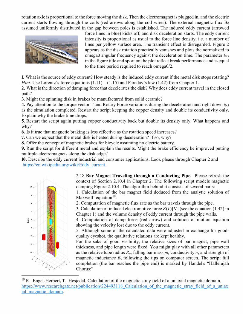
rotation axle is proportional to the force moving the disk. Then the electromagnet is plugged in, and the electric current starts flowing through the coils (red arrows along the coil wires). The external magnetic flux B0 assumed uniformly distributed in the gap between poles is established. The induced eddy current (arrowed

force lines in blue) kicks off, and disk deceleration starts. The eddy current intensity is proportional as usual to the force line density, i.e. a number of lines per yellow surface area. The transient effect is disregarded. Figure 2 appears as the disk rotation practically vanishes and plots the normalized to omega0 angular frequency against the deceleration time. The parameter t0.5 in the figure title and sport on the plot reflect break performance and is equal to the time period required to reach omega0/2.

1. What is the source of eddy current? How steady is the induced eddy current if the metal disk stops rotating? Hint. Use Lorentz’s force equations (1.11) – (1.15) and Faraday’s law (1.42) from Chapter 1. 2. What is the direction of damping force that decelerates the disk? Why does eddy current travel in the closed path? 3. Might the spinning disk in brakes be manufactured from solid ceramic? 4. Pay attention to the torque vector T and Rotary Force variations during the deceleration and right down t0.5 as the simulation completed. Restart the script keeping the copper density and double its conductivity only. Explain why the brake time drops. 5. Restart the script again putting copper conductivity back but double its density only. What happens and why? 6. Is it true that magnetic braking is less effective as the rotation speed increases? 7. Can we expect that the metal disk is heated during deceleration? If so, why? 8. Offer the concept of magnetic brakes for bicycle assuming no electric battery. 9. Run the script for different metal and explain the results. Might the brake efficiency be improved putting multiple electromagnets along the disk edge? 10. Describe the eddy current industrial and consumer applications. Look please through Chapter 2 and https://en.wikipedia.org/wiki/Eddy_current.

2.18 Bar Magnet Traveling through a Conducting Pipe. Please refresh the context of Section 2.10.4 in Chapter 2. The following script models magnetic damping Figure 2.10.4. The algorithm behind it consists of several parts: 1. Calculation of the bar magnet field deduced from the analytic solution of Maxwell’ equation19. 2. Computation of magnetic flux rate as the bar travels through the pipe. 3. Calculation of induced electromotive force ℰ(𝑑𝑑)[V] (see the equation (1.42) in Chapter 1) and the volume density of eddy current through the pipe walls. 4. Computation of damp force (red arrow) and solution of motion equation showing the velocity lost due to the eddy current. 5. Although some of the calculated data were adjusted in exchange for good-quality eyeshot, the qualitative relations are kept healthy. For the sake of good visibility, the relative sizes of bar magnet, pipe wall thickness, and pipe length were fixed. You might play with all other parameters as the relative tube radius Rp, falling bar mass m, conductivity σ, and strength of magnetic inductance B0 following the tips on computer screen. The script full completion (the bar reaches the pipe end) is marked by Handel's “Hallelujah Chorus:”

19 R. Engel-Herbert, T. Hesjedal, Calculation of the magnetic stray field of a uniaxial magnetic domain, https://www.researchgate.net/publication/224493118_Calculation_of_the_magnetic_stray_field_of_a_uniaxial_magnetic_domain.

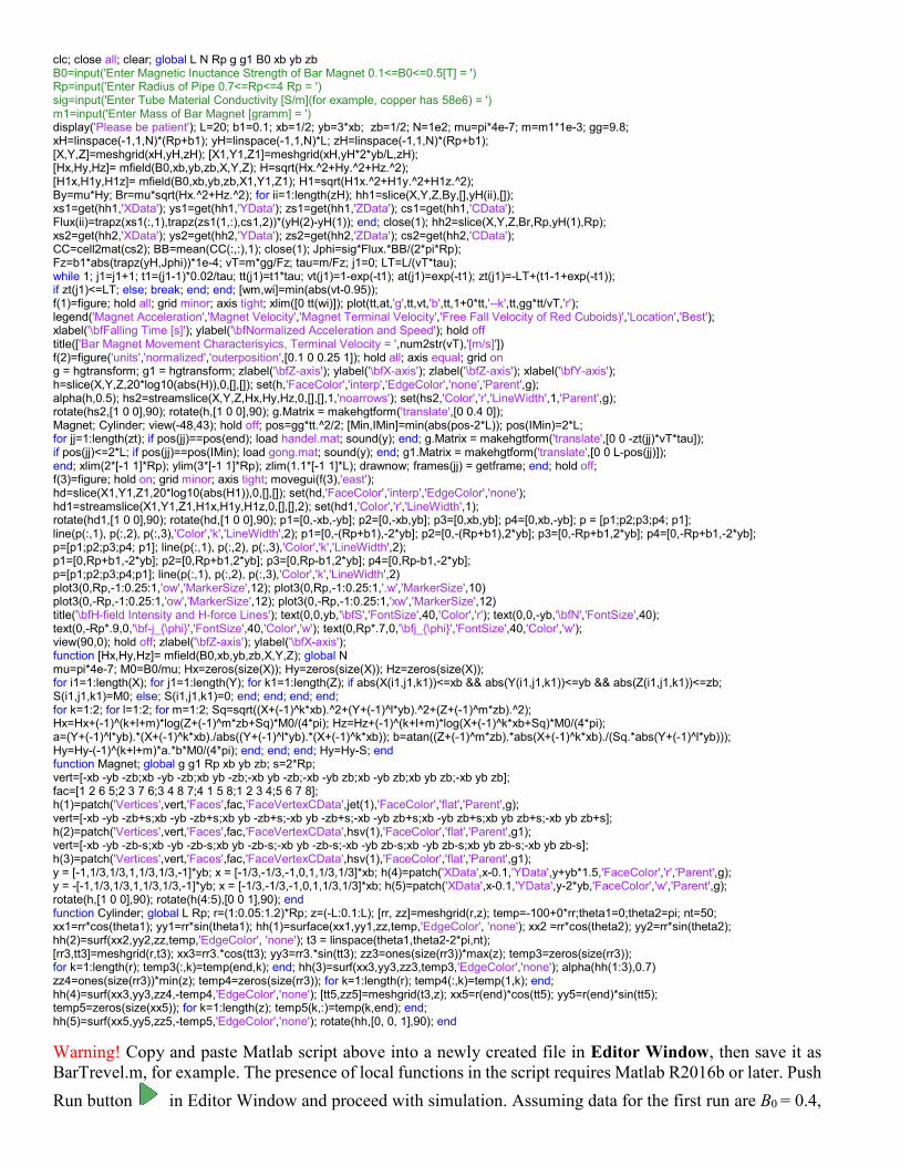
clc; close all; clear; global L N Rp g g1 B0 xb yb zb B0=input('Enter Magnetic Inuctance Strength of Bar Magnet 0.1<=B0<=0.5[T] = ') Rp=input('Enter Radius of Pipe 0.7<=Rp<=4 Rp = ') sig=input('Enter Tube Material Conductivity [S/m](for example, copper has 58e6) = ') m1=input('Enter Mass of Bar Magnet [gramm] = ') display('Please be patient'); L=20; b1=0.1; xb=1/2; yb=3*xb; zb=1/2; N=1e2; mu=pi*4e-7; m=m1*1e-3; gg=9.8; xH=linspace(-1,1,N)*(Rp+b1); yH=linspace(-1,1,N)*L; zH=linspace(-1,1,N)*(Rp+b1); [X,Y,Z]=meshgrid(xH,yH,zH); [X1,Y1,Z1]=meshgrid(xH,yH*2*yb/L,zH); [Hx,Hy,Hz]= mfield(B0,xb,yb,zb,X,Y,Z); H=sqrt(Hx.^2+Hy.^2+Hz.^2); [H1x,H1y,H1z]= mfield(B0,xb,yb,zb,X1,Y1,Z1); H1=sqrt(H1x.^2+H1y.^2+H1z.^2); By=mu*Hy; Br=mu*sqrt(Hx.^2+Hz.^2); for ii=1:length(zH); hh1=slice(X,Y,Z,By,[],yH(ii),[]); xs1=get(hh1,'XData'); ys1=get(hh1,'YData'); zs1=get(hh1,'ZData'); cs1=get(hh1,'CData'); Flux(ii)=trapz(xs1(:,1),trapz(zs1(1,:),cs1,2))*(yH(2)-yH(1)); end; close(1); hh2=slice(X,Y,Z,Br,Rp,yH(1),Rp); xs2=get(hh2,'XData'); ys2=get(hh2,'YData'); zs2=get(hh2,'ZData'); cs2=get(hh2,'CData'); CC=cell2mat(cs2); BB=mean(CC(:,:),1); close(1); Jphi=sig*Flux.*BB/(2*pi*Rp); Fz=b1*abs(trapz(yH,Jphi))*1e-4; vT=m*gg/Fz; tau=m/Fz; j1=0; LT=L/(vT*tau); while 1; j1=j1+1; t1=(j1-1)*0.02/tau; tt(j1)=t1*tau; vt(j1)=1-exp(-t1); at(j1)=exp(-t1); zt(j1)=-LT+(t1-1+exp(-t1)); if zt(j1)<=LT; else; break; end; end; [wm,wi]=min(abs(vt-0.95)); f(1)=figure; hold all; grid minor; axis tight; xlim([0 tt(wi)]); plot(tt,at,'g',tt,vt,'b',tt,1+0*tt,'--k',tt,gg*tt/vT,'r'); legend('Magnet Acceleration','Magnet Velocity','Magnet Terminal Velocity','Free Fall Velocity of Red Cuboids)','Location','Best'); xlabel('\bfFalling Time [s]'); ylabel('\bfNormalized Acceleration and Speed'); hold off title(['Bar Magnet Movement Characterisyics, Terminal Velocity = ',num2str(vT),'[m/s]']) f(2)=figure('units','normalized','outerposition',[0.1 0 0.25 1]); hold all; axis equal; grid on g = hgtransform; g1 = hgtransform; zlabel('\bfZ-axis'); ylabel('\bfX-axis'); zlabel('\bfZ-axis'); xlabel('\bfY-axis'); h=slice(X,Y,Z,20*log10(abs(H)),0,[],[]); set(h,'FaceColor','interp','EdgeColor','none','Parent',g); alpha(h,0.5); hs2=streamslice(X,Y,Z,Hx,Hy,Hz,0,[],[],1,'noarrows'); set(hs2,'Color','r','LineWidth',1,'Parent',g); rotate(hs2,[1 0 0],90); rotate(h,[1 0 0],90); g.Matrix = makehgtform('translate',[0 0.4 0]); Magnet; Cylinder; view(-48,43); hold off; pos=gg*tt.^2/2; [Min,IMin]=min(abs(pos-2*L)); pos(IMin)=2*L; for jj=1:length(zt); if pos(jj)==pos(end); load handel.mat; sound(y); end; g.Matrix = makehgtform('translate',[0 0 -zt(jj)*vT*tau]); if pos(jj)<=2*L; if pos(jj)==pos(IMin); load gong.mat; sound(y); end; g1.Matrix = makehgtform('translate',[0 0 L-pos(jj)]); end; xlim(2*[-1 1]*Rp); ylim(3*[-1 1]*Rp); zlim(1.1*[-1 1]*L); drawnow; frames(jj) = getframe; end; hold off; f(3)=figure; hold on; grid minor; axis tight; movegui(f(3),'east'); hd=slice(X1,Y1,Z1,20*log10(abs(H1)),0,[],[]); set(hd,'FaceColor','interp','EdgeColor','none'); hd1=streamslice(X1,Y1,Z1,H1x,H1y,H1z,0,[],[],2); set(hd1,'Color','r','LineWidth',1); rotate(hd1,[1 0 0],90); rotate(hd,[1 0 0],90); p1=[0,-xb,-yb]; p2=[0,-xb,yb]; p3=[0,xb,yb]; p4=[0,xb,-yb]; p = [p1;p2;p3;p4; p1]; line(p(:,1), p(:,2), p(:,3),'Color','k','LineWidth',2); p1=[0,-(Rp+b1),-2*yb]; p2=[0,-(Rp+b1),2*yb]; p3=[0,-Rp+b1,2*yb]; p4=[0,-Rp+b1,-2*yb]; p=[p1;p2;p3;p4; p1]; line(p(:,1), p(:,2), p(:,3),'Color','k','LineWidth',2); p1=[0,Rp+b1,-2*yb]; p2=[0,Rp+b1,2*yb]; p3=[0,Rp-b1,2*yb]; p4=[0,Rp-b1,-2*yb]; p=[p1;p2;p3;p4;p1]; line(p(:,1), p(:,2), p(:,3),'Color','k','LineWidth',2) plot3(0,Rp,-1:0.25:1,'ow','MarkerSize',12); plot3(0,Rp,-1:0.25:1,'.w','MarkerSize',10) plot3(0,-Rp,-1:0.25:1,'ow','MarkerSize',12); plot3(0,-Rp,-1:0.25:1,'xw','MarkerSize',12) title('\bfH-field Intensity and H-force Lines'); text(0,0,yb,'\bfS','FontSize',40,'Color','r'); text(0,0,-yb,'\bfN','FontSize',40); text(0,-Rp*.9,0,'\bf-j_{\phi}','FontSize',40,'Color','w'); text(0,Rp*.7,0,'\bfj_{\phi}','FontSize',40,'Color','w'); view(90,0); hold off; zlabel('\bfZ-axis'); ylabel('\bfX-axis'); function [Hx,Hy,Hz]= mfield(B0,xb,yb,zb,X,Y,Z); global N mu=pi*4e-7; M0=B0/mu; Hx=zeros(size(X)); Hy=zeros(size(X)); Hz=zeros(size(X)); for i1=1:length(X); for j1=1:length(Y); for k1=1:length(Z); if abs(X(i1,j1,k1))<=xb && abs(Y(i1,j1,k1))<=yb && abs(Z(i1,j1,k1))<=zb; S(i1,j1,k1)=M0; else; S(i1,j1,k1)=0; end; end; end; end; for k=1:2; for l=1:2; for m=1:2; Sq=sqrt((X+(-1)^k*xb).^2+(Y+(-1)^l*yb).^2+(Z+(-1)^m*zb).^2); Hx=Hx+(-1)^(k+l+m)*log(Z+(-1)^m*zb+Sq)*M0/(4*pi); Hz=Hz+(-1)^(k+l+m)*log(X+(-1)^k*xb+Sq)*M0/(4*pi); a=(Y+(-1)^l*yb).*(X+(-1)^k*xb)./abs((Y+(-1)^l*yb).*(X+(-1)^k*xb)); b=atan((Z+(-1)^m*zb).*abs(X+(-1)^k*xb)./(Sq.*abs(Y+(-1)^l*yb))); Hy=Hy-(-1)^(k+l+m)*a.*b*M0/(4*pi); end; end; end; Hy=Hy-S; end function Magnet; global g g1 Rp xb yb zb; s=2*Rp; vert=[-xb -yb -zb;xb -yb -zb;xb yb -zb;-xb yb -zb;-xb -yb zb;xb -yb zb;xb yb zb;-xb yb zb]; fac=[1 2 6 5;2 3 7 6;3 4 8 7;4 1 5 8;1 2 3 4;5 6 7 8]; h(1)=patch('Vertices',vert,'Faces',fac,'FaceVertexCData',jet(1),'FaceColor','flat','Parent',g); vert=[-xb -yb -zb+s;xb -yb -zb+s;xb yb -zb+s;-xb yb -zb+s;-xb -yb zb+s;xb -yb zb+s;xb yb zb+s;-xb yb zb+s]; h(2)=patch('Vertices',vert,'Faces',fac,'FaceVertexCData',hsv(1),'FaceColor','flat','Parent',g1); vert=[-xb -yb -zb-s;xb -yb -zb-s;xb yb -zb-s;-xb yb -zb-s;-xb -yb zb-s;xb -yb zb-s;xb yb zb-s;-xb yb zb-s]; h(3)=patch('Vertices',vert,'Faces',fac,'FaceVertexCData',hsv(1),'FaceColor','flat','Parent',g1); y = [-1,1/3,1/3,1,1/3,1/3,-1]*yb; x = [-1/3,-1/3,-1,0,1,1/3,1/3]*xb; h(4)=patch('XData',x-0.1,'YData',y+yb*1.5,'FaceColor','r','Parent',g); y = -[-1,1/3,1/3,1,1/3,1/3,-1]*yb; x = [-1/3,-1/3,-1,0,1,1/3,1/3]*xb; h(5)=patch('XData',x-0.1,'YData',y-2*yb,'FaceColor','w','Parent',g); rotate(h,[1 0 0],90); rotate(h(4:5),[0 0 1],90); end function Cylinder; global L Rp; r=(1:0.05:1.2)*Rp; z=(-L:0.1:L); [rr, zz]=meshgrid(r,z); temp=-100+0*rr;theta1=0;theta2=pi; nt=50; xx1=rr*cos(theta1); yy1=rr*sin(theta1); hh(1)=surface(xx1,yy1,zz,temp,'EdgeColor', 'none'); xx2 =rr*cos(theta2); yy2=rr*sin(theta2); hh(2)=surf(xx2,yy2,zz,temp,'EdgeColor', 'none'); t3 = linspace(theta1,theta2-2*pi,nt); [rr3,tt3]=meshgrid(r,t3); xx3=rr3.*cos(tt3); yy3=rr3.*sin(tt3); zz3=ones(size(rr3))*max(z); temp3=zeros(size(rr3)); for k=1:length(r); temp3(:,k)=temp(end,k); end; hh(3)=surf(xx3,yy3,zz3,temp3,'EdgeColor','none'); alpha(hh(1:3),0.7) zz4=ones(size(rr3))*min(z); temp4=zeros(size(rr3)); for k=1:length(r); temp4(:,k)=temp(1,k); end; hh(4)=surf(xx3,yy3,zz4,-temp4,'EdgeColor','none'); [tt5,zz5]=meshgrid(t3,z); xx5=r(end)*cos(tt5); yy5=r(end)*sin(tt5); temp5=zeros(size(xx5)); for k=1:length(z); temp5(k,:)=temp(k,end); end; hh(5)=surf(xx5,yy5,zz5,-temp5,'EdgeColor','none'); rotate(hh,[0, 0, 1],90); end Warning! Copy and paste Matlab script above into a newly created file in Editor Window, then save it as BarTrevel.m, for example. The presence of local functions in the script requires Matlab R2016b or later. Push Run button in Editor Window and proceed with simulation. Assuming data for the first run are B0 = 0.4,

Rp = 2, conductivity = 58e6 (copper), and m = 6. Appearing Figure 2 on the left demonstrates the magnet (light blue object) falling inside the pipe while two faster dropping non-magnetic objects (both red) are in free fall under the sole influence of gravity. The white arrow depicts the gravity force oriented down, and the red arrow shows the eddy current braking force oriented up. The magnet travels in company with its own magnetic field displayed in a vertical cross-section. The normalized characteristics of magnet movement like the acceleration a(t)/g (grin line) and velocity v(t)/vT (blue line) are pictured in Figure 1 in the center, where t is the time, g = 9.8 [m/s2], and vT is the terminal velocity. The red line reflects the non-magnetic objects’ velocity = gt. Figure 3 pictures the H-field intensity in dB, H-force lines, and traces (in white) of azimuthal component 𝑗𝑗𝑒𝑒𝑒𝑒𝑒𝑒 of eddy current in the pipe walls. 2.19 Eddy Current on Copper Disk in Uniform Magnetic Field of 50 Hz. Go to

https://1drv.ms/u/s!AjtsKS-uvNP1izLQ1kr-SD_FUV7W. Download file clicking on Download, save it, start CST STUDIO SUITE, and run the model. The copper disk of the 2mm radius and 0.5mm height is placed in external uniform AC magnetic H-field of 1000[A/m]. Beneath you can find some pictures illustrating the numerical simulation. Figure 1 depicts the 3D H-force lines around the disk, Figure 2 shows E-force lines in the XY-plane corresponding to

the top surface of the disk, i.e. z = 0.25mm, whereas Figure 3 reflects 𝑗𝑗𝑒𝑒𝑒𝑒𝑒𝑒-density and 𝑗𝑗𝑒𝑒𝑒𝑒𝑒𝑒-force lines of eddy current on the disk top. Bellow Figure 5 is the contour plot of the same current density as in Figure 4, while Figure 5 pictures E-field distribution on the top disk surface. Now is the time to check your

understanding and explain the received results.

1. Does the plot in Figure 1 demonstrate the uniform distribution of H-fields and their orientation correctly? How to calculate the flux of those fields? 2. What does happen if the frequency of the external H-fields drops to zero? 3. What is the induced EMF ℰ(𝑑𝑑) direction relative to

H-field flux variations causing it? 4. What is the source of E-fields on the disk surface and nearby?

H

Figure 1 Figure 2 Figure 3

Figure 4 Figure 5

5. Check the unit dimension of magnetic field flux Φ𝑚𝑚(𝑑𝑑)in the expression (1.42) using Table 1.5 in Chapter 1 and compare the units of this flux and magnetic current (1.10). 6. Might we interpret the source of E-fields as a model for magnetic current? If so, could the magnetic current in (1.10) be defined as 𝐼𝐼𝑚𝑚 = 𝑑𝑑Φ𝑚𝑚(𝑑𝑑) 𝑑𝑑𝑑𝑑⁄ and Lenz’s law rewritten as ℰ(𝑑𝑑) = −𝐼𝐼𝑚𝑚? 7. Do these E-fields is a conservative/irrotational ones, i.e. static and ∮𝑬𝑬 ∘ 𝑑𝑑𝒍𝒍 = 0 (check Section 2.2.8 in Chapter 2), or solenoidal, i.e. ∮𝑬𝑬 ∘ 𝑑𝑑𝒍𝒍 ≠ 0? Could the source of E-fields be defined as ∮𝑬𝑬 ∘ 𝑑𝑑𝒍𝒍 = ∮𝒗𝒗 × 𝑩𝑩 ∘ 𝑑𝑑𝒍𝒍 = −𝑰𝑰𝒎𝒎 (check (1.15)) where 𝒗𝒗 is the velocity vector of electrons’ circular movement around the alternative magnetic inductance vector 𝑩𝑩(𝑑𝑑)? 8. What happens with electrons inside the disk under the influence of these E-fields? What occurs with the energy H-fields transformed into E-fields and eddy current? Is the heat generated by the disk while AC H-field is supported? If not, why not? 9. Explain the eddy current orientation in Figure 3 and why the plots in Figure 2 and 3 are so similar (Hint. Check Lorentz’s force equation (1.11) in Chapter 1). How does the rate of flow of electric charge define electric current? 10. What is the difference between electric current and eddy current on the atomic level? 11. Might we be sure that the contour plots in Figure 4 and 5 correctly illustrate the eddy current and E-field distribution? If not, give the reasons. 12. What happens with the eddy current volume density if the copper is replaced with aluminum or iron? Rerun CST model to check your answer assuming the aluminum conductivity 𝜎𝜎 = 3.5 ∙ 107 and 𝜎𝜎 =1.04 ∙ 107 for iron. To check this density along the disk radius, open files in 1D Results of CST Navigation Tree (on the left), click consequently the plus signs of the folder ‘Field Along Curve’, ‘curve 1’, ‘Imag. Part’, and finally ‘Cond. Current Dens. [Freq]’. Look at the plots, write down the current peak at the disk edge for every run, and compare them. Explain the results. 13. What can be expected if the disk material is Alumina ceramic? 14. Offer ideas for a probe designed to measure eddy current magnitude. 15. Describe the area of practical applications of eddy current effect.

2.20 Effect of Electromagnetic Cloaking/Hiding Copper Cylinder (shown in yellow) by the Layer of Anisotropic Inhomogeneous Metamaterial (yellow).20 The central concept of an electromagnetic cloak is to create a shell-like structure, whose permittivity and permeability distributions allow the incident waves to be directed around the inner region containing a concealed object and recovered afterward. In our case, the hidden object is a copper cylinder (magenta) of radius a, conductivity =5.95*107, and infinite length along the z-axis. This cylinder is fully enclosed by metamaterial tube (yellow) of inner radius a and outer radius b. The propagating to the assembly EM-wave is depicted in the same way as perfectly circular

ripples emerged and moved (along white arrows) on the surface of the water when a pebble is thrown in a quiet pond. You can find more information about antennas radiating such EM-fields in Section 4.2 of Chapter 4 (look at Figure 4.2.3). As soon as the water or EM-wave touches some obstacle, the reflected or moving back wave appears as it demonstrated below. Therefore, the permittivity and permeability of tube metamaterial should be designed in such a way that there is no or almost no reflected wave. Consequently, the cylinder becomes practically undetectable, i.e. invisible. Since the math behind the cloaking effect is quite

20 The following Matlab script was kindly provided by Prof. Zsolt Szabo, Budapest University of Technology and Economics, Hungary. The detailed model and cloaking theory can be found at https://pp.bme.hu/eecs/article/download/7077/6154. See also the experimental verification of microwave clocking at http://www.wfsj.org/course/docs/Cloack_Schurig-10-20-06.pdf.

complicated20, the primary goal of the following Matlab scripts is just to illustrate (through numerical simulation) the cloaking effect showing the transitional EM-wave movement around the copper cylinder. Warning! To get results, Matlab PDE (Partial Differential Equation) Toolbox has to be installed on your computer.

When the vector of E-field orientates along the z-axis, the cloak tube must have the material property20 𝜀𝜀 =𝜀𝜀0(𝑏𝑏 (𝑏𝑏 − 𝑎𝑎)⁄ )2, 𝜇𝜇(𝑣𝑣) = 𝜇𝜇0((𝑣𝑣 − 𝑎𝑎)/𝑣𝑣)2 and absolute refraction index 𝑛𝑛(𝑣𝑣) = �𝜀𝜀𝜇𝜇(𝑣𝑣) where 0 < 𝑣𝑣 < 𝑏𝑏 the radial parameter is in transformed coordinates20. Meanwhile, the azimuthal permittivity component should be constant and equal to 𝜇𝜇0, i.e. the tube material is anisotropic and inhomogeneous. Note that on the tube surface (r = b) 𝑛𝑛(𝑏𝑏)2 =

𝜀𝜀𝜇𝜇(𝑏𝑏) = 𝜀𝜀0𝜇𝜇0. Accordingly, there is no real border separating the tube and free space. Metaphorically speaking, EM-wave is invited to go freely inside the tube. The purpose of coordinate transformation is to convert the piecewise medium of tube + copper rod into a single continuous material with fictional parameters21.

To get the required Matlab scripts, go to https://1drv.ms/f/s!AjtsKS-uvNP1avsbUFY9UsxLVVE and then

1. Click the right/secondary button on the mouse while the cursor hovers over the icon EM_Cloaking.m and choose Download.

2. Repeat this procedure and download the file Animation.m. 3. Save files in your Matlab directory and then open both of them into Matlab Editor Window.

4. To start numerical simulation open EM_Cloaking.m file and push Run button in Editor Window. The PDE Modeler Window appears and stays for some time until the initial and frozen in time EM-field plot emerges.

5. Click OK on the warning notice indicating that the finite element analysis (read Sections 9.1.2 – 9.1.4 in Chapter 9) in the time domain is finished.

6. The time has come to enjoy the animation demonstrating the EM-wave propagation around the copper cylinder. To save the mesh data, click on ‘Mesh’ button (top Menubar of PDE Modeler), choose the option ‘Export Mesh’, and just click ‘OK’ on the bottom of the small window. Note that p is the mesh node coordinates, e is the mesh edges, t is the mesh triangles.

7. Next click on ‘Solve’ button (top Menubar of PDE Modeler), choose ‘Export Solution’, and push OK to save the u-solution values.

8. That’s all, the numerical solution is ready for demonstration. To get it, in Edit Window switch to the file

Animation.m and push Run button . 9. Enjoy a movie in slow motion of EM-wave first and then accelerated one. The deep blue areas reveal the

temporal position of E-field nodes/minimums while the antinodes/maximums are marked in deep red. These nodes and antinodes indicate the location and shape of so-called phase wavefronts (See expression (4.64) in Chapter 3). Trace their movement watching how EM-wave penetrates through the metamaterial tube surface, deforms its wavefront, and bends around the copper rod. Pay attention to the circular shape of wavefronts before and after the tube.

21 A.V. Kildishev, W. Cai, U.K. Chettiar and V M Shalaev, Transformation optics: approaching broadband electromagnetic cloaking, New Journal of Physics, Volume 10, November 2008.

10. Figure 2 on the left depicts the gradually diminishing refraction index/coefficient distribution inside the tube while Figure 3 displays the tube material relative parameters vs. the normalized radius. All data are in the transform coordinates. The white area inside the tube in Figure 2 corresponds to the copper tube location. Please refresh the context of Section 2.8 and look at Figure 2.8.5 - 2.8.10 in Chapter 2. 1. Explain the bending effect as EM-wave propagates through the tube exercising the approach similar to shown in Figure 6.3.4 of Chapter 6. (Hint. Assume that the continuous refraction index in Figure 3 is approximated by piecewise constant function and then apply Snell’s law to each layer). 2. Explain the E-field intensity reduction as EM-wave penetrates the tube (Hint. Check the tube permeability in displayed Figure 3 and expression (2.12) in Chapter 2). 3. Using the bending effect explanation compare the paths ran by the wavefront around the copper rod and by the cylindrical wavefront moving straightforward outside in free space. Are they equal? If not, which path is longer? 4. Which of these wavefronts moves faster (see the expression for v in Section 2.8.1 of Chapter 2 and refraction index data are taken from Figure 3)? 5. How does it happen that the wavefront running longer path emerges from the tube at the same moment of time as straightforward one running in free space and complements the last to almost perfect cylindrical? 6. Does the animation really point out that the copper rod becomes invisible? If so, what is the key indicator? 7. What are the differences between the broad and narrow definition of metamaterials? Looking at Figure 2.8.6 – 2.8.10 in Chapter 2 explain how to manipulate the permittivity and permeability of materials. 8. What does it mean the sub-wavelength inclusions? 9. Describe the refraction and Doppler’s effect in metamaterials with negative refraction coefficient. 10. What does it mean close to perfect focusing by flat-lens? Visit and watch the animation at https://www.youtube.com/watch?v=FmPmEB4xUKk. For more information visit https://www.youtube.com/watch?v=gjfYohXoiz0, https://www.youtube.com/watch?v=jseHPnqXlPY, https://www.youtube.com/watch?v=LFxQEUDIAuk. 2.21. More about Hysteresis (B-H) Loop. If you have access to COMSOL Multiphysics®22, go to

https://1drv.ms/f/s!AjtsKS-uvNP1avsbUFY9UsxLVVE, download ‘vector_hysteresis_modeling.mph’ file, save and run it. Figure 1 on the left depicts the model geometry23 that is comprised of a magnetic core (brown) and two coils (blue) inducing the alternative magnetic field in the steel core. Both coils connected to the same harmonic voltage source of 14.5 sin(2𝜋𝜋𝑓𝑓𝑑𝑑) [V] where 𝑓𝑓 =10Hz. The core consists of 5 laminated steel layers of 0.48mm thickness each.

More information about material can be found in publication23 or checking Materials/ Jiles-Atherton Anisotropic Hysteretic Material (mat3) in the Model Builder tree. Figure 1 below illustrates the magnetic moments (red cone) of domains randomly oriented and spontaneous magnetized to saturation at t = 0 like shown in Figure 2.6.2 of Chapter 2. Meanwhile, Figure 2 demonstrates the magnetize flux density [T] at t = 245ms as the domains are forced to the total alignment. Figure 3 and 4 expose the hysteresis loop and coil current, respectively, while Figure 5 represents the data about the current harmonic components. Enjoy and understand the two impressive animations created by CST tool that are stored in https://1drv.ms/f/s!AjtsKS-uvNP1avsbUFY9UsxLVVE. Now several addition questions about the hysteresis. 1. Explain the magnetization process leading the domain structure from shown in Figure 1 to Figure 2. Is this process linear in time or not?

22 https://www.comsol.com/products 23 https://www.comsol.com/model/download/525641/models.acdc.vector_hysteresis_modeling.pdf

2. Correlate the shape of current in Figure 4 with the hysteresis loop in Figure 3. Why does the current variation not of the same form as the voltage (not in scale) at the beginning of the magnetization process up to ∆𝑑𝑑 ≤ 50ms?

3. Compare plots in Figure 3 and Figure 2.6.3 of Chapter 2 and estimate such steel parameters as Saturation, Retentivity, and Coercivity. What does each parameter mean? 4. Explain why the spectrum components of the current peak around the odd harmonics 30Hz, 50Hz, and so on. 5. What does Curie’s temperature mean for ferromagnetic? Suggest a method to experimentally measure it. 6. Continue your research running COMSOL and discussing the results with your instructor and team member.

Figure 1 Figure 2

Figure 3 Figure 4

Figure 5

X

Y

X

Y

B

H