
Principles of Turbomachinery 2.pdf - Free
467
-
Upload
khangminh22 -
Category
Documents
-
view
6 -
download
0
Transcript of Principles of Turbomachinery 2.pdf - Free


Principles of Turbomachinery

Principles of Turbomachinery
Seppo A. Korpela The Ohio State University
WILEY A JOHN WILEY & SONS, INC., PUBLICATION
Copyright © 2011 by John Wiley & Sons, Inc. All rights reserved.
Published by John Wiley & Sons, Inc., Hoboken, New Jersey. Published simultaneously in Canada.
No part of this publication may be reproduced, stored in a retrieval system or transmitted in any form or by any means, electronic, mechanical, photocopying, recording, scanning or otherwise, except as permitted under Section 107 or 108 of the 1976 United States Copyright Act, without either the prior written permission of the Publisher, or authorization through payment of the appropriate per-copy fee to the Copyright Clearance Center, Inc., 222 Rosewood Drive, Danvers, MA 01923, (978) 750-8400, fax (978) 750-4470, or on the web at www.copyright.com. Requests to the Publisher for permission should be addressed to the Permissions Department, John Wiley & Sons, Inc., 111 River Street, Hoboken, NJ 07030, (201) 748-6011, fax (201) 748-6008, or online at http://www.wiley.com/go/permission.
Limit of Liability/Disclaimer of Warranty: While the publisher and author have used their best efforts in preparing this book, they make no representation or warranties with respect to the accuracy or completeness of the contents of this book and specifically disclaim any implied warranties of merchantability or fitness for a particular purpose. No warranty may be created or extended by sales representatives or written sales materials. The advice and strategies contained herein may not be suitable for your situation. You should consult with a professional where appropriate. Neither the publisher nor author shall be liable for any loss of profit or any other commercial damages, including but not limited to special, incidental, consequential, or other damages.
For general information on our other products and services please contact our Customer Care Department within the United States at (800) 762-2974, outside the United States at (317) 572-3993 or fax (317) 572-4002.
Wiley also publishes its books in a variety of electronic formats. Some content that appears in print, however, may not be available in electronic formats. For more information about Wiley products, visit our web site at www.wiley.com.
Library of Congress Cataloging-in-Publication Data:
Korpela, S. A. Principles of turbomachinery / Seppo A. Korpela. — 1st ed.
p. cm. Includes index. ISBN 978-0-470-53672-8 (hardback)
1. Turbomachines. I. Title. TJ267.K57 2011 621.406—dc23 2011026170
Printed in the United States of America.
10 9 8 7 6 5 4 3 2 1

To my wife Terttu, to our daughter Liisa,
and to the memory of our daughter Katja
CONTENTS
Foreword
Acknowledgments
1 Introduction
1.1
1.2
Energy 1.1.1 1.1.2 1.1.3 1.1.4 1.1.5 1.1.6 1.1.7 1.1.8
and fluid machines Energy conversion of fossil fuels Steam turbines Gas turbines Hydraulic turbines Wind turbines Compressors Pumps and blowers Other uses and issues
Historical survey 1.2.1 1.2.2 1.2.3 1.2.4 1.2.5 1.2.6
Water power Wind turbines Steam turbines Jet propulsion Industrial turbines Note on units
M l
1 1 2 3 4 5 5 5 6 7 7 8 9
10 11 12
Viii CONTENTS
Principles of Thermodynamics and Fluid Flow 15
2.1 Mass conservation principle 15 2.2 First law of thermodynamics 17 2.3 Second law of thermodynamics 19
2.3.1 Tds equations 19 2.4 Equations of state 20
2.4.1 Properties of steam 21 2.4.2 Ideal gases 27 2.4.3 Air tables and isentropic relations 29 2.4.4 Ideal gas mixtures 31 2.4.5 Incompressibility 35 2.4.6 Stagnation state 35
2.5 Efficiency 36 2.5.1 Efficiency measures 36 2.5.2 Thermodynamic losses 42 2.5.3 Incompressible fluid 43 2.5.4 Compressible flows 44
2.6 Momentum balance 47 Exercises 54
Compressible Flow through Nozzles 57
3.1 Mach number and the speed of sound 57 3.1.1 Mach number relations 59
3.2 Isentropic flow with area change 61 3.2.1 Converging nozzle 65 3.2.2 Converging-diverging nozzle 67
3.3 Normal shocks 69 3.3.1 Rankine-Hugoniot relations 73
3.4 Influence of friction in flow through straight nozzles 75 3.4.1 Polytropic efficiency 75 3.4.2 Loss coefficients 79 3.4.3 Nozzle efficiency 82 3.4:4 Combined Fanno flow and area change 84
3.5 Supersaturation 90 3.6 Prandtl-Meyer expansion 92
3.6.1 Mach waves 92 3.6.2 Prandtl-Meyer theory 93
3.7 Flow leaving a turbine nozzle 100 Exercises 103
4 Principles of Turbomachine Analysis 105
CONTENTS ix
4.1 Velocity triangles 106 4.2 Moment of momentum balance 108 4.3 Energy transfer in turbomachines 109
4.3.1 Trothalpy and specific work in terms of velocities 113 4.3.2 Degree of reaction 116
4.4 Utilization 117 4.5 Scaling and similitude 124
4.5.1 Similitude 124 4.5.2 Incompressible flow 125 4.5.3 Shape parameter or specific speed 128 4.5.4 Compressible flow analysis 128
4.6 Performance characteristics 130 4.6.1 Compressor performance map 131 4.6.2 Turbine performance map 131 Exercises 132
135
135
137
137
146
150
152
158
160
162
Axial Turbines 165
6.1 Introduction 165 6.2 Turbine stage analysis 167 6.3 Flow and loading coefficients and reaction ratio 171
6.3.1 Fifty percent (50%) stage 176 6.3.2 Zero percent (0%) reaction stage 178 6.3.3 Off-design operation 179
6.4 Three-dimensional flow 181 6.5 Radial equilibrium 181
6.5.1 Free vortex flow 183 6.5.2 Fixed blade angle 186
6.6 Constant mass flux 187 6.7 Turbine efficiency and losses 190
6.7.1 Soderberg loss coefficients 190
Steam Turbines
5.1 5.2
5.3 5.4
Introduction Impulse turbines 5.2.1 5.2.2 5.2.3 5.2.4 Stage
Single-stage impulse turbine Pressure compounding Blade shapes Velocity compounding
with zero reaction Loss coefficients Exercises
X CONTENTS
6.7.2 Stage efficiency 191 6.7.3 Stagnation pressure losses 192 6.7.4 Performance charts 198 6.7.5 Zweifel correlation 203 6.7.6 Further discussion of losses 204 6.7.7 Ainley-Mathieson correlation 205 6.7.8 Secondary loss 209
6.8 Multistage turbine 214 6.8.1 Reheat factor in a multistage turbine 214 6.8.2 Polytropic or small-stage efficiency 216 Exercises 217
Axial Compressors 221
7.1 Compressor stage analysis 222 7.1.1 Stage temperature and pressure rise 223 7.1.2 Analysis of a repeating stage 225
7.2 Design deflection 230 7.2.1 Compressor performance map 234
7.3 Radial equilibrium 235 7.3.1 Modified free vortex velocity distribution 236 7.3.2 Velocity distribution with zero-power exponent 239 7.3.3 Velocity distribution with first-power exponent 240
7.4 Diffusion factor 242 7.4.1 Momentum thickness of a boundary layer 244
7.5 Efficiency and losses 247 7.5.1 Efficiency* 247 7.5.2 Parametric calculations 250
7.6 Cascade aerodynamics 252 7.6.1 Blade shapes and terms 252 7.6.2 Blade forces 253 7.6.3 Other losses 256 7.6.4 Diffuser performance 257 7.6.5 Flow deviation and incidence 257 7.6.6 Multistage compressor 259 7.6.7 Compressibility effects 261 Exercises 262
Centrifugal Compressors and Pumps 265
8.1 Compressor analysis 266 8.1.1 Slip factor 267 8.1.2 Pressure ratio 269

CONTENTS xi
8.2 Inlet design 274 8.2.1 Choking of the inducer 278
8.3 Exit design 281 8.3.1 Performance characteristics 281 8.3.2 Diffusion ratio 283 8.3.3 Blade height 284
8.4 Vaneless diffuser 285 8.5 Centrifugal pumps 290
8.5.1 Specific speed and specific diameter 294 8.6 Fans 302 8.7 Cavitation 302 8.8 Diffuser and volute design 305
8.8.1 Vaneless diffuser 305 8.8.2 Volute design 306 Exercises 309
9 Radial Inflow Turbines 313
9.1 Turbine analysis 314 9.2 Efficiency 319 9.3 Specific speed and specific diameter 323 9.4 Stator flow 329
9.4.1 Loss coefficients for stator flow 333 9.5 Design of the inlet of a radial inflow turbine 337
9.5.1 Minimum inlet Mach number 338 9.5.2 Blade stagnation Mach number 343 9.5.3 Inlet relative* Mach number 345
9.6 Design of the Exit 346 9.6.1 Minimum exit Mach number 346 9.6.2 Radius ratio r%s/r2 348 9.6.3 Blade height-to-radius ratio 62/^2 350 9.6.4 Optimum incidence angle and the number of blades 351 Exercises 356
10 Hydraulic Turbines 359
10.1 Hydroelectric Power Plants 359 10.2 Hydraulic turbines and their specific speed 361 10.3 Pelton wheel 363 10.4 Francis turbine 370 10.5 Kaplan turbine 377 10.6 Cavitation 380
Exercises 382
XII CONTENTS
11 Hydraulic Transmission of Power 385
11.1 Fluid couplings 385 11.1.1 Fundamental relations 386 11.1.2 Flow rate and hydrodynamic losses 388 11.1.3 Partially filled coupling 390
11.2 Torque converters 391 11.2.1 Fundamental relations 392 11.2.2 Performance 394 Exercises 398
12 Wind turbines 401
12.1 Horizontal-axis wind turbine 402 12.2 Momentum and blade element theory of wind turbines 403
12.2.1 Momentum Theory 403 12.2.2 Ducted wind turbine 407 12.2.3 Blade element theory and wake rotation 409 12.2.4 Irrotational wake 412
12.3 Blade Forces 415 12.3.1 Nonrotating wake 415 12.3.2 Wake with rotation 419 12.3.3 Ideal wind turbine 424 12.3.4 Prandtl's tip correction 425
12.4 Turbomachinery and future prospects for energy 429 Exercises 430
Appendix A: Streamline curvature and radial equilibrium 431 A.l Streamline curvature method 431
A. 1.1 Fundamental equations 431 A. 1.2 Formal solution 435
Appendix B: Thermodynamic Tables 437
References 449
Index 453

Foreword
Turbomachinery is a subject of considerable importance in a modern industrial civilization. Steam turbines are at the heart of central station power plants, whether fueled by coal or uranium. Gas turbines and axial compressors are the key components of jet engines. Aeroderivative gas turbines are also used to generate electricity with natural gas as fuel. Same technology is used to drive centrifugal compressors for transmitting this natural gas across continents. Blowers and fans are used for mine and industrial ventilation. Large pumps are often driven with steam turbines to provide feedwater to boilers. They are used in sanitation plants for wastewater cleanup. Hydraulic turbines generate electricity from water stored in reservoirs, and wind turbines do the same from the flowing wind.
This book is on the principles of turbomachines. It aims for a unified treatment of the subject matter, with consistent notation and concepts. In order to provide a ready reference to the reader, some of the developments have been repeated in more than one chapter. This also makes possible the omission of some chapters from a course of study. The subject matter becomes somewhat more general in three of the later chapters.
XIII
Acknowledgments
The subject of turbomachinery occupied a central place in mechanical engineering cur-riculum some half a century ago. In the early textbooks fluid mechanics was taught as a part of a course on turbomachinery, and many of the pioneers of fluid dynamics worked out the many technical issues related to these machines. The field still draws substantial interest. Today the situation has been turned around, and books on fluid dynamics introduce turbomachines in one or two chapters. The same relationship existed with thermodynamics and steam power plants, but today an introduction to steam power plants is usually found in a single chapter in an introductory^textbook on thermodynamics.
The British tradition on turbomachinery is long and illustrious. There W. J. Kearton established a center at the University of Liverpool nearly a century ago. His book Steam Turbine Theory and Practice became a standard reference source. After his retirement J. H. Horlock occupied the Harrison Chair of Mechanical Engineering there for a decade. His book Axial Flow Compressors appeared in 1958 and its complement, Axial Flow Tur-bines, in 1966. Whereas Horlock's books are best suited for advanced workers in the field, at University of Liverpool, S. L. Dixon's textbook Fluid Mechanics and Thermodynamics ofTurbomachinery appeared in 1966, and its later editions continue in print. It is well suited for undergraduates. Another textbook in the British tradition is the Gas Turbine Theory by H. Cohen and G. F. C. Rogers. It was first published in 1951 and in later editions still today. At a more advanced level are R. I. Lewis's Turbomachinery Performance Analysis from 1996, N. A. Cumpsty's Compressor Aerodynamics published in 1989, and the Design of Radial Turbomachines by A. Whitfield and N. C. Baines in 1990.
More than a generation of American students learned this subject from D. G. Sheppard's Principles ofTurbomachinery and later from the short Turbomachinery—Basic Theory and Applications by E. Logan, Jr. The venerable A. Stodola's Steam and Gas Turbines has been
xv
xvi
translated to English, but many others classic works, such as W. Traupel's Thermische Tur-bomaschinen and the seventh edition of Stromungsmachinen, by Pfieiderer and Petermann, require a good reading knowledge of German.
I am indebted to all the above mentioned authors for their fine efforts to make the study of this subject enjoyable.
My introduction to the field of turbomachinery came thanks to my longtime colleague, the late Richard H. Zimmerman. After working on other areas of mechanical engineering for many years, I returned to this subject after Reza Abhari invited me to spend a summer at ETH in Zurich. There I also met Anestis Kalfas, now also at the Aristotle University of Thessaloniki. I am grateful to both of them for sharing their lecture notes, which showed me how the subject was taught at the institutions of learning where they had completed their studies and how they have developed it further. I am grateful to my former student and friend, V. Babu, a professor of Mechanical Engineering of the Indian Institute of Technology, Madras, for reading the manuscript and making many helpful suggestions for improving it. Undoubtedly some errors have remained, and I will be thankful for readers who take the time to point them out by e-mail to me at the address: korpela.l @osu.edu.
I am grateful for permission to use graphs and figures from various published works and wish to acknowledge the generosity of the various organization for granting the permission to use them. These include Figures 1.1 and 1.2 from Siemens press photo, Siemens AG; Figure 1.3, from Schmalenberger Stromungstechnologie AG; Figures 1.6 and7.1 are by courtesy of MAN Diesel & Turbo SE, and Figures 4.12 and 4.11 are published by permission of BorgWarner Turbo Systems. Figure 3.7 is courtesy of Professor D. Papamaschou; Figures 10.3 and 10.11 are published under the GNU Free Documentation licenses with original courtesy of Voith Siemens Hydro. The Figure 10.9 is reproduced under the Gnu Free Documentation licence, with the original photo by Audrius Meskauskas. Figure 1.5 is also published under Gnu Free Documentation licence, and so is Figure 1.4 and by permission from Aermotor. The Institution of Mechanical Engineers has granted permission to reproduce Figures 3.14,6.16,7.5,7.6, and 7.16. Figure 4.10 is published under agreement with NASA. The Journal of the Royal Aeronautical Society granted permission to publish Figure 6.11. Figures 6.19 and 6.20 are published under the Crown Stationary Office's Open Government Licence of UK. Figure 3.11 has been adapted from J. H. Keenan, Thermodynamics, MIT Press and Figure 9.6 from O. E. Balje, Turbo machines A guide to Selection and Theory. Permission to use Figures 12.13 and 12.15 from Wind Turbine Handbook by T. Burton, N. Jenkins, D. Sharpe, and E. Bossanyi has been granted by John Wiley & Sons.
I have been lucky to have Terttu as a wife and a companion in my life. She has been and continues to be very supportive of all my efforts.
S. A. K.
CHAPTER 1
INTRODUCTION
1.1 ENERGY AND FLUID MACHINES
The rapid development of modern industrial societies was made possible by the large-scale extraction of fossil fuels buried in the earth's crust. Today oil makes up 37% of world's energy mix, coal's share is 27%, and that of natural gas is 23%, for a total of 87%. Hydropower and nuclear energy contribute each about 6% which increases the total from these sources to 99%. The final 1% is supplied by wind, geothermal energy, waste products, and solar energy. Biomass is excluded from these, for it is used largely locally, and thus its contribution is difficult to calculate. The best estimates put its use at 10% of the total, in which case the other percentages need to be adjusted downward appropriately [54].
1.1.1 Energy conversion of fossil fuels
Over the the last two centuries engineers invented methods to convert the chemical energy stored in fossil fuels into usable forms. Foremost among them are methods for converting this energy into electricity. This is done in steam power plants, in which combustion of coal is used to vaporize steam and the thermal energy of the steam is then converted to shaft work in a steam turbine. The shaft turns a generator that produces electricity. Nuclear power plants work on the same principle, with uranium, and in rare cases thorium, as the fuel.
Principles of Turbomachinery. By Seppo A. Korpela 1 Copyright © 2011 John Wiley & Sons, Inc.
2 INTRODUCTION
Oil is used sparingly this way, and it is mainly refined to gasoline and diesel fuel. The refinery stream also yields residual heating oil, which goes to industry and to winter heating of houses. Gasoline and diesel oil are used in internal-combustion engines for transportation needs, mainly in automobiles and trucks, but also in trains. Ships are powered by diesel fuel and aircraft, by jet fuel.
Natural gas is largely methane, and in addition to its importance in the generation of electricity, it is also used in some parts of the world as a transportation fuel. A good fraction of natural gas goes to winter heating of residential and commercial buildings, and to chemical process industries as raw material.
Renewable energy sources include the potential energy of water behind a dam in a river and the kinetic energy of blowing winds. Both are used for generating electricity. Water waves and ocean currents also fall into the category of renewable energy sources, but their contributions are negligible today.
In all the methods mentioned above, conversion of energy to usable forms takes place in a. fluid machine, and in these instances they are power-producing machines. There are also power-absorbing machines, such as pumps, in which energy is transferred into a fluid stream.
In both power-producing and power-absorbing machines energy transfer takes place be-tween a fluid and a moving machine part. In positive-displacement machines the interaction is between a fluid at high pressure and a reciprocating piston. Spark ignition and diesel engines are well-known machines of this class. Others include piston pumps, reciprocating and screw compressors, and vane pumps.
In turbomachines energy transfer takes place between a continuously flowing fluid stream and a set of blades rotating about a fixed axis. The blades in a pump are part of an impeller that is fixed to a shaft. In an axial compressor they are attached to a compressor wheel. In steam and gas turbines the blades are fastened to a disk, which is fixed to a shaft, and the assembly is called a turbine rotor. Fluid is guided into the rotor by stator vanes that are fixed to the casing of the machine. The inlet stator vanes are also called nozzles, or inlet guidevanes.
Examples of power-producing turbomachines are steam and gas turbines, and water and wind turbines. The power-absorbing turbomachines include pumps, for which the working fluid is a liquid, and fans, blowers, and compressors, which transfer energy to gases.
Methods derived from the principles of thermodynamics and fluid dynamics have been developed to analyze the design and operation of these machines. These subjects, and heat transfer, are the foundation of energy engineering, a discipline central to modern industry.
1.1.2 Steam tu rbi nes
Central station power plants, fueled either by coal or uranium, employ steam turbines to convert the thermal energy of steam to shaft power to run electric generators. Coal provides 50% and nuclear fuels 20% of electricity production in the United States. For the world the corresponding numbers are 40% and 15%, respectively. It is clear from these figures that steam turbine manufacture and service are major industries in both the United States and the world.
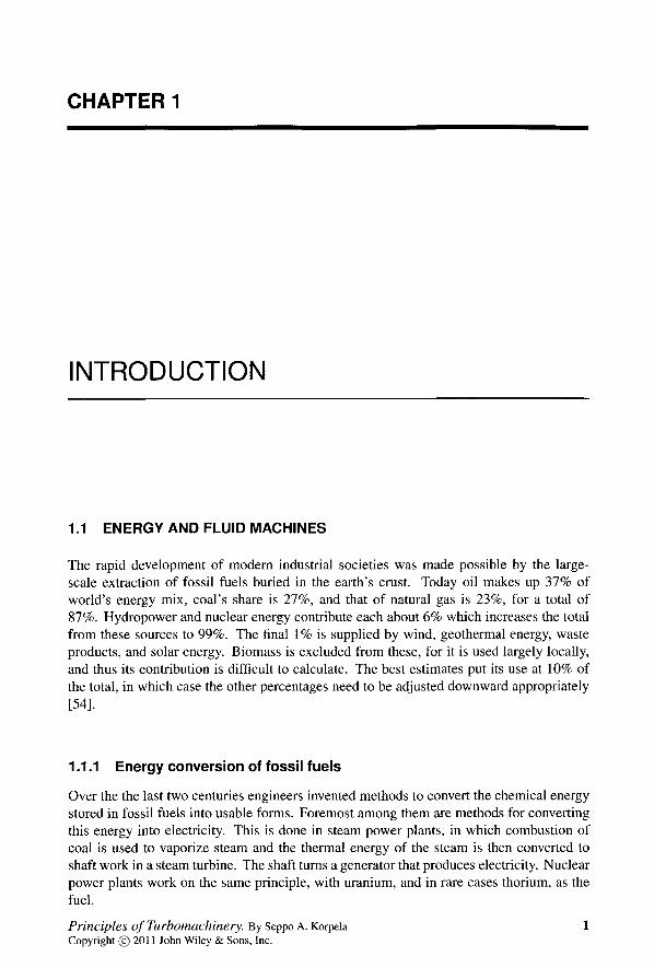
Figure 1.1 shows a 100-MW steam turbine manufactured by Siemens AG of Germany. Steam enters the turbine through the nozzles near the center of the machine, which direct the flow to a rotating set of blades. On leaving the first stage, steam flows (in the sketch toward the top right corner) through the rest of the 12 stages of the high-pressure section in this turbine. Each stage consists of a set rotor blades, preceded by a set of stator vanes.
ENERGY AND FLUID MACHINES 3
Figure 1.1 The Siemens SST-600 industrial steam turbine with a capacity of up to 100-MW. (Courtesy Siemens press picture, Siemens AG.)
The stators, fixed to the casing (of which one-quarter is removed in the illustration), are not clearly visible in this figure. After leaving the high-pressure section, steam flows into a two-stage low-pressure turbine, and from there it leaves the machine and enters a condenser located on the floor below the turbine bay. Temperature of the entering steam is up to 540° C and its pressure is up to 140 bar. Angular speed of the shaft is generally in the range 3500-15,000 rpm (rev/min). In this turbine there are five bleed locations for the steam. The steam extracted from the bleeds enters feedwater heaters, before it flows back to a boiler. The large regulator valve in the inlet section controls the steam flow rate through the machine.
In order to increase the plant efficiency, new designs operate at supercritical pressures. In an ultrasupercritical plant, the boiler pressure can reach 600 bar and turbine inlet tem-perature, 620°C. Critical pressure for steam is 220.9 bar, and its critical temperature is 373.14°C.
1.1.3 Gas turbines
Major manufacturers of gas turbines produce both jet engines and industrial turbines. Since the 1980s, gas turbines, with clean-burning natural gas as a fuel, have also made inroads into electricity production. Their use in combined cycle power plants has increased the plant overall thermal efficiency to just under 60%. They have also been employed for stand-alone power generation. In fact, most of the power plants in the United States since 1998 have been fueled by natural gas. Unfortunately, production from the old natural gas-fields of North America is strained, even if new resources have been developed from shale deposits. How long they will last is still unclear, for the technology of gas extraction from shale deposits is new and thus a long operating experience is lacking.
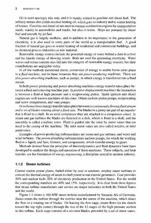
Figure 1.2 shows a gas turbine manufactured also by Siemens AG. The flow is from the back toward the front. The rotor is equipped with advanced single-crystal turbine blades, with a thermal barrier coating and film cooling. Flow enters a three-stage turbine from an annular combustion chamber which has 24 burners and walls made from ceramic
4 INTRODUCTION
tiles. These turbines power the 15 axial compressor stages that feed compressed air to the combustor. The fourth turbine stage, called a power turbine, drives an electric generator in a combined cycle power plant for which this turbine has been designed. The plant delivers a power output of 292-MW.
Figure 1.2 An open rotor and combustion chamber of an SGT5-4000F gas turbine. (Courtesy Siemens press picture, Siemens AG.)
1.1.4 Hydraulic turbines
In those areas of the world with large rivers, water turbines are used to generate electrical power. At the turn of the millennium hydropower represented 17% of the total electrical energy generated in the world. The installed capacity at the end of year 2007 was 940,000 MW, but generation was 330,000 MW, so their ratio, called a capacity factor, comes to 0.35.
With the completion of the 22,500-MW Three Gorges Dam, China has now the world's largest installed capacity of 145,000 MW, which can be estimated to give 50,000 MW of power. Canada, owing to its expansive landmass, is the world's second largest producer of hydroelectric power, with generation at 41,000 MW from installed capacity of 89,000 MW. Hydropower accounts for 58% of Canada's electricity needs. The sources of this power are the great rivers of British Columbia and Quebec. The next largest producer is Brazil, which obtains 38,000 MW from an installed capacity of 69,000 MW. Over 80% of Brazil's energy is obtained by water power. The Itaipu plant on the Parana River, which borders Brazil and Paraguay, generates 12,600 MW of power at full capacity. Of nearly the same size is Venezuela's Guri dam power plant with a rated capacity of 10,200 MW, based on 20 generators.
The two largest power stations in the United States are the Grand Coulee station in the Columbia River and the Hoover Dam station in the Colorado River. The capacity of the Grand Coulee is 6480 MW, and that of Hoover is 2000 MW. Tennessee Valley Authority operates a network of dams and power stations in the Southeastern parts of the country. Many small hydroelectric power plants can also be found in New England. Hydroelectric power in the United States today provides 289 billion kilowatthours (kwh) a year, or 33,000 MW, but this represents only 6% of the total energy used in the United States. Fossil fuels still account for 86% of the US energy needs.
ENERGY AND FLUID MACHINES 5
Next on the list of largest producers of hydroelectricity are Russia and Norway. With its small and thrifty population, Norway ships its extra generation to the other Scandinavian countries, and now with completion of a high-voltage powerline under the North Sea, also to western Europe. Norway and Iceland both obtain nearly all their electricity from hydropower.
1.1.5 Wind turbines
The Netherlands has been identified historically as a country of windmills. She and Denmark have seen a rebirth of wind energy generation since 1985 or so. These countries are relatively small in land area and both are buffeted by winds from the North Sea. Since the 1990s Germany has embarked on a quest to harness its winds. By 2007 it had installed wind turbines on most of its best sites with 22,600 MW of installed capacity. The installed capacity in the United States was 16,600 MW in the year 2007. It was followed by Spain, with an installed capacity of 15,400 MW. After that came India and Denmark.
The capacity factor for wind power is about 0.20, thus even lower than for hydropower. For this reason wind power generated in the United States constitutes only 0.5% of the country's total energy needs. Still, it is the fastest-growing of the renewable energy systems. The windy plains of North and South Dakota and of West and North Texas offer great potential for wind power generation.
1.1.6 Compressors
Compressors find many applications in industry. An important use is in the transmission of natural gas across continents.' Natural-gas production in the United States is centered in Texas and Louisiana as well as offshore in the Gulf of Mexico. The main users are the midwestern cities, in which natural gas is used in industry and for winter heating. Pipelines also cross the Canadian border with gas supplied to the west-coast and to the northern states from Alberta. In fact, half of Canada's natural-gas production is sold to the United States.
Russia has 38% of world's natural-gas reserves, and much of its gas is transported to Europe through the Ukraine. China has constructed a natural-gas pipeline to transmit the gas produced in the western provinces to the eastern cities. Extensions to Turkmenistan and Iran are in the planning stage, as both countries have large natural-gas resources.
1.1.7 Pumps and blowers
Pumps are used to increase pressure of liquids. Compressors, blowers, and fans do the same for gases. In steam power plants condensate pumps return water to feedwater heaters, from which the water is pumped to boilers. Pumps are also used for cooling water flows in these power plants.
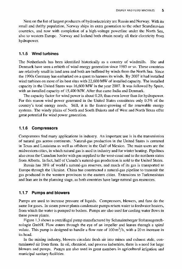
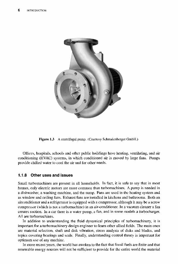
Figure 1.3 shows a centrifugal pump manufactured by Schmalenberger Stromungstech-nologie GmbH. Flow enters through the eye of an impeller and leaves through a spiral volute. This pump is designed to handle a flow rate of 100m3/h, with a 20 m increase in its head.
In the mining industry, blowers circulate fresh air into mines and exhaust stale, con-taminated air from them. In oil, chemical, and process industries, there is a need for large blowers and pumps. Pumps are also used in great numbers in agricultural irrigation and municipal sanitary facilities.
6 INTRODUCTION
Figure 1.3 A centrifugal pump. (Courtesy Schmalenberger GmbH.)
Offices, hospitals, schools and other public buildings have heating, ventilating, and air conditioning (HVAC) systems, in which conditioned air is moved by large fans. Pumps provide chilled water to cool the air and for other needs.
1.1.8 Other uses and issues
Small turbomachines are present in all households. In fact, it is safe to say that in most homes, only electric motors are more common than turbomachines. A pump is needed in a dishwasher, a washing machine, and the sump. Fans are used in the heating system and as window and ceiling fans. Exhaust fans are installed in kitchens and bathrooms. Both an airconditioner and a refrigerator is equipped with a compressor, although it may be a screw compressor (which is not a turbomachine) in an air-conditioner. In a vacuum cleaner a fan creates suction. In a car there is a water pump, a fan, and in some models a turbocharger. All are turbomachines.
In addition to understanding the fluid dynamical principles of turbomachinery, it is important for a turbomachinery design engineer to learn other allied fields. The main ones are material selection, shaft and disk vibration, stress analysis of disks and blades, and topics covering bearings and seals. Finally, understanding control theory is important for optimum use of any machine.
In more recent years, the world has awoken to the fact that fossil fuels are finite and that renewable energy sources will not be sufficient to provide for the entire world the material
HISTORICAL SURVEY 7
conditions that Western countries now enjoy. Hence, it is important that the machines that make use of these resources be well designed so that the remaining fuels are used with consideration, recognizing their finiteness and their value in providing for some of the vital needs of humanity.
1.2 HISTORICAL SURVEY
This section gives a short historical review of turbomachines. Turbines are power-producing machines and include water and wind turbines from early history. Gas and steam turbines date from the beginning of the last century. Rotary pumps have been in use for nearly 200 years. Compressors developed as advances were made in aircraft propulsion during the last century.
1.2.1 Water power
It is only logical that the origin of turbomachinery can be traced to the use of flowing water as a source of energy. Indeed, waterwheels, lowered into a river, were already known to the Greeks. The early design moved to the rest of Europe and became known as the norse mill because the archeological evidence first surfaced in northern Europe. This machine consists of a set of radial paddles fixed to a shaft. As the shaft was vertical, or somewhat inclined, its efficiency of energy extraction could be increased by directing the flow of water against the blades with the aid of a mill race and a chute. Such a waterwheel could provide only about one-half horsepower (0.5 hp), but owing to the simplicity of its construction, it survived in use until 1500 and can still be found in some primitive parts of the world.
By placing the axis horizontally and lowering the waterwheel into a river, a better design is obtained. In this undershot waterwheel, dating from Roman times, water flows through the lower part of the wheel. Such a wheel was first described by the Roman architect and engineer Marcus Vitruvius Pollio during the first century B.C.
Overshot waterwheel came into use in the hilly regions of Rome during the second century A.D. By directing water from a chute above the wheel into the blades increases the power delivered because now, in addition to the kinetic energy of the water, also part of the potential energy can be converted to mechanical energy. Power of overshot waterwheels increased from 3 hp to about 50 hp during the Middle Ages. These improved overshot waterwheels were partly responsible for the technical revolution in the twelfth-thirteenth century. In the William the Conquerer's Domesday Book of 1086, the number of watermills in England is said to have been 5684. In 1700 about 100,000 mills were powered by flowing water in France [12].
The genius of Leonardo da Vinci (1452-1519) is well recorded in history, and his notebooks show him to have been an exceptional observer of nature and technology around him. Although he is best known for his artistic achievements, most of his life was spent in the art of engineering. Illustrations of fluid machinery are found in da Vinci's notebooks, in De Re Metallica, published in 1556 by Agricola [3], and in a tome by Ramelli published in 1588. From these a good understanding of the construction methods can be gained and of the scale of the technology then in use. In Ramelli's book there is an illustration of a mill in which a grinding wheel, located upstairs, is connected to a shaft, the lower end of which has an enclosed impact wheel that is powered by water. There are also illustrations that show windmills to have been in wide use for grinding grain.
8 INTRODUCTION
Important progress to improve waterwheels came in the hands of the Frenchman Jean Victor Poncelet (1788-1867), who curved the blades of the undershot waterwheel, so that water would enter tangentially to the blades. This improved its efficiency. In 1826 he came up with a design for a horizontal wheel with radial inward flow. A water turbine of this design was built a few years later in New York by Samuel B. Howd and then improved by James Bicheno Francis (1815-1892). Improved versions of Francis turbines are in common use today.
About the same time in France an outward flow turbine was designed by Claude Burdin (1788-1878) and his student Benoit Fourneyron (1802-1867). They benefited greatly from the work of Jean-Charles de Borda (1733-1799) on hydraulics. Their machine had a set of guidevanes to direct the flow tangentially to the blades of the turbine wheel. Fourneyron in 1835 designed a turbine that operated from a head of 108 m with a flow rate of 20 liters per second (L/s), rotating at 2300 rpm, delivering 40 hp as output power at 80% efficiency.
In the 1880s in the California gold fields an impact wheel, known as a Pelton wheel, after Lester Allen Pelton (1829-1918) of Vermillion, Ohio, came into wide use.
An axial-flow turbine was developed by Carl Anton Henschel (1780-1861) in 1837 and by Feu Jonval in 1843. Modern turbines are improvements of Henschel's and Jonval's designs. A propeller type of turbine was developed by the Austrian engineer Victor Kaplan (1876-1934) in 1913. In 1926 a 11,000-hp Kaplan turbine was placed into service in Sweden. It weighed 62.5 tons, had a rotor diameter of 5.8 m, and operated at 62.5 rpm with a water head of 6.5 m. Modern water turbines in large hydroelectric power plants are either of the Kaplan type or variations of this design.
1.2.2 Wind turbines
Humans have drawn energy from wind and water since ancient times. The first recorded account of a windmill is from the Persian-Afghan border region in 644 A.D., where these vertical axis windmills were still in use in more recent times [32]. They operate on the principle of drag in the same way as square sails do when ships sail downwind.
In Europe windmills were in use by the twelfth century, and historical research suggests that they originated from waterwheels, for their axis was horizontal and the masters of the late Middle Ages had already developed gog-and-ring gears to transfer energy from a horizontal shaft into a vertical one. This then turned a wheel to grind grain [68]. An early improvement was to turn the entire windmill toward the wind. This was done by centering a round platform on a large-diameter vertical post and securing the structure of the windmill on this platform. The platform was free to rotate, but the force needed to turn the entire mill limited the size of the early postmills. This restriction was removed in a towermill found on the next page, in which only the platform, affixed to the top of the mill, was free to rotate. The blades were connected to a windshaft, which leaned about 15° from the horizontal so that the blades would clear the structure. The shaft was supported by a wooden main bearing at the blade end and a thrust bearing at the tail end. A band brake was used to limit the rotational speed at high wind speeds. The power dissipated by frictional forces in the brake rendered the arrangement susceptible to fire.
Over the next 500 years, to the beginning of the industrial revolution, progress was made in windmill technology, particularly in Great Britain. By accumulated experience, designers learned to move the position the spar supporting a blade from midcord to quarter-chord position, and to introduce a nonlinear twist and leading edge camber to the blade [68]. The blades were positioned at a steep angles to the wind and made use of the lift
HISTORICAL SURVEY 9
force, rather than drag. It is hard not to speculate that the use of lift had not been learned from sailing vessels using lanteen sails to tack.
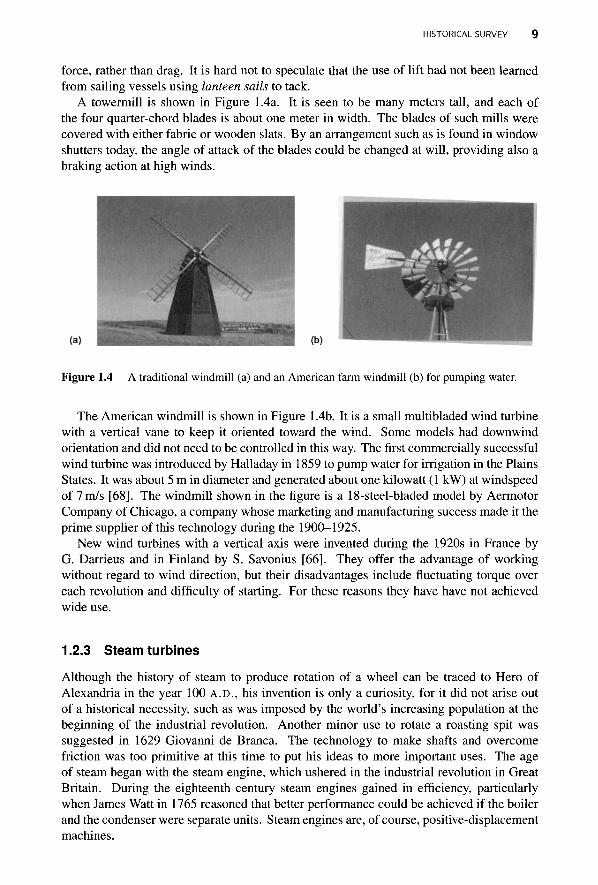
A towermill is shown in Figure 1.4a. It is seen to be many meters tall, and each of the four quarter-chord blades is about one meter in width. The blades of such mills were covered with either fabric or wooden slats. By an arrangement such as is found in window shutters today, the angle of attack of the blades could be changed at will, providing also a braking action at high winds.
Figure 1.4 A traditional windmill (a) and an American farm windmill (b) for pumping water.
The American windmill is shown in Figure 1.4b. It is a small multibladed wind turbine with a vertical vane to keep it oriented toward the wind. Some models had downwind orientation and did not need to be controlled in this way. The first commercially successful wind turbine was introduced by Halladay in 1859 to pump water for irrigation in the Plains States. It was about 5 m in diameter and generated about one kilowatt (1 kW) at windspeed of 7 m/s [68]. The windmill shown in the figure is a 18-steel-bladed model by Aermotor Company of Chicago, a company whose marketing and manufacturing success made it the prime supplier of this technology during the 1900-1925.
New wind turbines with a vertical axis were invented during the 1920s in France by G. Darrieus and in Finland by S. Savonius [66]. They offer the advantage of working without regard to wind direction, but their disadvantages include fluctuating torque over each revolution and difficulty of starting. For these reasons they have have not achieved wide use.
1.2.3 Steam turbines
Although the history of steam to produce rotation of a wheel can be traced to Hero of Alexandria in the year 100 A.D., his invention is only a curiosity, for it did not arise out of a historical necessity, such as was imposed by the world's increasing population at the beginning of the industrial revolution. Another minor use to rotate a roasting spit was suggested in 1629 Giovanni de Branca. The technology to make shafts and overcome friction was too primitive at this time to put his ideas to more important uses. The age of steam began with the steam engine, which ushered in the industrial revolution in Great Britain. During the eighteenth century steam engines gained in efficiency, particularly when James Watt in 1765 reasoned that better performance could be achieved if the boiler and the condenser were separate units. Steam engines are, of course, positive-displacement machines.
10 INTRODUCTION
Sir Charles Parsons (1854-1931) is credited with the development of the first steam turbine in 1884. His design used multiple turbine wheels, about 8 cm in diameter each, to drop the pressure in stages and this way to reduce the angular velocities. The first of Parson's turbines generated 7.5 kW using steam at inlet pressure of 550 kPa and rotating at 17,000 rpm. It took some 15 years before Parsons' efforts received their proper recognition.
An impulse turbine was developed in 1883 by the Swedish engineer Carl Gustav Patrik de Laval (1845-1913) for use in a cream separator. To generate the large steam velocities he also invented the supersonic nozzle and exhibited it in 1894 at the Columbian World's Fair in Chicago. From such humble beginnings arose rocketry and supersonic flight. Laval's turbines rotated at 26,000 rpm, and the largest of the rotors had a tip speed of 400 m/s. He used flexible shafts to alleviate vibration problems in the machinery.
In addition to the efforts in Great Britain and Sweden, the Swiss Federal Institute of Technology in Zurich [Eidgenossische Technische Hochschule, (ETH)] had become an im-portant center of research in early steam turbine theory through the efforts of Aurel Stodola (1859-1942). His textbook Steam and Gas Turbines became the standard reference on the subject for the first half of last century [75]. A similar effort was led by William J. Kearton (1893-?) at the University of Liverpool in Great Britain.
1.2.4 Jet propulsion
The first patent for gas turbine development was issued to John Barber (1734-C.1800) in England in 1791, but again technology was not yet sufficiently advanced to build a machine on the basis of the proposed design. Eighty years later in 1872 Franz Stolze (1836-1910) received a patent for a design of a gas turbine power plant consisting of a multistage axial-flow compressor and turbine on the same shaft, together with a combustion chamber and a heat exchanger. The first U.S. patent was issued to Charles Gordon Curtis (1860-1953) in 1895.
Starting in 1935, Hans J. P. von Ohain (1911-1998) directed efforts to design gas turbine power plants for the Heinkel aircraft in Germany. The model He 178 was a fully operational jet aircraft, and in August 1939 it was first such aircraft to fly successfully.
During the same timeframe Sir Frank Whittle (1907-1996) in Great Britain was de-veloping gas turbine power plants for aircraft based on a centrifugal compressor and a turbojet design. In 1930 he filed for a patent for a single-shaft engine with a two-stage axial compressor followed by a radial compressor from which the compressed air flowed into a straight-through burner. The burned gases then flowed through a two-stage axial turbine on a single disk. This design became the basis for the development of jet engines in Great Britain and later in the United States.
Others, such as Alan Arnold Griffith (1893-1963) and Hayne Constant (1904-1968), worked in 1931 on the design and testing of axial-flow compressors for use in gas turbine power plants. Already in 1926 Griffith had developed an aerodynamic theory of turbine design based on flow past airfoils.
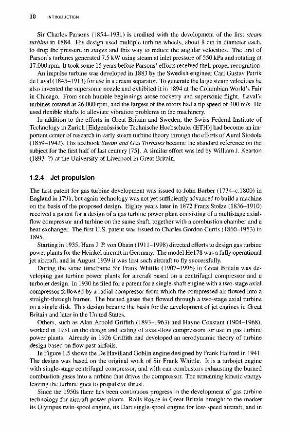
In Figure 1.5 shows the De Havilland Goblin engine designed by Frank Halford in 1941. The design was based on the original work of Sir Frank Whittle. It is a turbojet engine with single-stage centrifugal compressor, and with can combustors exhausting the burned combustion gases into a turbine that drives the compressor. The remaining kinetic energy leaving the turbine goes to propulsive thrust.
Since the 1950s there has been continuous progress in the development of gas turbine technology for aircraft power plants. Rolls Royce in Great Britain brought to the market its Olympus twin-spool engine, its Dart single-spool engine for low-speed aircraft, and in
HISTORICAL SURVEY 1 1
Figure 1.5 De Havilland Goblin turbojet engine.
1967 the Trent, which was the first three-shaft turbofan engine. The Olympus was also used in stationary power plants and in marine propulsion.
General Electric in the United States has also a long history in gas turbine development. Its 1-14, 1-16, 1-20, and 1-40 models were developed in the 1940s. The 1-14 and 1-16 powered the Bell P-59A aircraft, which was the first American turbojet. It had a single centrifugal compressor and a single-stage axial turbine. Allison Engines, then a division of General Motors, took over the manufacture and improvement of model 1-40. Allison also began the manufacture of General Electric's TG series of engines.
Many new engines were developed during the latter half of the twentieth century, not only by Rolls Royce and General Electric but also by Pratt and Whitney in the United States and Canada, Rateau in France, and by companies in Soviet Union, Sweden, Belgium, Australia, and Argentina. The modern engines that power the flight of today's large commercial aircraft by Boeing and by Airbus are based on the Trent design of Rolls Royce, or on General Electric's GE90 [7].
1.2.5 Industrial turbines
Brown Boveri in Switzerland developed a 4000-kW turbine power plant in 1939 to Neucha-tel for standby operation for electric power production. On the basis of this design, an oil-burning closed cycle gas turbine plant with a rating of 2 MW was built the following year.
Industrial turbine production at Ruston and Hornsby Ltd. of Great Britain began by establishment of a design group in 1946. The first unit produced by them was sold to Kuwait Oil Company in 1952 to power pumps in oil fields. It was still operational in

12 INTRODUCTION
1991 having completed 170,000 operating hours. Industrial turbines are in use today as turbocompressors and in electric power production.
Pumps and compressors
The centrifugal pump was invented by Denis Papin (1647-1710) in 1698 in France. To be sure, a suggestion to use centrifugal force to effect pumping action had also been made by Leonardo da Vinci, but neither his nor Papin's invention could be built, owing to the lack of sufficiently advanced shop methods. Leonhard Euler (1707-1783) gave a mathematical theory of the operation of a pump in 1751. This date coincides with the beginning of the industrial revolution and the advances made in manufacturing during the ensuing 100 years brought centrifugal pumps to wide use by 1850. The Massachusetts pump, built in 1818, was the first practical centrifugal pump manufactured. W. D. Andrews improved its performance in 1846 by introducing double-shrouding. At the same time in Great Britain engineers such as John Appold (1800-1865) and Henry Bessemer (1813-1898) were working on improved designs. Appold's pump operated at 788 rpm with an efficiency of 68% and delivered 78 L/s and a head of 5.9 m.
The same companies that in 1900 built steam turbines in Europe also built centrifugal blowers and compressors. The first applications were for providing ventilation in mines and for the steel industry. Since 1916 compressors have been used in chemical industries, since 1930 in the petrochemical industries, and since 1947 in the transmission of natural gas. The period 1945-1950 saw a large increase in the use of centrifugal compressors in American industry. Since 1956 they have been integrated into gas turbine power plants and have replaced reciprocating compressors in other applications.
The efficiencies of single stage centrifugal compressors increased from 70% to over 80% over the period 1935-1960 as a result of work done in companies such as Rateau, Moss-GE, Birmann-DeLaval, and Whittle in Europe and General Electric and Pratt & Whitney in the United States. The pressure ratios increased from 1.2 : 1 to 7 : 1. This development owes much to the progress that had been made in gas turbine design [26].
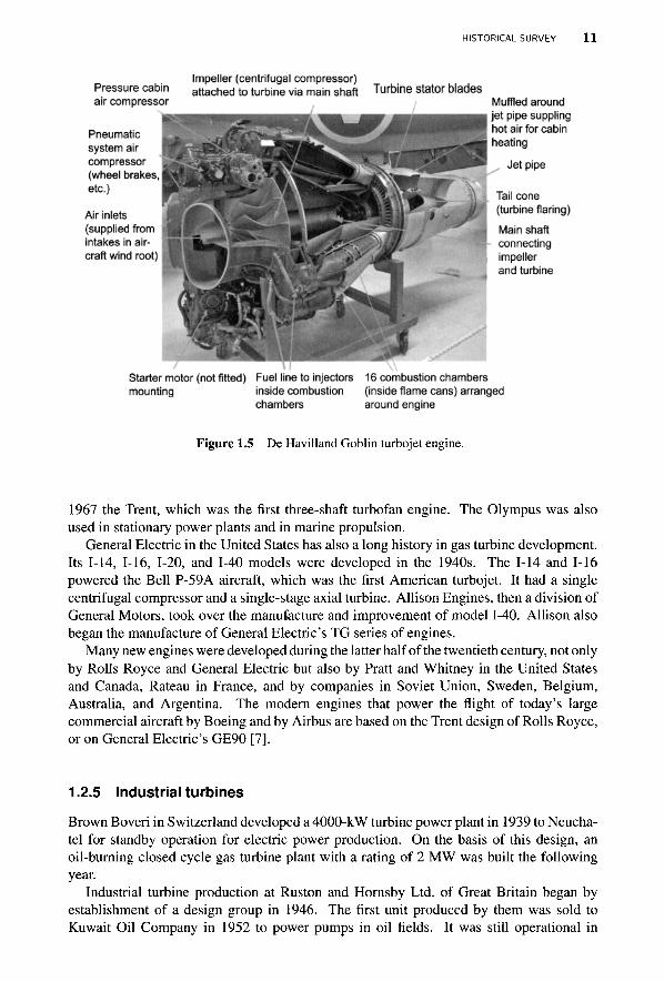
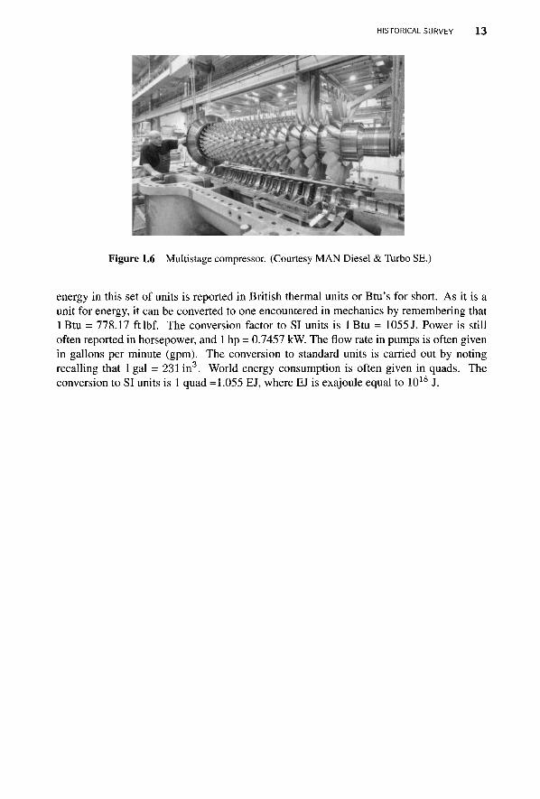
For large flow rates multistage axial compressors are used. Figure 1.6 shows such a compressor, manufactured by Man Diesel & Turbo SE in Germany. It has 14 axial stages followed by a centrifugal compressor stage. The rotor blades are seen in the exposed rotor. The stator blades are fixed to the casing, the lower half of which is shown. The flow is from right to left. The flow area decreases toward the exit, for in order to keep the axial velocity constant, as is commonly done, the increase in density on compression is accommodated by a decrease in the flow area.
1.2.6 Note on units
The Systeme International (d'Unites) (SI) system of units is used in this text. But it is still customary in some industries English Engineering system of units and if other reference books are consulted one finds that many still use this system. In this set of units mass is expressed as pound (lbm) and foot is the unit of length. The British gravitational system of units has slug as the unit of mass and the unit of force is pound force (lbf), obtained from Newton's law, as it represents a force needed to accelerate a mass of one slug at the rate of one foot per second squared. The use of slug for mass makes the traditional British gravitational system of units analogous to the SI units. When pound (lbm) is used for mass, it ought to be first converted to slugs (1 slug = 32.174 lbm), for then calculations follow smoothly as in the SI units. The unit of temperature is Fahrenheit or Rankine. Thermal
HISTORICAL SURVEY 13
Figure 1.6 Multistage compressor. (Courtesy MAN Diesel & Turbo SE.)
energy in this set of units is reported in British thermal units or Btu's for short. As it is a unit for energy, it can be converted to one encountered in mechanics by remembering that 1 Btu = 778.17 ftlbf. The conversion factor to SI units is 1 Btu = 1055 J. Power is still often reported in horsepower, and 1 hp = 0.7457 kW. The flow rate in pumps is often given in gallons per minute (gpm). The conversion to standard units is carried out by noting recalling that 1 gal = 231 in3. World energy consumption is often given in quads. The conversion to SI units is 1 quad =1.055 EJ, where EJ is exajoule equal to 1018 J.
CHAPTER 2
PRINCIPLES OF THERMODYNAMICS AND FLUID FLOW
This chapter begins with a review of the conservation principle for mass for steady uniform flow, after which follows the first and second laws of thermodynamics, also for steady uniform flow. Next, thermodynamic properties of gases and liquids are discussed. These principles enable the discussion of turbine and compressor efficiencies, which are described in relation to thermodynamic losses. The final section is on the Newton's second law for steady and uniform flow.
2.1 MASS CONSERVATION PRINCIPLE
Mass flow rate m in a uniform flow is related to density p and velocity V of the fluid, and the cross-sectional area of the flow channel A by
rh = pVnA
When this equation is used in the analysis of steam flows, specific volume, which is the reciprocal of density, is commonly used. The subscript n denotes the direction normal to the flow area. The product VnA arises from the scalar product V • n = V cos 9, in which n is a unit normal vector on the surface A and 9 is the angle between the normal and the direction of the velocity vector. Consequently, the scalar product can be written in the two alternative forms
V ■ n A = VA cos 9 = VnA = VAn
Principles of Turbomachinery. By Seppo A. Korpela 15 Copyright © 2011 John Wiley & Sons, Inc.
1 6 PRINCIPLES OF THERMODYNAMICS AND FLUID FLOW
in which An is the area normal to the flow. The principle of conservation of mass for a uniform steady flow through a control volume with one inlet and one exit takes the form
PiViAnl = p2V2An2
Turbomachinery flows are steady only in a time-averaged sense; that is, the flow is periodic, with a period equal to the time taken for a blade to move a distance equal to the spacing between adjacent blades. Despite the unsteadiness, in elementary analysis all variables are assumed to have steady values.
If the flow has more than one inlet and exit, then, in steady uniform flow, conservation of mass requires that
^TpiViAni =Y,PeVeAne (2.1) i e
in which the sums are over all the inlets and exits.
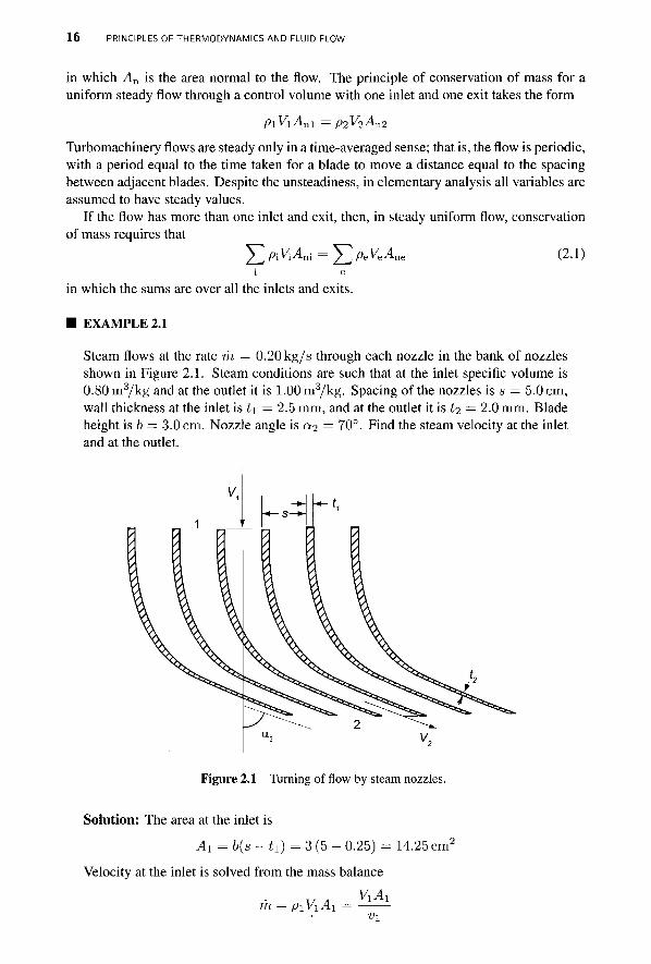
■ EXAMPLE 2.1 Steam flows at the rate m = 0.20 kg/s through each nozzle in the bank of nozzles shown in Figure 2.1. Steam conditions are such that at the inlet specific volume is 0.80 m3/kg and at the outlet it is 1.00 m3/kg. Spacing of the nozzles is s = 5.0 cm, wall thickness at the inlet is t\ = 2.5 mm, and at the outlet it is t2 = 2.0 mm. Blade height is b — 3.0 cm. Nozzle angle is a2 = 70°. Find the steam velocity at the inlet and at the outlet.
Figure 2.1 Turning of flow by steam nozzles.
Solution: The area at the inlet is
Ax =b(s-h) = 3 ( 5 - 0 . 2 5 ) = 14.25 cm2
Velocity at the inlet is solved from the mass balance
m = piVxAx = Vi
FIRST LAW OF THERMODYNAMICS 17
which gives . . mVl 0.20 • 0.80 • 1002
V\ = —,— = = 112.3 m/s 1 A1 14.25 ' At the exit the flow area is
A2 = b(s cos a2 -t2)= 3[5cos(70°) - 0.20] = 4.53cm2
hence the velocity is
. . rhv2 0.2 ■ 1.00 • 1002 . . . _ . V2 = —r~ = = 441.5 m/s A2 4.53 '
2.2 FIRST LAW OF THERMODYNAMICS
For a uniform steady flow in a channel, the first law of thermodynamics has the form
m (m + pwi +-V? + gzA + Q = fa (u2 + p2v2 + -V22 + gz2) +W (2.2)
The sum of specific internal energy u, kinetic energy V2/2, and potential energy gz is the specific energy e = u + \V2 + gz of the fluid. In the potential energy term g is the acceleration of gravity and z is a height. The term p\V\, in which p is the pressure, represents the work done by the fluid in the flow channel just upstream of the inlet to move the fluid ahead of it into the control volume, and it thus represents energy flow into the control volume. This work is called flow work. Similarly, p2v2 is the flow work done by the fluid inside the control volume to move the fluid ahead of it out of the control volume. It represents energy transfer as work leaving the control volume. The sum of internal energy and flow work is defined as enthalpy h = u + pv. The heat transfer rate into the control volume is denoted as Q and the rate at which work is delivered is W. Equation (2.2) can be extended to multiple inlets and outlets in the same manner as was done in Eq. (2.1).
Dividing both sides by m gives the first law of thermodynamics the form
hi + 2Vi +9Zi+q = h2 + -Vi +gz2+w
in which q = Q/rn and w = W/fn denote the heat transfer and work done per unit mass. By convention, heat transfer into the thermodynamic system is taken to be a positive quantity, as is work done by the system on the surroundings.
The sum of enthalpy, kinetic energy, and potential energy is called the stagnation enthalpy
h0 = h+-V2+gz
and the first law can also be written as
h0i+q = h02 + w
In the flow of gases the potential energy terms are small and can be neglected. Similarly, for pumps, the changes in elevation are small and potential energy difference is negligible.
1 8 PRINCIPLES OF THERMODYNAMICS AND FLUID FLOW
Only for some water turbines is there a need to retain the potential energy terms. When the change in potential energy is neglected, the first law reduces to
1 1, hi + »V{+q = h2 + -V2 ■w
In addition, even if velocity is large, the difference in kinetic energy between the inlet and exit may be small. In such a case first law is simply
hi + q = h2 + w
Turbomachinery flows are nearly adiabatic, so q can be dropped. Then work delivered by a turbine is given as
w = h0i — h02
and the work done on the fluid in a compressor is
w = h02- h0i
The compressor work has been written in a form that gives the work done a positive value. Hence the convention of thermodynamics of denoting work out from a system as positive and work in as negative is ignored, and the equations are written in a form that gives a positive value for work, for both a turbine and a compressor.
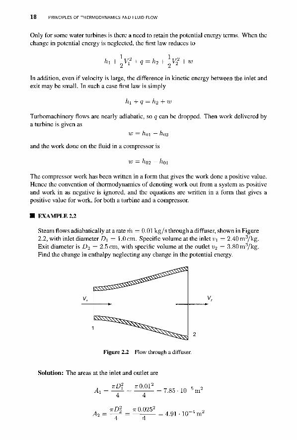
■ EXAMPLE 2.2
Steam flows adiabatically at a rate m = 0.01 kg/s through a diffuser, shown in Figure 2.2, with inlet diameter Di = 1.0 cm. Specific volume at the inlet v\ = 2.40 m3/kg. Exit diameter is D2 = 2.5 cm, with specific volume at the outlet v2 = 3.80m3/kg. Find the change in enthalpy neglecting any change in the potential energy.
Figure 2.2 Row through a diffuser.
Solution: The areas at the inlet and outlet are
TTD2 ^O.Ol2 „ o c 1 A _ 5 2 Ai = —- 1 = — - — = 7.85 -10 5 m2
irD2 TTO.0252
4.91 -10"4m2
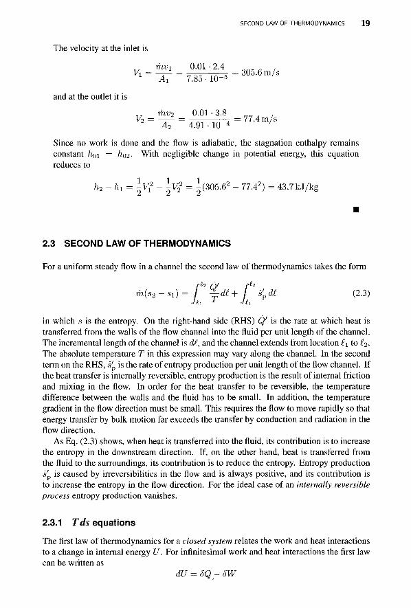
SECOND LAW OF THERMODYNAMICS 19
The velocity at the inlet is
rhui 0.01-2.4 V\ = —,— = r = 305.6 m/s
Ai 7.85 ■ 10-5 '
and at the outlet it is
m^2 0.01 ■ 3.8 Vo = —;— = T = 77.4 m/s 2 A2 4.91 -10"4 '
Since no work is done and the flow is adiabatic, the stagnation enthalpy remains constant hoi = -̂02- With negligible change in potential energy, this equation reduces to
h2 - fti = \v? - l-Vi = i(305.62 - 77.42) = 43.7kJ/kg
2.3 SECOND LAW OF THERMODYNAMICS
For a uniform steady flow in a channel the second law of thermodynamics takes the form
m ( s 2 - s i ) = [2%d£+ f2 s'pd£ (2.3)
in which s is the entropy. On the right-hand side (RHS) Q' is the rate at which heat is transferred from the walls of the flow channel into the fluid per unit length of the channel. The incremental length of the channel is d£, and the channel extends from location l\ to £2-The absolute temperature T in this expression may vary along the channel. In the second term on the RHS, s' is the rate of entropy production per unit length of the flow channel. If the heat transfer is internally reversible, entropy production is the result of internal friction and mixing in the flow. In order for the heat transfer to be reversible, the temperature difference between the walls and the fluid has to be small. In addition, the temperature gradient in the flow direction must be small. This requires the flow to move rapidly so that energy transfer by bulk motion far exceeds the transfer by conduction and radiation in the flow direction.
As Eq. (2.3) shows, when heat is transferred into the fluid, its contribution is to increase the entropy in the downstream direction. If, on the other hand, heat is transferred from the fluid to the surroundings, its contribution is to reduce the entropy. Entropy production s'p is caused by irreversibilities in the flow and is always positive, and its contribution is to increase the entropy in the flow direction. For the ideal case of an internally reversible process entropy production vanishes.
2.3.1 Tds equations The first law of thermodynamics for a closed system relates the work and heat interactions to a change in internal energy U. For infinitesimal work and heat interactions the first law can be written as
dU = SQ- 5W
2 0 PRINCIPLES OF THERMODYNAMICS AND FLUID FLOW
For a simple compressible substance, defined to be one for which the only relevant work is compression or expansion, reversible work is given by
SWS =pdV
This expression shows that when a fluid is compressed so that its volume decreases, work is negative, meaning that work is done on the system. For an internally reversible process the second law of thermodynamics relates heat transfer to a change in entropy by
SQs = TdS
in which it must be remembered that T is the absolute temperature. Hence, for an internally reversible process, the first law takes the differential form
dU = TdS-pdV
Dividing by the mass of the system converts this to an expression
du = Tds — pdv
between specific properties. Although derived for reversible processes, this is a relationship between intensive properties, and for this reason it is valid for all processes; reversible, or irreversible. It is usually written as
Tds = du + pdv (2.4)
and is called the first Gibbs equation. Writing u = h — pv and differentiating gives du = dh — pdv — vdp. Substituting this
into the first Gibbs equation gives
Tds = dh — v dp (2.5)
which is the second Gibbs equation.
2.4 EQUATIONS OF STATE
The state principle of thermodynamics guarantees that a thermodynamic state for a simple compressible substance is completely determined by specifying two independent thermo-dynamic properties. Other properties are then functions of these independent properties. Such functional relations are called equations of state.
In this section the equations of state for steam and those of ideal gases are reviewed. In addition, ideal gas mixtures are considered as they arise in combustion of hydrocarbon fuels. Combustion gases flow through the gas turbines of a jet engine and through industrial turbines burning natural gas. Preliminary calculations can be carried out using properties of air since air is 78% of nitrogen by volume, which, although contributing to formation of nitric oxides, is otherwise largely inert during combustion. Later in the chapter a better model for combustion gases is discussed, but for accurate calculations the actual composition is to be taken into account. Also in many applications, such as in oil and gas production, mixtures rich in complex molecules flow through compressors and expanders. Their equations of state may be very complicated, particularly at high pressures.
EQUATIONS OF STATE 2 1
2.4.1 Properties of steam
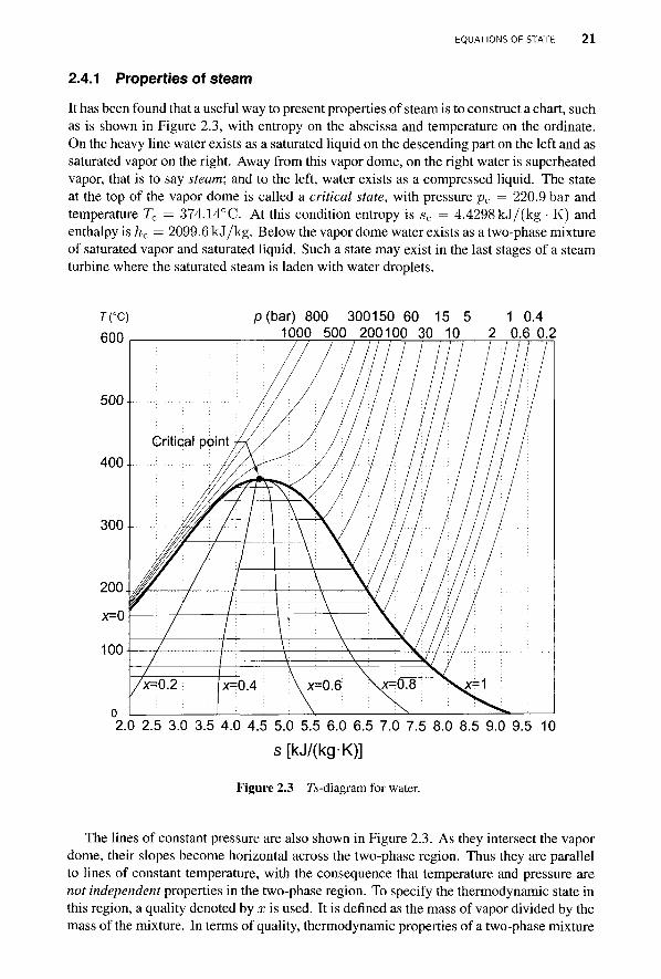
It has been found that a useful way to present properties of steam is to construct a chart, such as is shown in Figure 2.3, with entropy on the abscissa and temperature on the ordinate. On the heavy line water exists as a saturated liquid on the descending part on the left and as saturated vapor on the right. Away from this vapor dome, on the right water is superheated vapor, that is to say steam; and to the left, water exists as a compressed liquid. The state at the top of the vapor dome is called a critical state, with pressure pc = 220.9 bar and temperature Tc = 374.14°C. At this condition entropy is sc = 4.4298kJ/(kg ■ K) and enthalpy is hc = 2099.6 kJ/kg. Below the vapor dome water exists as a two-phase mixture of saturated vapor and saturated liquid. Such a state may exist in the last stages of a steam turbine where the saturated steam is laden with water droplets.
T(°C) P(bar) 800 300150 60 15 5 1 0.4 finn 1000 500 200100 30 10 2 0.6 0.2
s[kJ/(kg-K)]
Figure 2.3 Ji-diagram for water.
The lines of constant pressure are also shown in Figure 2.3. As they intersect the vapor dome, their slopes become horizontal across the two-phase region. Thus they are parallel to lines of constant temperature, with the consequence that temperature and pressure are not independent properties in the two-phase region. To specify the thermodynamic state in this region, a quality denoted by x is used. It is defined as the mass of vapor divided by the mass of the mixture. In terms of quality, thermodynamic properties of a two-phase mixture
2 2 PRINCIPLES OF THERMODYNAMICS AND FLUID FLOW
are calculated as a weighted average of the saturation properties. Thus, for example
h = (1 — a:)/if + xhg
or h = h{ + xhfg
in which h{ denotes the enthalpy of saturated liquid, hg that of saturated vapor, and their difference is denoted by hfg = hg — /if. Similarly, entropy of the two-phase mixture is
S = Sf + CCSfg
and its specific volume is V = V{ + XVfg
Integrating the second Gibbs equation Tds = dh — vdp between the saturated vapor and liquid states at constant pressure gives
his = T s fg
The first law of thermodynamics shows that the amount of heat transferred to a fluid flowing at constant pressure, as it is evaporated from its saturated liquid state to saturated vapor state, is
q = hg — hi = hfg
and this is therefore also 1 = T(sg ~ s f ) = T s f g
States with pressure above the critical pressure have the peculiar property that if water at such pressures is heated at constant pressure, it converts from a liquid state to a vapor state without ever forming a two-phase mixture. Thus, neither liquid droplets nor vapor bubbles can be discerned in the water during the transformation. This region is of interest because in a typical supercritical steam power plant built today water is heated at supercritical pressure of 262 bar to temperature 566°C, and in ultrasupercritical power plants steam generator pressures of 600 bar are in use. Steam at these pressures and temperatures then enters a high-pressure (HP) steam turbine, which must be designed with these conditions in mind.
Steam tables, starting with those prepared by H. L. Callendar in 1900, and Keenan and Kays in 1936, although still in use, are being replaced by computer programs today. Steam tables, found in Appendix B, were generated by the software EES, a product of the company F-chart Software, in Madison, Wisconsin. It was also used to prepare Figures 2.3 and 2.4. Its use is demonstrated in the following example.
■ EXAMPLE 2.3
Steam at pi = 6000 kPa and T\ = 400° C expands reversibly and adiabatically through a steam turbine to pressure p2 = 60 kPa. (a) Find the exit quality and (b) the work delivered if the change in kinetic energy is neglected.
Solution: (a) The fhermodynamic properties at the inlet to the turbine are first found from the steam tables, or calculated using computer software. Either way shows that hi = 3177.0kJ/kg and si = 6.5404kJ/(kg • K). Since the process is reversible
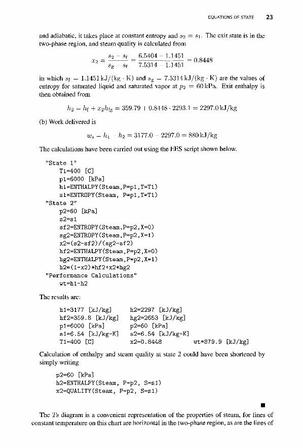
EQUATIONS OF STATE 23
and adiabatic, it takes place at constant entropy and s2 = si- The exit state is in the two-phase region, and steam quality is calculated from
a a = j ^ j f = 6-5404-1.1451 = 2 sg-sf 7.5314 - 1.1451
in which sf = 1.1451 kJ / (kg • K) and sg = 7.5314kJ/(kg • K) are the values of entropy for saturated liquid and saturated vapor at p2 = 60 kPa. Exit enthalpy is then obtained from
h2 = h(+ x2h{g = 359.79 + 0.8448 • 2293.1 = 2297.0 k J / k g
(b) Work delivered is
Ws = hi-h2= 3177.0 - 2297.0 = 880kJ /kg
The calculations have been carried out using the EES script shown below.
" S t a t e 1" Tl=400 [C] pl=6000 [kPa] hl=ENTHALPY(Steam,P=pl,T=Tl) sl=ENTR0PY(Steam, P=pl,T=Tl)
"State 2"
p2=60 [kPa] s 2 = s l sf2=ENTR0PY(Steam,P=p2,X=0) sg2=ENTR0PY(Steam,P=p2,X=l) x 2 = ( s 2 - s f 2 ) / ( s g 2 - s f 2 ) hf2=ENTHALPY(Steam,P=p2,X=0) hg2=ENTHALPY(Steam,P=p2,X=l) h2=( l -x2)*hf2+x2*hg2
"Performance C a l c u l a t i o n s " wt=h l -h2
The results are:
hl=3177 [kJ /kg ] h2=2297 [kJ /kg ] hf2=359.8 [kJ /kg ] hg2=2653 [kJ /kg ] pl=6000 [kPa] p2=60 [kPa] s l = 6 . 5 4 [kJ /kg-K] s2=6.54 [kJ /kg-K] Tl=400 [C] x2=0.8448 wt=879.9 [kJ /kg]
Calculation of enthalpy and steam quality at state 2 could have been shortened by simply writing
P2=60 [kPa] h2=ENTHALPY(Steam, P=p2, S=sl) x2=QUALITY(Steam, P=p2, S=sl)
The Ts diagram is a convenient representation of the properties of steam, for lines of constant temperature on this chart are horizontal in the two-phase region, as are the lines of
2 4 PRINCIPLES OF THERMODYNAMICS AND FLUID FLOW
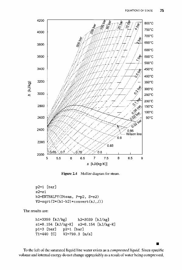
constant pressure. Isentropic processes pass through points along vertical lines. Adiabatic irreversible processes veer to the right of vertical lines, as entropy must increase. These make various processes easy to visualize. An even more useful representation is one in which entropy is on the abscissa and enthalpy is on the ordinate. A diagram of this kind was developed by R. Mollier in 1906. A Mollier diagram, with accurate steam properties calculated using EES, is shown in Figure 2.4.
The enthalpy drop used in the calculation of the work delivered by a steam turbine is now represented as a vertical distance between the end states. If the exit state is inside the vapor dome, there is a practical limit beyond which exit steam quality cannot be reduced. In a condensing steam turbine quality at the exit is generally kept above the line x = 0.955. Below this value droplets form, and, owing to their higher density, they do not turn as readily as vapor does, and thus on their impact on blades, they cause damage. A complicating factor in the analysis is the lack of thermodynamic equilibrium as steam crosses into the vapor dome. Droplets take a finite time to form, and if the water is clean and free of nucleation sites, their formation is delayed. Also, if the quality is not too low, by the time droplets form, steam may have left the turbine.
The line below which droplet formation is likely to occur is called the Wilson line. It is about 115 kJ/kg below the saturated vapor line, with a steam quality 0.96 at low pressures of about 0.1 bar. The quality decreases to 0.95 along the Wilson line as pressure increases to 14 bar. Steam inside the vapor dome is supersaturated above the Wilson line, a term that arises from water existing as vapor at conditions at which condensation should be taking place.
■ EXAMPLE 2.4
Steam from a steam chest of a single-stage turbine at pi = 3 bar and T\ = 440° C expands reversibly and adiabatically through a nozzle to pressure of p = 1 bar. Find the velocity of the steam at the exit.
Solution: Since the process is isentropic, the states move down along a vertical line on the Mollier chart. From the chart, steam tables — or using EES, enthalpy of steam in the reservoir — is determined to be hi = 3358.7 kJ/kg, and its entropy is s\ = 8.1536kJ/(kg • K). For an isentropic process, the exit state is determined by P2 = lbar and s2 — 8.1536kJ/(kg • K). Enthalpy, obtained by interpolating in the tables, is h2 = 3039.2 kJ/kg.
Assuming that the velocity in the steam chest is negligible, the exit velocity is obtained from
h^h2+l-V22
or V2 = y/2(ht - h2) = V ^ 3 3 5 8 - 7 - 3039.4) 1000 = 799.1 m/s
An EES script used to solve this example is shown below. Conversion between kilojoules and joules is carried out by the statement convert (kJ, J ) :
"State 1" pi=3 [bar] Tl=440 [C] hl=ENTHALPY(Steam, P=pl, T=T1) sl=ENTR0PY(Steam, P=pl, T=T1)
"State 2"
EQUATIONS OF STATE 25
s [kJ/(kg-K)]
Figure 2.4 Mollier diagram for steam.
p2=l [bar ] s2=sl b.2=ENTHALPY (Steam, P=p2, S=s2) V2=sqrt (2* (hl-h.2) * c o n v e r t ( k j , J ) )
The results are:
hl=3359 [kJ /kg ] h2=3039 [kJ /kg ] s1=8.154 [kJ /kg-K] s2=8.154 [kJ /kg-K] p l = 3 [bar ] p2=l [bar ] Tl=440 [C] V2=799.3 [m/s]
To the left of the saturated liquid line water exists as a compressed liquid. Since specific volume and internal energy do not change appreciably as a result of water being compressed,
2 6 PRINCIPLES OF THERMODYNAMICS AND FLUID FLOW
their values may be approximated as
v(T,p)^vt(T)
u(T,p)*uf(T) Enthalpy can then be obtained from
h(p,T) a ut(T) + pvf(T)
which can also be written as
h(p,T) = Uf(T)+MT)vf(T) + ( p - P f ( T ) K ( T )
or as h = hf + vi(p - Pf) (2.6)
in which explicit dependence on temperature has been dropped and it is understood that all the properties are given at the saturation temperature.
Consider next the calculation of a change in enthalpy along an isentropic path from the saturated liquid state to a compressed liquid state at higher pressure. Integration of
Tds — dh — vdp
along an isentropic path, assuming v to be constant, gives
h = hi +v{(p-pf) (2.7)
This equation is identical to Eq. (2.6). Both approximations use the value of specific volume at the saturation state.
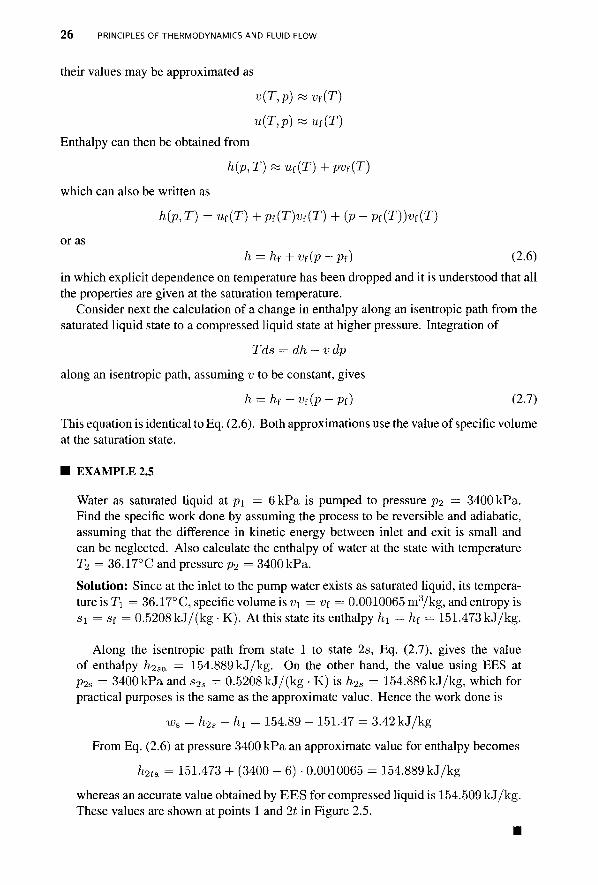
■ EXAMPLE 2.5
Water as saturated liquid at pi = 6 kPa is pumped to pressure p2 = 3400 kPa. Find the specific work done by assuming the process to be reversible and adiabatic, assuming that the difference in kinetic energy between inlet and exit is small and can be neglected. Also calculate the enthalpy of water at the state with temperature T2 = 36.17°C and pressure p2 = 3400 kPa.
Solution: Since at the inlet to the pump water exists as saturated liquid, its tempera-ture is 7\ = 36.17°C, specific volume is V\ = V{ — 0.0010065 m3/kg, and entropy is Sl = Sf = 0.5208 kJ/(kg ■ K). At this state its enthalpy hi — h{ = 151.473 kJ/kg.
Along the isentropic path from state 1 to state 2s, Eq. (2.7), gives the value of enthalpy h2sa = 154.889 kJ/kg. On the other hand, the value using EES at p2a = 3400 kPa and s2s = 0.5208 kJ/(kg • K) is h2a = 154.886kJ/kg, which for practical purposes is the same as the approximate value. Hence the work done is
ws = h2s -hi = 154.89 - 151.47 = 3.42kJ/kg
From Eq. (2.6) at pressure 3400 kPa an approximate value for enthalpy becomes
h2ta. = 151.473 + (3400 - 6) • 0.0010065 = 154.889 kJ/kg
whereas an accurate value obtained by EES for compressed liquid is 154.509 kJ/kg. These values are shown at points 1 and 2t in Figure 2.5.
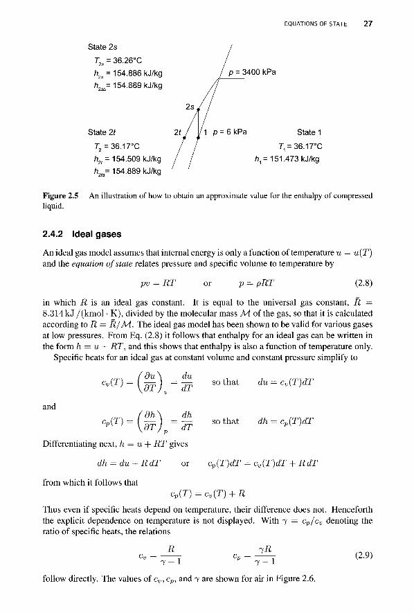
EQUATIONS OF STATE 27
State 2s T, =36.26°C '2s = 154.886 kJ/kg <2sa= 154.889 kJ/kg
State 2f 72 = 36.17°C h2t = 154.509 kJ/kg /? = 154.889 kJ/kg
p = 3400 kPa
6kPa State 1 T: = 36.17°C
/i,= 151.473kJ/kg
Figure 2.5 An illustration of how to obtain an approximate value for the enthalpy of compressed liquid.
2.4.2 Ideal gases
An ideal gas model assumes that internal energy is only a function of temperature u and the equation of state relates pressure and specific volume to temperature by
pv RT or p = pRT
u(T)
(2.8)
in which R is an ideal gas constant. It is equal to the universal gas constant, R = 8.314 kJ /(kmol • K), divided by the molecular mass M of the gas, so that it is calculated according to R = R/M. The ideal gas model has been shown to be valid for various gases at low pressures. From Eq. (2.8) it follows that enthalpy for an ideal gas can be written in the form h = u + RT, and this shows that enthalpy is also a function of temperature only.
Specific heats for an ideal gas at constant volume and constant pressure simplify to
cv(T) du df
du df
and _ fdh\ _ dh
dTjp dT cP{T)
Differentiating next, h = u + RT gives
dh = du + RdT
from which it follows that
so that du = cv(T)dT
so that dh = cp(T)dT
or cp(T)dT = cv(T)dT + RdT
cP(T) = cv{T) + R
Thus even if specific heats depend on temperature, their difference does not. Henceforth the explicit dependence on temperature is not displayed. With 7 = cp/cv denoting the ratio of specific heats, the relations
R -yR 7 — 1 7 — 1
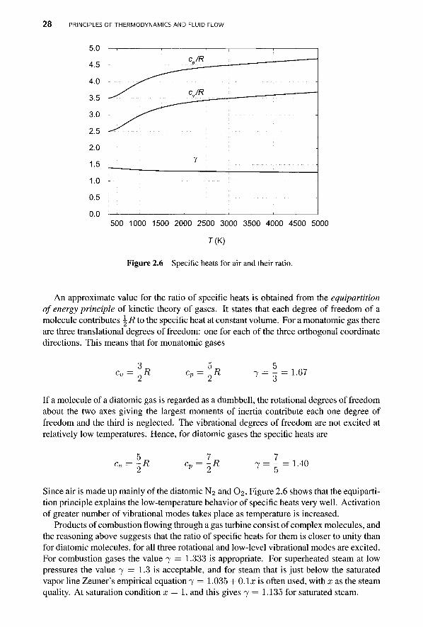
follow directly. The values of cv,cp, and 7 are shown for air in Figure 2.6.
(2.9)
2 8 PRINCIPLES OF THERMODYNAMICS AND FLUID FLOW
5.0
4.5
4.0
3.5
3.0
2.5
2.0
1.5
1.0
0.5
0.0 500 1000 1500 2000 2500 3000 3500 4000 4500 5000
7(K)
Figure 2.6 Specific heats for air and their ratio.
An approximate value for the ratio of specific heats is obtained from the equipartition of energy principle of kinetic theory of gases. It states that each degree of freedom of a molecule contributes ^R to the specific heat at constant volume. For a monatomic gas there are three translational degrees of freedom: one for each of the three orthogonal coordinate directions. This means that for monatomic gases
cv = -R cp= -R 7 = - = 1.67
If a molecule of a diatomic gas is regarded as a dumbbell, the rotational degrees of freedom about the two axes giving the largest moments of inertia contribute each one degree of freedom and the third is neglected. The vibrational degrees of freedom are not excited at relatively low temperatures. Hence, for diatomic gases the specific heats are
5 7 7 c„ = --R cp= -R 7 = - = 1.40
Since air is made up mainly of the diatomic N2 and O2, Figure 2.6 shows that the equiparti-tion principle explains the low-temperature behavior of specific heats very well. Activation of greater number of vibrational modes takes place as temperature is increased.
Products of combustion flowing through a gas turbine consist of complex molecules, and the reasoning above suggests that the ratio of specific heats for them is closer to unity than for diatomic molecules, for all three rotational and low-level vibrational modes are excited. For combustion gases the value 7 = 1.333 is appropriate. For superheated steam at low pressures the value 7 = 1.3 is acceptable, and for steam that is just below the saturated vapor line Zeuner's empirical equation 7 = 1.035 + O.lx is often used, with x as the steam quality. At saturation condition x = 1, and this gives 7 = 1.135 for saturated steam.
EQUATIONS OF STATE 29
2.4.3 Air tables and isentropic relations
In this section the influence of temperature variation of specific heats on the thermodynamic properties of air are considered. Entropy for ideal gases can be determined by first writing
in the form
and integrating. This gives
Tds = dh — vdp
dT dp
s(T2,p2) - s(Ti,pi) - s°(T2) - s°(Ti) - i ? l n ^ Pi
(2.10)
in which s° is defined as
AT) T t^dT
Vef J
Entropy is assigned the value zero at the reference state, Tref = 0 K and pret- = 1 atm. The value of entropy at temperature T and pressure p is then calculated from
s(T,p) = s°(T)-R\n P Pref
For a reversible process s2 = si, and Eq. (2.10) shows that
s°(r2)-s°(Ti) P2
Pi
which can be also be written as
Defining a reduced pressure as
exp R
p2 = exp[SQ(r2)/i?] P l exp[S?(T1)/JR]
pT{T) - exp s°(T)
R it is seen that pT is only a function of temperature. The ratio of pressures at the endpoints of a reversible process can now be expressed as
P2 _ PT2
P2 Prl
Specific volume ratio can be obtained from the pressure ratio by using the ideal gas law pv = RT to recast the pressure ratio into the form
P2_ _ RT2jh_ _ Pr2 pi v2 RTi pvi
Solving for the specific volume ratio yields
V2_
Now defining vT(T) = RT/pT(T) allows the specific volume ratio to be written as V2 _ Vr2
Vl VTi
The values of s°(T),pr(T) and vr(T) are listed in the air Table (B.4) in Appendix B.
" RT2 ' [Pr(T2)\
\Pr(Tl)] RTi
3 0 PRINCIPLES OF THERMODYNAMICS AND FLUID FLOW
EXAMPLE 2.6
Air enters a compressor at p\ = 100 kPa and T\ = 300 K. It is compressed isentropically to p2 = 1200 kPa. Assuming that there is no change in the kinetic energy between the inlet and the exit, find the work done by the compressor using the air tables.
Solution: Reversible work done is
wc = h2s - hi
At Ti = 300 K, prl = 1.386 and hi = 300.19 kJ/kg. For an isentropic process
V2 1200 pr2 = —pri = -TT^T 1 - 3 8 6 = 1 6 - 6 3 2
Pi 100
Temperature corresponding to this value of pr2 is T2s = 603.5 K and h2s = 610.64 kJ/kg. Hence
wc = h2s -hi= 610.64 - 300.19 = 310.45 kJ/kg
When specific heats are assumed to be constant, integrating the Tds equations gives
s2 - si = cv In —- + R in — Ti vi
or
Ti pi s2 — Si — cp In — R In ■
For an isentropic process, the first of these gives
/ T \ - x / ( 7 - i ) V2 1-1-2
vi \n
and the second one can be written as
/ T \ 7 / (7 -1) P2 ±2 Pi \Ti
Eliminating the temperature ratios gives
/ x 7 / \ 7
V2 f l V / 92 X
V\ \V2/ \ P l
The next example illustrates the use of these equations for the same conditions as in the previous example.
EQUATIONS OF STATE 3 1
EXAMPLE 2.7
Air enters a compressor at p\ = 100 kPa and Ti = 300 K. It is compressed isentropically to p2 — 1200 kPa. Find the work done by the compressor assuming constant specific heats with 7 = 1.4 and using variable specific heats and EES.
Solution: Work done is wc = cp(T2s - 7 \ )
Temperature T2$ is found from
/ \ ( 7 - l ) / 7 T2s=T1(— I =300-12 0 4 / 1 - 4 = 610.18 K
Hence
wc = cp(T2s - Tj) = 1.0045 (610.18 - 300) = 311.58kJ/kg
Carrying out the calculations with EES gives
"State 1" pl=100 [kPa] Tl=300 [K] sl=ENTROPY(Air,P=pl,T=Tl) hl=ENTHALPY(Air,T=Tl)
"State 2" p2=1200 [kPa] s2s=sl h2s=ENTHALPY(Air,P=p2, S=s2s) T2s=TEMPERATURE(Air, H=h2s)
"Work" wc=h2s-hl
The results are:
hl=300.4 [kJ/kg] h2s=611.2 [kJ/kg] pl=100 [kPa] p2=1200 [kPa] s1=5.705 [kJ/kg-K s2s=5.705 [kJ/kg-K] Tl=300 [K] T2s=603.7 [K] wc=310.8 [kJ/kg]
Owing to the relatively small temperature range, the error made in assuming constant specific heats is quite small. The difference between the computer calculation and using the air tables arises from interpolation and it is insignificant.
2.4.4 Ideal gas mixtures
Kinetic theory of ideal gas mixtures originates from the intuitive notion that the pressure on the walls of a vessel containing a gas is caused by the momentum of colliding molecules. This suggests that at relatively low densities each molecular species may be assumed to act independently.
3 2 PRINCIPLES OF THERMODYNAMICS AND FLUID FLOW
Dalton's model is based on such a consideration, and it states that the mixture pressure is equal to the sum of the component pressures p%, which each of the molecular species in the mixture would exert if it were to exist alone at the mixture temperature and volume. Expressed algebraically, this is
P - Pi + P2 H \-Pn
When ideal gas behavior can be assumed, the component pressure Pi can be represented by
NiRT
in which iVj is the number of moles of the ith component, T is the mixture temperature, and V is the mixture volume. The value of the universal gas constant in SI units is R = 8.314 kJ/(kmol • K).
For the mixture the ideal gas law is
NRT
and AT is the number of moles in the mixture. Dividing the last two equations by each other gives
Ni Pi = -j-jrP = ViP
and here y, is the mole fraction and Pi is the partial pressure of the ith component. It is equal to the component pressure only for ideal gases.
Other properties of an ideal gas mixture can be obtained by a generalization of Dalton's rule, called the Gibbs-Dalton rule. Thus internal energy of a mixture is given by
u = u1 + u2 + --- + un
Since the internal energy of the ith component can be written as
Ui = NiUi
in which U; is the internal energy per mole of the ith species, the internal energy of the mixture can be expressed as
U = iViiii + N2u2 + ■■■ + Nnun
Dividing this by the total number of moles gives
u = t/jUi + y2u2 H h ynun
On a mass basis internal energy can be written as
U = miUi + m2u2 + • • • + mnun
in which rrii is the mass of the ith component. Dividing this by the mass of the mixture gives
U = X\U\ + X2U2 + ■ ■ ■ + XnUn
and here Xi = rrii/m is the mass fraction of the ith component. Similar equations hold for enthalpy:
h = Vihi + y2h2 H h ynhn
EQUATIONS OF STATE 33
h = Xihi + x2h2 -\ h xnhn
Using the Gibbs-Dalton rule, entropy of the ith component in an ideal gas mixture behaves as if it existed alone at the mixture temperature and its own partial pressure. Thus
S = JVxai(r,pi) + N2s2(T,p2) + ■■■ + Nnsn(T,Pn)
or S = miSi(T,p1) + m2s2(T,p2) H \-mnsn(T,pn)
On a molar basis the specific entropy is
s = yiSi(T,v) + y2s2(T,v) -\ \-ynsn(T,v)
and on a mass basis it is
s = xis1(T,p1) +x2s2(T,p2) H \-xnsn(T,pn)
Gibbs equation for the ith component can be written as
Tdsi — dhi — Vi dpi
in which Vi = V/rrii is the specific volume of the ith component. Using the ideal gas law PiVi = RiT puts the Gibbs equation into the form
By assuming the specific
or on a molar basis
dsi dT R dpi
Vi
heat to be constant, integrating this
Asi = 1 T 2
cP,i In — ■ J-i
-RMP-^ Pi,I
gives
Asi = Cpti In — - R In T\ Pi,i
The pressure term on the right is called the entropy of mixing. In combustion reactions, once the combustion is complete, the mixture of combustion products may be considered a pure substance, just as is done for atmospheric air. Expansion through a turbine then takes place at a constant mixture composition and the entropy of mixing vanishes. If the specific heats are assumed to be constant, then, in order to carry out the calculations, it only remains to determine the specific heat and molecular mass of the mixture.
The molecular mass of the mixture is obtained from m1+m2 + ---+mn NxMi + N2M2 H + NnMn M = =
AT N = yiMi+y2M2 + \-ynMn
The mixture specific heat is n _
5P = Yl y^p1 and Cp = ~M i—\
3 4 PRINCIPLES OF THERMODYNAMICS AND FLUID FLOW
From earlier studies of combustion it may be recalled that combustion of methane with a stoichiometric amount of theoretical air leads to the chemical equation
CH4 + 2(02 + 3.76N2) -> C 0 2 + 2H20 + 7.52N2
Assuming that the water in the products remains as vapor, the total number of moles in the gaseous products is 10.52. If the amount of theoretical air is 125% of the stoichiometric amount, then the previous chemical equation becomes
CH4 + 2.5(02 + 3.76N2) -> C 0 2 + 2H20 + 0.5O2 + 9.40N2
and the number of moles of gaseous products is 12.90. The next example illustrates the calculation of the mixture specific heat.
■ EXAMPLE 2.8
Consider the combustion of methane with 125% of theoretical air. Find the molecular mass of the mixture and the specific heat at constant pressure.
Solution: The number of moles of each species has been calculated above and are as follows: -/VCo2 — 1 ,NH2O = 2,7Vo2 = 0.5, and 7VN2 = 9.4. Hence the total number of moles is N = 12.9 and the mole fractions are yco2 = 0.0775, 2/H2O = 0.1550, yo2 = 0.0388, and y^2 = 0.7287. The molecular masses and specific heats of common gases are listed in the Appendix B. Using them, the molecular mass of the mixture is given by
M = yco2MCo2 + VH2OMH2O + yo2Mo2 + y^2M^2
= 0.0775 • 44.0 + 0.1550 • 18.0 + 0.0388 ■ 32.0 + 0.7287 ■ 28.0 = 27.845 kg/kmol
The molar specific heat at constant pressure is then
cP = 2/co2cpco2 + 2/H2OCPH2O + 2/o2cpo2 + 2/N2CPN2
= 0.0775 • 37.3292+0.1550 • 33.5702+0.0388 • 29.3683+0.7287 ■ 29.1533 = 30.480 kJ/(kmol-K)
The mixture specific heat is
cp = ^- = 1.0946 kJ/(kg-K)
As pointed out by Cohen et al. [15], it has been found that for combustion products of jet fuel it is sufficiently accurate to use the values
cp = 1148 J/(kg • K) R = 287 J/(kg • K) 7 = |
As inspection of Figure 2.6 shows that the value of 7 decreases and that of cp increases as temperature increases. Hence, if the actual mean temperature during a process is lower than that for which these values apply, then the value of 7 is too large in the calculation in which it is used to determine the temperature change, and therefore this leads to an
EQUATIONS OF STATE 35
excessively large change in the temperature. But then the value of cp is too low and the product cp AT to determine the enthalpy change during the process is nearly correct, as it involves compensating errors. By a similar argument the constant values
cp = 1004.5 J / (kg-K) i? = 287J/(kg-K) 7 = 1.4
can be used for air.
2.4.5 Incompressibility
The important distinction between an incompressible fluid and incompressible flow is introduced next. Incompressibility may, on one hand, mean that specific volume does not change with pressure, but it is allowed to change with temperature. A stricter model is to have the specific volume remain an absolute constant. In liquid water even large changes in pressure lead to only small changes in the specific volume, and by this definition it is nearly incompressible, even if its specific volume changes appreciably with temperature. In the flow of gases at low speeds pressure changes are mild and the flow is considered incompressible, even if the fluid is clearly compressible.
With these distinctions in mind, consider a strictly incompressible fluid. With v constant, the first Gibbs equation reduces to
du = Tds
This shows that internal energy changes only if the entropy changes. If the flow is adiabatic, entropy increases only as a result of irreversibilities, and hence this can be the only cause of an increase in internal energy. Similarly, if the flow is reversible and adiabatic, then internal energy must remain constant. As a consequence, the first law of thermodynamics in such a flow takes the form
a + i*+ m = ? + ^ Vf +gZl = ̂ + -Vj+ gz2 + ws (2.11)
Thermal energy terms are completely absent, and this equation involves only mechanical energy. When no work is done, it reduces to
a + ̂ + m = ? + ^ + 0^1 + S*i = — + o y 2 + 9Z2 (2.12)
which is the familiar Bernoulli equation. Its usual development shows that for inviscid flows
1 ,
p + -pV + pgz = p0
is constant along a streamline, with the constant p0 called the Bernoulli constant. 2.4.6 Stagnation state
Stagnation state is defined by the equations
h0 = h+-V2+gz (2.13)
s0 = s
It is a reference state that may not correspond to any actual state in the flow. As was pointed out earlier, enthalpy ho is called the stagnation enthalpy and h is now called the
3 6 PRINCIPLES OF THERMODYNAMICS AND FLUID FLOW
static enthalpy. Other properties, such as pressure, temperature, specific volume, or density are designated similarly. This definition fixes to each static state in the flow a corresponding unique stagnation state. The stagnation state is arrived at by a thought experiment in which the flow is decelerated isentropically to zero velocity while it descends or ascends to a reference elevation.
From the definition of a stagnation state, integrating Tds = dh — vdp from a static state to its stagnation state gives the following equation, since ds = 0:
ho — h = vdp = — JP JP P
For an incompressible fluid this reduces to
ho — h = P P
Substituting for ho from Eq. (2.13) into this gives
Po=P+^pV2+pgz (2.14)
This is the same equation that defines the Bernoulli constant, which is now seen to define the stagnation pressure for an incompressible fluid. This expression can also be used in low-speed compressible flow as an approximation to the true stagnation pressure.
2.5 EFFICIENCY
In this section various measures of efficiency for turbomachinery flows and their relationship to thermodynamic losses are discussed.
2.5.1 Efficiency measures
Work delivered by a turbine is given as the difference between inlet and exit stagnation enthalpy. A greater amount of work would be delivered along a reversible path to the same exit pressure. With w the actual work and ws the isentropic work, their ratio
w h0i ~ h03 Vtt = — = T r— (2-15)
ws h 0 i - h03s is called a total-to-total efficiency. In the analysis of a turbine stage inlet to a stator (nozzle) is given label 1 and 3 is the exit state from the rotor. Label 2 is reserved to identify a state between the stator and the rotor. The process line for an adiabatic expansion between static states hi and h$ is shown in Figure 2.7, which also shows the process line between the stagnation states hoi and /io3- In addition to the constant pressure lines corresponding to these states a line of constant stagnation pressure po3i is drawn. This stagnation pressure corresponds to an end state along a reversible path with the same amount of work as in the actual process. As will be shown below, the loss of stagnation pressure Apo = Po3i — P03 is a measure of irreversibility in the flow. However, a stagnation pressure loss calculated in this way is only an estimate, and for a stage the losses across a stator and rotor need to be calculated separately. This is discussed in'Chapter 5 and Chapter 6.
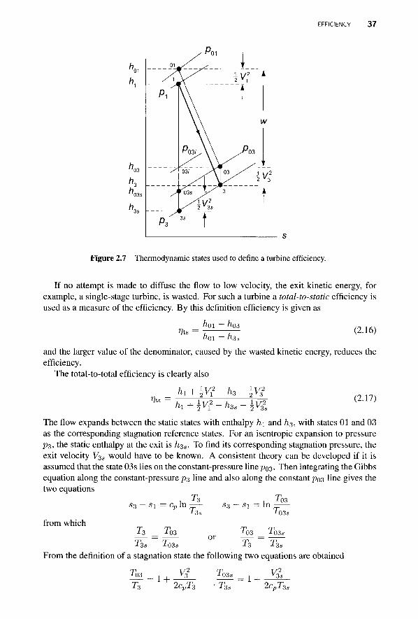
EFFICIENCY 37
Figure 2.7 Thermodynamic states used to define a turbine efficiency.
If no attempt is made to diffuse the flow to low velocity, the exit kinetic energy, for example, a single-stage turbine, is wasted. For such a turbine a total-to-static efficiency is used as a measure of the efficiency. By this definition efficiency is given as
r?ts '01 *03
^ 0 1 — ^ 3 s (2.16)
and the larger value of the denominator, caused by the wasted kinetic energy, reduces the efficiency.
The total-to-total efficiency is clearly also
% t fti + i V f - f t a I T / 2
2 V 3
hi + \V? h* l T / 2 2 V3s
(2.17)
The flow expands between the static states with enthalpy hi and h3, with states 01 and 03 as the corresponding stagnation reference states. For an isentropic expansion to pressure P3, the static enthalpy at the exit is / i 3 s . To find its corresponding stagnation pressure, the exit velocity V3s would have to be known. A consistent theory can be developed if it is assumed that the state 03s lies on the constant-pressure line p03- Then integrating the Gibbs equation along the constant-pressure p 3 line and also along the constant po3 line gives the two equations
^03
from which
«3 " S i
T3s
c P l n „
'03
3s S3 - si = In
Tr or
03s
TQ3
T3
TQ3S
TQ3S
From the definition of a stagnation state the following two equations are obtained
To3s vi T3 2cpT3 Tc 1 +
3s
V2 v3s
2cpT3 s
3 8 PRINCIPLES OF THERMODYNAMICS AND FLUID FLOW
and the equality of the temperature ratios on the left-hand sides (LHSs) of these equations shows that
V3s V T3s
so that V3 > V3S, but without a great loss of accuracy the temperature ratio is often replaced by unity, and then V3s is replaced by V3.
If a stage is designed such that V\ — V3, then the kinetic energy terms in the numerator of Eq. (2.17) be canceled. If next the approximation V3 = V3s is used, then Eq. (2.15) for total-to-total efficiency reduces to
hi - h3
Vt = hi - h3s
the more familiar definition of turbine efficiency from the study in the first course of thermodynamics. In a multistage turbine the exit state would need a different label. It will be denoted by label e when the distinction needs to be clarified.
■ EXAMPLE 2.9
Steam enters an adiabatic multistage turbine at static pressure of 80 bar, static tem-perature 520°C, and velocity 50m/s. It leaves the turbine at pressure 0.35 bar, temperature 80° C, and velocity 200 m/s. Find the total temperature and pressure at the inlet, total temperature and pressure at the exit, total-to-total efficiency, total-to-static efficiency, and the specific work done.
Solution: Using steam tables static enthalpy and entropy of steam at the inlet and exit are
hi = 3447.8 kJ/kg Sl = 6.7873 kJ/(kg • K)
he = 2645.0 kJ/kg se = 7.7553 kJ/(kg • K)
Stagnation enthalpies are
1 502
ftoi = hi + -Vi2 = 3447.8 + J-J^ = 3449.1 kJ/kg
1 2002
h0e = he + ~V% = 2645.0 + ^ - ^ = 2665.0 kJ/kg
Had the flow been isentropic, the exit state would have corresponded to pe = 0.35 bar and ses = Si. This is inside the vapor dome at quality
ses - sf 6.7873 - 0.9874 c c o i U.oOZl sg - Sf 7.7148 - 0.9874
and the enthalpy at this state is
hes =h{ + xes(hs - h{) = 304.20 + 0.8621 • (2630.7 - 304.20) = 2309.9kJ/kg
Assuming that Ves = Ve then gives
1 2002
hoe, = hes + 2Ve2 = 2309.9 + ^ - ^ = 2329.9 kJ/kg
EFFICIENCY 39
and the total-to-total efficiency is
= feoi ~ h0e = 3449.1 - 2665.0 = Vu h01-h0es 3449.1-2329.9
The total-to-static efficiency is
h01 - h0e 3449.1 - 2665.0 aQQQ r/ts = = = 0.6883 , t s hoi-hes 3449.1-2309.9
and the definition of efficiency when kinetic energy changes are neglected is
hi-he 3447.8-2645.0 rt /ii - /ies 3447.8 - 2309.9
The specific work delivered is
w = h01- h0e = 3449.1 - 2665.0 = 784.1 kJ/kg
Consider next a single-stage centrifugal compressor. The flow leaving the impeller enters a diffuser section, and then a volute. These stationary parts of the machine are designed to decelerate the flow so that at the exit velocity is well matched with the desired flow velocity in the discharge pipe. Since kinetic energy from the impeller is utilized in this way, it is again appropriate to define the efficiency as the total-to-total efficiency. It is given by
f?tt = — = T 7— (2.18) w ft03 - /ioi
The process lines between the stagnation states and the corresponding static states are shown in Figure 2.8. Now, as for the turbine, the state 03s is assumed to be on the constant-pressure line P03, and the sketch reflects this. Had the same amount of compression work been done reversibly the exit stagnation pressure would have been y>03i> which is also shown in the figure.
In ventilating blowers no use is made of the exit kinetic energy and in such applications the total-to-static efficiency is used. In these cases efficiency is defined as
_ fas — hpi <l03 — " 0 1
Since h3s is smaller than /io3S, the efficiency is likewise smaller, and the difference accounts for the wasted kinetic energy. To be sure, in ventilating a space, high velocity may be needed to blow off light particulate matter sitting on the floors or attached to walls. In this case a blower may be placed upstream of the ventilated space and forced draft used to remove the particles. In induced draft contaminated air is drawn from the ventilated space into a blower and the kinetic energy in the exhaust stream is lost to the surroundings.
■ EXAMPLE 2.10
Air is drawn into a fan of diameter D = 95.4 cm from atmosphere at pressure 101.325 kPa and temperature 288.0 K. The volumetric flow rate is Q = 4.72 m3 /s of standard air, and the power to the fan is W ■= 2.52 kW. The total-to-total efficiency
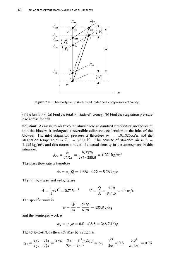
4 0 PRINCIPLES OF THERMODYNAMICS AND FLUID FLOW
Figure 2.8 Thermodynamic states used to define a compressor efficiency.
of the fan is 0.8. (a) Find the total-to-static efficiency, (b) Find the stagnation pressure rise across the fan.
Solution: As air is drawn from the atmosphere at standard temperature and pressure into the blower, it undergoes a reversible adiabatic acceleration to the inlet of the blower. The inlet stagnation pressure is therefore poi = 101.325 kPa, and the stagnation temperature is Toi = 288.0 K. The density of standard air is p = 1.225 kg/m3, and this corresponds to the actual density in the atmosphere in this situation:
Poi Poi RTQI
The mass flow rate is therefore
101325 287 ■ 288.0
1.225 kg/m3
TO = pQlQ = 1.225 • 4.72 = 5.78kg/s
The fan flow area and velocity are
1 „o o . . Q 4.72 -TTD2 = 0.715 m2 V
The specific work is W 2520
w m 5.78
0.715
435.8 J/kg
6.6 m/s
and the isentropic work is
Ws = r)ttw = 0.8 • 435.8 = 348.7 J/kg
The total-to-static efficiency may be written as
??ts T, 3s 101 T03s - T01 - V2/(2cp) TQS — TQI '03 ■Toi mt v3 6.62
0.8 2w 2 • 436 0.75
EFFICIENCY 4 1
(b) The stagnation pressure rise can be calculated from
P03-P01 = pws = 1.225-348.7 = 427Pa = 43.6 mm H 2 0
The exit states were labeled with subscript 3 even though this machine does not have anything that functions as a stator.
■ In a multistage compressor with large pressure and temperature differences, the variability of specific heats with temperature needs to be factored in to obtain an accurate result. This is illustrated in the next example.
■ EXAMPLE2.il
Air from the atmosphere flows into a multistage compressor at pressure 1 bar and temperature 300 K. The ratio of total pressures across the compressor is 30, and its total-to-total efficiency is 0.82. (a) Find the loss of stagnation pressure during this compression process, assuming specific heats to be constant, (b) Find also the loss in stagnation pressure assuming specific heats to vary with temperature.
Solution: (a) The inlet to the compressor is labeled as state 1, and its exit is denoted as e. The isentropic compression gives the stagnation temperature
Tm{ — ) = 300-30 1 / 3 5 = 792.8K ( 7 " l ) / 7
/ FUe \ 101 \P0lJ
From the definition of efficiency
_ TQ2S — J p i / t t /-*-] rj-\
J 0 2 — J o i
the exit temperature is
T0e = Toi + — (T0es - Toi) = 300 + ^ ( 7 9 2 . 8 - 300) = 901.0 K T]tt U.»2
If the same amount of work had been done isentropically, the pressure ratio would have been
Poa / T 0 e V / ( 7 _ 1 ) / 9 0 1 \ 3 ' 5 tont
Poi \ToiJ V300, Hence poei = 46.94 bar and the loss of stagnation pressure is Apoi = Pod — Poe = 4 6 . 9 4 - 3 0 = 16.94 bar. (b) For variable specific heats, at Toi = 300 K, from air tables pri — 1.386 and h01 = 300.19kJ/kg. Hence
P r e = P r l ^ = 1.386 • 30 = 41.58 Poi
From air tables Toes = 771.32 K and hoes = 790.56 kJ/kg. Using the definition of total-to-total efficiency
^Oes —ho\ mt = -7——7—
"Oe — " 0 1

4 2 PRINCIPLES OF THERMODYNAMICS AND FLUID FLOW
gives for the exit enthalpy the value
, , , h0es-h01 o n n i n , 790.56-300.19 SQH „ „ , , , , hoe = h0i H = 300.19 H —— = 898.26 kJ/kg
f]u U.82
From the air tables for this value pvei = 65.71. It then follows that
POei Prei 65.71 Poi Pri 1-386 47.41
and poei = 47'.41 bar. Hence the loss of stagnation pressure is ApoL = Pod — Poe = 47.41 — 30.0 = 17.41 bar. There is now some difference in the calculated results because the temperature range between inlet and exit states is large.
2.5.2 Thermodynamic losses
The effect of thermodynamic losses is illustrated by considering an increment on either a turbine or a compressor process line, as shown in Figure 2.9. From the Gibbs equation
Tds = dh — vdp
the slope of the constant-pressure line is
dh ~8s~ = T
which shows that this slope is equal to the absolute temperature on an enthalpy-entropy (hs) diagram The enthalpy change between the end states may be considered to be made up of two parts. The irreversible change in enthalpy is dhf — Tds, and the isentropic change is obtained by setting ds = 0, which gives dhs = v dp. Substituting these back into the Tds equation shows that in this notation
dh — dhs + dhf
For a compressor, all three terms are positive. For a turbine, dhf is positive, but dh and dhs have negative values. The irreversible process associated with dhf is called reheating, or internal heating. Although the former term is in general use to describe this, the latter is better for it reflects what is happening physically. In other words, the irreversibilities cause an increase in temperature.
The nature of the irreversibilities may be further illustrated by considering a flow channel that extends from an inlet at location Hi to some general location t. The first law of thermodynamics for this control volume is
Q + m (ui+pivi + -Vf+gzA = rh (u + pv + -V2 + gz\ +W
Differentiating this with respect to £ and rearranging gives
• du A' mTi=Q
d(pv) 1 dV1 dz dt 2 d£ y di
W' (2.19)
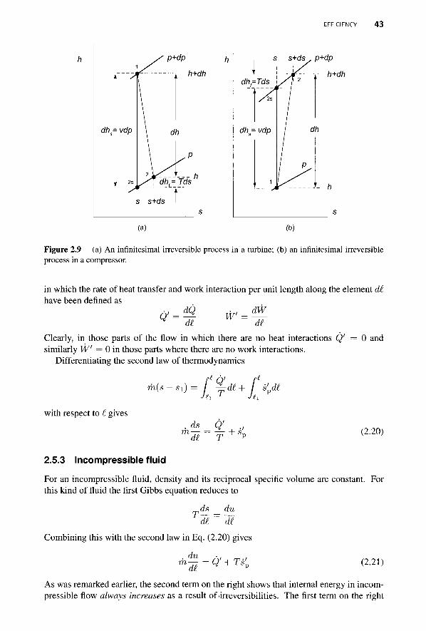
EFFICIENCY 43
J
dh,'
i
1
/
= vdp
' 2SJ
y p+dp
i •i
\ dh
2 i / 1 ^Tdh =
s s+ds
P
1 Tds
\
s s+ds, p+dp
,-- h+dh
y~ h
(a) (b)
Figure 2.9 (a) An infinitesimal irreversible process in a turbine; (b) an infinitesimal irreversible process in a compressor.
in which the rate of heat transfer and work interaction per unit length along the element di have been defined as
dQ_ d£
W' dW ~dJ
Clearly, in those parts of the flow in which there are no heat interactions Q' = 0 and similarly W' = 0 in those parts where there are no work interactions.
Differentiating the second law of thermodynamics
i ( s - s i ) T
d£- s'pd£
with respect to £ gives . ds Q'
md£ = Y + s* (2.20)
2.5.3 Incompressible fluid
For an incompressible fluid, density and its reciprocal specific volume are constant. For this kind of fluid the first Gibbs equation reduces to
ds du
Combining this with the second law in Eq. (2.20) gives
. du m- r+TS' (2.21)
As was remarked earlier, the second term on the right shows that internal energy in incom-pressible flow always increases as a result of-irreversibilities. The first term on the right
4 4 PRINCIPLES OF THERMODYNAMICS AND FLUID FLOW
side shows that internal energy increases by heat transfer into the fluid, but decreases when heat is lost to the surroundings. Integrating Eq. (2.21) gives
i re2
u2-u1=q+~ Ts'di (2.22) l r 2
m
Substituting Eq. (2.21) into Eq. (2.19) puts the latter into the form
U{pv) 1 dV2 dz ™{-^r + 2-dr+9di)+W' = ~T*v
Integrating this gives
Piv + \Vi + S*i = P2V + \vi + gz2+w+~ I Ts'p di (2.23) l z m Ji1
In Eqs. (2.21) and (2.23) absolute temperature T multiplies the entropy production rate s'p and it is the product Ts'p, having the dimensions of energy flow rate per unit length of the channel, which represents a thermodynamic energy loss.
In the first law of thermodynamics, flow work, kinetic and potential energy, and external work, are all associated with mechanical energy. On the other hand, internal energy and heat interaction are thermal energy terms. Viewed from this perspective Eq. (2.22) may be said to be a thermal energy balance and Eq. (2.23) a mechanical energy balance. The term associated with entropy production represents an irreversible conversion of mechanical energy into internal energy and is the reason why it is also called a thermodynamic energy loss. In contrast to a conservation principle in which there are no terms that would represent conversion of one form of energy to another, in a balance equation such conversion terms are present. Further examination shows that heat transfer to, or from, an incompressible fluid changes only the internal energy and not the pressure, velocity, or elevation. These quantities change only as a result of work done or extracted, and they decrease as a result of irreversibilities in the flow. It is customary not to make a distinction between conservation and balance principles in practice, and often the principle of conservation of mass, for example, is called simply the mass balance. This practice will also be followed in this text.
For an incompressible fluid stagnation pressure has been shown to be given by
Po = P + ^pV2 + pgz
Making use of this relationship, Eq. (2.23) takes the form
P02 = poi ~ pw - ^ / 2 Ts'p di (2.24)
This shows that stagnation pressure changes because of a work interaction with the sur-roundings and it drops because of irreversibilities in the flow.
2.5.4 Compressible flows
For compressible flows the first law of thermodynamics is written for a flow extending from location t\ to an arbitrary location £, as
Q + m(h! + -V? +gzx) = W + m (h + -V2 + gz
EFFICIENCY 45
or in terms of stagnation enthalpies as
Q + rhh0i = W + mh0
Differentiating gives
Q'-W' = m^- (2.25)
The second law of thermodynamics in the differential form has been shown to have the form
ds Q' ,
Writing next the second Tds equation between stagnation states as ds _ dh0 dp0 Tod£-^l'V°^i
and substituting ds/di from this into the second law leads to . dh0 . dp0 T0-, .,
Using Eq. (2.25) to eliminate dho/d£ yields the equation
dpp _ /To d£ ~ \T 7nvo^={-£-l)Q'-Tos'p-Wl (2.26)
Turbomachinery flows are adiabatic so the heat transfer term may be dropped. In an adiabatic flow integrating Eq. (2.26) gives
P02 ^ f^2
vQdp0 + w = - - T0s' d£ (2.27) POI m Jti
If the same amount of work had been done reversibly, then the exit stagnation pressure would have been different. Because the work done is the same, the pressure po2i lies along the constant ho2 line. A process line for this is shown in Figure 2.7, except that in that figure the exit enthalpy ho3 corresponds to the enthalpy ho2-
Integrating next Eq. (2.26) for a reversible process gives (•P02i
v0 dpo + ws = 0 (2.28) 'Poi
Thus, since it has been stipulated that w = ws, subtracting Eq. (2.27) from Eq. (2.28) gives rP02i i r^i I v0 dpo = — / T0s' d£
Jp02 m Jil Integration of this along the constant h02 line means that T02 remains constant and factors out after the substitution VQ = RTo/po- Then, carrying out the integration gives
i ? l n ^ l = - / s'd£ P02 ™ ' -
his equati
S2 — si = sp = .Rin '
But in an adiabatic flow mds = s' d£, and this equation reduces to P02i
P02
This relates the entropy increase to a loss in stagnation pressure. A simpler development of this result is given in later chap*0*"0
4 6 PRINCIPLES OF THERMODYNAMICS AND FLUID FLOW
EXAMPLE 2.12
The inlet stagnation temperature to a multistage turbine is 1400 K, and the inlet stagnation pressure is 1000 kPa. The pressure ratio is 10, and the total-to-total efficiency of the turbine is 0.89. Assuming that gases flowing through the turbine have 7 = | and R — 287 J/(kg • K), find the specific entropy production during the expansion assuming constant specific heats.
Solution: In this multistage turbine the inlet state is denoted by 1 and the exit by e. Assuming constant specific heats the definition of total-to-total efficiency reduces to
_ 7QI — Tpe _ 1 — Tpe/Tpi ??tt — ~ ~ or jjtt — - — ——
J 01 — JOes 1 — J 0es / J 01
from which Toe , /-, Toei — = 1-T)ti[l- —
The isentropic temperature ratio is
0es lPOe\ 0.5623
so that
and
T0i VPOI ) 101/4
r0es = 1400 • 0.5623 = 787.3 K
' 0 e 1400 [1 - 0.89(1 - 0.5623)] = 854.7 K
Since the amount of work done is proportional to the difference between the stagnation temperatures, if this work had been done reversibly the exit pressure would reach the value pod which is higher than before. It can be calculated from
Poa fT0ey/(l-1) /854.7\4 n i o o n
Wei _ I Oe \ _ I \ = 0 _ 1 3 8 9 Poi \ToiJ \U00
Hence poei = 1000 • 0.1389 = 138.9 kPa. Since the pressure ratio is 10, the exit stagnation pressure is P02 = 100 kPa, and the stagnation pressure loss is
Pod -Poe = 138.6 - 100 = 38.6 kPa
This represents 4.3% of the overall pressure difference poi — P02 = 900 kPa. The entropy production is calculated to be
S p = = i ? l n ^ l = 287 1n^=9.4J/(kg.K) POe 1UU.U

MOMENTUM BALANCE 47
2.6 MOMENTUM BALANCE
In this section the use of momentum balance is illustrated in applications of interest in turbomachinery. In uniform steady flow in a channel the momentum balance reduces to
m ( V 2 - V i ) (2.29)
in which F p is a pressure force and F v is a viscous force. The force F m is present if the control volume cuts across the solid parts of the machine. If the control volume contains only fluid, this term is absent. Weights of the fluid and hardware have been omitted with the understanding that when stress analysis is carried out, they will be taken into account. The first illustration on the use of the momentum equation is to calculate the force a that deflection of a jet causes on a fixed vane.
■ EXAMPLE 2.13
Consider a jet of water that flows into a vane at an angle a i . The vane is equiangular with a2 = —oil, and it turns the flow so that it leaves at a negative angle a2, as shown in Figure 2.10. Positive angles are measured in the counterclockwise direction from the x axis. The jet velocity at the inlet is V, and pressure surrounding the jet and the vane is atmospheric. Find the y component of the force on the vane.
Figure 2.10 Turning of a flow by a vane.
Solution: The inlet to the vane is denoted as station 1 and the exit as station 2. Since the streamlines are straight, both at the inlet and at the exit, pressure at both of these locations is equal to the atmospheric pressure pa across the jet. Then, with gravity neglected, Bernoulli equation shows that velocity at the exit is the same as at the inlet, so that Vi=V2 = V.
Momentum equation in the y direction gives
rn{V2y - Vly) py
in which the force Fpy is the y component of the pressure force exerted by the vane on the fluid. An equal and opposite force apts on the vane and it is denoted by Ry.
4 8 PRINCIPLES OF THERMODYNAMICS AND FLUID FLOW
At the inlet V\y = V sin a\ and at the exit Viy — V sin c*2, and for a negative value of ct-i this velocity component points in the minus y direction. The force on the blade is therefore
Ry = mV(smai — sin a^) The mass flow rate is m = pVA. Since the blade is equiangular, 012 = —a\. Substituting gives the force as
Ry — 2pAV2 sin ax
The force is largest when a\ = 90° and the flow is turned 180°. g
Consider again the flow shown in Figure 2.10, but now let the blade move in the y direction with velocity U, as shown in Figure 2.11. It is known that Newton's second law is valid in all coordinate systems that move at constant speed. Thus the momentum balance given by Eq. (2.29) is also valid for a control volume that moves with a uniform velocity U, if all velocities are to be replaced by relative velocities. In fact, noting that the relationship between the absolute velocity V and relative velocity W is given by
v = w + u and substituting this into Eq. (2.29) gives
m(W 2 + U - W i - U) = F p + F v + F m
or m(W 2 - W i ) = F p + F v + F m (2.30)
In the next example the momentum balance is used to analyze the force on a moving blade.
■ EXAMPLE 2.14 Consider a waterjet directed at a blade that moves with speed U. The angle 0:2 of the jet is such that the relative velocity meets the blade smoothly at the angle /J2. The blade is shaped such that it deflects the flow backward at an angle $3 = —02, as is shown in Figure 2.11. (a) Find the work done on the blade per unit mass of the flow and the blade speed for maximum work by carrying out the analysis in a set of fixed coordinates, (b) Carry out the same analysis in a set of moving coordinates, and find the y component of the force on the blade.
Solution: (a) The analysis is carried out first in fixed coordinates. Station 1 is now the inlet to a nozzle (not shown) that issues the water at station 2 at velocity V2 at angle ct<i. Station 2 is also the inlet to the moving blade, and its exit is station 3. The force that the blade exerts on the fluid is
Fpy = m(V3 s ina3 - V2 sina2)
and with Ry = —Fpy the force on the blade is
Ry = rh(V2 sin a2 — V3 sin a3)
Assuming that there are no losses, applying the first law to the control volume shown gives
V&, , -L Tr2 P a . i T A 2 , / I T I \ — + ^V2 = 1" ~V3 + Ws (2-31)
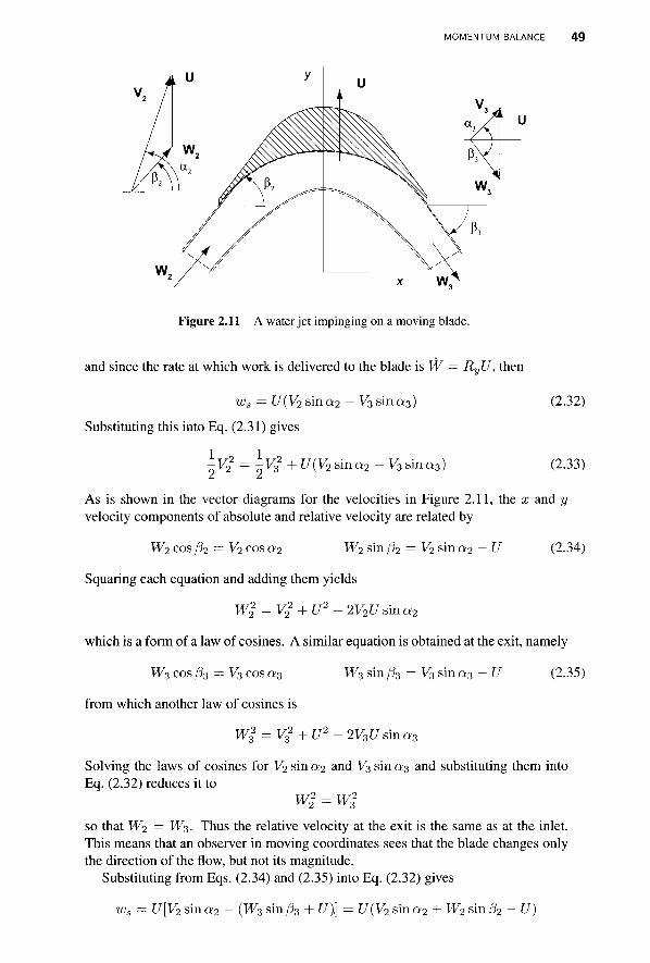
MOMENTUM BALANCE 49
Figure 2.11 A water jet impinging on a moving blade.
and since the rate at which work is delivered to the blade is W = RyU, then
ws — U(V2 sin 0:2 — V3 sin 0:3) (2.32)
Substituting this into Eq. (2.31) gives
\v% = \Vi + U(V2 sin a2 - V3 sin a3) (2.33)
As is shown in the vector diagrams for the velocities in Figure 2.11, the x and y velocity components of absolute and relative velocity are related by
W2 cos fa = V2 cos a2 W2 sin fa = V2 sin a.2 — U (2.34)
Squaring each equation and adding them yields
Wl = V22 + U2 - 2V2 U sin a2
which is a form of a law of cosines. A similar equation is obtained at the exit, namely
Wz cos fa = V3 cos a3 W3 sin fa = V3 sin a3 — U (2.35)
from which another law of cosines is
Wl = Vi + U2 - 2V3U sin a3
Solving the laws of cosines for V2 sin a.2 and V3 sin 0:3 and substituting them into Eq. (2.32) reduces it to
W2 = W2
so that Wi = W3. Thus the relative velocity at the exit is the same as at the inlet. This means that an observer in moving coordinates sees that the blade changes only the direction of the flow, but not its magnitude.
Substituting from Eqs. (2.34) and (2.35) into Eq. (2.32) gives
ws = U[V2 sin a2 - (W3 sin fa + £/),] = U(V2 sin a2 + W2 sin fa - U)
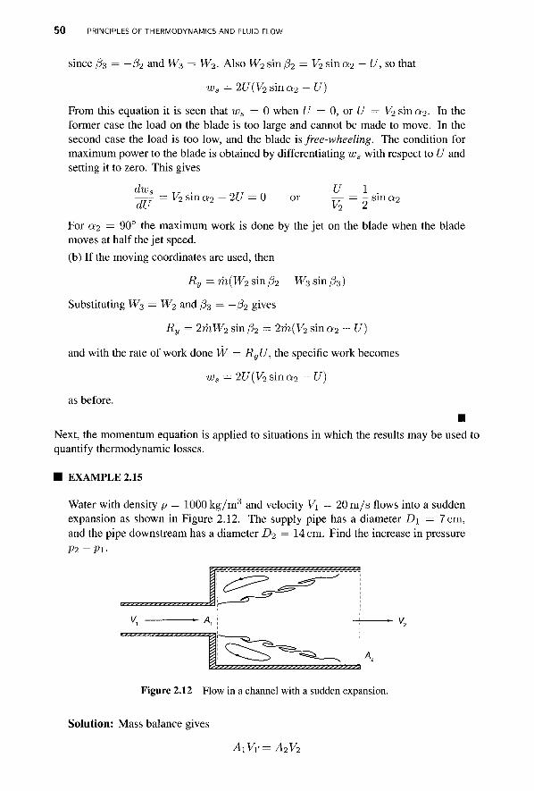
5 0 PRINCIPLES OF THERMODYNAMICS AND FLUID FLOW
since /33 = -(32 and W3 = W2. Also W2 sin j32 = V2 sin a2 - U, so that
wa = 2U(V2 sin a2 - U)
From this equation it is seen that ws = 0 when [/ = 0, or U — V2 sin 0:2. In the former case the load on the blade is too large and cannot be made to move. In the second case the load is too low, and the blade is free-wheeling. The condition for maximum power to the blade is obtained by differentiating ws with respect to U and setting it to zero. This gives
dws
~dU V2 sin a2 — 2U = 0 or U_
v2
1 sin a2
For a2 = 90° the maximum work is done by the jet on the blade when the blade moves at half the jet speed. (b) If the moving coordinates are used, then
R„
Substituting W3 = W2 and /33
m(W2 sin/32 — W3 sin/33)
= -j32 gives
Ry = 2mW2 sin ̂ 2 = 2m(V2 sina2 - U)
and with the rate of work done W = RyU, the specific work becomes
ws = 2U(V2 sin a2 - U)
as before. ■
Next, the momentum equation is applied to situations in which the results may be used to quantify thermodynamic losses.
■ EXAMPLE 2.15
Water with density p = 1000 kg/m3 and velocity V\ = 20 m/s flows into a sudden expansion as shown in Figure 2.12. The supply pipe has a diameter D\ = 7 cm, and the pipe downstream has a diameter D2 = 14 cm. Find the increase in pressure P2 -Pi-
Figure 2.12 Flow in a channel with a sudden expansion.
Solution: Mass balance gives
AXVY=A2V2
MOMENTUM BALANCE 5 1
Thus y2=y i!=2o(s)2=5-°m/s
As the water enters a sudden expansion, it detaches from the boundaries and moves into the larger space as a jet. Regions of recirculating flow develop at the upstream corners. Flow speed in these corners is sufficiently low to make the pressure uniform. The pressure across thejet at the exit plane is therefore equal to that in the recirculating regions. The stream velocity rises from small backflow in the recirculating regions to a large forward velocity in the jet. This leads to appreciable viscous forces in the free shear layers forming the jet boundary. Such free shear layers are unstable to small disturbances and roll up into vortices. These cause mixing of the low velocity fluid in the recirculating zone with the fast flow in the jet. As a consequence, the jet spreads and fills the channel. In the mixing zone the shear forces along the walls influence pressure much less than the mixing, and therefore they may be neglected.
Applying the momentum balance in the x direction leads to
pA2V2(V2 - Vi) = (pi - p2)A2
in which the mass balance, m = pV\A2 was used. Thus
P2 - P i = pV2(Vi -V2)
and the numerical value for the pressure increase is
p2-p! = 1000 • 5.0(20 - 5.0) = 75 kPa
As the area A2, is increased the exit velocity is reduced and finally becomes zero. In that case p2 = p\. This is the situation of a jet discharging to an atmosphere and then the exit pressure is equal to the atmospheric pressure.
The loss in stagnation pressure in a sudden expansion is
Poi - P02 =Pi + -^pVx -Vi-^pVi = 2py?-pViV2 + -pV22 = -p(V!-V2)2
or Poi - P02 = -z 1000 (20 - 5)2 = 112.5kPa
If the flow were to diffuse to the exit pipe without irreversibilities, there would be no loss of stagnation pressure and the exit pressure could be calculated from the Bernoulli equation. It would have the value
P2i ~Pi = \p(V? - V2) = ^1000(202 - 52) - 187.5 kPa
above the inlet pressure. Contrasting this to the value 75 kPa calculated in the actual case shows that not all pressure is recovered, and the irreversibility can be regarded as a loss in pressure.
This underscores the importance of a well-designed diffuser to recover as much of the pressure as possible. The reduction of kinetic energy in diffusion goes into flow work on the fluid particles ahead, causing pressure to increase. If part of the kinetic energy is dissipated by viscous action in mixing, less is available for increasing the pressure. This is clearly true if the sudden expansion takes place into a vast reservoir,
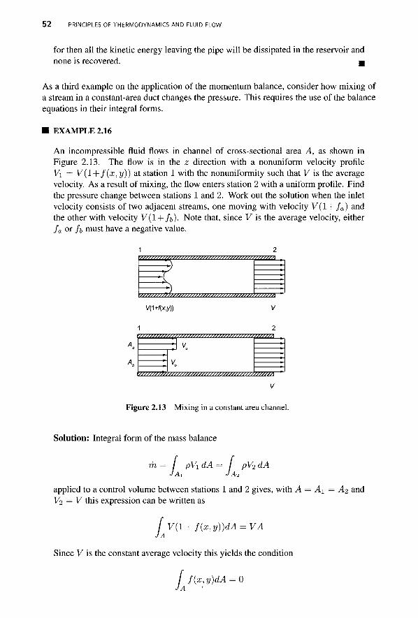
5 2 PRINCIPLES OF THERMODYNAMICS AND FLUID FLOW
for then all the kinetic energy leaving the pipe will be dissipated in the reservoir and none is recovered. g
As a third example on the application of the momentum balance, consider how mixing of a stream in a constant-area duct changes the pressure. This requires the use of the balance equations in their integral forms.
■ EXAMPLE 2.16
An incompressible fluid flows in channel of cross-sectional area A, as shown in Figure 2.13. The flow is in the z direction with a nonuniform velocity profile V\ — V(l + f(x,y)) at station 1 with the nonuniformity such that V is the average velocity. As a result of mixing, the flow enters station 2 with a uniform profile. Find the pressure change between stations 1 and 2. Work out the solution when the inlet velocity consists of two adjacent streams, one moving with velocity V(l + fa) and the other with velocity V ( l + /(,). Note that, since V is the average velocity, either fa or / t must have a negative value.
V////////(//////////S///////J///////////////////n -
a w;;;;;;#Jss/sss/sssjssssss/s;ssssssssss>s;;y>jM V(1+f(x,y))
rs/sssssssss/fsss/ssss/ss//sssssssss/sssss/l>ss//ssi
;;;;;;/;>;/;;;;;;;;;;;;;;;;;;;;;;;;;;;;;;/;J;;;;A
Figure 2.13 Mixing in a constant area channel.
Solution: Integral form of the mass balance
m= [ PVldA= I PV2dA JAi J A2
applied to a control volume between stations 1 and 2 gives, with A = A\ = A2 and V2 = V this expression can be written as
f V(l + f(x,y))dA = VA JA
Since V is the constant average velocity this yields the condition
[ f(x,y)dA = 0 JA

MOMENTUM BALANCE 53
The x component of the momentum equation applied to this control volume gives
/ PV2dA - [ pV2dA = (PI-P2)A JA2 JA1
Again, since at the exit velocity Vi = V is uniform, this can be written as
-pV2A + p [ V2(l + f(x,y))2dA = ( K - P l ) A JA
Wall shear has been neglected under the assumption that mixing influences the pressure change much more than does wall shear.
Expanding the integral leads to
f(l + f2(x,y))dA = f(l + 2f(x,y) + f2(x,y))dA = A + f f2(x,y)dA J A J A JA
for, as shown above, the middle term is zero. Denoting
P = j j f2(x,y)dA
the pressure increase is seen to be
P2-P1=PV2P
With the velocities as shown on the bottom half of the figure, mass balance gives
AaVa + AbVb = AV
and since A = Aa + Ab, this reduces to
y = V<>Aa + VbAb
Aa+Ab
Writing Va = V{1 + fa) and Vb = V(l + fb)
and solving for fa and fb gives
f _ Va _ _ (Va- Vb)Ab fa — TA t V VaAa + VbAb
and , Vb (Vb-Va)Aa Jb = 77 - J- ~ V VaAa + VbAb
The value of f2 is the area-weighted average
ji _ RK + ftAb _ (Va - Vb)2AaAb
Aa + Ab (VaAa + VbA,
Hence the pressure increase is
V2 -Pi = p{Va - Vb) 2 AaAb
(Aa + Atf
5 4 PRINCIPLES OF THERMODYNAMICS AND FLUID FLOW
As a special case, consider the situation in which Vf, = 0. Then
V = 4^T and Va-V=J«Ab Aa + Ab Aa + Ab
and P2-Pi=pV(Va-V) (2.36)
This is the same result that was developed in Example 2.15. B
In these examples the momentum equation could be used to obtain information about the downstream pressure. This was possible because the viscous forces could be neglected. Such a situation also characterizes many turbomachinery flows in which the important force balance is between the inertia of the flow and pressure forces.
EXERCISES
2.1 Steam flows through a bank of nozzles shown in Figure 2.1 with wall thickness i2 = 2 mm, spacing s = 4 cm, blade height b = 2.5 cm, and exit angle «2 = 68°. The exit velocity V2 = 400 m/s, pressure is p2 = 1-5 bar, and temperature is T2 = 200°C. Find the mass flow rate.
2.2 Air enters a compressor from atmosphere at pressure 102 kPa and temperature 42°C. Assuming that its density remains constant, determine the specific compression work required to raise its pressure to 140 kPa in a reversible adiabatic process, given an exit velocity of 50 m/s.
2.3 Steam flows through a turbine at the rate of rn — 9000 kg/h. The rate at which power is delivered by the turbine is W — 440 hp. The inlet total pressure is poi = 70 bar, and total temperature is T01 = 420° C. For a reversible and adiabatic process, find the total pressure and temperature leaving the turbine.
2.4 Water enters a pump as saturated liquid at total pressure of poi = 0.08 bar and leaves it at p02 = 30 bar. The mass flow rate is rh = 10,000 kg/h and assuming that the process takes place reversibly and adiabatically, determine the power required.
2.5 Liquid water at 700 kPa and temperature 20°C flows at velocity 15 m/s. Find the stagnation temperature and stagnation pressure.
2.6 Water at temperature Ti = 20° C flows through a turbine with inlet velocity V\ = 3 m/s, static pressure p\ = 780 kPa, and elevation z\ = 2 m. At the exit the conditions are V2 = 6 m/s, p2 = 100 kPa, and z2 = 1.2 m. Find the specific work delivered by the turbine.
2.7 Air at static pressure 2 bar and static temperature 300°K flows with velocity 60 m/s. Find total temperature and pressure.
2.8 Air at static temperature 300° K and static pressure 140 kPa flows with velocity 60 m/s. Evaluate the total temperature and total pressure of air. Repeat the calculation assuming that the airspeed is 300 m/s.
2.9 Air undergoes an increase of 1.75 kPa in total pressure through a blower. The inlet total pressure is one atmosphere, and the inlet total temperature is 21°C. Evaluate the exit total temperature assuming that the process is reversible adiabatic. Evaluate the energy added to the air per unit mass flow.
EXERCISES 55
2.10 Air enters a blower from the atmosphere where pressure is 101.3 kPa and temper-ature is 27°C. Its velocity at the inlet is 46 m/s. At the exit the total temperature is 28°C and the velocity is 123 m/s. Assuming that the flow is reversible and adiabatic, determine (a) the change in total pressure in millimeters of water and (b) the change in static pressure, also in millimeters of water.
2.11 The total pressure, static pressure, and the total temperature of air at a certain point in a flow are 700 kPa, 350 kPa, and 450 K, respectively. Find the velocity at that point.
2.12 Air has static pressure 2 bar and static temperature 300° K while flowing at speed 1000 m/s. (a) Assuming that air obeys the ideal gas law with constant specific heats, determine its stagnation temperature and stagnation pressure, (b) Repeat part (a) using the air tables.
2.13 At a certain location the velocity of air flowing in a duct is 321.5 m/s. At that location the stagnation pressure is 700 kPa and stagnation temperature is 450 K. What is the static density at this location?
2.14 Air flows in a circular duct of diameter 4 cm at the rate of 0.5 kg/s. The flow is adiabatic with stagnation temperature 288 K. At a certain location the static pressure is 110 kPa. Find the velocity at this location.
2.15 Saturated steam enters a nozzle at static pressure 14 bar at velocity 52 m/s. It expands isentropically to pressure 8.2 bar. Mass flow rate is m = 0.7 kg/s. Find the exit area, assuming that (a) steam behaves as an ideal gas with 7 = 1.135, and cp = 2731 J/kg K; (b) the end state is calculated with properties obtained from the steam tables.
2.16 A fluid enters a turbine with total temperature of 330 K and total pressure of 700 kPa. The outlet total pressure is 100 kPa, and assume that the expansion process through the turbine is isentropic. Evaluate (a) the work per unit mass flow assuming that the fluid is incompressible with a density 1000 kg/m3, (b) and assuming that the fluid is air.
2.17 Air flows through a turbine that has a total pressure ratio 5 to 1. The total-to-total efficiency is 80%, and the flow rate is 1.5 kg/s. The desired output power is to be 250hp (186.4kW). Determine (a) the inlet total temperature, (b) the outlet total temperature, (c) the outlet static temperature given an exit velocity 90 m/s. (d) Then draw the process on a Ts diagram and determine the total-to-static efficiency of the turbine.
2.18 A blower has a change in total enthalpy of 6000 J/kg, an inlet total temperature 288 K, and an inlet total pressure 101.3 kPa. Find (a) the exit total temperature assuming that the working fluid is air, (b) the total pressure ratio across the machine, given a total-to-total efficiency of 75%.
2.19 A multistage turbine has a total pressure ratio of 2.5 across each of four stages. The inlet total temperature is TQI = 1200 K and the total-to-total efficiency of each stage is 0.87. Evaluate the overall total-to-total efficiency of the turbine by assuming that steam is flowing through it. Steam can be assumed to behave as a perfect gas with 7 = 1.3. Why is the overall efficiency higher than the stage efficiency?
2.20 Gases from a combustion chamber enter a gas turbine at a total pressure of 700 kPa and a total temperature of 1100 K. The total pressure and total temperature at the exit of the turbine are 140 kPa and 780 K. Assuming that 7 = | is used for the mixture of combustion gases, which has a molecular mass of 28.97 kg/kmol, find the total-to-total efficiency and the total-to-static efficiency of the turbine, for an exit velocity of 210 m/s.

5 6 PRINCIPLES OF THERMODYNAMICS AND FLUID FLOW
2.21 Air enters a compressor from atmosphere at 101.3 kPa, 288 K. It is compressed to a static pressure of 420 kPa, and at the exit its velocity is 300 m/s. The compressor total-to-total efficiency is 0.82. (a) Find the exit static temperature by assuming that Vis = Vi-(b) Find the exit static temperature, without making the assumption that Vis is equal to Vi-
2.22 Liquid water issues at velocity V\ — 20 m/s from a bank of five oblique nozzles shown in Figure 2.14. The nozzles with wall thickness t = 0.2 cm are spaced s = 4 cm apart. The nozzle angle is a\ = 70°. Using the mass and momentum balance, (a) find the downstream velocity Vi, (b) find the pressure increase in the flow, (c) show how to deduce this result from Eq. 2.36. (d) Assuming that the thickness of the wall is vanishingly small, what is the change in pressure?
k? Figure 2.14 Nozzles with an oblique discharge.
2.23 Consider the flow shown in Figure 2.14. Prove that the kinetic energy lost in the flow as it moves to the downstream section is equal to that associated with the transverse component of the velocity. Neglect the wall thickness of the nozzles.
CHAPTER 3
COMPRESSIBLE FLOW THROUGH NOZZLES
In this chapter the dynamics and thermodynamics of compressible fluid flow through nozzles are discussed. First, the isentropic relations are developed and applied to a converging and a converging-diverging nozzle. After that normal shock relations are given. Then nozzle flows with friction are presented, various loss coefficients are introduced, and wet steam behavior is discussed. The last topic of the chapter is the Prandtl-Meyer expansion.
3.1 MACH NUMBER AND THE SPEED OF SOUND
Consider a stationary fluid in which a weak pressure wave travels to the right at velocity c, as is shown on the top part of Figure 3.1. Pressure and other thermodynamic properties change across the wavefront. Ahead of the front in the stagnant fluid velocity V = 0, and its pressure has the value p and its density is p. After the front has passed through a given location, let the velocity there be A y and pressure and density be p + Ap and p + Ap, respectively. It is advantageous to shift to a frame of reference that moves to the right with speed c, for in that frame the front is stationary. Hence the balance principles in their steady form can be applied to a stationary control volume containing the front. In this frame fluid approaches the control volume with speed c from the right. Mass balance then gives
pcA = (p + Ap){c~AV)A (3.1)
Principles of Turbomachinery. By Seppo A. Kcfrpela 57 Copyright © 2011 John Wiley & Sons, Inc.
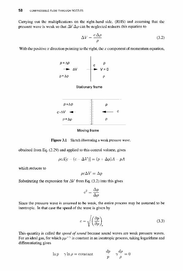
5 8 COMPRESSIBLE FLOW THROUGH NOZZLES
Carrying out the multiplications on the right-hand side, (RHS) and assuming that the pressure wave is weak so that AVAp can be neglected reduces this equation to
AV = cAp
(3.2)
With the positive x direction pointing to the right, the x component of momentum equation,
p + Ap
p + Ap
AV V=0
P
Stationary frame
r
p+Ap !
C-AV - * - !
p + Ap L
i P
r.
P
Moving frame
Figure 3.1 Sketch illustrating a weak pressure wave.
obtained from Eq. (2.29) and applied to this control volume, gives
pcA[c - (c - AV)] = {p + Ap)A - pA
which reduces to pcAV = Ap
Substituting the expression for AV from Eq. (3.2) into this gives
Ap
Since the pressure wave is assumed to be weak, the entire process may be assumed to be isentropic. In that case the speed of the wave is given by
dp dp
(3.3)
This quantity is called the speed of sound because sound waves are weak pressure waves. For an ideal gas, for which pp"1 is constant in an isentropic process, taking logarithms and differentiating gives
dp dp In p — 7 In p = constant 7— = 0
P P
MACH NUMBER AND THE SPEED OF SOUND 59
from which can be formed the partial derivative
dp\ p — = 7 - = 7RT dPJs P
Speed of sound c for a perfect gas is therefore given by c = y/'jRT = ^jRT/M
For air R = R/M = 8314/28.97 = 287 J/(kg • K) and 7 = 1.4 the speed of sound at T = 300 K is c = 347 m/s. For combustion gases with R = 287J/(kg • K) and T = 1200 K it is c = 677.6 m/s. For gases of large molecular mass the speed of sound is small and the opposite is true for gases of low molecular mass. For example, the refrigerant R134a, or tetrafluoroethane, with a chemical formula CH2FCF3, has a molecular mass of M = 102.0 kg/kmol. Its ratio of specific heats is 7 = 1.14. Hence at T = 300 K the speed of sound in R134a is only c = 167 m/s. For helium at the same temperature, speed of sound is c = 1019 m/s.
Mach number is defined to be the ratio of the local fluid velocity to the local sound speed
c
Subsonic flows have M < 1, supersonic ones have M > 1, and for hypersonic flows M » l . Flows for which M ~ 1 are called transonic.
3.1.1 Mach number relations
In an ideal gas with constant specific heats the definition of stagnation enthalpy
h0 = h+^V2
can be recast as y 2 _rr , ( 7 - l ) T , 2 _ ^ A , 7 - 1 , , 2 To = T+— =T+ v ' 'V1 = T 1 + -^^M 2cp 27K
from which
T 2 From the definition of a stagnation state, it follows that
frp \ 7 / ( 7 - l ) . / T \ l / ( 7 - l ) Po / - ' o \ Po Mo V \T J p
These can be written in terms of Mach number as
\ 7 / ( 7 - l ) ^ = ( l + ^ M 2 ) (3.4)
and / 1 \ l / ( 7 - l )
Po {-, , 7 - l » , 2 X . 1 + ^Y7M ) (3-5)
6 0 COMPRESSIBLE FLOW THROUGH NOZZLES
These equations are in dimensionless form, and they represent the most economical way to show functional dependence of variables on the flow velocity.
Equation (3.4) for pressure can be expanded by the binomial theorem1 for small values of Mach number. This leads to
?° = 1 + 2 M 2 + 1M4 _ lh^lMZ + ... = l + l M2 ( l + ~M2 +
p 2 8 48 2 V 4
which, when only the first two terms are retained, can be rearranged as
p 21RT 2p
so that Po = V + ^pV2
For incompressible fluids this was taken to be the definition of stagnation pressure. In fact, it is seen to be approximately valid also for flows of compressible fluids when M -C 1. In practice, this approximation is quite accurate if M < 0.3.
■ EXAMPLE 3.1
At a certain location in a flow of air static pressure has been measured to bep = 2.4 bar and stagnation pressure, p0 = 3 bar. Measurement of the total temperature shows it to be To = 468 K. Find the Mach number and flow rate per unit area.
Solution: Static temperature can be determined from
/ D \ ( 7 - D / 7 / 2 4 \ 1 / 3 - 5
T = T0 I — \ = 468 ( — j = 439.1 K
Then, solving
T 2 for Mach number gives M = 0.574. With Mach number known, velocity can be determined from V = Mc. Speed of sound at this temperature is
c = y/jRT = VIA ■ 287 • 439.1 = 420.0 m/s
so that the velocity is V = Mc = 241 m/s
Static density is given by
_ JP_ _ 240000 P~ ~KT ~ 287-439.1
Hence the mass flow rate per unit area is
m
1.904 kg/nr*
pV = 1.904 • 241 = 458.9 kg/(s • m2)
'Binomial theorem gives the expansion (l + a ) n = l + n a + ^^ j— -a 2 -f ^-^—^^—^-a3 + ■
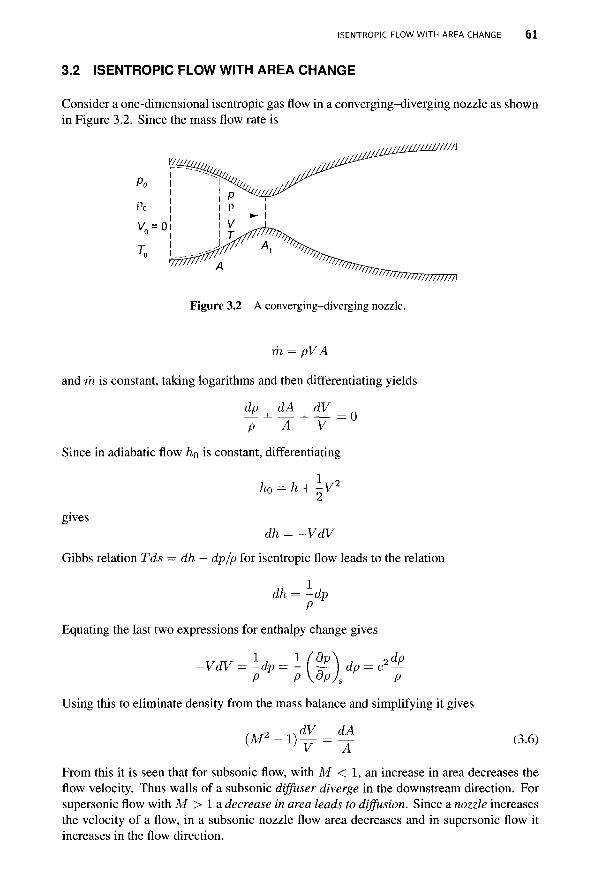
ISENTROPIC FLOW WITH AREA CHANGE 6 1
3.2 ISENTROPIC FLOW WITH AREA CHANGE
Consider a one-dimensional isentropic gas flow in a converging-diverging nozzle as shown in Figure 3.2. Since the mass flow rate is
■imuuiuA
'W7777//////////J
Figure 3.2 A converging-diverging nozzle.
rh — pVA
and m is constant, taking logarithms and then differentiating yields
dp P
dA A
dV_ V 0
Since in adiabatic flow ho is constant, differentiating
1, h0 = h+~V2
gives dh = ~VdV
Gibbs relation Tds — dh — dp/p for isentropic flow leads to the relation
dh = -dp P
Equating the last two expressions for enthalpy change gives
-VdV 1 -dp ■
dp dp ■■
,dp P ~ P \dP/s ' P
Using this to eliminate density from the mass balance and simplifying it gives
dV dA {Mz - 1 ) -
V A (3.6)
From this it is seen that for subsonic flow, with M < 1, an increase in area decreases the flow velocity. Thus walls of a subsonic dijfuser diverge in the downstream direction. For supersonic flow with M > 1 a decrease in area leads to diffusion. Since a nozzle increases the velocity of a flow, in a subsonic nozzle flow area decreases and in supersonic flow it increases in the flow direction.
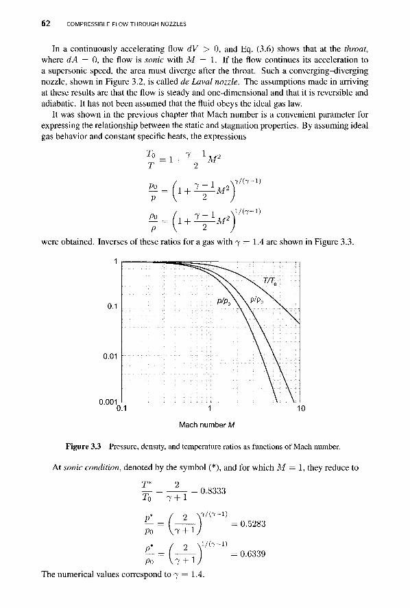
6 2 COMPRESSIBLE FLOW THROUGH NOZZLES
In a continuously accelerating flow dV > 0, and Eq. (3.6) shows that at the throat, where dA = 0, the flow is sonic with M = 1. If the flow continues its acceleration to a supersonic speed, the area must diverge after the throat. Such a converging-diverging nozzle, shown in Figure 3.2, is called de Laval nozzle. The assumptions made in arriving at these results are that the flow is steady and one-dimensional and that it is reversible and adiabatic. It has not been assumed that the fluid obeys the ideal gas law.
It was shown in the previous chapter that Mach number is a convenient parameter for expressing the relationship between the static and stagnation properties. By assuming ideal gas behavior and constant specific heats, the expressions
To T = 1 + 7 -M2
^ = ( 1 + P
Po
^ M 2
7 lM2
were obtained. Inverses of these ratios for a gas with 7 — 1.4 are shown in Figure 3.3.
7/ (7 -1)
1/(7-1)
0.01
0.001
Mach number M
Figure 3.3 Pressure, density, and temperature ratios as functions of Mach number.
At sonic condition, denoted by the symbol (*), and for which M = 1, they reduce to
0.8333 T0
P* Po
P*
7 + 1
-( 2 V7+1
- ( 2
7/ (7-1)
Po , 7 + 1 The numerical values correspond to 7 = 1.4.
0.5283
1/(7-1) = 0.6339
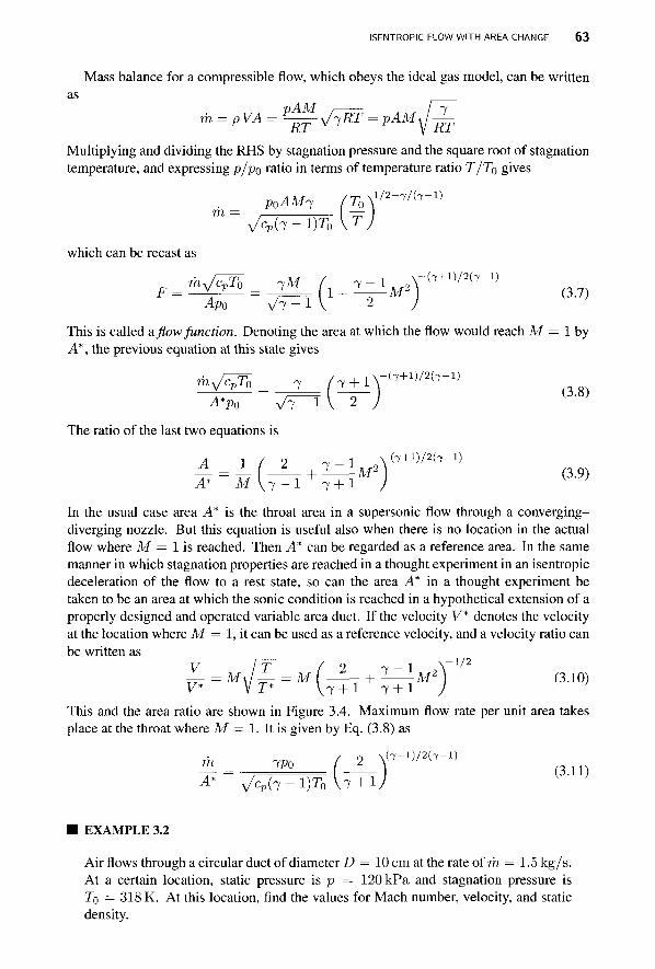
ISENTROPIC FLOW WITH AREA CHANGE 6 3
Mass balance for a compressible flow, which obeys the ideal gas model, can be written as
Multiplying and dividing the RHS by stagnation pressure and the square root of stagnation temperature, and expressing p/po ratio in terms of temperature ratio T/TQ gives
^ ( 7 - 1)T0 V T
which can be recast as
F = \ v = / 1 + -h—M2 (3.7) Ap0 \rv-i
This is called a. flow function. Denoting the area at which the flow would reach M = 1 by A*, the previous equation at this state gives
^r= VY^I I T J (3-8) The ratio of the last two equations is
A _ l ( 2 , 7 - l „ 2 ( 7 + l ) / 2 ( 7 - l ) + -M'A 1 (3 9)
A* M V7 + 1 7 + 1 ) In the usual case area A* is the throat area in a supersonic flow through a converging-diverging nozzle. But this equation is useful also when there is no location in the actual flow where M = 1 is reached. Then A* can be regarded as a reference area. In the same manner in which stagnation properties are reached in a thought experiment in an isentropic deceleration of the flow to a rest state, so can the area A* in a thought experiment be taken to be an area at which the sonic condition is reached in a hypothetical extension of a properly designed and operated variable area duct. If the velocity V* denotes the velocity at the location where M = 1, it can be used as a reference velocity, and a velocity ratio can be written as
V HT ( 2 7 - 1 9 \~ 1 / 2
— =M\\—=M\ - + 1—-M2) (3.10) V* V T* V 7 + 1 7 + 1 /
This and the area ratio are shown in Figure 3.4. Maximum flow rate per unit area takes place at the throat where M = 1. It is given by Eq. (3.8) as
A* ^ ( 7 - 1 ) 7 1 , W + l /
EXAMPLE 3.2
Air flows through a circular duct of diameter D = 10 cm at the rate of m = 1.5kg/s. At a certain location, static pressure is p = 120 kPa and stagnation pressure is T0 = 318 K. At this location, find the values for Mach number, velocity, and static density.
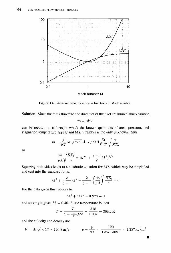
6 4 COMPRESSIBLE FLOW THROUGH NOZZLES
100
10
0.1 0.1 1 10
Mach number M
Figure 3.4 Area and velocity ratios as functions of Mach number.
Solution: Since the mass flow rate and diameter of the duct are known, mass balance
TO = pVA
can be recast into a form in which the known quantities of area, pressure, and stagnation temperature appear and Mach number is the only unknown. Thus
TO = J^M^RTA = pMA^ T RTQ 7
or TO RT0 „ , . „ 7 - 1 , ^ 9 x 1 / 2
' M( l + -L——M2)1'2 pA y 7
Squaring both sides leads to a quadratic equation for M2, which may be simplified and cast into the standard form:
M4 + _2_^__J_(j»Y^i>=0 7 —1 7 — 1 \pA J 7
For the data given this reduces to
M 4 + 5M2 - 0.828 = 0
and solving it gives M = 0.40. Static temperature is then To 318
1 + V M 2 1-032
and the velocity and density are
V = M^-fRT = 140.8 m/s
308.1 K
120 P = RT 0.287-308.1
1.357 kg/m3
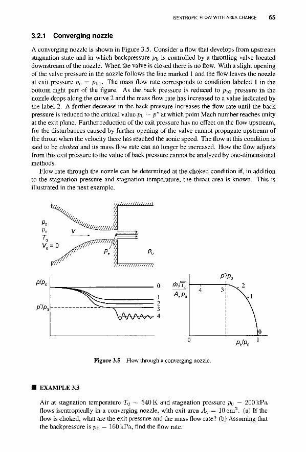
ISENTROPIC FLOW WITH AREA CHANGE 6 5
3.2.1 Converging nozzle
A converging nozzle is shown in Figure 3.5. Consider a flow that develops from upstream stagnation state and in which backpressure p^ is controlled by a throttling valve located downstream of the nozzle. When the valve is closed there is no flow. With a slight opening of the valve pressure in the nozzle follows the line marked 1 and the flow leaves the nozzle at exit pressure pe = pbi • The mass flow rate corresponds to condition labeled 1 in the bottom right part of the figure. As the back pressure is reduced to pb2 pressure in the nozzle drops along the curve 2 and the mass flow rate has increased to a value indicated by the label 2. A further decrease in the back pressure increases the flow rate until the back pressure is reduced to the critical value p^ = p* at which point Mach number reaches unity at the exit plane. Further reduction of the exit pressure has no effect on the flow upstream, for the disturbances caused by further opening of the valve cannot propagate upstream of the throat when the velocity there has reached the sonic speed. The flow at this condition is said to be choked and its mass flow rate can no longer be increased. How the flow adjusts from this exit pressure to the value of back pressure cannot be analyzed by one-dimensional methods.
Flow rate through the nozzle can be determined at the choked condition if, in addition to the stagnation pressure and stagnation temperature, the throat area is known. This is illustrated in the next example.
/////////II/II//K
/77777777777777777J
P/Po
P7Po Vwvw e " 0
4
P
3
!P0
. 2
X 1
\o Pb/Po
Figure 3.5 Flow through a converging nozzle.
EXAMPLE 3.3
Air at stagnation temperature T0 — 540 K and stagnation pressure po = 200 kPa flows isentropically in a converging nozzle, with exit area At = 10 cm2. (a) If the flow is choked, what are the exit pressure and the mass flow rate? (b) Assuming that the backpressure is pb = 160 kPa, find the flow rate.
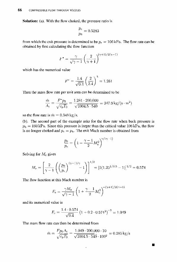
6 6 COMPRESSIBLE FLOW THROUGH NOZZLES
Solution: (a). With the flow choked, the pressure ratio is
Pe
PO 0.5283
from which the exit pressure is determined to be pe = 106 kPa. The flow rate can be obtained by first calculating the flow function
F* 7 Vl^l \ 7 + l
( 7 + l ) / 2 ( 7 - l )
which has the numerical value
F* 1.4 1.281
/OA \2.4
Then the mass flow rate per unit area can be determined to be
m F*p0 1.281 • 200,000 At ^/cJF0 V1004.5 ■ 540
347.9 kg/(s-m2)
so the flow rate is m = 0.348 kg/s. (b). The second part of the example asks for the flow rate when back pressure is Pb = 160 kPa. Since this pressure is larger than the critical value 106 kPa, the flow is no longer choked and pe = pt>- The exit Mach number is obtained from
Po
Pe 1
J-^M? 7/ (7-1)
Solving for Me gives
Mfi Po\
( 7 - l ) / 7 N
I " 1 \\PeJ
The flow function at this Mach number is
1/2
= [5(1.25 1/3.5 i l / 2 0.574
e VY^i and its numerical value is
1.4 • 0.574
lMe (, , 7 - l 2 1 + - ( 7 + l ) / 2 ( 7 - l )
/0.4 (1+0.2-0.5742) 3 = 1.049
The mass flow rate can then be determined from
Fp0At 1.049 • 200,000 • 10 m s/cplh V1004.5 ■ 540 • 1002 0.285 kg/s
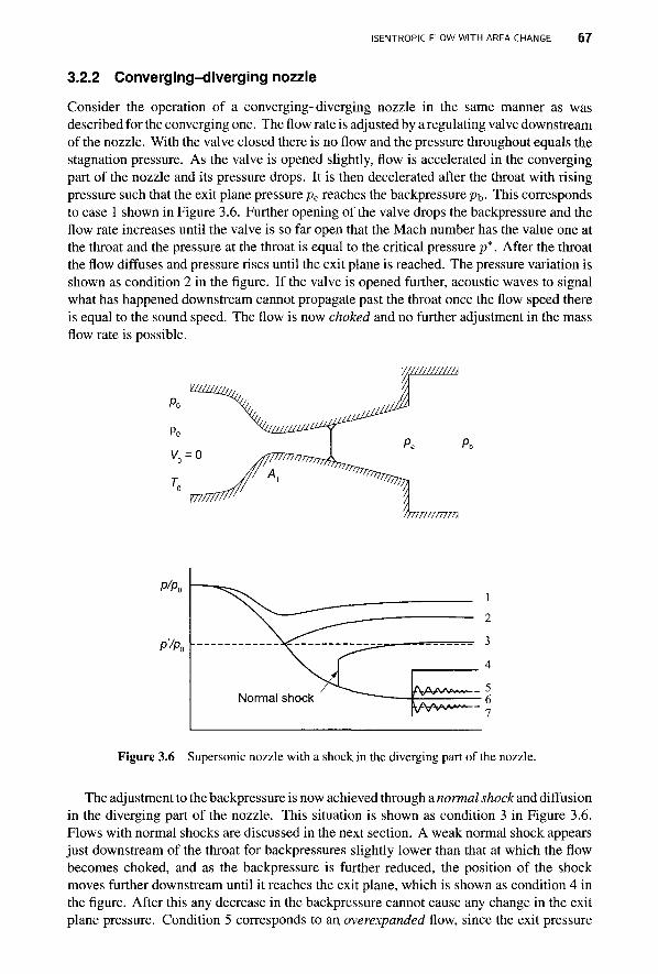
ISENTROPIC FLOW WITH AREA CHANGE 6 7
3.2.2 Converging-diverging nozzle
Consider the operation of a converging-diverging nozzle in the same manner as was described for the converging one. The flow rate is adjusted by a regulating valve downstream of the nozzle. With the valve closed there is no flow and the pressure throughout equals the stagnation pressure. As the valve is opened slightly, flow is accelerated in the converging part of the nozzle and its pressure drops. It is then decelerated after the throat with rising pressure such that the exit plane pressure pe reaches the backpressure p f This corresponds to case 1 shown in Figure 3.6. Further opening of the valve drops the backpressure and the flow rate increases until the valve is so far open that the Mach number has the value one at the throat and the pressure at the throat is equal to the critical pressure p*. After the throat the flow diffuses and pressure rises until the exit plane is reached. The pressure variation is shown as condition 2 in the figure. If the valve is opened further, acoustic waves to signal what has happened downstream cannot propagate past the throat once the flow speed there is equal to the sound speed. The flow is now choked and no further adjustment in the mass flow rate is possible.
Po
Po
V0 = 0
'// <//////////n
/7777777777m
p/pa
P'/Po
Normal shock
1
->■
L____ ^ 1
4
^A/w**" 5 ^ v w > ^ — "
Figure 3.6 Supersonic nozzle with a shock in the diverging part of the nozzle.
The adjustment to the backpressure is now achieved through a normal shock and diffusion in the diverging part of the nozzle. This situation is shown as condition 3 in Figure 3.6. Flows with normal shocks are discussed in the next section. A weak normal shock appears just downstream of the throat for backpressures slightly lower than that at which the flow becomes choked, and as the backpressure is further reduced, the position of the shock moves further downstream until it reaches the exit plane, which is shown as condition 4 in the figure. After this any decrease in the backpressure cannot cause any change in the exit plane pressure. Condition 5 corresponds to an overexpanded flow, since the exit pressure
6 8 COMPRESSIBLE FLOW THROUGH NOZZLES
has dropped below the backpressure and the adjustment to the backpressure takes place after the nozzle through a series of oblique shock waves and expansion fans.
There is one value of backpressure for which the flow is isentropic and supersonic all the way to the exit plane, and at this condition the exit plane pressure reaches the value of the backpressure. This corresponds to one of the two solutions in the area ratio graph of Figure 3.4. It is also shown by line 6 in Figure 3.6. For backpressures below this value, the flow is said to be underexpanded as its pressure remains above the backpressure. The flow adjusts to the backpressure by expanding through a series of oblique expansion waves and shock waves as schematically shown by line 7 in the figure.
In flows through turbomachinery blade passages, the flow channel is not symmetric about its centerline and oblique shocks may appear in the flow channel itself. In aircraft propulsion the aim is to build lightweight machines with large mass flows. This requires small blade passages and large velocities, which leads to locally supersonic flow. The next example illustrates the conditions for isentropic supersonic flow.
■ EXAMPLE 3.4
Air flows isentropically in a converging-diverging nozzle, with a throat of area of 10 cm2, such that at the exit Me = 2. The supply pressure and temperature at the inlet are 2 bar and 540 K, respectively, and the inlet velocity is negligibly small, (a) Find the fluid properties at the throat, (b) the exit area, pressure, and temperature, and (c) the flow rate.
Solution: (a) At the stagnation state density is »o 200 , , „
°̂ = 4 = 0287^540 = L 2 9 ° 5 k g / m
Since the flow is supersonic downstream of the throat, it is sonic at the throat. Hence
p* = 0.5283 po =0.5283-2 = 1.056 bar T* = 0.8333 T0 = 0.8333 • 540 = 450.0 K p* = 0.6339 po = 0.6339 ■ 1.32905 = 0.8180 kg/m3
V* = ^J^RT* = Vl-4 • 287 • 450.0 = 425.2 m/s
(b) At the exit plane, where Me = 2, temperature is
To 540
1 + ^ — M.
and pressure and density are
7 - 1 ^ 2 1 + 0.2-4 300 K
7/ (7 -1) /Qf )0 \ 3 - 5
Pe=Po[?J = 2 ( - j = 25.56 kPa
vi/(7-i) /800\2-5
po ( ^ = 1-2905 — = 0.2969 kg/m3 ;§r-"-(sj Since the throat area is A* = 10 cm2, exit area is obtained by first calculating the area ratio
-IT = 7 7 7 + ± TMe =-Z- = 1-6875 A* Me \ 7 + 1 7 + 1 ' / 2
NORMAL SHOCKS 69
from which the exit area is Ae = 16.875 cm2. (c) The mass flow rate is obtained from
m = p*A*V* = 0.8180 • 0.001 • 425.2 = 0.348 kg/s
Examination of Figure 3.4 shows that for a given area ratio A/A*, the Mach number can be supersonic or subsonic. The supersonic solution requires a low exit pressure, and this was examined in the previous example. To find the subsonic solution, Eq. (3.9) needs to be solved for Mach number when the area ratio is given. This can be carried out with Matlab's f zero function. Its syntax is
x=fzero(@(x) F ( x ) , [ x l , x 2 ] ) ;
This finds the value of x that satisfies F(x) = 0, with the zero in the range \x\, X2] ■ To obtain the subsonic solution, in the following Matlab script Mach number is bracketed
to the range [0.05,1.0]. The variable k is used for 7, and a is the area ratio.
c lea r a l l ; a=1.6875; k=1.4; M = fzero(@(M) fa rea (M,a ,k ) , [0 .05 ,1 .0 ] )
The function f area is defined as
function f = farea(M,a,k) f = a - ( l /M)*( (2 / (k+ l ) )* ( l+0 .5*(k - l )*M~2) ) - (0 .5* (k+ l ) / (k - l ) ) ; y,The name of t h i s M-file i s farea .
The result is:
M=0.3722
A separate function file is not needed if this is written as:
a=1.6875; k=1.4; M = fzero(@(M) a- ( l /M)*( (2 / (k+D) . . .
(1+0.5*(k-1)*M~2))"(0.5*(k+1)/(k-1)) , [0.05,1.0])
3.3 NORMAL SHOCKS
In a converging-diverging duct two isentropic solutions can be found for a certain range of backpressures. If the backpressure is reduced slightly from that corresponding to the subsonic branch of the flow, a normal shock develops just downstream of the throat where the flow is now supersonic. It will be seen that the flow after the shock is subsonic and there is a jump in pressure across the shock. After the shock, the flow diffuses to the backpressure. A Schlieren photograph of a normal shock is shown in Figure 3.7. The shock is seen to interact with the boundary layers along the walls, and downstream of the shock this interaction influences the flow across the entire channel. Still, one-dimensional analysis gives good results even in this part of the flow.
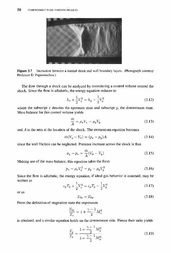
7 0 COMPRESSIBLE FLOW THROUGH NOZZLES
Figure 3.7 Interaction between a normal shock and wall boundary layers. (Photograph courtesy Professor D. Papamoschou.)
The flow through a shock can be analyzed by considering a control volume around the shock. Since the flow is adiabatic, the energy equation reduces to
hx + \vt = hy + \v* (3.12)
where the subscript x denotes the upstream state and subscript y, the downstream state. Mass balance for this control volume yields
771
■j=PxVx = pyVy (3.13)
and A is the area at the location of the shock. The momentum equation becomes
m(yy-Vx) = (px-py)A (3.14)
since the wall friction can be neglected. Pressure increase across the shock is thus
Til
Pv-Px = ^{Vx-Vv) (3.15)
Making use of the mass balance, this equation takes the form
Px + PxVt = Py + PyVy2 (3.16)
Since the flow is adiabatic, the energy equation, if ideal gas behavior is assumed, may be written as
cPTx + \vl = cpTy + l-V* (3.17) or as
TQX = Toy (3.18) From the definition of stagnation state the expression
Tx 2 is obtained, and a similar equation holds on the downstream side. Hence their ratio yields
(3.19) Ty Tx
i + V M ' 1'+ ^r^MJ
NORMAL SHOCKS 7 1
Making use of the ideal gas relation p = pRT and the mass balance pxVx = pvVy in this equation gives
Ty_ = Vy_Px_ = Py_ Vy_ Tx Vx Py Px Vx
and, using V = Mc to eliminate the velocities, leads to
Ty _ PyMyCy _ Py My Tx pxMx
Cx Px
Mx
from which Ty _(Py\2(My^ Tx \PxJ \MX
Combining this with Eq. (3.19) gives
(3.20)
Py _ Mx -Ml
v* My /x + I^IM* (3.21)
For an ideal gas pxVx = "fpxM^, and a similar equation holds on the downstream side. Substituting these into Eq. (3.16) gives
Py _ 1+7M, 2
px 1 + 7M2
Equating Eqs. (3.21) and (3.22) gives
(3.22)
MXJI + ^-1M? MVJI + 1-IM?, ly
1 + 7M2 1 + 7 M2
This is clearly satisfied if Mx = My, but in this case nothing interesting happens and the flow moves through the control volume undisturbed. Squaring both sides yields a quadratic equation in My. Solving it gives the result
2 + ( 7 - l ) A £ My 2 7 M | - ( 7 - I ) {XZi)
This equation relates the upstream and downstream Mach numbers across a shock, and the expression is plotted in Figure 3.8. It shows that upstream states have Mx > 1 and those downstream have My < 1. As will be shown below, only in this situation will entropy increase across the shock, as it must.
Pressure before and after the shock is obtained by substituting Eq. (3.23) into Eq. (3.22), giving the result
^ = ^-Ml - 2 ^ (3.24) Px 7 + 1 7 + 1
This shows that if Mx = 1, there is no pressure jump. Denning the fractional increase in pressure as measure of the strength of the shock, the strength is defined as
^ - l = ^1~{M2x-l) (3.25)
Px 7 - 1
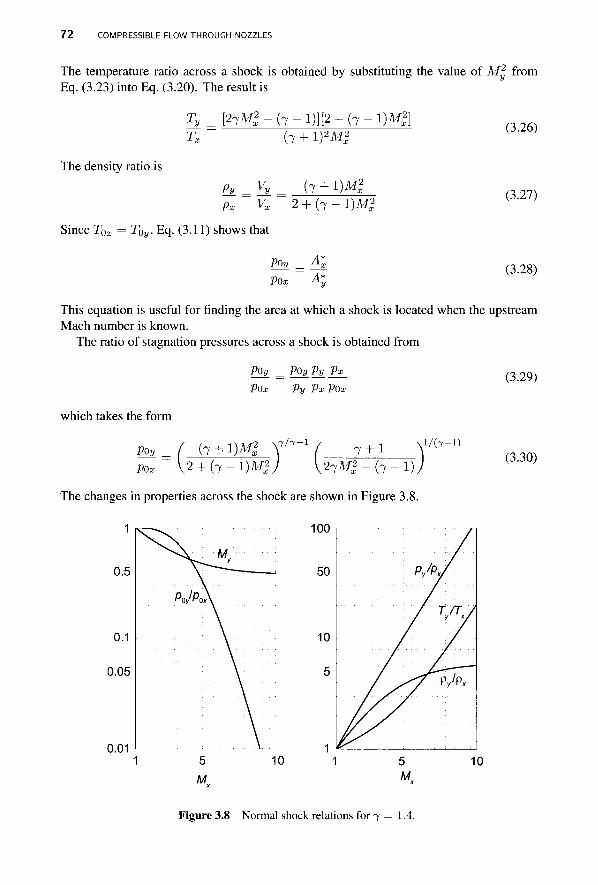
7 2 COMPRESSIBLE FLOW THROUGH NOZZLES
The temperature ratio across a shock is obtained by substituting the value of M 2 from Eq. (3.23) into Eq. (3.20). The result is
Ty _ [ 2 7 M , 2 - ( 7 - l ) ] [ 2 + ( 7 - l ) M j Tx
The density ratio is
(7+l)2MJ
Py _ Vy _ ( 7 + l)M2x
Px Vx 2 + ( 7 - 1 )M 2
Since T0x = T0y, Eq. (3.11) shows that
P0y_ = K POx A*
(3.26)
(3.27)
(3.28)
This equation is useful for finding the area at which a shock is located when the upstream Mach number is known.
The ratio of stagnation pressures across a shock is obtained from
POy = POyPy Px POx Py Px POx
(3.29)
which takes the form
PQ]L_( (7 + 1)M2
POx
2 \ 7 / 7 - 1 7 + 1 2 + ( 7 - l ) M x V V 2 7 M x
2 - ( 7 - l
The changes in properties across the shock are shown in Figure 3.8.
100
1/(7-1) (3.30)
0.01
Figure 3.8 Normal shock relations for 7 = 1.4.
NORMAL SHOCKS 73
3.3.1 Rankine-Hugoniot relations
A relationship between the pressure and density ratio across the shock can be obtained from the momentum equation
Px Py-Px= PxVx ~ PyVy = PxVx ( 1
which, when solved for upstream velocity, gives
y2 = \(Py-Px)Py'\ 1 / 2
l(py ~ Px)Px.
A similar expression is obtained downstream of the shock:
Py
Vy
The energy equation across the shock is
1
(Py -Px)Px
{Py ~ Px)Py_
1/2
hx + 2^x =K+ 2Vv
Since
">x My — Cp\J-x -Ly) 7 - 1 \P:
Py_
Py
the energy equation can be written as
7 Px Py ~ Px Py 7 Py Py ~Px Px
from which
7 - 1 Px %{py ~ px) Px 7 - 1 Py 2(Py ~ Px) Py
' 7 + l P y Px _
Py
Solving this for the density ratio gives
7 - IP* 7 + 1 Py_ 7 - 1 Px
Py_ Px
7+lPj/
7 - lPx 7 + 1 | Py
7 - 1 Px
(3.31)
(3.32)
(3.33)
Equations (3.32) and (3.33) are known as Rankine-Hugoniot relations [62,40]. The strength of the shock is obtained from the first of the Rankine-Hugoniot equations.
It is 27 (Py
Py 1 _ 7 " 1 \Px - 1 1
Px 7-1 .
Py - 1 (3.34)
7 4 COMPRESSIBLE FLOW THROUGH NOZZLES
and similarly for the density ratio
Py_ Px
1 + 2+l(Pv_1 27 \Px
1 + ^ 1 ( ^ - 1 27 \Px
(3.35)
Entropy change across a shock is given by integrating
Tds = du — pdv
across the shock. This gives
sy - sx = cv In - f + R In -^ = cv In f -^ J- T. Vx, \ -L x.
7 - 1
The temperature ratio is T 2̂/ Py Px -L x Px Vx Px Py
so that the entropy change can also be written as
sy - sx = cv In ( -^ ] ( — ) \PxJ \Py)
Substituting the expression for py / px from Eq. (3.34) to this and noting that cv = R/{^—\), this equation can be recast as
^ — ^ - l n | ^ ) - 7 l n Px
1 + l+l(Py_1 27 \P.
+ 7 In i + l^lfPy.! 27 \Px
For weak shocks py/px is just slightly greater than one. For this reason, let pv/px = 1 + e, and on substituting this in the previous equation and expanding in Taylor series for small value of e, leads to 2
sy - sx _ 72 - 1 fpy ^ _ 7 2 - l (py_ _ 1N 4
or
1272 \p: 87
2 \P:
Sy-Sx = 7 + 1 {Pv_i\ _ 7 + 1 (Pv_l\ 4. i? 127
2 \Px ) 872 Ux )
Using Eq. (3.25) to express the shock strength in terms of Mach number gives
i i 3 (7 + l)2 (7 + 1)= (3.36)
This shows that were Mx < 1, entropy would decrease across the shock. Thus shocks are possible only for Mx > 1. Furthermore, entropy increases only slightly across weak shocks.
2For small values of £ series expansion yields ln(l +'e) = e — e2 /2 + e3 /3 — e4/4
INFLUENCE OF FRICTION IN FLOW THROUGH STRAIGHT NOZZLES 7 5
The stagnation pressure change across weak shocks can also be developed by writing Ml = 1 + e in
POy_f (7 + l)A£ V 7 7 " 1 / 7 + 1 ^ ^ Pox V2+(7-l)MaV V 2 7 M | - ( 7 - l )
and expanding the resulting expression in for small values of e. The result, when written in terms of M% — 1, is
? ° » = 1 - - 1 ( M 2 - l ) 3 + — ^ (M 2 - l ) 4 + .-- (3 37) po, 3(7+l)2^ s j (7 + I)3 { x '
This is an important result as it shows that flows through weak shocks experience only a small loss in stagnation pressure. In fact, Eq. (3.37) may be shown to be accurate to 1% for Mx < 1.2, and for Mx = 1.2 it gives poy/pox = 0.986, or a stagnation pressure drop of less than 2%. The significance of this result for turbomachinery design is that in transonic flows with shocks stagnation pressure losses are relatively small.
3.4 INFLUENCE OF FRICTION IN FLOW THROUGH STRAIGHT NOZZLES
There are various ways in which the irreversibilities caused by friction have been taken into account in studies of nozzle flow. These are discussed in this section. First, a polytropic efficiency is introduced, and it is then related to a static enthalpy loss coefficient, which, in turn, is related to a loss of stagnation pressure. Next, nozzle efficiency and the velocity coefficient are discussed. After this the equations for compressible flow in a variable-area duct with wall friction are given. In the discussion that follows, the flow is adiabatic and no work is done. Therefore the stagnation temperature remains constant, and assuming constant specific heats and ideal gas behavior, the relation
Y = 1 + 1-^TM2 (3-38)
remains valid for adiabatic flow even when friction is present.
3.4.1 Polytropic efficiency
The concept of polytropic efficiency follows from examining the Tds equation
Tds = dh — vdp
for an isentropic process dhs=vdp (3.39)
and a nonisentropic one. A polytropic efficiency of an incremental expansion process is defined as
_ dh Vp~dh~s
so that dh = r]pdhs. The process is shown in Figure 2.9a in Chapter 2. Substituting this into Eq. (3.39) and making use of the ideal gas relation gives
dh = cpdT = T]„y dp = nD dp P
7 6 COMPRESSIBLE FLOW THROUGH NOZZLES
From this follows the relation
dT = T?P(7 - 1) dp
T I P
A polytropic index n is now introduced via the equation
(3.40)
?-l = Ikh^l sothat r^f^V-U (3.41) n 7 ' \ n J \-y-lJ
and Eq. (3.41) can also be written as
(3.42) 7?p + 7(1 - r)p)
Assuming that rjp and hence also n remain constant along the entire expansion path, integrating Eq. (3.40) yields
T> / \ ( n — l)/n
Rewriting this as n-l = l n r 2 /T i
n lnp2/pi gives an equation from which the polytropic exponent may be calculated, if the inlet and exit pressures and temperatures have been determined experimentally. Real gas effects have been incorporated into the theory by Shultz [69], Mallen and Saville [55], and Huntington [42].
If the inlet state is a stagnation state, then, writing Eq. (3.43) as
-i-oi _ I Pen \
and making use of the ideal gas relation in Eq. (3.44) it follows that
m = (±m_\ Poi = ( P°l\ P2 \T2 J p2 V P )
(3.44)
Finally, using Eq. (3.38) the pressure and density ratios may be written as
/ i \n/ln— 1) / , \ l / ( n - l )
The flow velocity is
V = M^/rRT = M^-fRTo ( 1 + -̂ —— M2 1
which can be used to express the mass flow rate per unit area at the throat in the form
mJ^T^ 7 / 7 - 1 \-(«+D/2(«-i) V \ = ~7=M2, 1 + ^ M 2 (3.45) POIA2 V7 - 1 V 2 y

INFLUENCE OF FRICTION IN FLOW THROUGH STRAIGHT NOZZLES 7 7
With the conditions at the inlet fixed, M2 is the only variable in this equation. Differentiating with respect to M2 gives that value of Mach number at the throat for which the maximum flow rate is achieved. This operation leads to
2 2 2 ( n - l ) 2
which, when simplified and solved for Mi, gives
Mt = ^ ^ - 1 (3.46)
in which the subscript indicates that this is the Mach number at the throat at a choked condition. Two alternative forms are
It is seen that Mach number at the throat is slightly less than one. Making use of this value of Mach number the critical pressure ratio becomes
/ 2 W ( n - l ) pt ' ' (3.48) Poi \ n + 1
This has the same form as the expression for isentropic flow when 7 replaced by n. Substituting Mt from Eq. (3.47) into Eq. (3.45) gives
- ) m a x ^ 2 W 0 1 , 0 1 ( — ) (3.49)
Velocity at the throat at this condition is
Vt = ^2cp(Tm - Tt) = J^~RTt (^r - l\ = Vv^RTt
in which the relation Toi/Tt = [n + l ) /2 was used. Alternatively, velocity at the throat may be determined from Vt = Mt \/jRTt.
■ EXAMPLE 3.5
Air in a reservoir, with temperature 540 K and pressure 200 kPa, flows into a converg-ing nozzle with a poly tropic efficiency r/p = 0.98. The throat area is At = 10 cm2. (a) If the flow is choked, what are the exit pressure and the mass flow rate? (b) Given that the backpressure is pb = 160 kPa, find the mass flow rate.
Solution: (a) The polytropic exponent is
7 1.4 %, + 7 ( l -%>) 0.98 + 1.4-0.02
and the Mach number can then be determined to be
1.389
n - \ / 1 . 3 8 9 - 1 _ „

7 8 COMPRESSIBLE FLOW THROUGH NOZZLES
With the flow choked, pressure and temperature at the throat are ,n/(n-l) / 0 \1.389/0.389
Pt = Poi I r I = 200 n + 1
Tt 27} 01
1.389+1
2-540
106 kPa
n + 1 1.389 + 1 Mass flux at the throat at choked condition is
-(n+l)/2(n-l)
452.1 K
m Poi
7 ,T / n + 1 -M2 343.42kg/(s-m2)
and, with A
iZToi V 2 10 cm2, flow rate is
m = 0.343 kg/s
(b) Forpb = 160 kPa the flow is not choked. Hence Mt is calculated from
Mt. = \ J 7 - 1 and the mass flux at the throat is obtained from
Poi Pb
(n-l)/n
0.5678
m At-fhVt-poiym[lvlt 7 Aft f 1 + 7 - r ^ M 2
-(n+l)/2(n-l)
281.7kg/(s-m2)
Hence the mass flow rate is m = 0.282 kg/s
By comparing this to the calculation in Example 3.3 for an isentropic flow, the mass flow rate is seen to be slightly smaller for the polytropic process. g
Since the sonic state does not appear anywhere in the actual flow, it serves as a reference state. At the sonic state the static properties may be calculated from the stagnation state upstream by using the following equations:
p Poi 7 + 1
P Poi 7 + 1
Since Toi remains constant, the relationship between the static temperature at the sonic state and its value at the inlet is
T* _ T* T0i T\ ~ ToT^T 7 + 1 1 + 7 - 1
Mr or rp*
2 ■ T l A f ? Ti 7 + 1 7 + 1
The pressure ratio is clearly
and the density ratio is Pi
Pi Pi
2 7 - 1 7 + " 7
7 + 1 7 + 1 M2
2 7 - l „ 2 -, + 7 + 1 - 7 + 1 Mf
n/(n-l)
l/(n-l)
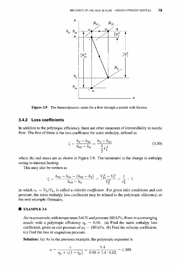
INFLUENCE OF FRICTION IN FLOW THROUGH STRAIGHT NOZZLES 7 9
Figure 3.9 The thermodynamic states for a flow through a nozzle with friction.
3.4.2 Loss coefficients
In addition to the polytropic efficiency, there are other measures of irreversibibty in nozzle flow. The first of these is the loss coefficient for static enthalpy, defined as
c ho - h 2s ho - h 2s
i02 2 2
(3.50)
where the end states are as shown in Figure 3.9. The numerator is the change in enthalpy owing to internal heating.
This may also be written as
c = h 02 {h02 - h2) vl v22 1
ho2 - h2 v22 1
in which cv = V2/V2s is called a velocity coefficient. For given inlet conditions and exit pressure, the static enthalpy loss coefficient may be related to the polytropic efficiency, as the next example illustrates.
■ EXAMPLE 3.6
Air in a reservoir, with temperature 540 K and pressure 200 kPa, flows in a converging nozzle with a polytropic efficiency r]p = 0.98. (a) Find the static enthalpy loss coefficient, given an exit pressure of p2 — 160 kPa. (b) Find the velocity coefficient. (c) Find the loss in stagnation pressure.
Solution: (a) As in the previous example, the polytropic exponent is
7 1.4 7 ? p + 7 ( l - ? 7 p ) 0 : 9 8 + 1 . 4 - 0 . 0 2
= 1.389
8 0 COMPRESSIBLE FLOW THROUGH NOZZLES
The exit temperature is therefore
T a = r ° i ( S ) < = 5 4 n ^ ' =5o7-29K
and the Mach number at the exit is
( n - l ) / n / , f i „ N 1.389/0.389
M2 = ,U- (^-l)= J±- (_^_ _ ,) = 0.5678 V ^ _ 1 V T 2 / y 0.4^506.29 J
The exit velocity is therefore
V2 = M2^/jRT2 = 0.5678\/l.4-287-507.3 = 256.34m/s
The temperature T2s is obtained from the expression for isentropic expansion
Hence the static enthalpy loss coefficient is
2cp(T2_- T2s) _ 2 • 1004.5 • (507.29 - 506.65) r = — '^ r±L = i '- = n 01976 <" V? 256.342 U 'U y / °
(b) The velocity coefficient is then
1 = 0.9903 v yrrc
(c) The loss of stagnation pressure is obtained by noting that
P02 P02P2 (TnV^-V (T^Y1^-" (Tz^-V POl V2 P01 \T2 J \T02
Hence
P „ s ^fpv 2 0 o ( i S ) "= 1 9 , l l k P a The loss in stagnation pressure is Ap0 = Poi — P02 = 890 Pa. Because the values of poi a nd P02 are nearly equal, on subtracting one from the other, a number of significant figures are lost. If the value of the static enthalpy loss coefficient is known, the polytropic efficiency may be calculated by reversing the steps in this example. _
The ratio of stagnation pressures P02/P01 may also be developed by integrating the Gibbs equation
Tds = dh — v dp
along the constant p2 line. This gives
s2 - si-~ CpIn—-J-2s
INFLUENCE OF FRICTION IN FLOW THROUGH STRAIGHT NOZZLES 8 1
Similarly, integrating it between states 01 and 02 along the constant ho line leads to
S2 — s\ = / cm P02
Hence /rp \ 7 / ( 7 - l )
P_02 = fT±\ Poi \T2 )
This may also be written as T / « \ ( 7 - l ) / 7 / „ A „ \ ( 7 - l ) / 7 / A „ \ ( 7 - l ) / 7 J- 2s I P02\ I POI - A-PO \ — M ?2 VPOl/ V POI / V POI
in which Ap0 = Poi — Po2- Assuming that Ap 0 /poi *C 1 and making use of the binomial theorem, the following approximation can be used
T2s = 1 7 - 1 Ap 0
?2 7 P01
which may be also recast as
T2 - T2s = 7 - 1 App T2 7 Poi
and from which i?T2Ap0 Apo/Poi
" 2 - ^2's — — 7777-j P 0 1 1 + ^ M 2
2
2 2
so that the static enthalpy loss coefficient is
Apo/poi c V f i + ^—iM.2
2 A I ^ " J U 2 2 z V 2
For small values of exit Mach number this reduces to
Apo/An c
2 V2
and this is often called a stagnation pressure loss coefficient. Another measure of the loss of stagnation pressure is given by
v _ Poi ~ P02 J P —
P02 ~ P2
which may be written as Y = P01/P02 ~ 1
P I - P 2 / P 0 2 The pressure ratios in this expression are
/T \ 7 / ( 7 - l )
P02 _ I 102
P2

8 2 COMPRESSIBLE FLOW THROUGH NOZZLES
and 7 / (7 -1 ) Pol = (T2s
P02 \T0i, and the definition of static enthalpy loss coefficient, Eq. (3.50), can be rewritten as
T2 C T02
T2 1
Substituting these into the expression for the stagnation pressure loss coefficient gives it the form
Yn
i -C ( | f -1 -7 / (7 -1 )
1
Tr
or
Y„ 1-C
02
X^IM?
-7 / (7-1)
-7 / (7-1)
1 - 1 + 7 "iM92 -7/(7-1)
For small M2 this reduces to Yp = £. The development indicates that the value of ( is not dependent on Mach number, but the loss of stagnation pressure is, and therefore also the value of Yp. For this reason ( ought to be favored over other measures of irreversiblity [18]. However, it is worthwhile to be familiar with the various loss coefficients, as they have been and still are in use in the analysis of turbine nozzles.
3.4.3 Nozzle efficiency
The nozzle efficiency is defined as
7?N hi - h2
hi - h2s
or, since the stagnation enthalpy remains constant so that hi + V^/2 relation can be rewritten as
h2 + V22/2, this
m V2
2
2(Ai - h2s) Similarly, when hi + Vf/2 = h2s + V2
2s/2 is used to rewrite the isentropic enthalpy
change in the denominator in terms of kinetic energy differences, nozzle efficiency takes the alternative form
m v2
2
vl - v? If the fluid enters the nozzle from a large reservoir where Vi = 0, nozzle efficiency becomes
VN V2
2
2(/i0i - h2s) Yl vl
Thus nozzle efficiency can be interpreted as a ratio of the actual increase in kinetic energy of the flow to that in reversible adiabatic 'flow. Nozzle efficiency takes into account the
INFLUENCE OF FRICTION IN FLOW THROUGH STRAIGHT NOZZLES 8 3
losses in the entire nozzle, from its inlet to its exit. If the nozzle is a converging-diverging type and the flow is subsonic, then most of the losses take place in the diverging part in which the flow diffuses to a low velocity. Nozzle efficiency of a converging nozzle has a value very close to unity.
For a flow that starts from the stagnation state nozzle efficiency
VN = V2
2
2cp(T0 -T2s)
may be further manipulated into the form
7 - 1 m
Ml 1
T2s \ TQI
Toi.
Expressing the isentropic temperature ratio T2s/T0i and T0i/T2 as
P2 Poi
( 7 - l ) / 7 Ik T2
7 - 1 Mi
and solving the resulting equation for the pressure ratio gives
P2_ Poi
(7 - 1)M| 1 7 / ( 7 - 1 )
77N(2 + ( 7 - l ) M 22 ) (3.52)
The following development of an expression for mass flow rate through a converging nozzle makes use of this equation. In such a nozzle the exit area A2 is equal to the throat area At, and the mass flux, which is the mass flow rate per unit area, at the throat is given by
7 _ [T^ RT0i A-rPtVt^PtMt\RT0,\Tt
or m A Poi
7 Pt M t W l 7 - 1
RT0i Poi V 2
Substituting the pressure ratio from Eq. (3.52) into this gives
1 7 / ( 7 - 1 )
M 2
m A Poi
7 RTQI
1 (7 " 1)M- Mt 1 7 - 1 Mi
-,1/2
77N(2 + ( 7 - l ) M t2 )
(3.53) In this equation square of Mach number appears and therefore differentiating this equation with respect to respect to Mt
2 and setting the result to zero gives the value of Mt for maximum mass flux at the throat. Carrying out the differentiation gives the equation
(7 - 1)2(1 - m)M? - [(7 - 1)3T/N - 27]M2 - 2m = 0
From this the throat Mach number at the condition of maximum mass flux is obtained as 1/2
M, (7 - 1 V>m -1 )-27+V/[(7- l ) (3??N-l)-27]2^r ? N( l - r ? N)(7- l ) 2
2 ( 7 - 1 ) 2 ( 1 ' - 7 ? N ) (3.54)
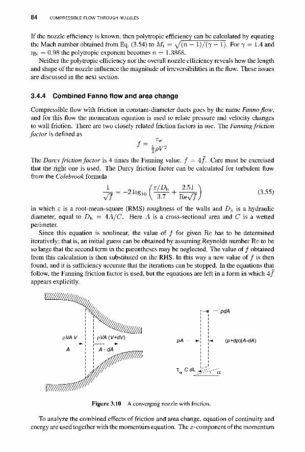
8 4 COMPRESSIBLE FLOW THROUGH NOZZLES
If the nozzle efficiency is known, then polytropic efficiency can be calculated by equating the Mach number obtained from Eq. (3.54) to Mt = 1/(71 — l ) / (7 — 1). For 7 = 1.4 and 7/N =0.98 the polytropic exponent becomes n = 1.3868.
Neither the polytropic efficiency nor the overall nozzle efficiency reveals how the length and shape of the nozzle influence the magnitude of irreversibilities in the flow. These issues are discussed in the next section.
3.4.4 Combined Fanno flow and area change
Compressible flow with friction in constant-diameter ducts goes by the name Fanno flow, and for this flow the momentum equation is used to relate pressure and velocity changes to wall friction. There are two closely related friction factors in use. The Fanning friction factor is defined as
The Darcy friction factor is 4 times the Fanning value, / = 4 / . Care must be exercised that the right one is used. The Darcy friction factor can be calculated for turbulent flow from the Colebrook formula
1 77 -2 log 10 +
2.51 3.7 ' RevTV
e/Dh (3.55)
in which e is a root-mean-square (RMS) roughness of the walls and D^ is a hydraulic diameter, equal to D^ = 4A/C. Here A is a cross-sectional area and C is a wetted perimeter.
Since this equation is nonlinear, the value of / for given Re has to be determined iteratively; that is, an initial guess can be obtained by assuming Reynolds number Re to be so large that the second term in the parentheses may be neglected. The value of / obtained from this calculation is then substituted on the RHS. In this way a new value of / is then found, and it is sufficiency accurate that the iterations can be stopped. In the equations that follow, the Fanning friction factor is used, but the equations are left in a form in which 4 / appears explicitly.
pdA
pA
X... C dL
(p+dp)(A-dA)
Figure 3.10 A converging nozzle with friction.
To analyze the combined effects of friction and area change, equation of continuity and energy are used together with the momentum equation. The ̂ -component of the momentum
INFLUENCE OF FRICTION IN FLOW THROUGH STRAIGHT NOZZLES 8 5
balance for the control volume, shown in Figure 3.10, gives
pAV(V + dV - V) = pA -pdA - {p + dp){A - dA) - rwCcosadL
Since in the sketch the flow area decreases, the downstream area is written as A — dA. In order to draw the vector p dA in the correct direction for a converging channel, the area change must be assumed to have the sign that is consistent with the sketch.
Making use of the relations C = AA/Dh and cos a dL = dx in this equation and neglecting the small term dp dA, reduces it to the form
4TW pVdV = —dp pr~dx
Introduction of the Fanning friction factor puts it into the form
pVdV = -dp - ^~^pV2dx Dh 2
Using the ideal gas relation and definition of Mach number to establish the equality pV2 = jpM2 gives, after each term has been divided by p, the equation
* + 2f^ + l M ! 4 / £ = 0 ,3,6, p 2 Vz 2 L>h
To see the effect of area ratio and friction on the flow, this equation is next recast into a form in which the first two terms are expressed in terms of area ratio and Mach number. The second term is considered first. Since V2 = M2/yRT, taking logarithms and differentiating this gives
dV2 _ dM2 dT
Next, since in adiabatic flow To is constant, taking logarithms and differentiating the adiabatic relation T0 = T(l + ^ M 2 ) gives
dT T
V M * dM* l^~lM2M2
(3.57)
and eliminating dT jT between the last two equations gives
dV2 1 dM2
V2 i , 7 - 1 , ,2 M2 (3.58) l + ^—Mz
Next, an equation between Mach number, area ratio, and friction factor is obtained by taking logarithms and differentiating the mass balance m = pAV. This gives
dp dA dV n
p A V
A similar operation on the ideal gas relation p = pRT leads to
dp _ dp dT 7 " 7 + ^
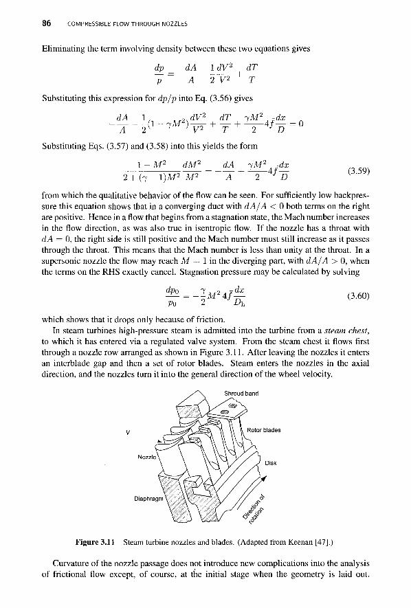
86 COMPRESSIBLE FLOW THROUGH NOZZLES
Eliminating the term involving density between these two equations gives
dp __dA_^dV^ dT ~p~ ~ A 2 V2 + T
Substituting this expression for dp/p into Eq. (3.56) gives
dA 1/ , » , 2 ^ 2 dT jM2 -dx n
Substituting Eqs. (3.57) and (3.58) into this yields the form
1 - M 2 dM2 dA , 7 M 2 -dx 2 + (7 - 1)M2 M2 A 2 J D
from which the qualitative behavior of the flow can be seen. For sufficiently low backpres-sure this equation shows that in a converging duct with dA/A < 0 both terms on the right are positive. Hence in a flow that begins from a stagnation state, the Mach number increases in the flow direction, as was also true in isentropic flow. If the nozzle has a throat with dA = 0, the right side is still positive and the Mach number must still increase as it passes through the throat. This means that the Mach number is less than unity at the throat. In a supersonic nozzle the flow may reach M — 1 in the diverging part, with dA/A > 0, when the terms on the RHS exactly cancel. Stagnation pressure may be calculated by solving
dj^ = ->Hf%- (3.60) Po 2 Dh
which shows that it drops only because of friction. In steam turbines high-pressure steam is admitted into the turbine from a steam chest,
to which it has entered via a regulated valve system. From the steam chest it flows first through a nozzle row arranged as shown in Figure 3.11. After leaving the nozzles it enters an interblade gap and then a set of rotor blades. Steam enters the nozzles in the axial direction, and the nozzles turn it into the general direction of the wheel velocity.
Shroud band
Rotor blades
Nozzle \ Disk
Diaphragm
Figure 3.11 Steam turbine nozzles and blades. (Adapted from Keenan [47].)
Curvature of the nozzle passage does not introduce new complications into the analysis of frictional flow except, of course, at the initial stage when the geometry is laid out.
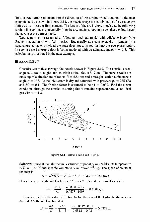
INFLUENCE OF FRICTION IN FLOW THROUGH STRAIGHT NOZZLES 8 7
To illustrate turning of steam into the direction of the turbine wheel rotation, in the next example, and as shown in Figure 3.12, the nozzle shape is a combination of a circular arc followed by a straight-line segment. The length of the arc is chosen such that the following straight line continues tangentially from the arc, and its direction is such that the flow leaves the nozzle at the correct angle.
Wet steam may be assumed to follow an ideal gas model with adiabatic index from Zeuner's equation 7 = 1.035 + 0.1a;. But usually as steam expands, it remains in a supersaturated state, provided the state does not drop too far into the two phase-region. In such a case isentropic flow is better modeled with an adiabatic index 7 = 1.3. This calculation is illustrated in the next example.
■ EXAMPLE 3.7
Consider steam flow through the nozzle shown in Figure 3.12. The nozzle is rect-angular, 3 cm in height, and its width at the inlet is 5.12 cm. The nozzle walls are made up of a circular arc of radius R = 2.85 cm and a straight section at the nozzle angle a = 75°. At the inlet steam is dry and saturated with pressure pi = 275 kPa and Mi = 0.1. The friction factor is assumed to be 4 / = 0.032. Find the steam conditions through the nozzle, assuming that it remains supersaturated as an ideal gas with 7 = 1.3.
1 2 3 4 5 6 7 8
x(cm)
Figure 3.12 Offset nozzle and its grid.
10 11 12
Solution: Since at the inlet steam is saturated vapor atp; = 275 kPa, its temperature is XI = 403.7 K and specific volume is v; = 0.6578 m3/kg. The speed of sound at the inlet is
c; = y/^RTi = Vl-3-461.5-403.7 = 492.1 m/s Hence the speed at the inlet is V\ = c\M\ = 49.2 m/s and the mass flow rate is
ViAi 49.3-3-5.12 m 0.6578 • 1002 0.116 kg/s
In order to check the value of friction factor, the size of the hydraulic diameter is needed. For the inlet section it is
AA 2Lb 2-0.0512-0.03 _ „ D* = ^ = LTl= 0.0512 + 0.03 = ° - 0 3 7 8 m
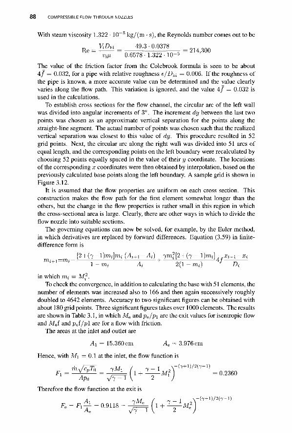
8 8 COMPRESSIBLE FLOW THROUGH NOZZLES
With steam viscosity 1.322 ■ 10 kg/(m • s), the Reynolds number comes out to be
p a ViDh> 49-3 • 0-0378
R e = ~ ^ r = 0.6578-1.322-10-s = 2 1 4 ' 3 ° ° The value of the friction factor from the Colebrook formula is seen to be about 4 / = 0.032, for a pipe with relative roughness e/D^i = 0.006. If the roughness of the pipe is known, a more accurate value can be determined and the value clearly varies along the flow path. This variation is ignored, and the value 4 / = 0.032 is used in the calculations.
To establish cross sections for the flow channel, the circular arc of the left wall was divided into angular increments of 3°. The increment dy between the last two points was chosen as an approximate vertical separation for the points along the straight-line segment. The actual number of points was chosen such that the realized vertical separation was closest to this value of dy. This procedure resulted in 52 grid points. Next, the circular arc along the right wall was divided into 51 arcs of equal length, and the corresponding points on the left boundary were recalculated by choosing 52 points equally spaced in the value of their y coordinate. The locations of the corresponding x coordinates were then obtained by interpolation, based on the previously calculated base points along the left boundary. A sample grid is shown in Figure 3.12.
It is assumed that the flow properties are uniform on each cross section. This construction makes the flow path for the first element somewhat longer than the others, but the change in the flow properties is rather small in this region in which the cross-sectional area is large. Clearly, there are other ways in which to divide the flow nozzle into suitable sections.
The governing equations can now be solved, for example, by the Euler method, in which derivatives are replaced by forward differences. Equation (3.59) in finite-difference form is
[2 + (^-l)mi]mi{Ai+i-Ai) 7m?[2+ (7 - l)mj] . jXi+i + / . ; - H 4 / :
Xi
l-rrii Ai 2(1-mi) J A
in which m, = Mf. To check the convergence, in addition to calculating the base with 51 elements, the
number of elements was increased also to 166 and then again successively roughly doubled to 4642 elements. Accuracy to two significant figures can be obtained with about 180 grid points. Three significant figures takes over 1000 elements. The results are shown in Table 3.1, in which Me and pe/p\ are the exit values for isentropic flow and Mef and pei/pi are for a flow with friction.
The areas at the inlet and outlet are
Ai = 15.360 cm Ae = 3.976 cm
Hence, with Mi = 0.1 at the inlet, the flow function is
m^T0 7 M l / 7 - I ^ + 1 ) / 2 h - 1 } = V r = + 1 + J Mz = Q 2 3 6 Q
APo v / 7^T V 2 l ' Therefore the flow function at the exit is
*-«£-<>■•» ' - T ^ T O ^ * ) ' -(7+l)/2(7-l)
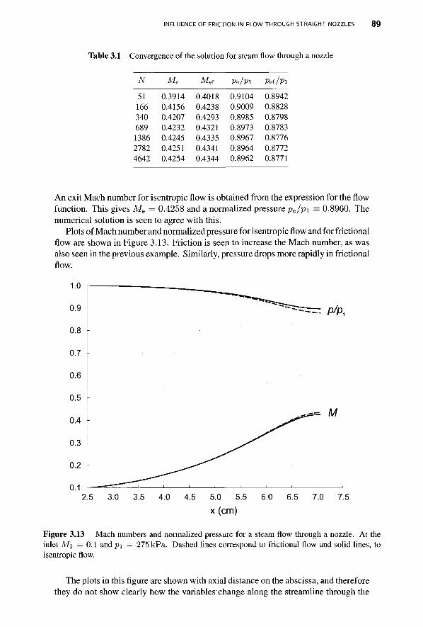
INFLUENCE OF FRICTION IN FLOW THROUGH STRAIGHT NOZZLES 8 9
Table 3.1 Convergence of the solution for steam flow through a nozzle
N
51 166 340 689 1386 2782 4642
Me
0.3914 0.4156 0.4207 0.4232 0.4245 0.4251 0.4254
Met
0.4018 0.4238 0.4293 0.4321 0.4335 0.4341 0.4344
Pe/Pl
0.9104 0.9009 0.8985 0.8973 0.8967 0.8964 0.8962
Pef/pi
0.8942 0.8828 0.8798 0.8783 0.8776 0.8772 0.8771
An exit Mach number for isentropic flow is obtained from the expression for the flow function. This gives Me = 0.4258 and a normalized pressure pe/pi = 0.8960. The numerical solution is seen to agree with this.
Plots of Mach number and normalized pressure for isentropic flow and for frictional flow are shown in Figure 3.13. Friction is seen to increase the Mach number, as was also seen in the previous example. Similarly, pressure drops more rapidly in frictional flow.
Figure 3.13 Mach numbers and normalized pressure for a steam flow through a nozzle. At the inlet Mi =0.1 and pi = 275 kPa. Dashed lines correspond to frictional flow and solid lines, to isentropic flow.
The plots in this figure are shown with axial distance on the abscissa, and therefore they do not show clearly how the variableschange along the streamline through the
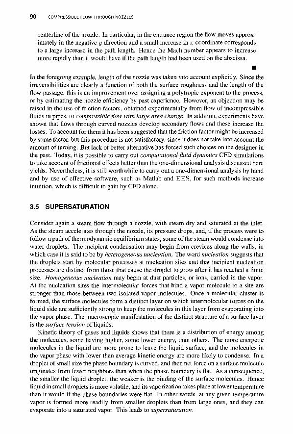
9 0 COMPRESSIBLE FLOW THROUGH NOZZLES
centerline of the nozzle. In particular, in the entrance region the flow moves approx-imately in the negative y direction and a small increase in x coordinate corresponds to a large increase in the path length. Hence the Mach number appears to increase more rapidly than it would have if the path length had been used on the abscissa.
■ In the foregoing example, length of the nozzle was taken into account explicitly. Since the irreversibilities are clearly a function of both the surface roughness and the length of the flow passage, this is an improvement over assigning a polytropic exponent to the process, or by estimating the nozzle efficiency by past experience. However, an objection may be raised in the use of friction factors, obtained experimentally from flow of incompressible fluids in pipes, to compressible flow with large area change. In addition, experiments have shown that flows through curved nozzles develop secondary flows and these increase the losses. To account for them it has been suggested that the friction factor might be increased by some factor, but this procedure is not satisfactory, since it does not take into account the amount of turning. But lack of better alternative has forced such choices on the designer in the past. Today, it is possible to carry out computational fluid dynamics CFD simulations to take account of frictional effects better than the one-dimensional analysis discussed here yields. Nevertheless, it is still worthwhile to carry out a one-dimensional analysis by hand and by use of effective software, such as Matlab and EES, for such methods increase intuition, which is difficult to gain by CFD alone.
3.5 SUPERSATURATION
Consider again a steam flow through a nozzle, with steam dry and saturated at the inlet. As the steam accelerates through the nozzle, its pressure drops, and, if the process were to follow a path of thermodynamic equilibrium states, some of the steam would condense into water droplets. The incipient condensation may begin from crevices along the walls, in which case it is said to be by heterogeneous nucleation. The word nucleation suggests that the droplets start by molecular processes at nucleation sites and that incipient nucleation processes are distinct from those that cause the droplet to grow after it has reached a finite size. Homogeneous nucleation may begin at dust particles, or ions, carried in the vapor. At the nucleation sites the intermolecular forces that bind a vapor molecule to a site are stronger than those between two isolated vapor molecules. Once a molecular cluster is formed, the surface molecules form a distinct layer on which intermolecular forces on the liquid side are sufficiently strong to keep the molecules in this layer from evaporating into the vapor phase. The macroscopic manifestation of the distinct structure of a surface layer is the surface tension of liquids.
Kinetic theory of gases and liquids shows that there is a distribution of energy among the molecules, some having higher, some lower energy, than others. The more energetic molecules in the liquid are more prone to leave the liquid surface, and the molecules in the vapor phase with lower than average kinetic energy are more likely to condense. In a droplet of small size the phase boundary is curved, and then net force on a surface molecule originates from fewer neighbors than when the phase boundary is flat. As a consequence, the smaller the liquid droplet, the weaker is the binding of the surface molecules. Hence liquid in small droplets is more volatile, and its vaporization takes place at lower temperature than it would if the phase boundaries were flat. In other words, at any given temperature vapor is formed more readily from smaller droplets than from large ones, and they can evaporate into a saturated vapor. This leads to supersaturation.
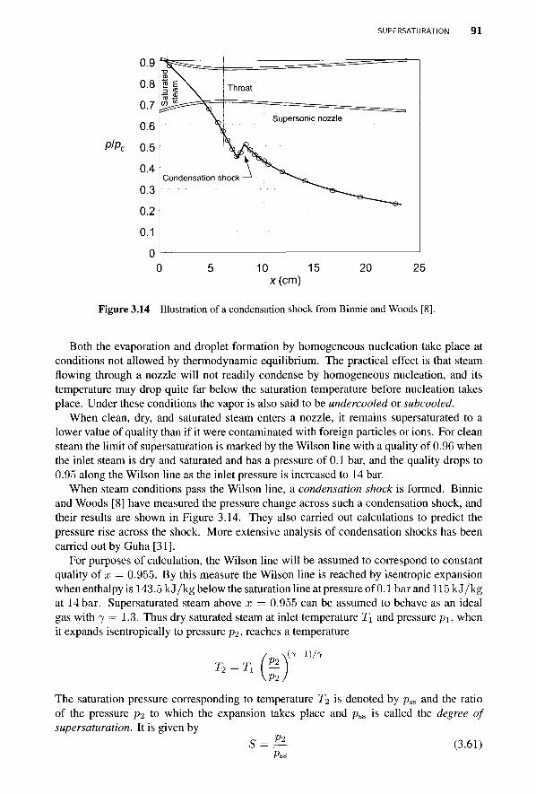
SUPERSATURATION 9 1
PlP,
Figure 3.14 Illustration of a condensation shock from Binnie and Woods [8].
Both the evaporation and droplet formation by homogeneous nucleation take place at conditions not allowed by thermodynamic equilibrium. The practical effect is that steam flowing through a nozzle will not readily condense by homogeneous nucleation, and its temperature may drop quite far below the saturation temperature before nucleation takes place. Under these conditions the vapor is also said to be undercooled or subcooled.
When clean, dry, and saturated steam enters a nozzle, it remains supersaturated to a lower value of quality than if it were contaminated with foreign particles or ions. For clean steam the limit of supersaturation is marked by the Wilson line with a quality of 0.96 when the inlet steam is dry and saturated and has a pressure of 0.1 bar, and the quality drops to 0.95 along the Wilson line as the inlet pressure is increased to 14 bar.
When steam conditions pass the Wilson line, a condensation shock is formed. Binnie and Woods [8] have measured the pressure change across such a condensation shock, and their results are shown in Figure 3.14. They also carried out calculations to predict the pressure rise across the shock. More extensive analysis of condensation shocks has been carried out by Guha [31].
For purposes of calculation, the Wilson line will be assumed to correspond to constant quality of x = 0.955. By this measure the Wilson line is reached by isentropic expansion when enthalpy is 143.5 kJ/kg below the saturation line at pressure of 0.1 bar and 115 kJ/kg at 14 bar. Supersaturated steam above x = 0.955 can be assumed to behave as an ideal gas with 7 — 1.3. Thus dry saturated steam at inlet temperature T\ and pressure p\, when it expands isentropically to pressure p2» reaches a temperature
T2 = T i Fl) ( 7 - l ) / 7
The saturation pressure corresponding to temperature T2 is denoted by pss and the ratio of the pressure P2 to which the expansion takes place and pss is called the degree of supersaturation. It is given by
S = ,— (3.61) Pss
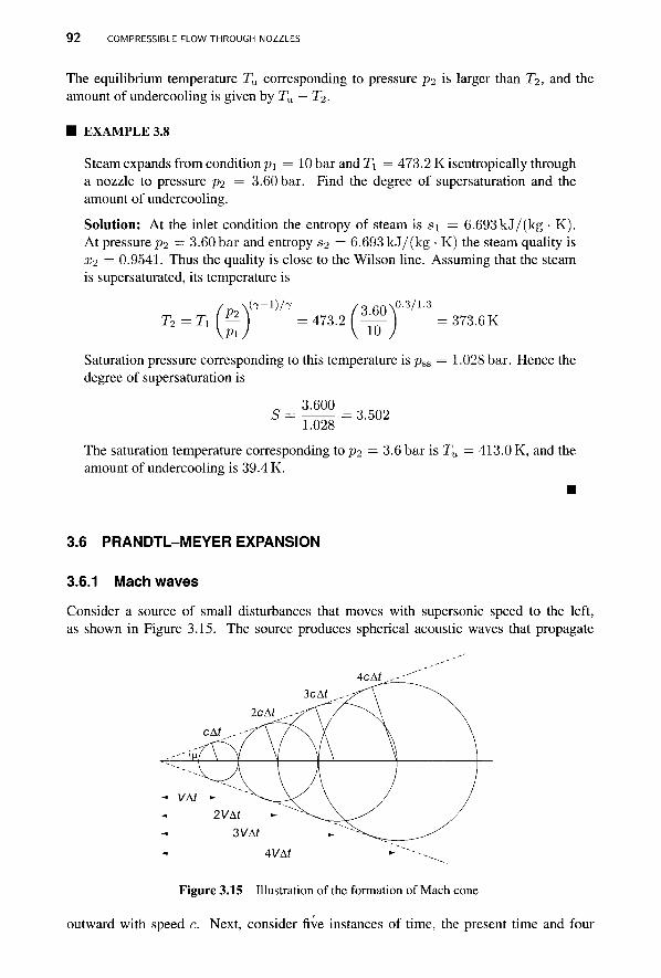
9 2 COMPRESSIBLE FLOW THROUGH NOZZLES
The equilibrium temperature Tu corresponding to pressure P2 is larger than T2, and the amount of undercooling is given by Tu — T^.
■ EXAMPLE 3.8
Steam expands from condition pi = 10 bar and T\ = 473.2 K isentropically through a nozzle to pressure P2 = 3.60 bar. Find the degree of supersaturation and the amount of undercooling.
Solution: At the inlet condition the entropy of steam is Si = 6.693 kJ/(kg • K). At pressure P2 = 3.60 bar and entropy S2 = 6.693 kJ/(kg • K) the steam quality is X2 = 0.9541. Thus the quality is close to the Wilson line. Assuming that the steam is supersaturated, its temperature is
T 2 = T 1 ( J M = 473.2 ( ^ ) = 373.6K
Saturation pressure corresponding to this temperature is pss = 1.028 bar. Hence the degree of supersaturation is
S= ^ ° = 3.502 1.028
The saturation temperature corresponding to P2 — 3.6 bar is Tu — 413.0 K, and the amount of undercooling is 39.4 K.
3.6 PRANDTL-MEYER EXPANSION
3.6.1 Mach waves
Consider a source of small disturbances that moves with supersonic speed to the left, as shown in Figure 3.15. The source produces spherical acoustic waves that propagate
Figure 3.15 Illustration of the formation of Mach cone
outward with speed c. Next, consider five instances of time, the present time and four
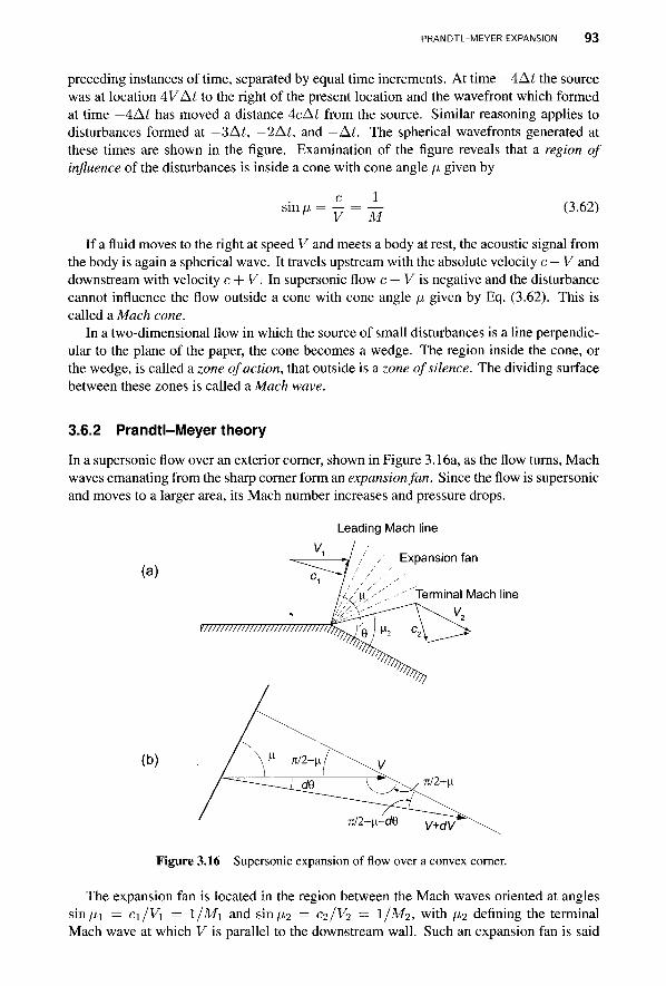
PRANDTL-MEYER EXPANSION 93
preceding instances of time, separated by equal time increments. At time — 4 At the source was at location 4V At to the right of the present location and the wavefront which formed at time —4Ai has moved a distance AcAt from the source. Similar reasoning applies to disturbances formed at -3At, —2At, and —At. The spherical wavefronts generated at these times are shown in the figure. Examination of the figure reveals that a region of influence of the disturbances is inside a cone with cone angle // given by
sin// V 1
M (3.62)
If a fluid moves to the right at speed V and meets a body at rest, the acoustic signal from the body is again a spherical wave. It travels upstream with the absolute velocity c — V and downstream with velocity c + V. In supersonic flow c — V is negative and the disturbance cannot influence the flow outside a cone with cone angle fi given by Eq. (3.62). This is called a Mach cone.
In a two-dimensional flow in which the source of small disturbances is a line perpendic-ular to the plane of the paper, the cone becomes a wedge. The region inside the cone, or the wedge, is called a zone of action, that outside is a zone of silence. The dividing surface between these zones is called a Mach wave.
3.6.2 Prandtl-Meyer theory
In a supersonic flow over an exterior corner, shown in Figure 3.16a, as the flow turns, Mach waves emanating from the sharp corner form an expansion fan. Since the flow is supersonic and moves to a larger area, its Mach number increases and pressure drops.
Leading Mach line
(a) Expansion fan
Terminal Mach line
(b)
Figure 3.16 Supersonic expansion of flow over a convex corner.
The expansion fan is located in the region between the Mach waves oriented at angles sin/xi = ci/Vi = 1/Mi and sin ^2 = C2/V2 = I/M2, with \±i defining the terminal Mach wave at which V is parallel to the downstream wall. Such an expansion fan is said
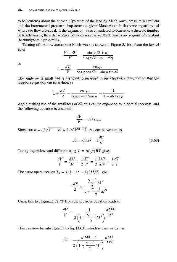
9 4 COMPRESSIBLE FLOW THROUGH NOZZLES
to be centered about the corner. Upstream of the leading Mach wave, pressure is uniform and the incremental pressure drop across a given Mach wave is the same regardless of where the flow crosses it. If the expansion fan is considered to consist of a discrete number of Mach waves, then the wedges between successive Mach waves are regions of constant thermodynamic properties.
Turning of the flow across one Mach wave is shown in Figure 3.16b. From the law of sines
V + dV _ sin(7r/2 + fi) V ~ sin(7r/2 - fi - dO)
or dV cos fi 1 + V cos /i cos d9 — sin /j, sin dO
The angle d9 is small and is assumed to increase in the clockwise direction so that the previous equation can be written as
dV cos a 1 1 + V cos [i — d9 sin /j, 1 — d9 tan \x
Again making use of the smallness of d9, this can be expanded by binomial theorem, and the following equation is obtained:
—— = d9 tan \JL
Since tan/i = c/\/V2 + c2 = l / \ / M 2 — 1, this can be written as
d9 = VM2 - 1 ~ (3.63)
Taking logarithms and differentiating V = Msj^RT gives
dV _dM 1 dT _ 1 dM2 1 dT ~V~ ~ W + 2^T ~ 2 M 2 + 2~¥
The same operations on T0 = T[l + (7 - l)M2/2)] give
T l + ^—M'
Using this to eliminate dT/T from the previous equation leads to
dV 1 dM2
V J, , 7 - 1 , ^ M2 2 ( 1 + J—r- M'
This can now be substituted into Eq. (3.63), which is then written as
sjM2-\ dM2
d9 7 - l ^ A M2
2 1 + ~—M
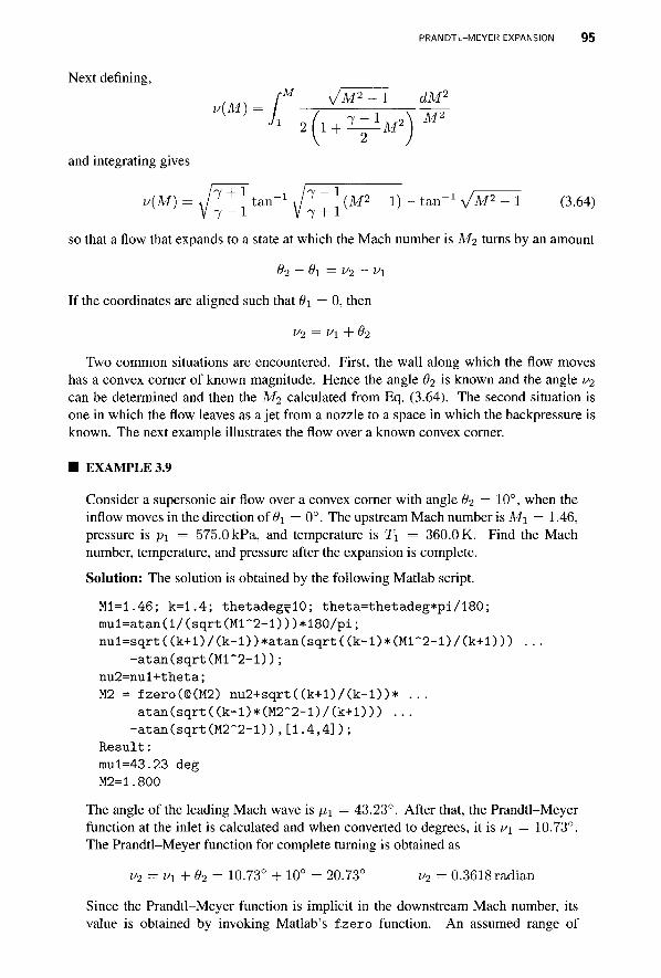
PRANDTL-MEYER EXPANSION 95
Next defining,
and integrating gives
„ „ , [M y^P^l dM2
V(M) = J^—r tan"1 J I — - ( M 2 - 1) - tan"1 V ^ 2 - 1 (3.64)
so that a flow that expands to a state at which the Mach number is M2 turns by an amount
82 - 0\ = vi - v\
If the coordinates are aligned such that 9\ = 0, then
V2 = V\ + #2
Two common situations are encountered. First, the wall along which the flow moves has a convex corner of known magnitude. Hence the angle 62 is known and the angle V2 can be determined and then the M2 calculated from Eq. (3.64). The second situation is one in which the flow leaves as a jet from a nozzle to a space in which the backpressure is known. The next example illustrates the flow over a known convex corner.
■ EXAMPLE 3.9
Consider a supersonic air flow over a convex corner with angle 62 = 10°, when the inflow moves in the direction of 6\ = 0°. The upstream Mach number is Mi = 1.46, pressure is p\ = 575.0 kPa, and temperature is T\ = 360.0 K. Find the Mach number, temperature, and pressure after the expansion is complete.
Solution: The solution is obtained by the following Matlab script.
Ml=1.46; k=1.4; thetadeg^lO; theta=thetadeg*pi/180; mul=atan(l/(sqrt(Ml~2-l)))*180/pi; nul=sqrt((k+l)/(k-l))*atan(sqrt((k-l)*(Ml~2-l)/(k+l))) ...
-atan(sqrt(Ml"2-l)); nu2=nul+theta;
M2 = fzero(@(M2) nu2+sqrt((k+l)/(k-l))* ... atan(sqrt((k-l)*(M2~2-l)/(k+l))) ...
-atan(sqrt(M2~2-D), [1.4,4]); Result: mul=43.23 deg M2=1.800
The angle of the leading Mach wave is //1 = 43.23°. After that, the Prandtl-Meyer function at the inlet is calculated and when converted to degrees, it is v\ = 10.73°. The Prandtl-Meyer function for complete turning is obtained as
V2 = Vl+02 = 10.73° + 10° = 20.73° v2 = 0.3618 radian
Since the Prandtl-Meyer function is implicit in the downstream Mach number, its value is obtained by invoking Matlab's fzero function. An assumed range of
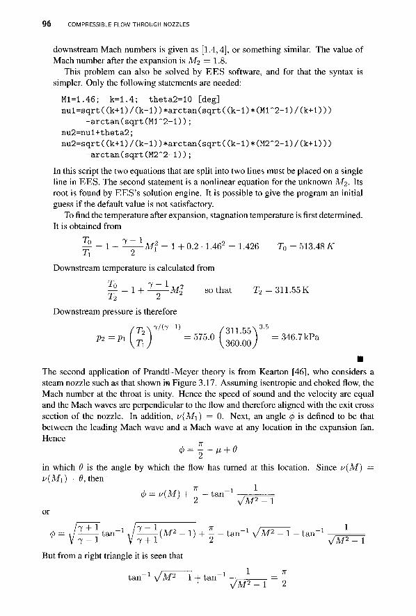
9 6 COMPRESSIBLE FLOW THROUGH NOZZLES
downstream Mach numbers is given as [1.4,4], or something similar. The value of Mach number after the expansion is M2 = 1.8.
This problem can also be solved by EES software, and for that the syntax is simpler. Only the following statements are needed:
Ml=1.46; k=1.4; theta2=10 [deg] n u l = s q r t ( ( k + l ) / ( k - l ) ) * a r c t a n ( s q r t ( ( k - l ) * ( M l " 2 - l ) / ( k + l ) ) )
- a r c t an ( sq r t (Ml~2- l ) ) ; nu2=nul+theta2; n u 2 = s q r t ( ( k + l ) / ( k - l ) ) * a r c t a n ( s q r t ( ( k - l ) * ( M 2 - 2 - l ) / ( k + l ) ) )
-a rc tan(sqr t (M2~2- l ) ) ;
In this script the two equations that are split into two lines must be placed on a single line in EES. The second statement is a nonlinear equation for the unknown M2. Its root is found by EES's solution engine. It is possible to give the program an initial guess if the default value is not satisfactory.
To find the temperature after expansion, stagnation temperature is first determined. It is obtained from
-^ = 1 + 7-^— Ml = 1 + 0.2 • 1.462 = 1.426 T0 = 513.48 K Xi 2
Downstream temperature is calculated from rp -i
— = 1 + ±^—Ml so that T2 = 311.55 K T2 2 z
Downstream pressure is therefore
T2Y/h-1) / 3 1 1 . 5 5 ^ 3 5
p2=Pll^L\ = 575.0 = 346.7kPa F \ T i / I 3 6 0 - 0 0 /
The second application of Prandtl-Meyer theory is from Kearton [46], who considers a steam nozzle such as that shown hi Figure 3.17. Assuming isentropic and choked flow, the Mach number at the throat is unity. Hence the speed of sound and the velocity are equal and the Mach waves are perpendicular to the flow and therefore aligned with the exit cross section of the nozzle. In addition, v(M\) = 0. Next, an angle <f> is defined to be that between the leading Mach wave and a Mach wave at any location in the expansion fan. Hence
</,= ! -n + 9
in which 6 is the angle by which the flow has turned at this location. Since v(M) — v{Mi) +d, then
7T i 1 cj) = u{M) H t a n - 1
VM2-l or
7 + 1 tan™1 J^—l-(M2 -l) + l - tan"1 \ / M 2 - 1 - tan"1
7 - 1 V 7 + 1 2 v JW But from a right triangle it is seen that
tan"1 y/M2 - 1 + tan"1 . = ^ VM2-l 2
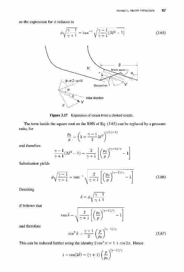
PRANDTL-MEYER EXPANSION 97
so the expression for 0 reduces to
7 - 1 7 + 1
t a n " 1 , / ^ — - ( M 2 - l ) 7 + 1
(3.65)
Initial direction
Figure 3.17 Expansion of steam from a choked nozzle.
The term inside the square root on the RHS of Eq. (3.65) can be replaced by a pressure ratio, for
\ 7 / ( 7 - l ) 1 + "
V and therefore
Po 7"±M2
7 - 1 7 + 1
(M2 - 1) 7 + 1
Substitution yields
( 7 - l ) / 7 1
Denoting
if follows that
and therefore
7 - 1 7 + 1 tan
\r ( 7 - l ) / 7
8 = <f> 7 - 1 7 + 1
t a n 5 ■■ \ 7 + l
( 7 - l ) / 7
(7" l ) /7 2 7 + 1 / p
cos2 5 = — 2 VPo
This can be reduced further using the identity 2 cos2 x = 1 + cos 2a:. Hence
1 + cos(2(5) = (7 + 1) Po
( 7 - l ) / 7
(3.66)
(3.67)

9 8 COMPRESSIBLE FLOW THROUGH NOZZLES
Rewriting this in terms of <fi gives
1 + cos(2 7 - 1 ( 7 + 1 ) P
(7-l)/7
7 + 1 " ' \Po, which can be solved for the pressure ratio. The final form is
7/(7-1)
(3.68)
V Po
1 + C 0 S ( 2 V ^ l 7 + 1
!♦'
Streamlines can be calculated by considering a control volume of a wedge-shaped region with an inlet at the throat and exit coinciding with an arbitrary Mach wave in the expansion fan. The lateral boundary is taken to be a streamline across which there is no flow. Since the component of velocity perpendicular to a Mach wave is the local sonic velocity, it is this component that carries the flow trough the inflow and outflow boundaries of the chosen control volume. For this reason, the continuity equation reduces to
P\A\C\ = pAc
Since the nozzle is rectangular, A = rb, in which b is the nozzle height and r is the distance from the corner to the chosen streamline. At the throat the area is A\ — rib, and r\ is the distance from the corner to the same streamline. Hence
r_ _ P\Ci _ pi f~T_ ri pc p\J Ti
In isentropic flow T/T\ = ( p / p i ) ' 7 - 1 ^ 7 , and this equation reduces to
n P \PI
From Eq. (3.67) the expression
(7-l)/27 -(7+l)/27
. , \ 1/2 / N (7-l)/27
7 + 1 \ f p x
2 / \Po,
is obtained. With sonic conditions at station 1, the pressure ratio there is
(3.69)
Po Pi
7 + iy/(7-1)
. 2 ) so that
1/2
and Eq. (3.69) can be recast as
_P_ . Pi cos Tzlt
7 + l '
7 + 1
27/(7-1)
(7-i)/27
Hence the distance from the corner to the streamline bounding the control volume is
r _ 1 r~i ~ ~/ ;„ i \(7+i)/(7-i)
cos
(3.70) 7 - 1 , 7 + l '
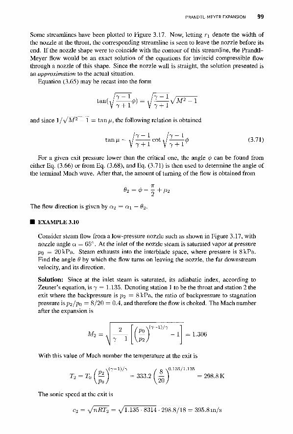
PRANDTL-MEYER EXPANSION 99
Some streamlines have been plotted to Figure 3.17. Now, letting r\ denote the width of the nozzle at the throat, the corresponding streamline is seen to leave the nozzle before its end. If the nozzle shape were to coincide with the contour of this streamline, the Prandtl-Meyer flow would be an exact solution of the equations for inviscid compressible flow through a nozzle of this shape. Since the nozzle wall is straight, the solution presented is an approximation to the actual situation.
Equation (3.65) may be recast into the form
tan(vfrr0) = ^Wi^^~l
and since l/\/M2 — 1 = tan p, the following relation is obtained
t a n / i = A/- 1-—cot J——<f> (3.71) 7 + 1 V 7 + 1
For a given exit pressure lower than the critical one, the angle <f> can be found from either Eq. (3.66) or from Eq. (3.68), and Eq. (3.71) is then used to determine the angle of the terminal Mach wave. After that, the amount of turning of the flow is obtained from
7T #2 = <t> ~ ~ + Pi
The flow direction is given by ct2 = «i — #2-
■ EXAMPLE 3.10
Consider steam flow from a low-pressure nozzle such as shown in Figure 3.17, with nozzle angle a = 65°. At the inlet of the nozzle steam is saturated vapor at pressure po = 20 kPa. Steam exhausts into the interblade space, where pressure is 8 kPa. Find the angle 6 by which the flow turns on leaving the nozzle, the far downstream velocity, and its direction.
Solution: Since at the inlet steam is saturated, its adiabatic index, according to Zeuner's equation, is 7 = 1.135. Denoting station 1 to be the throat and station 2 the exit where the backpressure is P2 = 8 kPa, the ratio of backpressure to stagnation pressure ispi/po = 8/20 = 0.4, and therefore the flow is choked. The Mach number after the expansion is
M2 Po f~l)h _ 1 P2J
= 1.306 ^ 7 - 1
With this value of Mach number the temperature at the exit is
/ \ ( 7 - l ) / 7 / o \0.135/1.135 T*=T°yi) = 3 3 3 - 2 U ) =298-8K
The sonic speed at the exit is
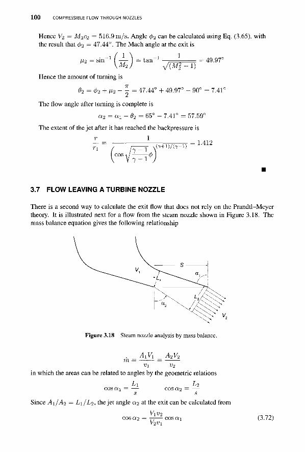
1 0 0 COMPRESSIBLE FLOW THROUGH NOZZLES
Hence V2 = M2C2 = 516.9 m / s . Angle 4>2 can be calculated using Eq. (3.65), with the result that <p2 = 47.44°. The Mach angle at the exit is
fJ-2 = sin - 1 1 Mo
= tan 1
V(Mi - 1) 49.97°
Hence the amount of turning is
02 = 02 + A<2 - x = 4 7 - 4 4 ° + 4 9 - 9 7 ° - 9 0 ° = 7 - 4 l C
The flow angle after turning is complete is
a2 = ax - 92 = 65° - 7.41° = 57.59°
The extent of the jet after it has reached the backpressure is
r 1
n cos
7 ~ 1 ;
7 + l '
(7+1)7(7-1) 1.412
3.7 FLOW LEAVING A TURBINE NOZZLE
There is a second way to calculate the exit flow that does not rely on the Prandtl-Meyer theory. It is illustrated next for a flow from the steam nozzle shown in Figure 3.18. The mass balance equation gives the following relationship
Figure 3.18 Steam nozzle analysis by mass balance.
m i4iVi A2V2
vi v2 in which the areas can be related to angles by the geometric relations
L\ L2 C O S a i = COSQI2 =
s s Since Ai/A2 = L1/L2, the jet angle 0.2 at the exit can be calculated from
Vxv2 c o s a 2 = 77—cos a i V2vi
(3.72)
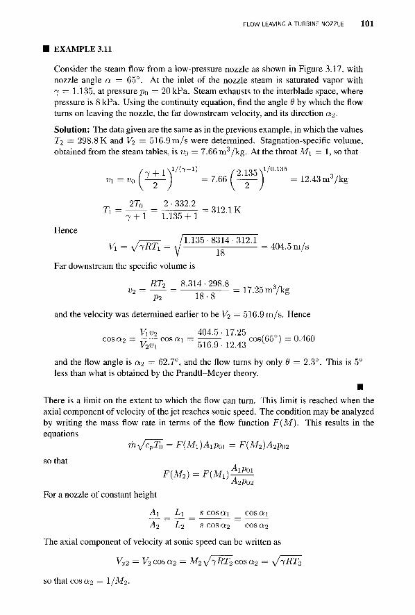
FLOW LEAVING A TURBINE NOZZLE 1 0 1
EXAMPLE 3.11
Consider the steam flow from a low-pressure nozzle as shown in Figure 3.17, with nozzle angle a = 65°. At the inlet of the nozzle steam is saturated vapor with 7 = 1.135, at pressure po = 20kPa. Steam exhausts to the interblade space, where pressure is 8 kPa. Using the continuity equation, find the angle 0 by which the flow turns on leaving the nozzle, the far downstream velocity, and its direction ab-solution: The data given are the same as in the previous example, in which the values T2 = 298.8 K and V2 = 516.9 m/s were determined. Stagnation-specific volume, obtained from the steam tables, is v0 = 7.66m3/kg. At the throat Mi = 1, so that
/ ^ + lV/(7-l) / 2 1 „ .U/0 .135 „ 1 = W o ( l ± i j = 7 . 6 6 ( ^ p J =12.43m3/kg
2T0 2 • 332.2 Tl = 7TT = n35TT = 312-1K
Hence 1.135-8314-312.1 V1 = ^RTi = ^ - =404.5 m/s
Far downstream the specific volume is
RT2 8.314-298.8 _ „ 3/1 v2 = = r ^ = 17.25 m3/kg
p2 18-8
and the velocity was determined earlier to be V2 = 516.9 m/s. Hence
VlV2 404.5 ■ 17.25 C 0 S a 2 = V^[ C ° S a i = 516.9 - 12.43 C ° S ( 6 5 } = °-46°
and the flow angle is a2 = 62.7°, and the flow turns by only 9 = 2.3°. This is 5° less than what is obtained by the Prandtl-Meyer theory.
■ There is a limit on the extent to which the flow can turn. This limit is reached when the axial component of velocity of the jet reaches sonic speed. The condition may be analyzed by writing the mass flow rate in terms of the flow function F(M). This results in the equations
rhyfipTo = F(Afi)Aipoi = F(M2)A2p02 so that
F(M2) = F (M 1 )4^ 5 1 A2P02
For a nozzle of constant height
Ai L\ s c o s a i cos oil A2 L2 s cosoi2 cosa2
The axial component of velocity at sonic speed can be written as
Vx2 = V2C0SCC2 = M2 \J^RT2 cos a2 = ^jRT2
so that cosa2 = l/M2.
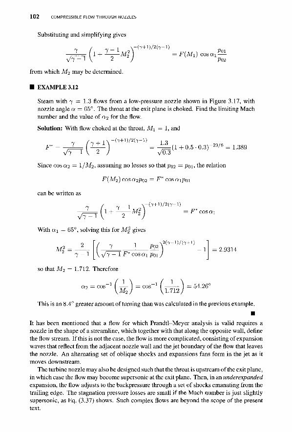
1 0 2 COMPRESSIBLE FLOW THROUGH NOZZLES
Substituting and simplifying gives
from which M2 may be determined.
■ EXAMPLE 3.12
Steam with 7 = 1.3 flows from a low-pressure nozzle shown in Figure 3.17, with nozzle angle a = 65°. The throat at the exit plane is choked. Find the limiting Mach number and the value of «2 for the flow.
Solution: With flow choked at the throat, Mi = 1, and
7 / 7 + 1N-(7+D/2(7-D L 3
f ^ ± i ) = 4 = ( l + 0.5-0.3)"23/6 = 1.389 V 2 y voT3v
Since cos 0:2 — I/M2, assuming no losses so thatpo2 = Poi> the relation
F{M2) cos a2po2 = -F* cos aipoi
can be written as
- ( 7 + l ) / 2 ( 7 - l )
VT = U 2 2 1 + -!——M£ = F * c o s a i
With Q;I = 65°, solving this for M | gives
2 M | =
7 - 1 7 1 Po2f7-1)/(7+1)_1
A/7 - 1 -F* c o s ai P01 2.9314
so that M2 = 1.712. Therefore
a2 = c o s - ( £ ) = M - i ( ^ ^ 54.26"
This is an 8.4° greater amount of turning than was calculated in the previous example. ■
It has been mentioned that a flow for which Prandtl-Meyer analysis is valid requires a nozzle in the shape of a streamline, which together with that along the opposite wall, define the flow stream. If this is not the case, the flow is more complicated, consisting of expansion waves that reflect from the adjacent nozzle wall and the jet boundary of the flow that leaves the nozzle. An alternating set of oblique shocks and expansions fans form in the jet as it moves downstream.
The turbine nozzle may also be designed such that the throat is upstream of the exit plane, in which case the flow may become supersonic at the exit plane. Then, in an underexpanded expansion, the flow adjusts to the backpressure through a set of shocks emanating from the trailing edge. The stagnation pressure losses are small if the Mach number is just slightly supersonic, as Eq. (3.37) shows. Such complex flows are beyond the scope of the present text.
EXERCISES 103
EXERCISES
3.1 Conditions in an air reservoir are 680 kPa and 560 K. From there the air flows isentropically though a convergent nozzle to a backpressure of 101.3 kPa. Find the velocity at the exit plane of the nozzle.
3.2 Air flows in a converging duct. At a certain location, where the area is A\ =6 .5 cm2, pressure is p\ = 140 kPa and Mach number is Mx = 0.6. The mass flow rate is, fa = 0.25 kg/s. (a) Find the stagnation temperature, (b) If the flow is choked, what is the size of the throat area? (c) Give the percent reduction in area from station 1 to the throat, (d) Find the pressure at the throat.
3.3 Air flows in a convergent nozzle. At a certain location, where the area is A\ = 5 cm2, pressure is p\ = 240 kPa and temperature is T\ = 360 K. Mach number at this location is Mi = 0.4. Find the mass flow rate.
3.4 The area of a throat in a circular nozzle is At = 1 cm2. For a choked flow find the diameter where M\ = 0 . 5 . Determine the Mach number value at a location where the diameter is D^ = 1.941 cm. Assume the flow to be isentropic and 7 = 1.4.
3.5 In a location in a circular nozzle where the area is Ai = 4, Mach number has the value M\ = 0.2. Find the diameter at a location where M = 0.6.
3.6 Air flows through a circular duct 15 cm in diameter with a flow rate 2.25 kg/s. The total temperature and static pressure at a certain location in the duct are 30° C and 106 kPa, respectively. Evaluate (a) the flow velocity, (b) the static temperature, (c) the total pressure, and (d) the density at this location.
3.7 Conditions in an air reservoir are 380 kPa and 460 K. From there the air flows through a convergent nozzle to a backpressure of 101.3 kPa. The polytropic efficiency of the nozzle is r\p = 0.98. Find, (a) exit plane pressure, (b) exit plane temperature, and (c) the velocity at the exit plane of the nozzle.
3.8 Air issues from a reservoir at conditions 260 kPa and 540 K into a converging nozzle. The nozzle efficiency is estimated to be ryn = 0.986. The backpressure is pb = 101.3 kPa. Find, (a) exit Mach number, (b) exit plane temperature, (c) exit plane pressure, and (d) exit velocity.
3.9 At the inlet to a nozzle the conditions are Mi = 0.3, poi = 320 kPa, and T0i = 430 K. The flow is irreversible with polytropic exponent n = 1.396. Show that
T1 /n \ 7 / ( 7 - l ) / „ \(n-\)/n J-02 I POl \ I Pi T2 \Pl ) \Pl,
Find the Mach number at a location where pi =210 kPa.
3.10 Flow from a reservoir with poi = 260 kPa and T0i = 530 K flows through a nozzle. It is estimated that the static enthalpy loss coefficient is C = 0.020. The exit pressure is P2 = 180 kPa. (a) Find the exit Mach number, (b) Find the polytropic efficiency of the nozzle.
3.11 A two-dimensional nozzle has a shape
4 x(x - 1) - - + 5 2(x + 2)
1 0 4 COMPRESSIBLE FLOW THROUGH NOZZLES
The nozzle stretches from 0 < x/a < 2(A/2 - 1). The throat is at xt/a = 2(A/2 - 1). The scale factor a is chosen such that the half-width of the nozzle at x = 0 is 4a/5. Assume that 4 / = 0.02 and the inlet Mach number is M\ = 0.5. Calculate and plot p/p\ as a function of x. Calculate the Mach number along the nozzle and graph it on the same plot.
3.12 Steam enters a nozzle from a steam chest at saturated vapor state at pressure po = 0.8 bar. It expands isentropically through a steam nozzle. Find the degree of supersaturation when it crosses the Wilson line at x = 0.96.
3.13 Consider a supersonic flow over a convex comer with angle #2 = 5°, when the inflow moves in the direction of 6\ = 0 ° . The upstream Mach number is Mi = 1.1, pressure is p\ = 130 kPa, and T\ = 310 K. Find, (a) Mach number, (b) temperature, and (c) pressure after the expansion is complete.
3.14 Consider the steam flow from a low-pressure nozzle at an angle a = 65°. At the inlet of the nozzle steam is saturated vapor at pressure po = 18 kPa. Steam exhausts into the interblade space, where pressure is 7 kPa. Find the angle 6 by which the flow turns on leaving the nozzle, the far downstream velocity, and its direction.
3.15 Consider the steam flow from a low-pressure nozzle at angle a = 65°. At the inlet of the nozzle steam is saturated vapor at pressure po — 18kPa. Steam exhausts to the interblade space, where pressure is 7 kPa. Using the continuity equation, find the angle 0 by which the flow turns on leaving the nozzle, the far downstream velocity, and its direction a2-
CHAPTER 4
PRINCIPLES OF TURBOMACHINE ANALYSIS
In this chapter the fundamental equation for turbomachinery analysis is developed from the moment of momentum balance. It gives an expression for the shaft torque in terms of the difference in the rate at which angular momentum of the working fluid leaves and enters a properly chosen control volume. Since power delivered (or absorbed) by a turbomachine is a product of torque and angular speed, a relationship between the flow rates of angular momentum at the inlet and exit, the rotational speed of the shaft, and power is obtained. The equation derived this way is called the Euler equation of turbomachinery. It is the most important equation in the study of this subject.
In earlier chapters power transferred to, or from, a turbomachine was expressed as the product of mass flow rate and a change in stagnation enthalpy. By equating the expression for work from the Euler equation of turbomachinery to the change in stagnation enthalpy, concepts from fluid mechanics become linked to thermodynamics. This link is central to understanding the performance of turbomachines.
In applying the momentum of momentum balance to a stationary control volume angular momentum is usually expressed in terms of absolute velocity of the fluid. In the analysis of the rotating blades velocity relative to the rotor is also needed. From it, together with the absolute velocity and the blade velocity, one can construct a velocity triangle. These velocity triangles are discussed first in this chapter. They are followed by the development of the Euler equation for turbomachinery. After that the work delivered, or absorbed, is recast in an alternative form and a concept of degree of reaction is developed. One measure of the effectiveness at which work transfer takes place in a turbomachine is called utilization. Although this concept is not extensively used today, it is introduced and its
Principles of Turbomachinery. By Seppo A. Korpela Copyright © 2011 John Wiley & Sons, Inc.
105
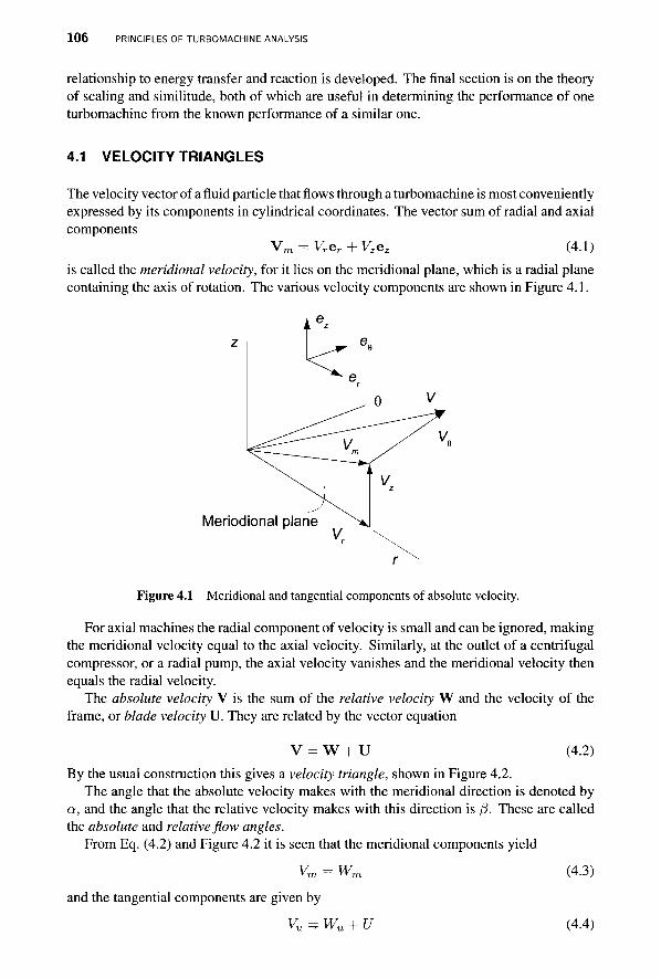
1 0 6 PRINCIPLES OF TURBOMACHINE ANALYSIS
relationship to energy transfer and reaction is developed. The final section is on the theory of scaling and similitude, both of which are useful in determining the performance of one turbomachine from the known performance of a similar one.
4.1 VELOCITY TRIANGLES
The velocity vector of a fluid particle that flows through a turbomachine is most conveniently expressed by its components in cylindrical coordinates. The vector sum of radial and axial components
Vm = Vrer + Vzez (4.1) is called the meridional velocity, for it lies on the meridional plane, which is a radial plane containing the axis of rotation. The various velocity components are shown in Figure 4.1.
Figure 4.1 Meridional and tangential components of absolute velocity.
For axial machines the radial component of velocity is small and can be ignored, making the meridional velocity equal to the axial velocity. Similarly, at the outlet of a centrifugal compressor, or a radial pump, the axial velocity vanishes and the meridional velocity then equals the radial velocity.
The absolute velocity V is the sum of the relative velocity W and the velocity of the frame, or blade velocity U. They are related by the vector equation
V = W + U (4.2) By the usual construction this gives a velocity triangle, shown in Figure 4.2.
The angle that the absolute velocity makes with the meridional direction is denoted by a, and the angle that the relative velocity makes with this direction is f3. These are called the absolute and relative flow angles.
From Eq. (4.2) and Figure 4.2 it is seen that the meridional components yield
Vm = Wm (4.3)
and the tangential components are given by
vu^wu + u (4.4)

VELOCITY TRIANGLES 107
Figure 4.2 A typical velocity triangle.
These velocities are related to the meridional velocity by
Vu = Vm tan a Wu = Wm tan (3 (4.5)
It is convenient to denote the tangential component by the subscript u and to take it positive when it is in the direction of the blade motion. Tangential components are associated with the blade forces; meridional components, with the rate at which fluid flows through the machine.
EXAMPLE 4.1
Consider the velocity diagram shown in Figure 4.3. The magnitude of the absolute velocity is V\ = 240m/s, and the flow angle is a\ = —20°. The blade speed is U = 300 m/s. Find the magnitude of the relative velocity and its flow angle. Solution: The axial velocity is given by
Vxl = Vi cosai = 240cos(-20°) = 225.5 m/s
and Wx\ =VX\. The tangential components of the absolute and relative velocities are calculated as
Vul = Vi sinai = 240sin(-20°) = -82.1 m/s
Wul = Vul-U = -82.1 - 300 = -382.1 m/s Hence the magnitude of the relative velocity is
'Wlx + Wlx = \j22^.h2 + 382.22 = 443.7 m/s
and the flow angle of the relative velocity becomes
-382.1' A = tan"1 ( ^ . 1 = t a ^ 1
225.5 -59.4°
The foregoing example illustrates the sign convention for angles. Positive angles are measured from the meridional direction, and they increase in counterclockwise direction. Negative angles become more negative in the clockwise direction. Strict adherence to this convention will be followed, and this makes computer calculations easy to implement.
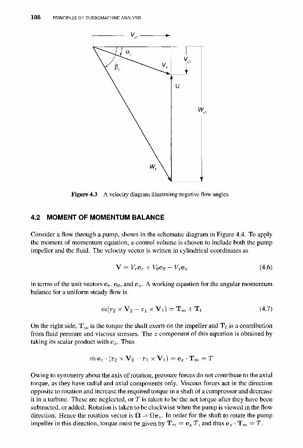
PRINCIPLES OF TURBOMACHINE ANALYSIS
Figure 4.3 A velocity diagram illustrating negative flow angles.
4.2 MOMENT OF MOMENTUM BALANCE
Consider a flow through a pump, shown in the schematic diagram in Figure 4.4. To apply the moment of momentum equation, a control volume is chosen to include both the pump impeller and the fluid. The velocity vector is written in cylindrical coordinates as
V = Vrer + Veee + Vzez (4.6)
in terms of the unit vectors e r , e$, and ez. A working equation for the angular momentum balance for a uniform steady flow is
ra(r2 x V2 - r i x Vi) (4.7)
On the right side, T m is the torque the shaft exerts on the impeller and Tf is a contribution from fluid pressure and viscous stresses. The z component of this equation is obtained by taking its scalar product with ez. Thus
me, (r2 x V2 - n x Vi) - ez ■ T m = T
Owing to symmetry about the axis of rotation, pressure forces do not contribute to the axial torque, as they have radial and axial components only. Viscous forces act in the direction opposite to rotation and increase the required torque in a shaft of a compressor and decrease it in a turbine. These are neglected, or T is taken to be the net torque after they have been subtracted, or added. Rotation is taken to be clockwise when the pump is viewed in the flow direction. Hence the rotation vector is fl = Qez. In order for the shaft to rotate the pump impeller in this direction, torque must be given by T m = ez T, and thus ez ■ T m = T.
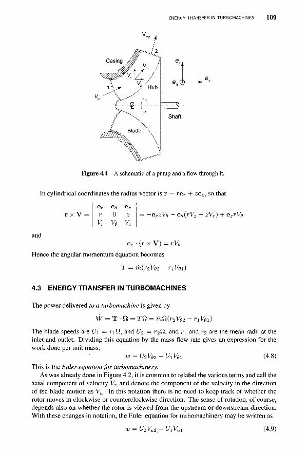
ENERGY TRANSFER IN TURBOMACHINES 1 0 9
e9&
Shaft
Figure 4.4 A schematic of a pump and a flow through it.
In cylindrical coordinates the radius vector is r = rer + zez, so that
r x V er ee ez r 0 z Vr V6 Vz
-erzVe - ee(rVz - zVr) + ezrVe
and ez • (r x V) = rVe
Hence the angular momentum equation becomes
T = m{r2Ve2 - nVei)
4.3 ENERGY TRANSFER IN TURBOMACHINES
The power delivered to a turbomachine is given by
W = T • ft = TO = mn{r2V02 - nVei)
The blade speeds are U\ = rifi, and U2 = r20., and r\ and r2 are the mean radii at the inlet and outlet. Dividing this equation by the mass flow rate gives an expression for the work done per unit mass,
w = U2V02 - C/iVfli (4.8) This is the Euler equation for turbomachinery.
As was already done in Figure 4.2, it is common to relabel the various terms and call the axial component of velocity Vx and denote the component of the velocity in the direction of the blade motion as Vu. In this notation there is no need to keep track of whether the rotor moves in clockwise or counterclockwise direction. The sense of rotation, of course, depends also on whether the rotor is viewed from the upstream or downstream direction. With these changes in notation, the Euler equation for turbomachinery may be written as
U2V,, C/iKi (4.9)
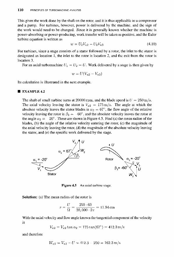
110 PRINCIPLES OF TURBOMACHINE ANALYSIS
This gives the work done by the shaft on the rotor, and it is thus applicable to a compressor and a pump. For turbines, however, power is delivered by the machine, and the sign of the work would need to be changed. Since it is generally known whether the machine is power-absorbing or power-producing, work transfer will be taken as positive, and the Euler turbine equation is written as
w = U2Vu2 - U3Vu3 (4.10)
For turbines, since a stage consists of a stator followed by a rotor, the inlet to the stator is designated as location 1, the inlet to the rotor is location 2, and the exit from the rotor is location 3.
For an axial turbomachine U\ =U2 = U. Work delivered by a stage is then given by
w = U(Vu2 - Vu3)
Its calculation is illustrated in the next example.
■ EXAMPLE 4.2
The shaft of small turbine turns at 20000 rpm, and the blade speed is U = 250 m/s. The axial velocity leaving the stator is Vx2 = 175 m/s. The angle at which the absolute velocity leaves the stator blades is a2 = 67°, the flow angle of the relative velocity leaving the rotor is f33 = —60°, and the absolute velocity leaves the rotor at the angle a3 = —20°. These are shown in Figure 4.5. Find (a) the mean radius of the blades, (b) the angle of the relative velocity entering the rotor, (c) the magnitude of the axial velocity leaving the rotor, (d) the magnitude of the absolute velocity leaving the stator, and (e) the specific work delivered by the stage.
Stator
Figure 4.5 An axial turbine stage.
Solution: (a) The mean radius of the rotor is
U 250 • 60 ft 20, 000 • 2TT
11.94 cm
With the axial velocity and flow angle known the tangential component of the velocity is
Vu2 = Vx2tana2 = 175tan(67°) = 412.3 m/s
and therefore
W„ Vu2 - U = 412.3 - 250 = 162.3 m/s

ENERGY TRANSFER IN TURBOMACHINES 1 1 1
Since WX2 = ■vx2
02 = tan
At the exit of the rotor
so that
vx3
Vu3 = wu3
u
-i (Wu2
\wx2.
+ u
= tan"1 ( ^ ) = 42.8° 175
Vx3 tan a3 = Vx3 tan j33 + U
2 5 0 182.7 m/s t a n a 3 - tan/33 tan(-20°) - tan(-60°)
(b) The absolute velocity is obtained by first calculating the tangential component
Vu3 = Vx3tana3 = 182.7 tan(-20°) = -66.5 m/s
and then
^3 = yjv£3 + V%3 = ^182.72 + 66.52 = 194.4 m/s
(c) Specific work done is
w = U(Vu2 - Vu3) = 250(412.3 + 66.5) = 119.7kJ/kg As the flow expands through the turbine, its density decreases, and to accommodate this, the product of axial velocity and cross-sectional area needs to increase. Often axial machines are designed to keep the axial velocity constant. In this example the axial velocity increases by a small amount, and the cross-sectional area must be adjusted to account for the increase in velocity and a decrease in density.
■ Work delivered by an axial turbine with constant axial velocity across a stage can be written as
w = U(Vu2 - Vu3) = UVx(tana2 - t ana 3 ) Dividing by U2 gives
w Vx 77̂ - = — (tano:2 - t a n a 3 ) U^ U Defining the blade-loading coefficient and flow coefficient as
gives a nondimensional version of this equation:
ip — (/>(tan «2 — tan a3)
The blade loading coefficient is an appropriate term for %p, since it is the blade force times the blade velocity that gives the work. Also, the flow coefficient 0 is a ratio of the axial velocity to blade velocity and is thus a measure of the flow rate through the machine. Much use will be made of these nondimensional parameters, for they are independent of the size of machine, and their values for best designs have been established over many years of practice.
As another example of the general use of the Euler equation for turbomachinery, analysis of a centrifugal pump is considered next.

1 1 2 PRINCIPLES OF TURBOMACHINE ANALYSIS
EXAMPLE 4.3
Water at 20°C leaves a pump impeller with an absolute velocity of 13.94 m/s at the angle 72.1°. The blade speed at the exit is 25.17m/s, and the shaft speed is 3450 rpm. The absolute velocity is axial at the inlet. The flow rate is 18.0 L/s. Find (a) the magnitude of the relative velocity and its flow angle /32, (b) the power required, and (c) the outlet blade radius and the blade height assuming that the open area at the periphery is 93% of the total area. The pump is shown in Figure 4.6.
U= 25.17 m/s
V= 13.94 m/s
a, = 72.1°
P, = - 70.2°\
W= 12.65 m/s
V= 13.26 m/s
V =4.29 m/s
W ,= -11.91 m/s
Figure 4.6 Pump exit and its velocity diagram.
Solution: (a) The tangential component of the absolute velocity at the exit is given by
Vu2 = V2sina2 = 13.94 sin(72.1°) = 13.26m/s
and its meridional component, which is radial here, is
Vr2 = 1/2 cosa2 = 13.94 cos(72.1°) = 4.29m/s
The tangential component of the relative velocity is determined as
Wu2 = Vu2 - U = 13.26 - 25.17 = -11.91 m/s
Since the radial component of the relative velocity is Wr2 = Vr2 = 4.29 m/s, the angle of the relative flow can be calculated as
f32 = tan 1 / Wu 2 tan -11.91
-70.2° Wr2) V 4-29
The magnitude of the relative velocity is then
W2 = \fw^+Wl2 = V4.292 + 11.912 = 12.65 m/s
A velocity triangle can now be completed. The flow angle of the relative velocity is approximately equal to the blade angle x, and in this pump the impeller blades curve backward; that is, they are curved in the direction opposite to blade rotation.
ENERGY TRANSFER IN TURBOMACHINES 113
(b) Since the flow is axial at the inlet, Vul = 0, and the work done is
w = U2Vu2 = 25.17 • 13.26 = 333.88 J/kg
With density of water at 20° C equal to p = 998 kg/m3, the mass flow rate is
m = pQ = 998 • 0.018 = 17.964 kg/s
and the power required is W = mw = 17.964 • 333.88 = 6.0 kW. (c) The outlet radius is
U2 25.17-30 „ „ „ r2 = -^- = = 6.97 cm 2 n 3450 • 7T
With the flow rate Q = 0.018 m3/s, the outlet area is
Q 0.018 4nn 2 A2 = T7- = = 42.0cm2
Vr2 4.29
The blade height is then
A2 42.0 0.93 • 2TT • r2 0.93 • 2TT • 6.97
1.03 cm
The blade-loading coefficient and flow coefficient are defined in terms of the tip speed of the blade at the exit:
/ w 3 3 3 ' 8 8 n^ov A Vr2 4 2 9 niTn C/j 25.17^ t/2 25.17
4.3.1 Trothalpy and specific work in terms of velocities
Since no work is done in the stator, total enthalpy remains constant across it. In this section an analogous quantity to the total enthalpy is developed for the rotor. Specifically, consider a mixed-flow compressor in which the meridional velocity at the inlet is not completely axial and at the exit from the blades not completely radial. The work done by the rotor blades is
w = hQ2-h0l = U2Vu2-UlVul (4.12)
When this equation is written as
h0i ~ UiVui = h02 - U2Vu2
the quantity I = ho- UVU
is seen to be constant across the impeller. It can also be written as
/ = h+ l-v2 - uvu = h + \vl + l-v2 - uvu
Adding and subtracting U2/2 to complete the square gives
I = h+\vl + \{Vu-Uf -\u2 = h+\vl + \wl-\u2

114 PRINCIPLES OF TURBOMACHINE ANALYSIS
or since Vm = Wm, and W2 = W^ + W2, it follows that
\w!-\u2 = k2 + \w2-h I = h!+ ^W2 - -U2 = h2 + -W2 - -U2 (4.13)
is constant across the impeller. The quantity / is called trothalpy? Solving Eq. (4.13) for h\ and h2 and substituting them into the equation for work
w = h02-h01=h2 + ~V2-h1 + ̂ V2 (4.14)
gives, after / has been canceled, the following equation:
1—2 1 W 2 , lTT2 I ! , r 2 1 T J / 2 , 1 r r 2 *=zV{--wi + -ui-\-v{--wt + jJi
Rearranging gives the form
w = \{V2 - V2) + \{U2 - U2) + \(W2 - W2) (4.15)
Equating this and Eq. (4.14) leads to
h2-h1 = \{U2 - U2) + ̂ {W2 - W2) (4.16)
From Eq. (4.14) it is seen that the work done in a centrifugal pump increases the kinetic energy and the static enthalpy. Equation (4.16) shows first that the static enthalpy increase involves moving the fluid into a larger radius, resulting in increased pressure. The second term causes an increase in pressure as the relative velocity is reduced; that is, diffusion with W2 < W\ leads to pressure recovery. The pressure is increased further in the volute of a centrifugal pump where diffusion of the absolute velocity takes place. Since this diffusion is against an adverse pressure gradient, the kinetic energy at the exit of the impeller cannot be so large that its deceleration through the volute causes separation of boundary layers and a great increase in irreversibility. The use of these concepts is illustrated in the next example.
■ EXAMPLE 4.4
A small centrifugal pump with an impeller radius r2 = 4.5 cm operates at 3450 rpm. Blades at the exit are curved back at an angle /32 = —65°. Radial velocity at the exit is Vr2 = Wr2 = 3.0 m/s. Flow at the inlet is axial with velocity Vi = 4.13 m/s. The mean radius of the impeller at the inlet is r\ =2 .8 cm. (a) Find the work done using Eq. (4.12). (b) Calculate the kinetic energy change of the relative velocity, absolute velocity, and that associated with the change in the blade speed and calculate work done using Eq. (4.15). Confirm that the two methods give the same answer.
Solution: (a) Blade speed at the exit is
^ 0.045 ■ 3450 • 2TT U2 = r2VL = — = 16.26 m/s
3This quantity is commonly called rothalpy, a compound word combining the terms rotation and enthalpy. Its construction does not conform to the established rules for formation of new words in the English language, namely, that the roots of the new word originate from the same language. The word trothalpy satisfies this requirement as trohos is the Greek root for wheel and enthalpy is to put heat in, whereas rotation is derived from Latin rotare.

ENERGY TRANSFER IN TURBOMACHINES 115
Since Wr2 = Vr2, the tangential component of the relative velocity is
Wu2 = y r 2 tan/32 = 3.0 tan(-65°) = -6 .43m/s
Tangential component of the absolute velocity is then
Vu2 = U2 + Wu2 = 16.26 - 6.43 = 9.83 m/s
Since the flow at the inlet is axial Vu\ = 0, the inlet does not contribute to the work done as calculated by the Euler equation for turbomachinery, which reduces to
w = U2Vu2 = 16.26 • 9.83 = 159.7 J/kg
(b) Magnitudes of the relative and absolute velocities at the exit are given by
W2 = JWl2 + W?2 = A/6 .43 2 + 3.02 = 7.10 m/s
V2 = ^V*2 + Vr% = \ /9.832 + 3.02 = 10.27 m/s
Since the flow is axial at the inlet. Vx\ = V\ = 4.13 m/s. The blade speed is
0.028-3450^ U\ — rAl = = 10.11 m/s
30 '
Tangential components of the expression relating absolute and relative velocity give
Wul =Vul-Ui=0- 10.11 = -10.11 m/s
and therefore the magnitude of the relative velocity is Wi = \Jwlx + W^ = v
/10.112+4.132 = 10.92 m/s
The kinetic energy changes are
\(v2-v\) = ^(10.272-4.132) = 44.21 m2/s2 = 44.21 J/kg
\{U2 ~ Uf) = ^(16.262 - 10.112) = 80.99m2/s2 = 80.99J/kg
]-{Wl - W%) = ^(10.932 - 7.102) = 34.51 m2/s2 = 34.51 J/kg
Their sum checks with the direct calculation of the work done.
Since there is no swirl at the inlet, Vui = 0, the work done is independent of the inlet conditions. This means that when work is represented in terms of kinetic energy changes, terms involving inlet velocities must cancel. Velocity triangle at the inlet is a right triangle with W\ as its hypothenuse, so that V? + [/2 = W±. Hence in this case
and using the law of cosines gives w = U2Vu2, as it should.
1 1 6 PRINCIPLES OF TURBOMACHINE ANALYSIS
4.3.2 Degree of reaction
Degree of reaction, or reaction for short, is defined as the change in static enthalpy across the rotor divided by the static enthalpy change across the entire stage. For the turbine this is given as
h2 - h3 R hi - h3
Since an enthalpy change is proportional to a pressure change, the degree of reaction can be regarded in terms of pressure changes. In compressors pressure increases downstream, and in order to keep the adverse pressure gradient small, the value of reaction provides a means to assess the strength of this gradient.
Work delivered by a rotor in a turbine is
l . . o , 1 , w = h02- h03 = h2 + ~V22 -h3- -Vf
Since for nozzles (or stator) /i0i = ho2, work can also be written as
w = h1-h3 + ± (V2 - V2)
Solving the last two equations for static enthalpy differences and substituting them into the definition of reaction gives
\{Vf-V2)+W R~\{vi-v2) + w
( 4 1 7 )
Substituting Eq. (4.15) for work into this and simplifying leads to
U2-UI + W2-W2 "■ T/2 _ T/2 , 172 _ TT-2 , W 2 _ M/2 ^ - 1 0 J
In a flow in which V\ = V2, the reaction R = 1. Such a machine is a pure reaction machine. A lawn sprinkler, rotating about an axis is such a machine, for all the pressure drops take place in the sprinkler arms. They turn as a reaction to the momentum leaving them.
The steam turbine shown in Figure 3.11 is an axial machine in which U2 = U3 and its reaction is zero when W2 = W3. For the rotor buckets shown, the blade angles are equal but opposite in sign and by adjustment of the flow area to account for the increase in specific volume, the magnitude of the relative velocity can be made constant across the rotor. Hence, since the trothalpy is also constant across the rotor, enthalpy change across it vanishes and the reaction becomes R — 0.
■ EXAMPLE 4.5
Consider an axial turbine stage with blade speed U = 350 m/s and axial velocity Vx = 280 m/s. Flow enters the rotor at angle a2 = 60°. It leaves the rotor at angle a3 — —30°. Assume a stage for which a\ = a3 and a constant axial velocity. Find the velocities and the degree of reaction.
Solution: Since axial velocity is constant and the flow angles are equal at both the entrance and exit of the stage, the velocity diagrams at the inlet of the stator and the
UTILIZATION 117
exit of the rotor are identical. From a velocity triangle, such as shown in Figure 4.2, the tangential velocities are:
Vu2 = Vxta,na2 = 280.0 tan(60°) = 484.97m/s
Vu3 = Vxtanai = 280.0 tan(-30°) = -161.66m/s
and work done is
w = U{Vu2 - Vu3) = 350(484.97+161.66) = 226.32 k J / k g
Tangential components of the relative velocities are
Wu2 = Vu2 - U = 484.97 - 350.00 = 134.97 m / s
Wu3 = Vu3 - U = -161.66 - 350.00 = -511 .66 m / s
Hence V2 = A/V„2
2 + V? = \ /484.97 2 + 280.02 = 560.00 m / s
V3 = J v ^ + V* = \ / l 61 .66 2 + 280.02 = 323.32 m / s
VF2 = ^ W ^ 2 + W 2 = \ / l 3 4 . 9 7 2 + 280.02 = 310.83 m / s
T^3 = ^/VF23 + 1^2 = V 5 H . 6 6 2 + 2 8 0 . 0 2 = 583.26 m / s
Since U2 = U3, the expression for reaction is
= W32 - Wj = 583.262 - 310.832
=
2zz; 2 -226 ,320
A reaction ratio close to one-half is often used to make the enthalpy drop, and thus also the pressure drop, in the stator and the rotor nearly equal. _
4.4 UTILIZATION
A measure of how effectively a turbine rotor converts the available kinetic energy at its inlet to work is called utilization, and a utilization factor is defined as the ratio
w (4.19) w+\Vf
The denominator is the available energy consisting of what is converted to work and the kinetic energy that leaves the turbine. This expression for utilization equals unity if the exit kinetic energy is negligible. But the exit kinetic energy cannot vanish completely because the flow has to leave the turbine. Hence utilization factor is always less than one. Maximum utilization is reached by turning the flow so much that the swirl component vanishes; that is, for the best utilization the exit velocity vector should lie on the meridional plane.
Making the appropriate changes in Eq. (4.15) to make it applicable to a turbine and substituting it into Eq. (4.19), gives an expression for utilization
. vf-vf + ul-ui + wj-wl v2 + m - m + wi - w? ( '
118 PRINCIPLES OF TURBOMACHINE ANALYSIS
in terms of velocities alone. Next, from Eq. (4.17) it is easy to see that the work delivered is also
Substituting this into Eq. (4.19) gives
2 2 I
V2 - RV2
'V?-RV?\ , 1-R )
-{l-R)V$
(4.21)
£ - V2-RV2 ( 4 ' 2 2 )
In the situation in which R = 1 and therefore also V2 = V\, this expression becomes indeterminate. It is valid for other values of R.
In a usual design of a multistage axial turbine the exit velocity triangle is identical to the velocity triangle at the inlet of a stage. Under this condition V\ = V3 and ct\ =0:3, and the utilization factor simplifies to
vi - vi £ = W^k (4'23) The expression for work reduces to
vi - vi w = 2M) (4-24) With velocities expressed in terms of their tangential and axial components, this becomes
2(1 -R)
or , VJ sin2 a2 + Vx\ - (VJ sin2 a3 + Vx%)
W~ 2(1 - R) { '
At maximum utilization 0:3 = 0 and the work is w = UVU2- Equating this to the work given in Eq. (4.25) leads to the equality
TTv «n Vism2a2 + Vx\-Vx%
C / y 2 S m a i = 2(1^)
from which follows the relation
U (Vi2-Vi3)/Vi+sin2a2 V2 2(1-R)sma2
(4.26)
The left-hand side (LHS) is a speed ratio. It is denoted by A = U/V2. Since Vx2/V2 cos a2, this reduces to
1 - vx%/vi
from which the ratio
2(1 — R)sma2
V2
- # = l - 2 ( l - i ? ) A s i n a (4.28) V4
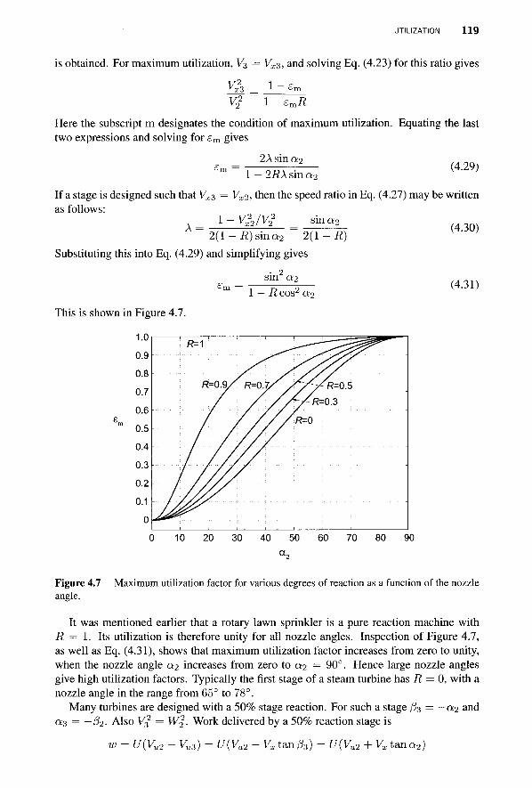
UTILIZATION 1 1 9
is obtained. For maximum utilization, V3 = Vxs, and solving Eq. (4.23) for this ratio gives
K23 _ 1 ~ £m v2
2 1 — emR
Here the subscript m designates the condition of maximum utilization. Equating the last two expressions and solving for em gives
2Asina2 1 — 2RX sin «2
(4.29)
If a stage is designed such that VX3 = Vx2, then the speed ratio in Eq. (4.27) may be written as follows:
s in 0:2 A i-vxyv*
2 ( l - i ? ) s i n a 2 2(1 - i?) Substituting this into Eq. (4.29) and simplifying gives
sin a2 1 — 7? cos2 a2
(4.30)
(4.31)
This is shown in Figure 4.7.
Figure 4.7 Maximum utilization factor for various degrees of reaction as a function of the nozzle angle.
It was mentioned earlier that a rotary lawn sprinkler is a pure reaction machine with R — 1. Its utilization is therefore unity for all nozzle angles. Inspection of Figure 4.7, as well as Eq. (4.31), shows that maximum utilization factor increases from zero to unity, when the nozzle angle a2 increases from zero to a2 = 90°. Hence large nozzle angles give high utilization factors. Typically the first stage of a steam turbine has R = 0, with a nozzle angle in the range from 65° to 78°.
Many turbines are designed with a 50% stage reaction. For such a stage j3% = —a2 and 0:3 = — j32- Also V3
2 = W%. Work delivered by a 50% reaction stage is
w = U(Vu2 - Vu3) = U(Vu2 - Vx tan 183) = U{Vu2 + Vx t ana 2 )
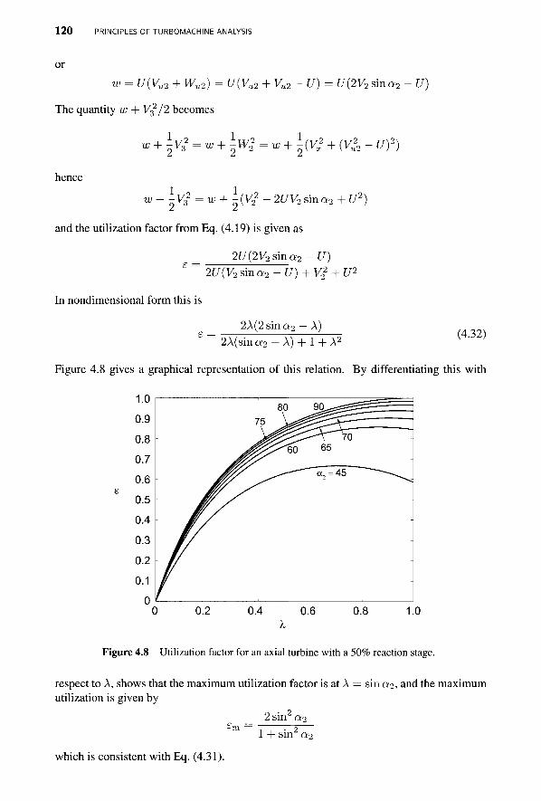
1 2 0 PRINCIPLES OF TURBOMACHINE ANALYSIS
w = U(Vu2 + Wu2) = U(Vu2 + Vu2 -U) = U(2V2 sina2 - U)
The quantity w + V2/2 becomes
l . „ , 1. w + -vi = w + -wi = w ~dvx2 + (vu\-uy)
hence
w+^Vi =w+ i(y22 - 2UV2 sina2 + U2)
and the utilization factor from Eq. (4.19) is given as
2U(2V2sina2-U) 2U(V2sma2-U) + Vi + U2
In nondimensional form this is
2A(2sina2 - A ) (4.32)
2A(sina 2 -A) + l + A2
Figure 4.8 gives a graphical representation of this relation. By differentiating this with
1.0
Figure 4.8 Utilization factor for an axial turbine with a 50% reaction stage.
respect to A, shows that the maximum utilization factor is at A = sin a2, and the maximum utilization is given by
2 sin2 a2 £m — 1 + sin a2
which is consistent with Eq. (4.31).
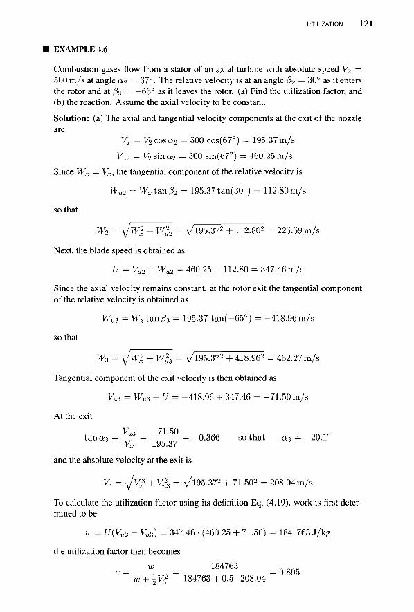
UTILIZATION 1 2 1
EXAMPLE 4.6
Combustion gases flow from a stator of an axial turbine with absolute speed V2 = 500 m/s at angle a2 = 67°. The relative velocity is at an angle f32 = 30° as it enters the rotor and at (33 = —65° as it leaves the rotor, (a) Find the utilization factor, and (b) the reaction. Assume the axial velocity to be constant.
Solution: (a) The axial and tangential velocity components at the exit of the nozzle are
Vx = V2cosa2 = 500 cos(67°) = 195.37m/s
Vu2 = V2 sina2 = 500 sin(67°) = 460.25 m/s
Since Wx = Vx, the tangential component of the relative velocity is
Wu2 = Wx tan/32 = 195.37 tan(30°) = 112.80 m/s
so that
W2 = \Jw% + Wl2 = V195.372 + 112.802 = 225.59 m/s
Next, the blade speed is obtained as
U = Vu2 - Wu2 = 460.25 - 112.80 = 347.46 m/s
Since the axial velocity remains constant, at the rotor exit the tangential component of the relative velocity is obtained as
Wu3 = Wxtan/33 = 195.37 tan(-65°) = -418.96 m/s
so that
W3 = yjW% + W%3 = \ / l95.372+418.962 = 462.27 m/s
Tangential component of the exit velocity is then obtained as
Vu3 = Wu3 + U = -418.96 + 347.46 = -71.50 m/s
At the exit
t a n a 3 = TT~ = ' = -0.366 so that a3 = -20 .1 c
Vx 195.37
and the absolute velocity at the exit is
V3 = yVj* + V%3 = v/195.372 + 71.502 = 208.04 m/s
To calculate the utilization factor using its definition Eq. (4.19), work is first deter-mined to be
w = U(Vu2 - Vu3) = 347.46 ■ (460.25 + 71.50) = 184, 763 J/kg
the utilization factor then becomes w 184763
0.895 iy32 184763 + 0.5-208.04
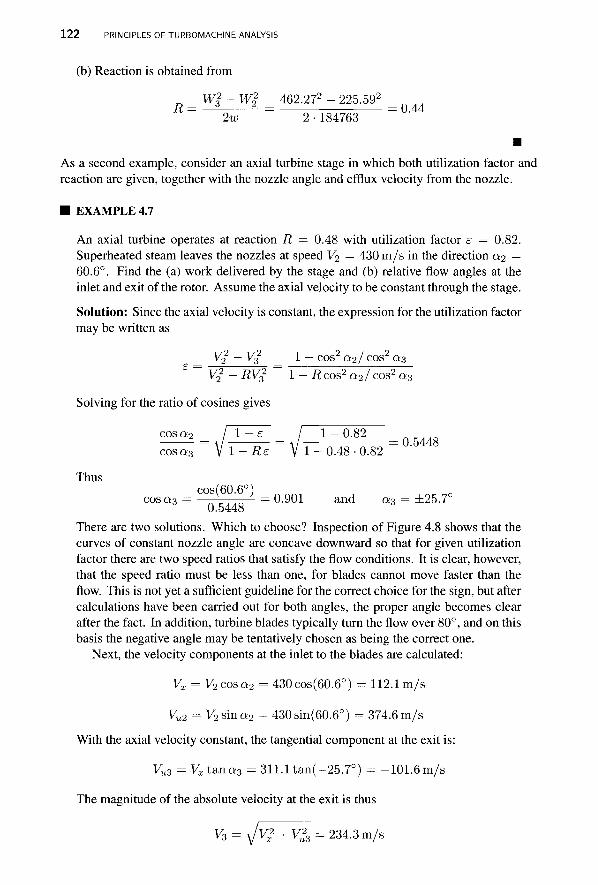
1 2 2 PRINCIPLES OF TURBOMACHINE ANALYSIS
(b) Reaction is obtained from
„ W?-W? 462.272 - 225.592
R = — = = 0.44 2w 2•184763
As a second example, consider an axial turbine stage in which both utilization factor and reaction are given, together with the nozzle angle and efflux velocity from the nozzle.
■ EXAMPLE 4.7
An axial turbine operates at reaction R — 0.48 with utilization factor e = 0.82. Superheated steam leaves the nozzles at speed V2 = 430 m/s in the direction a2 = 60.6°. Find the (a) work delivered by the stage and (b) relative flow angles at the inlet and exit of the rotor. Assume the axial velocity to be constant through the stage.
Solution: Since the axial velocity is constant, the expression for the utilization factor may be written as
rl T/2 ^ 2 ~~ ^ 3 1 _ c o s ° 2 / COS2 0:3 V2
2 - RV32 1 - R cos2 a21 cos2 a3
Solving for the ratio of cosines gives
^ = JJ-±- = J i - 0 - 8 2 = 0.5448 cosa3 Ml-Re V 1 - 0.48 ■ 0.82
Thus
c o s a 3 = n f ^ o =0-901 and a3 = ±25.7° 0.5448
There are two solutions. Which to choose? Inspection of Figure 4.8 shows that the curves of constant nozzle angle are concave downward so that for given utilization factor there are two speed ratios that satisfy the flow conditions. It is clear, however, that the speed ratio must be less than one, for blades cannot move faster than the flow. This is not yet a sufficient guideline for the correct choice for the sign, but after calculations have been carried out for both angles, the proper angle becomes clear after the fact. In addition, turbine blades typically turn the flow over 80°, and on this basis the negative angle may be tentatively chosen as being the correct one.
Next, the velocity components at the inlet to the blades are calculated:
Vx = V2cosa2 = 430cos(60.6°) = 112.1 m/s
Vu2 = y 2 s ina 2 = 430sin(60.6°) = 374.6 m/s
With the axial velocity constant, the tangential component at the exit is:
Vu3 = K c t ana 3 = 311.1 tan(-25.7°) = -101.6 m/s
The magnitude of the absolute velocity at the exit is thus
V3 = JV? + V*3 = 234.3 m/s
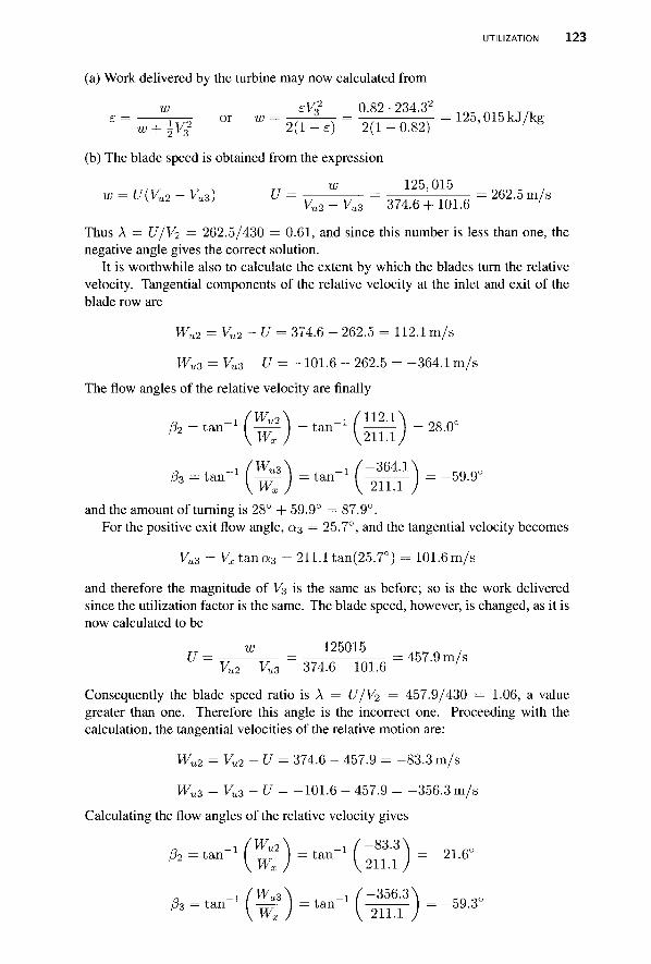
UTILIZATION 123
(a) Work delivered by the turbine may now calculated from
w = eVf 0.82 • 234.32
w + \V32 2(1 - e) 2(1 - 0.82)
(b) The blade speed is obtained from the expression
125,015kJ/kg
Thus A = U/V2 ~ 262.5/430 = 0.61, and since this number is less than one, the negative angle gives the correct solution.
It is worthwhile also to calculate the extent by which the blades turn the relative velocity. Tangential components of the relative velocity at the inlet and exit of the blade row are
Wu2 = Vu2 - U = 374.6 - 262.5 = 112.1 m/s
Wu3 = Vu3 - U = -101.6 - 262.5 = -364.1 m/s
The flow angles of the relative velocity are finally
and the amount of turning is 28° + 59.9° = 87.9°. For the positive exit flow angle, a3 = 25.7°, and the tangential velocity becomes
Vu3 = Vxtsnia3 = 211.1 tan(25.7°) = 101.6 m/s
and therefore the magnitude of V3 is the same as before; so is the work delivered since the utilization factor is the same. The blade speed, however, is changed, as it is now calculated to be
w 1 2 5 0 1 5 , c ™ / U = = = 457.9 m/s
Vu2 - Vu3 374.6 - 101.6 ' Consequently the blade speed ratio is A = U/V2 = 457.9/430 = 1.06, a value greater than one. Therefore this angle is the incorrect one. Proceeding with the calculation, the tangential velocities of the relative motion are:
Wu2 = Vu2 - U = 374.6 - 457.9 = -83.3 m/s
Wu3 = Vu3 - U = -101.6 - 457.9 = -356.3 m/s
Calculating the flow angles of the relative velocity gives
A—-(£)-«--( i irr)-"■•■
1 2 4 PRINCIPLES OF TURBOMACHINE ANALYSIS
Now the flow turns only -21.6° + 59.3° = 37.7°. This small amount of turning is typical of compressors, but not of turbines. Another way is to check the value of blade-loading coefficient. It is i\> = w/U2 = 125,015/262.52 = 1.82 for the negative angle. Experience shows that blade-loading coefficients in the range 1 < ip < 2.5 give good designs.
■ The examples in this chapter have illustrated the principles of turbomachinery analysis. Some of the fhermodynamic properties that appear in the examples are extensive, and some are intensive. Few are nondimensional, and of these the ones encountered so far include the blade-loading coefficient, flow coefficient or speed ratio, reaction, utilization factor, and Mach number. In addition, flow angles of the absolute and relative velocities are nondimensional quantities. Once the nondimensional parameters, including the flow angles, have been chosen, a choice is made for the magnitude of the exit velocity from the nozzles or the value of the axial velocity. The blade speed can then be calculated. In order to complete the aerothermodynamic analysis, fhermodynamic losses need to be estimated. After this, all the intensive parameters will be known.
For this much of the analysis there was no need to introduce any extensive variables. But, for example, a rate at which a liquid needs to be pumped, or a power delivered by a turbine, are typical design specifications. The size of the machine depends on these extensive variables. Thus the cross-sectional flow areas are calculated with these specifications in mind together with the size of rotor or impeller. Their diameter and the blade speed determine the rotational speed of the shaft. In large machines rotational speeds are low; in small machines they are high. Undoubtedly a design iteration needs to be carried out so that the machine conforms to a class of successful past designs. This includes also a stress analysis and vibrational characteristics of the blades, disks, and shafts. The next section introduces other aspects of the use of nondimensional variables.
4.5 SCALING AND SIMILITUDE
The aim of scaling analysis is to compare the performance of two turbomachines of similar design. Thus it is also used to relate the performance of a model turbomachine to its prototype. Both tasks are carried out in terms of proper nondimensional variables. In this section the conventional nondimensional groups for turbomachinery are introduced, scaling analysis of a model and a prototype is reviewed, and performance characteristics of a compressor and a turbine are presented.
4.5.1 Similitude
Similitude broadly refers to similarity in geometry and flow in two turbomachines. More precisely, dynamic similarity is obtained if the ratios of force components at corresponding points in the flow through these machines are equal. A necessary condition for dynamic similarity is kinematic similarity, which means that streamline patterns in two machines are the same. To achieve this, the two machines must be geometrically similar. This means that they differ only in scale. Proportionality of viscous force components implies that the Reynolds number is the same for the two machines. To obtain full dynamic similarity, the two flows must have similar density distributions, for then inertial forces are proportional at two corresponding points in kinematically similar flows. This is trivially satisfied for an incompressible fluid of uniform density, but for compressible fluids Mach numbers must be
SCALING AND SIMILITUDE 125
the same at two corresponding points in the flow. The definition of Mach number involves temperature, which together with pressure determine the value of density. Thus, in flows in which the Mach numbers match, forces at corresponding points in kinematically similar flows are proportional to each others and the flows are said to be dynamically similar.
In courses on fluid dynamics, systematic methods are presented for finding dimensionless groups. They consist of deciding first what the important variables are, and grouping them in categories of geometric parameters, fluid properties, operational variables, and performance variables.
The most obvious geometric variable is the diameter D of the rotor. Density p and viscosity p are the two most common fluid properties encountered in turbomachinery flows, and since the fluid particles move along curved paths through the machine, the flow is dominated by inertial effects. This means that pressure force is in balance with inertial force and viscous forces are small when compared to these. Since the inertial term is proportional to density, in turbomachinery flows density is a more important fluid property than viscosity.
The rotational speed fl of the rotor is the most important operational variable. It is conventionally given in revolutions per minute, and in many performance plots it is not converted to the standard form of radians per second. The performance variables include the volumetric flow rate Q and the reversible work done per unit mass ws, and quantities such as the power W, related to them.
4.5.2 Incompressible flow
The meridional velocity in a turbomachine accounts for the rate at which fluid flows through a machine. Thus the ratio Vm/U is a measure of the flow rate. As has been seen already, this ratio is used in theoretical analysis, but in testing it is converted and expressed in terms of more readily measurable quantities. The meridional velocity times the flow area equals the volumetric flow rate, and the blade speed is equal to radius times the rotational speed. Then, with Vm proportional to Q/D2 and blade speed proportional to QD, the combination
^ = <n* (433)
is dimensionless. It is called a flow coefficient. A nondimensional variable that includes the fluid viscosity \i will lead to some form of
Reynolds number, such as Re = pVmD/fi, for example. The usual form, however, is
p£W2 Q.D2
Re = =
in which v is the kinematic viscosity and the blade speed, proportional to Q.D, is used in place of the meridional velocity. If the boundary layers on the flow passage do not separate, viscous forces remain important only near the walls. Thus, as the machine size increases, boundary-layer regions become a smaller part of the flow. One contributing factor to losses in turbulent boundary layers is the size of wall roughness, which depends on manufacturing methods used. Hence, for example the casing and the impeller of two pumps of different size, but manufactured the same way may have about equal roughness. Since more of the flow through the larger pump does not contact the walls of the flow channel, this part of the flow does not experience as great a loss as does the flow through the boundary layer. This concept goes by the name scale effect, and it makes the performance variables quite

1 2 6 PRINCIPLES OF TURBOMACHINE ANALYSIS
independent of Reynolds number, provided the machine is sufficiently large. It is for this reason that in large machines Reynolds number effects are ignored in preliminary design and also that efficiency increases with machine size. This discussion of the influence of Reynolds number applies at a design condition. However, when turbomachines are operated at off-design conditions, boundary layers may separate. In worst cases such operation can be catastrophic. Thus the Reynolds number enters the theory of turbomachines indirectly through its influence on the behavior of boundary layers.
The most important performance variable is the work done on the fluid, or delivered by the machine. Its nondimensional form is the work coefficient
^ ~ n2D2
in which ws is the isentropic work and the product QD in the denominator is proportional to the blade speed, so that the denominator has the units of energy per unit mass, as does isentropic work.
In the Bernoulli equation
1 , 1 , Pi + 2pVl + p9Zl =P2 + 2pV2 + P9Z2
the kinetic energy term shows that in this form the units of each term are energy per unit volume, since density has replaced mass. Furthermore, weight equals mass times gravitational acceleration, and specific weight of a fluid is defined as pg. Dividing each term by pg gives
Pl ■ , 1 T/2 , , P2 , 1 T / 2 , — + 7TV\ +Z1 + — + 7TV2 + *2 pg 2g pg ?g
and each term has the dimensions of energy per unit weight of the fluid, which can be reduced to a length, as the potential energy term shows. From hydraulic practice it is common to call the first term in this equation a pressure head. The second term has the name kinetic energy or dynamic head, and the third term is an elevation head. The sum is called the total head.
The first law of thermodynamics applied to a flow through a pump gives
P1 i 1l/2 , , Vl . l T / 2 , 1" 2^1 +9Zi+ws = H 2 V2 + 9zi
which can also be written as ws = gH
and here H is the change in the total head across the pump. Pump manufacturers report the performance of pumps in terms of their head, making the values independent of the fluid being pumped. They also report a value for efficiency, so that actual work may be determined as w = ws/r).
From the definition of total pressure, isentropic work for an incompressible fluid can also be calculated from
P02 ~ P01 Ws =
P which shows that if the total pressure change across the pump is reported, then, to obtain the work done, density of the fluid being pumped needs to be known.
SCALING AND SIMILITUDE 127
Also from the hydraulic practice comes the custom of expressing pressure as a height of a mercury, or a water column, particularly in fans and blowers in which the pressure rise is small. The conversion is carried out by the manometer formula
Ap = pmgd (4.34)
in which pm is the density of the manometer fluid and d is the manometer deflection. As a consequence of the discussion above, for a pump, the work coefficient may be written as
fa - n2D2
Power coefficient may be introduced as
W Pd pWD5
Here W is the actual rate at which work is done. Hence, multiplying the denominator of fa by the mass flow rate and dividing it by a quantity with dimensions of mass flow rate, namely, by p f2D D2, gives this form, except that efficiency of the machine must also be taken into account. It is easy to see that the power coefficients for a turbine with efficiency rjt and compressor with efficiency r]c are
"d = Vtfafa Pd Vc
respectively. For dynamically similar situations two machines have the same values of the nondimen-
sional parameters fa and fa. They are also expected to have the same efficiency if the scale effect is neglected. This means that for machines 1 and 2 the following relationships are true:
/ ws \ = / ws \ / Q \n2D2Ji \n2D2J2 \ O D 3 I \nD3
EXAMPLE 4.8
Liquid water with density p = 998 kg/m3 flows through an axial flow pump, with a rotor diameter of 30 cm at a rate of 200 m3/h. The pump operates at 1600 rpm, and its efficiency is i]p = 0.78. The pump work is 180 J/kg. If a second pump in the same series has a diameter of 20 cm and operates at 3200 rpm, at the condition of same efficiency, find (a) flow rate, (b) the total pressure increase across it, and (c) the input power.
Solution: (a) Since the pumps are geometrically similar and their efficiencies are the same, dynamic similarity may be assumed. Thus
Qi Q* n n^D* o n n 3200 ■ 203 3
Q2 = Q I T ^ 3 = 200 1 g n n --■ = 118.5m /h nxD\ ft2D3 ^ ^'n-tDf 1600-303
and the mass flow rate is
998 • 118.5 , , TO2 = PQ2 = 3 6 0 Q - = 32.86 kg/s

1 2 8 PRINCIPLES OF TURBOMACHINE ANALYSIS
(b) With equal work coefficient and efficiency, it follows that
wsi ws2 UL\D\ i Q n 3 2 0 0 2 - 2 0 2
sm = sm W2=wiwm=18016002. so2 =320J/kg
The total pressure rise is given by
Ap02 = pw2r\ so that Ap02 = 998 • 320 • 0.78 = 249.1 kPa
(c) Pumping power is
W2 = m2w2 = 32.86 • 320 = 10.5 kW
Since the ratio of rotational speeds and flow rates are used in the calculations, there was no need to covert them to standard units. B
4.5.3 Shape parameter or specific speed
Flow coefficient and work coefficient can be combined in such a way that the diameter is eliminated. Raising the result to a power such that it becomes directly proportional to the rotational speed, gives a parameter that is called the specific speed, which is given by
a..(9j"(^)'"=a^ (435) SID3J \ gH J (gHfl
This equation is of relevance to pumps and hydraulic turbines, since the working fluid for them is a liquid. It shows that machines with low flow rates and high pressure rise have low fis. In centrifugal machines the inlet area, which is close to the shaft, is relatively small, and to keep the inlet velocity within a desirable range, the flow rate is relatively low. The centrifugal action causes a large pressure rise in such machines. Both make the specific speed low. In axial pumps and turbines a large flow rate is possible, as the annulus area is far from the axis and is therefore large. This leads to a high specific speed. The shape of the machines thus changes from a radial to an axial type as the shape parameter increases. Thus a better name for Qs would be a shape parameter. Diameter does not appear in the definition of the specific speed, but since the velocity must be kept within reasonable limits, it appears implicity through the flow rate, with a larger flow rate requiring a larger machine. Shapes for pumps are shown in Figure 4.9. The figure shows that large machines have higher efficiencies owing to the scale effect discussed above.
4.5.4 Compressible flow analysis
For compressible flows temperature must be listed among the fundamental dimensions. It appears in the definition of Mach number, M = V/c, and with c the speed of sound, equal to c = ^JjRT for an ideal gas, the ratio of specific heats appears as an additional parameter.
Flows with Mach numbers less than 0.3 can be approximated as incompressible. Hence, in low-Mach-number flows, the influence of Mach number will be slight. Testing of cen-trifugal compressors with refrigerants as working fluids also shows that their performance depends only weakly on the ratio of specific heats [17]. This is useful to notice, for then performance maps generated for air are not expected to lead to large errors when they are used for other gases.
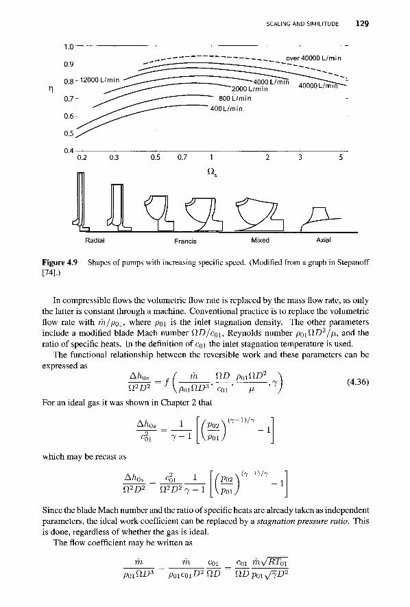
SCALING AND SIMILITUDE 129
1.0
0.9
0.8
0.7
0.6
0.5
0.4
-12000L/min - " J^ '
~~ ■ — _
—_. ——-^ —~^ 10001 ImTh 7"! 1— "
"2000 L/min 4UUUUL/m,n-
800 L/min 400 L/min
Radial Francis Mixed Axial
Figure 4.9 Shapes of pumps with increasing specific speed. (Modified from a graph in Stepanoff [74].)
In compressible flows the volumetric flow rate is replaced by the mass flow rate, as only the latter is constant through a machine. Conventional practice is to replace the volumetric flow rate with m/poi, where poi is the inlet stagnation density. The other parameters include a modified blade Mach number QD/coi, Reynolds number poiflD2/p, and the ratio of specific heats. In the definition of cm the inlet stagnation temperature is used.
The functional relationship between the reversible work and these parameters can be expressed as
Ah0s t ( rh SID p01nD2 \ / . n n . v ~ . : >7 (4-36) fl2D2 J V P O I ^ 3 ' coi ' p
For an ideal gas it was shown in Chapter 2 that
Ah 0s 1
^01
which may be recast as
7 - 1
4)1
P02\
POl]
( 7 - l ) / 7
A/ln
n2D2 n2D2 7 - I P02\
POl)
( 7 - l ) / 7
Since the blade Mach number and the ratio of specific heats are already taken as independent parameters, the ideal work coefficient can be replaced by a stagnation pressure ratio. This is done, regardless of whether the gas is ideal.
The flow coefficient may be written as
m coi coi m,^/RT0i p01nD* p0ic01D2nD nDpm^D2
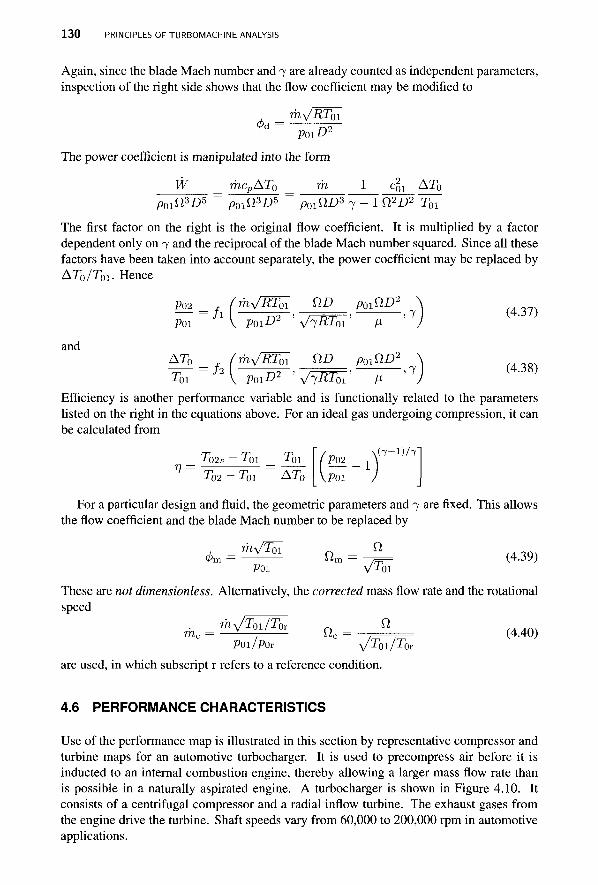
1 3 0 PRINCIPLES OF TURBOMACHINE ANALYSIS
Again, since the blade Mach number and 7 are already counted as independent parameters, inspection of the right side shows that the flow coefficient may be modified to
, my/RT01
P01D2
The power coefficient is manipulated into the form
W mcv AT0 m 1 c§! AT0
Poi^3-D5 ~ p o i ^ 3 ^ 5 ~ poi^D3 7 - 1 n2D2 IbT
The first factor on the right is the original flow coefficient. It is multiplied by a factor dependent only on 7 and the reciprocal of the blade Mach number squared. Since all these factors have been taken into account separately, the power coefficient may be replaced by AT0/T01. Hence
/1 _ n o . / - T * H - ' : >7 (4-37> P01 V P01D2 ' \/-iRTQi' n
and
-7^=f2\ =^-,-T===, ,7 (4.38) T01 V PoiDz V7i?T0i \i )
Efficiency is another performance variable and is functionally related to the parameters listed on the right in the equations above. For an ideal gas undergoing compression, it can be calculated from
_ T02s — Tg\ _ TQI TQ2 — TQ\ ATQ
P02 _ *
P01
For a particular design and fluid, the geometric parameters and 7 are fixed. This allows the flow coefficient and the blade Mach number to be replaced by
P01 VToi
These are not dimensionless. Alternatively, the corrected mass flow rate and the rotational speed
rnc = ^ Z ^ nc = " (4.40)
are used, in which subscript r refers to a reference condition.
4.6 PERFORMANCE CHARACTERISTICS
Use of the performance map is illustrated in this section by representative compressor and turbine maps for an automotive turbocharger. It is used to precompress air before it is inducted to an internal combustion engine, thereby allowing a larger mass flow rate than is possible in a naturally aspirated engine. A turbocharger is shown in Figure 4.10. It consists of a centrifugal compressor and a radial inflow turbine. The exhaust gases from the engine drive the turbine. Shaft speeds vary from 60,000 to 200,000 rpm in automotive applications.
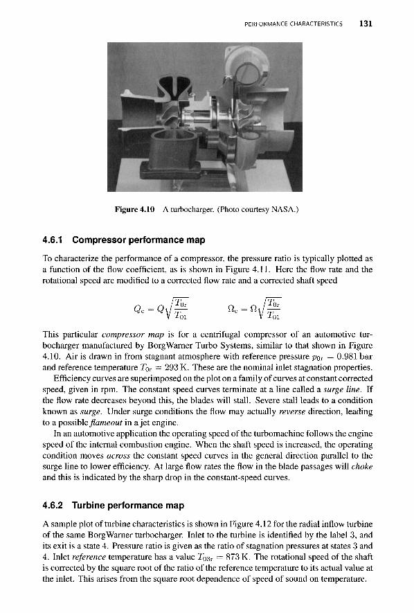
PERFORMANCE CHARACTERISTICS 1 3 1
Figure 4.10 A turbocharger. (Photo courtesy NASA.)
4.6.1 Compressor performance map
To characterize the performance of a compressor, the pressure ratio is typically plotted as a function of the flow coefficient, as is shown in Figure 4.11. Here the flow rate and the rotational speed are modified to a corrected flow rate and a corrected shaft speed
This particular compressor map is for a centrifugal compressor of an automotive tur-bocharger manufactured by BorgWarner Turbo Systems, similar to that shown in Figure 4.10. Air is drawn in from stagnant atmosphere with reference pressure por = 0.981 bar and reference temperature TQT — 293 K. These are the nominal inlet stagnation properties.
Efficiency curves are superimposed on the plot on a family of curves at constant corrected speed, given in rpm. The constant speed curves terminate at a line called a surge line. If the flow rate decreases beyond this, the blades will stall. Severe stall leads to a condition known as surge. Under surge conditions the flow may actually reverse direction, leading to a possible flameout in a jet engine.
In an automotive application the operating speed of the turbomachine follows the engine speed of the internal combustion engine. When the shaft speed is increased, the operating condition moves across the constant speed curves in the general direction parallel to the surge line to lower efficiency. At large flow rates the flow in the blade passages will choke and this is indicated by the sharp drop in the constant-speed curves.
4.6.2 Turbine performance map
A sample plot of turbine characteristics is shown in Figure 4.12 for the radial inflow turbine of the same BorgWarner turbocharger. Inlet to the turbine is identified by the label 3, and its exit is a state 4. Pressure ratio is given as the ratio of stagnation pressures at states 3 and 4. Inlet reference temperature has a value T^r = 873 K. The rotational speed of the shaft is corrected by the square root of the ratio of the reference temperature to its actual value at the inlet. This arises from the square root dependence of speed of sound on temperature.
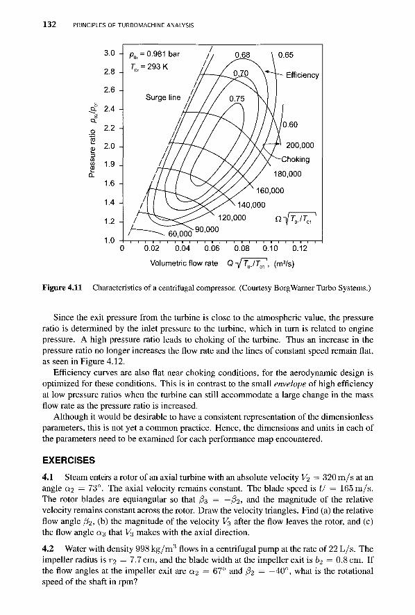
1 3 2 PRINCIPLES OF TURBOMACHIIME ANALYSIS
3.0
2.8
2.6
df 2.4 CM O
a 2.2
2.0 3
$ 1-9
1.6
1.4 -|
1.2
1.0
p0r = 0.981 bar
T0r = 293K
0
/ —~- 60,000 T 1 1 1 -
90,000
200,000
Choking
180,000
'160,000
•140,000
120,000 nfv^7
0.02 I I I I I I I I I I I I I I I I I I I T "
0.04 0.06 0.08 0.10 0.12
Volumetric flow rate Q^ffjT^, (m3/s)
Figure 4.11 Characteristics of a centrifugal compressor. (Courtesy BorgWarner Turbo Systems.)
Since the exit pressure from the turbine is close to the atmospheric value, the pressure ratio is determined by the inlet pressure to the turbine, which in turn is related to engine pressure. A high pressure ratio leads to choking of the turbine. Thus an increase in the pressure ratio no longer increases the flow rate and the lines of constant speed remain flat, as seen in Figure 4.12.
Efficiency curves are also flat near choking conditions, for the aerodynamic design is optimized for these conditions. This is in contrast to the small envelope of high efficiency at low pressure ratios when the turbine can still accommodate a large change in the mass flow rate as the pressure ratio is increased.
Although it would be desirable to have a consistent representation of the dimensionless parameters, this is not yet a common practice. Hence, the dimensions and units in each of the parameters need to be examined for each performance map encountered.
EXERCISES 4.1 Steam enters a rotor of an axial turbine with an absolute velocity V2 = 320 m/s at an angle a2 = 73°. The axial velocity remains constant. The blade speed is U = 165 m/s. The rotor blades are equiangular so that /33 = —f32, and the magnitude of the relative velocity remains constant across the rotor. Draw the velocity triangles. Find (a) the relative flow angle /32, (b) the magnitude of the velocity V3 after the flow leaves the rotor, and (c) the flow angle az that V3 makes with the axial direction.
4.2 Water with density 998 kg/m3 flows in a centrifugal pump at the rate of 22 L/s. The impeller radius is r2 = 7.7 cm, and the blade width at the impeller exit is b2 = 0.8 cm. If the flow angles at the impeller exit are a2 = 67° and /32 = —40°, what is the rotational speed of the shaft in rpm?
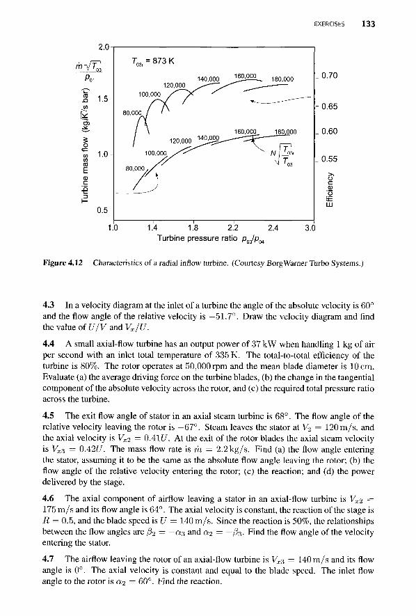
EXERCISES 133
2.0
™ V T 7 3
CD . O
5 o CO CO CO
E CD
c
1.5
1.0
0.5
7"o* = 873K
120,000 140,000 160,000 180,000 _0.70
1.0 1.4 1.8 2.2 2.4 Turbine pressure ratio p03/p04
3.0
Figure 4.12 Characteristics of a radial inflow turbine. (Courtesy BorgWarner Turbo Systems.)
4.3 In a velocity diagram at the inlet of a turbine the angle of the absolute velocity is 60° and the flow angle of the relative velocity is -51.7°. Draw the velocity diagram and find the value of U/V and Vx/U.
4.4 A small axial-flow turbine has an output power of 37 kW when handling 1 kg of air per second with an inlet total temperature of 335 K. The total-to-total efficiency of the turbine is 80%. The rotor operates at 50,000 rpm and the mean blade diameter is 10 cm. Evaluate (a) the average driving force on the turbine blades, (b) the change in the tangential component of the absolute velocity across the rotor, and (c) the required total pressure ratio across the turbine.
4.5 The exit flow angle of stator in an axial steam turbine is 68°. The flow angle of the relative velocity leaving the rotor is —67°. Steam leaves the stator at V% = 120m/s, and the axial velocity is Vx2 = 0.41f/. At the exit of the rotor blades the axial steam velocity is VX3 — 0.42(7. The mass flow rate is TO = 2.2kg/s. Find (a) the flow angle entering the stator, assuming it to be the same as the absolute flow angle leaving the rotor; (b) the flow angle of the relative velocity entering the rotor; (c) the reaction; and (d) the power delivered by the stage.
4.6 The axial component of airflow leaving a stator in an axial-flow turbine is Vx2 = 175 m/s and its flow angle is 64°. The axial velocity is constant, the reaction of the stage is R = 0.5, and the blade speed is U = 140 m/s. Since the reaction is 50%, the relationships between the flow angles are j32 = -a3 and a2 = —03- Find the flow angle of the velocity entering the stator.
4.7 The airflow leaving the rotor of an axial-flow turbine is Vx$ = 140 m/s and its flow angle is 0°. The axial velocity is constant and equal to the blade speed. The inlet flow angle to the rotor is a2 = 60°. Find the reaction.
1 3 4 PRINCIPLES OF TURBOMACHINE ANALYSIS
4.8 A large centrifugal pump operates at 6000 rpm and produces a head of 800 m while the flow rate is 30,000 L/min. (a) Find the value of the specific speed, (b) Estimate the efficiency of the pump.
4.9 A fan handles air at the rate of 500 L/s second when operating at 1800 rpm. (a) What is the flow rate if the same fan is operated at 3600 rpm? (b) What is the percentage increase in total pressure rise of the air assuming incompressible flow? (c) What is the power input required at 3600 rpm relative to that at 1800 rpm? Assume that the operating point of the fan in terms of the dimensionless parameters is the same in both cases.
4.10 An axial-flow pump having a rotor diameter of 20 cm handles water at the rate of 60 L/s when operating at 3550 rpm. The corresponding increase in total enthalpy of the water is 120 J/kg and the total-to-total efficiency is 75%. Suppose that a second pump in the same series is to be designed to handle water having a rotor diameter of 30 cm and operating at 1750 rpm. For this second pump what will be the predicted values for (a) the flow rate, (b) the change in the total pressure of water, and (c) the input power?
4.11 A small centrifugal pump handles water at the rate of 6 L/s with input power of 5 hp and total-to-total efficiency of 70%. Suppose that the fluid being handled is changed to gasoline having specific gravity 0.70. What are the predicted values for (a) flow rate, (b) input power, and (c) total pressure rise of the gasoline?
4.12 A blower handling air at the rate of 240 L/s at the inlet conditions of 103.1 kPa for total pressure and 288 K for total temperature. It produces a pressure rise of air equal to 250 mm of water. If the blower is operated at the same rotational speed, but with an inlet total pressure and total temperature of 20 kPa and 253 K. What are (a) the predicted value for the mass flow rate and (b) the total pressure rise?
4.13 Consider a fan with a flow rate of 1500 cfm, [cubic feet per minute (ft3/min)] and a shaft speed of 3600 rpm. If a similar fan one half its size is to have the same tip speed, what will the flow rate be at a dynamically similar operating condition? What is the ratio of power consumption of the second fan compared to the first one?
4.14 A fan operating at 1750 rpm at a volumetric flow of 4.25 m3/s develops a head of 153 mm of water. It is required to build a larger, geometrically similar fan that will deliver the same head at the same efficiency as the existing fan, but at the rotational speed of 1440 rpm. (a) Determine the volume flow rate of the larger fan. (b) If the diameter of the original fan is 40 cm, what is the diameter of the larger fan? (c) What are the specific speeds of these fans?
4.15 The impeller of a centrifugal pump, with an outlet radius T-I = 8.75 cm and a blade width 62 = 0.7 cm, operates at 3550 rpm and produces a pressure rise of 522 kPa at a flow rate of 1.5 L/min. Assume that the inlet flow is axial and that the pump efficiency is 0.63. (a) Find the specific speed, (b) Show that Eq. (4.15) for work reduces tow = (K22 + U$ - W%2)/2, and calculate the work two ways and confirm that they are equal.
CHAPTER 5
STEAM TURBINES
5.1 INTRODUCTION
The prime mover in a steam power plant is a steam turbine that converts part of the thermal energy of steam at high pressure and temperature to shaft power. Other components of the plant are a steam generator, a condenser, and feedwater pumps and heaters. The plants operate on various modifications of the Rankine cycle. The basic Rankine cycle, operating between 40°C and 565° C, has a Carnot efficiency of 37%. Modifications, including superheating, reheating, and feedwater heating, increase the efficiency by approximately an additional 10%.
Most large power plants have two reheats and three or more turbines. The turbines are said to be compounded when steam passes through each of them in series. The high-pressure (HP) turbine receives steam from the steam generator. After leaving this turbine the steam is reheated and then enters an intermediate-pressure (IP) turbine, also called a reheat turbine, through which it expands to an intermediate pressure. After the second reheat the rest of the expansion takes place through a low-pressure (LP) turbine, from which it enters a condenser at a pressure below the atmospheric value.
A turbine from which the steam leaves at quality near 90% is called a condensing turbine. An extraction turbine has ports from which steam is extracted for feedwater heating. An induction turbine receives steam at intermediate pressures for additional power generation.
In a noncondensing or backpressure turbine, steam leaves at superheated conditions and the thermal energy in the exhaust steam is used in various industrial processes. A well-designed combined heat and power plant generates appropriate amount of power to
Principles of Turbomachinery. By Seppo A. Korpela 135 Copyright © 2011 John Wiley & Sons, Inc.
136 STEAM TURBINES
drop the steam temperature and pressure to values that meet the process heating needs. District heating is an application in which steam is used at even lower temperatures than in many industrial processes. An important consideration in providing the heating needs of an economy is to match the source to the application. Combined heat and power plants are designed with this in mind.
In modern coal-burning power plants axial steam turbines are typically housed in three, four, or five casings. Many LP turbines are double-flow type, and their single casing accommodates a pair of turbines in which steam flows in opposite directions to balance axial forces on the turbine shaft. When two or more turbines are connected to a common shaft, they are said to operate in tandem, and the plant is said to be a tandem compound type. If the steam is directed to a set of turbines on different shafts, then the system is said to be cross-compounded. For example, a 1000-MW power plant could have an HP turbine and an IP turbine on a single shaft and three LP turbines on a different shaft. Rotational speeds are typically either 3600 or 1800 rpm; the lower speed for the LP turbines, that have larger rotors in order to accommodate the larger volumetric flow rate of steam at low pressure. The large volumetric flow rate at the low pressure end requires very long blades. As an example, a General Electric/Toshiba LP steam turbine running at 3600 rpm has blades 1016 mm in length and a flow area 8.2 m2 in the last stage. When this is designed to run at 3000 rpm for generating electricity at 50 Hz, the blades of the last stage are designed to be 1220 mm long, with a corresponding flow area 11.9m2. For a 26-stage steam turbine the hub-to-casing radius ratio for the last stage may have a value 0.42, whereas for the first stage a typical value is 0.96.
Outlet pressures from the boiler vary from a subcritical lOMPa to a supercritical 30 MPa, or more. The condenser pressure is below the atmospheric pressure, typically about 8 kPa, which corresponds to a saturation temperature of 41°C. This makes the overall pressure ratio equal to 1250 for a conventional plant and 3 times this for supercritical plants. In a 400-MW power plant the HP turbine provides about 100-MW, and power at about an equal rate is delivered by the IP turbine. A double-flow LP turbine delivers the remaining 200-MW. The pressure ratios are 4.5 doe the HP turbine and 3 for the IP turbine. The LP turbine has ports for extracting steam to feedwater heaters at pressure ratios ranging from 1.5 to 4.5.
Owing to the large inlet pressure, design of the HP turbine differs from that of the others. The first stage is designed for low reaction, so that most of the pressure drop takes place at the nozzles feeding this stage. This brings the steam to a very high velocity as it enters the first rotor. However, the pressure is now sufficiently low that leakage flow through seals is tolerable. Later stages are designed for higher reaction, and in IP and LP turbines the reaction is close to 50%.
Table 5.1 lists some typical designs and rated power outputs for coal-burning steam power plants. Designations such as 1SF and 3DF refer to one single-flow and three double-flow turbines [23]. At the preliminary design stage steam inlet pressure to the HP turbine is specified. Intermediate pressures at which reheating takes place are then calculated according to how much moisture is allowed at the exit of the HP and IP turbines. A similar decision is made for the reheat (RH) turbine to determine the appropriate pressure at the inlet of the LP turbines.
The steam turbine industry is very large. The annual worldwide electricity generation from steam plants is 38.5 EJ (exajoules) equal to 1.2 TW (terawatts) of generated power. This means that on the order of 10,000 steam turbines are in use. The major manufactures include GE power systems in the United States, Siemens, Alstom, and Ansaldo Energia in western Europe, Mitsubishi Heavy Industries, Hitachi and Toshiba in Japan. Many of the
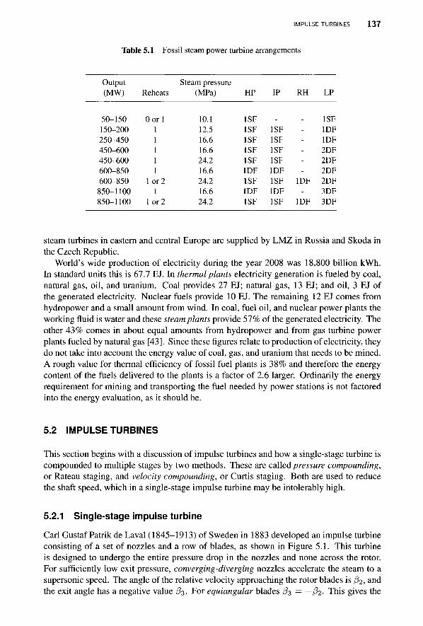
IMPULSE TURBINES 137
Table 5.1 Fossil steam power turbine arrangements
Output Steam pressure (MW) Reheats (MPa) HP IP RH LP
50-150 150-200 250-450 450-600 450-600 600-850 600-850 850-1100 850-1100
Oorl 1 1 1 1 1
1 or 2 1
lo r 2
10.1 12.5 16.6 16.6 24.2 16.6 24.2 16.6 24.2
1SF 1SF 1SF 1SF 1SF IDF 1SF IDF 1SF
-1SF 1SF 1SF 1SF IDF 1SF IDF 1SF
------
IDF -
IDF
1SF IDF IDF 2DF 2DF 2DF 2DF 3DF 3DF
steam turbines in eastern and central Europe are supplied by LMZ in Russia and Skoda in the Czech Republic.
World's wide production of electricity during the year 2008 was 18,800 billion kWh. In standard units this is 67.7 EJ. In thermal plants electricity generation is fueled by coal, natural gas, oil, and uranium. Coal provides 27 EJ; natural gas, 13 EJ; and oil, 3 EJ of the generated electricity. Nuclear fuels provide 10 EJ. The remaining 12 EJ comes from hydropower and a small amount from wind. In coal, fuel oil, and nuclear power plants the working fluid is water and these steam plants provide 57% of the generated electricity. The other 43% comes in about equal amounts from hydropower and from gas turbine power plants fueled by natural gas [43]. Since these figures relate to production of electricity, they do not take into account the energy value of coal, gas, and uranium that needs to be mined. A rough value for thermal efficiency of fossil fuel plants is 38% and therefore the energy content of the fuels delivered to the plants is a factor of 2.6 larger. Ordinarily the energy requirement for mining and transporting the fuel needed by power stations is not factored into the energy evaluation, as it should be.
5.2 IMPULSE TURBINES
This section begins with a discussion of impulse turbines and how a single-stage turbine is compounded to multiple stages by two methods. These are called pressure compounding, or Rateau staging, and velocity compounding, or Curtis staging. Both are used to reduce the shaft speed, which in a single-stage impulse turbine may be intolerably high.
5.2.1 Single-stage impulse turbine
Carl Gustaf Patrik de Laval (1845-1913) of Sweden in 1883 developed an impulse turbine consisting of a set of nozzles and a row of blades, as shown in Figure 5.1. This turbine is designed to undergo the entire pressure drop in the nozzles and none across the rotor. For sufficiently low exit pressure, converging-diverging nozzles accelerate the steam to a supersonic speed. The angle of the relative velocity approaching the rotor blades is (32, and the exit angle has a negative value (3^. For equiangular blades /3s = —fa- This gives the
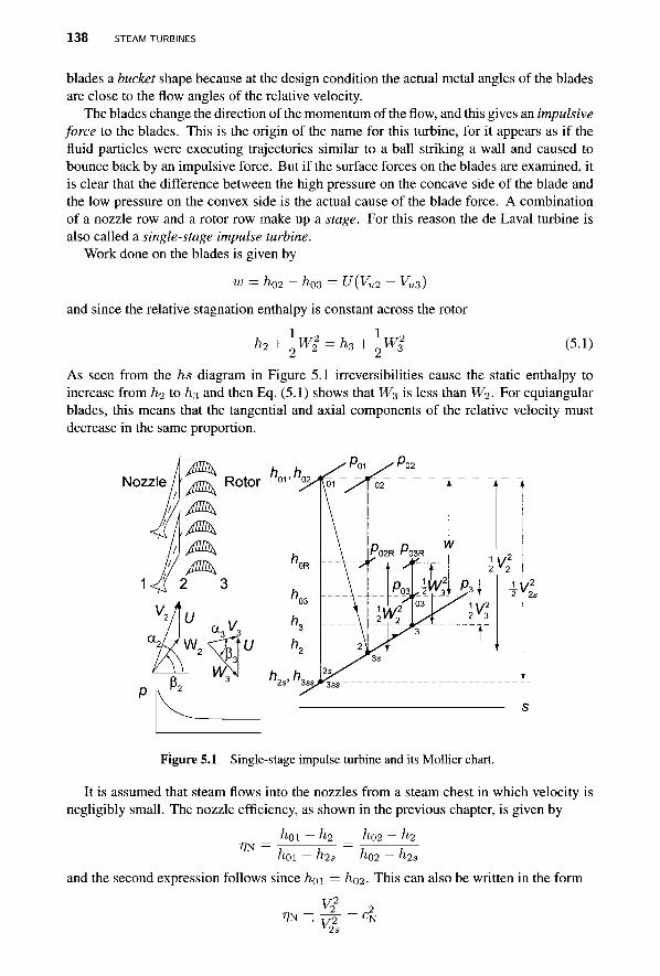
138 STEAM TURBINES
blades a bucket shape because at the design condition the actual metal angles of the blades are close to the flow angles of the relative velocity.
The blades change the direction of the momentum of the flow, and this gives an impulsive force to the blades. This is the origin of the name for this turbine, for it appears as if the fluid particles were executing trajectories similar to a ball striking a wall and caused to bounce back by an impulsive force. But if the surface forces on the blades are examined, it is clear that the difference between the high pressure on the concave side of the blade and the low pressure on the convex side is the actual cause of the blade force. A combination of a nozzle row and a rotor row make up a stage. For this reason the de Laval turbine is also called a single-stage impulse turbine.
Work done on the blades is given by
w K2 ~ h03 = U(Vu2 - Vu3)
and since the relative stagnation enthalpy is constant across the rotor
h2 + \wl 1, -Wi (5.1)
As seen from the hs diagram in Figure 5.1 irreversibilities cause the static enthalpy to increase from h2 to ho, and then Eq. (5.1) shows that W$ is less than W2. For equiangular blades, this means that the tangential and axial components of the relative velocity must decrease in the same proportion.
Nozzle / ' Rotor hn„h,
/)„, ft, „ 2s' 3ss,
Figure 5.1 Single-stage impulse turbine and its Mollier chart.
It is assumed that steam flows into the nozzles from a steam chest in which velocity is negligibly small. The nozzle efficiency, as shown in the previous chapter, is given by
/ioi — h2 ho2 — h2
"01 — n2s
and the second expression follows since /IQI = ho2 — h2s
ho2. This can also be written in the form
m C N
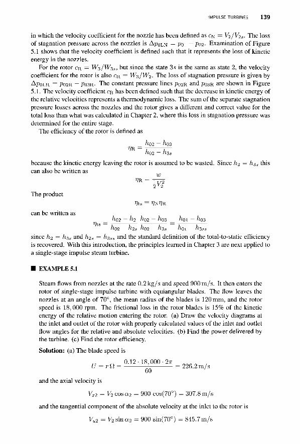
IMPULSE TURBINES 139
in which the velocity coefficient for the nozzle has been defined as CN = V^/V^. The loss of stagnation pressure across the nozzles is Ap0LN = Poi — Po2- Examination of Figure 5.1 shows that the velocity coefficient is defined such that it represents the loss of kinetic energy in the nozzles.
For the rotor CR = Wz/Wzs, but since the state 3s is the same as state 2, the velocity coefficient for the rotor is also CR = W3/W2. The loss of stagnation pressure is given by APOLR = P02K — P03R- The constant pressure lines p02R and p03R are shown in Figure 5.1. The velocity coefficient CR has been defined such that the decrease in kinetic energy of the relative velocities represents a thermodynamic loss. The sum of the separate stagnation pressure losses across the nozzles and the rotor gives a different and correct value for the total loss than what was calculated in Chapter 2, where this loss in stagnation pressure was determined for the entire stage.
The efficiency of the rotor is defined as
^R = i r~ because the kinetic energy leaving the rotor is assumed to be wasted. Since h^ = h%s this can also be written as
w VR IV2
2 V2 The product
can be written as ??tS
ho2 — h,2 ho2 — ho3 hoi — ^03 ho2 — h,2s ho2 — hss hoi — }l3ss
since ft-2 = hss and ft-2s = hsss and the standard definition of the total-to-static efficiency is recovered. With this introduction, the principles learned in Chapter 3 are next applied to a single-stage impulse steam turbine.
■ EXAMPLE 5.1
Steam flows from nozzles at the rate 0.2 kg/s and speed 900 m/s. It then enters the rotor of single-stage impulse turbine with equiangular blades. The flow leaves the nozzles at an angle of 70°, the mean radius of the blades is 120 mm, and the rotor speed is 18,000 rpm. The frictional loss in the rotor blades is 15% of the kinetic energy of the relative motion entering the rotor, (a) Draw the velocity diagrams at the inlet and outlet of the rotor with properly calculated values of the inlet and outlet flow angles for the relative and absolute velocities, (b) Find the power delivered by the turbine, (c) Find the rotor efficiency.
Solution: (a) The blade speed is
^ 0.12-18,000-27T U = rfl = = 226.2 m/s
60 '
and the axial velocity is
Vx2 = V2 cosa2 = 900 cos(70°) = 307.8 m/s
and the tangential component of the absolute velocity at the inlet to the rotor is
Vu2 = V2 sina2 = 900 sin(70°) = 845.7m/s
140 STEAM TURBINES
The tangential component of the relative velocity entering the rotor is therefore
Wu2 = Vu2 - U = 845.7 - 226.2 = 619.5 m/s
so that the relative flow speed, since Wx2 = Vx2, comes out to be
W2 = yJWix2 + Wl2 = V307.82 + 619.52 = 691.8 m/s
The inlet angle of the relative velocity is then
fc = t a n - ( ^ ) = t a n - («**)= 63.6° \Wx2) V 307.8 y
Since 15% of the kinetic energy of the relative motion is lost, at the exit the kinetic energy of the relative flow is
-Wi = - ( 1 - 0.15)Wf and W3 = V0.85 • 691.82 = 637.8m/s
For equiangular blades, j33 = —f32, and the axial velocity leaving the rotor is
Wx3 = W3cosP3 = 637.8 cos(-63.6°) = 283.8 m/s
and the tangential component of the relative velocity is
Wu3 = W3smP3 = 637.8sin(-63.6°) = -571.2 m/s
The tangential component of the absolute velocity becomes
Vu3 = U + Wu3 = 226.2 - 571.2 = -345.0 m/s
Hence, with Vx3 = Wx3, the flow angle at the exit is
and the velocity leaving the rotor is
V3 = ^ /V^ + yu23 = V283.82 + 3452 = 446.7 m/s
The velocity triangles at the inlet and outlet are shown in Figure 5.2.
(b) The specific work done on the blades is obtained as
w = U(Vu2 - Vu3) = 226.2(845.7 + 345.0) = 269.3 kJ/kg
and the power delivered is
W = mw = 0.2 • 269.3 = 53.87 kW
(c) The kinetic energy leaving the nozzle is
iK,2 = i900 2 =405 .0kJ /kg
IMPULSE TURBINES 1 4 1
Figure 5.2 Velocity diagrams for a single stage impulse turbine.
and the rotor efficiency therefore becomes
w 269.3 m VJ/2 405.0 0.665 66.5%
Of the difference 1 — T̂ R a fraction is lost as irreversibilities and the rest as kinetic energy leaving the rotor. The latter is obtained by calculating the ratio V*/2 to V% 1% which is (446.7/900)2 = 0.246. Hence loses from irreversibilities are 1 — 0.665 — 0.246 — 0.089, or about 9%. It turns out that the blade speed in this example is too low for optimum performance, as will be shown next. g
As the theory of turbomachinery advanced, measures more general than the velocity co-efficients to account for irreversibility replaced them. A useful measure is the increase in the static enthalpy by internal heating. The loss coefficients £N and £R are defined by the equations
ho - ho 1 ;CN^2
2 / I 3 - h, 1 3s CKW- (5.2)
2^ z 2 with the thermodynamic states as shown in Figure 5.1. Since the stagnation enthalpy is constant for the flow through the nozzle, it follows that
1, i 2s -Yl = h2
1, :V?
which is rearranged to the form
hi - h2s = ^(NVi = ±Vj
With VS2 = V2/CN, this equation can be expressed as
V^ = 1 _ V2a ~
--y?
CN
Since the relative stagnation enthalpy is constant for the rotor,
(5.3)
h: 3s wi h3 + l-wl
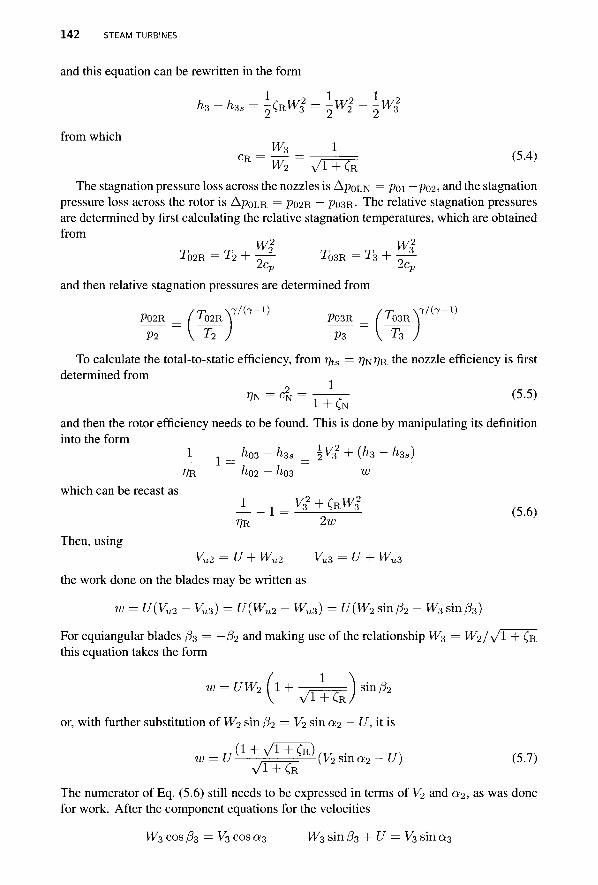
142 STEAM TURBINES
and this equation can be rewritten in the form
from which
k3 - h3s = ̂ Rwi = -wi - -wi
W3 1 cn = ~ = / r — - (5.4)
The stagnation pressure loss across the nozzles is ApoLN = Poi — P02. and the stagnation pressure loss across the rotor is A^OLR = P02R — P03R- The relative stagnation pressures are determined by first calculating the relative stagnation temperatures, which are obtained from
2 rr rp , ^ 3 W4 „ „ Wi T02R = T2 + -— T 0 3 R = T3 +
and then relative stagnation pressures are determined from
P02R _ / 7Q2R V 7 P03R _ (^03R \ VI ~ V T2 ) P3 ~ \ T3 )
To calculate the total-to-static efficiency, from rjts = VNVR m e nozzle efficiency is first determined from
2 1 VN = % = (5.5)
J- + <,N and then the rotor efficiency needs to be found. This is done by manipulating its definition into the form
1 1 = h03 - h 3 s = \VJ + (hs - h3s) VR h02 - h03 w
which can be recast as ±_1 = YI±CRWI VR %W
Then, using vu2 = u+wu2 vu3 = u + wu3
the work done on the blades may be written as w = U{Vu2 - Vu3) = U(Wu2 - Wu3) = U{W2 sin/32 - W3 sin/33)
For equiangular blades (33 = —f32 and making use of the relationship W3 = W2/y/l + CR this equation takes the form
w = UW2 (1 + 1 ) sin/?2 V V I + CR/
or, with further substitution of W2 sin f32 = V2 sin a2 — U, it is
r r ( l + \ / l +CR) ,rr ■ r n , - —.
w = U — ( V 2 s m a 2 -U) (5.7) v l + CR
The numerator of Eq. (5.6) still needs to be expressed in terms of V2 and a2, as was done for work. After the component equations for the velocities
W3 cos P3 = V3 cos a3 W3 sin (33 + U = V3 sin a3
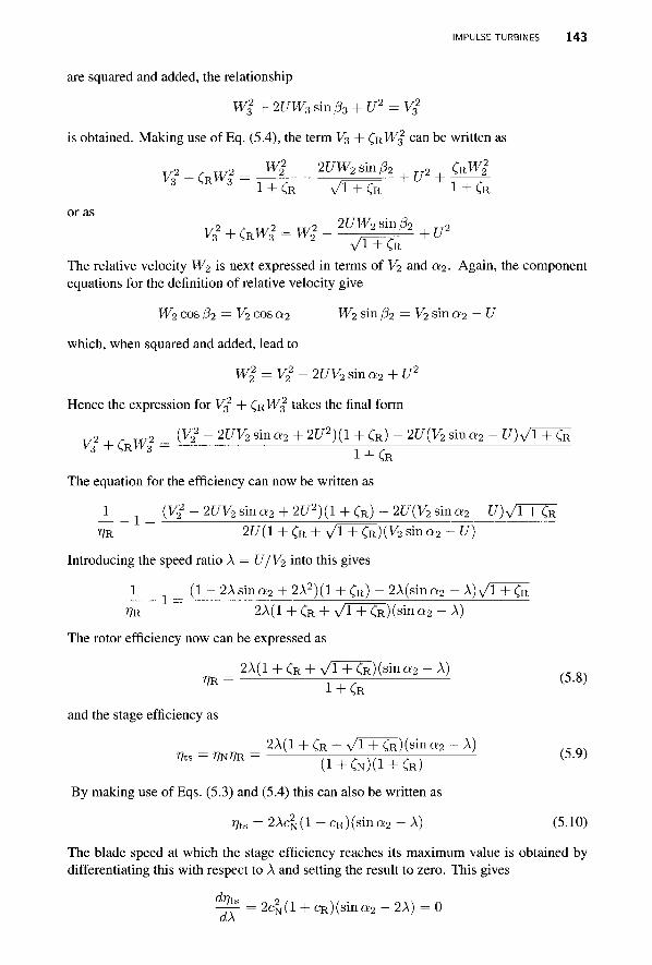
IMPULSE TURBINES 143
are squared and added, the relationship
Wi + 2UW3 sin j33 + U2 = Vf
is obtained. Making use of Eq. (5.4), the term V3 + C R W | c a n be written as
/ 2 , , W2 Wi 2UW2smP2 2 (RWl / 3 + CRM/3 = — + U +
i + CR V I + CR I + CR
T/2 , > W 2 W 2 2 £ W 2 s m / 3 2 r r 2
^3 + CR^S = W2 rr^rr- + U
v i + CR The relative velocity W2 is next expressed in terms of V2 and a2. Again, the component equations for the definition of relative velocity give
W2 cos /32 = V2 cos a2 W2 sin /32 = V2 sin a2 — U
which, when squared and added, lead to
Wl = V22 - 2UV2 sin a2 + U2
Hence the expression for V% + (RW2 takes the final form
2 2 (V2 - 2E/Vr2sina2+2C/2)(1 + CR) - 2U(V2sma2 - U)VTTCR~
v3 + CRW3 = — — 1 + CR
The equation for the efficiency can now be written as
1 1 = (V22 - 2UV2 sma2 + 2U2)(1 + CR) - 2U(V2 sina2 - £ / )yT+^a
7?R " 217(1 + CR + V^+CR)(V2 sina2 - £/)
Introducing the speed ratio A = U/V2 into this gives
1 _ (1 - 2Asina2 + 2A2)(1 + CR) - 2A(sina2 - A)VTTCR~
VK ~ 2A(1 + CR + \ / l + CR)(sina2 - A)
The rotor efficiency now can be expressed as
2A(1 + CR + Vr+CR)(sina2 - A) VR = 7—7 (5-8)
1 + CR and the stage efficiency as
2A(1 + CR + yrTCR")(sina2 - A) % s = m m = ( I + CN)(I + CR) ( 5-9 )
By making use of Eqs. (5.3) and (5.4) this can also be written as
rfcB = 2A4(1 + cR)(sina2 - A) (5.10)
The blade speed at which the stage efficiency reaches its maximum value is obtained by differentiating this with respect to A and setting the result to zero. This gives
^ = 2 4 ( l + C R ) ( s ina 2 -2A) = 0
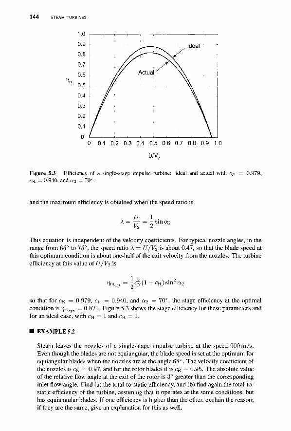
144 STEAM TURBINES
n*
0 0.1 0.2 0.3 0.4 0.5 0.6 0.7 0.8 0.9 1.0
UIV0
Figure 5.3 Efficiency of a single-stage impulse turbine: ideal and actual with CN CR = 0.940, and a2 = 70°.
0.979,
and the maximum efficiency is obtained when the speed ratio is
U 1 . A
Vo sm «2
This equation is independent of the velocity coefficients. For typical nozzle angles, in the range from 65° to 75°, the speed ratio A = U/V2 is about 0.47, so that the blade speed at this optimum condition is about one-half of the exit velocity from the nozzles. The turbine efficiency at this value of U/V2 is
1 ^tSop (1 + cR) sin2 a2
so that for CN = 0.979, CR = 0.940, and a2 = 70°, the stage efficiency at the optimal condition is r/tSopt = 0.821. Figure 5.3 shows the stage efficiency for these parameters and for an ideal case, with CN = 1 and CR = 1.
EXAMPLE 5.2
Steam leaves the nozzles of a single-stage impulse turbine at the speed 900 m/s. Even though the blades are not equiangular, the blade speed is set at the optimum for equiangular blades when the nozzles are at the angle 68°. The velocity coefficient of the nozzles is CN = 0.97, and for the rotor blades it is CR = 0.95. The absolute value of the relative flow angle at the exit of the rotor is 3° greater than the corresponding inlet flow angle. Find (a) the total-to-static efficiency, and (b) find again the total-to-static efficiency of the turbine, assuming that it operates at the same conditions, but has equiangular blades. If one efficiency is higher than the other, explain the reason; if they are the same, give an explanation for this as well.

IMPULSE TURBINES 145
Solution: (a) With the optimum operating blade speed determined from
1 1 U = -V2sma2 = -900sin(68°) =417.2 m/s
the velocity components at the exit from the nozzles are
Vx2 = V2cosa2 = 900cos(68°) = 337.2 m/s
Vu2 = y 2 s ina 2 = 900sin(68°) = 834.5 m/s
the velocity components of the relative velocity are
Wx2 = Vx2 = 337.2 m/s Wu2 = Vu2 - U = 834.5 - 417.2 = 417.3 m/s
The magnitude of the relative velocity is
w2 = \JW12 + Wl2 = \/337.22 + 417.32 = 536.4 m/s
The angle at which the relative velocity enters the rotor row is
*—-(£0='»-1 (^)-51«-and the exit angle is f33 = —51.06° — 3° = —54.06°, and the magnitude of the relative velocity is W3 = CRW2 — 0.95 • 536.4 = 509.6 m/s. Work delivered by the rotor is
w = U(Wu2 - Wu3) = U{1 + cRC)W2 sin/32
in which C — sin \/3s\/ sin /32 = 1.041 and CR = 0.95. Therefore the work delivered is w = 346.23 kJ/kg. Since the exit kinetic energy is wasted, its value is needed. The exit velocity components are
Vx3 = Wx3 = W3 cos /?3 = 509.6 cos(-54.06°) = 299.1 m/s
Vu3 = W3sin(33 + U = 509.6 sin(-54.06°) +417.2 = 4.6 m/s
Hence v3 = \]vx3 + K23 = \ /299.12+4.62 = 299.1 m/s
In the calculation of rotor efficiency the rotor loss coefficient is (R = 1/c2^ — 1 = 0.208, so that
= 2w = 2-346,230 =
VR 2w + V32 + (RW3
2 2 -346,230 + 299.12 • 0.1026 • 509.62
and since T/N = c2^ = 0.972 = 0.941 the total-to-static efficiency becomes
Vts = ??N??R = 0.941 • 0.855 = 0.805
(b) If the blades were equiangular and the turbine were to operate at its optimal condition, the total-to-static efficiency would be
Its = 2 C N ( ! + CR) sin2 a2 = 0.789
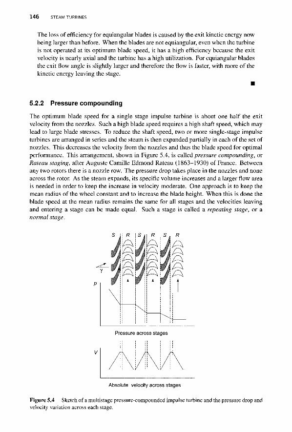
146 STEAM TURBINES
The loss of efficiency for equiangular blades is caused by the exit kinetic energy now being larger than before. When the blades are not equiangular, even when the turbine is not operated at its optimum blade speed, it has a high efficiency because the exit velocity is nearly axial and the turbine has a high utilization. For equiangular blades the exit flow angle is slightly larger and therefore the flow is faster, with more of the kinetic energy leaving the stage.
5.2.2 Pressure compounding
The optimum blade speed for a single stage impulse turbine is about one half the exit velocity from the nozzles. Such a high blade speed requires a high shaft speed, which may lead to large blade stresses. To reduce the shaft speed, two or more single-stage impulse turbines are arranged in series and the steam is then expanded partially in each of the set of nozzles. This decreases the velocity from the nozzles and thus the blade speed for optimal performance. This arrangement, shown in Figure 5.4, is called pressure compounding, or Rateau staging, after Auguste Camille Edmond Rateau (1863-1930) of France. Between any two rotors there is a nozzle row. The pressure drop takes place in the nozzles and none across the rotor. As the steam expands, its specific volume increases and a larger flow area is needed in order to keep the increase in velocity moderate. One approach is to keep the mean radius of the wheel constant and to increase the blade height. When this is done the blade speed at the mean radius remains the same for all stages and the velocities leaving and entering a stage can be made equal. Such a stage is called a repeating stage, or a normal stage.
Pressure across stages
V
Absolute velocity across stages
Figure 5.4 Sketch of a multistage pressure-compounded impulse turbine and the pressure drop and velocity variation across each stage.
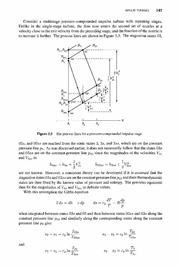
IMPULSE TURBINES 147
Consider a multistage pressure-compounded impulse turbine with repeating stages. Unlike in the single-stage turbine, the flow now enters the second set of nozzles at a velocity close to the exit velocity from the preceding stage, and the function of the nozzle is to increase it further. The process lines are shown in Figure 5.5. The stagnation states 03,
Figure 5.5 The process lines for a pressure-compounded impulse stage.
03s, and 03ss are reached from the static states 3, 3s, and 3ss, which are on the constant pressure line p3. As was discussed earlier, it does not necessarily follow that the states 03s and 03ss are on the constant-pressure line po3 since the magnitudes of the velocities V3S and V3ss in
ho3s — h3s + -V3s h03ss = h3ss + -V3ss
are not known. However, a consistent theory can be developed if it is assumed that the stagnation states 03s and 03ss are on the constant pressure line p$3 and their thermodynamic states are then fixed by the known value of pressure and entropy. The previous equations then fix the magnitudes of V3s and V3SS to definite values.
With this assumption the Gibbs equation
Tds = dh — vdp ds dT dp c» — — ft—
p T p when integrated between states 03s and 03 and then between states 03ss and 03s along the constant pressure line po3 and similarly along the corresponding states along the constant pressure line p3 give
s2 - si cDln TQ3S
TQ3SS
and S2 - s i = cp In
t 3 s
If
s3- s2 = cp
s3 - s 2
In Tp3
TQ3S
,ln-3ss t 3 s
148 STEAM TURBINES
from which — = ^~ and ^ - = ^~ (5.11) J03s J-3s -L03ss J 3 s s
and from these it follows that
7*03 _ TQ3S _ Tp3ss
T3 T3s T3ss
Expressing these temperature ratios in terms of Mach numbers yields
-*3 ^ J 3 s * J 3ss ^
so that M 3 = M 3 s = M 3 s s . The stage efficiency for a pressure-compounded stage is the total-to-total efficiency
hoi — hos %t = T T
flOl — ft03ss
which can be recast into the form
1 1 _ hos — / l03 s s _ hp3 ~ hp3s + hp3s — hp3ss
Vtt hoi — /l03 ^01 — ^03
Subtracting one from each side of both Eqs. (5.11), multiplying by cp, and rearranging gives
ho3 — ho3s = ~7^—(^3 — h3s) ho3s ~ ho3ss = Tf, (^3s — h3ss) J-3s 13ss
Substituting these into Eq. (5.13) leads to
1 777—(«3 -h3a) + — — { h 3 s - h 3 s s ) 1 = - ^ ^ (5.14)
or, since the temperature ratios are the same, according to Eqs. (5.12), this expression for efficiency becomes
1 (1 + 1-^M\ ) (h3 - h3s + h2- h2s) — - 1 = ^ '- (5.15) m w
The Mach number at the exit of the rotor is quite low and is often set to zero. It is, of course, easily determined once the work and exit velocity have been calculated. Then
w V? V3 T03 = T 0 i - - T 3 = T 0 3 - - ^ and M 3 cP 2cp y/^RT3
Ignoring the Mach number and introducing the static enthalpy loss coefficients gives
J_ _! = c*wl±ML (5.16)
IMPULSE TURBINES 149
The relationship W% = c^W2 may be substituted into this, giving
r?tt 2w or
_ 2w ^ " — 7 2~fj7—, /■ ir2 , o (5-17)
2
The relative velocity W2 can be written as
Wl = Vf - 2V2Usina2 + U2
so that 1 x = CR4(^2 2 ~ 2V2Usma2 + £/2) + CN^2
vu 2w The work delivered by the stage is w = U(Vu2 - V03) = U(Wu2 - Wu3) = £7(1 + cR)Wu2 = [7(1 + cR)(y2sirm2 - U)
Substituting A = U/V2 into the previous expression for the stage efficiency, it takes the form
J _ _ 1 = C R 4 ( 1 - 2 A s m Q 2 + A2) + CN ??tt 2A(1+ cR)(sina2 - A)
Defining the quantity /L as
A2 - 2Asina2 + 1 + CN(1 + CR)/CR /L = 2(1 + CR + v/rTC^/CR)(Asin a2 - A2)
in which the relation cR = 1/V'l + CR has been used, the stage efficiency can now be written as
from which it is clear that /L is a measure of the losses. The maximum value for the effi-ciency of a pressure-compounded stage is obtained by minimizing / L . Thus differentiating it with respect to A and setting the result to zero gives
2 2(CR + CN(1 + C R ) ) , , CR + CN(1 + CR) _ n A : A^ — U CRSina2 CR
Of the two roots
_ u _ CR + CN(I + CR) + V (CR + CN(I + CR))(CR + CN(I + CR) + CRSIH2 a2)
V2 CR sin a2
is the correct one, as the second root leads to U/V2 ratio greater than unity. This would mean that the wheel moves faster than the approaching steam. The stage efficiency now can be written as
= 2A(l + c R ) ( s i n a 2 - A ) Vu 2 A ( l + c R ) ( s i n a 2 - A ) + CRCR(A2-2Asina2 + l) + CN
The stage efficiencies for various nozzle angles are shown in Figure 5.6 for both a pressure-compounded stage and for a single-stage impulse turbine with exit kinetic energy wasted. The efficiency curves for the pressure-compounded stage are quite flat at the top and naturally higher as the exit kinetic energy is used at the inlet of the next stage.
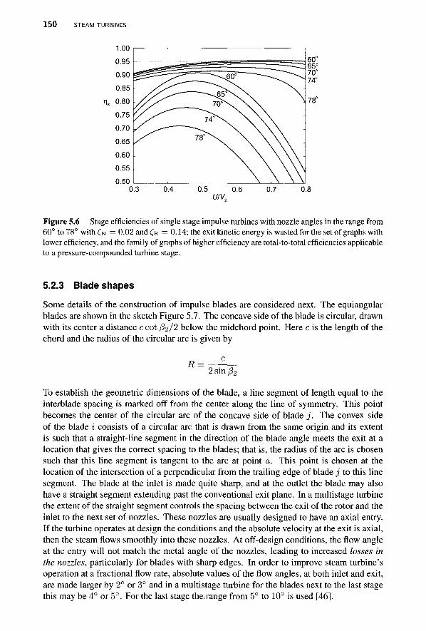
150 STEAM TURBINES
1.00 0.95 0.90 0.85
r|s 0.80 0.75 0.70 0.65 0.60 0.55 0.50
0.3 0.4 0.5 0.6 0.7 0.8 U/V2
Figure 5.6 Stage efficiencies of single stage impulse turbines with nozzle angles in the range from 60° to 78° with (N = 0.02 and £R = 0.14; the exit kinetic energy is wasted for the set of graphs with lower efficiency, and the family of graphs of higher efficiency are total-to-total efficiencies applicable to a pressure-compounded turbine stage.
5.2.3 Blade shapes
Some details of the construction of impulse blades are considered next. The equiangular blades are shown in the sketch Figure 5.7. The concave side of the blade is circular, drawn with its center a distance ccot /?2/2 below the midchord point. Here c is the length of the chord and the radius of the circular arc is given by
2 sin ^ 2
To establish the geometric dimensions of the blade, a line segment of length equal to the interblade spacing is marked off from the center along the line of symmetry. This point becomes the center of the circular arc of the concave side of blade j . The convex side of the blade i consists of a circular arc that is drawn from the same origin and its extent is such that a straight-line segment in the direction of the blade angle meets the exit at a location that gives the correct spacing to the blades; that is, the radius of the arc is chosen such that this line segment is tangent to the arc at point a. This point is chosen at the location of the intersection of a perpendicular from the trailing edge of blade j to this line segment. The blade at the inlet is made quite sharp, and at the outlet the blade may also have a straight segment extending past the conventional exit plane. In a multistage turbine the extent of the straight segment controls the spacing between the exit of the rotor and the inlet to the next set of nozzles. These nozzles are usually designed to have an axial entry. If the turbine operates at design the conditions and the absolute velocity at the exit is axial, then the steam flows smoothly into these nozzles. At off-design conditions, the flow angle at the entry will not match the metal angle of the nozzles, leading to increased losses in the nozzles, particularly for blades with sharp edges. In order to improve steam turbine's operation at a fractional flow rate, absolute values of the flow angles, at both inlet and exit, are made larger by 2° or 3° and in a multistage turbine for the blades next to the last stage this may be 4° or 5°. For the last stage the, range from 5° to 10° is used [46].

IMPULSE TURBINES 1 5 1
Impulse blading is designed to ensure equal pressures at the inlet and exit of the rotor. However, owing to irrereversibilities, temperature increases across the rotor, and this causes the specific volume to increase. Since mass flow rate is constant, mass balance gives
A2W2 cos /32 ^3 W3 cos j33 m — =
in which Vx2 = W2cosji2 and Vx3 = W3cos(53 have been used. Since f33 = —/32 and W3 < W2, then with v3 > v2, the flow area has to be increased. This is done by increasing the height of the blade. However, it is also possible to alter the exit angle as was mentioned above.
Figure 5.7 Equiangular bucket blade shape. (Modified from Kearton [46].)
For blades that are not equiangular the absolute value of the outlet blade angle in most impulse turbines is larger than the inlet angle. For them the radius of the concave surface of the blade is given by
R = c
sin/32 +sin|/33 | The offset between the leading and trailing edges in this case is
x = R(cosP2 — cos \P3\)
With |/33| = /?2 + 3° the bisector of the blade profile will lean to the right, as shown in Figure 5.8. The channel width at the exit is given by d = b (s cos \{33\ — t), in which t is the trailing edge blade thickness. For a flow with mass flow rate m and specific volume ^3 mass balance gives
mv3 = W3Zb(scos \(33\-t) (5.19)
in which Z is the number of blades in the rotor. For a given spacing of the blades, their thickness and number, and for a specified mass flow rate and exit specific volume, this equations shows that only two of the three parameters: blade height b, relative velocity W3, and flow angle \/33\, may be chosen independently. If it is possible to accommodate the increase in specific volume in the downstream direction by an increase in the blade

152 STEAM TURBINES
height, then this equation shows that increasing |/?3| decreases the channel width d, and this leads to an increase in the relative velocity W3. Equation (5.1) then shows that since the trothalpy is constant, the static enthalpy decreases. A drop in static enthalpy along the flow is associated with a drop of pressure, as process lines on a Mollier diagram show. The
Figure 5.8 Bucket construction details for unequal blade angles. (Modified from Kearton [46].)
acceleration of the flow increases the force on the blade, for by the momentum principle
Fu = m(Vu2 - Vu3) = m{Wu2 - Wu3)
and since Wu3 is negative, an increase in its magnitude increases the force component Fu. It has become conventional to call this additional force a reaction force in analogy to the thrust force given to a rocket being a reaction to the exit momentum leaving the rocket nozzle. Reaction turbines are discussed more fully in the next chapter.
5.2.4 Velocity compounding
A second way of compounding a turbine was developed by the American Charles Gordon Curtis (1860-1953). In his design steam first enters an impulse stage, and as it leaves this stage, it enters a stator row of equiangular vanes. They redirect it to the second rotor row of equiangular blades, but of course with a different magnitude for their angles than in the first row. All the pressure drop takes place in the upstream nozzles, and thus no further reduction of pressure takes place as the steam moves through the downstream stages. There are practical reasons for not fitting the turbine by more than four stages. Namely, work done by later stages drops rapidly. In this kind of Curtis staging, velocity is said to be compounded from one stage to the next.
IMPULSE TURBINES 153
Consider an n-stage Curtis turbine with equal velocity coefficients cv for each blade row. Analysis of the first stage is the same as for a single-stage impulse turbine. Work delivered is
wln = U(Vu2 - Vu3) = U{Wu2 - Wu3) As was shown above for equiangular blades, Wu3 = —cvWU2, and work delivered by the first stage may be written as
Win = U{\ + Cv)Wu2
In the same way work delivered by the second and third stages are
w2n = U{l + cv)Wu4
and w3n = [7(1 + cv)Wu6
If the relative velocity Wui is related to Wu2 and WUQ is related to Wui, work from each stage can be expressed in terms of Wu2. With VU4 = —cvVu3 for equiangular stator blades, WU4 can be written as
Wui = Vu4-U = -cvVu3 -U = -cv(Wu3 + U)-U = -cv(-cvWu2 + U)-U
in which Wu3 = —cvWu2 has been used. Hence the final result is
Wu4 = c2vWu2 - (1 + cv)U
Similarly Wu6 - c2
vWu4 - (1 + cv)U Substituting Wu4 from the previous expression into this gives
wu6 = 4 w u 2 - ( i + cv)(i + ̂ )[/ Work delivered by each of the three rotors is then
Win = U(l +Cv)(V2SillQ;2 - U)
w2n = U{l+cv)cl(V2sma2 - U) - (1 + cv)(l + cv)U2
w3n = U{1 + cv)c4v(V2sma2 -U)-(l + cv)(l + cv + cl + c3
v)U2
Work delivered by the next stage is easily shown to be
win = U(\ + cv)cl(V2 sina2 - U) - (1 + cv)(l + cv + c2w + cl + c\ + cl)U2
Inspection of these shows that work delivered by the nth stage is4
2n -2
wnn = U{\ + cv)c2vn-2(V2sma2 -U)-(l + cv) Y, < " 1 [ / 2
1=1
which can also be written as
wnn = U(l + cv)c2vn-2(V2sma2-U)-(^^](l-c2,n-2)U2 (5.20)
4That this conjecture is true can be shown by first proving by mathematical induction the three term recurrence relationship Wi+2,n — (1 + Cv)wi+i,n + Cvwi,n = 0 between the stages and solving this difference equation.
154 STEAM TURBINES
Optimum operating conditions are now developed for turbines with different numbers of wheels. Work delivered by the single wheel of single-stage turbine is given by
wi = U{\ + cv)(V2sina2 -U)
and the optimum blade speed was shown in the beginning of this chapter to be
U 1 - = - 8 1 n a 2
At the optimum speed work from a single-stage turbine is
1 + Cv ,r2 ■ 2 w\ = —-—V2 sin a.2
and if cv = 1, this is w\ — -V22sin2a2
Work delivered by a two-wheel Curtis turbine is, u>2 = w\2 + w22, or
w2 = U{1 + cv)(l + cv)(V2 sina2 - U) - (1 + cv)(l + cv)U2
and when this is differentiated with respect to U and the result is set to zero, the optimum blade speed is found to be
U _ (1 + c2,)sina2
V2 ~ 2(2 + cv + 4 ) For cv = 1 this reduces to
U 1 — = - sin a2 V2 4
Hence a two-wheel Curtis turbine can be operated at about one-half the shaft speed of a single-stage impulse turbine. At the optimum speed, work delivered by a two-wheel turbine is as follows:
(l + c v ) ( l + c 2 ) 2T / 2 ^ 2
4(2 + cv + c?) For Cv = 1 this reduces to
w 2 = A/n — 9X K2 sin a 2
w2 = -F 22 s in 2 a 2
which is exactly the same as in a single-stage turbine. For a three-wheel Curtis turbine work delivered is w^ = W13 + W23 + W33, and the expression for the work, when written in full, is
w3 = C/(l+cv)(l+cv+cv)(y2sina2 - f /)-( l+cv)( l+cv+c2+cv)C/2-( l+cv)( l+cv)f /2
Differentiating this to determine the value of blade speed for which work is maximum gives
U_ _ (1 + c 2 + c v ) sin q2
V2 ~ 2[(1 + cv + 4) + (1 + cv + cv + cv) + (1 + cv)]
and for cv = 1 this reduces to U 1 — = - sin a2 V2 6
IMPULSE TURBINES 155
and the work delivered at this speed is
(i + Cv)(i + 4 + 4)2 T,2,
4(3 + 2cv + 2c2, + 4 + 4) w3 = .,„ , „_ , „_o^ .3 , . ^ 2 sin a2
Finally, the optimum blade speed for a four-wheel turbine is
U (1 + 4 + 4+cl)sma2
v2 2[(i+4+4+4)+(i+Cv+4+4+4+4)+{i+cv+4+4)+(i+cv)} and work delivered at this speed is
(i + cv)(i + c ; + 4 + ^ ) 2 ir2 . 2
WA = — -+ ^ - — Vnsin a2
4{4 + 3cv+ 34+ 24+ 24 + 4 + 4) Although velocity compounding with four wheels have been built in the past, they are no longer in use.
If Cv = 1 for a two wheel turbine the ratio of the work done is 3:1 between the first and second stage. If further stages are included, the work ratios become 5 :3 :1 and 7 : 5 : 3 : 1 for three and four stage turbines respectively, and the optimum blade speeds drop to U = sin a2^2/6 and U = sin 0:2^2/8. As has been shown, addition of successive stages does not increase the amount of work delivered by the turbine in the ideal case, and its advantage lies entirely in the reduction of the shaft speed. When irreversibilites are taken into account turbines with multiple stages deliver less work than does a single-stage impulse turbine.
■ EXAMPLE 5.3
Consider a velocity-compounded two-stage steam turbine. The velocity at the inlet to the nozzle is axial and it leaves the nozzle with speed V2 = 850 m/s at angle a.2 = 67°. The blade speed is U — 195.6 m/s. The velocity coefficient for the nozzle is CN = 0.967 and for the rotors they are CRI = 0.939 and CR2 = 0.971. For the stator between the rotors it is cs = 0.954. The rotors and the stator are equiangular. Find the efficiency of the turbine.
Solution: The axial and tangential velocity components are
Vx2 = V2 cosa2 = 850cos(67°) = 332.1 m/s
Vu2 = y 2 s ina 2 = 850sin(67°) = 782.4 m/s
The relative velocity components are Wx2 = Vx2 = 332.1 m/s and
Wu2 = Vu2 - U = 782.4 - 195.6 = 586.8 m/s
so that W2 = yJW%2 + Wl2 = \ /332.12+586.82 = 674.3 m/s
and the flow angle becomes
156 STEAM TURBINES
The flow angle of the relative velocity leaving the first rotor is /33 = —60.49°, and its relative velocity is
W3 = cR1W2 = 0.939 • 674.3 = 633.2 m/s
so that its components are
Wx3 = W3cos/?3 = 633.2 cos(-60.49°) = 311.9 m/s
Wu3 = W3smP3 = 633.2 sin(-60.49°) = -551.0 m/s
The axial component of the absolute velocity entering the stator is Vx3 = Wx3 = 311.9 m/s, and its tangential component is
Vu3 = Wu3 + U = -551.0 + 195.6 = -355.4 m/s
Therefore
^3 = \JVX3 + Kf3 = V3H.92 + 355.42 = 472.9m/s
and the flow angle is
— - '(£) = -- '(=S) — The flow angle leaving the stator is a4 = —a3 = 48.74° and the magnitude of the velocity is
V4 = csV3 = 0.954 • 472.9 = 451.1 m/s
The components are
Vx4 = V4cosa4 = 451.1 cos(48.74°) = 297.5 m/s
Vu4 = V4 sin a4 = 451.1 sin(48.74°) = 339.1 m/s The axial component of the relative velocity is Wx4 = Vx4 = 297.5 m/s, and its tangential component is
Wu4 = Vu4-U = 339.1 - 195.6 = 143.5 m/s
so that W4 = y/wgi + W%4 = V297.52 + 143.52 = 330.3 m/s
and the flow angle is
/ ^ t a n - f ^ U t a n - f ^ = 25.75° \wx4) V 297.5;
At the inlet of the second rotor relative velocity is at the angle/35 = — /34 = —25.75°, and its relative velocity is
W5 = cR2W4 = 0.971 • 330.3 = 320.7 m/s
so that its components are
Wx5 = W5cosP5 = 320.7 cos(-25.75°) = 288.9 m/s

IMPULSE TURBINES 157
Wu5 = W5smP5 = 320.7 sin(-25.75°) = -139.3 m/s
The axial component of the absolute velocity leaving the second rotor is Vx5 = WX5 = 288.89 m/s, and its tangential component is
Vu5 = Wu5 + U = -139.3 + 195.6 = 56.3 m/s
For the exit velocity, this gives the value
V5 = ̂ V^3 + V*3 = \/288.92 + 56.32 = 294.3 m/s
and the flow angle is
„5=,.»-(^)^m-(|g)^l.»3= Work delivered by the two stages are
Wl2 = U{Vu2 - Vu3) = 195.6(782.4 + 355.4) = 222.6 kJ/kg
w22 = U{Vui - Vu5) = 195.6(339.1 - 56.3) = 55.3kJ/kg
so the total work is
w2 = Wl2 + w22 = 222.6 + 55.3 = 277.9 kJ/kg
If all the velocity coefficients had been equal to cv = 0.96, the work would have been
w* = i J r ^ i r ^ 8 i i i 2a 2 = 285.4 kj/kg
4(2 + cv + c$)
The total-to-total efficiency is 1 1 = VJ + C R 2 ^ I + CsKt2 + CmWj + CN^2
2
With
i " ! = n.̂ 5 " J = O-0 6 9 4 & = ̂ * 1 CN = 4 - 1 = ^ ^ " 1 = ° - 0 6 9 4 C s = = I ~ 1 = r I ^ - 1 = 0-0988
and 1 1 . 1
3" ^R2
the reciprocal of efficiency is
C M =sr 1 = o ^ - 1 = 0-1341 ^ ^ - ^ o ^ - ^ 0 - 0 6 0 6
1 _ 294.32+0.0606-320.72+0.0988-451.12+0.1341-633.22+0.0694-8502
^ ~ + 2 ■ 277, 890
= 1.390
so that r?tt = 0.719.
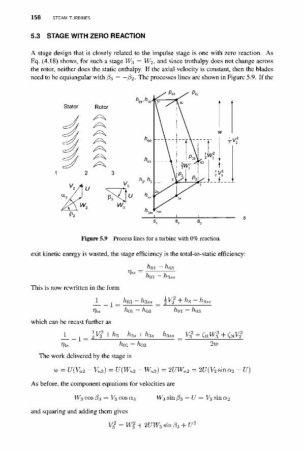
158 STEAM TURBINES
5.3 STAGE WITH ZERO REACTION
A stage design that is closely related to the impulse stage is one with zero reaction. As Eq. (4.18) shows, for such a stage W3 = W2> and since trothalpy does not change across the rotor, neither does the static enthalpy. If the axial velocity is constant, then the blades need to be equiangular with (33 = —(32- The processes lines are shown in Figure 5.9. If the
Stator
Figure 5.9 Process lines for a turbine with 0% reaction.
exit kinetic energy is wasted, the stage efficiency is the total-to-static efficiency:
This is now rewritten in the form
*oi h 03
hm
1 Tits
1 ft-03 ~ hzs \V3 + h3- h3ss
h which can be recast further as
I T / 2 1 7?ts
1 2 ^ 3 + ^ 3
'01
'3s
h 03
<-3s
h 01 h, 03
h3ss V32 + CnWi + C N ^
2w hoi — hos
The work delivered by the stage is
w = U{Vu2 - K3) = U(Wu2 - Wu3) = 2UWu2 = 2U(V2sina2 - U)
As before, the component equations for velocities are
W3 cos /J3 = V3 cos a3 W3 sin P3 + U = V3 sin a2
and squaring and adding them gives
Vf = Wl + 2UW3 sin /33 + U2

STAGE WITH ZERO REACTION 159
Since W3 = W2 and 03 = —02, this can be written as
Vi = W | - 2UW2 sin 02 + U2
Similarly W2 cos 02 — V2 cos a.2 W2 sin 02 = V2 sin o-i — U
which when squared and added give
Wf = Vf - 2UV2 sin a2 + U2
When these are included in the expression for efficiency, it takes the form
1 _ V22 - WV2 sin a2 + 4E/2 + CR(^2
2 - 2UV2 sin a2 + £/2) + CN ̂ 2 %s ~ W(y2sma-U)
This can be written as
rhM = T+K in which, after the substitution \ = U/V2 has been made, /L is given by
1 - 4 A s i n a 2 + 4A2 + CR(l - 2 A s i n a 2 + A2) + CN /L 4A(sina — A)
The maximum efficiency is obtained by minimizing the loss /]> Thus differentiating / L with respect to A and setting it to zero yields
A 2 _ 2 ( 1 + CR + CN) A 1 + CR + CN = Q
CR sin a2 CR
and the maximum efficiency is at the speed ratio
_ 1 + CR + CN - V (1 + CR + CN)(1 + CR + CN - CR sin2 a2) CR sin a2
The efficiency may be written as
4A(sina2 — A) %s
l + CR(A2-2Asina2 + l)+CN
These results are shown as the lower set of curves in Figure 5.10. The efficiencies of a zero reaction stage for various nozzle angles are slightly lower than those for the pressure-compounded impulse stage shown in Figure 5.6. The graphs for a 0% repeating stage are also shown. Both are denoted by r)s, which is to interpreted appropriately, either as repeating stage, or as single stage with kinetic energy wasted.
The efficiency of a repeating stage is obtained from
4A(sina2 — A) f?tt -
(CR - 4) A2 + (4 - 2CR) A sin a2 + CR + CN
with maxima at speed ratios
CR + Cs - v (CR + CN)(CR + CS - CR sin a2) A = CR sin a2
These are left to be worked out as an exercise.
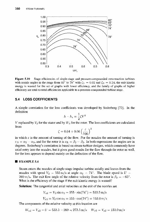
160 STEAM TURBINES
1.00 0.95 0.90 0.85
ns 0.80 0.75 0.70 0.65 0.60 0.55 0.50
0
Figure 5.10 Stage efficiencies of single-stage and pressure-compounded zero-reaction turbines with nozzle angles in the range from 60° to 78° with CN = 0.02 and £R = 0.14; the exit kinetic energy is wasted for the set of graphs with lower efficiency, and the family of graphs of higher efficiency are total-to-total efficiencies applicable to a pressure-compounded turbine stage.
5.4 LOSS COEFFICIENTS
A simple correlation for the loss coefficients was developed by Soderberg [72]. In the definition
h-h3 = \cv2
V replaced by V2 for the stator and by W3 for the rotor. The loss coefficients are calculated from
C = 0.04 +0.06 ( ^
in which e is the amount of turning of the flow. For the nozzles the amount of turning is £N = &2 — o?3, and for the rotor it is £TR = fa ~~ fa- In both expressions the angles are in degrees. Soderberg's correlation is based on steam turbine designs, which commonly have axial entry into the nozzles, but it gives good results for the flow through the rotor as well, for the loss appears to depend mainly on the deflection of the flow.
■ EXAMPLE 5.4
Steam enters the nozzles of single-stage impulse turbine axially and leaves from the nozzles with speed V2 — 555 m / s at angle 0.-2 — 74°. The blade speed is U = 260 m / s . The exit flow angle of the relative velocity from the rotor is fa = —65°. What is the efficiency of the stage if the exit kinetic energy is wasted?
Solution: The tangential and axial velocities at the exit of the nozzles are
VU2 = V2 sin a2 = 555 • sin(74°) = 533.5 m / s
Vx2 = V2 cosa2 = 555 • cos(74°) = 153.0m/s
The components of the relative velocity at this location are
Wu2 = Vu2-U = 533.5 - 260 = 273.5 m / s Wx2 = Vx2 = 153.0 m / s
u/v
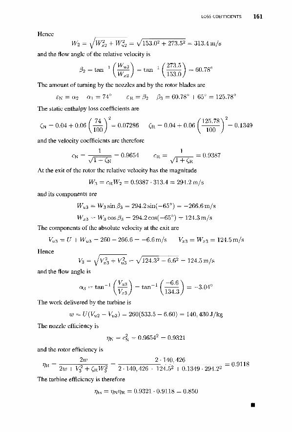
LOSS COEFFICIENTS 1 6 1
Hence W2 = \JW12 + W^2 = V153.02 + 273.52 = 313.4 m/s
and the flow angle of the relative velocity is
The amount of turning by the nozzles and by the rotor blades are
eN = a2 - ax = 74° eR = fo ~ Ps = 60.78° + 65° = 125.78°
The static enthalpy loss coefficients are
74 \ 2 „ „ „ _ , _ „ „ „ / 1 2 5 . 7 8 x 2
CN = 0.04 + 0.06 I — I = 0.07286 CR = 0.04 + 0.06 I - ^ - 1 = 0.1349
and the velocity coefficients are therefore
cN = ; = 0.9654 cR = , = 0.9387
At the exit of the rotor the relative velocity has the magnitude
W3 = cRW2 = 0.9387 • 313.4 = 294.2 m/s
and its components are
Wu3 = W3sin/33 = 294.2 sin(-65°) = -266.6 m/s
Wx3 = W3cos/33 = 294.2 cos(-65°) = 124.3 m/s The components of the absolute velocity at the exit are
Vu3 = U + Wu3 = 260 - 266.6 = -6.6 m/s Vx3 = Wx3 = 124.5 m/s
Hence v3 = \jyx3 + K23 = V124.32 + 6.62 = 124.5 m/s
and the flow angle is
— "■ -(£)-"■- ' ( i l H M ° The work delivered by the turbine is
w = U(Vu2 - Vu3) = 260(533.5 + 6.60) = 140,430 J/kg
The nozzle efficiency is
m = 4 = 0.96542 = 0.9321
and the rotor efficiency is _ 2w _ 2-140,426
VR ~ 2w + V£ + (nW$ ~ 2 • 140,426 + 124.52 + 0.1349 • 294.22 ~~ °"
The turbine efficiency is therefore
Vts = mVR = 0-9321 • 0.9118 = 0.850
162 STEAM TURBINES
EXERCISES
5.1 Steam leaves the nozzles of a de Laval turbine with the velocity V2 = 1000 m/s. The flow angle from the nozzle is «2 = 70°. The blade velocity is U = 360 m/s, and the mass flow rate is 800kg/h. Take the rotor velocity coefficient to be CR = 0.8. The rotor blade is equiangular. Draw the velocity diagrams and determine (a) the flow angle of the relative velocity at the rotor, (b) the relative velocity of the steam entering the blade row, (c) the tangential force on the blades, (d) the axial thrust on the blades, (e) the power developed, and (e) the rotor efficiency.
5.2 The diameter of a wheel of a single-stage impulse turbine is 1060 mm and shaft speed, 3000 rpm. The nozzle angle is 72°, and the ratio of the blade speed to the speed at which steam issues from the nozzles is 0.42. The ratio of the relative velocity leaving the blades is 0.84 of that entering the blades. The outlet flow angle of the relative velocity is 3° more than the inlet flow angle. The mass flow rate of steam is 7.23 kg/s. Draw the velocity diagram for the blades and determine (a) the axial thrust on the blades, (b) the tangential force on the blades, (c) power developed by the blade row, and (d) rotor efficiency.
5.3 The wheel diameter of a single-stage impulse steam turbine is 400 mm, and the shaft speed is 3000 rpm. The steam issues from nozzles at velocity 275 m/s at the nozzle angle of 70°. The rotor blades are equiangular, and friction reduces the relative velocity as the steam flows through the blade row to 0.86 times the entering velocity. Find the power developed by the wheel when the axial thrust is Fx = 120 N.
5.4 Steam issues from the nozzles of a single-stage impulse turbine with the velocity 400 m/s. The nozzle angle is at 74°. The absolute velocity at the exit is 94 m/s, and its direction is —8.2°. Assuming that the blades are equiangular, find (a) the power developed by the blade row when the steam flow rate is 7.3 kg/s and (b) the rate of irreversible energy conversion per kilogram of steam flowing through the rotor.
5.5 Carry out the steps in the development of the expression for ratio of the optimum blade speed to the steam velocity for a single-stage impulse turbine with equiangular blades. Note that this expression is independent of the velocity coefficient. Carry out the algebra to obtain the expression for the rotor efficiency at this condition, (a) Find the numerical value for the velocity ratio when the nozzle angle is 76°. (b) Find the rotor efficiency at this condition, assuming that CR = 0.9. (c) Find the flow angle of the relative velocity entering the blades at the optimum condition.
5.6 Steam flows from a set of nozzles of a single-stage impulse turbine at a2 = 78° with the velocity V2 = 305 m/s. The blade speed is U = 146 m/s. The outlet flow angle of the relative velocity is 3° greater than its inlet angle, and the velocity coefficient is CR = 0.84. The nozzle velocity coefficient is CN = 1. The power delivered by the wheel is 1000 kW. Draw the velocity diagrams at the inlet and outlet of the blades. Calculate the mass flow rate of steam.
5.7 Steam flows from a set of nozzles of a single-stage impulse turbine at an angle a2 = 70°. (a). Find the maximum total-to-static efficiency given velocity coefficients CR = 0.83 and CN = 0.98. (b) If the rotor efficiency is 90% of its maximum value, what are the possible outlet flow angles for the relative velocity.
5.8 The nozzles of a single-stage impulse turbine have a wall thickness t = 0.3 cm and height b — 15 cm. The mean diameter of the wheel is 1160 mm and the nozzle angle is «2 = 72°. The number of nozzles in a ring is 72. The specific volume of steam at the exit
EXERCISES 163
of the nozzles is 15.3 m3/kg and the velocity there is V2 = 366 m/s. (a) Find the mass flow rate of steam through the steam nozzle ring, (b) Find the power developed by the blades for an impulse wheel of equiangular blades, given that the velocity coefficient is CR = 0.86 and CN = 1.0. The shaft turns at 3000 rpm.
5.9 The isentropic static enthalpy change across a stage of a single-stage impulse turbine is Ahs = 22 kJ/kg. The nozzle exit angle is a2 = 74°. The mean diameter of the wheel is 148 cm and the shaft turns at 1500 rpm. The blades are equiangular with a velocity coefficient of CR = 0.87. The nozzle velocity coefficient is CN = 0.98. (a) Find the steam velocity at the exit from the nozzles, (b) Find the flow angles of the relative velocity at the inlet and exit of the wheel, (c) Find the overall efficiency of the stage.
5.10 An impulse turbine has a nozzle angle a2 = 72° and steam velocity V2 = 244 m/s. The velocity coefficient for the rotor blades is CR = 0.85, and the nozzle efficiency is ?7N = 0.92. The output power generated by the wheel is W = 562 kW when the mass flow rate is m = 23 kg/s. Find the total-to-static efficiency of the turbine.
5.11 A two-row velocity-compounded impulse wheel is part of a steam turbine with many other stages. The steam velocity from the nozzles is V2 = 580 m/s, and the mean speed of the blades is U = 116 m/s. The flow angle leaving the nozzle is a2 = 74°, and the flow angle of the relative velocity leaving the first set of rotor blades is fa = —72°. The absolute velocity of the flow as it leaves the stator vanes between the two rotors is Q4 = 68°, and the outlet angle of the relative velocity leaving the second rotor is $5 = —54°. The steam flow rate is m = 2.4 kg/s. The velocity coefficient is cv = 0.84 for both the stator and the rotor row. (a) Find the axial thrust from each wheel, (b) Find the tangential thrust from each wheel, (c) Find the total-to-static efficiency of the rotors defined as the work out divided by the kinetic energy available from the nozzles.
5.12 A velocity-compounded impulse wheel has two rows of moving blades with a mean diameter of D = 72 cm. The shaft rotates at 3000 rpm. Steam issues from the nozzles at angle a2 = 74° with velocity V2 = 555 m/s. The mass flow rate is m = 5.1 kg/s. The energy loss through each of the moving blades is 24% of the kinetic energy entering the blades, based on the relative velocity. Steam leaves the first set of moving blades at 03 = —72° the guide vanes between the rows at 0:4 = 68° and the second set of moving blades at /3s = —52°. (a) Draw the velocity diagrams and find the flow angles at the blade inlets both for absolute and relative velocities, (b) Find the power developed by each row of blades, (c) Find the rotor efficiency as a whole.
5.13 Steam flows from the nozzles of a 0% repeating stage at an angle a2 = 69° and speed V2 = 450 m/s and enters the rotor with blade speed moving at U = 200 m/s. Find (a) its efficiency when the loss coefficients are calculated from Soderberg's correlation and (b) the work delivered by the stage.
5.14 For a repeating stage the efficiency of a 0% reaction, by neglecting the temperature factors show that the approximate form of the total-to-total efficiency is
4A(sin a2 — A) VU = (CR - 4)A2 + (4 - 2CR)A sin a2 + CR + CN
and its maximum values is at the condition A = U/V2 given by
CR + Cs - y (CR + CN)(CR + Cs - CR sin2 a2) CR sin a2
CHAPTER 6
AXIAL TURBINES
In the previous chapter the impulse stages of steam turbines were analyzed. This chapter extends the development of axial turbine theory to reaction turbines. These include gas turbines and all except the leading stages of steam turbines. The extent of the global steam turbine industry was mentioned in the last chapter. Gas turbine industry is even larger, owing to the use of gas turbine in a jet engine. Gas turbines are also used for electric power generation in central station power plants. In addition, they drive the large pipeline compressors that transmit natural gas across continents and provide power on oil-drilling platforms.
The chapter begins with the development of the working equations for the reaction stages. These relate the flow angles of the absolute and relative velocities to the degree of reaction, flow coefficient, and the blade-loading coefficient. Three-dimensional aspects of the flow are considered next. Then semiempirical theories are introduced to calculate the static enthalpy rise caused by internal heating, which is then used to develop an expression for the stage efficiency. After this the equations used to calculate the stagnation pressure losses across the stator and the rotor are developed.
6.1 INTRODUCTION
Two adjacent blades of an axial reaction turbine are shown in Figure 6.1. Their spacing along the periphery of the disk is called the pitch. The pitch increases in the radial direction from the hub of the rotor to its casing. The nominal value of the pitch is at the mean radius.
Principles of Turbomachinery. By Seppo A. Korpela 165 Copyright © 2011 John Wiley & Sons, Inc.

166 AXIAL TURBINES
The lateral boundaries of the flow channel are along the pressure and suction sides of the blades and the endwalls along the hub and the casing.
The flow is from front to back in Figure 6.1. The blade chord is the straight distance from the leading edge of the blade to its trailing edge. Its projection in the axial direction is the axial chord. The path of a fluid particle, as it passes through the blade passage, is curved and thus longer than the chord.
Figure 6.1 Flow channel between two adjacent turbine blades.
The annular region formed from the blade passage areas is called the flow annulus. The annulus area is calculated as
A = 2irrm(rc - rh) = Tr{r% - rl)
if the mean radius rm is taken as the arithmetic average
1 /
of the casing radius rc and the hub radius rh. The blade height, or span, is b = rc — r^ and 2irrm = Zs, in which Z is the number of blades and s is the mean pitch or spacing of the blades. Therefore the annulus area is also A = Zsb.
An alternative is to define a mean radius such that the flow area from it to the hub and to the casing are equal. This definition leads to the equality
A?™ - rl) = ir(rl - f2m)
which, when solved for fm, gives
r^+rl 2 rm =
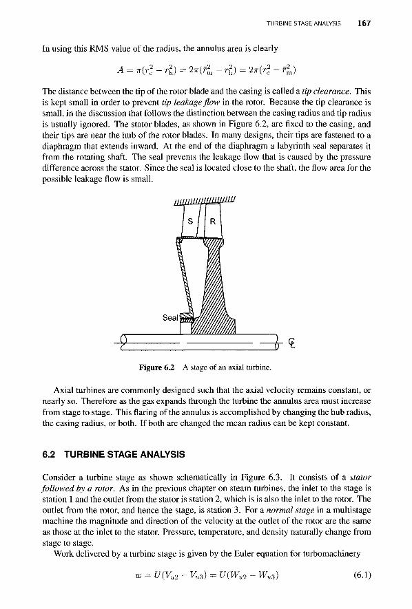
TURBINE STAGE ANALYSIS 167
In using this RMS value of the radius, the annulus area is clearly
A = 7r(rc2 - rl) = 2n(f2
m - r2h) = 27r(rc
2 - f2J
The distance between the tip of the rotor blade and the casing is called a tip clearance. This is kept small in order to prevent tip leakage flow in the rotor. Because the tip clearance is small, in the discussion that follows the distinction between the casing radius and tip radius is usually ignored. The stator blades, as shown in Figure 6.2, are fixed to the casing, and their tips are near the hub of the rotor blades. In many designs, their tips are fastened to a diaphragm that extends inward. At the end of the diaphragm a labyrinth seal separates it from the rotating shaft. The seal prevents the leakage flow that is caused by the pressure difference across the stator. Since the seal is located close to the shaft, the flow area for the possible leakage flow is small.
S R
Seal
-P -k-i Figure 6.2 A stage of an axial turbine.
Axial turbines are commonly designed such that the axial velocity remains constant, or nearly so. Therefore as the gas expands through the turbine the annulus area must increase from stage to stage. This flaring of the annulus is accomplished by changing the hub radius, the casing radius, or both. If both are changed the mean radius can be kept constant.
6.2 TURBINE STAGE ANALYSIS
Consider a turbine stage as shown schematically in Figure 6.3. It consists of a stator followed by a rotor. As in the previous chapter on steam turbines, the inlet to the stage is station 1 and the outlet from the stator is station 2, which is is also the inlet to the rotor. The outlet from the rotor, and hence the stage, is station 3. For a normal stage in a multistage machine the magnitude and direction of the velocity at the outlet of the rotor are the same as those at the inlet to the stator. Pressure, temperature, and density naturally change from stage to stage.
Work delivered by a turbine stage is given by the Euler equation for turbomachinery
w = U(Vu2 - Vu3) = U(Wu2 - Wu3) (6.1)
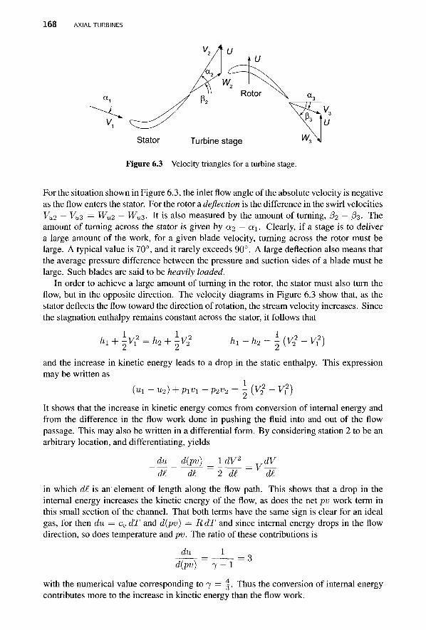
168 AXIAL TURBINES
Figure 6.3 Velocity triangles for a turbine stage.
For the situation shown in Figure 6.3, the inlet flow angle of the absolute velocity is negative as the flow enters the stator. For the rotor a deflection is the difference in the swirl velocities Vu2 — VU3 = Wu2 — Wus. It is also measured by the amount of turning, (32 — 03. The amount of turning across the stator is given by a2 — &\- Clearly, if a stage is to deliver a large amount of the work, for a given blade velocity, turning across the rotor must be large. A typical value is 70°, and it rarely exceeds 90°. A large deflection also means that the average pressure difference between the pressure and suction sides of a blade must be large. Such blades are said to be heavily loaded.
In order to achieve a large amount of turning in the rotor, the stator must also turn the flow, but in the opposite direction. The velocity diagrams in Figure 6.3 show that, as the stator deflects the flow toward the direction of rotation, the stream velocity increases. Since the stagnation enthalpy remains constant across the stator, it follows that
h1 + \v? = h2 + \v? hl-h2=l-{vi-v?)
and the increase in kinetic energy leads to a drop in the static enthalpy. This expression may be written as
(ui - u2)+piv1 - p2v2 = - {V22 - i f )
It shows that the increase in kinetic energy comes from conversion of internal energy and from the difference in the flow work done in pushing the fluid into and out of the flow passage. This may also be written in a differential form. By considering station 2 to be an arbitrary location, and differentiating, yields
_du _ d{pv) _ ldV^ _ dV ~~dl d£~ ~ 2~dT ~ ~di
in which d£ is an element of length along the flow path. This shows that a drop in the internal energy increases the kinetic energy of the flow, as does the net pv work term in this small section of the channel. That both terms have the same sign is clear for an ideal gas, for then du = cv dT and d{pv) = RdT and since internal energy drops in the flow direction, so does temperature and pv. The ratio of these contributions is
du = 1 d(pv) 7 — 1
with the numerical value corresponding to 7 = | . Thus the conversion of internal energy contributes more to the increase in kinetic energy than the flow work.
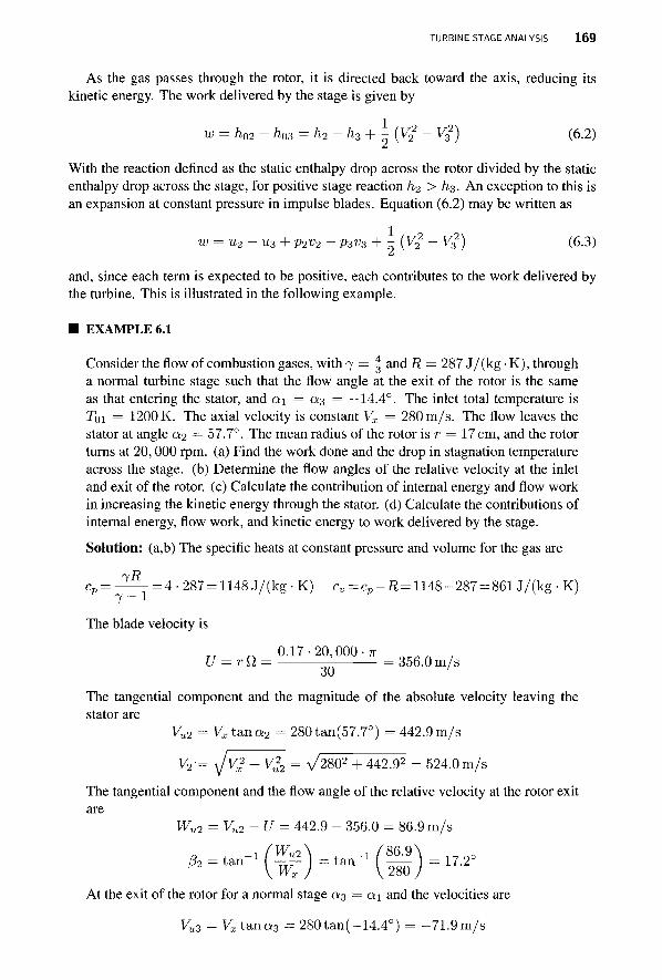
TURBINE STAGE ANALYSIS 169
As the gas passes through the rotor, it is directed back toward the axis, reducing its kinetic energy. The work delivered by the stage is given by
w = h02- h03 = h2-h3 + - (V% - V£) (6.2)
With the reaction defined as the static enthalpy drop across the rotor divided by the static enthalpy drop across the stage, for positive stage reaction h2 > h3. An exception to this is an expansion at constant pressure in impulse blades. Equation (6.2) may be written as
w = u2-u3 + p2v2 - p3v3 + - (V2 - V32) (6.3)
and, since each term is expected to be positive, each contributes to the work delivered by the turbine. This is illustrated in the following example.
■ EXAMPLE 6.1
Consider the flow of combustion gases, with 7 = | and R = 287 J/(kg • K), through a normal turbine stage such that the flow angle at the exit of the rotor is the same as that entering the stator, and a\ = a3 = —14.4°. The inlet total temperature is T0i = 1200 K. The axial velocity is constant Vx = 280 m/s. The flow leaves the stator at angle a2 = 57.7°. The mean radius of the rotor is r = 17 cm, and the rotor turns at 20,000 rpm. (a) Find the work done and the drop in stagnation temperature across the stage, (b) Determine the flow angles of the relative velocity at the inlet and exit of the rotor, (c) Calculate the contribution of internal energy and flow work in increasing the kinetic energy through the stator. (d) Calculate the contributions of internal energy, flow work, and kinetic energy to work delivered by the stage.
Solution: (a,b) The specific heats at constant pressure and volume for the gas are
iR cp = -!—- =4 ■ 287= 1148 J/(kg • K) cv=cp-R= 1148-287 = 861 J/(kg • K)
7 - 1
The blade velocity is
„ 0.17-20,000-TT „ „ „ . U = rQ = -^ = 356.0m/s
OK)
The tangential component and the magnitude of the absolute velocity leaving the stator are
Vu2 = y x t a n a 2 = 280tan(57.7°) = 442.9m/s
V2 = -y/v;2 + Vl2 = A/280 2 + 442.92 = 524.0 m/s
The tangential component and the flow angle of the relative velocity at the rotor exit are
Wu2 = Vu2 - U = 442.9 - 356.0 = 86.9 m/s
At the exit of the rotor for a normal stage a 3 = a\ and the velocities are
Vu3 = K t a n a 3 = 280tan(-14.4°) = -71.9 m/s
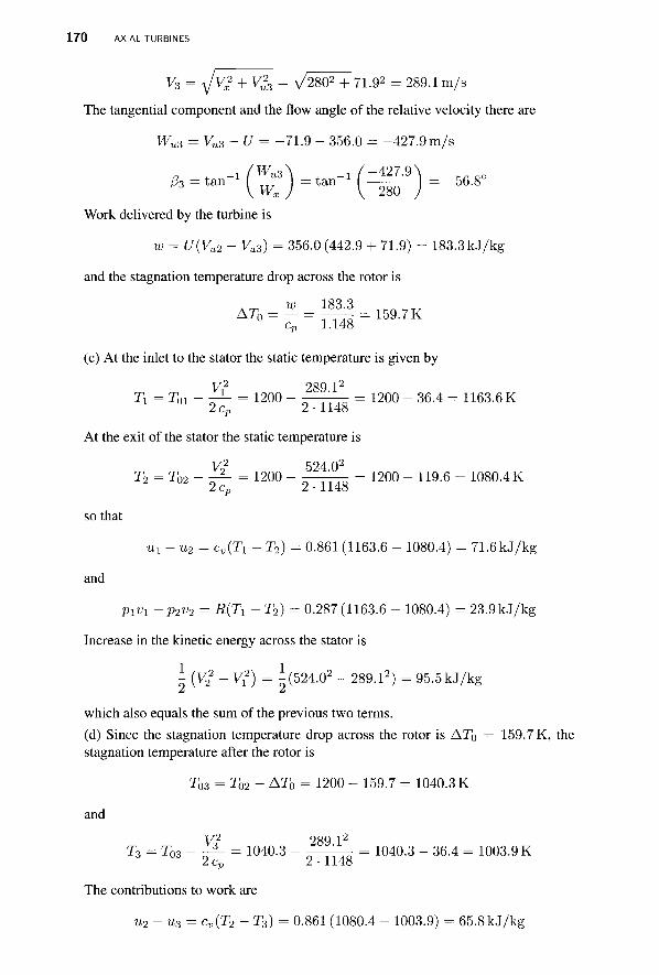
170 AXIAL TURBINES
V3 = yJV* + V*3 = \/2802 + 71.92 = 289.1 m/s
The tangential component and the flow angle of the relative velocity there are
Wu3 = Vu3 - U = -71.9 - 356.0 = -427.9 m/s
A = tan"1 ( ^ ) = t a n - (=*™) = -56.8° \WXJ \ 280 ) Work delivered by the turbine is
w = U(Vu2 - Vu3) = 356.0 (442.9 + 71.9) = 183.3 kJ/kg
and the stagnation temperature drop across the rotor is
AT0 = ^ = ^ = 159.7K cp 1.148
(c) At the inlet to the stator the static temperature is given by
V? 289.12
7\ = T01 - -±- = 1200 - = 1200 - 36.4 = 1163.6 K
At the exit of the stator the static temperature is
V? 524.02
T2 = T02 - -Z- = 1200 - = 1200 - 119.6 = 1080.4 K
so that
ul-u2= cv{Tx - T2) = 0.861 (1163.6 - 1080.4) = 71.6kJ/kg
and
Pivi -p2v2 = R(TX - T 2 ) = 0.287(1163.6 - 1080.4) = 23.9kJ/kg
Increase in the kinetic energy across the stator is
\ (V22 ~ V,2) = i(524.02 - 289.12) = 95.5kJ/kg
which also equals the sum of the previous two terms. (d) Since the stagnation temperature drop across the rotor is ATQ — 159.7 K, the stagnation temperature after the rotor is
Tos = T02 - AT0 = 1200 - 159.7 = 1040.3 K
and
V? „ 289.12 (3 — J03
Up
T3=TQ3 5_ = 1040.3 - """' = 1040.3 - 36.4 = 1003.9K 2cD 2-1148
The contributions to work are
u2-u3 = cv(T2 - T3) = 0.861 (1080.4 - 1003.9) = 65.8kJ/kg

FLOW AND LOADING COEFFICIENTS AND REACTION RATIO 1 7 1
and
P2V2 ~ P3V3 = R(T2 - T3) = 0.287 (1080.4 - 1003.9) = 21.9kJ/kg
In a normal stage the increase in kinetic energy across the stator is equal to its decrease across the rotor. Hence the decrease in kinetic energy across the rotor is
- {V2 ~ V%) = T;(524.02 - 289.12) = 95.5kJ/kg
The sums of internal energy changes and pv work, and the change in kinetic energy across the rotor, add up to the work delivered by the stage.
6.3 FLOW AND LOADING COEFFICIENTS AND REACTION RATIO
The work delivered by a stage is given by
w = U(Vu2 - Vu3) = U(Wu2 - Wu3)
which, if Vx = Wx is constant across the stage, may be written as
w = UVx(ta.na2 — tanas) = UVx(ta,n (32 — tan f33) (6.4)
Let 4> = Vx/U denote a flow coefficient and ijj = w/U2 a blade-loading coefficient. Then, dividing both sides of this equation by U2 gives the Euler turbine equation in a nondimensional form as
ip = 0( tana2 — tana 3 ) (6.5)
Other names for the blade-loading coefficient are work coefficient and loading factor. In addition to tp and <f>, a third nondimensional quantity of importance in the theory is the reaction ratio R, introduced previously. It was defined as the ratio of the static enthalpy change across the rotor to that across the entire stage. Hence
h2-h3 hi - h3- (hi - h2) hx - h2
hi - h3 hi- h3 hi - h3
Reaction naturally falls into the range 0 < R < 1, but it was seen to be slightly negative for a pure impulse stage. This equation shows that the reaction is zero, if the entire static enthalpy drop takes place in the stator.
Recalling that the total enthalpy of the relative motion, given by Eq. (4.13), remains constant across a rotor in an axial stage, it follows that
h2 + \w2 = h3+l-W2
or h2-h3=l- (W2 - W2)
Hence, if W2 = W3 the reaction is zero. Across the stator the stagnation enthalpy is constant so that
hi-h2 = \ (V2 - V2)
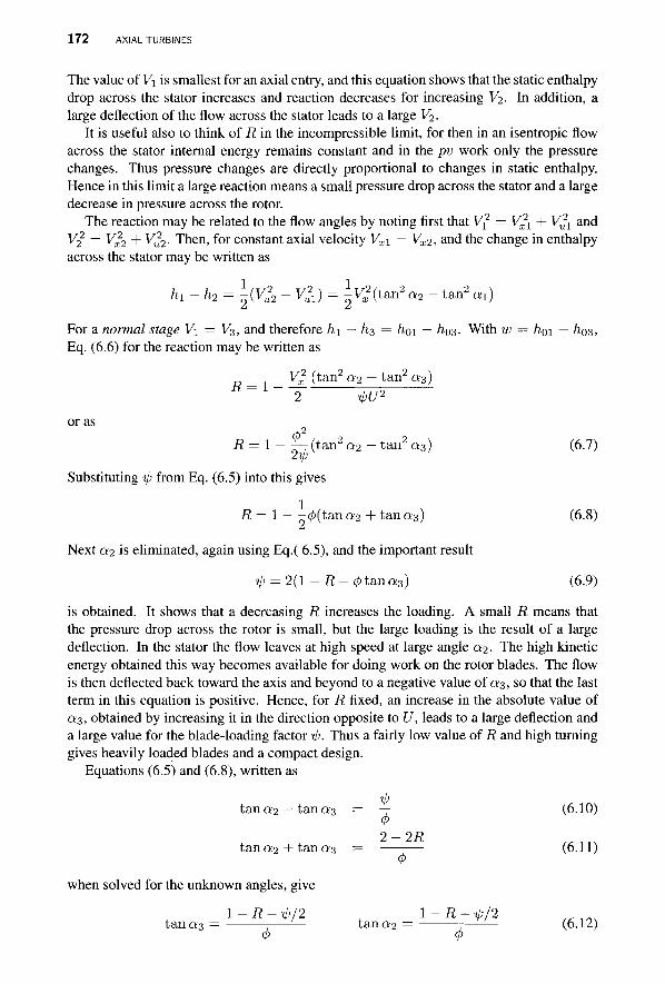
172 AXIAL TURBINES
The value of V\ is smallest for an axial entry, and this equation shows that the static enthalpy drop across the stator increases and reaction decreases for increasing V2. In addition, a large deflection of the flow across the stator leads to a large V2.
It is useful also to think of R in the incompressible limit, for then in an isentropic flow across the stator internal energy remains constant and in the pv work only the pressure changes. Thus pressure changes are directly proportional to changes in static enthalpy. Hence in this limit a large reaction means a small pressure drop across the stator and a large decrease in pressure across the rotor.
The reaction may be related to the flow angles by noting first that Vy = V£i + V^i and V2
2 = Vx22 + V%2- Then, for constant axial velocity Vx\ = Vx2, and the change in enthalpy
across the stator may be written as
hl-h2 = i(K22 - O = ^ , 2 ( t a n 2 a2 - tan2
Ql)
For a normal stage V\ = V3, and therefore h\ — h3 = ft-01 — h03. With w — hoi — ho3, Eq. (6.6) for the reaction may be written as
R=l
or as
V£ (tan2 oi2 — tan2 a3) ~2 ^C/2
A2 ,2 „.. + „ „ 2 . R = 1 - j— (tan2 a2 - tan2 a3) (6.7)
zip Substituting xp from Eq. (6.5) into this gives
R = 1 — -0( tan«2 + tan«3) (6.8)
Next a2 is eliminated, again using Eq.( 6.5), and the important result
ip = 2(l- R-<pt&na3) (6.9)
is obtained. It shows that a decreasing R increases the loading. A small R means that the pressure drop across the rotor is small, but the large loading is the result of a large deflection. In the stator the flow leaves at high speed at large angle a2. The high kinetic energy obtained this way becomes available for doing work on the rotor blades. The flow is then deflected back toward the axis and beyond to a negative value of a3, so that the last term in this equation is positive. Hence, for R fixed, an increase in the absolute value of a3, obtained by increasing it in the direction opposite to U, leads to a large deflection and a large value for the blade-loading factor ip. Thus a fairly low value of R and high turning gives heavily loaded blades and a compact design.
Equations (6.5) and (6.8), written as
tp tanc*2 — t a n a 3 = — (6.10)
tan « 2 + t a n 0:3 = — (6.11)
when solved for the unknown angles, give
l-R-ip/2 l-R + ip/2 ^ , „ s t a n a 3 = tana2 = (6.12)
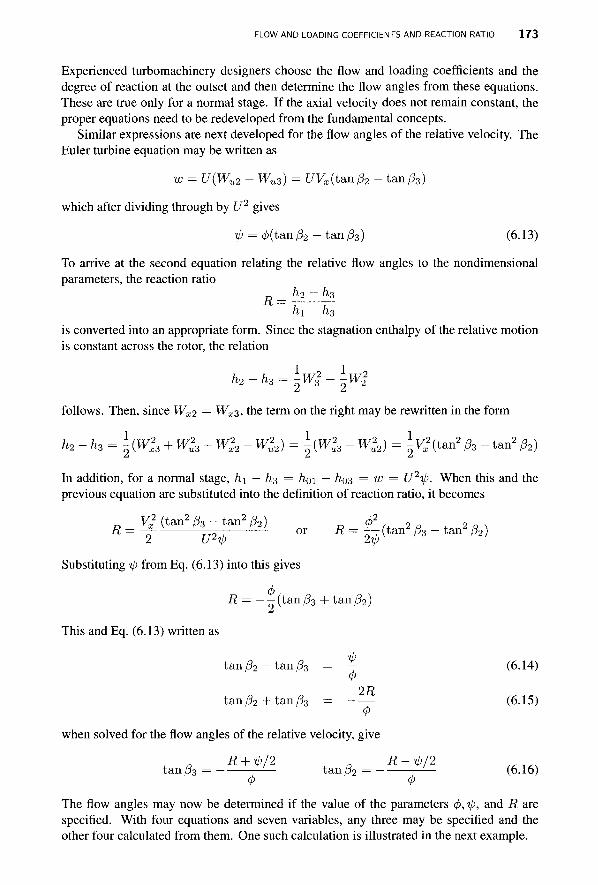
FLOW AND LOADING COEFFICIENTS AND REACTION RATIO 1 7 3
Experienced turbomachinery designers choose the flow and loading coefficients and the degree of reaction at the outset and then determine the flow angles from these equations. These are true only for a normal stage. If the axial velocity does not remain constant, the proper equations need to be redeveloped from the fundamental concepts.
Similar expressions are next developed for the flow angles of the relative velocity. The Euler turbine equation may be written as
w = U(Wu2 - Wu3) = UVx{tanP2 - tan ft)
which after dividing through by U2 gives
ip = </>(tanft - t a n ft) (6.13)
To arrive at the second equation relating the relative flow angles to the nondimensional parameters, the reaction ratio
h2 - h3
hi - h3
is converted into an appropriate form. Since the stagnation enthalpy of the relative motion is constant across the rotor, the relation
k2-h3 = ±wi-±w2
follows. Then, since Wx2 = Wx3, the term on the right may be rewritten in the form
h2-h3 = \{W23 + W2
3 - W22 - W2
2) = \{W2u3 - W2
2) = ^ Vx2(tan2 ft - tan2 ft)
In addition, for a normal stage, h\ — h3 = hoi — ho3 = w = U2ip. When this and the previous equation are substituted into the definition of reaction ratio, it becomes
V2 (tan2 ft - tan2 ft) cf>2 2 2
R=T—im— or R=^(tan h"tan N
Substituting tp from Eq. (6.13) into this gives
R = — — (tan ft + tan ft
This and Eq. (6.13) written as
t a n f t - t a n f t = — (6.14) o p
t a n f t + t a n f t = (6.15)
when solved for the flow angles of the relative velocity, give
t anf t = - ^ t anf t = - ^ (6.16)
The flow angles may now be determined if the value of the parameters <f>, tb, and R are specified. With four equations and seven variables, any three may be specified and the other four calculated from them. One such calculation is illustrated in the next example.
174 AXIAL TURBINES
EXAMPLE 6.2
Combustion gases with 7 = | andcp = 1148 J/(kg-K) flow through an axial turbine stage with <f> = 0.80 as the design value for the flow coefficient and ip — 1.7 for the blade-loading coefficient. The stage is normal with flow into the stator at angle a\ = —21.2°. The absolute velocity of the gases leaving the stator is V2 = 463 m/s. The inlet stagnation temperature is T0\ = 1200 K, and the total-to-total efficiency is 0.89. (a) Find the flow angles for a normal stage, and the amount of turning by the stator and the rotor, (b) Calculate the work delivered by the stage, and the drop in the stagnation temperature, (c) Determine the static pressure ratio across the stage.
Solution: (a) With a 3 = a\, solving
ip = 2(1 - R-<pta,na3)
for R gives
R=l- -^ - 4>t&na3 = 1 - 0.85 - 0.8tan(-21.2°) = 0.46
The remaining flow angles are
t a n a 2 = — — ^ - ^ = 1.737 a2 = 60.08°
tan/3 3 = ~ ( f i + ^ / 2 ) = - 1 , 6 3 8 fa = -58.59° <P
t a n f e = ~ ( f i ~ ^ / 2 ) =o ,4 8 7 /32 = 25.97°
The amounts of turning by the stator and the rotor are
a2-a3 = 81.27° /32 - /33 = 84.57°
(b) The axial velocity is
Vx = V2cosa2 = 463cos(60.08°) = 231.0 m/s
and the blade speed is
<p 0.8 '
Hence the work done may be calculated from
w = xbU2 = 1.7 • 288.72 = 141.7kJ/kg
and the drop in stagnation temperature is
AT0 = ^ = H ^ = 123.4K cp 1.148
The isentropic work is obtained by dividing the work w by the stage efficiency, which is the total-to-total efficiency,
w 141.7 ??tt 0.89
FLOW AND LOADING COEFFICIENTS AND REACTION RATIO 1 7 5
(c) The static temperature at the inlet is
V? 247 82
T1=T01 L = 1200 — = 1173.3 K
2cp 2-1148
Neither the static nor the stagnation pressure is known at the inlet, but their ratio can be calculated from
Poi \ToiJ V 1200
The stagnation temperature at the exit of the stage comes out to be
w 141.7 T03 = T01 - - = 1200 - — - = 1076.6 K
cp 1.148 The exit velocity from the stage is
Va = ^ = f3l01° = 2 4 7 . 8 m / s
cosa3 cos(-21.2°) '
and therefore the static temperature at the exit is
V? 247.82
T3 = T03 - -^ = 1094.7 - — — = 1049.8 K 2cp 1148
This can be used to calculate the ratio of static to stagnation pressure at the exit:
«..raY'h",,.r^?Y=o.8o« P03 \T03J V1 0 7 6 - 5 /
The stagnation temperature at the isentropic end state is determined to be
T03s = T01 - — = 1200 - i ^ | = 1061.3 K cp 1.1148
and the stagnation pressure ratio across the stage is therefore
Poi {TotV^-V / 1 2 0 0 ^ 4
= 1.635 P03 \To3sJ V 1061.3,
The ratio of static pressures across the stage can now be determined:
Pi Pi Poi Pos 0.9138 ■ 1.635 P3 Poi P03 P3 0.9043 1.652
The representative values for an axial turbine stage ip = 1.7, <p = 0.8 and R = 0.46 give these values for the stagnation and static pressure ratios and the amount of turning comes out to be about 80°- 85°. In addition, the stagnation pressure drop of ATQ = 123.4 K is representative for a stage.
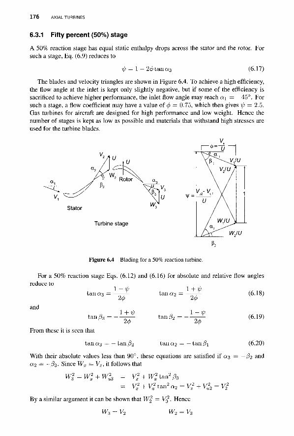
176 AXIAL TURBINES
6.3.1 Fifty percent (50%) stage
A 50% reaction stage has equal static enthalpy drops across the stator and the rotor. For such a stage, Eq. (6.9) reduces to
ip = 1 — 2<p t an «3 (6.17)
The blades and velocity triangles are shown in Figure 6.4. To achieve a high efficiency, the flow angle at the inlet is kept only slightly negative, but if some of the efficiency is sacrificed to achieve higher performance, the inlet flow angle may reach a\ = —45°. For such a stage, a flow coefficient may have a value of </> = 0.75, which then gives ip = 2.5. Gas turbines for aircraft are designed for high performance and low weight. Hence the number of stages is kept as low as possible and materials that withstand high stresses are used for the turbine blades.
V =
Stator
Turbine stage
W2IU
Figure 6.4 Blading for a 50% reaction turbine.
For a 50% reaction stage Eqs. (6.12) and (6.16) for absolute and relative flow angles reduce to
tanof3
and tan/?3
From these it is seen that
l - V
20
2(j>
tan a3 — — tan p2
tana2
tan/32
tanof2
1 + V> 2<j)
l - V
20~
— tan Pi With their absolute values less than 90°, these equations are satisfied if a3
a2 = —03- Since Wx = Vx, it follows that
(6.18)
(6.19)
(6.20)
-/32 and
wl = wl + wl, u3 = Vx + Wl t an 2 p3
= V% + Vl t an 2 a2 = V? + V*2 = V22
By a similar argument it can be shown that W% = V32. Hence
w3 = v2 w2 = v3
FLOW AND LOADING COEFFICIENTS AND REACTION RATIO 1 7 7
A combined velocity diagram is shown also in Figure 6.4. It is constructed by drawing the inlet and exit velocity diagrams with a common side of distance U. If all velocities are then divided by U, the diagram is normalized with a right side of length unity. The blade-loading coefficient ip can be identified as the vertical distance between the left vertices of the two triangles. For a constant axial velocity, widths of the triangles are the same and in a normalized diagram equal to the flow coefficient 0. The results for the angles and velocities show that the velocity triangles for 50% reaction stage are symmetric.
■ EXAMPLE 6.3
Combustion gases, with 7 = | andR = 287 kJ/(kg-K), flow through a 50% reaction stage of an axial turbine, that has a total-to-total efficiency r]u = 0.91 and design flow coefficient 0 = 0.80. The flow into the stator is at an angle ct\ = —14.0°, and the axial velocity is Vx = 240 m/s and constant across the stage. The inlet stagnation temperature is Toi — 1200 K. (a) Find the flow angles for a normal stage, and the amount of turning by the stator and the rotor, (b) Find the work delivered by the stage and the drop in the stagnation temperature, (c) Show that 1/^ts = 1/^tt + (p2/2tp cos2 a3 and calculate the total-to-static efficiency.
Solution: (a) The blade-loading coefficient is
rp = l - 2<£ tan o<3 = 1 - 2 • 0.8tan(-14.0°)) = 1.40
The remaining flow angles are
1-ip t ana 2 = » *= 1-50 so that a2 = 56.3°
20 and
fa = - a 2 = -56.3° fa = -a3 = 14.0°
The amount turning by the stator and rotor are
a2-a3 = 70.3° fa - fa = 70.3°
(b) The blade speed is
TT V* 2 4 0 Qnnn / U = — = —- = 300.0 m/s 0 0.8 '
Hence the work delivered may be calculated from
w = <0£/2 = 1.40 ■ 300.02 = 125.9 kJ/kg
and the drop in stagnation temperature becomes ATo = w/cp = 109.7 K, since cp = 1148 J/(kg • K). The isentropic work is
t«. = ^ = ^ = 138.4kJ/kg r)tt 0.91
(c) The total-to-static efficiency is obtained from
hoi ~ h03 h0i ~ h03 w »7ts hoi - h3s hoi - h03s + Vl/2 ws + V3
2J2
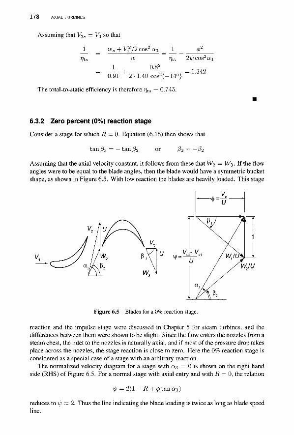
178 AXIAL TURBINES
Assuming that Vzs = V3 so that
1 ws + V^2/2cos2a3 _ 1
w %t
1 0.82
0.91 2-1.40 cos2(-14°)
The total-to-static efficiency is therefore 77ts = 0.745.
2lp COS2a3
= 1.342
6.3.2 Zero percent (0%) reaction stage
Consider a stage for which R = 0. Equation (6.16) then shows that
tan /33 = - tan j32 or / 3 3 — —f52
Assuming that the axial velocity constant, it follows from these that W2 = W3. If the flow angles were to be equal to the blade angles, then the blade would have a symmetric bucket shape, as shown in Figure 6.5. With low reaction the blades are heavily loaded. This stage
Figure 6.5 Blades for a 0% reaction stage.
reaction and the impulse stage were discussed in Chapter 5 for steam turbines, and the differences between them were shown to be slight. Since the flow enters the nozzles from a steam chest, the inlet to the nozzles is naturally axial, and if most of the pressure drop takes place across the nozzles, the stage reaction is close to zero. Here the 0% reaction stage is considered as a special case of a stage with an arbitrary reaction.
The normalized velocity diagram for a stage with a3 = 0 is shown on the right hand side (RHS) of Figure 6.5. For a normal stage with axial entry and with R — 0, the relation
ip = 2(1 -_R + 0 t a n a 3 )
reduces to ip = 2. Thus the line indicating the blade loading is twice as long as blade speed line.

FLOW AND LOADING COEFFICIENTS AND REACTION RATIO 1 7 9
EXAMPLE 6.4
A normal stage with R = 0 operates with axial entry. The nozzle turns the flow by 64°. (a) Find the flow coefficient, (b) What is the discharge velocity from the nozzles, if the axial velocity is Vx = 240 m/s? (c) Calculate the work delivered by the stage and the drop in the stagnation temperature, given gases with cp = 1148 J / ( k g • K).
Solution: (a) From V> = 2(1 - R-(j)ta,nai)
a stage with R = 0 and axial entry has tp — 2. Next, solving
1 + ^ / 2 tanct2 = ; <P
for 4>, gives 0 = 2 c o t a 2 = 2cot(64°) = 0.9755
(b) The discharge velocity is
T/ V* 240 V2 = = -. r = 547.5 m/s
cosc*2 cos (64°) (c) The blade speed is
[ / = K = _ ? 4 0 _ = 2 4 6 . 0 m / s 6 0.9755 '
and the work delivered and the drop in the stagnation temperature are
w = ij)U2 = 121.1 k J / k g AT 0 = — = ^ | = 105.5 K
6.3.3 Off-design operation
When a turbine is operated away from its design conditions, the incidence of the flow entering the blades changes, and this will increase the thermodynamic losses in the flow. The angle at which the flow leaves the stator tends not to change, however; nor does the angle of the relative velocity leaving the rotor. By recasting the Euler turbine equation
w = U(Vu2 - Vu3)
in terms of the exit angles gives an equation that shows how the turbine performs under off-design conditions. Replacing the exit velocity by
vu3 = u + wu3
gives w = U{~U - Wu3 + Vu2) = -U2 + UVx(tana2 - tan/33)
Dividing though by U2 yields
iP = - 1 + 0 ( t a n a 2 - t a n / 3 3 ) (6.21)
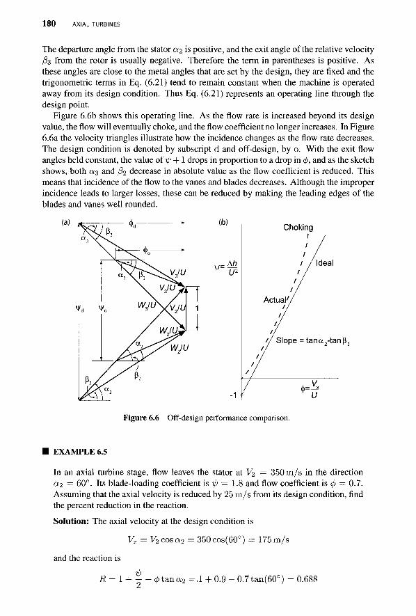
180 AXIAL TURBINES
The departure angle from the stator a2 is positive, and the exit angle of the relative velocity /?3 from the rotor is usually negative. Therefore the term in parentheses is positive. As these angles are close to the metal angles that are set by the design, they are fixed and the trigonometric terms in Eq. (6.21) tend to remain constant when the machine is operated away from its design condition. Thus Eq. (6.21) represents an operating line through the design point.
Figure 6.6b shows this operating line. As the flow rate is increased beyond its design value, the flow will eventually choke, and the flow coefficient no longer increases. In Figure 6.6a the velocity triangles illustrate how the incidence changes as the flow rate decreases. The design condition is denoted by subscript d and off-design, by o. With the exit flow angles held constant, the value of tb + 1 drops in proportion to a drop in <f>, and as the sketch shows, both «3 and f32 decrease in absolute value as the flow coefficient is reduced. This means that incidence of the flow to the vanes and blades decreases. Although the improper incidence leads to larger losses, these can be reduced by making the leading edges of the blades and vanes well rounded.
Figure 6.6 Off-design performance comparison.
■ EXAMPLE 6.5
In an axial turbine stage, flow leaves the stator at V2 = 350 m/s in the direction a2 — 60°. Its blade-loading coefficient is tp = 1.8 and flow coefficient is 4> — 0.7. Assuming that the axial velocity is reduced by 25 m/s from its design condition, find the percent reduction in the reaction.
Solution: The axial velocity at the design condition is
Vx = V2cosa2 = 350cos(60°) = 175 m/s
and the reaction is
R = 1 + j - - <j>t&na2 =.l + 0.9 - 0.7tan(60°) = 0.688
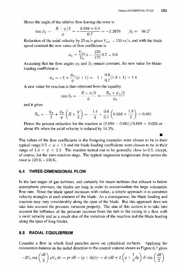
THREE-DIMENSIONAL FLOW 1 8 1
Hence the angle of the relative flow leaving the rotor is R + ^/2 0.688 + 0.9
tan/33 = —!—= — = -2.2678 /33 = -66.2 <p U. r
Reduction of the axial velocity by 25 m/s gives V^n = 150 m/s, and with the blade speed constant the new value of flow coefficient is
K = ^ * = ~ 0 . 7 = 0.6 Vi 175
Assuming that the flow angles a 2 and /33 remain constant, the new value for blade-loading coefficient is
Vn = " I + j(<P + 1) = " I + ^ ( 1 - 8 + 1) = 1.4
A new value for reaction is then obtained from the equality
+ R + ^/2 fln + ^n/2 tan/33 = =
<p 0n and it gives
Hence the percent reduction for the reaction is (0.688 — 0.661)/0.688 = 0.039 or about 4% when the axial velocity is reduced by 14.3%.
■ The values of the flow coefficients in the foregoing examples were chosen to be in their typical range 0.5 < <fi < 1.0 and the blade-loading coefficients were chosen to be in their range of 1.4 < ip < 2.2. The reaction turned out to be generally close to 0.5, except, of course, for the zero-reaction stage. The typical stagnation temperature drop across the rotor is 120 K - 1 5 0 K.
6.4 THREE-DIMENSIONAL FLOW
In the last stages of gas turbines, and certainly for steam turbines that exhaust to below atmospheric pressure, the blades are long in order to accommodate the large volumetric flow rate. Since the blade speed increases with radius, a simple approach is to construct velocity triangles at each element of the blade. As a consequence, the blade loading and reaction may vary considerably along the span of the blade. But this approach does not take into account the pressure variation properly. The aim of this section is to take into account the influence of the pressure increase from the hub to the casing in a flow with a swirl velocity and as a result also of the variation of the reaction and the blade loading along the span of long blades.
6.5 RADIAL EQUILIBRIUM
Consider a flow in which fluid particles move on cylindrical surfaces. Applying the momentum balance in the radial direction to the control volume shown in Figure 6.7 gives
- 2 K s i n ( — ) pVudr =prd9 - (p + dp)(r + dr)d6 + 2 (p+ -dp) drsin ( — j
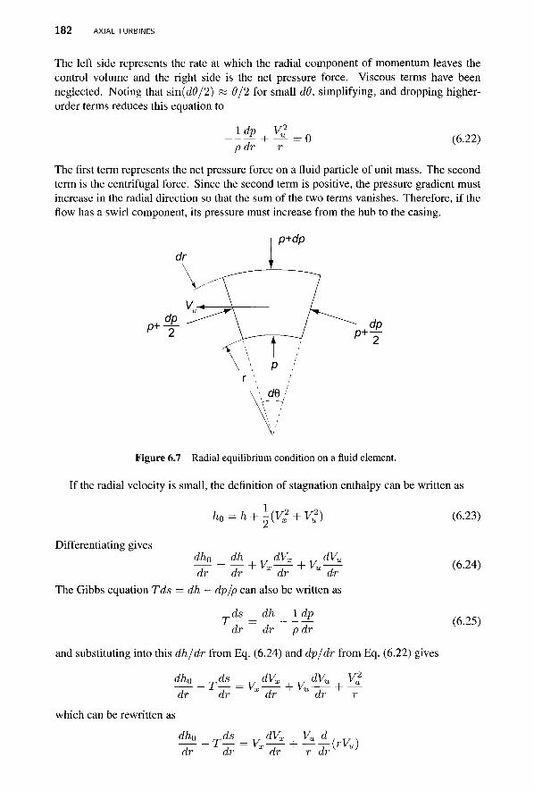
182 AXIAL TURBINES
The left side represents the rate at which the radial component of momentum leaves the control volume and the right side is the net pressure force. Viscous terms have been neglected. Noting that sm(d9/2) « 0/2 for small dO, simplifying, and dropping higher-order terms reduces this equation to
I dp p dr
V2 = 0 (6.22)
The first term represents the net pressure force on a fluid particle of unit mass. The second term is the centrifugal force. Since the second term is positive, the pressure gradient must increase in the radial direction so that the sum of the two terms vanishes. Therefore, if the flow has a swirl component, its pressure must increase from the hub to the casing.
p+dp
Figure 6.7 Radial equilibrium condition on a fluid element.
If the radial velocity is small, the definition of stagnation enthalpy can be written as
Differentiating gives
h0 = h+1-(Vx2 + V*)
dh0 _ dh dVx_ dVu
dr dr dr dr The Gibbs equation Tds = dh — dp/p can also be written as
ds dh 1 dp dr dr p dr
and substituting into this dh/dr from Eq. (6.24) and dp/dr from Eq. (6.22) gives
dh0 ds T dVx Tr dVu V2
dr dr dr dr r
(6.23)
(6.24)
(6.25)
which can be rewritten as
dh o T— = y ^ + Y^L — (ry ) dr dr dr r dr
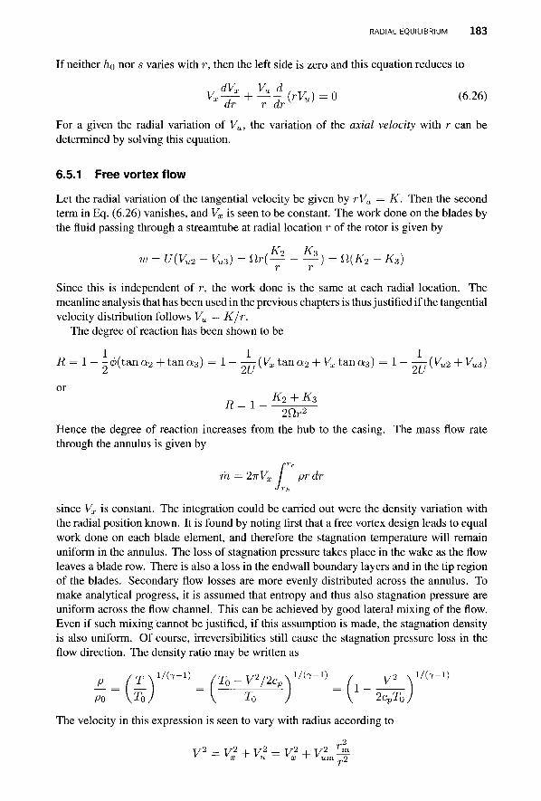
RADIAL EQUILIBRIUM 183
If neither HQ nor s varies with r, then the left side is zero and this equation reduces to
dr r dr
For a given the radial variation of Vu, the variation of the axial velocity with r can be determined by solving this equation.
6.5.1 Free vortex flow
Let the radial variation of the tangential velocity be given by rVu = K. Then the second term in Eq. (6.26) vanishes, and Vx is seen to be constant. The work done on the blades by the fluid passing through a streamtube at radial location r of the rotor is given by
w = U(Vu2 - Ka) = fir(^ - ^ ) = n(K2 - K3) r r
Since this is independent of r, the work done is the same at each radial location. The meanline analysis that has been used in the previous chapters is thus justified if the tangential velocity distribution follows Vu = K/r.
The degree of reaction has been shown to be
R= l - - 0 ( t a n a 2 + t a n a 3 ) = 1 - — (Vx t ana 2 + Vx t ana 3 ) = 1 - — {Vu2 + Vu3)
or
2Q,r2
Hence the degree of reaction increases from the hub to the casing. The mass flow rate through the annulus is given by
rh = 2irVx / pr dr Jrh
since Vx is constant. The integration could be carried out were the density variation with the radial position known. It is found by noting first that a free vortex design leads to equal work done on each blade element, and therefore the stagnation temperature will remain uniform in the annulus. The loss of stagnation pressure takes place in the wake as the flow leaves a blade row. There is also a loss in the endwall boundary layers and in the tip region of the blades. Secondary flow losses are more evenly distributed across the annulus. To make analytical progress, it is assumed that entropy and thus also stagnation pressure are uniform across the flow channel. This can be achieved by good lateral mixing of the flow. Even if such mixing cannot be justified, if this assumption is made, the stagnation density is also uniform. Of course, irreversibilities still cause the stagnation pressure loss in the flow direction. The density ratio may be written as
P_ = /TV'^-V = /^-y2/2c£y/(7-D = / _ _^2 x i / h -D
Po \ToJ V To J V 2cpT0
The velocity in this expression is seen to vary with radius according to
v2 = v2 + v2 = v2 + v2 r-^

184 AXIAL TURBINES
Here r m is the mean radius, at which the tangential velocity is Vum. Defining y = r/rm, the mass balance can be converted to the form
r 2 / ( l + K) / V2 V2 i \ 1/(7-1) v x urn
*/(!+*) V 2CPTO ^cpT0y2/
rh = 27rVxr2mPo h _ _JE_ _ _»^_L ) y d y (6.27)
J2K/(1 + K) V
in which rc/rm = 2 / (1 + K) , rh/rm = 2 K / ( 1 + K ) , and K = r^/rc. This integral can be evaluated in closed form, at least for values of 7 for which 1/(7 — 1) is an integer. But, for example, if 7 = | , the result of the integration is sufficiently complicated, that it is better to proceed by numerical integration.
Cohen et al. [15] use the mean radius as a reference value and express at the inlet to the rotor, the free vortex velocity distribution in the form
r2mVu2m = r2Vu2
which can be recast as r2mVx2 t a n a 2 m = r2Vx2 t an a2
from which it follows that t a n a 2 = —— tana^m (6.28)
T2
Here r 2 denotes an arbitrary radial position at the inlet of the rotor. Similarly, at the exit
t an a-i = —— tan a^m (6.29)
The relative velocity at the inlet is Wu2 = VU2 — U, from which
tan y02 = tan «2 U
or
Similarly
r2 1 tan /?2 = tan a2 — (6.30)
tan /3 3 = t a n a 3 — (6.31) ^3m03
These equations are valid even if the axial velocity differs between the inlet and exit of the rotor.
■ EXAMPLE 6.6
Combustion gases with 7 = | and R = 287 J / ( k g • K) expand through a turbine stage. The inlet stagnation temperature is T0i = HOOK and the stagnation pressure is P01 = 420 kPa. The mean radius is r m = 0.17 cm, and it is constant across the stage. The turbine is flared so that the axial velocity remains constant. The hub-to-casing radius is K2 = 0.7 at the inlet and K3 = 0.65 at exit of the rotor. The flow angles at the mean radius at the inlet are a2m = 60.08° and /3 2 m — 25.98°. At the exit the corresponding angles are a?,m = —21.20° and /?3m = —58.59°. The axial velocity is Vx = 231 m / s . (a) Plot the inlet and exit flow angles along the span of the blades, (b) Determine the reaction at the hub. (c) Calculate the mass flow rate using both numerical integration and the mean density.
RADIAL EQUILIBRIUM 185
Solution: (a) The reaction at the mean radius of this stage can be obtained by adding both parts of Eq. (6.16) together and doing the same for Eq. (6.12) and then dividing one by the other. This gives
1 _ tan a2m + tan a3m
Rm tan j32m + tan /33m
Substituting the values of the angles gives Rm = 0.460. The flow coefficient is then obtained from
4>m = * . R = 0-800 tan a2 m - tan p2m
and the blade-loading coefficient is
■tp = 2(1 — Rm — 0 m tana3 m ) = 1.700
The flow angles are next calculated using Eqs. (6.28) - 6.31. At the hub
1 + K 9 1.7 tan «2h = ~i—~ t a n a 2 m = -— tan(60.08°) =2.11 a2 h = 64.64°
2K2 1.4
tan/32h = i ± ^ t a n a 2 m - - ^ - \ = 1.08 /32h = 47.22° 2K2 1 + re2 (f>
At the casing
t ana 2 c = + K2 t a n a 2 m = ~y tan(60.08°) = 1.48 a2c = 55.90°
tan (32c = ^ - ^ tan a2m ~ —?— \ = 0.0064 /32c = 0.37° 2 1 + K2 cp
The exit angles are calculated similarly. They are
a3h = -26.72° /33h =-55 .90° a3c = -17.74° /33c = -61.41°
The variation in flow angles along the span is obtained from Eqs. (6.28) - (6.31), which, together with the blade shapes, are shown in Figure 6.8.
(b) The reaction at the hub is
Rh = 1 Y [ ~o J ( t a n a2m + t a n a?im>
= 1 - ^ C^A (tan(60.08°) + tan(-21.2°)) = 0.204
(c) The mass flow rate is calculated from Eq. (6.27). The stagnation density is Poi 420,000 3
^ 1 = i ^ 1= 2 8 7 T T l 0 0 = 1 - 3 3 0 k g / m
With hub radius rh = 0.14 m, and casing radius, rc = 0.20 m, numerical integration gives
m = 15.068 kg/s
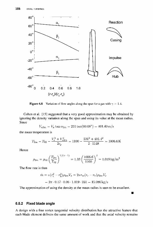
186 AXIAL TURBINES
80c
60c
40c
20c
0C
-20c
-40c
-60c
-80c
— - ^ - - _
^ ^ ^ ^ 1
^______^__
p3
Reaction
Casing
Impulse
Hub
0 0.2 0.4 0.6 0.8 1 0
Figure 6.8 Variation of flow angles along the span for a gas with 7 = 1.4.
Cohen et al. [15] suggested that a very good approximation may be obtained by ignoring the density variation along the span and using its value at the mean radius. Since
Kx2m = Vxtana2m = 231 tan(60.08°) = 401.40 m/s
the mean temperature is
T2m = T02
Hence
V2 + V\ x u2m = 1100 2c„
2312+401.42
2-1148 = 1006.6 K
p2m — P02 12m
T< 02
1/(7-1)
- ( ^ ) * — " «/-■ The flow rate is then
m = n(r2 - rl)p2mVx = 2irrm(rc - rh)p2myx
= 2TT • 0.17 • 0.06 • 1.019 • 231 = 15.086 kg/s
The approximation of using the density at the mean radius is seen to be excellent.
6.5.2 Fixed blade angle
A design with a free vortex tangential velocity distribution has the attractive feature that each blade element delivers the same amount of work and that the axial velocity remains
CONSTANT MASS FLUX 187
constant. On the other hand, the reaction varies quite strongly along the span of the blade. Other design possibilities exist. For example, if the nozzle angle is kept constant along the span, manufacturing cost of nozzles can be reduced. As the flow moves through the nozzles its stagnation enthalpy will not change, and, if the radial entropy gradients may be neglected, the equation for radial equilibrium
dr dr dr dr r
reduces to TrdVx Tr dVu V2
n V - 4- V - -I — = 0
dr dr r as before. This can also be written as
dr l 2 x 2 " / r
' X ' ' U Since VU = V sin a and V2 + V2 = V2 this becomes
dV V2sin2a
or
If the angle a is constant,
dr
dV _ V
integrating gives
V{r) vm
r
- sin2 a dr r
(T)
0
(6.32)
In addition, Vu = V sin a and Vx = V cos a, so that for constant a
sin2QT/ _ _ s i n 2 Q m T / ' v u — ' m *um
For nozzles the exit flow angle is quite large (often between 60° and 70°). Therefore sin2Qf2 is in the range 0.75 - 0.88 and the velocity distribution is nearly the same as for a free vortex. The rotor blades may then be twisted properly to give the free vortex distribution at their exit.
6.6 CONSTANT MASS FLUX
It has been seen that, if the tangential velocity varies inversely with radius, axial velocity is independent of radius. Since the density varies also, Horlock [35] suggested that a designer might decide to hold the axial mass flux pVx constant. This requires the blade angle to vary in such a way that
pVcos a = pm Vm cos am
remains independent of radius. The flow angle in terms of the velocity and density ratios is therefore
cos a Vmpm = - — — (6.33) cos am V p
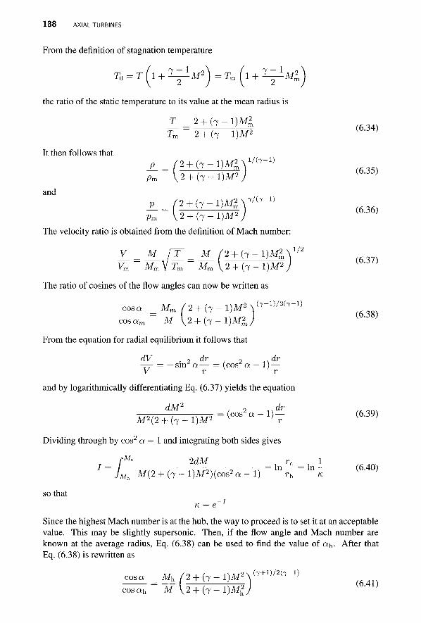
188 AXIAL TURBINES
From the definition of stagnation temperature
7 - 1 , ^ _rr (, , 7 - 1 . ,2 T0 = T I 1 + ^-M'j = Tm I 1 + ^~M,
the ratio of the static temperature to its value at the mean radius is
T 2 + ( 7 - 1)M2
It then follows that
and
Tm 2 + ( 7 - 1)M2
p / 2 + ( 7 - l ) M ^ \ 1 / ( 7 " 1 )
p m V 2 + (7 - l)Af
P 2 + (7^1)M2V/ ( 7-1 )
Pm V2 + ( 7 - l ) M 2 . The velocity ratio is obtained from the definition of Mach number:
V _ M j~T _ M / 2 + ( 7 - l ) M , 2 x l / 2
Vm Mm\Tm M m V 2 + ( 7 - l ) M 2
The ratio of cosines of the flow angles can now be written as
cos a Mm ( 2 + (7 - 1)M2 N ^ W ^ " 1 ) cosaTO M V2 + ( 7 - l ) M 2 ,
From the equation for radial equilibrium it follows that
dV . 2 dr 2 dr —— — —sin a— = (cos a — 1) — V r r
and by logarithmically differentiating Eq. (6.37) yields the equation
(6.34)
(6.35)
(6.36)
(6.37)
(6.38)
cos2 a-I)— (6.39) M2(2 + ( 7 - l ) M 2 v 'r
Dividing through by cos2 a — 1 and integrating both sides gives
[Mc 2dM rc 1 I = JMh M(2 + (7 - l)M2)(cos2 a - 1) = l n r ^ = l n K ( 6 ' 4 0 )
so that K = e"1
Since the highest Mach number is at the hub, the way to proceed is to set it at an acceptable value. This may be slightly supersonic. Then, if the flow angle and Mach number are known at the average radius, Eq. (6.38) can be used to find the value of a^. After that Eq. (6.38) is rewritten as
cos a Mh ^2 + ( 7 - l ) M 2 V 7 + 1 ) / 2 ( 7 _ 1 )
— (6.41) cosah M \ 2 + ( 7 - l ) M ^
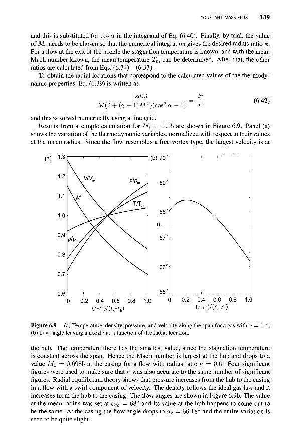
CONSTANT MASS FLUX 189
and this is substituted for cos a in the integrand of Eq. (6.40). Finally, by trial, the value of Mc needs to be chosen so that the numerical integration gives the desired radius ratio K. For a flow at the exit of the nozzle the stagnation temperature is known, and with the mean Mach number known, the mean temperature Tm can be determined. After that, the other ratios are calculated from Eqs. (6.34) - (6.37).
To obtain the radial locations that correspond to the calculated values of the thermody-namic properties, Eq. (6.39) is written as
2dM dr M(2 + ( 7 - l ) M 2 ) ( c o s 2 a - l )
(6.42)
and this is solved numerically using a fine grid. Results from a sample calculation for M^ = 1.15 are shown in Figure 6.9. Panel (a)
shows the variation of the thermodynamic variables, normalized with respect to their values at the mean radius. Since the flow resembles a free vortex type, the largest velocity is at
(a)
69°
68°
a
67°
66°
65° 0.2 0.4 0.6 0.8
(r-rhV(rc-rh) 0.2 0.4 0.6 0.8 1.0
Figure 6.9 (a) Temperature, density, pressure, and velocity along the span for a gas with 7 (b) flow angle leaving a nozzle as a function of the radial location.
1.4;
the hub. The temperature there has the smallest value, since the stagnation temperature is constant across the span. Hence the Mach number is largest at the hub and drops to a value Mc = 0.6985 at the casing for a flow with radius ratio K = 0.6. Four significant figures were used to make sure that K was also accurate to the same number of significant figures. Radial equilibrium theory shows that pressure increases from the hub to the casing in a flow with a swirl component of velocity. The density follows the ideal gas law and it increases from the hub to the casing. The flow angles are shown in Figure 6.9b. The value at the mean radius was set at am = 68° and its value at the hub happens to come out to be the same. At the casing the flow angle drops to ac = 66.18° and the entire variation is seen to be quite slight.
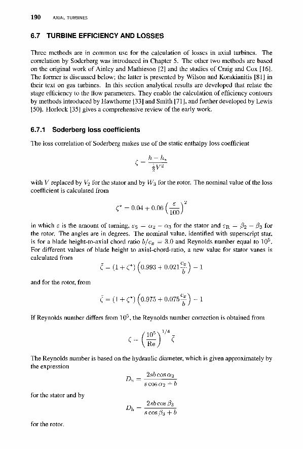
190 AXIAL TURBINES
6.7 TURBINE EFFICIENCY AND LOSSES
Three methods are in common use for the calculation of losses in axial turbines. The correlation by Soderberg was introduced in Chapter 5. The other two methods are based on the original work of Ainley and Mathieson [2] and the studies of Craig and Cox [16]. The former is discussed below; the latter is presented by Wilson and Korakianitis [81] in their text on gas turbines. In this section analytical results are developed that relate the stage efficiency to the flow parameters. They enable the calculation of efficiency contours by methods introduced by Hawthorne [33] and Smith [71], and further developed by Lewis [50]. Horlock [35] gives a comprehensive review of the early work.
6.7.1 Soderberg loss coefficients
The loss correlation of Soderberg makes use of the static enthalpy loss coefficient
_ h- hs
2 y
with V replaced by Vi for the stator and by Wz for the rotor. The nominal value of the loss coefficient is calculated from
C* = 0.04 + 0.06 ( ^ ) 2
in which e is the amount of turning, es = a2 — a 3 for the stator and £R = fa — /?3 for the rotor. The angles are in degrees. The nominal value, identified with superscript star, is for a blade height-to-axial chord ratio b/cx = 3.0 and Reynolds number equal to 105. For different values of blade height to axial-chord-ratio, a new value for stator vanes is calculated from
C = (1 + O (0-993 + 0 .021y) - 1
and for the rotor, from
< = (1 + O (0.975 + 0 .075y) - 1
If Reynolds number differs from 105, the Reynolds number correction is obtained from
The Reynolds number is based on the hydraulic diameter, which is given approximately by the expression
2s6cosa2
for the stator and by
Dh
for the rotor.
S COS «2 + b
2s6cos/33 s cos ^3 + b
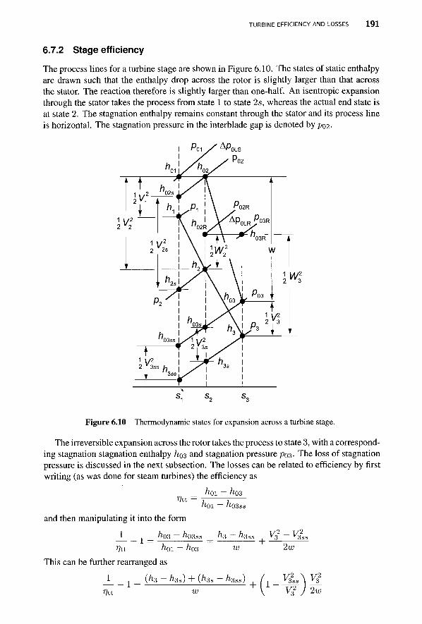
TURBINE EFFICIENCY AND LOSSES 1 9 1
6.7.2 Stage efficiency
The process lines for a turbine stage are shown in Figure 6.10. The states of static enthalpy are drawn such that the enthalpy drop across the rotor is slightly larger than that across the stator. The reaction therefore is slightly larger than one-half. An isentropic expansion through the stator takes the process from state 1 to state 2s, whereas the actual end state is at state 2. The stagnation enthalpy remains constant through the stator and its process line is horizontal. The stagnation pressure in the interblade gap is denoted by po2-
Figure 6.10 Thermodynamic states for expansion across a turbine stage.
The irreversible expansion across the rotor takes the process to state 3, with a correspond-ing stagnation stagnation enthalpy ho3 and stagnation pressure po3. The loss of stagnation pressure is discussed in the next subsection. The losses can be related to efficiency by first writing (as was done for steam turbines) the efficiency as
^01 — ^03 »7tt
and then manipulating it into the form
_1 , _ hp3 — hp3ss
ritt h0i ~ h
*01 — "03ss
h3 - h3aa + V£ - V£ss
03
This can be further rearranged as
1 ??tt
- 1 (h3 - h3s) + (h3s - h3ss)
w
2w
YL 2w
192 AXIAL TURBINES
The first term in the numerator is simply
h3 ~ h3s = -CRW*
Next, integrating the Gibbs equation along the constant-pressure line p3 from state 3ss to 3s gives
, T3s s2-si= cp In —— J-3ss
Similarly, integration along the constant pressure line p2 yields
T2 s2 - Si = cp In ; t-2s
Equating the RHSs gives T3s = T2
T3ss T2s
Subtracting one from each side, rearranging, and multiplying by cp gives
(6.43)
h3s — h3ss — ——(h2 — h2s) J-2s
Since T3ss/T2s = T3s/T2 and
h2 ~ h2s = -Cs^ 22
the expression for efficiency can be written as
1 1 2sw T2
(RWi + ^CsV? + ( 1 -L
3SS V'
In the last term the equality V32ss/V3
2 = T3sa/T3 was used, which follows from the fact that M3 = M3ss, as was shown in Chapter 5. Furthermore, since Vx = W3COS/33 = V2 cos a2 = V3 cos 0:3, the expression for efficiency can be recast as
1 1
ritt 2?/>
Often this is approximated by
1
CR , T3s Cs COS2/33 T2 COS2Qf2
T, 3SS
COS2Ct3
1 CR CS
rjtt 2tp \cos2/33 cos 2 a 2
It will shown in an example that the error in using this approximation is very small.
(6.44)
(6.45)
6.7.3 Stagnation pressure losses
The stagnation pressure drop across the stator can be related to the static enthalpy loss coefficient by first integrating the Gibbs equation along the constant-stagnation-pressure line/ioi = h02:
' Po i ' S2 ~ Si Rln
P02

TURBINE EFFICIENCY AND LOSSES 1 9 3
Similarly, integrating the Gibbs equation along the constant-pressure line p2 gives
S2-Sl = 7^Tlnte / T \7/(7"l)
Equating the RHSs gives
P02 \T 2 |
The definition for the static enthalpy loss coefficient
1
can be written as
from which
2s = 7,CsV2
7 - 1 . w 2 , T2-T2s = -^CsMi1RT2
T2 A 7 - 1 x ' T . 1 - ^ C s M | J2s V ^
Since the second term involving the Mach number is small, this can be expanded as
T2s 2 Sb 2
The pressure ratio P01/P02 is therefore
and expanding this gives ^ = l + ^CsM| P02 2
The expression for the stagnation pressure loss now takes the form
ApoLS = 0P02CS-M22 = -^/902CsV22
Z I ±2
or APOLS = P02 (1 + ^ M2
2) 1 Cs V22 (6.46)
Since the loss coefficient C$ is rather insensitive to Mach number, this shows how the stagnation pressure loss increases as compressibility becomes important.
The development of the stagnation pressure loss across the rotor is similar. It will be carried out in detail in order to highlight the use of stagnation properties on the basis of relative velocity. First, the stagnation enthalpy of relative motion is defined as
frosR = h3 + -Wj
and in using the Mach number in terms of W3, defined as
W3 M3R = 7TS5!

194 AXIAL TURBINES
this can be rewritten in the form
T3 2 3 R
The relative stagnation pressure is calculated from
P3 " V 1 + 2 MsR
Since /102R = /k>3R across the rotor, integrating the Gibbs equation along the line of constant relative stagnation enthalpy and also along the constant-pressure line p%, gives
s 3 - s 2 = i ? l n s 3 - s2 = cp In —— P03R -*3s
so that Pom = (Ts_V^-1]
P03R \T3s)
From the definition for static enthalpy loss coefficient for the rotor
h3 ~ h3s = \CnWi
the temperature ratio
is obtained. Noting again that the term involving the Mach number is small and expanding the RHS gives
~ - = 1 + ^ C R M 32
R ±3s ^
and the pressure ratio P02R/P03R is therefore
P03R \ 2
Expanding this gives
1 + K R M | R P03R 2
The stagnation pressure loss across the rotor is therefore
ApoLR - -P03RCR^3R = ^^^P03RC,RW% Z I I3
or
APOLR = P03R ( 1 + ^ M f n J \CRW^ (6-47)
TURBINE EFFICIENCY AND LOSSES 1 9 5
EXAMPLE 6.7
Combustion gases with 7 = § and cp = 1148 J/(kg ■ K) flow through a normal turbine stage with R = 0.60. The flow enters the stator at a.\ = —33.0° and leaves at velocity V2 = 450 m/s. The inlet stagnation temperature is 1200 K, and the inlet stagnation pressure is 15 bar. The flow coefficient is <f> = 0.7, the blade height-to-axial chord ratio is b/cx = 3.5, and the Reynolds number is 105. Find the efficiency of the stage.
Solution: The blade-loading coefficient is first determined from
■4> = 2(1 - R - 0 t a n a 3 ) = 2(1 - 0.6 - 0.7tan(-33°)) = 1.709
The flow angle leaving the stator is
, (l-R + ip/2\ 1 / l - 0 . 6 + 1 . 7 0 9 / 2 \ „„ O J O a2 = tarT1 -—^— = t a n - 1 ^- '— = 60.84° / l - 0 . 6 + 1 . 7 0 9 / 2 \ V 0J )
and the angle of the relative velocity leaving the stage is
1f-R-i!/2\ j / - 0 . 6 - 1 . 7 0 9 / 2 \ & = tan"1 I - ^ - J = tan"1 ( — '— \ = -64.30°
The angle of the relative velocity at the inlet of the rotor is
h = t a n - ( = ^ ) = t a n - ( ^ ± i M ? ) = 19.99°
The deflections are therefore
es = a2 - ai = 60.84 + 33.00 = 93.84°
£R = P2- Ps = 19.99 + 64.30 = 84.29°
and the loss coefficients can now be calculated. First, the nominal values are
/ f o \2 / 93 8 4 \ 2
Cs = 0.04 + 0.06 ( ^ J = 0.04 + 0.06 ( ^ 5 - I =0.0928
and / £■„ \ 2 / 84 29"
CR = 0.04 + 0.06 ( - £ - ) = 0.04 + 0.06 - — - I = 0.0826 1 \
V100V " ' " ' ' V ioo~
When corrected for b/cx = 3.5 they are
Cs = (1 + Cs) (o.993+0.021y ) - 1 = (1 + 0.0928) (0.993+ ^ y 1 ) = 0-0917
(R = (1 + CR) ( o . 9 7 5 + 0 . 0 7 5 ^ ) - l = (l+0.0826) ( o . 9 7 5 + ^ ^ j =0.0788
The axial velocity is
Vx = V2cosa2 = 450cos(60.84°) = 219.26 m/s
196 AXIAL TURBINES
and the tangential velocity leaving the rotor is
Vu3 = 14 t ana 3 = 219.26 tan(-33°) = -142.39 m/s
so that Vs = \l^x + Vus = \/219.262 + 124.392 = 261.44 m/s
The blade speed is U = Vx/<fi = 219.26/0.7 = 313.23 m/s. The tangential compo-nent of the relative velocity leaving the stage is
Wu3 = Vu3 - U = -142.39 - 313.23 = -455.62 m/s
so that
W3 = y % 2 + W%3 = A/219 .26 2 + 455.622 = 505.63 m/s
The work done by the stage is w = ipU2 = 1.709 • 313.232 = 167.69 kJ/kg. An approximate value for the stage efficiency may now be obtained by setting T3ss = T2s and T3ss = T3 in
1 (nWi + ^(sVi + (l " | f ) V32
so that this expression evaluates to
1 1 0.0788 • 505.632 + 0.0917 • 4502 „ n „ I = — 0.124
77tt 2 ■ 167690
with the result that r)tt = 0.8965. To see the extent to which neglecting the temperature ratio T3s/T2 and the ki-
netic energy correction changes the efficiency, these terms are calculated next. The isentropic stage work is ws = W/T]U - 167.69/0.8965 = 187.05 kJ /kg . With T02 = Toi = 1200 K, the exit temperature is
T03 = T02-™ = 1 2 0 0 - ^ = 1053.9 K cp 1148
and for an isentropic process it is
. T03ss = T 0 2 - ^ = 1 2 0 0 - 1 ^ = 1037.1 K cp 1148
The static temperature at the exit is
V2 252 092
T 3 = T 0 3 - ^ = 1053.9- ^ = 1024.2 K
and T3ss can be calculated from
T3ss = ^ T 3 = ^ i 1024.2 = 1007.8 K s T03 1053.9
TURBINE EFFICIENCY AND LOSSES 197
From the definition of static enthalpy loss coefficient across the rotor
T3 s = T3 - W% = 999.0 - ° - ° 7 8 8 - 5 0 5 - 6 3 2 = 1015.4 K
In addition T2 = T02 - -^- = 1200 - „ ~ : ,„ = 1111.8K
V22 4502
2cp 2 -1148 so that
1 0.0788 • 505.632 + ±2IM Q 0 g l 7 . 4 5 Q 2 + r} _ I2gL|)261.442
1 = i i i i ^ m^M = 0.1154 y?tt 2 • 167690
Therefore the total-to-total efficiency of the stage is r?tt = 0.8965, which to four significant figures is the same as that without the temperature and velocity correction. The temperature correction makes the loss through the rotor lower, but the velocity correction adds slightly to the losses, with the net result that these are compensating errors, and the shorter calculation gives an accurate result.
The stagnation pressure at the exit of the stator is obtained from
P02 2
The Mach number is
V2 450 M 2 = . ' = . = 0.690
VjRT2 Vl-333-287- 1111.8 so that
poi 2 • 0.0917 ■ 0.6902 „ 1500 — = 1 + 5 = 1.0291 P02 = 7 7 ^ 7 = 1457.6 kPa P02 3 1.0291
and the stagnation pressure loss across the stator is
Ap0Ls = 1500 - 1457.6 = 42.4 kPa
To calculate the loss of stagnation pressure across the rotor, the relative and absolute Mach numbers at the exit are determined first:
V3 261.44 M3 = ; ' = . = 0.4176
s/WTz Vl-333-287- 1024.2 W3 505.63
M 3 R = , ; L = . = 0.8077 V7RT3 Vl .333 • 287 • 1024.2
Then stagnation pressure at the exit is
«-=»»(^r"i,=iMo(w)'-,B,u,kp' and P3 is
/ - 7 - 1 „ V 7 / ( 7 _ 1 ) / 0 4 1 7 6 2 \ - 4
P3 = P03 1 + L^^Ml = 836.8 1 + — = 746.14 kPa

198 AXIAL TURBINES
The stagnation pressure po3R is obtained from
\ 7 / ( 7 - l ) P03R = P 3 1 l ^ M 2
3R = 746.14 1 + 0.8077" 6
1127.5 kPa
and the value of P02R is then
P02R = P03R ( l + |CflM32
R) = 1127.5 (l + I 0.088 • 0.80772") = 1166.1 kPa
so that the loss of stagnation pressure across the rotor is
APOLR = H66.1 - 1127.5 = 38.6 kPa
6.7.4 Performance charts
A useful collection of turbine performance characteristics was compiled by Smith [71] in 1965. His chart is shown in Figure 6.11. Each design is labeled in a small circle by the value of efficiency that may be achieved for a given choice of flow coefficient <j> = Vx/U and a stage-loading coefficient ip = w/U2 = Aho/U2. The curves of constant efficiency are based on a theory by Smith. He took blade losses other than tip losses into account, and for this reason the actual values of efficiency are expected to drop slightly.
Lines of constant efficiency
c CD 'o it CD o o en c
T 3 CD CD
J3 CO
3 0.4 0.5 0.6 0.7 0.8 0.8 1.0 1.1 1.2 1.3
Flow coefficient $ = VJU
Figure 6.11 Variation of measured stage efficiency with stage loading coefficient and flow coefficient for axial-flow turbines. (Adapted from Smith [71].)
The flow coefficients in the range from 0.6 < <j> < 1.0 give uncorrected efficiencies in a range from 90% to 94%, depending on how heavily loaded the blades are. Typical turbines
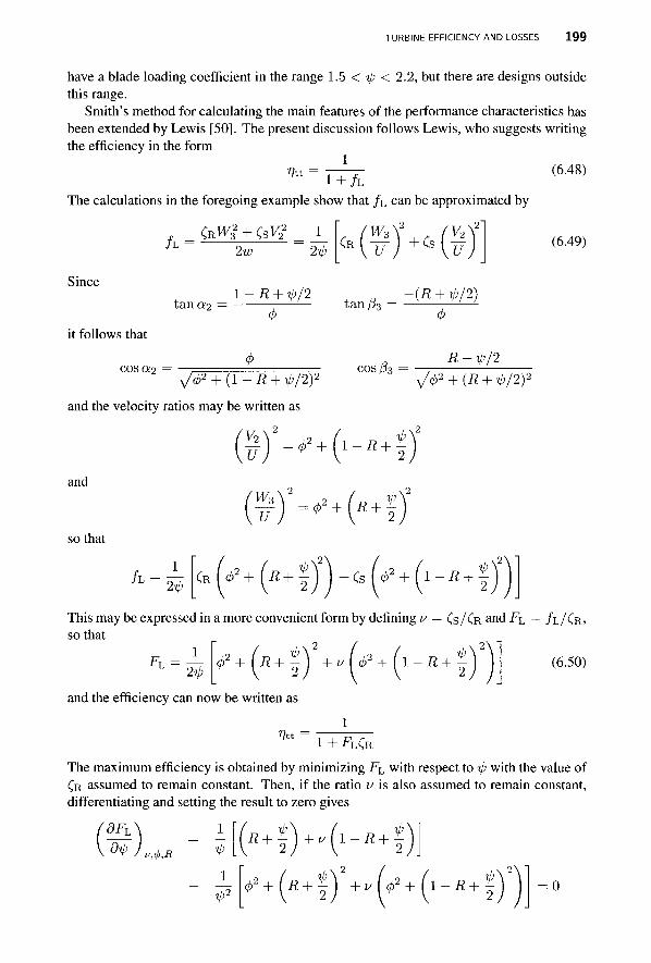
TURBINE EFFICIENCY AND LOSSES 199
have a blade loading coefficient in the range 1.5 < ip < 2.2, but there are designs outside this range.
Smith's method for calculating the main features of the performance characteristics has been extended by Lewis [50]. The present discussion follows Lewis, who suggests writing the efficiency in the form
1
The calculations in the foregoing example show that / L can be approximated by
/ L
Since
it follows that
cosa^
tan«2
CP Wl + Cs^l l 2w 2ip
l-R + tp/2
<*mM%
(6.48)
(6.49)
V 0 2 + (1 - R + ^ / 2 ) 2
and the velocity ratios may be written as
Yi u
tan/33
cos/33
1 -R +
-(R + rf>/2)
R + ijj/2 vV 2 + 0R + V>/2)2
i,
and
so that
U R + 2
1 2AP
R i, Cs + [1-R + *l>
This may be expressed in a more convenient form by defining v = CS/CR a nd -PL = JL/CR>
so that
FT, 1
24> "+lR+t + v 1 -R + i> (6.50)
and the efficiency can now be written as
i + ^LCR
The maximum efficiency is obtained by minimizing FL with respect to tp with the value of CR assumed to remain constant. Then, if the ratio v is also assumed to remain constant, differentiating and setting the result to zero gives
dFL 1
l ^ 2
R+±yvu-R+± «+lR+t + 1-R + 1> = 0
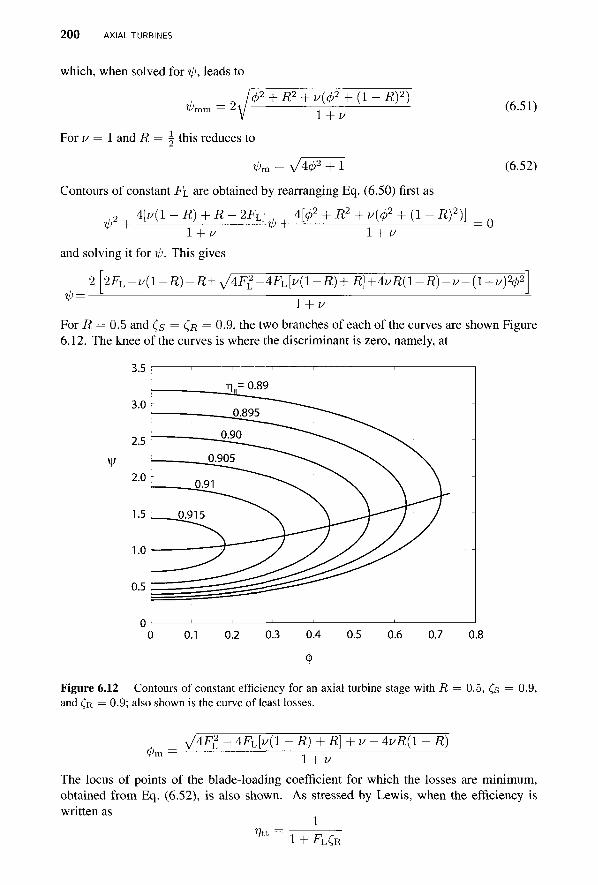
200 AXIAL TURBINES
which, when solved for tp, leads to
Ipn + R2 + is(<j)2 + (1 - Rf
l + v
For v = 1 and R= \ this reduces to
V»m - V 7 ^ 2 + 1
Contours of constant F L are obtained by rearranging Eq. (6.50) first as
^ 2 + 4[v(l-R)+R-2Fh] + 4 # 2 + fl2 + ̂ 2 + (1 - fl)2)] = Q
(6.51)
(6.52)
l + v
and solving it for tp. This gives l + i/
V> = 2FL-v(l-R)-R±^4Fl-4FLlv(l-R)+R}+4vR(l-R)-is-(l + v)24
l + y
For i? = 0.5 and Cs = Cfl = 0-9, the two branches of each of the curves are shown Figure 6.12. The knee of the curves is where the discriminant is zero, namely, at
V
Figure 6.12 Contours of constant efficiency for an axial turbine stage with R = 0.5, Cs = 0.9, and £R = 0.9; also shown is the curve of least losses.
_ yjAF2 - AFh[v{l -R) + R]+v- AvR{\ =R) 4>m~ 1 + v
The locus of points of the blade-loading coefficient for which the losses are minimum, obtained from Eq. (6.52), is also shown. As stressed by Lewis, when the efficiency is written as
»7tt 1
1 + F L C R
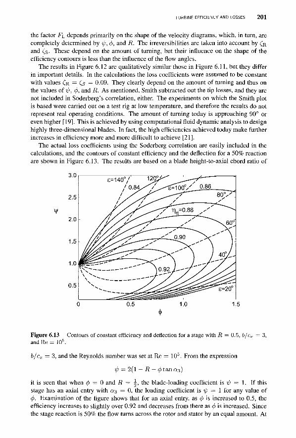
TURBINE EFFICIENCY AND LOSSES 2 0 1
the factor FL depends primarily on the shape of the velocity diagrams, which, in turn, are completely determined by ip, <p, and R. The irreversibilities are taken into account by fa and Cs- These depend on the amount of turning, but their influence on the shape of the efficiency contours is less than the influence of the flow angles.
The results in Figure 6.12 are qualitatively similar those in Figure 6.11, but they differ in important details. In the calculations the loss coefficients were assumed to be constant with values CR = Cs = 0.09. They clearly depend on the amount of turning and thus on the values of ip, <fi, and R. As mentioned, Smith subtracted out the tip losses, and they are not included in Soderberg's correlation, either. The experiments on which the Smith plot is based were carried out on a test rig at low temperature, and therefore the results do not represent real operating conditions. The amount of turning today is approaching 90° or even higher [19]. This is achieved by using computational fluid dynamic analysis to design highly three-dimensional blades. In fact, the high efficiencies achieved today make further increases in efficiency more and more difficult to achieve [21].
The actual loss coefficients using the Soderberg correlation are easily included in the calculations, and the contours of constant efficiency and the deflection for a 50% reaction are shown in Figure 6.13. The results are based on a blade height-to-axial chord ratio of
3.0
2.5
2.0
1.5
1.0
0.5
0 0.5 1.0 1.5
Figure 6.13 Contours of constant efficiency and deflection for a stage with R = 0.5, b/cx = 3, and Re = 106.
b/cx = 3, and the Reynolds number was set at Re = 105. From the expression
ip = 2(1 - R-(j)tana3)
it is seen that when (p — 0 and R — \, the blade-loading coefficient is ip = 1. If this stage has an axial entry with 0:3 = 0, the loading coefficient is ip = 1 for any value of (p. Examination of the figure shows that for an axial entry, as <p is increased to 0.5, the efficiency increases to slightly over 0.92 and decreases from there as <p is increased. Since the stage reaction is 50% the flow turns across the rotor and stator by an equal amount. At
\
6=140°/' 1 2 0 ^ ^^7^~~~ / 0 . R 4 / / ^<U\tf/ 0.86
/ y ^ y __——^l_o.90 ><- \
g ^ ^ ~7>r' \ J \$L §2&**
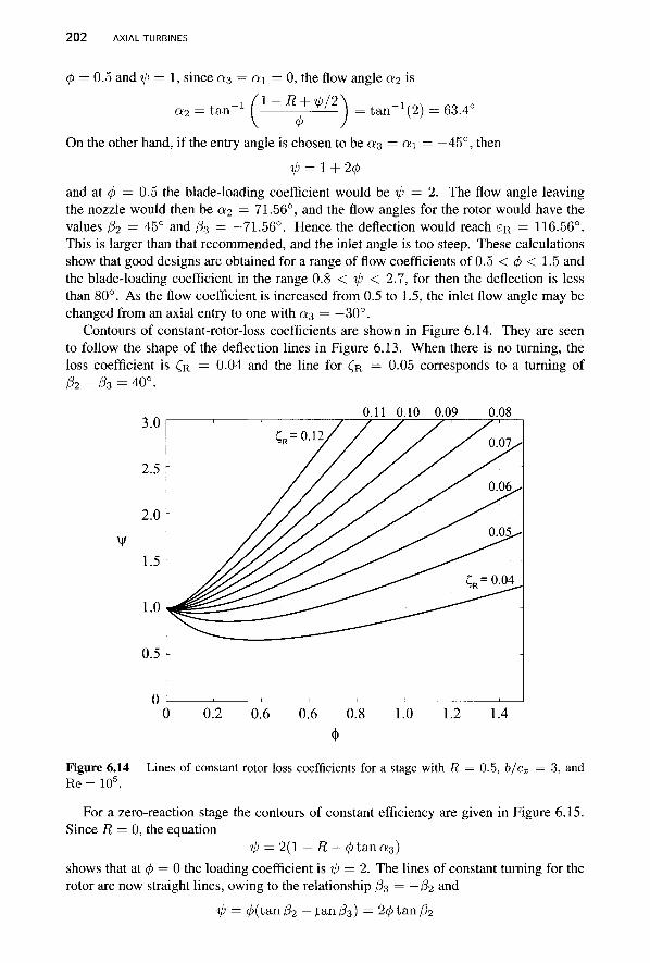
202 AXIAL TURBINES
<p = 0.5 and ip = 1, since a^ — a.\ = 0, the flow angle «2 is
a2 = t a n - i (l~R^,2\ = tan"1 (2) = 63.4°
On the other hand, if the entry angle is chosen to be a 3 = ot\ = —45°, then
ip = 1 + 20
and at <p = 0.5 the blade-loading coefficient would be ip = 2. The flow angle leaving the nozzle would then be «2 = 71.56°, and the flow angles for the rotor would have the values /?2 = 45° and 03 = —71.56°. Hence the deflection would reach £R = 116.56°. This is larger than that recommended, and the inlet angle is too steep. These calculations show that good designs are obtained for a range of flow coefficients of 0.5 < <j> < 1.5 and the blade-loading coefficient in the range 0.8 < ip < 2.7, for then the deflection is less than 80°. As the flow coefficient is increased from 0.5 to 1.5, the inlet flow angle may be changed from an axial entry to one with 0:3 = —30°.
Contours of constant-rotor-loss coefficients are shown in Figure 6.14. They are seen to follow the shape of the deflection lines in Figure 6.13. When there is no turning, the loss coefficient is £R = 0.04 and the line for £FI = 0.05 corresponds to a turning of & - & = 40°.
0.11 0.10 0.09 0.08
01 , , , , , , ,—1 0 0.2 0.6 0.6 0.8 1.0 1.2 1.4
Figure 6.14 Lines of constant rotor loss coefficients for a stage with R = 0.5, b/cx = 3, and Re = 106.
For a zero-reaction stage the contours of constant efficiency are given in Figure 6.15. Since R = 0, the equation
ip = 2(1 - R-4>tana3) shows that at <j> = 0 the loading coefficient is ip = 2. The lines of constant turning for the rotor are now straight lines, owing to the relationship $3 = — P2 and
ip = 0(tan/?2 — fan/33) = 2<£ tan 02
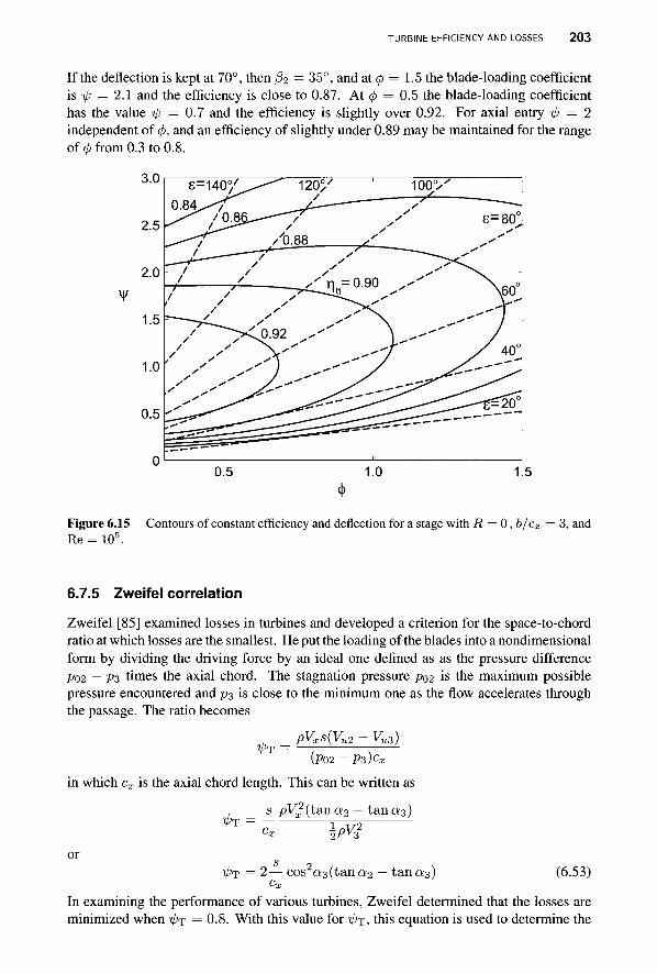
TURBINE EFFICIENCY AND LOSSES 2 0 3
If the deflection is kept at 70°, then /32 — 35°, and at <f> = 1.5 the blade-loading coefficient is ip = 2.1 and the efficiency is close to 0.87. At 0 = 0.5 the blade-loading coefficient has the value tp = 0.7 and the efficiency is slightly over 0.92. For axial entry ip = 2 independent of <j>, and an efficiency of slightly under 0.89 may be maintained for the range of <b from 0.3 to 0.8.
V
Figure 6.15 Contours of constant efficiency and deflection for a stage with R = 0, b/cx = 3, and Re = 105.
6.7.5 Zweifel correlation
Zweifel [85] examined losses in turbines and developed a criterion for the space-to-chord ratio at which losses are the smallest. He put the loading of the blades into a nondimensional form by dividing the driving force by an ideal one defined as as the pressure difference P02 — Pz times the axial chord. The stagnation pressure P02 is the maximum possible pressure encountered and p% is close to the minimum one as the flow accelerates through the passage. The ratio becomes
ipi pVxs(Vu2 - Vu3)
(Po2 -Ps)cx
in which cx is the axial chord length. This can be written as
s pVrx
2(tana2 — tan a3) ip-i \pvi
or T/>T = 2— cos2a3(tana2 — tanas) (6.53)
In examining the performance of various turbines, Zweifel determined that the losses are minimized when ip^ = 0.8. With this value for V'T, this equation is used to determine the
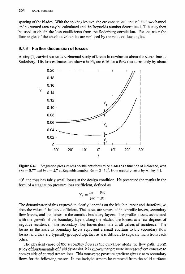
204 AXIAL TURBINES
spacing of the blades. With the spacing known, the cross-sectional area of the flow channel and its wetted area may be calculated and the Reynolds number determined. This may then be used to obtain the loss coefficients from the Soderberg correlation. For the rotor the flow angles of the absolute velocities are replaced by the relative flow angles.
6.7.6 Further discussion of losses
Ainley [1] carried out an experimental study of losses in turbines at about the same time as Soderberg. His loss estimates are shown in Figure 6.16 for a flow that turns only by about
0.20
0.18
0.16 y
0.14
0.12
0.10
0.08
0.06
0.04
0.02
0 -30° -20° -10° 0° 10° 20° 30°
/
Figure 6.16 Stagnation pressure loss coefficients for turbine blades as a function of incidence, with s/c = 0.77 and b/c = 2.7 at Reynolds number Re = 2 • 105, from measurements by Ainley [1].
40° and thus has fairly small losses at the design condition. He presented the results in the form of a stagnation pressure loss coefficient, defined as
Y = Poi ~ -PQ2 P P02 ~ P2
The denominator of this expression clearly depends on the Mach number and therefore, so does the value of the loss coefficient. The losses are separated into profile losses, secondary flow losses, and the losses in the annulus boundary layers. The profile losses, associated with the growth of the boundary layers along the blades, are lowest at a few degrees of negative incidence. The secondary flow losses dominate at all values of incidence. The losses in the annulus boundary layers represent a small addition to the secondary flow losses, and they are typically grouped together as it is difficult to separate them from each other.
The physical cause of the secondary flows is the curvature along the flow path. From study of fundamentals of fluid dynamics, it is known that pressure increases from concave to convex side of curved streamlines. This transverse pressure gradient gives rise to secondary flows for the following reason. In the inviscid stream far removed from the solid surfaces
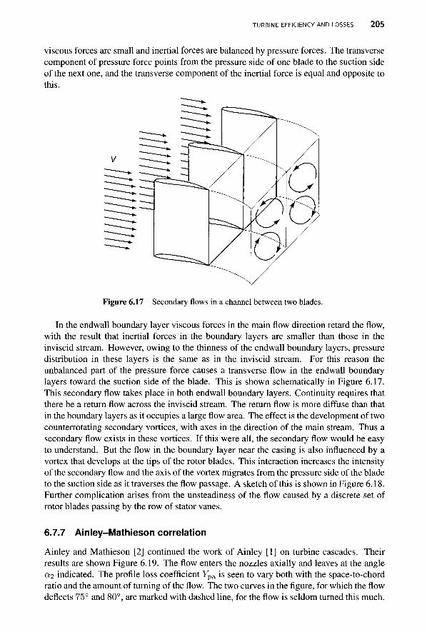
TURBINE EFFICIENCY AND LOSSES 2 0 5
viscous forces are small and inertial forces are balanced by pressure forces. The transverse component of pressure force points from the pressure side of one blade to the suction side of the next one, and the transverse component of the inertial force is equal and opposite to this.
Figure 6.17 Secondary flows in a channel between two blades.
In the endwall boundary layer viscous forces in the main flow direction retard the flow, with the result that inertial forces in the boundary layers are smaller than those in the inviscid stream. However, owing to the thinness of the endwall boundary layers, pressure distribution in these layers is the same as in the inviscid stream. For this reason the unbalanced part of the pressure force causes a transverse flow in the endwall boundary layers toward the suction side of the blade. This is shown schematically in Figure 6.17. This secondary flow takes place in both endwall boundary layers. Continuity requires that there be a return flow across the inviscid stream. The return flow is more diffuse than that in the boundary layers as it occupies a large flow area. The effect is the development of two counterrotating secondary vortices, with axes in the direction of the main stream. Thus a secondary flow exists in these vortices. If this were all, the secondary flow would be easy to understand. But the flow in the boundary layer near the casing is also influenced by a vortex that develops at the tips of the rotor blades. This interaction increases the intensity of the secondary flow and the axis of the vortex migrates from the pressure side of the blade to the suction side as it traverses the flow passage. A sketch of this is shown in Figure 6.18. Further complication arises from the unsteadiness of the flow caused by a discrete set of rotor blades passing by the row of stator vanes.
6.7.7 Ainley-Mathieson correlation
Ainley and Mathieson [2] continued the work of Ainley [1] on turbine cascades. Their results are shown Figure 6.19. The flow enters the nozzles axially and leaves at the angle a?2 indicated. The profile loss coefficient Fp a is seen to vary both with the space-to-chord ratio and the amount of turning of the flow. The two curves in the figure, for which the flow deflects 75° and 80°, are marked with dashed line, for the flow is seldom turned this much.
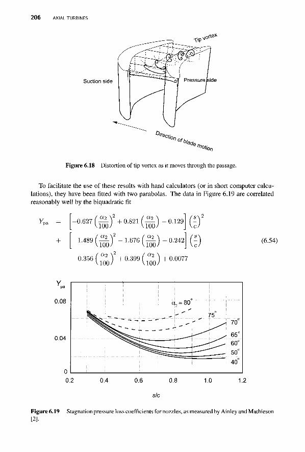
206 AXIAL TURBINES
TO***
Suction side Pressure (side
Figure 6.18 Distortion of tip vortex as it moves through the passage.
To facilitate the use of these results with hand calculators (or in short computer calcu-lations), they have been fitted with two parabolas. The data in Figure 6.19 are correlated reasonably well by the biquadratic fit
Y — 1 pa —
+
- ° - 6 2 7 ( i S ) ) + 0 - 8 2 1 ( i S ) ) - 0 - 1 2 9
1.489 ( ^ - 1.676 ( ^ ) + 0.242' (3 -0.356 ( ^ ) + 0 . 3 9 9 ( ^ ) + 0 . 0 0 7 7
(6.54)
0.08
0.04
Figure 6.19 Stagnation pressure loss coefficients for nozzles, as measured by Ainley and Mathieson [2].
TURBINE EFFICIENCY AND LOSSES 207
EXAMPLE 6.8
A nozzle row is tested with air. The air enters the row axially and leaves it at angle 60°. The space-to-chord ratio is s/c — 0.7. The inlet pressure is poi = 200kPa, stagnation temperature at the inlet is T0i = 540 K, and the exit static pressure is p2 = 160 kPa. Find (a) the exit stagnation pressure and (b) the static enthalpy loss coefficient.
Solution: (a) For s/c = 0.7, the stagnation pressure loss coefficient is
.2
Y — 1 pa —
+
-°-6 2 7(0+ O-8 2 1(^))-0-1 2 9 . L 4 8 9 ( ^ ) 2 - L 6 7 6 ( ^ ) + 0 - 2 4 2
0.7^
0.7
/ ar\ \ / fid \ -0.356 ( — J + 0.399 f — j + 0.0077 = 0.0272
Examination of Figure 6.19 shows that this value is smaller than what can be read from the figure, which suggests that it should be increased to 0.032. If this error can be tolerated, solving next
P01 ~ P02 Y — P02 ~ P2
for p02 gives
P02 Poi + ypaP2 _ 200 + 0.0272 ■ 160
1 +Ypa ~ 1.0279 198.94 kPa
so that Apos = 106 kPa. A more accurate value using the actual charts is 1.24 kPa. (b) The exit static temperature is
T( 02 M ( 7 - l ) / 7
540 160,000 V 1/3.5
507.44 K Pm) V 198,9137
and velocity is therefore
V2 = ^2cp(T02 - T2) = y/2 ■ 1004.5(540 - 507.44) = 255.77m/s
These give a Mach number value of M2 = V^/y/jBT^ = 0.566. The stagnation density at the exit is
P02 Po2 198,940 1.284 kg/m3
RT02 287 ■ 540
The static enthalpy loss coefficient is calculated from
4Apos/po2 4 • 1060/1.284 Cs y2
2(2 + (7 - 1)M|) 255.772(2 + (1.4 - 1)0.5662) 0.0237
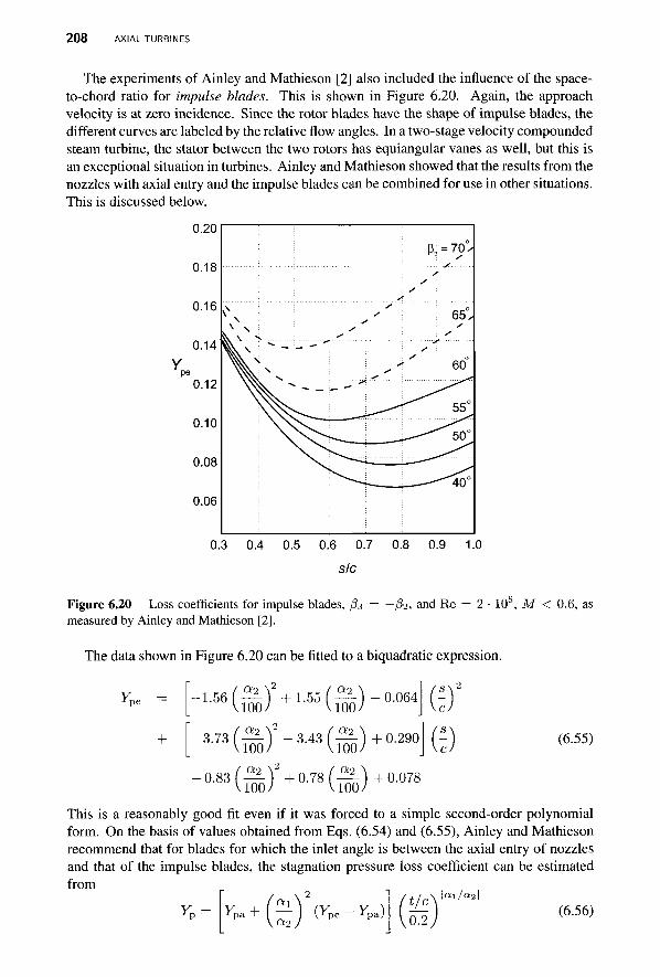
208 AXIAL TURBINES
The experiments of Ainley and Mathieson [2] also included the influence of the space-to-chord ratio for impulse blades. This is shown in Figure 6.20. Again, the approach velocity is at zero incidence. Since the rotor blades have the shape of impulse blades, the different curves are labeled by the relative flow angles. In a two-stage velocity compounded steam turbine, the stator between the two rotors has equiangular vanes as well, but this is an exceptional situation in turbines. Ainley and Mathieson showed that the results from the nozzles with axial entry and the impulse blades can be combined for use in other situations. This is discussed below.
0.20
0.18
0.16
0.14
0.12
0.10
0.08
0.06
Y
\ ^ \ ^ _
>
s s
= 70°. s s
65°,
60°
55°
50°
"40°
0.3 0.4 0.5 0.6 0.7 0.8
sic 0.9 1.0
Figure 6.20 Loss coefficients for impulse blades, fa measured by Ainley and Mathieson [2].
-fa, and Re = 2 • 105, M < 0.6, as
The data shown in Figure 6.20 can be fitted to a biquadratic expression.
Y pe
+
.1.56 (^-) + 1.55 (^-)- 0.064
«3(Si)2-3-4 3O+ 0-2 9 0 (6.55)
°«©+°-S) 0.078
This is a reasonably good fit even if it was forced to a simple second-order polynomial form. On the basis of values obtained from Eqs. (6.54) and (6.55), Ainley and Mathieson recommend that for blades for which the inlet angle is between the axial entry of nozzles and that of the impulse blades, the stagnation pressure loss coefficient can be estimated from
YP = Y„: (6.56)
TURBINE EFFICIENCY AND LOSSES 2 0 9
The subscripts in this expression have the following meaning: Yp is the profile loss at zero incidence; Ypa is the profile loss coefficient for axial entry, and Ype is the profile loss coefficient for equiangular impulse blades. The absolute values are needed in the exponent because a\ could be negative.
For a rotor the angle, a.\ is replaced by fa and a2 is replaced by fa. Thus Eq. (6.56) takes the form
^P /V2
*pa + | o ] (,Jpe Jpa j 0.2 < ( 6 - 5 ? )
In evaluating the loss coefficient from Eq. (6.55) for impulse blades, a2 is replaced by fa for rotor blades, since fa will be positive and fa = —fa. The ratio of maximum thickness to the length of the chord in these expressions is t/c, with a nominal value of 20%. Should it be greater than 25% the value t/c = 0.2 is used. If it is less than 15%, its value is set at t /c = 0.15.
6.7.8 Secondary loss
Secondary and tip losses require examination of lift and drag on the rotor blades. Unlike in the case for an airfoil, for which lift is the force component perpendicular to incoming flow direction, in turbomachinery flows the direction of the lift is defined as the force perpendicular to a mean flow direction. This, together with other important geometric parameters, is shown in Figure 6.21. The mean direction is obtained by first defining the mean tangential component of the relative velocity as
wum=l-{wul + wu2)
which can be rewritten in the form
Wum = -Wx(t&nfa + tan fa)
Next, writing Wum = Wx tan /3m gives
tan/3m — -( tan/32 + tan/?3)
and /?m defines the mean direction. For the situation shown in the figure tan /3m is negative and so is Vum.
Next, applying the momentum theorem to the rotor, the force in the direction of the wheel motion is given by
Fu = PsWx(Wu3 - Wu2) = psW^t&nfa - tan/32)
This is the force that the blade exerts on the fluid per unit height of the blade. The reaction force Ru = — Fu is the force by the fluid on the blade, and it is given by
Ru = psWl(tan fa - tan/33) (6.58)
The component of the reaction forces are related to lift L and drag D by
Rx = D cos Pm — L sin /3m Ru = D sin /3m + L cos /3m
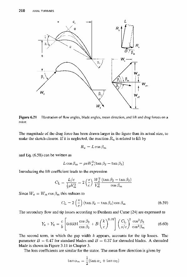
210 AXIAL TURBINES
Figure 6.21 Illustration of flow angles, blade angles, mean direction, and lift and drag forces on a rotor.
The magnitude of the drag force has been drawn larger in the figure than its actual size, to make the sketch clearer. If it is neglected, the reaction Ru is related to lift by
Ru = L cos /3m
and Eq. (6.58) can be written as
L cos j3m = psW% (tan (32 — tan /33)
Introducing the lift coefficient leads to the expression
Cr L/c s\ Wl (tan/32 - t a n / ? 3 © V2
v m cos/?„
Since Wx = Wm cos j3m this reduces to
Ch = 2 ( - ) (tan/32 - tan /33) cos (3n (6.59)
The secondary flow and tip losses according to Dunham and Came [24] are expressed as
YB + Yk 0 . 0 3 3 4 ^ + B(k-cos pi \c
0.78 ch cos2/33
s/cj cos3/?n (6.60)
The second term, in which the gap width k appears, accounts for the tip losses. The parameter B = 0.47 for standard blades and B = 0.37 for shrouded blades. A shrouded blade is shown in Figure 3.11 in Chapter 3.
The loss coefficients are similar for the stator. The mean flow direction is given by
t ana n 1 ( tanai + tan a2)
TURBINE EFFICIENCY AND LOSSES 2 1 1
and the lift coefficient is
CL = 2 I - J (tan «2 — tana.\) cos an
The loss coefficient of the secondary flows is
Ys =
as there are no tip losses.
■ EXAMPLE 6.9
-I \ COS «i J Wc, v2 2
^ cosza2
/ cos3am
(6.61)
Combustion gases, with 7 = § and cp = 1148 J/(kg • K), flow through a normal turbine stage with R = 0.60. The flow enters the stator at a.\ = —33° and leaves at velocity V2 — 450 m/s. The inlet stagnation temperature is T01 = 1200 K, and the inlet stagnation pressure is 15 bar. The flow coefficient is <p = 0.7, blade height-to-axial chord ratio is b/cx = 3.5, and the Reynolds number is 105. The blades are unshrouded with B = 0.4, and the tip-gap-to-blade height ratio is k/b = 0.02. Find the stagnation pressure loss across the stator and the rotor based on Ainley-Matheison correlations.
Solution: The blade-loading coefficient is first determined from
ip = 2(1 - R - 0 t a n a 3 ) = 2(1 - 0.6 - 0.7tan(-33°)) = 1.709
The flow angle leaving the stator is
Qf2 = t a n 1 - R + V>/2
= tan 1 -0 .6 +1.709/2 \
0.7 60.84°
Hence the mean flow angle is
ttn tan ( tanai + tan 02) 29.74°
The lift coefficient is
CLS = 2 I - j (tan 0:2 — tana\) cos am
= 2 • 0.9(tan(60.84) - tan(-33)) cos(29.74) = 3.82
The secondary loss coefficient for the nozzles is
YsN = 0.0334 \ ^ ^ = 0.0434 0 COS^QJm
The value of profile losses obtained from Eqs. (6.54) and (6.55) are
Fp a N = 0.0269 yp e N = 0.1151
so that for the particular nozzle row
YT p N ^paN + ( ^ p e N — ^ p a N ) t/c 02
| a i / a 2 |
212 AXIAL TURBINES
comes out to be
YpN = 0.0269 -33 60.84
(0.1151 ^0.0269) 0.0529
Thus the stagnation pressure loss coefficient is YN = YPN + YSN = 0.0963. For the rotor, the angle of the relative velocity leaving the stage is
/ ? 3 = t a n - 1 ( ~ J ? ~ V ; / 2 | = t a n - 1 -0 .6-1 .709/2^ = _ 6 4 3 0
0.7
and the angle of the relative velocity at the inlet of the rotor is
_1f-R + ip/2\ _j / - 0 . 6 +1.709/2 \ ft tan tan 0.7 20.0°
The mean flow angle is
A,
The lift coefficient is
tan -(tan/32 + tan/33) -40.6°
C L R = 2 (-) (tan/32 - tan ft) cos/3n
= 2 • 0.9[tan(20) - tan(-64.3)] cos(-40.6) = 3.34
The secondary flow and tip losses can then be determined from
rsi YkR 0.0334 ^ + Brk
cos/32
0.78 Ch \2 cos2ft
YsR + Y, 1 sR-t--<kR = 0.0334 COs{,64:r) +0.47-0.02078
cos(20.0°)
From Eqs. (6.54) and (6.55) the profile losses coefficients are
YpaR = 0.0322 YpeR = 0.1334
s/cj cos3/3n
3.34\2cos2(-64.3°) 09~j cos3!-40.6°I
0.075
so that
is
Y pR
YpR =
Yr paR
0.0322 +
(YpeR — YpaR) t/c 02
-20.0° -64.3°
(0.1334-0.0322)
102/% I
0.0419
The stagnation pressure loss coefficient for the rotor is therefore YR = YPR + YSR + YkR = 0.1169.
The stagnation pressure loss across the nozzle row is obtained from
YN P01 ~ P02
P02 - V2 P01 - P02 = YN(po2 - Vi)
TURBINE EFFICIENCY AND LOSSES 213
Dividing through by po2 gives
m I + YJI P2
P02
Since the temperature T2 is
P02 1 + *N
To
1-02
7/ (7-1) '
VZ 4502
T2=T02 = 1200 u 2c„ 2-1148
1111.8K
and M2 = V2/y/jRT2 = 0.690, the stagnation pressure ratio is
.4" P01 P02
1 + 0.0963 1 1111.8 1200
1.02534
Hence p02 = 1500/1.02534 = 1462.9 kPa, and the stagnation pressure loss is Ap0LS = 37.2kPa.
The static pressure at the exit is
V2 = P02 1 + 7"V2 -7/ (7-1)
1462.9 1 6902
2 V V 6 Some preliminary calculations are necessary for the rotor. First
Vx = V;COSQ!2 = 450cos(60.84) = 219.3 m / s
1078.0 kPa
and then
W2 = Vx 219.3
cos/32 cos(20°)
Vx 219.3 cos/33 cos(-64.3°)
Vx
233.4 m / s
505.6 m / s
219.3 cosc*3 cos(—33°)
261.5 m / s
Also
V 219 3 U = — = - ^ - ^ = 3 1 2 . 2 m / s w = ipU2 = 1.709 • 313.22 = 167.69 k J / k g
so that
and
Next
0.7
W 167 69 T0 3 = T02 = 1200 - — — - = 1053.7 K
c„ 1148
T/2 ofil ^2
T3 = T03 - - ^ - = 1053.7 - „ , ; .„ = 1024.2 K ZCn 2-1148
TQ3R — T3 + 2c„ 1024.2 +
505.62
2 •1148
and since T02R = T03R
7/ (7-1) P02R = p2 I - ^ - ! = 1078.0
1111.8
1135.5K
= 1128.3kPa
214 AXIAL TURBINES
The stagnation pressure loss coefficient for the rotor is
P02R — P03R YR =
P03R - P3
so that
H ( I - - ^ = 1 -» = i + y R ( i - ^ - ) = i + FR P03R V P03R) \ To3R /
7 / (7-1) '
The numerical value for the pressure ratio is
P02R
P03R 1 + 0.1169 1 -
/1024.2 V 1135.5 1.040
andpo3R = 1172.9/1.040 = 1128.28 kPa. Hence the stagnation pressure loss across the rotor is ApoLR = 44.6 kPa. The value obtained the by Soderberg correlation was 38.6 kPa, but that correlation neglects the tip losses. For the nozzle row the loss is APOLS = 37.lkPa, and the Soderberg correlation gave 42.4 kPa. Ainley-Mathieson and Soderberg correlations are therefore in reasonable agreement.
6.8 MULTISTAGE TURBINE
6.8.1 Reheat factor in a multistage turbine
Consider next a multistage turbine with process lines as shown in Figure 6.22. The isentropic work delivered by the jth stage is denoted as WjS, whereas the actual stage work is Wj. The stage efficiency is defined to be
Vs Wj
and it is assumed to be the same for each stage. With
Wjs = hoj — /lo,j + l,s
the sum over all the stages gives
N N
j = i j = i
The isentropic work delivered by the turbine is ws = hoi — ho,N+i,ss- A reheat factor is defined as
Y^N ... v^JV RF
j=1 wjs _ r, J2j=i Wj
w, Vs w N in which w = ^2j=1 Wj, so that
RF

MULTISTAGE TURBINE 215
Oj
Oj+1
Figure 6.22 Processes in a multistage turbine.
Since the slope of constant-pressure line increases as temperature increases, it follows that
N
j = l
and R F > 1. Hence 77 > r]s, and the overall efficiency of a turbine is greater than the stage efficiency. The reason is the internal heating, for the increase in static enthalpy by irreversibilities becomes partly available as the expansion proceeds over the next stage. The increase in the overall efficiency depends on the number of stages.
If the ideal gas model can be used, then the actual and ideal work delivered by the first stage are
w = cp(Toi - T02) ws = cp(Toi - T02s) Since
-MD2s
T01 P02_\
P01)
( 7 - l ) / 7
the temperature difference for the isentropic process becomes
\ ( 7 " l ) / 7 ' TQI — T02S — 2c 01
Letting
'P02V
The actual temperature drop is then
x = 1 ( 7 - l ) / 7
1
then
P02Y P 0 1 /
Tr\\ — Tms — xTi 01
(01 '02 7]SXT{ 01 so tha t To2 = T 0 1 ( l - 7 7 s x )
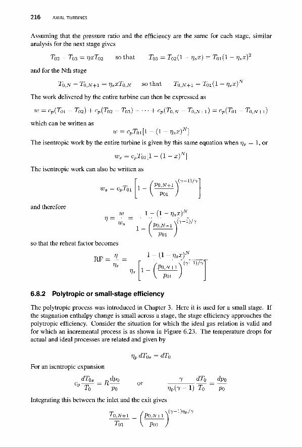
216 AXIAL TURBINES
Assuming that the pressure ratio and the efficiency are the same for each stage, similar analysis for the next stage gives
T02 - T03 = r,xT02 so that T03 = T02 (1 - %x) = T01 (1 - r)sx)2
and for the Nth stage
T0,N - T0tN+i = VsxToiN so that T0>N+1 = T0i(l - r]sx)N
The work delivered by the entire turbine can then be expressed as
w = cp(T0i - T02) + cp(To2 - T03) H h CV(T0,N - T0,N+I) = cp(T0i - T0,JV+I)
which can be written as w = CpT0i[l - (1 - r)sx)N]
The isentropic work by the entire turbine is given by this same equation when r]s = 1, or
ws = cpT01[l - (1 - x)N]
The isentropic work can also be written as v ( 7 - l ) / 7 "
W, = C„T(
and therefore
p ^ O l
w
1 P0,N+1
POl
1 - (1 - risx)N
Ws P0,JV+1
POl
( 7 " l ) / 7
so that the reheat factor becomes
Vs Vs
l-(l-r,sx)N
/„ \ ( 7 - l ) / 7 _
V POl )
6.8.2 Polytropic or small-stage efficiency
The polytropic process was introduced in Chapter 3. Here it is used for a small stage. If the stagnation enthalpy change is small across a stage, the stage efficiency approaches the polytropic efficiency. Consider the situation for which the ideal gas relation is valid and for which an incremental process is as shown in Figure 6.23. The temperature drops for actual and ideal processes are related and given by
For an isentropic expansion
dT0s dp0
To Po
rjp dT0s = dT0
7 dT0 dp0
Vp(l ~ 1) To Po Integrating this between the inlet and the exit gives
lQ,N+l
T0i P0,N+1
POl
( 7 - l ) f ? p / 7

EXERCISES 217
Figure 6.23 Processes across a small stage.
The reheat factor can then be written as
RF =
Po,iv+i Poi
( 7 - 1 ) » 7 P / T
^P VP
P0,N+1
POI
( 7 - l ) / 7 '
The relationship between the turbine efficiency and polytropic, or small-stage efficiency is
1 - I -r
( 7 - ! ) W 7
1 ( 7 - l ) / 7
in which r = Poi/poe is the overall pressure ratio of the turbine. This relationship is shown in Figure 6.24.
This completes the study of axial turbines, which began in the previous chapter on steam turbines. Wind turbines and some hydraulic turbines are also axial machines. They are discussed later. Many of the concepts introduced in this chapter are carried over to the next one, on axial compressors.
EXERCISES
6.1 At inlet to the rotor in a single-stage axial-flow turbine the magnitude of the absolute velocity of fluid is 610 m/s. Its direction is 61° as measured from the cascade front in the direction of the blade motion. At exit of this rotor the absolute velocity of the fluid is 305 m/s directed such that its tangential component is negative. The axial velocity is constant, the blade speed is 305 m/s, and the flow rate through the rotor is 5kg/s. (a) Construct the rotor inlet and exit velocity diagrams showing the axial and tangential components of the absolute velocities, (b) Evaluate the change in total enthalpy across the rotor, (c) Evaluate the power delivered by the rotor, (d) Evaluate the average driving force
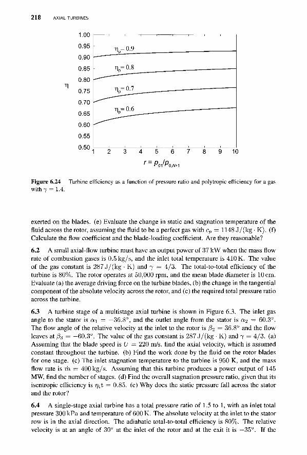
218 AXIAL TURBINES
1.00 0.95 0.90 0.85 0.80 0.75 0.70 0.65 0.60 0.55 0.50
Figure 6.24 Turbine efficiency as a function of pressure ratio and polytropic efficiency for a gas with 7 = 1.4.
exerted on the blades, (e) Evaluate the change in static and stagnation temperature of the fluid across the rotor, assuming the fluid to be a perfect gas with cp = 1148 J/(kg • K). (f) Calculate the flow coefficient and the blade-loading coefficient. Are they reasonable?
6.2 A small axial-flow turbine must have an output power of 37 kW when the mass flow rate of combustion gases is 0.5kg/s, and the inlet total temperature is 410 K. The value of the gas constant is 287 J/(kg • K) and 7 = 4/3. The total-to-total efficiency of the turbine is 80%. The rotor operates at 50,000 rpm, and the mean blade diameter is 10 cm. Evaluate (a) the average driving force on the turbine blades, (b) the change in the tangential component of the absolute velocity across the rotor, and (c) the required total pressure ratio across the turbine.
6.3 A turbine stage of a multistage axial turbine is shown in Figure 6.3. The inlet gas angle to the stator is a\ = —36.8°, and the outlet angle from the stator is a-i — 60.3°. The flow angle of the relative velocity at the inlet to the rotor is 02 = 36.8° and the flow leaves at /33 = -60.3°. The value of the gas constant is 287 J/(kg • K) and 7 = 4/3. (a) Assuming that the blade speed is U = 220 m/s, find the axial velocity, which is assumed constant throughout the turbine, (b) Find the work done by the fluid on the rotor blades for one stage, (c) The inlet stagnation temperature to the turbine is 950 K, and the mass flow rate is m = 400kg/s. Assuming that this turbine produces a power output of 145 MW, find the number of stages, (d) Find the overall stagnation pressure ratio, given that its isentropic efficiency is r)tt = 0.85. (e) Why does the static pressure fall across the stator and the rotor?
6.4 A single-stage axial turbine has a total pressure ratio of 1.5 to 1, with an inlet total pressure 300 kPa and temperature of 600 K. The absolute velocity at the inlet to the stator row is in the axial direction. The adiabatic total-to-total efficiency is 80%. The relative velocity is at an angle of 30° at the inlet of the rotor and at the exit it is —35°. If the
EXERCISES 219
flow coefficient is (f> = 0.9, find the blade velocity. Use compressible flow analysis with cp = 1148 J/(kg • K), 7 = §, and R = 287 J/(kg ■ K).
6.5 An axial turbine has a total pressure ratio of 4 to 1, with an inlet total pressure 650 kPa and total temperature of 800 K. The combustion gases that pass through the turbine have 7 = | , and R = 287 J/(kg • K). (a) Justify the choice of two stages for this turbine. Each stage is normal stage and they are designed the same way, with the blade-loading coefficient equal to 1.1 and the flow coefficient equal to 0.6. The absolute velocity at the inlet to the stator row is at angle 5° from the axial direction. The adiabatic total-to-total efficiency is 91.0%. Find, (b) the angle at which the the absolute velocity leaves the stator, (c) the angle of the relative velocity at the inlet of the rotor, (d) the angle at which the relative velocity leaves the rotor, (f) Draw the velocity diagrams at the inlet and outlet of the rotor, (g) What are the blade speed and the axial velocity? A consequence of the design is that each stage has the same work output and efficiency. Find, (h) the stage efficiency and (i) the pressure ratio for each stage.
6.6 For a steam turbine rotor the blade speed at the casing is U = 300 m/s and at the hub its speed is 240 m/s. The absolute velocity at the casing section at the inlet to the rotor is V2c = 540 m/s and at the hub section it is V2h = 667 m/s. The angle of the absolute and relative velocities at the inlet and exit of the casing and hub sections are a2c = 65°, f33c = -60° , a2 h = 70°, and (33h = -50° . The exit relative velocity at the casing is W3c — 456 m/s and at the hub it is W3h = 355 m/s. For the tip section, evaluate (a) the axial velocity at the inlet and exit; (b) the change in total enthalpy of the steam across the rotor; and (c) the outlet total and static temperatures at the hub and casing sections, assuming that the inlet static temperature is 540° C and inlet total pressure is 7 MPa, and they are the same at. all radii. Assume that the process is adiabatic and steam can be considered a perfect gas with 7 = 1.3. The static pressure at the exit of the rotor is the same for all radii and is equal to the static pressure at inlet of the hub section. Repeat the calculations for the hub section, (d) Find the stagnation pressure at the outlet at the casing and the hub.
6.7 Combustion gases, with 7 = | and R = 287kJ/(kg • K), flow through a turbine stage. The inlet flow angle for a normal stage is a.\ = 0 ° . The flow coefficient is <j> = 0.52, and the blade-loading coefficient is xp = 1.4. (a) Draw the velocity diagrams for the stage. (b) Determine the angle at which relative velocity leaves the rotor, (c) Find the flow angle at the exit of the stator. (d) A two-stage turbine has an inlet stagnation temperature of T01 = 1250 K and blade speed U = 320 m/s. Assuming that the total-to-total efficiency of the turbine is r)tt = 0.89, find the stagnation temperature of the gas at the exit of the turbine and the stagnation pressure ratio for the turbine, (e) Assuming that the density ratio across the turbine based on static temperature and pressure ratios is the same as that based on the stagnation temperature and stagnation pressure ratios, find the ratio of the cross-sectional areas across the two-stage turbine.
6.8 Steam enters a 10-stage 50%-reaction turbine at the stagnation pressure 0.8 MPa and stagnation temperature 200° C and leaves at pressure 5kPa and with quality equal to 0.86. (a) Assuming that the steam flow rate is 7kg/s, find the power output and the overall efficiency of the turbine, (b) The steam enters each stator stage axially with velocity of 75 m/s. The mean rotor diameter for all stages is 1.4 m, and the axial velocity is constant through the machine. Find the rotational speed of the shaft, (c) Find the absolute and relative inlet and exit flow angles at the mean blade height assuming equal enthalpy drops for each stage.
220 AXIAL TURBINES
6.9 Combustion gases enter axially into a normal stage at stagnation temperature TQI = 1200 K and stagnation pressure poi = 1500 kPa. The flow coefficient is 0 = 0.8 and the reaction is R = 0.4. The inlet Mach number to the stator is Mi = 0.4. Find, (a) the blade speed and (b) the Mach number leaving the stator and the relative Mach number leaving the rotor, (c) Using the Soderberg loss coefficients, find the efficiency of the stage, (d) Repeat the calculations with inlet Mach number Mi = 0.52.
6.10 For a normal turbine stage fluid enters the stator at angle 10°. The relative velocity has an angle —40° as it leaves the rotor. The blade-loading factor is 1.6. (a) Determine the exit angle of the flow leaving the stator and the angle of the relative velocity as it enters the rotor. Determine the degree of reaction, (b) For the conditions of part (a), find the angle at which the flow leaves the stator and the angle of the relative velocity entering the rotor, as well as the degree of reaction, (c) Calculate the total-to-total efficiency using Soderberg correlations. Take the blade height to axial chord ratio to be b/cx = 3.5. (d) Determine the stagnation pressure loss across the stator, given that the inlet conditions are Xbi = 700 K and poi = 380 kPa, and the velocity after the stator is V2 = 420m/s.
6.11 For Example 6.6, write a computer program to calculate the mass flow rate and plot the variation of the reaction from the hub to the casing.
6.12 For a normal turbine stage the exit blade angle of the stator at 70° and relative velocity has angle —60° as it leaves the rotor. For a range of flow coefficients 0 = 0.2 — 0.8, calculate and plot the gas exit angle from the rotor, the angle the relative velocity makes as it leaves the stator, the blade-loading coefficient, and the degree of reaction. Comment on what is a good operating range and what are the deleterious effects in flow over the blades if the mass flow rate is reduced too much or if it is increased far beyond this range.
6.13 For a normal turbine stage fluid enters the stator with the inlet conditions TQI = HOOK and poi = 380kPa. The inlet flow angle is 10°, and the velocity after the stator is V2 = 420 m/s. The relative velocity has angle —40° as it leaves the rotor. The blade-loading factor is 1.6. (a) Determine the exit angle of the flow leaving the stator and the angle of the relative velocity as it enters the rotor. Determine the degree of reaction, (b) For the conditions in part (a), calculate the flow exit angle and the angle of the relative velocity entering the rotor, (c) Calculate the stagnation pressure losses across the stator and the rotor using Ainley-Mathiesen correlations. Take the space to axial chord ratio equal to s/cx = 0.75 and assume that the maximum thickness-to-chord ratio is t/c = 0.22. (d) Determine the stagnation pressure loss across the stator, assuming the inlet conditions are TQi = 1100 K, and p01 = 380 kPa, and the velocity after the stator is V2 = 420 m/s.
CHAPTER 7
AXIAL COMPRESSORS
In Chapter 4 it was pointed out that axial compressors are well suited for high flow rates and centrifugal machines are used when a large pressure rise is needed at a relatively low flow rate. To obtain the high flow rate, gas enters the compressor at a large radius. The gas is often atmospheric air and as it is compressed, it becomes denser and the area is reduced from stage to stage, often in such a way that the axial velocity remains constant. As in axial turbines, this may accomplished keeping the mean radius constant and by reducing the casing radius and increasing the hub radius. In jet engines high pressure ratios are obtained by pairing one multistage compressor with a turbine sufficiently powerful to turn that compressor. This arrangement of a turbine and compressor running on the same shaft is called a spool. A second spool consisting of intermediate-pressure (IP) compressor and turbine is then configured with a compressor in front of, and a turbine behind, the central high-pressure (HP) spool. The shaft of the IP spool is hollow and concentric with that of the HP spool. These high and intermediate pressure spools serve as gas generators to provide a flow to a low-pressure (LP) turbine that drives the fan in a turbofan jet aircraft or a generator for electricity production in a power plant [64].
The larger IP compressor turns at a lower speed than the HP spool in order to keep the blade speed sufficiently low to ensure that compressibility effects do not deteriorate the performance of the machine. In a typical spool one turbine stage drives six or seven compressor stages. The stage pressure ratio has increased with improved designs, reaching 1.3 and 1.4 in modern jet engine core compressors [64].
Pipeline compressors are often driven by a power turbine that uses a jet engine spool as the gas generator. Alternatively, a diesel engine may provide the power to the compressor.
Principles of Turbomachinery. By Seppo A. Korpela 221 Copyright © 2011 John Wiley & Sons, Inc.
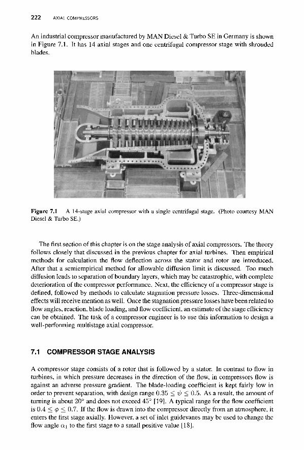
222 AXIAL COMPRESSORS
An industrial compressor manufactured by MAN Diesel & Turbo SE in Germany is shown in Figure 7.1. It has 14 axial stages and one centrifugal compressor stage with shrouded blades.
Figure 7.1 A 14-stage axial compressor with a single centrifugal stage. (Photo courtesy MAN Diesel & Turbo SE.)
The first section of this chapter is on the stage analysis of axial compressors. The theory follows closely that discussed in the previous chapter for axial turbines. Then empirical methods for calculation the flow deflection across the stator and rotor are introduced. After that a semiempirical method for allowable diffusion limit is discussed. Too much diffusion leads to separation of boundary layers, which may be catastrophic, with complete deterioration of the compressor performance. Next, the efficiency of a compressor stage is defined, followed by methods to calculate stagnation pressure losses. Three-dimensional effects will receive mention as well. Once the stagnation pressure losses have been related to flow angles, reaction, blade loading, and flow coefficient, an estimate of the stage efficiency can be obtained. The task of a compressor engineer is to use this information to design a well-performing multistage axial compressor.
7.1 COMPRESSOR STAGE ANALYSIS
A compressor stage consists of a rotor that is followed by a stator. In contrast to flow in turbines, in which pressure decreases in the direction of the flow, in compressors flow is against an adverse pressure gradient. The blade-loading coefficient is kept fairly low in order to prevent separation, with design range 0.35 <ip< 0.5. As a result, the amount of turning is about 20° and does not exceed 45° [19]. A typical range for the flow coefficient is 0.4 < <fi < 0.7. If the flow is drawn into the compressor directly from an atmosphere, it enters the first stage axially. However, a set of inlet guidevanes may be used to change the flow angle cx\ to the first stage to a small positive value [18].

COMPRESSOR STAGE ANALYSIS 223
7.1.1 Stage temperature and pressure rise Figure 7.2 shows a typical compressor stage. Since the rotor now precedes the stator, the inlet to the rotor is station 1 and its outlet is station 2. The outlet from the stator is station 3 and for a repeating stage the flow angles and velocity magnitudes there are equal to those at the inlet to the rotor.
Figure 7.2 A typical axial compressor stage.
Work done by the blades is w = U(Vu2~Vul)
or
(7.1)
w = ^02 — /ioi = UVX (tan a2 — t ana j ) = UVx(t&n /32 — tan/3i) With w = cp(T03 — T0i), this can also expressed in the form
w AT0 UVX
CpToi foi C-nTl p-tOl -(tan/32 — tan/3i)
which gives the nondimensional stagnation temperature rise. From the definition of stage efficiency
TQ3S ~ T0i
T03 — TQI
the stage pressure ratio can be written as
P03
P01 l + %t
AT0
to i
7/ (7 -1)
The stage temperature rise can also be written in the form
AT0
Toi U V2
(7-l)TT-f-(tan/32-tan/3i) Vx C01
For axial entry, Vx is the inlet velocity. In terms of the flow coefficient and stagnation Mach number, defined as
Vx C0l
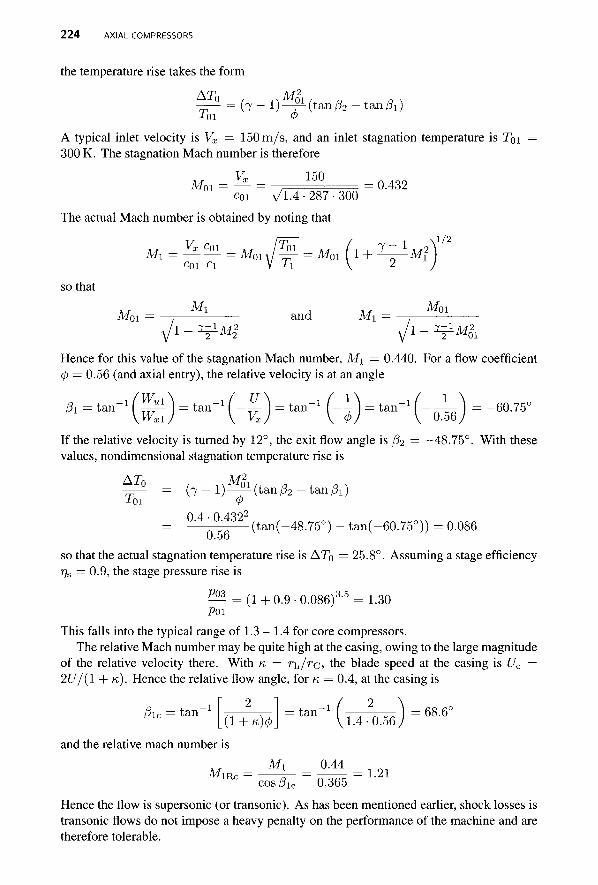
224 AXIAL COMPRESSORS
the temperature rise takes the form
^ = ( 7 - l ) ^ ( t a n / 3 2 - t a n A ) J-oi 9
A typical inlet velocity is Vx = 150 m / s , and an inlet stagnation temperature is TQI 300 K. The stagnation Mach number is therefore
M 0 1 = ^ = , 1 5 ° = 0 . 4 3 2 coi V l . 4 - 2 8 7 - 3 0 0
The actual Mach number is obtained by noting that
Vx coi ,,,. /Thi %/r (^ , 7 - 1 , ^ 1/2
Ml = - ^ - ^ = M 0 i W ^ - = M 0 i 1 + - ^ - M j * coi ci V Ti V 2
so that Mi , M0i
M0i — , = and Mi 1 + V M | V1 " V^oi
Hence for this value of the stagnation Mach number, M i = 0.440. For a flow coefficient </> = 0.56 (and axial entry), the relative velocity is at an angle
If the relative velocity is turned by 12°, the exit flow angle is fa — —48.75°. With these values, nondimensional stagnation temperature rise is
A7-1 M 2
— ± = ( 7 - l ) - f ( t a n / 3 2 - t a n / 3 1 )
0 4-0 4322
= . (tan(-48.75°) - tan(-60.75°)) = 0.086 u.oo
so that the actual stagnation temperature rise is ATQ = 25.8°. Assuming a stage efficiency r)s = 0.9, the stage pressure rise is
— = (1 + 0.9 • 0.086)3,5 = 1.30 Poi
This falls into the typical range of 1.3 - 1.4 for core compressors. The relative Mach number may be quite high at the casing, owing to the large magnitude
of the relative velocity there. With K = r\Jrc the blade speed at the casing is Uc = 2C//(1 + K ) . Hence the relative flow angle, for K = 0.4, at the casing is
fac — tan 1
( l + «) and the relative mach number is
t a n " ( i ^ L 5 6 ' = 6 8 - 6 °
Mi 0.44 M1Rc = ±— = = 1.21
cospic 0.365
Hence the flow is supersonic (or transonic). As has been mentioned earlier, shock losses is transonic flows do not impose a heavy penalty on the performance of the machine and are therefore tolerable.
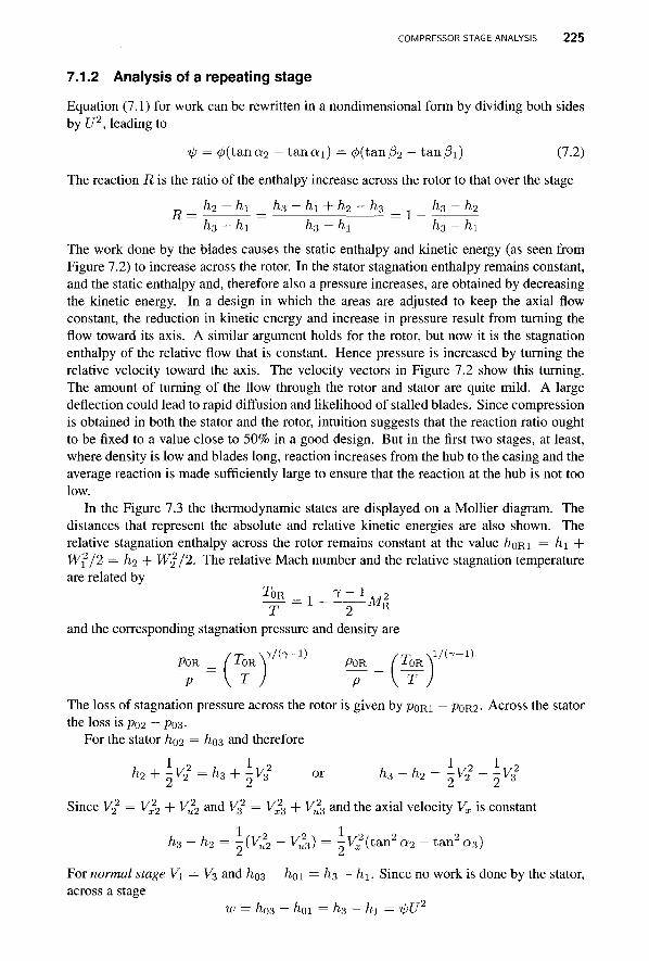
COMPRESSOR STAGE ANALYSIS 225
7.1.2 Analysis of a repeating stage
Equation (7.1) for work can be rewritten in a nondimensional form by dividing both sides by U2, leading to
tp = 0( tana 2 — tana i ) = (j>(ta,n(52 — tan/3i) (7.2)
The reaction R is the ratio of the enthalpy increase across the rotor to that over the stage
_ h2 - hi _ h3 - hi + h2 - h3 _ _ h3 - h2
h3 -hi h3- hi h3 - hi The work done by the blades causes the static enthalpy and kinetic energy (as seen from Figure 7.2) to increase across the rotor. In the stator stagnation enthalpy remains constant, and the static enthalpy and, therefore also a pressure increases, are obtained by decreasing the kinetic energy. In a design in which the areas are adjusted to keep the axial flow constant, the reduction in kinetic energy and increase in pressure result from turning the flow toward its axis. A similar argument holds for the rotor, but now it is the stagnation enthalpy of the relative flow that is constant. Hence pressure is increased by turning the relative velocity toward the axis. The velocity vectors in Figure 7.2 show this turning. The amount of turning of the flow through the rotor and stator are quite mild. A large deflection could lead to rapid diffusion and likelihood of stalled blades. Since compression is obtained in both the stator and the rotor, intuition suggests that the reaction ratio ought to be fixed to a value close to 50% in a good design. But in the first two stages, at least, where density is low and blades long, reaction increases from the hub to the casing and the average reaction is made sufficiently large to ensure that the reaction at the hub is not too low.
In the Figure 7.3 the thermodynamic states are displayed on a Mollier diagram. The distances that represent the absolute and relative kinetic energies are also shown. The relative stagnation enthalpy across the rotor remains constant at the value /IORI = hi + W2/2 = h2 + W2/2. The relative Mach number and the relative stagnation temperature are related by
T 2 R
and the corresponding stagnation pressure and density are
POR = /TOR V 7 ^ ^ POR = / T O R V / ( 7 _ 1 )
P \T ) P \T )
The loss of stagnation pressure across the rotor is given by PORI — PoR2- Across the stator the loss isp02 — Po3-
For the stator /102 = ̂ 03 and therefore
h2 + \v22 = h3 + \v2 or h3-h* = ±V2-\v2
Since V2 — V22 + V2
2 and V3 — V23 + V2
3 and the axial velocity Vx is constant
h3-h2 = -{V22 - V2
3) = -V2(Un2 a2 - tan2 a3) For normal stage V\ = V3 and foo3 — ^01 = h3 ~ hi. Since no work is done by the stator, across a stage
w = h03 - h0i = h3 - hi = tpU2
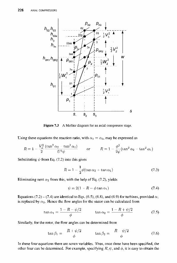
226 AXIAL COMPRESSORS
02 03
0R1 "0R2
Figure 7.3 A Mollier diagram for an axial compressor stage.
Using these equations the reaction ratio, with a\ = a^, may be expressed as
V^ (tan2 a2 — tan2 a.\) ~ ~ ~2 Whp
Substituting tp from Eq. (7.2) into this gives
R = 1 — -</>(tana2 + t ana i )
Eliminating next oti from this, with the help of Eq. (7.2), yields
i) = 2(1 - i ? - 0 t a n a i )
i? = 1 — ——(tan2 a.2 — tan2 a i )
(7.3)
(7.4)
Equations (7.2) - (7.4) are identical to Eqs. (6.5), (6.8), and (6.9) for turbines, provided a.\ is replaced by 0̂ 3. Hence the flow angles for the stator can be calculated from
t a n a l-R-ip/2
t an 0:2 l-R + xp/2
(7.5)
Similarly, for the rotor, the flow angles can be determined from
tan/3i R + ip/2
tan/32 R-ip/2
(7.6)
In these four equations there are seven variables. Thus, once three have been specified, the other four can be determined. For example, specifying R, tp, and <p>, it is easy to obtain the
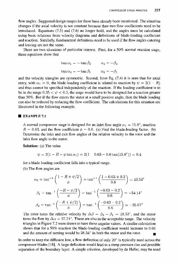
COMPRESSOR STAGE ANALYSIS 227
flow angles. Suggested design ranges for these have already been mentioned. The situation changes if the axial velocity is not constant because then two flow coefficients need to be introduced. Equations (7.5) and (7.6) no longer hold, and the angles must be calculated using basic relations from velocity diagrams and definitions of blade-loading coefficient and reaction. Similarly, fundamental definitions need to be used if the flow angles entering and leaving are not the same.
There are two situations of particular interest. First, for a 50% normal reaction stage, these equations show that
tancti = — tan/?2 a\ = —02
tan OL2 = — tan /3i a2 = ~Pi
and the velocity triangles are symmetric. Second, from Eq. (7.4) it is seen that for axial entry, with a>\ = 0, the blade-loading coefficient is related to reaction by ip — 2(1 - R) and thus cannot be specified independently of the reaction. If the loading coefficient is to be in the range 0.35 < tp < 0.5, the stage would have to be designed for a reaction greater than 50%. But if the flow enters the stator at a small positive angle, then the blade loading can also be reduced by reducing the flow coefficient. The calculations for this situation are illustrated in the following example.
■ EXAMPLE 7.1
A normal compressor stage is designed for an inlet flow angle a\ = 15.8°, reaction R — 0.63, and the flow coefficient <f> = 0.6. (a) Find the blade-loading factor, (b) Determine the inlet and exit flow angles of the relative velocity to the rotor and the inlet flow angle to the stator.
Solution: (a) The value
ip = 2(1 - R - </>tanai) = 2(1 - 0.63 - 0.6tan(15.8°)) = 0.4
for a blade loading coefficient falls into a typical range. (b) The flow angles are
+ _ 1 / l - J R + ^ / 2 \ _x / l - 0 . 6 3 + 0.2\ AOKAO a2 = tan { j = tan { - j = 43.54
1f-R~i>/2\ , /-0.63-0.2\ r ,1„0
*=tan (—* ) = tan I o.6 ) = -5414
lf-R + ^/2)\ , f-0.63 + 0.2\ „„„_ h = tan- ( — f t l ) = tan- ( Q 6 ) = -35.61°
The rotor turns the relative velocity by A/3 = j32 — Pi = 18.53°, and the stator turns the flow by Aa = 27.74°. These are also in the acceptable range. The velocity triangles in Figure 7.2 were drawn to have these angular values. A similar calculation shows that for a 50% reaction the blade-loading coefficient would increase to 0.66 and the amount of turning would be 38.34° in both the stator and the rotor. a
In order to keep the diffusion low, a flow deflection of only 20° is typically used across the compressor blades [18]. A large deflection would lead to a steep pressure rise and possible separation of the boundary layer. A simple criterion, developed by de Haller, may be used
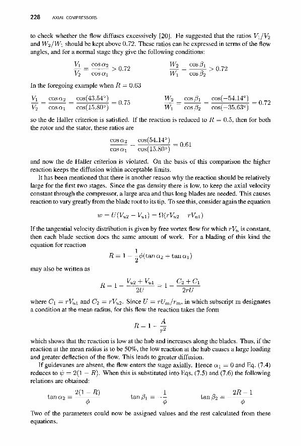
228 AXIAL COMPRESSORS
to check whether the flow diffuses excessively [20]. He suggested that the ratios Vi/V2 and W2/W1 should be kept above 0.72. These ratios can be expressed in terms of the flow angles, and for a normal stage they give the following conditions:
£ = ^ > 0 . 7 2 ^ = ^ > 0 . 7 2 V2 cosai W\ cosp2
In the foregoing example when R = 0.63
Vi _ cosa2 _ cos(43.54°) _ „ ? , W2 _ cos ft _ cos(-54.14°) _ „ ? 9
V2 ~ cosai ~ cos(15.80°) ~ ' w[ ~ cos/32 ~ cos(-35.63°) ~~
so the de Haller criterion is satisfied. If the reaction is reduced to R = 0.5, then for both the rotor and the stator, these ratios are
cosa2 _ cos(54.14°) _ cosai cos(15.80°)
and now the de Haller criterion is violated. On the basis of this comparison the higher reaction keeps the diffusion within acceptable limits.
It has been mentioned that there is another reason why the reaction should be relatively large for the first two stages. Since the gas density there is low, to keep the axial velocity constant through the compressor, a large area and thus long blades are needed. This causes reaction to vary greatly from the blade root to its tip. To see this, consider again the equation
w = U(Vu2 -Vul) = n(rVu2 - rVul)
If the tangential velocity distribution is given by free vortex flow for which rVu is constant, then each blade section does the same amount of work. For a blading of this kind the equation for reaction
R = 1 — - 0 ( t a n a 2 + t ana i )
may also be written as
D , Vu2 + K l , C2+C1 R=1" 2U =l~^MT
where C\ = rVu\ and C2 = rVu2. Since U = rUm/rm, in which subscript m designates a condition at the mean radius, for this flow the reaction takes the form
R = l - ~
which shows that the reaction is low at the hub and increases along the blades. Thus, if the reaction at the mean radius is to be 50%, the low reaction at the hub causes a large loading and greater deflection of the flow. This leads to greater diffusion.
If guidevanes are absent, the flow enters the stage axially. Hence a.\ = 0 and Eq. (7.4) reduces to tp = 2(1 — R). When this is substituted into Eqs. (7.5) and (7.6) the following relations are obtained:
2(1 -R) 1 „ 2R-1 tan«2 = 7 tanpi = ta,np2 =
<P <P <t>
Two of the parameters could now be assigned values and the rest calculated from these equations.
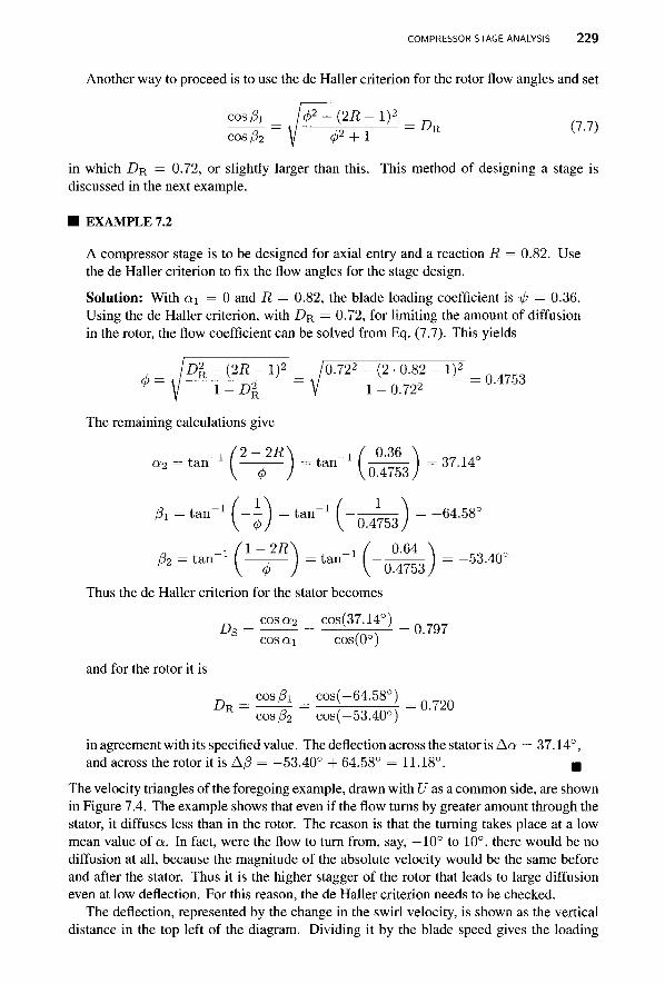
COMPRESSOR STAGE ANALYSIS 229
Another way to proceed is to use the de Haller criterion for the rotor flow angles and set
cos ft 4>2 + {2R-l)2 cos ft y q>2 + 1
in which D R = 0.72, or slightly larger than this. This method of designing a stage is discussed in the next example.
■ EXAMPLE 7.2
A compressor stage is to be designed for axial entry and a reaction R = 0.82. Use the de Haller criterion to fix the flow angles for the stage design.
Solution: With a\ = 0 and R = 0.82, the blade loading coefficient is ip = 0.36. Using the de Haller criterion, with DR = 0.72, for limiting the amount of diffusion in the rotor, the flow coefficient can be solved from Eq. (7.7). This yields
(2R - 1)2 _ /0.722 - (2 • 0.82 - If = Q ^ 1 - Dl V 1 - 0.722
The remaining calculations give
_, [2-2R\ , / 0.36 \ o „ 1 i l 0 a 2 = t a n ( - r ~ r t a n (04753)=37-14
A = t a n"1(4)= t a n"1(-oi53)=- 6 4 - 5 8 0
Thus the de Haller criterion for the stator becomes
Ds = cosas = coS(37.14°) = Q7Q7
coscti cos(0°)
and for the rotor it is
cos ft cos(-64.58°) „ „„„ rj "-1 v /_ n yon
R ~ cos ft ~ cos(-53.40°) ~ in agreement with its specified value. The deflection across the stator is Aa = 37.14°, and across the rotor it is A,3 = -53.40° + 64.58° = 11.18°. B
The velocity triangles of the foregoing example, drawn with U as a common side, are shown in Figure 7.4. The example shows that even if the flow turns by greater amount through the stator, it diffuses less than in the rotor. The reason is that the turning takes place at a low mean value of a. In fact, were the flow to turn from, say, —10° to 10°, there would be no diffusion at all, because the magnitude of the absolute velocity would be the same before and after the stator. Thus it is the higher stagger of the rotor that leads to large diffusion even at low deflection. For this reason, the de Haller criterion needs to be checked.
The deflection, represented by the change in the swirl velocity, is shown as the vertical distance in the top left of the diagram. Dividing it by the blade speed gives the loading
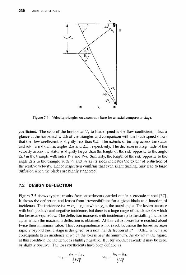
230 AXIAL COMPRESSORS
' vu. -vu1
V
\y
/aA\ \ p y \
1 ^
/ V 2
W1 A P \ \
w2\^
Figure 7.4 Velocity triangles on a common base for an axial compressor stage.
coefficient. The ratio of the horizontal Vx to blade speed is the flow coefficient. Thus a glance at the horizontal width of the triangles and comparison with the blade speed shows that the flow coefficient is slightly less than 0.5. The extents of turning across the stator and rotor are shown as angles A a and A/3, respectively. The decrease in magnitude of the velocity across the stator is slightly larger than the length of the side opposite to the angle A/3 in the triangle with sides W\ and W2. Similarly, the length of the side opposite to the angle A a in the triangle with V\ and V2 as its sides indicates the extent of reduction of the relative velocity. Hence inspection confirms that even slight turning, may lead to large diffusion when the blades are highly staggered.
7.2 DESIGN DEFLECTION
Figure 7.5 shows typical results from experiments carried out in a cascade tunnel [37]. It shows the deflection and losses from irreversibilities for a given blade as a function of incidence. The incidence is i = a2 — \ 2 , in which \ 2 is the metal angle. The losses increase with both positive and negative incidence, but there is a large range of incidence for which the losses are quite low. The deflection increases with incidence up to the stalling incidence es, at which the maximum deflection is obtained. At this value losses have reached about twice their minimum value. This correspondence is not exact, but since the losses increase rapidly beyond this, a stage is designed for a nominal deflection of e* = 0.8ers, which also corresponds to an incidence at which the loss is near its minimum. As shown in the figure, at this condition the incidence is slightly negative. But for another cascade it may be zero, or slightly positive. The loss coefficients have been defined as
WR h2 - h2
2 1
ha ~ h U)S
3s I T / 2 2 V2
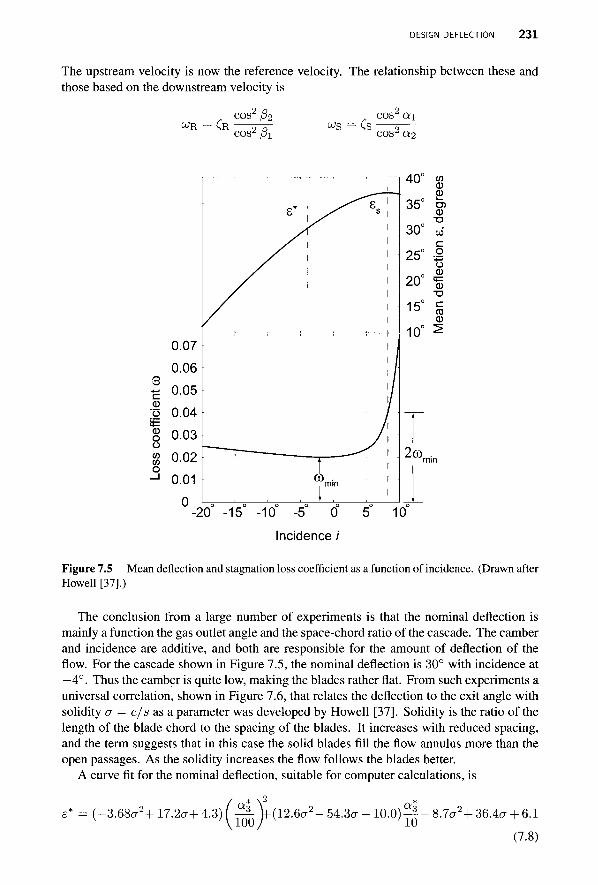
DESIGN DEFLECTION 2 3 1
The upstream velocity is now the reference velocity. The relationship between these and those based on the downstream velocity is
WR = CR COS2 / ? 2
cos2 /3i COS tti
WS = CS 2 C O S z OL<i
c 0 'o it= 0 o o CO CO
o
-20 -15 -10 -5 0
Incidence /'
CO 0 £
T3
'-*—> o j o M— 0 ■o c ca 0
Figure 7.5 Mean deflection and stagnation loss coefficient as a function of incidence. (Drawn after Howell [37].)
The conclusion from a large number of experiments is that the nominal deflection is mainly a function the gas outlet angle and the space-chord ratio of the cascade. The camber and incidence are additive, and both are responsible for the amount of deflection of the flow. For the cascade shown in Figure 7.5, the nominal deflection is 30° with incidence at —4°. Thus the camber is quite low, making the blades rather flat. From such experiments a universal correlation, shown in Figure 7.6, that relates the deflection to the exit angle with solidity a = c/s as a parameter was developed by Howell [37]. Solidity is the ratio of the length of the blade chord to the spacing of the blades. It increases with reduced spacing, and the term suggests that in this case the solid blades fill the flow annulus more than the open passages. As the solidity increases the flow follows the blades better.
A curve fit for the nominal deflection, suitable for computer calculations, is
e* = (-3.68cr2+17.2cr+4.3) 5 ^ ( 1 2 . ^ - 5 4 . 3 . ■ «"»£- 8.7cr2+36.4cr + 6.1
(7.8)
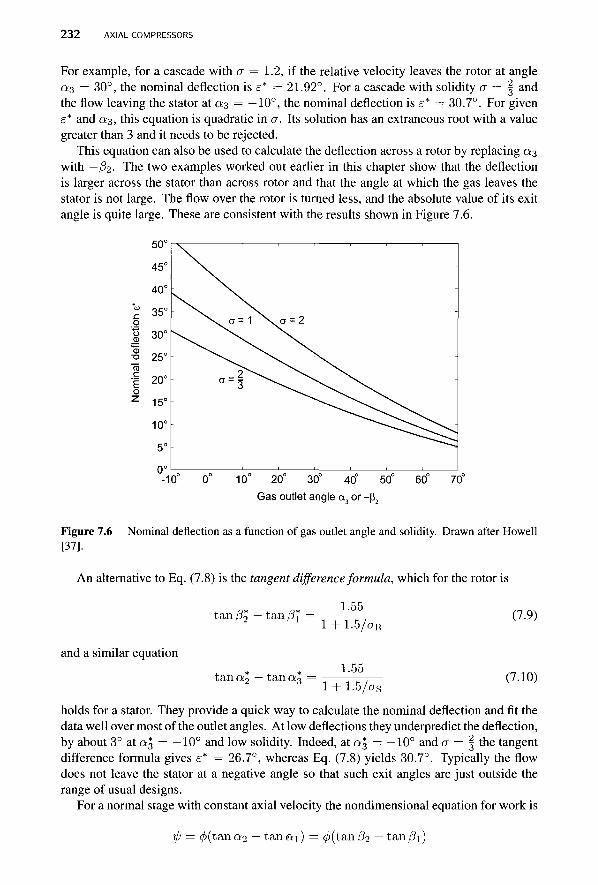
232 AXIAL COMPRESSORS
For example, for a cascade with a = 1.2, if the relative velocity leaves the rotor at angle ct3 = 30°, the nominal deflection is e* = 21.92°. For a cascade with solidity a = | and the flow leaving the stator at a 3 = —10°, the nominal deflection is e* = 30.7°. For given e* and a^, this equation is quadratic in er. Its solution has an extraneous root with a value greater than 3 and it needs to be rejected.
This equation can also be used to calculate the deflection across a rotor by replacing a^ with — 02- The two examples worked out earlier in this chapter show that the deflection is larger across the stator than across rotor and that the angle at which the gas leaves the stator is not large. The flow over the rotor is turned less, and the absolute value of its exit angle is quite large. These are consistent with the results shown in Figure 7.6.
c o CD
<B T3
E o
10 20 30 40" 50" Gas outlet angle a3 or -|32
70
Figure 7.6 Nominal deflection as a function of gas outlet angle and solidity. Drawn after Howell [37].
An alternative to Eq. (7.8) is the tangent difference formula, which for the rotor is
and a similar equation
tan 02 — tan /3jf
tan a? — tan aj
1.55 1 + 1.5/CTR
1.55 1 + 1.5/ag
(7.9)
(7.10)
holds for a stator. They provide a quick way to calculate the nominal deflection and fit the data well over most of the outlet angles. At low deflections they underpredict the deflection, by about 3° at a^ = —10° and low solidity. Indeed, at a% = —10° and a = | the tangent difference formula gives s* = 26.7°, whereas Eq. (7.8) yields 30.7°. Typically the flow does not leave the stator at a negative angle so that such exit angles are just outside the range of usual designs.
For a normal stage with constant axial velocity the nondimensional equation for work is
ip = 0(tan Q!2 — tan a\) = 0(tan /?2 - tan Pi)
DESIGN DEFLECTION 233
The tangent difference formulas now show that the solidity for the rotor is the same as that for the stator, as the design is based on nominal conditions. It is determined by solving
ip* 1.55 <p* 1 + 1.5/cr
for a. In order to prevent resonance vibrations, the number of blades in the rotor is slightly different from the number of stator blades. Thus the spacing is changed, but the same solidity can still be achieved by changing the length of the chord.
■ EXAMPLE 7.3
A normal compressor stage is designed to have the flow leave the stator at the angle ot\ = 12.60°. Assume that the optimum design condition for least losses is achieved when the reaction is R = 0.68, and the flow coefficient 0 = 0.56. For a normal stage, find the blade loading factor, and the optimum value for the solidity. Check also that the de Haller criterion is satisfied.
Solution: The loading coefficient is first determined from
ip = 2(l-R- 0 t a n a i ) = 2(1 - 0.68 - 0.56tan(12.6°)) = 0.39
and the flow angles are
0,-«m-.(I^)-^(I^±!^)-^
A — - ( ^ ) — - ■ ( ^ ^ ) — ! f-R + ip/2)\ ! / - 0 . 6 8 +0.195 \
A = tan"1 ( — ^ ) = tan"1 ( Q , 5 6 j = "40.90°
The deflections are therefore
£s = 30.00° £R = 16.48°
The diffusion factors are cosQ2 = cos(42.60°) = 7 M cos/3i = cos(-57.38°) =
cos en cos(12.60°) ' cos/32 cos(-40.90°) so that the diffusion in the rotor is marginally too high. If the solidity is calculated from the tangent difference formula, it yields
1.5 r/> a= — = 1.22
1 . 5 5 0 - ^
In actual machines the values of (f>, ip, and R vary across the span, owing to the change in the blade velocity with the radius, and ip tends to be high near the hub and low near the casing. The reaction is low near the hub and high near the casing, as R moves in opposite direction to the loading coefficient. The blade angles are adjusted to counteract the natural tendency that causes the values to change so that the loading can be kept more uniform. A 50% reaction ratio is common, and the blade-loading coefficient is typically in the range 0.3 < ip < 0.45.
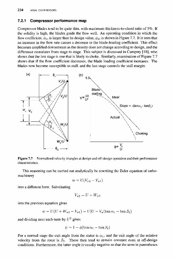
234 AXIAL COMPRESSORS
7.2.1 Compressor performance map
Compressor blades tend to be quite thin, with maximum thickness-to-chord ratio of 5%. If the solidity is high, the blades guide the flow well. An operating condition in which the flow coefficient, <po, is larger than its design value, <pd, is shown in Figure 7.7. It is seen that an increase in the flow rate causes a decrease in the blade-loading coefficient. This effect becomes amplified downstream as the density does not change according to design, and the difference cumulates from stage to stage. This subject is discussed in Cumpsty [18], who shows that the last stage is one that is likely to choke. Similarly, examination of Figure 7.7 shows that if the flow coefficient decreases, the blade loading coefficient increases. The blades now become susceptible to stall, and the last stage controls the stall margin.
\ \ Slope = -(tana. - tanp )
\ Choking
Figure 7.7 Normalized velocity triangles at design and off-design operation and their performance characteristics.
This reasoning can be carried out analytically be rewriting the Euler equation of turbo-machinery
w = U(Vu2-Vul) into a different form. Substituting
vu2 = u + wu2
into the previous equation gives
w = U(U + Wu2 - Vul) = U[U - Vx(tanai - t<m/32)}
and dividing next each term by U2 gives
ip = 1 — </>(tanofi — t&n/32)
For a normal stage the exit angle from the stator is a\, and the exit angle of the relative velocity from the rotor is ft2. These then tend to remain constant even at off-design conditions. Furthermore, the latter angle is'usually negative so that the term in parentheses

RADIAL EQUILIBRIUM 235
is positive. With the trigonometric factors constant, this means that increasing the flow coefficient decreases the loading.
This equation gives the compressor characteristic for an ideal compressor. It is a straight line with a negative slope when the blade-loading coefficient is plotted against the flow coefficient. This is shown in Figure 7.7b. The actual compressor characteristic is also shown, and the differences away from the design point are caused by irreversibilites. Far away from the design point to the left, the blades stall and at even lower flow rates (smaller 4>) the compressor may experience surge. This means that the flow can actually reverse its direction and flow out the front of the compressor. For this reason compressors are operated some distance away from the stall line. To the right of the design point irreversibilities again cause deviation from the theoretical curve, and as the flow rate increases, the blade row will choke.
7.3 RADIAL EQUILIBRIUM
The mean line analysis on which most of the calculations in this text are based ignores the cross-stream variation in the flow. In axial-flow machines this means that only the influence of the blade speed, that increases with radius, is taken into account. Today it is possible to carry out calculations by CFD methods to resolve the three-dimensional aspects of the flow. However, as was seen in the discussion of axial turbines, the elementary radial equilibrium theory advances the understanding on how the important variables, such as the reaction and the loading, vary from the hub to the casing. There (and in Appendix A) it was shown that the principal equation to be solved is
^=r*+l^+^+e a u ) dr ar dr dr r
The first term on the right represents the entropy variation in the radial direction. Owing to the entropy production in the endwall boundary layers, tip vortices, and possible shocks, this is likely to be important near the walls. However, if the flow mixes well in the radial direction, entropy gradients diminish and it may be reasonable to neglect this term. Of course, irreversibilities would still cause entropy to increase in the downstream direction, even if it does not have radial gradients.
The stagnation enthalpy is uniform at the entrance to the first row of rotor blades, and if every blade section does an equal amount of work on the flow, it will remain uniform even if the stagnation enthalpy increases in the direction of the stream. As a consequence, the term on the left side of this equation may be neglected, and the equation reduces to
V« + n^ + !2=0 (7.12) dr dr r
This is a relationship between the velocity components Vu and Vx. If the radial variation of one of them is assumed, the variation of the other is obtained by solving this equation. For example, as was seen in the discussion of axial turbines, if the axial component Vx is assumed to be uniform, then the radial component must satisfy the equation
dVu dr
the solution of which is rVu = constant. This is the free vortex velocity distribution. Before and after a row of blades the tangential velocity is
v - Cl v - C2
r r
236 AXIAL COMPRESSORS
It was observed earlier that the expression for work is now
w = U(Vu2 - K i ) = rfi ( ^ - ^ ) = n(c2 - Cl)
so that the work is independent of radius. This justifies dropping the term dho/dr in Eq.(7.11).
7.3.1 Modified free vortex velocity distribution
The free vortex velocity distribution is a special case of the family of distributions
Vul=crn-- Vu2=crn+d (7.13) r r
in which n is a parameter. Regardless of the value of n, each member of this family has a velocity distribution for which each blade section does an equal amount of work, as seen from
w = U(Vu2 - Vul) = nr (- + -)= 2nd
With the mean radius rm the same at the inlet and the exit, a nondimensional radius may be introduced as y = r/rm. The tangential velocity components for a free vortex distribution with n = — 1 may now be written as
a b a — b a b a + b Vui = = Vu2 = —I— =
y y y y y y
When the Eq. (7.12) for radial'equilibrium is recast into the form
T/ dVx Vu d ay y dy
it shows that for this velocity distribution RHS vanishes, as the substitution shows
T r dVx a — b d(a — b) Vx —— = —7, ; = 0 Vx — constant
dy yz dy
Clearly, the same result is obtained for the outlet, as only the sign of b needs to be changed to describe the tangential velocity there. This reduced equation now shows that the axial velocity is constant along the span of the blade, but it does not follow that it has the same constant value before and after the blade row. The axial velocities can be made the same by proper taper of the flow channel.
The reaction is given by
R=l- - — ( tana2 + t a n a 2 ) = 1 - - — 2 U 2 Umy
Here U = rfl = rUm/rm, or U = Umy was used. Since Vu2 + Vu\ = 2a/y, the reaction is
R = l a
Umy2
If Rm is the reaction at the mean radius y = 1, then a = Um{\ — Rm) and the reaction can be written as
R(y) = 1 - (1 - Rm) \ y
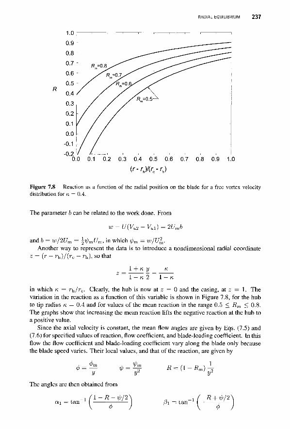
RADIAL EQUILIBRIUM 237
R
0.3 0.4 0.5 0.6 (r-ru)'(rc-rh)
1.0
Figure 7.8 Reaction as a function of the radial position on the blade for a free vortex velocity distribution for K = 0.4.
The parameter 6 can be related to the work done. From
U{VX l»2 Vul) = 2Umb
J-2 and b = w/2Um = ^ipmUm, in which ipm = w/U^ Another way to represent the data is to introduce a nondimensional radial coordinate
z = (r - rh)/(rc - r h) , so that
K = l + K1 1 - K 2 1 - K
in which K = rh/rc. Clearly, the hub is now at z = 0 and the casing, at z = 1. The variation in the reaction as a function of this variable is shown in Figure 7.8, for the hub to tip radius K = 0.4 and for values of the mean reaction in the range 0.5 < Rm < 0.8. The graphs show that increasing the mean reaction lifts the negative reaction at the hub to a positive value.
Since the axial velocity is constant, the mean flow angles are given by Eqs. (7.5) and (7.6) for specified values of reaction, flow coefficient, and blade-loading coefficient. In this flow the flow coefficient and blade-loading coefficient vary along the blade only because the blade speed varies. Their local values, and that of the reaction, are given by
y ■<!>
Ipn R = (1 — Rm) -^
The angles are then obtained from
Qi = tan 1 (l-R-tp/2 tan
R + ^/2"
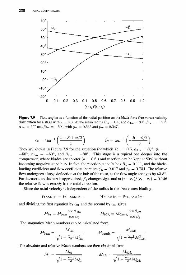
238 AXIAL COMPRESSORS
0.1 0.2 0.3 0.4 0.5 0.6 0.7 0.8 0.9 1.0 (r-rhVire-Th)
Figure 7.9 Flow angles as a function of the radial position on the blade for a free vortex velocity distribution for a stage with K = 0.6. At the mean radius i?m = 0.5, and a\m = 30°, /3 l m = —50°, Q 2 m = 50° and /32m = -50° , with <£m = 0.565 and tpm = 0.347.
a 2 = tan l - R + ^/2
P2 t an R jP/2\
$ ) They are shown in Figure 7.9 for the situation for which Rm = 0.5, a\m = 30°, j3\m = —50°, a2m = —50°, and /3 2 m = —30°. This stage is a typical one deeper into the compressor, where blades are shorter {K = 0.6 ) and reaction can be kept at 50% without becoming negative at the hub. In fact, the reaction at the hub is i?h = 0.111, and the blade-loading coefficient and flow coefficient there are tph = 0.617 and 4>h = 0.754. The relative flow undergoes a large deflection at the hub of the rotor, as the flow angle changes by 43.8°. Furthermore, as the hub is approached, /32 changes sign, and at (r — r h ) / ( r c — rh) = 0.146 the relative flow is exactly in the axial direction.
Since the axial velocity is independent of the radius in the free vortex blading,
Vi cos a\ = Vim cos a i m W2 cos /32 = W2m cos /3 2 m
and dividing the first equation by CQI and the second by CQ2 gives
M, 01 M, cos a i m 0 1 m ' M„2 R = Mi
c o s a i
The stagnation Mach numbers can be calculated from
Mim
02mR/ COS / 3 2 n
COS/32
M< Olr y/l + ^M^
M)2mR M2mR
1 + 2 J U 2 m R
The absolute and relative Mach numbers are then obtained from Moi , , M 0 2 R Mi
1 2 J W 0 1
M 2 R
1 7 - 1 M2
2 i v J 0 2 R
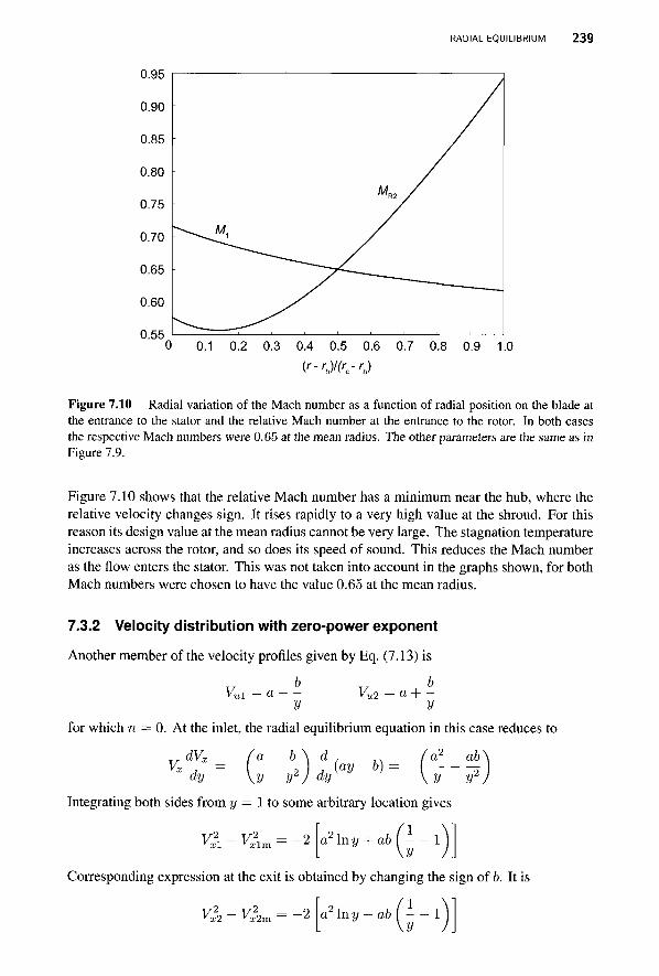
RADIAL EQUILIBRIUM 239
0.55 0 0.1 0.2 0.3 0.4 0.5 0.6 0.7 0.8 0.9 1.0
(r-rh)l(r0-rh)
Figure 7.10 Radial variation of the Mach number as a function of radial position on the blade at the entrance to the stator and the relative Mach number at the entrance to the rotor. In both cases the respective Mach numbers were 0.65 at the mean radius. The other parameters are the same as in Figure 7.9.
Figure 7.10 shows that the relative Mach number has a minimum near the hub, where the relative velocity changes sign. It rises rapidly to a very high value at the shroud. For this reason its design value at the mean radius cannot be very large. The stagnation temperature increases across the rotor, and so does its speed of sound. This reduces the Mach number as the flow enters the stator. This was not taken into account in the graphs shown, for both Mach numbers were chosen to have the value 0.65 at the mean radius.
7.3.2 Velocity distribution with zero-power exponent
Another member of the velocity profiles given by Eq. (7.13) is
Vui=a Vu2 = a + -y y
for which n = 0. At the inlet, the radial equilibrium equation in this case reduces to
V, dy y y2Jdy -(ay-b) a2 ab
y y2
Integrating both sides from y = 1 to some arbitrary location gives
V\ - V\ 2 / 1 a In y + ab [ 1
y Corresponding expression at the exit is obtained by changing the sign of b. It is
Vz — V2 ., , 1 a In y — ab \ 1
V
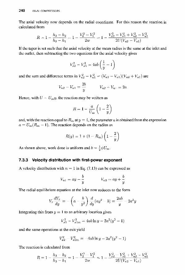
240 AXIAL COMPRESSORS
The axial velocity now depends on the radial coordinate. For this reason the reaction is calculated from
R = 1 h3-h2 V2 - V2 = V2
2 - Vx\ + V22 - V2,
hn-fn 2w 2U(Vu2~Vul)
If the taper is set such that the axial velocity at the mean radius is the same at the inlet and the outlet, then subtracting the two equations for the axial velocity gives
Vx\ ~ Vli = 4a6 ( - - 1 \y
and the sum and difference terms in V22 — V2
X = (Yu2 — KuXK^ + Ku) are
26 Vu2 -Vul = — Vu2 + K i = 2a
V Hence, with U = Umy, the reaction may be written as
and, with the reaction equal to Rm at y = 1, the parameter a is obtained from the expression a- = Um(Rm — 1). The reaction depends on the radius as
R(y) = 1 + (1 - Rm) (1 - -V V
As shown above, work done is uniform and b — \tj)Um.
7.3.3 Velocity distribution with first-power exponent
A velocity distribution with n = 1 in Eq. (7.13) can be expressed as
b b K i = ay Vu2 = ay+-
y y The radial equilibrium equation at the inlet now reduces to the form
dVx ( b \ d / 2 2ab 2
Integrating this from y = 1 to an arbitrary location gives
Vxi - K2im = 4a61ny - 2a2 (y2 - 1)
and the same operations at the exit yield
V?2 ~ V22m = -iablny - 2a2(y2 - 1)
The reaction is calculated from
h3 - h2 V2 - V2 V22 - Vx\ + V2
2 - V2X
h3-h! 2w 2U(Vu2-Vul)
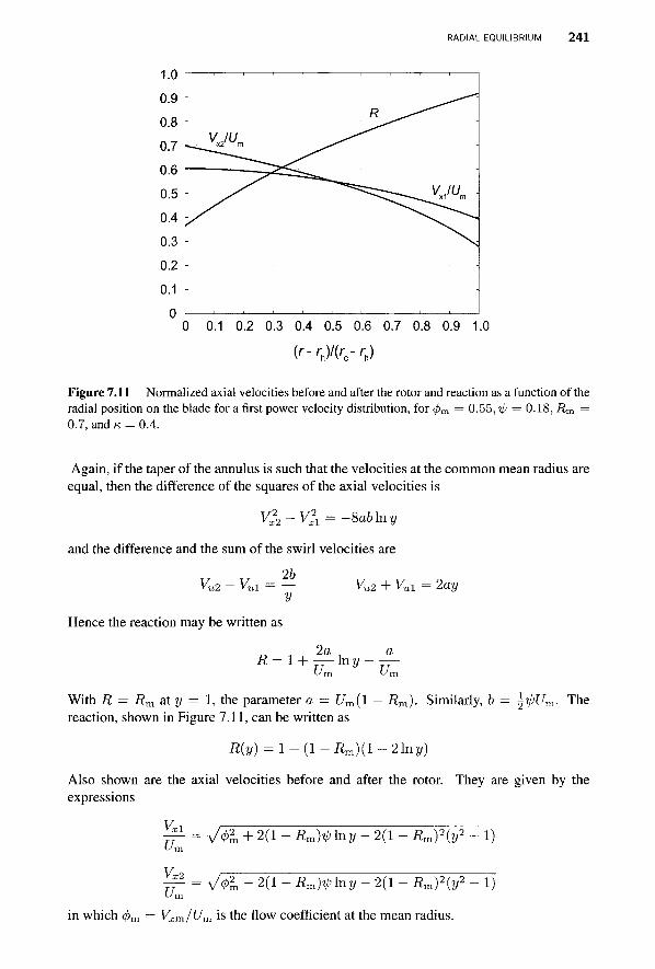
RADIAL EQUILIBRIUM 2 4 1
0.1 0.2 0.3 0.4 0.5 0.6 0.7 0.8 0.9 1.0
( r - r h ) / ( f c - r h )
Figure 7.11 Normalized axial velocities before and after the rotor and reaction as a function of the radial position on the blade for a first power velocity distribution, for <j>m = 0.55, rp = 0.18, Rm = 0.7, and K = 0.4.
Again, if the taper of the annulus is such that the velocities at the common mean radius are equal, then the difference of the squares of the axial velocities is
V^-V^ = -8ablny
and the difference and the sum of the swirl velocities are
26 Vu2 ~ Vul =
y
Hence the reaction may be written as
R=l
Vu2 + Vui = 2ay
2a a
With R = Rm at y = 1, the parameter a = Um(l — Rm). Similarly, b = \ipUm. The reaction, shown in Figure 7.11, can be written as
R(y) = l-(l-Rm)(l-2\ny)
Also shown are the axial velocities before and after the rotor. They are given by the expressions
um
V*2 um
= y/<f?m + 2(1 - Rm)^\ny - 2(1 - i?m)2(y2 - 1)
y/fa - 2(1 - Rm)ipiny - 2(1 - Rm)2(y2 - 1)
in which 4>m = Vxm/Um is the flow coefficient at the mean radius.
242 AXIAL COMPRESSORS
7.4 DIFFUSION FACTOR
Earlier in this chapter the de Haller criterion was used as a criterion to ensure that the diffusion in the flow passages would not be strong enough to cause separation of the boundary layers. The adverse pressure gradient associated with diffusion is seen in Figure 7.12, which shows a typical stator blade surface pressure measurement, plotted as a pressure coefficient Cp = (p — P2)/(po2 — P2) against the fractional distance along the chord for three different values of solidity a = c/s. The bottom branch of the curve gives the suction-side pressure distribution and the top branch, that for the pressure side of the blade. Under ideal conditions at low Mach number the spike in the pressure coefficient on the top branch should reach unity at the stagnation point located near the leading edge. From there the pressure falls as the flow accelerates to a location of maximum blade thickness followed by diffusion toward the trailing edge. Near the trailing edge the flow may accelerate slightly owing to its orientation and camber. On the suction side of the blade the negative spike is caused by the need for the flow to negotiate the blunt leading edge of the blade as it flows from the location of the stagnation point to the suction side. Pressure then increases sharply from the suction spike all the way to the trailing edge as the flow diffuses. This diffusion must be kept within acceptable limits. The difference in the value of pressure at any given chord location is a measure of the local loading on the blade and, as seen from Figure 7.12, the blade becomes unloaded as the trailing edge is approached.
Since the blade force is obtained by integrating the pressure acting over the blade surface, the area inscribed by the curves represents the blade force normal to the chord. As the solidity increases, this force is reduced, but now with reduced spacing, more blades can be fitted to the rotor wheel to carry the load. Increased solidity lifts the value of the minimum pressure, with the result that the pressure gradient decreases. Therefore, the flow can be turned by a greater amount without danger of boundary-layer separation.
A local diffusion factor is defined as
,-. Vmax — V3 Moc = v2
in which ym a x is the velocity at the location of minimum pressure. This definition would be useful, if the profile shape were known and Vmax could be easily calculated. It can, in fact, be done quite readily with a computer code for inviscid flows. But before this became a routine task, an alternative was sought. Lieblein and Roudebush [51] suggested a diffusion factor of the form
B f = ^ + ' ^ ! ( 7 . ,4) V2 la V2
The first part is similar to the local diffusion factor, and the second part accounts for the amount of turning and the solidity of the blade row. Since reduced turning and higher solidity both contribute to lighter loading on the blades, diffusion is expected to diminish by both effects. The Lieblein diffusion factor for the stator can be expressed as
COS Q!3 — COS Ct.2 1 DFs = \--—(tano;2 — tana3)cosa2 (7-15)
COS « 3 2<7s
and for the rotor it takes the form
cos p2 - cos Pi 1 DFR= h -—(tan/?i - tan/32)cos/3i (7.16)
cos P2 2<rR
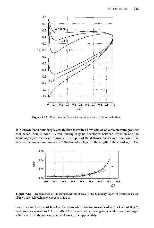
DIFFUSION FACTOR 243
1.0
0.8
0.8
0.4
0.2
Cp 0.0
-0.2
-0.2
-0.4
-0.6
-0.2
-1.0
-1.2
\ \ a = 0.75 :
^~"~a=1.0i ^^^ J
0 0.1 0.2 0.3 0.4 0.5 0.6 0.7 0.8 0.9 1.0 x/c
Figure 7.12 Pressure coefficient for a cascade with different solidities.
It is known that a boundary layers thicken faster in a flow with an adverse pressure gradient than when there is none. A relationship may be developed between diffusion and the boundary-layer thickness. Figure 7.13 is a plot of the diffusion factor as a function of the ratio of the momentum thickness of the boundary layer to the length of the chord 6/c. The
0.06
0.04
0.02
0.00
Figure 7.13 Dependence of the momentum thickness of the boundary layer on diffusion factor. (Drawn after Lieblein and Roudebush [51].)
curve begins its upward bend at the momentum thickness-to-chord ratio of about 0.007, and this corresponds to DF = 0.45. Thus values below these give good designs. For larger DF values the stagnation pressure losses grow appreciably.

244 AXIAL COMPRESSORS
Equations (7.15) and (7.16) are two additional equations among the design variables. In an earlier section it was shown that specifying the values for i?, tp, 4> fixes the flow angles. With the tangent difference formulas and the two diffusion factor formulas, three more equations are added, but solidity is the only new unknown. Hence in principle the designer has the freedom to choose only one of the parameters, such as reaction, or else violate either the tangent difference equation, or one of the diffusion factor equations. However, if the design is such that either DFs or DFR, or both are less than 0.42, then the tangent difference formula fixes the solidity. Thus the choice for the acceptable range of values of reaction, blade loading, and the flow coefficient to achieve the mild diffusion restricts the design parameter space. The typical design ranges 0.35 < ip < 0.5 and 0.4 < <p < 0.7 reflect this.
7.4.1 Momentum thickness of a boundary layer
The momentum thickness of a boundary layer is related to the diffusion factor in Figure 7.13. It and the displacement thickness are now discussed further. The latter is denoted by 5* and is introduced by the expression
S*V{ (V( - V(y))dy (7.17)
in which Vf is the uniform velocity outside the boundary layer of thickness S. Clearly, this equation can be rewritten as
V(y)dy = V{(5-6*) (7.18)
and its interpretation is shown with the aid of Figure 7.14, in which the shadowed areas in parts (a) and (b) are equal according to Eq. (7.17). Figure 7.14b shows the blocking effect of the boundary layer; that is, the flow can be envisioned to have velocity Vf to the edge of S* and inside the layer to have zero velocity, as if the flow were completely blocked. Another way to say this is that if the wall were to be displaced by 5*, the same mass flow rate would exist in the inviscid flow as in a real flow without a displacement of the wall.
(a) (b) (c)
Figure 7.14 Illustration of displacement and momentum thickness.
The momentum thickness 9 is defined by the equation
9V{= / V(y)(V(-V(y))dy Jo
(7.19)
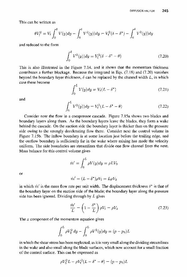
DIFFUSION FACTOR 245
This can be written as
rS 9V2 = V{ [ V(y)dy- f V2(y))dy = V{
2(6-6*)~ I V2(y))dy Jo Jo Jo
and reduced to the form
/ V2(y))dy = V2(S -6*-0) (7.20) Jo
This is also illustrated in the Figure 7.14, and it shows that the momentum thickness contributes a further blockage. Because the integrand in Eqs. (7.18) and (7.20) vanishes beyond the boundary layer thickness, 5 can be replaced by the channel width L, in which case these become
i-L
V(y)dy = V{(L - 6*) (7.21) /o / ' Jo and
/ V2(y))dy = V2(L-5* -9) (7.22) Jo
Consider now the flow in a compressor cascade. Figure 7.15a shows two blades and boundary layers along them. As the boundary layers leave the blades, they form a wake behind the cascade. On the suction side the boundary layer is thicker than on the pressure side owing to the strongly decelerating flow there. Consider next the control volume in Figure 7.15b. The inflow boundary is at some location just before the trailing edge, and the outflow boundary is sufficiently far in the wake where mixing has made the velocity uniform. The side boundaries are streamlines that divide one flow channel from the next. Mass balance for this control volume gives
m
or
[ PV(y)dy = pLV3 Jo
(L - S*)pV{ = LpV3
in which m' is the mass flow rate per unit width. The displacement thickness 5* is that of the boundary layer on the suction side of the blade; the boundary layer along the pressure side has been ignored. Dividing through by L gives
m 1 - - )pVt = pV3 (7.23) L V L,
The x component of the momentum equation gives
rL rL f pV2dy- f pV2(y)dy = (p-p3)L
Jo Jo
in which the shear stress has been neglected, as it is very small along the dividing streamlines in the wake and also small along the blade surfaces, which now account for a small fraction of the control surface. This can be expressed as
PV2L - pVf2(L -F-0) = (p- P3)L
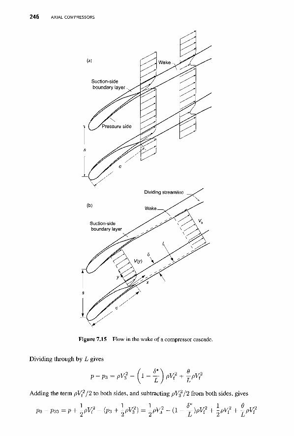
246 AXIAL COMPRESSORS
Figure 7.15 Flow in the wake of a compressor cascade.
Dividing through by L gives
P - p3 = pvi -(^-j) pyi + ] W
Adding the term pVf2 / 2 to both sides, and subtracting pV£/2 from both sides, gives
1 1 1 A* 1 f) P0~P03=P+ 2^f2 - (P3 + 2^32) = 2 ^ 3 2 - (1 " ^)P^f2 + 2 ^ + ZPVf2
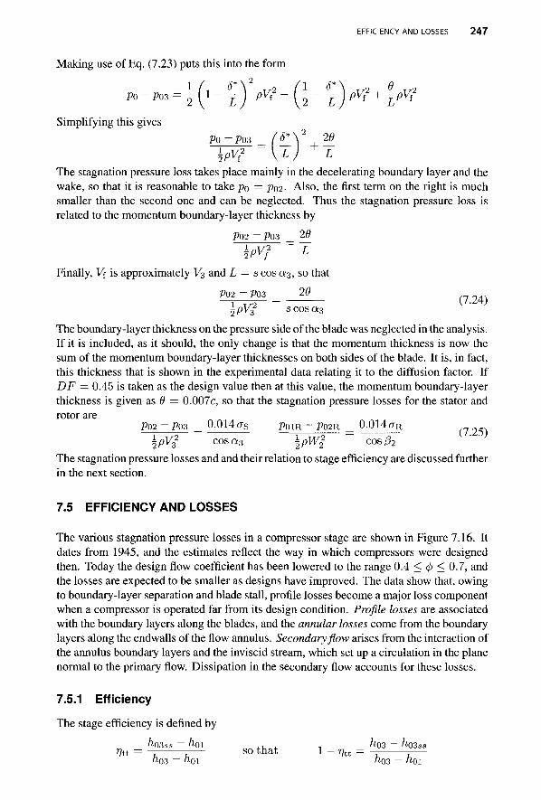
EFFICIENCY AND LOSSES 2 4 7
Making use of Eq. (7.23) puts this into the form
»-»»=Ki-T)a"7-G-T)',?+£'* Simplifying this gives
P0-P03 (S_lY , ^ \Pv? \L) + L
The stagnation pressure loss takes place mainly in the decelerating boundary layer and the wake, so that it is reasonable to take po = Po2- Also, the first term on the right is much smaller than the second one and can be neglected. Thus the stagnation pressure loss is related to the momentum boundary-layer thickness by
P02 - P03 29
Finally, Vf is approximately V3 and L
P02
hpv? = scos
~P03
«3>
L
so that 20
1 T ,2 - ( 7 - 2 4 ) |pVg scosa3
The boundary-layer thickness on the pressure side of the blade was neglected in the analysis. If it is included, as it should, the only change is that the momentum thickness is now the sum of the momentum boundary-layer thicknesses on both sides of the blade. It is, in fact, this thickness that is shown in the experimental data relating it to the diffusion factor. If DF = 0.45 is taken as the design value then at this value, the momentum boundary-layer thickness is given as 9 = 0.007c, so that the stagnation pressure losses for the stator and rotor are
P02 ~ P03 _ 0-014 as PQ\R-~PO2R _ 0-014 aR
\pV$ cosa3 \pW2 cos/32
The stagnation pressure losses and and their relation to stage efficiency are discussed further in the next section.
7.5 EFFICIENCY AND LOSSES
The various stagnation pressure losses in a compressor stage are shown in Figure 7.16. It dates from 1945, and the estimates reflect the way in which compressors were designed then. Today the design flow coefficient has been lowered to the range 0.4 < <\> < 0.7, and the losses are expected to be smaller as designs have improved. The data show that, owing to boundary-layer separation and blade stall, profile losses become a major loss component when a compressor is operated far from its design condition. Profile losses are associated with the boundary layers along the blades, and the annular losses come from the boundary layers along the endwalls of the flow annulus. Secondary flow arises from the interaction of the annulus boundary layers and the inviscid stream, which set up a circulation in the plane normal to the primary flow. Dissipation in the secondary flow accounts for these losses.
7.5.1 Efficiency
The stage efficiency is defined by
ho3ss — ho\ , , , -. /l03 — ho3ss
'to = T. u— s o t h a t 1 - %t = -r r— ft03 — ft01 "03 — ftoi
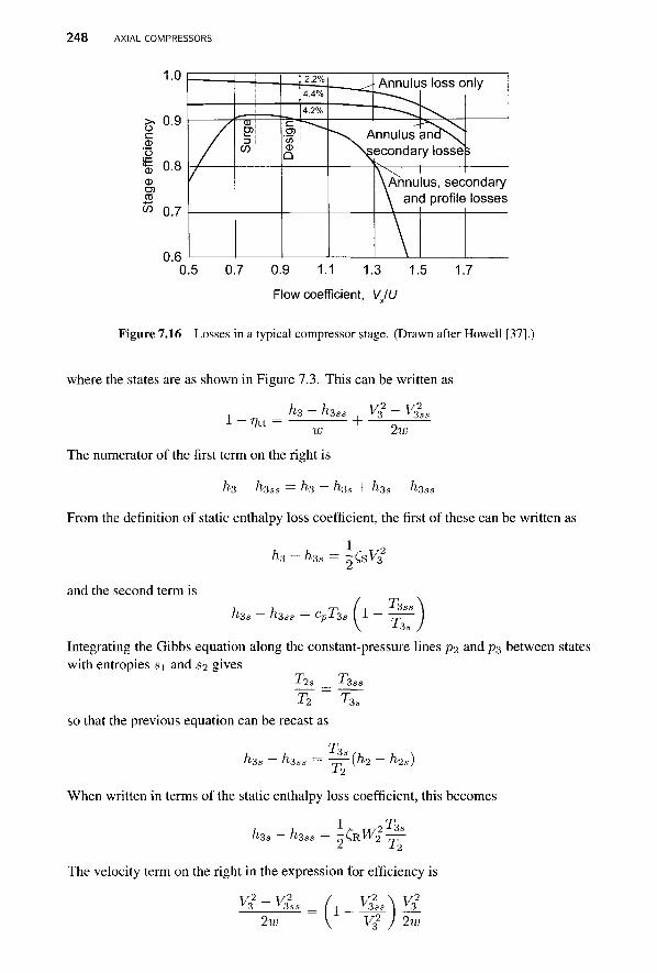
2 4 8 AXIAL COMPRESSORS
0.5 0.7 0.9 1.1 1.3 1.5 1.7
Flow coefficient, V/U
Figure 7.16 Losses in a typical compressor stage. (Drawn after Howell [37].)
where the states are as shown in Figure 7.3. This can be written as
^ 3 — ^ 3 s s 1 -r]tt
v;2 - v;2
^3 v3ss 2w
The numerator of the first term on the right is
^-3 — h3ss = /I3 — / l3 s + h,3s — Jl3ss
From the definition of static enthalpy loss coefficient, the first of these can be written as
1 h3 - h3s = -CsV^
and the second term is h3s ~ h, 3ss L-p-L 3 CvTz* 1
T3s
Integrating the Gibbs equation along the constant-pressure lines p2 and p 3 between states with entropies si and s2 gives
T"2s_ __ T3ss
T2 ~ T3s
so that the previous equation can be recast as
^3s ^ 3 s s t 3 s (h2 - h2s)
When written in terms of the static enthalpy loss coefficient, this becomes
i3s — i^ss r2T3-1&W2-
The velocity term on the right in the expression for efficiency is
V? - V? y 3 y 3ss
2w
v 3ss \ r 3 V3
2 ) 2w
EFFICIENCY AND LOSSES 2 4 9
But is has been shown in Chapter 5 that M3ss = M3. Therefore V32ss/V3
2 = T3ss/T3, and the expression for the efficiency now takes the form
(sV32 + (RW2
1 -%t
2T3s
T2 1 - | ) ^
1w
The first and the last term have a common factor in V3, and they could be combined. However, for a typical stage the temperature factor of the last term has a value of about 0.008. If this is neglected and the term T3s/T2 is set to unity, the right side is simplified somewhat. Therefore the reduced equation
1 - r / t t CsVJ + CRWJ
1w
although simple to use, underestimates the losses by about 1.5%. The relationship to stagnation pressure loss can be developed by writing for the stator
h3 - h3s = cp(T3 - T3s) = cpT3 1 t3s cpT3 Voz\ Pm)
(7-1)7'
which can be rewritten and then expanded for small stagnation pressure loss as
h3 - h-3s cPT3
cPT3
1 P03 ( 7 - l ) / 7 '
Po3 + Ap0Lsy
7 - 1 ApoLS P3 ApoLS
cpT3 1 - 1 ApoLS
P03
- ( 7 - l ) / 7 '
Thus
7 P03
h3 - h3
P03 P3
ApoLs/P3
1 +
A similar analysis for the rotor gives
/i2« = cp(T2 - T2s) = cpT2 I 1
i^V2
To
7/ (7 -1)
cPT2 1 _ (P0*2^\
\P0Rl)
(7-1)7'
which can be rewritten and then expanded for small stagnation pressure loss as
h2 - h2s = cpT2 1 P0R2 ( 7 - l ) / 7
cPT2-
Therefore
PoR2 + ApOL:
7 - 1 AppLR _ P2 AppLR 7 P0R2 P0R2 Pi
A P O L R / P 2
--cpT2 1 - 1 + AppLR P0R2
- ( 7 - l ) / 7 '
ho - h2
1 + ^ M ? R2
7 / (7-1)
250 AXIAL COMPRESSORS
The stagnation pressure losses can now be written as
1 f 2 7/ (7-1)
(7.26)
7 / (7 -1) C R ^ 2 I 1 + ^ M i 2 ) (7.27) APOLR _ I, „ , 2 / , , 7 - 1 , , 2
and
~P2 2 Since the rotor turns the flow toward the axis, the magnitude of the relative velocity diminishes and the relative Mach number leaving the rotor is fairly small. The same is true for the absolute Mach number leaving the stator. Hence, if the Mach number terms in Eqs. (7.26) and (7.27) are neglected, then with some loss of accuracy, substituting the these expressions for the stagnation pressure losses into Eqs. (7.25), gives
COS P 2 COS « 3
l - ^ = ( - § L - + - ^ ) ^ ; (7-29)
Since Vx = V3 cos a^ = W2 cos p~2 the efficiency may be rewritten in the form
' CR , Cs W 2
vcos2ai cos2/3i/ 2tp
7.5.2 Parametric calculations
The development of the theory for axial compressors has been carried out in terms of assumed values for a flow coefficient <j>, a blade-loading factor ip, and a reaction ratio R. These three quantities are nondimensional parameters and are sufficient for calculating the flow angles. Solidity was obtained from experimental measurements of deflection for given flow outlet angle. It was used to establish the permissible diffusion, and the stagnation pressure coefficient for profile losses was established. The efficiency can then be cast in terms of the loss coefficients for the rotor and the stator. This is the most effective way to display results, and when the actual parameters for a machine are given, all the important results are quickly calculated from the nondimensional ones. Thus flow angles for a compressor stator and rotor have been shown to be
l-R-ip/2 l-R + rp/2 t ana i = tan 0:2 — ;
R + ^/2 R-iP/2 — tan pi = - — tan p2 = ;
<f> 4> Hence with <fi, ijj and R given, they can be determined. The rest of the calculations then follow directly. Results from such calculations are shown in Figure 7.17. The flow coefficient was taken to be <p = 0.6 and the degree of reaction, R = 0.4. For Figures 7.17a - 7.17c, the Lieblein diffusion factor was taken to be equal to 0.45, and solidities of the rotor and stator were calculated in terms of this value. Figure 7.17a represents the diffusion in the flow. If the stagnation pressure losses are neglected and the flow is assumed incompressible, then
P2 + i;pV22=P3 + -pVi
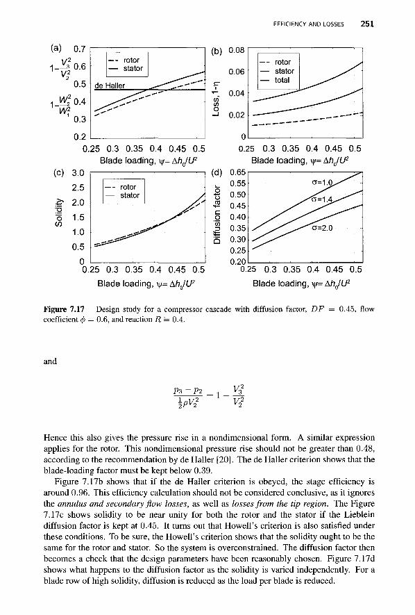
EFFICIENCY AND LOSSES 2 5 1
(a) 0.7 I/2
1_l3 0.6 V2
0.5
-!_!*£ 0.4 W2
(c)
"o
0.3
0.2 0
3.0 2.5 2.0 1.5 1.0 0.5
0 0.
' — - rotor — stator
de Haller
■
^ ^ ^ ^
25 0.3 0.35 0.4 0.45 Blade loading, v|/
0.5 AhJU2
— - rotor — stator
\ ^ ^
(d)
c g en
b
25 0.3 0.35 0.4 0.45 0.5
Blade loading, v|/= Art IU2
(b) 0.08
0.06 P"
--„ 0.04 in in o - " 0.02
n
— - rotor — stator — total
' - -
0.45 0.5
0.65 0.55 0.50 0.45 0.40 0.35 0.30 0.25 0.20
Blade loading V|/=
a--
''&=
a-
-- Ah0/U2
-ASs^
- \ A ^ ^ ^
=2.0
0.25 0.3 0.35 0.4 0.45 0.5
Blade loading, \|/= AhJU2
Figure 7.17 Design study for a compressor cascade with diffusion factor, DF coefficient <b = 0.6, and reaction R = 0.4.
0.45, flow
and
PZ ~P2 Yl v2
2
Hence this also gives the pressure rise in a nondimensional form. A similar expression applies for the rotor. This nondimensional pressure rise should not be greater than 0.48, according to the recommendation by de Haller [20]. The de Haller criterion shows that the blade-loading factor must be kept below 0.39.
Figure 7.17b shows that if the de Haller criterion is obeyed, the stage efficiency is around 0.96. This efficiency calculation should not be considered conclusive, as it ignores the annulus and secondary flow losses, as well as losses from the tip region. The Figure 7.17c shows solidity to be near unity for both the rotor and the stator if the Lieblein diffusion factor is kept at 0.45. It turns out that Howell's criterion is also satisfied under these conditions. To be sure, the Howell's criterion shows that the solidity ought to be the same for the rotor and stator. So the system is overconstrained. The diffusion factor then becomes a check that the design parameters have been reasonably chosen. Figure 7.17d shows what happens to the diffusion factor as the solidity is varied independently. For a blade row of high solidity, diffusion is reduced as the load per blade is reduced.
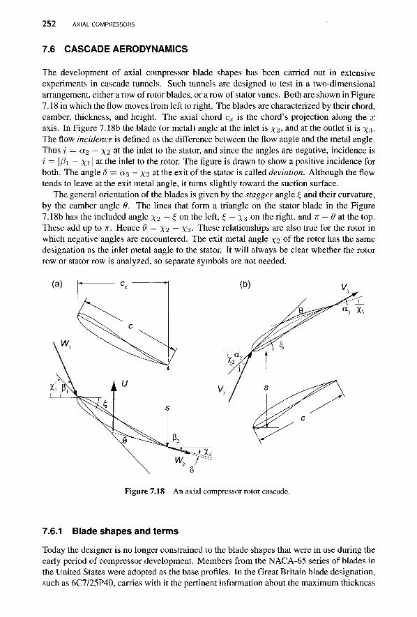
252 AXIAL COMPRESSORS
7.6 CASCADE AERODYNAMICS
The development of axial compressor blade shapes has been carried out in extensive experiments in cascade tunnels. Such tunnels are designed to test in a two-dimensional arrangement, either a row of rotor blades, or a row of stator vanes. Both are shown in Figure 7.18 in which the flow moves from left to right. The blades are characterized by their chord, camber, thickness, and height. The axial chord cx is the chord's projection along the x axis. In Figure 7.18b the blade (or metal) angle at the inlet is \2, and at the outlet it is \3-The flow incidence is defined as the difference between the flow angle and the metal angle. Thus i = «2 — X2 at the inlet to the stator, and since the angles are negative, incidence is i = \Pi — xi | at the inlet to the rotor. The figure is drawn to show a positive incidence for both. The angle 5 = a^ — X3 a t m e exit of the stator is called deviation. Although the flow tends to leave at the exit metal angle, it turns slightly toward the suction surface.
The general orientation of the blades is given by the stagger angle £ and their curvature, by the camber angle 0. The lines that form a triangle on the stator blade in the Figure 7.18b has the included angle \2 — £ on the left, £ — X3 on the right, and w — 9 at the top. These add up to TT. Hence 6 = \2 — X3- These relationships are also true for the rotor in which negative angles are encountered. The exit metal angle \2 of the rotor has the same designation as the inlet metal angle to the stator. It will always be clear whether the rotor row or stator row is analyzed, so separate symbols are not needed.
Figure 7.18 An axial compressor rotor cascade.
7.6.1 Blade shapes and terms
Today the designer is no longer constrained to the blade shapes that were in use during the early period of compressor development. Members from the NACA-65 series of blades in the United States were adopted as the base profiles. In the Great Britain blade designation, such as 6C7/25P40, carries with it the pertinent information about the maximum thickness
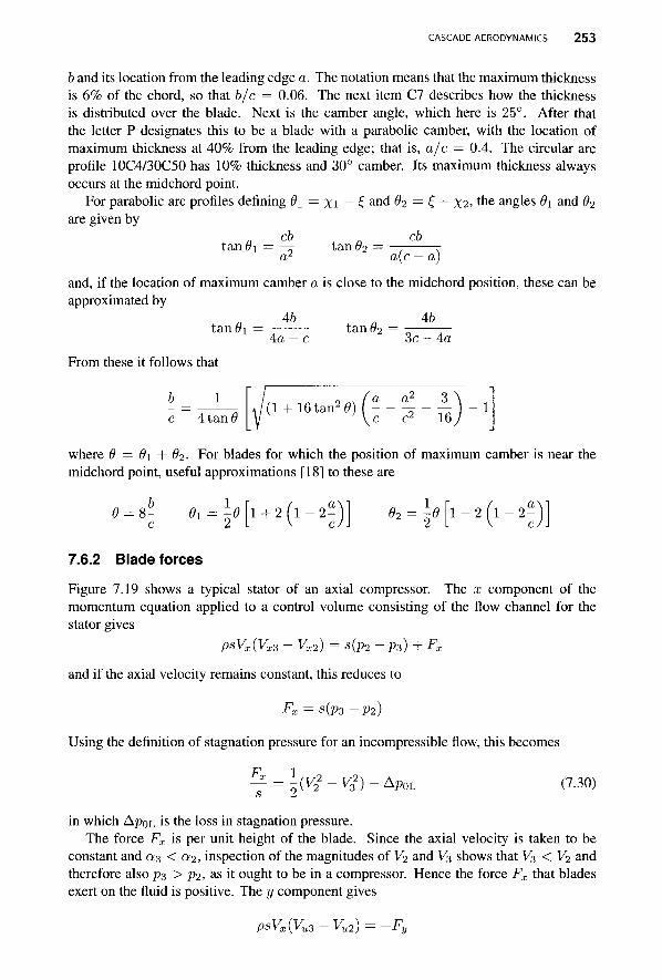
CASCADE AERODYNAMICS 253
b and its location from the leading edge a. The notation means that the maximum thickness is 6% of the chord, so that b/c = 0.06. The next item C7 describes how the thickness is distributed over the blade. Next is the camber angle, which here is 25°. After that the letter P designates this to be a blade with a parabolic camber, with the location of maximum thickness at 40% from the leading edge; that is, a/c = 0.4. The circular arc profile 10C4/30C50 has 10% thickness and 30° camber. Its maximum thickness always occurs at the midchord point.
For parabolic arc profiles defining Oi = xi ~ £ a nd 82 = £ - X2, the angles 0i and 82 are given by
cb tan#i = tan #2
cb a{c -
and, if the location of maximum camber a is close to the midchord position, these can be approximated by
tan 0i = tan #2 4a 3 c - 4 a
From these it follows that
1 4tan0
(1 + 16 tan2 (9) _3_ 16
where 8 = #1 + 82. For blades for which the position of maximum camber is near the midchord point, useful approximations [18] to these are
71 = 1 + 2 1 ( ' - » ; ) 1 — 2 ( 1 cJ
7.6.2 Blade forces
Figure 7.19 shows a typical stator of an axial compressor. The x component of the momentum equation applied to a control volume consisting of the flow channel for the stator gives
psVx{Vx3 - Vx2) = s(p2 - p3) + Fx
and if the axial velocity remains constant, this reduces to
Fx = s(p3 -p2)
Using the definition of stagnation pressure for an incompressible flow, this becomes
F± s
1 (v22 - v£) - A P 0 L (7.30)
in which ApoL is the loss in stagnation pressure. The force Fx is per unit height of the blade. Since the axial velocity is taken to be
constant and a3 < a2, inspection of the magnitudes of V2 and V3 shows that V3 < V2 and therefore also p3 > p2, as it ought to be in a compressor. Hence the force Fx that blades exert on the fluid is positive. The y component gives
psVx(Vu3 - Vu2)
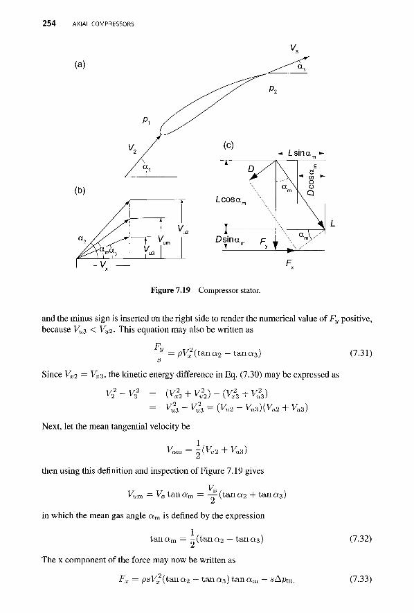
254 AXIAL COMPRESSORS
Figure 7.19 Compressor stator.
and the minus sign is inserted tin the right side to render the numerical value of Fy positive, because Vu3 < VU2. This equation may also be written as
p — = pVx
2(.trnia2 - t ana 3 ) (7.31) s
Since VX2 = Vx3, the kinetic energy difference in Eq. (7.30) may be expressed as
vi-vi = 0& + V&-V& + V&) = Vu3 - Vus = (vU2 - vu3)(vu2 + yu3)
Next, let the mean tangential velocity be
VUm= ^{Vu2 + Vu3)
then using this definition and inspection of Figure 7.19 gives
Km = Vxtanam = - y ( t a n a 2 + tana 3 )
in which the mean gas angle am is defined by the expression
t a n a m = -(tan<22 + tana 3 ) (7.32)
The x component of the force may now be written as
Fx = psVx2{t&na.2 — tana 3 ) t a n a m — sAp0^ (7.33)
CASCADE AERODYNAMICS 255
In addition to the axial and tangential components of forces, the lift and the drag force are also shown in Figure 7.19. They are the forces that the blades exert on the fluid. Lift and drag are obtained by resolving the resultant along the direction of the mean flow angle and one perpendicular to it. With the resultant expressed as
F = FJ - Fy]
the component D parallel and L normal to the mean flow vector, as shown in Figure 7.19c, are
L = Fx sin am + Fy cos am (7.34)
D = —Fx cos am + Fy sin am (7.35)
Introducing Eqs. (7.33) and (7.31) into Eq. (7.34) gives
L = psV^(tana.i — tanas) secam — sApoL sinam
The lift coefficient now becomes „ L 2 ApoL sinam CL = i Tr0 = - (tan a2 - tan a3) cos am - ,
yV^c a ±PV£ cr
Substituting Eqs. (7.30) and (7.31) into Eq. (7.35) gives
D = s ApoL cos am (7.36)
The choice in defining the direction of drag and lift as parallel and perpendicular to the mean flow direction as given by the angle am is guided exactly by this result, since the stagnation pressure drop from profile losses should depend mainly on the drag and not the lift.
Defining next the drag coefficient as
in which c is the chord, and making use of the preceding equation, gives
_ Ap0LCOsam
For the stator the stagnation pressure loss can be written as
APOLS = -zpC&VS = -zpVi T a 2' m c o s a m
so that Cs = ^ ? ^ C D (7.38)
cos^ am in which Vm/V-j = cos 0:3/ cos a m has been used. For the rotor similarly
CK = ^ ^ C D (7.39) cos^ /3m
The drag coefficients in these expressions are not the same, but are the appropriately calculated ones for the stator and the rotor., As will be seen below, the various losses
256 AXIAL COMPRESSORS
are expressed in terms of the drag coefficients, and their sum gives the total. The two preceding equations can then be used to relate the drag coefficients to the static enthalpy loss coefficients.
The expression for the lift coefficient for the stator can now be written as 2
CL = — (tan a2 — tan 0:3) cos am — Cn tan am
In a typical unstalled blade Co ~ 0.025CL, and, as will be shown shortly, it is advantageous to keep am less than 45°. Under these conditions the drag term may be neglected. This gives the following expression for the lift-to-drag ratio:
CL L 2 cos2 a 3 — = — = — (tana-2 - t a n a 3 ) 5 CD D CS cos2am
To make use of these expressions for compressor rotors, the flow angle a2 is replaced by /?i and a 3 by /32 and the rotor loss coefficient CR is substituted for Cs-
7.6.3 Other losses
The drag coefficients for annulus losses are given by
CDa = 0.02 J 0
in which b is the blade height, and the annulus losses become a smaller fraction of the total losses as the blade height increases. Secondary losses are a complicated subject, but all these complications are sidestepped by calculating the loss coefficient from the expression
CDs = 0.018C£
The tip losses arise from a tip vortex and leakage loss through the tip clearance for the rotor. They are taken into account by the empirical relation
CDt = 0-29 jCl/2
where bt is the tip clearance. The total loss coefficient is then obtained by summing these
CD = C D P + Cua + CDs + CDt
The equivalent drag coefficients for secondary and tip losses are a way of expressing the total pressure loss on the same basis for profile and annulus losses. With the sum of drag coefficients determined, the total static enthalpy loss coefficient can be calculated from either Eq. (7.38) or (7.39). The calculation of losses using the method outlined above has been questioned over the years [18, 21], for it is clear that in the complicated flow structure with highly staggered blades, dividing the losses neatly into constituent parts and adding them is suspect. Modern CFD analysis gives a powerful alternative that can be used to calculate stagnation pressure losses. Even if the modern methods are an improvement over what has been done in the past, there are still hurdles to overcome. One important advancement has been to develop methods to include unsteady interactions between moving and stationary blade rows. The theory still hinges on accurate methods to calculate local entropy production of a turbulent velocity and temperature fields. New turbulence models and large-eddy-simulation methods show promise and for this reason industry has moved to rely more and more on CFD to resolve the flow fields in compressors and turbines.
CASCADE AERODYNAMICS 257
7.6.4 Diffuser performance
The expression for the lift-to-drag ratio can be used to assess under which conditions a compressor cascade performs well as a diffuser. The diffuser efficiency is defined as
P3 -P2 VD =
P3s ~ P2
which is the ratio of the static pressure rise to the maximum possible. The labels are chosen to reflect that diffusion through the stator is considered. In a reversible adiabatic flow the stagnation pressure remains constant and
P02 ~ P03s =Pl~ P3s + -jPWZ - V3s) = °
Hence
P3s-p2 = \P{Vi-Vl)
Assuming that V3 = V3s, the diffuser efficiency can thus be written as
P3 -P2 m ~ \P{vi - vi)
Now
Fx - s(p3 - p2) Fx = Fv tan am - sAp0S Fy = psV*(tan a2 - tan a3)
so that P3 - P2 = pV% t a n a m ( t a n a 2 - t ana 3 ) - Ap0LS
Thus _ .. APOLS
pV£ tan am(tan a2 — tan a3) or in terms of CD and CL the diffuser efficiency can be written as
VD = 1 - n ■ r,
GL sin 2am
The maximum efficiency is determined by differentiating. Thus dr]D 4 C D cos 2an dam CL sin2 2an
0
Hence am = 45° at the condition of maximum diffuser efficiency and for C D / C L = 0.05 the efficiency is 90%. This result is due to Horlock [34].
7.6.5 Flow deviation and incidence
Before the blade angle can be set, the deviation at the exit from the blade row must be established. The flow deviation is given by S = a2 — Xi, in which \2 is the blade angle. Deviation is positive when the flow deflects from the pressure side toward the suction side. A positive deviation for the stator is shown in Figure 7.19, and for the rotor the flow is deflected in the opposite direction.
258 AXIAL COMPRESSORS
Deviation is an inviscid flow effect and not related to viscosity and therefore to losses. It can be regarded as incomplete turning of the flow. Hence, to obtain the desired turning, blades need to be curved more than in the absence of deviation.
Carter [14] recommends that deviation be calculated from
5* =m9,'S
at the design conditions, and Howell [37] proposed the formula
a2
m = 0.92— + 500
for m, in which a^ is given in degrees and a/c is the ratio of maximum thickness to the chord.
■ EXAMPLE 7.4
A compressor stage with reaction ratio R = | , and stator outlet metal angle X3 = 3°. The camber angle is 9 = 34°, pitch chord ratio is s/c = 0.88, and the position of maximum camber a/c — 0.5. The ratio of the blade height to the chord is b/c = 2. For 50% reaction the rotor flow angles have the same magnitudes as those for the stator, but they are of opposite sign. Find (a) the deviation of the flow leaving the stator, (b) the deflection, and (c) the flow coefficient and blade-loading coefficient, assuming that the inflow is at zero incidence.
Solution: (a) The flow deviation is calculated first. Since a 3 = X3 + <5*' the fl°w
angle can be calculated from
„ s „ „a . s o& . s a3=X3+^-=X3+0.92W- + ^ J -
Solving this for 0:3 gives
, _ X3 + 0 . 9 2 ^ ( 9 ^ _ 3 + 0.92 • 0.25 • 34 v/ 0 l
1-^nx/f 1 - H v C T 11.04°
500 V c -1- 500
so that 5* =a*3-xs = 11.04° - 3° = 8.04°. (b) The nominal deflection is calculated by first solving
1-55 tan a9 — tan a , = r-2 6 l + 1.5s/c
for a*2. It yields
a% = t a n - 1 ( t ana? + —— = t a n - 1 0.1927 + ' „ „„ ) = 40.8° 2 1 3 . i + i . 5 s / c y y 1 + 1.5-0..
Thus the nominal deflection is
e* = al- a% = 40.8° - 11.0° = 29..
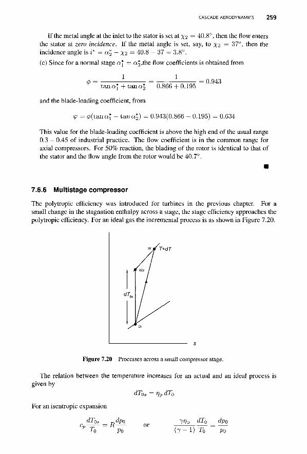
CASCADE AERODYNAMICS 259
If the metal angle at the inlet to the stator is set at \2 =40.8°, then the flow enters the stator at zero incidence. If the metal angle is set, say, to \2 = 37°, then the incidence angle is i* = a*2 - xi = 40.8 - 37 = 3.8°. (c) Since for a normal stage a\ = a^the flow coefficients is obtained from
1 1 0.943 t a n a ^ + t a n a ^ 0.866 + 0.195
and the blade-loading coefficient, from
ip = 4>{ta,nal - tuna^) = 0.943(0.866 - 0.195) = 0.634
This value for the blade-loading coefficient is above the high end of the usual range 0.3 - 0.45 of industrial practice. The flow coefficient is in the common range for axial compressors. For 50% reaction, the blading of the rotor is identical to that of the stator and the flow angle from the rotor would be 40.7°.
7.6.6 Multistage compressor
The polytropic efficiency was introduced for turbines in the previous chapter. For a small change in the stagnation enthalpy across a stage, the stage efficiency approaches the polytropic efficiency. For an ideal gas the incremental process is as shown in Figure 7.20.
T+dT
Figure 7.20 Processes across a small compressor stage.
The relation between the temperature increases for an actual and an ideal process is given by
dT0s = T]p dT0
For an isentropic expansion
dT0s dpo cD^=— = R or P T0 po (7 - 1) T0 po
7??p dT0 _ dp0
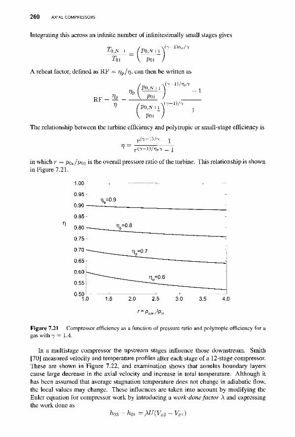
260 AXIAL COMPRESSORS
Integrating this across an infinite number of infinitesimally small stages gives
To,N + l P0,N + 1 ( 7 - l ) W 7
Toi V Poi
A reheat factor, defined as R F = j]p/rj, can then be written as
\ ( 7 - 1 ) A / P 7
R F VP
P0,N+1
Poi
P0,N+l
P01
(7~ l ) /7 1
The relationship between the turbine efficiency and polytropic or small-stage efficiency is
r ( 7 - l ) / 7 _ I
^ ~ T - ( 7 - 1 ) / ' J P 7 - 1
in which r = poe/poi is the overall pressure ratio of the turbine. This relationship is shown in Figure 7.21.
Figure 7.21 Compressor efficiency as a function of pressure ratio and polytropic efficiency for a gas with 7 = 1.4.
In a multistage compressor the upstream stages influence those downstream. Smith [70] measured velocity and temperature profiles after each stage of a 12-stage compressor. These are shown in Figure 7.22, and examination shows that annulus boundary layers cause large decrease in the axial velocity and increase in total temperature. Although it has been assumed that average stagnation temperature does not change in adiabatic flow, the local values may change. These influences are taken into account by modifying the Euler equation for compressor work by introducing a work-done factor A and expressing the work done as
^03 ~ h0i = MJ(Vx2 - Vxi)
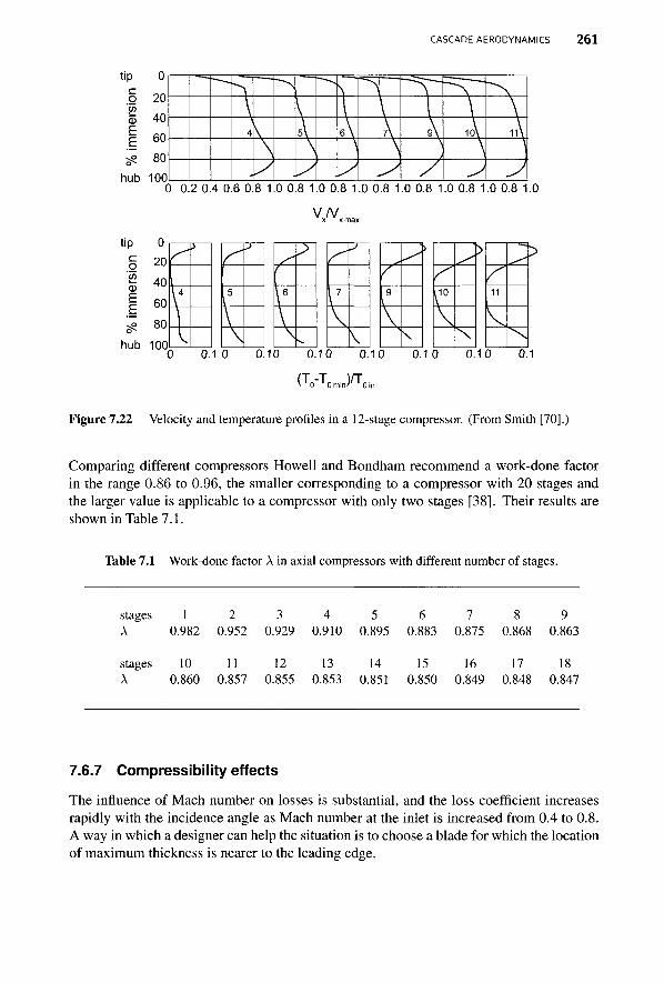
CASCADE AERODYNAMICS 2 6 1
tip 0 c o <r> a) E E
s-?
20
40 60
80
hub 100
4 V \
y
\
\ \ \
u \ \
\
"
.
\
/
io\
^
i n
J\ 0 0.2 0.4 0.6 0.8 1.0 0.8 1.0 0.8 1.0 0.8 1.0 0.8 1.0 0.8 1.0 0.8 1.0
V/V x xmax
tip 0
§ 20
1 40 | 60
^o 80
hub 100 %
~5
^
£ ^ \
^ 9
\ > \
s 110
J> 11
>
X 0 0.10 0.10 0.10 0.10 0.10 0.10 0.1
I 0 Omin' Oin
Figure 7.22 Velocity and temperature profiles in a 12-stage compressor. (From Smith [70].)
Comparing different compressors Howell and Bondham recommend a work-done factor in the range 0.86 to 0.96, the smaller corresponding to a compressor with 20 stages and the larger value is applicable to a compressor with only two stages [38]. Their results are shown in Table 7.1.
Table 7.1 Work-done factor A in axial compressors with different number of stages.
stages 1 2 3 4 5 6 7 8 9 A 0.982 0.952 0.929 0.910 0.895 0.883 0.875 0.868 0.863
stages 10 11 12 13 14 15 16 17 18 A 0.860 0.857 0.855 0.853 0.851 0.850 0.849 0.848 0.847
7.6.7 Compressibility effects
The influence of Mach number on losses is substantial, and the loss coefficient increases rapidly with the incidence angle as Mach number at the inlet is increased from 0.4 to 0.8. A way in which a designer can help the situation is to choose a blade for which the location of maximum thickness is nearer to the leading edge.
262 AXIAL COMPRESSORS
EXERCISES
7.1 The inlet and exit total pressures of air flowing through a compressor are 100 and 1000 kPa. The inlet total temperature is 281 K. What is the work of compression if the adiabatic total-to-total efficiency is 0.75?
7.2 Air flows through an axial fan rotor at mean radius of 15 cm. The tangential component of the absolute velocity is increased by 15 m/s through the rotor. The rotational speed of the shaft is 3000 rpm. (a) Evaluate the torque exerted on the air by the rotor, assuming that the flow rate is 0.471 m3/s and the pressure and temperature of the air are 100 kPa and 300 K. (b) What is the rate of energy transfer to the air?
7.3 The blade speed of a compressor rotor is U = 280 m/s, and the total enthalpy change across a normal stage is 31.6kJ/kg. If the flow coefficient <p = 0.5 and the inlet to the rotor is axial, what are the absolute and relative gas angles leaving the rotor?
7.4 Air flows through an axial-flow fan, with an axial velocity of 40 m/s. The absolute velocities at the inlet and the outlet of the stator are at angles of 60° and 30°, respectively. The relative velocity at the outlet of the rotor is at an angle —25°. Assume reversible adiabatic flow and a normal stage, (a) Draw the velocity diagrams at the inlet and outlet of the rotor, (b) Determine the flow coefficient, (c) Determine the blade-loading coefficient. (d) Determine at what angle the relative velocity enters the rotor, (e) Determine the static pressure increase across the rotor in pascals. The inlet total temperature is 300 K and the inlet total pressure is 101.3 kPa. (f) Determine the degree of reaction.
7.5 Air flows through an axial-flow compressor. The axial velocity is 60% of the blade speed at the mean radius. The reaction ratio is 0.4. The absolute velocity enters the stator at an angle of 55° from the axial direction. Assume a normal stage, (a) Draw the velocity diagrams at the inlet and outlet of the rotor, (b) Determine the flow coefficient, (c) Determine the blade-loading coefficient, (d) Determine at what angle the relative velocity enters the rotor, (e) Determine at what angle the relative velocity leaves the rotor, (f) Determine at what angle the absolute velocity leaves the stator.
7.6 A single stage of a multistage axial compressor is shown in Figure 7.2. The angle at which the absolute velocity enters the rotor is a\ — 40°, and the relative velocity at the inlet of the rotor is ji\ = -60°. These angles at the inlet of the stator are a2 = 60° and /32 = —40°. The mean radius of the rotor is 30 cm, and the hub-to-tip radius is 0.8. The axial velocity is constant and has a value Vx = 125 m/s. The inlet air is atmospheric at pressure 101.325 kPa and temperature 293 K. (a) Find the mass flow rate, (b) What is the rotational speed of the shaft under these conditions? (c) What is the power requirement of the compressor?
7.7 A single stage of a multistage axial compressor is shown in Figure 7.2. The angle at which the absolute velocity enters the rotor is a\ — 35°, and the relative velocity makes an angle of fii = -60°. The corresponding angles at the inlet to the stator are a2 = 60° and /32 = —35°. The stage is normal, and the axial velocity is constant through the compressor. (a) Why does the static pressure rise across both the rotor and the stator? (b) Draw the velocity triangles, (c) If the blade speed is U = 290 m/s, what is the axial velocity? (d) Find the work done per unit mass flow for a stage and the increase in stagnation temperature across it. (e) The stagnation temperature at the inlet is 300 K. The overall adiabatic efficiency of the compressor is r)c = 0.9, and the overall stagnation pressure ratio
EXERCISES 263
is 17.5. Determine the number of stages in the compressor, (f) How many axial turbine stages will it take to power this compressor?
7.8 The blade speed of a rotor of an axial air compressor is U = 150 m/s. The axial velocity is constant and equal to Vx = 75 m/s. The tangential component of the relative velocity leaving the rotor is WU2 = —30 m/s; the tangential component of the absolute velocity entering the rotor is Vu\ = 55 m/s. The stagnation temperature and pressure at the inlet to the rotor are 340 K and 185 kPa. The stage efficiency is 0.9, and one-half of the loss in stagnation pressure takes place through the rotor, (a) Draw the velocity diagrams at the inlet and exit of the rotor, (b) Find the work done per unit mass flow through the compressor, (c) Draw the states in an hs diagram. Find the (d) stagnation and static temperatures between rotor and stator, and (e) stagnation pressure between rotor and stator.
7.9 Air from ambient at 101.325 kPa and temperature 20°C enters into a blower axially with the velocity 61 m/s. The blade tip radius is 60 cm, and the hub radius is is 42 cm. The shaft speed is 1800 rpm. The air enters a stage axially and leaves it axially at the same speed. The rotor turns the relative velocity 18.7° toward the direction of the blade movement. The total-to-total stage efficiency is 0.87. (a) Draw the inlet and exit velocity diagrams for the rotor, (b) Draw the blade shapes, (c) Determine the flow coefficient and the blade-loading factor, (d) Determine the mass flow rate, (e) What is the specific work required? (f) What is the total pressure ratio for the stage? (g) Determine the degree of reaction.
7.10 Air from ambient at 101.325 kPa and temperature 300 K enters an axial-flow com-pressor stage axially with velocity 122 m/s. The blade casing radius is 35 cm, and the hub radius is 30 cm. The shaft speed is 6000 rpm. At the exit relative velocity is at an angle —45°. The total-to-total stage efficiency is 0.86. (a) Draw the inlet and exit velocity diagrams for the rotor, (b) Draw the blade shapes, (c) Determine the flow coefficient and the blade-loading factor, (d) Determine the mass flow rate, (e) What is the total pressure ratio for the stage? (f) Determine the degree of reaction.
7.11 Perform design calculations for a compressor stage with blade loading factor in the range tp = 0.25 to ip = 0.55, flow coefficient <f> = 0.7, and reaction R = 0.6. Keep the diffusion factor equal to 0.45. Calculate and plot 1 — 77, solidity, and the static pressure rise 1 — V2/V1 for rotor and stator (including the de Haller criterion). What are the stagnation losses across stator and rotor?
7.12 A normal compressor stage has a reaction ratio R = 0.54, and stator outlet metal angle %3 = 14.5°. The camber angle is 9 = 32°, pitch chord ratio is s/c = 0.82, and the position of maximum camber a/c = 0.45. The ratio of the blade height to the chord is b/c =1 .7 . (a) Find the deviation of the flow leaving the stator. (b) Find the deflection. (c) Find the flow coefficient and blade-loading coefficient by assuming the inflow at zero incidence.
7.13 The circular arc blades of a compressor cascade have camber 9 = 30° and maximum thickness at a/c = 0.5. The space-to-chord ratio is s/c = 1.0. The nominal outflow angle is 0:3 = 25°. (a) Determine the nominal incidence, (b) Determine that lift coefficient at the nominal incidence given a drag coefficient of C-Q = 0.016.
7.14 Air with density 1.21 kg/m3 flows into a compressor stator with velocity V2 — 120m/s and leaves at angle 03 = 30°. If the Leiblein diffusion factor is to be held at

264 AXIAL COMPRESSORS
0.5 and the the stagnation pressure loss across a compressor stator is 0.165 kPa, assuming incompressible flow, what is the static pressure increase across the stage?
7.15 Air at temperature 288 K and at pressure 101.325 kPa flows into a compressor with 10 stages. The efficiency of the first stage is 0.920 and the second stage, 0.916. For the remaining stages, the stage efficiency drops by 0.004 successively so that the last stage has an efficiency of 0.884. The axial velocity is constant, and the flow angles are the same at the inlet and exit of each of the stages. Hence the work done by each stage is the same, (a) Find the overall efficiency of the compressor, (b) Find the overall efficiency by using the theory for a polytropic compression with small stage efficiency r]p = 0.902.
7.16 Air flows in a axial flow fan of free vortex design, with hub radius r^ = 7.5 cm and casing radius 17 cm. The fan operates at 2400 rpm. The volumetric flow rate Q = l . l m 3 / s and the stagnation pressure rise is 3 cm H2O. The fan efficiency is 7?tt — 0.86. (a) Find the axial velocity, (b) Find the work done on the fluid, (c) Find the absolute and relative flow angles at the inlet and exit of the rotor when the inlet is axial.
7.17 Consider an axial-flow compressor in which flow leaves the stator with a tangential velocity distributed as a free vortex. The hub radius is 10 cm and the static pressure at the hub is 94 kPa, and the static temperature there is 292 K. The radius of the casing is 15 cm, and the static pressure at the casing is 97 kPa. The total pressure at this location is 101.3 kPa. Find the exit flow angles at the hub and the casing.
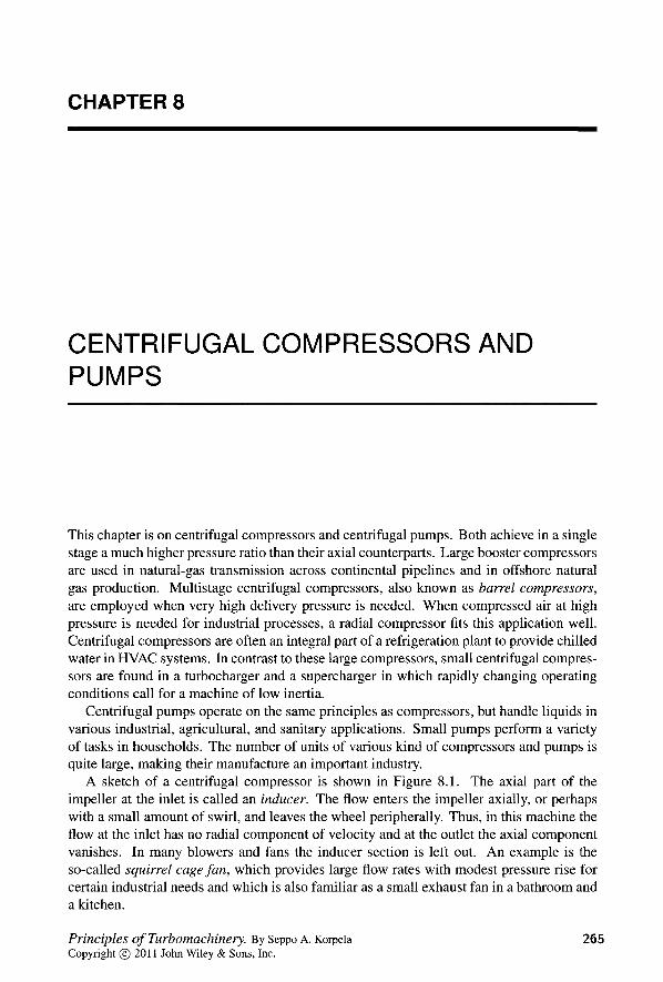
CHAPTER 8
CENTRIFUGAL COMPRESSORS AND PUMPS
This chapter is on centrifugal compressors and centrifugal pumps. Both achieve in a single stage a much higher pressure ratio than their axial counterparts. Large booster compressors are used in natural-gas transmission across continental pipelines and in offshore natural gas production. Multistage centrifugal compressors, also known as barrel compressors, are employed when very high delivery pressure is needed. When compressed air at high pressure is needed for industrial processes, a radial compressor fits this application well. Centrifugal compressors are often an integral part of a refrigeration plant to provide chilled water in HVAC systems. In contrast to these large compressors, small centrifugal compres-sors are found in a turbocharger and a supercharger in which rapidly changing operating conditions call for a machine of low inertia.
Centrifugal pumps operate on the same principles as compressors, but handle liquids in various industrial, agricultural, and sanitary applications. Small pumps perform a variety of tasks in households. The number of units of various kind of compressors and pumps is quite large, making their manufacture an important industry.
A sketch of a centrifugal compressor is shown in Figure 8.1. The axial part of the impeller at the inlet is called an inducer. The flow enters the impeller axially, or perhaps with a small amount of swirl, and leaves the wheel peripherally. Thus, in this machine the flow at the inlet has no radial component of velocity and at the outlet the axial component vanishes. In many blowers and fans the inducer section is left out. An example is the so-called squirrel cage fan, which provides large flow rates with modest pressure rise for certain industrial needs and which is also familiar as a small exhaust fan in a bathroom and a kitchen.
Principles of Turbomachinery. By Seppo A. Korpela Copyright © 2011 John Wiley & Sons, Inc.
265
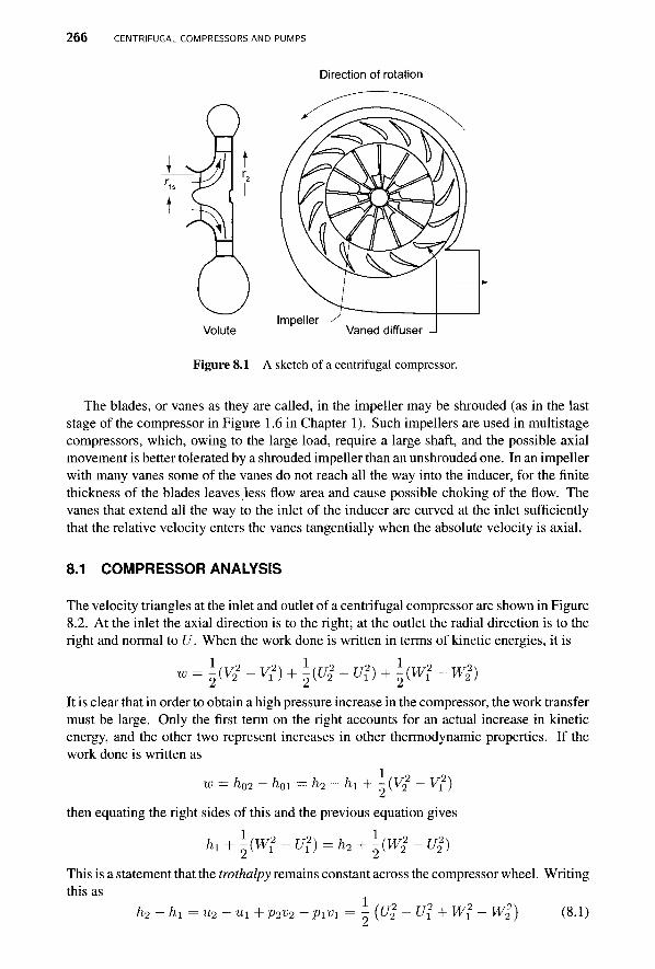
2 6 6 CENTRIFUGAL COMPRESSORS AND PUMPS
Direction of rotation
Figure 8.1 A sketch of a centrifugal compressor.
The blades, or vanes as they are called, in the impeller may be shrouded (as in the last stage of the compressor in Figure 1.6 in Chapter 1). Such impellers are used in multistage compressors, which, owing to the large load, require a large shaft, and the possible axial movement is better tolerated by a shrouded impeller than an unshrouded one. In an impeller with many vanes some of the vanes do not reach all the way into the inducer, for the finite thickness of the blades leaves less flow area and cause possible choking of the flow. The vanes that extend all the way to the inlet of the inducer are curved at the inlet sufficiently that the relative velocity enters the vanes tangentially when the absolute velocity is axial.
8.1 COMPRESSOR ANALYSIS
The velocity triangles at the inlet and outlet of a centrifugal compressor are shown in Figure 8.2. At the inlet the axial direction is to the right; at the outlet the radial direction is to the right and normal to U. When the work done is written in terms of kinetic energies, it is
" = \(V22 - V,2) + \{Ul - V?) + \(W? ~ Wl)
It is clear that in order to obtain a high pressure increase in the compressor, the work transfer must be large. Only the first term on the right accounts for an actual increase in kinetic energy, and the other two represent increases in other thermodynamic properties. If the work done is written as
w = h02 ~ hoi ^h2~h1 + -(V22 - V?)
then equating the right sides of this and the previous equation gives
hi + \(W? - Ul) = h2 + \{Wi - Ui)
This is a statement that the trothalpy remains constant across the compressor wheel. Writing this as
h2 - hi = u2 - ui + p2v2 - pivi = i {U\ - Ul + Wl - Wl) (8.1)
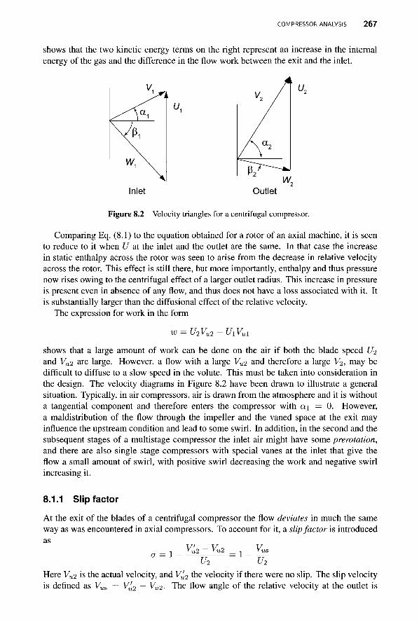
COMPRESSOR ANALYSIS 267
shows that the two kinetic energy terms on the right represent an increase in the internal energy of the gas and the difference in the flow work between the exit and the inlet.
Inlet Outlet
Figure 8.2 Velocity triangles for a centrifugal compressor.
Comparing Eq. (8.1) to the equation obtained for a rotor of an axial machine, it is seen to reduce to it when U at the inlet and the outlet are the same. In that case the increase in static enthalpy across the rotor was seen to arise from the decrease in relative velocity across the rotor. This effect is still there, but more importantly, enthalpy and thus pressure now rises owing to the centrifugal effect of a larger outlet radius. This increase in pressure is present even in absence of any flow, and thus does not have a loss associated with it. It is substantially larger than the diffusional effect of the relative velocity.
The expression for work in the form
w u2vu2 - uxvul shows that a large amount of work can be done on the air if both the blade speed U2 and Vu2 are large. However, a flow with a large Vu2 and therefore a large V2, may be difficult to diffuse to a slow speed in the volute. This must be taken into consideration in the design. The velocity diagrams in Figure 8.2 have been drawn to illustrate a general situation. Typically, in air compressors, air is drawn from the atmosphere and it is without a tangential component and therefore enters the compressor with a\ = 0. However, a maldistribution of the flow through the impeller and the vaned space at the exit may influence the upstream condition and lead to some swirl. In addition, in the second and the subsequent stages of a multistage compressor the inlet air might have some prerotation, and there are also single stage compressors with special vanes at the inlet that give the flow a small amount of swirl, with positive swirl decreasing the work and negative swirl increasing it.
8.1.1 Slip factor
At the exit of the blades of a centrifugal compressor the flow deviates in much the same way as was encountered in axial compressors. To account for it, a slip factor is introduced as
i Vu2 - vu2 , Vus a = l - — u 2 — = 1 - u 2 -
Here Vu2 is the actual velocity, and V^2 m e velocity if there were no slip. The slip velocity
is defined as Vus = V^2 — Vu2. The flow angle of the relative velocity at the outlet is
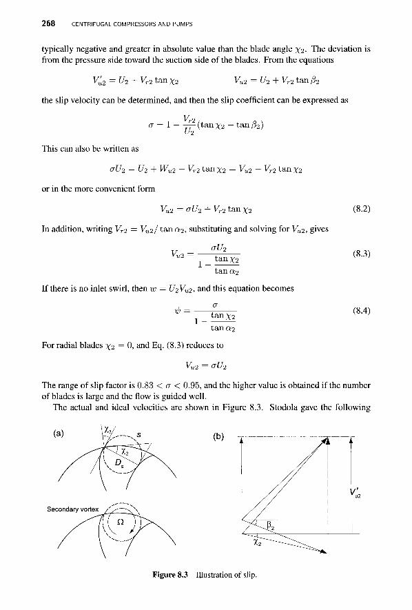
2 6 8 CENTRIFUGAL COMPRESSORS AND PUMPS
typically negative and greater in absolute value than the blade angle \2- The deviation is from the pressure side toward the suction side of the blades. From the equations
Ki = U2 + Vr2 tan X2 Vu2 = U2 + Vr2 tan /32
the slip velocity can be determined, and then the slip coefficient can be expressed as
<J = 1 - — (tan X2 ~ tan/32) U2
This can also be written as
aU2 = U2 + Wu2 - Vr2 tan%2 = Vu2 - Vr2 tan%2
or in the more convenient form
Vu2=aU2 + Vr2tanX2 (8.2)
In addition, writing Vr2 = Vu2/ tana2, substituting and solving for Vu2, gives
aU2 Vu2 1 tanx2 (8.3)
tan«2
If there is no inlet swirl, then w = U2Vu2, and this equation becomes
1 tanx2 (8.4)
tanci2
For radial blades \2 = 0, and Eq. (8.3) reduces to
Vu2 = aU2
The range of slip factor is 0.83 < a < 0.95, and the higher value is obtained if the number of blades is large and the flow is guided well.
The actual and ideal velocities are shown in Figure 8.3. Stodola gave the following
(b)
Secondary vortex
Figure 8.3 Illustration of slip.
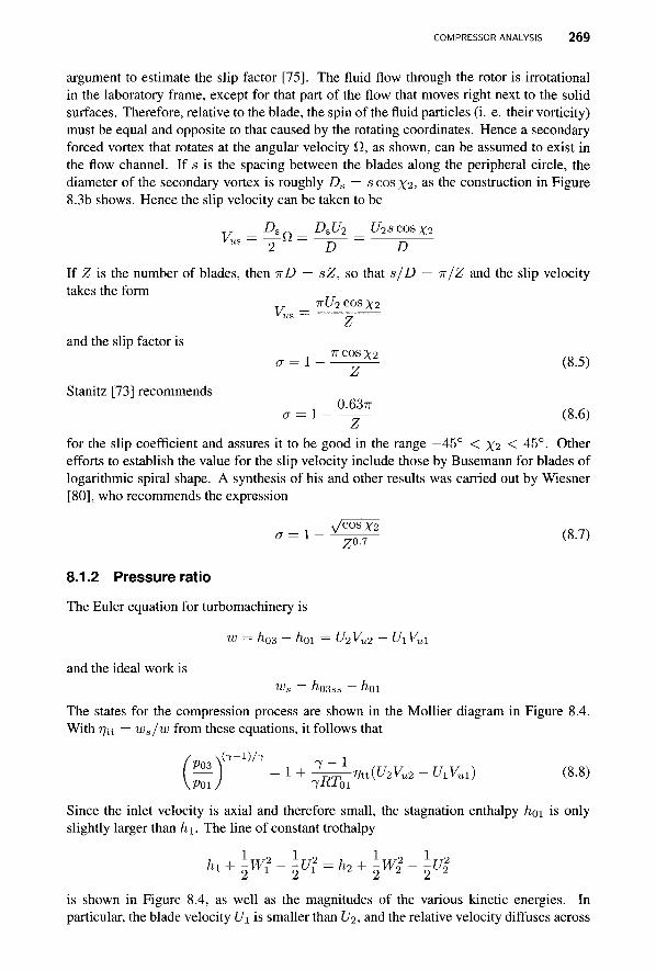
COMPRESSOR ANALYSIS 269
argument to estimate the slip factor [75]. The fluid flow through the rotor is irrotational in the laboratory frame, except for that part of the flow that moves right next to the solid surfaces. Therefore, relative to the blade, the spin of the fluid particles (i. e. their vorticity) must be equal and opposite to that caused by the rotating coordinates. Hence a secondary forced vortex that rotates at the angular velocity fl, as shown, can be assumed to exist in the flow channel. If s is the spacing between the blades along the peripheral circle, the diameter of the secondary vortex is roughly Ds = scosx2, as the construction in Figure 8.3b shows. Hence the slip velocity can be taken to be
v = A^ = DaU2 = U2SCOSX2 us ~ 2 ~ D ~ D
If Z is the number of blades, then TTD = sZ, so that s/D = TT/Z and the slip velocity takes the form
TTU2 cos \2
and the slip factor is
Stanitz [73] recommends
1 n C O S * 2 «Z ^ 0" = 1 — (8.5)
0.63?r (7=1- —^- (8.6)
for the slip coefficient and assures it to be good in the range —45° < \2 < 45°. Other efforts to establish the value for the slip velocity include those by Busemann for blades of logarithmic spiral shape. A synthesis of his and other results was carried out by Wiesner [80], who recommends the expression
,/COS Y2
8.1.2 Pressure ratio
The Euler equation for turbomachinery is
w = h03- h0i = U2Vu2 - UiVui
and the ideal work is wa = ho3SS — hoi
The states for the compression process are shown in the Mollier diagram in Figure 8.4. With 77tt = ws/w from these equations, it follows that
\ ( 7 - D / 7 j — = 1 + \^Vtt{U2Vu2 - C/1K1) (8.8) P01 / IRTQI
Since the inlet velocity is axial and therefore small, the stagnation enthalpy /ioi is only slightly larger than h\. The line of constant trothalpy
hr + \w* -\U* = h2 + \wl -\ul
is shown in Figure 8.4, as well as the magnitudes of the various kinetic energies. In particular, the blade velocity U\ is smaller than U2, and the relative velocity diffuses across
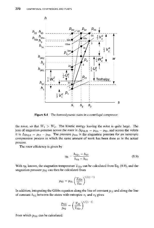
2 7 0 CENTRIFUGAL COMPRESSORS AND PUMPS
02 03
Figure 8.4 The thermodynamic states in a centrifugal compressor.
the rotor, so that W\ > W2. The kinetic energy leaving the rotor is quite large. The loss of stagnation pressure across the rotor is Ap0 LR = po2i — P02, and across the volute it is ApoLS = P02 — Po3- The pressure po2i is the stagnation pressure for an isentropic compression process in which the same amount of work has been done as in the actual process.
The rotor efficiency is given by
??R = h, 02s ^01 h02 — h,
(8.9) 01
With 7?R known, the stagnation temperature T02S can be calculated from Eq. (8.9), and the stagnation pressure P02 can then be calculated from
P02 = P01 TQ2S
T01
7/ (7 -1)
In addition, integrating the Gibbs equation along the line of constant P02 and along the line of constant ft-02 between the states with entropies si and s2 gives
P02i P02 T, 02s
7 / (7 -1 )
from which p02i can be calculated.

COMPRESSOR ANALYSIS 271
For an axial inlet flow Vu\ = 0 and introducing Vu2 = 1PU2 into Eq. (8.8), the pressure ratio can be written as
P03
P01 [l + ( 7 - l ) ^ t A C ] 7 / ( 7 - 1 ) (8.10)
in which M0u = U2/CQI. A plot of this relation is shown in Figure 8.5. Similarly, the pressure ratio across the rotor alone is
P02
P01
It was seen earlier that in the expression for constant trothalpy
[l + ( 7 - D ^ < . ] 7 / ( 7 _ 1 ) (8.11)
Po_3 P01
Mn
Figure 8.5 Pressure ratio as a function of blade stagnation Mach number, for various values of iprjtt and for gas with 7 = 1.4.
h*-hx = \(U*-Ul) + \{W*-W*)
the first term on the right side is a kinematic effect and therefore represents a reversible process. If the left side is written as
h2 - hi = h2 - h2s + h2s - h\
then the reversible enthalpy change may be written as
h2s - hi - \{U\ - Ul) + (1 - f)\{W2i - Wi)
and for the irreversible change
h2-h2s = f-{W2i-Wl)
2 7 2 CENTRIFUGAL COMPRESSORS AND PUMPS
in which / is the fraction of the change in relative kinetic energy lost to irreversibility. The static enthalpy loss coefficient £R in
h2 ~ h2s = 1-CKWI
k-'dr1) is related to / by the equation
CB ■ - , 2
The ratio (1 — ??R)/(1 — 7jtt) of rotor losses to the total losses is between 0.5 and 0.6. Hence for r/tt = 0.8, the rotor efficiency is about T?R = 0.89.
Writing the rotor efficiency as
= h2s~h1 + ±(V£-V?) VR h2-h1 + \{V2-V?)
and assuming that V2s = V2, this becomes
= h2s - fa2 + fea - /t! + \{V22 - V?)
m ~ h2-hl + \{V2-V?)
which can also be written as
h2 ~ h2s = _ CnWl = __ (nW[ w 2w 2ipU$ m = i = i — - z - ^ - = i
Squaring and adding the component equations
W2 sin f32 = Vu2 - U2 W2 cos /?2 = V*
gives
In addition
so that
Wi = Vl2 - 2Vu2U2 + Ul + K22
vu2 Vr2 =
t ana 2
M - 1 o, , ^
and the rotor efficiency can be written as
TT2 = 1 - 2 ^ + ^ 2 — (8.12) U2 s in a2
, . ( l - 2 ^ + ^ 2 /sm 2 a 2 ) ??R = 1 - C R ^
in which
tana2
Solving the equation for rotor efficiency for £R gives
(1 " T?R)2^
ip = 1 (8.13) tanx2
CP 1 - 2 ^ + V>2/sin <*2

COMPRESSOR ANALYSIS 273
For a typical case xi = —40° and c*2 = 67°. With a — 0.85, these equations give ip = 0.627, and for a rotor efficiency r/R = 0.89, the loss coefficient is £R = 0.656. This appears to be quite large, but when calculating the stagnation pressure losses this is multiplied by W| , which is small because the flow will have been diffused through the rotor. In addition, a typical value for W1/W2 = 1.6. For these values the fraction of the relative kinetic energy lost to irreversibility is / = 0.38. This number accords with Cumpsty's [18] review of the field. Although this number appears to be large, in a typical compressor the centrifugal effect accounts for over three quarters of the pressure rise and the diffusion of the relative velocity the rest. Hence 38% loss keeps the rotor efficiency still over 90%.
■ EXAMPLE 8.1
Air flows from atmosphere at pressure 101.325 kPa and temperature 288 K into a centrifugal compressor with radial blades at the exit of the impeller. The inlet velocity is V\ = 93m/s, and there is no preswirl. The compressor wheel has 33 blades, and its tip speed is U2 = 398 m/s. The total-to-total efficiency is r/tt = 0.875. Find (a) the stagnation pressure ratio and (b) the power required assuming that the mass flow rate is rn — 2.2 kg/s. Use the Stanitz formula to find the slip coefficient.
Solution: (a) Since the air comes from the atmosphere, where it is stagnant, the atmo-spheric pressure and temperature are the inlet stagnation properties. The stagnation speed of sound is
coi = V7-R7bi = Vl.4-287-288 = 340.2 m/s
and the stagnation blade Mach number is therefore
Ui 398 Mou = — = irr^ = 1.17
coi 340.2 The Stanitz slip coefficient is
, 0.63TT 1 - — = 0 . 9 4
Since for radial blades Eq. (8.4) shows that ip = a, the pressure ratio can be calculated from
M = [1 + ( 7 _ l)arhtMltpH'*-1'> = (1 + 0.4 • 0.94 • 0.875 • 1.172)3'5 = 3.674 P01
(b) The stagnation temperature for an isentropic process is
/ \ ( 7 - l ) / 7 T03. = Tni — = 288 • 3.6741/35 = 417.7K
KPOIJ
and the ideal work is therefore
ws = cp(T03s - T01) = 1004.5(417.7 - 288) = 130.29 kJ/kg
The actual work is w = ws/r]tt = 130.29/0.875 = 148.90 kJ/kg, and the power required has the value W = rhw = 2.2 • 148.90 = 327.6 kW.
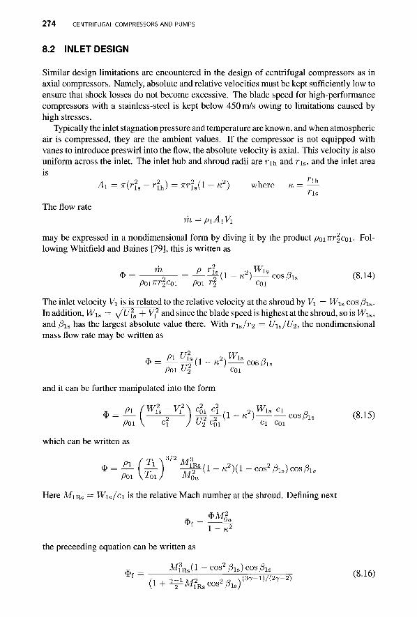
2 7 4 CENTRIFUGAL COMPRESSORS AND PUMPS
8.2 INLET DESIGN
Similar design limitations are encountered in the design of centrifugal compressors as in axial compressors. Namely, absolute and relative velocities must be kept sufficiently low to ensure that shock losses do not become excessive. The blade speed for high-performance compressors with a stainless-steel is kept below 450 m/s owing to limitations caused by high stresses.
Typically the inlet stagnation pressure and temperature are known, and when atmospheric air is compressed, they are the ambient values. If the compressor is not equipped with vanes to introduce preswirl into the flow, the absolute velocity is axial. This velocity is also uniform across the inlet. The inlet hub and shroud radii are rih and ri s , and the inlet area is
A\ = 7r(r2s — r2
h) = 7rr2s(l — K2) where K = —
?~ls
The flow rate m = piA-iVi
may be expressed in a nondimensional form by diving it by the product poiirr^coi. Fol-lowing Whitfield and Baines [79], this is written as
$ = , ; " 2 = ^ 4 ( 1 - « 2 ) ^ c o s / 3 l s (8.14) . . <2) P o i s e d An r% coi
The inlet velocity V\ is is related to the relative velocity at the shroud by V\ = W\s cos /3is. In addition, W\s = \ZU2
S + V2 and since the blade speed is highest at the shroud, so is Wis, and /3is has the largest absolute value there. With r\s/r2 = U\s/U2, the nondimensional mass flow rate may be written as
A n ^ 2 c o i 3>=—T£(1~K2)—cos f3ls
and it can be further manipulated into the form
* = ̂ f%^§4(i-^^»sA, «8,5) A)l V c l / U2 c01 °1 c01
which can be written as
3 / 2 M3
* = — ( £~ ) ^ T ( l - « 2 ) ( 1 -cos2/3 l s )cos/3 l s PLflj-Y Ml**n -2vi _ 2 An \T0J M0
2„
Here M I R S = W\s/ci is the relative Mach number at the shroud. Defining next
the preceeding equation can be written as
10u
(1 + V M l R s C O S As)
INLET DESIGN 275
Graphs calculated from Eq. (8.16) are shown in Figure 8.6. The angle f5\s at which the flow rate reaches its maximum value is obtained differentiating this equation with respect to cos/3is and setting the derivative to zero:
cos4 f3ls - 3 + j f l 2 R s cos2 pls + -±- = 0 (8.17) 2 ^ His , 2
J W lRs M l R s The solution of this equation is
Another way to plot the data is shown in Figure 8.7. The optimum angle from Eq. (8.18) is /3ls = —57.15° for M I R S = 0.6, and if the relative Mach number is increased to M I R S = 1.2, the optimum angle is /3is = —62.56°. In the incompressible limit the optimum angle is j3\s = —54.74°.
Equation (8.16) can be recast also in the form
g I = Pl (Wl-V?\ c' ^ ci
pm \ c\ ) cgj ci coi
and further as
Solving this for M2Rs gives
2 _ *,2 , * f ^ , 7 - 1 . , 2 ( 3 7 - l ) / ( 2 7 - 2 )
M/R s = M( + ^ ^1 + ^ M (
This result is plotted graphically in Figure 8.8. Since M\ = MIRSCOS/?IS, the lines of constant cos /3is are straight on this set of graphs and the optimum angle is at the minima of the curves.
■ EXAMPLE 8.2
In an air compressor the relative Mach number is M\RS = 0.9 at the shroud of the impeller. The inlet stagnation pressure and temperature are 101.325 kPa and 288 K. The mass flow rate is m = 1.2 kg/s. The hub-to-shroud radius ratio is 0.4, and the inlet flow is axial. Determine (a) the rotational speed of the impeller, (b) the axial velocity, and (c) the inducer shroud diameter, assuming that the inducer is designed for optimum relative flow angle, and that the compressor operates at the design point.
Solution: The stagnation density is
poi 101325 3 P01 = 1U^ = 2 ^ 2 8 8 - 1 - 2 2 5 9 k g / m
and the stagnation speed of sound is

2 7 6 CENTRIFUGAL COMPRESSORS AND PUMPS
Figure 8.6 Nondimensional mass flow rate for given inlet angle of relative flow with relative Mach number as a parameter, for a gas with 7 = 1.4.
M„
Figure 8.7 Relative Mach number for given inlet angle of relative flow with nondimensional flow rate as a parameter, for a gas with 7 = 1.4.
The optimum relative flow angle can be found from
cos2 /3is mr)(-f 4 M 2R s
(3 + 7 M? R s )2
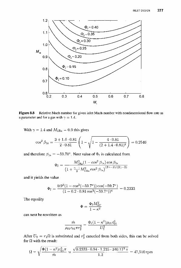
INLET DESIGN 277
M„
1.2
1.1
1.0
0.9
0.8
0.7
0.6
\ « \ = 0.'
v ^ ^ O f = 0 . 4 0 ^ ^ ^ ^ ^ ^
\ ^ c j ^ = 0 . 3 5 ^ ^ ^ " ^ ^ '
\ ^ O f = 0 . 3 0 ^ ^ ^ ^ ^ '
\ O f = 0 . 2 5 ^ ^ ^ ^ " s
3>f=0.20 ^ ^ > ^ / * /
= 0.15 ^ ^ ^ S ' '
0 ^ ^
0.2 0.3 0.4 0.5 0.6 0.7 0.8
Figure 8.8 Relative Mach number for given inlet Mach number with nondimensional flow rate as a parameter and for a gas with 7 = 1.4.
With 7 = 1.4 and M 1 R s = 0.9 this gives
2 . 3 + 1 . 4 - 0 . 8 1 cos /3is = 1 - 4 1
4 -0 .81 2-0 .81 l~ V~ (2 + 1.4-0.81)2 I
and therefore /3is = —59.70°. Next value of $f is calculated from
M 3R s ( l - C O S 2 / 3 i s ) c O S / ? l s
0.2546
$ f ( l + V M m s c o s 2 / 3 l s )
and it yields the value
0.93(1 - cos 2 ( -59.7°) ) cos ( -59 .7
( 3 7 - l ) / ( 2 7 - 2 )
$ f (1 + 0 . 2 - 0 . 8 1 cos 2 ( -59 .7° ) ) 4 0.2333
The equality
$ \-K2
can next be rewritten as
m $ f ( l - K2)poic\ 01 ,ooicoi7rr| r/2
^ 2
After t/2 = r20, is substituted and r\ canceled from both sides, this can be solved for f2 with the result:
^(1-K2)CLTT V0.2333 • 0.84 • 1.225 • 340.173 ix _ r l „ Q = \l —i . ' U1 = — = 4 7 , 5 1 0 r p m
m 1.2
2 7 8 CENTRIFUGAL COMPRESSORS AND PUMPS
(b) The inlet Mach number is
Mx = M1Rscos/3le = 0.9 cos(-59.7°) = 0.454
and hence the inlet static temperature has the value
T l - i + ^ i M | " 1 + 0.2-0.4542 " 2 7 6 ' 6 K
The static density comes out to be
/ j i \ 1/(7-1) / 2 7 6 6 \ 2 ' 5
pi = "»{it) =1-2259(wJ =1-1081kg/-3
and the axial velocity is
Vi = Mj V7.RT1 = 0.454V1.4-287-276.6 =151.4m/s
The mass flow rate,
m = pxAiVi = p\-Kr\s{l - K2)VI
when solved for n s gives
r i s = W pl7r(l-^i = V 1.1081-J'-L-151.4 = °-°521 m
so that the inducer diameter of the impeller is D l s = 10.42 cm.
8.2.1 Choking of the inducer
The inducer is shown in Figure 8.9. The flow is axial at the inlet, and the relative velocity forms an angle Pi at the mean radius and j3is at the shroud. The corresponding blade velocities are U\ and L71S with C/ls = r\sU\/r\m. The blade angle is xi, and the stagger is £. The throat width is denoted by t. From the shape of the blade, its thickness distribution, and the stagger, the width of the throat can be determined. As the sketch shows, a reasonable estimate is given by t = s cos xi- A typical value for incidence i = fix — xi is —4° to —6° [63].
Mass balance in the form
Pi rh = piAxWi cos A = —frA^M^^RT^ cos/3i HI1
can be written in terms of functions of the relative Mach number, by introducing the ratios
TQK TI
T°R - 1 + ^ M f R
and
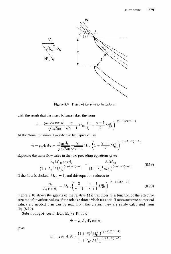
INLET DESIGN 279
V.
Figure 8.9 Detail of the inlet to the inducer.
with the result that the mass balance takes the form
POR-4ICOS/3I 7 / 7 - 1 , 1 , 2 m = = = = = M i R 1 + — — Mx
VCpToR V7 - 1 V 2 At the throat the mass flow rate can be expressed as
R
-(7+l)/2(7-l)
, u / PORA 7 , , A . 7 -m = ptAtWt = -7===-7==MtK I H -7"V [tR
A/CP^OR V7
Equating the mass flow rates in the two preceding equations gives
A1Mmcos(il AtMtR
-(7+l)/2(7-l)
If the flow is choked, MtR = 1, and this equation reduces to
(7+l)/2(7-l)
At Ai cos /3] = Mi R
7 - 1 7 + 1 7 + 1 M?K
-(7+l)/2(7-l)
(8.19)
(8.20) ■"■1 ^^^ Hi- \ 1 < * I ' * /
Figure 8.10 shows the graphs of the relative Mach number as a function of the effective area ratio for various values of the relative throat Mach number. If more accurate numerical values are needed than can be read from the graphs, they are easily calculated from Eq. (8.19).
Substituting A\ cos /?i from Eq. (8.19) into
gives
m = p\A\W\ cos/3i
h+l=lM2 )(7+D/2(7-l)
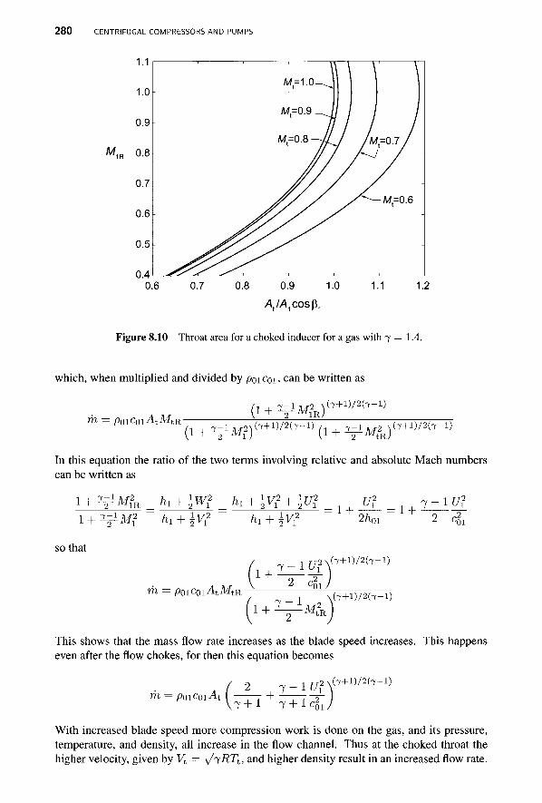
2 8 0 CENTRIFUGAL COMPRESSORS AND PUMPS
WlR
I . 1
1.0
0.9
0.8
0.7
0.6
0.5
n A
M=1.0-^J
M=0.9 _ / i
M=0.8 —JJ
\
j -
/M=0.7 I
/ y^-M=0.6
-
0.6 0.7 0.8 0.9 1.0
/4,/^COSp^
1.1 1.2
Figure 8.10 Throat area for a choked inducer for a gas with 7 = 1.4.
which, when multiplied and divided by poiCoii c a n be written as
m = PoiCoiAtMtR- 1 + iJW?R)(7+1)/2(7"1)
1 7 - 1 M?) ( 7 + l ) / 2 ( 7 - l ) (1 + V^t 2 R) ( 7 + l ) / 2 ( 7 - l )
In this equation the ratio of the two terms involving relative and absolute Mach numbers can be written as
1 + V M m _ ftl + \Wl _ hl + \Vl + \Ul l + V M i 2 h^ + \v? ^1 + 2^1
so that
= 1 + il = 1 + ^ 1 " ? 2/i, 01 2 r2
m = P01C01 A-W t R
1 + 7 - l ^ 2
2 coi 7 - 1 M, t R
( 7 + l ) / 2 ( 7 - l )
This shows that the mass flow rate increases as the blade speed increases. This happens even after the flow chokes, for then this equation becomes
m = poiCoiAt 2 7 ~ 1 Uj
7 + 1 7 + 1 c§i
2 \ ( 7 + l ) / 2 ( 7 - l )
With increased blade speed more compression work is done on the gas, and its pressure, temperature, and density, all increase in the flow channel. Thus at the choked throat the higher velocity, given by Vt = \/^RTt, and higher density result in an increased flow rate.
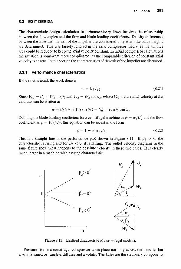
EXIT DESIGN 2 8 1
8.3 EXIT DESIGN
The characteristic design calculation in turbomachinery flows involves the relationship between the flow angles and the flow and blade loading coefficients. Density differences between the inlet and the exit of the impeller are considered only when the blade heights are determined. This was largely ignored in the axial compressor theory, as the annulus area could be reduced to keep the axial velocity constant. In radial compressor calculations the situation is somewhat more complicated, as the comparable criterion of constant axial velocity is absent. In this section the characteristics of the exit of the impeller are discussed.
8.3.1 Performance characteristics
If the inlet is axial, the work done is
w u2v, 2 ^ 2 (8.21)
Since VU2 = t/2 + W2 sin/32 and Vr2 = W2 cos/32, where Vr2 is the radial velocity at the exit, this can be written as
w U2(U2 + W2 sin/32) = Ul + Vr2U2 tan/32
Denning the blade-loading coefficient for a centrifugal machine as tp = tu/C/f and the flow coefficient as </> = Vr2/U2, this equation can be recast in the form
i\) — 1 + 4> tan /32 (8.22)
This is a straight line in the performance plot shown in Figure 8.11. If /32 > 0, the characteristic is rising and for /32 < 0, it is falling. The outlet velocity diagrams in the same figure show what happens to the absolute velocity in these two cases. It is clearly much larger in a machine with a rising characteristic.
V
Figure 8.11 Idealized characteristic of a centrifugal machine.
Pressure rise in a centrifugal compressor takes place not only across the impeller but also in a vaned or vaneless diffuser and a volute. The latter are the stationary components
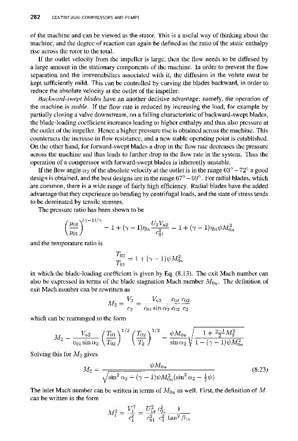
2 8 2 CENTRIFUGAL COMPRESSORS AND PUMPS
of the machine and can be viewed as the stator. This is a useful way of thinking about the machine, and the degree of reaction can again be defined as the ratio of the static enthalpy rise across the rotor to the total.
If the outlet velocity from the impeller is large, then the flow needs to be diffused by a large amount in the stationary components of the machine. In order to prevent the flow separation and the irreversibilites associated with it, the diffusion in the volute must be kept sufficiently mild. This can be controlled by curving the blades backward, in order to reduce the absolute velocity at the outlet of the impeller.
Backward-swept blades have an another decisive advantage; namely, the operation of the machine is stable. If the flow rate is reduced by increasing the load, for example by partially closing a valve downstream, on a falling characteristic of backward-swept blades, the blade-loading coefficient increases leading to higher enthalpy and thus also pressure at the outlet of the impeller. Hence a higher pressure rise is obtained across the machine. This counteracts the increase in flow resistance, and a new stable operating point is established. On the other hand, for forward-swept blades a drop in the flow rate decreases the pressure across the machine and thus leads to further drop in the flow rate in the system. Thus the operation of a compressor with forward-swept blades is inherently unstable.
If the flow angle a2 of the absolute velocity at the outlet is in the range 63° - 72° a good design is obtained, and the best designs are in the range 67° - 69°. For radial blades, which are common, there is a wide range of fairly high efficiency. Radial blades have the added advantage that they experience no bending by centrifugal loads, and the state of stress tends to be dominated by tensile stresses.
The pressure ratio has been shown to be
^ ( 7 " 1 ) / 7 = 1 + (7 - D * t ^ » = l + (7 - l M M l c o i vPOl /
and the temperature ratio is
in which the blade-loading coefficient is given by Eq. (8.13). The exit Mach number can also be expressed in terms of the blade stagnation Mach number MQU. The definition of exit Mach number can be rewritten as
, , V2 Vu2 Coi C02 1V12
= =
c2 coi sin a2 c02 c2
which can be rearranged to the form
M2 VU2 (T01\1/2 (T02\1/2 ^M0u I 1 + ^ M 2
coi sina2 \T02 J \T2 ) sina2 y 1 + (7 - l)ipM§u
Solving this for M2 gives
M2 = ^ ° » (8.23) sin2 a2 + (7 - l)^-Mou(sin2 a2 - \ij})
The inlet Mach number can be written in terms of MQU as well. First, the definition of Mi can be written in the form
y2 TJ2 2 1 M2 = — = —^- —
1 c\ c2,! c\ tan2/3is
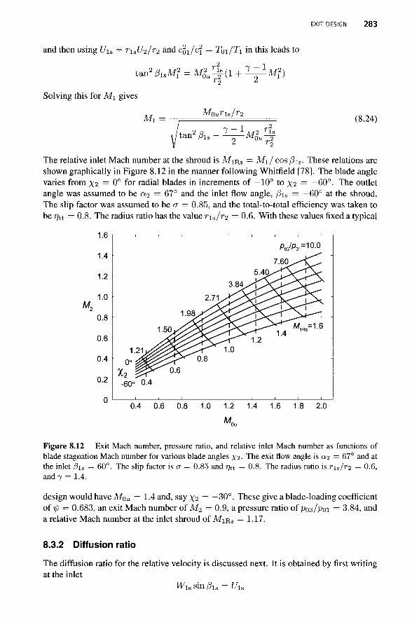
EXIT DESIGN 283
and then using Uis = r l sC/2 / r2 and c^/cl — T0i/Ti in this leads to
T0
7 - 1 Mi
Solving this for M\ gives
Mi M0uris/r2
/ t an 2 /3 i s 7 - 1
(8.24) M2 -is.
2 °"r22
The relative inlet Mach number at the shroud is M I R S — M\j cos /3is. These relations are shown graphically in Figure 8.12 in the manner following Whitfield [78]. The blade angle varies from \2 = 0° for radial blades in increments of —10° to \2 = —60°. The outlet angle was assumed to be a2 = 67° and the inlet flow angle, j3\B = —60° at the shroud. The slip factor was assumed to be a = 0.85, and the total-to-total efficiency was taken to be rju = 0.8. The radius ratio has the value r\s/r2 = 0.6. With these values fixed a typical
1.6
M,
1.4
1.2
1.0
0.8
0.6
0.4
0.2
0
p03/p01=10.0
7.60.
M I R . = 1 - 6
0.4 0.6 0.8 1.0 1.2 1.4 1.6 1.8 2.0
M„..
Figure 8.12 Exit Mach number, pressure ratio, and relative inlet Mach number as functions of blade stagnation Mach number for various blade angles %2- The exit flow angle is «2 = 67° and at the inlet j3\s = 60°. The slip factor is a = 0.85 and rjtt = 0.8. The radius ratio is r\s/r2 = 0.6, and 7 = 1.4.
design would have M0u = 1.4 and, say \2 = —30°. These give a blade-loading coefficient of if; = 0.683, an exit Mach number of M 2 = 0.9, a pressure ratio of P03/P01 = 3.84, and a relative Mach number at the inlet shroud of M I R S = 1.17.
8.3.2 Diffusion ratio
The diffusion ratio for the relative velocity is discussed next. It is obtained by first writing at the inlet
Wls sin Pls = Uis
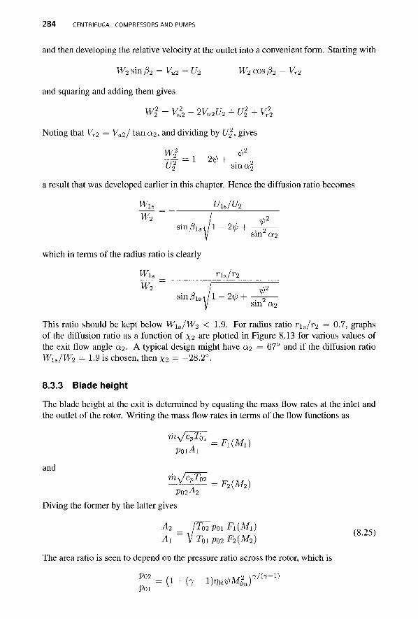
2 8 4 CENTRIFUGAL COMPRESSORS AND PUMPS
and then developing the relative velocity at the outlet into a convenient form. Starting with
W2 sin j32 = Vu2 - U2 W2 cos /32 = Vr2
and squaring and adding them gives
Wl = Vl2 - 2Vu2U2 + Ul + K22
Noting that Vr2 = Vu2/ t&na2, and dividing by U2, gives
Wi , „ , V>2 - | = l - 2 ^ + . 2 (7| sin at;
a result that was developed earlier in this chapter. Hence the diffusion ratio becomes
Wls
w2 sin/3ls-i
uls/u2
/ l - 2^ + T ^ -/ sin «2
which in terms of the radius ratio is clearly
Wls rls/r2
W-2 n \ V>2
sin,»isWl - 2ip + — sin a2
This ratio should be kept below Wis/W2 < 1.9. For radius ratio r\s/r2 = 0.7, graphs of the diffusion ratio as a function of \2 are plotted in Figure 8.13 for various values of the exit flow angle a2. A typical design might have a2 = 67° and if the diffusion ratio Wis/W2 = 1.9 is chosen, then \2 = -28.2°.
8.3.3 Blade height
The blade height at the exit is determined by equating the mass flow rates at the inlet and the outlet of the rotor. Writing the mass flow rates in terms of the flow functions as
^ ^ = F1(M1) Poi-Ai
and m^/cpT02 — - b2{M2) P02M
Diving the former by the latter gives
M= / l ^"po iF i (Mi) Ax V T01 p 0 2 F2(M2)
The area ratio is seen to depend on the pressure ratio across the rotor, which is
P o 2 (t , I ^\ 1 T\t2 \7/(7-l) —- = (1 + (7 - l)r?R^M0u) P01
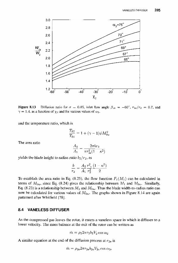
VANELESS DIFFUSER 285
W, Is
Figure 8.13 Diffusion ratio for a = 0.85, inlet flow angle /?is 7 = 1.4, as a function of \2 and for various values of a2.
-60°, rls/r2 = 0.7, and
and the temperature ratio, which is
TQ2
'01
The area ratio
1 + (7 - 1)^M02
U
2irbr2 M=
A± 7rrfs(l - K2) yields the blade height to radius ratio b2/r2, as
b A2 rl (1 - K2)
7-2 A i r i
To establish the area ratio in Eq. (8.25), the flow function Fi(Mi) can be calculated in terms of M0u, since Eq. (8.24) gives the relationship between Mi and M0u. Similarly, Eq. (8.23) is a relationship between M2 and M0u. Thus the blade width-to-radius ratio can now be calculated for various values of MQU. The graphs shown in Figure 8.14 are again patterned after Whitfield [78].
8.4 VANELESS DIFFUSER
As the compressed gas leaves the rotor, it enters a vaneless space in which it diffuses to a lower velocity. The mass balance at the exit of the rotor can be written as
rh = p22Tvr2b2V2 cos a2
A similar equation at the end of the diffusion process at r2e is
m = P2e2nr2eb2eV2e cos a2e
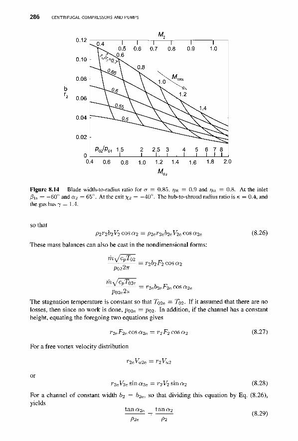
2 8 6 CENTRIFUGAL COMPRESSORS AND PUMPS
0.12
0.10
0.08
0.06
0.04
0.02
M, 0 4 I I I I I T"
0.5 0.6 0.7 0.8 0.9 1.0 J3.6
0.4 0.6 0.8 1.0 1.2 1.4 1.6 1.8 2.0
0u
Figure 8.14 Blade width-to-radius ratio for a = 0.85, TJR = 0.9 and 77a = 0.8. At the inlet /Sis = —60° and 0:2 = 65°. At the exit \2 = —40°. The hub-to-shroud radius ratio is K = 0.4, and the gas has 7 = 1.4.
so that P2r2b2V2 cosa2 = p2er2eb2eV2e cosa2e
These mass balances can also be cast in the nondimensional forms:
m i / c p T 0 2
P0227T
m\JcpTQ2e
r2b2F2cosa2
'- r2eb2eF2e COS a 2 e
(8.26)
P02e27T
The stagnation temperature is constant so that T02e = To2- If it assumed that there are no losses, then since no work is done, po2e = P02- In addition, if the channel has a constant height, equating the foregoing two equations gives
?*2e-F2e cos a 2 e = r2-F2 cos a 2
For a free vortex velocity distribution
T2eVu2e = r2Vu2
(8.27)
r2eV2e sin a 2 e = r2V2 sin a2 (8.28)
For a channel of constant width b2 = b2e, so that dividing this equation by Eq. (8.26), yields
tan a2e t an a2
P2e Pi
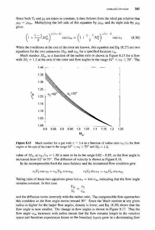
VANELESS DIFFUSER 287
Since both T0 and p0 are taken as constant, it then follows from the ideal gas relation that P02 = Po2e- Multiplying the left side of this equation by p02e and the right side by p02 gives
1 + 1_}LM? 2e
1/(7-1) tan a2e 1 + 7' 1 -Ml
1/(7-1) t an 0:2 (8.30)
When the conditions at the exit of the rotor are known, this equation and Eq. (8.27) are two equations for the two unknowns M2e and a2e for a specified location r2e.
Mach number M2e as a function of the radius ratio is shown in Figure 8.15 for a flow with M2 = 1.2 at the exit of the rotor and flow angles in the range 62° < a2 < 70°. The
0.8 0.85 0.9 0.95 1.0 1.05 1.1 1.15 1.2 1.25
Figure 8.15 Mach number for a gas with 7 = 1.4 as a function of radius ratio r2e/?"2 for flow angles at the exit of the rotor in the range 62° < 0:2 < 70° and Mi = 1.2.
value of M2e at r2e/r2 = 1.30 is seen to be in the range 0.82 - 0.85, as the flow angle is increased from 62° to 70°. The diffusion of velocity is shown in Figure 8.16.
In the incompressible limit the mass balance and the irrotational flow condition give
r2V2 cos a2 = r2eV2e cos a2e r2V2 sina2 = r2eV2e sina2e
Taking ratio of these two equations gives tan 0:2 = tan a2e indicating that the flow angle remains constant. In this case
V2e _ T2
V2 r2e
and the diffusion varies inversely with the radius ratio. The compressible flow approaches this condition as the flow angle moves toward 90°. Since the Mach number at any given radius is higher for the larger flow angles, density is lower, and Eq. (8.29) shows that the flow angle is now smaller. The change in flow angles is shown in Figure 8.17. That the flow angle a2e increases with radius means that the flow remains longer in the vaneless space and therefore experiences losses as the boundary layers grow in a decelerating flow
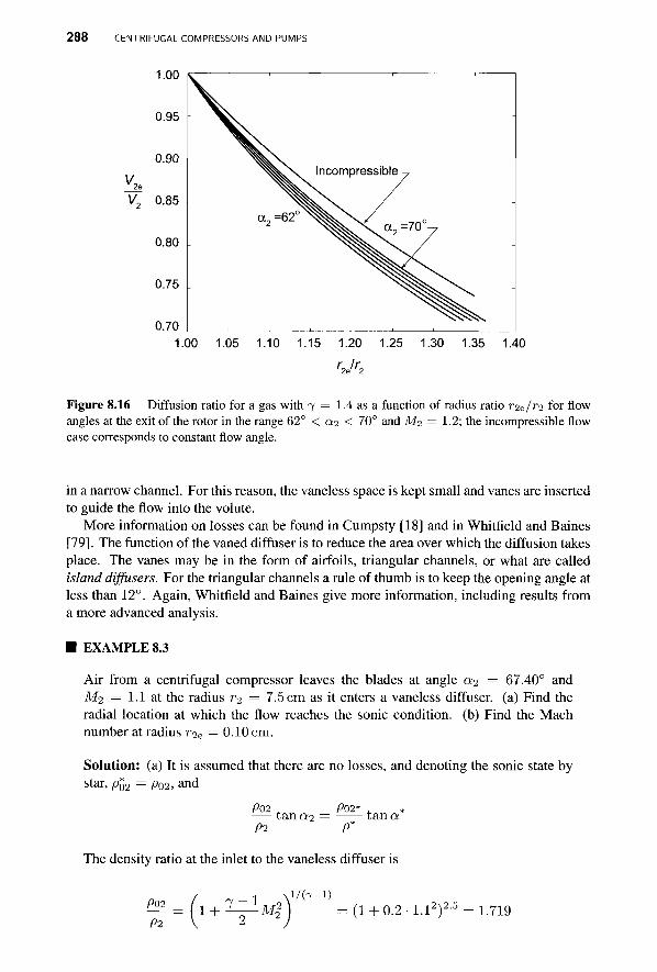
2 8 8 CENTRIFUGAL COMPRESSORS AND PUMPS
1.00 1.05 1.10 1.15 1.20 1.25 1.30 1.35 1.40
'2e"2
Figure 8.16 Diffusion ratio for a gas with 7 = 1.4 as a function of radius ratio r2e/?*2 for flow angles at the exit of the rotor in the range 62° < 02 < 70° and M2 = 1.2; the incompressible flow case corresponds to constant flow angle.
in a narrow channel. For this reason, the vaneless space is kept small and vanes are inserted to guide the flow into the volute.
More information on losses can be found in Cumpsty [18] and in Whitfield and Baines [79]. The function of the vaned diffuser is to reduce the area over which the diffusion takes place. The vanes may be in the form of airfoils, triangular channels, or what are called island diffusers. For the triangular channels a rule of thumb is to keep the opening angle at less than 12°. Again, Whitfield and Baines give more information, including results from a more advanced analysis.
■ EXAMPLE 8.3
Air from a centrifugal compressor leaves the blades at angle a2 = 67.40° and M2 = 1.1 at the radius ri = 7.5 cm as it enters a vaneless diffuser. (a) Find the radial location at which the flow reaches the sonic condition, (b) Find the Mach number at radius r2e = 0.10 cm.
Solution: (a) It is assumed that there are no losses, and denoting the sonic state by star, Po2 = p02, and
P02 , P02' , * tan 0:2 = tan a
Pi P* The density ratio at the inlet to the vaneless diffuser is
/ _ 1 \ 1 / ( 7 ~ 1 )
£21 = (l + 1-^Ml\ = (1 + 0.2 • l.l2)2-5 = 1.719
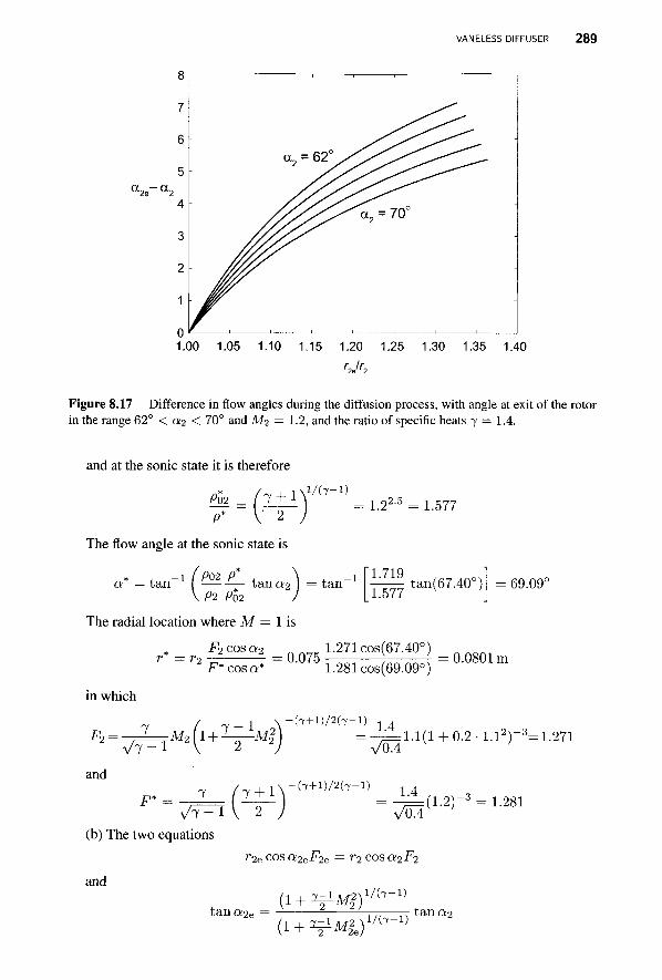
VANELESS DIFFUSER 289
1.00 1.05 1.10 1.15 1.20 1.25 1.30 1.35 1.40 riJr2
Figure 8.17 Difference in flow angles during the diffusion process, with angle at exit of the rotor in the range 62° < Q2 < 70° and Mi = 1.2, and the ratio of specific heats 7 = 1.4.
and at the sonic state it is therefore
P" V 2
The flow angle at the sonic state is
A > a _ / 7 + n = 1.22-5 = 1.577
* , -1 I P02 P , \ , - 1 a = t an tan a2 = t an
V P2 P02
The radial location where M — 1 is
1.719 1.577
tan(67.40°) 69.09°
r* = r2 ^ i = 0.075 ^ l ^ ^ l = 0.0801 m F* cos a* 1.281 cos(69.09°)
in which
VT^T 7 ^ 1 ,
2 M2(l + ±-^zM$
- ( 7 + l ) / 2 ( 7 - l ) 1.4 /0A
1.1(1 + 0.2- 1 .12)- J=1.271
and ~ / ~ + l \ - ( 7 + l ) / 2 ( 7 - l ) 1 4
F* =-^2=^ ( 2±1) = -±l( l .2)- 3 = 1.281
(b) The two equations
r 2 e cos a2eF2e = r2 cos a2F2
and
tan a2e
(l + ^Ml) — TJl^T) t a n a 2
2 9 0 CENTRIFUGAL COMPRESSORS AND PUMPS
are to be solved simultaneously for a2e and M2e. The angle can be eliminated using
1 COS 0!2e
V 1 + tan2 a2e
Substituting, simplifying, and rearranging gives
r2ejM2e
VT^Vl + ^Mfe
1/(7-1) / x \ 1/(7-1) r cos a2F2\l I 1 + -^—M'L 1 + 1 + -—r-Mk2 I tan2 a2
Solving this by iteration gives M2e = 0.7571. g
A well designed vaned diffuser improves the efficiency by 2% or 3% over a vaneless one. However, this comes at a cost, for at off-design operation the efficiency of a vaned diffuser will deteriorate; that is, a compressor with a vaned diffuser will have a narrow operating range at the peak efficiency, owing to stalling of the vanes. To widen the range, adjustable vanes can be implemented into the design at added complexity and initial cost. The payback is reduction in operating costs at higher efficiency. A low-cost option is to have a vaneless diffuser, which has a lower efficiency but a flatter operating range near peak efficiency. As the flow leaves the vaneless, or vaned, diffuser, it enters a volute. Its design with respect to pumps is discussed at the end of this chapter.
8.5 CENTRIFUGAL PUMPS
The operation and design of pumps follows principles similar to those of centrifugal compressors. Compressibility can be clearly ignored in pumping liquids, but it may also be neglected in fans in which the pressure rise is slight.
The first law of thermodynamics across a pump is
w = h02 - h0i = (u2 + ~ + - V? + gZl J - (m + — + -V22 + gz2
In incompressible fluids, as was discussed in Chapter 2, internal energy increases only as a result of irreversibilities in an adiabatic flow. Hence, if the flow through the pump is reversible and adiabatic, internal energy does not increase and u2 = u\. In this situation the preceding equation reduces to
Pi • lir2 , _ \ (V\ , 1T,2 P
+2vi+9Z>)-{i; + 2v'+^ The total head developed by a pump is defined as
P2 , X T,2 , \ / P i , 1 T,2 H = + ^ 2 + Z 2 " + ^Vi+Z^ \pg 2g ) \pg 2g
so it represents the work done by a reversible pump per unit weight of the fluid. On the unit mass basis the reversible work is
w3 = gH
CENTRIFUGAL PUMPS 2 9 1
Since the total head is readily measurable, the pump industry reports it, as well as the overall efficiency, in the pump specifications.
The shaft power to the pump is given by
V The overall efficiency r/ can be expressed as the product
V = ??m??vr?h
in which rjh is a hydraulic efficiency, rjv is a volumetric efficiency, and -qm is a mechanical efficiency. The hydraulic efficiency accounts for the irreversibilities in the flow through the pump. If the loss term is written as
gHL = u2~ui
then w = ws+ gHL = gH + gHL
and the hydraulic efficiency is defined as
ws gH w gH + gHL
The hydraulic efficiency may be calculated from the empirical equation
0.4 % = 1 - Q I T I (8-3D
where Q is in liters per second. If the volumetric flow rate is given in gallons per minute, as is still done in part of the pump industry today, the constant 0.4 has to be replaced by 0.8. It is in this form that this expression for hydraulic efficiency appears in the Pump Handbook [45].
A typical set of pump performance curves is given in Figure 8.18. (The quantity on the right ordinate axis, N P S H R = required net positive suction head, and its significance is discussed later in conjunction with consideration of cavitation.) For an impeller diameter of 31cm and flow rate of 18L/s, the delivered head is 48 m at the shaft speed of 1750 rpm. The efficiency at this condition is about 0.63. The contours of constant efficiency and the power for pumping water are shown. Since the reversible work is ws = gH, and w = Ws/rih, the power calculated using W = rhw, then, because of leakage flow through the clearances from the exit of the impeller back to the inlet, work will be redone on some of the fluid as it crosses the impeller, and the value obtained will be too low. To correct for this, the power into the impeller is obtained from
WR = (m + rhi,)w
in which m^ is the leakage flow. The power transferred to the fluid is
W = rhw
and the ratio of these two expression for power is defined as the volumetric efficiency. Hence it also equals the ratio of the mass flow rates and can be written as
_ rh _ Q Q _ W rh + rh-L Q + QL QR WK
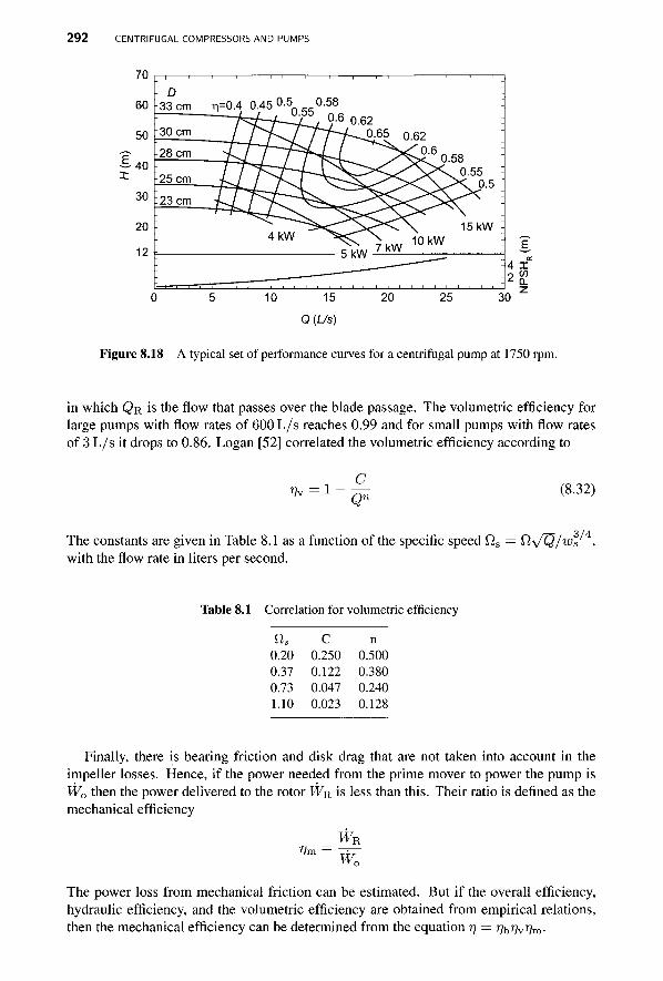
2 9 2 CENTRIFUGAL COMPRESSORS AND PUMPS
70
60
50
1 4 0
30
20
12
:30 cm
33 cm r}=0A 0.45 0-5Q
28 cm
25 cm
23 cm
55 0.6 o 62 .£■65 0.62
'0 .6,
Figure 8.18 A typical set of performance curves for a centrifugal pump at 1750 rpm.
in which Q R is the flow that passes over the blade passage. The volumetric efficiency for large pumps with flow rates of 600 L/s reaches 0.99 and for small pumps with flow rates of 3 L / s it drops to 0.86. Logan [52] correlated the volumetric efficiency according to
Vv c_ Qn (8.32)
The constants are given in Table 8.1 as a function of the specific speed fls — fl^/Q/ws , with the flow rate in liters per second.
Table 8.1 Correlation for volumetric efficiency
Os C n 0.20 0.250 0.500 0.37 0.122 0.380 0.73 0.047 0.240 1.10 0.023 0.128
Finally, there is bearing friction and disk drag that are not taken into account in the impeller losses. Hence, if the power needed from the prime mover to power the pump is W0 then the power delivered to the rotor WR, is less than this. Their ratio is defined as the mechanical efficiency
% WR
The power loss from mechanical friction can be estimated. But if the overall efficiency, hydraulic efficiency, and the volumetric efficiency are obtained from empirical relations, then the mechanical efficiency can be determined from the equation r\ = r\\{q^r\m.
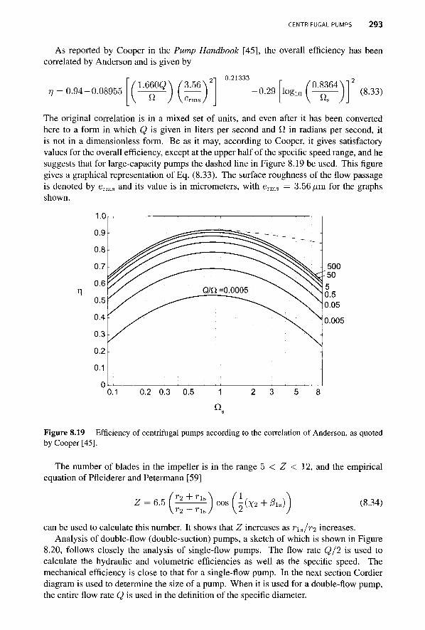
CENTRIFUGAL PUMPS 293
As reported by Cooper in the Pump Handbook [45], the overall efficiency has been correlated by Anderson and is given by
77 = 0.94-0.08955 1.660Q\ [3.56
n ) -0.21333
-0.29 , 0.8364 \ l o g i ° l -^r) (8.33)
The original correlation is in a mixed set of units, and even after it has been converted here to a form in which Q is given in liters per second and fl in radians per second, it is not in a dimensionless form. Be as it may, according to Cooper, it gives satisfactory values for the overall efficiency, except at the upper half of the specific speed range, and he suggests that for large-capacity pumps the dashed line in Figure 8.19 be used. This figure gives a graphical representation of Eq. (8.33). The surface roughness of the flow passage is denoted by erms and its value is in micrometers, with erms = 3.56 /jm for the graphs shown.
0.005
Figure 8.19 Efficiency of centrifugal pumps according to the correlation of Anderson, as quoted by Cooper [45].
The number of blades in the impeller is in the range 5 < Z < 12, and the empirical equation of Pfleiderer and Petermann [59]
6.5 T2 + Tu r2 - ru
(X2 + As) (8.34)
can be used to calculate this number. It shows that Z increases as r\s/r2 increases. Analysis of double-flow (double-suction) pumps, a sketch of which is shown in Figure
8.20, follows closely the analysis of single-flow pumps. The flow rate Q/2 is used to calculate the hydraulic and volumetric efficiencies as well as the specific speed. The mechanical efficiency is close to that for a single-flow pump. In the next section Cordier diagram is used to determine the size of a pump. When it is used for a double-flow pump, the entire flow rate Q is used in the definition of the specific diameter.
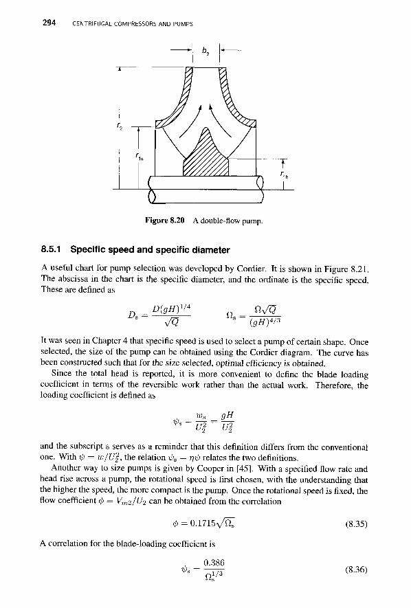
2 9 4 CENTRIFUGAL COMPRESSORS AND PUMPS
Figure 8.20 A double-flow pump.
8.5.1 Specific speed and specific diameter
A useful chart for pump selection was developed by Cordier. It is shown in Figure 8.21. The abscissa in the chart is the specific diameter, and the ordinate is the specific speed. These are defined as
A D(gH) 1/4
V a It was seen in Chapter 4 that specific speed is used to select a pump of certain shape. Once selected, the size of the pump can be obtained using the Cordier diagram. The curve has been constructed such that for the size selected, optimal efficiency is obtained.
Since the total head is reported, it is more convenient to define the blade loading coefficient in terms of the reversible work rather than the actual work. Therefore, the loading coefficient is defined as
A Ws gH_
and the subscript s serves as a reminder that this definition differs from the conventional one. With tp = w/U^, the relation tj)B = -qip relates the two definitions.
Another way to size pumps is given by Cooper in [45]. With a specified flow rate and head rise across a pump, the rotational speed is first chosen, with the understanding that the higher the speed, the more compact is the pump. Once the rotational speed is fixed, the flow coefficient </> = Vrn2/U2 can be obtained from the correlation
(/> = 0.1715Vf2s
A correlation for the blade-loading coefficient is
A 0.386
a 1/3
(8.35)
(8.36)

CENTRIFUGAL PUMPS 295
Q : QQ1/;
(9H)3'
n - D(9Hy Q1/2
20 30
Figure 8.21 Cordier diagram for fans and pumps. (Adapted from Csanady [17].)
and after the loading coefficient is determined, the blade speed is obtained from
U2
After that, the impeller radius is calculated from r2 = U^/Sl and the flow meridional velocity determined from Vm2 = 4>U2- Finally the blade thickness 62 is determined from
27rr2K„2
where QR is the sum of the delivered flow Q and the leakage flow QL- Shapes of the velocity diagrams for low and high specific speeds are shown in Figure 8.22. Since
4>s w. rjw r]Vu2U2
the relationship
~m vu2 u2
ui ui
tps 0.383
is obtained. When the specific speed is high, Vu2 becomes much smaller than U2 and vanes have a large backsweep. The backsweep reduces as the specific speed decreases. It also decreases because lowering the specific speed lowers the efficiency. A sufficient reduction in the specific speed leads to forward-swept vanes, and such pumps are prone to unstable operation if the load changes. When the specific speed becomes very low, the centrifugal pump is no longer suitable for the application and it should be replaced by a positive displacement pump, such as a screw pump or a rotary vane pump. In typical designs VU2 is slightly over 0.5 of U2, and then the absolute values of both flow angles are quite large. For such pumps the exit relative flow angle ranges from —65° to —73°.
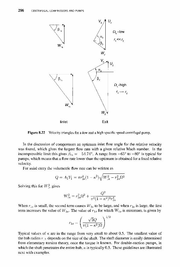
2 9 6 CENTRIFUGAL COMPRESSORS AND PUMPS
n„ -low
Qs-high
linlet Exit
Figure 8.22 Velocity triangles for a low and a high specific speed centrifugal pump.
In the discussion of compressors an optimum inlet flow angle for the relative velocity was found, which gives the largest flow rate with a given relative Mach number. In the incompressible limit this gives 0is = —54.74°. A range from —65° to —80° is typical for pumps, which means that a flow rate lower than the optimum is obtained for a fixed relative velocity.
For axial entry the volumetric flow rate can be written as
Q = A1V1=nr2la{l-K?)JW?a-rlW
Solving this for W^s gives
WTs = ris& + 7r2( l -K2)2 r f
When r i s is small, the second term causes W\s to be large, and when ri s is large, the first term increases the value of W\s. The value of r\s for which W\s is minimum, is given by
T\s V2Q
1/3
7T(1-K2)fi
Typical values of K are in the range from very small to about 0.5. The smallest value of the hub radius r\h depends on the size of the shaft. The shaft diameter is easily determined from elementary torsion theory, once the torque is known. For double-suction pumps, in which the shaft penetrates the entire hub, K is typically 0.5. These guidelines are illustrated next with examples.
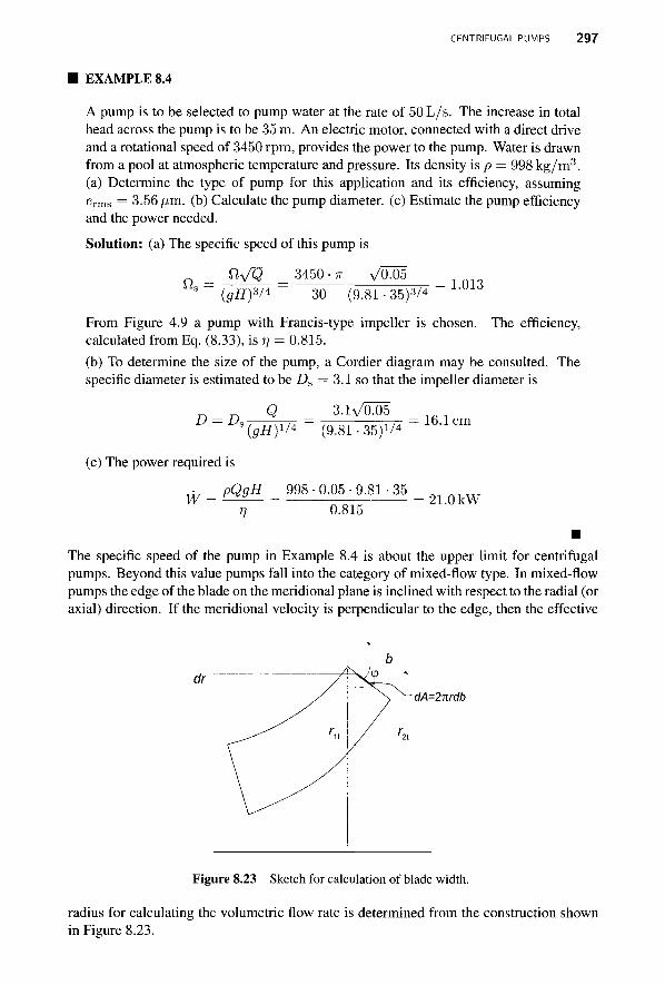
CENTRIFUGAL PUMPS 297
EXAMPLE 8.4
A pump is to be selected to pump water at the rate of 50 L/s. The increase in total head across the pump is to be 35 m. An electric motor, connected with a direct drive and a rotational speed of 3450 rpm, provides the power to the pump. Water is drawn from a pool at atmospheric temperature and pressure. Its density is p = 998 kg/m3. (a) Determine the type of pump for this application and its efficiency, assuming erms = 3.56 yum. (b) Calculate the pump diameter, (c) Estimate the pump efficiency and the power needed.
Solution: (a) The specific speed of this pump is
fi„ = JWQ_ ( 5 f f ) 3 / 4
3450 ■ 7T v'cTos 30 (9.81 • 35)3/4 1.013
From Figure 4.9 a pump with Francis-type impeller is chosen. The efficiency, calculated from Eq. (8.33), is r\ — 0.815. (b) To determine the size of the pump, a Cordier diagram may be consulted. The specific diameter is estimated to be Ds = 3.1 so that the impeller diameter is
D = DS Q _ 3.1^/005
{gH)1/* ~ (9.81 -35)1/4
(c) The power required is
pQgH W =
V 998 ■ 0.05 ■ 9.81 • 35
0.815
16.1 cm
21.0 kW
The specific speed of the pump in Example 8.4 is about the upper limit for centrifugal pumps. Beyond this value pumps fall into the category of mixed-flow type. In mixed-flow pumps the edge of the blade on the meridional plane is inclined with respect to the radial (or axial) direction. If the meridional velocity is perpendicular to the edge, then the effective
dA=2izrdb
Figure 8.23 Sketch for calculation of blade width.
radius for calculating the volumetric flow rate is determined from the construction shown in Figure 8.23.
2 9 8 CENTRIFUGAL COMPRESSORS AND PUMPS
The differential area is dA = 2-rrr db and dr = sin ip db. Hence
- 2 ^ ^ = n(rl - rl) = n(rlt - r 2 t ) ( r l t + r2 t) = +
r i t sinip smi(3 sin^j
Thus the effective radius is the mean radius rm = i ( r n + r2t) and A2 = 2nrmb.
EXAMPLE 8.5
A pump handles water at the rate of 10 L/s with a head of 100 m across the pump. The power is provided by an electric motor with shaft speed 3450 rpm. Water is at 20° C with density p = 998m3/kg. (a) Calculate the specific speed of the pump. (b) Determine the flow coefficient and the blade-loading coefficient, (c) Find the directions of the absolute velocity and the relative velocity of water leaving the impeller, (d) Find the tip radius of the impeller, (d) Find the power needed.
Solution: (a) The specific speed of this pump is
_ nVQ _345Q.7r VOM _ s " (5ff)3/4 " 30 (9.81 • IOO)3/4 "
(b) The flow coefficient is determined from
4> = 0 . 1 7 1 5 ^ ^ = 0 .1715^0.2061 = 0.0779
and the blade loading coefficient is obtained from
0.386 0.386 Ws = —nr = 77X = 0.6535 v fii/3 0.2061V3
From ips = gH/U^ the blade tip speed is / w „ 9-81 • 100 „ a _
U> = \l— = V ^ 6 5 3 5 - = 3 8 - 7 m / s
(c) The hydraulic efficiency is
0.4 0.4
and the work done is therefore ws 9.81 • 100 1.266 kJ/kg r]h 0.775
The tangential and radial components of the velocity are
Vu2 = ^- = ^ ^ = 32.7 m / s Vr2 = <j>U2 = 0.0779 • 38.7 = 3.01 m / s L/2 38.7
so that the flow angle is
*2 = ta„-.(£W.(5|I)=84.72-
CENTRIFUGAL PUMPS 299
The tangential and radial components of the relative velocity are
Wu2 = Vu2 -U2 = 32.7 - 38.7 = -6.0 m/s Wr2 = Vr2 = 3.01 m/s
and therefore
, - i / W M _.„„-i f - ™ A = tan U S J = t a n UorJ=-63-61° (d) The impeller radius can be calculated to be
U2 38.7 • 30 r2 = TT= 3450^7= °-1 0 7 2 m
The volumetric efficiency is obtained by first finding the constants in Eq. (8.32) by interpolation. They are C = 0.2454 and n = 0.4957 for fis = 0.2061. The volumetric efficiency is then
C , 0.2454 _ „ * = * " ^ = * " IQoliar = ° - 9 2 1 6
so that QK = Q/r)v = 0.01/0.9216 = 0.01085 m2/s. The blade width is therefore
52 = 77— = o nin-77 q m = 0 ' 0 0 5 3 m h^ = ° ' 5 3 C m
2?rr2 Vm2 27T • 0.1077 • 3.01 (c) The overall efficiency is determined from Eq. (8.33) to be 77 = 0.66. Hence the power to the pump is
fr=pggg = 998-10-9-81-l(0 n 1000 • 0.66
In the next example the number of vanes and their metal angle are also considered.
EXAMPLE 8.6
Water flows axially into a double-suction centrifugal pump at the rate of 0.120 m3/s. The pump delivers a head of 20 m while operating at 880 rpm. The hub-to-shroud ratio at the inlet is 0.50, and the relative velocity makes an angle —73° at the inlet. (a) Find the reversible work done by the pump, (b) What is the work done by the impeller? (c) Find the radius of the impeller and the inlet radius of the shroud. (d) Determine the blade width at the exit of the impeller, (e) Assume a reasonable number of blades and calculate the blade angle at the exit. Use the Pfleiderer equation to determine more accurately the number of blades and recalculate the blade angle at the exit if needed.
Solution: (a) The reversible work is
ws=gH = 9.81 • 20 = 196.2 J/kg
(b) The hydraulic efficiency is
0.4 0.4 Vh = 1 - —— = 1 — = 0.856 ' n i / 4 6 0 i / 4
3 0 0 CENTRIFUGAL COMPRESSORS AND PUMPS
and the actual work by the impeller is
ws 196.2 w rjh 0.856
229.1J/kg
(c) The specific speed is
n = j W g = 880-, Vom = a 4 3 1 3/4 30 • 196.23/4
w.
and the loading coefficient is
0.383 0.383 n CfVT
^ = ^ = o ^ 3 T ^ = 0-507
Therefore the impeller tip speed is
196.2 U2 - Vw^A
0.507 21.25 m/s
and the impeller radius is
U2 21.25 -20 nnn r2 = — = = 0.231 m
2 Q 880 • 7T The volumetric flow rate can be written as
7 r r l s ( l - K2 )C/ l s TT(1 - K 2 )S> 3
S = A1V1
Solving this for n s gives
tan(-/3is) tan(^is)
ris = Qtan(-/3is) 7 T ( 1 - K 2 ) 0 _
-,1/3
so that
and
ru 60 ■tan(73°) •30
1000 • 7r2(l - 0.502) • 880
1/3
0.0967 m
rih = ^ l s = 0.5 • 0.0967 = 0.0483 m
and thus the blade speed at the shroud is
0.0967 • 880 • 7T Ula = risfl 30
- = 8.91 m/s
(d) The flow coefficient is
4> = 0 . 1715 \ / ^ = 0.1715^0.431 = 0.1125
and the radial velocity at the exit is then
Vr2 = <t>U2 = 0.1125 • 21.25 = 2.39 m/s
CENTRIFUGAL PUMPS 3 0 1
To calculate the leakage flow, the coefficients for the expression of volumetric are interpolated to be
C = 0.1094 n = 0.3564 so that
and the flow through the exit is
QR=®=-±§- =0.123 m3/s r/v 0.975
Hence the blade width has the value QR 0.123
3.55 cm 2irr2Vr2 2 • 7T • 0.231 ■ 2.39
(e) The tangential component of the exit velocity is calculated to be
and the flow angle at the exit is
---(£)—-(££)-™ The tangential component of the relative velocity becomes
Wu2 = Vu2 -U2 = 10.78 - 21.25 = -10.47 m/s
so that the flow angle is
Next, the number of blades is assumed. Let Z — 6, and the blade angle is guessed to be, say, \2 = —60°. Then the slip coefficient is calculated from
V5osx^ \/cos(-60°) a = X " zo.7 = ! ^ 7 = ° ' 7 9 8
and the equation Vu2 = aU2 + Vr2 tan \2
is solved for \2, giving , -x(Vu2-°U2\ . -x( 10-78 -0 .798 -21.25^
X 2 = tan ( — ^ r ^ J = t a n ^ — j = -68.86
Now a new value of a is obtained from Jcosx2 1/cos(-68.86°)
With this value for CT, repeating the calculation gives X2 = —70.7° and a = 0.836. The number of blades can now be calculated from Pfleiderer's equation
Z = 6.5 [ I±WM cos (§±+M\ = 6.00 l-ru/r2J V 2
so that the initial guess was correct. One more iteration gives \2 = — 71. lc
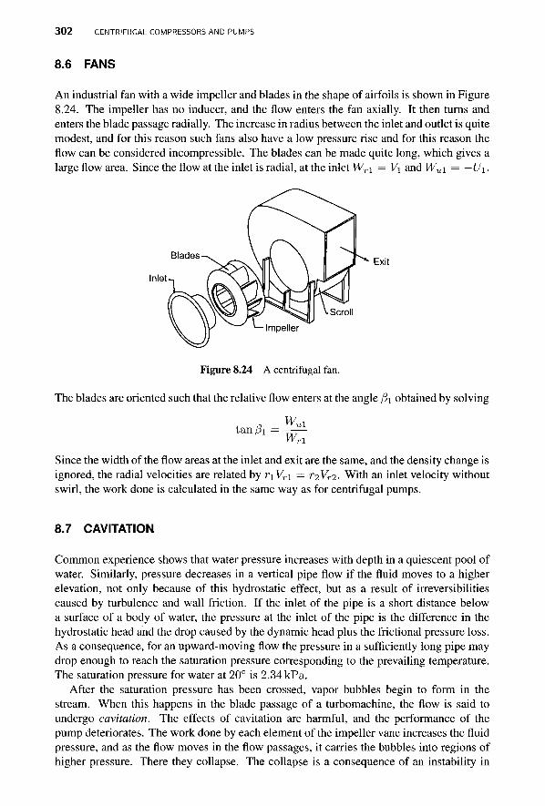
3 0 2 CENTRIFUGAL COMPRESSORS AND PUMPS
8.6 FANS
An industrial fan with a wide impeller and blades in the shape of airfoils is shown in Figure 8.24. The impeller has no inducer, and the flow enters the fan axially. It then turns and enters the blade passage radially. The increase in radius between the inlet and outlet is quite modest, and for this reason such fans also have a low pressure rise and for this reason the flow can be considered incompressible. The blades can be made quite long, which gives a large flow area. Since the flow at the inlet is radial, at the inlet Wr\ = V\ and Wu\ = —U\.
Figure 8.24 A centrifugal fan.
The blades are oriented such that the relative flow enters at the angle fti obtained by solving
Since the width of the flow areas at the inlet and exit are the same, and the density change is ignored, the radial velocities are related by r\Vr\ = 7*2V̂ 2. With an inlet velocity without swirl, the work done is calculated in the same way as for centrifugal pumps.
8.7 CAVITATION
Common experience shows that water pressure increases with depth in a quiescent pool of water. Similarly, pressure decreases in a vertical pipe flow if the fluid moves to a higher elevation, not only because of this hydrostatic effect, but as a result of irreversibilities caused by turbulence and wall friction. If the inlet of the pipe is a short distance below a surface of a body of water, the pressure at the inlet of the pipe is the difference in the hydrostatic head and the drop caused by the dynamic head plus the frictional pressure loss. As a consequence, for an upward-moving flow the pressure in a sufficiently long pipe may drop enough to reach the saturation pressure corresponding to the prevailing temperature. The saturation pressure for water at 20° is 2.34 kPa.
After the saturation pressure has been crossed, vapor bubbles begin to form in the stream. When this happens in the blade passage of a turbomachine, the flow is said to undergo cavitation. The effects of cavitation are harmful, and the performance of the pump deteriorates. The work done by each element of the impeller vane increases the fluid pressure, and as the flow moves in the flow passages, it carries the bubbles into regions of higher pressure. There they collapse. The collapse is a consequence of an instability in

CAVITATION 303
the size and shape of the bubble. As the instability develops the bubble flattens out, and a liquid from the back accelerates toward the center, forming a jet that pierces through the bubble. These impinging jets from the bubbles located next to the impeller of the pump cause erosion. This kind of cavitation damage is seen also in marine propellers.
Any dissolved air tends to come out of the liquid at low pressures. These small air bubbles act as nucleation sites for bubble formation. They are aided in turbulent flow by local negative pressure spikes. The kinetics of nucleation, turbulence, and growth rates of bubbles are complicated subjects and make prediction of cavitation difficult. Hence pump manufacturers rely on experimentation to determine when the pump performance is significantly affected. A comprehensive review of the mechanisms of cavitation is given by Arakeri [4] and by Brennen [10, 9].
A pressure difference called net positive suction pressure (NPSP) is defined as
PN = P + ^PV2 ~ Pv
in which pv is the saturation pressure, p is the static pressure, and V is the velocity at the pump end of the suction pipe (which is the inlet to the pump). When expressed in units of a height of water, the net positive suction pressure is called the net positive suction head (NPSH).
The manufacturer tests the pump and gives a value for the required net positive suction head, N P S H R . This increases with the flow rate as the accelerating flow into the inlet causes the pressure to drop. The application engineer can now determine what is the minimum total head at the pump end of the suction pipe and from this determine the actual net positive suction head, N P S H A . In order to avoid cavitation, N P S H A > N P S H R . In the lower half of Figure 8.18 is a curve showing values (on the ordinate on the right) for the N P S H R as a function of the flow rate.
A suction specific speed is defined as
ss (5NPSH)3/4
For a single-flow pump a rough rule is to keep the suction specific speed under Qss = 0.3 and for a double flow, under f2ss = 0.4 .
■ EXAMPLE 8.7
A pump draws water at the rate of 20 L/s from a large reservoir open to atmosphere with pressure 101.325 kPa. As shown in Figure 8.25, the pump is situated a height z = 4 m above the reservoir surface. The pipe diameter is 7.6 cm, and the suction pipe is 10 m in length. The entrance loss coefficient is K\ = 0.8, the loss coefficient of the elbow is Ke = 0.6, and the pipe roughness is 45 /x m. Find the suction specific speed given a shaft speed is of 1800 rpm. The viscosity of water is 1.08 • 10~3 kg/(m • s).
Solution: A control volume containing the water in the reservoir and in the suction pipe is
so that
PI + \vp -pv=Pa- pgzi - (f^- + Ki + KA l-Pv£ - Pv
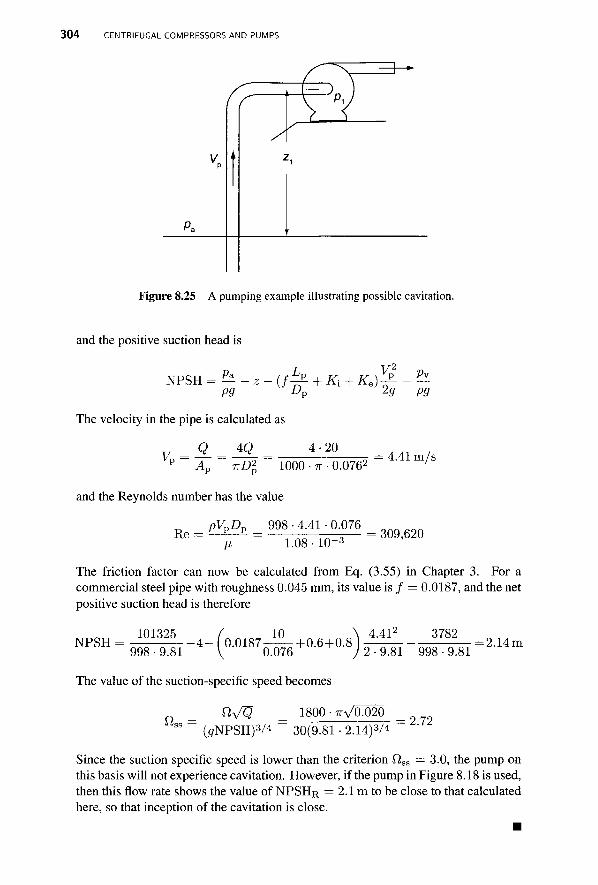
3 0 4 CENTRIFUGAL COMPRESSORS AND PUMPS
Figure 8.25 A pumping example illustrating possible cavitation.
and the positive suction head is
NPSH ,L K2 Pv
pg n 2g pg D
The velocity in the pipe is calculated as
K Q__ 4Q_ 4 - 2 0
irDl 1000 • TT ■ 0.0762
and the Reynolds number has the value
Re pVpD p-^p 998 ■ 4.41 ■ 0.076
1.08-10"3
= 4.41 m/s
309,620
The friction factor can now be calculated from Eq. (3.55) in Chapter 3. For a commercial steel pipe with roughness 0.045 mm, its value is / = 0.0187, and the net positive suction head is therefore
NPSH 101325 10 \ 4 412
4 - ( 0 . 0 1 8 7 ; r ^ +0.6+0.8 3782
998-9.81 " V °- 0 7 6
The value of the suction-specific speed becomes
tly/Q 1800 • TIVO.020
2 • 9.81 998 • 9.81 = 2.14m
a (5NPSH)3/4 30(9.81 • 2.14)3/4 2.72
Since the suction specific speed is lower than the criterion Q,ss = 3.0, the pump on this basis will not experience cavitation. However, if the pump in Figure 8.18 is used, then this flow rate shows the value of N P S H R = 2.1 m to be close to that calculated here, so that inception of the cavitation is close.
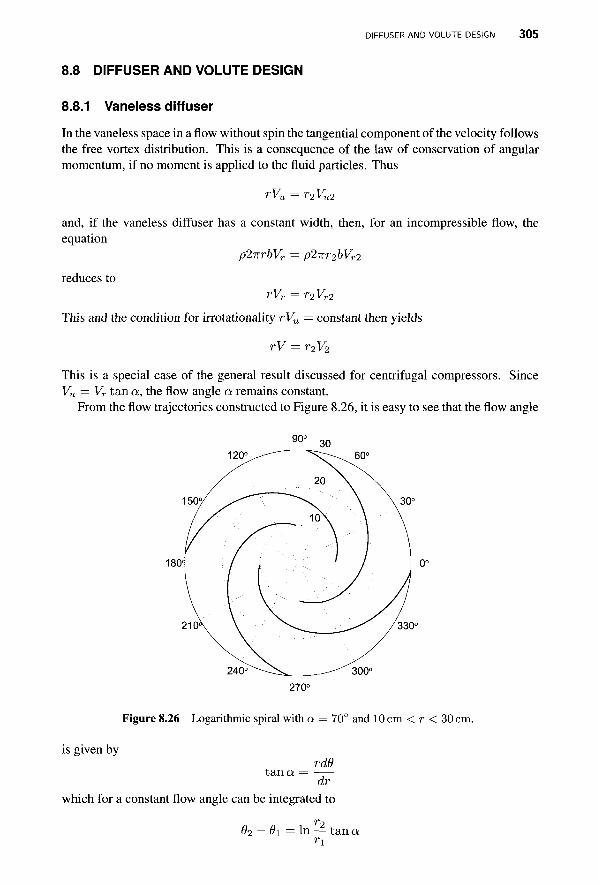
DIFFUSER AND VOLUTE DESIGN 305
8.8 DIFFUSER AND VOLUTE DESIGN
8.8.1 Vaneless diffuser
In the vaneless space in a flow without spin the tangential component of the velocity follows the free vortex distribution. This is a consequence of the law of conservation of angular momentum, if no moment is applied to the fluid particles. Thus
rVu = r2Vu2
and, if the vaneless diffuser has a constant width, then, for an incompressible flow, the equation
p1-KrbVr = p2zr2bVr2
reduces to rVr = r2Vr2
This and the condition for irrotationality rVu = constant then yields
rV = r2V2
This is a special case of the general result discussed for centrifugal compressors. Since Vu = Vr tan a, the flow angle a remains constant.
From the flow trajectories constructed to Figure 8.26, it is easy to see that the flow angle
Figure 8.26 Logarithmic spiral with a = 70° and 10 cm < r < 30 cm.
is given by rd9
tana = —— dr
which for a constant flow angle can be integrated to 02 — 01 = In — tan a
n
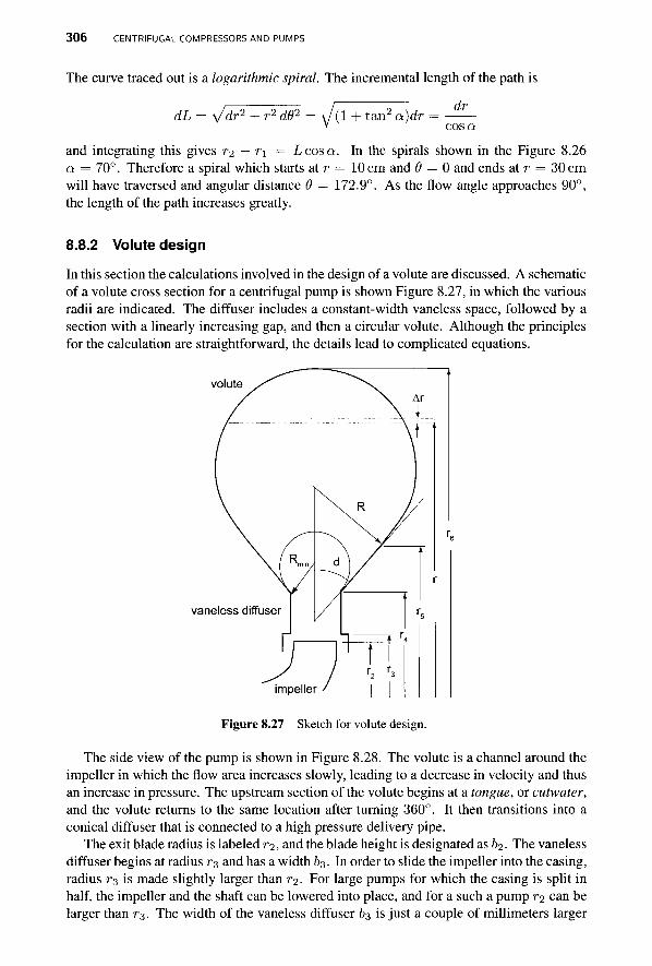
3 0 6 CENTRIFUGAL COMPRESSORS AND PUMPS
The curve traced out is a logarithmic spiral. The incremental length of the path is
dL = \Jdr2 + r2 d62 = J(l + tan2 a)dr = -^~
and integrating this gives r-i — r\ = Lcosa. In the spirals shown in the Figure 8.26 a = 70°. Therefore a spiral which starts at r = 10 cm and 9 = 0 and ends at r = 30 cm will have traversed and angular distance 0 = 172.9°. As the flow angle approaches 90°, the length of the path increases greatly.
8.8.2 Volute design
In this section the calculations involved in the design of a volute are discussed. A schematic of a volute cross section for a centrifugal pump is shown Figure 8.27, in which the various radii are indicated. The diffuser includes a constant-width vaneless space, followed by a section with a linearly increasing gap, and then a circular volute. Although the principles for the calculation are straightforward, the details lead to complicated equations.
volute
vaneless diffuser
impeller
Figure 8.27 Sketch for volute design.
The side view of the pump is shown in Figure 8.28. The volute is a channel around the impeller in which the flow area increases slowly, leading to a decrease in velocity and thus an increase in pressure. The upstream section of the volute begins at a tongue, or cutwater, and the volute returns to the same location after turning 360°. It then transitions into a conical diffuser that is connected to a high pressure delivery pipe.
The exit blade radius is labeled r-i, and the blade height is designated as b^. The vaneless diffuser begins at radius r^ and has a width 63. In order to slide the impeller into the casing, radius r% is made slightly larger than 7-2. For large pumps for which the casing is split in half, the impeller and the shaft can be lowered into place, and for a such a pump r2 can be larger than r3. The width of the vaneless diffuser 63 is just a couple of millimeters larger
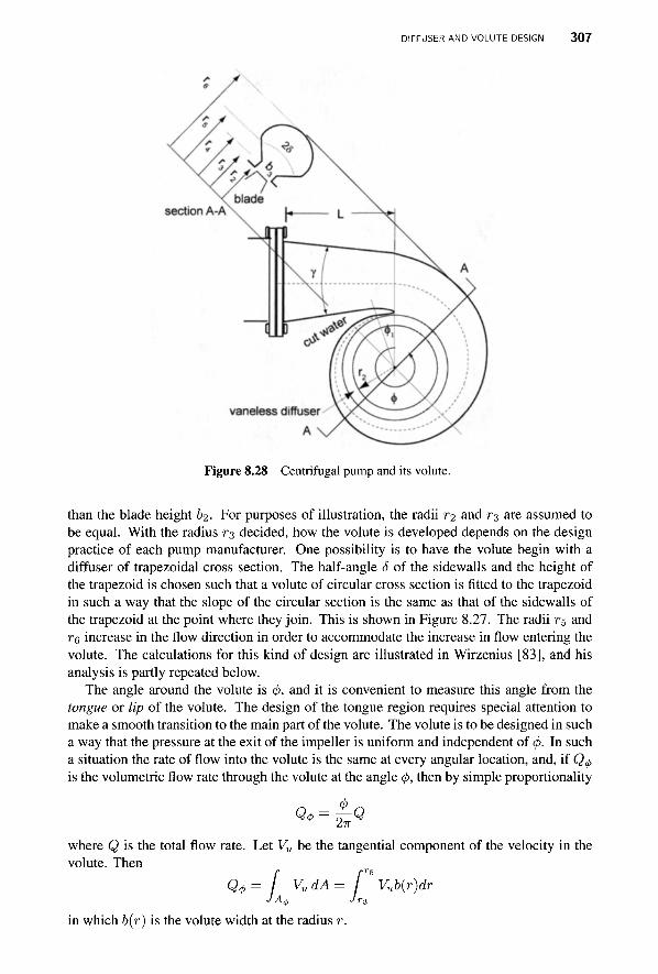
DIFFUSER AND VOLUTE DESIGN 3 0 7
Figure 8.28 Centrifugal pump and its volute.
than the blade height &2- For purposes of illustration, the radii r2 and rz are assumed to be equal. With the radius r^ decided, how the volute is developed depends on the design practice of each pump manufacturer. One possibility is to have the volute begin with a diffuser of trapezoidal cross section. The half-angle S of the sidewalls and the height of the trapezoid is chosen such that a volute of circular cross section is fitted to the trapezoid in such a way that the slope of the circular section is the same as that of the sidewalls of the trapezoid at the point where they join. This is shown in Figure 8.27. The radii r$ and re increase in the flow direction in order to accommodate the increase in flow entering the volute. The calculations for this kind of design are illustrated in Wirzenius [83], and his analysis is partly repeated below.
The angle around the volute is 0, and it is convenient to measure this angle from the tongue or lip of the volute. The design of the tongue region requires special attention to make a smooth transition to the main part of the volute. The volute is to be designed in such a way that the pressure at the exit of the impeller is uniform and independent of <\>. In such a situation the rate of flow into the volute is the same at every angular location, and, if Q$ is the volumetric flow rate through the volute at the angle </>, then by simple proportionality
where Q is the total flow rate. Let Vu be the tangential component of the velocity in the volute. Then
Q4> = f VudA= f C' Vub{r)dr J Aj, Jr3
in which b(r) is the volute width at the radius r.
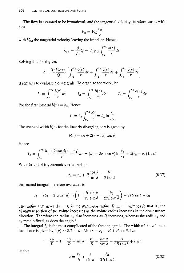
3 0 8 CENTRIFUGAL COMPRESSORS AND PUMPS
The flow is assumed to be irrotational, and the tangential velocity therefore varies with r as
K = Vu2 T2
with VU2 the tangential velocity leaving the impeller. Hence
2TT
r5 b(r) Q = Vu2r2 I -^dr
Solving this for <fi gives
2irVu2r2 r4 b(r)
dr -r5b^dr+rb-^dr
■dr
>r3 Jr4 Jr5
It remains to evaluate the integrals. To organize the work, let
h = r b^dr i2 = r Mdr h = r b± J r$ ' Jr4 ' J r$ '
For the first integral b(r) = 63. Hence
T h rdr K 1 r 4
h =h — = 63 In — Jr3 r r3
The channel width b{r) for the linearly diverging part is given by
b(r) = b3 + 2(r ~r4)ta,nS
Hence 7,5 b3 + 2tan<5(r — r4) r§
dr = (03 — 2r4 tan o) In \- 2{r§ — r4) tan o With the aid of trigonometric relationships
r5 =r4 + R
the second integral therefore evaluates to
cos 6 tan 5 2 tan S
(8.37)
I2 = (63 -2r4tan<5)ln 1 R cos S r4 tan S 2r4 tan 5
+ 2Rcos5 - 6 3
The radius that gives I2 = 0 is the minimum radius Rmin = 63/2 cos <5; that is, the triangular section of the volute increases as the volute radius increases in the downstream direction. Therefore the radius r$ also increases as R increases, whereas the radii r4 and r3 remain fixed, as does the angle S.
The integral I3 is the most complicated of the three integrals. The width of the volute at location r is given by b{r) = 2R sin 9. Also r = r§ — R + R cos 6. Let
r e _ 1 _ ^ 5 . _ l i , cosS _ ^3 R ~ R ~ R tan<5 2i?tan<5
+ sin<5
so that 1 T\
R sin S 2i?tan£ (8.38)
EXERCISES 309
The integral ^3 now can be written as
b(r) dr = 2R
TT/2+5 sin
R -d6 = 2R
^ s i n 2 ! c + cos (
-d6
Evaluation of this leads to
2R (^ +S) -cosS-2Vc2 - ltan" 1 1 + tan(<5/2)
T 1 - tan(<5/2)
Collecting the results gives the design formula
27rr2r4K2 {h {, r4 V Q T4
In^ i
+ 63 2tan<5 In 1
•̂3 2 ,
R cos 8 ri tan S 2r4 tan S + 2- 1 + C (i+')
cos 5 — 2\/c2 — 1 tan / c - l l + t a n ( J / 2 ) \ c + 1 l-tan(<5/2) J
(8.39)
The calculation now proceeds by starting with Rmin and incrementing R by AR, so that the new value of R is i?m;n + Ai?. Next, the value of c is determined from Eq. (8.38) and r$ is calculated from Eq. (8.37). Then r%, the outer extent of the volute, is determined from re = (1 + c)R, but this is not needed in the calculation of angle <j>. The value of angle <fr is finally determined from Eq. (8.39). These values then trace out the volute and its trapezoidal base.
EXERCISES
8.1 An industrial air compressor has 29 backward-swept blades with blade angle —21°. The tip speed of the blades is 440 m/s, and the radial component of the velocity is 110 m/s. Air is inducted from atmospheric conditions at 101.3 kPa and 298 K with an axial velocity equal to 95 m/s. The hub-to-tip ratio at the inlet is 0.4. The total-to-total efficiency of the compressor is 0.83, and the mass flow rate is 2.4 kg/s. Find: (a) The total pressure ratio using the Stodola slip factor and (b) the tip radius of the impeller.
8.2 A centrifugal compressor has 23 radial vanes and an exit area equal to 0.12 m2, where the radial velocity is 27 m/s, and the tip speed of the impeller is 350 m/s. The total-to-total efficiency is 0.83. (a) Find the mass flow rate of air, given that the total pressure and temperature are 101.3 kPa and 298 K at the inlet, (b) What is the exit Mach number? (c) If the blade height at the exit is b = 3 cm and there is no leakage flow, what is the tip radius of the impeller? (d) Find the rotational speed of the compressor wheel, and the required power neglecting mechanical losses.
8.3 A centrifugal compressor has an axial inlet and the outlet blades at an angle such that the tangential component of the exit velocity has a value equal to 0.9 times the blade speed. The outlet radius is 30 cm, and the desired pressure ratio is 3.5. The inlet stagnation temperature is T0\ = 298 K. If the total-to-total efficiency of the compressor is 0.8, at what angular speed does it need to be operated?
8.4 A small centrifugal compressor as a part of a turbocharger operates at 55,000 rpm. It draws air from atmosphere at temperature 288 K and pressure 101.325 kPa. The inlet

3 1 0 CENTRIFUGAL COMPRESSORS AND PUMPS
Mach number is Mi = 0.4, and the flow angle of the relative velocity is /3\s = —60° at the shroud. The radius ratio at the inlet is K = vih/T"is = 0.43. (a) Find the blade speed at the inlet shroud and (b) the mass flow rate, (c) If the inducer is choked, what is the throat area?
8.5 A centrifugal compressor in a turbocharger operates at 40,000 rpm and inlet Mach number Mi = 0.35. It draws air from atmosphere at temperature 293 K and pressure 101.325 kPa. The radius ratio is r\s/r2 = 0.71, and the diffusion ratio is W\sjWi = 1.8. The inlet angle of the relative velocity at the shroud is fiis = —63°. The slip factor is a = 0.85, and the flow angle at the exit is «2 = 69°. Find (a) the tip speed of the blade at the inlet, (b) the tip speed of the blade at the outlet, (c) the loading coefficient, and (d) the metal angle at the exit.
8.6 A small centrifugal compressor draws atmospheric air at 293 K and 101.325 kPa. At the inlet rih = 3.2 cm and r\s = 5 cm. The rotor efficiency of the compressor is 0.88. The relative Mach number at the inlet shroud is 0.9 and the corresponding relative flow angle is /?is = —62°. At the outlet the absolute velocity is at angle a^ = 69°. The diffusion ratio is Wis/W2 — 1.8 and the radius ratio is ris/r2 — 0.72. Find, (a) the rotational speed of the shaft, (b) the blade-loading coefficient w/C/f, (c) the flow coefficient <f> = Vr2/U2, and (d) the blade width at the exit.
8.7 Show that in the incompressible limit the angle of the relative velocity at the inlet is optimum at 54.7°.
8.8 Show that the expression for the dimensionless mass flow rate for a compressor with preswirl at angle a.\ is
_ MfR(tano;i - tan/3is)2cos3/?is
\ l sin a.\ J Plot the results for a.\ = 30°, with /3is on the abscissa and $f on the ordinate, for relative Mach numbers 0.6,0.7,0.8. For a given mass flow rate, does the pre-swirl increase or decrease the allowable relative Mach number, and does the absolute value of the relative flow angle increase or decrease with preswirl?
8.9 Water with density 998 kg/m3 flows through the inlet pipe of a centrifugal pump at a velocity of 6 m/s. The inlet shroud radius is 6.5 cm, and the hub radius is 5 cm. The entry is axial. The relative velocity at the exit of the impeller is 15 m/s and is directed by backward-curved impeller blades such that the exit angle of the absolute velocity is OL2 = 65°. The impeller rotates at 1800 rpm and has a tip radius of 15 cm. Assume that the rotor efficiency of the pump is 75%. Evaluate (a) the power into the pump, (b) the increase in total pressure of the water across the impeller, and (c) the change in static pressure of the water between the inlet and outlet of the impeller, (d) What is the ratio of the change in kinetic energy of the water across the impeller to the total enthalpy of the water across the pump, the change in the relative kinetic energy, and the change in the kinetic energy owing to the centrifugal effect as a fraction of work done? (e) If the velocity at the exit of the volute is 6 m/s, what is the ratio of change in static pressure across the rotor to the change in static pressure across the entire pump?
8.10 A centrifugal-pump that handles water operates with backward-curving blades. The angle between the relative velocity and the tip section is 45°. The radial velocity at the tip section is 4.5 m/s, the flow at the inlet is axial, and the impeller rotational speed is 1800 rpm. Assume that there is no leakage and that the mechanical friction may be neglected, and
EXERCISES 3 1 1
that the total-to-total efficiency is 70%. (a) Construct the velocity diagram at the impeller exit and (b) evaluate the required tip radius for a water pressure rise of 600 kPa across the pump, (c) For the total pressure rise of 600 kPa, evaluate the difference between the total and static pressure of water at the impeller tip section.
8.11 A centrifugal water pump has an impeller diameter D2 = 27 cm, and when its shaft speed is 1750 rpm, it produces a head H = 33 m. Find, (a) the volumetric flow rate, (b) the blade height at the exit of the impeller assuming that there are no leakage losses, and (c) the blade angle at the exit of the impeller, given that it has 11 blades.
8.12 A centrifugal water pump has an impeller diameter of D% = 25 cm, and when its shaft speed is 1750 rpm, it delivers 20 L/s of water. Find, (a) the head of water delivered by the pump, and (b) the power needed to drive the pump, (c) The impeller has nine blades. Use the Stanitz slip factor to find the blade angle at the exit of the impeller, (d) Use the Wiesner slip factor to find the blade exit blade angle.
8.13 A centrifugal pump delivers water at 0.075 m3/s with a head of 20 m while operating at 880 rpm. The hub-to-shroud radius ratio at the inlet is 0.35, and the relative velocity makes an angle of —52° at the inlet, (a) Find the reversible work done by the pump, (b) What is the work done by the impeller? (c) Find the impeller radius and the inlet radius of the shroud, (d) Determine the blade width at the exit of the impeller, (e) Assume a reasonable number of blades, and calculate the blade angle at the exit. Use the Pfleiderer equation to determine more accurately the number of blades and recalculate the blade angle at the exit if needed, (f) What is the power required to drive the pump?
8.14 A fan draws in atmospheric air at 0.4 m3/s at pressure 101.32 kPa and temperature 288 K. The total pressure rise across the fan, which has 30 radial blades, is 2.8 cm of water. The inner radius is 14.8 cm, and outer radius is 17.0 cm. The rotational speed of the fan is 980 rpm and the hydraulic efficiency is the fan is 0.78. Use the Stanitz slip factor. (a) Assuming that velocity into the fan is radially outward, find the angle of the relative velocity at the shroud at the inlet, (b) Determine the power to the fan, given that 4% is lost to mechanical friction, (c) Find the angle blade angle at the exit.
8.15 A pump draws water at the rate of 75 L/s from a large tank with the air pressure above the free surface at 98.00 kPa. The pump is z = 2 m above the water level in the tank. The pipe diameter is 14.0 cm, and the suction pipe is 20 m in length. The entrance loss coefficient is K\ = 0.2, and the loss coefficient of the elbow is Ke = 0.6 and the pipe roughness is 55 /xm. Find the suction specific speed given a shaft speed of 1800 rpm. The viscosity of water is 1.08 • 10~3 kg/(m • s).
8.16 Consider a volute consisting only a of circular section in which the tangential velocity varies as Vu = K/r, and r is the location from the center of the volute to a location on the circular section, (a) Show that the value of K in terms of the volumetric flow rate Q, the radius of the circular section R, and the radius to the center of the of the circular section a, is given by
Q K = , 27ri?(A - T F ^ T )
in which A = a/R. (b) For R = 0.5 m, a = 2 m, and Q = 1.5m3/s, find the pressure difference p2 — Pi at the centerline, between the outside and inside edges of the section.
CHAPTER 9
RADIAL INFLOW TURBINES
The best known use of radial inflow turbines is in automobile turbochargers, but they also appear as auxiliary power turbines and, for example, in turboprop aircraft engines. They are used in processing industries (including refineries), natural-gas processing, air liquefaction, and geothermal energy production. In the automotive application burned gases from the engine exhaust manifold are directed into a radial inflow turbine of the turbocharger, which powers a centrifugal compressor on the same axis. The compressor, in turn, increases the pressure and density of the supply air to the engine. As the engine speed may change quite rapidly, turbochargers must respond to the changing operating conditions nimbly. Therefore they are made light in weight and low in inertia.
A sketch on the left side in Figure 9.1 shows a side view of a radial inflow turbine. It looks like a centrifugal compressor, but with a reversed flow direction. Hot gases enter through a volute and move into a vaned stator, which redirects them into a vaneless space and then into the rotor. On the right is a front view of the rotor. The velocity diagrams at the inlet and exit are shown in Figure 9.2. For best efficiency, the inflow angle fa is negative. But the blades at the inlet are typically radial, which means that the entering flow is at a negative incidence. Since the blades operate in a high-temperature environment and material strength diminishes as temperature increases, radial blades can withstand the imposed loads better than curved blades. It is for this reason that the blade angle at the inlet is set at \2 = 0. The rotor turns the flow toward the axis as it passes through the flow channel, so that its radial velocity is zero at the exit and the absolute velocity is axial. For this reason these machines are also called 90° inward-flow radial (IFR) turbines.
Principles of Turbomachinery. By Seppo A. Korpela 313 Copyright © 2011 John Wiley & Sons, Inc.
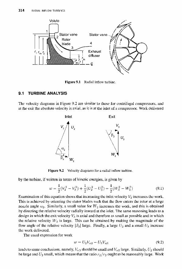
314 RADIAL INFLOW TURBINES
Volute
Stator vane Stator vane Rotor blade 4
3 , Exhaust diffuser
■^ ' 3 ±_«2
Figure 9.1 Radial inflow turbine.
9.1 TURBINE ANALYSIS
The velocity diagrams in Figure 9.2 are similar to those for centrifugal compressors, and at the exit the absolute velocity is axial, as it is at the inlet of a compressor. Work delivered
Inlet Exit
2 W,
Figure 9.2 Velocity diagrams for a radial inflow turbine.
by the turbine, if written in terms of kinetic energies, is given by
\{v?-vi) + \(u,. 1 ^ ) + j ^ w4 (9.1)
Examination of this equation shows that increasing the inlet velocity V2 increases the work. This is achieved by orienting the stator blades such that the flow enters the rotor at a large nozzle angle o^- Similarly, a small value for W2 increases the work, and this is obtained by directing the relative velocity radially inward at the inlet. The same reasoning leads to a design in which the exit velocity V3 is axial and therefore as small as possible and in which the relative velocity W3 is large. This can be obtained by making the magnitude of the flow angle of the relative velocity \/3s\ large. Finally, a large U2 and a small U3 increase the work delivered.
The usual expression for work
w u2vu2 - u3vt K3 (9.2)
leads to same conclusions, namely, VU3 should be small and VU2 large. Similarly, U2 should be large and U3 small, which means that the ratio r2/rz ought to be reasonably large. Work
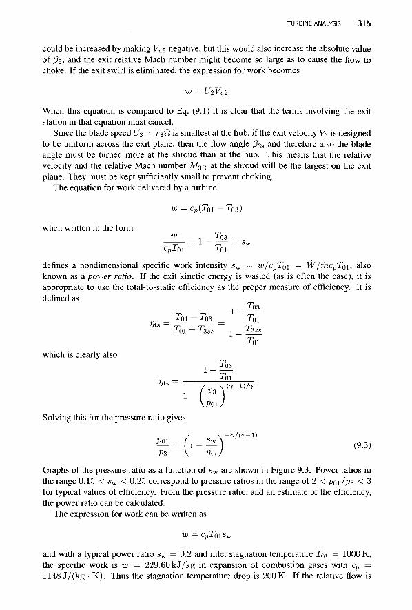
TURBINE ANALYSIS 315
could be increased by making VU3 negative, but this would also increase the absolute value of fa, and the exit relative Mach number might become so large as to cause the flow to choke. If the exit swirl is eliminated, the expression for work becomes
w = U2Vu2
When this equation is compared to Eq. (9.1) it is clear that the terms involving the exit station in that equation must cancel.
Since the blade speed L73 = r^fl is smallest at the hub, if the exit velocity V3 is designed to be uniform across the exit plane, then the flow angle Psa and therefore also the blade angle must be turned more at the shroud than at the hub. This means that the relative velocity and the relative Mach number M 3 R at the shroud will be the largest on the exit plane. They must be kept sufficiently small to prevent choking.
The equation for work delivered by a turbine
when written in the form
CP{TQI — T03)
, T03 CPTQI TQI
defines a nondimensional specific work intensity s w = w/cpT0i = W/mcpT0i, also known as a power ratio. If the exit kinetic energy is wasted (as is often the case), it is appropriate to use the total-to-static efficiency as the proper measure of efficiency. It is defined as
r?ts
1 _ T^l TQI — T03 _ TQI foi — T3ss _ T3SS
T01 which is clearly also
1 »7ts
T03 T01
P3_ P01
( 7 - l ) / 7
Solving this for the pressure ratio gives
/ c \ ~ T / ( 7 - 1 ) M = ( 1 _ £21) (9.3)
Graphs of the pressure ratio as a function of sw are shown in Figure 9.3. Power ratios in the range 0.15 < s w < 0.25 correspond to pressure ratios in the range of 2 < P01/P3 < 3 for typical values of efficiency. From the pressure ratio, and an estimate of the efficiency, the power ratio can be calculated.
The expression for work can be written as
W = CpToiSw
and with a typical power ratio s w = 0.2 and inlet stagnation temperature T0i = 1000 K, the specific work is w = 229.60 k J / k g in expansion of combustion gases with cp — 1148 J / (kg • K). Thus the stagnation temperature drop is 200 K. If the relative flow is

316 RADIAL INFLOW TURBINES
Figure 9.3 Pressure ratio for a gas with 7 = 1.4 as a function of power ratio, or total-to-static efficiency ?7ts = 0.8 to r]tB = 1-0 with adjacent graphs incremented by 0.02.
radially inward and there is no exit swirl, the Euler turbine equation shows that w = L7| , so that a typical blade speed is 479 m/s. The size of the machine depends on the mass flow rate. Thus, as a rough estimate, a turbocharger operating at shaft speed of 40,000 rpm gives an inlet radius of about 10 cm, and one operating at 200,000 rpm gives a radius of 2 cm. A turbocharger from an automobile and with a rotor diameter of approximately 3 cm is shown in Figure 9.4.
Figure 9.4 An automotive turbocharger.
At the exit, in addition to being uniform, the axial velocity V3 should be small, so that the exit kinetic energy is small. Whatever exit kinetic energy is left in the exit stream may
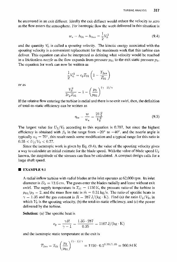
TURBINE ANALYSIS 317
be recovered in an exit diffuser. Ideally the exit diffuser would reduce the velocity to zero as the flow enters the atmosphere. For isentropic flow the work delivered in this situation is
ws = /i0i - h3ss = -V£ (9.4)
and the quantity V0 is called a spouting velocity. The kinetic energy associated with the spouting velocity is a convenient replacement for the maximum work that this turbine can deliver. This equation can also be interpreted as defining what velocity would be reached in a frictionless nozzle as the flow expands from pressure poi to the exit static pressure p3. The equation for work can now be written as
or as
2cpT0i \ p o i .
If the relative flow entering the turbine is radial and there is no exit swirl, then, the definition of total-to-static efficiency can be written as
»hs = — = -jrf (9-5)
The largest value for U2/V0 according to this equation is 0.707, but since the highest efficiency is obtained with /32 in the range from —20° to —40°, and the nozzle angle is typically 0.2 = 70°, this result needs some modification and a typical range for this ratio is 0.55 < U2/V0 < 0.77.
Since the isentropic work is given by Eq. (9.4), the value of the spouting velocity gives a way to calculate an initial estimate for the blade speed. With the value of blade speed U2 known, the magnitude of the stresses can then be calculated. A compact design calls for a large shaft speed.
■ EXAMPLE 9.1
A radial inflow turbine with radial blades at the inlet operates at 62,000 rpm. Its inlet diameter is D2 = 12.6 cm. The gases enter the blades radially and leave without exit swirl. The supply temperature is TQI = 1150 K, the pressure ratio of the turbine is P01/P3 = 2, and the mass flow rate is m = 0.31 kg/s. The ratio of specific heats is 7 = 1.35 and the gas constant is R = 287 J/(kg • K). Find (a) the ratio U2/V0, in which Vo is the spouting velocity, (b) the total-to-static efficiency, and (c) the power delivered by the turbine.
Solution: (a) The specific heat is
*-#-^-i™-K, and the isentropic static temperature at the exit is
/ \ ( 7 - l ) / 7 T3ss = T01 ( — ) = 1150 • o.5°-35/1-35 = 960.84 K
\P01J
318 RADIAL INFLOW TURBINES
The isentropic work is therefore
ws = cp(Toi - T3ss) = 1107(1150 - 960.84) = 209.40kJ/kg
and the spouting velocity is
Vo = V2w~s = A/2 • 209,400 = 647.1 m/s
The blade speed at the inlet is
^ 12.6 -62,000 -7T „„„„ . U*=T**= 2 .100-30 = 4 0 9 - ° m / s
so that the ratio U2/V0 becomes 0.632.
(b) Since there is no exit swirl, the work becomes
w = Ul = 167.31 kJ/kg
and the stagnation temperature drop amounts to 151°C. The total-to-static efficiency comes out to be
w 167.31 r?ts = — = = 0.799 /ts ws 209.40
(c) The power delivered is
W = mw = 0.31 • 167.31 = 51.87 kW
The next example gives an analysis for a choked rotor passage.
■ EXAMPLE 9.2
Combustion gases with 7 = 1.35, Cp = 1107 J/(kg-K) and R = 287 J/(kg-K) flow from conditions poi = 390 kPa and T01 = 1150K through a radial inflow turbine to an exit pressure p3 = 100 kPa. The total-to-static efficiency is 77ts = 0.8, and the flow leaving the stator is choked with M% = 1. (a) Find the work delivered by the turbine, given that the relative velocity at the inlet of the rotor is radial and that flow leaves without swirl, (b) Find the angle of the absolute velocity at the inlet of the rotor.
Solution: Since the stator is choked, the static temperature at the exit of the stator is
T2 = - ^ - - T o 2 = 978.7 K 7 + 1
and the velocity is
V2 = y/jRT2 = v^l.35 • 287 ■ 978.7 = 615.8 m/s
Solving the definition of total-to-static efficiency _ rpi — T03
/tS ry\ rrt J01 — J-3ss
EFFICIENCY 319
for the exit stagnation temperature gives
T03
J o i
n ^ ( 7 - l ) / 7 '
P3
so that T03 = 1150 [1 - 0.8 (1 - 3.9-0-35/1.35)] = 8W5 K
Work delivered by the turbine is therefore
w = cp(Toi - T03) = 1107(1150 - 876.5) = 302.80 kJ/kg
This is also w = Ul
so that U2 = y/w= v/302,800 = 550.27 m/s
The flow angle at the inlet to the rotor is
a2 = sin"1 (y-j = s in - 1 (0.893) = 63.3°
The foregoing two examples assumed that the relative velocity at the inlet to the rotor is radial and that there is no exit swirl. In the next section a general development based on this assumption is carried out in order to relate the important flow parameters to the total-to-static efficiency.
9.2 EFFICIENCY
The total-to-static efficiency of a turbine is
__ hgi — hp3
" 0 1 — n3ss
with the thermodynamic states as shown in Figure 9.5. This can be written as
1 -, ^03 — hsss
flu h0i - h03
If the turbine is fitted with a diffuser and its exit pressure is p^, then, if the flow exhausts to the atmosphere, the pressure p^ is the atmospheric pressure and the small amount of residual kinetic energy is lost into the atmosphere. In this situation the pressure p3 is below the atmospheric value. If the flow through this diffuser were reversible, then the pressure P\ would correspond to the stagnation pressure poz- In this case the appropriate efficiency to use is the total-to-total efficiency. On the other hand, if the flow is not diffused and the flow is exhausted to the atmosphere directly, then the exit pressure p3 is the atmospheric pressure and the residual kinetic energy is lost. In this case the efficiency is the total-to-static efficiency. The numerator can be rewritten as
1 Vo + /i3 - /i3., + /i3., - ha 103 — 'I'Zss — 1Z v3 T ' ' 3 — '*3s T "3s — n3ss
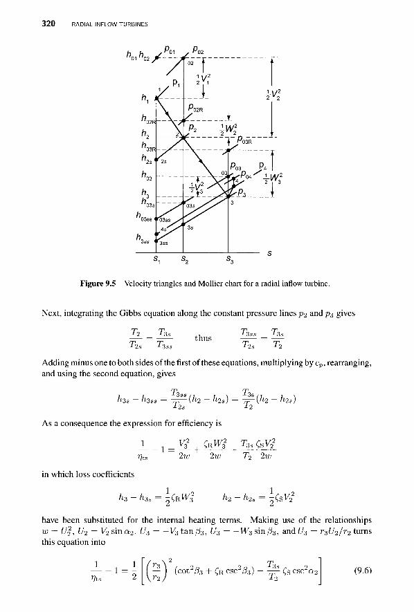
320 RADIAL INFLOW TURBINES
* o i W °1
Figure 9.5 Velocity triangles and Mollier chart for a radial inflow turbine.
Next, integrating the Gibbs equation along the constant pressure lines p2 and p3 gives
T3s T2 = T3s
T2s T3ss thus Ts 2s
Ik T2
Adding minus one to both sides of the first of these equations, multiplying by cp, rearranging, and using the second equation, gives
fi38 - h3ss = -=^-(h2 - h2s) = ~^r(h2 - h2s) J-2s J-1
As a consequence the expression for efficiency is
in which loss coefficients
h3 ~ h3s
2w 2w + T2 2w
-XRWJ TCS^2
have been substituted for the internal heating terms. Making use of the relationships w = J7|i U2 = V2 sma2 , U3 = -V3 tan £3, U3 = -W3 sin/33, and U3 = r3U2/r2 turns this equation into
1 _ 1 »7ts 2 ) ^ rp
(cot2/33 + CR CSC2/33) + -^ Cs csc2a2 T2
(9.6)
EFFICIENCY 321
The temperature ratio in this expression can be written in a form from which it is easy to calculate. First, it is recast as
^ = 1 - ^ ( T 2 - T 3 + T 3 - T 3 s ) J2 J-2
in which temperature difference T2 — T3 is obtained from
w = U2 = h,
Solving this for T2 — T3 gives
T2-T3
2 — "-02 - ^03 — cp(T2 — T3) + -V2 - - v 3 :V?
- ui -lv22 + \v2
c n \ 2 2 2 2 3
But the from the velocity diagrams in Figure 9.2, since (32 — 0 and 0:3 = 0, it is seen that
v22 = wi + ui wi = v£ + u$
so that
and therefore
n 2c, ■(wi-wi + ui-Ui
1 1 -(Wi - W2 + Ui - U2 + CRW2)
T2 2cpT2
in which CR = 2cp(T3 — T3s)/W2 has been used. This can now be written as
T3s , 1 1 T2 2cpT2
and, with C/3 = U2r3/r2, as
{Ui c s c ^ 3 - U22 cot2a2 + U2
2 - U£ + CR[/3 CSC'/33)
Ik T2
1 2cpT2
1 + ( ? ) ((! + CR) csc2/33 - 1) - cot2a2
From
so that
'02
ui
ZCTI -v2 2cpT2 = 2cpTo2 - Ui csc2a2
T°2 ^ • 2 7 - 1 , , 2 • 2 — 1 I sin a2 = -——M2 sin a2 2cpT2
and it follows that the temperature ratio can also be written as
2
T2 1 7 1 1/2 ■ 2
—-— Mj sin a2 1 ( ( 1 + C R ) C S C 2 / 3 3 - 1 ) - c o t 2 a 2
The value of Cs is measured in a stationary test apparatus, and the total-to-static efficiency can be measured from the overall balance for the turbine [15]. The value of CR can then be determined from the theory developed above. These calculations are illustrated in the following example.

322 RADIAL INFLOW TURBINES
EXAMPLE 9.3
In a radial-inflow turbine, combustion gases, with 7 = | and cp = 1148 J/(kg • K), leave the stator at the angle a2 = 67°. The rotor blades at the inlet are radial, with a radius r2 = 5.8 cm. At the outlet the shroud radius of the blade is r3s = 4.56 cm, the hub-to-shroud radius ratio is K = 0.35, and the relative flow makes an angle (83 = —38° with the axial direction at the exit. The relative velocity at the inlet to the rotor is radial. The power delivered by the turbine is W — 58.2 kW when the mass flow rate is m — 0.34 kg/s and the rotational speed is 64,000 rpm. The stagnation temperature and pressure at the inlet to the stator are T01 = HOOK and poi = 2.5 bar. The static enthalpy loss coefficient for the flow across the stator is Cs = 0.08. The outlet static pressure is p3 = 1 bar. Find (a) the Mach number at the inlet of the rotor, (b) the total-to-static efficiency, and (c) the static enthalpy loss coefficient of the rotor.
Solution: (a) The blade speed at the inlet is
^ 0.058 • 64000 • 7T U2 = r2Vt = — = 388.72 m/s
ou
and since the relative flow is radial, Vu2 = U2 and
sin 0:2 sm(o7°)
Since T02 = T0i, the static temperature at the inlet is
V? 422.292
T2=T02 2- = 1100 = 1022.3 K
2cp 2-1148
and the Mach number becomes
V2 422.29 M2 = . * = . = 0.675
V7RT2 v^l.333 • 287 • 1022.3 (b) The specific work is given by
W 58200
and the stagnation temperature at the outlet is therefore
T03 =T01-- = 1100 - ¥±£ = 950.9 K cp 1.148
In an isentropic process to the exit pressure the static temperature at the exit is
( 7 - l ) / 7 / -, \ 0.25
\P01J V2-5 T3ss=T01[^) =1100 1 — 1 =874.8K
and the total-to-static efficiency is therefore
TQI - T03 1100-950.9 rjt, = = = 0.662 /ts T0i - T3ss 1100 - 874.8
SPECIFIC SPEED AND SPECIFIC DIAMETER 3 2 3
(c) If in the expression for efficiency the temperature ratio T3s/T2 is set to 1, then the static enthalpy loss coefficient £R can be solved from
1 ??ts
- 1 = 1
" 2tan2/33
(rsV Ca \r2J 2sin2/33 \ r 2 ,
) 2 + ^ ' 2sin2a2
With Cs = 0.08, fa = -38°, and r3 = (r3s + r3 h) /2 = 0.0308m, solving this equation gives £R = 0.6256. Now the temperature ratio is calculated as
^ = l - ^ M 2S i n 2 a 2 T2 2 2 1 + ( ^ J ((l + CR)csc 2 /3 3 - l ) -co t 2 a 2 = 0.8876
Substituting this into Eq. (9.6) and repeating the calculation with the new temperature ratio gives CR = 0.6399. The static loss coefficient for the rotor is larger than that for the stator, not only because the flow path is long but also because the flow undergoes a great deal of turning through the rotor.
9.3 SPECIFIC SPEED AND SPECIFIC DIAMETER
The specific speed, defined as
3/4 Ws
characterizes the shape of a turbomachine, and a machine with a small specific speed has a low flow rate and a large specific work. A related quantity is the specific diameter given by
D*
It is small in axial turbines because the flow rate is large and the work per stage is relatively small. For radial inflow turbines this quantity is large because the work per stage is large and the volumetric flow rate is rather small. The product of specific speed and specific diameter is
Jws Vo
When the work is given by w = £/f, this reduces to
fls-Ds = 2 ^ t e (9-7)
Balje [5] has constructed a large number of diagrams with specific speed on the abscissa and specific diameter as the ordinate. A Balje diagram for radial inflow turbines is shown in Figure 9.6, and the region of highest efficiency falls into the range 0.2 < fls < 0.8. The corresponding specific diameter can be calculated according to Eq. (9.7). Lines of constant r3 /r2 are also drawn with an optimum value near 0.7. The recommended range is 0.53 < r3/r2 < 0.66. The slight discrepancy in this range and the optimum value 0.7
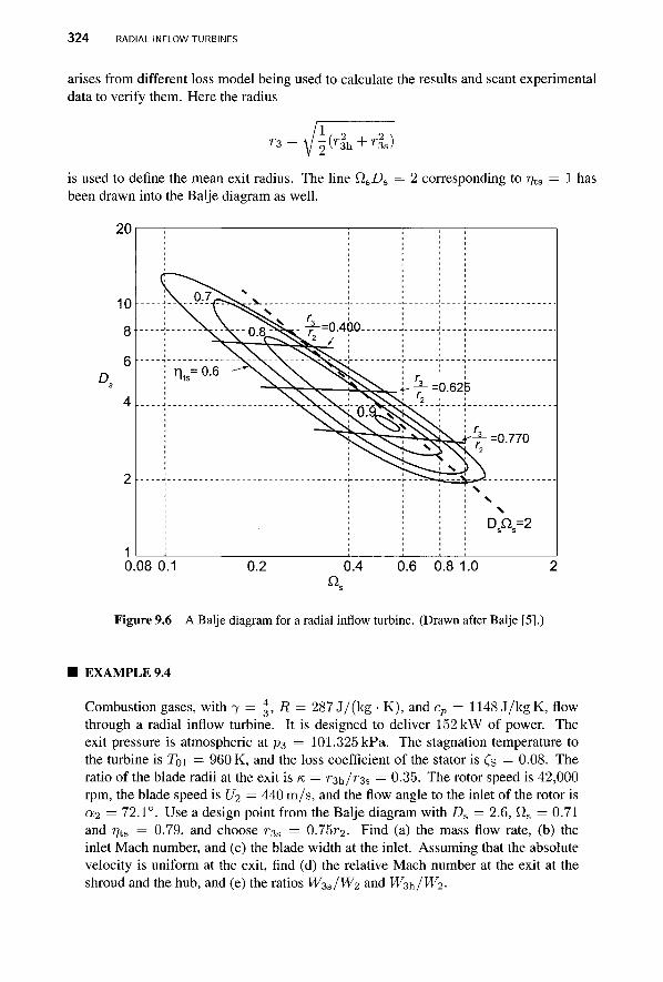
324 RADIAL INFLOW TURBINES
arises from different loss model being used to calculate the results and scant experimental data to verify them. Here the radius
*"3 ^rk + rl) is used to define the mean exit radius. The line QSDS = 2 corresponding to rjts = 1 has been drawn into the Balje diagram as well.
Figure 9.6 A Balje diagram for a radial inflow turbine. (Drawn after Balje [5].)
EXAMPLE 9.4
Combustion gases, with 7 = | , R = 287 J/(kg • K), and cp = 1148 J/kgK, flow through a radial inflow turbine. It is designed to deliver 152 kW of power. The exit pressure is atmospheric at P3 = 101.325 kPa. The stagnation temperature to the turbine is T0i = 960 K, and the loss coefficient of the stator is Cs = 0.08. The ratio of the blade radii at the exit is K = rs^/rss = 0.35. The rotor speed is 42,000 rpm, the blade speed is Ui = 440 m/s, and the flow angle to the inlet of the rotor is c*2 = 72.1°. Use a design point from the Balje diagram with Da = 2.6, fis = 0.71 and 77ts = 0.79, and choose r^,s = 0.75r2. Find (a) the mass flow rate, (b) the inlet Mach number, and (c) the blade width at the inlet. Assuming that the absolute velocity is uniform at the exit, find (d) the relative Mach number at the exit at the shroud and the hub, and (e) the ratios Wss/W2 and W^h/W^-
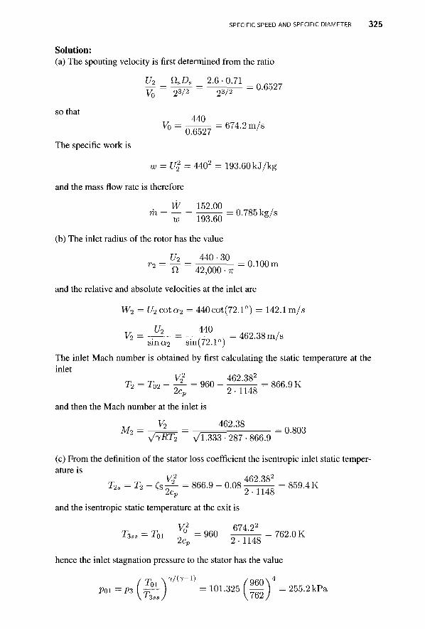
SPECIFIC SPEED AND SPECIFIC DIAMETER 3 2 5
Solution: (a) The spouting velocity is first determined from the ratio
U2 nsDs 2.6-0.71 : a 6 5 2 ?
so that
The specific work is
V0 23/2 23/2
440 V° = 06527 = 6 7 4 - 2 m / s
w = \Jl = 4402 = 193.60 kJ/kg
and the mass flow rate is therefore
W 152.00 „ w n r l . m = ^ = l93^0=°-7 8 5 k g / s
(b) The inlet radius of the rotor has the value
U2 440-30 „ _ r 2 = 7T = 4 ^ 0 0 0 ^ = ° - 1 0 ° m
and the relative and absolute velocities at the inlet are
W2 = U2cota2 = 440cot(72.1°) = 142.1 m/s
Uo 440 V2 = -r-=— = . , „ n , , = 462.38 m/s
sina2 sin(72.1°) ' The inlet Mach number is obtained by first calculating the static temperature at the inlet
T2 = T 0 2 - ^ - = 9 6 0 - ^ ^ = 8 6 6 . 9 K 2cp 2 • 1148
and then the Mach number at the inlet is
V2 462.38 nnnn M2 = , ", = , = 0.803
VlRT2 Vl-333- 287 -866.9 (c) From the definition of the stator loss coefficient the isentropic inlet static temper-ature is
T/2 d(\2 3 8 2
T2S = T 2 - C s ^ = 866.9-0.08 ^ - T I ^ = 8 5 9 . 4 K
and the isentropic static temperature at the exit is
T/2 (V7A 2 2
T3ss =T01--*-= 960 - — — - = 762.0 K 2cp 2 • 1148
hence the inlet stagnation pressure to the stator has the value
/ rp \ 7/(7-1) / 9 6 0 \ 4
P 0 i = P 3 ( ^ J = 1 0 1 - 3 2 5 ( ^ j = 255.2 kPa
326 RADIAL INFLOW TURBINES
At the inlet to the rotor the static pressure is
T 2 s \ 7 / ( 7 - 1 } „ „ „ / 8 5 9 . 4 N 4
p 2 = P o i ^ j =255-2U6U0j =163-9kPa
so that the density at the inlet becomes
P2 = lk = 0.287 3 8 6 6 . 9 = a 6 5 9 k g / i n 3
The blade height can now be determined from the mass balance
TO 0.785 0.0133 m
27rr2p2V/2 cos a2 TT • 0.020 • 0.659 • 462.4 cos(72.1°)
The ratio of the inlet blade height to the inlet radius is 62/r2 = 0.133. (d) The rotor shroud and hub radii are
r3s = 0.75r2 = 0.75 ■ 0.1 = 0.075 m r3h = Kr3s = 0.35 • 0.075 = 0.0263 m
When the Balje diagram is used, the average exit radius is its root mean square value
r3 = \l\(rlh+rl)= 0.0562 m
The blade speed at the mean radius is therefore
^ 0.0562 • 42,000 • TT „„„„ . U3 = r3n = ^ = 247.2 m/s
At the shroud and the hub the blade speeds are
„ 0.075 • 42,000 • TT „ _ , U3s = r3sn = ^ = 330.0 m/s
and U3h = U3s— = 330 = 115.5 m/s
r3s 0.075 To calculate the exit velocity, the exit Mach number is needed. First, the exit stagnation temperature is found to be
w 193,600 J03 = J02 = 960 ,_ ,„ = 791.4K cp 1148
Rearranging the mass balance
TO = p3V3A3 = ——M3^~iRT3 Kl3
leads to 1/2
* lRT03-M3(l + ^ M ! P3A
SPECIFIC SPEED AND SPECIFIC DIAMETER 3 2 7
which on squaring can be written as a quadratic equation in Mf
»,4 2 *,2 2RT03rh2
3 7 - 1 7 ( 7 - l ) ^ §
and after numerical values are inserted this reduces to
Ml + 6 M | - 0.2548 = 0
Solution of this is M3 = 0.205. (e) The exit velocity can now be determined by first calculating the static temperature at the exit
T3 = T03 (l + -^Mi) = 785.8K
which gives the exit velocity
V3 = M3V7-RT3 = 0.2(Wl.333- 287 -785.8 = 112.6 m/s
Since the absolute velocity is axial at the exit, the angles that the relative flow makes at the shroud and the hub at the exit are
«-=- - m —- ■ m)— The relative velocities at the shroud and hub are
W3a = JUl + V£ = \/330.02 + 112.62 = 348.7 m/s
W3h = y/u^ + Vf = \ / l l 5 .5 2 + 112.62 = 161.3 m/s
and at the inlet the relative velocity is
W2 = y % 2 - [/| = \/462.42 - 142.12 = 142.1 m/s
Hence the relative velocity ratios are W3s/W2 = 2.45 and W^/W^ = 1.14. The relative Mach numbers are M 3 R S = 0.636 and M3Rh = 0.294. g
In the foregoing example the mass balance was used to link the upstream and downstream states. Depending on what kind of information is known, this may become a somewhat involved calculation. The general approach is to express the mass balance in terms of the flow function. Upstream, this leads to
fnJcpT02 = b2 cos a2
and downstream the corresponding statement is
P03^3

328 RADIAL INFLOW TURBINES
in which the flow function is
/ . , _ ■ , x - ( l / 2 ) [ ( 7 + l ) / ( 7 - l ) ] F = , ' M 1 + - M
The term cos a2 appears in the upstream expression because it is the radial inflow velocity, Vr2 = V^coso^. that enters the expression for the mass flow rate. Downstream the corresponding factor is missing because it is assumed that the absolute velocity is axial.
Dividing these gives A.2 F3 T02P03
The temperature ratio is A3 F2 cos a2 V T03 P02
T02 = 1 T03 1 - Sw
and the pressure ratios may be written as
P03 __ P03 P3 POI
P02 Pz P01 P02
in which
and
In addition
P03 _ ( 1 + 1 ^ 1 M2 7/ (7 -1)
P3
7/ (7 -1) POI _
P3 V 7-1
P01 ^ f T2
P02 \T2s
7/ (7 -1)
= I 1 - Cs
Substituting gives
A , = F3 ( 1 + ^Mj Y7^-^/ e^m-V 1 A3 F2cosa2 ^ l - C s V ^ 2 / V Ths) v T ^ 7 ^
From this it is clear that if the power ratio sw can be determined and the total-to-static efficiency and the stator loss coefficient can be estimated, then the mass balance in this form involves only M2, M3, and the area ratio A2/A3 as unknowns. Hence, if two of these can be determined in other ways, this equation may be solved for the third. Clearly, if the area ratio is the only unknown, then it can be solved from this explicitly. However, if one of the Mach numbers is unknown, then an iterative solution of a nonlinear equation must be carried out. This can be readily performed with the aid of a computer. In hand calculations, it may be worthwhile to calculate the results directly from
m = p2A2Vr2 = /03-A3V3
by assuming one of the unknowns and then using the mass balance to check that the other converges by iterations to its correct value.
A collection of typical ranges of parameters for a well-designed radial inflow turbines has been compiled by Logan [52]. It is reproduced as Table 9.1.
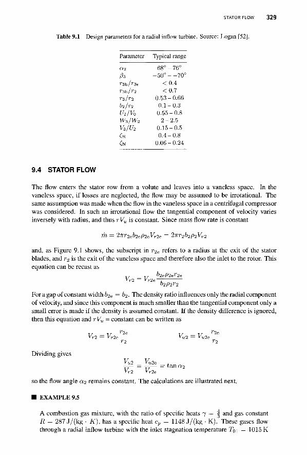
STATOR FLOW 329
Table 9.1 Design parameters for a radial inflow turbine. Source: Logan [52].
Parameter
a.i /°3 r3h/r3s r3h/V2 r3/r2 b2/r2
U2/V0
W3/W2
v3/u2 CR CN
Typical range
68° - 76° -50° - -70°
< 0 . 4 < 0 . 7
0.53-0.66 0.1-0.3
0.55-0.8 2 - 2 . 5
0.15-0.5 0 .4-0.8
0.06-0.24
9.4 STATOR FLOW
The flow enters the stator row from a volute and leaves into a vaneless space. In the vaneless space, if losses are neglected, the flow may be assumed to be irrotational. The same assumption was made when the flow in the vaneless space in a centrifugal compressor was considered. In such an irrotational flow the tangential component of velocity varies inversely with radius, and thus rVu is constant. Since mass flow rate is constant
m = 2irr2eb2ep2eVr2e = 2nr2b2p2Vr2
and, as Figure 9.1 shows, the subscript in r2e refers to a radius at the exit of the stator blades, and r2 is the exit of the vaneless space and therefore also the inlet to the rotor. This equation can be recast as
b2ep2er2e Vr2 — K-2e b2p2T2
For a gap of constant width &2e = b2. The density ratio influences only the radial component of velocity, and since this component is much smaller than the tangential component only a small error is made if the density is assumed constant. If the density difference is ignored, then this equation and rVu = constant can be written as
v -v r2e v -v T2e
Vr2 — Vr2e *u2 — Vu2e
r2 r2 Dividing gives
VU2 Vu2e = tan a.2 Vr2 Vr2e
so the flow angle a2 remains constant. The calculations are illustrated next.
■ EXAMPLE 9.5
A combustion gas mixture, with the ratio of specific heats 7 — | and gas constant R = 287 J/(kg • K), has a specific heat cp = 1148 J/(kg • K). These gases flow through a radial inflow turbine with the inlet stagnation temperature Toi = 1015 K
330 RADIAL INFLOW TURBINES
and the stagnation pressure at the exit of the stator is po2e = 8.5 bar. The mass flow rate is fa = 2.8 kg/s. The outlets of the stator blades are at the circle of radius r2e = 11.2 cm, where the flow angle is a2e = 74.0°. The stator blade height is b = 1.7cm. The inlet of the rotor blade is at r2 = 9.8 cm and at the exit of the rotor the shroud radius is rss = 7.7 cm and the hub radius is r3h = 2.7 cm. The shaft rotates at 40,000 rpm and the turbine efficiency is r]u = 0.89. At the exit the absolute velocity is axial. Find (a) the Mach number at the inlet to the rotor; (b) the power delivered by the turbine; (c) the Mach number at the exit of the turbine, assuming that the exit static pressure is lbar; (d) the flow angle of the relative velocity at the inlet to the rotor; and (e) the blade-loading coefficient I/J = w/U2, the flow coefficient <t> = Vr2/U2, and the specific speed of the turbine.
Solution: (a) If the thickness of the trailing edge of the stator blades is ignored, the flow area leaving the stator is
c\ 1 1 O 1 7 A2e = 2irr2eb = '„ ' ' ' = 0.01196 m2
100 • 100 To determine the exit Mach number, the flow function is first calculated. It has the value
mjc^g = 2.8^1148-1015 = Q 7 g 2e ^2eP02eCosa2e 0.01196 • 850,000 • cos(74°)
Now the exit Mach number is obtained by iteration from the nonlinear equation
- ( l / 2 ) [ ( 7 + l ) / ( 7 - l ) ] 2̂e = ^ = M 2 e ( 1 + ^ — W | = 1.078
With 7 = | , its solution is M2e = 0.557. The temperature can now be determined from
T2e = T02 (l + 1 ^ M l \ = 1015 (l + ^ f ^ ) = 965.1 K
and the pressure is
"-"»(^r""-8-5(s)*-■•*"-The static density is therefore
p2e 6.948-105 „ „„, , , p2e = J-^- = = 2.508 kg/m3 He RT2e 287-965.1 s /
The exit velocity is next determined from
V2e = M2e^RT2e = 0.557^1.333-287-965.1 = 338.5m/s
and the radial velocity component is
Vr2e = V^cosc^e = 838.5 cos(74°) = 93.3 m/s
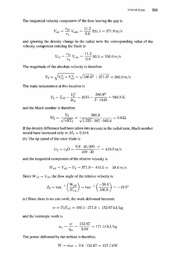
STATOR FLOW 3 3 1
The tangential velocity component of the flow leaving the gap is
Vu2 = — Vu2e = ^ 325.4 = 371.9 m/s r2 9.8
and ignoring the density change in the radial term the corresponding value of the velocity component entering the blade is
Vr2 = — Vr2e = -— 93.3 = 106.6 m/s r2 9.8
The magnitude of the absolute velocity is therefore
^2 = y/v?2 + Vl2 = A/106.6 2 + 371.92 = 386.9 m/s
The static temperature at this location is
ra = r 0 2 - g = 1015_!^ = 949.8K and the Mach number is therefore
M2 = - ^ = = l 3 8 6 - 9 =0.642
VlRT2 ^1.333-287-949.8 If the density difference had been taken into account in the radial term, Mach number would have increased only to M2 = 0.644. (b) The tip speed of the rotor blade is
9.8-40,000-^ U^=r^= 10Q.30 = 4 1 0 - W s
and the tangential component of the relative velocity is
Wu2 = Vu2 -U2= 371.9 - 410.5 = -38.6 m/s
Since Wr2 = Vr2, the flow angle of the relative velocity is
(c) Since there is no exit swirl, the work delivered becomes
w = U2Vu2 = 410.5 • 371.9 = 152.67 kJ/kg
and the isentropic work is
w 152.67 , „ ^ = ^ = l ) ^ = m-54kJ/kg
The power delivered by the turbine is therefore
W = raw = 2.8 • 152.67 = 427.5 kW

332 RADIAL INFLOW TURBINES
(d) The stagnation temperature at the exit is
Tos = T02 - » = 1015- ^ J Z ° = 882.0 K cp 1148
and the corresponding temperature for an isentropic flow is
rr ^ Wc i m _ 171,540 „ „ _ „ „ To3s =T02 = 1015 = 865.6 K
cp 1148 The exit stagnation pressure is therefore
» = M , ( ^ f ^ 8 . 5 ( ^ f ) 4 = 44,6lra With the exit area
A3 = 7r(r|s - r | h ) = TT(0.0772 - 0.0272) = 0.01634 m2
the exit flow function is equal to
m^pWs 2.8^1148 • 882.0 n0QA r^t = = = U.oo4
A3p03 0.01634 • 449,550 and the Mach number can then be obtained by iteration from the nonlinear equation
~ / ~ _ 1 \ - ( l / 2 ) [ ( 7 + l ) / ( 7 - l ) l F3 = -7=JM* ( l + J L 2 _ M 3 2 ) = 0 - 3 8 4
in which 7 = | . The solution is M3 = 0.169. The exit static temperature is then
l + ^ - M f j =882.0 f l + - ^ — J =877.8K
so that the exit velocity becomes
V3 = M3^/-fRT3 = 0.315^1.333- 287 -877.8 = 97.9 m/s
The volumetric flow rate is therefore
Q3 = V3A3 = 97.9 • 0.01634 = 1.60 m3/s
(e) The blade-loading coefficient is
w 152,670 „
and the flow coefficient is
± Vr2 106.6 U2 410.5
0.260
The flow coefficient for radial inflow turbines is usually less than 0.5. The specific speed is
0 _ nyoi _ 40,000 ■ TTVYM _ s " u-o-75 " 30-171,540°-75 _
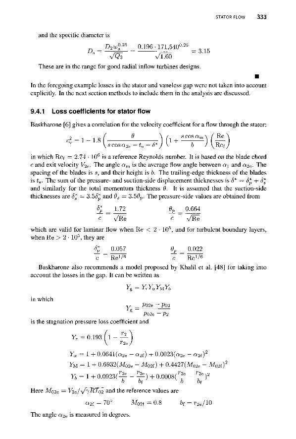
STATOR FLOW 333
and the specific diameter is
__ D2w°s-25 _ 0.196-171,540025
J-)s — y== — — 0.15
VQ3 Vim These are in the range for good radial inflow turbines designs.
■ In the foregoing example losses in the stator and vaneless gap were not taken into account explicitly. In the next section methods to include them in the analysis are discussed.
9.4.1 Loss coefficients for stator flow
Baskharone [6] gives a correlation for the velocity coefficient for a flow through the stator:
0 \ /j s cos am \ /Re \ v s cos a2e — te — 5*) \ b / \ Ref /
in which Ref = 2.74 • 106 is a reference Reynolds number. It is based on the blade chord c and exit velocity V2e- The angle am is the average flow angle between a\ and a2e. The spacing of the blades is s, and their height is b. The trailing-edge thickness of the blades is te. The sum of the pressure- and suction-side displacement thicknesses is 5* — 5* + 5* and similarly for the total momentum thickness 9. It is assumed that the suction-side thicknesses are 5* = 3.55* and 9S = 3.59p. The pressure-side values are obtained from
5; _ 1.72 9P _ 0.664 c VRe c VRe
which are valid for laminar flow when Re < 2 • 105, and for turbulent boundary layers, when Re > 2 • 105, they are
5* _ 0.057 9P _ 0.022 ~C ~ Rel/6 7" ~ Rgl/6
Baskharone also recommends a model proposed by Khalil et al. [48] for taking into account the losses in the gap. It can be written as
yg = YrYaYy[Yb
in which Y = PQ2e ~ P02
S P02e ~ Vl
is the stagnation pressure loss coefficient and
Yr = 0.193 I 1 - — T2e
Ya = 1 + 0.0641 (a2e ~ a2f) + 0.0023(a2e - a2 f ) 2
YM = 1 + 0.6932(M02e - M02f) + 0.4427(M02e - M02f )2
n = 1 + 0 .0923(^ - ^ ) + 0 .0008(^ - ^ ) 2
b bf b Of
Here Mo2e = ^W\/7-ft7o2 and the reference values are
a2i = 70° M02f = 0.8 b{ = r2e/10
The angle a2e is measured in degrees.
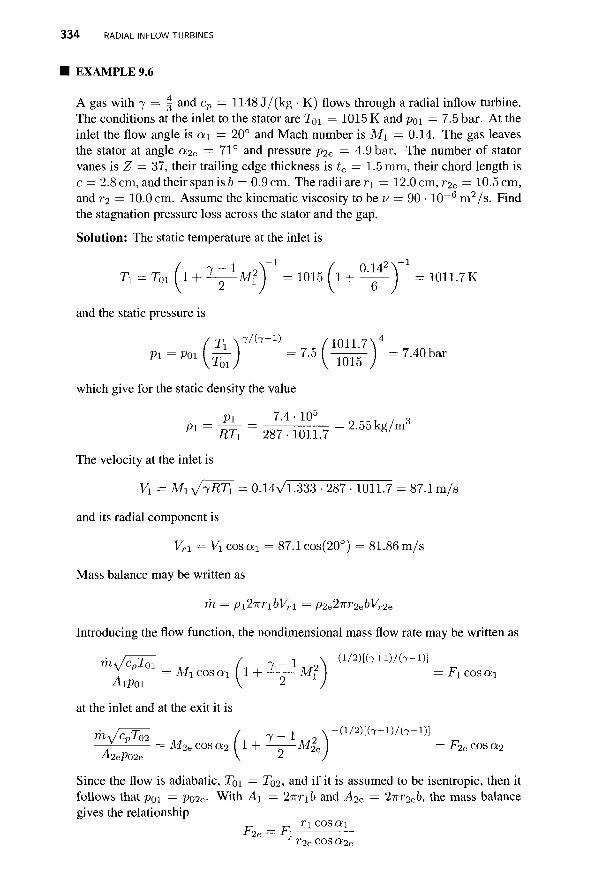
334 RADIAL INFLOW TURBINES
EXAMPLE 9.6
A gas with 7 = f and cp = 1148 J/(kg • K) flows through a radial inflow turbine. The conditions at the inlet to the stator are T0i = 1015 K and poi = 7.5 bar. At the inlet the flow angle is a\ = 20° and Mach number is M\ = 0.14. The gas leaves the stator at angle a2e — 71° and pressure p2e = 4.9 bar. The number of stator vanes is Z = 37, their trailing edge thickness is te = 1.5 mm, their chord length is c = 2.8 cm, and their span is b = 0.9 cm. The radii are r\ = 12.0 cm, r2e = 10.5 cm, and r2 = 10.0 cm. Assume the kinematic viscosity to be v = 90 • 10~6 m2/s. Find the stagnation pressure loss across the stator and the gap.
Solution: The static temperature at the inlet is
Ti=T01[l + ~-Mt) = 1015 ( 1 + —^— } =1011.7K
and the static pressure is
T X 7/(7-D /10H.7N 4
p l = P 0 1 U t > =™{-m<r) =7-40bar
which give for the static density the value
Pl = M\=2874lJl l .7= 2-5 5 k g / m 3
The velocity at the inlet is
Vi = Mi ^7-RTi = 0.14\/1.333-287-1011.7 = 87.1 m/s
and its radial component is
Vrl = Vicosai = 87.1cos(20°) = 81.86 m/s
Mass balance may be written as
m = pi2irribVrl = P2^r2ebVr2s
Introducing the flow function, the nondimensional mass flow rate may be written as
raJ^T^ ( 7 - l V(i/2)[(7+D/(7-i)] V p - Mi cosai ( 1 + -!-— M\ = Fx cosai
at the inlet and at the exit it is
V P = M2e cosa2 ( 1 + ^—M^ = F2e cosa2 A2eP02e
Since the flow is adiabatic, 7b 1 = TQ2, and if it is assumed to be isentropic, then it follows thatpoi = Po2e- With Ay = 2nrib and A2e = 2nr2eb, the mass balance gives the relationship
F z e = F i ncc-sai ' r2ecosa2e
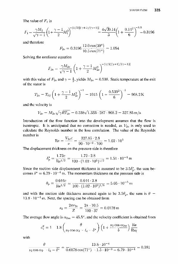
STATOR FLOW 335
The value of Fi is
7 M l / 7 - l \-(V2)[(7+i)/(7-Dl 4 ^ . 1 4 / 0.142, F I = ^ T ( 1 + V M I J = ^ ( 1 + — ) =0-3196
and therefore
10.5cos(71°) Solving the nonlinear equation
- ( l / 2 ) ( 7 + l ) / ( 7 - l ) ] , / 1 -I- 1 1 M? \ ^ = ^ ( l + ^ * £
with this value of F2e and 7 = | , yields M2e = 0.538. Static temperature at the exit of the stator is
T2e = T02 ( 1 + ^ M f e ) = 1015 (1 + ° ^ _ j = 9 6 8 2 K
_ 1 / n C;QO2 — M2 I
2
and the velocity is
V2e = M2e^jRT2e = 0.538^1.333 • 287 • 968.2 = 327.85m/s
Introduction of the flow function into the development assumes that the flow is isentropic. It is anticipated that no correction is needed, as V2e is only used to calculate the Reynolds number in the loss correlation. The value of the Reynolds number is
^ = ^ = Q n3 2 7 f 6
2 l = l - 0 2 - 1 0 5 v 90 • 10"6 ■ 100
The displacement thickness on the pressure side is therefore
A* - L 7 2 c - 1-72 ■ 2.8 _ 4 6p ~ ReV2 " 100 • (1.02 ■ 105)V2 " i 5 i ' i U m
Since the suction side displacement thickness is assumed to be 3.5<5*, the sum be-comes 5* = 6.79 • 10~4 m. The momentum thickness on the pressure side is
0.644c 0.644-2.8 r nr n n _ 5
°p = B&* = 100- (1.02- i 0 5 ) 1 / 6 = 5 - 6 5 - 1 0 m
and with the suction side thickness assumed again to be 3.5#p, the sum is 6 — 13.8 • 10~4 m. Next, the spacing can be obtained from
27rr2e 27T-10.5 S2 = ^ = T 0 0 T 3 7 = 0 - ° 1 7 8 m
The average flow angle is a2m = 45.5°, and the velocity coefficient is obtained from
c£ = 1 - 1.8 ( - ) f 1 + ?lcosa^ R e 00 v s2 cos a2 — te — S* J \ b ) Ref
with
6 13.8-10" s2cosa2-te-6* 0 .0178cos(71°)-1 .5-10- 3 -6 .79- 10" 0.381
336 RADIAL INFLOW TURBINES
and s2 cos a2m =1 0.178 cos(45.5°) =
6 0.009 the velocity coefficient becomes
9 102,000 c2 = 1 - 1.8 • 0.381 • 2.389 ' = 0.939 so that cv = 0.969
The actual exit velocity is therefore
V2e = cvV2es = 0.969 ■ 327.8 = 317.7 m/s
As anticipated, the difference from the ideal is such that no correction is needed. The static temperature at the exit of the stator is now
V2 317 72
T2e = T 0 2 - ^ = 1015- ^ ^ = 9 7 1 . 0 K
and the Mach number at the exit does not change significantly, for it is M2e = 0.521. The stagnation pressure is now
The loss of stagnation pressure across the stator is therefore
APOLS = Poi - P02e = 750.0 - 584.9 = 165.1 kPa
To determine the stagnation pressure loss across the gap, the stagnation Mach number at the inlet to the gap is needed. With Toi = TQ2, it is
M02e = - ^ = = , 3 2 4 - 5 = 0.5028 VlRT02 Vl-333-287-1015
The stagnation loss coefficients for the gap are
Yr = 0.193 ( l - j j j ^ j =0.00919
Ya = 1 + 0.0641(71-70) +0.0023(71 - 70)2 = 1.0664 YM = 1 + 0.6932(0.5028 - 0.8) + 0.4427(0.5028 - 0.8)2 = 0.8410
Yb = 1 + 0 . 0 9 2 3 ( ^ - 1 0 ) + 0 . 0 0 0 8 ( ^ - 1 0 ) 2 = 1.1561
and the overall loss coefficient comes out as
Yg = 0.00919 • 1.0664 • 0.8410 ■ 1.1561 = 0.00952
The stagnation pressure at the inlet to the rotor is therefore
P02 = Po2e ~ Yg(P02e - P2) = 589.6 - 0.00952(589.6 - 490) = 588.6 kPa
DESIGN OF THE INLET OF A RADIAL INFLOW TURBINE 337
and the stagnation pressure loss across the gap is
APOLG = P02e ~ P02 = 589.6 - 588.6 = 1.0 kPa
Hence this loss is relatively small, and upstream of the rotor the stagnation pressure loss is
APOLS + AJJQLG = 165.1 + 1.0 = 166.1 kPa
Note that the Mach number increases across the stator from 0.14 to 0.52 owing to the acceleration of the flow as a result of the turning. There is a significant density change associated with this acceleration.
As has been shown above, across the gap the flow angle does not change for irrotational flow. Since the gap is also quite narrow, the area does not decrease greatly and the acceleration of the flow is rather slight. For this reason it is possible to assume the flow to be incompressible across the gap and calculate it by the formula
V -V T2e
Vr2 — Vr2e T2
This cannot be used for the stator flow, and using it in the foregoing example would have yielded for the radial component of the stator exit velocity the value
K2 e = Vri— = 81.86 ^ ? = 93.55m/s r2e 10.5
and the exit velocity would have been
Vr2e 93.55 V2e = = 7i^-r = 287.4 m/s
COSO!2 C 0 S ( 7 1 ° )
This would have been significantly in error as the correct value came out to be 324.5 m/s.
9.5 DESIGN OF THE INLET OF A RADIAL INFLOW TURBINE
The foregoing developments and examples illustrate the basic methods for carrying out design calculations for radial inflow turbines. The loss calculations for the stator and interblade gap, together with the expression for the overall efficiency and its appropriate value obtained from the Balje diagram, are sufficient to determine the loss through the rotor. Table 9.1 gives the appropriate geometric length ratios for a design. Methods to obtain some of these values are developed from the theory discussed in this section. This work has been carried out, among others, by Rodgers and Geiser [63], Rohlik [65], and Whitfield [78]. The extensive study by Whitfield as been included in the book by Whitfield and Baines [79]. The following development follows their studies.
Since
nT< 01
the blade loading coefficient is
* Ul U* M & , 7 - 1
338 RADIAL INFLOW TURBINES
in which the blade stagnation Mach number is
U2 Ma VrRToT
This is based on the inlet stagnation temperature as a reference value. If at the exit the flow has no swirl component and at the inlet the relative velocity is
radially inward, then w = U2, ar>d the blade-loading coefficient is
w
Experiments have shown that efficiency is increased if — 40° < fi2 < —20°. This introduces a negative incidence into the flow since the blade angle \i is invariably zero. The blade-loading coefficient is now given by
, vu2 u2 + wu2 ip = — = = 1 + (pt&nfo U2 U2
in which the flow coefficient is defined as
The flow angle of the relative velocity is the range j32 min < &i < 0, and fi2 min is chosen such that the blade loading coefficient is in the range 0 < tp < 1.
9.5.1 Minimum inlet Mach number
Whitfield [78] has shown how to optimize the inlet to the rotor by choosing (for a given power ratio) the absolute and relative flow angles that give the smallest inlet Mach number. Improper flow angles might lead to high inlet Mach numbers, and a possibility for choking. Following his development, the tangential velocity is first written as
vu2 = u2 + wu2 = u2 + vu2t-^
t ana 2
in which the second equation follows by using Vu2 = Vr2 tan a2 Wu2 — Wr2 tan j32
together with Vr2 = Wr2. Multiplying through by Vu2 and rearranging gives
/ _ t a n ^ X =
\ tan a2 )
The right side is the work delivered, and since this is related to the power ratio, it will be taken to be a fixed quantity. Dividing both sides by V2 leads to
. 2 / tan/32\ sin a2 [ 1 = u (9.8) \ tan a2 J
in which = U2Vu2 _ U2Vu2 C2
02 U T/2 2 T/2
v2 c 0 2 V2

DESIGN OF THE INLET OF A RADIAL INFLOW TURBINE 339
or sw 1 s
(7 - 1) Af022 m ^02
where the following notation has been introduced:
m = M£2 7 - 1
The inlet stagnation Mach number has been defined as
V2 M, 02 VrR7o2
which can be written also as
M2 _Yl-Yl±-M2ll_ 02 ~ r2 ~~ r2 r2 ~ 2 Tno c02 c2 c02 -102
so that M2
M2 = ^ 2 ( 9 9 ) 02 1 + ^ M f
Dividing Eq. (9.8) next by cos2 a2, and noting that 1/ cos2 «2 = tan2 a2 + 1, gives
(1 — u) tan2 «2 — tan /?2 tan a2 — u = 0
or (m - s) t an 2 a 2 - m tan/32 tan a2 - s = 0 (9.10)
For given values of sw, M2, and ^2. this quadratic equation can be solved for tan a2- The solution is displayed in Figure 9.7 with /32 and sw as parameters.
For a given power ratio and relative flow angle, the minimum of each curve is sought next. To find it, let a — tan 0:2 and b = tan/?2- This puts Eq. (9.10) into the form
s ( l +a2) (m — s)a2 - mba- s = 0 m =—. - f (9.11)
a(a - 0) The minimum for m, for a fixed s and b, is obtained by setting the derivative of this with respect to a to zero. Thus
dm _ 2s(a - b)a2 ~ s(2a - &)(1 + a2) _ da a2(b — a)2
and this reduces to ba2 + 2a - b = 0
Solving this quadratic equation gives
- i±v / r+6 2 a = 1
Substituting this value of a into Eq. (9.11) gives
2s m = .
lTv/TT62
(9.12)
(9.13)
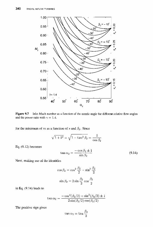
340 RADIAL INFLOW TURBINES
M,
1.00
0.95
0.90
0.85
0.80
0.75
0.70
0.65
0.60
0.55
\ V
\ \ \
\ \
\ k
\ ^
S.
Y= 1.4
V \ ^V. ^ ^ 2 0 °
\ ^ ^ 5 . \ - 4 0 °
N^ \ \ ^ 3 0 ° ^ ~ ~
N. > v \ - 4 0 '
\ \ S J - 4 0 ° "
s. x^o^v
^ - 4 0 ^
P2 = -10°
—-y/
^ = - 1 0 °
^ /
j ^ - l t f
P 2 = - 1 0 ° -
o CO d II
40 50 60 70 80 90
Figure 9.7 Inlet Mach number as a function of the nozzle angle for different relative flow angles and the power ratio with 7 = 1.4.
for the minimum of m as a function of s and fa- Since
A/I + &2 = V1 + tan2 j3: cos/32
Eq. (9.12) becomes
t a n a 2 ■ cos /32 ± 1
sin/32
Next, making use of the identities
a ifil . 2 &2 cos p2 = cos —— sin —
■ o o ■ & &
sin p2 = I sin — cos —
inEq. (9.14) leads to
t a n « 2
The positive sign gives
- c o s 2 ( / 3 2 / 2 ) + s i n 2 ( / 3 2 / 2 ) ± l 2sin(/32/2)cos(^2/2)
f & t an CK2 = tan ——
(9.14)
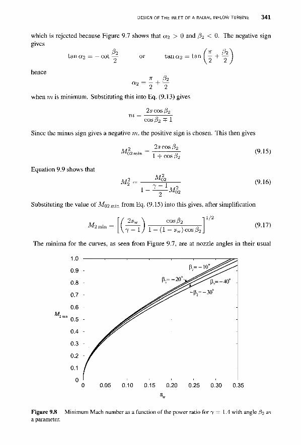
DESIGN OF THE INLET OF A RADIAL INFLOW TURBINE 3 4 1
which is rejected because Figure 9.7 shows that a^ > 0 and fa < 0. The negative sign gives
P2 ^ . frc , fa" tan o;2 = — cot: or tan a2 = tan
hence a 2 = 2 + y
when TO is minimum. Substituting this into Eq. (9.13) gives
2s cos fa m = a T
cos fa =F 1
Since the minus sign gives a negative m, the positive sign is chosen. This then gives 2 s cos fa
Equation 9.9 shows that
M2
Ml
1 + COS fa
M02
2
(9.15)
7 - 1 , , 2 02
(9.16) -M,
Substituting the value of M02 min from Eq. (9.15) into this gives, after simplification
M2 2sv cos/32
1/2
(9.17) \ 7 - l / 1 + (1 - sw)cosfa_
The minima for the curves, as seen from Figure 9.7, are at nozzle angles in their usual
M,
Figure 9.8 Minimum Mach number as a function of the power ratio for 7 = 1.4 with angle 02 as a parameter.
342 RADIAL INFLOW TURBINES
range between 60° < a2 < 80°. For a given M2, sw, and /32, there may be two angles a2 that satisfy Eq. (9.10). The smaller angle is to be chosen. The larger angles put a limit on how large the inlet Mach number can be. As a2 —¥ 90°, t ana 2 —> oo, and the second of Eqs. (9.11) shows that m = s. This means that at a2 = 90° the inlet Mach number is
M2 2sv
L ( 7 - l ) ( 2 - s w )
1/2
In particular, for 7 = 1.4 and sw = 0.15, M2 = 0.637, as the graph shows. Figure 9.8 shows how the minimum Mach number depends on the power ratio and that its dependence on the angle /32, and correspondingly on a2, is weak.
■ EXAMPLE 9.7
Gas with 7 = 1.4, and R = 287J/(kg • K) flows into a radial inflow turbine. The inlet stagnation temperature is TQI = HOOK, and the design-specific work is w = 165.74 kJ/kg. (a) Find the value of the total-to-static efficiency that would give a pressure ratio of P01/P3 = 2.0. (b) At what angle should the flow leave the stator in order for M2 = 0.62 be the minimum possible Mach number at the exit of the stator? (c) Find the blade speed at this condition, (d) Assume that the blade speed is increased to C/2 = 460 m/s and that the flow angle and the magnitude of the exit velocity from the stator remain the same. Find the new value for the relative flow angle /32 entering the rotor.
Solution: (a) From the expression
W = SwCpT()l
the power ratio is 1 6 5 J 4 ° 0.15
1004.5-1100 The pressure ratio is related to the power ratio and the total-to-static efficiency by Eq. (9.3), so that
Sw 0-15 n„_ J7ts = ? TTT" = 77TT = 0.835 ' ' p3 \ (7~l)/7 1 - 0.&/™
vPOl.
(b) The flow angle at the minimum inlet Mach number is obtained from the equation
M2 = 2sw \ cos/?2
-11/2
Kj-lJ 1 + (1 - sw)cos/32
which, when solved for cos /32, gives
M2
cos & = ——. —-+J- — 2 p2 = -24.74°
The minus sign must be chosen for the angle. At the minimum
a2 = 90° + — = 90° - 12.37° = 77.63°
DESIGN OF THE INLET OF A RADIAL INFLOW TURBINE 343
(c) To determine the blade speed, the velocity leaving the nozzle is needed, and therefore the stagnation Mach number is calculated first as:
M02 = , M 2 = - °-6 2 = 0.5975 /l + 1^±Ml V l + 0-2-0-6^
The exit velocity from the stator is therefore
V2 = M02^/jRT02 = 0.5975^1.4-287-1100 = 397.2m/s
and the tangential and radial components are
Vu2 = V2sina2 = 397.2 sin(77.63°) = 388.0 m/s
Vr2 = V2cosa2 = 397.2 cos(77.63°) = 85.10 m/s
The blade speed can be obtained, for example, from
w 165,740 innn . C/2 = ̂ = ^ 8 ~ - 4 2 7 - 2 m / s
(d) If the blade speed is increased to U2 = 460 m/s and the nozzle exit speed and direction are the same, then the new work done is
w = U2Vu2 = 460 • 388 = 178.48 kJ/kg
The new value for the tangential component of the relative velocity is
Wu2 = Vu2 -U2= 388.0 - 460.0 = -72.0 m/s
Since the radial component of the inlet velocity remains the same, the flow angle is
& = tan-i (^] = tan-i (zll) = _40.2°
It is expected that the total-to-static efficiency will be somewhat lower at this angle. If the efficiency drops greatly, adjustable stator blades may be used to adjust the exit stator angle, which then influences the incidence. However, in a turbocharger an increase in blade speed comes from a larger cylinder pressure and a larger flow rate through the engine. Hence the radial component of the inlet velocity to the rotor also increases. The control of the stator blade angle must account for this as well. g
9.5.2 Blade stagnation Mach number
The blade stagnation Mach number is yet another parameter of interest. It is obtained from the definition of the power ratio, which may be written as
so that M0u
U2 Vu2 sw
coi coi 7 - 1
U2 sw coi c2
coi 7 _ 1 c2 V2sma2
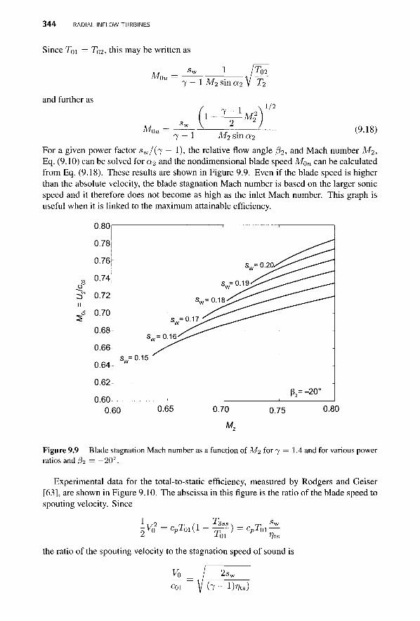
344 RADIAL IMFLOW TURBINES
Since T0i = T02, this may be written as
M, Ou Sw 1 T02
7 — 1 M2 sin a2 V T2
and further as
M, 1
7 - 1 MA 1/2
Ou (9.18) 7 — 1 M2 sin a?2
For a given power factor s w / ( 7 — 1), the relative flow angle /32, and Mach number M 2 , Eq. (9.10) can be solved for a2 and the nondimensional blade speed M0u can be calculated from Eq. (9.18). These results are shown in Figure 9.9. Even if the blade speed is higher than the absolute velocity, the blade stagnation Mach number is based on the larger sonic speed and it therefore does not become as high as the inlet Mach number. This graph is useful when it is linked to the maximum attainable efficiency.
oS
=f It
5°
0.80
0.78
0.76
0.74
0.72
0.70
0.68
0.66
0.64
0.62
0.60 0. 60 0.65 0.70 0.75 0.80
Figure 9.9 Blade stagnation Mach number as a function of Mi for 7 = 1.4 and for various power ratios and/32 = -20° .
Experimental data for the total-to-static efficiency, measured by Rodgers and Geiser [63], are shown in Figure 9.10. The abscissa in this figure is the ratio of the blade speed to spouting velocity. Since
1, :Vrn2 = C p T 0 i ( l -
T, 3ss ) = Cpioi
* J-01 »7ts
the ratio of the spouting velocity to the stagnation speed of sound is
2sv Vn
coi V (7 - l)??ts)
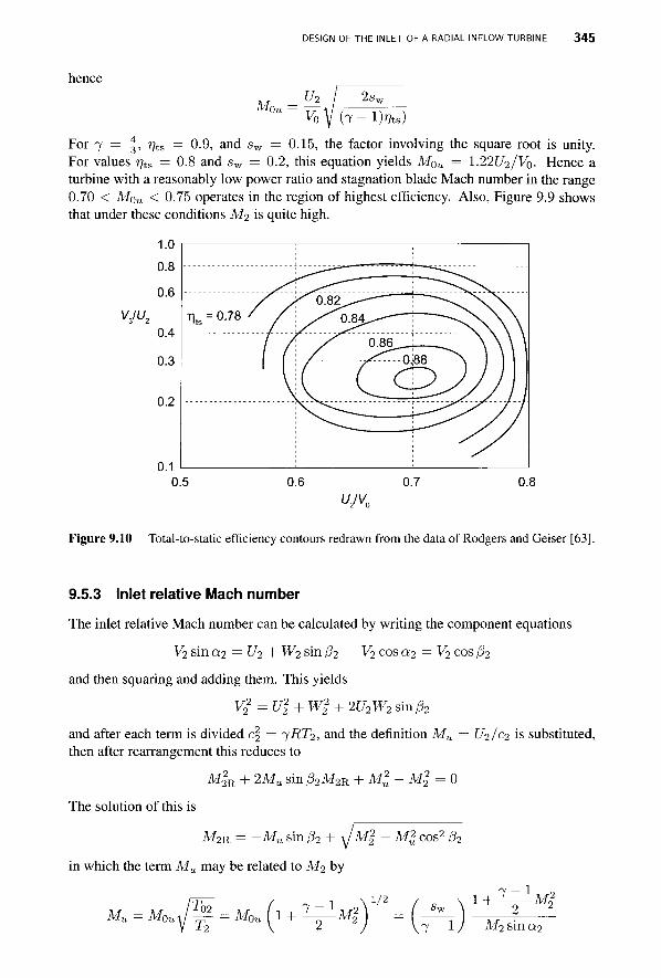
DESIGN OF THE INLET OF A RADIAL INFLOW TURBINE 345
hence
M0u U2 2sv
Vo V (7 - lHs) For 7 = | , ryts = 0.9, and sw = 0.15, the factor involving the square root is unity. For values 77ts = 0.8 and sw = 0.2, this equation yields MQU = I.22U2/V0. Hence a turbine with a reasonably low power ratio and stagnation blade Mach number in the range 0.70 < M0u < 0.75 operates in the region of highest efficiency. Also, Figure 9.9 shows that under these conditions M2 is quite high.
V3IU2
1.0 0.8 0.6
0.4
0.3
0.2
0.1 0.5 0.6 0.7 0.8
UJV„
Figure 9.10 Total-to-static efficiency contours redrawn from the data of Rodgers and Geiser [63].
9.5.3 Inlet relative Mach number
The inlet relative Mach number can be calculated by writing the component equations
V2 sin «2 = U2 + W2 sin fo V2 cos 0:2 = V2 cos fo
and then squaring and adding them. This yields
y22 = [/f + W% + 2U2W2 sin/32
and after each term is divided c\ = 7-RT2, and the definition Mu = U2/C2 is substituted, then after rearrangement this reduces to
M22R + 2MU sin (32M2K + M 2 - M2
2 = 0
The solution of this is
M2 R = -My. sin p2 + \JMl - Ml cos2 &
in which the term Mu may be related to M2 by
Mu = Mou\l~ = M0u \1 + —j-™2 7 - 1 MA
1/2 1 + l ^ M 2
7 — 1 / M2 sin a2
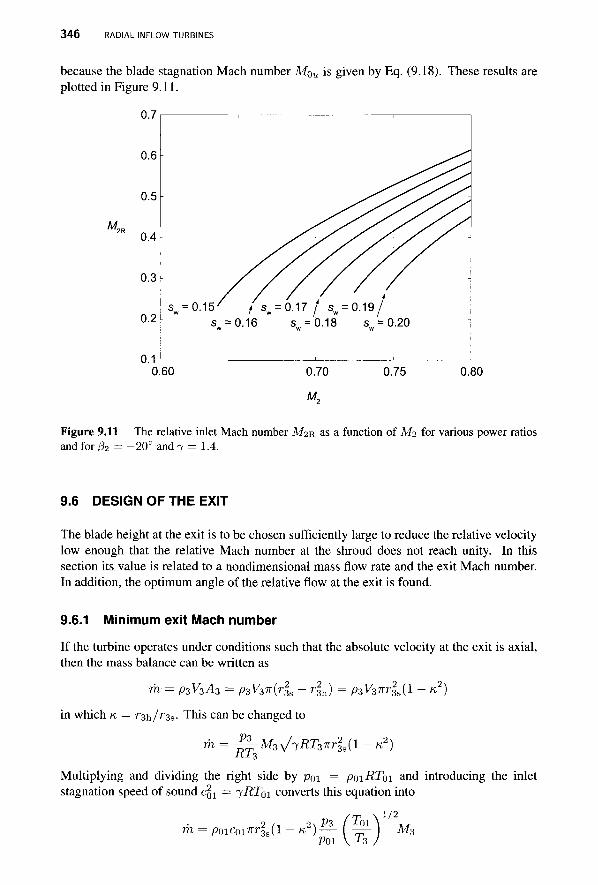
346 RADIAL INFLOW TURBINES
because the blade stagnation Mach number MQU is given by Eq. (9.18). These results are plotted in Figure 9.11.
0.7
M„c
0.6
0.5
0.4
0.3
0.2
0.1
SL, = 0 . 1 5 ' f sw = 0 . 1 7 / sw = 0 . 1 9 / s =0.16 s... = 0.18 s .=0 .20
0.60 0.70
M„
0.75 0.80
Figure 9.11 The relative inlet Mach number M2R as a function of M2 for various power ratios and for /32 = -20° and 7 = 1.4.
9.6 DESIGN OF THE EXIT
The blade height at the exit is to be chosen sufficiently large to reduce the relative velocity low enough that the relative Mach number at the shroud does not reach unity. In this section its value is related to a nondimensional mass flow rate and the exit Mach number. In addition, the optimum angle of the relative flow at the exit is found.
9.6.1 Minimum exit Mach number
If the turbine operates under conditions such that the absolute velocity at the exit is axial, then the mass balance can be written as
m = p3V3A3 = p3V3ix(r23s - r2
3h) = p3V3Trr23a{l - K2)
in which K = r3h/r3s. This can be changed to
m _P3_ M3^RT3Trr2
3s(l - K2
Multiplying and dividing the right side by poi = P01RT01 and introducing the inlet stagnation speed of sound c 0 l = ^RT0i converts this equation into
2 ,-t 2\ P3 (TQI m = poic0iirr3s(l - K ) —
P01 \ T 3
1/2 M3
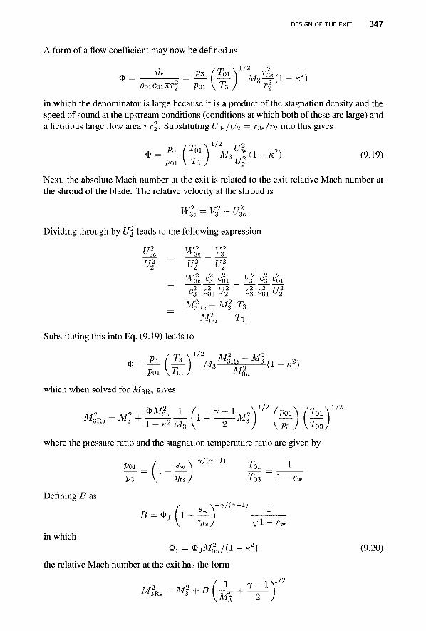
DESIGN OF THE EXIT 347
A form of a flow coefficient may now be defined as
* = — ^ = ̂ (~)1/2M/-f(l ~ K2) A)iCoi7rr| poi \T3 J r%
in which the denominator is large because it is a product of the stagnation density and the speed of sound at the upstream conditions (conditions at which both of these are large) and a fictitious large flow area -nr\. Substituting U3s/U2 = ^3s/^2 into this gives
^-l^) 1 ^ 1 -^) (9-19) P 3 TmY A f , r i ' i ^
Next, the absolute Mach number at the exit is related to the exit relative Mach number at the shroud of the blade. The relative velocity at the shroud is
wl = vi + ul Dividing through by C/| leads to the following expression
ul = wi_Yl m ul ul
W2 2 2 1/2 2 2
~~ „2 . 2 r / 2 r2 „2 r / 2 c 3 c 0 1 u2 c 3 c 0 1 u2
MJRs - Mj T3
M2au T01
Substituting this into Eq. (9.19) leads to
T, \ 1 / 2 . , M|„„ - Ml Poi U J M 3 M 0
2O * = — \^-\ Ma^^^a-O
which when solved for Af3RS gives
^,JH2 1 / „,_-, \ l / 2 / „ . . \ / T - . X 1 ^
3Rs = IV13 ' M*.=tf + ̂ ± l + l^lMtV' f*>^(T" 1-K2M3\ 2 V VP3 (03
where the pressure ratio and the stagnation temperature ratio are given by
/ „ \ - 7 / ( 7 - l ) T
Poi / -. sw \ i 0 i
Defining £? as
in which
P3 \ VtsJ T03
„ x -7/(7-1) B = $ , [1 v
^ %sy v^r
* f = $0M02J(1 - K
2) (9.20)
the relative Mach number at the exit has the form ,1/2
2 , o f 1 , 7 - 1 M 3 ^ = M3̂ + B l ^ ?
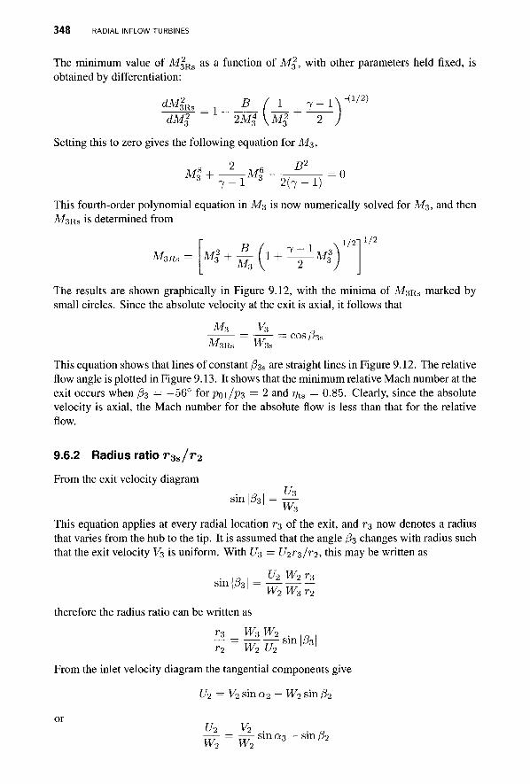
348 RADIAL INFLOW TURBINES
The minimum value of M$Rs as a function of Mf, with other parameters held fixed, is obtained by differentiation:
dM!Rs , B (I , 7 - l ^ / 2 > dMl l 2M$ VMI + 2
Setting this to zero gives the following equation for M 3.
This fourth-order polynomial equation in M3 is now numerically solved for M3, and then Af3RS is determined from
M 3Rs l\ + ^- (1 + ^ ^ M f d M3 V 2 J
1/2
The results are shown graphically in Figure 9.12, with the minima of M3RS marked by small circles. Since the absolute velocity at the exit is axial, it follows that
M3 V3 = COS 0 3 s M3Rs W3s
This equation shows that lines of constant 03s are straight lines in Figure 9.12. The relative flow angle is plotted in Figure 9.13. It shows that the minimum relative Mach number at the exit occurs when /33 = —56° for poi/p3 = 2 and T̂ S = 0.85. Clearly, since the absolute velocity is axial, the Mach nufnber for the absolute flow is less than that for the relative flow.
9.6.2 Radius ratio rSs/r2
From the exit velocity diagram
This equation applies at every radial location r3 of the exit, and r3 now denotes a radius that varies from the hub to the tip. It is assumed that the angle /33 changes with radius such that the exit velocity V3 is uniform. With U3 = U2r3/r2, this may be written as
U2 W2r3 sin /33 = - — - — —
vvi W3 r2 therefore the radius ratio can be written as
r3 W3 W2 . r2 W2 U2
From the inlet velocity diagram the tangential components give
U2 = V2 sin a2 — W2 sin /32
or U2 V2 . — = — sina3 - s i n 0 2 W2 W2
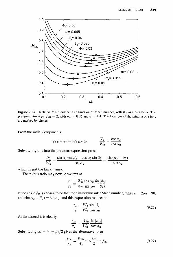
DESIGN OF THE EXIT 349
M„
Figure 9.12 Relative Mach number as a function of Mach number, with $ / as a parameter. The pressure ratio is P01/P3 = 2, with rjts = 0.85 and 7 = 1.4. The locations of the minima of MSRS are marked by circles.
From the radial components
V2 cos 02 v2 V2 cos a2 = W2 cos 02 —— =
W2 cos a2 Substituting this into the previous expression gives
U2 sin a2 cos j32 — cos a2 sin 02 sin(ai2 — 02) 11 W2 cosa2 cosa2
which is just the law of sines. The radius ratio may now be written as
7-3 _ W3 c o s a 2 s i n | / ? 3 | r2 W2 s in(a2 - P2)
If the angle f32 is chosen to be that for a minimum inlet Mach number, then f32 = 2a2 — 90, and sin(a2 — f32) = sin a2, and this expression reduces to
r, = M ^ s i n ^ r2 W2 t a n a 2
At the shroud it is clearly r3s _ W3Ssin| /33 s | r2 W2 t an a2
Substituting a2 = 90 + ^2/2 gives the alternative form
»-3s ^33 . 02 . a ,„ - - . — = -T7T- t an — sin 03s (9.22) r2 W2 2

350 RADIAL INFLOW TURBINES
M,
Figure 9.13 The flow angle of the relative velocity at the exit as a function of Mach number, with <l>f as a parameter. The pressure ratio is poi/p3 = 2, with r/ts = 0.85 and 7 = 1.4. The locations of the angle corresponding to minima of M^B.S are marked by circles.
Rohlik [65] suggested that the relative velocity ratio W3/W2 = 2 gives a good design, or if the relative velocity at the shroud is used, then W3s/W2 = 2.5 is appropriate [79].
9.6.3 Blade height-to-radius ratio b2/r2
The final parameter to be determined is the blade height-to-radius ratio 62 /V2 at the inlet. By casting the mass balance
m = P2Vr2A2 = p3V3A3
in terms of the flow functions, the area ratio becomes
A3 _ F2 cos a3 /T03po2 _ F2cosa3 /T03p02Poi P3 A2 ~ F3 T02 P03 T02P0I P3 P03
The stagnation pressure ratio P02/P01 is related to the static temperature ratio T2IT2S by integrating the Gibbs equation along the constant-pressure line P2 and along the line of constant stagnation temperature TQI = T02. Equality of entropy changes then gives
P02
Po\ Ik T2
7/ (7 -1)
From the definition of the static enthalpy loss coefficient in the stator
h2 - h2s Cs 11/2 2 V2
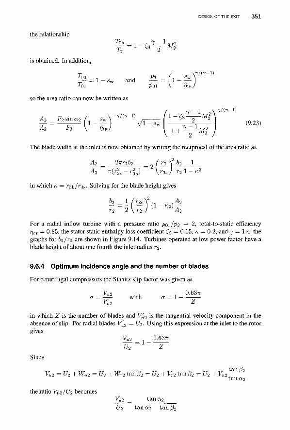
DESIGN OF THE EXIT 3 5 1
the relationship T 2s _ 1 A 7 - 1 »^2
is obtained. In addition,
\ 7 / ( 7 - l ) —- = 1 - sw and = 1 Toi poi \ »7ts/
so the area ratio can now be written as
7 - 1 f 2 7/ (7-1)
* ^ ^ r * 7 ' 1 ^ " V i A2 F 3 V W w l 1 + 7^IM|
2 3
The blade width at the inlet is now obtained by writing the reciprocal of the area ratio as o
A2 2irr2b2 ( r2 \ b2 1 M 7r(r|s - r | h ) V r 3 s / r - 2 l - K 2
in which K = r^/rzs. Solving for the blade height gives
r2 2\r2)K VA3
For a radial inflow turbine with a pressure ratio P01/P3 — 2, total-to-static efficiency T]ts = 0.85, the stator static enthalpy loss coefficient Cs = 0.15, K = 0.2, and 7 = 1.4, the graphs for 62/^2 are shown in Figure 9.14. Turbines operated at low power factor have a blade height of about one fourth the inlet radius r2.
9.6.4 Optimum incidence angle and the number of blades
For centrifugal compressors the Stanitz slip factor was given as
a = — with CT = 1 — Vu2 Z
in which Z is the number of blades and V^2 is the tangential velocity component in the absence of slip. For radial blades V^2 = U2. Using this expression at the inlet to the rotor gives
K2 0.63TT
U2~ Z Since
vu2 = ■u2
the ratio Vu2/U-2
+ wu2 =
> becomes
u2 + wr2
vu2 u2
tan/32
tan
= U2 + Vr2
tan a2
a2 — tan (32
tan/3; '2
' tano;2
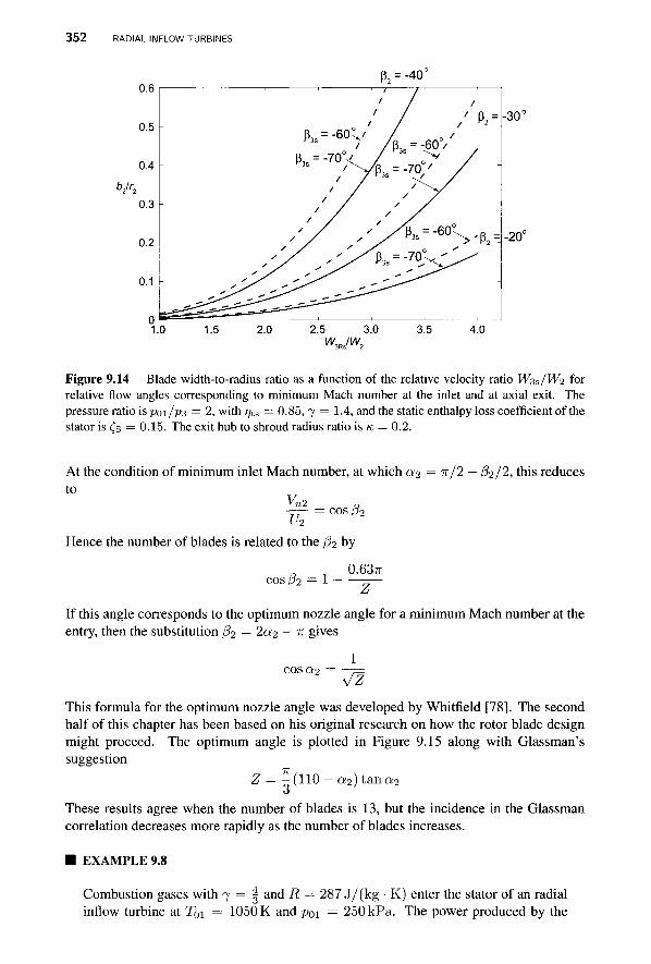
352 RADIAL INFLOW TURBINES
0.6
0.5
0.4
0.3
0.2
0.1
n
P2 = -40° i i i i / / i
' / '
P =-60^/ / „ / ^ /K = -60/
p = -70°< / " > / / / '^^•Z
y\s^ "" ^-^ *** ^*-*—
1
p2=
-
' P 2 =
•30°
1.0 1.5 2.0 2.5 3.0 3.5 4.0
Figure 9.14 Blade width-to-radius ratio as a function of the relative velocity ratio Wss/W? for relative flow angles corresponding to minimum Mach number at the inlet and at axial exit. The pressure ratio is poi /p3 = 2, with r)ts = 0.85, 7 = 1.4, and the static enthalpy loss coefficient of the stator is £s = 0.15. The exit hub to shroud radius ratio is K = 0.2.
At the condition of minimum inlet Mach number, at which 0:2 = 7r/2 — (82/2, this reduces to
Vu2 R — = COS / ? 2
Hence the number of blades is related to the fa by
0.63TT cosp2 = 1 —
If this angle corresponds to the optimum nozzle angle for a minimum Mach number at the entry, then the substitution fa = 2c*2 — ^ gives
1 cosa2 =
This formula for the optimum nozzle angle was developed by Whitfield [78]. The second half of this chapter has been based on his original research on how the rotor blade design might proceed. The optimum angle is plotted in Figure 9.15 along with Glassman's suggestion
TV
Z = —(110 — 0:2) tana2
These results agree when the number of blades is 13, but the incidence in the Glassman correlation decreases more rapidly as the number of blades increases.
■ EXAMPLE 9.8
Combustion gases with 7 = f and R = 287 J/(kg • K) enter the stator of an radial inflow turbine at T0i = 1050K and poi = 250kPa. The power produced by the
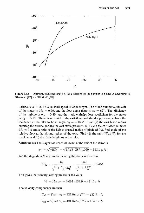
DESIGN OF THE EXIT 353
-15°
-20^
-25^
-30c
-35°
-40^
Glassman
10 15 20 25 30 35
Figure 9.15 Optimum incidence angle fii as a function of the number of blades Z according to Glassman [27] and Whitfield [78].
turbine is W = 232 kW at shaft speed of 35,000 rpm. The Mach number at the exit of the stator is M2 — 0.69, and the flow angle there is a2 = 67°. The efficiency of the turbine is 7]ts = 0.89, and the static enthalpy loss coefficient for the stator is Cs = 0.15. There is no swirl in the exit flow, and the design seeks to have the incidence at the inlet to be at angle j32 = —18.9°. Find (a) the exit blade radius entering the turbine and (b) the exit static pressure, (c) Given the exit Mach number M3 = 0.5 and a ratio of the hub-to-shroud radius of blade of 0.3, find angle of the relative flow at the shroud radius of the exit. Find (d) the ratio Wss/W2 for the machine and (e) the blade height b2 at the inlet.
Solution: (a) The stagnation speed of sound at the exit of the stator is
C01 = \/lRT0l = Vl.333 • 287 • 1050 = 633.9m/s
and the stagnation Mach number leaving the stator is therefore
M2 0.69 M02 =
i + V M f \/i + 0.664
0.692
This gives the velocity leaving the stator the value
V2 = M02coi = 0.664 • 633.9 = 421.0 m/s
The velocity components are then
Vu2 = V2 sin a2 = 421.0 sin(67°) = 387.5 m/s
Vr2 = V2cosa2 = 421.0 cos(67°) = 164.5 m/s
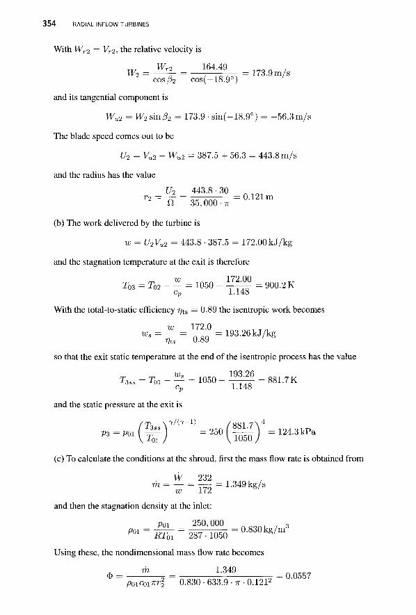
354 RADIAL INFLOW TURBINES
With Wr2 = Vr2, the relative velocity is
w Wr2 164.49 W2 = — = -,—-—r = 173.9 m/s
cos/32 cos(-18.9°)
and its tangential component is
Wu2 = W2smfi2 = 173.9-sin(-18.9°) = -56.3m/s
The blade speed comes out to be
U2 = Vu2 - Wu2 = 387.5 + 56.3 = 443.8 m/s
and the radius has the value
U2 443.8-30 _ , r2 = ~n = 3 ^ 0 0 0 ^ = 0 1 2 1 m
(b) The work delivered by the turbine is
w = U2Vu2 = 443.8 • 387.5 = 172.00 kJ/kg
and the stagnation temperature at the exit is therefore
T03 = T02 - - = 1050 - ^ ^ = 900.2 K cp 1.148
With the total-to-static efficiency r)ts = 0.89 the isentropic work becomes
w° = — = 7riF = 1 9 3-2 6 k J / ks r?ts 0.89
so that the exit static temperature at the end of the isentropic process has the value T3ss = Toi - — = 1050 - ^ ^ = 881.7 K d cp 1.148
and the static pressure at the exit is
T^V^-V _/881.7N4
p3 = Pol -^- =250 = 124.3kPa FA wi yToi j y 1050 j
(c) To calculate the conditions at the shroud, first the mass flow rate is obtained from
W 232 m = - = — = 1.349 kg/s
and then the stagnation density at the inlet:
poi 250,000 3 P o i = i ^ = 2 8 7 T T 0 5 0 = ° - 8 3 0 k g / m
Using these, the nondimensional mass flow rate becomes
m L349 ~ poiCoiTrrf ~ 0.830 ■ 633.9 • TT • 0.1212 "
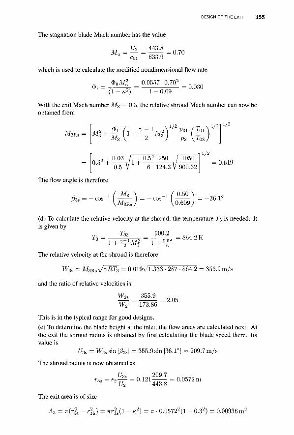
DESIGN OF THE EXIT 355
The stagnation blade Mach number has the value
U2 443.8 Mu = — = 7^77: = 0.70
C01 633.9
which is used to calculate the modified nondimensional flow rate
$ 0 M 2 _ 0.0557 • 0.702 <j>f
( 1 - K 2 ) 1 - 0.09 0.030
With the exit Mach number M3 = 0.5, the relative shroud Mach number can now be obtained from
M3 R s L u f + * f (l + 'lf-1Ml]1/2p01(T 3 M3 V 2 V P3 V?
2 0.03 / 0.52 250 / 1050 °-5 + 0.5 V 1 + 6 124.3 V 900.32
\ 1/2"
" ) 0 3 / 1/2
= c
1/2
0.619
The flow angle is therefore
33s COS ( M3 \ \M3Rs) -cos
0.50 0.609
-36.1°
(d) To calculate the relative velocity at the shroud, the temperature T3 is needed. It is given by
T03 900.2
1 + ^Mi 1 + 0.52 864.2 K 2 J " 3 * ' 6
The relative velocity at the shroud is therefore
W3s = Af3RsV/7i?T3 = 0.619V1.333 • 287 • 864.2 = 355.9 m/s
and the ratio of relative velocities is
W3s 355.9 25. _ — 2 05
W2 173.86 This is in the typical range for good designs. (e) To determine the blade height at the inlet, the flow areas are calculated next. At the exit the shroud radius is obtained by first calculating the blade speed there. Its value is
U3s = W3ssin|/33s| = 355.9sin|36.1°| = 209.7m/s
The shroud radius is now obtained as
U3s n i 0 209.7 r3s = r 2 — = 0 . 1 2 1 ^ ^ = 0.0572m
The exit area is of size
A3 = 7r(r|s - r | h ) = 7rr|,(l - K2) = TT • 0.05722(1 - 0.32) = 0.00936m2
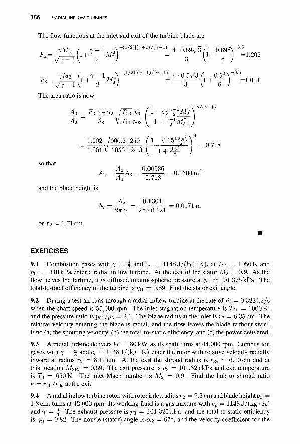
356 RADIAL INFLOW TURBINES
The flow functions at the inlet and exit of the turbine blade are
7 ^ 2 / 7 " 1 , ̂ -< 1 / 2 ) [ h + 1 ) / ( T- 1 ) ] 4 • 0 . 6 9 ^ / 0.692V3-5
7 M 3 / ! x-(i/2)[(7+i)/(7-i)] 4 . 0 . 5 ^ 3 / 0 .5 2 V 3 ' 5
The area ratio is now
A3 = F2COSa2 /7^_P3_ A - C s V M l V A2 F3 V T01 P03 I 1 + V M ! /
1.202 /900.2 250 / l - 0 . 1 5 ^ \ 1.001 V 1050 124.3 I 1 + °#
V 6
0.718
so that A2 , 0.00936 _ _ 2
i2 = ̂ = W = ai304m
and the blade height is
A2 0.1304 o2 = = = 0.0171 m
27rr2 2TT • 0.121
or 69 = 1.71 cm.
EXERCISES
9.1 Combustion gases with 7 = § and cp = 1148 J/(kg ■ K), at T0i = 1050 K and P01 = 310 kPa enter a radial inflow turbine. At the exit of the stator M2 = 0.9. As the flow leaves the turbine, it is diffused to atmospheric pressure atp4 = 101.325 kPa. The total-to-total efficiency of the turbine is r)tt = 0.89. Find the stator exit angle.
9.2 During a test air runs through a radial inflow turbine at the rate of m = 0.323 kg/s when the shaft speed is 55,000 rpm. The inlet stagnation temperature is T0i = 1000 K, and the pressure ratio is P01/P3 = 2.1. The blade radius at the inlet is r-z = 6.35 cm. The relative velocity entering the blade is radial, and the flow leaves the blade without swirl. Find (a) the spouting velocity, (b) the total-to-static efficiency, and (c) the power delivered.
9.3 A radial turbine delivers W = 80 kW as its shaft turns at 44,000 rpm. Combustion gases with 7 = | and cp = 1148 J/(kg • K) enter the rotor with relative velocity radially inward at radius r2 = 8.10 cm. At the exit the shroud radius is r^s — 6.00 cm and at this location M3RS = 0.59. The exit pressure is p$ = 101.325 kPa and exit temperature is T3 = 650 K. The inlet Mach number is M2 = 0.9. Find the hub to shroud ratio K = r^/rzs at the exit.
9.4 A radial inflow turbine rotor, with rotor inlet radius T2 = 9.3 cm and blade height 62 = 1.8 cm, turns at 42,000 rpm. Its working fluid is a gas mixture with cp = 1148 J/(kg • K) and 7 = | . The exhaust pressure is p^ = 101.325 kPa, and the total-to-static efficiency is rjts = 0.82. The nozzle (stator) angle is.0,2 = 67°, and the velocity coefficient for the
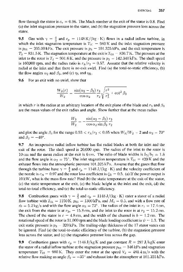
EXERCISES 357
flow through the stator is cv = 0.96. The Mach number at the exit of the stator is 0.8. Find (a) the inlet stagnation pressure to the stator, and (b) the stagnation pressure loss across the stator.
9.5 Gas with 7 = § and cp = 1148K/(kg • K) flows in a radial inflow turbine, in which the inlet stagnation temperature is T0i = 980 K and the inlet stagnation pressure is Poi = 205.00 kPa. The exit pressure is p3 = 101.325 kPa, and the exit temperature is T3 = 831.5 K. The stagnation temperature at the exit is T03 = 836.7 K. The pressure at the inlet to the rotor is T2 = 901.6 K, and the pressure is p2 = 142.340 kPa. The shaft speed is 160P00 rpm, and the radius ratio is r3/r2 = 0.57. Assume that the relative velocity is radial at the inlet and that there is no exit swirl. Find (a) the total-to-static efficiency, (b) the flow angles a2 and fi3, and (c) rjs and TJR.
9.6 For an exit with no swirl, show that
j W = s i n ( a a - f t ) r * /r» W2 cosa2 r2 y r3
in which r is the radius at an arbitrary location of the exit plane of the blade and r3 and f33 are the mean values of the exit radius and angle. Show further that at the mean radius
W3 _ sin(q2 - fc) r3
W2 cos a2 sin /33 r2
and plot the angle /33 for the range 0.53 < r3/r2 < 0.65 when W3/W2 = 2 and a2 = 70° and/32 = -40°.
9.7 An inexpensive radial inflow turbine has flat radial blades at both the inlet and the exit of the rotor. The shaft speed is 20,000 rpm. The radius of the inlet to the rotor is 10 cm and the mean radius at the exit is 6 cm. The ratio of blade widths is b3/b2 = 1.8 and the flow angle is a2 = 75°. The inlet stagnation temperature is Toi — 420 K and the exhaust flows into the atmospheric pressure 101.325 kPa. Assume that the gases that flow through the turbine have 7 = § and cp = 1148 J / (kg • K) and the velocity coefficient of the nozzle is CN = 0.97 and the rotor loss coefficient is CR = 0.5. (a) If the power output is 10 kW, what is the mass flow rate? Find (b) the static temperature at the exit of the stator, (c) the static temperature at the exit, (c) the blade height at the inlet and the exit, (d) the total-to-total efficiency, and (e) the total-to-static efficiency.
9.8 Combustion gases with 7 = § and cp = 1148 J/(kg • K) enter a stator of a radial flow turbine with Tm = 1150 K, p01 = 1300 kPa, and Mx = 0.5, and with a flow rate of m = 5.2 kg/s and with the flow angle a2 — 72°. The radius of the inlet is r\ — 17A cm, the exit from the stator is at r2e = 15.8 cm, and the inlet to the rotor is at r2 = 15.2 cm. The chord of the stator is c = 4.8 cm, and the width of the channel is b = 1.2 cm. The rotational speed of the rotor is 31,000 rpm and the blade loading coefficient is ip = 1.3. The exit static pressure is p3 = 320 kPa. The trailing-edge thickness of the 17 stator vanes can be ignored. Find (a) the total-to-static efficiency of the turbine, (b) the stagnation pressure loss across the stator, and (c) the stagnation pressure loss across the gap.
9.9 Combustion gases with cp = 1148 J/kgK and gas constant R = 287J/kgK enter the stator of a radial inflow turbine at the stagnation pressure poi = 346 kPa and stagnation temperature T0i = 980 K. They enter the rotor at the speed V2 = 481.4 m/s with the relative flow making an angle (32 = —35° and exhaust into the atmosphere at 101.325 kPa.

358 RADIAL INFLOW TURBINES
The total-to-static efficiency of the turbine is r)ts = 0.83. Find (a) the angle at which the flow enters the rotor and (b) the relative Mach number at the inlet.
CHAPTER 10
HYDRAULIC TURBINES
Hydroelectric power plants are important providers of electricity in those countries in which there are large rivers or rainy high mountain regions, or both. In the United States large hydropower installations exist in the western states of Washington, Oregon, Idaho, and Nevada. The Tennessee Valley Authority, (TVA) has a large network of dams and hydropower stations in Tennessee and other southeastern states. Smaller plants in New England account for the rest of the installed capacity. In addition to the United States, large hydropower installations exist in Canada, Brazil, Russia, and China. Norway, Switzerland, Sweden, and Iceland obtain a large part of their power needs from hydroelectricity, and Norway in particular exports its excess generation. About 7% of primary energy pro-duction and 17% of total electricity generation in the world are obtained by hydropower. Hydropower plants exceeding 30 MW are designated as large plants. Plants with generation from 0.1 to 30 MW fall into a range of small plants and those with capacity below 0.1 MW are classified as microhydropower. Although hydropower is a clean form of energy, its negative aspects relate to blocking of fish migration paths and displacement of populations from valleys that have been cultivated for hundreds of years by local communities.
10.1 HYDROELECTRIC POWER PLANTS
The preliminary design of a power plant begins with the siting analysis, which consists of determining the available flow rate of water and its head. The rate of water flow depends on the season, and for large power plants with high capital costs, dams are used not only to
Principles of Turbomachinery. By Seppo A. Korpela Copyright © 2011 John Wiley & Sons, Inc.
359
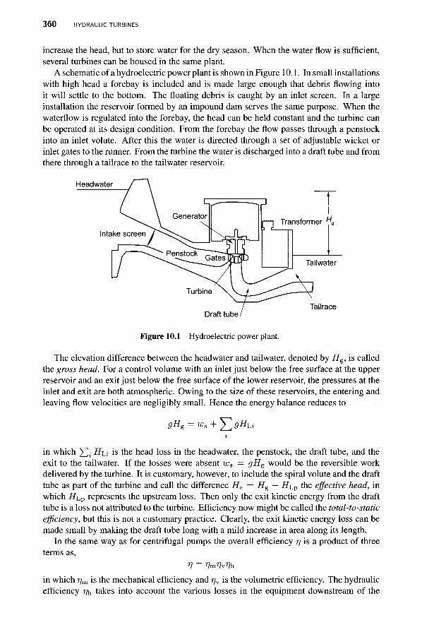
360 HYDRAULIC TURBINES
increase the head, but to store water for the dry season. When the water flow is sufficient, several turbines can be housed in the same plant.
A schematic of a hydroelectric power plant is shown in Figure 10.1. In small installations with high head a forebay is included and is made large enough that debris flowing into it will settle to the bottom. The floating debris is caught by an inlet screen. In a large installation the reservoir formed by an impound dam serves the same purpose. When the waterflow is regulated into the forebay, the head can be held constant and the turbine can be operated at its design condition. From the forebay the flow passes through a penstock into an inlet volute. After this the water is directed through a set of adjustable wicket or inlet gates to the runner. From the turbine the water is discharged into a draft tube and from there through a tailrace to the tailwater reservoir.
Figure 10.1 Hydroelectric power plant.
The elevation difference between the headwater and tailwater, denoted by Hg, is called the gross head. For a control volume with an inlet just below the free surface at the upper reservoir and an exit just below the free surface of the lower reservoir, the pressures at the inlet and exit are both atmospheric. Owing to the size of these reservoirs, the entering and leaving flow velocities are negligibly small. Hence the energy balance reduces to
gHg = ws + ^2 gHLi i
in which Y^i H^i is the head loss in the headwater, the penstock, the draft tube, and the exit to the tailwater. If the losses were absent ws = gHE would be the reversible work delivered by the turbine. It is customary, however, to include the spiral volute and the draft tube as part of the turbine and call the difference He = Hg — H^p the effective head, in which HLP represents the upstream loss. Then only the exit kinetic energy from the draft tube is a loss not attributed to the turbine. Efficiency now might be called the total-to-static efficiency, but this is not a customary practice. Clearly, the exit kinetic energy loss can be made small by making the draft tube long with a mild increase in area along its length.
In the same way as for centrifugal pumps the overall efficiency r\ is a product of three terms as,
V = VrnVvVh in which r]m is the mechanical efficiency and rjv is the volumetric efficiency. The hydraulic efficiency rfo takes into account the various losses in the equipment downstream of the
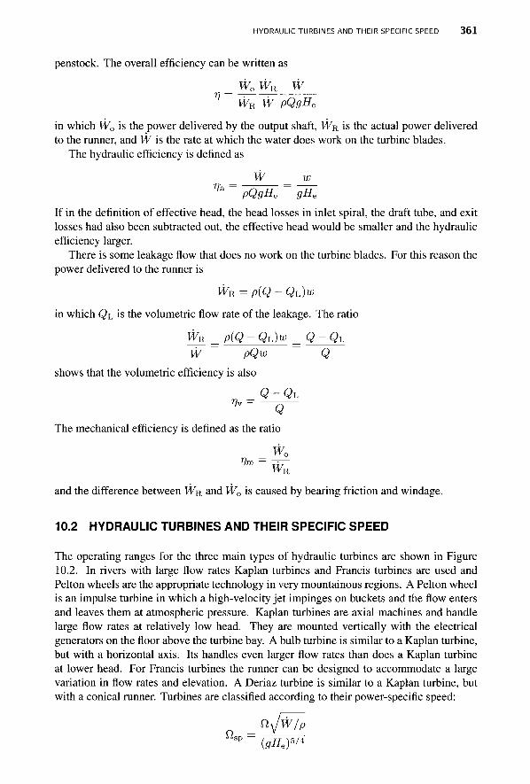
HYDRAULIC TURBINES AND THEIR SPECIFIC SPEED 3 6 1
penstock. The overall efficiency can be written as
= WQWR W 71 WRW pQgHe
in which W0 is the power delivered by the output shaft, WR is the actual power delivered to the runner, and W is the rate at which the water does work on the turbine blades.
The hydraulic efficiency is defined as
_ W _ _w_ pQgHe gHe
If in the definition of effective head, the head losses in inlet spiral, the draft tube, and exit losses had also been subtracted out, the effective head would be smaller and the hydraulic efficiency larger.
There is some leakage flow that does no work on the turbine blades. For this reason the power delivered to the runner is
WR = p(Q - QL)w
in which QL is the volumetric flow rate of the leakage. The ratio
WR = p(Q - Qh)w = Q - QL
W pQw Q shows that the volumetric efficiency is also
Q-QL
The mechanical efficiency is defined as the ratio
_ Wo Vm — ■
WR
and the difference between WR and W0 is caused by bearing friction and windage.
10.2 HYDRAULIC TURBINES AND THEIR SPECIFIC SPEED
The operating ranges for the three main types of hydraulic turbines are shown in Figure 10.2. In rivers with large flow rates Kaplan turbines and Francis turbines are used and Pelton wheels are the appropriate technology in very mountainous regions. A Pelton wheel is an impulse turbine in which a high-velocity jet impinges on buckets and the flow enters and leaves them at atmospheric pressure. Kaplan turbines are axial machines and handle large flow rates at relatively low head. They are mounted vertically with the electrical generators on the floor above the turbine bay. A bulb turbine is similar to a Kaplan turbine, but with a horizontal axis. Its handles even larger flow rates than does a Kaplan turbine at lower head. For Francis turbines the runner can be designed to accommodate a large variation in flow rates and elevation. A Deriaz turbine is similar to a Kaplan turbine, but with a conical runner. Turbines are classified according to their power-specific speed:
ilJW/p Qsp ~ (gHe)V*
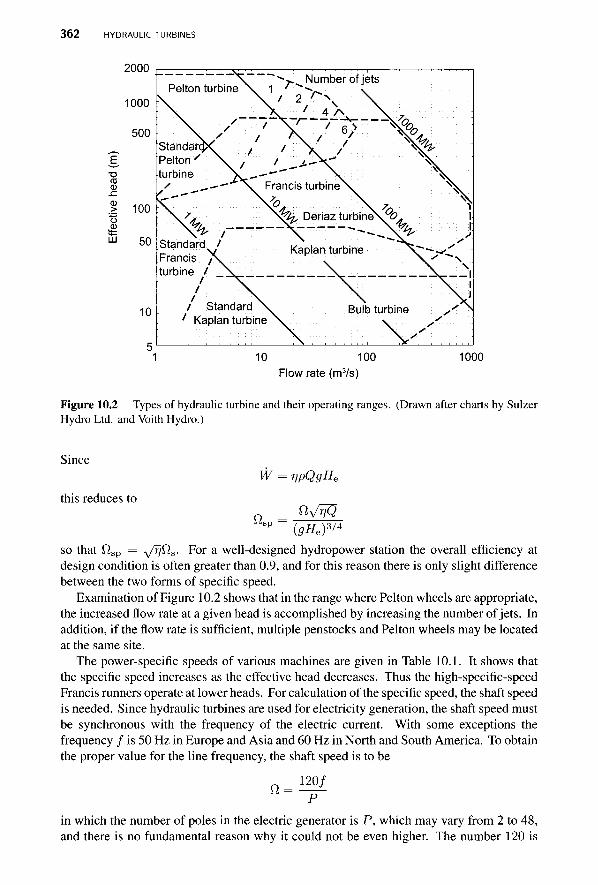
362 HYDRAULIC TURBINES
2000
10 100 Flow rate (m3/s)
1000
Figure 10.2 Types of hydraulic turbine and their operating ranges. (Drawn after charts by Sulzer Hydro Ltd. and Voith Hydro.)
Since
this reduces to
w = r,pQgHe
a ftvW sp (<7#e)3/4
so that flsp = ,ff}Qs. For a well-designed hydropower station the overall efficiency at design condition is often greater than 0.9, and for this reason there is only slight difference between the two forms of specific speed.
Examination of Figure 10.2 shows that in the range where Pelton wheels are appropriate, the increased flow rate at a given head is accomplished by increasing the number of jets. In addition, if the flow rate is sufficient, multiple penstocks and Pelton wheels may be located at the same site.
The power-specific speeds of various machines are given in Table 10.1. It shows that the specific speed increases as the effective head decreases. Thus the high-specific-speed Francis runners operate at lower heads. For calculation of the specific speed, the shaft speed is needed. Since hydraulic turbines are used for electricity generation, the shaft speed must be synchronous with the frequency of the electric current. With some exceptions the frequency / is 50 Hz in Europe and Asia and 60 Hz in North and South America. To obtain the proper value for the line frequency, the shaft speed is to be
n 120/
in which the number of poles in the electric generator is P, which may vary from 2 to 48, and there is no fundamental reason why it could not be even higher. The number 120 is
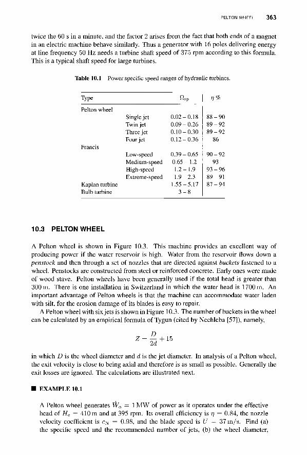
PELTON WHEEL 363
twice the 60 s in a minute, and the factor 2 arises from the fact that both ends of a magnet in an electric machine behave similarly. Thus a generator with 16 poles delivering energy at line frequency 50 Hz needs a turbine shaft speed of 375 rpm according to this formula. This is a typical shaft speed for large turbines.
Table 10.1 Power specific speed ranges of hydraulic turbines.
Type
Pelton wheel
Francis
Kaplan turbine Bulb turbine
Single jet Twin jet Three jet Four jet
Low-speed Medium-speed High-speed Extreme-speed
Q
0.02-0.09-0.10-0.12-
0.39-0.65 1.2-1.9-
1.55-3 -
3P
-0.18 -0.26 -0.30 -0.36
-0.65 -1 .2 -1.9 -2.3 -5.17 -8
r/%
88 -90 89 -92 89 -92
86
9 0 - 9 2 93
9 3 - 9 6 89 -91 8 7 - 9 4
10.3 PELTON WHEEL
A Pelton wheel is shown in Figure 10.3. This machine provides an excellent way of producing power if the water reservoir is high. Water from the reservoir flows down a penstock and then through a set of nozzles that are directed against buckets fastened to a wheel. Penstocks are constructed from steel or reinforced concrete. Early ones were made of wood stave. Pelton wheels have been generally used if the total head is greater than 300 m. There is one installation in Switzerland in which the water head is 1700 m. An important advantage of Pelton wheels is that the machine can accommodate water laden with silt, for the erosion damage of its blades is easy to repair.
A Pelton wheel with six jets is shown in Figure 10.3. The number of buckets in the wheel can be calculated by an empirical formula of Tygun (cited by Nechleba [57]), namely,
D 2d
+ 15
in which D is the wheel diameter and d is the jet diameter. In analysis of a Pelton wheel, the exit velocity is close to being axial and therefore is as small as possible. Generally the exit losses are ignored. The calculations are illustrated next.
■ EXAMPLE 10.1
A Pelton wheel generates W0 = 1MW of power as it operates under the effective head of He — 410 m and at 395 rpm. Its overall efficiency is r\ = 0.84, the nozzle velocity coefficient is CN = 0.98, and the blade speed is U = 37m/s. Find (a) the specific speed and the recommended number of jets, (b) the wheel diameter,
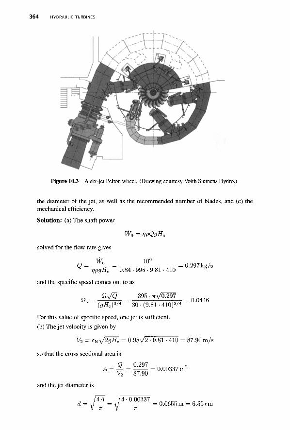
364 HYDRAULIC TURBINES
Figure 10.3 A six-jet Pelton wheel. (Drawing courtesy Voith Siemens Hydro.)
the diameter of the jet, as well as the recommended number of blades, and (c) the mechanical efficiency.
Solution: (a) The shaft power
W0 — ripQgHe
solved for the flow rate gives
W 106
0.297 kg/s ^ T)pgHe 0.84 • 998 • 9.81 • 410
and the specific speed comes out to as
ily/Q _ 395 • 7ry/fl297 _nnAAa s " (gHe)V* ~ 30 • (9.81 • 410)3/* " U"U44b
For this value of specific speed, one jet is sufficient. (b) The jet velocity is given by
V2 = cNV/2gHe = 0.98\/2 • 9.81 ■ 410 = 87.90 m/s
so that the cross sectional area is
Q 0.297 9 A=£r = —— = 0.00337 m2
V2 87.90
and the jet diameter is
AA 4 ■ 0.00337 a = \ — = \ = 0.0655 m = 6.55 cm V 7T V TT
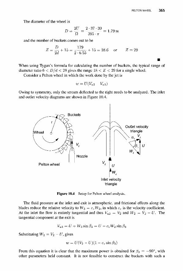
PELTON WHEEL 365
The diameter of the wheel is
D 2U 2-37-30 n 395 • 7T
and the number of buckets comes out to be
„ D _ 179
1.79 m
2d 15 2-6.55
15 = 28.6 or 29
When using Tygun's formula for calculating the number of buckets, the typical range of diameter ratio 6 < D/d < 28 gives the range 18 < Z < 29 for a single wheel.
Consider a Pelton wheel in which the work done by the jet is
w = U(Vu2 - Vu3)
Owing to symmetry, only the stream deflected to the right needs to be analyzed. The inlet and outlet velocity diagrams are shown in Figure 10.4.
Buckets
Nozzle
Outlet velocity triangle
V,
Pelton wheel
Inlet velocity triangle
Figure 10.4 Setup for Pelton wheel analysis.
The fluid pressure at the inlet and exit is atmospheric, and frictional effects along the blades reduce the relative velocity to W3 = cvW"2, in which cv is the velocity coefficient. At the inlet the flow is entirely tangential and thus VU2 = V2 and W2 = V2 — U. The tangential component at the exit is
Vu3 = U + Wz sin p3 = U + cvW2 sin /33
Substituting W2 = V2 — U, gives
u, = C / ( l / 2 - t / ) ( l - c v s i n ^ 3 )
From this equation it is clear that the maximum power is obtained for /33 = —90°, with other parameters held constant. It is not feasible to construct the buckets with such a
366 HYDRAULIC TURBINES
large amount of turning, as the water would not clear the wheel. For this reason in actual installations /33 is in the neighborhood of —65°. Any water that is partly spilled during the operation does no work on the blades. This spillage is taken into account by the volumetric efficiency.
In the expression for the overall efficiency
the hydraulic efficiency can be written as the sum of the nozzle efficiency and the rotor efficiency
in which v2
2 m = y-2
"0
and Vo = \/2gHe is the spouting velocity. The rotor efficiency is then
w I T / 2 2 V2
The mechanical losses are taken to be proportional to U2, with the proportionality constant denoted by Ku. The fluid dynamic losses in turbulent flows are often proportional to the square of the flow velocity, and therefore the windage losses should have this dependence on the blade speed. Then
Hence
wa VrnVv ^
ri = Vh hv ~
2rjvw V ~ 2gHe
WR - PQ\KUU2 KUU2
W Vv 2w
KUU2\ _ ( KJJ2\ w 2w ) V v 2w ) gHe
-K2;l'v^w-K-u2> Substituting the expression for work into this and replacing Vo by V^/y^N gives
V = ^[2VvU(V2 -U)(l- cvsin/33) - KJJ2)
This can be written is terms of the ratio of the blade speed to the nozzle velocity A = U /V2, as follows:
r, = 7?N(2T?VA(1 - A)(l - cvsin/33) - Ku\2)
To determine the rotational speed at which the power is maximum, this expression is differentiated with respect to A while other parameters are held fixed. Setting the result to zero gives
$ = 2jjv(l - 2A)(1 - cvsin/33) - 2KU\ = 0
from which _ 1 - cv sin j33
An 2r)v(l -c v s in /3 3 ) + Ku
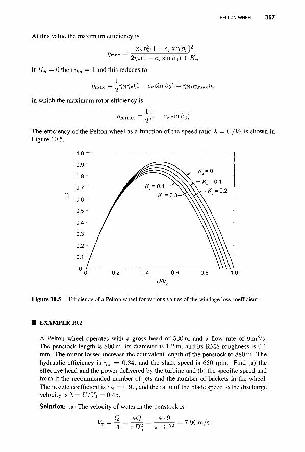
PELTON WHEEL 367
At this value the maximum efficiency is
TJNVU1 - c v s in / ? 3 ) 2
Vn 277v(l - c v s i n ^ 3 ) + Ku
If Ku — 0 then rym = 1 and this reduces to
IJmax = 2^N?7v(l - Cv s in /3 3 ) = %))Rmax)?v
in which the maximum rotor efficiency is
7?Rmax = n ^ 1 - C v S m / ? 3 )
The efficiency of the Pelton wheel as a function of the speed ratio A = U/V2 is shown in Figure 10.5.
Figure 10.5 Efficiency of a Pelton wheel for various values of the windage loss coefficient.
EXAMPLE 10.2
A Pelton wheel operates with a gross head of 530 m and a flow rate of 9 m3/s. The penstock length is 800 m, its diameter is 1.2 m, and its RMS roughness is 0.1 mm. The minor losses increase the equivalent length of the penstock to 880 m. The hydraulic efficiency is % = 0.84, and the shaft speed is 650 rpm. Find (a) the effective head and the power delivered by the turbine and (b) the specific speed and from it the recommended number of jets and the number of buckets in the wheel. The nozzle coefficient is CN = 0.97, and the ratio of the blade speed to the discharge velocity is A = U/V2 = 0.45.
Solution: (a) The velocity of water in the penstock is
v ._ Q _ 4Q Vp ~ A ~ vDl
4-9 r-1.22 7.96 m/s
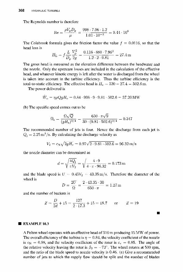
368 HYDRAULIC TURBINES
The Reynolds number is therefore
P V D £ = 998 .7 .96 .12 =
[i 1.01 • 10~3
The Colebrook formula gives the friction factor the value / = 0.0116, so that the head loss is
A ^ = 0 : 1 1 6 _ ^ 8 0 ^ : 9 6 ! = 2 7 4 m
Dp2g 1.2-2-9.81 The gross head is measured as the elevation difference between the headwater and the nozzle. Only the upstream losses are included in the calculation of the effective head, and whatever kinetic energy is left after the water is discharged from the wheel is taken into account in the turbine efficiency. Thus the turbine efficiency is the total-to-static efficiency. The effective head is He = 530 — 27.4 = 502.6 m.
The power delivered is
Wo = r]pQgHe = 0.84 • 998 • 9 • 9.81 ■ 502.6 = 37.20 MW
(b) The specific speed comes out to be
n = " ^ = 6 5 ° • " ^ = 0 3 4 7 s (gHe)3/4 30 • (9.81 • 502.6)3/4
The recommended number of jets is four. Hence the discharge from each jet is Qj = 2.25 m3/s. By calculating the discharge velocity as
V2 = cN^2gHe = 0.97V2 • 9.81 • 502.6 = 96.32m/s
the nozzle diameter can be determined as
d=J^ = J 4"9 =0.173m V KV2 V 4 ■ TT • 96.32
and the blade speed is U — 0.451^ = 43.35 m/s. Therefore the diameter of the wheel is
„ 2U 2 • 43.35 -30 D= — = = 1.27m
n 650 • TT
and the number of buckets is
^ + 1 5 -2d 2-17.3
D 127 Z = — + 15 = -——- + 15 = 18.7 or Z = 19
EXAMPLE 10.3
A Pelton wheel operates with an effective head of 310 m producing 15 MW of power. The overall efficiency of the turbine is rj = 0.84, the velocity coefficient of the nozzle is CN = 0.98, and the velocity coefficient of the rotor is cv = 0.85. The angle of the relative velocity leaving the rotor is /?3 = —73°. The wheel rotates at 500 rpm, and the ratio of the blade speed to nozzle velocity is 0.46. (a) Give a recommended number of jets to which the supply flow should be split and the number of blades
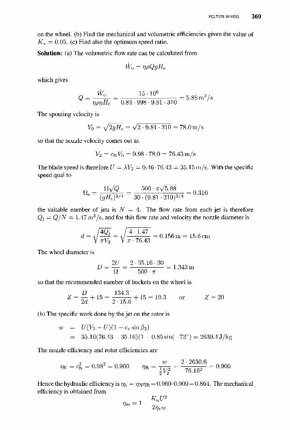
PELTON WHEEL 369
on the wheel, (b) Find the mechanical and volumetric efficiencies given the value of Ku — 0.05. (c) Find also the optimum speed ratio.
Solution: (a) The volumetric flow rate can be calculated from
W0 = r]pQgHe
which gives
Q = ^ = ^ = 5.88m3/s ^ rjpgHe 0.84 • 998 • 9.81 ■ 310 '
The spouting velocity is
V0 = \/2gHe = A/2-9.81 -310 = 78.0m/s
so that the nozzle velocity comes out as
V2 = cNV0 = 0.98 • 78.0 = 76.43 m/s The blade speed is therefore U = XV2 = 0.46 • 76.43 = 35.15 m/s. With the specific speed qual to
1VQ = 500-TryCT = s (5F e ) 3 / 4 30 • (9.81 • 310)3/4
the suitable number of jets is N = 4. The flow rate from each jet is therefore Q] — Q/N — 1.47 m3/s, and for this flow rate and velocity the nozzle diameter is
4Qj / 4 • 1.47 -KV-2, V 7T • 76.43
The wheel diameter is
2U 2 -35.16 -30 D = —— = — = 1.343 m
Q 500 • 7T
so that the recommended number of buckets on the wheel is
D 134 3 Z = ^ + 15 = ^-^ + 15 = 19-3 or Z = 20
2d 2 • 15.6 (b) The specific work done by the jet on the rotor is
w = U(V2-U){l-cvsm{33) = 35.16(76.43 - 35.16)(1 - 0.85sin(-73°) = 2630.4 J/kg
The nozzle efficiency and rotor efficiencies are
_ 2 • 2630.6
2 " 2 ' m = cz
N = 0.98^ = 0.960 VR = j ^ = ? 6 1 6 2 - 0.900
Hence the hydraulic efficiency is 7?h = ?7N77R = 0.960-0.900 = 0.864. The mechanical efficiency is obtained from
, KUU2
Vm = 1 - -7; 2r]vw
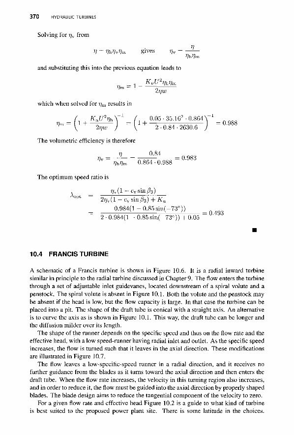
370 HYDRAULIC TURBINES
Solving for r]v from
V V = VhilvVm gives rjv
and substituting this into the previous equation leads to
Kull2r]hr]m Vm = 1 7.
lr\w which when solved for rjm results in
(, ^ KuU^Y1 (, , 0.05-35.162-0.864V1
T]m={1 + ^2^r) ={1+ 2-0.84-2630.6 ) = °"
The volumetric efficiency is therefore
_ V _ 0.84 Vv ~ mJh, ~ 0.864 • 0.988 "
The optimum speed ratio is
7yv(l-cvsin/33) ^opt — 2i]v(l -cvs in/33) + Ku
0.984(1 - 0.85sin(-73°)) ^ ^ U- = 0 493
2 • 0.984(1 - 0.85 sin(-73°)) + 0.05
10.4 FRANCIS TURBINE
A schematic of a Francis turbine is shown in Figure 10.6. It is a radial inward turbine similar in principle to the radial turbine discussed in Chapter 9. The flow enters the turbine through a set of adjustable inlet guidevanes, located downstream of a spiral volute and a penstock. The spiral volute is absent in Figure 10.1. Both the volute and the penstock may be absent if the head is low, but the flow capacity is large. In that case the turbine can be placed into a pit. The shape of the draft tube is conical with a straight axis. An alternative is to curve the axis as is shown in Figure 10.1. This way, the draft tube can be longer and the diffusion milder over its length.
The shape of the runner depends on the specific speed and thus on the flow rate and the effective head, with a low speed-runner having radial inlet and outlet. As the specific speed increases, the flow is turned such that it leaves in the axial direction. These modifications are illustrated in Figure 10.7.
The flow leaves a low-specific-speed runner in a radial direction, and it receives no further guidance from the blades as it turns toward the axial direction and then enters the draft tube. When the flow rate increases, the velocity in this turning region also increases, and in order to reduce it, the flow must be guided into the axial direction by properly shaped blades. The blade design aims to reduce the tangential component of the velocity to zero.
For a given flow rate and effective head Figure 10.2 is a guide to what kind of turbine is best suited to the proposed power plant site. There is some latitude in the choices.
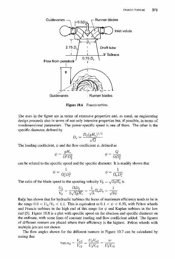
FRANCIS TURBINE 3 7 1
Guidevanes
Flow from penstock
Runner blades
Inlet volute
Draft tube
s. Tailrace
Guidevanes i Runner blades
Figure 10.6 Francis turbine.
The axes in the figure are in terms of extensive properties and, as usual, an engineering design proceeds also in terms of not only intensive properties but, if possible, in terms of nondimensional parameters. The power-specific speed is one of them. The other is the specific diameter, defined by
_ £>2(flHe)1/4
s ~ VQ The loading coefficient, tp and the flow coefficient < , defined as
1>: n2D% Q
can be related to the specific speed and the specific diameter. It is readily shown that 1 1
r/j-.
The ratio of the blade speed to the spouting velocity Vo
lh SID2 1 Vo
nHi>B =
\f2,gHe is 1
Balje has shown that for hydraulic turbines the locus of maximum efficiency tends to be in the range 0.6 < U2/V0 < 1.1. This is equivalent to 0.1 < tp < 0.35, with Pelton wheels and Francis turbines in the high end of this range for tp and Kaplan turbines in the low end [5]. Figure 10.8 is a plot with specific speed on the abscissa and specific diameter on the ordinate, with some lines of constant loading and flow coefficient added. The figures of different runners are placed where their efficiency is the highest. Pelton wheels with multiple jets are not shown.
The flow angles shown for the different runners in Figure 10.7 can be calculated by noting that
VU2 _ UlVu2 _ W
Vr2 ~ tan«2 U2V7 2Vr2 UoVr,

372 HYDRAULIC TURBINES
0.39 < n < 0.65
0.65 <fi < 1.2
n . = 0.39
P2 S low-speed runners
Q =0.65
1.2 < n <1.9 sp
U
Q. = 1.2
P2 W2 H igh-speed
1.9 < n <2.3
U
W,
a =2.3
Figure 10.7 Shapes of Francis turbine runners.
and since Q = nD2b2Vr2, a n d w = r]hgHe, this can be written as
r]hgHeTTD2b2 tanai2 U2Q
From the definition of the specific speed the ratio
Q Ws^gTTe
follows immediately, and with fl = 2U2/D2 and VQ = \/2gHe, the formula for the tangent of a2 can further be written as
t a i l o r 4??hv/27r6r U2
Ws V0
in which the ratio 6r = b/D2 appears. A graph of this ratio appears in the book by Nechleba [57]. A quadratic curve fit over the range Of the power-specific speeds for Francis turbines
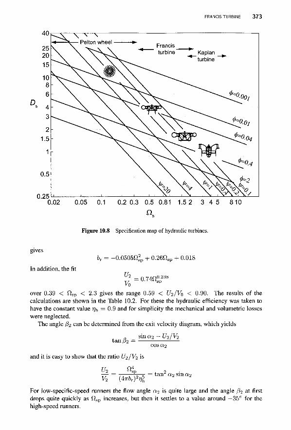
FRANCIS TURBINE 373
■ Pelton wheel Francis turbine Kaplan
turbine
0.02 0.05 0.1 0.2 0.3 0.5 0.81 1.5 2 3 4 5 810
a Figure 10.8 Specification map of hydraulic turbines.
gives
In addition, the fit
br = -0.0505fti, + 0.26f2sp + 0.018
£ = 0.74J4238
over 0.39 < Q.sp < 2.3 gives the range 0.59 < U2/V0 < 0.90. The results of the calculations are shown in the Table 10.2. For these the hydraulic efficiency was taken to have the constant value % = 0.9 and for simplicity the mechanical and volumetric losses were neglected.
The angle /32 can be determined from the exit velocity diagram, which yields
tan/32 = sina2 — U2/V2
and it is easy to show that the ratio U2/V2 is
ft4 U* = V2 (477^)2^5
COSC*2
tan a2 sin a2
For low-specific-speed runners the flow angle a2 is quite large and the angle /32 at first drops quite quickly as flsp increases, but then it settles to a value around —35° for the high-speed runners.
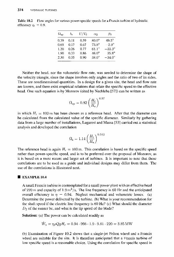
374 HYDRAULIC TURBINES
Table 10.2 Flow angles for various power-specific speeds for a Francis turbine of hydraulic efficiency ?7h = 0.9.
" 'sp
0.39 0.65 1.20 1.90 2.30
6r
0.11 0.17 0.26 0.33 0.35
U/Vo
0.59 0.67 0.77 0.86 0.90
Ct2
80.0° 73.8° 61.1° 46.0° 38.0°
P2
49.5° -2.9°
-33.3° -35.8° -34.0°
Neither the head, nor the volumetric flow rate, was needed to determine the shape of the velocity triangle, since the shape involves only angles and the ratio of two of its sides. These are nondimensional quantities. In a design for a given site, the head and flow rate are known, and there exist empirical relations that relate the specific speed to the effective head. One such equation is by Mozorov (cited by Nechleba [57]) can be written as
/ TT \ 0-57
n s p = 0 .82f -^
in which Hv = 100 m has been chosen as a reference head. After that the diameter can be calculated from the calculated value of the specific diameter. Similarly by gathering data from a large number of installations, Lugaresi and Massa [53] carried out a statistical analysis and developed the correlation
„ \ 0.512 a = 1.14. „
The reference head is again Hv = 100 m. This correlation is based on the specific speed rather than power-specific speed, and is to be preferred over the proposal of Mozorov, as it is based on a more recent and larger set of turbines. It is important to note that these correlations are to be used as a guide and individual designs may differ from them. The use of the correlations is illustrated next.
■ EXAMPLE 10.4
A small Francis turbine is contemplated for a small power plant with an effective head of 220 m and capacity of 1.9 m3/s. The line frequency is 60 Hz and the anticipated overall efficiency is 77 = 0.94. Neglect mechanical and volumetric losses, (a) Determine the power delivered by the turbine, (b) What is your recommendation for the shaft speed if the electric line frequency is 60 Hz? (c) What should the diameter D2 of the runner be, and what is the tip speed of the blade?
Solution: (a) The power can be calculated readily as
W0 = r]PQgHe = 0.94 • 998 • 1.9 • 9.81 • 220 = 3.85 MW
(b) Examination of Figure 10.2 shows that a single-jet Pelton wheel and a Francis wheel are suitable for the site. It is therefore anticipated that a Francis turbine of low specific speed is a reasonable choice. Using the correlation for specific speed in

FRANCIS TURBINE 375
terms of the effective head gives
/ioo\0-512 fls = 1.14 = 0.7614
\220y
and then from the definition of the specific speed the shaft speed can be determined to be
n O s ( g g e ) 3 / 4 0.7614(9.81 ■ 220 ) 3 / 4 30 SZ — —-—■==!■ = = = — = 1641 r p m
If the shaft speed is taken to be 1800 rpm, then the number of poles in the generator
„ 120/ 120-60 , P = —PT- = = 4
n i8oo (c) With this shaft speed the specific speed is
_ n V 3 _ 1800 ■ 7rvT9 _ s (gHe)^ 30 • (9.81 • 2 2 0 ) 3 / 4
and the power-specific speed is $7sp = ^/rjQs = %/0.94 0.821 = 0.796. The velocity ratio is
~ =0 .74f t f D2 3 8 = 0.701
V0 sp
The specific diameter can then be calculated from
Ds = ^ U ^ = ° - 7 0 1 ■ ^ = 2.415 ns 0.821
and the diameter is
Ds^/Q 2.415x/T9 D2 = , \?IA = -, „ , , = 0.488 m
( 5 H e ) 1 / 4 (9.81-220)1/4
The blade speed is therefore U<i = D2^/2 = 46.0 m/s. ■
To obtain more accurate results, the volumetric flow rate at the inlet to the runner can be calculated from
Q = (TTD2 - - ^ - ) b2Wr2 V cos/32/
in which t is the blade thickness, Z is the number of blades, and Wr2 is the radial component of the relative velocity with the flow angle /32, at the inlet. The number of blades can be taken to be between Z = IIV0/C/2 and^ = l3Vo/U2, which for the typical range of U2/Vo comes close to 16 blades. The runner in Figure 10.9 has 17 blades, which is appropriately a prime number to prevent some resonance vibrations.
As the flow enters the draft tube, the axial velocity Vxs can be obtained from the expression for the volumetric flow rate, which is
Q = ^-vx3 (lo.i)
It is assumed that the flow enters without swirl so that Vx% = V3. For the conical draft tube shown in Figure 10.6, the length of the tube is 2.5 - 3 times the diameter D3 and its
376 HYDRAULIC TURBINES
Figure 10.9 Francis turbine viewed from downstream.
submerged length into the tailwater ranges from O.5D3 to D3. Since the function of the draft tube is to diffuse the flow, its flare must be kept small enough to prevent separation.
The diffuser efficiency is defined as
_ 2gHd 2gHd/V32
in which H& is the head loss in the diffuser. For a conical diffuser the peak efficiency is at the cone angle 20 = 6° and has a value of about TJ^ max — 0.9. Defining the loss coefficient Kd via the equation
vi Hd = Kd -
it can readily seen that it can be expressed in terms of the diffuser efficiency as
Kd = (1 - Tfc) ( l - ^ l
Since all the kinetic energy leaving the draft tube is dissipated in the tail water pool, the exit loss is
= vi = viyl = Aivi e 2g V3
22g A\ 2g so that the loss coefficient based on the velocity V3 is
e A\
The draft tube and exit loss coefficients and their sum are shown as a function of the ratio A4/A3 in Figure 10.10. If the inlet and exit diameters D3 and D4 are known, so is the area
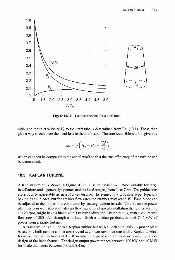
KAPLAN TURBINE 377
Figure 10.10 Loss coefficients for a draft tube.
ratio, and the inlet velocity V3 to the draft tube is determined from Eq. (10.1). These then give a way to calculate the head loss in the draft tube. The true reversible work is given by
which can then be compared to the actual work so that the true efficiency of the turbine can be determined.
10.5 KAPLAN TURBINE
A Kaplan turbine is shown in Figure 10.11. It is an axial-flow turbine suitable for large installations and it generally operates under a head ranging from 20 to 70 m. The guidevanes are similarly adjustable as in a Francis turbine. Its runner is a propeller type, typically having 3 to 6 blades, but for smaller flow rates the number may reach 10. Each blade can be adjusted to the proper flow conditions by rotating it about its axis. This makes the power plant perform well also at off-design flow rates. In a typical installation the runner, turning at 120 rpm, might have a blade with 1 m hub radius and 3 m tip radius, with a volumetric flow rate of 200m3/s through a turbine. Such a turbine produces around 74.5 MW of power from a single turbine.
A bulb turbine is similar to a Kaplan turbine but with a horizontal axis. A power plant based on a bulb turbine can be constructed at a lower cost than one with a Kaplan turbine. It can be used at low heads of 4 - 10 m when the speed of the flow is increased by proper design of the inlet channel. The design output power ranges between 100 kW and 50 MW for blade diameters between 0.8 and 8.4 m.
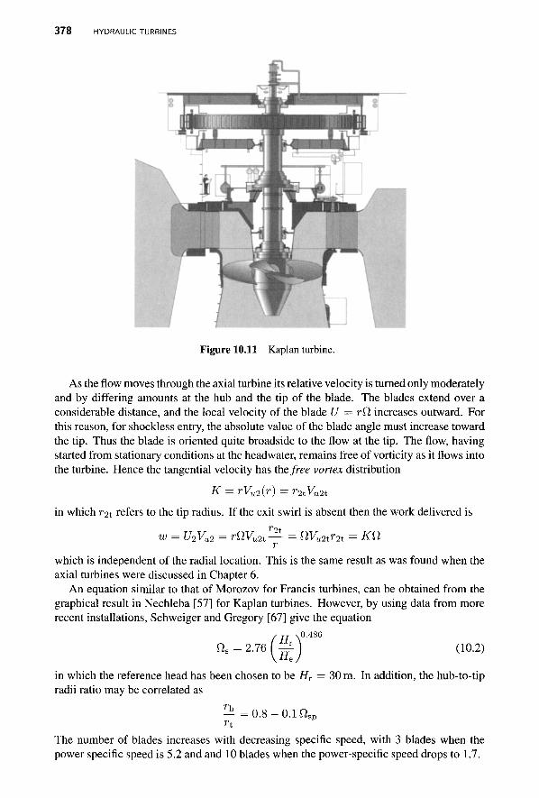
378 HYDRAULIC TURBINES
Figure 10.11 Kaplan turbine.
As the flow moves through the axial turbine its relative velocity is turned only moderately and by differing amounts at the hub and the tip of the blade. The blades extend over a considerable distance, and the local velocity of the blade U — rQ increases outward. For this reason, for shockless entry, the absolute value of the blade angle must increase toward the tip. Thus the blade is oriented quite broadside to the flow at the tip. The flow, having started from stationary conditions at the headwater, remains free of vorticity as it flows into the turbine. Hence the tangential velocity has the free vortex distribution
K = rVu2(r) = r 2 t y u 2 t
in which r2t refers to the tip radius. If the exit swirl is absent then the work delivered is
w = U2Vu2 = rQVu2t— - QVu2tr2t = KQ. r which is independent of the radial location. This is the same result as was found when the axial turbines were discussed in Chapter 6.
An equation similar to that of Morozov for Francis turbines, can be obtained from the graphical result in Nechleba [57] for Kaplan turbines. However, by using data from more recent installations, Schweiger and Gregory [67] give the equation
/ I T \0.486
a = 2.76f-^J (10.2) in which the reference head has been chosen to be HT = 30 m. In addition, the hub-to-tip radii ratio may be correlated as
— = o.8-o.insp n
The number of blades increases with decreasing specific speed, with 3 blades when the power specific speed is 5.2 and and 10 blades when the power-specific speed drops to 1.7.
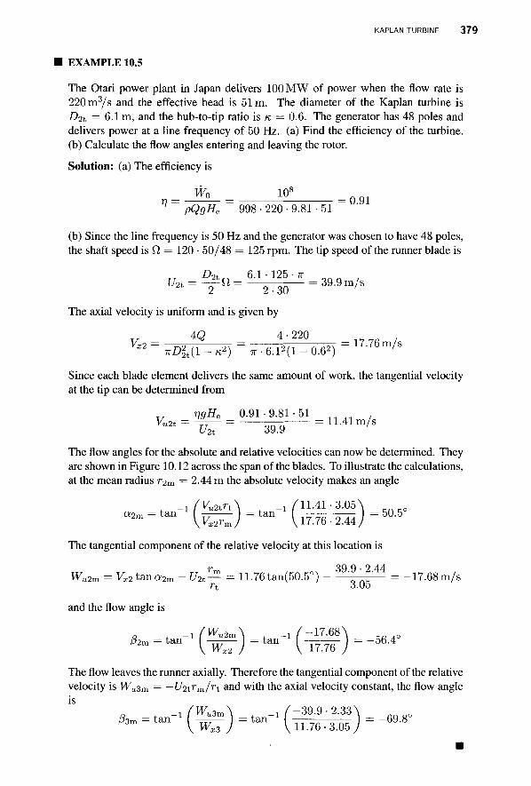
KAPLAN TURBINE 379
EXAMPLE 10.5
The Otari power plant in Japan delivers 100 MW of power when the flow rate is 220 m3/s and the effective head is 51 m. The diameter of the Kaplan turbine is D2t = 6.1 m, and the hub-to-tip ratio is K = 0.6. The generator has 48 poles and delivers power at a line frequency of 50 Hz. (a) Find the efficiency of the turbine. (b) Calculate the flow angles entering and leaving the rotor.
Solution: (a) The efficiency is
= Wo = 108 =
V pQgHe 998 • 220 • 9.81 • 51
(b) Since the line frequency is 50 Hz and the generator was chosen to have 48 poles, the shaft speed is fl = 120 • 50/48 — 125 rpm. The tip speed of the runner blade is
D2t 6 . 1 - 1 2 5 - T T U2t = " = = 39.9 m/s
* 2 2-30 '
The axial velocity is uniform and is given by
v 4Q 4-220 V^ = n2 n 2T = TTu\ 7TM\ = 17-76m/s
■KD^X-K1) 7r • 6.1^(1 - 0.62) Since each blade element delivers the same amount of work, the tangential velocity at the tip can be determined from
VgHe 0.91-9.81-51 VU2t — —^— = = 11.41 m/s
U2i 39.9 '
The flow angles for the absolute and relative velocities can now be determined. They are shown in Figure 10.12 across the span of the blades. To illustrate the calculations, at the mean radius r2m = 2.44 m the absolute velocity makes an angle
. -1fVu2trt\ . _! f 11-41 -3.05^ Q 2 m = t a n {V^r)=tlin (,17.76- 2.44 j = 5 ° - 5
The tangential component of the relative velocity at this location is
r 39 9 • 2 44 Wu2m = Vx2ta,na2m - U2t— = 11.76tan(50.5°) ' ' = -17.68m/s
r t 3.05
and the flow angle is
R . _ ! / ^ 2 m \ _! ̂ - 17 .68^
The flow leaves the runner axially. Therefore the tangential component of the relative velocity is WU3m = —U2trm/rt and with the axial velocity constant, the flow angle
a t - l ^ u 3 m \ . _! ̂ -39 .9 2.33^ /?3m = t a n l " ^ 7 j = t a n { 11-76- 3.05 j = ~ 6 9 - 8
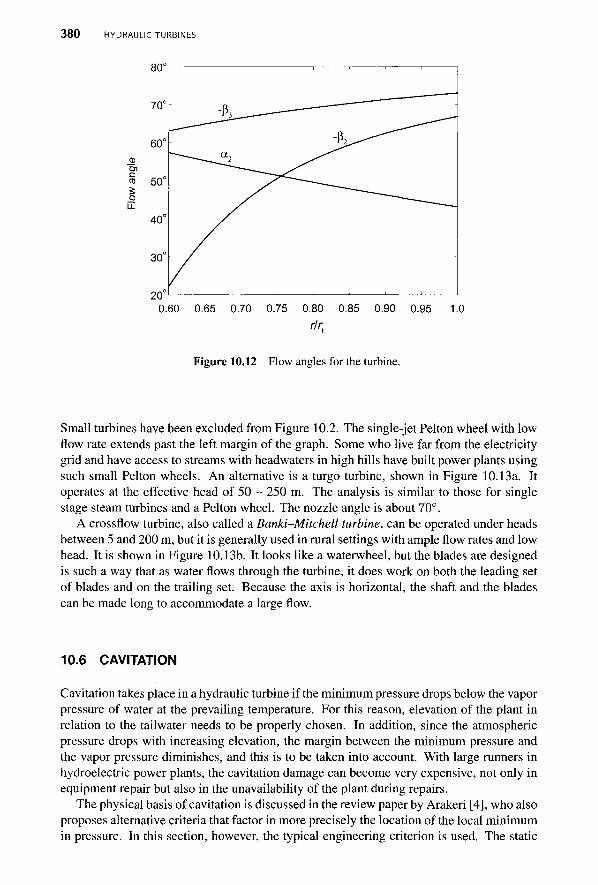
380 HYDRAULIC TURBINES
0.60 0.65 0.70 0.75 0.80 0.85 0.90 0.95 1.0 rlrt
Figure 10.12 Flow angles for the turbine.
Small turbines have been excluded from Figure 10.2. The single-jet Pelton wheel with low flow rate extends past the left margin of the graph. Some who live far from the electricity grid and have access to streams with headwaters in high hills have built power plants using such small Pelton wheels. An alternative is a turgo turbine, shown in Figure 10.13a. It operates at the effective head of 50 - 250 m. The analysis is similar to those for single stage steam turbines and a Pelton wheel. The nozzle angle is about 70°.
A crossflow turbine, also called a Banki-Mitchell turbine, can be operated under heads between 5 and 200 m, but it is generally used in rural settings with ample flow rates and low head. It is shown in Figure 10.13b. It looks like a waterwheel, but the blades are designed is such a way that as water flows through the turbine, it does work on both the leading set of blades and on the trailing set. Because the axis is horizontal, the shaft and the blades can be made long to accommodate a large flow.
10.6 CAVITATION
Cavitation takes place in a hydraulic turbine if the minimum pressure drops below the vapor pressure of water at the prevailing temperature. For this reason, elevation of the plant in relation to the tailwater needs to be properly chosen. In addition, since the atmospheric pressure drops with increasing elevation, the margin between the minimum pressure and the vapor pressure diminishes, and this is to be taken into account. With large runners in hydroelectric power plants, the cavitation damage can become very expensive, not only in equipment repair but also in the unavailability of the plant during repairs.
The physical basis of cavitation is discussed in the review paper by Arakeri [4], who also proposes alternative criteria that factor in more precisely the location of the local minimum in pressure. In this section, however, the typical engineering criterion is used. The static
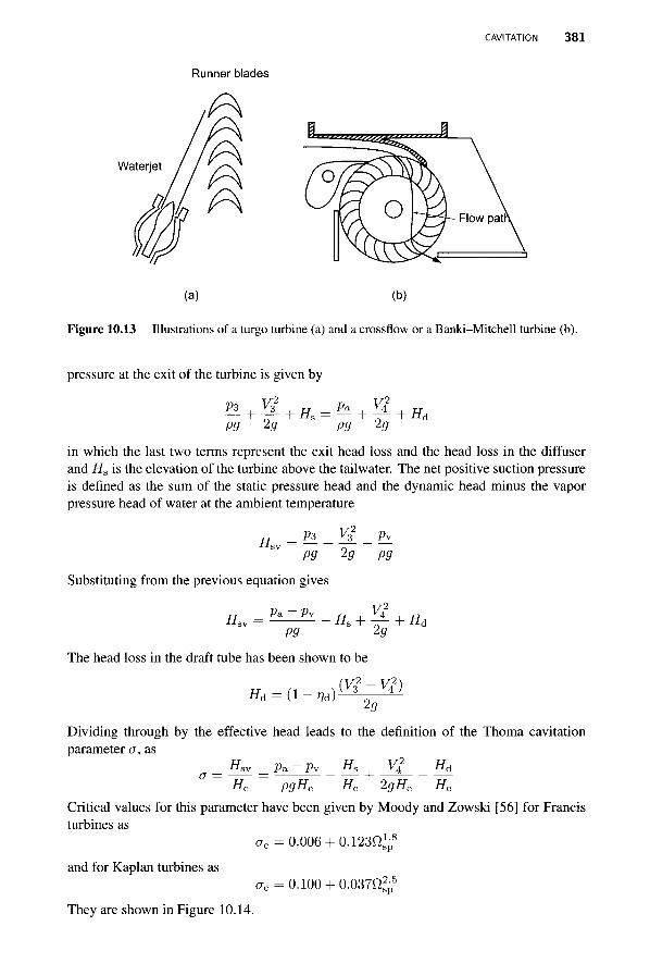
CAVITATION 3 8 1
Runner blades
(a) (b)
Figure 10.13 Illustrations of a turgo turbine (a) and a crossflow or a Banki-Mitchell turbine (b).
pressure at the exit of the turbine is given by
h-r— + W S - h — + -Hd pg 2g pg ^g
in which the last two terms represent the exit head loss and the head loss in the diffuser and Hs is the elevation of the turbine above the tailwater. The net positive suction pressure is defined as the sum of the static pressure head and the dynamic head minus the vapor pressure head of water at the ambient temperature
„ P3 , Vi pv
P9 2gr pg
Substituting from the previous equation gives
Hsv = Hs + — h Hd pg 25
The head loss in the draft tube has been shown to be
i f d - ( i - % ) — Y g —
Dividing through by the effective head leads to the definition of the Thoma cavitation parameter a, as
= Hsv = Pa-Pv _ Hs Vl _ H^ a ~ He ~ pgHe He 2gHe He
Critical values for this parameter have been given by Moody and Zowski [56] for Francis turbines as
<7C =0.006 + 0 . 1 2 3 ^
and for Kaplan turbines as ac = 0.100 + 0.037f^p
5
They are shown in Figure 10.14.
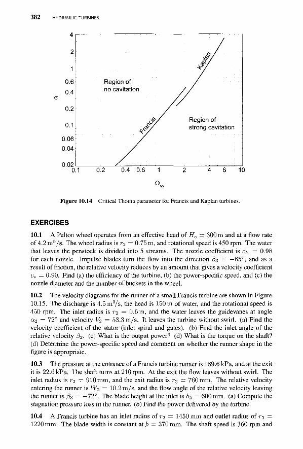
382 HYDRAULIC TURBINES
&/ Region of ,<£/ strong cavitation
0.1 0.2 0.4 0.6 1 2 4 6 10
O sp
Figure 10.14 Critical Thoma parameter for Francis and Kaplan turbines.
EXERCISES
10.1 A Pelton wheel operates from an effective head of He = 300 m and at a flow rate of 4.2 m3/s. The wheel radius is T2 = 0.75 m, and rotational speed is 450 rpm. The water that leaves the penstock is divided into 5 streams. The nozzle coefficient is CN = 0.98 for each nozzle. Impulse blades turn the flow into the direction /J3 = —65°, and as a result of friction, the relative velocity reduces by an amount that gives a velocity coefficient cv = 0.90. Find (a) the efficiency of the turbine, (b) the power-specific speed, and (c) the nozzle diameter and the number of buckets in the wheel.
10.2 The velocity diagrams for the runner of a small Francis turbine are shown in Figure 10.15. The discharge is 4.5m3/s, the head is 150m of water, and the rotational speed is 450 rpm. The inlet radius is r2 = 0.6 m, and the water leaves the guidevanes at angle «2 = 72° and velocity V2 = 53.3 m/s. It leaves the turbine without swirl, (a) Find the velocity coefficient of the stator (inlet spiral and gates), (b) Find the inlet angle of the relative velocity /32. (c) What is the output power? (d) What is the torque on the shaft? (d) Determine the power-specific speed and comment on whether the runner shape in the figure is appropriate.
10.3 The pressure at the entrance of a Francis turbine runner is 189.6 kPa, and at the exit it is 22.6 kPa. The shaft turns at 210 rpm. At the exit the flow leaves without swirl. The inlet radius is r2 — 910 mm, and the exit radius is r3 = 760 mm. The relative velocity entering the runner is W2 = 10.2 m/s, and the flow angle of the relative velocity leaving the runner is ^3 = —72°. The blade height at the inlet is 62 = 600 mm. (a) Compute the stagnation pressure loss in the runner, (b) Find the power delivered by the turbine.
10.4 A Francis turbine has an inlet radius of r2 = 1450 mm and outlet radius of r% = 1220 mm. The blade width is constant at t> = 370 mm. The shaft speed is 360 rpm and
1
0.6 0.4
0.2
0.1
0.06 0.04
on?
Region of no cavitation
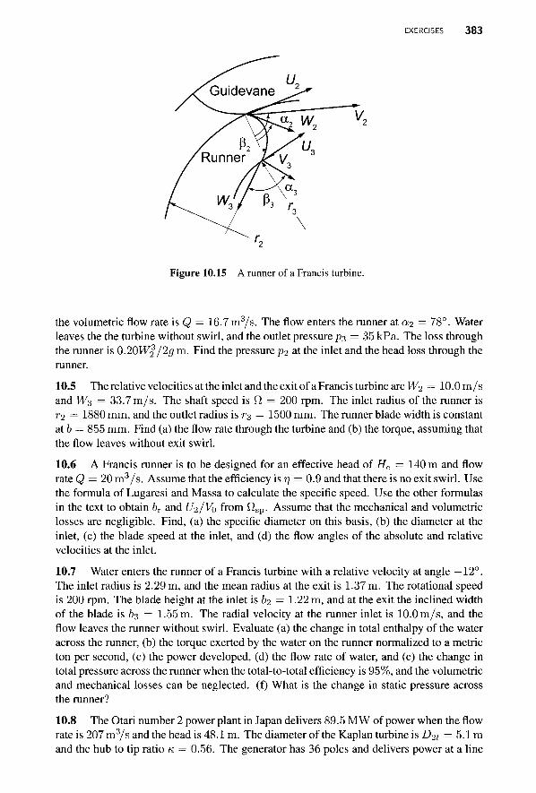
EXERCISES 383
Figure 10.15 A runner of a Francis turbine.
the volumetric flow rate is Q = 16.7m3/s. The flow enters the runner at «2 = 78°. Water leaves the the turbine without swirl, and the outlet pressure p3 = 35 kPa. The loss through the runner is 0.20 Wf /2g m. Find the pressure p2 at the inlet and the head loss through the runner.
10.5 The relative velocities at the inlet and the exit of a Francis turbine are Wi = lO.Om/s and Ws = 33.7 m/s. The shaft speed is fi = 200 rpm. The inlet radius of the runner is r-2 = 1880 mm, and the outlet radius is r3 = 1500 mm. The runner blade width is constant at b — 855 mm. Find (a) the flow rate through the turbine and (b) the torque, assuming that the flow leaves without exit swirl.
10.6 A Francis runner is to be designed for an effective head of He — 140 m and flow rate Q = 20 m3/s. Assume that the efficiency is r\ = 0.9 and that there is no exit swirl. Use the formula of Lugaresi and Massa to calculate the specific speed. Use the other formulas in the text to obtain &r and U2/V0 from £lsp. Assume that the mechanical and volumetric losses are negligible. Find, (a) the specific diameter on this basis, (b) the diameter at the inlet, (c) the blade speed at the inlet, and (d) the flow angles of the absolute and relative velocities at the inlet.
10.7 Water enters the runner of a Francis turbine with a relative velocity at angle —12°. The inlet radius is 2.29 m, and the mean radius at the exit is 1.37 m. The rotational speed is 200 rpm. The blade height at the inlet is 62 = 1-22 m, and at the exit the inclined width of the blade is 63 = 1.55 m. The radial velocity at the runner inlet is 10.0 m/s, and the flow leaves the runner without swirl. Evaluate (a) the change in total enthalpy of the water across the runner, (b) the torque exerted by the water on the runner normalized to a metric ton per second, (c) the power developed, (d) the flow rate of water, and (e) the change in total pressure across the runner when the total-to-total efficiency is 95%, and the volumetric and mechanical losses can be neglected, (f) What is the change in static pressure across the runner?
10.8 The Otari number 2 power plant in Japan delivers 89.5 MW of power when the flow rate is 207 m3/s and the head is 48.1 m. The diameter of the Kaplan turbine is D-it = 5.1 m and the hub to tip ratio K = 0.56. The generator has 36 poles and delivers power at a line
V,

384 HYDRAULIC TURBINES
frequency of 50 Hz. (a) Find the efficiency of the turbine, (b) Calculate and flow angles entering and leaving the rotor, and construct a graph to show their variation across the span.
CHAPTER 11
HYDRAULIC TRANSMISSION OF POWER
The subject of this chapter is hydraulic transmission of power by fluid couplings and torque converters. In these the driver shaft turns impeller blades of a centrifugal pump, and the driven shaft is powered by a radial turbine. The pump and its driver shaft are also called a primary and the turbine and the driven shaft, a secondary. The working fluid is oil, and the work done by the pump increases the oil pressure, which then drops as the oil flows through the turbine. The work done by the pump is greater than that delivered by the turbine; the difference is lost to irreversibilities.
Transmission of power by hydraulic means offers the advantages of quiet operation, damping of torsional vibrations, and low wear. As both the pump and the turbine are in a common casing, these machines are compact and safe to use in industrial settings. Such advantages come with some loss in efficiency when hydraulic transmissions are compared to rigid couplings.
11.1 FLUID COUPLINGS
A fluid coupling was invented by Hermann Fottinger while he was an engineer at AG Vulcan in Stettin, Germany.5 Such a coupling is shown in Figure 11.1. It is toroidal in shape with a centrifugal pump on the primary side and a radial inflow turbine on the secondary side.
5H. Fottinger (1877-1945) received a PhD from TH Miinchen in 1904 and moved to work at AG Vulcan. In 1909 he left the company to assume a professorship in marine engineering at the Technical University of Danzig. From there he moved to the Chair of Turbomachinery of the Technical University of Berlin in 1924.
Principles of Turbomachinery. By Seppo A. Korpela 385 Copyright © 2011 John Wiley & Sons, Inc.
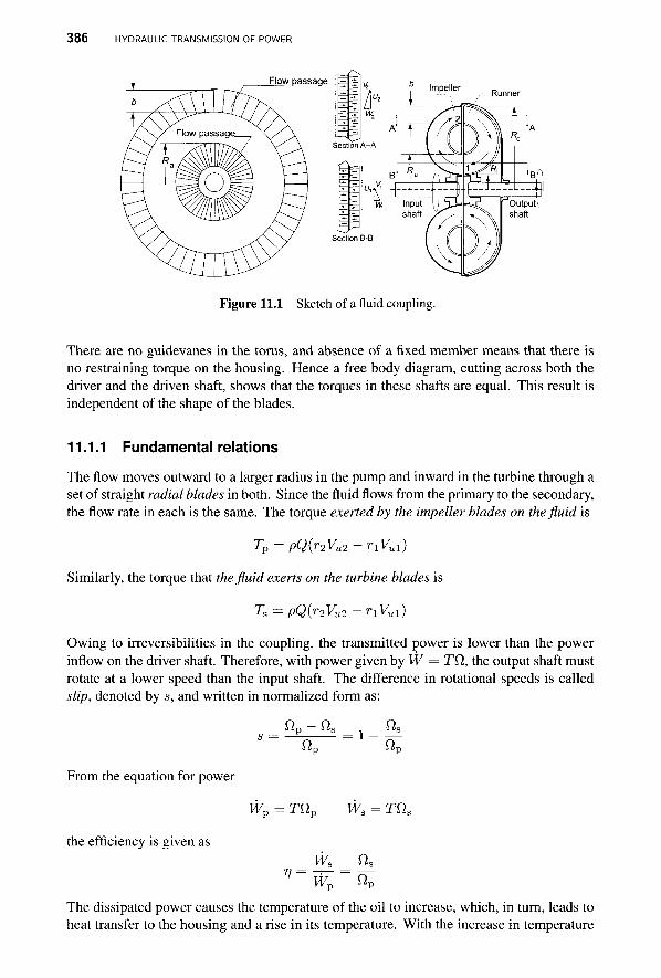
3 8 6 HYDRAULIC TRANSMISSION OF POWER
Impeller
Figure 11.1 Sketch of a fluid coupling.
There are no guidevanes in the torus, and absence of a fixed member means that there is no restraining torque on the housing. Hence a free body diagram, cutting across both the driver and the driven shaft, shows that the torques in these shafts are equal. This result is independent of the shape of the blades.
11.1.1 Fundamental relations
The flow moves outward to a larger radius in the pump and inward in the turbine through a set of straight radial blades in both. Since the fluid flows from the primary to the secondary, the flow rate in each is the same. The torque exerted by the impeller blades on the fluid is
Tv = PQ{r2Vu2-rlVul)
Similarly, the torque that the fluid exerts on the turbine blades is
Ts = PQ(r2Vu2 - nVul)
Owing to irreversibilities in the coupling, the transmitted power is lower than the power inflow on the driver shaft. Therefore, with power given by W = Tfi, the output shaft must rotate at a lower speed than the input shaft. The difference in rotational speeds is called slip, denoted by s, and written in normalized form as:
1 ip i £s
fin a fin
From the equation for power
Wn = Tfir Ws = TQS
the efficiency is given as
a fin
The dissipated power causes the temperature of the oil to increase, which, in turn, leads to heat transfer to the housing and a rise in its temperature. With the increase in temperature
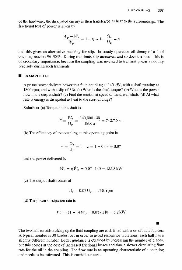
FLUID COUPLINGS 387
of the hardware, the dissipated energy is then transferred as heat to the surroundings. The fractional loss of power is given by
Wp-Wa * , fis —^-. = 1-77 = 1 - — = s
Wp ^p and this gives an alternative meaning for slip. In steady operation efficiency of a fluid coupling reaches 96-98%. During transients slip increases, and so does the loss. This is of secondary importance, because the coupling was invented to transmit power smoothly precisely during such transients.
■ EXAMPLE 11.1
A prime mover delivers power to a fluid coupling at 140 kW, with a shaft rotating at 1800 rpm, and with a slip of 3%. (a) What is the shaft torque? (b) What is the power flow in the output shaft? (c) Find the rotational speed of the driven shaft, (d) At what rate is energy is dissipated as heat to the surroundings?
Solution: (a) Torque on the shaft is
T=WR= 140,000-30 = 7 4 2 J N . m
ftp 1800 n
(b) The efficiency of the coupling at this operating point is
7 7 = - p = l - s = l - 0.03 = 0.97 i 'p
and the power delivered is
WS = T)WP= 0.97 ■ 140 = 135.8 kW
(c) The output shaft rotates at
fts = 0.97 ftp = 1746 rpm
(d) The power dissipation rate is
Wd = (1 - 77) Wp = 0.03 • 140 = 4.2 kW
The two half-toroids making up the fluid coupling are each fitted with a set of radial blades. A typical number is 30 blades, but in order to avoid resonance vibrations, each half has a slightly different number. Better guidance is obtained by increasing the number of blades, but this comes at the cost of increased frictional losses and thus a slower circulating flow rate for the oil in the coupling. The flow rate is an operating characteristic of a coupling and needs to be estimated. This is carried out next.
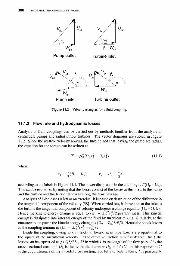
388 HYDRAULIC TRANSMISSION OF POWER
Pump outlet P2 W; "2 s2
Turbine inlet
iJVX1
t
p.,
a
w, s1
Pump inlet Turbine outlet
Figure 11.2 Velocity triangles for a fluid coupling.
11.1.2 Flow rate and hydrodynamic losses
Analysis of fluid couplings can be carried out by methods familiar from the analysis of centrifugal pumps and radial inflow turbines. The vector diagrams are shown in Figure 11.2. Since the relative velocity leaving the turbine and that leaving the pump are radial, the equation for the torque can be written as
T = PQ(npr22 - nsrj) (11.1)
where
n = -{Ri + Ra) Tl Rr,
according to the labels in Figure 11.1. The power dissipation in the coupling is T(QP — Qs). This can be estimated by noting that the losses consist of the losses at the inlets to the pump and the turbine and the frictional losses along the flow passage.
Analysis of inlet losses is left as an exercise. It is based on destruction of the difference in the tangential component of the velocity [58]. When carried out, it shows that at the inlet to the turbine the tangential component of velocity undergoes a change equal to (fip — Qs)^2-Hence the kinetic energy change is equal to (fip — fi s ) 2 r | /2 per unit mass. This kinetic energy is dissipated into internal energy of the fluid by turbulent mixing. Similarly, at the entrance to the pump the kinetic energy change is (fip — fls)2r2/2. Hence the shock losses in the coupling amount to (f2p — Q,s)2{r2 + r | ) / 2 .
Inside the coupling, owing to skin friction, losses, as in pipe flow, are proportional to the square of the meridional velocity. If the effective friction factor is denoted by / the losses can be expressed as fLQ2/2Dy,A2 in which L is the length of the flow path, A is the cross-sectional area, and D^ is the hydraulic diameter D^ = AA/C. In this expression C is the circumference of the toroidal cross section. For fully turbulent flows, / is practically
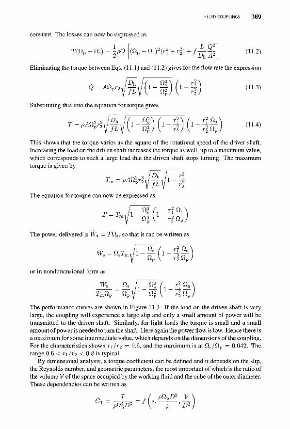
FLUID COUPLINGS 389
constant. The losses can now be expressed as
T(np - ns) = ~PQ (fip-fi ,rW+r22) + /
L Q2
(11.2) DhA\
Eliminating the torque between Eqs. (11.1) and (11.2) gives for the flow rate the expression
Q = Anpr2 «2 1 -
Substituting this into the equation for torque gives
1 - 1 - 1 -Try \lT
(11.3)
(11.4)
This shows that the torque varies as the square of the rotational speed of the driver shaft. Increasing the load on the driven shaft increases the torque as well, up to a maximum value, which corresponds to such a large load that the driven shaft stops turning. The maximum torque is given by
The equation for torque can now be expressed as
"l *'s
2 s 'p
The power delivered is Ws = Tfls, so that it can be written as
wa = naTmji
or in nondimensional form as
Ws
T fi
r2 O ' 2 s i P
Try \lT
The performance curves are shown in Figure 11.3. If the load on the driven shaft is very large, the coupling will experience a large slip and only a small amount of power will be transmitted to the driven shaft. Similarly, for light loads the torque is small and a small amount of power is needed to turn the shaft. Here again the power flow is low. Hence there is a maximum for some intermediate value, which depends on the dimensions of the coupling. For the characteristics shown r\/r2 — 0.6, and the maximum is at f2s/f2p — 0.642. The range 0.6 < r\jr2 < 0.8 is typical.
By dimensional analysis, a torque coefficient can be defined and it depends on the slip, the Reynolds number, and geometric parameters, the most important of which is the ratio of the volume V of the space occupied by the working fluid and the cube of the outer diameter. These dependencies can be written as
CV T PniD5 f[s,
pnpD2 v_
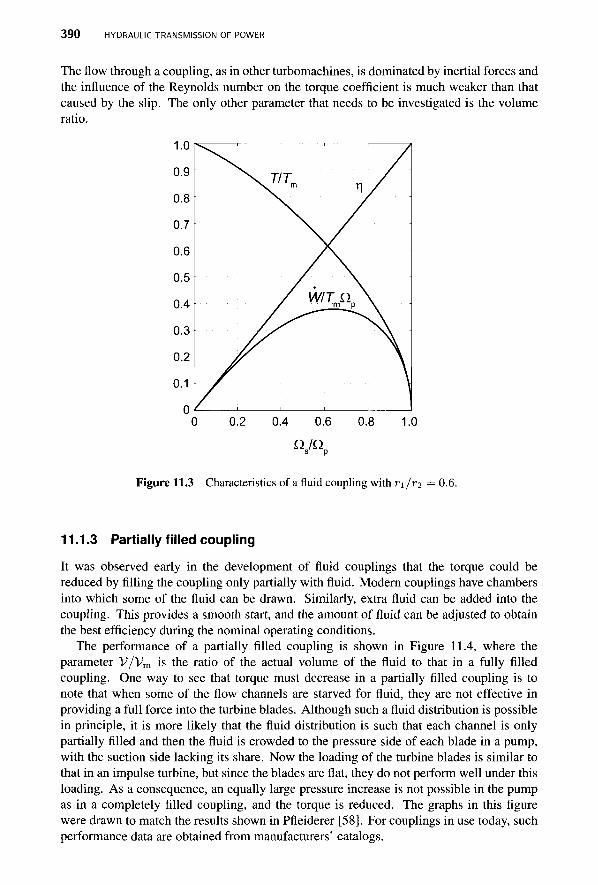
390 HYDRAULIC TRANSMISSION OF POWER
The flow through a coupling, as in other turbomachines, is dominated by inertial forces and the influence of the Reynolds number on the torque coefficient is much weaker than that caused by the slip. The only other parameter that needs to be investigated is the volume ratio.
1.0
0.9
0.8
0.7
0.6
0.5
0.4
0.3
0.2
0.1
0 0 0.2 0.4 0.6 0.8 1.0
Q / Q s p
Figure 11.3 Characteristics of a fluid coupling with r\jr2 = 0.6.
11.1.3 Partially filled coupling
It was observed early in the development of fluid couplings that the torque could be reduced by filling the coupling only partially with fluid. Modern couplings have chambers into which some of the fluid can be drawn. Similarly, extra fluid can be added into the coupling. This provides a smooth start, and the amount of fluid can be adjusted to obtain the best efficiency during the nominal operating conditions.
The performance of a partially filled coupling is shown in Figure 11.4, where the parameter V/Vm is the ratio of the actual volume of the fluid to that in a fully filled coupling. One way to see that torque must decrease in a partially filled coupling is to note that when some of the flow channels are starved for fluid, they are not effective in providing a full force into the turbine blades. Although such a fluid distribution is possible in principle, it is more likely that the fluid distribution is such that each channel is only partially filled and then the fluid is crowded to the pressure side of each blade in a pump, with the suction side lacking its share. Now the loading of the turbine blades is similar to that in an impulse turbine, but since the blades are flat, they do not perform well under this loading. As a consequence, an equally large pressure increase is not possible in the pump as in a completely filled coupling, and the torque is reduced. The graphs in this figure were drawn to match the results shown in Pfleiderer [58]. For couplings in use today, such performance data are obtained from manufacturers' catalogs.
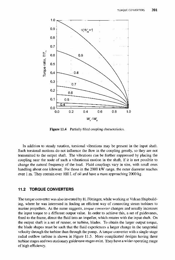
TORQUE CONVERTERS 3 9 1
1.0
0.9
0.8
0.7
|= 0.6 o 2 0.5 a)
I 0.4 0.3
0.2
0.1
0.0 0.0 0.2 0.4 0.6 0.8 1.0
WJK
Figure 11.4 Partially filled coupling characteristics.
In addition to steady rotation, torsional vibrations may be present in the input shaft. Such torsional motions do not influence the flow in the coupling greatly, so they are not transmitted to the output shaft. The vibrations can be further suppressed by placing the coupling near the node of such a vibrational motion in the shaft, if it is not possible to change the natural frequency of the load. Fluid couplings vary in size, with small ones handling about one kilowatt. For those in the 2000 kW range, the outer diameter reaches over 1 m. They contain over 100 L of oil and have a mass approaching 2000 kg.
11.2 TORQUE CONVERTERS
The torque converter was also invented by H. Fottinger, while working at Vulcan Shipbuild-ing, where he was interested in finding an efficient way of connecting steam turbines to marine propellers. As the name suggests, torque converter changes and usually increases the input torque to a different output value. In order to achieve this, a set of guidevanes, fixed to the frame, direct the fluid into an impeller, which rotates with the input shaft. On the output shaft is a set of runner, or turbine, blades. To obtain the larger output torque, the blade shapes must be such that the fluid experiences a larger change in the tangential velocity through the turbine than through the pump. A torque converter with a single-stage radial outflow turbine is shown in Figure 11.5. More complicated designs having three turbine stages and two stationary guidevane stages exist. They have a wider operating range of high efficiency.
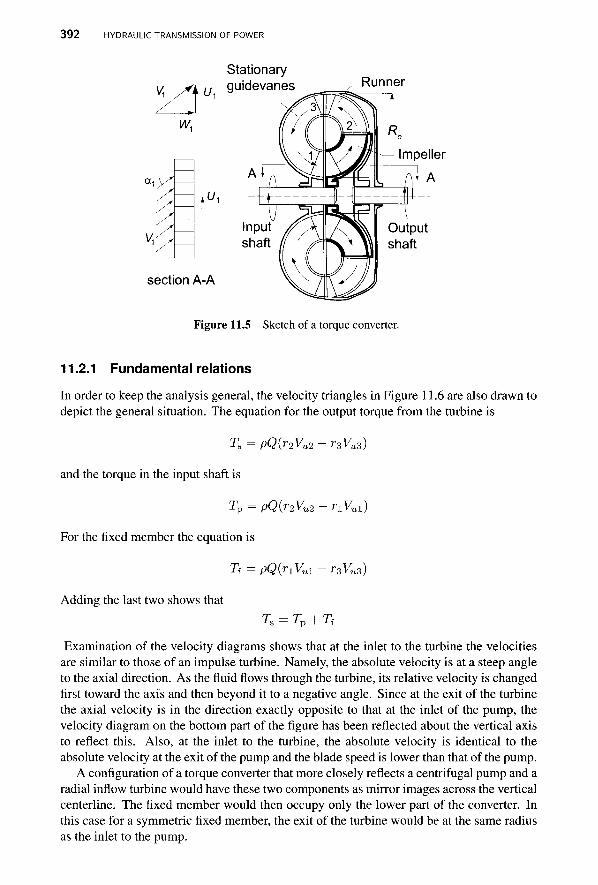
392 HYDRAULIC TRANSMISSION OF POWER
Stationary v -fk y guidevanes Runner
W,
U,
section A-A
Impeller
Input shaft
Output shaft
Figure 11.5 Sketch of a torque converter.
11.2.1 Fundamental relations
In order to keep the analysis general, the velocity triangles in Figure 11.6 are also drawn to depict the general situation. The equation for the output torque from the turbine is
Ts = pQ(r2Vu2 - r3Vu3)
and the torque in the input shaft is
TP = pQ(r2VU2 ~ nVui)
For the fixed member the equation is
T{ = pQ(nVul - r3Vu3)
Adding the last two shows that TS = TP + Tt
Examination of the velocity diagrams shows that at the inlet to the turbine the velocities are similar to those of an impulse turbine. Namely, the absolute velocity is at a steep angle to the axial direction. As the fluid flows through the turbine, its relative velocity is changed first toward the axis and then beyond it to a negative angle. Since at the exit of the turbine the axial velocity is in the direction exactly opposite to that at the inlet of the pump, the velocity diagram on the bottom part of the figure has been reflected about the vertical axis to reflect this. Also, at the inlet to the turbine, the absolute velocity is identical to the absolute velocity at the exit of the pump and the blade speed is lower than that of the pump.
A configuration of a torque converter that more closely reflects a centrifugal pump and a radial inflow turbine would have these two components as mirror images across the vertical centerline. The fixed member would then occupy only the lower part of the converter. In this case for a symmetric fixed member, the exit of the turbine would be at the same radius as the inlet to the pump.
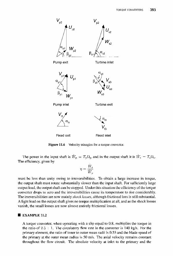
TORQUE CONVERTERS 393
Turbine inlet
a„
Pump inlet
S3
W
S3
I
S3
S3
Turbine exit
■f3
vf3
Fixed exit Fixed inlet
Figure 11.6 Velocity triangles for a torque converter.
The power in the input shaft is Wp = Tpf2p and in the output shaft it is Ws = TSQ,S. The efficiency, given by
V =
must be less than unity owing to irreversibilities. To obtain a large increase in torque, the output shaft must rotate substantially slower than the input shaft. For sufficiently large output load, the output shaft can be stopped. Under this situation the efficiency of the torque converter drops to zero and the irreversibilities cause its temperature to rise considerably. The irreversibilities are now mainly shock losses, although frictional loss is still substantial. A light load on the output shaft gives no torque multiplication at all, and as the shock losses vanish, the small losses are now almost entirely frictional losses.
■ EXAMPLE 11.2
A torque converter, when operating with a slip equal to 0.8, multiplies the torque in the ratio of 2.5 : 1. The circulatory flow rate in the converter is 140 kg/s. For the primary element, the ratio of inner to outer mean radii is 0.55 and the blade speed of the primary at the outer mean radius is 50 m/s. The axial velocity remains constant throughout the flow circuit. The absolute velocity at inlet to the primary and the
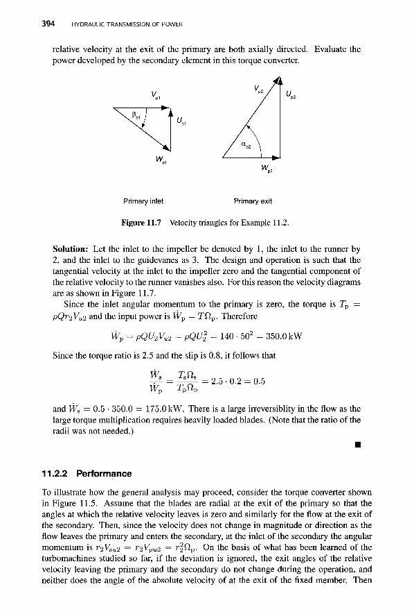
394 HYDRAULIC TRANSMISSION OF POWER
relative velocity at the exit of the primary are both axially directed. Evaluate the power developed by the secondary element in this torque converter.
W^
Primary inlet Primary exit
Figure 11.7 Velocity triangles for Example 11.2.
Solution: Let the inlet to the impeller be denoted by 1, the inlet to the runner by 2, and the inlet to the guidevanes as 3. The design and operation is such that the tangential velocity at the inlet to the impeller zero and the tangential component of the relative velocity to the runner vanishes also. For this reason the velocity diagrams are as shown in Figure 11.7.
Since the inlet angular momentum to the primary is zero, the torque is Tp = pQriVU2 and the input power is Wp — TQ,p. Therefore
Wp = pQU2Vu2 = pQUl = 140 • 502 = 350.0kW
Since the torque ratio is 2.5 and the slip is 0.8, it follows that
2.5 ■ 0.2 = 0.5
and Ws = 0.5 • 350.0 = 175.0 kW. There is a large irreversiblity in the flow as the large torque multiplication requires heavily loaded blades. (Note that the ratio of the radii was not needed.)
11.2.2 Performance
To illustrate how the general analysis may proceed, consider the torque converter shown in Figure 11.5. Assume that the blades are radial at the exit of the primary so that the angles at which the relative velocity leaves is zero and similarly for the flow at the exit of the secondary. Then, since the velocity does not change in magnitude or direction as the flow leaves the primary and enters the secondary, at the inlet of the secondary the angular momentum is ^ V ^ = ?*2̂ pu2 = r^flp- On the basis of what has been learned of the turbomachines studied so far, if the deviation is ignored, the exit angles of the relative velocity leaving the primary and the secondary do not change during the operation, and neither does the angle of the absolute velocity of at the exit of the fixed member. Then
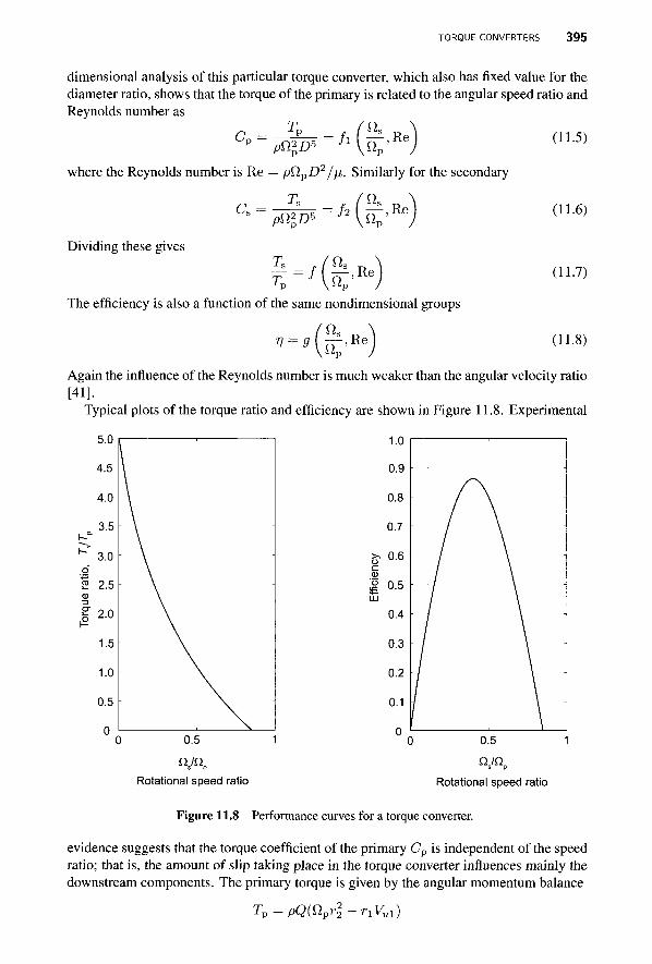
TORQUE CONVERTERS 395
dimensional analysis of this particular torque converter, which also has fixed value for the diameter ratio, shows that the torque of the primary is related to the angular speed ratio and Reynolds number as
Cn Tn
pft2£>5 *[%•*> where the Reynolds number is Re = pQ,pD2/ii. Similarly for the secondary
Cs Ts
pWD5
Dividing these gives
= /2
a
Re
The efficiency is also a function of the same nondimensional groups
V = 9 ,Re
(11.5)
(11.6)
(11.7)
(11.8)
Again the influence of the Reynolds number is much weaker than the angular velocity ratio [41].
Typical plots of the torque ratio and efficiency are shown in Figure 11.8. Experimental
5.0
4.5
4.0
3.5
K " 3.0
[ue
ratio
,
cn
| 2.0
1.5
1.0
0.5
0 C
1
) 0.5
S p
1.0
0.9
0.8
0.7
>- 0.6
Effic
ieni
o cn
0.4
0.3
0.2
0.1
°C
1
-
/ \
" / \ / \
" / \ "
/ \ 7 \ 7 \ ' / \ " \ ) 0.5 1
n/n„ s p
Rotational speed ratio Rotational speed ratio
Figure 11.8 Performance curves for a torque converter.
evidence suggests that the torque coefficient of the primary Cp is independent of the speed ratio; that is, the amount of slip taking place in the torque converter influences mainly the downstream components. The primary torque is given by the angular momentum balance
Tp = pQ(npr2 - r iKx i )
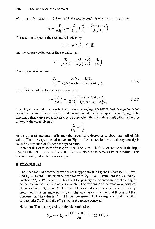
396 HYDRAULIC TRANSMISSION OF POWER
With Vui = Vxi tan a\ = Q tan a i /A, the torque coefficient of the primary is then
Tp Q (r\ Qritanai P (&l%,\ fipr3 ^ 2 Ar3Qp
The reaction torque of the secondary is given by
Ts = PQ(npr22 - Var2
3)
and the torque coefficient of the secondary is
,-, _ Ts _ Q i r2 S ls
'p'3 " p ' 3
The torque ratio becomes
Pni4 nprf \r2 nP
r2H'$ " s / ^ ' p TP rllrl - Qritan a i M ^ P r i
The efficiency of the torque converter is then
_ rsfts _ {r\irl - ns/np)ns/rip Tpflp r\jr\ - Qr\ tanai/ylrffip
(11-9)
(11.10)
Since Cp is assumed to be constant, it follows that Q/Qp is constant, and for a given torque converter the torque ratio is seen to decrease linearly with the speed ratio fis/fip. The efficiency then varies parabolically, being zero when the secondary shaft either is fixed or rotates at the value given by
" s __ r2 s 'p '3
At the point of maximum efficiency the speed ratio decreases to about one-half of this value. That the experimental curves of Figure 11.8 do not follow this theory exactly is caused by variation of Cp with the speed ratio.
Another design is shown in Figure 11.9. The output shaft is concentric with the input one, and the inlet mean radius of the fixed member is the same as its exit radius. This design is analyzed in the next example.
■ EXAMPLE 11.3
The mean radii of a torque converter of the type shown in Figure 11.9 are r\ = 10 cm and ri = 15 cm. The primary operates with Qp = 3000 rpm, and the secondary rotates at Qs — 1200 rpm. The blades of the primary are oriented such that the angle of the relative flow at the exit is /3P2 = 35°. The exit angle of the relative velocity of the secondary is /3S3 = —63°. The fixed blades are shaped such that the exit velocity from them is at the angle an = 55°. The axial velocity is constant throughout the converter, and its value is Vx = 15 m/s. Determine the flow angles and calculate the torque ratio Ts/Tp and the efficiency of the torque converter.
Solution: The blade speeds are first determined as
Upl = ri n p = — = 26.78 m/s
TORQUE CONVERTERS 397
Runner
Impeller
Input shaft f\r 7$
Stationary guidevanes
Output shaft
Figure 11.9 Torque converter with concentric shafts.
0.15- 1200 -7T o o r . Us2 = r2tts = — = 18.85 m/s
U. s3 r3ftp =
30 0.10-1200-7r
30 12.57 m/s
Next, the tangential velocity at the exit of the primary is determined. Since the flow angle of the relative flow is given, the tangential component Wpu2 is
Wpu2 = 14tan/?p2 = 15tan(35°) = 10.50 m/s
and the tangential component of the absolute velocity is
Vpu2 = Up2 + Wpu2 = 39.27 + 10.50 = 49.77 m/s
The flow angle is therefore
Q p 2 = tan"1 ( ^ - ) = tan"1 f ^ T ) = 73.23° Vx 15.00
The absolute velocity and its flow angle at the inlet of the secondary are the same as those leaving the primary. Hence Vsu2 = 49.77 m/s. The relative velocity entering the secondary has the tangential component
Wsu2 = Vsu2 - Us2 = 49.77 - 18.85 = 30.92 m/s
and its flow angle is
Ps2 = tan" W« su2
vx tan
30.92 15.00
= 64.12°
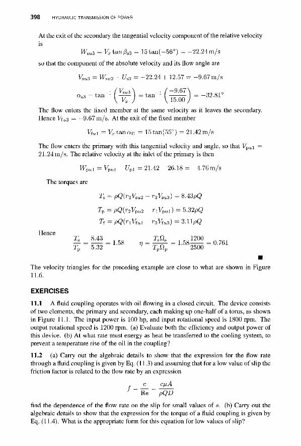
398 HYDRAULIC TRANSMISSION OF POWER
At the exit of the secondary the tangential velocity component of the relative velocity is
Wau3 = Vx tan/3s3 = 15tan(-56°) = -22.24m/s
so that the component of the absolute velocity and its flow angle are
Vsu3 = Wsu2 + Us3 = -22.24 + 12.57 = -9.67 m/s
as3 = tan-i (Y^A = tan-i (zMl) = _32.81° V Vx ) \ 15.00 )
The flow enters the fixed member at the same velocity as it leaves the secondary. Hence Vfu3 = —9.67 m/s. At the exit of the fixed member
Vfui = 14 tan an = 15tan(55°) = 21.42 m/s
The flow enters the primary with this tangential velocity and angle, so that Vpui = 21.24 m/s. The relative velocity at the inlet of the primary is then
Wpul = Vpul - Upl = 21.42 - 26.18 = -4.76 m/s
The torques are
Ts = PQ(r2Vsu2 - r3Vsu3) = 8A3pQ
Tp = PQ(r2Vpu2 - nVpul) = 5.32pQ
T{ = pQ{nViul - r3Viu3) = 3.11/oQ
Hence Ts 8.43 Tsns 1200 Tt = 5 ^ 2 = 1 - 5 8 ^ ^ = L 5 8 2 5 0 0 = 0 - 7 6 1
The velocity triangles for the preceding example are close to what are shown in Figure 11.6.
EXERCISES
11.1 A fluid coupling operates with oil flowing in a closed circuit. The device consists of two elements, the primary and secondary, each making up one-half of a torus, as shown in Figure 11.1. The input power is 100 hp, and input rotational speed is 1800 rpm. The output rotational speed is 1200 rpm. (a) Evaluate both the efficiency and output power of this device, (b) At what rate must energy as heat be transferred to the cooling system, to prevent a temperature rise of the oil in the coupling?
11.2 (a) Carry out the algebraic details to show that the expression for the flow rate through a fluid coupling is given by Eq. (11.3) and assuming that for a low value of slip the friction factor is related to the flow rate by an expression
t - JL - CA^ 1 ~ R^ ~ pQD
find the dependence of the flow rate on the slip for small values of s. (b) Carry out the algebraic details to show that the expression for the torque of a fluid coupling is given by Eq. (11.4). What is the appropriate form for this equation for low values of slip?
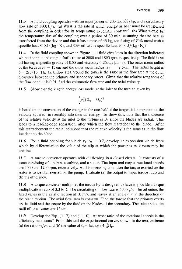
EXERCISES 399
11.3 A fluid coupling operates with an input power of 200 hp, 5% slip, and a circulatory flow rate of 1500 L/s. (a) What is the rate at which energy as heat must be transferred from the coupling in order for its temperature to remain constant? (b) What would be the temperature rise of the coupling over a period of 30 min, assuming that no heat is transferred from the device and that it has a mass of 45 kg, consisting of 70% metal with a specific heat 840 J/(kg • K), and 30% oil with a specific heat 2000 J/(kg • K)?
11.4 In the fluid coupling shown in Figure 11.1 fluid circulates in the direction indicated while the input and output shafts rotate at 2000 and 1800 rpm, respectively. The fluid is an oil having a specific gravity of 0.88 and viscosity 0.25 kg/(m • s). The outer mean radius of the torus is r-i = 15 cm and the inner mean radius is r\ = 7.5 cm. The radial height is b = 2^ /15 . The axial flow area around the torus is the same as the flow area at the outer clearance between the primary and secondary rotors. Given that the relative roughness of the flow conduit is 0.01, find the volumetric flow rate and the axial velocity.
11.5 Show that the kinetic energy loss model at the inlet to the turbine given by
— r 2 ( i i p — ils)
is based on the conversion of the change in the one-half of the tangential component of the velocity squared, irreversibly into internal energy. To show this, note that the incidence of the relative velocity at the inlet to the turbine is 02 since the blades are radial. This leads to a leading-edge separation, after which the flow reattaches to the blade. After this reattachement the radial component of the relative velocity is the same as in the flow incident on the blade.
11.6 For a fluid coupling for which r\JT2 = 0.7, develop an expression which from which by differentiation the value of the slip at which the power is maximum may be obtained.
11.7 A torque converter operates with oil flowing in a closed circuit. It consists of a torus consisting of a pump, a turbine, and a stator. The input and output rotational speeds are 4000 and 1200 rpm, respectively. At this operating condition the torque exerted on the stator is twice that exerted on the pump. Evaluate (a) the output to input torque ratio and (b) the efficiency.
11.8 A torque converter multiplies the torque by is designed to have to provide a torque multiplication ratio of 3.3 to 1. The circulating oil flow rate is 500 kg/s. The oil enters the fixed vanes in the axial direction at 10 m/s, and leaves at an angle 60° in the direction of the blade motion. The axial flow area is constant. Find the torque that the primary exerts on the fluid and the torque by the fluid on the blades of the secondary. The inlet and outlet radii of fixed vanes are 15 cm.
11.9 Develop the Eqs. (11.7) and (11.10). At what ratio of the rotational speeds is the efficiency maximum? From this and the experimental curves shown in the text, estimate (a) the ratio rijr?, and (b) the value of Qr\ tan a\jAr\^\v.
CHAPTER 12
WIND TURBINES
A brief history of wind turbines was given in Chapter 1. The early uses for grinding grain and lifting water have been replaced by the need to generate electricity. For this reason the designation windmill has been dropped and it has been replaced by a wind turbine. Wind turbines, such as are shown in Figure 12.1b, are the most rapidly growing renewable energy technology, but as they provide for only 0.5% of the primary energy production in the world, it will take a long time before their contribution becomes significant. Since the installed base of wind turbines is still relatively small, even a large yearly percentage increase in their use does not result in a large increase in the net capacity. But the possibility of growing wind capacity is large. The most windy regions of the United States are in the North and South Dakotas. These states, as well as the mountain ridges of Wyoming, the high plains of Texas, and the mountain passes of California, have seen the early gains in the number of wind turbines.
In countries such as Denmark and Germany, the growth of wind turbine power has been quite rapid. The winds from the North Sea provide particularly good wind prospects both onshore and offshore in Denmark's Jutland region. In fact, during the year 2011, 22% of Denmark's electricity was generated from wind, and the entire power needs of western Denmark are provided by its windfarms on the windiest days. The installed capacity of 3800 MW in Denmark in year 2010 come from 5000 units. Because she adopted wind technology early, Denmark's old wind turbines are being replaced today with larger modern units. Denmark's electricity production from wind in 2010 was about 7810GWh per year. The capacity factor is a modest 23% cent, owing to the intermittency of wind.
Principles of Turbomachinery. By Seppo A. Korpela 401 Copyright © 2011 John Wiley & Sons, Inc.
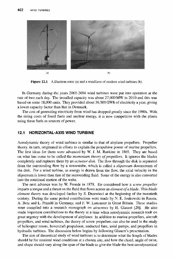
402 WIND TURBINES
(a) (b)
Figure 12.1 A Darrieus rotor (a) and a windfarm of modern wind turbines (b).
In Germany during the years 2001-2004 wind turbines were put into operation at the rate of two each day. The installed capacity was about 27,000 MW in 2010 and this was based on some 18,000 units. They provided about 36,500 GWh of electricity a year, giving a lower capacity factor than that in Denmark.
The cost of generating electricity from wind has dropped greatly since the 1980s. With the rising costs of fossil fuels and nuclear energy, it is now competitive with the plants using these fuels as sources of power.
12.1 HORIZONTAL-AXIS WIND TURBINE
Aerodynamic theory of wind turbines is similar to that of airplane propellers. Propeller theory, in turn, originated in efforts to explain the propulsive power of marine propellers. The first ideas for them were advanced by W. J. M. Rankine in 1865. They are based on what has come to be called the momentum theory of propellers. It ignores the blades completely and replaces them by an actuator disk. The flow through the disk is separated from the surrounding flow by a streamtube, which is called a slipstream downstream of the disk. For a wind turbine, as energy is drawn from the flow, the axial velocity in the slipstream is lower than that of the surrounding fluid. Some of the energy is also converted into the rotational motion of the wake.
The next advance was by W. Froude in 1878. He considered how a screw propeller imparts a torque and a thrust on the fluid that flows across an element of a blade. This blade element theory was developed further by S. Drzewieci at the beginning of the twentieth century. During the same period contributions were made by N. E. Joukowski in Russia, A. Betz and L. Prandtl in Germany, and F. W. Lancaster in Great Britain. These studies were compiled into a research monograph on airscrews by H. Glauert [28]. He also made important contributions to the theory at a time when aerodynamic research took on great urgency with the development of airplanes. In addition to marine propellers, aircraft propellers, and wind turbines, the theory of screw propellers can also be used in the study of helicopter rotors, hovercraft propulsion, unducted fans, axial pumps, and propellers in hydraulic turbines. The discussion below begins by following Glauert's presentation.
The aim of theoretical study of wind turbines is to determine what the length of blades should be for nominal wind conditions at a chosen site, and how the chord, angle of twist, and shape should vary along the span of the blade to give the blade the best aerodynamical
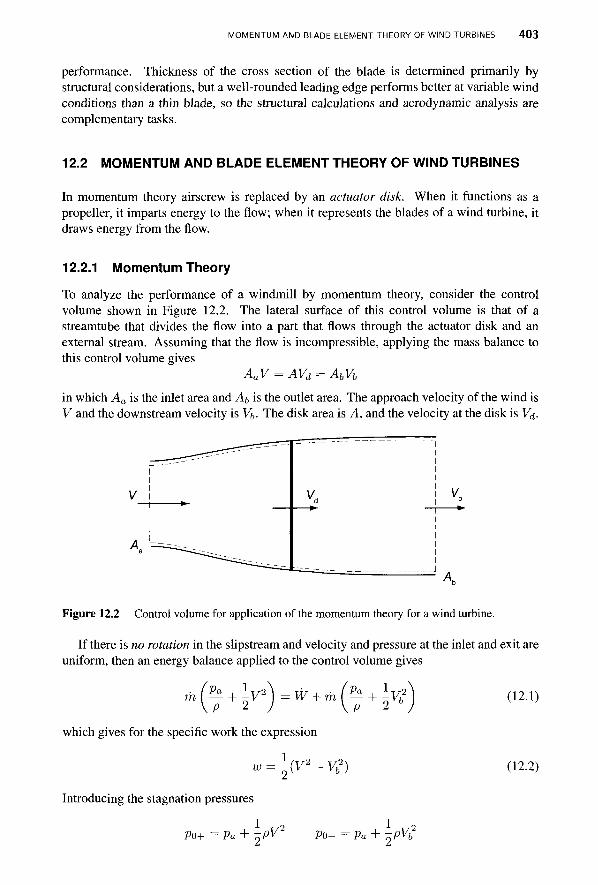
MOMENTUM AND BLADE ELEMENT THEORY OF WIND TURBINES 403
performance. Thickness of the cross section of the blade is determined primarily by structural considerations, but a well-rounded leading edge performs better at variable wind conditions than a thin blade, so the structural calculations and aerodynamic analysis are complementary tasks.
12.2 MOMENTUM AND BLADE ELEMENT THEORY OF WIND TURBINES
In momentum theory airscrew is replaced by an actuator disk. When it functions as a propeller, it imparts energy to the flow; when it represents the blades of a wind turbine, it draws energy from the flow.
12.2.1 Momentum Theory
To analyze the performance of a windmill by momentum theory, consider the control volume shown in Figure 12.2. The lateral surface of this control volume is that of a streamtube that divides the flow into a part that flows through the actuator disk and an external stream. Assuming that the flow is incompressible, applying the mass balance to this control volume gives
AaV = AVd = AbVb
in which Aa is the inlet area and Ab is the outlet area. The approach velocity of the wind is V and the downstream velocity is Vb. The disk area is A, and the velocity at the disk is V .̂
Figure 12.2 Control volume for application of the momentum theory for a wind turbine.
If there is no rotation in the slipstream and velocity and pressure at the inlet and exit are uniform, then an energy balance applied to the control volume gives
m l ^ + V P 2
W + rh Pa , 1 K2 (12.1)
which gives for the specific work the expression
1 (V*-VJ) (12.2)
Introducing the stagnation pressures
p0+ = Pa + -^PV2 P0- =Pa + ^pVb
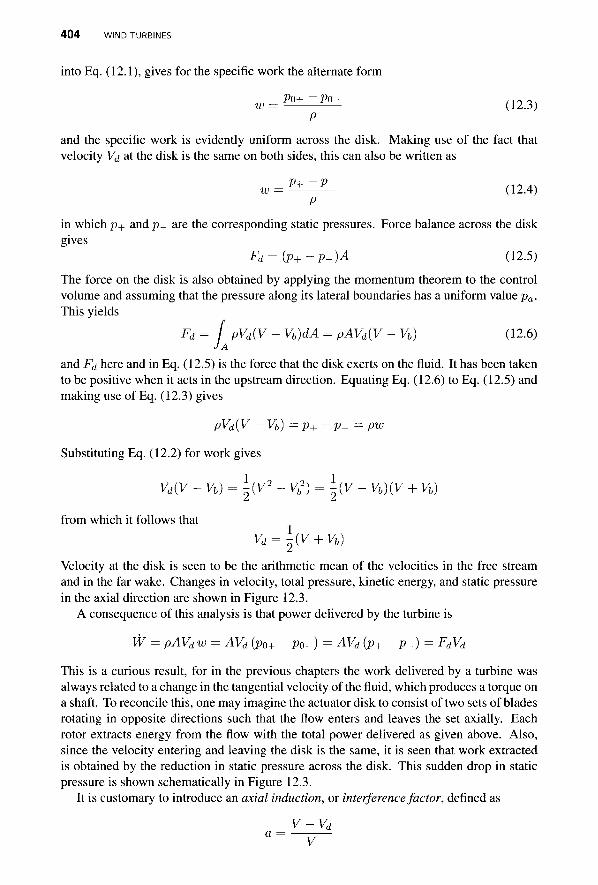
404 WIND TURBINES
into Eq. (12.1), gives for the specific work the alternate form
w = (12.3) P
and the specific work is evidently uniform across the disk. Making use of the fact that velocity Vd at the disk is the same on both sides, this can also be written as
w = P+~P- (12.4) P
in which p+ and p_ are the corresponding static pressures. Force balance across the disk gives
Fd = {p+~p.)A (12.5)
The force on the disk is also obtained by applying the momentum theorem to the control volume and assuming that the pressure along its lateral boundaries has a uniform value pa. This yields
Fd = [ PVd(V - Vb)dA = PAVd(V - Vb) (12.6) J A
and Fd here and in Eq. (12.5) is the force that the disk exerts on the fluid. It has been taken to be positive when it acts in the upstream direction. Equating Eq. (12.6) to Eq. (12.5) and making use of Eq. (12.3) gives
pw
(V-Vb)(V + Vb)
Velocity at the disk is seen to be the arithmetic mean of the velocities in the free stream and in the far wake. Changes in velocity, total pressure, kinetic energy, and static pressure in the axial direction are shown in Figure 12.3.
A consequence of this analysis is that power delivered by the turbine is
W = pAVd w = AVd (Po+ - po-) = AVd (p+ -p-) = FdVd
This is a curious result, for in the previous chapters the work delivered by a turbine was always related to a change in the tangential velocity of the fluid, which produces a torque on a shaft. To reconcile this, one may imagine the actuator disk to consist of two sets of blades rotating in opposite directions such that the flow enters and leaves the set axially. Each rotor extracts energy from the flow with the total power delivered as given above. Also, since the velocity entering and leaving the disk is the same, it is seen that work extracted is obtained by the reduction in static pressure across the disk. This sudden drop in static pressure is shown schematically in Figure 12.3.
It is customary to introduce an axial induction, or interference factor, defined as
V-Vd
pVd(
Substituting Eq. (12.2) for work g
Vd(V-
from which it follows that
vb) =
y-vb: ;ives
\(v>-
vd =
) = p+-
- vb2) =
\iv +
-p-
V vb)
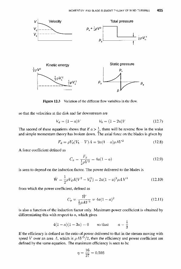
MOMENTUM AND BLADE ELEMENT THEORY OF WIND TURBINES 4 0 5
Velocity
pa+jpv-iM/2
Total pressure
IPK 2
Kinetic energy Static pressure
Figure 12.3 Variation of the different flow variables in the flow.
so that the velocities at the disk and far downstream are
Vd = (l-a)V Vb = (l-2a)V (12.7)
The second of these equations shows that if a > | , there will be reverse flow in the wake and simple momentum theory has broken down. The axial force on the blades is given by
Fd = PVd{Vb - V)A = 2a(l - a)PAV2
A force coefficient defined as Fx
(^.T \pv2 4a(l - a)
is seen to depend on the induction factor. The power delivered to the blades is
W 1 PVdA(V2 - Vb
2) = 2o(l - afpAV3
from which the power coefficient, defined as
W Or, hAV3 = 4 a ( l - a ) 2
(12.8)
(12.9)
(12.10)
(12.11)
is also a function of the induction factor only. Maximum power coefficient is obtained by differentiating this with respect to a, which gives
4 ( l - a ) ( l - 3 a ) - 0 so that 1
a — — 3
If the efficiency is defined as the ratio of power delivered to that in the stream moving with speed V over an area A, which is pAV3/2, then the efficiency and power coefficient are defined by the same equation. The maximum efficiency is seen to be
V 16 27 0.593
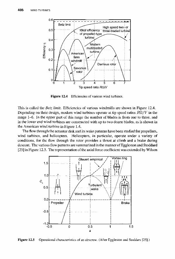
406 WIND TURBINES
2 3 4 5 6 7 Tip speed ratio RC1IV
Figure 12.4 Efficiencies of various wind turbines.
This is called the Betz limit. Efficiencies of various windmills are shown in Figure 12.4. Depending on their design, modern wind turbines operate at tip speed ratios Rfl/V in the range 1-6. In the upper part of this range the number of blades is from one to three, and in the lower end wind turbines are constructed with up to two dozen blades, as is shown in the American wind turbine in Figure 1.4.
The flow through the actuatpr disk and its wake patterns have been studied for propellers, wind turbines, and helicopters. Helicopters, in particular, operate under a variety of conditions, for the flow through the rotor provides a thrust at climb and a brake during descent. The various flow patterns are summarized in the manner of Eggleston and Stoddard [25] in Figure 12.5. The representation of the axial force coefficient was extended by Wilson
Figure 12.5 Operational characteristics of an airscrew. (After Eggleston and Stoddars [25].)
MOMENTUM AND BLADE ELEMENT THEORY OF WIND TURBINES 407
and Lissaman [82] to the brake range a > 1, by rewriting it as
Cx = 4a|l - a\
This explains the diskontinuity in the slope at a = 1. For a < 0, the airscrew operates as a propeller. The limit of vanishing approach velocity corresponds to a tending to a large negative value at a rate that keeps Vd finite while V tends to zero. Under this condition the airscrew functions as an unducted axial fan. Since the flow leaves the fan as a jet, pressure is atmospheric short distance into the wake, and with a pressure increase across the fan, pressure will be lower than atmospheric at the inlet to the fan. This low pressure causes the ambient air to accelerate toward the front of the fan. At a given rotational speed, proper orientation of the blades gives a smooth approach. A slipstream forms downstream of the fan, separating the wake from the external flow. The wake is in angular rotation, and vorticity that is shed from the blades forms a cylindrical vortex sheet that constitutes the boundary of the slipstream. As a consequence, at the slipstream boundary velocity changes discontinuously from the wake to the surrounding fluid. This discontinuous change and rotation are absent in the flow upstream of the disk where the flow is axial, if the small radial component near the disk is neglected.
As the approach velocity increases to some small value V, the airscrew functions as a propeller, in which case V can be taken to be the velocity of an airplane flying through still air. The continuity equation now shows that the mass flow rate m across the propeller comes from an upstream cylindrical region of area Aa, given by Aa = rii/pV, and the area decreases as the velocity V increases.
A further increase in the approach velocity leads to a condition at which a = 0. At this state no energy is imparted to, or extracted from, the flow, and the slipstream neither expands nor contracts. As the velocity V increases from this condition, the angle of attack changes to transform what was the pressure side of the blade into the suction side, and the airscrew then extracts energy from the flow. The airscrew under this condition operates as a wind turbine. The blades are naturally redesigned so that they function optimally when they are used to extract energy from the wind. In a wind turbine pressure increases as it approaches the plane of the blades and drops across them. The diameter of the slipstream, in contrast to that of a propeller, increases in the downstream direction.
For a > \ the slipstream boundary becomes unstable and forms vortex structures that mix into the wake. This is shown in Figure 12.5 as the turbulent wake state. The theoretical curve in the figure no longer holds, and an empirical curve of Glauert gives the value of the force coefficient in this range. At the condition a = 1 the flow first enters a vortex ring state and for large values, a brake state. Flows in these regions are sufficiently complex that they cannot be analyzed by elementary methods.
The aim of wind turbine theory is to explain how the induction factors change as a result of design and operating conditions. When the theory is developed further, it will be seen that wind turbines operate in the range 0 < a < \, which is consistent with the momentum theory.
12.2.2 Ducted wind turbine
Insight can be gained by repeating the analysis for a wind turbine placed in a duct and then considering the limit as the duct radius tends to infinity. Such an arrangement is shown in Figure 12.6. Applying the momentum equation to the flow through the control volume
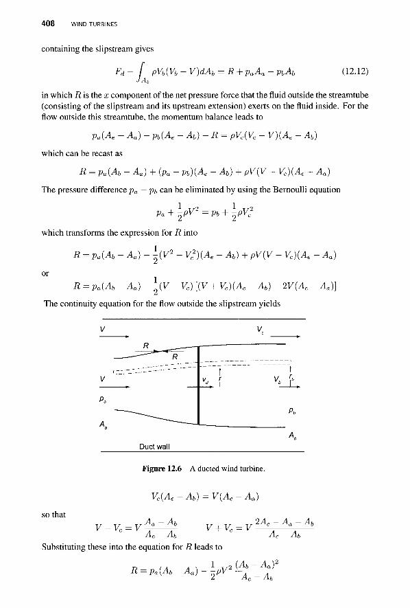
408 WIND TURBINES
containing the slipstream gives
Fd- I pVb{Vb - V)dAb = R + PaAa - PbAb JAb
(12.12)
in which R is the x component of the net pressure force that the fluid outside the streamtube (consisting of the slipstream and its upstream extension) exerts on the fluid inside. For the flow outside this streamtube, the momentum balance leads to
Pa(Ae - Aa)-Pb(Ae -Ab)-R = PVC(VC - V)(Ae - Ab)
which can be recast as
R = Pa{Ab - Aa) + (Pa - Pb)(Ae - Ab) + pViy - Vc)(Ae - Aa)
The pressure difference pa — pb can be eliminated by using the Bernoulli equation
Pa + ^pV2 =Pb + ̂ pVc2
which transforms the expression for R into
R = Pa(Ab - Aa) ~\(V2- V2)(Ae - Ab) + PV(V - Vc)(Ae - Aa)
or R = Pa(Ab -Aa)-±{V- Vc) [(V + Vc)(Ae - At) - 2V(Ae - Aa)}
The continuity equation for the flow outside the slipstream yields
V
V
R |
-~"~~* R —
vc
1
t K 'f,
Duct wall
Figure 12.6 A ducted wind turbine.
so that
Vc(Ae ~ Ab) - V(Ae - Aa)
V -V, = V Ab
Ae-Ab
Substituting these into the equation for R leads to
V + Vc = V ■ 2A„ Ah
AP-Ab
fl=p«(^-^)-^»*(^_y
MOMENTUM AND BLADE ELEMENT THEORY OF WIND TURBINES 4 0 9
This shows that, as Ae becomes large in comparison to Aa and Ab, then
R = pa{Ab~Aa)
The extra term then accounts for the variable pressure along the streamtube boundary. That the pressure is not exactly atmospheric along this boundary is also clear by noting that whenever streamlines are curved, pressure increases in the direction from the concave to the convex sides. Also, as the axial velocity decreases, pressure increases, but this is compensated partly by the flow acquiring a small radial velocity as the area of the streamtube increases downstream.
Equation 12.12 for the force on the blades now takes the form
Fd- f PVb{Vb-V)dAb = R + PaAa PbA b
I \ A 1 tr2 \Ab Aa) = {Pa-pb)Ab--PV A e _ A
= \p{V?-V2)Ab-l-pV2{Ab~Aa)2
2 r v c ' " T Ae-A b
Since
v2 - v2 = (yc - v)(vc + v) = v2
this can be written as
/2Ae-Aa-At
V Ae-Ab
Fd- f PVb(Vb - V)dAb - \pV2 (Ah Aal [Ae(Aa + Ab) - 2AaAb] JA„ 2 (Ae - Ab)z
For large Ae this reduces to
Fd= f PVb{V -Vb)dAb (12.13) JAb
This is equivalent to Eq. (12.6) obtained above. It is now assumed that this equation is also valid for each annular element of the streamtube shown in Figure 12.6. The differential form can be written as
dFd = pVb{V - Vb)dAb = PV{V - Vb)dA
The analysis based on this equation is called a blade element analysis and is justified if no interactions take place between adjacent annular elements. This assumption has been criticized by Goorjian [30], but evidently in many applications of the theory the error is small.
12.2.3 Blade element theory and wake rotation
Wake rotation was included in the theory by Joukowski in 1918 and its presentation can be found in Glauert [28]. This theory is considered next.
The continuity equation for an annular section of the slipstream gives
Vdx dA = Vbx dAb or Vdx rdr = Vbx rbdrb (12.14)
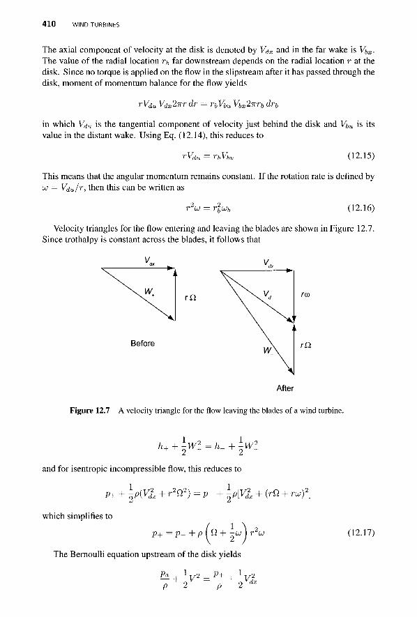
410 WIND TURBINES
The axial component of velocity at the disk is denoted by Vdx and in the far wake is Vbx. The value of the radial location rb far downstream depends on the radial location r at the disk. Since no torque is applied on the flow in the slipstream after it has passed through the disk, moment of momentum balance for the flow yields
rVdu Vdx2irr dr — rbVbu Vbx2nrb drb
in which Vdu is the tangential component of velocity just behind the disk and Vbu is its value in the distant wake. Using Eq. (12.14), this reduces to
rVdu = rbVbu (12.15)
This means that the angular momentum remains constant. If the rotation rate is defined by w = Vdu/r, then this can be written as
r2cu = r2tob (12.16)
Velocity triangles for the flow entering and leaving the blades are shown in Figure 12.7. Since trothalpy is constant across the blades, it follows that
V..
r n
Before
\A
After
Figure 12.7 A velocity triangle for the flow leaving the blades of a wind turbine.
h+ + \w\ = h^+ l-W2_
and for isentropic incompressible flow, this reduces to
P+ + \p(Vl + r2Q2) = v- + \p[Vl + (rn + ru)2}
which simplifies to
P+ = P- + P \ 0 + 2 u ) r w
The Bernoulli equation upstream of the disk yields
(12.17)
^ + > = ^ + M
MOMENTUM AND BLADE ELEMENT THEORY OF WIND TURBINES 4 1 1
and downstream it yields
P - 1 P
, ~ir2 , 1 2 2 Pb , 1 T A 2 , " ' ■ 2 2 + 2 ^ + 2 r W = 7 + 2 ^ + 2 ^
Adding the last two equations and using Eq. (12.17) to eliminate the pressure difference p+ — p- leads to
Pa Pb-\vbl-V^+[n + -nu}b)rlu}b P P 2
Differentiating this with respect to rb gives
_ldpb = 1 _^(V2 _ y2] , A_ pdrb 2drb
(bx ' drb tf. + ^ujb ) r̂ Wft
(12.18)
Since the radial pressure variation in the downstream section is also given by
p drb rb
equating these two pressure gradients produces
= rbub
or
1 d 2~dVb
l_d_ Ydrb
(Vbl ~ V2) -
(Vb2x - V*)
drb ^ + xwb ) r\ub ■nub
drb
drb
2 2 d-U)b 2
rbu)b -rbwb- rbwb
2dujb\ bdrb)
- tob I 2rbub + r\
drlujb
drb (12.19)
Momentum balance for the streamtube containing the flow through the disk yields
/ pVbx(Vbx - V)dAb = / (pa- pb)dAb - Fd
JAh JAb
Assuming that this is also valid for an annular element yields
dFd = pVbx{V - Vbx)dAb + {pa - pb)dAb
This elemental force is related to the pressures difference across the disk, which according to Eq. (12.17) can be related to rotation as
dFd = (p+ - p-)dA = p (n + -r2co
When Eq. (12.14) is used, this takes the form
dFd = pUl+ ^r2w) ^dAb
412 WIND TURBINES
Therefore the momentum balance for an elemental annulus becomes
pVbxiV - Vbx) + Pa ~ Pb = P ( ft + T^2 ) r2uj7T'
Eliminating the pressure difference pa — pb by making use of Eq. (12.18) gives
Vbx{V - Vbx) - \{V2 - V2X) + (to + i W b ) riui O i l l\ 2 Vbx
n+2U} rlJWx
which simplifies to
(v-vbx)2 _ {n + \Lobybu}b 2Vbx Vbx
(ft + \w)r2uj Wx
(12.20)
This is the main result of Joukowski's analysis. If ojb is now specified, then Eq. (12.19) can be solved for Vbx(rb)- After this, from Eq. (12.16), rotation w{r, rb) at the disk can be obtained as a function of r and r;,. The axial velocity Vdx(r,rb) at the disk is then obtained from Eq. (12.20). Substituting these into the continuity equation [Eq. (12.14)] gives a differential equation that relates rb to r. Appropriate boundary conditions fix the values for the integration constants.
12.2.4 Irrotational wake
The analysis of the previous section is valid for an arbitrary rotational velocity distribution in the wake. An important special case is to assume the wake to be irrotational. Then r2ui = r2Ub = k is constant. Equation (12.19) then shows that Vbx is constant across the wake, and Eq. (12.20) can be recast in the form
Vdx [1
Vbx [2
Writing Eq. (12.14) as
(V - Vbx)2 n+2r>]k
Vdx _ rbdrb
Vhx r dr and making use of it in Eq. (12.21) leads to
^ + 2 ^ 1 ^ (12.21)
(V - Vbx)2 - ftfc n drb k2 drb
~2^b~ -Vlkrdr —
k2 dr
Integrating this gives
'1 (v - vbxy ftfc n ^ - - l n -
2 2 eRb -flk-
k2 r
where R is the disk radius and Rb the downstream slipstream radius. Owing to the logarithmic singularity, the lower limits of integration were taken to be eR and eRb, so that as e tends to zero, eR/eRb tends to R/Rb. Thus the solution takes the form
\(V-Vbx) ■Clk 1 In rRb
MOMENTUM AND BLADE ELEMENT THEORY OF WIND TURBINES 4 1 3
The most reasonable way to satisfy this equation is to choose the r dependence of rb to be
Rb
for the logarithmic term then vanishes and the second term is a constant, which balances the first constant term. Thus an equation is obtained that relates the far wake axial velocity to the slipstream radius Rb
i , „ „ ,2 ~ . (- R2
2(V - Vbxy = Qk \1 - j ^ j (12.22)
Furthermore the following ratios are obtained:
4 = ^ = ^ = | (12-23) rg u Vdx Rl
Following Glauert's notation [28] this equation can be put into a nondimensional form by introducing the parameters
, V Vdx Vbx q k A = - — (i = - — Hb Rn ^ Rn ™ Rn n R2n
In terms of these parameters, Eq. (12.22) can be written as
q = y? (A - nb? 2 {(i-(ib)
Equation (12.18), namely
Pa Pb _ l n r 2 T/2N , (r, , l,.\„2
(12.24)
evaluated at the edge of the slipstream, where pb = p a , gives
In terms of the nondimensional parameters this can be transformed into
1-(X^M)=(l + ^ ) q - (12.25)
Eliminating q between this and Eq. (12.24) gives
4(A* - iib)(2(jt -fib-X)= (i(X ~ (ib)3 (12.26)
Equations (12.25) and (12.26) determine (i and (ib in terms of ratio A and q. Equation (12.26) can be written as
V = 7,{X + (Ln) + — (12.27) 2 8(fj, - (ib)
or in dimensional variables as
2V °x' 8{Vdx-Vbx)WR2
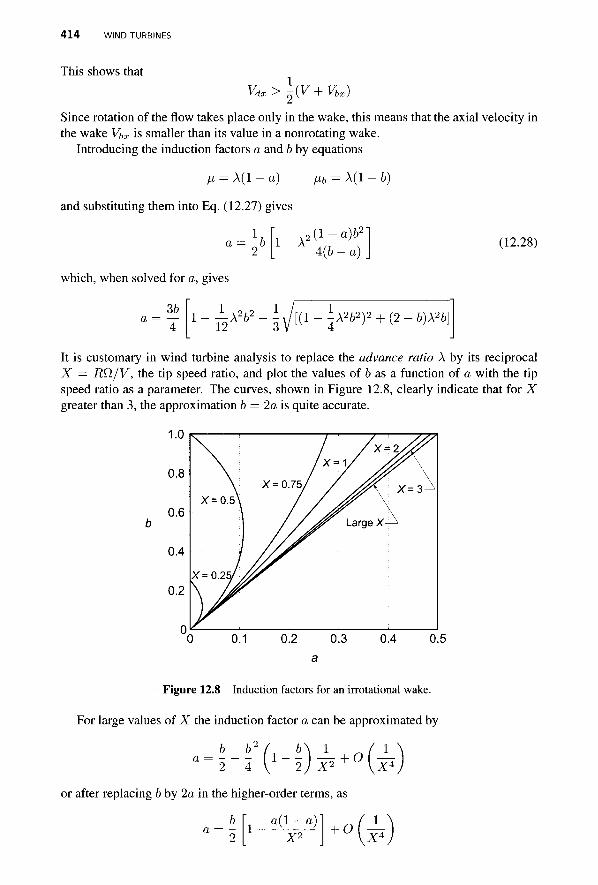
4 1 4 WIND TURBINES
This shows that Vdx>1-{V + Vbx)
Since rotation of the flow takes place only in the wake, this means that the axial velocity in the wake Vbx is smaller than its value in a nonrotating wake.
Introducing the induction factors a and b by equations
fi = A(l — a)
and substituting them into Eq. (12.27) gives
1 1 - A
fib = A(l - b)
2(l-a)b2
4(6 - a) (12.28)
which, when solved for a, gives
36 i - ^ A V - ^ K i -A262)2 + (2 - 6)A26]
It is customary in wind turbine analysis to replace the advance ratio A by its reciprocal X = Rtt/V, the tip speed ratio, and plot the values of 6 as a function of a with the tip speed ratio as a parameter. The curves, shown in Figure 12.8, clearly indicate that for X greater than 3, the approximation b = 2a is quite accurate.
Figure 12.8 Induction factors for an irrotational wake.
For large values of X the induction factor a can be approximated by
b b2 / b\ 1 / 1 a = 2 " 4 ( 1 - 2 ) x ^ + 0 ( x ^
or after replacing b by 2a in the higher-order terms, as
a(l — a) X2 + 0 X4
BLADE FORCES 415
Similarly a(l
2a 1 X2 Ol± This formula gives an estimate of the extent to which the axial velocity in the wake has been reduced as a result of wake rotation.
The expression for torque is
dT = 2-7TpVdxrVdur dr = 2npVdxkrdr
which when integrated over the span gives
T = PAVdxk
Hence the torque coefficient
Vdxk pAil2E? il2R3 H
is given by the parameter q. With W = Til, the power coefficient becomes
Til _2q_ b2(l-a)2
p ~ pVA\V2 ~~ A3 ~~ b-a
Since r2to is constant, the rate of rotation in an irrotational wake increases with decreas-ing radius and for small enough radius the rotation rate becomes unreasonably large. This leads to an infinite value for the power coefficient. To remedy this, the wake structure needs modification, and a reasonable model is obtained by making it a combination of solid body rotation at small radii and free vortex flow over large radii. The power coefficient for this, called the Rankine combined vortex, was stated by Wilson and Lissaman to be
Cp = b^bZaJ l2aN + &(1 ~ N)]
in which N = il/u>mSiX. The details on how to develop this are not in their report, and it appears that in order to develop it, some assumptions need to be made [82].
12.3 BLADE FORCES
The blade forces can be calculated at each location of the span by the blade element analysis. This is carried out for an annular slice of thickness dr from the disk, as is shown in Figure 12.9. Across each blade element airflow is assumed to be the same as that for an isolated airfoil. The situation in which wake rotation is ignored is considered first. Then the general analysis including wake rotation and Prandtl's tip loss model is discussed.
12.3.1 Nonrotating wake
If the wake rotation is ignored, the velocity triangle at the midchord is as shown in Figure 12.10. The approach velocity at the disk is (1 — a)V and the blade element moves at the tangential speed ril. The broken (dashed) line gives the direction of the chord and thus defines the blade pitch angle 9, which is measured from the plane of the disk. The angle
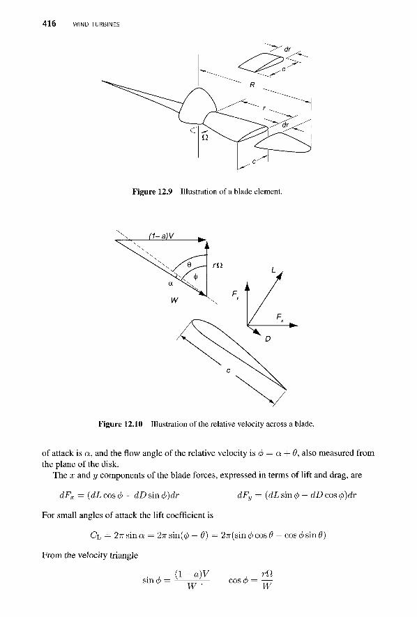
416 WIND TURBINES
Figure 12.9 Illustration of a blade element.
Figure 12.10 Illustration of the relative velocity across a blade.
of attack is a, and the flow angle of the relative velocity is <j> = a + 9, also measured from the plane of the disk.
The x and y components of the blade forces, expressed in terms of lift and drag, are
dFx = {dL cos (f> + dD sin (f>)dr dFy = (dL sin (p — dD cos (p)dr
For small angles of attack the lift coefficient is
CL = 2-K sin a = 2n sm(<f> — 9) = 27r(sin <p cos 9 — cos (f> sin 9)
From the velocity triangle
. (l-a)V rn
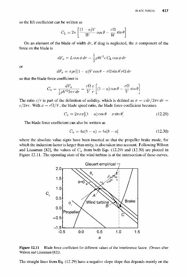
BLADE FORCES 417
so the lift coefficient can be written as
-(l-a)V Cx. = 2n
W rtt
smt
On an element of the blade of width dr, if drag is neglected, the x component of the force on the blade is
dFx = Lcos<j>dr = ~PW2CCL COS(pdr
or dFx — 7rpc[(l — a)V cos 9 — rfl sin 9]rfl dr
so that the blade force coefficient is
dFT rfl c ^x \pV22'Kr dr V r rVL
(1 — a)cos# —— sin(
The ratio c/r is part of the definition of solidity, which is defined as a = cdr/2nr dr c/2nr. With x = r£l/V, the blade speed ratio, the blade force coefficient becomes
Cx = 2irax[(l — a) cos 9 — x sin9]
The blade force coefficient can also be written as
Cx = 4a(l - a) = 4a|l - a\
(12.29)
(12.30)
where the absolute value signs have been inserted so that the propeller brake mode, for which the induction factor is larger than unity, is also taken into account. Following Wilson and Lissaman [82], the values of Cx from both Eqs. (12.29) and (12.30) are plotted in Figure 12.11. The operating state of the wind turbine is at the intersection of these curves.
Glauert empirical
Figure 12.11 Blade force coefficient for different values of the interference factor. (Drawn after Wilson and Lissaman [82]).
The straight lines from Eq. (12.29) have a negative slope slope that depends mainly on the
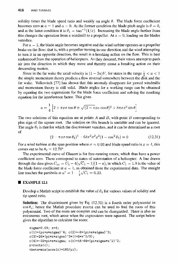
418 WIND TURBINES
solidity times the blade speed ratio and weakly on angle 9. The blade force coefficient becomes zero at a = 1 and a — 0. At the former condition the blade pitch angle is 6 = 0, and at the latter condition it is 9\ = tan_ 1( l / : r ) . Increasing the blade angle further from this changes the operation from a windmill to a propeller. At a = 0, loading on the blades vanishes.
For a = 1, the blade angle becomes negative and the wind turbine operates as a propeller brake on the flow; that is, with a propeller turning in one direction and the wind attempting to turn it in an opposite direction, the result is a breaking action on the flow. This is best understood from the operation of helicopters. As they descend, their rotors attempt to push air into the direction in which they move and thereby cause a breaking action on their descending motion.
Since in the far wake the axial velocity is (1 — 2a) V, for states in the range \ < a < 1 the simple momentum theory predicts a flow reversal somewhere between the disk and the far wake. Volkovitch [77] has shown that this anomaly disappears for yawed windmills and momentum theory is still valid. Blade angles for a working range can be obtained by equating the two expressions for the blade force coefficient and solving the resulting equation for the interference factor. This gives
a = — 2 + nxa cos 9 ± v ( 2 — irxa cos 9)2 + Snax2 sin 9
The two solutions of this equation are at points A and B, with point B corresponding to plus sign of the square root. The solution on this branch is unstable and can be ignored. The angle 92 is that for which the discriminant vanishes, and it can be determined as a root of
(2 - nxa-cos02)4 - 6 4 7 T 2 , T V ( 1 - cos2 92) = 0 (12.31)
For a wind turbine at the span position where a = 0.03 and blade speed ratio is x = 4, this comes out to be 92 = 12.76°.
The experimental curve of Glauert is for free-running rotors, which thus have a power coefficient zero. These correspond to states of autorotation of a helicopter. A line drawn through the data gives Cxe = C\ — 4(v/CT — 1)(1 — a), in which C\ = 1.8 is the value of the blade force coefficient at a = 1, as obtained from the experimental data. The straight line touches the parabola at a* = 1 — \\/C\ = 0.33.
■ EXAMPLE 12.1
Develop a Matlab script to establish the value of 92 for various values of solidity and tip speed ratio.
Solution: The discriminant given by Eq. (12.31) is a fourth order polynomial in cos8s; hence the Matlab procedure roo t s can be used to find the roots of this polynomial. Two of the roots are complex and can be disregarded. There is also an extraneous root, which arose when the expressions were squared. The script below gives the algorithm to calculate the roots:
sigma=0.03; x=4; c(l)=(pi*x*sigma)~4; c(2)=-8*(pi*x*sigma)"3; c(3)=24*(pi*x*sigma)~2*(l+8*x~2/3); c(4)=-32*pi*x*sigma; c(5)=16-64*(pi*sigma*x~2)~2; r= roo t s ( c ) ; theta=min(acos(r)*180/pi) ;
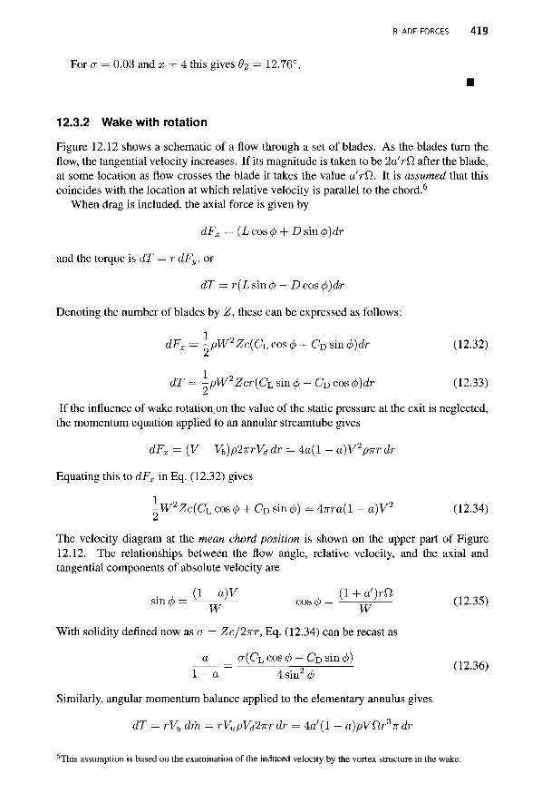
BLADE FORCES 419
For a = 0.03 and x = 4 this gives 62 = 12.76°
12.3.2 Wake with rotation
Figure 12.12 shows a schematic of a flow through a set of blades. As the blades turn the flow, the tangential velocity increases. If its magnitude is taken to be 2a'rQ, after the blade, at some location as flow crosses the blade it takes the value a'rQ.. It is assumed that this coincides with the location at which relative velocity is parallel to the chord.6
When drag is included, the axial force is given by
dFx = (L cos 4> + D sin <j))dr
and the torque is dT = r dFy, or
dT = r (L sin (f> — D cos (j>)dr
Denoting the number of blades by Z, these can be expressed as follows:
dFx = -pW2Zc(CL cos 4> + CD sin <j>)dr (12.32)
dT = ^pW2Zcr(Ch sin 0 - CD cos <j))dr (12.33)
If the influence of wake rotation on the value of the static pressure at the exit is neglected, the momentum equation applied to an annular streamtube gives
dFx = {V - Vb)p2irrVd dr = 4a(l - a)V2pnr dr
Equating this to dFx in Eq. (12.32) gives
]-W2Zc{CL cos <j> + CD sin0) = 4nra(l - a)V2 (12.34)
The velocity diagram at the mean chord position is shown on the upper part of Figure 12.12. The relationships between the flow angle, relative velocity, and the axial and tangential components of absolute velocity are
sin 0 = V w ' cos 4> = ± ^ — (12.35)
With solidity defined now as a = Zc/2irr, Eq. (12.34) can be recast as
a cr(CL cos 4> — CD sin <j>) I - a 4 sin2 </>
Similarly, angular momentum balance applied to the elementary annulus gives
dT = rVu dm = rVupVd2irrdr = 4a''(1 - a)pVSlr'i'K dr
(12.36)
6This assumption is based on the examination of the induced velocity by the vortex structure in the wake.
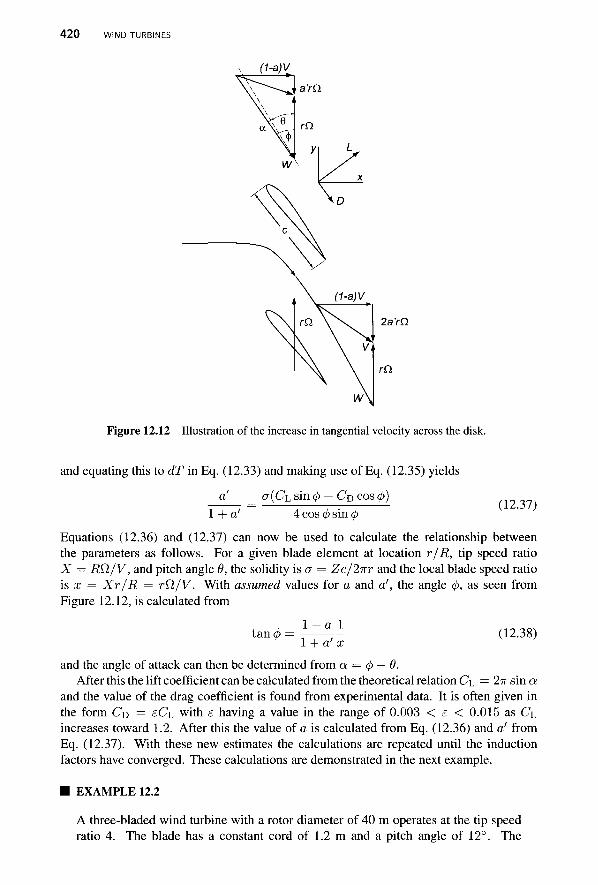
4 2 0 WIND TURBINES
x (1-a)V V^^.
\ ^^^^ \ \ \\ \\ .
Y
a'rQ.
rCl
y
2a'rQ
Figure 12.12 Illustration of the increase in tangential velocity across the disk.
and equating this to dT in Eq. (12.33) and making use of Eq. (12.35) yields
a' CT(CL sin (j> — CD cos cf>)
1+a' 4 cos 6 sin < (12.37)
Equations (12.36) and (12.37) can now be used to calculate the relationship between the parameters as follows. For a given blade element at location r/R, tip speed ratio X — RQ/V, and pitch angle 9, the solidity is a = Zc/2nr and the local blade speed ratio is x = Xr/R = rfl/V. With assumed values for a and a', the angle <f>, as seen from Figure 12.12, is calculated from
tan< 1 - a l 1 + a' x
(12.38)
and the angle of attack can then be determined from a = cf> — 9. After this the lift coefficient can be calculated from the theoretical relation CL = 27r sin a
and the value of the drag coefficient is found from experimental data. It is often given in the form CD = £CL with e having a value in the range of 0.003 < e < 0.015 as CL increases toward 1.2. After this the value of a is calculated from Eq. (12.36) and a' from Eq. (12.37). With these new estimates the calculations are repeated until the induction factors have converged. These calculations are demonstrated in the next example.
EXAMPLE 12.2
A three-bladed wind turbine with a rotor diameter of 40 m operates at the tip speed ratio 4. The blade has a constant cord of 1.2 m and a pitch angle of 12°. The
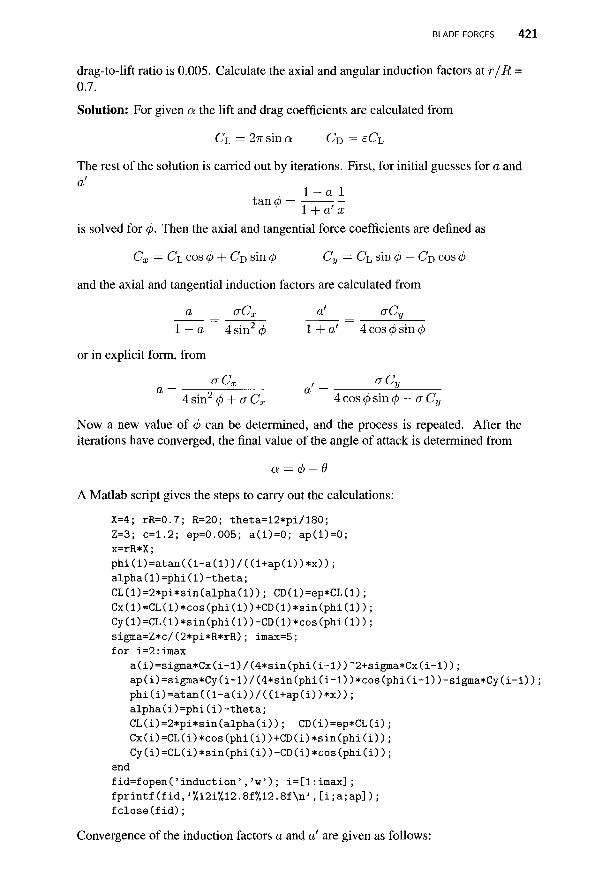
BLADE FORCES 421
drag-to-lift ratio is 0.005. Calculate the axial and angular induction factors at r/R = 0.7.
Solution: For given a the lift and drag coefficients are calculated from
CL = 2-n- sin a CD = ECL
The rest of the solution is carried out by iterations. First, for initial guesses for a and a'
1 - a l tan< 1 + a' x is solved for <j>. Then the axial and tangential force coefficients are defined as
Cx = CL COS 4> + CD sin <j> Cy = CL sin <p — CD cos <j>
and the axial and tangential induction factors are calculated from
a oCx a ®Cy I — a 4 sin2 <f> 1 + a' 4 cos <fi sin <
or in explicit form, from
a Gx , ^ a Gy
4sin (p + aCx 4cos<j>sincf> - aCy
Now a new value of <fi can be determined, and the process is repeated. After the iterations have converged, the final value of the angle of attack is determined from
a = 4>-9
A Matlab script gives the steps to carry out the calculations:
X=4; rR=0.7; R=20; theta=12*pi/180; Z=3; c=1.2; ep=0.005; a ( l )=0 ; ap( l )=0; x=rR*X; p h i ( l ) = a t a n ( ( l - a ( l ) ) / ( ( l + a p ( l ) ) * x ) ) ; a lpha (1 )=ph i ( l ) - t he t a ; CL(l )=2*pi*s in(a lpha(D); CD(l)=ep*CL(l); Cx( l )=CL(l )*cos(phi ( l ) )+CD(l)*s in(phi (D) ; Cy( l )=CL( l )*s in(ph i ( l ) ) -CD( l )*cos(ph i (D) ; sigma=Z*c/(2*pi*R*rR); imax=5; for i=2:imax
a ( i )=s igma*Cx( i - l ) / (4*s in (ph i ( i - l ) ) "2+s igma*Cx( i - l ) ) ; ap ( i )=s igma*Cy( i - l ) / (4*s in (ph i ( i - l ) )*cos (ph i ( i - l ) ) - s igma*Cy( i -D) ; p h i ( i ) = a t a n ( ( l - a ( i ) ) / ( ( l + a p ( i ) ) * x ) ) ; a l p h a ( i ) = p h i ( i ) - t h e t a ; CL(i )=2*pi*s in(a lpha( i ) ) ; CD(i)=ep*CL(i); Cx( i )=CL(i )*cos(phi ( i ) )+CD(i)*s in(phi ( i ) ) : Cy( i )=CL( i )*s in(ph i ( i ) ) -CD(i )*cos(phi ( i ) ) ;
end f i d = f o p e n ( ' i n d u c t i o n ' , ' w ' ) ; i= [ l : imax] ; fpr in t f ( f id , '•/.12i7„12.8f,/.12.8f\n', [ i ; a ; a p ] ) ; f c l o s e ( f i d ) ;
Convergence of the induction factors a and a' are given as follows:
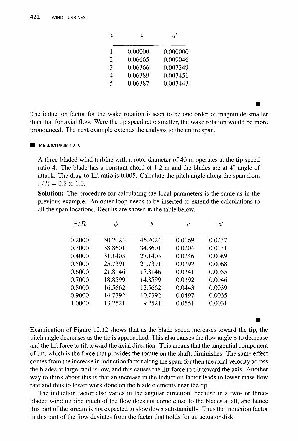
422 WIND TURBINES
i a a'
1 2 3 4 5
0.00000 0.06665 0.06366 0.06389 0.06387
0.000000 0.009046 0.007349 0.007451 0.007443
The induction factor for the wake rotation is seen to be one order of magnitude smaller than that for axial flow. Were the tip speed ratio smaller, the wake rotation would be more pronounced. The next example extends the analysis to the entire span.
■ EXAMPLE 12.3
A three-bladed wind turbine with a rotor diameter of 40 m operates at the tip speed ratio 4. The blade has a constant chord of 1.2 m and the blades are at 4° angle of attack. The drag-to-lift ratio is 0.005. Calculate the pitch angle along the span from r/R = 0.2 to 1.0. Solution: The procedure for calculating the local parameters is the same as in the previous example. An outer loop needs to be inserted to extend the calculations to all the span locations. Results are shown in the table below.
r/R
0.2000 0.3000 0.4000 0.5000 0.6000 0.7000 0.8000 0.9000 1.0000
<t>
50.2024 38.8601 31.1403 25.7391 21.8146 18.8599 16.5662 14.7392 13.2521
e
46.2024 34.8601 27.1403 21.7391 17.8146 14.8599 12.5662 10.7392 9.2521
a
0.0169 0.0204 0.0246 0.0292 0.0341 0.0392 0.0443 0.0497 0.0551
a1
0.0237 0.0131 0.0089 0.0068 0.0055 0.0046 0.0039 0.0035 0.0031
Examination of Figure 12.12 shows that as the blade speed increases toward the tip, the pitch angle decreases as the tip is approached. This also causes the flow angle <fi to decrease and the lift force to tilt toward the axial direction. This means that the tangential component of lift, which is the force that provides the torque on the shaft, diminishes. The same effect comes from the increase in induction factor along the span, for then the axial velocity across the blades at large radii is low, and this causes the lift force to tilt toward the axis. Another way to think about this is that an increase in the induction factor leads to lower mass flow rate and thus to lower work done on the blade elements near the tip.
The induction factor also varies in the angular direction, because in a two- or three-bladed wind turbine much of the flow does not come close to the blades at all, and hence this part of the stream is not expected to slow down substantially. Thus the induction factor in this part of the flow deviates from the factor that holds for an actuator disk.
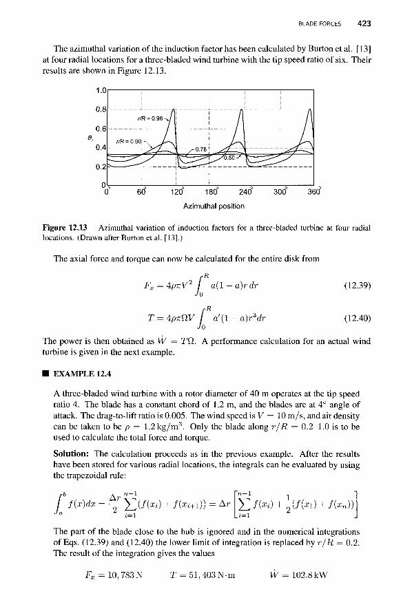
BLADE FORCES 423
The azimuthal variation of the induction factor has been calculated by Burton et al. [13] at four radial locations for a three-bladed wind turbine with the tip speed ratio of six. Their results are shown in Figure 12.13.
120 180 240
Azimuthal position
360
Figure 12.13 Azimuthal variation of induction factors for a three-bladed turbine at four radial locations. (Drawn after Burton et al. [13].)
The axial force and torque can now be calculated for the entire disk from
rR
Fx =4P-KV2 / a{l-a)rdr Jo
T = 4p7iW / a'(l - a)r3dr Jo
(12.39)
(12.40)
The power is then obtained as W = Tfi. A performance calculation for an actual wind turbine is given in the next example.
■ EXAMPLE 12.4
A three-bladed wind turbine with a rotor diameter of 40 m operates at the tip speed ratio 4. The blade has a constant chord of 1.2 m, and the blades are at 4° angle of attack. The drag-to-lift ratio is 0.005. The wind speed is V = 10 m/s, and air density can be taken to be p = 1.2kg/m3. Only the blade along r/R = 0.2-1.0 is to be used to calculate the total force and torque.
Solution: The calculation proceeds as in the previous example. After the results have been stored for various radial locations, the integrals can be evaluated by using the trapezoidal rule:
f f{x)dx = ^L J2(f(xt) + f(xi+1)) = Ar J2 / ( * 0 + ^ ( / ( z i ) + ZOO) Ja z i=\ Li=i
The part of the blade close to the hub is ignored and in the numerical integrations of Eqs. (12.39) and (12.40) the lower limit of integration is replaced by r/R = 0.2. The result of the integration gives the values
Fx = 10, 783 N T = 51,403N-m W = 102.8 kW
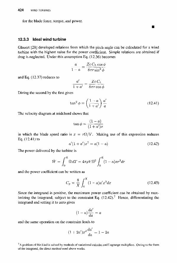
4 2 4 WIND TURBINES
for the blade force, torque, and power.
12.3.3 Ideal wind turbine
Glauert [28] developed relations from which the pitch angle can be calculated for a wind turbine with the highest value for the power coefficient. Simple relations are obtained if drag is neglected. Under this assumption Eq. (12.36) becomes
a Zc CL cos <j> I — a 8irr sin2 <
and Eq. (12.37) reduces to a' Z C C L
1 + a' 8"7TT COS (
Diving the second by the first gives
tan20=(i-4)^ (12.41) 1 + a' I a
The velocity diagram at midchord shows that
(I-a) tancp = (1 + a')x
in which the blade speed ratio is x = rfl/V. Making use of this expression reduces Eq. (12.41) to
a'(l + a')x2 = a(l-a) (12.42)
The power delivered by the turbine is
rR rR W= ndT = 4npVn2 (l-a)ar3dr
Jo Jo and the power coefficient can be written as
Cp = - | / (1 - a)a'x3dx (12.43) X Jo
Since the integrand is positive, the maximum power coefficient can be obtained by max-imizing the integrand, subject to the constraint Eq. (12.42).7 Hence, differentiating the integrand and setting it to zero gives
da' ( 1 " a ) ^ = a
and the same operation on the constraint leads to
(l + 2 a V ^ = l - 2 a da
7 A problem of this kind is solved by methods of variational calculus and Lagrange multipliers. Owing to the form of the integrand, the direct method used above works.
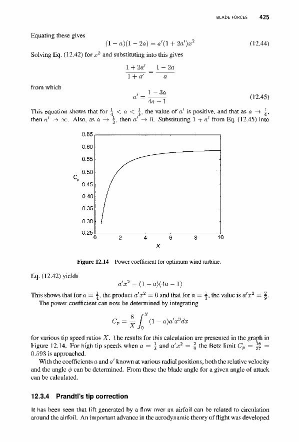
BLADE FORCES 425
Equating these gives ( l - a ) ( l - 2 a ) =a'(l+2a')x2 (12.44)
Solving Eq. (12.42) for x2 and substituting into this gives
1 + 2a! I-2a l + o'
from which l - 3 o 4 a - 1
(12.45)
I This equation shows that for | < a < | , the value of a' is positive, and that as a then a' —> oo. Also, as a —> | , then a' —> 0. Substituting 1 + a' from Eq. (12.45) into
0.65
0.60
0.55
0.50
0.45
0.40
0.35
0.30
0.25
Figure 12.14 Power coefficient for optimum wind turbine.
Eq. (12.42) yields a'x2 = ( l - a ) ( 4 a - l )
iji This shows that for a — \, the product a'x2 — 0 and that for a — | , the value is a'x The power coefficient can now be determined by integrating
2 9 '
c„ X / (1 - a)a'
Jo x dx
for various tip speed ratios X. The results for this calculation are presented in the graph in Figure 12.14. For high tip speeds when a = | and a'x2 = | the Betz limit Cp = | | = 0.593 is approached.
With the coefficients a and a' known at various radial positions, both the relative velocity and the angle (j> can be determined. From these the blade angle for a given angle of attack can be calculated.
12.3.4 Prandtl's tip correction
It has been seen that lift generated by a flow over an airfoil can be related to circulation around the airfoil. An important advance in the aerodynamic theory of flight was developed
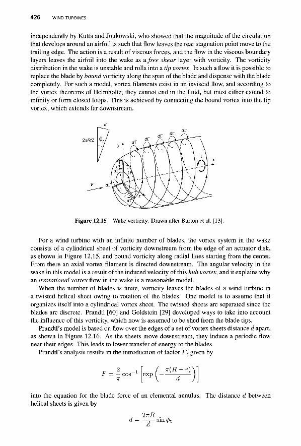
426 WIND TURBINES
independently by Kutta and Joukowski, who showed that the magnitude of the circulation that develops around an airfoil is such that flow leaves the rear stagnation point move to the trailing edge. The action is a result of viscous forces, and the flow in the viscous boundary layers leaves the airfoil into the wake as a free shear layer with vorticity. The vorticity distribution in the wake is unstable and rolls into a tip vortex. In such a flow it is possible to replace the blade by bound vorticity along the span of the blade and dispense with the blade completely. For such a model, vortex filaments exist in an inviscid flow, and according to the vortex theorems of Helmholtz, they cannot end in the fluid, but must either extend to infinity or form closed loops. This is achieved by connecting the bound vortex into the tip vortex, which extends far downstream.
2nR/Z
Figure 12.15 Wake vorticity. Drawn after Burton et al. [13].
For a wind turbine with an infinite number of blades, the vortex system in the wake consists of a cylindrical sheet of vorticity downstream from the edge of an actuator disk, as shown in Figure 12.15, and bound vorticity along radial lines starting from the center. From there an axial vortex filament is directed downstream. The angular velocity in the wake in this model is a result of the induced velocity of this hub vortex, and it explains why an irrotational vortex flow in the wake is a reasonable model.
When the number of blades is finite, vorticity leaves the blades of a wind turbine in a twisted helical sheet owing to rotation of the blades. One model is to assume that it organizes itself into a cylindrical vortex sheet. The twisted sheets are separated since the blades are discrete. Prandtl [60] and Goldstein [29] developed ways to take into account the influence of this vorticity, which now is assumed to be shed from the blade tips.
Prandtl's model is based on flow over the edges of a set of vortex sheets distance d apart, as shown in Figure 12.16. As the sheets move downstream, they induce a periodic flow near their edges. This leads to lower transfer of energy to the blades.
Prandtl's analysis results in the introduction of factor F, given by
F ■ cos exp w{R-r)
into the equation for the blade force of an elemental annulus. The distance d between helical sheets is given by
d 2ITR
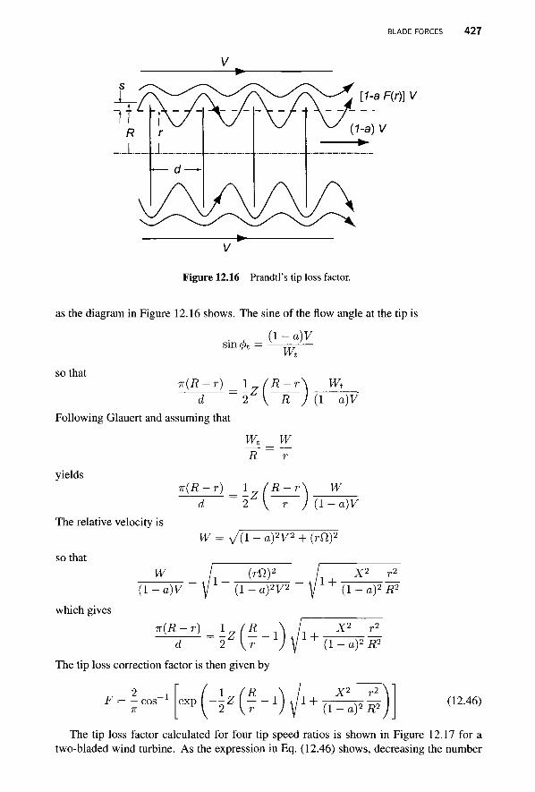
BLADE FORCES 427
V
V
Figure 12.16 Prandtl's tip loss factor.
as the diagram in Figure 12.16 shows. The sine of the flow angle at the tip is
( l - a ) V sm<pt Wt
so that n(R-r) _ \7(R~r
d ~ 2 Wt
R ) (l-a)V Following Glauert and assuming that
w1_w_ R ~ r
yields
The relative velocity is
so that W
W ir(R-r) _ 1 (R-r" ~~d _ 2 V r ) {l-a)V
W= y/(l - a)2V2 + (rfi)2
(rO)2 X2
(l-a)V (l-a)2V2 (1 - a)2 R2
which gives n(R-r) = lz(R
d 2 1 i / l + X2
(1 - a)2 R?
The tip loss correction factor is then given by
F = — cos 7T
exp \-\Z{T 1 4/1 + X2
(1 - a)2 R? (12.46)
The tip loss factor calculated for four tip speed ratios is shown in Figure 12.17 for a two-bladed wind turbine. As the expression in Eq. (12.46) shows, decreasing the number
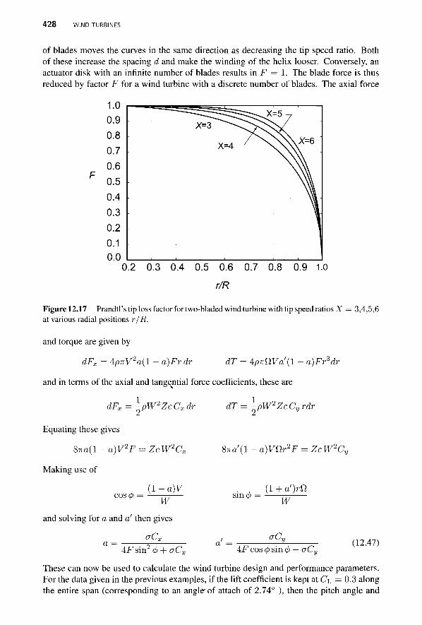
428 WIND TURBINES
of blades moves the curves in the same direction as decreasing the tip speed ratio. Both of these increase the spacing d and make the winding of the helix looser. Conversely, an actuator disk with an infinite number of blades results in F = 1. The blade force is thus reduced by factor F for a wind turbine with a discrete number of blades. The axial force
0.2 0.3 0.4 0.5 0.6 0.7 0.8 0.9 1.0
r/R
Figure 12.17 Prandtl's tip loss factor for two-bladed wind turbine with tip speed ratios X = 3,4,5,6 at various radial positions r/R.
and torque are given by
dFx = ApTrV2a(l - a)Frdr dT = 4PTrttVa'(l - a)Fr3dr
and in terms of the axial and tangential force coefficients, these are
dFx = \>pW2ZcCxdr
Equating these gives
87ro(l -a)V2F = ZCW2CX
Making use of
( l - o ) V cost
dT = -PW2ZcCyrdr
8ira'{l - a)VVLr2F = ZcW2Cy
{l + a')rn W sin< W
and solving for a and a' then gives
aCx rd, AF sin^ aCx AF cos 6 sin 6 — aCv
(12.47)
These can now be used to calculate the wind turbine design and performance parameters. For the data given in the previous examples, if the lift coefficient is kept at C\, = 0.3 along the entire span (corresponding to an angle'of attach of 2.74° ), then the pitch angle and

TURBOMACHINERY AND FUTURE PROSPECTS FOR ENERGY 4 2 9
induction factors are as shown in table below. The results differ slightly from those in which the tip correction was neglected.
r/R
0.2000 0.3000 0.4000 0.5000 0.6000 0.7000 0.8000 0.9000
0
44.0145 32.8470 25.7736 21.0284 17.6605 15.1463 13.1644 11.4195
o
41.2778 30.1103 23.0369 18.2917 14.9237 12.4095 10.4277 8.6828
a
0.0176 0.0224 0.0279 0.0340 0.0408 0.0491 0.0612 0.0876
a'
0.0168 0.0095 0.0066 0.0051 0.0043 0.0037 0.0035 0.0038
12.4 TURBOMACHINERY AND FUTURE PROSPECTS FOR ENERGY
In some sections of this book the reader's attention has been drawn to how the present primary energy resources of the world are used and how important turbomachines are in converting the energy in fossil fuels into shaft work. Turbomachines powered by hydro-electric energy and wind energy are the main two machines that contribute to significant forms of renewable energy in the mix. It is unfortunate that they account for such a small fraction of the world's energy supply, because the fossil energy resources will be mostly exhausted during this century. The recent high prices for oil are a signal that soon the world's aging oil fields will be unable to keep up with the demand of the world's growing population (which in 2011 reached 7 billion). The production curves for oil, natural gas, and coal are bell-shaped, and the significant event on the road to their exhaustion is when each production peak will be passed. After that, the world will need to get by with less of these nonrenewable fuels. The peak production for world's oil is likely to occur before the year 2015, and the production peaks for natural gas and coal will not be far behind. Coal, which is thought to be the most abundant of the three, has seen its reserve-to-production ratio drop from 227 years to 119 years during the first decade of the present century. A 119-life for the existing reserve might seem like a long time, but the 108-year drop during the last decade indicates that the rate at which the reserves decrease is quite rapid. In addition, the reserve-to-production ratio gives a misleading number, as it assumes that production stays flat until the resource is completely exhausted. A 40-year reserve-to-production ratio is, in fact, an indication of a production peak [49].
In the United States coal became the primary source of energy in the late 1800s overtaking biomass, which met the energy needs of the early settlers. It took some 40 years for coal's share to rise from 1% to 10% of the mix and the historical record shows similar timespans for the rise of oil and natural gas as well. Nuclear energy's share, after 50 years of effort, is still less than 10% of the energy supply in the United States. The prospects for renewable forms to offset the growing population and its growing demand for energy are exceedingly slim. Decisions to launch a comprehensive strategy for coping with the exhaustion of fossil fuels have been delayed many times despite warnings throughout the last century [11, 39]. Still installed wind energy capacity is increasing rapidly (even if not rapidly enough), and wind power offers the best possibility of becoming a significant source of energy in the
430 WIND TURBINES
United States. Denmark in particular has demonstrated that wind power can make up a sizeable fraction of a country's energy supply with a continuous and sustained effort.
EXERCISES
12.1 Reconsider the ducted wind turbine, but now let the duct be a cylindrical control volume Ae in cross sectional area. Show that the axial force on the blades is
Fd = PAbVb(V - Vb)
which is in agreement with Eq. (12.6).
12.2 The nondimensional pressure difference can be expressed as
P+ ~Pa
in which the pressure difference is that just upstream the disk and the free stream, (a) Use the momentum theory for a wind turbine to express this relationship in terms of the interference factor a. For which value of a is this maximum? Interpret this physically, (b) Develop a similar relationship for the expression
Pa-P-
and determine for which value of a is this the maximum?
12.3 A wind turbine operates at wind speed of V = 12 m/s. Its blade radius is R = 20 m and its tip speed radius RQ/V = 4. It operates at the condition Cp = 0.3. Find (a) the rate of rotation of the blades, (b) the power developed by the turbine, (c) the value of the interference factor a using the momentum theory, and (d) the pressure on the front of the actuator disk, assuming that the free stream pressure is 101.30 kPa.
12.4 Using the axial momentum theory, calculate the ratio of the slipstream radius to that of the disk radius in terms of the interference factor a. If the wind turbine blades are 80 m long, what is the radius of the slipstream far downstream? What is the radius of the streamtube far upstream?
12.5 In a wind with speed V = 8.7 m/s and air density p = 1.2 kg/m3, a wind turbine operates at a condition with Cp = 0.31. Find the blade length, assuming that the power delivered to the turbine is to be W = 250 kW.
12.6 Consider a three-bladed wind turbine with blade radius of R = 35 m and constant chord of c = 80 cm, which operates with a rotational speed of ft = 10 rpm. The wind speed is V = 12 m/s. (a) Find the axial and tangential induction factors at r = 10 m, assuming that the angle of attack is 6° and CD = O.OlCx,. (b) Find the axial force and the torque, assuming the air density is p = 0.12 kg/m3. (c) Calculate the axial force and the torque by assuming that the induction factors are uniform and equal to their values at r/R = 0.6.
Appendix A Streamline curvature and radial equilibrium
A.1 STREAMLINE CURVATURE METHOD
In this appendix the governing equations for the streamline curvature method are developed. The derivation of the acceleration terms follows that of Cumpsty [18]. The blade surfaces may be highly curved, but it is useful to visualize locally flat surface patches in them.
A.1.1 Fundamental equations
The acceleration of a fluid particle is given by its substantial derivative
<9V a = — + V - V V
at in which the unsteady term vanishes in steady flow. The second term represents the spatial acceleration of the flow. In cylindrical coordinates the gradient operator can be written as
_ d eg d d dr r 89 z dz
By defining the meridional component as
* m *m^m Vrer ~r Vz^z
Principles of Turbomachinery. By Seppo A. Korpela Copyright © 2011 John Wiley & Sons, Inc.
431
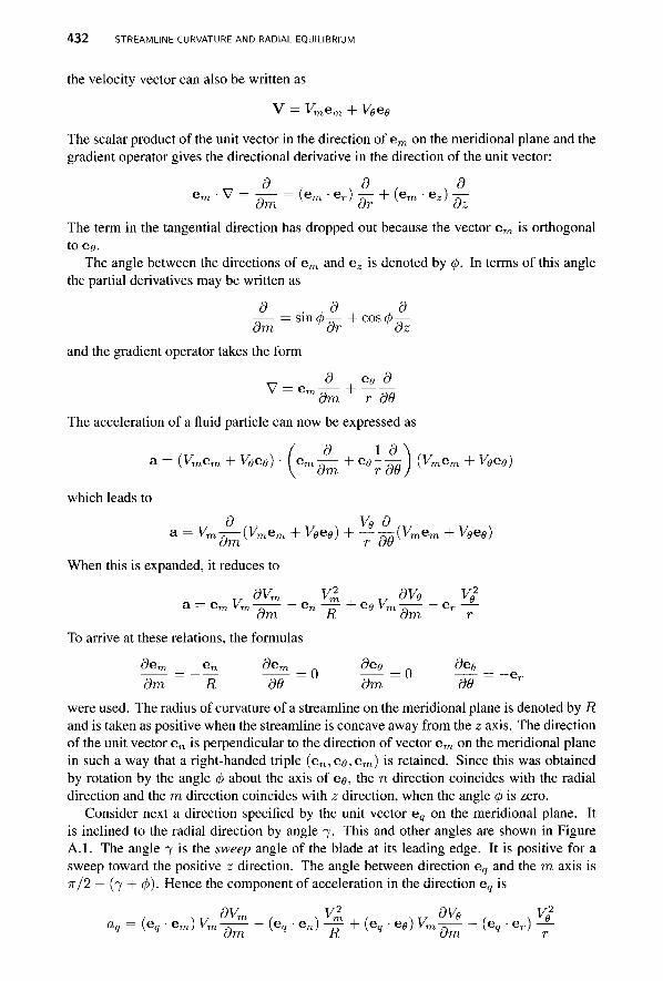
432 STREAMLINE CURVATURE AND RADIAL EQUILIBRIUM
the velocity vector can also be written as
V = Vmem + Veee
The scalar product of the unit vector in the direction of e m on the meridional plane and the gradient operator gives the directional derivative in the direction of the unit vector:
_ 8 8 8 &m ' V — — — \&m ' er) 7T~ ' l ^ m * ez) ~7\
dm or dz The term in the tangential direction has dropped out because the vector e m is orthogonal toe,?.
The angle between the directions of e m and ez is denoted by <f>. In terms of this angle the partial derivatives may be written as
d_ _ . , d , 8 dm
and the gradient operator takes the form
s m 0 — + c o s v „ am or oz
V = e — + ^ — dm r 88
The acceleration of a fluid particle can now be expressed as
a = (Vmem + Veee) ■ ( e m - h ee- 7-r J (Vmem + Veee)
which leads to d Vg d
Vm — (Vmem + V0ee) H -7^(Vmem + Veee)
When this is expanded, it reduces to
a — em ^m n en ~t ee vm er dm R dm r
To arrive at these relations, the formulas
dm R 36 dm 88 were used. The radius of curvature of a streamline on the meridional plane is denoted by R and is taken as positive when the streamline is concave away from the z axis. The direction of the unit vector e„ is perpendicular to the direction of vector e m on the meridional plane in such a way that a right-handed triple (en, ee, em) is retained. Since this was obtained by rotation by the angle 4> about the axis of ee, the n direction coincides with the radial direction and the m direction coincides with z direction, when the angle <p is zero.
Consider next a direction specified by the unit vector eq on the meridional plane. It is inclined to the radial direction by angle 7. This and other angles are shown in Figure A. 1. The angle 7 is the sweep angle of the blade at its leading edge. It is positive for a sweep toward the positive z direction. The angle between direction e,j and the m axis is IT/2 — (7 + 0). Hence the component of acceleration in the direction eq is
XT, 9Vm , . V* . .„ 8Ve . . V02
aq = (e, ■ em) Vm-^- - {eq ■ e„) — + (e, ■ ee) Vm-^ - (e, • er) —
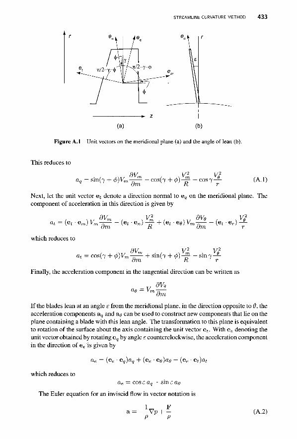
STREAMLINE CURVATURE METHOD 4 3 3
Figure A.l Unit vectors on the meridional plane (a) and the angle of lean (b).
This reduces to
dV V2 V2
aq = sin(7 + <p)Vm-^- - cos(7 + <j>)-^- COS7— dm R r (A.1)
Next, let the unit vector et denote a direction normal to eq on the meridional plane. The component of acceleration in this direction is given by
3V V2
at = (et ■ em) Vm— (et • en) — (et-e9)Vm— _ ( e t . e r ) —
which reduces to
dV V2 V2
at = cos(7 + <j>)Vm—^ + sin(7 + </>)-^ - s i n 7 - ^ dm R r
Finally, the acceleration component in the tangential direction can be written as
dVg ae = Vm dm
If the blades lean at an angle e from the meridional plane, in the direction opposite to 9, the acceleration components aq and a# can be used to construct new components that lie on the plane containing a blade with this lean angle. The transformation to this plane is equivalent to rotation of the surface about the axis containing the unit vector et. With ee denoting the unit vector obtained by rotating eq by angle e counterclockwise, the acceleration component in the direction of ee is given by
ae = (ee ■ eq)aq + (ee • ee)ae + (ee ■ et)at
which reduces to ae = cos eaq— sin e ae
The Euler equation for an inviscid flow in vector notation is
!,-, F — V p + -P P
(A.l)
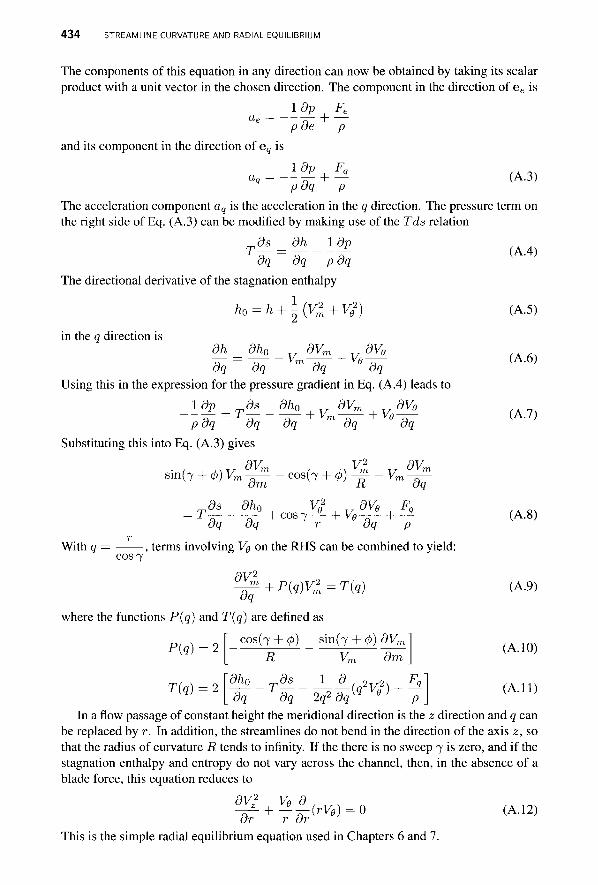
434 STREAMLINE CURVATURE AND RADIAL EQUILIBRIUM
The components of this equation in any direction can now be obtained by taking its scalar product with a unit vector in the chosen direction. The component in the direction of ee is
p de p and its component in the direction of eq is
aq = -1-9/ + ^ (A.3) pdq p
The acceleration component aq is the acceleration in the q direction. The pressure term on the right side of Eq. (A.3) can be modified by making use of the Tds relation
n<9s dh 1 dp dq dq p dq
The directional derivative of the stagnation enthalpy
T- (A.4)
ho = h+\(V^ + Ve2)
in the q direction is dh dq
dh0
dq Vm dVm
dq Ve
dVg
Using this in the expression for the pressure gradient in Eq. (A.4) leads to ,ds I dp
pdq Substituting this into Eq. (A.3) gives
sin(7 + <p) Vm
,ds
_dho dVrn dq dq dq Ve
T-
■ cos(7 + 4>)
V}
V2
R dV„
Vr
dV9
dq
dVm
(A.5)
(A.6)
(A.7)
dq
With q cos 7
dm
-^- + COS7-2- + Ve-^- + -J±
dq r dq p
terms involving Vg on the RHS can be combined to yield:
dV2
dq + P(9)V™ = T(q)
where the functions P(q) and T(q) are defined as
cos (7 + (p) sin(7 + 1 P(q)
T(q)
dVrr, R V„. dm
dh0
dq T%-U^-Fi
(A.8)
(A.9)
(A. 10)
(A. 11)
In a flow passage of constant height the meridional direction is the z direction and q can be replaced by r. In addition, the streamlines do not bend in the direction of the axis z, so that the radius of curvature R tends to infinity. If the there is no sweep 7 is zero, and if the stagnation enthalpy and entropy do not vary across the channel, then, in the absence of a blade force, this equation reduces to
dV2 Ve d -T~ + —^-(rVg) dr r dr
0 (A. 12)
This is the simple radial equilibrium equation used in Chapters 6 and 7.
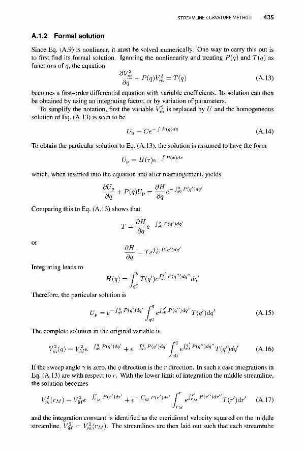
STREAMLINE CURVATURE METHOD 435
A.1.2 Formal solution
Since Eq. (A.9) is nonlinear, it must be solved numerically. One way to carry this out is to first find its formal solution. Ignoring the nonlinearity and treating P(q) and T(q) as functions of q, the equation
8V2
-^+P{q)V^=T{q) (A.13)
becomes a first-order differential equation with variable coefficients. Its solution can then be obtained by using an integrating factor, or by variation of parameters.
To simplify the notation, first the variable V^ is replaced by U and the homogeneous solution of Eq. (A. 13) is seen to be
Uh = Ce-$p{q)dq (A. 14)
To obtain the particular solution to Eq. (A.13), the solution is assumed to have the form
Up = H{r)e-fp{x)dx
which, when inserted into the equation and after rearrangement, yields
Comparing this to Eq. (A.13) shows that
or
Integrating leads to
dq
dq
H{q)= rT{q')etiP^di"dq<
Up = e - •& P{q')dql f" e''o p^">dq"T(q')dq' (A.15) JaO
IqO
Therefore, the particular solution is
ri
IqO
The complete solution in the original variable is
V£(q) = V^e~ -ft n*'W + e tfo W f e/,'o' p^q")dq" T{q')dq' (A.16) JqO
If the sweep angle 7 is zero, the q direction is the r direction. In such a case integrations in Eq. (A.13) are with respect to r. With the lower limit of integration the middle streamline, the solution becomes
Vl(rM) = Vle~ KM p^dr' + e" /.M *V)*-' f JlM p(r'">dr"T(r')dr' (A.17)
JrM
and the integration constant is identified as the meridional velocity squared on the middle / 2
' M streamline, Vj^ = V^TM)- The streamlines are then laid out such that each streamtube
436 STREAMLINE CURVATURE AND RADIAL EQUILIBRIUM
has the same mass flow rate, and grid is set up on the qz plane, with grid points on the streamlines a specified distance apart. The solution then proceeds by iteration. The simplest situation is to consider the intergap region so that the blades are not present. The quasiorthogonals q can be spaced and oriented such that the first one is aligned with the trailing edge of a blade and the last one with the leading edge of the next blade row. The curvature is calculated at the grid locations, and the velocity gradients are determined by finite-difference approximations. This fixes the values of P and T. Integration of Eq. (A. 17) from the central streamline toward the hub and the casing gives the velocity field. Next, the mass flow rates are calculated for each streamtube. The residual is examined, and the streamlines are adjusted so that the fluid again flows at the same rate through each streamtube. The process is repeated until convergence for the location of the streamlines is obtained. This requires the use of relaxation.

Appendix B
Thermodynamic Tables
B.1 Thermodynamic properties of steam, temperature table
B.2 Thermodynamic properties of steam, pressure table
B.3 Thermodynamic properties of superheated steam
B.4 Thermodynamic properties of air
B.5 Specific heats of common gases
B.6 Molar specific heats of common gases
Principles of Turbomachinery. By Seppo A. Korpela 437 Copyright © 2011 John Wiley & Sons, Inc.

438 THERMODYNAMIC TABLES
Table B.l Thermodynamic Properties
T p v{ ■ 103 ve U{ °C bar m3/kg m3/kg kj/kg
0.01 1 2 3 4
0.00611 0.00657 0.00706 0.00758 0.00814
1.0002 1.0002 1.0001 1.0001 1.0001
206.136 192.439 179.762 168.016 157.126
0.00 4.18 8.40 12.61 16.82
5 6 7 8 9
0.00873 0.00935 0.01002 0.01073 0.01148
1.0001 1.0001 1.0001 1.0002 1.0002
147.024 137.647 128.939 120.847 113.323
21.02 25.22 29.41 33.61 37.80
10 11 12 13 14
0.01228 0.01313 0.01403 0.01498 0.01599
1.0003 1.0004 1.0005 1.0006 1.0008
106.323 99.808 93.740 88.086 82.814
41.99 46.17 50.36 54.55 58.73
15 16 17 18 19
0.01706 0.01819 0.01938 0.02064 0.02198
1.0009 1.0011 1.0012 1.0014 1.0016
77.897 73.308 69.023 65.019 61.277
62.92 67.10 71.28 75.47 79.65
20 21 22 23 24
0.02339 0.02488 0.02645 0.02810 0.02985
1.0018 1.0020 1.0023 1.0025 1.0027
57.778 54.503 51.438 48.568 45.878
83.83 88.02 92.20 96.38 100.57
25 26 27 28 29
0.03169 0.03363 0.03567 0.03782 0.04008
1.0030 1.0033 1.0035 1.0038 1.0041
43.357 40.992 38.773 36.690 34.734
104.75 108.93 113.12 117.30 121.48
30 31 32 33 34
0.04246 0.04495 0.04758 0.05033 0.05323
1.0044 1.0047 1.0050 1.0054 1.0057
32.896 31.168 29.543 28.014 26.575
125.67 129.85 134.03 138.22 142.40
35 0.05627 1.0060 25.220 146.58 40 0.07381 1.0079 19.528 167.50 45 0.09593 1.0099 15.263 188.41 50 0.12345 1.0122 12.037 209.31
of Saturated Steam, Temperature Table
ug hi hg Si Sg kJ/kg kJ/kg kJ/kg kJ/kgK kJ/kgK
2375.3 2375.9 2377.3 2378.7 2380.0
0.01 4.183 8.401 12.61 16.82
2501.3 2502.4 2504.2 2506.0 2507.9
0.0000 0.0153 0.0306 0.0459 0.0611
9.1562 9.1277 9.1013 9.0752 9.0492
2381.4 2382.8 2384.2 2385.6 2386.9
21.02 25.22 29.42 33.61 37.80
2509.7 2511.5 2513.4 2515.2 2517.1
0.0763 0.0913 0.1063 0.1213 0.1361
9.0236 8.9981 8.9729 8.9479 8.9232
2388.3 2389.7 2391.1 2392.4 2393.8
41.99 46.18 50.36 54.55 58.73
2518.9 2520.7 2522.6 2524.4 2526.2
0.1510 0.1657 0.1804 0.1951 0.2097
8.8986 8.8743 8.8502 8.8263 8.8027
2395.2 2396.6 2397.9 2399.3 2400.7
62.92 67.10 71.28 75.47 79.65
2528.0 2529.9 2531.7 2533.5 2535.3
0.2242 0.2387 0.2532 0.2676 0.2819
8.7792 8.7560 8.7330 8.7101 8.6875
2402.0 2403.4 2404.8 2406.1 2407.5
83.84 88.02 92.20 96.39 100.57
2537.2 2539.0 2540.8 2542.6 2544.5
0.2962 0.3104 0.3246 0.3388 0.3529
8.6651 8.6428 8.6208 8.5990 8.5773
2408.9 2410.2 2411.6 2413.0 2414.3
104.75 108.94 113.12 117.30 121.49
2546.3 2548.1 2549.9 2551.7 2553.5
0.3670 0.3810 0.3949 0.4088 0.4227
8.5558 8.5346 8.5135 8.4926 8.4718
2415.7 2417.0 2418.4 2419.8 2421.1
125.67 129.85 134.04 138.22 142.41
2555.3 2557.1 2559.0 2560.8 2562.6
0.4365 0.4503 0.4640 0.4777 0.4914
8.4513 8.4309 8.4107 8.3906 8.3708
2422.5 146.59 2564.4 0.5050 8.3511 2429.2 167.50 2573.4 0.5723 8.2550 2435.9 188.42 2582.3 0.6385 8.1629 2442.6 209.33 2591.2 0.7037 8.0745
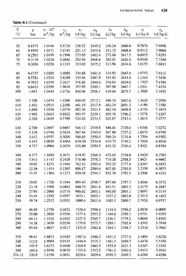
THERMODYNAMIC TABLES 439
Table B.l (C<
T p °C bar
55 0.1575 60 0.1993 65 0.2502 70 0.3118 75 0.3856
80 0.4737 85 0.5781 90 0.7012 95 0.8453 100 1.013
105 1.208 110 1.432 115 1.690 120 1.985 125 2.320
130 2.700 135 3.130 140 3.612 145 4.153 150 4.757
160 6.177 170 7.915 180 10.02 190 12.54 200 15.55
210 19.07 220 23.18 230 27.95 240 33.45 250 39.74
260 46.89 270 55.00 280 64.13 290 74.38 300 85.84
310 98.61 320 112.8 340 145.9 360 186.6
374.12 220.9
id)
vf ■ 103 vg
m3/kg m3/kg
1.0146 9.5726 1.0171 7.6743 1.0199 6.1996 1.0228 5.0446 1.0258 4.1333
1.0290 3.4088 1.0324 2.8289 1.0359 2.3617 1.0396 1.9828 1.0434 1.6736
1.0474 1.4200 1.0515 1.2106 1.0558 1.0370 1.0603 0.8922 1.0649 0.7709
1.0697 0.6687 1.0746 0.5824 1.0797 0.5090 1.0850 0.4464 1.0904 0.3929
1.1019 0.3071 1.1142 0.2428 1.1273 0.1940 1.1414 0.1565 1.1564 0.1273
1.1726 0.1044 1.1900 0.0862 1.2088 0.0716 1.2292 0.0597 1.2515 0.0501
1.2758 0.0422 1.3026 0.0356 1.3324 0.0302 1.3658 0.0256 1.4037 0.0217
1.4473 0.0183 1.4984 0.0155 1.6373 0.0108 1.8936 0.0070 3.1550 0.0031
Uf Ug
kJ/kg kJ/kg
230.22 2449.2 251.13 2455.8 272.05 2462.4 292.98 2468.8 313.92 2475.2
334.88 2481.6 355.86 2487.9 376.86 2494.0 397.89 2500.1 418.96 2506.1
440.05 2512.1 461.19 2517.9 482.36 2523.5 503.57 2529.1 524.82 2534.5
546.12 2539.8 567.46 2545.0 588.85 2550.0 610.30 2554.8 631.80 2559.5
674.97 2568.3 718.40 2576.3 762.12 2583.4 806.17 2589.6 850.58 2594.7
895.43 2598.7 940.75 2601.6 986.62 2603.1 1033.1 2603.1 1080.4 2601.6
1128.4 2598.4 1177.4 2593.2 1227.5 2585.7 1279.0 2575.7 1332.0 2562.8
1387.0 2546.2 1444.4 2525.2 1569.9 2463.9 1725.6 2352.2 2029.6 2029.6
h{ hg
kJ/kg kJ/kg
230.24 2600.0 251.15 2608.8 272.08 2617.5 293.01 2626.1 313.96 2634.6
334.93 2643.1 355.92 2651.4 376.93 2659.6 397.98 2667.7 419.06 2675.7
440.18 2683.6 461.34 2691.3 482.54 2698.8 503.78 2706.2 525.07 2713.4
546.41 2720.4 567.80 2727.2 589.24 2733.8 610.75 2740.2 632.32 2746.4
675.65 2758.0 719.28 2768.5 763.25 2777.8 807.60 2785.8 852.38 2792.5
897.66 2797.7 943.51 2801.3 990.00 2803.1 1037.2 2803.0 1085.3 2800.7
1134.4 2796.2 1184.6 2789.1 1236.1 2779.2 1289.1 2765.9 1344.1 2748.7
1401.2 2727.0 1461.3 2699.7 1593.8 2621.3 1761.0 2482.0 2099.3 2099.3
sf ss kJ/kgK kJ/kgK
0.7679 7.9896 0.8312 7.9080 0.8935 7.8295 0.9549 7.7540 1.0155 7.6813
1.0753 7.6112 1.1343 7.5436 1.1925 7.4784 1.2501 7.4154 1.3069 7.3545
1.3630 7.2956 1.4186 7.2386 1.4735 7.1833 1.5278 7.1297 1.5815 7.0777
1.6346 7.0272 1.6873 6.9780 1.7394 6.9302 1.7910 6.8836 1.8421 6.8381
1.9429 6.7503 2.0421 6.6662 2.1397 6.5853 2.2358 6.5071 2.3308 6.4312
2.4246 6.3572 2.5175 6.2847 2.6097 6.2131 2.7013 6.1423 2.7926 6.0717
2.8838 6.0009 2.9751 5.9293 3.0669 5.8565 3.1595 5.7818 3.2534 5.7042
3.3491 5.6226 3.4476 5.5356 3.6587 5.3345 3.9153 5.0542 4.4298 4.4298
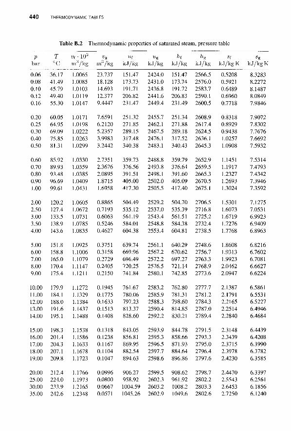
440 THERMODYNAMIC TABLES
Table B.2 Thermodynamic properties of saturated steam, pressure table
p bar
0.06 0.08 0.10 0.12 0.16
0.20 0.25 0.30 0.40 0.50
0.60 0.70 0.80 0.90 1.00
2.00 2.50 3.00 3.50 4.00
5.00 6.00 7.00 8.00 9.00
10.00 11.00 12.00 13.00 14.00
15.00 16.00 17.00 18.00 19.00
20.00 25.00 30.00 35.00
T °C
36.17 41.49 45.79 49.40 55.30
60.05 64.95 69.09 75.85 81.31
85.92 89.93 93.48 96.69 99.61
120.2 127.4 133.5 138.9 143.6
151.8 158.8 165.0 170.4 175.4
179.9 184.1 188.0 191.6 195.1
198.3 201.4 204.3 207.1 209.8
212.4 224.0 233.9 242.6
vi • 103
m 3/kg
1.0065 1.0085 1.0103 1.0119 1.0147
1.0171 1.0198 1.0222 1.0263 1.0299
1.0330 1.0359 1.0385 1.0409 1.0431
1.0605 1.0672 1.0731 1.0785 1.0835
1.0925 1.1006 1.1079 1.1147 1.1211
1.1272 1.1329 1.1384 1.1437 1.1488
1.1538 1.1586 1.1633 1.1678 1.1723
1.1766 1.1973 1.2165 1.2348
ve m 3/kg
23.737 18.128 14.693 12.377 9.4447
7.6591 6.2120 5.2357 3.9983 3.2442
2.7351 2.3676 2.0895 1.8715 1.6958
0.8865 0.7193 0.6063 0.5246 0.4627
0.3751 0.3158 0.2729 0.2405 0.2150
0.1945 0.1775 0.1633 0.1513 0.1408
0.1318 0.1238 0.1167 0.1104 0.1047
0.0996 0.0800 0.0667 0.0571
ut kJ/kg
151.47 173.73 191.71 206.82 231.47
251.32 271.85 289.15 317.48 340.38
359.73 376.56 391.51 405.00 417.30
504.49 535.12 561.19 584.01 604.38
639.74 669.96 696.49 720.25 741.84
761.67 780.06 797.23 813.37 828.60
843.05 856.81 869.95 882.54 894.63
906.27 958.92 1004.59 1045.26
Kg
kJ/kg
2424.0 2431.0 2436.8 2441.6 2449.4
2455.7 2462.1 2467.5 2476.1 2483.1
2488.8 2493.8 2498.1 2502.0 2505.5
2529.2 2537.0 2543.4 2548.8 2553.4
2561.1 2567.2 2572.2 2576.5 2580.1
2583.2 2585.9 2588.3 2590.4 2592.2
2593.9 2595.3 2596.5 2597.7 2598.6
2599.5 2602.3 2603.2 2602.9
hi kJ/kg
151.47 173.74 191.72 206.83 231.49
251.34 271.88 289.18 317.52 340.43
359.79 376.64 391.60 405.09 417.40
504.70 535.39 561.51 584.38 604.81
640.29 670.62 697.27 721.14 742.85
762.80 781.31 798.60 814.85 830.21
844.78 858.66 871.93 884.64 896.86
908.62 961.92 1008.2 1049.6
hg
kJ/kg
2566.5 2576.0 2583.7 2590.1 2600.5
2608.9 2617.4 2624.5 2636.1 2645.3
2652.9 2659.5 2665.3 2670.5 2675.1
2706.5 2716.8 2725.2 2732.4 2738.5
2748.6 2756.7 2763.3 2768.9 2773.6
2777.7 2781.2 2784.3 2787.0 2789.4
2791.5 2793.3 2795.0 2796.4 2797.6
2798.7 2802.2 2803.3 2802.6
Sf
kJ/kgK
0.5208 0.5921 0.6489 0.6960 0.7718
0.8318 0.8929 0.9438 1.0257 1.0908
1.1451 1.1917 1.2327 1.2693 1.3024
1.5301 1.6073 1.6719 1.7276 1.7768
1.8608 1.9313 1.9923 2.0462 2.0947
2.1387 2.1791 2.2165 2.2514 2.2840
2.3148 2.3439 2.3715 2.3978 2.4230
2.4470 2.5543 2.6453 2.7250
ss kJ/kg K
8.3283 8.2272 8.1487 8.0849 7.9846
7.9072 7.8302 7.7676 7.6692 7.5932
7.5314 7.4793 7.4342 7.3946 7.3592
7.1275 7.0531 6.9923 6.9409 6.8963
6.8216 6.7602 6.7081 6.6627 6.6224
6.5861 6.5531 6.5227 6.4946 6.4684
6.4439 6.4208 6.3990 6.3782 6.3585
6.3397 6.2561 6.1856 6.1240
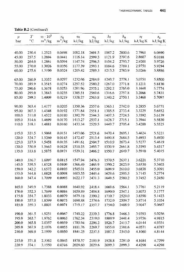
THERMODYNAMIC TABLES 4 4 1
Table B.2 (Continued)
p T vt ■ 103 vg ut bar °C m3/kg m3/kg kJ/kg
40.00 45.00 50.00 55.00 60.00
250.4 257.5 264.0 270.0 275.6
1.2523 1.2694 1.2861 1.3026 1.3190
0.0498 0.0441 0.0394 0.0356 0.0324
1082.18 1116.14 1147.74 1177.39 1205.42
65.00 70.00 75.00 80.00 85.00
280.9 285.9 290.6 295.0 299.3
1.3352 1.3515 1.3678 1.3843 1.4009
0.0297 0.0274 0.0253 0.0235 0.0219
1232.06 1257.52 1281.96 1305.51 1328.27
90.00 95.00 100.0 105.0 110.0
303.4 307.3 311.0 314.6 318.1
1.4177 1.4348 1.4522 1.4699 1.4881
0.0205 0.0192 0.0180 0.0170 0.0160
1350.36 1371.84 1392.79 1413.27 1433.34
115.0 120.0 125.0 130.0 135.0
321.5 324.7 327.9 330.9 333.8
1.5068 1.5260 1.5458 1.5663 1.5875
0.0151 0.0143 0.0135 0.0128 0.0121
1453.06 1472.47 1491.61 1510.55 1529.31
140.0 145.0 150.0 155.0 160.0
336.7 339.5 342.2 344.8 347.4
1.6097 1.6328 1.6572 1.6828 1.7099
0.0115 0.0109 0.0103 0.0098 0.0093
1547.94 1566.49 1585.01 1603.55 1622.17
165.0 170.0 175.0 180.0 185.0
349.9 352.3 354.7 357.0 359.3
1.7388 1.7699 1.8033 1.8399 1.8801
0.0088 0.0084 0.0079 0.0075 0.0071
1640.92 1659.89 1679.18 1698.88 1719.17
190.0 195.0 200.0 205.0 210.0
361.5 363.7 365.8 367.9 369.9
1.9251 1.9762 2.0357 2.1076 2.1999
0.0067 0.0063 0.0059 0.0055 0.0050
1740.22 1762.34 1785.94 1811.76 1841.25
215.0 371.8 2.3362 0.0045 1878.57 220.9 374.1 3.1550 0.0316 2029.60
u g ht he S{ sg
kJ/kg kJ/kg kJ/kg kJ/kgK kJ/kgK
2601.5 2599.3 2596.5 2593.1 2589.3
1087.2 1121.9 1154.2 1184.6 1213.3
2800.6 2797.6 2793.7 2789.1 2783.9
2.7961 2.8607 2.9201 2.9751 3.0266
6.0690 6.0188 5.9726 5.9294 5.8886
2584.9 2580.2 2575.1 2569.6 2563.8
1240.7 1267.0 1292.2 1316.6 1340.2
2778.1 2771.8 2765.0 2757.8 2750.1
3.0751 3.1211 3.1648 3.2066 3.2468
5.8500 5.8130 5.7774 5.7431 5.7097
2557.6 2551.1 2544.3 2537.1 2529.5
1363.1 1385.5 1407.3 1428.7 1449.7
2742.0 2733.4 2724.5 2715.1 2705.4
3.2855 3.3229 3.3592 3.3944 3.4288
5.6771 5.6452 5.6139 5.5830 5.5525
2521.6 2513.4 2504.7 2495.7 2486.2
1470.4 1490.8 1510.9 1530.9 1550.7
2695.1 2684.5 2673.4 2661.8 2649.7
3.4624 3.4953 3.5277 3.5595 3.5910
5.5221 5.4920 5.4619 5.4317 5.4015
2476.3 2465.9 2455.0 2443.4 2431.3
1570.5 1590.2 1609.9 1629.6 1649.5
2637.1 2623.9 2610.0 2595.5 2580.2
3.6221 3.6530 3.6838 3.7145 3.7452
5.3710 5.3403 5.3091 5.2774 5.2450
2418.4 2404.8 2390.2 2374.6 2357.7
1669.6 1690.0 1710.7 1732.0 1754.0
2564.1 2547.1 2529.0 2509.7 2488.9
3.7761 3.8073 3.8390 3.8714 3.9047
5.2119 5.1777 5.1423 5.1054 5.0667
2339.3 2319.0 2296.2 2269.7 2237.5
1776.8 1800.9 1826.7 1855.0 1887.5
2466.3 2441.4 2413.7 2381.6 2343.0
3.9393 3.9756 4.0144 4.0571 4.1060
5.0256 4.9815 4.9331 4.8787 4.8144
2193.9 1928.8 2291.0 4.1684 4.7299 2029.6 2099.3 2099.3 4.4298 4.4298
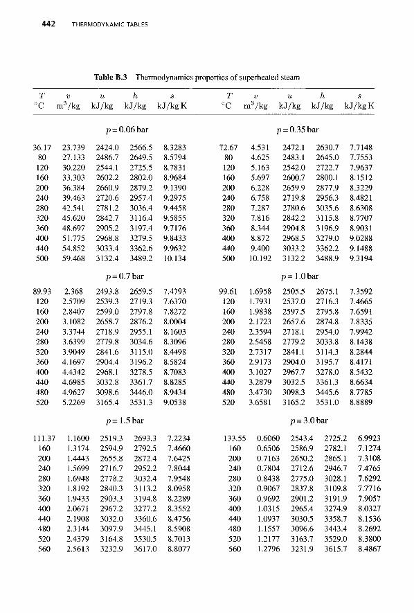
442 THERMODYNAMIC TABLES
Table B.3 Thermodynamics
T v u h s °C m3/kg kJ/kg kJ/kg kJ /kgK
p = 0.06 bar
36.17 80 120 160 200 240 280 320 360 400 440 500
23.739 27.133 30.220 33.303 36.384 39.463 42.541 45.620 48.697 51.775 54.852 59.468
2424.0 2486.7 2544.1 2602.2 2660.9 2720.6 2781.2 2842.7 2905.2 2968.8 3033.4 3132.4
2566.5 2649.5 2725.5 2802.0 2879.2 2957.4 3036.4 3116.4 3197.4 3279.5 3362.6 3489.2
8.3283 8.5794 8.7831 8.9684 9.1390 9.2975 9.4458 9.5855 9.7176 9.8433 9.9632 10.134
p = 0.7 bar
89.93 120 160 200 240 280 320 360 400 440 480 520
2.368 2.5709 2.8407 3.1082 3.3744
3.6399 3.9049 4.1697 4.4342 4.6985 4.9627 5.2269
2493.8 2539.3 2599.0 2658.7 2718.9 2779.8 2841.6 2904.4 2968.1 3032.8 3098.6 3165.4
2659.5 2719.3 2797.8 2876.2 2955.1 3034.6 3115.0 3196.2 3278.5 3361.7 3446.0 3531.3
7.4793 7.6370 7.8272 8.0004 8.1603 8.3096 8.4498 8.5824 8.7083 8.8285 8.9434 9.0538
p = 1.5 bar
111.37 160 200 240 280 320 360 400 440 480 520 560
1.1600 1.3174 1.4443 1.5699 1.6948 1.8192 1.9433 2.0671 2.1908 2.3144 2.4379 2.5613
2519.3 2594.9 2655.8 2716.7 2778.2 2840.3 2903.3 2967.2 3032.0 3097.9 3164.8 3232.9
2693.3 2792.5 2872.4 2952.2 3032.4 3113.2 3194.8 3277.2 3360.6 3445.1 3530.5 3617.0
7.2234 7.4660 7.6425 7.8044 7.9548 8.0958 8.2289 8.3552 8.4756 8.5908 8.7013 8.8077
of superheated steam
T v u h s °C m3/kg kJ/kg kJ/kg kJ /kgK
p = 0.35 bar
72.67 80 120 160 200 240 280 320 360 400 440 500
99.61 120 160 200 240 280 320 360 400 440 480 520
4.531 4.625 5.163 5.697 6.228 6.758 7.287 7.816 8.344 8.872 9.400 10.192
1.6958 1.7931 1.9838 2.1723 2.3594 2.5458 2.7317 2.9173 3.1027 3.2879 3.4730 3.6581
2472.1 2483.1 2542.0 2600.7 2659.9 2719.8 2780.6 2842.2 2904.8 2968.5 3033.2 3132.2
2630.7 2645.0 2722.7 2800.1 2877.9 2956.3 3035.6 3115.8 3196.9 3279.0 3362.2 3488.9
p= l.Obar 2505.5 2537.0 2597.5 2657.6 2718.1 2779.2 2841.1 2904.0 2967.7 3032.5 3098.3 3165.2
2675.1 2716.3 2795.8 2874.8 2954.0 3033.8 3114.3 3195.7 3278.0 3361.3 3445.6 3531.0
7.7148 7.7553 7.9637 8.1512 8.3229 8.4821 8.6308 8.7707 8.9031 9.0288 9.1488 9.3194
7.3592 7.4665 7.6591 7.8335 7.9942 8.1438 8.2844 8.4171 8.5432 8.6634 8.7785 8.8889
133.55 160 200 240 280 320 360 400 440 480 520 560
0.6060 0.6506 0.7163 0.7804 0.8438 0.9067 0.9692 1.0315 1.0937 1.1557 1.2177 1.2796
p - 3.0 bar
2543.4 2586.9 2650.2 2712.6 2775.0 2837.8 2901.2 2965.4 3030.5 3096.6 3163.7 3231.9
2725.2 2782.1 2865.1 2946.7 3028.1 3109.8 3191.9 3274.9 3358.7 3443.4 3529.0 3615.7
6.9923 7.1274 7.3108 7.4765 7.6292 7.7716 7.9057 8.0327 8.1536 8.2692 8.3800 8.4867
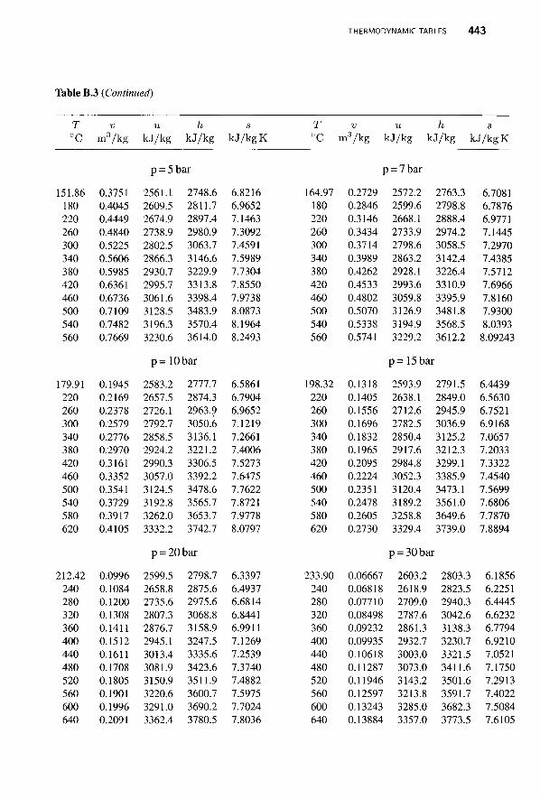
THERMODYNAMIC TABLES 4 4 3
Table B.3 (Continued)
T °C m3/kg
u kJ/kg kJ/kg kJ /kgK
T v u h s °C m3/kg kJ/kg kJ/kg kJ /kgK
p = 5 bar
151.86 0.3751 2561.1 2748.6 6.8216 180 0.4045 2609.5 2811.7 6.9652 220 0.4449 2674.9 2897.4 7.1463 260 0.4840 2738.9 2980.9 7.3092 300 0.5225 2802.5 3063.7 7.4591 340 0.5606 2866.3 3146.6 7.5989 380 0.5985 2930.7 3229.9 7.7304 420 0.6361 2995.7 3313.8 7.8550 460 0.6736 3061.6 3398.4 7.9738 500 0.7109 3128.5 3483.9 8.0873 540 0.7482 3196.3 3570.4 8.1964 560 0.7669 3230.6 3614.0 8.2493
p = 7 bar
164.97 0.2729 2572.2 2763.3 6.7081 180 0.2846 2599.6 2798.8 6.7876 220 0.3146 2668.1 2888.4 6.9771 260 0.3434 2733.9 2974.2 7.1445 300 0.3714 2798.6 3058.5 7.2970 340 0.3989 2863.2 3142.4 7.4385 380 0.4262 2928.1 3226.4 7.5712 420 0.4533 2993.6 3310.9 7.6966 460 0.4802 3059.8 3395.9 7.8160 500 0.5070 3126.9 3481.8 7.9300 540 0.5338 3194.9 3568.5 8.0393 560 0.5741 3229.2 3612.2 8.09243
p = 1 0 b a r
179.91 0.1945 2583.2 2777.7 6.5861 220 0.2169 2657.5 2874.3 6.7904 260 0.2378 2726.1 2963.9 6.9652 300 0.2579 2792.7 3050.6 7.1219 340 0.2776 2858.5 3136.1 7.2661 380 0.2970 2924.2 3221.2 7.4006 420 0.3161 2990.3 3306.5 7.5273 460 0.3352 3057.0 3392.2 7.6475 500 0.3541 3124.5 3478.6 7.7622 540 0.3729 3192.8 3565.7 7.8721 580 0.3917 3262.0 3653.7 7.9778 620 0.4105 3332.2 3742.7 8.0797
p = 15 bar
198.32 0.1318 2593.9 2791.5 6.4439 220 0.1405 2638.1 2849.0 6.5630 260 0.1556 2712.6 2945.9 6.7521 300 0.1696 2782.5 3036.9 6.9168 340 0.1832 2850.4 3125.2 7.0657 380 0.1965 2917.6 3212.3 7.2033 420 0.2095 2984.8 3299.1 7.3322 460 0.2224 3052.3 3385.9 7.4540 500 0.2351 3120.4 3473.1 7.5699 540 0.2478 3189.2 3561.0 7.6806 580 0.2605 3258.8 3649.6 7.7870 620 0.2730 3329.4 3739.0 7.8894
p = 20bar
212.42 0.0996 2599.5 2798.7 6.3397 240 0.1084 2658.8 2875.6 6.4937 280 0.1200 2735.6 2975.6 6.6814 320 0.1308 2807.3 3068.8 6.8441 360 0.1411 2876.7 3158.9 6.9911 400 0.1512 2945.1 3247.5 7.1269 440 0.1611 3013.4 3335.6 7.2539 480 0.1708 3081.9 3423.6 7.3740 520 0.1805 3150.9 3511.9 7.4882 560 0.1901 3220.6 3600.7 7.5975 600 0.1996 3291.0 3690.2 7.7024 640 0.2091 3362.4 3780.5 7.8036
p = 30bar
233.90 0.06667 2603.2 2803.3 6.1856 240 0.06818 2618.9 2823.5 6.2251 280 0.07710 2709.0 2940.3 6.4445 320 0.08498 2787.6 3042.6 6.6232 360 0.09232 2861.3 3138.3 6.7794 400 0.09935 2932.7 3230.7 6.9210 440 0.10618 3003.0 3321.5 7.0521 480 0.11287 3073.0 3411.6 7.1750 520 0.11946 3143.2 3501.6 7.2913 560 0.12597 3213.8 3591.7 7.4022 600 0.13243 3285.0 3682.3 7.5084 640 0.13884 3357.0 3773.5 7.6105
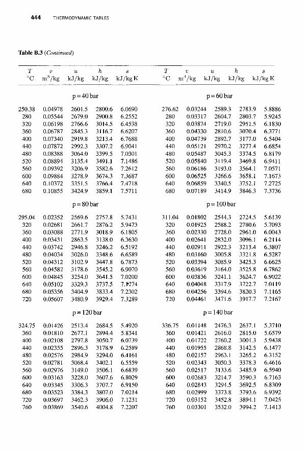
444 THERMODYNAMIC TABLES
Table B.3 (Continued)
T °C
250.38 280 320 360 400 440 480 520 560 600 640 680
295.04 320 360 400 440 480 520 560 600 640 680 720
324.75 360 400 440 480 520 560 600 640 680 720 760
V
m 3/kg
0.04978 0.05544 0.06198 0.06787 0.07340 0.07872 0.08388 0.08894 0.09392 0.09884 0.10372 0.10855
0.02352 0.02681 0.03088 0.03431 0.03742 0.04034 0.04312 0.04582 0.04845 0.05102 0.05356 0.05607
0.01426 0.01810 0.02108 0.02355 0.02576 0.02781 0.02976 0.03163 0.03345 0.03523 0.03697 0.03869
u kJ/kg
h kJ/kg
p = 40 bar
2601.5 2679.0 2766.6 2845.3 2919.8 2992.3 3064.0 3135.4 3206.9 3278.9 3351.5 3424.9
2800.6 2900.8 3014.5 3116.7 3213.4 3307.2 3399.5 3491.1 3582.6 3674.3 3766.4 3859.1
p = 80bar
2569.6 2661.7 2771.9 2863.5 2946.8 3026.0 3102.9 3178.6 3254.0 3329.3 3404.9 3480.9
2757.8 2876.2 3018.9 3138.0 3246.2 3348.6 3447.8 3545.2 3641.5 3737.5 3833.4 3929.4
p = 120 bar
2513.4 2677.1 2797.8 2896.3 2984.9 3068.4 3149.0 3228.0 3306.3 3384.3 3462.3 3540.6
2684.5 2894.4 3050.7 3178.9 3294.0 3402.1 3506.1 3607.6 3707.7 3807.0 3906.0 4004.8
s kJ/kgK
6.0690 6.2552 6.4538 6.6207 6.7688 6.9041 7.0301 7.1486 7.2612 7.3687 7.4718 7.5711
5.7431 5.9473 6.1805 6.3630 6.5192 6.6589 6.7873 6.9070 7.0200 7.1*274 7.2302 7.3289
5.4920 5.8341 6.0739 6.2589 6.4161 6.5559 6.6839 6.8029 6.9150 7.0214 7.1231 7.2207
T °C rr
276.62 280 320 360 400 440 480 520 560 600 640 680
311.04 320 360 400 440 480 520 560 600 640 680 720
336.75 360 400 440 480 520 560 600 640 680 720 760
V u l h s L3/kg kJ/kg kJ/kg kJ/kgK
p
0.03244 0.03317 0.03874 0.04330 0.04739 0.05121 0.05487 0.05840 0.06186 0.06525 0.06859 0.07189
P
0.01802 0.01925 0.02330 0.02641 0.02911 0.03160 0.03394 0.03619 0.03836 0.04048 0.04256 0.04461
P =
0.01148 0.01421 0.01722 0.01955 0.02157 0.02343 0.02517 0.02683 0.02843 0.02999 0.03152 0.03301
= 60 bar
2589.3 2604.7 2719.0 2810.6 2892.7 2970.2 3045.3 3119.4 3193.0 3266.6 3340.5 3414.9
= 100 bar
2544.3 2588.2 2728.0 2832.0 2922.3 3005.8 3085.9 3164.0 3241.1 3317.9 3394.6 3471.6
: 140 bar
2476.3 2616.0 2760.2 2868.8 2963.1 3050.3 3133.6 3214.7 3294.5 3373.8 3452.8 3532.0
2783.9 2803.7 2951.5 3070.4 3177.0 3277.4 3374.5 3469.8 3564.1 3658.1 3752.1 3846.3
2724.5 2780.6 2961.0 3096.1 3213.4 3321.8 3425.3 3525.8 3624.7 3722.7 3820.3 3917.7
2637.1 2815.0 3001.3 3142.5 3265.2 3378.3 3485.9 3590.3 3692.5 3793.6 3894.1 3994.2
5.8886 5.9245 6.1830 6.3771 6.5404 6.6854 6.8179 6.9411 7.0571 7.1673 7.2725 7.3736
5.6139 5.7093 6.0043 6.2114 6.3807 6.5287 6.6625 6.7862 6.9022 7.0119 7.1165 7.2167
5.3710 5.6579 5.9438 6.1477 6.3152 6.4616 6.5940 6.7163 6.8309 6.9392 7.0425 7.1413
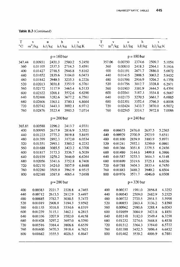
THERMODYNAMIC TABLES 445
Table B.3 (Continued)
T v u h s °C m3/kg kJ/kg kJ/kg kJ /kgK
347.44 360 400 440 480 520 560 600 640 680 720 760
365.81 400 440 480 520 560 600 640 680 720 760 800
400 440 480 520 560 600 640 680 720 760 800
0.00931 0.01105 0.01427 0.01652 0.01842 0.02013 0.02172 0.02322 0.02466 0.02606 0.02742 0.02876
0.00588 0.00995 0.01223 0.01399 0.01551 0.01688 0.01817 0.01939 0.02056 0.02170 0.02280 0.02388
0.00383 0.00712 0.00885 0.01019 0.01135 0.01239 0.01336 0.01428 0.01516 0.01600 0.01682
p = 160 bar
2431.3 2537.5 2718.5 2839.6 2940.5 3031.8 3117.9 3201.1 3282.6 3363.1 3443.3 3523.4
2580.2 2714.3 2946.8 3104.0 3235.3 3353.9 3465.4 3572.6 3677.2 3780.1 3882.1 3983.5
p = 200 bar
2296.2 2617.9 2775.2 2892.3 2993.1 3085.5 3173.3 3258.2 3341.6 3424.0 3505.9 3587.8
2413.7 2816.9 3019.8 3172.0 3303.2 3423.2 3536.7 3646.0 3752.8 3857.9 3961.9 4065.4
p = 280 bar
2221.7 2613.5 2782.7 2908.9 3016.8 3115.1 3207.9 3297.2 3384.4 3470.3 3555.5
2328.8 2812.9 3030.5 3194.3 3334.6 3462.1 3582.0 3697.0 3808.8 3918.4 4026.5
5.2450 5.4591 5.8162 6.0433 6.2226 6.3761 6.5133 6.6390 6.7561 6.8664 6.9712 7.0714
4.9331 5.5521 5.8455 6.0534 6.2232 6.3708 6.5039 6.6264 6.7408 6.8488 6.9515 7.0498
4.7465 5.4497 5.7472 5.9592 6.1319 6.2815 6.4158 6.5390 6.6539 6.7621 6.8647
T v u h s °C m3/kg kJ/kg kJ/kg kJ /kgK
357.06 360 400 440 480 520 560 600 640 680 720 760
P = 0.00750 0.00810 0.01191 0.01415 0.01596 0.01756 0.01903 0.02041 0.02173 0.02301 0.02424 0.02545
P =
: 180 bar
2374.6 2418.3 2671.7 2808.5 2916.9 3012.7 3101.9 3187.3 3270.5 3352.4 3433.7 3514.7
: 240 bar
2509.7 2564.1 2886.0 3063.2 3204.2 3328.8 3444.5 3554.8 3661.7 3766.5 3870.0 3972.8
5.1054 5.1916 5.6872 5.9432 6.1358 6.2971 6.4394 6.5687 6.6885 6.8008 6.9072 7.0086
400 440 480 520 560 600 640 680 720 760 800
0.00673 0.00929 0.01100 0.01241 0.01366 0.01480 0.01587 0.01690 0.01788 0.01883 0.01976
2476.0 2700.9 2839.9 2952.1 3051.8 3144.6 3233.3 3319.6 3404.3 3488.2 3571.7
2637.5 2923.9 3103.9 3250.0 3379.5 3499.8 3614.3 3725.1 3833.4 3940.2 4046.0
5.2365 5.6511 5.8971 6.0861 6.2456 6.3866 6.5148 6.6336 6.7450 6.8504 6.9508
400 440 480 520 560 600 640 680 720 760 800
P
0.00237 0.00543 0.00722 0.00853 0.00962 0.01059 0.01148 0.01232 0.01312 0.01388 0.01462
= 320 bar
1981.0 2509.0 2720.5 2863.4 2980.6 3084.9 3182.0 3274.6 3364.3 3452.3 3539.2
2056.8 2682.9 2951.5 3136.2 3288.4 3423.8 3549.4 3668.8 3784.0 3896.4 4006.9
4.3252 5.2325 5.5998 5.8390 6.0263 6.1851 6.3258 6.4538 6.5722 6.6832 6.7881

446 THERMODYNAMIC TABLES
Table B.4 Thermodynamic Properties of Air
T
K
200 210 220 230 240
250 260 270 280 285
290 295 300 305 310
315 320 325 330 340
350 360 370 380 390
400 410 420 430 440
h
kJ/kg
199.97 209.97 219.97 230.02 240.02
250.05 260.09 270.11 280.13 285.14
290.16 295.17 300.19 305.22 310.24
315.27 320.29 325.31 330.34 340.42
350.49 360.58 370.67 380.77 390.88
400.98 411.12 421.26 431.43 441.61
s°
kJ/(kg-,K)
1.29559 1.34444 1.39105 1.43557 1.47824
1.51917 1.55848 1.59634 1.63279 1.65055
1.66802 1.68515 1.70203 1.71865 1.73498
1.75106 1.76690 1.78249 1.79783 1.82790
1.85708 1.88543 1.91313 1.94001 1.96633
1.99194 2.01699 2.40142 2.06533 2.08870
Pr
0.3363 0.3987 0.4690 0.5477 0.6355
0.7329 0.8405 0.9590 1.0889 1.1584
1.2311 1.3068 1.-3860 1.4686 1.5546
1.6442 1.7375 1.8345 1.9352 2.149
2.379 2.626 2.892 3.176 3.481
3.806 4.153 4.522 4.915 5.332
vr
1707.0 1512.0 1346.0 1205.0 1084.0
979.0 887.8 808.0 738.0 706.1
676.1 647.9 621.2 596.0 572.3
549.8 528.6 508.4 489.4 454.1
422.2 393.4 367.2 343.4 321.5
301.6 283.3 266.6 251.1 236.8
T
K
450 460 470 480 490
500 510 520 530 540
550 560 570 580 590
600 610 620 630 640
650 660 670 680 690
700 710 720 730 740
h
kJ/kg
451.80 462.02 472.24 482.49 492.74
503.02 513.32 523.63 533.98 544.35
554.74 565.17 575.59 586.04 596.52
607.02 617.53 628.63 638.63 649.22
659.84 670.47 681.14 691.82 702.52
713.27 724.04 734.82 745.62 756.44
s°
kJ/(kg•K)
2.11161 2.13407 2.15604 2.17760 2.19876
2.21952 2.23993 2.25997 2.27967 2.29906
2.31809 2.33685 2.35531 2.37348 2.39140
2.40902 2.42644 2.44356 2.46048 2.47716
2.49364 2.50985 2.52589 2.54175 2.55731
2.57277 2.58810 2.60319 2.61803 2.63280
Pr
5.775 6.245 6.742 7.268 7.824
8.411 9.031 9.684 10.37 11.10
11.86 12.66 13.50 14.38 15.31
16.28 17.30 18.36 19.84 20.64
21.86 23.13 24.46 25.85 27.29
28.80 30.38 32.02 33.72 35.50
Vr
223.6 211.4 200.1 189.5 179.7
170.6 162.1 154.1 146.7 139.7
133.1 127.0 121.2 115.7 110.6
105.8 101.2 96.92 92.84 88.99
85.34 81.89 78.61 75.50 72.56
69.76 67.07 64.53 62.13 59.82
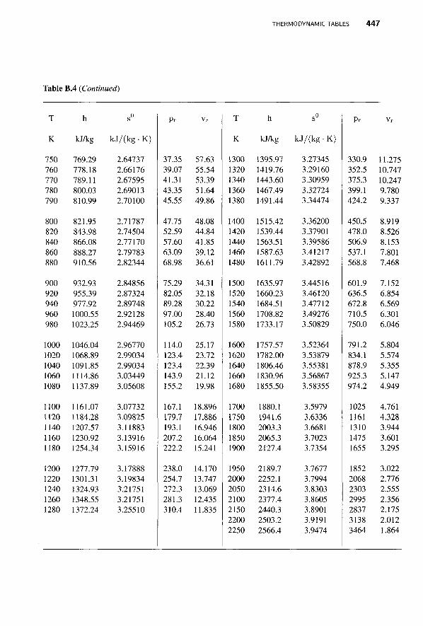
THERMODYNAMIC TABLES 447
Table B.4 (Continued)
K
750 760 770 780 790
800 820 840 860 880
h
kJ/kg
769.29 778.18 789.11 800.03 810.99
821.95 843.98 866.08 888.27 910.56
900 932.93 920 955.39 940 977.92 960 1000.55 980 1023.25
1000 1046.04 1020 1068.89 1040 1091.85 1060 1114.86 1080 1137.89
1100 1161.07 1120 1184.28 1140 1207.57 1160 1230.92 1180 1254.34
1200 1277.79 1220 1301.31 1240 1324.93 1260 1348.55 1280 1372.24
kJ/(kg ■ K)
2.64737 2.66176 2.67595 2.69013 2.70100
2.71787 2.74504 2.77170 2.79783 2.82344
2.84856 2.87324 2.89748 2.92128 2.94469
2.96770 2.99034 2.99034 3.03449 3.05608
3.07732 3.09825 3.11883 3.13916 3.15916
3.17888 3.19834 3.21751 3.21751 3.25510
Pr
37.35 39.07 41.31 43.35 45.55
47.75 52.59 57.60 63.09 68.98
75.29 82.05 89.28 97.00 105.2
114.0 123.4 123.4 143.9 155.2
167.1 179.7 193.1 207.2 222.2
238.0 254.7 272.3 281.3 310.4
57.63 55.54 53.39 51.64 49.86
48.08 44.84 41.85 39.12 36.61
34.31 32.18 30.22 28.40 26.73
25.17 23.72 22.39 21.12 19.98
18.896 17.886 16.946 16.064 15.241
14.170 13.747 13.069 12.435 11.835
K
1300 1320 1340 1360 1380
kJ/kg kJ/(kg • K )
1700 1750 1800 1850 1900
1950 2000 2050 2100 2150 2200 2250
1395.97 1419.76 1443.60 1467.49 1491.44
1400 1515.42 1420 1539.44 1440 1563.51 1460 1587.63 1480 1611.79
1500 1635.97 1520 1660.23 1540 1684.51 1560 1708.82 1580 1733.17
1600 1757.57 1620 1782.00 1640 1806.46 1660 1830.96 1680 1855.50
1880.1 1941.6 2003.3 2065.3 2127.4
2189.7 2252.1 2314.6 2377.4 2440.3 2503.2 2566.4
3.27345 3.29160 3.30959 3.32724 3.34474
3.36200 3.37901 3.39586 3.41217 3.42892
3.44516 3.46120 3.47712 3.49276 3.50829
3.52364 3.53879 3.55381 3.56867 3.58355
3.5979 3.6336 3.6681 3.7023 3.7354
3.7677 3.7994 3.8303 3.8605 3.8901 3.9191 3.9474
330.9 11.275 352.5 10.747 375.3 10.247 399.1 9.780 424.2 9.337
450.5 8.919 478.0 8.526 506.9 8.153 537.1 7.801 568.8 7.468
601.9 636.5 672.8 710.5 750.0
791.2 834.1 878.9 925.3 974.2
1025 1161 1310 1475 1655
1852 2068 2303 2995 2837 3138 3464
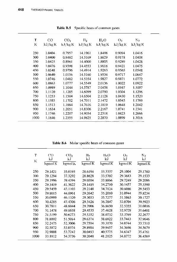
NO
NO
OO
Oo
-j
-o
.O
NO
Nt
-n
<-
n-
t^
4^
u>
u>
to
(j
iO
<-
fl
O<
-/
iO
C>
iO
Ln
OL
n©
i/
iO
C/
i o
oo
oo
oo
oo
oo
oo
oo
W
H
U)U
>U
>l>
JU>
U)U
>U
)U>
U>
tOIO
tOtO
(OtO
u
ito
toto
*-^
-~-o
po
NO
NO
NO
NO
NO
No
^-
o ui
N)
bo u
^
^4
^ b
bo u
i w
^
- ^
- i-
OO
OO
Ot
'(
10
"4
!.
OO
WI
OO
**
^K
Ui
^-
O-
J-
Jv
oo
-J
— o
o oo
— in
«
vo v
o (O
-4(O
U>
OO
tOO
NO
u
>-t
^-o
o^
--Jt
_n
4^
ON
t0.t^
ON
-P>.
U>0
0.&
>. v
)a
4i
UH
VO
vl
U
!t
i.
^-
ON
«L
>4
>l
oo
Ot
OO
NO
tO
NO
NO
NO
O
NO
^-
00
tO
4^
tO
<-
^>
PC
cm w
PC
cm «
pc
O
C-l
O
I
OO
NO
NO
NO
NO
NO
NO
NO
NO
NO
NO
NO
NO
OO
OO
Cm
fo
bb
o^
JO
>u
i^
oj
ww
to
N)
Mb
bo
b\
B
0^
\C
Ui
WO
JU
i^
4i
OO
\^
4i
W^
M
O
*»
00
\0
^I
UI
UO
IO
U*
*H
OM
* |—
'
t-II
O
-o
iO
'C
ao
o^
aa
ic
nu
ij
i^
uw
u
MS
]J
1M
\O
V]
O\
O\
00
IO
O
tO
s]
L/
1-
Ot
OU
>t
OL
/l
4i
.~
-J
*-
UU
i-
JO
MN
OO
Ov
l-
JO
to
»
ui
w
-O
00
-O U
>
—
ON
O
U>
O
O
N t
o -4
PC
cm 3
UJ
U>
U>
UiU
>U
)L
*J
U>
U>
UiC
>}
l>0
(>
JtO
tOtO
4^
-t^
-^
-t^
00
ON
U
) ~
J U
) O
N
-J
**
NO
to
-O
O
N
U
U)
fj
M
N
^i
bj
lo
yi
b
^ s
i N
1 U
v
] -fc
. O
N to
u\
o U
V
O V
D
Ui
*.
>—
*-
o O
N
O N
O
NO
c/i
o 00
NO
ON
*
*
0\
M
V]
U
►-
O
4^
to
ON
O
GO
L
h
-P*
OO
O
O
N
~J
NO
OJ
-^.
PC
cm 3 o. EP
WU
UW
WW
WW
WW
tO
Wt
OI
OK
IW
O
\U
I^
US
)I
N)
M«
OO
NO
NO
NO
NO
NO
NO
^^
Ln
^i
pt
pb
bi
ji
i-
bo
ui
UM
^'
H-
Ln
~-
J0
NU
)0
N0
N-
^.
00
N0
sl
tO
^.
U>
O<
-n
-J
~~
' ""
'
O*
-t
Ot
OU
>L
HN
00
0L
00
N
Mi
MJ
sH
iU
iO
CJ
WO
O
N
ON
NO
*
-H
- -fc
- ~
J O
O
N
PC
cm w E
2
N0
ND
00
00
-0
-J
0N
0N
L/
lL
/1
-t
^-
t*
.U
)U
>t
O
Ui
OC
ft
O^
O'
-'
iO
l/
iO
^O
Ui
OC
Ji
ooooooooooooooo
W H
W
to
N
W
M
«
►—
>—
OO
OO
OO
OO
^
i i?
1
oa
uo
Ni
c«
to
oc
-J
ou
i*
»-
(»
t»
t»
^^
r1
H- O
N*
.-t^
oN
toN
ON
Oto
~j-
i^^
s!t
oo
^ cm
^
ON
ON
>—
tON
OO
ON
-JtO
tO-J
OO
LnO
OO
OO
N
M
■I*
00
K-
^^
^^
-K
- —
O
OO
OO
OO
OO
0
0-
O0
Nt
_n
U>
tO
^-
N0
00
-O
0N
l/
l4
^-
p>
--
f^
-£
>-
^^
w^
oo
cn
to
oo
o-
t^
^v
ii
oo
o a
o4
»u
wu
o*
uo
iO
»a
ui
OA
p t
ot
oi
oM
MM
MM
bb
bi
ov
ob
ob
o^
UW
OO
Os
lU
IO
O-
Oi
'-
-J
U>
NO
-P
* N
O
L/
iO
Ui
oo
oo
oo
-t
^-
oo
oc
yi
NO
NO
ON
OO
Ln
<J
i-
jK
-4
^t
O4
^m
-l
^-
-J
tO
ON
ON
00
—
to
-J
©p
op
O
O
NO
NO
Op
00
-f̂
4>
4
^ 4
^ J>
NO
N
O 0
0 s
] s
) OO
O
tO
l/
l t-n
4
^
u>
o ON
ON
ON
O -̂
0\
bN
lf
tC
yi
Ui
Lf
i4
^4
^4
^C
>J
^ L
/l
Os
JL
fl
U>
^-
*N
O<
-/
lO
*-
NO
o
^o
o^
ui
c^
^u
io
oo
^N
D-
JN
O-
t^
O-
l^
l>
JO
NO
^-
PC
c^
PC
cm
O
O
PC
PC
cm
PC
C-i
cm
'
W
In
to
toto
toto
toto
toio
to»
—
c*c*
c*
c- c*
r"
to t
o to
^-
U
k-
oo
ON
ON
ON
ON
ob
ob
ob
o 0
0U
l^0
04
N'-
-0
^'-
00
Ult
OO
00
Os
^ s
ii
-a
f-
vi
w\
ou
iu
io
uw
ot
oc
O0
0-J
N0
tO0
0O
00
0N
-J4
^U
)00
UlN
00
0
OO
OO
OO
OO
O
00
00
-J
ON
Ul
4^
U>
«0
N0
tO
4^
4^
-t
^t
->
0O
0N
lO
\
OW
^O
OU
lO
A^
lt
O
p p
p p
p p
p NO NO NO NO NO NO NO
00 ~J
<J> 4^ tO *- O
si H- ON tO 00 -J NO
H
N]
U
H
iO
OO
4i
PC
PC «
i. cm
O
PC >p
cm
W
o 3 cm
References
1. D. G. Ainley, Performance of axial flow turbines, Proceedings of the Institute of Mechanical Engineers, 159, 1948.
2. D. G. Ainley and G. C. R. Mathieson, A Method for Performance Estimation for Axial-Flow Turbines, Aeronautical Research Council, Reports and Memoranda, 2974, 1957.
3. G. Agricola, De Re Metallica, Translated by Herbert Clark Hoover and Lou Henry Hoover, Dover, New York, 1950.
4. V. Arakeri, Contributions to some cavitation problems in turbomachinery, Proceedings Acadey of Engineering Sciences, India, 24:454-483, 1999.
5. O. E. Balje, Turbo Machines: A Guide to Selection and Theory, Wiley, New York, 1981. 6. E. A. Baskharone, Principles of Turbomachinery in Air-Breating Engines, Cambridge University
Press, Cambridge, UK, 2006. 7. W. W. Bathie, Fundamentals of Gas Turbines, Wiley, New York, 1984. 8. A. M. Binnie and M. W. Woods, The pressure distribution in a convergent-divergent steam nozzle,
Proceedings of the Institute of Mechanical Engineers, 138, 1938. 9. C. E. Brennen, Hydrodynamics of Pumps, Concepts NREC and Oxford University Press, White
River Junction, VT, 1994. 10. C. E. Brennen, Cavitation and Bubble Dynamics, Oxford University Press, 1995. 11. H. Brown, The Challenge of Man's Future, The Viking Press, New York, 1954. 12. A. F. Burstall, A History of Mechanical Engineering, MIT Press, Cambridge, MA, 1965. 13. T. Burton, D. Sharpe, N. Jenkins, and E. Bossanyi, Wind Energy Handbook, Wiley, New York,
USA, 2001. 14. A. D. S. Carter, The Low Speed Performance of Related Airfoils in Cascade, Aeronautical
Research Council, CP 29, 1950.
Principles of Turbomachinery. By Seppo A. Korpela 449 Copyright © 2011 John Wiley & Sons, Inc.
450 REFERENCES
15. H. Cohen, G. F. C. Rogers, and H. I. H. Saravanamuttoo, Gas Turbine Theory, 3rd ed., Longman Scientific & Technical, London, 1972.
16. H. R. M. Craig and H. J. A. Cox, Performance estimation of axial-flow turbines, Proceedings of the Institute of Mechanical Engineers, 185:407-424, 1970.
17. G. T. Csanady, Theory ofTurbomachines, McGraw-Hill, New York, 1964. 18. N. A. Cumpsty, Compressor Aerodynamics, Longman Scientific & Technical, London, 1989.
19. N. A. Cumpsty, Jet Propulsion, Cambridge University Press, Cambridge, UK, 2003. 20. P. de Haller, Das Verhalten von Tragflugelgittern in Axialverdichtern und in Windkanal, Bernstoff-
Warmer-Kraft 5, Heft 10, 1953. 21. J. D. Denton, Loss mechanisms in turbomachines, Journal of Turbomachinery, 115:621-653,
1993. 22. S. L. Dixon, Thermodynamics and Fluid Dynamics ofTurbomachinery, 5th ed., Elsevier, Oxford,
2005.
23. L. F. Drbal, P. G. Boston, and K. L. Westra, Power Plant Engineering, Springer, Berlin, 1995. 24. J. Dunham and P. M. Came, Improvements to the Ainley-Mathiesen Method of Turbine Perfor-
mance Prediction, ASME paper 70-GT-2, 1970. 25. D. M. Eggleston and F. S. Stoddard, Wind Turbine Engineering Design, Van Nostrand Reinhold,
New York, 1987.
26. J. Fullermann, Centrifugal compressors, in Advances in Petroleum Chemistry and Refining, Engineering. J. McKetta, ed. Interscience Publishers, New York, 1962.
27. A. J. Glassman, Computer Programfor Design and Analysis of Radial Inflow Turbines, TN-8164, NASA, 1976.
28. H. Glauert, Airplane propellers, in Aerodynamic Theory, A General Review of Progress, Vol IV, W. F. Durand, ed. Dover, New York, 1963.
29. S. Goldstein, On the vortex theory of screw propellers, Proceedings of the Royal Society, 123, 929.
30. P. M. Goorjian, An invalid equation in the general momentum theory of actuator disk, AIAA Journal, 10, 1972.
31. A. Guha, A unified theory of aerodynamic and condensastion shock waves in vapor-droplet flows with or without a carrier gas, Physics of Fluids, 6:1893-1913, 1983.
32. E. Hau, Wind Turbines, Fundamentals, Technologies, Application, Economics, Springer, Berlin, 2006.
33. W. R. Hawthorne, Elements of Turbine and Compressor Theory, Gas Turbine Laboratory Note, MIT, 1957, (quoted by Horlock, in Axial Flow Turbines [34].)
34. J. H. Horlock, Axial Flow Compressors, Butterworth & Co., London, 1958. 35. J. H. Horlock, Axial Flow Turbines, Butterworth & Co., London, 1966. 36. A. R. Howell, The Present Basis of Axial Flow Compressor Design, Part I, Cascade Theory and
Performance, Aeronautical Research Council Reports and Memoranda, No. 2095, 1942. 37. A. R. Howell, Design of axial compressors, Proceedings of the Institution of Mechanical Engi-
neers, 153, 1945. 38. A. R. Howell and R. P. Bonham, Overall and stage characteristics of axial-flow compressors,
Proceedings of the Institution of Mechanical Engineers, 163, 1950. 39. M. K. Hubbert, Energy from fossil fuels, Science, 109:103-109, 1945. 40. H. Hugoniot, Propagation des mouvements dans les corps et specialement dans les gaz parfaits,
Journal de I'Ecole Poly technique, 57, 1887.
REFERENCES 451
41. J. C. Hunsaker and B. G. Rightmire, Engineering Applications of Fluid Mechanics, McGraw-Hill, New York, 1947.
42. R. A. Huntington, Evaluation of polytropic calculation methods for turbomachinery analysis, ASME Journal of Engineering for Gas Turbines and Power, 107:872-879, 1985.
43. International Energy Outlook 2009, US-DOE, released May 27, 2009.
44. V. Kadambi and M. Prasad, An Introduction to Energy Conversion, Vol. Ill Turbomachinery, New Age International Publishers, New Delhi, 1977.
45. I. J. Karrasik, J. P. Messina, P. Cooper, and C. C. Heald, Pump Handbook, McGraw-Hill, New York, 2007.
46. W. J. Kearton, Steam Turbine Theory and Practice, Pitman and Sons, Bath, UK, 1931.
47. J. H. Keenan, Thermodynamics, MIT Press, Cambridge USA, 1971. 48. I. M. Khalil, W. Tabakoff, and A. Hamed, Losses in a radial inflow turbine, Journal of Fluids
Engineering, 98:364-372, 1976.
49. S. A. Korpela, Oil depletion in the world, Current Science, 91:1148-1152, 2006. 50. R. I. Lewis, Turbomachinery Performance Analysis, Elsevier, Oxford, 1996. 51. S. Lieblein and W. H. Roudebush, Theoretical Loss Relation for Low-Speed 2D Cascade Flow,
TN 3662, NASA, 1956. 52. E. Logan, Jr., Turbomachinery; Basic Theory and Applications, Marcel-Dekker, New York,
1981. 53. A. Lugaresi and A. Massa, Designing Francis turbines: Trends in the last decade, Water Power
& Dam Construction, 1987. 54. A. Maddison, Contours of world economy and the art of macro-measurement 1500-2001, Rug-
glers lecture, IARIW 28th General Conference, Cork, Ireland, Aug. 2004. 55. M. Mallen and G. Saville, Polytropic Processes in the Performance Prediction of Centrifugal
Compressors, Institution of Mechanical Engineers, Paper C183/77, 89-96, 1977. 56. L. F. Moody and T. Zowski, Fluid machinery, in Handbook of Applied Hydraulics, C. V. Davis
and K. W. Sorenson, eds. McGraw-Hill, New-York, 1969.
57. M. Nechleba, Hydraulic Turbines, Their Design and Equipment, Artia, Praque, Czechoslovakia, 1957.
58. C. Pfleiderer, Die Wasserturbinen, mit einem Anhang iiber Strbmungsgetriebe, Wolfenbiitteler Verlag-Anst.,
59. C. Pfleiderer and H. Pertermann, Strbmungsmachinen, Springer-Verlag, Berlin, 1986. Hannover, Germany, 1947.
60. L. Prandtl, Schraubenpropeller mit geringstem Energieverlust, Nachrichten Mathematischphyis-calishe Klasse, Gottingen, Germany, 1919, (Appendix to the article of A. Betz).
61. W. Rankine, On the mechanical principles of propellors, Transactions of the Institute of Naval Architects, 6:13-30, 1865.
62. W. Rankine, On the fhermodynamic theory of waves of finite longitudinal disturbances. Philo-sophical Transactions of the Royal Socciety, 160:27, 1870.
63. C. Rodgers and R. Gleiser, Performance of a high-efficiency radial/axial turbine. ASME Journal of Turbomachinery 109:151-154, 1987.
64. Rolls Royce, The Jet Engine, London, 2005. 65. H. Rohlik, Radial-inflow turbines, in Turbine Design and Applications A. J. Glassman, ed.,
SP290, NASA, 1975. 66. S. J. Savonius, The S-rotor and its applications, Mechanical Engineering, 53, issue 5, 1931.
452 REFERENCES
67. F. Schweiger and J. Gregory, Developments in the design of Kaplan turbines, Water Power & Dam Construction, 1987.
68. D. G. Sheppard, Historical Development of the Windmill, in Wind Turbine Technology, D. A. Spera, ed., ASME Press, New York, 1995.
69. J. M. Shultz, The polytropic analysis of centrifugal compressors, ASME Journal of Engineering for Power, 69-82, 1962.
70. L. H. Smith, Jr., Casing Boundary Layers in Multistage Compressors, in Proceedings of the Symposium on Flow Research on Blading, L. S. DZung, ed., Elsevier, Burlington, MA, 1970.
71. S. F. Smith, A simple correlations of turbine efficiency, Journal of Royal Aeronautical Society, 69:467-470, 1965.
72. C. R. Soderberg, Unpublished Notes of the Gaqs Turbine Laboratory, MIT, Cambridge, MA, (quoted by Horlock [35]).
73. J. D. Stanitz, Some theoretical aerodynamic investigations of impellers in radial and mixed-flow centrifugal compressors, ASME Transactions, Series A, 1A:A12I-A91, 1952.
74. A. J. Stepanoff, Centrifugal and Axial Flow Pumps, 2nd ed., Wiley, New York, 1957.
75. A. Stodola, Steam and Gas Turbines, 6th ed., P. Smith, New York, 1945.
76. W. Traupel, Thermische Turbomachinen, 2nd ed. Springer, 1971.
77. J. Volkovitch, Analytical prediction of vortex ring boundaries for helicopters in steep descents, Journal of American Helicopter Society, 17(3), 1973.
78. A. Whitfield, The preliminary design of radial inflow turbines, Journal ofTurbomachinery, 112, 1990.
79. A. Whitfield and N. C. Baines, Design of Radial Turbomachines, Longman Scientific and Technical, Essex, UK, 1990.
80. F. J. Wiesner, A review of slip factors for centrifugal compressors, Journal of Engineering Power, ASME, 89:558-572, 1967.
81. D. G. Wilson and T. Korakianitis, Design of High-Efficiency Turbomachinery and Gas Turbines, 2nd ed., Prentice-Hall, Upper Saddle River, NJ, 1998.
82. R. E. Wilson and P. .B. .E. Lissaman, Applied Aerodynamics of Wind Power Machines, Oregon State University , May 1974.
83. A. Wirzenius, Keskipakopumput (Centrifugal Pumps, 3rd. ed., (in Finnish), Kustannusyhtyma, Tampere, Finland, 1978.
84. R. H. Zimmerman, Lecture Notes on Turbomachinery, The Ohio State University, Columbus, Ohio USA, 1989.
85. O. Zweifel, The Spacing of turbomachinery Blading, Especially with Large Angular Deflection, Brown Boveri Review, 32:12, 1945.
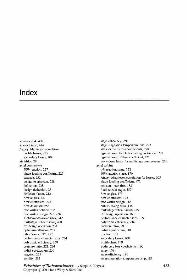
Index
actuator disk, 402 advance ratio, 414 Ainley-Mathieson correlation
profile losses, 205 secondary losses, 208
air tables, 29 axial compressor
50% reaction, 227 blade-loading coefficient, 225 cascade, 252 de Haller criterion, 228 deflection, 228 design deflection, 231 diffusion factor, 242 flow angles, 227 flow coefficient, 225 flow deviation, 258 free vortex defined, 236 free vortex design, 228, 236 Lieblein diffusion factor, 242 multistage reheat factor, 260 off-design operation, 234 optimum diffusion, 257 other losses, 247, 257 performance characteristics, 234 polytropic efficiency, 259 pressure ratio, 221, 224 radial equilibrium, 235 reaction, 225 solidity, 233
stage efficiency, 250 stage stagnation temperature rise, 223 static enthalpy loss coefficients, 250 typical range for blade-loading coefficient, 222 typical range of flow coefficient, 222 work-done factor for multistage compressors, 260
axial turbine 0% reaction stage, 178 50% reaction stage, 176 Ainley-Mathieson correlation for losses, 205 blade-loading coefficient, 172 constant mass flux, 188 fixed nozzle angle, 187 flow angles, 173 flow coefficient, 172 free vortex design, 183 hub-to-casing ratio, 136 multistage reheat factor, 215 off-design operation, 180 performance characteristics, 199 polytropic efficiency, 216 pressure ratio, 193 radial equilibrium, 181 reaction, 172 secondary losses, 208 Smith chart, 199 Soderberg loss coefficients, 190 stage, 167 stage efficiency, 191 stage stagnation temperature drop, 181
453 Principles of Turbomachinery. By Seppo A. KorpelaCopyright © 2011 John Wiley & Sons, Inc.
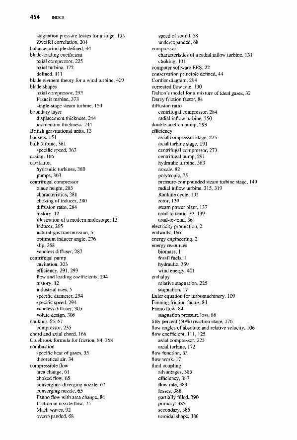
454 INDEX
stagnation pressure losses for a stage, 193 Zweifel correlation, 204
balance principle defined, 44 blade-loading coefficient
axial compressor, 225 axial turbine, 172 defined, 111
blade element theory for a wind turbine, 409 blade shapes
axial compressor, 253 Francis turbine, 373 single-stage steam turbine, 150
boundary layer displacement thickness, 244 momentum thickness, 244
British gravitational units, 13 buckets, 151 bulb turbine, 361
specific speed, 363 casing, 166 cavitation
hydraulic turbines, 380 pumps, 303
centrifugal compressor blade height, 285 characteristics, 281 choking of inducer, 280 diffusion ratio, 284 history, 12 illustration of a modern multistage, 12 inducer, 265 natural-gas transmission, 5 optimum inducer angle, 276 slip, 268 vaneless diffuser, 287
centrifugal pump cavitation, 303 efficiency, 291,293 flow and loading coefficients, 294 history, 12 industrial uses, 5 specific diameter, 294 specific speed, 294 vaneless diffuser, 305 volute design, 306
choking, 65, 67 compressor, 235
chord and axial chord, 166 Colebrook formula for friction, 84, 368 combustion
specific heat of gases, 35 theoretical air, 34
compressible flow area change, 61 choked flow, 65 converging-diverging nozzle, 67 converging nozzle, 65 Fanno flow with area change, 84 friction in nozzle flow, 75 Mach waves, 92 overexpanded, 68
speed of sound, 58 underexpanded, 68
compressor characteristics of a radial inflow turbine, 131 choking, 131
computer software EES, 22 conservation principle defined, 44 Cordier diagram, 294 corrected flow rate, 130 Dalton's model for a mixture of ideal gases, 32 Darcy friction factor, 84 diffusion ratio
centrifugal compressor, 284 radial inflow turbine, 350
double-suction pump, 293 efficiency
axial compressor stage, 225 axial turbine stage, 191 centrifugal compressor, 273 centrifugal pump, 291 hydraulic turbine, 363 nozzle, 82 polytropic, 75 pressure-compounded steam turbine stage, 149 radial inflow turbine, 315, 319 Rankine cycle, 135 rotor, 139 steam power plant, 137 total-to-static, 37, 139 total-to-total, 36
electricity production, 2 endwalls, 166 energy engineering, 2 energy resources
biomass, 1 fossil fuels, 1 hydraulic, 359 wind energy, 401
enthalpy relative stagnation, 225 stagnation, 17
Euler equation for turbomachinery, 109 Fanning friction factor, 84 Fanno flow, 84
stagnation pressure loss, 86 fifty percent (50%) reaction stage, 176 flow angles of absolute and relative velocity, 106 flow coefficient, 111, 125
axial compressor, 225 axial turbine, 172
flow function, 63 flow work, 17 fluid coupling
advantages, 385 efficiency, 387 flow rate, 389 losses, 388 partially filled, 390 primary, 385 secondary, 385 toroidal shape, 386
INDEX 455
torque coefficient, 390 Francis turbine, 362, 370
specific speed, 363 friction factor
Colebrook, 84 Darcy, 84 Fanning, 84
gas turbine electricity generation, 4 industrial, 11
Gibbs-Dalton model for ideal gases, 33 Helmholtz vortex theorem, 426 hub, 166 hydraulic turbine
bulb turbine, 361 capacity factor, 4 crossflow or Banki-Mitchell turbine, 380 effective head, 360 electricity generation, 5 Francis turbine, 362, 370, 373 gross head, 360 history, 8 Kaplan turbine, 361, 377-378 mechanical efficiency, 361 overall efficiency, 360 Pelton wheel, 362 pit turbine, 371 power-specific speed, 362 synchronous speed, 363 turgo, 380 volumetric efficiency, 361
incompressible fluid internal energy and irreversibility, 35 stagnation pressure, 44
induced and forced draft, 39 induction factor, 405 internal heating, 42 jet engine
gas generator, 221 history, 11 spool, 221
Kaplan turbine, 361 number of blades, 378 specific speed, 363
kinetic theory of specific heats for gases, 28 Mach number, 59 manometer formula, 127 mass conservation principle, 16 meridional velocity, 106 mixing and pressure change, 53 Mollier diagram, 24 moment of momentum balance, 108 momentum equation, 47 nondimensional groups, 125 normal shock, 68-69 nozzle
efficiency, 83 polytropic process, 76 static enthalpy loss coefficient, 79 steam, 87 velocity coefficient, 79
nuclear fuels—uranium and thorium, 1 nucleation—homogeneous and heterogeneous, 90 oblique shock, 68 off-design operation of an axial turbine, 180 overexpanded flow, 68 Pelton wheel, 362
number of buckets, 363 specific speed, 363
Pfleiderer correlation for pumps, 293 pitch, 166 polytropic efficiency, 216, 259 positive-displacement machine, 2 power-absorbing machine, 2 power-producing machine, 2 power-specific speed, 362 power coefficient, 127 power ratio of a radial inflow turbine, 315 Prandtl-Meyer theory, 93 pressure compounding, 146 pressure ratio
axial compressor, 224 axial turbine, 193 steam turbine, 136
pressure recovery partial, 51 pressure side of blade, 166 primary energy production
wind energy, 401 radial equilibrium
axial compressor, 235 axial turbine, 181 constant mass flux, 188 first power exponent, 241 fixed nozzle angle, 187 zero-power exponent, 240
radial inflow turbine, 313 Balje diagram, 324 blade height, 351 efficiency, 319, 345 minimum exit Mach number, 347 number of blades, 352 optimum incidence, 352 optimum inlet, 339 radius ratio, 350 recommended diffusion, 350 specific diameter, 324 specific speed, 324 stator flow, 329 stator loss coefficients, 333 typical design parameters, 328
Rankine combined vortex wake, 415 reaction
axial compressor, 225 axial turbine, 172 definition, 116 in terms of kinetic energies, 116
reheat factor axial compressor, 260 axial turbine, 215
renewable energy, 1 Reynolds number, 125 rothalpy, 114
456 INDEX
rotor efficiency centrifugal compressor, 270
scale effect, 125 scaling analysis, 124 shape parameter, 128 shock
normal, 68-69 Rankine-Hugoniot relations, 73 shock relations, 72 strength, 75
similitude, 125 slip, 268 slip stream, 402 sonic state, 62 specific diameter
centrifugal pump, 294 radial inflow turbine, 323
specific speed, 128 centrifugal pump, 294 hydraulic turbines, 361, 363 radial inflow turbine, 323
speed of sound, 59 influence of molecular mass, 59
spouting velocity, 317 stage
axial compressor, 223 axial turbine, 167 normal, 167
stagnation density, 60 stagnation pressure, 60 stagnation pressure loss and entropy, 45 stagnation pressure losses
axial turbine, 193 profile losses for axial compressor, 247
stagnation pressure low Mach number, 60
stagnation state defined, 36
stagnation temperature, 60 static enthalpy loss coefficients, 141 steam tables, 22 steam turbine, 3
blade shape, 151 electricity production, 2 history, 10 nozzle coefficient, 138 pressure compounding, 146 rotor efficiency, 139 single-stage impulse, 138 single-stage optimum blade speed, 144 Soderberg correlation, 160 types, 136 velocity compounding, 152 zero-reaction stage, 158
steam computer software EES, 22 condensation shock, 91 equation of state, 22 Mollier diagram, 24 supersaturation, 24, 90 undercooling, 91
Wilson line, 24 Zeuner equation, 28
streamline curvature method, 431 subsonic flow defined, 59 suction side of blade, 166 supercritical and ultrasupercritical steam cycle, 3 supersonic flow defined, 59 swirl velocity, 168 thermodynamics
compressed liquid, 26 equation of state for air, 29 equation of state for steam, 22 first law, 17 Gibbs equations, 20 ideal gas, 27 ideal gas mixutures, 31 incompressible fluid, 35 second law, 19
three-dimensional flow axial compressor, 235 axial turbine, 181
tip clearance and leakage flow, 167 torque converter
efficiency, 393, 396 torque multiplication, 391
total head, 291 transonic flow defined, 59 trothalpy, 114 turbine characteristics of a radial inflow turbine, 132 turbocharger, 130 turbomachine
definition of, 2 history, 7 household use, 6 names of components, 2
Tygun formula, 363 underexpanded flow, 68 unloading of a blade, 242 utilization
definition, 117 maximum, 119 relation to reaction, 118
variable specific heats, 41 velocity compounding, 152 velocity triangle, 106 ventilating blower, 39 volute, 306 water wheel history, 7 Wilson line, 24 wind energy
capacity factor, 401 Denmark, 401 Germany, 401 installed capacity, 5 United States, 401
wind turbine, 401 actuator disk, 403 American windmill, 9 Betz limit, 406 blade element theory contributions by
N. E.Joukovsky, 409

INDEX 4 5 7
blade element theory development by S. Drzewieci, 402
blade element theory of W. Froude, 402 blade forces for a nonrotating wake, 415 capacity factor, 5 ducted turbine, 408 Glauert theory for an ideal turbine, 424 history, 8 induction factors for an irrotational wake, 415 momentum theory, 403 momentum theory of W. J. M. Rankine, 402 operation as a propeller, 407
power coefficient, 406 Prandtl's tip correction, 426 pressure drop across the actuator disk, 404 Savonius rotor, 9 tip speed ratio, 406, 414 velocity at the actuator disk, 404 wake rotation, 409
windmill, 401 work coefficient, 126 zero percent (0%) reaction, 158, 178 Zeuner's equation, 87 Zweifel correlation, 204