Prey-size selection by brown trout ( Salmo trutta L.) in a stream in northern Spain

Prey-size selection by brown trout (Salmotrutta L.) in a stream in northern Spain

Pedro A. Rincón and Javier Lobón-Cerviá

Abstract: Brown trout in the River Negro in northern Spain preferentially ate larger aquatic prey items (foundthroughout the water column). A model based on size-dependent prey encounters was able to account for this trend andto generate accurate predictions of the consumption of aquatic prey of different sizes. In contrast, the same modelfailed to predict the size composition of terrestrial prey (restricted to the upper layers of the water column) eaten bvthe trout. Trout ignored the larger (more profitable) terrestrial prey, and the consumption of prey of a given size classwas more dependent on their relative abundance than on their size. However, the smallest prey were rejected. Wesuggest that trout were switching, i.e., overexploiting the most abundant prey, because of perceptual limitationsmediated by large differences in relative abundance of the different size classes of terrestrial prey. The size-frequencydistributions of the available terrestrial prey were always greatly dominated (75–90%) by the two smallest size classes(1–2 and 2–3 mm long), prey over 4 mm long being extremely scarce, while size distributions of aquatic prey wereless skewed. Overall, active choice guided by energetic optimization criteria appeared to be of limited importance indetermining the size composition of prey eaten by this population of brown trout Our results also indicate that theoperating mechanisms of prey-size selection are probably not independent of the characteristics of the size-frequencydistribution of the available prey.

Résumé: Les Truites brunes du Rio Negro dans le nord de l’Espagne consomment de préférence de grandes proiesqu’elles trouvent dans toute la colonne d’eau. Un modèle basé sur les interactions avec les proies en fonction de leurtaille permet d’expliquer cette tendance et de formuler des prédictions justes sur la consommation de proies aquatiquesde différentes tailles. En revanche, le même modèle ne peut prédire la composition en classes de taille de l’ensembledes proies terrestres consommées par les poissons (restreintes à la portion supérieure de la colonne d’eau). Les truitesignorent les proies terrestres de grande taille (plus profitables) et la consommation de proies d’une taille donnéedépend plus de leur abondance relative que de leur taille. Les truites évitent cependant les plus petites proies. Nouscroyons que les truites varient leur consommation, i.e. qu’elles surexploitent les proies les plus abondantes, à cause deleur perception limitée par les grandes différences dans l’abondance relative des diverses classes de taille dansl’ensemble des proies terrestres. Les distributions de fréquence des tailles des proies terrestres disponibles sont toujoursdominées (75–90%) par les deux classes de taille les plus petites (1–2, 2–3 mm) et les proies de plus de 4 mm sontextrêmement rares; les distributions de fréquence des proies aquatiques sont plus régulières. Il semble que lacomposition selon la taille de l’ensemble des proies consommées par cette population de truites ne résulte pas d’unchoix guidé par les critères d’optimisation énergétique. Nos résultats indiquent que les mécanismes de sélection desproies selon leur taille ne sont sans doute pas indépendants des caractéristiques de la courbe de distribution defréquence des tailles au sein de la communauté de proies.

[Traduit par la Rédaction] 765

Rincón and Lobón-CerviáIntroduction

Fishes that feed on invertebrates carried by the water cur-rent (drift; Waters 1972) are widespread and common preda-tors in streams (Allen 1969; Hynes 1970). Typically, theyare visual, size-selective predators that consume larger preyin proportions greater than their relative abundance in theenvironment (e.g., Angermeier 1982; Newman and Waters1984; Skinner 1985; Lobón-Cerviá and Rincón 1994; Keeleyand Grant 1997). Both empirical (e.g., Dunbrack and Dill

1983; Newman 1987; Dunbrack 1992; Rincón and Lobón-Cerviá 1995) and theoretical (Maiorana 1981; Asknes andGiske 1993) work has shown that the increased visibility of(and, hence, higher probability of encounter with) largerprey can explain this size selectivity to a considerable ex-tent. In most cases, however, the ratio between prey andpredator sizes makes larger prey not only more visible butalso more profitable in terms of net energy intake (Bannonand Ringler 1986; Newman 1987), therefore predator choiceguided by energy-intake-optimization criteria could also beinvoked to explain positive prey-size selection.

Increased relative encounter and higher preference neednot be mutually exclusive. Hence, drift-feeding fishes maystill make active choices according to prey profitability overthe already positively size-biased array of prey they actuallyencounter (Newman 1987), as has been shown for somelacustrine fishes (Werner and Hall 1974; Osenberg andMittelbach 1989). Other authors, however, have concludedthat energy-intake optimization is irrelevant in the diet com-

Can. J. Zool.77: 755–765 (1999) © 1999 NRC Canada

755

Received August 5, 1998. Accepted January 5, 1999.

P.A. Rincón1 and J. Lobón-Cerviá. Departamento deEcología Evolutiva, Museo Nacional de Ciencias Naturales,Consejo Superior de Investigaciones Científicas (CSIC), calleJosé Gutiérrez Abascal 2, 28006 Madrid, Spain.

1Author to whom all correspondence should be addressed(e-mail: [email protected]).

J:\cjz\cjz77\cjz-05\Z99-031.vpWednesday, September 29, 1999 9:57:30 AM

Color profile: DisabledComposite Default screen

position of some drift-feeding fishes (e.g., Bres 1986, 1989).There is some evidence of perceptual and cognitive limita-tions (e.g., prey detection and recognition) in a number ofdrift-feeding fish species (Ringler 1979, 1985; Bres 1986,1989; Johnsen and Ugedal 1986; O’Brien and Showalter1993) that may influence the process of prey-size selection.

We examined the pattern of size selectivity of prey ofboth aquatic and terrestrial origin exhibited by a wild,stream-dwelling population of brown trout in northern Spain,and we attempted to make inferences about the importanceof the different factors in shaping it. We have relied in thejoint application of what Holling (1966) called componentanalysis, an approach that has been applied to the study ofthe foraging behavior of diverse predators, including fishes(Holling 1959, 1966; Wright and O’Brien 1984; Scott 1987),and on predictive models of size-dependent prey encounter(e.g., Dunbrack and Dill 1983; Newman 1987; Dunbrack1992; Rincón and Lobón-Cerviá 1995).

Methods

Study areaWe conducted fieldwork in the River Negro, a 22 km long

coastal stream in northern Spain (Valdés Council, Asturias). Oursampling site was situated at 10 m asl, 3 km upstream from thetown of Luarca, where the river flows into the Cantabrian Sea. Thesite comprised a long run (≈200 m) with short riffles at both theup- and down-stream ends (≈20 and 10 m, respectively). Thismacrohabitat structure (predominance of runs and scarcity of rif-fles or pools) is typical of the lower reaches of the River Negro.The water was always clear during sampling, the depth rarely ex-ceeding 80 cm (average about 50 cm). Channel width was 8–12 m.Rubble and gravel predominated in the bottom substrate; larger orsmaller particles were uncommon. European alder,Alnus glutinosaGaertner, was abundant and formed a dense riparian canopy.The European eel,Anguilla anguilla (L.), was the only other fishspecies present.

Our sampling site is about 70 m upstream the reach whereRincón and Lobón-Cerviá (1993) examined microhabitat use bybrown trout. See Rincón (1993) for further details.

Data collectionWe collected samples of brown trout, drift, and benthos on July

2, August 29, and October 1, 1986, and January 10, March 23, andMay 27, 1987. To capture trout we electrofished different sections(≈20 m long) of the sampling site every 3 h (beginning about 0.5 hafter sunrise) until we had completed a 24-h cycle (8 samples). Tominimize disturbance we started at the downstream end of the siteand initiated each successive fishing period 2–3 m upstream fromthe end of the previous one. Each fishing effort took 20–30 minand usually yielded 8–12 fish that were immediately killed andtransferred to 10% formalin.

We used a net (30 × 30 cm, 0.25-mm mesh size) placed at theupstream end of the site to obtain drift samples. We installed thenet at the beginning of each fishing period and kept it operating forperiods of 0.5–1 h. We set the net in such a way that it could cap-ture items drifting at the water surface because terrestrial inverte-brates and winged adults of aquatic origin form a considerable partof both River Negro drift (Rincón and Lobón-Cerviá 1997) and thetrout diet (Rincón 1993). We collected benthic invertebrates (4 rep-licates in March, 5 in August, October, and May, 7 in January, and8 in July) from the upper 5 cm of the substrate (rubble) at theupstream end of the station with a Surber sampler (30 × 30 cm,0.25-mm mesh size). We fitted screens of the same mesh sizeon the sides and front of the sampler to avoid capturing driftinginvertebrates. We recognize that this degree of sampling replicationdoes not allow for accurate estimates of absolute abundances of in-dividual taxa for either drift or benthos. However, we were interested inobtaining reliable estimates of relative abundance, for which oursampling effort was adequate (Allan and Russek 1985; Canton andChadwick 1988); it is also comparable to that of other, similarstudies (Allan 1981; Johnsen and Ugedal 1986). We preserved bothdrift and benthic samples in 4% formalin.

The protocol described above yielded 8 simultaneous drift andtrout samples per sampling date, except in July, when, owing tologistical problems, we were unable to perform the seventh sam-

© 1999 NRC Canada

756 Can. J. Zool. Vol. 77, 1999

Terrestrial prey

Month and sizeclass of trout Avg. length

Aquatic preyconsumed

Benthic preyavailable

Drifting preyavailable Consumed Available

July10–15 cm 128±3 (30) 4.5±0.07 (984) 3.4±0.05 (2190) 2.4±0.08 (940) 1.9±0.01 (1940) 2.0±0.08 (204)15–20 cm 170±3 (23) 4.9±0.12 (407) 2.1±0.02 (1073)

August10–15 cm 134±3 (26) 3.9±0.08 (407) 4.1±0.09 (960) 3.3±0.16 (162) 2.8±0.13 (127) 3.3±0.15 (103)15–20 cm 170±3 (31) 4.1±0.07 (516) 2.8±0.08 (280)

October10–15 cm 130±2 (25) 5.1±0.06 (986) 3.8±0.11 (913) 3.4±0.08 (799) 2.3±0.11 (97) 2.2±0.12 (107)15–20 cm 165±2 (280) 5.1±0.09 (555) 2.4±0.10 (134)

January10–15 cm 126±6 (11) 3.7±0.14 (269) 3.5±0.06 (1462) 3.1±0.18 (246) 2.8±0.41 (13) 1.9±0.13 (65)15–20 cm 167±3 (15) 4.7±0.23 (153) 2.4±0.23 (29)

March10–15 cm 121±3 (28) 4.7±0.15 (246) 3.5±0.06 (916) 3.1±0.06 (531) 2.0±0.18 (35) 2.1±0.05 (306)15–20 cm 168±3 (16) 6.4±0.31 (113) 2.1±0.11 (67)

May10–15 cm 127±2 (30) 4.1±0.09 (544) 4.1±0.04 (2452) 3.1±0.05 (713) 2.6±0.08 (279) 3.2±0.17 (230)15–20 cm 166±2 (21) 4.7±0.16 (301) 2.6±0.07 (609)

Table 1. Average lengths (mm; ±SD) and numbers (in parentheses) of brown trout and their invertebrate prey examined.



pling. An accident resulted in the additional loss of the second driftsample from July and the fifth trout sample from May plus somescattered individual stomach contents. However, sample sizes werestill adequate for our purposes (see Table 1).

We identified and counted organisms in trout stomachs and driftsamples using a binocular microscope with a micrometer eyepiece(20×). The foraging models we used did not account for majormorphological differences among prey, therefore we excluded non-arthropods (oligochaetes, turbellarians, mollusks) and some mark-edly vermiform dipteran larvae (e.g., chironomids) from furtheranalyses of size selection. We did not include water mites (Hydra-carina) either, as they seem to be unpalatable for fish and thiscould also be a confounding factor (Kerfoot 1982; Dunbrack 1992).We measured (maximum length, excluding appendages, ±0.05 mm)the remaining terrestrial invertebrates, terrestrial stages of aquaticforms, and aquatic arthropod prey and grouped them into 1-mmclasses.

Prey in trout stomachs were generally well preserved, but insome cases we estimated prey length (L, mm) from the width ofthe cephalic capsule (H, mm), which resisted digestion better thanother body parts. We usually employed the regression equations re-ported in Rincón (1993). The coefficients of determination for allthese regressions were always over 0.7 and usually exceeded 0.85.We utilized equations from Smock (1980) for miscellaneous Coleop-tera and miscellaneous Trichoptera and from Meyer (1989) for Psycho-myidae, Limnephilidae,Sericostomaspp., andRhyacophilaspp.

To account for possible ontogenetic differences in feeding, weseparated trout into two size groups: 10–15 and 15–20 cm. Browntrout 10–20 cm long may have difficulty in retaining items smallerthan 1 mm in the branchial basket and may not even recognizethem as prey (Wankowski 1979; Bannon and Ringler 1986). There-fore, we excluded prey under 1 mm long from the analyses. Also,prey over 13 mm long were extremely rare in both trout stomachsand availability samples (less than 0.5%) and were not consideredin our calculations. Terrestrial prey in trout stomachs in Januaryand March were too scarce (Table 1) and we did not perform size-selection analyses for them.

Attack probability and prey-encounter frequencyTo analyze the features of prey-size selection by brown trout,

we applied a component analysis (Holling 1966) to the foragingprocess of a drift-feeding fish. In brief, we consider the foragingprocess to be composed of a series of behavioral events, each witha given probability of occurring, that, if dependent on prey size,may introduce a bias into the size composition of the array of in-gested prey (Maiorana 1981). From previous knowledge, we esti-mated the direction and strength of this size selectivity for allevents save one (attack) that was directly related to active choiceby trout. Applying this information to drift samples, we generatedexpected size distributions of prey consumed by trout and inferredthe effect of the remaining behavioral component by contrastingthose distributions against the actual stomach contents. Finally, wecompared our findings with theoretical expectations.

According to the descriptions in Ringler (1985) and Scott(1987) and our own observations (Rincón and Lobón-Cerviá 1993;P.A. Rincón and J. Lobón-Cerviá, unpublished data), the feedingbehavior of drift-feeding fishes in general and of brown trout in theRiver Negro can be reduced to four events: detection, attack, cap-ture, and ingestion (Dunbrack and Dill 1983). Size selectivity canresult from size biases in any of these events, but active choice, thedecision to pursue or ignore a prey item already detected, occursat the attack level (Werner and Hall 1974; Getty 1985) and, there-fore, should determine the attack probabilities for different prey(Osenberg and Mittelbach 1989).

Optimal foraging theory, in its original form (e.g., Werner andHall 1974), predicts that prey above a given profitability thresholdshould always be attacked and prey below that threshold alwaysignored, i.e., attack probability should be either 0 or 1. Real forag-ers, though, generally show attack probabilities between these val-ues for at least some of their prey (partial preferences; for a dis-cussion of this phenomenon see Stephens (1985) or McNamara andHouston (1987)). However, the likelihood of attack is still expectedto increase with prey profitability (e.g., Osenberg and Mittelbach1989). In this paper we compare these theoretical expectationswith estimates of attack probability and prey profitability forwild brown trout feeding on drifting terrestrial invertebrates in theRiver Negro. We also evaluate the relative performance of a size-dependent encounter model in order to predict the size compositionof the trout diet in terms of terrestrial and aquatic prey.

We recognized four successive events leading to prey consump-tion: detection, attack, capture, and ingestion. The relative fre-quency, then, of prey of theith size class in the trout diet accordingto our foraging model should be (see Table 2 for a definition of theterms used in equations throughout this paper):

[1] GE A C SE A C S

ii i i i

i i i i

= ⋅ ⋅ ⋅⋅ ⋅ ⋅Σ ( )

As we pointed out above,Ai is expected to be higher for moreprofitable prey. However, several of the terms in eq. 1 are notlikely to influence the size composition of the trout diet. Thus,Wankowski (1979, 1981) and Dunbrack and Dill (1983) found thatfor the range of prey and predator sizes that we are examining,drift-feeding salmonids exhibit consistently high and, more signifi-cantly, essentially size-independent, probabilities of attack success(Ci). Data in those papers also show that the probability of swal-lowing a captured prey item (Si) is practically 1 until prey widthreaches about 0.6 times the mouth width of the predator. Then itdecreases in an approximately linear manner, and can be consid-ered 0 for prey wider than the predator’s mouth. Prey widths (ex-cluding appendages) range between 0.33 and 0.37 of prey length inour study, and mouth width (M, mm) of trout from the River Negrois related to fork length (F, mm) as

[2] M = 0.07 + 0.08·F (R2 = 0.93, N = 42)

© 1999 NRC Canada

Rincón and Lobón-Cerviá 757

Term Definition

n Number of prey size classesNi Relative abundance of prey in theith size classLi Length (mm) of prey in theith size classGi Observed frequency of consumption of prey in theith size classEi Frequency of encounter of prey of theith size classAi Probability of attacking a detected prey of theith size classCi Probability of capturing an attacked prey of theith size classSi Probability of swallowing a captured prey of theith size class

Table 2. Terms used in the foraging models.



Estimates based on this information show that only the veryscarce prey in the largest size class (12–13 mm), when captured bythe smallest trout (never more than two fish on any given samplingdate), had any chance to experience ingestion probabilities < 1 butstill quite high (>0.8). Hence, like Newman (1987), we believe thatthe overall influence of gape-limited prey ingestion on the sizecomposition of the trout diet in the River Negro is negligible.Thus, under the conditions of our study, the major determinants ofthe consumption of prey of a given size would be their relative fre-quency of encounter and their probability of being attacked, andconsumption could then be approximated as

[3] GE AE A

ii i

i i

= ⋅⋅Σ ( )

In attempts to model the process of prey encounter, a basic tenetis that larger prey are detected at a greater distance than smallerones (Confer et al. 1978; Wankowski 1979). Accordingly, thespace where fish search for them is larger too, therefore the rela-tive abundance of prey of a given size class in the search space (Ei)depends on both their numbers in the environment and their length(Eggers 1977, 1982; Wetterer and Bishop 1985). The relationshipbetween reactive distance and prey length appears to be linearunder most conditions (Confer et al. 1978; Wankowski 1979;Dunbrack and Dill 1983). Then the basic form of an encountermodel (Wetterer and Bishop 1985; Newman 1987) predicts that(for defininitions of variables see Table 2)

[4] EN LN L

ii i

i i

= ⋅⋅

α

αΣ ( )

The exponentα in eq. 4 depends on the geometric shape of thereactive volume (Eggers 1982; Wetterer and Bishop 1985). For afish capturing drifting prey in the whole water column, the shape isapproximately cylindrical, and thenα = 2. In shallow water, how-ever, the cylinder can be substantially truncated at the bottom andsurface, in which caseα approximates 1 as truncation increases(Dunbrack 1992). For drift-feeding fish taking prey from the sur-face, α = 1. For a thorough discussion of the possibleα values,and encounter models in general, we refer the reader to Eggers(1977, 1982), Wetterer and Bishop (1985), Dunbrack and Dill(1983), Newman (1987), and Dunbrack (1992).

Now, using eq. 4 we can estimate the size composition of the ar-ray of prey located by the trout and cancel the effect of size-dependent encounter. To do this we divideEi · Ai by Ei and thenstandardize, dividing again by the sum of that expression over then prey size classes, and we obtain

[5]E A E

E A EAA

ai i i

i i i

i

ii

⋅⋅

= =Σ Σ( )

Equation 5 is not very useful per se because it requires previousestimates ofAi, which we lack. However, according to eq. 3,

[6] Ei·Ai = Gi·Σ (Ei · Ai)

Then, substituting eq. 6 into eq. 5,

[7]G EG E

ai i

i iiΣ ( )

=

Now we can substitute the observed frequency of consumptionof each size class of prey into eq. 7 and use it and eq. 4 to estimateai, its relative attack probability (Osenberg and Mittelbach 1989).

Theai values convey information about the importance of activechoice in the selection of prey size in the same way as theAi val-ues would. Thus, if there is no post-encounter selection, there

should be no differences among theai values and these should beequal to 1/n. If prey profitability determines post-encounter choice(optimal foraging) and there are no partial preferences,ai = 0 forthose prey classes not eaten andai = 1/k for the k size classes in-cluded in the optimal diet. If partial preferences occur, we still ex-pect ai to increase with prey profitability. This approach to theanalysis of active prey choice is basically the same as that ofOsenberg and Mittelbach (1989) and very similar to that ofWetterer (1989), though he examined the variation in the values ofthe numerator in eq. 7 multiplied by 100 (he termed this the mea-sure of prey acceptance).

We obtained estimates of the relative attack probability for ter-restrial prey. We estimatedNi from the size distribution of terres-trial arthropods in drift samples in July, August, October, and Mayand madeα = 1 (Dunbrack and Dill 1983) in eq. 4 in order to pre-dict the relative frequency of encounter for each prey size class(Ei) and then we estimatedai. We compared encounter predictionswith actual prey consumption (Gi) by computing the residual sumof squares (SS) as

[8] SS = Σ (Gi – Ei)2

and then expressing it as a percentage of the SS of a null modelthat assumed no effect of prey size on prey encounter (i.e.,Ei =Ni). Low values indicate an important effect of size-dependent en-counter on prey-size selection. Additionally, we used the propor-tional similarity index, PS (Wolda 1980), to estimate the similaritybetween the predicted size distribution of encountered prey andthat observed in trout stomachs:

[9] PS = (1 – 0.5Σ |Gi – Ei|)·100

PS ranges from 0 to 100. The higher the value the better theagreement between predicted encounter and actual consumptionfrequencies.

The consumption of organisms absent from drift samples (sev-eral caddisfly species, the gastropodAncyllus fluviatilisMüller) in-dicates that River Negro trout take at least some prey from thebottom (Rincón 1993; Rincón and Lobón-Cerviá 1997). Also, theyoccupy a variety of total water column depths and distances fromthe bottom (Rincón and Lobón-Cerviá 1993) and, as a conse-quence, the degree of truncation of their reactive fields for driftingaquatic prey varies among individuals. This precludes the unam-biguous estimation ofEi and of a precise a priori value ofα.Therefore, we did not estimateai for aquatic prey, but generatedestimates ofEi from both drift and benthic prey size distributionsusing α values ranging from 0.5 to 4 in increments of 0.5.

We compared actual consumption (Gi) and predicted prey en-counter frequency (Ei) by inspecting the changes in SS relative tothe null model and the PS values for each sampling date and troutsize class. In the same way we evaluated whichα values and preysource produced a closer fit between predictions and observations.Considering inter-individual differences in the shape and degree oftruncation of the visual field, non-integer values may more accu-rately represent the relationship between prey length and the sizeof the reactive space at the population level. See Newman (1987)for a discussion on the interpretation of non-integerα values.

Prey profitabilityThe profitability of a prey item of sizei is the net energy ac-

quired by a predator consuming it divided by the time the predatorspent handling it (Werner and Hall 1974). We used prey dry massdivided by handling time as a surrogate of profitability (Bannonand Ringler 1986). We considered this simplification adequate forour purposes because energy content is directly related to preymass, and we were more interested in the pattern of variation in

© 1999 NRC Canada

758 Can. J. Zool. Vol. 77, 1999



profitability with prey size than in accurate estimates of true profit-ability.

We estimated the dry mass (W) of terrestrial prey using the fol-lowing equation from Roberts et al. (1976):

[10] W = 0.0305·L2.62

According to Bannon and Ringler (1986), prey handling time (HT)for brown trout at 15°C can be estimated from prey length (L) andtrout mouth width (M) as

[11] HT = 1 + 0.84e2.35(L/M)

Using eqs. 10 and 11 we calculated the profitability of each sizeclass of terrestrial prey for each individual trout and then averagedthese values for each of the two trout size classes. Mean daily wa-ter temperatures (average of measurements taken immediately aftereach of the 8 daily samples) were quite close to the 15°C at whichBannon and Ringler (1986) ran their experiments (17.5°C in July,15°C in August, and 14°C in October and May) and the range ofdaily variation was small (1–1.5°C).

Results

Aquatic preyOrganisms 1–2 mm long were generally the most numer-

ous size class of aquatic prey (25–40% of the total) presentin drift and benthos samples from the River Negro. Abun-dance decreased with increasing prey size and prey over8 mm long were uncommon. The trout diet was usuallydominated by items 4–6 mm long that we considered to beintermediate in both size and availability (Fig. 1).

The predicted size-frequency distributions of aquatic preyencountered by trout appeared closer than their simple rela-tive abundances in the environment to their observed fre-quencies of consumption (Fig. 1). The similarity betweenthe best-fitting predictions and the consumption frequenciesranged between 70 and 86%, usually more than 10 (range 3–22)PS units higher than the corresponding similarity betweenconsumption frequency and overall relative abundance. Sumsof squares were generally reduced to about 30% (range 67–13%) of those produced by the null model (Table 3). Over-all, size-dependent encounter appeared to explain most ofthe size selectivity for aquatic prey displayed by brown trout.

Size distributions of drifting prey generated the best-fitting predictions (judged by PS values) in 8 of 12 cases, al-though the difference in January was small. Benthic samplesproduced a closer fit only in July and March. In a givenmonth, the same prey source, either benthos or drift, pro-duced the best fit for both trout size classes (Table 3).

Surface-drifting preyExcept in August, items 1–2 mm long represented from

about 50% to more than 75% of the available terrestrialprey. Together, the 1- to 2- and 2- to 3-mm size classes al-ways comprised from more than 70% to almost 90% of thetotal (Fig. 2). Prey longer than 4 mm were very scarce. Iden-tical trends, perhaps more marked, characterized the sizedistribution of aerial prey in trout stomachs (Fig. 2).

The encounter model tended to underestimate the con-sumption of those size classes that were most abundant inthe diet (1–2 and 2–3 mm) and overestimate that of preyover 3 mm long (especially those >5 mm long). Interest-

ingly, the simple relative frequencies in the drift (nullmodel) displayed a similar bias: prey 1–3 and >3 mm longwere consumed in greater and lower proportions, respec-tively, than those in which they occurred in the environment(Fig. 2).

In contrast to our results for aquatic prey, the predictionsof the null model fitted the frequencies of consumption ofthe different size classes of terrestrial prey better than theencounter model. Available/consumed similarity ranged from78 to 91%, while encountered/consumed was 52–84% (Ta-ble 4). In only one case (July, trout 15–20 cm) were encoun-ter predictions slightly more similar to the observations(PS = 84 vs. 81%) and the residual SS values were some-what smaller (83%) than those of the null model. In all otherinstances the residual SS increased (103–699%) and similar-ity was lower, although in October, values for the null andencounter models were similar (Table 4).

We obtained two sets of estimates of relative attack proba-bility by substituting the predictions of each model in eq. 7.Both sets ofai values showed an essentially identical patternof variation inai with prey profitability. For brevity, we de-scribe here only the results for the null model. In our cir-cumstances, this can be considered a conservative approach,because assuming that there is no positive effect of size onencounter probability results in lower encounter frequencyestimates for larger prey and, therefore, higher estimates ofrelative attack probability than in the size-dependent model.

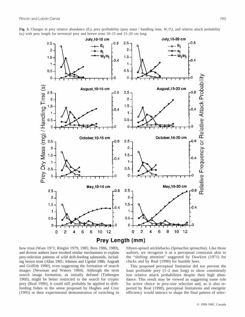
Prey profitability for trout 10–15 cm long increased at adecreasing rate with prey length until the latter reached12 mm and then decreased slightly for prey 12–13 mm long.For trout 15–20 cm long the profitability of terrestrial preyincreased at a faster rate than that for their smallerconspecifics and kept increasing throughout the whole preysize range (Fig. 3). Attack probability exhibited the samepattern of variation for both trout size classes. Initially, it in-creased markedly with prey profitability for the smaller, rel-atively abundant prey and then, contrary to theoreticalexpectations (see Methods), declined sharply and remainedlow despite the still increasing profitability. This trend paral-leled the decrease in relative abundance of the larger prey(Fig. 3). Thus, brown trout in the River Negro appeared toignore at least some valuable, but seldom encountered, preyitems while preferentially attacking less profitable, thoughmuch more abundant, prey. However, we would remark thatin the limited size range in our study (1–3, 1–5 mm), wherethe relative abundances of the different prey size classeswere not so dissimilar, trout showed a lower probability ofattacking prey <2 mm long (the least profitable items) de-spite their usually high abundance (Fig. 3).

Discussion

Active choice guided by energy-optimization criteria didnot appear to be important in the mechanics of prey-size se-lection by brown trout in the River Negro. When feeding onsurface-drifting (terrestrial) prey, trout ignored the largest,and presumably most profitable, prey items and showed neg-ative size selectivity. In contrast, they showed positive sizeselection for aquatic (water column or benthic) prey. How-ever, a model of prey encounter based only on the mechan-

© 1999 NRC Canada




ics of visual prey encounter generated size distributions ofencountered aquatic prey that showed great similarity to thesize distribution of these prey consumed by the trout and

achieved a considerable reduction in the residual SS relativeto the null model. Therefore, it seems that a large part of thispositive size selectivity can be explained without invoking

© 1999 NRC Canada

760 Can. J. Zool. Vol. 77, 1999

Fig. 1. Length-frequency distributions of aquatic invertebrate prey (open bars) available in drift (D) or benthic (B) samples (whicheverprovided the best fit for the encounter model predictions) consumed by brown trout (solid bars) and the corresponding best-fittingpredictions of the encounter model (hatched bars). The numbers in parentheses show theα value that produced the best-fittingprediction displayed.



active predator choice. Other authors have reported similarresults for other drift-feeding fishes (Wankowski 1979;Grant and Noakes 1986; Newman 1987; Dunbrack 1992;Rincón and Lobón-Cerviá 1995).

On the other hand, the apparent negative size selection ofterrestrial prey not only runs counter to our own findings onaquatic prey, but is also in contrast to most reported cases ofsize-selective predation among salmonids and other freshwa-ter fishes (Werner and Hall 1974; Hall et al. 1979; Zaret1980; Angermeier 1982; Newman and Waters 1984; Skinner1985; Urabe and Maruyama 1986; Rakocinski 1991, to men-tion just a few). However, the pattern of disproportionate useof the most abundant prey and under-exploitation of thescarcer ones very closely matches the definition of the phe-nomenon of predator switching reported for diverse foragers(Murdoch 1969; Murdoch et al. 1975; Real 1990; Hughesand Croy 1993), including brown trout (Ringler 1979, 1985).

The cause of predator switching may lie in some type ofperceptual limitation of the forager, such as the inability toremember scarce prey (Holling 1959), the need to form“search images” (Tinbergen 1960), or “shifts in attention”(Dawkins 1971; Real 1990), but may also be explained byenergetic considerations. For example, predators learn par-ticular search, attack, or handling techniques that are suitedto the prey types they have been encountering most fre-quently, and thus the profitabilities of such prey increase(Winfield et al. 1983; Bence 1986; Scott 1987; Croy andHughes 1991). The scarcer prey may actually be more prof-itable if the proper (different) foraging behavior is used, butlimitations in the learning capacity of the predator may pre-vent the simultaneous acquisition and use of different sets offoraging techniques (e.g., Werner et al. 1981; Persson 1985).

We believe that, of these two explanations for switching(which are not mutually exclusive), some perceptual con-

straint is more likely to have caused the pattern of terrestrialprey selection observed in the River Negro brown trout.First, absolute encounter rates of terrestrial prey above 4 mmin length seem to be very low. A rough assessment, based ondrift rates reported in Rincón (1993) and Rincón and Lobón-Cerviá (1997), suggests that values about 0–2 prey/h areusual. Only exceptionally do they reach 5 prey/h. In addi-tion, Real (1990) listed six alternatives that had to be ruledout in order for the existence of perceptual limitation to beaccepted. Foragers may (1) learn to search in a particularplace, (2) learn to distinguish a particular type of place,(3) alter their search path, (4) learn specialized capture tech-niques, (5) learn specialized handling techniques, and, fi-nally, (6) reject prey on the basis of factors other thanperceptual cues. Trout find all terrestrial prey at the watersurface, attack them in the same way (Ringler 1985; P.A.Rincón, unpublished observations), and, particularly in the

© 1999 NRC Canada


Drifting prey Benthic prey

Month and sizeclass of trout PSn PSm % SS α PSn PSm % SS αJuly

10–15 cm 52 64 50 1.5 66 75 37 115–20 cm 45 57 52 2 62 72 30 1.5

August10–15 cm 67 77 48 1 51 58 82 0.515–20 cm 67 76 31 1 58 60 77 0.5

October10–15 cm 59 77 21 1.5 49 53 63 115–20 cm 62 84 13 1.5 58 66 61 1

January10–15 cm 71 74 67 1 66 67 86 0.515–20 cm 56 70 34 1.5 58 68 50 1.5

March10–15 cm 65 73 54 1 76 84 28 115–20 cm 46 58 61 2 55 70 35 2

May10–15 cm 73 86 21 1 63 63 117 0.515–20 cm 76 82 29 1 61 58 122 0.5

Note: PSn is the similarity value achieved by the null model (α = 0). The highest PS values for a given month and length group and the correspondingα values are shown in boldface type.

Table 3. Maximum percent reduction in the residual sums of squares (% SS) achieved by the encounter model and the correspondingα values and similarities (PSm) for brown trout 10–15 and 15–20 cm long and their aquatic prey.

Trout size class

10–15 cm 15–20 cm

PSn PSm % SS PSn PSm % SS

July 91 73 577 81 84 83August 83 63 488 81 62 433October 80 79 103 78 76 106May 82 52 699 82 52 516

Note: PSn is the similarity value achieved by the null model (α = 0).The highest PS values for a given month and length group are shown inboldface type.

Table 4. Maximum percent reduction in the residual sums ofsquares (% SS) achieved by the encounter model (α = 1) andthe corresponding similarities (PSm) for brown trout 10–15 and15–20 cm long and their terrestrial prey.



prey size range that we are considering, the largest itemsdo not seem to require specialized handling (Bannon andRingler 1986). Hence, we feel that we are justified in reject-ing the first five scenarios.

Scenario 6 may be very hard to exclude absolutely in fieldsituations; for example, there may be differences in prey pal-atability unknown to us. However, we could not discern any

obvious pattern in the taxonomic composition of the sizeclasses either attacked preferentially (Hemiptera in July andAugust, Hymenoptera in October, Diptera in May (Rincón1993)) or ignored on the different sampling dates.

As we have suggested, in a number of laboratory studies,an increased probability of attack induced by familiaritywith a given prey type has been found for brown and rain-

© 1999 NRC Canada

762 Can. J. Zool. Vol. 77, 1999

Fig. 2. Length-frequency distributions of terrestrial invertebrate prey (open bars), available in drift samples, consumed by brown trout(solid bars) and predicted by the encounter model (hatched bars).



bow trout (Ware 1971; Ringler 1979, 1985; Bres 1986, 1989),and diverse authors have invoked similar mechanisms to explainprey-selection patterns of wild drift-feeding salmonids, includ-ing brown trout (Allan 1981; Johnsen and Ugedal 1986; Angradiand Griffith 1990), even suggesting the formation of searchimages (Newman and Waters 1984). Although the termsearch image formation, as initially defined (Tinbergen1960), might be better restricted to the search for crypticprey (Real 1990), it could still probably be applied to drift-feeding fishes in the sense proposed by Hughes and Croy(1993) in their experimental demonstration of switching in

fifteen-spined sticklebacks (Spinachia spinachia). Like thoseauthors, we recognize it as a perceptual constraint akin tothe “shifting attention” suggested by Dawkins (1971) forchicks and by Real (1990) for bumble bees.

This proposed perceptual limitation did not prevent theleast profitable prey (1–2 mm long) to show consistentlylow relative attack probabilities despite their high abun-dance. This result may be viewed as suggesting some rolefor active choice in prey-size selection and, as is also re-ported by Real (1990), perceptual limitations and energeticefficiency would interact to shape the final pattern of selec-

© 1999 NRC Canada


Fig. 3. Changes in prey relative abundance (Ei), prey profitability (prey mass / handling time,Wi /Ti), and relative attack probability(ai) with prey length for terrestrial prey and brown trout 10–15 and 15–20 cm long.



tivity exhibited by the forager. However, the 1- to 2-mmsize class is immediately above the prey length that seems tobe the absolute minimum (1 mm) for brown trout of compa-rable size (Bannon and Ringler 1986). So caution in inter-preting this result seems to be appropriate.

In any case, our results show that active choice is only asecondary factor in the process of prey-size selection byRiver Negro trout. Size-dependent encounter (due to increasedvisibility of the larger prey) with aquatic prey and relativeabundance plus a possible perceptual/cognitive constraint inthe case of terrestrial prey (induced by very low encounterrates for the larger prey) play a more determinant role. Thisminor influence of active choice is consistent with previousfindings. Dunbrack and Dill (1983), Grant and Noakes (1986),Newman (1987), Dunbrack (1992), and Rincón and Lobón-Cerviá (1995) have all found that size-dependent encounter,sometimes coupled with gape limitation, can largely explainthe pattern of prey-size selection exhibited by different drift-feeding fishes.

Acknowledgements

We benefited from the use of the facilities of the EstaciónBiológica de Valdés of the CSIC while carrying out field-work. Y. Bernat and J. Cubo helped in this task. Commentsfrom G. Grossman, R. Newman, N. Ringler and E. Morenoimproved earlier drafts of the manuscript. T. Northcote andan anonymous reviewer provided valuable comments. Thestudy was funded by Diverción General de InvestigationCientífica y Techológica project PB 89-0040 and a coopera-tion protocol between Valdés Municipal Council and theCSIC. During that time P.A.R. received a Progama deformación de Personal Investigator grant from the Ministeriode Educación y Ciencia (MEC) and the manuscript wascompleted while P.A.R. was the recipient of a postdoctoralMEC/Fullbright scholarship at the Warnell School of ForestResources of the University of Georgia.

References

Allan, J.D. 1981. Determinants of diet of brook trout (Salvelinusfontinalis) in a mountain stream. Can. J. Fish. Aquat. Sci.38: 184–192.

Allan, J.D., and Russek, E. 1985. The quantification of streamdrift. Can. J. Fish. Aquat. Sci.42: 210–215.

Allen, K.R. 1969. Distinctive aspects of the ecology of streamfishes: a review. J. Fish. Res. Board Can.26: 1429–1438.

Angermeier, P.L. 1982. Resource seasonality and fish diets in anIllinois stream. Environ. Biol. Fishes,7: 251–264.

Angradi, T.R., and Griffith, J.S. 1990. Diel feeding chronology anddiet selection of rainbow trout (Oncorhynchus mykiss) in theHenry’s Fork of the Snake River, Idaho. Can. J. Fish. Aquat.Sci. 47: 199–209.

Asknes, D.L., and Giske, J. 1993. A theoretical model of aquaticvisual feeding. Ecol. Model.67: 233–250.

Bannon, E., and Ringler, N.H. 1986. Optimal prey size for streamresident brown trout (Salmo trutta): tests of predictive models.Can. J. Zool.64: 704–713.

Bence, J.R. 1986. Feeding rate and attack specialization: the rolesof predator experience and energetic trade offs. Environ. Biol.Fishes,16: 113–121.

Bres, M. 1986. A new at look optimal foraging behaviour; rule ofthumb in the rainbow trout. J. Fish Biol.29(Suppl. A): 25–36.

Bres, M. 1989. The effects of prey relative abundance and chemicalcues on prey selection by rainbow trout. J. Fish Biol.35: 439–445.

Canton, S.P., and Chadwick, S.W. 1988. Variability in benthic in-vertebrate density estimates from stream samples. J. Freshw.Ecol. 4: 291–298.

Confer, J.L., Holwick, G.L., Corzette, M.H., Kramer, S.L., Fitz-gibbon, S., and Landesberg, R. 1978. Visual predation byplanktivores. Oikos,31: 27–37.

Croy, M.I., and Hughes, R.N. 1991. The role of learning in thefeeding behaviour of the fifteen-spined stickleback,SpinachiaspinachiaL. Anim. Behav.41: 149–159.

Dawkins, M. 1971. Shifts of ‘attention’ in chicks during feeding.Anim. Behav.19: 575–582.

Dunbrack, R.L. 1992. Sub-surface drift feeding by coho salmon(Oncorhynchus kisutchWalbaum): a model and a test. J. FishBiol. 40: 455–464.

Dunbrack, R.L., and Dill, L.M. 1983. A model of size-dependentfeeding on a stream dwelling salmonid. Environ. Biol. Fishes,8: 203–216.

Eggers, D.M. 1977. The nature of prey selection by planktivorousfish. Ecology,58: 46–59.

Eggers, D.M. 1982. Planktivore preference by prey size. Ecology,63: 381–390.

Getty, T. 1985. Discriminability and the sigmoid functional re-sponse: how optimal foragers could stabilize model–mimic com-plexes. Am. Nat.125: 239–256.

Hall, D.J., Werner, E.E., Gilliam, J.F., Mittelbach, G.G., Howard,D., Donner, C.G., Dickerman, J.A., and Stewart, A.J. 1979. Dielforaging behavior and prey selection in the golden shiner (Notemi-gonus chrysoleucas). J. Fish. Res. Board Can.36: 1029–1039.

Holling, C.S. 1959. The components of predation as revealed by astudy of small-mammal predation of the European pine sawfly.Can. Entomol.91: 293–320.

Holling, C.S. 1966. The functional response of invertebrate preda-tors to prey density. Mem. Entomol. Soc. Can. No. 48. pp. 1–86.

Hughes, R.N., and Croy, M.I. 1993. An experimental analysis offrequency-dependent predation (switching) in the 15-spinedstickleback,Spinachia spinachia. J. Anim. Ecol.62: 341–352.

Hynes, H.B.N. 1970. The ecology of running waters. UniversityPress, Liverpool.

Johnsen, B.O., and Ugedal, O. 1986. Feeding in hatchery-rearedand wild brown trout,Salmo truttaL., in a Norwegian stream.Aquacult. Fish. Manage.17: 281–287.

Keeley, E.R., and Grant, J.W.A. 1997. Allometry of diet selectivityin juvenile Atlantic salmon (Salmo salar). Can. J. Fish. Aquat.Sci. 54: 1894–1902.

Kerfoot, W.C. 1982. A question of taste: crypsis and warning colora-tion in freshwater zooplankton communities. Ecology,63: 538–554.

Lobón-Cerviá, J., and Rincón, P.A. 1994. The trophic ecology ofred roachRutilus arcasii in a seasonal stream: an example ofdetritivory as a feeding tactic. Freshw. Biol.32: 123–132.

Maiorana, V.C. 1981. Prey selection by sight: random or economic.Am. Nat. 118: 450–451.

McNamara, J.M., and Houston, A.I. 1987. Partial prey preferencesand foraging. Anim. Behav.35: 1084–1099.

Meyer, E. 1989. The relationship between body length parametersand dry mass in running water invertebrates. Arch. Hydrobiol.117: 191–203.

Murdoch, W.W. 1969. Switching in general predators: experimentson predator specificity and stability of prey populations. Ecol.Monogr. 39: 336–353.

© 1999 NRC Canada

764 Can. J. Zool. Vol. 77, 1999



© 1999 NRC Canada


Murdoch, W.W., Avery, S., and Smythe, M.E. 1975. Switching inpredatory fish. Ecology,56: 1094–1105.

Newman, R.M. 1987. Comparison of encounter model predictionswith observed size-selectivity by stream trout. J. N. Am. Benthol.Soc.6: 56–64.

Newman, R.M., and Waters, T.F. 1984. Size-selective predationon Gammarus pseudolimnaeusby trout and sculpins. Ecology,65: 1535–1545.

O’Brien, W.J., and Showalter, J.J. 1993. Effects of current velocityand suspended debris on the drifit feeding of arctic grayling.Trans. Am. Fish. Soc.122: 609–615.

Osenberg, C.W., and Mittelbach, G.G. 1989. The effects of bodysize on predator–prey interaction between pumpkinseed sunfishand gastropods. Ecol. Monogr.59: 405–432.

Persson, L. 1985. Optimal foraging: the difficulty of exploiting differ-ent feeding strategies simultaneously. Oecologia,67: 338–341.

Rakocinski, C. 1991. Prey-size relationships and feeding tacticsof primitive stream dwelling darters. Can. J. Fish. Aquat. Sci.48: 681–693.

Real, L.A. 1990. Predator switching and the interpretation of ani-mal choice behavior: the case for constrained optimization.InBehavioral mechanisms of food selection.Edited by R.N.Hughes. NATO ASI (Adv. Sci. Inst. Ser.) Ser. G Geol. Sci.No. 20. pp. 1–20.

Rincón, P.A. 1993. Utilización integrada de diferentes recursos:patrones en la alimentación y el uso del microhábitat de unapoblación de trucha común (Salmo truttaL.) en el río Negro,Asturias. Ph.D. thesis, Universidad Complutense, Madrid.

Rincón, P.A., and Lobón-Cerviá, J. 1993. Microhabitat use bystream-resident brown trout: bioenergetic consequences. Trans.Am. Fish. Soc.122: 575–587.

Rincón, P.A., and Lobón-Cerviá, J. 1995. Use of an encountermodel to predict size-selective predation by a stream-dwellingcyprinid. Freshw. Biol.33: 181–191.

Rincón, P.A., and Lobón-Cerviá, J. 1997. Temporal patterns inmacroinvertebrate drift in a northern Spanish stream. Mar.Freshw. Res.48: 455–464.

Ringler, N.H. 1979. Selective predation by drift-feeding browntrout (Salmo trutta). J. Fish. Res. Board Can.36: 392–403.

Ringler, N.H. 1985. Individual and temporal variation in preyswitching by brown trout,Salmo trutta. Copeia, 4: 918–926.

Roberts, L.E., Hinds, W.T., and Buschbom, R.L. 1976. A generalweight vs. length relationship for insects. Ann. Entomol. Soc.Am. 69: 387–389.

Scott, A. 1987. Prey selection by juvenile cyprinids from runningwater. Freshw. Biol.17: 129–142.

Skinner, W.D. 1985. Size selection of food by cutthroat trout(Salmo clarki) in an Idaho stream. Great Basin Nat.45: 327–331.

Smock, L.A. 1980. Relationships between body size and biomassof aquatic insects. Freshw. Biol.10: 375–383.

Stephens, D.W. 1985. How important are partial preferences?Anim. Behav.33: 667–669.

Tinbergen, L. 1960. The natural control of insects in pine woods.I. Factors influencing the intensity of predation by songbirds.Arch. Neerl. Zool.13: 265–343.

Urabe, J., and Maruyama, T. 1986. Prey selectivity of two cyprinidfishes in Ogochi reservoir. Bull. Jpn. Soc. Sci. Fish.52: 2045–2054.

Wankowski, J.W.J. 1979. Morphological limitations, prey size se-lectivity, and growth response of juvenile atlantic salmon,Salmosalar. J. Fish Biol.14: 89–100.

Wankowski, J.W.J. 1981. Behavioural aspects of predation by juve-nile Atlantic salmon (Salmo salarL.) on particulate driftingprey. Anim. Behav.29: 557–571.

Ware, D.M. 1971. Predation by rainbow trout (Salmo gairdneri):the effect of experience. J. Fish. Res. Board Can.28: 1847–1852.

Waters, T.F. 1972. The drift of stream insects. Annu. Rev. Entomol.17: 253–272.

Werner, E.E., and Hall, D.J. 1974. Optimal foraging and the sizeselection of prey by the bluegill sunfish (Lepomis macrochirus).Ecology,55: 1042–1052.

Werner, E.E., Mittelbach, G.G., and Hall, D.J. 1981. Foragingprofitability and the role of experience in habitat use by bluegillsunfish. Ecology,62: 116–125.

Wetterer, J.K. 1989. Mechanisms of prey choice by planktivorousfish: perceptual constraints and rules of thumb. Anim. Behav.37: 955–967.

Wetterer, J.K., and Bishop, C.J. 1985. Planktivore prey selection:the reactive field volume model vs. the apparent size model.Ecology,66: 457–464.

Winfield, I.J., Peirson, G., Cryer, M., and Townsend, C. 1983. Thebehavioral basis of prey selection by underyearling breamAbramis brama(L.) and roachRutilus rutilus(L.). Freshw. Biol.13: 139–149.

Wolda, H. 1980. Similarity indices, sample size and diversity.Oecologia (Berl.),50: 296–302.

Wright, D.I., and O’Brien, W.J. 1984. The development and fieldtesting of a tactical model of the planktivorous feeding of whitecrappie (Pomoxis annularis). Ecol. Monogr.54: 65–98.

Zaret, T.M. 1980. Predation and freshwater communities. YaleUniversity Press, New Haven, Conn.



Prey-size selection by brown trout ( Salmo trutta L.) in a stream in northern Spain

Documents

Transcript of Prey-size selection by brown trout ( Salmo trutta L.) in a stream in northern Spain