
Present-day climatic equivalents of European Cenozoic climates
Upload
khangminh22Category
view
0download
0
HAL Id: tel-01317607https://tel.archives-ouvertes.fr/tel-01317607
Submitted on 18 May 2016
HAL is a multi-disciplinary open accessarchive for the deposit and dissemination of sci-entific research documents, whether they are pub-lished or not. The documents may come fromteaching and research institutions in France orabroad, or from public or private research centers.
L’archive ouverte pluridisciplinaire HAL, estdestinée au dépôt et à la diffusion de documentsscientifiques de niveau recherche, publiés ou non,émanant des établissements d’enseignement et derecherche français ou étrangers, des laboratoirespublics ou privés.
Present day sea level: global and regional variationsHindumathi K. Palanisamy
To cite this version:Hindumathi K. Palanisamy. Present day sea level: global and regional variations. Oceanography.Universite Toulouse III Paul Sabatier, 2016. English. �tel-01317607�
En vue de l'obtention du
DE DE T
Délivré par l'Université Toulouse III - Paul Sabatier Discipline ou spécialité : Océanographie Spatiale
Présentée et soutenue par Hindumathi Kulaiappan Palanisamy
Le 06 janvier 2016
Titre: Le niveau de la mer actuel: variations globale et régionales
Title: Present day sea level: global and regional variations
JURY
Nicholas Hall (Président du Jury)
Jérôme Vialard (Rapporteur) Johnny A. Johannessen (Rapporteur)
Joshua Willis (Examinateur) Anny Cazenave (Directrice de Thèse) Thierry Delcroix (Directeur de Thèse)
Ecole doctorale: SDUEE Unité de recherche: LEGOS UMR 5566
Directeurs de Thèse: Anny Cazenave et Thierry Delcroix Rapporteurs: voir le Jury


iii
Acknowledgements
I would first like to thank Anny for her marvelous support all through the duration of this
thesis. Her vast knowledge is highly impressive and her curiosity to learn new things has always
been a motivating factor to me. Through her, I learnt that neither age nor intellectual status is a
barrier when it comes to constant quest for knowledge. I am also impressed with the importance
she has given and still continues to give her students irrespective of her schedule. I am deeply
honored to be one of her students.
I would also like to thank Thierry for his patience, pedagogic skills and his vast
knowledge in the field of oceanography. His astonishing ability to explain concepts in a very
simple manner has been of great help for someone like me having no prior education in the
domain of oceanography. Our Thursday discussions have also helped me uncover his humorous
and easy-going attitude!
I would also to acknowledge the financial support from CNES and CLS and thank
Michaël, Gilles for their support in obtaining the financement.
My sincere thanks to Philippe; without his help I would not have been able to start my
career in this field of research. I would also like to thank Benoit and Mélanie who have both
been my first mentors. It’s still a great pleasure to discuss and learn a lot from you both.
My special thanks to Martine, Nadine, Catherine and Agathe for their help with the paper
works irrespective of their workloads. I still remember the days when I hardly spoke French and
would go to them for help. If not for them, I would have had a tough time getting adapted at
LEGOS.
Thanks to Olivier with whom I shared my office for more than two years. It was fun
working with him, discuss science and have various other non-scientific debates. I would also
like to thank Brigitte for the coffee break sessions. It has always been a pleasure and a great
relief to take a break and just walk into her office to discuss everything but science. My special
thanks also go to Wojtek, Vanessa, Ivonne, Sylvain, Laurence, Angélique, Elodie, Téodolina,
William, Akhil, Alejandro, Caroline and every other colleague who has made this journey
pleasurable.
I would also like to take this opportunity to thanks my friends Thomas, Olivier, Pascal,
Eric, Sangeeth and Florian for their moral support and my family members Brigitte, François,
Charlotte, Alix, Hubert and Brinda for having stood by me through rough times.
I am deeply grateful to my parents for who I am today…
I dedicate this thesis to Thibaud…

iv
v
Le niveau de la mer actuel: variations globale et régionales
Auteur: Hindumathi K. Palanisamy
Directrice/Directeur de thèse: Anny Cazenave & Thierry Delcroix
Discipline: Océanographie Spatiale
Lieu et date de soutenance: Observatoire Midi-Pyrénées, 6 Janvier, 2016
Laboratoire: LEGOS, UMR5566 CNRS/CNES/IRD/UPS, Toulouse, France.
Résumé: Le niveau de la mer est une des variables climatiques essentielles dont la variabilité résulte de
nombreuses interactions complexes entre toutes les composantes du système climatique sur une large
gamme d'échelles spatiales et temporelles. Au cours du XXème siècle, les mesures marégraphiques ont
permis d’estimer la hausse du niveau de la mer global entre 1,6 mm/an et 1,8 mm/an. Depuis 1993, les
observations faites par les satellites altimétriques indiquent une hausse du niveau de la mer plus rapide de
3,3 mm/an. Grâce à leur couverture quasi-globale, elles révèlent aussi une forte variabilité du niveau de la
mer à l’échelle régionale, parfois plusieurs fois supérieure à la moyenne globale du niveau de la mer.
Compte tenu de l'impact très négatif de l’augmentation du niveau de la mer pour la société, sa
surveillance, la compréhension de ses causes ainsi que sa prévision sont désormais considérées comme
des priorités scientifiques et sociétales majeures.
Dans cette thèse, nous validons d’abord les variations du niveau de la mer mesurées par la
nouvelle mission d'altimétrie satellitaire, SARAL-AltiKa, en comparant les mesures avec celles de Jason-
2 et des marégraphes. Un autre volet de cette première partie de thèse a consisté à estimer les parts
respectives des facteurs responsables des variations du niveau de la mer depuis 2003 en utilisant des
observations issues de l'altimétrie satellitaire (missions altimétrique Jason-1, Jason-2 et Envisat), de la
mission GRACE, et des profils de température et salinité de l’océan par les flotteurs Argo. Une attention
particulière est portée à la contribution de l’océan profond non ‘vue’ par Argo. Nous montrons que les
incertitudes dues aux approches du traitement des données et aux erreurs systématiques des différents
systèmes d'observation nous empêchent encore d'obtenir des résultats précis sur cette contribution.
Dans la deuxième partie de la thèse, en utilisant les données de reconstruction du niveau de la mer
dans le passé, nous étudions la variabilité régionale du niveau de la mer et estimons sa hausse totale
(composante régionale plus moyenne globale) de 1950 à 2009 dans trois régions vulnérables: l’océan
Indien, la mer de Chine méridionale et la mer des Caraïbes. Pour les sites où l’on dispose de mesures du
mouvement de la croûte terrestre par GPS, nous évaluons la hausse locale du niveau de la mer relatif
(hausse du niveau de la mer totale plus mouvement de la croûte locale) depuis 1950. En comparant les
résultats de ces trois régions avec une étude précédente sur le Pacifique tropical, nous constatons que le
Pacifique tropical présente la plus forte amplitude des variations du niveau de la mer sur la période
d’étude.
Dans la dernière partie de la thèse, nous nous concentrons par conséquent sur le Pacifique
tropical. Nous analysons les rôles respectifs de la dynamique océanique, des modes de variabilité interne
du climat et du forçage anthropique sur les structures de la variabilité régionale du niveau de la mer du
Pacifique tropical depuis 1993. Nous montrons qu’une partie importante de la variabilité régionale du
niveau de la mer du Pacifique tropical peut être expliquée par le mouvement vertical de la thermocline en
réponse à l’action du vent. En tentant de séparer le signal correspondant au mode de variabilité interne du
climat de celui de la hausse régionale du niveau de la mer dans le Pacifique tropical, nous montrons
également que le signal résiduel restant (c’est-à-dire le signal total moins le signal de variabilité interne)
ne correspond probablement pas à l’empreinte externe du forçage anthropique.
Mots-clés: Hausse du niveau de la mer, SARAL-AltiKa, bilan du niveau de la mer, contribution l'océan
profond, Pacifique tropical, thermocline, mode de la variabilité interne, impacts anthropiques.


vii
Present day sea level: global and regional variations
Author: Hindumathi K. Palanisamy
Ph.D. directors: Anny Cazenave & Thierry Delcroix
Discipline: Space Oceanography
Place and Date of defense: Observatoire Midi-Pyrénees, 6th January, 2016
Laboratory: LEGOS, UMR5566 CNRS/CNES/IRD/UPS, OMP, 14 Avenue Edouard Belin, 31400,
Toulouse, France.
Summary: Sea level is an integrated climate parameter that involves interactions of all components
of the climate system (oceans, ice sheets, glaciers, atmosphere, and land water reservoirs) on a wide
range of spatial and temporal scales. Over the 20th century, tide gauge records indicate a rise in global
sea level between 1.6mm/yr and 1.8 mm/yr. Since 1993, sea level variations have been measured
precisely by satellite altimetry. They indicate a faster sea level rise of 3.3 mm/yr over 1993-2015.
Owing to their global coverage, they also reveal a strong regional sea level variability that sometimes
is several times greater than the global mean sea level rise. Considering the highly negative impact of
sea level rise for society, monitoring sea level change and understanding its causes are henceforth
high priorities.
In this thesis, we first validate the sea level variations measured by the new satellite altimetry
mission, SARAL-AltiKa by comparing the measurements with Jason-2 and tide gauge records. We
then attempt to close the global mean sea level budget since 2003 and estimate the deep ocean
contribution by making use of observational data from satellite altimetry, Argo profiles and GRACE
mission. We show that uncertainties due to data processing approaches and systematic errors of
different observing systems still prevent us from obtaining accurate results.
In the second part of the thesis, by making use of past sea level reconstruction, we study the
patterns of the regional sea level variability and estimate climate related (global mean plus regional
component) sea level change over 1950-2009 at three vulnerable regions: Indian Ocean, South China
and Caribbean Sea. For the sites where vertical crustal motion monitoring is available, we compute
the total relative sea level (i.e. total sea level rise plus the local vertical crustal motion) since 1950.
On comparing the results from these three regions with already existing results in tropical Pacific, we
find that tropical Pacific displays the highest magnitude of sea level variations.
In the last part of the thesis, we therefore focus on the tropical Pacific and analyze the
respective roles of ocean dynamic processes, internal climate modes and external anthropogenic
forcing on tropical Pacific sea level spatial trend patterns since 1993. Building up on the relationship
between thermocline and sea level in the tropical region, we show that most of the observed sea level
spatial trend pattern in the tropical Pacific can be explained by the wind driven vertical thermocline
movement. By performing detection and attribution study on sea level spatial trend patterns in the
tropical Pacific and attempting to eliminate signal corresponding to the main internal climate mode,
we further show that the remaining residual sea level trend pattern does not correspond to externally
forced anthropogenic sea level signal. In addition, we also suggest that satellite altimetry
measurement may not still be accurate enough to detect the anthropogenic signal in the 20 year
tropical Pacific sea level trends.
Keywords: Sea level rise, SARAL-AltiKa, Global mean sea level budget, deep ocean contribution,
regional sea level variability, total relative sea level change, tropical Pacific, thermocline, internal
climate mode, anthropogenic sea level fingerprint.


Table of Contents
General introduction in French ...................................................................................... 1
Chapter 1 Introduction................................................................................................... 5
1.1 Paleo sea level ....................................................................................................... 6
1.2 Instrumental era sea level ...................................................................................... 8
1.2.1 Tide gauge records ........................................................................................... 8
1.2.2 Satellite altimetry ........................................................................................... 10
1.3 Contributors to global mean sea level rise during the instrumental era .............. 11
1.3.1 Ocean temperature and salinity changes ........................................................ 11
1.3.2 Glaciers melting ............................................................................................. 12
1.3.3 Ice sheets ........................................................................................................ 13
1.3.4 Land waters .................................................................................................... 13
1.4 Thesis objectives ................................................................................................. 15
Chapter 2 Multi satellite altimetry record and global mean sea level budget .... 19
2.1 Evolution of altimetry satellites .......................................................................... 19
2.1.1 Principle of satellite altimetry ........................................................................ 21
2.1.2 Corrections involved in Sea Surface Height measurement ............................ 21
1) Orbital correction ........................................................................................... 23
2) Propagation corrections ................................................................................. 23
a) Ionosphere correction ................................................................................. 23
b) Wet troposphere correction ........................................................................ 24
c) Dry troposphere correction ........................................................................ 24
3) Geophysical corrections ................................................................................. 24
a) Ocean, solid Earth tidal and loading corrections ....................................... 25
b) Polar tidal correction .................................................................................. 25
4) Surface corrections......................................................................................... 25
a) Inverse barometric (IB) correction ............................................................. 25
b) Sea State Bias (SSB) correction ................................................................. 26
5) Other potential errors ..................................................................................... 26
2.1.3 Multi-mission SSH altimetry data ................................................................. 27
2.1.4 SARAL-AltiKa, the new altimetry mission ................................................... 28
2.2 Global mean sea level (GMSL) budget since altimetry era ................................ 47
2.2.1 Future needs ................................................................................................... 74
Chapter 3 Regional sea level variability and total relative sea level change ..... 77
3.1 Regional sea level trend variability: Causes ....................................................... 78
3.1.1 Climate related regional sea level variability ................................................. 79
1) Thermal expansion and salinity changes ....................................................... 79
2) Ocean mass changes ...................................................................................... 82
3.1.2 Non climatic causes for regional sea level variability ................................... 82
3.1.3 Vertical Land Motions ................................................................................... 85
3.2 Long term regional sea level variability, total relative sea level change and coastal
impacts .................................................................................................................. 85
3.2.1 Indian Ocean .................................................................................................. 89
3.2.2 Caribbean Sea .............................................................................................. 107
3.2.3 South China Sea ........................................................................................... 118
3.2.4 The vulnerable zones: a synthesis ................................................................ 140
Chapter 4 The role of internal climate variability and external forcing on
regional sea level variations ................................................................... 143
4.1 Internal climate variability ................................................................................ 143
4.1.1 El Niño-Southern Oscillation (ENSO)......................................................... 144
4.1.2 Pacific Decadal Oscillation (PDO)/ Interdecadal Pacific Oscillation (IPO) 146
4.1.3 Indian Ocean Dipole (IOD) ......................................................................... 148
4.1.4 North Atlantic Oscillation (NAO) ............................................................... 149
4.1.5 Other modes of internal climate variability ................................................. 151
4.2 Externally-forced climate variability ................................................................ 151
4.2.1 Natural external forcing ............................................................................... 152
4.2.2 Anthropogenic external forcing ................................................................... 153
4.3 Detection and attribution of climate change ..................................................... 156
4.3.1 Detection and attribution on global mean sea level variations .................... 157
4.3.2 Detection and attribution on regional sea level variability .......................... 159
4.4 The case of the Pacific Ocean ........................................................................... 161
4.5 Role of external anthropogenic forcing on internal climate modes – A synthesis ..
........................................................................................................................... 200
4.6 Internal climate variability uncertainty in CMIP5 models ................................ 201
Conclusion and perspectives ...................................................................................... 203
General conclusion in French ..................................................................................... 209
Bibliography ................................................................................................................. 213
Appendix A: List of publications ............................................................................... 241
Appendix B: List of publications not included in the context of the manuscript ....
..................................................................................................................... 243

1
Introduction générale (en français)
L'élévation du niveau de la mer est considérée comme une menace majeure pour les
zones côtières de basse altitude de la planète en raison du réchauffement climatique actuel
d'origine humaine (Nicholls et al., 2008). Terres riches fertiles, transports maritimes, accès aux
ressources halieutiques ont toujours attiré les populations humaines le long de la frange côtière
des terres émergées. Au cours des dernières décennies, de nombreuses mégalopoles du monde
peuplées de plusieurs dizaines de millions d’habitants se sont développées le long des côtes. On
estime qu'au moins 650 millions de personnes vivent à moins de 10m du niveau actuel de la mer
(McGranahan et al., 2007), et ce nombre est en croissance constante. Il devrait atteindre 800
millions d'ici 2080 (Nicholls et al. , 2010).
L'élévation du niveau de la mer et ses impacts côtiers sont l'une des principales
conséquences du changement climatique. Elle affecte non seulement les côtes continentales mais
aussi de nombreuses îles basses des océans tropicaux (Mimura et al., 2007, Nicholls et al., 2011).
L’élévation du niveau de la mer en réponse aux concentrations croissantes de gaz à effet de serre
est un défi majeur auquel l'humanité doit faire face au 21e siècle. Des enregistrements
marégraphiques indiquent que le niveau moyen de la mer s’est élevé d’environ 20 cm au cours
du 20ème
siècle. Les modèles de climat montrent aussi que cette hausse va se poursuivre au 21ème
siècle et même au-delà. Bien que les estimations de l'élévation future du niveau de la mer soient
encore incertaines en raison des incertitudes des émissions futures de gaz à effet de serre et de la
réponse associée du système climatique, on estime que le niveau de la mer va continuer à monter
de plusieurs dizaines de cm, voire plus d’1 m dans les prochaines décennies (IPCC, 2013). En
effet, même si les émissions de gaz à effet de serre se stabilisaient rapidement, la durée de vie du
dioxyde de carbone dans l’atmosphère, l'inertie thermique de l’océan et le lent temps de réponse
de certaines composantes du système climatique, la hausse du niveau de la mer se poursuivra
pendant plusieurs siècles (Dutton et al., 2015, GIEC, 2013, Levermann et al ., 2013, Meehl et al.,
Introduction générale
2
2012, Meehl et al., 2005, Wigley, 2005). Par conséquent, il est impératif d'identifier et de
quantifier les causes qui contribuent aux variations actuelles du niveau de la mer, non seulement
pour la compréhension des phénomènes en jeu, mais aussi afin que d’améliorer les performances
des modèles climatiques développés pour simuler les évolutions futures.
Ma thèse contribue à une meilleure estimation et à la compréhension des variations du
niveau de la mer au cours des dernières décennies, non seulement à l'échelle mondiale mais aussi
régionale. En effet, nous savons aujourd’hui que régionalement, la hausse du niveau de la mer
peut très sensiblement dévier de la moyenne mondiale sur une large gamme d'échelles spatiales
et temporelles. Les principaux objectifs et l'organisation de la thèse sont décrits ci-dessous.
• Le premier chapitre est une introduction dans laquelle nous résumons l’état des
connaissances sur les variations actuelles et passées du niveau de la mer, depuis le dernière
maximum glaciaire il y a 20000 ans jusqu’à l'ère instrumentale. Nous décrivons aussi les
principales contributions à la variation moyenne globale du niveau de la mer du 20ème
siècle. Ce
chapitre fournit ainsi le cadre général dans lequel s’inscrivent les sujets abordés au cours de ce
travail de thèse.
• Dans le deuxième chapitre, nous fournissons une description détaillée des différentes
missions altimétriques utilisées pour mesurer de façon précise et globale le niveau de la mer
depuis le début des années 1990s. Nous décrivons aussi le principe de mesure de la hauteur de la
surface de la mer par altimétrie satellitaire et les différentes corrections géophysiques et
instrumentales appliquées à la mesure de la hauteur de la surface de la mer. Dans ce chapitre,
nous présentons un premier travail dédié à la validation des mesures du niveau de la mer
réalisées par la nouvelle mission d'altimétrie spatiale, SARAL-AltiKa, lancée en février 2013.
Cette validation est basée sur la comparaison avec les mesures du satellite Jason-2 et des données
marégraphiques. Un autre volet de cette première partie de thèse a consisté à estimer les parts
respectives des facteurs responsables des variations du niveau de la mer depuis 2003 en utilisant
des observations issues de l'altimétrie satellitaire (missions altimétriques Jason-1, Jason-2 et
Envisat), de la mission de gravimétrie spatiale GRACE, et des profils de température et salinité
de l’océan par les flotteurs Argo. Une attention particulière est portée à la contribution de l’océan
profond non ‘vue’ par Argo.
Introduction générale
3
• Le chapitre 3 porte sur la variabilité régionale du niveau de la mer et ses causes. Il décrit
les études que nous avons réalisées sur l’estimation de la variation totale du niveau relatif de la
mer depuis 1950 dans diverses régions vulnérables du monde: en utilisant les données de
reconstruction du niveau de la mer dans le passé, nous étudions la variabilité régionale du niveau
de la mer et estimons sa hausse totale (composante régionale plus moyenne globale) de 1950 à
2009 dans trois régions, l’océan Indien, la mer de Chine méridionale et la mer des Caraïbes. Pour
les sites où l’on dispose de mesures du mouvement de la croûte terrestre par GPS, nous évaluons
la hausse locale du niveau de la mer relatif (hausse du niveau de la mer totale plus mouvement de
la croûte locale) depuis 1950.
• Dans le chapitre 4 nous analysons les rôles respectifs de la dynamique océanique, des
modes de variabilité interne du climat et du forçage anthropique sur les structures de la
variabilité régionale du niveau de la mer du Pacifique tropical au cours des 20 dernières années.
On observe en effet sur cette période que la hausse de la mer dans cette région a été 3 à 4 fois
plus importante qu’en moyenne globale. Au cours de cette thèse, nous expliquons les
mécanismes physiques causant cette hausse plus rapide. Enfin dans une dernière partie, nous
cherchons à déterminer les parts respectives du forçage anthropique et de la variabilité naturelle
interne du climat, pour expliquer l’origine de cette importante variabilité régionale observée dans
la hausse de la mer.

4
5
Chapter 1
Introduction
Sea level rise has been seen as a major threat to low-lying coastal areas around the globe
since the issue of human-induced global warming emerged in the 1980s (Nicholls et al., 2008).
Rich fertile land, transport connections, port access, coastal and deep sea fishing have attracted
millions of people along the coastal fringes of continents. Many of the world’s megacities with
population of many millions have been developed along the coasts with little consideration of sea
level rise and its impacts. While in global terms relatively small in number, the very existence of
small-island nation states makes them more vulnerable to rises in sea level (Mimura et al., 2007,
Nicholls et al., 2011). It is estimated that at least 600 million people live within 10m of sea level
currently (McGranahan et al., 2007), and these populations are growing more rapidly than global
trends and is expected to reach 800 million by the 2080s (Nicholls et al., 2010).
Sea level rise and its resultant coastal impact are one of the main consequences of present
day anthropogenic global climate change. Sea level rise from ocean warming and land ice melt is
a central part of the Earth’s response to increasing greenhouse gas (GHG) concentrations and is
therefore identified as the major challenge facing humankind in the 21st century. Though
estimates of timescales, magnitudes and rates of future sea level rise vary considerably, partly as
a consequence of uncertainties in future emissions and associated climate response, it is expected
that the sea level will continue to rise in the near future. This is because, even if the GHG
emissions are stabilized, the oceanic thermal inertia and the slow response time of different
climate components would still aid in the continuation of sea level rise (Dutton et al., 2015,
IPCC, 2013, Levermann et al., 2013, Meehl et al., 2012, Meehl et al., 2005, Wigley, 2005).
Therefore it is imperative to identify and quantify the causes contributing to the present observed
Chapter 1 Introduction
6
sea level change not only for basic understanding and scientific challenges but also in order that
better models can be developed and more reliable predictions can be provided. Furthermore, the
study of past sea level changes by making use of historical records and their proxies will also
offer means for understanding and quantifying uncertainties, as well as determining how well sea
level rise can be monitored in the future. In addition, the Earth has a memory of past events, and
the pattern of relative sea-level change, today and in the future, will continue to respond to past
events (Lambeck et al., 2010).
In this introductory chapter, we provide a brief synthesis of what is known about sea level
variations between the paleo and the instrumental era. In addition to this, we also address the
main contributors to global mean sea level change since the instrumental era. This chapter does
not present the results of the Ph.D. work but rather creates a base for the subjects addressed in
the work and explains the framework of my Ph.D. thesis.
1.1 Paleo sea level
Sea level changes have occurred throughout Earth history with magnitudes and timing of
the changes being extremely variable. On geological time scales, hundreds of millions of years
ago, sea level variations were mainly controlled by changes in the shape and volume of the
oceanic basins due to tectonic activities such as formation of oceanic plates at mid-ocean ridges,
collision with continents etc. Over the Quaternary period, the oscillations between glacial and
inter-glacial climate conditions during the past three millions of years have caused large-scale
global mean sea level fluctuations in order > ± 100 m as a result of immense amount of water
transferred between oceans and ice sheets (Lambeck et al., 2002). So far there have been 17 such
glacial and inter-glacial cycles associated with successive cold (northern hemisphere covered by
ice sheets) and warm (equivalent to present conditions) periods. During the last interglacial
period around 125,000 years ago, studies have shown that the global mean sea level was at least
5m higher than at present (Dutton and Lambeck, 2012, Kopp et al., 2013, Church et al., 2013,
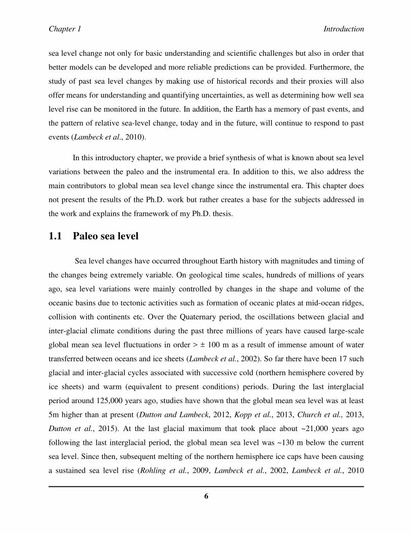
Dutton et al., 2015). At the last glacial maximum that took place about ~21,000 years ago
following the last interglacial period, the global mean sea level was ~130 m below the current
sea level. Since then, subsequent melting of the northern hemisphere ice caps have been causing
a sustained sea level rise (Rohling et al., 2009, Lambeck et al., 2002, Lambeck et al., 2010
Chapter 1 Introduction
7
Fig.1.1). However, several paleo sea level indicators such as microfossils, coral data, beach rocks
etc. have shown that the rate of sea level rise was not constant. Episodes of rapid rise of
approximately 40 mm/yr have been reported about 14,000 years ago (Deschamps et al., 2012)
followed by significant decrease recorded at the beginning of Holocene 11,000 years ago and
stabilization between 6,000 and 2,000 years ago (Bard et al., 2010, Lambeck et al., 2010). Over
the past 2,000 years, based on salt-marsh microfossil analyses, studies (Kemp et al., 2011,
Lambeck et al., 2004, Lambeck et al., 2010) have shown that the sea level rise did not exceed
0.05-0.07 m per century with a large upward sea level trend becoming well apparent since the
beginning of industrial era (late 18th
to early 19th
century, Lambeck et al., 2004, Kemp et al.,
2011, Woodworth et al., 2011, Gehrels and Woodworth, 2013). This period also corresponds to
the beginning of instrumental era that has been allowing direct sea level measurements.
Figure 1.1: Changes in global ice volume in sea level equivalent from the last glacial maximum to
present from Lambeck et al., 2002 and Haneburth et al., 2009. The ice-volume equivalent sea level is
based on isostatically adjusted sea-level data from different locations. Courtesy: E.Bard
Chapter 1 Introduction
8
1.2 Instrumental era sea level
The instrumental record of sea level change is comprised of tide gauge measurements and
satellite-based radar altimeters since the early 1990s.
1.2.1 Tide gauge records
The first systematic measurements of sea level from direct observations date back to the
late 17th
century mainly to provide information on ocean tides for commercial and military
purposes , but it was not until the mid-19th
century that the first ‘automatic’ tide gauges were
developed. However, there were only a handful of such tide gauge records spanning the 19th
-21st
centuries, and most of these long time series come from tide gauges in the northern hemisphere,
in specific, northern Europe (Mitchum et al., 2010, Gehrels and Woodworth, 2013). In the
southern hemisphere, tide gauge records in Australia are among the longest (starting in the late
19th
century). Since the 20th
century, the tide gauge network extended progressively covering the
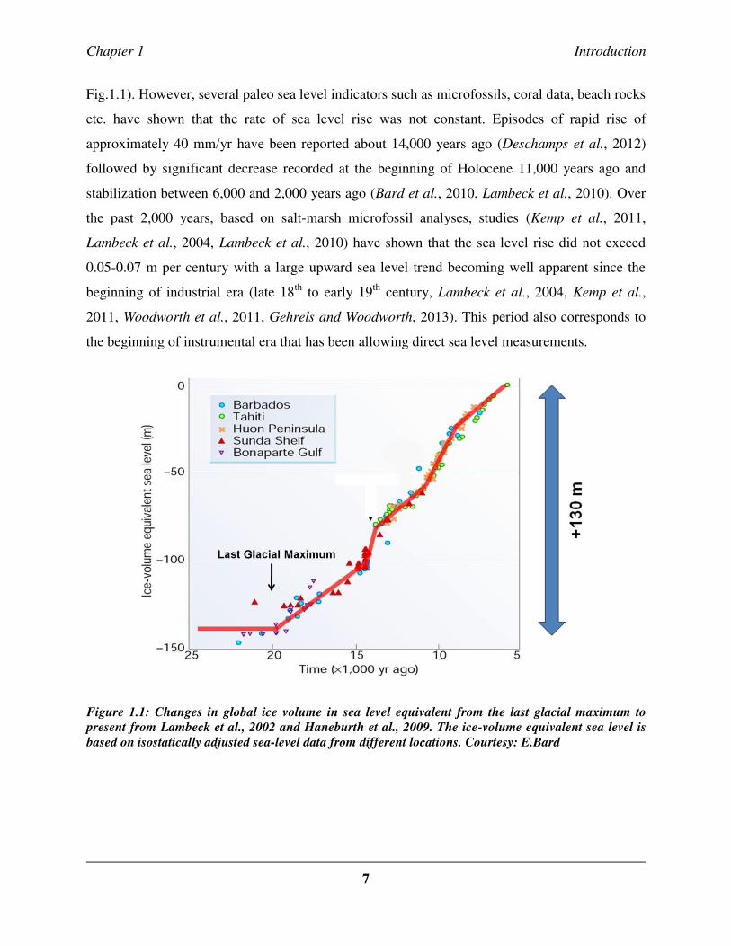
southern hemisphere. However for long term sea level studies, the number of long term records
still remains small and geographically inhomogeneous with a strong density coverage in the
northern hemisphere(Fig.1.2).
Figure 1.2: number of the tide gauge measurements available since 1807. Brown colour corresponds to
the mean sea level data available from Northern Hemisphere and blue colour corresponds to the
limited number of mean sea level data available from Southern Hemisphere. Source: PSMSL-
http://www.psmsl.org/products/data_coverage/
Chapter 1 Introduction
9
Besides, tide gauge records often have multi-year or multi-decade long gaps. The sparse and
heterogeneous coverage of tide gauge records, both temporally and geographically poses a
problem for estimating reliable historical mean sea level variations (Meyssignac and Cazenave,
2012). Tide gauges measure sea level relative to the ground, hence monitor ground motions in
areas subjected to strong natural (Glacial Isostatic Adjustment (GIA), tectonic/volcanic) or
anthropogenic (ground water pumping, oil/gas extraction, sediment loading) ground subsidence.
Therefore in order to study the absolute sea level change, the ground motion needs to be
removed. Note however that for studying local impacts, the total relative sea level change
(climatic sea level change plus vertical land motion) needs to be known (See Section 3.2 of
Chapter 3). By developing various strategies, several studies (Douglas, 2001, Church and White,
2006, Jevrejeva et al., 2006 Jevrejeva et al., 2008, Church and White, 2011, Wöppelmann et al.,
2007, Wöppelmann et al., 2009) have provided tide gauge based reliable historical sea level time
series. In spite of the various approaches used, the results based from these studies are
homogeneous and give a mean 20th
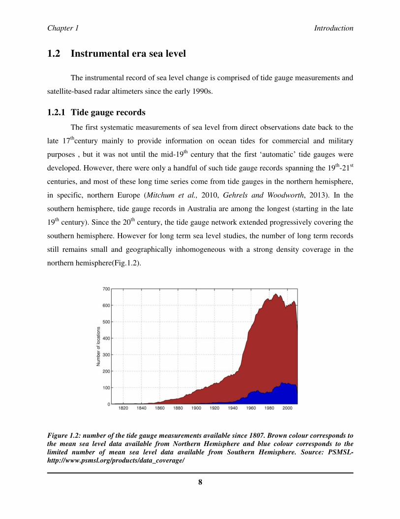
century sea level rate in the range of 1.6-1.8 mm/yr. Fig.1.3
displays the 20th
century global mean sea level curve of Church and White 2011 from tide gauge
based past sea level reconstruction (in blue) with the satellite altimetry based sea level curve
superimposed in red.
Figure 1.3: 20th
century sea level curve (in blue) from tide gauge based past sea level reconstruction of
Church and White, 2011and altimetry-based sea level curve (in red) between 1993 and 2015 from
AVISO.
Chapter 1 Introduction
10
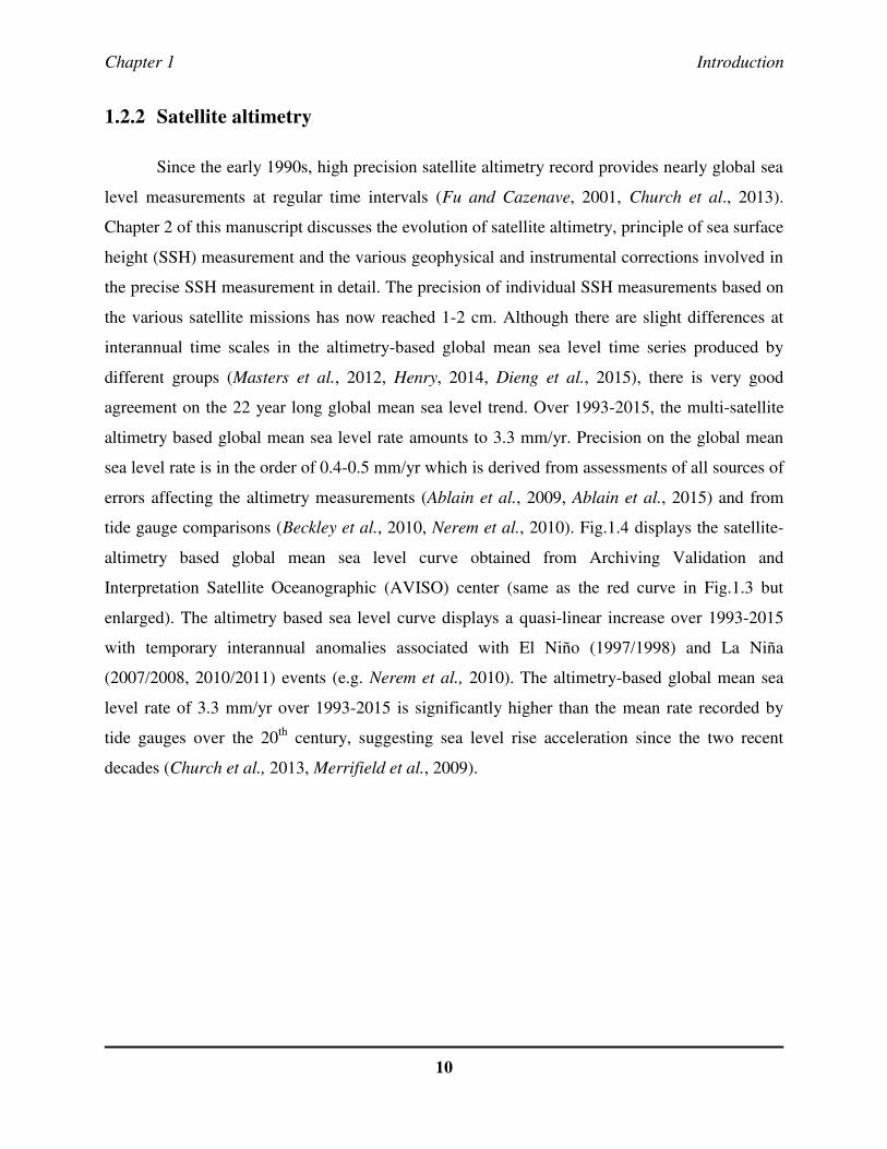
1.2.2 Satellite altimetry
Since the early 1990s, high precision satellite altimetry record provides nearly global sea
level measurements at regular time intervals (Fu and Cazenave, 2001, Church et al., 2013).
Chapter 2 of this manuscript discusses the evolution of satellite altimetry, principle of sea surface
height (SSH) measurement and the various geophysical and instrumental corrections involved in
the precise SSH measurement in detail. The precision of individual SSH measurements based on
the various satellite missions has now reached 1-2 cm. Although there are slight differences at
interannual time scales in the altimetry-based global mean sea level time series produced by
different groups (Masters et al., 2012, Henry, 2014, Dieng et al., 2015), there is very good
agreement on the 22 year long global mean sea level trend. Over 1993-2015, the multi-satellite
altimetry based global mean sea level rate amounts to 3.3 mm/yr. Precision on the global mean
sea level rate is in the order of 0.4-0.5 mm/yr which is derived from assessments of all sources of
errors affecting the altimetry measurements (Ablain et al., 2009, Ablain et al., 2015) and from
tide gauge comparisons (Beckley et al., 2010, Nerem et al., 2010). Fig.1.4 displays the satellite-
altimetry based global mean sea level curve obtained from Archiving Validation and
Interpretation Satellite Oceanographic (AVISO) center (same as the red curve in Fig.1.3 but
enlarged). The altimetry based sea level curve displays a quasi-linear increase over 1993-2015
with temporary interannual anomalies associated with El Niño (1997/1998) and La Niña
(2007/2008, 2010/2011) events (e.g. Nerem et al., 2010). The altimetry-based global mean sea
level rate of 3.3 mm/yr over 1993-2015 is significantly higher than the mean rate recorded by
tide gauges over the 20th
century, suggesting sea level rise acceleration since the two recent
decades (Church et al., 2013, Merrifield et al., 2009).
Chapter 1 Introduction
11
Figure 1.4: Altimetry-based global mean sea level temporal curve since 1993. The post glacial rebound
correction of -0.3mm/yr has been applied and the annual, semi-annual signals have been removed. A 6
month filter has been applied on the red curve.
1.3 Contributors to global mean sea level rise during the
instrumental era
The two main causes of global mean sea level change are the thermal expansion
/contraction of the sea waters in response to ocean warming and the addition of freshwater to
ocean basins as a result of land ice loss and water exchange with terrestrial reservoirs (soil and
underground reservoirs, lakes, snowpack, etc.).
1.3.1 Ocean temperature and salinity changes
Anomalies in temperature and salinity in the ocean water column change density, which
further gives rise to sea level variations (classically called steric variations, or thermosteric or
halosteric if associated with only temperature or salinity variations respectively, Cazenave and
Chapter 1 Introduction
12
Llovel, (2010)). Analyses of in situ hydrographic measurements collected by ships over the past
50 years and recently by Argo profiling floats indicate that in terms of global mean, the oceans
have warmed significantly since 1950. Over the 1971-2010 period, the 5th
Assessment Report of
the Intergovernmental Panel on Climate Change (IPCC AR5) shows that the global mean
thermosteric sea level (including estimates of deep ocean contribution) trend amounts to 0.8±0.3
mm/yr accounting for about 40% of the observed sea level rise. Over the altimetry period of
1993-2010, the thermosteric sea level trend amounts to 1.1±0.3 mm/yr accounting for about 35%
of the total observed sea level rise (Church et al., 2013). Assuming constant total salt content,
density changes arising from redistribution of salinity by ocean circulation (halosteric effect) has
almost no effect on global mean sea level, although it plays a role at regional scales (Antonov et
al., 2002, Wunsch et al., 2007, von Schuckmann et al., 2009, Cazenave and Llovel, 2010,
Stammer et al., 2013, Church et al., 2013, Durack et al., 2014). For example, for the period
1955-2003, Ishii et al., (2006) estimated a halosteric sea level rate of 0.04±0.02 mm/yr. While it
is of interest to quantify this effect, only about 1% of the halosteric expansion contributes to the
global sea level rise budget. This is because the halosteric expansion is nearly compensated by a
decrease in volume of the added freshwater when its salinity is raised (by mixing) to the mean
ocean value; the compensation would be exact for a linear state equation (Gille, 2004, Lowe and
Gregory, 2006). Hence, for global sums of sea level change, halosteric expansion cannot be
counted separately from the volume of added land freshwater (Solomon et al., 2007, Church et
al., 2013).
1.3.2 Glaciers melting
Being very sensitive to global warming, observations have indicated that since 1970s,
mountain glaciers and ice caps are retreating and thinning with noticeable acceleration since the
early 1990s. They represent another significant source of freshwater mass to be added to world’s
oceans thereby raising sea level (Church et al., 2013, Gardner et al., 2013, Vaughan et al.,
2013). Contribution of glacier ice melt to sea level has been estimated through mass balance
studies of a large number of glaciers (Marzeion et al., 2014, Gregory et al., 2013, Church et al.,
2013, Leclercq et al., 2011, Church et al., 2011, Cogley, 2009, Meier et al., 2007, Kaser et al.,
2006). The mass balance estimates are either based on in situ measurements (monitoring of the
annual mean snow accumulation and ice loss from melt) or geodetic techniques (measurements
Chapter 1 Introduction
13
of surface elevation and area change from airborne altimetry or digital elevation models,
Vaughan et al., 2013). The sea level contribution of all glaciers excluding those surrounding the
periphery of Greenland and Antarctica ice sheets has been estimated as 0.62±0.37 mm/yr sea
level equivalent (SLE) for 1971-2009 in IPCC AR5. For 1993-2009, its contribution amounts to
0.76±0.37 mm/yr, around 25% of the total observed sea level rise (Church et al., 2013, Church et
al., 2011).
1.3.3 Ice sheets
The mass balance of ice sheets is a topic of considerable interest in the context of global
warming and sea level rise since it is expected that if totally melted, Greenland and West
Antarctica would raise sea level by several meters. While little was known on the mass balance
of ice sheets before the 1990s mainly because of inadequate observations, since then, different
remote sensing techniques (e.g. airborne and satellite radar and laser altimetry, Synthetic
Aperture Radar Interferometry-InSAR) and space gravimetry since 2002 (Gravity Recovery and
Climate Experiment-GRACE) have enabled the monitoring of ice sheet mass balance. Mass
balance estimates from data obtained through the various techniques unambiguously show an
accelerated ice mass loss from both the ice sheets in the recent years (Hanna et al., 2013,
Gregory et al., 2013, Fettweis et al., 2013, Church et al., 2011, Chen et al., 2009, Velicogna,
2009, Rignot et al., 2008, Hanna et al., 2008 and Vaughan et al., 2013 for a review). During
1993-2003, the IPCC AR5 synthesis has shown that only around 13.5% of the total observed sea
level rise was explained by the ice sheet mass loss. However, since then this contribution has
augmented resulting in approximately 40% during 2003-2004 showing that this is not constant
through time. Over the entire 1993-2009 time period, the ice sheet mass loss contribution to sea
level was estimated to be 0.7±0.4 mm/yr SLE, that is, ~ 25% of the total observed sea level rise.
Of the total ice mass loss contribution, 0.4±0.2 mm/yr SLE and 0.3±0.2 mm/yr SLE were
contributed by Greenland and Antarctica respectively (Church et al., 2013).
1.3.4 Land waters
Changes in water storage on land in response to climate change and variability (i.e., water
stored in rivers, lakes, wetlands, aquifers and snow pack at high latitudes and altitudes) and from
direct human-induced effects (i.e., storage of water in man-made reservoirs along rivers and
Chapter 1 Introduction
14
ground water pumping) have the potential to contribute to sea level change (Milly et al., 2010).
Estimates of climate-related changes in land water storage over the past few decades rely on
global hydrological models due to inadequate observational data. Based on hydrological
modelling, Milly et al., (2003)and Ngo-Duc et al., (2005) found no long term sea level trend
associated with natural land water storage change but interannual to decadal fluctuations,
equivalent to several millimeters of sea level. Furthermore, recent studies (Cazenave et al., 2014,
Fasullo et al., 2013, Boening et al., 2012, Cazenave et al., 2012, Llovel et al., 2011, Nerem et al.,
2010) have shown that interannual variability in observed global mean sea level correlates with
El Niño Southern Oscillation (ENSO) indices and is inversely related to ENSO-driven changes
of terrestrial water storage. While climate-related changes in land water storage do not show
significant long-term sea level trends for the recent decades, direct human (anthropogenic)
interventions in land water storage (reservoir impoundment and groundwater depletion) have
each contributed at least several tenths of mm of sea level change (Church et al., 2013, Konikow,
2013, Pokhrel et al., 2012, Wada et al., 2012, Konikow, 2011, Milly et al., 2010, Chao et al.,
2008). Reservoir impoundment causes a sea level decrease whereas ground water depletion
increases the sea level since most of the water extracted from the ground ends up in one form or
another into the oceans. Reservoir impoundment exceeded groundwater depletion for the
majority of the 20th
century but groundwater depletion has increased and now exceeds current
rates of impoundment, contributing to an increased rate of global mean sea level rise. IPCC AR5
estimated the net anthropogenic contribution of land waters to sea level to be 0.12±0.1 mm/yr for
1970-2010. Over 1993-2010, its contribution amounts to 0.38± 0.12 mm/yr, around 12% of the
total rate of observed sea level rise (Church et al., 2013).
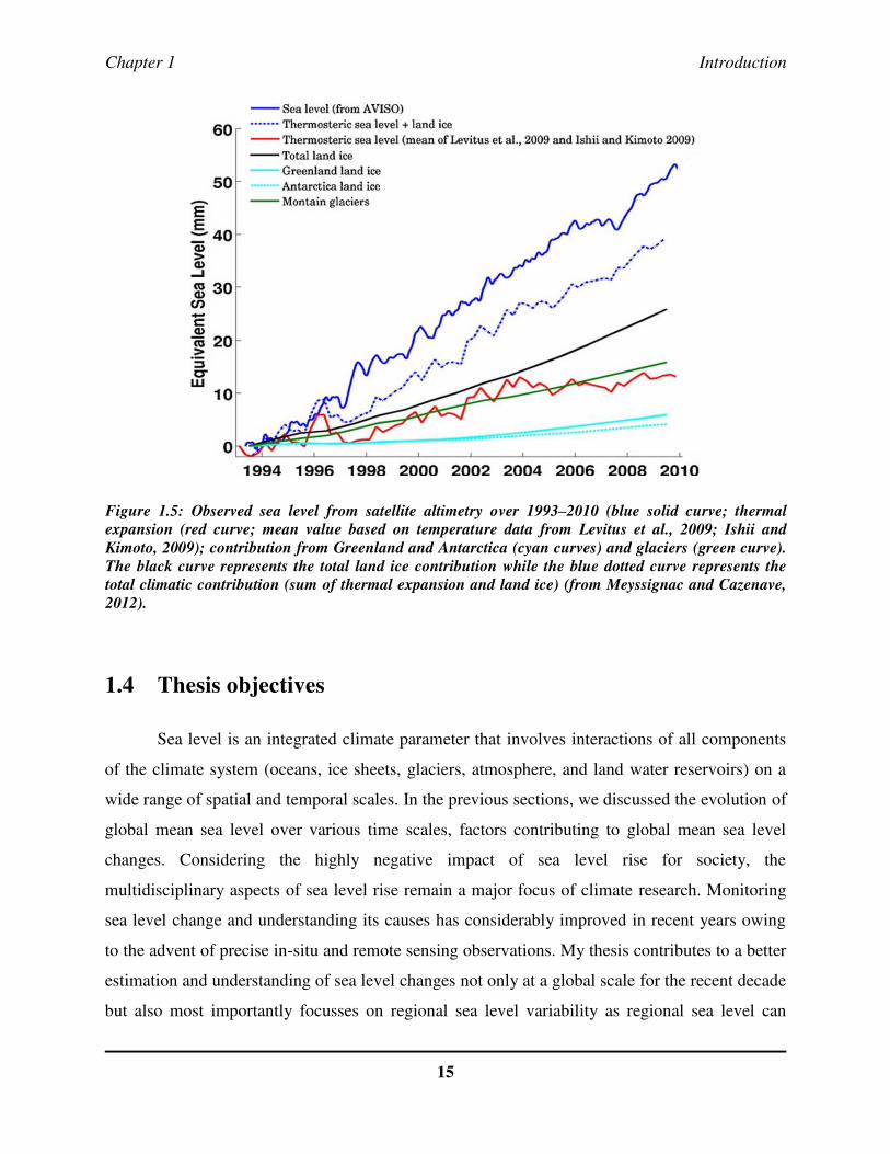
Fig.1.5 (adapted from Meyssignac and Cazenave, 2012) compares the observed global
mean sea level rise to different components and their sum over the altimetry era.
Chapter 1 Introduction
15
Figure 1.5: Observed sea level from satellite altimetry over 1993–2010 (blue solid curve; thermal
expansion (red curve; mean value based on temperature data from Levitus et al., 2009; Ishii and
Kimoto, 2009); contribution from Greenland and Antarctica (cyan curves) and glaciers (green curve).
The black curve represents the total land ice contribution while the blue dotted curve represents the
total climatic contribution (sum of thermal expansion and land ice) (from Meyssignac and Cazenave,
2012).
1.4 Thesis objectives
Sea level is an integrated climate parameter that involves interactions of all components
of the climate system (oceans, ice sheets, glaciers, atmosphere, and land water reservoirs) on a
wide range of spatial and temporal scales. In the previous sections, we discussed the evolution of
global mean sea level over various time scales, factors contributing to global mean sea level
changes. Considering the highly negative impact of sea level rise for society, the
multidisciplinary aspects of sea level rise remain a major focus of climate research. Monitoring
sea level change and understanding its causes has considerably improved in recent years owing
to the advent of precise in-situ and remote sensing observations. My thesis contributes to a better
estimation and understanding of sea level changes not only at a global scale for the recent decade
but also most importantly focusses on regional sea level variability as regional sea level can
Chapter 1 Introduction
16
substantially deviate from the global mean and can vary on a broad range of spatial and temporal
scales. The main objectives and the organization of the thesis are outlined below.
Chapter 2 of this thesis presents two main works that involve the validation of sea level
variations measured by the most recent satellite altimetry mission and the global mean sea level
closure budget for the recent decade using various observational data.
In the first part of this chapter, we provide a detailed description on the evolution of different
altimetry satellites since the beginning of the altimetry era, principle of SSH measurement and
the various geophysical and instrumental corrections involved in the precise SSH measurement.
This is then followed by the validation of sea level variations measured by SARAL-AltiKa by
comparing them with SSH measurements from JASON-2 and various available tide gauge
records. The second part of the chapter attempts to answer the following questions: Can the
global mean sea level budget be closed using available observational datasets of sea level and its
contributing components over 2003-2012? If not, can the significant residual signal be possibly
related to deep ocean contribution and/or signal that corresponds to regions that are not
monitored by observing systems or uncertainties in data processing?
Chapter 3 deals with regional sea level variability, its causes and estimates of total
relative sea level change at various vulnerable regions of the world.
In the first part of the chapter, climate-related and non-climatic causes of regional sea level
variability over the altimetry era (1993-2013) are discussed in detail. In the second part of the
chapter, we then focus our interest on long-term (i.e. at least 60 years) regional sea level
variability. By making use of a two dimensional past sea level reconstruction and long term in-
situ steric sea level data, the causes of regional sea level variability over 1950-2009 in the Indian
Ocean, South China Sea and Caribbean Sea are first discussed. Furthermore, estimates of total
relative sea level change (sea level change as felt by the population) since 1950 at several tide
gauge locations at the vulnerable coasts and islands of the above mentioned regions obtained
using a multidisciplinary approach as in Becker et al., (2012) are then discussed and compared.
In the final chapter (Chapter 4) we discuss the role of ocean dynamics, internal climate
variability and external forcing on regional sea level variability with a special focus on the
Pacific Ocean (especially the western tropical Pacific) where the regional sea level trends since
the two recent decades are estimated to be three times the global mean sea level rate. This
chapter has various sections. The first two sections are dedicated to various well known internal

Chapter 1 Introduction
17
unforced climate modes and two main sources of externally forced climate variability. This is
then followed by a section that focusses on detection and attribution of climate change on global
and regional sea level variability where a review of various studies on this subject is performed.
The next section focusses on the Pacific Ocean sea level spatial trend patterns over the altimetry
era. The contribution of internal climate modes and ocean dynamic processes to the Pacific
Ocean sea level trend pattern estimated using observation in-situ data is first discussed. The
presence of anthropogenic sea level fingerprint in the Pacific Ocean sea level since 1993 is also
studied using observational altimetry and phase 5 of Coupled Model Inter-comparison Project
(CMIP5) climate model-based sea level data.

18
Chapter 2 Multi satellite altimetry record and global mean sea level budget
19
Chapter 2
Multi satellite altimetry record and global
mean sea level budget
Satellite altimetry missions have transformed the way we view Earth and its ocean and
has been the main tool for continuously and precisely monitoring the sea surface height (SSH)
with quasi-global coverage and short revisit time. In Chapter 1, we have seen the evolution of
global mean sea level (GMSL) as measured by satellite altimeters since 1993. In this chapter, we
first discuss the evolution of various altimetry satellites used for ocean observation, principle
behind the altimetry-based SSH measurement and different error corrections involved in precise
SSH measurements. We then move on to the estimation of global mean sea level budget since a
decade using various observational and in-situ data.
2.1 Evolution of altimetry satellites
Satellite altimetry was developed in the 1960s soon after the flight of artificial satellites
became a reality (Fu and Cazenave, 2001). The first altimetry satellite, GEOS 3 (Geodynamics
Experimental Ocean Satellite) was launched in 1975 and carried instruments to yield useful
measurements of sea level and its variability. However, its performance was not good enough to
extract useful scientific information from its measurements. This was then followed by Seasat
(SEA faring SATellite) and Geosat (GEOdetic SATellite) missions in 1978 and 1985
respectively. While Seasat gave us the first global view of ocean circulation, waves and winds,
Geosat was the first mission to provide long-term (over 3 years) of high quality altimetry data.
However, until the early 1990s, satellite altimetry has been more useful to marine geophysics
rather than oceanography. This is mainly because the orbital error (see section 2.1.2 for details)
Chapter 2 Multi satellite altimetry record and global mean sea level budget
20
for these missions was so large (from several decimeters to ~1m) that the altimetry range
uncertainty prevented detection and precise measurements of phenomena associated with ocean
dynamics such as dynamic topography, tides, sea level etc. (Fu and Cazenave, 2001, Palanisamy
et al., 2015a).
The era of precise satellite altimetry dedicated to space oceanography began in the early
1990s with the launch of ERS-1, a European Space Agency (ESA) mission in 1991 and the
National Aeronautics and Space Agency (NASA)/ Centre National d’Etudes Spatiales (CNES)
joint venture TOPEX/Poseidon in 1992. In fact, TOPEX/Poseidon revolutionized the study of
Earth’s oceans by providing the first continuous, global coverage of ocean surface topography.
Its data made a huge difference in our understanding of the oceans and their effect on global
climatic conditions. Its repeat cycle (i.e. the time taken for the satellite to pass vertically over the
same location) of ~10 days provided more information than in-situ measurements over hundred
years. The mission far exceeded the expectations in terms of both mission duration (initial design
life was 5 years but stayed in operation for 13 years) and measurement system performance (Buis
et al., 2006).
During the period of TOPEX/Poseidon (1992-2006), several other new altimetry
missions were launched: ERS-2 (ESA, 1995-2011), Jason-1 (NASA/CNES, 2001-2012),
ENVISAT (ENVIronmental SATellite, ESA, 2002-2012) and Jason-2 (NASA/CNES, 2008- ).
The combination of several satellites available at the same time enabled a good compromise
between the spatial and temporal resolutions for ocean monitoring. For example, while the repeat
cycle of TOPEX/Poseidon was ~10 days (good temporal resolution), its inter-track spacing at the
Equator was in the order of 315 km; whereas in the case of ENVISAT, its repeat cycle was 30
days with inter-track spacing in the order of 80 km at the Equator (good spatial resolution).
Moreover, while TOPEX/Poseidon, Jason-1 and Jason-2 flew at the non- sun synchronous orbit
(up to 66°N/S), ENVISAT’s polar sun synchronous orbit further enabled high latitude ocean
coverage (up to 81.5° N/S) thereby complementing to the other existing missions.
Cryosat-2 and HY-2A are two other satellite altimetry missions launched by ESA and
China in 2010 and 2011 respectively. The Cryosat-2 orbit at an inclination of about 92 degree
and an altitude of 717 km covers almost all the polar region and henceforth is dedicated to polar
observation while HY-2A at sun synchronous and geodetic orbit helps in monitoring the

Chapter 2 Multi satellite altimetry record and global mean sea level budget
21
dynamics of the ocean. Since the beginning of 2013, a new altimetry mission, SARAL-AltiKa, a
joint venture between CNES and Indian Space Research Organization (ISRO), now ensures the
continuity of high precision sea level data along with the existing Jason-2 measures (Verron et
al., 2015). It is the first oceanographic mission using a high frequency Ka band altimeter for
improved spatial and temporal resolution and flies in the same orbit as that of ENVISAT (a
detailed explanation on SARAL-AltiKa is presented in Section 2.1.4). Another mission, Jason-3
in the framework of a co-operation between CNES, NASA, Eumetsat (EUropean METeorology
SATellite) and NOAA (National Oceanic and Atmospheric Administration) is proposed to be
launched soon. This mission is similar to those of TOPEX/Poseidon, Jason-1 and Jason-2 with
the same kind of payload and orbital parameters.
Since satellite altimetry has proven to be a valuable source of data for ocean monitoring
and understanding, several future missions are foreseen such as Sentinel-3 Jason-CS, SWOT
(Surface Water Ocean Topography). Continuous monitoring with the help of such satellite
altimeters will further enhance our understanding of oceans and their mechanisms.
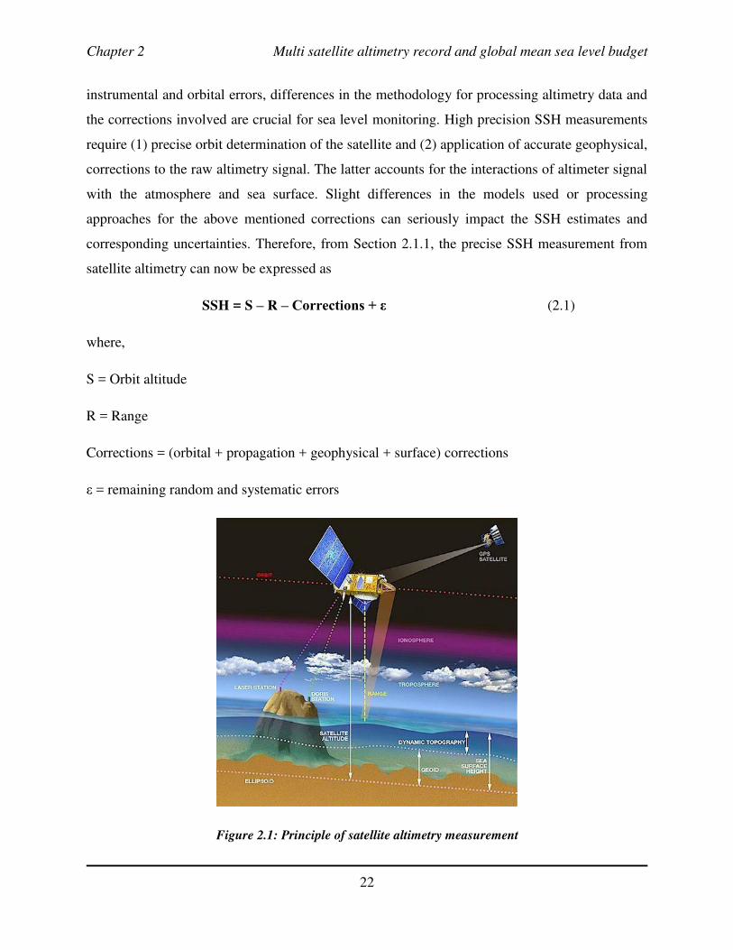
2.1.1 Principle of satellite altimetry
The radar altimeters on board the satellite transmit signals at high frequency (over 1700
pulses per second) towards the sea surface which is partly reflected back to the satellite.
Measurement of the round-trip travel time is then converted to obtain the distance of the satellite
above the instantaneous sea surface, called as ‘range’. SSH measurement is deduced from the
difference between the satellite distance to the Earth’s centre of mass (deduced from precise
orbitography and called ‘satellite/orbit altitude’) and the satellite distance (range) above the sea
surface (Fig.2.1) Besides sea surface height, wave height and wind speed over the oceans can
also be measured from the amplitude and waveform of the return signal.
2.1.2 Corrections involved in Sea Surface Height measurement
The determination of precise SSH measurements from satellite altimetry is influenced by
many factors. Amongst the most important are sensor characteristics, long-term stability of the
altimeter, and the methods used in altimeter data processing (Fernandes et al., 2006). While the
sensor characteristics of the altimeter are pre-determined depending on the altimetry missions,
Chapter 2 Multi satellite altimetry record and global mean sea level budget
22
instrumental and orbital errors, differences in the methodology for processing altimetry data and
the corrections involved are crucial for sea level monitoring. High precision SSH measurements
require (1) precise orbit determination of the satellite and (2) application of accurate geophysical,
corrections to the raw altimetry signal. The latter accounts for the interactions of altimeter signal
with the atmosphere and sea surface. Slight differences in the models used or processing
approaches for the above mentioned corrections can seriously impact the SSH estimates and
corresponding uncertainties. Therefore, from Section 2.1.1, the precise SSH measurement from
satellite altimetry can now be expressed as
SSH = S – R – Corrections + ε (2.1)
where,
S = Orbit altitude
R = Range
Corrections = (orbital + propagation + geophysical + surface) corrections
ε = remaining random and systematic errors
Figure 2.1: Principle of satellite altimetry measurement
Chapter 2 Multi satellite altimetry record and global mean sea level budget
23
In this section, we discuss several of these corrections involved for precise SSH
estimation.
1) Orbital correction
The quality of the altimetry data depends on the ability to precisely determine a satellite’s
position on orbit. Orbital error is caused by imperfect knowledge of the spacecraft position in the
radial orbit direction and is the largest error source on altimetry measurements for SSH
monitoring. Therefore, a very precise knowledge of the satellite orbit with respect to Earth’s
reference ellipsoid is essential. The satellite’s orbit can be also perturbed by gravitational forces
related to the non-uniform distribution of Earth’s gravity field, and those caused by the sun,
moon and other planets. Forces on the satellite’s surface such as atmospheric drag (e.g. low orbit
satellites experience more atmospheric drag) and radiative pressure (e.g. solar radiation, Earth’s
IR radiation etc.) also play a role in the perturbation of the satellite’s orbit. This indicates that a
detailed knowledge of the satellite and its variations due to maneuvers, fuel consumption, solar
panel orientation etc. are also necessary in order to precisely model the above mentioned forces
acting on it. Precise orbit determination is done through a combination of satellite tracking and
dynamic modelling. Satellite tracking in general involves the use of Satellite Laser Ranging
(SLR), Global Positioning System (GPS) and Doppler Orbitography and Radio positioning
System (DORIS). A dynamical model taking into account the forces acting on the satellite is then
fitted through the tracking data to obtain the precise orbit of the satellite.
2) Propagation corrections
As the radar altimetry signal travels through the atmosphere to the sea surface, it is
slowed down due to the presence of various elements in its path. The delay in the propagation of
the radar signal thus needs to be corrected in order to estimate the precise range, i.e. the distance
between the satellite and sea surface. There are three types of propagation delays that need to be
accounted for: (1) ionospheric, (2) wet and (3) dry tropospheric corrections.
a) Ionosphere correction
This correction takes into account the path delay in the radar signal due to the presence of
electrons in the ionosphere. The ionosphere is the uppermost layer of the atmosphere (ranging
between 60 and 800 km) and the electrons are produced as a result of ionization attributed to
solar radiation. As a result, it causes the altimeter to slightly over estimate the range by 1 to 20
Chapter 2 Multi satellite altimetry record and global mean sea level budget
24
cm. This amount can vary with respect to the seasons, solar cycle and occurrences of
geomagnetic storms with the maximum influence occurring at the tropical band. Since the range
delay due to the presence of electrons is related to electromagnetic radiation frequency, the
correction can be estimated using two different radar frequencies (for example, C-band and Ku-
band for TOPEX and Jason-1). This correction can also be taken into account from models of the
vertically integrated electron density (Fu and Cazenave, 2001, Callahan, 1984, Imel, 1995).
b) Wet troposphere correction
The wet tropospheric correction is the correction for the delay of the radar signal due to
the presence of water vapor content in the atmosphere. This is a difficult correction to be
accounted for as the wet atmospheric effect highly varies both spatially and temporally with
maximum occurring in the tropical convergence zones and magnitudes ranging from 5cm to 30
cm. Over the oceans, the wet tropospheric correction is in general computed using on-board
microwave radiometer measurements. But, such radiometric measurements generally fail near
the coasts where the signal coming from the surrounding land surface contaminates the
radiometer measurements (Desportes et al., 2007). In such cases, the correction is computed
from meteorological model outputs such as ECMWF (European Center for Medium Range
Weather Forecast) or NCEP (National Centers for Environmental Prediction) models (Legeais et
al., 2014).
c) Dry troposphere correction
The mass of dry air molecules in the atmosphere causes a range delay known as the dry
tropospheric effect. It is directly proportional to sea level pressure and is the largest adjustment
that has to be applied to altimetry measurement as its order of magnitude is about 2.3m.
However, its temporal variations are low and range a few centimeters only. The dry tropospheric
correction is computed using atmospheric model pressure forecasts such as ECMWF.
3) Geophysical corrections
The gravity forces generated by the Sun and Moon on the Earth can create perturbations
on the earth’s interior and also sea surface elevations of few meters. These geophysical effects
are called as tidal effects and can be classified into four types: (1) ocean, (2) solid Earth, (3)
polar tidal and (4) loading effects.

Chapter 2 Multi satellite altimetry record and global mean sea level budget
25
a) Ocean, solid Earth tidal and loading corrections
Ocean tides and their variations are the result of the combined attraction of Sun and
Moon and represent more than 80% of the surface variability in open ocean. The tidal periods
(half a day or one day) are shorter than the repeat periods of an altimetry satellite. Tidal
correction is therefore essential since they contaminate the low frequency altimetry signals.
Furthermore, for the estimation of dynamic sea surface height, the magnitude of ocean tides are
very large and must therefore be removed as they are considered as noise. Ocean tidal
corrections are performed using assimilated hydrodynamic and statistical models that estimate
tides globally with high spatial resolution (Fu and Cazenave, 2001, Ray, 1999).
The gravitational attraction of the Sun and Moon also impacts Earth’s interior causing the
surface of the Earth beneath the ocean to be slightly deformed. This is called as the solid Earth
tidal effect. This effect is nearly in phase with the ocean tide and is corrected using models.
Furthermore, the change in the weight of the water column due to variations in tides
causes an elastic loading effect on the sea floor that is also corrected using models.
b) Polar tidal correction
The axis of rotation of the Earth deviates slightly from the Earth’s ellipsoidal axis over a
period of several moths annually. This as a result causes variations to both solid Earth and
oceans and is called as polar tidal effect (Desai, 2002, Wahr, 1985). The polar tide correction is
implemented through modelling that requires precise knowledge on the Earth’s axis of rotation.
4) Surface corrections
Apart from propagation and geophysical corrections applied to altimetry signal, there are
two types of surface corrections that need to be accounted for: (1) inverse barometric and (2) sea
state bias corrections.
a) Inverse barometric (IB) correction
The response of the sea surface to changes in atmospheric pressure has a large effect on
measured sea surface height as the ocean responds directly to atmospheric pressure changes. Sea
level falls (rises) as the atmospheric pressure loading increases (decreases). For example, an
increase in the atmospheric pressure by 1mbar pushes the sea level down by 1 cm. This is called
as the isostatic inverse barometric effect (Wunsch and Stammer, 1997, Ponte and Gaspar, 1999,
Chapter 2 Multi satellite altimetry record and global mean sea level budget
26
Carrère and Lyard, 2003). The magnitude of the IB effect can reach up to ± 15 cm and is
corrected using meteorological models such as ECMWF.
b) Sea State Bias (SSB) correction
This correction includes the electromagnetic bias (EM bias) and skewness bias. The EM
bias is the correction for bias in measurements due to varying reflectivity of the wave troughs
and crests (Chelton, 1994). The concave form of wave troughs tends to concentrate and reflect
the altimetry signal better than the wave crests that disperse the signal. Therefore the altimetry
signal return from the troughs is stronger than from the crests. Furthermore, in the case of wind
waves, the wave troughs have a larger surface area than the pointy crests and this is called as
skewness bias. Both the EM and skewness bias causes the mean reflecting surface to be shifted
towards the troughs. They vary with increasing wind speed and wave height. SSB is estimated
using empirical formulas derived from altimeter data analysis and models (Tran et al., 2006).
The range correction varies from a few to 30 cm.
5) Other potential errors
Other sources of potential errors in SSH measurements include altimeter instrumental
ageing errors. Altimeter parameters are precisely monitored over all the mission life-time to
detect instrumental anomalies (Ablain et al., 2009). Based on the instrumental anomalies
observed in the satellites, corrections such as for centre of gravity, waveforms etc. are applied.
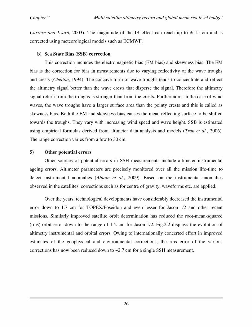
Over the years, technological developments have considerably decreased the instrumental
error down to 1.7 cm for TOPEX/Poseidon and even lesser for Jason-1/2 and other recent
missions. Similarly improved satellite orbit determination has reduced the root-mean-squared
(rms) orbit error down to the range of 1-2 cm for Jason-1/2. Fig.2.2 displays the evolution of
altimetry instrumental and orbital errors. Owing to internationally concerted effort in improved
estimates of the geophysical and environmental corrections, the rms error of the various
corrections has now been reduced down to ~2.7 cm for a single SSH measurement.
Chapter 2 Multi satellite altimetry record and global mean sea level budget
27
Figure 2.2: Evolution of orbital and instrumental errors in satellite altimetry (Source: AVISO-CNES)
2.1.3 Multi-mission SSH altimetry data
We carried out global and regional sea level studies by making use of multi-mission
merged SSH altimetry data. The purpose of using multi-mission altimetry data is to obtain the
most stringent accuracy requirements that are needed for climate research. Moreover, as
mentioned in Section 2.1, the combination of several satellites enables a better compromise on
spatial and temporal resolution. Merging multiple altimeter data sets is not easy. It requires
homogenous, inter-calibrated data sets; correcting of orbit error for the less precise altimeter
missions; extracting the sea level anomaly using a common reference surface; and combining the
data through a mapping (or assimilation) method (Le Traon et al., 1998). After calculating the
along track sea level measures for each of the satellite missions, the main steps consists of:
combining all missions together, reducing the orbit and the long wavelength errors, computing
the gridded sea level anomalies using an objective analysis approach (Ducet et al., 2000, Le
Traon et al., 2003), and generating mean sea level products (e.g. GMSL time series, gridded sea
level time series) dedicated for climate studies (Ablain et al., 2015). Owing to the
homogenization of the altimetry corrections between all the missions, the uncertainty in multi-
mission GMSL trend over 1993-2010 is now reduced to 0.5 mm/yr. The main source of this error
Chapter 2 Multi satellite altimetry record and global mean sea level budget
28
remains to be the wet tropospheric correction with a drift uncertainty in the range of 0.2-0.3
mm/yr (Legeais et al., 2014). Orbit error and altimeter parameters error also add an uncertainty
in the order of 0.1 mm/yr. Furthermore, imperfect links between various altimetry missions cause
a GMSL trend error of about 0.15 mm/yr (Ablain et al., 2015).
2.1.4 SARAL-AltiKa, the new altimetry mission
SARAL-AltiKa mission, launched in February 2013, is an answer to the needs of the
oceanographic community, continuity of high accuracy, high resolution, near-real time
observations of the ocean surface topography as at least 2 simultaneous altimetry missions are
required to fulfill this need. As a consequence, along with the existing Jason-2, SARAL-AltiKa
mission is considered as ‘gap filler’ between ENVISAT (lost in April 2012) and Jason-
3/Sentinel-3 (expected in 2015; Verron et al., 2015). This is the first oceanographic mission that
uses a high frequency Ka band altimeter (frequency and bandwidth of 35.75 GHz and 500 MHz).
The main objective of this mission is to help the oceanographic community to improve
knowledge on the ocean meso-scale variability, a class of high energy processes with
wavelengths in the range of 50 km to 500 km (Verron et al., 2015). The Ka band frequency of
SARAL-AltiKa improves spatial and temporal resolution and thus enables a better observation of
the ocean at meso-scale. It is also well suitable for studying mean sea level variations, sea and
land ice, wave heights and coastal dynamic processes (as SARAL-AltiKa can reach as close as
8km to the coasts while Jason-2 has managed only up to 15 km), as well as continental water
bodies like rivers, lakes, wet lands, etc. (Palanisamy et al., 2015a). Furthermore, SARAL-AltiKa
flies at an almost polar (final inclination at 98.55°) sun-synchronous orbit as that of ENVISAT.
This enables better observation of polar ice and oceans. With a repeat cycle of 35 days (similar to
ENVISAT), SARAL-AltiKa provides a high resolution coverage of the oceanic domain with an
inter-track spacing at the equator of 75 km.
In our study, we performed a global and regional validation of the sea level variations
measured by SARAL-AltiKa by comparing it with Jason-2 and tide gauge records. This has been
published as an article titled ‘Sea level variations measured by the new altimetry mission
SARAL-AltiKa and its validation based on spatial and temporal curves using Jason-2,tide gauge
data and an over view of the annual sea level budget’.
Chapter 2 Multi satellite altimetry record and global mean sea level budget
29
Summary of the article: ‘Sea level variations measured by the new altimetry mission SARAL-AltiKa and its validation based on spatial and temporal curves using Jason-2,tide
gauge data and an over view of the annual sea level budget’ (the original article is inserted at
the end of this section).
In the first part of our study, we compared the temporal mean sea level spatial patterns of
SARAL-AltiKa with those of Jason-2 over March 2013 to August 2014. At global scale, the
temporal mean sea level spatial patterns between SARAL-AltiKa and Jason-2 were found to be
very similar. However, differences in the order of ±30 mm were noticed between the two
missions (Fig.2.3). Since, SARAL-AltiKa was still in its verification phase at the time the article
was written, it was presumed that these differences occurred due to various orbital and
geophysical corrections that were not yet completely taken into account in the case of SARAL-
AltiKa. For example, from Fig.2.3 we can observe noticeable positive SSH differences between
SARAL-AltiKa and Jason-2 in the Southern Hemisphere below 40°S latitudinal range. This is
the region with generally high and spontaneous ocean waves that have high significant wave
height. Therefore the differences in SSH measurements in this region is probably due to the
differences in SSB corrections as the SSB correction in SARAL-AltiKa had not yet been tuned.
While in terms of global mean time series, both SARAL-AltiKa and Jason-2 relatively agree
well, in terms of regional mean, the difference was found to be maximum at the southern
hemisphere extra-tropical latitudinal band. All the preliminary analyses show that the sea level
variations measured by SARAL-AltiKa looks very promising.
The second part of the study consisted of comparing SARAL-AltiKa sea level data with
Jason-2 and tide gauge records. SARAL-AltiKa and Jason-2 sea level grids were first
interpolated within a 1° radius of the tide gauge location and their corresponding time series
were compared with that of the tide gauge time series. It was observed that at most tide gauge
sites, SARAL-AltiKa time series were well correlated with both tide gauge and Jason-2 time
series. There were several locations such as Maloy in the Atlantic and Fremantle in the Indian
Ocean that had high amplitudes of sea level variations observed by the tide gauges but not by
SARAL-AltiKa and Jason-2. However the high amplitude sea level variations were related to
local seasonal phenomena captured by tide gauge records that are not reflected in satellite
altimeters.
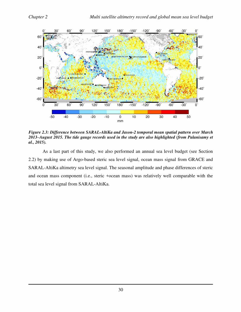
Chapter 2 Multi satellite altimetry record and global mean sea level budget
30
Figure 2.3: Difference between SARAL-AltiKa and Jason-2 temporal mean spatial pattern over March
2013–August 2015. The tide gauge records used in the study are also highlighted (from Palanisamy et
al., 2015).
As a last part of this study, we also performed an annual sea level budget (see Section
2.2) by making use of Argo-based steric sea level signal, ocean mass signal from GRACE and
SARAL-AltiKa altimetry sea level signal. The seasonal amplitude and phase differences of steric
and ocean mass component (i.e., steric +ocean mass) was relatively well comparable with the
total sea level signal from SARAL-AltiKa.
Full Terms & Conditions of access and use can be found athttp://www.tandfonline.com/action/journalInformation?journalCode=umgd20
Download by: [Universite Paul Sabatier] Date: 18 November 2015, At: 07:09
Marine Geodesy
ISSN: 0149-0419 (Print) 1521-060X (Online) Journal homepage: http://www.tandfonline.com/loi/umgd20
Sea-Level Variations Measured by the NewAltimetry Mission SARAL/AltiKa and its ValidationBased on Spatial Patterns and Temporal CurvesUsing Jason-2, Tide Gauge Data and an Overview ofthe Annual Sea Level Budget
H. Palanisamy, A. Cazenave, O. Henry, P. Prandi & B. Meyssignac
To cite this article: H. Palanisamy, A. Cazenave, O. Henry, P. Prandi & B. Meyssignac (2015)Sea-Level Variations Measured by the New Altimetry Mission SARAL/AltiKa and its ValidationBased on Spatial Patterns and Temporal Curves Using Jason-2, Tide Gauge Data andan Overview of the Annual Sea Level Budget, Marine Geodesy, 38:sup1, 339-353, DOI:10.1080/01490419.2014.1000469
To link to this article: http://dx.doi.org/10.1080/01490419.2014.1000469
Accepted author version posted online: 23Jan 2015.
Submit your article to this journal
Article views: 80
View related articles
View Crossmark data
Marine Geodesy, 38(S1):339–353, 2015
Copyright © Taylor & Francis Group, LLC
ISSN: 0149-0419 print / 1521-060X online
DOI: 10.1080/01490419.2014.1000469
Sea-Level Variations Measured by the New
Altimetry Mission SARAL/AltiKa and its Validation
Based on Spatial Patterns and Temporal Curves
Using Jason-2, Tide Gauge Data and an Overview
of the Annual Sea Level Budget
H. PALANISAMY,1,1 A. CAZENAVE,1 O. HENRY,1 P. PRANDI,2
AND B. MEYSSIGNAC1
1Laboratoire d’Etudes en Geophysique et Oceanographie Spatiale (LEGOS),
Centre National d’Etudes Spatiales (CNES), Toulouse, France2Collecte Localisation Satellites (CLS), Ramonville-St.Agne, France
High-precision satellite altimeters help in measuring the variations in sea levelsince the early 1990s. After a number of such successful altimetry missions such asTopex/Poseidon, Jason-1, Jason-2, and Envisat, SARAL/AltiKa, a high resolution al-timetry mission based on the Ka frequency band that can also cover high latitudinalzones, was launched in February 2013. Even though the data set available from thisrecent mission is not yet suitable for climate research owing to its short duration, inthis study we perform a preliminary validation of SARAL/AltiKa sea-level data. Thefirst part of the validation is the comparison of SARAL/AltiKa and Jason-2 sea-leveldata between March 2013 and August 2014 in terms of temporal mean spatial pattern.Comparisons in terms of global mean sea-level time series and latitudinal band-basedmean time series are also performed. The second part of the validation is the compar-ison of the SARAL/AltiKa sea-level based time series with several tide gauge recordscovering the period of our study. Finally, an analysis of the annual sea-level budgetwith SARAL/AltiKa data, steric sea level, and ocean mass is performed. Results of thesepreliminary comparisons show good agreement with other sea-level data.
Keywords SARAL/AltiKa, preliminary validation, Jason-2, tide gauges, annual sealevel budget
1. Introduction
Satellite altimetry is now recognized as the main tool for precisely and continuously
monitoring the sea surface height (SSH) with quasi-global coverage and short revisit time.
The first altimeter satellite Geos 3 was launched in 1975. Since then, several altimetry
missions have flown with the purpose of studying the oceans from space (e.g., Seasat
1978; Geosat 1985–1989). However, until the early 1990s, satellite altimetry has been
more useful to marine geophysics than oceanography. In effect, for the early missions,
Received 12 July 2014; accepted 28 November 2014.
Address correspondence to H. Palanisamy, LEGOS/CNES, 18 Avenue Edouard Belin, 31400,Toulouse, France. E-mail: [email protected]
339
Do
wnlo
aded
by
[U
niv
ersi
te P
aul
Sab
atie
r] a
t 07
:10 1
8 N
ovem
ber
20
15
340 H. Palanisamy et al.
the orbital error was so large (from several decimeters to ∼1 m) that the altimetric range
uncertainty prevented detecting and precisely measuring phenomena associated with ocean
dynamics (e.g., dynamic topography, tides, sea level). The early 1990s began the era of
precise altimetry dedicated to space oceanography (Fu and Cazenave 2001) with the launch
of the following missions: ERS-1 in 1991, ERS-2 in 1995, and Envisat in 2002 launched
by the European Space Agency (ESA), and the NASA/CNES missions Topex-Poseidon
(1992–2006), Jason-1 (2001–2012), and Jason-2 (2008-). Over the years, technological
improvements have considerably decreased the instrumental noise, down to 1.7 cm for
Topex/Poseidon and Jason-1&2 for point-to-point measurement. Thanks to internationally
concerted effort in improved estimates of the geophysical and environmental corrections,
the root-mean-squared (rms) error of the various corrections has been reduced down to
∼2.7 cm for a single SSH measurement. Similarly, improved satellite orbit determination
has reduced the rms orbit error to ∼2.5 cm. For Jason-1 and Jason-2, the orbit error is even
smaller, in the range of 1–2 cm. The total rms measurement accuracy from multisatellite
missions is about 4 cm for a single SSH measurement. In terms of global mean sea level,
current errors are on the order of 4 mm for a single estimate and about 0.4 mm/yr for
interannual to decadal trends (Ablain et al. 2009; Ablain et al. 2014).
The new altimetry mission, SARAL/AltiKa (launched in February 2013), now en-
sures the continuity of high precision sea-level data, complementing the Jason-2 data set.
SARAL/AltiKa is the first oceanographic mission that uses a high frequency Ka band al-
timeter (frequency and bandwidth of 35.75 GHz and 500MHz, respectively). The Ka band
frequency improves the spatial and temporal resolution and thus enables a better observation
of the ocean at meso-scale. It is also well suitable for studying mean sea level variations, sea
and land ice, wave heights, and coastal dynamic processes (as SARAL/AltiKa can reach
as close as 8 km to the coasts while Jason-2 has managed only up to 15 km), as well as
continental water bodies such as rivers, lakes, and wet lands. The only drawback of the
Ka band frequency is its sensitivity to rain and clouds that can lead to signal attenuation.
This could result in data loss in zones with high rainy and cloudy conditions. Furthermore,
SARAL/AltiKa flies on the same orbit as Envisat, thus covers high latitude ocean (up to
81.5◦N/S), enabling the observation of polar ice and oceans. With the same orbital cycle
as Envisat (35 days), SARAL/AltiKa provides a high-resolution coverage of the oceanic
domain (with an intertrack spacing at the equator of 75 km).
Global mean sea level (GMSL) is one of the most important variables in climate studies.
Sea level is rising in response to global warming at a rate of 3.2 ± 0.4 mm/yr (e.g., Ablain
et al. 2015). It should continue to rise because of expected continuing ocean warming and
land ice melt, with possible negative impacts in a number of low altitude coastal regions
(Cazenave and Cozannet 2014; Church et al. 2013). Therefore, precise measurement and
understanding of the GMSL is important and of high scientific interest. The high precision
and spatial resolution of SARAL/AltiKa will ensure continuity of sea level measurements,
contributing to improved understanding of the evolution of the GMSL.
Even though the available SARAL/AltiKa sea level data are not yet suitable for climate
research owing to its relatively recent launch, validation of this product by comparing with
other existing products such as Jason-2 and tide gauge sea level data is feasible. Validation
of sea level data is an important step that needs to be performed before they can be used
for climate studies.
In this article, we perform a preliminary validation of SARAL/AltiKa sea level data
using Jason-2 and tide gauge records. The first part of the validation is the comparison of
SARAL/AltiKa and Jason-2 sea level data between March 2013 and August 2014 in terms
Do
wnlo
aded
by
[U
niv
ersi
te P
aul
Sab
atie
r] a
t 07
:10 1
8 N
ovem
ber
20
15
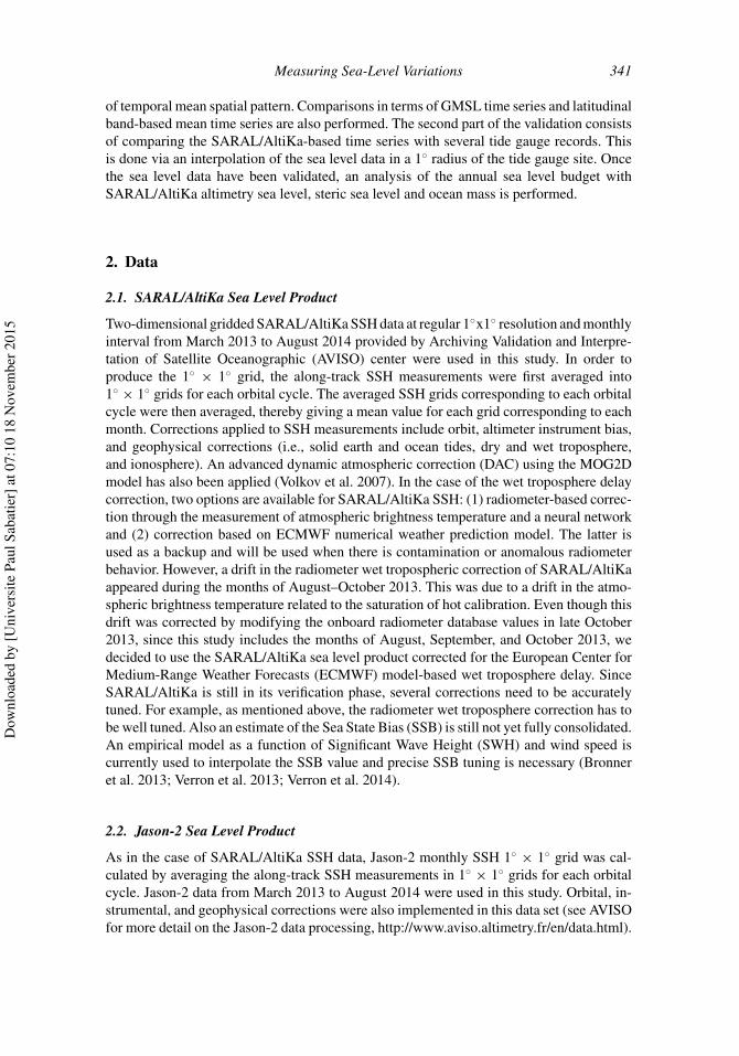
Measuring Sea-Level Variations 341
of temporal mean spatial pattern. Comparisons in terms of GMSL time series and latitudinal
band-based mean time series are also performed. The second part of the validation consists
of comparing the SARAL/AltiKa-based time series with several tide gauge records. This
is done via an interpolation of the sea level data in a 1◦ radius of the tide gauge site. Once
the sea level data have been validated, an analysis of the annual sea level budget with
SARAL/AltiKa altimetry sea level, steric sea level and ocean mass is performed.
2. Data
2.1. SARAL/AltiKa Sea Level Product
Two-dimensional gridded SARAL/AltiKa SSH data at regular 1◦x1◦ resolution and monthly
interval from March 2013 to August 2014 provided by Archiving Validation and Interpre-
tation of Satellite Oceanographic (AVISO) center were used in this study. In order to
produce the 1◦ × 1◦ grid, the along-track SSH measurements were first averaged into
1◦ × 1◦ grids for each orbital cycle. The averaged SSH grids corresponding to each orbital
cycle were then averaged, thereby giving a mean value for each grid corresponding to each
month. Corrections applied to SSH measurements include orbit, altimeter instrument bias,
and geophysical corrections (i.e., solid earth and ocean tides, dry and wet troposphere,
and ionosphere). An advanced dynamic atmospheric correction (DAC) using the MOG2D
model has also been applied (Volkov et al. 2007). In the case of the wet troposphere delay
correction, two options are available for SARAL/AltiKa SSH: (1) radiometer-based correc-
tion through the measurement of atmospheric brightness temperature and a neural network
and (2) correction based on ECMWF numerical weather prediction model. The latter is
used as a backup and will be used when there is contamination or anomalous radiometer
behavior. However, a drift in the radiometer wet tropospheric correction of SARAL/AltiKa
appeared during the months of August–October 2013. This was due to a drift in the atmo-
spheric brightness temperature related to the saturation of hot calibration. Even though this
drift was corrected by modifying the onboard radiometer database values in late October
2013, since this study includes the months of August, September, and October 2013, we
decided to use the SARAL/AltiKa sea level product corrected for the European Center for
Medium-Range Weather Forecasts (ECMWF) model-based wet troposphere delay. Since
SARAL/AltiKa is still in its verification phase, several corrections need to be accurately
tuned. For example, as mentioned above, the radiometer wet troposphere correction has to
be well tuned. Also an estimate of the Sea State Bias (SSB) is still not yet fully consolidated.
An empirical model as a function of Significant Wave Height (SWH) and wind speed is
currently used to interpolate the SSB value and precise SSB tuning is necessary (Bronner
et al. 2013; Verron et al. 2013; Verron et al. 2014).
2.2. Jason-2 Sea Level Product
As in the case of SARAL/AltiKa SSH data, Jason-2 monthly SSH 1◦ × 1◦ grid was cal-
culated by averaging the along-track SSH measurements in 1◦ × 1◦ grids for each orbital
cycle. Jason-2 data from March 2013 to August 2014 were used in this study. Orbital, in-
strumental, and geophysical corrections were also implemented in this data set (see AVISO
for more detail on the Jason-2 data processing, http://www.aviso.altimetry.fr/en/data.html).
Do
wnlo
aded
by
[U
niv
ersi
te P
aul
Sab
atie
r] a
t 07
:10 1
8 N
ovem
ber
20
15
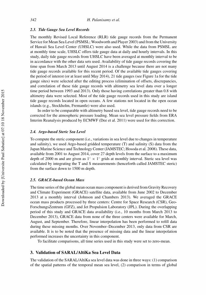
342 H. Palanisamy et al.
2.3. Tide Gauge Sea Level Records
The monthly Revised Local Reference (RLR) tide gauge records from the Permanent
Service for Mean Sea Level (PSMSL; Woodworth and Player 2003) and from the University
of Hawaii Sea Level Center (UHSLC) were also used. While the data from PSMSL are
at monthly time scale, UHSLC offers tide gauge data at daily and hourly intervals. In this
study, daily tide gauge records from UHSLC have been averaged at monthly interval to be
in accordance with the other data sets used. Availability of tide gauge records covering the
time span from March 2013 until August 2014 is a challenge because there are not many
tide gauge records available for this recent period. Of the available tide gauges covering
the period of interest (or at least until May 2014), 21 tide gauges (see Figure 1a for the tide
gauge sites) were selected after the editing process (elimination of offsets, discrepancies,
and correlation of these tide gauge records with altimetry sea level data over a longer
time period between 1993 and 2013). Only those having correlations greater than 0.8 with
altimetry data were selected. Most of the tide gauge records used in this study are island
tide gauge records located in open oceans. A few stations not located in the open ocean
islands (e.g., Stockholm, Fremantle) were also used.
In order to be comparable with altimetry based sea level, tide gauge records need to be
corrected for the atmospheric pressure loading. Mean sea level pressure fields from ERA
Interim Reanalysis produced by ECMWF (Dee et al. 2011) were used for this correction.
2.4. Argo-based Steric Sea Level
To compute the steric component (i.e., variations in sea level due to changes in temperature
and salinity), we used Argo-based gridded temperature (T) and salinity (S) data from the
Japan Marine Science and Technology Center (JAMSTEC; Hosoda et al. 2008). These data,
available from 2001 to August 2014, cover 27 depth levels from the surface to a maximum
depth of 2000 m and are given as 1◦ × 1◦ grids at monthly interval. Steric sea level was
calculated by integrating the T and S measurements (henceforth called JAMSTEC steric)
from the surface down to 1500 m depth.
2.5. GRACE-based Ocean Mass
The time series of the global mean ocean mass component is derived from Gravity Recovery
and Climate Experiment (GRACE) satellite data, available from June 2002 to December
2013 at a monthly interval (Johnson and Chambers 2013). We averaged the GRACE
ocean mass products processed by three centers: Centre for Space Research (CSR), Geo-
ForschungsZentrum (GFZ), and Jet Propulsion Laboratory (JPL). During the overlapping
period of this study and GRACE data availability (i.e., 10 months from March 2013 to
December 2013), GRACE data from none of the three centers were available for March,
August, and September. Therefore, linear interpolation has been performed to refill data
during these missing months. Over November–December 2013, only data from CSR are
available. It is to be noted that the presence of missing data and the linear interpolation
performed increases the uncertainty in this component.
To facilitate comparisons, all time series used in this study were set to zero-mean.
3. Validation of SARAL/AltiKa Sea Level Data
The validation of the SARAL/AltiKa sea level data was done in three ways: (1) comparison
of the spatial patterns of the temporal mean sea level, (2) comparison in terms of global
Do
wnlo
aded
by
[U
niv
ersi
te P
aul
Sab
atie
r] a
t 07
:10 1
8 N
ovem
ber
20
15
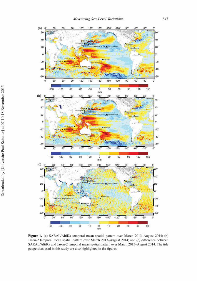
Measuring Sea-Level Variations 343
Figure 1. (a) SARAL/AltiKa temporal mean spatial pattern over March 2013–August 2014; (b)
Jason-2 temporal mean spatial pattern over March 2013–August 2014; and (c) difference between
SARAL/AltiKa and Jason-2 temporal mean spatial pattern over March 2013–August 2014. The tide
gauge sites used in this study are also highlighted in the figures.
Do
wnlo
aded
by
[U
niv
ersi
te P
aul
Sab
atie
r] a
t 07
:10 1
8 N
ovem
ber
20
15
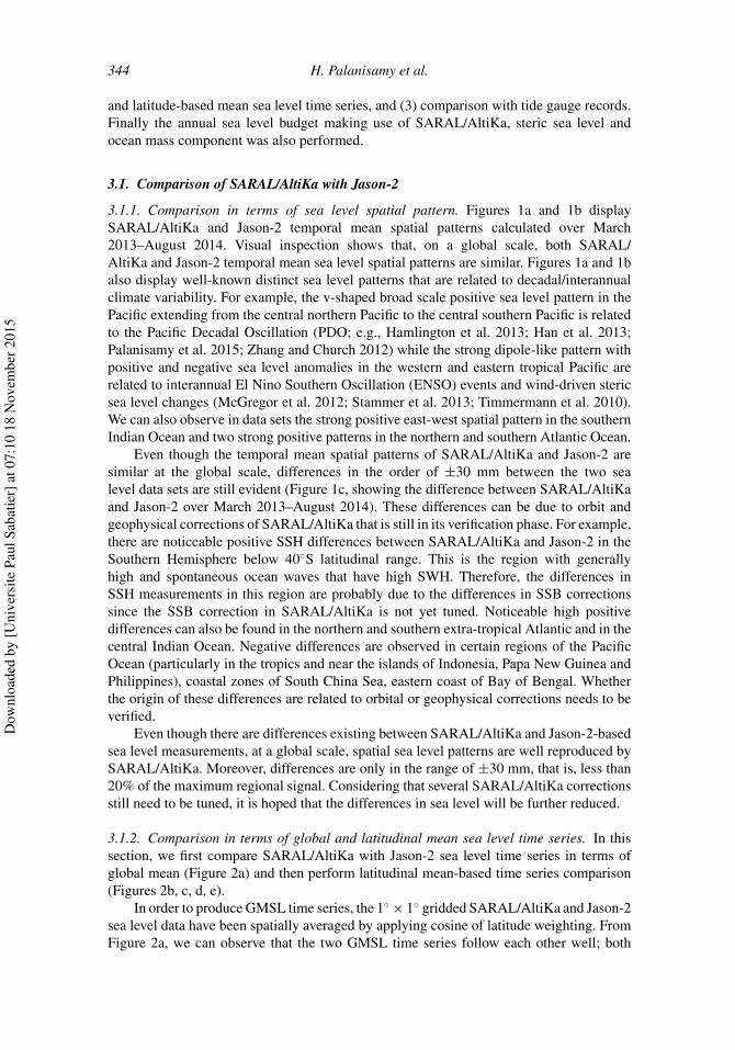
344 H. Palanisamy et al.
and latitude-based mean sea level time series, and (3) comparison with tide gauge records.
Finally the annual sea level budget making use of SARAL/AltiKa, steric sea level and
ocean mass component was also performed.
3.1. Comparison of SARAL/AltiKa with Jason-2
3.1.1. Comparison in terms of sea level spatial pattern. Figures 1a and 1b display
SARAL/AltiKa and Jason-2 temporal mean spatial patterns calculated over March
2013–August 2014. Visual inspection shows that, on a global scale, both SARAL/
AltiKa and Jason-2 temporal mean sea level spatial patterns are similar. Figures 1a and 1b
also display well-known distinct sea level patterns that are related to decadal/interannual
climate variability. For example, the v-shaped broad scale positive sea level pattern in the
Pacific extending from the central northern Pacific to the central southern Pacific is related
to the Pacific Decadal Oscillation (PDO; e.g., Hamlington et al. 2013; Han et al. 2013;
Palanisamy et al. 2015; Zhang and Church 2012) while the strong dipole-like pattern with
positive and negative sea level anomalies in the western and eastern tropical Pacific are
related to interannual El Nino Southern Oscillation (ENSO) events and wind-driven steric
sea level changes (McGregor et al. 2012; Stammer et al. 2013; Timmermann et al. 2010).
We can also observe in data sets the strong positive east-west spatial pattern in the southern
Indian Ocean and two strong positive patterns in the northern and southern Atlantic Ocean.
Even though the temporal mean spatial patterns of SARAL/AltiKa and Jason-2 are
similar at the global scale, differences in the order of ±30 mm between the two sea
level data sets are still evident (Figure 1c, showing the difference between SARAL/AltiKa
and Jason-2 over March 2013–August 2014). These differences can be due to orbit and
geophysical corrections of SARAL/AltiKa that is still in its verification phase. For example,
there are noticeable positive SSH differences between SARAL/AltiKa and Jason-2 in the
Southern Hemisphere below 40◦S latitudinal range. This is the region with generally
high and spontaneous ocean waves that have high SWH. Therefore, the differences in
SSH measurements in this region are probably due to the differences in SSB corrections
since the SSB correction in SARAL/AltiKa is not yet tuned. Noticeable high positive
differences can also be found in the northern and southern extra-tropical Atlantic and in the
central Indian Ocean. Negative differences are observed in certain regions of the Pacific
Ocean (particularly in the tropics and near the islands of Indonesia, Papa New Guinea and
Philippines), coastal zones of South China Sea, eastern coast of Bay of Bengal. Whether
the origin of these differences are related to orbital or geophysical corrections needs to be
verified.
Even though there are differences existing between SARAL/AltiKa and Jason-2-based
sea level measurements, at a global scale, spatial sea level patterns are well reproduced by
SARAL/AltiKa. Moreover, differences are only in the range of ±30 mm, that is, less than
20% of the maximum regional signal. Considering that several SARAL/AltiKa corrections
still need to be tuned, it is hoped that the differences in sea level will be further reduced.
3.1.2. Comparison in terms of global and latitudinal mean sea level time series. In this
section, we first compare SARAL/AltiKa with Jason-2 sea level time series in terms of
global mean (Figure 2a) and then perform latitudinal mean-based time series comparison
(Figures 2b, c, d, e).
In order to produce GMSL time series, the 1◦ × 1◦ gridded SARAL/AltiKa and Jason-2
sea level data have been spatially averaged by applying cosine of latitude weighting. From
Figure 2a, we can observe that the two GMSL time series follow each other well; both
Do
wnlo
aded
by
[U
niv
ersi
te P
aul
Sab
atie
r] a
t 07
:10 1
8 N
ovem
ber
20
15

Measuring Sea-Level Variations 345
Figure 2. Sea level time series of SARAL/AltiKa (red dashed line with stars), Jason-2 (blue dashed
line with circles) and the corresponding SARAL/AltiKa minus Jason-2 time series (black continuous
line) in terms of (a) Global, (b) 0◦−30◦N, (c) 30◦N-66◦N (d) 0◦−30◦S, and (e) 30◦S-66◦S latitudinal
bands.
display a clear seasonal variability. The observed seasonal variation in GMSL reaching
a maximum of around 5–7 mm between October and November corresponding to North
Hemisphere’s late summer is in agreement with previous studies on the annual GMSL (e.g.,
Cazenave et al. 2000; Chen et al. 1998). Even though the magnitude of SARAL/AltiKa time
series is slightly less than that of Jason-2, it is highly correlated with Jason-2 (correlation
0.85) GMSL. Figure 2a also displays the difference between SARAL/AltiKa based and
Jason-2 based GMSL time series (black curve, with a downward offset of 9 mm for clarity).
From this curve, we can observe that there are differences in the order of ∼4 mm occurring
between SARAL/AltiKa and Jason-2 in terms of global mean at certain time period. The
Do
wnlo
aded
by
[U
niv
ersi
te P
aul
Sab
atie
r] a
t 07
:10 1
8 N
ovem
ber
20
15
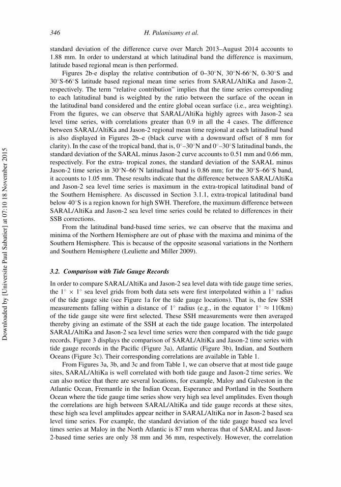
346 H. Palanisamy et al.
standard deviation of the difference curve over March 2013–August 2014 accounts to
1.88 mm. In order to understand at which latitudinal band the difference is maximum,
latitude based regional mean is then performed.
Figures 2b-e display the relative contribution of 0–30◦N, 30◦N-66◦N, 0-30◦S and
30◦S-66◦S latitude based regional mean time series from SARAL/AltiKa and Jason-2,
respectively. The term “relative contribution” implies that the time series corresponding
to each latitudinal band is weighted by the ratio between the surface of the ocean in
the latitudinal band considered and the entire global ocean surface (i.e., area weighting).
From the figures, we can observe that SARAL/AltiKa highly agrees with Jason-2 sea
level time series, with correlations greater than 0.9 in all the 4 cases. The difference
between SARAL/AltiKa and Jason-2 regional mean time regional at each latitudinal band
is also displayed in Figures 2b–e (black curve with a downward offset of 8 mm for
clarity). In the case of the tropical band, that is, 0◦–30◦N and 0◦–30◦S latitudinal bands, the
standard deviation of the SARAL minus Jason-2 curve accounts to 0.51 mm and 0.66 mm,
respectively. For the extra- tropical zones, the standard deviation of the SARAL minus
Jason-2 time series in 30◦N–66◦N latitudinal band is 0.86 mm; for the 30◦S–66◦S band,
it accounts to 1.05 mm. These results indicate that the difference between SARAL/AltiKa
and Jason-2 sea level time series is maximum in the extra-tropical latitudinal band of
the Southern Hemisphere. As discussed in Section 3.1.1, extra-tropical latitudinal band
below 40◦S is a region known for high SWH. Therefore, the maximum difference between
SARAL/AltiKa and Jason-2 sea level time series could be related to differences in their
SSB corrections.
From the latitudinal band-based time series, we can observe that the maxima and
minima of the Northern Hemisphere are out of phase with the maxima and minima of the
Southern Hemisphere. This is because of the opposite seasonal variations in the Northern
and Southern Hemisphere (Leuliette and Miller 2009).
3.2. Comparison with Tide Gauge Records
In order to compare SARAL/AltiKa and Jason-2 sea level data with tide gauge time series,
the 1◦ × 1◦ sea level grids from both data sets were first interpolated within a 1◦ radius
of the tide gauge site (see Figure 1a for the tide gauge locations). That is, the few SSH
measurements falling within a distance of 1◦ radius (e.g., in the equator 1◦ ≈ 110km)
of the tide gauge site were first selected. These SSH measurements were then averaged
thereby giving an estimate of the SSH at each the tide gauge location. The interpolated
SARAL/AltiKa and Jason-2 sea level time series were then compared with the tide gauge
records. Figure 3 displays the comparison of SARAL/AltiKa and Jason-2 time series with
tide gauge records in the Pacific (Figure 3a), Atlantic (Figure 3b), Indian, and Southern
Oceans (Figure 3c). Their corresponding correlations are available in Table 1.
From Figures 3a, 3b, and 3c and from Table 1, we can observe that at most tide gauge
sites, SARAL/AltiKa is well correlated with both tide gauge and Jason-2 time series. We
can also notice that there are several locations, for example, Maloy and Galveston in the
Atlantic Ocean, Fremantle in the Indian Ocean, Esperance and Portland in the Southern
Ocean where the tide gauge time series show very high sea level amplitudes. Even though
the correlations are high between SARAL/AltiKa and tide gauge records at these sites,
these high sea level amplitudes appear neither in SARAL/AltiKa nor in Jason-2 based sea
level time series. For example, the standard deviation of the tide gauge based sea level
times series at Maloy in the North Atlantic is 87 mm whereas that of SARAL and Jason-
2-based time series are only 38 mm and 36 mm, respectively. However, the correlation
Do
wnlo
aded
by
[U
niv
ersi
te P
aul
Sab
atie
r] a
t 07
:10 1
8 N
ovem
ber
20
15
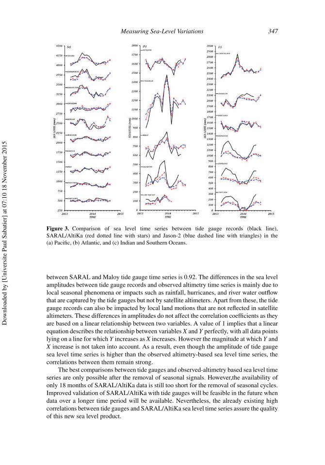
Measuring Sea-Level Variations 347
Figure 3. Comparison of sea level time series between tide gauge records (black line),
SARAL/AltiKa (red dotted line with stars) and Jason-2 (blue dashed line with triangles) in the
(a) Pacific, (b) Atlantic, and (c) Indian and Southern Oceans.
between SARAL and Maloy tide gauge time series is 0.92. The differences in the sea level
amplitudes between tide gauge records and observed altimetry time series is mainly due to
local seasonal phenomena or impacts such as rainfall, hurricanes, and river water outflow
that are captured by the tide gauges but not by satellite altimeters. Apart from these, the tide
gauge records can also be impacted by local land motions that are not reflected in satellite
altimeters. These differences in amplitudes do not affect the correlation coefficients as they
are based on a linear relationship between two variables. A value of 1 implies that a linear
equation describes the relationship between variables X and Y perfectly, with all data points
lying on a line for which Y increases as X increases. However the magnitude at which Y and
X increase is not taken into account. As a result, even though the amplitude of tide gauge
sea level time series is higher than the observed altimetry-based sea level time series, the
correlations between them remain strong.
The best comparisons between tide gauges and observed-altimetry based sea level time
series are only possible after the removal of seasonal signals. However,the availability of
only 18 months of SARAL/AltiKa data is still too short for the removal of seasonal cycles.
Improved validation of SARAL/AltiKa with tide gauges will be feasible in the future when
data over a longer time period will be available. Nevertheless, the already existing high
correlations between tide gauges and SARAL/AltiKa sea level time series assure the quality
of this new sea level product.
Do
wnlo
aded
by
[U
niv
ersi
te P
aul
Sab
atie
r] a
t 07
:10 1
8 N
ovem
ber
20
15
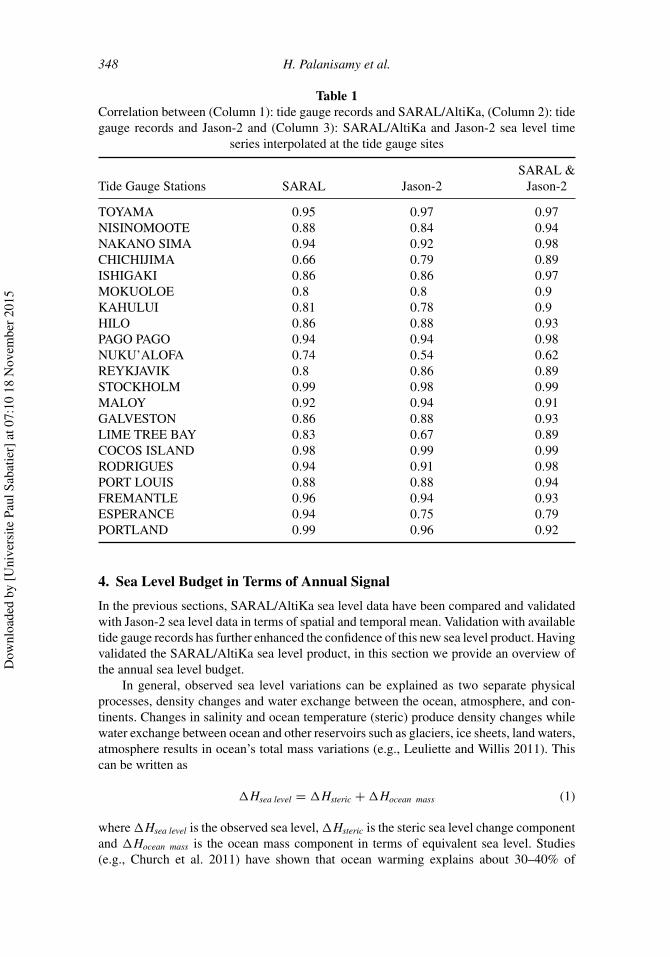
348 H. Palanisamy et al.
Table 1
Correlation between (Column 1): tide gauge records and SARAL/AltiKa, (Column 2): tide
gauge records and Jason-2 and (Column 3): SARAL/AltiKa and Jason-2 sea level time
series interpolated at the tide gauge sites
SARAL &
Tide Gauge Stations SARAL Jason-2 Jason-2
TOYAMA 0.95 0.97 0.97
NISINOMOOTE 0.88 0.84 0.94
NAKANO SIMA 0.94 0.92 0.98
CHICHIJIMA 0.66 0.79 0.89
ISHIGAKI 0.86 0.86 0.97
MOKUOLOE 0.8 0.8 0.9
KAHULUI 0.81 0.78 0.9
HILO 0.86 0.88 0.93
PAGO PAGO 0.94 0.94 0.98
NUKU’ALOFA 0.74 0.54 0.62
REYKJAVIK 0.8 0.86 0.89
STOCKHOLM 0.99 0.98 0.99
MALOY 0.92 0.94 0.91
GALVESTON 0.86 0.88 0.93
LIME TREE BAY 0.83 0.67 0.89
COCOS ISLAND 0.98 0.99 0.99
RODRIGUES 0.94 0.91 0.98
PORT LOUIS 0.88 0.88 0.94
FREMANTLE 0.96 0.94 0.93
ESPERANCE 0.94 0.75 0.79
PORTLAND 0.99 0.96 0.92
4. Sea Level Budget in Terms of Annual Signal
In the previous sections, SARAL/AltiKa sea level data have been compared and validated
with Jason-2 sea level data in terms of spatial and temporal mean. Validation with available
tide gauge records has further enhanced the confidence of this new sea level product. Having
validated the SARAL/AltiKa sea level product, in this section we provide an overview of
the annual sea level budget.
In general, observed sea level variations can be explained as two separate physical
processes, density changes and water exchange between the ocean, atmosphere, and con-
tinents. Changes in salinity and ocean temperature (steric) produce density changes while
water exchange between ocean and other reservoirs such as glaciers, ice sheets, land waters,
atmosphere results in ocean’s total mass variations (e.g., Leuliette and Willis 2011). This
can be written as
�Hsea level = �Hsteric + �Hocean mass (1)
where �Hsea level is the observed sea level, �Hsteric is the steric sea level change component
and �Hocean mass is the ocean mass component in terms of equivalent sea level. Studies
(e.g., Church et al. 2011) have shown that ocean warming explains about 30–40% of
Do
wnlo
aded
by
[U
niv
ersi
te P
aul
Sab
atie
r] a
t 07
:10 1
8 N
ovem
ber
20
15
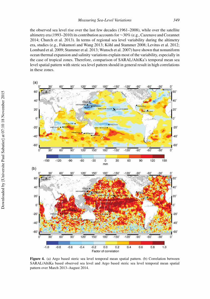
Measuring Sea-Level Variations 349
the observed sea level rise over the last few decades (1961–2008), while over the satellite
altimetry era (1993–2010) its contribution accounts for ∼30% (e.g., Cazenave and Cozannet
2014; Church et al. 2013). In terms of regional sea level variability during the altimetry
era, studies (e.g., Fukumori and Wang 2013; Kohl and Stammer 2008; Levitus et al. 2012;
Lombard et al. 2009; Stammer et al. 2013; Wunsch et al. 2007) have shown that nonuniform
ocean thermal expansion and salinity variations explain most of the variability, especially in
the case of tropical zones. Therefore, comparison of SARAL/AltiKa’s temporal mean sea
level spatial pattern with steric sea level pattern should in general result in high correlations
in these zones.
Figure 4. (a) Argo based steric sea level temporal mean spatial pattern. (b) Correlation between
SARAL/AltiKa based observed sea level and Argo based steric sea level temporal mean spatial
pattern over March 2013–August 2014.
Do
wnlo
aded
by
[U
niv
ersi
te P
aul
Sab
atie
r] a
t 07
:10 1
8 N
ovem
ber
20
15
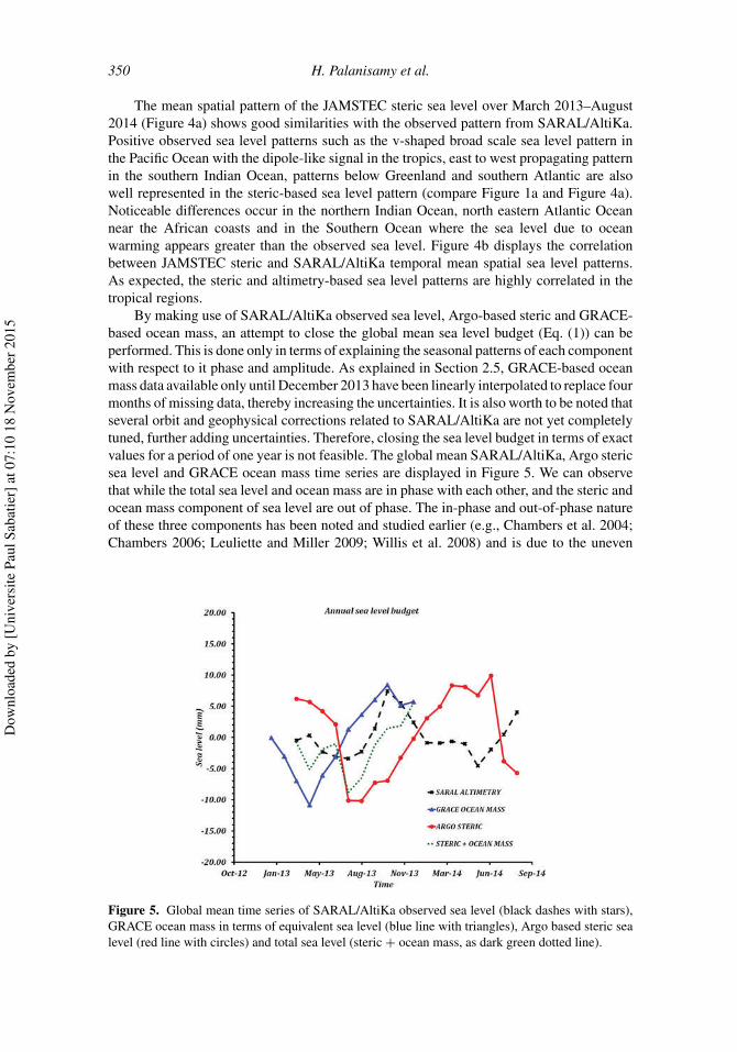
350 H. Palanisamy et al.
The mean spatial pattern of the JAMSTEC steric sea level over March 2013–August
2014 (Figure 4a) shows good similarities with the observed pattern from SARAL/AltiKa.
Positive observed sea level patterns such as the v-shaped broad scale sea level pattern in
the Pacific Ocean with the dipole-like signal in the tropics, east to west propagating pattern
in the southern Indian Ocean, patterns below Greenland and southern Atlantic are also
well represented in the steric-based sea level pattern (compare Figure 1a and Figure 4a).
Noticeable differences occur in the northern Indian Ocean, north eastern Atlantic Ocean
near the African coasts and in the Southern Ocean where the sea level due to ocean
warming appears greater than the observed sea level. Figure 4b displays the correlation
between JAMSTEC steric and SARAL/AltiKa temporal mean spatial sea level patterns.
As expected, the steric and altimetry-based sea level patterns are highly correlated in the
tropical regions.
By making use of SARAL/AltiKa observed sea level, Argo-based steric and GRACE-
based ocean mass, an attempt to close the global mean sea level budget (Eq. (1)) can be
performed. This is done only in terms of explaining the seasonal patterns of each component
with respect to it phase and amplitude. As explained in Section 2.5, GRACE-based ocean
mass data available only until December 2013 have been linearly interpolated to replace four
months of missing data, thereby increasing the uncertainties. It is also worth to be noted that
several orbit and geophysical corrections related to SARAL/AltiKa are not yet completely
tuned, further adding uncertainties. Therefore, closing the sea level budget in terms of exact
values for a period of one year is not feasible. The global mean SARAL/AltiKa, Argo steric
sea level and GRACE ocean mass time series are displayed in Figure 5. We can observe
that while the total sea level and ocean mass are in phase with each other, and the steric and
ocean mass component of sea level are out of phase. The in-phase and out-of-phase nature
of these three components has been noted and studied earlier (e.g., Chambers et al. 2004;
Chambers 2006; Leuliette and Miller 2009; Willis et al. 2008) and is due to the uneven
Figure 5. Global mean time series of SARAL/AltiKa observed sea level (black dashes with stars),
GRACE ocean mass in terms of equivalent sea level (blue line with triangles), Argo based steric sea
level (red line with circles) and total sea level (steric + ocean mass, as dark green dotted line).
Do
wnlo
aded
by
[U
niv
ersi
te P
aul
Sab
atie
r] a
t 07
:10 1
8 N
ovem
ber
20
15
Measuring Sea-Level Variations 351
distribution of continents in the Northern and Southern Hemispheres and the difference in
timing between ocean heating/cooling and fresh water run-off.
The annual mass component (mostly due to the snow pack; e.g., Biancamaria et al.
2011; Cazenave et al. 2000; Chen et al. 1998) has its maximum around September. There-
fore, the ocean mass signal is in-phase with the total sea level around this time but at am-
plitude higher than that of the total sea level. In the case of steric sea level, even though the
ocean heating in Northern and Southern Hemisphere tend to cancel out when the global av-
erage is performed, since most of the world’s ocean is in the Southern hemisphere, the peak
amplitude occurs in the late summer of the Southern hemisphere (around March–April).
This signal tends to be much larger than the average steric signal and henceforth is still
evident in the global mean steric sea level
Therefore, the seasonal amplitude and differences in phase of the steric and the ocean
mass component (i.e., steric + ocean mass) tends to compare relatively well with the total
sea level signal from SARAL/AltiKa.
5. Conclusion
In this study, we have performed a preliminary validation of SARAL/AltiKa SSH measure-
ments on a global scale by making use of AVISO-based Jason-2 sea level data set. Consid-
ering that this mission is quite recent and many algorithms for several corrections are not
yet completely tuned, comparisons in terms of sea level temporal mean spatial patterns and
global mean time series already look promising. At local scales, SARAL/AltiKa sea level
is highly correlated with tide gauge records confirming the quality of SARAL/AltiKa’s
Ka band altimeter. A preliminary analysis of the annual sea level budget by comparing
observed sea level with the sum of the steric and ocean mass components is also highly
satisfactory.
The validation of SARAL/AltiKa SSH measurements performed in this study shows
that even though there are regional differences in the range of ±30 mm in the case of
comparison with Jason-2, the results are highly in line with other existing sea level data.
Over a longer time period with more availability of SARAL/AltiKa sea level data in the
future, we are confident that this mission will ensure an improved understanding of the
evolution of sea level and its coastal impacts.
Acknowledgements
We thank L. Fenoglio-Marc and an anonymous reviewer for their comments and
suggestions.
Funding
H. Palanisamy is supported by a CNES-CLS grant. O. Henry is supported by an ESA
Climate Change Initiative grant.
References
Ablain, M., A. Cazenave, G. Larnicol, M. Balmaseda, P. Cipollini, Y. Faugere, M. J. Fernandes,
O. Henry, J. A. Johannessen, P. Knudsen, O. Andersen, J. Legeais, B. Meyssignac, N. Picot,
M. Roca, S. Rudenko, M. G. Scharffenberg, D. Stammer, G. Timms, and J. Benveniste. 2015.
Do
wnlo
aded
by
[U
niv
ersi
te P
aul
Sab
atie
r] a
t 07
:10 1
8 N
ovem
ber
20
15

352 H. Palanisamy et al.
Improved sea level record over satellite altimetry era (1993–2010) from the Climate Change
Initiative project. Ocean Sciences 11(1):67–82.
Ablain, M., A. Cazenave, G. Valladeau, and S. Guinehut. 2009. A new assessment of the error budget
of global mean sea level rate estimated by satellite altimetry over 1993-2008. Ocean Science
5(2):193–201.
Biancamaria, S., A. Cazenave, N. M. Mognard, W. Llovel, and F. Frappart. 2011. Satellite-based high
latitude snow volume trend, variability and contribution to sea level over 1989/2006. Global and
Planetary Change 75(3–4):99–107.
Bronner, E., A. K. Shukla, N. Picot, A. Guillot, J. P. Dumont, V. Rosmorduc, J. Lillibridge, S.
Desai, H. Bonekamp, R. Scharroo, and J. Figa. 2013. SARAL/AltiKa Products Handbook,
Issue 2, France: AVISO, CNES. Available at http://www.aviso.altimetry.fr/fileadmin/documents/
data/tools/SARAL Altika products handbook.pdf. Last accessed 28 July 2015.
Cazenave, A., F. Remy, K. Dominh, and H. Douville. 2000. Global ocean mass variation, continental
hydrology and the mass balance of the Antarctica ice sheet at the seasonal time scale. Geophysical
Research Letters 27:3755–3758.
Cazenave, A. and G. Le Cozannet. 2014. Sea level rise and its coastal impacts. Earth’s Future
2(2):15–34.
Chambers, D. P., J. Wahr, and R. S. Nerem. 2004. Preliminary observations of global ocean mass
variations with GRACE. Geophysical Research Letters 31:L13310.
Chambers, D. P. 2006. Evaluation of new GRACE time-variable gravity data over the ocean. Geo-
physical Research Letters 33(17):L17603.
Chen, J. L., C. R. Wilson, D. P. Chambers, R. S. Nerem, and B. D. Tapley. 1998. Seasonal global water
mass budget and mean sea level variations. Geophysical Research Letters 25(19):3555–3558.
Church, J. A., P. U. Clark, A. Cazenave, J. M. Gregory, S. Jevrejeva, A. Levermann, M. A. Merrifield,
G. A. Milne, R. S. Nerem, P. D. Nunn, A. J. Payne, W. T. Pfeffer, D. Stammer, and A. S.
Unnikrishnan. 2013. Sea level change. In Climate Change 2013: The Physical Science Basis.
Contribution of Working Group I to the Fifth Assessment Report of the Intergovernmental Panel
on Climate Change. Stocker, T. F., D. Qin, G. -K. Plattner, M. Tignor, S. K. Allen, J. Boschung,
A. Nauels, Y. Xia, V. Bex, and P. M. Midgley (eds.), Cambridge, UK: Cambridge University
Press.
Church, J. A., N. J. White, L. F. Konikow, C. M. Domingues, J. G. Cogley, E. Rignot, J. M.
Gregory, M. R.Van denBroeke, A. J. Monaghan, and I. Velicogna. 2011. Revisiting the earth’s
sea-level and energy budgets from 1961 to 2008. Geophysical Research Letters 38(September).
doi:10.1029/2011GL048794.
Dee, D. P., S. M. Uppala, A. J. Simmons, P. Berrisford, P. Poli, P. Kobayashi, U. Andrae, M.A.
Balmaseda, G. Balsamo, P. Bauer, P. Bechtold, A.C.M. Beljaars, L. van de Berg, J. Bidlot,
N. Bormann, C. Delsol, R. Dragani, M. Fuentes, A.J. Geer, L. Haimberger, S.B. Healy, H.
Hersbach, E.V. Holm, L. Isaksen, P. Kallberg, M. Kohler, M. Matricardi, A.P. McNally, B.M.
Monge-Sanz, J.-J. Morcrette, B.-K. Park, C. Peubey, P. de Rosnay, C. Tavolato, J.-N. Thepaut,
and F. Vitart. 2011. The ERA-interim reanalysis: Configuration and performance of the data
assimilation system. Quarterly Journal of the Royal Meteorological Society 137(656):553–597.
Fu, L. L. and A. Cazenave. 2001. Satellite Altimetry and Earth Sciences, Vol. 69: A Handbook of
Techniques and Applications. San Diego, CA: Academic Press.
Fukumori, I. and O. Wang. 2013. Origins of heat and freshwater anomalies underlying regional
decadal sea level trends. Geophysical Research Letters 40(3):563–567.
Hamlington, B. D., R. R. Leben, M. W. Strassburg, R. S. Nerem, and K. -Y. Kim. 2013. Contribution
of the Pacific decadal oscillation to global mean sea level trends. Geophysical Research Letters
40(19):5171–5175.
Han, W., G. A. Meehl, A. Hu, M. A. Alexander, T. Yamagata, D. Yuan, M. Ishii, P. Pegion, J.
Zheng, B.D. Hamlington, X.-W. Quan, and R.R. Leben. 2013. Intensification of decadal and
multi-decadal sea level variability in the western tropical Pacific during recent decades. Climate
Dynamics October:1–23. doi: 10.1007/s00382-013-1951-1.
Do
wnlo
aded
by
[U
niv
ersi
te P
aul
Sab
atie
r] a
t 07
:10 1
8 N
ovem
ber
20
15
Measuring Sea-Level Variations 353
Hosoda, S., T. Ohira, and T. Nakamura. 2008. A monthly mean dataset of global oceanic temper-
ature and salinity derived from Argo float observations. JAMSTEC Report of Research and
Development 8:47–59.
Johnson, G. C. and D. P. Chambers. 2013. Ocean bottom pressure seasonal cycles and decadal trends
from GRACE release-05: Ocean circulation implications. Journal of Geophysical Research:
Oceans 118(9):4228–4240.
Kohl, A. and D. Stammer. 2008. Decadal sea level changes in the 50-year GECCO ocean synthesis.
Journal of Climate 21(9):1876–1890.
Leuliette, E. W. and L. Miller. 2009. Closing the sea level rise budget with altimetry, Argo, and
GRACE. Geophysical Research Letters 36:04608.
Leuliette, E. W. and J. K. Willis. 2011. Balancing the sea level budget. Oceanography 24(2):122–129.
Levitus, S., J. I. Antonov, T. P. Boyer, O. K. Baranova, H. E. Garcia, R. A. Locarnini, A. V.
Mishonov, J. R. Reagan, D. Seidov, E. S. Yarosh, and M. M. Zweng. 2012. World ocean
heat content and thermosteric sea level change (0–2000 M), 1955–2010. Geophysical Research
Letters 39(10):L10603.
Lombard, A., G. Garric, T. Penduff, and J. M. Molines. 2009. Regional variability of sea level change
using a global ocean model at 1/4◦ resolution. Ocean Dynamics 3:433–449.
McGregor, S., A. Sen Gupta, and M. H. England. 2012. Constraining wind stress products with
sea surface height observations and implications for Pacific Ocean sea level trend attribution.
Journal of Climate 25(23):8164–8176.
Palanisamy, H., A. Cazenave, T. Delcroix, and B. Meyssignac. 2015. Spatial trend patterns in Pacific
Ocean sea level during the altimetry era: The contribution of thermocline depth change and
internal climate variability. Ocean Dynamics. 1–16, doi:10.1007/s10236-014-0805-7.
Stammer, D., A. Cazenave, R. M. Ponte, and M. E. Tamisiea. 2013. Causes for contemporary regional
sea level changes. Annual Review of Marine Science 5(September). doi:10.1146/annurev-marine-
121211-172406.
Timmermann, A., S. McGregor, and F. -F. Jin. 2010. Wind effects on past and future regional sea
level trends in the southern Indo-Pacific. Journal of Climate 23(16):4429–4437.
Verron, J., S. Philipps, P. Bonnefond, Y. Faugere, J. Richman, D. Griffin, A. Pascual, F. Birol, L.
Aouf, S. Calmant, A. Michel, and J. Tournadre. 2013. AVISO Users Newsletter, SARAL/AltiKa
Special Issue, 10.
Verron, J., P. Sengenes, J. Lambin, J. Noubel, N. Steunou, A. Guillot, N. Picot, S. Coutin-Faye, R.
Gairola, D. V. A. Raghava Murthy, J. Richman, D. Griffin, A. Pascual, F. Remy, and P. K. Gupta.
2015. The SARAL/AltiKa altimetry satellite mission. Marine Geodesy 38(S1): this issue.
Volkov, D. L., G. Larnicol, and J. Dorandeu. 2007. Improving the quality of satellite altime-
try data over continental shelves. Journal Geophysical Research: Oceans 112(C6). doi:
10.1029/2006JC003765.
Willis, J. K., D. P. Chambers, and R. S. Nerem. 2008. Assessing the globally averaged sea level
budget on seasonal to interannual timescales. Journal of Geophysical Research: Oceans 113(C6):
C06015.
Woodworth, P. L. and R. Player. 2003. The permanent service for mean sea level: An update to the
21st century. Journal of Coastal Research 19:287–295.
Wunsch, C., R. M. Ponte, and P. Heimbach. 2007. Decadal trends in sea level patterns: 1993–2004.
Journal of Climate 20(24):5889–5911.
Zhang, X. and J. A. Church. 2012. Sea level trends, interannual and decadal variability in the Pacific
Ocean. Geophysical Research Letters 39(November). doi: 10.1029/2012GL053240.
Do
wnlo
aded
by
[U
niv
ersi
te P
aul
Sab
atie
r] a
t 07
:10 1
8 N
ovem
ber
20
15
Chapter 2 Multi satellite altimetry record and global mean sea level budget
47
2.2 Global mean sea level (GMSL) budget since altimetry era
In the previous chapter we have discussed the two main contributors to global mean sea
level change: steric changes (density changes due to thermal expansion and salinity changes) and
ocean mass changes (due to water exchange between the ocean and other reservoirs such as
glaciers, ice caps, ice sheets and ground water. To meaning-fully interpret the causes of sea level
change over a particular period, changes in observed sea level should be equal to the sum of
changes due to ocean density and mass exchange (Leuliette and Willis, 2011). This is called as
the sea level budget and can be written as ∆� �� ��� = ∆� � �� + ∆� ��� � 2.2
where ∆� �� ��� is the observed sea level, ∆� � �� is the steric sea level change component and ∆� ��� � is the ocean mass component in terms of equivalent sea level. Sea level budget
closure also indicates that the observations are complete and accurate. Furthermore, quantifying
the causes of sea level rise individually is important for predicting how much the sea level will
rise in the future and also to understand the magnitude of changes that has already occurred
(Leuliette and Willis, 2011, Church et al., 2011).
When we consider the satellite altimetry era, the 4th
Assessment Report (AR4) of the
IPCC estimated the sea level budget over the 1993-2003 time span. The contribution of thermal
expansion was estimated at 1.6 ± 0.25 mm/yr (until 700 m depth) while those of glaciers and ice
sheets were estimated to be 0.8 ± 0.11 mm/yr and 0.4 ± 0.2 mm/yr respectively. The sum of the
contributions, 2.8 ± 0.35 mm/yr was found to be rather in good agreement with the satellite
altimetry based GMSL rise of 3.1 ± 0.4 mm/yr with thermal expansion contributing ~50% of the
total rate (Bindoff et al., 2007). Over the 1993-2010 time span, IPCC AR5 estimated the sum of
contributions amounting to 2.8 ± 0.5 mm/yr, a value slightly lower than the observed sea level
rate of 3.2 ± 0.4 mm/yr. During this time span, land ice melt contributed 50% of the total sea
level rate while ocean thermal expansion (up to 1500m) and anthropogenic land water storage
decrease contributed 35% and 13% respectively (Church et al., 2013).
The contribution of sea level components is in fact not constant through time. Since the
last decade, the contribution of ice sheets has accelerated (Shepherd et al., 2012) while the upper

Chapter 2 Multi satellite altimetry record and global mean sea level budget
48
ocean thermal expansion has increased less rapidly (Lyman et al., 2010) than the previous
decade. This period of slower upper ocean thermal expansion rate also coincides with the so-
called ‘pause’ in global mean air and sea surface temperature evolution since the early 2000s,
popularly called as the ‘hiatus’ (Held, 2013, Trenberth and Fasullo, 2013, Smith, 2013).
However the issue of ‘hiatus’ remains puzzling because studies (e.g. Peters et al., 2012) have
shown that the greenhouse gases have in fact continued to accumulate at an increased rate and
the Earth’s energy imbalance still remains to be positive in the order of 0.5 -1 W/m2
(Hansen et
al., 2011, Trenberth et al., 2014). Different explanations have been proposed by various studies
on this issue that ranges from reduction in radiative forcing due to longer solar minimum,
increase in aerosols and volcanic eruptions, stratospheric water vapor changes and enhanced
deep ocean heat uptake in the Pacific or Atlantic Ocean. Of all these, the most favored
explanation for the hiatus is the deep ocean heat uptake. However, the exact mechanism that
causes this still remains an unanswered question (Solomon et al., 2010, Hansen et al., 2011,
Guemas et al., 2013, Trenberth and Fasullo, 2013, Kosaka and Xie, 2013, Balmaseda et al.,
2013, Watanabe et al., 2013, Chen and Tung, 2014, England et al., 2014, Goddard, 2014).
Fig.2.4 displays the global mean altimetry based sea level variations and its two main
components, ocean mass measure by GRACE and Argo based thermosteric sea level since 2005.
The slow rate of ocean thermal expansion is noticeable.
Understanding the contribution of deep ocean heat content to global warming hiatus is
possible by means of accurate observations of sea level change and its components (ocean
thermal expansion and mass changes, von Schuckmann et al., 2014, Dieng et al., 2015, Llovel et
al., 2014). GMSL change from satellite altimetry when corrected for the ocean mass change
from GRACE space gravimetry results in an estimate of ocean thermal expansion that also
includes the deep ocean contribution. This can then be compared with Argo-based ocean thermal
expansion available until a depth of ~ 1500 m and would help in quantifying the deep ocean
contribution below 1500 m. We therefore performed such a sea level budget analysis since 2003
with an aim on estimating the deep ocean contribution to sea level change. The 2003-2012
decade corresponds to the hiatus period and also to the availability of new observational systems
for ocean thermal expansion (global ocean temperature and salinity measurement until 2000 m of
depth by Argo floats) and ocean mass changes (direct ocean mass measurements from GRACE).
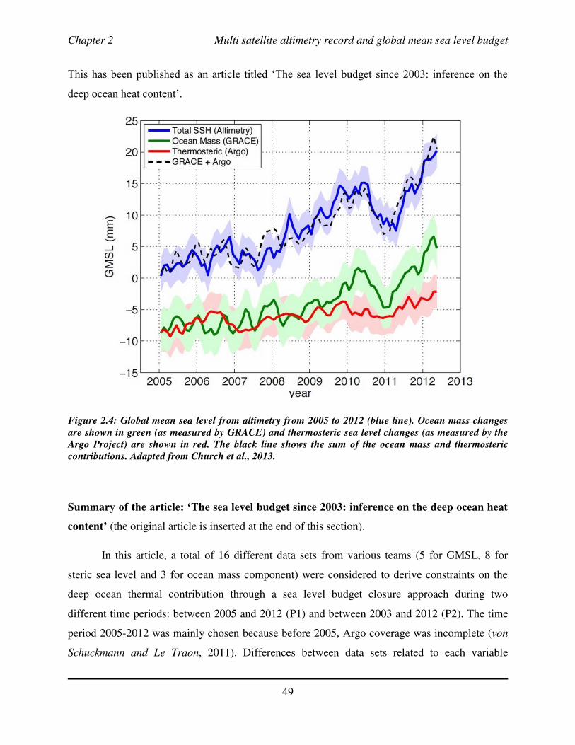
Chapter 2 Multi satellite altimetry record and global mean sea level budget
49
This has been published as an article titled ‘The sea level budget since 2003: inference on the
deep ocean heat content’.
Figure 2.4: Global mean sea level from altimetry from 2005 to 2012 (blue line). Ocean mass changes
are shown in green (as measured by GRACE) and thermosteric sea level changes (as measured by the
Argo Project) are shown in red. The black line shows the sum of the ocean mass and thermosteric
contributions. Adapted from Church et al., 2013.
Summary of the article: ‘The sea level budget since 2003: inference on the deep ocean heat
content’ (the original article is inserted at the end of this section).
In this article, a total of 16 different data sets from various teams (5 for GMSL, 8 for
steric sea level and 3 for ocean mass component) were considered to derive constraints on the
deep ocean thermal contribution through a sea level budget closure approach during two
different time periods: between 2005 and 2012 (P1) and between 2003 and 2012 (P2). The time
period 2005-2012 was mainly chosen because before 2005, Argo coverage was incomplete (von
Schuckmann and Le Traon, 2011). Differences between data sets related to each variable

Chapter 2 Multi satellite altimetry record and global mean sea level budget
50
(observed sea level, ocean mass and steric sea level) were noticed and were mostly attributed to
data processing issues. While the large number of datasets can provide 120 different
combinations of sea level budget estimates, in this study, the averages of each data type (GMSL,
ocean mass and steric sea level) were used and their dispersion ranges were estimated. This
provides an insight on the uncertainty range due to variations in processing approach used by
different teams.
Figure 2.5: Difference time series ‘GMSL minus GOM’ (based on the averaged curves), mean steric sea level (average of Argo steric) and residual curve (‘GMSL minus GOM’ minus mean steric sea
level, with downward offset of 7.5 mm for clarity over 2005-2012 from Dieng et al., 2015
Over P1 (2005-2012) period, the residual trend value obtained after removing the
contribution of Argo based steric (0-1500 m) sea level from the GMSL minus GOM time series
accounts to 0.3 ± 0.21 mm/yr (See Fig.2.5 for the corresponding curves). This residual reflects
errors affecting all the data sets, errors due to insufficient Argo floats coverage and the potential
deep ocean contribution below 1500 m. Similarly, over P2 (2003-2012) period, the residual trend
value accounts to 0.55 ± 0.19 mm/yr. In both the cases, the residual curves display important
interannual variability. Since direct steric observations below 1500 m depth are very sparse over
P1 and P2 time periods (Purkey and Johnson, 2010, Kouketsu et al., 2011), in order to obtain the
deep ocean steric contribution below this depth, an ocean reanalyses ORAS4 (available until
2009) was also considered in the study. The ORAS4 reanalyses was first compared with the
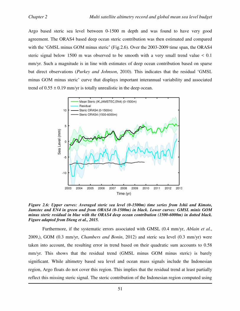
Chapter 2 Multi satellite altimetry record and global mean sea level budget
51
Argo based steric sea level between 0-1500 m depth and was found to have very good
agreement. The ORAS4 based deep ocean steric contribution was then estimated and compared
with the ‘GMSL minus GOM minus steric’ (Fig.2.6). Over the 2003-2009 time span, the ORAS4
steric signal below 1500 m was observed to be smooth with a very small trend value < 0.1
mm/yr. Such a magnitude is in line with estimates of deep ocean contribution based on sparse
but direct observations (Purkey and Johnson, 2010). This indicates that the residual ‘GMSL
minus GOM minus steric’ curve that displays important interannual variability and associated
trend of 0.55 ± 0.19 mm/yr is totally unrealistic in the deep ocean.
Figure 2.6: Upper curves: Averaged steric sea level (0-1500m) time series from Ishii and Kimoto,
Jamstec and EN4 in green and from ORAS4 (0-1500m) in black. Lower curves: GMSL minis GOM
minus steric residual in blue with the ORAS4 deep ocean contribution (1500-6000m) in dotted black.
Figure adapted from Dieng et al., 2015.
Furthermore, if the systematic errors associated with GMSL (0.4 mm/yr, Ablain et al.,
2009,), GOM (0.3 mm/yr, Chambers and Bonin, 2012) and steric sea level (0.3 mm/yr) were
taken into account, the resulting error in trend based on their quadratic sum accounts to 0.58
mm/yr. This shows that the residual trend (GMSL minus GOM minus steric) is barely
significant. While altimetry based sea level and ocean mass signals include the Indonesian
region, Argo floats do not cover this region. This implies that the residual trend at least partially
reflect this missing steric signal. The steric contribution of the Indonesian region computed using
Chapter 2 Multi satellite altimetry record and global mean sea level budget
52
ORAS4 results in a trend value of ~ 0.3 mm/yr. Therefore, removal of this value from the
residual trend (deep ocean) value results in a new residual trend range ~ 0 and 0.25 mm/yr. This
range of trend can thus be considered as an upper limit for the deep ocean contribution to recent
years sea level rise.
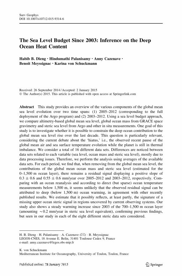
The Sea Level Budget Since 2003: Inference on the Deep
Ocean Heat Content
Habib B. Dieng • Hindumathi Palanisamy • Anny Cazenave •
Benoit Meyssignac • Karina von Schuckmann
Received: 26 September 2014 / Accepted: 2 January 2015
� The Author(s) 2015. This article is published with open access at Springerlink.com
Abstract This study provides an overview of the various components of the global mean
sea level evolution over two time spans: (1) 2005–2012 (corresponding to the full
deployment of the Argo program) and (2) 2003–2012. Using a sea level budget approach,
we compare altimetry-based global mean sea level, global ocean mass from GRACE space
gravimetry and steric sea level from Argo and other in situ measurements. One goal of this
study is to investigate whether it is possible to constrain the deep ocean contribution to the
global mean sea level rise over the last decade. This question is particularly relevant,
considering the current debate about the ‘hiatus,’ i.e., the observed recent pause of the
global mean air and sea surface temperature evolution while the planet is still in thermal
imbalance. We consider a total of 16 different data sets. Differences are noticed between
data sets related to each variable (sea level, ocean mass and steric sea level), mostly due to
data processing issues. Therefore, we perform the analysis using averages of the available
data sets. For each period, we find that, when removing from the global mean sea level, the
contributions of the global mean ocean mass and steric sea level (estimated for the
0–1,500 m ocean layer), there remains a residual signal displaying a positive slope of
0.3 ± 0.6 and 0.55 ± 0.6 mm/year over 2005–2012 and 2003–2012, respectively. Com-
paring with an ocean reanalysis and according to direct (but sparse) ocean temperature
measurements below 1,500 m, it seems unlikely that the observed residual signal can be
attributed to deep (below 1,500 m) ocean warming, in agreement with other recently
published results. We estimate that it possibly reflects, at least partly, the signature of a
missing upper ocean steric signal in regions uncovered by current observing systems. Our
study also shows a steady warming increase since 2003 of the 700–1,500 m ocean layer
(amounting *0.2 mm/year in steric sea level equivalent), confirming previous findings,
but seen in our study in each of the eight different steric data sets considered.
H. B. Dieng � H. Palanisamy � A. Cazenave (&) � B. Meyssignac
LEGOS-CNES, 18 Avenue E. Belin, 31401 Toulouse Cedex 9, France
e-mail: [email protected]
K. von Schuckmann
Mediterranean Institute for Oceanography, University of Toulon, Toulon, France
123
Surv Geophys
DOI 10.1007/s10712-015-9314-6
Keywords Sea level rise � Thermal expansion � Ocean mass � Deep ocean warming
1 Introduction
Sea level is an interesting quantity in Earth sciences research as it integrates variations
from different climatic and non-climatic variables. For example, in terms of global mean,
current sea level rise mostly results from thermal expansion of seawater due to ocean
temperature changes and water mass addition into ocean basins due to glacier melting, ice
sheet mass loss and land water storage changes of anthropogenic origin (e.g., Leuliette and
Willis 2011; Chen et al. 2013; Church et al. 2013). At interannual timescales, in particular
during ENSO (El Nino–Southern Oscillation) events, global mean sea level fluctuations are
largely due to land–ocean asymmetry in precipitation, causing temporary ocean mass
excess (during El Nino) or deficit (during La Nina) (Boening et al. 2012; Cazenave et al.
2012, 2014; Fasullo et al. 2013). While regional variations in absolute sea level mostly
result from ocean temperature and salinity variations (and to a lesser extent from direct
atmospheric forcing on the sea surface) (Stammer et al. 2013), non-climatic factors also
play a role. In effect, the viscous/elastic response of the solid Earth to past (i.e., last
deglaciation) and ongoing land ice melt causes complex deformations of ocean basins and
changes in the mutual attraction of ice-water bodies, and hence of sea level (e.g., Stammer
et al. 2013). Finally, along coastlines, relative sea level changes occur because of a
combination of absolute sea level changes and vertical movements of the Earth’s crust
(Woppelmann et al. 2009).
In the 5th Assessment Report (AR5) of the Intergovernmental Panel on Climate
Change (IPCC), it was reported that over the 1993–2010 time span (corresponding to
the high-precision satellite altimetry era), the rate of global mean sea level (GMSL)
rise is due to the combined effects of land ice melt (50 %), ocean thermal expansion
(37 %) and anthropogenic land water storage decrease (13 %) (Church et al. 2013).
The sum of these contributions amounts to 2.8 ± 0.5 mm/year, a value only slightly
lower than the rate of sea level rise observed by altimeter satellites, of 3.2 ± 0.4 mm/
year. Although of the same order of magnitude as associated uncertainties, the dif-
ference may also reflect other contributions either not or incompletely accounted for,
e.g., the deep ocean (below 700–1,000 m depth where the coverage of available data is
poor or non-existent).
In the IPCC 4th Assessment Report (AR4), the sea level budget was estimated over
the 1993–2003 time span (Bindoff et al. 2007). Over that decade, the thermal
expansion contribution was *50 % the rate of sea level rise, i.e., significantly larger
than the 1993–2010 average (note, however, that in AR4, thermal expansion estimates
were contaminated by Expandable Bathy Thermographers—XBT biases). In fact, the
sea level components are not constant through time. During the last 10–15 years, the
land ice (mostly the ice sheets) component has accelerated (i.e., Shepherd et al. 2012;
see also IPCC AR5 and references herein) while the upper ocean thermal expansion
has increased less rapidly than during the 1993–2003 decade (Lyman et al. 2010). This
recent slower rate in thermal expansion of the upper ocean coincides with the pause
(also called the ‘hiatus,’ e.g., Held 2013) in global mean air and sea surface temper-
ature evolution observed since the early 2000s (e.g., Trenberth and Fasullo 2013; Smith
2013). The current global warming hiatus is puzzling because greenhouse gases have
Surv Geophys
123
continued to accumulate at an increased rate (Peters et al. 2012) and the Earth’s energy
imbalance at the top of the atmosphere is estimated to still be positive, on the order of
0.5–1 Wm-2 (e.g., Hansen et al. 2011; Trenberth et al. 2014). This issue has been the
object of considerable attention in the very recent years, and different explanations
have been proposed, ranging from reduced radiative forcing due to prolonged solar
minimum, increased aerosols and numerous volcanic eruptions, changes in strato-
spheric water vapor, enhanced heat uptake in the deep ocean, either in the Pacific or
Atlantic regions (e.g., Trenberth and Fasullo 2010, 2013; Hansen et al. 2011; Solomon
et al. 2010; Guemas et al. 2013; Kosaka and Xie 2013 Balmaseda et al. 2013a; Wa-
tanabe et al. 2013; England et al. 2014; Chen and Tung 2014). While deep ocean heat
uptake is currently the favored explanation of the hiatus, no consensus yet exists on the
exact mechanism at work and on the place where deep ocean warming may occur (e.g.,
Goddard 2014; Trenberth et al. 2014; Chen and Tung 2014).
Accurate observations of sea level rise and its components (ocean thermal expansion
and ocean mass change) can, in principle, help to constrain the problem (e.g., von
Schuckmann et al. 2014). In particular satellite altimetry-based GMSL rise corrected
for ocean mass change (e.g., using GRACE space gravimetry data over the oceans)
provides an estimate of the total (full depth integrated) ocean thermal expansion (or
equivalently ocean heat content). Comparison with observed Argo-based ocean thermal
expansion (down to *1,500 m depth) may help to quantify any deep ocean contri-
bution (below 1,500 m) and geographically localize any ocean warming. The first issue
is addressed in the present study. Our analysis focusses on the 2003–2012 decade
which corresponds to the hiatus period and the availability of new observing systems
for estimating thermal expansion and ocean mass (nearly full ocean temperature and
salinity coverage down to 2,000 m from Argo floats and direct ocean mass measure-
ments from GRACE space gravimetry). Time series of satellite altimetry-based sea
level, thermal expansion and ocean mass components are currently constructed by
different groups (see Sect. 2) so that several data sets of each variable are available.
But as we will see below, for some of them, in particular ocean thermal expansion,
significant discrepancies are noticed between the data sets. Thus, part of our study
consists of discussing the differences observed between the different records and
estimate the uncertainty of each component. We further address the question: Can we
close the sea level budget with available data sets for sea level and components or, if
not, can we extract a significant residual possibly related to the deep ocean contri-
bution? The present study deals with global mean time series. Contributions from
oceanic regions will be presented in another study. Inside the 2003–2012 time span,
two subperiods are considered: period P1 covering January 2005 to December 2012,
corresponding to quasi global coverage of Argo data (before 2005, the Argo coverage
is incomplete, e.g., von Schuckmann and Le Traon 2011), and period P2 covering
January 2003 to December 2012 where GRACE data are available, as well as several
steric data sets and ocean reanalyses products (in general available over a longer time
span, e.g., 1950–present). In the following, we study periods P1 (2005–2012) and P2
(2003–2012).
While our manuscript was under review, another study by Llovel et al. (2014) was
published on the same issue. Llovel et al. (2014) consider the 2005–2013 time span, and
not as many data sets as in the present study, but their conclusion is not at odds with ours.
In the last section, we discuss their results and compare them with ours.
Surv Geophys
123
2 Data
2.1 Sea Level Data
We used five different products from five processing groups for the altimetry-based sea
level data:
1. Archiving Validation and Interpretation Satellite Oceanographic Center (AVISO; http://
www.aviso.altimetry.fr/en/data/products/ocean-indicators-products/actualitesindicateurs-
des-oceansniveau-moyen-des-mersindexhtml.html)
2. Colorado University (CU Release 3; http://sealevel.colorado.edu/)
3. Goddard Space Flight Center (GSFC version 2; http://podaac-ftp.jpl.nasa.gov/dataset/
MERGED_TP_J1_OSTM_OST_GMSL_ASCII_V2)
4. National Oceanographic and Atmospheric Administration (NOAA; http://www.star.
nesdis.noaa.gov/sod/lsa/SeaLevelRise/LSA_SLR_timeseries_global.php)
5. Commonwealth Scientific and Industrial Research Organization (CSIRO; www.cmar.
csiro.au/sealevel/sl_data_cmar.html).
All five sea level data sets are based on Topex/Poseidon, Jason-1 and Jason-2 data
averaged over the 66�S–66�N domain, except for the CSIRO data averaged between 65�S
and 65�N. For each product, a set of instrumental and geophysical corrections is applied
(details are given on the websites of each data set). In addition, the effect of glacial
isostatic adjustment (GIA, i.e., a small correction of -0.3 mm/year, Peltier 2004) is
accounted for in each sea level time series except in the NOAA data set. We thus corrected
the latter sea level data for the GIA effect, using the -0.3 mm/year value. The five sea
level time series (AVISO, CU, GSFC, NOAA and CSIRO) are obtained either by directly
averaging the along-track sea surface height data (e.g., CU) or by firstly gridding the
unevenly distributed along-track data and then performing grid averaging (e.g., AVISO
and NOAA). In all cases, an area weighting is applied. In addition to the geographical
averaging method, other differences exist between the GMSL data sets because of the
applied geophysical and instrumental corrections and the number of satellites considered
(discussion on these differences can be found in Masters et al. 2012 and Henry et al. 2014).
The sea level time series used in this study cover the period January 2003–December 2012.
Recently, in the context of the European Space Agency (ESA) Climate Change Ini-
tiative (CCI) ‘Sea Level’ project (ftp.esa-sealevel-cci.org/Products/SeaLevel-ECV/
V1_11092012/), a new, improved product, combining the Topex/Poseidon and Jason-1/2
with the ERS-1/2 and Envisat missions, has been computed (Ablain et al. 2014). However,
at the date of writing it is available until December 2010 only. Even if, for the sea level
budget, we will not use the CCI data set as it does not yet extend to 2012, we will compare
the CCI-based GMSL with the other data sets during their overlapping time span (January
2003–December 2010) (see Sect. 3.1).
2.2 Ocean Mass Data
For estimating the ocean mass component, we used three different data sets: The GRACE
Release 05 products from the Center for Space Research from Texas University (CSR
RL05), the German GeoForschungsZentrum (GFZ RL05) and the Jet Propulsion Labora-
tory (JPL RL05). To study the ocean mass evolution, a specific processing has been carried
out by D. Chambers, using the GRACE Release 05 data sets over the oceans. In effect, as
warned on the http://grace.jp.nasa.gov Web site, gridded Release 05 data cannot be used to
Surv Geophys
123
compute ocean mass changes because they have the global mean removed. In this study,
we used the Chambers’ ocean data. They are provided as global mean (averaged over the
90�S–90�N domain) time series with associated uncertainty. They are publicly available
from https://dl.dropboxusercontent.com/u/31563267/ocean_mass_orig.txt. The processing
methodology is described in Johnson and Chambers (2013) (see also Chambers and
Schroeter 2011; Chambers and Bonin 2012). The GIA component has been subtracted
from each GRACE ocean mass time series using the GIA correction computed in
Chambers et al. (2010).
2.3 Steric Data
The steric component is estimated using in situ ocean temperature and salinity data sets.
We considered seven different datasets, including four Argo products, plus an ocean
reanalysis.
2.3.1 Period P1: Argo Data
We used Argo temperature and salinity data sets provided by four different groups:
• the International Pacific Research Center (IPRC),
• the Japan Agency for Marine-Earth Science and Technology (Jamstec),
• the Scripps Institution of Oceanography (SCRIPPS).
These data sets are available at monthly intervals on a global 1� 9 1� grid down to
2,000 m, over the period January 2005–December 2012. They can be downloaded from the
http://www.argo.ucsd.edu/Gridded_fields Web site.
Using these data sets, we computed the steric sea level time series (and associated
uncertainty; but note that only Jamstec provides errors), integrating the data over the
0–1,500 m depth range. The gridded steric time series from IPRC, Jamstec and SCRIPPS
are estimated over the 62.5�S–64.5�N, 60.5�S–70.5�N and 61.5�S–64.5�N domains,
respectively (i.e., corresponding to the data availability). An area weighting is applied
when computing the global mean time series.
We also used an updated version of the global mean steric time series computed by von
Schuckmann and Le Traon (2011) (0–1,500 m ocean layer). This monthly time series is
based on a weighted box averaging scheme of Argo data, within the 60�S–60�N domain. In
the following, this data set is called KvS.
Therefore, a total of four steric data sets are considered over period P1.
2.3.2 Period P2
In addition to the Jamstec data set, we also used other steric data sets to study the sea level
budget over period P2 (since 2003): an updated version of Ishii and Kimoto (2009), the
NOAA data set from Levitus et al. (2012) and the EN4 data set (Good et al. 2013). In
addition, we also used the ORAS4 reanalysis from Balmaseda et al. (2013b). Over the
recent years, these data sets integrate Argo data. Prior to Argo, most data are based on XBT
devices and other in situ measurements (see Abraham et al. 2013). A few details on these
data sets are given below:
• Ishii and Kimoto (2009) data set (called IK hereinafter): We used the updated 6.13
version available at http://rda.ucar.edu/datasets/ds285.3/. It is based on the World
Surv Geophys
123
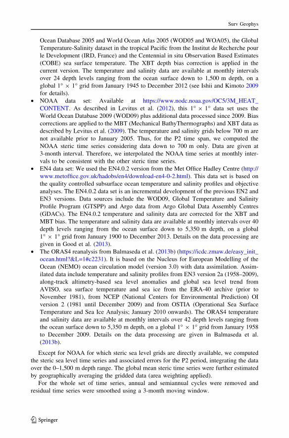
Ocean Database 2005 and World Ocean Atlas 2005 (WOD05 and WOA05), the Global
Temperature-Salinity dataset in the tropical Pacific from the Institut de Recherche pour
le Development (IRD, France) and the Centennial in situ Observation Based Estimates
(COBE) sea surface temperature. The XBT depth bias correction is applied in the
current version. The temperature and salinity data are available at monthly intervals
over 24 depth levels ranging from the ocean surface down to 1,500 m depth, on a
global 1� 9 1� grid from January 1945 to December 2012 (see Ishii and Kimoto 2009
for details).
• NOAA data set: Available at https://www.nodc.noaa.gov/OC5/3M_HEAT_
CONTENT. As described in Levitus et al. (2012), this 1� 9 1� data set uses the
World Ocean Database 2009 (WOD09) plus additional data processed since 2009. Bias
corrections are applied to the MBT (Mechanical BathyThermographs) and XBT data as
described by Levitus et al. (2009). The temperature and salinity grids below 700 m are
not available prior to January 2005. Thus, for the P2 time span, we computed the
NOAA steric time series considering data down to 700 m only. Data are given at
3-month interval. Therefore, we interpolated the NOAA time series at monthly inter-
vals to be consistent with the other steric time series.
• EN4 data set: We used the EN4.0.2 version from the Met Office Hadley Centre (http://
www.metoffice.gov.uk/hadobs/en4/download-en4-0-2.html). This data set is based on
the quality controlled subsurface ocean temperature and salinity profiles and objective
analyses. The EN4.0.2 data set is an incremental development of the previous EN2 and
EN3 versions. Data sources include the WOD09, Global Temperature and Salinity
Profile Program (GTSPP) and Argo data from Argo Global Data Assembly Centres
(GDACs). The EN4.0.2 temperature and salinity data are corrected for the XBT and
MBT bias. The temperature and salinity data are available at monthly intervals over 40
depth levels ranging from the ocean surface down to 5,350 m depth, on a global
1� 9 1� grid from January 1900 to December 2013. Details on the data processing are
given in Good et al. (2013).
• The ORAS4 reanalysis from Balmaseda et al. (2013b) (https://icdc.zmaw.de/easy_init_
ocean.html?&L=1#c2231). It is based on the Nucleus for European Modelling of the
Ocean (NEMO) ocean circulation model (version 3.0) with data assimilation. Assim-
ilated data include temperature and salinity profiles from EN3 version 2a (1958–2009),
along-track altimetry-based sea level anomalies and global sea level trend from
AVISO, sea surface temperature and sea ice from the ERA-40 archive (prior to
November 1981), from NCEP (National Centers for Environmental Prediction) OI
version 2 (1981 until December 2009) and from OSTIA (Operational Sea Surface
Temperature and Sea Ice Analysis; January 2010 onwards). The ORAS4 temperature
and salinity data are available at monthly intervals over 42 depth levels ranging from
the ocean surface down to 5,350 m depth, on a global 1� 9 1� grid from January 1958
to December 2009. Details on the data processing are given in Balmaseda et al.
(2013b).
Except for NOAA for which steric sea level grids are directly available, we computed
the steric sea level time series and associated errors for the P2 period, integrating the data
over the 0–1,500 m depth range. The global mean steric time series were further estimated
by geographically averaging the gridded data (area weighting applied).
For the whole set of time series, annual and semiannual cycles were removed and
residual time series were smoothed using a 3-month moving window.
Surv Geophys
123
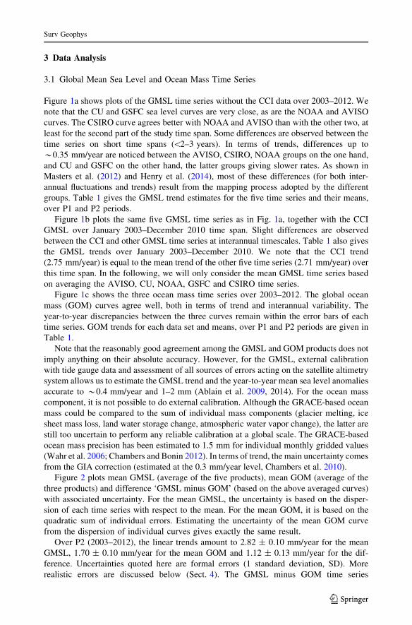
3 Data Analysis
3.1 Global Mean Sea Level and Ocean Mass Time Series
Figure 1a shows plots of the GMSL time series without the CCI data over 2003–2012. We
note that the CU and GSFC sea level curves are very close, as are the NOAA and AVISO
curves. The CSIRO curve agrees better with NOAA and AVISO than with the other two, at
least for the second part of the study time span. Some differences are observed between the
time series on short time spans (\2–3 years). In terms of trends, differences up to
*0.35 mm/year are noticed between the AVISO, CSIRO, NOAA groups on the one hand,
and CU and GSFC on the other hand, the latter groups giving slower rates. As shown in
Masters et al. (2012) and Henry et al. (2014), most of these differences (for both inter-
annual fluctuations and trends) result from the mapping process adopted by the different
groups. Table 1 gives the GMSL trend estimates for the five time series and their means,
over P1 and P2 periods.
Figure 1b plots the same five GMSL time series as in Fig. 1a, together with the CCI
GMSL over January 2003–December 2010 time span. Slight differences are observed
between the CCI and other GMSL time series at interannual timescales. Table 1 also gives
the GMSL trends over January 2003–December 2010. We note that the CCI trend
(2.75 mm/year) is equal to the mean trend of the other five time series (2.71 mm/year) over
this time span. In the following, we will only consider the mean GMSL time series based
on averaging the AVISO, CU, NOAA, GSFC and CSIRO time series.
Figure 1c shows the three ocean mass time series over 2003–2012. The global ocean
mass (GOM) curves agree well, both in terms of trend and interannual variability. The
year-to-year discrepancies between the three curves remain within the error bars of each
time series. GOM trends for each data set and means, over P1 and P2 periods are given in
Table 1.
Note that the reasonably good agreement among the GMSL and GOM products does not
imply anything on their absolute accuracy. However, for the GMSL, external calibration
with tide gauge data and assessment of all sources of errors acting on the satellite altimetry
system allows us to estimate the GMSL trend and the year-to-year mean sea level anomalies
accurate to *0.4 mm/year and 1–2 mm (Ablain et al. 2009, 2014). For the ocean mass
component, it is not possible to do external calibration. Although the GRACE-based ocean
mass could be compared to the sum of individual mass components (glacier melting, ice
sheet mass loss, land water storage change, atmospheric water vapor change), the latter are
still too uncertain to perform any reliable calibration at a global scale. The GRACE-based
ocean mass precision has been estimated to 1.5 mm for individual monthly gridded values
(Wahr et al. 2006; Chambers and Bonin 2012). In terms of trend, the main uncertainty comes
from the GIA correction (estimated at the 0.3 mm/year level, Chambers et al. 2010).
Figure 2 plots mean GMSL (average of the five products), mean GOM (average of the
three products) and difference ‘GMSL minus GOM’ (based on the above averaged curves)
with associated uncertainty. For the mean GMSL, the uncertainty is based on the disper-
sion of each time series with respect to the mean. For the mean GOM, it is based on the
quadratic sum of individual errors. Estimating the uncertainty of the mean GOM curve
from the dispersion of individual curves gives exactly the same result.
Over P2 (2003–2012), the linear trends amount to 2.82 ± 0.10 mm/year for the mean
GMSL, 1.70 ± 0.10 mm/year for the mean GOM and 1.12 ± 0.13 mm/year for the dif-
ference. Uncertainties quoted here are formal errors (1 standard deviation, SD). More
realistic errors are discussed below (Sect. 4). The GMSL minus GOM time series
Surv Geophys
123
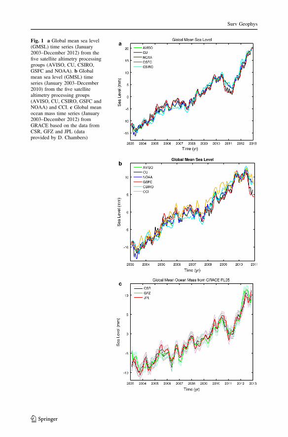
Fig. 1 a Global mean sea level
(GMSL) time series (January
2003–December 2012) from the
five satellite altimetry processing
groups (AVISO, CU, CSIRO,
GSFC and NOAA). b Global
mean sea level (GMSL) time
series (January 2003–December
2010) from the five satellite
altimetry processing groups
(AVISO, CU, CSIRO, GSFC and
NOAA) and CCI. c Global mean
ocean mass time series (January
2003–December 2012) from
GRACE based on the data from
CSR, GFZ and JPL (data
provided by D. Chambers)
Surv Geophys
123
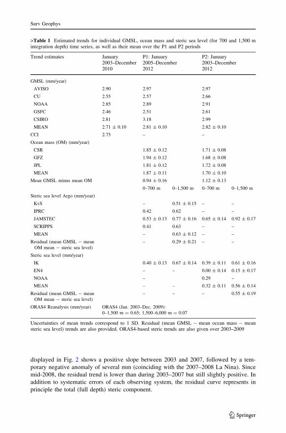
displayed in Fig. 2 shows a positive slope between 2003 and 2007, followed by a tem-
porary negative anomaly of several mm (coinciding with the 2007–2008 La Nina). Since
mid-2008, the residual trend is lower than during 2003–2007 but still slightly positive. In
addition to systematic errors of each observing system, the residual curve represents in
principle the total (full depth) steric component.
>Table 1 Estimated trends for individual GMSL, ocean mass and steric sea level (for 700 and 1,500 m
integration depth) time series, as well as their mean over the P1 and P2 periods
Trend estimates January
2003–December
2010
P1: January
2005–December
2012
P2: January
2003–December
2012
GMSL (mm/year)
AVISO 2.90 2.97 2.97
CU 2.55 2.57 2.66
NOAA 2.85 2.89 2.91
GSFC 2.46 2.51 2.61
CSIRO 2.81 3.18 2.99
MEAN 2.71 ± 0.10 2.81 ± 0.10 2.82 ± 0.10
CCI 2.75 – –
Ocean mass (OM) (mm/year)
CSR 1.85 ± 0.12 1.71 ± 0.08
GFZ 1.94 ± 0.12 1.68 ± 0.08
JPL 1.81 ± 0.12 1.72 ± 0.08
MEAN 1.87 ± 0.11 1.70 ± 0.10
Mean GMSL minus mean OM 0.94 ± 0.16 1.12 ± 0.13
0–700 m 0–1,500 m 0–700 m 0–1,500 m
Steric sea level Argo (mm/year)
KvS – 0.51 ± 0.15 – –
IPRC 0.42 0.62 – –
JAMSTEC 0.53 ± 0.13 0.77 ± 0.16 0.65 ± 0.14 0.92 ± 0.17
SCRIPPS 0.41 0.63 – –
MEAN – 0.63 ± 0.12 – –
Residual (mean GMSL - mean
OM mean - steric sea level)
– 0.29 ± 0.21 – –
Steric sea level (mm/year)
IK 0.40 ± 0.13 0.67 ± 0.14 0.39 ± 0.11 0.61 ± 0.16
EN4 – – 0.00 ± 0.14 0.15 ± 0.17
NOAA – 0.29 –
MEAN – – 0.32 ± 0.11 0.56 ± 0.14
Residual (mean GMSL - mean
OM mean - steric sea level)
– – – 0.55 ± 0.19
ORAS4 Reanalysis (mm/year) ORAS4 (Jan. 2003–Dec. 2009):
0–1,500 m = 0.65; 1,500–6,000 m = 0.07
Uncertainties of mean trends correspond to 1 SD. Residual (mean GMSL - mean ocean mass - mean
steric sea level) trends are also provided. ORAS4-based steric trends are also given over 2003–2009
Surv Geophys
123
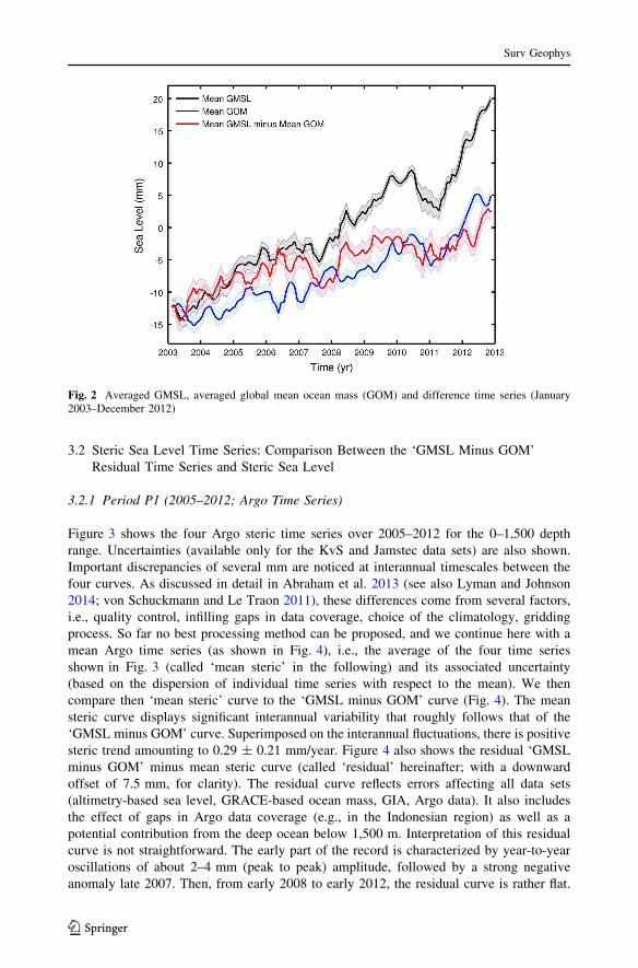
3.2 Steric Sea Level Time Series: Comparison Between the ‘GMSL Minus GOM’
Residual Time Series and Steric Sea Level
3.2.1 Period P1 (2005–2012; Argo Time Series)
Figure 3 shows the four Argo steric time series over 2005–2012 for the 0–1,500 depth
range. Uncertainties (available only for the KvS and Jamstec data sets) are also shown.
Important discrepancies of several mm are noticed at interannual timescales between the
four curves. As discussed in detail in Abraham et al. 2013 (see also Lyman and Johnson
2014; von Schuckmann and Le Traon 2011), these differences come from several factors,
i.e., quality control, infilling gaps in data coverage, choice of the climatology, gridding
process. So far no best processing method can be proposed, and we continue here with a
mean Argo time series (as shown in Fig. 4), i.e., the average of the four time series
shown in Fig. 3 (called ‘mean steric’ in the following) and its associated uncertainty
(based on the dispersion of individual time series with respect to the mean). We then
compare then ‘mean steric’ curve to the ‘GMSL minus GOM’ curve (Fig. 4). The mean
steric curve displays significant interannual variability that roughly follows that of the
‘GMSL minus GOM’ curve. Superimposed on the interannual fluctuations, there is positive
steric trend amounting to 0.29 ± 0.21 mm/year. Figure 4 also shows the residual ‘GMSL
minus GOM’ minus mean steric curve (called ‘residual’ hereinafter; with a downward
offset of 7.5 mm, for clarity). The residual curve reflects errors affecting all data sets
(altimetry-based sea level, GRACE-based ocean mass, GIA, Argo data). It also includes
the effect of gaps in Argo data coverage (e.g., in the Indonesian region) as well as a
potential contribution from the deep ocean below 1,500 m. Interpretation of this residual
curve is not straightforward. The early part of the record is characterized by year-to-year
oscillations of about 2–4 mm (peak to peak) amplitude, followed by a strong negative
anomaly late 2007. Then, from early 2008 to early 2012, the residual curve is rather flat.
Fig. 2 Averaged GMSL, averaged global mean ocean mass (GOM) and difference time series (January
2003–December 2012)
Surv Geophys
123
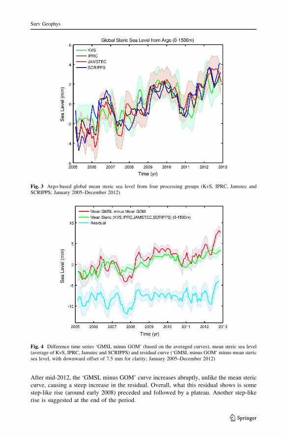
After mid-2012, the ‘GMSL minus GOM’ curve increases abruptly, unlike the mean steric
curve, causing a steep increase in the residual. Overall, what this residual shows is some
step-like rise (around early 2008) preceded and followed by a plateau. Another step-like
rise is suggested at the end of the period.
Fig. 3 Argo-based global mean steric sea level from four processing groups (KvS, IPRC, Jamstec and
SCRIPPS; January 2005–December 2012)
Fig. 4 Difference time series ‘GMSL minus GOM’ (based on the averaged curves), mean steric sea level
(average of KvS, IPRC, Jamstec and SCRIPPS) and residual curve (‘GMSL minus GOM’ minus mean steric
sea level, with downward offset of 7.5 mm for clarity; January 2005–December 2012)
Surv Geophys
123
Table 1 gives the steric trends estimated over the P1 period for each Argo time series
(integration down to 1,500 m) and mean steric trend. Trends of ‘mean GMSL minus mean
GOM’ and residual time series over P1 are also given.
3.2.2 Period P2 (2003–2012; Other Steric Products)
Over the 2003–2005 time span, only the IK, Jamstec and EN4 data sets provide data over
the 0–1,500 m depth range (however, we must keep in mind the limited raw data available
below 700 m over this time span). So we present below the steric curves for the 0–700 and
0–1,500 m depth ranges separately.
Figure 5a shows the IK, Jamstec, NOAA and EN4 steric curves for the 0–700 m depth
range, with associated uncertainties for IK, Jamstec and EN4. Very large errors affect the
early part of the time span (2003–2005), and strong discrepancies are noticed between the
four curves. These differences predominantly occur from data processing methodologies,
in particular different gap filling methods. Moreover, prior to 2005—where the data source
is mostly based on XBT measurements—differences in the XBT bias correction add to the
discrepancies (see Lyman et al. 2010; Abraham et al. 2013; Lyman and Johnson 2014).
Figure 5b shows the IK, Jamstec and EN4 steric curves for the 1,500 m depth range.
Similar comments apply as for the 0–700 m depth range. In both cases, the EN4 curve is
almost flat over the whole time span (its trend over 2003–2012 is 0.0 ± 0.14 and
0.15 ± 0.17 mm/year for 700 and 1,500 m integration depths, respectively). This is unlike
the IK and Jamstec curves that display larger positive trends. Over P2, the IK trend
amounts 0.39 ± 0.11 and 0.61 ± 0.16 mm/year down to 700 and 1,500 m, respectively,
while the Jamstec trend amounts 0.65 ± 0.14 and 0.92 ± 0.17 mm/year for the same two
integration depth. The behavior of the EN4 time series is puzzling and needs further
investigation. However, we still consider this data set in our analysis.
Figure 6 shows the mean of IK, Jamstec, NOAA and EN4 for 0–700 m and mean of IK,
Jamstec and EN4 for 0–1,500 m depth range (the NOAA data down to 1,500 m are
available only as of 2005) for the 2003–2012 time span (P2 period). Interannual variability
is very similar for the 700 and 1,500 m cases, as expected since it is essentially due to the
upper ocean layers. The main difference between the two curves is a 0.24 mm/year short-
term trend increase, from 700 to 1,500 m.
Steric trends estimated over P2 for each time series (0–700 and 0–1,500 m depth
ranges) and means are given in Table 1. Trends of ‘mean GMSL minus mean GOM’ and
residual time series over P2 are also given.
Figure 7 shows the ‘GMSL minus GOM’ curve and mean steric curve (average of IK,
Jamstec and EN4) for the 0–1,500 m depth, as well as the residual curve (‘GMSL minus
GOM’ minus mean steric curve; with a downward offset of 7.5 mm, for clarity). Over
2005–2012, the residual curve is very similar to that shown in Fig. 4 when using Argo data,
with similar behavior though time. Over 2003–2012 (P2 period), the residual curve dis-
plays a positive trend of 0.55 ± 0.19 mm/year.
4 Mid-Ocean and Deep Ocean Contribution
Comparing the upper 700 and 1,500 m steric contributions and their evolution through
time shows an interesting behavior. As expected, the 1,500 m steric contribution is larger
than the 700 m steric one. But, more interestingly, the difference seems to increase linearly
with time. This implies that more and more heat reaches the ocean below 700 m. This is
Surv Geophys
123
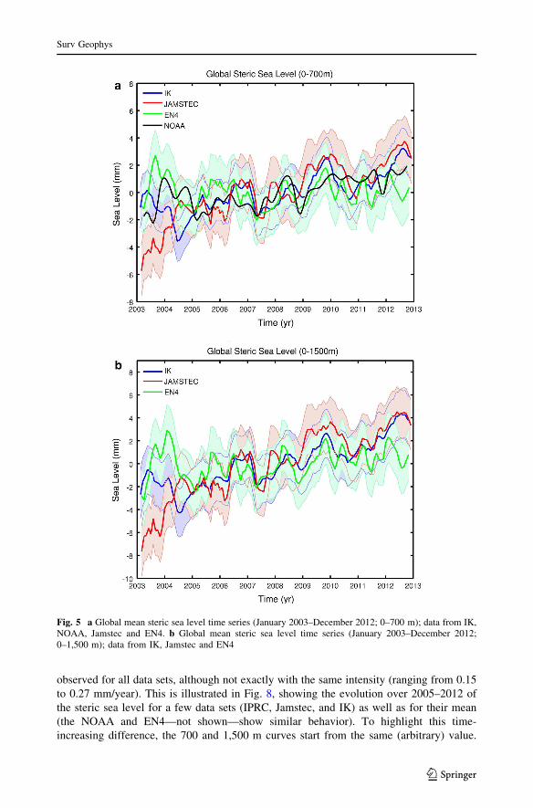
observed for all data sets, although not exactly with the same intensity (ranging from 0.15
to 0.27 mm/year). This is illustrated in Fig. 8, showing the evolution over 2005–2012 of
the steric sea level for a few data sets (IPRC, Jamstec, and IK) as well as for their mean
(the NOAA and EN4—not shown—show similar behavior). To highlight this time-
increasing difference, the 700 and 1,500 m curves start from the same (arbitrary) value.
Fig. 5 a Global mean steric sea level time series (January 2003–December 2012; 0–700 m); data from IK,
NOAA, Jamstec and EN4. b Global mean steric sea level time series (January 2003–December 2012;
0–1,500 m); data from IK, Jamstec and EN4
Surv Geophys
123

Figure 8 clearly shows that the layers below 700 m have gained heat over the last few
years. This observation is in agreement with previous results from Levitus et al. (2012)
based on the NOAA data set, and Balmaseda et al. (2013a) based on the ORAS4 reanalysis.
The latter study showed an increasing warming trend below 700 m. However, it did not
Fig. 6 Averaged steric sea level time series (January 2003–December 2012) for 0–700 m (average of IK,
NOAA, Jamstec and EN4) and 0–1,500 m (average of IK, Jamstec and EN4)
Fig. 7 Difference time series ‘GMSL minus GOM’ (based on the averaged curves), mean steric sea level
for 0–1,500 m (average of IK, Jamstec and EN4) and residual curve (‘GMSL minus GOM’ minus mean
steric sea level, with downward offset of 7.5 mm for clarity; January 2003–December 2012)
Surv Geophys
123
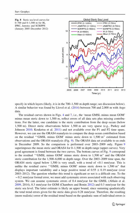
specify in which layers (likely, it is in the 700–1,500 m depth range; see discussion below).
A similar behavior was found by Llovel et al. (2014) between 700 and 2,000 m with Argo
data.
The residual curves shown in Figs. 4 and 7, i.e., the ‘mean GMSL minus mean GOM’
minus mean steric down to 1,500 m, reflect errors of all data sets plus missing contribu-
tions. For the latter, one candidate is the steric contribution from the deep ocean (below
1,500 m). Direct steric observations below 1,500 m are very sparse (e.g., Purkey and
Johnson 2010; Kouketsu et al. 2011) and not available over the P1 and P2 time spans.
However, we can use the ORAS4 reanalysis to compare the deep ocean contribution based
on the residual ‘‘‘GMSL minus GOM’ minus steric down to 1,500 m’’ estimated from
observations and the ORAS4 reanalysis (Fig. 9). The ORAS4 data set available to us ends
in December 2009. So the comparison is performed over 2003–2009 only. Figure 9
superimposes the mean steric and ORAS4 for 0–1,500 m depth range (upper curves). Very
good agreement is found between the two curves. The bottom curves of Fig. 9 correspond
to the residual ‘‘‘GMSL minus GOM’ minus steric down to 1,500 m’’ and the ORAS4
steric contribution for the 1,500–6,000 m depth range. Over the 2003–2009 time span, the
ORAS4 steric signal below 1,500 is very small, with a trend of\0.1 mm/year. This is
unlike the residual curve ‘‘‘GMSL minus GOM’ minus steric down to 1,500 m’’ that
displays important variability and a large positive trend of 0.55 ± 0.19 mm/year (over
2003–2012). The question whether this trend is significant or not is a difficult one. To the
*0.2 mm/year formal error, we must add systematic errors associated with each observing
system. We can assume systematic errors of 0.4 mm/year for the GMSL (Ablain et al.
2009, 2014), 0.3 mm/year for GOM (Chambers and Bonin 2012) and 0.3 mm/year for the
steric sea level. The latter estimate is likely an upper bound, since summing quadratically
the total trend errors given for the steric data gives 0.28 mm/year. Therefore, the resulting
(more realistic) error of the residual trend based on the quadratic sum of individual errors is
Fig. 8 Steric sea level curves for
0–700 and 0–1,500 m for IK,
IPRC, Jamstec and SCRIPPS
(January 2005–December 2012)
Surv Geophys
123
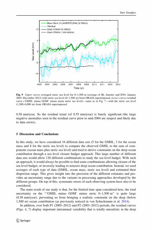
0.58 mm/year. So the residual trend (of 0.55 mm/year) is barely significant (the large
negative anomalies seen in the residual curve prior to mid-2004 are suspect and likely due
to data errors).
5 Discussion and Conclusions
In this study, we have considered 16 different data sets (5 for the GMSL, 3 for the ocean
mass and 8 for the steric sea level) to compare the observed GMSL to the sum of com-
ponents (ocean mass plus steric sea level) and tried to derive constraints on the deep ocean
contribution through a sea level closure budget approach. This large number of different
data sets would allow 120 different combinations to study the sea level budget. With such
an approach, it would always be possible to find some combinations allowing closure of the
sea level budget, or inversely leading to nonzero deep ocean contribution. Instead, we used
averages of each type of data (GMSL, ocean mass, steric sea level) and estimated their
dispersion range. This gives insight into the precision of the different estimates and pro-
vides an uncertainty range due to the variants in processing approaches developed by the
different groups. On top of this, systematic errors of each observing system have also to be
considered.
The main result of our study is that, for the limited time span considered here, the total
uncertainty on the ‘‘‘GMSL minus GOM’ minus steric 0–1,500 m’’ is quite large
(0.58 mm/year), preventing us from bringing a realistic constraint on the deep (below
1,500 m) ocean contribution (as previously noticed in von Schuckmann et al. 2014).
In addition, over both P1 (2005–2012) and P2 (2003–2012) periods, the residual curves
(Figs. 4, 7) display important interannual variability that is totally unrealistic in the deep
Fig. 9 Upper curves averaged steric sea level for 0–1,500 m (average of IK, Jamstec and EN4; January
2003–December 2012) with steric sea level (0–1,500 m) from ORAS4 superimposed. Lower curves residual
curve (‘GMSL minus GOM’ minus mean steric sea level)—same as in Fig. 7—with the steric sea level
(1,500–6,000 m) from ORAS4 superimposed
Surv Geophys
123
ocean. Very likely, it reflects errors at interannual timescales in one of the components
(GMSL, ocean mass or steric sea level) or in all of them. Previous studies (e.g., Cazenave
et al. 2012; Masters et al. 2012; Henry et al. 2014; Ablain et al. 2014) showed that at
interannual timescales, the (detrended) GMSL time series displays 2–4 mm differences
from one data set to another. Thus, it is quite possible that the year-to-year fluctuations
seen here in the residual curves are at least partly due to errors in the GMSL. Current
efforts conducted in the context of the ESA Climate Change Initiative ‘sea level’ project
already provide improved sea level data (Ablain et al. 2014), but assessment of this new
product is still an ongoing work. Moreover, gaps in coverage in the steric data, in particular
Argo data (e.g., in the Indonesian region), and the associated missing steric signal very
likely impact the residual time series at interannual timescales.
The short-term trends displayed by the residual curves for both P1 and P2 periods are
also very likely contaminated by uncertainties in interannual variability as well as by
longer-term systematic errors. As shown in Cazenave et al. (2014), ENSO events cause
temporary positive or negative sea level anomalies (mostly of mass origin, but also in the
steric component) that significantly alter estimates of the rate of sea level rise. However,
even if the short-term variability is removed, the trend estimated from the filtered residual
curves (not shown) remain unrealistically large to be attributed to the deep ocean
([1,500 m) contribution. As shown in Fig. 9, the ORAS4 reanalysis estimates the
1,500–6,000 m steric trend to *0.1 mm/year. Such a magnitude is in line with estimates
based on sparse, but direct observations. For example, Purkey and Johnson (2010) report a
(non uniform) deep ocean contribution of the order of 0.1 mm/year for the 1990–2000
decade. For the same time span, Kouketsu et al. (2011) also find observational support for a
deep ocean warming, but not larger than 0.1 mm/year (in steric sea level equivalent) for
layers below 3,000 m. Such values agree well with the ORAS4 reanalysis (the ORAS4
steric sea level trend amounts to 0.17 mm/year for the 1993–2003 decade and
1,500–6,000 m depth range). Although it can be expected that more heat has reached the
deep ocean since the early 2000s, the residual values reported here for the P1 and P2
periods appear anomalously large.
We suspect that gaps in steric data coverage, like in the Indonesian region, and the
associated missing signal, contribute to the residual curves over the P1 and P2 periods. For
example, in the oceanic region covering the China Sea, Indonesian region and north of
Australia, satellite altimetry shows strong positive spatial trends over these two time spans
(also observed over the whole altimetry era). As regional sea level trends are mainly of
steric origin (e.g., Stammer et al. 2013), it is possible that the residual curves shown in
Figs. 4 and 7 reflect at least partly the missing steric signal. To check this, we computed
the altimetry-based sea level trend associated with the Indonesian region over the P1 and
P2 periods and found that it contributes by*0.3 mm/year, hence about 10 % the total sea
level trend. Since this region has been considered in the GMSL (as well as in the ocean
mass; but a rough estimate indicates a very small mass contribution to the residual trend,
less than 0.05 mm/year), but not is the steric data due to the gap in data coverage (since
2005 but also earlier), we conclude that the steric trend has been underestimated because of
these missing data. To investigate this issue somewhat further, we computed the steric
contribution of the Indonesian region (considering an area covering the Indonesian region,
the Timor Sea plus the South China Sea; see Fig. 10) using the ORAS4 data. The steric
contribution of this area to the residual trend is estimated to 0.29 and 0.31 mm/year over
2003–2009 and 2005–2009, respectively (after weighting by the ratio of the area to the
total ocean surface between 66�S and 66�N). Assuming that the Indonesian steric trend
remains more or less constant over the whole P1 and P2 periods and subtracting it (using a
Surv Geophys
123

value of 0.3 mm/year) from the above estimated residual trends, we find new residual
trends of *0 and 0.25 mm/year for P1 and P2, respectively. We consider such a range
(0–0.25 mm/year) as an upper limit for the deep ocean contribution to recent years sea
level rise.
The recently published study by Llovel et al. (2014) uses different data sets (Colorado
University/CU altimetry and CSR GRACE data) for the GMSL and ocean mass. They also
integrate Argo data down to 2,000 m (instead of 1,500 m in our study) and consider the
January 2005–December 2013 time span. They come up with a residual trend (GMSL
rise corrected for GRACE ocean mass and 0–2,000 m Argo steric trends) of
-0.13 ± 0.72 mm/year. That their residual trend is lower than ours (amounting 0.29 mm/
year over 2005–2012; see Table 1) is largely due to the fact that the CU GMSL trend over
P1 is lower by*0.25 mm/year than the mean GMSL trend used in our study (see Table 1).
The remaining difference (on the order of 0.15 mm/year) arises because of differences in
the integration depth and study period. Llovel et al. (2014) further consider the upper value
of the ±0.72 mm/year uncertainty range to derive an upper bound for the GMSL rise due
to deep ocean warming below 2,000 m. Doing this, they estimate at 0.59 mm/year the
maximum contribution of the deep ocean warming for the period from 2005 to 2013. This
is more than twice our estimate after correcting for the data gap effect. Clearly, more
investigations are needed on this important issue.
Probably, the most reliable result of our study is the evidence of a continuing warming
of the 700–1,500 m ocean layer. While reported earlier by Levitus et al. (2012) and von
Schuckmann et al. (2014) using the NOAA and KvS steric data sets, respectively,
Balmaseda et al. (2013a) using the ORAS4 reanalysis, as well as Llovel et al. (2014) using
Argo data since 2005, here we observe a similar behavior for each of the eight steric data
sets considered over the P1 and P2 periods, indicating that the result is most probably
robust. Expressed in steric sea level equivalent, the trend contribution of the 700–1,500 m
layer is on the order of 0.2 mm/year.
As discussed in the introduction, the favored candidate for explaining the current hiatus
in global warming is deep ocean heat uptake. In the absence of direct deep ocean
Fig. 10 Steric trend map based on Jamstec data over January 2005–December 2012 showing the Argo data
gap in the Indonesian region and the contours (black line) of the area considered in this study to estimate—
using the ORAS4 reanalysis—its contribution to the global mean steric trend
Surv Geophys
123
temperature measurements, the sea level budget approach may in principle help to con-
strain the problem. But as shown here and in previous studies (e.g., Abraham et al. 2013;
von Schuckmann et al. 2014), uncertainties due to data processing approaches and sys-
tematic errors of the different observing systems still prevent us from obtaining accurate
enough results, even when using almost all available data sets—as done here, instead of
just a selection of them. Besides, regional gaps in the steric coverage of the upper ocean,
like in the Indonesian region, complicate the sea level budget approach.
Priority for future work is to improve the data processing of each observing system.
Systematic intercomparisons of observational products (i.e., sea level, ocean mass and
steric sea level—including ocean reanalyses) should be implemented in an international
context in order to better understand the causes of the reported differences and define a best
processing methodology (if possible). The following step should be a global reprocessing
of all data sets, following the approach of the ESA Climate Change Initiative program. In
parallel, implementation of new observing systems (e.g., deep Argo) should be a sustained
goal of the scientific community and institutional organizations.
Priority in terms of observing systems is definitely the development of a deep Argo
program and improved coverage of the upper ocean temperature and salinity measure-
ments, as advocated in a number of recent articles (e.g., Abraham et al. 2013).
Acknowledgments We thank Don Chambers and two anonymous referees for their constructive reviews.
We also thank William Llovel for interesting discussions about our respective studies. H.B.D. PhD is funded
by the European Space Agency in the context of the Climate Change Initiative Sea Level Project. H.P. is
supported by a joint CNES-CLS PhD grant.
Open Access This article is distributed under the terms of the Creative Commons Attribution License
which permits any use, distribution, and reproduction in any medium, provided the original author(s) and the
source are credited.
References
Ablain M, Cazenave A, Valladeau G, Guinehut S (2009) A new assessment of the error budget of global
mean sea level rate estimated by satellite altimetry over 1993–2008. Ocean Sci 5(2):193–201
Ablain M et al (2014) Improved Sea Level record over the satellite altimetry era 1 (1993–2010) from the
Climate Change Initiative project. Ocean Sci (in press)
Abraham JP et al (2013) A review of global ocean temperature observations: implications for ocean heat
content estimates and climate change. Rev Geophys 51:450 2013RG000432
Balmaseda MA, Trenberth K, Kallen E (2013a) Distinctive climate signals in reanalysis of global ocean heat
content. Geophys Res Lett 40:1–6. doi:10.1002/grl.50382
Balmaseda MA, Mogensen K, Weaver A (2013b) Evaluation of the ECMWF ocean reanalysis ORAS4. Q J
R Meteorol Soc. doi:10.1002/qj.2063
Bindoff N, Willebrand J, Artale V, Cazenave A, Gregory J, Gulev S, Hanawa K, Le Quere C, Levitus S,
Nojiri Y, Shum CK, Talley L, Unnikrishnan A (2007) Observations: oceanic climate and sea level. In:
Solomon S, Qin D, Manning M, Chen Z, Marquis M, Averyt KB, Tignor M, Miller HL (eds) Climate
change 2007: the physical science basis. Contribution of Working Group I to the fourth assessment
report of the intergovernmental panel on climate change. Cambridge University Press, Cambridge and
New York
Boening C, Willis JK, Landerer FW, Nerem RS (2012) The 2011 La Nina: so strong, the oceans fell.
Geophys Res Lett 39:L19602. doi:10.1029/2012GL053055
Cazenave A, Henry O, Munier S, Meyssignac B, Delcroix T, Llovel W, Palanisamy H, Becker M (2012)
ENSO influence on the global mean sea level over 1993–2010. Mar Geod 35(S1):82–97
Cazenave A, Dieng H, Meyssignac B, von Schuckmann K, Decharme B, Berthier E (2014) The rate of sea
level rise. Nat Clim Change. doi:10.1038/NCLIMATE2159
Surv Geophys
123
Chambers DP, Bonin JA (2012) Evaluation of Release-05 GRACE time variable gravity coefficients over
the ocean. Ocean Sci 8:859–868. doi:10.5194/os-8-859-2012
Chambers DP, Schroeter J (2011) Measuring ocean mass variations from satellite gravimetry. J Geodyn
52:333–343
Chambers DP, Wahr J, Tamisiea ME, Nerem RS (2010) Ocean mass from GRACE and glacial isostatic
adjustment. J Geophys Res 115:B11415. doi:10.1029/2010JB007530
Chen X, Tung K-K (2014) Varying planetary heat sink led to global warming slowdown and acceleration.
Science 345:897–903
Chen JL, Wilson CR, Tapley BD (2013) Contribution of ice sheet and mountain glacier melt to recent sea
level rise. Nat Geosci 6:549–552
Church JA, Clark PU, Cazenave A, Gregory JM, Jevrejeva S, Levermann A, Merrifield MA, Milne GA,
Nerem RS, Nunn PD, Payne AJ, Pfeffer WT, Stammer D, Unnikrishnan AS (2013) Sea Level Change.
In: Stocker TF, Qin D, Plattner G-K, Tignor M, Allen SK, Boschung J, Nauels A, Xia Y, Bex V,
Midgley PM (eds) Climate change 2013: the physical science basis. Contribution of Working Group I
to the fifth assessment report of the intergovernmental panel on climate change. Cambridge University
Press, Cambridge and New York
England MH et al (2014) Recent intensification of wind-driven circulation in the pacific and the ongoing
warming hiatus. Nat Clim Change 4:222–227
Fasullo JT, Boening C, Landerer FW, Nerem RS (2013) Australia’s unique influence on global mean sea
level in 2010–2011. Geophys Res Lett 40(16):4368–4373. doi:10.1002/grl.50834
Goddard L (2014) Heat hide and seek. Nat Clim Change 4:158161
Good SA, Martin MJ, Rayner NA (2013) EN4: quality controlled ocean temperature and salinity profiles and
monthly objective analyses with uncertainty estimates. J Geophys Res Oceans 118:6704–6716. doi:10.
1002/2013JC009067
Guemas V, Doblas-Reyes FJ, Andreu-Burillo I, Asif M (2013) Retrospective prediction of global warming
slowdown in the past decade. Nat Clim Change 3:649–653
Hansen J, Sato M, Kharecha P, von Schuckmann K (2011) Earth’s energy imbalance and implications.
Atmos Chem Phys 11:13421–13449. doi:10.5194/acp-11-13421-2011
Held IM (2013) The cause of the pause. Nature 501:318–319
Henry O, Ablain M, Meyssignac B, Cazenave A, Masters D, Nerem S, Leuliette E, Garric G (2014)
Investigating and reducing differences between the satellite altimetry-based global mean sea level time
series provided by different processing groups. J Geod 88:351–361. doi:10.1007/s00190-013-0687-3
Ishii M, Kimoto M (2009) Reevaluation of historical ocean heat content variations with time-varying XBT
and MBT depth bias corrections. J Oceanogr 65(3):287–299. doi:10.1007/s10872-009-0027-7
Johnson GC, Chambers DP (2013) Ocean bottom pressure seasonal cycles and decadal trends from GRACE
Release-05: ocean circulation implications. J Geophys Res Oceans 118:4228–4240. doi:10.1002/jgrc.
20307
Kosaka Y, Xie S-P (2013) Recent global warming hiatus tied to equatorial Pacific surface cooling. Nature
501:403–407
Kouketsu S et al (2011) Deep ocean heat content changes estimated from observation and reanalysis product
and their influence on sea level change. J Geophys Res 116:C03012
Leuliette EW, Willis JK (2011) Balancing the sea level budget. Oceanography 24:122–129
Levitus S et al (2009) Global ocean heat content 1955–2008 in light of recently revealed instrumentation
problems. Geophys Res Lett 36:L07608. doi:10.1029/2008GL037155
Levitus S, Antonov JI, Boyer TP, Baranova OK, Garcia HE, Locarnini RA, Mishonov AV, Reagan JR,
Seidov D, Yarosh ES, Zweng MM (2012) World ocean heat content and thermosteric sea level change
(0–2000 m), 1955–2010. Geophys Res Lett 39:L10603. doi:10.1019/2012GL051106
Llovel W, Willis JK, Landerer FW, Fukumori I (2014) Deep-ocean contribution to sea level and energy
budget not detectable over the past decade. Nat Clim Change. doi:10.1038/NCLIMATE2387
Lyman JM, Johnson GC (2014) Estimating global ocean heat content changes in the upper 1800 m since
1950 and the influence of climatology choice. J Clim. doi:10.1175/JCLIM-D-12-00752.1
Lyman JM, Godd SA, Gouretski VV, Ishii M, Johnson GC, Palmer MD, Smith DM, Willis JK (2010)
Robust warming of the global upper ocean. Nature 465:334–337. doi:10.1038/nature09043
Masters D, Nerem RS, Choe C, Leuliette E, Beckley B, White N, Ablain M (2012) Comparison of global
mean sea level time series from TOPEX/Poseidon, Jason-1, and Jason-2. Mar Geod 35:20–41
Peltier WR (2004) Global glacial isostasy and the surface of the ice-age Earth: the ICE-5G (VM2) model
and GRACE. Annu Rev Earth Planet Sci 32:111–149
Peters GP, Marland G, Le Quere C, Boden T, Canadell JG, Raupach MR (2012) Rapid growth in CO2
emissions after the 2008–2009 global financial crisis. Nat Clim Change 2:2–4
Surv Geophys
123
Purkey S, Johnson GC (2010) Warming of global abyssal and deep southern ocean waters between the 1990s
and 2000s: contributions to global heat and sea level rise budget. J Clim 23:6336–6351
Shepherd A et al (2012) A reconciled estimate of ice sheet mass balance. Science 338(6111):1183–1189.
doi:10.1126/science.1228102
Smith D (2013) Has global warming stalled? Nat Clim Change 3:618–6919
Solomon S, Rosenlof K, Portmann R, Daniel J, Davis S, Sanford T, Plattner G-K (2010) Contributions of
stratospheric water vapour to decadal changes in the rate of global warming. Science. doi:10.1126/
science.1182488
Stammer D, Cazenave A, Ponte RM, Tamisiea ME (2013) Causes for contemporary regional sea level
changes. Annu Rev Mar Sci 5:21–46. doi:10.1146/annurev-marine-121211-172406
Trenberth KE, Fasullo JT (2010) Tracking Earth’s energy. Science 328:316–317
Trenberth KE, Fasullo JT (2013) An apparent hiatus in global warming? Earth’s Future. doi:10.102/
2013EF000165
Trenberth KE, Fasullo JT, Balmaseda MA (2014) Earth’s energy imbalance. J Clim 27:3129–3144. doi:10.
1175/JCLI-D-13-00294.1
Von Schuckmann K, Le Traon PY (2011) How well can we derive Global Ocean Indicators from Argo data?
Ocean Sci 7(6):783–791. doi:10.5194/os-7-783-2011
Von Schuckmann K, Sallee JB, Chambers D, Le Traon PY, Cabanes C, Gaillard C, Speich S, Hamon M
(2014) Consistency of the current global ocean observing systems from an Argo perspective. Ocean Sci
10:547–557. doi:10.5194/os-10-547-2014
Wahr J, Swenson S, Velicogna I (2006) Accuracy of GRACE mass estimates. Geophys Res Lett 33:L06401.
doi:10.1029/2005GL025305
Watanabe M, Kamae Y, Yoshimori M, Oka A, Sato M, Ishii M, Mochizuki T, Kimoto M (2013)
Strengthening of ocean heat uptake efficiency associated with the recent climate hiatus. Geophys Res
Lett 40:3175–3179. doi:10.1002/grl.50541
Woppelmann G, Letetrel C, Santamaria A, Bouin MN, Collilieux X, Altamimi Z, Williams SDP, Miguez
BM (2009) Rates of sea-level change over the past century in a geocentric reference frame. Geophys
Res Lett. doi:10.1029/2009gl038720
Surv Geophys
123
Chapter 2 Multi satellite altimetry record and global mean sea level budget
74
2.2.1 Future needs
In our study, we have shown how the sea level budget can help constraint the problem of
sparse temperature measurements to estimate the deep ocean contribution. However,
uncertainties due to data processing approaches and systematic errors of different observing
systems still prevent us from obtaining accurate results (Dieng et al., 2015a, Von Schuckmann et
al., 2014, Abraham et al, 2013). Besides we have also shown that incomplete steric data
coverage of the upper ocean such as in the Indonesian region further complicates the sea level
budget approach.
Of late, studies have worked on investigating the sources causing differences in
observational climate variables (GMSL in specific) that are processed by different institutions.
For example, Masters et al., (2012) investigated the effects of different GMSL computation
methodologies and different geophysical corrections applied to satellite altimetry data by five
different groups (Colorado University, AVISO, National Oceanic and Atmospheric
Administration-NOAA, National Aeronautics and Space Agency-NASA, Commonwealth
Scientific and Industrial Research Organization-CSIRO). This study suggested that the main
source of difference is caused by the choice of averaging method used to estimate GMSL from
along-track SSH data. Following this, Henry et al., (2014) attempted to identify the main cause
of difference found in the short-term (<10 years) GMSL trends based on altimetry data from
AVISO and CU processing groups over Jason-1 operating period (2002–2009) by considering an
ocean circulation model as reference and studying the impacts of averaging methods, bathymetry
and grid resolution. In agreement with Master et al., (2012), they also showed that the essential
trend difference arises from the averaging methods adopted by the groups. In a very recent study,
by studying the role of data errors in the closure of global mean sea level budget over 2005-2013,
Dieng et al., 2015b have shown that the main source of trend uncertainty comes from the
altimetry-based sea level data processing; while at sub-seasonal to multi-annual time scales, the
main source of uncertainty comes from short-terms errors in GRACE and Argo data.
All these studies imply that there is a prior need to improve data processing
methodologies of each observational products followed by systematic comparisons between
various teams. This has to be implemented in an international context in order to understand the
Chapter 2 Multi satellite altimetry record and global mean sea level budget
75
causes for the differences and to define a best methodology. One such attempt has already been
made by ESA. Since 2010, ESA has developed a new program, the Climate Change Initiative
(CCI), dedicated to reprocessing a set of 13 essential Climate Variables (ECVs) currently
observed from space; among them, the satellite altimetry-based sea level being one of the main
ECVs. The objective of the CCI sea level project is to produce a consistent and precise sea level
record covering the past two decades, based on the reprocessing of all satellite altimetry data
available from all missions. In the framework of this project, a new validation protocol has been
brought into use in order to develop new altimeter corrections and algorithms that can be applied
for precise sea level calculation (Ablain et al., 2015). This protocol focusses on three main
objectives: (1) global internal analyses with the aim of checking the internal consistency of a
specific mission-related altimetry system by analyzing the computed sea level, its instrumental
parameters (from altimeter and radiometer) and associated geophysical corrections, (2) global
multi mission comparisons in order to evaluate the coherence between two different altimetry
missions and (3) altimetry in-situ data comparison dedicated to the computation of sea level
differences between altimetry data and in-situ sea level measurements such as tide gauges, Argo
steric etc. as in Valladeau et al., (2012). As a result, the newly developed CCI sea level products
exhibit improvements at different levels of importance for climate studies. In fact, Dieng et al.,
(2015b) have shown that the observed altimetry based GMSL from the CCI program shows less
GMSL short term errors when compared to other data sets. Therefore, such international
programs if implemented for steric and ocean mass components also can largely help in
minimizing their uncertainties.
Furthermore, as mentioned in our study and in various recent studies, there is a need for
deep Argo and improved coverage of upper ocean temperature and salinity measurements. For
example, Durack et al., (2014a) have shown that there has been an underestimation of the long-
term upper ocean warming due to poor sampling of the Southern Hemisphere. The need for
improved coverage is not only essential for ocean observational variables but also for other
variables such as surface temperature. In fact, very recently, using an updated global surface
temperature analysis, Karl et al., (2015) have shown that the global surface temperature trend in
the recent decade is higher and suggest that the global warming hiatus is an artifact due biases in
temperature observation networks.

Chapter 2 Multi satellite altimetry record and global mean sea level budget
76
Therefore, scientific community and institutional organizations should consider all these
factors as high priority for better understanding of climate change.
Chapter 3 Regional sea level variability and total relative sea level change
77
Chapter 3
Regional sea level variability and total relative
sea level change
In the previous chapters we have discussed sea level variations at global scale, their
causes and the various missions/ instruments that help in the continuous sea level monitoring.
Though sea level has been rising at a rate of 1.6-1.8 mm/yr over the twentieth century (Jevrejeva
et al., 2008, Wöppelmann et al., 2009, Church and White, 2011) and at a rate of 3.2 mm/yr since
the altimetry era (Nerem et al., 2010), this rate is far from being spatially uniform (Stammer et
al., 2013, Church et al., 2013, Cazenave and Cozannet, 2014). Prior to the altimetry era, tide
gauge records at various locations suggested the non-uniform sea level variations (Douglas,
2001). Since the altimetry era, the quasi global coverage of the satellite altimeters enables us to
study the regional sea level variability precisely. Fig.3.1 displays the altimetry-based sea level
spatial trend patterns between 1993 and 2013 after having removed the uniform global mean
trend of 3.2 mm/yr. We can observe that in certain regions such as the western and northern
Pacific, south of Greenland in the Atlantic Ocean and southern Indian Ocean and the southern
Austral Ocean, sea level rates reach up to three times the global mean rate. There are also regions
such as the eastern Pacific Ocean that face sea level rates lower than the global mean rate. In
fact, the regional sea level variability superimposes on the GMSL thereby either reducing or
amplifying the regional sea level rate. This implies that different parts of the world face different
range of sea level risks (Palanisamy et al., 2015b). Therefore it becomes highly essential to
understand the regional sea level variability and its driving forces. In this chapter, first we
discuss the various causes of regional sea level variability and then move on to the estimate of
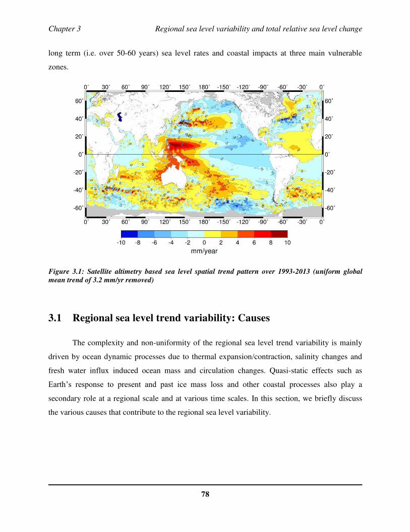
Chapter 3 Regional sea level variability and total relative sea level change
78
long term (i.e. over 50-60 years) sea level rates and coastal impacts at three main vulnerable
zones.
Figure 3.1: Satellite altimetry based sea level spatial trend pattern over 1993-2013 (uniform global
mean trend of 3.2 mm/yr removed)
3.1 Regional sea level trend variability: Causes
The complexity and non-uniformity of the regional sea level trend variability is mainly
driven by ocean dynamic processes due to thermal expansion/contraction, salinity changes and
fresh water influx induced ocean mass and circulation changes. Quasi-static effects such as
Earth’s response to present and past ice mass loss and other coastal processes also play a
secondary role at a regional scale and at various time scales. In this section, we briefly discuss
the various causes that contribute to the regional sea level variability.
Chapter 3 Regional sea level variability and total relative sea level change
79
3.1.1 Climate related regional sea level variability
1) Thermal expansion and salinity changes
The ocean thermal expansion and salinity changes not only have an impact on the GMSL
change but also on regional variability. The main contribution to regional sea level variability
results from the changes in the density structure of the ocean due to non-uniform thermal
expansion (thermosteric) and salinity changes (halosteric, Bindoff et al., 2007). Studies using in-
situ hydrographic measures (Ishii and Kimoto, 2009, Levitus et al., 2009, Levitus et al., 2012,
Lombard et al., 2005) and ocean circulation models (Carton and Giese, 2008, Köhl and
Stammer, 2008) have shown that the regional sea level trends during the altimetry era mostly
result from non-uniform thermal expansion of the ocean. Salinity changes also play a non-
negligible role in the regional sea level evolution such as in the North Atlantic and Arctic Ocean
as they can either enhance or compensate for the thermosteric changes (Wunsch et al., 2007,
Landerer et al., 2007, Köhl and Stammer, 2008, Durack and Wijffels, 2010, Stammer et al.,
2013, Durack et al., 2014). This compensation can amount to 25% of the thermosteric
contribution (Wunsch et al., 2007). While model simulations (Lowe and Gregory, 2006,
Pardaens et al., 2011) have suggested that the halosteric changes can dominate sea level change
in the Arctic Ocean, recent observation studies (eg. Morison et al., 2012) suggest that this might
already be the case.
Fig.3.2a displays an updated version, V6.13, of Ishii and Kimoto, 2009 based steric
(thermosteric plus halosteric) sea level spatial trend patterns over the altimetry period of 1992-
2013. The steric sea level anomaly was calculated between the depth of 0 to 700 m and the
uniform global mean steric sea level trend of mm/yr has been removed. Comparing Fig.3.2a with
Fig.3.1, we can see that the observed altimetry based and steric regional sea level trends agree
very well both in amplitude and regional location. Fig.3.2b displays the map of sea level trend
difference between the altimetry based seal level signal (as in Fig.3.1) and steric sea level signal.
The range of difference is relatively smaller (value) when compared to the actual range of the
altimetry and steric sea level signals (in the order of 10 mm/yr). This indicates that the upper
ocean (0-700 m) steric variations dominate the regional sea level variability during the altimetry
era. The residual (altimetry-steric) signal can also give us an idea on the contribution of deep
Chapter 3 Regional sea level variability and total relative sea level change
80
ocean (>700 m) heat content and ocean mass variations. Over longer time period (i.e. since mid-
1950s), by making use of observational ocean temperature data, Lombard et al., (2005), has
shown that the regional thermosteric sea level trends are not only non- uniform but they also
fluctuate in both time and space in response to internal climate modes like ENSO, Interdecadal
Pacific Oscillation (IPO)/ Pacific Decadal Oscillation (PDO) etc. This indicates that the non-
uniform regional sea level trends also fluctuate in space and time.
Regional steric sea level changes in different ocean basins are attributed to differential
heating and freshening of various ocean layers and associated physical processes such as air-sea
interaction, lateral and vertical mixing or advective processes (Yin et al., 2010) with ocean
circulation changes playing a major role (Stammer et al., 2013). Fukumori and Wang, (2013)
showed that the internal re distribution of pre-existing heat and salt anomalies accounts for most
of the regional sea level trends in regions of strong currents except in the western tropical Pacific
where external sources dominate the sea level. This is in agreement with studies (Merrifield,
2011, Merrifield and Maltrud, 2011, Palanisamy et al., 2015b) that showed that the high sea
level trends in this region during the altimetry era are related to the deepening of the thermocline
in response to intensified trade winds.
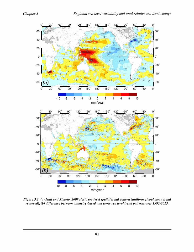
Chapter 3 Regional sea level variability and total relative sea level change
81
Figure 3.2: (a) Ishii and Kimoto, 2009 steric sea level spatial trend pattern (uniform global mean trend
removed), (b) difference between altimetry-based and steric sea level trend patterns over 1993-2013.
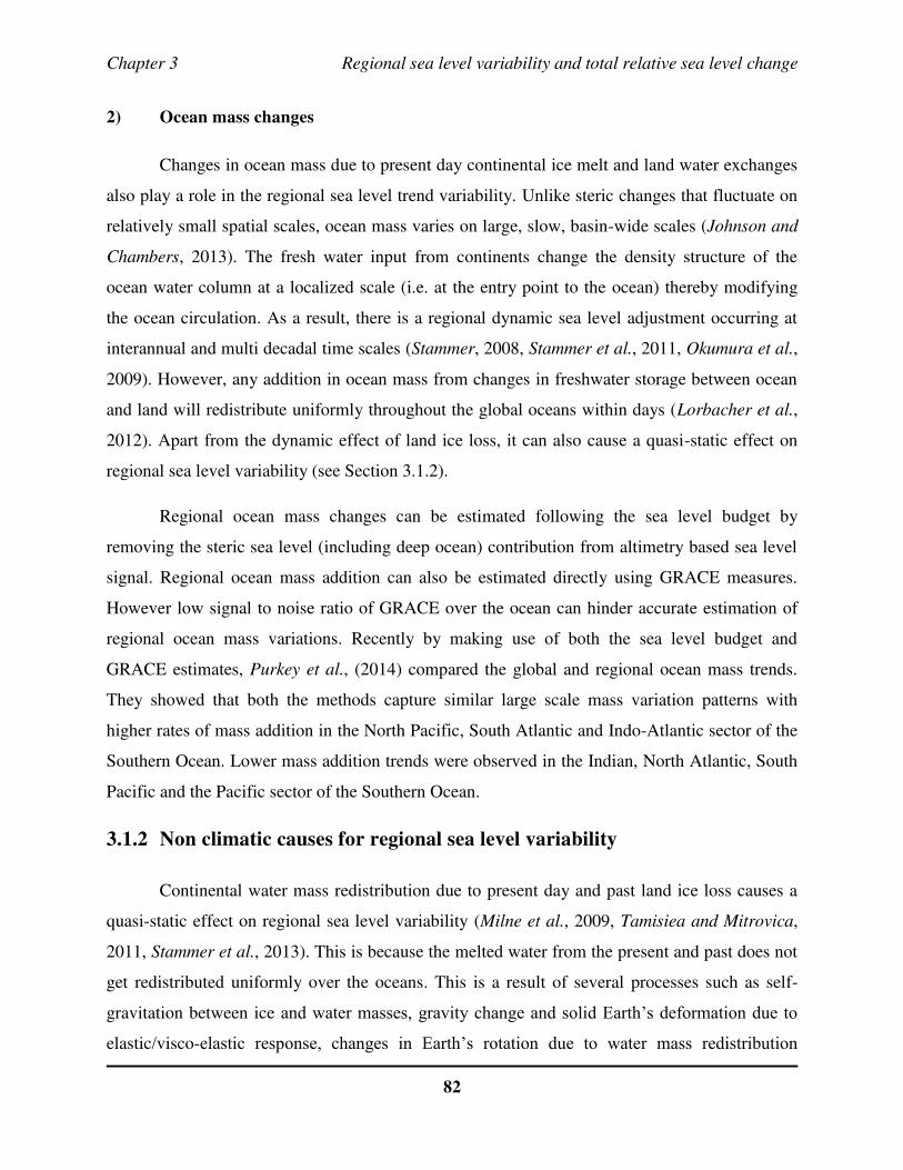
Chapter 3 Regional sea level variability and total relative sea level change
82
2) Ocean mass changes
Changes in ocean mass due to present day continental ice melt and land water exchanges
also play a role in the regional sea level trend variability. Unlike steric changes that fluctuate on
relatively small spatial scales, ocean mass varies on large, slow, basin-wide scales (Johnson and
Chambers, 2013). The fresh water input from continents change the density structure of the
ocean water column at a localized scale (i.e. at the entry point to the ocean) thereby modifying
the ocean circulation. As a result, there is a regional dynamic sea level adjustment occurring at
interannual and multi decadal time scales (Stammer, 2008, Stammer et al., 2011, Okumura et al.,
2009). However, any addition in ocean mass from changes in freshwater storage between ocean
and land will redistribute uniformly throughout the global oceans within days (Lorbacher et al.,
2012). Apart from the dynamic effect of land ice loss, it can also cause a quasi-static effect on
regional sea level variability (see Section 3.1.2).
Regional ocean mass changes can be estimated following the sea level budget by
removing the steric sea level (including deep ocean) contribution from altimetry based sea level
signal. Regional ocean mass addition can also be estimated directly using GRACE measures.
However low signal to noise ratio of GRACE over the ocean can hinder accurate estimation of
regional ocean mass variations. Recently by making use of both the sea level budget and
GRACE estimates, Purkey et al., (2014) compared the global and regional ocean mass trends.
They showed that both the methods capture similar large scale mass variation patterns with
higher rates of mass addition in the North Pacific, South Atlantic and Indo-Atlantic sector of the
Southern Ocean. Lower mass addition trends were observed in the Indian, North Atlantic, South
Pacific and the Pacific sector of the Southern Ocean.
3.1.2 Non climatic causes for regional sea level variability
Continental water mass redistribution due to present day and past land ice loss causes a
quasi-static effect on regional sea level variability (Milne et al., 2009, Tamisiea and Mitrovica,
2011, Stammer et al., 2013). This is because the melted water from the present and past does not
get redistributed uniformly over the oceans. This is a result of several processes such as self-
gravitation between ice and water masses, gravity change and solid Earth’s deformation due to
elastic/visco-elastic response, changes in Earth’s rotation due to water mass redistribution
Chapter 3 Regional sea level variability and total relative sea level change
83
(Peltier, 2004, 2009, Chambers et al., 2010, Tamisiea et al., 2010, Spada et al., 2013, Cazenave
and Cozannet, 2014). While the present day ice melt produces an elastic response of the Earth,
the last deglaciation that started approximately 20,000 years ago produces a visco-elastic
response (GIA) of the Earth. Even though the impact due to present day and past ice melt is
broad-scale, their regional fingerprint is different depending on the melting source (i.e.
Greenland, Antarctica, glaciers or last glaciation ice sheets, (Mitrovica et al., 2001, Lambeck et
al., 2010, Riva et al., 2010, Cazenave and Cozannet, 2014). Fig.3.3a and Fig.3.3b display the
numerical prediction (ICE5G-VM, Peltier et al., 2009) of the present-day impact of GIA on
relative sea level as measured by tide gauges and altimetry respectively. From Fig.3.3a, we can
observe that near the loading centers such as northern Europe and northern American continents,
relative sea level is falling due to continued uplift of the crust. Surrounding these loading centers,
the crust is subsiding thereby causing an increase in the relative sea level. The relative sea level
as measured by altimetry due to GIA (Fig.3.3b) is much smoother than that measured by tide
gauges.
It is to be noted that the regional sea level variability due to present day land ice loss is
still negligible and difficult to detect in altimetry based observations (Kopp et al., 2010,
Meyssignac and Cazenave, 2012). However with the accelerating rate of land ice loss, it is
expected that this will become a major contributor in the future (Slangen et al., 2011).

Chapter 3 Regional sea level variability and total relative sea level change
84
Figure 3.3: ICE5G-VM model based GIA contribution to relative sea level as measured by (a) tide
gauges, (b) satellite altimetry
Chapter 3 Regional sea level variability and total relative sea level change
85
3.1.3 Vertical Land Motions
There are other coastal and tectonic processes that result in vertical land motion (VLM)
that can cause highly localized sea level changes. VLM is either an uplift or subsidence of the
ground due to natural (such as GIA, sediment loading, tectonic and volcanic activities) or
anthropogenic (such as ground water pumping, oil/gas extraction, mining etc.) causes and
produces sea level variations relative to the ground(Ballu et al., 2011, Wöppelmann and Marcos,
2012). These localized phenomena may either reduce or amplify the climate related sea level
variations. For example, ground subsidence in the Mississippi delta due to Holocene sediment
compaction (Törnqvist et al., 2008) and oil/gas mining (Morton et al., 2006) has resulted in
ground subsidence along the Gulf Coast of the United States in the range of 5-10 mm/yr (Ericson
et al., 2006). Similarly, ground subsidence due to groundwater withdrawal from deltaic regions
has resulted in subsidence of megacities such as Tokyo by 5m, Shanghai and Bangkok by 3 m
and 2 m respectively (Nicholls, 2010, Stammer et al., 2013). All these imply the importance of
understanding the role of vertical land motion in the estimation of local relative sea level change.
3.2 Long term regional sea level variability, total relative sea level
change and coastal impacts
Sea level rise due to human induced global warming has been seen as a major threat to
low-lying coastal and island regions. The immediate effect of sea level rise is the submergence
and increased flooding of coastal land as well as salt water intrusion into surface waters. Longer
term impacts of sea level rise include wetland loss, changes in response to higher water tables
and increasing salinity, erosion of beaches, salt water intrusion into groundwater etc. (Nicholls et
al., 2007, 2010, 2011, Nicholls and Cazenave, 2010). These longer term impacts can further
interact with immediate effects of sea level rise and exacerbate them. For example, erosion of
sedimentary features will result in the degradation or disappearance of natural protection such as
mangroves, salt marshes etc. This will increase the vulnerability of such regions to coastal
flooding (Nicholls, 2011). There is also increasing concern about higher extreme sea levels due
to more intense storms superimposed on these mean rises, especially for areas affected by
tropical storms (Meehl et al., 2007). These possible storms would exacerbate the impacts of sea
level rise, particularly the risk of more damaging floods and storms (Nicholls, 2011). Sea level
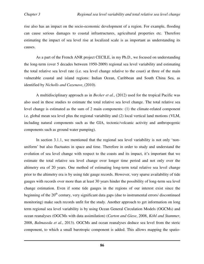
Chapter 3 Regional sea level variability and total relative sea level change
86
rise also has an impact on the socio-economic development of a region. For example, flooding
can cause serious damages to coastal infrastructures, agricultural properties etc. Therefore
estimating the impact of sea level rise at localized scale is as important as understanding its
causes.
As a part of the French ANR project CECILE, in my Ph.D., we focused on understanding
the long-term (over 5 decades between 1950-2009) regional sea level variability and estimating
the total relative sea level rate (i.e. sea level change relative to the coast) at three of the main
vulnerable coastal and island regions: Indian Ocean, Caribbean and South China Sea, as
identified by Nicholls and Cazenave, (2010).
A multidisciplinary approach as in Becker et al., (2012) used for the tropical Pacific was
also used in these studies to estimate the total relative sea level change. The total relative sea
level change is estimated as the sum of 2 main components: (1) the climate-related component
i.e. global mean sea level plus the regional variability and (2) local vertical land motions (VLM,
including natural components such as the GIA, tectonic/volcanic activity and anthropogenic
components such as ground water pumping).
In section 3.1.1, we mentioned that the regional sea level variability is not only ‘non-
uniform’ but also fluctuates in space and time. Therefore in order to study and understand the
evolution of sea level change with respect to the coasts and its impact, it’s important that we
estimate the total relative sea level change over longer time period and not only over the
altimetry era of 20 years. One method of estimating long-term total relative sea level change
prior to the altimetry era is by using tide gauge records. However, very sparse availability of tide
gauges with records over more than at least 30 years hinder the possibility of long-term sea level
change estimation. Even if some tide gauges in the regions of our interest exist since the
beginning of the 20th
century, very significant data gaps (due to instrumental errors/ discontinued
monitoring) make such records unfit for the study. Another approach to get information on long
term regional sea level variability is by using Ocean General Circulation Models (OGCMs) and
ocean reanalyses (OGCMs with data assimilation) (Carton and Giese, 2008, Köhl and Stammer,
2008, Balmaseda et al., 2013). OGCMs and ocean reanalyses deduce sea level from the steric
component, to which a small barotropic component is added. This allows mapping the spatio-
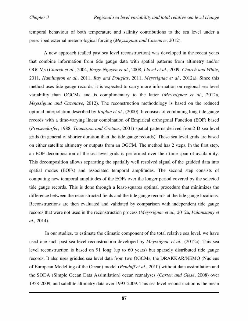
Chapter 3 Regional sea level variability and total relative sea level change
87
temporal behaviour of both temperature and salinity contributions to the sea level under a
prescribed external meteorological forcing (Meyssignac and Cazenave, 2012).
A new approach (called past sea level reconstruction) was developed in the recent years
that combine information from tide gauge data with spatial patterns from altimetry and/or
OGCMs (Church et al., 2004, Berge-Nguyen et al., 2008, Llovel et al., 2009, Church and White,
2011, Hamlington et al., 2011, Ray and Douglas, 2011, Meyssignac et al., 2012a). Since this
method uses tide gauge records, it is expected to carry more information on regional sea level
variability than OGCMs and is complimentary to the latter (Meyssignac et al., 2012a,
Meyssignac and Cazenave, 2012). The reconstruction methodology is based on the reduced
optimal interpolation described by Kaplan et al., (2000). It consists of combining long tide gauge
records with a time-varying linear combination of Empirical orthogonal Function (EOF) based
(Preisendorfer, 1988, Toumazou and Cretaux, 2001) spatial patterns derived from2-D sea level
grids (in general of shorter duration than the tide gauge records). These sea level grids are based
on either satellite altimetry or outputs from an OGCM. The method has 2 steps. In the first step,
an EOF decomposition of the sea level grids is performed over their time span of availability.
This decomposition allows separating the spatially well resolved signal of the gridded data into
spatial modes (EOFs) and associated temporal amplitudes. The second step consists of
computing new temporal amplitudes of the EOFs over the longer period covered by the selected
tide gauge records. This is done through a least-squares optimal procedure that minimizes the
difference between the reconstructed fields and the tide gauge records at the tide gauge locations.
Reconstructions are then evaluated and validated by comparison with independent tide gauge
records that were not used in the reconstruction process (Meyssignac et al., 2012a, Palanisamy et
al., 2014).
In our studies, to estimate the climatic component of the total relative sea level, we have
used one such past sea level reconstruction developed by Meyssignac et al., (2012a). This sea
level reconstruction is based on 91 long (up to 60 years) but sparsely distributed tide gauge
records. It also uses gridded sea level data from two OGCMs, the DRAKKAR/NEMO (Nucleus
of European Modelling of the Ocean) model (Penduff et al., 2010) without data assimilation and
the SODA (Simple Ocean Data Assimilation) ocean reanalyses (Carton and Giese, 2008) over
1958-2009, and satellite altimetry data over 1993-2009. This sea level reconstruction is the mean
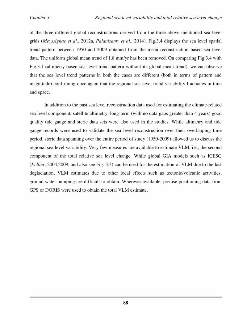
Chapter 3 Regional sea level variability and total relative sea level change
88
of the three different global reconstructions derived from the three above mentioned sea level
grids (Meyssignac et al., 2012a, Palanisamy et al., 2014). Fig.3.4 displays the sea level spatial
trend pattern between 1950 and 2009 obtained from the mean reconstruction based sea level
data. The uniform global mean trend of 1.8 mm/yr has been removed. On comparing Fig.3.4 with
Fig.3.1 (altimetry-based sea level trend pattern without its global mean trend), we can observe
that the sea level trend patterns in both the cases are different (both in terms of pattern and
magnitude) confirming once again that the regional sea level trend variability fluctuates in time
and space.
In addition to the past sea level reconstruction data used for estimating the climate-related
sea level component, satellite altimetry, long-term (with no data gaps greater than 4 years) good
quality tide gauge and steric data sets were also used in the studies. While altimetry and tide
gauge records were used to validate the sea level reconstruction over their overlapping time
period, steric data spanning over the entire period of study (1950-2009) allowed us to discuss the
regional sea level variability. Very few measures are available to estimate VLM, i.e., the second
component of the total relative sea level change. While global GIA models such as ICE5G
(Peltier, 2004,2009, and also see Fig. 3.3) can be used for the estimation of VLM due to the last
deglaciation, VLM estimates due to other local effects such as tectonic/volcanic activities,
ground water pumping are difficult to obtain. Wherever available, precise positioning data from
GPS or DORIS were used to obtain the total VLM estimate.
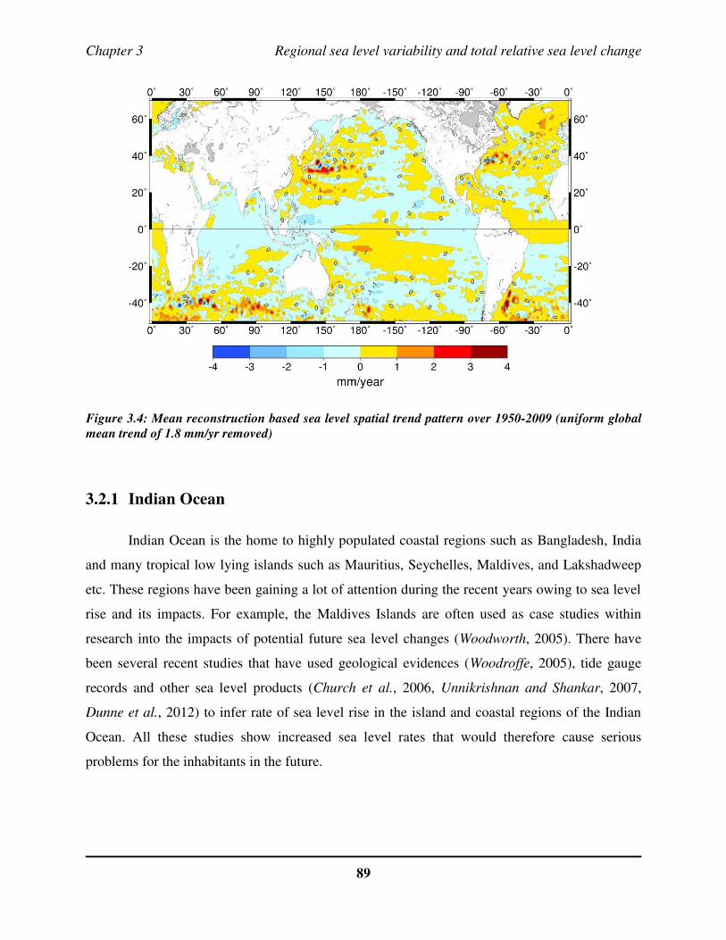
Chapter 3 Regional sea level variability and total relative sea level change
89
Figure 3.4: Mean reconstruction based sea level spatial trend pattern over 1950-2009 (uniform global
mean trend of 1.8 mm/yr removed)
3.2.1 Indian Ocean
Indian Ocean is the home to highly populated coastal regions such as Bangladesh, India
and many tropical low lying islands such as Mauritius, Seychelles, Maldives, and Lakshadweep
etc. These regions have been gaining a lot of attention during the recent years owing to sea level
rise and its impacts. For example, the Maldives Islands are often used as case studies within
research into the impacts of potential future sea level changes (Woodworth, 2005). There have
been several recent studies that have used geological evidences (Woodroffe, 2005), tide gauge
records and other sea level products (Church et al., 2006, Unnikrishnan and Shankar, 2007,
Dunne et al., 2012) to infer rate of sea level rise in the island and coastal regions of the Indian
Ocean. All these studies show increased sea level rates that would therefore cause serious
problems for the inhabitants in the future.
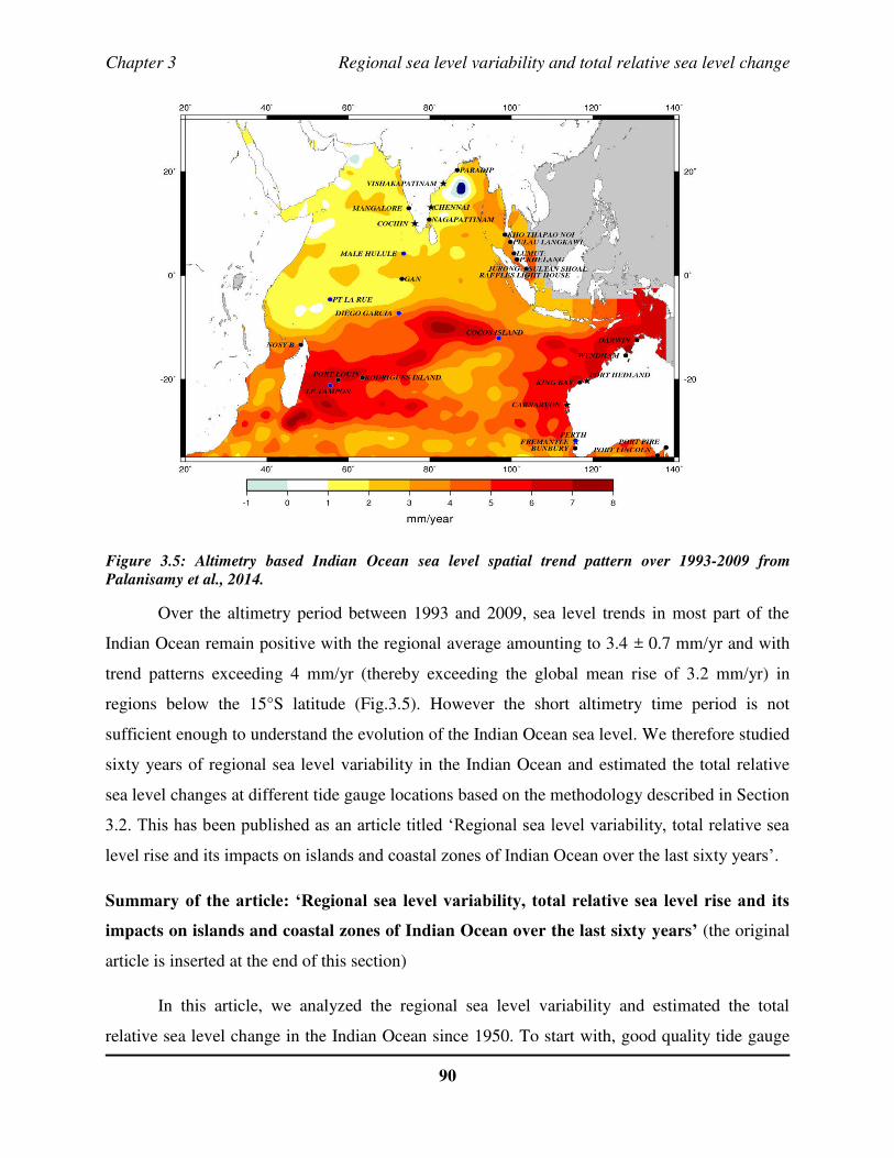
Chapter 3 Regional sea level variability and total relative sea level change
90
Figure 3.5: Altimetry based Indian Ocean sea level spatial trend pattern over 1993-2009 from
Palanisamy et al., 2014.
Over the altimetry period between 1993 and 2009, sea level trends in most part of the
Indian Ocean remain positive with the regional average amounting to 3.4 ± 0.7 mm/yr and with
trend patterns exceeding 4 mm/yr (thereby exceeding the global mean rise of 3.2 mm/yr) in
regions below the 15°S latitude (Fig.3.5). However the short altimetry time period is not
sufficient enough to understand the evolution of the Indian Ocean sea level. We therefore studied
sixty years of regional sea level variability in the Indian Ocean and estimated the total relative
sea level changes at different tide gauge locations based on the methodology described in Section
3.2. This has been published as an article titled ‘Regional sea level variability, total relative sea
level rise and its impacts on islands and coastal zones of Indian Ocean over the last sixty years’.
Summary of the article: ‘Regional sea level variability, total relative sea level rise and its impacts on islands and coastal zones of Indian Ocean over the last sixty years’ (the original
article is inserted at the end of this section)
In this article, we analyzed the regional sea level variability and estimated the total
relative sea level change in the Indian Ocean since 1950. To start with, good quality tide gauge
Chapter 3 Regional sea level variability and total relative sea level change
91
records from the data archive of Permanent Service Mean Sea Level (PSMSL) were first
analyzed. Based on their geographical location, the tide gauges were all regionally grouped into
four zones: (1) Indian Ocean island zone, coastal regions of (2) India, (3) South East Asia, and
(4) Western Australia. The tide gauge based coastal ‘mean’ sea level and their corresponding
uncertainties based on data availability over time were estimated. It was observed that in three
among the four regions of study, the uncertainties are larger between 1950s and 1970s indicating
the very sparse availability of tide gauge records during this time period. Therefore, to estimate
the six decades of climate-related sea level change, mean past sea level reconstruction (MRESL)
data of Meyssignac et al., (2012) was used in this study. VLM estimates were obtained from the
latest ULR5 (Santamaría-Gómez et al., 2012) GPS solution and International DORIS Service
(IDS) based DORIS (Willis et al., 2010) solutions.
Over the period of 60 years, the climate-related mean sea level trend in the Indian Ocean
amounts to 1.5±0.5 mm/yr, a value lesser (although not statistically different) from the global
mean sea level rise of 1.8±0.5 mm/yr as obtained by Church and White, (2011) and Meyssignac
et al., (2012). The spatial-temporal characteristics of the regional sea level variability since 1950
show high correlation with those of steric sea level variability. Distinct positive-negative dipole
patterns between the western and eastern parts of Indian Ocean also show good correlation with
the Dipole Mode Index (DMI), a proxy of the internal climate mode called the Indian Ocean
Dipole (IOD; Saji et al., 1999, Behera and Yamagata, 2001, Saji and Yamagata, 2003). This
validates that the regional sea level variability in the Indian Ocean is driven by steric changes in
response to surface wind and Ekman pumping velocity changes as mentioned by Han et al.,
(2010) and oscillates in response to the IOD. Total climate-related sea level change was also
studied in the four different regions of the Indian Ocean mentioned above and was found that in
most cases, they lie well within or lesser than the range of global mean sea level rise over 60
years. The mean sea level trends over 60 years in the coastal Indian subcontinent and in the
Indian Ocean islands amount to 1.5 mm/yr each. In the South East Asian coasts and Western
Australian coasts they amount to 1.4 mm/yr and 1.3 mm/yr respectively. However, over the two
recent decades, South East Asian and Western Australian coasts were found to exhibit high sea
level trend values of 3.5 mm/yr and 5.5 mm/yr respectively presumably linked to the western
tropical Pacific trade wind intensification (Merrifield, 2011, Merrifield and Maltrud, 2011,
Chapter 3 Regional sea level variability and total relative sea level change
92
Merrifield et al., 2012). The results obtained in this study were also found to be consistent to
those obtained by Church et al., (2006).
Estimation of total relative sea level change over 60 years with the help of VLM data
from GPS and DORIS showed that in two islands, Cocos Island and Diego Garcia, the rates are
the same as that of the global mean sea level rise. Whereas in the case of Malé Hulule
(Maldives), le Tampon (Reunion) and Perth (Australia) , the values exceed the global mean rate
with subsidence playing an important role. The contribution of subsidence at Malé Hulule and Le
Tampon exceed 50% while at Perth, it exceeds 70%. Ground water extraction has been suggested
(Featherstone et al., 2012) as the main contributor to subsidence in Perth. Therefore it is likely
that the long term total- relative sea level change at this location is overestimated.
Regional sea level variability, total relative sea level rise and its impactson islands and coastal zones of Indian Ocean over the last sixty years
H. Palanisamy a,⁎, A. Cazenave a, B. Meyssignac a, L. Soudarin b, G. Wöppelmann c, M. Becker d
a LEGOS/CNES, Toulouse, Franceb CLS, Ramonville Saint-Agne, Francec LIENSs, UMR7266, CNRS, University of La Rochelle, Franced UAG, UMR ESPACE-DEV (IRD, UM2, UAG, UR), Cayenne, France
a b s t r a c ta r t i c l e i n f o
Article history:
Received 2 June 2013
Received in revised form 31 January 2014
Accepted 1 February 2014
Available online 8 February 2014
Keywords:
Regional sea level variability
Mean Reconstructed Sea Level
Altimetry
Tide gauge
Vertical land motion
Indian Ocean
Indian Ocean Dipole
Indian Ocean is the home to many tropical low lying islands and highly populated coastal zones. Since a few re-
cent decades, many of these zones have been gaining a lot of international attention due to fears of sea level rise
and possible submersions of islands. In this study we estimate sea level rise and regional sea level variability in
IndianOcean (20°E–140°E, 30°N–35°S) over a period of 60 years from1950until 2009.Wedetermine the climat-
ic factors that influence the sea level change and variability in this region. We find that the changes in the Indian
Ocean sea level are of steric origin and are also driven by short-term Indian Ocean Dipole events. The trend in this
region over 60 years amounts to 1.5 mm/yr, a value lesser (although not statistically different) than the global
mean sea level rise over the same period. There is also an east–west increase in sea level trend pattern below
15°S latitude which is more amplified since the two recent decades. Climate-related sea level changes are also
studied at different sites in the Indian ocean corresponding to the existence of tide gauge records and has been
found that over the long term period (60 years), the sea level trend at most of the individual locations are well
within the global mean sea level rise. Total relative sea level change which is the sum of climate-related sea
level change and vertical land motion is also estimated at 5 locations with the help of GPS and DORIS measures.
© 2014 Elsevier B.V. All rights reserved.
1. Introduction
High precision satellite altimetry available since the early 1990s has
for the first time provided sea level time series over the whole oceanic
domain. This invaluable data set has confirmed that in terms of global
mean, the rate of sea level rise during the last 20 years is twice larger
than during the previous longer multidecadal time period (e.g., Nerem
et al., 2010; Church andWhite, 2011). It also revealed high regional var-
iability in the rates of sea level change (e.g., Cazenave and Llovel, 2010).
Sea level trend patterns over the past 20 years show high sea level rates
in the western tropical Pacific (up to 3 times the global mean), in the
northern Atlantic and Austral oceans. While the main cause of last
20 years global mean sea level rise (GMSLR) is land ice melt (~55%),
followed by ocean thermal expansion (~30%) (Church et al., 2011;
Meyssignac and Cazenave, 2012; Hanna et al., 2013), the regional sea
level trends mostly result from non-uniform ocean thermal expansion
and salinity variations (Lombard et al., 2005; Levitus et al., 2012) related
to ocean circulation changes (e.g., Bindoff et al., 2007; Stammer et al.,
2013). There are other processes causing regional variability in sea
level rates, among these are deformations of ocean basins and self-
gravitational changes due to glacial isostatic adjustment (GIA) resulting
from the last deglaciation and due to present-day land ice melt, respec-
tively (e.g., Milne et al., 2009; Stammer et al., 2013). However so far,
their contribution is small compared to ocean temperature and salinity
changes. In the recent years, growing attention has been given in the lit-
erature to the regional variability in sea level rates (see Stammer et al.,
2013 for a review). In fact this regional sea level variability superim-
poses on the GMSLR, either amplifying or reducing it. When studying
the impacts of sea level rise, what does matter locally is indeed the
sum of the GMSLR plus the regional variability (and including the effect
of vertical land motions, see below). There are also raising concerns
whether the shoreline erosion reported today in many coastal regions
of the world is mostly due to sea level rise (e.g., Bruun, 1962; Bird,
1996; Zhang et al., 2004) or whether it also results from other factors,
including urbanization, coastal management, reduced sediment trans-
port, etc. To answer these questions, the estimate of the ‘total relative’
sea level change at local scale is needed (e.g., Le Cozannet et al., 2013).
The term ‘total relative’ here means total ‘climatic’ sea level change,
i.e., GMSLR plus the regional trend in sea level, plus eventual vertical
Global and Planetary Change 116 (2014) 54–67
⁎ Corresponding author at: 18. Avenue Edouard Belin, 31400 Toulouse, France.
Tel.: +33 5 61 33 29 72.
E-mail address: [email protected] (H. Palanisamy).
http://dx.doi.org/10.1016/j.gloplacha.2014.02.001
0921-8181 © 2014 Elsevier B.V. All rights reserved.http://dx.doi.org/10.1016/j.gloplacha.2014.02.001
0921-8181/© 2014 Elsevier B.V. All rights reserved.
Contents lists available at ScienceDirect
Global and Planetary Change
j ourna l homepage: www.e lsev ie r .com/ locate /g lop lacha
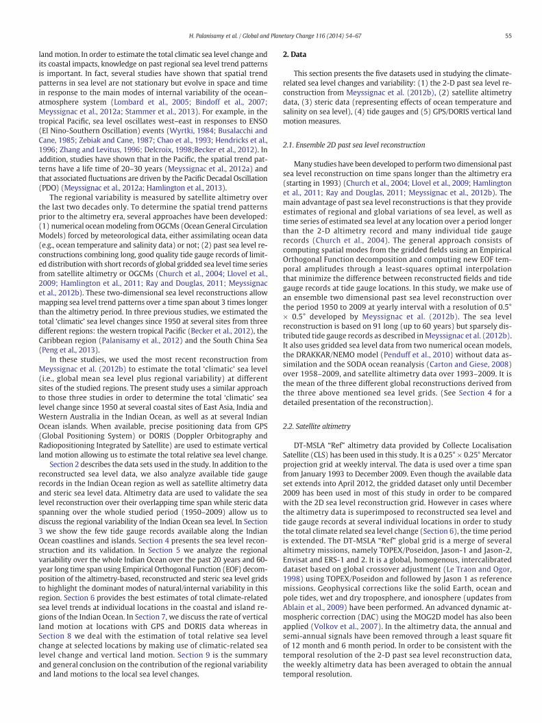
landmotion. In order to estimate the total climatic sea level change and
its coastal impacts, knowledge on past regional sea level trend patterns
is important. In fact, several studies have shown that spatial trend
patterns in sea level are not stationary but evolve in space and time
in response to the main modes of internal variability of the ocean–
atmosphere system (Lombard et al., 2005; Bindoff et al., 2007;
Meyssignac et al., 2012a; Stammer et al., 2013). For example, in the
tropical Pacific, sea level oscillates west–east in responses to ENSO
(El Nino-Southern Oscillation) events (Wyrtki, 1984; Busalacchi and
Cane, 1985; Zebiak and Cane, 1987; Chao et al., 1993; Hendricks et al.,
1996; Zhang and Levitus, 1996; Delcroix, 1998;Becker et al., 2012). In
addition, studies have shown that in the Pacific, the spatial trend pat-
terns have a life time of 20–30 years (Meyssignac et al., 2012a) and
that associated fluctuations are driven by the Pacific Decadal Oscillation
(PDO) (Meyssignac et al., 2012a; Hamlington et al., 2013).
The regional variability is measured by satellite altimetry over
the last two decades only. To determine the spatial trend patterns
prior to the altimetry era, several approaches have been developed:
(1) numerical oceanmodeling fromOGCMs (OceanGeneral Circulation
Models) forced by meteorological data, either assimilating ocean data
(e.g., ocean temperature and salinity data) or not; (2) past sea level re-
constructions combining long, good quality tide gauge records of limit-
ed distributionwith short records of global gridded sea level time series
from satellite altimetry or OGCMs (Church et al., 2004; Llovel et al.,
2009; Hamlington et al., 2011; Ray and Douglas, 2011; Meyssignac
et al., 2012b). These two-dimensional sea level reconstructions allow
mapping sea level trend patterns over a time span about 3 times longer
than the altimetry period. In three previous studies, we estimated the
total ‘climatic’ sea level changes since 1950 at several sites from three
different regions: the western tropical Pacific (Becker et al., 2012), the
Caribbean region (Palanisamy et al., 2012) and the South China Sea
(Peng et al., 2013).
In these studies, we used the most recent reconstruction from
Meyssignac et al. (2012b) to estimate the total ‘climatic’ sea level
(i.e., global mean sea level plus regional variability) at different
sites of the studied regions. The present study uses a similar approach
to those three studies in order to determine the total ‘climatic’ sea
level change since 1950 at several coastal sites of East Asia, India and
Western Australia in the Indian Ocean, as well as at several Indian
Ocean islands. When available, precise positioning data from GPS
(Global Positioning System) or DORIS (Doppler Orbitography and
Radiopositioning Integrated by Satellite) are used to estimate vertical
land motion allowing us to estimate the total relative sea level change.
Section 2 describes the data sets used in the study. In addition to the
reconstructed sea level data, we also analyze available tide gauge
records in the Indian Ocean region as well as satellite altimetry data
and steric sea level data. Altimetry data are used to validate the sea
level reconstruction over their overlapping time span while steric data
spanning over the whole studied period (1950–2009) allow us to
discuss the regional variability of the Indian Ocean sea level. In Section
3 we show the few tide gauge records available along the Indian
Ocean coastlines and islands. Section 4 presents the sea level recon-
struction and its validation. In Section 5 we analyze the regional
variability over the whole Indian Ocean over the past 20 years and 60-
year long time span using Empirical Orthogonal Function (EOF) decom-
position of the altimetry-based, reconstructed and steric sea level grids
to highlight the dominant modes of natural/internal variability in this
region. Section 6 provides the best estimates of total climate-related
sea level trends at individual locations in the coastal and island re-
gions of the Indian Ocean. In Section 7, we discuss the rate of vertical
land motion at locations with GPS and DORIS data whereas in
Section 8 we deal with the estimation of total relative sea level
change at selected locations by making use of climatic-related sea
level change and vertical land motion. Section 9 is the summary
and general conclusion on the contribution of the regional variability
and land motions to the local sea level changes.
2. Data
This section presents the five datasets used in studying the climate-
related sea level changes and variability: (1) the 2-D past sea level re-
construction from Meyssignac et al. (2012b), (2) satellite altimetry
data, (3) steric data (representing effects of ocean temperature and
salinity on sea level), (4) tide gauges and (5) GPS/DORIS vertical land
motion measures.
2.1. Ensemble 2D past sea level reconstruction
Many studies have been developed to perform two dimensional past
sea level reconstruction on time spans longer than the altimetry era
(starting in 1993) (Church et al., 2004; Llovel et al., 2009; Hamlington
et al., 2011; Ray and Douglas, 2011; Meyssignac et al., 2012b). The
main advantage of past sea level reconstructions is that they provide
estimates of regional and global variations of sea level, as well as
time series of estimated sea level at any location over a period longer
than the 2-D altimetry record and many individual tide gauge
records (Church et al., 2004). The general approach consists of
computing spatial modes from the gridded fields using an Empirical
Orthogonal Function decomposition and computing new EOF tem-
poral amplitudes through a least-squares optimal interpolation
that minimize the difference between reconstructed fields and tide
gauge records at tide gauge locations. In this study, we make use of
an ensemble two dimensional past sea level reconstruction over
the period 1950 to 2009 at yearly interval with a resolution of 0.5°
× 0.5° developed by Meyssignac et al. (2012b). The sea level
reconstruction is based on 91 long (up to 60 years) but sparsely dis-
tributed tide gauge records as described inMeyssignac et al. (2012b).
It also uses gridded sea level data from two numerical ocean models,
the DRAKKAR/NEMO model (Penduff et al., 2010) without data as-
similation and the SODA ocean reanalysis (Carton and Giese, 2008)
over 1958–2009, and satellite altimetry data over 1993–2009. It is
the mean of the three different global reconstructions derived from
the three above mentioned sea level grids. (See Section 4 for a
detailed presentation of the reconstruction).
2.2. Satellite altimetry
DT-MSLA “Ref” altimetry data provided by Collecte Localisation
Satellite (CLS) has been used in this study. It is a 0.25° × 0.25° Mercator
projection grid at weekly interval. The data is used over a time span
from January 1993 to December 2009. Even though the available data
set extends into April 2012, the gridded dataset only until December
2009 has been used in most of this study in order to be compared
with the 2D sea level reconstruction grid. However in cases where
the altimetry data is superimposed to reconstructed sea level and
tide gauge records at several individual locations in order to study
the total climate related sea level change (Section 6), the time period
is extended. The DT-MSLA “Ref” global grid is a merge of several
altimetry missions, namely TOPEX/Poseidon, Jason-1 and Jason-2,
Envisat and ERS-1 and 2. It is a global, homogenous, intercalibrated
dataset based on global crossover adjustment (Le Traon and Ogor,
1998) using TOPEX/Poseidon and followed by Jason 1 as reference
missions. Geophysical corrections like the solid Earth, ocean and
pole tides, wet and dry troposphere, and ionosphere (updates from
Ablain et al., 2009) have been performed. An advanced dynamic at-
mospheric correction (DAC) using the MOG2D model has also been
applied (Volkov et al., 2007). In the altimetry data, the annual and
semi-annual signals have been removed through a least square fit
of 12 month and 6 month period. In order to be consistent with the
temporal resolution of the 2-D past sea level reconstruction data,
the weekly altimetry data has been averaged to obtain the annual
temporal resolution.
55H. Palanisamy et al. / Global and Planetary Change 116 (2014) 54–67
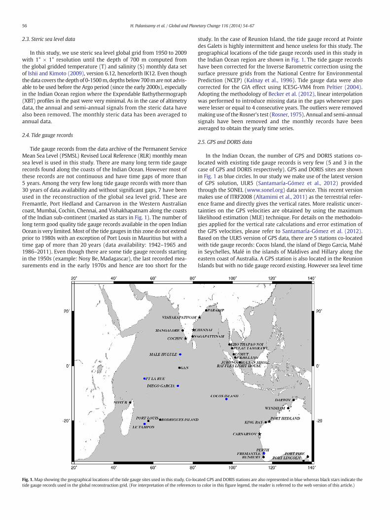
2.3. Steric sea level data
In this study, we use steric sea level global grid from 1950 to 2009
with 1° × 1° resolution until the depth of 700 m computed from
the global gridded temperature (T) and salinity (S) monthly data set
of Ishii and Kimoto (2009), version 6.12, henceforth IK12. Even though
the data covers the depth of 0-1500m, depths below700mare not advis-
able to be used before the Argo period (since the early 2000s), especially
in the Indian Ocean region where the Expendable Bathythermograph
(XBT) profiles in the past were very minimal. As in the case of altimetry
data, the annual and semi-annual signals from the steric data have
also been removed. The monthly steric data has been averaged to
annual data.
2.4. Tide gauge records
Tide gauge records from the data archive of the Permanent Service
Mean Sea Level (PSMSL) Revised Local Reference (RLR) monthly mean
sea level is used in this study. There are many long term tide gauge
records found along the coasts of the Indian Ocean. However most of
these records are not continuous and have time gaps of more than
5 years. Among the very few long tide gauge records with more than
30 years of data availability and without significant gaps, 7 have been
used in the reconstruction of the global sea level grid. These are
Fremantle, Port Hedland and Carnarvon in the Western Australian
coast, Mumbai, Cochin, Chennai, and Vishakhapatnam along the coasts
of the Indian sub-continent (marked as stars in Fig. 1). The number of
long term good quality tide gauge records available in the open Indian
Ocean is very limited. Most of the tide gauges in this zone do not extend
prior to 1980s with an exception of Port Louis in Mauritius but with a
time gap of more than 20 years (data availability: 1942–1965 and
1986–2011). Even though there are some tide gauge records starting
in the 1950s (example: Nosy Be, Madagascar), the last recorded mea-
surements end in the early 1970s and hence are too short for the
study. In the case of Reunion Island, the tide gauge record at Pointe
des Galets is highly intermittent and hence useless for this study. The
geographical locations of the tide gauge records used in this study in
the Indian Ocean region are shown in Fig. 1. The tide gauge records
have been corrected for the Inverse Barometric correction using the
surface pressure grids from the National Centre for Environmental
Prediction (NCEP) (Kalnay et al., 1996). Tide gauge data were also
corrected for the GIA effect using ICE5G-VM4 from Peltier (2004).
Adopting the methodology of Becker et al. (2012), linear interpolation
was performed to introduce missing data in the gaps whenever gaps
were lesser or equal to 4 consecutive years. The outliers were removed
making use of the Rosner's test (Rosner, 1975). Annual and semi-annual
signals have been removed and the monthly records have been
averaged to obtain the yearly time series.
2.5. GPS and DORIS data
In the Indian Ocean, the number of GPS and DORIS stations co-
located with existing tide gauge records is very few (5 and 3 in the
case of GPS and DORIS respectively). GPS and DORIS sites are shown
in Fig. 1 as blue circles. In our study we make use of the latest version
of GPS solution, ULR5 (Santamaría-Gómez et al., 2012) provided
through the SONEL (www.sonel.org) data service. This recent version
makes use of ITRF2008 (Altamimi et al., 2011) as the terrestrial refer-
ence frame and directly gives the vertical rates. More realistic uncer-
tainties on the GPS velocities are obtained by using the maximum
likelihood estimation (MLE) technique. For details on the methodolo-
gies applied for the vertical rate calculations and error estimation of
the GPS velocities, please refer to Santamaría-Gómez et al. (2012).
Based on the ULR5 version of GPS data, there are 5 stations co-located
with tide gauge records: Cocos Island, the island of Diego Garcia, Mahé
in Seychelles, Malé in the islands of Maldives and Hillary along the
eastern coast of Australia. A GPS station is also located in the Reunion
Islands but with no tide gauge record existing. However sea level time
Fig. 1.Map showing the geographical locations of the tide gauge sites used in this study. Co-located GPS and DORIS stations are also represented in blue whereas black stars indicate the
tide gauge records used in the global reconstruction grid. (For interpretation of the references to color in this figure legend, the reader is referred to the web version of this article.)
56 H. Palanisamy et al. / Global and Planetary Change 116 (2014) 54–67
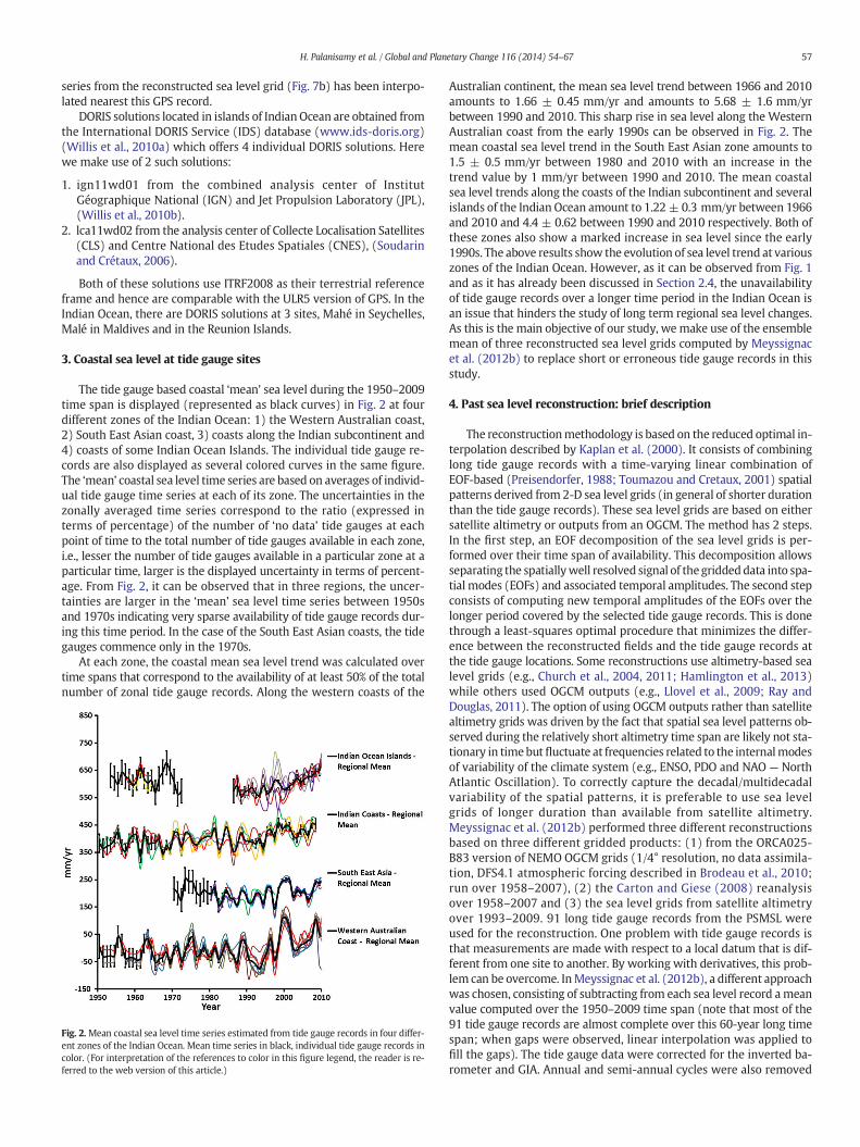
series from the reconstructed sea level grid (Fig. 7b) has been interpo-
lated nearest this GPS record.
DORIS solutions located in islands of Indian Ocean are obtained from
the International DORIS Service (IDS) database (www.ids-doris.org)
(Willis et al., 2010a) which offers 4 individual DORIS solutions. Here
we make use of 2 such solutions:
1. ign11wd01 from the combined analysis center of Institut
Géographique National (IGN) and Jet Propulsion Laboratory (JPL),
(Willis et al., 2010b).
2. lca11wd02 from the analysis center of Collecte Localisation Satellites
(CLS) and Centre National des Etudes Spatiales (CNES), (Soudarin
and Crétaux, 2006).
Both of these solutions use ITRF2008 as their terrestrial reference
frame and hence are comparable with the ULR5 version of GPS. In the
Indian Ocean, there are DORIS solutions at 3 sites, Mahé in Seychelles,
Malé in Maldives and in the Reunion Islands.
3. Coastal sea level at tide gauge sites
The tide gauge based coastal ‘mean’ sea level during the 1950–2009
time span is displayed (represented as black curves) in Fig. 2 at four
different zones of the Indian Ocean: 1) the Western Australian coast,
2) South East Asian coast, 3) coasts along the Indian subcontinent and
4) coasts of some Indian Ocean Islands. The individual tide gauge re-
cords are also displayed as several colored curves in the same figure.
The ‘mean’ coastal sea level time series are based on averages of individ-
ual tide gauge time series at each of its zone. The uncertainties in the
zonally averaged time series correspond to the ratio (expressed in
terms of percentage) of the number of ‘no data’ tide gauges at each
point of time to the total number of tide gauges available in each zone,
i.e., lesser the number of tide gauges available in a particular zone at a
particular time, larger is the displayed uncertainty in terms of percent-
age. From Fig. 2, it can be observed that in three regions, the uncer-
tainties are larger in the ‘mean’ sea level time series between 1950s
and 1970s indicating very sparse availability of tide gauge records dur-
ing this time period. In the case of the South East Asian coasts, the tide
gauges commence only in the 1970s.
At each zone, the coastal mean sea level trend was calculated over
time spans that correspond to the availability of at least 50% of the total
number of zonal tide gauge records. Along the western coasts of the
Australian continent, the mean sea level trend between 1966 and 2010
amounts to 1.66 ± 0.45 mm/yr and amounts to 5.68 ± 1.6 mm/yr
between 1990 and 2010. This sharp rise in sea level along the Western
Australian coast from the early 1990s can be observed in Fig. 2. The
mean coastal sea level trend in the South East Asian zone amounts to
1.5 ± 0.5 mm/yr between 1980 and 2010 with an increase in the
trend value by 1 mm/yr between 1990 and 2010. The mean coastal
sea level trends along the coasts of the Indian subcontinent and several
islands of the Indian Ocean amount to 1.22 ± 0.3 mm/yr between 1966
and 2010 and 4.4 ± 0.62 between 1990 and 2010 respectively. Both of
these zones also show a marked increase in sea level since the early
1990s. The above results show the evolution of sea level trend at various
zones of the Indian Ocean. However, as it can be observed from Fig. 1
and as it has already been discussed in Section 2.4, the unavailability
of tide gauge records over a longer time period in the Indian Ocean is
an issue that hinders the study of long term regional sea level changes.
As this is the main objective of our study, we make use of the ensemble
mean of three reconstructed sea level grids computed by Meyssignac
et al. (2012b) to replace short or erroneous tide gauge records in this
study.
4. Past sea level reconstruction: brief description
The reconstructionmethodology is based on the reduced optimal in-
terpolation described by Kaplan et al. (2000). It consists of combining
long tide gauge records with a time-varying linear combination of
EOF-based (Preisendorfer, 1988; Toumazou and Cretaux, 2001) spatial
patterns derived from 2-D sea level grids (in general of shorter duration
than the tide gauge records). These sea level grids are based on either
satellite altimetry or outputs from an OGCM. The method has 2 steps.
In the first step, an EOF decomposition of the sea level grids is per-
formed over their time span of availability. This decomposition allows
separating the spatiallywell resolved signal of the griddeddata into spa-
tial modes (EOFs) and associated temporal amplitudes. The second step
consists of computing new temporal amplitudes of the EOFs over the
longer period covered by the selected tide gauge records. This is done
through a least-squares optimal procedure that minimizes the differ-
ence between the reconstructed fields and the tide gauge records at
the tide gauge locations. Some reconstructions use altimetry-based sea
level grids (e.g., Church et al., 2004, 2011; Hamlington et al., 2013)
while others used OGCM outputs (e.g., Llovel et al., 2009; Ray and
Douglas, 2011). The option of using OGCM outputs rather than satellite
altimetry grids was driven by the fact that spatial sea level patterns ob-
served during the relatively short altimetry time span are likely not sta-
tionary in timebutfluctuate at frequencies related to the internalmodes
of variability of the climate system (e.g., ENSO, PDO and NAO — North
Atlantic Oscillation). To correctly capture the decadal/multidecadal
variability of the spatial patterns, it is preferable to use sea level
grids of longer duration than available from satellite altimetry.
Meyssignac et al. (2012b) performed three different reconstructions
based on three different gridded products: (1) from the ORCA025-
B83 version of NEMO OGCM grids (1/4° resolution, no data assimila-
tion, DFS4.1 atmospheric forcing described in Brodeau et al., 2010;
run over 1958–2007), (2) the Carton and Giese (2008) reanalysis
over 1958–2007 and (3) the sea level grids from satellite altimetry
over 1993–2009. 91 long tide gauge records from the PSMSL were
used for the reconstruction. One problem with tide gauge records is
that measurements are made with respect to a local datum that is dif-
ferent from one site to another. By working with derivatives, this prob-
lem can be overcome. InMeyssignac et al. (2012b), a different approach
was chosen, consisting of subtracting from each sea level record amean
value computed over the 1950–2009 time span (note that most of the
91 tide gauge records are almost complete over this 60-year long time
span; when gaps were observed, linear interpolation was applied to
fill the gaps). The tide gauge data were corrected for the inverted ba-
rometer and GIA. Annual and semi-annual cycles were also removed
Fig. 2.Mean coastal sea level time series estimated from tide gauge records in four differ-
ent zones of the Indian Ocean. Mean time series in black, individual tide gauge records in
color. (For interpretation of the references to color in this figure legend, the reader is re-
ferred to the web version of this article.)
57H. Palanisamy et al. / Global and Planetary Change 116 (2014) 54–67
and yearly-averages were computed. Each of the three reconstructions
was validated at global scale by comparison with independent tide
gauges not used in the reconstruction process. To do this, for each
case (i.e., for each gridded product), 91 new reconstructions were per-
formed, leaving out successively each one of the 91 tide gauge records
(thus each of these new 91 reconstructions now uses a set of 90 tide
gauges). For each deleted tide gauge, the reconstructed sea level time
series at the tide gauge site was compared with the observed data.
The validation results are discussed in detail in Meyssignac et al.
(2012b). 70% of the reconstructed sea level time series present a corre-
lation coefficient with the observed sea level greater than 0.8 (95%
confidence level) (28% have a correlation between 0.5 and 0.7). The
rootmean squared (rms) differences between (detrended) reconstruct-
ed sea levels and observed sea level time series were compared. 75% of
the rms differences between detrended tide gauge-based and recon-
structed sea level time series are below 30 mm. The uncertainty of
reconstructed sea level trends over the 1950–2009 time span was
found on the order of 0.5 mm/yr. This uncertainty was based on the
sum of errors due to the least-squares method and errors of the tide
gauge records. This latter error was estimated from a bootstrapmethod
(Efron and Tibshirani, 1993) for standard errors of the tide gauge
records for each year (significant at the 95% level). Another way to
check the validity of the new reconstruction was to look at recon-
structed sea level trends over the altimetry period (here 1993–2009)
and compare with altimetry data for which the spatial trend patterns
are trusted. As shown in Meyssignac et al. (2012b), spatial trend maps
agree well over their overlapping periods. Finally, the study of Becker
et al. (2012) compared reconstructed sea level time series with tide
gauge records in the tropical Pacific region not used in the reconstruc-
tion and showed very good agreement between the two sets of data.
Meyssignac et al. (2012b) computed an ensemble mean of the three
reconstructions as well as a map of the associated uncertainty. It is this
reconstruction, called the Mean REconstructed Sea Level, henceforth
MRESL, which we use in the following study.
In the absence of long-term tide gauge records in the Indian
Ocean, the validity of the MRESL in the Indian Ocean was checked by
comparing the MRESL spatial trend pattern over the altimetry period
(here 1993–2009) with the altimetry based spatial trend pattern
(Meyssignac et al., 2012b). This is illustrated in Fig. 3a, b and c which
present the altimetry based and reconstruction based sea level spatial
trend patterns along with the correlation plot. The correlation between
the two spatial trend patterns is 0.64 with level of significance greater
than 95%. Visual inspection also indicates that the spatial trend patterns
agree well. The altimetry based trendmap shows slightly higher ampli-
tude when compared to the reconstruction based trend map. This is
mainly due to the fact that the reconstruction is developed based on
limited set of EOF modes and this act as low pass filter. Nevertheless,
since the reconstruction uses long-term (~50 years) spatial information
from two OGCMs, the decadal natural modes of regional sea level vari-
ability in the Indian Ocean are assumed to be well represented and
therefore suitable for this study.
5. Regional variability of the Indian Ocean
In this section we discuss the spatial trend patterns observed in sea
level and steric data over different time spans.
5.1. Spatial trend patterns over the satellite altimetry period (1993–2009)
and 60-year long time span (1950–2009)
Over the 1993–2009 time span, the sea level trends in most part of
the Indian Ocean remain positive (Fig. 3a and b). The Indian Ocean
mean sea level trend over 1993–2009 amounts to 3.4 ± 0.7 mm/yr
from observed altimetry and 3.0 ± 0.5 mm/yr from reconstruction.
There is also a noticeable high sea level trend pattern below 15°S latitude
extending fromeast towest. This couldbe attributed to the intensification
of trade winds in the Western Tropical Pacific since the recent two
decades (Merrifield and Maltrud, 2011), which as a result has its impact
in the Indian Ocean also. Knowing that the spatial trend patterns are
not stationary but evolve in space and time, sea level spatial trend
patterns in the Indian Ocean over 60 years is studied.
Fig. 4 shows the reconstructed spatial trend patterns in the Indian
Ocean between 1950 and 2009. As in Fig. 3a and b but at smallermagni-
tude, we can also observe patterns of high sea level trend (with maxi-
mum of 3.5 mm/yr) below 15°S latitude along the Eastern Indian
Ocean propagating westward. There are also patterns of higher sea
level trend values along the eastern coasts of African continent and in
central Bay of Bengal and Northern Arabian Sea. Patterns of relatively
lower sea level trends are also seen in the western part of the central
Indian Ocean. Over the period of 60 years, the mean sea level trend in
the Indian Ocean amounts to 1.5 ± 0.5 mm/yr, a value lesser (although
not statistically different) than the global mean sea level rise of 1.8 ±
0.5 mm/yr over the same period as obtained from (Church and White,
2011; Meyssignac et al., 2012b).
Han et al. (2010) have attributed the regional sea level changes in
the Indian Ocean to steric changes in response to surface wind and
Ekman pumping velocity changes. These changes are due to enhance-
ment of Indian Ocean regional Hadley and Walker cells as a result of
Indo-Pacific warming pool. As a result there is a marked pattern of pos-
itive trend values extending from the east toward the west below 15°S
latitude and negative values above (Fig. 1, middle panel of Han et al.
(2010)). This pattern is also exhibited in the MRESL spatial trend map
in Fig. 4 calculated between 1950 and 2009. Since the period of study
in Han et al. (2010) is between 1961 and 2008, MRESL spatial trend
pattern was calculated for the same time period (not shown in this
study) and was found to exhibit similar pattern as that of Han et al.
(2010).
5.2. Steric and Indian Ocean Dipole impact on the Indian Ocean sea level
variability
As steric sea level is the main cause of regional variability of ob-
served sea level, here we analyze the evolution of the steric spatial
patterns.
EOF decomposition of the MRESL and IK12 steric sea level grid for
the Indian Ocean over the 1950–2009 time periods was performed in
order to capture the characteristics of the regional sea level variability.
The mean sea level trend of 1.5 ± 0.5 mm/yr over the Indian Ocean
and the mean steric Indian Ocean trend of 0.2 ± 0.04 mm/yr were re-
moved from the MRESL and IK12 grids respectively before performing
the EOFdecomposition. TheMRESL EOFmodewith 15% of total variance
shows high correlation (correlation 0.8 with significance N 95%) with
the IK12 EOF mode with 17% of total variance (Fig. 5a). This further
validates that the regional sea level variability in the Indian Ocean is
driven by steric changes in response to surface wind and Ekman
pumping velocity changes as mentioned by Han et al. (2010).
In both EOF spatial patterns, we also clearly observe the negative–
positive dipole patterns between the eastern and western parts of the
Indian Ocean indicating the influence of the Indian Ocean Dipole
(IOD) events. IOD event is a coupled ocean–atmosphere phenomenon
which evolves with an east–west dipole Sea Surface Temperature
(SST) anomaly (Saji et al., 1999; Behera and Yamagata, 2001). SST
anomalies during the IOD events are strongly coupled to surface wind
anomalies in the central equatorial Indian Ocean (Saji et al., 1999; Saji
and Yamagata, 2003). However the IOD is a short term event and usual-
ly begins to develop during the summer of the northern hemisphere,
reaches its maximum in fall and ends in winter as a result of strong sea-
sonalwinds (Behera and Yamagata, 2001; Black et al., 2003; Hastenrath,
2007). Even though the spatial patterns in Fig. 5a capture the IOD events
well, the temporal curves being averaged on an annual scale do not cap-
ture the short term IOD events. This is a minor constraint of MRESL grid
available only on annual time scale. In order to capture the short term
58 H. Palanisamy et al. / Global and Planetary Change 116 (2014) 54–67
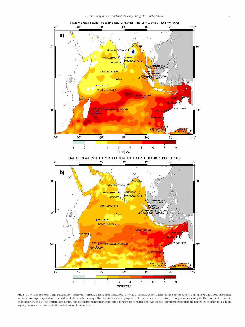
Fig. 3 (a): Map of sea level trend pattern from observed altimetry during 1993 and 2009. (b): Map of reconstruction based sea level trend pattern during 1993 and 2009. Tide gauge
locations are superimposed and marked in black in both the maps. The stars indicate tide gauge records used in mean reconstruction of global sea level grid. The blue circles indicate
co-located GPS and DORIS stations. (c): Correlation plot between reconstruction and altimetry based spatial sea level trends. (For interpretation of the references to color in this figure
legend, the reader is referred to the web version of this article.).
59H. Palanisamy et al. / Global and Planetary Change 116 (2014) 54–67

IOD events on the temporal curve, EOF analysis was performed on the
monthly IK12 steric sea level grid over the Indian Ocean. Fig. 5b shows
spatial pattern and temporal curve of the first EOFmode of themonthly
IK12 steric sea level over 1950–2009. The IOD signals appear stronger in
the first EOF spatial pattern obtained from the monthly data than from
that of the annual IK12 data set. Fig. 5b also shows the correlation (cor-
relation = 0.5 with level of significance N 95%) between the monthly
temporal (with a smoothing of 3 months) curve of IK12 EOF first
mode and the Dipole Mode Index (DMI), implying the link between
the short-term IOD events and steric sea level variability. DMI is a mea-
sure of the anomalous zonal SST gradient across the equatorial Indian
Ocean. It is defined as the difference in SST anomaly between the trop-
ical western Indian Ocean (50°E ± 70°E, 10°S ± 10°N) and the tropical
south-eastern Indian Ocean (90°E ± 110°E, 10°S— Equator) (Saji et al.,
1999).
6. Total climate-related sea level change at coastal and island sites of
the Indian Ocean
In this section, we study the total ‘climate’ related sea level change at
several sites in the Indian Ocean. For this purpose, we take into account
several sites along the coasts of the Indian sub-continent, South-East
Asian coast, Western Australian coast and islands of the Indian Ocean.
Siteswith existing tide gauge recordswere chosen as the points of inter-
est in each of the region of study. As already discussed in Section 3, tide
gauge records do not sufficiently cover the 60 year time period that is
the interest of this study. Therefore, MRESL grid interpolated within a
1° radius of the tide gauge location is used to compute the long-term
climate-related sea level change at those locations. Estimates from
tide gauge records and observed altimetry are also discussed at each
of the zones whenever feasible. Similar to theMRESL grid, the observed
altimetry grid has also been interpolated within a 1° radius of each tide
gauge site thereby giving the observed altimetry sea level time series at
each location.
Figs. 6 and 7 show the interpolated climate-related sea level time se-
ries obtained fromMRESL at several zones of the Indian Ocean. The cor-
responding tide gauge records and interpolated altimetry time series
are also superimposed over the MRESL time series. The figures also dis-
play certain sites with no tide gauge time series. These are the sites
where the sea level recorded by the tide gauges show very high fluctu-
ations (in certain cases as high as 30 cm), and/or highly intermittent.
Some of these do not have data extending into the altimetry period
and hence cannot be verified. Individual case study on each of these
tide gauges is beyond the scope of this study. Hence three such dubious
tide gauge records have been discarded and only the MRESL and
altimetry time series have been studied at these sites.
It can be observed in Figs. 6 and 7 that there are some discrepancies
between theMRESL and tide gauge time series, in terms of interannual/
decadal variability in certain cases and trend values in other cases (as
shown in Table 1). The discrepancies may arise due to the fact that
when the tide gauge records are short (i.e., when data availability is lim-
ited to few years), they are highly dominated by signals related to inter-
annual variability like ENSO or IOD. These signals mask out the long
term decadal sea level trends whereas MRESL, due to its 60 year time
span, captures the low frequency long term decadal sea level trends.
So tide gauges with longer records agree better with MRESL trends
(e.g., Cochin, Vishakaptinam, Paradip, Port Hedland, Bunbury etc.).
Apart from this, even though the GIA related vertical land motion has
been corrected for the tide gauge records, local ground motion impacts
like subsidence due to ground water/hydrocarbon extraction are
reflected in tide gauge records while the MRESL does not contain this
signal. These could further add to the differences in the trend values.
6.1. Coastal zones of Indian sub-continent
Fig. 6a shows the sea level time series obtained by interpolating the
MRESL corresponding to several sites chosen along the coastal regions
of the Indian sub-continent. Available tide gauge records and the inter-
polated observed altimetry time series have also been superimposed to
the MRESL time series. The mean rms difference between tide gauges
andMRESL in this zone amounts to 2.9 cm.We observe that themagni-
tude of the interannual variability exhibited by the sites located on the
western coast is lesser than that of the sites on the eastern coast. This
was mathematically quantified by calculating the standard deviation
of the interannual anomalies of the sites located on the western and
eastern coasts. The mean of the standard deviations of the MRESL time
series of the sites on thewestern coast is 26 mm against themean stan-
dard deviation value of 30mmon the eastern coasts. The sea level trend
over a period of 60 years (1950–2009) along the Indian coasts ranges
between 1.3 mm/yr and 1.7 mm/yr with the maximum trend rate of
1.7 mm/yr observed at Chennai on the eastern coast. Table 1 lists the
different locations and the trend values that have been studied.
6.2. South East Asian coasts
Fig. 6b shows theMRESL, tide gauge andobserved altimetry sea level
time series at various locations on the coastal zones of South East Asia.
The mean rms difference between MRESL and tide gauges amounts to
2.8 cm. Over 60 years, the sea level rate calculated from MRESL at
these sites range between 1.4 mm/yr and 1.6 mm/yr. However, since
the two recent decades, the sites at the South East Asian coasts exhibit
an increased rate of sea level. For example, between 1950 and 2009,
the MRESL trend at Sultan Shoal amounts to 1.5 ± 0.5 mm/yr whereas
at the same location, the MRESL trend over 1992–2009 period is
4.0 ± 0.7 mm/yr. The tide gauge sea level trend at Sultan Shoal
between 1992 and 2009 is 1.8 mm/yr. For the same time period,
at Sultan Shoal, altimetry data also exhibits high sea level trend of
3.9 ± 1.3 mm/yr which is consistent with the MRESL trend value.
The higher rate of sea level rise since two decades in South East
Asia is similar to that exhibited in the Western Tropical Pacific as
in Merrifield and Maltrud (2011) thereby indicating the influence
of Western Tropical Pacific trade wind intensification along the
coastal zones of South East Asia.
6.3. Western Australian coast
Fig. 7a shows individual MRESL sea level time series over 60 years
with tide gauge records and observed altimetry time series super-
imposed at sites along theWestern Australian coast. The mean rms dif-
ference between the tide gauges andMRESL is 2.8 cm. In Fig. 7a, we can
Fig. 3 (continued).
60 H. Palanisamy et al. / Global and Planetary Change 116 (2014) 54–67

observe that between 1950 and the beginning of 1990s, the sea level
trend at every site is almost flat whereas from the 1990s, there is a
steep increase in the sea level rise rates in all the stations. To verify
this, mean sea level trends were calculated prior to and after 1990s
from available tide gauges and MRESL time series. Mean sea level
trend from tide gauges available between 1966 (as most of the records
start only in the1960s) and 1991 amounts to 0.6± 0.8 mm/yr, whereas
between 1992 and 2009 (100% availability of tide gauges), the mean
trend amounts to 5.5 ± 1.6 mm/yr. The tide gauge records clearly
show a marked increase in sea level rate since 1990s. The mean of
MRESL trend values along the western coast during 1950–1991
amounts to 0.8 ± 0.3 mm/yr. Between 1992 and 2009, the mean
MRESL trend value amounts to 5.5 ± 1.7 mm/yr. Over the same
time period, the mean altimetry sea level trend at this zone is 5.6 ±
2 mm/yr. The trend values from MRESL and altimetry are consistent
with each other. As in the case of tide gauges, the MRESL also shows a
marked increase in sea level trend since the 1990s when compared to
the previous decades. This is also consistent with the spatial trend pat-
terns showing high sea level trends during 1992–2009 along theWest-
ern Australian coasts observed in Fig. 3a and b. And as discussed in
Section 5, the sudden increase in the sea level trend seen in these sites
since the two recent decades is attributed to the enhancement in the
Walker and Hadley cells Indo Pacific warm pool warming (Han et al.,
2010).Moreover, the interannual sea level variability along theWestern
Australian coasts prior to 1970 is lesser than that of the variability after
1970. The mean of the standard deviation of interannual anomalies at
the individual stations prior to 1970 is 14 mm whereas after 1970 it is
42 mm as calculated from the MRESL. This remains true with the stan-
dard deviation values obtained from tide gauge records wherever they
extend prior to 1970s. Similar phenomenon has also been observed in
the western tropical Pacific as noted by Church et al. (2006) and
Becker et al. (2012).
6.4. Indian Ocean Islands
Fig. 7b shows the long term sea level time series of Indian Ocean
islands. Even though lacking a tide gauge site, MRESL time series has
been interpolated at Le Tampon in the Reunion Island as there are GPS
andDORISmeasures at this site and henceforth are useful in the estima-
tion of total relative sea level change (Section 8). The tide gauges and
MRESL exhibit a mean rms difference of 3.5 cm. Rodrigues Island, Port
Louis (Mauritius), Le Tampon (Reunion) lying below the 15°S and
Nosy Be (Madagascar) at 13°S show very similar sea level variability
(correlation exceeding 0.9 with significance greater than 95%) over the
entire period between 1950 and 2009 estimated from the MRESL time
series. This similarity in sea level variability is consistentwith the results
of Church et al. (2006) between Port Louis and Rodrigues Island. Church
et al. (2006) mention a lag of 2 months between the two sites which
however is not visible in our result as the data used in this study is at
an annual sampling. In order to verify theMRESL results and also to con-
firm the2 months lagmentioned byChurchet al. (2006), we studied the
monthly tide gauge records at Rodrigues Island and Port Louis between
1988 and 2009. The two tide gauge time series are highly correlated
(correlation 0.9 with significance greater than 95%) with Port Louis
tide gauge time series lagging Rodrigues by 2 months. This is consistent
with MRESL results and Church et al. (2006).
The location of Rodrigues, Port Louis, Le Tampon and Nosy Be below
the 15°S latitude band also corresponds to the pattern of high sea level
Fig. 4.Map of sea level trend patterns fromMean Reconstructed Sea Level grid during 1950–2009 with tide gauge sites superimposed as black circles. Co-located GPS and DORIS stations
are represented in blue whereas black stars indicate the tide gauge records used in the global reconstruction grid. (For interpretation of the references to color in this figure legend, the
reader is referred to the web version of this article.)
61H. Palanisamy et al. / Global and Planetary Change 116 (2014) 54–67
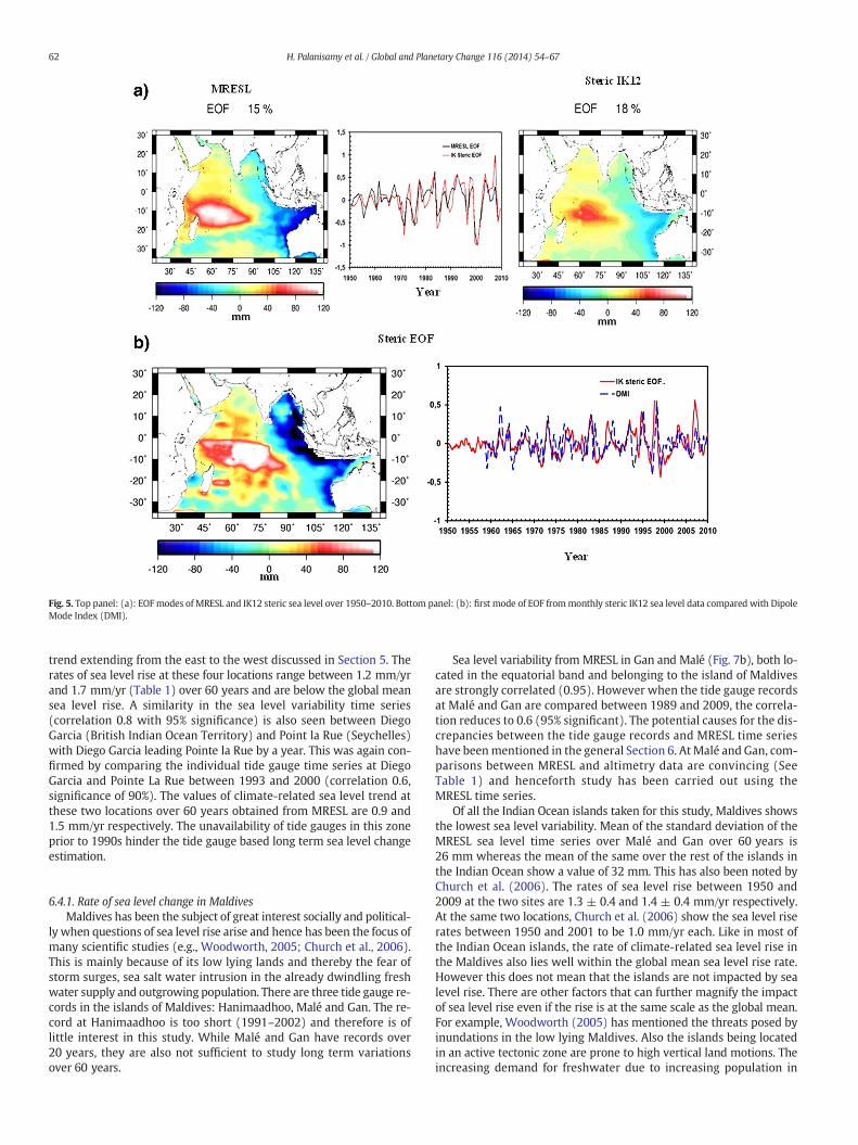
trend extending from the east to the west discussed in Section 5. The
rates of sea level rise at these four locations range between 1.2 mm/yr
and 1.7 mm/yr (Table 1) over 60 years and are below the global mean
sea level rise. A similarity in the sea level variability time series
(correlation 0.8 with 95% significance) is also seen between Diego
Garcia (British Indian Ocean Territory) and Point la Rue (Seychelles)
with Diego Garcia leading Pointe la Rue by a year. This was again con-
firmed by comparing the individual tide gauge time series at Diego
Garcia and Pointe La Rue between 1993 and 2000 (correlation 0.6,
significance of 90%). The values of climate-related sea level trend at
these two locations over 60 years obtained from MRESL are 0.9 and
1.5 mm/yr respectively. The unavailability of tide gauges in this zone
prior to 1990s hinder the tide gauge based long term sea level change
estimation.
6.4.1. Rate of sea level change in Maldives
Maldives has been the subject of great interest socially and political-
ly when questions of sea level rise arise and hence has been the focus of
many scientific studies (e.g., Woodworth, 2005; Church et al., 2006).
This is mainly because of its low lying lands and thereby the fear of
storm surges, sea salt water intrusion in the already dwindling fresh
water supply and outgrowing population. There are three tide gauge re-
cords in the islands of Maldives: Hanimaadhoo, Malé and Gan. The re-
cord at Hanimaadhoo is too short (1991–2002) and therefore is of
little interest in this study. While Malé and Gan have records over
20 years, they are also not sufficient to study long term variations
over 60 years.
Sea level variability from MRESL in Gan and Malé (Fig. 7b), both lo-
cated in the equatorial band and belonging to the island of Maldives
are strongly correlated (0.95). However when the tide gauge records
at Malé and Gan are compared between 1989 and 2009, the correla-
tion reduces to 0.6 (95% significant). The potential causes for the dis-
crepancies between the tide gauge records and MRESL time series
have beenmentioned in the general Section 6. AtMalé and Gan, com-
parisons between MRESL and altimetry data are convincing (See
Table 1) and henceforth study has been carried out using the
MRESL time series.
Of all the Indian Ocean islands taken for this study, Maldives shows
the lowest sea level variability. Mean of the standard deviation of the
MRESL sea level time series over Malé and Gan over 60 years is
26 mm whereas the mean of the same over the rest of the islands in
the Indian Ocean show a value of 32 mm. This has also been noted by
Church et al. (2006). The rates of sea level rise between 1950 and
2009 at the two sites are 1.3 ± 0.4 and 1.4 ± 0.4 mm/yr respectively.
At the same two locations, Church et al. (2006) show the sea level rise
rates between 1950 and 2001 to be 1.0 mm/yr each. Like in most of
the Indian Ocean islands, the rate of climate-related sea level rise in
the Maldives also lies well within the global mean sea level rise rate.
However this does not mean that the islands are not impacted by sea
level rise. There are other factors that can further magnify the impact
of sea level rise even if the rise is at the same scale as the global mean.
For example, Woodworth (2005) has mentioned the threats posed by
inundations in the low lying Maldives. Also the islands being located
in an active tectonic zone are prone to high vertical land motions. The
increasing demand for freshwater due to increasing population in
Fig. 5. Top panel: (a): EOFmodes of MRESL and IK12 steric sea level over 1950–2010. Bottom panel: (b): first mode of EOF frommonthly steric IK12 sea level data compared with Dipole
Mode Index (DMI).
62 H. Palanisamy et al. / Global and Planetary Change 116 (2014) 54–67
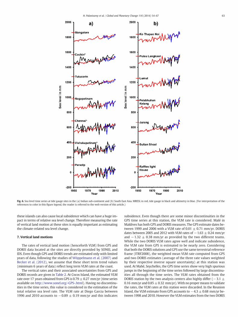
these islands can also cause local subsidencewhich can have a huge im-
pact in terms of relative sea level change. Therefore measuring the rate
of vertical land motion at these sites is equally important as estimating
the climate-related sea level change.
7. Vertical land motions
The rates of vertical land motion (henceforth VLM) from GPS and
DORIS data located at the sites are directly provided by SONEL and
IDS. Even though GPS and DORIS trends are estimated only with limited
years of data, following the studies of Wöppelmann et al. (2007) and
Becker et al. (2012), we assume that these short term trend values
(minimum 6 years of data) reflect long term VLM rates at the coast.
The vertical rates and their associated uncertainties from GPS and
DORIS records are given in Table 2. At Cocos Island, the estimated VLM
rate over 17 years obtained fromGPS is 0.79± 0.27 mm/yr (time series
available on http://www.sonel.org/-GPS-.html). Having no discontinu-
ities in the time series, this value is considered in the estimation of the
total relative sea level rate. The VLM rate at Diego Garcia between
1996 and 2010 accounts to −0.89 ± 0.19 mm/yr and this indicates
subsidence. Even though there are some minor discontinuities in the
GPS time series at this station, the VLM rate is considered. Malé in
Maldives has both GPS andDORISmeasures. The GPS estimate dates be-
tween 1999 and 2006 with a VLM rate of 0.01 ± 0.71 mm/yr. DORIS
dates between 2005 and 2012 with VLM rates of −1.63 ± 0.24 mm/yr
and −1.32 ± 0.38 mm/yr as provided by the two different teams.
While the two DORIS VLM rates agree well and indicate subsidence,
the VLM rate from GPS is estimated to be nearly zero. Considering
that both theDORIS solutions andGPSuse the same terrestrial reference
frame (ITRF2008), the weighted mean VLM rate computed from GPS
and two DORIS estimates (average of the three rate values weighted
by their respective inverse square uncertainty) at this station was
used. At Mahé, Seychelles, the GPS time series show very high spurious
jumps in the beginning of the time series followed by large discontinu-
ities all through the time series. The VLM rates obtained from the
DORIS station by the two analysis centers also highly differ (−3.1 ±
0.16 mm/yr and 0.85±0.32 mm/yr).With nopropermeans to validate
the rates, the VLM rates at this station were discarded. In the Reunion
Island, the VLM estimate fromGPS accounts to−4.3± 0.68 mm/yr be-
tween 1998 and 2010. However the VLM estimates from the two DORIS
Fig. 6. Sea level time series at tide gauge sites in the (a) Indian sub-continent and (b) South East Asia. MRESL in red, tide gauge in black and altimetry in blue. (For interpretation of the
references to color in this figure legend, the reader is referred to the web version of this article.)
63H. Palanisamy et al. / Global and Planetary Change 116 (2014) 54–67
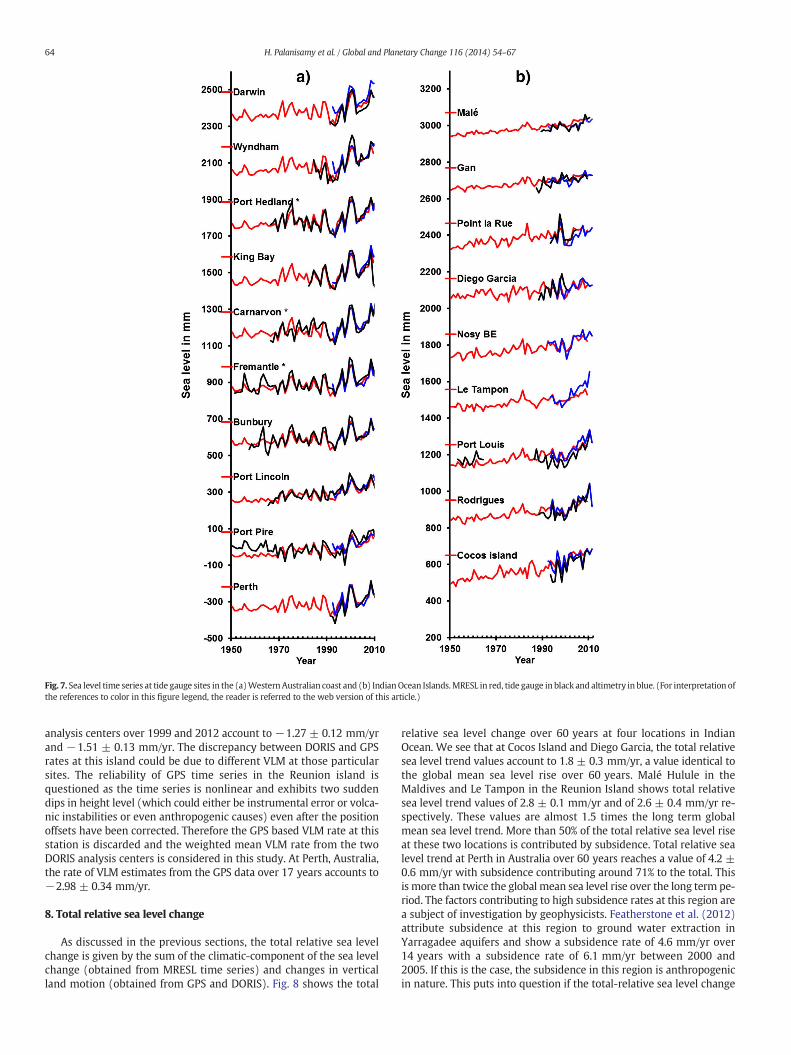
analysis centers over 1999 and 2012 account to −1.27 ± 0.12 mm/yr
and −1.51 ± 0.13 mm/yr. The discrepancy between DORIS and GPS
rates at this island could be due to different VLM at those particular
sites. The reliability of GPS time series in the Reunion island is
questioned as the time series is nonlinear and exhibits two sudden
dips in height level (which could either be instrumental error or volca-
nic instabilities or even anthropogenic causes) even after the position
offsets have been corrected. Therefore the GPS based VLM rate at this
station is discarded and the weighted mean VLM rate from the two
DORIS analysis centers is considered in this study. At Perth, Australia,
the rate of VLM estimates from the GPS data over 17 years accounts to
−2.98 ± 0.34 mm/yr.
8. Total relative sea level change
As discussed in the previous sections, the total relative sea level
change is given by the sum of the climatic-component of the sea level
change (obtained from MRESL time series) and changes in vertical
land motion (obtained from GPS and DORIS). Fig. 8 shows the total
relative sea level change over 60 years at four locations in Indian
Ocean. We see that at Cocos Island and Diego Garcia, the total relative
sea level trend values account to 1.8 ± 0.3 mm/yr, a value identical to
the global mean sea level rise over 60 years. Malé Hulule in the
Maldives and Le Tampon in the Reunion Island shows total relative
sea level trend values of 2.8 ± 0.1 mm/yr and of 2.6 ± 0.4 mm/yr re-
spectively. These values are almost 1.5 times the long term global
mean sea level trend. More than 50% of the total relative sea level rise
at these two locations is contributed by subsidence. Total relative sea
level trend at Perth in Australia over 60 years reaches a value of 4.2 ±
0.6 mm/yr with subsidence contributing around 71% to the total. This
is more than twice the global mean sea level rise over the long term pe-
riod. The factors contributing to high subsidence rates at this region are
a subject of investigation by geophysicists. Featherstone et al. (2012)
attribute subsidence at this region to ground water extraction in
Yarragadee aquifers and show a subsidence rate of 4.6 mm/yr over
14 years with a subsidence rate of 6.1 mm/yr between 2000 and
2005. If this is the case, the subsidence in this region is anthropogenic
in nature. This puts into question if the total-relative sea level change
Fig. 7. Sea level time series at tide gauge sites in the (a)Western Australian coast and (b) IndianOcean Islands.MRESL in red, tide gauge in black and altimetry in blue. (For interpretation of
the references to color in this figure legend, the reader is referred to the web version of this article.)
64 H. Palanisamy et al. / Global and Planetary Change 116 (2014) 54–67
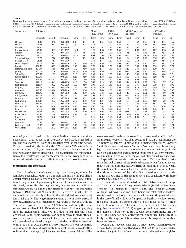
over 60 years calculated in this study at Perth is overestimated since
subsidence is anthropogenic in nature. A detailed study is needed in
this zone to analyze the rates of subsidence over longer time period.
For now, considering the fact that the GPS estimated VLM rate at Perth
covers a period of 17 years, we use the same to calculate the total-
relative sea level change. However it is highly probable that this estima-
tion of total relative sea level change over the long term period at Perth
is overestimated and may not reflect the exact scenario of the past.
9. Summary and conclusion
The Indian Ocean is the home to many tropical low lying islands like
Maldives, Seychelles, Mauritius, and Reunion and highly populated
coastal regions like Bangladesh which have been gaining a lot of atten-
tion during the recent years owing to sea level rise and its impacts. In
this work, we studied the long term regional sea level variability in
the Indian Ocean. We find that the mean sea level rise over this region
between 1950 and 2009 amounts to 1.5 mm/yr, a value lesser
(although not statistically different) than the global mean sea level
rise of 1.8 mm/yr. The long term spatial trend patterns show eastward
to westward increase in regional sea level trend below 15°S latitude.
This pattern grows stronger from 1993 thereby confirming the influ-
ence of Western Tropical Pacific trade wind intensification propagating
into the Indian Ocean also. We also determined that the steric
and IndianOceanDipole events play an important role in driving the cli-
matic component of the sea level change in the Indian Ocean. Total
climate-related sea level change is also studied in different regions
within the Indian Ocean between 1950 and 2009 and was found that
in most cases, the total climate-related sea level change lies well within
or lesser than the range of global mean sea level rise over 60 years. The
mean sea level trends in the coastal Indian-subcontinent, South-East
Asian coasts, Western Australian coasts and Indian Ocean Islands are
1.4 mm/yr, 1.5 mm/yr, 1.3 mm/yr and 1.5 mm/yr respectively. However
South-East Asian locations and Western Australian coast showed very
high sea level trends during the two recent decades (3.5 mm/yr in the
case of South East Asia and 5.5 mm/yr in the case of Western Australia)
presumably linked toWestern Tropical Pacific tradewind intensification.
A special focus was also made in the case of Maldives Island to esti-
mate the total-climate related sea level change. It was found that even
though there is a positive sea level trend at this location over 60 years,
the variability of interannual sea level at this island was found lower
than those in the rest of the Indian Ocean considered in this study.
The results obtained at this location were also consistent with those
obtained by Church et al. (2006).
In this study, we also estimated the total relative sea level change
at 5 locations: Cocos and Diego Garcia Islands (British Indian Ocean
Territory), Le Tampon in Reunion Islands and Perth in Western
Australia. In Cocos Island and Diego Garcia, the total relative sea level
rise is equal to the global mean sea level rise over 60 years whereas
in the case of Malé Hulule, Le Tampon and Perth, the values exceed
the global mean. The contribution of subsidence at Malé Hulule
and Le Tampon exceed 50% while at Perth, it exceeds 70%. Studies
(e.g. Featherstone et al., 2012) suggest ground water extraction as
the main contributor to the land subsidence in Perth indicating the
cause of subsidence to be anthropogenic in nature. Therefore it is
likely that the long term total-relative sea level change at this location
is overestimated.
Overall, this study demonstrates the importance of regional sea level
variability. Our results show that during 1950–2009, the climate-related
sea level change in IndianOcean is in the same order as that of the global
Table 1
Locations of tide gauge records in IndianOceanwith their respective trend and error values. Trends and error values are also obtained fromobserved altimetry between 1992 and 2009 and
MRESL records over 1950–2010, tide gauge time span and altimetry time span. The stars indicate the sites used in developing theMRESL grids. The symbol * replaces values that could not
be calculated due to tide gauge records that were intermittent/absent. CF corresponds to Correlation Factor, which is a measure of correlation existing between two data sets.
Station name Tide gauge Altimetry
(1992–2009)
MRESL
1950–2009
MRESL (tide gauge
time span)
MRESL (altimetry
time span)
Longitude Latitude Time span Trend Error Trend Error Trend Error Trend Error CF Trend Error CF
Chennai⋆ 80.30 13.10 1950–2008 0.4 0.3 0.87 1.5 1.70 0.51 1.63 0.52 0.58 2.04 0.75 0.55
Cochin⋆ 76.27 9.97 1950–2007 1.2 0.2 2.18 0.77 1.40 0.51 1.39 0.51 0.66 1.81 0.60 0.68
Mangalore 74.80 12.92 1976–2000 * * 1.56 0.82 1.40 0.51 1.41 0.61 * 1.72 0.63 0.50
Nagapattinam 79.85 10.77 1971–1989 −2.4 1.3 2.28 1.46 1.40 0.51 1.53 1.00 0.56 1.87 0.76 0.59
Paradip 86.70 20.27 1966–2008 1.3 0.5 0.28 1.9 1.40 0.54 1.58 0.59 0.74 1.84 0.93 0.54
Tutucorin 78.20 8.75 1964–1991 −1.3 0.4 1.64 0.65 1.40 0.51 0.98 0.65 −0.02 1.70 0.58 0.56
Vishakapattinam⋆ 83.28 17.68 1957–2008 1.1 0.3 2.86 1.46 1.30 0.51 1.24 0.52 0.77 2.18 0.95 0.78
Ko Taphao Noi 98.43 7.83 1950–2010 * * 2.51 1.5 1.40 0.54 1.40 0.52 * 2.80 0.84 0.68
Pulau Langkawi 99.77 6.43 1986–2010 1.80 0.90 2.72 1.55 1.50 0.54 3.11 0.73 0.70 2.93 0.87 0.73
Lumut 100.62 4.23 1984–2010 1.00 0.80 3.79 1.60 1.50 0.54 2.28 0.85 0.74 3.38 0.99 0.73
Pelabhuhan Kelang 101.37 3.05 1984–2010 1.50 0.90 3.25 1.57 1.40 0.51 2.10 0.79 0.75 3.29 0.97 0.61
Jurang 103.72 1.30 1970–1997 −0.90 0.70 4.57 1.39 1.50 0.51 0.71 0.58 0.26 4.03 0.64 0.72
Sultan Shoal 103.65 1.23 1969–2011 2.10 0.53 3.90 1.32 1.50 0.51 2.73 0.59 0.64 4.04 0.64 0.71
Raffles light house 103.75 1.17 1973–2011 0.40 0.50 4.21 1.38 1.60 0.51 2.92 0.59 0.65 3.99 0.67 0.67
Darwin 130.85 −12.47 1991–2011 6.90 1.90 7.44 2.35 1.40 0.58 7.49 1.58 0.94 6.91 1.71 0.90
Wyndham 128.10 −15.45 1984–2010 6.20 1.70 6.69 2.13 1.40 0.58 3.74 1.25 0.88 6.89 1.77 0.91
Port Hedland⋆ 118.57 −20.32 1966–2010 1.60 0.60 5.91 2.52 1.40 0.58 1.57 0.71 0.93 5.79 2.15 0.96
King Bay 116.75 −20.62 1982–2010 2.30 1.30 7.77 2.40 1.50 0.58 3.99 1.15 0.90 6.49 2.14 0.95
Carnarvon⋆ 113.65 −24.90 1965–2010 2.10 0.56 6.16 2.40 1.30 0.58 1.63 0.71 0.83 6.02 2.24 0.97
Fremantle⋆ 115.75 −32.07 1897–2010 1.40 0.30 3.85 2.34 1.20 0.54 1.18 0.55 0.93 4.91 1.90 0.93
Hillarys/Perth 115.74 −31.83 1991–2011 7.20 1.80 4.92 1.83 1.20 0.54 6.55 1.76 0.96 4.91 1.90 0.92
Bunbury 115.66 −33.32 1957–2010 1.34 0.37 4.34 1.87 1.10 0.54 1.22 0.58 0.86 4.99 1.85 0.97
Port Lincoln 135.87 −34.72 1965–2010 2.10 0.30 4.48 1.31 1.40 0.54 1.55 0.58 0.86 4.00 1.29 0.90
Port Pire 138.01 −33.18 1950–2010 0.80 0.30 4.57 1.01 1.40 0.54 1.42 0.53 0.65 3.98 1.20 0.84
Male-B Hulule 73.53 4.18 1989–2010 2.90 0.60 2.07 0.82 1.40 0.51 1.98 0.61 0.72 2.07 0.70 0.74
Gan 73.15 −0.68 1987–2009 2.80 0.64 1.79 0.96 1.30 0.51 1.81 0.60 0.43 1.76 0.71 0.65
Point la Rue 55.53 −4.67 1993–2004 1.85 4.10 1.51 1.94 1.50 0.54 0.88 2.71 0.76 1.65 1.38 0.74
Diego Garcia 72.40 −7.28 1988–2000 6.41 2.78 3.26 1.64 0.90 0.54 −4.10 1.85 −0.02 2.21 1.29 0.56
Nosy B 48.28 −13.40 1958–1972 * * 4.11 1.81 1.50 0.54 −0.59 1.05 * 2.65 1.25 0.89
Le Tampon 55.57 −21.21 * * * 7.50 1.50 1.20 0.65 * * * 1.72 1.21 0.32
Port Louis 57.50 −20.15 1986–2011 2.60 1.08 7.25 1.32 1.70 0.51 2.80 0.81 0.68 3.81 1.13 0.82
Rodrigues Island 63.42 −19.67 1986–2011 3.60 1.10 5.09 1.57 1.60 0.51 2.46 0.96 0.81 3.21 1.27 0.73
Cocos island 96.89 −12.12 1993–2011 8.29 1.89 4.20 1.40 2.60 0.54 5.36 1.19 0.84 5.50 1.08 0.74
65H. Palanisamy et al. / Global and Planetary Change 116 (2014) 54–67
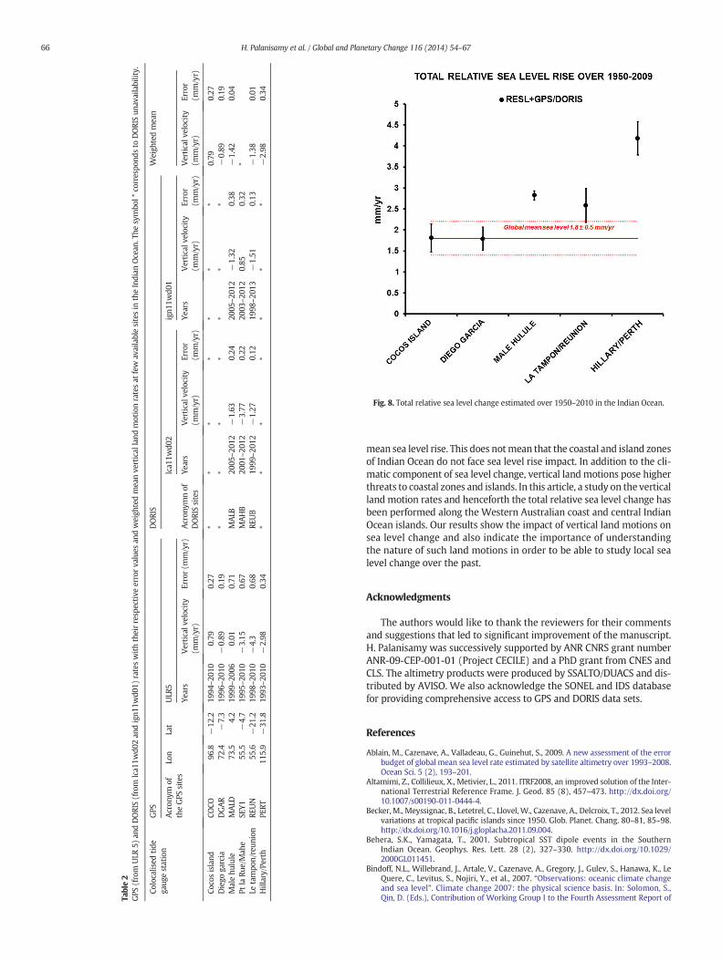
mean sea level rise. This does notmean that the coastal and island zones
of Indian Ocean do not face sea level rise impact. In addition to the cli-
matic component of sea level change, vertical landmotions pose higher
threats to coastal zones and islands. In this article, a study on the vertical
land motion rates and henceforth the total relative sea level change has
been performed along the Western Australian coast and central Indian
Ocean islands. Our results show the impact of vertical land motions on
sea level change and also indicate the importance of understanding
the nature of such land motions in order to be able to study local sea
level change over the past.
Acknowledgments
The authors would like to thank the reviewers for their comments
and suggestions that led to significant improvement of the manuscript.
H. Palanisamy was successively supported by ANR CNRS grant number
ANR-09-CEP-001-01 (Project CECILE) and a PhD grant from CNES and
CLS. The altimetry products were produced by SSALTO/DUACS and dis-
tributed by AVISO. We also acknowledge the SONEL and IDS database
for providing comprehensive access to GPS and DORIS data sets.
References
Ablain, M., Cazenave, A., Valladeau, G., Guinehut, S., 2009. A new assessment of the errorbudget of global mean sea level rate estimated by satellite altimetry over 1993–2008.Ocean Sci. 5 (2), 193–201.
Altamimi, Z., Collilieux, X., Metivier, L., 2011. ITRF2008, an improved solution of the Inter-national Terrestrial Reference Frame. J. Geod. 85 (8), 457–473. http://dx.doi.org/10.1007/s00190-011-0444-4.
Becker, M., Meyssignac, B., Letetrel, C., Llovel,W., Cazenave, A., Delcroix, T., 2012. Sea levelvariations at tropical pacific islands since 1950. Glob. Planet. Chang. 80–81, 85–98.http://dx.doi.org/10.1016/j.gloplacha.2011.09.004.
Behera, S.K., Yamagata, T., 2001. Subtropical SST dipole events in the SouthernIndian Ocean. Geophys. Res. Lett. 28 (2), 327–330. http://dx.doi.org/10.1029/2000GL011451.
Bindoff, N.L., Willebrand, J., Artale, V., Cazenave, A., Gregory, J., Gulev, S., Hanawa, K., LeQuere, C., Levitus, S., Nojiri, Y., et al., 2007. “Observations: oceanic climate changeand sea level”. Climate change 2007: the physical science basis. In: Solomon, S.,Qin, D. (Eds.), Contribution of Working Group I to the Fourth Assessment Report ofT
able
2
GPS(from
ULR
5)an
dDORIS
(from
lca1
1wd02an
dign11wd01)rateswiththeirresp
ectiveerrorvalues
andweightedmea
nverticallandmotionratesat
few
available
sitesin
theIndianOcean
.Thesymbol*co
rrespondsto
DORIS
unav
ailability.
Colocalisedtide
gau
gestation
GPS
DORIS
Weightedmea
n
Acronym
of
theGPSsites
Lon
Lat
ULR
5lca1
1wd02
ign11wd01
Yea
rsVerticalvelocity
(mm/yr)
Error(m
m/yr)
Acronymnof
DORIS
sites
Years
Verticalvelocity
(mm/yr)
Error
(mm/yr)
Years
Verticalvelocity
(mm/yr)
Error
(mm/yr)
Verticalvelocity
(mm/yr)
Error
(mm/yr)
Coco
sisland
COCO
96.8
−12.2
1994–2010
0.79
0.27
**
**
**
*0.79
0.27
Diegogarcia
DGAR
72.4
−7.3
1996–2010
−0.89
0.19
**
**
**
*−
0.89
0.19
Malehulule
MALD
73.5
4.2
1999–2006
0.01
0.71
MALB
2005–2012
−1.63
0.24
2005–2012
−1.32
0.38
−1.42
0.04
Ptla
Rue/Mah
eSE
Y1
55.5
−4.7
1995–2010
−3.15
0.67
MAHB
2001–2012
−3.77
0.22
2003–2012
0.85
0.32
*
Letampon/reu
nion
REUN
55.6
−21.2
1998–2010
−4.3
0.68
REUB
1999–2012
−1.27
0.12
1998–2013
−1.51
0.13
−1.38
0.01
Hillary/Perth
PERT
115.9
−31.8
1993–2010
−2.98
0.34
**
**
**
*−
2.98
0.34
Fig. 8. Total relative sea level change estimated over 1950–2010 in the Indian Ocean.
66 H. Palanisamy et al. / Global and Planetary Change 116 (2014) 54–67
the Intergovernmental Panel on Climate Change. M. Cambridge University Press,Cambridge.
Bird, E.C.F., 1996. Coastal erosion and rising sea level. In: Millimann, J.D., Haq, B.U. (Eds.),Sea Level Rise and Coastal Subsidence. Kluwer Academic Publishers, Dordrecht, theNetherlands, pp. 87–103.
Black, E., Slingo, J., Sperber, K.R., 2003. An observational study of the relationship betweenexcessively strong short rains in coastal East Africa and Indian Ocean SST. Mon.Weather Rev. 131 (1), 74–94. http://dx.doi.org/10.1175/1520-0493(2003) 131.
Brodeau, L., Barnier, B., Treguier, A.M., Penduff, T., Gulev, S., 2010. An ERA40-based atmo-spheric forcing for global ocean circulation models. Ocean Model. 31, 88–104.
Bruun, P., 1962. Sea-level rise as a cause of shoreline erosion. J. Waterw. Harb. Div. 88(1–3), 117–130.
Busalacchi, A.J., Cane, M.A., 1985. Hindcasts of sea level variations during the 1982–83 ElNiño. J. Phys. Oceanogr. 15, 213–221.
Carton, J.A., Giese, B.S., 2008. A reanalysis of ocean climate using Simple Ocean DataAssimilation (SODA). Mon. Weather Rev. 136 (8), 2999–3017. http://dx.doi.org/10.1175/2007MWR1978.1.
Cazenave, A., Llowel, W., 2010. Contemporary sea level rise Annual Review of MarineScience 2, 145–173.
Chao, Y., Halpern, D., Perigaud, C., 1993. Sea surface height variability during 1986–1988in the Tropical Pacific Ocean. J. Geophys. Res. 98 (C4), 6947–6959. http://dx.doi.org/10.1029/92JC02984.
Church, J.A., White, N.J., 2011. Sea-level rise from the late 19th to the early 21st century.Surv. Geophys. 32 (4–5), 585–602. http://dx.doi.org/10.1007/s10712-011-9119-1.
Church, J.A., White, N.J., Coleman, R., Lambeck, K., Mitrovica, J.X., 2004. Estimates of the re-gional distribution of sea level rise over the 1950–2000 period. J. Clim. 17, 2609–2625.
Church, J.A., White, N.J., Hunter, J.R., 2006. Sea-level rise at tropical Pacific and IndianOcean islands. Glob. Planet. Chang. 53 (3), 155–168. http://dx.doi.org/10.1016/j.gloplacha.2006.04.001.
Church, J.A., Gregory, J.M., White, N.J., Platten, S.M., Mitrovica, J.X., 2011. Understandingand projecting sea level change. Oceanography 24 (2), 130–143.
Delcroix, T., 1998. Observed surface oceanic and atmospheric variability in the tropicalPacific at seasonal and ENSO timescales: a tentative overview. J. Geophys. Res. 103(C9), 18611–18633.
Efron, B., Tibshirani, R.J., 1993. An Introduction to the Bootstrap. Chapman & Hall.Featherstone,W.E., Filmer, M.S., Penna, N.T.,Morgan, L.M., Schenk, A., 2012. Anthropogen-
ic land subsidence in the Perth Basin: challenges for its retrospective geodetic detec-tion. J. R. Soc. West. Aust. 95, 53–62.
Hamlington, B.D., Leben, R.R., Nerem, R.S., Han, W., Kim, K.-Y., 2011. Reconstructing sealevel using cyclostationary empirical orthogonal functions. J. Geophys. Res. Oceans116. http://dx.doi.org/10.1029/2011JC007529.
Hamlington, B.D., Leben, R.R., Strassburg, M.W., Nerem, R.S., Kim, K.-Y., 2013. Contributionof the Pacific Decadal Oscillation to global mean sea level trends. Geophys. Res. Lett.40, 5171–5175. http://dx.doi.org/10.1002/grl.50950.
Han, W., Meehl, G.A., Rajagopalan, B., Fasullo, J.T., Hu, A., Lin, J., Large, W.G., et al., 2010.Patterns of Indian Ocean sea-level change in a warming climate. Nat. Geosci. 3 (8),546–550. http://dx.doi.org/10.1038/ngeo901.
Hanna, E., Navarro, F.J., Pattyn, F., Domingues, C., Fettweis, X., Ivins, E., Nicholls, R.J., Ritz, C.,Smith, B., Tulaczyk, S., Whitehouse, P., Zwally, J., 2013. Ice-sheet mass balance andclimate change. Nature 498, 51–59. http://dx.doi.org/10.1038/nature12238.
Hastenrath, S., 2007. Circulation mechanisms of climate anomalies in East Africa and theEquatorial Indian Ocean. Dyn. Atmos. Oceans 43 (1–2), 25–35. http://dx.doi.org/10.1016/j.dynatmoce.2006.06.002.
Hendricks, J.R., Leben, R.R., Born, G.H., Koblinsky, C.J., 1996. Empirical orthogonal functionanalysis of global TOPEX/POSEIDON altimeter data and implications for detection ofglobal sea level rise. J. Geophys. Res. 101 (C6), 14,131–14,145. http://dx.doi.org/10.1029/96JC00922.
Ishii, M., Kimoto, M., 2009. Reevaluation of historical ocean heat content variations withtime-varying XBT and MBT depth bias corrections. J. Oceanogr. 65 (3), 287–299.http://dx.doi.org/10.1007/s10872-009-0027-7.
Kalnay, E., Kanamitsu, M., Kistler, R., Collins, W., Deaven, D., Gandin, L., Iredell, M., et al.,1996. The NCEP/NCAR 40-year reanalysis project. Bull. Am. Meteorol. Soc. 77 (3),437–471. http://dx.doi.org/10.1175/1520-0477(1996) 077.
Kaplan, A., Kushnir, Y., Cane, M.A., 2000. Reduced space optimal interpolation of historicalmarine sea level pressure: 1854–1992. J. Clim. 13, 2987–3002.
Le Cozannet, G., Garcin, M., Petitjean, L., Cazenave, A., Becker, M., Meyssignac, B., Walker,P., Devilliers, C., Le Brun, O., Lecacheux, S., Baills, A., Bulteau, T., Yates, M.,Wöppelmann, G., 2013. Exploring the relation between sea level rise and shorelineerosion using sea level reconstructions: an example in French Polynesia. J. Coast.Res. Special Issue No. 65, 2137–2142 (ISSN 0749-0208).
Le Traon, P.-Y., Ogor, F., 1998. ERS-1/2 orbit improvement using TOPEX/POSEIDON: the2 cm challenge. J. Geophys. Res. 103 (C4), 8045. http://dx.doi.org/10.1029/97JC01917.
Levitus, S., Antonov, J.I., Boyer, T.P., Baranoval, O.K., Garcia, H.E., Locarnini, R.A., Mishonov,A.V., Reagan, J.R., Seidov, D., Yarosh, E.S., Zweng, M.M., 2012. World ocean heat con-tent and thermosteric sea level change (0–2000 m), 1955–2010. Geophys. Res. Lett.39, L10603. http://dx.doi.org/10.1029/2012GL051106.
Llovel, W., Cazenave, A., Rogel, P., Lombard, A., Bergé-Nguyen, M., 2009. 2-D reconstruc-tion of past sea level (1950–2003) using tide gauge records and spatial patternsfrom a general ocean circulation model. Clim. Past Discuss. 5 (2), 1109–1132.http://dx.doi.org/10.5194/cpd-5-1109-2009.
Lombard, A., Cazenave, A., Le Traon, P.Y., Ishii, M., 2005. Contribution of thermal expan-sion to present-day sea-level change revisited. Glob. Planet. Chang. 47 (1), 1–16.http://dx.doi.org/10.1016/j.gloplacha.2004.11.016.
Merrifield, M.A., Maltrud, M.E., 2011. Regional sea level trends due to a Pacific trade windintensification. Geophys. Res. Lett. 38. http://dx.doi.org/10.1029/2011GL049576.
Meyssignac, B., Cazenave, A., 2012. Sea level: a review of present-day and recent-pastchanges and variability. J. Geodyn. 58, 96–109. http://dx.doi.org/10.1016/j.jog.2012.03.005.
Meyssignac, B., Llovel, W., Cazenave, A., Salas-Melia, D., Becker, M., 2012a. Tropical Pacificspatial trend patterns in observed sea level: internal variability and/or anthropogenicsignature? Clim. Past 8, 787–802. http://dx.doi.org/10.5194/cp-8-787-2012.
Meyssignac, B., Becker, M., Llovel, W., Cazenave, A., 2012b. An assessment of two-dimensional past sea level reconstructions over 1950–2009 based on tide gaugedata and different input sea level grids. Surv. Geophys. 33 (5), 945–972. http://dx.doi.org/10.1007/s10712-011-9171-x.
Milne, G.A., Gehrels, W.R., Hughes, C.W., Tamisiea, M.E., 2009. Identifying the causes ofsea-level change. Nat. Geosci. http://dx.doi.org/10.1038/ngeo544.
Nerem, R.S., Chambers, D.P., Choe, C., Mitchum, G.T., 2010. Estimating mean sea levelchange from the TOPEX and Jason altimeter missions. Mar. Geod. 33, 435–446.http://dx.doi.org/10.1080/01490419.2010.491031.
Palanisamy, H., Becker, M., Meyssignac, B., Henry, O., Cazenave, A., 2012. Regional sealevel change and variability in the Caribbean Sea since 1950. J. Geod. Sci. 2,125–133. http://dx.doi.org/10.2478/v10156-011-0029-4.
Peltier, W.R., 2004. Global glacial isostasy and the surface of the ice-age Earth: the ICE-5G(VM2) model and GRACE. Ann. Rev. Earth Planet. Sci. 32, 111–149.
Penduff, T., Juza, M., Brodeau, L., Smith, G.C., Barnier, B., Molines, J.-M., Treguier, A.-M.,Madec, G., 2010. Impact of global ocean model resolution on sea-level variabilitywith emphasis on interannual time scales. Ocean Sci. 6 (1), 269–284. http://dx.doi.org/10.5194/os-6-269-2010.
Peng, D., Palanisamy, H., Cazenave, A., Meyssignac, B., 2013. Interannual sea level varia-tions in South China Sea over 1950–2009. Mar. Geod. 36 (2), 164–182. http://dx.doi.org/10.1080/01490419.2013.771595.
Preisendorfer, R.W., 1988. Principal component analysis in meteorology and oceanogra-phy. Developments in Atmospheric Science, vol. 17. Elsevier (425 pp.).
Ray, R.D., Douglas, B.C., 2011. Experiments in reconstructing twentieth-century sea levels.Prog. Oceanogr. 91 (4), 496–515. http://dx.doi.org/10.1016/j.pocean.2011.07.021.
Rosner, B., 1975. On the detection of many outliers. Technometrics 17 (2), 221. http://dx.doi.org/10.2307/1268354.
Saji, N.H., Yamagata, T., 2003. Possible impacts of Indian Ocean Dipole mode events onglobal climate. Clim. Res. 25, 151–169. http://dx.doi.org/10.3354/cr025151.
Saji, N.H., Goswami, B.N., Vinayachandran, P.N., Yamagata, T., 1999. A dipole mode in thetropical Indian Ocean. Nature 401 (6751), 360–363. http://dx.doi.org/10.1038/43854.
Santamaría-Gómez, A., Gravelle, M., Collilieux, X., Guichard, M., Martín Míguez, B.,Tiphaneau, P., Wöppelmann, G., 2012. Mitigating the effects of vertical land motionin tide gauge records using a state-of-the-art GPS velocity field. Glob. Planet.Chang. 98–99, 6–17. http://dx.doi.org/10.1016/j.gloplacha.2012.07.007 (Science2, 145–173.).
Soudarin, L., Crétaux, J.F., 2006. A model of present-day tectonic plate motions from12 years of DORIS measurements. J. Geod. 80 (8–11), 609–624. http://dx.doi.org/10.1007/s00190-006-0090-4.
Stammer, D., Cazenave, A., Ponte, R.M., Tamisiea, M.E., 2013. Causes for contemporary re-gional sea level changes. Ann. Rev. Mar. Sci. 5. http://dx.doi.org/10.1146/annurev-marine-121211-172406.
Toumazou, V., Cretaux, J.F., 2001. Using a Lanczos eigensolver in the computation ofempirical orthogonal functions. Mon. Weather Rev. 129, 1243–1250.
Volkov, D.L., Larnicol, G., Dorandeu, J., 2007. Improving the quality of satellite altimetrydata over continental shelves. J. Geophys. Res. Oceans 112 (C6). http://dx.doi.org/10.1029/2006JC003765.
Willis, P., Fagard, H., Ferrage, P., Lemoine, F.G., Noll, C.E., Noomen, R., Otten, M., Ries, J.C.,Rothacher, M., Soudarin, L., Tavernier, G., Valette, J.J., 2010a. The InternationalDORIS Service, toward maturity. Adv. Space Res. 45 (12), 1408–1420. http://dx.doi.org/10.1016/j.asr.2009.11.018.
Willis, P., Boucher, C., Fagard, H., Garayt, B., Gobinddass, M.-L., 2010b. Contributions of theFrench Institut Géographique National (IGN) to the International DORIS Service. Adv.Space Res. 45 (12), 1470–1480. http://dx.doi.org/10.1016/j.asr.2009.09.019.
Woodworth, P.L., 2005. Have there been large recent sea level changes in the MaldiveIslands? Glob. Planet. Chang. 49 (1–2), 1–18. http://dx.doi.org/10.1016/j.gloplacha.2005.04.001.
Wöppelmann, G., MartinMiguez, B., Bouin, M.-N., Altamimi, Z., 2007. Geocentric sea-leveltrend estimates from GPS analyses at relevant tide gauges world-wide. Glob. Planet.Chang. 57 (3–4), 396–406. http://dx.doi.org/10.1016/j.gloplacha.2007.02.002.
Wyrtki, K., 1984. The slope of sea level along the equator during the 1982/1983 El Niño.J. Geophys. Res. 89 (C6), 10,419–10,424. http://dx.doi.org/10.1029/JC089iC06p10419.
Zebiak, S.E., Cane, M.A., 1987. A model El Niño-southern oscillation. Mon. Weather Rev.115, 2262–2278.
Zhang, R.H., Levitus, S., 1996. Structure and evolution of interannual variability of thetropical Pacific upper ocean temperature. J. Geophys. Res. 101 (C9), 20,501–20,524.http://dx.doi.org/10.1029/96JC01805.
Zhang, K.Q., Douglas, B.C., Leatherman, S.P., 2004. Global warming and coastal erosion.Clim. Chang. 64, 1–2.
67H. Palanisamy et al. / Global and Planetary Change 116 (2014) 54–67
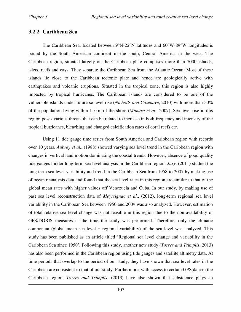
Chapter 3 Regional sea level variability and total relative sea level change
107
3.2.2 Caribbean Sea
The Caribbean Sea, located between 9°N-22°N latitudes and 60°W-89°W longitudes is
bound by the South American continent in the south, Central America in the west. The
Caribbean region, situated largely on the Caribbean plate comprises more than 7000 islands,
islets, reefs and cays. They separate the Caribbean Sea from the Atlantic Ocean. Most of these
islands lie close to the Caribbean tectonic plate and hence are geologically active with
earthquakes and volcanic eruptions. Situated in the tropical zone, this region is also highly
impacted by tropical hurricanes. The Caribbean islands are considered to be one of the
vulnerable islands under future se level rise (Nicholls and Cazenave, 2010) with more than 50%
of the population living within 1.5km of the shore (Mimura et al., 2007). Sea level rise in this
region poses various threats that can be related to increase in both frequency and intensity of the
tropical hurricanes, bleaching and changed calcification rates of coral reefs etc.
Using 11 tide gauge time series from South America and Caribbean region with records
over 10 years, Aubrey et al., (1988) showed varying sea level trend in the Caribbean region with
changes in vertical land motion dominating the coastal trends. However, absence of good quality
tide gauges hinder long-term sea level analysis in the Caribbean region. Jury, (2011) studied the
long term sea level variability and trend in the Caribbean Sea from 1958 to 2007 by making use
of ocean reanalysis data and found that the sea level rates in this region are similar to that of the
global mean rates with higher values off Venezuela and Cuba. In our study, by making use of
past sea level reconstruction data of Meyssignac et al., (2012), long-term regional sea level
variability in the Caribbean Sea between 1950 and 2009 was also analyzed. However, estimation
of total relative sea level change was not feasible in this region due to the non-availability of
GPS/DORIS measures at the time the study was performed. Therefore, only the climatic
component (global mean sea level + regional variability) of the sea level was analyzed. This
study has been published as an article titled ‘Regional sea level change and variability in the
Caribbean Sea since 1950’. Following this study, another new study (Torres and Tsimplis, 2013)
has also been performed in the Caribbean region using tide gauges and satellite altimetry data. At
time periods that overlap to the period of our study, they have shown that sea level rates in the
Caribbean are consistent to that of our study. Furthermore, with access to certain GPS data in the
Caribbean region, Torres and Tsimplis, (2013) have also shown that subsidence plays an
Chapter 3 Regional sea level variability and total relative sea level change
108
important role in the total relative sea level change with certain locations subsiding at the rate of
- 2.4 mm/yr.
Summary of the article: ‘Regional sea level change and variability in the Caribbean Sea
since 1950’ (the original article is inserted at the end of this section).
In this study, as mentioned above, we analyzed the long-term climatic component of sea
level change in the Caribbean Sea using the ensemble mean sea level reconstruction data. Only
10 tide gauge records (7 records having more than 30 years of data) were available in the region
of our study. Therefore these records were mainly used for the validation of the reconstruction
based sea level time series interpolated at the tide gauge locations. Over the altimetry era, the
mean sea level trend averaged over the Caribbean Sea amounts to 1.7±0.6 mm/yr with strong
positive trend patterns in the range of 4 mm/yr to5 mm/yr occurring along the coastal region of
the South American continent. Negative sea level trend values in the range of -1 mm/yr to -
2mm/yr were observed in the central Caribbean Sea. Over the 1950-2009 period, mean
reconstruction based regional sea level trend value amounts to 1.8±0.1 mm/yr, a value similar to
that of the global mean rate over 60 years.
Good correlations of the Caribbean interannual sea level time series with the ENSO
indices such as NINO3.4 and CAR (Caribbean SST index) especially since 1985 indicates that
the interannual sea level variability in this region is influenced by and responds to ENSO events.
Furthermore, Northern Caribbean (that includes the island nations of Cayman, Cuba, Haiti,
Dominican Republic, Jamaica, and Puerto Rico etc.) was found to exhibit interannual variability
at magnitudes higher than those of the Southern or Eastern Caribbean regions. This coincides
with the studies of Goldenberg et al., (2001) and Pielke et al.,(2003) who have shown increase in
hurricane activity and intensity in the Northern Caribbean when compared to the other Caribbean
regions. The increased activity and intensity of the tropical hurricanes have been attributed to the
simultaneous increases in the North Atlantic Sea Surface Temperature (SST) and decrease in the
vertical wind shear. It is possible that this also explains a part of the Caribbean interannual sea
level variability. Future studies are however needed to investigate this.

Journal ofGeodetic Science• 2(2) • 2012 • 125-133 DOI: 10.2478/v10156-011-0029-4 •
Regional sea level change and variability in theCaribbean sea since 1950Research ArticleH. Palanisamy1∗, M. Becker2, B. Meyssignac1, O. Henry1, A. Cazenave1
1 LEGOS/OMP, Toulouse, France
2 UMR 228 ESPACE-DEV/UAG, Cayenne, French Guiana
Abstract:
We investigate the regional variability in sea level in the Caribbean Sea region over the past 60 years (1950-2009) using an Empirical
Orthogonal Function (EOF)-based 2-dimensional past sea level reconstruction (amean of 3 reconstructions based on few long tide gauge
records and different sea level grids from satellite altimetry and ocean circulation models) and satellite altimetry data for the last two
decades. We nd that over the past 60 years, themean rate of sea level rise in the regionwas similar to the global mean rise (∼1.8mm/yr).
The interannual mean sea level of the placeCaribbean region appears highly correlated with El Nino-Southern Oscillation (ENSO) indices.
Interpolationof the sea level reconstructiongrid at different sites, in particular at theCaribbean Islandswhere tidegauge records are either
very short or inexistent, shows that locally, the sea level trend is on the order of 2 mm/yr, i.e. only slightly larger than the mean trend over
the region. Besides, correlationwith ENSO is in general good, especially since themid-1980s.We also nd a signi cant correlationbetween
the interannual variability in sea level andhurricane activity, especially over the past decadeduringwhich hurricane intensity and sea level
interannual variability have both increased.
Keywords:
Caribbean Sea • sea level variability • 2-D past sea level reconstruction • satellite altimetry • tide gauge • ENSO • hurricane
© Versita sp. z o.o.
Received 23-03-2012 ; accepted 06-04-2012
1. Introduction
Sea level is a very sensitive indicator of climate change and variabil-
ity as it integrates the responses of all components of the climate
system to natural and human-induced forcing. Sea level also re-
ects the natural variability of the climate system. During the 20th
century, the global mean sea level (GMSL) has risen at an average
rate of ∼1.8 mm/yr (e.g., Church and White, 2011). Since the early
1990s, sea level is routinelymeasured by high-precision satellite al-
timetry which indicates a GMSL rise of 3.2 mm/yr since over 1993-
2011. Sea level budget studies conducted over the altimetry era
(since 1993) have shown the GMSL rise results from ocean thermal
expansion (contributing by ∼30%) and land ice loss from glaciers
∗E-mail: [email protected], 18, Av. E. Belin, 31400Toulouse, France, tel. +33 5 61 33 29 72
and the Greenland and Antarctica ice sheets (contributing in total
to∼55%-60%) (e.g., Church et al., 2011, Cazenave and Llovel, 2010,
Cazenave and Remy, 2011).
Satellite altimetry has revealed high regional variability in the rates
of sea level rise, with faster rates (up to 3 times than the global
mean) in the western Paci c, North Atlantic and southern oceans.
The main cause of regional variability over the altimetry era is non
uniform ocean heat content as well as salinity variations (e.g., Lom-
bard et al., 2005, 2009). 2-dimensional past sea level reconstruc-
tions developed to study the regional variability in sea level prior
to the altimetry era (e.g., Church et al., 2004, Llovel et al., 2009, Ray
and Douglas, 2011, Meyssignac et al., 2012a) have shown that the
spatial trend patterns are not stationary but uctuate in time and
space in responses to the natural modes of the ocean-atmosphere
coupled system like El Nino-Southern Oscillation (ENSO), Paci c
Decadal Oscillation (PDO), North Atlantic Oscillation (NAO) (e.g.,
Meyssignac et al, 2012a, b). This indicates that, at regional scale,
Unauthenticated
Download Date | 5/14/15 5:02 PM

Journal ofGeodetic Science126
there is a low-frequency (multidecadal) component of the regional
variability that superimposes to the GMSL rise. This component
may either amplify or reduce the GMSL rise. When investigating
the effective rate of sea level change in selected regions, it is of pri-
mary importance to account for this regional component in addi-
tion to the global mean rise. In a previous study focusing on the
western tropical Paci c islands, (Becker et al., 2012) found that at
Funafuti, an island in the Tropical Paci c belonging to the nation
of Tuvalu, because of the low-frequency regional variability com-
ponent, the total (absolute) sea level rise is almost three times the
globalmean rate of sea level rise over the past half century (i.e., ∼5
mm/yr versus 1.8 mm/yr over 1950-2010). This shows the impor-
tance of estimating the rate of sea level rise not only globally but
also in terms of regional variability in order to understand the level
of impacts that the sea level rise can have on the local population.
In the present study, we focus on the Caribbean Sea, a region sur-
rounded by highly populated countries and islands, and develop
an approach similar to that of (Becker et al., 2012) to determine the
total sea level change (i.e., GMSL plus regional variability) in this
area since 1950.
The Caribbean Sea, located between 9◦N and 22◦N latitude and
between 60◦W and 89◦W longitude is bound by South America
to the South, Central America to the West. The Antilles, a chain
of islands, separate the Caribbean Sea from the Atlantic Ocean to
the North and East and from the Gulf of Mexico to the South West.
TheCaribbean region, situated largely on theCaribbeanplate com-
prises more than 7000 islands, islets, reefs and cays. Most of the
Caribbean islands lie close to theboundariesof theCaribbeanplate
and hence are geologically active with earthquakes from time to
time and a number of volcanic activities. The Caribbean islands
are considered to be one of the vulnerable islands under future sea
level rise (Nicholls and Cazenave, 2010) with more than 50% of the
population living within 1.5 km of the shore (Mimura et al., 2007).
To estimate the low-frequency regional sea level variability in the
Caribbean, we make use of an Empirical Orthogonal Function
(EOF)-based (Preisendorfer, 1988) 2-dimensional past sea level re-
construction (Meyssignac et al., 2012a). This is a mean of 3 re-
constructions that combines nearly one hundred long tide gauge
records (1950-2009) with different sea level grids of shorter du-
ration. The Caribbean does not possess many good quality tide
gauge records and even the few available (about 10) do not cover
thewhole 60 years period. Of the available records, onlyMagueyes
has been used in the global sea level reconstruction. Thus the re-
construction is an important tool to study the regional sea level
variability. To understand what drives the Caribbean Sea regional
variability, we estimate the effects of ocean temperature and salin-
ity on the observed sea level variations and also compare the sea
level with different climatic indices, in particular ENSO indices. We
also investigate a potential link between sea level variability and
hurricane activity in the Caribbean region.
2. Data
2.1. Satellite Altimetry
We use the DT-MSLA “Ref” series of satellite altime-
try data provided by Collecte Localisation Satellite
(http://www.aviso.oceanobs.com/en/data/products/sea-surface-
height-products/global/msla/index.html). The data set is based
on the combination of several altimetry missions namely
Topex/Poseidon (T/P), Jason-1 and 2, Envisat and ERS 1 and 2. It is
a global homogenous inter-calibrated dataset based on a global
crossover adjustment that considers T/P and then Jason-1/2 as
reference missions. Usual geophysical corrections are applied:
solid Earth, ocean and pole tides, wet and dry troposphere, iono-
sphere (see Ablain et al., 2009 for details) and inverted barometric
correction (Carrere and Lyard, 2003). The altimetry data set is used
over the time span from January 1993 until December 2009. It
is available as 0.25◦ x 0.25◦Mercator projection grids at weekly
intervals.
2.2. Tide gauges
Revised Local Reference monthly mean sea level data of the Per-
manent Service for the Mean Sea Level (PSMSL; Woodworth and
Player, 2003; http://www.psmsl.org/) are used in this study. As
mentioned above, the tide gauge coverage in the Caribbean Sea
region is rather poor. Only 7 tide gauges have >30 years of data
between 1950 and 2009. In this study, we havemade use of 10 tide
gauge records: 7 having > 30 years of data and 3 having data only
between 15 to 20 years but of good quality. Linear interpolation
wasperformed to introducemissingdata in thegapswhenever the
gaps are ≤ 4 consecutive years (otherwise the record is not con-
sidered). Gaps and discontinuities occur in the tide gauge records
due to natural factors like earthquakes or changes in instrumenta-
tion or even due to anthropogenic factors. Fig. 1 (as star symbols)
shows the location of the tide gauges and their characteristics are
given in Table 1 (in Fig. 1 -as blue dots- and Table 1 are also listed a
few additional tide gauges with shorter records, records with time
gaps exceeding 4 consecutive years or incorrect tide gauge data.
In view of the poor quality of the tide gauge records, only the past
sea level reconstruction (see Section 2.3), and observed altimetry
data have been considered in these locations in order to study the
past and recent sea level variability.
The tide gauge time series have been corrected for the inverted
barometric response of sea level to atmospheric pressure forcing
using the surface pressure grids from the National Centre for En-
vironmental Prediction (NCEP, Kalnay et al., 1996). Glacial Isostatic
Adjustment (GIA) is very small in the placeCaribbean region and
henceforth the tidegauge records havenot been corrected forGIA.
In order to concentrate only on the interannual variability, the sea-
sonal cycles have been ltered through a least-squares t of 12-
month and 6-month period sinusoids.
Unauthenticated
Download Date | 5/14/15 5:02 PM
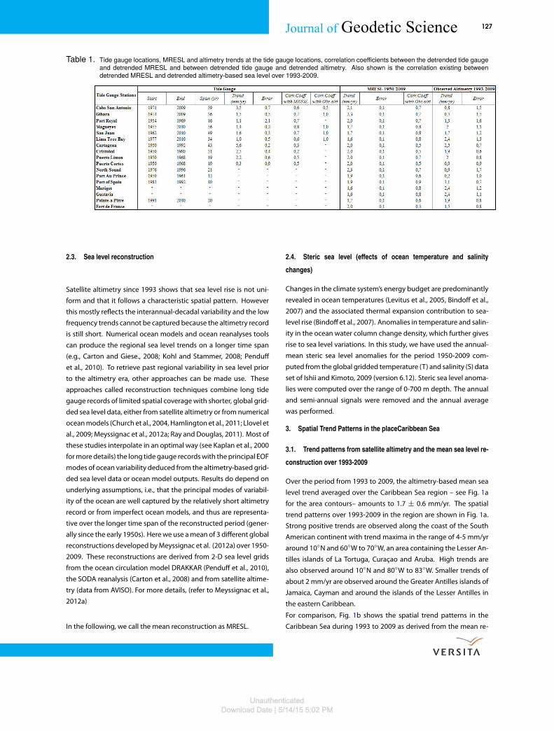
Journal ofGeodetic Science 127
Table 1. Tide gauge locations, MRESL and altimetry trends at the tide gauge locations, correlation coefficients between the detrended tide gaugeand detrended MRESL and between detrended tide gauge and detrended altimetry. Also shown is the correlation existing betweendetrended MRESL and detrended altimetry-based sea level over 1993-2009.
2.3. Sea level reconstruction
Satellite altimetry since 1993 shows that sea level rise is not uni-
form and that it follows a characteristic spatial pattern. However
this mostly re ects the interannual-decadal variability and the low
frequency trends cannot be captured because the altimetry record
is still short. Numerical ocean models and ocean reanalyses tools
can produce the regional sea level trends on a longer time span
(e.g., Carton and Giese., 2008; Kohl and Stammer, 2008; Penduff
et al., 2010). To retrieve past regional variability in sea level prior
to the altimetry era, other approaches can be made use. These
approaches called reconstruction techniques combine long tide
gauge records of limited spatial coveragewith shorter, global grid-
ded sea level data, either from satellite altimetry or from numerical
oceanmodels (Church et al., 2004, Hamlingtonet al., 2011; Llovel et
al., 2009; Meyssignac et al., 2012a; Ray and Douglas, 2011). Most of
these studies interpolate in an optimal way (see Kaplan et al., 2000
formoredetails) the long tide gauge recordswith theprincipal EOF
modes of ocean variability deduced from the altimetry-based grid-
ded sea level data or ocean model outputs. Results do depend on
underlying assumptions, i.e., that the principal modes of variabil-
ity of the ocean are well captured by the relatively short altimetry
record or from imperfect ocean models, and thus are representa-
tive over the longer time span of the reconstructed period (gener-
ally since the early 1950s). Herewe use amean of 3 different global
reconstructions developed byMeyssignac et al. (2012a) over 1950-
2009. These reconstructions are derived from 2-D sea level grids
from the ocean circulation model DRAKKAR (Penduff et al., 2010),
the SODA reanalysis (Carton et al., 2008) and from satellite altime-
try (data from AVISO). For more details, (refer to Meyssignac et al.,
2012a)
In the following, we call the mean reconstruction as MRESL.
2.4. Steric sea level (effects of ocean temperature and salinity
changes)
Changes in the climate system’s energy budget are predominantly
revealed in ocean temperatures (Levitus et al., 2005, Bindoff et al.,
2007) and the associated thermal expansion contribution to sea-
level rise (Bindoff et al., 2007). Anomalies in temperature and salin-
ity in the ocean water column change density, which further gives
rise to sea level variations. In this study, we have used the annual-
mean steric sea level anomalies for the period 1950-2009 com-
puted from the global gridded temperature (T) and salinity (S) data
set of Ishii and Kimoto, 2009 (version 6.12). Steric sea level anoma-
lies were computed over the range of 0-700 m depth. The annual
and semi-annual signals were removed and the annual average
was performed.
3. Spatial Trend Patterns in the placeCaribbean Sea
3.1. Trend patterns from satellite altimetry and the mean sea level re-
construction over 1993-2009
Over the period from 1993 to 2009, the altimetry-based mean sea
level trend averaged over the Caribbean Sea region – see Fig. 1a
for the area contours– amounts to 1.7 ± 0.6 mm/yr. The spatial
trend patterns over 1993-2009 in the region are shown in Fig. 1a.
Strong positive trends are observed along the coast of the South
American continent with trend maxima in the range of 4-5 mm/yr
around 10◦N and 60◦W to 70◦W, an area containing the Lesser An-
tilles islands of La Tortuga, Curaçao and Aruba. High trends are
also observed around 10◦N and 80◦W to 83◦W. Smaller trends of
about 2 mm/yr are observed around the Greater Antilles islands of
Jamaica, Cayman and around the islands of the Lesser Antilles in
the eastern Caribbean.
For comparison, Fig. 1b shows the spatial trend patterns in the
Caribbean Sea during 1993 to 2009 as derived from the mean re-
Unauthenticated
Download Date | 5/14/15 5:02 PM
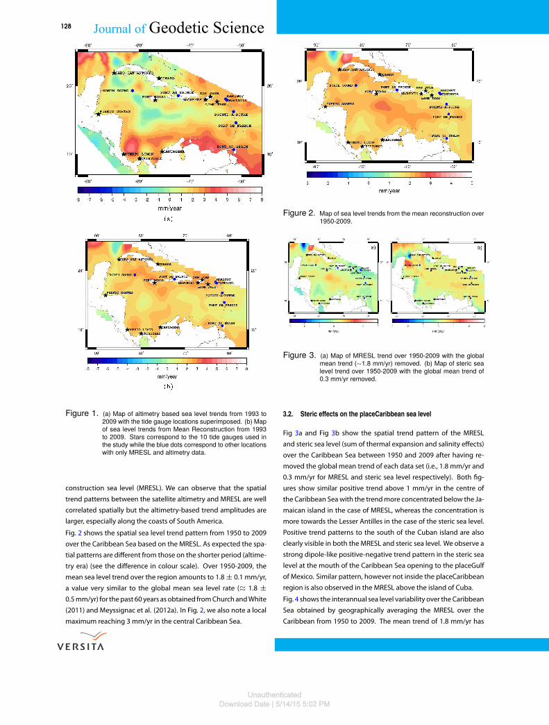
Journal ofGeodetic Science128
(a)
(b)
Figure 1. (a) Map of altimetry based sea level trends from 1993 to2009 with the tide gauge locations superimposed. (b) Mapof sea level trends from Mean Reconstruction from 1993to 2009. Stars correspond to the 10 tide gauges used inthe study while the blue dots correspond to other locationswith only MRESL and altimetry data.
construction sea level (MRESL). We can observe that the spatial
trend patterns between the satellite altimetry and MRESL are well
correlated spatially but the altimetry-based trend amplitudes are
larger, especially along the coasts of South America.
Fig. 2 shows the spatial sea level trend pattern from 1950 to 2009
over the Caribbean Sea based on the MRESL. As expected the spa-
tial patterns are different from those on the shorter period (altime-
try era) (see the difference in colour scale). Over 1950-2009, the
mean sea level trend over the region amounts to 1.8 ± 0.1 mm/yr,
a value very similar to the global mean sea level rate (≈ 1.8 ±
0.5mm/yr) for thepast 60 years as obtained fromChurchandWhite
(2011) and Meyssignac et al. (2012a). In Fig. 2, we also note a local
maximum reaching 3 mm/yr in the central Caribbean Sea.
Figure 2. Map of sea level trends from the mean reconstruction over1950-2009.
Figure 3. (a) Map of MRESL trend over 1950-2009 with the globalmean trend (∼1.8 mm/yr) removed. (b) Map of steric sealevel trend over 1950-2009 with the global mean trend of0.3 mm/yr removed.
3.2. Steric effects on the placeCaribbean sea level
Fig 3a and Fig 3b show the spatial trend pattern of the MRESL
and steric sea level (sum of thermal expansion and salinity effects)
over the Caribbean Sea between 1950 and 2009 after having re-
moved the global mean trend of each data set (i.e., 1.8 mm/yr and
0.3 mm/yr for MRESL and steric sea level respectively). Both g-
ures show similar positive trend above 1 mm/yr in the centre of
the Caribbean Seawith the trendmore concentrated below the Ja-
maican island in the case of MRESL, whereas the concentration is
more towards the Lesser Antilles in the case of the steric sea level.
Positive trend patterns to the south of the Cuban island are also
clearly visible in both the MRESL and steric sea level. We observe a
strong dipole-like positive-negative trend pattern in the steric sea
level at the mouth of the Caribbean Sea opening to the placeGulf
of Mexico. Similar pattern, however not inside the placeCaribbean
region is also observed in the MRESL above the island of Cuba.
Fig. 4 shows the interannual sea level variability over the Caribbean
Sea obtained by geographically averaging the MRESL over the
Caribbean from 1950 to 2009. The mean trend of 1.8 mm/yr has
Unauthenticated
Download Date | 5/14/15 5:02 PM
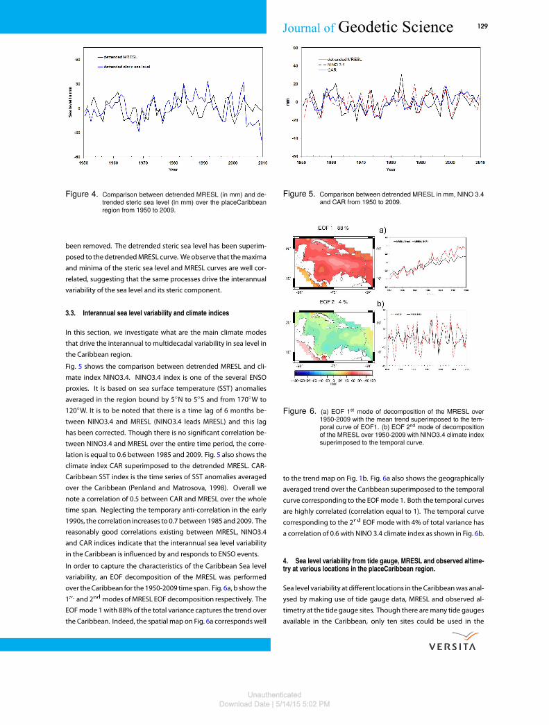
Journal ofGeodetic Science 129
Figure 4. Comparison between detrended MRESL (in mm) and de-trended steric sea level (in mm) over the placeCaribbeanregion from 1950 to 2009.
been removed. The detrended steric sea level has been superim-
posed to the detrendedMRESL curve. Weobserve that themaxima
and minima of the steric sea level and MRESL curves are well cor-
related, suggesting that the same processes drive the interannual
variability of the sea level and its steric component.
3.3. Interannual sea level variability and climate indices
In this section, we investigate what are the main climate modes
that drive the interannual to multidecadal variability in sea level in
the Caribbean region.
Fig. 5 shows the comparison between detrended MRESL and cli-
mate index NINO3.4. NINO3.4 index is one of the several ENSO
proxies. It is based on sea surface temperature (SST) anomalies
averaged in the region bound by 5◦N to 5◦S and from 170◦W to
120◦W. It is to be noted that there is a time lag of 6 months be-
tween NINO3.4 and MRESL (NINO3.4 leads MRESL) and this lag
has been corrected. Though there is no signi cant correlation be-
tween NINO3.4 and MRESL over the entire time period, the corre-
lation is equal to 0.6 between 1985 and 2009. Fig. 5 also shows the
climate index CAR superimposed to the detrended MRESL. CAR-
Caribbean SST index is the time series of SST anomalies averaged
over the Caribbean (Penland and Matrosova, 1998). Overall we
note a correlation of 0.5 between CAR and MRESL over the whole
time span. Neglecting the temporary anti-correlation in the early
1990s, the correlation increases to 0.7 between1985 and2009. The
reasonably good correlations existing between MRESL, NINO3.4
and CAR indices indicate that the interannual sea level variability
in the Caribbean is in uenced by and responds to ENSO events.
In order to capture the characteristics of the Caribbean Sea level
variability, an EOF decomposition of the MRESL was performed
over theCaribbean for the1950-2009 time span. Fig. 6a, b show the
1st and 2nd modes ofMRESL EOF decomposition respectively. The
EOFmode 1 with 88% of the total variance captures the trend over
the Caribbean. Indeed, the spatial map on Fig. 6a correspondswell
Figure 5. Comparison between detrended MRESL in mm, NINO 3.4and CAR from 1950 to 2009.
Figure 6. (a) EOF 1st mode of decomposition of the MRESL over1950-2009 with the mean trend superimposed to the tem-poral curve of EOF1. (b) EOF 2nd mode of decompositionof the MRESL over 1950-2009 with NINO3.4 climate indexsuperimposed to the temporal curve.
to the trend map on Fig. 1b. Fig. 6a also shows the geographically
averaged trend over the Caribbean superimposed to the temporal
curve corresponding to the EOFmode 1. Both the temporal curves
are highly correlated (correlation equal to 1). The temporal curve
corresponding to the 2nd EOF mode with 4% of total variance has
a correlation of 0.6 with NINO 3.4 climate index as shown in Fig. 6b.
4. Sea level variability from tide gauge, MRESL and observed altime-try at various locations in the placeCaribbean region.
Sea level variability at different locations in theCaribbeanwas anal-
ysed by making use of tide gauge data, MRESL and observed al-
timetry at the tide gauge sites. Though there aremany tide gauges
available in the Caribbean, only ten sites could be used in the
Unauthenticated
Download Date | 5/14/15 5:02 PM
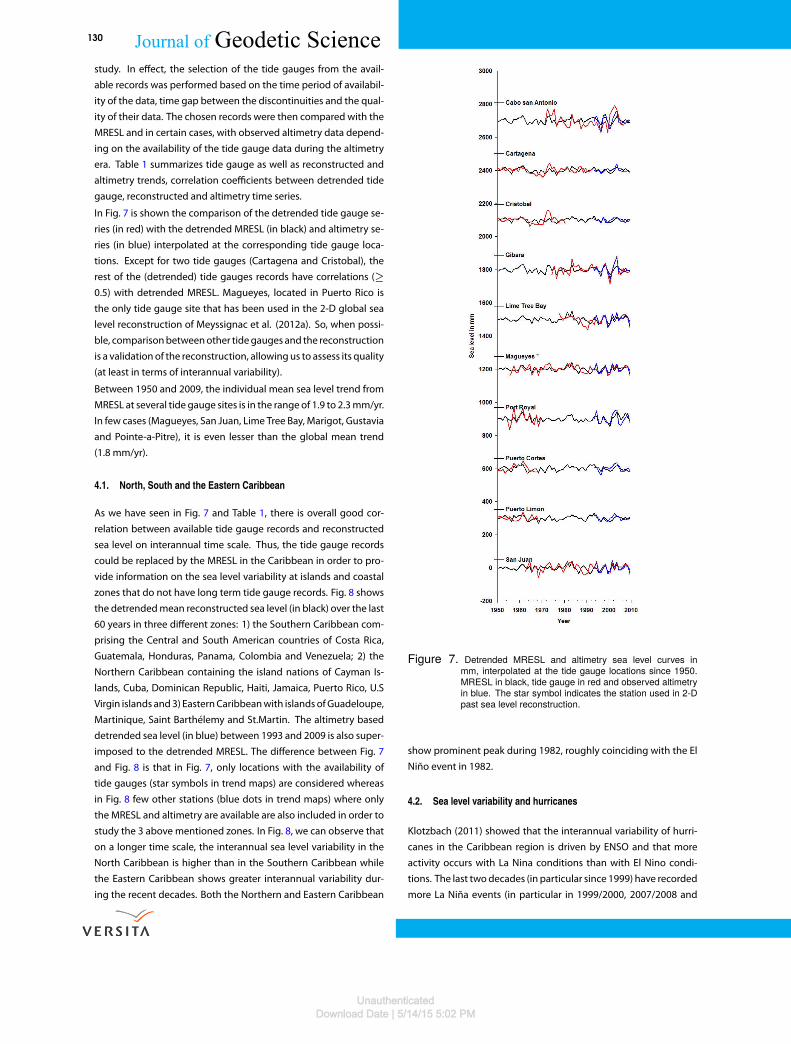
Journal ofGeodetic Science130
study. In effect, the selection of the tide gauges from the avail-
able records was performed based on the time period of availabil-
ity of the data, time gap between the discontinuities and the qual-
ity of their data. The chosen records were then compared with the
MRESL and in certain cases, with observed altimetry data depend-
ing on the availability of the tide gauge data during the altimetry
era. Table 1 summarizes tide gauge as well as reconstructed and
altimetry trends, correlation coefficients between detrended tide
gauge, reconstructed and altimetry time series.
In Fig. 7 is shown the comparison of the detrended tide gauge se-
ries (in red) with the detrended MRESL (in black) and altimetry se-
ries (in blue) interpolated at the corresponding tide gauge loca-
tions. Except for two tide gauges (Cartagena and Cristobal), the
rest of the (detrended) tide gauges records have correlations (≥
0.5) with detrended MRESL. Magueyes, located in Puerto Rico is
the only tide gauge site that has been used in the 2-D global sea
level reconstruction of Meyssignac et al. (2012a). So, when possi-
ble, comparisonbetweenother tidegauges and the reconstruction
is a validationof the reconstruction, allowingus to assess its quality
(at least in terms of interannual variability).
Between 1950 and 2009, the individual mean sea level trend from
MRESL at several tide gauge sites is in the range of 1.9 to 2.3mm/yr.
In few cases (Magueyes, San Juan, Lime Tree Bay, Marigot, Gustavia
and Pointe-a-Pitre), it is even lesser than the global mean trend
(1.8 mm/yr).
4.1. North, South and the Eastern Caribbean
As we have seen in Fig. 7 and Table 1, there is overall good cor-
relation between available tide gauge records and reconstructed
sea level on interannual time scale. Thus, the tide gauge records
could be replaced by the MRESL in the Caribbean in order to pro-
vide information on the sea level variability at islands and coastal
zones that do not have long term tide gauge records. Fig. 8 shows
the detrendedmean reconstructed sea level (in black) over the last
60 years in three different zones: 1) the Southern Caribbean com-
prising the Central and South American countries of Costa Rica,
Guatemala, Honduras, Panama, Colombia and Venezuela; 2) the
Northern Caribbean containing the island nations of Cayman Is-
lands, Cuba, Dominican Republic, Haiti, Jamaica, Puerto Rico, U.S
Virgin islands and3) EasternCaribbeanwith islandsofGuadeloupe,
Martinique, Saint Barthélemy and St.Martin. The altimetry based
detrended sea level (in blue) between 1993 and 2009 is also super-
imposed to the detrended MRESL. The difference between Fig. 7
and Fig. 8 is that in Fig. 7, only locations with the availability of
tide gauges (star symbols in trend maps) are considered whereas
in Fig. 8 few other stations (blue dots in trend maps) where only
the MRESL and altimetry are available are also included in order to
study the 3 above mentioned zones. In Fig. 8, we can observe that
on a longer time scale, the interannual sea level variability in the
North Caribbean is higher than in the Southern Caribbean while
the Eastern Caribbean shows greater interannual variability dur-
ing the recent decades. Both the Northern and Eastern Caribbean
Figure 7. Detrended MRESL and altimetry sea level curves inmm, interpolated at the tide gauge locations since 1950.MRESL in black, tide gauge in red and observed altimetryin blue. The star symbol indicates the station used in 2-Dpast sea level reconstruction.
show prominent peak during 1982, roughly coinciding with the El
Niño event in 1982.
4.2. Sea level variability and hurricanes
Klotzbach (2011) showed that the interannual variability of hurri-
canes in the Caribbean region is driven by ENSO and that more
activity occurs with La Nina conditions than with El Nino condi-
tions. The last twodecades (in particular since 1999) have recorded
more La Niña events (in particular in 1999/2000, 2007/2008 and
Unauthenticated
Download Date | 5/14/15 5:02 PM

Journal ofGeodetic Science 131
Figure 8. Detrended MRESL (in black) and altimetry sea level (inblue) curves in mm since 1950 at the tide gauge locationsarranged based on their location: Southern Caribbean,Northern Caribbean and Eastern Caribbean.
2010/2011) than before. Furthermore, Goldenberg et al. (2001)
showed that the years 1995 to 2000 have seen a 2.5 fold increase in
major hurricane activity and a vefold increase in hurricane activ-
ity affecting the Caribbean due to simultaneous increases in North
Atlantic sea surface temperatures and decreases in vertical wind
shear. These authors also showed that this phenomenon is likely to
persist for an additional 10 to 40 years. In section 3.2 we have seen
that theNINO3.4, a proxy of El Nino and LaNina events andCAR, an
index based on the Caribbean SST correlate well with MRESL over
the Caribbean since 1985. This period also corresponds to the in-
creased frequency of La Niña events and hurricane activity.
Pielke et al. (2003) showed that between1944 and1999, theNorth-
ern Caribbean hurricanes ( hurricanes hitting Bahamas, British Vir-
gin Islands, Cayman Islands, Cuba, Dominican Republic, Haiti, Ja-
maica, Puerto Rico etc.) show high interannual variability as well
as large multi decadal changes with a long term average of 1.0
hurricane strike per year. The Eastern Caribbean experiences hur-
ricanes at a lower rate than the Northern Caribbean with 0.4 hurri-
cane strike per year, whereas the hurricanes hitting the Central and
SouthAmericanpart of theCaribbean show small decadal changes
with only 0.2 strike per year. The pattern is very similar to the inter-
annual variability in sea level observed in the Northern and South-
ern Caribbean as discussed in section 4.1, i.e. Northern Caribbean
showing higher interannual sea level variability than the Southern.
This seems to suggest that both the sea level interannual variability
andhurricaneactivity in theplaceCaribbeanare related. Further in-
vestigation is needed to understand the link between the sea level
variability and hurricane activity in that region.
5. Conclusion
In this study, we have analysed the sea level variability in the
Caribbean since 1950 by making use of the mean of a mean 2-
D past sea level reconstruction, observed satellite altimetry and
tide gauge records wherever available. We observe that the spa-
tial trend pattern in sea level during 1950 -2009 is quite different
from that during the altimetry era (since 1993). Moreover themean
sea level trend in the Caribbean is very similar to the global mean
sea level rise rate thereby indicating that the Caribbean is not fac-
ing a sea level rise larger than the global mean rise (unlike at some
islands of the western tropical Paci c, as shown by Becker et al.,
2012). Our results also show that the increase in thenumber of hur-
ricanes during the recent decades have caused so far more dam-
ages to the coastal areas than the sea level rise itself. However,
projected sea level rise in the future decades in response to global
warming will represent an additional threat in this region.
Acknowledgements
Hindumathi Palanisamy is supported by the ‘CECILE’ project of the
AgenceNationale de la Recherche (ANR)while Olivier Henry is sup-
ported by the European project MONARCH.
References
Ablain M., Cazenave A., Guinehut S. and Valladeau G., 2009,
A new assessment of global mean sea level from altimeters
highlights a reduction of global slope from 2005 to 2008 in
agreement with in-situ measurements Ocean Sciences, 5,
193-201.
Becker M., Meyssignac B., Llovel W., Cazenave A. and Del-
croix T., 2012, Sea level variations at Tropical Paci c Islands
during 1950-2009, Glob. Planet. Chan., 80/81, 85-98.
Bindoff N.L., Willebrand J., Artale V., Cazenave A., Gregory
J., Gulev S., Hanawa K., Le Quéré C., Levitus S., Nojiri Y., Shum
C.K., Talley L.D. and Unnikrishnan A., 2007, Observations:
Unauthenticated
Download Date | 5/14/15 5:02 PM
Journal ofGeodetic Science132
Oceanic Climate Change and Sea Level. In: Climate Change
2007: The Physical Science Basis. Contribution of Working
Group I to the Fourth Assessment Report of the intergov-
ernmental Panel on Climate Change [Solomon, S., D. Qin, M.
Manning, Z. Chen, M. Marquis, K.B. Averyt, M. Tignor and H.L.
Miller (eds.)]. Cambridge University Press, Cambridge, United
Kingdom and New York, NY, USA.
Carrere L. and Lyard F., 2003, Modeling the barotropic re-
sponse of the global ocean to atmospheric wind and pressure
forcing -comparisons with observations, Geophys. Res. Lett.,
30, 6, 1275, DOI:10.1029/2002GL016473.
Carton J.A. and Giese B.S., 2008, A reanalysis of ocean cli-
mate using Simple Ocean Data Assimilation (SODA), Mon.
Weath. Rev., 136, 2999–3017.
Cazenave A. and Llovel W., 2010, Contemporary sea level
rise, Ann. Rev. Marine Sci., 2, 145-173.
Cazenave A. and Remy F., 2011, Sea level and climate:
measurements and causes of changes, Interdisciplinary Re-
views: Climate Change, 2, 5, 647–662, DOI:10.1002/wcc.139.
Church J.A., White N.J., Konikow L.F., Domingues C.M.,
Cogley J.C., Rignot E., Gregory J. M., van den Broeke M. R.,
Monaghan A. J., and Velicogna I., 2011, Revisiting the Earth’s
sea-level and energy budgets from 1961 to 2008, Geophys.
Res. Lett., 38, L18601, DOI: 10.1029/2011GL048794.
Church J.A., White N.J., Coleman R., Lambeck K. and Mitrovica
J.X., 2004, Estimates of the regional distribution of sea level
rise over the 1950–2000 period, J Climat., 17, 2609–2625.
Church J.A. and White N.J., 2011, Changes in the rate of
sea level rise from the late 19th to the early 21st century, Surv.
Geophys., 1–18, DOI:10.1007/s10712-011-9119-1.
Goldenberg S.B., Landsea C. W., Mestas-Nunez A.M., and
Gray W.M., 2001, The recent increase in Atlantic hurricane
activity: Causes and implications, Science, 293, 474–79
Hamlington B.D., Leben R., Nerem S., Han W. and Kim
K.Y., 2011, Reconstructing sea level using cyclostationary
empirical orthogonal functions, J Geophys. Res., 116, C12, DOI:
10.1029/2011JC007529.
Ishii M. and Kimoto M., 2009, Reevaluation of historical
ocean heat content variations with varying XBT and MBT
depth bias corrections, J Oceanog., 65, 287-299.
Kalnay E.C., Kanamitsu M., Kistler R., Collins W., Deaven
D., Gandin L., Iredell M., Saha S., White G., Woollen J., Zhu Y.,
Leetmaa A., Reynolds B., Chelliah M., Ebisuzaki W., Higgins
W., Janowiak J., Mo K. C., Ropelewski C., Wang J., Jenne R. and
Dennis J., 1996, The NCEP/NCAR 40-year reanalysis project.
Bull. American Meteo. Soci., 77, 437–472.
Kaplan A., Kushnir Y. and Cane M.A., 2000, Reduced space
optimal interpolation of historical marine sea level pressure:
1854–1992, J Climat., 13, 2987–3002.
Klotzback P.J., 2011, The in uence of El Nino-southern
oscillation and the atlantic multidecadal oscillation on Car-
ribean tropical cyclone activity, J Climat., 721-731.
Kohl A. and Stammer D., 2008, Decadal sea level changes
in the 50-year GECCO ocean synthesis. J Climat., 21, 1876–90.
Levitus S., Antonov J. and Boyer T., 2005, Warming of the
world ocean, 1955–2003, Geophys. Res. Lett., 32, L02604,
DOI:10.1029/2004GL021592.
Llovel W., Cazenave A., Rogel P. and Berge-Nguyen M.,
2009, 2-D reconstruction of past sea level (1950-2003) using
tide gauge records and spatial patterns from a general ocean
circulation model, Climat. Past, 5, 1-11.
Lombard A., Cazenave A., DoMinh K., Cabanes C., Nerem
R., 2005, Thermosteric sea level rise for the past 50 years;
comparison with tide gauges and inference on water mass
contribution. Global and Planetary Change, 48, 303-312.
Lombard A., Cazenave A., Le Traon P.Y. and Ishii M., 2005,
Contribution of thermal expansion to present-day sea level
rise revisited, Glob. Planet. Chan., 47, 1-16.
Lombard A., Garric G., Penduff T. and Molines J.M., 2009,
Regional variability of sea level change using a global ocean
model at 1/4_ resolution, Ocean Dyn., DOI: 10.1007/s10236-
009-0161-6.
Meyssignac B., Llovel W., Becker M. and Cazenave A., 2012, An
assessment of two-dimensional past sea level reconstructions
over 1950 - 2009 based on tide gauge data and different input
sea level grids, Surv. Geophys., in press, DOI:10.1007/s10712-
011-9171-x.
Meyssignac B., Salas y Melia D., Becker M., Llovel W., and
Cazenave A., 2012, Tropical Paci c spatial trend patterns in
observed sea level: internal variability and/or anthropogenic
signature?, Climat. Past, in press, DOI: 10.5194/cpd-8-349-2012.
Mimura N., Nurse L., McLean R.F., Agard J., Briguglio L,
Unauthenticated
Download Date | 5/14/15 5:02 PM
Journal ofGeodetic ScienceLefale P., et al., 2007, Small islands. Climate Change, 2007:
Impacts, Adaptation and Vulnerability. Contribution of
Working Group II to the Fourth Assessment Report of the
Intergovernmental Panel on Climate Change, M.L. Parry,
O.F. Canziani, J.P. Palutikof, P.J. van der Linden and C.E. Han-
son, Eds., CambridgeUniversity Press, Cambridge, UK, 687-716.
Nicholls R. and Cazenave A., 2010, Sea level change and
the impacts in coastal zones, Science, 328, 1517-1520.
Peltier W.R., 2010, Global glacial isostasy and the surface
of the ice-age Earth: The ICE-5G (VM2)model and GRACE, Ann.
Rev. Earth Planet. Sci., 32, 111-149.
Penduff T., Juza M., Brodeau L., Smith G., Barnier B., Mo-
lines J., Treguier A.-M., and Madec G., 2010, Impact of global
ocean model resolution on sea-level variability with emphasis
on interannual time scales, Ocean Sci., 6, 269-284.
Penland C. and Matrosova L., 1998, Prediction of tropical
Atlantic sea surface temperatures using linear inverse model-
ing, J Climat., 483-496.
Pielke A.J., Rubiera J., Landsea C., Fernandez M.L. and Klein
R., 2003, Hurricane Vulnerability in Latin America and the
Caribbean: Normalized Damage and Loss Potentials. Nat. Haz.
Rev., 4, 3, DOI: 10.1061/(ASCE)1527- 6988(2003)4:3(101).
Preisendorfer R.W., 1988, Principal component Analysis in
Meteorology and oceanography, Develop. Atmos. Sci., 17,
Elsevier, 425pp.
Ray R. and Douglas B., 2011, Experiments in reconstruct-
ing twentieth-century sea levels. Prog. Oceanog., 91, 4,
496-515.
Woodworth P.L. and Player R., 2003, The permanent ser-
vice for mean sea level: an update to the 21st century, J Coas.
Res., 19, 287-295.
Unauthenticated
Download Date | 5/14/15 5:02 PM
Chapter 3 Regional sea level variability and total relative sea level change
118
3.2.3 South China Sea
South China Sea, a region sometimes called as the Asian Mediterranean, located between
western Pacific and eastern Indian Ocean, is the largest semi-enclosed marginal sea in the
northwest Pacific Ocean. Three major rivers namely Mekong, Red and Pearl drain into the South
China Sea. The sea level in this region has presented significant changes over the recent decades
and this deviates greatly from those in is adjacent and global oceans (Nidheesh et al., 2013). Its
bottom topography is characterized by two extended continental shelves with water depth less
than 200 m along the north and southwest coasts and a deep basin with a maximum water depth
of about 5000 m in the central region (See Fig.3.6). Its coastal sub regions are home to about 270
million people and have been one of the fastest developing and most vibrant economies on Earth.
Rising sea level would therefore severely threaten the coastal zones (Peng et al., 2013).
A number of previous studies have investigated South China Sea level trends over the
satellite altimetry era. In our study, we analyzed the long-term (60 years) sea level variability in
the South China Sea using the past sea level reconstruction data set. Only the climate-related sea
level component was studied due to the inaccessibility of GPS measures in the region of South
China Sea for the VLM estimates. However, anthropogenic land subsidence plays a major role in
this region. For example, the Bangkok megacity has subsided by 2 m due to ground water
withdrawal (Nicholls, 2010, Stammer et al., 2013). Our study has been published as an article
titled ‘Interannual sea level variations in the South China Sea over 1950-2009’.
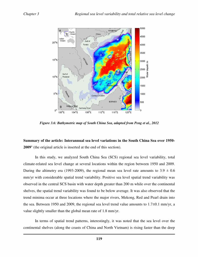
Chapter 3 Regional sea level variability and total relative sea level change
119
Figure 3.6: Bathymetric map of South China Sea, adapted from Peng et al., 2012
Summary of the article: Interannual sea level variations in the South China Sea over 1950-
2009’ (the original article is inserted at the end of this section).
In this study, we analyzed South China Sea (SCS) regional sea level variability, total
climate-related sea level change at several locations within the region between 1950 and 2009.
During the altimetry era (1993-2009), the regional mean sea level rate amounts to 3.9 ± 0.6
mm/yr with considerable spatial trend variability. Positive sea level spatial trend variability was
observed in the central SCS basin with water depth greater than 200 m while over the continental
shelves, the spatial trend variability was found to be below average. It was also observed that the
trend minima occur at three locations where the major rivers, Mekong, Red and Pearl drain into
the sea. Between 1950 and 2009, the regional sea level trend value amounts to 1.7±0.1 mm/yr, a
value slightly smaller than the global mean rate of 1.8 mm/yr.
In terms of spatial trend patterns, interestingly, it was noted that the sea level over the
continental shelves (along the coasts of China and North Vietnam) is rising faster than the deep
Chapter 3 Regional sea level variability and total relative sea level change
120
water region which is almost the reverse case during the satellite altimetry era. This once again
shows that satellite altimetry cannot capture low-frequency trend signals owing to its short time
period. Comparison of the long-term regional sea level trend patterns with those of upper steric
(0-700 m) regional trend patterns showed that while in the central SCS basin, the patterns are
similar; it is not the case in the northern SCS region. This suggests that the sea level variability in
the north SCS is either caused by the ocean water mass contribution or by the thermal expansion
of the shallow water (considering the shallow bathymetry of the region). If it is the latter, the
inability of the upper steric sea level to produce this signal could be due to the lack of complete
coverage of temperature and salinity data in this region. Good correlation of long-term
interannual sea level time series with the ENSO NINO3.4 index indicates that the interannual sea
level variability in SCS is driven by ENSO events. Estimation of long-term total climate-related
sea level change at different locations in SCS showed that in the northern SCS, several locations
exhibit sea level change at rates higher than that of the global mean rate.
Marine Geodesy, 36:164–182, 2013
Copyright © Taylor & Francis Group, LLC
ISSN: 0149-0419 print / 1521-060X online
DOI: 10.1080/01490419.2013.771595
Interannual Sea Level Variations in the South China
Sea Over 1950–2009
DONGJU PENG,1,2 HINDUMATHI PALANISAMY,2
ANNY CAZENAVE,2 AND BENOIT MEYSSIGNAC2
1Shanghai Astronomical Observatory, CAS, Shanghai, China2LEGOS/OMP, Toulouse, France
Spatial patterns of interannual sea level variations in the South China Sea (SCS) areinvestigated by analyzing an EOF-based 2-dimensional past sea level reconstructionfrom 1950 to 2009 and satellite altimetry data from 1993 to 2009. Long-term tide gaugerecords from 14 selected stations in this region are also used to assess the quality ofreconstructed sea levels and determine the rate of sea level along the coastal area. Wefound that the rising rate of sea levels derived from merged satellite altimetry data during1993–2009 and past sea level reconstruction over 1950–2009 is about 3.9 ± 0.6 mm/yrand 1.7 ± 0.1 mm/yr, respectively. For the longer period, this rate is not significantlydifferent from the global mean rate (of 1.8 ± 0.3 mm/yr). The interannual mean sealevel of the SCS region appears highly correlated with Nino 4 indices (a proxy of ElNino-Southern Oscillation/ENSO), suggesting that the interannual sea level variationsover the SCS region is driven by ENSO events. Interpolation of the reconstructed sealevel data for 1950–2009 at sites where tide gauge records are of poor quality (eithershort or gapped) show that sea level along the Chinese coastal area is rising faster thanthe global mean rate of 1.8 mm/yr. At some sites, the rate is up to 2.5 mm/yr.
Keywords Sea level variations, South China Sea, 2-D past sea level reconstruction,ENSO
Introduction
Sea level rise represents one of the potentially catastrophic consequences of climate change.
It has received much attention since the emergence of concerns about human-induced
global warming in the 1980s (e.g., Church et al. 2010). Sea level has been rising at a rate of
1.8 ± 0.3 mm/yr during the last century (Church et al. 2011), while satellite altimetry-
based estimation indicates that sea level risen to a even faster rate of 3.2 ± 0.4 mm/yr
during 1993–2012 (Nicholls and Cazenave 2010). The fact that geographically sea level is
not rising uniformly has been revealed by many studies (e.g., Cazenave and Nerem 2004;
Stammer and Gregory 2011). Over 1993–2012, in some regions such as the tropical Western
Pacific, rates are up to 3–4 times higher than the global rate of 3.3 ± 0.4 mm/yr (Cazenave
and Remy 2011). Considering the potential impacts of rapid sea-level rise in vulnerable
coastal areas, it is of great importance to estimate and understand the regional variability
of sea level change.
Received 21 July 2012; accepted 14 January 2013.
Address correspondence to Dongju Peng, 80 Nandan Road, Shanghai 200030, China. E-mail:[email protected]
164
Dow
nlo
aded
by [
RM
IT U
niv
ersi
ty]
at 2
2:5
7 0
7 J
uly
2013

South China Sea Interannual Variations 165
Figure 1. (A) Location of the South China Sea (SCS). (B) Bathymetric map of the SCS, the bottom
topography and coastlines presented in this figure are based on 5-min Earth Topography (ETOPO5)
data set. (Color figure available online.)
In the present study, we focus on the South China Sea (SCS), a region sometimes
referred to as the Asian Mediterranean. Located between the western Pacific and the
eastern Indian oceans, the SCS is the largest marginal sea in the southeast Asia covering
an area from equator to 24oN and from 99oE to 121oE (see Fig. 1 for location). The SCS
is a semi-enclosed basin, connecting with the East China Sea to the northeast through
the Taiwan Strait, the Pacific Ocean and the Sulu Sea to the east through Luzon Strait,
Balabec and Mindoro Straits, respectively, Java Sea to the South through Karimata Strait,
and the Indian Ocean to the west through the Malacca Strait. Its bottom topography is
characterized by two extended continental shelves with water depth less than 200 m along
the north and southwest coasts and a deep basin with a maximum water depth of about
5,000 m in the central region. Its costal subregions are home to about 270 million people
that have had some of the fastest developing and most vibrant economies on Earth. Rising
sea levels would therefore severely threaten the costal zones of the SCS due to high density
population and fast growing economies.
Because of its geographical location, between the north tropical Pacific and Indian
oceans, the SCS has considerable seasonal, interannual and decadal sea level variability
associated with the El Nino-Southern Oscillation (ENSO), the East Asian monsoon and
phenomena such as the Indian Ocean Dipole. The seasonal variations of sea level in the SCS
respond to seasonally reversing monsoon winds, as demonstrated by Shaw et al. (1999)
and Ho et al. (2000) using TOPEX/Poseidon (T/P) satellite altimetry data. They showed
in particular that the SCS sea level is higher during summer and lower during winter. The
interannual variations of sea level response to ENSO were successfully identified by Rong
Dow
nlo
aded
by [
RM
IT U
niv
ersi
ty]
at 2
2:5
7 0
7 J
uly
2013
166 D. Peng et al.
et al. (2007). Based on satellite altimeter observations over 1993–2004, these authors found
that the correlation between interannual SCS mean sea level anomalies and SOI (Southern
Oscillation Index, a proxy of ENSO) reaches 0.78, with SOI leading the mean sea level
anomalies by 4 months.
Sea level trends in the SCS have been investigated in a number of previous studies (Li
et al. 2002; Cheng and Qi 2007; Rong et al. 2007). These studies were based on satellite
altimeter data over a short time period, that is, less than 15 years. Using satellite altimetry
data from 1993 to 2006, Cheng and Qi (2007) reported that SCS mean sea level rose
at a rate of 11.3 mm/yr during 1993–2000 and then fell at a rate of 11.8 mm/yr during
2001–2005. As revealed by recent studies, the altimetry-based spatial trend patterns are
not long-lived features, they mostly reflects the interannual-decadal variability and the low
frequency trends cannot be captured since the altimetry record is still too short. However, it
has become increasingly important to take account of long-term trends in sea level, extreme
surges and extreme waves in ensuring the protection of life and property in coastal regions.
To retrieve past regional variability in sea level prior to the altimetry era, other ap-
proaches can be made use. These approaches include the use of Ocean General Circulation
Models (OGCMs) and ocean reanalyzes (i.e., OGCMs with data assimilation) as well as
two-dimensional (2-D) past sea level reconstructions (Church et al. 2004; Llovel et al.
2009; Ray and Douglas 2011; Meyssignac et al. 2012). Meyssignac et al. (2012) suggest
that being partly based on tide-gauge observations, the reconstructions may in principle
carry more information on the regional variability factors than OGCMs. The past sea level
reconstruction method has been successfully used by several previous studies to investigate
long-term sea level rise over tropical Pacific Ocean (Church et al. 2006; Becker et al. 2012),
Caribbean Sea (Palanisamy et al. 2012) and Indian Ocean (Church et al. 2006).
Improving our understanding of sea level rise and variability, as well as reducing the
associated uncertainties, critically depends on the availability of adequate observations.
Currently, longer time period of sea level measurements (over the past ∼60 years) are
available from tide gauge, satellite altimetry, past 2-D reconstruction and steric data to
study sea level variations. These data can not only improve the accuracy and credibility of
observed sea level variation rate, but they also can reveal sea level variability over a wider
range of time scales. In the present study, satellite altimetry observed sea level for the last
two decades, 60-year-long reconstructed and steric sea level, as well as tide gauge records
are employed to examine the interannual sea level variations in the SCS.
Data Sets
The data used to investigate the interannual sea level variations over the SCS in the present
study contain satellite altimetry, tide gauge records, 2-D past sea level reconstructions and
steric (effects of ocean temperature and salinity on sea level) data. As we are only interested
in the interannual sea level variability, all the data presented here have had a seasonal (annual
plus semi-annual) signal removed by fitting 6-month and 12-month sinusoids.
Satellite Altimetry Data
Satellite altimetry provides direct, near-global observations of the rate of sea-level rise
and its temporal and spatial variability; it has been widely used to study the global
and regional sea level variations since the launch of the first oceanographic satel-
lite T/P in 1992. In the present study, we use DT-MSLA “Ref” series satellite al-
timetry data provided by Collecte Localisation Satellite (CLS) space oceanography
Division (http://www.aviso.oceanobs.com/en/data/products/sea-surface-height-products/
global/msla/index.html). The data set is a merged sea level anomaly product based on
Dow
nlo
aded
by [
RM
IT U
niv
ersi
ty]
at 2
2:5
7 0
7 J
uly
2013
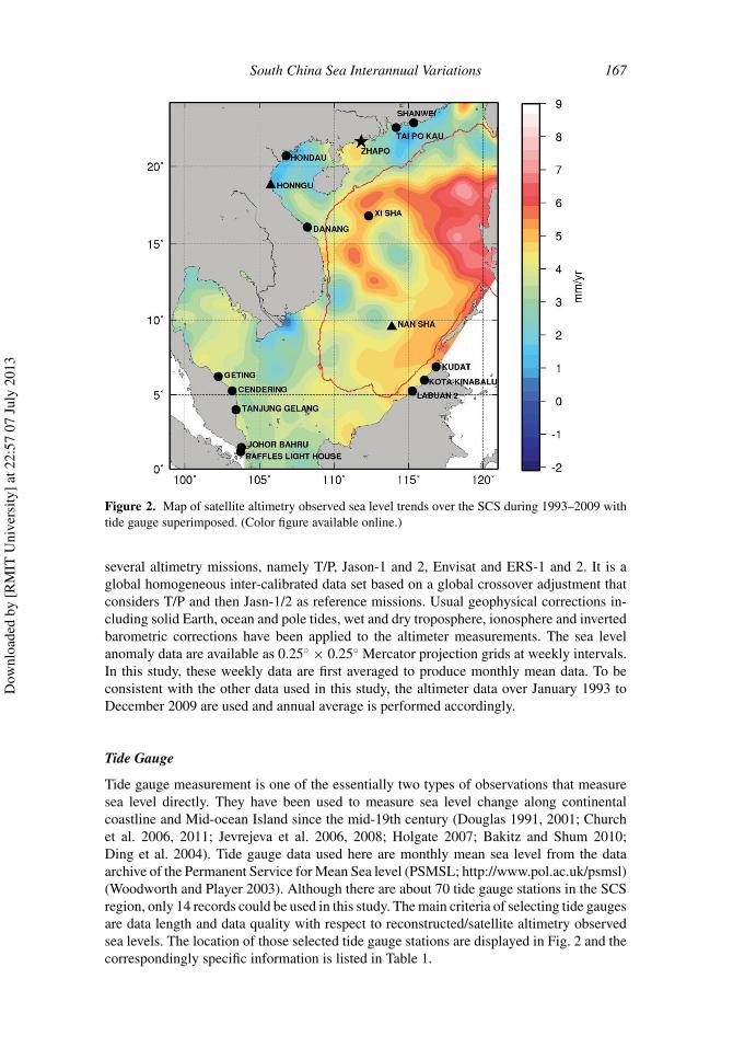
South China Sea Interannual Variations 167
Figure 2. Map of satellite altimetry observed sea level trends over the SCS during 1993–2009 with
tide gauge superimposed. (Color figure available online.)
several altimetry missions, namely T/P, Jason-1 and 2, Envisat and ERS-1 and 2. It is a
global homogeneous inter-calibrated data set based on a global crossover adjustment that
considers T/P and then Jasn-1/2 as reference missions. Usual geophysical corrections in-
cluding solid Earth, ocean and pole tides, wet and dry troposphere, ionosphere and inverted
barometric corrections have been applied to the altimeter measurements. The sea level
anomaly data are available as 0.25◦ × 0.25◦ Mercator projection grids at weekly intervals.
In this study, these weekly data are first averaged to produce monthly mean data. To be
consistent with the other data used in this study, the altimeter data over January 1993 to
December 2009 are used and annual average is performed accordingly.
Tide Gauge
Tide gauge measurement is one of the essentially two types of observations that measure
sea level directly. They have been used to measure sea level change along continental
coastline and Mid-ocean Island since the mid-19th century (Douglas 1991, 2001; Church
et al. 2006, 2011; Jevrejeva et al. 2006, 2008; Holgate 2007; Bakitz and Shum 2010;
Ding et al. 2004). Tide gauge data used here are monthly mean sea level from the data
archive of the Permanent Service for Mean Sea level (PSMSL; http://www.pol.ac.uk/psmsl)
(Woodworth and Player 2003). Although there are about 70 tide gauge stations in the SCS
region, only 14 records could be used in this study. The main criteria of selecting tide gauges
are data length and data quality with respect to reconstructed/satellite altimetry observed
sea levels. The location of those selected tide gauge stations are displayed in Fig. 2 and the
correspondingly specific information is listed in Table 1.
Dow
nlo
aded
by [
RM
IT U
niv
ersi
ty]
at 2
2:5
7 0
7 J
uly
2013
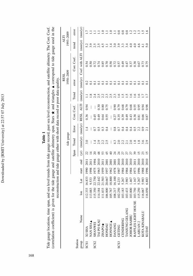
Tab
le1
Tid
egau
ge
loca
tions,
tim
esp
an,
and
sea
level
tren
ds
from
tide
gau
ge
reco
rd,
pas
tse
ale
vel
reco
nst
ruct
ion,
and
sate
llit
eal
tim
etry
.T
he
Corr
.C
oef
.
(corr
elat
ion
coef
fici
ent)
isgiv
enfo
rth
eti
de
gau
ge
and
sate
llit
eal
tim
etry
span
.S
tars
⋆an
dtr
iangle
s�
corr
espond
toti
de
gau
ge
use
din
the
reco
nst
ruct
ion
and
tide
gau
ge
eith
erw
ith
short
dat
are
cord
or
poor
dat
aqual
ity. RE
SL
AL
TI
tide
gau
ge
1950–2009
1993–2009
Span
Tre
nd
Err
or
Corr
.C
oef
.T
rend
erro
rC
orr
.C
oef
.tr
end
erro
rS
tati
on
gro
up
Nam
elo
nL
atst
art
end
(yr)
(mm
/yr)
(mm
/yr)
RE
SL
AL
TI
(mm
/yr)
(mm
/yr)
Coef
.w
ith
AL
TI
(mm
/yr)
(mm
/yr)
SC
S1
XI
SH
A112.3
33
16.8
33
1990
2011
22
3.0
1.4
0.3
60.9
41.1
0.2
0.5
45.2
1.7
NA
NS
HA
�113.8
83
9.5
33
1998
2011
14
——
——
1.8
0.1
0.5
03.9
1.1
SC
S2
SH
AN
WE
I115.3
50
22.7
50
1975
1994
20
1.4
0.7
0.4
5—
2.4
0.1
0.7
22.5
1.1
TA
IP
OK
AU
114.1
84
22.4
42
1963
2010
48
2.9
0.5
0.4
90.3
02.5
0.1
0.7
42.5
1.1
ZH
AP
O⋆
111.8
33
21.5
83
1959
2011
53
2.2
0.3
0.6
40.8
02.2
0.1
0.8
54.5
1.0
HO
ND
AU
106.8
00
20.6
67
1957
2001
45
2.5
0.4
0.5
50.7
52.3
0.1
0.7
01.1
1.1
HO
NN
GU
�105.7
67
18.8
00
1962
2001
40
——
——
2.5
0.1
0.5
81.4
1.0
DA
NA
NG
108.2
17
16.1
00
1978
2001
24
4.3
0.8
0.2
70.9
02.3
0.1
0.7
23.0
1.1
SC
S3
GE
TIN
G102.2
50
6.2
33
1987
2010
24
2.0
0.7
0.3
50.7
91.6
0.1
0.5
73.9
0.8
CE
ND
ER
ING
103.1
83
5.2
67
1984
2010
27
2.2
0.4
0.3
90.6
81.5
0.1
0.4
93.3
0.8
TA
NJU
NG
GE
LA
NG
103.4
33
3.9
83
1984
2010
27
2.1
0.4
0.4
90.7
91.5
0.1
0.4
73.4
0.8
JOH
OR
BA
HR
U103.8
00
1.4
67
1984
2010
27
2.0
0.4
0.4
30.6
81.6
0.1
0.3
74.0
1.2
RA
FF
LE
SL
IGH
TH
OU
SE
103.7
50
1.1
67
1973
2011
39
1.8
0.5
0.3
80.5
51.6
0.1
0.3
84.0
1.2
LA
BU
AN
2115.2
50
5.2
67
1996
2010
15
1.8
2.2
0.8
10.9
51.6
0.1
0.6
74.6
1.3
KO
TA
KIN
AB
AL
U116.0
67
5.9
83
1988
2010
23
3.6
0.9
0.6
60.9
41.7
0.1
0.7
34.1
1.5
KU
DA
T116.8
50
6.8
83
1996
2010
15
2.9
2.1
0.8
70.9
81.7
0.1
0.7
55.0
1.6
168
Dow
nlo
aded
by [
RM
IT U
niv
ersi
ty]
at 2
2:5
7 0
7 J
uly
2013
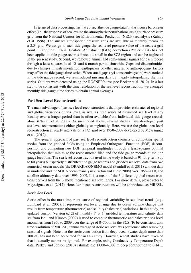
South China Sea Interannual Variations 169
In terms of data processing, we first correct the tide gauge data for the inverse barometer
effect (i.e., the response of sea level to the atmospheric perturbations) using surface pressure
grid from the National Centers for Environmental Prediction (NECP) reanalysis (Kalnay
et al. 1996). The surface atmospheric pressure grids are available as monthly means on
a 2.5o grid. We assign to each tide gauge the sea level pressure value of the nearest grid
point. In addition, Glacial Isostatic Adjustment (GIA) correction (Peltier 2004) has not
been applied to tide gauge records since it is small in the SCS region and can be neglected
in the present study. Second, we removed annual and semi-annual signals for each record
through a least-squares fit of 12- and 6-month period sinusoids. Gaps and discontinuities
due to changes in instrumentation, earthquakes or other natural or anthropogenic factors
may affect the tide gauge time series. When small gaps (≤4 consecutive years) were noticed
in the tide gauge record, we reintroduced missing data by linearly interpolating the time
series. Outliers were detected using the ROSNER’s test (see Becker et al. 2012). In a last
step to be consistent with the time resolution of the sea level reconstruction, we averaged
monthly tide gauge time series to obtain annual averages.
Past Sea Level Reconstruction
The main advantage of past sea level reconstruction is that it provides estimates of regional
and global variations of sea level, as well as time series of estimated sea level at any
locality over a longer period than is often available from individual tide gauge records
alone (Church et al. 2006). As mentioned above, several studies have developed past
sea level reconstructions either globally or regionally. Here, we use the global sea level
reconstruction at yearly intervals on a 1/2o grid over 1950–2009 developed by Meyssignac
et al. (2012).
The general approach of past sea level reconstruction consists of computing spatial
modes from the gridded fields using an Empirical Orthogonal Function (EOF) decom-
position and computing new EOF temporal amplitudes through a least-squares optimal
interpolation that minimize the reconstructed filed and the tide gauge records at the tide
gauge locations. The sea level reconstruction used in the study is based on 91 long-term (up
to 60 years) but sparsely distributed tide gauge records and gridded sea level data from two
numerical ocean models (the DRAKKAR/NEMO model (Penduff et al. 2011) without data
assimilation and the SODA ocean reanalysis (Carton and Giese 2008) over 1958–2008, and
satellite altimetry data over 1993–2009. It is a mean of the 3 different global reconstruc-
tions derived from the 3 above mentioned sea level grids. For more details, please refer to
Meyssignac et al. (2012). Hereafter, mean reconstructions will be abbreviated as MRESL.
Steric Sea Level
Steric effect is the most important cause of regional variability in sea level trends (e.g.,
Lombard et al. 2005). It represents sea level change due to ocean volume change that
results from temperature (thermosteric) and salinity (halosteric) variations. In this study, an
updated version (version 6.12) of monthly 1o × 1o gridded temperature and salinity data
set from Ishii and Kimoto (2009) is used to compute thermosteric and halosteric sea level
anomalies from 1950 to 2009 over the range of 0–700 m in the SCS. To be consistent with
time resolution of MRESL, annual average of steric sea level was performed after removing
seasonal signals. Note that the steric contribution from deep-ocean (water depth more than
700 m) has not been accounted for in this study. However, recent studies have revealed
that it actually cannot be ignored. For example, using Conductivity-Temperature-Depth
data, Purkey and Johson (2010) estimate the 1,000–4,000 m deep contribution to 0.14 ±
Dow
nlo
aded
by [
RM
IT U
niv
ersi
ty]
at 2
2:5
7 0
7 J
uly
2013
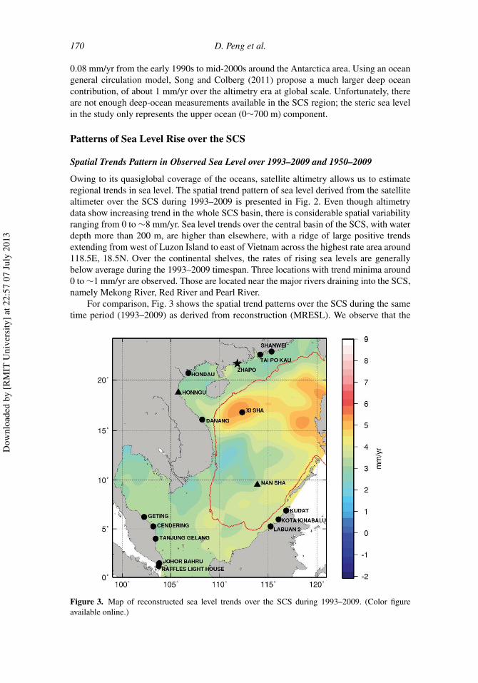
170 D. Peng et al.
0.08 mm/yr from the early 1990s to mid-2000s around the Antarctica area. Using an ocean
general circulation model, Song and Colberg (2011) propose a much larger deep ocean
contribution, of about 1 mm/yr over the altimetry era at global scale. Unfortunately, there
are not enough deep-ocean measurements available in the SCS region; the steric sea level
in the study only represents the upper ocean (0∼700 m) component.
Patterns of Sea Level Rise over the SCS
Spatial Trends Pattern in Observed Sea Level over 1993–2009 and 1950–2009
Owing to its quasiglobal coverage of the oceans, satellite altimetry allows us to estimate
regional trends in sea level. The spatial trend pattern of sea level derived from the satellite
altimeter over the SCS during 1993–2009 is presented in Fig. 2. Even though altimetry
data show increasing trend in the whole SCS basin, there is considerable spatial variability
ranging from 0 to ∼8 mm/yr. Sea level trends over the central basin of the SCS, with water
depth more than 200 m, are higher than elsewhere, with a ridge of large positive trends
extending from west of Luzon Island to east of Vietnam across the highest rate area around
118.5E, 18.5N. Over the continental shelves, the rates of rising sea levels are generally
below average during the 1993–2009 timespan. Three locations with trend minima around
0 to ∼1 mm/yr are observed. Those are located near the major rivers draining into the SCS,
namely Mekong River, Red River and Pearl River.
For comparison, Fig. 3 shows the spatial trend patterns over the SCS during the same
time period (1993–2009) as derived from reconstruction (MRESL). We observe that the
Figure 3. Map of reconstructed sea level trends over the SCS during 1993–2009. (Color figure
available online.)
Dow
nlo
aded
by [
RM
IT U
niv
ersi
ty]
at 2
2:5
7 0
7 J
uly
2013
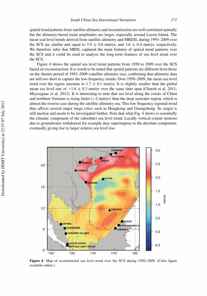
South China Sea Interannual Variations 171
spatial trend patterns from satellite altimetry and reconstruction are well correlated spatially
but the altimetry-based trend amplitudes are larger, especially around Luzon Island. The
mean seal level trends derived from satellite altimetry and MRESL during 1993–2009 over
the SCS are similar and equal to 3.9 ± 0.6 mm/yr, and 3.6 ± 0.4 mm/yr, respectively.
We therefore infer that MRSL captured the main features of spatial trend patterns over
the SCS and it could be used to analyze the long-term features of sea level trend over
the SCS.
Figure 4 shows the spatial sea level trend patterns from 1950 to 2009 over the SCS
based on reconstruction. It is worth to be noted that spatial patterns are different from those
on the shorter period of 1993–2009 (satellite altimetry era), confirming that altimetry data
are still too short to capture the low-frequency trends. Over 1950–2009, the mean sea level
trend over the region amounts to 1.7 ± 0.1 mm/yr, It is slightly smaller than the global
mean sea level rate of ∼1.8 ± 0.3 mm/yr over the same time span (Church et al. 2011;
Meyssignac et al. 2012). It is interesting to note that sea level along the coasts of China
and northern Vietnam is rising faster (>2 mm/yr) than the deep seawater region, which is
almost the reverse case during the satellite altimetry era. This low frequency regional trend
thus affects several major mega cities such as Hongkong and Guangzhong. Its origin is
still unclear and needs to be investigated further. Note that what Fig. 4 shows is essentially
the climatic component of the (absolute) sea level trend. Locally vertical crustal motions
due to groundwater withdrawal for example may superimpose to the absolute component,
eventually giving rise to larger relative sea level rise.
Figure 4. Map of reconstructed sea level trend over the SCS during 1950–2009. (Color figure
available online.)
Dow
nlo
aded
by [
RM
IT U
niv
ersi
ty]
at 2
2:5
7 0
7 J
uly
2013
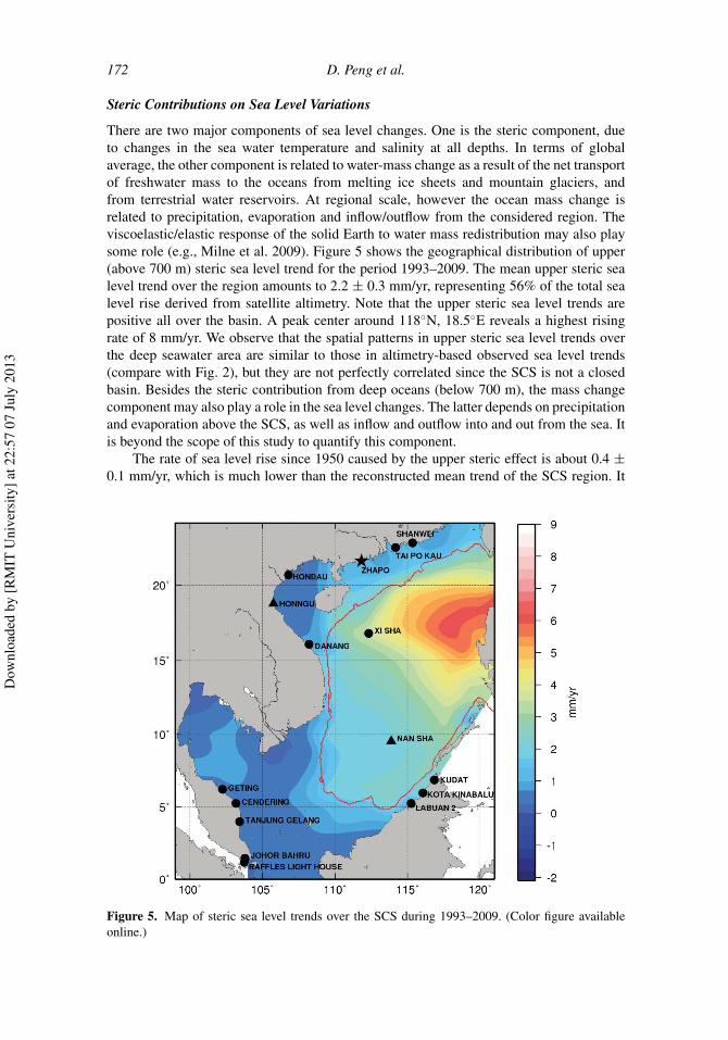
172 D. Peng et al.
Steric Contributions on Sea Level Variations
There are two major components of sea level changes. One is the steric component, due
to changes in the sea water temperature and salinity at all depths. In terms of global
average, the other component is related to water-mass change as a result of the net transport
of freshwater mass to the oceans from melting ice sheets and mountain glaciers, and
from terrestrial water reservoirs. At regional scale, however the ocean mass change is
related to precipitation, evaporation and inflow/outflow from the considered region. The
viscoelastic/elastic response of the solid Earth to water mass redistribution may also play
some role (e.g., Milne et al. 2009). Figure 5 shows the geographical distribution of upper
(above 700 m) steric sea level trend for the period 1993–2009. The mean upper steric sea
level trend over the region amounts to 2.2 ± 0.3 mm/yr, representing 56% of the total sea
level rise derived from satellite altimetry. Note that the upper steric sea level trends are
positive all over the basin. A peak center around 118◦N, 18.5◦E reveals a highest rising
rate of 8 mm/yr. We observe that the spatial patterns in upper steric sea level trends over
the deep seawater area are similar to those in altimetry-based observed sea level trends
(compare with Fig. 2), but they are not perfectly correlated since the SCS is not a closed
basin. Besides the steric contribution from deep oceans (below 700 m), the mass change
component may also play a role in the sea level changes. The latter depends on precipitation
and evaporation above the SCS, as well as inflow and outflow into and out from the sea. It
is beyond the scope of this study to quantify this component.
The rate of sea level rise since 1950 caused by the upper steric effect is about 0.4 ±
0.1 mm/yr, which is much lower than the reconstructed mean trend of the SCS region. It
Figure 5. Map of steric sea level trends over the SCS during 1993–2009. (Color figure available
online.)
Dow
nlo
aded
by [
RM
IT U
niv
ersi
ty]
at 2
2:5
7 0
7 J
uly
2013
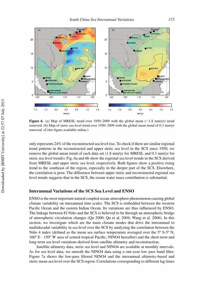
South China Sea Interannual Variations 173
Figure 6. (a) Map of MRESL trend over 1950–2009 with the global mean (∼1.8 mm/yr) trend
removed. (b) Map of steric sea level trend over 1950–2009 with the global mean trend of 0.3 mm/yr
removed. (Color figure available online.)
only represents 24% of the reconstructed sea level rise. To check if there are similar regional
trend patterns in the reconstructed and upper steric sea level in the SCS since 1950, we
remove the global mean trend of each data set (1.8 mm/yr for MRESL and 0.3 mm/yr for
steric sea level trends). Fig. 6a and 6b show the regional sea level trends in the SCS derived
from MRESL and upper steric sea level, respectively. Both figures show a positive rising
trend to the southeast of the region, especially in the deeper part of the SCS. Elsewhere,
the correlation is poor. The difference between upper steric and reconstructed regional sea
level trends suggests that in the SCS, the ocean water mass contribution is substantial.
Interannual Variations of the SCS Sea Level and ENSO
ENSO is the most important natural coupled ocean-atmosphere phenomenon causing global
climate variability on interannual time scales. The SCS is embedded between the western
Pacific Ocean and the eastern Indian Ocean. Its variations are thus influenced by ENSO.
The linkage between El Nino and the SCS is believed to be through an atmospheric bridge
of atmospheric circulation changes (Qu 2000; Qu et al. 2004; Wang et al. 2006). In this
section, we investigate which are the main climate modes that drive the interannual to
multidecadal variability in sea level over the SCS by analyzing the correlation between the
Nino 4 index (defined as the mean sea surface temperature averaged over the 5o S-5o N,
160o E - 150o W area of central tropical Pacific; NINO4 hereafter) and the short-term and
long-term sea level variations derived from satellite altimetry and reconstruction.
Satellite altimetry data, steric sea level and NINO4 are available at monthly intervals.
As for sea level data, we smooth the NINO4 data using a one-year low pass band filter.
Figure 7a shows the low-pass filtered NINO4 and the interannual altimetry-based and
steric mean sea level over the SCS region. Correlations corresponding to different lag times
Dow
nlo
aded
by [
RM
IT U
niv
ersi
ty]
at 2
2:5
7 0
7 J
uly
2013
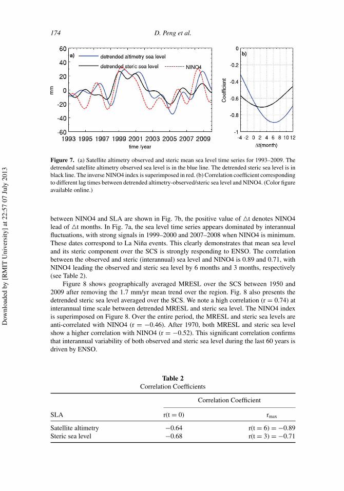
174 D. Peng et al.
Figure 7. (a) Satellite altimetry observed and steric mean sea level time series for 1993–2009. The
detrended satellite altimetry observed sea level is in the blue line. The detrended steric sea level is in
black line. The inverse NINO4 index is superimposed in red. (b) Correlation coefficient corresponding
to different lag times between detrended altimetry-observed/steric sea level and NINO4. (Color figure
available online.)
between NINO4 and SLA are shown in Fig. 7b, the positive value of △t denotes NINO4
lead of △t months. In Fig. 7a, the sea level time series appears dominated by interannual
fluctuations, with strong signals in 1999–2000 and 2007–2008 when NINO4 is minimum.
These dates correspond to La Nina events. This clearly demonstrates that mean sea level
and its steric component over the SCS is strongly responding to ENSO. The correlation
between the observed and steric (interannual) sea level and NINO4 is 0.89 and 0.71, with
NINO4 leading the observed and steric sea level by 6 months and 3 months, respectively
(see Table 2).
Figure 8 shows geographically averaged MRESL over the SCS between 1950 and
2009 after removing the 1.7 mm/yr mean trend over the region. Fig. 8 also presents the
detrended steric sea level averaged over the SCS. We note a high correlation (r = 0.74) at
interannual time scale between detrended MRESL and steric sea level. The NINO4 index
is superimposed on Figure 8. Over the entire period, the MRESL and steric sea levels are
anti-correlated with NINO4 (r = −0.46). After 1970, both MRESL and steric sea level
show a higher correlation with NINO4 (r = −0.52). This significant correlation confirms
that interannual variability of both observed and steric sea level during the last 60 years is
driven by ENSO.
Table 2
Correlation Coefficients
Correlation Coefficient
SLA r(t = 0) rmax
Satellite altimetry −0.64 r(t = 6) = −0.89
Steric sea level −0.68 r(t = 3) = −0.71
Dow
nlo
aded
by [
RM
IT U
niv
ersi
ty]
at 2
2:5
7 0
7 J
uly
2013
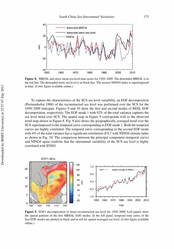
South China Sea Interannual Variations 175
Figure 8. MRESL and steric mean sea level time series for 1950–2009. The detrended MRESL is in
the red line. The detrended steric sea level is in black line. The inverse NINO4 index is superimposed
in blue. (Color figure available online.)
To capture the characteristics of the SCS sea level variability, an EOF decomposition
(Preisendorfer 1988) of the reconstructed sea level was performed over the SCS for the
1950–2009 timespan. Figures 9 and 10 show the first and second modes of RESL EOF
decomposition, respectively. The EOF mode 1 with 92% of the total variance captures the
sea level trend over SCS. The spatial map in Figure 9 corresponds well to the observed
trend map shown in Figure 8. Fig. 9 also shows the geographically averaged trend over the
SCS superimposed to the temporal curve corresponding to EOF mode 1. Both the temporal
curves are highly correlated. The temporal curve corresponding to the second EOF mode
with 4% of the total variance has a significant correlation of 0.7 with NINO4 climate index
as shown in Fig. 10. The comparison between the principal component (temporal curve)
and NINO4 again confirms that the interannual variability of the SCS sea level is highly
correlated with ENSO.
Figure 9. EOF1 decomposition of mean reconstructed sea level for 1950–2009. Left panels show
the spatial patterns of the first MRESL EOF modes. In the left panel, temporal time series of the
first EOF modes are plotted in black and in red for spatial averaged sea level. (Color figure available
online.)
Dow
nlo
aded
by [
RM
IT U
niv
ersi
ty]
at 2
2:5
7 0
7 J
uly
2013
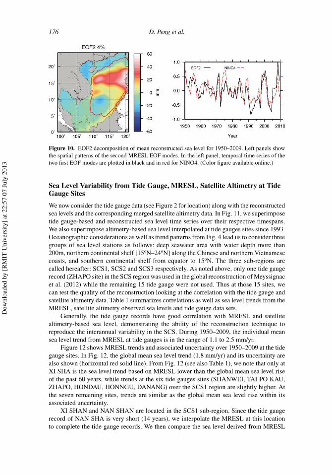
176 D. Peng et al.
Figure 10. EOF2 decomposition of mean reconstructed sea level for 1950–2009. Left panels show
the spatial patterns of the second MRESL EOF modes. In the left panel, temporal time series of the
two first EOF modes are plotted in black and in red for NINO4. (Color figure available online.)
Sea Level Variability from Tide Gauge, MRESL, Satellite Altimetry at TideGauge Sites
We now consider the tide gauge data (see Figure 2 for location) along with the reconstructed
sea levels and the corresponding merged satellite altimetry data. In Fig. 11, we superimpose
tide gauge-based and reconstructed sea level time series over their respective timespans.
We also superimpose altimetry-based sea level interpolated at tide gauges sites since 1993.
Oceanographic considerations as well as trend patterns from Fig. 4 lead us to consider three
groups of sea level stations as follows: deep seawater area with water depth more than
200m, northern continental shelf [15oN–24oN] along the Chinese and northern Vietnamese
coasts, and southern continental shelf from equator to 15oN. The three sub-regions are
called hereafter: SCS1, SCS2 and SCS3 respectively. As noted above, only one tide gauge
record (ZHAPO site) in the SCS region was used in the global reconstruction of Meyssignac
et al. (2012) while the remaining 15 tide gauge were not used. Thus at those 15 sites, we
can test the quality of the reconstruction looking at the correlation with the tide gauge and
satellite altimetry data. Table 1 summarizes correlations as well as sea level trends from the
MRESL, satellite altimetry observed sea levels and tide gauge data sets.
Generally, the tide gauge records have good correlation with MRESL and satellite
altimetry-based sea level, demonstrating the ability of the reconstruction technique to
reproduce the interannual variability in the SCS. During 1950–2009, the individual mean
sea level trend from MRESL at tide gauges is in the range of 1.1 to 2.5 mm/yr.
Figure 12 shows MRESL trends and associated uncertainty over 1950–2009 at the tide
gauge sites. In Fig. 12, the global mean sea level trend (1.8 mm/yr) and its uncertainty are
also shown (horizontal red solid line). From Fig. 12 (see also Table 1), we note that only at
XI SHA is the sea level trend based on MRESL lower than the global mean sea level rise
of the past 60 years, while trends at the six tide gauges sites (SHANWEI, TAI PO KAU,
ZHAPO, HONDAU, HONNGU, DANANG) over the SCS1 region are slightly higher. At
the seven remaining sites, trends are similar as the global mean sea level rise within its
associated uncertainty.
XI SHAN and NAN SHAN are located in the SCS1 sub-region. Since the tide gauge
record of NAN SHA is very short (14 years), we interpolate the MRESL at this location
to complete the tide gauge records. We then compare the sea level derived from MRESL
Dow
nlo
aded
by [
RM
IT U
niv
ersi
ty]
at 2
2:5
7 0
7 J
uly
2013
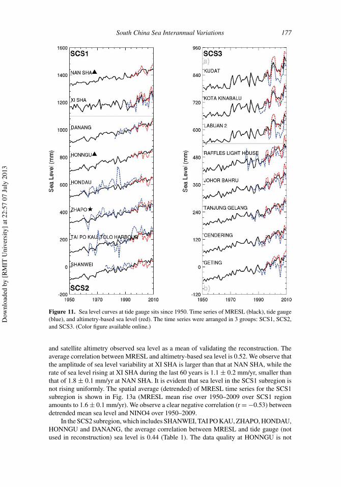
South China Sea Interannual Variations 177
Figure 11. Sea level curves at tide gauge sits since 1950. Time series of MRESL (black), tide gauge
(blue), and altimetry-based sea level (red). The time series were arranged in 3 groups: SCS1, SCS2,
and SCS3. (Color figure available online.)
and satellite altimetry observed sea level as a mean of validating the reconstruction. The
average correlation between MRESL and altimetry-based sea level is 0.52. We observe that
the amplitude of sea level variability at XI SHA is larger than that at NAN SHA, while the
rate of sea level rising at XI SHA during the last 60 years is 1.1 ± 0.2 mm/yr, smaller than
that of 1.8 ± 0.1 mm/yr at NAN SHA. It is evident that sea level in the SCS1 subregion is
not rising uniformly. The spatial average (detrended) of MRESL time series for the SCS1
subregion is shown in Fig. 13a (MRESL mean rise over 1950–2009 over SCS1 region
amounts to 1.6 ± 0.1 mm/yr). We observe a clear negative correlation (r = −0.53) between
detrended mean sea level and NINO4 over 1950–2009.
In the SCS2 subregion, which includes SHANWEI, TAI PO KAU, ZHAPO, HONDAU,
HONNGU and DANANG, the average correlation between MRESL and tide gauge (not
used in reconstruction) sea level is 0.44 (Table 1). The data quality at HONNGU is not
Dow
nlo
aded
by [
RM
IT U
niv
ersi
ty]
at 2
2:5
7 0
7 J
uly
2013
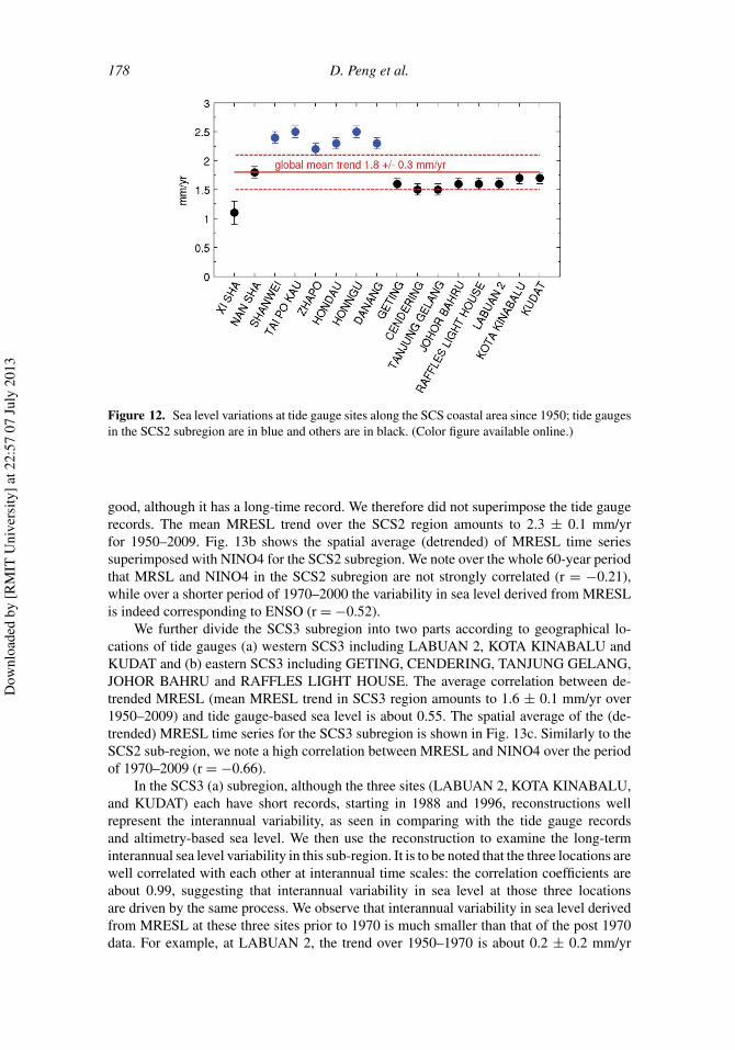
178 D. Peng et al.
Figure 12. Sea level variations at tide gauge sites along the SCS coastal area since 1950; tide gauges
in the SCS2 subregion are in blue and others are in black. (Color figure available online.)
good, although it has a long-time record. We therefore did not superimpose the tide gauge
records. The mean MRESL trend over the SCS2 region amounts to 2.3 ± 0.1 mm/yr
for 1950–2009. Fig. 13b shows the spatial average (detrended) of MRESL time series
superimposed with NINO4 for the SCS2 subregion. We note over the whole 60-year period
that MRSL and NINO4 in the SCS2 subregion are not strongly correlated (r = −0.21),
while over a shorter period of 1970–2000 the variability in sea level derived from MRESL
is indeed corresponding to ENSO (r = −0.52).
We further divide the SCS3 subregion into two parts according to geographical lo-
cations of tide gauges (a) western SCS3 including LABUAN 2, KOTA KINABALU and
KUDAT and (b) eastern SCS3 including GETING, CENDERING, TANJUNG GELANG,
JOHOR BAHRU and RAFFLES LIGHT HOUSE. The average correlation between de-
trended MRESL (mean MRESL trend in SCS3 region amounts to 1.6 ± 0.1 mm/yr over
1950–2009) and tide gauge-based sea level is about 0.55. The spatial average of the (de-
trended) MRESL time series for the SCS3 subregion is shown in Fig. 13c. Similarly to the
SCS2 sub-region, we note a high correlation between MRESL and NINO4 over the period
of 1970–2009 (r = −0.66).
In the SCS3 (a) subregion, although the three sites (LABUAN 2, KOTA KINABALU,
and KUDAT) each have short records, starting in 1988 and 1996, reconstructions well
represent the interannual variability, as seen in comparing with the tide gauge records
and altimetry-based sea level. We then use the reconstruction to examine the long-term
interannual sea level variability in this sub-region. It is to be noted that the three locations are
well correlated with each other at interannual time scales: the correlation coefficients are
about 0.99, suggesting that interannual variability in sea level at those three locations
are driven by the same process. We observe that interannual variability in sea level derived
from MRESL at these three sites prior to 1970 is much smaller than that of the post 1970
data. For example, at LABUAN 2, the trend over 1950–1970 is about 0.2 ± 0.2 mm/yr
Dow
nlo
aded
by [
RM
IT U
niv
ersi
ty]
at 2
2:5
7 0
7 J
uly
2013
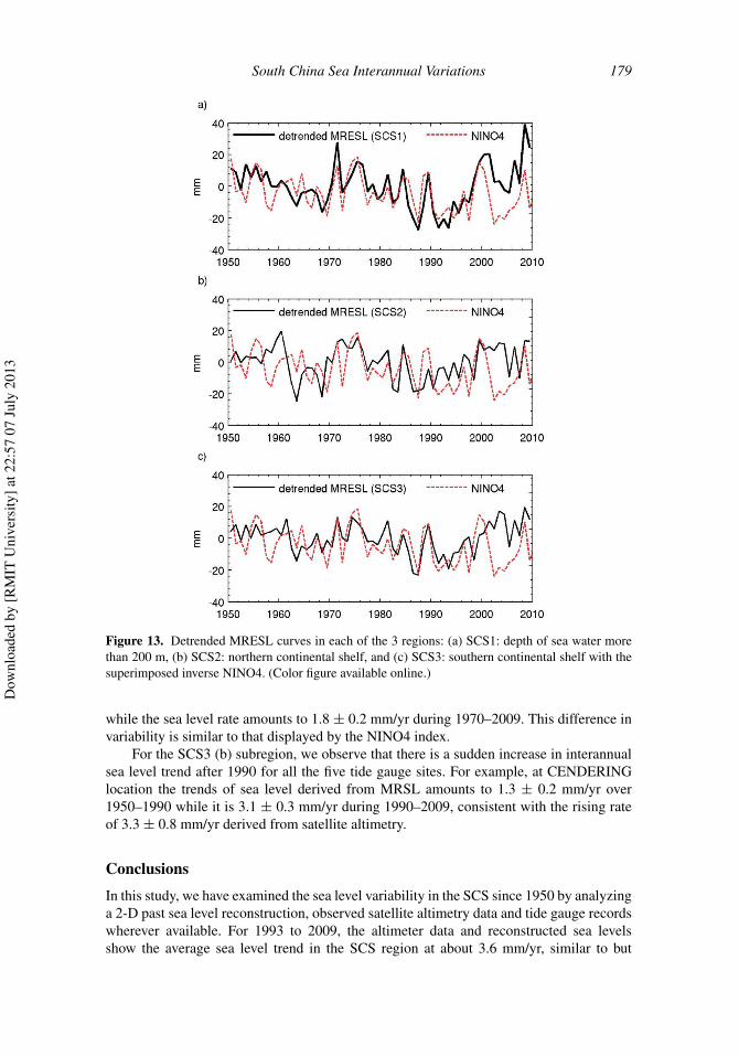
South China Sea Interannual Variations 179
Figure 13. Detrended MRESL curves in each of the 3 regions: (a) SCS1: depth of sea water more
than 200 m, (b) SCS2: northern continental shelf, and (c) SCS3: southern continental shelf with the
superimposed inverse NINO4. (Color figure available online.)
while the sea level rate amounts to 1.8 ± 0.2 mm/yr during 1970–2009. This difference in
variability is similar to that displayed by the NINO4 index.
For the SCS3 (b) subregion, we observe that there is a sudden increase in interannual
sea level trend after 1990 for all the five tide gauge sites. For example, at CENDERING
location the trends of sea level derived from MRSL amounts to 1.3 ± 0.2 mm/yr over
1950–1990 while it is 3.1 ± 0.3 mm/yr during 1990–2009, consistent with the rising rate
of 3.3 ± 0.8 mm/yr derived from satellite altimetry.
Conclusions
In this study, we have examined the sea level variability in the SCS since 1950 by analyzing
a 2-D past sea level reconstruction, observed satellite altimetry data and tide gauge records
wherever available. For 1993 to 2009, the altimeter data and reconstructed sea levels
show the average sea level trend in the SCS region at about 3.6 mm/yr, similar to but
Dow
nlo
aded
by [
RM
IT U
niv
ersi
ty]
at 2
2:5
7 0
7 J
uly
2013
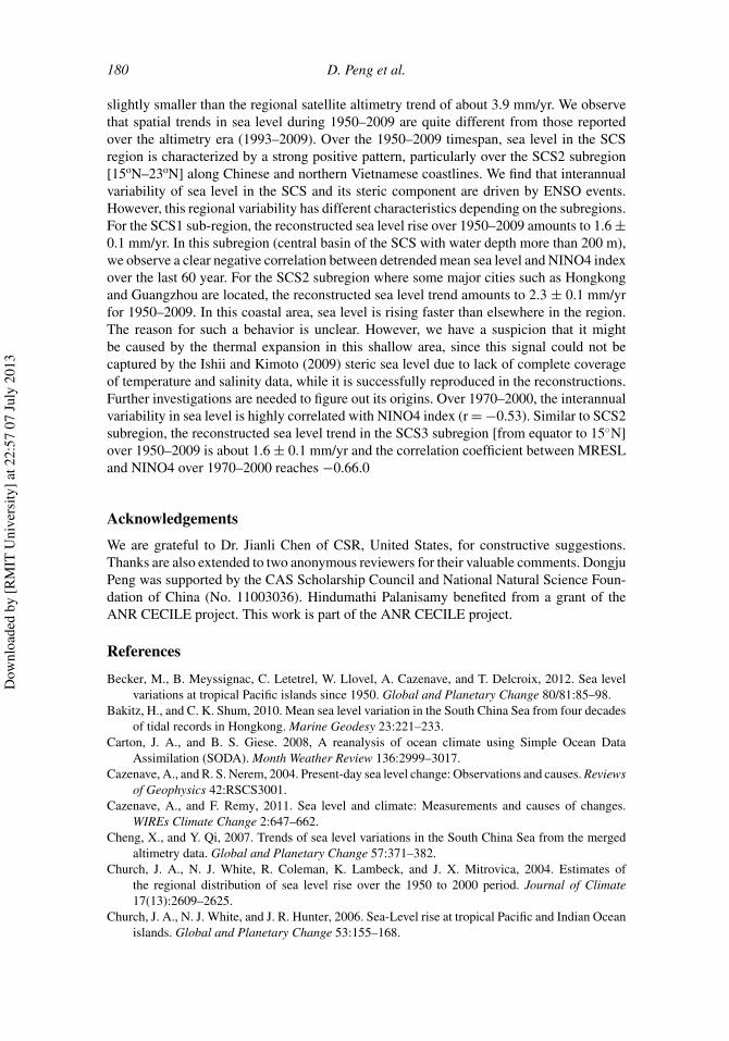
180 D. Peng et al.
slightly smaller than the regional satellite altimetry trend of about 3.9 mm/yr. We observe
that spatial trends in sea level during 1950–2009 are quite different from those reported
over the altimetry era (1993–2009). Over the 1950–2009 timespan, sea level in the SCS
region is characterized by a strong positive pattern, particularly over the SCS2 subregion
[15oN–23oN] along Chinese and northern Vietnamese coastlines. We find that interannual
variability of sea level in the SCS and its steric component are driven by ENSO events.
However, this regional variability has different characteristics depending on the subregions.
For the SCS1 sub-region, the reconstructed sea level rise over 1950–2009 amounts to 1.6 ±
0.1 mm/yr. In this subregion (central basin of the SCS with water depth more than 200 m),
we observe a clear negative correlation between detrended mean sea level and NINO4 index
over the last 60 year. For the SCS2 subregion where some major cities such as Hongkong
and Guangzhou are located, the reconstructed sea level trend amounts to 2.3 ± 0.1 mm/yr
for 1950–2009. In this coastal area, sea level is rising faster than elsewhere in the region.
The reason for such a behavior is unclear. However, we have a suspicion that it might
be caused by the thermal expansion in this shallow area, since this signal could not be
captured by the Ishii and Kimoto (2009) steric sea level due to lack of complete coverage
of temperature and salinity data, while it is successfully reproduced in the reconstructions.
Further investigations are needed to figure out its origins. Over 1970–2000, the interannual
variability in sea level is highly correlated with NINO4 index (r = −0.53). Similar to SCS2
subregion, the reconstructed sea level trend in the SCS3 subregion [from equator to 15◦N]
over 1950–2009 is about 1.6 ± 0.1 mm/yr and the correlation coefficient between MRESL
and NINO4 over 1970–2000 reaches −0.66.0
Acknowledgements
We are grateful to Dr. Jianli Chen of CSR, United States, for constructive suggestions.
Thanks are also extended to two anonymous reviewers for their valuable comments. Dongju
Peng was supported by the CAS Scholarship Council and National Natural Science Foun-
dation of China (No. 11003036). Hindumathi Palanisamy benefited from a grant of the
ANR CECILE project. This work is part of the ANR CECILE project.
References
Becker, M., B. Meyssignac, C. Letetrel, W. Llovel, A. Cazenave, and T. Delcroix, 2012. Sea level
variations at tropical Pacific islands since 1950. Global and Planetary Change 80/81:85–98.
Bakitz, H., and C. K. Shum, 2010. Mean sea level variation in the South China Sea from four decades
of tidal records in Hongkong. Marine Geodesy 23:221–233.
Carton, J. A., and B. S. Giese. 2008, A reanalysis of ocean climate using Simple Ocean Data
Assimilation (SODA). Month Weather Review 136:2999–3017.
Cazenave, A., and R. S. Nerem, 2004. Present-day sea level change: Observations and causes. Reviews
of Geophysics 42:RSCS3001.
Cazenave, A., and F. Remy, 2011. Sea level and climate: Measurements and causes of changes.
WIREs Climate Change 2:647–662.
Cheng, X., and Y. Qi, 2007. Trends of sea level variations in the South China Sea from the merged
altimetry data. Global and Planetary Change 57:371–382.
Church, J. A., N. J. White, R. Coleman, K. Lambeck, and J. X. Mitrovica, 2004. Estimates of
the regional distribution of sea level rise over the 1950 to 2000 period. Journal of Climate
17(13):2609–2625.
Church, J. A., N. J. White, and J. R. Hunter, 2006. Sea-Level rise at tropical Pacific and Indian Ocean
islands. Global and Planetary Change 53:155–168.
Dow
nlo
aded
by [
RM
IT U
niv
ersi
ty]
at 2
2:5
7 0
7 J
uly
2013
South China Sea Interannual Variations 181
Church, J. A., N. J. White, L. Konikow, C. Domingues, J. Goley, and E. Rignot, 2011. Revisiting
the Earth’s sea level and energy budget from 1961 to 2008. Geophysical Research Letters 38:
L18601.
Church, J. A., P. Woodworth, T. Aarup, and W. S. Wilson. 2010. Understanding sea-level rise and
variability. London: Wiley.
Ding, X., D. Zheng, W. T. Wong, K. W. Li, W. Chen, and P. Zhong, 2004. Recent sea level varia-
tions in Southern China from tide gauge observations. Proceedings of the Asia-Pacific Space
Geodynamics Symposium, Singapore, 6–8 July 2004, 126–136.
Douglas, B. C. 1991. Global sea level rise. Journal of Geophysical Research 96(C4):6981–6992.
Douglas, B. C. 2001. Sea level change in the era of the recording tide gauge. International Geophysics
75:37–64.
Ho, C., Q. Zheng, Y. Soong, N. Kuo, and J. Hu, 2000. Seasonal variability of sea surface height in
the South China Sea observed with TOPEX/Poseidon altimeter data. Journal of Geophysical
Research 105:13981–13990.
Holgate, S. 2007. On the decadal rates of sea level change during the twentieth century. Geophysical
Research Letters 34:L01602.
Ishii, M., and M. Kimoto, 2009. Reevaluation of historical ocean heat content variations with varying
XBT and MBT depth bias corrections. Journal of Oceanography 65:287–299.
Jevrejeva, S., A. Grinsted, J. Moore, and S. Holgate, 2006. Nonlinear trends and multiyear cycles in
sea level records. Journal of Geophysical Research 111:C09012.
Jevrejeva, S., J. Moore, A. Grinsted, and P. Woodworth, 2008. Recent global sea level acceleration
started over 200 years ago? Geophysical Research Letters 35:L08715.
Kalnay, E., M. Kanamitsu, R. Kistler, W. Collins, D. Deaven, L. Gandin, M. Iredell, S. Saha, G. White,
J. Woollen, Y. Zhu, M. Chelliah, W. Ebisuzaki, W. Higgins, J. Janowiak, K. C. Mo, C. Ropelewski,
J. Wang, A. Leetmaa, R. Reynolds, R. Jenne, and D. Joseph, 1996. The NCEP/NCAR 40-year
reanalysis project. Bulletin of the American Meteorological Society 77:437–472.
Li, L., J. Xu, and R. Cai, 2002. Trends of sea level rise in the South China Sea during 1990s: An
altimetry result. Chinese Science Bulletin 47:582–585.
Llovel, W., A. Cazenave, P. Rogel, A. Lombard, and M. Berge-Nguyen. 2009. Two-dimensional
reconstruction of past sea level (1950–2003) from tide gauge and Ocean General Circulation
Model. Climate of the Past 5:217–227.
Lombard, A., A. Cazenave, P. Y. Le Traon, and M. Ishii, 2005. Contribution of thermal expansion to
present-day sea-level change revisited. Global and Planetary Change 47:1–16.
Meyssignac, B., W. Llovel, M. Becker, and A. Cazenave, 2012. An assessment of two-dimensional
past sea level reconstructions over 1950–2009 based on tide gauge data and different input sea
level grids. Surveys in Geophysics 33:945–972.
Milne, G., W. Gehrels, C. Hughes, and M. Tamisiea, 2009. Identifying the causes of sea-level change.
Nature Geoscience 2(7):471–478.
Nicholls, R. J., and A. Cazenave, 2010. Sea-level rise and its impact on coastal zones. Science
328:1517–1520.
Palanisamy, H., M. Becker, B. Meyssignac, O. Henry, and A. Cazenave, 2012. Regional sea
level change and variability in the Caribbean Sea since 1950. Journal of Geodetic Science
2/2:125–133.
Peltier, W. R. 2004. Global glacial isostasy and the surface of the ice-age Earth: The ICE-5G (VM2)
model and GRACE. Annual Review of Earth and Planetary Sciences 32:111–149.
Penduff, T., M. Juza, L. Brodeau, G. Smith, B. Barnier, J.-M. Molines, A.-M. Treguier, and G.
Madec, 2011. Impact of global ocean model resolution on sea-level variability with emphasis
on interannual time scales. Ocean Science 6:269–284.
Preisendorfer, R. W. 1988. Principal component analysis in meteorology and oceanography. Devel-
opments in Atmospheric Science 17.
Purkey, S., and G. C. Johnson, 2010. Warming of global abyssal and deep southern ocean waters
between the 1990s and 2000s: Contributions to global heat and sea level rise budget. Journal of
Climate 23:6336–6351.
Dow
nlo
aded
by [
RM
IT U
niv
ersi
ty]
at 2
2:5
7 0
7 J
uly
2013
182 D. Peng et al.
Qu, T. 2000. Upper-layer circulation in the South China Sea. Journal of Physical Oceanography
30:1450–1460.
Qu, T., Y. Y. Kim, M. Yaremchuk, T. Tozuka, A. Ishida, and T. Yamagata. 2004. Can Luzon strait
transport play a role in conveying the impact of ENSO to the South China Sea? Journal of
Climate 17:3644–3657.
Ray, R., and B. Douglas, 2011. Experiments in reconstructing twentieth-century sea levels. Progress
in Oceanography 91(4):496–515.
Rong, Z., Y. Liu, H. Zong, and Y. Cheng, 2007. Interannual sea level variabilty in the South China
Sea and its response to ENSO. Global and Planetary Change 55:257–272.
Shaw, P., S. Chao, and L. Fu, 1999. Sea surface height in the South China Sea from satellite altimetry.
Oceanologica Acta 22(1):1–17.
Song, Y. T., and F. Colberg, 2011. Deep ocean warming assessed from altimeters, gravity recovery
and climate experiment, in situ measurements, and a non-Boussinesq ocean general circulation
model. Journal of Geophysical Research 116:C02020.
Wang, C., W. Wang, D. Wang, and Q. Wang, 2006. Interannual variability of the South China Sea
associated with El Nino. Journal of Geophysical Research 111:C030203.
Woodworth, P., and R. Player, 2003. The permanent service for mean sea level: An update to the 21st
century. Journal of Coastal Research 19:287–295.
Dow
nlo
aded
by [
RM
IT U
niv
ersi
ty]
at 2
2:5
7 0
7 J
uly
2013
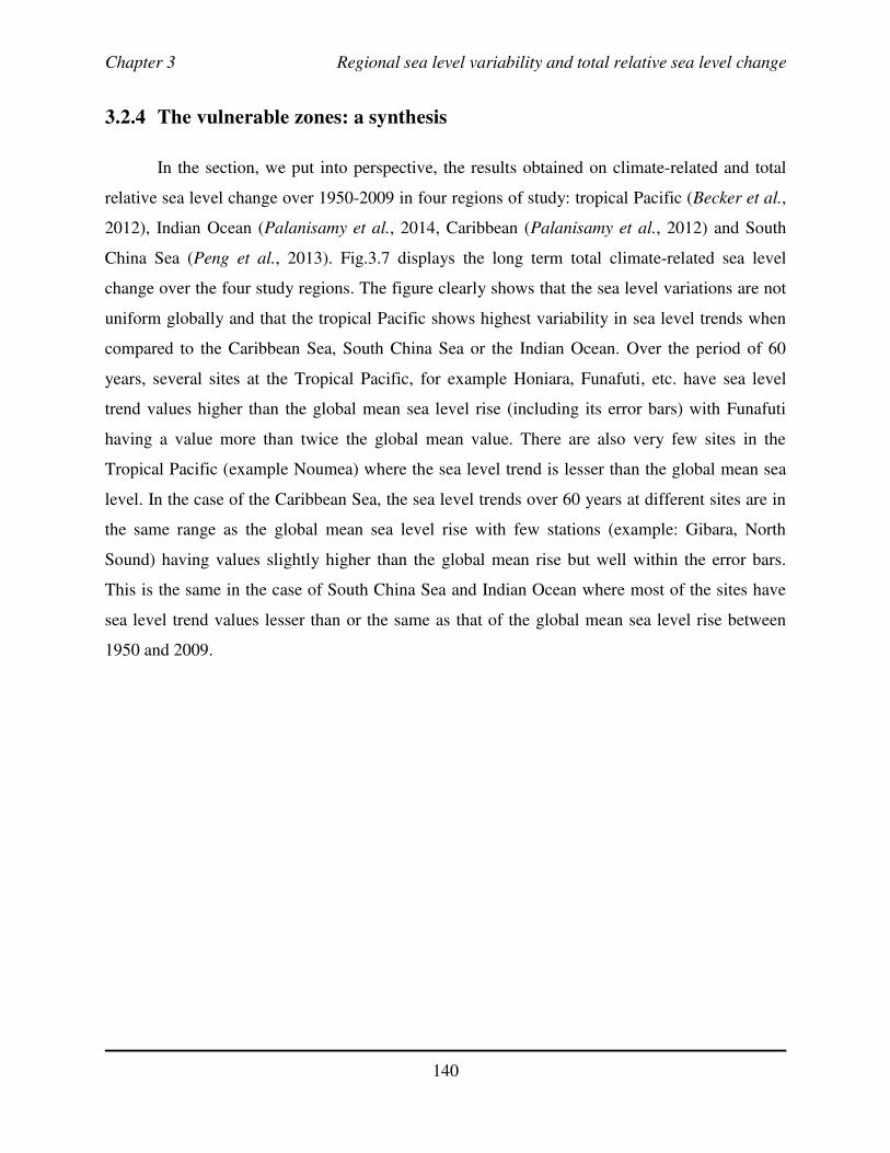
Chapter 3 Regional sea level variability and total relative sea level change
140
3.2.4 The vulnerable zones: a synthesis
In the section, we put into perspective, the results obtained on climate-related and total
relative sea level change over 1950-2009 in four regions of study: tropical Pacific (Becker et al.,
2012), Indian Ocean (Palanisamy et al., 2014, Caribbean (Palanisamy et al., 2012) and South
China Sea (Peng et al., 2013). Fig.3.7 displays the long term total climate-related sea level
change over the four study regions. The figure clearly shows that the sea level variations are not
uniform globally and that the tropical Pacific shows highest variability in sea level trends when
compared to the Caribbean Sea, South China Sea or the Indian Ocean. Over the period of 60
years, several sites at the Tropical Pacific, for example Honiara, Funafuti, etc. have sea level
trend values higher than the global mean sea level rise (including its error bars) with Funafuti
having a value more than twice the global mean value. There are also very few sites in the
Tropical Pacific (example Noumea) where the sea level trend is lesser than the global mean sea
level. In the case of the Caribbean Sea, the sea level trends over 60 years at different sites are in
the same range as the global mean sea level rise with few stations (example: Gibara, North
Sound) having values slightly higher than the global mean rise but well within the error bars.
This is the same in the case of South China Sea and Indian Ocean where most of the sites have
sea level trend values lesser than or the same as that of the global mean sea level rise between
1950 and 2009.
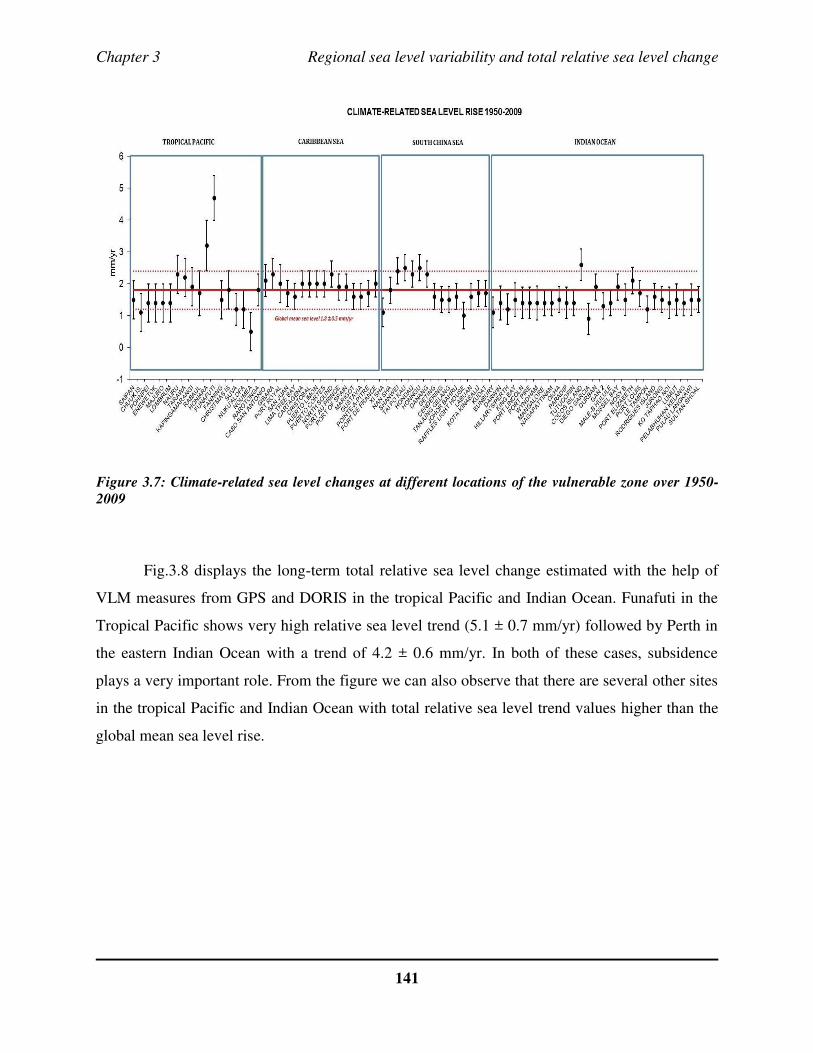
Chapter 3 Regional sea level variability and total relative sea level change
141
Figure 3.7: Climate-related sea level changes at different locations of the vulnerable zone over 1950-
2009
Fig.3.8 displays the long-term total relative sea level change estimated with the help of
VLM measures from GPS and DORIS in the tropical Pacific and Indian Ocean. Funafuti in the
Tropical Pacific shows very high relative sea level trend (5.1 ± 0.7 mm/yr) followed by Perth in
the eastern Indian Ocean with a trend of 4.2 ± 0.6 mm/yr. In both of these cases, subsidence
plays a very important role. From the figure we can also observe that there are several other sites
in the tropical Pacific and Indian Ocean with total relative sea level trend values higher than the
global mean sea level rise.
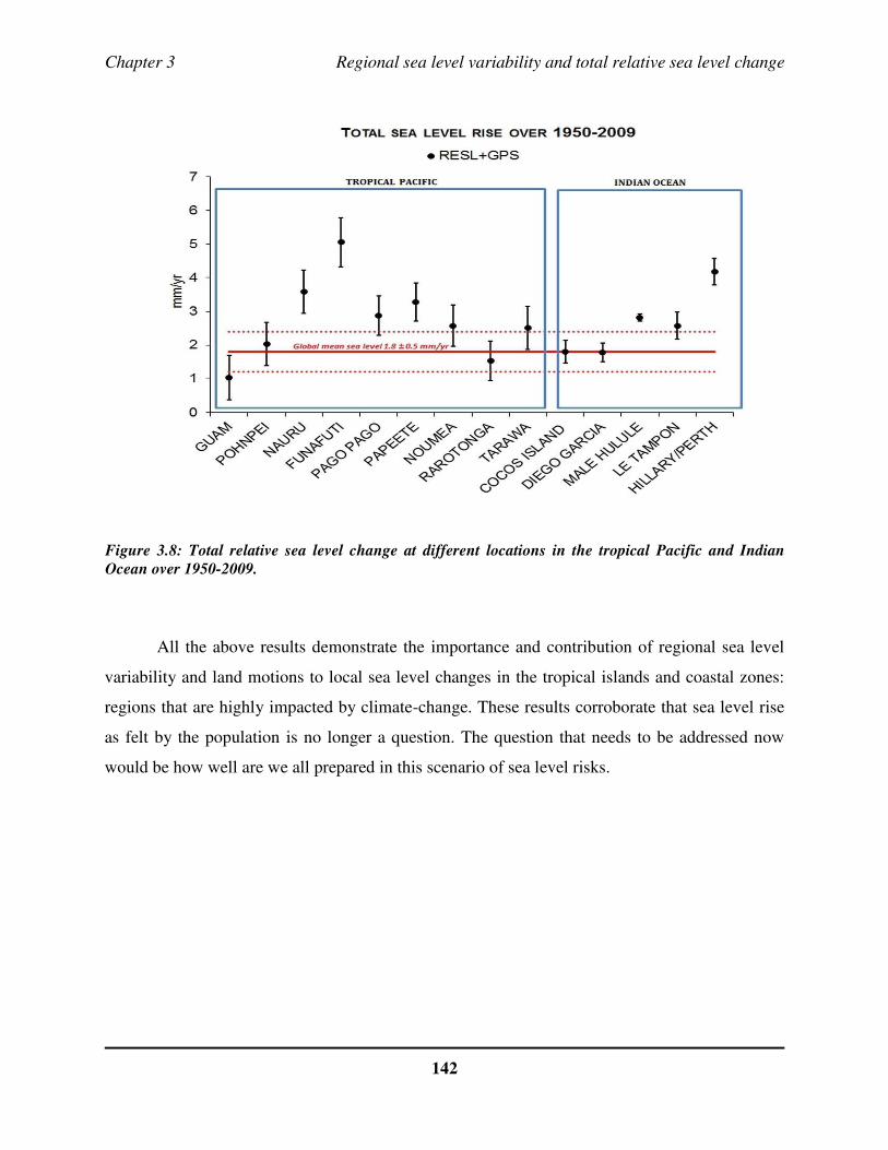
Chapter 3 Regional sea level variability and total relative sea level change
142
Figure 3.8: Total relative sea level change at different locations in the tropical Pacific and Indian
Ocean over 1950-2009.
All the above results demonstrate the importance and contribution of regional sea level
variability and land motions to local sea level changes in the tropical islands and coastal zones:
regions that are highly impacted by climate-change. These results corroborate that sea level rise
as felt by the population is no longer a question. The question that needs to be addressed now
would be how well are we all prepared in this scenario of sea level risks.
Chapter 4 Role of internal climate variability and external forcing
143
Chapter 4
The role of internal climate variability and
external forcing on regional sea level variations
In chapter 3, we have discussed the various causes that contribute to regional sea level
variability with non-uniform thermosteric and halosteric changes being the most important
contributor. In fact, the spatial and temporal variability of steric sea level changes is tightly
linked to complex ocean dynamic processes that are also related to internal climate modes such
as ENSO, IPO/PDO etc. While the internal climate modes are in general natural climate
variability not resulting from human (i.e. anthropogenic) influences, understanding the impact of
external anthropogenic influences (i.e. climate change) on regional sea level variability and on
internal climate modes has so far remained a great challenge for sea level and climate scientists.
For studies on global warming and climate change, it is important to distinguish between
internally generated and externally-forced climate variability. In this chapter, we first provide a
detailed explanation on the roles of internal climate variability and external forcing in regional
sea level variability. We then discuss our two main works related to this thematic applied on the
Pacific Ocean.
4.1 Internal climate variability
Internal climate variability refers to what is frequently called ‘unforced’ climate changes
or ‘modes’ of variability that do not involve changes in Earth’s net radiative balance. Hunt,
(2006) called the unforced internal climate variability as that which occurs solely due to internal
interactions such as complex ocean-atmosphere dynamics within the climate system without any
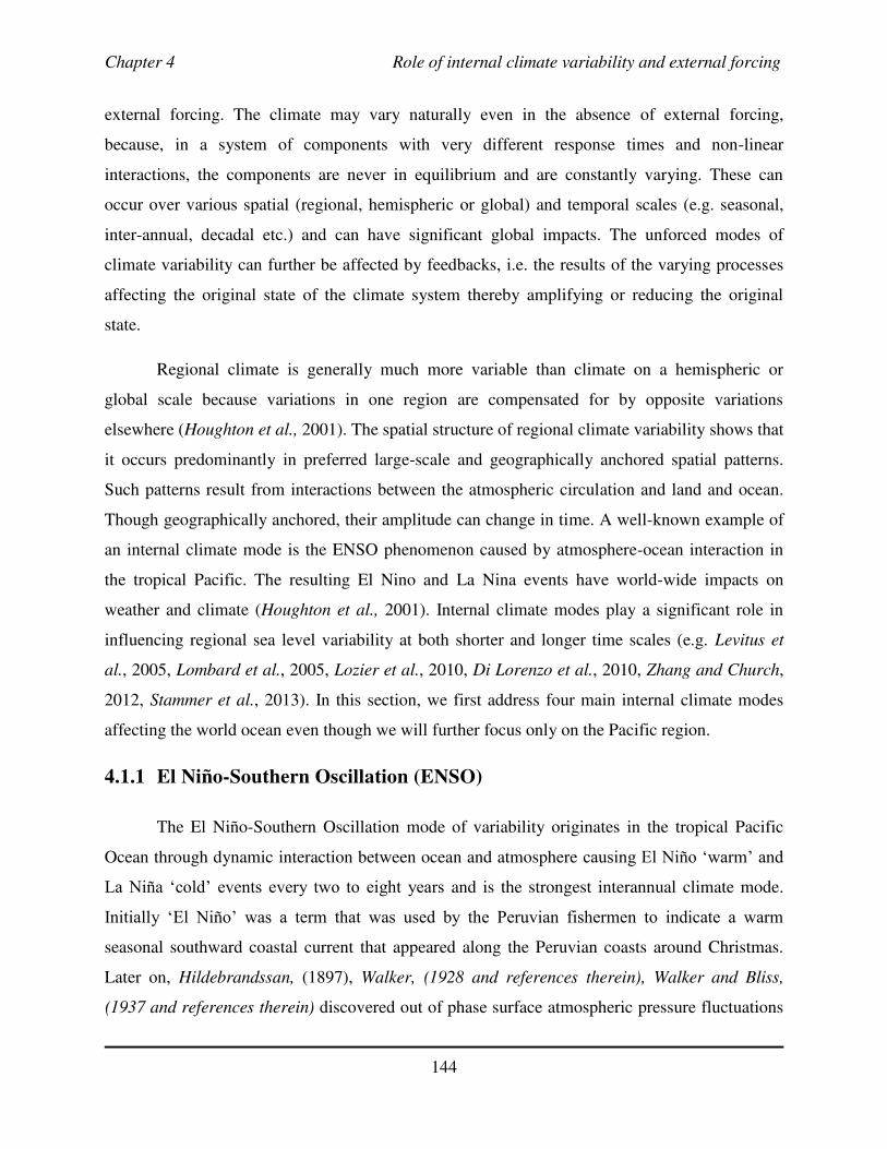
Chapter 4 Role of internal climate variability and external forcing
144
external forcing. The climate may vary naturally even in the absence of external forcing,
because, in a system of components with very different response times and non-linear
interactions, the components are never in equilibrium and are constantly varying. These can
occur over various spatial (regional, hemispheric or global) and temporal scales (e.g. seasonal,
inter-annual, decadal etc.) and can have significant global impacts. The unforced modes of
climate variability can further be affected by feedbacks, i.e. the results of the varying processes
affecting the original state of the climate system thereby amplifying or reducing the original
state.
Regional climate is generally much more variable than climate on a hemispheric or
global scale because variations in one region are compensated for by opposite variations
elsewhere (Houghton et al., 2001). The spatial structure of regional climate variability shows that
it occurs predominantly in preferred large-scale and geographically anchored spatial patterns.
Such patterns result from interactions between the atmospheric circulation and land and ocean.
Though geographically anchored, their amplitude can change in time. A well-known example of
an internal climate mode is the ENSO phenomenon caused by atmosphere-ocean interaction in
the tropical Pacific. The resulting El Nino and La Nina events have world-wide impacts on
weather and climate (Houghton et al., 2001). Internal climate modes play a significant role in
influencing regional sea level variability at both shorter and longer time scales (e.g. Levitus et
al., 2005, Lombard et al., 2005, Lozier et al., 2010, Di Lorenzo et al., 2010, Zhang and Church,
2012, Stammer et al., 2013). In this section, we first address four main internal climate modes
affecting the world ocean even though we will further focus only on the Pacific region.
4.1.1 El Niño-Southern Oscillation (ENSO)
The El Niño-Southern Oscillation mode of variability originates in the tropical Pacific
Ocean through dynamic interaction between ocean and atmosphere causing El Niño ‘warm’ and
La Niña ‘cold’ events every two to eight years and is the strongest interannual climate mode.
Initially ‘El Niño’ was a term that was used by the Peruvian fishermen to indicate a warm
seasonal southward coastal current that appeared along the Peruvian coasts around Christmas.
Later on, Hildebrandssan, (1897), Walker, (1928 and references therein), Walker and Bliss,
(1937 and references therein) discovered out of phase surface atmospheric pressure fluctuations
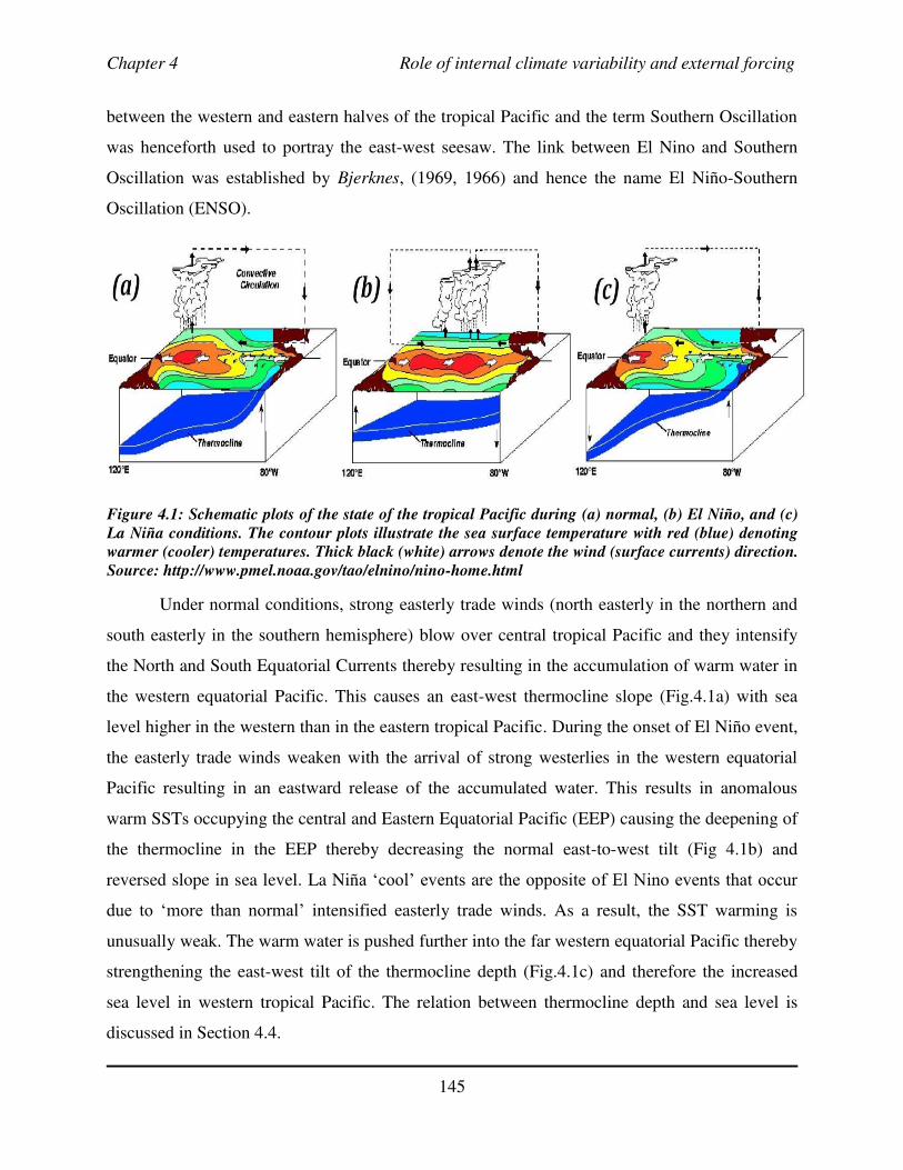
Chapter 4 Role of internal climate variability and external forcing
145
between the western and eastern halves of the tropical Pacific and the term Southern Oscillation
was henceforth used to portray the east-west seesaw. The link between El Nino and Southern
Oscillation was established by Bjerknes, (1969, 1966) and hence the name El Niño-Southern
Oscillation (ENSO).
Figure 4.1: Schematic plots of the state of the tropical Pacific during (a) normal, (b) El Niño, and (c)
La Niña conditions. The contour plots illustrate the sea surface temperature with red (blue) denoting
warmer (cooler) temperatures. Thick black (white) arrows denote the wind (surface currents) direction.
Source: http://www.pmel.noaa.gov/tao/elnino/nino-home.html
Under normal conditions, strong easterly trade winds (north easterly in the northern and
south easterly in the southern hemisphere) blow over central tropical Pacific and they intensify
the North and South Equatorial Currents thereby resulting in the accumulation of warm water in
the western equatorial Pacific. This causes an east-west thermocline slope (Fig.4.1a) with sea
level higher in the western than in the eastern tropical Pacific. During the onset of El Niño event,
the easterly trade winds weaken with the arrival of strong westerlies in the western equatorial
Pacific resulting in an eastward release of the accumulated water. This results in anomalous
warm SSTs occupying the central and Eastern Equatorial Pacific (EEP) causing the deepening of
the thermocline in the EEP thereby decreasing the normal east-to-west tilt (Fig 4.1b) and
reversed slope in sea level. La Niña ‘cool’ events are the opposite of El Nino events that occur
due to ‘more than normal’ intensified easterly trade winds. As a result, the SST warming is
unusually weak. The warm water is pushed further into the far western equatorial Pacific thereby
strengthening the east-west tilt of the thermocline depth (Fig.4.1c) and therefore the increased
sea level in western tropical Pacific. The relation between thermocline depth and sea level is
discussed in Section 4.4.
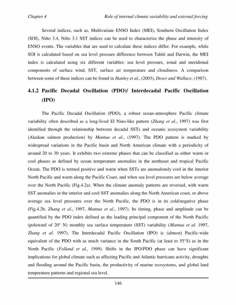
Chapter 4 Role of internal climate variability and external forcing
146
Several indices, such as, Multivariate ENSO Index (MEI), Southern Oscillation Index
(SOI), Niño 3.4, Niño 3.1 SST indices can be used to characterize the phase and intensity of
ENSO events. The variables that are used to calculate these indices differ. For example, while
SOI is calculated based on sea level pressure difference between Tahiti and Darwin, the MEI
index is calculated using six different variables: sea level pressure, zonal and meridional
components of surface wind, SST, surface air temperature and cloudiness. A comparison
between some of these indices can be found in Hanley et al., (2003), Deser and Wallace, (1987).
4.1.2 Pacific Decadal Oscillation (PDO)/ Interdecadal Pacific Oscillation
(IPO)
The Pacific Decadal Oscillation (PDO), a robust ocean-atmosphere Pacific climate
variability often described as a long-lived El Nino-like pattern (Zhang et al., 1997) was first
identified through the relationship between decadal SSTs and oceanic ecosystem variability
(Alaskan salmon production) by Mantua et al., (1997). The PDO pattern is marked by
widespread variations in the Pacific basin and North American climate with a periodicity of
around 20 to 30 years. It exhibits two extreme phases that can be classified as either warm or
cool phases as defined by ocean temperature anomalies in the northeast and tropical Pacific
Ocean. The PDO is termed positive and warm when SSTs are anomalously cool in the interior
North Pacific and warm along the Pacific Coast, and when sea level pressures are below average
over the North Pacific (Fig.4.2a). When the climate anomaly patterns are reversed, with warm
SST anomalies in the interior and cool SST anomalies along the North American coast, or above
average sea level pressures over the North Pacific, the PDO is in its cold/negative phase
(Fig.4.2b, Zhang et al., 1997, Mantua et al., 1997). Its timing, phase and amplitude can be
quantified by the PDO index defined as the leading principal component of the North Pacific
(poleward of 20° N) monthly sea surface temperature (SST) variability (Mantua et al. 1997,
Zhang et al. 1997). The Interdecadal Pacific Oscillation (IPO) is (almost) Pacific-wide
equivalent of the PDO with as much variance in the South Pacific (at least to 55°S) as in the
North Pacific (Folland et al., 1999). Shifts in the IPO/PDO phase can have significant
implications for global climate such as affecting Pacific and Atlantic hurricane activity, droughts
and flooding around the Pacific basin, the productivity of marine ecosystems, and global land
temperature patterns and regional sea level.
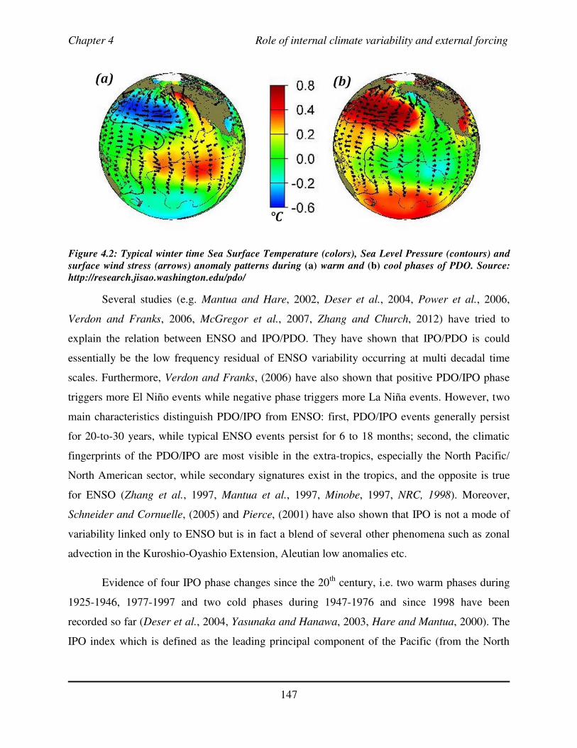
Chapter 4 Role of internal climate variability and external forcing
147
Figure 4.2: Typical winter time Sea Surface Temperature (colors), Sea Level Pressure (contours) and
surface wind stress (arrows) anomaly patterns during (a) warm and (b) cool phases of PDO. Source:
http://research.jisao.washington.edu/pdo/
Several studies (e.g. Mantua and Hare, 2002, Deser et al., 2004, Power et al., 2006,
Verdon and Franks, 2006, McGregor et al., 2007, Zhang and Church, 2012) have tried to
explain the relation between ENSO and IPO/PDO. They have shown that IPO/PDO is could
essentially be the low frequency residual of ENSO variability occurring at multi decadal time
scales. Furthermore, Verdon and Franks, (2006) have also shown that positive PDO/IPO phase
triggers more El Niño events while negative phase triggers more La Niña events. However, two
main characteristics distinguish PDO/IPO from ENSO: first, PDO/IPO events generally persist
for 20-to-30 years, while typical ENSO events persist for 6 to 18 months; second, the climatic
fingerprints of the PDO/IPO are most visible in the extra-tropics, especially the North Pacific/
North American sector, while secondary signatures exist in the tropics, and the opposite is true
for ENSO (Zhang et al., 1997, Mantua et al., 1997, Minobe, 1997, NRC, 1998). Moreover,
Schneider and Cornuelle, (2005) and Pierce, (2001) have also shown that IPO is not a mode of
variability linked only to ENSO but is in fact a blend of several other phenomena such as zonal
advection in the Kuroshio-Oyashio Extension, Aleutian low anomalies etc.
Evidence of four IPO phase changes since the 20th
century, i.e. two warm phases during
1925-1946, 1977-1997 and two cold phases during 1947-1976 and since 1998 have been
recorded so far (Deser et al., 2004, Yasunaka and Hanawa, 2003, Hare and Mantua, 2000). The
IPO index which is defined as the leading principal component of the Pacific (from the North

Chapter 4 Role of internal climate variability and external forcing
148
Pacific until at least 55°S) monthly SST variability is in general used to characterize the intensity
of IPO events. The influence of IPO on sea level will be discussed in Section 4.4.
4.1.3 Indian Ocean Dipole (IOD) mode
The Indian Ocean Dipole (IOD) is a coupled ocean-atmosphere phenomenon occurring in
the equatorial Indian Ocean that affects the climate of Australia and other countries that surround
the Indian Ocean basin and is a significant contributor to rainfall in this region (Saji et al., 1999).
The IOD involves aperiodic east-west oscillation of SST between ‘positive’, ‘neutral’ and
‘negative’ phases and are strongly coupled to surface wind anomalies in the central equatorial
Indian Ocean (Saji et al., 1999, Behera and Yamagata, 2001, Saji and Yamagata, 2003). A
positive IOD period is characterized by anomalous SST cooling in the south eastern equatorial
Indian Ocean and anomalous SST warming in the western equatorial Indian Ocean (Fig.4.3a). As
a result, the normal convection situated over the eastern Indian Ocean warm pool shifts to the
west. This brings heavy rainfall over east Africa, decrease in rainfall over central and southern
Australia and severe droughts over the Indonesian regions. Conversely, negative IOD period is
characterized by anomalous SST warming in the south eastern equatorial and cooling in the
western equatorial Indian Ocean (Fig.4.3b) resulting in more rainfall in the Indonesian and
Australian regions and drought in east Africa.
IOD is a short term event and usually begins to develop during the summer of the
Northern Hemisphere, reaches its maximum in fall and ends in winter as a result of seasonal
winds (Behera and Yamagata, 2001, Black et al., 2003, Hastenrath, 2007). Several IOD events
have occurred simultaneously with ENSO events and there is a significant debate on whether
IOD is an independent climate variability occurring in the Indian Ocean or whether it is triggered
by ENSO (Reason et al., 2000, Allan et al., 2001). Positive IOD events are often associated with
El Niño events and negative IOD with La Niña events. The link between IOD and ENSO is
thought to be through the extension of the Walker circulation to the west and associated
Indonesian through flow i.e. the flow of warm tropical ocean water from the Pacific into the
Indian Ocean. Studies (e.g. Deser et al., 2004, Clark et al., 2003) have also shown good
correlations between inter-decadal and decadal variability of SST-based IOD, ENSO and
IPO/PDO indices, raising the issue of coupled mechanisms governing IOD, ENSO and
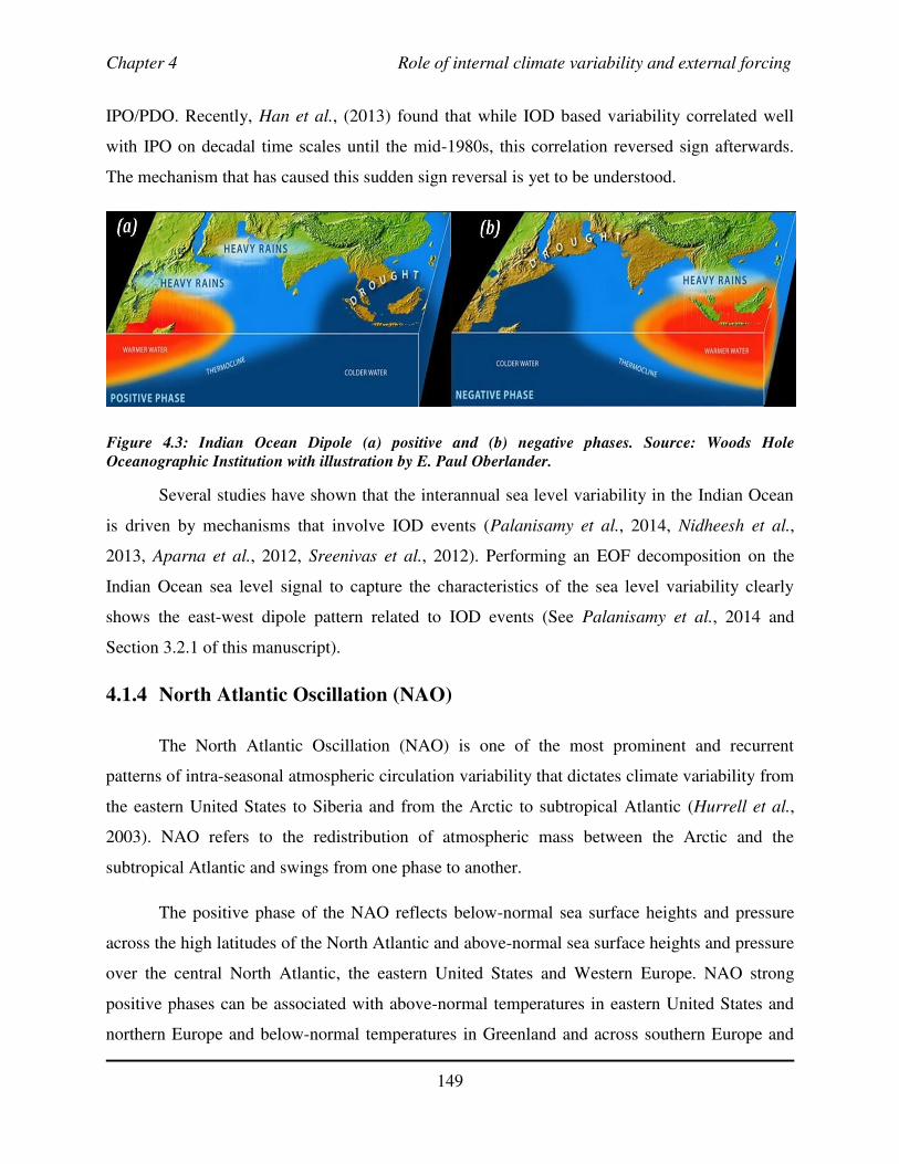
Chapter 4 Role of internal climate variability and external forcing
149
IPO/PDO. Recently, Han et al., (2013) found that while IOD based variability correlated well
with IPO on decadal time scales until the mid-1980s, this correlation reversed sign afterwards.
The mechanism that has caused this sudden sign reversal is yet to be understood.
Figure 4.3: Indian Ocean Dipole (a) positive and (b) negative phases. Source: Woods Hole
Oceanographic Institution with illustration by E. Paul Oberlander.
Several studies have shown that the interannual sea level variability in the Indian Ocean
is driven by mechanisms that involve IOD events (Palanisamy et al., 2014, Nidheesh et al.,
2013, Aparna et al., 2012, Sreenivas et al., 2012). Performing an EOF decomposition on the
Indian Ocean sea level signal to capture the characteristics of the sea level variability clearly
shows the east-west dipole pattern related to IOD events (See Palanisamy et al., 2014 and
Section 3.2.1 of this manuscript).
4.1.4 North Atlantic Oscillation (NAO)
The North Atlantic Oscillation (NAO) is one of the most prominent and recurrent
patterns of intra-seasonal atmospheric circulation variability that dictates climate variability from
the eastern United States to Siberia and from the Arctic to subtropical Atlantic (Hurrell et al.,
2003). NAO refers to the redistribution of atmospheric mass between the Arctic and the
subtropical Atlantic and swings from one phase to another.
The positive phase of the NAO reflects below-normal sea surface heights and pressure
across the high latitudes of the North Atlantic and above-normal sea surface heights and pressure
over the central North Atlantic, the eastern United States and Western Europe. NAO strong
positive phases can be associated with above-normal temperatures in eastern United States and
northern Europe and below-normal temperatures in Greenland and across southern Europe and
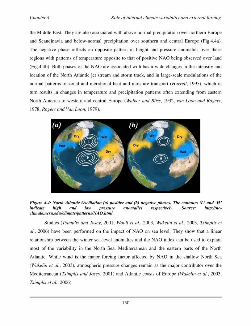
Chapter 4 Role of internal climate variability and external forcing
150
the Middle East. They are also associated with above-normal precipitation over northern Europe
and Scandinavia and below-normal precipitation over southern and central Europe (Fig.4.4a).
The negative phase reflects an opposite pattern of height and pressure anomalies over these
regions with patterns of temperature opposite to that of positive NAO being observed over land
(Fig.4.4b). Both phases of the NAO are associated with basin-wide changes in the intensity and
location of the North Atlantic jet stream and storm track, and in large-scale modulations of the
normal patterns of zonal and meridional heat and moisture transport (Hurrell, 1995), which in
turn results in changes in temperature and precipitation patterns often extending from eastern
North America to western and central Europe (Walker and Bliss, 1932, van Loon and Rogers,
1978, Rogers and Van Loon, 1979).
Figure 4.4: North Atlantic Oscillation (a) positive and (b) negative phases. The contours ‘L’ and ‘H’ indicate high and low pressure anomalies respectively. Source: http://nc-
climate.ncsu.edu/climate/patterns/NAO.html
Studies (Tsimplis and Josey, 2001, Woolf et al., 2003, Wakelin et al., 2003, Tsimplis et
al., 2006) have been performed on the impact of NAO on sea level. They show that a linear
relationship between the winter sea-level anomalies and the NAO index can be used to explain
most of the variability in the North Sea, Mediterranean and the eastern parts of the North
Atlantic. While wind is the major forcing factor affected by NAO in the shallow North Sea
(Wakelin et al., 2003), atmospheric pressure changes remain as the major contributor over the
Mediterranean (Tsimplis and Josey, 2001) and Atlantic coasts of Europe (Wakelin et al., 2003,
Tsimplis et al., 2006).
Chapter 4 Role of internal climate variability and external forcing
151
4.1.5 Other modes of internal climate variability
Many other patterns of internal climate variability have also been identified over the
years occurring at various time scales such as the Atlantic Multi-decadal Oscillation (AMO,
Kerr, 2000, McCarthy et al., 2015), Antarctic Circumpolar Wave (ACW, White et al., 1998,
Venegas, 2003), Arctic Oscillation or Northern Annular Mode (NAM, Lorenz, 1951, Thompson
and Wallace, 1998, Ripesi et al., 2012), Southern Annular Mode (SAM, Hartmann and Lo, 1998,
Abram et al., 2014), Madden-Julian Oscillation (MJO, Madden and Julian, 1971, Madden and
Julian, 1994, Zhang et al., 1997) etc. In this manuscript, I have focused on four of the main
internal climate modes that have major impacts on regional sea level variability.
4.2 Externally-forced climate variability
Externally-forced climate variability refers to variations over time in one or more
measures of climate caused by some factors outside the climate system. These factors include
both natural and anthropogenic sources. Examples of natural external forcing include solar
variability and volcanic eruptions. Examples of anthropogenic forcing are from changing
concentrations of greenhouse gases and aerosols and land use produced by human activities.
The magnitude of externally- forced variability depends on the extent of the forcing
involved and the sensitivity of the climate system to the forcing. Therefore the response time of
various components of the climate system to external forcing highly varies. Within the
atmosphere, the response time of the troposphere to external forcing is relatively shorter, only
from days to weeks, whereas the stratosphere comes into equilibrium only within a time period
of few months. In the case of oceans, due to their large heat capacity, they have a much longer
response time, typically decades but also up to centuries. The response time of the strongly
coupled surface-troposphere system is therefore slow compared with that of the stratosphere, and
is mainly determined by the oceans. Therefore the climate system may respond to variations in
external forcing on a wide range of space- and time-scales (Houghton et al., 2001). In this
section, we briefly explain the two sources of external forcing that impact the climate.
Chapter 4 Role of internal climate variability and external forcing
152
4.2.1 Natural external forcing
Several natural external drivers of climate change operate on multiple time scales (Myhre
et al., 2013). For example, solar variability takes place at many time scales that include
centennial and millennial time scales as the radiant energy output of the Sun changes (Helama et
al., 2010). Furthermore, variations in Earth’s orbital and rotational parameters result in
redistribution of incoming solar radiation and trigger glacial and interglacial cycles. While these
occur at very large time scales, Earth’s revolution around the sun and rotation results in seasonal
and daily cycle changes respectively. All the mentioned natural external forcings are gradual and
do not produce drastic changes at short time scale thereby enabling different components of the
climate system to retain their equilibrium. However this is not the case with forcing that
produces immediate changes or consists of short-lived impulse such as volcanic eruptions
(Philander, 2012).
Volcanic eruptions that inject substantial amounts of SO2 gas (sulphate aerosols) into the
stratosphere are the dominant natural cause of externally forced climate change on the annual to
multi-decadal time scales, both because of the multi-decadal variability of eruptions and the time
scale of the climate system response. Volcanic eruptions and solar variability can explain much
of the pre-industrial climate change of the last two millennia (Schneider et al., 2009, Brovkin et
al., 2010; Legras et al., 2010; Miller et al., 2012). Though sulphate aerosols remain in the
troposphere only for a few weeks, those in the stratosphere from tropical eruptions have a
lifetime of about one year. Those from high latitude eruptions can last several months. Thus,
mostly major eruptions such as the eruption of Mt. Pinatubo (Philippines) in 1991 can penetrate
the lower stratosphere and can have significant impact on global climate. The aerosols generated
by major volcanic eruptions result in the reduction of incoming solar radiation incident on the
Earth’s surface largely through the process of scattering back the incident solar radiation. This
results in the cooling of the Earth’s atmosphere and surface. The duration of the cooling of the
Earth following major volcanic eruptions is longer than the duration of the presence of aerosols
in the stratosphere and can last several years. This is due to the interaction of the ocean mixed
layer and its large heat capacity. More time is needed for the layer to regain the heat lost due to
air-sea temperature imbalance while the aerosols were in the atmosphere. The Earth returns back
to its pre-eruption level only when the equilibrium of the ocean is restored (Philander, 2012).

Chapter 4 Role of internal climate variability and external forcing
153
4.2.2 Anthropogenic external forcing
Human beings, more than any other living organisms, have always influenced the
environment. Human activity has caused a variety of changes that has played a direct/ indirect
role in climate change. However, it is only since the beginning of the Industrial Era, mid-18th
century that the impact of human activities has begun to extend to a much larger scale.
Substantial increase of anthropogenic greenhouse gases has occurred over the Industrial Era and
this has had complex and diverse influences on climate change. The Earth has a natural
greenhouse effect where certain atmospheric gases known as the greenhouse gases (GHGs) such
as water vapor, carbon dioxide (CO2), methane (CH4), nitrous oxide (N2O), chlorofluorocarbons
(CFCs) etc. absorb part of infrared heat radiation back from the Earth’s surface. Due to the heat
absorbed by these gases, Earth’s average surface temperature remains around 14°C instead of -
19°C.
However, since the start of the industrial era, human activity has increased the amount of
GHGs emitted into the atmosphere. This increased amount of GHGs absorb more infrared heat
which leads to more heat being retained in the lower atmosphere and thus an increase in global
average surface temperature. This is called as the enhanced greenhouse effect. The increase in
temperature is known as global warming, although additional effects on the climate system are
also observed. Together, these affects are known as anthropogenic climate change. The IPCC
AR5 (IPCC, 2013) states with high confidence that the anthropogenic GHG emissions since the
pre-industrial era have driven large increases in the atmospheric concentrations of carbon
dioxide, methane and nitrous oxide. Between 1750 and 2011, about 40% of these emissions have
remained in the atmosphere, while the rest was removed from the atmosphere and stored on land
(in plants and soils) and in the ocean. While the process of emission is called as source, the
process of absorption is called as sink. The ocean has absorbed about 30% of the emitted
anthropogenic CO2. About half of the anthropogenic CO2 emissions between 1750 and 2011
have occurred in the last 40 years. Over the last 40 years between 1970 and 2010, large absolute
increases in the total anthropogenic GHG emissions occurred between 2000 and 2010 (Fig.4.5).
Emissions of CO2 from fossil fuel combustion and industrial processes contributed 78% of the
total GHG emissions increase from 1970 to 2010 with a similar percentage contribution for the
increase during 2000 to 2010 (IPCC, 2013).
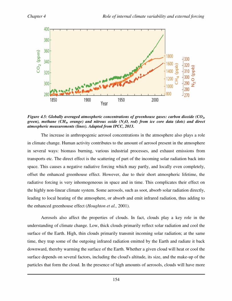
Chapter 4 Role of internal climate variability and external forcing
154
Figure 4.5: Globally averaged atmospheric concentrations of greenhouse gases: carbon dioxide (CO2,
green), methane (CH4, orange) and nitrous oxide (N2O, red) from ice core data (dots) and direct
atmospheric measurements (lines). Adapted from IPCC, 2013.
The increase in anthropogenic aerosol concentrations in the atmosphere also plays a role
in climate change. Human activity contributes to the amount of aerosol present in the atmosphere
in several ways: biomass burning, various industrial processes, and exhaust emissions from
transports etc. The direct effect is the scattering of part of the incoming solar radiation back into
space. This causes a negative radiative forcing which may partly, and locally even completely,
offset the enhanced greenhouse effect. However, due to their short atmospheric lifetime, the
radiative forcing is very inhomogeneous in space and in time. This complicates their effect on
the highly non-linear climate system. Some aerosols, such as soot, absorb solar radiation directly,
leading to local heating of the atmosphere, or absorb and emit infrared radiation, thus adding to
the enhanced greenhouse effect (Houghton et al., 2001).
Aerosols also affect the properties of clouds. In fact, clouds play a key role in the
understanding of climate change. Low, thick clouds primarily reflect solar radiation and cool the
surface of the Earth. High, thin clouds primarily transmit incoming solar radiation; at the same
time, they trap some of the outgoing infrared radiation emitted by the Earth and radiate it back
downward, thereby warming the surface of the Earth. Whether a given cloud will heat or cool the
surface depends on several factors, including the cloud's altitude, its size, and the make-up of the
particles that form the cloud. In the presence of high amounts of aerosols, clouds will have more
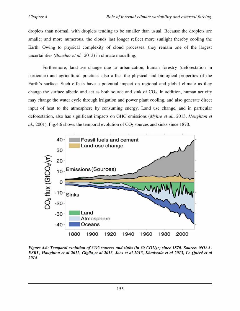
Chapter 4 Role of internal climate variability and external forcing
155
droplets than normal, with droplets tending to be smaller than usual. Because the droplets are
smaller and more numerous, the clouds last longer reflect more sunlight thereby cooling the
Earth. Owing to physical complexity of cloud processes, they remain one of the largest
uncertainties (Boucher et al., 2013) in climate modelling.
Furthermore, land-use change due to urbanization, human forestry (deforestation in
particular) and agricultural practices also affect the physical and biological properties of the
Earth’s surface. Such effects have a potential impact on regional and global climate as they
change the surface albedo and act as both source and sink of CO2. In addition, human activity
may change the water cycle through irrigation and power plant cooling, and also generate direct
input of heat to the atmosphere by consuming energy. Land use change, and in particular
deforestation, also has significant impacts on GHG emissions (Myhre et al., 2013, Houghton et
al., 2001). Fig.4.6 shows the temporal evolution of CO2 sources and sinks since 1870.
Figure 4.6: Temporal evolution of CO2 sources and sinks (in Gt CO2/yr) since 1870. Source: NOAA-
ESRL, Houghton et al 2012, Giglio et al 2013, Joos et al 2013, Khatiwala et al 2013, Le Quéré et al
2014

Chapter 4 Role of internal climate variability and external forcing
156
4.3 Detection and attribution of climate change
There is little doubt that global warming will continue and even increase during the future
decades as GHG emissions, the main contributor to anthropogenic global warming will likely
continue to grow in the future (Myhre et al., 2013, IPCC, 2013). The response of the climate
system to anthropogenic external forcing occurs against a backdrop of natural internal and
externally forced climate variability that can occur on similar temporal and spatial scales. This
implies that the detection and attribution of anthropogenic climate change becomes a statistical
‘signal-in-noise’ problem where the unforced internal variability is the noise. Detection is the
process of demonstrating that an observed change is significantly different from changes due to
unforced internal variability only, while attribution evaluates the causes for the observed changes
(Hegerl et al; 2010).
Although observational evidence for detectable human influence on climate was still
weak at the time of the IPCC first assessment report (AR1) in 1990 (Houghton et al., 1990),
since then, observational data and more numerical analyses have multiplied and the first
detection/attribution (D&A) studies were performed on the global atmospheric temperature.
Based on these results, the IPCC third assessment report (AR3) in 2001 (Houghton et al., 2001)
concluded that the signal corresponding to GHG was weakly detectable in Earth’s global
atmospheric temperature and that the majority of the global warming signal observed since the
last 50 years was ‘probably’ of anthropogenic origin. Following this, by making use of models
and simulations from the Phase 3 of CMIP (CMIP3), D&A studies were performed on other
parameters such as SST, surface wind, precipitation etc. Based on these results, IPCC AR3 and
the IPCC forth assessment report (AR4, Solomon et al., 2007) concluded that it was ‘highly
probable’ that the majority of global warming signal observed both in oceans and continents
since the last 50 years was due to anthropogenic GHG emissions. Since 2007, D&A studies are
also being performed on other parameters such as sea level pressure (e.g. Gillett and Stott, 2009),
sea ice (Kay et al., 2011, Jahn et al., 2011), ice sheets and glaciers (e.g. Hanna et al., 2008,
Marzeion et al., 2014a, Marzeion et al., 2014b), ocean salinity (e.g. Terray et al., 2012, Pierce et
al., 2012, Durack et al., 2014), ocean heat content and sea level (see Section 4.3.1). Based on
these results, the IPCC fifth assessment report (AR5) in 2013 (IPCC, 2013) has concluded that
anthropogenic influences have ‘very likely’ contributed to Arctic sea-ice loss since 1979 and
Chapter 4 Role of internal climate variability and external forcing
157
have ‘very likely’ made a substantial contribution to increases in global upper ocean heat content
(0–700 m) and to global mean sea level rise observed since the 1970s.
4.3.1 Detection and attribution on global mean sea level variations
Global mean sea level is an important indicator of climate change. Only few studies
quantifying the contribution of external anthropogenic forcing on sea level directly at global and
regional scales exist so far. However, when the global mean sea level change is considered, there
exist many D&A studies on each of the main sea level contributors (thermal expansion, glaciers,
sea ice, and ice sheets). For example, a number of D&A studies have been performed on ocean
heat content (OHC), one of the two main contributors to sea level change. Studies (e.g.
Domingues et al., 2008, Levitus et al., 2012, Gleckler et al., 2012) have shown that the upper
ocean layer between 0-700m depth has been warming up since the 1950s. This ocean warming
represents ~93% of the total Earth’s energy increase. This is in accordance with the Earth’s
energy imbalance which shows that during the same time period, the Earth received more solar
energy than it had reflected back to the space (Church et al., 2011, Hansen et al., 2011).
Barnett et al., (2001, 2005) compared a climate model driven by external anthropogenic
and natural forcings on observed OHC changes and showed evidence of anthropogenic influence
on observed OHC in the upper 700m layer of the ocean. Studies (Church et al., 2005, AchutaRao
et al., 2006, Gregory et al., 2006, Domingues et al., 2008) have also shown that models that take
into account only the anthropogenic GHG emission forcing (without considering external natural
forcing such as volcanic eruptions) in fact have underestimated the inter-decadal ocean warming
variability and overestimated the OHC trend over the last 50 years. This is because of the
ocean’s response to volcanic eruption that results in a sudden cooling of its upper layer that can
last for few decades. This was further confirmed by Gleckler et al., (2012) and Gregory et al.,
(2013) who by making use of CMIP3 models showed that only the models that take both the
anthropogenic GHG emissions and natural volcanic eruptions into account represent the global
warming signal in the upper 700m of the ocean layer better.
In the case of global mean sea level rise, Jevrejeva et al., (2010) utilized a statistical
semi-empirical method to relate global mean sea level rise rate from observational data to
different external natural and anthropogenic forcing. They found that before 1800, the global
Chapter 4 Role of internal climate variability and external forcing
158
mean sea level variations were explained only by the external natural forcing whereas since
1800, external natural forcing contributes only 25% to global mean sea level rise while 75% is
contributed by external anthropogenic effects. Recently, Gregory et al., (2013) performed a sea
level closure budget over the twentieth century by summing up different sea level contributors
and arrived to a conclusion that the relationship between global temperature change and global
mean sea level rise rate is weak or absent in the twentieth century. However the reason for this
weak link was related to the recovery of sea level from large volcanic eruptions that occurred in
the later part of 19th
century and also in the late 20th
century (since 1960s) that were not well
taken into account in the pre-industrialized control runs of CMIP3 models.
Recently, Marcos and Amores, (2014) performed D&A studies on CMIP5 based
thermosteric sea level changes using signal-to-noise maximizing empirical orthogonal function
technique for the period 1950–2005. Their study concluded that about 87% of the observed
warming-related sea level rise in the 0-700m of the global ocean is of anthropogenic in origin.
Similarly, Slangen et al., (2014) compared three different full-depth observational thermosteric
sea level changes with 28 different CMIP5 models for the period 1950-2005. CMIP5 models
driven by various single external forcings such as natural only, anthropogenic only, GHG only
and aerosol only were compared with historical simulations, pre-industrialized control runs (for
internal climate variability) and observational data. They concluded that the observed
thermosteric sea level change cannot be explained by models driven by internal climate
variability and natural forcing alone. Furthermore, the observed thermosteric sea level changes
were not solely caused by GHG forcing either, because the GHG experiments overestimated the
observed change. The observed global mean thermosteric sea level change, including the
observed trends over various time periods, were best explained by using a combination of natural
and anthropogenic forcings to drive the models. The anthropogenic forcing was found to be the
leading factor in explaining the magnitude of the observed sea level change, while most of the
variability in the models was caused by natural forcing.
A recent study of Becker et al., (2014) used a statistical approach developed by Lennartz
and Bunde, (2009) to provide evidence of anthropogenic forcing in global mean sea level
change. They concluded that the rate of global mean sea level change is beyond its unforced
internal variability by exceeding the 99% confidence interval. Furthermore, their statistical
Chapter 4 Role of internal climate variability and external forcing
159
analysis showed that more than half of the total observed global sea level trend during the 20th
century was of anthropogenic origin. Similarly, very recently, Dangendorf et al., (2015)
concluded that it was virtually certain that at least 45% of the observed 21st century global mean
sea level change is of anthropogenic origin.
4.3.2 Detection and attribution on regional sea level variability
As seen in Chapter 3, the physical processes which determine global mean sea level rise
and regional sea level change are not identical, although they are related. While D&A studies at
global scales (i.e. in terms of global mean sea level) have been feasible, performing similar
studies on regional sea level is highly challenging. One main reason is that the internal climate
variability introduces strong changes in regional sea level on time scales from years to decades
and makes the signal to noise ratio very unfavorable to detect the forced response above the
unforced internal variability (Richter and Marzeion, 2014, Palanisamy et al., 2015c). For
example, the regional sea level changes in the tropical Pacific Ocean are governed by natural
climates modes such as ENSO, PDO/IPO at interannual and decadal time scales respectively
(e.g. Stammer et al., 2013, Zhang and Church, 2012, Han et al., 2013, Hamlington et al., 2014a
and references therein). The internal sea level variability related to such climate modes of the
order of ± 10-20 cm can therefore mask sea level changes due to externally forced signal
(Palanisamy et al., 2015c). Moreover, the patterns of regional sea level variations before the
altimetry era (i.e. before 1990s) are known mainly from tide gauge records that are relatively few
in number existing only along coastlines and from OGCMs and sea level reconstructions.
Therefore the short record of regional sea level change imposes a limit on the statistical
significance of detection and attribution studies (Bilbao et al., 2015).
Recently, in line with D&A studies, a number of ‘Time of Emergence (ToE)’ studies
(Lyu et al., 2014, Jordà, 2014, Richter and Marzeion, 2014,Bilbao et al., 2015) have been
performed on regional sea level variability. ToE is defined as the time when the ratio of the
climate change signal to the noise of natural variability exceeds a particular threshold and
emerges from the natural climate variability at regional scale. Lyu et al., (2014) find that relative
to the 1986-2005 reference period, under RCP4.5and RCP8.5 scenarios, the externally forced
trend would be detectable in both steric and dynamic sea level by early to mid-2040s in 50% of
Chapter 4 Role of internal climate variability and external forcing
160
all the oceans. The RCP refers to Representative Concentration Pathway, new key scenarios used
in CMIP5 models. The RCPs describe a wide range of potential futures for the main drivers of
climate change such as greenhouse gas and air pollutant emissions and land use and are
expressed in terms of net radiative forcing (e.g. RCP8.5 = +8.5 W/m2). The RCP4.5 is a
stabilization scenario where GHG emissions peak around 2040 and is later stabilized before 2100
by employment of a range of technologies and strategies for reducing greenhouse gas emissions.
The RCP8.5 scenario assumes continuous GHG emissions throughout the 21st century and can
also be considered as a representative extrapolation of the present day emission (IPCC, 2013). In
a ToE study similar to that of Lyu et al., (2014), Richter and Marzeion, (2014) also find that the
externally forced signal is detectable in the early 2030s relative to 1990 in 50% of the world
oceans. These regions include the South Atlantic Ocean, Arctic Ocean, eastern Pacific Ocean and
most parts of the Indian Ocean. Furthermore Jordà, (2014) has shown that on an average, it
would require a minimum time period of 40 years to identify the externally forced signal at
regional scale. However in regions with strong decadal and interannual sea level variability, the
emergence time increases up to 60-80 years. These results are also in agreement to that of
Richter and Marzeion, (2014) and Lyu et al., (2014). Recently Bilbao et al., (2015) have used
pattern scaling method to study the time of emergence of regional sea level change. The
assumption underlying this method is that the local response of a climate variable (sea level in
this case) is linearly related to a global variable called the predictor (e.g. global mean surface air
temperature, global mean sea surface temperature, ocean volume mean temperature etc.) with the
geographical pattern of the change independent of the forcing. Choosing ocean volume mean
temperature over the total ocean depth as predictor, Bilbao et al., (2015) have shown that the
local sea level change will emerge first or may have already emerged in the northern latitudes of
the Southern Ocean and in the tropical Atlantic where the unforced internal variability is smaller.
While in the case of the southern latitudes of the Southern Ocean, it may not emerge until after
2100. Interestingly, they note that the local time of emergence is independent of the RCP
scenarios, since the local sea level signal emerges in the early 21st century when the RCP
scenarios have not yet significantly varied.
While D&A studies on the patterns of regional sea level variability are still lacking, at
regional scale, few studies do exist. For example, apart from D&A analysis on global mean
upper layer (0-700 m) thermosteric sea level change, Marcos and Amores, 2014 also performed
Chapter 4 Role of internal climate variability and external forcing
161
D&A analysis on ocean basin- based regional mean upper layer thermosteric sea level for 1970-
2005 period. They concluded that at regional scale the impact of anthropogenic forcing was
highly variable with the impact being particularly large in the North Atlantic. Becker et al.,
(2014), using the same method applied for their global mean sea level study, also performed
D&A studies at very local scale. They considered long term good quality tide gauge records
available wherever possible all over the world in their study. It was concluded that strong
anthropogenic sea level trend contributed to more than 80% of the total observed trend at places
located in the extreme western Baltic Sea and at least as much as 67% in New York and more
than 50% in Baltimore, Marseille, Mumbai etc. Overall, the presence of significant
anthropogenic trends was found in two thirds of the longest century- scale tide gauge records.
4.4 The case of the Pacific Ocean
Pacific Ocean has always been a subject of keen interest among the climate and sea level
community as the largest sea level trends over the altimetry period (since 1993) are observed
here (See Fig.3.1 of Chapter 3). In fact, we have also discussed in Chapter 3 (Section 3.2.4 and
also Fig.3.7) that the tropical Pacific displays the highest climate-related regional sea level trend
variability when compared to other regions not only during the altimetry era but also at longer
time scales (for the past 6 decades at least). Understanding the origin and mechanisms involved
in the Pacific Ocean sea level spatial trend patterns over the altimetry era has been the subject of
interest of several recent studies. When we consider the spatial patterns of Pacific Ocean sea
level trend (with the global mean removed) since 1993 (Fig.4.7), we can clearly observe two
distinct patterns: (1) a V-shaped broad-scale positive trend pattern extending from about 30°–50°
N in the central basin to the western equatorial Pacific and then 30°–50° S in the central–eastern
basin and (2) a well-pronounced strong dipole-like pattern with positive trends in the western
tropical Pacific (with two relative maxima near 10° N and 10° S) and negative trends in the
central–eastern tropical Pacific (with relative minima trapped in the equatorial band) limited to
about 30° N and 20° S (Palanisamy et al., 2015b).
Bindoff et al., (2007), Levitus et al., (2009), Becker et al., (2012), Stammer et al., (2013)
have shown that the strong dipole-like pattern with a positive (negative) trend in the western
(eastern) tropical Pacific during the altimetry era is mainly of thermosteric (0-700m) origin and

Chapter 4 Role of internal climate variability and external forcing
162
have related this to the ENSO events. Furthermore, using numerical ocean models, Carton et al.,
(2005), Köhl et al., (2007), and Timmermann et al., (2010), Merrifield, (2011) for example, have
shown that in these regions, the thermosteric sea level trends are driven by surface wind stress
and changes in circulation. In particular, Merrifield, (2011), by making use of tide gauges in the
western Pacific, showed that the sea level trend in this region has highly increased since the
1990s when compared to the previous years in the past. McGregor et al., (2012), Merrifield,
(2011), Merrifield and Maltrud, (2011), Merrifield et al., (2012), and Nidheesh et al., (2013)
have attributed the high sea level trends in the western tropical Pacific during the last two
decades to the intensification of trade winds and/or wind stress curl variations.
Figure 4.7: Observed altimetry based Pacific Ocean sea level spatial trend pattern over 1993-2012
(uniform global mean has been removed) from Palanisamy et al., 2015.
While the strong dipole-like sea level trend pattern in the tropical Pacific has been related
to the ENSO internal climate variability, the V-shaped broad-scale positive trend pattern
extending towards the entire Pacific Ocean has been linked with the decadal IPO/PDO climate
variability (Zhang and Church, 2012, Han et al., 2013, England et al., 2014, Hamlington et al.,
2014). In particular, Zhang and Church, (2012), studied the regional sea level variability patterns
in the Pacific Ocean during the altimetry era by making use of a multiple linear regression
model. Interannual and decadal climate indices similar to ENSO and IPO were defined and their
Chapter 4 Role of internal climate variability and external forcing
163
relationships with the regional sea level were studied. It was concluded that the interannual
variability pattern could be explained by ENSO while the decadal patterns could be explained by
IPO. Moreover they also showed that combining these two modes explains about 60 % of the
total sea level variance in the Pacific Ocean over the altimetry era. This leads us to question if
the observed regional sea level trend pattern in the Pacific Ocean is the result of only natural
unforced interannual and decadal climate variability or if there is a role of anthropogenic forcing
too. If that is the case, how successfully can we separate the anthropogenic signal from the signal
due to internal climate variability? This has been the study subject of Meyssignac et al., (2012b)
who by making use of CMIP3 models concluded that over the short altimetry record (17 year at
the time of their study), the amplitude of the noise represented by the internal climate variability
has been so strong in the tropical Pacific that it prevents the detection of anthropogenic forcing
on the regional variability of the sea level trends in this region. However, in a more recent study,
Hamlington et al., (2014), attempted to remove the contribution of IPO from Pacific Ocean sea
level signal and related the residual signal to anthropogenic warming of the tropical Indian
Ocean (Han et al., 2013). They concluded that the anthropogenic fingerprint was already visible
in the Pacific Ocean regional sea level trend pattern over altimetry era.
The contradictory results lead us to wonder if the regional sea level spatial trend pattern
in the Pacific Ocean has been well understood. Therefore one of the main focuses of my Ph.D.
work was on explaining the regional sea level patterns in the Pacific Ocean (in specific, the
tropical Pacific) in terms of the ocean dynamic processes involved, the role of internal climate
variability (with main focus on IPO) and finally the possible role of anthropogenic forcing. An
article has been published based on our work that focuses on the ocean dynamic processes and
internal climate variability in the ‘Ocean Dynamics’ journal whereas another article on the
detection of anthropogenic fingerprint in the Pacific Ocean has been published in the
‘Environmental Research Letters’. Our work published in the two articles has been resumed in
the following pages.
Summary of the article: ‘Spatial trend patterns in the Pacific Ocean sea level during the
altimetry era: the contribution of thermocline depth change and internal climate
variability’ (the original article is inserted at the end of this section)
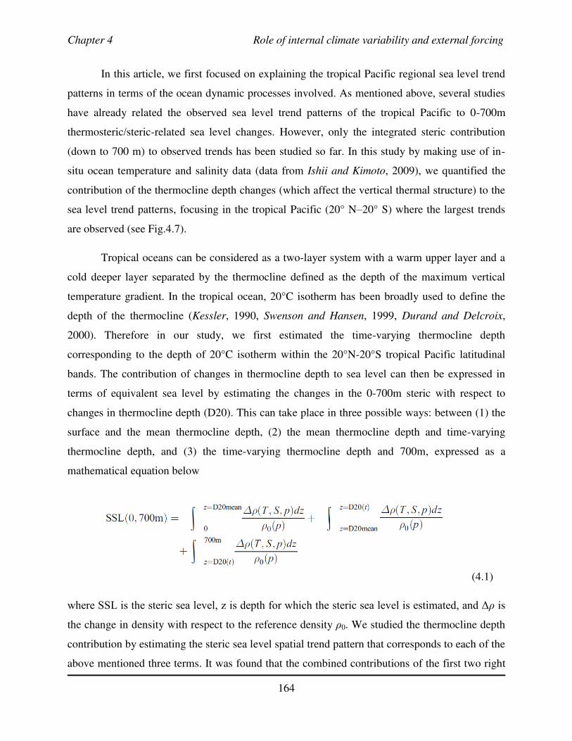
Chapter 4 Role of internal climate variability and external forcing
164
In this article, we first focused on explaining the tropical Pacific regional sea level trend
patterns in terms of the ocean dynamic processes involved. As mentioned above, several studies
have already related the observed sea level trend patterns of the tropical Pacific to 0-700m
thermosteric/steric-related sea level changes. However, only the integrated steric contribution
(down to 700 m) to observed trends has been studied so far. In this study by making use of in-
situ ocean temperature and salinity data (data from Ishii and Kimoto, 2009), we quantified the
contribution of the thermocline depth changes (which affect the vertical thermal structure) to the
sea level trend patterns, focusing in the tropical Pacific (20° N–20° S) where the largest trends
are observed (see Fig.4.7).
Tropical oceans can be considered as a two-layer system with a warm upper layer and a
cold deeper layer separated by the thermocline defined as the depth of the maximum vertical
temperature gradient. In the tropical ocean, 20°C isotherm has been broadly used to define the
depth of the thermocline (Kessler, 1990, Swenson and Hansen, 1999, Durand and Delcroix,
2000). Therefore in our study, we first estimated the time-varying thermocline depth
corresponding to the depth of 20°C isotherm within the 20°N-20°S tropical Pacific latitudinal
bands. The contribution of changes in thermocline depth to sea level can then be expressed in
terms of equivalent sea level by estimating the changes in the 0-700m steric with respect to
changes in thermocline depth (D20). This can take place in three possible ways: between (1) the
surface and the mean thermocline depth, (2) the mean thermocline depth and time-varying
thermocline depth, and (3) the time-varying thermocline depth and 700m, expressed as a
mathematical equation below
(4.1)
where SSL is the steric sea level, z is depth for which the steric sea level is estimated, and Δρ is
the change in density with respect to the reference density ρ0. We studied the thermocline depth
contribution by estimating the steric sea level spatial trend pattern that corresponds to each of the
above mentioned three terms. It was found that the combined contributions of the first two right

Chapter 4 Role of internal climate variability and external forcing
165
hand sided terms of Eq.(4.1) explained most of the 0-700 m steric sea level changes in the
tropical Pacific. This indicates that over 1993-2012 period, it is essentially the thermocline
attributed upper steric layer due to time-varying vertical movement of the thermocline (i.e.
between the surface and D20 (t)) that governs most of the observed sea level changes and trends
in the tropical Pacific.
In the next part of the study, we focused on the mechanism responsible for the time-
varying vertical thermocline movement that explains the sea level changes in the tropical Pacific.
Studies using wind stress forced models (e.g. McGregor et al., 2012, Merrifield et al., 2012,
Merrifield and Maltrud, 2011) have shown that the recent sea level intensification in the western
tropical Pacific is due to the intensification of trade winds. Therefore, in our study, we studied
the relationship between wind stress, thermocline and the thermocline attributed upper layer
steric sea level following the physical equations of Meyers, (1979), Garzoli and Katz, (1983),
Kessler, (1990, see equations.(2), (3) and(4) in Palanisamy et al., 2015b). In the equatorial band
(5°N-5°S latitudes), the slope of the thermocline was calculated along 130°E to 90°W and was
compared with the zonal wind stress averaged over the same latitudinal and longitudinal bands
(Fig.4.8). The thermocline slope and zonal wind stress were highly (anti) correlated (anti-
correlation because the conventional sign of zonal wind stress is positive towards the east).
Furthermore, the presence of negative trend in the zonal wind stress further confirms the
intensification of west-ward blowing trade winds which thereby deepens the thermocline further
(as seen by positive trend in thermocline slope). Away from the equatorial bands (i.e. between
5°-15° north and south latitudes), direct comparison of the thermocline attributed upper layer
steric sea level with zonal wind stress showed good (anti) correlations between the two with time
lags of around 3 to 4 months that is consistent with the time taken for the wind stress-generated
Rossby waves to propagate towards the west. These results show that in the equatorial band, the
changes in the upper ocean thermal structure are in direct response to the zonal wind stress
whereas away from the equatorial band (say, within 5°–15° latitude),the changes in the upper
ocean thermal structure are consistent with the wind stress-generated Rossby waves.

Chapter 4 Role of internal climate variability and external forcing
166
Figure 4.8: Normalized thermocline slope (black) and zonally averaged zonal wind stress (red dotted)
computed from 130° E to 90° W and averaged within 5° N–5° S. The solid black and dashed red lines
denote their respective linear trends. Figure adapted from Palanisamy et al., 2015.
In the last part, we studied the contribution of IPO-related internal climate variability on
the upper layer steric sea level by performing a linear regression of the IPO climatic index on the
upper layer steric sea level. We showed that while IPO is responsible for explaining most of the
sea level trend in the tropical Pacific, removal of its contribution from the sea level results in
some significant residual trend signal. This wind forced residual closely resembles to that found
by Hamlington et al., (2014) which was attributed as the response of tropical Pacific to
anthropogenic warming in the tropical Indian Ocean. However we concluded that it is possible
that the residual pattern could also reflect some non-linear internal climate modes that have not
been totally removed. Therefore a detailed study on this was the focus of our next following
study.
Spatial trend patterns in the Pacific Ocean sea level
during the altimetry era: the contribution of thermocline depth
change and internal climate variability
H. Palanisamy & A. Cazenave & T. Delcroix &
B. Meyssignac
Received: 11 July 2014 /Accepted: 16 December 2014# Springer-Verlag Berlin Heidelberg 2015
Abstract This study investigates the spatial trend patterns
and variability of observed sea level and upper ocean thermal
structure in the Pacific Ocean during the altimetry era (1993–
2012), and the role of thermocline depth changes. The ob-
served sea level trend pattern in this region results from the
superposition of two main signals: (1) a strong broad-scale V-
shaped positive trend anomaly extending to mid-latitudes in
the central Pacific and (2) another very strong positive trend
anomaly located in the western tropical Pacific within about
120° E–160° E and 20° S–20° N latitude. In this study, we
focus on the tropical Pacific (20° N–20° S) where the stron-
gest trends in sea level are observed. By making use of in situ
observational data, we study the impact of thermocline depth
changes on steric sea level between the surface and 700 m and
its relation with the altimetry-based observed sea level chang-
es. This is done by calculating the time-varying thermocline
depth (using the 20 °C isotherm depth as a proxy) and esti-
mating the sea level trend patterns of the thermocline-
attributed individual steric components. We show that it is
essentially the vertical movement of the thermocline that
governs most of the observed sea level changes and trends
in the tropical Pacific. Furthermore, we also show that in the
equatorial band, the changes in the upper ocean thermal
structure are in direct response to the zonal wind stress.
Away from the equatorial band (say, within 5°–15° latitude),
the changes in the upper ocean thermal structure are consistent
with the wind stress-generated Rossby waves. We also esti-
mate the contribution of the Interdecadal Pacific Oscillation
(IPO) on the vertical thermal structure of the tropical Pacific
Ocean. Removing the IPO contribution to the upper layer
steric sea level provides a non-negligible residual pattern,
suggesting that IPO-related internal ocean variability alone
cannot account for the observed trend patterns in the Pacific
sea level. It is likely that the residual signal may also reflect
non-linear interactions between different natural modes like El
Niño Southern Oscillation (ENSO), IPO, etc.
Keywords Tropical Pacific .Wind-driven thermocline depth
changes . Upper layer steric sea level contribution . Internal
climate variability . Interdecadal Pacific Oscillation
1 Introduction
Since the early 1990s, satellite altimetry has become the main
tool for precisely and continuously measuring sea level with
quasi-global coverage and short revisit time. Analyses of
altimetry data have shown that since 1993, sea level is rising
at a global mean rate of 3.2±0.4 mm/year (Nerem et al. 2010),
but the rate is far from being spatially uniform (e.g., Cazenave
and Cozannet 2014; Stammer et al. 2013; Church et al. 2013).
In regions like the western tropical Pacific, north Atlantic
around Greenland, and southern Austral Ocean, rates up to
three times the global mean rate are observed over the altim-
etry period, while other regions like the eastern tropical Pacific
face lower rates of sea level rise (Bromirski et al. 2011;
Thompson et al. 2014). The regional sea level variability
superimposes on the global mean sea level rate and thus
amplifies or reduces the sea level rate. This implies that
different parts of the world do not face the same extent of
sea level risks. This shows the importance of regional
Responsible Editor: Richard John Greatbatch
H. Palanisamy (*) :A. Cazenave :B. Meyssignac
LEGOS/CNES, 18 Avenue Edouard Belin, 31400 Toulouse, France
e-mail: [email protected]
T. Delcroix
LEGOS/IRD, 18 Avenue Edouard Belin, 31400 Toulouse, France
Ocean Dynamics
DOI 10.1007/s10236-014-0805-7
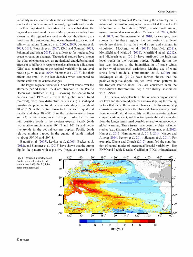
variability in sea level trends in the estimation of relative sea
level and its potential impact on low-lying coasts and islands.
It is thus important to understand the causes that drive the
regional sea level trend patterns. Many previous studies have
shown that the regional sea level trends over the altimetry era
mostly result from non-uniform ocean thermal expansion and
salinity variations (Lombard et al. 2005a; 2009; Levitus et al.
2005, 2012; Wunsch et al. 2007; Köhl and Stammer 2008;
Fukumori and Wang 2013), thus at least to first order reflect
ocean circulation changes. Theoretical studies have shown
that other phenomena such as gravitational and deformational
effects of solid Earth in response to glacial isostatic adjustment
(GIA) also contribute to the regional variability in sea level
rates (e.g., Milne et al. 2009; Stammer et al. 2013), but their
effects are small in the last decades when compared to
thermosteric and halosteric changes.
The largest regional variations in sea level trends over the
altimetry period (since 1993) are observed in the Pacific
Ocean (as illustrated in Fig. 1 showing the spatial trend
patterns over 1993–2012, with the global mean trend
removed), with two distinctive patterns: (1) a V-shaped
broad-scale positive trend pattern extending from about
30°–50° N in the central basin to the western equatorial
Pacific and then 30°–50° S in the central–eastern basin
and (2) a well-pronounced strong dipole-like pattern
with positive trends in the western tropical Pacific (with
two relative maxima near 10° N and 10° S) and nega-
tive trends in the central–eastern tropical Pacific (with
relative minima trapped in the equatorial band) limited
to about 30° N and 20° S.
Bindoff et al. (2007), Levitus et al. (2009), Becker et al.
(2012), and Stammer et al. (2013) have shown that the strong
dipole-like pattern with a positive (negative) trend in the
western (eastern) tropical Pacific during the altimetry era is
mainly of thermosteric origin and have related this to the El
Niño Southern Oscillation (ENSO) events. Furthermore,
using numerical ocean models, Carton et al. 2005, Köhl
et al. 2007, and Timmermann et al. 2010, for example, have
shown that in these regions, the thermosteric sea level
trends are driven by surface wind stress and changes in
circulation. McGregor et al. (2012), Merrifield (2011),
Merrifield and Maltrud (2011), Merrifield et al. (2012),
and Nidheesh et al. (2013) have attributed the high sea
level trends in the western tropical Pacific during the
last two decades to the intensification of trade winds
and/or wind stress curl variations. Making use of wind
stress forced models, Timmermann et al. (2010) and
McGregor et al. (2012) have further shown that the
positive–negative dipole-like sea level trend patterns in
the tropical Pacific since 1993 are consistent with the
wind-driven thermocline depth variability associated
with ENSO.
The first level of explanation relies on comparing observed
sea level and steric trend patterns and investigating the forcing
factors that cause the regional changes. The following step
consists of asking whether the observed changes mostly result
from internal/natural variability of the ocean–atmosphere
coupled system or not, and how to separate the natural modes
from the longer term signal possibly related to anthropogenic
global warming. These issues have been the object of other
studies (e.g., Zhang and Church 2012;Meyssignac et al. 2012;
Han et al. 2013; Hamlington et al. 2013, 2014; Marcos and
Amores 2014; Becker et al. 2014; Slangen et al. 2014). For
example, Zhang and Church (2012) quantified the contribu-
tion of natural modes of interannual/decadal variability—like
ENSO and Pacific Decadal Oscillation (PDO) or Interdecadal
Fig. 1 Observed altimetry-based
Pacific sea level spatial trend
pattern over 1993–2012 (global
mean trend removed)
Ocean Dynamics
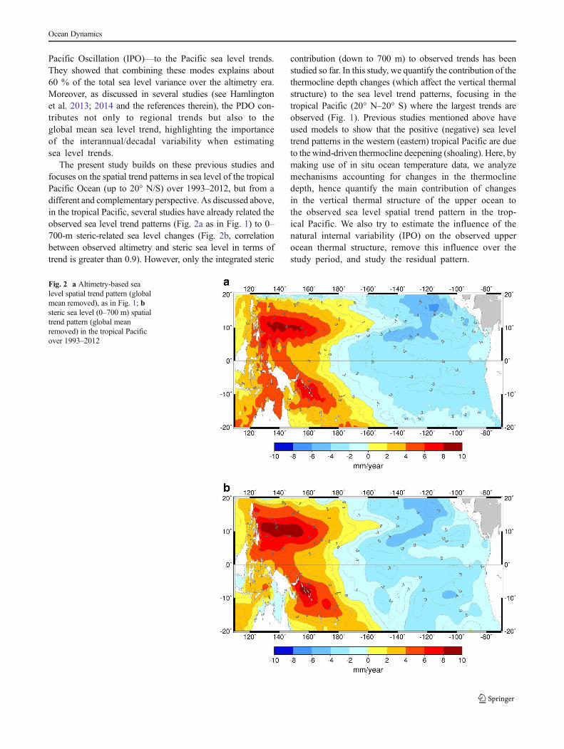
Pacific Oscillation (IPO)—to the Pacific sea level trends.
They showed that combining these modes explains about
60 % of the total sea level variance over the altimetry era.
Moreover, as discussed in several studies (see Hamlington
et al. 2013; 2014 and the references therein), the PDO con-
tributes not only to regional trends but also to the
global mean sea level trend, highlighting the importance
of the interannual/decadal variability when estimating
sea level trends.
The present study builds on these previous studies and
focuses on the spatial trend patterns in sea level of the tropical
Pacific Ocean (up to 20° N/S) over 1993–2012, but from a
different and complementary perspective. As discussed above,
in the tropical Pacific, several studies have already related the
observed sea level trend patterns (Fig. 2a as in Fig. 1) to 0–
700-m steric-related sea level changes (Fig. 2b, correlation
between observed altimetry and steric sea level in terms of
trend is greater than 0.9). However, only the integrated steric
contribution (down to 700 m) to observed trends has been
studied so far. In this study, we quantify the contribution of the
thermocline depth changes (which affect the vertical thermal
structure) to the sea level trend patterns, focusing in the
tropical Pacific (20° N–20° S) where the largest trends are
observed (Fig. 1). Previous studies mentioned above have
used models to show that the positive (negative) sea level
trend patterns in the western (eastern) tropical Pacific are due
to the wind-driven thermocline deepening (shoaling). Here, by
making use of in situ ocean temperature data, we analyze
mechanisms accounting for changes in the thermocline
depth, hence quantify the main contribution of changes
in the vertical thermal structure of the upper ocean to
the observed sea level spatial trend pattern in the trop-
ical Pacific. We also try to estimate the influence of the
natural internal variability (IPO) on the observed upper
ocean thermal structure, remove this influence over the
study period, and study the residual pattern.
Fig. 2 a Altimetry-based sea
level spatial trend pattern (global
mean removed), as in Fig. 1; b
steric sea level (0–700 m) spatial
trend pattern (global mean
removed) in the tropical Pacific
over 1993–2012
Ocean Dynamics
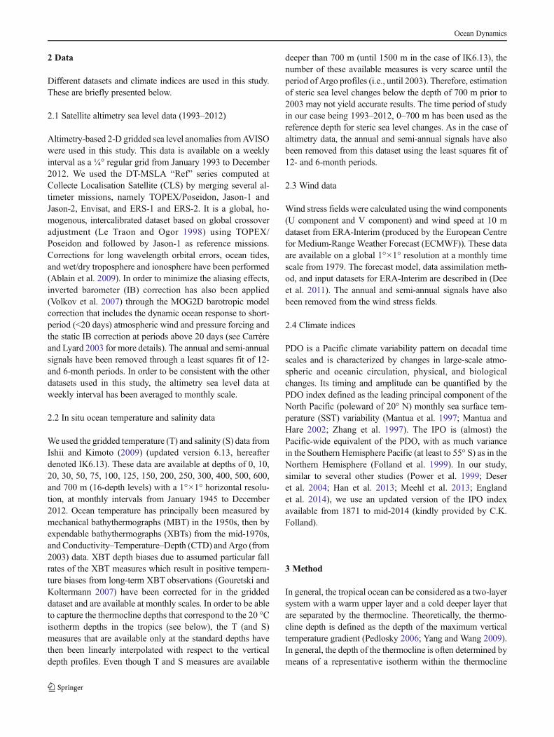
2 Data
Different datasets and climate indices are used in this study.
These are briefly presented below.
2.1 Satellite altimetry sea level data (1993–2012)
Altimetry-based 2-D gridded sea level anomalies fromAVISO
were used in this study. This data is available on a weekly
interval as a ¼° regular grid from January 1993 to December
2012. We used the DT-MSLA “Ref” series computed at
Collecte Localisation Satellite (CLS) by merging several al-
timeter missions, namely TOPEX/Poseidon, Jason-1 and
Jason-2, Envisat, and ERS-1 and ERS-2. It is a global, ho-
mogenous, intercalibrated dataset based on global crossover
adjustment (Le Traon and Ogor 1998) using TOPEX/
Poseidon and followed by Jason-1 as reference missions.
Corrections for long wavelength orbital errors, ocean tides,
and wet/dry troposphere and ionosphere have been performed
(Ablain et al. 2009). In order to minimize the aliasing effects,
inverted barometer (IB) correction has also been applied
(Volkov et al. 2007) through the MOG2D barotropic model
correction that includes the dynamic ocean response to short-
period (<20 days) atmospheric wind and pressure forcing and
the static IB correction at periods above 20 days (see Carrère
and Lyard 2003 for more details). The annual and semi-annual
signals have been removed through a least squares fit of 12-
and 6-month periods. In order to be consistent with the other
datasets used in this study, the altimetry sea level data at
weekly interval has been averaged to monthly scale.
2.2 In situ ocean temperature and salinity data
We used the gridded temperature (T) and salinity (S) data from
Ishii and Kimoto (2009) (updated version 6.13, hereafter
denoted IK6.13). These data are available at depths of 0, 10,
20, 30, 50, 75, 100, 125, 150, 200, 250, 300, 400, 500, 600,
and 700 m (16-depth levels) with a 1°×1° horizontal resolu-
tion, at monthly intervals from January 1945 to December
2012. Ocean temperature has principally been measured by
mechanical bathythermographs (MBT) in the 1950s, then by
expendable bathythermographs (XBTs) from the mid-1970s,
and Conductivity–Temperature–Depth (CTD) and Argo (from
2003) data. XBT depth biases due to assumed particular fall
rates of the XBT measures which result in positive tempera-
ture biases from long-term XBT observations (Gouretski and
Koltermann 2007) have been corrected for in the gridded
dataset and are available at monthly scales. In order to be able
to capture the thermocline depths that correspond to the 20 °C
isotherm depths in the tropics (see below), the T (and S)
measures that are available only at the standard depths have
then been linearly interpolated with respect to the vertical
depth profiles. Even though T and S measures are available
deeper than 700 m (until 1500 m in the case of IK6.13), the
number of these available measures is very scarce until the
period of Argo profiles (i.e., until 2003). Therefore, estimation
of steric sea level changes below the depth of 700 m prior to
2003 may not yield accurate results. The time period of study
in our case being 1993–2012, 0–700 m has been used as the
reference depth for steric sea level changes. As in the case of
altimetry data, the annual and semi-annual signals have also
been removed from this dataset using the least squares fit of
12- and 6-month periods.
2.3 Wind data
Wind stress fields were calculated using the wind components
(U component and V component) and wind speed at 10 m
dataset from ERA-Interim (produced by the European Centre
for Medium-Range Weather Forecast (ECMWF)). These data
are available on a global 1°×1° resolution at a monthly time
scale from 1979. The forecast model, data assimilation meth-
od, and input datasets for ERA-Interim are described in (Dee
et al. 2011). The annual and semi-annual signals have also
been removed from the wind stress fields.
2.4 Climate indices
PDO is a Pacific climate variability pattern on decadal time
scales and is characterized by changes in large-scale atmo-
spheric and oceanic circulation, physical, and biological
changes. Its timing and amplitude can be quantified by the
PDO index defined as the leading principal component of the
North Pacific (poleward of 20° N) monthly sea surface tem-
perature (SST) variability (Mantua et al. 1997; Mantua and
Hare 2002; Zhang et al. 1997). The IPO is (almost) the
Pacific-wide equivalent of the PDO, with as much variance
in the Southern Hemisphere Pacific (at least to 55° S) as in the
Northern Hemisphere (Folland et al. 1999). In our study,
similar to several other studies (Power et al. 1999; Deser
et al. 2004; Han et al. 2013; Meehl et al. 2013; England
et al. 2014), we use an updated version of the IPO index
available from 1871 to mid-2014 (kindly provided by C.K.
Folland).
3 Method
In general, the tropical ocean can be considered as a two-layer
system with a warm upper layer and a cold deeper layer that
are separated by the thermocline. Theoretically, the thermo-
cline depth is defined as the depth of the maximum vertical
temperature gradient (Pedlosky 2006; Yang and Wang 2009).
In general, the depth of the thermocline is often determined by
means of a representative isotherm within the thermocline
Ocean Dynamics
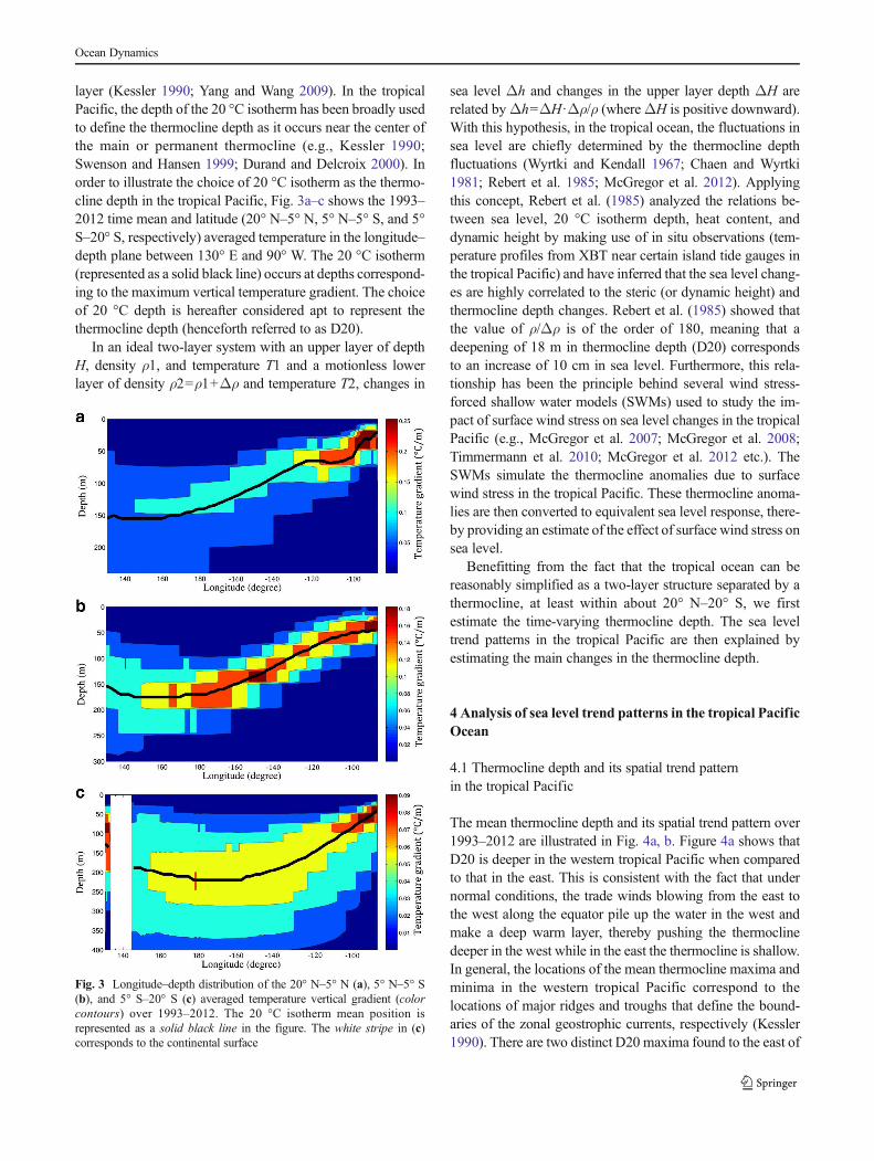
layer (Kessler 1990; Yang and Wang 2009). In the tropical
Pacific, the depth of the 20 °C isotherm has been broadly used
to define the thermocline depth as it occurs near the center of
the main or permanent thermocline (e.g., Kessler 1990;
Swenson and Hansen 1999; Durand and Delcroix 2000). In
order to illustrate the choice of 20 °C isotherm as the thermo-
cline depth in the tropical Pacific, Fig. 3a–c shows the 1993–
2012 time mean and latitude (20° N–5° N, 5° N–5° S, and 5°
S–20° S, respectively) averaged temperature in the longitude–
depth plane between 130° E and 90° W. The 20 °C isotherm
(represented as a solid black line) occurs at depths correspond-
ing to the maximum vertical temperature gradient. The choice
of 20 °C depth is hereafter considered apt to represent the
thermocline depth (henceforth referred to as D20).
In an ideal two-layer system with an upper layer of depth
H, density ρ1, and temperature T1 and a motionless lower
layer of density ρ2=ρ1+Δρ and temperature T2, changes in
sea level Δh and changes in the upper layer depth ΔH are
related byΔh=ΔH·Δρ/ρ (whereΔH is positive downward).
With this hypothesis, in the tropical ocean, the fluctuations in
sea level are chiefly determined by the thermocline depth
fluctuations (Wyrtki and Kendall 1967; Chaen and Wyrtki
1981; Rebert et al. 1985; McGregor et al. 2012). Applying
this concept, Rebert et al. (1985) analyzed the relations be-
tween sea level, 20 °C isotherm depth, heat content, and
dynamic height by making use of in situ observations (tem-
perature profiles from XBT near certain island tide gauges in
the tropical Pacific) and have inferred that the sea level chang-
es are highly correlated to the steric (or dynamic height) and
thermocline depth changes. Rebert et al. (1985) showed that
the value of ρ/Δρ is of the order of 180, meaning that a
deepening of 18 m in thermocline depth (D20) corresponds
to an increase of 10 cm in sea level. Furthermore, this rela-
tionship has been the principle behind several wind stress-
forced shallow water models (SWMs) used to study the im-
pact of surface wind stress on sea level changes in the tropical
Pacific (e.g., McGregor et al. 2007; McGregor et al. 2008;
Timmermann et al. 2010; McGregor et al. 2012 etc.). The
SWMs simulate the thermocline anomalies due to surface
wind stress in the tropical Pacific. These thermocline anoma-
lies are then converted to equivalent sea level response, there-
by providing an estimate of the effect of surface wind stress on
sea level.
Benefitting from the fact that the tropical ocean can be
reasonably simplified as a two-layer structure separated by a
thermocline, at least within about 20° N–20° S, we first
estimate the time-varying thermocline depth. The sea level
trend patterns in the tropical Pacific are then explained by
estimating the main changes in the thermocline depth.
4 Analysis of sea level trend patterns in the tropical Pacific
Ocean
4.1 Thermocline depth and its spatial trend pattern
in the tropical Pacific
The mean thermocline depth and its spatial trend pattern over
1993–2012 are illustrated in Fig. 4a, b. Figure 4a shows that
D20 is deeper in the western tropical Pacific when compared
to that in the east. This is consistent with the fact that under
normal conditions, the trade winds blowing from the east to
the west along the equator pile up the water in the west and
make a deep warm layer, thereby pushing the thermocline
deeper in the west while in the east the thermocline is shallow.
In general, the locations of the mean thermocline maxima and
minima in the western tropical Pacific correspond to the
locations of major ridges and troughs that define the bound-
aries of the zonal geostrophic currents, respectively (Kessler
1990). There are two distinct D20 maxima found to the east of
Fig. 3 Longitude–depth distribution of the 20° N–5° N (a), 5° N–5° S
(b), and 5° S–20° S (c) averaged temperature vertical gradient (color
contours) over 1993–2012. The 20 °C isotherm mean position is
represented as a solid black line in the figure. The white stripe in (c)
corresponds to the continental surface
Ocean Dynamics
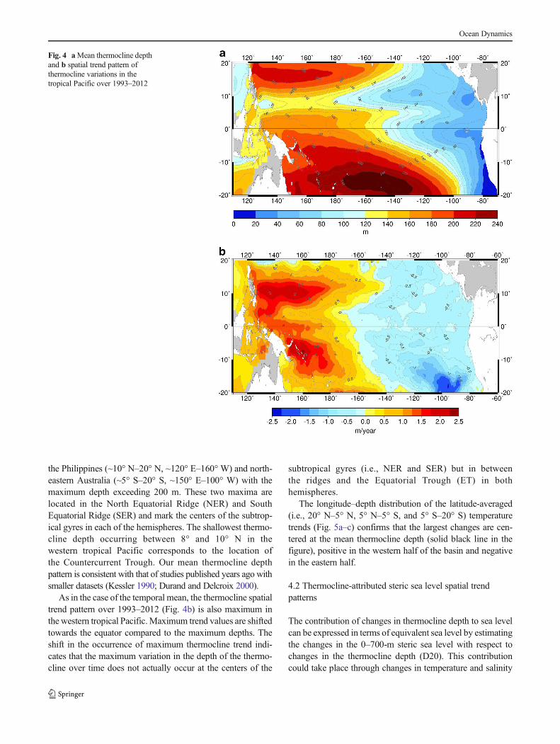
the Philippines (~10° N–20° N, ~120° E–160° W) and north-
eastern Australia (~5° S–20° S, ~150° E–100° W) with the
maximum depth exceeding 200 m. These two maxima are
located in the North Equatorial Ridge (NER) and South
Equatorial Ridge (SER) and mark the centers of the subtrop-
ical gyres in each of the hemispheres. The shallowest thermo-
cline depth occurring between 8° and 10° N in the
western tropical Pacific corresponds to the location of
the Countercurrent Trough. Our mean thermocline depth
pattern is consistent with that of studies published years ago with
smaller datasets (Kessler 1990; Durand and Delcroix 2000).
As in the case of the temporal mean, the thermocline spatial
trend pattern over 1993–2012 (Fig. 4b) is also maximum in
the western tropical Pacific.Maximum trend values are shifted
towards the equator compared to the maximum depths. The
shift in the occurrence of maximum thermocline trend indi-
cates that the maximum variation in the depth of the thermo-
cline over time does not actually occur at the centers of the
subtropical gyres (i.e., NER and SER) but in between
the ridges and the Equatorial Trough (ET) in both
hemispheres.
The longitude–depth distribution of the latitude-averaged
(i.e., 20° N–5° N, 5° N–5° S, and 5° S–20° S) temperature
trends (Fig. 5a–c) confirms that the largest changes are cen-
tered at the mean thermocline depth (solid black line in the
figure), positive in the western half of the basin and negative
in the eastern half.
4.2 Thermocline-attributed steric sea level spatial trend
patterns
The contribution of changes in thermocline depth to sea level
can be expressed in terms of equivalent sea level by estimating
the changes in the 0–700-m steric sea level with respect to
changes in the thermocline depth (D20). This contribution
could take place through changes in temperature and salinity
Fig. 4 aMean thermocline depth
and b spatial trend pattern of
thermocline variations in the
tropical Pacific over 1993–2012
Ocean Dynamics
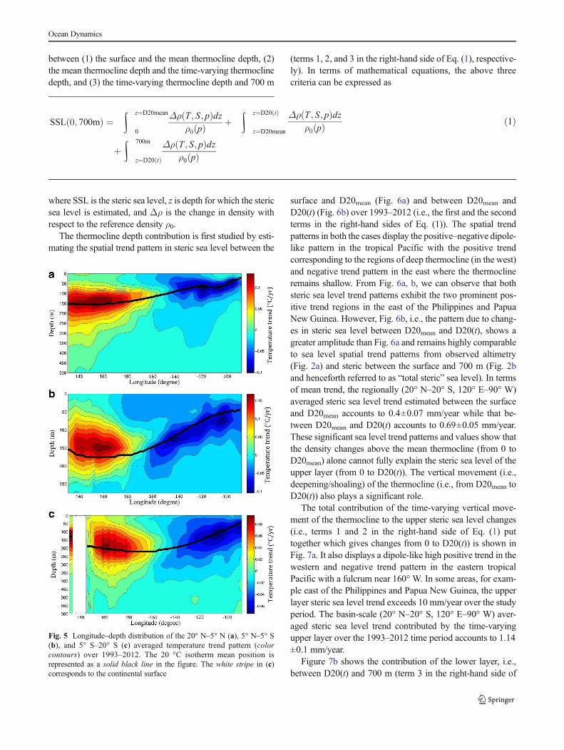
between (1) the surface and the mean thermocline depth, (2)
the mean thermocline depth and the time-varying thermocline
depth, and (3) the time-varying thermocline depth and 700 m
(terms 1, 2, and 3 in the right-hand side of Eq. (1), respective-
ly). In terms of mathematical equations, the above three
criteria can be expressed as
SSL 0; 700mð Þ ¼
Z z¼D20mean
0
Δρ T ; S; pð Þdz
ρ0pð Þ
þ
Z z¼D20 tð Þ
z¼D20mean
Δρ T ; S; pð Þdz
ρ0pð Þ
þ
Z 700m
z¼D20 tð Þ
Δρ T ; S; pð Þdz
ρ0 pð Þ
ð1Þ
where SSL is the steric sea level, z is depth for which the steric
sea level is estimated, and Δρ is the change in density with
respect to the reference density ρ0.
The thermocline depth contribution is first studied by esti-
mating the spatial trend pattern in steric sea level between the
surface and D20mean (Fig. 6a) and between D20mean and
D20(t) (Fig. 6b) over 1993–2012 (i.e., the first and the second
terms in the right-hand sides of Eq. (1)). The spatial trend
patterns in both the cases display the positive–negative dipole-
like pattern in the tropical Pacific with the positive trend
corresponding to the regions of deep thermocline (in the west)
and negative trend pattern in the east where the thermocline
remains shallow. From Fig. 6a, b, we can observe that both
steric sea level trend patterns exhibit the two prominent pos-
itive trend regions in the east of the Philippines and Papua
New Guinea. However, Fig. 6b, i.e., the pattern due to chang-
es in steric sea level between D20mean and D20(t), shows a
greater amplitude than Fig. 6a and remains highly comparable
to sea level spatial trend patterns from observed altimetry
(Fig. 2a) and steric between the surface and 700 m (Fig. 2b
and henceforth referred to as “total steric” sea level). In terms
of mean trend, the regionally (20° N–20° S, 120° E–90° W)
averaged steric sea level trend estimated between the surface
and D20mean accounts to 0.4±0.07 mm/year while that be-
tween D20mean and D20(t) accounts to 0.69±0.05 mm/year.
These significant sea level trend patterns and values show that
the density changes above the mean thermocline (from 0 to
D20mean) alone cannot fully explain the steric sea level of the
upper layer (from 0 to D20(t)). The vertical movement (i.e.,
deepening/shoaling) of the thermocline (i.e., from D20mean to
D20(t)) also plays a significant role.
The total contribution of the time-varying vertical move-
ment of the thermocline to the upper steric sea level changes
(i.e., terms 1 and 2 in the right-hand side of Eq. (1) put
together which gives changes from 0 to D20(t)) is shown in
Fig. 7a. It also displays a dipole-like high positive trend in the
western and negative trend pattern in the eastern tropical
Pacific with a fulcrum near 160° W. In some areas, for exam-
ple east of the Philippines and Papua New Guinea, the upper
layer steric sea level trend exceeds 10 mm/year over the study
period. The basin-scale (20° N–20° S, 120° E–90° W) aver-
aged steric sea level trend contributed by the time-varying
upper layer over the 1993–2012 time period accounts to 1.14
±0.1 mm/year.
Figure 7b shows the contribution of the lower layer, i.e.,
between D20(t) and 700 m (term 3 in the right-hand side of
Fig. 5 Longitude–depth distribution of the 20° N–5° N (a), 5° N–5° S
(b), and 5° S–20° S (c) averaged temperature trend pattern (color
contours) over 1993–2012. The 20 °C isotherm mean position is
represented as a solid black line in the figure. The white stripe in (c)
corresponds to the continental surface
Ocean Dynamics

Eq. (1)), to the spatial trend pattern in steric sea level. The
dipole-like positive/negative patterns are reversed with a neg-
ative pattern in the west and a positive pattern in the east. The
magnitude of the trend values in this case remains low, prob-
ably within the error bars, noting that positive/negative values
appear consistent over two large regions (each covering about
half of the basin). The basin-scale averaged steric sea level
trend contributed by this lower layer accounts to −0.19±
0.03 mm/year. The change in sign of the steric sea level trend
value between the surface and D20(t) (positive) and between
D20(t) and 700 m (negative) is because an increased thickness
of the upper tropical ocean layer implies a reduced thickness
of the lower tropical ocean layer. Moreover, in the equatorial
band, this dipole reversal could also be related to the strength-
ening of the trade winds over the last two decades (England
et al. 2014). As discussed below, such a strengthening induces
an increased tilt of the thermocline, hence a stronger
Equatorial Undercurrent (EUC) that in general brings heat
from the western to the eastern tropical Pacific in the deeper
layers. Further analysis would be needed to test this
assumption.
The basin-scale steric sea level trend estimates in the upper
(1.14±0.1 mm/year) and lower (−0.19±0.03 mm/year) ther-
mocline layers imply that most of the changes in the total (0–
700 m) steric sea level (net trend=0.94±0.09 mm/year) in the
tropical Pacific are contributed by changes in the upper layer
of the time-varying thermocline.
To further highlight the different contributions, Fig. 8 com-
pares the basin-scale averaged steric sea level changes due to
the various thermocline cases discussed above with the 0–
700-m steric sea level changes. It is to be noted that when the
steric sea level due to changes in thermocline depth is com-
pared with the total steric (i.e., between the surface and
700 m), the global steric sea level trend should be included
in the latter. This is because the steric sea level changes due to
vertical thermocline movement contain the global steric
Fig. 6 Steric sea level spatial
trend pattern between the surface
and D20mean (a) and between
D20mean and D20(t) (b) in the
tropical Pacific over 1993–2012
(see Eq. 1 for the definitions of
D20mean and D20(t))
Ocean Dynamics
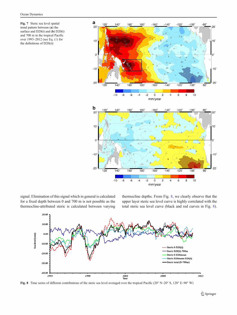
signal. Elimination of this signal which in general is calculated
for a fixed depth between 0 and 700 m is not possible as the
thermocline-attributed steric is calculated between varying
thermocline depths. From Fig. 8, we clearly observe that the
upper layer steric sea level curve is highly correlated with the
total steric sea level curve (black and red curves in Fig. 8).
Fig. 7 Steric sea level spatial
trend pattern between (a) the
surface and D20(t) and (b) D20(t)
and 700 m in the tropical Pacific
over 1993–2012 (see Eq. (1) for
the definitions of D20(t))
Fig. 8 Time series of different contributions of the steric sea level averaged over the tropical Pacific (20° N–20° S, 120° E–90° W)
Ocean Dynamics

Furthermore, Table 1 lists the correlation between the total
steric (0–700 m) and the individual steric components. We can
observe that among various steric components, the maximum
correlation with the total steric occurs in the case of the upper
layer steric (0-D20(t)). In terms of variance, the upper layer
steric explains most of the variance of the total steric signal.
These once again confirm that in the tropical Pacific, most of
the signal corresponding to the steric sea level change can be
explained by the verticallymoving thermocline and associated
vertical density structure changes. The spatial trend pattern of
the upper layer steric sea level also shows high correlation
(correlation>0.9 and significance>95 %, not shown here)
with the observed altimetry sea level spatial trend pattern.
4.3 Relation between upper layer steric sea level and wind
stress
From previous sections, we have seen that the sea level trend
pattern during 1993–2012 in the tropical Pacific is essentially
due to steric variations related to the changes in the vertical
movement of the thermocline. Therefore, understanding the
mechanism of the vertical thermocline movement is necessary
when we focus on sea level variations in the tropical Pacific.
The low-frequency changes in the tropical thermocline
depth are mainly caused by wind stress anomalies that alter
the horizontal pressure gradient, the Ekman pumping, and the
resulting westward-propagating oceanic Rossby waves
(Meyers 1979; Kessler 1990; McGregor et al. 2012). In terms
of physical equations, this can be expressed as
dH
dx¼ τx ð2Þ
dH
dt−cr
dH
dx¼ −curl τ=ρ: fð Þ ð3Þ
where H is the thermocline depth (also called D20 here), τ the
wind stress vector (τx positive to the east and τy to the north), ρ
the density of sea water, and cr the long gravity Rossby wave
phase speed equals √ (βc2/f2) where c is the first baroclinic
mode phase speed (of the order of 2.8 m/s), β the meridional
(y) derivative of f, and f the Coriolis parameter. Equation (2)
applies in the equatorial band only and denotes the equilibri-
um between the zonal thermocline slope and the zonal wind
stress (Sverdrup 1947), and Eq. (3) applies about 5° off the
equator only and denotes the quasi-geostrophic vorticity equa-
tion (Meyers 1979; Garzoli and Katz 1983; Kessler 1990).
The Ekman pumping term in Eq (3) can be written as
curl τ=ρ: fð Þ ¼ curl τð Þ þ β= fð Þ:τxð Þ= ρ: fð Þ ð4Þ
indicating that its magnitude, at a given latitude (and so f), is
thus determined both by the wind stress curl and the zonal
wind stress (Delcroix and Hénin 1989).
Therefore, from Eqs. (2) and (3), we can expect an impact
of the zonal wind stress on the thermocline both in the equa-
torial band (Eq. (2)) and away from the equatorial band
(Eq. (3)). In order to confirm this, we first focus on the
equatorial band and thus compare the two terms of Eq. (2).
The left-hand side term was computed at each time step as a
linear regression of D20 along each degree latitude from 130°
E to 90° W and then averaged within 5° N–5° S. The right-
hand side term was computed at each time step as the average
of the zonal wind stress within 130° E–90° Wand 5° N–5° S.
The comparison is shown in Fig. 9. Both the thermocline
slope and zonal wind stress were low-pass filtered with half
a year cutoff frequency and normalized by their respective
standard deviations to ease comparison. We find that the
thermocline slope and zonal wind stress are highly correlated
(significance>95 %), with the highest correlation (−0.92)
occurring when the thermocline slope lags behind the zonal
wind stress by 2 months (the correlation at 0 lag is −0.85). The
thermocline slope and zonal wind stress are anti-correlated
because the conventional sign of zonal wind stress is positive
Table 1 Correlation between total steric (0–700 m) and individual
components of the steric sea level time series in the tropical Pacific
over 1993–2012
Steric components Total steric (0–700 m)
0-D20mean 0.90
0-D20mean-D20(t) 0.86
0-D20(t) 0.96
D20-700 m −0.40
Fig. 9 Normalized thermocline slope (black) and zonally averaged zonal
wind stress (red dotted) computed from 130° E to 90° W and averaged
within 5° N–5° S. The solid black and dashed red lines denote their
respective linear trends. The thermocline slope and the zonal wind stress
time series have been low-pass filtered with half a year cutoff frequency
for clarity
Ocean Dynamics
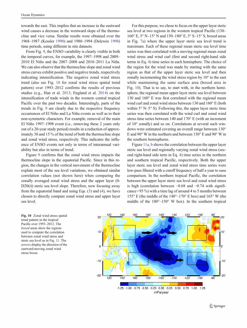
towards the east. This implies that an increase in the eastward
wind causes a decrease in the westward slope of the thermo-
cline and vice versa. Similar results were obtained over the
1968–1987 (Kessler 1990) and 1980–1994 (Delcroix 1998)
time periods, using different in situ datasets.
From Fig. 9, the ENSO variability is clearly visible in both
the temporal curves, for example, the 1997–1998 and 2009–
2010 El Niño and the 2007–2008 and 2010–2011 La Niña.
We can also observe that the thermocline slope and zonal wind
stress curves exhibit positive and negative trends, respectively
indicating intensification. The negative zonal wind stress
trend (also see Fig. 10 for zonal wind stress spatial trend
pattern) over 1993–2012 confirms the results of previous
studies (e.g., Han et al. 2013; England et al. 2014) on the
intensification of trade winds in the western–central tropical
Pacific over the past two decades. Interestingly, parts of the
trends in Fig. 9 are clearly due to the respective frequency
occurrences of El Niño and La Niña events as well as to their
non-symmetric characters. For example, removal of the main
El Niño 1997–1998 event (i.e., removing these 2 years only
out of a 20-year study period) results in a reduction of approx-
imately 30 and 15% of the trend of both the thermocline slope
and zonal wind stress, respectively. This indicates the influ-
ence of ENSO events not only in terms of interannual vari-
ability but also in terms of trend.
Figure 9 confirms that the zonal wind stress impacts the
thermocline slope in the equatorial Pacific. Since in this re-
gion, the changes in the vertical movement of the thermocline
explain most of the sea level variations, we obtained similar
correlation values (not shown here) when comparing the
zonally averaged zonal wind stress and the upper layer (0-
D20(t)) steric sea level slope. Therefore, now focusing away
from the equatorial band and using Eqs. (3) and (4), we have
chosen to directly compare zonal wind stress and upper layer
sea level.
For this purpose, we chose to focus on the upper layer steric
sea level at two regions in the western tropical Pacific (130–
160° E, 5° N–15° N and 150–180° E, 5° S–15° S, boxed areas
in Fig. 7a) where the upper layer steric sea level trend is
maximum. Each of these regional mean steric sea level time
series was then correlated with a moving regional mean zonal
wind stress and wind curl (first and second right-hand side
terms in Eq. 4) time series in each hemisphere. The choice of
the region for the wind was made by starting with the same
region as that of the upper layer steric sea level and then
zonally incrementing the wind stress region by 10° to the east
while maintaining the same surface area (boxed area in
Fig. 10). That is to say, to start with, in the northern hemi-
sphere, the regional mean upper layer steric sea level between
130 and 160° E was first correlated with the regional mean
wind curl and zonal wind stress between 130 and 160° E (both
within 5° N–5° S). Following this, the upper layer steric time
series was then correlated with the wind curl and zonal wind
stress time series between 140 and 170° E (with an increment
of 10° zonally) and so on. Correlations at several such win-
dows were estimated covering an overall range between 130°
E and 90°W in the northern and between 150° E and 90°W in
the southern hemispheres.
Figure 11a, b shows the correlation between the upper layer
steric sea level and regionally varying zonal wind stress (sec-
ond right-hand side term in Eq. 4) time series in the northern
and southern tropical Pacific, respectively. Both the upper
layer steric sea level and zonal wind stress time series were
low-pass filtered with a cutoff frequency of half a year to ease
comparison. In the northern tropical Pacific, the correlation
between the upper layer steric sea level and zonal wind stress
is high (correlation between −0.68 and −0.74 with signifi-
cance>95%) with a time lag of around 4 to 5 months between
155° E (the middle of the 140°–170° E box) and 165° W (the
middle of the 180°–150° W box). In the southern tropical
Fig. 10 Zonal wind stress spatial
trend pattern in the tropical
Pacific over 1993–2012. The
boxed areas show the regions
used to compute the correlation
between zonal wind stress and
steric sea level as in Fig. 11. The
arrows display the direction of the
eastward-moving zonal wind
stress boxes
Ocean Dynamics
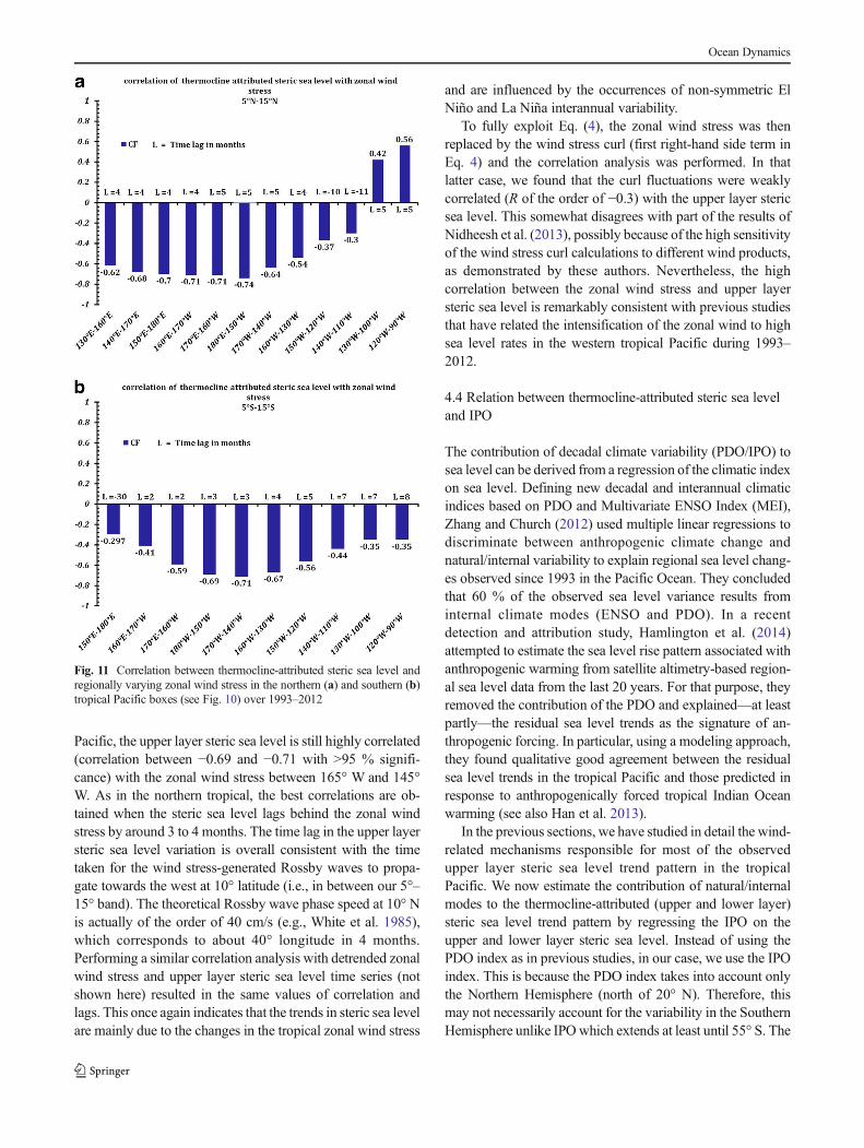
Pacific, the upper layer steric sea level is still highly correlated
(correlation between −0.69 and −0.71 with >95 % signifi-
cance) with the zonal wind stress between 165° W and 145°
W. As in the northern tropical, the best correlations are ob-
tained when the steric sea level lags behind the zonal wind
stress by around 3 to 4 months. The time lag in the upper layer
steric sea level variation is overall consistent with the time
taken for the wind stress-generated Rossby waves to propa-
gate towards the west at 10° latitude (i.e., in between our 5°–
15° band). The theoretical Rossby wave phase speed at 10° N
is actually of the order of 40 cm/s (e.g., White et al. 1985),
which corresponds to about 40° longitude in 4 months.
Performing a similar correlation analysis with detrended zonal
wind stress and upper layer steric sea level time series (not
shown here) resulted in the same values of correlation and
lags. This once again indicates that the trends in steric sea level
are mainly due to the changes in the tropical zonal wind stress
and are influenced by the occurrences of non-symmetric El
Niño and La Niña interannual variability.
To fully exploit Eq. (4), the zonal wind stress was then
replaced by the wind stress curl (first right-hand side term in
Eq. 4) and the correlation analysis was performed. In that
latter case, we found that the curl fluctuations were weakly
correlated (R of the order of −0.3) with the upper layer steric
sea level. This somewhat disagrees with part of the results of
Nidheesh et al. (2013), possibly because of the high sensitivity
of the wind stress curl calculations to different wind products,
as demonstrated by these authors. Nevertheless, the high
correlation between the zonal wind stress and upper layer
steric sea level is remarkably consistent with previous studies
that have related the intensification of the zonal wind to high
sea level rates in the western tropical Pacific during 1993–
2012.
4.4 Relation between thermocline-attributed steric sea level
and IPO
The contribution of decadal climate variability (PDO/IPO) to
sea level can be derived from a regression of the climatic index
on sea level. Defining new decadal and interannual climatic
indices based on PDO and Multivariate ENSO Index (MEI),
Zhang and Church (2012) used multiple linear regressions to
discriminate between anthropogenic climate change and
natural/internal variability to explain regional sea level chang-
es observed since 1993 in the Pacific Ocean. They concluded
that 60 % of the observed sea level variance results from
internal climate modes (ENSO and PDO). In a recent
detection and attribution study, Hamlington et al. (2014)
attempted to estimate the sea level rise pattern associated with
anthropogenic warming from satellite altimetry-based region-
al sea level data from the last 20 years. For that purpose, they
removed the contribution of the PDO and explained—at least
partly—the residual sea level trends as the signature of an-
thropogenic forcing. In particular, using a modeling approach,
they found qualitative good agreement between the residual
sea level trends in the tropical Pacific and those predicted in
response to anthropogenically forced tropical Indian Ocean
warming (see also Han et al. 2013).
In the previous sections, we have studied in detail the wind-
related mechanisms responsible for most of the observed
upper layer steric sea level trend pattern in the tropical
Pacific. We now estimate the contribution of natural/internal
modes to the thermocline-attributed (upper and lower layer)
steric sea level trend pattern by regressing the IPO on the
upper and lower layer steric sea level. Instead of using the
PDO index as in previous studies, in our case, we use the IPO
index. This is because the PDO index takes into account only
the Northern Hemisphere (north of 20° N). Therefore, this
may not necessarily account for the variability in the Southern
Hemisphere unlike IPOwhich extends at least until 55° S. The
Fig. 11 Correlation between thermocline-attributed steric sea level and
regionally varying zonal wind stress in the northern (a) and southern (b)
tropical Pacific boxes (see Fig. 10) over 1993–2012
Ocean Dynamics
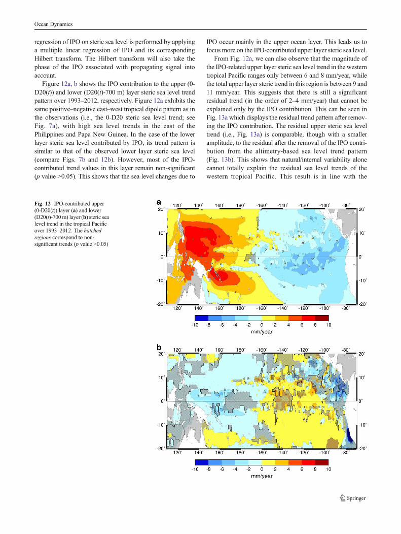
regression of IPO on steric sea level is performed by applying
a multiple linear regression of IPO and its corresponding
Hilbert transform. The Hilbert transform will also take the
phase of the IPO associated with propagating signal into
account.
Figure 12a, b shows the IPO contribution to the upper (0-
D20(t)) and lower (D20(t)-700 m) layer steric sea level trend
pattern over 1993–2012, respectively. Figure 12a exhibits the
same positive–negative east–west tropical dipole pattern as in
the observations (i.e., the 0-D20 steric sea level trend; see
Fig. 7a), with high sea level trends in the east of the
Philippines and Papa New Guinea. In the case of the lower
layer steric sea level contributed by IPO, its trend pattern is
similar to that of the observed lower layer steric sea level
(compare Figs. 7b and 12b). However, most of the IPO-
contributed trend values in this layer remain non-significant
(p value >0.05). This shows that the sea level changes due to
IPO occur mainly in the upper ocean layer. This leads us to
focus more on the IPO-contributed upper layer steric sea level.
From Fig. 12a, we can also observe that the magnitude of
the IPO-related upper layer steric sea level trend in the western
tropical Pacific ranges only between 6 and 8 mm/year, while
the total upper layer steric trend in this region is between 9 and
11 mm/year. This suggests that there is still a significant
residual trend (in the order of 2–4 mm/year) that cannot be
explained only by the IPO contribution. This can be seen in
Fig. 13a which displays the residual trend pattern after remov-
ing the IPO contribution. The residual upper steric sea level
trend (i.e., Fig. 13a) is comparable, though with a smaller
amplitude, to the residual after the removal of the IPO contri-
bution from the altimetry-based sea level trend pattern
(Fig. 13b). This shows that natural/internal variability alone
cannot totally explain the residual sea level trends of the
western tropical Pacific. This result is in line with the
Fig. 12 IPO-contributed upper
(0-D20(t)) layer (a) and lower
(D20(t)-700m) layer (b) steric sea
level trend in the tropical Pacific
over 1993–2012. The hatched
regions correspond to non-
significant trends (p value >0.05)
Ocean Dynamics
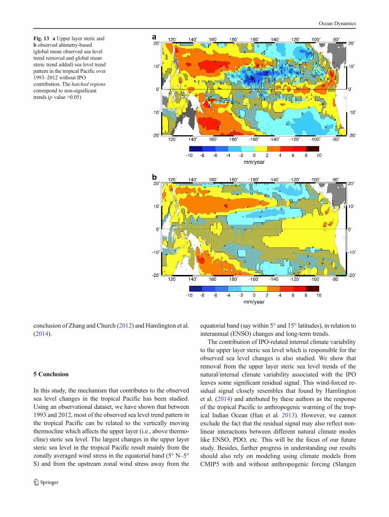
conclusion of Zhang and Church (2012) and Hamlington et al.
(2014).
5 Conclusion
In this study, the mechanism that contributes to the observed
sea level changes in the tropical Pacific has been studied.
Using an observational dataset, we have shown that between
1993 and 2012, most of the observed sea level trend pattern in
the tropical Pacific can be related to the vertically moving
thermocline which affects the upper layer (i.e., above thermo-
cline) steric sea level. The largest changes in the upper layer
steric sea level in the tropical Pacific result mainly from the
zonally averaged wind stress in the equatorial band (5° N–5°
S) and from the upstream zonal wind stress away from the
equatorial band (say within 5° and 15° latitudes), in relation to
interannual (ENSO) changes and long-term trends.
The contribution of IPO-related internal climate variability
to the upper layer steric sea level which is responsible for the
observed sea level changes is also studied. We show that
removal from the upper layer steric sea level trends of the
natural/internal climate variability associated with the IPO
leaves some significant residual signal. This wind-forced re-
sidual signal closely resembles that found by Hamlington
et al. (2014) and attributed by these authors as the response
of the tropical Pacific to anthropogenic warming of the trop-
ical Indian Ocean (Han et al. 2013). However, we cannot
exclude the fact that the residual signal may also reflect non-
linear interactions between different natural climate modes
like ENSO, PDO, etc. This will be the focus of our future
study. Besides, further progress in understanding our results
should also rely on modeling using climate models from
CMIP5 with and without anthropogenic forcing (Slangen
Fig. 13 a Upper layer steric and
b observed altimetry-based
(global mean observed sea level
trend removed and global mean
steric trend added) sea level trend
pattern in the tropical Pacific over
1993–2012 without IPO
contribution. The hatched regions
correspond to non-significant
trends (p value >0.05)
Ocean Dynamics
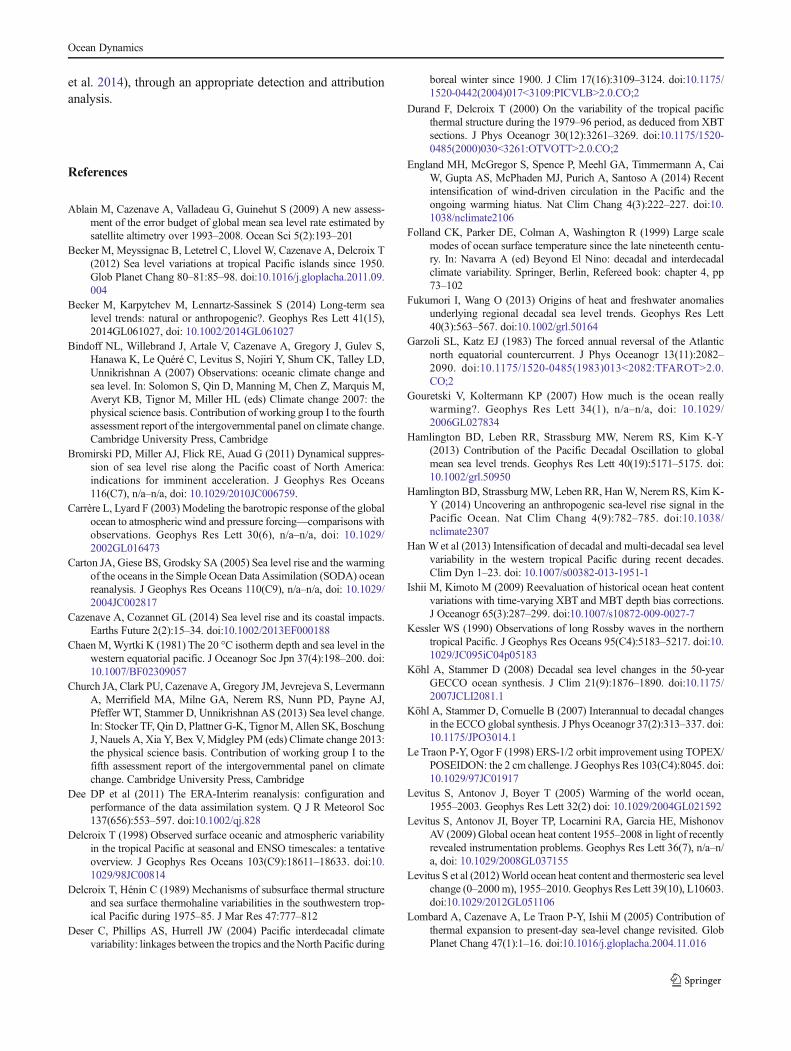
et al. 2014), through an appropriate detection and attribution
analysis.
References
Ablain M, Cazenave A, Valladeau G, Guinehut S (2009) A new assess-
ment of the error budget of global mean sea level rate estimated by
satellite altimetry over 1993–2008. Ocean Sci 5(2):193–201
Becker M, Meyssignac B, Letetrel C, Llovel W, Cazenave A, Delcroix T
(2012) Sea level variations at tropical Pacific islands since 1950.
Glob Planet Chang 80–81:85–98. doi:10.1016/j.gloplacha.2011.09.
004
Becker M, Karpytchev M, Lennartz-Sassinek S (2014) Long-term sea
level trends: natural or anthropogenic?. Geophys Res Lett 41(15),
2014GL061027, doi: 10.1002/2014GL061027
Bindoff NL, Willebrand J, Artale V, Cazenave A, Gregory J, Gulev S,
Hanawa K, Le Quéré C, Levitus S, Nojiri Y, Shum CK, Talley LD,
Unnikrishnan A (2007) Observations: oceanic climate change and
sea level. In: Solomon S, Qin D, Manning M, Chen Z, Marquis M,
Averyt KB, Tignor M, Miller HL (eds) Climate change 2007: the
physical science basis. Contribution of working group I to the fourth
assessment report of the intergovernmental panel on climate change.
Cambridge University Press, Cambridge
Bromirski PD, Miller AJ, Flick RE, Auad G (2011) Dynamical suppres-
sion of sea level rise along the Pacific coast of North America:
indications for imminent acceleration. J Geophys Res Oceans
116(C7), n/a–n/a, doi: 10.1029/2010JC006759.
Carrère L, Lyard F (2003) Modeling the barotropic response of the global
ocean to atmospheric wind and pressure forcing—comparisons with
observations. Geophys Res Lett 30(6), n/a–n/a, doi: 10.1029/
2002GL016473
Carton JA, Giese BS, Grodsky SA (2005) Sea level rise and the warming
of the oceans in the Simple Ocean Data Assimilation (SODA) ocean
reanalysis. J Geophys Res Oceans 110(C9), n/a–n/a, doi: 10.1029/
2004JC002817
Cazenave A, Cozannet GL (2014) Sea level rise and its coastal impacts.
Earths Future 2(2):15–34. doi:10.1002/2013EF000188
ChaenM,Wyrtki K (1981) The 20 °C isotherm depth and sea level in the
western equatorial pacific. J Oceanogr Soc Jpn 37(4):198–200. doi:
10.1007/BF02309057
Church JA, Clark PU, Cazenave A, Gregory JM, Jevrejeva S, Levermann
A, Merrifield MA, Milne GA, Nerem RS, Nunn PD, Payne AJ,
Pfeffer WT, Stammer D, Unnikrishnan AS (2013) Sea level change.
In: Stocker TF, Qin D, Plattner G-K, TignorM, Allen SK, Boschung
J, Nauels A, Xia Y, Bex V, Midgley PM (eds) Climate change 2013:
the physical science basis. Contribution of working group I to the
fifth assessment report of the intergovernmental panel on climate
change. Cambridge University Press, Cambridge
Dee DP et al (2011) The ERA-Interim reanalysis: configuration and
performance of the data assimilation system. Q J R Meteorol Soc
137(656):553–597. doi:10.1002/qj.828
Delcroix T (1998) Observed surface oceanic and atmospheric variability
in the tropical Pacific at seasonal and ENSO timescales: a tentative
overview. J Geophys Res Oceans 103(C9):18611–18633. doi:10.
1029/98JC00814
Delcroix T, Hénin C (1989) Mechanisms of subsurface thermal structure
and sea surface thermohaline variabilities in the southwestern trop-
ical Pacific during 1975–85. J Mar Res 47:777–812
Deser C, Phillips AS, Hurrell JW (2004) Pacific interdecadal climate
variability: linkages between the tropics and theNorth Pacific during
boreal winter since 1900. J Clim 17(16):3109–3124. doi:10.1175/
1520-0442(2004)017<3109:PICVLB>2.0.CO;2
Durand F, Delcroix T (2000) On the variability of the tropical pacific
thermal structure during the 1979–96 period, as deduced from XBT
sections. J Phys Oceanogr 30(12):3261–3269. doi:10.1175/1520-
0485(2000)030<3261:OTVOTT>2.0.CO;2
England MH, McGregor S, Spence P, Meehl GA, Timmermann A, Cai
W, Gupta AS, McPhaden MJ, Purich A, Santoso A (2014) Recent
intensification of wind-driven circulation in the Pacific and the
ongoing warming hiatus. Nat Clim Chang 4(3):222–227. doi:10.
1038/nclimate2106
Folland CK, Parker DE, Colman A, Washington R (1999) Large scale
modes of ocean surface temperature since the late nineteenth centu-
ry. In: Navarra A (ed) Beyond El Nino: decadal and interdecadal
climate variability. Springer, Berlin, Refereed book: chapter 4, pp
73–102
Fukumori I, Wang O (2013) Origins of heat and freshwater anomalies
underlying regional decadal sea level trends. Geophys Res Lett
40(3):563–567. doi:10.1002/grl.50164
Garzoli SL, Katz EJ (1983) The forced annual reversal of the Atlantic
north equatorial countercurrent. J Phys Oceanogr 13(11):2082–
2090. doi:10.1175/1520-0485(1983)013<2082:TFAROT>2.0.
CO;2
Gouretski V, Koltermann KP (2007) How much is the ocean really
warming?. Geophys Res Lett 34(1), n/a–n/a, doi: 10.1029/
2006GL027834
Hamlington BD, Leben RR, Strassburg MW, Nerem RS, Kim K-Y
(2013) Contribution of the Pacific Decadal Oscillation to global
mean sea level trends. Geophys Res Lett 40(19):5171–5175. doi:
10.1002/grl.50950
Hamlington BD, Strassburg MW, Leben RR, HanW, Nerem RS, Kim K-
Y (2014) Uncovering an anthropogenic sea-level rise signal in the
Pacific Ocean. Nat Clim Chang 4(9):782–785. doi:10.1038/
nclimate2307
Han Wet al (2013) Intensification of decadal and multi-decadal sea level
variability in the western tropical Pacific during recent decades.
Clim Dyn 1–23. doi: 10.1007/s00382-013-1951-1
Ishii M, Kimoto M (2009) Reevaluation of historical ocean heat content
variations with time-varying XBT and MBT depth bias corrections.
J Oceanogr 65(3):287–299. doi:10.1007/s10872-009-0027-7
Kessler WS (1990) Observations of long Rossby waves in the northern
tropical Pacific. J Geophys Res Oceans 95(C4):5183–5217. doi:10.
1029/JC095iC04p05183
Köhl A, Stammer D (2008) Decadal sea level changes in the 50-year
GECCO ocean synthesis. J Clim 21(9):1876–1890. doi:10.1175/
2007JCLI2081.1
Köhl A, Stammer D, Cornuelle B (2007) Interannual to decadal changes
in the ECCO global synthesis. J Phys Oceanogr 37(2):313–337. doi:
10.1175/JPO3014.1
Le Traon P-Y, Ogor F (1998) ERS-1/2 orbit improvement using TOPEX/
POSEIDON: the 2 cm challenge. J Geophys Res 103(C4):8045. doi:
10.1029/97JC01917
Levitus S, Antonov J, Boyer T (2005) Warming of the world ocean,
1955–2003. Geophys Res Lett 32(2) doi: 10.1029/2004GL021592
Levitus S, Antonov JI, Boyer TP, Locarnini RA, Garcia HE, Mishonov
AV (2009) Global ocean heat content 1955–2008 in light of recently
revealed instrumentation problems. Geophys Res Lett 36(7), n/a–n/
a, doi: 10.1029/2008GL037155
Levitus S et al (2012)World ocean heat content and thermosteric sea level
change (0–2000m), 1955–2010. Geophys Res Lett 39(10), L10603.
doi:10.1029/2012GL051106
Lombard A, Cazenave A, Le Traon P-Y, Ishii M (2005) Contribution of
thermal expansion to present-day sea-level change revisited. Glob
Planet Chang 47(1):1–16. doi:10.1016/j.gloplacha.2004.11.016
Ocean Dynamics
Lombard A, Garric G, Penduff T (2009) Regional patterns of observed
sea level change: insights from a ¼° global ocean/sea-ice hindcast.
Ocean Dyn 59(3):433–449. doi:10.1007/s10236-008-0161-6
Mantua NJ, Hare SR (2002) The Pacific Decadal Oscillation. J Oceanogr
58(1):35–44. doi:10.1023/A:1015820616384
Mantua NJ, Hare SR, Zhang Y, Wallace JM, Francis RC (1997) A pacific
interdecadal climate oscillation with impacts on salmon production.
Bull Am Meteorol Soc 78(6):1069–1079. doi:10.1175/1520-
0477(1997)078<1069:APICOW>2.0.CO;2
Marcos M, Amores A (2014) Quantifying anthropogenic and natural
contributions to thermosteric sea level rise. Geophys. Res. Lett.,
41(7) 2014GL059766, doi: 10.1002/2014GL059766
McGregor S, Holbrook NJ, Power SB (2007) Interdecadal sea surface
temperature variability in the equatorial Pacific Ocean. Part I: the
role of off-equatorial wind stresses and oceanic Rossby waves. J
Clim 20(11):2643–2658. doi:10.1175/JCLI4145.1
McGregor S, Holbrook NJ, Power SB (2008) Interdecadal sea surface
temperature variability in the equatorial pacific ocean. Part II: the
role of equatorial/off-equatorial wind stresses in a hybrid coupled
model. J Clim 21(17):4242–4256. doi:10.1175/2008JCLI2057.1
McGregor S, Gupta AS, England MH (2012) Constraining wind stress
products with sea surface height observations and implications for
Pacific Ocean sea level trend attribution*. J Clim 25(23) 8164–
8176, doi: 10.1175/JCLI-D-12-00105.1
Meehl GA, Hu A, Arblaster JM, Fasullo J, Trenberth KE (2013)
Externally forced and internally generated decadal climate variabil-
ity associated with the Interdecadal Pacific Oscillation. J Clim
26(18):7298–7310. doi:10.1175/JCLI-D-12-00548.1
Merrifield MA (2011) A shift in western tropical Pacific sea level trends
during the 1990s. J Clim 24(15):4126–4138. doi:10.1175/
2011JCLI3932.1
Merrifield MA, Maltrud ME (2011) Regional sea level trends due to a
Pacific trade wind intensification. Geophys Res Lett 38. doi: 10.
1029/2011GL049576
Merrifield MA, Thompson PR, Lander M (2012) Multidecadal sea level
anomalies and trends in the western tropical Pacific. Geophys Res
Lett 39. doi: 10.1029/2012GL052032
Meyers G (1979) On the annual Rossbywave in the tropical North Pacific
Ocean. J Phys Oceanogr 9(4):663–674. doi:10.1175/1520-0485
Meyssignac B, Salas yMelia D, BeckerM, LlovelW, Cazenave A (2012)
Tropical Pacific spatial trend patterns in observed sea level: internal
variability and/or anthropogenic signature? Clim Past 8(2):787–802.
doi:10.5194/cp-8-787-2012
Milne GA, Gehrels WR, Hughes CW, Tamisiea ME (2009) Identifying
the causes of sea-level change. Nat Geosci. doi:10.1038/ngeo544
Nerem RS, Chambers DP, Choe C,MitchumGT (2010) Estimating mean
sea level change from the TOPEX and Jason altimeter missions.Mar
Geod 33:435–446. doi:10.1080/01490419.2010.491031
Nidheesh AG, Lengaigne M, Vialard J, Unnikrishnan AS, Dayan H
(2013) Decadal and long-term sea level variability in the tropical
Indo-Pacific Ocean. ClimDyn 41(2):381–402. doi:10.1007/s00382-
012-1463-4
Pedlosky J (2006) A history of thermocline theory. In: Jochum M,
Murtugudde R (eds) Physical oceanography. Springer, New York,
pp 139–152
Power S, Casey T, Folland C, Colman A, Mehta V (1999) Inter-decadal
modulation of the impact of ENSO on Australia. Clim Dyn 15:319–
324. doi:10.1007/s003820050284
Rebert JP, Donguy JR, Eldin G, Wyrtki K (1985) Relations between sea
level, thermocline depth, heat content, and dynamic height in the
tropical Pacific Ocean. J Geophys Res Oceans 90(C6):11719–
11725. doi:10.1029/JC090iC06p11719
Slangen ABA, Church JA, Zhang X,Monselesan D (2014) Detection and
attribution of global mean thermosteric sea level change. Geophys
Res Lett n/a–n/a, doi: 10.1002/2014GL061356
Stammer D, Cazenave A, Ponte RM, Tamisiea ME (2013) Causes for
contemporary regional sea level changes. Annu. Rev. Mar. Sci, 5.
doi: 10.1146/annurev-marine-121211-172406
Sverdrup HU (1947) Wind-driven currents in a baroclinic ocean; with
application to the equatorial currents of the eastern pacific. Proc Natl
Acad Sci U S A 33(11):318–326
Swenson MS, Hansen DV (1999) Tropical Pacific Ocean mixed layer
heat budget: the pacific cold tongue. J Phys Oceanogr 29(1):69–81.
doi:10.1175/1520-0485(1999)029<0069:TPOMLH>2.0.CO;2
Thompson PR,MerrifieldMA,Wells JR, Chang CM (2014)Wind-driven
coastal sea level variability in the northeast Pacific. J Clim 27(12):
4733–4751. doi:10.1175/JCLI-D-13-00225.1
Timmermann A, McGregor S, Jin F-F (2010) Wind effects on past and
future regional sea level trends in the southern Indo-Pacific*. J.
Clim., 23(16), 4429–4437, doi: 10.1175/2010JCLI3519.1
Volkov DL, Larnicol G, Dorandeu J (2007) Improving the quality of
satellite altimetry data over continental shelves. J. Geophys. Res.
Oceans 112(C6), n/a–n/a, doi: 10.1029/2006JC003765
White W, Meyers G, Donguy JR, Pazan S (1985) Short-term climatic
variability in the thermal structure of the Pacific Ocean during 1979–
82. J Phys Oceanogr 15:917–935
Wunsch C, Ponte RM, Heimbach P (2007) Decadal trends in sea level
patterns: 1993–2004. J Clim 20(24):5889–5911. doi:10.1175/
2007JCLI1840.1
Wyrtki K, Kendall R (1967) Transports of the Pacific equatorial counter-
current. J Geophys Res 72(8):2073–2076
YangH,Wang F (2009) Revisiting the thermocline depth in the equatorial
Pacific*. J. Clim., 22(13) 3856–3863. doi: 10.1175/2009JCLI2836.
1
Zhang X, Church JA (2012) Sea level trends, interannual and decadal
variability in the Pacific Ocean. Geophys Res Lett 39. doi: 10.1029/
2012GL053240
Zhang Y, Wallace JM, Battisti DS (1997) ENSO-like interdecadal vari-
ability: 1900–93. J Clim 10(5):1004–1020. doi:10.1175/1520-
0442(1997)010<1004:ELIV>2.0.CO;2
Ocean Dynamics
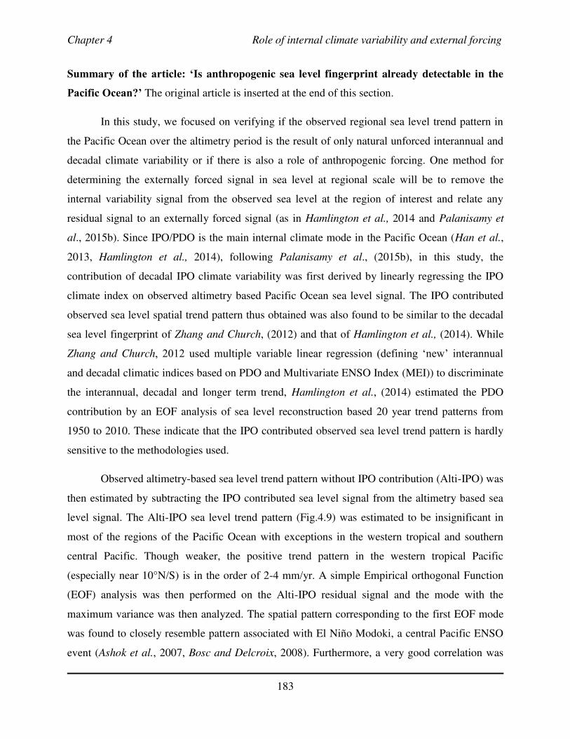
Chapter 4 Role of internal climate variability and external forcing
183
Summary of the article: ‘Is anthropogenic sea level fingerprint already detectable in the
Pacific Ocean?’ The original article is inserted at the end of this section.
In this study, we focused on verifying if the observed regional sea level trend pattern in
the Pacific Ocean over the altimetry period is the result of only natural unforced interannual and
decadal climate variability or if there is also a role of anthropogenic forcing. One method for
determining the externally forced signal in sea level at regional scale will be to remove the
internal variability signal from the observed sea level at the region of interest and relate any
residual signal to an externally forced signal (as in Hamlington et al., 2014 and Palanisamy et
al., 2015b). Since IPO/PDO is the main internal climate mode in the Pacific Ocean (Han et al.,
2013, Hamlington et al., 2014), following Palanisamy et al., (2015b), in this study, the
contribution of decadal IPO climate variability was first derived by linearly regressing the IPO
climate index on observed altimetry based Pacific Ocean sea level signal. The IPO contributed
observed sea level spatial trend pattern thus obtained was also found to be similar to the decadal
sea level fingerprint of Zhang and Church, (2012) and that of Hamlington et al., (2014). While
Zhang and Church, 2012 used multiple variable linear regression (defining ‘new’ interannual
and decadal climatic indices based on PDO and Multivariate ENSO Index (MEI)) to discriminate
the interannual, decadal and longer term trend, Hamlington et al., (2014) estimated the PDO
contribution by an EOF analysis of sea level reconstruction based 20 year trend patterns from
1950 to 2010. These indicate that the IPO contributed observed sea level trend pattern is hardly
sensitive to the methodologies used.
Observed altimetry-based sea level trend pattern without IPO contribution (Alti-IPO) was
then estimated by subtracting the IPO contributed sea level signal from the altimetry based sea
level signal. The Alti-IPO sea level trend pattern (Fig.4.9) was estimated to be insignificant in
most of the regions of the Pacific Ocean with exceptions in the western tropical and southern
central Pacific. Though weaker, the positive trend pattern in the western tropical Pacific
(especially near 10°N/S) is in the order of 2-4 mm/yr. A simple Empirical orthogonal Function
(EOF) analysis was then performed on the Alti-IPO residual signal and the mode with the
maximum variance was then analyzed. The spatial pattern corresponding to the first EOF mode
was found to closely resemble pattern associated with El Niño Modoki, a central Pacific ENSO
event (Ashok et al., 2007, Bosc and Delcroix, 2008). Furthermore, a very good correlation was
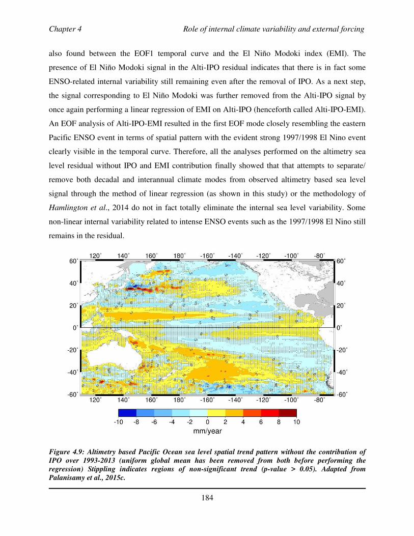
Chapter 4 Role of internal climate variability and external forcing
184
also found between the EOF1 temporal curve and the El Niño Modoki index (EMI). The
presence of El Niño Modoki signal in the Alti-IPO residual indicates that there is in fact some
ENSO-related internal variability still remaining even after the removal of IPO. As a next step,
the signal corresponding to El Niño Modoki was further removed from the Alti-IPO signal by
once again performing a linear regression of EMI on Alti-IPO (henceforth called Alti-IPO-EMI).
An EOF analysis of Alti-IPO-EMI resulted in the first EOF mode closely resembling the eastern
Pacific ENSO event in terms of spatial pattern with the evident strong 1997/1998 El Nino event
clearly visible in the temporal curve. Therefore, all the analyses performed on the altimetry sea
level residual without IPO and EMI contribution finally showed that that attempts to separate/
remove both decadal and interannual climate modes from observed altimetry based sea level
signal through the method of linear regression (as shown in this study) or the methodology of
Hamlington et al., 2014 do not in fact totally eliminate the internal sea level variability. Some
non-linear internal variability related to intense ENSO events such as the 1997/1998 El Nino still
remains in the residual.
Figure 4.9: Altimetry based Pacific Ocean sea level spatial trend pattern without the contribution of
IPO over 1993-2013 (uniform global mean has been removed from both before performing the
regression) Stippling indicates regions of non-significant trend (p-value > 0.05). Adapted from
Palanisamy et al., 2015c.
Chapter 4 Role of internal climate variability and external forcing
185
In order to further confirm our results, we then worked on 21 CMIP5 models. Performing
a Multi Model Ensemble (MME) of the 21 CMIP5 models would in general average out/ reduce
the sea level signal due to internal climate modes. The MME containing only the expected sea
level response to external forcings (natural and anthropogenic) can then be compared with the
Alti-IPO and Alti-IPO-EMI residual sea level trend patterns. Before a direct comparison of the
sea level trend patterns, the presence of any internal climate modes in the MME was first verified
by performing EOF decomposition on the MME based global and Pacific Ocean sea level signal
between 1900 and 2098 and the corresponding spatial and temporal patterns were studied. This
would enable us to verify the effectiveness of MME in reducing the impact of internal climate
modes not only in the Pacific but also in the other oceans. Furthermore, such verification would
also give us an idea on regions where the impact of external forcing is the maximum and the
structure of their corresponding spatial patterns. The first EOF mode of the global MME signal
explains a total variance of 96%. In terms of spatial pattern, this increase in sea level appears in
the northern high latitudinal bands, North Atlantic Ocean south of Greenland and also in the
southern latitudinal bands. Regions of positive sea level patterns also occur in the western extra-
tropical Pacific Ocean and in western Indian and central Atlantic oceans. Region of negative sea
level change appears in the Southern Ocean beyond the 50°S latitudinal band. This is in
agreement with the results from Bilbao et al., (2015). Performing the same EOF analysis only on
the Pacific Ocean, we obtain the same Pacific Ocean spatial pattern (with a variance of 93%).
The temporal curves of both the global and Pacific Ocean EOF1 mode are almost flat until 1970
after which there is an increase that continues over time implying accelerated dynamic sea level
change. These are in agreement with studies showing increased anthropogenic forcing since
1970s. Small amplitude oscillations displayed in both EOF1 temporal curves were removed by
performing a spline smoothing (Ribes et al., 2009). The smoothed global EOF1 temporal curve
was then regressed on to the CMIP5 MME sea level signal.
Analysis of the regressed CMIP5 MME based Pacific Ocean sea level spatial trend
pattern over 1993-2013 period (Fig.4.10) showed that in the western tropical Pacific it was not
comparable with the Alti-IPO-EMI based residual trend pattern. Contrary to the Alti- IPO and
Alti-IPO-EMI trend patterns, the CMIP5 MME based positive trend pattern that appears in the
western tropical Pacific extending towards the east between 10°N to 20°N and 120°E to 120°W
is only in the range of 0.1 mm/yr to 0.3 mm/yr. The absence of significantly high positive sea
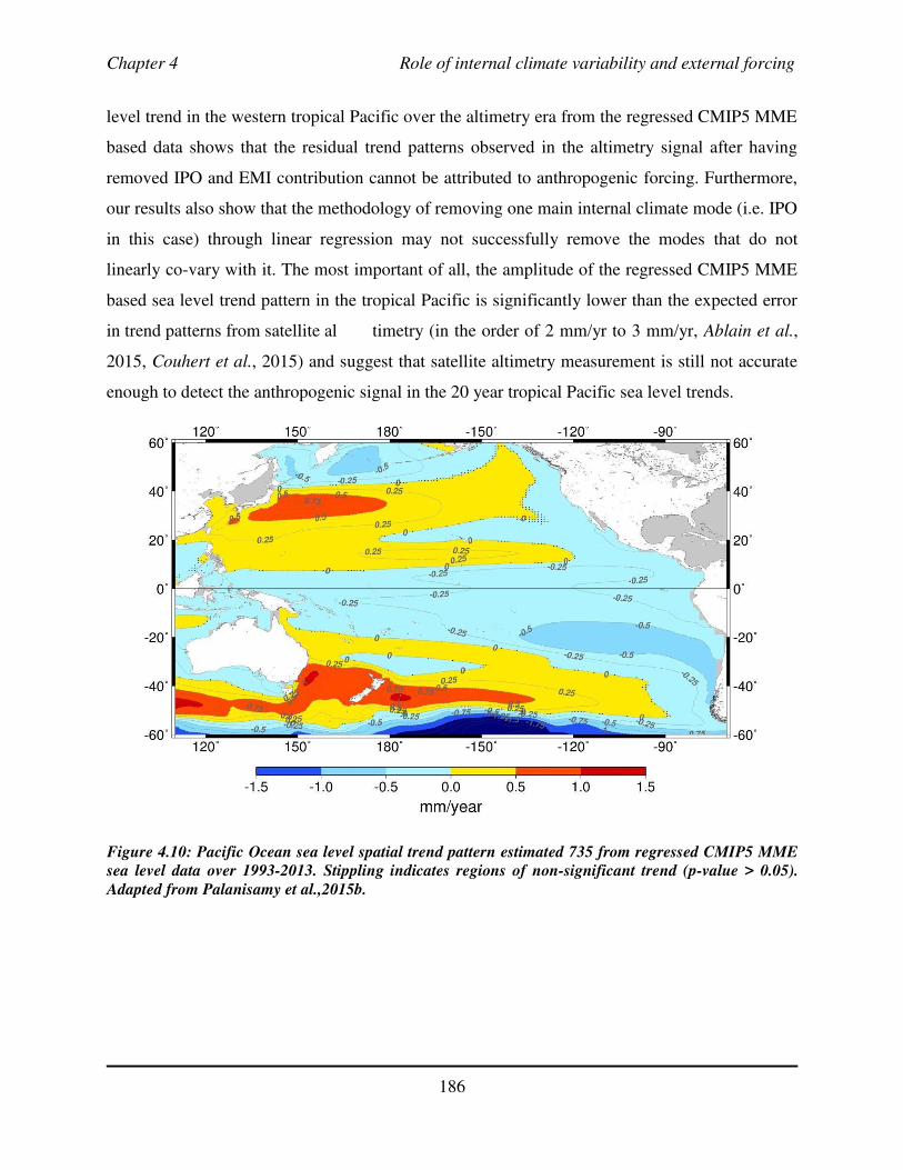
Chapter 4 Role of internal climate variability and external forcing
186
level trend in the western tropical Pacific over the altimetry era from the regressed CMIP5 MME
based data shows that the residual trend patterns observed in the altimetry signal after having
removed IPO and EMI contribution cannot be attributed to anthropogenic forcing. Furthermore,
our results also show that the methodology of removing one main internal climate mode (i.e. IPO
in this case) through linear regression may not successfully remove the modes that do not
linearly co-vary with it. The most important of all, the amplitude of the regressed CMIP5 MME
based sea level trend pattern in the tropical Pacific is significantly lower than the expected error
in trend patterns from satellite al timetry (in the order of 2 mm/yr to 3 mm/yr, Ablain et al.,
2015, Couhert et al., 2015) and suggest that satellite altimetry measurement is still not accurate
enough to detect the anthropogenic signal in the 20 year tropical Pacific sea level trends.
Figure 4.10: Pacific Ocean sea level spatial trend pattern estimated 735 from regressed CMIP5 MME
sea level data over 1993-2013. Stippling indicates regions of non-significant trend (p-value > 0.05).
Adapted from Palanisamy et al.,2015b.
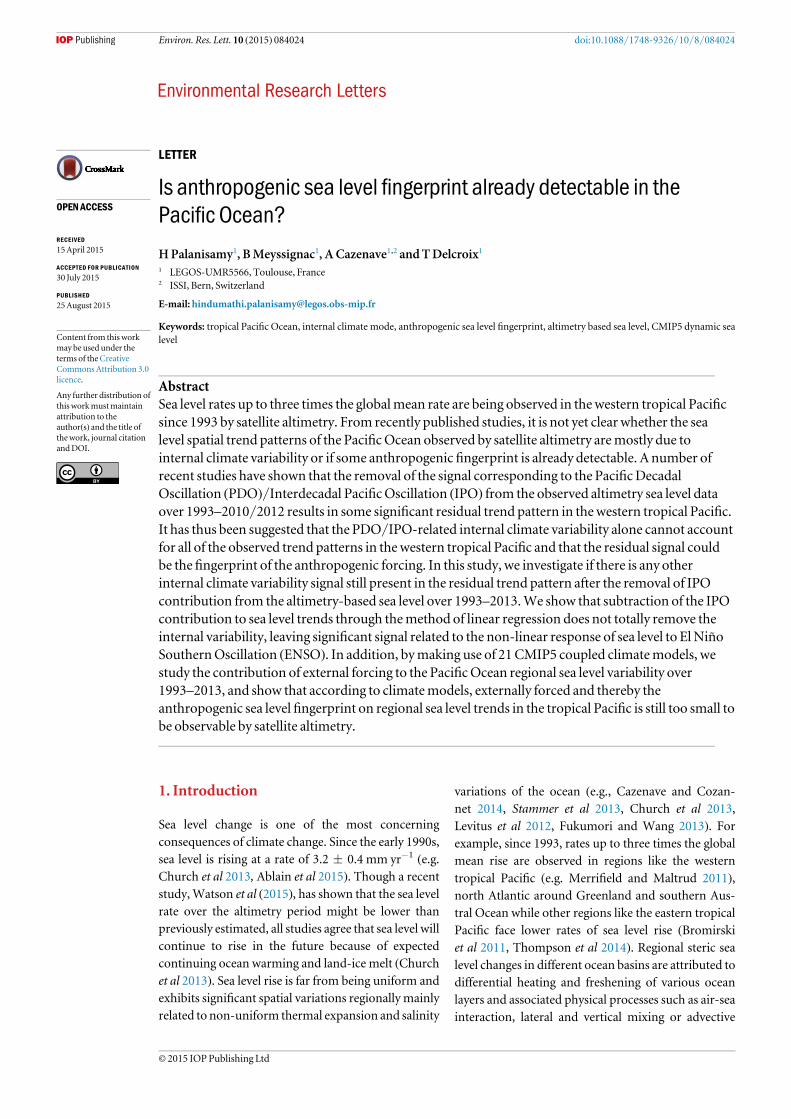
Environ. Res. Lett. 10 (2015) 084024 doi:10.1088/1748-9326/10/8/084024
LETTER
Is anthropogenic sea level fingerprint already detectable in the
Pacific Ocean?
HPalanisamy1, BMeyssignac1, ACazenave1,2 andTDelcroix1
1 LEGOS-UMR5566, Toulouse, France2 ISSI, Bern, Switzerland
E-mail: [email protected]
Keywords: tropical Pacific Ocean, internal climate mode, anthropogenic sea level fingerprint, altimetry based sea level, CMIP5 dynamic sea
level
Abstract
Sea level rates up to three times the globalmean rate are being observed in thewestern tropical Pacific
since 1993 by satellite altimetry. From recently published studies, it is not yet clear whether the sea
level spatial trend patterns of the PacificOcean observed by satellite altimetry aremostly due to
internal climate variability or if some anthropogenic fingerprint is already detectable. A number of
recent studies have shown that the removal of the signal corresponding to the PacificDecadal
Oscillation (PDO)/Interdecadal PacificOscillation (IPO) from the observed altimetry sea level data
over 1993–2010/2012 results in some significant residual trend pattern in thewestern tropical Pacific.
It has thus been suggested that the PDO/IPO-related internal climate variability alone cannot account
for all of the observed trend patterns in thewestern tropical Pacific and that the residual signal could
be thefingerprint of the anthropogenic forcing. In this study, we investigate if there is any other
internal climate variability signal still present in the residual trend pattern after the removal of IPO
contribution from the altimetry-based sea level over 1993–2013.We show that subtraction of the IPO
contribution to sea level trends through themethod of linear regression does not totally remove the
internal variability, leaving significant signal related to the non-linear response of sea level to ElNiño
SouthernOscillation (ENSO). In addition, bymaking use of 21CMIP5 coupled climatemodels, we
study the contribution of external forcing to the PacificOcean regional sea level variability over
1993–2013, and show that according to climatemodels, externally forced and thereby the
anthropogenic sea levelfingerprint on regional sea level trends in the tropical Pacific is still too small to
be observable by satellite altimetry.
1. Introduction
Sea level change is one of the most concerning
consequences of climate change. Since the early 1990s,
sea level is rising at a rate of 3.2±0.4 mm yr−1 (e.g.
Church et al 2013, Ablain et al 2015). Though a recent
study,Watson et al (2015), has shown that the sea level
rate over the altimetry period might be lower than
previously estimated, all studies agree that sea level will
continue to rise in the future because of expected
continuing ocean warming and land-ice melt (Church
et al 2013). Sea level rise is far from being uniform and
exhibits significant spatial variations regionally mainly
related to non-uniform thermal expansion and salinity
variations of the ocean (e.g., Cazenave and Cozan-
net 2014, Stammer et al 2013, Church et al 2013,
Levitus et al 2012, Fukumori and Wang 2013). For
example, since 1993, rates up to three times the global
mean rise are observed in regions like the western
tropical Pacific (e.g. Merrifield and Maltrud 2011),
north Atlantic around Greenland and southern Aus-
tral Ocean while other regions like the eastern tropical
Pacific face lower rates of sea level rise (Bromirski
et al 2011, Thompson et al 2014). Regional steric sea
level changes in different ocean basins are attributed to
differential heating and freshening of various ocean
layers and associated physical processes such as air-sea
interaction, lateral and vertical mixing or advective
OPEN ACCESS
RECEIVED
15April 2015
ACCEPTED FOR PUBLICATION
30 July 2015
PUBLISHED
25August 2015
Content from this workmay be used under theterms of theCreativeCommonsAttribution 3.0licence.
Any further distribution ofthis workmustmaintainattribution to theauthor(s) and the title ofthework, journal citationandDOI.
©2015 IOPPublishing Ltd
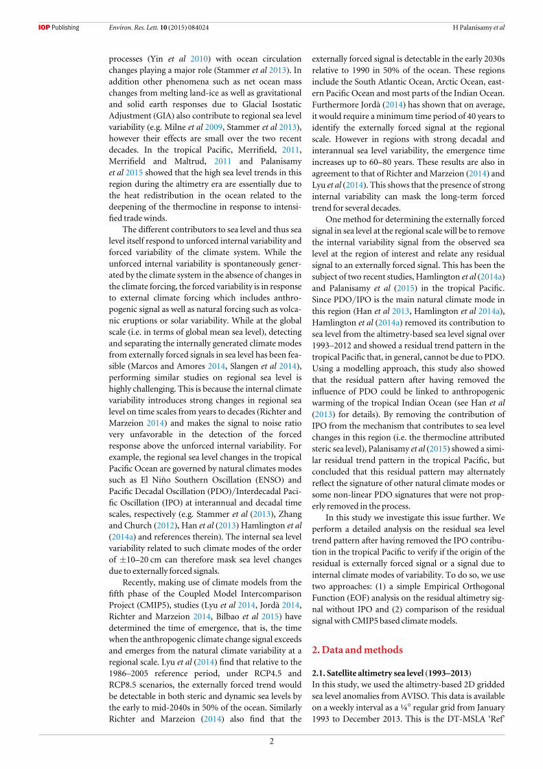
processes (Yin et al 2010) with ocean circulation
changes playing a major role (Stammer et al 2013). In
addition other phenomena such as net ocean mass
changes from melting land-ice as well as gravitational
and solid earth responses due to Glacial Isostatic
Adjustment (GIA) also contribute to regional sea level
variability (e.g. Milne et al 2009, Stammer et al 2013),
however their effects are small over the two recent
decades. In the tropical Pacific, Merrifield, 2011,
Merrifield and Maltrud, 2011 and Palanisamy
et al 2015 showed that the high sea level trends in this
region during the altimetry era are essentially due to
the heat redistribution in the ocean related to the
deepening of the thermocline in response to intensi-
fied tradewinds.
The different contributors to sea level and thus sea
level itself respond to unforced internal variability and
forced variability of the climate system. While the
unforced internal variability is spontaneously gener-
ated by the climate system in the absence of changes in
the climate forcing, the forced variability is in response
to external climate forcing which includes anthro-
pogenic signal as well as natural forcing such as volca-
nic eruptions or solar variability. While at the global
scale (i.e. in terms of global mean sea level), detecting
and separating the internally generated climate modes
from externally forced signals in sea level has been fea-
sible (Marcos and Amores 2014, Slangen et al 2014),
performing similar studies on regional sea level is
highly challenging. This is because the internal climate
variability introduces strong changes in regional sea
level on time scales from years to decades (Richter and
Marzeion 2014) and makes the signal to noise ratio
very unfavorable in the detection of the forced
response above the unforced internal variability. For
example, the regional sea level changes in the tropical
Pacific Ocean are governed by natural climates modes
such as El Niño Southern Oscillation (ENSO) and
Pacific Decadal Oscillation (PDO)/Interdecadal Paci-
fic Oscillation (IPO) at interannual and decadal time
scales, respectively (e.g. Stammer et al (2013), Zhang
and Church (2012), Han et al (2013) Hamlington et al
(2014a) and references therein). The internal sea level
variability related to such climate modes of the order
of ±10–20 cm can therefore mask sea level changes
due to externally forced signals.
Recently, making use of climate models from the
fifth phase of the Coupled Model Intercomparison
Project (CMIP5), studies (Lyu et al 2014, Jordà 2014,
Richter and Marzeion 2014, Bilbao et al 2015) have
determined the time of emergence, that is, the time
when the anthropogenic climate change signal exceeds
and emerges from the natural climate variability at a
regional scale. Lyu et al (2014) find that relative to the
1986–2005 reference period, under RCP4.5 and
RCP8.5 scenarios, the externally forced trend would
be detectable in both steric and dynamic sea levels by
the early to mid-2040s in 50% of the ocean. Similarly
Richter and Marzeion (2014) also find that the
externally forced signal is detectable in the early 2030s
relative to 1990 in 50% of the ocean. These regions
include the South Atlantic Ocean, Arctic Ocean, east-
ern Pacific Ocean and most parts of the Indian Ocean.
Furthermore Jordà (2014) has shown that on average,
it would require aminimum time period of 40 years to
identify the externally forced signal at the regional
scale. However in regions with strong decadal and
interannual sea level variability, the emergence time
increases up to 60–80 years. These results are also in
agreement to that of Richter andMarzeion (2014) and
Lyu et al (2014). This shows that the presence of strong
internal variability can mask the long-term forced
trend for several decades.
One method for determining the externally forced
signal in sea level at the regional scale will be to remove
the internal variability signal from the observed sea
level at the region of interest and relate any residual
signal to an externally forced signal. This has been the
subject of two recent studies, Hamlington et al (2014a)
and Palanisamy et al (2015) in the tropical Pacific.
Since PDO/IPO is the main natural climate mode in
this region (Han et al 2013, Hamlington et al 2014a),
Hamlington et al (2014a) removed its contribution to
sea level from the altimetry-based sea level signal over
1993–2012 and showed a residual trend pattern in the
tropical Pacific that, in general, cannot be due to PDO.
Using a modelling approach, this study also showed
that the residual pattern after having removed the
influence of PDO could be linked to anthropogenic
warming of the tropical Indian Ocean (see Han et al
(2013) for details). By removing the contribution of
IPO from the mechanism that contributes to sea level
changes in this region (i.e. the thermocline attributed
steric sea level), Palanisamy et al (2015) showed a simi-
lar residual trend pattern in the tropical Pacific, but
concluded that this residual pattern may alternately
reflect the signature of other natural climate modes or
some non-linear PDO signatures that were not prop-
erly removed in the process.
In this study we investigate this issue further. We
perform a detailed analysis on the residual sea level
trend pattern after having removed the IPO contribu-
tion in the tropical Pacific to verify if the origin of the
residual is externally forced signal or a signal due to
internal climate modes of variability. To do so, we use
two approaches: (1) a simple Empirical Orthogonal
Function (EOF) analysis on the residual altimetry sig-
nal without IPO and (2) comparison of the residual
signal withCMIP5 based climatemodels.
2.Data andmethods
2.1. Satellite altimetry sea level (1993–2013)
In this study, we used the altimetry-based 2D gridded
sea level anomalies from AVISO. This data is available
on a weekly interval as a ¼° regular grid from January
1993 to December 2013. This is the DT-MSLA ‘Ref’
2
Environ. Res. Lett. 10 (2015) 084024 HPalanisamy et al
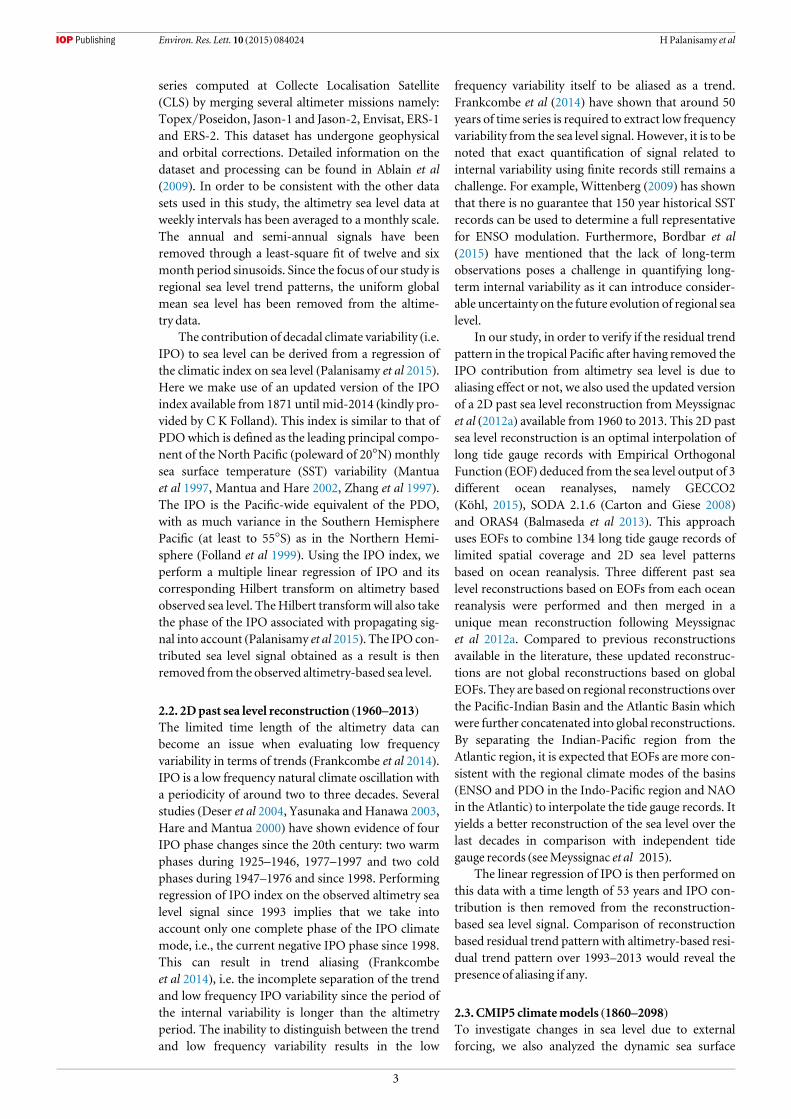
series computed at Collecte Localisation Satellite
(CLS) by merging several altimeter missions namely:
Topex/Poseidon, Jason-1 and Jason-2, Envisat, ERS-1
and ERS-2. This dataset has undergone geophysical
and orbital corrections. Detailed information on the
dataset and processing can be found in Ablain et al
(2009). In order to be consistent with the other data
sets used in this study, the altimetry sea level data at
weekly intervals has been averaged to a monthly scale.
The annual and semi-annual signals have been
removed through a least-square fit of twelve and six
month period sinusoids. Since the focus of our study is
regional sea level trend patterns, the uniform global
mean sea level has been removed from the altime-
try data.
The contribution of decadal climate variability (i.e.
IPO) to sea level can be derived from a regression of
the climatic index on sea level (Palanisamy et al 2015).
Here we make use of an updated version of the IPO
index available from 1871 until mid-2014 (kindly pro-
vided by C K Folland). This index is similar to that of
PDOwhich is defined as the leading principal compo-
nent of the North Pacific (poleward of 20°N) monthly
sea surface temperature (SST) variability (Mantua
et al 1997, Mantua and Hare 2002, Zhang et al 1997).
The IPO is the Pacific-wide equivalent of the PDO,
with as much variance in the Southern Hemisphere
Pacific (at least to 55°S) as in the Northern Hemi-
sphere (Folland et al 1999). Using the IPO index, we
perform a multiple linear regression of IPO and its
corresponding Hilbert transform on altimetry based
observed sea level. TheHilbert transformwill also take
the phase of the IPO associated with propagating sig-
nal into account (Palanisamy et al 2015). The IPO con-
tributed sea level signal obtained as a result is then
removed from the observed altimetry-based sea level.
2.2. 2Dpast sea level reconstruction (1960–2013)
The limited time length of the altimetry data can
become an issue when evaluating low frequency
variability in terms of trends (Frankcombe et al 2014).
IPO is a low frequency natural climate oscillation with
a periodicity of around two to three decades. Several
studies (Deser et al 2004, Yasunaka and Hanawa 2003,
Hare and Mantua 2000) have shown evidence of four
IPO phase changes since the 20th century: two warm
phases during 1925–1946, 1977–1997 and two cold
phases during 1947–1976 and since 1998. Performing
regression of IPO index on the observed altimetry sea
level signal since 1993 implies that we take into
account only one complete phase of the IPO climate
mode, i.e., the current negative IPO phase since 1998.
This can result in trend aliasing (Frankcombe
et al 2014), i.e. the incomplete separation of the trend
and low frequency IPO variability since the period of
the internal variability is longer than the altimetry
period. The inability to distinguish between the trend
and low frequency variability results in the low
frequency variability itself to be aliased as a trend.
Frankcombe et al (2014) have shown that around 50
years of time series is required to extract low frequency
variability from the sea level signal. However, it is to be
noted that exact quantification of signal related to
internal variability using finite records still remains a
challenge. For example, Wittenberg (2009) has shown
that there is no guarantee that 150 year historical SST
records can be used to determine a full representative
for ENSO modulation. Furthermore, Bordbar et al
(2015) have mentioned that the lack of long-term
observations poses a challenge in quantifying long-
term internal variability as it can introduce consider-
able uncertainty on the future evolution of regional sea
level.
In our study, in order to verify if the residual trend
pattern in the tropical Pacific after having removed the
IPO contribution from altimetry sea level is due to
aliasing effect or not, we also used the updated version
of a 2D past sea level reconstruction from Meyssignac
et al (2012a) available from 1960 to 2013. This 2D past
sea level reconstruction is an optimal interpolation of
long tide gauge records with Empirical Orthogonal
Function (EOF) deduced from the sea level output of 3
different ocean reanalyses, namely GECCO2
(Köhl, 2015), SODA 2.1.6 (Carton and Giese 2008)
and ORAS4 (Balmaseda et al 2013). This approach
uses EOFs to combine 134 long tide gauge records of
limited spatial coverage and 2D sea level patterns
based on ocean reanalysis. Three different past sea
level reconstructions based on EOFs from each ocean
reanalysis were performed and then merged in a
unique mean reconstruction following Meyssignac
et al 2012a. Compared to previous reconstructions
available in the literature, these updated reconstruc-
tions are not global reconstructions based on global
EOFs. They are based on regional reconstructions over
the Pacific-Indian Basin and the Atlantic Basin which
were further concatenated into global reconstructions.
By separating the Indian-Pacific region from the
Atlantic region, it is expected that EOFs are more con-
sistent with the regional climate modes of the basins
(ENSO and PDO in the Indo-Pacific region and NAO
in the Atlantic) to interpolate the tide gauge records. It
yields a better reconstruction of the sea level over the
last decades in comparison with independent tide
gauge records (seeMeyssignac et al 2015).
The linear regression of IPO is then performed on
this data with a time length of 53 years and IPO con-
tribution is then removed from the reconstruction-
based sea level signal. Comparison of reconstruction
based residual trend pattern with altimetry-based resi-
dual trend pattern over 1993–2013 would reveal the
presence of aliasing if any.
2.3. CMIP5 climatemodels (1860–2098)
To investigate changes in sea level due to external
forcing, we also analyzed the dynamic sea surface
3
Environ. Res. Lett. 10 (2015) 084024 HPalanisamy et al

height from 21 climate models from CMIP5 (Taylor
et al 2012). Table 1 displays the list of CMIP5 models
used. The dynamic sea surface height includes changes
in the thermohaline and wind-driven circulations
(Richter and Marzeion 2014). The CMIP5 climate
models do not include the net ocean mass changes
from melting ice sheets and glaciers as well as
associated gravitational and solid earth responses. But
this term is almost uniform over the last 20 years and
likely negligible (Landerer et al 2014, Yin et al 2010) in
terms of spatial variability in regional sea level trends.
Hence it is not important for our study. We used the
historical ‘all forcing’ CMIP5 climate simulations
available from 1850/1860. These simulations are
forced by natural forcing agents (solar radiation,
volcanic aerosols) and anthropogenic forcing agents
(e.g. greenhouse gas, anthropogenic aerosols, and
ozone etc, Taylor et al 2012). CMIP5 historical
simulations in general end in 2005. Since our period of
interest corresponds to that of the satellite altimetry
era from 1993 until 2013, we therefore extended the
historical simulations by concatenating the 21st cen-
tury projections under the Representative Concentra-
tion Pathway (RCP) 8.5 scenario (2006–2098/2100) to
the historical simulations. The RCP8.5 scenario
assumes continuous anthropogenic GHG emission
throughout the 21st century and can also be consid-
ered as a representative of the present scenario
(IPCC 2013).
Among the 21 models, some models provide mul-
tiple realizations of the historical experiment. For
example, CMIP5 historical runs initialized from dif-
ferent times of a control run would be identified as
‘r1’,’r2’, etc. The RCP simulation is assigned the same
realization number as the historical run from which it
was initiated (information on CMIP5 data reference
syntax can be found at http://cmip-pcmdi.llnl.gov/
cmip5/output_req.html). In our study, all possible
realizations that correspond to theHistorical+RCP8.5
simulations were taken into account (see table 1). As a
result, 53 realizations were used in this study. The data
is at yearly resolution and the spatial fields are remap-
ped to a regular 1°×1° resolution. All climatemodels
are corrected for the model drift (Gregory et al 2001,
Sen Gupta et al 2012) by removing the quadratic trend
in the time series of the accompanying pre-industrial
control run. The global mean was removed from the
dynamic sea level data at every time step.
The temporal phases of the internal climate varia-
bility in the CMIP5models are not reproduced. This is
because in Global Coupled Models (GCMs), the
unforced internal climate modes (e.g. ENSO, IPO) are
not constrained to be synchronized to real-world
occurrence (Landerer et al 2014). Furthermore, the
ability of climate models to accurately reproduce the
internal climate modes has been a questionable sub-
ject. Since the interest of this study is to look for exter-
nally forced sea level signals, performing a multi-
model ensemble (MME) of several such CMIP5 mod-
els will in general average out/reduce signals related to
internal climate variability thereby reflecting the
forced signal mostly due to external forcings. To avoid
bias to models with more realizations, in this study,
the realizations of each model are first averaged to
obtain the model mean and then the 21 models are
averaged (as in Yin, 2012).Taking into account one
realization per model (instead of averaging all realiza-
tions of eachmodel first) produces the same results.
3. Results
3.1.Observation based PacificOcean sea level trend
pattern and internal climatemodes
Figure 1(a) displays the observed altimetry based sea
level spatial trend pattern over 1993–2013 (with the
global mean sea level (GMSL) removed) and figure 1
(b) displays the contribution of IPO to Pacific Ocean
sea level trend over 1993–2013 based on the regression
of IPO index on sea level signal. Stippling indicates
regions where the trends are non-significant (p-
value>0.05). The IPO contributed sea level trend
pattern exhibits similar broad scale positive v-shaped
trend pattern and east-west tropical dipole as the
observed altimetry-based sea level trend pattern. This
trend pattern is also similar to the decadal sea level
fingerprint of Zhang and Church (2012) (see their
figure 4(b)) and the PDO contributed sea level trend
Table 1. List of CMIP5 dynamic sea levelmodelsand the corresponding number of realizationsused in the study.
Dynamic sea level data
CMIP5models No. of realizations
ACCESS1.0 1
ACCESS1.3 1
CanESM2 5
CCSM4 6
CNRM-CM5 5
CSIRO-Mk3.6.0 10
GFDL-CM3 1
GFDL-ESM2M 1
HadGEM2-CC 1
HadGEM2-ES 4
INM-CM4 1
IPSL-CM5A-LR 4
IPSL-CM5A-Mr 1
MIROC5 3
MIROC-ESM 1
MIROC-ESM-CHEM 1
MPI-ESM-LR 3
MPI-ESM-Mr 1
MRI-CGCM3 1
NorESM1-M 1
NorESM1-ME 1
Total no. of realizations 53
Total no. ofmodels 21
4
Environ. Res. Lett. 10 (2015) 084024 HPalanisamy et al

pattern of Hamlington et al (2014a) (see their figure 1
(b)). Their methodology of calculation of the decadal
sea level fingerprint somewhat differs from the meth-
odology used in this study. Zhang and Church (2012)
used multiple variable linear regression (defining
‘new’ interannual and decadal climatic indices based
on PDO and Multivariate ENSO Index (MEI)) to
discriminate the interannual, decadal and longer term
trend. On the other hand, Hamlington et al (2014a)
estimated the PDO contribution by an EOF analysis of
sea level reconstruction (Hamlington et al 2014b)
based 20 year trend patterns from 1950 to 2010. Based
on the results obtained in this study and studies of
Zhang and Church (2012) and Hamlington et al
(2014a), we can observe that the IPO contributed
observed sea level spatial trend pattern is hardly
sensitive to themethodologies used.
Observed altimetry-based sea level trend pattern
without IPO contribution (figure 2(a)) and henceforth
called the (Alti-IPO) residual signal, is estimated by
subtracting the IPO contributed sea level signal from
the altimetry based sea level signal. The Alti-IPO sea
level trend pattern is insignificant in most of the
regions of the Pacific Ocean with exceptions in the
western tropical and southern central Pacific. Though
weaker, the positive trend pattern in the western tropi-
cal Pacific (especially near 10°N/S) is in the order of
2–4 mm yr-1. The residual sea level trend pattern is
similar to figure 1(c) of Hamlington et al (2014a) that
has been attributed to an anthropogenic sea level
fingerprint.
In order to verify if the residual trend pattern is
due to aliasing of IPO and sea level signal as a result of
short time length of study, we used the 2D reconstruc-
tion based Pacific Ocean (until 40°S latitude as the
reconstruction data is not available further south) sea
level spatial trend pattern over 1993–2013 without
IPO contribution (figure 2(b)). As described in
section 2.2, this is obtained by performing a regression
of IPO on reconstruction based sea level signal over 53
years and removing its contribution. The residual
trend patterns in both figure 2(a) (Alti-IPO) and
figure 2(b) (reconstruction-IPO) at the region of inter-
est, i.e the western tropical Pacific are very similar.
This implies that the trend pattern of the Alti-IPO resi-
dual signal is likely not a result of the aliasing effect.
3.1.1. Analysis of Alti-IPO residual signal
As the next step, we tried to verify if Alti-IPO residual
pattern can be related to any physical processes. So an
EOF analysis was first performed on the Alti-IPO
residual signal and the mode with the maximum
variance was analyzed. Figures 3(a) and (b) show the
spatial pattern and corresponding temporal curve of
the first EOF mode of Alti-IPO sea level signal,
respectively. The maximum variance explained by the
first EOF mode of the Alti-IPO residual is only 6%.
Performing an EOF analysis directly on the Pacific
Ocean observed altimetry based sea level results in a
first mode with a variance of 17% (not shown here).
The reduction in the maximum variance explained by
the Alti-IPO EOF implies the significant role of IPO in
the Pacific Ocean sea level. From figure 3(a), we can
observe that the spatial pattern very closely resembles
the central Pacific ENSO event, also called the El Niño
Modoki. While conventional El Niño is characterized
by strong anomalous warming in the eastern tropical
Pacific, El Niño Modoki is associated with strong
anomalous warming in the central tropical Pacific and
cooling in the eastern and western tropical Pacific
(Ashok et al 2007, also see figure 14 of Bosc and
Delcroix (2008)).
The temporal curve that corresponds to EOF1 was
then analyzed. Firstly, it was correlated with the El
Niño Modoki Index (EMI). The index is calculated as
the area averaged sea surface temperature anomaly
(SSTA) over 3 regions: (1) 165°E–140°W, 10°S–10°N,
(2) 110°W–70°W, 15°S–5°N, and (3) 125°E–145°E,
10°S–20°N (see Ashok et al (2007) for more details).
Over 1993–2013, we find a correlation of 0.7 between
the temporal curve and the EMI index. If we consider
only the time period between 1993 and 2008 (since
from figure 3(b), we can observe deterioration
between the two temporal curves after 2008), the cor-
relation increases to 0.8. The correlations are all sig-
nificant at the 95% confidence level. One possible
reason for the deterioration of correlation after 2008
(correlation=−0.2) could be related to the occur-
rence of two extreme La Niña events (2007–2008 and
2010–2011). However this needs to be further investi-
gated. Even though this mode represents only 6% of
the total variance, it can have an impact on sea level
trends. For example, the positive trend observed in the
temporal curve between 2004 and 2008/2009 is rela-
ted to the period of El Niño Modoki events (see figure
1 of Singh et al (2011)). As a result, during this time
period, the central tropical Pacific experienced
increased sea level rates.
On performing a power spectral analysis on the
EOF1 temporal curve over 1993–2013, we obtain a
periodicity of approximately 3 years. This corresponds
to the periodicity of ENSO events that ranges between
3 and 8 years.
The presence of El NiñoModoki signal in the Alti-
IPO residual indicates that there is in fact some ENSO-
related (in specific El Niño Modoki until 2008) inter-
nal variability still remaining even after the removal
of IPO.
3.1.2. Analysis of Alti-IPO-EMI residual signal
To further analyze the residual trend pattern, we then
removed the El Niño Modoki contributed signal from
the Alti-IPO residual signal (henceforth called Alti-
IPO-EMI) by once again performing a linear regres-
sion of EMI on Alti-IPO. Figure 4 displays the sea level
spatial trend pattern in the Pacific Ocean from
observed altimetry without IPO and El Niño Modoki
related internal variability. On comparison with Alti-
5
Environ. Res. Lett. 10 (2015) 084024 HPalanisamy et al
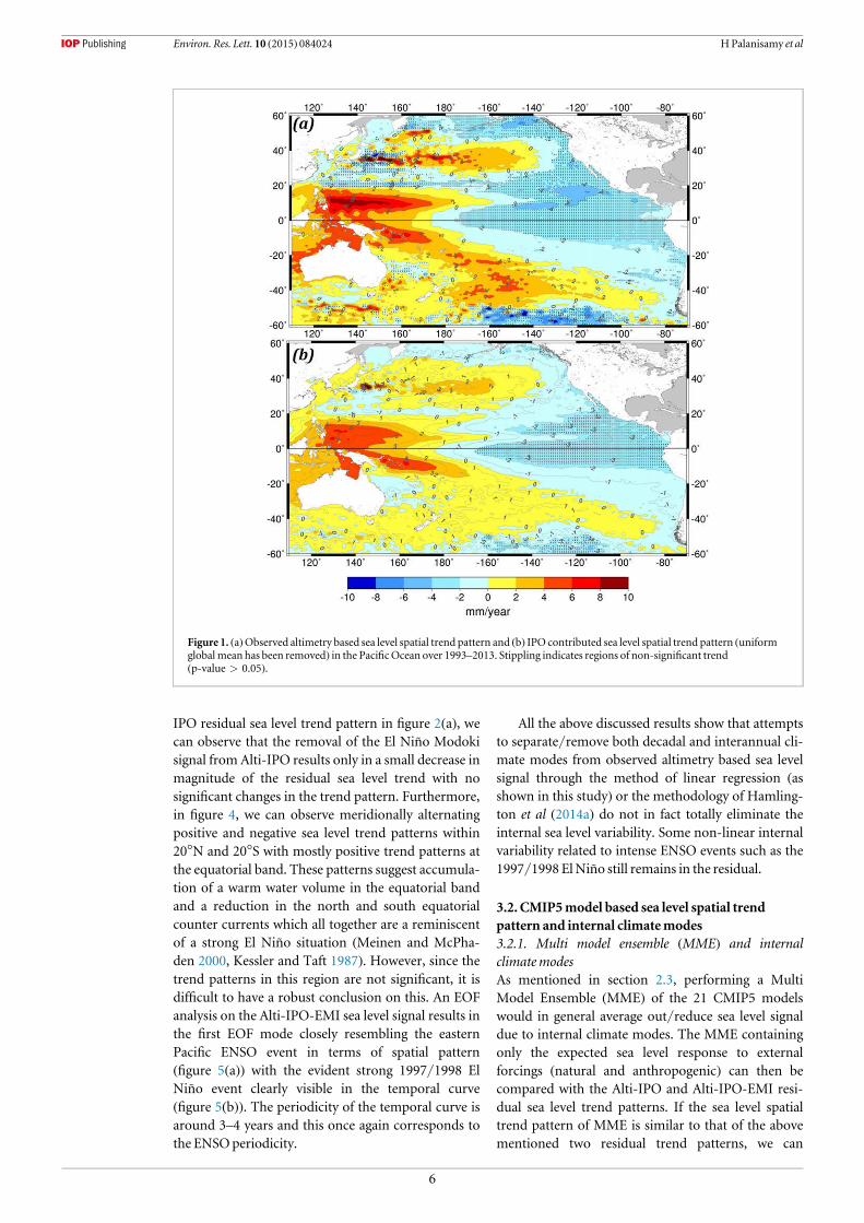
IPO residual sea level trend pattern in figure 2(a), we
can observe that the removal of the El Niño Modoki
signal from Alti-IPO results only in a small decrease in
magnitude of the residual sea level trend with no
significant changes in the trend pattern. Furthermore,
in figure 4, we can observe meridionally alternating
positive and negative sea level trend patterns within
20°N and 20°S with mostly positive trend patterns at
the equatorial band. These patterns suggest accumula-
tion of a warm water volume in the equatorial band
and a reduction in the north and south equatorial
counter currents which all together are a reminiscent
of a strong El Niño situation (Meinen and McPha-
den 2000, Kessler and Taft 1987). However, since the
trend patterns in this region are not significant, it is
difficult to have a robust conclusion on this. An EOF
analysis on the Alti-IPO-EMI sea level signal results in
the first EOF mode closely resembling the eastern
Pacific ENSO event in terms of spatial pattern
(figure 5(a)) with the evident strong 1997/1998 El
Niño event clearly visible in the temporal curve
(figure 5(b)). The periodicity of the temporal curve is
around 3–4 years and this once again corresponds to
the ENSOperiodicity.
All the above discussed results show that attempts
to separate/remove both decadal and interannual cli-
mate modes from observed altimetry based sea level
signal through the method of linear regression (as
shown in this study) or the methodology of Hamling-
ton et al (2014a) do not in fact totally eliminate the
internal sea level variability. Some non-linear internal
variability related to intense ENSO events such as the
1997/1998 ElNiño still remains in the residual.
3.2. CMIP5model based sea level spatial trend
pattern and internal climatemodes
3.2.1. Multi model ensemble (MME) and internal
climatemodes
As mentioned in section 2.3, performing a Multi
Model Ensemble (MME) of the 21 CMIP5 models
would in general average out/reduce sea level signal
due to internal climate modes. The MME containing
only the expected sea level response to external
forcings (natural and anthropogenic) can then be
compared with the Alti-IPO and Alti-IPO-EMI resi-
dual sea level trend patterns. If the sea level spatial
trend pattern of MME is similar to that of the above
mentioned two residual trend patterns, we can
Figure 1. (a)Observed altimetry based sea level spatial trend pattern and (b) IPO contributed sea level spatial trend pattern (uniformglobalmean has been removed) in the PacificOcean over 1993–2013. Stippling indicates regions of non-significant trend(p-value>0.05).
6
Environ. Res. Lett. 10 (2015) 084024 HPalanisamy et al
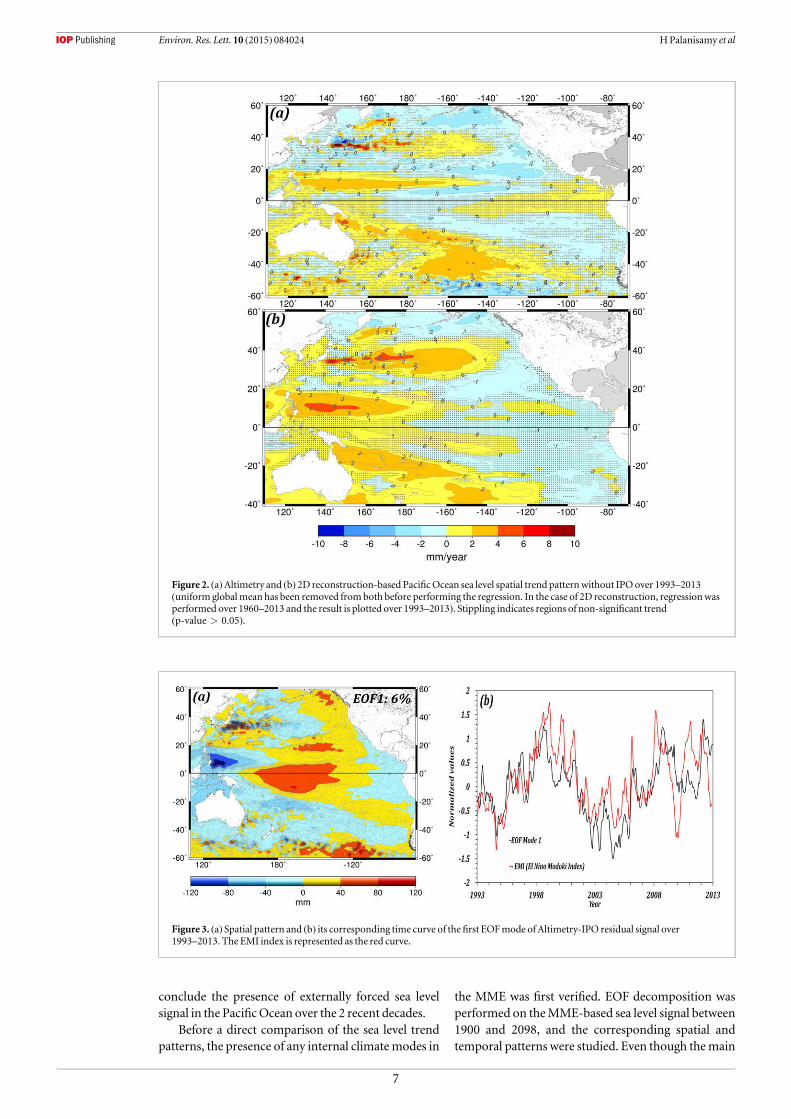
conclude the presence of externally forced sea level
signal in the PacificOcean over the 2 recent decades.
Before a direct comparison of the sea level trend
patterns, the presence of any internal climatemodes in
the MME was first verified. EOF decomposition was
performed on theMME-based sea level signal between
1900 and 2098, and the corresponding spatial and
temporal patterns were studied. Even though themain
Figure 2. (a)Altimetry and (b) 2D reconstruction-based PacificOcean sea level spatial trend patternwithout IPOover 1993–2013(uniform globalmean has been removed fromboth before performing the regression. In the case of 2D reconstruction, regressionwasperformed over 1960–2013 and the result is plotted over 1993–2013). Stippling indicates regions of non-significant trend(p-value>0.05).
Figure 3. (a) Spatial pattern and (b) its corresponding time curve of thefirst EOFmode of Altimetry-IPO residual signal over1993–2013. The EMI index is represented as the red curve.
7
Environ. Res. Lett. 10 (2015) 084024 HPalanisamy et al
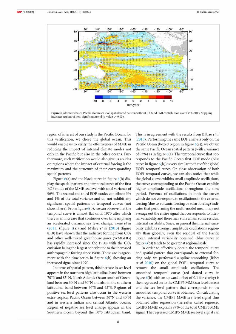
region of interest of our study is the Pacific Ocean, for
this verification, we chose the global ocean. This
would enable us to verify the effectiveness of MME in
reducing the impact of internal climate modes not
only in the Pacific but also in the other oceans. Fur-
thermore, such verification would also give us an idea
on regions where the impact of external forcing is the
maximum and the structure of their corresponding
spatial patterns.
Figure 6(a) and the black curve in figure 6(b) dis-
play the spatial pattern and temporal curve of the first
EOF mode of the MME sea level with total variance of
96%. The second and third EOFmodes contribute 3%
and 1% of the total variance and do not exhibit any
significant spatial patterns or temporal curves (not
shown here). From figure 6(b), we can observe that the
temporal curve is almost flat until 1970 after which
there is an increase that continues over time implying
an accelerated dynamic sea level change. Skeie et al
(2011) (figure 1(a)) and Myhre et al (2013) (figure
8.18) have shown that the radiative forcing from CO2
and other well-mixed greenhouse gases (WMGHG)
has rapidly increased since the 1950s with the CO2
emission being the largest contributor to the increased
anthropogenic forcing since 1960s. These are in agree-
ment with the time series in figure 6(b) showing an
increased signal since 1970.
In terms of spatial pattern, this increase in sea level
appears in the northern high latitudinal band between
70°Nand 85°N,North Atlantic Ocean south of Green-
land between 30°N and 60°N and also in the southern
latitudinal band between 40°S and 45°S. Regions of
positive sea level patterns also occur in the western
extra-tropical Pacific Ocean between 30°N and 40°N
and in western Indian and central Atlantic oceans.
Region of negative sea level change appears in the
Southern Ocean beyond the 50°S latitudinal band.
This is in agreement with the results from Bilbao et al
(2015). Performing the same EOF analysis only on the
Pacific Ocean (boxed region in figure 6(a)), we obtain
the same Pacific Ocean spatial pattern (with a variance
of 93%) as in figure 6(a). The temporal curve that cor-
responds to the Pacific Ocean first EOF mode (blue
curve in figure 6(b)) is very similar to that of the global
EOF1 temporal curve. On close observation of both
EOF1 temporal curves, we can also notice that while
the global curve exhibits small amplitude oscillations,
the curve corresponding to the Pacific Ocean exhibits
higher amplitude oscillations throughout the time
period. Presence of oscillations in both the curves
which do not correspond to oscillations in the external
forcing (due to volcanic forcing or solar forcing) indi-
cates that performing the multi-model mean may not
average out the entire signal that corresponds to inter-
nal variability and theremay still remain some residual
internal variability. Since, in general the internal varia-
bility exhibits stronger amplitude oscillations region-
ally than globally, even the residual of the Pacific
Ocean internal variability obtained (blue curve in
figure 6(b)) tends to be greater at regional scale.
In order to effectively obtain the temporal curve
and spatial pattern that corresponds to external for-
cing only, we performed a spline smoothing (Ribes
et al 2010) on the global EOF1 temporal curve to
remove the small amplitude oscillations. The
smoothed temporal curve (red dotted curve in
figure 6(b) with an upward offset of 0.1 for clarity) is
then regressed on to the CMIP5MME sea level dataset
and the sea level pattern that corresponds to the
smoothed temporal curve is obtained. On calculating
the variance, the CMIP5 MME sea level signal thus
obtained after regression (hereafter called regressed
CMIP5MME) explains 97% of the total CMIP5MME
signal. The regressed CMIP5MME sea level signal can
Figure 4.Altimetry based PacificOcean sea level spatial trend patternwithout IPO and EMI contribution over 1993–2013. Stipplingindicates regions of non-significant trend (p-value>0.05).
8
Environ. Res. Lett. 10 (2015) 084024 HPalanisamy et al
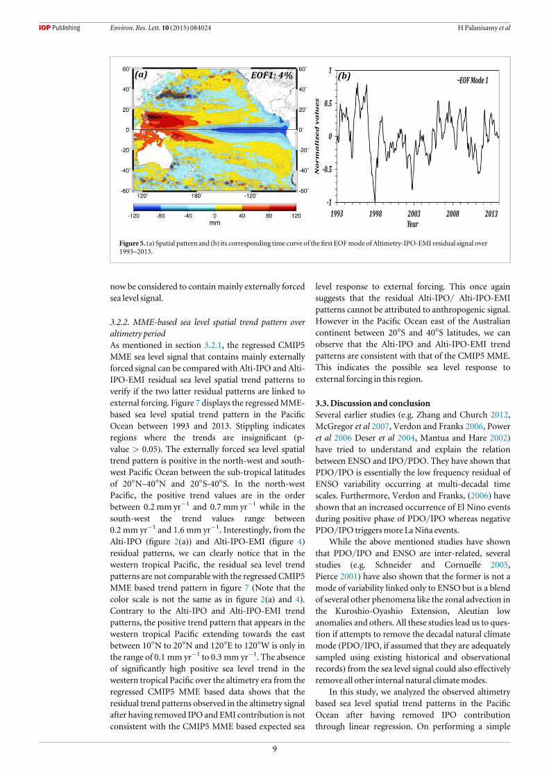
now be considered to contain mainly externally forced
sea level signal.
3.2.2. MME-based sea level spatial trend pattern over
altimetry period
As mentioned in section 3.2.1, the regressed CMIP5
MME sea level signal that contains mainly externally
forced signal can be compared with Alti-IPO and Alti-
IPO-EMI residual sea level spatial trend patterns to
verify if the two latter residual patterns are linked to
external forcing. Figure 7 displays the regressedMME-
based sea level spatial trend pattern in the Pacific
Ocean between 1993 and 2013. Stippling indicates
regions where the trends are insignificant (p-
value>0.05). The externally forced sea level spatial
trend pattern is positive in the north-west and south-
west Pacific Ocean between the sub-tropical latitudes
of 20°N–40°N and 20°S-40°S. In the north-west
Pacific, the positive trend values are in the order
between 0.2 mm yr−1 and 0.7 mm yr−1 while in the
south-west the trend values range between
0.2 mm yr−1 and 1.6 mm yr−1. Interestingly, from the
Alti-IPO (figure 2(a)) and Alti-IPO-EMI (figure 4)
residual patterns, we can clearly notice that in the
western tropical Pacific, the residual sea level trend
patterns are not comparable with the regressed CMIP5
MME based trend pattern in figure 7 (Note that the
color scale is not the same as in figure 2(a) and 4).
Contrary to the Alti-IPO and Alti-IPO-EMI trend
patterns, the positive trend pattern that appears in the
western tropical Pacific extending towards the east
between 10°N to 20°N and 120°E to 120°W is only in
the range of 0.1 mm yr−1 to 0.3 mm yr−1. The absence
of significantly high positive sea level trend in the
western tropical Pacific over the altimetry era from the
regressed CMIP5 MME based data shows that the
residual trend patterns observed in the altimetry signal
after having removed IPO and EMI contribution is not
consistent with the CMIP5 MME based expected sea
level response to external forcing. This once again
suggests that the residual Alti-IPO/ Alti-IPO-EMI
patterns cannot be attributed to anthropogenic signal.
However in the Pacific Ocean east of the Australian
continent between 20°S and 40°S latitudes, we can
observe that the Alti-IPO and Alti-IPO-EMI trend
patterns are consistent with that of the CMIP5 MME.
This indicates the possible sea level response to
external forcing in this region.
3.3.Discussion and conclusion
Several earlier studies (e.g. Zhang and Church 2012,
McGregor et al 2007, Verdon and Franks 2006, Power
et al 2006 Deser et al 2004, Mantua and Hare 2002)
have tried to understand and explain the relation
between ENSO and IPO/PDO. They have shown that
PDO/IPO is essentially the low frequency residual of
ENSO variability occurring at multi-decadal time
scales. Furthermore, Verdon and Franks, (2006) have
shown that an increased occurrence of El Nino events
during positive phase of PDO/IPO whereas negative
PDO/IPO triggersmore LaNiña events.
While the above mentioned studies have shown
that PDO/IPO and ENSO are inter-related, several
studies (e.g. Schneider and Cornuelle 2005,
Pierce 2001) have also shown that the former is not a
mode of variability linked only to ENSO but is a blend
of several other phenomena like the zonal advection in
the Kuroshio-Oyashio Extension, Aleutian low
anomalies and others. All these studies lead us to ques-
tion if attempts to remove the decadal natural climate
mode (PDO/IPO, if assumed that they are adequately
sampled using existing historical and observational
records) from the sea level signal could also effectively
remove all other internal natural climatemodes.
In this study, we analyzed the observed altimetry
based sea level spatial trend patterns in the Pacific
Ocean after having removed IPO contribution
through linear regression. On performing a simple
Figure 5. (a) Spatial pattern and (b) its corresponding time curve of thefirst EOFmode of Altimetry-IPO-EMI residual signal over1993–2013.
9
Environ. Res. Lett. 10 (2015) 084024 HPalanisamy et al

EOF analysis on the residual (Alti-IPO) sea level signal,
we found the presence of ENSO-related El NinoMod-
oki (Central Pacific) signal in the residual. Further
efforts to remove the El NiñoModoki signal fromAlti-
IPO signal through linear regression still resulted in
the presence of Eastern Pacific ENSO signal in the resi-
dual. This indicates that linearly regressing IPO on
observed sea level and removing its contribution does
not totally remove the entire internal sea level varia-
bility. Nonlinear ENSO-related variability that does
not linearly co-vary with IPO still remains in the resi-
dual sea level signal. Our results show that the metho-
dology of removing the main decadal natural climate
mode from sea level signal and analyzing the residual is
not an effective way to explain the contribution of
external anthropogenic sea level fingerprint.
The range of altimetry-based regional sea level
trend uncertainties/error estimate should also be con-
sidered in these studies as the residual sea level trend
pattern after removing IPO and ENSO contributions
should be compared to the pattern of uncertainty. A
detailed comparison is beyond the scope of this study
as further investigations are needed to obtain accurate
altimetry-based trend error patterns at regional scale.
However we expect that the patterns of regional alti-
metry error do not coincide to those in figure 2(a)
(Alti-IPO) and figure 4 (Alti-IPO-EMI) as the errors
are mainly large spatial patterns at hemispherical scale
in the order of 2 mm yr-1 to 3 mm yr−1 with orbital
errors contributing the most (Ablain et al 2015, Cou-
hert et al 2015).
Furthermore, regressed CMIP5 MME-based sea
level spatial trend pattern in the tropical Pacific over
the altimetry period do not display any positive sea
level trend values that are comparable to the altimetry
based sea level signal after having removed the con-
tribution of the decadal natural climate mode. This
suggests that the residual positive trend pattern
observed in the western tropical Pacific is not exter-
nally forced and thereby not anthropogenic in origin.
In addition the amplitude of the sea level spatial trend
pattern from regressed CMIP5 MME is low over the
altimetry period in the tropical Pacific. This amplitude
is significantly lower than the expected error in trend
patterns from satellite altimetry (in the order of 2 mm
yr-1 to 3 mm yr−1, Ablain et al 2015, Couhert
et al 2015) and suggest that satellite altimetrymeasure-
ment is still not accurate enough to detect the anthro-
pogenic signal in the 20 year tropical Pacific sea level
trends.
Our results are also in agreement with studies of
Richter and Marzeion (2014), Lyu et al (2014), Jordà
(2014), Frankcombe et al (2014), Bilbao et al (2015)
who have shown that in regions of high internal varia-
bility, the trend due to externally forced signal is
masked during longer time spans than in regions of
low internal variability. This is the case of tropical
Pacific which is a region highly impacted by internal
variability. Studying the residual sea level signal after
separating/removing the internal climate modes over
a short time period of 20 years in this region may not
yield significant results with respect to external for-
cing. This is also in agreement with Meyssignac
et al (2012b) who have shown that over the 17 years
altimetry period, the tropical Pacific observed sea level
spatial trend pattern is mainly due to internal
variability.
Our study suggests that detection/attribution stu-
dies should be focused on other regions such asNorth-
ern and Southern Oceans, North Atlantic, Southern
Pacific to the east of Australia. Based on CMIP5MME
(see figures 6 and 7), these are the regions that show
significant externally forced sea level signals. Detailed
studies on these regions could help us understand the
role of externally forced signal on sea level.
Lastly, another important factor to consider would
be the impact of external anthropogenic forcing on the
natural internal climatemodes. In the previous studies
(Hamlington et al 2014b, Palanisamy et al 2015) and
this current study, it has been assumed that the natural
Figure 6. (a) Spatial pattern of thefirst EOFmode of CMIP5MME sea level over 1900–2098; (b) its corresponding temporal curve(black curve). The red dotted curve corresponds to the spline-smoothed EOF1 temporal curve (with an upward offset of 0.1 for clarity)and the blue curve corresponds to the PacificOcean EOF1 temporal curve estimated over the boxed region in (a).
10
Environ. Res. Lett. 10 (2015) 084024 HPalanisamy et al
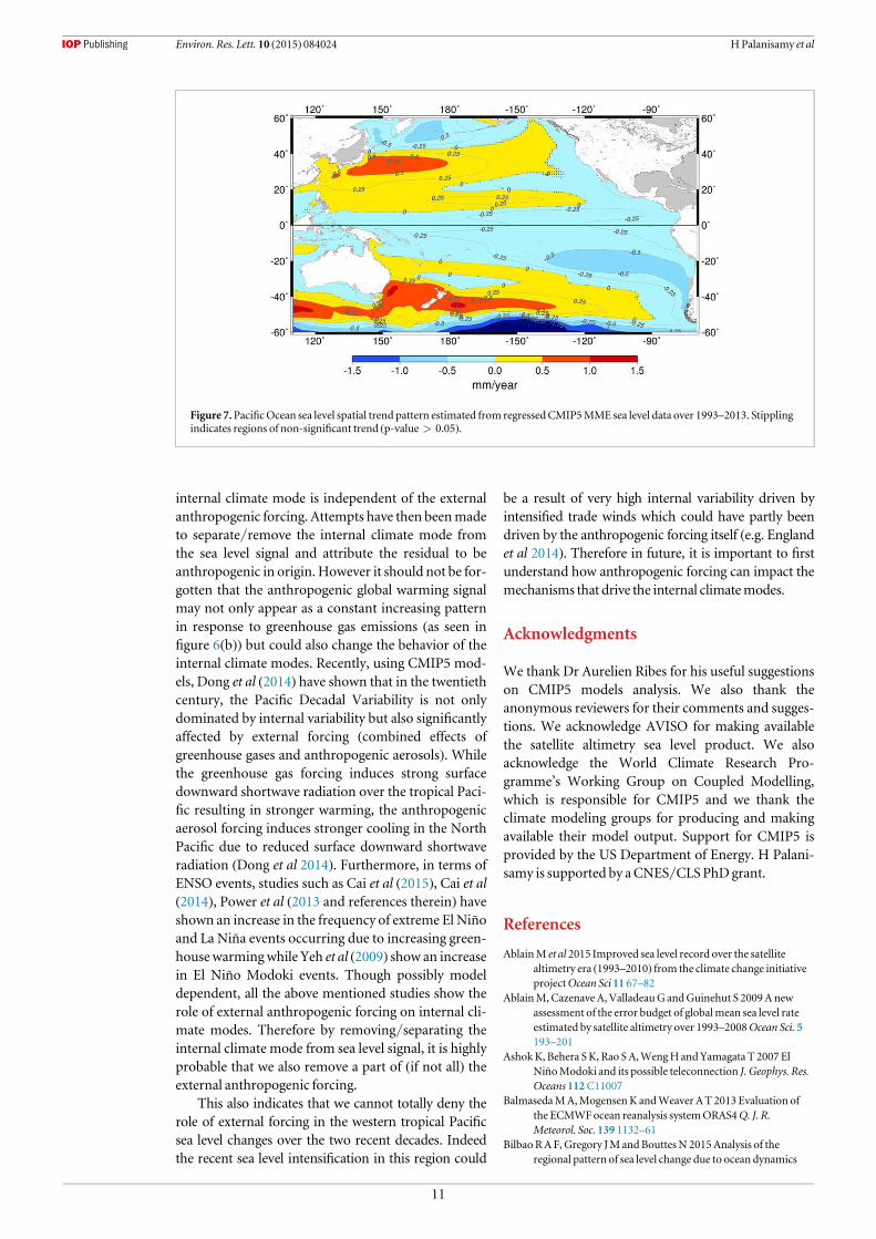
internal climate mode is independent of the external
anthropogenic forcing. Attempts have then beenmade
to separate/remove the internal climate mode from
the sea level signal and attribute the residual to be
anthropogenic in origin. However it should not be for-
gotten that the anthropogenic global warming signal
may not only appear as a constant increasing pattern
in response to greenhouse gas emissions (as seen in
figure 6(b)) but could also change the behavior of the
internal climate modes. Recently, using CMIP5 mod-
els, Dong et al (2014) have shown that in the twentieth
century, the Pacific Decadal Variability is not only
dominated by internal variability but also significantly
affected by external forcing (combined effects of
greenhouse gases and anthropogenic aerosols). While
the greenhouse gas forcing induces strong surface
downward shortwave radiation over the tropical Paci-
fic resulting in stronger warming, the anthropogenic
aerosol forcing induces stronger cooling in the North
Pacific due to reduced surface downward shortwave
radiation (Dong et al 2014). Furthermore, in terms of
ENSO events, studies such as Cai et al (2015), Cai et al
(2014), Power et al (2013 and references therein) have
shown an increase in the frequency of extreme El Niño
and La Niña events occurring due to increasing green-
housewarmingwhile Yeh et al (2009) show an increase
in El Niño Modoki events. Though possibly model
dependent, all the above mentioned studies show the
role of external anthropogenic forcing on internal cli-
mate modes. Therefore by removing/separating the
internal climate mode from sea level signal, it is highly
probable that we also remove a part of (if not all) the
external anthropogenic forcing.
This also indicates that we cannot totally deny the
role of external forcing in the western tropical Pacific
sea level changes over the two recent decades. Indeed
the recent sea level intensification in this region could
be a result of very high internal variability driven by
intensified trade winds which could have partly been
driven by the anthropogenic forcing itself (e.g. England
et al 2014). Therefore in future, it is important to first
understand how anthropogenic forcing can impact the
mechanisms that drive the internal climatemodes.
Acknowledgments
We thank Dr Aurelien Ribes for his useful suggestions
on CMIP5 models analysis. We also thank the
anonymous reviewers for their comments and sugges-
tions. We acknowledge AVISO for making available
the satellite altimetry sea level product. We also
acknowledge the World Climate Research Pro-
gramme’s Working Group on Coupled Modelling,
which is responsible for CMIP5 and we thank the
climate modeling groups for producing and making
available their model output. Support for CMIP5 is
provided by the US Department of Energy. H Palani-
samy is supported by aCNES/CLSPhD grant.
References
AblainM et al 2015 Improved sea level record over the satellite
altimetry era (1993–2010) from the climate change initiative
projectOcean Sci 11 67–82
AblainM,Cazenave A, ValladeauG andGuinehut S 2009Anew
assessment of the error budget of globalmean sea level rate
estimated by satellite altimetry over 1993–2008Ocean Sci. 5
193–201
AshokK, Behera SK, Rao SA,WengHandYamagata T 2007 El
NiñoModoki and its possible teleconnection J. Geophys. Res.
Oceans 112C11007
BalmasedaMA,MogensenK andWeaver AT 2013 Evaluation of
the ECMWFocean reanalysis systemORAS4Q. J. R.
Meteorol. Soc. 139 1132–61
Bilbao RAF,Gregory JM andBouttesN 2015Analysis of the
regional pattern of sea level change due to ocean dynamics
Figure 7.PacificOcean sea level spatial trend pattern estimated from regressedCMIP5MME sea level data over 1993–2013. Stipplingindicates regions of non-significant trend (p-value>0.05).
11
Environ. Res. Lett. 10 (2015) 084024 HPalanisamy et al
and density change for 1993–2099 in observations and
CMIP5AOGCMsClim.Dyn. 1–20
BordbarMH,Martin T, LatifM and ParkW2015 Effects of long-
term variability on projections of twenty-first century
dynamic sea levelNat. Clim. Change 5 343–7
BoscC andDelcroix T 2008Observed equatorial Rossbywaves and
ENSO-relatedwarmwater volume changes in the equatorial
PacificOcean J. Geophys. Res. Oceans 113C06003
Bromirski PD,Miller A J, Flick R E andAuadG 2011Dynamical
suppression of sea level rise along the Pacific coast ofNorth
America: indications for imminent acceleration J. Geophys.
Res. Oceans 116C07005
CaiW et al 2014 Increasing frequency of extreme ElNino events due
to greenhouse warmingNat. Clim. Change 4 111–6
CaiW et al 2015 Increased frequency of extreme LaNina events
under greenhouse warmingNat. Clim. Change 5 132–7
Carton J A andGiese B S 2008A reanalysis of ocean climate using
simple ocean data assimilation (SODA)Mon.Weather Rev.
136 2999–3017
Cazenave A andCozannet GL 2014 Sea level rise and its coastal
impacts Earths Future 2 15–34
Church J A et al 2013 Sea level changeClimate Change 2013: The
Physical Science Basis. Contribution ofWorkingGroup I to the
Fifth Assessment Report of the Intergovernmental Panel on
Climate Change ed T F Stocker, DQin, G-KPlattner,
MTignor, SKAllen, J Boschung, ANauels, YXia, VBex and
PMMidgley (Cambridge, UnitedKingdom:: Cambridge
University Press)
Couhert A, Cerri L, Legeais J-F, AblainM,ZelenskyNP,Haines B J,
Lemoine FG, BertigerW I,Desai SD andOttenM2015
Towards the 1 mm/y stability of the radial orbit error at
regional scalesAdv. Space Res. 55 2–23
Deser C, Phillips A S andHurrell JW2004 Pacific interdecadal
climate variability: linkages between the tropics and the north
pacific during boreal winter since 1900 J. Clim., 17 3109–24
Dong L, ZhouT andChenX 2014Changes of Pacific decadal
variability in the twentieth century driven by internal
variability, greenhouse gases, and aerosolsGeophys. Res. Lett.
41 8570–7
EnglandMH,McGregor S, Spence P,Meehl GA, TimmermannA,
CaiW,Gupta A S,McPhadenM J, PurichA and SantosoA
2014Recent intensification ofwind-driven circulation in the
Pacific and the ongoingwarming hiatusNat. Clim. Change 4
222–7
FollandCK, ParkerDE, ColmanA andWashingtonR 1999 Large
scalemodes of ocean surface temperature since the late
nineteenth century Refereed book: ch 4, pp 73–102of Beyond
ElNino: Decadal and Interdecadal Climate Variability ed
ANavarra (Berlin: Springer)
Frankcombe LM,McGregor S and EnglandMH2014Robustness
of themodes of Indo-Pacific sea level variabilityClim.Dyn.
1–18 doi:10.1007/s00382-014-2377-0
Fukumori I andWangO2013Origins of heat and freshwater
anomalies underlying regional decadal sea level trends
Geophys. Res. Lett. 40 563–7
Gregory JM et al 2001Comparison of results from several AOGCMs
for global and regional sea-level change 1900–2100Clim.
Dyn. 18 225–40
Hamlington BD, StrassburgMW, LebenRR,HanW,
NeremRS andKimK-Y 2014aUncovering an anthropogenic
sea-level rise signal in the PacificOceanNat. Clim. Change 4
782–5
Hamlington BD, LebenRR, StrassburgMWandKimK-Y 2014b
Cyclostationary empirical orthogonal function sea-level
reconstructionGeosci. Data J. 1 13–9
HanW et al 2013 Intensification of decadal andmulti-decadal
sea level variability in thewestern tropical Pacific during
recent decadesClim.Dyn.1–23 doi:10.1007/s00382-013-
1951-1
Hare SR andMantuaN J 2000 Empirical evidence forNorth Pacific
regime shifts in 1977 and 1989Prog. Oceanogr. 47 103–45
IPCC2013Climate Change 2013: The Physical Science Basis.
Contribution ofWorkingGroup I to the Fifth Assessment Report
of the Intergovernmental Panel on Climate Change ed
T F Stocker, DQin, G-KPlattner,MTignor, S KAllen,
J Boschung, ANauels, YXia, VBex and PMMidgley
(Cambridge, UnitedKingdom: CambridgeUniversity Press)
1535 doi:10.1017/CBO9781107415324
JordàG2014Detection time for global and regional sea level trends
and accelerations J. Geophys. Res. Oceans 119 7164–74
KesslerWS andTaft BA 1987Dynamic heights and zonal
geostrophic transports in the central tropical Pacific during
1979-84 J. Phys. Oceanogr. 17 97–122
Köhl A 2015 Evaluation of theGECCO2ocean synthesis: transports
of volume, heat and freshwater in theAtlanticQ. J. R.
Meteorol. Soc. 141 166–81
Landerer FW,Gleckler P J and Lee T 2014 Evaluation of CMIP5
dynamic sea surface heightmulti-model simulations against
satellite observations , Clim.Dyn. 43 1271–83
Levitus S et al 2012World ocean heat content and thermosteric sea
level change (0–2000m), 1955–2010Geophys. Res. Lett. 39
L10603
LyuK, ZhangX, Church J A, SlangenABA andHu J 2014Time of
emergence for regional sea-level changeNat. Clim. Change 4
1006–10
MantuaN J andHare SR 2002The pacific decadal oscillation
J. Oceanogr. 58 35–44
MantuaN J,Hare S R, Zhang Y,Wallace JM and Francis RC 1997A
Pacific interdecadal climate oscillationwith impacts on
salmon productionBull. Am.Meteorol. Soc. 78 1069–79
MarcosMandAmores A 2014Quantifying anthropogenic and
natural contributions to thermosteric sea level riseGeophys.
Res. Lett. 41 2014GL059766
McGregor S,HolbrookN J and Power S B 2007 Interdecadal sea
surface temperature variability in the equatorial pacific
ocean: I. the role of off-equatorial wind stresses and oceanic
rossbywaves J. Clim. 20 2643–58
MeinenC S andMcPhadenM J 2000Observations of warmwater
volume changes in the equatorial pacific and their
relationship to ElNiño and LaNiña J. Clim. 13 3551–9
MerrifieldMA2011A shift inwestern tropical Pacific Sea level
trends during the 1990s J. Clim. 24 4126–38
MerrifieldMA andMaltrudME2011Regional sea level trends due
to a Pacific tradewind intensificationGeophys. Res. Lett. 38
L21605
Meyssignac B,HenryO, PalanisamyHandCazenave A 2015
Advances in understanding regional sea level variations from
2D sea level reconstructions based on tide gauge records, in
preparation
Meyssignac B, BeckerM, LlovelWandCazenave A 2012aAn
assessment of two-dimensional past sea level reconstructions
over 1950–2009 based on tide-gauge data and different input
sea level grids Surv. Geophys. 33 945–72
Meyssignac B, Salas yMelia D, BeckerM, LlovelWandCazenave A
2012bTropical Pacific spatial trend patterns in observed sea
level: internal variability and/or anthropogenic signature?
Clim. Past 8 787–802
MilneGA,GehrelsWR,Hughes CWandTamisieaME2009
Identifying the causes of sea-level changeNat. Geosci. 2 471–8
MyhreG et al 2013Anthropogenic andnatural radiative forcing
Climate Change 2013: The Physical Science Basis. Contribution
ofWorkingGroup I to the Fifth Assessment Report of the
Intergovernmental Panel on Climate Change edT F Stocker,
DQin, G-KPlattner,MTignor, SKAllen, J Boschung,
ANauels, YXia, VBex and PMMidgley (Cambridge, United
Kingdom: CambridgeUniversity Press)
PalanisamyH,Cazenave A,Delcroix T andMeyssignac B 2015
Spatial trend patterns in the PacificOcean sea level during the
altimetry era: the contribution of thermocline depth change
and internal climate variabilityOceanDyn. 65 341–56
PierceDW2001Distinguishing coupled ocean-atmosphere
interactions frombackground noise in theNorth PacificProg.
Oceanogr. 49 331–52
Power S, Delage F, ChungC,KociubaG andKeayK 2013Robust
twenty-first-century projections of El Nino and related
precipitation variabilityNature 502 541–5
12
Environ. Res. Lett. 10 (2015) 084024 HPalanisamy et al
Power S,HaylockM,ColmanR andWangX 2006The predictability
of interdecadal changes in ENSO activity andENSO
teleconnections J. Clim. 19 4755–71
Ribes A, Azaïs J-M and Planton S 2010Amethod for regional
climate change detection using smooth temporal patterns
Clim.Dyn. 35 391–406
Richter K andMarzeion B 2014 Earliest local emergence of forced
dynamic and steric sea-level trends in climatemodels
Environ. Res. Lett. 9 114009
SchneiderN andCornuelle BD2005The forcing of the pacific
decadal oscillation* J. Clim. 18 4355–73
SenGupta LC,Muir JN, Brown S J, Phipps P J, DurackD,
Monselesan andWijffels S E 2012Climate drift in theCMIP3
models J. Clim. 25 4621–40
SinghA,Delcroix T andCravatte S 2011Contrasting theflavors of El
NINO-SOUTHERNOSCILLATIONUSINg sea surface
salinity observations J. Geophys. Res. 116 1–16
Skeie RB, BerntsenTK,MyhreG, TanakaK,KvalevågMMand
Hoyle CR 2011Anthropogenic radiative forcing time series
frompre-industrial times until 2010AtmosChemPhys. 11
11827–57
SlangenABA, Church JA, ZhangX andMonselesanD2014
Detection and attribution of globalmean thermosteric sea
level changeGeophys. Res. Lett. 41 5951–9
StammerD,Cazenave A, Ponte RMandTamisieaME2013Causes
for contemporary regional sea level changesAnnu. Rev.Mar.
Sci. 5 21–46
Taylor K E, Stouffer R J andMeehl GA 2012Anoverview of CMIP5
and the experiment designBull. Am.Meteorol. Soc. 93 485–98
ThompsonPR,MerrifieldMA,Wells J R andChangCM2014
Wind-driven coastal sea level variability in the northeast
pacific J. Clim. 27 4733–51
VerdonDC and Franks SW2006 Long-term behaviour of ENSO:
Interactionswith the PDOover the past 400 years inferred
frompaleoclimate recordsGeophys. Res. Lett. 33 L06712
WatsonC S,WhiteN J, Church J A, KingMA, Burgette R J and
Legresy B 2015Unabated globalmean sea-level rise over the
satellite altimeter eraNat. Clim. Change 5 565–8
Wittenberg AT 2009Are historical records sufficient to constrain
ENSO simulations?Geophys. Res. Lett. 36 L12702
Yasunaka S andHanawaK 2003Regime shifts in the northern
hemisphere SSTfield: revisited in relation to tropical
variations J.Meteorol. Soc. Jpn. Ser II 81 415–24
Yeh S-W,Kug J-S, Dewitte B, KwonM-H,KirtmanBP and Jin F-F
2009 ElNiño in a changing climateNature 461 511–4
Yin J 2012Century tomulti-century sea level rise projections from
CMIP5modelsGeophys. Res. Lett. 39 17709
Yin J, Griffies SMand Stouffer R J 2010 Spatial variability of sea
level rise in twenty-first century projections J. Clim. 23
4585–607
ZhangX andChurch J A 2012 Sea level trends, interannual and
decadal variability in the PacificOceanGeophys. Res. Lett. 39
Zhang Y,Wallace JM andBattisti D S 1997 ENSO-like interdecadal
variability: 1900–93 J. Clim. 10 1004–20
13
Environ. Res. Lett. 10 (2015) 084024 HPalanisamy et al

Chapter 4 Role of internal climate variability and external forcing
200
4.5 Role of external anthropogenic forcing on internal climate
modes – A synthesis
From our results we have shown that it is not yet possible to detect anthropogenic sea
level fingerprint in the tropical Pacific, a region known for high internal variability. This is also
in agreement with Meyssignac et al., (2012b) who have shown that over 17 years of altimetry
period, the tropical Pacific observed sea level spatial trend pattern is mainly due to internal
variability. Furthermore, studies of Richter and Marzeion, (2014), Lyu et al., (2014), Jordà,
(2014), Frankcombe et al., (2014), Bilbao et al., (2015) have also shown that in regions of high
internal variability, the trend due to externally forced signal is masked during longer time spans
than in regions of low internal variability.
Another most important factor that needs to be considered in D&A studies is the role of
external anthropogenic forcing on internal climate modes. So far, most of the D&A studies have
assumed that the natural internal climate mode is independent of the external anthropogenic
forcing. Attempts have then been made to separate/remove the internal climate mode from the
sea level signal and attribute the residual to be anthropogenic in origin. However it should not be
forgotten that the anthropogenic global warming signal may not only appear as a constant
increasing pattern in response to greenhouse gas emissions but could also change the behavior of
the internal climate modes (Palanisamy et al., 2015c). Considering this into account, some recent
studies have shown that the external anthropogenic forcing in fact has an impact on driving/
changing the behavior of different internal climate modes. Using CMIP5 models, Dong et al.,
(2014) have shown that in the twentieth century, the Pacific decadal variability is not only
dominated by internal variability but also significantly affected by external. Furthermore, in
terms of ENSO events, studies such as Cai et al., (2014), Cai et al., (2015), Power et al., (2013
and references therein) have shown an increase in the frequency of extreme El Niño and La Niña
events occurring due to increasing greenhouse warming while Yeh et al., (2009) show an
increase in El Niño Modoki events. Though possibly model dependent, all the above mentioned
studies show the possible role of external anthropogenic forcing on internal climate modes
(Palanisamy et al., 2015c). This also indicates that the role of external forcing cannot be
completely denied in the case of western tropical Pacific sea level changes over the two recent
Chapter 4 Role of internal climate variability and external forcing
201
decades. Indeed the recent sea level intensification in this region could be a result of very high
internal variability driven by intensified trade winds which could have partly been driven by the
anthropogenic forcing itself (e.g. England et al., 2014).
4.6 Internal climate variability uncertainty in CMIP5 models
Since several years, it has been a common practice for climate change and sea level
community to use CMIP3/CMIP5 models not only for D&A studies but also for the projection of
future sea level changes. Therefore, characterizing and quantifying uncertainties in these climate
models is of fundamental importance for such studies. There are three main uncertainties in
climate models: (1) model uncertainty which arises because of an incomplete understanding of
the physical processes and the limitations of implementation of the understanding, (2) scenario
uncertainty arising because of incomplete information about future emissions and (3) internal
variability modelling uncertainty that arises because the complex processes intrinsic to the
atmosphere, ocean and the ocean-atmosphere coupling are highly aleatoric and cannot be easily
modelled (Yip et al., 2011, Deser et al., 2010, Hawkins and Sutton, 2009). While the influence of
these uncertainties are largely variable, internal variability uncertainty plays an important role in
D&A studies as the main objective of such studies are to separate the signal (i.e. anthropogenic
forcing) from the noise (i.e. internal variability).
Of late, there have been few studies that have focused on the role of internal variability
uncertainty in future sea level changes. By making use of a 40 member ensemble of the
Community Climate System Model version 3 (CCSM3), Hu and Deser, (2013) isolated
uncertainty in 2000-2060 regional sea level trends. They concluded that the uncertainty in the
projected trends were mainly due to unpredictable internal climate fluctuations that can vary by a
factor of two depending on the region, with coastal areas bordering the North Pacific and
Atlantic showing the greatest range. More recently, Bordbar et al., (2015) demonstrated that in
the case of centennial regional dynamic sea level projections, uncertainty in long term internal
variability plays as great a part as external forcing. Furthermore, the study also mentions that the
lack of long term observations poses a challenge in quantifying the long term internal variability
thereby adding on to the uncertainty. Subsequently, Carson et al., 2014 have also shown that
internal variability can be a substantial portion of the model spread for both short and long-term
Chapter 4 Role of internal climate variability and external forcing
202
regional sea level projections. Little et al., (2015), in a very detailed and exhaustive work
partitioned the different sources of uncertainty over two projection periods, 2040 and 2090 using
different RCP scenarios and various models of CMIP5 archive. They concluded that the three
sources of uncertainty play a role in future sea level projection. The internal variability
uncertainty was attributed to differences in the representation of internal variability among the
various CMIP5 models. They further stress the importance of characterization of internal
variability along two fronts: 1) developing alternate techniques to capture the representation of
internal variability in models and 2) model–data comparison aimed at determining whether
model-based methods capture observed modes of sea level variability, particularly those relevant
to long-term climate changes.
As a work in progress, we are currently studying the capability of CMIP5 models on
capturing ‘realistic’ decadal climate variability. As the study is not yet completed, we therefore
do not include it in this Ph.D. manuscript.
203
Conclusion and perspectives
There is no doubt that global warming will continue during the future decades owing to
continuous GHG emissions, the main contributor to anthropogenic global warming. An
important consequence of global warming and thereby climate change over the next few decades
is sea level rise and its impacts. Theoretical estimations of sea level projections in the future are
regularly being proposed by climate scientists based on different scenarios of global mean
temperature rise in response to increasing GHG concentration. All the scenarios correspond to an
increase in global mean sea level during the 21st century and beyond because of expected
continuing ocean warming and land ice loss. Using climate models, for the high emission
scenario (RCP8.5) that can also be considered as a representative extrapolation of the present day
emission, IPCC AR5 now predicts the likely range of global mean sea level rise between 52cm
and 98cm by the year 2100 with a median value of 74 cm. This would threaten the survival of
several coastal cities and entire low-lying island nations. Even with aggressive emissions
reductions, for the RCP2.6 scenario (peak in global annual GHG emissions between 2010-2020
followed by a substantial decline thereafter), a rise of 28-61 cm by 2100 is predicted indicating
that even under the highly optimistic scenario we might see over half a meter of sea-level rise. In
all scenarios, thermal expansion is predicted to be the largest contributor accounting for about 30
to 55% of the projections. Glaciers are the next largest, accounting for 15-35% of the projections.
By 2100, 35 to 85% of the present volume of glaciers outside Antarctica is projected to be
eliminated under RCP8.5 scenario (Church et al., 2013).
Despite these recent updates, uncertainties in sea level projections remain very large (±25
cm in the case of global mean sea level). They come from the difficulty of climate models to
precisely simulate the global mean sea level contributors (ocean thermal expansion, melting of
glaciers and polar ice sheets, and land water storage) in a realistic manner. While this is the case
for future sea level projections, uncertainty in different sea level contributors also play an
Conclusion and perspectives
204
important role in the present sea level changes especially in understanding thermal expansion
contribution from the deep ocean and/or the precise role of internal climate modes. During the
course of the thesis, attempts were made to close the global mean sea level budget and estimate
the deep ocean contribution by using sea level observations from satellite altimetry, GRACE
based ocean mass changes and Argo-based ocean thermal expansion since 2003. We showed that
uncertainties due to data processing approaches and systematic errors of different observing
systems still prevent us from obtaining accurate results. Absence of observations in certain
regions further adds on to the uncertainty thereby complicating accurate estimations. Our work
emphasized the importance of systematic inter-comparisons of observational products in order to
better understand the causes of the differences. This would further result in a better
understanding of various global mean sea level rise contributors that can be applied for future
projections.
In this thesis, we were particularly interested in regional sea level trends and variability
and have put in evidence the importance of regional sea level changes by a better estimate of its
signal since 1950 in different vulnerable regions. Our results showed that sea level variations are
not uniform globally and that they are highly dominated by regional variability at both
interannual and decadal time scales. Estimates of local long-term total relative sea level change
further demonstrated the importance of not only regional sea level variability but also the role of
vertical land motion, in particular land subsidence that exacerbates the sea level rise impact
leading us to question sea level risks in the future. The results obtained during the course of the
thesis indicate the importance of regional sea level change estimation for better coastal
management for the present and in future. The IPCC AR5 projections indicate stronger regional
sea level variability than at present by the end of 2100 largely dominated by increased heat
uptake and changes in wind forcing. The IPCC AR5 sea level projections towards the end of 21st
century from CMIP5 models reveal a clear regional pattern in dynamic sea level change with
largest sea level rise in the North Atlantic, Arctic and in the tropical oceans. In terms of regional
relative sea level change, CMIP5 model estimates resulting from GIA, glacier and land-ice
melting during 2081-2100 relative to 1986-2000 suggest that for the 21st century, past, present
and future loss of land-ice mass will very likely be an important contributor to spatial patterns in
relative sea level change, leading to rates of maximum rise at low-to-mid latitudes. It is very
likely that over about 75% of world oceans, regional relative sea level rise will be positive, while
Conclusion and perspectives
205
most regions that will experience sea level fall are located near current and former glaciers and
ice sheets (Church et al., 2013).
Regions showing enhanced relative sea level changes towards the end of 21st century
from CMIP5 estimates also coincide with those showing the largest uncertainty indicating strong
differences in between different climate models. Sea level contribution due to Earth’s visco-
elastic response strongly depends on the magnitude of the melting ice which highly differs from
one model to another. In addition, climate models poorly simulate land water storage due to
groundwater depletion in aquifers. Therefore, uncertainty hinders accurate projections of
regional relative sea level changes. Knowing the importance of regional relative sea level
changes emphasized in this thesis and in other studies, if we want a better estimation of sea level
rise impacts and risks in 2100, it is crucial to reduce uncertainty in assessing, understanding and
modelling of regional relative sea level rise and variability.
Another main focus of this thesis was to analyze respective roles of ocean dynamic
processes, internal climate modes and external anthropogenic forcing on regional sea level
spatial trend patterns in the tropical Pacific Ocean over the altimetry observational era. Building
up on the relationship between thermocline and sea level in the tropical region, we showed that
most of the observed sea level spatial trend pattern in the tropical Pacific can be explained by the
wind driven vertical thermocline movement. By performing detection and attribution study on
sea level spatial trend patterns in the tropical Pacific and attempting to eliminate signal
corresponding to the main internal climate mode, we further showed that the remaining residual
sea level trend pattern does not correspond to externally forced anthropogenic sea level signal
and that some non-linear internal climate modes still remain as residual. In addition, the
amplitude of the residual trend pattern is significantly lower than the expected error in trend
patterns from satellite altimetry (in the order of 2 mm/yr to 3 mm/yr) and therefore suggests that
satellite altimetry measurement is still not accurate enough to detect the anthropogenic signal in
the 20 year tropical Pacific sea level trends.
While the thesis has helped in answering sea level-related questions and in having a
better understanding of regional sea level variability, there are numerous subjects that still need
to be addressed in the near future. Few of the subjects that will be studied by the sea level team
of LEGOS are listed below:
Conclusion and perspectives
206
Cross validation of ESA CCI ECVs involved in the sea level budget.
In the context of ESA CCI, this work will involve inter-comparisons of various
observational products of altimetry sea level, ocean mass and steric sea level in order to better
understand existing differences in sea level closure budget studies and identify a best processing
methodology that can be implemented to minimize the differences. Furthermore, statistical
approaches will be developed to identify best combination from among different set of
components that will enable the closure of global mean sea level budget with accurate
estimations of each of its contributing components. Similar studies will also be performed at
regional scale.
Validation of CMIP5 climate models based on their ability to characterize decadal
internal climate variability.
This study will involve model–data comparison aimed at determining whether CMIP5
model-based methods capture observed modes of sea level variability, particularly those relevant
to long-term climate changes over the 20th
century. Various OGCMs and ocean reanalyses such
as DRAKKAR, SODA, GECCO, ORAS4 and two dimensional past sea level reconstructions
will be used in this study along with 21 CMIP5 based climate models. Regional patterns of
decadal sea level variability estimated from ocean models and reanalyses since 1950 will be
compared with those from CMIP5 based control run and historical simulations. The ultimate aim
of this work will be to select climate models that realistically reproduce observed long term sea
level variability which can later be used for regional sea level projections. This is currently an
ongoing work and preliminary results are already interesting.
Projections of 21st sea level rise using CMIP5 climate models under different warming
scenarios.
It is intended to develop sea level projections until 2100 at various coastal locations by
making use of the CMIP5 climate models under different warming scenarios validated in the
above mentioned previous study. While CMIP5 climate models mainly represent the steric sea
level component, collaborations with other scientific community will help in obtaining land ice
melt (glaciers and ice sheets) contribution which will then be included along with the steric
contribution from CMIP5 models. Furthermore, sea level variations due to post glacial rebound
(GIA) and other solid Earth response to ice/water mass redistribution caused by future land ice
Conclusion and perspectives
207
melt will also be considered. Sea level changes thus computed from CMIP5 models over 1950 to
present will be compared with observations such as tide gauges and GPS for relative sea level
variations and vertical land motions, satellite altimetry for absolute sea level variations. This will
allow us to calibrate the CMIP5 models to obtain future sea level projections at various
vulnerable regions.

208
209
Conclusion générale (en français)
Il ne fait aucun doute que le réchauffement climatique se poursuivra pendant les
décennies à venir en raison des émissions de gaz à effet de serre, le principal contributeur au
réchauffement climatique anthropique. Une conséquence importante du réchauffement de la
planète actuel et futur est l'élévation du niveau de la mer et ses impacts. Des estimations
théoriques de projections du niveau de la mer dans le futur sont régulièrement proposées par les
scientifiques en fonction de différents scénarios d'augmentation des gaz à effet de serre. Quel que
soit le scénario, du plus optimiste au plus pessimiste, donne lieu à une augmentation du niveau
moyen de la mer au cours du 21e siècle et même au-delà en raison de la poursuite attendue du
réchauffement de l'océan et de la perte de masse des calottes polaires et des glaciers. En utilisant
des modèles climatiques, pour le scénario d'émission élevée (RCP8.5), le 5ème
rapport du GIEC
prédit désormais une élévation moyenne globale du niveau de la mer comprise entre 52 cm et 98
cm à l’horizon 2100, avec une valeur médiane de 74cm. De telles valeurs menaceraient de
nombreuses villes côtières et les nations insulaires de faible altitude. Même avec les réductions
d'émissions agressives, comme pour le scénario RCP2.6, une hausse de 28-61 cm d'ici 2100 est
prévue, indiquant que même dans ce scénario très optimiste, nous pourrions voir plus de un
demi-mètre d'élévation du niveau de la mer. Dans tous les scénarios, la contribution de
l’expansion thermique de l’océan à la hausse future de la mer domine, dans une proportion de 30
à 55%. La seconde contribution provient des glaciers (pour 15 à 35%). On estime qu’en 2100, 35
à 85% des glaciers hors de l'Antarctique pourraient avoir disparu dans le cas du scénario RCP8.5
(Church et al., 2013).
En dépit des mises à jour récentes, les incertitudes sur les projections future du niveau de
la mer restent très importantes (± 25 cm dans le cas de niveau moyen global). Celle-ci provient
des imperfections des modèles climatiques et leur inaptitude à simuler précisément et de façon
réaliste les différentes contributions à la hausse future de la mer. Pour les variations actuelles de

Conclusion générale
210
la mer, l'incertitude sur les différentes composantes joue également un rôle important, en
particulier dans la compréhension de la contribution de l’expansion thermique de l'océan profond
et /ou le rôle précis de modes climatiques internes. Au cours de ma thèse, des tentatives ont été
faites pour fermer le bilan du niveau moyen de la mer et estimer la contribution de l'océan
profond utilisant des observations issues de l'altimétrie satellitaire (missions altimétrique Jason-
1, Jason-2 et Envisat), de la mission GRACE, et des profils de température et salinité de l’océan
par les flotteurs Argo depuis 2003. Nous avons montré que les incertitudes dues au traitement
des données et aux erreurs systématiques des différents systèmes d'observation nous empêchent
encore d'obtenir des résultats précis sur cette contribution. L’absence d'observations dans
certaines régions océaniques ajoute encore de l'incertitude, ce qui empêche d’obtenir des
estimations précises des différents termes du bilan. Notre travail a souligné l'importance des
inter-comparaisons systématiques de produits d'observation afin de mieux comprendre les causes
des différences observées entre les différents jeux de données.
Dans cette thèse, nous avons été particulièrement intéressés par les tendances et la
variabilité régionale du niveau de la mer. Nos résultats ont montré que les variations du niveau
de la mer ne sont pas uniformes à l'échelle mondiale, même sur des périodes longues (par
exemple les soixante dernières années), et qu'ils sont fortement dominés par les modes de
variabilité internes au système couplé océan-atmosphère, à des échelles de temps interannuelles
et décennales. L’estimation de la hausse locale du niveau de la mer relatif a démontré
l'importance non seulement de la variabilité régionale, mais aussi le rôle des mouvements
verticaux du sol, en particulier la subsidence qui exacerbe l'impact de l'élévation du niveau de la
mer d’origine climatique. De toutes les régions étudiées, c’est le Pacifique tropical qui présente
la plus forte amplitude des variations du niveau de la mer depuis 1950.
Dans la dernière partie de cette thèse, nous nous sommes concentrés sur le Pacifique
tropical, puisque c’est la région qui montre la plus forte hausse de la mer. Nous avons analysé,
sur les 20 dernières années, les rôles respectifs de la dynamique océanique, des modes de
variabilité interne du climat et du forçage anthropique sur les structures de la variabilité régionale
du niveau de la mer. Nous avons montré qu’une partie importante de la variabilité régionale du
niveau de la mer du Pacifique tropical peut être expliquée par le mouvement vertical de la
thermocline en réponse à l’action du vent. En estimant la contribution du signal correspondant
Conclusion générale
211
aux modes de variabilité interne du climat à la hausse régionale observée du niveau de la mer
dans le Pacifique tropical, nous avons montré que le signal résiduel (c’est-à-dire le signal total
moins le signal de variabilité interne) ne correspond probablement pas encore à l’empreinte
externe du forçage anthropique. De ces études, nous concluons que le signal régional actuel,
notamment celui observé par les satellites altimétriques depuis 25 ans, est encore dominé par la
variabilité interne du système climatique.
Alors que cette thèse a contribué à répondre aux questions liées au niveau de la mer, en
particulier à mieux comprendre la variabilité régionale du niveau de la mer et ses cause, de
nombreuses questions scientifiques demeurent non résolues, en particulier sur les projections
futures. Certains de ces sujets sont déjà à l'étude par l'équipe travaillent sur le niveau de la mer au
LEGOS.

212
213
Bibliography
Ablain, M. et al. (2015), Improved sea level record over the satellite altimetry era (1993–2010)
from the Climate Change Initiative project, Ocean Sci, 11(1), 67–82, doi:10.5194/os-11-
67-2015.
Ablain, M., A. Cazenave, G. Valladeau, and S. Guinehut (2009), A new assessment of the error
budget of global mean sea level rate estimated by satellite altimetry over 1993-2008,
Ocean Sci., 5(2), 193–201.
Abraham et al. (2013), A review of global ocean temperature observations: Implications for
ocean heat content estimates and climate change, Rev. Geophys., 51, 450–483,
doi:10.1002/rog.20022.
Abram, N. J., R. Mulvaney, F. Vimeux, S. J. Phipps, J. Turner, and M. H. England (2014),
Evolution of the Southern Annular Mode during the past millennium, Nat. Clim. Change,
4(7), 564–569, doi:10.1038/nclimate2235.
AchutaRao, K. M., B. D. Santer, P. J. Gleckler, K. E. Taylor, D. W. Pierce, T. P. Barnett, and T.
M. L. Wigley (2006), Variability of ocean heat uptake: Reconciling observations and
models, J. Geophys. Res. Oceans, 111(C5), C05019, doi:10.1029/2005JC003136.
Allan, R. J., D. Chambers, W. Drosdowsky, H. Hendon, M. Latif, N. Nicholls, I. Smith, R. C.
Stone, and Y. Tourre (2001), Is there an Indian Ocean dipole and is it independent of the
El Niño-Southern Oscillation?, CLIVAR Exch., 6(3 (no.), 18–22.
Antonov, J. I., S. Levitus, and T. P. Boyer (2002), Steric sea level variations during 1957–1994:
Importance of salinity, J. Geophys. Res. Oceans, 107(C12), 8013,
doi:10.1029/2001JC000964.
Aparna, S. G., J. P. McCreary, D. Shankar, and P. N. Vinayachandran (2012), Signatures of
Indian Ocean Dipole and El Niño–Southern Oscillation events in sea level variations in
the Bay of Bengal, J. Geophys. Res. Oceans, 117(C10), C10012,
doi:10.1029/2012JC008055.
Ashok, K., S. K. Behera, S. A. Rao, H. Weng, and T. Yamagata (2007), El Niño Modoki and its
possible teleconnection, J. Geophys. Res. Oceans, 112(C11), C11007,
doi:10.1029/2006JC003798.
Bibliography
214
Aubrey, D. G., K. O. Emery, and E. Uchupi (1988), Changing coastal levels of South America
and the Caribbean region from tide-gauge records, Tectonophysics, 154(3–4), 269–284,
doi:10.1016/0040-1951(88)90108-4.
Ballu, V., M.-N. Bouin, P. Siméoni, W. C. Crawford, S. Calmant, J.-M. Boré, T. Kanas, and B.
Pelletier (2011), Comparing the role of absolute sea-level rise and vertical tectonic
motions in coastal flooding, Torres Islands (Vanuatu), Proc. Natl. Acad. Sci., 108(32),
13019–13022, doi:10.1073/pnas.1102842108.
Balmaseda, M. A., K. E. Trenberth, and E. Källén (2013), Distinctive climate signals in
reanalysis of global ocean heat content, Geophys. Res. Lett., 40(9), 1754–1759,
doi:10.1002/grl.50382.
Balmaseda, M. A., K. Mogensen, and A. T. Weaver (2013), Evaluation of the ECMWF ocean
reanalysis system ORAS4, Q. J. R. Meteorol. Soc., 139(674), 1132–1161,
doi:10.1002/qj.2063.
Bard, E., B. Hamelin, and D. Delanghe-Sabatier (2010), Deglacial Meltwater Pulse 1B and
Younger Dryas Sea Levels Revisited with Boreholes at Tahiti, Science, 327(5970), 1235–1237, doi:10.1126/science.1180557.
Barnett, T. P., D. W. Pierce, and R. Schnur (2001), Detection of anthropogenic climate change in
the world’s oceans, Science, 292(5515), 270–274, doi:10.1126/science.1058304.
Barnett, T. P., D. W. Pierce, K. M. AchutaRao, P. J. Gleckler, B. D. Santer, J. M. Gregory, and
W. M. Washington (2005), Penetration of Human-Induced Warming into the World’s Oceans, Science, 309(5732), 284–287, doi:10.1126/science.1112418.
Becker, M., B. Meyssignac, C. Letetrel, W. Llovel, A. Cazenave, and T. Delcroix (2012), Sea
level variations at tropical Pacific islands since 1950, Glob. Planet. Change, 80–81, 85–98, doi:10.1016/j.gloplacha.2011.09.004.
Becker, M., M. Karpytchev, and S. Lennartz-Sassinek (2014), Long-term sea level trends:
Natural or anthropogenic?, Geophys. Res. Lett., 41(15), 2014GL061027,
doi:10.1002/2014GL061027.
Beckley, B. D., N. P. Zelensky, S. A. Holmes, F. G. Lemoine, R. D. Ray, G. T. Mitchum, S. D.
Desai, and S. T. Brown (2010), Assessment of the Jason-2 Extension to the
TOPEX/Poseidon, Jason-1 Sea-Surface Height Time Series for Global Mean Sea Level
Monitoring, Mar. Geod., 33(sup1), 447–471, doi:10.1080/01490419.2010.491029.
Behera, S. K., and T. Yamagata (2001), Subtropical SST dipole events in the southern Indian
Ocean, Geophys. Res. Lett., 28(2), 327–330, doi:10.1029/2000GL011451.
Berge-Nguyen, M., A. Cazenave, A. Lombard, W. Llovel, J. Viarre, and J. F. Cretaux (2008),
Reconstruction of past decades sea level using thermosteric sea level, tide gauge, satellite
altimetry and ocean reanalysis data, Glob. Planet. Change, 62(1–2), 1–13,
doi:10.1016/j.gloplacha.2007.11.007.
Bibliography
215
Bilbao, R. A. F., J. M. Gregory, and N. Bouttes (2015), Analysis of the regional pattern of sea
level change due to ocean dynamics and density change for 1993–2099 in observations
and CMIP5 AOGCMs, Clim. Dyn., 1–20, doi:10.1007/s00382-015-2499-z.
Bindoff, N., et al. (2007), Observations: Oceanic climate and sea level, in Climate Change 2007:
The Physical Science Basis. Contribution of Working Group I to the Fourth Assessment
Report of the Intergovernmental Panel on Climate Change, edited by S. Solomon, D.
Qin, M. Manning, Z. Chen, M. Marquis, K. B. Averyt, M. Tignor, and H. L. Miller,
Cambridge Univ. Press, Cambridge, U. K.
Bjerknes, J. (1966), A possible response of the atmospheric Hadley circulation to equatorial
anomalies of ocean temperature, Tellus, 18(4), 820–829, doi:10.1111/j.2153-
3490.1966.tb00303.x.
Bjerknes, J. (1969), Atmospheric teleconnections from the equatorial pacific1, Mon. Weather
Rev., 97(3), 163–172, doi:10.1175/1520-0493(1969)097<0163:ATFTEP>2.3.CO;2.
Black, E., J. Slingo, and K. R. Sperber (2003), An Observational Study of the Relationship
between Excessively Strong Short Rains in Coastal East Africa and Indian Ocean SST,
Mon. Weather Rev., 131(1), 74–94, doi:10.1175/1520-
0493(2003)131<0074:AOSOTR>2.0.CO;2.
Boening, C., J. K. Willis, F. W. Landerer, R. S. Nerem, and J. Fasullo (2012), The 2011 La Niña:
So strong, the oceans fell, Geophys. Res. Lett., 39(19), L19602,
doi:10.1029/2012GL053055.
Bordbar, M. H., T. Martin, M. Latif, and W. Park (2015), Effects of long-term variability on
projections of twenty-first century dynamic sea level, Nat. Clim. Change, 5(4), 343–347,
doi:10.1038/nclimate2569.
Bosc, C., and T. Delcroix (2008), Observed equatorial Rossby waves and ENSO-related warm
water volume changes in the equatorial Pacific Ocean, J. Geophys. Res. Oceans, 113(C6),
C06003, doi:10.1029/2007JC004613.
Boucher, O., D. Randall, P. Artaxo, C. Bretherton, G. Feingold, P. Forster, V.-M. Kerminen, Y.
Kondo, H. Liao, U. Lohmann, P. Rasch, S.K. Satheesh, S. Sherwood, B. Stevens and
X.Y. Zhang, 2013: Clouds and Aerosols. In: Climate Change 2013: The Physical Science
Basis. Contribution of Working Group I to the Fifth Assessment Report of the
Intergovernmental Panel on Climate Change [Stocker, T.F., D. Qin, G.-K. Plattner, M.
Tignor, S.K. Allen, J. Boschung, A. Nauels, Y. Xia, V. Bex and P.M. Midgley (eds.)].
Cambridge University Press, Cambridge, United Kingdom and New York, NY, USA.
Brovkin, V., S. J. Lorenz, J. Jungclaus, T. Raddatz, C. Timmreck, C. H. Reick, J. Segschneider,
and K. Six (2010), Sensitivity of a coupled climate-carbon cycle model to large volcanic
eruptions during the last millennium, Tellus B, 62(5), doi:10.3402/tellusb.v62i5.16620.
Cai, W. et al. (2014), Increasing frequency of extreme El Nino events due to greenhouse
warming, Nat. Clim. Change, 4(2), 111–116, doi:10.1038/nclimate2100.
Bibliography
216
Cai, W. et al. (2015), Increased frequency of extreme La Nina events under greenhouse
warming, Nat. Clim. Change, 5(2), 132–137, doi:10.1038/nclimate2492.
Callahan, P. S. (1984), Ionospheric Variations Affecting Altimeter Measurements: A Brief
Synopsis, Mar. Geod., 8(1-4), 249–263, doi:10.1080/15210608409379505.
Carrère, L., and F. Lyard (2003), Modeling the barotropic response of the global ocean to
atmospheric wind and pressure forcing - comparisons with observations, Geophys. Res.
Lett., 30(6), n/a–n/a, doi:10.1029/2002GL016473.
Carson, M., A. Köhl, and D. Stammer (2014), The Impact of Regional Multidecadal and
Century-Scale Internal Climate Variability on Sea Level Trends in CMIP5 Models, J.
Clim., 28(2), 853–861, doi:10.1175/JCLI-D-14-00359.1.
Carton, J. A., and B. S. Giese (2008), A reanalysis of ocean climate using Simple Ocean Data
Assimilation (SODA), Mon. Weather Rev., 136(8), 2999–3017,
doi:10.1175/2007MWR1978.1.
Carton, J. A., B. S. Giese, and S. A. Grodsky (2005), Sea level rise and the warming of the
oceans in the Simple Ocean Data Assimilation (SODA) ocean reanalysis, J. Geophys.
Res. Oceans, 110(C9), n/a–n/a, doi:10.1029/2004JC002817.
Cazenave, A., and G. L. Cozannet (2014), Sea level rise and its coastal impacts, Earths Future,
2(2), 15–34, doi:10.1002/2013EF000188.
Cazenave, A., and W. Llovel (2010), Contemporary Sea Level Rise, Annu. Rev. Mar. Sci., 2(1),
145–173, doi:10.1146/annurev-marine-120308-081105.
Cazenave, A., H.-B. Dieng, B. Meyssignac, K. von Schuckmann, B. Decharme, and E. Berthier
(2014), The rate of sea-level rise, Nat. Clim. Change, 4(5), 358–361,
doi:10.1038/nclimate2159.
Cazenave, A., O. Henry, S. Munier, T. Delcroix, A. L. Gordon, B. Meyssignac, W. Llovel, H.
Palanisamy, and M. Becker (2012), Estimating ENSO Influence on the Global Mean Sea
Level, 1993–2010, Mar. Geod., 35(sup1), 82–97, doi:10.1080/01490419.2012.718209.
Chambers, D. P., and J. A. Bonin (2012), Evaluation of Release-05 GRACE time-variable
gravity coefficients over the ocean, Ocean Sci, 8(5), 859–868, doi:10.5194/os-8-859-
2012.
Chambers, D. P., J. Wahr, M. E. Tamisiea, and R. S. Nerem (2010), Ocean mass from GRACE
and glacial isostatic adjustment, J. Geophys. Res. Solid Earth, 115(B11), B11415,
doi:10.1029/2010JB007530.
Chao, B. F., Y. H. Wu, and Y. S. Li (2008), Impact of Artificial Reservoir Water Impoundment
on Global Sea Level, Science, 320(5873), 212–214, doi:10.1126/science.1154580.
Bibliography
217
Chelton, D. B. (1994), The sea state bias in altimeter estimates of sea level from collinear
analysis of TOPEX data, J. Geophys. Res. Oceans, 99(C12), 24995–25008,
doi:10.1029/94JC02113.
Chen, J. L., C. R. Wilson, D. Blankenship, and B. D. Tapley (2009), Accelerated Antarctic ice
loss from satellite gravity measurements, Nat. Geosci., 2(12), 859–862,
doi:10.1038/ngeo694.
Chen, X., and K.-K. Tung (2014), Varying planetary heat sink led to global-warming slowdown
and acceleration, Science, 345(6199), 897–903, doi:10.1126/science.1254937.
Church JA, Clark PU, Cazenave A, Gregory JM, Jevrejeva S, Levermann A, Merrifield MA,
Milne GA, Nerem RS, Nunn PD, Payne AJ, PfefferWT, Stammer D, Unnikrishnan AS
(2013) Sea level change. In: Stocker TF, Qin D, Plattner G-K, Tignor M, Allen SK,
Boschung J, Nauels A, Xia Y, Bex V, Midgley PM(eds) Climate change 2013: the
physical science basis. Contribution of working group I to the fifth assessment report of
the intergovernmental panel on climate change. Cambridge University Press,
CambridgeChurch, J. A., and N. J. White (2006), A 20th century acceleration in global
sea-level rise, Geophys. Res. Lett., 33(1), L01602, doi:10.1029/2005GL024826.
Church, J. A., and N. J. White (2011), Sea-Level Rise from the Late 19th to the Early 21st
Century, Surv. Geophys., 32(4-5), 585–602, doi:10.1007/s10712-011-9119-1.
Church, J. A., N. J. White, and J. M. Arblaster (2005), Significant decadal-scale impact of
volcanic eruptions on sea level and ocean heat content, Nature, 438(7064), 74–77,
doi:10.1038/nature04237.
Church, J. A., N. J. White, and J. R. Hunter (2006), Sea-level rise at tropical Pacific and Indian
Ocean islands, Glob. Planet. Change, 53(3), 155–168,
doi:10.1016/j.gloplacha.2006.04.001.
Church, J. A., N. J. White, L. F. Konikow, C. M. Domingues, J. G. Cogley, E. Rignot, J. M.
Gregory, M. R. van den Broeke, A. J. Monaghan, and I. Velicogna (2011), Revisiting the
Earth’s sea-level and energy budgets from 1961 to 2008, Geophys. Res. Lett., 38,
doi:10.1029/2011GL048794.
Church, J. A., N. J. White, L. F. Konikow, C. M. Domingues, J. G. Cogley, E. Rignot, J. M.
Gregory, M. R. van den Broeke, A. J. Monaghan, and I. Velicogna (2011), Revisiting the
Earth’s sea-level and energy budgets from 1961 to 2008, Geophys. Res. Lett., 38,
doi:10.1029/2011GL048794.
Church, J. A., N. J. White, R. Coleman, K. Lambeck, and J. X. Mitrovica (2004), Estimates of
the Regional Distribution of Sea Level Rise over the 1950–2000 Period, J. Clim., 17(13),
2609–2625, doi:10.1175/1520-0442(2004)017<2609:EOTRDO>2.0.CO;2.
Clark, C. O., P. J. Webster, and J. E. Cole (2003), Interdecadal Variability of the Relationship
between the Indian Ocean Zonal Mode and East African Coastal Rainfall Anomalies, J.
Clim., 16(3), 548–554, doi:10.1175/1520-0442(2003)016<0548:IVOTRB>2.0.CO;2.
Bibliography
218
Cogley, J. G. (2009), Geodetic and direct mass-balance measurements: comparison and joint
analysis, Ann. Glaciol., 50(50), 96–100, doi:10.3189/172756409787769744.
Couhert, A., L. Cerri, J.-F. Legeais, M. Ablain, N. P. Zelensky, B. J. Haines, F. G. Lemoine, W.
I. Bertiger, S. D. Desai, and M. Otten (2015), Towards the 1 mm/y stability of the radial
orbit error at regional scales, Adv. Space Res., 55(1), 2–23,
doi:10.1016/j.asr.2014.06.041.
Dangendorf, S., M. Marcos, A. Müller, E. Zorita, R. Riva, K. Berk, and J. Jensen (2015),
Detecting anthropogenic footprints in sea level rise, Nat. Commun., 6,
doi:10.1038/ncomms8849.
Desai, S. D. (2002), Observing the pole tide with satellite altimetry, J. Geophys. Res. Oceans,
107(C11), doi:10.1029/2001JC001224.
Deschamps, P., N. Durand, E. Bard, B. Hamelin, G. Camoin, A. L. Thomas, G. M. Henderson, J.
Okuno, and Y. Yokoyama (2012), Ice-sheet collapse and sea-level rise at the Bolling
warming 14,600 years ago, Nature, 483(7391), 559–564, doi:10.1038/nature10902.
Deser, C., A. Phillips, V. Bourdette, and H. Teng (2010), Uncertainty in climate change
projections: the role of internal variability, Clim. Dyn., 38(3-4), 527–546,
doi:10.1007/s00382-010-0977-x.
Deser, C., A. S. Phillips, and J. W. Hurrell (2004), Pacific Interdecadal Climate Variability:
Linkages between the Tropics and the North Pacific during Boreal Winter since 1900, J.
Clim., 17(16), 3109–3124, doi:10.1175/1520-0442(2004)017<3109:PICVLB>2.0.CO;2.
Deser, C., and J. M. Wallace (1987), El Niño events and their relation to the Southern
Oscillation: 1925–1986, J. Geophys. Res. Oceans, 92(C13), 14189–14196,
doi:10.1029/JC092iC13p14189.
Desportes, C., E. Obligis, and L. Eymard (2007), On the Wet Tropospheric Correction for
Altimetry in Coastal Regions, IEEE Trans. Geosci. Remote Sens., 45(7), 2139–2149,
doi:10.1109/TGRS.2006.888967.
Di Lorenzo, E., K. M. Cobb, J. C. Furtado, N. Schneider, B. T. Anderson, A. Bracco, M. A.
Alexander, and D. J. Vimont (2010), Central Pacific El Nino and decadal climate change
in the North Pacific Ocean, Nat. Geosci., 3(11), 762–765, doi:10.1038/ngeo984.
Dieng, H. B., H. Palanisamy, A. Cazenave, B. Meyssignac, and K. von Schuckmann (2015a),
The Sea Level Budget Since 2003: Inference on the Deep Ocean Heat Content, Surv.
Geophys., 36(2), 209–229, doi:10.1007/s10712-015-9314-6.
Dieng, H. B., A. Cazenave, K. von Schuckmann, M.Ablain, B. Meyssignac (2015b), Sea level
budget over 2005-2013: Missing contributions and data errors, Ocean Sciences,
Accepted.

Bibliography
219
Domingues, C. M., J. A. Church, N. J. White, P. J. Gleckler, S. E. Wijffels, P. M. Barker, and J.
R. Dunn (2008), Improved estimates of upper-ocean warming and multi-decadal sea-level
rise, Nature, 453(7198), 1090–1093, doi:10.1038/nature07080.
Dong, L., T. Zhou, and X. Chen (2014), Changes of Pacific decadal variability in the twentieth
century driven by internal variability, greenhouse gases, and aerosols, Geophys. Res.
Lett., 41(23), 2014GL062269, doi:10.1002/2014GL062269.
Douglas, B.C., (2001), Sea level change in the era of the recording tide gauge, in Sea Level Rise:
History and Consequences, Douglas, B.C., Kearney, M.S., and Leatherman, S.P., eds.,
International Geophysics Series, vol. 75, New York, Academic Press, pp. 37–62.
Douglas, B.C., (2001), Sea level change in the era of the recording tide gauge, in Sea Level Rise:
History and Consequences, Douglas, B.C., Kearney, M.S., and Leatherman, S.P., eds.,
International Geophysics Series, vol. 75, New York, Academic Press, pp. 37–62.
Ducet, N., P. Y. Le Traon, and G. Reverdin (2000), Global high-resolution mapping of ocean
circulation from TOPEX/Poseidon and ERS-1 and -2, J. Geophys. Res. Oceans, 105(C8),
19477–19498, doi:10.1029/2000JC900063.
Dunne, R. P., S. M. Barbosa, and P. L. Woodworth (2012), Contemporary sea level in the
Chagos Archipelago, central Indian Ocean, Glob. Planet. Change, 82–83, 25–37,
doi:10.1016/j.gloplacha.2011.11.009.
Durack, P. J., and S. E. Wijffels (2010), Fifty-Year Trends in Global Ocean Salinities and Their
Relationship to Broad-Scale Warming, J. Clim., 23(16), 4342–4362,
doi:10.1175/2010JCLI3377.1.
Durack, P. J., P. J. Gleckler, F. W. Landerer, and K. E. Taylor (2014a), Quantifying
underestimates of long-term upper-ocean warming, Nat. Clim. Change, 4(11), 999–1005,
doi:10.1038/nclimate2389.
Durack, P. J., S. E. Wijffels, and P. J. Gleckler (2014b), Long-term sea-level change revisited:
the role of salinity, Environ. Res. Lett., 9(11), 114017, doi:10.1088/1748-
9326/9/11/114017.
Durand, F., and T. Delcroix (2000), On the Variability of the Tropical Pacific Thermal Structure
during the 1979–96 Period, as Deduced from XBT Sections, J. Phys. Oceanogr., 30(12),
3261–3269, doi:10.1175/1520-0485(2000)030<3261:OTVOTT>2.0.CO;2.
Dutton, A., A. E. Carlson, A. J. Long, G. A. Milne, P. U. Clark, R. DeConto, B. P. Horton, S.
Rahmstorf, and M. E. Raymo (2015), Sea-level rise due to polar ice-sheet mass loss
during past warm periods, Science, 349(6244), aaa4019, doi:10.1126/science.aaa4019.
Dutton, A., and K. Lambeck (2012), Ice Volume and Sea Level During the Last Interglacial,
Science, 337(6091), 216–219, doi:10.1126/science.1205749.
Bibliography
220
England, M. H., S. McGregor, P. Spence, G. A. Meehl, A. Timmermann, W. Cai, A. S. Gupta,
M. J. McPhaden, A. Purich, and A. Santoso (2014), Recent intensification of wind-driven
circulation in the Pacific and the ongoing warming hiatus, Nat. Clim. Change, 4(3), 222–227, doi:10.1038/nclimate2106.
Ericson, J. P., C. J. Vörösmarty, S. L. Dingman, L. G. Ward, and M. Meybeck (2006), Effective
sea-level rise and deltas: Causes of change and human dimension implications, Glob.
Planet. Change, 50(1–2), 63–82, doi:10.1016/j.gloplacha.2005.07.004.
Fasullo, J. T., C. Boening, F. W. Landerer, and R. S. Nerem (2013), Australia’s unique influence on global sea level in 2010–2011, Geophys. Res. Lett., 40(16), 4368–4373,
doi:10.1002/grl.50834.
Featherstone, W.E., Filmer,M.S., Penna, N.T.,Morgan, L.M., Schenk, A., 2012. Anthropogenic
land subsidence in the Perth Basin: challenges for its retrospective geodetic detection. J.
R. Soc. West. Aust. 95, 53–62.
Fernandes, M. J., S. Barbosa, and C. Lázaro (2006), Impact of Altimeter Data Processing on Sea
Level Studies, Sensors, 6(3), 131–163.
Fettweis, X., B. Franco, M. Tedesco, J. H. van Angelen, J. T. M. Lenaerts, M. R. van den
Broeke, and H. Gallée (2013), Estimating the Greenland ice sheet surface mass balance
contribution to future sea level rise using the regional atmospheric climate model MAR,
The Cryosphere, 7(2), 469–489, doi:10.5194/tc-7-469-2013.
Folland CK, Parker DE, Colman A, Washington R (1999) Large scale modes of ocean surface
temperature since the late nineteenth century. In: Navarra A (ed) Beyond El Nino:
decadal and interdecadal climate variability. Springer, Berlin, Refereed book: chapter 4,
pp 73–102.
Frankcombe, L. M., S. McGregor, and M. H. England (2014), Robustness of the modes of Indo-
Pacific sea level variability, Clim. Dyn., 1–18, doi:10.1007/s00382-014-2377-0.
Fu, L.-L., and A. Cazenave (2001), Satellite Altimetry and Earth Sciences, Volume 69: A
Handbook of Techniques and Applications, 1st edition., Academic Press, San Diego, CA.
Fukumori, I., and O. Wang (2013), Origins of heat and freshwater anomalies underlying regional
decadal sea level trends, Geophys. Res. Lett., 40(3), 563–567, doi:10.1002/grl.50164.
Gardner, A. S. et al. (2013), A Reconciled Estimate of Glacier Contributions to Sea Level Rise:
2003 to 2009, Science, 340(6134), 852–857, doi:10.1126/science.1234532.
Garzoli, S. L., and E. J. Katz (1983), The Forced Annual Reversal of the Atlantic North
Equatorial Countercurrent, J. Phys. Oceanogr., 13(11), 2082–2090, doi:10.1175/1520-
0485(1983)013<2082:TFAROT>2.0.CO;2.
Gehrels, W. R., and P. L. Woodworth (2013), When did modern rates of sea-level rise start?,
Glob. Planet. Change, 100, 263–277, doi:10.1016/j.gloplacha.2012.10.020.

Bibliography
221
Gille, S. T. (2004), How nonlinearities in the equation of state of seawater can confound
estimates of steric sea level change, J. Geophys. Res., 109(C3),
doi:10.1029/2003JC002012.
Gillett, N. P., and P. A. Stott (2009), Attribution of anthropogenic influence on seasonal sea level
pressure, Geophys. Res. Lett., 36(23), L23709, doi:10.1029/2009GL041269.
Gleckler, P. J. et al. (2012), Human-induced global ocean warming on multidecadal timescales,
Nat. Clim. Change, 2(7), 524–529, doi:10.1038/nclimate1553.
Goddard, L. (2014), Heat hide and seek, Nat. Clim. Change, 4(3), 158–161,
doi:10.1038/nclimate2155.
Goldenberg, S. B., C. W. Landsea, A. M. Mestas-Nuñez, and W. M. Gray (2001), The Recent
Increase in Atlantic Hurricane Activity: Causes and Implications, Science, 293(5529),
474–479, doi:10.1126/science.1060040.
Gregory, J. M. et al. (2013), Twentieth-Century Global-Mean Sea Level Rise: Is the Whole
Greater than the Sum of the Parts?, J. Clim., 26(13), 4476–4499, doi:10.1175/JCLI-D-12-
00319.1.
Gregory, J. M., J. A. Lowe, and S. F. B. Tett (2006), Simulated Global-Mean Sea Level Changes
over the Last Half-Millennium, J. Clim., 19(18), 4576–4591, doi:10.1175/JCLI3881.1.
Guemas, V., F. J. Doblas-Reyes, I. Andreu-Burillo, and M. Asif (2013), Retrospective prediction
of the global warming slowdown in the past decade, Nat. Clim. Change, 3(7), 649–653,
doi:10.1038/nclimate1863.
Hamlington, B. D., M. W. Strassburg, R. R. Leben, W. Han, R. S. Nerem, and K.-Y. Kim
(2014), Uncovering an anthropogenic sea-level rise signal in the Pacific Ocean, Nat.
Clim. Change, 4(9), 782–785, doi:10.1038/nclimate2307.
Hamlington, B. D., R. R. Leben, R. S. Nerem, W. Han, and K.-Y. Kim (2011), Reconstructing
sea level using cyclostationary empirical orthogonal functions, J. Geophys. Res.-
Oceans, 116, doi:10.1029/2011JC007529.
Han, W. et al. (2010), Patterns of Indian Ocean sea-level change in a warming climate, Nat.
Geosci., 3(8), 546–550, doi:10.1038/ngeo901.
Han, W. et al. (2013), Intensification of decadal and multi-decadal sea level variability in the
western tropical Pacific during recent decades, Clim. Dyn., 1–23, doi:10.1007/s00382-
013-1951-1.
Hanley, D. E., M. A. Bourassa, J. J. O’Brien, S. R. Smith, and E. R. Spade (2003), A
Quantitative Evaluation of ENSO Indices, J. Clim., 16(8), 1249–1258, doi:10.1175/1520-
0442(2003)16<1249:AQEOEI>2.0.CO;2.
Bibliography
222
Hanna, E. et al. (2013), Ice-sheet mass balance and climate change, Nature, 498(7452), 51–59,
doi:10.1038/nature12238.
Hanna, E., P. Huybrechts, K. Steffen, J. Cappelen, R. Huff, C. Shuman, T. Irvine-Fynn, S. Wise,
and M. Griffiths (2008), Increased Runoff from Melt from the Greenland Ice Sheet: A
Response to Global Warming, J. Clim., 21(2), 331–341, doi:10.1175/2007JCLI1964.1.
Hansen, J., M. Sato, P. Kharecha, and K. von Schuckmann (2011), Earth’s energy imbalance and implications, Atmos Chem Phys, 11(24), 13421–13449, doi:10.5194/acp-11-13421-2011.
Hare, S. R., and N. J. Mantua (2000), Empirical evidence for North Pacific regime shifts in 1977
and 1989, Prog. Oceanogr., 47(2–4), 103–145, doi:10.1016/S0079-6611(00)00033-1.
Hartmann, D. L., and F. Lo (1998), Wave-Driven Zonal Flow Vacillation in the Southern
Hemisphere, J. Atmospheric Sci., 55(8), 1303–1315, doi:10.1175/1520-
0469(1998)055<1303:WDZFVI>2.0.CO;2.
Hastenrath, S. (2007), Circulation mechanisms of climate anomalies in East Africa and the
equatorial Indian Ocean, Dyn. Atmospheres Oceans, 43(1–2), 25–35,
doi:10.1016/j.dynatmoce.2006.06.002.
Hawkins, E., and R. Sutton (2009), The Potential to Narrow Uncertainty in Regional Climate
Predictions, Bull. Am. Meteorol. Soc., 90(8), 1095–1107, doi:10.1175/2009BAMS2607.1.
Hegerl, G. C., O. Hoegh-Guldberg, G. Casassa, M. Hoerling, S. Kovats, C. Parmesan, D. Pierce,
and P. Stott (2010), Good practice guidance paper on detection and attribution related to
anthropogenic climate change, in Meeting Report of the Intergovernmental Panel on
Climate Change Expert Meeting on Detection and Attribution of Anthropogenic Climate
Change, edited by T. Stocker et al., IPCC Working Group I Technical Support Unit,
Univ. of Bern, Bern, Switzerland.
Helama, S., M. M. Fauria, K. Mielikäinen, M. Timonen, and M. Eronen (2010), Sub-
Milankovitch solar forcing of past climates: Mid and late Holocene perspectives, Geol.
Soc. Am. Bull., B30088.1, doi:10.1130/B30088.1.
Held, I. M. (2013), Climate science: The cause of the pause, Nature, 501(7467), 318–319,
doi:10.1038/501318a.
Henry (2014), Effect of the processing methodology on satellite altimetry-based global mean sea
level rise over the Jason-1 operating period, J. Geod., 88(4), 351–361,
doi:10.1007/s00190-013-0687-3.
Hildbrand Hildebrandsson, H. (1897), Quelques recherches sur les centres d’action de
l’atmosphère. L’Académie Royale des Sciences de Suède 29(3).

Bibliography
223
Houghton, J., G. Jenkins, and J. Ephraums (Eds.), Report prepared for Intergovernmental Panel
on Climate Change by Working Group I, Cambridge University Press, Cambridge,
United Kingdom and New York, NY, USA, 1990.
Houghton, J., Y. Ding, D. Griggs, M. Noguer, P. van der Linden, X. Dai, K. Maskell, and C.
Johnson (Eds.),(2001), Contribution of Working Group I to the Third Assessment Report
of the Intergovernmental Panel on Climate Change, 2001, Cambridge University Press,
Cambridge, United Kingdom and New York, NY, USA, 2001.
Hu, A., and C. Deser (2013), Uncertainty in future regional sea level rise due to internal climate
variability, Geophys. Res. Lett., 40(11), 2768–2772, doi:10.1002/grl.50531.
Hunt, B. G. (2006), Climatological Extremes of Simulated Annual Mean Rainfall, J. Clim.,
19(20), 5289–5304, doi:10.1175/JCLI3921.1.
Hurrell, J. W. (1995), Decadal Trends in the North Atlantic Oscillation: Regional Temperatures
and Precipitation, Science, 269(5224), 676–679, doi:10.1126/science.269.5224.676.
Hurrell, J. W., Y. Kushnir, G. Ottersen, and M. Visbeck (2003), An Overview of the North
Atlantic Oscillation, in The North Atlantic Oscillation: Climatic Significance and
Environmental Impact, edited by J. W. Hurrell, Y. Kushnir, G. Ottersen, and rtin
Visbeck, pp. 1–35, American Geophysical Union.
Imel, D. A. (1995), Evaluation of the TOPEX/POSEIDON dual-frequency ionosphere
correction, J. Geophys. Res. Atmospheres, 99(C12), doi:10.1029/94JC01869.
IPCC, 2013: Climate Change 2013: The Physical Science Basis. Contribution of Working Group
I to the Fifth Assessment Report of the Intergovernmental Panel on Climate Change,
Stocker, T.F., D. Qin, G.-K. Plattner, M. Tignor, S.K. Allen, J. Boschung, A. Nauels, Y.
Xia, V. Bex and P.M. Midgley (eds.). Cambridge University Press, Cambridge, United
548 Kingdom and New York, NY, USA, 1535 pp, doi:10.1017/CBO9781107415324.
Ishii, M., and M. Kimoto (2009), Reevaluation of historical ocean heat content variations with
time-varying XBT and MBT depth bias corrections, J. Oceanogr., 65(3), 287–299,
doi:10.1007/s10872-009-0027-7.
Ishii, M., M. Kimoto, K. Sakamoto, and S.-I. Iwasaki (2006), Steric sea level changes estimated
from historical ocean subsurface temperature and salinity analyses, J. Oceanogr., 62(2),
155–170, doi:10.1007/s10872-006-0041-y.
Jahn, A. et al. (2011), Late-Twentieth-Century Simulation of Arctic Sea Ice and Ocean
Properties in the CCSM4, J. Clim., 25(5), 1431–1452, doi:10.1175/JCLI-D-11-00201.1.
Jevrejeva, S., A. Grinsted, J. C. Moore, and S. Holgate (2006), Nonlinear trends and multiyear
cycles in sea level records, J. Geophys. Res. Oceans, 111(C9), C09012,
doi:10.1029/2005JC003229.
Bibliography
224
Jevrejeva, S., J. C. Moore, A. Grinsted, and P. L. Woodworth (2008), Recent global sea level
acceleration started over 200 years ago?, Geophys. Res. Lett., 35(8), L08715,
doi:10.1029/2008GL033611.
Johnson, G. C., and D. P. Chambers (2013), Ocean bottom pressure seasonal cycles and decadal
trends from GRACE Release-05: Ocean circulation implications, J. Geophys. Res.
Oceans, 118(9), 4228–4240, doi:10.1002/jgrc.20307.
Jordà, G. (2014), Detection time for global and regional sea level trends and accelerations, J.
Geophys. Res. Oceans, 119(10), 7164–7174, doi:10.1002/2014JC010005.
Jury, M. R. (2011), Long-Term Variability and Trends in the Caribbean Sea, Int. J. Oceanogr.,
2011, e465810, doi:10.1155/2011/465810.
Kaplan, A., Kushnir, Y., Cane,M.A., 2000. Reduced space optimal interpolation of historical
marine sea level pressure: 1854–1992. J. Clim. 13, 2987–3002.
Karl, T. R., A. Arguez, B. Huang, J. H. Lawrimore, J. R. McMahon, M. J. Menne, T. C.
Peterson, R. S. Vose, and H.-M. Zhang (2015), Possible artifacts of data biases in the
recent global surface warming hiatus, Science, aaa5632, doi:10.1126/science.aaa5632.
Kaser, G., J. G. Cogley, M. B. Dyurgerov, M. F. Meier, and A. Ohmura (2006), Mass balance of
glaciers and ice caps: Consensus estimates for 1961–2004, Geophys. Res. Lett., 33(19),
L19501, doi:10.1029/2006GL027511.
Kay, J. E., M. M. Holland, and A. Jahn (2011), Inter-annual to multi-decadal Arctic sea ice
extent trends in a warming world, Geophys. Res. Lett., 38(15), L15708,
doi:10.1029/2011GL048008.
Kemp, A. C., B. P. Horton, J. P. Donnelly, M. E. Mann, M. Vermeer, and S. Rahmstorf (2011),
Climate related sea-level variations over the past two millennia, Proc. Natl. Acad. Sci.,
108(27), 11017–11022, doi:10.1073/pnas.1015619108.
Kerr, R. A. (2000), A North Atlantic Climate Pacemaker for the Centuries, Science, 288(5473),
1984–1985, doi:10.1126/science.288.5473.1984.
Kessler, W. S. (1990), Observations of long Rossby waves in the northern tropical Pacific, J.
Geophys. Res. Oceans, 95(C4), 5183–5217, doi:10.1029/JC095iC04p05183.
Köhl, A., and D. Stammer (2008), Decadal Sea Level Changes in the 50-Year GECCO Ocean
Synthesis, J. Clim., 21(9), 1876–1890, doi:10.1175/2007JCLI2081.1.
Köhl, A., D. Stammer, and B. Cornuelle (2007), Interannual to Decadal Changes in the ECCO
Global Synthesis, J. Phys. Oceanogr., 37(2), 313–337, doi:10.1175/JPO3014.1.
Konikow, L. F. (2011), Contribution of global groundwater depletion since 1900 to sea-level
rise, Geophys. Res. Lett., 38(17), L17401, doi:10.1029/2011GL048604.
Bibliography
225
Konikow, L. F. (2013), Overestimated water storage, Nat. Geosci., 6(1), 3–3,
doi:10.1038/ngeo1659.
Kopp, R. E., F. J. Simons, J. X. Mitrovica, A. C. Maloof, and M. Oppenheimer (2013), A
probabilistic assessment of sea level variations within the last interglacial stage, Geophys.
J. Int., 193(2), 711–716, doi:10.1093/gji/ggt029.
Kopp, R. E., J. X. Mitrovica, S. M. Griffies, J. Yin, C. C. Hay, and R. J. Stouffer (2010), The
impact of Greenland melt on local sea levels: a partially coupled analysis of dynamic and
static equilibrium effects in idealized water-hosing experiments, Clim. Change, 103(3-4),
619–625, doi:10.1007/s10584-010-9935-1.
Kosaka, Y., and S.-P. Xie (2013), Recent global-warming hiatus tied to equatorial Pacific surface
cooling, Nature, 501(7467), 403–407, doi:10.1038/nature12534.
Kouketsu, S. et al. (2011), Deep ocean heat content changes estimated from observation and
reanalysis product and their influence on sea level change, J. Geophys. Res. Oceans,
116(C3), C03012, doi:10.1029/2010JC006464.
Lambeck, K., C. D. Woodroffe, F. Antonioli, M. Anzidei, W. R. Gehrels, J. Laborel, and A. J.
Wright (2010), Paleoenvironmental Records, Geophysical Modeling, and Reconstruction
of Sea-Level Trends and Variability on Centennial and Longer Timescales, in
Understanding Sea-Level Rise and Variability, edited by J. A. Church, P. L. W. former
D. Chairman, T. A. S. P. Specialist, and W. S. W. S. Scientist, pp. 61–121, Wiley-
Blackwell.
Lambeck, K., M. Anzidei, F. Antonioli, A. Benini, and A. Esposito (2004), Sea level in Roman
time in the Central Mediterranean and implications for recent change, Earth Planet. Sci.
Lett., 224(3–4), 563–575, doi:10.1016/j.epsl.2004.05.031.
Lambeck, K., T. M. Esat, and E.-K. Potter (2002), Links between climate and sea levels for the
past three million years, Nature, 419(6903), 199–206, doi:10.1038/nature01089.
Landerer, F. W., J. H. Jungclaus, and J. Marotzke (2007), Regional Dynamic and Steric Sea
Level Change in Response to the IPCC-A1B Scenario, J. Phys. Oceanogr., 37(2), 296–312, doi:10.1175/JPO3013.1.
Le Traon, P. Y., F. Nadal, and N. Ducet (1998), An Improved Mapping Method of Multisatellite
Altimeter Data, J. Atmospheric Ocean. Technol., 15(2), 522–534, doi:10.1175/1520-
0426(1998)015<0522:AIMMOM>2.0.CO;2.
Le Traon, P. Y., Y. Faugère, F. Hernandez, J. Dorandeu, F. Mertz, and M. Ablain (2003), Can
We Merge GEOSAT Follow-On with TOPEX/Poseidon and ERS-2 for an Improved
Description of the Ocean Circulation?, J. Atmospheric Ocean. Technol., 20(6), 889–895,
doi:10.1175/1520-0426(2003)020<0889:CWMGFW>2.0.CO;2.
Bibliography
226
Leclercq, P. W., J. Oerlemans, and J. G. Cogley (2011), Estimating the Glacier Contribution to
Sea-Level Rise for the Period 1800–2005, Surv. Geophys., 32(4-5), 519–535,
doi:10.1007/s10712-011-9121-7.
Legeais, J.-F., M. Ablain, and S. Thao (2014), Evaluation of wet troposphere path delays from
atmospheric reanalyses and radiometers and their impact on the altimeter sea level,
Ocean Sci, 10(6), 893–905, doi:10.5194/os-10-893-2014.
Legras, B., O. Mestre, E. Bard, and P. Yiou (2010), A critical look at solar-climate relationships
from long temperature series, Clim Past, 6(6), 745–758, doi:10.5194/cp-6-745-2010.
Lennartz, S., and A. Bunde (2009), Trend evaluation in records with long-term memory:
Application to global warming, Geophys. Res. Lett., 36(16), L16706,
doi:10.1029/2009GL039516.
Leuliette, and J. K. Willis (2011), Balancing the Sea Level Budget, Oceanography, 24(2), 122–129, doi:10.5670/oceanog.2011.32.
Levermann, A., P. U. Clark, B. Marzeion, G. A. Milne, D. Pollard, V. Radic, and A. Robinson
(2013), The multimillennial sea-level commitment of global warming, Proc. Natl. Acad.
Sci., 110(34), 13745–13750, doi:10.1073/pnas.1219414110.
Levitus, S. et al. (2012), World ocean heat content and thermosteric sea level change (0–2000 m), 1955–2010, Geophys. Res. Lett., 39(10), L10603, doi:10.1029/2012GL051106.
Levitus, S., J. Antonov, and T. Boyer (2005), Warming of the world ocean, 1955-2003, Geophys.
Res. Lett., 32(2), doi:10.1029/2004GL021592.
Levitus, S., J. I. Antonov, T. P. Boyer, R. A. Locarnini, H. E. Garcia, and A. V. Mishonov
(2009), Global ocean heat content 1955–2008 in light of recently revealed
instrumentation problems, Geophys. Res. Lett., 36(7), n/a–n/a,
doi:10.1029/2008GL037155.
Little, C. M., R. M. Horton, R. E. Kopp, M. Oppenheimer, and S. Yip (2015), Uncertainty in
Twenty-First-Century CMIP5 Sea Level Projections, J. Clim., 28(2), 838–852,
doi:10.1175/JCLI-D-14-00453.1.
Llovel, W., A. Cazenave, P. Rogel, A. Lombard, and M. Bergé-Nguyen (2009), 2-D
reconstruction of past sea level (1950–2003) using tide gauge records and spatial patterns
from a general ocean circulation model, Clim. Past Discuss., 5(2), 1109–1132,
doi:10.5194/cpd-5-1109-2009.
Llovel, W., J. K. Willis, F. W. Landerer, and I. Fukumori (2014), Deep-ocean contribution to sea
level and energy budget not detectable over the past decade, Nat. Clim. Change, 4(11),
1031–1035, doi:10.1038/nclimate2387.
Bibliography
227
Llovel, W., M. Becker, A. Cazenave, S. Jevrejeva, R. Alkama, B. Decharme, H. Douville, M.
Ablain, and B. Beckley (2011), Terrestrial waters and sea level variations on interannual
time scale, Glob. Planet. Change, 75(1–2), 76–82, doi:10.1016/j.gloplacha.2010.10.008.
Lombard, A., A. Cazenave, K. DoMinh, C. Cabanes, and R. S. Nerem (2005), Thermosteric sea
level rise for the past 50 years; comparison with tide gauges and inference on water mass
contribution, Glob. Planet. Change, 48(4), 303–312,
doi:10.1016/j.gloplacha.2005.02.007.
Lorbacher, K., S. J. Marsland, J. A. Church, S. M. Griffies, and D. Stammer (2012), Rapid
barotropic sea level rise from ice sheet melting, J. Geophys. Res. Oceans, 117(C6),
C06003, doi:10.1029/2011JC007733.
Lorenz, E. N. (1951), Seasonal and irregular variations of the northern hemisphere sea-level
pressure profile, J. Meteorol., 8(1), 52–59, doi:10.1175/1520-
0469(1951)008<0052:SAIVOT>2.0.CO;2.
Lowe, J. A., and J. M. Gregory (2006), Understanding projections of sea level rise in a Hadley
Centre coupled climate model, J. Geophys. Res. Oceans, 111(C11), C11014,
doi:10.1029/2005JC003421.
Lozier, M. S., V. Roussenov, M. S. C. Reed, and R. G. Williams (2010), Opposing decadal
changes for the North Atlantic meridional overturning circulation, Nat. Geosci., 3(10),
728–734, doi:10.1038/ngeo947.
Lyman, J. M., S. A. Good, V. V. Gouretski, M. Ishii, G. C. Johnson, M. D. Palmer, D. M. Smith,
and J. K. Willis (2010), Robust warming of the global upper ocean, Nature, 465(7296),
334–337, doi:10.1038/nature09043.
Lyu, K., X. Zhang, J. A. Church, A. B. A. Slangen, and J. Hu (2014), Time of emergence for
regional sea-level change, Nat. Clim. Change, 4(11), 1006–1010,
doi:10.1038/nclimate2397.
Madden, R. A., and P. R. Julian (1971), Detection of a 40–50 Day Oscillation in the Zonal Wind
in the Tropical Pacific, J. Atmospheric Sci., 28(5), 702–708, doi:10.1175/1520-
0469(1971)028<0702:DOADOI>2.0.CO;2.
Mantua, N. J., and S. R. Hare (2002), The Pacific Decadal Oscillation, J. Oceanogr., 58(1), 35–44, doi:10.1023/A:1015820616384.
Mantua, N. J., S. R. Hare, Y. Zhang, J. M. Wallace, and R. C. Francis (1997), A Pacific
Interdecadal Climate Oscillation with Impacts on Salmon Production, Bull. Am.
Meteorol. Soc., 78(6), 1069–1079, doi:10.1175/1520-
0477(1997)078<1069:APICOW>2.0.CO;2.
Marcos, M., and A. Amores (2014), Quantifying anthropogenic and natural contributions to
thermosteric sea level rise, Geophys. Res. Lett., 41(7), 2014GL059766,
doi:10.1002/2014GL059766.
Bibliography
228
Marzeion, B., A. H. Jarosch, and J. M. Gregory (2014b), Feedbacks and mechanisms affecting
the global sensitivity of glaciers to climate change, The Cryosphere, 8(1), 59–71,
doi:10.5194/tc-8-59-2014.
Marzeion, B., J. G. Cogley, K. Richter, and D. Parkes (2014a), Attribution of global glacier mass
loss to anthropogenic and natural causes, Science, 345(6199), 919–921,
doi:10.1126/science.1254702.
Masters, D., R. S. Nerem, C. Choe, E. Leuliette, B. Beckley, N. White, and M. Ablain (2012),
Comparison of Global Mean Sea Level Time Series from TOPEX/Poseidon, Jason-1, and
Jason-2, Mar. Geod., 35(sup1), 20–41, doi:10.1080/01490419.2012.717862.
McCarthy, G. D., I. D. Haigh, J. J.-M. Hirschi, J. P. Grist, and D. A. Smeed (2015), Ocean
impact on decadal Atlantic climate variability revealed by sea-level observations, Nature,
521(7553), 508–510, doi:10.1038/nature14491.
McGranahan, G., D. Balk, and B. Anderson (2007), The rising tide: assessing the risks of climate
change and human settlements in low elevation coastal zones, Environ. Urban., 19(1),
17–37, doi:10.1177/0956247807076960.
McGregor, S., A. S. Gupta, and M. H. England (2012), Constraining Wind Stress Products with
Sea Surface Height Observations and Implications for Pacific Ocean Sea Level Trend
Attribution*, J. Clim., 25(23), 8164–8176, doi:10.1175/JCLI-D-12-00105.1.
McGregor, S., N. J. Holbrook, and S. B. Power (2007), Interdecadal Sea Surface Temperature
Variability in the Equatorial Pacific Ocean. Part I: The Role of Off-Equatorial Wind
Stresses and Oceanic Rossby Waves, J. Clim., 20(11), 2643–2658,
doi:10.1175/JCLI4145.1.
Meehl, G. A., A. Hu, C. Tebaldi, J. M. Arblaster, W. M. Washington, H. Teng, B. M. Sanderson,
T. Ault, W. G. Strand, and J. B. W. Iii (2012), Relative outcomes of climate change
mitigation related to global temperature versus sea-level rise, Nat. Clim. Change, 2(8),
576–580, doi:10.1038/nclimate1529.
Meehl, G. A., W. M. Washington, W. D. Collins, J. M. Arblaster, A. Hu, L. E. Buja, W. G.
Strand, and H. Teng (2005), How Much More Global Warming and Sea Level Rise?,
Science, 307(5716), 1769–1772, doi:10.1126/science.1106663.
Meehl, G.A., T.F. Stocker, W.D. Collins, P. Friedlingstein, A.T. Gaye, J.M. Gregory, A. Kitoh,
R. Knutti, J.M. Murphy, A. Noda, S.C.B. Raper, I.G. Watterson, A.J. Weaver and Z.-C.
Zhao, (2007): Global Climate Projections. In: Climate Change 2007: The Physical
Science Basis. Contribution of Working Group I to the Fourth Assessment Report of the
Intergovernmental Panel on Climate Change [Solomon, S., D. Qin, M. Manning, Z.
Chen, M. Marquis, K.B. Averyt, M. Tignor and H.L. Miller (eds.)]. Cambridge
University Press, Cambridge, United Kingdom and New York, NY, USA.
Bibliography
229
Meier, M. F., M. B. Dyurgerov, U. K. Rick, S. O’Neel, W. T. Pfeffer, R. S. Anderson, S. P. Anderson, and A. F. Glazovsky (2007), Glaciers Dominate Eustatic Sea-Level Rise in the
21st Century, Science, 317(5841), 1064–1067, doi:10.1126/science.1143906.
Merrifield, M. A. (2011), A Shift in Western Tropical Pacific Sea Level Trends during the
1990s, J. Clim., 24(15), 4126–4138, doi:10.1175/2011JCLI3932.1.
Merrifield, M. A., and M. E. Maltrud (2011), Regional sea level trends due to a Pacific trade
wind intensification, Geophys. Res. Lett., 38, doi:10.1029/2011GL049576.
Merrifield, M. A., P. R. Thompson, and M. Lander (2012), Multidecadal sea level anomalies and
trends in the western tropical Pacific, Geophys. Res. Lett., 39,
doi:10.1029/2012GL052032.
Merrifield, M. A., S. T. Merrifield, and G. T. Mitchum (2009), An Anomalous Recent
Acceleration of Global Sea Level Rise, J. Clim., 22(21), 5772–5781,
doi:10.1175/2009JCLI2985.1.
Meyers, G. (1979), On the Annual Rossby Wave in the Tropical North Pacific Ocean, J. Phys.
Oceanogr., 9(4), 663–674, doi:10.1175/1520-0485(1979)009<0663:OTARWI>2.0.CO;2.
Meyssignac, B., and A. Cazenave (2012), Sea level: A review of present-day and recent-past
changes and variability, J. Geodyn., 58, 96–109, doi:10.1016/j.jog.2012.03.005.
Meyssignac, B., D. Salas y Melia, M. Becker, W. Llovel, and A. Cazenave (2012b), Tropical
Pacific spatial trend patterns in observed sea level: internal variability and/or
anthropogenic signature?, Clim. Past, 8(2), 787–802, doi:10.5194/cp-8-787-2012.
Meyssignac, B., M. Becker, W. Llovel, and A. Cazenave (2012a), An Assessment of Two-
Dimensional Past Sea Level Reconstructions Over 1950-2009 Based on Tide-Gauge
Data and Different Input Sea Level Grids, Surv. Geophys., 33(5), 945–972,
doi:10.1007/s10712-011-9171-x.
Miller, G. H. et al. (2012), Abrupt onset of the Little Ice Age triggered by volcanism and
sustained by sea-ice/ocean feedbacks, Geophys. Res. Lett., 39(2), L02708,
doi:10.1029/2011GL050168.
Milly, P. C. D., A. Cazenave, and C. Gennero (2003), Contribution of climate-driven change in
continental water storage to recent sea-level rise, Proc. Natl. Acad. Sci., 100(23), 13158–13161, doi:10.1073/pnas.2134014100.
Milly, P. C. D., et al., 2010: Terrestrial water-storage contributions to sea-level rise and
variability. In: Understanding Sea-Level Rise and Variability [J. A. Church, P. L.
Woodworth, T. Aarup and W. S. Wilson (eds.)]. Wiley-Blackwell, Hoboken, NJ, USA,
pp. 226–255.
Milne, G. A., W. R. Gehrels, C. W. Hughes, and M. E. Tamisiea (2009), Identifying the causes
of sea-level change, Nat. Geosci., 2(7), 471–478, doi:10.1038/ngeo544.
Bibliography
230
Mimura N., Nurse L., McLean R.F., Agard J., Briguglio L, Lefale P., et al., 2007, Small islands.
Climate Change, 2007: Impacts, Adaptation and Vulnerability. Contribution of Working
Group II to the Fourth Assessment Report of the Intergovernmental Panel on Climate
Change, M.L. Parry, O.F. Canziani, J.P. Palutikof, P.J. van der Linden and C.E. Hanson,
Eds., Cambridge University Press, Cambridge, UK, 687-716.
Minobe, S. (1997), A 50–70 year climatic oscillation over the North Pacific and North America,
Geophys. Res. Lett., 24(6), 683–686, doi:10.1029/97GL00504.
Mitchum, G. T., R. S. Nerem, M. A. Merrifield, andW. R. Gehrels (2010), Modern sea level
change estimates, in Understanding Sea-Level Rise and Variability, edited by J. A.
Church, P. L. Woodworth, T. Aarup, and W. S. Wilson, pp. 122–142, Wiley-Blackwell.
Mitrovica, J. X., M. E. Tamisiea, J. L. Davis, and G. A. Milne (2001), Recent mass balance of
polar ice sheets inferred from patterns of global sea-level change, Nature, 409(6823),
1026–1029, doi:10.1038/35059054.
Morison, J., R. Kwok, C. Peralta-Ferriz, M. Alkire, I. Rigor, R. Andersen, and M. Steele (2012),
Changing Arctic Ocean freshwater pathways, Nature, 481(7379), 66–70,
doi:10.1038/nature10705.
Morton, R. A., J. C. Bernier, and J. A. Barras (2006), Evidence of regional subsidence and
associated interior wetland loss induced by hydrocarbon production, Gulf Coast region,
USA, Environ. Geol., 50(2), 261–274, doi:10.1007/s00254-006-0207-3.
Myhre, G., D. Shindell, F.-M. Bréon, W. Collins, J. Fuglestvedt, J. Huang, D. Koch, J.-F.
Lamarque, D. Lee, B. Mendoza, T. Nakajima, A. Robock, G. Stephens, T. Takemura and
H. Zhang, 2013: Anthropogenic and Natural Radiative Forcing. In: Climate Change
2013: The Physical Science Basis. Contribution of Working Group I to the Fifth
Assessment Report of the Intergovernmental Panel on Climate Change [Stocker, T.F., D.
Qin, G.-K. Plattner, M. Tignor, S.K. Allen, J. Boschung, A. Nauels, Y. Xia, V. Bex and
P.M. Midgley (eds.)]. Cambridge University Press, Cambridge, United Kingdom and
New York, NY, USA.
National Research Council (NRC) (1998): Decade-to-Century Scale Climate Variability and
Change: A Science Strategy. National Academy Press, Washington, D.C., 141 pp.
(http://www.nap.edu).
Nerem, R. S., D. P. Chambers, C. Choe, and G. T. Mitchum (2010), Estimating Mean Sea Level
Change from the TOPEX and Jason Altimeter Missions, Mar. Geod., 33, 435–446,
doi:10.1080/01490419.2010.491031.
Ngo-Duc, T., K. Laval, J. Polcher, A. Lombard, and A. Cazenave (2005), Effects of land water
storage on global mean sea level over the past half century, Geophys. Res. Lett., 32(9),
L09704, doi:10.1029/2005GL022719.
Nicholls, R. (2011), Planning for the Impacts of Sea Level Rise, Oceanography, 24(2), 144–157,
doi:10.5670/oceanog.2011.34.
Bibliography
231
Nicholls, R. J. (2010), Impacts of and responses to Sea-Level rise, in Understanding Sea-Level
Rise and Variability, edited by J. A. Church, P. L. Woodworth, T. Aarup, and W. S.
Wilson, pp. 17–51, Wiley-Blackwell.
Nicholls, R. J., and A. Cazenave (2010), Sea-Level Rise and Its Impact on Coastal Zones,
Science, 328(5985), 1517–1520, doi:10.1126/science.1185782.
Nicholls, R. J., N. Marinova, J. A. Lowe, S. Brown, P. Vellinga, D. de Gusmão, J. Hinkel, and R.
S. J. Tol (2011), Sea-level rise and its possible impacts given a “beyond 4°C world” in the twenty-first century, Philos. Trans. R. Soc. Lond. Math. Phys. Eng. Sci., 369(1934),
161–181, doi:10.1098/rsta.2010.0291.
Nicholls, R. J., S. Hanson, C. Herweijer, N. Patmore, S. Hallegatte, J. Corfee-Morlot, J. Château,
and R. Muir-Wood (2008), Ranking Port Cities with High Exposure and Vulnerability to
Climate Extremes, OECD Environment Working Papers, Organisation for Economic Co-
operation and Development, Paris.
Nicholls, R.J., P.P. Wong, V.R. Burkett, J.O. Codignotto, J.E. Hay, R.F. McLean, S.
Ragoonaden and C.D. Woodroffe, 2007: Coastal systems and low-lying areas. Climate
Change 2007: Impacts, Adaptation and Vulnerability. Contribution of Working Group II
to the Fourth Assessment Report of the Intergovernmental Panel on Climate Change,
M.L. Parry, O.F. Canziani, J.P. Palutikof, P.J. van der Linden and C.E. Hanson, Eds.,
Cambridge University Press, Cambridge, UK, 315-356.
Nidheesh, A. G., M. Lengaigne, J. Vialard, A. S. Unnikrishnan, and H. Dayan (2013), Decadal
and long-term sea level variability in the tropical Indo-Pacific Ocean, Clim. Dyn., 41(2),
381–402, doi:10.1007/s00382-012-1463-4.
Okumura, Y. M., C. Deser, A. Hu, A. Timmermann, and S.-P. Xie (2009), North Pacific Climate
Response to Freshwater Forcing in the Subarctic North Atlantic: Oceanic and
Atmospheric Pathways, J. Clim., 22(6), 1424–1445, doi:10.1175/2008JCLI2511.1.
Palanisamy, H., A. Cazenave, B. Meyssignac, L. Soudarin, G. Wöppelmann, and M. Becker
(2014), Regional sea level variability, total relative sea level rise and its impacts on
islands and coastal zones of Indian Ocean over the last sixty years, Glob. Planet. Change,
116, 54–67, doi:10.1016/j.gloplacha.2014.02.001.
Palanisamy, H., A. Cazenave, O. Henry, P. Prandi, and B. Meyssignac (2015a), Sea Level
Variations Measured by the New Altimetry Mission SARAL-AltiKa and its Validation
Based on Spatial Patterns and Temporal Curves Using Jason-2, Tide Gauge Data and an
Overview of the Annual Sea Level Budget, Mar. Geod., 0(ja), 00–00,
doi:10.1080/01490419.2014.1000469.
Palanisamy, H., A. Cazenave, T. Delcroix, and B. Meyssignac (2015b), Spatial trend patterns in
the Pacific Ocean sea level during the altimetry era: the contribution of thermocline depth
change and internal climate variability, Ocean Dyn., 1–16, doi:10.1007/s10236-014-
0805-7.
Bibliography
232
Palanisamy, H., B. Meyssignac, A. Cazenave, and T. Delcroix (2015c), Is anthropogenic sea
level fingerprint already detectable in the Pacific Ocean?, Environ. Res. Lett., 10(8),
084024, doi:10.1088/1748-9326/10/8/084024.
Palanisamy, H., M. Becker, B. Meyssignac, O. Henry, and A. Cazenave (2012), Regional sea
level change and variability in the Caribbean sea since 1950, J. Geod. Sci., 2(2), 125–133.
Pardaens, A. K., J. A. Lowe, S. Brown, R. J. Nicholls, and D. de Gusmão (2011), Sea-level rise
and impacts projections under a future scenario with large greenhouse gas emission
reductions, Geophys. Res. Lett., 38(12), L12604, doi:10.1029/2011GL047678.
Peltier, W. R. (2004), Global glacial isostasy and the surface of the ice-age earth: the ice-5g
(vm2) model and grace, Annu. Rev. Earth Planet. Sci., 32(1), 111–149,
doi:10.1146/annurev.earth.32.082503.144359.
Peltier, W. R. (2009), Closure of the budget of global sea level rise over the GRACE era: the
importance and magnitudes of the required corrections for global glacial isostatic
adjustment, Quat. Sci. Rev., 28(17–18), 1658–1674, doi:10.1016/j.quascirev.2009.04.004.
Penduff, T., M. Juza, L. Brodeau, G. C. Smith, B. Barnier, J.-M. Molines, A.-M. Treguier, and
G. Madec (2010), Impact of global ocean model resolution on sea-level variability with
emphasis on interannual time scales, Ocean Sci., 6(1), 269–284, doi:10.5194/os-6-269-
2010.
Peng, D., H. Palanisamy, A. Cazenave, and B. Meyssignac (2013), Interannual Sea Level
Variations in the South China Sea Over 1950–2009, Mar. Geod., 36(2), 164–182,
doi:10.1080/01490419.2013.771595.
Peters, G. P., G. Marland, C. Le Quéré, T. Boden, J. G. Canadell, and M. R. Raupach (2012),
Rapid growth in CO2 emissions after the 2008-2009 global financial crisis, Nat. Clim.
Change, 2(1), 2–4, doi:10.1038/nclimate1332.
Philander, S.G. (2012), Encyclopedia of Global Warming and Climate Change, Second Edition,
Sage Publications.
Pielke A.J., Rubiera J., Landsea C., Fernandez M.L. and Klein R., 2003, Hurricane Vulnerability
in Latin America and the Caribbean: Normalized Damage and Loss Potentials. Nat. Haz.
Rev., 4, 3, DOI: 10.1061/(ASCE)1527- 6988(2003)4:3(101).
Pierce, D. W. (2001), Distinguishing coupled ocean-atmosphere interactions from background
noise in the North Pacific, Prog. Oceanogr., 49(1), 331–352, doi:10.1016/S0079-
6611(01)00029-5.
Pierce, D. W., P. J. Gleckler, T. P. Barnett, B. D. Santer, and P. J. Durack (2012), The fingerprint
of human-induced changes in the ocean’s salinity and temperature fields, Geophys. Res.
Lett., 39(21), L21704, doi:10.1029/2012GL053389.
Bibliography
233
Pokhrel, Y. N., N. Hanasaki, P. J.-F. Yeh, T. J. Yamada, S. Kanae, and T. Oki (2012), Model
estimates of sea-level change due to anthropogenic impacts on terrestrial water storage,
Nat. Geosci., 5(6), 389–392, doi:10.1038/ngeo1476.
Ponte, R. M., and P. Gaspar (1999), Regional analysis of the inverted barometer effect over the
global ocean using TOPEX/POSEIDON data and model results, J. Geophys. Res.
Oceans, 104(C7), 15587–15601, doi:10.1029/1999JC900113.
Power, S., F. Delage, C. Chung, G. Kociuba, and K. Keay (2013), Robust twenty-first-century
projections of El Nino and related precipitation variability, Nature, 502(7472), 541–545,
doi:10.1038/nature12580.
Power, S., M. Haylock, R. Colman, and X. Wang (2006), The Predictability of Interdecadal
Changes in ENSO Activity and ENSO Teleconnections, J. Clim., 19(19), 4755–4771,
doi:10.1175/JCLI3868.1.
Preisendorfer, R.W., 1988. Principal component analysis in meteorology and oceanography.
Developments in Atmospheric Science, vol. 17. Elsevier (425 pp.).
Purkey, S. G., and G. C. Johnson (2010), Warming of Global Abyssal and Deep Southern Ocean
Waters between the 1990s and 2000s: Contributions to Global Heat and Sea Level Rise
Budgets*, J. Clim., 23(23), 6336–6351, doi:10.1175/2010JCLI3682.1.
Purkey, S. G., G. C. Johnson, and D. P. Chambers (2014), Relative contributions of ocean mass
and deep steric changes to sea level rise between 1993 and 2013, J. Geophys. Res.
Oceans, 119(11), 7509–7522, doi:10.1002/2014JC010180.
Ray, R. D. (1999), A Global Ocean Tide Model From TOPEX/POSEIDON Altimetry: GOT99.2,
Ray, R. D., and B. C. Douglas (2011), Experiments in reconstructing twentieth-century sea
levels, Prog. Oceanogr., 91(4), 496–515, doi:10.1016/j.pocean.2011.07.021.
Reason, C. J. C., R. J. Allan, J. A. Lindesay, and T. J. Ansell (2000), ENSO and climatic signals
across the Indian Ocean Basin in the global context: part I, interannual composite
patterns, Int. J. Climatol., 20(11), 1285–1327, doi:10.1002/1097-
0088(200009)20:11<1285::AID-JOC536>3.0.CO;2-R.
Ribes, A., J.-M. Azaïs, and S. Planton (2009), A method for regional climate change detection
using smooth temporal patterns, Clim. Dyn., 35(2-3), 391–406, doi:10.1007/s00382-009-
0670-0.
Richter, K., and B. Marzeion (2014), Earliest local emergence of forced dynamic and steric sea-
level trends in climate models, Environ. Res. Lett., 9(11), 114009, doi:10.1088/1748-
9326/9/11/114009.
Rignot, E., J. E. Box, E. Burgess, and E. Hanna (2008), Mass balance of the Greenland ice sheet
from 1958 to 2007, Geophys. Res. Lett., 35(20), L20502, doi:10.1029/2008GL035417.
Bibliography
234
Ripesi, P., F. Ciciulla, F. Maimone, and V. Pelino (2012), The February 2010 Arctic Oscillation
Index and its stratospheric connection, Q. J. R. Meteorol. Soc., 138(669), 1961–1969,
doi:10.1002/qj.1935.
Riva, R. E. M., J. L. Bamber, D. A. Lavallée, and B. Wouters (2010), Sea-level fingerprint of
continental water and ice mass change from GRACE, Geophys. Res. Lett., 37(19),
L19605, doi:10.1029/2010GL044770.
Rogers, J. C., and H. Van Loon (1979), The Seesaw in Winter Temperatures between Greenland
and Northern Europe. Part II: Some Oceanic and Atmospheric Effects in Middle and
High Latitudes, Mon. Weather Rev., 107(5), 509–519, doi:10.1175/1520-
0493(1979)107<0509:TSIWTB>2.0.CO;2.
Rohling, E. J., K. Grant, M. Bolshaw, A. P. Roberts, M. Siddall, C. Hemleben, and M. Kucera
(2009), Antarctic temperature and global sea level closely coupled over the past five
glacial cycles, Nat. Geosci., 2(7), 500–504, doi:10.1038/ngeo557.
Saji, N. H., B. N. Goswami, P. N. Vinayachandran, and T. Yamagata (1999), A dipole mode in
the tropical Indian Ocean, Nature, 401(6751), 360–363, doi:10.1038/43854.
Saji, N., and T. Yamagata (2003), Possible impacts of Indian Ocean Dipole mode events on
global climate, Clim. Res., 25, 151–169, doi:10.3354/cr025151.
Santamaría-Gómez, A., M. Gravelle, X. Collilieux, M. Guichard, B. M. Míguez, P. Tiphaneau,
and G. Wöppelmann (2012), Mitigating the effects of vertical land motion in tide gauge
records using a state-of-the-art GPS velocity field, Glob. Planet. Change, 98–99, 6–17,
doi:10.1016/j.gloplacha.2012.07.007.
Schneider, D. P., C. M. Ammann, B. L. Otto-Bliesner, and D. S. Kaufman (2009), Climate
response to large, high-latitude and low-latitude volcanic eruptions in the Community
Climate System Model, J. Geophys. Res. Atmospheres, 114(D15), D15101,
doi:10.1029/2008JD011222.
Schneider, N., and B. D. Cornuelle (2005), The Forcing of the Pacific Decadal Oscillation*, J.
Clim., 18(21), 4355–4373, doi:10.1175/JCLI3527.1.
Shepherd, A. et al. (2012), A Reconciled Estimate of Ice-Sheet Mass Balance, Science,
338(6111), 1183–1189, doi:10.1126/science.1228102.
Slangen, A. B. A., C. A. Katsman, R. S. W. van de Wal, L. L. A. Vermeersen, and R. E. M. Riva
(2011), Towards regional projections of twenty-first century sea-level change based on
IPCC SRES scenarios, Clim. Dyn., 38(5-6), 1191–1209, doi:10.1007/s00382-011-1057-6.
Slangen, A. B. A., J. A. Church, X. Zhang, and D. Monselesan (2014), Detection and attribution
of global mean thermosteric sea level change, Geophys. Res. Lett., n/a–n/a,
doi:10.1002/2014GL061356.
Bibliography
235
Smith, D. (2013), Oceanography: Has global warming stalled?, Nat. Clim. Change, 3(7), 618–619, doi:10.1038/nclimate1938.
Solomon, S., D. Qin, M. Manning, Z. Chen, M. Marquis, K. Averyt, M. Tignor, and H. Miller
(Eds.), Contribution of Working Group I to the Fourth Assessment Report of the
Intergovernmental Panel on Climate Change, 2007, Cambridge University Press,
Cambridge, United Kingdom and New York, NY, USA, 2007.
Solomon, S., K. H. Rosenlof, R. W. Portmann, J. S. Daniel, S. M. Davis, T. J. Sanford, and G.-K.
Plattner (2010), Contributions of Stratospheric Water Vapor to Decadal Changes in the
Rate of Global Warming, Science, 327(5970), 1219–1223, doi:10.1126/science.1182488.
Spada, G., J. L. Bamber, and R. T. W. L. Hurkmans (2013), The gravitationally consistent sea-
level fingerprint of future terrestrial ice loss, Geophys. Res. Lett., 40(3), 482–486,
doi:10.1029/2012GL053000.
Sreenivas, P., C. Gnanaseelan, and K. V. S. R. Prasad (2012), Influence of El Niño and Indian
Ocean Dipole on sea level variability in the Bay of Bengal, Glob. Planet. Change, 80–81,
215–225, doi:10.1016/j.gloplacha.2011.11.001.
Stammer, D. (2008), Response of the global ocean to Greenland and Antarctic ice melting, J.
Geophys. Res. Oceans, 113(C6), C06022, doi:10.1029/2006JC004079.
Stammer, D., A. Cazenave, R. M. Ponte, and M. E. Tamisiea (2013), Causes for contemporary
regional sea level changes., Annu. Rev. Mar. Sci., 5, doi:10.1146/annurev-marine-
121211-172406.
Stammer, D., A. Cazenave, R. M. Ponte, and M. E. Tamisiea (2013), Causes for contemporary
regional sea level changes., Annu. Rev. Mar. Sci., 5, doi:10.1146/annurev-marine-
121211-172406.
Stammer, D., N. Agarwal, P. Herrmann, A. Köhl, and C. R. Mechoso (2011), Response of a
Coupled Ocean–Atmosphere Model to Greenland Ice Melting, Surv. Geophys., 32(4-5),
621–642, doi:10.1007/s10712-011-9142-2.
Swenson, M. S., and D. V. Hansen (1999), Tropical Pacific Ocean Mixed Layer Heat Budget:
The Pacific Cold Tongue, J. Phys. Oceanogr., 29(1), 69–81, doi:10.1175/1520-
0485(1999)029<0069:TPOMLH>2.0.CO;2.
Tamisiea, M. E., E. M. Hill, R. M. Ponte, J. L. Davis, I. Velicogna, and N. T. Vinogradova
(2010), Impact of self-attraction and loading on the annual cycle in sea level, J. Geophys.
Res. Oceans, 115(C7), C07004, doi:10.1029/2009JC005687.
Tamisiea, M.E., and J.X. Mitrovica. 2011. The moving boundaries of sea level change:
Understanding the origins of geographic variability. Oceanography 24(2):24–39,
http://dx.doi.org/10.5670/oceanog.2011.25.

Bibliography
236
Tamisiea, M.E., and J.X. Mitrovica. 2011. The moving boundaries of sea level change:
Understanding the origins of geographic variability. Oceanography 24(2):24–39,
http://dx.doi.org/10.5670/oceanog.2011.25.
Terray, L., L. Corre, S. Cravatte, T. Delcroix, G. Reverdin, and A. Ribes (2012), Near-Surface
Salinity as Nature’s Rain Gauge to Detect Human Influence on the Tropical Water Cycle, J. Clim., 25(3), 958–977, doi:10.1175/JCLI-D-10-05025.1.
Thompson, D. W. J., and J. M. Wallace (1998), The Arctic oscillation signature in the wintertime
geopotential height and temperature fields, Geophys. Res. Lett., 25(9), 1297–1300,
doi:10.1029/98GL00950.
Timmermann, A., S. McGregor, and F.-F. Jin (2010), Wind Effects on Past and Future Regional
Sea Level Trends in the Southern Indo-Pacific*, J. Clim., 23(16), 4429–4437,
doi:10.1175/2010JCLI3519.1.
Törnqvist, T. E., D. J. Wallace, J. E. A. Storms, J. Wallinga, R. L. van Dam, M. Blaauw, M. S.
Derksen, C. J. W. Klerks, C. Meijneken, and E. M. A. Snijders (2008), Mississippi Delta
subsidence primarily caused by compaction of Holocene strata, Nat. Geosci., 1(3), 173–176, doi:10.1038/ngeo129.
Torres, R. R., and M. N. Tsimplis (2013), Sea-level trends and interannual variability in the
Caribbean Sea, J. Geophys. Res. Oceans, 118(6), 2934–2947, doi:10.1002/jgrc.20229.
Toumazou, V., Cretaux, J.F., 2001. Using a Lanczos eigensolver in the computation of empirical
orthogonal functions. Mon. Weather Rev. 129, 1243–1250.
Tran, N., D. Vandemark, B. Chapron, S. Labroue, H. Feng, B. Beckley, and P. Vincent (2006),
New models for satellite altimeter sea state bias correction developed using global wave
model data, J. Geophys. Res. Oceans, 111(C9), C09009, doi:10.1029/2005JC003406.
Trenberth, K. E., and J. T. Fasullo (2013), An apparent hiatus in global warming?, Earths
Future, 1(1), 19–32, doi:10.1002/2013EF000165.
Trenberth, K. E., J. T. Fasullo, and M. A. Balmaseda (2014), Earth’s Energy Imbalance, J. Clim.,
27(9), 3129–3144, doi:10.1175/JCLI-D-13-00294.1.
Tsimplis, M. N., A. G. P. Shaw, R. A. Flather, and D. K. Woolf (2006), The influence of the
North Atlantic Oscillation on the sea-level around the northern European coasts
reconsidered: the thermosteric effects, Philos. Trans. R. Soc. Lond. Math. Phys. Eng. Sci.,
364(1841), 845–856, doi:10.1098/rsta.2006.1740.
Tsimplis, M. N., and S. A. Josey (2001), Forcing of the Mediterranean Sea by atmospheric
oscillations over the North Atlantic, Geophys. Res. Lett., 28(5), 803–806,
doi:10.1029/2000GL012098.

Bibliography
237
Unnikrishnan, A. S., and D. Shankar (2007), Are sea-level-rise trends along the coasts of the
north Indian Ocean consistent with global estimates?, Glob. Planet. Change, 57(3–4),
301–307, doi:10.1016/j.gloplacha.2006.11.029.
van Loon, H., and J. C. Rogers (1978), The Seesaw in Winter Temperatures between Greenland
and Northern Europe. Part I: General Description, Mon. Weather Rev., 106(3), 296–310,
doi:10.1175/1520-0493(1978)106<0296:TSIWTB>2.0.CO;2.
Vaughan, D.G., J.C. Comiso, I. Allison, J. Carrasco, G. Kaser, R. Kwok, P. Mote, T. Murray, F.
Paul, J. Ren, E. Rignot, O. Solomina, K. Steffen and T. Zhang, 2013: Observations:
Cryosphere. In: Climate Change 2013: The Physical Science Basis. Contribution of
Working Group I to the Fifth Assessment Report of the Intergovernmental Panel on
Climate Change [Stocker, T.F., D. Qin, G.-K. Plattner, M. Tignor, S.K. Allen, J.
Boschung, A. Nauels, Y. Xia, V. Bex and P.M. Midgley (eds.)]. Cambridge University
Press, Cambridge, United Kingdom and New York, NY, USA.
Velicogna, I. (2009), Increasing rates of ice mass loss from the Greenland and Antarctic ice
sheets revealed by GRACE, Geophys. Res. Lett., 36(19), L19503,
doi:10.1029/2009GL040222.
Venegas, S. A. (2003), The Antarctic Circumpolar Wave: A Combination of Two Signals?, J.
Clim., 16(15), 2509–2525, doi:10.1175/1520-
0442(2003)016<2509:TACWAC>2.0.CO;2.
Verdon, D. C., and S. W. Franks (2006), Long-term behaviour of ENSO: Interactions with the
PDO over the past 400 years inferred from paleoclimate records, Geophys. Res. Lett.,
33(6), L06712, doi:10.1029/2005GL025052.
Verron, J. et al. (2015), The SARAL/AltiKa Altimetry Satellite Mission, Mar. Geod., 0(ja), 00–00, doi:10.1080/01490419.2014.1000471.
von Schuckmann, K., and P.-Y. Le Traon (2011), How well can we derive Global Ocean
Indicators from Argo data?, Ocean Sci, 7(6), 783–791, doi:10.5194/os-7-783-2011.
von Schuckmann, K., F. Gaillard, and P.-Y. Le Traon (2009), Global hydrographic variability
patterns during 2003–2008, J. Geophys. Res. Oceans, 114(C9), C09007,
doi:10.1029/2008JC005237.
von Schuckmann, K., J.-B. Sallée, D. Chambers, P. Y. Le Traon, C. Cabanes, F. Gaillard, S.
Speich, and M. Hamon (2014), Consistency of the current global ocean observing
systems from an Argo perspective, Ocean Sci., 10(3), 547–557, doi:10.5194/os-10-547-
2014.
Wada, Y., L. P. H. van Beek, F. C. Sperna Weiland, B. F. Chao, Y.-H. Wu, and M. F. P.
Bierkens (2012), Past and future contribution of global groundwater depletion to sea-
level rise, Geophys. Res. Lett., 39(9), L09402, doi:10.1029/2012GL051230.
Wahr, J. M. (1985), Deformation induced by polar motion, , doi:10.1029/JB090iB11p09363.

Bibliography
238
Wakelin, S. L., P. L. Woodworth, R. A. Flather, and J. A. Williams (2003), Sea-level
dependence on the NAO over the NW European Continental Shelf, Geophys. Res. Lett.,
30(7), 1403, doi:10.1029/2003GL017041.
Walker, G. T. (1928). World weather, III, Memoirs of India Meteorological Department, 2, 97-
106.
Walker, G. T., and Bliss, E. W. (1930). World weather, IV, Memoirs of Royal Meteorological
Society, 3, 81-95.
Walker, G.T. and Bliss, E.W., (1932). World Weather V,Memoirs of the Royal Meteorological
Society,4, (36),53-84.
Watanabe, M., Y. Kamae, M. Yoshimori, A. Oka, M. Sato, M. Ishii, T. Mochizuki, and M.
Kimoto (2013), Strengthening of ocean heat uptake efficiency associated with the recent
climate hiatus, Geophys. Res. Lett., 40(12), 3175–3179, doi:10.1002/grl.50541.
White, W. B., S.-C. Chen, and R. G. Peterson (1998), The Antarctic Circumpolar Wave: A Beta
Effect in Ocean–Atmosphere Coupling over the Southern Ocean, J. Phys. Oceanogr.,
28(12), 2345–2361, doi:10.1175/1520-0485(1998)028<2345:TACWAB>2.0.CO;2.
Wigley, T. M. L. (2005), The Climate Change Commitment, Science, 307(5716), 1766–1769,
doi:10.1126/science.1103934.
Willis, P., C. Boucher, H. Fagard, B. Garayt, and M.-L. Gobinddass (2010), Contributions of the
French Institut Géographique National (IGN) to the International DORIS Service, Adv.
Space Res., 45(12), 1470–1480, doi:10.1016/j.asr.2009.09.019.
Woodroffe, C. D. (2005), Late Quaternary sea-level highstands in the central and eastern Indian
Ocean: A review, Glob. Planet. Change, 49(1–2), 121–138,
doi:10.1016/j.gloplacha.2005.06.002.
Woodworth, P. L. (2005), Have there been large recent sea level changes in the Maldive
Islands?, Glob. Planet. Change, 49(1-2), 1–18, doi:10.1016/j.gloplacha.2005.04.001.
Woodworth, P. L., M. Menéndez, and W. R. Gehrels (2011), Evidence for Century-Timescale
Acceleration in Mean Sea Levels and for Recent Changes in Extreme Sea Levels, Surv.
Geophys., 32(4-5), 603–618, doi:10.1007/s10712-011-9112-8.
Woolf, D. K., A. G. P. Shaw, and M. N. Tsimplis (2003), The influence of the North Atlantic
Oscillation on sea-level variability in the North Atlantic region, J. Atmospheric Ocean
Sci., 9(4), 145–167, doi:10.1080/10236730310001633803.
Bibliography
239
Wöppelmann, G., and M. Marcos (2012), Coastal sea level rise in southern Europe and the
nonclimate contribution of vertical land motion, J. Geophys. Res. Oceans, 117(C1),
C01007, doi:10.1029/2011JC007469.
Wöppelmann, G., B. Martin Miguez, M.-N. Bouin, and Z. Altamimi (2007), Geocentric sea-level
trend estimates from GPS analyses at relevant tide gauges world-wide, Glob. Planet.
Change, 57(3–4), 396–406, doi:10.1016/j.gloplacha.2007.02.002.
Wöppelmann, G., C. Letetrel, A. Santamaria, M.-N. Bouin, X. Collilieux, Z. Altamimi, S. D. P.
Williams, and B. M. Miguez (2009), Rates of sea-level change over the past century in a
geocentric reference frame, Geophys. Res. Lett., 36(12), L12607,
doi:10.1029/2009GL038720.
Wunsch, C., and D. Stammer (1997), Atmospheric loading and the oceanic “inverted barometer” effect, Rev. Geophys., 35(1), 79–107, doi:10.1029/96RG03037.
Wunsch, C., R. M. Ponte, and P. Heimbach (2007), Decadal Trends in Sea Level Patterns: 1993–2004, J. Clim., 20(24), 5889–5911, doi:10.1175/2007JCLI1840.1.
Wyrtki K, Kendall R (1967) Transports of the Pacific equatorial countercurrent. J Geophys Res
72(8):2073–2076
Yasunaka, S., and K. Hanawa (2003), Regime Shifts in the Northern Hemisphere SST Field:
Revisited in Relation to Tropical Variations, J. Meteorol. Soc. Jpn. Ser II, 81(2), 415–424, doi:10.2151/jmsj.81.415.
Yeh, S.-W., J.-S. Kug, B. Dewitte, M.-H. Kwon, B. P. Kirtman, and F.-F. Jin (2009), El Niño in
a changing climate, Nature, 461(7263), 511–514, doi:10.1038/nature08316.
Yin, J., S. M. Griffies, and R. J. Stouffer (2010), Spatial Variability of Sea Level Rise in Twenty-
First Century Projections, J. Clim., 23(17), 4585–4607, doi:10.1175/2010JCLI3533.1.
Yip, S., C. A. T. Ferro, D. B. Stephenson, and E. Hawkins (2011), A Simple, Coherent
Framework for Partitioning Uncertainty in Climate Predictions, J. Clim., 24(17), 4634–4643, doi:10.1175/2011JCLI4085.1.
Zhang, X., and J. A. Church (2012), Sea level trends, interannual and decadal variability in the
Pacific Ocean, Geophys. Res. Lett., 39, doi:10.1029/2012GL053240.
Zhang, Y., J. M. Wallace, and D. S. Battisti (1997), ENSO-like Interdecadal Variability: 1900–93, J. Clim., 10(5), 1004–1020, doi:10.1175/1520-0442(1997)010<1004:ELIV>2.0.CO;2.

240

241
Appendix A: List of publications
Palanisamy, H., M. Becker, B. Meyssignac, O. Henry, and A. Cazenave (2012), Regional sea
level change and variability in the Caribbean sea since 1950, J. Geod. Sci., 2(2), 125–133.
Munier, S., H. Palanisamy, P. Maisongrande, A. Cazenave, and E. F. Wood (2012), Global
runoff anomalies over 1993–2009 estimated from coupled Land–Ocean–Atmosphere
water budgets and its relation with climate variability, Hydrol Earth Syst Sci, 16(10),
3647–3658, doi:10.5194/hess-16-3647-2012.
Cazenave, A., O. Henry, S. Munier, T. Delcroix, A. L. Gordon, B. Meyssignac, W. Llovel, H.
Palanisamy, and M. Becker (2012), Estimating ENSO Influence on the Global Mean Sea
Level, 1993–2010, Mar. Geod., 35(sup1), 82–97, doi:10.1080/01490419.2012.718209.
Cazenave A., Dieng H.B., Munier S., Henry O., Meyssignac B., Palanisamy H., Llovel W,
2012, L’influence d’El Niño et de La Niña sur le niveau de la mer. La Météorologie - n°
79.
Peng, D., H. Palanisamy, A. Cazenave, and B. Meyssignac (2013), Interannual Sea Level
Variations in the South China Sea Over 1950–2009, Mar. Geod., 36(2), 164–182,
doi:10.1080/01490419.2013.771595.
Palanisamy, H., A. Cazenave, B. Meyssignac, L. Soudarin, G. Wöppelmann, and M. Becker
(2014), Regional sea level variability, total relative sea level rise and its impacts on
islands and coastal zones of Indian Ocean over the last sixty years, Glob. Planet. Change,
116, 54–67, doi:10.1016/j.gloplacha.2014.02.001.
Dieng, H. B., A. Cazenave, B. Meyssignac, O. Henry, K. von Schuckmann, H. Palanisamy, and
J. M. Lemoine (2014), Effect of La Niña on The Global Mean Sea Level And North
Pacifc Ocean Mass Over 2005-2011, J. Geod. Sci., 4(1).
Bulteau, T., A. Baills, L. Petitjean, M. Garcin, H. Palanisamy, and G. Le Cozannet (2015),
Gaining insight into regional coastal changes on La Réunion island through a Bayesian
data mining approach, Geomorphology, 228, 134–146,
doi:10.1016/j.geomorph.2014.09.002.
Palanisamy, H., A. Cazenave, O. Henry, P. Prandi, and B. Meyssignac (2015a), Sea Level
Variations Measured by the New Altimetry Mission SARAL-AltiKa and its Validation
Based on Spatial Patterns and Temporal Curves Using Jason-2, Tide Gauge Data and an
Appendix A: List of publications
242
Overview of the Annual Sea Level Budget, Mar. Geod., 0(ja), 00–00,
doi:10.1080/01490419.2014.1000469.
Palanisamy, H., A. Cazenave, T. Delcroix, and B. Meyssignac (2015b), Spatial trend patterns in
the Pacific Ocean sea level during the altimetry era: the contribution of thermocline depth
change and internal climate variability, Ocean Dyn., 1–16, doi:10.1007/s10236-014-
0805-7.
Palanisamy, H., B. Meyssignac, A. Cazenave, and T. Delcroix (2015c), Is anthropogenic sea
level fingerprint already detectable in the Pacific Ocean?, Environ. Res. Lett., 10(8),
084024, doi:10.1088/1748-9326/10/8/084024.
Dieng, H. B., H. Palanisamy, A. Cazenave, B. Meyssignac, and K. von Schuckmann (2015),
The Sea Level Budget Since 2003: Inference on the Deep Ocean Heat Content, Surv.
Geophys., 36(2), 209–229, doi:10.1007/s10712-015-9314-6.

243
Appendix B: List of publications not included
in the context of the manuscript
In this appendix, we have attached five co-authored publications worked on during the
course of the Ph.D. but have not been a part of the Ph.D. framework.

244
Hydrol. Earth Syst. Sci., 16, 3647–3658, 2012
www.hydrol-earth-syst-sci.net/16/3647/2012/
doi:10.5194/hess-16-3647-2012
© Author(s) 2012. CC Attribution 3.0 License.
Hydrology andEarth System
Sciences
Global runoff anomalies over 1993–2009 estimated from coupled
Land–Ocean–Atmosphere water budgets and its relation with
climate variability
S. Munier1, H. Palanisamy1, P. Maisongrande1, A. Cazenave1, and E. F. Wood2
1Laboratoire d’etudes en geophysique et oceanographie spatiales, UMR5566, LEGOS/CNES/CNRS/IRD/UPS,
Toulouse, France2Department of Civil and Environmental Engineering, Princeton University, Princeton, NJ, USA
Correspondence to: S. Munier ([email protected])
Received: 14 March 2012 – Published in Hydrol. Earth Syst. Sci. Discuss.: 11 April 2012
Revised: 3 August 2012 – Accepted: 13 September 2012 – Published: 16 October 2012
Abstract. Whether the global runoff (or freshwater discharge
from land to the ocean) is currently increasing and the global
water cycle is intensifying is still a controversial issue. Here
we compute land–atmosphere and ocean–atmosphere water
budgets and derive two independent estimates of the global
runoff over the period 1993–2009. Water storage variations
in the land, ocean and atmosphere reservoirs are estimated
from different types of data sets: atmospheric reanalyses,
land surface models, satellite altimetry and in situ ocean tem-
perature data (the difference between altimetry based global
mean sea level and ocean thermal expansion providing an
estimate of the ocean mass component). These data sets are
first validated using independent data, and then the global
runoff is computed from the two methods. Results for the
global runoff show a very good correlation between both es-
timates. More importantly, no significant trend is observed
over the whole period. Besides, the global runoff appears to
be clearly impacted by large-scale climate phenomena such
as major ENSO events. To infer this, we compute the zonal
runoff over four latitudinal bands and set up for each band
a new index (combined runoff index) obtained by optimiza-
tion of linear combinations of various climate indices. Re-
sults show that, in particular, the intertropical and northern
mid-latitude runoffs are mainly driven by ENSO and the At-
lantic multidecadal oscillation (AMO) with opposite behav-
ior. Indeed, the zonal runoff in the intertropical zone de-
creases during major El Nino events, whereas it increases
in the northern mid-latitudes, suggesting that water masses
over land are shifted northward/southward during El Nino/La
Nina. In addition to this study, we propose an innovative
method to estimate the global ocean thermal expansion. The
method is based on the assumption that the difference be-
tween both runoff estimates is mainly due to the thermal ex-
pansion term not accounted for in the estimation of the ocean
mass. We find that our reconstructed thermal expansion time
series compares well with two existing data sets in terms
of year-to-year fluctuations but somewhat differs on longer
(multi-year) time scales. Possible explanations include non
negligible steric variations from the deep ocean.
1 Introduction
Continental waters are continuously exchanged with atmo-
sphere and oceans through vertical and horizontal mass
fluxes (precipitation, evaporation, transpiration of the vege-
tation, surface runoff and underground flow). Freshwater dis-
charge from land to ocean (or global runoff) is a key compo-
nent of the global water cycle. Its variability reflects the con-
tinental hydrological dynamics and is then impacted by cli-
mate change (e.g. intensification of precipitation over land)
and anthropogenic activities (reservoirs, land use changes, ir-
rigation, groundwater pumping). As noted by many authors
(e.g. Labat, 2004; Huntington, 2006; Gerten et al., 2008; Dai
et al., 2009), global runoff may be seen as an indicator of
the intensification of the hydrological cycle. Besides, since
global runoff represents an integrated response to continen-
tal hydrological dynamics, it has also been used to detect the
Published by Copernicus Publications on behalf of the European Geosciences Union.
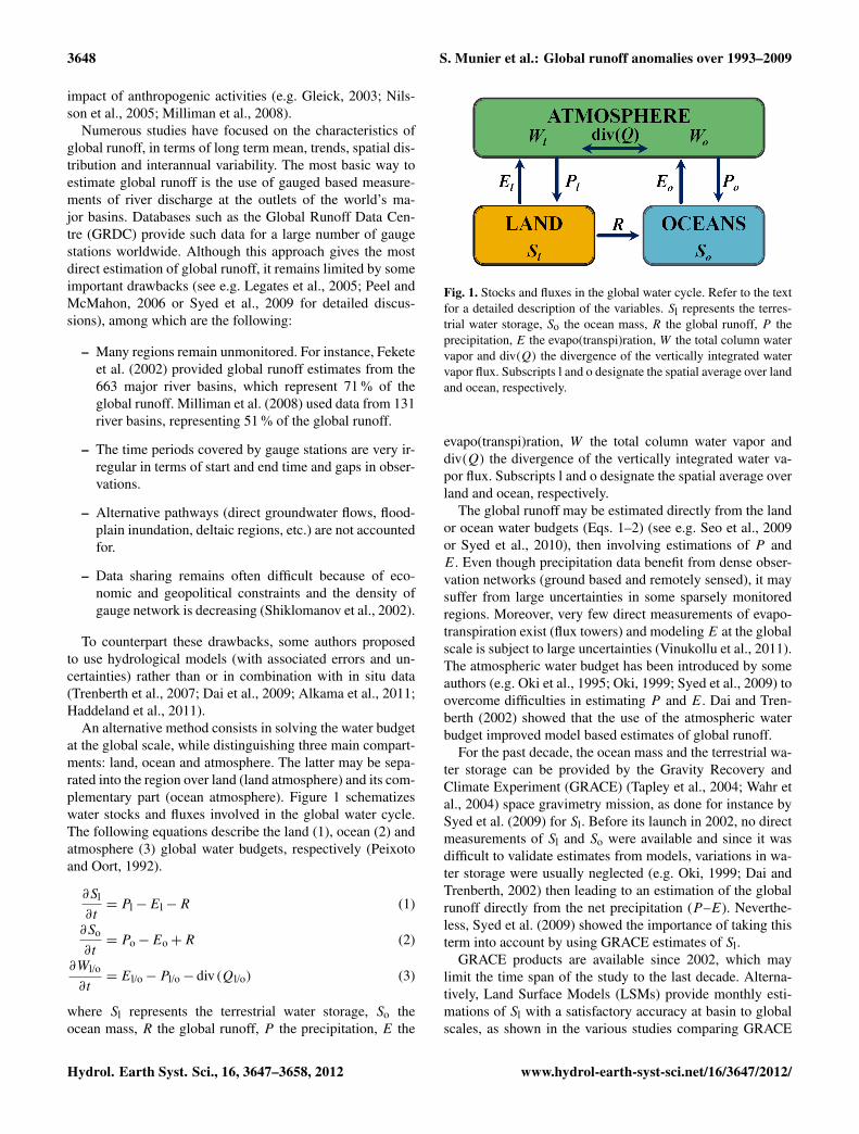
3648 S. Munier et al.: Global runoff anomalies over 1993–2009
impact of anthropogenic activities (e.g. Gleick, 2003; Nils-
son et al., 2005; Milliman et al., 2008).
Numerous studies have focused on the characteristics of
global runoff, in terms of long term mean, trends, spatial dis-
tribution and interannual variability. The most basic way to
estimate global runoff is the use of gauged based measure-
ments of river discharge at the outlets of the world’s ma-
jor basins. Databases such as the Global Runoff Data Cen-
tre (GRDC) provide such data for a large number of gauge
stations worldwide. Although this approach gives the most
direct estimation of global runoff, it remains limited by some
important drawbacks (see e.g. Legates et al., 2005; Peel and
McMahon, 2006 or Syed et al., 2009 for detailed discus-
sions), among which are the following:
– Many regions remain unmonitored. For instance, Fekete
et al. (2002) provided global runoff estimates from the
663 major river basins, which represent 71 % of the
global runoff. Milliman et al. (2008) used data from 131
river basins, representing 51 % of the global runoff.
– The time periods covered by gauge stations are very ir-
regular in terms of start and end time and gaps in obser-
vations.
– Alternative pathways (direct groundwater flows, flood-
plain inundation, deltaic regions, etc.) are not accounted
for.
– Data sharing remains often difficult because of eco-
nomic and geopolitical constraints and the density of
gauge network is decreasing (Shiklomanov et al., 2002).
To counterpart these drawbacks, some authors proposed
to use hydrological models (with associated errors and un-
certainties) rather than or in combination with in situ data
(Trenberth et al., 2007; Dai et al., 2009; Alkama et al., 2011;
Haddeland et al., 2011).
An alternative method consists in solving the water budget
at the global scale, while distinguishing three main compart-
ments: land, ocean and atmosphere. The latter may be sepa-
rated into the region over land (land atmosphere) and its com-
plementary part (ocean atmosphere). Figure 1 schematizes
water stocks and fluxes involved in the global water cycle.
The following equations describe the land (1), ocean (2) and
atmosphere (3) global water budgets, respectively (Peixoto
and Oort, 1992).
∂Sl
∂t= Pl − El − R (1)
∂So
∂t= Po − Eo + R (2)
∂Wl/o
∂t= El/o − Pl/o − div(Ql/o) (3)
where Sl represents the terrestrial water storage, So the
ocean mass, R the global runoff, P the precipitation, E the
Fig. 1. Stocks and fluxes in the global water cycle. Refer to the text
for a detailed description of the variables. Sl represents the terres-
trial water storage, So the ocean mass, R the global runoff, P the
precipitation, E the evapo(transpi)ration, W the total column water
vapor and div(Q) the divergence of the vertically integrated water
vapor flux. Subscripts l and o designate the spatial average over land
and ocean, respectively.
evapo(transpi)ration, W the total column water vapor and
div(Q) the divergence of the vertically integrated water va-
por flux. Subscripts l and o designate the spatial average over
land and ocean, respectively.
The global runoff may be estimated directly from the land
or ocean water budgets (Eqs. 1–2) (see e.g. Seo et al., 2009
or Syed et al., 2010), then involving estimations of P and
E. Even though precipitation data benefit from dense obser-
vation networks (ground based and remotely sensed), it may
suffer from large uncertainties in some sparsely monitored
regions. Moreover, very few direct measurements of evapo-
transpiration exist (flux towers) and modeling E at the global
scale is subject to large uncertainties (Vinukollu et al., 2011).
The atmospheric water budget has been introduced by some
authors (e.g. Oki et al., 1995; Oki, 1999; Syed et al., 2009) to
overcome difficulties in estimating P and E. Dai and Tren-
berth (2002) showed that the use of the atmospheric water
budget improved model based estimates of global runoff.
For the past decade, the ocean mass and the terrestrial wa-
ter storage can be provided by the Gravity Recovery and
Climate Experiment (GRACE) (Tapley et al., 2004; Wahr et
al., 2004) space gravimetry mission, as done for instance by
Syed et al. (2009) for Sl. Before its launch in 2002, no direct
measurements of Sl and So were available and since it was
difficult to validate estimates from models, variations in wa-
ter storage were usually neglected (e.g. Oki, 1999; Dai and
Trenberth, 2002) then leading to an estimation of the global
runoff directly from the net precipitation (P –E). Neverthe-
less, Syed et al. (2009) showed the importance of taking this
term into account by using GRACE estimates of Sl.
GRACE products are available since 2002, which may
limit the time span of the study to the last decade. Alterna-
tively, Land Surface Models (LSMs) provide monthly esti-
mations of Sl with a satisfactory accuracy at basin to global
scales, as shown in the various studies comparing GRACE
Hydrol. Earth Syst. Sci., 16, 3647–3658, 2012 www.hydrol-earth-syst-sci.net/16/3647/2012/

S. Munier et al.: Global runoff anomalies over 1993–2009 3649
and LSMs (see Ramillien et al., 2008 for a review of studies
prior to 2008). The covered period of LSMs depends on the
model, but simulations generally run at least over the last
two decades. Besides, the ocean mass So may be derived
from satellite radar altimetry observations, which provide es-
timations of the global mean sea level (GMSL), and from in
situ hydrographic data. To derive the ocean mass variations,
GMSL has to be corrected from the steric component (effect
of temperature and salinity), as done by, for example, Syed
et al. (2010).
In this study, we use the coupled land–ocean–atmosphere
water budgets to estimate the interannual variability of
global runoff. Two estimates are computed: one from the
land/atmosphere coupling (Eq. 4) and the other from the
ocean/atmosphere coupling (Eq. 5).
Rl = −∂Wl
∂t− div(Ql)−
dSl
dt(4)
Ro =∂Wo
∂t+ div(Qo) +
dSo
dt. (5)
Sl is estimated from three LSMs, So from altimetry based
GMSL and the net precipitation term (time derivative of W
and div(Q)) from atmospheric reanalyses. Considering the
level of uncertainties on each term appearing in the above
equations, each data set used to compute the global runoff is
cross-validated with independent data. Besides, since altime-
try observations are used, our global runoff estimates cover
the altimetry time span (1993–2009). This study expands the
previous ones by providing for the first time a comparison of
global runoff estimates from land and ocean water budgets,
in terms of interannual variability, over the last two decades.
Section 2 presents the data sets used in this study, whereas
results are presented in Sects. 3, 4 and 5. In Sect. 3, each data
set is compared with independent data to ensure its reliabil-
ity and to give an idea of its uncertainties. The comparison
between both global runoff estimates, in terms of interan-
nual variability, is given in Sect. 4. Our global runoff estimate
is also compared with global climate indices (ENSO related
SOI, AMO). A discussion on the ocean thermal expansion
used in the estimation of the ocean mass and an innovative
method to estimate it are provided in Sect. 5.
2 Data and models used in this study
In this section, we present the data and models used to com-
pute global runoff by the two methods (Rl and Ro from
Eqs. 4–5). Data used for validation purposes are also pre-
sented.
2.1 Altimetry-based sea level data
For the altimetry-based sea level data, we use the DT-MSLA
“Ref” series provided by Collecte Localisation Satellite
(CLS; http://www.aviso.oceanobs.com/en/data/products/
sea-surface-height-products/global/msla/index.html). This
data set is used over the time span from January 1993 to
December 2009. It is available as 0.25◦× 0.25◦ Mercator
projection grids at weekly interval from a combination
of several altimetry missions (Topex/Poseidon, Jason-1
and 2, Envisat and ERS 1 and 2). Most recently improved
geophysical corrections are applied to the sea level data (see
Ablain et al., 2009, for details). The weekly sea level grids
are geographically averaged between 65◦ S and 65◦ N to
obtain a GMSL time series. The data are further averaged on
a monthly basis.
2.2 Steric data
Steric sea level is estimated using the updated in situ ocean
temperature and salinity data from Ishii and Kimoto (2009),
v6.12 (called hereafter IK09). The IK09 temperature data
are corrected for the XBT depth bias. The temperature and
salinity data are available at monthly intervals over 16 depth
levels ranging from the ocean surface down to 700 m depth,
on a global 1◦× 1◦ grid from 1955 to 2009. Steric sea level
anomalies are computed over the 0–700 m depth range for
the period January 1993 to December 2009. The deep ocean
contribution cannot be accounted for since hydrographical
data below 700 m are too sparse. Recent studies have shown
that in terms of trend, the deep ocean contributes by ∼ 10 %
to the total steric effect (Church et al., 2011). Besides, almost
all interannual variability in steric sea level is confined in the
upper 300–500 m of the ocean (e.g. Llovel et al., 2011). At
global scale, salinity does not contribute to the GMSL and is
therefore neglected in the following.
2.3 Land Surface Models
To estimate the terrestrial water storage component (Sl),
we use monthly gridded outputs of three different LSMs:
(1) the WaterGAP Global Hydrology Model (WGHM)
(Doll et al., 2003); (2) the Interactions between Soil, Bio-
sphere and Atmosphere – Total Runoff Integrating Pathways
(ISBA-TRIP) model (Alkama et al., 2011; Decharme et al.,
2010); and (3) the Land Dynamics (LaD) model (Milly and
Shmakin, 2002). WGHM outputs are available through De-
cember 2009, whereas ISBA ends in December 2008 and
LaD in July 2007. Discrepancies among Sl derived from the
different LSMs may come from differences in the numeri-
cal schemes and meteorological forcing. As noted by Syed et
al. (2009), discrepancies among models outputs provide an
estimation of the model uncertainties.
Independently, the evapotranspiration modeled by the
three LSMs is used for the validation of net precipitation over
land (Pl–El) computed from the atmospheric water budget
(Eq. 3).
www.hydrol-earth-syst-sci.net/16/3647/2012/ Hydrol. Earth Syst. Sci., 16, 3647–3658, 2012

3650 S. Munier et al.: Global runoff anomalies over 1993–2009
2.4 GRACE data
To validate LSMs derived Sl and altimetry-based So, a com-
parison with GRACE data is proposed in Sect. 3. Here we
use GRACE products (release 2) for the period 2003–2009
(with missing data for June 2003), computed by the Groupe
de Recherche de Geodesie Spatiale (GRGS) (Bruinsma et al.,
2010). It consists of monthly 1◦× 1◦ gridded time series of
water volume (Sl or So), expressed in terms of equivalent
water height (EWH). At each grid mesh, the volume anoma-
lies are obtained by removing the temporal mean. The GRGS
data are stabilized during the generation process so that no
smoothing or filtering is necessary. When GRACE data is
used at basin scales, it has to be corrected from leakage ef-
fects due to its low resolution (Longuevergne et al., 2010).
Nevertheless, such effects have minor impact at the global
scale and GRACE data is not corrected here.
As said previously, GRACE provides reliable estimations
of spatiotemporal water volume variations since 2002 and
it would have been possible to complete GRACE data with
LSMs outputs and altimetry based ocean mass for the period
1993–2002. In order to keep consistency in our computations
over 1993–2009, we prefer not to use GRACE products to
estimate terrestrial water storage and ocean mass variations.
Nevertheless, in both cases, comparison with GRACE obser-
vations is performed to increase confidence in data.
2.5 Meteorological data
Data used in this study to compute P-E from the atmospheric
water budget (W and div(Q)) are based on reanalysis prod-
ucts from the European Centre for Medium-Range Weather
Forecast (ECMWF) ERA-Interim data set (Dee et al., 2011).
These are daily global data provided on 1.5◦× 1.5◦ grids in
units of mm day−1. All gridded data are further expressed in
terms of monthly averages over the period 1993–2009.
For validation purposes, we also consider six global pre-
cipitation data sets: Global Precipitation Climatology Cen-
tre (GPCC, Schneider et al., 2008), Climatic Research
Unit (CRU, available online at http://badc.nerc.ac.uk/data/
cru/), the Willmott-Matsuura product (WM, Willmott and
Matsuura, 2010), Global Precipitation Climatology Project
(GPCP, Adler et al., 2003), Climate Prediction Center (CPC)
Merged Analysis of Precipitation (CMAP, Xie and Arkin,
1997), the Princeton Global Forcing (PGF, Sheffield et al.,
2006). These data sets are obtained either from ground based
observations (GPCC, CRU, WM) or from merged ground
based and satellite observations (GPCP, CMAP, PGF).
3 Processing and evaluation of the data and models
3.1 Data processing
As the focus of this study is the interannual variability of
the global runoff, the seasonal component of each signal
presented in the following is removed. This component is
obtained by fitting two sinusoidal signals periods of 6 and
12 months. Moreover, although the mean value of the global
runoff is still subject to discussions (see e.g. Syed et al., 2009,
and references therein), it is not in the scope of this paper.
Hence, the temporal mean is also removed from the global
runoff estimates. In Eqs. (5)–(6), Sl and So are derivated with
respect to time and any trend in Sl and So would lead to con-
stants in the runoff. Consequently, Sl and So are detrended in
the following. Note that detrending Sl and So does not im-
pact the runoff trend since change in storage (i.e. first order
differencing) filters out linear trends.
As a spherical harmonics (SH) truncation at degree 50
(resolution of 400 km) is applied on GRACE data to obtain
water mass variations, we applied the same SH truncation
to LSM outputs for a more relevant comparison between
GRACE and LSMs derived Sl (as suggested by many au-
thors, e.g. Longuevergne et al., 2010). SH truncation is ap-
plied only for the model validation, not for the runoff com-
putation.
Finally, all graphs showing temporal evolution of the spa-
tial mean of any variable have been smoothed using a 3-
months moving average.
3.2 Land/Ocean masks: estimate of the high latitudes
contribution
As indicated above, altimetry products used here are avail-
able only in the 65◦ S–65◦ N domain. Moreover, ice sheets
(Greenland and Antarctica) are generally not modeled in
LSMs because of their very specific hydrological behavior,
all the more so as very few in situ data are available in
these regions and the models’ validation is then quite diffi-
cult. Hence ice sheets and high latitude oceans are excluded
from the present study. Figure 2a shows the land and ocean
regions considered here.
The exclusion of ice sheets and high latitude oceans has
no major consequences in the following since these regions
only play a minor role in the interannual variability of global
runoff. To assess this, Fig. 2b and c presents Sl and So vari-
ations derived from GRACE over the four regions shown in
Fig. 2a. Despite significant trends in water mass variations
– not shown in the graphs – in ice sheets (−160 km3 yr−1)
and high latitude oceans (−66 km3 yr−1), these regions are
scarcely involved in the global water cycle in terms of inter-
annual variability.
3.3 Comparison of terrestrial water storage from
GRACE and LSMs
Figure 3a shows the total water storage derived from the
LSMs; the blue shading represents the root mean square
(RMS) deviation of each model with respect to the average.
The RMS between LSMs is 1.26 mm, which is quite low
compared to the amplitude of the interannual variations of Sl.
Hydrol. Earth Syst. Sci., 16, 3647–3658, 2012 www.hydrol-earth-syst-sci.net/16/3647/2012/
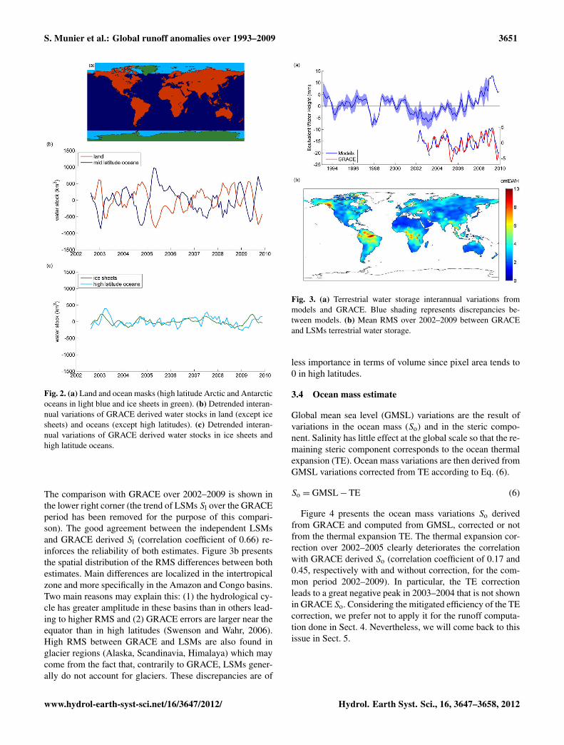
S. Munier et al.: Global runoff anomalies over 1993–2009 3651
Fig. 2. (a) Land and ocean masks (high latitude Arctic and Antarctic
oceans in light blue and ice sheets in green). (b) Detrended interan-
nual variations of GRACE derived water stocks in land (except ice
sheets) and oceans (except high latitudes). (c) Detrended interan-
nual variations of GRACE derived water stocks in ice sheets and
high latitude oceans.
The comparison with GRACE over 2002–2009 is shown in
the lower right corner (the trend of LSMs Sl over the GRACE
period has been removed for the purpose of this compari-
son). The good agreement between the independent LSMs
and GRACE derived Sl (correlation coefficient of 0.66) re-
inforces the reliability of both estimates. Figure 3b presents
the spatial distribution of the RMS differences between both
estimates. Main differences are localized in the intertropical
zone and more specifically in the Amazon and Congo basins.
Two main reasons may explain this: (1) the hydrological cy-
cle has greater amplitude in these basins than in others lead-
ing to higher RMS and (2) GRACE errors are larger near the
equator than in high latitudes (Swenson and Wahr, 2006).
High RMS between GRACE and LSMs are also found in
glacier regions (Alaska, Scandinavia, Himalaya) which may
come from the fact that, contrarily to GRACE, LSMs gener-
ally do not account for glaciers. These discrepancies are of
Fig. 3. (a) Terrestrial water storage interannual variations from
models and GRACE. Blue shading represents discrepancies be-
tween models. (b) Mean RMS over 2002–2009 between GRACE
and LSMs terrestrial water storage.
less importance in terms of volume since pixel area tends to
0 in high latitudes.
3.4 Ocean mass estimate
Global mean sea level (GMSL) variations are the result of
variations in the ocean mass (So) and in the steric compo-
nent. Salinity has little effect at the global scale so that the re-
maining steric component corresponds to the ocean thermal
expansion (TE). Ocean mass variations are then derived from
GMSL variations corrected from TE according to Eq. (6).
So = GMSL − TE (6)
Figure 4 presents the ocean mass variations So derived
from GRACE and computed from GMSL, corrected or not
from the thermal expansion TE. The thermal expansion cor-
rection over 2002–2005 clearly deteriorates the correlation
with GRACE derived So (correlation coefficient of 0.17 and
0.45, respectively with and without correction, for the com-
mon period 2002–2009). In particular, the TE correction
leads to a great negative peak in 2003–2004 that is not shown
in GRACE So. Considering the mitigated efficiency of the TE
correction, we prefer not to apply it for the runoff computa-
tion done in Sect. 4. Nevertheless, we will come back to this
issue in Sect. 5.
www.hydrol-earth-syst-sci.net/16/3647/2012/ Hydrol. Earth Syst. Sci., 16, 3647–3658, 2012
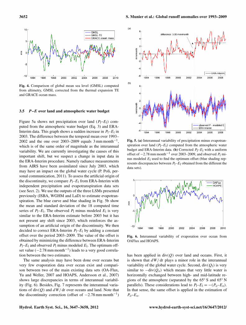
3652 S. Munier et al.: Global runoff anomalies over 1993–2009
Fig. 4. Comparison of global mean sea level (GMSL) computed
from altimetry, GMSL corrected from the thermal expansion TE
and GRACE ocean mass.
3.5 P –E over land and atmospheric water budget
Figure 5a shows net precipitation over land (Pl–El) com-
puted from the atmospheric water budget (Eq. 3) and ERA-
Interim data. This graph shows a sudden increase in Pl–El in
2003. The difference between the temporal mean over 1993–
2002 and the one over 2003–2009 equals 3 mm month−1,
which is of the same order of magnitude as the interannual
variability. We are currently investigating the causes of this
important shift, but we suspect a change in input data in
the ERA-Interim procedure. Namely radiance measurements
from AIRS have been assimilated since July 2003, which
may have an impact on the global water cycle (P. Poli, per-
sonal communication, 2011). To assess the artificial origin of
the discontinuity, we compare Pl–El from ERA-Interim with
independent precipitation and evapotranspiration data sets
(see Sect. 2). We use the outputs of the three LSMs presented
previously (ISBA, WGHM and LaD) to estimate evapotran-
spiration. The blue curve and blue shading in Fig. 5b show
the mean and standard deviation of the 18 computed time
series of Pl–El. The observed Pl minus modeled El is very
similar to the ERA-Interim estimate before 2003 but it has
not present any shift since 2003, which reinforces the as-
sumption of an artificial origin of the discontinuity. We then
decided to correct ERA-Interim Pl–El by adding a constant
offset over the period 2003–2009. The value of the offset is
obtained by minimizing the difference between ERA-Interim
Pl–El and observed Pl minus modeled El. The optimum off-
set value (−2.78 mm month−1) leads to a very good correla-
tion between the two estimates.
The same analysis may have been done over oceans but
very few evaporation data over ocean exist and compari-
son between two of the main existing data sets (OA-Flux,
Yu and Weller, 2007 and HOAPS, Andersson et al., 2007)
shows large discrepancies in terms of interannual variabil-
ity (Fig. 6). Besides, Fig. 7 represents the interannual varia-
tions of div(Q) and dW/ dt over oceans and land. Note that
the discontinuity correction (offset of −2.78 mm month−1)
Fig. 5. (a) Interannual variability of precipitation minus evapotran-
spiration over land (Pl–El) computed from the atmospheric water
budget and ERA-Interim data. (b) Corrected Pl–El with a uniform
offset of −2.78 mm month−1 over 2003–2009, and observed Pl mi-
nus modeled El used to find the optimum offset (blue shading rep-
resents discrepancies between Pl–El obtained from the different the
data sets).
Fig. 6. Interannual variability of evaporation over ocean from
OAFlux and HOAPS.
has been applied in div(Q) over land and oceans. First, it
is shown that dW/ dt plays a minor role in the interannual
variability of the global water cycle. Second, div(Ql) is very
similar to −div(Qo) which means that very little water is
horizontally exchanged between high- and mid-latitude re-
gions of the atmosphere (separated by the 65◦ S and 65◦ N
parallels). These considerations lead to Pl–El = −(Po–Eo).
In that sense, the same offset is applied in the estimation of
Po–Eo.
Hydrol. Earth Syst. Sci., 16, 3647–3658, 2012 www.hydrol-earth-syst-sci.net/16/3647/2012/

S. Munier et al.: Global runoff anomalies over 1993–2009 3653
Fig. 7. Components of the atmospheric water budget. Spatial mean
over ocean and land. The dW/ dt time series are shifted vertically
for clarity.
4 Global runoff and climate variability
4.1 Comparison of the two global runoff estimates
The comparison between estimates of the global runoff from
the land–atmosphere and the ocean–atmosphere water bud-
gets is shown in Fig. 8. Both estimates are very well cor-
related (correlation coefficient of 0.73, mean standard devi-
ation of 63 km3 month−1). Interannual variations of global
runoff ranges from about −200 to 200 km3 month−1, with
higher peaks during major ENSO events. In particular, nega-
tive peaks in 1994–1995, 1997–1998 and 2009–2010 are re-
lated to lower than normal precipitation over land during El
Nino events, whereas the positive peak in 1999–2000 is re-
lated to higher than normal land precipitation during La Nina
event. One can notice that the 1997–1998 El Nino event is
clearly visible on Fig. 3a, which shows a great negative peak
in Sl during this period, a result of lower/higher precipitation
intensity over land/ocean (Gu et al., 2007). The ENSO ef-
fects on precipitation over land and oceans is also shown on
Fig. 7.
Besides, no significant trend is observed over the whole
period. Indeed, the trend equals 48 km3 month−1 per decade
for Rl and 72 km3 month−1 per decade for Ro, which is neg-
ligible compared to the mean standard deviation of Rl and
Ro (169 and 228 km3 month−1, respectively). These values
are quite lower than the one found by Syed et al. (2010)
(540 km3 yr−2 or 450 km3 month−1 per decade) but are in
agreement with results of some other previous studies (Dai
et al., 2009; Milliman et al., 2008) which found insignificant
trends. The difference with Syed et al. (2010) may be partly
explained by the fact that the authors computed the trend
over 1995–2006 and that the global runoff presents higher
values before 1995 and lower values after 2006, leading to a
Fig. 8. Comparison of runoff computed from land–atmosphere (Rl)
and ocean–atmosphere (Ro) water budgets. The red shading repre-
sents discrepancies relative to the different considered LSMs.
reduction of the global trend. Indeed, with the methodology
developed in this study, the global runoff trend over the pe-
riod 1995–2006 equals 128 km3 month−1 per decade for Rl
and 143 km3 month−1 per decade for Ro. While these values
are higher than for the period 1993–2009, they are still lower
than the value obtained by Syed et al. (2010). The difference
likely comes from the different data sets used to compute P –
E over oceans. Namely, Syed et al. (2010) considered two
estimates of Eo (OA-Flux and HOAPS) which are quite dif-
ferent in terms of interannual variability (Fig. 6).
Other authors (Dai et al., 2009; Alkama et al., 2011) found
non negligible trends over some of the major river basins for
the last decades, but these trends seem to compensate against
each other at the global scale.
The differences between Rl and Ro may be explained by
two main factors: modeling errors and TE not accounted for
in the ocean mass estimation. Concerning the former, con-
sidering three different LSMs help us to quantify modeling
errors. We find a mean standard deviation of 43 km3 month−1
due to LSMs discrepancies (represented by the red shading in
Fig. 8), which is very low compared to the interannual vari-
ability of R. This suggests that the differences between Rl
and Ro are mainly explained by the fact that the ocean mass
is not corrected from TE. Nevertheless, the good correlation
between Ro and Rl shows that TE plays a minor role in the
interannual variability of global runoff. In Sect. 5, we inves-
tigate a new method to estimate the ocean thermal expansion
component by using the difference Ro–Rl.
4.2 Zonal runoff and correlation with climate indices
As said previously, the global runoff seems to be highly
impacted by major ENSO events. Many studies, including
Dai et al. (2009), Syed et al. (2010) and Labat (2010), also
showed this particular link. In addition, Gu et al. (2007) re-
ported high correlations between ENSO and land precipita-
tion in the intertropical zone and lower but not null correla-
tions in mid- and high latitudes. In this section, we propose
www.hydrol-earth-syst-sci.net/16/3647/2012/ Hydrol. Earth Syst. Sci., 16, 3647–3658, 2012

3654 S. Munier et al.: Global runoff anomalies over 1993–2009
to investigate the correlation between the zonal runoff and
different global scale climate phenomena.
First, the zonal runoff is computed over four latitudinal
bands separated by the 60◦ N, 20◦ N and 20◦ S parallels
(solid lines in Fig. 9). As expected, while the intertropical
zone contributes for the most part to the interannual variabil-
ity of the global runoff, northern high latitude and southern
mid latitude zonal runoffs are quite negligible.
For each zone, the zonal runoff is then compared with dif-
ferent linear combinations of several climate indices. The
indices considered here are the following: the Multivariate
ENSO Index (MEI), the Atlantic multidecadal oscillation
(AMO), the Pacific Decadal Oscillation (PDO), the Pacific–
North America teleconnection (PNA) and the Arctic Oscilla-
tion index (AO). The reader may refer to Rossi et al. (2011)
for a detailed presentation of these indices. For each subset
of one or two indices, the linear combination is optimized
by maximizing the correlation between the zonal runoff and
the combined index. Subsets that give the best results are
used to compute a new index called combined runoff index
(CRI). Optimization results are given, for each zonal band,
by Eq. (7) (climate indices have been normalized before the
optimization).
CRI(−60/−20) = 0.53 × PDO + 0.47 × AMO (7)
CRI(−20/ + 20) = −0.62 × MEI−0.38 × AMO
CRI(+20/ + 60) = 0.54 × MEI + 0.46 × AMO
CRI(+60/ + 90) = 0.73 × PNA + 0.27 × AO
Since LSMs and ERA-Interim outputs are available since
1980 or earlier (apart from WGHM which is only avail-
able since 1992), we also compared CRI and zonal Rl over
the period 1980–1992, period not used in the calibration of
CRI. Figure 9 shows (dashed lines) results of calibration (pe-
riod 1993–2009) and validation (period 1980–1992); CRI
has been normalized to match the range of zonal runoffs vari-
ability. The two numbers in the brackets in the legend repre-
sent the correlation between zonal Rl and CRI for the calibra-
tion period and for the overall period, respectively. Figure 9
clearly shows a very good correlation for the intertropical
zone (namely during the validation period) and more con-
trasted correlations in mid- and high latitudes.
Not surprisingly, MEI contributes for the most part in
the intertropical and northern mid-latitude zonal runoffs. For
these two zonal runoffs, AMO also plays an important role.
Figure 9 and Eq. (7) show that these two zonal runoffs are
highly anti-correlated, namely with higher/lower runoffs than
normal in mid-latitude/intertropical zones during major El-
Nino events (e.g. in 1983 or in 1998). The reciprocal is true
for La-Nina events (e.g. in 1989 or in 2000). This suggests
that during El-Nino events, while water mass is shifted west-
ward from the South American continent to the tropical Pa-
cific Ocean (Gu et al., 2007), it is also shifted northward
to mid-latitude continents. Besides, ENSO seems to play a
less important role in northern high latitudes and southern
Fig. 9. Comparison of zonal runoff computed from land–
atmosphere–water budgets (Rl, solid lines) and combined runoff in-
dex (CRI, dashed lines) over northern high latitudes (60◦ N–90◦ N),
northern mid-latitudes (20◦ N–60◦ N), intertropical zone (20◦ S–
20◦ N) and southern mid-latitudes (60◦ S–20◦ S). For each zone,
time series are shifted vertically for clarity. CRI has been normal-
ized to match the range of global runoff variability. The two num-
bers in the brackets represent the correlation between Rl and CRI
for the calibration period (1993–2009) and the whole period, re-
spectively. Results of calibration (climate indices and related coef-
ficients) are given in the legend box.
mid-latitudes. Northern high latitude zonal runoff is logically
governed by northern mid- to high latitude climate phenom-
ena (Pacific–North America teleconnection and Arctic Os-
cillation). For each of the three other zones, CRI is a com-
bination of a climate index related to the Pacific Ocean and
another related to the Atlantic Ocean.
Further investigations are suggested to complete these pre-
liminary results, namely about the relationship between the
zonal runoff and climate indices characteristics in the fre-
quency domain (Rossi et al., 2011).
5 Reconstruction of the ocean thermal expansion
In this subsidiary section, we come back to the aforemen-
tioned problem of the ocean thermal expansion (TE) correc-
tion and propose an innovative method to reconstruct this
component of the global mean sea level. Indeed, as said pre-
viously, the observed difference between Rl and Ro may
be mainly attributed to TE. Assuming that Pl–El = −(Po–
Eo) (see Sect. 3.5) and combining Eqs. (1)–(2) leads to
Sl + So = constant. Then combining this last equation with
Eq. (6) leads to the following estimate of TE (after removing
the constant):
Hydrol. Earth Syst. Sci., 16, 3647–3658, 2012 www.hydrol-earth-syst-sci.net/16/3647/2012/
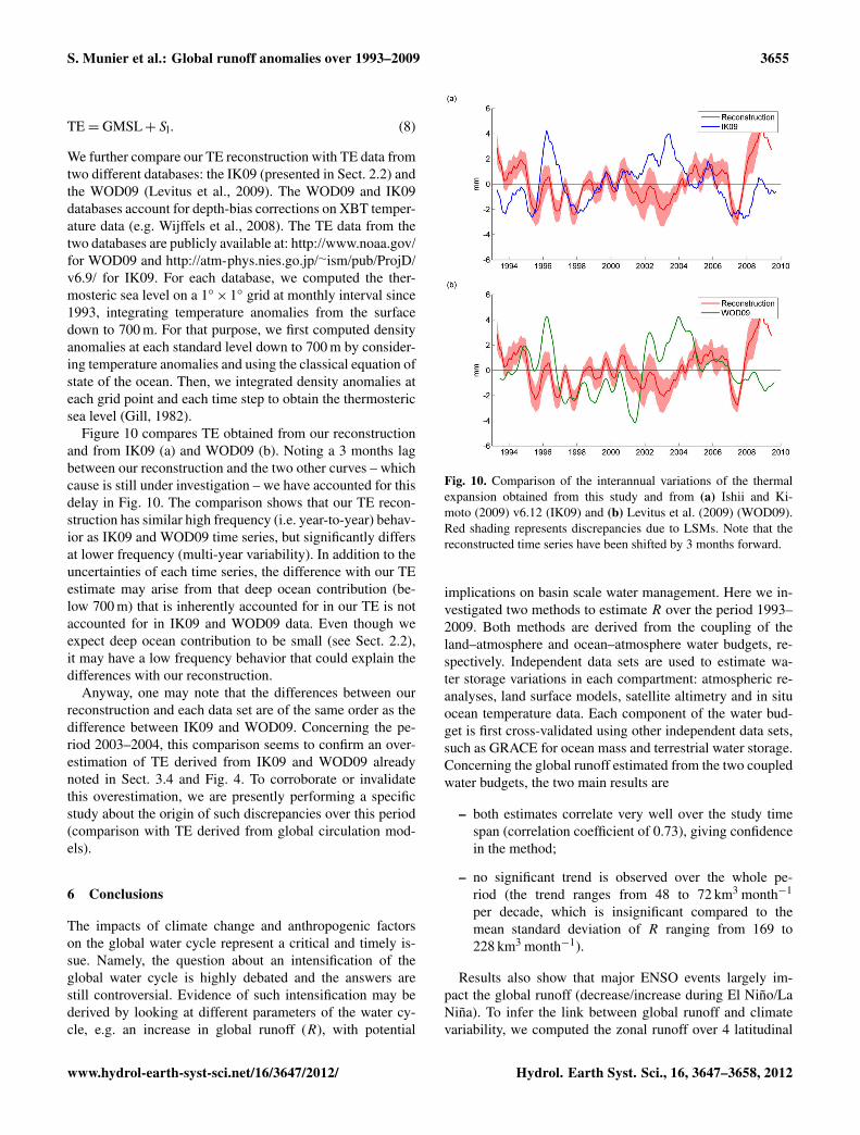
S. Munier et al.: Global runoff anomalies over 1993–2009 3655
TE = GMSL + Sl. (8)
We further compare our TE reconstruction with TE data from
two different databases: the IK09 (presented in Sect. 2.2) and
the WOD09 (Levitus et al., 2009). The WOD09 and IK09
databases account for depth-bias corrections on XBT temper-
ature data (e.g. Wijffels et al., 2008). The TE data from the
two databases are publicly available at: http://www.noaa.gov/
for WOD09 and http://atm-phys.nies.go.jp/∼ism/pub/ProjD/
v6.9/ for IK09. For each database, we computed the ther-
mosteric sea level on a 1◦× 1◦ grid at monthly interval since
1993, integrating temperature anomalies from the surface
down to 700 m. For that purpose, we first computed density
anomalies at each standard level down to 700 m by consider-
ing temperature anomalies and using the classical equation of
state of the ocean. Then, we integrated density anomalies at
each grid point and each time step to obtain the thermosteric
sea level (Gill, 1982).
Figure 10 compares TE obtained from our reconstruction
and from IK09 (a) and WOD09 (b). Noting a 3 months lag
between our reconstruction and the two other curves – which
cause is still under investigation – we have accounted for this
delay in Fig. 10. The comparison shows that our TE recon-
struction has similar high frequency (i.e. year-to-year) behav-
ior as IK09 and WOD09 time series, but significantly differs
at lower frequency (multi-year variability). In addition to the
uncertainties of each time series, the difference with our TE
estimate may arise from that deep ocean contribution (be-
low 700 m) that is inherently accounted for in our TE is not
accounted for in IK09 and WOD09 data. Even though we
expect deep ocean contribution to be small (see Sect. 2.2),
it may have a low frequency behavior that could explain the
differences with our reconstruction.
Anyway, one may note that the differences between our
reconstruction and each data set are of the same order as the
difference between IK09 and WOD09. Concerning the pe-
riod 2003–2004, this comparison seems to confirm an over-
estimation of TE derived from IK09 and WOD09 already
noted in Sect. 3.4 and Fig. 4. To corroborate or invalidate
this overestimation, we are presently performing a specific
study about the origin of such discrepancies over this period
(comparison with TE derived from global circulation mod-
els).
6 Conclusions
The impacts of climate change and anthropogenic factors
on the global water cycle represent a critical and timely is-
sue. Namely, the question about an intensification of the
global water cycle is highly debated and the answers are
still controversial. Evidence of such intensification may be
derived by looking at different parameters of the water cy-
cle, e.g. an increase in global runoff (R), with potential
Fig. 10. Comparison of the interannual variations of the thermal
expansion obtained from this study and from (a) Ishii and Ki-
moto (2009) v6.12 (IK09) and (b) Levitus et al. (2009) (WOD09).
Red shading represents discrepancies due to LSMs. Note that the
reconstructed time series have been shifted by 3 months forward.
implications on basin scale water management. Here we in-
vestigated two methods to estimate R over the period 1993–
2009. Both methods are derived from the coupling of the
land–atmosphere and ocean–atmosphere water budgets, re-
spectively. Independent data sets are used to estimate wa-
ter storage variations in each compartment: atmospheric re-
analyses, land surface models, satellite altimetry and in situ
ocean temperature data. Each component of the water bud-
get is first cross-validated using other independent data sets,
such as GRACE for ocean mass and terrestrial water storage.
Concerning the global runoff estimated from the two coupled
water budgets, the two main results are
– both estimates correlate very well over the study time
span (correlation coefficient of 0.73), giving confidence
in the method;
– no significant trend is observed over the whole pe-
riod (the trend ranges from 48 to 72 km3 month−1
per decade, which is insignificant compared to the
mean standard deviation of R ranging from 169 to
228 km3 month−1).
Results also show that major ENSO events largely im-
pact the global runoff (decrease/increase during El Nino/La
Nina). To infer the link between global runoff and climate
variability, we computed the zonal runoff over 4 latitudinal
www.hydrol-earth-syst-sci.net/16/3647/2012/ Hydrol. Earth Syst. Sci., 16, 3647–3658, 2012
3656 S. Munier et al.: Global runoff anomalies over 1993–2009
bands (intertropical zone, northern and southern mid-
latitudes and northern high latitudes) and compared it with
different climate indices. We then set up a combined runoff
index (CRI) obtained for each zone by optimization of cli-
mate indices linear combinations. We showed that CRI well
correlates with the zonal runoff even over a validation period
not used for the optimization, especially for the intertropical
zone, which contributes for the most part in the global runoff.
Besides, linear coefficients resulting from the optimization
provide information about which large-scale climate phe-
nomena are the main drivers for each zonal runoff. Namely,
the intertropical and northern mid-latitude zonal runoffs are
mainly driven by ENSO and AMO. Moreover, the zonal
runoffs in these two zones are anti-correlated, particularly
during ENSO events. This suggests that water masses are
shifted northward/southward during major El Nino/La Nina
events.
Lastly, the difference between the two runoff estimates
may be mainly explained by the ocean thermal expansion
(TE) term which has not been accounted for in the ocean
mass estimate. Consequently, we used our runoff reconstruc-
tion to propose an innovative method for providing a new
estimate of TE. The comparison with two existing data sets
shows a quite good agreement in terms of interannual vari-
ability, showing the relevance of the method, but points out a
period (2003–2004) during which ocean thermal expansion
data may be in error.
More generally, these results have implications for stud-
ies on the global water cycle, with the underlying issues of
global warming and water resources availability. Namely, we
show that an intensification of the global water cycle due to
the global warming is not obvious over the last two decades.
Besides, as large scale climate phenomena may be seen as
drivers of the zonal (or regional) runoffs, analyzing their evo-
lution with climate change should provide indicators of po-
tential evolutions of the global runoff. The mechanisms re-
lating such phenomena and runoff need to be addressed in
further studies.
Acknowledgements. We would like to acknowledge Andreas
Guntner (GFZ German Research Centre for Geosciences) and
Bertrand Decharme (CNRM, MeteoFrance) for sharing WGHM
and ISBA outputs, respectively. S. Munier and H. Palanisamy
received a grant from the Centre National d’Etudes Spatiales
(CNES, France) and from ANR Cecile, respectively. We are also
grateful to the two anonymous reviewers who helped us to improve
the paper.
Edited by: H. Cloke
The publication of this article is financed by CNRS-INSU.
References
Ablain, M., Cazenave, A., Valladeau, G., and Guinehut, S.: A new
assessment of the error budget of global mean sea level rate esti-
mated by satellite altimetry over 1993–2008, Ocean Sci., 5, 193–
201, doi:10.5194/os-5-193-2009, 2009.
Adler, R. F., Huffman, G. J., Chang, A., Ferraro, R., Xie, P. P.,
Janowiak, J., Rudolf, B., Schneider, U., Curtis, S., Bolvin, D.,
Gruber, A., Susskind, J., Arkin, P., and Nelkin, E: The version-
2 global precipitation climatology project (GPCP) monthly pre-
cipitation analysis (1979–present), J. Hydrometeorol., 4, 1147–
1167, 2003.
Alkama, R., Decharme, B., Douville, H., and Ribes, A.: Trends in
Global and Basin-Scale Runoff over the Late Twentieth Century:
Methodological Issues and Sources of Uncertainty, J. Climate,
24, 3000–3014, doi:10.1175/2010JCLI3921.1, 2011.
Andersson, A., Bakan, S., Fennig, K., Grassl, H., Klepp, C., and
Schulz, J.: Hamburg Ocean Atmosphere Parameters and Fluxes
from Satellite Data – HOAPS-3 – monthly mean, World Data
Center for Climate, electronic publication, 2007.
Bruinsma, S., Lemoine, J. M., Biancale, R., and Vales,
N.: CNES/GRGS 10-day gravity field models (release
2) and their evaluation, Adv. Space Res., 45, 587–601,
doi:10.1016/j.asr.2009.10.012, 2010.
Church, J. A., White, N. J., Konikow, L. F., Domingues, C. M.,
Cogley, J. G., Rignot, E., Gregory, J. M., van den Broeke, M.
R., Monaghan, A. J., and Velicogna, I.: Revisiting the Earth’s
sea-level and energy budgets from 1961 to 2008, Geophys. Res.
Lett., 38, L18601, doi:10.1029/2011GL048794, 2011.
Dai, A. and Trenberth, K. E.: Estimates of Freshwater Discharge
from Continents: Latitudinal and Seasonal Variations, J. Hy-
drometeorol., 3, 660–687, 2002.
Dai, A., Qian, T. T., Trenberth, K. E., and Milliman, J. D.: Changes
in Continental Freshwater Discharge from 1948 to 2004, J. Cli-
mate, 22, 2773–2792, doi:10.1175/2008JCLI2592.1, 2009.
Decharme, B., Alkama, R., Douville, H., Becker, M., and Cazenave,
A.: Global Evaluation of the ISBA-TRIP Continental Hydrolog-
ical System, Part II: Uncertainties in River Routing Simulation
Related to Flow Velocity and Groundwater Storage, J. Hydrom-
eteorol., 11, 601–617, doi:10.1175/2010JHM1212.1, 2010.
Dee, D. P., Uppala, S. M., Simmons, A. J., Berrisford, P., Poli,
P., Kobayashi, S., Andrae, U., Balmaseda, M. A., Balsamo, G.,
Bauer, P., Bechtold, P., Beljaars, A. C. M., van de Berg, L., Bid-
lot, J., Bormann, N., Delsol, C., Dragani, R., Fuentes, M., Geer,
A. J., Haimberger, L., Healy, S. B., Hersbach, H., Holm, E. V.,
Isaksen, L., Kallberg, P., Koehler, M., Matricardi, M., McNally,
A. P., Monge-Sanz, B. M., Morcrette, J. J., Park, B. K., Peubey,
C., de Rosnay, P., Tavolato, C., Thepaut, J. N., and Vitart, F.: The
ERA-Interim reanalysis: configuration and performance of the
Hydrol. Earth Syst. Sci., 16, 3647–3658, 2012 www.hydrol-earth-syst-sci.net/16/3647/2012/
S. Munier et al.: Global runoff anomalies over 1993–2009 3657
data assimilation system, Q. J. Roy. Meteor. Soc., 137, 553–597,
doi:10.1002/qj.828, 2011.
Doll, P., Kaspar, F., and Lehner, B.: A global hydrological model
for deriving water availability indicators: model tuning and vali-
dation, J. Hydrol., 270, 105–134, 2003.
Fekete, B. M., Vorosmarty, C. J., and Grabs, W.: High-resolution
fields of global runoff combining observed river discharge and
simulated water balances, Global Biogeochem. Cy., 16, 1042,
doi:10.1029/1999GB001254, 2002.
Gerten, D., Rost, S., von Bloh, W., and Lucht, W.: Causes of change
in 20th century global river discharge, Geophys. Res. Lett., 35,
L20405, doi:10.1029/2008GL035258, 2008.
Gill, A. E.: Atmosphere-Ocean Dynamics, Academic Press, San
Diego, 1982.
Gleick, P.: Global freshwater resources: Soft-path solu-
tions for the 21st century, Science, 302, 1524–1528,
doi:10.1126/science.1089967, 2003.
Gu, G., Adler, R. F., Huffman, G. J., and Curtis, S.: Tropical rainfall
variability on interannual-to-interdecadal and longer time scales
derived from the GPCP monthly product, J. Climate, 20, 4033–
4046, doi:10.1175/JCLI4227.1, 2007.
Haddeland, I., Clark, D. B., Franssen, W., Ludwig, F., Voß, F.,
Arnell, N. W., Bertrand, N., Best, M., Folwell, S., Gerten, D.,
Gomes, S., Gosling, S. N., Hagemann, S., Hanasaki, N., Harding,
R., Heinke, J., Kabat, P., Koirala, S., Oki, T., Polcher, J., Stacke,
T., Viterbo, P., Weedon, G. P., and Yeh, P.: Multi-Model Estimate
of the Global Terrestrial Water Balance: Setup and First Results,
J. Hydrometeorol., 12, 869–884, doi:10.1175/2011JHM1324.1,
2011.
Huntington, T. G.: Evidence for intensification of the global water
cycle: Review and synthesis, J. Hydrol., 319, 83–95, 2006.
Ishii, M. and Kimoto, M.: Reevaluation of historical ocean heat
content variations with time-varying XBT and MBT depth bias
corrections, J. Oceanogr., 65, 287–299, doi:10.1007/s10872-009-
0027-7, 2009.
Labat, D.: Evidence for global runoff increase related to
climate warming, Adv. Water Resour., 27, 631–642,
doi:10.1016/j.advwatres.2004.02.020, 2004.
Labat, D.: Cross wavelet analyses of annual continental freshwater
discharge and selected climate indices, J. Hydrol., 385, 269–278,
doi:16/j.jhydrol.2010.02.029, 2010.
Legates, D., Lins, H., and Mccabe, G.: Comments on “Evi-
dence for global runoff increase related to climate warm-
ing” by Labat et al., Adv. Water Resour., 28, 1310–1315,
doi:10.1016/j.advwatres.2005.04.006, 2005.
Levitus, S., Antonov, J. I., Boyer, T. P., Locarnini, R. A., Garcia, H.
E. and Mishonov, A. V.: Global ocean heat content 1955-2008 in
light of recently revealed instrumentation problems, Geophys.
Res. Lett., 36, L07608, doi:10.1029/2008GL037155, 2009.
Llovel, W., Meyssignac, B., and Cazenave, A.: Steric sea
level variations over 2004–2010 as a function of region
and depth: Inference on the mass component variability in
the North Atlantic Ocean, Geophys. Res. Lett., 38, L15608,
doi:201110.1029/2011GL047411, 2011.
Longuevergne, L., Scanlon, B. R., and Wilson, C. R.: GRACE Hy-
drological estimates for small basins: Evaluating processing ap-
proaches on the High Plains Aquifer, USA, Water Resour. Res.,
46, W11517, doi:10.1029/2009WR008564, 2010.
Milliman, J. D., Farnsworth, K. L., Jones, P. D., Xu, K. H.,
and Smith, L. C.: Climatic and anthropogenic factors affecting
river discharge to the global ocean, 1951–2000, Global Planet.
Change, 62, 187–194, doi:10.1016/j.gloplacha.2008.03.001,
2008.
Milly, P. C. D. and Shmakin, A. B.: Global modeling of land water
and energy balances. Part I: the land dynamics (LaD) model, J.
Hydrometeorol., 3, 283–299, 2002.
Nilsson, C., Reidy, C., Dynesius, M., and Revenga, C.: Fragmenta-
tion and flow regulation of the world’s large river systems, Sci-
ence, 308, 405–408, doi:10.1126/science.1107887, 2005.
Oki, T.: The global water cycle, Global Energy and Water Cycles,
edited by: Browning, K. A. and Gurney, R. J., Cambridge Uni-
versity Press, 10–29, 1999.
Oki, T., Musiake, K., Matsuyama, H., and Masuda, K.: Global at-
mospheric water balance and runoff from large river basins, Hy-
drol. Process., 9, 655–678, doi:10.1002/hyp.3360090513, 1995.
Peel, M. C. and McMahon, T. A.: Continental Runoff: A quality-
controlled global runoff data set, Nature, 444, E14–E14,
doi:10.1038/nature05480, 2006.
Peixoto, J. P. and Oort, A. H.: Physics of climate, Springer, 1992.
Ramillien, G., Famiglietti, J., and Wahr, J.: Detection of Continen-
tal Hydrology and Glaciology Signals from GRACE: A Review,
Surv. Geophys., 29, 361–374, 2008.
Rossi, A., Massei, N., and Laignel, B.: A synthesis of the time-
scale variability of commonly used climate indices using con-
tinuous wavelet transform, Global Planet. Change, 78, 1–13,
doi:10.1016/j.gloplacha.2011.04.008, 2011.
Schneider, U., Fuchs, T., Meyer-Christoffer, A., and Rudolf, B.:
Global Precipitation Analysis Products of the GPCC, Global Pre-
cipitation Climatology Centre (GPCC), DWD, Internet Publica-
tion, available at: http://www.dwd.de, 1–12, 2008.
Seo, K. W., Waliser, D. E., Tian, B. J., Famiglietti, J. S., and Syed,
T. H.: Evaluation of global land-to-ocean fresh water discharge
and evapotranspiration using space-based observations, J. Hy-
drol., 373, 508–515, doi:10.1016/j.jhydrol.2009.05.014, 2009.
Sheffield, J., Goteti, G., and Wood, E. F.: Development of a 50-year
high-resolution global dataset of meteorological forcings for land
surface modeling, J. Climate, 19, 3088–3111, 2006.
Shiklomanov, A. I., Lammers, R. B., and Vorosmarty, C. J.:
Widespread decline in hydrological monitoring threatens Pan-
Arctic Research, Eos, Transactions American Geophysical
Union, 83, 13, doi:10.1029/2002EO000007, 2002.
Swenson, S. and Wahr, J.: Post-processing removal of corre-
lated errors in GRACE data, Geophys. Res. Lett., 33, L08402,
doi:10.1029/2005GL025285, 2006.
Syed, T. H., Famiglietti, J. S., and Chambers, D. P.: GRACE-
Based Estimates of Terrestrial Freshwater Discharge from
Basin to Continental Scales, J. Hydrometeorol., 10, 22–40,
doi:10.1175/2008JHM993.1, 2009.
Syed, T. H., Famiglietti, J. S., Chambers, D. P., Willis, J. K., and
Hilburn, K.: Satellite-based global-ocean mass balance estimates
of interannual variability and emerging trends in continental
freshwater discharge, Proc. Natl. Ac. Sci. USA, 107, 17916–
17921, doi:10.1073/pnas.1003292107, 2010.
Tapley, B. D., Bettadpur, S., Watkins, M. M., and Reigber,
C.: The gravity recovery and climate experiment; mission
overview and early results, Geophys. Res. Lett., 31, L09607,
doi:10.1029/2004GL019920, 2004.
www.hydrol-earth-syst-sci.net/16/3647/2012/ Hydrol. Earth Syst. Sci., 16, 3647–3658, 2012
3658 S. Munier et al.: Global runoff anomalies over 1993–2009
Trenberth, K. E., Smith, L., Qian, T. T., Dai, A., and Fasullo, J.:
Estimates of the global water budget and its annual cycle using
observational and model data, J. Hydrometeorol., 8, 758–769,
doi:10.1175/JHM600.1, 2007.
Vinukollu, R. K., Sheffield, J., Wood, E. F., Bosilovich, M. G.,
and Mocko, D.: Multi-model analysis of Energy and Water
Fluxes: Intercomparisons between Operational Analyses, Land
Surface Model and Remote Sensing, J. Hydrometeorol., 13, 3–
26, doi:10.1175/2011JHM1372.1, 2011.
Wahr, J., Swenson, S., Zlotnicki, V., and Velicogna, I.: Time-
variable gravity from GRACE: First results, Geophys. Res. Lett.,
31, L11501, doi:10.1029/2004GL019779, 2004.
Wijffels, S. E., Willis, J., Domingues, C. M., Barker, P., White, N.
J., Gronell, A., Ridgway, K., and Church, J. A.: Changing Ex-
pendable Bathythermograph Fall Rates and Their Impact on Es-
timates of Thermosteric Sea Level Rise, J. Climate, 21, 5657–
5672, doi:10.1175/2008JCLI2290.1, 2008.
Willmott, C. J. and Matsuura, K.: Terrestrial air temperature and
precipitation: monthly and annual time series (1900–2008),
V2.01, Center of Climatic Research, University of Delaware,
2010.
Xie, P. P. and Arkin, P. A.: Global precipitation: A 17-year monthly
analysis based on gauge observations, satellite estimates, and nu-
merical model outputs, B. Am. Meteorol. Soc., 78, 2539–2558,
1997.
Yu, L. and Weller, R. A.: Objectively analyzed air-sea heat fluxes for
the global ice-free oceans (1981–2005), B. Am. Meteorol. Soc.,
88, 527–539, doi:10.1175/BAMS-88-4-527, 2007.
Hydrol. Earth Syst. Sci., 16, 3647–3658, 2012 www.hydrol-earth-syst-sci.net/16/3647/2012/
Marine Geodesy, 35(S1):82–97, 2012
Copyright © Taylor & Francis Group, LLC
ISSN: 0149-0419 print / 1521-060X online
DOI: 10.1080/01490419.2012.718209
Estimating ENSO Influence on the Global Mean Sea
Level, 1993–2010
A. CAZENAVE,1 O. HENRY,1 S. MUNIER,1 T. DELCROIX,1
A. L. GORDON,3 B. MEYSSIGNAC,1 W. LLOVEL,2
H. PALANISAMY,1 AND M. BECKER4
1LEGOS, OMP, Toulouse, France2JPL, Pasadena, California, USA3LDEO, Columbia University, New York, New York, USA4UMR Espace-DEV/UAG, Cayenne, French Guiana
Interannual global mean sea level (GMSL) variations and El Nino-Southern Oscilla-tion (ENSO) are highly correlated, with positive/negative GMSL anomalies during ElNino/La Nina events. In a previous study, we showed that interannual GMSL and totalland water storage variations are inversely correlated, with lower-than-average totalwater storage on land and higher-than-average GMSL during El Nino. This result isin agreement with the observed rainfall deficit/excess over land/oceans during El Nino(and vice versa during La Nina). It suggests that the positive GMSL anomaly observedduring El Nino is likely due to an ocean mass rather than thermal expansion increase.Here, we analyze the respective contribution of the Atlantic, Indian, and Pacific oceansto the interannual (ENSO-related) GMSL anomalies observed during the altimetry era(i.e., since 1993) with an emphasis on the 1997/1998 El Nino event. For each oceanicregion, we compute the steric contribution, and remove it from the altimetry-based meansea level to estimate the ocean mass component. We find that mass changes of the tropicalPacific Ocean, mainly in the region within 0–25◦N, are mostly responsible for the ob-served 1997/1998 ENSO-related GMSL anomaly. The ocean mass excess of this regionalmost perfectly compensates the total land water deficit during the 1997/1998 El Nino.An estimate of the ocean-atmosphere water balance of this region shows that the timederivative of the ocean mass component is well correlated with net P-E (precipitationminus evaporation) over most of the study period, except during the 1997/1998 ENSOevent, where there is a temporary ocean mass increase, not compensated by the net P-E.We thus propose that the 1997/1998 ocean mass increase of this north tropical Pacificarea be linked to an imbalance between the inflow/outflow entering/leaving the northtropical Pacific. A preliminary qualitative analysis indicates that a significant reductionof the Makassar Strait transport, (about 80% of the total Indonesian throughflow), aspreviously reported in the literature during the strong 1997/1998 El Nino event, couldexplain the north tropical Pacific Ocean mass excess reported in this study, hence theobserved positive GMSL anomaly.
Keywords Sea level, ENSO, land waters, steric sea level, ocean mass
Received 13 January 2012; accepted 27 April 2012.
Address correspondence to Anny Cazenave, LEGOS, 18 Avenue Edouard Belin, 31401 ToulouseCedex 9, France. E-mail: [email protected]
82
Dow
nlo
aded
by [
Univ
ersi
te P
aul
Sab
atie
r], [A
nny C
azen
ave]
at
04:2
4 2
0 D
ecem
ber
2012
Estimating ENSO Influence 83
1. Introduction
On interannual to multidecadal time scales, global mean sea level (GMSL) variations
can be explained by ocean thermal expansion and water mass variations (due to land ice
melt and land water storage changes) (e.g., Bindoff et al. 2007). Over the altimetry era
(1993–2010), the rate of GMSL rise amounts to 3.2 +/− 0.4 mm/yr (e.g., Ablain et al.
2009; Nerem et al. 2010) and is rather well explained by ocean thermal expansion (by
∼30%) and land ice loss (∼60%) (e.g., Cazenave and Llovel 2010; Church et al. 2011). So
far, however, little attention has been given to explain the origin of the GMSL interannual
variability. For the altimetry era, Nerem et al. (2010) noticed that detrended GMSL changes
are correlated to El Nino-Southern Oscillation (ENSO) occurrences, with positive/negative
sea level anomalies observed during El Nino/La Nina. This is illustrated in Figure 1a
showing detrended altimetry-based GMSL over 1993–2010 and the Multivariate ENSO
Index (MEI; Wolter and Timlin 1998). The correlation between the two monthly data sets
is rather modest (equal to 0.4) for the whole time span but reaches 0.7 when the calculation
is performed over the 1997–98 period including the very strong record-breaking 1997/1998
El Nino event. This suggests that ENSO influences either ocean thermal expansion or
ocean mass (or both). Interestingly, Llovel et al. (2011a) reported that the interannual
GMSL variations are inversely correlated to interannual variations in global land water
storage, with a tendency for a deficit in land water storage during El Nino events (and vice
versa during La Nina). This was shown through a global water mass conservation approach
using Gravity Recovery and Climate Experiment (GRACE) space gravimetry data and the
Interactions between Soil, Biosphere and Atmosphere–Total Runoff Integrating Pathways
(ISBA-TRIP) global hydrological model developed at MeteoFrance (Alkama et al. 2010)
to estimate land water storage changes over the altimetry era.
Continental waters are continuously exchanged between atmosphere, land and oceans
through vertical and horizontal mass fluxes (precipitation, evaporation, transpiration of
the vegetation, surface runoff, and underground flow). Conservation of total water mass
in the climate system at interannual time scale (neglecting to a first approximation, the
atmospheric reservoir as in Llovel et al. 2011a) leads to:
�Mocean ≈ − �MLW (1)
where �Mocean and �MLW represent changes with time of ocean mass and total land water
storage due to total fresh water input/output from precipitation, evaporation-transpiration,
and runoff. Total land water storage change can be further expressed in terms of equivalent
sea level change by simply dividing the total continental water volume change by the mean
surface of the oceans and changing its sign (i.e., multiplying by −1 to reflect that less
water on land corresponds to more water in the oceans, and inversely). Figure 1b shows
the total land water storage change over 1993–2008 (an update of Llovel et al. 2011a; see
Section 2.3), expressed in equivalent sea level, superimposed to the detrended GMSL. We
can note the good quantitative agreement between the two curves, in particular during the
1997/1998 El Nino event. This result is not surprising as it is known that during an El
Nino, there is more rain over the oceans and less rain on land as reported by several studies
(e.g., Dai and Wigley 2000; Gu et al. 2007; Gu and Adler 2011). The fact that the positive
1997/1998 GMSL anomaly is quantitatively explained by the negative total land water
storage anomaly suggests that there is almost perfect water mass compensation between
ocean and land during that period and that other processes (e.g., ocean heat storage change)
are negligible.
Dow
nlo
aded
by [
Univ
ersi
te P
aul
Sab
atie
r], [A
nny C
azen
ave]
at
04:2
4 2
0 D
ecem
ber
2012
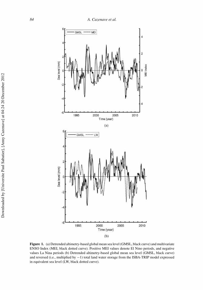
84 A. Cazenave et al.
Figure 1. (a) Detrended altimetry-based global mean sea level (GMSL, black curve) and multivariate
ENSO Index (MEI, black dotted curve). Positive MEI values denote El Nino periods, and negative
values La Nina periods (b) Detrended altimetry-based global mean sea level (GMSL, black curve)
and reversed (i.e., multiplied by −1) total land water storage from the ISBA-TRIP model expressed
in equivalent sea level (LW, black dotted curve).
Dow
nlo
aded
by [
Univ
ersi
te P
aul
Sab
atie
r], [A
nny C
azen
ave]
at
04:2
4 2
0 D
ecem
ber
2012
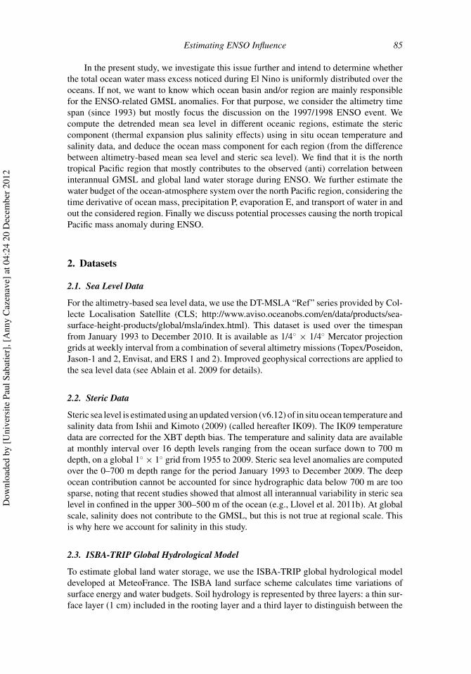
Estimating ENSO Influence 85
In the present study, we investigate this issue further and intend to determine whether
the total ocean water mass excess noticed during El Nino is uniformly distributed over the
oceans. If not, we want to know which ocean basin and/or region are mainly responsible
for the ENSO-related GMSL anomalies. For that purpose, we consider the altimetry time
span (since 1993) but mostly focus the discussion on the 1997/1998 ENSO event. We
compute the detrended mean sea level in different oceanic regions, estimate the steric
component (thermal expansion plus salinity effects) using in situ ocean temperature and
salinity data, and deduce the ocean mass component for each region (from the difference
between altimetry-based mean sea level and steric sea level). We find that it is the north
tropical Pacific region that mostly contributes to the observed (anti) correlation between
interannual GMSL and global land water storage during ENSO. We further estimate the
water budget of the ocean-atmosphere system over the north Pacific region, considering the
time derivative of ocean mass, precipitation P, evaporation E, and transport of water in and
out the considered region. Finally we discuss potential processes causing the north tropical
Pacific mass anomaly during ENSO.
2. Datasets
2.1. Sea Level Data
For the altimetry-based sea level data, we use the DT-MSLA “Ref” series provided by Col-
lecte Localisation Satellite (CLS; http://www.aviso.oceanobs.com/en/data/products/sea-
surface-height-products/global/msla/index.html). This dataset is used over the timespan
from January 1993 to December 2010. It is available as 1/4◦× 1/4◦ Mercator projection
grids at weekly interval from a combination of several altimetry missions (Topex/Poseidon,
Jason-1 and 2, Envisat, and ERS 1 and 2). Improved geophysical corrections are applied to
the sea level data (see Ablain et al. 2009 for details).
2.2. Steric Data
Steric sea level is estimated using an updated version (v6.12) of in situ ocean temperature and
salinity data from Ishii and Kimoto (2009) (called hereafter IK09). The IK09 temperature
data are corrected for the XBT depth bias. The temperature and salinity data are available
at monthly interval over 16 depth levels ranging from the ocean surface down to 700 m
depth, on a global 1◦× 1◦ grid from 1955 to 2009. Steric sea level anomalies are computed
over the 0–700 m depth range for the period January 1993 to December 2009. The deep
ocean contribution cannot be accounted for since hydrographic data below 700 m are too
sparse, noting that recent studies showed that almost all interannual variability in steric sea
level in confined in the upper 300–500 m of the ocean (e.g., Llovel et al. 2011b). At global
scale, salinity does not contribute to the GMSL, but this is not true at regional scale. This
is why here we account for salinity in this study.
2.3. ISBA-TRIP Global Hydrological Model
To estimate global land water storage, we use the ISBA-TRIP global hydrological model
developed at MeteoFrance. The ISBA land surface scheme calculates time variations of
surface energy and water budgets. Soil hydrology is represented by three layers: a thin sur-
face layer (1 cm) included in the rooting layer and a third layer to distinguish between the
Dow
nlo
aded
by [
Univ
ersi
te P
aul
Sab
atie
r], [A
nny C
azen
ave]
at
04:2
4 2
0 D
ecem
ber
2012
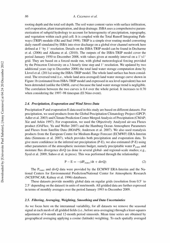
86 A. Cazenave et al.
rooting depth and the total soil depth. The soil water content varies with surface infiltration,
soil evaporation, plant transpiration, and deep drainage. ISBA uses a comprehensive param-
eterization of subgrid hydrology to account for heterogeneity of precipitation, topography,
and vegetation within each grid cell. It is coupled with the Total Runoff Integrating Path-
ways (TRIP) module (Oki and Sud 1998). TRIP is a simple river routing model converting
daily runoff simulated by ISBA into river discharge on a global river channel network here
defined at 1◦ by 1◦ resolution. Details on the ISBA-TRIP model can be found in Decharme
et al. (2006) and Alkama et al. (2010). The outputs of the ISBA-TRIP model cover the
period January 1950 to December 2008, with values given at monthly interval on a 1◦x1◦
grid. They are based on a forced mode run, with global meteorological forcing provided
by the Princeton University on a 3-hourly time step and 1◦ resolution. We updated by two
additional years (up to December 2008) the total land water storage computation done by
Llovel et al. (2011a) using the ISBA-TRIP model. The whole land surface has been consid-
ered. The reversed total (i.e., whole land area-averaged) land water storage curve shown in
Figure 1b (estimated from ISBA-TRIP model and expressed in sea level equivalent) has not
been detrended (unlike the GMSL curve) because the land water storage trend is negligible.
The correlation between the two curves is 0.4 over the whole period. It increases to 0.70
when considering the 1997–98 timespan (El Nino event).
2.4. Precipitation, Evaporation and Wind Stress Data
Precipitation P and evaporation E data used in this study are based on different datasets. For
precipitation, we used products from the Global Precipitation Climatology Project (GPCP;
Adler et al. 2003) and Climate Prediction Center Merged Analysis of Precipitation (CMAP;
Xie and Arkin 1997). For evaporation, we used the Objectively Analyzed air-sea Fluxes
product (OAFlux; Yu and Weller 2007) and the Hamburg Ocean Atmosphere Parameters
and Fluxes from Satellite Data (HOAPS; Anderson et al. 2007). We also used reanalysis
products from the European Centre for Medium-Range Forecast (ECMWF) ERA-Interim
data (Simmons et al. 2007), which provides both precipitation and evaporation data. To
give more confidence in the inferred net precipitation (P-E), we also estimated (P-E) using
other parameters of the atmospheric moisture budget, namely precipitable water Pwater and
moisture flux divergence divQ (as done in several global- and regional-scale studies; e.g.,
Syed et al. 2009; Sahoo et al. in press). This was performed through the relationship:
P − E = −(dPwater/dt + divQ) (2)
The Pwater and divQ data were provided by the ECMWF ERA-Interim and the Na-
tional Centers for Environmental Prediction/National Center for Atmospheric Research
(NCEP/NCAR; Kalnay et al. 1996) databases.
These datasets provide monthly global data on regular grids (resolution from 0.5◦ to
2.5◦ depending on the dataset) in units of mm/month. All gridded data are further expressed
in terms of monthly averages over the period January 1993 to December 2009.
2.5. Filtering, Averaging, Weighting, Smoothing and Data Uncertainties
As we focus here on the interannual variability, for all datasets we remove the seasonal
signal at each mesh of all gridded fields (i.e., before area-averaging) through a least-squares
adjustment of 6-month and 12-month period sinusoids. Mean time series are obtained by
geographical averaging applying a cosine (latitude) weighting. To each spatially averaged
Dow
nlo
aded
by [
Univ
ersi
te P
aul
Sab
atie
r], [A
nny C
azen
ave]
at
04:2
4 2
0 D
ecem
ber
2012
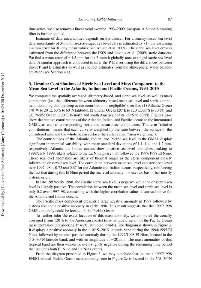
Estimating ENSO Influence 87
time series, we also remove a linear trend over the 1993–2009 timespan. A 3-month running
filter is further applied.
Estimate of data uncertainties depends on the dataset. For altimetry-based sea level
data, uncertainty of 3-month area-averaged sea level data is estimated to ∼1 mm (assuming
a 4 mm error for 10-day mean values; see Ablain et al. 2009). The steric sea level error is
estimated from the difference between the IK09 and Levitus et al. (2009) steric datasets.
We find a mean error of ∼1.5 mm for the 3-month globally area-averaged steric sea level
data. A similar approach is conducted to infer the P-E error using the differences between
direct P and E estimates as well as indirect estimates from the atmospheric water balance
equation (see Section 4.1).
3. Results: Contributions of Steric Sea Level and Mass Component to theMean Sea Level in the Atlantic, Indian and Pacific Oceans, 1993–2010
We computed the spatially averaged, altimetry-based, and steric sea level, as well as mass
component (i.e., the difference between altimetry-based mean sea level and steric compo-
nent, assuming that the deep ocean contribution is negligible) over the: (1) Atlantic Ocean
(70◦W to 20◦E; 60◦S to 60◦N latitude), (2) Indian Ocean (20◦E to 120◦E, 60◦S to 30◦N), and
(3) Pacific Ocean (120◦E to north and south America coasts, 60◦S to 60◦N). Figures 2a–c
show the relative contributions of the Atlantic, Indian, and Pacific oceans to the interannual
GMSL, as well as corresponding steric and ocean mass components. The term “relative
contributions” means that each curve is weighted by the ratio between the surface of the
considered area and the whole ocean surface (hereafter called “area weighting”).
The contributions of the Atlantic, Indian, and Pacific sea level to the GMSL display
significant interannual variability, with mean standard deviations of 1.1, 1.4, and 1.2 mm,
respectively. Atlantic and Indian oceans show positive sea level anomalies peaking in
1998/early 1999, likely related to the La Nina phase that followed the 1997/1998 El Nino.
These sea level anomalies are likely of thermal origin as the steric component closely
follows the observed sea level. The correlation between mean sea level and steric sea level
over 1997–98 is 0.75 and 0.67 for the Atlantic and Indian oceans, respectively, reinforcing
the fact that during this El Nino period the sea level anomaly in these two basins has mostly
a steric origin.
In late 1997/early 1998, the Pacific steric sea level is negative while the observed sea
level is slightly positive. The correlation between the mean sea level and steric sea level is
only 0.2 over 1997–98, contrasting with the higher correlation values discussed above for
the Atlantic and Indian oceans.
The Pacific mass component presents a large negative anomaly in 1997 followed by
a steep rise and a positive anomaly in early 1998. This result suggests that the 1997/1998
GMSL anomaly could be located in the Pacific Ocean.
To further infer the exact location of this mass anomaly, we computed the zonally
averaged (from 120◦E to the American coasts) time-latitude diagram of the Pacific Ocean
mass anomalies (considering 1◦ wide latitudinal bands). The diagram is shown in Figure 3.
It displays a positive anomaly in the ∼10◦S–20◦N latitude band during the 1994/1995 El
Nino, followed by another positive anomaly during the 1997/1998 El Nino, located in the
5◦S–30◦N latitude band, and with an amplitude of ∼20 mm. The mass anomalies of this
tropical band are then weaker or even slightly negative during the remaining time period
that includes both El Nino and La Nina events.
From the diagram presented in Figure 3, we may conclude that the main 1997/1998
ENSO-related Pacific Ocean mass anomaly seen in Figure 2c is located in the 5◦S–30◦N
Dow
nlo
aded
by [
Univ
ersi
te P
aul
Sab
atie
r], [A
nny C
azen
ave]
at
04:2
4 2
0 D
ecem
ber
2012
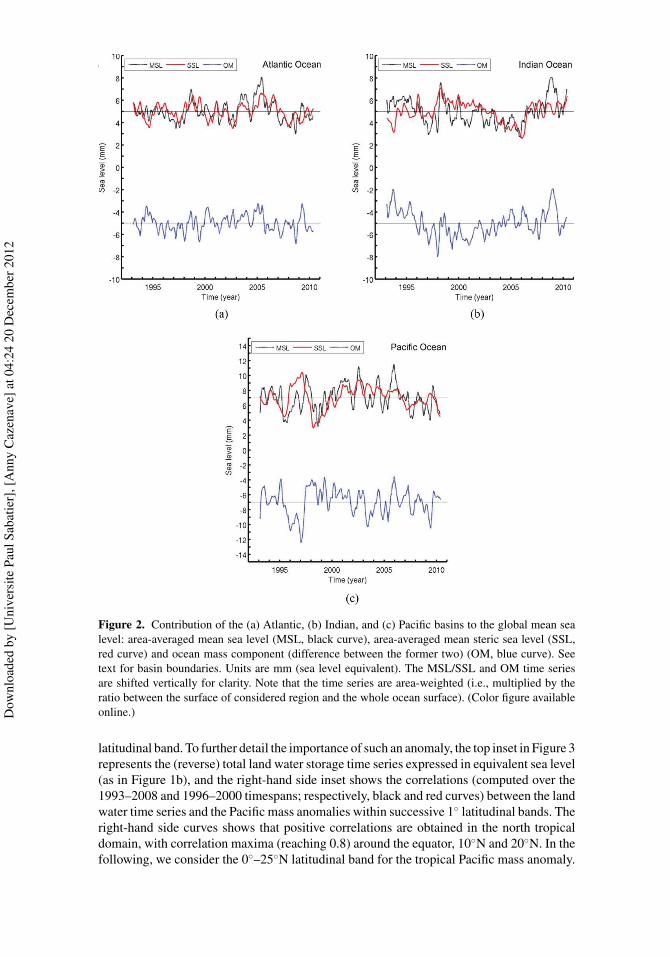
88 A. Cazenave et al.
Figure 2. Contribution of the (a) Atlantic, (b) Indian, and (c) Pacific basins to the global mean sea
level: area-averaged mean sea level (MSL, black curve), area-averaged mean steric sea level (SSL,
red curve) and ocean mass component (difference between the former two) (OM, blue curve). See
text for basin boundaries. Units are mm (sea level equivalent). The MSL/SSL and OM time series
are shifted vertically for clarity. Note that the time series are area-weighted (i.e., multiplied by the
ratio between the surface of considered region and the whole ocean surface). (Color figure available
online.)
latitudinal band. To further detail the importance of such an anomaly, the top inset in Figure 3
represents the (reverse) total land water storage time series expressed in equivalent sea level
(as in Figure 1b), and the right-hand side inset shows the correlations (computed over the
1993–2008 and 1996–2000 timespans; respectively, black and red curves) between the land
water time series and the Pacific mass anomalies within successive 1◦ latitudinal bands. The
right-hand side curves shows that positive correlations are obtained in the north tropical
domain, with correlation maxima (reaching 0.8) around the equator, 10◦N and 20◦N. In the
following, we consider the 0◦–25◦N latitudinal band for the tropical Pacific mass anomaly.
Dow
nlo
aded
by [
Univ
ersi
te P
aul
Sab
atie
r], [A
nny C
azen
ave]
at
04:2
4 2
0 D
ecem
ber
2012
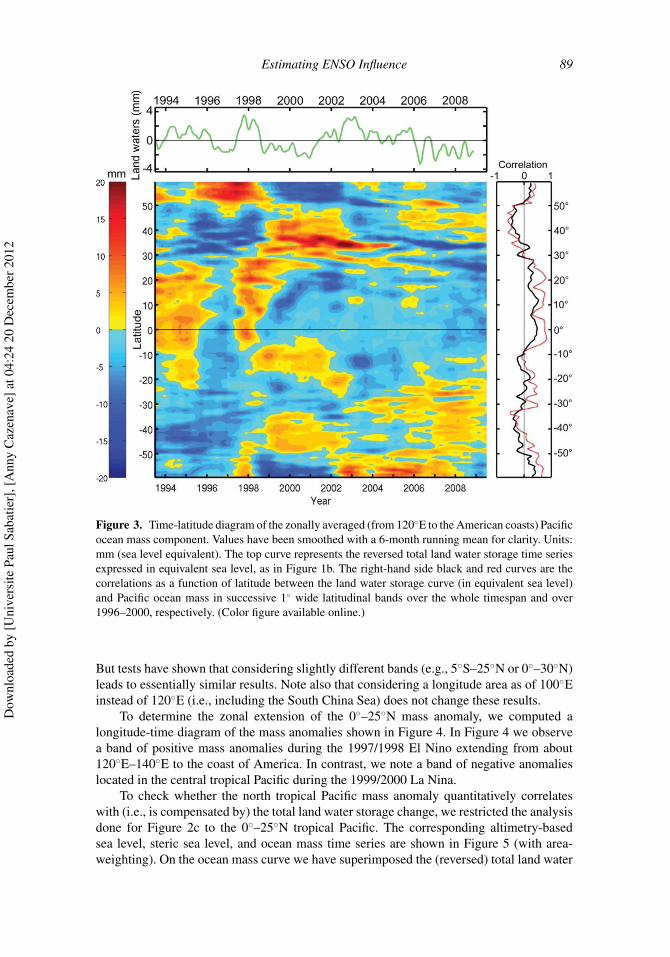
Estimating ENSO Influence 89
Figure 3. Time-latitude diagram of the zonally averaged (from 120◦E to the American coasts) Pacific
ocean mass component. Values have been smoothed with a 6-month running mean for clarity. Units:
mm (sea level equivalent). The top curve represents the reversed total land water storage time series
expressed in equivalent sea level, as in Figure 1b. The right-hand side black and red curves are the
correlations as a function of latitude between the land water storage curve (in equivalent sea level)
and Pacific ocean mass in successive 1◦ wide latitudinal bands over the whole timespan and over
1996–2000, respectively. (Color figure available online.)
But tests have shown that considering slightly different bands (e.g., 5◦S–25◦N or 0◦–30◦N)
leads to essentially similar results. Note also that considering a longitude area as of 100◦E
instead of 120◦E (i.e., including the South China Sea) does not change these results.
To determine the zonal extension of the 0◦–25◦N mass anomaly, we computed a
longitude-time diagram of the mass anomalies shown in Figure 4. In Figure 4 we observe
a band of positive mass anomalies during the 1997/1998 El Nino extending from about
120◦E–140◦E to the coast of America. In contrast, we note a band of negative anomalies
located in the central tropical Pacific during the 1999/2000 La Nina.
To check whether the north tropical Pacific mass anomaly quantitatively correlates
with (i.e., is compensated by) the total land water storage change, we restricted the analysis
done for Figure 2c to the 0◦–25◦N tropical Pacific. The corresponding altimetry-based
sea level, steric sea level, and ocean mass time series are shown in Figure 5 (with area-
weighting). On the ocean mass curve we have superimposed the (reversed) total land water
Dow
nlo
aded
by [
Univ
ersi
te P
aul
Sab
atie
r], [A
nny C
azen
ave]
at
04:2
4 2
0 D
ecem
ber
2012
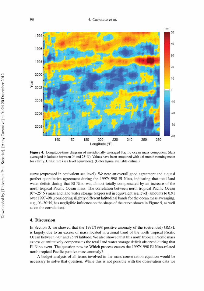
90 A. Cazenave et al.
Figure 4. Longitude-time diagram of meridionally averaged Pacific ocean mass component (data
averaged in latitude between 0◦ and 25◦N). Values have been smoothed with a 6-month running mean
for clarity. Units: mm (sea level equivalent). (Color figure available online.)
curve (expressed in equivalent sea level). We note an overall good agreement and a quasi
perfect quantitative agreement during the 1997/1998 El Nino, indicating that total land
water deficit during that El Nino was almost totally compensated by an increase of the
north tropical Pacific Ocean mass. The correlation between north tropical Pacific Ocean
(0◦–25◦N) mass and land water storage (expressed in equivalent sea level) amounts to 0.91
over 1997–98 (considering slightly different latitudinal bands for the ocean mass averaging,
e.g., 0◦–30◦N, has negligible influence on the shape of the curve shown in Figure 5, as well
as on the correlation).
4. Discussion
In Section 3, we showed that the 1997/1998 positive anomaly of the (detrended) GMSL
is largely due to an excess of mass located in a zonal band of the north tropical Pacific
Ocean between ∼0◦ and 25◦N latitude. We also showed that this north tropical Pacific mass
excess quantitatively compensates the total land water storage deficit observed during that
El Nino event. The question now is: Which process causes the 1997/1998 El Nino-related
north tropical Pacific positive mass anomaly?
A budget analysis of all terms involved in the mass conservation equation would be
necessary to solve that question. While this is not possible with the observation data we
Dow
nlo
aded
by [
Univ
ersi
te P
aul
Sab
atie
r], [A
nny C
azen
ave]
at
04:2
4 2
0 D
ecem
ber
2012
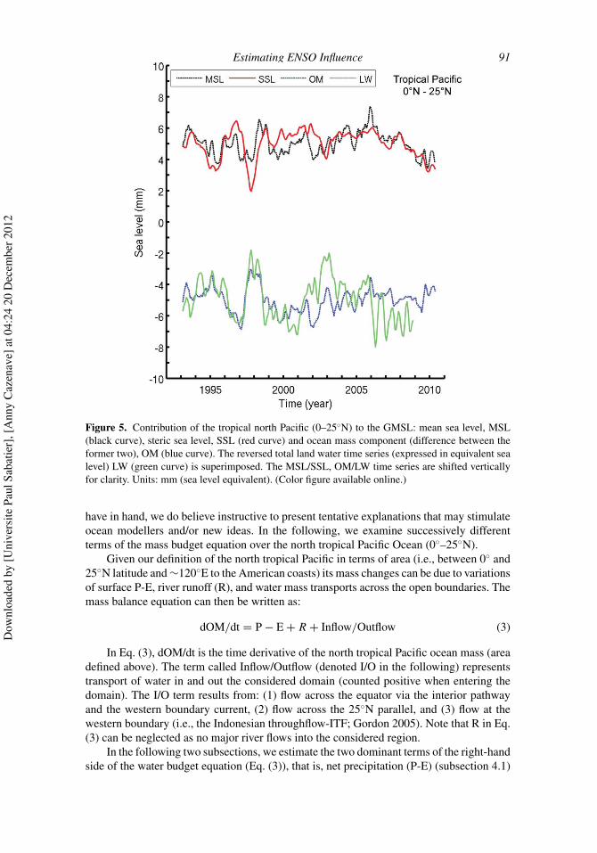
Estimating ENSO Influence 91
Figure 5. Contribution of the tropical north Pacific (0–25◦N) to the GMSL: mean sea level, MSL
(black curve), steric sea level, SSL (red curve) and ocean mass component (difference between the
former two), OM (blue curve). The reversed total land water time series (expressed in equivalent sea
level) LW (green curve) is superimposed. The MSL/SSL, OM/LW time series are shifted vertically
for clarity. Units: mm (sea level equivalent). (Color figure available online.)
have in hand, we do believe instructive to present tentative explanations that may stimulate
ocean modellers and/or new ideas. In the following, we examine successively different
terms of the mass budget equation over the north tropical Pacific Ocean (0◦–25◦N).
Given our definition of the north tropical Pacific in terms of area (i.e., between 0◦ and
25◦N latitude and ∼120◦E to the American coasts) its mass changes can be due to variations
of surface P-E, river runoff (R), and water mass transports across the open boundaries. The
mass balance equation can then be written as:
dOM/dt = P − E + R + Inflow/Outflow (3)
In Eq. (3), dOM/dt is the time derivative of the north tropical Pacific ocean mass (area
defined above). The term called Inflow/Outflow (denoted I/O in the following) represents
transport of water in and out the considered domain (counted positive when entering the
domain). The I/O term results from: (1) flow across the equator via the interior pathway
and the western boundary current, (2) flow across the 25◦N parallel, and (3) flow at the
western boundary (i.e., the Indonesian throughflow-ITF; Gordon 2005). Note that R in Eq.
(3) can be neglected as no major river flows into the considered region.
In the following two subsections, we estimate the two dominant terms of the right-hand
side of the water budget equation (Eq. (3)), that is, net precipitation (P-E) (subsection 4.1)
Dow
nlo
aded
by [
Univ
ersi
te P
aul
Sab
atie
r], [A
nny C
azen
ave]
at
04:2
4 2
0 D
ecem
ber
2012
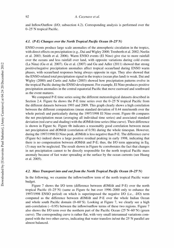
92 A. Cazenave et al.
and Inflow/Outflow (I/O; subsection 4.2). Corresponding analysis is performed over the
0–25◦N tropical Pacific.
4.1. (P-E) Changes over the North Tropical Pacific Ocean (0–25◦N)
ENSO events produce large scale anomalies of the atmospheric circulation in the tropics,
with direct effects on precipitation (e.g., Dai and Wigley 2000; Trenberth et al. 2002; Neelin
et al. 2003; Smith et al. 2006). Warm ENSO events (El Nino) give rise to more rainfall
over the oceans and less rainfall over land, with opposite variations during cold events
(La Nina) (Gu et al. 2007). Gu et al. (2007) and Gu and Adler (2011) showed that strong
positive/negative precipitation anomalies affect tropical ocean/land during ENSO warm
phases, with ocean/land responses being always opposite in sign. They also showed that
the ENSO-related total precipitation signal in the tropics (ocean plus land) is weak. Dai and
Wigley (2000) and Curtis and Adler (2003) showed how precipitation patterns evolve in
the tropical Pacific during the ENSO development. For example, El Nino produces positive
precipitation anomalies in the central equatorial Pacific that move eastward and southward
as the event matures.
We computed P-E time series using the different meteorological datasets described in
Section 2.4. Figure 6a shows the P-E time series over the 0–25◦N tropical Pacific from
the different datasets between 1993 and 2009. This graph clearly shows a high correlation
between the different computations (mean standard deviation of 0.44 mm/month over the
whole period) and particularly during the 1997/1998 El Nino event. Figure 6b compares
the net precipitation mean (averaging all individual time series) and associated standard
deviation (red curve and shading) with the dOM/dt time series (blue curve). Their difference
is shown in Figure 6c. Figure 6b indicates a reasonably good correlation between mean
net precipitation and dOM/dt (correlation of 0.58) during the whole timespan. However,
during the 1997/1998 El Nino peak, dOM/dt is less negative than P-E. The difference curve
(Figure 6c) indeed shows a large positive residual peaking in early 1998, indicating that
there is no compensation between dOM/dt and P-E; thus, the I/O term appearing in Eq.
(3) may not be neglected. The result shown in Figure 6c corroborates the fact that changes
in net precipitation cannot to be directly responsible for the north tropical Pacific mass
anomaly because of fast water spreading at the surface by the ocean currents (see Huang
et al. 2005).
4.2. Mass Transport into and out from the North Tropical Pacific Ocean (0–25◦N)
In the following, we examine the inflow/outflow term of the north tropical Pacific water
budget.
Figure 7 shows the I/O term (difference between dOM/dt and P-E) over the north
tropical Pacific (0–25◦N) (same as Figure 6c but over 1996–2000 only to enhance the
1997/1998 ENSO period) on which is superimposed the negative I/O (i.e., -I/O) term
computed as the difference between dOM/dt and P-E over the whole Indian Ocean
and whole south Pacific domain (0–60◦S). Looking at Figure 7, we clearly see a high
anti-correlation (−0.95) between the inflow/outflow terms of these two regions. Figure 7
also shows the I/O term over the northern part of the Pacific Ocean (25◦N–60◦N) (green
curve). The corresponding curve is rather flat, with very small interannual variations com-
pared with the two other curves, indicating that water transfers in/out the 25◦N parallel are
almost balanced.
Dow
nlo
aded
by [
Univ
ersi
te P
aul
Sab
atie
r], [A
nny C
azen
ave]
at
04:2
4 2
0 D
ecem
ber
2012
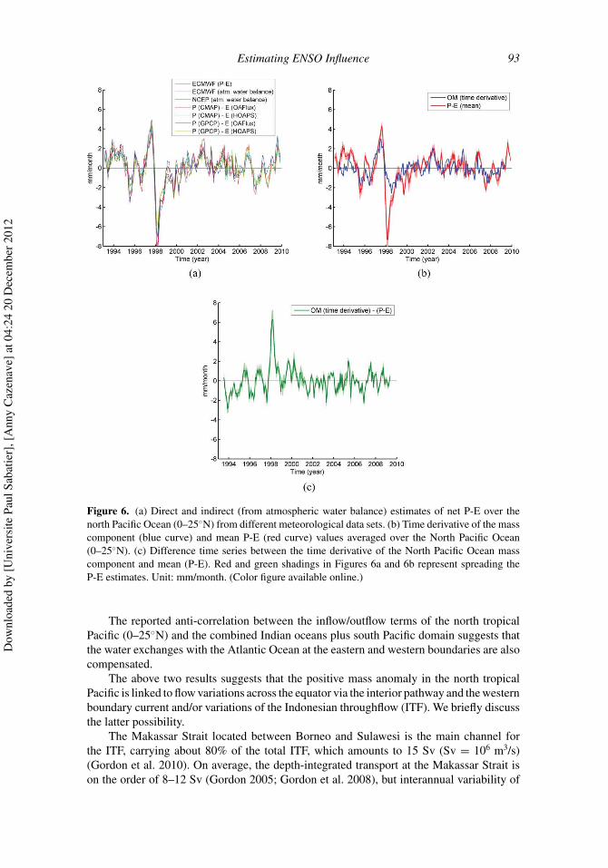
Estimating ENSO Influence 93
Figure 6. (a) Direct and indirect (from atmospheric water balance) estimates of net P-E over the
north Pacific Ocean (0–25◦N) from different meteorological data sets. (b) Time derivative of the mass
component (blue curve) and mean P-E (red curve) values averaged over the North Pacific Ocean
(0–25◦N). (c) Difference time series between the time derivative of the North Pacific Ocean mass
component and mean (P-E). Red and green shadings in Figures 6a and 6b represent spreading the
P-E estimates. Unit: mm/month. (Color figure available online.)
The reported anti-correlation between the inflow/outflow terms of the north tropical
Pacific (0–25◦N) and the combined Indian oceans plus south Pacific domain suggests that
the water exchanges with the Atlantic Ocean at the eastern and western boundaries are also
compensated.
The above two results suggests that the positive mass anomaly in the north tropical
Pacific is linked to flow variations across the equator via the interior pathway and the western
boundary current and/or variations of the Indonesian throughflow (ITF). We briefly discuss
the latter possibility.
The Makassar Strait located between Borneo and Sulawesi is the main channel for
the ITF, carrying about 80% of the total ITF, which amounts to 15 Sv (Sv = 106 m3/s)
(Gordon et al. 2010). On average, the depth-integrated transport at the Makassar Strait is
on the order of 8–12 Sv (Gordon 2005; Gordon et al. 2008), but interannual variability of
Dow
nlo
aded
by [
Univ
ersi
te P
aul
Sab
atie
r], [A
nny C
azen
ave]
at
04:2
4 2
0 D
ecem
ber
2012
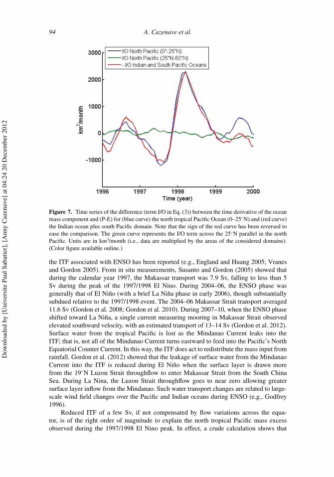
94 A. Cazenave et al.
Figure 7. Time series of the difference (term I/O in Eq. (3)) between the time derivative of the ocean
mass component and (P-E) for (blue curve) the north tropical Pacific Ocean (0–25◦N) and (red curve)
the Indian ocean plus south Pacific domain. Note that the sign of the red curve has been reversed to
ease the comparison. The green curve represents the I/O term across the 25◦N parallel in the north
Pacific. Units are in km3/month (i.e., data are multiplied by the areas of the considered domains).
(Color figure available online.)
the ITF associated with ENSO has been reported (e.g., England and Huang 2005; Vranes
and Gordon 2005). From in situ measurements, Susanto and Gordon (2005) showed that
during the calendar year 1997, the Makassar transport was 7.9 Sv, falling to less than 5
Sv during the peak of the 1997/1998 El Nino. During 2004–06, the ENSO phase was
generally that of El Nino (with a brief La Nina phase in early 2006), though substantially
subdued relative to the 1997/1998 event. The 2004–06 Makassar Strait transport averaged
11.6 Sv (Gordon et al. 2008; Gordon et al. 2010). During 2007–10, when the ENSO phase
shifted toward La Nina, a single current measuring mooring in Makassar Strait observed
elevated southward velocity, with an estimated transport of 13–14 Sv (Gordon et al. 2012).
Surface water from the tropical Pacific is lost as the Mindanao Current leaks into the
ITF; that is, not all of the Mindanao Current turns eastward to feed into the Pacific’s North
Equatorial Counter Current. In this way, the ITF does act to redistribute the mass input from
rainfall. Gordon et al. (2012) showed that the leakage of surface water from the Mindanao
Current into the ITF is reduced during El Nino when the surface layer is drawn more
from the 19◦N Luzon Strait throughflow to enter Makassar Strait from the South China
Sea. During La Nina, the Luzon Strait throughflow goes to near zero allowing greater
surface layer inflow from the Mindanao. Such water transport changes are related to large-
scale wind field changes over the Pacific and Indian oceans during ENSO (e.g., Godfrey
1996).
Reduced ITF of a few Sv, if not compensated by flow variations across the equa-
tor, is of the right order of magnitude to explain the north tropical Pacific mass excess
observed during the 1997/1998 El Nino peak. In effect, a crude calculation shows that
Dow
nlo
aded
by [
Univ
ersi
te P
aul
Sab
atie
r], [A
nny C
azen
ave]
at
04:2
4 2
0 D
ecem
ber
2012
Estimating ENSO Influence 95
1 Sv reduction over 1 month corresponds to a water volume of 2600 km3 remaining in
the north tropical Pacific while the observed mass excess in this region corresponds to
∼1500 km3.
The above results may suggest that the 1997/1998 El Nino event could be related to
an important variation of the water mass transfer between the north tropical Pacific Ocean
(0–25◦N) and Indian and South Pacific oceans. In particular, a reduction of the ITF possibly
combined with an intensification of water transfers from the south Pacific could have led to
an important water mass increase in the north tropical Pacific region. Even though this study
does not allow us to discriminate between the relative importance of these contributions, we
cannot exclude that an important part of the water transport variations may have occurred at
the Makassar Strait. Further quantitative analyses are required to confirm this, for example,
using ocean general circulation model outputs.
5. Conclusion
The results presented in this study confirm that interannual variability of the GMSL has
essentially a water mass origin, as the interannual GMSL is highly inversely correlated
with total land water storage change, in particular during ENSO events. Focusing on the
large positive GMSL anomaly observed during the 1997/1998 El Nino, we show that this
anomaly is largely due to a mass excess of the north tropical Pacific (located between
0◦ and 25◦N in latitude and ∼120◦E to the American coasts in longitude). We also show
that the ocean-atmosphere water budget computed over the north tropical Pacific (0–25◦N)
is not closed during the 1997/1998 El Nino peak if the inflow/outflow terms are not
accounted for. The north tropical Pacific mass excess associated with this El Nino event
is consistent with the reduced depth-integrated water transport at the Makassar Strait
(the Indonesian throughflow) previously reported during the 1997/1998 El Nino, although
we cannot exclude that flow across the equator via the interior pathway and the western
boundary current also play some role. Further analyses are required to quantitatively confirm
or infirm this conclusion.
A similar investigation should be performed for La Nina events, during which impor-
tant drops of the GMSL are observed. This was the case, for example, in 2007–08 and
2010–11. It will be interesting to determine whether the transport at the Makassar Strait
is also a good candidate to explain the GMSL variability, as well as to assess the poten-
tial role of meridional mass transports across the equator. In line with our observation-
based results, a precise quantification of all processes responsible for the GMSL at the
ENSO time scale will be conducted with the help of ocean general circulation model
outputs.
Acknowledgements
O. Henry, S. Munier, W. Llovel, and H. Palanisamy are supported, respectively, by a
European grant in the context of the Monarch Project, a postdoctoral grant from CNES, a
postdoctoral grant from JPL/NASA, and the French ANR CECILE project. A. L. Gordon
research is supported by the National Science Foundation grant OCE-0725935. This is
Lamont-Doherty contribution number 7545.
We thank H. Douville, B. Decharme, and R. Alkama for providing us with the ISBA-
TRIP model outputs.
Dow
nlo
aded
by [
Univ
ersi
te P
aul
Sab
atie
r], [A
nny C
azen
ave]
at
04:2
4 2
0 D
ecem
ber
2012
96 A. Cazenave et al.
References
Ablain, M., A. Cazenave, S. Guinehut, and G. Valladeau. 2009. A new assessment of global mean
sea level from altimeters highlights a reduction of global slope from 2005 to 2008 in agreement
with in-situ measurements. Ocean Sci. 5(2):193–201.
Adler, R. F., G. J. Huffman, A. Chang, R. Ferraro, P. P. Xie, J. Janowiak, B. Rudolf, U. Schneider,
S. Curtis, D. Bolvin, A. Gruber, J. Susskind, P. Arkin, and E. Nelkin. 2003. The version-2
global precipitation climatology project (GPCP) monthly precipitation analysis (1979–present).
Journal of Hydrometeorology 4:1147–1167.
Alkama, R., B. Decharme, H. Douville, A. Voldoire, S. Tyteca, P. Le Moigne, M. Becker, A. Cazenave,
and J. Sheffield. 2010. Global evaluation of the ISBA-TRIP continental hydrological system Part
1: Comparison to GRACE terrestrial water storage estimates and in-situ river discharges. Journal
of Hydrometeorology 11:583–600. doi: 10.1175/2010JHM1211
Andersson, A., S. Bakan, K. Fennig, H. Grassl, C. Klepp, and J. Schulz. 2007. Hamburg ocean
atmosphere parameters and fluxes from satellite data – HOAPS-3 – monthly mean. World Data
Center for Climate electronic publication.
Bindoff, N., J. Willebrand, V. Artale, A. Cazenave, J. Gregory, S. Gulev, K. Hanawa, C. Le Quere,
S. Levitus, Y. Nojiri, C. K. Shum, L. Talley, and A. Unnikrishnan. 2007. Observations: Oceanic
climate and sea level. In ed. S. Solomon, D. Qin, M. Manning, Z. Chen, M. Marquis, K. B. Averyt,
M. Tignor, and H. L. Miller, Climate Change 2007: The Physical Science Basis. Contribution of
Working Group I to the Fourth Assessment Report of the Intergouvernmental Panel on Climate
Change. Cambridge: Cambridge University Press.
Cazenave, A., and W. Llovel. 2010. Contemporary sea level rise. Annual Review in Marine Science
2:145–173.
Church, J. A., N. J. White, L. F. Konikow, C. M. Domingues, J. G. Cogley, E. Rignot, J. M. Gregory, M.
R. van den Broeke, A. J. Monaghan, and I. Velicogna. 2011. Revisiting the Earth’s sea level and
energy budgets from 1961 to 2008. Geophys. Res. Lett. 38:L18601. doi: 10.1029/2011GL048794
Curtis, S., and R. F. Adler. 2003. Evolution of El Nino-precipitation relationships from satellites and
gauges. J. Geophys. Res. 108:4153. doi: 10.1029/2002JD002690
Dai, A., and T. M. L. Wigley. 2000. Global patterns of ENSO-induced precipitation. Geophys. Res.
Lett. 27(9):1283–1286.
Decharme, B., and H. Douville. 2006. Introduction of a sub-grid hydrology in the ISBA land surface
model. Climate Dyn. 26:65–78.
England, M., and F. Huang. 2005. On the interannual variability of the Indonesian throughflow and
its linkage with ENSO. J. Clim. 18:1435–1444.
Godfrey, J. S. 1996. The effect of the Indonesian throughflow on ocean circulation and heat exchange
with the atmosphere: A review. J. Geophys. Res. 101(C5):12217–12237.
Gordon, A. L. 2005. Oceanography of the Indonesian seas and their throughflow. Oceanography
18(4):14–27.
Gordon, A. L., R. D. Susanto, A. Ffield, B. A. Huber, W. Pranowo, and S. Wirasantosa.
2008. Makassar Strait throughflow, 2004 to 2006. Geophys. Res. Letters 35:L24605. doi:
10.1029/2008GL036372
Gordon, A. L., J. Sprintall, H. M. Van Aken, D. Susanto, S. Wijffels, R. Molcard, A. Ffield, W.
Pranowo, and S. Wirasantosa. 2010. The Indonesian throughflow during 2004–2006 as observed
by the INSTANT program. Modeling and observing the Indonesian throughflow. In Ed. A. L.
Gordon and V. M. Kamenkovich, Dynamics of Atmosphere and Oceans 50:115–128.
Gordon, A. L., B. A. Huber, E. J. Metzger, R. D. Susanto, H. E. Hurlburt, and T. R. Adi. 2012. South
China Sea throughflow impact on the Indonesian throughflow. Geophys. Res. Lett. (in revision).
Gu, G., R. F. Adler, G. J. Huffman, and S. Curtis. 2007. Tropical rainfall variability on interannual
to interdecadal and longer time scales derived from the GPCP monthly products. J. Climate
20:4033–4046.
Gu, G., and R. F. Adler. 2011. Precipitation and temperature variations on the interannual time scale:
Assessing the impact of ENSO and volcanic eruptions. J. Climate 24:2258–2270.
Dow
nlo
aded
by [
Univ
ersi
te P
aul
Sab
atie
r], [A
nny C
azen
ave]
at
04:2
4 2
0 D
ecem
ber
2012
Estimating ENSO Influence 97
Huang, B. Y., V. M. Mehta, and N. Schneider. 2005. Oceanic response to idealized net atmospheric
freshwater in the Pacific at the decadal time scale. J. Phys. Oceanography 35(12):2467–2486.
doi: 10.1175/JPO2820.1
Ishii, M., and M. Kimoto. 2009. Reevaluation of historical ocean heat content variations with varying
XBT and MBT depth bias corrections. Journal of Oceanography 65:287–299.
Kalnay, E., M. Kanamitsu, R. Kistler, W. Collins, D. Deaven, L. Gandin, M. Iredell, S. Saha, G. White,
J. Woollen, Y. Zhu, M. Chelliah, W. Ebisuzaki, W. Higgins, J. Janowiak, K. C. Mo, C. Ropelewski,
J. Wang, A. Leetmaa, R. Reynolds, R. Jenne, and D. Joseph. 1996. The NCEP/NCAR 40-year
reanalysis project. Bulletin of the American Meteorological Society 77:437–471.
Levitus, S., J. I. Antonov, T. P. Boyer, R. A. Locarnini, H. E. Garcia, and A. V. Mishonov. 2009.
Global ocean heat content 1955–2008 in light of recently revealed instrumentation problems.
Geophys. Res. Lett. 36:L07608. doi: 10.1029/2008GL037155
Llovel, W., M. Becker, A. Cazenave, S. Jevrejeva, R. Alkama, B. Decharme, H. Douville, M. Ablain,
and B. Beckley. 2011a. Terrestrial waters and sea level variations on interannual time scale.
Global Planet Change 75:76–82. doi: 10.1016/j.gloplacha.2010.10.008
Llovel, W., B. Meyssignac, and A. Cazenave. 2011b. Steric sea level variations over 2004–2010 as a
function of region and depth: Inference on the mass component variability of the North Atlantic.
Geophys. Res. Lett. 38:L15608. doi: 101029/2011GL047411
Neelin, J. D., C. Chou, and H. Su. 2003. Tropical drought regions in global warming and El Nino
teleconnections. Geophys. Res. Lett. 30:2275. doi: 10.1029/2003GL018625
Nerem, R. S., D. P. Chambers, C. Choe, and G. T. Mitchum. 2010. Estimating mean sea level change
from the TOPEX and Jason altimeter missions. Marine Geodesy 33(1):435–446.
Oki, T., and Y. C. Sud. 1998. Design of total runoff integrating pathways (TRIP)—a global river
channel network. Earth Interactions 2(1):1–37.
Sahoo, A. K., M. Pan, T. J. Troy, R. K. Vinukollu, J. Sheffield, and E. F. Wood. in press. Reconciling
the global terrestrial water budget using satellite remote sensing. Remote Sensing of Environment.
Simmons, A., S. Uppala, D. Dee, and S. Kobayashi. 2007. Era-interim: New ECMWF reanalysis
products from 1989 onwards. ECMWF Newsletter 110.
Smith, T. M., X. Yin, and A. Gruber. 2006. Variations in annual global precipitation (1979–2004),
based on the global precipitation climatology project 2.5◦ analysis. Geophys. Res. Lett.
33:L06705. doi: 10.1029/2005GL025393
Susanto, R. D., and A. L. Gordon. 2005. Velocity and transport of the Makassar Strait throughflow.
J. Geophys. Res. 110:C01005. doi: 10.1029/2004JC002425
Syed, T. H., J. S. Famiglietti, and D. P. Chambers. 2009. GRACE-based estimates of terrestrial
freshwater discharge from basin to continental scales. Journal of Hydrometeorology 10:22–40.
Trenberth, K. E., J. M. Caron, D. P. Stepaniak, and S. Worley. 2002. Evolution of El Nino-
southern oscillation and global atmospheric surface temperatures. J. Geophys. Res. 107:4065.
doi: 10.1029/2000JD000298
Vranes, K., and A. L. Gordon. 2005. Comparison if Indonesian troughflow transport obser-
vations, Makassar Strait to eastern Indian Ocean. Geophys. Res. Lett. 32:L10606. doi:
10.1029/2004GL022158
Wolter, K., and M. S. Timlin. 1998. Measuring the strength of ENSO—how does 1997/98 rank?
Weather 53:315–324.
Xie, P. P., and P. A. Arkin. 1997. Global precipitation: A 17-year monthly analysis based on gauge
observations, satellite estimates, and numerical model outputs. Bulletin of the American Meteo-
rological Society 78:2539–2558.
Yu, L., and R. A. Weller. 2007. Objectively analyzed air-sea heat fluxes for the global ice-free oceans
(1981–2005). Bull. Amer. Meteorol. Soc. 88(4):527–539.
Dow
nlo
aded
by [
Univ
ersi
te P
aul
Sab
atie
r], [A
nny C
azen
ave]
at
04:2
4 2
0 D
ecem
ber
2012

34 La Météorologie - n° 79 - novembre 2012Océanetatm
osphère
L’influence d’El Niño etde La Niña sur le niveaude la mer
Anny Cazenave(1), Habib Boubacar Dieng(1), SimonMunier(1),Olivier Henry(1), BenoitMeyssignac(1), Hindumathi Palanisamy(1)
etWilliam Llovel(2)
(1) Laboratoire d’études en géophysique et océanographie spatiales (LEGOS)ObservatoireMidi-Pyrénées18 avenue Édouard Belin - 31401 Toulouse Cedex 9, France
(2) Jet Propulsion Laboratory, Pasadena, États-Unis
Résumé
Outre une hausse moyenne de l’ordrede 3 mm par an, le niveau moyen glo-bal de la mer présente des fluctua-tions de quelques millimètres durantles événements El Niño et La Niña.Lors de El Niño, on observe une ano-malie positive alors qu’à La Niña cor-respond une anomalie négative duniveau de la mer. Ces fluctuations duniveau moyen global de la mer sontinversement corrélées aux variationsdu stock d’eau total sur les conti-nents. Cette observation est en accordavec le fait que, durant El Niño, ilpleut davantage sur l’océan que surles continents, et inversement durantLa Niña. Cela suggère que les fluc-tuations du niveau moyen global de lamer associées aux événements ElNiño/La Niña sont plutôt dues à desvariations de masse de l’océan qu’àdes variations d’origine thermique.Dans cet article, on montre qu’aucours de l’événement El Niño de1997-1998, l’anomalie positive demasse de l’océan est localisée dansl’océan Pacif ique tropical nord.L’excès de masse de cette région com-pense de manière quasi parfaite ledéficit du stock d’eau total des conti-nents à cette période.
…
L’altimétrie spatiale de haute préci-sion a révélé que le niveau moyenglobal de la mer a monté assez
régulièrement depuis début 1993, à lavitesse moyenne de 3,2 ± 0,4 mm par an(Meyssignac et Cazenave, 2012).Cependant, si l’on y regarde de près, onremarque de petites oscillations interan-nuelles autour de la tendance linéaire(après retrait du cycle saisonnier), dontl’amplitude est de l’ordre de quelquesmillimètres. Il est assez frappant que leniveau moyen global de la mer présenteune anomalie positive assez marquéelors du grand El Niño de 1997-1998.Cela est illustré sur la figure 1 qui pré-sente les fluctuations du niveau moyenglobal de la mer entre 1993 et 2011
(après retrait d’une tendance linéairemoyenne sur la période). La figure 1montre aussi des anomalies négativesdu niveau moyen global de la mer lorsdes événements La Niña de 2007-2008et de 2010-2011. Quelle est la cause deces anomalies et quel est le lien entre leniveau moyen de la mer et les événe-ments ENSO (El Niño-SouthernOscillation) ?
Aux échelles de temps interannuelles àmulti-décennales, les principaux phéno-mènes à l’origine des variations duniveau moyen global de la mer sont :- l’expansion (ou la contraction) ther-mique des océans, causée par des varia-tions de la température de la mer
(lorsque la tempéra-ture augmente, l’eaude mer se dilate et leniveau de la mers’élève, et inverse-ment) ;- l’augmentation (oula diminution) ducontenu en eau des
Figure 1 - En noir : niveaumoyen global de la mer mesurépar altimétrie spatiale entrejanvier 1993 et décembre 2011(données du site AVISO :www.aviso.oceanobs.com). Latendance linéaire de 3,1 mm/ana été retirée. Les données entre60° S et 60° N sont consi-dérées.En vert : stock d’eau continentaltotal, estimé à partir du modèlehydrologique ISBA-TRIP deMétéo-France, exprimé enéquivalent « niveau de la mer ».
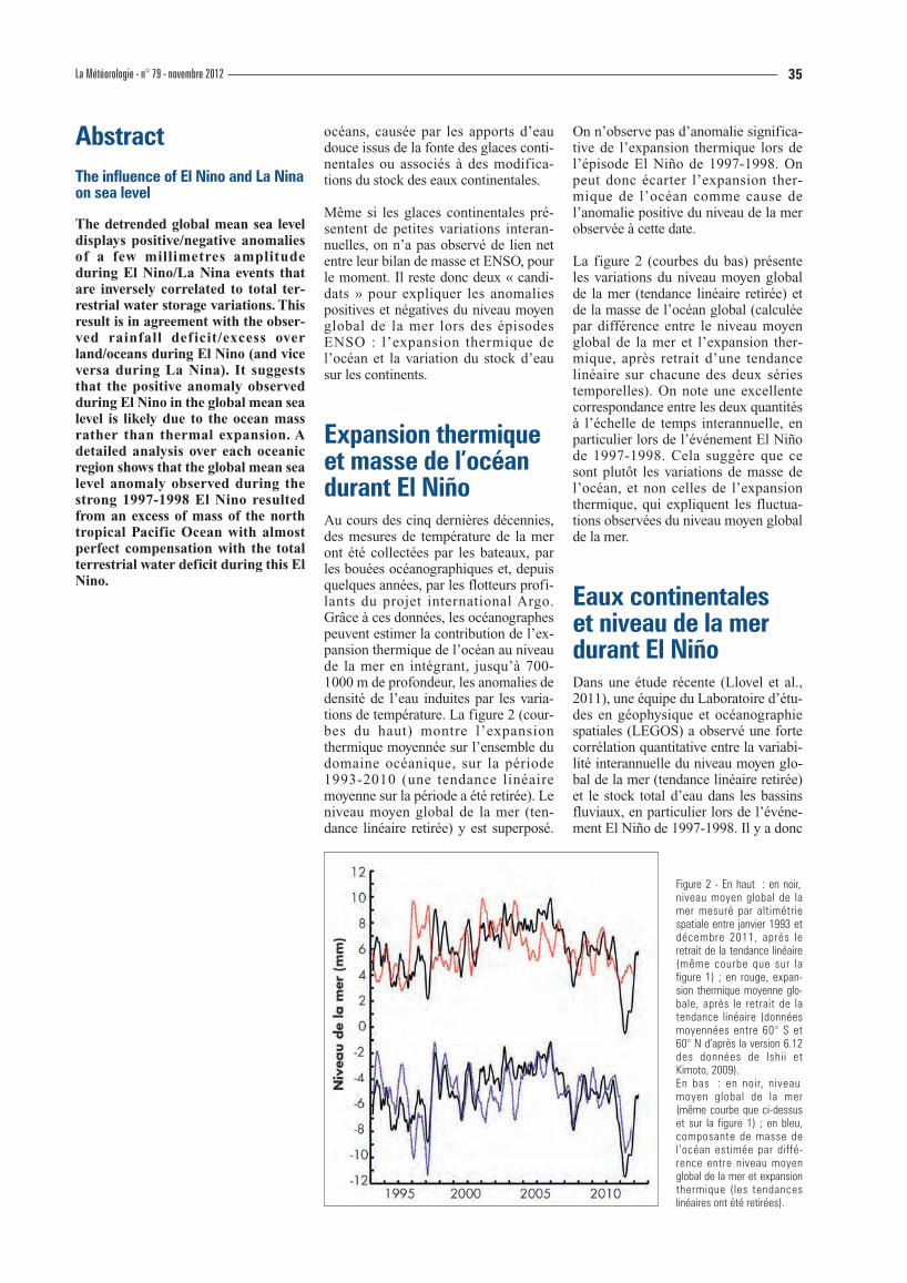
35La Météorologie - n° 79 - novembre 2012
Abstract
The influence of El Nino and La Ninaon sea level
The detrended global mean sea leveldisplays positive/negative anomaliesof a few millimetres amplitudeduring El Nino/La Nina events thatare inversely correlated to total ter-restrial water storage variations. Thisresult is in agreement with the obser-ved rainfall def icit/excess overland/oceans during El Nino (and viceversa during La Nina). It suggeststhat the positive anomaly observedduring El Nino in the global mean sealevel is likely due to the ocean massrather than thermal expansion. Adetailed analysis over each oceanicregion shows that the global mean sealevel anomaly observed during thestrong 1997-1998 El Nino resultedfrom an excess of mass of the northtropical Pacific Ocean with almostperfect compensation with the totalterrestrial water deficit during this ElNino.
océans, causée par les apports d’eaudouce issus de la fonte des glaces conti-nentales ou associés à des modifica-tions du stock des eaux continentales.
Même si les glaces continentales pré-sentent de petites variations interan-nuelles, on n’a pas observé de lien netentre leur bilan de masse et ENSO, pourle moment. Il reste donc deux « candi-dats » pour expliquer les anomaliespositives et négatives du niveau moyenglobal de la mer lors des épisodesENSO : l’expansion thermique del’océan et la variation du stock d’eausur les continents.
Expansion thermiqueet masse de l’océandurant El NiñoAu cours des cinq dernières décennies,des mesures de température de la meront été collectées par les bateaux, parles bouées océanographiques et, depuisquelques années, par les flotteurs profi-lants du projet international Argo.Grâce à ces données, les océanographespeuvent estimer la contribution de l’ex-pansion thermique de l’océan au niveaude la mer en intégrant, jusqu’à 700-1000 m de profondeur, les anomalies dedensité de l’eau induites par les varia-tions de température. La figure 2 (cour-bes du haut) montre l’expansionthermique moyennée sur l’ensemble dudomaine océanique, sur la période1993-2010 (une tendance linéairemoyenne sur la période a été retirée). Leniveau moyen global de la mer (ten-dance linéaire retirée) y est superposé.
On n’observe pas d’anomalie significa-tive de l’expansion thermique lors del’épisode El Niño de 1997-1998. Onpeut donc écarter l’expansion ther-mique de l’océan comme cause del’anomalie positive du niveau de la merobservée à cette date.
La figure 2 (courbes du bas) présenteles variations du niveau moyen globalde la mer (tendance linéaire retirée) etde la masse de l’océan global (calculéepar différence entre le niveau moyenglobal de la mer et l’expansion ther-mique, après retrait d’une tendancelinéaire sur chacune des deux sériestemporelles). On note une excellentecorrespondance entre les deux quantitésà l’échelle de temps interannuelle, enparticulier lors de l’événement El Niñode 1997-1998. Cela suggère que cesont plutôt les variations de masse del’océan, et non celles de l’expansionthermique, qui expliquent les fluctua-tions observées du niveau moyen globalde la mer.
Eaux continentaleset niveau de la merdurant El NiñoDans une étude récente (Llovel et al.,2011), une équipe du Laboratoire d’étu-des en géophysique et océanographiespatiales (LEGOS) a observé une fortecorrélation quantitative entre la variabi-lité interannuelle du niveau moyen glo-bal de la mer (tendance linéaire retirée)et le stock total d’eau dans les bassinsfluviaux, en particulier lors de l’événe-ment El Niño de 1997-1998. Il y a donc
Figure 2 - En haut : en noir,niveau moyen global de lamer mesuré par altimétriespatiale entre janvier 1993 etdécembre 2011, après leretrait de la tendance linéaire(même courbe que sur lafigure 1) ; en rouge, expan-sion thermique moyenne glo-bale, après le retrait de latendance linéaire (donnéesmoyennées entre 60° S et60° N d’après la version 6.12des données de Ishii etKimoto, 2009).En bas : en noir, niveaumoyen global de la mer(même courbe que ci-dessuset sur la figure 1) ; en bleu,composante de masse del’océan estimée par diffé-rence entre niveau moyenglobal de la mer et expansionthermique (les tendanceslinéaires ont été retirées).
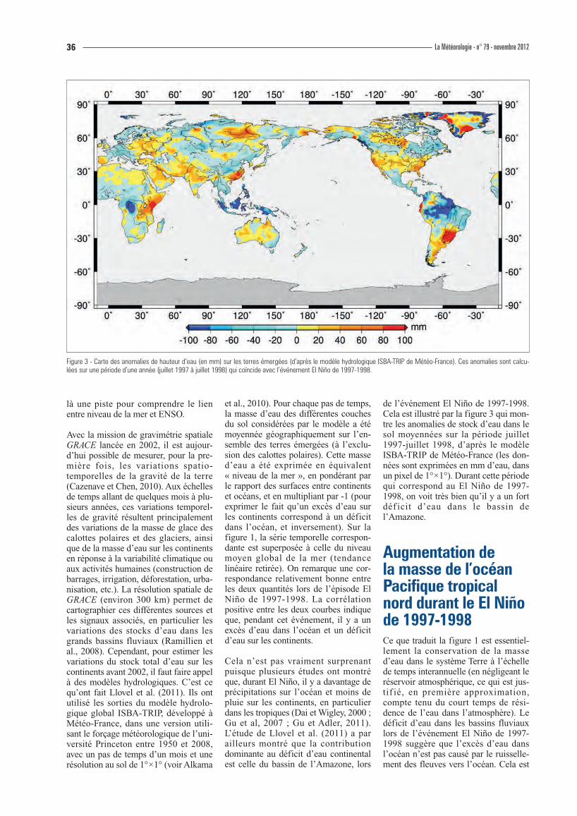
36 La Météorologie - n° 79 - novembre 2012
Figure 3 - Carte des anomalies de hauteur d’eau (en mm) sur les terres émergées (d’après le modèle hydrologique ISBA-TRIP de Météo-France). Ces anomalies sont calcu-lées sur une période d’une année (juillet 1997 à juillet 1998) qui coïncide avec l’événement El Niño de 1997-1998.
là une piste pour comprendre le lienentre niveau de la mer et ENSO.
Avec la mission de gravimétrie spatialeGRACE lancée en 2002, il est aujour-d’hui possible de mesurer, pour la pre-mière fois, les variations spatio-temporelles de la gravité de la terre(Cazenave et Chen, 2010). Aux échellesde temps allant de quelques mois à plu-sieurs années, ces variations temporel-les de gravité résultent principalementdes variations de la masse de glace descalottes polaires et des glaciers, ainsique de la masse d’eau sur les continentsen réponse à la variabilité climatique ouaux activités humaines (construction debarrages, irrigation, déforestation, urba-nisation, etc.). La résolution spatiale deGRACE (environ 300 km) permet decartographier ces différentes sources etles signaux associés, en particulier lesvariations des stocks d’eau dans lesgrands bassins fluviaux (Ramillien etal., 2008). Cependant, pour estimer lesvariations du stock total d’eau sur lescontinents avant 2002, il faut faire appelà des modèles hydrologiques. C’est cequ’ont fait Llovel et al. (2011). Ils ontutilisé les sorties du modèle hydrolo-gique global ISBA-TRIP, développé àMétéo-France, dans une version utili-sant le forçage météorologique de l’uni-versité Princeton entre 1950 et 2008,avec un pas de temps d’un mois et unerésolution au sol de 1°×1° (voir Alkama
et al., 2010). Pour chaque pas de temps,la masse d’eau des différentes couchesdu sol considérées par le modèle a étémoyennée géographiquement sur l’en-semble des terres émergées (à l’exclu-sion des calottes polaires). Cette massed’eau a été exprimée en équivalent« niveau de la mer », en pondérant parle rapport des surfaces entre continentset océans, et en multipliant par -1 (pourexprimer le fait qu’un excès d’eau surles continents correspond à un déficitdans l’océan, et inversement). Sur lafigure 1, la série temporelle correspon-dante est superposée à celle du niveaumoyen global de la mer (tendancelinéaire retirée). On remarque une cor-respondance relativement bonne entreles deux quantités lors de l’épisode ElNiño de 1997-1998. La corrélationpositive entre les deux courbes indiqueque, pendant cet événement, il y a unexcès d’eau dans l’océan et un déficitd’eau sur les continents.
Cela n’est pas vraiment surprenantpuisque plusieurs études ont montréque, durant El Niño, il y a davantage deprécipitations sur l’océan et moins depluie sur les continents, en particulierdans les tropiques (Dai etWigley, 2000 ;Gu et al, 2007 ; Gu et Adler, 2011).L’étude de Llovel et al. (2011) a parailleurs montré que la contributiondominante au déficit d’eau continentalest celle du bassin de l’Amazone, lors
de l’événement El Niño de 1997-1998.Cela est illustré par la figure 3 qui mon-tre les anomalies de stock d’eau dans lesol moyennées sur la période juillet1997-juillet 1998, d’après le modèleISBA-TRIP de Météo-France (les don-nées sont exprimées en mm d’eau, dansun pixel de 1°×1°). Durant cette périodequi correspond au El Niño de 1997-1998, on voit très bien qu’il y a un fortdéf icit d’eau dans le bassin del’Amazone.
Augmentation dela masse de l’océanPacifique tropicalnord durant le El Niñode 1997-1998Ce que traduit la figure 1 est essentiel-lement la conservation de la massed’eau dans le système Terre à l’échellede temps interannuelle (en négligeant leréservoir atmosphérique, ce qui est jus-tif ié, en première approximation,compte tenu du court temps de rési-dence de l’eau dans l’atmosphère). Ledéficit d’eau dans les bassins fluviauxlors de l’événement El Niño de 1997-1998 suggère que l’excès d’eau dansl’océan n’est pas causé par le ruisselle-ment des fleuves vers l’océan. Cela est
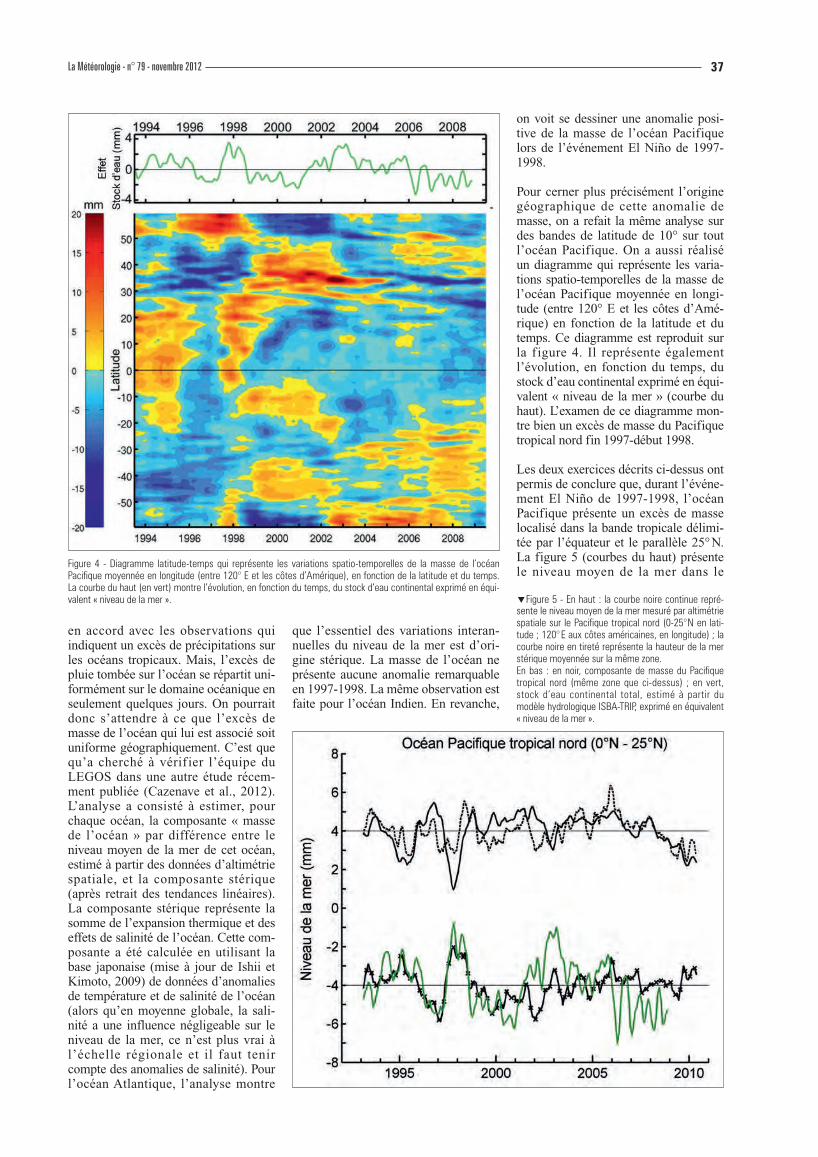
37La Météorologie - n° 79 - novembre 2012
Figure 4 - Diagramme latitude-temps qui représente les variations spatio-temporelles de la masse de l’océanPacifique moyennée en longitude (entre 120° E et les côtes d’Amérique), en fonction de la latitude et du temps.La courbe du haut (en vert) montre l’évolution, en fonction du temps, du stock d’eau continental exprimé en équi-valent « niveau de la mer ».
en accord avec les observations quiindiquent un excès de précipitations surles océans tropicaux. Mais, l’excès depluie tombée sur l’océan se répartit uni-formément sur le domaine océanique enseulement quelques jours. On pourraitdonc s’attendre à ce que l’excès demasse de l’océan qui lui est associé soituniforme géographiquement. C’est quequ’a cherché à vérif ier l’équipe duLEGOS dans une autre étude récem-ment publiée (Cazenave et al., 2012).L’analyse a consisté à estimer, pourchaque océan, la composante « massede l’océan » par différence entre leniveau moyen de la mer de cet océan,estimé à partir des données d’altimétriespatiale, et la composante stérique(après retrait des tendances linéaires).La composante stérique représente lasomme de l’expansion thermique et deseffets de salinité de l’océan. Cette com-posante a été calculée en utilisant labase japonaise (mise à jour de Ishii etKimoto, 2009) de données d’anomaliesde température et de salinité de l’océan(alors qu’en moyenne globale, la sali-nité a une influence négligeable sur leniveau de la mer, ce n’est plus vrai àl’échelle régionale et il faut tenircompte des anomalies de salinité). Pourl’océan Atlantique, l’analyse montre
que l’essentiel des variations interan-nuelles du niveau de la mer est d’ori-gine stérique. La masse de l’océan neprésente aucune anomalie remarquableen 1997-1998. La même observation estfaite pour l’océan Indien. En revanche,
on voit se dessiner une anomalie posi-tive de la masse de l’océan Pacifiquelors de l’événement El Niño de 1997-1998.
Pour cerner plus précisément l’originegéographique de cette anomalie demasse, on a refait la même analyse surdes bandes de latitude de 10° sur toutl’océan Pacifique. On a aussi réaliséun diagramme qui représente les varia-tions spatio-temporelles de la masse del’océan Pacifique moyennée en longi-tude (entre 120° E et les côtes d’Amé-rique) en fonction de la latitude et dutemps. Ce diagramme est reproduit surla figure 4. Il représente égalementl’évolution, en fonction du temps, dustock d’eau continental exprimé en équi-valent « niveau de la mer » (courbe duhaut). L’examen de ce diagramme mon-tre bien un excès de masse du Pacifiquetropical nord fin 1997-début 1998.
Les deux exercices décrits ci-dessus ontpermis de conclure que, durant l’événe-ment El Niño de 1997-1998, l’océanPacifique présente un excès de masselocalisé dans la bande tropicale délimi-tée par l’équateur et le parallèle 25°N.La figure 5 (courbes du haut) présentele niveau moyen de la mer dans le
�Figure 5 - En haut : la courbe noire continue repré-sente le niveau moyen de la mer mesuré par altimétriespatiale sur le Pacifique tropical nord (0-25°N en lati-tude ; 120°E aux côtes américaines, en longitude) ; lacourbe noire en tireté représente la hauteur de la merstérique moyennée sur la même zone.En bas : en noir, composante de masse du Pacifiquetropical nord (même zone que ci-dessus) ; en vert,stock d’eau continental total, estimé à partir dumodèle hydrologique ISBA-TRIP, exprimé en équivalent« niveau de la mer ».
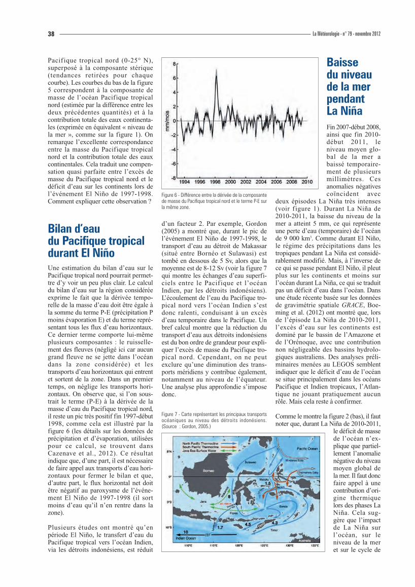
38 La Météorologie - n° 79 - novembre 2012
Figure 6 - Différence entre la dérivée de la composantede masse du Pacifique tropical nord et le terme P-E surla même zone.
Pacif ique tropical nord (0-25° N),superposé à la composante stérique(tendances retirées pour chaquecourbe). Les courbes du bas de la figure5 correspondent à la composante demasse de l’océan Pacifique tropicalnord (estimée par la différence entre lesdeux précédentes quantités) et à lacontribution totale des eaux continenta-les (exprimée en équivalent « niveau dela mer », comme sur la figure 1). Onremarque l’excellente correspondanceentre la masse du Pacifique tropicalnord et la contribution totale des eauxcontinentales. Cela traduit une compen-sation quasi parfaite entre l’excès demasse du Pacifique tropical nord et ledéficit d’eau sur les continents lors del’événement El Niño de 1997-1998.Comment expliquer cette observation ?
Bilan d’eaudu Pacifique tropicaldurant El NiñoUne estimation du bilan d’eau sur lePacifique tropical nord pourrait permet-tre d’y voir un peu plus clair. Le calculdu bilan d’eau sur la région considéréeexprime le fait que la dérivée tempo-relle de la masse d’eau doit être égale àla somme du terme P-E (précipitation Pmoins évaporation E) et du terme repré-sentant tous les flux d’eau horizontaux.Ce dernier terme comporte lui-mêmeplusieurs composantes : le ruisselle-ment des fleuves (négligé ici car aucungrand fleuve ne se jette dans l’océandans la zone considérée) et lestransports d’eau horizontaux qui entrentet sortent de la zone. Dans un premiertemps, on néglige les transports hori-zontaux. On observe que, si l’on sous-trait le terme (P-E) à la dérivée de lamasse d’eau du Pacifique tropical nord,il reste un pic très positif fin 1997-début1998, comme cela est illustré par lafigure 6 (les détails sur les données deprécipitation et d’évaporation, utiliséespour ce calcul, se trouvent dansCazenave et al., 2012). Ce résultatindique que, d’une part, il est nécessairede faire appel aux transports d’eau hori-zontaux pour fermer le bilan et que,d’autre part, le flux horizontal net doitêtre négatif au paroxysme de l’événe-ment El Niño de 1997-1998 (il sortmoins d’eau qu’il n’en rentre dans lazone).
Plusieurs études ont montré qu’enpériode El Niño, le transfert d’eau duPacifique tropical vers l’océan Indien,via les détroits indonésiens, est réduit
d’un facteur 2. Par exemple, Gordon(2005) a montré que, durant le pic del’événement El Niño de 1997-1998, letransport d’eau au détroit de Makassar(situé entre Bornéo et Sulawasi) esttombé en dessous de 5 Sv, alors que lamoyenne est de 8-12 Sv (voir la figure 7qui montre les échanges d’eau superfi-ciels entre le Pacif ique et l’océanIndien, par les détroits indonésiens).L’écoulement de l’eau du Pacifique tro-pical nord vers l’océan Indien s’estdonc ralenti, conduisant à un excèsd’eau temporaire dans le Pacifique. Unbref calcul montre que la réduction dutransport d’eau aux détroits indonésiensest du bon ordre de grandeur pour expli-quer l’excès de masse du Pacifique tro-pical nord. Cependant, on ne peutexclure qu’une diminution des trans-ports méridiens y contribue également,notamment au niveau de l’équateur.Une analyse plus approfondie s’imposedonc.
Baissedu niveaude la merpendantLa NiñaFin 2007-début 2008,ainsi que fin 2010-début 2011, leniveau moyen glo-bal de la mer abaissé temporaire-ment de plusieursmillimètres. Cesanomalies négativescoïncident avec
deux épisodes La Niña très intenses(voir f igure 1). Durant La Niña de2010-2011, la baisse du niveau de lamer a atteint 5 mm, ce qui représenteune perte d’eau (temporaire) de l’océande 9 000 km3. Comme durant El Niño,le régime des précipitations dans lestropiques pendant La Niña est considé-rablement modifié. Mais, à l’inverse dece qui se passe pendant El Niño, il pleutplus sur les continents et moins surl’océan durant La Niña, ce qui se traduitpas un déficit d’eau dans l’océan. Dansune étude récente basée sur les donnéesde gravimétrie spatiale GRACE, Boe-ming et al. (2012) ont montré que, lorsde l’épisode La Niña de 2010-2011,l’excès d’eau sur les continents estdominé par le bassin de l’Amazone etde l’Orénoque, avec une contributionnon négligeable des bassins hydrolo-giques australiens. Des analyses préli-minaires menées au LEGOS semblentindiquer que le déficit d’eau de l’océanse situe principalement dans les océansPacifique et Indien tropicaux, l’Atlan-tique ne jouant pratiquement aucunrôle. Mais cela reste à confirmer.
Comme lemontre la figure 2 (bas), il fautnoter que, durant La Niña de 2010-2011,
le déficit de massede l’océan n’ex-plique que partiel-lement l’anomalienégative du niveaumoyen global delamer. Il faut doncfaire appel à unecontribution d’ori-gine thermiquelors des phases LaNiña. Cela sug-gère que l’impactde La Niña surl’océan, sur leniveau de la meret sur le cycle de
Figure 7 - Carte représentant les principaux transportsocéaniques au niveau des détroits indonésiens.(Source : Gordon, 2005.)

39La Météorologie - n° 79 - novembre 2012
l’eau n’est pas l’exact symétrique decelui d’El Niño, comme suggéré parOkumura et Deser (2010). Des étudesdevront être menées pour clarifier cettequestion.
ConclusionJusqu’à présent, les études sur le niveaude la mer ont principalement concernéles causes de la hausse moyenne globaleobservée depuis quelques décennies, en
lien avec le réchauffement climatique.En revanche, les fluctuations interan-nuelles ont très peu été analysées. Lesrésultats récents, mentionnés dans cetarticle, montrent le rôle majeur des évé-nements ENSO sur le niveau moyenglobal de la mer, via des modificationsimportantes du cycle hydrologique glo-bal. Plus généralement, ces résultatsrévèlent que les fluctuations interan-nuelles du niveau de la mer, associéesaux événements El Niño, sont essentiel-lement causées par des changements de
la masse des océans. La composantethermique de l’océan joue un rôlemineur.
Les données globales de niveau de lamer par altimétrie spatiale, ainsi que lesdonnées de masse de l’océan par gravi-métrie spatiale GRACE disponiblesdepuis 2002, apportent des informa-tions nouvelles et indépendantes desdonnées hydrologiques classiques sur lecycle global de l’eau, en particulier àl’échelle de temps interannuelle.
Alkama R., B. Decharme, H. Douville, A. Voldoire, S. Tyteca, P. Le Moigne, M. Becker, A. Cazenave et J. Sheffield, 2010 : Global evaluation of the ISBA-TRIP
continental hydrological system. Part 1: Comparison to GRACE Terrestrial Water Storage estimates and in-situ river discharges. J. Hydrometeor., 11, 583-600,
doi:10.1175/2010JHM1211.
Boeming C., J. K. Willis, F. Landerer, S. Nerem et J. Fasullo, 2012 : The 2011 La Nina: so strong, the oceans fell. Geophys. Res. Lett., sous presse.
Cazenave A., O. Henry, S. Munier, B. Meyssignac, T. Delcroix, W. Llovel et H. Palanisamy, 2012 : ENSO influence on the global mean sea level over 1993-2010.
Marine Geodesy, doi: 10.1080/01490419.2012.718209, accepté.
Cazenave A. et J. Chen, 2010 : Time-variable gravity from space and present-day mass redistribution in the Earth system. Earth Planet. Sci. Lett., 298, 263-274.
Dai A. et T. M. L. Wigley, 2000 : Global patterns of ENSO-induced precipitation. Geophys. Res. Lett., 27, 9, 1283-1286.
Gordon A. L., 2005 : Oceanography of the Indonesian seas and their throughflow. Oceanography, 18 (4), 14-27.
Gu G. et R. F. Adler, 2011 : Precipitation and temperature variations on the interannual time scale: assessing the impact of ENSO and volcanic eruptions. J. Climate, 24,
2258-2270.
Gu G., R. F. Adler, G. J.Huffman et S. Curtis, 2007 : Tropical rainfall variability on interannual to interdecadal and longer time scales derived from the GPCP monthly pro-
ducts. J. Climate, 20, 4033-4046.
Ishii M. et M. Kimoto, 2009 : Reevaluation of historical ocean heat content variations with varying XBT and MBT depth bias corrections. Journal of Oceanography, 65,
287-299.
Llovel W., M. Becker, A. Cazenave, S. Jevrejeva, R. Alkama, B. Decharme, H. Douville, M. Ablain et B. Beckley, 2011 : Terrestrial waters and sea level varia-
tions on interannual time scale. Global and Planetary Change, 75, 76-82, doi: 10.1016/j.gloplacha.2010.10.008.
Meyssignac B. et A. Cazenave, 2012 : Sea level: a review of present-day and recent-past sea level change and variability. J. Geodyn., 58, 96-109.
Okumura Y. et C. Deser, 2010 : Asymmetry in the duration of El Nino and La Nina. J. Climate, 23, 5826-5843.
Ramillien G., S. Bouhours, A. Lombard, A. Cazenave, F. Flechtner et R. Schmidt, 2008 : Land water contributions from GRACE to sea level rise over 2002-2006.
Global and Planetary Change, 60, 381-392.
Bibliographie
© 2014 Habib B. Dieng et al., licensee De Gruyter Open. This work is licensed under the Creative Commons Attribution-NonCommercial-NoDerivs3.0 License.
DOI 10.2478/jogs-2014-0003 | J. Geod. Sci. 2014; 4:19–27
Research Article Open Access
Habib B. Dieng, Anny Cazenave, Benoit Meyssignac, Olivier Henry, Karina von Schuckmann,
Hindumathi Palanisamy, and Jean Michel Lemoine
E�ect of La Niña on the global mean sea level andnorth Paci�c ocean mass over 2005-2011Abstract: Interannual �uctuations of the global mean sea
level are highly correlated with El Niño-Southern Oscilla-
tion (ENSO) events, with positive/negative anomalies dur-
ing El Niño/La Niña. In a previous study we showed that
during the 1997 – 1998 El Niño, a positive anomaly ob-
served in the global mean sea level was mostly caused by
an increase of the ocean mass component rather than by
steric (thermal) e�ects. This result was related to an in-
crease of precipitation over the tropical ocean and a de�cit
in land water storage. In the present study, we investi-
gate the e�ect of the recent 2008 and 2011 La Niña events
on the satellite altimetry-based global mean sea level. We
�nd that the large global mean sea level drop associated
with the 2011 La Niña results from the combined decrease
of the steric and ocean mass components, with a slightly
dominant contribution from the latter. We show that the
oceanmass contribution to the global mean sea level drop
is spatially con�ned over the north eastern tropical Pa-
ci�c (just as was found previously for the 1997 – 1998 El
Niño, but with opposite sign). Corresponding ocean mass
spatial pattern is closely correlated to observed sea level
and steric spatial patterns over the duration of the La Niña
event. This is also observed for previous El Niño and La
Niña events. Such adrop in oceanmass during ENSO in the
eastern part of the tropical Paci�c has not been reported
before. It is possibly related to a temporary decrease in the
net precipitation over the north eastern Paci�c (opposite
situation was found during the 1997 – 1998 El Niño).
||Habib B. Dieng: LEGOS, OMP, 18 avenue Edouard Belin, 31401
Toulouse Cedex 9
Anny Cazenave: LEGOS, OMP, 18 avenue Edouard Belin, 31401
Toulouse Cedex 9, E-mail: [email protected]
Benoit Meyssignac, Olivier Henry: LEGOS, OMP, 18 avenue Edouard
Belin, 31401 Toulouse Cedex 9
Karina von Schuckmann: University of Toulon
Hindumathi Palanisamy: LEGOS, OMP, 18 avenue Edouard Belin,
31401 Toulouse Cedex 9
Jean Michel Lemoine: GRGS
1 Introduction
On interannual to decadal time scales, global mean sea
level (GMSL) variations mostly result from thermal ex-
pansion and mass variations of the oceans. The ocean
mass variations themselves result from land ice mass
changes (from glaciers and ice sheets), land water stor-
age changes plus a small contribution from atmospheric
water vapor. Over the satellite altimetry era (1993-2012),
GMSL rise (amounting to 3.1 +/- 0.4 mm/yr) is due to the
ocean thermal expansion (by ~30%) and land ice loss
(~55%) contributions (e.g., Church et al., 2011, Hansen et
al., 2011, Meyssignac and Cazenave, 2012, Hannna et al.,
2013, Church et al., 2013). While thermal expansion and
land ice dominate the GMSL trend, this is not the case at
interannual time scale, as shown by a few recent studies
(Llovel et al., 2010, 2011, Cazenave et al., 2012, Boening et
al., 2012). These interannual variations appear closely re-
lated to ENSO (El Niño-Southern Oscillation) events, with
positive/negative sea level anomalies observed during El
Niño/La Niña (Nerem et al., 2010). Focusing on the 1997 –
1998 El Niño, Llovel et al. (2010, 2011) showed that GMSL
anomalies are inversely related to interannual variations
in global land water storage, with a tendency for water
de�cit on landduringElNiño events. Thiswas investigated
in more details by Cazenave et al. (2012) who showed that
during the 1997 – 1998 El Niño, the GMSL anomaly was
largely due to an increase in oceanmass almost fully com-
pensated by water storage de�cit on land (with a domi-
nant contribution from tropical river basins –mostly the
Amazon-). This is related to the fact that during an El Niño,
there is rainfall de�cit on land and rainfall excess over
tropical oceans (mostly the Paci�c Ocean, e.g., Dai and
Wigley, 2000, Gu and Adler, 2011). Another result from the
Cazenave et al. (2012)’ study concerned the location of the
ocean mass increase. Counter intuitively, the ocean mass
increase was not uniformly distributed over the oceans
but concentrated over the northeast tropical Paci�c. To ex-
plain this ocean mass excess during the 1997 – 1998 El
Niño, several hypotheses were investigated (for example,
a possible reduced water �ow between the Paci�c and In-
Brought to you by | Universite Toulouse 3 Paul Sabatier
Authenticated | 130.120.245.221
Download Date | 6/4/14 12:32 PM
20 | Habib B. Dieng et al.
dian oceans at the Indonesian straits, Gordon et al., 2010)
but no de�nite conclusion has been drawn.
In the present study, we study the interannual varia-
tions of the GMSL over 2005-2011, a period with prevailing
La Niña events. Over this time span, the interannual GMSL
displays negative anomalies of several mm amplitude, co-
inciding with the 2008 and 2011 La Niña events. As shown
by Boening et al. (2012), the GMSL drop during the 2011
La Niña in part results from a temporary decrease in ocean
mass (and associated increase in land water storage, Fa-
sullo et al., 2013), as estimated fromGRACE space gravime-
try data. Here we also compare the interannual GMSLwith
the sum of the contributions (i.e., the steric andmass com-
ponents, estimated using di�erent data sets) and explore
whether, as for the 1997 – 1998 El Niño, the LaNiña-related
ocean mass decrease has a particular spatial pattern or
not.
2 Method
Interannual variations inGMSL are computed in twoways:
1. Directly from satellite altimetry data after removing,
over the study period, the longer-term signal in the
GMSL time series,
2. By estimating separately the steric (i.e., due to ocean
temperature and salinity) and ocean mass (∆Mocean)
contributions.
The ∆Mocean component can itself be estimated in two
ways:
1. By averaging the GRACE space gravimetry data over
the oceans to recover the ocean mass variations,
2. By summing up the land water, atmospheric water va-
por and land ice components.
In e�ect, conservation of total water mass in the climate
system at interannual time scale leads to:
∆Mocean = −∆MLW − ∆MWV − ∆MLI (1)
where ∆Mocean, ∆MLW and ∆MWV represent interannual
changes of the ocean mass, total land water storage and
atmospheric water vapor, respectively. ∆MLI refers to in-
terannual �uctuations in land ice mass.
For regional comparisons with the 1997 – 1998 El Niño
(i.e., prior to the GRACE era), we also estimate the ocean
mass component by computing the di�erence between the
altimetry-based sea level and steric sea level.
All components are expressed in equivalent sea level
(ESL) (see below).
3 Data
3.1 Sea level data
For the altimetry-based sea level data, we use two di�erent
products : (1) the GMSL time series fromAVISO (Archiving,
Validation and Interpretation of Satellite Oceanographic
Data,www.aviso.oceanobs.com/en/data/products/sea-
surface-height-products/global/msla/, AVISO hereafter)
and (2) the Colorado University GMSL (http://sealevel.
colorado.edu/, CU hereinafter). Both data sets are based
on Topex/Poseidon, Jason-1 and Jason-2 data.
The two GMSL time series (AVISO and Colorado Uni-
versity) are based on di�erent processing approaches, in
particular the geographical averaging process. Moreover
some of the geophysical corrections applied to the data are
slightly di�erent as well as the editing procedure (seeMas-
ters et al., 2012 and Henry et al., 2014, for a discussion on
these di�erences). The two GMSL time series cover the pe-
riod 1993-2013. But for thepurposeof thepresent study that
focuses on GRACE and Argo periods, we limit the study
time span to January 2005 to December 2011. In the follow-
ing, we average the two data sets to produce a single GMSL
time series, as no preferred product has been identi�ed so
far. The corresponding curve and associated uncertainty
(based on the dispersion around the mean) is shown in
Fig. 1 for the 2005-2011 time span. For the regional anal-
ysis presented in section 6, we also use the gridded AVISO
data over 1993-2012 (www.aviso.oceanobs.com). The grid-
ded data are based on a larger set of altimetry missions
merged together: in addition to the Topex/Poseidon and
Jason-1&2- data, ERS-1&2, Envisat and Geosat follow-on
data are also used. The gridded data are provided on a
1/4 degree grid at weekly interval.
Both, global mean and gridded sea level data are cor-
rected for the inverted barometer correction. For detailed
description of the geophysical corrections, the reader is re-
ferred to the AVISO and Colorado University web sites.
3.2 Steric data
Two steric data sets have been considered:
1. Argo data processed as explained in von Schuckmann
and Le Traon (2011). The global mean steric time se-
ries (data averaged over the 60°N/60°S domain) is
based on a weighted box averaging scheme of Argo
data. A reference depth of 1500 m is chosen as the
number of pro�les in the 1500 m-2000 m depth layer
is signi�cantly less than within 0-1500 m before year
Brought to you by | Universite Toulouse 3 Paul Sabatier
Authenticated | 130.120.245.221
Download Date | 6/4/14 12:32 PM
E�ect of La Niña on the global mean sea level and north Paci�c ocean mass over 2005-2011 | 21
2009 (Cabanes et al., 2013, their Figure 7). The Argo
pro�les undergo re-quali�ed data validation methods
using a tool developed by Gaillard et al. (2009) (see
also von Schuckmann et al., 2009). Black-listed pro-
�les and platforms are excluded from the data set. Ev-
ery pro�le on alert has been checked visually which
allows excluding spurious data (e.g. data drift). This
procedure minimizes systematic biases in the global
Argo data set as discussed by Barker et al. (2011). Er-
ror bars represent one standard error, accounting for
reduced degrees of freedom in the mapping and un-
certainty in the reference climatology as described in
von Schuckmann and Le Traon (2011). The Argo based
steric sea level time series covers the period 2005-2011.
In the following, we consider both the thermosteric
and halosteric components.
2. For comparisons between the recent La Niña events
and former El Niño events (in particular the 1997 –
1998 El Niño), we also consider the recent update
(V6.12) of the Ishii and Kimoto (2009) ocean temper-
ature data (covering the 0-700 m depth range). These
data are vertically integrated to estimate the ther-
mosteric sea level from 1993 onwards at monthly in-
terval. This thermosteric product is called IK12.
3.3 GRACE-based space gravimetry data
To estimate the ocean mass variation, we use the GRACE
Release 2 products from the Groupe de Recherche en
Geodesie Spatiale (GRGS) (http://www.grgs.obs-mip.
fr/grace/variable-models-grace-lageos/grace-solutions-
release-02). The degree 2 coe�cients –poorly determined
by GRACE- are those derived from satellite laser ranging
to Lageos 1 and 2. These data are provided at 10-day in-
terval on 1°x1° grids. However the real spatial resolution
of this data set is coarser, on the order of 400 km (see
below). No Gaussian �ltering nor destripping are applied
to the GRGS data. Such post-processing is developed by
other groups for removing the various errors a�ecting the
GRACE data, in particular the north-south noise (stripes)
due to systematic correlated errors of GRACE data within a
particular spectral order or the leakage of nearby signals
onto the study area due to the coarse GRACE resolution
(see Velicogna and Wahr, 2013 for a discussion on errors
impacting the GRACE data). Such post processing proce-
dure is usually applied to the GRACE products available
from the TELLUS website (http://grace.jpl.nasa.gov) that
provides gridded ocean data after strong smoothing (due
to the application of a destripping �lter, a 500 km half-
width Gaussian �lter and a spherical harmonic cuto� at
degree 40). As indicated on this web site, such a data set
should not be used for global ocean mass studies due to
strong attenuation of the signal (see also Chambers and
Schröter, 2011).
A gain factor is sometimes applied to the data in or-
der to compensate for signal attenuation due to the coarse
GRACE resolution (the truncation of the GRACE spheri-
cal harmonics series at a given degree implies that short-
wavelength signal associated with the missing spherical
harmonic coe�cients, cannot be recovered). In the case of
the GRGS data, this truncation is at degree 50, which cor-
responds to a spatial resolution of 400 km. No gain fac-
tor is applied. When computing the ocean mass, we use
a mask that ignores data within 400 km of the continents
to avoid leakage from continental hydrology and ice sheet
mass loss. Finally, as we only consider the interannual
variability, we do not correct the GRACE data for Glacial
Isostatic Adjustment (i.e., the visco-elastic response of the
solid Earth to last deglaciation) because this e�ect is a
purely linear trend.
3.4 Atmospheric water vapor
To estimate change in atmospheric water vapor mass,
we used three di�erent products : (1) atmospheric sur-
face pressure grids from the European Centre for Medium-
Range Forecast (ECMWF) ERA-Interim data (//data-portal.
ecmwf.int/data/d/interim_moda/), (2) the vertically inte-
grated water vapor grids, also from ERA Interim, and (3)
vertically integrated water vapor based on AMSRE remote
sensing data (kindly provided to us by R. Allan). As shown
by Trenberth and Smith (2005), seasonal and interannual
variations in atmospheric surface pressure essentially re-
sult from changes in atmospheric water vapor content be-
cause of dry air mass conservation. Thus atmospheric sur-
face pressure data can be used to estimate change inwater
mass of the atmosphere. Data from ERA Interim are pro-
vided as 1.5°x1.5° grids, at monthly interval. Data from (3)
are given as globally averaged water vapor time series at
monthly interval.
The atmospheric water vapor contribution is further
expressed in ESL by weighting by the ratio of the total
Earth’s area to the ocean area and multiplied by -1 (to ex-
press the fact that more water in the atmosphere leads to
lower sea level, and inversely).
Brought to you by | Universite Toulouse 3 Paul Sabatier
Authenticated | 130.120.245.221
Download Date | 6/4/14 12:32 PM
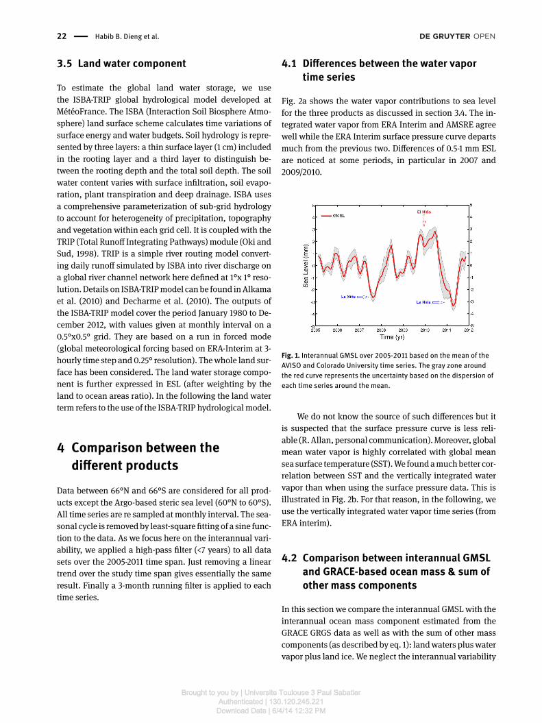
22 | Habib B. Dieng et al.
3.5 Land water component
To estimate the global land water storage, we use
the ISBA-TRIP global hydrological model developed at
MétéoFrance. The ISBA (Interaction Soil Biosphere Atmo-
sphere) land surface scheme calculates time variations of
surface energy and water budgets. Soil hydrology is repre-
sented by three layers: a thin surface layer (1 cm) included
in the rooting layer and a third layer to distinguish be-
tween the rooting depth and the total soil depth. The soil
water content varies with surface in�ltration, soil evapo-
ration, plant transpiration and deep drainage. ISBA uses
a comprehensive parameterization of sub-grid hydrology
to account for heterogeneity of precipitation, topography
and vegetation within each grid cell. It is coupled with the
TRIP (Total Runo� Integrating Pathways) module (Oki and
Sud, 1998). TRIP is a simple river routing model convert-
ing daily runo� simulated by ISBA into river discharge on
a global river channel network here de�ned at 1°x 1° reso-
lution.Details on ISBA-TRIPmodel canbe found inAlkama
et al. (2010) and Decharme et al. (2010). The outputs of
the ISBA-TRIP model cover the period January 1980 to De-
cember 2012, with values given at monthly interval on a
0.5°x0.5° grid. They are based on a run in forced mode
(global meteorological forcing based on ERA-Interim at 3-
hourly time step and 0.25° resolution). Thewhole land sur-
face has been considered. The land water storage compo-
nent is further expressed in ESL (after weighting by the
land to ocean areas ratio). In the following the land water
term refers to the use of the ISBA-TRIP hydrological model.
4 Comparison between the
di�erent products
Data between 66°N and 66°S are considered for all prod-
ucts except the Argo-based steric sea level (60°N to 60°S).
All time series are re sampled atmonthly interval. The sea-
sonal cycle is removedby least-square�ttingof a sine func-
tion to the data. As we focus here on the interannual vari-
ability, we applied a high-pass �lter (<7 years) to all data
sets over the 2005-2011 time span. Just removing a linear
trend over the study time span gives essentially the same
result. Finally a 3-month running �lter is applied to each
time series.
4.1 Di�erences between the water vapor
time series
Fig. 2a shows the water vapor contributions to sea level
for the three products as discussed in section 3.4. The in-
tegrated water vapor from ERA Interim and AMSRE agree
well while the ERA Interim surface pressure curve departs
much from the previous two. Di�erences of 0.5-1 mm ESL
are noticed at some periods, in particular in 2007 and
2009/2010.
Fig. 1. Interannual GMSL over 2005-2011 based on the mean of the
AVISO and Colorado University time series. The gray zone around
the red curve represents the uncertainty based on the dispersion of
each time series around the mean.
We do not know the source of such di�erences but it
is suspected that the surface pressure curve is less reli-
able (R.Allan, personal communication).Moreover, global
mean water vapor is highly correlated with global mean
sea surface temperature (SST).We foundamuchbetter cor-
relation between SST and the vertically integrated water
vapor than when using the surface pressure data. This is
illustrated in Fig. 2b. For that reason, in the following, we
use the vertically integrated water vapor time series (from
ERA interim).
4.2 Comparison between interannual GMSL
and GRACE-based ocean mass & sum of
other mass components
In this section we compare the interannual GMSL with the
interannual ocean mass component estimated from the
GRACE GRGS data as well as with the sum of other mass
components (as described by eq. 1): landwaters pluswater
vapor plus land ice. We neglect the interannual variability
Brought to you by | Universite Toulouse 3 Paul Sabatier
Authenticated | 130.120.245.221
Download Date | 6/4/14 12:32 PM

E�ect of La Niña on the global mean sea level and north Paci�c ocean mass over 2005-2011 | 23
(a)
(b)
Fig. 2. a) Interannual global mean water vapor component (ex-
pressed in equivalent sea level) from ERA Interim surface pressure
(green curve), integrated water vapor from ERA Interim (blue curve)
and from AMSRE (red curve); b) Interannual global mean water va-
por contribution from ERA Interim (expressed in equivalent sea
level, blue curve) and global mean SST (multiplied by -1) (red curve).
of the glaciers as no data are available to estimate it, but
account for that of the ice sheets. The latter has been es-
timated from the GRGS GRACE data averaged over Green-
land and Antarctica. It is generally very small, of at most
0.3 – 0.4 mm ESL on interannual time scale (see below).
Fig. 3a compares the interannual GMSL with the
GRACE-based oceanmass and the sum of ‘land water stor-
age + water vapor + interannual ice sheet component’. Er-
ror bars are not shown on this plot. The GRACE GRGS data
are not provided with error bars. However from discus-
sions with the GRGS processing group, it comes out that
the uncertainty of a single global mean monthly value is
on the order of 0.6 mm (1-sigma) (see also Wahr et. al.,
2006). Uncertainty of the sum ‘land water storage + wa-
ter vapor + interannual ice sheet component’ is also not
known. We assume that it is of the same order of magni-
tude as for the GRACE-based ocean mass. Fig. 3a indicates
that the mass component (either from GRACE or from the
sum ‘land water storage + water vapor + interannual ice
sheet component’) has a signi�cant contribution to the in-
terannual GMSL, especially during the 2011 La Niña. But
clearly not all interannual GMSL signal is of mass origin.
In Fig. 3b,wehave superimposed theArgo-based steric sea
level to the interannual GMSL. The steric signal obviously
plays some role at interannual time scale. On Fig. 3b, is
also shown the interannual variability of the ice sheets. As
mentioned above, this contribution is small, of the same
order of magnitude as the water vapor component.
5 Sea level budget at interannual
time scale
Fig. 4a,b show the interannual GMSL together with the
sum of the steric and mass components (GRACE-based
ocean mass for Fig. 4a and sum ‘land water storage + wa-
ter vapor + interannual ice sheet component’ for Fig. 4b).
From these �gures, we clearly see that the negative sea
level anomalies coinciding with the 2011 La Niña is almost
equally due to adecrease of the oceanmass and steric com-
ponents. The agreement between the GMSL and the sum
of components is less good during the 2008 La Niña, al-
though the use of the sum ‘land water storage + water va-
por + interannual ice sheet component’ (Fig. 4b) gives bet-
ter result than the use of GRACE (Fig. 4a).
Overall, over the 2005– 2011 time span, the correlation
between interannual GMSL and sum of the contributions
amounts to 0.78 in both cases (Fig. 4a and Fig. 4b).We con-
clude, as previously shown by Boening et al. (2012), that
the GMSL drop during the 2011 La Niña event is reason-
ably well reproduced by the sum of the steric and ocean
mass contributions. As indicated above, lesser agreement
is noticed for the 2008 La Niña. This calls for further inves-
tigation to identify which data set is in error.
6 Spatial patterns of sea level and
ocean mass during 2011 La Niña
In this section, we investigate the geographical patterns of
the GMSL, steric sea level and oceanmass component dur-
ing the 2011 La Niña. In particular, we would like to check
whether the ocean mass component associated with the
2011 La Niña presents a spatial pattern similar (but with
Brought to you by | Universite Toulouse 3 Paul Sabatier
Authenticated | 130.120.245.221
Download Date | 6/4/14 12:32 PM
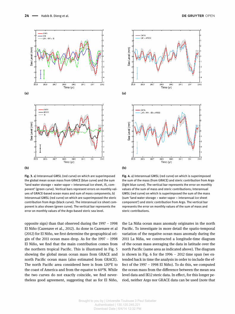
24 | Habib B. Dieng et al.
(a)
(b)
Fig. 3. a) Interannual GMSL (red curve) on which are superimposed
the global mean ocean mass from GRACE (blue curve) and the sum
‘land water storage + water vapor + interannual ice sheet, IS, com-
ponent’ (green curve). Vertical bars represent errors on monthly val-
ues of GRACE-based ocean mass and sum of mass components; b)
Interannual GMSL (red curve) on which are superimposed the steric
contribution from Argo (black curve). The interannual ice sheet com-
ponent is also shown (green curve). The vertical bar represents the
error on monthly values of the Argo-based steric sea level.
opposite sign) than that observed during the 1997 – 1998
El Niño (Cazenave et al., 2012). As done in Cazenave et al
(2012) for El Niño, we �rst determine the geographical ori-
gin of the 2011 ocean mass drop. As for the 1997 – 1998
El Niño, we �nd that the main contribution comes from
the northern tropical Paci�c. This is illustrated in Fig. 5
showing the global mean ocean mass from GRACE and
north Paci�c ocean mass (also estimated from GRACE).
The north Paci�c area considered here is from 120°E to
the coast of America and from the equator to 60°N. While
the two curves do not exactly coincide, we �nd never-
theless good agreement, suggesting that as for El Niño,
(a)
(b)
Fig. 4. a) Interannual GMSL (red curve) on which is superimposed
the sum of the mass (from GRACE) and steric contribution from Argo
(light blue curve). The vertical bar represents the error on monthly
values of the sum of mass and steric contributions; Interannual
GMSL (red curve) on which is superimposed the sum of the mass
(sum ‘land water storage + water vapor + interannual ice sheet
component’) and steric contribution from Argo. The vertical bar
represents the error on monthly values of the sum of mass and
steric contributions.
the La Niña ocean mass anomaly originates in the north
Paci�c. To investigate in more detail the spatio-temporal
variation of the negative ocean mass anomaly during the
2011 La Niña, we constructed a longitude-time diagram
of the ocean mass averaging the data in latitude over the
north Paci�c (same area as indicated above). The diagram
is shown in Fig. 6 for the 1996 – 2012 time span (we ex-
tended back in time the analysis in order to include the ef-
fect of the 1997 – 1998 El Niño). To do this, we computed
the ocean mass from the di�erence between the mean sea
level data and IK12 steric data. In e�ect, for this longer pe-
riod, neither Argo nor GRACE data can be used (note that
Brought to you by | Universite Toulouse 3 Paul Sabatier
Authenticated | 130.120.245.221
Download Date | 6/4/14 12:32 PM
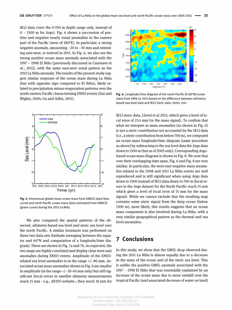
E�ect of La Niña on the global mean sea level and north Paci�c ocean mass over 2005-2011 | 25
IK12 data cover the 0-700 m depth range only, instead of
0 – 1500 m for Argo). Fig. 6 shows a succession of pos-
itive and negative nearly zonal anomalies in the eastern
part of the Paci�c (west of 180°E). In particular, a strong
negative anomaly, amounting −20 to −30 mm and extend-
ing east-west, is noticed in 2011. In Fig. 6, we also see the
strong positive ocean mass anomaly associated with the
1997 – 1998 El Niño (previously discussed in Cazenave et
al., 2012), with the same east-west zonal pattern as the
2011 LaNiña anomaly. The results of the present study sug-
gest similar response of the ocean mass during La Niña
(but with opposite sign compared to El Niño), likely re-
lated to precipitation minus evaporation patterns over the
north eastern Paci�c characterizing ENSO events (Dai and
Wigley, 2000, Gu and Adler, 2011).
Fig. 5. Interannual global mean ocean mass from GRACE (dark blue
curve) and north Paci�c ocean mass (also estimated from GRACE)
(green curve) during the 2011 La Niña.
We also compared the spatial patterns of the ob-
served, altimetry-based sea level and steric sea level over
the north Paci�c. A similar treatment was performed on
these two data sets (latitude averaging between the equa-
tor and 60°N and computation of a longitude/time dia-
gram). These are shown in Fig. 7a and 7b. As expected, the
twomaps are highly correlated and display clear west-east
anomalies during ENSO events. Amplitude of the ENSO-
related sea level anomalies is in the range +/−80 mm. As-
sociated oceanmass anomalies shown in Fig. 6 are smaller
in amplitude (in the range +/−30-40mmonly) but still sig-
ni�cant (local errors in satellite altimetry measurements
reach 15 mm –e.g., AVISO website-; they reach 18 mm for
Fig. 6. Longitude/time diagram of the north Paci�c (0-60°N) ocean
mass from 1996 to 2011 based on the di�erence between altimetry-
based sea level data and IK12 steric data. Units: mm.
IK12 steric data, Llovel et al 2013, which gives a level of lo-
cal error of 23.4 mm for the mass signal). To con�rm that
what we interpret as mass anomalies (as shown in Fig. 6)
is not a steric contribution not accounted by the IK12 data
(i.e., a steric contribution frombelow700m),we computed
an ocean mass longitude/time diagram (same procedure
as above) by subtracting to the sea level data the Argo data
down to 1500m (but as of 2005 only). CorrespondingArgo-
based oceanmass diagram is shown in Fig. 8.We note that
over their overlapping time span, Fig. 6 and Fig. 8 are very
similar. In particular, the west-east negative mass anoma-
lies related to the 2008 and 2011 La Niña events are well
reproduced and is still signi�cant when using Argo data
down to 1500 instead of IK12 data down to 700m (local er-
rors in the Argo dataset for the North Paci�c reach 15 mm
which gives a level of local error of 15 mm for the mass
signal). While we cannot exclude that the resulting map
contains some steric signal from the deep ocean (below
1500 m), more likely, this results suggests that an ocean
mass component is also involved during La Niña, with a
very similar geographical pattern as the thermal and sea
level anomalies.
7 Conclusions
In this study, we show that the GMSL drop observed dur-
ing the 2011 La Niña is almost equally due to a decrease
in the mass of the ocean and of the steric sea level. This
is unlike the positive GMSL anomaly associated with the
1997 – 1998 El Niño that was essentially explained by an
increase of the ocean mass due to more rainfall over the
tropical Paci�c (and associated decrease of water on land)
Brought to you by | Universite Toulouse 3 Paul Sabatier
Authenticated | 130.120.245.221
Download Date | 6/4/14 12:32 PM

26 | Habib B. Dieng et al.
(a)
(b)
Fig. 7. Longitude/time diagram of the north Paci�c (0-60°N)
altimetry-based sea level data from 1996 to 2011. Units: mm; Longi-
tude/time diagram of the north Paci�c (0-60°N) steric sea level data
from IK12 from 1996 to 2011. Units: mm.
Fig. 8. Longitude/time diagram of the north Paci�c ocean (0-60°N)
mass sea level data based on the di�erence between altimetry-
based sea level data and Argo steric data (down to 1500 m) over
2005-2011. Units: mm.
(Cazenave et al., 2012). This suggests that the e�ect of La
Niña on the GMSL does not just mirror that of El Niño, as
suggested by Okumura and Deser (2010) for other charac-
teristics of these events. This is unlike the spatial patterns
in ocean mass anomalies: we �nd that during the 2011 La
Niña, the ocean mass decrease is temporarily con�ned in
the northeastern Paci�c, as for 1997 – 1998 El Niño (but
with opposite sign).
The origin of this oceanmass decrease during La Niña
events is possibly related to the net precipitation over the
area, but the exact origin of the observed pattern remains
to be investigated. This will be the object of a forthcoming
study that should also analyze the relationship between
oceanmass anomaly and surface salinity, in particular us-
ing data from the SMOS and Aquarius satellite missions.
It will be also of interest to investigate whether numerical
ocean models are able to reproduce the observed ocean
mass decrease and its spatial pattern. This should help
better understanding the physical cause of the observed
pattern.
Acknowledgement: We thank R. Allan for kindly provid-
ing us with water vapor data. H. Palanisamy was sup-
ported by a CNES-CLS PhDGrant. K. von Schuckmannwas
partly supported by the French Lefe/GMMC research pro-
gramme.
References
Alkama R., Decharme B., Douville H., Becker M., Cazenave A.,
She�eld J., Voldoire A., Tyteca S., Le Moigne P. (2010). Global
evaluation of the ISBA-TRIP continental hydrologic system; Part
1 : a two-fold constraint using GRACE terrestrial water storage
estimates and in situ river discharges J. Hydrometeorology, 11,
583-600, doi:10.1175/2010JHM1211.
Barker P. M., Dunn J. R., Domingues C. M., and Wij�els S. E., (2011)
Pressure Sensor Drifts in Argo and Their Impacts, J. Atmos.
Ocean. Tech., 28, 1036–1049.
Boening C., Willis J.K., Landerer F.W. and Nerem R.S. (2012). The
2011 La Niña: so strong, the oceans fell, Geophys. Res. Lett.,
39, L19602, doi:10.1029/2012GL053055.
Cabanes, C., A. Gourazel, K. von Schuckmann, M. Hamon, V.
Turpin, C. Coatanoan, S. Guinehut, C. Boone, N. Ferry, G.
Reverdin, S. Pouliquen and P.Y. Le Traon (2013): The CORA
dataset: validation and diagnostics of ocean temperature
and salinity in situ measurements, Ocean Sci., 9, 1–18,
www.ocean-sci.net/9/1/2013/, doi:10.5194/os-9-1-2013.
Cazenave A., O. Henry, S. Munier, B. Meyssignac, T. Delcroix, W.
Llovel, H. Palanisamy and M. Becker, (2012). ENSO influence
on the global mean sea level over 1993-2010, Marine Geodesy,
35(S1), 82–97.
Chambers D. and J. Schröter (2011). Measuring ocean mass variabil-
ity from satellite gravimetry, Journal of Geodynamics, 52, 333–
Brought to you by | Universite Toulouse 3 Paul Sabatier
Authenticated | 130.120.245.221
Download Date | 6/4/14 12:32 PM
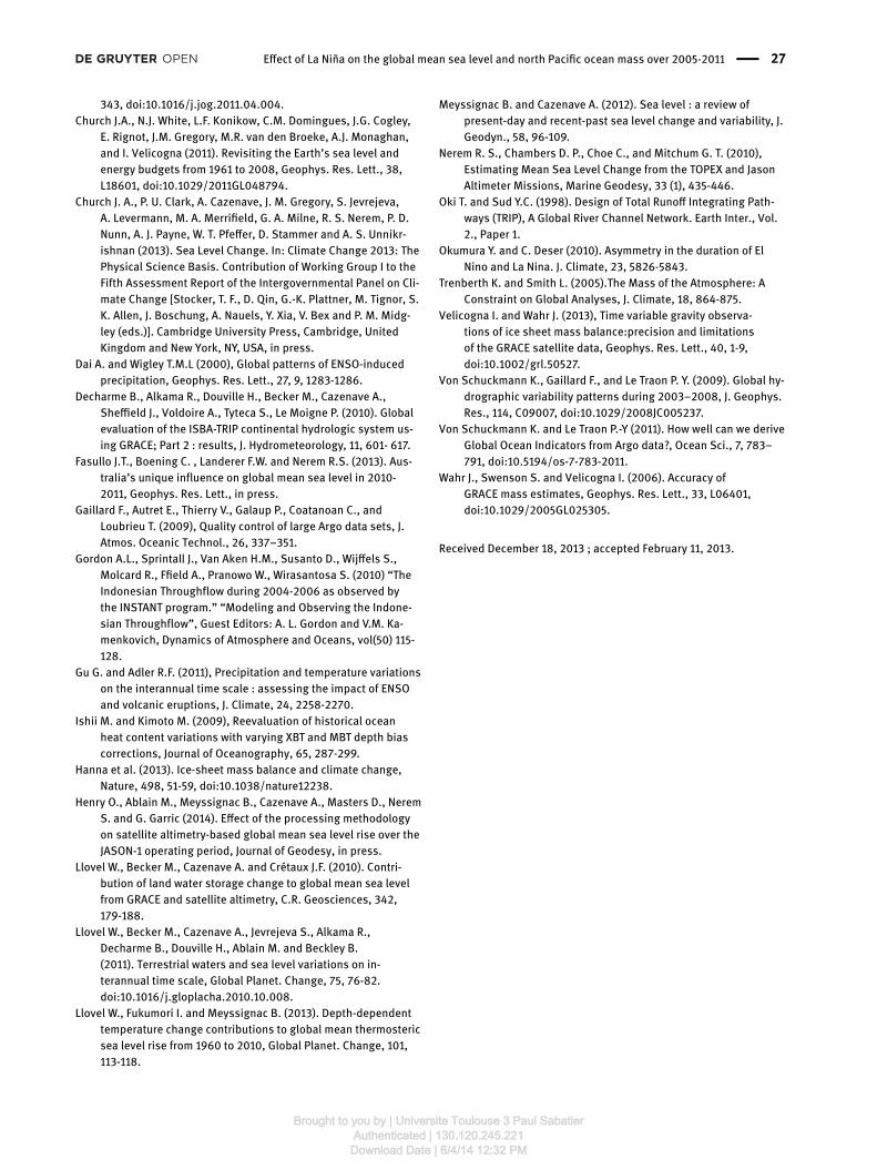
E�ect of La Niña on the global mean sea level and north Paci�c ocean mass over 2005-2011 | 27
343, doi:10.1016/j.jog.2011.04.004.
Church J.A., N.J. White, L.F. Konikow, C.M. Domingues, J.G. Cogley,
E. Rignot, J.M. Gregory, M.R. van den Broeke, A.J. Monaghan,
and I. Velicogna (2011). Revisiting the Earth’s sea level and
energy budgets from 1961 to 2008, Geophys. Res. Lett., 38,
L18601, doi:10.1029/2011GL048794.
Church J. A., P. U. Clark, A. Cazenave, J. M. Gregory, S. Jevrejeva,
A. Levermann, M. A. Merri�eld, G. A. Milne, R. S. Nerem, P. D.
Nunn, A. J. Payne, W. T. Pfe�er, D. Stammer and A. S. Unnikr-
ishnan (2013). Sea Level Change. In: Climate Change 2013: The
Physical Science Basis. Contribution of Working Group I to the
Fifth Assessment Report of the Intergovernmental Panel on Cli-
mate Change [Stocker, T. F., D. Qin, G.-K. Plattner, M. Tignor, S.
K. Allen, J. Boschung, A. Nauels, Y. Xia, V. Bex and P. M. Midg-
ley (eds.)]. Cambridge University Press, Cambridge, United
Kingdom and New York, NY, USA, in press.
Dai A. and Wigley T.M.L (2000), Global patterns of ENSO-induced
precipitation, Geophys. Res. Lett., 27, 9, 1283-1286.
Decharme B., Alkama R., Douville H., Becker M., Cazenave A.,
She�eld J., Voldoire A., Tyteca S., Le Moigne P. (2010). Global
evaluation of the ISBA-TRIP continental hydrologic system us-
ing GRACE; Part 2 : results, J. Hydrometeorology, 11, 601- 617.
Fasullo J.T., Boening C. , Landerer F.W. and Nerem R.S. (2013). Aus-
tralia’s unique influence on global mean sea level in 2010-
2011, Geophys. Res. Lett., in press.
Gaillard F., Autret E., Thierry V., Galaup P., Coatanoan C., and
Loubrieu T. (2009), Quality control of large Argo data sets, J.
Atmos. Oceanic Technol., 26, 337–351.
Gordon A.L., Sprintall J., Van Aken H.M., Susanto D., Wij�els S.,
Molcard R., F�eld A., Pranowo W., Wirasantosa S. (2010) “The
Indonesian Throughflow during 2004-2006 as observed by
the INSTANT program.” “Modeling and Observing the Indone-
sian Throughflow”, Guest Editors: A. L. Gordon and V.M. Ka-
menkovich, Dynamics of Atmosphere and Oceans, vol(50) 115-
128.
Gu G. and Adler R.F. (2011), Precipitation and temperature variations
on the interannual time scale : assessing the impact of ENSO
and volcanic eruptions, J. Climate, 24, 2258-2270.
Ishii M. and Kimoto M. (2009), Reevaluation of historical ocean
heat content variations with varying XBT and MBT depth bias
corrections, Journal of Oceanography, 65, 287-299.
Hanna et al. (2013). Ice-sheet mass balance and climate change,
Nature, 498, 51-59, doi:10.1038/nature12238.
Henry O., Ablain M., Meyssignac B., Cazenave A., Masters D., Nerem
S. and G. Garric (2014). E�ect of the processing methodology
on satellite altimetry-based global mean sea level rise over the
JASON-1 operating period, Journal of Geodesy, in press.
Llovel W., Becker M., Cazenave A. and Crétaux J.F. (2010). Contri-
bution of land water storage change to global mean sea level
from GRACE and satellite altimetry, C.R. Geosciences, 342,
179-188.
Llovel W., Becker M., Cazenave A., Jevrejeva S., Alkama R.,
Decharme B., Douville H., Ablain M. and Beckley B.
(2011). Terrestrial waters and sea level variations on in-
terannual time scale, Global Planet. Change, 75, 76-82.
doi:10.1016/j.gloplacha.2010.10.008.
Llovel W., Fukumori I. and Meyssignac B. (2013). Depth-dependent
temperature change contributions to global mean thermosteric
sea level rise from 1960 to 2010, Global Planet. Change, 101,
113-118.
Meyssignac B. and Cazenave A. (2012). Sea level : a review of
present-day and recent-past sea level change and variability, J.
Geodyn., 58, 96-109.
Nerem R. S., Chambers D. P., Choe C., and Mitchum G. T. (2010),
Estimating Mean Sea Level Change from the TOPEX and Jason
Altimeter Missions, Marine Geodesy, 33 (1), 435-446.
Oki T. and Sud Y.C. (1998). Design of Total Runo� Integrating Path-
ways (TRIP), A Global River Channel Network. Earth Inter., Vol.
2., Paper 1.
Okumura Y. and C. Deser (2010). Asymmetry in the duration of El
Nino and La Nina. J. Climate, 23, 5826-5843.
Trenberth K. and Smith L. (2005).The Mass of the Atmosphere: A
Constraint on Global Analyses, J. Climate, 18, 864-875.
Velicogna I. and Wahr J. (2013), Time variable gravity observa-
tions of ice sheet mass balance:precision and limitations
of the GRACE satellite data, Geophys. Res. Lett., 40, 1-9,
doi:10.1002/grl.50527.
Von Schuckmann K., Gaillard F., and Le Traon P. Y. (2009). Global hy-
drographic variability patterns during 2003–2008, J. Geophys.
Res., 114, C09007, doi:10.1029/2008JC005237.
Von Schuckmann K. and Le Traon P.-Y (2011). How well can we derive
Global Ocean Indicators from Argo data?, Ocean Sci., 7, 783–
791, doi:10.5194/os-7-783-2011.
Wahr J., Swenson S. and Velicogna I. (2006). Accuracy of
GRACE mass estimates, Geophys. Res. Lett., 33, L06401,
doi:10.1029/2005GL025305.
Received December 18, 2013 ; accepted February 11, 2013.
Brought to you by | Universite Toulouse 3 Paul Sabatier
Authenticated | 130.120.245.221
Download Date | 6/4/14 12:32 PM
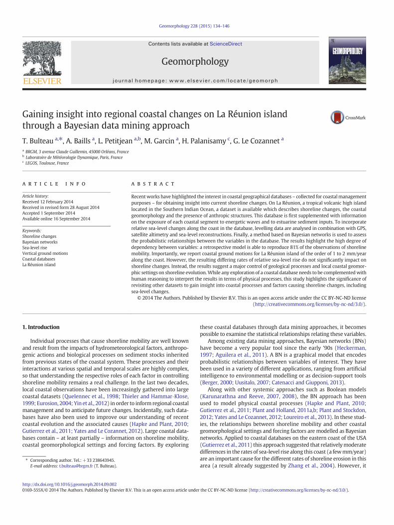
Gaining insight into regional coastal changes on La Réunion islandthrough a Bayesian data mining approach
T. Bulteau a,⁎, A. Baills a, L. Petitjean a,b, M. Garcin a, H. Palanisamy c, G. Le Cozannet a
a BRGM, 3 avenue Claude Guillemin, 45000 Orléans, Franceb Laboratoire de Météorologie Dynamique, Paris, Francec LEGOS, Toulouse, France
a b s t r a c ta r t i c l e i n f o
Article history:
Received 12 February 2014
Received in revised form 28 August 2014
Accepted 1 September 2014
Available online 16 September 2014
Keywords:
Shoreline changes
Bayesian networks
Sea-level rise
Vertical ground motions
Coastal databases
La Réunion island
Recentworks have highlighted the interest in coastal geographical databases – collected for coastalmanagement
purposes – for obtaining insight into current shoreline changes. On La Réunion, a tropical volcanic high island
located in the Southern Indian Ocean, a dataset is available which describes shoreline changes, the coastal
geomorphology and the presence of anthropic structures. This database is first supplemented with information
on the exposure of each coastal segment to energetic waves and to estuarine sediment inputs. To incorporate
relative sea-level changes along the coast in the database, levelling data are analysed in combination with GPS,
satellite altimetry and sea-level reconstructions. Finally, a method based on Bayesian networks is used to assess
the probabilistic relationships between the variables in the database. The results highlight the high degree of
dependency between variables: a retrospective model is able to reproduce 81% of the observations of shoreline
mobility. Importantly, we report coastal ground motions for La Réunion island of the order of 1 to 2 mm/year
along the coast. However, the resulting differing rates of relative sea-level rise do not significantly impact on
shoreline changes. Instead, the results suggest a major control of geological processes and local coastal geomor-
phic settings on shoreline evolution.While any exploration of a coastal database needs to be complementedwith
human reasoning to interpret the results in terms of physical processes, this study highlights the significance of
revisiting other datasets to gain insight into coastal processes and factors causing shoreline changes, including
sea-level changes.
© 2014 The Authors. Published by Elsevier B.V. This is an open access article under the CC BY-NC-ND license
(http://creativecommons.org/licenses/by-nc-nd/3.0/).
1. Introduction
Individual processes that cause shoreline mobility are well known
and result from the impacts of hydrometeorological factors, anthropo-
genic actions and biological processes on sediment stocks inherited
from previous states of the coastal system. These processes and their
interactions at various spatial and temporal scales are highly complex,
so that understanding the respective roles of each factor in controlling
shoreline mobility remains a real challenge. In the last two decades,
local coastal observations have been increasingly gathered into large
coastal datasets (Quelennec et al., 1998; Thieler and Hammar‐Klose,
1999; Eurosion, 2004; Yin et al., 2012) in order to inform regional coastal
management and to anticipate future changes. Incidentally, such data-
bases have also been used to improve our understanding of recent
coastal evolution and the associated causes (Hapke and Plant, 2010;
Gutierrez et al., 2011; Yates and Le Cozannet, 2012). Large coastal data-
bases contain – at least partially – information on shoreline mobility,
coastal geomorphological settings and forcing factors. By exploring
these coastal databases through data mining approaches, it becomes
possible to examine the statistical relationships relating these variables.
Among existing data mining approaches, Bayesian networks (BNs)
have become a very popular tool since the early '90s (Heckerman,
1997; Aguilera et al., 2011). A BN is a graphical model that encodes
probabilistic relationships between variables of interest. They have
been used in a variety of different applications, ranging from artificial
intelligence to environmental modelling or as decision-support tools
(Berger, 2000; Uusitalo, 2007; Catenacci and Giupponi, 2013).
Along with other systemic approaches such as Boolean models
(Karunarathna and Reeve, 2007, 2008), the BN approach has been
used to model physical coastal processes (Hapke and Plant, 2010;
Gutierrez et al., 2011; Plant and Holland, 2011a,b; Plant and Stockdon,
2012; Yates and Le Cozannet, 2012; Loureiro et al., 2013). In these stud-
ies, the relationships between shoreline mobility and other coastal
geomorphological settings and forcing factors are modelled as Bayesian
networks. Applied to coastal databases on the eastern coast of the USA
(Gutierrez et al., 2011) this approach suggested that relativelymoderate
differences in the rates of sea-level rise along this coast (a fewmm/year)
are an important cause for the different rates of shoreline erosion in this
area (a result already suggested by Zhang et al., 2004). However, it
Geomorphology 228 (2015) 134–146
⁎ Corresponding author. Tel.: +33 238643945.
E-mail address: [email protected] (T. Bulteau).
http://dx.doi.org/10.1016/j.geomorph.2014.09.002
0169-555X/© 2014 The Authors. Published by Elsevier B.V. This is an open access article under the CC BY-NC-ND license (http://creativecommons.org/licenses/by-nc-nd/3.0/).
Contents lists available at ScienceDirect
Geomorphology
j ourna l homepage: www.e lsev ie r .com/ locate /geomorph

remains unclear whether this conclusion can be generalized to other
coastal sites (Cazenave and Le Cozannet, 2014). To confirm such
results, it is necessary to explore other coastal datasets in order to
check whether these relationships between sea-level rise and shoreline
erosion are fortuitous, related to local conditions or if they apply to
many coasts around the world.
The coastal dataset for La Réunion island (Southern Indian
Ocean; De La Torre, 2004) was initially compiled for coastal manage-
ment purposes, in order to characterize and map the coastal mor-
phology and morphodynamics of the island and anticipate future
trends (Le Cozannet et al., 2013). For each coastal segment, this
dataset describes the observed multidecadal shoreline mobility,
geomorphic settings and the presence of anthropic structures in
the vicinity of the segment. In this study, we first complete this
coastal dataset by constructing three other variables, namely the
exposure to energetic waves, the presence of an estuary and the
rate of relative sea-level rise, then, we use the method proposed by
Gutierrez et al. (2011) to quantify the strength of known relation-
ships between the variables. This enables one to identify the main
factors driving decadal shoreline mobility in La Réunion while re-
vealing the particular role of the rate of relative sea-level rise in
coastal evolution.
The paper is organized as follows: in part 2, the theory of the BN
approach and the tools used to evaluate the BN performance are
briefly presented; in part 3, the study site and the dataset used are
described; part 4 presents the results (relative sea-level changes at
the coast and assessment of the BN performance); and part 5 exam-
ines to which extent the results can be interpreted in terms of phys-
ical processes.
2. Bayesian networks and their application for exploring
coastal databases
A BN is a tool to graphically represent knowledge about a given
system and to compute dependencies between parts of that system in
terms of probabilities (Pearl, 1986). Formally, a BNℬ=(G, θ) is defined
by:
– A directed acyclic graph G = (X,E), E being the set of directed edges
representing causal relationships between the nodes of the graph
that represent a set of random variables X = {X1, …, Xn},
– Parameters θ = {P(Xi|Pa(Xi))}i = 1.. n that depict the conditional
probability of each node Xi given its parents Pa(Xi) within G.
While G describes qualitatively the dependence (or independence)
between variables, θ provides a more quantitative insight. In addition,
the conditional independencies expressed by G allow simplification of
the joint probability distribution of X into a product of local conditional
probabilities which depend only on the considered node and its parents
(see e.g. Pearl, 1986):
P X1;…;Xnð Þ ¼ ∏n
i¼1
P Xi Pa Xið Þjð Þ ¼ ∏n
i¼1
θi: ð1Þ
This formula is a fundamental property of BNs. It is used for inference
that is to compute the probability of any random variable Xi from obser-
vations of the others.
Hapke and Plant (2010) and Gutierrez et al. (2011) proposed a BN-
based approach to explore coastal databases. The first step in their
approach consists of defining a network structure G , formalizing a
qualitative understanding of coastal systems. Therefore, G displays the
relationships between a few important parameters of a coastal database
such as, for example: geomorphology,wave climate, tidal range, decadal
sea-level changes and shoreline evolution. Importantly, in order to be
used in a BN, the coastal variables must have states that are mutually
exclusive and collectively exhaustive (Heckerman, 1997), which im-
plies simplifying and harmonizing the raw coastal observations, like,
for example, considering only a limitednumber of coastal geomorphology
classes (cliffs, wetlands, beaches…) out of the numerous existing ones
(Finkl, 2004).
In a second step, the parameters θ are computed from the database
(learning phase). When a complete dataset (i.e. no missing data) is
considered, the learning phase is straightforward: the parameters θ
are determined using the maximum likelihood approach, which
consists in estimating the probability of an event with its frequency of
appearance in the dataset (Naïm et al., 2007).
The next step of the approach consists of creating a predictivemodel
for shorelinemobility. The conditional probability distribution of shore-
line mobility is written as:
P SMi eX j
���� �
;∀i ð2Þ
where SMi is the ith discretized state of the shoreline mobility vari-
able and eX j represents a combination of all the other variables. For
a given combination eX j , the predicted shoreline mobility is the
mode of the conditional probability distribution (2). This is written
as:
SMpred ¼ arg maxi
P SMi eX j
���� �� �
ð3Þ
The probability value gives an indication of the prediction uncertain-
ty. Assessing to which extent the observed shoreline mobility can be
correctly predicted helps us evaluate the relevance and efficiency of
our BN to represent the coastal system. As the same data were used
for inference and learning, we are in a case of ‘overfitting’ (Aguilera
et al., 2011) and the resulting predictions might be biased. However,
the Bayesian model here is not used to predict future states of coastal
geomorphology but as a data mining technique to analyse the relation-
ships between the variables in the database.
The last step consists of analysing what are the most discriminating
variables with respect to shoreline changes. This is done by evaluating
the BN performance through statistical tools, such as the log-
likelihood ratio (LR) which evaluates how much the knowledge of
shoreline mobility has been improved owing to the other observations.
For a given coastal segment (k) the LR is defined as follows:
LR kð Þ ¼ log P SM kð Þ O kð Þ
���� �� �
− log P SM kð Þ
� �� �ð4Þ
where SM(k) is the observed shoreline mobility of segment (k) and O(k)
represents the set of all the other variable states corresponding to
segment (k).
The LR(k) can be summed over all coastal segments to give a global
score of the model performance. By comparing how the global LR
evolves with the number and type of variables, Gutierrez et al. (2011)
evaluate the relative importance of each variable of the model with
respect to shoreline changes.
In this paper, the samemethod is applied to another dataset for La
Réunion island. However, in this application, because each coastal
segment has a different length, the learning phase of the network is
modified in a way that the importance of each segment is evaluated
according to its length. In other words, each coastal segment does
not count for one observation during the learning phase; its own
length is used instead to weight it in the computation of the maxi-
mum likelihood estimators of parameters θ. Subsequently, the global
score of LR is also computed accounting for the respective lengths of
the segments:
LR ¼1
total length
X
k
LR kð Þlength kð Þ: ð5Þ
135T. Bulteau et al. / Geomorphology 228 (2015) 134–146
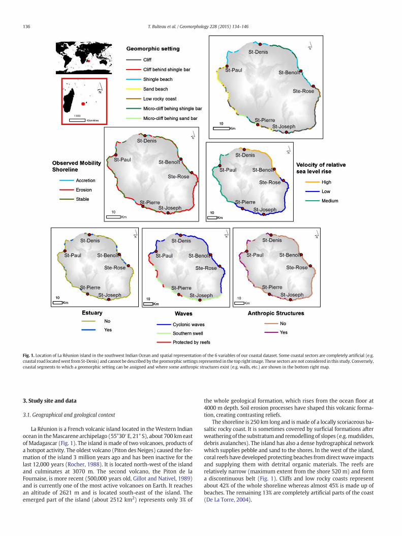
3. Study site and data
3.1. Geographical and geological context
La Réunion is a French volcanic island located in theWestern Indian
ocean in theMascarene archipelago (55°30′ E, 21° S), about 700 kmeast
of Madagascar (Fig. 1). The island is made of two volcanoes, products of
a hotspot activity. The oldest volcano (Piton des Neiges) caused the for-
mation of the island 3 million years ago and has been inactive for the
last 12,000 years (Rocher, 1988). It is located north-west of the island
and culminates at 3070 m. The second volcano, the Piton de la
Fournaise, is more recent (500,000 years old, Gillot and Nativel, 1989)
and is currently one of the most active volcanoes on Earth. It reaches
an altitude of 2621 m and is located south-east of the island. The
emerged part of the island (about 2512 km2) represents only 3% of
the whole geological formation, which rises from the ocean floor at
4000 m depth. Soil erosion processes have shaped this volcanic forma-
tion, creating contrasting reliefs.
The shoreline is 250 km long and is made of a locally scoriaceous ba-
saltic rocky coast. It is sometimes covered by surficial formations after
weatheringof the substratumand remodellingof slopes (e.g.mudslides,
debris avalanches). The island has also a dense hydrographical network
which supplies pebble and sand to the shores. In the west of the island,
coral reefs have developed protecting beaches fromdirectwave impacts
and supplying them with detrital organic materials. The reefs are
relatively narrow (maximum extent from the shore 520 m) and form
a discontinuous belt (Fig. 1). Cliffs and low rocky coasts represent
about 42% of the whole shoreline whereas almost 45% is made up of
beaches. The remaining 13% are completely artificial parts of the coast
(De La Torre, 2004).
Fig. 1. Location of La Réunion island in the southwest Indian Ocean and spatial representation of the 6 variables of our coastal dataset. Some coastal sectors are completely artificial (e.g.
coastal road locatedwest fromSt-Denis) and cannot be described by the geomorphic settings represented in the top right image. These sectors are not considered in this study. Conversely,
coastal segments to which a geomorphic setting can be assigned and where some anthropic structures exist (e.g. walls, etc.) are shown in the bottom right map.
136 T. Bulteau et al. / Geomorphology 228 (2015) 134–146

3.2. Description of the coastal database
3.2.1. Database as a whole
The coastal database for La Réunion island is based on a GIS (Geo-
graphical Information System) dataset compiled by the FrenchGeological
Survey (BRGM) from field campaigns undertaken between March and
June 2004 (De La Torre, 2004), which were updated using more recent
information on coastal processes and harmonized to make it suitable
for use within a BN approach.
The initial database comprised three variables (Table 1):
morphotype (11 states), the presence of anthropic structures (3 states)
and shoreline mobility (5 states), that divided the coastline into seg-
mentswith homogeneous characteristics. This dataset cannot be readily
explored using a Bayesian network: for example, the geomorphic set-
ting of a given coastal segment could be described with a combination
of 2 morphotypes (e.g. coherent cliff plus marine shingle bar). This
counters to the rule of mutually exclusive and collectively exhaustive
states for BN variables (Heckerman, 1997). Hence, new classes were
defined that both comply with this rule and adequately represent the
coastal geomorphology in the island. Another point to consider when
preparing the database is as follows: the more states per variable and
the more complicated the model structure, the more data is needed to
efficiently capture complex empirical distributions (Myllymäki et al.,
2002; Uusitalo, 2007). Here, observations are limited by the island
shoreline length. Thus, the number of stateswas reduced to aminimum
while maintaining a satisfying representation of the coastal system:
from the initial numbers of states of morphotype, anthropic structures
and shoreline mobility, we settled on only 7 geomorphic settings, 2
states for the presence of anthropic structures and 3 states of shoreline
mobility.
The states of the simplified variables are presented in Table 1. This
table also shows that to complete the description of the coastal system,
three new variables were added — exposure to energetic waves (3
states) (adapted from Lecacheux et al., 2012), presence of an estuary
(2 states) (created within the present study), and the rate of relative
sea-level rise (3 states) (created within the present study). Detailed
information on the different variables is given in the following
subsections. Fig. 1 presents the final coastal data used in the next
steps of the approach. The final database divides the island's coastline
into 384 segments with different lengths.
3.2.2. Shoreline evolution
The shoreline evolution dataset is based on extensive field observa-
tions of shoreline change indicators, such as micro-cliff, apparent tree
roots at the upper beach, beach slopes, traces of fallen rocks at the top
of the cliff, the presence of an upper beach berm, a small delta, a shingle
bar at the foot of the cliff, vegetation of backshore or dunes. De La Torre
(2004) positively compared his interpretation from field observations
with aerial photographs from IGN campaigns of 1966, 1978 and
orthophotographs of 1997. Although this period covers the intense
economic and demographic development of the island, several signifi-
cant climatic events (cyclones Hyacinthe (1980), Florine (1981),
Clotilda (1987), Firinga (1989), Colina (1993), Hollanda (1994), Dina
(2002)…) as well as volcanic events (eruptions of the Piton de la
Fournaise reaching the sea in 1977 and 1986), the good agreement
between the two approaches suggests that the coastal dataset can be
interpreted as an indication of the main trends of coastal mobility over
the last three decades.
3.2.3. Coastal geomorphology, human actions, inputs from river sediments
to the coast
In addition to the shoreline evolution, the coastal dataset collected
by De La Torre (2004) includes a description of the geomorphic setting
for each coastal segment, as well as information about potential
anthropic structures in the vicinity of the segment (a wall at the upper
beach, a ramp for boats on a shingle beach, homes on top of micro-cliffs
or directly on the beach, tourism facilities such as coastal promenades
or artificial saltwater swimming pools, jetties, etc.) (Fig. 1). All these
anthropic structures can potentially affect shoreline mobility (Eurosion,
2004) by disrupting the alongshore sedimentary transport (e.g. jetty at
Saint-Benoît), the sediment transfer from rivers (e.g. river d'Abord at
Saint-Pierre) or between sand dunes and beaches (e.g. Etang-Salé les
bains), or by modifying the local wave regime (e.g. homes at Saint-
Pierre located on the seafront). Thus, they can favour erosion but they
can also locally protect the shoreline from it (e.g. a jetty can favour accre-
tion upstream of the alongshore drift, an artificial swimming pool can
protect a beach from the erosive action of waves, as has been observed
at the Grande Anse beach.). Coastal segments that are completely artifi-
cial are discarded from the dataset. In addition, we added information,
through a Boolean variable ‘presence of an estuary’, about the potential
for each coastal segment to be significantly nourished by river sediments.
This information is derived from the hydrographical network (source BD
Carthage, French Geographical Institute (IGN)) considering that themain
rivers are those that bring a significant amount of sediments to the coast.
In practice, every coastal segment co-locatedwith a rivermouthwas con-
sidered as significantly nourished by river sediments. This does not take
into account alongshore sedimentary transport, that is, the capacity of a
segment to be supplied with sediments from adjacent segments.
3.2.4. Cyclonic and seasonal waves and swells
The exposure to energeticwaves is based on themodelling of the dif-
ferent types of waves affecting La Reunion (Lecacheux et al., 2012): the
island is exposed to three main wave regimes — trade waves, southern
swells and cyclonic waves. Trade waves are generated by trade winds
(persistent planetary-scale surface winds). They come from the
east-south-east in the Southern hemisphere and cause alongshore
Table 1
Description of the initial (De La Torre, 2004) and final states of the variables.
Variable Initial Final
Morphotype
(initial)/Geomorphic
setting (GS) (final)
Coherent cliff
Low rocky coast
Loose or mixed cliff
Loose or mixed
micro-cliff
Riverine shingle bar
Marine shingle bar
Basaltic sand beach
Basaltic sand dune
Unevolved coral
mixed sand beach
Unevolved coral
biodetrital sand
beach
Evolved coral
biodetrital sand
beach
1-Cliff
2-Cliff behind shingle bar
3-Low rocky coast
4-Micro-cliff behind shingle bar
5-Micro-cliff behind sand bar
6-Shingle beach
7-Sand beach
Anthropic
structure (AS)
Completely
artificialized
Partially
artificialized
No
1-Yes (corresponding to Partially
artificialized state)
2-No
Shoreline
mobility (SM)
Stability
In transition
Moderate erosion
Severe erosion
Accretion
1-Stability (combining Stability and
In transition states)
2-Erosion (combining Moderate
erosion and Severe erosion states)
3-Accretion
Estuary N/A 1-Yes
2-No
Exposure to
energetic waves
(Waves)
N/A 1-Mainly exposed to cyclonic waves
2-Mainly exposed to southern
swells
3-Protected by reefs
Velocity of relative
sea level rise (RSLR)
N/A 1-High
2-Low
3-Medium
137T. Bulteau et al. / Geomorphology 228 (2015) 134–146
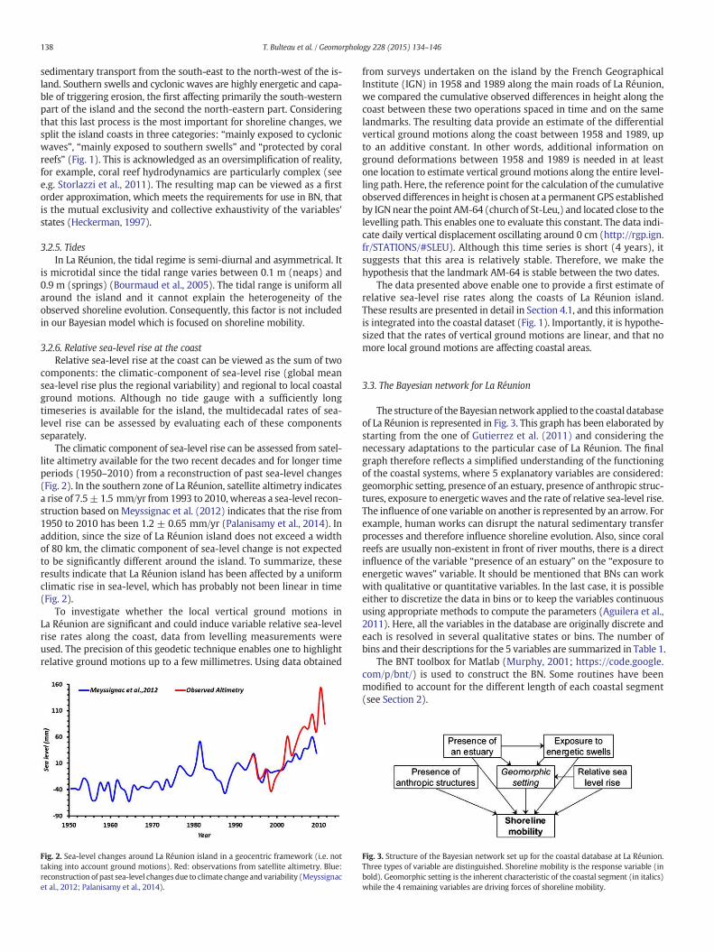
sedimentary transport from the south-east to the north-west of the is-
land. Southern swells and cyclonic waves are highly energetic and capa-
ble of triggering erosion, the first affecting primarily the south-western
part of the island and the second the north-eastern part. Considering
that this last process is the most important for shoreline changes, we
split the island coasts in three categories: “mainly exposed to cyclonic
waves”, “mainly exposed to southern swells” and “protected by coral
reefs” (Fig. 1). This is acknowledged as an oversimplification of reality,
for example, coral reef hydrodynamics are particularly complex (see
e.g. Storlazzi et al., 2011). The resulting map can be viewed as a first
order approximation, which meets the requirements for use in BN, that
is the mutual exclusivity and collective exhaustivity of the variables'
states (Heckerman, 1997).
3.2.5. Tides
In La Réunion, the tidal regime is semi-diurnal and asymmetrical. It
is microtidal since the tidal range varies between 0.1 m (neaps) and
0.9 m (springs) (Bourmaud et al., 2005). The tidal range is uniform all
around the island and it cannot explain the heterogeneity of the
observed shoreline evolution. Consequently, this factor is not included
in our Bayesian model which is focused on shoreline mobility.
3.2.6. Relative sea-level rise at the coast
Relative sea-level rise at the coast can be viewed as the sum of two
components: the climatic-component of sea-level rise (global mean
sea-level rise plus the regional variability) and regional to local coastal
ground motions. Although no tide gauge with a sufficiently long
timeseries is available for the island, the multidecadal rates of sea-
level rise can be assessed by evaluating each of these components
separately.
The climatic component of sea-level rise can be assessed from satel-
lite altimetry available for the two recent decades and for longer time
periods (1950–2010) from a reconstruction of past sea-level changes
(Fig. 2). In the southern zone of La Réunion, satellite altimetry indicates
a rise of 7.5± 1.5 mm/yr from 1993 to 2010,whereas a sea-level recon-
struction based on Meyssignac et al. (2012) indicates that the rise from
1950 to 2010 has been 1.2 ± 0.65 mm/yr (Palanisamy et al., 2014). In
addition, since the size of La Réunion island does not exceed a width
of 80 km, the climatic component of sea-level change is not expected
to be significantly different around the island. To summarize, these
results indicate that La Réunion island has been affected by a uniform
climatic rise in sea-level, which has probably not been linear in time
(Fig. 2).
To investigate whether the local vertical ground motions in
La Réunion are significant and could induce variable relative sea-level
rise rates along the coast, data from levelling measurements were
used. The precision of this geodetic technique enables one to highlight
relative ground motions up to a few millimetres. Using data obtained
from surveys undertaken on the island by the French Geographical
Institute (IGN) in 1958 and 1989 along the main roads of La Réunion,
we compared the cumulative observed differences in height along the
coast between these two operations spaced in time and on the same
landmarks. The resulting data provide an estimate of the differential
vertical ground motions along the coast between 1958 and 1989, up
to an additive constant. In other words, additional information on
ground deformations between 1958 and 1989 is needed in at least
one location to estimate vertical groundmotions along the entire level-
ling path. Here, the reference point for the calculation of the cumulative
observed differences in height is chosen at a permanent GPS established
by IGNnear the point AM-64 (church of St-Leu,) and located close to the
levelling path. This enables one to evaluate this constant. The data indi-
cate daily vertical displacement oscillating around 0 cm (http://rgp.ign.
fr/STATIONS/#SLEU). Although this time series is short (4 years), it
suggests that this area is relatively stable. Therefore, we make the
hypothesis that the landmark AM-64 is stable between the two dates.
The data presented above enable one to provide a first estimate of
relative sea-level rise rates along the coasts of La Réunion island.
These results are presented in detail in Section 4.1, and this information
is integrated into the coastal dataset (Fig. 1). Importantly, it is hypothe-
sized that the rates of vertical ground motions are linear, and that no
more local ground motions are affecting coastal areas.
3.3. The Bayesian network for La Réunion
The structure of the Bayesiannetwork applied to the coastal database
of La Réunion is represented in Fig. 3. This graph has been elaborated by
starting from the one of Gutierrez et al. (2011) and considering the
necessary adaptations to the particular case of La Réunion. The final
graph therefore reflects a simplified understanding of the functioning
of the coastal systems, where 5 explanatory variables are considered:
geomorphic setting, presence of an estuary, presence of anthropic struc-
tures, exposure to energetic waves and the rate of relative sea-level rise.
The influence of one variable on another is represented by an arrow. For
example, human works can disrupt the natural sedimentary transfer
processes and therefore influence shoreline evolution. Also, since coral
reefs are usually non-existent in front of river mouths, there is a direct
influence of the variable “presence of an estuary” on the “exposure to
energetic waves” variable. It should be mentioned that BNs can work
with qualitative or quantitative variables. In the last case, it is possible
either to discretize the data in bins or to keep the variables continuous
using appropriate methods to compute the parameters (Aguilera et al.,
2011). Here, all the variables in the database are originally discrete and
each is resolved in several qualitative states or bins. The number of
bins and their descriptions for the 5 variables are summarized in Table 1.
The BNT toolbox for Matlab (Murphy, 2001; https://code.google.
com/p/bnt/) is used to construct the BN. Some routines have been
modified to account for the different length of each coastal segment
(see Section 2).
Fig. 2. Sea-level changes around La Réunion island in a geocentric framework (i.e. not
taking into account ground motions). Red: observations from satellite altimetry. Blue:
reconstruction of past sea-level changes due to climate change and variability (Meyssignac
et al., 2012; Palanisamy et al., 2014).
Fig. 3. Structure of the Bayesian network set up for the coastal database at La Réunion.
Three types of variable are distinguished. Shoreline mobility is the response variable (in
bold). Geomorphic setting is the inherent characteristic of the coastal segment (in italics)
while the 4 remaining variables are driving forces of shoreline mobility.
138 T. Bulteau et al. / Geomorphology 228 (2015) 134–146
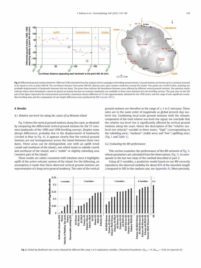
4. Results
4.1. Relative sea-level rise along the coasts of La Réunion island
Fig. 4 shows the vertical groundmotions along the coast, as obtained
by comparing the differential vertical ground motions for the 57 com-
mon landmarks of the 1989 and 1958 levelling surveys. Despite some
abrupt differences, probably due to the displacement of landmarks
(circled in blue in Fig. 4), it appears clearly that the vertical ground
motions are not homogeneous across the island between these two
dates. Three areas can be distinguished, one with an uplift trend
(south and southeast of the island), one which tends to subside (north
and northeast of the island) and a “stable” or slightly subsiding area
(western part of the island).
These results are rather consistent with intuition since it highlights
uplift of the active volcanic system of the island. For the following, an
assumption is made that these observed vertical ground motions are
representative of a long-term general tendency. The rates of the vertical
ground motions are therefore in the range of ±1 to 2 mm/year. These
rates are in the same order of magnitude as global present-day sea-
level rise. Combining local-scale ground motions with the climatic
component of the total relative sea-level rise signal, we conclude that
the relative sea-level rise is significantly affected by vertical ground
motions along the coast. Hence the description of the “relative sea-
level rise velocity” variable in three states: “high” (corresponding to
the subsiding area), “medium” (stable area) and “low” (uplifting area)
(Fig. 1 and Table 1).
4.2. Evaluating the BN performance
This section examines the performance of the BN network of Fig. 3,
whose parameters are calculated from the observations (Fig. 1). It corre-
sponds to the last two steps of the method described in part 2.
Using all 5 variables, a predictive model based on our BN correctly
reproduces the observed mobility for about 83% of the shoreline length
(compared to 58% in the random case, see Appendix A). More precisely,
Fig. 4.Differential groundmotions between 1989 and 1958 estimated from the analysis of two campaigns of levellingmeasurements. Groundmotions are knownup to a constant assumed
to be equal to zero at point AM-64. The curvilinear distance from point AM-64 (abscissa axis) goes counter-clockwise around the island. Two points are circled in blue, pointing out
probable displacements of landmarks between the two dates. The green lines indicate the boundaries between areas affected by different vertical ground motions. The question marks
indicate where these boundaries cannot be placed accurately because no common landmarks are available in these areas between the two levelling surveys. The grey area on the left
part of the figure represents the measurement uncertainty (maximum closure difference of 13mm approximately, obtained for the 1958 series) and the range of non-significant results.
Raw levelling data and the computation of raw height differences were produced by IGN (Lavoué, 2013).
Fig. 5. Global log-likelihood ratio scores obtained for different BNs using 1 to 5 explanatory variables. (Theoretical boundaries: LRmin = 0; LRmax = 0.38, see Appendix B).
139T. Bulteau et al. / Geomorphology 228 (2015) 134–146
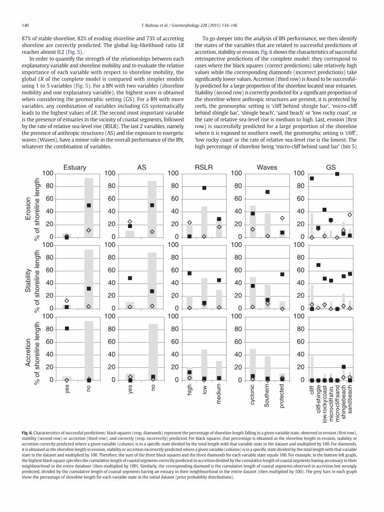
87% of stable shoreline, 82% of eroding shoreline and 73% of accreting
shoreline are correctly predicted. The global log-likelihood ratio LR
reaches almost 0.2 (Fig. 5).
In order to quantify the strength of the relationships between each
explanatory variable and shorelinemobility and to evaluate the relative
importance of each variable with respect to shoreline mobility, the
global LR of the complete model is compared with simpler models
using 1 to 5 variables (Fig. 5). For a BN with two variables (shoreline
mobility and one explanatory variable), the highest score is obtained
when considering the geomorphic setting (GS). For a BN with more
variables, any combination of variables including GS systematically
leads to the highest values of LR. The second most important variable
is the presence of estuaries in the vicinity of coastal segments, followed
by the rate of relative sea-level rise (RSLR). The last 2 variables, namely
the presence of anthropic structures (AS) and the exposure to energetic
waves (Waves), have aminor role in the overall performance of the BN,
whatever the combination of variables.
To go deeper into the analysis of BN performance, we then identify
the states of the variables that are related to successful predictions of
accretion, stability or erosion. Fig. 6 shows the characteristics of successful
retrospective predictions of the complete model: they correspond to
cases where the black squares (correct predictions) take relatively high
values while the corresponding diamonds (incorrect predictions) take
significantly lower values. Accretion (third row) is found to be successful-
ly predicted for a large proportion of the shoreline located near estuaries.
Stability (second row) is correctly predicted for a significant proportion of
the shoreline where anthropic structures are present, it is protected by
reefs, the geomorphic setting is ‘cliff behind shingle bar’, ‘micro-cliff
behind shingle bar’, ‘shingle beach’, ‘sand beach’ or ‘low rocky coast’, or
the rate of relative sea-level rise is medium to high. Last, erosion (first
row) is successfully predicted for a large proportion of the shoreline
where it is exposed to southern swell, the geomorphic setting is ‘cliff’,
‘low rocky coast’ or the rate of relative sea-level rise is the lowest. The
high percentage of shoreline being ‘micro-cliff behind sand bar’ (bin 5)
0
20
40
60
80
100
0
20
40
60
80
100
0
20
40
60
80
100
0
20
40
60
80
100
0
20
40
60
80
100
0
20
40
60
80
100
0
20
40
60
80
100
0
20
40
60
80
100
0
20
40
60
80
100
0
20
40
60
80
100
0
20
40
60
80
100
0
20
40
60
80
100
0
20
40
60
80
100
0
20
40
60
80
100
0
20
40
60
80
100
Estuary AS RSLR Waves GS
Ero
sio
nS
tab
ility
Accre
tio
n
% o
f shore
line leng
th
% o
f shore
line leng
th
% o
f shore
line leng
th
ye
s
no
ye
s
no
hig
h
low
me
diu
m
cyclo
nic
South
ern
pro
tecte
d
clif
fclif
f-shin
gle
low
rockycoast
mic
ro- c
liffs
hin
.m
icro
-clif
fsand
sh
ing
le b
each
sand
beach
Fig. 6.Characteristics of successful predictions: black squares (resp. diamonds) represent the percentage of shoreline length falling in a given variable state, observed in erosion (first row),
stability (second row) or accretion (third row), and correctly (resp. incorrectly) predicted. For black squares, that percentage is obtained as the shoreline length in erosion, stability or
accretion correctly predicted where a given variable (column) is in a specific state divided by the total length with that variable state in the dataset and multiplied by 100. For diamonds,
it is obtained as the shoreline length in erosion, stability or accretion incorrectly predictedwhere a given variable (column) is in a specific state divided by the total lengthwith that variable
state in the dataset andmultiplied by 100. Therefore, the sum of the three black squares and the three diamonds for each variable state equals 100. For example, in the bottom left graph,
thehighest black square specifies the cumulative length of coastal segments correctly predicted in accretion divided by the cumulative length of coastal segments having an estuary in their
neighbourhood in the entire database (then multiplied by 100). Similarly, the corresponding diamond is the cumulative length of coastal segments observed in accretion but wrongly
predicted, divided by the cumulative length of coastal segments having an estuary in their neighbourhood in the entire dataset (then multiplied by 100). The grey bars in each graph
show the percentage of shoreline length for each variable state in the initial dataset (prior probability distributions).
140 T. Bulteau et al. / Geomorphology 228 (2015) 134–146

correctly predicted in erosion comes from the low representation of that
variable category in the dataset (2.5% of the whole shoreline). The pres-
ence of anthropic structures does not inform much about erosion (black
square and diamond taking similar values) but seems to be related to
shoreline stability.
All the strong links found between each explanatory variable and
shoreline mobility, as shown in Fig. 6, are consistent with an intuitive
analysis, except for the rate of relative sea-level rise: for more than
55% of the shorelinewhere RSLR velocity is the highest, shorelinemobil-
ity is correctly predicted as stable, whereas for about 80% of the shore-
line whose RSLR velocity is the lowest, shoreline mobility is correctly
predicted in erosion. In other words, erosion is more frequent when
the RSLR velocity is the lowest. This paradoxical behaviour of RSLR in
the model is discussed in detail in Section 5.2.
Because of the counter-intuitive behaviour of the variable RSLR ve-
locity, the next results are obtained using only the four other variables.
4.3. Performance with 4 variables
The global LR score of the BN using 4 variables (geomorphic setting,
presence of estuary, presence of anthropic structures and exposure to
energetic waves) is 0.18 (Fig. 5) and the proportion of the shoreline
whose observed mobility is correctly predicted is 81%. More precisely,
85% of stable shoreline, 79% of eroding shoreline and 73% of accreting
shoreline are correctly predicted. Fig. 7 (top) shows the locations
where the retrospective predictions are correct or not.
Fig. 7 (bottom) maps the probability of the most likely outcome, an
indicator which can be interpreted as the confidence in the
Fig. 7. Spatial variability of the predictivemodel outcome. Top: false and correct predictions and observed shorelinemobility for each coastal segment. Bottom:mapof the confidence in the
predictions, i.e. the probability of the predicted outcome. The red rectangles identify 3 segments that are incorrectly predictedwith ‘very high’ confidence. Predictions in the northern part
of the island aremore uncertain than in the southernpart. This indicates characteristics of coastal segments in the northwith relativelywider probability distributions of shorelinemobility
than in the south.
141T. Bulteau et al. / Geomorphology 228 (2015) 134–146

retrospective prediction. This map can be used to identify areas
where there is a high level of uncertainties or great confidence in
the outcome prediction (Gutierrez et al., 2011) which is useful to tar-
get where the BN needs improvements. Globally, more than 67% of
the shoreline is correctly predicted with a ‘high’ confidence level or
above (probability of the most likely outcome greater than 0.66)
and almost 23% of the shoreline is correctly predicted with a ‘very
high’ confidence level or above (probability of the most likely out-
come greater than 0.9). By comparing Fig. 7 (top) and (bottom), we
can also identify areas where there is great confidence in the out-
come while the prediction is wrong. Only 3 of these particular sites
are found falling within the ‘very high’ category, they are identified
by red rectangles in Fig. 7 (bottom).
5. Discussion
5.1. Interpretation of BN results in terms of physical processes
Section 4.2 showed that geomorphic setting is the most important
variable for understanding shoreline mobility on La Réunion. This is
due to the fact that in the dataset, some well represented categories of
GS are strongly linked to specific shoreline mobility. For example, 93%
of cliffs in La Réunion are observed in erosion and cliffs are the main
geomorphic settings around the island (38% of the shoreline). The pres-
ence of an estuary in the vicinity of a segment is the secondmost impor-
tant variable for understanding shorelinemobility. In particular, it is the
only characteristic identified to successfully predict accretion (see
Section 4.2 and Fig. 6). This can be easily interpreted as accreting seg-
ments around the island are often subjected to the influence of river
sediment supply: 73% of accreting shoreline has an estuary in its
neighbourhood.
Stable and eroding coasts are better predicted by the BN than accret-
ing shorelines, but the result for the latter category is still satisfying
(73%, see Section 4.3). In fact, 100% of correctly predicted accreting
shoreline has an estuary nearby which indicates that the remaining
27% of accreting shoreline has no estuary and is systematically
mispredicted. That might be the result of a combination of factors in-
cluding the relative scarcity of data for the accretion category (only 7%
of the coast is accreting), which may prevent the BN from accurately
identifying combinations of variables leading to accretion, and the
incompleteness of the BN structure which does not take into account
processes of sedimentary transport along the coast.
Alongshore sedimentary transport processes are generated by
currents induced mainly by trade waves (see Section 3.2.4). They redis-
tribute fine and coarse materials of marine or terrestrial origin (cliff and
riverine sediments) along the coast from the south-east to the north-
west. Although it is difficult to quantify the effect of these processes
on shorelinemobility, there is evidence of their influence on local coast-
al evolution. For example, a natural rocky outcrop at La Pointe du
Bourbier acts as a wall, stopping the coastal drift and accumulating sed-
iments upstream. As a result, the coastal segment located immediately
upstream of the outcrop is accreting (Fig. 8). Anthropic structures
implanted directly on the shoreline, such as harbours,marinas or jetties,
also highlight the importance of alongshore sedimentary transport
when they disrupt it. A case in point is the jetty of Le Butor at Saint-
Benoît where sediments accumulate updrift of the structure whereas
erosion is observed downdrift (Fig. 8). These examples attest to the
significant role played by alongshore transport in local sedimentary
budgets and coastal evolution. As our BN model fails to take it into
account, we might expect some mispredictions in the evaluation of BN
performance in these cases.
It was noted in Section 4.2 and Fig. 5 that the presence of anthropic
structures is the variable which has the weakest explanatory power
with respect to shoreline mobility. However, stability seems to be
successfully predicted when such structures are present (Fig. 6). This
feature is then probably due to spatial correlation with other variables
having higher explanatory power. Indeed, anthropic structures are
mostly located on the west coast, where sandy beaches can be found
as well as protecting reefs. These two variables' states are related to
successful stability predictions and the corresponding variables
(Geomorphic Setting and Waves) have stronger links with respect to
shoreline mobility. Therefore, even if locally there is evidence of the
direct influence of human interventions on shoreline mobility, other
variables seem to dominate and control shoreline mobility at the scale
of the island. It is worth noting that the influence of a human works
located on a given coastal segment on an adjacent segment is not
taken into account in our model. That might also explain the relatively
weak link between the variables Anthropic Structures and Shoreline
Fig. 8. Satellite views and localisation of a) the natural rocky outcrop at La Pointe du Bourbier, and b) the jetty of Le Butor at Saint-Benoît. The direction of the alongshore sedimentary
transport is indicated by an orange arrow.
142 T. Bulteau et al. / Geomorphology 228 (2015) 134–146
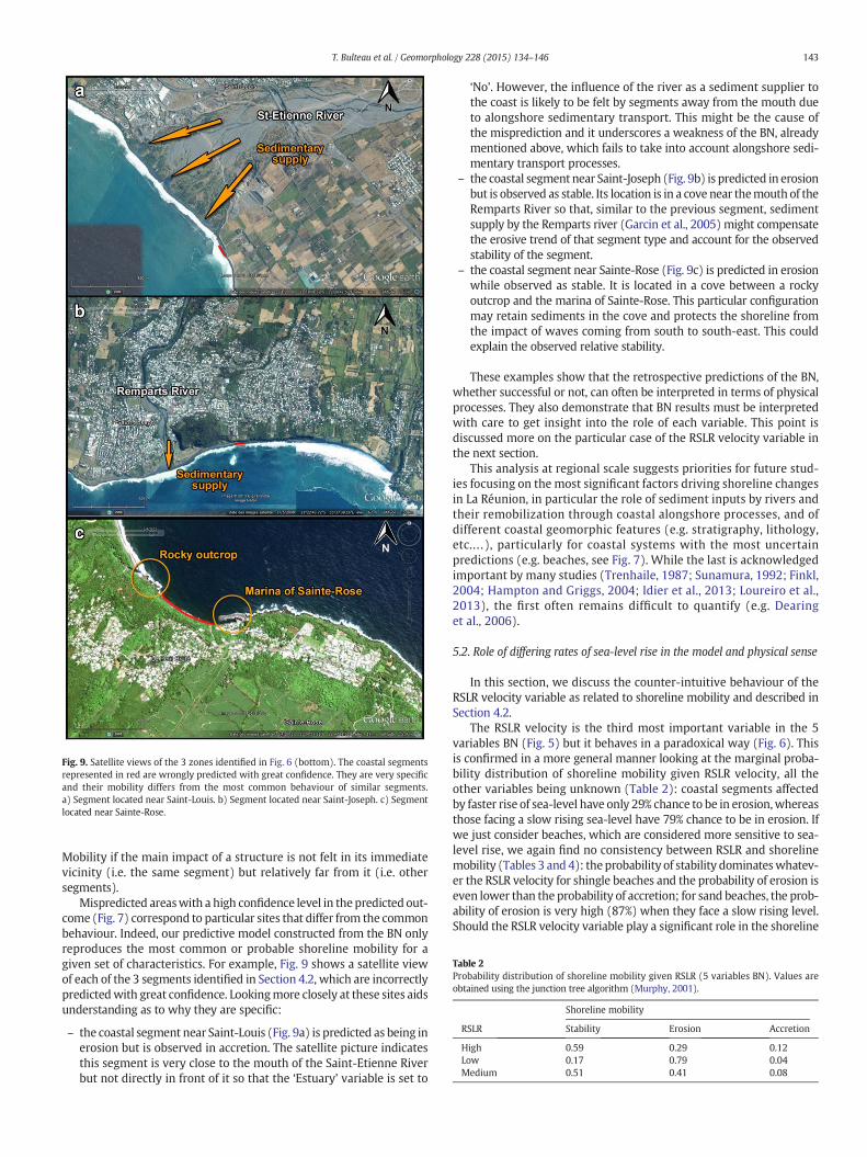
Mobility if the main impact of a structure is not felt in its immediate
vicinity (i.e. the same segment) but relatively far from it (i.e. other
segments).
Mispredicted areaswith a high confidence level in thepredicted out-
come (Fig. 7) correspond to particular sites that differ from the common
behaviour. Indeed, our predictive model constructed from the BN only
reproduces the most common or probable shoreline mobility for a
given set of characteristics. For example, Fig. 9 shows a satellite view
of each of the 3 segments identified in Section 4.2, which are incorrectly
predictedwith great confidence. Lookingmore closely at these sites aids
understanding as to why they are specific:
– the coastal segment near Saint-Louis (Fig. 9a) is predicted as being in
erosion but is observed in accretion. The satellite picture indicates
this segment is very close to the mouth of the Saint-Etienne River
but not directly in front of it so that the ‘Estuary’ variable is set to
‘No’. However, the influence of the river as a sediment supplier to
the coast is likely to be felt by segments away from the mouth due
to alongshore sedimentary transport. This might be the cause of
the misprediction and it underscores a weakness of the BN, already
mentioned above, which fails to take into account alongshore sedi-
mentary transport processes.
– the coastal segment near Saint-Joseph (Fig. 9b) is predicted in erosion
but is observed as stable. Its location is in a cove near themouth of the
Remparts River so that, similar to the previous segment, sediment
supply by the Remparts river (Garcin et al., 2005) might compensate
the erosive trend of that segment type and account for the observed
stability of the segment.
– the coastal segment near Sainte-Rose (Fig. 9c) is predicted in erosion
while observed as stable. It is located in a cove between a rocky
outcrop and the marina of Sainte-Rose. This particular configuration
may retain sediments in the cove and protects the shoreline from
the impact of waves coming from south to south-east. This could
explain the observed relative stability.
These examples show that the retrospective predictions of the BN,
whether successful or not, can often be interpreted in terms of physical
processes. They also demonstrate that BN results must be interpreted
with care to get insight into the role of each variable. This point is
discussed more on the particular case of the RSLR velocity variable in
the next section.
This analysis at regional scale suggests priorities for future stud-
ies focusing on the most significant factors driving shoreline changes
in La Réunion, in particular the role of sediment inputs by rivers and
their remobilization through coastal alongshore processes, and of
different coastal geomorphic features (e.g. stratigraphy, lithology,
etc.…), particularly for coastal systems with the most uncertain
predictions (e.g. beaches, see Fig. 7). While the last is acknowledged
important by many studies (Trenhaile, 1987; Sunamura, 1992; Finkl,
2004; Hampton and Griggs, 2004; Idier et al., 2013; Loureiro et al.,
2013), the first often remains difficult to quantify (e.g. Dearing
et al., 2006).
5.2. Role of differing rates of sea-level rise in the model and physical sense
In this section, we discuss the counter-intuitive behaviour of the
RSLR velocity variable as related to shoreline mobility and described in
Section 4.2.
The RSLR velocity is the third most important variable in the 5
variables BN (Fig. 5) but it behaves in a paradoxical way (Fig. 6). This
is confirmed in a more general manner looking at the marginal proba-
bility distribution of shoreline mobility given RSLR velocity, all the
other variables being unknown (Table 2): coastal segments affected
by faster rise of sea-level have only 29% chance to be in erosion,whereas
those facing a slow rising sea-level have 79% chance to be in erosion. If
we just consider beaches, which are considered more sensitive to sea-
level rise, we again find no consistency between RSLR and shoreline
mobility (Tables 3 and 4): theprobability of stability dominateswhatev-
er the RSLR velocity for shingle beaches and the probability of erosion is
even lower than the probability of accretion; for sand beaches, the prob-
ability of erosion is very high (87%) when they face a slow rising level.
Should the RSLR velocity variable play a significant role in the shoreline
Fig. 9. Satellite views of the 3 zones identified in Fig. 6 (bottom). The coastal segments
represented in red are wrongly predicted with great confidence. They are very specific
and their mobility differs from the most common behaviour of similar segments.
a) Segment located near Saint-Louis. b) Segment located near Saint-Joseph. c) Segment
located near Sainte-Rose.
Table 2
Probability distribution of shoreline mobility given RSLR (5 variables BN). Values are
obtained using the junction tree algorithm (Murphy, 2001).
Shoreline mobility
RSLR Stability Erosion Accretion
High 0.59 0.29 0.12
Low 0.17 0.79 0.04
Medium 0.51 0.41 0.08
143T. Bulteau et al. / Geomorphology 228 (2015) 134–146
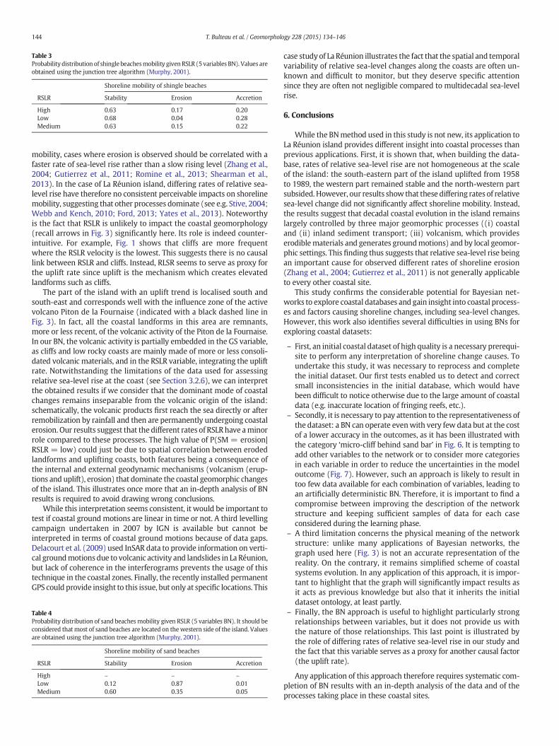
mobility, cases where erosion is observed should be correlated with a
faster rate of sea-level rise rather than a slow rising level (Zhang et al.,
2004; Gutierrez et al., 2011; Romine et al., 2013; Shearman et al.,
2013). In the case of La Réunion island, differing rates of relative sea-
level rise have therefore no consistent perceivable impacts on shoreline
mobility, suggesting that other processes dominate (see e.g. Stive, 2004;
Webb and Kench, 2010; Ford, 2013; Yates et al., 2013). Noteworthy
is the fact that RSLR is unlikely to impact the coastal geomorphology
(recall arrows in Fig. 3) significantly here. Its role is indeed counter-
intuitive. For example, Fig. 1 shows that cliffs are more frequent
where the RSLR velocity is the lowest. This suggests there is no causal
link between RSLR and cliffs. Instead, RLSR seems to serve as proxy for
the uplift rate since uplift is the mechanism which creates elevated
landforms such as cliffs.
The part of the island with an uplift trend is localised south and
south-east and corresponds well with the influence zone of the active
volcano Piton de la Fournaise (indicated with a black dashed line in
Fig. 3). In fact, all the coastal landforms in this area are remnants,
more or less recent, of the volcanic activity of the Piton de la Fournaise.
In our BN, the volcanic activity is partially embedded in the GS variable,
as cliffs and low rocky coasts are mainly made of more or less consoli-
dated volcanic materials, and in the RSLR variable, integrating the uplift
rate. Notwithstanding the limitations of the data used for assessing
relative sea-level rise at the coast (see Section 3.2.6), we can interpret
the obtained results if we consider that the dominant mode of coastal
changes remains inseparable from the volcanic origin of the island:
schematically, the volcanic products first reach the sea directly or after
remobilization by rainfall and then are permanently undergoing coastal
erosion. Our results suggest that the different rates of RSLR have aminor
role compared to these processes. The high value of P(SM = erosion|
RSLR = low) could just be due to spatial correlation between eroded
landforms and uplifting coasts, both features being a consequence of
the internal and external geodynamic mechanisms (volcanism (erup-
tions and uplift), erosion) that dominate the coastal geomorphic changes
of the island. This illustrates once more that an in-depth analysis of BN
results is required to avoid drawing wrong conclusions.
While this interpretation seems consistent, it would be important to
test if coastal ground motions are linear in time or not. A third levelling
campaign undertaken in 2007 by IGN is available but cannot be
interpreted in terms of coastal ground motions because of data gaps.
Delacourt et al. (2009) used InSAR data to provide information on verti-
cal groundmotionsdue to volcanic activity and landslides in La Réunion,
but lack of coherence in the interferograms prevents the usage of this
technique in the coastal zones. Finally, the recently installed permanent
GPS could provide insight to this issue, but only at specific locations. This
case study of La Réunion illustrates the fact that the spatial and temporal
variability of relative sea-level changes along the coasts are often un-
known and difficult to monitor, but they deserve specific attention
since they are often not negligible compared to multidecadal sea-level
rise.
6. Conclusions
While the BNmethod used in this study is not new, its application to
La Réunion island provides different insight into coastal processes than
previous applications. First, it is shown that, when building the data-
base, rates of relative sea-level rise are not homogeneous at the scale
of the island: the south-eastern part of the island uplifted from 1958
to 1989, the western part remained stable and the north-western part
subsided. However, our results show that these differing rates of relative
sea-level change did not significantly affect shoreline mobility. Instead,
the results suggest that decadal coastal evolution in the island remains
largely controlled by three major geomorphic processes ((i) coastal
and (ii) inland sediment transport; (iii) volcanism, which provides
erodiblematerials and generates groundmotions) and by local geomor-
phic settings. This finding thus suggests that relative sea-level rise being
an important cause for observed different rates of shoreline erosion
(Zhang et al., 2004; Gutierrez et al., 2011) is not generally applicable
to every other coastal site.
This study confirms the considerable potential for Bayesian net-
works to explore coastal databases and gain insight into coastal process-
es and factors causing shoreline changes, including sea-level changes.
However, this work also identifies several difficulties in using BNs for
exploring coastal datasets:
– First, an initial coastal dataset of high quality is a necessary prerequi-
site to perform any interpretation of shoreline change causes. To
undertake this study, it was necessary to reprocess and complete
the initial dataset. Our first tests enabled us to detect and correct
small inconsistencies in the initial database, which would have
been difficult to notice otherwise due to the large amount of coastal
data (e.g. inaccurate location of fringing reefs, etc.).
– Secondly, it is necessary to pay attention to the representativeness of
the dataset: a BN can operate evenwith very few data but at the cost
of a lower accuracy in the outcomes, as it has been illustrated with
the category ‘micro-cliff behind sand bar’ in Fig. 6. It is tempting to
add other variables to the network or to consider more categories
in each variable in order to reduce the uncertainties in the model
outcome (Fig. 7). However, such an approach is likely to result in
too few data available for each combination of variables, leading to
an artificially deterministic BN. Therefore, it is important to find a
compromise between improving the description of the network
structure and keeping sufficient samples of data for each case
considered during the learning phase.
– A third limitation concerns the physical meaning of the network
structure: unlike many applications of Bayesian networks, the
graph used here (Fig. 3) is not an accurate representation of the
reality. On the contrary, it remains simplified scheme of coastal
systems evolution. In any application of this approach, it is impor-
tant to highlight that the graph will significantly impact results as
it acts as previous knowledge but also that it inherits the initial
dataset ontology, at least partly.
– Finally, the BN approach is useful to highlight particularly strong
relationships between variables, but it does not provide us with
the nature of those relationships. This last point is illustrated by
the role of differing rates of relative sea-level rise in our study and
the fact that this variable serves as a proxy for another causal factor
(the uplift rate).
Any application of this approach therefore requires systematic com-
pletion of BN results with an in-depth analysis of the data and of the
processes taking place in these coastal sites.
Table 3
Probability distribution of shingle beachesmobility given RSLR (5 variables BN). Values are
obtained using the junction tree algorithm (Murphy, 2001).
Shoreline mobility of shingle beaches
RSLR Stability Erosion Accretion
High 0.63 0.17 0.20
Low 0.68 0.04 0.28
Medium 0.63 0.15 0.22
Table 4
Probability distribution of sand beaches mobility given RSLR (5 variables BN). It should be
considered that most of sand beaches are located on thewestern side of the island. Values
are obtained using the junction tree algorithm (Murphy, 2001).
Shoreline mobility of sand beaches
RSLR Stability Erosion Accretion
High – – –
Low 0.12 0.87 0.01
Medium 0.60 0.35 0.05
144 T. Bulteau et al. / Geomorphology 228 (2015) 134–146
The complexity of coastal system behaviours currently prevents
their modelling purely based on physical concepts. In addition, there is
a crucial need for public authorities to understand and manage coastal
environments. Bayesian networks contribute to answering this need
by improving our understanding of coastal evolution at decadal time-
scales. They could ultimately allow moving towards long-term predic-
tions of future coastal environment evolution.
Acknowledgements
This work has been completed within the CECILE project (Coastal
Environmental Changes: Impact of sea LEvel rise) supported by the
French National Agency for Research (ANR) within its Planetary Envi-
ronmental Changes (CEP) framework: convention n°ANR-09-CEP-001.
We thank the regional office of BRGM at La Réunion island (S. Bès
de Berc, E. Chateauminois, Y. de la Torre) for providing coastal data
initially collected for the Region and DIREN and for their comments.
We also thank IGN (S. Lavoué, A. Coulomb) for providing raw level-
ling data and A. Cazenave, B. Meyssignac, D. Raucoules and C. Mirgon
for useful discussions. Last, we thank two anonymous reviewers as
well as A.J. Plater for their comments which contributed to improve
this paper.
Appendix A. Calculation of the percentage of shoreline length
correctly reproduced in the random case
In order to evaluate the significance level of themodel, it is necessary
to compare the percentage of shoreline length correctly predicted to the
one obtained with a completely randomized dataset (while respecting
the prior probability distributions of all variables, i.e. the probability
distributions of the variables calculated from their frequencies of
appearance in the database), thus removing any dependency between
variables. In that case, Eq. (2) becomes:
SMpred ¼ arg maxi
P SMi eX j
���� �� �
¼ argmaxi
P SMi
� �� �ðA:1Þ
As a result, whatever the coastal segment, the shoreline mobility
state having themaximum prior probability is systematically predicted.
We then deduce the percentage of shoreline length correctly predicted
in the case of a completely randomized dataset as follows:
% correct predictions ¼ maxi
P SMi
� �� �� 100 ðA:2Þ
In our dataset, the prior probability distribution of shorelinemobility
is: P(erosion) = 0.58, P(accretion) = 0.07, P(stability) = 0.35. There-
fore, the percentage of shoreline length correctly reproduced in the
random case is 58%.
Appendix B. Calculation of the possible maximum and minimum
theoretical values of the global log-likelihood ratio
The possiblemaximum theoretical LR can be computed directly from
Eq. (4) by replacing LR(k) by its maximum theoretical value:
LR kð Þ ¼ log P SM kð Þ O kð Þ
���� �� �
− log P SM kð Þ
� �� �¼ − log P SM kð Þ
� �� �ðB:1Þ
From our dataset, we obtain LRmax = 0.38.
Theminimum LR is computedwhen the entire dataset is randomized
(but still following the prior probability distributions) thus removing
any dependency between variables and is equal to 0.
References
Aguilera, P.A., Fernandez, A., Fernandez, R., Rumi, R., Salmeron, A., 2011. Bayesiannetworks in environmental modelling. Environ. Model Softw. 26 (12), 1376–1388.
Berger, J.O., 2000. Bayesian analysis: a look at today and thoughts of tomorrow. J. Am. Stat.Assoc. 95, 1269–1276.
Bourmaud, C.A.F., Abouïdane, A., Boissier, P., Leclère, L., Mirault, E., Pennober, G., 2005.Coastal and marine biodiversity of La Réunion. Indian J. Mar. Sci. 34 (1), 98–103.
Catenacci, M., Giupponi, C., 2013. Integrated assessment of sea-level rise adaptation strat-egies using a Bayesian decision network approach. Environ. Model Softw. 44, 87–100.
Cazenave, A., Le Cozannet, G., 2014. Sea level rise and its coastal impacts. Earths Futur. 2(2), 15–34.
De La Torre, Y., 2004. Synthèse morphodynamique des littoraux de La Réunion, état deslieux et tendances d'évolution à l'échelle de l'île. Open file report BRGM/RP-53307-FR.
Dearing, J.A., Richmond, N., Plater, A.J., Wolf, J., Prandle, D., Coulthard, T.J., 2006. Modellingapproaches for coastal simulation based on cellular automata: the need and potential.Philos. Trans. R. Soc. A Math. Phys. Eng. Sci. 364 (1841), 1051–1071.
Delacourt, C., Raucoules, D., Le Mouelic, S., Carnec, C., Feurer, D., Allemand, P., Cruchet, M.,2009. Observation of a large landslide on La Reunion Island using differential SarInterferometry (JERS and Radarsat) and correlation of optical (Spot5 and aerial)images. Sensors 9 (1), 616–630.
Eurosion, 2004. Living with coastal erosion in Europe: sediment and space for sustainabil-ity. Part I: Major findings and policy recommendations of the EUROSION project.
Finkl, C.W., 2004. Coastal classification: systematic approaches to consider in the develop-ment of a comprehensive scheme. J. Coast. Res. 20 (1), 166–213.
Ford, M., 2013. Shoreline changes interpreted from multi-temporal aerial photographsand high resolution satellite images: Wotje Atoll, Marshall Islands. Remote Sens.Environ. 135, 130–140.
Garcin, M., Poisson, B., Pouget, R., 2005. High rate of geomorphological processes in atropical area: the Remparts river case study (Réunion Island, Indian Ocean). Geomor-phology 67 (3–4), 335–550.
Gillot, P.Y., Nativel, P., 1989. Eruptive history of the Piton de la Fournaise volcano, Réunionisland, Indian Ocean. J. Volcanol. Geotherm. Res. 36, 53–65.
Gutierrez, B.T., Plant, N.G., Thieler, E.R., 2011. A Bayesian network to predict coastalvulnerability to sea level rise. J. Geophys. Res. Earth Surf. 116, 15.
Hampton, M.A., Griggs, G.B., 2004. Formation, evolution and stability of coastal cliffs —status and trends. USGS Professional Paper. 1683 (123 pp.).
Hapke, C., Plant, N., 2010. Predicting coastal cliff erosion using a Bayesian probabilisticmodel. Mar. Geol. 278 (1–4), 140–149.
Heckerman, D., 1997. Bayesian networks for datamining. DataMin. Knowl. Disc. 1, 79–119.Idier, D., et al., 2013. Vulnerability of sandy coasts to climate variability. Clim. Res. 57 (1),
19–44.Karunarathna, H., Reeve, D., 2007. Predicting morphodynamic response of a coastal plain
estuary using a Boolean model. Proceedings of the 5th IAHR Symposium on River,Coastal and Estuarine Morphodynamics, Enschede, NL, 17–21 September 2007,pp. 1109–1115.
Karunarathna, H., Reeve, D., 2008. A Boolean approach to prediction of long-term evolutionof estuary morphology. J. Coast. Res. 24 (2B), 51–61.
Lavoué, S., 2013. Comparaisons de nivellement sur le littoral réunionnais. CR/G 276, IGN,Servive de Géodésie et de Nivellement.
Le Cozannet, G., Garcin, M., Bulteau, T., Mirgon, C., Yates, M.L., Mendez, M., Baills, A., Idier, D.,Oliveros, C., 2013. An AHP-derived method for mapping the physical vulnerability ofcoastal areas at regional scales. Nat. Hazards Earth Syst. Sci. 13 (5), 1209–1227.
Lecacheux, S., Pedreros, R., Le Cozannet, G., Thiebot, J., De La Torre, Y., Bulteau, T., 2012. Amethod to characterize the different extreme waves for islands exposed to variouswave regimes: a case study devoted to Reunion Island. Nat. Hazards Earth Syst. Sci.12 (7).
Loureiro, C., Ferreira, O., Cooper, J.A.G., 2013. Applicability of parametric beachmorphodynamic state classification on embayed beaches. Mar. Geol. 346, 153–164.
Meyssignac, B., Becker, M., Llovel, W., Cazenave, A., 2012. An assessment of two-dimensional past sea level reconstructions over 1950–2009 based on tide-gaugedata and different input sea level grids. Surv. Geophys. 33 (5), 945–972.
Murphy, K.P., 2001. The Bayes net toolbox for Matlab. Comput. Sci. Stat. 33 (2),1024–1034.
Myllymäki, P., Silander, T., Tirri, H., Uronen, P., 2002. B-Course, a web-based tool forBayesian and causal data analysis. Int. J. Artif. Intell. Tools 11 (3), 369–387.
Naïm, P., Wuillemin, P.-H., Leray, P., Pourret, O., Becker, A., 2007. Réseaux bayésiens.Eyrolles, Paris.
Palanisamy, H., Cazenave, A., Meyssignac, B., Soudarin, L., Woppelmann, G., Becker, M.,2014. Regional sea level variability, total relative sea level rise and its impacts onislands and coastal zones of Indian Ocean over the last sixty years. Glob. Planet.Chang. http://dx.doi.org/10.1016/j.gloplacha.2014.02.001.
Pearl, J., 1986. Fusion, propagation and structuring in belief networks. Artif. Intell. 29,241–288.
Plant, N.G., Holland, K.T., 2011a. Prediction and assimilation of surf-zone processes using aBayesian network part I: forward models. Coast. Eng. 58 (1), 119–130.
Plant, N.G., Holland, K.T., 2011b. Prediction and assimilation of surf-zone processes using aBayesian network part II: inverse models. Coast. Eng. 58 (3), 256–266.
Plant, N.G., Stockdon, H.F., 2012. Probabilistic prediction of barrier-island response tohurricanes. J. Geophys. Res. Earth Surf. 117.
Quelennec, R.-E., Oliveros, C., Uhel, R., Devos, W., 1998. Corine: érosion côtière. Environ-mental and quality of life series. Office for Official Publications of the European Com-munities, Luxembourg (170 pp.).
Rocher, P., 1988. Contexte volcanique et structural de l'hydrothermalisme récent dans lemassif du Piton des Neiges, île de La Réunion(PhD Thesis) Etude détaillée du Cirquede Salazie. Université de Paris Orsay.
145T. Bulteau et al. / Geomorphology 228 (2015) 134–146

Romine, B.M., Fletcher, C.H., Barbee, M.M., Anderson, T.R., Frazer, L.N., 2013. Are beacherosion rates and sea-level rise related in Hawaii? Glob. Planet. Chang. 108, 149–157.
Shearman, P., Bryan, J., Walsh, J.P., 2013. Trends in deltaic change over three decades inthe Asia-Pacific Region. J. Coast. Res. 29 (5), 1169–1183.
Stive, M.J.F., 2004. How important is global warming for coastal erosion? An editorialcomment. Clim. Chang. 64 (1–2).
Storlazzi, C.D., Elias, E., Field, M.E., Presto, M.K., 2011. Numerical modeling of the impact ofsea-level rise on fringing coral reef hydrodynamics and sediment transport. CoralReefs 30.
Sunamura, T., 1992. Geomorphology of Rocky Coasts. John Wiley and Sons, New York.Thieler, E.R., Hammar‐Klose, E.S., 1999. National assessment of coastal vulnerability to fu-
ture sea‐level rise: preliminary results for U.S. Atlantic Coast. U.S. Geol. Surv. OpenFile Report, Woods Hole, Massachusetts, 99-593.
Trenhaile, A.S., 1987. The Geomorphology of Rock Coasts. Oxford University Press, NewYork.
Uusitalo, L., 2007. Advantages and challenges of Bayesian networks in environmentalmodelling. Ecol. Model. 203, 312–318.
Webb, A.P., Kench, P.S., 2010. The dynamic response of reef islands to sea-level rise:evidence from multi-decadal analysis of island change in the Central Pacific. Glob.Planet. Chang. 72 (3), 234–246.
Yates, M.L., Le Cozannet, G., 2012. Brief communication ‘Evaluating European CoastalEvolution using Bayesian Networks’. Nat. Hazards Earth Syst. Sci. 12 (4), 1173–1177.
Yates, M.L., Le Cozannet, G., Garcin, M., Salaï, E., Walker, P., 2013. Multidecadal atoll shore-line change on Manihi and Manuae, French Polynesia. J. Coast. Res. 29 (4), 870–882.
Yin, J., Yin, Z., Wang, J., Xu, S., 2012. National assessment of coastal vulnerability to sea-level rise for the Chinese coast. J. Coast. Conserv. 16 (1), 123–133.
Zhang, K.Q., Douglas, B.C., Leatherman, S.P., 2004. Global warming and coastal erosion.Clim. Chang. 64 (1–2).
146 T. Bulteau et al. / Geomorphology 228 (2015) 134–146

Copyright © 2022 FDOKUMEN