Prediction of total organic carbon content inshale reservoir based on a new integratedhybrid neural network and conventional welllogging curves

Linqi Zhu1,2, Chong Zhang1,2,3, Chaomo Zhang1,2, Yang Wei1,2,Xueqing Zhou1,2, Yuan Cheng1,2, Yuyang Huang1,2 and Le Zhang1,2

1Key Laboratory of Exploration Technologies for Oil and Gas Resources (Yangtze University), Wuhan,Hubei 430100, People’s Republic of China2Hubei Cooperative Innovation Center of Unconventional Oil and Gas, Wuhan, Hubei 430100, People’sRepublic of China

E-mail: yzlogging@163.com

Received 20 October 2017, revised 18 December 2017Accepted for publication 15 January 2018Published 22 March 2018

AbstractThere is increasing interest in shale gas reservoirs due to their abundant reserves. As a key evaluationcriterion, the total organic carbon content (TOC) of the reservoirs can reflect its hydrocarbongeneration potential. The existing TOC calculation model is not very accurate and there is still thepossibility for improvement. In this paper, an integrated hybrid neural network (IHNN) model isproposed for predicting the TOC. This is based on the fact that the TOC information on the low TOCreservoir, where the TOC is easy to evaluate, comes from a prediction problem, which is the inherentproblem of the existing algorithm. By comparing the prediction models established in 132 rocksamples in the shale gas reservoir within the Jiaoshiba area, it can be seen that the accuracy of theproposed IHNN model is much higher than that of the other prediction models. The meansquare error of the samples, which were not joined to the established models, was reduced from0.586 to 0.442. The results show that TOC prediction is easier after logging prediction has beenimproved. Furthermore, this paper puts forward the next research direction of the prediction model.The IHNN algorithm can help evaluate the TOC of a shale gas reservoir.

Keywords: shale reservoir, organic carbon content, machine learning, integrated hybrid neuralnetwork, adaptive tabu compound rainforest optimizing algorithm, low TOC reservoir

(Some figures may appear in colour only in the online journal)

1. Introduction

The hydrocarbon generation potential of shale gas reservoirs hasattracted a lot of attention (Dong 2012, Chen 2013, Geet al 2016). The gas content is determined by the abundance oforganic matter in the shale, and the total organic carbon content(TOC) is closely related to the shale gas content. Therefore, theTOC is a key criterion for evaluating the gas reserves of theshale reservoir (Zhou 2009, Wang et al 2014, Zhang et al 2017).

Currently, there are three main models for calculating theTOC using conventional well logging curves. The first type ofprediction model is based on the good single correlationbetween conventional well logging curves and the TOC, suchas the methods for calculating the TOC using the density,value of uranium or thorium uranium ratio (Huang et al 2014,Li et al 2014, Huang et al 2015, Haecker et al 2016). Thesecond type of method for calculating the TOC is based on acombination of conventional logging acoustic waves andelectrical resistivity, such as the ΔlogR method, the CAG-BOLOG method and a method based on a combination of the

Journal of Geophysics and Engineering

J. Geophys. Eng. 15 (2018) 1050–1061 (12pp) https://doi.org/10.1088/1742-2140/aaa7af

3 Author to whom any correspondence should be addressed.

1742-2132/18/0301050+12$33.00 © 2018 Sinopec Geophysical Research Institute Printed in the UK1050

Dow

nloaded from https://academ

ic.oup.com/jge/article/15/3/1050/5203196 by guest on 12 February 2022

ΔlogR method and the density curve (Zhang andZhang 2000, Huo et al 2011, Xie et al 2013, Yang et al 2013,Hu et al 2016, Zhao et al 2016, Zhao et al 2017). The lasttype of method calculates the TOC by taking advantage ofmulti-curve features, such as the multiple regression method,the BP neural network (BPNN), the fuzzy neural network(FNN), the ACO-BP neural network, the support vectormachine (SVM), the extreme learning machine (ELM) andthe deep learning model (Kadkhodaie-Ilkhchi et al 2009,Lecun et al 2015, Meng et al 2015, Ouadfeul andAliouane 2015, Sfidari et al 2015, Tan et al 2015, Shi et al2016). Calculation of the TOC using well logging curves isactually pattern recognition. From the theory of patternrecognition, the advantage of the first two methods is thesimplicity of implementation. However, the two methods donot make full use of information when calculating the TOC,and their precision is not very satisfactory. Therefore, theresearch subject of this paper is based on the TOC calculatingmethod using machine learning. However, the existingmachine-learning-based methods do not consider the pro-blems that may exist in the well logging interpretation, butonly focus on the accuracy of existing algorithms for the TOCprediction. The key point of TOC prediction is to select theappropriate model and make targeted improvements based onthe characteristic of well logging.

In view of the problems existing in the BPNN, theintegrated hybrid neural network (IHNN), as an improvedmethod, is optimized on the basis of BPNN from the fol-lowing aspects including weight optimization before iteration,network structure optimization and serial-parallel integration.IHNN is easier to implement and the model prediction speedis acceptable. Besides this, it is more in line with the idea ofevaluating the TOC using conventional logging curves (lowfeature dimensions). In the third part of this paper, by com-paring different methods, it is proved that the improved neuralnetwork method is effective and has a strong predictiveability.

2. The integrated hybrid neural network

From the 1980s to the 1990s, the scientific and technologicalcommunity set off a boom of research on neural networks(Hopfield 1984, Rumelhart et al 1986, Broomhead andLowe 1988). The BP neural network, the radial basis function(RBF) neural network, the Hopfield neural network and otherneural networks were successively birthed. There is wideinterest in the neural network for its strong function approx-imation ability, ease of use and autonomous learning ability.Among all the networks, the BPNN is the most commonlyused, especially in well logging. However, traditional BPNNsuffers from problems such as slow convergence, being sus-ceptible to local minima, difficulties in determining the net-work structure and weak generalization ability. Moreover,there is a lot of noise in the logging curves, which needs to beimproved. In particular, in low TOC reservoirs, the responsesignals of the TOC are suppressed by other elements and thecalculation results of existing algorithms are greatly reduced.

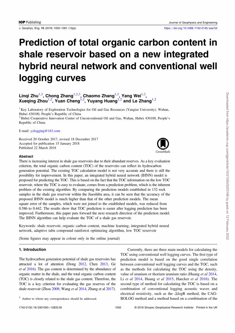
To solve the above problems, an adaptive tabu compoundrainforest optimizing–chaos circular self-configurationmethod–P-AdaBoost–BP neural network is proposed. Inorder to help facilitate the appellation, we call it the IHNNmodel. The structure of this model is shown in figure 1.

The hybrid neural network is a combination of theadaptive tabu compound rainforest optimizing algorithm andthe BPNN. The number of optimal hidden layer neurons inthe network is determined by the chaos cycle self-configura-tion algorithm. The TOC is predicted by the integration of theoutput results. The principle of the improved method, as wellas its role in the IHNN model, is going to be analyzed indetail.

2.1. Adaptive tabu compound rainforest optimizing algorithm

The gradient descent method can efficiently adjust the weightand threshold of a neural network, but it is difficult to find theglobal optimal value in a nonconvex function. The randomnature of the initial weight and threshold of the traditionalBPNN makes it more susceptible to minima. To solve thisproblem, a popular approach is to optimize the initial weightthreshold using the meta heuristic optimization algorithm.More accurate weights and thresholds can reduce the prob-ability of being susceptible to a local optimum. Currently,there are mainly five types of optimization algorithm,including meta heuristic optimization algorithms for imitatingthe evolution process (such as the genetic algorithm and thedifferential evolution algorithm, etc) (Holland 1992, Mahersiaet al 2016), the meta heuristic optimization algorithms forimitating biological colony behavior (such as the particleswarm optimization algorithm, the ant colony algorithm andthe krill herd algorithm, etc) (Frans and Engelbrecht 2004,Dorigo et al 2006, Gandomi and Alavi 2012, Kaveh andFarhoudi 2013), optimization algorithms for imitating thephysical process (such as the simulated annealing algorithm,black hole algorithm and the galaxy search algorithm, etc)

Figure 1. The construct of the IHNN model.

1051

J. Geophys. Eng. 15 (2018) 1050 L Zhu et al

Dow

nloaded from https://academ

ic.oup.com/jge/article/15/3/1050/5203196 by guest on 12 February 2022

(Černý 1985, Shah-Hosseini 2011, Hatamlou 2013), optim-ization algorithms for imitating human behaviors (such as thefirework explosion algorithm, the harmony search algorithm,the group search algorithm and the empirical competitionalgorithm, etc) (Geem et al 2001, Atashpaz-Gargari andLucas 2007, He et al 2009, Tan and Zhu 2010) and algo-rithms based on plant growth (such as the weed algorithm, theroot growth algorithm and the rainforest algorithm, etc)(Mehrabian and Lucas 2006, Gao et al 2013, Labbiet al 2016). In this paper, we chose the rain forest algorithm,which can avoid virtual collisions, reducing the uncertainty ofthe optimization results.

The rainforest algorithm is an algorithm for imitating thegrowth and evolution processes of plants. The strategy of therainforest algorithm is to combine global partition manage-ment sampling with local classification sampling. It is theo-retically proved that uniform sampling is one of the mosteffective ways to explore an unknown region. This methodhas good optimization efficiency for the distribution of thenonconvex function.

The rainforest algorithm effectively solves the problemof virtual collision. When parameter selection is reasonable,the algorithm can ensure that the search result is a globaloptimal region. However, as the algorithm focuses on thediscovery of the global optimal region, its ability to seekthe global optimal solution of the global optimal region in thelater period is somewhat lacking (only one or several agentsare used in the search for a global optimal solution in theglobal optimal region). Accurate weights can make the neuralnetwork gradient descent method less susceptible to a localminimum. Only by increasing the number of agents of theoptimization algorithm can the ability of local optimization beimproved. However, it will take up a lot of memory to slowdown the optimization speed. With the aim of solving thisproblem, an adaptive tabu compound rainforest optimizingalgorithm (ATCRFA) is proposed based on a combination ofthe tabu operator and the compound operator to improve thelocal search ability for the rainforest optimizing algorithm.

The tabu search algorithm is a sub-heuristic algorithm inwhich the optimal solution can be selected in the searchprocess. The algorithm has a strong local search ability whendealing with constrained optimization problems (Amaral andPais 2016). In order to get the parent node of the local opti-mum, the tabu search algorithm is added to the competitionstep of the original rainforest algorithm, because of its stronglocal optimization ability. Due to the problem of the rainforest algorithm converging to the local optimal regioninstead of the local optimal solution, we proposed transferringthe result of the rain forest algorithm to the complex algo-rithm, so as to find the optimal local optimization withoutrestraints. The composite vertex algorithm, as a deterministiclocal search algorithm, constructs a polyhedron of K bound-ary points in the feasible region. The search direction of thenext iteration is determined by the function value of the objectcalculated by the complex boundary point. The performanceindex of the composite was replaced by the best performance

index, which was the worst point. A good performance pointwas used to replace the worst performance point in thecomplex boundary point, in order to meet the requirements ofoptimization. Since the optimization process was carried outin the global optimal region, it had strong local search abilityfor the low dimensional unconstrained problem (Panet al 2016).

In addition, an adaptive learning factor adjustmentmethod was proposed to avoid the premature convergence ofthe rain forest algorithm. The formula is as follows:

e 1.10tTa = - ( )

In the formula, α is the learning factor in the algorithm, t isthe current number of iterations, and T is the total number ofiterations set in advance.

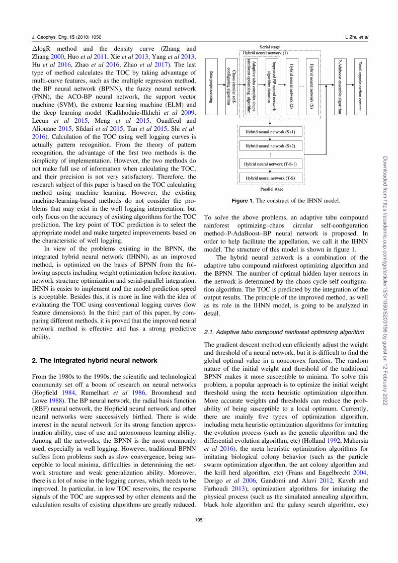
Figure 2 is the flow chart of optimization of ATCRFA.As the model combination method has been described, wewill not expand it in detail here. To prove that the proposedmodel can effectively enhance the optimization ability of therainforest algorithm, we will conduct the simulation andoptimization of the initial weight and threshold of the BPNNusing the TOC and the corresponding logging response data.

2.2. Chaos circular self-configuration method

In BPNN, the number of neurons in each layer has an enor-mous influence on the network. Theoretically speaking, eachneuron will record part of the intrinsic law of the function.That is to say, an insufficient number of hidden layer neuronswill result in the BPNN failing to characterize the complexfunction, while an excessive amount of hidden layer neuronsis likely to record secondary laws (such as noise), which mayresult in the problem of over-fitting. In addition, the procedureof finding weights in the optimization algorithm takes moretime. The reduction of hidden layer neurons can also greatlyreduce the run time of the programs. The chaos circular

Figure 2. The construct of the adaptive tabu compound rainforestoptimizing algorithm.

1052

J. Geophys. Eng. 15 (2018) 1050 L Zhu et al

Dow

nloaded from https://academ

ic.oup.com/jge/article/15/3/1050/5203196 by guest on 12 February 2022

self-configuration method which is proposed in this paper canbe used to calculate the relevance of the outputs of the hiddennodes and to carry out neural network pruning steps. Afterthat, the completed neural network structure can be used forfunction optimization.

In theory, no matter how many initial hidden layer neu-rons there are, the circular self-configuration method canreduce the network structure to the best point. Compared withtraditional algorithms, the circular self-configuration methodhas obvious advantages. Next, the realization method of cir-cular self-configuration is introduced (Rao et al 2008).

The correlation coefficient of hidden layer neurons iscalculated as follows:

R

o o o o

o o o o

.

2

N

N

N

N N

N

N

N

N

N

N

N

N

ij

1p 1 ip jp

1p 1 ip p 1 jp

1p 1 ip

2 1p 1 ip

2 1p 1 jp

2 1p 1 jp

2

2

2 2

å å å

å å å å=

-

- -

= = =

= = = =

( )

In the formula, N is the number of training samples, oip isthe output of the hidden layer neuron i in the learning processof the pth sample, and ojp is the output of the hidden layerneuron j in the learning process of the pth sample.

The correlation coefficient of the hidden layer neuronsshows the linear relevance between the outputs of the hiddenlayer neurons. When Rij is too large, the hidden layer neuronsneed to be compressed.

The sample dispersion is calculated as follows:

QN N

1o

1o . 3

N N

ip 1

ip2

2p 1

ipå å= -= =

( )

The sample dispersion is a parameter that represents thedifference between the output of a certain hidden layer neuronand the average output. The small sample dispersion meansthat the output of a certain hidden layer neuron is similar tothe average output of the whole hidden layer. In this way, theoutput can be deleted. The combination and deletion ofneurons are based on the above two parameters:

R Qand , Q . 4ij 1 i j 2 s s∣ ∣ ( )

In the formula, σ1 and σ2 are thresholds, the range of σ1is generally 0.6–0.9 and the range of σ2 is generally0.001–0.01. If the hidden layer neurons satisfy formula (4),the two neurons i and j can be combined into one. Then,the corresponding weights and thresholds are modified asfollows:

If there is Qi<σ2, namely formula (6)

Q 6i 2s< ( )

this hidden layer neuron should be deleted and thecorresponding threshold will be adjusted as follows:

o 7i kik kq q w= + ( )

where k is the threshold adjustment of neurons after deletingthe neuron.

However, the BPNN generates weight randomly, so thatthe final results may fall into the local minima. This situationis difficult to avoid, which makes the threshold in a circularself-configuration difficult to select. So, we propose animproved circular self-configuration method, i.e. the chaoscircular self-configuration method, in order to improve thepruning efficiency of hidden neurons by using the ergodicityof chaotic optimization.

Here, we define a parameter called the neuron reductionthreshold. If a unreduced neuron state is maintained for sev-eral iteration calculations (the iteration times exceed thereduction threshold), then we believe that the simplest net-work topology is obtained.

We need to introduce the chaos algorithm first. A lot ofchaos mappings are used in chaos optimization algorithms,such as logistic mapping, tent mapping and Liebovith map-ping, etc. In view of these functions, Moroni compared theiroptimization ability and came to the conclusion that theoptimal speed and stability of logistic mapping were betterthan that of other mappings (Moroni et al 2016). Thecorresponding logistic mapping is as follows:

x x 1 x . 8n 1 n nm= -+ ( ) ( )

In the formula, μ is the control parameter. When μ=4, themapping is a completely chaotic state, so we take it as 4; xm isthe independent variable value of the N generation, and xn+1

is the independent variable value of the generation of N+1.As a chaos algorithm is susceptible to the initial value,

formula (9) is assigned with a differential initial valuet0,i(i=1, 2,K, l), which generates a chaos variable tn,i(i=1,2, K, l) with different trajectories. The corresponding chaosvariable is as follows:

c dw x . 9n,i n= + ( )

In the formula, c and d are both constants.The process of the chaos circular self-configuration

method is shown in figure 3. As shown in the figure, severalgenerations of initial chaos weight are established throughthe chaos optimization algorithm mentioned above (good

N

o o o o

o o

oo o o o

o o

1o

. 5

N

N

N

N N

N

N

N

N

NN

N

N

N N

N

N

N

N

N

ki ki

1p 1 ip jp

1p 1 ip p 1 jp

1p 1 ip

2 1p 1 jp

2kj

k kp 1

jp

1p 1 ip jp

1p 1 ip p 1 jp

1p 1 ip

2 1p 1 jp

2p 1

ip kj

2

2

2

2

å å åå å

åå å å

å åå

w w w

q q w

= +-

-

= + --

-

= = =

= =

=

= = =

= = =

⎧

⎨

⎪⎪⎪

⎩

⎪⎪⎪⎛

⎝⎜⎜

⎞

⎠⎟⎟

( )

1053

J. Geophys. Eng. 15 (2018) 1050 L Zhu et al

Dow

nloaded from https://academ

ic.oup.com/jge/article/15/3/1050/5203196 by guest on 12 February 2022

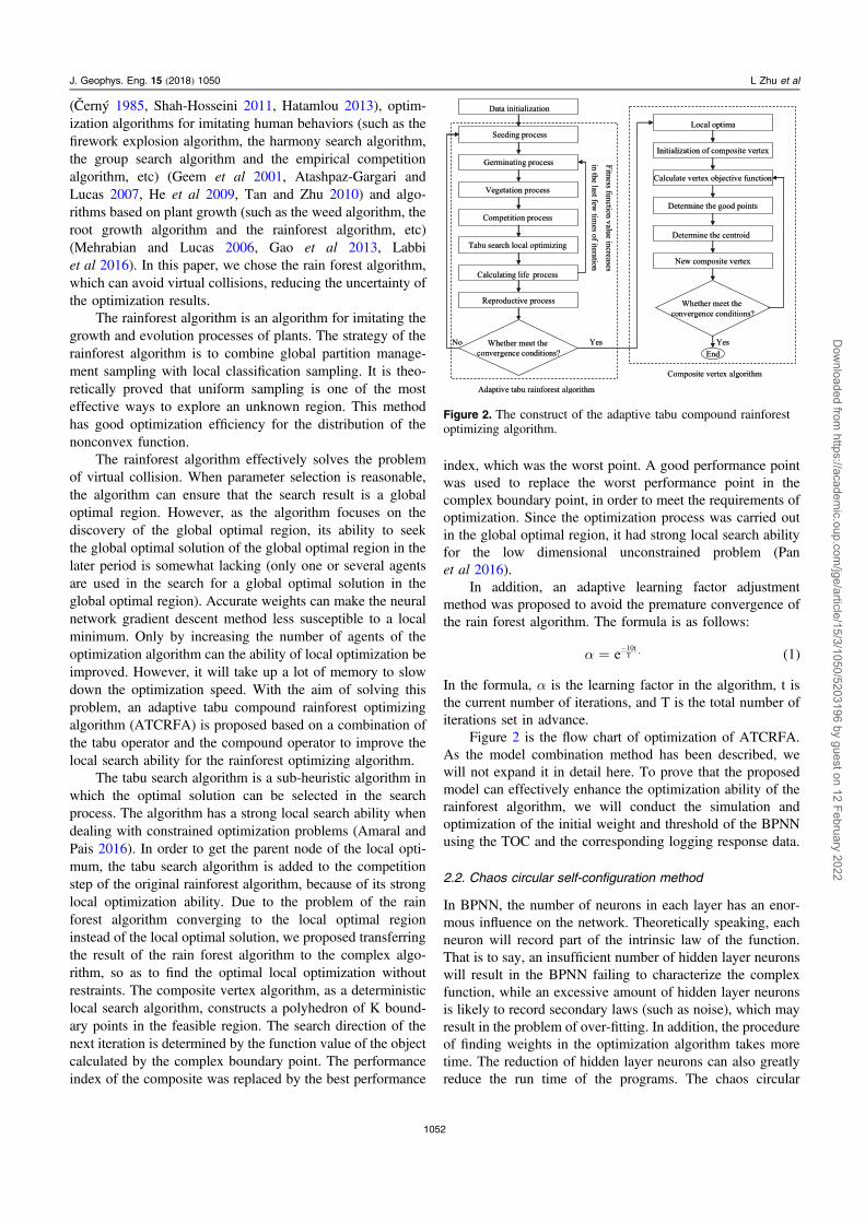
ergodicity can be obtained while the iteration times are greaterthan 200. In this paper, the iteration times are set to 300). Thelearning of the self-configuration algorithm is carried outusing several initial weight matrices in each generation. Inthis way, the process of looping basically determines whetherthe hidden layer is reduced. Compared with traditional cir-cular self-configuration algorithms, this proposed algorithmhas not only reduced randomness, but has also reduced theiteration time needed to determine the optimal amount ofhidden layer neurons. The required iteration time is obviouslyreduced. If the network hidden layer nodes are not reducedafter each generation of the initial weight has been learned,the reduction value increases by 1. In the opposite case, it willdecrease to 0. If the reduction value is greater than thereduction threshold, the iteration will be finished. Then, theoptimal number of network hidden layers is output. Theore-tically speaking, as long as the reduction threshold is largeenough, the network will shrink to the simplest structure. Thenetwork structure can be simplified to a great extent, whichwill greatly accelerate the network training speed and pre-diction speed and significantly improve the generalizationability of the network.

2.3. P-AdaBoost integrated algorithm

AdaBoost is an algorithm which integrates base predictorssuch as the decision tree, BPNN and SVM and thus hasimproved prediction accuracy. The biggest advantage of thisalgorithm is that it can improve the generalization ability of

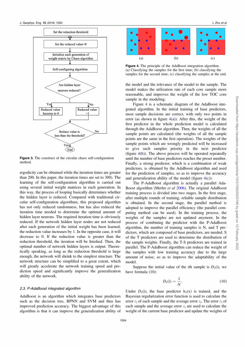
the model and the relevance of the model to the sample. Themodel makes the utilization rate of each core sample morereasonable, and improves the weight of the low TOC coresample in the modeling.

Figure 4 is a schematic diagram of the AdaBoost inte-grated algorithm. In the initial training of base predictors,most sample decisions are correct, with only two points inerror (as shown in figure 4(a)). After this, the weight of thefirst predictor in the whole prediction model is calculatedthrough the AdaBoost algorithm. Then, the weights of all thesample points are calculated (the weights of all the samplepoints are the same in the first operation). The weights of thesample points which are wrongly predicted will be increasedto give such samples priority in the next predictor(figure 4(b)). The above process will be operated repeatedlyuntil the number of base predictors reaches the preset number.Finally, a strong predictor, which is a combination of weakpredictors, is obtained by the AdaBoost algorithm and usedfor the prediction of samples, so as to improve the accuracyand generalization ability of the model (figure 4(c)).

The P-AdaBoost algorithm is actually a parallel Ada-Boost algorithm (Merler et al 2006). The original AdaBoosttraining process is divided into two stages. In the first stage,after multiple rounds of training, reliable sample distributionis obtained. In the second stage, the parallel method isadopted to improve the parallel efficiency (the parallel com-puting method can be used). In the training process, theweights of the samples are not updated anymore. In theprocess of combining the predictor with the P-AdaBoostalgorithm, the number of training samples is N, and T pre-dictors, which are composed of base predictors, are needed. Sof the T predictors are used to determine the distribution ofthe sample weights. Finally, the T-S predictors are trained inparallel. The P-AdaBoost algorithm can reduce the weight ofthe samples with low training accuracy due to the largeamount of noise, so as to improve the adaptability of themodel.

Suppose the initial value of the ith sample is D1(i), wehave formula (10):

DN

i1

. 101 =( ) ( )

Under D1(i), the base predictor h1(x) is trained, and theBayesian regularization error function is used to calculate theerror εi of each sample and the average error εt. The error εi ofeach sample and the average error εt are used to calculate theweight of the current base predictor and update the weights of

Figure 3. The construct of the circular chaos self-configurationmethod.

Figure 4. The principle of the AdaBoost integration algorithm.(a) Classifying the samples for the first time; (b) classifying thesamples for the second time; (c) classifying the samples at the end.

1054

J. Geophys. Eng. 15 (2018) 1050 L Zhu et al

Dow

nloaded from https://academ

ic.oup.com/jge/article/15/3/1050/5203196 by guest on 12 February 2022

different samples for the next iteration

W

DD

D

1

2ln

1

ii

i

11

i

n

tt

t

t 1

t 1

1 t 1

t

t

t

t

i

i

å

ee

=-

=

ee

e

ee

e+-

-

= -

-

⎧

⎨⎪⎪⎪

⎩⎪⎪⎪

⎛⎝⎜

⎞⎠⎟

( )( )

( )( )

( )

( )

( )

where Wt is the weight of the tth classifier and Dt+1(i) is theweight of the tth+1 BPNN sample.

After S iterations, assuming that a more reliable sampledistribution has been obtained, D(i) can be calculated byformula (19):

D ix e

. 121 x

a q=

G

a q

a

- -( )

( )( )

/

In the formula, α and θ are parameters. The expectation andvariance of sample distribution can be calculated by formula(20)

132 2

m aqs aq

==

⎧⎨⎩ ( )

where μ is the expectation calculated and σ2 is the variancecalculated. Through the calculated sample weights, the inte-gration of base predictors can be conducted in parallel.

All the improvements mentioned above are based on theinherent problems of neural networks or the problems thatmay be encountered in the prediction of the TOC through theneural networks. Theoretically, the accuracy and the predic-tion speed can be improved significantly. We will carry out alot of simulations through examples, and compare the modelwith the existing TOC prediction models to prove that theproposed method is superior to the TOC prediction methodbased on conventional logging curves.

3. The selection of models and simulation analysis

In order to compare the models conveniently, the measure-ment of the TOC was carried out on 132 rock samples from

the Longmaxi shale gas reservoir of the Jiaoshiba area in theSichuan Basin (the first large shale gas field in China). Withthe sample points of the abnormal response value removed,the simple linear correlation of the log response and the TOCwas analyzed using a crossplot single linear fit module in thecommercial software Excel 2003; the cross-plot was drawnbased on this result (as shown in figure 5).

In figure 5, the abscissa represents the determinationcoefficient, the ordinate in the RD represents the responsevalue of the deep resistivity curve, TH represents the responsecurve of the thorium content value, KTH represents the ura-nium gamma curve response value, CNL represents theneutron log response value, PE represents the value of thephotoelectric absorption index log response curve, GRrepresents the gamma ray logging curve value, AC representsthe wave slowness response curve, U represents the responsecurve of the uranium content value and DEN represents thedensity curve of the response value. It can be seen fromfigure 5 that the TOC and the density value have the biggestcorrelation. This is because the density of kerogen (a comp-onent of TOC) is much smaller than that of other lithology.Where the content of the TOC is higher, the density of therock must be smaller. Of course, other curves are more or lesscorrelated with the TOC. Although there is a good singlecorrelation between some well logging curves and the TOC,the goal of accurately predicting the TOC still cannot beachieved. Through correlation analysis, the uranium contentcurve (U), density curve (DEN), natural gamma curve (GR),acoustic curve (AC), neutron curve (CNL) and photoelectricabsorption cross-section index (PE) were selected as inputcurves; the content of the TOC was taken as the output. Theywere all normalized. The samples were randomly grouped(the samples were divided into four groups, each containing33 samples). The network parameters were all determined bythe K-CV method in order to obtain an ideal fitting model(Jiang et al 2015).

In order to facilitate the comparison with other nonlinearapproximation models, we attempted to write the AdaBoost-BP neural network model, SVM model and the kernelextreme machine (KELM) model, and using MATLABsoftware obtained the model parameters with the samples

Figure 5. Correlation between the well logging response andthe TOC.

Figure 6. The normalized error surface of the BP_AdaBoostalgorithm.

1055

J. Geophys. Eng. 15 (2018) 1050 L Zhu et al

Dow

nloaded from https://academ

ic.oup.com/jge/article/15/3/1050/5203196 by guest on 12 February 2022

mentioned above. The network parameters and the normal-ized error surfaces of the hidden layers of the AdaBoost-BPneural network model, the SVM neural network model andthe KELM neural network model are shown in figures 6, 7, 8,respectively.

It can be seen in figure 6 that if the number of neurons isfixed while the number of neural networks that are integratedis changed, the root mean square error (RMSE) initiallyincreases and then decreases gradually. Moreover, withregard to the error surface fluctuations, there are some randomerror surfaces outside the real overall trend. This shows thatthe weight and threshold of the BPNN easily fall into the localminimum, and the prediction error of the forecast samplebecomes large; therefore the accuracy requirements of theAdaBoost predictor algorithm cannot be satisfied (since thealgorithm was proposed for improving the prediction accur-acy of the classification algorithms, the relevant requirementsfor predictor accuracy are not present. Theoretically, thepredictor accuracy should be higher than 0.5, and the accur-acy requirements of the predictor should exist; unfortunately,very little research has ever been conducted on the predictoraccuracy limit. In this paper, we think of the lower limit of theRMSE as 0.1 in our research problem). Afterwards, with theincreasing number of networks, the RMSE of the prediction isgradually reduced, which shows that some networks will fallinto local minima in training, although most of the networkhas reached the lower accuracy limit of the AdaBoost

algorithm. Therefore, the AdaBoost model still plays animportant role and the prediction accuracy of the model willcontinue to increase. This shows that the AdaBoost integratedalgorithm can improve the accuracy of the model, and theneural network easily falls into a minimum problem, whichindicates that it is necessary to calculate the initial weightthreshold of each network using a high-performance optim-ization algorithm. When the hidden neuron number is greaterthan four, the relative error of the model will rise; thereforefor low dimensional problems, the number of neurons in theneural network should not be too much, otherwise it willeasily fall into the local minimum due to the over-fittingmodel. According to the error surface, the final model para-meters are set as follows: the number of integrated neuralnetworks is 302, the number of neurons is two and the lowestRMSE of the corresponding model is 0.2032.

Figure 7 shows the cross validation result of the KELMmodel. It can clearly be seen that the error surface has a lowvalley area, in which the minimum relative error should exist.By searching for the best parameters, the correspondingminimum RMSE is 0.2456, the kernel function value is 24and the regularization coefficient is 29. It is worth noting thatusing a back-propagation algorithm to compute the leastsquare solution greatly reduces the model learning speed (theaverage speed of the training model is only 0.012 s)—although the solution is not accurate. In this experiment, thecomputer models used were a Lenovo P900, with a Xeon E5-2660 V3 processor, a frequency of 2.60 GHz and a memoryof 32 GB. All procedures were implemented using the com-mercial software MATLAB 2016b). If the accuracy require-ment of the model is not very high, or the model is only usedfor qualitative evaluation, the KELM model would be a betterchoice.

Figure 8 shows the cross validation of the SVM model. Itcan be seen that the kernel function value is 22 and the reg-ularization coefficient is 21. The corresponding minimumRMSE is 0.2176. The accuracy of the SVM model is higherthan that of the KELM model, which shows that the SVMmodel has some advantages for small sample problems.However, the prediction effect of the SVM model is slightlylower than that of the AdaBoost-BP, which shows that the

Figure 7. The normalized error surface of the KELM algorithm.

Figure 8. The normalized error surface of the SVM algorithm.

Figure 9. Finding the results of hidden neurons in the neuralnetwork.

1056

J. Geophys. Eng. 15 (2018) 1050 L Zhu et al

Dow

nloaded from https://academ

ic.oup.com/jge/article/15/3/1050/5203196 by guest on 12 February 2022

SVM model is not strong enough for samples with certainamounts of noise.

Before the the IHNN model can be established, we needto obtain the optimal number of neurons. Figure 9 shows theoptimal number of hidden layer neurons of the 132 rocksamples using the chaos circular self-configuration methodand the circular self-configuration method, respectively. Thenumber of initial neurons is set to 20, the reduction thresholdof the chaos circular self-configuration method is set to 15,and the reduction thresholds of the circular self-configurationmethod are set to 15, 100 and 150, respectively, for com-parison. The simulated results are shown in figure 9, fromwhich we can see that it is difficult to compress the number ofhidden neurons into a small number using the circular self-configuration method: even if the reduction threshold is set to150, the number of neurons can still be reduced to only three.It only takes 110.23 s to determine the optimal number ofhidden neurons using the chaos circular self-configurationmethod, which is a pretty acceptable speed (during testing, theconvergence time is faster by 50 s when the number of hiddenlayer neurons is two rather than three. Moreover, the gen-eralization ability of the network when the number of hiddenlayer neurons is two is stronger than the network establishedwhen the number of hidden layer neurons is three. Thismethod achieves our purpose of reducing speed andimproving the generalization ability). Generally speaking, theSVM algorithm is better than the existing hidden layer neuronmerging algorithms. It is worth mentioning that although thefinal neural network structure is relatively simple, the inputdimension is low; therefore the abnormal data network issensitive to the number of neurons in the hidden layer net-work. The number of hidden layer neurons greatly influencesthe final accuracy and speed; therefore it is necessary todetermine the number of hidden layer neurons in advance.

It is necessary to prove that the adaptive tabu compoundrainforest optimizing algorithm (ATCRFA) proposed in thispaper can better find the optimal initial weight and thresholdvalue than the rainforest algorithm (RFA). We integrated 50networks (the network structure is simulated by the chaoscircular self-configuration method) using the AdaBoostalgorithm, in which the iteration times of the optimization

algorithm were set to 60. Through calculating the iterativemean of the fitness function of the optimization results of the50 network models, the optimization results between theATCRFA algorithm and RFA algorithm were compared.The results are shown in figure 10, where ATCRFA is thechange curve of the fitness function of the ATCRFA algo-rithm and the RFA is the change curve of the fitness functionof the RFA algorithm. The composite vertex algorithm(CVA) is the result of executing the iterative algorithm to dealwith the complex algorithm. It can be seen in figure 10, firstof all, that the ATCRFA has a faster convergence speed thanthe RFA in the early stage. This is because the ATCRFA canavoid the adaptive mechanism of early maturing due to thepresence of the tabu operator; therefore it has a strong abilityto jump out of the local optimum model. From the results, wecan see that the RFA is not only slower than the ATCRFA, itsfitness will also be maintained at 0.07. This is probablybecause the RFA algorithm does not jump out of the localextremum. Finally, after finishing the iteration of theATCRFA algorithm, the complex algorithm further reducesthe value of the fitness function, which shows that it has alocal mining capacity of information, so as to further improvethe precision of the optimization algorithm. All in all, it canbe concluded that the ATCRFA algorithm is more effectivethan the RFA algorithm.

After determining the optimization algorithm and theoptimal network structure, it is necessary to verify the validityof AdaBoost and P-AdaBoost and determine the parametersof the optimal integrated algorithm. Figure 11 shows thecorresponding simulation result. Firstly, 300 neural networkmodels are integrated by using the AdaBoost algorithm, andthe accuracies of the models are determined by calculating theRMSE. It can be found that for the four groups of crossvalidation data, the number of network models reaches 100,the integrated model is basically stable and the number ofpredictors in the AdaBoost algorithm is set to 100. After that,the AdaBoost algorithm is used to integrate 100 neural net-works, and then 100 neural networks are integrated by theP-AdaBoost algorithm. It can be seen that the P-AdaBoostalgorithm can increase the prediction accuracy—especiallywhen the prediction error is large—which demonstrates good

Figure 10. The result of optimizing the optimization algorithm. Figure 11. The result of the P-AdaBoost algorithm.

1057

J. Geophys. Eng. 15 (2018) 1050 L Zhu et al

Dow

nloaded from https://academ

ic.oup.com/jge/article/15/3/1050/5203196 by guest on 12 February 2022

generalization ability. To some extent, the P-AdaBoostalgorithm still avoids the network becoming trapped in thelocal minima, so it is suitable for a neural network model. Aswe can see from figure 11, the P-AdaBoost is set to 100 toachieve error stability, so the phase is set to 100.

The final RMSE cross validation figures of the four groupsare respectively 0.5023, 0.1117, 0.0746, 0.0237, and theaverage RMSE is 0.1781 in figure 11. The results are betterthan those of other algorithms, which shows that the TOCmeasurement problem in the logging interpretation can beimproved and the prediction accuracy of the neural networkmodel is better than that of the mainstream prediction model.

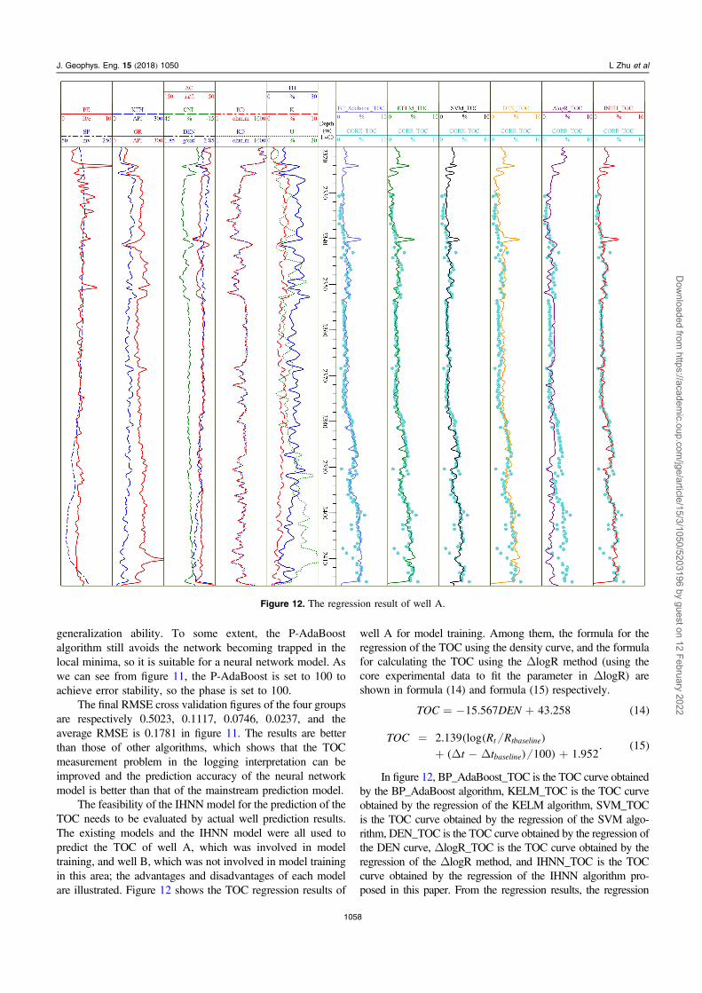
The feasibility of the IHNN model for the prediction of theTOC needs to be evaluated by actual well prediction results.The existing models and the IHNN model were all used topredict the TOC of well A, which was involved in modeltraining, and well B, which was not involved in model trainingin this area; the advantages and disadvantages of each modelare illustrated. Figure 12 shows the TOC regression results of

well A for model training. Among them, the formula for theregression of the TOC using the density curve, and the formulafor calculating the TOC using the ΔlogR method (using thecore experimental data to fit the parameter in ΔlogR) areshown in formula (14) and formula (15) respectively.

TOC DEN15.567 43.258 14= - + ( )

TOC R R

t t

2.139 log100 1.952

. 15t tbaseline

baseline

=+ D - D +

( ( )( ) )

( )

In figure 12, BP_AdaBoost_TOC is the TOC curve obtainedby the BP_AdaBoost algorithm, KELM_TOC is the TOC curveobtained by the regression of the KELM algorithm, SVM_TOCis the TOC curve obtained by the regression of the SVM algo-rithm, DEN_TOC is the TOC curve obtained by the regression ofthe DEN curve, ΔlogR_TOC is the TOC curve obtained by theregression of the ΔlogR method, and IHNN_TOC is the TOCcurve obtained by the regression of the IHNN algorithm pro-posed in this paper. From the regression results, the regression

Figure 12. The regression result of well A.

1058

J. Geophys. Eng. 15 (2018) 1050 L Zhu et al

Dow

nloaded from https://academ

ic.oup.com/jge/article/15/3/1050/5203196 by guest on 12 February 2022

curves of the SVM regression algorithm have low precisionwithin the 2330–2345m depth section, which shows that theapproximation abilities of both DEN curve regression methods,the ΔlogR method and the SVM algorithm for the conventionalcurve prediction TOC problem are insufficient. Moreover, undera lower TOC reservoir, the comprehensive relationship betweenthe TOC and the conventional curve cannot be accuratelydetermined, nor can the reservoir TOC be accurately calculated.The TOC calculated at a depth of 2352m–2378m is relativelysmaller, like the regression method of the DEN curve. Since theBP_AdaBoost algorithm enhances the diversity of the network,the regression effects in high TOC and low TOC are both good.However, the low prediction accuracy of the TOC is still notideal, which is a common problem in the existing predictionmethods of the TOC (the TOC response is suppressed in the lowTOC reservoir and the prediction accuracy will decline). TheTOC curve obtained by the IHNN regression algorithm canachieve good accuracy both for a high TOC and low TOC. Thisis because the network weights of the hidden layer neurons areoptimized through the deleting and optimizing algorithms, so thateach network achieves the best result. The robustness of thenetwork can therefore be enhanced and the final prediction

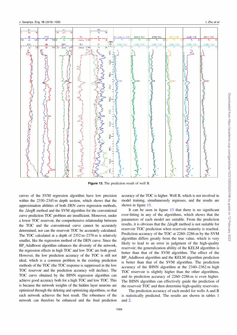
accuracy of the TOC is higher. Well B, which is not involved inmodel training, simultaneously regresses, and the results areshown in figure 13.

It can be seen in figure 13 that there is no significantover-fitting in any of the algorithms, which shows that theparameters of each model are suitable. From the predictionresults, it is obvious that the ΔlogR method is not suitable forreservoir TOC prediction when reservoir maturity is reached.Prediction accuracy of the TOC at 2260–2286 m by the SVMalgorithm differs greatly from the true value, which is verylikely to lead to an error in judgment of the high-qualityreservoir; the generalization ability of the KELM algorithm isbetter than that of the SVM algorithm. The effect of theBP_AdaBoost algorithm and the KELM algorithm predictionis better than that of the SVM algorithm. The predictionaccuracy of the IHNN algorithm at the 2340–2362 m highTOC reservoir is slightly higher than the other algorithms,and its prediction accuracy of 2260–2286 m is even higher.The IHNN algorithm can effectively guide the prediction ofthe reservoir TOC and then determine high-quality reservoirs.

The prediction accuracy of each model for wells A and Bis statistically predicted. The results are shown in tables 1and 2.

Figure 13. The prediction result of well B.

1059

J. Geophys. Eng. 15 (2018) 1050 L Zhu et al

Dow

nloaded from https://academ

ic.oup.com/jge/article/15/3/1050/5203196 by guest on 12 February 2022

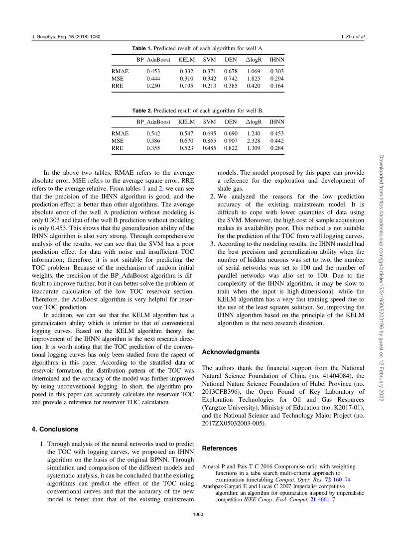
In the above two tables, RMAE refers to the averageabsolute error, MSE refers to the average square error, RRErefers to the average relative. From tables 1 and 2, we can seethat the precision of the IHNN algorithm is good, and theprediction effect is better than other algorithms. The averageabsolute error of the well A prediction without modeling isonly 0.303 and that of the well B prediction without modelingis only 0.453. This shows that the generalization ability of theIHNN algorithm is also very strong. Through comprehensiveanalysis of the results, we can see that the SVM has a poorprediction effect for data with noise and insufficient TOCinformation; therefore, it is not suitable for predicting theTOC problem. Because of the mechanism of random initialweights, the precision of the BP_AdaBoost algorithm is dif-ficult to improve further, but it can better solve the problem ofinaccurate calculation of the low TOC reservoir section.Therefore, the AdaBoost algorithm is very helpful for reser-voir TOC prediction.

In addition, we can see that the KELM algorithm has ageneralization ability which is inferior to that of conventionallogging curves. Based on the KELM algorithm theory, theimprovement of the IHNN algorithm is the next research direc-tion. It is worth noting that the TOC prediction of the conven-tional logging curves has only been studied from the aspect ofalgorithms in this paper. According to the stratified data ofreservoir formation, the distribution pattern of the TOC wasdetermined and the accuracy of the model was further improvedby using unconventional logging. In short, the algorithm pro-posed in this paper can accurately calculate the reservoir TOCand provide a reference for reservoir TOC calculation.

4. Conclusions

1. Through analysis of the neural networks used to predictthe TOC with logging curves, we proposed an IHNNalgorithm on the basis of the original BPNN. Throughsimulation and comparison of the different models andsystematic analysis, it can be concluded that the existingalgorithms can predict the effect of the TOC usingconventional curves and that the accuracy of the newmodel is better than that of the existing mainstream

models. The model proposed by this paper can providea reference for the exploration and development ofshale gas.

2. We analyzed the reasons for the low predictionaccuracy of the existing mainstream model. It isdifficult to cope with lower quantities of data usingthe SVM. Moreover, the high cost of sample acquisitionmakes its availability poor. This method is not suitablefor the prediction of the TOC from well logging curves.

3. According to the modeling results, the IHNN model hadthe best precision and generalization ability when thenumber of hidden neurons was set to two, the numberof serial networks was set to 100 and the number ofparallel networks was also set to 100. Due to thecomplexity of the IHNN algorithm, it may be slow totrain when the input is high-dimensional, while theKELM algorithm has a very fast training speed due tothe use of the least squares solution. So, improving theIHNN algorithm based on the principle of the KELMalgorithm is the next research direction.

Acknowledgments

The authors thank the financial support from the NationalNatural Science Foundation of China (no. 41404084), theNational Nature Science Foundation of Hubei Province (no.2013CFB396), the Open Found of Key Laboratory ofExploration Technologies for Oil and Gas Resources(Yangtze University), Ministry of Education (no. K2017-01),and the National Science and Technology Major Project (no.2017ZX05032003-005).

References

Amaral P and Pais T C 2016 Compromise ratio with weightingfunctions in a tabu search multi-criteria approach toexamination timetabling Comput. Oper. Res. 72 160–74

Atashpaz-Gargari E and Lucas C 2007 Imperialist competitivealgorithm: an algorithm for optimization inspired by imperialisticcompetition IEEE Congr. Evol. Comput. 21 4661–7

Table 1. Predicted result of each algorithm for well A.

BP_AdaBoost KELM SVM DEN ΔlogR IHNN

RMAE 0.453 0.332 0.371 0.678 1.069 0.303MSE 0.444 0.310 0.342 0.742 1.825 0.294RRE 0.250 0.195 0.213 0.385 0.420 0.164

Table 2. Predicted result of each algorithm for well B.

BP_AdaBoost KELM SVM DEN ΔlogR IHNN

RMAE 0.542 0.547 0.695 0.690 1.240 0.453MSE 0.586 0.670 0.865 0.907 2.328 0.442RRE 0.355 0.523 0.485 0.822 1.309 0.284

1060

J. Geophys. Eng. 15 (2018) 1050 L Zhu et al

Dow

nloaded from https://academ

ic.oup.com/jge/article/15/3/1050/5203196 by guest on 12 February 2022

Broomhead D S and Lowe D 1988 Multivariable functionalinterpolation and adaptive networks Complex Syst. 2 321–55

Černý V 1985 Thermodynamical approach to the traveling salesmanproblem: an efficient simulation algorithm J. Optimiz. Theor.Appl. 45 41–51

Chen W L 2013 Analysis of the shale gas reservoir in the lowerSilurian Longmaxi formation, Changxin 1 well, SoutheastSichuan Basin, China Acta. Petr. Sin. 29 1073–86 (inChinese)

Dong D Z 2012 Progress and prospects of shale gas exploration anddevelopment in China Acta. Petrol. Sin. 33 107–14 (inChinese)

Dorigo M, Birattari M and Stutzle T 2006 Ant colony optimizationIEEE Comput. Intell. Mag. 1 28–39

Frans V D B and Engelbrecht A P A 2004 Cooperative approach toparticle swarm optimization IEEE Transon. Evol. Comp. 8 225–39

Gandomi A H and Alavi A H 2012 Krill herd: a new bio-inspiredoptimization algorithm Commun. Nonlinear Sci. Numer. Simul.17 4831–45

Gao W S, Shao C and Gao Q 2013 Pseudo-collision in swarmoptimization algorithm and solution: rain forest algorithm ActaPhys. Sin. 62 1–16 (in Chinese)

Ge X M 2016 Investigation of organic related pores inunconventional reservoir and its quantitative evaluation EnergyFuels 30 4699–709

Geem Z W, Kim J H and Loganathan G V 2001 A new heuristicoptimization algorithm: harmony search Simulation 76 60–8

Guo C, Zhang C and Zhu L 2017 Predicting the total porosity of shalegas reservoirs Petroleum Sci. Tech. 35 1022–31 (in Chinese)

Haecker A, Carvajal H and White J 2016 Comparison of organicmatter correlations in North American shale plays SPWLA 57thAnnual Logging Symp.

Hatamlou A 2013 Black hole: a new heuristic optimization approachfor data clustering Inform. Sciences 222 175–84

He S, Wu Q H and Saunders J R 2009 Group search optimizer: anoptimization algorithm inspired by animal searching behaviorIEEE Trans. Evol. Comput. 13 973–90

Holland J H 1992 Genetic algorithms Sci. Amer. 267 66–72Hopfield J J 1984 Neurons with graded response have collective

computational properties like those of two-state neuronsBiophysics 81 3088–92

Hu H T, Liu C and Lu S F 2016 The method and application of usinggeneralized ΔLgR technology to predict the organic carboncontent of continental deep source rocks Nat. Gas Geosci. 27149–55

Huang R C et al 2014 Optimal selection of logging-based TOCcalculation methods of shale reservoirs: a case study of theJiaoshiba shale gas field, Sichuan Basin Nat. Gas Ind. 34 25–32

Huang W et al 2015 Interpretation model of organic carbon contentof shale in Member 7 of Yanchang Formation, central-southernOrdos Basin Acta. Petrol. Sin. 36 1508–15

Huo Q L et al 2011 The advance of ΔlgR method and its applicationin Songliao Basin J. Jilin Univ. Earth Sci. 42 586–91 (inChinese)

Jiang F B, Dai Q W and Dong L 2015 Ultra-high density resistivitynonlinear inversion based on principal component-regularizedELM Chin. J. Geophys. 58 3356–69 (in Chinese)

Kadkhodaie-Ilkhchi A, Rahimpour-Bonab H and Rezaee M A 2009Committee machine with intelligent systems for estimation oftotal organic carbon content from petrophysical data: anexample from Kangan and Dalan reservoirs in South Pars GasField, Iran Comput. Geosci. 35 459–74

Kaveh A and Farhoudi N A 2013 New optimization method: dolphinecholocation Advan. Eng. Softw. 59 53–70

Labbi Y et al 2016 A new rooted tree optimization algorithm foreconomic dispatch with value-point effect Electr. PowerEnerg. Syst. 79 298–311

Lecun Y, Bengio Y and Hinton G 2015 Deep learning Nature 521436–44

Li J et al 2014 ‘Four-pore’modeling and its quantitative loggingdescription of shale gas reservoir Oil Gas Geol. 35 266–71 (inChinese)

Mahersia H, Boulehmi H and Hamrouni K 2016 Development ofintelligent systems based on Bayesian regularization networkand neuro-fuzzy models for mass detection in mammograms: acomparative analysis Comput. Method Program. Biomed. 12646–62

Mehrabian A R and Lucas C 2006 A novel numerical optimizationalgorithm inspired from weed colonization Ecol. Inform. 1 355–66

Meng Z P, Guo Y S and Liu W 2015 Relationship between organiccarbon content of shale gas reservoir and logging parametersand its prediction model J. Chin. Coal. Soc. 40 247–53 (inChinese)

Merler S, Caprile B and Furlanello C 2006 Parallelizing AdaBoostby weights dynamics Comput. Stat. Data Anal. 51 2487–98

Moroni G, Syam W P and Petrò S 2016 Comparison of chaosoptimization functions for performance improvement of fittingof non-linear geometries Measurement 86 79–92

Ouadfeul S A and Aliouane L 2015 Total organic carbon predictionin shale gas reservoirs from well logs data using the multilayerperceptron neural network with Levenberg Marquardt trainingalgorithm: application to Barnett Shale Petrol. Eng. 40 3345–9

Pan B Z, Duan Y N, Zhang H T, Yang X M and Han X 2016 BFA-CM optimization log interpretation method Chin. J. Geophys.59 391–8 (in Chinese)

Rao H, Fu M F and Chen L 2008 Structure optimization for neuralnetwork based on circular self-configuring algorithm Comput.Eng. Des. 29 411–7

Rumelhart D E, Hinton G E and Williams R J 1986 Learningrepresentations by back-propagation errors Nature 323 533–6

Sfidari E, Kadkhodaie-Ilkhchi A and Najjari S 2015 Comparison ofintelligent and statistical clustering approaches to predictingtotal organic carbon using intelligent systems J. Pet. Sci. Eng.40 3345–9

Shah-Hosseini H 2011 Principal components analysis by the Galaxy-based search algorithm:a novel metaheuristic for continuousoptimization Int. J. Comput. Sci. Eng. 6 132–40

Shi X et al 2016 Application of extreme learning machine and neuralnetworks in total organic carbon content prediction in organicshale with wire line logs J. Nat. Gas. Sci. Eng. 33 687–702

Tan M J et al 2015 Support-vector-regression machine technologyfor total organic carbon content prediction from wireline logsin organic shale: a comparative study J. Nat. Gas. Sci. Eng. 26792–802

Tan Y and Zhu Y C 2010 Fireworks algorithm for optimization Adv.Swarm. Intell. 21 355–64

Wang X Z, Gao S L and Gao C 2014 Geological features ofmesozoic continental shale gas in south of Ordos Basin, NWChina Petr. Explor. Dev. 41 294–304 (in Chinese)

Xie H C et al 2013 TOC logging interpretation method and itsapplication to Yanchang Formation shales, the Ordos BasinOil. Gas. Geol. 34 731–6 (in Chinese)

Yang S C et al 2013 The logging evaluation of source rocks ofTriassic Yanchang formation in Chongxin area, Ordos BasinNat. Gas. Geosci. 24 470–6

Zhang C, Guo C, Zhu L, Cheng Y and Yan W 2017 A logginginterpretation method for total porosity considering organic mattercorrection of shale gas reservoirs Chin. Coal. Soc. 42 1527–34

Zhang Z W and Zhang L H 2000 A method of source evaluation bywell-logging and its application result Petr. Explor. Dev. 2784–7 (in Chinese)

Zhao P Q et al 2017 A improved method for estimating the TOC inshale formations Mar. Petr. Geol. 83 174–83

Zhao P Q et al 2016 A new method for estimating total organiccarbon content from well logs AAPG Bulletin 100 149–55

Zhou Z Y 2009 Quantitative analysis of variation of organic carbonmass and content in source rock during evolution process Petr.Explor. Dev. 36 463–8 (in Chinese)

1061

J. Geophys. Eng. 15 (2018) 1050 L Zhu et al

Dow

nloaded from https://academ

ic.oup.com/jge/article/15/3/1050/5203196 by guest on 12 February 2022