HAL Id: hal-02624898https://hal.inrae.fr/hal-02624898

Submitted on 21 Dec 2021

HAL is a multi-disciplinary open accessarchive for the deposit and dissemination of sci-entific research documents, whether they are pub-lished or not. The documents may come fromteaching and research institutions in France orabroad, or from public or private research centers.

L’archive ouverte pluridisciplinaire HAL, estdestinée au dépôt et à la diffusion de documentsscientifiques de niveau recherche, publiés ou non,émanant des établissements d’enseignement et derecherche français ou étrangers, des laboratoirespublics ou privés.

Distributed under a Creative Commons Attribution - NonCommercial| 4.0 InternationalLicense

Prediction of plant diversity in grasslands usingSentinel-1 and -2 satellite image time series

Mathieu Fauvel, Mailys Lopes, Titouan Dubo, Justine Rivers-Moore,Pierre-Louis Frison, Nicolas Gross, Annie Ouin

To cite this version:Mathieu Fauvel, Mailys Lopes, Titouan Dubo, Justine Rivers-Moore, Pierre-Louis Frison, et al.. Pre-diction of plant diversity in grasslands using Sentinel-1 and -2 satellite image time series. RemoteSensing of Environment, Elsevier, 2020, 237 (février), 13 p. �10.1016/j.rse.2019.111536�. �hal-02624898�

Abstract

The prediction of grasslands plant diversity using satellite image time series is considered in this article. Fifteen monthsof freely available Sentinel optical and radar data were used to predict taxonomic and functional diversity at the pixelscale (10m×10m) over a large geographical extent (40 000 km2). 415 field measurements were collected in 83 grasslandsto train and validate several statistical learning methods. The objective was to link the satellite spectro-temporal data tothe plant diversity indices. Among the several diversity indices tested, Simpson and Shannon indices were best predictedwith a coefficient of determination around 0.4 using a Random Forest predictor and Sentinel-2 data. The use of Sentinel-1 data was not found to improve significantly the prediction accuracy. Using the Random Forest algorithm and theSentinel-2 time series, the prediction of the Simpson index was performed. The resulting map highlights the intra-parcelvariability and demonstrates the capacity of satellite image time series to monitor grasslands plant taxonomic diversityfrom an ecological viewpoint.

Keywords: Satellite image time series, Sentinel-1&-2, Statistical learning, Grasslands, taxonomic diversity

1. Introduction

Natural and semi-natural grasslands cover 22% of theEuropean agricultural land surface (Bengtsson et al., 2019).Grasslands are today one of the most endangered ecosys-tems due to land use change, agricultural intensification,and abandonment (Pärtel et al., 2005). Grasslands hosta unique biodiversity, which support the provision of keyecosystem services such as carbon storage, food produc-tion crop polination, pest regulation and contribute tolandscape scale amenities such as landscape scenic view.Permanent grasslands are crucial to maintain biodiversityin many agricultral landscape (Watkinson and Ormerod,2001; Habel et al., 2013), and particularly insect diver-sity: they provide host plants, nectar, pollen (Ockingerand Smith, 2007) as well as nest sites (Carrié et al., 2018;Potts and Willmer, 1997).

Yet, despite recent regulation in favor of grasslands,agriculture intensification, abandonment and urbanizationgenerate a decrease of both grasslands surface area and

∗Corresponding authorEmail addresses: mathieu.fauvel@inra.fr (Mathieu Fauvel),

mailys.lopes@inra.fr (Mailys Lopes), titouan-dubo@hotmail.fr(Titouan Dubo), justine.rivers-moore@inra.fr (JustineRivers-Moore), pierre-louis.frison@univ-mlv.fr (Pierre-LouisFrison), nicolas.gross@inra.fr (Nicolas Gross),annie.ouin@ensat.fr (Annie Ouin)

plant diversity (O’Mara, 2012; Newbold et al., 2016) lead-ing to a loss of biodiversity (plants, insects, birds) and itsrelated ecosystem services. Therefore, there is an urgentneed to monitor grasslands over large extents in order toassess their current state in terms of area covered but alsoto estimate their plant diversity and their carrying capac-ity for insect populations. While the area information canbe extracted from land cover databases (e.g. CORINELand Cover (Heymann, 1994)) diversity and carrying ca-pacity data are scarcely available. Though, spatial loca-tion, extent and quality of grasslands are crucial for theirconservation per se but also to produce maps of relatedecosystem services in agricultural areas. For instance, mo-bile agents based ecosystem services (Kremen et al., 2007)such as pollination and pest regulation rely on the pres-ence of a mosaic of crops and semi-natural elements amongwhich grasslands are crucial and represent the largest sur-face area.

Plant diversity is usually assessed by botanical surveysof the grasslands and indices related to the diversity inspecies of a community are commonly computed (rich-ness, Shannon and Simpson diversity (Magurran, 2004)).Functional diversity can also be derived from the botanicalsurvey through functional types, i.e., set of species exhibit-ing similar attributes having similar effect on ecosystems(Diaz and Cabido, 2001). Field surveys, sometimes calledground-truth in the remote sensing community, require

Preprint submitted to Remote Sensing of Environment October 31, 2019

Prediction of plant diversity in grasslands using Sentinel-1 and -2 satellite imagetime series

Mathieu Fauvela,∗, Mailys Lopesb, Titouan Dubob, Justine Rivers-Mooreb, Pierre-Louis Frisond, Nicolas Grossc, AnnieOuinb

aCESBIO, Université de Toulouse, CNES/CNRS/INRA/IRD/UPS, Toulouse, FrancebDYNAFOR, Université de Toulouse, INRA, Castanet-Tolosan, France

cUCA, INRA, VetAgro Sup, UMR 0874 Ecosystème Prairial, 63000 Clermont-Ferrand, FrancedLaSTIG, Université Paris-Est, IGN, 5 Bd Descartes, Champs sur Marne,77455 Marne la Vallée, France

© 2019 published by Elsevier. This manuscript is made available under the CC BY NC user licensehttps://creativecommons.org/licenses/by-nc/4.0/

Version of Record: https://www.sciencedirect.com/science/article/pii/S0034425719305553Manuscript_a2e72de04e47ff0cf988711e1c381d7e

significant human and material resources, the knowledge ofthe assessor and a sampling strategy, which make them ex-pensive and time consuming (Magurran, 2004). Ecologicalsurveys are thus limited in spatial extent and in temporalfrequency, limiting grassland monitoring to a local scaleand usually over a short period of time. Although fieldsurveys provide valuable and high quality data at a pointscale, they cannot easily be upscaled while taking into ac-count the landsape heterogeneity. Therefore, field surveysalone cannot address the needs to monitor grassland bio-diversity over large spatial extents and other techniquesrelating to field surveys should be considered.

Among such complementary techniques, remote sens-ing has received an increasing attention in the last decades(Turner, 2014; Buck et al., 2015). However, grasslandshave been rarely studied in the remote sensing literaturecompared to other land covers like crops or forest (Newtonet al., 2009). Most of the studies focusing on grasslandshave agronomic applications, such as estimating biomassproductivity and growth rate (Gu and Wylie, 2015; Liet al., 2013) or deriving biophysical parameters like theLeaf Ara Index (LAI), the fraction of PhotosyntheticallyActive Radiation (fPAR) or the fraction of Vegetation Cover(fCOVER) (Darvishzadeh et al., 2008; He et al., 2009).

Regarding ecological applications, Corbane et al. (2013)mapped semi-natural grasslands types using two RapidEyeimages, while Stenzel et al. (2017) used five RapidEye im-ages to classify high nature value grasslands. Species rich-ness of herbaceous ecosystems such as grasslands, prairiesand savannah was assessed using airborne hyperspectralimagery in Möckel et al. (2016), Gholizadeh et al. (2019)and Oldeland et al. (2010), respectively. Airborne hy-perspectral imagery has also been used to map groups ofspecies (Schuster et al., 2015), flower types (Landmannet al., 2015) or pollination types (Feilhauer et al., 2016).

Schematically, the different approaches to analyse grass-land with remote sensing data can be divided into threecategories: 1. Techniques that use vegetation indices orspectral reflectance as explanatory variables (Rapinel et al.,2019; Féret et al., 2015) 2. Techniques that use the spa-tial heterogeneity of vegetation indices as explanatory vari-ables (Goodin and Henebry, 1998; Tuanmu and Jetz, 2015),3. Techniques that use the “spectral variation hypothe-sis” (SVH) to extract explanatory variables (Lopes et al.,2017b; Hall et al., 2012).

In terms of remote sensing data, the majority of thestudies having ecological schemes were conducted usingvery high spatial resolution data (≤ 5 meters/pixel), e.g.,hyperspectral data issued from an airborne sensor or mul-tispectral satellite data such as RapidEye. Although a veryhigh spatial resolution might seem necessary to estimategrasslands plant diversity as plant are typically small ingrasslands, these types of acquisitions are limited in timeand in space because of their current cost. In addition,medium spatial resolution satellite image time series (e.g,MODIS or SPOT-VEGETATION) have been found notappropriate for small and heterogeneous elements, such as

grasslands. In particular, Ali et al. (2016) have statedthat the moderate spatial resolution “precludes their usefor field-scale application in many countries”. As a con-sequence, the grassland biodiversity monitoring from re-mote sensing data is nowadays limited to “low temporalresolution & small spatial cover & high spatial resolution”(Giménez et al., 2017; Wang et al., 2019; Gholizadeh et al.,2019; Lopatin et al., 2017) or “high temporal resolution &large spatial cover & coarse spatial resolution” (Ge et al.,2018; Schmidt et al., 2018; Yang et al., 2018; Barrett et al.,2014; Si et al., 2012).

The launch of Sentinel-1&-2 satellites, issued from theEuropean Union Copernicus and European Space Agencyprogram, has enabled continuous and regular monitoringof small vegetated areas over large spatial extents thanksto their high spatial resolution (10m per pixel) and theirfrequent revisit (every 5 days for Sentinel-2) (Drusch et al.,2012; Defourny et al., 2019). Sentinel-1&-2 satellite imagetime series (SITS) open new possibilities to bridge the gapbetween high spatial resolution and high temporal reso-lution. First, their high temporal resolution enables themonitoring of plant phenology. Because plant communi-ties differ in their temporal behavior, the phenological di-versity measured by these sensors could be used as a proxyto estimate the plant diversity. Second, they provide com-plementary information about the grassland cover: opticaldata are influenced by chemical composition of the ele-ments while radar data are sensitive to the geometric con-figuration of the elements (Joshi et al., 2016). Then, beingavailable for free, they can be used to process large areasand complement field surveys at a reduced cost. Yet, re-cent works using Sentinel-2 images are still performed onsmall areas (a few square kilometers) (Rapinel et al., 2019).Although interesting, studies over such small areas do nothave to cope with a high diversity of grasslands in termsof composition neither with the spatial variability of mete-orological, topographical conditions and farmers pratices.Hence, it is unlikely that classification accuracies reportedin such cases can be reached on larger spatial areas. Fur-thermore, they do not cope with the spectro-temporal vari-ability of Sentinel satellite image series.

In this paper, we use Sentinel’s optical and radar SITSto estimate plant taxonomic and functional diversity ingrasslands over a a large spatial extent (40 000 km2) for onegrowing season. Fifteen months of acquisitions of Sentinel-1&-2 images were used to predict at the pixel level plantdiversity indices (richness, Shannon and Simpson diversityindices) and functional diversity indices related to polli-nation (flower diversity, insect dependence) of grasslandslocated in farmed landscapes in the southwest of France.Various linear and non-linear algorithms were investigatedto cover different kinds of possible statistical relationshipsbetween the biodiversity indices and the SITS.

2

Figure 1: Study area. The region in the black frame is a zoom of thered area at the bottom of the image. The blue circles indicate thesampled plots in the grasslands. See section 2.2 for a full description.Data: 1:10m Natural Earth I (https://www.naturalearthdata.com);BD ORTHO R© 50 cm IGN (background aerial photography)

2. Materials

2.1. Study siteThe study area is part of the Long-Term Socio-Ecological

Research site “Pyrénées-Garonne” located in southwestFrance near the city of Toulouse (43 ◦17 0 N, 0 ◦54 0 E), seeFigure 1. This hilly area of around 900 km2 is character-ized by a mosaic of crops, small woods and grasslands. Itis dominated by mixed crop-livestock farming. Grasslandsprovide food for cattle by grazing and/or producing hay orsilage. They range from mono-specific, annual grasslandssown with rye-grass (improved with mineral fertilizing andmown up to three times a year) to permanent, semi-naturalgrasslands composed of spontaneous plant species (not fer-tilized and mown once a year). Grasslands are mainlylocated on steep slopes, whereas annual crops are in thevalleys on the most productive, often irrigated lands. Theclimate is sub-Atlantic with sub-Mediterranean and moun-tain influences (mean annual temperature, 12.5 ◦C; meanannual precipitation, 750 mm).

2.2. Field botanical surveys

10m

Figure 2: Field sampling: a plot (light red area) is made of 5 quadrats(red squares), 4 of them being located at 10 m from the center one.The light blue squares represent the corresponding Sentinel-2 pixelgrid.

Table 1: Plant cover percentage bins.Coverage estimation Assigned value

(%) (%)

[1, 2.5] 1[2.5, 7.5] 5[7.5, 11.5] 10[11.5, 20] 15[21, 30] 25[31, 40] 35[41, 50] 45[51, 60] 55[61, 70] 65[71, 80] 75[81, 90] 85[91, 99] 95100 100

Botanical surveys were conducted in 83 plots from dis-tinct grasslands between April and May 2018 after theflowering and before the mowing. The average distancebetween two plots was 13.4 km with a standard deviationof 9.1 km and the minimum and the maximum distanceswere 0.08 km and 44.37 km, respectively. Each plot wascomposed of 5 quadrats of 1 square meter area (Figure 2).The center of each quadrat corresponded to the theoreticalcenter of a Sentinel-2 pixel. Note that since the absolutegeolocation is below 11 meter at 95.5% confidence (ESA,2019), a possible mis-registration between Sentinel-2 dataand GNSS can be observed for few pixels at some dates.After a ground checking and getting owners agreement,the position of the central quadrat was controlled witha high-accuracy GNSS handhelds (Trimble Geo 7X Ter-raSync). The grasslands were digitized using the agricul-tural Land Parcel Information System “Registre Parcel-laire Graphique” (RPG) (Cantelaube and Carles, 2014).

Plants were identified at the species level and the abun-dance of each species was estimated by its cover percent-age value in the one square meter area, according to 12bins, see Table 1. Vegetation height was measured in twolocations in each quadrat and averaged. A total of 415quadrats (leading to 415 Sentinel pixels), belonging to 83grasslands, was recorded and used in this study.

Three indices were computed using vegan package ofR 3.2.3 (Oksanen et al., 2007; Team, 2012): plant richnessSq, defined as the number of plant species in quadrat q,the Shannon diversity index

H ′(q) = −Sq∑

s=1pqs ln(pqs),

where pqs is the relative abundance of the species s inquadrat q and Simpson index of diversity (refers to Simp-son index in the paper for simplicity) ,

L(q) = 1 −Sq∑

s=1p2

qs.

The Shannon index measures heterogeneity taking into ac-count the number of species and the relative abundance of

3

each species, while the Simpson index is the inverse of adominance index reflecting how much the community isdominated (or not) by few species.

We also consider vegetation attribute related to polli-nation. Following Clough et al. (2014), Insect Dependencewas assessed for each plant species, based on pollinationsyndrome (insects, wind, water..) and its frequency. Thevalues were: 1 if insects are the major pollination vector,0.5 if insects and an other vector are the major pollina-tion vector, 0 if insects are not an important pollinationvector. The Reward Index combines the amount of nec-tar and pollen which values run from: 0 for “none”, 1 for“little”, 2 for “present”, 3 for “plenty”. The sum of nectarand the amount of pollen score lead to values from 0 to 6for the Reward Index of the species. Averaged at the com-munity level using the FD package Laliberté and Legendre(2010) of R 3.2.3, the diversity and the abundance of thesetwo vegetation attributes may reflect how species impactcommunity and ecosystems. Finally, the Color Diversitywas derived from the Shannon index,

CD(q) = −Jq∑

j=1rqj ln(rqj),

where rqj is the sum of the relative abundance of thespecies whom major color of flowers is j in quadrat q andJq is the number of major colors in quadrat q.

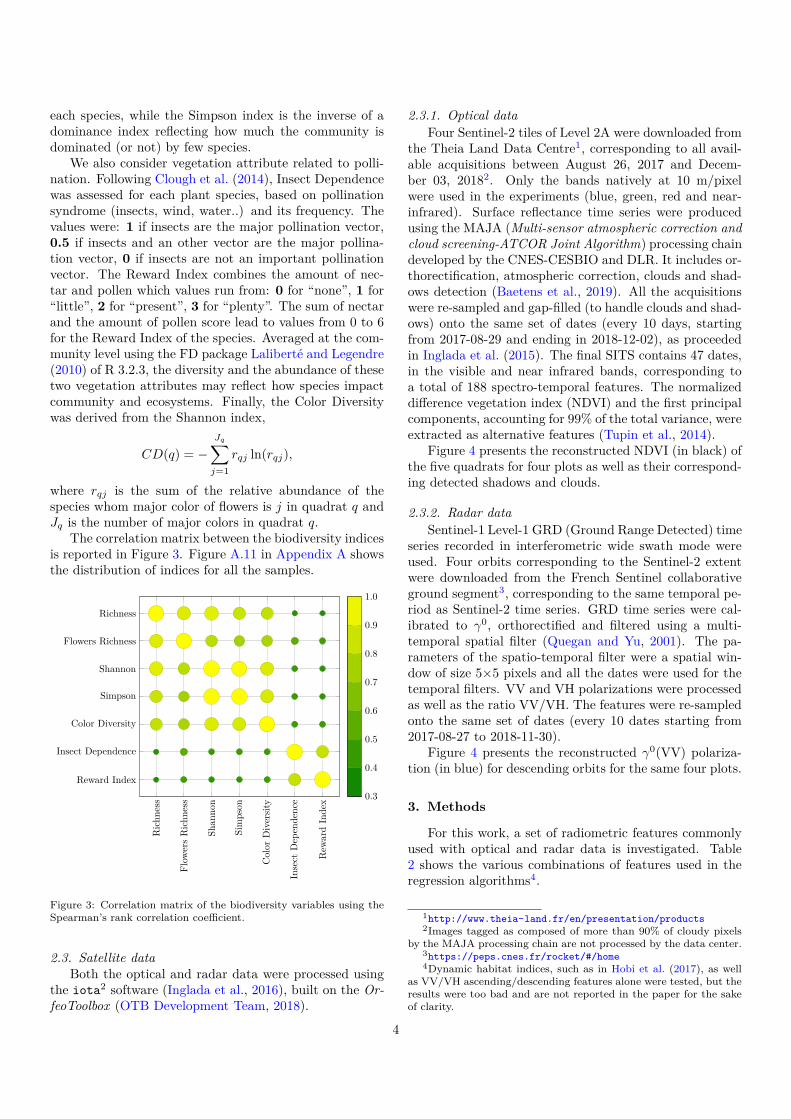
The correlation matrix between the biodiversity indicesis reported in Figure 3. Figure A.11 in Appendix A showsthe distribution of indices for all the samples.

Richn

ess

Flow

ersRichn

ess

Shan

non

Simpson

Color

Diversit

y

Insect

Dep

ende

nce

Rew

ardInde

x

Richness

Flowers Richness

Shannon

Simpson

Color Diversity

Insect Dependence

Reward Index0.3

0.4

0.5

0.6

0.7

0.8

0.9

1.0

Figure 3: Correlation matrix of the biodiversity variables using theSpearman’s rank correlation coefficient.

2.3. Satellite dataBoth the optical and radar data were processed using

the iota2 software (Inglada et al., 2016), built on the Or-feoToolbox (OTB Development Team, 2018).

2.3.1. Optical dataFour Sentinel-2 tiles of Level 2A were downloaded from

the Theia Land Data Centre1, corresponding to all avail-able acquisitions between August 26, 2017 and Decem-ber 03, 20182. Only the bands natively at 10 m/pixelwere used in the experiments (blue, green, red and near-infrared). Surface reflectance time series were producedusing the MAJA (Multi-sensor atmospheric correction andcloud screening-ATCOR Joint Algorithm) processing chaindeveloped by the CNES-CESBIO and DLR. It includes or-thorectification, atmospheric correction, clouds and shad-ows detection (Baetens et al., 2019). All the acquisitionswere re-sampled and gap-filled (to handle clouds and shad-ows) onto the same set of dates (every 10 days, startingfrom 2017-08-29 and ending in 2018-12-02), as proceededin Inglada et al. (2015). The final SITS contains 47 dates,in the visible and near infrared bands, corresponding toa total of 188 spectro-temporal features. The normalizeddifference vegetation index (NDVI) and the first principalcomponents, accounting for 99% of the total variance, wereextracted as alternative features (Tupin et al., 2014).

Figure 4 presents the reconstructed NDVI (in black) ofthe five quadrats for four plots as well as their correspond-ing detected shadows and clouds.

2.3.2. Radar dataSentinel-1 Level-1 GRD (Ground Range Detected) time

series recorded in interferometric wide swath mode wereused. Four orbits corresponding to the Sentinel-2 extentwere downloaded from the French Sentinel collaborativeground segment3, corresponding to the same temporal pe-riod as Sentinel-2 time series. GRD time series were cal-ibrated to γ0, orthorectified and filtered using a multi-temporal spatial filter (Quegan and Yu, 2001). The pa-rameters of the spatio-temporal filter were a spatial win-dow of size 5×5 pixels and all the dates were used for thetemporal filters. VV and VH polarizations were processedas well as the ratio VV/VH. The features were re-sampledonto the same set of dates (every 10 dates starting from2017-08-27 to 2018-11-30).

Figure 4 presents the reconstructed γ0(VV) polariza-tion (in blue) for descending orbits for the same four plots.

3. Methods

For this work, a set of radiometric features commonlyused with optical and radar data is investigated. Table2 shows the various combinations of features used in theregression algorithms4.

1http://www.theia-land.fr/en/presentation/products2Images tagged as composed of more than 90% of cloudy pixels

by the MAJA processing chain are not processed by the data center.3https://peps.cnes.fr/rocket/#/home4Dynamic habitat indices, such as in Hobi et al. (2017), as well

as VV/VH ascending/descending features alone were tested, but theresults were too bad and are not reported in the paper for the sakeof clarity.

4

Table 2: List of inputs used for the prediction. The last column provides the number of variables for each input.Acronym Description Size

S2 Blue, Green, Red and Near Infra-red spectral bands for all temporal acquisitions. 188

NDVI NDVI for all the temporal acquisitions. 47

S2 NDVI Combination of S2 and NDVI. 235

S2 PCA First principal component accounting for 99% of the cumulative variance computed on S2. 49

R IR Red and Near Infra-red spectral bands for all temporal acquisitions. 94

S1 VV, VH and ratio for all temporal acquisitions. 279

S1 S2 Full stack of S1 and S2 data. 467

PCA S1 S2 First principal component accounting for 99% of the cumulative variance computed on the S1 and S2stack.

117

2017-09

2017-10

2017-11

2017-12

2018-01

2018-02

2018-03

2018-04

2018-05

2018-06

2018-07

2018-08

2018-09

2018-10

2018-11

2018-12

0.00.20.40.60.81.0

−15

−10

−5

0

ND

VI

Plot 943_2647, Shannon index=0

γO

(VV

)

Figure 4: Reconstructed S2-NDVI (in black) and S1-VV polarization(in blue) with a 10 days step for different plots. For each plot, the5 pixels corresponding to each quadrat are plotted. The red verticallines indicate the dates of the detected clouds and shadows for theraw S2 pixels, before the gap-filling.

3.1. Regression techniquesFive conventional machine learning algorithms were

used in the experiments with different set-up (Lary et al.,2016): Linear regression (with ridge and lasso regulariza-tion) (Hastie et al., 2009, Chap. 3), K-Nearest Neighbors(K-NN) (Hastie et al., 2009, Chap. 13), Kernel Ridge Re-gression (KRR) (Murphy, 2013, Chap. 14), Random For-est (RF) (Hastie et al., 2009, Chap. 15) and Gaussian Pro-cess (GP) (Rasmussen and Williams, 2006). K-NN, KRR,RF and GP are non-parametric and non-linear algorithmsthat have been used successfully in many remote sensingapplications, see for instance Maxwell et al. (2018). In allthe experiments, the Scikit-learn python library was used(Pedregosa et al., 2011). Hyperparameters of ridge, lasso,K-NN, RF and KR methods were fitted through cross-validation (Hastie et al., 2009, Chap 7) and those for GPwere found by maximizing of the likelihood (Rasmussenand Williams, 2006).

3.2. Statistical accuracy assessmentThe accuracy of the prediction of a biodiversity vari-

able value y was assessed using the coefficient of determi-nation (r2) (Draper and Smith, 1998):

r2 = 1 −∑nv

i=1(yi − yi)2∑nv

i=1(yi − y)2

where nv is the number of validation sample, yi is the truebiodiversity variable value associated with the ith sample,yi is its corresponding predicted value and y is the meanvalue of the validation sample.

In order to correctly estimate r2, the k-fold cross val-idation was used. Cross-validation directly estimates thegeneralization error of a given method (Hastie et al., 2009,Chap. 7): The data is split into K almost equal-size folds,and the model is fitted on K − 1 folds. The predictionerror, here r2, is computed on the remaining unseen fold.This process is done for all folds k = 1, 2, . . . ,K. The aver-age error over the K folds is the estimated generalizationerror.

RS Data

Field Data

Spatial CV

CV Fold 1 Train Model Predict r21

CV Fold 2 Train Model Predict r22

CV Fold 3 Train Model Predict r23

CV Fold 4 Train Model Predict r24

CV Fold 5 Train Model Predict r25

r2

Figure 5: Spatial cross validation processing flow. For clarity, onlythe data assignment between the folds and the training step for theestimation of r2

5 is shown. This process is performed for every bio-diversity variable.

However, in our experimental setting, the 5 quadratscorresponding to one plot are spatially correlated and thismust be taken into account when constructing the K foldsof the cross-validation (Hammond and Verbyla, 1996). Itis proposed in this work to perform a grouped cross valida-tion by splitting the samples according to their plot mem-bership (Pohjankukka et al., 2017; Le Rest et al., 2014):quadrats from a same plot are all included in one fold andnot shared among several folds. Hence, in the experiments,a five fold-grouped cross validation was performed, wherethe first four folds contain 16 plots (80 quadrats) and thelast fold contains 19 plots (95 quadrats). The same splitswere used for all experiments, i.e., the error assessmentwas done using the same folds whatever the methods, datasources and indices. Figure 5 shows the whole process.

5

Table 3: Estimated accuracy for the best predicted variables (r2 >0.3) and the corresponding standard deviation (σr2 ) of the 5-foldspatial cross validation.

Data Variable Method r2 σr2

R IR Simpson RF 0.45 0.13R IR Shannon RF 0.43 0.13S2 Color Diversity RF 0.40 0.08S1 S2 Richness KRidge 0.34 0.15S1 S2 Insect Dependence KRidge 0.32 0.15S1 S2 Flowers Richness KRidge 0.32 0.16S1 S2 Reward Index GP RBF 0.32 0.20

4. Results

The Appendix C shows the results for the predictionof each variable. For clarity, only the best results for eachvariable corresponding to an average r2 > 0.3 are pre-sented in the core of the paper, Table 3.

0.0 0.2 0.4 0.6 0.8 1.00.0

0.2

0.4

0.6

0.8

1.0

y

y

0.00

0.10

0.20

σ

Figure 6: Scatter plot of the predicted Simpson values obtained withRF and R-IR data (see table 3). The black line is the identity line,i. e., when y = y; r2 = 0.45. The colormap corresponds to theconfidence interval σ of the prediction.

4.1. Biodiversity indices prediction accuracyOf all indices, four indices were predicted with an esti-

mated r2 above 0.3 and three indices above 0.4. The bestpredictions are obtained for the taxonomic diversity in-dices, i.e., Richness, Shannon and Simpson. These indicesare strongly correlated (Figure 3), but they are also cor-related with Color Diversity, which is well predicted too.The two others indices, Insect Dependence and RewardIndex are not correlated with the others ones and are lessaccurately predicted.

The scatter plot of the prediction for the best resultis displayed in Figure 6, and the second and third bestresults are displayed in Appendix B, figures B.12 and B.13.They were built during the spatial cross validation. Theyalso show the confidence interval of the Random Forestpredictions for each plot (see the colormap). Their maintendency is that lower values of indices is overestimated(above the black line) while high values are underestimated(below the black line).

4.2. Impact of the regression algorithmLinear method with ridge regularization performs the

worst in terms of prediction accuracy. Lasso and K-NNprovide in-between results, sometimes Lasso works better,e.g., for Shannon, sometimes K-NN works better, e.g., forSimpson and sometimes they perform equally bad than theother methods. Among linear models, Lasso provides thebest results, but it does not reach the best accuracy andthe corresponding estimated r2 are usually low. Non lin-ear regression methods, such as RF, GP and kernel ridge,provide overwhelmingly the best results.

From Table 3, RF is the method that provides the bestoverall results for three indices with an estimated r2 above0.4. Kernel methods follow closely. Gaussian process per-forms slightly better on average than Kernel ridge. Re-garding the influence of the kernel used in the GP, nosignificant differences are observed. For instance, Shan-non indices were predicted with a r2 of 0.39±0.20 for theRational quadratic kernel and of 0.38±0.19 for the RBFkernel, see Table C.6.

From the different results, no best method clearly ap-pears. Depending on the indices, they may perform almostequally well for some indices while for others indices onemethod clearly outperforms the other ones. For instance,for Richness in table C.4, the estimated highest r2 are 0.32for the GP with a rational quadratic kernel and 0.34 forthe Kernel Ridge with a RBF kernel. However, for Simp-son (table C.7), RF provides the best prediction by farwith a r2 of 0.45 while GP RBF and GP RQ reach only0.31.

4.3. Influence of the data sourceFrom the tables in Appendix C, the optical data alone

leads in general to better results than the radar data alone,see as example the Color Diversity results. Radar featuresdid not lead to results close to the optical ones, for indicespredicted with an r2 significantly higher than 0.

For the optical features, the NDVI and the PCA fea-tures are less informative than the original set of spectro-temporal features and the prediction accuracy is in gen-eral lower. However, combining the NDVI and spectro-temporal features can improve the prediction performancemarginally for some indices, as it can be seen for Shannonindex, table C.6. Surprisingly, using only the red and in-frared bands – those used to compute the NDVI – resultsin highest, or close to highest, accuracy for most of thebiodiversity indices, see for instance in Table 3.

Combining optical and radar data has positive influ-ence on the prediction accuracy for some indices. For in-stance in Table 3, the four last indices were best predictedusing a full stack of S1 and S2 features. Again, apply-ing PCA does not lead to an increase of the predictionaccuracy.

4.4. Influence of the spatial auto-correlationFor the three best estimated indices, the prediction

accuracy was also estimated using a conventional cross-

6

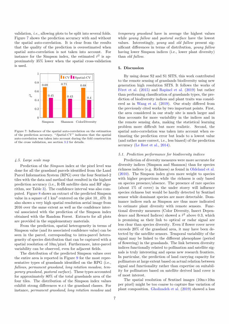
validation, i.e., allowing plots to be split into several folds.Figure 7 shows the prediction accuracy with and withoutthe spatial auto-correlation. It is clear from the resultsthat the quality of the prediction is overestimated whenspatial auto-correlation is not taken into account. Forinstance for the Simpson index, the estimated r2 is ap-proximately 35% lower when the spatial cross-validationis used.

Simpson Shannon ColorDiversity0

0.2

0.4

0.6

0.8

1

0.69 0.71 0.68

0.45 0.43 0.4r2

CV Spatial-CV

Figure 7: Influence of the spatial auto-correlation on the estimationof the prediction accuracy. “Spatial-CV” indicates that the spatialauto-correlation was taken into account during the fold constructionof the cross validation, see section 3.2 for details.

4.5. Large scale mapPrediction of the Simpson index at the pixel level was

done for all the grassland parcels identified from the LandParcel Information System (RPG) over the four Sentinel-2tiles with the data and method that resulted in the highestprediction accuracy (i.e., R-IR satellite data and RF algo-rithm, see Table 3). The confidence interval was also com-puted. Figure 8 shows an extract of the predicted Simpsonvalue in a square of 1 km2 centered on the plot 10_470. Italso shows a very high spatial resolution aerial image from2016 over the same extent as well as the confidence inter-val associated with the prediction of the Simpson indexobtained with the Random Forest. Extracts for all plotsare provided in the supplementary materials.

From the prediction, spatial heterogeneity in terms ofSimpson value (and its associated confidence value) can beseen in the parcel, corresponding to intra-parcel hetero-geneity of species distribution that can be captured with aspatial resolution of 10m/pixel. Furthermore, inter-parcelvariability can be observed, even for adjacent fields.

The distribution of the predicted Simpson values overthe entire area is reported in Figure 9 for the most repre-sentative types of grasslands identified on the RPG (i.e.,fallows, permanent grassland, long rotation meadow, tem-porary grassland, pastoral surface). These types accountedfor approximately 80% of the total grasslands area of thefour tiles. The distribution of the Simpson index valuesexhibit strong differences w.r.t the grassland classes. Forinstance, permanent grassland, long rotation meadow and

temporary grassland have in average the highest valueswhile young fallow and pastoral surface have the lowestvalues. Interestingly, young and old fallow present sig-nificant differences in terms of distribution, young fallowhaving lower Simpson indices (i.e., lower plant diversity)than old fallow.

5. Discussion

By using dense S2 and S1 SITS, this work contributedto the remote sensing of grasslands biodiversity using newgeneration high resolution SITS. It follows the works ofFéret et al. (2015) and Rapinel et al. (2019) but ratherthan performing classification of grasslands types, the pre-diction of biodiversity indices and plant traits was consid-ered as in Wang et al. (2019). Our study differed fromthe previously cited works by two important points. First,the area considered in our study site is much larger andthus accounts for more variability in the indices and inthe remote sensing data, making the statistical learningproblem more difficult but more realistic. Second, thespatial auto-correlation was taken into account when es-timating the prediction error but leads to a lowest value(and rather more correct, i.e., less biased) of the predictionaccuracy (Le Rest et al., 2014).

5.1. Prediction performance for biodiversity indicesPrediction of diversity measures were more accurate for

diversity indices (Simpson and Shannon) than for speciesrichness indices (e.g. Richness) as found in Oldeland et al.(2010). The Simpson index gives more weight to specieswith higher proportions while the richness is only basedon species presence/absence. The presence of rare species(about 1% of cover) in the under storey will influencespecies richness but would be hardly detected by Sentinelsensor while dominant species are more detectable. Dom-inance indices such as Simpson are thus more indicatedto estimate plant diversity with remote sensors. Func-tional diversity measures (Color Diversity, Insect Depen-dence and Reward Indices) showed a r2 above 0.3, whichis promising as their link to optical or radar signal areless clear than species diversity. Even if flower cover neverexceeds 20% of the grassland area, it may have been de-tected by the satellite sensors. Temporal variability of thesignal may be linked to the different phenophase (periodof flowering) in the grasslands. The link between diversityindices functionally related to pollination and satellite sig-nals is truly interesting and opens new research frontiers.In particular, the prediction of land carrying capacity forpollinators at large extent based on actual relation betweensignal and functionality rather than expertise on suitabil-ity for pollinators based on satellite derived land cover isof most interest.

The spatial resolution of Sentinel images (10m×10mper pixel) might be too coarse to capture fine variation ofplant composition. Gholizadeh et al. (2019) showed a loss

7

0

0.23

0.46

0.69

0.91

0.01

0.11

0.2

0.3

0.4

(a) (b) (c)

Figure 8: Simpson index around plot 132_1699. (a) Very high spatial resolution aerial image from 2016, (b) Prediction of the Simpsonvalue for pixels corresponding to grasslands in the national agricultural Land Parcel Information System and (c) Confidence interval valueassociated to the prediction.

0.0 0.2 0.4 0.6 0.8 1.00.0

2.0

4.0

6.0

8.0

Fallow (≤ 5 years)

0.0 0.2 0.4 0.6 0.8 1.00.0

2.0

4.0

6.0

8.0

Fallow (≥ 6 years)

0.0 0.2 0.4 0.6 0.8 1.00.0

2.0

4.0

6.0

8.0

Permanent grassland

0.0 0.2 0.4 0.6 0.8 1.00.0

2.0

4.0

6.0

8.0

Long rotation meadow (≥ 6 years)

0.0 0.2 0.4 0.6 0.8 1.00.0

2.0

4.0

6.0

8.0

Temporary grassland

0.0 0.2 0.4 0.6 0.8 1.00.0

2.0

4.0

6.0

8.0

Pastoral surface (grass resources)

Figure 9: Distribution of the predicted Simpson index for the most represented types of grasslands identified from the RPG. The horizontalaxis represents the Simpson index and the vertical axis represents the probability density function value associated with the Simpson indexvalue. For the fallow classes or long rotation meadow, number in brackets indicates their ages. For the pastoral surfaces, the string in bracketsindicates the most predominant resources in the parcels. The densities have been estimated by a non-parametric kernel density estimatorwith a Gaussian kernel and using the Scott rules for the selection of the bandwidth (Scott, 1992).

of correlation between the spectral feature and α-diversityindex (Shannon) for simulated hyperspectral image witha spatial resolution above 2m per pixel. Nonetheless, theyused only one date and captured little information aboutphenology. Feilhauer et al. (2013) found that spectral cov-erage of the entire solar-reflective domain is the most im-portant characteristic to successfully assess floristic varia-tion in grasslands, while multi-seasonal data did not im-prove it. These results obtained from simulated data con-tradict ours obtained with satellite imagery where the bestprediction accuracies were reached using only the red andinfrared bands and SITS. Our prediction accuracies areequivalent to the ones of Möckel et al. (2016) in predict-ing the inverse Simpson index in grasslands using airbornehyperspectral data. Their approach based on spectral re-flectance reached a r2 of 0.45 using 245 wavebands and0.40 using 35 wavebands. Our results suggest that dif-

ferences in phenology can be used as a proxy for plantdiversity when spatial resolution and spectral resolutionare not high enough.

Similar ideas were considered by Rapinel et al. (2019)who assumed that differences in phenology can be ac-counted for using SITS. However, in large scale setting,clouds and shadows are unavoidably present in the op-tical images, particularly during the key period for plantflowering (April-June), resulting in missing values that arereconstructed during the pre-processing. Figure 10 showsthe proportion of masked pixels corresponding to the 415quadrats: for the period between 2018-05-21 and 2018-06-20, the information was missing because of a too high levelof clouds proportion (see section 2.3.1) and thus the cor-responding dates were interpolated (Inglada et al., 2015).Hence, differences in terms of phenology during that pe-riod of time were not captured by the optical sensors and

8

could explain why the indices based on flower composi-tion only were not accurately predicted. This also sug-gests that other drivers influencing the botanical composi-tion are captured by the optical SITS, such as agriculturalpractices (Moog et al., 2002).

By comparison with our previous works (Lopes et al.,2017a,b), in which biodiversity indices were surveyed atthe field scale, here the sampling was done at the pixelscale, with a spatial match between the sensor acquisi-tion and the field work. This sampling strategy has aclear positive influence on the predictive accuracy, sincethe estimated r2 for the Shannon index was no more than0.17 in (Lopes et al., 2017a). The heterogeneity of grass-lands, in particular semi-natural grasslands, can be highand thus the spatial measurement unit of botanical com-position should match as much as possible the sensor’sspatial resolution. These findings show that the remotesensing-based estimation of plant diversity in grasslandsshould be done at the pixel level and not at the field level.

5.2. SITS pre-processingIn very cloudy situations, SAR data, not affected by

clouds, provide additional information that can help forprediction (Clerici et al., 2017). Indeed, the combinationof Sentinel-1 and Sentinel-2 SITS improved the predictionaccuracy for some indices, e.g. Richness and Insect De-pendence, but not for all. Sentinel-1 data can comple-ment Sentinel-2 information for the learning algorithm,but SAR SITS alone are not sufficient. SAR data hasbeen shown to provide relevant information for grasslandmanagement practices monitoring and cutting practicesin particular (Voormansik et al., 2016; Hill et al., 1999;Dusseux et al., 2012). Hence, although SAR data wasobviously not expected to be sensitive to botanical com-position, it could have been sensitive to biomass, providinginformation about variations in plant height that could beassociated with variation in species. Yet, S1 data was notfound correlated to plant height in this study. However,the aforementioned works were conducted on a reducedgeographical area and the variability in SAR acquisitions,e.g. due to different orbit and incident angles, were neg-ligible in comparison with our context. Another possibleexplanation could be the smoothing effect of the spatio-temporal filter that alters the spatial resolution of S1-SITSand thus reduces the sensibility of such filtered data. Thissuggests in future studies to investigate a more sophis-ticated pre-processing of Sentinel-1 for a joint use withSentinel-2 data.

In this work, the full stack of temporal acquisition wasused, and the irregular temporal acquisitions between var-ious Sentinel tiles was handled using linear interpolation(Inglada et al., 2015). This leads to a large amount offeatures, as displayed in Table 2, that can complexify thestatistical learning step. In such situation, it is commonto reduce the dimensionality, i.e., the number of featuresused. In this work, a conventional principal componentanalysis was used but it resulted in a loss of prediction

accuracy. More advanced feature extraction have been in-vestigated, such as partial least square or forward featurereduction, but they did not improve the prediction accu-racy. As Rapinel et al. (2019), we found that using the fullset of Sentinel-2 bands (restricted here to spectral bandsnatively at 10m per pixel) works well in most of cases.Yet, using only red and near-infra red channels, with allthe temporal features, provided very good results too. Itmay indicate that ignoring the spectro/backscatter or tem-poral structure of the Sentinel SITS when performing thedimension reduction is not appropriate and that further in-vestigation is needed to extract relevant information fromthe data without loosing significant details.

2017

-09

2017

-10

2017

-11

2017

-12

2018

-01

2018

-02

2018

-03

2018

-04

2018

-05

2018

-06

2018

-07

2018

-08

2018-09

2018-10

2018-11

2018-120.0

0.20.40.60.81.0

Figure 10: Proportion of free (in yellow) and masked (in gray) pixelsfor each temporal acquisition.

5.3. Importance of the spatial auto-correlationSpatial auto-correlation was scarcely taken into account

in previous studies on grasslands while it can have a stronginfluence on the estimated prediction accuracy (Hammondand Verbyla, 1996). Results obtained is this work are sim-ilar to those reported in Pohjankukka et al. (2017). Thissuggests that working on a large spatial area that allowsthe construction of a validation set that is spatially un-correlated to the training set is an essential step to assessthe quality of the results. Fortunately, with the increasingavailability of high resolution SITS it will not be a criticalissue in the future. However, for small spatial coveragedata, such as hyperspectral or UAV ones, a careful statis-tical analysis should be done to prevent optimistic results.

5.4. Large scale predictionThe large scale map we produced highlights the grass-

land intra-parcel heterogeneity in terms of plant diversity,underlining the limits of predicting biodiversity indices atthe field scale (Lopes et al., 2017b). Such a map can beused to assess the relationships between environmental fac-tors and plant diversity at fine scale.

Part of the prediction associated with the large confi-dence interval observed in the images can be explained bygeographical factors. First, the edges of the parcels couldcorrespond to mixed pixels and therefore exhibit atypicalvalues. Second, individual trees and hedgerows are some-times included in the field. Their spectral-temporal fea-tures do not correspond to inputs from which the systemis learned and unconfident predictions are done. Looking

9

at the confidence interval thus could inform on the relia-bility of the predicted values, at the pixel scale.

The decreasing average predicted Simpson values fromthe permanent, long rotation and temporary meadows ob-served on figure 9 are in accordance with the importanceof long term no tillage and low intensity practices to keepgrassland biodiversity at high level (Klimek et al., 2007).However, the temporary grasslands present a distributionof predicted Simpson values similar to the permanent ones.This pattern may be explained by the fact that the numberof reported permanent grasslands by farmers is lower thanthe actual number (they are declared as “temporary” in-stead). This is because permanent grasslands have tillagerestriction, while temporary grasslands do not. As a con-sequence, a large number of declared temporary grasslandsare, actually, permanent grasslands.

5.5. PerspectivesPerspectives for this work are two-fold. First, field

work for different grassland areas (mountains, wetland ...)should be conducted to enrich the learning database andto assess the robustness of the prediction at the countryscale. Second, different stratification strategies should beinvestigated, for instance according to their types or theireco-climatic conditions. Third, additional data set, suchas DEM or surface temperature, should be used jointly forthe prediction in order to capture more information aboutgrasslands. This would require specific methodological de-velopments to properly use such a heterogeneous data set.

6. Conclusions

The prediction of grasslands biodiversity indices usingSentinel-1&-2 times series was investigated in this work.We have shown that abundance-based indices based onthe dominance of some species (Simpson) can be predictedover a large area with a coefficient of determination above0.4 using Sentinel-2 SITS.

This study indicates that the temporal informationcontained in the SITS can compensate for the limited spec-tral information and spatial resolution compared to hyper-spectral imagery. Another finding is that the spatial auto-correlation tends to bias the estimation of the predictionaccuracy and thus, should be taken into account duringvalidation.

The contribution of this work does not lie in selectingthe best set of dates nor the best machine learning regres-sion methods but in assessing the potential of Sentinel-1and -2 dense times series as explanatory variables for theprediction of grasslands biodiversity indices. We believethat our results, using large scale data with various agri-cultural practices for different meteorological and topo-graphic conditions, demonstrate the capacity of such datato monitor grasslands from an ecological viewpoint. Inparticular, intra-parcel variability was highlighted in thiswork and can be monitored over large areas.

Acknowledgement

This work was supported by the SEBIOREF (NationalInstitute for Agronomic Research and Occitanie Région)project which funded part of the field work. CatherineBataillon, Sylvie Ladet, François Calatayud, Wilfried Heintz,Xavier Henry and Jérôme Willm are gratefully acknowl-edged for the field work in Spring 2018. We also ac-knowledge farmers for allowing full access to their grass-lands. Mathieu Fauvel is thankful to Jordi Inglada, Vin-cent Thierion and Arthur Vincent for their support andhelp with iota2 software. The authors would also like tothank the reviewers and the handling editor whose com-ments and suggestions improved this paper.

References

Ali, I., Cawkwell, F., Dwyer, E., Barrett, B., Green, S., 2016.Satellite remote sensing of grasslands: from observation to man-agement. Journal of Plant Ecology 9, 649–671. URL: http://dx.doi.org/10.1093/jpe/rtw005, doi:10.1093/jpe/rtw005.

Baetens, L., Desjardins, C., Hagolle, O., 2019. Validation of coper-nicus sentinel-2 cloud masks obtained from maja, sen2cor, andfmask processors using reference cloud masks generated witha supervised active learning procedure. Remote Sensing 11.URL: http://www.mdpi.com/2072-4292/11/4/433, doi:10.3390/rs11040433.

Barrett, B., Nitze, I., Green, S., Cawkwell, F., 2014. Assess-ment of multi-temporal, multi-sensor radar and ancillary spatialdata for grasslands monitoring in ireland using machine learn-ing approaches. Remote Sensing of Environment 152, 109 –124. URL: http://www.sciencedirect.com/science/article/pii/S0034425714002065, doi:https://doi.org/10.1016/j.rse.2014.05.018.

Bengtsson, J., Bullock, J.M., Egoh, B., Everson, C., Ev-erson, T., O’Connor, T., O’Farrell, P.J., Smith, H.G.,Lindborg, R., 2019. Grasslands—more important forecosystem services than you might think. Ecosphere 10,e02582. URL: https://esajournals.onlinelibrary.wiley.com/doi/abs/10.1002/ecs2.2582, doi:10.1002/ecs2.2582,arXiv:https://esajournals.onlinelibrary.wiley.com/doi/pdf/10.1002/ecs2.2582.

Buck, O., Millán, V.E.G., Klink, A., Pakzad, K., 2015. Us-ing information layers for mapping grassland habitat distri-bution at local to regional scales. International Journalof Applied Earth Observation and Geoinformation 37, 83 –89. URL: http://www.sciencedirect.com/science/article/pii/S0303243414002359, doi:https://doi.org/10.1016/j.jag.2014.10.012. special Issue on Earth observation for habitat map-ping and biodiversity monitoring.

Cantelaube, P., Carles, M., 2014. Le registre parcellaire graphique:des données géographiques pour décrire la couverture du sol agri-cole. Le Cahier des Techniques de lINRA,(N Spécial GéoExpé) ,58–64.

Carrié, R., Lopes, M., Ouin, A., Andrieu, E., 2018. Bee diversityin crop fields is influenced by remotely-sensed nesting resourcesin surrounding permanent grasslands. Ecological Indicators 90,606–614.

Clerici, N., Calderón, C.A.V., Posada, J.M., 2017. Fusion ofsentinel-1a and sentinel-2a data for land cover mapping: acase study in the lower magdalena region, colombia. Jour-nal of Maps 13, 718–726. URL: https://doi.org/10.1080/17445647.2017.1372316, doi:10.1080/17445647.2017.1372316,arXiv:https://doi.org/10.1080/17445647.2017.1372316.

Clough, Y., Ekroos, J., Báldi, A., Batáry, P., Bommarco, R.,Gross, N., Holzschuh, A., Hopfenmüller, S., Knop, E., Kuus-saari, M., Lindborg, R., Marini, L., Öckinger, E., Potts, S.G.,Pöyry, J., Roberts, S.P., Steffan-Dewenter, I., Smith, H.G., 2014.

10

Density of insect-pollinated grassland plants decreases with in-creasing surrounding land-use intensity. Ecology Letters 17,1168–1177. URL: https://onlinelibrary.wiley.com/doi/abs/10.1111/ele.12325, doi:10.1111/ele.12325.

Corbane, C., Alleaume, S., Deshayes, M., 2013. Mapping natu-ral habitats using remote sensing and sparse partial least squarediscriminant analysis. International Journal of Remote Sensing34, 7625–7647. URL: https://doi.org/10.1080/01431161.2013.822603, doi:10.1080/01431161.2013.822603.

Darvishzadeh, R., Skidmore, A., Schlerf, M., Atzberger,C., Corsi, F., Cho, M., 2008. Lai and chlorophyll es-timation for a heterogeneous grassland using hyperspec-tral measurements. ISPRS Journal of Photogrammetryand Remote Sensing 63, 409 – 426. URL: http://www.sciencedirect.com/science/article/pii/S0924271608000166,doi:https://doi.org/10.1016/j.isprsjprs.2008.01.001.

Defourny, P., Bontemps, S., Bellemans, N., Cara, C., Dedieu, G.,Guzzonato, E., Hagolle, O., Inglada, J., Nicola, L., Rabaute, T.,Savinaud, M., Udroiu, C., Valero, S., Bégué, A., Dejoux, J.F.,Harti, A.E., Ezzahar, J., Kussul, N., Labbassi, K., Lebourgeois,V., Miao, Z., Newby, T., Nyamugama, A., Salh, N., Shelestov,A., Simonneaux, V., Traore, P.S., Traore, S.S., Koetz, B., 2019.Near real-time agriculture monitoring at national scale at parcelresolution: Performance assessment of the sen2-agri automatedsystem in various cropping systems around the world. RemoteSensing of Environment 221, 551 – 568. doi:https://doi.org/10.1016/j.rse.2018.11.007.

Diaz, S., Cabido, M., 2001. Vive la difference: Plant func-tional diversity matters to ecosystem processes. Trends inEcology & Evolution 16, 646 – 655. URL: http://www.sciencedirect.com/science/article/pii/S0169534701022832,doi:https://doi.org/10.1016/S0169-5347(01)02283-2.

Draper, N., Smith, H., 1998. Applied regression analysis. Numberv. 1 in Wiley series in probability and statistics: Texts and refer-ences section, Wiley. URL: https://books.google.fr/books?id=8n8pAQAAMAAJ.

Drusch, M., Bello, U.D., Carlier, S., Colin, O., Fernandez, V., Gas-con, F., Hoersch, B., Isola, C., Laberinti, P., Martimort, P., Mey-gret, A., Spoto, F., Sy, O., Marchese, F., Bargellini, P., 2012.Sentinel-2: ESA’s optical high-resolution mission for GMES op-erational services. Remote Sensing of Environment 120, 25 –36. doi:https://doi.org/10.1016/j.rse.2011.11.026. the Sen-tinel Missions - New Opportunities for Science.

Dusseux, P., Gong, X., Corpetti, T., L. Hubert-Moy, S.C., 2012.Contribution of radar images for grassland management identi-fication, in: SPIE Remote Sensing. URL: https://doi.org/10.1117/12.974547, doi:10.1117/12.974547.

ESA, 2019. L1c data quality report. https://sentinel.esa.int/documents/247904/685211/Sentinel-2_L1C_Data_Quality_Report.

Feilhauer, H., Doktor, D., Schmidtlein, S., Skidmore, A.K., 2016.Mapping pollination types with remote sensing. Journal of Vegeta-tion Science 27, 999–1011. URL: https://onlinelibrary.wiley.com/doi/abs/10.1111/jvs.12421, doi:10.1111/jvs.12421.

Feilhauer, H., Thonfeld, F., Faude, U., He, K.S., Roc-chini, D., Schmidtlein, S., 2013. Assessing floristic com-position with multispectral sensors—a comparison based onmonotemporal and multiseasonal field spectra. Interna-tional Journal of Applied Earth Observation and Geoinforma-tion 21, 218 – 229. URL: http://www.sciencedirect.com/science/article/pii/S0303243412001936, doi:http://dx.doi.org/10.1016/j.jag.2012.09.002.

Féret, J., Corbane, C., Alleaume, S., 2015. Detecting the phenol-ogy and discriminating mediterranean natural habitats with mul-tispectral sensors—an analysis based on multiseasonal field spec-tra. IEEE Journal of Selected Topics in Applied Earth Obser-vations and Remote Sensing 8, 2294–2305. doi:10.1109/JSTARS.2015.2431320.

Ge, J., Meng, B., Liang, T., Feng, Q., Gao, J., Yang,S., Huang, X., Xie, H., 2018. Modeling alpine grass-land cover based on modis data and support vector ma-

chine regression in the headwater region of the huangheriver, china. Remote Sensing of Environment 218, 162 –173. URL: http://www.sciencedirect.com/science/article/pii/S0034425718304309, doi:https://doi.org/10.1016/j.rse.2018.09.019.

Gholizadeh, H., Gamon, J.A., Townsend, P.A., Zygielbaum,A.I., Helzer, C.J., Hmimina, G.Y., Yu, R., Moore, R.M.,Schweiger, A.K., Cavender-Bares, J., 2019. Detectingprairie biodiversity with airborne remote sensing. RemoteSensing of Environment 221, 38 – 49. URL: http://www.sciencedirect.com/science/article/pii/S0034425718304991,doi:https://doi.org/10.1016/j.rse.2018.10.037.

Giménez, M.G., de Jong, R., Peruta, R.D., Keller, A., Schaep-man, M.E., 2017. Determination of grassland use inten-sity based on multi-temporal remote sensing data and ecolog-ical indicators. Remote Sensing of Environment 198, 126 –139. URL: http://www.sciencedirect.com/science/article/pii/S0034425717302638, doi:https://doi.org/10.1016/j.rse.2017.06.003.

Goodin, D.G., Henebry, G.M., 1998. Seasonality of finely-resolvedspatial structure of ndvi and its component reflectances in tall-grass prairie. International Journal of Remote Sensing 19, 3213–3220. doi:10.1080/014311698214280.

Gu, Y., Wylie, B.K., 2015. Developing a 30-m grassland productivityestimation map for central nebraska using 250-m modis and 30-mlandsat-8 observations. Remote Sensing of Environment 171, 291– 298. URL: http://www.sciencedirect.com/science/article/pii/S0034425715301693, doi:https://doi.org/10.1016/j.rse.2015.10.018.

Habel, J.C., Dengler, J., Janišová, M., Török, P., Wellstein, C.,Wiezik, M., 2013. European grassland ecosystems: threat-ened hotspots of biodiversity. Biodiversity and Conservation 22,2131–2138. URL: https://doi.org/10.1007/s10531-013-0537-x, doi:10.1007/s10531-013-0537-x.

Hall, K., Reitalu, T., Sykes, M.T., Prentice, H.C., 2012. Spec-tral heterogeneity of quickbird satellite data is related tofine-scale plant species spatial turnover in semi-naturalgrasslands. Applied Vegetation Science 15, 145–157. URL:https://onlinelibrary.wiley.com/doi/abs/10.1111/j.1654-109X.2011.01143.x, doi:10.1111/j.1654-109X.2011.01143.x,arXiv:https://onlinelibrary.wiley.com/doi/pdf/10.1111/j.1654-109X.2011.01143.x.

Hammond, T.O., Verbyla, D.L., 1996. Optimistic bias in classifica-tion accuracy assessment. International Journal of Remote Sens-ing 17, 1261–1266. doi:10.1080/01431169608949085.

Hastie, T., Tibshirani, R., Friedman, J.H., 2009. The elements ofstatistical learning: data mining, inference, and prediction, 2ndEdition. Springer series in statistics, Springer. URL: http://www.worldcat.org/oclc/300478243.

He, Y., Guo, X., Wilmshurst, J.F., 2009. Reflectance measures ofgrassland biophysical structure. International Journal of RemoteSensing 30, 2509–2521. doi:10.1080/01431160802552751.

Heymann, Y., 1994. CORINE land cover: Technical guide. Officefor Official Publ. of the Europ. Communities.

Hill, M.J., Donald, G.E., Vickery, P.J., 1999. Relatingradar backscatter to biophysical properties of temperate peren-nial grassland. Remote Sensing of Environment 67, 15 –31. URL: http://www.sciencedirect.com/science/article/pii/S0034425798000637, doi:https://doi.org/10.1016/S0034-4257(98)00063-7.

Hobi, M.L., Dubinin, M., Graham, C.H., Coops, N.C., Clayton,M.K., Pidgeon, A.M., Radeloff, V.C., 2017. A compari-son of dynamic habitat indices derived from different modisproducts as predictors of avian species richness. RemoteSensing of Environment 195, 142 – 152. URL: http://www.sciencedirect.com/science/article/pii/S0034425717301682,doi:https://doi.org/10.1016/j.rse.2017.04.018.

Inglada, J., Arias, M., Tardy, B., Hagolle, O., Valero, S., Morin,D., Dedieu, G., Sepulcre, G., Bontemps, S., Defourny, P., Koetz,B., 2015. Assessment of an operational system for crop type mapproduction using high temporal and spatial resolution satelliteoptical imagery. Remote Sensing 7, 12356–12379. URL: http:

11

//www.mdpi.com/2072-4292/7/9/12356, doi:10.3390/rs70912356.Inglada, J., Vincent, A., Arias, M., Tardy, B., 2016. iota2-

a25386. URL: https://doi.org/10.5281/zenodo.58150, doi:10.5281/zenodo.58150.

Joshi, N., Baumann, M., Ehammer, A., Fensholt, R., Grogan,K., Hostert, P., Jepsen, M.R., Kuemmerle, T., Meyfroidt, P.,Mitchard, E.T.A., Reiche, J., Ryan, C.M., Waske, B., 2016. Areview of the application of optical and radar remote sensing datafusion to land use mapping and monitoring. Remote Sensing8. URL: http://www.mdpi.com/2072-4292/8/1/70, doi:10.3390/rs8010070.

Klimek, S., Richter gen. Kemmermann, A., Hofmann, M., Isselstein,J., 2007. Plant species richness and composition in managed grass-lands: The relative importance of field management and environ-mental factors. Biological Conservation 134, 559–570.

Kremen, C., Williams, N.M., Aizen, M.A., Gemmill-Herren,B., LeBuhn, G., Minckley, Robert a nd Packer, L., Potts,S.G., Roulston, T., Stef fan Dewenter, I., Vázquez, D.P.,Winfree, R., Adams, L., Crone, E.E., Greenleaf, S.S.,Keitt, T.H., Klein, A.M., Regetz, J., Ricketts, T.H., 2007.Pollination and other ecosystem services produced by mo-bile organisms: a conceptual framework for the effectsof land-use change. Ecology Letters 10, 299–314. URL:https://onlinelibrary.wiley.com/doi/abs/10.1111/j.1461-0248.2007.01018.x, doi:10.1111/j.1461-0248.2007.01018.x,arXiv:https://onlinelibrary.wiley.com/doi/pdf/10.1111/j.1461-0248.2007.01018.x.

Laliberté, E., Legendre, P., 2010. A distance-based framework formeasuring functional diversity from mutliple traits. Ecology 91,299–305. Ao2846ev.

Landmann, T., Piiroinen, R., Makori, D.M., Abdel-Rahman,E.M., Makau, S., Pellikka, P., Raina, S.K., 2015. Appli-cation of hyperspectral remote sensing for flower mapping inafrican savannas. Remote Sensing of Environment 166, 50– 60. URL: http://www.sciencedirect.com/science/article/pii/S0034425715300353, doi:https://doi.org/10.1016/j.rse.2015.06.006.

Lary, D.J., Alavi, A.H., Gandomi, A.H., Walker, A.L., 2016. Machinelearning in geosciences and remote sensing. Geoscience Frontiers 7,3 – 10. URL: http://www.sciencedirect.com/science/article/pii/S1674987115000821, doi:https://doi.org/10.1016/j.gsf.2015.07.003. special Issue: Progress of Machine Learning in Geo-sciences.

Le Rest, K., Pinaud, D., Monestiez, P., Chadoeuf, J., Bretagnolle,V., 2014. Spatial leave-one-out cross-validation for variable selec-tion in the presence of spatial autocorrelation. Global Ecologyand Biogeography 23, 811–820. URL: https://onlinelibrary.wiley.com/doi/abs/10.1111/geb.12161, doi:10.1111/geb.12161,arXiv:https://onlinelibrary.wiley.com/doi/pdf/10.1111/geb.12161.

Li, Z., Huffman, T., McConkey, B., Townley-Smith, L., 2013. Mon-itoring and modeling spatial and temporal patterns of grass-land dynamics using time-series modis ndvi with climate andstocking data. Remote Sensing of Environment 138, 232 –244. URL: http://www.sciencedirect.com/science/article/pii/S0034425713002320, doi:https://doi.org/10.1016/j.rse.2013.07.020.

Lopatin, J., Fassnacht, F.E., Kattenborn, T., Schmidtlein,S., 2017. Mapping plant species in mixed grassland com-munities using close range imaging spectroscopy. RemoteSensing of Environment 201, 12 – 23. URL: http://www.sciencedirect.com/science/article/pii/S0034425717303966,doi:https://doi.org/10.1016/j.rse.2017.08.031.

Lopes, M., Fauvel, M., Ouin, A., Girard, S., 2017a. Potential ofsentinel-2 and spot5 (take5) time series for the estimation of grass-lands biodiversity indices, in: 2017 9th International Workshopon the Analysis of Multitemporal Remote Sensing Images (Multi-Temp), pp. 1–4. doi:10.1109/Multi-Temp.2017.8035206.

Lopes, M., Fauvel, M., Ouin, A., Girard, S., 2017b. Spectro-temporalheterogeneity measures from dense high spatial resolution satelliteimage time series: Application to grassland species diversity es-timation. Remote Sensing 9. URL: http://www.mdpi.com/2072-4292/9/10/993, doi:10.3390/rs9100993.

Magurran, A., 2004. Measuring Biological Diversity. Wiley. URL:https://books.google.fr/books?id=tUqzLSUzXxcC.

Maxwell, A.E., Warner, T.A., Fang, F., 2018. Implementationof machine-learning classification in remote sensing: an appliedreview. International Journal of Remote Sensing 39, 2784–2817. URL: https://doi.org/10.1080/01431161.2018.1433343,doi:10.1080/01431161.2018.1433343.

Moog, D., Poschlod, P., Kahmen, S., Schreiber, K.F., 2002.Comparison of species composition between different grasslandmanagement treatments after 25 years. Applied VegetationScience 5, 99–106. URL: https://onlinelibrary.wiley.com/doi/abs/10.1111/j.1654-109X.2002.tb00539.x, doi:10.1111/j.1654-109X.2002.tb00539.x.

Murphy, K.P., 2013. Machine learning : a probabilistic perspective.MIT Press, Cambridge, Mass. [u.a.].

Möckel, T., Dalmayne, J., Schmid, B.C., Prentice, H.C., Hall, K.,2016. Airborne hyperspectral data predict fine-scale plant speciesdiversity in grazed dry grasslands. Remote Sensing 8. URL: http://www.mdpi.com/2072-4292/8/2/133, doi:10.3390/rs8020133.

Newbold, T., Hudson, L.N., Arnell, A.P., Contu, S., De Palma,A., Ferrier, S., Hill, S.L.L., Hoskins, A.J., Lysenko, I., Phillips,H.R.P., Burton, V.J., Chng, C.W.T., Emerson, S., Gao, D.,Pask-Hale, G., Hutton, J., Jung, M., Sanchez-Ortiz, K., Sim-mons, B.I., Whitmee, S., Zhang, H., Scharlemann, J.P.W.,Purvis, A., 2016. Has land use pushed terrestrial biodiver-sity beyond the planetary boundary? a global assessment.Science 353, 288–291. URL: https://science.sciencemag.org/content/353/6296/288, doi:10.1126/science.aaf2201,arXiv:https://science.sciencemag.org/content/353/6296/288.full.pdf.

Newton, A.C., Hill, R.A., Echeverría, C., Golicher, D., Benayas,J.M.R., Cayuela, L., Hinsley, S.A., 2009. Remote sensing andthe future of landscape ecology. Progress in Physical Geogra-phy: Earth and Environment 33, 528–546. URL: https://doi.org/10.1177/0309133309346882, doi:10.1177/0309133309346882,arXiv:https://doi.org/10.1177/0309133309346882.

Ockinger, E., Smith, H.G., 2007. Semi-natural grasslands as pop-ulation sources for pollinating insects in agricultural landscapes.Journal of Applied Ecology 44, 50–59. Ao1658ev.

Oksanen, J., Kindt, R., Legendre, P., O’Hara, B., Stevens, M.H.H.,2007. Vegan: Community ecology package.ordination methods,diversity analysis and other functions for community and vegeta-tion ecologists.

Oldeland, J., Wesuls, D., Rocchini, D., Schmidt, M., Jürgens, N.,2010. Does using species abundance data improve estimatesof species diversity from remotely sensed spectral heterogene-ity? Ecological Indicators 10, 390 – 396. URL: http://www.sciencedirect.com/science/article/pii/S1470160X09001241,doi:https://doi.org/10.1016/j.ecolind.2009.07.012.

O’Mara, F., 2012. The role of grasslands in food security and cli-mate change. Annals of Botany 110, 1263–1270. doi:10.1093/aob/mcs209.

OTB Development Team, 2018. Orfeo toolbox 6.6.0. URL: https://doi.org/10.5281/zenodo.1294917, doi:10.5281/zenodo.1294917.

Pärtel, M., Bruun, H., Sammul, M., 2005. Biodiversity in temper-ate european grasslands: origin and conservation., in: GrasslandScience in Europe, Grassland Science in Europe. pp. 1–14. Theinformation about affiliations in this record was updated in De-cember 2015. The record was previously connected to the follow-ing departments: Plant Ecology and Systematics (Closed 2011)(011004000).

Pedregosa, F., Varoquaux, G., Gramfort, A., Michel, V., Thirion,B., Grisel, O., Blondel, M., Prettenhofer, P., Weiss, R., Dubourg,V., Vanderplas, J., Passos, A., Cournapeau, D., Brucher, M., Per-rot, M., Duchesnay, E., 2011. Scikit-learn: Machine learning inPython. Journal of Machine Learning Research 12, 2825–2830.

Pohjankukka, J., Pahikkala, T., Nevalainen, P., Heikkonen, J., 2017.Estimating the prediction performance of spatial models via spa-tial k-fold cross validation. International Journal of GeographicalInformation Science 31, 2001–2019. doi:10.1080/13658816.2017.1346255.

Potts, S., Willmer, P., 1997. Abiotic and biotic factors influencing

12

nest-site selection by halictus rubicundus, a ground-nestinghalictine bee. Ecological Entomology 22, 319–328. URL:https://onlinelibrary.wiley.com/doi/abs/10.1046/j.1365-2311.1997.00071.x, doi:10.1046/j.1365-2311.1997.00071.x,arXiv:https://onlinelibrary.wiley.com/doi/pdf/10.1046/j.1365-2311.1997.00071.x.

Quegan, S., Yu, J.J., 2001. Filtering of multichannel sar images.IEEE Transactions on Geoscience and Remote Sensing 39, 2373–2379. doi:10.1109/36.964973.

Rapinel, S., Mony, C., Lecoq, L., Clément, B., Thomas, A.,Hubert-Moy, L., 2019. Evaluation of sentinel-2 time-seriesfor mapping floodplain grassland plant communities. RemoteSensing of Environment 223, 115 – 129. URL: http://www.sciencedirect.com/science/article/pii/S0034425719300185,doi:https://doi.org/10.1016/j.rse.2019.01.018.

Rasmussen, C., Williams, C., 2006. Gaussian Processes for MachineLearning. Adaptive Computation and Machine Learning, MITPress, Cambridge, MA, USA.

Schmidt, S., Alewell, C., Meusburger, K., 2018. Mappingspatio-temporal dynamics of the cover and managementfactor (c-factor) for grasslands in switzerland. RemoteSensing of Environment 211, 89 – 104. URL: http://www.sciencedirect.com/science/article/pii/S0034425718301536,doi:https://doi.org/10.1016/j.rse.2018.04.008.

Schuster, C., Schmidt, T., Conrad, C., Kleinschmit, B.,Förster, M., 2015. Grassland habitat mapping by intra-annual time series analysis – comparison of rapideye andterrasar-x satellite data. International Journal of Ap-plied Earth Observation and Geoinformation 34, 25 –34. URL: http://www.sciencedirect.com/science/article/pii/S0303243414001378, doi:https://doi.org/10.1016/j.jag.2014.06.004.

Scott, D., 1992. Multivariate Density Estimation: Theory, Practice,and Visualization. A Wiley-interscience publication, Wiley. URL:https://books.google.fr/books?id=7crCUS_F2ocC.

Si, Y., Schlerf, M., Zurita-Milla, R., Skidmore, A., Wang,T., 2012. Mapping spatio-temporal variation of grass-land quantity and quality using meris data and the pro-sail model. Remote Sensing of Environment 121, 415 –425. URL: http://www.sciencedirect.com/science/article/pii/S0034425712001046, doi:https://doi.org/10.1016/j.rse.2012.02.011.

Stenzel, S., Fassnacht, F.E., Mack, B., Schmidtlein, S.,2017. Identification of high nature value grassland withremote sensing and minimal field data. Ecological Indi-cators 74, 28 – 38. URL: http://www.sciencedirect.com/science/article/pii/S1470160X16306422, doi:https://doi.org/10.1016/j.ecolind.2016.11.005.

Team, R.c., 2012. R: A language and environment for statisticalcomputing.

Tuanmu, M.N., Jetz, W., 2015. A global, remote sensing-based char-acterization of terrestrial habitat heterogeneity for biodiversityand ecosystem modelling. Global Ecology and Biogeography 24,1329–1339. URL: https://onlinelibrary.wiley.com/doi/abs/10.1111/geb.12365, doi:10.1111/geb.12365.

Tupin, F., Inglada, J., Nicolas, J., 2014. Remote Sensing Im-agery. ISTE, Wiley. URL: https://books.google.fr/books?id=GfcXAwAAQBAJ.

Turner, W., 2014. Sensing biodiversity. Science 346,301–302. URL: http://science.sciencemag.org/content/346/6207/301, doi:10.1126/science.1256014,arXiv:http://science.sciencemag.org/content/346/6207/301.full.pdf.

Voormansik, K., Jagdhuber, T., Zalite, K., Noorma, M., Hajnsek, I.,2016. Observations of cutting practices in agricultural grasslandsusing polarimetric sar. IEEE Journal of Selected Topics in AppliedEarth Observations and Remote Sensing 9, 1382–1396. doi:10.1109/JSTARS.2015.2503773.

Wang, Z., Townsend, P.A., Schweiger, A.K., Couture, J.J., Singh,A., Hobbie, S.E., Cavender-Bares, J., 2019. Mapping foliarfunctional traits and their uncertainties across three years in agrassland experiment. Remote Sensing of Environment 221, 405– 416. URL: http://www.sciencedirect.com/science/article/

pii/S003442571830525X, doi:https://doi.org/10.1016/j.rse.2018.11.016.

Watkinson, A.R., Ormerod, S.J., 2001. Grasslands, grazing and bio-diversity: editor’s introduction. Journal of Applied Ecology 38,233–237. Ao1128.

Yang, S., Feng, Q., Liang, T., Liu, B., Zhang, W., Xie, H.,2018. Modeling grassland above-ground biomass based on ar-tificial neural network and remote sensing in the three-riverheadwaters region. Remote Sensing of Environment 204, 448– 455. URL: http://www.sciencedirect.com/science/article/pii/S0034425717304741, doi:https://doi.org/10.1016/j.rse.2017.10.011.

Appendix A. Biodiversity indices distribution

5 10 15 20 250

20

40

60

Richness0 2 4 6 8 101214

0

20

40

60

Flowers Richness0 0.5 1 1.5 2 2.5 3

0

20

40

60

Shannon

0 0.2 0.4 0.6 0.8 10

20

40

60

Simpson0 0.4 0.8 1.2 1.6 2

0

20

40

60

Color diversity1 1.4 1.8 2.2 2.6 3

0

20

40

60

Insect Dependence

1 1.5 2 2.5 3 3.5 40

20

40

60

Reward Index

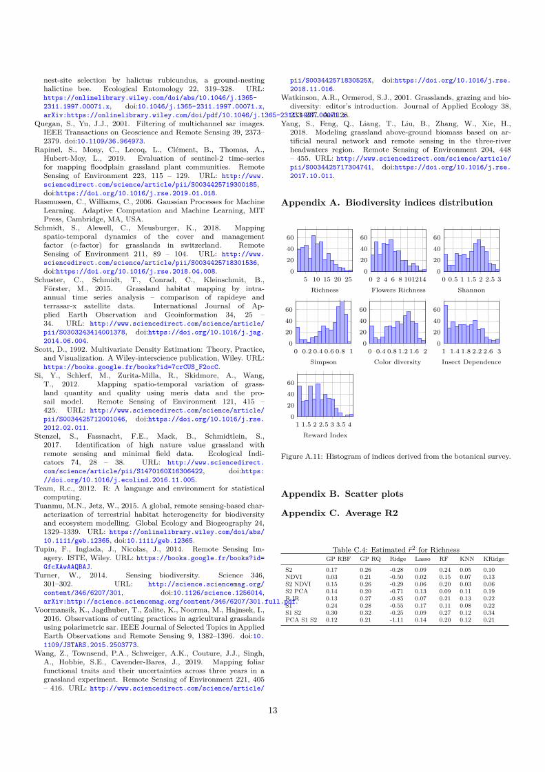
Figure A.11: Histogram of indices derived from the botanical survey.

Appendix B. Scatter plots

Appendix C. Average R2

Table C.4: Estimated r2 for RichnessGP RBF GP RQ Ridge Lasso RF KNN KRidge

S2 0.17 0.26 -0.28 0.09 0.24 0.05 0.10NDVI 0.03 0.21 -0.50 0.02 0.15 0.07 0.13S2 NDVI 0.15 0.26 -0.29 0.06 0.20 0.03 0.06S2 PCA 0.14 0.20 -0.71 0.13 0.09 0.11 0.19R IR 0.13 0.27 -0.85 0.07 0.21 0.13 0.22S1 0.24 0.28 -0.55 0.17 0.11 0.08 0.22S1 S2 0.30 0.32 -0.25 0.09 0.27 0.12 0.34PCA S1 S2 0.12 0.21 -1.11 0.14 0.20 0.12 0.21

13

0.0 0.5 1.0 1.5 2.0 2.5 3.00.0

0.5

1.0

1.5

2.0

2.5

3.0

y

y

0.00

0.10

0.20

σ

Figure B.12: Scatter plot of the predicted Shannon values obtainedwith RF and R-IR data (see table 3). The black line is the identityline, i. e., when y = y; r2 = 0.43. The colormap corresponds to theconfidence interval σ of the prediction.

0.0 0.4 0.8 1.2 1.6 2.00.0

0.4

0.8

1.2

1.6

2.0

y

y

0.00

0.10

0.20

σ

Figure B.13: Scatter plot of the predicted color diversity values ob-tained with RF and S2 data (see table 3). The black line is theidentity line y = y; r2 = 0.40. The colormap corresponds to theconfidence interval σ of the prediction.

Table C.5: Estimated r2 for Flowers RichnessGP RBF GP RQ Ridge Lasso RF KNN KRidge

S2 0.12 0.19 -0.35 0.08 0.16 0.02 0.09NDVI 0.02 0.16 -0.37 -0.05 0.15 0.02 0.07S2 NDVI 0.09 0.19 -0.43 0.09 0.17 0.01 0.09S2 PCA 0.10 0.15 -0.71 0.07 0.10 0.07 0.10R IR 0.08 0.20 -0.62 0.06 0.11 0.03 0.13S1 0.21 0.25 -0.62 0.22 0.15 0.09 0.21S1 S2 0.28 0.30 -0.42 0.12 0.23 0.08 0.32PCA S1 S2 0.06 0.14 -1.04 0.09 0.06 0.07 0.05

Table C.6: Estimated r2 for ShannonGP RBF GP RQ Ridge Lasso RF KNN KRidge

S2 0.30 0.31 -0.08 0.06 0.40 0.13 0.16NDVI 0.17 0.31 -0.21 0.05 0.24 0.18 0.22S2 NDVI 0.28 0.30 -0.00 0.13 0.41 0.15 0.17S2 PCA 0.20 0.26 -0.30 0.29 0.28 0.21 0.26R IR 0.28 0.35 -0.43 0.11 0.43 0.23 0.18S1 0.31 0.32 -0.27 0.20 0.14 0.19 0.25S1 S2 0.38 0.39 -0.08 0.21 0.34 0.15 0.31PCA S1 S2 0.22 0.28 -0.61 0.29 0.24 0.23 0.18

Table C.7: Estimated r2 for SimpsonGP RBF GP RQ Ridge Lasso RF KNN KRidge

S2 0.29 0.27 -0.24 -0.12 0.44 0.16 0.10NDVI 0.19 0.26 -0.16 0.13 0.30 0.20 0.07S2 NDVI 0.27 0.25 -0.13 -0.01 0.43 0.18 0.12S2 PCA 0.16 0.20 -0.52 0.19 0.25 0.25 0.01R IR 0.27 0.27 -0.57 -0.12 0.45 0.24 0.08S1 0.26 0.26 -0.48 -0.11 0.15 0.16 0.14S1 S2 0.31 0.31 -0.36 -0.04 0.41 0.23 0.19PCA S1 S2 0.20 0.22 -0.88 0.22 0.03 0.20 0.09

Table C.8: Estimated r2 for Color DiversityGP RBF GP RQ Ridge Lasso RF KNN KRidge

S2 0.29 0.28 -0.24 -0.06 0.40 0.13 0.22NDVI 0.17 0.26 -0.23 -0.02 0.25 0.13 0.12S2 NDVI 0.27 0.27 -0.18 0.03 0.34 0.16 0.23S2 PCA 0.13 0.19 -0.40 0.17 0.26 0.18 0.05R IR 0.27 0.28 -0.31 0.02 0.39 0.20 0.16S1 0.23 0.22 -0.74 0.01 0.14 0.13 0.23S1 S2 0.33 0.33 -0.47 0.11 0.35 0.16 0.30PCA S1 S2 0.14 0.20 -0.54 0.25 0.06 0.16 0.09

Table C.9: Estimated r2 for Insect DependenceGP RBF GP RQ Ridge Lasso RF KNN KRidge

S2 0.11 0.18 -0.21 0.25 0.27 0.17 0.29NDVI 0.04 0.20 0.03 0.24 0.18 0.21 0.24S2 NDVI 0.12 0.19 -0.24 0.26 0.25 0.19 0.29S2 PCA 0.04 0.07 -0.35 0.12 0.07 0.09 0.14R IR 0.12 0.18 -0.17 0.23 0.22 0.17 0.28S1 0.14 0.15 -0.26 0.11 0.08 -0.03 0.18S1 S2 0.29 0.30 -0.39 0.28 0.25 0.18 0.32PCA S1 S2 0.02 0.09 -0.51 0.19 0.09 0.11 0.22

Table C.10: Estimated r2 for Reward IndiceGP RBF GP RQ Ridge Lasso RF KNN KRidge

S2 0.15 0.24 -0.12 0.24 0.23 0.15 0.27NDVI 0.07 0.24 -0.11 0.23 0.24 0.23 0.23S2 NDVI 0.14 0.24 -0.17 0.24 0.22 0.15 0.30S2 PCA 0.08 0.15 -0.31 0.18 0.09 0.06 0.15R IR 0.14 0.23 -0.09 0.25 0.24 0.15 0.22S1 0.12 0.12 -0.62 0.09 0.12 0.00 0.17S1 S2 0.32 0.32 -0.56 0.25 0.26 0.16 0.29PCA S1 S2 0.06 0.17 -0.45 0.21 0.11 0.09 0.25

14