
Prediction of order statistics and record values based on ordered ranked set sampling
13
This article was downloaded by: [University of Leicester] On: 13 June 2013, At: 12:33 Publisher: Taylor & Francis Informa Ltd Registered in England and Wales Registered Number: 1072954 Registered office: Mortimer House, 37-41 Mortimer Street, London W1T 3JH, UK Journal of Statistical Computation and Simulation Publication details, including instructions for authors and subscription information: http://www.tandfonline.com/loi/gscs20 Prediction of order statistics and record values based on ordered ranked set sampling Mahdi Salehi a , Jafar Ahmadi a & N. Balakrishnan b c a Department of Statistics, Ordered and Spatial Data Center of Excellence , Ferdowsi University of Mashhad , PO Box 1159, Mashhad , 91775 , Iran b Department of Mathematics and Statistics , McMaster University , Hamilton , ON , Canada , L8S 4K1 c Department of Statistics , King Abdulaziz University , Jeddah , Saudi Arabia Published online: 29 May 2013. To cite this article: Mahdi Salehi , Jafar Ahmadi & N. Balakrishnan (2013): Prediction of order statistics and record values based on ordered ranked set sampling, Journal of Statistical Computation and Simulation, DOI:10.1080/00949655.2013.803194 To link to this article: http://dx.doi.org/10.1080/00949655.2013.803194 PLEASE SCROLL DOWN FOR ARTICLE Full terms and conditions of use: http://www.tandfonline.com/page/terms-and-conditions This article may be used for research, teaching, and private study purposes. Any substantial or systematic reproduction, redistribution, reselling, loan, sub-licensing, systematic supply, or distribution in any form to anyone is expressly forbidden. The publisher does not give any warranty express or implied or make any representation that the contents will be complete or accurate or up to date. The accuracy of any instructions, formulae, and drug doses should be independently verified with primary sources. The publisher shall not be liable for any loss, actions, claims, proceedings, demand, or costs or damages whatsoever or howsoever caused arising directly or indirectly in connection with or arising out of the use of this material.
Transcript of Prediction of order statistics and record values based on ordered ranked set sampling

This article was downloaded by: [University of Leicester]On: 13 June 2013, At: 12:33Publisher: Taylor & FrancisInforma Ltd Registered in England and Wales Registered Number: 1072954 Registeredoffice: Mortimer House, 37-41 Mortimer Street, London W1T 3JH, UK
Journal of Statistical Computation andSimulationPublication details, including instructions for authors andsubscription information:http://www.tandfonline.com/loi/gscs20
Prediction of order statistics and recordvalues based on ordered ranked setsamplingMahdi Salehi a , Jafar Ahmadi a & N. Balakrishnan b ca Department of Statistics, Ordered and Spatial Data Centerof Excellence , Ferdowsi University of Mashhad , PO Box 1159,Mashhad , 91775 , Iranb Department of Mathematics and Statistics , McMaster University ,Hamilton , ON , Canada , L8S 4K1c Department of Statistics , King Abdulaziz University , Jeddah ,Saudi ArabiaPublished online: 29 May 2013.
To cite this article: Mahdi Salehi , Jafar Ahmadi & N. Balakrishnan (2013): Prediction of orderstatistics and record values based on ordered ranked set sampling, Journal of StatisticalComputation and Simulation, DOI:10.1080/00949655.2013.803194
To link to this article: http://dx.doi.org/10.1080/00949655.2013.803194
PLEASE SCROLL DOWN FOR ARTICLE
Full terms and conditions of use: http://www.tandfonline.com/page/terms-and-conditions
This article may be used for research, teaching, and private study purposes. Anysubstantial or systematic reproduction, redistribution, reselling, loan, sub-licensing,systematic supply, or distribution in any form to anyone is expressly forbidden.
The publisher does not give any warranty express or implied or make any representationthat the contents will be complete or accurate or up to date. The accuracy of anyinstructions, formulae, and drug doses should be independently verified with primarysources. The publisher shall not be liable for any loss, actions, claims, proceedings,demand, or costs or damages whatsoever or howsoever caused arising directly orindirectly in connection with or arising out of the use of this material.

Journal of Statistical Computation and Simulation, 2013http://dx.doi.org/10.1080/00949655.2013.803194
Prediction of order statistics and record values based on orderedranked set sampling
Mahdi Salehia, Jafar Ahmadia* and N. Balakrishnanb,c
aDepartment of Statistics, Ordered and Spatial Data Center of Excellence, Ferdowsi University ofMashhad, PO Box 1159, Mashhad 91775, Iran; bDepartment of Mathematics and Statistics, McMaster
University, Hamilton, ON, Canada L8S 4K1; cDepartment of Statistics, King Abdulaziz University,Jeddah, Saudi Arabia
(Received 6 April 2012; final version received 4 May 2013)
In this paper, we consider two-sample prediction problems. First, based on ordered ranked set sampling(ORSS) introduced by Balakrishnan and Li [Ordered ranked set samples and applications to inference. AnnInst Statist Math. 2006;58:757–777], we obtain prediction intervals for order statistics from a future sampleand compare the results with the one based on the usual-order statistics. Next, we construct predictionintervals for record values from a future sequence based on ORSS and compare the results with the one basedon an another independent record sequence developed recently by Ahmadi and Balakrishnan [Predictionof order statistics and record values from two independent sequences. Statistics. 2010;44:417–430].
Keywords: coverage probability; distribution-free; prediction interval; record data; ranked set sampling;ordered ranked set sampling
Mathematics Subject Classification: 62G30; 62G15
1. Introduction
Let {Xi, i ≥ 1} be a sequence of independent and identically distributed (iid) random variables.An observation Xj is called an upper (or lower) record value if its value exceeds (less than) allprevious observations, i.e. Xj is an upper (or lower) record if Xj > Xi (or Xj < Xi) for every i < j.For convenience of notations, let the 1th upper and lower records be taken as L1 = U1 ≡ X1, andthe nth upper and lower records be denoted by Un and Ln, respectively (for n ≥ 1). These typesof data arise in a wide variety of practical situations such as industrial stress testing, meteorology,hydrology, sports, and stock market analysis. Interested readers may refer to the book by Arnoldet al.[1] and the references contained therein.
Now, independently of the X-sequence, suppose Y1, Y2, . . . , Yn are iid random variables fromthe same distribution. The corresponding order statistics are the Yi’s arranged in the increasingorder of magnitude, denoted by Y1:n ≤ Y2:n ≤ · · · ≤ Yn:n. These order statistics play an importantrole in many problems including the characterization of probability distributions and goodness-of-fit tests, analysis of censored data, and reliability analysis; see, for example, [2–5] for moredetails concerning the theory and applications of order statistics.
*Corresponding author. Email: [email protected]
© 2013 Taylor & Francis
Dow
nloa
ded
by [
Uni
vers
ity o
f L
eice
ster
] at
12:
33 1
3 Ju
ne 2
013

2 M. Salehi et al.
Several authors have discussed prediction problems in both one- and two-sample cases, withthe data involving record values and order statistics. In this context, the prediction of recordsbased on records and of order statistics based on order statistics has been addressed. One mayrefer to, among others, Dunsmore [6], who derived the mean coverage and guaranteed coveragetolerance region for the (m + r)th record value based on the first m record values in the classicalframework and also under the Bayesian setup. Kaminsky and Nelson [7] considered the predictionof order statistics in one-sample as well as two-sample cases, and obtained linear point predictorsand prediction intervals based on samples from location-scale families. Ahmadi and Doostparast[8] discussed a Bayesian estimation and prediction for some life distributions based on recordvalues. Raqab and Balakrishnan [9] derived distribution-free prediction intervals for records fromthe Y -sequence based on record values from the X-sequence of iid random variables from thesame continuous distribution. Recently, Vock and Balakrishnan [10] discussed non-parametricprediction intervals for order statistics based on ranked set sampling (RSS) using conditional andunconditional approaches, by making use of an algorithm proposed by Frey.[11]
In this paper, we consider the prediction of order statistics and record values based on orderedranked set sampling (ORSS), and in both cases, we obtain explicit expressions for predictioncoefficients. Throughout the paper, we use the following simplifying notation:
ψ(f , t; m, n, k) =∑St(m)
m∑b1=j1
· · ·m∑
bt=jt
jt+1−1∑bt+1=0
· · ·jm−1∑bm=0
[m∏
s=1
(m
bs
)]f (B; m, n, k), (1)
where f is an arbitrary real function, B := ∑mi=1 bi, t and m (t ≤ m) are positive integers values
and∑
St(m) denotes the summation over all permutations (j1, . . . , jm) of {1, . . . , m} for whichj1 < · · · < jt and jt+1 < · · · < jm.
The rest of this paper proceeds as follows. In Section 2, after describing briefly the conceptof ORSS, we develop the exact distribution-free prediction interval for an order statistic from afuture sample and also discuss the determination of an optimal interval. Next, in Sections 3 and4, we develop the distribution-free prediction of the sample mean and record values from a futuresequence.
2. Prediction of order statistics
McIntyre [12] proposed a method for unbiased selective sampling, using ranked sets that hasbeen termed as RSS in the literature. This sample, in turn, yields more efficient estimators ofmany population parameters of interest than a simple random sample (SRS) of the same sizedoes. Throughout this paper, we assume that {Xi, i ≥ 1} is a sequence of iid continuous randomvariables with cumulative distribution function (cdf) F(x) and probability density function (pdf)f (x), and Y1:n ≤ Y2:n ≤ · · · ≤ Yn:n denote the order statistics from a future random sample of sizen from the same distribution F(x). The observation process of a one-cycle RSS of size m can bedescribed as follows:
1 : X(1:m)1 X(2:m)1 · · · X(m:m)1 → X1,1 = X(1:m)1
2 : X(1:m)2 X(2:m)2 · · · X(m:m)2 → X2,2 = X(2:m)2...
......
. . ....
......
m : X(1:m)m X(2:m)m · · · X(m:m)m → Xm,m = X(m:m)m,
where X(i:m)j denote the ith-order statistic from the jth simple random sample of size m. The vec-tor of observations XRSS = (X1,1, . . . , Xm,m) is a one-cycle RSS of size m; note that Xi,i’s are not
Dow
nloa
ded
by [
Uni
vers
ity o
f L
eice
ster
] at
12:
33 1
3 Ju
ne 2
013
Journal of Statistical Computation and Simulation 3
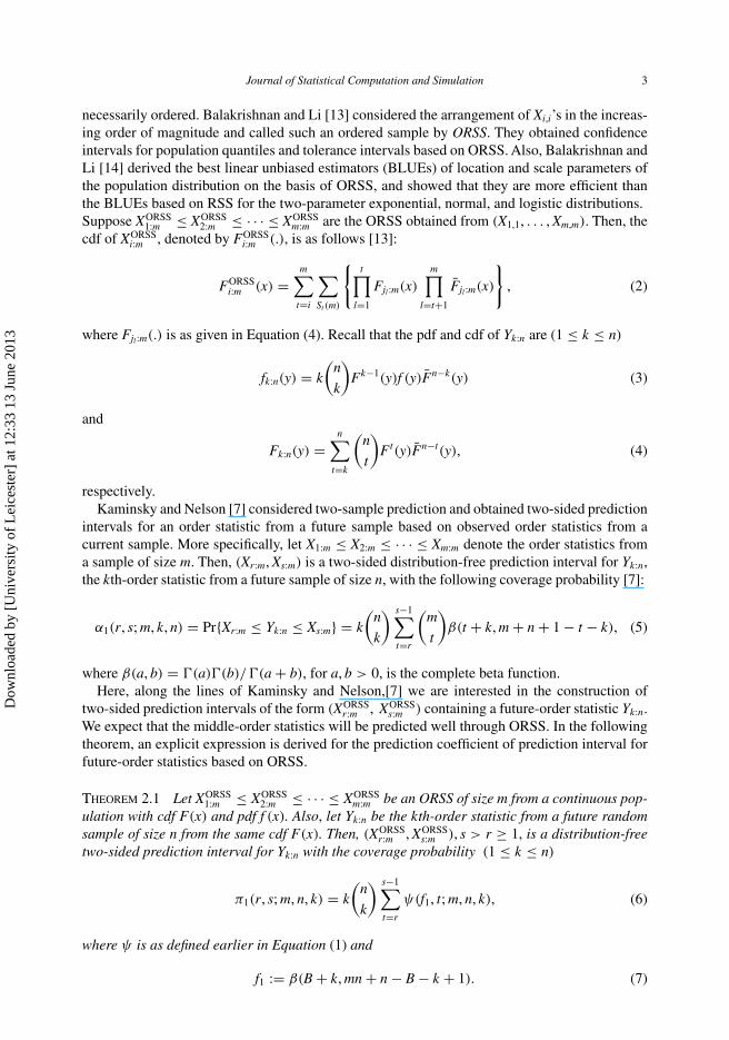
necessarily ordered. Balakrishnan and Li [13] considered the arrangement of Xi,i’s in the increas-ing order of magnitude and called such an ordered sample by ORSS. They obtained confidenceintervals for population quantiles and tolerance intervals based on ORSS. Also, Balakrishnan andLi [14] derived the best linear unbiased estimators (BLUEs) of location and scale parameters ofthe population distribution on the basis of ORSS, and showed that they are more efficient thanthe BLUEs based on RSS for the two-parameter exponential, normal, and logistic distributions.Suppose XORSS
1:m ≤ XORSS2:m ≤ · · · ≤ XORSS
m:m are the ORSS obtained from (X1,1, . . . , Xm,m). Then, thecdf of XORSS
i:m , denoted by FORSSi:m (.), is as follows [13]:
FORSSi:m (x) =
m∑t=i
∑St(m)
{t∏
l=1
Fjl :m(x)m∏
l=t+1
Fjl :m(x)
}, (2)
where Fjl :m(.) is as given in Equation (4). Recall that the pdf and cdf of Yk:n are (1 ≤ k ≤ n)
fk:n(y) = k
(n
k
)Fk−1(y)f (y)Fn−k(y) (3)
and
Fk:n(y) =n∑
t=k
(n
t
)Ft(y)Fn−t(y), (4)
respectively.Kaminsky and Nelson [7] considered two-sample prediction and obtained two-sided prediction
intervals for an order statistic from a future sample based on observed order statistics from acurrent sample. More specifically, let X1:m ≤ X2:m ≤ · · · ≤ Xm:m denote the order statistics froma sample of size m. Then, (Xr:m, Xs:m) is a two-sided distribution-free prediction interval for Yk:n,the kth-order statistic from a future sample of size n, with the following coverage probability [7]:
α1(r, s; m, k, n) = Pr{Xr:m ≤ Yk:n ≤ Xs:m} = k
(n
k
) s−1∑t=r
(m
t
)β(t + k, m + n + 1 − t − k), (5)
where β(a, b) = �(a)�(b)/�(a + b), for a, b > 0, is the complete beta function.Here, along the lines of Kaminsky and Nelson,[7] we are interested in the construction of
two-sided prediction intervals of the form (XORSSr:m , XORSS
s:m ) containing a future-order statistic Yk:n.We expect that the middle-order statistics will be predicted well through ORSS. In the followingtheorem, an explicit expression is derived for the prediction coefficient of prediction interval forfuture-order statistics based on ORSS.
Theorem 2.1 Let XORSS1:m ≤ XORSS
2:m ≤ · · · ≤ XORSSm:m be an ORSS of size m from a continuous pop-
ulation with cdf F(x) and pdf f (x). Also, let Yk:n be the kth-order statistic from a future randomsample of size n from the same cdf F(x). Then, (XORSS
r:m , XORSSs:m ), s > r ≥ 1, is a distribution-free
two-sided prediction interval for Yk:n with the coverage probability (1 ≤ k ≤ n)
π1(r, s; m, n, k) = k
(n
k
) s−1∑t=r
ψ(f1, t; m, n, k), (6)
where ψ is as defined earlier in Equation (1) and
f1 := β(B + k, mn + n − B − k + 1). (7)
Dow
nloa
ded
by [
Uni
vers
ity o
f L
eice
ster
] at
12:
33 1
3 Ju
ne 2
013
4 M. Salehi et al.
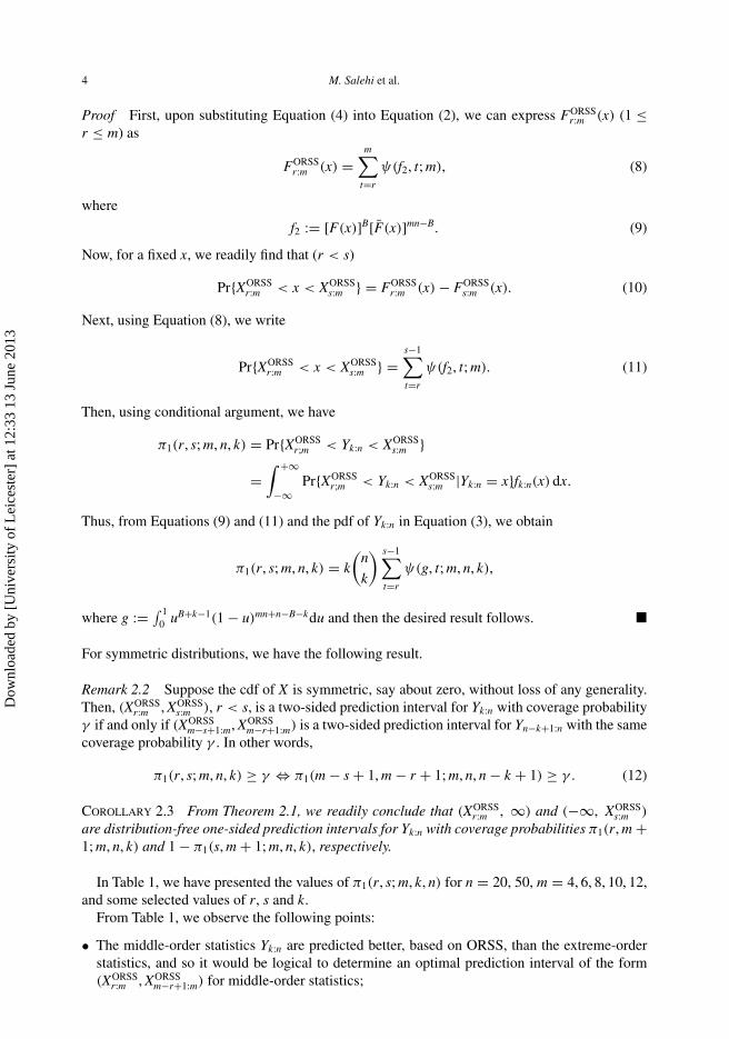
Proof First, upon substituting Equation (4) into Equation (2), we can express FORSSr:m (x) (1 ≤
r ≤ m) as
FORSSr:m (x) =
m∑t=r
ψ(f2, t; m), (8)
where
f2 := [F(x)]B[F(x)]mn−B. (9)
Now, for a fixed x, we readily find that (r < s)
Pr{XORSSr:m < x < XORSS
s:m } = FORSSr:m (x) − FORSS
s:m (x). (10)
Next, using Equation (8), we write
Pr{XORSSr:m < x < XORSS
s:m } =s−1∑t=r
ψ(f2, t; m). (11)
Then, using conditional argument, we have
π1(r, s; m, n, k) = Pr{XORSSr;m < Yk:n < XORSS
s:m }
=∫ +∞
−∞Pr{XORSS
r;m < Yk:n < XORSSs:m |Yk:n = x}fk:n(x) dx.
Thus, from Equations (9) and (11) and the pdf of Yk:n in Equation (3), we obtain
π1(r, s; m, n, k) = k
(n
k
) s−1∑t=r
ψ(g, t; m, n, k),
where g := ∫ 10 uB+k−1(1 − u)mn+n−B−kdu and then the desired result follows. �
For symmetric distributions, we have the following result.
Remark 2.2 Suppose the cdf of X is symmetric, say about zero, without loss of any generality.Then, (XORSS
r:m , XORSSs:m ), r < s, is a two-sided prediction interval for Yk:n with coverage probability
γ if and only if (XORSSm−s+1:m, XORSS
m−r+1:m) is a two-sided prediction interval for Yn−k+1:n with the samecoverage probability γ . In other words,
π1(r, s; m, n, k) ≥ γ ⇔ π1(m − s + 1, m − r + 1; m, n, n − k + 1) ≥ γ . (12)
Corollary 2.3 From Theorem 2.1, we readily conclude that (XORSSr:m , ∞) and (−∞, XORSS
s:m )
are distribution-free one-sided prediction intervals for Yk:n with coverage probabilities π1(r, m +1; m, n, k) and 1 − π1(s, m + 1; m, n, k), respectively.
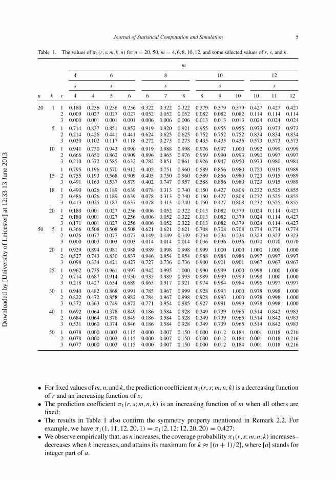
In Table 1, we have presented the values of π1(r, s; m, k, n) for n = 20, 50, m = 4, 6, 8, 10, 12,and some selected values of r, s and k.
From Table 1, we observe the following points:
• The middle-order statistics Yk:n are predicted better, based on ORSS, than the extreme-orderstatistics, and so it would be logical to determine an optimal prediction interval of the form(XORSS
r:m , XORSSm−r+1:m) for middle-order statistics;
Dow
nloa
ded
by [
Uni
vers
ity o
f L
eice
ster
] at
12:
33 1
3 Ju
ne 2
013
Journal of Statistical Computation and Simulation 5
Table 1. The values of π1(r, s; m, k, n) for n = 20, 50, m = 4, 6, 8, 10, 12, and some selected values of r, s, and k.
m
4 6 8 10 12
s s s s s
n k r 4 4 5 6 6 7 8 8 9 10 10 11 12
20 1 1 0.180 0.256 0.256 0.256 0.322 0.322 0.322 0.379 0.379 0.379 0.427 0.427 0.4272 0.009 0.027 0.027 0.027 0.052 0.052 0.052 0.082 0.082 0.082 0.114 0.114 0.1143 0.000 0.001 0.001 0.001 0.006 0.006 0.006 0.013 0.013 0.013 0.024 0.024 0.024
5 1 0.714 0.837 0.851 0.852 0.919 0.920 0.921 0.955 0.955 0.955 0.973 0.973 0.9732 0.214 0.426 0.441 0.441 0.624 0.625 0.625 0.752 0.752 0.752 0.834 0.834 0.8343 0.020 0.102 0.117 0.118 0.272 0.273 0.273 0.435 0.435 0.435 0.573 0.573 0.573
10 1 0.941 0.730 0.943 0.990 0.919 0.988 0.998 0.976 0.997 1.000 0.992 0.999 0.9992 0.666 0.650 0.862 0.909 0.896 0.965 0.976 0.969 0.990 0.993 0.990 0.997 0.9973 0.210 0.372 0.585 0.632 0.782 0.851 0.861 0.926 0.947 0.950 0.973 0.980 0.981
1 0.795 0.196 0.570 0.912 0.405 0.751 0.960 0.589 0.856 0.980 0.723 0.915 0.98915 2 0.755 0.193 0.568 0.909 0.405 0.750 0.960 0.589 0.856 0.980 0.723 0.915 0.989
3 0.491 0.163 0.537 0.879 0.402 0.747 0.957 0.588 0.856 0.980 0.723 0.915 0.989
18 1 0.490 0.026 0.189 0.639 0.078 0.313 0.740 0.150 0.427 0.808 0.232 0.525 0.8552 0.486 0.026 0.189 0.639 0.078 0.313 0.740 0.150 0.427 0.808 0.232 0.525 0.8553 0.413 0.025 0.187 0.637 0.078 0.313 0.740 0.150 0.427 0.808 0.232 0.525 0.855
20 1 0.180 0.001 0.027 0.256 0.006 0.052 0.322 0.013 0.082 0.379 0.024 0.114 0.4272 0.180 0.001 0.027 0.256 0.006 0.052 0.322 0.013 0.082 0.379 0.024 0.114 0.4273 0.171 0.001 0.027 0.256 0.006 0.052 0.322 0.013 0.082 0.379 0.024 0.114 0.427
50 5 1 0.366 0.508 0.508 0.508 0.621 0.621 0.621 0.708 0.708 0.708 0.774 0.774 0.7742 0.026 0.077 0.077 0.077 0.149 0.149 0.149 0.234 0.234 0.234 0.323 0.323 0.3233 0.000 0.003 0.003 0.003 0.014 0.014 0.014 0.036 0.036 0.036 0.070 0.070 0.070
20 1 0.929 0.894 0.981 0.988 0.989 0.998 0.998 0.999 1.000 1.000 1.000 1.000 1.0002 0.527 0.743 0.830 0.837 0.946 0.954 0.954 0.988 0.988 0.988 0.997 0.997 0.9973 0.098 0.334 0.421 0.427 0.727 0.736 0.736 0.900 0.901 0.901 0.967 0.967 0.967
25 1 0.962 0.735 0.961 0.997 0.942 0.995 1.000 0.990 0.999 1.000 0.998 1.000 1.0002 0.714 0.687 0.914 0.950 0.935 0.989 0.993 0.989 0.999 0.999 0.998 1.000 1.0003 0.218 0.427 0.654 0.689 0.863 0.917 0.921 0.974 0.984 0.984 0.996 0.997 0.997
30 1 0.940 0.482 0.868 0.991 0.785 0.967 0.999 0.928 0.993 1.000 0.978 0.998 1.0002 0.822 0.472 0.858 0.982 0.784 0.967 0.998 0.928 0.993 1.000 0.978 0.998 1.0003 0.372 0.363 0.749 0.872 0.771 0.954 0.985 0.927 0.991 0.999 0.978 0.998 1.000
40 1 0.692 0.064 0.378 0.849 0.186 0.584 0.928 0.349 0.739 0.965 0.514 0.842 0.9832 0.684 0.064 0.378 0.849 0.186 0.584 0.928 0.349 0.739 0.965 0.514 0.842 0.9833 0.531 0.060 0.374 0.846 0.186 0.584 0.928 0.349 0.739 0.965 0.514 0.842 0.983
50 1 0.078 0.000 0.003 0.115 0.000 0.007 0.150 0.000 0.012 0.184 0.001 0.018 0.2162 0.078 0.000 0.003 0.115 0.000 0.007 0.150 0.000 0.012 0.184 0.001 0.018 0.2163 0.077 0.000 0.003 0.115 0.000 0.007 0.150 0.000 0.012 0.184 0.001 0.018 0.216
• For fixed values of m, n, and k, the prediction coefficient π1(r, s; m, n, k) is a decreasing functionof r and an increasing function of s;
• The prediction coefficient π1(r, s; m, n, k) is an increasing function of m when all others arefixed;
• The results in Table 1 also confirm the symmetry property mentioned in Remark 2.2. Forexample, we have π1(1, 11; 12, 20, 1) = π1(2, 12; 12, 20, 20) = 0.427;
• We observe empirically that, as n increases, the coverage probability π1(r, s; m, n, k) increases–decreases when k increases, and attains its maximum for k ≈ [(n + 1)/2], where [a] stands forinteger part of a.
Dow
nloa
ded
by [
Uni
vers
ity o
f L
eice
ster
] at
12:
33 1
3 Ju
ne 2
013
6 M. Salehi et al.
2.1. Optimal prediction interval
It is important to mention that, for specified values of π0, k, and n, the two-sided prediction interval(XORSS
r:m , XORSSs:m ) exists if and only if for a suitable m, the inequality max1≤r<s≤m π1(r, s; m, n, k) ≥
π0 holds. From Equation (6), this condition is equivalent to
π1(1, m; m, n, k) = k
(n
k
) m−1∑t=r
ψ(f1, t; m, n, k) ≥ π0, (13)
where f1 is as given in Equation (7).For example, if n = 30, k = 15, and the given value of π0 is 0.95, then the minimum m which
satisfies the inequality in Equation (13), say mORSSopt , is equal to 4. For more such cases, one may
see the results in Table 3.For choosing an optimal prediction interval, if n, k, and the desired prediction level π0 are all
specified, we should start with m = 2 and increase it until π1(r, s; m, n, k) exceeds π0. Suppose,in addition, m is known too. Then, since there can be different choices of r and s for whichπ1(r, s; m, n, k) ≥ π0, we shall follow the algorithm to find an optimal prediction interval, say,(ropt, sopt):
(i) For given values of m, n, and π0, take C = {(r, s); π1(r, s; m, n, k) ≥ π0} and select (r, s) fromC such that minimizes the difference s − r;
(ii) If some choices of (r, s) have the same difference, then choose r and s such that
(ropt, sopt) = argmin{E(XORSSs:m − XORSS
r:m ), r < s}. (14)
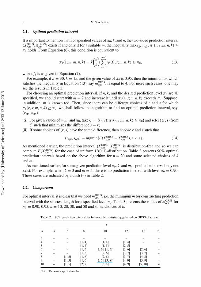
As mentioned earlier, the prediction interval (XORSSs:m , XORSS
r:m ) is distribution-free and so we cancompute E(XORSS
r:m ) for the case of uniform U(0, 1)-distribution. Table 2 presents 90% optimalprediction intervals based on the above algorithm for n = 20 and some selected choices of kand m.
As mentioned earlier, for some given prediction level π0, k, and m, a prediction interval may notexist. For example, when k = 3 and m = 5, there is no prediction interval with level π0 = 0.90.These cases are indicated by a dash (–) in Table 2.
2.2. Comparison
For optimal interval, it is clear that we need mORSSopt , i.e. the minimum m for constructing prediction
interval with the shortest length for a specified level π0. Table 3 presents the values of mORSSopt for
π0 = 0.90, 0.95, n = 10, 20, 30, and 50 and some choices of k.
Table 2. 90% prediction interval for future-order statistic Yk:20 based on ORSS of size m.
k
m 3 5 8 10 12 15 20
3 – – – – – – –4 – – [1, 4] [1, 4] [1, 4] – –5 – – [1, 4] [1, 5] [2, 5] – –6 – – [1, 5] [2, 6], [1, 5]a [2, 6] [2, 6] –7 – – [1, 5] [2, 6] [3, 7] [3, 7] –8 – [1, 5] [1, 6] [2, 6] [3, 7] [4, 8] –9 – [1, 5] [1, 6] [2, 7], [3, 8]a [4, 9] [5, 9] –10 – [1, 5] [2, 7] [3, 8] [4, 9] [5, 10] –
Note: aThe same expected widths.
Dow
nloa
ded
by [
Uni
vers
ity o
f L
eice
ster
] at
12:
33 1
3 Ju
ne 2
013
Journal of Statistical Computation and Simulation 7
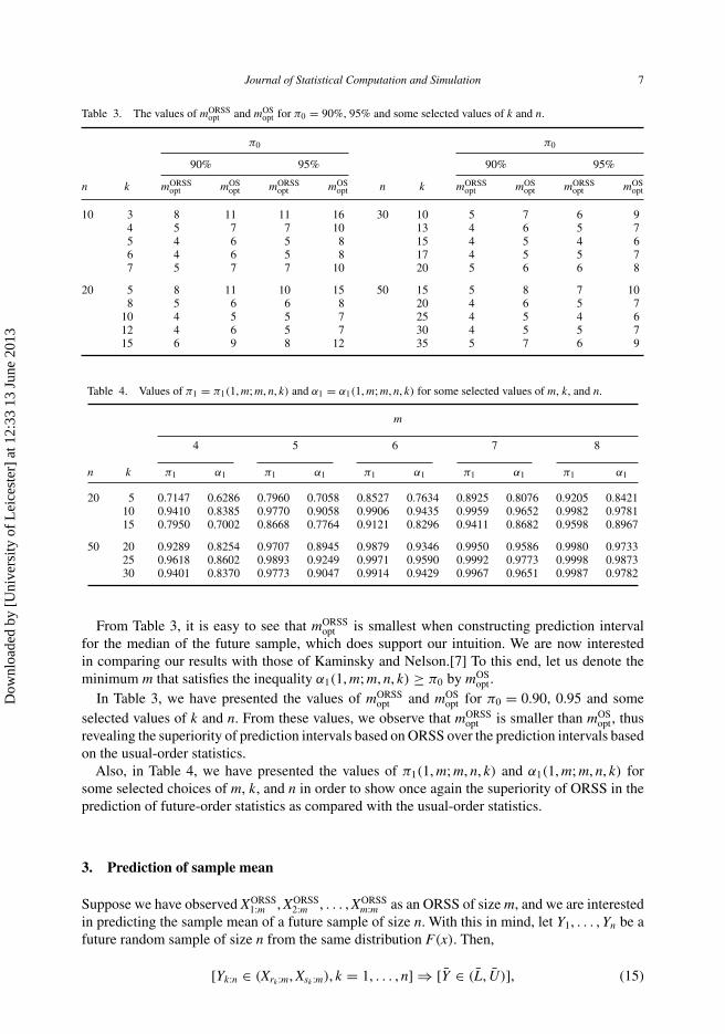
Table 3. The values of mORSSopt and mOS
opt for π0 = 90%, 95% and some selected values of k and n.
π0 π0
90% 95% 90% 95%
n k mORSSopt mOS
opt mORSSopt mOS
opt n k mORSSopt mOS
opt mORSSopt mOS
opt
10 3 8 11 11 16 30 10 5 7 6 94 5 7 7 10 13 4 6 5 75 4 6 5 8 15 4 5 4 66 4 6 5 8 17 4 5 5 77 5 7 7 10 20 5 6 6 8
20 5 8 11 10 15 50 15 5 8 7 108 5 6 6 8 20 4 6 5 7
10 4 5 5 7 25 4 5 4 612 4 6 5 7 30 4 5 5 715 6 9 8 12 35 5 7 6 9
Table 4. Values of π1 = π1(1, m; m, n, k) and α1 = α1(1, m; m, n, k) for some selected values of m, k, and n.
m
4 5 6 7 8
n k π1 α1 π1 α1 π1 α1 π1 α1 π1 α1
20 5 0.7147 0.6286 0.7960 0.7058 0.8527 0.7634 0.8925 0.8076 0.9205 0.842110 0.9410 0.8385 0.9770 0.9058 0.9906 0.9435 0.9959 0.9652 0.9982 0.978115 0.7950 0.7002 0.8668 0.7764 0.9121 0.8296 0.9411 0.8682 0.9598 0.8967
50 20 0.9289 0.8254 0.9707 0.8945 0.9879 0.9346 0.9950 0.9586 0.9980 0.973325 0.9618 0.8602 0.9893 0.9249 0.9971 0.9590 0.9992 0.9773 0.9998 0.987330 0.9401 0.8370 0.9773 0.9047 0.9914 0.9429 0.9967 0.9651 0.9987 0.9782
From Table 3, it is easy to see that mORSSopt is smallest when constructing prediction interval
for the median of the future sample, which does support our intuition. We are now interestedin comparing our results with those of Kaminsky and Nelson.[7] To this end, let us denote theminimum m that satisfies the inequality α1(1, m; m, n, k) ≥ π0 by mOS
opt.In Table 3, we have presented the values of mORSS
opt and mOSopt for π0 = 0.90, 0.95 and some
selected values of k and n. From these values, we observe that mORSSopt is smaller than mOS
opt, thusrevealing the superiority of prediction intervals based on ORSS over the prediction intervals basedon the usual-order statistics.
Also, in Table 4, we have presented the values of π1(1, m; m, n, k) and α1(1, m; m, n, k) forsome selected choices of m, k, and n in order to show once again the superiority of ORSS in theprediction of future-order statistics as compared with the usual-order statistics.
3. Prediction of sample mean
Suppose we have observed XORSS1:m , XORSS
2:m , . . . , XORSSm:m as an ORSS of size m, and we are interested
in predicting the sample mean of a future sample of size n. With this in mind, let Y1, . . . , Yn be afuture random sample of size n from the same distribution F(x). Then,
[Yk:n ∈ (Xrk :m, Xsk :m), k = 1, . . . , n] ⇒ [Y ∈ (L, U)], (15)
Dow
nloa
ded
by [
Uni
vers
ity o
f L
eice
ster
] at
12:
33 1
3 Ju
ne 2
013
8 M. Salehi et al.
where L = (1/n)∑n
k=1 Xrk :m and U = (1/n)∑n
k=1 Xsk :m. Equation (15) implies that
Pr(Y ∈ (L, U)) ≥ Pr
{n⋂
k=1
(Xrk :m ≤ Yk:n ≤ Xsk :m)
}
≥ 1 −n∑
k=1
[1 − Pr(Xrk :m ≤ Yk:n ≤ Xsi:m)]
= 1 − n +n∑
k=1
π1(rk , sk; m, n, k), (16)
where π1(r, s; m, n, k) is as given in Equation (6).
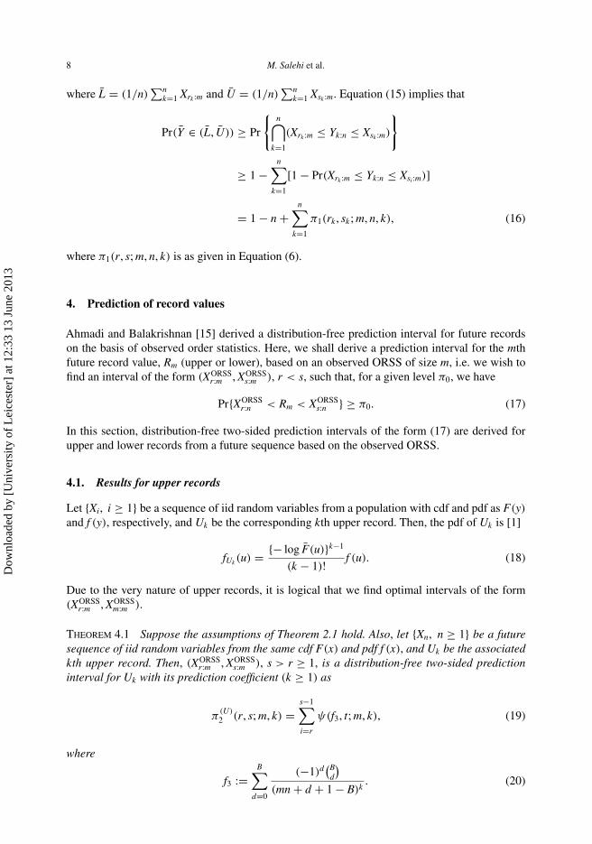
4. Prediction of record values
Ahmadi and Balakrishnan [15] derived a distribution-free prediction interval for future recordson the basis of observed order statistics. Here, we shall derive a prediction interval for the mthfuture record value, Rm (upper or lower), based on an observed ORSS of size m, i.e. we wish tofind an interval of the form (XORSS
r:m , XORSSs:m ), r < s, such that, for a given level π0, we have
Pr{XORSSr:n < Rm < XORSS
s:n } ≥ π0. (17)
In this section, distribution-free two-sided prediction intervals of the form (17) are derived forupper and lower records from a future sequence based on the observed ORSS.
4.1. Results for upper records
Let {Xi, i ≥ 1} be a sequence of iid random variables from a population with cdf and pdf as F(y)and f (y), respectively, and Uk be the corresponding kth upper record. Then, the pdf of Uk is [1]
fUk (u) = {− log F(u)}k−1
(k − 1)! f (u). (18)
Due to the very nature of upper records, it is logical that we find optimal intervals of the form(XORSS
r:m , XORSSm:m ).
Theorem 4.1 Suppose the assumptions of Theorem 2.1 hold. Also, let {Xn, n ≥ 1} be a futuresequence of iid random variables from the same cdf F(x) and pdf f (x), and Uk be the associatedkth upper record. Then, (XORSS
r:m , XORSSs:m ), s > r ≥ 1, is a distribution-free two-sided prediction
interval for Uk with its prediction coefficient (k ≥ 1) as
π(U)2 (r, s; m, k) =
s−1∑i=r
ψ(f3, t; m, k), (19)
where
f3 :=B∑
d=0
(−1)d(B
d
)(mn + d + 1 − B)k
. (20)
Dow
nloa
ded
by [
Uni
vers
ity o
f L
eice
ster
] at
12:
33 1
3 Ju
ne 2
013
Journal of Statistical Computation and Simulation 9
Proof Using conditional argument in Equation (11), we obtain
π(U)2 (r, s; m, k) = Pr{XORSS
r:m ≤ Uk ≤ XORSSs:m }
=∫ +∞
−∞Pr{XORSS
r:m < u < XORSSs:m }fUk (u) du
=∫ +∞
−∞
s−1∑t=r
ψ(f2fUk (u), t; m, k) du
=s−1∑t=r
ψ(h, t; m, k), (21)
where f2 is as given in Equation (9) and h := ∑Bd=0(−1)d
(Bd
) ∫ +∞−∞ [F(u)]mn−B+dfUk (u) du. Upon
substituting fUk (u) in Equation (18) into the function h and then using the substitution v =− log F(u), the proof follows readily. �
Corollary 4.2 Suppose the conditions of Theorem 4.1 hold. Then, XORSSr:m and XORSS
s:m are,respectively, the lower and upper prediction bounds for Uk , k ≥ 1, with prediction coefficients asπ
(U)2 (r, m + 1; m, k) and 1 − π
(U)2 (s, m + 1; m, k), respectively.
As is the proceeding subsection, for a given k and the level π0, the necessary and sufficientcondition for the existence of the prediction interval (XORSS
r:m , XORSSs:m ) in Theorem 4.1 is
max1≤r≤s≤m
π(U)2 (r, s; m, k) = π
(U)2 (1, m; m, k) ≥ π0. (22)
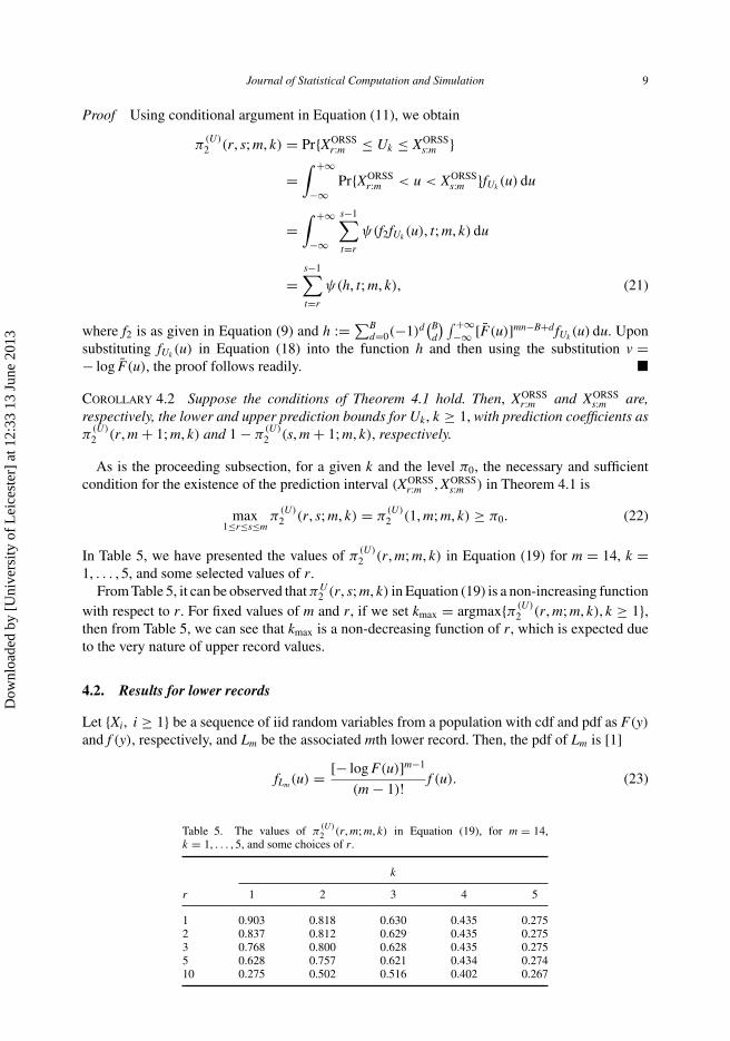
In Table 5, we have presented the values of π(U)2 (r, m; m, k) in Equation (19) for m = 14, k =
1, . . . , 5, and some selected values of r.From Table 5, it can be observed that πU
2 (r, s; m, k) in Equation (19) is a non-increasing functionwith respect to r. For fixed values of m and r, if we set kmax = argmax{π(U)
2 (r, m; m, k), k ≥ 1},then from Table 5, we can see that kmax is a non-decreasing function of r, which is expected dueto the very nature of upper record values.
4.2. Results for lower records
Let {Xi, i ≥ 1} be a sequence of iid random variables from a population with cdf and pdf as F(y)and f (y), respectively, and Lm be the associated mth lower record. Then, the pdf of Lm is [1]
fLm(u) = [− log F(u)]m−1
(m − 1)! f (u). (23)
Table 5. The values of π(U)2 (r, m; m, k) in Equation (19), for m = 14,
k = 1, . . . , 5, and some choices of r.
k
r 1 2 3 4 5
1 0.903 0.818 0.630 0.435 0.2752 0.837 0.812 0.629 0.435 0.2753 0.768 0.800 0.628 0.435 0.2755 0.628 0.757 0.621 0.434 0.27410 0.275 0.502 0.516 0.402 0.267
Dow
nloa
ded
by [
Uni
vers
ity o
f L
eice
ster
] at
12:
33 1
3 Ju
ne 2
013
10 M. Salehi et al.
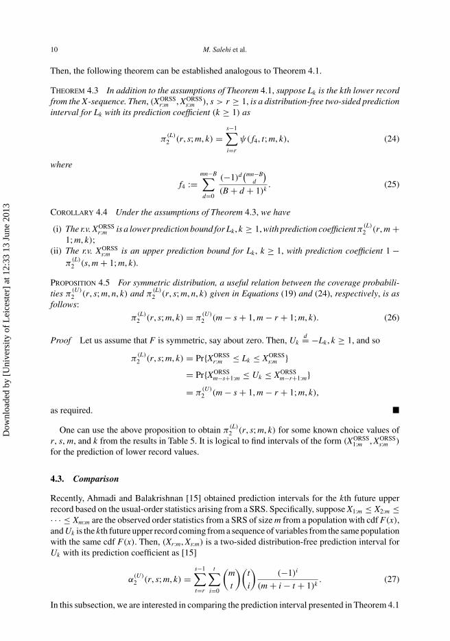
Then, the following theorem can be established analogous to Theorem 4.1.
Theorem 4.3 In addition to the assumptions of Theorem 4.1, suppose Lk is the kth lower recordfrom the X-sequence. Then, (XORSS
r:m , XORSSs:m ), s > r ≥ 1, is a distribution-free two-sided prediction
interval for Lk with its prediction coefficient (k ≥ 1) as
π(L)2 (r, s; m, k) =
s−1∑i=r
ψ( f4, t; m, k), (24)
where
f4 :=mn−B∑d=0
(−1)d(mn−B
d
)(B + d + 1)k
. (25)
Corollary 4.4 Under the assumptions of Theorem 4.3, we have
(i) The r.v. XORSSr:m is a lower prediction bound for Lk , k ≥ 1, with prediction coefficient π(L)
2 (r, m +1; m, k);
(ii) The r.v. XORSSs:m is an upper prediction bound for Lk , k ≥ 1, with prediction coefficient 1 −
π(L)2 (s, m + 1; m, k).
Proposition 4.5 For symmetric distribution, a useful relation between the coverage probabili-ties π
(U)2 (r, s; m, n, k) and π
(L)2 (r, s; m, n, k) given in Equations (19) and (24), respectively, is as
follows:
π(L)2 (r, s; m, k) = π
(U)2 (m − s + 1, m − r + 1; m, k). (26)
Proof Let us assume that F is symmetric, say about zero. Then, Ukd= −Lk , k ≥ 1, and so
π(L)2 (r, s; m, k) = Pr{XORSS
r:m ≤ Lk ≤ XORSSs:m }
= Pr{XORSSm−s+1:m ≤ Uk ≤ XORSS
m−r+1:m}= π
(U)2 (m − s + 1, m − r + 1; m, k),
as required. �
One can use the above proposition to obtain π(L)2 (r, s; m, k) for some known choice values of
r, s, m, and k from the results in Table 5. It is logical to find intervals of the form (XORSS1:m , XORSS
s:m )
for the prediction of lower record values.
4.3. Comparison
Recently, Ahmadi and Balakrishnan [15] obtained prediction intervals for the kth future upperrecord based on the usual-order statistics arising from a SRS. Specifically, suppose X1:m ≤ X2:m ≤· · · ≤ Xm:m are the observed order statistics from a SRS of size m from a population with cdf F(x),and Uk is the kth future upper record coming from a sequence of variables from the same populationwith the same cdf F(x). Then, (Xr:m, Xs:m) is a two-sided distribution-free prediction interval forUk with its prediction coefficient as [15]
α(U)2 (r, s; m, k) =
s−1∑t=r
t∑i=0
(m
t
)(t
i
)(−1)i
(m + i − t + 1)k. (27)
In this subsection, we are interested in comparing the prediction interval presented in Theorem 4.1
Dow
nloa
ded
by [
Uni
vers
ity o
f L
eice
ster
] at
12:
33 1
3 Ju
ne 2
013
Journal of Statistical Computation and Simulation 11
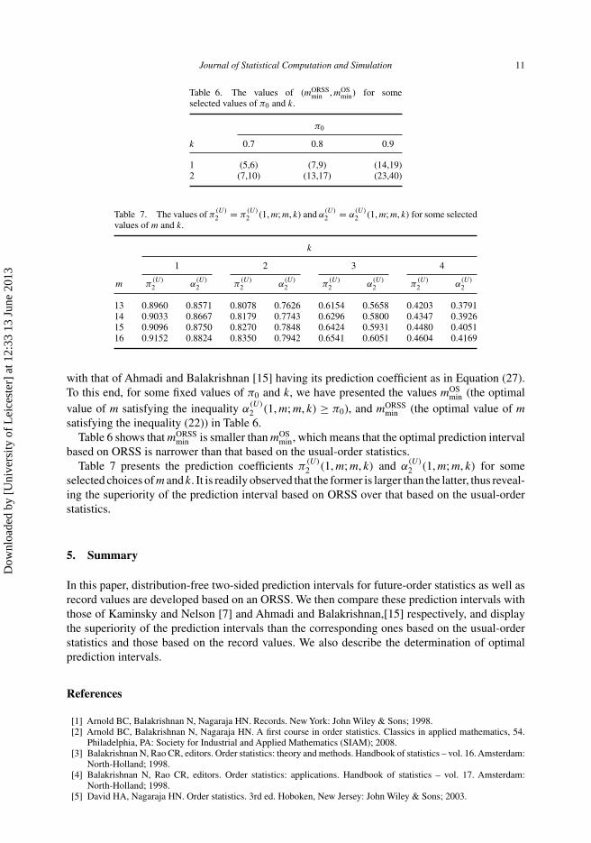
Table 6. The values of (mORSSmin , mOS
min) for someselected values of π0 and k.
π0
k 0.7 0.8 0.9
1 (5,6) (7,9) (14,19)2 (7,10) (13,17) (23,40)
Table 7. The values of π(U)2 = π
(U)2 (1, m; m, k) and α
(U)2 = α
(U)2 (1, m; m, k) for some selected
values of m and k.
k
1 2 3 4
m π(U)2 α
(U)2 π
(U)2 α
(U)2 π
(U)2 α
(U)2 π
(U)2 α
(U)2
13 0.8960 0.8571 0.8078 0.7626 0.6154 0.5658 0.4203 0.379114 0.9033 0.8667 0.8179 0.7743 0.6296 0.5800 0.4347 0.392615 0.9096 0.8750 0.8270 0.7848 0.6424 0.5931 0.4480 0.405116 0.9152 0.8824 0.8350 0.7942 0.6541 0.6051 0.4604 0.4169
with that of Ahmadi and Balakrishnan [15] having its prediction coefficient as in Equation (27).To this end, for some fixed values of π0 and k, we have presented the values mOS
min (the optimalvalue of m satisfying the inequality α
(U)2 (1, m; m, k) ≥ π0), and mORSS
min (the optimal value of msatisfying the inequality (22)) in Table 6.
Table 6 shows that mORSSmin is smaller than mOS
min, which means that the optimal prediction intervalbased on ORSS is narrower than that based on the usual-order statistics.
Table 7 presents the prediction coefficients π(U)2 (1, m; m, k) and α
(U)2 (1, m; m, k) for some
selected choices of m and k. It is readily observed that the former is larger than the latter, thus reveal-ing the superiority of the prediction interval based on ORSS over that based on the usual-orderstatistics.
5. Summary
In this paper, distribution-free two-sided prediction intervals for future-order statistics as well asrecord values are developed based on an ORSS. We then compare these prediction intervals withthose of Kaminsky and Nelson [7] and Ahmadi and Balakrishnan,[15] respectively, and displaythe superiority of the prediction intervals than the corresponding ones based on the usual-orderstatistics and those based on the record values. We also describe the determination of optimalprediction intervals.
References
[1] Arnold BC, Balakrishnan N, Nagaraja HN. Records. New York: John Wiley & Sons; 1998.[2] Arnold BC, Balakrishnan N, Nagaraja HN. A first course in order statistics. Classics in applied mathematics, 54.
Philadelphia, PA: Society for Industrial and Applied Mathematics (SIAM); 2008.[3] Balakrishnan N, Rao CR, editors. Order statistics: theory and methods. Handbook of statistics – vol. 16. Amsterdam:
North-Holland; 1998.[4] Balakrishnan N, Rao CR, editors. Order statistics: applications. Handbook of statistics – vol. 17. Amsterdam:
North-Holland; 1998.[5] David HA, Nagaraja HN. Order statistics. 3rd ed. Hoboken, New Jersey: John Wiley & Sons; 2003.
Dow
nloa
ded
by [
Uni
vers
ity o
f L
eice
ster
] at
12:
33 1
3 Ju
ne 2
013

12 M. Salehi et al.
[6] Dunsmore IR. The future occurrence of records. Ann Inst Statist Math. 1983;35:267–277.[7] Kaminsky KS, Nelson PI. Prediction of order statistics. In: Balakrishnan N, Rao CR, editors. Order statistics:
applications. Handbook of statistics – vol. 17. Amsterdam: North-Holland; 1998. p. 431–450.[8] Ahmadi J, Doostparast, M. Bayesian estimation and prediction for some life distributions based on record values.
Statist Papers. 2006;47:373–392.[9] Raqab M, Balakrishnan N. Prediction intervals for future records. Stat Probab Lett. 2008;78:1955–1963.
[10] Vock M, Balakrishnan N. Nonparametric prediction intervals based on ranked set samples. Commun Statist TheoryMethods. 2012;41:2256–2268.
[11] Frey J. A note on a probability involving independent order statistics. J Stat Comput Simul. 2007;77:969–975.[12] McIntyre GA. A method for unbiased selective sampling, using ranked sets. Aust J Agri Res. 1952;3:385–390.[13] Balakrishnan N, Li T. Ordered ranked set samples and applications to inference. Ann Inst Statist Math. 2006;58:
757–777.[14] Balakrishnan N, Li T. Ordered ranked set samples and applications to inference. J Statist Plann Inference.
2008;138:3512–3524.[15] Ahmadi J, Balakrishnan N. Prediction of order statistics and record values from two independent sequences. Statistics.
2010;44:417–430.
Dow
nloa
ded
by [
Uni
vers
ity o
f L
eice
ster
] at
12:
33 1
3 Ju
ne 2
013