Citation: Song, M.; Xue, J.; Gao, S.;

Cheng, G.; Chen, J.; Lu, H.; Dong, Z.

Prediction of NOx Concentration at

SCR Inlet Based on BMIFS-LSTM.

Atmosphere 2022, 13, 686. https://

doi.org/10.3390/atmos13050686

Academic Editor: James Lee

Received: 1 March 2022

Accepted: 22 April 2022

Published: 25 April 2022

Publisher’s Note: MDPI stays neutral

with regard to jurisdictional claims in

published maps and institutional affil-

iations.

Copyright: © 2022 by the authors.

Licensee MDPI, Basel, Switzerland.

This article is an open access article

distributed under the terms and

conditions of the Creative Commons

Attribution (CC BY) license (https://

creativecommons.org/licenses/by/

4.0/).

atmosphere

Article

Prediction of NOx Concentration at SCR Inlet Basedon BMIFS-LSTMMeiyan Song 1,*, Jianzhong Xue 1, Shaohua Gao 1, Guodong Cheng 1, Jun Chen 2, Haisong Lu 2 and Ze Dong 3

1 Xi’an Thermal Power Research Institute Co., Ltd., Xi’an 710054, China; xuejianzhong@tpri.com.cn (J.X.);gaoshaohua@tpri.com.cn (S.G.); chengguodong@tpri.com.cn (G.C.)

2 Nanjing NR Electric Co., Ltd., Nanjing 211102, China; chenj@nrec.com (J.C.); luhaisong@nrec.com (H.L.)3 Hebei Technology Innovation Center of Simulation & Optimized Control for Power Generation,

North China Electric Power University, Baoding 071066, China; dongze@ncepu.edu.cn* Correspondence: songmeiyan@tpri.com.cn; Tel.: +86-135-7247-9295

Abstract: As the main energy source for thermal power generation, coal generates a large amount ofNOx during its incineration in boilers, and excessive NOx emissions can cause serious pollution tothe air environment. Selective catalytic reduction denitrification (SCR) selects the optimal amount ofammonia to be injected for denitrification based on the measurement of NOx concentration by theautomatic flue gas monitoring system. Since the automatic flue gas monitoring system has a largedelay in measurement, it cannot accurately reflect the real-time changes of NOx concentration atthe SCR inlet when the unit load fluctuates, leading to problems such as ammonia escape and NOxemission exceeding the standard. In response to these problems, this paper proposes an SCR inlet NOxconcentration prediction algorithm based on BMIFS-LSTM. An improved mutual information featureselection algorithm (BMIFS) is used to filter out the auxiliary variables with maximum correlation andminimum redundancy with NOx concentration, and reduce the coupling and dimensionality amongthe variables in the data set. The dominant and auxiliary variables are then fed together into a longshort-term memory neural network (LSTM) to build a prognostic model. Simulation experimentsare conducted using historical operation data of a 300 MW thermal power unit. The experimentalresults show that the algorithm in this paper reduces the average relative error by 3.45% and the rootmean square error by 1.50 compared with the algorithm without auxiliary variable extraction, whichcan accurately reflect the real-time changes of NOx concentration at the SCR inlet, solve the problemof delay in NOx concentration measurement, and reduce the occurrence of atmospheric pollutioncaused by excessive NOx emissions.

Keywords: NOx concentration; LSTM; mutual information feature selection; SCR; model prediction

1. Introduction

In China’s electricity market, coal-fired thermal power generation has been dominant,and NOx from the combustion of coal-fired boilers in thermal power plants is one of themain sources of air pollutants [1]. Coal, the main energy source for power generation inthermal power plants, generates large amounts of nitrogen oxides (NOx) during combustionin the boilers, which are commonly referred to as NOx. In nature, the formation and fallof rain and snow absorbs NOx and other substances in the air, which in turn forms acidrain causing building corrosion, crop death, and other bad results. At the same time,NOx will also produce photochemical reactions with other pollutants under the action ofsunlight (ultraviolet), producing a secondary mixture of pollutants, namely photochemicalsmog pollution. With the increasing awareness of environmental protection in China,optimization of flue gas denitrification is on the agenda [2,3].

Selective catalyst reduction (SCR) is the current denitrification method used by mostthermal power units. SCR is based on the measurement of NOx concentration by theautomatic flue gas monitoring system and selects the optimal amount of ammonia to

Atmosphere 2022, 13, 686. https://doi.org/10.3390/atmos13050686 https://www.mdpi.com/journal/atmosphere

Atmosphere 2022, 13, 686 2 of 14

be injected for denitrification. However, the automatic flue gas monitoring system hasa large delay in measuring the NOx concentration, which does not accurately reflectthe real-time changes of the NOx concentration at the SCR inlet, resulting in ammoniaescape and NOx emission exceeding the standard. This research attempts to propose anew NOx concentration prediction algorithm using an artificial intelligence method toaccurately predict the NOx concentration at the SCR inlet. It works to solve the problemof delay in NOx measurement and accurately reflect the real-time changes of SCR inletNOx concentration, so as to effectively reduce the emission of excess NOx and prevent thepollution of the air environment.

In recent years, long short-term memory neural networks (LSTM) [4] have achievedremarkable results in processing big data. It can not only accomplish what traditional neu-ral networks provide after learning and training, extracting features, and then constructinghigh-level features by organizing the underlying features and finally obtaining the distribu-tion characteristics under the data, but more importantly, LSTM incorporates state gates inits neurons, which can filter and process massive data, effectively solving the problems ofgradient disappearance and gradient explosion and improving the processing capability ofbig data, and these advantages were verified in the literature [5–9]. Because of the multipleadvantages of LSTM for data processing, the algorithm is not only applied in the electricpower industry [10,11], but also widely used in many fields such as aerospace [12,13],shipping [14–16], finance [17,18], and water conservancy and hydropower [19,20].

Baomin Sun et al. [21] used artificial neural networks for NOx prediction based on thestudy of material characteristics, and compared the prediction accuracy before and afterthe environmental modification of the unit, and found that the algorithm has outstandingprediction accuracy and generalization ability. Xiangjun Li et al. [22] proposed to trainthe model with an LSTM network to address the problem of low prediction accuracydue to many uncertainties in the wind power generation process, and finally significantlyreduced the error of prediction results in each index. Zhai Yi et al. [23] used LSTM toextract the periodic characteristics in the load data and successfully achieved the electricload prediction. Xuejiao Mao et al. [24] used LSTM combined with the Adam optimizationmethod to train the network model for the characteristics of strong uncertainty and timecorrelation in saturation load prediction, and finally placed the model in saturation loadprediction under different scenarios and verified its effectiveness. Zhenhao Tang et al. [25]initially used mutual information to filter the time series feature length, then extractedthe time domain information and the frequency domain information, and modeled onthis basis using the improved SWLSTM; the results proved that the method could achieveaccurate wind prediction with the prediction error controlled below 1.73%.

For denitrification of thermal power units, most thermal power plants are currentlyusing selective catalytic reduction (SCR) technology to reduce NOx emissions. For NOxcontent in flue gas, plants generally use an automatic flue gas monitoring system tomeasure its concentration in real time, and the selective catalytic reduction denitrification(SCR) method selects the best amount of ammonia spray for denitrification based on themeasurement results of NOx concentration by the automatic flue gas monitoring system.However, the automatic flue gas monitoring system has a large delay in measurement,which cannot accurately reflect the real-time changes of NOx concentration at the SCR inlet,and thus cannot guide the reactor operation in a timely manner, leading to problems suchas ammonia escape and excessive NOX emissions. Therefore, this paper focuses on theNOx concentration at the inlet of SCR denitrification system as the research object, andadopts the long short-term memory network (LSTM) to establish a prediction model toaccurately predict NOx concentration at the SCR inlet, so as to solve the problem of delayin NOx concentration measurement and reduce the occurrence of air pollution caused byexcessive NOx emissions. The overall research process of this paper is shown in Figure 1.

Atmosphere 2022, 13, 686 3 of 14Atmosphere 2022, 13, x FOR PEER REVIEW 3 of 15

Figure 1. Overall research process flow chart.

2. Influencing Factors of NOx Production

With the increasing emphasis on environmental protection related to production of

thermal power in China, SCR denitrification systems are widely used in various coal-fired

thermal power plants. In this paper, the inlet NOx concentration of an SCR denitrification

system in a 300 MW thermal power plant is studied, and the nitrogen oxides produced by

the operation of coal-fired boilers is generally referred to as NOx.

The NOx produced by boiler combustion generally refers to NO and NO2, with NO

being the main component, accounting for 90% to 95%, and NO2 being obtained from the

oxidation reaction of NO with O2 at low temperatures. Boiler combustion is a complex

process in which many chemical reactions are interwoven, and the NOx content produced

is not only affected by the temperature during combustion, but also related to the air in

the boiler that provides conditions for combustion.

Thermal power plants generally adopt graded combustion technology to achieve rea-

sonable control of NOx generation. The principle is shown in Figure 2. The pulverized

coal burner feeds the pulverized coal into the furnace chamber, and along with the pri-

mary and secondary air fed into the main combustion zone, the pulverized coal starts to

burn violently while generating NOx, CO, CO2, and other gases. The high temperature

flue gas forms an upward flow and comes to the reduction zone of the furnace chamber,

where NOx is reduced to N2 and other nitrogen-containing compounds. When the flue

gas comes to the combustion zone, the combustion wind will come in to assist the com-

bustion, and a small amount of NOx is again produced, but generally, the total amount of

NOx finally produced by the pulverized coal is greatly reduced after the furnace is

graded.

Raise research question Build predictive models Simulation experiments

Literature review

Influencing factors of NOx

generation

Data collection and

preprocessing

LSTM predicts model

structure

Propose BMIFS algorithm

Algorithm Process Steps

Auxiliary variable filter

Predict experimental

results

Comparative experimental

results

Figure 1. Overall research process flow chart.

2. Influencing Factors of NOx Production

With the increasing emphasis on environmental protection related to production ofthermal power in China, SCR denitrification systems are widely used in various coal-firedthermal power plants. In this paper, the inlet NOx concentration of an SCR denitrificationsystem in a 300 MW thermal power plant is studied, and the nitrogen oxides produced bythe operation of coal-fired boilers is generally referred to as NOx.

The NOx produced by boiler combustion generally refers to NO and NO2, with NObeing the main component, accounting for 90% to 95%, and NO2 being obtained from theoxidation reaction of NO with O2 at low temperatures. Boiler combustion is a complexprocess in which many chemical reactions are interwoven, and the NOx content producedis not only affected by the temperature during combustion, but also related to the air in theboiler that provides conditions for combustion.

Thermal power plants generally adopt graded combustion technology to achievereasonable control of NOx generation. The principle is shown in Figure 2. The pulverizedcoal burner feeds the pulverized coal into the furnace chamber, and along with the primaryand secondary air fed into the main combustion zone, the pulverized coal starts to burnviolently while generating NOx, CO, CO2, and other gases. The high temperature flue gasforms an upward flow and comes to the reduction zone of the furnace chamber, whereNOx is reduced to N2 and other nitrogen-containing compounds. When the flue gas comesto the combustion zone, the combustion wind will come in to assist the combustion, and asmall amount of NOx is again produced, but generally, the total amount of NOx finallyproduced by the pulverized coal is greatly reduced after the furnace is graded.

Atmosphere 2022, 13, x FOR PEER REVIEW 4 of 15

Figure 2. Schematic diagram of pulverized coal combustion.

The baffle opening of the secondary air and the combustion air largely affect the com-

bustion of pulverized coal in the furnace chamber. By adjusting the baffle opening of sec-

ondary air to control the combustion of pulverized coal in the furnace chamber, the anoxic

combustion in the main combustion zone pushes back the whole combustion process, thus

effectively reducing the generation of NOx. The combustion exhaust dampers are then

used to adjust the combustion, so that the pulverized coal can be fully combusted while

reducing the generation of NOx, thus reducing the generation of NOx from the boiler

combustion level. Therefore, it can be seen that opening the combustion dampers and the

baffle of the secondary dampers is an important factor influencing the amount of NOx

generation. The ratio between the amount of fuel in the boiler and the amount of air affects

the boiler load and also has an impact on NOx production. In fact, the difference in the

air–coal ratio makes a significant change in the total amount of NOx.

3. Data Collection and Preprocessing

Before data collection, it is necessary to confirm which data need to be collected, in-

cluding historical operating data of auxiliary variables and dominant variables, and then

data need to be collected under appropriate operating conditions to ensure that the range

of data values is reasonable.

With the continuous advancement of information technology, thermal power plants

have also incorporated many advanced information technology monitoring and control

systems, including: distributed control system (DCS), supervisory information system

(SIS), management information system (MIS), and other systems. Through these reliable

information monitoring and management systems, real-time recording of historical oper-

ation data can be achieved, which provides a strongly supports later data collection and

analysis [26].

Through the above analysis of the mechanism affecting boiler NOx generation, this

paper finally reports on unit load, total coal volume, total primary air volume, total sec-

ondary air volume, 14 levels of damper baffle opening (including: OFA2, OFA1, EF, E,

DE, D, CD2, CD1, C, BC, B, AB, A, AA), 3 levels of combustion air baffle opening, flue gas

temperature, and flue gas oxygen content, including a total of 23 factors influencing the

inlet NOx of the SCR denitrification reactor, and these variables were used as inputs to

the prediction model. In order to make the constructed model have the expected predic-

tion capability, the filtered data should be available for not only the steady-state condition

but also for the variable operating conditions. After analyzing the acquired data, we fi-

nally screened the historical operating data of the unit load between 218 and 265 MW,

pulverized coal burner

spout

burnout air nozzle

main

combustion

zone

NOx reduction

zone

burnout zone

smoke

Figure 2. Schematic diagram of pulverized coal combustion.

Atmosphere 2022, 13, 686 4 of 14

The baffle opening of the secondary air and the combustion air largely affect thecombustion of pulverized coal in the furnace chamber. By adjusting the baffle openingof secondary air to control the combustion of pulverized coal in the furnace chamber,the anoxic combustion in the main combustion zone pushes back the whole combustionprocess, thus effectively reducing the generation of NOx. The combustion exhaust dampersare then used to adjust the combustion, so that the pulverized coal can be fully combustedwhile reducing the generation of NOx, thus reducing the generation of NOx from the boilercombustion level. Therefore, it can be seen that opening the combustion dampers and thebaffle of the secondary dampers is an important factor influencing the amount of NOxgeneration. The ratio between the amount of fuel in the boiler and the amount of air affectsthe boiler load and also has an impact on NOx production. In fact, the difference in theair–coal ratio makes a significant change in the total amount of NOx.

3. Data Collection and Preprocessing

Before data collection, it is necessary to confirm which data need to be collected,including historical operating data of auxiliary variables and dominant variables, and thendata need to be collected under appropriate operating conditions to ensure that the rangeof data values is reasonable.

With the continuous advancement of information technology, thermal powerplants have also incorporated many advanced information technology monitoring andcontrol systems, including: distributed control system (DCS), supervisory informationsystem (SIS), management information system (MIS), and other systems. Throughthese reliable information monitoring and management systems, real-time recordingof historical operation data can be achieved, which provides a strongly supports laterdata collection and analysis [26].

Through the above analysis of the mechanism affecting boiler NOx generation,this paper finally reports on unit load, total coal volume, total primary air volume, totalsecondary air volume, 14 levels of damper baffle opening (including: OFA2, OFA1, EF,E, DE, D, CD2, CD1, C, BC, B, AB, A, AA), 3 levels of combustion air baffle opening, fluegas temperature, and flue gas oxygen content, including a total of 23 factors influencingthe inlet NOx of the SCR denitrification reactor, and these variables were used as inputsto the prediction model. In order to make the constructed model have the expectedprediction capability, the filtered data should be available for not only the steady-statecondition but also for the variable operating conditions. After analyzing the acquireddata, we finally screened the historical operating data of the unit load between 218 and265 MW, with the overall time span of about four and a half hours and one point takenevery 10 s, totaling 1600 sets of data, which can describe in a comprehensive mannerthe characteristics of the SCR inlet NOx under two operating conditions. The data wereobtained from the DCS system of a 300 MW thermal power unit, and the value rangesof some variables are shown in Table 1.

Table 1. Part of the input and output variables of the model.

Variable Minimum Maximum

Load 218.0 265.4Coal feed 123.2 168.1

Total air volume 368.4 479.2Total secondary air volume 589.8 824.1Oxygen content of flue gas 1.46 3.09

SOFA3 layer air door damper opening 47.5 57.8OF2 layer damper opening 27.3 46.1DE layer damper opening 12.5 17.1

SCR reactor inlet NOx concentration 128.5 289.1Note: NOx concentration is the average value on both sides of A and B.

Atmosphere 2022, 13, 686 5 of 14

Although the DCS were filtered before recording the data, due to some externaluncontrollable factors, there were some data showing obvious differences compared withother data. As shown in Equation (1), by calculating the difference between each datum andits arithmetic mean, when the difference is three times larger than its standard deviation,the datum is considered to have a gross error, rejected, and then replaced by the nearestnormal point before and after the rejected datum.∣∣Xi − X

∣∣ > 3σ (1)

In this formula, X is the sample mean, X =m∑

i=1Xi/m, and σ is the standard deviation,

σ =

√m∑

i=1(Xi−X)

2

m−1 .

When modeling, variables with larger numerical values tend to cover smaller numeri-cal variables, thus it is necessary to use Formula (2) to normalize the data and normalizeit to dimensionless values, unified within the interval [–1,1]. After the model is built,Equation (3) is used to denormalize the data to restore the original engineering unit of thedata. In the formula, min(x) is the minimum value of the sample data and max(x) is themaximum value of the sample data.

X = −1 + 2× xi −min(x) + 1max(x)−min(x) + 1

(2)

xi = 0.5× (X + 1)× [max(x)−min(x) + 1] + min(x)− 1 (3)

4. NOx Concentration Prediction Model Based on BMIFS-LSTM4.1. Improved Mutual Information Feature Selection Algorithm (BMIFS)

Reciprocal information is the amount of information used to evaluate the correlationbetween random variables, the contribution of the independent variable to the dependentvariable, and is a way to evaluate the correlation between variables. I(X, Y) represents thedistance measure between two probability distributions, X and Y, indicating the amountof information held jointly between two random variables. The relationship between thevariables can be linear or nonlinear, and its value is a number greater than or equal to zero.If the value is zero, it means that there is no correlation between the two variables and theyare independent of each other. The formula for mutual information follows:

I(X, Y) = −∫y

∫x

p(x, y) logp(x, y)

p(x)p(y)dxdy (4)

In Equation (4), p(x) is the marginal probability distribution of x, p(y) is themarginal probability distribution of y, and p(x, y) is the joint probability distributionbetween x and y.

In 1994, Battiti pioneered the application of mutual information to feature selectionby proposing the MIFS (mutual information selection) algorithm based on the BIF (bestindividual feature) algorithm, which is a forward-search algorithm in which the initial setof variables is the empty set, based on the evaluation of Function (5); one variable is addedevery cycle:

J( fi) = I( fi; c)− β ∑Sj∈S

I( fi; Sj) (5)

In this equation, fi ∈ F is the candidate variable, c is the dominant variable, β is thepenalty factor, and Sj ∈ S is the selected variable.

The goal of MIFS is to maximize the correlation between the selected variables and thedominant variables and minimize the redundancy among the selected variables. However,this process shows that the evaluation function does not take into account the influence of

Atmosphere 2022, 13, 686 6 of 14

the set of selected variables, which leads to an increase in the number of selected variablesas the search process progresses. The right side of the minus sign in Equation (5) continuesto increase in weight, and at the same time weakens the role of mutual information on theleft side of the minus sign. When the screening proceeds to a later stage, some variablesthat are more related to the dominant variable are missed.

Since MIFS cannot guarantee the relevance and redundancy of auxiliary variableselection, this paper adopts an improved mutual information feature selection algorithm,namely, the BMIFS algorithm. The improvement of this algorithm is that during the loopselection of auxiliary variables, it takes into account the influence of the number of selectedvariables |S| and uses 1/|S| as the weight; at the same time, the correlation between thevariable to be selected and the dominant variable is added to the correlation between thevariables to be selected, so as to solve the defects of the MIFS algorithm. The expression ofthe algorithm is given in (6):

GMI = argmax

I( fi; c)− β

|S| ∑Sj∈S

MR

(6)

In this formula, |S| represents the number of selected feature variables and MR isin the selected variable set S, fi is the relative minimum redundancy to Sj. Its formulais given in (7):

MR =I(

fi; Sj)

I( fi; c)(7)

If I( fi; c) = 0, the characteristic variable fi is eliminated; if there is a large correlationbetween fi and Sj with the dominant variable, but there is also a high degree of redundancybetween fi and Sj, then fi is also eliminated. Therefore, the thresholds TH = 0 and GMI arepreset here. Comparing, if GMI ≥ 0, then it is assumed that there is not much correlationbetween the current variable fi and the dominant variable, so it is eliminated. If GMI ≥ 0,then it places fi into the variable set to be selected.

4.2. LSTM Prediction Model Structure

By using the sample training set x ∈ Rb×s×i, where b is the number of batch samplesused for each training and t is the sample data dimension, then by adding the time di-mension, the sample data can be converted into a three-dimensional matrix, i.e., x ∈ Rb×s×i,where s is the data sample time dimension and i is the input neuron dimension ateach moment.

The number of samples of the input sample data does not change after passing throughthe CNN network, but the length of the sequence is reduced to s/h after passing throughthe pooling layer. Assuming that the LSTM network unit has n neurons and the hiddenlayer output of the sample sequence at the last moment is labeled yl , then yl ∈ Rb×d. Thefinal output of the network is obtained after softmax. The network structure of CNN-LSTMis shown in Figure 3.

To shorten the training time of the model and optimize the parameter variables, it isnecessary to standardize the input samples. This reduces the vector space of the data intothe normal distribution space according to a certain proportion and can eliminate the largedifferences in data under different dimensions and improve the convergence speed. Theformula follows:

X∗ =X− E(X)√

D(X)(8)

Next, divide the data into a training set and a test set and perform standardizedprocessing. Then, follow the steps below to establish an LSTM-based SCR entry NOxprediction model.

Atmosphere 2022, 13, 686 7 of 14

(1) Input layer

Training sample data x ∈ Rb×t, where b is the number of samples used in each modeltraining, and t is the sample data dimension. The LSTM input layer requires the sampledata to be three-dimensional:

1©Sample: A sequence is a sample, and it can contain multiple samples.2©Time step: A time step represents an observation point in the sample.3©Feature: A feature is obtained in a time step.

The expression of the transformed three-dimensional matrix is x ∈ Rb×s×i, whichs represents the time dimension of the sample and i represents the feature. In Keras, we canuse the reshape() function in the Numpy array to perform three-dimensional reconstruction.By mapping x ∈ Rb×s×i in the input layer, we can obtain the input after changing the sampledimension, as shown in Equation (9):

y(i) = x ·W(i) + b(i) (9)

In this formula, W(i) ∈ Ri×i1, b(i) ∈ Ri1, y(i) ∈ Rb×s×i1.

Atmosphere 2022, 13, x FOR PEER REVIEW 7 of 15

0TH = and MIG are preset here. Comparing, if 0MIG , then it is assumed that there is

not much correlation between the current variable if and the dominant variable, so it is

eliminated. If 0MIG , then it places if into the variable set to be selected.

4.2. LSTM Prediction Model Structure

By using the sample training set b s ix R , where b is the number of batch samples

used for each training and t is the sample data dimension, then by adding the time di-

mension, the sample data can be converted into a three-dimensional matrix, i.e., b s ix R

, where s is the data sample time dimension and i is the input neuron dimension at

each moment.

The number of samples of the input sample data does not change after passing through the CNN network, but the length of the sequence is reduced to /s h after pass-

ing through the pooling layer. Assuming that the LSTM network unit has 𝑛 neurons and

the hidden layer output of the sample sequence at the last moment is labeled ly , then b d

ly R . The final output of the network is obtained after softmax. The network structure

of CNN-LSTM is shown in Figure 3.

Figure 3. CNN-LSTM network architecture.

To shorten the training time of the model and optimize the parameter variables, it is

necessary to standardize the input samples. This reduces the vector space of the data into

the normal distribution space according to a certain proportion and can eliminate the large

LSTM network layer output

Hidden layer output

h

Memory Unit C

LSTM has n

neurons

i1 input

neuron

s moments

Pooling layerSwipe right

i1 input

neuron

Swipe right

i1 input

neuron

Convolutional layer

Figure 3. CNN-LSTM network architecture.

Atmosphere 2022, 13, 686 8 of 14

(2) LSTM network layer

The input of LSTM is y(i) ∈ Rb×s×i1, assuming that the network has n neurons; theoutput of the hidden layer at the last moment of each sample is regarded as the output ofLSTM y(h). Then, y(h) ∈ Rb×d. The input and output process structure is shown in Figure 4:

Atmosphere 2022, 13, x FOR PEER REVIEW 8 of 15

differences in data under different dimensions and improve the convergence speed. The

formula follows:

* ( )

( )

X E XX

D X

−= (8)

Next, divide the data into a training set and a test set and perform standardized pro-

cessing. Then, follow the steps below to establish an LSTM-based SCR entry NOx predic-

tion model.

(1) Input layer

Training sample data b tx R , where b is the number of samples used in each

model training, and t is the sample data dimension. The LSTM input layer requires the

sample data to be three-dimensional:

①Sample: A sequence is a sample, and it can contain multiple samples.

②Time step: A time step represents an observation point in the sample.

③Feature: A feature is obtained in a time step.

The expression of the transformed three-dimensional matrix is b s ix R , which s

represents the time dimension of the sample and i represents the feature. In Keras, we

can use the reshape() function in the Numpy array to perform three-dimensional recon-

struction. By mapping b s ix R in the input layer, we can obtain the input after changing

the sample dimension, as shown in Equation (9):

( ) ( ) ( )i i iy x W b= + (9)

In this formula, ( ) 1 ( ) 1 ( ) 1, ,i i i i i i b s iW R b R y R .

(2) LSTM network layer

The input of LSTM is ( ) 1i b s iy R , assuming that the network has n neurons; the out-

put of the hidden layer at the last moment of each sample is regarded as the output of

LSTM ( )hy . Then, ( )h b dy R . The input and output process structure is shown in Figure

4:

Figure 4. LSTM network input and output.

(3) Output layer

This network uses the softmax layer for output; the output formula follows:

( )( )softmax h oy y W = (10)

LSTM network layer output

Hidden layer

output h

Memory unit C

LSTM has n

neurons

i1 input

neurons

s moments

Figure 4. LSTM network input and output.

(3) Output layer

This network uses the softmax layer for output; the output formula follows:

y′ = softmax(

yh ·W(o))

(10)

In this formula, W(o) ∈ Rd×n, n is the number of classifications, and y′ is the networkoutput, y′ ∈ Rb×n.

(4) Loss function

By comparing the output of the training model with the actual data output, thedifference between the two can be obtained, which is called loss. The smaller the loss value,the better the training effect of the model. If the predicted value is consistent with the actualvalue, there is no loss. The function used to calculate the size of the loss is called the Lossfunction, and the Loss function can be used to give an objective measure of the predictioneffect. The formula is shown in (11):

H(y) = −∑b

y′ log(y) (11)

After repeated tests, it was finally determined that the LSTM network model hastwo LSTM layers, each with 100 nodes, the optimization algorithm is Adam, the batchsize is set to 20, and the time is set to 2000. The algorithm flow of the model is shownin Figure 5.

Atmosphere 2022, 13, 686 9 of 14

Atmosphere 2022, 13, x FOR PEER REVIEW 9 of 15

In this formula, 𝑊(𝑜) ∈ 𝑅𝑑×𝑛, n is the number of classifications, and y is the net-

work output, 𝑦′ ∈ 𝑅𝑏×𝑛.

(4) Loss function

By comparing the output of the training model with the actual data output, the dif-

ference between the two can be obtained, which is called loss. The smaller the loss value,

the better the training effect of the model. If the predicted value is consistent with the

actual value, there is no loss. The function used to calculate the size of the loss is called

the Loss function, and the Loss function can be used to give an objective measure of the

prediction effect. The formula is shown in (11):

( ) log( )b

H y y y= − (11)

After repeated tests, it was finally determined that the LSTM network model has two

LSTM layers, each with 100 nodes, the optimization algorithm is Adam, the batch size is

set to 20, and the time is set to 2000. The algorithm flow of the model is shown in Figure

5.

Figure 5. Model flow chart.

5. Discussion

5.1. NOx Auxiliary Variable Screening Results

The research object of this paper is to estimate the NOx concentration at the entrance

of the SCR denitrification system. Through the above analysis of the NOx generation

mechanism, after collecting reliable on-site historical operating data from a 300 MW ther-

mal power unit, they were preprocessed and combined with the improved BMIFS selec-

tion assistance variable dimensionality reduction, where β was set to 0.7.

The original input variables include: boiler load, total coal, total primary air, total

secondary air, 17 levels of damper baffle opening (including: SOFA3, SOFA2, SOFA1,

OFA2, OFA1, EF, E, DE, D, CD2, CD1, C, BC, B, AB, A, AA), flue gas temperature, flue

gas oxygen content, and NOx concentration at the inlet of the denitrification reactor. Since

OF1 and CD2 baffle openings are always zero, they are eliminated during preprocessing.

After calculating by the BMIFS algorithm, the variable with the largest correlation

with the dominant variable can be obtained; that is, the variable with the largest mutual

information value is the total secondary air volume. Based on this, the remaining six

Input

layer

LSTM

network

layer

Output layer

Calculate the LOSS

function and adjust the

weight of each layer

Number of

training

i=i+1

i>T?

Collect raw data

Data investigation and

extraction

Divide the data set

Training data Test Data

Yes

Set training times

T

Begin

Output

predicted

value

End

No

Figure 5. Model flow chart.

5. Discussion5.1. NOx Auxiliary Variable Screening Results

The research object of this paper is to estimate the NOx concentration at the entranceof the SCR denitrification system. Through the above analysis of the NOx generationmechanism, after collecting reliable on-site historical operating data from a 300 MW thermalpower unit, they were preprocessed and combined with the improved BMIFS selectionassistance variable dimensionality reduction, where β was set to 0.7.

The original input variables include: boiler load, total coal, total primary air, totalsecondary air, 17 levels of damper baffle opening (including: SOFA3, SOFA2, SOFA1, OFA2,OFA1, EF, E, DE, D, CD2, CD1, C, BC, B, AB, A, AA), flue gas temperature, flue gas oxygencontent, and NOx concentration at the inlet of the denitrification reactor. Since OF1 andCD2 baffle openings are always zero, they are eliminated during preprocessing.

After calculating by the BMIFS algorithm, the variable with the largest correlationwith the dominant variable can be obtained; that is, the variable with the largest mutualinformation value is the total secondary air volume. Based on this, the remaining sixauxiliary variables that make the evaluation function GM > 0 are further obtained, asshown in Table 2.

Table 2. Auxiliary variable evaluation function value.

Variable GMI

primary air volume 0.015total coal 0.4461

load 0.1834AB layer secondary air door baffle 0.3455

oxygen 0.098flue gas temperature 0.2056

After screening, this investigation finally determined seven auxiliary variables, whichare load, total coal amount, total primary air, total secondary air, secondary air damperopening of AB layer, oxygen content of flue gas, and flue gas temperature.

Atmosphere 2022, 13, 686 10 of 14

5.2. Forecast Result

When using the Keras framework for LSTM network building, it is necessary to set thenecessary parameters, and the final characteristics presented by the model differ dependingon the parameter settings. Parameter optimization is the process of selecting an optimalset of parameters for the learning algorithm. In the Keras framework, the parameters thatneed to be adjusted include the number of neural network layers, the number of neurons inthe hidden layer, the total number of training sessions, the batch sample size, the learningrate, among others. In this paper, for the LSTM prediction model, the two parameters oftotal number of training and learning rate are mainly tuned.

It is found that the accuracy gradually converges when the training reaches about1000 times, and the accuracy decreases significantly after the number reaches about9000 times, which is mainly due to the gradient explosion caused by too much train-ing. Therefore, by setting the number of training sessions to 2000, the network model canbe trained in less time while avoiding the gradient explosion. With learning rates of 0.001,0.003, and 0.006, the accuracy of the model is consistent up to 5000 training sessions, but thecurve with a learning rate of 0.001 decreases more significantly after 5000 training sessions,and the curve with a learning rate of 0.006 also decreases significantly after 6800 trainingsessions. To a certain extent, the size of the learning rate determines the speed of updatingthe parameters to the optimal value. From the analysis of the experimental results, weknow that when the learning rate is too large, the gradient step of the model is too large foreach training, and the optimal solution is easily missed.

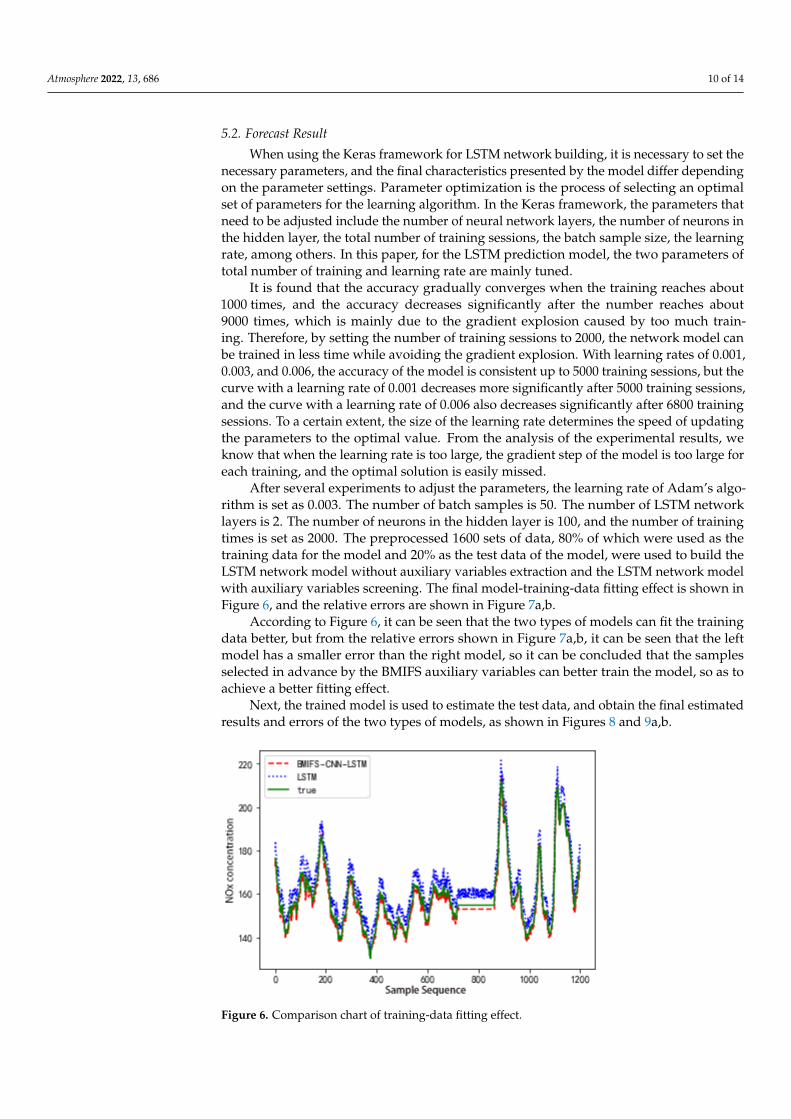
After several experiments to adjust the parameters, the learning rate of Adam’s algo-rithm is set as 0.003. The number of batch samples is 50. The number of LSTM networklayers is 2. The number of neurons in the hidden layer is 100, and the number of trainingtimes is set as 2000. The preprocessed 1600 sets of data, 80% of which were used as thetraining data for the model and 20% as the test data of the model, were used to build theLSTM network model without auxiliary variables extraction and the LSTM network modelwith auxiliary variables screening. The final model-training-data fitting effect is shown inFigure 6, and the relative errors are shown in Figure 7a,b.

According to Figure 6, it can be seen that the two types of models can fit the trainingdata better, but from the relative errors shown in Figure 7a,b, it can be seen that the leftmodel has a smaller error than the right model, so it can be concluded that the samplesselected in advance by the BMIFS auxiliary variables can better train the model, so as toachieve a better fitting effect.

Next, the trained model is used to estimate the test data, and obtain the final estimatedresults and errors of the two types of models, as shown in Figures 8 and 9a,b.

Atmosphere 2022, 13, x FOR PEER REVIEW 11 of 15

Figure 6. Comparison chart of training-data fitting effect.

(a) (b)

Figure 7. (a) Training-data estimation error. (b) Training-data estimation error.

According to Figure 6, it can be seen that the two types of models can fit the training

data better, but from the relative errors shown in Figure 7a,b, it can be seen that the left

model has a smaller error than the right model, so it can be concluded that the samples

selected in advance by the BMIFS auxiliary variables can better train the model, so as to

achieve a better fitting effect.

Next, the trained model is used to estimate the test data, and obtain the final esti-

mated results and errors of the two types of models, as shown in Figures 8 and 9a,b.

Figure 8. Comparison chart of estimated effect of test data.

Figure 6. Comparison chart of training-data fitting effect.

Atmosphere 2022, 13, 686 11 of 14

Atmosphere 2022, 13, x FOR PEER REVIEW 11 of 15

Figure 6. Comparison chart of training-data fitting effect.

(a) (b)

Figure 7. (a) Training-data estimation error. (b) Training-data estimation error.

According to Figure 6, it can be seen that the two types of models can fit the training

data better, but from the relative errors shown in Figure 7a,b, it can be seen that the left

model has a smaller error than the right model, so it can be concluded that the samples

selected in advance by the BMIFS auxiliary variables can better train the model, so as to

achieve a better fitting effect.

Next, the trained model is used to estimate the test data, and obtain the final esti-

mated results and errors of the two types of models, as shown in Figures 8 and 9a,b.

Figure 8. Comparison chart of estimated effect of test data.

Figure 7. (a) Training-data estimation error. (b) Training-data estimation error.

Atmosphere 2022, 13, x FOR PEER REVIEW 11 of 15

Figure 6. Comparison chart of training-data fitting effect.

(a) (b)

Figure 7. (a) Training-data estimation error. (b) Training-data estimation error.

According to Figure 6, it can be seen that the two types of models can fit the training

data better, but from the relative errors shown in Figure 7a,b, it can be seen that the left

model has a smaller error than the right model, so it can be concluded that the samples

selected in advance by the BMIFS auxiliary variables can better train the model, so as to

achieve a better fitting effect.

Next, the trained model is used to estimate the test data, and obtain the final esti-

mated results and errors of the two types of models, as shown in Figures 8 and 9a,b.

Figure 8. Comparison chart of estimated effect of test data. Figure 8. Comparison chart of estimated effect of test data.

Atmosphere 2022, 13, x FOR PEER REVIEW 12 of 15

(a) (b)

Figure 9. (a) Estimated error of test data. (b) Estimated error of test data.

According to Figure 8, it can be analyzed and found that the prediction accuracy of

the prediction model without auxiliary variable extraction is not as high as that of the

prediction model with auxiliary variable extraction. Combined with the results shown in

Figure 9a,b, it can be further found that the prediction based on BMIFS-LSTM gives a

relative error of the model that is smaller in comparison, which further shows that the

prediction accuracy of the model is higher.

The error descriptions of the two types of prediction models are shown in Table 3.

Table 3. Comparison table of simulation results.

Model MRE (%) RMSE

BMIFS-LSTM training model 0.0246 1.3715

LSTM training model 0.0458 2.2024

BMIFS-LSTM test model 0.0297 1.5237

LSTM test model 0.0643 3.0251

The addition of CNN for automatic feature extraction in addition to the original

LSTM model can greatly improve model accuracy and training speed. The total training

time of LSTM model is 340 s, while the total training time of BMIFS-CNN-LSTM is only

86 s, and its final prediction is shown in Figure 10 with the relative error given in Figure

11.

Figure 10. BMIFS-CNN-LSTM images of predicted and actual values.

Figure 9. (a) Estimated error of test data. (b) Estimated error of test data.

According to Figure 8, it can be analyzed and found that the prediction accuracy ofthe prediction model without auxiliary variable extraction is not as high as that of theprediction model with auxiliary variable extraction. Combined with the results shownin Figure 9a,b, it can be further found that the prediction based on BMIFS-LSTM gives arelative error of the model that is smaller in comparison, which further shows that theprediction accuracy of the model is higher.

The error descriptions of the two types of prediction models are shown in Table 3.

Atmosphere 2022, 13, 686 12 of 14

Table 3. Comparison table of simulation results.

Model MRE (%) RMSE

BMIFS-LSTM training model 0.0246 1.3715LSTM training model 0.0458 2.2024

BMIFS-LSTM test model 0.0297 1.5237LSTM test model 0.0643 3.0251

The addition of CNN for automatic feature extraction in addition to the original LSTMmodel can greatly improve model accuracy and training speed. The total training time ofLSTM model is 340 s, while the total training time of BMIFS-CNN-LSTM is only 86 s, andits final prediction is shown in Figure 10 with the relative error given in Figure 11.

Atmosphere 2022, 13, x FOR PEER REVIEW 12 of 15

(a) (b)

Figure 9. (a) Estimated error of test data. (b) Estimated error of test data.

According to Figure 8, it can be analyzed and found that the prediction accuracy of

the prediction model without auxiliary variable extraction is not as high as that of the

prediction model with auxiliary variable extraction. Combined with the results shown in

Figure 9a,b, it can be further found that the prediction based on BMIFS-LSTM gives a

relative error of the model that is smaller in comparison, which further shows that the

prediction accuracy of the model is higher.

The error descriptions of the two types of prediction models are shown in Table 3.

Table 3. Comparison table of simulation results.

Model MRE (%) RMSE

BMIFS-LSTM training model 0.0246 1.3715

LSTM training model 0.0458 2.2024

BMIFS-LSTM test model 0.0297 1.5237

LSTM test model 0.0643 3.0251

The addition of CNN for automatic feature extraction in addition to the original

LSTM model can greatly improve model accuracy and training speed. The total training

time of LSTM model is 340 s, while the total training time of BMIFS-CNN-LSTM is only

86 s, and its final prediction is shown in Figure 10 with the relative error given in Figure

11.

Figure 10. BMIFS-CNN-LSTM images of predicted and actual values. Figure 10. BMIFS-CNN-LSTM images of predicted and actual values.

Atmosphere 2022, 13, x FOR PEER REVIEW 13 of 15

Figure 11. Error curve chart.

The BMIFS-CNN-LSTM model is compared with the model without CNN feature

extraction in the following experimental analysis. Statistically, the errors of the two types

of models are shown in Table 4.

Table 4. Comparison of model error statistics.

Models Average Relative Error (%) Root Mean Square Error

BMIFS-LSTM Prediction Model 0.0297 1.5237

BMIFS-CNN-LSTM Prediction Model 0.0126 1.0113

In summary, compared with the BMIFS-LSTM model, the BMIFS-CNN-LSTM model

has a lower average relative error and root mean square error, and the model training

time is shorter. The rationality of introducing CNN automatic feature extraction is demon-

strated. Meanwhile, compared with the traditional long short-term memory neural net-

work (LSTM), the LSTM algorithm with the introduction of the improved mutual infor-

mation feature selection algorithm (BMIFS) has a lower average relative error of 3.45%

and a lower root mean square error of 1.50, which indicates a better prediction of NOX

concentration at the SCR inlet and effectively solves the problem of delay in NOx concen-

tration measurement.

6. Conclusions

At present, most thermal power plants use selective catalytic reduction (SCR) tech-

nology to reduce NOx emissions, using automatic flue gas monitoring systems to measure

NOx concentration in real time and combine the measurement results to select the optimal

amount of ammonia injection for denitrification treatment. However, the system has a

large delay in making measurements and cannot accurately reflect the real-time changes

in the NOx concentration at the SCR inlet when the unit load fluctuates frequently, thus

failing to guide the reactor action in a timely manner. In response, this paper establishes

an SCR inlet NOx concentration prediction algorithm based on BMIFS-LSTM. A modified

mutual information feature selection algorithm (BMIFS) is used to screen seven auxiliary

variables such as unit load and total secondary air, and the dominant variables are input

into a long short-term memory neural network (LSTM) together with the auxiliary varia-

bles to establish a BMIFS-LSTM prediction model. To verify, the historical operation data

of a 300 MW thermal power unit are used for simulation experiments. The experimental

results show that the model reduces the average relative error by 3.45% and the root mean

square error by 1.50, compared with the LSTM model without auxiliary variable screen-

ing. The prediction results have less deviation and higher accuracy, and have better pre-

diction effect on the NOX concentration at the SCR inlet. The problem of delay in NOx

concentration measurement is solved, which effectively reduces the occurrence of envi-

ronmental pollution problems such as ammonia escape and NOX emission overload.

Figure 11. Error curve chart.

The BMIFS-CNN-LSTM model is compared with the model without CNN featureextraction in the following experimental analysis. Statistically, the errors of the two typesof models are shown in Table 4.

Atmosphere 2022, 13, 686 13 of 14

Table 4. Comparison of model error statistics.

Models Average Relative Error (%) Root Mean Square Error

BMIFS-LSTM Prediction Model 0.0297 1.5237BMIFS-CNN-LSTM Prediction Model 0.0126 1.0113

In summary, compared with the BMIFS-LSTM model, the BMIFS-CNN-LSTM modelhas a lower average relative error and root mean square error, and the model training timeis shorter. The rationality of introducing CNN automatic feature extraction is demonstrated.Meanwhile, compared with the traditional long short-term memory neural network (LSTM),the LSTM algorithm with the introduction of the improved mutual information featureselection algorithm (BMIFS) has a lower average relative error of 3.45% and a lower rootmean square error of 1.50, which indicates a better prediction of NOX concentration at theSCR inlet and effectively solves the problem of delay in NOx concentration measurement.

6. Conclusions

At present, most thermal power plants use selective catalytic reduction (SCR) technol-ogy to reduce NOx emissions, using automatic flue gas monitoring systems to measureNOx concentration in real time and combine the measurement results to select the optimalamount of ammonia injection for denitrification treatment. However, the system has alarge delay in making measurements and cannot accurately reflect the real-time changesin the NOx concentration at the SCR inlet when the unit load fluctuates frequently, thusfailing to guide the reactor action in a timely manner. In response, this paper establishesan SCR inlet NOx concentration prediction algorithm based on BMIFS-LSTM. A modifiedmutual information feature selection algorithm (BMIFS) is used to screen seven auxiliaryvariables such as unit load and total secondary air, and the dominant variables are inputinto a long short-term memory neural network (LSTM) together with the auxiliary variablesto establish a BMIFS-LSTM prediction model. To verify, the historical operation data ofa 300 MW thermal power unit are used for simulation experiments. The experimentalresults show that the model reduces the average relative error by 3.45% and the root meansquare error by 1.50, compared with the LSTM model without auxiliary variable screening.The prediction results have less deviation and higher accuracy, and have better predictioneffect on the NOX concentration at the SCR inlet. The problem of delay in NOx concen-tration measurement is solved, which effectively reduces the occurrence of environmentalpollution problems such as ammonia escape and NOX emission overload.

Author Contributions: Methodology, M.S.; resources, J.X.; supervision, S.G.; writing—original draft,G.C.; writing—review and editing, J.C., H.L. and Z.D. All authors have read and agreed to thepublished version of the manuscript.

Funding: This research received no external funding.

Institutional Review Board Statement: Not applicable.

Informed Consent Statement: Not applicable.

Data Availability Statement: Not applicable.

Conflicts of Interest: The authors declare no conflict of interest.

References1. Zhong, J. The Economics of Low-NOx Technology and the Exploration of New Low-NOx Control Technology; Zhejiang University:

Hangzhou, China, 2006.2. Li, Y.; Huang, W.; Xi, J. Power plant NO_x emission prediction based on Stacking algorithm integration model. Therm. Energy

Power Eng. 2021, 36, 73–81. [CrossRef]3. Liu, K.; Wei, B.; Chen, L.; Wang, J.; Li, J.; Liu, J. Influence of low-load flue gas recirculation on combustion and NOx emissions of

pulverized coal boilers. Chin. J. Power Eng. 2021, 41, 345–349, 379.4. Hochreiter, S.; Schmidhuber, J. Long short-term memory. Neural Comput. 1997, 9, 1735–1780. [CrossRef]

Atmosphere 2022, 13, 686 14 of 14

5. Kingma, D.; Ba, J. Adam: A method for stochastic optimization. arXiv 2014, arXiv:1412.6980.6. Verma, S.; Singh, S.; Majumdar, A. Multi-label LSTM autoencoder for non-intrusive appliance load monitoring. Electr. Power Syst.

Res. 2021, 199, 107414. [CrossRef]7. Wu, P.; Luo, L. Prediction of ship motion trajectory based on RNN-LSTM. Shipbuild. Technol. 2021, 49, 11–16.8. Xiang, Z. Confidence Interval Prediction of Smart Grid Link Quality Based on LSTM. Electrical Measurement and Instrumentation.

pp. 1–10. Available online: http://kns.cnki.net/kcms/detail/23.1202.TH.20210623.0948.004.html (accessed on 4 July 2021).9. Zhao, Y. Power data analysis method combining GA and LSTM network. Electron. Des. Eng. 2021, 29, 161–165.10. Song, S.; Li, B. Research on short-term prediction method of photovoltaic power generation based on LSTM network. Renew.

Energy 2021, 39, 594–602.11. Chen, C.; Wang, X.; Liang, J.; Ma, W. LSTM photovoltaic power generation prediction method based on a new attention

mechanism. Mod. Comput. 2021, 11, 28–32+38.12. Zhang, Z. Research on Spacecraft Time Series Prediction Method Based on LSTM; Beijing Jiaotong University: Beijing, China, 2020.13. Zheng, T. Near-Space Hypersonic Target Track Estimation and Prediction Based on Recurrent Neural Network; Harbin Institute of

Technology: Harbin, China, 2020.14. Hu, D.; Meng, X.; Lu, S.; Xing, L. The application of a parallel LSTM-FCN model in ship trajectory prediction. Control Decis. 2021,

4, 1–7. [CrossRef]15. Yang, B. Research and Application of Ship Trajectory Analysis Based on AIS; University of Electronic Science and Technology of China:

Chengdu, China, 2018.16. Lu, J.; Song, S.; Jing, Y.; Zhang, Y.; Gu, L.; Lu, F.; Hu, Z.; Li, S. Fundamental Frequency Detection of Underwater Moving Target

Noise Based on DEMON Spectrum and LSTM Network. Applied Acoustics. pp. 1–11. Available online: http://kns.cnki.net/kcms/detail/11.2121.o4.20210621.1436.006.html (accessed on 4 July 2021).

17. Ding, C. Planning of RMB Exchange Rate Prediction Scheme Based on Multi-Time Scale CNN-LSTM Neural Network; Shanghai NormalUniversity: Shanghai, China, 2021.

18. Tian, Y. Research on Stock Price Trend Prediction Based on Investor Sentiment and LSTM; Shanghai Normal University: Shanghai,China, 2021.

19. Wei, Q.; Chen, S.; Tan, Z.; Huang, W.; Ma, G. Based on SA-LSTM, the dynamic lag relationship between hydropower stations.Hydropower Energy Sci. 2021, 39, 16–19.

20. Zhang, D. Research on Optimization Technology of Large-Scale Reservoir Water Temperature Regulation Based on Artificial IntelligenceAlgorithm; China Institute of Water Resources and Hydropower Research: Beijing, China, 2020.

21. Sun, B.M.; Wang, D.H.; Yang, B.; Zhang, S.H.; Kong, L.Y. Prediction Model for the Boiler NOx Emission with Material PropertiesBased on the Artificial Neural Network. Adv. Mater. Res. 2013, 676, 40–45. [CrossRef]

22. Li, X.; Xu, G. Wind power generation power prediction method based on long short-term memory neural network. Power Gener.Technol. 2019, 40, 426–433.

23. Zhai, Y.; Xu, L.; Ji, X.; Ji, H.; Wang, J.; Sha, Y. Short-term load forecasting based on long and short-term memory neural network.Inf. Technol. 2019, 10, 27–31.

24. Mao, X.; Tan, J.; Yao, Y.; Li, B.; Wu, C. Saturated load forecasting method and application based on long and short-term memoryneural network. Hydropower Energy Sci. 2019, 37, 192–195+168.

25. Tang, Z.; Zhao, G.; Cao, S.; Zhao, B. Ultra-short-term wind direction prediction based on SWLSTM algorithm. Chin. J. Electr. Eng.2019, 39, 4459–4468.

26. Peng, H.; Long, F.; Ding, C. Feature selection based on mutual information criteria of max-dependency, max-relevance, andmin-redundancy. IEEE Trans. Pattern Anal. Mach. Intell. 2005, 27, 1226–1238. [CrossRef] [PubMed]